Wiley.The.Data.Warehouse.Toolkit.The..Guide.to.Dimensional.ing.Second.Edition
User Manual:
Open the PDF directly: View PDF ![]() .
.
Page Count: 447 [warning: Documents this large are best viewed by clicking the View PDF Link!]

John Wiley & Sons, Inc.
NEW YORK • CHICHESTER • WEINHEIM • BRISBANE • SINGAPORE • TORONTO
Wiley Computer Publishing
Ralph Kimball
Margy Ross
The Data Warehouse
Toolkit
Second Edition
The Complete Guide to
Dimensional Modeling
TEAMFLY
Team-Fly®

The Data Warehouse Toolkit
Second Edition


John Wiley & Sons, Inc.
NEW YORK • CHICHESTER • WEINHEIM • BRISBANE • SINGAPORE • TORONTO
Wiley Computer Publishing
Ralph Kimball
Margy Ross
The Data Warehouse
Toolkit
Second Edition
The Complete Guide to
Dimensional Modeling

Publisher: Robert Ipsen
Editor: Robert Elliott
Assistant Editor: Emilie Herman
Managing Editor: John Atkins
Associate New Media Editor: Brian Snapp
Text Composition: John Wiley Composition Services
Designations used by companies to distinguish their products are often claimed as trade-
marks. In all instances where John Wiley & Sons, Inc., is aware of a claim, the product names
appear in initial capital or ALL CAPITAL LETTERS. Readers, however, should contact the
appropriate companies for more complete information regarding trademarks and registration.
This book is printed on acid-free paper. ∞
Copyright © 2002 by Ralph Kimball and Margy Ross. All rights reserved.
Published by John Wiley and Sons, Inc.
Published simultaneously in Canada.
No part of this publication may be reproduced, stored in a retrieval system or transmitted
in any form or by any means, electronic, mechanical, photocopying, recording, scanning
or otherwise, except as permitted under Sections 107 or 108 of the 1976 United States
Copyright Act, without either the prior written permission of the Publisher, or authoriza-
tion through payment of the appropriate per-copy fee to the Copyright Clearance Center,
222 Rosewood Drive, Danvers, MA 01923, (978) 750-8400, fax (978) 750-4744. Requests
to the Publisher for permission should be addressed to the Permissions Department,
John Wiley & Sons, Inc., 605 Third Avenue, New York, NY 10158-0012, (212) 850-6011, fax
(212) 850-6008, E-Mail: PERMREQ@WILEY.COM.
This publication is designed to provide accurate and authoritative information in regard to
the subject matter covered. It is sold with the understanding that the publisher is not
engaged in professional services. If professional advice or other expert assistance is
required, the services of a competent professional person should be sought.
Library of Congress Cataloging-in-Publication Data:
Kimball, Ralph.
The data warehouse toolkit : the complete guide to dimensional modeling /
Ralph Kimball, Margy Ross. — 2nd ed.
p. cm.
“Wiley Computer Publishing.”
Includes index.
ISBN 0-471-20024-7
1. Database design. 2. Data warehousing. I. Ross, Margy, 1959– II. Title.
QA76.9.D26 K575 2002
658.4'038'0285574—dc21 2002002284
Printed in the United States of America.
10 9 8 7 6 5 4 3 2 1

CONTENTS
v
Acknowledgments xv
Introduction xvii
Chapter 1 Dimensional Modeling Primer 1
Different Information Worlds 2
Goals of a Data Warehouse 2
The Publishing Metaphor 4
Components of a Data Warehouse 6
Operational Source Systems 7
Data Staging Area 8
Data Presentation 10
Data Access Tools 13
Additional Considerations 14
Dimensional Modeling Vocabulary 16
Fact Table 16
Dimension Tables 19
Bringing Together Facts and Dimensions 21
Dimensional Modeling Myths 24
Common Pitfalls to Avoid 26
Summary 27
Chapter 2 Retail Sales 29
Four-Step Dimensional Design Process 30
Retail Case Study 32
Step 1. Select the Business Process 33
Step 2. Declare the Grain 34
Step 3. Choose the Dimensions 35
Step 4. Identify the Facts 36

Dimension Table Attributes 38
Date Dimension 38
Product Dimension 42
Store Dimension 45
Promotion Dimension 46
Degenerate Transaction Number Dimension 50
Retail Schema in Action 51
Retail Schema Extensibility 52
Resisting Comfort Zone Urges 54
Dimension Normalization (Snowflaking) 55
Too Many Dimensions 57
Surrogate Keys 58
Market Basket Analysis 62
Summary 65
Chapter 3 Inventory 67
Introduction to the Value Chain 68
Inventory Models 69
Inventory Periodic Snapshot 69
Inventory Transactions 74
Inventory Accumulating Snapshot 75
Value Chain Integration 76
Data Warehouse Bus Architecture 78
Data Warehouse Bus Matrix 79
Conformed Dimensions 82
Conformed Facts 87
Summary 88
Chapter 4 Procurement 89
Procurement Case Study 89
Procurement Transactions 90
Multiple- versus Single-Transaction Fact Tables 91
Complementary Procurement Snapshot 93
Contents
vi

Slowly Changing Dimensions 95
Type 1: Overwrite the Value 95
Type 2: Add a Dimension Row 97
Type 3: Add a Dimension Column 100
Hybrid Slowly Changing Dimension Techniques 102
Predictable Changes with Multiple Version Overlays 102
Unpredictable Changes with Single Version Overlay 103
More Rapidly Changing Dimensions 105
Summary 105
Chapter 5 Order Management 107
Introduction to Order Management 108
Order Transactions 109
Fact Normalization 109
Dimension Role-Playing 110
Product Dimension Revisited 111
Customer Ship-To Dimension 113
Deal Dimension 116
Degenerate Dimension for Order Number 117
Junk Dimensions 117
Multiple Currencies 119
Header and Line Item Facts with Different Granularity 121
Invoice Transactions 122
Profit and Loss Facts 124
Profitability—The Most Powerful Data Mart 126
Profitability Words of Warning 127
Customer Satisfaction Facts 127
Accumulating Snapshot for the Order Fulfillment Pipeline 128
Lag Calculations 130
Multiple Units of Measure 130
Beyond the Rear-View Mirror 132
Fact Table Comparison 132
Transaction Fact Tables 133
Periodic Snapshot Fact Tables 134
Accumulating Snapshot Fact Tables 134
Contents vii

Designing Real-Time Partitions 135
Requirements for the Real-Time Partition 136
Transaction Grain Real-Time Partition 136
Periodic Snapshot Real-Time Partition 137
Accumulating Snapshot Real-Time Partition 138
Summary 139
Chapter 6 Customer Relationship Management 141
CRM Overview 142
Operational and Analytical CRM 143
Packaged CRM 145
Customer Dimension 146
Name and Address Parsing 147
Other Common Customer Attributes 150
Dimension Outriggers for a Low-Cardinality Attribute Set 153
Large Changing Customer Dimensions 154
Implications of Type 2 Customer Dimension Changes 159
Customer Behavior Study Groups 160
Commercial Customer Hierarchies 161
Combining Multiple Sources of Customer Data 168
Analyzing Customer Data from Multiple Business Processes 169
Summary 170
Chapter 7 Accounting 173
Accounting Case Study 174
General Ledger Data 175
General Ledger Periodic Snapshot 175
General Ledger Journal Transactions 177
Financial Statements 180
Budgeting Process 180
Consolidated Fact Tables 184
Role of OLAP and Packaged Analytic Solutions 185
Summary 186
Contents
viii

Chapter 8 Human Resources Management 187
Time-Stamped Transaction Tracking in a Dimension 188
Time-Stamped Dimension with Periodic Snapshot Facts 191
Audit Dimension 193
Keyword Outrigger Dimension 194
AND/OR Dilemma 195
Searching for Substrings 196
Survey Questionnaire Data 197
Summary 198
Chapter 9 Financial Services 199
Banking Case Study 200
Dimension Triage 200
Household Dimension 204
Multivalued Dimensions 205
Minidimensions Revisited 206
Arbitrary Value Banding of Facts 207
Point-in-Time Balances 208
Heterogeneous Product Schemas 210
Heterogeneous Products with Transaction Facts 215
Summary 215
Chapter 10 Telecommunications and Utilities 217
Telecommunications Case Study 218
General Design Review Considerations 220
Granularity 220
Date Dimension 222
Degenerate Dimensions 222
Dimension Decodes and Descriptions 222
Surrogate Keys 223
Too Many (or Too Few) Dimensions 223
Draft Design Exercise Discussion 223
Geographic Location Dimension 226
Location Outrigger 226
Leveraging Geographic Information Systems 227
Summary 227
Contents ix

Chapter 11 Transportation 229
Airline Frequent Flyer Case Study 230
Multiple Fact Table Granularities 230
Linking Segments into Trips 233
Extensions to Other Industries 234
Cargo Shipper 234
Travel Services 235
Combining Small Dimensions into a Superdimension 236
Class of Service 236
Origin and Destination 237
More Date and Time Considerations 239
Country-Specific Calendars 239
Time of Day as a Dimension or Fact 240
Date and Time in Multiple Time Zones 240
Summary 241
Chapter 12 Education 243
University Case Study 244
Accumulating Snapshot for Admissions Tracking 244
Factless Fact Tables 246
Student Registration Events 247
Facilities Utilization Coverage 249
Student Attendance Events 250
Other Areas of Analytic Interest 253
Summary 254
Chapter 13 Health Care 255
Health Care Value Circle 256
Health Care Bill 258
Roles Played By the Date Dimension 261
Multivalued Diagnosis Dimension 262
Extending a Billing Fact Table to Show Profitability 265
Dimensions for Billed Hospital Stays 266
Contents
x
TEAMFLY
Team-Fly®

Complex Health Care Events 267
Medical Records 269
Fact Dimension for Sparse Facts 269
Going Back in Time 271
Late-Arriving Fact Rows 271
Late-Arriving Dimension Rows 273
Summary 274
Chapter 14 Electronic Commerce 277
Web Client-Server Interactions Tutorial 278
Why the Clickstream Is Not Just Another Data Source 281
Challenges of Tracking with Clickstream Data 282
Specific Dimensions for the Clickstream 287
Clickstream Fact Table for Complete Sessions 292
Clickstream Fact Table for Individual Page Events 295
Aggregate Clickstream Fact Tables 298
Integrating the Clickstream Data Mart into the
Enterprise Data Warehouse 299
Electronic Commerce Profitability Data Mart 300
Summary 303
Chapter 15 Insurance 305
Insurance Case Study 306
Insurance Value Chain 307
Draft Insurance Bus Matrix 309
Policy Transactions 309
Dimension Details and Techniques 310
Alternative (or Complementary) Policy
Accumulating Snapshot 315
Policy Periodic Snapshot 316
Conformed Dimensions 316
Conformed Facts 316
Heterogeneous Products Again 318
Multivalued Dimensions Again 318
Contents xi

More Insurance Case Study Background 319
Updated Insurance Bus Matrix 320
Claims Transactions 322
Claims Accumulating Snapshot 323
Policy/Claims Consolidated Snapshot 324
Factless Accident Events 325
Common Dimensional Modeling Mistakes to Avoid 326
Summary 330
Chapter 16 Building the Data Warehouse 331
Business Dimensional Lifecycle Road Map 332
Road Map Major Points of Interest 333
Project Planning and Management 334
Assessing Readiness 334
Scoping 336
Justification 336
Staffing 337
Developing and Maintaining the Project Plan 339
Business Requirements Definition 340
Requirements Preplanning 341
Collecting the Business Requirements 343
Postcollection Documentation and Follow-up 345
Lifecycle Technology Track 347
Technical Architecture Design 348
Eight-Step Process for Creating the Technical Architecture 348
Product Selection and Installation 351
Lifecycle Data Track 353
Dimensional Modeling 353
Physical Design 355
Aggregation Strategy 356
Initial Indexing Strategy 357
Data Staging Design and Development 358
Dimension Table Staging 358
Fact Table Staging 361
Contents
xii

Lifecycle Analytic Applications Track 362
Analytic Application Specification 363
Analytic Application Development 363
Deployment 364
Maintenance and Growth 365
Common Data Warehousing Mistakes to Avoid 366
Summary 369
Chapter 17 Present Imperatives and Future Outlook 371
Ongoing Technology Advances 372
Political Forces Demanding Security and Affecting Privacy 375
Conflict between Beneficial Uses and Insidious Abuses 375
Who Owns Your Personal Data? 376
What Is Likely to Happen? Watching the Watchers . . . 377
How Watching the Watchers Affects Data
Warehouse Architecture 378
Designing to Avoid Catastrophic Failure 379
Catastrophic Failures 380
Countering Catastrophic Failures 380
Intellectual Property and Fair Use 383
Cultural Trends in Data Warehousing 383
Managing by the Numbers
across the Enterprise 383
Increased Reliance on Sophisticated Key
Performance Indicators 384
Behavior Is the New Marquee Application 385
Packaged Applications Have Hit Their High Point 385
Application Integration Has to Be Done by Someone 386
Data Warehouse Outsourcing Needs a Sober Risk Assessment 386
In Closing 387
Glossary 389
Index 419
Contents xiii


ACKNOWLEDGMENTS
xv
First of all, we want to thank the thousands of you who have read our Toolkit
books, attended our courses, and engaged us in consulting projects. We have
learned as much from you as we have taught. As a group, you have had a pro-
foundly positive impact on the data warehousing industry. Congratulations!
This book would not have been written without the assistance of our business
partners. We want to thank Julie Kimball of Ralph Kimball Associates for her
vision and determination in getting the project launched. While Julie was the
catalyst who got the ball rolling, Bob Becker of DecisionWorks Consulting
helped keep it in motion as he drafted, reviewed, and served as a general
sounding board. We are grateful to them both because they helped an enor-
mous amount.
We wrote this book with a little help from our friends, who provided input or
feedback on specific chapters. We want to thank Bill Schmarzo of Decision-
Works, Charles Hagensen of Attachmate Corporation, and Warren Thorn-
thwaite of InfoDynamics for their counsel on Chapters 6, 7, and 16, respectively.
Bob Elliott, our editor at John Wiley & Sons, and the entire Wiley team have
supported this project with skill, encouragement, and enthusiasm. It has been
a pleasure to work with them. We also want to thank Justin Kestelyn, editor-
in-chief at Intelligent Enterprise for allowing us to adapt materials from sev-
eral of Ralph’s articles for inclusion in this book.
To our families, thanks for being there for us when we needed you and for giv-
ing us the time it took. Spouses Julie Kimball and Scott Ross and children Sara
Hayden Smith, Brian Kimball, and Katie Ross all contributed a lot to this book,
often without realizing it. Thanks for your unconditional support.


xvii
INTRODUCTION
The data warehousing industry certainly has matured since Ralph Kimball pub-
lished the first edition of The Data Warehouse Toolkit (Wiley) in 1996. Although
large corporate early adopters paved the way, since then, data warehousing
has been embraced by organizations of all sizes. The industry has constructed
thousands of data warehouses. The volume of data continues to grow as we
populate our warehouses with increasingly atomic data and update them with
greater frequency. Vendors continue to blanket the market with an ever-
expanding set of tools to help us with data warehouse design, development,
and usage. Most important, armed with access to our data warehouses, busi-
ness professionals are making better decisions and generating payback on
their data warehouse investments.
Since the first edition of The Data Warehouse Toolkit was published, dimen-
sional modeling has been broadly accepted as the dominant technique for data
warehouse presentation. Data warehouse practitioners and pundits alike have
recognized that the data warehouse presentation must be grounded in sim-
plicity if it stands any chance of success. Simplicity is the fundamental key that
allows users to understand databases easily and software to navigate data-
bases efficiently. In many ways, dimensional modeling amounts to holding the
fort against assaults on simplicity. By consistently returning to a business-
driven perspective and by refusing to compromise on the goals of user under-
standability and query performance, we establish a coherent design that
serves the organization’s analytic needs. Based on our experience and the
overwhelming feedback from numerous practitioners from companies like
your own, we believe that dimensional modeling is absolutely critical to a suc-
cessful data warehousing initiative.
Dimensional modeling also has emerged as the only coherent architecture for
building distributed data warehouse systems. When we use the conformed
dimensions and conformed facts of a set of dimensional models, we have a
practical and predictable framework for incrementally building complex data
warehouse systems that have no center.
For all that has changed in our industry, the core dimensional modeling tech-
niques that Ralph Kimball published six years ago have withstood the test of
time. Concepts such as slowly changing dimensions, heterogeneous products,

factless fact tables, and architected data marts continue to be discussed in data
warehouse design workshops around the globe. The original concepts have
been embellished and enhanced by new and complementary techniques. We
decided to publish a second edition of Kimball’s seminal work because we felt
that it would be useful to pull together our collective thoughts on dimensional
modeling under a single cover. We have each focused exclusively on decision
support and data warehousing for over two decades. We hope to share the
dimensional modeling patterns that have emerged repeatedly during the
course of our data warehousing careers. This book is loaded with specific,
practical design recommendations based on real-world scenarios.
The goal of this book is to provide a one-stop shop for dimensional modeling
techniques. True to its title, it is a toolkit of dimensional design principles and
techniques. We will address the needs of those just getting started in dimen-
sional data warehousing, and we will describe advanced concepts for those of
you who have been at this a while. We believe that this book stands alone in its
depth of coverage on the topic of dimensional modeling.
Intended Audience
This book is intended for data warehouse designers, implementers, and man-
agers. In addition, business analysts who are active participants in a ware-
house initiative will find the content useful.
Even if you’re not directly responsible for the dimensional model, we believe
that it is important for all members of a warehouse project team to be comfort-
able with dimensional modeling concepts. The dimensional model has an
impact on most aspects of a warehouse implementation, beginning with the
translation of business requirements, through data staging, and finally, to the
unveiling of a data warehouse through analytic applications. Due to the broad
implications, you need to be conversant in dimensional modeling regardless
whether you are responsible primarily for project management, business
analysis, data architecture, database design, data staging, analytic applica-
tions, or education and support. We’ve written this book so that it is accessible
to a broad audience.
For those of you who have read the first edition of this book, some of the famil-
iar case studies will reappear in this edition; however, they have been updated
significantly and fleshed out with richer content. We have developed vignettes
for new industries, including health care, telecommunications, and electronic
commerce. In addition, we have introduced more horizontal, cross-industry
case studies for business functions such as human resources, accounting, pro-
curement, and customer relationship management.
Introduction
xviii

Introduction xix
The content in this book is mildly technical. We discuss dimensional modeling
in the context of a relational database primarily. We presume that readers have
basic knowledge of relational database concepts such as tables, rows, keys,
and joins. Given that we will be discussing dimensional models in a non-
denominational manner, we won’t dive into specific physical design and
tuning guidance for any given database management systems.
Chapter Preview
The book is organized around a series of business vignettes or case studies. We
believe that developing the design techniques by example is an extremely
effective approach because it allows us to share very tangible guidance. While
not intended to be full-scale application or industry solutions, these examples
serve as a framework to discuss the patterns that emerge in dimensional mod-
eling. In our experience, it is often easier to grasp the main elements of a
design technique by stepping away from the all-too-familiar complexities of
one’s own applications in order to think about another business. Readers of
the first edition have responded very favorably to this approach.
The chapters of this book build on one another. We will start with basic con-
cepts and introduce more advanced content as the book unfolds. The chapters
are to be read in order by every reader. For example, Chapter 15 on insurance
will be difficult to comprehend unless you have read the preceding chapters
on retailing, procurement, order management, and customer relationship
management.
Those of you who have read the first edition may be tempted to skip the first
few chapters. While some of the early grounding regarding facts and dimen-
sions may be familiar turf, we don’t want you to sprint too far ahead. For
example, the first case study focuses on the retailing industry, just as it did in
the first edition. However, in this edition we advocate a new approach, mak-
ing a strong case for tackling the atomic, bedrock data of your organization.
You’ll miss out on this rationalization and other updates to fundamental con-
cepts if you skip ahead too quickly.
Navigation Aids
We have laced the book with tips, key concepts, and chapter pointers to make
it more usable and easily referenced in the future. In addition, we have pro-
vided an extensive glossary of terms.

You can find the tips sprinkled throughout this book by flipping through the chapters
and looking for the lightbulb icon.
We begin each chapter with a sidebar of key concepts, denoted by the key icon.
Purpose of Each Chapter
Before we get started, we want to give you a chapter-by-chapter preview of the
concepts covered as the book unfolds.
Chapter 1: Dimensional Modeling Primer
The book begins with a primer on dimensional modeling. We explore the com-
ponents of the overall data warehouse architecture and establish core vocabu-
lary that will be used during the remainder of the book. We dispel some of the
myths and misconceptions about dimensional modeling, and we discuss the
role of normalized models.
Chapter 2: Retail Sales
Retailing is the classic example used to illustrate dimensional modeling. We
start with the classic because it is one that we all understand. Hopefully, you
won’t need to think very hard about the industry because we want you to
focus on core dimensional modeling concepts instead. We begin by discussing
the four-step process for designing dimensional models. We explore dimen-
sion tables in depth, including the date dimension that will be reused repeat-
edly throughout the book. We also discuss degenerate dimensions,
snowflaking, and surrogate keys. Even if you’re not a retailer, this chapter is
required reading because it is chock full of fundamentals.
Chapter 3: Inventory
We remain within the retail industry for our second case study but turn our
attention to another business process. This case study will provide a very vivid
example of the data warehouse bus architecture and the use of conformed
dimensions and facts. These concepts are critical to anyone looking to con-
struct a data warehouse architecture that is integrated and extensible.
Introduction
xx
TEAMFLY
Team-Fly®

Chapter 4: Procurement
This chapter reinforces the importance of looking at your organization’s value
chain as you plot your data warehouse. We also explore a series of basic and
advanced techniques for handling slowly changing dimension attributes.
Chapter 5: Order Management
In this case study we take a look at the business processes that are often the
first to be implemented in data warehouses as they supply core business per-
formance metrics—what are we selling to which customers at what price? We
discuss the situation in which a dimension plays multiple roles within a
schema. We also explore some of the common challenges modelers face when
dealing with order management information, such as header/line item con-
siderations, multiple currencies or units of measure, and junk dimensions with
miscellaneous transaction indicators. We compare the three fundamental
types of fact tables: transaction, periodic snapshot, and accumulating snap-
shot. Finally, we provide recommendations for handling more real-time ware-
housing requirements.
Chapter 6: Customer Relationship Management
Numerous data warehouses have been built on the premise that we need to bet-
ter understand and service our customers. This chapter covers key considera-
tions surrounding the customer dimension, including address standardization,
managing large volume dimensions, and modeling unpredictable customer
hierarchies. It also discusses the consolidation of customer data from multiple
sources.
Chapter 7: Accounting
In this totally new chapter we discuss the modeling of general ledger informa-
tion for the data warehouse. We describe the appropriate handling of year-to-
date facts and multiple fiscal calendars, as well as the notion of consolidated
dimensional models that combine data from multiple business processes.
Chapter 8: Human Resources Management
This new chapter explores several unique aspects of human resources dimen-
sional models, including the situation in which a dimension table begins to
behave like a fact table. We also introduce audit and keyword dimensions, as
well as the handling of survey questionnaire data.
Introduction xxi

Introduction
xxii
Chapter 9: Financial Services
The banking case study explores the concept of heterogeneous products in
which each line of business has unique descriptive attributes and performance
metrics. Obviously, the need to handle heterogeneous products is not unique
to financial services. We also discuss the complicated relationships among
accounts, customers, and households.
Chapter 10: Telecommunications and Utilities
This new chapter is structured somewhat differently to highlight considera-
tions when performing a data model design review. In addition, we explore
the idiosyncrasies of geographic location dimensions, as well as opportunities
for leveraging geographic information systems.
Chapter 11: Transportation
In this case study we take a look at related fact tables at different levels of gran-
ularity. We discuss another approach for handling small dimensions, and we
take a closer look at date and time dimensions, covering such concepts as
country-specific calendars and synchronization across multiple time zones.
Chapter 12: Education
We look at several factless fact tables in this chapter and discuss their impor-
tance in analyzing what didn’t happen. In addition, we explore the student
application pipeline, which is a prime example of an accumulating snapshot
fact table.
Chapter 13: Health Care
Some of the most complex models that we have ever worked with are from the
health care industry. This new chapter illustrates the handling of such com-
plexities, including the use of a bridge table to model multiple diagnoses and
providers associated with a patient treatment.
Chapter 14: Electronic Commerce
This chapter provides an introduction to modeling clickstream data. The con-
cepts are derived from The Data Webhouse Toolkit (Wiley 2000), which Ralph
Kimball coauthored with Richard Merz.

Introduction xxiii
Chapter 15: Insurance
The final case study serves to illustrate many of the techniques we discussed
earlier in the book in a single set of interrelated schemas. It can be viewed
as a pulling-it-all-together chapter because the modeling techniques will be
layered on top of one another, similar to overlaying overhead projector
transparencies.
Chapter 16: Building the Data Warehouse
Now that you are comfortable designing dimensional models, we provide a
high-level overview of the activities that are encountered during the lifecycle
of a typical data warehouse project iteration. This chapter could be considered
a lightning tour of The Data Warehouse Lifecycle Toolkit (Wiley 1998) that we
coauthored with Laura Reeves and Warren Thornthwaite.
Chapter 17: Present Imperatives and Future Outlook
In this final chapter we peer into our crystal ball to provide a preview of what
we anticipate data warehousing will look like in the future.
Glossary
We’ve supplied a detailed glossary to serve as a reference resource. It will help
bridge the gap between your general business understanding and the case
studies derived from businesses other than your own.
Companion Web Site
You can access the book’s companion Web site at www.kimballuniversity.com.
The Web site offers the following resources:
■■ Register for Design Tips to receive ongoing, practical guidance about
dimensional modeling and data warehouse design via electronic mail on a
periodic basis.
■■ Link to all Ralph Kimball’s articles from Intelligent Enterprise and its
predecessor, DBMS Magazine.
■■ Learn about Kimball University classes for quality, vendor-independent
education consistent with the authors’ experiences and writings.

Summary
The goal of this book is to communicate a set of standard techniques for
dimensional data warehouse design. Crudely speaking, if you as the reader
get nothing else from this book other than the conviction that your data ware-
house must be driven from the needs of business users and therefore built and
presented from a simple dimensional perspective, then this book will have
served its purpose. We are confident that you will be one giant step closer to
data warehousing success if you buy into these premises.
Now that you know where we are headed, it is time to dive into the details.
We’ll begin with a primer on dimensional modeling in Chapter 1 to ensure that
everyone is on the same page regarding key terminology and architectural
concepts. From there we will begin our discussion of the fundamental tech-
niques of dimensional modeling, starting with the tried-and-true retail industry.
Introduction
xxiv

Dimensional Modeling
Primer
CHAPTER 1
1
In this first chapter we lay the groundwork for the case studies that follow.
We’ll begin by stepping back to consider data warehousing from a macro per-
spective. Some readers may be disappointed to learn that it is not all about
tools and techniques—first and foremost, the data warehouse must consider
the needs of the business. We’ll drive stakes in the ground regarding the goals
of the data warehouse while observing the uncanny similarities between the
responsibilities of a data warehouse manager and those of a publisher. With
this big-picture perspective, we’ll explore the major components of the ware-
house environment, including the role of normalized models. Finally, we’ll
close by establishing fundamental vocabulary for dimensional modeling. By
the end of this chapter we hope that you’ll have an appreciation for the need
to be half DBA (database administrator) and half MBA (business analyst) as
you tackle your data warehouse.
Chapter 1 discusses the following concepts:
■■ Business-driven goals of a data warehouse
■■ Data warehouse publishing
■■ Major components of the overall data warehouse
■■ Importance of dimensional modeling for the data
warehouse presentation area
■■ Fact and dimension table terminology
■■ Myths surrounding dimensional modeling
■■ Common data warehousing pitfalls to avoid

Different Information Worlds
One of the most important assets of any organization is its information. This
asset is almost always kept by an organization in two forms: the operational
systems of record and the data warehouse. Crudely speaking, the operational
systems are where the data is put in, and the data warehouse is where we get
the data out.
The users of an operational system turn the wheels of the organization. They
take orders, sign up new customers, and log complaints. Users of an opera-
tional system almost always deal with one record at a time. They repeatedly
perform the same operational tasks over and over.
The users of a data warehouse, on the other hand, watch the wheels of the orga-
nization turn. They count the new orders and compare them with last week’s
orders and ask why the new customers signed up and what the customers
complained about. Users of a data warehouse almost never deal with one row
at a time. Rather, their questions often require that hundreds or thousands of
rows be searched and compressed into an answer set. To further complicate
matters, users of a data warehouse continuously change the kinds of questions
they ask.
In the first edition of The Data Warehouse Toolkit (Wiley 1996), Ralph Kimball
devoted an entire chapter to describe the dichotomy between the worlds of
operational processing and data warehousing. At this time, it is widely recog-
nized that the data warehouse has profoundly different needs, clients, struc-
tures, and rhythms than the operational systems of record. Unfortunately, we
continue to encounter supposed data warehouses that are mere copies of the
operational system of record stored on a separate hardware platform. While
this may address the need to isolate the operational and warehouse environ-
ments for performance reasons, it does nothing to address the other inherent
differences between these two types of systems. Business users are under-
whelmed by the usability and performance provided by these pseudo data
warehouses. These imposters do a disservice to data warehousing because
they don’t acknowledge that warehouse users have drastically different needs
than operational system users.
Goals of a Data Warehouse
Before we delve into the details of modeling and implementation, it is helpful
to focus on the fundamental goals of the data warehouse. The goals can be
developed by walking through the halls of any organization and listening to
business management. Inevitably, these recurring themes emerge:
CHAPTER 1
2

■■ “We have mountains of data in this company, but we can’t access it.”
■■ “We need to slice and dice the data every which way.”
■■ “You’ve got to make it easy for business people to get at the data directly.”
■■ “Just show me what is important.”
■■ “It drives me crazy to have two people present the same business metrics
at a meeting, but with different numbers.”
■■ “We want people to use information to support more fact-based decision
making.”
Based on our experience, these concerns are so universal that they drive the
bedrock requirements for the data warehouse. Let’s turn these business man-
agement quotations into data warehouse requirements.
The data warehouse must make an organization’s information easily acces-
sible. The contents of the data warehouse must be understandable. The
data must be intuitive and obvious to the business user, not merely the
developer. Understandability implies legibility; the contents of the data
warehouse need to be labeled meaningfully. Business users want to sepa-
rate and combine the data in the warehouse in endless combinations, a
process commonly referred to as slicing and dicing. The tools that access the
data warehouse must be simple and easy to use. They also must return
query results to the user with minimal wait times.
The data warehouse must present the organization’s information consis-
tently. The data in the warehouse must be credible. Data must be carefully
assembled from a variety of sources around the organization, cleansed,
quality assured, and released only when it is fit for user consumption.
Information from one business process should match with information
from another. If two performance measures have the same name, then they
must mean the same thing. Conversely, if two measures don’t mean the
same thing, then they should be labeled differently. Consistent information
means high-quality information. It means that all the data is accounted for
and complete. Consistency also implies that common definitions for the
contents of the data warehouse are available for users.
The data warehouse must be adaptive and resilient to change. We simply
can’t avoid change. User needs, business conditions, data, and technology
are all subject to the shifting sands of time. The data warehouse must be
designed to handle this inevitable change. Changes to the data warehouse
should be graceful, meaning that they don’t invalidate existing data or
applications. The existing data and applications should not be changed or
disrupted when the business community asks new questions or new data
is added to the warehouse. If descriptive data in the warehouse is modi-
fied, we must account for the changes appropriately.
Dimensional Modeling Primer 3

The data warehouse must be a secure bastion that protects our information
assets. An organization’s informational crown jewels are stored in the data
warehouse. At a minimum, the warehouse likely contains information
about what we’re selling to whom at what price—potentially harmful
details in the hands of the wrong people. The data warehouse must effec-
tively control access to the organization’s confidential information.
The data warehouse must serve as the foundation for improved decision
making. The data warehouse must have the right data in it to support deci-
sion making. There is only one true output from a data warehouse: the deci-
sions that are made after the data warehouse has presented its evidence.
These decisions deliver the business impact and value attributable to the
warehouse. The original label that predates the data warehouse is still the
best description of what we are designing: a decision support system.
The business community must accept the data warehouse if it is to be
deemed successful. It doesn’t matter that we’ve built an elegant solution
using best-of-breed products and platforms. If the business community has
not embraced the data warehouse and continued to use it actively six
months after training, then we have failed the acceptance test. Unlike an
operational system rewrite, where business users have no choice but to use
the new system, data warehouse usage is sometimes optional. Business
user acceptance has more to do with simplicity than anything else.
As this list illustrates, successful data warehousing demands much more than
being a stellar DBA or technician. With a data warehousing initiative, we have
one foot in our information technology (IT) comfort zone, while our other foot
is on the unfamiliar turf of business users. We must straddle the two, modify-
ing some of our tried-and-true skills to adapt to the unique demands of data
warehousing. Clearly, we need to bring a bevy of skills to the party to behave
like we’re a hybrid DBA/MBA.
The Publishing Metaphor
With the goals of the data warehouse as a backdrop, let’s compare our respon-
sibilities as data warehouse managers with those of a publishing editor-in-
chief. As the editor of a high-quality magazine, you would be given broad
latitude to manage the magazine’s content, style, and delivery. Anyone with
this job title likely would tackle the following activities:
■■ Identify your readers demographically.
■■ Find out what the readers want in this kind of magazine.
■■ Identify the “best” readers who will renew their subscriptions and buy
products from the magazine’s advertisers.
CHAPTER 1
4

■■ Find potential new readers and make them aware of the magazine.
■■ Choose the magazine content most appealing to the target readers.
■■ Make layout and rendering decisions that maximize the readers’ pleasure.
■■ Uphold high quality writing and editing standards, while adopting a
consistent presentation style.
■■ Continuously monitor the accuracy of the articles and advertiser’s claims.
■■ Develop a good network of writers and contributors as you gather new
input to the magazine’s content from a variety of sources.
■■ Attract advertising and run the magazine profitably.
■■ Publish the magazine on a regular basis.
■■ Maintain the readers’ trust.
■■ Keep the business owners happy.
We also can identify items that should be nongoals for the magazine editor-in-
chief. These would include such things as building the magazine around the
technology of a particular printing press, putting management’s energy into
operational efficiencies exclusively, imposing a technical writing style that
readers don’t easily understand, or creating an intricate and crowded layout
that is difficult to peruse and read.
By building the publishing business on a foundation of serving the readers
effectively, your magazine is likely to be successful. Conversely, go through
the list and imagine what happens if you omit any single item; ultimately, your
magazine would have serious problems.
The point of this metaphor, of course, is to draw the parallel between being a
conventional publisher and being a data warehouse manager. We are con-
vinced that the correct job description for a data warehouse manager is pub-
lisher of the right data. Driven by the needs of the business, data warehouse
managers are responsible for publishing data that has been collected from a
variety of sources and edited for quality and consistency. Your main responsi-
bility as a data warehouse manager is to serve your readers, otherwise known
as business users. The publishing metaphor underscores the need to focus out-
ward to your customers rather than merely focusing inward on products and
processes. While you will use technology to deliver your data warehouse, the
technology is at best a means to an end. As such, the technology and tech-
niques you use to build your data warehouses should not appear directly in
your top job responsibilities.
Let’s recast the magazine publisher’s responsibilities as data warehouse man-
ager responsibilities:
Dimensional Modeling Primer 5

■■ Understand your users by business area, job responsibilities, and com-
puter tolerance.
■■ Determine the decisions the business users want to make with the help of
the data warehouse.
■■ Identify the “best” users who make effective, high-impact decisions using
the data warehouse.
■■ Find potential new users and make them aware of the data warehouse.
■■ Choose the most effective, actionable subset of the data to present in the
data warehouse, drawn from the vast universe of possible data in your
organization.
■■ Make the user interfaces and applications simple and template-driven,
explicitly matching to the users’ cognitive processing profiles.
■■ Make sure the data is accurate and can be trusted, labeling it consistently
across the enterprise.
■■ Continuously monitor the accuracy of the data and the content of the
delivered reports.
■■ Search for new data sources, and continuously adapt the data warehouse
to changing data profiles, reporting requirements, and business priorities.
■■ Take a portion of the credit for the business decisions made using the data
warehouse, and use these successes to justify your staffing, software, and
hardware expenditures.
■■ Publish the data on a regular basis.
■■ Maintain the trust of business users.
■■ Keep your business users, executive sponsors, and boss happy.
If you do a good job with all these responsibilities, you will be a great data
warehouse manager! Conversely, go down through the list and imagine what
happens if you omit any single item. Ultimately, your data warehouse would
have serious problems. We urge you to contrast this view of a data warehouse
manager’s job with your own job description. Chances are the preceding list is
much more oriented toward user and business issues and may not even sound
like a job in IT. In our opinion, this is what makes data warehousing interesting.
Components of a Data Warehouse
Now that we understand the goals of a data warehouse, let’s investigate the
components that make up a complete warehousing environment. It is helpful
to understand the pieces carefully before we begin combining them to create a
CHAPTER 1
6
TEAMFLY
Team-Fly®

data warehouse. Each warehouse component serves a specific function. We
need to learn the strategic significance of each component and how to wield it
effectively to win the data warehousing game. One of the biggest threats to
data warehousing success is confusing the components’ roles and functions.
As illustrated in Figure 1.1, there are four separate and distinct components to
be considered as we explore the data warehouse environment—operational
source systems, data staging area, data presentation area, and data access tools.
Operational Source Systems
These are the operational systems of record that capture the transactions of the
business. The source systems should be thought of as outside the data ware-
house because presumably we have little to no control over the content and for-
mat of the data in these operational legacy systems. The main priorities of the
source systems are processing performance and availability. Queries against
source systems are narrow, one-record-at-a-time queries that are part of the nor-
mal transaction flow and severely restricted in their demands on the opera-
tional system. We make the strong assumption that source systems are not
queried in the broad and unexpected ways that data warehouses typically are
queried. The source systems maintain little historical data, and if you have a
good data warehouse, the source systems can be relieved of much of the
responsibility for representing the past. Each source system is often a natural
stovepipe application, where little investment has been made to sharing com-
mon data such as product, customer, geography, or calendar with other opera-
tional systems in the organization. It would be great if your source systems
were being reengineered with a consistent view. Such an enterprise application
integration (EAI) effort will make the data warehouse design task far easier.
Figure 1.1 Basic elements of the data warehouse.
Extract
Extract
Extract
Load
Load
Operational
Source
Systems
Data
Staging
Area
Services:
Clean, combine,
and standardize
Conform
dimensions
NO USER QUERY
SERVICES
Data Store:
Flat files and
relational tables
Processing:
Sorting and
sequential
processing
Access
Access
Ad Hoc Query Tools
Report Writers
Analytic
Applications
Modeling:
Forecasting
Scoring
Data mining
Data
Presentation
Area
Data
Access
Tools
Data Mart #1
DIMENSIONAL
Atomic and
summary data
Based on a single
business process
Data Mart #2 ...
(Similarly designed)
DW Bus:
Conformed
facts &
dimensions
Dimensional Modeling Primer 7

Data Staging Area
The data staging area of the data warehouse is both a storage area and a set of
processes commonly referred to as extract-transformation-load (ETL). The data
staging area is everything between the operational source systems and the
data presentation area. It is somewhat analogous to the kitchen of a restaurant,
where raw food products are transformed into a fine meal. In the data ware-
house, raw operational data is transformed into a warehouse deliverable fit for
user query and consumption. Similar to the restaurant’s kitchen, the backroom
data staging area is accessible only to skilled professionals. The data ware-
house kitchen staff is busy preparing meals and simultaneously cannot be
responding to customer inquiries. Customers aren’t invited to eat in the
kitchen. It certainly isn’t safe for customers to wander into the kitchen. We
wouldn’t want our data warehouse customers to be injured by the dangerous
equipment, hot surfaces, and sharp knifes they may encounter in the kitchen,
so we prohibit them from accessing the staging area. Besides, things happen in
the kitchen that customers just shouldn’t be privy to.
The key architectural requirement for the data staging area is that it is off-limits to
business users and does not provide query and presentation services.
Extraction is the first step in the process of getting data into the data ware-
house environment. Extracting means reading and understanding the source
data and copying the data needed for the data warehouse into the staging area
for further manipulation.
Once the data is extracted to the staging area, there are numerous potential
transformations, such as cleansing the data (correcting misspellings, resolving
domain conflicts, dealing with missing elements, or parsing into standard for-
mats), combining data from multiple sources, deduplicating data, and assign-
ing warehouse keys. These transformations are all precursors to loading the
data into the data warehouse presentation area.
Unfortunately, there is still considerable industry consternation about whether
the data that supports or results from this process should be instantiated in
physical normalized structures prior to loading into the presentation area for
querying and reporting. These normalized structures sometimes are referred
to in the industry as the enterprise data warehouse; however, we believe that this
terminology is a misnomer because the warehouse is actually much more
encompassing than this set of normalized tables. The enterprise’s data ware-
house more accurately refers to the conglomeration of an organization’s data
warehouse staging and presentation areas. Thus, throughout this book, when
we refer to the enterprise data warehouse, we mean the union of all the diverse
data warehouse components, not just the backroom staging area.
CHAPTER 1
8

The data staging area is dominated by the simple activities of sorting and
sequential processing. In many cases, the data staging area is not based on
relational technology but instead may consist of a system of flat files. After you
validate your data for conformance with the defined one-to-one and many-to-
one business rules, it may be pointless to take the final step of building a full-
blown third-normal-form physical database.
However, there are cases where the data arrives at the doorstep of the data
staging area in a third-normal-form relational format. In these situations, the
managers of the data staging area simply may be more comfortable perform-
ing the cleansing and transformation tasks using a set of normalized struc-
tures. A normalized database for data staging storage is acceptable. However,
we continue to have some reservations about this approach. The creation of
both normalized structures for staging and dimensional structures for presen-
tation means that the data is extracted, transformed, and loaded twice—once
into the normalized database and then again when we load the dimensional
model. Obviously, this two-step process requires more time and resources for
the development effort, more time for the periodic loading or updating of
data, and more capacity to store the multiple copies of the data. At the bottom
line, this typically translates into the need for larger development, ongoing
support, and hardware platform budgets. Unfortunately, some data ware-
house project teams have failed miserably because they focused all their
energy and resources on constructing the normalized structures rather than
allocating time to development of a presentation area that supports improved
business decision making. While we believe that enterprise-wide data consis-
tency is a fundamental goal of the data warehouse environment, there are
equally effective and less costly approaches than physically creating a normal-
ized set of tables in your staging area, if these structures don’t already exist.
It is acceptable to create a normalized database to support the staging processes;
however, this is not the end goal. The normalized structures must be off-limits to
user queries because they defeat understandability and performance. As soon as a
database supports query and presentation services, it must be considered part of the
data warehouse presentation area. By default, normalized databases are excluded
from the presentation area, which should be strictly dimensionally structured.
Regardless of whether we’re working with a series of flat files or a normalized
data structure in the staging area, the final step of the ETL process is the load-
ing of data. Loading in the data warehouse environment usually takes the
form of presenting the quality-assured dimensional tables to the bulk loading
facilities of each data mart. The target data mart must then index the newly
arrived data for query performance. When each data mart has been freshly
loaded, indexed, supplied with appropriate aggregates, and further quality
Dimensional Modeling Primer 9

assured, the user community is notified that the new data has been published.
Publishing includes communicating the nature of any changes that have
occurred in the underlying dimensions and new assumptions that have been
introduced into the measured or calculated facts.
Data Presentation
The data presentation area is where data is organized, stored, and made avail-
able for direct querying by users, report writers, and other analytical applica-
tions. Since the backroom staging area is off-limits, the presentation area is the
data warehouse as far as the business community is concerned. It is all the
business community sees and touches via data access tools. The prerelease
working title for the first edition of The Data Warehouse Toolkit originally was
Getting the Data Out. This is what the presentation area with its dimensional
models is all about.
We typically refer to the presentation area as a series of integrated data marts.
A data mart is a wedge of the overall presentation area pie. In its most sim-
plistic form, a data mart presents the data from a single business process.
These business processes cross the boundaries of organizational functions.
We have several strong opinions about the presentation area. First of all, we
insist that the data be presented, stored, and accessed in dimensional schemas.
Fortunately, the industry has matured to the point where we’re no longer
debating this mandate. The industry has concluded that dimensional model-
ing is the most viable technique for delivering data to data warehouse users.
Dimensional modeling is a new name for an old technique for making data-
bases simple and understandable. In case after case, beginning in the 1970s, IT
organizations, consultants, end users, and vendors have gravitated to a simple
dimensional structure to match the fundamental human need for simplicity.
Imagine a chief executive officer (CEO) who describes his or her business as,
“We sell products in various markets and measure our performance over
time.” As dimensional designers, we listen carefully to the CEO’s emphasis on
product, market, and time. Most people find it intuitive to think of this busi-
ness as a cube of data, with the edges labeled product, market, and time. We
can imagine slicing and dicing along each of these dimensions. Points inside
the cube are where the measurements for that combination of product, market,
and time are stored. The ability to visualize something as abstract as a set of
data in a concrete and tangible way is the secret of understandability. If this
perspective seems too simple, then good! A data model that starts by being
simple has a chance of remaining simple at the end of the design. A model that
starts by being complicated surely will be overly complicated at the end.
Overly complicated models will run slowly and be rejected by business users.
CHAPTER 1
10

Dimensional modeling is quite different from third-normal-form (3NF) mod-
eling. 3NF modeling is a design technique that seeks to remove data redun-
dancies. Data is divided into many discrete entities, each of which becomes a
table in the relational database. A database of sales orders might start off with
a record for each order line but turns into an amazingly complex spiderweb
diagram as a 3NF model, perhaps consisting of hundreds or even thousands of
normalized tables.
The industry sometimes refers to 3NF models as ER models. ER is an acronym
for entity relationship. Entity-relationship diagrams (ER diagrams or ERDs) are
drawings of boxes and lines to communicate the relationships between tables.
Both 3NF and dimensional models can be represented in ERDs because both
consist of joined relational tables; the key difference between 3NF and dimen-
sional models is the degree of normalization. Since both model types can be
presented as ERDs, we’ll refrain from referring to 3NF models as ER models;
instead, we’ll call them normalized models to minimize confusion.
Normalized modeling is immensely helpful to operational processing perfor-
mance because an update or insert transaction only needs to touch the data-
base in one place. Normalized models, however, are too complicated for data
warehouse queries. Users can’t understand, navigate, or remember normal-
ized models that resemble the Los Angeles freeway system. Likewise, rela-
tional database management systems (RDBMSs) can’t query a normalized
model efficiently; the complexity overwhelms the database optimizers, result-
ing in disastrous performance. The use of normalized modeling in the data
warehouse presentation area defeats the whole purpose of data warehousing,
namely, intuitive and high-performance retrieval of data.
There is a common syndrome in many large IT shops. It is a kind of sickness
that comes from overly complex data warehousing schemas. The symptoms
might include:
■■ A $10 million hardware and software investment that is performing only a
handful of queries per day
■■ An IT department that is forced into a kind of priesthood, writing all the
data warehouse queries
■■ Seemingly simple queries that require several pages of single-spaced
Structured Query Language (SQL) code
■■ A marketing department that is unhappy because it can’t access the sys-
tem directly (and still doesn’t know whether the company is profitable in
Schenectady)
■■ A restless chief information officer (CIO) who is determined to make some
changes if things don’t improve dramatically
Dimensional Modeling Primer 11

Fortunately, dimensional modeling addresses the problem of overly complex
schemas in the presentation area. A dimensional model contains the same infor-
mation as a normalized model but packages the data in a format whose design
goals are user understandability, query performance, and resilience to change.
Our second stake in the ground about presentation area data marts is that they
must contain detailed, atomic data. Atomic data is required to withstand
assaults from unpredictable ad hoc user queries. While the data marts also
may contain performance-enhancing summary data, or aggregates, it is not
sufficient to deliver these summaries without the underlying granular data in
a dimensional form. In other words, it is completely unacceptable to store only
summary data in dimensional models while the atomic data is locked up in
normalized models. It is impractical to expect a user to drill down through
dimensional data almost to the most granular level and then lose the benefits
of a dimensional presentation at the final step. In Chapter 16 we will see that
any user application can descend effortlessly to the bedrock granular data by
using aggregate navigation, but only if all the data is available in the same,
consistent dimensional form. While users of the data warehouse may look
infrequently at a single line item on an order, they may be very interested in
last week’s orders for products of a given size (or flavor, package type, or man-
ufacturer) for customers who first purchased within the last six months (or
reside in a given state or have certain credit terms). We need the most finely
grained data in our presentation area so that users can ask the most precise
questions possible. Because users’ requirements are unpredictable and con-
stantly changing, we must provide access to the exquisite details so that they
can be rolled up to address the questions of the moment.
All the data marts must be built using common dimensions and facts, which
we refer to as conformed. This is the basis of the data warehouse bus architec-
ture, which we’ll elaborate on in Chapter 3. Adherence to the bus architecture
is our third stake in the ground regarding the presentation area. Without
shared, conformed dimensions and facts, a data mart is a standalone stovepipe
application. Isolated stovepipe data marts that cannot be tied together are the
bane of the data warehouse movement. They merely perpetuate incompatible
views of the enterprise. If you have any hope of building a data warehouse
that is robust and integrated, you must make a commitment to the bus archi-
tecture. In this book we will illustrate that when data marts have been
designed with conformed dimensions and facts, they can be combined and
used together. The data warehouse presentation area in a large enterprise data
warehouse ultimately will consist of 20 or more very similar-looking data
marts. The dimensional models in these data marts also will look quite similar.
Each data mart may contain several fact tables, each with 5 to 15 dimension
tables. If the design has been done correctly, many of these dimension tables
will be shared from fact table to fact table.
CHAPTER 1
12

Using the bus architecture is the secret to building distributed data warehouse
systems. Let’s be real—most of us don’t have the budget, time, or political
power to build a fully centralized data warehouse. When the bus architecture
is used as a framework, we can allow the enterprise data warehouse to
develop in a decentralized (and far more realistic) way.
Data in the queryable presentation area of the data warehouse must be dimen-
sional, must be atomic, and must adhere to the data warehouse bus architecture.
If the presentation area is based on a relational database, then these dimen-
sionally modeled tables are referred to as star schemas. If the presentation area
is based on multidimensional database or online analytic processing (OLAP)
technology, then the data is stored in cubes. While the technology originally
wasn’t referred to as OLAP, many of the early decision support system ven-
dors built their systems around the cube concept, so today’s OLAP vendors
naturally are aligned with the dimensional approach to data warehousing.
Dimensional modeling is applicable to both relational and multidimensional
databases. Both have a common logical design with recognizable dimensions;
however, the physical implementation differs. Fortunately, most of the recom-
mendations in this book pertain, regardless of the database platform. While
the capabilities of OLAP technology are improving continuously, at the time of
this writing, most large data marts are still implemented on relational data-
bases. In addition, most OLAP cubes are sourced from or drill into relational
dimensional star schemas using a variation of aggregate navigation. For these
reasons, most of the specific discussions surrounding the presentation area are
couched in terms of a relational platform.
Contrary to the original religion of the data warehouse, modern data marts
may well be updated, sometimes frequently. Incorrect data obviously should
be corrected. Changes in labels, hierarchies, status, and corporate ownership
often trigger necessary changes in the original data stored in the data marts
that comprise the data warehouse, but in general, these are managed-load
updates, not transactional updates.
Data Access Tools
The final major component of the data warehouse environment is the data
access tool(s). We use the term tool loosely to refer to the variety of capabilities
that can be provided to business users to leverage the presentation area for
analytic decision making. By definition, all data access tools query the data in
the data warehouse’s presentation area. Querying, obviously, is the whole
point of using the data warehouse.
Dimensional Modeling Primer 13

A data access tool can be as simple as an ad hoc query tool or as complex as a
sophisticated data mining or modeling application. Ad hoc query tools, as
powerful as they are, can be understood and used effectively only by a small
percentage of the potential data warehouse business user population. The
majority of the business user base likely will access the data via prebuilt
parameter-driven analytic applications. Approximately 80 to 90 percent of the
potential users will be served by these canned applications that are essentially
finished templates that do not require users to construct relational queries
directly. Some of the more sophisticated data access tools, like modeling or
forecasting tools, actually may upload their results back into operational
source systems or the staging/presentation areas of the data warehouse.
Additional Considerations
Before we leave the discussion of data warehouse components, there are sev-
eral other concepts that warrant discussion.
Metadata
Metadata is all the information in the data warehouse environment that is not
the actual data itself. Metadata is akin to an encyclopedia for the data ware-
house. Data warehouse teams often spend an enormous amount of time talk-
ing about, worrying about, and feeling guilty about metadata. Since most
developers have a natural aversion to the development and orderly filing of
documentation, metadata often gets cut from the project plan despite every-
one’s acknowledgment that it is important.
Metadata comes in a variety of shapes and forms to support the disparate
needs of the data warehouse’s technical, administrative, and business user
groups. We have operational source system metadata including source
schemas and copybooks that facilitate the extraction process. Once data is in
the staging area, we encounter staging metadata to guide the transformation
and loading processes, including staging file and target table layouts, trans-
formation and cleansing rules, conformed dimension and fact definitions,
aggregation definitions, and ETL transmission schedules and run-log results.
Even the custom programming code we write in the data staging area is meta-
data.
Metadata surrounding the warehouse DBMS accounts for such items as the
system tables, partition settings, indexes, view definitions, and DBMS-level
security privileges and grants. Finally, the data access tool metadata identifies
business names and definitions for the presentation area’s tables and columns
as well as constraint filters, application template specifications, access and
usage statistics, and other user documentation. And of course, if we haven’t
CHAPTER 1
14

included it already, don’t forget all the security settings, beginning with source
transactional data and extending all the way to the user’s desktop.
The ultimate goal is to corral, catalog, integrate, and then leverage these dis-
parate varieties of metadata, much like the resources of a library. Suddenly, the
effort to build dimensional models appears to pale in comparison. However,
just because the task looms large, we can’t simply ignore the development of a
metadata framework for the data warehouse. We need to develop an overall
metadata plan while prioritizing short-term deliverables, including the pur-
chase or construction of a repository for keeping track of all the metadata.
Operational Data Store
Some of you probably are wondering where the operational data store (ODS)
fits in our warehouse components diagram. Since there’s no single universal
definition for the ODS, if and where it belongs depend on your situation. ODSs
are frequently updated, somewhat integrated copies of operational data. The
frequency of update and degree of integration of an ODS vary based on the
specific requirements. In any case, the O is the operative letter in the ODS
acronym.
Most commonly, an ODS is implemented to deliver operational reporting,
especially when neither the legacy nor more modern on-line transaction pro-
cessing (OLTP) systems provide adequate operational reports. These reports
are characterized by a limited set of fixed queries that can be hard-wired in a
reporting application. The reports address the organization’s more tactical
decision-making requirements. Performance-enhancing aggregations, signifi-
cant historical time series, and extensive descriptive attribution are specifically
excluded from the ODS. The ODS as a reporting instance may be a stepping-
stone to feed operational data into the warehouse.
In other cases, ODSs are built to support real-time interactions, especially in cus-
tomer relationship management (CRM) applications such as accessing your
travel itinerary on a Web site or your service history when you call into customer
support. The traditional data warehouse typically is not in a position to support
the demand for near-real-time data or immediate response times. Similar to the
operational reporting scenario, data inquiries to support these real-time interac-
tions have a fixed structure. Interestingly, this type of ODS sometimes leverages
information from the data warehouse, such as a customer service call center
application that uses customer behavioral information from the data warehouse
to precalculate propensity scores and store them in the ODS.
In either scenario, the ODS can be either a third physical system sitting between
the operational systems and the data warehouse or a specially administered hot
partition of the data warehouse itself. Every organization obviously needs
Dimensional Modeling Primer 15

operational systems. Likewise, every organization would benefit from a data
warehouse. The same cannot be said about a physically distinct ODS unless the
other two systems cannot answer your immediate operational questions.
Clearly, you shouldn’t allocate resources to construct a third physical system
unless your business needs cannot be supported by either the operational data-
collection system or the data warehouse. For these reasons, we believe that the
trend in data warehouse design is to deliver the ODS as a specially adminis-
tered portion of the conventional data warehouse. We will further discuss hot-
partition-style ODSs in Chapter 5.
Finally, before we leave this topic, some have defined the ODS to mean the
place in the data warehouse where we store granular atomic data. We believe
that this detailed data should be considered a natural part of the data ware-
house’s presentation area and not a separate entity. Beginning in Chapter 2, we
will show how the lowest-level transactions in a business are the foundation
for the presentation area of the data warehouse.
Dimensional Modeling Vocabulary
Throughout this book we will refer repeatedly to fact and dimension tables.
Contrary to popular folklore, Ralph Kimball didn’t invent this terminology. As
best as we can determine, the terms dimensions and facts originated from a joint
research project conducted by General Mills and Dartmouth University in the
1960s. In the 1970s, both AC Nielsen and IRI used these terms consistently to
describe their syndicated data offerings, which could be described accurately
today as dimensional data marts for retail sales data. Long before simplicity
was a lifestyle trend, the early database syndicators gravitated to these con-
cepts for simplifying the presentation of analytic information. They under-
stood that a database wouldn’t be used unless it was packaged simply.
It is probably accurate to say that a single person did not invent the dimensional ap-
proach. It is an irresistible force in the design of databases that will always result
when the designer places understandability and performance as the highest goals.
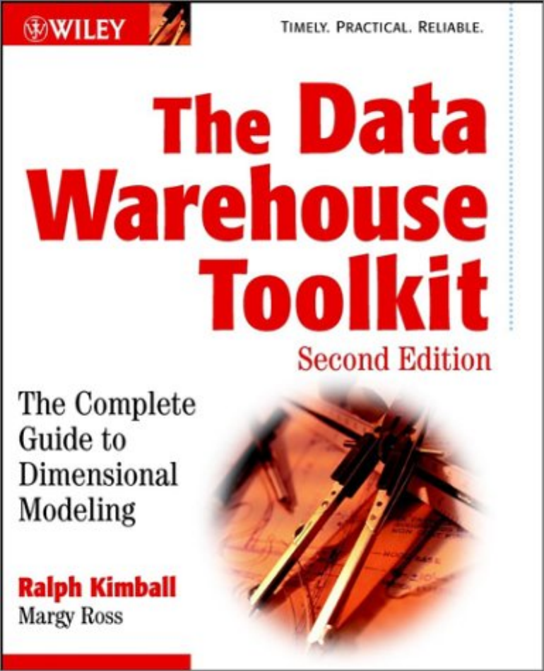
Fact Table
A fact table is the primary table in a dimensional model where the numerical
performance measurements of the business are stored, as illustrated in Figure
1.2. We strive to store the measurement data resulting from a business process
in a single data mart. Since measurement data is overwhelmingly the largest
part of any data mart, we avoid duplicating it in multiple places around the
enterprise.
CHAPTER 1
16
TEAMFLY
Team-Fly®

Figure 1.2 Sample fact table.
We use the term fact to represent a business measure. We can imagine standing
in the marketplace watching products being sold and writing down the quan-
tity sold and dollar sales amount each day for each product in each store. A
measurement is taken at the intersection of all the dimensions (day, product,
and store). This list of dimensions defines the grain of the fact table and tells us
what the scope of the measurement is.
A row in a fact table corresponds to a measurement. A measurement is a row in a
fact table. All the measurements in a fact table must be at the same grain.
The most useful facts are numeric and additive, such as dollar sales amount.
Throughout this book we will use dollars as the standard currency to make the
case study examples more tangible—please bear with the authors and substi-
tute your own local currency if it doesn’t happen to be dollars.
Additivity is crucial because data warehouse applications almost never
retrieve a single fact table row. Rather, they bring back hundreds, thousands,
or even millions of fact rows at a time, and the most useful thing to do with so
many rows is to add them up. In Figure 1.2, no matter what slice of the data-
base the user chooses, we can add up the quantities and dollars to a valid total.
We will see later in this book that there are facts that are semiadditive and still
others that are nonadditive. Semiadditive facts can be added only along some
of the dimensions, and nonadditive facts simply can’t be added at all. With
nonadditive facts we are forced to use counts or averages if we wish to sum-
marize the rows or are reduced to printing out the fact rows one at a time. This
would be a dull exercise in a fact table with a billion rows.
The most useful facts in a fact table are numeric and additive.
We often describe facts as continuously valued mainly as a guide for the
designer to help sort out what is a fact versus a dimension attribute. The dol-
lar sales amount fact is continuously valued in this example because it can take
on virtually any value within a broad range. As observers, we have to stand
Date Key (FK)
Product Key (FK)
Store Key (FK)
Quantity Sold
Dollar Sales Amount
Daily Sales Fact Table
Dimensional Modeling Primer 17

out in the marketplace and wait for the measurement before we have any idea
what the value will be.
It is theoretically possible for a measured fact to be textual; however, the con-
dition arises rarely. In most cases, a textual measurement is a description of
something and is drawn from a discrete list of values. The designer should
make every effort to put textual measures into dimensions because they can be
correlated more effectively with the other textual dimension attributes and
will consume much less space. We do not store redundant textual information
in fact tables. Unless the text is unique for every row in the fact table, it belongs
in the dimension table. A true text fact is rare in a data warehouse because the
unpredictable content of a text fact, like a free text comment, makes it nearly
impossible to analyze.
In our sample fact table (see Figure 1.2), if there is no sales activity on a given
day in a given store for a given product, we leave the row out of the table. It is
very important that we do not try to fill the fact table with zeros representing
nothing happening because these zeros would overwhelm most of our fact
tables. By only including true activity, fact tables tend to be quite sparse.
Despite their sparsity, fact tables usually make up 90 percent or more of the
total space consumed by a dimensional database. Fact tables tend to be deep in
terms of the number of rows but narrow in terms of the number of columns.
Given their size, we are judicious about fact table space utilization.
As we develop the examples in this book, we will see that all fact table grains
fall into one of three categories: transaction, periodic snapshot, and accumu-
lating snapshot. Transaction grain fact tables are among the most common. We
will introduce transaction fact tables in Chapter 2, periodic snapshots in Chap-
ter 3, and accumulating snapshots in Chapter 5.
All fact tables have two or more foreign keys, as designated by the FK notation
in Figure 1.2, that connect to the dimension tables’ primary keys. For example,
the product key in the fact table always will match a specific product key in the
product dimension table. When all the keys in the fact table match their respec-
tive primary keys correctly in the corresponding dimension tables, we say that
the tables satisfy referential integrity. We access the fact table via the dimension
tables joined to it.
The fact table itself generally has its own primary key made up of a subset of
the foreign keys. This key is often called a composite or concatenated key. Every
fact table in a dimensional model has a composite key, and conversely, every
table that has a composite key is a fact table. Another way to say this is that in
a dimensional model, every table that expresses a many-to-many relationship
must be a fact table. All other tables are dimension tables.
CHAPTER 1
18

Fact tables express the many-to-many relationships between dimensions in dimen-
sional models.
Only a subset of the components in the fact table composite key typically is
needed to guarantee row uniqueness. There are usually about a half dozen
dimensions that have robust many-to-many relationships with each other and
uniquely identify each row. Sometimes there are as few as two dimensions,
such as the invoice number and the product key. Once this subset has been
identified, the rest of the dimensions take on a single value in the context of the
fact table row’s primary key. In other words, they go along for the ride. In most
cases, there is no advantage to introducing a unique ROWID key to serve as
the primary key in the fact table. Doing so makes your fact table larger, while
any index on this artificial ROWID primary key would be worthless. However,
such a key may be required to placate the database management system, espe-
cially if you can legitimately, from a business perspective, load multiple iden-
tical rows into the fact table.
Dimension Tables
Dimension tables are integral companions to a fact table. The dimension tables
contain the textual descriptors of the business, as illustrated in Figure 1.3. In a
well-designed dimensional model, dimension tables have many columns or
attributes. These attributes describe the rows in the dimension table. We strive
to include as many meaningful textlike descriptions as possible. It is not
uncommon for a dimension table to have 50 to 100 attributes. Dimension
tables tend to be relatively shallow in terms of the number of rows (often far
fewer than 1 million rows) but are wide with many large columns. Each
dimension is defined by its single primary key, designated by the PK notation
in Figure 1.3, which serves as the basis for referential integrity with any given
fact table to which it is joined.
Dimension attributes serve as the primary source of query constraints, group-
ings, and report labels. In a query or report request, attributes are identified as
the by words. For example, when a user states that he or she wants to see dol-
lar sales by week by brand, week and brand must be available as dimension
attributes.
Dimension table attributes play a vital role in the data warehouse. Since they
are the source of virtually all interesting constraints and report labels, they are
key to making the data warehouse usable and understandable. In many ways,
the data warehouse is only as good as the dimension attributes. The power of
the data warehouse is directly proportional to the quality and depth of the
Dimensional Modeling Primer 19

dimension attributes. The more time spent providing attributes with verbose
business terminology, the better the data warehouse is. The more time spent
populating the values in an attribute column, the better the data warehouse is.
The more time spent ensuring the quality of the values in an attribute column,
the better the data warehouse is.
Dimension tables are the entry points into the fact table. Robust dimension attrib-
utes deliver robust analytic slicing and dicing capabilities. The dimensions imple-
ment the user interface to the data warehouse.
The best attributes are textual and discrete. Attributes should consist of real
words rather than cryptic abbreviations. Typical attributes for a product
dimension would include a short description (10 to 15 characters), a long
description (30 to 50 characters), a brand name, a category name, packaging
type, size, and numerous other product characteristics. Although the size is
probably numeric, it is still a dimension attribute because it behaves more like
a textual description than like a numeric measurement. Size is a discrete and
constant descriptor of a specific product.
Sometimes when we are designing a database it is unclear whether a numeric
data field extracted from a production data source is a fact or dimension
attribute. We often can make the decision by asking whether the field is a mea-
surement that takes on lots of values and participates in calculations (making
it a fact) or is a discretely valued description that is more or less constant and
participates in constraints (making it a dimensional attribute). For example,
the standard cost for a product seems like a constant attribute of the product
but may be changed so often that eventually we decide that it is more like a
measured fact. Occasionally, we can’t be certain of the classification. In such
cases, it may be possible to model the data field either way, as a matter of
designer’s prerogative.
Figure 1.3 Sample dimension table.
Product Key (PK)
Product Description
SKU Number (Natural Key)
Brand Description
Category Description
Department Description
Package Type Description
Package Size
Fat Content Description
Diet Type Description
Weight
Weight Units of Measure
Storage Type
Shelf Life Type
Shelf Width
Shelf Height
Shelf Depth
... and many more
Product Dimension Table
CHAPTER 1
20

We strive to minimize the use of codes in our dimension tables by replacing
them with more verbose textual attributes. We understand that you may have
already trained the users to make sense of operational codes, but going for-
ward, we’d like to minimize their reliance on miniature notes attached to their
computer monitor for code translations. We want to have standard decodes for
the operational codes available as dimension attributes so that the labeling on
data warehouse queries and reports is consistent. We don’t want to encourage
decodes buried in our reporting applications, where inconsistency is
inevitable. Sometimes operational codes or identifiers have legitimate busi-
ness significance to users or are required to communicate back to the opera-
tional world. In these cases, the codes should appear as explicit dimension
attributes, in addition to the corresponding user-friendly textual descriptors.
We have identified operational, natural keys in the dimension figures, as
appropriate, throughout this book.
Operational codes often have intelligence embedded in them. For example, the
first two digits may identify the line of business, whereas the next two digits
may identify the global region. Rather than forcing users to interrogate or fil-
ter on the operational code, we pull out the embedded meanings and present
them to users as separate dimension attributes that can be filtered, grouped, or
reported on easily.
Dimension tables often represent hierarchical relationships in the business. In
our sample product dimension table, products roll up into brands and then
into categories. For each row in the product dimension, we store the brand and
category description associated with each product. We realize that the hierar-
chical descriptive information is stored redundantly, but we do so in the spirit
of ease of use and query performance. We resist our natural urge to store only
the brand code in the product dimension and create a separate brand lookup
table. This would be called a snowflake. Dimension tables typically are highly
denormalized. They are usually quite small (less than 10 percent of the total
data storage requirements). Since dimension tables typically are geometrically
smaller than fact tables, improving storage efficiency by normalizing or
snowflaking has virtually no impact on the overall database size. We almost
always trade off dimension table space for simplicity and accessibility.
Bringing Together Facts and
Dimensions
Now that we understand fact and dimension tables, let’s bring the two build-
ing blocks together in a dimensional model. As illustrated in Figure 1.4, the
fact table consisting of numeric measurements is joined to a set of dimension
tables filled with descriptive attributes. This characteristic starlike structure is
often called a star join schema. This term dates back to the earliest days of rela-
tional databases.
Dimensional Modeling Primer 21
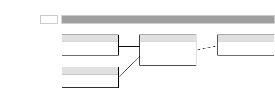
Figure 1.4 Fact and dimension tables in a dimensional model.
The first thing we notice about the resulting dimensional schema is its sim-
plicity and symmetry. Obviously, business users benefit from the simplicity
because the data is easier to understand and navigate. The charm of the design
in Figure 1.4 is that it is highly recognizable to business users. We have
observed literally hundreds of instances where users agree immediately that
the dimensional model is their business. Furthermore, the reduced number of
tables and use of meaningful business descriptors make it less likely that mis-
takes will occur.
The simplicity of a dimensional model also has performance benefits. Data-
base optimizers will process these simple schemas more efficiently with fewer
joins. A database engine can make very strong assumptions about first con-
straining the heavily indexed dimension tables, and then attacking the fact
table all at once with the Cartesian product of the dimension table keys satis-
fying the user’s constraints. Amazingly, using this approach it is possible to
evaluate arbitrary n-way joins to a fact table in a single pass through the fact
table’s index.
Finally, dimensional models are gracefully extensible to accommodate change.
The predictable framework of a dimensional model withstands unexpected
changes in user behavior. Every dimension is equivalent; all dimensions are
symmetrically equal entry points into the fact table. The logical model has no
built-in bias regarding expected query patterns. There are no preferences for
the business questions we’ll ask this month versus the questions we’ll ask next
month. We certainly don’t want to adjust our schemas if business users come
up with new ways to analyze the business.
We will see repeatedly in this book that the most granular or atomic data has
the most dimensionality. Atomic data that has not been aggregated is the
Date Key (FK)
Date Attributes...
Date Dimension
Date Key (PK)
Product Key (FK)
Store Key (FK)
Facts...
Daily Sales Facts
Product Key (PK)
Product Attributes...
Product Dimension
Store Key (PK)
Store Attributes...
Store Dimension
CHAPTER 1
22

most expressive data; this atomic data should be the foundation for every
fact table design in order to withstand business users’ ad hoc attacks where
they pose unexpected queries. With dimensional models, we can add com-
pletely new dimensions to the schema as long as a single value of that
dimension is defined for each existing fact row. Likewise, we can add new,
unanticipated facts to the fact table, assuming that the level of detail is con-
sistent with the existing fact table. We can supplement preexisting dimension
tables with new, unanticipated attributes. We also can break existing dimen-
sion rows down to a lower level of granularity from a certain point in time
forward. In each case, existing tables can be changed in place either simply
by adding new data rows in the table or by executing an SQL ALTER TABLE
command. Data would not have to be reloaded. All existing data access
applications continue to run without yielding different results. We’ll
examine this graceful extensibility of our dimensional models more fully in
Chapter 2.
Another way to think about the complementary nature of fact and dimension
tables is to see them translated into a report. As illustrated in Figure 1.5,
dimension attributes supply the report labeling, whereas the fact tables supply
the report’s numeric values.
Finally, as we’ve already stressed, we insist that the data in the presentation
area be dimensionally structured. However, there is a natural relationship
between dimensional and normalized models. The key to understanding the
relationship is that a single normalized ER diagram often breaks down into
multiple dimensional schemas. A large normalized model for an organization
may have sales calls, orders, shipment invoices, customer payments, and
product returns all on the same diagram. In a way, the normalized ER diagram
does itself a disservice by representing, on a single drawing, multiple business
processes that never coexist in a single data set at a single point in time. No
wonder the normalized model seems complex.
If you already have an existing normalized ER diagram, the first step in con-
verting it into a set of dimensional models is to separate the ER diagram into
its discrete business processes and then model each one separately. The second
step is to select those many-to-many relationships in the ER diagrams that con-
tain numeric and additive nonkey facts and designate them as fact tables. The
final step is to denormalize all the remaining tables into flat tables with single-
part keys that join directly to the fact tables. These tables become the dimen-
sion tables.
Dimensional Modeling Primer 23
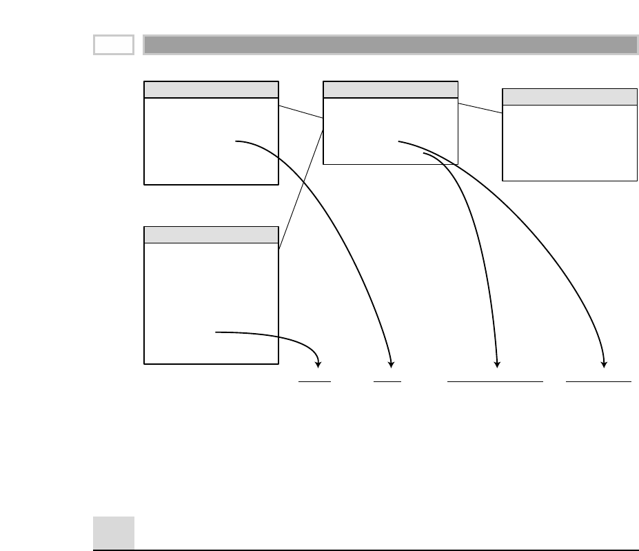
Figure 1.5 Dragging and dropping dimensional attributes and facts into a simple report.
Dimensional Modeling Myths
Despite the general acceptance of dimensional modeling, some mispercep-
tions continue to be disseminated in the industry. We refer to these miscon-
ceptions as dimensional modeling myths.
Myth 1. Dimensional models and data marts are for summary data only. This first
myth is the root cause of many ill-designed dimensional models. Because
we can’t possibly predict all the questions asked by business users, we
need to provide them with queryable access to the most detailed data so
that they can roll it up based on the business question at hand. Data at the
lowest level of detail is practically impervious to surprises or changes. Our
data marts also will include commonly requested summarized data in
dimensional schemas. This summary data should complement the granu-
lar detail solely to provide improved performance for common queries, but
not attempt to serve as a replacement for the details.
A related corollary to this first myth is that only a limited amount of histor-
ical data should be stored in dimensional structures. There is nothing
Date Key (PK)
Date
Day of Week
Month
Year
... and more
Date Dimension
Date Key (PK)
Product Key (FK)
Store Key (FK)
Quantity Sold
Dollar Sales Amount
Daily Sales Facts
Product Key (PK)
Product Description...
SKU Number (Natural Key)
Brand Description
Subcategory Description
Category Description
... and more
Product Dimension
Store Key (PK)
Store Number
Store Name
Store Address
Store City
Store State
Store Zip
Store District
Store Region
... and more
Store Dimension
Brand
Clean Fast
More Power
Zippy
Clean Fast
More Power
Zippy
Quantity Sold
1,370
2,035
707
2,330
2,207
527
Dollar Sales Amount
1,233
2,239
848
2,097
2,428
633
District
Atherton
Atherton
Atherton
Belmont
Belmont
Belmont
SumSum SumSum
CHAPTER 1
24

about a dimensional model that prohibits the storage of substantial history.
The amount of history available in data marts must be driven by the busi-
ness’s requirements.
Myth 2. Dimensional models and data marts are departmental, not enterprise, solu-
tions. Rather than drawing boundaries based on organizational depart-
ments, we maintain that data marts should be organized around business
processes, such as orders, invoices, and service calls. Multiple business
functions often want to analyze the same metrics resulting from a single
business process. We strive to avoid duplicating the core measurements in
multiple databases around the organization.
Supporters of the normalized data warehouse approach sometimes draw
spiderweb diagrams with multiple extracts from the same source feeding
into multiple data marts. The illustration supposedly depicts the perils of
proceeding without a normalized data warehouse to feed the data marts.
These supporters caution about increased costs and potential inconsisten-
cies as changes in the source system of record would need to be rippled to
each mart’s ETL process.
This argument falls apart because no one advocates multiple extracts from
the same source. The spiderweb diagrams fail to appreciate that the data
marts are process-centric, not department-centric, and that the data is
extracted once from the operational source and presented in a single place.
Clearly, the operational system support folks would frown on the multiple-
extract approach. So do we.
Myth 3. Dimensional models and data marts are not scalable. Modern fact tables
have many billions of rows in them. The dimensional models within our
data marts are extremely scalable. Relational DBMS vendors have
embraced data warehousing and incorporated numerous capabilities into
their products to optimize the scalability and performance of dimensional
models.
A corollary to myth 3 is that dimensional models are only appropriate for
retail or sales data. This notion is rooted in the historical origins of dimen-
sional modeling but not in its current-day reality. Dimensional modeling
has been applied to virtually every industry, including banking, insurance,
brokerage, telephone, newspaper, oil and gas, government, manufacturing,
travel, gaming, health care, education, and many more. In this book we use
the retail industry to illustrate several early concepts mainly because it is
an industry to which we have all been exposed; however, these concepts
are extremely transferable to other businesses.
Myth 4. Dimensional models and data marts are only appropriate when there is a
predictable usage pattern. A related corollary is that dimensional models
aren’t responsive to changing business needs. On the contrary, because of
Dimensional Modeling Primer 25

their symmetry, the dimensional structures in our data marts are extremely
flexible and adaptive to change. The secret to query flexibility is building
the fact tables at the most granular level. In our opinion, the source of
myth 4 is the designer struggling with fact tables that have been prema-
turely aggregated based on the designer’s unfortunate belief in myth 1
regarding summary data. Dimensional models that only deliver summary
data are bound to be problematic. Users run into analytic brick walls when
they try to drill down into details not available in the summary tables.
Developers also run into brick walls because they can’t easily accommo-
date new dimensions, attributes, or facts with these prematurely summa-
rized tables. The correct starting point for your dimensional models is to
express data at the lowest detail possible for maximum flexibility and
extensibility.
Myth 5. Dimensional models and data marts can’t be integrated and therefore lead
to stovepipe solutions. Dimensional models and data marts most certainly
can be integrated if they conform to the data warehouse bus architecture.
Presentation area databases that don’t adhere to the data warehouse bus
architecture will lead to standalone solutions. You can’t hold dimensional
modeling responsible for the failure of some organizations to embrace one
of its fundamental tenets.
Common Pitfalls to Avoid
While we can provide positive recommendations about dimensional data
warehousing, some readers better relate to a listing of common pitfalls or traps
into which others have already stepped. Borrowing from a popular late-night
television show, here is our favorite top 10 list of common errors to avoid while
building your data warehouse. These are all quite lethal errors—one alone
may be sufficient to bring down your data warehouse initiative. We’ll further
elaborate on these in Chapter 16; however, we wanted to plant the seeds early
on while we have your complete attention.
Pitfall 10. Become overly enamored with technology and data rather than
focusing on the business’s requirements and goals.
Pitfall 9. Fail to embrace or recruit an influential, accessible, and reasonable
management visionary as the business sponsor of the data warehouse.
Pitfall 8. Tackle a galactic multiyear project rather than pursuing more man-
ageable, while still compelling, iterative development efforts.
Pitfall 7. Allocate energy to construct a normalized data structure, yet run
out of budget before building a viable presentation area based on dimen-
sional models.
CHAPTER 1
26
TEAMFLY
Team-Fly®

Pitfall 6. Pay more attention to backroom operational performance and ease
of development than to front-room query performance and ease of use.
Pitfall 5. Make the supposedly queryable data in the presentation area overly
complex. Database designers who prefer a more complex presentation
should spend a year supporting business users; they’d develop a much
better appreciation for the need to seek simpler solutions.
Pitfall 4. Populate dimensional models on a standalone basis without regard
to a data architecture that ties them together using shared, conformed
dimensions.
Pitfall 3. Load only summarized data into the presentation area’s dimen-
sional structures.
Pitfall 2. Presume that the business, its requirements and analytics, and the
underlying data and the supporting technology are static.
Pitfall 1. Neglect to acknowledge that data warehouse success is tied directly
to user acceptance. If the users haven’t accepted the data warehouse as a
foundation for improved decision making, then your efforts have been
exercises in futility.
Summary
In this chapter we discussed the overriding goals for the data warehouse and
the differences between data warehouses and operational source systems. We
explored the major components of the data warehouse and discussed the per-
missible role of normalized ER models in the staging area, but not as the end
goal. We then focused our attention on dimensional modeling for the presen-
tation area and established preliminary vocabulary regarding facts and
dimensions. Stay tuned as we put these concepts into action in our first case
study in the next chapter.
Dimensional Modeling Primer 27


Retail Sales
CHAPTER 2
29
The best way to understand the principles of dimensional modeling is to work
through a series of tangible examples. By visualizing real cases, we can hold
the particular design challenges and solutions in our minds much more effec-
tively than if they are presented abstractly. In this book we will develop exam-
ples from a range of businesses to help move past one’s own detail and come
up with the right design.
To learn dimensional modeling, please read all the chapters in this book, even if
you don’t manage a retail business or work for a telecommunications firm. The
chapters are not intended to be full-scale solution handbooks for a given indus-
try or business function. Each chapter is a metaphor for a characteristic set of
dimensional modeling problems that comes up in nearly every kind of busi-
ness. Universities, insurance companies, banks, and airlines alike surely will
need the techniques developed in this retail chapter. Besides, thinking about
someone else’s business is refreshing at times. It is too easy to let historical
complexities derail us when we are dealing with data from our own compa-
nies. By stepping outside our own organizations and then returning with a
well-understood design principle (or two), it is easier to remember the spirit of
the design principles as we descend into the intricate details of our businesses.

Chapter 2 discusses the following concepts:
■■ Four-step process for designing dimensional models
■■ Transaction-level fact tables
■■ Additive and non-additive facts
■■ Sample dimension table attributes
■■ Causal dimensions, such as promotion
■■ Degenerate dimensions, such as the transaction ticket number
■■ Extending an existing dimension model
■■ Snowflaking dimension attributes
■■ Avoiding the “too many dimensions” trap
■■ Surrogate keys
■■ Market basket analysis
Four-Step Dimensional Design Process
Throughout this book we will approach the design of a dimensional database
by consistently considering four steps in a particular order. The meaning of
these four steps will become more obvious as we proceed with the various
designs, but we’ll provide initial definitions at this time.
1. Select the business process to model. A process is a natural business activ-
ity performed in your organization that typically is supported by a source
data-collection system. Listening to your users is the most efficient means
for selecting the business process. The performance measurements that
they clamor to analyze in the data warehouse result from business mea-
surement processes. Example business processes include raw materials
purchasing, orders, shipments, invoicing, inventory, and general ledger.
It is important to remember that we’re not referring to an organizational
business department or function when we talk about business processes.
For example, we’d build a single dimensional model to handle orders
data rather than building separate models for the sales and marketing
departments, which both want to access orders data. By focusing on busi-
ness processes, rather than on business departments, we can deliver con-
sistent information more economically throughout the organization. If we
establish departmentally bound dimensional models, we’ll inevitably
duplicate data with different labels and terminology. Multiple data flows
into separate dimensional models will make us vulnerable to data incon-
sistencies. The best way to ensure consistency is to publish the data once.
A single publishing run also reduces the extract-transformation-load
(ETL) development effort, as well as the ongoing data management and
disk storage burden.
CHAPTER 2
30

2. Declare the grain of the business process. Declaring the grain means speci-
fying exactly what an individual fact table row represents. The grain con-
veys the level of detail associated with the fact table measurements. It
provides the answer to the question, “How do you describe a single row
in the fact table?”
Example grain declarations include:
■■ An individual line item on a customer’s retail sales ticket as measured
by a scanner device
■■ A line item on a bill received from a doctor
■■ An individual boarding pass to get on a flight
■■ A daily snapshot of the inventory levels for each product in a
warehouse
■■ A monthly snapshot for each bank account
Data warehouse teams often try to bypass this seemingly unnecessary
step of the process. Please don’t! It is extremely important that everyone
on the design team is in agreement regarding the fact table granularity.
It is virtually impossible to reach closure in step 3 without declaring the
grain. We also should warn you that an inappropriate grain declaration
will haunt a data warehouse implementation. Declaring the grain is a crit-
ical step that can’t be taken lightly. Having said this, you may discover in
steps 3 or 4 that the grain statement is wrong. This is okay, but then you
must return to step 2, redeclare the grain correctly, and revisit steps 3 and
4 again.
3. Choose the dimensions that apply to each fact table row. Dimensions fall
out of the question, “How do businesspeople describe the data that results
from the business process?” We want to decorate our fact tables with a
robust set of dimensions representing all possible descriptions that take
on single values in the context of each measurement. If we are clear about
the grain, then the dimensions typically can be identified quite easily.
With the choice of each dimension, we will list all the discrete, textlike
attributes that will flesh out each dimension table. Examples of common
dimensions include date, product, customer, transaction type, and status.
4. Identify the numeric facts that will populate each fact table row. Facts are
determined by answering the question, “What are we measuring?” Business
users are keenly interested in analyzing these business process performance
measures. All candidate facts in a design must be true to the grain defined in
step 2. Facts that clearly belong to a different grain must be in a separate fact
table. Typical facts are numeric additive figures such as quantity ordered or
dollar cost amount.
Retail Sales 31

Throughout this book we will keep these four steps in mind as we develop
each of the case studies. We’ll apply a user’s understanding of the business to
decide what dimensions and facts are needed in the dimensional model.
Clearly, we need to consider both our business users’ requirements and the
realities of our source data in tandem to make decisions regarding the four
steps, as illustrated in Figure 2.1. We strongly encourage you to resist the
temptation to model the data by looking at source data files alone. We realize
that it may be much less intimidating to dive into the file layouts and copy-
books rather than interview a businessperson; however, they are no substitute
for user input. Unfortunately, many organizations have attempted this path-
of-least-resistance data-driven approach, but without much success.
Retail Case Study
Let’s start with a brief description of the retail business that we’ll use in this
case study to make dimension and fact tables more understandable. We begin
with this industry because it is one to which we can all relate. Imagine that we
work in the headquarters of a large grocery chain. Our business has 100 gro-
cery stores spread over a five-state area. Each of the stores has a full comple-
ment of departments, including grocery, frozen foods, dairy, meat, produce,
bakery, floral, and health/beauty aids. Each store has roughly 60,000 individ-
ual products on its shelves. The individual products are called stock keeping
units (SKUs). About 55,000 of the SKUs come from outside manufacturers and
have bar codes imprinted on the product package. These bar codes are called
universal product codes (UPCs). UPCs are at the same grain as individual SKUs.
Each different package variation of a product has a separate UPC and hence is
a separate SKU.
Figure 2.1 Key input to the four-step dimensional design process.
Business
Requirements
Data
Realities
Dimensional Model
1. Business Process
2. Grain
3. Dimensions
4. Facts
CHAPTER 2
32

The remaining 5,000 SKUs come from departments such as meat, produce,
bakery, or floral. While these products don’t have nationally recognized UPCs,
the grocery chain assigns SKU numbers to them. Since our grocery chain is
highly automated, we stick scanner labels on many of the items in these other
departments. Although the bar codes are not UPCs, they are certainly SKU
numbers.
Data is collected at several interesting places in a grocery store. Some of the
most useful data is collected at the cash registers as customers purchase prod-
ucts. Our modern grocery store scans the bar codes directly into the point-of-
sale (POS) system. The POS system is at the front door of the grocery store
where consumer takeaway is measured. The back door, where vendors make
deliveries, is another interesting data-collection point.
At the grocery store, management is concerned with the logistics of ordering,
stocking, and selling products while maximizing profit. The profit ultimately
comes from charging as much as possible for each product, lowering costs for
product acquisition and overhead, and at the same time attracting as many
customers as possible in a highly competitive pricing environment. Some of
the most significant management decisions have to do with pricing and pro-
motions. Both store management and headquarters marketing spend a great
deal of time tinkering with pricing and promotions. Promotions in a grocery
store include temporary price reductions, ads in newspapers and newspaper
inserts, displays in the grocery store (including end-aisle displays), and
coupons. The most direct and effective way to create a surge in the volume of
product sold is to lower the price dramatically. A 50-cent reduction in the price
of paper towels, especially when coupled with an ad and display, can cause
the sale of the paper towels to jump by a factor of 10. Unfortunately, such a big
price reduction usually is not sustainable because the towels probably are
being sold at a loss. As a result of these issues, the visibility of all forms of pro-
motion is an important part of analyzing the operations of a grocery store.
Now that we have described our business case study, we’ll begin to design the
dimensional model.
Step 1. Select the Business Process
The first step in the design is to decide what business process(es) to model by
combining an understanding of the business requirements with an under-
standing of the available data.
The first dimensional model built should be the one with the most impact—it should
answer the most pressing business questions and be readily accessible for data
extraction.
Retail Sales 33

In our retail case study, management wants to better understand customer
purchases as captured by the POS system. Thus the business process we’re
going to model is POS retail sales. This data will allow us to analyze what
products are selling in which stores on what days under what promotional
conditions.
Step 2. Declare the Grain
Once the business process has been identified, the data warehouse team faces
a serious decision about the granularity. What level of data detail should be
made available in the dimensional model? This brings us to an important
design tip.
Preferably you should develop dimensional models for the most atomic information
captured by a business process. Atomic data is the most detailed information col-
lected; such data cannot be subdivided further.
Tackling data at its lowest, most atomic grain makes sense on multiple fronts.
Atomic data is highly dimensional. The more detailed and atomic the fact
measurement, the more things we know for sure. All those things we know for
sure translate into dimensions. In this regard, atomic data is a perfect match
for the dimensional approach.
Atomic data provides maximum analytic flexibility because it can be con-
strained and rolled up in every way possible. Detailed data in a dimensional
model is poised and ready for the ad hoc attack by business users.
Of course, you can always declare higher-level grains for a business process
that represent an aggregation of the most atomic data. However, as soon as we
select a higher-level grain, we’re limiting ourselves to fewer and/or poten-
tially less detailed dimensions. The less granular model is immediately vul-
nerable to unexpected user requests to drill down into the details. Users
inevitably run into an analytic wall when not given access to the atomic data.
As we’ll see in Chapter 16, aggregated summary data plays an important role
as a performance-tuning tool, but it is not a substitute for giving users access
to the lowest-level details. Unfortunately, some industry pundits have been
confused on this point. They claim that dimensional models are only appro-
priate for summarized data and then criticize the dimensional modeling
approach for its supposed need to anticipate the business question. This mis-
understanding goes away when detailed, atomic data is made available in a
dimensional model.
In our case study, the most granular data is an individual line item on a POS
transaction. To ensure maximum dimensionality and flexibility, we will proceed
CHAPTER 2
34

with this grain. It is worth noting that this granularity declaration represents a
change from the first edition of this text. Previously, we focused on POS data, but
rather than representing transaction line item detail in the dimensional model,
we elected to provide sales data rolled up by product and promotion in a store
on a day. At the time, these daily product totals represented the state of the art
for syndicated retail sales databases. It was unreasonable to expect then-current
hardware and software to deal effectively with the volumes of data associated
with individual POS transaction line items.
Providing access to the POS transaction information gives us with a very
detailed look at store sales. While users probably are not interested in analyz-
ing single items associated with a specific POS transaction, we can’t predict all
the ways that they’ll want to cull through that data. For example, they may
want to understand the difference in sales on Monday versus Sunday. Or they
may want to assess whether it’s worthwhile to stock so many individual sizes
of certain brands, such as cereal. Or they may want to understand how many
shoppers took advantage of the 50-cents-off promotion on shampoo. Or they
may want to determine the impact in terms of decreased sales when a com-
petitive diet soda product was promoted heavily. While none of these queries
calls for data from one specific transaction, they are broad questions that
require detailed data sliced in very precise ways. None of them could have
been answered if we elected only to provide access to summarized data.
A data warehouse almost always demands data expressed at the lowest possible
grain of each dimension not because queries want to see individual low-level rows,
but because queries need to cut through the details in very precise ways.
Step 3. Choose the Dimensions
Once the grain of the fact table has been chosen, the date, product, and store
dimensions fall out immediately. We assume that the calendar date is the date
value delivered to us by the POS system. Later, we will see what to do if we
also get a time of day along with the date. Within the framework of the pri-
mary dimensions, we can ask whether other dimensions can be attributed to
the data, such as the promotion under which the product is sold. We express
this as another design principle:
A careful grain statement determines the primary dimensionality of the fact table. It
is then often possible to add more dimensions to the basic grain of the fact table,
where these additional dimensions naturally take on only one value under each
combination of the primary dimensions. If the additional dimension violates the
grain by causing additional fact rows to be generated, then the grain statement must
be revised to accommodate this dimension.
Retail Sales 35
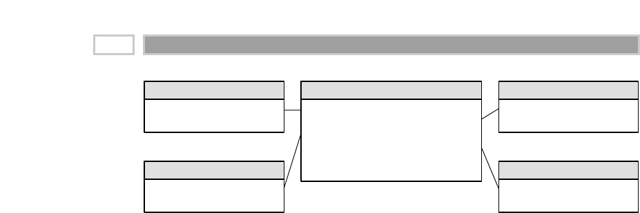
Figure 2.2 Preliminary retail sales schema.
“TBD” means “to be determined.”
In our case study we’ve decided on the following descriptive dimensions:
date, product, store, and promotion. In addition, we’ll include the POS trans-
action ticket number as a special dimension. More will be said on this later in
the chapter.
We begin to envision the preliminary schema as illustrated in Figure 2.2.
Before we delve into populating the dimension tables with descriptive attrib-
utes, let’s complete the final step of the process. We want to ensure that you’re
comfortable with the complete four-step process—we don’t want you to lose
sight of the forest for the trees at this stage of the game.
Step 4. Identify the Facts
The fourth and final step in the design is to make a careful determination of
which facts will appear in the fact table. Again, the grain declaration helps
anchor our thinking. Simply put, the facts must be true to the grain: the indi-
vidual line item on the POS transaction in this case. When considering poten-
tial facts, you again may discover that adjustments need to be made to either
our earlier grain assumptions or our choice of dimensions.
The facts collected by the POS system include the sales quantity (e.g., the num-
ber of cans of chicken noodle soup), per unit sales price, and the sales dollar
amount. The sales dollar amount equals the sales quantity multiplied by the unit
price. More sophisticated POS systems also provide a standard dollar cost for
the product as delivered to the store by the vendor. Presuming that this cost fact
is readily available and doesn’t require a heroic activity-based costing initiative,
we’ll include it in the fact table. Our fact table begins to take shape in Figure 2.3.
Three of the facts, sales quantity, sales dollar amount, and cost dollar amount,
are beautifully additive across all the dimensions. We can slice and dice the fact
table with impunity, and every sum of these three facts is valid and correct.
Date Key (PK)
Date Attributes TBD
Date Dimension
Date Key (FK)
Product Key (FK)
Store Key (FK)
Promotion Key (FK)
POS Transaction Number
Facts TBD
POS Retail Sales Transaction Fact
Product Key (PK)
Product Attributes TBD
Product Dimension
Store Key (PK)
Store Attributes TBD
Store Dimension
Promotion Key (PK)
Promotion Attributes TBD
Promotion Dimension
CHAPTER 2
36
TEAMFLY
Team-Fly®

Figure 2.3 Measured facts in the retail sales schema.
We can compute the gross profit by subtracting the cost dollar amount from
the sales dollar amount, or revenue. Although computed, this gross profit is
also perfectly additive across all the dimensions—we can calculate the gross
profit of any combination of products sold in any set of stores on any set of
days. Dimensional modelers sometimes question whether a calculated fact
should be stored physically in the database. We generally recommend that it
be stored physically. In our case study, the gross profit calculation is straight-
forward, but storing it eliminates the possibility of user error. The cost of a user
incorrectly representing gross profit overwhelms the minor incremental stor-
age cost. Storing it also ensures that all users and their reporting applications
refer to gross profit consistently. Since gross profit can be calculated from adja-
cent data within a fact table row, some would argue that we should perform
the calculation in a view that is indistinguishable from the table. This is a rea-
sonable approach if all users access the data via this view and no users with ad
hoc query tools can sneak around the view to get at the physical table. Views
are a reasonable way to minimize user error while saving on storage, but the
DBA must allow no exceptions to data access through the view. Likewise,
some organizations want to perform the calculation in the query tool. Again,
this works if all users access the data using a common tool (which is seldom
the case in our experience).
The gross margin can be calculated by dividing the gross profit by the dollar
revenue. Gross margin is a nonadditive fact because it can’t be summarized
along any dimension. We can calculate the gross margin of any set of products,
stores, or days by remembering to add the revenues and costs before dividing.
This can be stated as a design principle:
Percentages and ratios, such as gross margin, are nonadditive. The numerator and
denominator should be stored in the fact table. The ratio can be calculated in a data
access tool for any slice of the fact table by remembering to calculate the ratio of
the sums, not the sum of the ratios.
Date Key (PK)
Date Attributes TBD
Date Dimension
Date Key (FK)
Product Key (FK)
Store Key (FK)
Promotion Key (FK)
POS Transaction Number
Sales Quantity
Sales Dollar Amount
Cost Dollar Amount
Gross Profit Dollar Amount
POS Retail Sales Transaction Fact
Product Key (PK)
Product Attributes TBD
Product Dimension
Store Key (PK)
Store Attributes TBD
Store Dimension
Promotion Key (PK)
Promotion Attributes TBD
Promotion Dimension
Retail Sales 37

Unit price is also a nonadditive fact. Attempting to sum up unit price across any
of the dimensions results in a meaningless, nonsensical number. In order to ana-
lyze the average selling price for a product in a series of stores or across a period
of time, we must add up the sales dollars and sales quantities before dividing the
total dollars by the total quantity sold. Every report writer or query tool in the
data warehouse marketplace should automatically perform this function cor-
rectly, but unfortunately, some still don’t handle it very gracefully.
At this early stage of the design, it is often helpful to estimate the number of
rows in our largest table, the fact table. In our case study, it simply may be a
matter of talking with a source system guru to understand how many POS
transaction line items are generated on a periodic basis. Retail traffic fluctuates
significantly from day to day, so we’ll want to understand the transaction activ-
ity over a reasonable period of time. Alternatively, we could estimate the num-
ber of rows added to the fact table annually by dividing the chain’s annual
gross revenue by the average item selling price. Assuming that gross revenues
are $4 billion per year and that the average price of an item on a customer ticket
is $2.00, we calculate that there are approximately 2 billion transaction line
items per year. This is a typical engineer’s estimate that gets us surprisingly
close to sizing a design directly from our armchairs. As designers, we always
should be triangulating to determine whether our calculations are reasonable.
Dimension Table Attributes
Now that we’ve walked through the four-step process, let’s return to the
dimension tables and focus on filling them with robust attributes.
Date Dimension
We will start with the date dimension. The date dimension is the one dimen-
sion nearly guaranteed to be in every data mart because virtually every data
mart is a time series. In fact, date is usually the first dimension in the underly-
ing sort order of the database so that the successive loading of time intervals of
data is placed into virgin territory on the disk.
For readers of the first edition of The Data Warehouse Toolkit (Wiley 1996), this
dimension was referred to as the time dimension in that text. Rather than stick-
ing with that more ambiguous nomenclature, we use the date dimension in this
book to refer to daily-grained dimension tables. This helps distinguish the date
and time-of-day dimensions, which we’ll discuss later in this chapter.
Unlike most of our other dimensions, we can build the date dimension table in
advance. We may put 5 or 10 years of rows representing days in the table so
CHAPTER 2
38
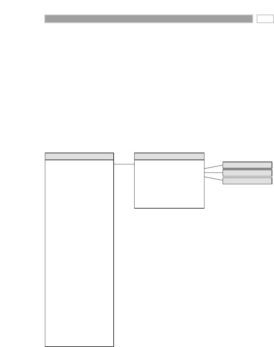
that we can cover the history we have stored, as well as several years in the
future. Even 10 years’ worth of days is only about 3,650 rows, which is a rela-
tively small dimension table. For a daily date dimension table in a retail envi-
ronment, we recommend the partial list of columns shown in Figure 2.4.
Each column in the date dimension table is defined by the particular day that
the row represents. The day-of-week column contains the name of the day, such
as Monday. This column would be used to create reports comparing the busi-
ness on Mondays with Sunday business. The day number in calendar month
column starts with 1 at the beginning of each month and runs to 28, 29, 30, or
31, depending on the month. This column is useful for comparing the same day
each month. Similarly, we could have a month number in year (1, ... , 12). The
day number in epoch is effectively a Julian day number (that is, a consecutive
day number starting at the beginning of some epoch). We also could include
Figure 2.4 Date dimension in the retail sales schema.
Date Dimension
Date Key (FK)
Product Key (FK)
Store Key (FK)
Promotion Key (FK)
POS Transaction Number
Sales Quantity
Sales Dollar Amount
Cost Dollar Amount
Gross Profit Dollar Amount
POS Retail Sales Transaction Fact
Product Dimension
Store Dimension
Promotion Dimension
Date Key (PK)
Date
Full Date Description
Day of Week
Day Number in Epoch
Week Number in Epoch
Month Number in Epoch
Day Number in Calendar Month
Day Number in Calendar Year
Day Number in Fiscal Month
Day Number in Fiscal Year
Last Day in Week Indicator
Last Day in Month Indicator
Calendar Week Ending Date
Calendar Week Number in Year
Calendar Month Name
Calendar Month Number in Year
Calendar Year-Month (YYYY-MM)
Calendar Quarter
Calendar Year-Quarter
Calendar Half Year
Calendar Year
Fiscal Week
Fiscal Week Number in Year
Fiscal Month
Fiscal Month Number in Year
Fiscal Year-Month
Fiscal Quarter
Fiscal Year-Quarter
Fiscal Half Year
Fiscal Year
Holiday Indicator
Weekday Indicator
Selling Season
Major Event
SQL Date Stamp
… and more
Retail Sales 39

absolute week and month number columns. All these integers support simple
date arithmetic between days across year and month boundaries. For reporting,
we would want a month name with values such as January. In addition, a year-
month (YYYY-MM) column is useful as a report column header. We likely also
will want a quarter number (Q1, ... , Q4), as well as a year quarter, such as 2001-
Q4. We would have similar columns for the fiscal periods if they differ from
calendar periods.
The holiday indicator takes on the values of Holiday or Nonholiday. Remem-
ber that the dimension table attributes serve as report labels. Simply populat-
ing the holiday indicator with a Y or an N would be far less useful. Imagine a
report where we’re comparing holiday sales for a given product versus non-
holiday sales. Obviously, it would be helpful if the columns had meaningful
values such as Holiday/Nonholiday versus a cryptic Y/N. Rather than decod-
ing cryptic flags into understandable labels in a reporting application, we pre-
fer that the decode be stored in the database so that a consistent value is
available to all users regardless of their reporting environment.
A similar argument holds true for the weekday indicator, which would have a
value of Weekday or Weekend. Saturdays and Sundays obviously would be
assigned the Weekend value. Of course, multiple date table attributes can be
jointly constrained, so we can easily compare weekday holidays with week-
end holidays, for example.
The selling season column is set to the name of the retailing season, if any.
Examples in the United States could include Christmas, Thanksgiving, Easter,
Valentine’s Day, Fourth of July, or None. The major event column is similar to
the season column and can be used to mark special outside events such as
Super Bowl Sunday or Labor Strike. Regular promotional events usually are
not handled in the date table but rather are described more completely by
means of the promotion dimension, especially since promotional events are
not defined solely by date but usually are defined by a combination of date,
product, and store.
Some designers pause at this point to ask why an explicit date dimension table
is needed. They reason that if the date key in the fact table is a date-type field,
then any SQL query can directly constrain on the fact table date key and use
natural SQL date semantics to filter on month or year while avoiding a sup-
posedly expensive join. This reasoning falls apart for several reasons. First of
all, if our relational database can’t handle an efficient join to the date dimen-
sion table, we’re already in deep trouble. Most database optimizers are quite
efficient at resolving dimensional queries; it is not necessary to avoid joins like
the plague. Also, on the performance front, most databases don’t index SQL
date calculations, so queries constraining on an SQL-calculated field wouldn’t
take advantage of an index.
CHAPTER 2
40

In terms of usability, the typical business user is not versed in SQL date seman-
tics, so he or she would be unable to directly leverage inherent capabilities
associated with a date data type. SQL date functions do not support filtering
by attributes such as weekdays versus weekends, holidays, fiscal periods, sea-
sons, or major events. Presuming that the business needs to slice data by these
nonstandard date attributes, then an explicit date dimension table is essential.
At the bottom line, calendar logic belongs in a dimension table, not in the
application code. Finally, we’re going to suggest that the date key is an integer
rather than a date data type anyway. An SQL-based date key typically is 8 bytes,
so you’re wasting 4 bytes in the fact table for every date key in every row. More
will be said on this later in this chapter.
Figure 2.5 illustrates several rows from a partial date dimension table.
Data warehouses always need an explicit date dimension table. There are many
date attributes not supported by the SQL date function, including fiscal periods,
seasons, holidays, and weekends. Rather than attempting to determine these non-
standard calendar calculations in a query, we should look them up in a date dimen-
sion table.
If we wanted to access the time of the transaction for day-part analysis (for
example, activity during the evening after-work rush or third shift), we’d han-
dle it through a separate time-of-day dimension joined to the fact table. Date
and time are almost completely independent. If we combined the two dimen-
sions, the date dimension would grow significantly; our neat date dimension
with 3,650 rows to handle 10 years of data would expand to 5,256,000 rows if
we tried to handle time by minute in the same table (or via an outrigger). Obvi-
ously, it is preferable to create a 3,650-row date dimension table and a separate
1,440-row time-of-day by minute dimension.
In Chapter 5 we’ll discuss the handling of multiple dates in a single schema.
We’ll explore international date and time considerations in Chapters 11
and 14.
Figure 2.5 Date dimension table detail.
Date
Key Date
Full Date
Description Day of Week
Calendar
Month
Calendar
Year
Fiscal Year-
Month
Holiday
Indicator
Weekday
Indicator
1
2
3
4
5
6
7
8
01/01/2002
01/02/2002
01/03/2002
01/04/2002
01/05/2002
01/06/2002
01/07/2002
01/08/2002
January 1, 2002
January 2, 2002
January 3, 2002
January 4, 2002
January 5, 2002
January 6, 2002
January 7, 2002
January 8, 2002
Tuesday
Wednesday
Thursday
Friday
Saturday
Sunday
Monday
Tuesday
January
January
January
January
January
January
January
January
2002
2002
2002
2002
2002
2002
2002
2002
F2002-01
F2002-01
F2002-01
F2002-01
F2002-01
F2002-01
F2002-01
F2002-01
Holiday
Non-Holiday
Non-Holiday
Non-Holiday
Non-Holiday
Non-Holiday
Non-Holiday
Non-Holiday
Weekday
Weekday
Weekday
Weekday
Weekend
Weekend
Weekday
Weekday
Retail Sales 41

Product Dimension
The product dimension describes every SKU in the grocery store. While a typ-
ical store in our chain may stock 60,000 SKUs, when we account for different
merchandising schemes across the chain and historical products that are no
longer available, our product dimension would have at least 150,000 rows
and perhaps as many as a million rows. The product dimension is almost
always sourced from the operational product master file. Most retailers
administer their product master files at headquarters and download a subset
of the file to each store’s POS system at frequent intervals. It is headquarters’
responsibility to define the appropriate product master record (and unique
SKU number) for each new UPC created by packaged goods manufacturers.
Headquarters also defines the rules by which SKUs are assigned to such items
as bakery goods, meat, and produce. We extract the product master file into
our product dimension table each time the product master changes.
An important function of the product master is to hold the many descriptive
attributes of each SKU. The merchandise hierarchy is an important group of
attributes. Typically, individual SKUs roll up to brands. Brands roll up to
categories, and categories roll up to departments. Each of these is a many-to-
one relationship. This merchandise hierarchy and additional attributes are
detailed for a subset of products in Figure 2.6.
For each SKU, all levels of the merchandise hierarchy are well defined. Some
attributes, such as the SKU description, are unique. In this case, there are at
least 150,000 different values in the SKU description column. At the other
extreme, there are only perhaps 50 distinct values of the department attribute.
Thus, on average, there are 3,000 repetitions of each unique value in the
department attribute. This is all right! We do not need to separate these
repeated values into a second normalized table to save space. Remember that
dimension table space requirements pale in comparison with fact table space
considerations.
Figure 2.6 Product dimension table detail.
Product
Key Product Description
Brand
Description
Category
Description
Department
Description Fat Content
1
2
3
4
5
6
7
8
9
Baked Well Light Sourdough Fresh Bread
Fluffy Sliced Whole Wheat
Fluffy Light Sliced Whole Wheat
Fat Free Mini Cinnamon Rolls
Diet Lovers Vanilla 2 Gallon
Light and Creamy Butter Pecan 1 Pint
Chocolate Lovers 1/2 Gallon
Strawberry Ice Creamy 1 Pint
Icy Ice Cream Sandwiches
Baked Well
Fluffy
Fluffy
Light
Coldpack
Freshlike
Frigid
Icy
Icy
Bread
Bread
Bread
Sweeten Bread
Frozen Desserts
Frozen Desserts
Frozen Desserts
Frozen Desserts
Frozen Desserts
Bakery
Bakery
Bakery
Bakery
Frozen Foods
Frozen Foods
Frozen Foods
Frozen Foods
Frozen Foods
Reduced Fat
Regular Fat
Reduced Fat
Non-Fat
Non-Fat
Reduced Fat
Regular Fat
Regular Fat
Regular Fat
CHAPTER 2
42

Figure 2.7 Product dimension in the retail sales schema.
Many of the attributes in the product dimension table are not part of the mer-
chandise hierarchy. The package-type attribute, for example, might have values
such as Bottle, Bag, Box, or Other. Any SKU in any department could have one
of these values. It makes perfect sense to combine a constraint on this attribute
with a constraint on a merchandise hierarchy attribute. For example, we could
look at all the SKUs in the Cereal category packaged in Bags. To put this another
way, we can browse among dimension attributes whether or not they belong to
the merchandise hierarchy, and we can drill up and drill down using attributes
whether or not they belong to the merchandise hierarchy. We can even have
more than one explicit hierarchy in our product dimension table.
A recommended partial product dimension for a retail grocery data mart
would look similar to Figure 2.7.
A reasonable product dimension table would have 50 or more descriptive
attributes. Each attribute is a rich source for constraining and constructing row
headers. Viewed in this manner, we see that drilling down is nothing more
than asking for a row header that provides more information. Let’s say we
have a simple report where we’ve summarized the sales dollar amount and
quantity by department.
Department Sales Dollar
Description Amount Sales Quantity
Bakery $12,331 5,088
Frozen Foods $31,776 15,565
Product Dimension
Date Key (FK)
Product Key (FK)
Store Key (FK)
Promotion Key (FK)
POS Transaction Number
Sales Quantity
Sales Dollar Amount
Cost Dollar Amount
Gross Profit Dollar Amount
POS Retail Sales Transaction Fact
Date Dimension
Store Dimension
Promotion Dimension
Product Key (PK)
Product Description
SKU Number (Natural Key)
Brand Description
Category Description
Department Description
Package Type Description
Package Size
Fat Content
Diet Type
Weight
Weight Units of Measure
Storage Type
Shelf Life Type
Shelf Width
Shelf Height
Shelf Depth
… and more
Retail Sales 43

If we want to drill down, we can drag virtually any other attribute, such as
brand, from the product dimension into the report next to department, and we
automatically drill down to this next level of detail. A typical drill down within
the merchandise hierarchy would look like this:
Department Brand Sales Dollar Sales
Description Description Amount Quantity
Bakery Baked Well $3,009 1,138
Bakery Fluffy $3,024 1,476
Bakery Light $6,298 2,474
Frozen Foods Coldpack $5,321 2,640
Frozen Foods Freshlike $10,476 5,234
Frozen Foods Frigid $7,328 3,092
Frozen Foods Icy $2,184 1,437
Frozen Foods QuickFreeze $6,467 3,162
Or we could drill down by the fat-content attribute, even though it isn’t in the
merchandise hierarchy roll-up.
Department Sales Dollar Sales
Description Fat Content Amount Quantity
Bakery Non-Fat $6,298 2,474
Bakery Reduced Fat $5,027 2,086
Bakery Regular Fat $1,006 528
Frozen Foods Non-Fat $5,321 2,640
Frozen Foods Reduced Fat $10,476 5,234
Frozen Foods Regular Fat $15,979 7,691
We have belabored the examples of drilling down in order to make a point,
which we will express as a design principle.
Drilling down in a data mart is nothing more than adding row headers from the
dimension tables. Drilling up is removing row headers. We can drill down or up on
attributes from more than one explicit hierarchy and with attributes that are part of
no hierarchy.
The product dimension is one of the two or three primary dimensions in
nearly every data mart. Great care should be taken to fill this dimension with
as many descriptive attributes as possible. A robust and complete set of
dimension attributes translates into user capabilities for robust and complete
analysis. We’ll further explore the product dimension in Chapter 4, where
we’ll also discuss the handling of product attribute changes.
CHAPTER 2
44

Store Dimension
The store dimension describes every store in our grocery chain. Unlike the
product master file that is almost guaranteed to be available in every large
grocery business, there may not be a comprehensive store master file. The
product master needs to be downloaded to each store every time there’s a
new or changed product. However, the individual POS systems do not
require a store master. Information technology (IT) staffs frequently must
assemble the necessary components of the store dimension from multiple
operational sources at headquarters.
The store dimension is the primary geographic dimension in our case study.
Each store can be thought of as a location. Because of this, we can roll stores up
to any geographic attribute, such as ZIP code, county, and state in the United
States. Stores usually also roll up to store districts and regions. These two dif-
ferent hierarchies are both easily represented in the store dimension because
both the geographic and store regional hierarchies are well defined for a single
store row.
It is not uncommon to represent multiple hierarchies in a dimension table. Ideally,
the attribute names and values should be unique across the multiple hierarchies.
A recommended store dimension table for the grocery business is shown in
Figure 2.8.
Figure 2.8 Store dimension in the retail sales schema.
Store Dimension
Date Key (FK)
Product Key (FK)
Store Key (FK)
Promotion Key (FK)
POS Transaction Number
Sales Quantity
Sales Dollar Amount
Cost Dollar Amount
Gross Profit Dollar Amount
POS Retail Sales Transaction Fact
Date Dimension
Product Dimension
Promotion Dimension
Store Key (PK)
Store Name
Store Number (Natural Key)
Store Street Address
Store City
Store County
Store State
Store Zip Code
Store Manager
Store District
Store Region
Floor Plan Type
Photo Processing Type
Financial Service Type
Selling Square Footage
Total Square Footage
First Open Date
Last Remodel Date
… and more
Retail Sales 45

The floor plan type, photo processing type, and finance services type are all
short text descriptors that describe the particular store. These should not be
one-character codes but rather should be 10- to 20-character standardized
descriptors that make sense when viewed in a pull-down list or used as a
report row header.
The column describing selling square footage is numeric and theoretically
additive across stores. One might be tempted to place it in the fact table. How-
ever, it is clearly a constant attribute of a store and is used as a report constraint
or row header more often than it is used as an additive element in a summa-
tion. For these reasons, we are confident that selling square footage belongs in
the store dimension table.
The first open date and last remodel date typically are join keys to copies of the
date dimension table. These date dimension copies are declared in SQL by the
VIEW construct and are semantically distinct from the primary date dimen-
sion. The VIEW declaration would look like
CREATE VIEW FIRST_OPEN_DATE (FIRST_OPEN_DAY_NUMBER, FIRST_OPEN_MONTH ...)
AS SELECT DAY_NUMBER, MONTH, ...
FROM DATE
Now the system acts as if there is another physical copy of the date dimension
table called FIRST_OPEN_DATE. Constraints on this new date table have
nothing to do with constraints on the primary date dimension table. The first
open date view is a permissible outrigger to the store dimension. Notice that
we have carefully relabeled all the columns in the view so that they cannot be
confused with columns from the primary date dimension. We will further dis-
cuss outriggers in Chapter 6.
Promotion Dimension
The promotion dimension is potentially the most interesting dimension in our
schema. The promotion dimension describes the promotion conditions under
which a product was sold. Promotion conditions include temporary price
reductions, end-aisle displays, newspaper ads, and coupons. This dimension
is often called a causal dimension (as opposed to a casual dimension) because
it describes factors thought to cause a change in product sales.
Managers at both headquarters and the stores are interested in determining
whether a promotion is effective or not. Promotions are judged on one or more
of the following factors:
■■ Whether the products under promotion experienced a gain in sales during
the promotional period. This is called the lift. The lift can only be measured
CHAPTER 2
46
TEAMFLY
Team-Fly®

if the store can agree on what the baseline sales of the promoted products
would have been without the promotion. Baseline values can be estimated
from prior sales history and, in some cases, with the help of sophisticated
mathematical models.
■■ Whether the products under promotion showed a drop in sales just prior
to or after the promotion, canceling the gain in sales during the promotion
(time shifting). In other words, did we transfer sales from regularly priced
products to temporarily reduced-priced products?
■■ Whether the products under promotion showed a gain in sales but other
products nearby on the shelf showed a corresponding sales decrease (can-
nibalization).
■■ Whether all the products in the promoted category of products experi-
enced a net overall gain in sales taking into account the time periods
before, during, and after the promotion (market growth).
■■ Whether the promotion was profitable. Usually the profit of a promotion
is taken to be the incremental gain in profit of the promoted category over
the baseline sales taking into account time shifting and cannibalization, as
well as the costs of the promotion, including temporary price reductions,
ads, displays, and coupons.
The causal conditions potentially affecting a sale are not necessarily tracked
directly by the POS system. The transaction system keeps track of price reduc-
tions and markdowns. The presence of coupons also typically is captured with
the transaction because the customer either presents coupons at the time of
sale or does not. Ads and in-store display conditions may need to be linked
from other sources.
The various possible causal conditions are highly correlated. A temporary
price reduction usually is associated with an ad and perhaps an end-aisle
display. Coupons often are associated with ads. For this reason, it makes
sense to create one row in the promotion dimension for each combination of
promotion conditions that occurs. Over the course of a year, there may be
1,000 ads, 5,000 temporary price reductions, and 1,000 end-aisle displays,
but there may only be 10,000 combinations of these three conditions affect-
ing any particular product. For example, in a given promotion, most of
the stores would run all three promotion mechanisms simultaneously, but
a few of the stores would not be able to deploy the end-aisle displays. In
this case, two separate promotion condition rows would be needed, one for
the normal price reduction plus ad plus display and one for the price reduc-
tion plus ad only. A recommended promotion dimension table is shown in
Figure 2.9.
Retail Sales 47
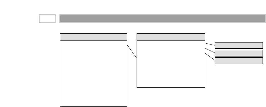
Figure 2.9 Promotion dimension in the retail sales schema.
From a purely logical point of view, we could record very similar information
about the promotions by separating the four major causal mechanisms (price
reductions, ads, displays, and coupons) into four separate dimensions rather
than combining them into one dimension. Ultimately, this choice is the
designer’s prerogative. The tradeoffs in favor of keeping the four dimensions
together include the following:
■■ Since the four causal mechanisms are highly correlated, the combined sin-
gle dimension is not much larger than any one of the separated dimen-
sions would be.
■■ The combined single dimension can be browsed efficiently to see how the
various price reductions, ads, displays, and coupons are used together.
However, this browsing only shows the possible combinations. Browsing
in the dimension table does not reveal which stores or products were
affected by the promotion. This information is found in the fact table.
The tradeoffs in favor of separating the four causal mechanisms into distinct
dimension tables include the following:
■■ The separated dimensions may be more understandable to the business
community if users think of these mechanisms separately. This would be
revealed during the business requirement interviews.
■■ Administration of the separate dimensions may be more straightforward
than administering a combined dimension.
Keep in mind that there is no difference in the information content in the data
warehouse between these two choices.
Promotion Dimension
Date Key (FK)
Product Key (FK)
Store Key (FK)
Promotion Key (FK)
POS Transaction Number
Sales Quantity
Sales Dollar Amount
Cost Dollar Amount
Gross Profit Dollar Amount
POS Retail Sales Transaction Fact
Date Dimension
Product Dimension
Store Dimension
Promotion Key (PK)
Promotion Name
Price Reduction Type
Promotion Media Type
Ad Type
Display Type
Coupon Type
Ad Media Name
Display Provider
Promotion Cost
Promotion Begin Date
Promotion End Date
… and more
CHAPTER 2
48

Typically, many sales transaction line items involve products that are not being
promoted. We will need to include a row in the promotion dimension, with its
own unique key, to identify “No Promotion in Effect” and avoid a null promo-
tion key in the fact table. Referential integrity is violated if we put a null in a
fact table column declared as a foreign key to a dimension table. In addition to
the referential integrity alarms, null keys are the source of great confusion to
our users because they can’t join on null keys.
You must avoid null keys in the fact table. A proper design includes a row in the
corresponding dimension table to identify that the dimension is not applicable
to the measurement.
Promotion Coverage Factless Fact Table
Regardless of the handling of the promotion dimension, there is one important
question that cannot be answered by our retail sales schema: What products
were on promotion but did not sell? The sales fact table only records the SKUs
actually sold. There are no fact table rows with zero facts for SKUs that didn’t
sell because doing so would enlarge the fact table enormously. In the relational
world, a second promotion coverage or event fact table is needed to help
answer the question concerning what didn’t happen. The promotion coverage
fact table keys would be date, product, store, and promotion in our case study.
This obviously looks similar to the sales fact table we just designed; however,
the grain would be significantly different. In the case of the promotion cover-
age fact table, we’d load one row in the fact table for each product on promo-
tion in a store each day (or week, since many retail promotions are a week in
duration) regardless of whether the product sold or not. The coverage fact
table allows us to see the relationship between the keys as defined by a pro-
motion, independent of other events, such as actual product sales. We refer to
it as a factless fact table because it has no measurement metrics; it merely cap-
tures the relationship between the involved keys. To determine what products
where on promotion but didn’t sell requires a two-step process. First, we’d
query the promotion coverage table to determine the universe of products that
were on promotion on a given day. We’d then determine what products sold
from the POS sales fact table. The answer to our original question is the set dif-
ference between these two lists of products. Stay tuned to Chapter 12 for more
complete coverage of factless fact tables; we’ll illustrate the promotion cover-
age table and provide the set difference SQL. If you’re working with data in a
multidimensional online analytical processing (OLAP) cube environment, it is
often easier to answer the question regarding what didn’t sell because the cube
typically contains explicit cells for nonbehavior.
Retail Sales 49

Degenerate Transaction Number
Dimension
The retail sales fact table contains the POS transaction number on every line
item row. In a traditional parent-child database, the POS transaction number
would be the key to the transaction header record, containing all the informa-
tion valid for the transaction as a whole, such as the transaction date and store
identifier. However, in our dimensional model, we have already extracted this
interesting header information into other dimensions. The POS transaction
number is still useful because it serves as the grouping key for pulling together
all the products purchased in a single transaction.
Although the POS transaction number looks like a dimension key in the fact
table, we have stripped off all the descriptive items that might otherwise fall in
a POS transaction dimension. Since the resulting dimension is empty, we refer
to the POS transaction number as a degenerate dimension (identified by the DD
notation in Figure 2.10). The natural operational ticket number, such as the
POS transaction number, sits by itself in the fact table without joining to a
dimension table. Degenerate dimensions are very common when the grain of
a fact table represents a single transaction or transaction line item because the
degenerate dimension represents the unique identifier of the parent. Order
numbers, invoice numbers, and bill-of-lading numbers almost always appear
as degenerate dimensions in a dimensional model.
Degenerate dimensions often play an integral role in the fact table’s primary
key. In our case study, the primary key of the retail sales fact table consists of
the degenerate POS transaction number and product key (assuming that the
POS system rolls up all sales for a given product within a POS shopping cart
into a single line item). Often, the primary key of a fact table is a subset of the
table’s foreign keys. We typically do not need every foreign key in the fact
table to guarantee the uniqueness of a fact table row.
Operational control numbers such as order numbers, invoice numbers, and bill-of-
lading numbers usually give rise to empty dimensions and are represented as degen-
erate dimensions (that is, dimension keys without corresponding dimension tables)
in fact tables where the grain of the table is the document itself or a line item in the
document.
If, for some reason, one or more attributes are legitimately left over after all the
other dimensions have been created and seem to belong to this header entity,
we would simply create a normal dimension record with a normal join. How-
ever, we would no longer have a degenerate dimension.
CHAPTER 2
50
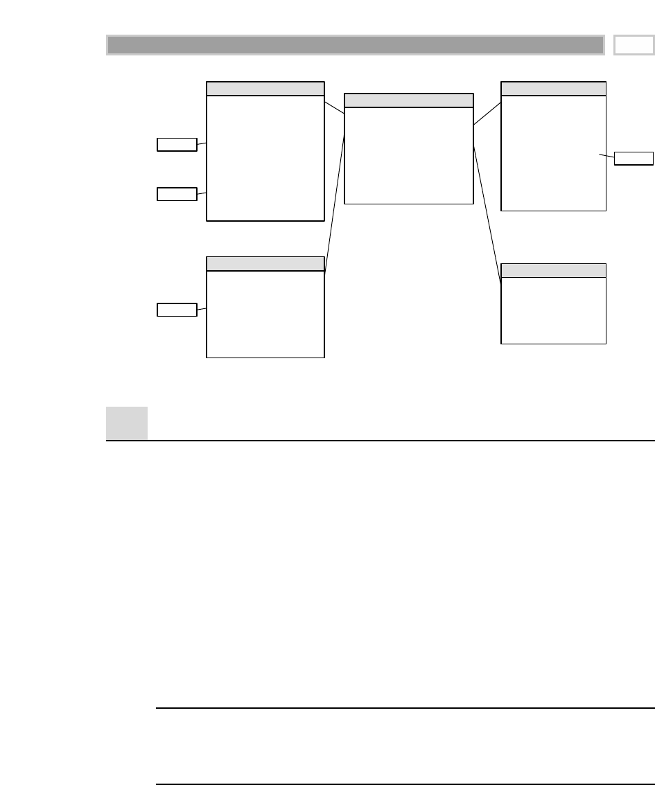
Figure 2.10 Querying the retail sales schema.
Retail Schema in Action
With our retail POS schema designed, let’s illustrate how it would be put to use
in a query environment. A business user might be interested in better under-
standing weekly sales dollar volume by promotion for the snacks category dur-
ing January 2002 for stores in the Boston district. As illustrated in Figure 2.10,
we would place query constraints on month and year in the date dimension,
district in the store dimension, and category in the product dimension.
If the query tool summed the sales dollar amount grouped by week-ending
date and promotion, the query results would look similar to those below. You
can plainly see the relationship between the dimensional model and the asso-
ciated query. High-quality dimension attributes are crucial because they are
the source of query constraints and result set labels.
Calendar Week Sales
Ending Date Promotion Name Dollar Amount
January 6, 2002 No Promotion 22,647
January 13, 2002 No Promotion 4,851
January 20, 2002 Super Bowl Promotion 7,248
January 27, 2002 Super Bowl Promotion 13,798
If you are using a data access tool with more functionality, the results may
appear as a cross-tabular report. Such reports are more appealing to business
users than the columnar data resulting from an SQL statement.
Date Dimension
Date Key (FK)
Product Key (FK)
Store Key (FK)
Promotion Key (FK)
POS Transaction Number (DD)
Sales Quantity
Sales Dollar Amount
Cost Dollar Amount
Gross Profit Dollar Amount
POS Retail Sales Transaction Fact Product Key (PK)
Product Description
SKU Number
Brand Description
Subcategory Description
Category Description
Department Description
Package Type
Fat Content
Diet Type
… and more
Product Dimension
Snacks
January
2002
Boston
Promotion Key (PK)
Promotion Name
Promotion Media Type
Promotion Begin Date
Promotion End Date
… and more
Promotion Dimension
Date Key (PK)
Date
Day of Week
Calendar Week Ending Date
Calendar Month
Calendar Year - Month
Calendar Quarter
Calendar Year - Quarter
Calendar Half Year
Calendar Year
Holiday Indicator
… and more
Store Dimension
Store Key (PK)
Store Name
Store Number
Store District
Store Region
First Open Date
Last Remodel Date
… and more
Retail Sales 51

Super Bowl No Promotion
Calendar Week Promotion Sales Sales Dollar
Ending Date Dollar Amount Amount
January 6, 2002 0 22,647
January 13, 2002 0 4,851
January 20, 2002 7,248 0
January 27, 2002 13,793 0
Retail Schema Extensibility
Now that we’ve completed our first dimensional model, let’s turn our atten-
tion to extending the design. Assume that our retailer decides to implement a
frequent shopper program. Now, rather than knowing that an unidentified
shopper had 26 items in his or her shopping cart, we’re able to see exactly what
a specific shopper, say, Julie Kimball, purchases on a weekly basis. Just imag-
ine the interest of business users in analyzing shopping patterns by a multi-
tude of geographic, demographic, behavioral, and other differentiating
shopper characteristics.
The handling of this new frequent shopper information is relatively straight-
forward. We’d create a frequent shopper dimension table and add another
foreign key in the fact table. Since we can’t ask shoppers to bring in all
their old cash register receipts to tag our historical sales transactions with
their new frequent shopper number, we’d substitute a shopper key corre-
sponding to a “Prior to Frequent Shopper Program” description on our his-
torical fact table rows. Likewise, not everyone who shops at the grocery store
will have a frequent shopper card, so we’d also want to include a “Frequent
Shopper Not Identified” row in our shopper dimension. As we discussed
earlier with the promotion dimension, we must avoid null keys in the fact
table.
As we embellished our original design with a frequent shopper dimension, we
also could add dimensions for the time of day and clerk associated with the
transaction, as illustrated in Figure 2.11. Any descriptive attribute that has a
single value in the presence of the fact table measurements is a good candidate
to be added to an existing dimension or be its own dimension. The decision
regarding whether a dimension can be attached to a fact table should be a
binary yes/no based on the declared grain. If you are in doubt, it’s time to
revisit step 2 of the design process.
CHAPTER 2
52
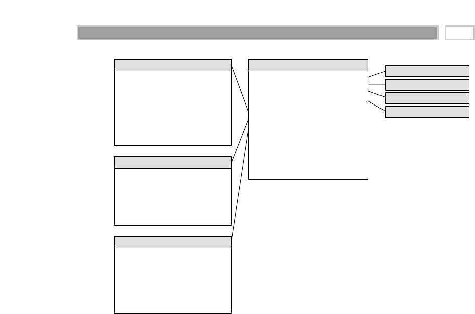
Figure 2.11 Embellished retail sales schema.
Our original schema gracefully extends to accommodate these new dimen-
sions largely because we chose to model the POS transaction data at its most
granular level. The addition of dimensions that apply at that granularity did
not alter the existing dimension keys or facts; all preexisting applications con-
tinue to run without unraveling or changing. If we had declared originally that
the grain would be daily retail sales (transactions summarized by day, store,
product, and promotion) rather than at transaction line detail, we would not
have been able to easily incorporate the frequent-shopper, time-of-day, or clerk
dimensions. Premature summarization or aggregation inherently limits our
ability to add supplemental dimensions because the additional dimensions
often don’t apply at the higher grain.
Obviously, there are some changes that can never be handled gracefully. If a
data source ceases to be available and there is no compatible substitute, then
the data warehouse applications depending on this source will stop working.
However, the predictable symmetry of dimensional models allow them to
absorb some rather significant changes in source data and/or modeling
assumptions without invalidating existing applications. We’ll describe several
of these unexpected modification categories, starting with the simplest:
Frequent Shopper Dimension
Date Key (FK)
Product Key (FK)
Store Key (FK)
Promotion Key (FK)
Frequent Shopper Key (FK)
Clerk Key (FK)
Time of Day Key (FK)
POS Transaction Number (DD)
Sales Quantity
Sales Dollar Amount
Cost Dollar Amount
Gross Profit Dollar Amount
POS Retail Sales Transaction Fact Date Dimension
Product Dimension
Store Dimension
Promotion Dimension
Frequent Shopper Key (PK)
Frequent Shopper Name
Frequent Shopper Address
Frequent Shopper City
Frequent Shopper State
Frequent Shopper Zip Code
Frequent Shopper Segment
… and more
Clerk Dimension
Clerk Key (PK)
Clerk Name
Clerk Job Grade
Clerk Supervisor
Date of Hire
… and more
Time Of Day Dimension
Time of Day Key (PK)
Time
Hour
AM/PM Indicator
Shift
Day Part Segment
… and more
Retail Sales 53

New dimension attributes. If we discover new textual descriptors of a prod-
uct, for example, we add these attributes to the dimension as new columns.
All existing applications will be oblivious to the new attributes and con-
tinue to function. If the new attributes are available only after a specific
point in time, then “Not Available” or its equivalent should be populated
in the old dimension records.
New dimensions. As we just illustrated in Figure 2.11, we can add a dimen-
sion to an existing fact table by adding a new foreign key field and popu-
lating it correctly with values of the primary key from the new dimension.
New measured facts. If new measured facts become available, we can add
them gracefully to the fact table. The simplest case is when the new facts
are available in the same measurement event and at the same grain as the
existing facts. In this case, the fact table is altered to add the new columns,
and the values are populated into the table. If the ALTER TABLE statement
is not viable, then a second fact table must be defined with the additional
columns and the rows copied from the first. If the new facts are only avail-
able from a point in time forward, then null values need to be placed in the
older fact rows. A more complex situation arises when new measured facts
occur naturally at a different grain. If the new facts cannot be allocated or
assigned to the original grain of the fact table, it is very likely that the new
facts belong in their own fact table. It is almost always a mistake to mix
grains in the same fact table.
Dimension becoming more granular. Sometimes it is desirable to increase
the granularity of a dimension. In most cases, the original dimension
attributes can be included in the new, more granular dimension because
they roll up perfectly in a many-to-one relationship. The more granular
dimension often implies a more granular fact table. There may be no alter-
native but to drop the fact table and rebuild it. However, all the existing
applications would be unaffected.
Addition of a completely new data source involving existing dimensions
as well as unexpected new dimensions. Almost always, a new source of
data has its own granularity and dimensionality, so we create a new fact
table. We should avoid force-fitting new measurements into an existing
fact table of consistent measurements. The existing applications will still
work because the existing fact and dimension tables are untouched.
Resisting Comfort Zone Urges
With our first dimensional design behind us, let’s directly confront several of the
natural urges that tempt modelers coming from a more normalized background.
We’re consciously breaking some traditional modeling rules because we’re
CHAPTER 2
54

focused on delivering business value through ease of use and performance, not
on transaction processing efficiencies.
Dimension Normalization
(Snowflaking)
The flattened, denormalized dimension tables with repeating textual values
may make a normalization modeler uncomfortable. Let’s revisit our case
study product dimension table. The 150,000 products roll up into 50 distinct
departments. Rather than redundantly storing the 20-byte department
description in the product dimension table, modelers with a normalized
upbringing want to store a 2-byte department code and then create a new
department dimension for the department decodes. In fact, they would feel
more comfortable if all the descriptors in our original design were normalized
into separate dimension tables. They argue that this design saves space
because we’re only storing cryptic codes in our 150,000-row dimension table,
not lengthy descriptors.
In addition, some modelers contend that the normalized design for the dimen-
sion tables is easier to maintain. If a department description changes, they’d
only need to update the one occurrence rather than the 3,000 repetitions in our
original product dimension. Maintenance often is addressed by normalization
disciplines, but remember that all this happens back in the staging area, long
before the data is loaded into a presentation area’s dimensional schema.
Dimension table normalization typically is referred to as snowflaking. Redun-
dant attributes are removed from the flat, denormalized dimension table and
placed in normalized secondary dimension tables. Figure 2.12 illustrates
the partial snowflaking of our original schema. If the schema were fully
snowflaked, it would appear as a full third-normal-form entity-relationship
diagram. The contrast between Figure 2.12 and the earlier design in Figure 2.10
is startling. While the fact tables in both figures are identical, the plethora of
dimension tables (even in our simplistic representation) is overwhelming.
Figure 2.12 Partially snowflaked product dimension.
Brand Dimension
Date Key (FK)
Product Key (FK)
Store Key (FK)
Promotion Key (FK)
POS Transaction Number (DD)
Sales Quantity
Sales Dollar Amount
Cost Dollar Amount
Gross Profit Dollar Amount
POS Retail Sales Transaction Fact
Product Key (PK)
Product Description
SKU Number (Natural Key)
Brand Key (FK)
Package Type Key (FK)
Fat Content
Weight
Weight Units of Measure
Storage Type Key (FK)
Shelf Width
Shelf Height
Shelf Depth
… and more
Product Dimension
Brand Key (PK)
Brand Description
Category Key (FK)
Package Type Dimension
Package Type Key (PK)
Package Type Description
Storage Type Dimension
Storage Type Key (PK)
Storage Type Description
Shelf Life Type Key (FK)
Shelf Life Type Dimension
Shelf Life Type Key (PK)
Shelf Life Type Description
Category Dimension
Category Key (PK)
Category Description
Department Key (FK)
Department Dimension
Department Key (PK)
Department Description
Retail Sales 55

While snowflaking is a legal extension of the dimensional model, in general,
we encourage you to resist the urge to snowflake given our two primary
design drivers, ease of use and performance.
■■ The multitude of snowflaked tables makes for a much more complex pre-
sentation. Users inevitably will struggle with the complexity. Remember
that simplicity is one of the primary objectives of a denormalized dimen-
sional model.
■■ Likewise, database optimizers will struggle with the complexity of the
snowflaked schema. Numerous tables and joins usually translate into
slower query performance. The complexities of the resulting join specifi-
cations increase the chances that the optimizer will get sidetracked and
choose a poor strategy.
■■ The minor disk space savings associated with snowflaked dimension
tables are insignificant. If we replaced the 20-byte department description
in our 150,000-row product dimension table with a 2-byte code, we’d save
a whopping 2.7 MB (150,000 x 18 bytes), but we may have a 10-GB fact
table! Dimension tables are almost always geometrically smaller than fact
table. Efforts to normalize most dimension tables in order to save disk
space are a waste of time.
■■ Snowflaking slows down the users’ ability to browse within a dimension.
Browsing often involves constraining one or more dimension attributes
and looking at the distinct values of another attribute in the presence of
these constraints. Browsing allows users to understand the relationship
between dimension attribute values.
Obviously, a snowflaked product dimension table would respond well if
we just wanted a list of the category descriptions. However, if we wanted
to see all the brands within a category, we’d need to traverse the brand
and category dimensions. If we then wanted to also list the package types
for each brand in a category, we’d be traversing even more tables. The
SQL needed to perform these seemingly simple queries is quite complex,
and we haven’t even touched the other dimensions or fact table.
■■ Finally, snowflaking defeats the use of bitmap indexes. Bitmap indexes are
very useful when indexing low-cardinality fields, such as the category
and department columns in our product dimension tables. They greatly
speed the performance of a query or constraint on the single column in
question. Snowflaking inevitably would interfere with your ability to
leverage this performance-tuning technique.
CHAPTER 2
56
TEAMFLY
Team-Fly®

The dimension tables should remain as flat tables physically. Normalized,
snowflaked dimension tables penalize cross-attribute browsing and prohibit the use
of bit-mapped indexes. Disk space savings gained by normalizing the dimension ta-
bles typically are less than 1 percent of the total disk space needed for the overall
schema. We knowingly sacrifice this dimension table space in the spirit of perfor-
mance and ease-of-use advantages.
There are times when snowflaking is permissible, such as our earlier example
with the date outrigger on the store dimension, where a clump of correlated
attributes is used repeatedly in various independent roles. We just urge you to
be conservative with snowflaked designs and use them only when they are
obviously called for.
Too Many Dimensions
The fact table in a dimensional schema is naturally highly normalized and
compact. There is no way to further normalize the extremely complex many-
to-many relationships among the keys in the fact table because the dimensions
are not correlated with each other. Every store is open every day. Sooner or
later, almost every product is sold on promotion in most or all of our stores.
Interestingly, while uncomfortable with denormalized dimension tables, some
modelers are tempted to denormalize the fact table. Rather than having a sin-
gle product foreign key on the fact table, they include foreign keys for the fre-
quently analyzed elements on the product hierarchy, such as brand,
subcategory, category, and department. Likewise, the date key suddenly turns
into a series of keys joining to separate week, month, quarter, and year dimen-
sion tables. Before you know it, our compact fact table has turned into an
unruly monster that joins to literally dozens of dimension tables. We affection-
ately refer to these designs as centipedes because the fact tables appear to have
nearly 100 legs, as shown in Figure 2.13. Clearly, the centipede design has
stepped into the too-many-dimensions trap.
Remember, even with its tight format, the fact table is the behemoth in a
dimensional design. Designing a fact table with too many dimensions leads to
significantly increased fact table disk space requirements. While we’re willing
to use extra space for dimension tables, fact table space consumption concerns
us because it is our largest table by orders of magnitude. There is no way to
index the enormous multipart key effectively in our centipede example. The
numerous joins are an issue for both usability and query performance.
Retail Sales 57
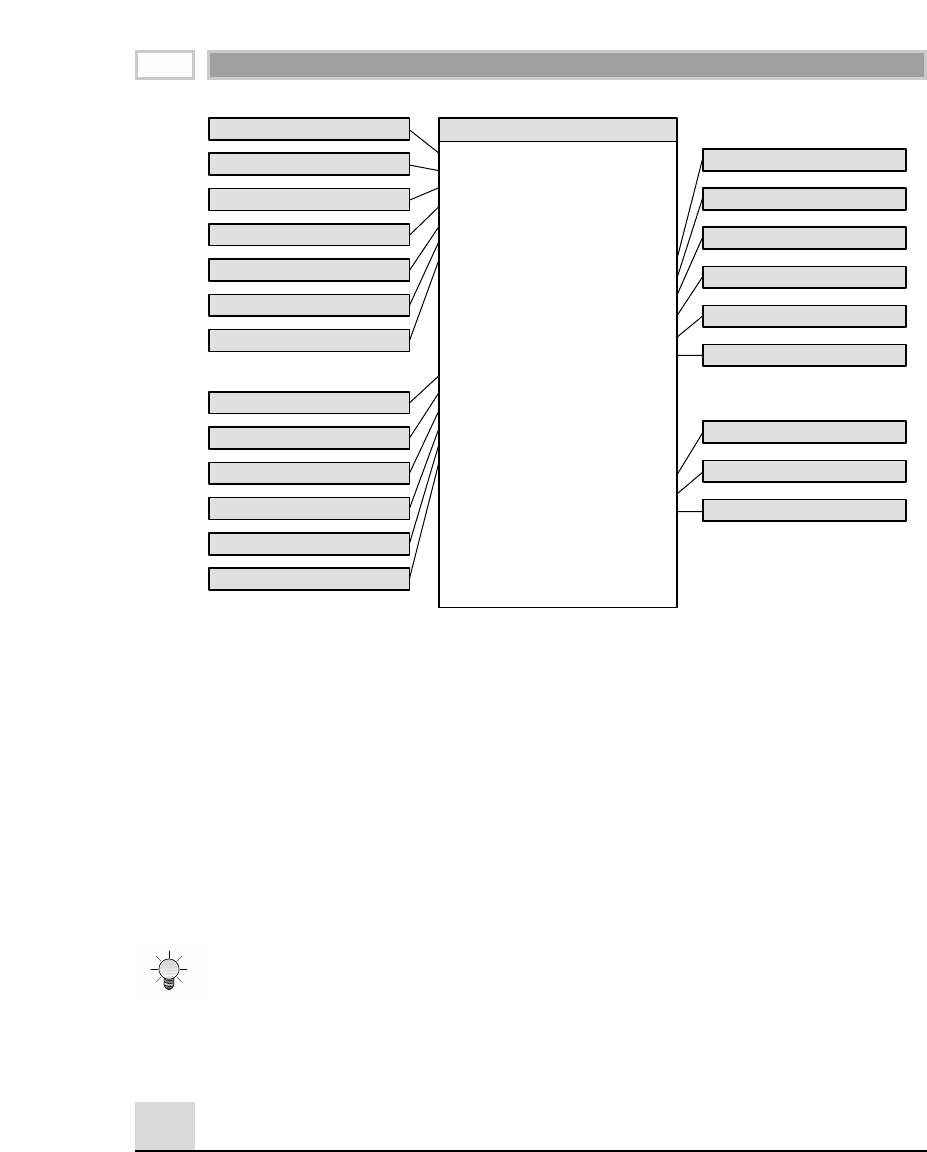
Figure 2.13 Centipede fact table with too many dimensions.
Most business processes can be represented with less than 15 dimensions in
the fact table. If our design has 25 or more dimensions, we should look for
ways to combine correlated dimensions into a single dimension. Perfectly cor-
related attributes, such as the levels of a hierarchy, as well as attributes with a
reasonable statistical correlation, should be part of the same dimension. You
have made a good decision to combine dimensions when the resulting new
single dimension is noticeably smaller than the Cartesian product of the sepa-
rate dimensions.
A very large number of dimensions typically is a sign that several dimensions are not
completely independent and should be combined into a single dimension. It is a di-
mensional modeling mistake to represent elements of a hierarchy as separate di-
mensions in the fact table.
Surrogate Keys
We strongly encourage the use of surrogate keys in dimensional models rather
than relying on operational production codes. Surrogate keys go by many
Date Key (FK)
Week Key (FK)
Month Key (FK)
Quarter Key (FK)
Year Key (FK)
Fiscal Year (FK)
Fiscal Month (FK)
Product Key (FK)
Brand Key (FK)
Subcategory Key (FK)
Category Key (FK)
Department Key (FK)
Package Type Key (FK)
Store Key (FK)
Store County (FK)
Store State Key (FK)
Store District Key (FK)
Store Region Key (FK)
Store Floor Plan (FK)
Promotion Key (FK)
Promotion Reduction Type (FK)
Promotion Media Type (FK)
POS Transaction Number (DD)
Sales Quantity
Sales Dollar Amount
Cost Dollar Amount
Gross Profit Dollar Amount
POS Retail Sales Transaction Fact
Product Dimension
Brand Dimension
Subcategory Dimension
Category Dimension
Department Dimension
Package Type Dimension
Promotion Dimension
Promotion Reduction Type
Promotion Media Type
Date Dimension
Week Dimension
Month Dimension
Quarter Dimension
Year Dimension
Fiscal Year Dimension
Store Floor Plan Dimension
Fiscal Month Dimension
Store Dimension
Store County Dimension
Store State Dimension
Store District Dimension
Store Region Dimension
CHAPTER 2
58

other aliases: meaningless keys, integer keys, nonnatural keys, artificial keys, syn-
thetic keys, and so on. Simply put, surrogate keys are integers that are assigned
sequentially as needed to populate a dimension. For example, the first product
record is assigned a product surrogate key with the value of 1, the next prod-
uct record is assigned product key 2, and so forth. The surrogate keys merely
serve to join the dimension tables to the fact table.
Modelers sometimes are reluctant to give up their natural keys because they
want to navigate the fact table based on the operational code while avoiding a
join to the dimension table. Remember, however, that dimension tables are our
entry points to the facts. If the fifth through ninth characters in the operational
code identify the manufacturer, then the manufacturer’s name should be
included as a dimension table attribute. In general, we want to avoid embed-
ding intelligence in the data warehouse keys because any assumptions that we
make eventually may be invalidated. Likewise, queries and data access appli-
cations should not have any built-in dependency on the keys because the logic
also would be vulnerable to invalidation.
Every join between dimension and fact tables in the data warehouse should be
based on meaningless integer surrogate keys. You should avoid using the natural op-
erational production codes. None of the data warehouse keys should be smart,
where you can tell something about the row just by looking at the key.
Initially, it may be faster to implement a dimensional model using operational
codes, but surrogate keys definitely will pay off in the long run. We sometimes
think of them as being similar to a flu shot for the data warehouse—like an
immunization, there’s a small amount of pain to initiate and administer surro-
gate keys, but the long-run benefits are substantial.
One of the primary benefits of surrogate keys is that they buffer the data ware-
house environment from operational changes. Surrogate keys allow the ware-
house team to maintain control of the environment rather than being
whipsawed by operational rules for generating, updating, deleting, recycling,
and reusing production codes. In many organizations, historical operational
codes (for example, inactive account numbers or obsolete product codes) get
reassigned after a period of dormancy. If account numbers get recycled fol-
lowing 12 months of inactivity, the operational systems don’t miss a beat
because their business rules prohibit data from hanging around for that long.
The data warehouse, on the other hand, will retain data for years. Surrogate
keys provide the warehouse with a mechanism to differentiate these two sep-
arate instances of the same operational account number. If we rely solely on
operational codes, we also are vulnerable to key overlap problems in the case
Retail Sales 59

of an acquisition or consolidation of data. Surrogate keys allow the data ware-
house team to integrate data from multiple operational source systems, even if
they lack consistent source keys.
There are also performance advantages associated with the use of surrogate
keys. The surrogate key is as small an integer as possible while ensuring that it
will accommodate the future cardinality or maximum number of rows in the
dimension comfortably. Often the operational code is a bulky alphanumeric
character string. The smaller surrogate key translates into smaller fact tables,
smaller fact table indices, and more fact table rows per block input-output
operation. Typically, a 4-byte integer is sufficient to handle most dimension sit-
uations. A 4-byte integer is a single integer, not four decimal digits. It has 32
bits and therefore can handle approximately 2 billion positive values (232–1) or
4 billion total positive and negative values (–232–1 to +232–1). As we said, this is
more than enough for just about any dimension. Remember, if you have a
large fact table with 1 billion rows of data, every byte in each fact table row
translates into another gigabyte of storage.
As we mentioned earlier, surrogate keys are used to record dimension con-
ditions that may not have an operational code, such as the “No Promotion in
Effect” condition. By taking control of the warehouse’s keys, we can assign
a surrogate key to identify this condition despite the lack of operational
coding.
Similarly, you may find that your dimensional models have dates that are yet
to be determined. There is no SQL date value for “Date to be Determined” or
“Date Not Applicable.” This is another reason we advocate using surrogate
keys for your date keys rather than SQL date data types (as if our prior ratio-
nale wasn’t convincing enough).
The date dimension is the one dimension where surrogate keys should be
assigned in a meaningful, sequential order. In other words, January 1 of the
first year would be assigned surrogate key value 1, January 2 would be
assigned surrogate key 2, February 1 would be assigned surrogate key 32, and
so on. We don’t want to embed extensive calendar intelligence in these keys
(for example, YYYY-MM-DD) because doing so may encourage people to
bypass the date lookup dimension table. And, of course, in using this smart
format, we would again have no way to represent “Hasn’t happened yet” and
other common date situations. We just want our fact table rows to be in
sequential order. Treating the surrogate date key as a date sequence number
will allow the fact table to be physically partitioned on the basis of the date
key. Partitioning a large fact table on the basis of date is highly effective
because it allows old data to be removed gracefully and new data to be loaded
and indexed without disturbing the rest of the fact table.
CHAPTER 2
60

Finally, surrogate keys are needed to support one of the primary techniques
for handling changes to dimension table attributes. This is actually one of the
most important reasons to use surrogate keys. We’ll devote a whole section in
Chapter 4 to using surrogate keys for slowly changing dimensions.
Of course, some effort is required to assign and administer surrogate keys, but
it’s not nearly as intimidating as many people imagine. We’ll need to establish
and maintain a cross-reference table in the staging area that will be used to
substitute the appropriate surrogate key on each fact and dimension table row.
In Chapter 16 we lay out a flow diagram for administering and processing sur-
rogate keys in our dimensional schemas.
Before we leave the topic of keys, we want to discourage the use of concate-
nated or compound keys for dimension tables. We can’t create a truly surro-
gate key simply by gluing together several natural keys or by combining the
natural key with a time stamp. Also, we want to avoid multiple parallel joins
between the dimension and fact tables, sometimes referred to as double-barreled
joins, because they have an adverse impact on performance.
While we don’t typically assign surrogate keys to degenerate dimensions, you
should evaluate each situation to determine if one is required. A surrogate key
is necessary if the transaction control numbers are not unique across locations
or get reused. For example, our retailer’s POS system may not assign unique
transaction numbers across stores. The system may wrap back to zero and
reuse previous control numbers once its maximum has been reached. Also,
your transaction control number may be a bulky 24-byte alphanumeric column.
In such cases, it would be advantageous to use a surrogate key. Technically, con-
trol number dimensions modeled in this way are no longer degenerate.
For the moment, let’s assume that the first version of the retail sales schema rep-
resents both the logical and physical design of our database. In other words, the
relational database contains only five actual tables: retail sales fact table and
date, product, store, and promotion dimension tables. Each of the dimension
tables has a primary key, and the fact table has a composite key made up of
these four foreign keys, in addition to the degenerate transaction number. Per-
haps the most striking aspect of the design at this point is the simplicity of the
fact table. If the four foreign keys are tightly administered consecutive integers,
we could reserve as little as 14 bytes for all four keys (4 bytes each for date,
product, and promotion and 2 bytes for store). The transaction number might
require an additional 8 bytes. If the four facts in the fact table were each 4-byte
integers, we would need to reserve only another 16 bytes. This would make our
fact table row only 38 bytes wide. Even if we had a billion rows, the fact table
would occupy only about 38 GB of primary data space. Such a streamlined fact
table row is a very typical result in a dimensional design.
Retail Sales 61

Our embellished retail sales schema, illustrated in Figure 2.11, has three addi-
tional dimensions. If we allocate 4 bytes each for shopper and clerk and 2 bytes
for the time of day (to the nearest minute), then our fact table width grows to
only 48 bytes. Our billion-row fact table occupies just 48 GB.
Market Basket Analysis
The retail sales schema tells us in exquisite detail what was purchased at each
store and under what conditions. However, the schema doesn’t allow us to
very easily analyze which products were sold in the same market basket
together. This notion of analyzing the combination of products that sell
together is known by data miners as affinity grouping but more popularly is
called market basket analysis. Market basket analysis gives the retailer insights
about how to merchandise various combinations of items. If frozen pasta din-
ners sell well with cola products, then these two products perhaps should be
located near each other or marketed with complementary pricing. The concept
of market basket analysis can be extended easily to other situations. In the
manufacturing environment, it is useful to see what products are ordered
together because we may want to offer product bundles with package pricing.
The retail sales fact table cannot be used easily to perform market basket
analyses because SQL was never designed to constrain and group across line
item fact rows. Data mining tools and some OLAP products can assist with
market basket analysis, but in the absence of these tools, we’ll describe a more
direct approach below. Be forewarned that this is a rather advanced technique;
if you are not doing market basket analysis today, simply skim this section to
get a general sense of the techniques involved.
In Figure 2.14 we illustrate a market basket fact table that was derived from
retail sales transactions. The market basket fact table is a periodic snapshot
representing the pairs of products purchased together during a specified time
period. The facts include the total number of baskets (customer tickets) that
included products A and B, the total number of product A dollars and units in
this subset of purchases, and the total number of product B dollars and units
purchased. The basket count is a semiadditive fact. For example, if a customer
ticket contains line items for pasta, soft drinks, and peanut butter in the mar-
ket basket fact table, this single order is counted once on the pasta-soft drinks
fact row, once on the row for the pasta-peanut butter combination, and so on.
Obviously, care must be taken to avoid summarizing purchase counts for more
than one product.
CHAPTER 2
62
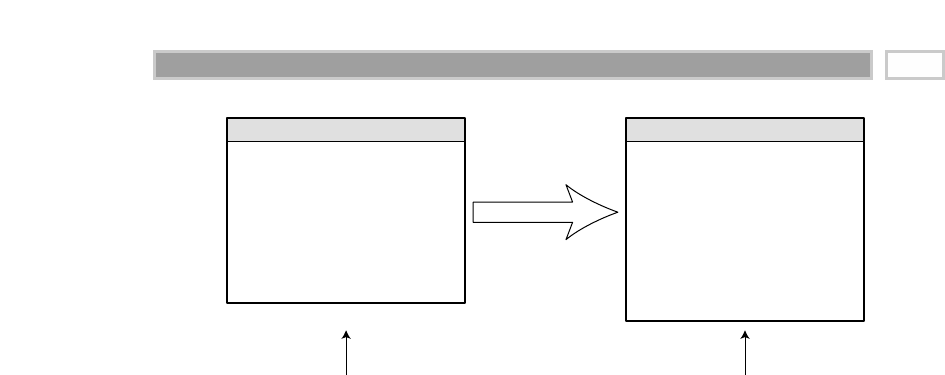
Figure 2.14 Market basket fact table populated from purchase transactions.
You will notice that there are two generalized product keys (product keys A
and B) in the market basket fact table. Here we have built a single product
dimension table that contains entries at multiple levels of the hierarchy, such
as individual products, brands, and categories. This specialized variant of our
normal product dimension table contains a small number of rather generic
attributes. The surrogate keys for the various levels of the product hierarchy
have been assigned so that they don’t overlap.
Conceptually, the idea of recording market basket correlations is simple, but
the sheer number of product combinations makes the analysis challenging. If
we have Nproducts in our product portfolio and we attempt to build a table
with every possible pair of product keys encountered in product orders, we
will approach N2product combinations [actually Nx (N – 1) for the mathe-
maticians among you]. In other words, if we have 10,000 products in our port-
folio, there would be nearly 100,000,000 pairwise combinations. The number
of possible combinations quickly approaches absurdity when we’re dealing
with a large number of products. If a retail store sells 100,000 SKUs, there are
10 billion possible SKU combinations.
The key to realistic market basket analysis is to remember that the primary
goal is to understand the meaningful combinations of products sold together.
Thinking about our market basket fact table, we would first be interested in
rows with high basket counts. Since these product combinations are
observed frequently, they warrant further investigation. Second, we would
Populates
Date Key (FK)
Product Key (FK)
Store Key (FK)
Promotion Key (FK)
POS Transaction Number (DD)
Sales Quantity
Sales Dollar Amount
Cost Dollar Amount
Gross Profit Dollar Amount
POS Retail Sales Transaction Fact
Date Key (FK)
Product A Key (FK)
Product B Key (FK)
Store Key (FK)
Promotion Key (FK)
Basket Count
Sales Quantity Product A
Sales Quantity Product B
Sales Dollar Amount Product A
Sales Dollar Amount Product B
POS Market Basket Fact
Grain = 1 row per POS
transaction line
Grain = 1 row for each pair of
products sold on a day by store
and promotion
Retail Sales 63

look for situations where the dollars or units for products A and B were in
reasonable balance. If the dollars or units are far out of balance, all we’ve
done is find high-selling products coupled with insignificant secondary
products, which wouldn’t be very helpful in making major merchandising or
promotion decisions.
In order to avoid the combinatorial explosion of product pairs in the market
basket fact table, we rely on a progressive pruning algorithm. We begin at the
top of the product hierarchy, which we’ll assume is category. We first enumer-
ate all the category-to-category market basket combinations. If there are 25 cat-
egories, this first step generates 625 market basket rows. We then prune this
list for further analysis by selecting only the rows that have a reasonably high
order count and where the dollars and units for products A and B (which are
categories at this point) are reasonably balanced. Experimentation will tell you
what the basket count threshold and balance range should be.
We then push down to the next level of detail, which we’ll assume is brand.
Starting with the pruned set of combinations from the last step, we drill down
on product A by enumerating all combinations of brand (product A) by cate-
gory (product B). Similarly, we drill down one level of the hierarchy for prod-
uct B by looking at all combinations of brand (product A) by brand (product B).
Again, we prune the lists to those with the highest basket count frequencies and
dollar or unit balance and then drill down to the next level in the hierarchy.
As we descend the hierarchy, we produce rows with smaller and smaller bas-
ket counts. Eventually, we find no basket counts greater than the reasonable
threshold for relevance. It is permissible to stop at any time once we’ve satis-
fied the analyst’s curiosity. One of the advantages of this top-down approach
is that the rows found at each point are those with the highest relevance and
impact. Progressively pruning the list provides more focus to already relevant
results. One can imagine automating this process, searching the product hier-
archy downward, ignoring the low basket counts, and always striving for bal-
anced dollars and units with the high basket counts. The process could halt
when the number of product pairs reached some desired threshold or when
the total activity expressed in basket count, dollars, or units reached some
lower limit.
A variation on this approach could start with a specific category, brand, or
even a product. Again, the idea would be to combine this specific product first
with all the categories and then to work down the hierarchy. Another twist
would be to look at the mix of products purchased by a given customer during
a given time period, regardless of whether they were in the same basket. In
any case, much of the hard work associated with market basket analysis has
been off-loaded to the staging area’s ETL processes in order to simplify the
ultimate query and presentation aspects of the analysis.
CHAPTER 2
64

Summary
In this chapter we got our first exposure to designing a dimensional model.
Regardless of industry, we strongly encourage the four-step process for tack-
ling dimensional model designs. Remember that it is especially important that
we clearly state the grain associated with our dimensional schema. Loading
the fact table with atomic data provides the greatest flexibility because we can
summarize that data “every which way.” As soon as the fact table is restricted
to more aggregated information, we’ll run into walls when the summarization
assumptions prove to be invalid. Also remember that it is vitally important to
populate our dimension tables with verbose, robust descriptive attributes.
In the next chapter we’ll remain within the retail industry to discuss tech-
niques for tackling a second business process within the organization, ensur-
ing that we’re leveraging our earlier efforts while avoiding stovepipes.
Retail Sales 65

TEAMFLY
Team-Fly®

Inventory
CHAPTER 3
67
In Chapter 2 we developed a dimensional model for the sales transactions in a
large grocery chain. We remain within the same industry in this chapter but
move up the value chain to tackle the inventory process. The designs devel-
oped in this chapter apply to a broad set of inventory pipelines both inside and
outside the retail industry.
Even more important, this chapter provides a thorough discussion of the data
warehouse bus architecture. The bus architecture is essential to creating an
integrated data warehouse from a distributed set of related business processes.
It provides a framework for planning the overall warehouse, even though we
will build it incrementally. Finally, we will underscore the importance of using
common, conformed dimensions and facts across the warehouse’s dimen-
sional models.
Chapter 3 discusses the following concepts:
■■ Value chain implications
■■ Inventory periodic snapshot model, as well as transaction and accumulating
snapshot models
■■ Semi-additive facts
■■ Enhanced inventory facts
■■ Data warehouse bus architecture and matrix
■■ Conformed dimensions and facts
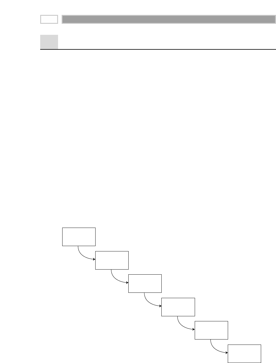
Introduction to the Value Chain
Most organizations have an underlying value chain consisting of their key
business processes. The value chain identifies the natural, logical flow of an
organization’s primary activities. For example, in the case of a retailer, the
company may issue a purchase order to a product manufacturer. The products
are delivered to the retailer’s warehouse, where they are held in inventory. A
delivery is then made to an individual store, where again the products sit in
inventory until a consumer makes a purchase. We have illustrated this subset
of a retailer’s value chain in Figure 3.1. Obviously, products sourced from a
manufacturer that delivers directly to the retail store would bypass the ware-
housing steps of the value chain.
Operational source systems typically produce transactions or snapshots at
each step of the value chain, generating interesting performance metrics along
the way. The primary objective of most analytic decision support systems is to
monitor the performance results of key processes. Since each business process
produces unique metrics at unique time intervals with unique granularity and
dimensionality, each process typically spawns one or more fact tables. To this
end, the value chain provides high-level insight into the overall enterprise
data warehouse. We’ll devote more time to this topic later in this chapter.
Figure 3.1 Subset of a retailer’s value chain.
Retailer Issues
Purchase
Order
Deliveries at
Retailer
Warehouse
Retailer
Warehouse
Inventory
Deliveries at
Retail Store
Retail Store
Inventory
Retail Store
Sales
CHAPTER 3
68

Inventory Models
In the meantime, we’ll delve into several complementary inventory models.
The first is the inventory periodic snapshot. Every day (or at some other regu-
lar time interval), we measure the inventory levels of each product and place
them as separate rows in a fact table. These periodic snapshot rows appear
over time as a series of data layers in the dimensional model, much like geo-
logic layers represent the accumulation of sediment over long periods of time.
We’ll explore this common inventory model in some detail. We’ll also discuss
briefly a second inventory model where we record every transaction that has
an impact on inventory levels as products move through the warehouse.
Finally, in the third model, we’ll touch on the inventory accumulating snap-
shot, where we build one fact table row for each product delivery and update
the row until the product leaves the warehouse. Each of the three inventory
models tells a different story. In some inventory applications, two or even all
three models may be appropriate simultaneously.
Inventory Periodic Snapshot
Let’s return to our retail case study. Optimized inventory levels in the stores
can have a major impact on chain profitability. Making sure the right product
is in the right store at the right time minimizes out-of-stocks (where the prod-
uct isn’t available on the shelf to be sold) and reduces overall inventory carry-
ing costs. The retailer needs the ability to analyze daily quantity-on-hand
inventory levels by product and store.
It is time to put the four-step process for designing dimensional models to
work again. The business process we’re interested in analyzing is the retail
store inventory. In terms of granularity, we want to see daily inventory by
product at each individual store, which we assume is the atomic level of detail
provided by the operational inventory system. The dimensions immediately
fall out of this grain declaration: date, product, and store. We are unable to
envision additional descriptive dimensions at this granularity. Inventory typi-
cally is not associated with a retail promotion dimension. Although a store
promotion may be going on while the products are sitting in inventory, the
promotion usually is not associated with the product until it is actually sold.
After the promotion has ended, the products still may be sitting in inventory.
Typically, promotion dimensions are associated with product movement, such
as when the product is ordered, received, or sold.
The simplest view of inventory involves only a single fact: quantity on
hand. This leads to an exceptionally clean dimensional design, as shown in
Figure 3.2.
Inventory 69
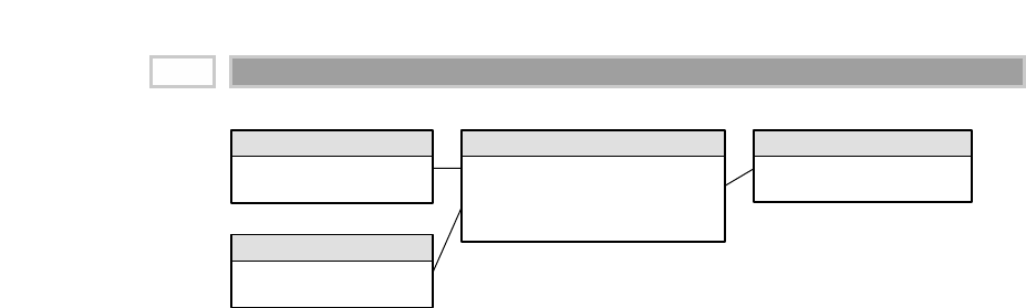
Figure 3.2 Store inventory periodic snapshot schema.
The date dimension table in this case study is identical to the table developed
in the earlier case for retail store sales. The product and store dimensions also
may be identical. Alternatively, we may want to further decorate these dimen-
sion tables with additional attributes that would be useful for inventory analy-
sis. For example, the product dimension could be enhanced to include
columns such as the minimum reorder quantity, assuming that they are con-
stant and discrete descriptors of each product stock keeping unit (SKU). Like-
wise, in the store dimension, in addition to the selling square-footage attribute
we discussed in Chapter 2, we also might include attributes to identify the
frozen and refrigerated storage square footages. We’ll talk more about the
implications of adding these dimension attributes later in this chapter.
If we are analyzing inventory levels at the retailer’s warehouse rather than at
the store location, the schema would look quite similar to Figure 3.2. Obvi-
ously, the store dimension would be replaced with a warehouse dimension.
When monitoring inventory levels at the warehouse, normally we do not
retain the store dimension as a fourth dimension unless the warehouse inven-
tory has been allocated to a specific store.
Even a schema as simple as this one can be very useful. Numerous insights can
be derived if inventory levels are measured frequently for many products in
many storage locations. If we’re analyzing the in-store inventory levels of a
mass merchandiser, this database could be used to balance store inventories
each night after the stores close.
This periodic snapshot fact table faces a serious challenge that Chapter 2’s
sales transaction fact table did not. The sales fact table was reasonably sparse
because only about 10 percent of the products in each of our hypothetical
stores actually sold each day. If a product didn’t sell in a store on a given day,
then there was no row in the fact table for that combination of keys. Inventory,
on the other hand, generates dense snapshot tables. Since the retailer strives to
avoid out-of-stock situations where the product is not available for sale, there
is a row in the fact table for virtually every product in every store every day.
Date Key (PK)
Data Attributes ...
Date Dimension
Date Key (FK)
Product Key (FK)
Store Key (FK)
Quantity on Hand
Store Inventory Snapshot Fact
Product Key (PK)
Product Attributes …
Product Dimension
Store Key (PK)
Store Attributes …
Store Dimension
CHAPTER 3
70

We may well include the zero measurements as explicit records. For our gro-
cery retailer with 60,000 products stocked in 100 stores, we would insert
approximately 6 million rows (60,000 products x 100 stores) with each fact
table load. With a row width of just 14 bytes, the fact table would grow by 84
MB each time we append more fact table rows. A year’s worth of daily snap-
shots would consume over 30 GB. The denseness of inventory snapshots
sometimes mandates some compromises.
Perhaps the most obvious compromise is to reduce the snapshot frequencies
over time. It may be acceptable to keep the last 60 days of inventory at the
daily level and then revert to less granular weekly snapshots for historical
data. In this way, instead of retaining 1,095 snapshots during a 3-year period,
the number could be reduced to 208 total snapshots (60 daily + 148 weekly
snapshots in two separate fact tables given their unique periodicity). We have
reduced the total data size by more than a factor of 5.
Semiadditive Facts
We stressed the importance of fact additivity in Chapter 2. When we modeled
the flow of product past a point at the checkout cash register, only the products
that actually sold were measured. Once a product was sold, it couldn’t be
counted again in a subsequent sale. This made most of the measures in the
retail sales schema perfectly additive across all dimensions.
In the inventory snapshot schema, the quantity on hand can be summarized
across products or stores and result in a valid total. Inventory levels, however,
are not additive across dates because they represent snapshots of a level or bal-
ance at one point in time. It is not possible to tell whether yesterday’s inven-
tory is the same or different from today’s inventory solely by looking at
inventory levels. Because inventory levels (and all forms of financial account
balances) are additive across some dimensions but not all, we refer to them as
semiadditive facts.
The semiadditive nature of inventory balance facts is even more understand-
able if we think about our checking account balances. On Monday, let’s pre-
sume that you have $50 in your account. On Tuesday, the balance remains
unchanged. On Wednesday, you deposit another $50 into your account so that
the balance is now $100. The account has no further activity through the end of
the week. On Friday, you can’t merely add up the daily balances during the
week and declare that your balance is $400 (based on $50 + 50 + 100 + 100 +
100). The most useful way to combine account balances and inventory levels
across dates is to average them (resulting in an $80 average balance in the
checking example). We are all familiar with our bank referring to the average
daily balance on our monthly account summary.
Inventory 71

All measures that record a static level (inventory levels, financial account balances,
and measures of intensity such as room temperatures) are inherently nonadditive
across the date dimension and possibly other dimensions. In these cases, the mea-
sure may be aggregated usefully across time, for example, by averaging over the
number of time periods.
The last few words in this design principle contain a trap. Unfortunately, you
cannot use the SQL AVG function to calculate the average over time. The SQL
AVG function averages over all the rows received by the query, not just the
number of dates. For example, if a query requested the average inventory for
a cluster of three products in four stores across seven dates (that is, what is the
average daily inventory of a brand in a geographic region during a given
week), the SQL AVG function would divide the summed inventory value by
84 (3 products x 4 stores x 7 dates). Obviously, the correct answer is to divide
the summed inventory value by 7, which is the number of daily time periods.
Because SQL has no standard functionality such as an AVG_DATE_SUM oper-
ator that would compute the average over just the date dimension, inventory
calculations are burdened with additional complexity. A proper inventory
application must isolate the date constraint and retrieve its cardinality alone
(in this case, the 7 days comprising the requested week). Then the application
must divide the final summed inventory value by the date constraint cardinal-
ity. This can be done with an embedded SQL call within the overall SQL state-
ment or by querying the date dimension separately and then storing the
resulting value in an application that is passed to the overall SQL statement.
Enhanced Inventory Facts
The simplistic view of inventory we developed in our periodic snapshot fact
table allows us to see a time series of inventory levels. For most inventory
analysis, quantity on hand isn’t enough. Quantity on hand needs to be used in
conjunction with additional facts to measure the velocity of inventory move-
ment and develop other interesting metrics such as the number of turns, num-
ber of days’ supply, and gross margin return on inventory (GMROI,
pronounced “jem-roy”).
If we added quantity sold (or equivalently, quantity depleted or shipped if
we’re dealing with a warehouse location) to each inventory fact row, we could
calculate the number of turns and days’ supply. For daily inventory snapshots,
the number of turns measured each day is calculated as the quantity sold
divided by the quantity on hand. For an extended time span, such as a year,
the number of turns is the total quantity sold divided by the daily average
quantity on hand. The number of days’ supply is a similar calculation. Over a
time span, the number of days’ supply is the final quantity on hand divided by
the average quantity sold.
CHAPTER 3
72

In addition to the quantity sold, we probably also can supply the extended value
of the inventory at cost, as well as the value at the latest selling price. The differ-
ence between these two values is the gross profit, of course. The gross margin is
equal to the gross profit divided by the value at the latest selling price.
Finally, we can multiply the number of turns by the gross margin to get the
GMROI, as expressed in the following formula:
GMROI = total quantity sold x (value at latest selling price – value at cost)
daily average quantity on hand x value at the latest selling price
Although this formula looks complicated, the idea behind GMROI is simple. By
multiplying the gross margin by the number of turns, we create a measure of the
effectiveness of our inventory investment. A high GMROI means that we are
moving the product through the store quickly (lots of turns) and are making
good money on the sale of the product (high gross margin). A low GMROI means
that we are moving the product slowly (low turns) and aren’t making very much
money on it (low gross margin). The GMROI is a standard metric used by inven-
tory analysts to judge a company’s quality of investment in its inventory.
If we want to be more ambitious than our initial design in Figure 3.2, then we
should include the quantity sold, value at cost, and value at the latest selling
price columns in our snapshot fact table, as illustrated in Figure 3.3. Of course,
if some of these metrics exist at different granularity in separate fact tables, a
requesting application would need to retrieve all the components of the
GMROI computation at the same level.
Notice that quantity on hand is semiadditive but that the other measures in
our advanced periodic snapshot are all fully additive across all three dimen-
sions. The quantity sold amount is summarized to the particular grain of the
fact table, which is daily in this case. The value columns are extended, additive
amounts. We do not store GMROI in the fact table because it is not additive.
We can calculate GMROI from the constituent columns across any number of
fact rows by adding the columns up before performing the calculation, but we
are dead in the water if we try to store GMROI explicitly because we can’t use-
fully combine GMROIs across multiple rows.
Figure 3.3 Enhanced inventory periodic snapshot to support GMROI analysis.
Date Key (PK)
Date Attributes …
Date Dimension
Date Key (FK)
Product Key (FK)
Store Key (FK)
Quantity on Hand
Quantity Sold
Dollar Value at Cost
Dollar Value at Latest Selling Price
Store Inventory Snapshot Fact
Product Key (PK)
Product Attributes …
Product Dimension
Store Key (PK)
Store Attributes …
Store Dimension
Inventory 73

The periodic snapshot is the most common inventory schema. We’ll touch
briefly on two alternative perspectives to complement the inventory snapshot
just designed. For a change of pace, rather than describing these models in the
context of the retail in-store inventory, we’ll move up the value chain to dis-
cuss the inventory located in our warehouses.
Inventory Transactions
A second way to model an inventory business process is to record every trans-
action that affects inventory. Inventory transactions at the warehouse might
include the following:
■■ Receive product
■■ Place product into inspection hold
■■ Release product from inspection hold
■■ Return product to vendor due to inspection failure
■■ Place product in bin
■■ Authorize product for sale
■■ Pick product from bin
■■ Package product for shipment
■■ Ship product to customer
■■ Receive product from customer
■■ Return product to inventory from customer return
■■ Remove product from inventory
Each inventory transaction identifies the date, product, warehouse, vendor,
transaction type, and in most cases, a single amount representing the inven-
tory quantity impact caused by the transaction. Assuming that the granularity
of our fact table is one row per inventory transaction, the resulting schema is
illustrated in Figure 3.4.
Figure 3.4 Warehouse inventory transaction model.
Date Dimension Date Key (FK)
Product Key (FK)
Warehouse Key (FK)
Vendor Key (FK)
Inventory Transaction Type Key (FK)
Inventory Transaction Dollar Amount
Warehouse Inventory Transaction Fact
Product Dimension
Warehouse Key (PK)
Warehouse Name
Warehouse Address
Warehouse City
Warehouse State
Warehouse Zip
Warehouse Zone
Warehouse Total Square Footage
… and more
Warehouse Dimension
Inventory Transaction Type Key (PK)
Inventory Transaction Type Description
Inventory Transaction Type Group
Inventory Transaction Type Dimension
Vendor Dimension
CHAPTER 3
74

Even though the transaction-level fact table is again very simple, it contains the
most detailed information available about inventory because it mirrors fine-
scale inventory manipulations. The transaction-level fact table is useful for mea-
suring the frequency and timing of specific transaction types. For instance, only
a transaction-grained inventory fact table can answer the following questions:
■■ How many times have we placed a product into an inventory bin on the
same day we picked the product from the same bin at a different time?
■■ How many separate shipments did we receive from a given vendor, and
when did we get them?
■■ On which products have we had more than one round of inspection
failures that caused return of the product to the vendor?
Even so, it is impractical to use this table as the sole basis for analyzing inven-
tory performance. Although it is theoretically possible to reconstruct the exact
inventory position at any moment in time by rolling all possible transactions
forward from a known inventory position, it is too cumbersome and impracti-
cal for broad data warehouse questions that span dates or products.
Remember that there’s more to life than transactions alone. Some form of snapshot
table to give a more cumulative view of a process often accompanies a transaction
fact table.
Inventory Accumulating Snapshot
The final inventory model that we’ll explore briefly is the accumulating snap-
shot. In this model we place one row in the fact table for a shipment of a par-
ticular product to the warehouse. In a single fact table row we track the
disposition of the product shipment until it has left the warehouse. The accu-
mulating snapshot model is only possible if we can reliably distinguish prod-
ucts delivered in one shipment from those delivered at a later time. This
approach is also appropriate if we are tracking disposition at very detailed lev-
els, such as by product serial number or lot number.
Let’s assume that the inventory goes through a series of well-defined events or
milestones as it moves through the warehouse, such as receiving, inspection,
bin placement, authorization to sell, picking, boxing, and shipping. The phi-
losophy behind the accumulating snapshot fact table is to provide an updated
status of the product shipment as it moves through these milestones. Each fact
table row will be updated until the product leaves the warehouse. As illus-
trated in Figure 3.5, the inventory accumulating snapshot fact table with its
multitude of dates and facts looks quite different from the transaction or peri-
odic snapshot schemas.
Inventory 75
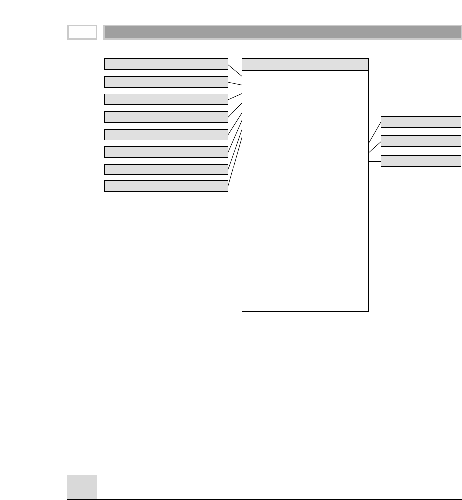
Figure 3.5 Warehouse inventory accumulating snapshot.
Accumulating snapshots are the third major type of fact table. They are inter-
esting both because of the multiple date-valued foreign keys at the beginning
of the key list and also because we revisit and modify the same fact table
records over and over. Since the accumulating snapshot rarely is used in long-
running, continuously replenished inventory processes, rather than focusing
on accumulating snapshots at this time, we’ll provide more detailed coverage
in Chapter 5. The alert reader will notice the four non-additive metrics at the
end of the fact table. Again, stay tuned for Chapter 5.
Value Chain Integration
Now that we’ve completed the design of three inventory model variations,
let’s revisit our earlier discussion about the retailer’s value chain. Both the
business and IT organizations typically are very interested in value chain inte-
gration. Low-level business analysts may not feel much urgency, but those in
the higher ranks of management are very aware of the need to look across the
business to better evaluate performance. Numerous data warehouse projects
have focused recently on management’s need to better understand customer
relationships from an end-to-end perspective. Obviously, this requires the
ability to look consistently at customer information across processes, such as
Date Received Key (FK)
Date Inspected Key (FK)
Date Placed in Inventory Key (FK)
Date Authorized to Sell Key (FK)
Date Picked Key (FK)
Date Boxed Key (FK)
Date Shipped Key (FK)
Date of Last Return Key (FK)
Product Key (FK)
Warehouse Key (FK)
Vendor Key (FK)
Quantity Received
Quantity Inspected
Quantity Returned to Vendor
Quantity Placed in Bin
Quantity Authorized to Sell
Quantity Picked
Quantity Boxed
Quantity Shipped
Quantity Returned by Customer
Quantity Returned to Inventory
Quantity Damaged
Quantity Lost
Quantity Written Off
Unit Cost
Unit List Price
Unit Average Price
Unit Recovery Price
Warehouse Inventory Accumulating Fact
Product Dimension
Warehouse Dimension
Vendor Dimension
Date Received Dimension
Date Inspected Dimension
Date Placed in Inventory Dimension
Date Authorized to Sell Dimension
Date Picked Dimension
Date Boxed Dimension
Date Shipped Dimension
Date of Last Return Dimension
CHAPTER 3
76
TEAMFLY
Team-Fly®

quotes, orders, invoicing, payments, and customer service. Even if your man-
agement’s vision is not so lofty, business users certainly are tired of getting
reports that don’t match from different systems or teams.
IT managers know all too well that integration is needed to deliver on the
promises of data warehousing. Many consider it their fiduciary responsibility
to manage the organization’s information assets. They know that they’re not
fulfilling their responsibilities if they allow standalone, nonintegrated data-
bases to proliferate. In addition to better addressing the business’s needs, the
IT organization also benefits from integration because it allows the organiza-
tion to better leverage scarce resources and gain efficiencies through the use of
reusable components.
Fortunately, the folks who typically are most interested in integration also
have the necessary organizational influence and economic willpower to make
it happen. If they don’t place a high value on integration, then you’re facing a
much more serious organizational challenge. It shouldn’t be the sole responsi-
bility of the data warehouse manager to garner organizational consensus for
an integrated warehouse architecture across the value chain. The political sup-
port of senior management is very important. It takes the data warehouse
manager off the hook and places the burden of the decision-making process on
senior management’s shoulders, where it belongs.
In Chapters 1 and 2 we modeled data from several processes of the value
chain. While separate fact tables in separate data marts represent the data from
each process, the models share several common business dimensions, namely,
date, product, and store. We’ve logically represented this dimension sharing in
Figure 3.6. Using shared, common dimensions is absolutely critical to design-
ing data marts that can be integrated. They allow us to combine performance
measurements from different processes in a single report. We use multipass
SQL to query each data mart separately, and then we outer join the query
results based on a common dimension attribute. This linkage, often referred to
as drill across, is straightforward if the dimension table attributes are identical.
Figure 3.6 Sharing dimensions between business processes.
POS Retail Sales
Transaction Fact
Retail Inventory
Snapshot Fact
Warehouse Inventory
Transaction Fact
Store Dimension
Date Dimension
Promotion Dimension
Product Dimension
Warehouse Dimension
Vendor Dimension
Inventory 77
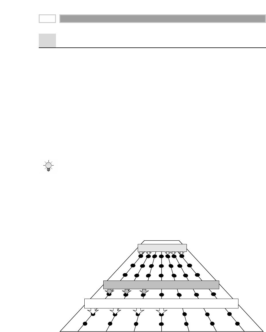
Data Warehouse Bus Architecture
Obviously, building the enterprise’s data warehouse in one step is too daunt-
ing, yet building it as isolated pieces defeats the overriding goal of consistency.
For long-term data warehouse success, we need to use an architected, incre-
mental approach to build the enterprise’s warehouse. The approach we advo-
cate is the data warehouse bus architecture.
The word bus is an old term from the electrical power industry that is now
used commonly in the computer industry. A bus is a common structure to
which everything connects and from which everything derives power. The bus
in your computer is a standard interface specification that allows you to plug
in a disk drive, CD-ROM, or any number of other specialized cards or devices.
Because of the computer’s bus standard, these peripheral devices work
together and usefully coexist, even though they were manufactured at differ-
ent times by different vendors.
By defining a standard bus interface for the data warehouse environment, separate
data marts can be implemented by different groups at different times. The separate
data marts can be plugged together and usefully coexist if they adhere to the standard.
If we think back to the value chain diagram in Figure 3.1, we can envision
many business processes plugging into the data warehouse bus, as illustrated
in Figure 3.7. Ultimately, all the processes of an organization’s value chain will
create a family of dimensional models that share a comprehensive set of com-
mon, conformed dimensions. We’ll talk more about conformed dimensions
later in this chapter, but for now, assume that the term means similar.
Figure 3.7 Sharing dimensions across the value chain.
Date Store Promotion Warehouse Vendor ShipperProduct
Store Sales
Store Inventory
Purchase Orders
CHAPTER 3
78

The data warehouse bus architecture provides a rational approach to decom-
posing the enterprise data warehouse planning task. During the limited-
duration architecture phase, the team designs a master suite of standardized
dimensions and facts that have uniform interpretation across the enterprise.
This establishes the data architecture framework. We then tackle the imple-
mentation of separate data marts in which each iteration closely adheres to
the architecture. As the separate data marts come on line, they fit together like
the pieces of a puzzle. At some point, enough data marts exist to make good
on the promise of an integrated enterprise data warehouse.
The bus architecture allows data warehouse managers to get the best of both
worlds. They have an architectural framework that guides the overall design,
but the problem has been divided into bite-sized data mart chunks that can be
implemented in realistic time frames. Separate data mart development teams
follow the architecture guidelines while working fairly independently and
asynchronously.
The bus architecture is independent of technology and the database platform.
All flavors of relational and online analytical processing (OLAP)-based data
marts can be full participants in the data warehouse bus if they are designed
around conformed dimensions and facts. Data warehouses will inevitably
consist of numerous separate machines with different operating systems and
database management systems (DBMSs). If designed coherently, they will
share a uniform architecture of conformed dimensions and facts that will
allow them to be fused into an integrated whole.
Data Warehouse Bus Matrix
The tool we use to create, document, and communicate the bus architecture is
the data warehouse bus matrix, which we’ve illustrated in Figure 3.8.
Figure 3.8 Sample data warehouse bus matrix.
BUSINESS PROCESSES
COMMON DIMENSIONS
Retail Sales
Retail Inventory
Retail Deliveries
Warehouse Inventory
Warehouse Deliveries
Purchase Orders
Date
Product
Store
Promotion
Warehouse
Vendor
Contract
Shipper
Inventory 79

Working in a tabular fashion, we lay out the business processes of the organi-
zation as matrix rows. It is important to remember that we are identifying the
business processes closely identified with sources of data, not the organiza-
tion’s business departments. The matrix rows translate into data marts based
on the organization’s primary activities. We begin by listing the data marts
that are derived from a single primary source system, commonly known as
first-level data marts. These data marts are recognizable complements to their
operational source.
The rows of the bus matrix correspond to data marts. You should create separate
matrix rows if the sources are different, the processes are different, or if the matrix
row represents more than what can reasonably be tackled in a single implementa-
tion iteration.
Once it is time to begin a data mart development project, we recommend start-
ing the actual implementation with first-level data marts because they mini-
mize the risk of signing up for an implementation that is too ambitious. Most
of the overall risk of failure comes from biting off too much of the extract-
transformation-load (ETL) data staging design and development effort. In
many cases, first-level data marts provide users with enough interesting data
to keep them happy and quiet while the data mart teams keep working on
more difficult issues.
Once we’ve fully enumerated the list of first-level data marts, then we can
identify more complex multisource marts as a second step. We refer to these
data marts as consolidated data marts because they typically cross business
processes. While consolidated data marts are immensely beneficial to the orga-
nization, they are more difficult to implement because the ETL effort grows
alarmingly with each additional major source that’s integrated into a single
dimensional model. It is prudent to focus on the first-level data marts as
dimensional building blocks before tackling the task of consolidating. In some
cases the consolidated data mart is actually more than a simple union of data
sets from the first-level data marts.
Profitability is a classic example of a consolidated data mart where separate
revenue and cost factors are combined from different process marts to provide
a complete view of profitability. While a highly granular profitability mart is
exciting because it provides visibility into product and customer profit perfor-
mance, it is definitely not the first mart you should attempt to implement. You
could easily drown while attempting to stage all the components of revenue
and cost. If you are absolutely forced to focus on profitability as your first mart,
then you should begin by allocating costs on a rule-of-thumb basis rather than
doing the complete job of sourcing all the underlying cost detail. Even so,
CHAPTER 3
80

attempting to get organization consensus on allocation rules may be a project
showstopper given the sensitive (and perhaps wallet-impacting) nature of the
allocations. One of the project prerequisites, outside the scope of the warehouse
project team’s responsibilities, should be business agreement on the allocation
rules. It is safe to say that it is best to avoid dealing with the complexities of
profitability until you have some data warehousing successes under your belt.
The columns of the matrix represent the common dimensions used across the
enterprise. It is often helpful to create a comprehensive list of dimensions
before filling in the matrix. When you start with a large list of potential dimen-
sions, it becomes a useful creative exercise to determine whether a given
dimension possibly could be associated with a data mart.
The shaded cells indicate that the dimension column is related to the business
process row. The resulting matrix will be surprisingly dense. Looking across
the rows is revealing because you can see the dimensionality of each data mart
at a glance. However, the real power of the matrix comes from looking at the
columns as they depict the interaction between the data marts and common
dimensions.
The matrix is a very powerful device for both planning and communication.
Although it is relatively straightforward to lay out the rows and columns, in
the process, we’re defining the overall data architecture for the warehouse. We
can see immediately which dimensions warrant special attention given their
participation in multiple data marts. The matrix helps prioritize which dimen-
sions should be tackled first for conformity given their prominent roles.
The matrix allows us to communicate effectively within and across data mart
teams, as well as upward and outward throughout the organization. The
matrix is a succinct deliverable that visually conveys the entire plan at once. It
is a tribute to its simplicity that the matrix can be used effectively to directly
communicate with senior IT and business management.
Creating the data warehouse bus matrix is one of the most important up-front deliv-
erables of a data warehouse implementation. It is a hybrid resource that is part tech-
nical design tool, part project management tool, and part communication tool.
It goes without saying that it is unacceptable to build separate data marts that
ignore a framework to tie the data together. Isolated, independent data marts
are worse than simply a lost opportunity for analysis. They deliver access to
irreconcilable views of the organization and further enshrine the reports that
cannot be compared with one another. Independent data marts become legacy
implementations in their own right; by their very existence, they block the
development of a coherent warehouse environment.
Inventory 81

So what happens if you’re not starting with a blank data warehousing slate?
Perhaps several data marts have been constructed already without regard to
an architecture of conformed dimensions. Can you rescue your stovepipes and
convert them to the bus architecture? To answer this question, you should start
first with an honest appraisal of your existing nonintegrated data marts. This
typically entails a series of face-to-face meetings with the separate teams
(including the clandestine teams within business organizations) to determine
the gap between the current environment and the organization’s architected
goal. Once the gap is understood, you need to develop an incremental plan to
convert the data marts to the enterprise architecture. The plan needs to be sold
internally. Senior IT and business management must understand the current
state of data chaos, the risks of doing nothing, and the benefits of moving for-
ward according to your game plan. Management also needs to appreciate that
the conversion will require a commitment of support, resources, and funding.
If an existing data mart is based on a sound dimensional design, perhaps you
can simply map an existing dimension to a standardized version. The original
dimension table would be rebuilt using a cross-reference map. Likewise, the
fact table also would need to be reprocessed to replace the original dimension
keys with the conformed dimension keys. Of course, if the original and con-
formed dimension tables contain different attributes, rework of the preexisting
queries is inevitable. More typically, existing data marts are riddled with
dimensional modeling errors beyond just the lack of adherence to standard-
ized dimensions. In some cases, the stovepipe data mart already has outlived
its useful life. Isolated data marts often are built for a specific functional area.
When others try to leverage the environment, they typically discover that the
data mart was implemented at an inappropriate level of granularity and is
missing key dimensionality. The effort required to retrofit these data marts
into the warehouse architecture may exceed the effort to start over from
scratch. As difficult as it is to admit, stovepipe data marts often have to be shut
down and rebuilt in the proper bus architecture framework.
Conformed Dimensions
Now that you understand the importance of the bus architecture, let’s further
explore the standardized conformed dimensions that serve as the cornerstone of
the warehouse bus. Conformed dimensions are either identical or strict mathe-
matical subsets of the most granular, detailed dimension. Conformed dimen-
sions have consistent dimension keys, consistent attribute column names,
consistent attribute definitions, and consistent attribute values (which translates
into consistent report labels and groupings). Dimension tables are not con-
formed if the attributes are labeled differently or contain different values. If a
customer or product dimension is deployed in a nonconformed manner, then
CHAPTER 3
82

either the separate data marts cannot be used together or, worse, attempts to use
them together will produce invalid results.
Conformed dimensions come in several different flavors. At the most basic level,
conformed dimensions mean the exact same thing with every possible fact table
to which they are joined. The date dimension table connected to the sales facts is
identical to the date dimension table connected to the inventory facts. In fact, the
conformed dimension may be the same physical table within the database.
However, given the typical complexity of our warehouse’s technical environ-
ment with multiple database platforms, it is more likely that the dimensions are
duplicated synchronously in each data mart. In either case, the date dimensions
in both data marts will have the same number of rows, same key values, same
attribute labels, same attribute definitions, and same attribute values. There is
consistent data content, data interpretation, and user presentation.
Most conformed dimensions are defined naturally at the most granular level
possible. The grain of the customer dimension naturally will be the individual
customer. The grain of the product dimension will be the lowest level at which
products are tracked in the source systems. The grain of the date dimension
will be the individual day.
Sometimes dimensions are needed at a rolled-up level of granularity. Perhaps
the roll-up dimension is required because the fact table represents aggregated
facts that are associated with aggregated dimensions. This would be the case if
we had a weekly inventory snapshot in addition to our daily snapshot. In
other situations, the facts simply may be generated by another business
process at a higher level of granularity. One business process, such as sales,
captures data at the atomic product level, whereas forecasting generates data
at the brand level. You couldn’t share a single product dimension table across
the two business process schemas because the granularity is different. The
product and brand dimensions still would conform if the brand table were a
strict subset of the atomic product table. Attributes that are common to both
the detailed and rolled-up dimension tables, such as the brand and category
descriptions, should be labeled, defined, and valued identically in both tables,
as illustrated in Figure 3.9.
Roll-up dimensions conform to the base-level atomic dimension if they are a strict
subset of that atomic dimension.
We may encounter other legitimate conformed dimension subsets with dimen-
sion tables at the same level of granularity. For example, in the inventory snap-
shot schema we added supplemental attributes to the product and store
dimensions that may not be useful to the sales transaction schema. The prod-
uct dimension tables used in these two data marts still conform if the keys and
Inventory 83
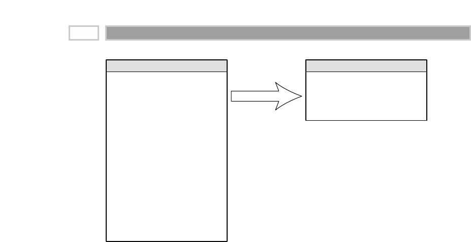
Figure 3.9 Conforming roll-up dimension subsets.
common columns are identical. Of course, given that the supplemental attrib-
utes were limited to the inventory data mart, we would be unable to look
across processes using these add-on attributes.
Another case of conformed dimension subsetting occurs when two dimen-
sions are at the same level of detail but one represents only a subset of rows.
For example, we may have a corporate product dimension that contains data
for our full portfolio of products across multiple disparate lines of business,
as illustrated in Figure 3.10. Analysts in the separate businesses may want to
view only their subset of the corporate dimension, restricted to the product
rows for their business. By using a subset of rows, they aren’t encumbered
with the entire product set for the organization. Of course, the fact table
joined to this subsetted dimension must be limited to the same subset of
products. If a user attempts to use a subset dimension while accessing a fact
table consisting of the complete product set, he or she may encounter unex-
pected query results. Technically, referential integrity would be violated. We
need to be cognizant of the potential opportunity for user confusion or error
with dimension row subsetting. We will further elaborate on dimension sub-
sets when we discuss heterogeneous products in Chapter 9.
Conforms
Product Key (PK)
Product Description
SKU Number (Natural Key)
Brand Description
Subcategory Description
Category Description
Department Description
Package Type Description
Package Size
Fat Content Description
Diet Type Description
Weight
Weight Units of Measure
Storage Type
Shelf Life Type
Shelf Width
Shelf Height
Shelf Depth
… and more
Product Dimensions
Brand Key (PK)
Brand Description
Subcategory Description
Category Description
Department Description
Brand Dimension
CHAPTER 3
84

The conformed date dimension in our daily sales and monthly forecasting sce-
nario is a unique example of both row and column dimension subsetting. Obvi-
ously, we can’t simply use the same date dimension table because of
the difference in roll-up granularity. However, the month dimension may
consist of strictly the month-end daily date table rows with the exclusion of
all columns that don’t apply at the monthly granularity. Excluded columns
would include daily date columns such as the date description, day number in
epoch, weekday/weekend indicator, week-ending date, holiday indicator, day
number within year, and others. You might consider including a month-end
indicator on the daily date dimension to facilitate creation of this monthly table.
Conformed dimensions will be replicated either logically or physically through-
out the enterprise; however, they should be built once in the staging area. The
responsibility for each conformed dimension is vested in a group we call the
dimension authority. The dimension authority has responsibility for defining,
maintaining, and publishing a particular dimension or its subsets to all the data
mart clients who need it. They take responsibility for staging the gold-standard
dimension data. Ultimately, this may involve sourcing from multiple opera-
tional systems to publish a complete, high-quality dimension table.
Figure 3.10 Conforming dimension subsets at the same granularity.
Corporate
Product Dimension
Drilling across (conforming)
both appliance products and
apparel products requires using
attributes common to both types.
Appliance
Products
Apparel
Products
Inventory 85

The major responsibility of the centralized dimension authority is to establish, main-
tain, and publish the conformed dimensions to all the client data marts.
Once a set of master conformed dimensions has been defined for the enter-
prise, it is extremely important that the data mart teams actually use these
dimensions. The commitment to use conformed dimensions is more than a
technical decision; it is a business policy decision that is key to making the
enterprise data warehouse function. Agreement on conformed dimensions
faces far more political challenges than technical hurdles. Given the political
issues surrounding them, conformed dimensions must be supported from the
outset by the highest levels of the organization. Business executives must
stress the importance to their teams, even if the conformed dimension causes
some compromises. The CIO also should appreciate the importance of con-
formed dimensions and mandate that each data mart team takes the pledge to
always use them.
Obviously, conformed dimensions require implementation coordination.
Modifications to existing attributes or the addition of new attributes must be
reviewed with all the data mart teams employing the conformed dimension.
You will also need to determine your conformed dimension release strategy.
Changes to identical dimensions should be replicated synchronously to all
associated data marts. This push approach to dimension publishing maintains
the requisite consistency across the organization.
Now that we’ve preached about the importance of conformed dimensions,
we’ll discuss the situation where it may not be realistic or necessary to estab-
lish conformed dimensions for the organization. If you are a conglomerate
with subsidiaries that span widely varied industries, there may be little point
in trying to integrate. If you don’t want to cross-sell the same customers from
one line of business to another, sell products that span lines of business, or
assign products from multiple lines of business to a single salesperson, then it
may not make sense to attempt a comprehensive data warehouse architecture.
There likely isn’t much perceived business value to conform your dimensions.
The willingness to seek a common definition for product or customer is a
major litmus test for an organization theoretically intent on building an enter-
prise data warehouse. If the organization is unwilling to agree on common
definitions across all data marts, the organization shouldn’t attempt to build a
data warehouse that spans these marts. You would be better off building sep-
arate, self-contained data warehouses for each subsidiary.
In our experience, while many organizations find it currently mission impos-
sible to combine data across their disparate lines of business, some degree of
integration is typically an ultimate goal. Rather than throwing your hands in
CHAPTER 3
86
TEAMFLY
Team-Fly®

the air and declaring that it can’t possibly be done, we suggest starting down
the path toward conformity. Perhaps there are a handful of attributes that can
be conformed across disparate lines of business. Even if it is merely a product
description, category, and line of business attribute that is common to all busi-
nesses, this least-common-denominator approach is still a step in the right
direction. You don’t have to get all your businesses to agree on everything
related to a dimension before proceeding.
Conformed Facts
Thus far we have talked about the central task of setting up conformed dimen-
sions to tie our data marts together. This is 90 percent of the up-front data
architecture effort. The remaining effort goes into establishing conformed fact
definitions.
Revenue, profit, standard prices, standard costs, measures of quality, measures
of customer satisfaction, and other key performance indicators (KPIs) are facts
that must be conformed. In general, fact table data is not duplicated explicitly
in multiple data marts. However, if facts do live in more than one location,
such as in first-level and consolidated marts, the underlying definitions and
equations for these facts must be the same if they are to be called the same
thing. If they are labeled identically, then they need to be defined in the same
dimensional context and with the same units of measure from data mart to
data mart.
We must be disciplined in our data naming practices. If it is impossible to conform a
fact exactly, then you should give different names to the different interpretations.
This makes it less likely that incompatible facts will be used in a calculation.
Sometimes a fact has a natural unit of measure in one fact table and another
natural unit of measure in another fact table. For example, the flow of product
down the retail value chain may best be measured in shipping cases at the
warehouse but in scanned units at the store. Even if all the dimensional con-
siderations have been taken into account correctly, it would be difficult to use
these two incompatible units of measure in one drill-across report. The usual
solution to this kind of problem is to refer the user to a conversion factor
buried in the product dimension table and hope that the user can find the con-
version factor and use it correctly. This is unacceptable in terms of both over-
head and vulnerability to error. The correct solution is to carry the fact in both
units of measure so that a report can easily glide down the value chain, pick-
ing off comparable facts. We’ll talk more about multiple units of measure in
Chapter 5.
Inventory 87

Summary
Inventory is an important process to measure and monitor in many industries.
In this chapter we developed dimensional models for the three complemen-
tary views of inventory. Either the periodic or accumulating snapshot model
will serve as a good stand-alone depiction of inventory. The periodic snapshot
would be chosen for long-running, continuously replenished inventory sce-
narios. The accumulating snapshot would be used for one-time, finite inven-
tory situations with a definite beginning and end. More in-depth inventory
applications will want to augment one or both of these models with the trans-
action model.
We introduced key concepts surrounding the data warehouse bus architecture
and matrix. Each business process of the value chain, supported by a primary
source system, translates into a data mart, as well as a row in the bus matrix.
The data marts share a surprising number of standardized, conformed dimen-
sions. Developing and adhering to the bus architecture is an absolute must if
you intend to build a data warehouse composed of an integrated set of data
marts.
CHAPTER 3
88

Procurement
CHAPTER 4
89
We’ll explore the procurement process in this chapter. This topic has obvious cross-
industry appeal because it is applicable to anyone who acquires products or ser-
vices for either use or resale. In addition to developing several purchasing
models in this chapter, we will provide in-depth coverage of the techniques for
handling changes to our dimension table attributes. While the descriptive attrib-
utes in dimension tables are relatively static, they are subject to change over
time. Product lines are restructured, causing product hierarchies to change. Cus-
tomers move, causing their geographic information to change. Sales reps are
realigned, causing territory assignments to change. We’ll discuss several
approaches to dealing with these inevitable changes in our dimension tables.
Chapter 4 discusses the following concepts:
■■ Value chain reinforcement
■■ Blended versus separate transaction schemas
■■ Slowly changing dimension techniques, both basic and advanced
Procurement Case Study
Thus far we have studied downstream retail sales and inventory processes in the
value chain. We understand the importance of mapping out the data warehouse
bus architecture where conformed dimensions are used across process-centric
fact tables. In this chapter we’ll extend these concepts as we work our way fur-
ther up the value chain to the procurement process.

For many companies, procurement is a critical business activity. Effective pro-
curement of products at the right price for resale is obviously important to
retailers such as our grocery chain. Procurement also has strong bottom-line
implications for any large organization that buys products as raw materials for
manufacturing. Significant cost-savings opportunities are associated with
reducing the number of suppliers and negotiating agreements with preferred
suppliers.
Demand planning drives efficient materials management. Once demand is
forecasted, procurement’s goal is to source the appropriate materials/prod-
ucts in the most economical manner. Procurement involves a wide range of
activities from negotiating contracts to issuing purchase requisitions and pur-
chase orders (POs) to tracking receipts and authorizing payments. The follow-
ing list gives you a better sense of a procurement organization’s common
analytic requirements:
■■ Which materials or products are purchased most frequently? How many
vendors supply these products? At what prices? In what units of measure
(such as bulk or drum)?
■■ Looking at demand across the enterprise (rather than at a single physical
location), are there opportunities to negotiate favorable pricing by consoli-
dating suppliers, single sourcing, or making guaranteed buys?
■■ Are our employees purchasing from the preferred vendors or skirting the
negotiated vendor agreements (maverick spending)?
■■ Are we receiving the negotiated pricing from our vendors (vendor con-
tract purchase price variance)?
■■ How are our vendors performing? What is the vendor’s fill rate? On-time
delivery performance? Late deliveries outstanding? Percent of orders
backordered? Rejection rate based on receipt inspection?
Procurement Transactions
As we begin working through the four-step design process, we first decide that
procurement is the business process to be modeled. We study the process in
detail and observe a flurry of procurement transactions, such as purchase requi-
sitions, purchase orders, shipping notifications, receipts, and payments. Similar
to the approach we took in Chapter 3 with the inventory transactions, we first
elect to build a fact table with the grain of one row per procurement transaction.
We identify transaction date, product, vendor, contract terms, and procurement
transaction type as our key dimensions. Procured units and transaction amount
are the facts. The resulting design looks similar to Figure 4.1.
CHAPTER 4
90
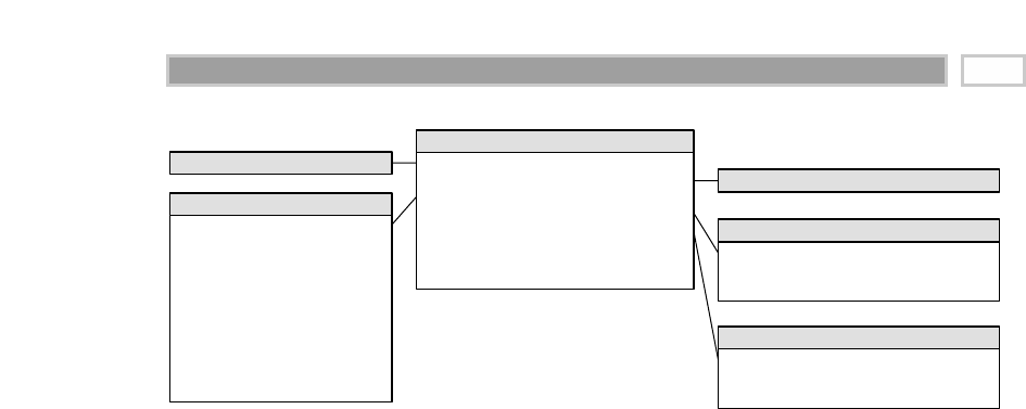
Figure 4.1 Procurement fact table with multiple transaction types.
If we are still working for the same grocery retailer, then the transaction date
and product dimensions are the same conformed dimensions we developed
originally in Chapter 2. If we’re working with manufacturing procurement,
the raw materials products likely are located in a separate raw materials
dimension table rather than included in the product dimension for salable
products. The vendor, contract terms, and procurement transaction type
dimensions are new to this schema. The vendor dimension contains one row
for each vendor, along with interesting descriptive attributes to support a vari-
ety of vendor analyses. The contract terms dimension contains one row for
each generalized set of terms negotiated with a vendor, similar to the promo-
tion dimension in Chapter 2. The procurement transaction type dimension
allows us to group or filter on transaction types, such as purchase orders. The
contract number is a degenerate dimension. It would be used to determine the
volume of business conducted under each negotiated contract.
Multiple- versus Single-Transaction
Fact Tables
As we review the initial procurement schema design with business users, we
are made aware of several new details. First of all, we learn that the business
users describe the various procurement transactions differently. To the busi-
ness, purchase orders, shipping notices, warehouse receipts, and vendor pay-
ments are all viewed as separate and unique processes.
It turns out that several of the procurement transactions actually come from
different source systems. There is no single procurement system to source all
the procurement transactions. Instead, there is a purchasing system that pro-
vides purchase requisitions and purchase orders, a warehousing system that
provides shipping notices and warehouse receipts, and an accounts payable
system that deals with vendor payments.
Date Dimension Procurement Transaction Date Key (FK)
Product Key (FK)
Vendor Key (FK)
Contract Terms Key (FK)
Procurement Transaction Type Key (FK)
Contract Number (DD)
Procurement Transaction Quantity
Procurement Transaction Dollar Amount
Procurement Transaction Fact
Product Dimension
Vendor Key (PK)
Vendor Name
Vendor Street Address
Vendor City
Vendor Zip
Vendor State/Province
Vendor Country
Vendor Status
Vendor Minority Ownership Flag
Vendor Corporate Parent
… and more
Vendor Dimension
Contract Terms Key (PK)
Contract Terms Description
Contract Terms Type
Contract Terms Dimension
Procurement Transaction Type Key (PK)
Procurement Transaction Type Description
Procurement Transaction Type Category
Procurement Trasaction Type Dimension
Procurement 91

We further discover that several of our transaction types have different dimen-
sionality. For example, discounts taken are applicable to vendor payments but
not to the other transaction types. Similarly, the name of the warehouse clerk
who received the goods at the warehouse applies to receipts but doesn’t make
sense elsewhere.
We also learn about a variety of interesting control numbers, such as purchase
order and payment check numbers, that are created at various steps in the pro-
curement process. These control numbers are perfect candidates for degener-
ate dimensions. For certain transaction types, more than one control number
may apply.
While we sort through these new details, we are faced with a design decision.
Should we build a blended transaction fact table with a transaction type
dimension to view all our procurement transactions together, or do we build
separate fact tables for each transaction type? This is a common design
quandary that surfaces in many transactional situations, not just procurement.
As dimensional modelers, we need to make design decisions based on a thor-
ough understanding of the business requirements weighed against the trade-
offs of the available options. In this case, there is no simple formula to make
the definite determination of whether to use a single or multiple fact tables. A
single fact table may be the most appropriate solution in some situations,
whereas multiple fact tables are most appropriate in others. When faced with
this design decision, we look to the following considerations to help us sort
things out:
■■ First, what are the users’ analytic requirements? As designers, our goal is
to reduce complexity in order to present the data in the most effective form
for the business users. How will the business users most commonly ana-
lyze this data? Do the required analyses often require multiple transaction
types together, leading us to consider a single blended fact table? Or do
they more frequently look solely at a single transaction type in an analysis,
causing us to favor separate fact tables for each type of transaction?
■■ Are there really multiple unique business processes? In our procurement
example, it seems that buying products (purchase orders) is distinctly dif-
ferent from receiving products (receipts). The existence of separate control
numbers for each step in the process is a clue that we are dealing with
separate processes. Given this situation, we would lean toward separate
fact tables. In Chapter 3’s inventory example, all the varied inventory
transactions clearly related to a single inventory process, resulting in a
single fact table design.
■■ Are multiple source systems involved? In our example, we’re dealing
with three separate source systems: purchasing, warehousing, and
CHAPTER 4
92

accounts payable. Again, this would suggest separate fact tables. The data
staging activities required to source the single-transaction fact table from
three separate source systems is likely daunting.
■■ What is the dimensionality of the facts? In our procurement example we
discovered several dimensions that applied to some transaction types but
not to others. This would again lead us to separate fact tables.
In our hypothetical case study we decide to implement multiple transaction
fact tables as illustrated in Figure 4.2. We have separate fact tables for purchase
requisitions, purchase orders, shipping notices, warehouse receipts, and ven-
dor payments. We arrived at this decision because the users view these activi-
ties as separate and distinct business processes, the data comes from different
source systems, and there is unique dimensionality for the various transaction
types. Multiple fact tables allow us to provide richer, more descriptive dimen-
sions and attributes. As we progress from purchase requisitions all the way to
vendor payments, we inherit date dimensions and degenerate dimensions
from the previous steps. The single fact table approach would have required
generalization of the labeling for some dimensions. For example, purchase
order date and receipt date likely would have been generalized to transaction
date. Likewise, purchasing agent and receiving clerk would become
employee. In another organization with different business requirements,
source systems, and data dimensionality, the single blended fact table may be
more appropriate.
We understand that multiple fact tables may require more time to manage and
administer because there are more tables to load, index, and aggregate. Some
would argue that this approach increases the complexity of the data staging
processes. In fact, it may simplify the staging activities. Since the operational
data exist in separate source systems, we would need multiple staging
processes in either fact table scenario. Loading the data into separate fact
tables likely will be less complex than attempting to integrate data from the
multiple sources into a single fact table.
Complementary Procurement
Snapshot
Separate from the decision regarding procurement transaction fact tables, we
may find that we also need to develop some sort of snapshot fact table to fully
address the needs of the business. As we suggested in Chapter 3, an accumu-
lating snapshot that crosses processes would be extremely useful if the busi-
ness is interested in monitoring product movement as it proceeds through the
procurement pipeline (including the duration or lag at each stage). We’ll spend
more time on this topic in Chapter 5.
Procurement 93

Figure 4.2 Multiple fact tables for procurement processes.
Requisition Date Key (FK)
Requested Date Key (FK)
Product Key (FK)
Vendor Key (FK)
Contract Terms Key (FK)
Requested By Key (FK)
Contract Number (DD)
Purchase Requisition Number (DD)
Purchase Requisition Quantity
Purchase Requisition Dollar Amount
Purchase Requisition Fact
Requisition Date Key (FK)
Requested Date Key (FK)
Purchase Order Date Key (FK)
Product Key (FK)
Vendor Key (FK)
Contract Terms Key (FK)
Requested By Key (FK)
Purchase Agent Key (FK)
Contract Number (DD)
Purchase Requisition Number (DD)
Purchase Order Number (DD)
Purchase Order Quantity
Purchase Order Dollar Amount
Purchase Order Fact
Shipping Notification Date Key (FK)
Ship Date Key (FK)
Requested Date Key (FK)
Product Key (FK)
Vendor Key (FK)
Contract Terms Key (FK)
Requested By Key (FK)
Purchase Agent Key (FK)
Contract Number (DD)
Purchase Requisition Number (DD)
Purchase Order Number (DD)
Shipping Notification Number (DD)
Shipped Quantity
Shipping Notices Fact
Warehouse Receipt Date Key (FK)
Ship Date Key (FK)
Requested Date Key (FK)
Product Key (FK)
Vendor Key (FK)
Received Condition Key (FK)
Warehouse Clerk (FK)
Purchase Requisition Number (DD)
Purchase Order Number (DD)
Shipping Notification Number (DD)
Received Quantity
Warehouse Receipts Fact
Payment Date Key (FK)
Ship Date Key (FK)
Warehouse Receipt Date Key (FK)
Product Key (FK)
Vendor Key (FK)
Contract Terms Key (FK)
Discount Taken Key (FK)
Contract Number (DD)
Purchase Requisition Number (DD)
Purchase Order Number (DD)
Shipping Notification Number (DD)
Accounts Payable Check Number (DD)
Vendor Payment Quantity
Vendor Gross Payment Dollar Amount
Vendor Payment Discount Dollar Amount
Vendor Net Payment Dollar Amount
Vendor Payment Fact
Product DimensionDate Dimension
Contract Terms DimensionVendor Dimension
Received Condition DimensionEmployee Dimension
Discount Taken Dimension
CHAPTER 4
94

Slowly Changing Dimensions
Up to this point we have pretended that each dimension is logically indepen-
dent from all the other dimensions. In particular, dimensions have been
assumed to be independent of time. Unfortunately, this is not the case in the
real world. While dimension table attributes are relatively static, they are not
fixed forever. Dimension attributes change, albeit rather slowly, over time.
Dimensional designers must engage business representatives proactively to
help determine the appropriate change-handling strategy. We can’t simply
jump to the conclusion that the business doesn’t care about dimension changes
just because its representatives didn’t mention it during the requirements
process. While we’re assuming that accurate change tracking is unnecessary,
business users may be assuming that the data warehouse will allow them to
see the impact of each and every dimension change. Even though we may not
want to hear that change tracking is a must-have because we are not looking
for any additional development work, it is obviously better to receive the mes-
sage sooner rather than later.
When we need to track change, it is unacceptable to put everything into the
fact table or make every dimension time-dependent to deal with these
changes. We would quickly talk ourselves back into a full-blown normalized
structure with the consequential loss of understandability and query perfor-
mance. Instead, we take advantage of the fact that most dimensions are nearly
constant over time. We can preserve the independent dimensional structure
with only relatively minor adjustments to contend with the changes. We refer
to these nearly constant dimensions as slowly changing dimensions. Since Ralph
Kimball first introduced the notion of slowly changing dimensions in 1994,
some IT professionals—in a never-ending quest to speak in acronymese—have
termed them SCDs.
For each attribute in our dimension tables, we must specify a strategy to han-
dle change. In other words, when an attribute value changes in the operational
world, how will we respond to the change in our dimensional models? In the
following section we’ll describe three basic techniques for dealing with
attribute changes, along with a couple hybrid approaches. You may decide
that you need to employ a combination of these techniques within a single
dimension table.
Type 1: Overwrite the Value
With the type 1 response, we merely overwrite the old attribute value in the
dimension row, replacing it with the current value. In so doing, the attribute
always reflects the most recent assignment.
Procurement 95

Let’s assume that we work for an electronics retailer. The procurement buyers
are aligned along the same departmental lines as the store, so the products
being acquired roll up into departments. One of the procured products is Intel-
liKidz software. The existing row in the product dimension table for Intel-
liKidz looks like the following:
Product SKU Number
Product Key Description Department (Natural Key)
12345 IntelliKidz 1.0 Education ABC922-Z
Of course, there would be numerous additional descriptive attributes in the
product dimension, but we’ve abbreviated the column listing given our page
space constraints. As we discussed earlier, a surrogate product key is the pri-
mary key of the table rather than just relying on the stock keeping unit (SKU)
number. Although we have demoted the SKU number to being an ordinary
product attribute, it still has a special significance because it remains the nat-
ural key. Unlike all other product attributes, the natural key must remain invi-
olate. Throughout the discussion of all three SCD types, we assume that the
natural key of a dimension remains constant.
Suppose that a new merchandising person decides that IntelliKidz should be
moved from the Education software department to the Strategy department
on January 15, 2002, in an effort to boost sales. With the type 1 response, we’d
simply update the existing row in the dimension table with the new depart-
ment description. The updated row would look like the following:
Product SKU Number
Product Key Description Department (Natural Key)
12345 IntelliKidz 1.0 Strategy ABC922-Z
In this case, no dimension or fact table keys were modified when IntelliKidz’s
department changed. The rows in the fact table still reference product key
12345, regardless of IntelliKidz’s departmental location. When sales take off
following the move to the Strategy department, we have no information to
explain the performance improvement because the historical and more
recently loaded data both appear as if IntelliKidz has always rolled up into
Strategy.
The type 1 response is the simplest approach to dealing with dimension
attribute changes. The advantage of type 1 is that it is fast and easy. In the
dimension table, we merely overwrite the preexisting value with the current
assignment. The fact table is left untouched. The problem with a type 1 response
CHAPTER 4
96
TEAMFLY
Team-Fly®

is that we lose all history of attribute changes. Since overwriting obliterates his-
torical attribute values, we’re left solely with the attribute values as they exist
today. A type 1 response obviously is appropriate if the attribute change is a cor-
rection. It also may be appropriate if there is no value in keeping the old descrip-
tion. We need input from the business to determine the value of retaining the old
attribute value; we shouldn’t make this determination on our own in an IT vac-
uum. Too often project teams use a type 1 response as the default response for
dealing with slowly changing dimensions and end up totally missing the mark
if the business needs to track historical changes accurately.
The type 1 response is easy to implement, but it does not maintain any history of
prior attribute values.
Before we leave the topic of type 1 changes, there’s one more easily overlooked
catch that you should be aware of. When we used a type 1 response to deal
with the relocation of IntelliKidz, any preexisting aggregations based on the
department value will need to be rebuilt. The aggregated data must continue
to tie to the detailed atomic data, where it now appears that IntelliKidz has
always rolled up into the Strategy department.
Type 2: Add a Dimension Row
We made the claim earlier in this book that one of the primary goals of the data
warehouse was to represent prior history correctly. A type 2 response is the
predominant technique for supporting this requirement when it comes to
slowly changing dimensions.
Using the type 2 approach, when IntelliKidz’s department changed, we issue
a new product dimension row for IntelliKidz to reflect the new department
attribute value. We then would have two product dimension rows for Intel-
liKidz, such as the following:
Product SKU Number
Product Key Description Department (Natural Key)
12345 IntelliKidz 1.0 Education ABC922-Z
25984 IntelliKidz 1.0 Strategy ABC922-Z
Now we see why the product dimension key can’t be the SKU number natural
key. We need two different product surrogate keys for the same SKU or phys-
ical barcode. Each of the separate surrogate keys identifies a unique product
attribute profile that was true for a span of time. With type 2 changes, the fact
table is again untouched. We don’t go back to the historical fact table rows to
Procurement 97

modify the product key. In the fact table, rows for IntelliKidz prior to January
15, 2002, would reference product key 12345 when the product rolled into the
Education department. After January 15, the IntelliKidz fact rows would have
product key 25984 to reflect the move to the Strategy department until we are
forced to make another type 2 change. This is what we mean when we say that
type 2 responses perfectly partition or segment history to account for the
change.
If we constrain only on the department attribute, then we very precisely dif-
ferentiate between the two product profiles. If we constrain only on the prod-
uct description, that is, IntelliKidz 1.0, then the query automatically will fetch
both IntelliKidz product dimension rows and automatically join to the fact
table for the complete product history. If we need to count the number of prod-
ucts correctly, then we would just use the SKU natural key attribute as the
basis of the distinct count rather than the surrogate key. The natural key field
becomes a kind of reliable glue that holds the separate type 2 records for a sin-
gle product together. Alternatively, a most recent row indicator might be
another useful dimension attribute to allow users to quickly constrain their
query to only the current profiles.
The type 2 response is the primary technique for accurately tracking slowly changing
dimension attributes. It is extremely powerful because the new dimension row auto-
matically partitions history in the fact table.
It certainly would feel natural to include an effective date stamp on a dimen-
sion row with type 2 changes. The date stamp would refer to the moment
when the attribute values in the row become valid or invalid in the case of
expiration dates. Effective and expiration date attributes are necessary in the
staging area because we’d need to know which surrogate key is valid when
we’re loading historical fact records. In the dimension table, these date stamps
are helpful extras that are not required for the basic partitioning of history. If
you use these extra date stamps, just remember that there is no need to con-
strain on the effective date in the dimension table in order to get the right
answer. This is often a point of confusion in the design and use of type 2 slowly
changing dimensions.
While including effective and expiration date attributes may feel comfortable to
database designers, we should be aware that the effective date on the dimen-
sion table may have little to do with the dates in the fact table. Attempting to
constrain on the dimension row effective date actually may yield an incorrect
result. Perhaps version 2.0 of IntelliKidz software will be released on May 1,
2002. A new operational SKU code (and corresponding data warehouse surro-
gate key) would be created for the new product. This isn’t a type 2 change
CHAPTER 4
98

because the product is a completely new physical entity. However, if we look at
a fact table for the retailer, we don’t see such an abrupt partitioning of history.
The old version 1.0 of the software inevitably will continue to be sold in stores
after May 1, 2002, until the existing inventory is depleted. The new version 2.0
will appear on the shelves on May 1 and gradually will supersede the old ver-
sion. There will be a transition period where both versions of the software will
move past the cash registers in any given store. Of course, the product overlap
period will vary from store to store. The cash registers will recognize both oper-
ational SKU codes and have no difficulty handling the sale of either version. If
we had an effective date on the product dimension row, we wouldn’t dare con-
strain on this date to partition sales because the date has no relevance. Even
worse, using such a constraint may even give us the wrong answer.
Nevertheless, the effective/expiration date stamps in the dimension may be
useful for more advanced analysis. The dates support very precise time slicing
of the dimension by itself. The row effective date is the first date the descrip-
tive profile is valid. The row expiration date would be one day less than the
row effective date for the next assignment, or the date the product was retired
from the catalog. We could determine what the product catalog looked like as
of December 31, 2001, by constraining a product table query to retrieve all
rows where the row effective date to less than or equal to December 31, 2001,
and the row expiration date to greater than or equal to December 31, 2001.
We’ll further discuss opportunities to leverage effective and expiration dates
when we delve into the human resources schema in Chapter 8.
The type 2 response is the workhorse technique to support analysis using his-
torically accurate attributes. This response perfectly segments fact table his-
tory because prechange fact rows use the prechange surrogate key. Another
type 2 advantage is that we can gracefully track as many dimension changes
as required. Unlike the type 1 approach, there is no need to revisit preexisting
aggregation tables when using the type 2 approach.
Of course, the type 2 response to slowly changing dimensions requires the use
of surrogate keys, but you’re already using them anyhow, right? It is not suffi-
cient to use the underlying operational key with two or three version digits
because you’ll be vulnerable to the entire list of potential operational key
issues discussed in Chapter 2. Likewise, it is certainly inadvisable to append
an effective date to the otherwise primary key of the dimension table to
uniquely identify each version. With the type 2 response, we create a new
dimension row with a new single-column primary key to uniquely identify the
new product profile. This single-column primary key establishes the linkage
between the fact and dimension tables for a given set of product characteris-
tics. There’s no need to create a confusing secondary join based on effective or
expiration dates, as we have pointed out.
Procurement 99

We recognize that some of you may be concerned about the administration of
surrogate keys to support type 2 changes. In Chapter 16 we’ll discuss a work-
flow for managing surrogate keys while accommodating type 2 changes in
more detail. In the meantime, we want to put your mind somewhat at ease
about the administrative burden. When we’re staging dimension tables, we’re
often handed a complete copy of the latest, greatest source data. It would be
wonderful if only the changes since the last extract, or deltas, were delivered
to the staging area, but more typically, the staging application has to find the
changed dimensions. A field-by-field comparison of each dimension row to
identify the changes between yesterday’s and today’s versions would be
extremely laborious, especially if we have 100 attributes in a several-million-
row dimension table. Rather than checking each field to see if something has
changed, we instead compute a checksum for the entire row all at once. A
cyclic redundancy checksum (CRC) algorithm helps us quickly recognize that
a wide, messy row has changed without looking at each of its constituent
fields. In our staging area we calculate the checksum for each row in a dimen-
sion table and add it to the row as an administrative column. At the next data
load, we compute the CRCs on the incoming records to compare with the prior
CRCs. If the CRCs match, all the attributes on both rows are identical; there’s
no need to check every field. Obviously, any new rows would trigger the cre-
ation of a new product dimension row. Finally, when we encounter a changed
CRC, then we’ll need to deal with the change based on our dimension-change
strategy. If we’re using a type 2 response for all the attributes, then we’d just
create another new row. If we’re using a combination of techniques, then we’d
have to look at the fields in more detail to determine the appropriate action.
Since the type 2 technique spawns new dimension rows, one downside of this
approach is accelerated dimension table growth. Hence it may be an inappro-
priate technique for dimension tables that already exceed a million rows. We’ll
discuss an alternative approach for handling change in large, multimillion-
row dimension tables when we explore the customer dimension in Chapter 6.
Type 3: Add a Dimension Column
While the type 2 response partitions history, it does not allow us to associate
the new attribute value with old fact history or vice versa. With the type 2
response, when we constrain on Department = Strategy, we will not see Intel-
liKidz facts from before January 15, 2002. In most cases, this is exactly what we
want.
However, sometimes we want the ability to see fact data as if the change never
occurred. This happens most frequently with sales force reorganizations. Dis-
trict boundaries have been redrawn, but some users still want the ability to see
CHAPTER 4
100

today’s sales in terms of yesterday’s district lines just to see how they would
have done under the old organizational structure. For a few transitional
months, there may be a desire to track history in terms of the new district
names and conversely to track new data in terms of old district names. A type
2 response won’t support this requirement, but the type 3 response comes to
the rescue.
In our software example, let’s assume that there is a legitimate business need
to track both the old and new values of the department attribute both forward
and backward for a period of time around the change. With a type 3 response,
we do not issue a new dimension row, but rather we add a new column to cap-
ture the attribute change. In the case of IntelliKidz, we alter the product
dimension table to add a prior department attribute. We populate this new col-
umn with the existing department value (Education). We then treat the depart-
ment attribute as a type 1 response, where we overwrite to reflect the current
value (Strategy). All existing reports and queries switch over to the new
department description immediately, but we can still report on the old depart-
ment value by querying on the prior department attribute.
Product Product Prior SKU Number
Key Description Department Department (Natural Key)
12345 IntelliKidz 1.0 Strategy Education ABC922-Z
Type 3 is appropriate when there’s a strong need to support two views of the
world simultaneously. Some designers call this an alternate reality. This often
occurs when the change or redefinition is soft or when the attribute is a
human-applied label rather than a physical characteristic. Although the
change has occurred, it is still logically possible to act as if it has not. The type
3 response is distinguished from the type 2 response because both the current
and prior descriptions can be regarded as true at the same time. In the case of
a sales reorganization, management may want the ability to overlap and ana-
lyze results using either map of the sales organization for a period of time.
Another common variation occurs when your users want to see the current
value in addition to retaining the original attribute value rather than the prior.
The type 3 response is used rather infrequently. Don’t be fooled into thinking
that the higher type number associated with the type 3 response indicates that
it is the preferred approach. The techniques have not been presented in good,
better, and best practice sequence. There is a time and place where each of
them is the most appropriate response.
The type 3 slowly changing dimension technique allows us to see new and historical
fact data by either the new or prior attribute values.
Procurement 101

A type 3 response is inappropriate if you want to track the impact of numerous
intermediate attribute values. Obviously, there are serious implementation
and usage limitations to creating attributes that reflect the prior minus 1, prior
minus 2, and prior minus 3 states of the world, so we give up the ability to ana-
lyze these intermediate values. If there is a need to track a myriad of unpre-
dictable changes, then a type 2 response should be used instead in most cases.
Hybrid Slowly Changing Dimension Techniques
In this section we’ll discuss two hybrid approaches that combine basic slowly
changing dimension techniques. Many IT professionals become enamored of
these techniques because they seem to provide the best of all worlds. However,
the price we pay for greater flexibility is often greater complexity. While some
IT professionals are easily impressed by elegant flexibility, our business users
are just as easily turned off by complexity. You should not pursue these options
unless the business agrees that they are needed to address their requirements.
Predictable Changes with
Multiple Version Overlays
This technique is used most frequently to deal with sales organization realign-
ments, so we’ll depart from our IntelliKidz example to present the concept in
a more realistic scenario. Consider the situation where a sales organization
revises the map of its sales districts on an annual basis. Over a 5-year period,
the sales organization is reorganized five times. On the surface, this may seem
like a good candidate for a type 2 approach, but we discover through business
user interviews that they have a more complex set of requirements, including
the following capabilities:
■■ Report each year’s sales using the district map for that year.
■■ Report each year’s sales using a district map from an arbitrary
different year.
■■ Report an arbitrary span of years’ sales using a single district map from
any chosen year. The most common version of this requirement would
be to report the complete span of fact data using the current district map.
We cannot address this set of requirements with a standard type 2 response
because it partitions history. A year of fact data can only be reported using the
assigned map at that point in time with a type 2 approach. The requirements
can’t be met with a standard type 3 response because we want to support more
than two simultaneous maps.
CHAPTER 4
102

Figure 4.3 Sample dimension table with multiple version overlays.
In this case we take advantage of the regular, predictable nature of these
changes by geralizing the type 3 approach to have five versions of the district
attribute for each sales rep. The sales rep dimension would include the attrib-
utes shown in Figure 4.3.
Each sales rep dimension row would include all prior district assignments.
The business user could choose to roll up the sales facts with any of the five
district maps. If a sales rep were hired in 2000, the dimension attributes for
1998 and 1999 would contain values along the lines of “Not Applicable.”
We label the most recent assignment as “Current District.” This attribute will
be used most frequently; we don’t want to modify our existing queries and
reports to accommodate next year’s change. When the districts are redrawn
next, we’d alter the table to add a district 2002 attribute. We’d populate this
column with the current district values and then overwrite the current
attribute with the 2003 district assignments.
Unpredictable Changes with
Single-Version Overlay
This final approach is relevant if you’ve been asked to preserve historical accu-
racy surrounding unpredictable attribute changes while supporting the ability
to report historical data according to the current values. None of the standard
slowly changing dimension techniques enable this requirement independently.
In the case of the electronics retailer’s product dimension, we would have two
department attributes on each row. The current department column represents
the current assignment; the historical department column represents the his-
torically accurate department attribute value.
Sales Rep Key
Sales Rep Name
Sales Rep Address...
Current District
District 2001
District 2000
District 1999
District 1998
… and more
Sales Rep Dimension
Procurement 103

When IntelliKidz software is procured initially, the product dimension row
would look like the following:
SKU
Product Product Current Historical Number
Key Description Department Department (Natural Key)
12345 IntelliKidz 1.0 Education Education ABC922-Z
When the departments are restructured and IntelliKidz is moved to the Strat-
egy department, we’d use a type 2 response to capture the attribute change by
issuing a new row. In this new dimension row for IntelliKidz, the current
department will be identical to the historical department. For all previous
instances of IntelliKidz dimension rows, the current department attribute will
be overwritten to reflect the current structure. Both IntelliKidz rows would
identify the Strategy department as the current department.
SKU
Product Product Current Historical Number
Key Description Department Department (Natural Key)
12345 IntelliKidz 1.0 Strategy Education ABC922-Z
25984 IntelliKidz 1.0 Strategy Strategy ABC922-Z
In this manner we’re able to use the historical attribute to segment history and
see facts according to the departmental roll-up at that point in time. Mean-
while, the current attribute rolls up all the historical fact data for product keys
12345 and 25984 into the current department assignment. If IntelliKidz were
then moved into the Critical Thinking software department, our product table
would look like the following:
SKU
Product Product Current Historical Number
Key Description Department Department (Natural Key)
12345 IntelliKidz 1.0 Critical Education ABC922-Z
Thinking
25984 IntelliKidz 1.0 Critical Strategy ABC922-Z
Thinking
31726 IntelliKidz 1.0 Critical Critical ABC922-Z
Thinking Thinking
With this hybrid approach, we issue a new row to capture the change (type
2) and add a new column to track the current assignment (type 3), where
CHAPTER 4
104

subsequent changes are handled as a type 1 response. Someone once sug-
gested that we refer to this combo approach as type 6 (2 + 3 + 1). This tech-
nique allows us to track the historical changes accurately while also
supporting the ability to roll up history based on the current assignments.
We could further embellish (and complicate) this strategy by supporting
additional static department roll-up structures, in addition to the current
department, as separate attributes.
Again, while this powerful technique may be naturally appealing to some
readers, it is important that we always consider the users’ perspective as we
strive to arrive at a reasonable balance between flexibility and complexity.
More Rapidly Changing Dimensions
In this chapter we’ve focused on the typically rather slow, evolutionary
changes to our dimension tables. What happens, however, when the rate of
change speeds up? If a dimension attribute changes monthly, then we’re no
longer dealing with a slowly changing dimension that can be handled reason-
ably with the techniques just discussed. One powerful approach for handling
more rapidly changing dimensions is to break off these rapidly changing
attributes into one or more separate dimensions. In our fact table we would
then have two foreign keys—one for the primary dimension table and another
for the rapidly changing attribute(s). These dimension tables would be associ-
ated with one another every time we put a row in the fact table. Stay tuned for
more on this topic when we cover customer dimensions in Chapter 6.
Summary
In this chapter we discussed several approaches to handling procurement
data. Effectively managing procurement performance can have a major impact
on an organization’s bottom line.
We also introduced several techniques to deal with changes to our dimension
table attributes. The slowly changing responses range from merely overwriting
the value (type 1), to adding a new row to the dimension table (type 2), to the
least frequently used approach in which we add a column to the table (type 3).
We also discussed several powerful, albeit more complicated, hybrid
approaches that combine the basic techniques.
Procurement 105

TEAMFLY
Team-Fly®

Order Management
CHAPTER 5
107
Order management consists of several critical business processes, including
order, shipment, and invoice processing. These processes spawn important
business metrics, such as sales volume and invoice revenue, that are key per-
formance indicators for any organization that sells products or services to
others. In fact, these foundation metrics are so crucial that data warehouse
teams most frequently tackle one of the order management processes for their
initial data warehouse implementation. Clearly, the topics in this case study
transcend industry boundaries.
In this chapter we’ll explore several different order management transactions,
including the common characteristics and complications you might encounter
when dimensionally modeling these transactions. We’ll elaborate on the con-
cept of an accumulating snapshot to analyze the order-fulfillment pipeline
from initial order through release to manufacturing, into finished goods inven-
tory, and finally to product shipment and invoicing. We’ll close the chapter by
comparing and contrasting the three types of fact tables: transaction, periodic
snapshot, and accumulating snapshot. For each of these fact table types, we’ll
also discuss the handling of real-time warehousing requirements.
Chapter 5 discusses the following concepts:
■■ Orders transaction schema
■■ Fact table normalization considerations
■■ Date dimension role-playing

■■ More on product dimensions
■■ Ship-to / bill-to customer dimension considerations
■■ Junk dimensions
■■ Multiple currencies and units of measure
■■ Handling of header and line item facts with different granularity
■■ Invoicing transaction schema with profit and loss facts
■■ Order fulfillment pipeline as accumulating snapshot schema
■■ Lag calculations
■■ Comparison of transaction, periodic snapshot, and accumulating snapshot fact
tables
■■ Special partitions to support the demand for near real time data warehousing
Introduction to Order Management
If we take a closer look at the order management function, we see that
it’s comprised of a series of business processes. In its most simplistic form,
we can envision a subset of the data warehouse bus matrix that resembles
Figure 5.1.
As we saw in earlier chapters, the data warehouse bus matrix closely corre-
sponds to the organization’s value chain. In this chapter we’ll focus specifi-
cally on the order and invoice rows of the matrix. We’ll also describe an
accumulating snapshot fact table that combines data from multiple order man-
agement processes.
Figure 5.1 Subset of data warehouse bus matrix for order management processes.
Quotes
Orders
Shipments
Invoicing
Date
Product
Customer
Deal
Sales Rep
Ship From
Shipper
CHAPTER 5
108
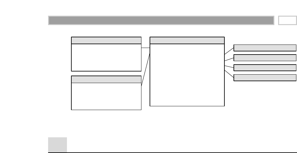
Figure 5.2 Order transaction fact table.
Order Transactions
The first process we’ll explore is order transactions. As companies have grown
through acquisition, they often find themselves with multiple operational
order transaction processing systems in the organization. The existence of
multiple source systems often creates a degree of urgency to integrate the dis-
parate results in the data warehouse rather than waiting for the long-term
application integration.
The natural granularity for an order transaction fact table is one row for each line
item on an order. The facts associated with this process typically include the order
quantity, extended gross order dollar amount, order discount dollar amount, and
extended net order dollar amount (which is equal to the gross order amount less
the discounts). The resulting schema would look similar to Figure 5.2.
Fact Normalization
Rather than storing a list of facts, as in Figure 5.2, some designers want to fur-
ther normalize the fact table so that there’s a single, generic fact amount, along
with a dimension that identifies the type of fact. The fact dimension would
indicate whether it is the gross order amount, order discount amount, or some
other measure. This technique may make sense when the set of facts is
sparsely populated for a given fact row and no computations are made
between facts. We have used this technique to deal with manufacturing qual-
ity test data, where the facts vary widely depending on the test conducted.
However, we generally resist the urge to further normalize the fact table. As we
see with orders data, facts usually are not sparsely populated within a row. In
this case, if we were to normalize the facts, we’d be multiplying the number of
rows in the fact table by the number of fact types. For example, assume that we
started with 10 million order line fact table rows, each with six keys and four
Order Date Key (FK)
Requested Ship Date Key (FK)
Product Key (FK)
Customer Ship To Key (FK)
Sales Rep Key (FK)
Deal Key (FK)
Order Number (DD)
Order Line Number (DD)
Order Quantity
Gross Order Dollar Amount
Order Deal Discount Dollar Amount
Net Order Dollar Amount
Order Transaction Fact
Order Date Key (PK)
Order Date
Order Date Day of Week
Order Date Month
… and more
Order Date Dimension
Product Dimension
Customer Ship To Dimension
Sales Rep Dimension
Deal Dimension
Requested Ship Date Key (PK)
Requested Ship Date
Requested Ship Date Day of Week
Requested Ship Date Month
… and more
Requested Ship Date Dimension
Order Management 109

facts. If we normalized the facts, we’d end up with 40 million fact rows, each
with seven keys and one fact. In addition, if we are performing any arithmetic
function between the facts (such as discount amount as a percentage of gross
order amount), it is far easier if the facts are in the same row because SQL makes
it difficult to perform a ratio or difference between facts in different rows. In
Chapter 13 we’ll explore a situation where a fact dimension makes more sense.
Dimension Role-Playing
By now we all know that a date dimension is found in every fact table because
we are always looking at performance over time. In a transaction-grained fact
table, the primary date column is the transaction date, such as the order date.
Sometimes we also discover other dates associated with each transaction, such
as the requested ship date for the order.
Each of the dates should be a foreign key in the fact table. However, we cannot
simply join these two foreign keys to the same date dimension table. SQL
would interpret such a two-way simultaneous join as requiring both the dates
to be identical, which isn’t very likely.
Even though we cannot literally join to a single date dimension table, we can
build and administer a single date dimension table behind the scenes. We cre-
ate the illusion of two independent date tables by using views. We are careful
to uniquely label the columns in each of the SQL views. For example, order
month should be uniquely labeled to distinguish it from requested ship
month. If we don’t practice good data housekeeping, we could find ourselves
in the uncomfortable position of not being able to tell the columns apart when
both are dragged into a report.
As we briefly described in Chapter 2, you would define the order date and
requested order date views as follows:
CREATE VIEW ORDER_DATE (ORDER_DATE_KEY, ORDER_DAY_OF_WEEK,
ORDER_MONTH...)
AS SELECT DATE_KEY, DAY_OF_WEEK, MONTH, . . . FROM DATE
and
CREATE VIEW REQ_SHIP_DATE (REQ_SHIP_DATE_KEY, REQ_SHIP_DAY_OF_WEEK,
REQ_SHIP_MONTH ...)
AS SELECT DATE_KEY, DAY_OF_WEEK, MONTH, . . . FROM DATE
We now have two unique date dimensions that can be used as if they were inde-
pendent with completely unrelated constraints. We refer to this as role-playing
because the date dimension simultaneously serves different roles in a single
fact table. We’ll see additional examples of dimension role-playing sprinkled
throughout this book.
CHAPTER 5
110

Role-playing in a data warehouse occurs when a single dimension simultaneously
appears several times in the same fact table. The underlying dimension may exist as
a single physical table, but each of the roles should be presented to the data access
tools in a separately labeled view.
To handle the multiple dates, some designers are tempted to create a single
date table with a key for each unique order date and requested ship date com-
bination. This approach falls apart on several fronts. First, our clean and sim-
ple daily date table with approximately 365 rows per year would balloon in
size if it needed to handle all the date combinations. Second, such a combina-
tion date table would no longer conform to our other frequently used daily,
weekly, and monthly date dimensions.
Product Dimension Revisited
A product dimension has participated in each of the case study vignettes pre-
sented so far in this book. The product dimension is one of the most common
and most important dimension tables you’ll encounter in a dimensional
model.
The product dimension describes the complete portfolio of products sold by a
company. In most cases, the number of products in the portfolio turns out to be
surprisingly large, at least from an outsider’s perspective. For example, a
prominent U.S. manufacturer of dog and cat food tracks nearly 20,000 manu-
facturing variations of its products, including retail products everyone (or
every dog and cat) is familiar with, as well as numerous specialized products
sold through commercial and veterinary channels. We’ve worked with
durable goods manufacturers who sell literally millions of unique product
configurations.
Most product dimension tables share the following characteristics:
Numerous verbose descriptive columns. For manufacturers, it’s not unusual
to maintain 100 or more descriptors about the products they sell. Dimen-
sion table attributes naturally describe the dimension row, do not vary
because of the influence of another dimension, and are virtually constant
over time, although as we just discussed in Chapter 4, some attributes do
change slowly over time.
One or more attribute hierarchies in addition to many nonhierarchical
attributes. It is too limiting to think of products as belonging to a single
hierarchy. Products typically roll up according to multiple defined hierar-
chies. All the hierarchical data should be presented in a single flattened,
Order Management 111

denormalized product dimension table. We resist creating normalized
snowflaked sub-tables for the product dimension. The costs of a more com-
plicated presentation and slower intradimension browsing performance
outweigh the minimal storage savings benefits. It is misleading to think
about browsing in a small dimension table, where all the relationships can
be imagined or visualized. Real product dimension tables have thousands
of entries, and the typical user does not know the relationships intimately.
If there are 20,000 dog and cat foods in the product dimension, it is not too
useful to request a pull-down list of the product descriptions. It would be
essential, in this example, to have the ability to constrain on one attribute,
such as flavor, and then another attribute, such as package type, before
attempting to display the product description listings. Notice that the first
two constraints were not drawn strictly from a product hierarchy. Any of
the product attributes, regardless of whether they belong to a hierarchy,
should be used freely for drilling down and up. In fact, most of the attrib-
utes in a large product table are standalone low-cardinality attributes, not
part of explicit hierarchies.
The existence of an operational product master aids in maintenance of the
product dimension, but a number of transformations and administrative steps
must occur to convert the operational master file into the dimension table,
including:
Remap the operational product key to a surrogate key. As we discussed in
Chapter 2, this smaller, more efficient join key is needed to avoid havoc
caused by duplicate use of the operational product key over time. It also
might be necessary to integrate product information sourced from different
operational systems. Finally, as we just learned in Chapter 4, the surrogate
key is needed to track changing product attributes in cases where the oper-
ational system has not generated a new product master key.
Add readable text strings to augment or replace numeric codes in the opera-
tional product master. We don’t accept the excuse that the businesspeople
are familiar with the codes. The only reason businesspeople are familiar
with codes is that they have been forced to use them! Remember that the
columns in a product dimension table are the sole source of query con-
straints and report labels, so the contents must be legible. Keep in mind that
cryptic abbreviations are as bad as outright numeric codes; they also should
be augmented or replaced with readable text. Multiple abbreviated codes in
a single field should be expanded and separated into distinct fields.
Quality assure all the text strings to ensure that there are no misspellings,
impossible values, or cosmetically different versions of the same
attribute. In addition to automated procedures, a simple backroom
CHAPTER 5
112

technique for flushing out minor misspellings of attribute values is to just
sort the distinct values of the attribute and look down the list. Spellings
that differ by a single character usually will sort next to each other and can
be found with a visual scan of the list. This supplemental manager’s qual-
ity assurance check should be performed occasionally to monitor data
quality. Data access interfaces and reports rely on the precise contents of
the dimension attributes. SQL will happily produce another line in a report
if the attribute value varies in any way based on trivial punctuation or
spelling differences. We also should ensure that the attribute values are
completely populated because missing values easily cause misinterpreta-
tions. Incomplete or poorly administered textual dimension attributes lead
to incomplete or poorly produced reports.
Document the product attribute definitions, interpretations, and origins in
the data warehouse’s metadata. Remember that the metadata is analogous
to the data warehouse encyclopedia. We must be vigilant about populating
and maintaining the metadata.
Customer Ship-To Dimension
The customer ship-to dimension contains one row for each discrete location to
which we ship a product. Customer ship-to dimension tables can range from
moderately sized (thousands of rows) to extremely large (millions of rows)
depending on the nature of the business. A typical customer ship-to dimension
is shown in Figure 5.3.
Figure 5.3 Sample customer ship-to dimension.
Order Date Key (FK)
Requested Ship Date Key (FK)
Product Key (FK)
Customer Ship To Key (FK)
Sales Rep Key (FK)
Deal Key (FK)
Order Number (DD)
Order Line Number (DD)
Order Quantity
Gross Order Dollar Amount
Order Deal Discount Dollar Amount
Net Order Dollar Amount
Order Transaction Fact
Customer Ship To Key (PK)
Customer Ship To ID (Natural Key)
Customer Ship To Name
Customer Ship To Address
Customer Ship To City
Customer Ship To State
Customer Ship To Zip + 4
Customer Ship To Zip
Customer Ship To Zip Region
Customer Ship To Zip Sectional Center
Customer Bill To Name
Customer Bill To Address Attributes …
Customer Organization Name
Customer Corporate Parent Name
Customer Credit Rating
Assigned Sales Rep Name
Assigned Sales Rep Team Name
Assigned Sales District
Assigned Sales Region
Customer Ship To Dimension
Order Date Dimension
Request Ship Date Dimension
Product Dimension
Sales Rep Dimension
Deal Dimension
Order Management 113

Several separate and independent hierarchies typically coexist in a customer
ship-to dimension. The natural geographic hierarchy is clearly defined by the
ship-to location. Since the ship-to location is a point in space, any number of
geographic hierarchies may be defined by nesting ever-larger geographic enti-
ties around the point. In the United States, the usual geographic hierarchy is
city, county, and state. The U.S. ZIP code identifies a secondary geographic
breakdown. The first digit of the ZIP code identifies a geographic region of the
United States (for example, 0 for the Northeast and 9 for certain western states),
whereas the first three digits of the ZIP code identify a mailing sectional center.
Another common hierarchy is the customer’s organizational hierarchy, assum-
ing that the customer is a corporate entity. For each customer ship-to, we
might have a customer bill-to and customer corporation. For every base-level
row in the customer ship-to dimension, both the physical geography and the
customer organizational affiliation are well defined, even though the hierar-
chies roll up differently.
It is natural and common, especially for customer-oriented dimensions, for a dimen-
sion to simultaneously support multiple independent hierarchies. The hierarchies
may have different numbers of levels. Drilling up and drilling down within each of
these hierarchies must be supported in a data warehouse.
The alert reader may have a concern with the implied assumption that multi-
ple ship-tos roll up to a single bill-to in a many-to-one relationship. The real
world is rarely quite this clean and simple. There are always a few exceptions
involving ship-tos that are associated with more than one bill-to. Obviously,
this breaks the simple hierarchical relationship that we have assumed in the
earlier denormalized customer ship-to dimension. If this is a rare occurrence,
it would be reasonable to generalize the customer ship-to dimension so that
the grain of the dimension is each unique ship-to/bill-to combination. If there
are two sets of bill-to information associated with a given ship-to location,
then there would be two rows in the dimension, one for each combination. On
the other hand, if many of the ship-tos are associated with many bill-tos in a
robust many-to-many relationship, then ship-to and bill-to probably need to
be handled as separate dimensions that are linked together by the fact table.
This is the designer’s prerogative. With either approach, exactly the same
information is preserved at the fact table order line-item level. We’ll spend
more time on customer organizational hierarchies, including the handling of
recursive customer parent-child relationships, in Chapter 6.
Another potential independent hierarchy in the customer ship-to dimension
might be the manufacturer’s sales organization. Designers sometimes ques-
tion whether sales organization attributes should be modeled as a separate
CHAPTER 5
114

dimension or the attributes just should be added to the existing customer
dimension. Similar to the preceding discussion about bill-tos, the designer
should use his or her judgment. If sales reps are highly correlated with cus-
tomer ship-tos in a one-to-one or many-to-one relationship, combining the
sales organization attributes with the customer ship-to dimension is a viable
approach. The resulting dimension is only about as big as the larger of the two
dimensions. The relationships between sales teams and customers can be
browsed efficiently in the single dimension without traversing the fact table.
However, sometimes the relationship between sales organization and cus-
tomer ship-to is more complicated. The following factors must be taken into
consideration:
The one-to-one or many-to-one relationship may turn out to be a many-to-
many relationship. As we discussed earlier, if the many-to-many relation-
ship is an exceptional condition, then we may still be tempted to combine
the sales rep attributes into the ship-to dimension, knowing that we’d need
to treat these rare many-to-many occurrences by issuing another surrogate
ship-to key.
If the relationship between sales rep and customer ship-to varies over time
or under the influence of a fourth dimension such as product, then the
combined dimension is in reality some kind of fact table itself! In this
case, we’d likely create separate dimensions for the sales rep and the cus-
tomer ship-to.
If the sales rep and customer ship-to dimensions participate independently
in other business process fact tables, we’d likely keep the dimensions
separate. Creating a single customer ship-to dimension with sales rep
attributes exclusively around orders data may make some of the other
processes and relationships difficult to express.
When entities have a fixed, time-invariant, strongly correlated relationship,
they obviously should be modeled as a single dimension. In most other cases,
your design likely will be simpler and more manageable when you separate
the entities into two dimensions (while remembering the general guidelines
concerning too many dimensions). If you’ve already identified 25 dimensions
in your schema, you should give strong consideration to combining dimen-
sions, if possible.
When the dimensions are separate, some designers want to create a little table
with just the two dimension keys to show the correlation without using the fact
table. This two-dimension table is unnecessary. There is no reason to avoid the
fact table to respond to this relationship inquiry. Fact tables are incredibly effi-
cient because they contain only dimension keys and measurements. The fact
table was created specifically to represent the correlation between dimensions.
Order Management 115

Before we leave the topic of sales rep assignments to customers, users some-
times want the ability to analyze the complex assignment of sales reps to cus-
tomers over time, even if no order activity has occurred. In this case, we could
construct a factless fact table, as we briefly introduced in Chapter 2, to capture
the sales rep coverage. The coverage table would provide a complete map of
the historical assignments of sales reps to customers, even if some of the
assignments never resulted in a sale. As we’ll learn in Chapter 13, we’d likely
include effective and expiration dates in the sales rep coverage table because
coverage assignments change over time.
Deal Dimension
The deal dimension is similar to the promotion dimension from Chapter 2. The
deal dimension describes the incentives that have been offered to the customer
that theoretically affect the customers’ desire to purchase products. This
dimension is also sometimes referred to as the contract. As shown in Figure 5.4,
the deal dimension describes the full combination of terms, allowances, and
incentives that pertain to the particular order line item.
The same issues that we faced in the retail promotion dimension also arise
with this deal dimension. If the terms, allowances, and incentives are usefully
correlated, then it makes sense to package them into a single deal dimension.
If the terms, allowances, and incentives are quite uncorrelated and we find
ourselves generating the Cartesian product of these factors in the dimension,
then it probably makes sense to split such a deal dimension into its separate
components. Once again, this is not an issue of gaining or losing information,
since the database contains the same information in both cases, but rather the
issues of user convenience and administrative complexity determine whether
to represent these deal factors as multiple dimensions. In a very large fact
table, with tens of millions or hundreds of millions of rows, the desire to
reduce the number of keys in the fact table composite key would favor keep-
ing the deal dimension as a single dimension. Certainly any deal dimension
smaller than 100,000 rows would be tractable in this design.
Figure 5.4 Sample deal dimension.
Order Date Key (FK)
Requested Ship Date Key (FK)
Product Key (FK)
Customer Ship To Key (FK)
Sales Rep Key (FK)
Deal Key (FK)
Order Number (DD)
Order Line Number (DD)
Order Quantity
Gross Order Dollar Amount
Order Deal Discount Dollar Amount
Net Order Dollar Amount
Order Transaction Fact
Deal Key (PK)
Deal Description
Deal Terms Description
Deal Terms Type Description
Allowance Description
Allowance Type Description
Special Incentive Description
Special Incentive Type Description
Deal Dimension
Order Date Dimension
Request Ship Date Dimension
Product Dimension
Customer Ship To Dimension
Sales Rep Dimension
CHAPTER 5
116
TEAMFLY
Team-Fly®

Degenerate Dimension for
Order Number
Each line item row in the orders fact table includes the order number as a
degenerate dimension, as we introduced in Chapter 2. Unlike a transactional
parent-child database, the order number in our dimensional models is not tied
to an order header table. We have stripped all the interesting details from the
order header into separate dimensions such as the order date, customer ship-to,
and other interesting fields. The order number is still useful because it allows us
to group the separate line items on the order. It enables us to answer such ques-
tions as the average number of line items on an order. In addition, the order
number is used occasionally to link the data warehouse back to the operational
world. Since the order number is left sitting by itself in the fact table without
joining to a dimension table, it is referred to as a degenerate dimension.
Degenerate dimensions typically are reserved for operational transaction identifiers.
They should not be used as an excuse to stick a cryptic code in the fact table without
joining to a descriptive decode in a dimension table.
If the designer decides that certain data elements actually do belong to the
order itself and do not usefully fall into another natural business dimension,
then order number is no longer a degenerate dimension but rather is a normal
dimension with its own surrogate key and attribute columns. However,
designers with a strong parent-child background should resist the urge simply
to lump the traditional order header information into an order dimension. In
almost all cases, the header information belongs in other analytic dimensions
rather than merely being dumped into a dimension that closely resembles the
transaction order header table.
Junk Dimensions
When we’re confronted with a complex operational data source, we typically
perform triage to quickly identify fields that are obviously related to dimen-
sions, such as date stamps or attributes. We then identify the numeric mea-
surements in the source data. At this point, we are often left with a number of
miscellaneous indicators and flags, each of which takes on a small range of dis-
crete values. The designer is faced with several rather unappealing options,
including:
Leave the flags and indicators unchanged in the fact table row. This could
cause the fact table row to swell alarmingly. It would be a shame to create a
nice tight dimensional design with five dimensions and five facts and then
leave a handful of uncompressed textual indicator columns in the row.
Order Management 117

Make each flag and indicator into its own separate dimension. Doing so
could cause our 5-dimension design to balloon into a 25-dimension design.
Strip out all the flags and indicators from the design. Of course, we ask the
obligatory question about removing these miscellaneous flags because they
seem rather insignificant, but this notion is often vetoed quickly because
someone might need them. It is worthwhile to examine this question care-
fully. If the indicators are incomprehensible, noisy, inconsistently popu-
lated, or only of operational significance, they should be left out.
An appropriate approach for tackling these flags and indicators is to study
them carefully and then pack them into one or more junk dimensions. You can
envision the junk dimension as being akin to the junk drawer in your kitchen.
The kitchen junk drawer is a dumping ground for miscellaneous household
items, such as rubber bands, paper clips, batteries, and tape. While it may be
easier to locate the rubber bands if we dedicated a separate kitchen drawer to
them, we don’t have adequate storage capacity to do so. Besides, we don’t
have enough stray rubber bands, nor do we need them very frequently, to war-
rant the allocation of a single-purpose storage space. The junk drawer pro-
vides us with satisfactory access while still retaining enough kitchen storage
for the more critical and frequently accessed dishes and silverware.
A junk dimension is a convenient grouping of typically low-cardinality flags and indi-
cators. By creating an abstract dimension, we remove the flags from the fact table
while placing them into a useful dimensional framework.
A simple example of a useful junk dimension would be to remove 10 two-value
indicators, such as the cash versus credit payment type, from the order fact table
and place them into a single dimension. At the worst, you would have 1,024 (210)
rows in this junk dimension. It probably isn’t very interesting to browse among
these flags within the dimension because every flag occurs with every other flag
if the database is large enough. However, the junk dimension is a useful holding
place for constraining or reporting on these flags. Obviously, the 10 foreign keys
in the fact table would be replaced with a single small surrogate key.
On the other hand, if you have highly uncorrelated attributes that take on
more numerous values, then it may not make sense to lump them together into
a single junk dimension. Unfortunately, the decision is not entirely formulaic.
If you have five indicators that each take on only three values, the single junk
dimension is the best route for these attributes because the dimension has only
243 (35) possible rows. However, if the five uncorrelated indicators each have
100 possible values, we’d suggest the creation of separate dimensions because
you now have 100 million (1005) possible combinations.
CHAPTER 5
118

Figure 5.5 Sample rows of an order indicator junk dimension.
We’ve illustrated sample rows from an order indicator dimension in Figure 5.5. A
subtle issue regarding junk dimensions is whether you create rows for all the
combinations beforehand or create junk dimension rows for the combinations as
you actually encounter them in the data. The answer depends on how many pos-
sible combinations you expect and what the maximum number could be. Gener-
ally, when the number of theoretical combinations is very high and you don’t
think you will encounter them all, you should build a junk dimension row at
extract time whenever you encounter a new combination of flags or indicators.
Another interesting application of the junk dimension technique is to use it to
handle the infrequently populated, open-ended comments field sometimes
attached to a fact row. Optimally, the comments have been parameterized in a
dimension so that they can be used for robust analysis. Even if this is not the
case, users still may feel that the comments field is meaningful enough to
include in the data warehouse. In this case, a junk dimension simply contains
all the distinct comments. The junk dimension is noticeably smaller than the
fact table because the comments are relatively rare. Of course, you will need a
special surrogate key that points to the “No Comment” row in the dimension
because most of your fact table rows will use this key.
Multiple Currencies
Suppose that we are tracking the orders of a large multinational California-
based company with sales offices around the world. We may be capturing
order transactions in more than 15 different currencies. We certainly wouldn’t
want to include columns in the fact table for each currency because theoreti-
cally there are an open-ended number of currencies.
Order
Indicator
Key
Payment Type
Description
Payment
Type
Group
Inbound/
Outbound
Order Indicator
Commission Credit
Indicator
Order Type
Indicator
1
2
3
4
5
6
7
8
9
10
11
12
13
14
Cash
Cash
Cash
Cash
Cash
Discover Card
Discover Card
Discover Card
Discover Card
Discover Card
MasterCard
MasterCard
MasterCard
MasterCard
Cash
Cash
Cash
Cash
Cash
Credit
Credit
Credit
Credit
Credit
Credit
Credit
Credit
Credit
Inbound
Inbound
Inbound
Outbound
Outbound
Inbound
Inbound
Inbound
Outbound
Outbound
Inbound
Inbound
Inbound
Outbound
Commissionable
Non-Commissionable
Non-Commissionable
Commissionable
Non-Commissionable
Commissionable
Non-Commissionable
Non-Commissionable
Commissionable
Non-Commissionable
Commissionable
Non-Commissionable
Non-Commissionable
Commissionable
Regular
Display
Demonstration
Regular
Display
Regular
Display
Demonstration
Regular
Display
Regular
Display
Demonstration
Regular
Order Management 119
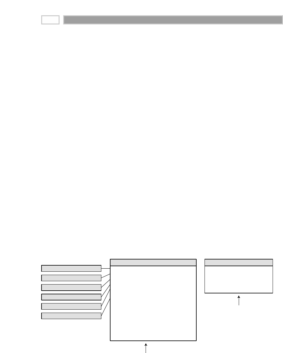
The most obvious requirement is that order transactions be expressed in both
local currency and the standardized corporate currency, such as U.S. dollars in
this example. To satisfy this need, we would replace each underlying order
fact with a pair of facts, one for the applicable local currency and another for
the equivalent standard corporate currency. This would allow all transactions
to easily roll up to the corporate currency without complicated application
coding. We’d also supplement the fact table with an additional currency
dimension to identify the currency type associated with the local-currency
facts. A currency dimension is needed even if the location of the transaction is
otherwise known because the location does not necessarily guarantee which
currency was used.
However, you may find the multicurrency support requirements are more
complicated than we just described. We may need to allow a manager in any
country to see order volume in any currency. For example, the sales office in
Bangkok may monitor sales orders in Thai bhat, the Asia-Pacific region man-
ager in Tokyo may want to look at the region’s orders in Japanese yen, and the
sales department in California may want to see the orders based on U.S. dol-
lars. Embellishing our initial design with an additional currency conversion
fact table, as shown in Figure 5.6, can deliver this flexibility. The dimensions in
this fact table represent currencies, not countries, because the relationship
between currencies and countries is not one to one. The needs of the sales rep
in Thailand and U.S.-based sales management would be met simply by query-
ing the orders fact table. The region manager in Tokyo could roll up all Asia-
Pacific orders in Japanese yen by using the special currency conversion table.
Figure 5.6 Tracking multiple currencies with a daily currency exchange fact table.
Order Date Key (FK)
Product Key (FK)
Customer Ship To Key (FK)
Sales Rep Key (FK)
Deal Key (FK)
Local Currency Dimension Key (FK)
Order Number (DD)
Order Line Number (DD)
Order Quantity
Local Currency Gross Order Amount
Local Currency Order Discount Amount
Local Currency Net Order Amount
Standard US Dollar Gross Order Amount
Standard US Dollar Order Discount Amount
Standard US Dollar Net Order Amount
Order Transaction Fact
Conversion Date Key (FK)
Source Currency Key (FK)
Destination Currency Key (FK)
Source-Destination Exchange Rate
Destination-Source Exchange Rate
Currency Conversion Fact
Date Dimension
Product Dimension
Customer Ship To Dimension
Sales Rep Dimension
Deal Dimension
Currency Dimension
Supports reporting of facts
in two currencies
Supports reporting of facts
in multiple currencies
CHAPTER 5
120

Within each fact table row, the amount expressed in local currency is
absolutely accurate because the sale occurred in that currency on that day. The
equivalent U.S. dollar value would be based on a conversion rate to U.S. dol-
lars for that day. The conversion rate table contains all combinations of effec-
tive currency exchange rates going in both directions because the symmetric
rates between two currencies are not exactly equal.
Header and Line Item Facts with
Different Granularity
It is quite common in parent-child transaction databases to encounter facts of dif-
fering granularity. On an order, for example, there may be a shipping charge that
applies to the entire order that isn’t available at the individual product-level line
item in the operational system. The designer’s first response should be to try to
force all the facts down to the lowest level. We strive to flatten the parent-child
relationship so that all the rows are at the child level, including facts that are cap-
tured operationally at the higher parent level, as illustrated in Figure 5.7. This pro-
cedure is broadly referred to as allocating. Allocating the parent order facts to the
child line-item level is critical if we want the ability to slice and dice and roll up all
order facts by all dimensions, including product, which is a common requirement.
Unfortunately, allocating header-level facts down to the line-item level may
entail a political wrestling match. It is wonderful if the entire allocation issue is
handled by the finance department, not by the data warehouse team. Getting
organizational agreement on allocation rules is often a controversial and com-
plicated process. The data warehouse team shouldn’t be distracted and delayed
by the inevitable organizational negotiation. Fortunately, in many companies,
the need to rationally allocate costs has been recognized already. A task force,
independent of the data warehouse team, already may have established activ-
ity-based costing measures. This is just another name for allocating.
Figure 5.7 Allocating header facts to the line item.
Allocated to line level
Order Date Key (FK)
Customer Ship To Key (FK)
Sales Rep Key (FK)
Deal Key (FK)
Order Number (DD)
Order Shipping Charges
Order Header Fact Order Date Key (FK)
Product Key (FK)
Customer Ship To Key (FK)
Sales Rep Key (FK)
Deal Key (FK)
Order Number (DD)
More Line Item Facts …
Order Shipping Charges
Order Line Fact
Note the absence of a product dimension
in this fact table since product
doesn't apply to the order header
When header facts are allocated to the
line level, we're able to analyze them
by the product dimension
Order Management 121

If the shipping charges and other header-level facts cannot be allocated suc-
cessfully, then they must be presented in an aggregate table for the overall
order. We clearly prefer the allocation approach, if possible, because the sepa-
rate higher-level fact table has some inherent usability issues. Without alloca-
tions, we’d be unable to explore header facts by product because the product
isn’t identified in a header-grain fact table. If we are successful in allocating
facts down to the lowest level, the problem goes away.
We shouldn’t mix fact granularities (for example, order and order line facts) within a
single fact table. Instead, we need to either allocate the higher-level facts to a more
detailed level or create two separate fact tables to handle the differently grained
facts. Allocation is the preferred approach. Optimally, a finance or business team
(not the data warehouse team) spearheads the allocation effort.
Invoice Transactions
If we work for a manufacturing company, invoicing typically occurs when
products are shipped from our facility to the customer. We visualize shipments
at the loading dock as boxes of product are loaded onto a truck destined for a
particular customer address. The invoice associated with the shipment is cre-
ated at this time. The invoice governs the current shipment of products on that
truck on that day to a particular customer address. The invoice has multiple
line items, each corresponding to a particular product being shipped. Various
prices, discounts, and allowances are associated with each line item. The
extended net amount for each line item is also available.
Although we don’t show it on the invoice to the customer, a number of other
interesting facts are potentially known about each product at the time of ship-
ment. We certainly know list prices; manufacturing and distribution costs may
be available as well. Thus we know a lot about the state of our business at the
moment of customer shipment.
In the shipment invoice fact table we can see all the company’s products, all
the customers, all the contracts and deals, all the off-invoice discounts and
allowances, all the revenue generated by customers purchasing products, all
the variable and fixed costs associated with manufacturing and delivering
products (if available), all the money left over after delivery of product (con-
tribution), and customer satisfaction metrics such as on-time shipment.
CHAPTER 5
122

For any company that ships products to customers or bills customers for services ren-
dered, the optimal place to start a data warehouse typically is with invoices. We often
refer to the data resulting from invoicing as the most powerful database because it
combines the company’s customers, products, and components of profitability.
We choose the grain of the invoice fact table to be the individual invoice line
item. A sample invoice fact table associated with manufacturer shipments is
illustrated in Figure 5.8.
As you’d expect, the shipment invoice fact table contains a number of dimen-
sions that we’ve seen previously in this chapter. The conformed date dimen-
sion table again would play multiple roles in the fact table. The customer,
product, and deal dimensions also would conform so that we can drill across
from fact table to fact table and communicate using common attributes. We’d
also have a degenerate order number, assuming that a single order number is
associated with each invoice line item, as well as the invoice number degener-
ate dimension.
The shipment invoice fact table also contains some interesting new dimen-
sions we haven’t seen yet in our designs. The ship-from dimension contains
one row for each manufacturer warehouse or shipping location. This is a rela-
tively simple dimension with name, address, contact person, and storage facil-
ity type. The attributes are somewhat reminiscent of the facility dimension
describing stores from Chapter 2.
The shipper dimension describes the method and carrier by which the product
was shipped from the manufacturer to the customer. Sometimes a shipment
database contains only a simple carrier dimension, with attributes about the
transportation company. There is only one ship method, namely, truck to cus-
tomer. However, both manufacturers and customers alike are interested in
tracking alternative delivery methods, such as direct store delivery (product
delivered directly to the retail outlet), cross-docking (product transferred from
one carrier to another without placing it in a warehouse), back hauling (carrier
transports the product on a return trip rather than returning empty), and cus-
tomer pallet creation (product custom assembled and shrink-wrapped on a
pallet destined for a retail outlet). Since investments are made in these alterna-
tive shipping models, manufacturers (and their customers) are interested in
analyzing the businesses along the shipper dimension. The customer satisfac-
tion dimension provides textual descriptions that summarize the numeric sat-
isfaction flags at the bottom of the fact table.
Order Management 123
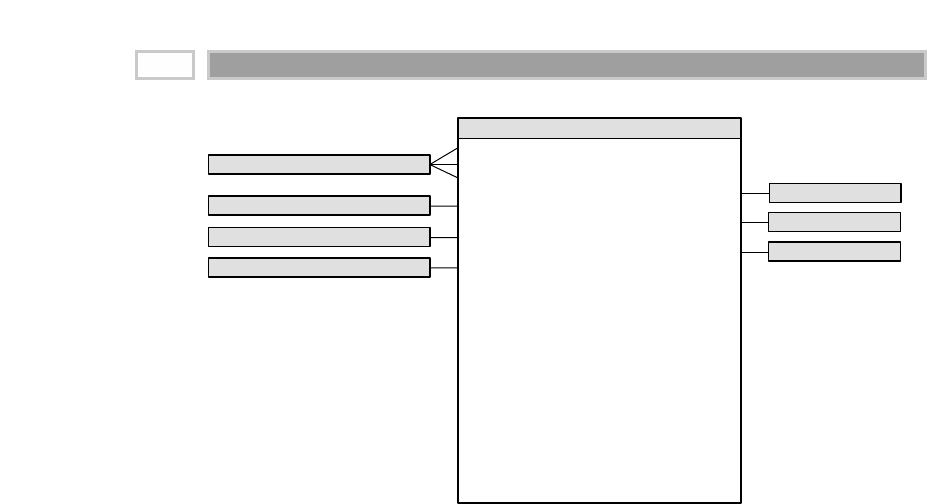
Figure 5.8 Shipment invoice fact table.
Profit and Loss Facts
If your organization has tackled activity-based costing or implemented a
robust enterprise resource planning (ERP) system, you are likely in a position
to identify many of the incremental revenues and costs associated with ship-
ping finished products to the customer. It is traditional to arrange these rev-
enues and costs in sequence from the top line, which represents the
undiscounted value of the products shipped to the customer, down to the bot-
tom line, which represents the money left over after discounts, allowances,
and costs. This list of revenues and costs is called a profit and loss (P&L) state-
ment. We typically don’t make an attempt to carry the P&L statement all the
way to a complete view of company profit, including general and administra-
tive costs. For this reason, we will refer to the bottom line in our P&L statement
as the contribution.
Keeping in mind that each row in the invoice fact table represents a single line
item on the shipment invoice, the elements of our P&L statement, as shown in
Figure 5.8, have the following interpretations:
Quantity shipped. This is the number of cases of the particular line-item
product. We’ll discuss the use of multiple equivalent quantities with differ-
ent units of measure later in the chapter.
Extended gross invoice amount. This is also know as extended list price
because it is the quantity shipped multiplied by the list unit price. This and
all subsequent dollar values are extended amounts or, in other words, unit
Invoice Date Key (FK)
Requested Ship Date Key (FK)
Actual Ship Date Key (FK)
Product Key (FK)
Customer Ship To Key (FK)
Deal Key (FK)
Ship From Key (FK)
Shipper Key (FK)
Customer Satisfaction Key (FK)
Invoice Number (DD)
Order Number (DD)
Quantity Shipped
Extended Gross Invoice Dollar Amount
Extended Allowance Dollar Amount
Extended Discount Dollar Amount
Extended Net Invoice Dollar Amount
Extended Fixed Manufacturing Cost
Extended Variable Manufacturing Cost
Extended Storage Cost
Extended Distribution Cost
Contribution Dollar Amount
Shipment Line Item On-Time Count
Shipment Line Item Complete Count
Shipment Line Item Damage Free Count
Shipment Invoice Line Item Transaction Fact
Date Dimension (views for 3 roles)
Customer Ship To Dimension
Ship From Dimension
Customer Satisfaction Dimension
Product Dimension
Deal Dimension
Shipper Dimension
CHAPTER 5
124

rates multiplied by the quantity shipped. This insistence on additive val-
ues simplifies most access and reporting applications. It is relatively rare
for the user to ask for the price from a single row of the fact table. When
the user wants an average price drawn from many rows, the extended
prices are first added, and then the result is divided by the sum of the
shipped quantities.
Extended allowance amount. This is the amount subtracted from the
invoice-line gross amount for deal-related allowances. The allowances are
described in the adjoined deal dimension. The allowance amount is often
called an off-invoice allowance. The actual invoice may have several
allowances for a given line item. In this example design, we lumped the
allowances together. If the allowances need to be tracked separately and
there are potentially many simultaneous allowances on a given line item,
then an additional dimension structure is needed. An allowance-detail fact
table could be used to augment the invoice fact table, serving as a drill-
down target for a detailed explanation of the allowance bucket in the
invoice fact table.
Extended discount amount. This is the amount subtracted on the invoice for
volume or payment-term discounts. The explanation of which discounts
are taken is also found in the deal dimension row that points to this fact
table row. As discussed in the section on the deal dimension, the decision
to code the explanation of the allowances and discount types together is
the designer’s prerogative. It makes sense to do this if allowances and dis-
counts are correlated and users wish to browse within the deal dimension
to study the relationships between allowances and discounts. Note that the
discount for payment terms is characteristically a forecast that the cus-
tomer will pay within the time period called for in the terms agreement. If
this does not happen, or if there are other corrections to the invoice, then
the Finance Department probably will back out the original invoice in a
subsequent month and post a new invoice. In all likelihood, the data ware-
house will see this as three transactions. Over time, all the additive values
in these rows will add up correctly, but care must be taken in performing
rows counts not to impute more activity than actually exists.
All allowances and discounts in this fact table are represented at the line
item level. As we discussed earlier, some allowances and discounts may be
calculated operationally at the invoice level, not the line-item level. An
effort should be made to allocate them down to the line item. An invoice
P&L statement that does not include the product dimension poses a serious
limitation on our ability to present meaningful P&L slices of the business.
Extended net invoice amount. This is the amount the customer is expected to
pay for this line item before tax. It is equal to the gross invoice amount less
the allowances and discounts.
Order Management 125

The facts described so far likely would be displayed to the customer on the
invoice document. The following cost amounts, leading to a bottom-line con-
tribution, are for internal consumption only.
Extended fixed manufacturing cost. This is the amount identified by manu-
facturing as the pro rata fixed manufacturing cost of the product.
Extended variable manufacturing cost. This is the amount identified by
manufacturing as the variable manufacturing cost of the product. This
amount may be more or less activity-based, reflecting the actual location
and time of the manufacturing run that produced the product being
shipped to the customer. Conversely, this number may be a standard value
set by a committee of executives. If the manufacturing costs or any of the
other storage and distribution costs are too much averages of averages,
then the detailed P&Ls in the data warehouse may become meaningless.
The existence of the data warehouse tends to illuminate this problem and
accelerate the adoption of activity-based costing methods.
Extended storage cost. This is the cost charged to the product for storage
prior to being shipped to the customer.
Extended distribution cost. This is the cost charged to the product for trans-
portation from the point of manufacture to the point of shipment. This cost
is notorious for not being activity-based. Sometimes a company doesn’t
want to see that it costs more to do business in Seattle because the manu-
facturing plant is in Alabama. The distribution cost possibly can include
freight to the customer if the company pays the freight, or the freight cost
can be presented as a separate line item in the P&L.
Contribution amount. This is the final calculation of the extended net invoice
less all the costs just discussed. This is not the true bottom line of the over-
all company because general and administrative expenses and other finan-
cial adjustments have not been made, but it is important nonetheless. This
column sometimes has alternative labels, such as margin, depending on the
company culture.
Profitability—The Most Powerful
Data Mart
We should step back and admire the dimensional model we just built. We often
describe this design as the most powerful data mart. We have constructed a
detailed P&L view of our business, showing all the activity-based elements of
revenue and costs. We have a full equation of profitability. However, what
makes this design so compelling is that the P&L view sits inside a very rich
dimensional framework of calendar dates, customers, products, and causal
CHAPTER 5
126
TEAMFLY
Team-Fly®

factors. Do you want see customer profitability? Just constrain and group on the
customer dimension and bring the components of the P&L into your report. Do
you want to see product profitability? Do you want to see deal profitability? All
these analyses are equally easy and take the same analytic form in your query
and report-writing tools. Somewhat tongue in cheek, we recommend that you
not deliver this data mart too early in your career because you will get promoted
and won’t be able to work directly on any more data warehouses!
Profitability Words of Warning
We must balance the last paragraph with a more sober note. Before leaving this
topic, we are compelled to pass along some cautionary words of warning. It
goes without saying that most of your users probably are very interested in
granular P&L data that can be rolled up to analyze customer and product prof-
itability. The reality is that delivering these P&L statements often is easier said
than done. The problems arise with the cost facts. Even with advanced ERP
implementations, it is fairly common to be unable to capture the cost facts at
this atomic level of granularity. You will face a complex process of mapping, or
allocating, the original cost data down to the invoice line level of the shipment
invoice. Furthermore, each type of cost may turn out to require a separate
extraction from some source system. Ten cost facts may mean 10 different
extract and transformation programs. Before you sign up for mission impossi-
ble, be certain to perform a detailed assessment of what is available and feasi-
ble from your source systems. You certainly don’t want the data warehouse
team saddled with driving the organization to consensus on activity-based
costing as a side project, on top of managing a number of parallel extract
implementations. If time permits, profitability is often tackled as a consoli-
dated data mart after the components of revenue and cost have been sourced
and delivered separately to business users in the data warehouse.
Customer Satisfaction Facts
In addition to the P&L facts, business users often are interested in customer
satisfaction metrics, such as whether the line item was shipped on time,
shipped complete, or shipped damage-free. We can add separate columns to
the fact table for each of these line item-level satisfaction metrics. These new
fact columns are populated with additive ones and zeroes, supporting inter-
esting analyses of line item performance metrics such as the percentage of
orders shipped to a particular customer on time. We also would augment the
design with a customer satisfaction dimension that combines these flags into a
single dimension (ala the junk dimension we discussed earlier) to associate
text equivalents with the flags for reporting purposes.
Order Management 127

Accumulating Snapshot for the Order
Fulfillment Pipeline
We can think of the order management process as a pipeline, especially in a
build-to-order manufacturing business, as illustrated in Figure 5.9. Customers
place an order that goes into backlog until it is released to manufacturing to be
built. The manufactured products are placed in finished goods inventory and
then shipped to the customers and invoiced. Unique transactions are gener-
ated at each spigot of the pipeline. Thus far we’ve considered each of these
pipeline activities as a separate fact table. Doing so allows us to decorate the
detailed facts generated by each process with the greatest number of detailed
dimensions. It also allows us to isolate our analysis to the performance of a sin-
gle business process, which is often precisely what the business users want.
However, there are times when users are more interested in analyzing the
entire order fulfillment pipeline. They want to better understand product
velocity, or how quickly products move through the pipeline. The accumulat-
ing snapshot fact table provides us with this perspective of the business, as
illustrated in Figure 5.10. It allows us to see an updated status and ultimately
the final disposition of each order.
The accumulating snapshot complements our alternative perspectives of the
pipeline. If we’re interested in understanding the amount of product flowing
through the pipeline, such as the quantity ordered, produced, or shipped, we rely
on transaction schemas that monitor each of the pipeline’s major spigots. Periodic
snapshots give us insight into the amount of product sitting in the pipeline, such
as the backorder or finished goods inventories, or the amount of product flowing
through a spigot during a predefined time period. The accumulating snapshot
helps us better understand the current state of an order, as well as product move-
ment velocities to identify pipeline bottlenecks and inefficiencies.
We notice immediately that the accumulating snapshot looks different from
the other fact tables we’ve designed thus far. The reuse of conformed dimen-
sions is to be expected, but the number of date and fact columns is larger than
we’ve seen in the past. We capture a large number of dates and facts as the
Figure 5.9 Order fulfillment pipeline diagram.
Orders Backlog
Mfg
Release
Finished Goods
Inventory Shipment Invoicing
CHAPTER 5
128
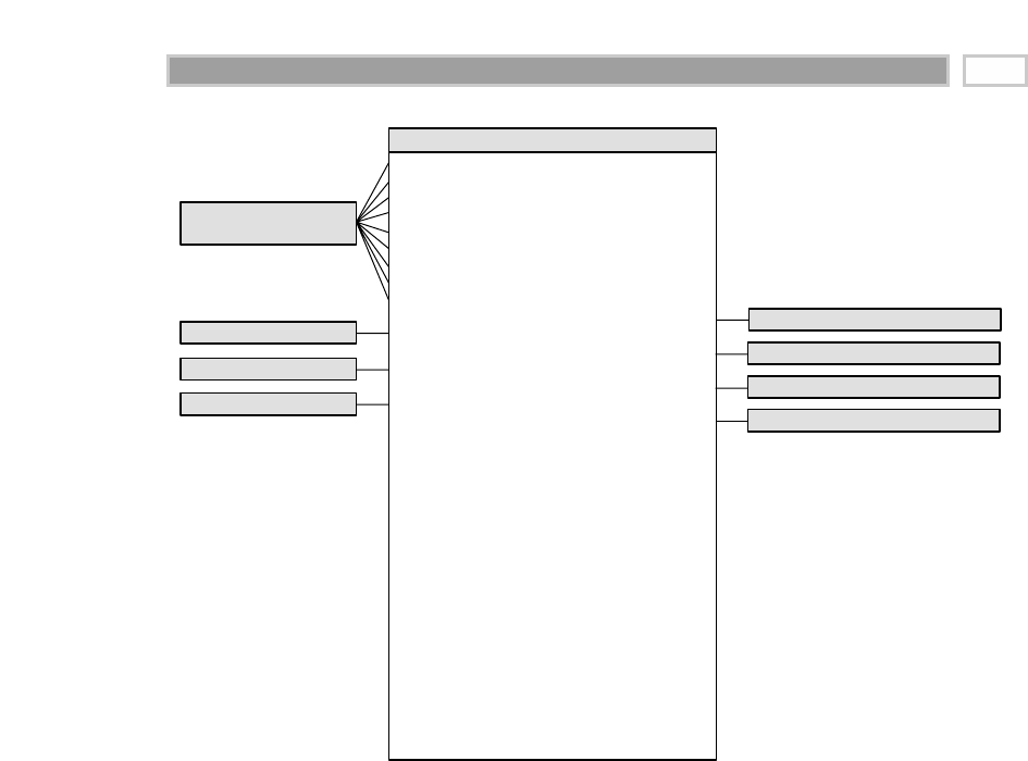
Figure 5.10 Order fulfillment accumulating snapshot fact table.
order progresses through the pipeline. Each date represents a major milestone
of the fulfillment pipeline. We handle each of these dates as dimension roles by
creating either physically distinct tables or logically distinct views. It is critical
that a surrogate key is used for these date dimensions rather than a literal SQL
date stamp because many of the fact table date fields will be “Unknown” or
“To be determined” when we first load the row. Obviously, we don’t need to
declare all the date fields in the fact table’s primary key.
The fundamental difference between accumulating snapshots and other fact
tables is the notion that we revisit and update existing fact table rows as more
information becomes available. The grain of an accumulating snapshot fact
table is one row per the lowest level of detail captured as the pipeline is
entered. In our example, the grain would equal one row per order line item.
However, unlike the order transaction fact table we designed earlier with the
same granularity, the fact table row in the accumulating snapshot is modified
while the order moves through the pipeline as more information is collected
from every stage of the lifecycle.
Order Date Key (FK)
Backlog Date Key (FK)
Release to Manufacturing Date Key (FK)
Finished Inventory Placement Date Key (FK)
Requested Ship Date Key (FK)
Scheduled Ship Date Key (FK)
Actual Ship Date Key (FK)
Arrival Date Key (FK)
Invoice Date Key (FK)
Product Key (FK)
Customer Key (FK)
Sales Rep Key (FK)
Deal Key (FK)
Manufacturing Facility Key (FK)
Warehouse Key (FK)
Shipper Key (FK)
Order Number (DD)
Order Line Number (DD)
Invoice Number (DD)
Order Quantity
Order Dollar Amount
Release to Manufacturing Quantity
Manufacturing Pass Inspection Quantity
Manufacturing Fail Inspection Quantity
Finished Goods Inventory Quantity
Authorized to Sell Quantity
Shipment Quantity
Shipment Damage Quantity
Customer Return Quantity
Invoice Quantity
Invoice Dollar Amount
Order to Manufacturing Release Lag
Manufacturing Release to Inventory Lag
Inventory to Shipment Lag
Order to Shipment Lag
Order Fulfillment Accumulating Fact
Date Dimension
(views for 9 roles)
Customer Dimension
Deal Dimension
Warehouse Dimension
Product Dimension
Sales Rep Dimension
Manufacturing Facility Dimension
Shipper Dimension
Order Management 129

Accumulating snapshots typically have multiple dates in the fact table representing the
major milestones of the process. However, just because a fact table has several dates
doesn’t dictate that it is an accumulating snapshot. The primary differentiator of an ac-
cumulating snapshot is that we typically revisit the fact rows as activity takes place.
The accumulating snapshot technique is very useful when the product moving
through the pipeline is uniquely identified, such as an automobile with a vehi-
cle identification number, electronics equipment with a serial number, lab
specimens with a identification number, or process manufacturing batches
with a lot number. The accumulating snapshot helps us understand through-
put and yield. If the granularity of an accumulating snapshot is at the serial or
lot number, we’re able to see the disposition of a discrete product as it moves
through the manufacturing and test pipeline. The accumulating snapshot fits
most naturally with short-lived processes that have a definite beginning and
end. Long-lived processes, such as bank accounts, are better modeled with
periodic snapshot fact tables.
Lag Calculations
The lengthy list of date columns is used to measure the spans of time over
which the product is processed through the pipeline. The numerical difference
between any two of these dates is a number, which can be averaged usefully
over all the dimensions. These date lag calculations represent basic measures of
the efficiency of the order fulfillment process. We could build a view on this fact
table that calculated a large number of these date differences and presented
them to the user as if they were stored in the underlying table. These view fields
could include such measures as orders to manufacturing release lag, manufac-
turing release to finished goods lag, and order to shipment lag, depending on
the date spans that your organization is interested in monitoring.
Multiple Units of Measure
Sometimes different functional organizations within the business want to see
the same performance metrics expressed in different units of measure. For
instance, manufacturing managers may want to see the product flow in terms
of pallets or shipping cases. Sales and marketing managers, on the other hand,
may wish to see the quantities in retail cases, scan units (sales packs), or con-
sumer units (such as individual sticks of gum).
Designers sometimes are tempted to bury the unit-of-measure conversion
factors, such as ship case factor, in the product dimension. Users are then
required to appropriately multiply (or was it divide?) the order quantity by the
conversion factor. Obviously, this approach places a burden on business users,
CHAPTER 5
130

in addition to being susceptible to calculation errors. The situation is further
complicated because the conversion factors may change over time, so users
also would need to determine which factor is applicable at a specific point
in time.
Rather than risk miscalculating the equivalent quantities by placing conver-
sion factors in the dimension table, we recommend that they be stored in the
fact table instead. In the orders pipeline fact table example, assume that we
had 10 basic fundamental quantity facts, in addition to five units of measure.
If we physically stored all the facts expressed in the different units of measure,
we’d end up with 50 (10 x 5) facts in each fact row. Instead, we compromise
by building an underlying physical row with 10 quantity facts and 4 unit-of-
measure conversion factors. We only need four unit-of-measure conversion
factors rather than five since the base facts are already expressed in one of
the units of measure. Our physical design now has 14 quantity-related facts
(10 + 4), as shown in Figure 5.11. With this design, we are able to see perfor-
mance across the value chain based on different units of measure.
Of course, we would deliver this fact table to the business users through one
or more views. The extra computation involved in multiplying quantities by
conversion factors is negligible compared with other database management
system (DBMS) overhead. Intrarow computations are very efficient. The most
comprehensive view actually could show all 50 facts expressed in every unit
of measure, but obviously, we could simplify the user interface for any spe-
cific user group by only making available the units of measure the group
wants to see.
Figure 5.11 Support for multiple units of measure with fact table conversion factors.
Date Keys (FKs)
Product Key (FK)
More Foreign Keys …
Degenerate Dimensions …
Order Quantity
Release to Manufacturing Quantity
Manufacturing Pass Inspection Quantity
Manufacturing Fail Inspection Quantity
Finished Goods Inventory Quantity
Authorized to Sell Quantity
Shipment Quantity
Shipment Damage Quantity
Customer Return Quantity
Invoice Quantity
Retail Case Factor
Shipping Case Factor
Pallet Factor
Car Load Factor
Order Fulfillment Fact
The factors are physically
packaged on each fact row.
In the user interface, a view
multiplies out the combinations.
Order Management 131

Packaging all the facts and conversion factors together in the same fact table row
provides the safest guarantee that these factors will be used correctly. The converted
facts are presented in a view(s) to the users.
Finally, another side benefit of storing these factors in the fact table is that it
reduces the pressure on the product dimension table to issue new product
rows to reflect minor factor modifications. These factors, especially if they
evolve routinely over time, behave more like facts than dimension attributes.
Beyond the Rear-View Mirror
Much of what we’ve discussed in this chapter focuses on effective ways to
analyze historical product movement performance. People sometimes refer to
these as rear-view mirror metrics because they allow us to look backward and
see where we’ve been. As the brokerage industry reminds us, past perfor-
mance is no guarantee of future results. The current trend is to supplement
these historical performance metrics with additional facts that provide a
glimpse of what lies ahead of us. Rather than focusing on the pipeline at the
time an order is received, some organizations are trying to move further back
to analyze the key drivers that have an impact on the creation of an order. For
example, in a sales organization, drivers such as prospecting or quoting activ-
ity can be extrapolated to provide some visibility to the expected order activ-
ity volume. Some organizations are implementing customer relationship
management (CRM) solutions in part to gain a better understanding of con-
tact management and other leading indicators. While the concepts are
extremely powerful, typically there are feasibility concerns regarding this
early predictive information, especially if you’re dealing with a legacy data
collection source. Because organizations build products and bill customers
based on order and invoice data, they often do a much better job at collecting
the rear-view mirror information than they do the early indicators. Of course,
once the organization moves beyond the rear-view mirror to reliably capture
front-window leading indicators, these indicators can be added gracefully to
the data warehouse.
Fact Table Comparison
As we mentioned previously, there are three fundamental types of fact
tables: transaction, periodic snapshot, and accumulating snapshot. All three
types serve a useful purpose; you often need two complementary fact tables
to get a complete picture of the business. Table 5.1 compares and contrasts
the variations.
CHAPTER 5
132

Table 5.1 Fact Table Type Comparison
PERIODIC ACCUMULATING
TRANSACTION SNAPSHOT SNAPSHOT
CHARACTERISTIC GRAIN GRAIN GRAIN
Time period Point in time Regular, Indeterminate time
represented predictable span, typically
intervals short-lived
Grain One row per One row per One row per life
transaction event period
Fact table loads Insert Insert Insert and update
Fact row updates Not revisited Not revisited Revisited whenever
activity
Date dimension Transaction date End-of-period Multiple dates for
date standard milestones
Facts Transaction activity Performance for Performance over
predefined time finite lifetime
interval
These three fact table variations are not totally dissimilar because they share
conformed dimensions, which are the keys to building separate fact tables that
can be used together with common, consistent filters and labels. While the
dimensions are shared, the administration and rhythm of the three fact tables
are quite different.
Transaction Fact Tables
The most fundamental view of the business’s operations is at the individual
transaction level. These fact tables represent an event that occurred at an
instantaneous point in time. A row exists in the fact table for a given customer
or product only if a transaction event occurred. Conversely, a given customer
or product likely is linked to multiple rows in the fact table because hopefully
the customer or product is involved in more than one transaction.
Transaction data often is structured quite easily into a dimensional frame-
work. The lowest-level data is the most naturally dimensional data, support-
ing analyses that cannot be done on summarized data. Transaction-level data
let us analyze behavior in extreme detail. Once a transaction has been posted,
we typically don’t revisit it.
Having made a solid case for the charm of transaction-level detail, you may be
thinking that all you need is a big, fast DBMS to handle the gory transaction
Order Management 133

minutiae, and your job is over. Unfortunately, even with transaction-level
data, there is still a whole class of urgent business questions that are impracti-
cal to answer using only transaction detail. As we indicated earlier, dimen-
sional modelers cannot survive on transactions alone.
Periodic Snapshot Fact Tables
Periodic snapshots are needed to see the cumulative performance of the busi-
ness at regular, predictable time intervals. Unlike the transaction fact table,
where we load a row for each event occurrence, with the periodic snapshot, we
take a picture (hence the snapshot terminology) of the activity at the end of a
day, week, or month, then another picture at the end of the next period, and so
on. The periodic snapshots are stacked consecutively into the fact table. The
periodic snapshot fact table often is the only place to easily retrieve a regular,
predictable, trendable view of the key business performance metrics.
Periodic snapshots typically are more complex than individual transactions.
When transactions equate to little pieces of revenue, we can move easily from
individual transactions to a daily snapshot merely by adding up the transac-
tions, such as with the invoice fact tables from this chapter. In this situation, the
periodic snapshot represents an aggregation of the transactional activity that
occurred during a time period. We probably would build the daily snapshot
only if we needed a summary table for performance reasons. The design of the
snapshot table is closely related to the design of its companion transaction table
in this case. The fact tables share many dimension tables, although the snapshot
usually has fewer dimensions overall. Conversely, there often are more facts in a
periodic snapshot table than we find in a transaction table.
In many businesses, however, transactions are not components of revenue.
When you use your credit card, you are generating transactions, but the credit
card issuer’s primary source of customer revenue occurs when fees or charges
are assessed. In this situation, we can’t rely on transactions alone to analyze
revenue performance. Not only would crawling through the transactions be
time-consuming, but also the logic required to interpret the effect of different
kinds of transactions on revenue or profit can be horrendously complicated.
The periodic snapshot again comes to the rescue to provide management
with a quick, flexible view of revenue. Hopefully, the data for this snapshot
schema is sourced directly from an operational system. If it is not, the ware-
house staging area must incorporate very complex logic to interpret the finan-
cial impact of each transaction type correctly at data load time.
Accumulating Snapshot Fact Tables
Last, but not least, the third type of fact table is the accumulating snapshot.
While perhaps not as common as the other two fact table types, accumulating
CHAPTER 5
134

snapshots can be very insightful. As we just observed in this chapter, accumu-
lating snapshots represent an indeterminate time span, covering the complete
life of a transaction or discrete product (or customer).
Accumulating snapshots almost always have multiple date stamps, represent-
ing the predictable major events or phases that take place during the course of
a lifetime. Often there’s an additional date column that indicates when the
snapshot row was last updated. Since many of these dates are not known
when the fact row is first loaded, we must use surrogate date keys to handle
undefined dates. It is not necessary to accommodate the most complex sce-
nario that might occur very infrequently. The analysis of these rare outliers can
always be done in the transaction fact table.
In sharp contrast to the other fact table types, we purposely revisit accumulat-
ing snapshot fact table rows to update them. Unlike the periodic snapshot,
where we hang onto the prior snapshot, the accumulating snapshot merely
reflects the accumulated status and metrics.
Sometimes accumulating and periodic snapshots work in conjunction with
one another. Such is the case when we build the monthly snapshot incremen-
tally by adding the effect of each day’s transactions to an accumulating snap-
shot. If we normally think of the data warehouse as storing 36 months of
historical data in the periodic snapshot, then the current rolling month would
be month 37. Ideally, when the last day of the month has been reached, the
accumulating snapshot simply becomes the new regular month in the time
series, and a new accumulating snapshot is started the next day. The new
rolling month becomes the leading breaking wave of the warehouse.
Transactions and snapshots are the yin and yang of dimensional data ware-
houses. Used together, companion transaction and snapshot fact tables pro-
vide a complete view of the business. We need them both because there is often
no simple way to combine these two contrasting perspectives. Although there
is some theoretical data redundancy between transaction and snapshot tables,
we don’t object to such redundancy because as data warehouse publishers our
mission is to publish data so that the organization can analyze it effectively.
These separate types of fact tables each provide a different perspective on the
same story.
Designing Real-Time Partitions
In the past couple years, a major new requirement has been added the data
warehouse designer’s list. The data warehouse now must extend its existing
historical time series seamlessly right up to the current instant. If the customer
has placed an order in the last hour, we need to see this order in the context of
Order Management 135

the entire customer relationship. Furthermore, we need to track the hourly
status of this most current order as it changes during the day.
Even though the gap between the operational transaction-processing systems
and the data warehouse has shrunk in most cases to 24 hours, the rapacious
needs of our marketing users require the data warehouse to fill this gap with
near real-time data.
Most data warehouse designers are skeptical that the existing extract-trans-
form-load (ETL) jobs simply can be sped up from a 24-hour cycle time to a 15-
minute cycle time. Even if the data cleansing steps are pipelined to occur in
parallel with the final data loading, the physical manipulations surrounding
the biggest fact and dimension tables simply can’t be done every 15 minutes.
Data warehouse designers are responding to this crunch by building a real-
time partition in front of the conventional static data warehouse.
Requirements for the Real-Time
Partition
To achieve real-time reporting, we build a special partition that is separated
physically and administratively from the conventional static data warehouse
tables. Actually, the name partition is a little misleading. The real-time partition
in many cases should not be a literal table partition in the database sense.
Rather, the real-time partition is a separate table subject to special update and
query rules.
The real-time partition ideally should meet the following stringent set of
requirements. It must:
■■ Contain all the activity that occurred since the last update of the static
data warehouse. We will assume that the static tables are updated each
night at midnight.
■■ Link as seamlessly as possible to the grain and content of the static data
warehouse fact tables.
■■ Be so lightly indexed that incoming data can be continuously dribbled in.
In this chapter we just described the three main types of fact tables: transaction
grain, periodic snapshot grain, and accumulating snapshot grain. The real-
time partition has a different structure corresponding to each fact table type.
Transaction Grain Real-Time Partition
If the static data warehouse fact table has a transaction grain, then it contains
exactly one record for each individual transaction in the source system from
CHAPTER 5
136
TEAMFLY
Team-Fly®

the beginning of recorded history. If no activity occurs in a time period, there
are no transaction records. Conversely, there can be a blizzard of closely
related transaction records if the activity level is high. The real-time partition
has exactly the same dimensional structure as its underlying static fact table. It
only contains the transactions that have occurred since midnight, when we
loaded the regular data warehouse tables. The real-time partition may be com-
pletely unindexed both because we need to maintain a continuously open
window for loading and because there is no time series (since we only keep
today’s data in this table). Finally, we avoid building aggregates on this table
because we want a minimalist administrative scenario during the day.
We attach the real-time partition to our existing applications by drilling across
from the static fact table to the real-time partition. Time-series aggregations
(for example, all sales for the current month) will need to send identical
queries to the two fact tables and add them together.
In a relatively large retail environment experiencing 10 million transactions
per day, the static fact table would be pretty big. Assuming that each transac-
tion grain record is 40 bytes wide (7 dimensions plus 3 facts, all packed into 4-
byte fields), we accumulate 400 MB of data each day. Over a year this would
amount to about 150 GB of raw data. Such a fact table would be heavily
indexed and supported by aggregates. However, the daily tranche of 400 MB
for the real-time partition could be pinned in memory. Forget indexes, except
for a B-Tree index on the fact table primary key to facilitate the most efficient
loading. Forget aggregations too. Our real-time partition can remain biased
toward very fast loading performance but at the same time provide speedy
query performance.
Since we send identical queries to the static fact table and the real-time parti-
tion, we relax and let the aggregate navigator sort out whether either of the
tables has supporting aggregates. In the case we have just described, only the
large static table needs them.
Periodic Snapshot Real-Time Partition
If the static data warehouse fact table has a periodic grain (say, monthly), then
the real-time partition can be viewed as the current hot-rolling month. Suppose
that we are working for a big retail bank with 15 million accounts. The static fact
table has the grain of account by month. A 36-month time series would result in
540 million fact table records. Again, this table would be indexed extensively
and supported by aggregates to provide good query performance. The real-time
partition, on the other hand, is just an image of the current developing month,
updated continuously as the month progresses. Semiadditive balances and fully
additive facts are adjusted as frequently as they are reported. In a retail bank, the
Order Management 137

core fact table spanning all account types is likely to be quite narrow, with per-
haps 4 dimensions and 4 facts, resulting in a real-time partition of 480 MB. The
real-time partition again can be pinned in memory.
Query applications drilling across from the static fact table to the real-time par-
tition have a slightly different logic compared with the transaction grain.
Although account balances and other measures of intensity can be trended
directly across the tables, additive totals accumulated during the current
rolling period may need to be scaled upward to the equivalent of a full month
to keep the results from looking anomalous.
Finally, on the last day of the month, hopefully the accumulating real-time par-
tition can just be loaded onto the static data warehouse as the most current
month, and the process can start again with an empty real-time partition.
Accumulating Snapshot
Real-Time Partition
Accumulating snapshots are used for short-lived processes such as orders and
shipments. A record is created for each line item on the order or shipment. In
the main fact table this record is updated repeatedly as activity occurs. We cre-
ate the record for a line item when the order is first placed, and then we update
it whenever the item is shipped, delivered to the final destination, paid for, or
maybe returned. Accumulating snapshot fact tables have a characteristic set of
date foreign keys corresponding to each of these steps.
In this case it is misleading to call the main accumulating fact table static
because this is the one fact table type that is deliberately updated, often repeat-
edly. However, let’s assume that for query performance reasons this update
occurs only at midnight when the users are offline. In this case, the real-time
partition will consist of only those line items which have been updated today.
At the end of the day, the records in the real-time partition will be precisely the
new versions of the records that need to be written onto the main fact table
either by inserting the records if they are completely new or overwriting exist-
ing records with the same primary keys.
In many order and shipment situations, the number of line items in the real-
time partition will be significantly smaller than in the first two examples. For
example, a manufacturer may process about 60,000 shipment invoices per
month. Each invoice may have 20 line items. If an invoice line has a normal
lifetime of 2 months and is updated 5 times in this interval, then we would see
about 7,500 line items updated on an average working day. Even with the
rather wide 80-byte records typical of shipment invoice accumulating fact
tables, we only have 600 kB (7,500 updated line items per day x 80 bytes) of
data in our real-time partition. This obviously will fit in memory. Forget
indexes and aggregations on this real-time partition.
CHAPTER 5
138

Queries against an accumulating snapshot with a real-time partition need to
fetch the appropriate line items from both the main fact table and the partition
and can either drill across the two tables by performing a sort merge (outer
join) on the identical row headers or perform a union of the rows from the two
tables, presenting the static view augmented with occasional supplemental
rows in the report representing today’s hot activity.
In this section we have made a case for satisfying the new real-time require-
ment with specially constructed but nevertheless familiar extensions to our
existing fact tables. If you drop all the indexes (except for a basic B-Tree index
for updating) and aggregations on these special new tables and pin them in
memory, you should be able to get the combined update and query perfor-
mance needed.
Summary
In this chapter we covered a lengthy laundry list of topics in the context of the
order management process. We discussed multiples on several fronts: multiple
references to the same dimension in a fact table (dimension role-playing), mul-
tiple equivalent units of measure, and multiple currencies. We explored sev-
eral of the common challenges encountered when modeling orders data,
including facts at different levels of granularity and junk dimensions. We also
explored the rich set of facts associated with invoice transactions.
We used the order fulfillment pipeline to illustrate the power of accumulating
snapshot fact tables. Accumulating snapshots allow us to see the updated sta-
tus of a specific product or order as it moves through a finite pipeline. The
chapter closed with a summary of the differences between the three funda-
mental types of fact tables, along with suggestions for handling near real-time
reporting with each fact table type.
Order Management 139


Customer Relationship
Management
CHAPTER 6
141
Long before customer relationship management (CRM) was a buzzword, organiza-
tions were designing and developing customer-centric dimensional models to
better understand their customers’ behavior. For nearly two decades these
models have been used to respond to management’s inquiries about which
customers were solicited, which responded, and what was the magnitude of
their response. The perceived business value of understanding the full spec-
trum of customers’ interactions and transactions has propelled CRM to the top
of the charts. CRM has emerged as a mission-critical business strategy that
many view as essential to a company’s survival.
In this chapter we discuss the implications of CRM on the world of data ware-
housing. Given the broad interest in CRM, we’ve allocated more space than
usual to an overview of the underlying principles. Since customers play a role
in so many business processes within our organizations, rather than develop-
ing schemas to reflect all customer interaction and transaction facts captured,
we’ll devote the majority of this chapter to the all-important customer dimen-
sion table.
Chapter 6 discusses the following concepts:
■■ CRM overview, including its operational and analytic roles
■■ Customer name and address parsing, along with international considerations
■■ Common customer dimension attributes, such as dates, segmentation attributes,
and aggregated facts
■■ Dimension outriggers for large clusters of low-cardinality attributes

■■ Minidimensions for attribute browsing and change tracking in large dimensions, as
well as variable-width attribute sets
■■ Implications of using type 2 slowing changing dimension technique on dimension
counts
■■ Behavior study groups to track a set of customers that exhibit common character-
istics or behaviors
■■ Commercial customer hierarchy considerations, including both fixed and variable
depth
■■ Combining customer data from multiple data sources
■■ Analyzing customer data across multiple business processes
CRM Overview
Regardless of the industry, organizations are flocking to the concept of
CRM. They’re jumping on the bandwagon in an attempt to migrate from a
product-centric orientation to one that is driven by customer needs. While all-
encompassing terms like customer relationship management sometimes
seem ambiguous or overly ambitious, the premise behind CRM is far from
rocket science. It is based on the simple notion that the better you know your
customers, the better you can maintain long-lasting, valuable relationships
with them. The goal of CRM is to maximize relationships with your cus-
tomers over their lifetime. It entails focusing all aspects of the business, from
marketing, sales, operations, and service, to establishing and sustaining
mutually beneficial customer relations. To do so, the organization must
develop a single, integrated view of each customer.
CRM promises significant returns for organizations that embrace it in terms of
both increased revenue and greater operational efficiencies. Switching to a cus-
tomer-driven perspective can lead to increased sales effectiveness and closure
rates, revenue growth, enhanced sales productivity at reduced cost, improved
customer profitability margins, higher customer satisfaction, and increased
customer retention. Ultimately, every organization wants more loyal, more
profitable customers. Since it often requires a sizable investment to attract new
customers, we can’t afford to have the profitable ones leave. Likewise, one of
CRM’s objectives is to convert unprofitable customers into profitable ones.
In many organizations, the view of the customer varies depending on the
product line, business unit, business function, or geographic location. Each
group may use different customer data in different ways with different results.
The evolution from the existing silos to a more integrated perspective obvi-
ously requires organizational commitment. CRM is like a stick of dynamite
that knocks down the silo walls. It requires the right integration of business
processes, people resources, and application technology to be effective.
CHAPTER 6
142

In many cases, the existing business processes for customer interactions have
evolved over time as operational or organization work-arounds. The resulting
patchwork set of customer-related processes is often clumsy at best. Merely
better automating the current inefficient customer-centric processes actually
may be more harmful than doing nothing at all. If you’re faced with broken
processes, operational adjustments are necessary.
Since it is human nature to resist change, it comes as no surprise that people-
related issues often challenge CRM implementations. CRM involves new
ways of interacting with your customers. It often entails radical changes to the
sales channels. CRM requires new information flows based on the complete
acquisition and dissemination of customer touch-point data. Often organiza-
tion structures and incentive systems are altered dramatically.
Unfortunately, you can’t just buy an off-the-shelf CRM product and expect it to
be a silver bullet that solves all your problems. While many organizations
focus their attention on CRM technology, in the end this may be the simplest
component with which to contend compared to other larger issues. Obviously,
the best place to start CRM is with a strategy and plan. Tackling the acquisition
of technology first actually may impede progress for a successful CRM imple-
mentation. Technology should support, not drive, your CRM solution. With-
out a sound CRM strategy, technology merely may accelerate organizational
chaos through the deployment of additional silos.
Earlier in this book we stated that it is imperative for both senior business and
IT management to support a data warehousing initiative. We stress this advice
again when it comes to a CRM implementation because of the implications of
its cross-functional focus. CRM requires clear business vision. Without busi-
ness strategy, buy-in, and authorization to change, CRM becomes an exercise
in futility. Neither the IT community nor the business community is capable of
implementing CRM successfully on its own; it demands a joint commitment of
support.
Operational and Analytic CRM
It could be said that CRM suffers from a split personality syndrome because it
addresses both operational and analytic requirements. Effective CRM relies on
the collection of data at every interaction we have with a customer and then
the leveraging of that breadth of data through analysis.
On the operational front, CRM calls for the synchronization of customer-
facing processes. Often operational systems must be either updated or supple-
mented to coordinate across sales, marketing, operations, and service. Think
about all the customer interactions that occur during the purchase and use
of a product or service—from the initial prospect contact, quote generation,
Customer Relationship Management 143

purchase transaction, fulfillment, payment transaction, and ongoing cus-
tomer service. Rather than thinking about these processes as independent
silos (or multiple silos that vary by product line), the CRM mind-set is to inte-
grate these customer activities. Each touch point in the customer contact cycle
represents an opportunity to collect more customer metrics and characteris-
tics, as well as leverage existing customer data to extract more value from the
relationship.
As data is created on the operational side of the CRM equation, we obviously
need to store and analyze the historical metrics resulting from our customer
interaction and transaction systems. Sounds familiar, doesn’t it? The data
warehouse sits at the core of CRM. It serves as the repository to collect and
integrate the breadth of customer information found in our operational sys-
tems, as well as from external sources. The data warehouse is the foundation
that supports the panoramic 360-degree view of our customers, including cus-
tomer data from the following typical sources: transactional data, interaction
data (solicitations, call center), demographic and behavioral data (typically
augmented by third parties), and self-provided profile data.
Analytic CRM is enabled via accurate, integrated, and accessible customer
data in the warehouse. We are able to measure the effectiveness of decisions
made in the past in order to optimize future interactions. Customer data can be
leveraged to better identify up-sell and cross-sell opportunities, pinpoint inef-
ficiencies, generate demand, and improve retention. In addition, we can lever-
age the historical, integrated data to generate models or scores that close the
loop back to the operational world. Recalling the major components of a ware-
house environment from Chapter 1, we can envision the model results pushed
back to where the relationship is operationally managed (for example, sales
rep, call center, or Web site), as illustrated in Figure 6.1. The model output can
translate into specific proactive or reactive tactics recommended for the next
point of customer contact, such as the appropriate next product offer or antiat-
trition response. The model results also are retained in the data warehouse for
subsequent analysis.
In other situations, information must feed back to the operational Web site or
call center systems on a more real-time basis. This type of operational support
is appropriately the responsibility of the operational data store (ODS), as
described in Chapter 1. In this case, the closed loop is much tighter than Figure
6.1 because it is a matter of collection and storage and then feedback to the col-
lection system. The ODS generally doesn’t require the breadth or depth of cus-
tomer information available in the data warehouse; it contains a subset of data
required by the touch-point applications. Likewise, the integration require-
ments are typically not as stringent.
CHAPTER 6
144

Figure 6.1 Closed-loop analytic CRM.
Obviously, as the organization becomes more centered on the customer, so
must the data warehouse. CRM inevitably will drive change in the data ware-
house. Data warehouses will grow even more rapidly as we collect more and
more information about our customers, especially from front-office sources
such as the field force. Our data staging processes will grow more complicated
as we match and integrate data from multiple sources. Most important, the
need for a conformed customer dimension becomes even more paramount.
Packaged CRM
In response to the urgent need of business for CRM, project teams may be
wrestling with a buy versus build decision. In the long run, the build approach
may match the organization’s requirements better than the packaged applica-
tion, but the implementation likely will take longer and require more
resources, potentially at a higher cost. Buying a packaged application will
deliver a practically ready-to-go solution, but it may not focus on the integra-
tion and interface issues needed for it to function in the larger IT context. For-
tunately, some providers are supporting common data interchange through
Extensible Markup Language (XML), publishing their data specifications so
that IT can extract dimension and fact data, and supporting customer-specific
conformed dimensions.
Buying a packaged solution, regardless of its application breadth, does not
give us an excuse to dodge the challenge of creating conformed dimensions,
Collect
(Operational
Source System)
Store
(Data Presentation)
Integrate
(Data Staging)
Model Analyze and Report
(Data Access Tools)
Customer Relationship Management 145

including the customer dimension. If we fail to welcome the packaged appli-
cation as a full member of the data warehouse, then it is likely to become a
stovepipe data mart. The packaged application should not amount to dis-
connected customer information sitting on another data island. The recent
CRM hype is based on the notion that we have an integrated view of the cus-
tomer. Any purchased component must be linked to a common data ware-
house and conformed dimensions. Otherwise, we have just armed our
business analysts with access to more inconsistent customer data, resulting
in more inconsistent customer analysis. The last thing any organization
needs is another data stovepipe, so be certain to integrate any packaged solu-
tion properly.
Customer Dimension
The conformed customer dimension is a critical element for effective CRM. A
well-maintained, well-deployed conforming customer dimension is the cor-
nerstone of sound customer-centric analysis.
The customer dimension is typically the most challenging dimension for any
data warehouse. In a large organization, the customer dimension can be
extremely deep (with millions of rows), extremely wide (with dozens or even
hundreds of attributes), and sometimes subject to rather rapid change. One
leading direct marketer maintains over 3,000 attributes about its customers.
Any organization that deals with the general public needs an individual
human being dimension. The biggest retailers, credit card companies, and
government agencies have monster customer dimensions whose sizes exceed
100 million rows. To further complicate matters, the customer dimension often
represents an amalgamation of data from multiple internal and external source
systems.
In this next section we focus on numerous customer dimension design con-
siderations. The customer data we maintain will differ depending on
whether we operate in a business-to-business (B2B) customer environment,
such as distributors, versus a business-to-consumer (B2C) mode. Regardless,
many of these considerations apply to both scenarios. We’ll begin with
name/address parsing and other common customer attributes, including
coverage of dimension outriggers. From there we’ll discuss minidimension
tables to address query performance and change tracking in very large cus-
tomer dimensions. We’ll also describe the use of behavior study group
dimensions to track ongoing activity for a group of customers that share a
common characteristic. Finally, we’ll deal with fixed- and variable-depth
commercial customer hierarchies.
CHAPTER 6
146
TEAMFLY
Team-Fly®

Name and Address Parsing
Regardless of whether we’re dealing with individual human beings or com-
mercial entities, we typically capture our customers’ name and address attrib-
utes. The operational handling of name and address information is usually too
simplistic to be very useful in the data warehouse. Many designers feel that a
liberal design of general-purpose columns for names and addresses, such as
Name-1 through Name-3 and Address-1 through Address-6, can handle any
situation. Unfortunately, these catchall columns are virtually worthless when
it comes to better understanding and segmenting the customer base. Design-
ing the name and location columns in a generic way actually can contribute to
data quality problems. Consider the sample design in Table 6.1 with general-
purpose columns.
In this design, the name column is far too limited. There is no consistent
mechanism for handling salutations, titles, or suffixes. We can’t identify
what the person’s first name is or how she should be addressed in a person-
alized greeting. If we looked at additional sample data from this operational
system, potentially we would find multiple customers listed in a single name
field. We also might find additional descriptive information in the name
field, such as “Confidential,” “Trustee,” or “UGMA” (Uniform Gift to
Minors Act).
In our sample address fields, inconsistent abbreviations are used in various
places. The address columns may contain enough room for any address, but
there is no discipline imposed by the columns that will guarantee conformance
with postal authority regulations or support address matching or latitude/
longitude identification.
Table 6.1 Sample Customer Dimension with Overly General Columns
DIMENSION ATTRIBUTE EXAMPLE VALUES
Name Ms. R. Jane Smith, Atty
Address-1 123 Main Rd, North West, Ste 100A
Address-2 P.O. Box 2348
City Kensington
State Ark.
ZIP Code 88887-2348
Phone Number 888-555-3333 x776 main, 555-4444 fax
Customer Relationship Management 147

Instead of using a few general-purpose fields, the name and location attributes
should be broken down into as many elemental parts as possible. The extract
process needs to perform significant parsing on the original dirty names and
addresses. Once the attributes have been parsed, then they can be standard-
ized. For example, “Rd” would become “Road” and “Ste” would become
“Suite.” The attributes also can be verified, such as validating that the ZIP code
and associated state combination is correct. Fortunately, name and address
data cleansing and scrubbing tools are available on the market to assist with
parsing, standardization, and verification.
A sample set of name and location attributes for individuals in the United
States is shown in Table 6.2. We’ve filled in every attribute to make the design
clearer, but no single real instance would look like this row.
Table 6.2 Sample Customer Dimension with Parsed Name and Address Elements
DIMENSION ATTRIBUTE EXAMPLE VALUES
Salutation Ms.
Informal Greeting Name Jane
Formal Greeting Name Ms. Smith
First and Middle Names R. Jane
Surname Smith
Suffix Jr.
Ethnicity English
Title Attorney
Street Number 123
Street Name Main
Street Type Road
Street Direction North West
Post Box 2348
Suite 100A
City Kensington
District Cornwall
Second District Berkeleyshire
State Arkansas
Region South
Country United States
(Continues)
CHAPTER 6
148

Table 6.2 Continued.
DIMENSION ATTRIBUTE EXAMPLE VALUES
Continent North America
Primary Postal ZIP Code 88887
Secondary Postal ZIP Code 2348
Postal Code Type United States
Office Telephone Country Code 1
Office Telephone Area Code 888
Office Telephone Number 5553333
Office Extension 776
FAX Telephone Country Code 1
FAX Telephone Area Code 888
FAX Telephone Number 5554444
E-mail address RJSmith@ABCGenIntl.com
Web Site www.ABCGenIntl.com
Unique Customer ID 7346531
Commercial customers typically have multiple addresses, such as physical
and shipping addresses; each of these addresses would follow much the same
logic as the address structure we just developed.
Before leaving this topic, it is worth noting that some organizations maintain
the complete set of name and address characteristics in their customer dimen-
sion in order to produce mail-ready addresses, as well as support other com-
munication channels such as telephone, fax, and electronic mail, directly from
the data warehouse. Here the data warehouse customer dimension becomes a
kind of operational system because it is the enterprise-wide authority for valid
addresses. This is most likely to happen when no other operational system has
taken responsibility for consolidating customer information across the enter-
prise. In other cases, organizations already have decided to capture solicitation
and communication touch points in an operational system. In these environ-
ments, the customer dimension in the warehouse may consist of a more
reduced subset of attributes meaningful to analysis, as opposed to the complete
set of attributes necessary to generate the mailing labels or call list details.
International Name and Address
Considerations
Customer geographic attributes become more complicated if we’re dealing
with customers from multiple countries. Even if you don’t have international
Customer Relationship Management 149

customers, you may need to contend with international names and addresses
somewhere in your data warehouse for international suppliers or human
resources personnel records.
When devising a solution for international names and addresses, we need to
keep the following in mind, in addition to the name and address parsing
requirements we discussed earlier:
Universal representation. The design should be consistent from country to
country so that similar data elements appear in predictable, similar places
in the customer dimension table.
Cultural correctness. This includes the appropriate salutation and personal-
ization for a letter, electronic mail, or telephone greeting.
Differences in addresses. Different addresses may be required whether
they’re foreign mailings from the country of origin to the destination coun-
try (including idiosyncrasies such as presenting the destination city and
country in capital letters), domestic mailings within the destination coun-
try, and package delivery services (which don’t accept post office boxes).
The attributes we described earlier are still applicable for international names
and addresses. In addition, we should include an address block attribute with
a complete valid postal address including line breaks rendered in the proper
order according to regulations of the destination country. Creating this
attribute once in the staging process, based on the correct country-by-country
address formation rules, simplifies downstream usage.
Similar to international addresses, telephone numbers must be presented dif-
ferently depending on where the phone call is originated. We need to provide
attributes to represent the complete foreign dialing sequence, complete
domestic dialing sequence, and local dialing sequence. Unfortunately, the
complete foreign dialing sequence will vary by country of origin.
We have barely scratched the surface concerning the intricacies of interna-
tional names and addresses. For more detailed coverage, we recommend Toby
Atkinson’s book on the subject, Merriam-Webster’s Guide to International Busi-
ness Communications (Merriam-Webster, 1999).
Other Common Customer Attributes
While geographic attributes are some of the most common attributes found on
a customer dimension, here are others you’ll likely encounter. Of course, the
list of customer attributes typically is quite lengthy. The more descriptive
information we capture about our customers, the more robust the customer
dimension will be—and the more interesting the analysis.
CHAPTER 6
150

Figure 6.2 Date dimension outrigger.
Dates
We often find dates in the customer dimension, such as date of first purchase,
date of last purchase, and date of birth. Although these dates may initially be
SQL date format fields, if we want to take full advantage of our date dimension
with the ability to summarize these dates by the special calendar attributes of
our enterprise, such as seasons, quarters, and fiscal periods, the dates should be
changed to foreign key references to the date dimension. We need to be careful
that all such dates fall within the span of our corporate date dimension. These
date dimension copies are declared as semantically distinct views, such as a
“First Purchase Date” dimension table with unique column labels. The system
behaves as if there is another physical date table. Constraints on any of these
tables have nothing to do with constraints on the primary date dimension table.
Shown in Figure 6.2, this design is an example of a dimension outrigger, which
we’ll discuss further later in this chapter. Dates outside the span of our corpo-
rate date dimension should be represented as SQL date fields.
Customer Segmentation
Attributes and Scores
Some of the most powerful attributes in a customer dimension are segmenta-
tion classifications or scores. These attributes obviously vary greatly by busi-
ness context. For an individual customer, they may include:
■■ Gender
■■ Ethnicity
■■ Age or other life-stage classifications
■■ Income or other lifestyle classifications
■■ Status (for example, new, active, inactive, closed)
■■ Referring source
Transasction Date Key (FK)
Customer Key (FK)
More Foreign Keys …
Facts …
Fact Table
Customer Key (PK)
Customer ID (Natural Key)
Customer Salutation
Customer First Name
Customer Surname
Customer City
Customer State
Customer Attributes …
Date of 1st Purchase (FK)
Customer Dimension
Date of 1st Purchase Key (PK)
Date of 1st Purchase
Date of 1st Purchase Month
Date of 1st Purchase Year
Date of 1st Purchase Fiscal Month
Date of 1st Purchase Fiscal Quarter
Date of 1st Purchase Fiscal Year
Date of 1st Purchase Season
… and more
Date of 1st Purchase Dimension
Customer Relationship Management 151

■■ Recency (for example, date of last purchase), frequency (for example, total
purchase transaction count), and intensity (for example, total net purchase
amount), as well as cluster labels generated by data mining cluster analy-
sis of these recency, frequency, and intensity measures
■■ Business-specific market segment (such as a preferred customer identifier)
■■ Scores characterizing the customer, such as purchase behavior, payment
behavior, product preferences, propensity to churn, and probability of
default. Statistical segmentation models typically generate these scores,
which are then tagged onto each customer dimension row as an attribute.
Aggregated Facts as Attributes
Users often are interested in constraining the customer dimension based on
aggregated performance metrics, such as wanting to filter on all customers
who spent over a certain dollar amount during last year. To make matters
worse, perhaps they want to constrain based on how much the customer has
purchased during his or her lifetime. Providing aggregated facts as dimension
attributes is sure to be a crowd pleaser with the business users. Rather than
issuing a separate query to determine all customers who satisfied the spending-
habits criteria and then issuing another fact query to further inquire about that
group of customers, storing an aggregated fact as an attribute allows users
simply to constrain on that spending attribute, just like they might on a geo-
graphic attribute. These attributes are to be used for constraining and labeling;
they are not to be used in numeric calculations. While there are query usabil-
ity and performance advantages to storing these attributes, the downside bur-
den falls on the backroom staging processes to ensure that the attributes are
accurate, up-to-date, and consistent with the actual fact rows. In other words,
they require significant care and feeding. If you opt to include some aggre-
gated facts as dimension attributes, be certain to focus on those which will be
used frequently. In addition, you should strive to minimize the frequency with
which these attributes need to be updated. For example, an attribute for last
year’s spending would require much less maintenance than one that identifies
year-to-date behavior. Rather than storing attributes down to the specific dol-
lar value, they are sometimes replaced (or supplemented) with more mean-
ingful descriptive values, such as “High Spender,” as we just discussed with
segmentation attributes. These descriptive values minimize our vulnerability
to the fact that the numeric attributes may not tie back exactly to the appropri-
ate fact tables. In addition, they ensure that all users have a consistent defini-
tion for high spenders, for example, rather than resorting to their own
individual business rules.
CHAPTER 6
152

Dimension Outriggers for a
Low-Cardinality Attribute Set
As we said in Chapter 2, a dimension is said to be snowflaked when the low-car-
dinality columns in the dimension have been removed to separate normalized
tables that then link back into the original dimension table. Generally,
snowflaking is not recommended in a data warehouse environment because it
almost always makes the user presentation more complex, in addition to hav-
ing a negative impact on browsing performance. Despite this prohibition
against snowflaking, there are some situations where you should build a
dimension outrigger that has the appearance of a snowflaked table. Outriggers
have special characteristics that cause them to be permissible snowflakes.
In Figure 6.3, the dimension outrigger is a set of data from an external data
provider consisting of 150 demographic and socioeconomic attributes regarding
the customers’ county of residence. The data for all customers residing in a given
county is identical. Rather than repeating this large block of data for every cus-
tomer within a county, we opt to model it as an outrigger. There are several fac-
tors that cause us to bend our no-snowflake rule. First of all, the demographic
data is available at a significantly different grain than the primary dimension
data (county versus individual customer). The data is administered and loaded
at different times than the rest of the data in the customer dimension. Also, we
really do save significant space in this case if the underlying customer dimen-
sion is large. If you have a query tool that insists on a classic star schema with no
snowflakes, you can hide the outrigger under a view declaration.
Dimension outriggers are permissible, but they should be the exception rather than
the rule. A red warning flag should go up if your design is riddled with outriggers;
you may have succumbed to the temptation to overly normalize the design.
Figure 6.3 Permissible snowflaking with a dimension outrigger for cluster of low-cardinality
attributes.
Customer Key (FK)
More Foreign Keys …
Facts …
Fact Table
Customer Key (PK)
Customer ID (Natural Key)
Customer Salutation
Customer First Name
Customer Surname
Customer City
Customer County
County Demographics Key (FK)
Customer State
… and more
Customer Dimension
County Demographics Key (PK)
Total Population
Population under 5 Years
% Population under 5 Years
Population under 18 Years
% Population under 18 Years
Population 65 Years and Older
% Population 65 Years and Older
Female Population
% Female Population
Male Population
% Male Population
Number of High School Graduates
Number of College Graduates
Number of Housing Units
Homeownership Rate
… and more
County Demographics Outrigger Dimension
Customer Relationship Management 153

Large Changing Customer
Dimensions
Multimillion-row customer dimensions present two unique challenges that
warrant special treatment. Even if a clean, flat dimension table has been imple-
mented, it generally takes too long to constrain or browse among the relation-
ships in such a big table. In addition, it is difficult to use our tried-and-true
techniques from Chapter 4 for tracking changes in these large dimensions. We
probably don’t want to use the type 2 slowly changing dimension technique
and add more rows to a customer dimension that already has millions of rows
in it. Unfortunately, huge customer dimensions are even more likely to change
than moderately sized dimensions. We sometimes call this situation a rapidly
changing monster dimension!
Business users often want to track the myriad of customer attribute changes.
In some businesses, tracking change is not merely a nice-to-have analytic capa-
bility. Insurance companies, for example, must update information about their
customers and their specific insured automobiles or homes because it is criti-
cal to have an accurate picture of these dimensions when a policy is approved
or claim is made.
Fortunately, a single technique comes to the rescue to address both the brows-
ing-performance and change-tracking challenges. The solution is to break off
frequently analyzed or frequently changing attributes into a separate dimen-
sion, referred to as a minidimension. For example, we could create a separate
minidimension for a package of demographic attributes, such as age, gender,
number of children, and income level, presuming that these columns get used
extensively. There would be one row in this minidimension for each unique
combination of age, gender, number of children, and income level encoun-
tered in the data, not one row per customer. These columns are the ones that
are analyzed to select an interesting subset of the customer base. In addition,
users want to track changes to these attributes. We leave behind more constant
or less frequently queried attributes in the original huge customer table.
Sample rows for a demographic minidimension are illustrated in Table 6.3.
When creating the minidimension, continuously variable attributes, such as
income and total purchases, should be converted to banded ranges. In other
words, we force the attributes in the minidimension to take on a relatively small
number of discrete values. Although this restricts use to a set of predefined
bands, it drastically reduces the number of combinations in the minidimension.
If we stored income at a specific dollar and cents value in the minidimension,
when combined with the other demographic attributes, we could end up with as
many rows in the minidimension as in the main customer dimension itself. The
use of band ranges is probably the most significant compromise associated
CHAPTER 6
154

Table 6.3 Sample Rows from a Demographic Minidimension
DEMOGRAPHIC KEY AGE GENDER INCOME LEVEL
1 20-24 Male <$20,000
2 20-24 Male $20,000-$24,999
3 20-24 Male $25,000-$29,999
18 25-29 Male $20,000-$24,999
19 25-29 Male $25,000-$29,999
with the minidimension technique because once we decide on the value bands,
it is quite impractical to change to a different set of bands at a later time. If users
insist on access to a specific raw data value, such as a credit bureau score that is
updated monthly, it also should be included in the fact table, in addition to
being represented as a value band in the demographic minidimension. In
Chapter 9 we’ll see how to construct on-the-fly value-banding queries against
the facts in the fact table, although such queries are much less efficient than
directly constraining the value band in our minidimension table.
Every time we build a fact table row, we include two foreign keys related to the
customer: the regular customer dimension key and the minidimension demo-
graphics key. As shown in Figure 6.4, the demographics key should be part of
the fact table’s set of foreign keys in order to provide efficient access to the fact
table through the demographics attributes. This design delivers browsing and
constraining performance benefits by providing a smaller point of entry to the
facts. Queries can avoid the huge customer dimension table altogether unless
attributes from that table are constrained.
When the demographics key participates as a foreign key in the fact table,
another benefit is that the fact table serves to capture the demographic profile
changes. Let’s presume that we are loading data into a periodic snapshot fact
table on a monthly basis. Referring back to our sample demographic minidi-
mension sample rows in Table 6.3, if one of our customers, John Smith, was 24
years old with an income of $24,000, we’d begin by assigning demographics
key 2 when loading the fact table. If John has a birthday several weeks later,
we’d assign demographics key 18 when the fact table was next loaded. The
demographics key on the earlier fact table rows for John would not be
changed. In this manner, the fact table tracks the age change. We’d continue to
assign demographics key 18 when the fact table is loaded until there’s another
change in John’s demographic profile. If John receives a raise to $26,000 sev-
eral months later, a new demographics key would be reflected in the next fact
table load. Again, the earlier rows would be unchanged. Historical demo-
graphic profiles for each customer can be constructed at any time by referring
Customer Relationship Management 155
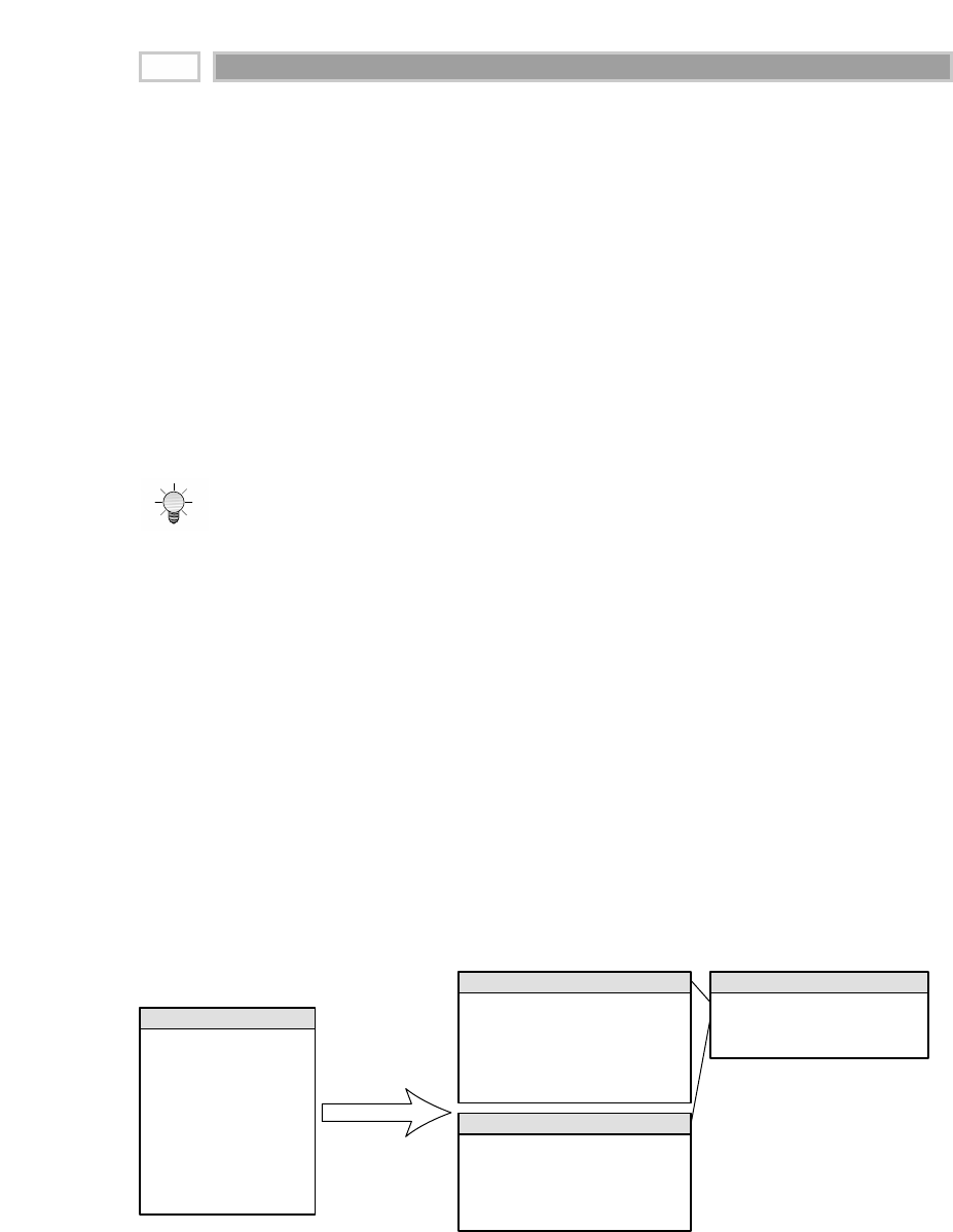
to the fact table and picking up the simultaneous customer key and its con-
temporary demographics key, which in general will be different from the most
recent demographics key.
Customer dimensions are unique in that customer attributes frequently are
queried independently of the fact table. For example, users may want to know
how many female customers live in Dade County by age bracket. Counts such
as these are extremely common with customer segmentation and profiling.
Rather than forcing any analysis that combines solely customer and demo-
graphic data to link through the fact table, the most recent value of the demo-
graphics key also can exist as a foreign key on the customer dimension table.
In this case, we refer to the demographics table as a customer dimension outrig-
ger, as we discussed earlier in this chapter.
The minidimension terminology refers to when the demographics key is part of the
fact table composite key; if the demographics key is a foreign key in the customer di-
mension, we refer to it as an outrigger.
If you embed the most recent demographics key in the customer dimension,
you must treat it as a type 1 attribute. If you tracked all the demographics
changes over time as a type 2 slowly changing dimension, you would have
reintroduced the rapidly changing monster dimension problem that we have
been working to avoid! With a type 1 change, as we discussed in Chapter 4, we
overwrite the demographics key in the customer row whenever it changes
instead of creating a new customer row. We also recommend that these outrig-
ger demographic attributes be labeled as most recent or current values to min-
imize confusion. Even with unique labeling, be aware that presenting users
with two avenues for accessing demographic data, through either the minidi-
mension or the outrigger, can deliver more functionality and complexity than
some users can handle.
Figure 6.4 Demographic minidimension with a customer dimension.
Becomes ...
Customer Key (PK)
Customer ID (Natural Key)
Customer Name
Customer Address
Customer Date of Birth
Customer Date of 1st Order
…
Age
Gender
Annual Income
Number of Children
Marital Status
Customer Dimension
Customer Key (PK)
Customer ID (Natural Key)
Customer Name
Customer Address
Customer Date of Birth
Customer Date of 1st Order
…
Customer Dimension
Customer Demographics Key (PK)
Customer Age Band
Customer Gender
Customer Income Band
Customer Number of Children Band
Customer Marital Status
Customer Demographics Dimension
Customer Key (FK)
Customer Demographics Key (FK)
More Foreign Keys …
Facts …
Fact Table
CHAPTER 6
156
TEAMFLY
Team-Fly®
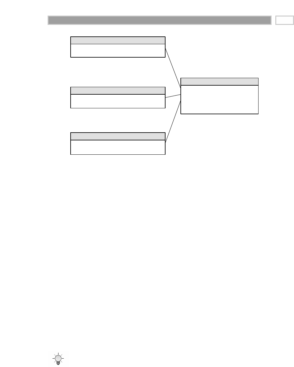
Figure 6.5 Separate demographic and behavioral minidimensions.
The demographic dimension itself cannot be allowed to grow too large. If we
have 5 demographic attributes, each with 10 possible values, then the demo-
graphics dimension could have 100,000 (105) rows. This is a reasonable upper
limit for the number of rows in a minidimension. However, there are certainly
cases where we need to support more than 5 demographic attributes with 10
values each. In this case, we would build a second demographics dimension,
as shown in Figure 6.5. For example, we may have one set of attributes con-
cerning traditional demographic income and lifestyle attributes and another
set that focuses on purchase and credit behavioral scores. Multiple minidi-
mensions address the issue of minidimension growth while also clustering
like attributes together for a more intuitive user presentation. Another motiva-
tion for creating these two minidimensions is that they are potentially sourced
from two different data providers with different update frequencies. However,
remember to bear in mind our advice from Chapter 2 concerning too many
dimensions. We certainly don’t want to create a separate minidimension with
a foreign key in the fact table for each demographic attribute, such as an age
dimension, gender dimension, and income dimension. Likewise, we shouldn’t
jump immediately on the minidimension technique unless we’re dealing with
a large or rapidly changing dimension; we can’t forget the advantages of main-
taining a simple, flat, denormalized dimension table.
The best approach for efficiently browsing and tracking changes of key attributes in
really huge dimensions is to break off one or more minidimensions from the dimen-
sion table, each consisting of small clumps of attributes that have been administered
to have a limited number of values.
Customer Key (PK)
Relatively constant attributes …
Customer Dimension
Customer Demographics Key (PK)
Demographics attributes …
Customer Demographics Dimension
Customer Purchase-Credit Key (PK)
Credit and payment behavioral attributes …
Customer Purchase-Credit Dimension
Customer Key (FK)
Customer Demographics Key (FK)
Customer Purchase-Credit Key (FK)
More Foreign Keys …
Facts …
Fact Table
Customer Relationship Management 157

Variable-Width Attribute Set
Finally, a minidimension can be created to handle a variable number of
customer attributes. Obviously, the longer we have a relationship with a
customer, the more descriptive information we know about him or her. If we
think about the sales cycle, we have many more prospects than we do cus-
tomers; however, we know much less about the prospects than we do about
our customers. We may have 10 million initial prospects, described by a
handful of characteristics, who are worked through the sales pipeline even-
tually to result in 1 million official customers with a much broader set of
known characteristics.
When using external prospect lists, we often are permitted only a one-time use
of the list and don’t have the legal right to store the prospect information inter-
nally. However, if we’ve generated our own prospect information, it certainly
can be stored in the data warehouse. Let’s assume that we’re capturing metrics,
perhaps associated with solicitation or quote-generation events that apply to
both prospects and customers. We could store the prospects and customers
together in a single contact dimension; however, there is a significant disparity
between the numbers of attributes for prospective versus customer contacts. As
illustrated in Figure 6.6, we may know only a handful of identification and loca-
tion attributes about our prospects. On the other hand, we may know 50 addi-
tional attributes for a customer, covering purchase, payment, credit and service
behaviors, directly elicited profile attributes, and third-party purchased demo-
graphic attributes. In the world of electronic retailing, we can equate prospects
to be the anonymous Web site visitors as opposed to our registered customers.
Figure 6.6 Variable-width customer attributes handled as a base dimension and
minidimension.
Contact Key (PK)
Contact ID (Natural Key)
Contact Zip
Contact State
Extended Customer Key (FK)
Contact Dimension
Extended Customer Key (PK)
Empty Customer Flag
Customer Name
Customer Address
Customer City
Customer State
Customer Zip
Purchase Behavior Score
Payment Behavior Score
Credit Behavior Score
Homeownership Indicator
… and more
Extended Customer Dimension
Contact Key (FK)
Extended Customer Key (FK)
More Foreign Keys …
Facts …
Fact Table
CHAPTER 6
158

If we assume that many of the final 50 customer attributes are textual, we eas-
ily could have a total row width of 1,000 bytes. Suppose that we have 10 mil-
lion contacts (9 million prospects and 1 million official customers). Obviously,
we are concerned that the trailing 50 columns in 90 percent of our contacts
have no data. This gets our attention when we’re dealing with a 10-GB dimen-
sion table. In this case, we may wish to introduce a minidimension.
If we’re dealing with a database platform that supports variable-width rows,
such as Oracle, we may be able to build a single dimension with the full com-
plement of attributes if the total attributes list is not too long; in some of these
cases, we don’t need to worry about all the prospects’ null columns because
they take up virtually zero disk space. However, if we have a fixed-width data-
base, or if the attributes list is very long, we are uncomfortable with all the
empty columns for the prospects. In this case, as shown in Figure 6.6, we break
the dimension into a 10-million-row base dimension table consisting of attrib-
utes that are common to both prospects and customers, along with a 1-million-
row customer minidimension that contains the additional attributes we know
about our customers. Again, we include two foreign keys in the fact table.
Nine of ten fact table rows would join to an empty customer row in the
extended customer minidimension.
Implications of Type 2 Customer
Dimension Changes
Perhaps your organization sells to tens of thousands of customers rather than
tens of millions. In this case, the techniques we discussed in Chapter 4 for track-
ing dimension changes are still viable. The slowly changing dimension type 2
technique, where another row is added to the dimension table, would remain
the predominant technique for tracking change in customer dimensions with
less than 100,000 rows. Even if we have a truly large customer dimension, we
likely will need to still use the type 2 response to handle very slowly changing
attributes left behind in the customer dimension.
As we mentioned earlier, users frequently want to count customers based on
their attributes without joining to a fact table. If we used a type 2 response to
track customer dimension changes, we would need to be careful to avoid
overcounting because we may have multiple rows in the customer dimension
for the same individual. Doing a COUNT DISTINCT on a unique customer
identifier is a possibility, assuming that the attribute is indeed unique and
also hasn’t been altered. A most recent row indicator in the customer dimen-
sion is also helpful to do counts based on the most up-to-date descriptive val-
ues for a customer.
Customer Relationship Management 159

Things get more complicated if we need to do a customer count at a given his-
torical point in time using effective and expiration dates in the customer
dimension. For example, if we need to know the number of customers we had
at the beginning of 2002, we could constrain the row effective date to less than
or equal to “1/1/2002” and the row expiration date to greater than or equal to
“1/1/2002” to restrict the result set to only those rows which were valid on
January 1, 2002. Note that the comparison operators depend on the business
rules used to set our effective/expiration dates. In this example, the row expi-
ration date on the no-longer-valid customer row is one day less than the effec-
tive date on the new row. Alternatively, as we discussed earlier, the dates may
be surrogate date keys joined to a date dimension outrigger table. In this case,
we would use unequal joins between the outrigger date tables and the effec-
tive/expiration dates on the customer dimension.
Customer Behavior Study Groups
With customer analysis, simple queries, such as how much have we sold to
customers in this geographic area in the past year, rapidly evolve to more
complex inquiries, such as how many customers bought more this past
month than their average monthly purchase amount from last year. The latter
question is much too complicated for business users to express in a single
SQL request. Some data access tool vendors allow embedded subqueries,
whereas others have implemented multipass SQL capabilities, in which com-
plex requests are broken into multiple select statements and then combined in
a subsequent pass.
In other situations, we may want to capture the set of customers from a query
or exception report, such as the top 100 customers from last year, customers
who spent more than $1,000 last month, or customers who received a specific
test solicitation, and then use that group of customers, which we call a behavior
study group, for subsequent analysis without reprocessing to identify the initial
condition. To create a behavior study group, we run a query (or series of
queries) to identify the set of customers we want to further analyze and then
capture the customer keys of the result set as an actual physical table. We then
use this special behavior study group dimension table of customer identifiers
whenever we wish to constrain any analysis to that set of specially defined
customers, as shown in Figure 6.7.
The secret to building complex behavioral study group queries is to capture the keys
of the customers or products whose behavior you are tracking. You then use the cap-
tured keys to constrain other fact tables without having to rerun the original behav-
ior analysis.
CHAPTER 6
160

The behavior study group dimension is attached with an equijoin to the nat-
ural key (named “Customer ID” in Figure 6.7) of the customer dimension. This
can be even done in a view that hides the explicit join to the behavior dimen-
sion. In this way, the resulting dimensional model looks and behaves like an
uncomplicated schema. If the study group dimension table is hidden under a
view, it should be labeled to uniquely identify it as being associated with the
top 100 customers, for example. Virtually any data access tool should be able
to analyze this specially restricted schema without paying syntax or user-
interface penalties for the complex processing that defined the original subset
of customers.
Like many design decisions, this one represents certain compromises. First,
this approach requires a user interface for capturing, creating, and administer-
ing physical behavior study group tables in the data warehouse. After a com-
plex exception report has been defined, we need the ability to capture the
resulting keys into an applet to create the special behavior study group dimen-
sion. These study group tables must live in the same space as the primary fact
table because they are going to be joined to the customer dimension table
directly. This obviously affects the DBA’s responsibilities.
Commercial Customer Hierarchies
One of the most challenging aspects of dealing with commercial customers is
modeling their internal organizational hierarchy. Commercial customers often
have a nested hierarchy of entities ranging from individual locations or
organizations up through regional offices, business unit headquarters, and
ultimate parent companies. These hierarchical relationships may change fre-
quently as customers reorganize themselves internally or are involved in
acquisitions and divestitures.
Figure 6.7 Behavior study group dimension consisting of selected keys joined directly to the natural
key of the customer dimension.
Customer ID (Natural Key)
Customer Behavior Study
Group Dimension Customer Key (PK)
Customer ID (Natural Key)
… and more
Customer Dimension Date Key (FK)
Product Key (FK)
Customer Key (FK)
Store Key (FK)
Promotion Key (FK)
POS Transaction Number (DD)
Sales Quantity
Sales Dollar Amount
POS Retail Sales Transaction Fact
Customer Relationship Management 161

We’ll talk about two approaches to handling customer hierarchies. The first is
straightforward but relies heavily on brute force rather than elegance. Still, it
may address your requirements adequately with a simplistic approach. The
second approach is more advanced and complicated but also much more
extensible. If you’re not dealing with unpredictable, ragged hierarchies (such
as variable customer and cost center hierarchies or manufacturing parts explo-
sion), you may want to skim the coverage on variable-depth hierarchies
because it is a bit of a brainteaser.
Fixed-Depth Hierarchies
Although this occurs relatively uncommonly, the lucky ones among us some-
times are confronted with a customer dimension that is highly predictable
with a fixed number of levels. Suppose that we track a maximum of three roll-
up levels, such as the ultimate corporate parent, business unit headquarters,
and regional offices (from top to bottom). In this case, we have three distinct
attributes in the customer dimension corresponding to these three levels. For
commercial customers with complicated organizational hierarchies, we’d pop-
ulate all three levels to appropriately represent the three different entities
involved at each roll-up level. By contrast, if another customer had a much
simpler organization structure, such as a one-location corporation, we’d dupli-
cate the lower-level value to populate the higher-level attributes. In this way,
all regional offices will sum to the sum of all business unit headquarters,
which will sum to the sum of all ultimate corporate parents. We can report by
any level of the hierarchy and see the complete customer base represented.
As we acknowledged up front, this simplistic approach doesn’t necessarily
address real-world complexity adequately; however, we would be remiss in not
mentioning it because it does provide a satisfactory solution for some. The tech-
nique described next is more robust, but the robustness comes with baggage. In
some situations, the more complex method may be impractical or overkill.
Variable-Depth Hierarchies
Representing an arbitrary, ragged organization hierarchy is an inherently dif-
ficult task in a relational environment. For example, we may want to report the
revenues for a set of commercial customers who have intricate relationships
with each other, such as in Figure 6.8. Each square on the diagram represents
an individual customer entity connected in an organizational tree. The illus-
trated organization has four levels; other customer organizations may have
one, ten, or more levels. Let’s assume that we sell our products or services to
any of these commercial customers. Thus the customer dimension rows can
play the role of parent as well as child. We may want to look at the customers
and their sales revenue individually. At other times, we may want to summa-
rize revenue to any node in the overall organizational tree.
CHAPTER 6
162

The computer science approach for handling this unpredictable hierarchy
would be to include a recursive parent customer key pointer on each cus-
tomer dimension row. Although this is a compact and effective way to repre-
sent an arbitrary hierarchy, this kind of recursive structure cannot be used
effectively with standard SQL. The GROUP BY function in SQL cannot fol-
low the recursive tree structure downward to summarize an additive fact
in a companion fact table such as revenue in an organization. Oracle’s
CONNECT BY SQL extension is able to navigate a recursive pointer in a
dimension table, but the CONNECT BY phrase cannot be used in the same
SQL statement as a join, which prohibits us from connecting a recursive
dimension table to any fact table. While we can fool the parser and perform
the join by hiding the CONNECT BY in a VIEW declaration, performance
likely would suffer significantly.
Instead of using a recursive pointer, we insert a bridge table between the cus-
tomer dimension and fact tables, as depicted in Figure 6.9. The bridge table has
been called a helper or associative table in the past, but going forward, we’ll con-
sistently use the bridge terminology. Use of the bridge table is optional; neither
the customer dimension table nor the fact table has to be modified in any way.
If the bridge table is left out, the customer dimension table joins to the fact
table in the usual way. We can report revenue by customer, but we’re unable to
navigate the organization hierarchy. When the bridge table is inserted between
the customer dimension and fact tables, we’re able to analyze revenue results
at any hierarchical level using standard SQL, albeit via a more complicated
presentation.
The bridge table contains one row for each pathway in Figure 6.8 from a customer
entity to each subsidiary beneath it, as well as a row for the zero-length pathway
Figure 6.8 Organization diagram of parent and subsidiary companies.
Customer
1
Customer
7
Customer
2
Customer
4
Customer
8
Customer
3
Customer
6
Customer
5
Customer Relationship Management 163

from a customer to itself. Each pathway row contains the customer key of the par-
ent roll-up entity, the customer key of the subsidiary entity, the number of levels
between the parent and the subsidiary, a bottom-most flag that identifies a sub-
sidiary with no further nodes beneath it, and finally, a top-most flag to indicate
that there are no further nodes above the parent. The sample bridge table rows
corresponding to the hierarchy in Figure 6.8 are shown as in Table 6.4.
The number of rows in the bridge table typically is several times larger than the
number of rows in the customer dimension. The eight individual parent and
subsidiary customers in the Figure 6.8 hierarchy translated into 22 rows in the
Table 6.4 bridge table. As an aside, a quick way to calculate the total number of
rows for a given customer organization is to multiply the number of values at
each level times the depth of the level (counting from the top), and then sum up
the resulting products. Let’s refer to the Figure 6.8 organization diagram again.
At top level 1 of the hierarchy, we have 1 customer (customer 1), which trans-
lates into 1 = (1 x 1) row in the bridge table. At the second level, we have 2 cus-
tomers (customers 2 and 7), which translate into another 4 = (2 x 2) rows in the
bridge. At level 3, we have 3 customers (customers 3, 4, and 8), which translate
into 9 = (3 x 3) bridge table rows. Finally, at the bottom (fourth) level, we have
2 customers (customers 5 and 6), which translate into an additional 8 = (4 x 2)
rows. The sum total number of rows is 22 = (1 + 4 + 9 + 8). If you don’t believe
us, go ahead and count up the number of sample rows in Table 6.4.
When we want to descend the organization hierarchy, we join the tables
together as shown in Figure 6.9. We can now constrain the customer table to a
particular parent customer and request any aggregate measure of all the sub-
sidiaries at or below that customer. We can use the “# of Levels from Parent”
column in the organization bridge table to control the depth of the analysis.
Constraining to a value of 1 would give all the direct subsidiaries of the cus-
tomer. A value greater than zero would give all subsidiary customers but not
the original parent. We can use the “Bottom Flag” column to jump directly to all
the bottom-most customer entities but omit all higher-level customer entities.
Figure 6.9 Customer dimension and bridge tables with join configuration to descend
the tree.
Customer Key (PK)
Customer ID (Natural Key)
Customer Name
Customer Address
Customer Attributes …
Customer Dimension
Parent Customer Key
Subsidiary Customer Key
# Levels from Parent
Level Name
Bottom Flag
Top Flag
Customer Hierarchy Bridge
Date Key (FK)
Customer Key (FK)
More Foreign Keys …
Facts …
Fact Table
Optional view definition to look
like normal fact table
with single-valued keys
CHAPTER 6
164

Table 6.4 Sample Bridge Table Rows Corresponding to Hierarchy in Figure 6.8
PARENT SUBSIDIARY #LEVELS
CUSTOMER CUSTOMER FROM BOTTOM TOP
KEY KEY PARENT FLAG FLAG
11 0NY
12 1NN
13 2YN
14 2NN
15 3YN
16 3YN
17 1NN
18 2YN
22 0NN
23 1YN
24 1NN
25 2YN
26 2YN
33 0YN
44 0NN
45 1YN
46 1YN
55 0YN
66 0YN
77 0NN
78 1YN
88 0YN
When we want to ascend the organization hierarchy, we reverse the joins by
connecting the customer dimension primary key to the bridge subsidiary key,
as shown in Figure 6.10. By constraining the “# of Levels” column in the bridge
table to the value of 1, we find the immediate parent of the customer in the cus-
tomer dimension. When the top-most flag is Y, we have selected the ultimate
parent for a given customer.
When issuing SQL statements using the bridge table, we need to be cautious
about overcounting the facts. When connecting the tables as shown in Figures
6.9 and 6.10, we must constrain the customer dimension to a single value and
Customer Relationship Management 165
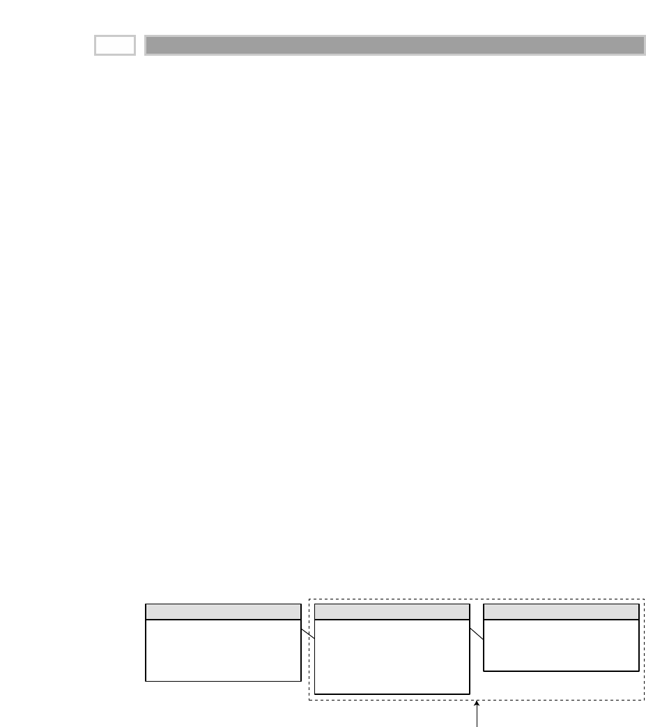
then join to the bridge table, which is then joined to the fact table. If we wanted
to sum up revenue in the fact table for a given customer and all its subsidiaries,
the SQL code would look something like the following:
SELECT C.CUSTOMER_NAME, SUM(F.REVENUE)
FROM CUSTOMER C, BRIDGE B, FACT F, DATE D
WHERE C.CUSTOMER_KEY = B.PARENT_KEY
AND B.SUBSIDIARY_KEY = F.CUSTOMER_KEY
AND F.DATE_KEY = D.DATE_KEY //along with joins for other dimensions
AND C.CUSTOMER_NAME = 'ABC General International' //for example
AND D.MONTH = 'January 2002'
GROUP BY C.CUSTOMER_NAME
We can request all the revenue from the organizations associated with many
parents at once, but we have to get the subsidiary keys distinctly or risk dou-
ble counting. In the following example we retrieve the January 2002 revenue
from all organizations whose parents are located in San Francisco. The SQL
code is messier, but it works for both unique and multiple parent customers.
SELECT 'San Francisco', SUM(F.REVENUE)
FROM FACT F, DATE D
WHERE F.CUSTOMER_KEY IN
(SELECT DISTINCT B.SUBSIDIARY_KEY
FROM CUSTOMER C, BRIDGE B
WHERE C.CUSTOMER_KEY = B.PARENT_KEY
AND C.CUSTOMER_CITY = 'San Francisco') //to sum all SF parents
AND F.DATE_KEY = D.DATE_KEY
AND D.MONTH = 'January 2002'
GROUP BY 'San Francisco'
Figure 6.10 Different bridge table join configuration to climb the organizational tree.
Customer Key (PK)
Customer ID (Natural Key)
Customer Name
Customer Address
Customer Attributes …
Customer Dimension
Parent Customer Key
Subsidiary Customer Key
# Levels from Parent
Level Name
Bottom Flag
Top Flag
Customer Hierarchy Bridge
Date Key (FK)
Customer Key (FK)
More Foreign Keys …
Facts …
Fact Table
Optional view definition to look
like normal fact table
with single-valued keys
CHAPTER 6
166
TEAMFLY
Team-Fly®

There are a number of administrative issues in building and maintaining an orga-
nization bridge table. Perhaps the biggest question is, where does the information
come from? How do you identify that an organizational change occurred, and
then how do you handle the change? If a complete history of changing organiza-
tional many-to-many relationships needs to be maintained, then the organization
bridge table can be generalized to include effective and expiration dates on each
row, as we’ll elaborate on in Chapter 13. A most recent indicator to identify the
most current organizational roll-up also would be useful. If these dates are
administered properly, then every requesting application would have to con-
strain on a specific date between the effective and expiration dates.
When a group of nodes is moved from one part of an organizational hierarchy
to another, only the bridge table rows that refer to paths from outside parents
to the moved structure need to be altered. All rows referring to paths within
the moved structure are unaffected. Of course, we’d need to add rows if the
moved structure had new parentage. This is an advantage over other tree-
representation schemas that often require a global renumbering to handle a
change such as this.
If two or more parents jointly own a subsidiary, then we can add a weighting
factor to the bridge table to reflect the fractional ownership. We’ll further elab-
orate on weighted bridge tables in Chapter 13.
Small and medium-sized parts explosions in a manufacturing application can
be modeled using the same kind of bridge table between a part/assembly
dimension table and a fact table. The main limitation to using this approach for
manufacturing parts explosions is the sheer number of subassemblies and
parts. A very large manufacturing parts explosion with hundreds of thousands
or millions of parts could result in a bridge table with “more rows than there
are molecules in the universe.”
Organization hierarchies and parts-explosion hierarchies may be represented with
the help of a bridge table. This approach allows the regular SQL grouping and sum-
marizing functions to work through ordinary query tools.
Having made the case for a bridge table to handle recursive variable-depth
hierarchies, we’d be the first to admit that it is not a perfect solution. The
approach attempts to bridge two inherently distinct structures, fixed rectangu-
lar relational tables and free-form hierarchical formations, which is akin
to blending oil and water. While the bridge table can be navigated via the
Customer Relationship Management 167

standard SQL code generated by many query tools, it is not for the faint of heart.
Analytical applications should be preconstructed to shield users from this non-
trivial SQL code. Fortunately, a number of nonrelational OLAP tools are provid-
ing more robust built-in support for navigating these pesky hierarchies for small
to medium-sized dimensions typically with less than 64,000 members.
Combining Multiple Sources of
Customer Data
Now that we’ve designed the customer dimension, it is time to populate it. It
is likely that the conformed customer dimension is a distillation of data from
several operational systems and possibly outside sources. In the worst case, a
unique customer has multiple identifiers in multiple operational touch-point
systems. Obviously, one of operational CRM’s objectives is create a unique
customer identifier and restrict the creation of unnecessary identifiers. In the
meantime, the data warehouse team likely will find itself responsible for sort-
ing out and integrating the disparate sources of customer information.
Unfortunately, there’s no secret weapon for tackling this data consolidation. The
attributes in the customer dimension should represent the best source available
for that data in the enterprise. We’ll want to integrate a national change of
address (NCOA) process to ensure that address changes are captured. Much of
the heavy lifting associated with customer data consolidation demands cus-
tomer-matching or deduplicating logic. Removing duplicates or invalid
addresses from large customer lists is critical to eliminating the financial and
customer satisfaction costs associated with redundant, misdirected, or undeliv-
erable communications, in addition to avoiding misleading customer counts.
The science of customer matching is more sophisticated than it might first
appear. It involves fuzzy logic, address-parsing algorithms, and enormous
look-up directories to validate address elements and postal codes, which vary
significantly by country. There are specialized commercially available software
and service offerings that can perform individual customer or commercial
entity matching with remarkable accuracy. Often these products match the
address components with standardized census codes, such as state codes,
country codes, census tracts, block groups, metropolitan statistical areas
(MSAs), and latitude/longitude, which facilitates the merging of external data.
As we’ll discuss in Chapter 9, there are also householding capabilities that
group or link customers who share similar name and address information.
Rather than merely performing intrafile matching, some services maintain an
enormous external reference file of everyone in the United States to match
against. Although these products and services are potentially expensive and
complex, it’s worthwhile to make the investment if customer matching (as in
the foundation of rudimentary CRM) is strategic to your organization. In the
end, effective consolidation of customer data depends on a balance of capturing
CHAPTER 6
168

the data as accurately as possible in the source systems coupled with powerful
data cleansing/merging tools in the staging process.
Analyzing Customer Data from Multiple
Business Processes
As we indicated in earlier chapters, data warehouses should be built process
by process, not department by department, on a foundation of conformed
dimensions to support cross-process integration. We can imagine querying the
sales or support service fact tables to better understand a customer’s purchase
or service history.
Since the sales and support tables both contain a customer foreign key, we can
further imagine joining both fact tables to a common customer dimension to
simultaneously summarize sales facts along with support facts for a given cus-
tomer, as in Figure 6.11. Unfortunately, the many-to-one-to-many join will
return the wrong answer in a relational environment because of the differences
in fact table cardinality.
Consider the case in which we have a fact table of customer solicitations and
another fact table with the customer responses resulting both from the solici-
tations and other independent sources. There is a one-to-many relationship
between customer and solicitation and another one-to-many relationship
between customer and response. The solicitation and response fact tables have
different cardinalities; in other words, not every solicitation results in a
response (unfortunately for the marketing department), and some responses
are received for which there is no solicitation. Simultaneously joining the solic-
itation fact table to the customer dimension, which is in turn joined to the
response fact table, does not return the correct answer in a relational DBMS
because of the cardinality differences. Fortunately, this problem is easily
avoided. We simply issue multipass SQL code to query the solicitation and
response tables in separate queries and then outer join the two answer sets.
The multipass approach has additional benefits in terms of better controlling
performance parameters, in addition to supporting queries that combine data
from fact tables in different physical locations.
Figure 6.11 Many-to-one-to-many joined tables should not be queried with a single
SELECT statement.
Solicitation Date Key (FK)
Customer Key (FK)
More Foreign Keys ...
Solicitation Facts …
Customer Solicitation Facts
Customer Key (PK)
Customer ID (Natural Key)
Customer Attributes …
Customer Dimensions Response Date Key (FK)
Customer Key (FK)
More Foreign Keys ...
Response Facts …
Customer Response Facts
Customer Relationship Management 169

Be very careful when simultaneously joining a single dimension table to two fact
tables of different cardinality. In many cases, relational systems will return the
wrong answer. A similar problem arises when joining two fact tables of different
granularity together directly.
If users are frequently combining data from multiple business processes, then
an additional fact table can be constructed that combines the data once into a
second-level, consolidated fact table rather than relying on users to combine
the data consistently and accurately on their own. We’ll discuss consolidated
fact tables further in Chapter 7. Merely using SQL code to drill across fact
tables to combine the results makes more sense when the underlying processes
are less closely correlated. Of course, when constructing the consolidated fact
table, we’d still need to establish business rules to deal with the differing car-
dinality (for example, does the combined fact table include all the solicitations
and responses or only those where both a solicitation and response occurred?).
Summary
In this chapter we focused exclusively on the customer, beginning with an
overview of CRM basics. We then delved into design issues surrounding the
customer dimension table. We discussed name and address parsing where
operational fields are decomposed to their basic elements so that they can be
standardized and validated. We explored several other types of common cus-
tomer dimension attributes, such as dates, segmentation attributes, and aggre-
gated facts. Dimension outriggers that contain a large block of relatively
low-cardinality attributes were described as permissible snowflakes in our
dimensional designs.
In cases where our customer dimension has millions of rows, we recom-
mended creating a minidimension of frequently analyzed or frequently chang-
ing attributes. A minidimension is also appropriate for variable-width
attribute sets. The fact table then has two customer-related foreign keys, one
for the primary customer dimension and another for the minidimension. We
discussed the implications of counting within a customer dimension where
additional type 2 rows are created to handle change. We also explored the
notion of creating behavioral study group dimensions, which merely consist of
customer keys that share a common trait or experience. Finally, we tackled the
handling of simple and complex commercial customer hierarchies. The unpre-
dictable, variable-depth customer hierarchies commonly require the use of a
bridge table to reflect the recursive hierarchy in a manner that can be queried
by standard SQL code.
CHAPTER 6
170

We briefly discussed the use of external software and service offerings to con-
solidate customer information effectively while managing duplicate data.
Finally, we stepped back into the world of fact tables for a moment to discuss
the potential downfalls of querying across two fact tables joined through a
common customer dimension table.
Customer Relationship Management 171


Accounting
CHAPTER 7
173
Financial analysis spans a variety of accounting applications, including the gen-
eral ledger and detailed subledgers for purchasing and accounts payable,
invoicing and accounts receivable, and fixed assets. Since we’ve already
touched on purchase orders and invoices in this book, we’ll focus on the gen-
eral ledger in this chapter. General ledgers were one of the first applications to
be computerized decades ago, given the need for accurate handling of a com-
pany’s financial records. Perhaps some of you are still running your business
on a twenty-year-old ledger system. In this chapter we’ll discuss the data
collected by the general ledger in terms of both journal entry transactions
and snapshots at the close of an accounting period. We’ll also talk about the
budgeting process.
Chapter 7 discusses the following concepts:
■■ General ledger periodic snapshots and transactions
■■ Year-to-date facts
■■ Multiple fiscal accounting calendars
■■ Budgeting process and associated data, including net change granularity
■■ Consolidated fact tables that combine metrics from multiple business processes,
such as actual and budget data
■■ Role of online analytic processing (OLAP) and packaged analytic financial solutions

Accounting Case Study
Since finance was an early adopter of technology to better run businesses, it
comes as no surprise that early decision support solutions focused on the
analysis of financial data. Financial analysts are some of the most data-literate
and spreadsheet-savvy individuals around. Often their analysis is dissemi-
nated or leveraged by many others in an organization. Managers at all levels
need timely access to key financial metrics. In addition to receiving standard
reports, managers need the ability to analyze performance trends, variances,
and anomalies with relative speed and minimal effort. Unfortunately, the
backlog of special requests for financial data is often quite lengthy. As we
observe frequently in operational source systems, the data in the general
ledger is likely scattered among hundreds of tables. Gaining access to financial
data and creating ad hoc reports may require a decoder ring to navigate
through the maze of screens. This runs counter to the objective of many orga-
nizations to push fiscal responsibility and accountability to line managers.
The data warehouse can provide a single source of usable, understandable
financial information, ensuring that everyone is working with the same data
based on common definitions and metrics. The audience for financial data is
quite diverse in many organizations, ranging from analysts to operational
managers to executives. For each group, we need to determine which subset of
corporate financial data is needed, in which format, and with what frequency.
Analysts and managers will want to view information at a high level and then
drill down to journal entries for more detail. For executives, financial data
from the data warehouse often feeds their dashboard or scorecard of key per-
formance indicators. Armed with direct access to information, managers can
obtain answers to questions more readily than when forced to work through
an intermediary. Meanwhile, the finance department can turn its attention to
information dissemination and value-added analysis rather than focusing on
report creation.
The benefits of improved access to financial data focus on opportunities to bet-
ter manage risk, streamline operations, and identify potential cost savings.
While financial analysis has cross-organization impact, many businesses focus
their initial data warehouse implementation on strategic revenue-generating
opportunities. Consequently, accounting data is often not the very first subject
area tackled by the data warehouse team. Given its proficiency with technol-
ogy, the finance department often has already performed magic with spread-
sheets and personal databases to create work-around analytic solutions,
perhaps to its short-term detriment, since these imperfect interim fixes likely
are stressed to the limits.
CHAPTER 7
174

General Ledger Data
The general ledger (G/L) is a core foundation financial system because it ties
together the detailed information collected by the purchasing, payables (what
you owe to others), and receivables (what others owe you) subledgers or sys-
tems. In this case study we’ll focus on the general ledger rather than the sub-
ledgers, which would be handled as separate business processes and fact tables.
As we work through a basic design for G/L data, we discover, once again, that
two complementary schemas with periodic snapshot and transaction-grained
fact tables working together are required.
General Ledger Periodic Snapshot
We begin by delving into a snapshot of the G/L accounts at the end of each fis-
cal period (or month if your fiscal accounting periods align with calendar
months). Referring once again to our four-step process for designing dimen-
sional models, the business process obviously focuses on the G/L. The grain of
this periodic snapshot is one row per accounting period for the most granular
level in the G/L’s chart of accounts.
Chart of Accounts
The cornerstone of the G/L is the chart of accounts. The G/L’s chart of
accounts is the epitome of an intelligent key because it usually consists of a
series of identifiers. For example, the first set of digits may identify the
account, account type (for example, asset, liability, equity, income, or expense),
and other account roll-ups. Sometimes intelligence is embedded in the account
numbering scheme. For example, account numbers from 1,000 through 1,999
might be asset accounts, whereas account numbers ranging from 2,000 to 2,999
may identify liabilities. Obviously, in the data warehouse, we’d include the
account type as a dimension attribute rather than forcing users to filter on the
first digit of the account number.
The chart of accounts also likely provides insight regarding the organizational
cost center associated with the account. Typically, the organizational elements
provide a complete roll-up from cost center to department to division, for
example. If the corporate G/L combines data across multiple business units,
the chart of accounts also would indicate the business unit or subsidiary
company.
Obviously, charts of accounts vary from company to company. They’re often
extremely complicated. In our case study vignette we assume that the chart of
Accounting 175

accounts naturally decomposes into two dimensions. One dimension focuses
on the attributes of the financial G/L account, whereas the other represents the
organizational roll-up. The organization roll-up may be a fixed-depth hierar-
chy, where we can handle the hierarchy levels as separate attributes in the
organization cost center dimension. If the organizational hierarchy is ragged
with imbalanced roll-up trees, then we’ll need to resort to the bridge table
technique from Chapter 6 for dealing with variable-depth hierarchies.
The G/L sometimes tracks financial results for multiple sets of books or sub-
ledgers to support different requirements, such as taxation or regulatory
agency reporting. We’ll treat this as a separate dimension because it is such a
fundamental filter.
Period Close
At the end of each accounting period, the finance organization is responsible
for finalizing the financial results so that they can be officially reported inter-
nally and externally. It typically takes several days at the end of each period to
reconcile and balance the books before they can be closed with the finance
department’s official stamp of approval. From there, finance’s focus turns to
reporting and interpreting the results. The finance department often produces
countless reports and responds to countless variations on the same questions
each month.
Financial analysts are constantly looking to streamline the processes for
period-end closing, reconciliation, and reporting of G/L results. While opera-
tional G/L systems often support these requisite capabilities, they may be
cumbersome, especially if you’re not dealing with a modern G/L. In this chap-
ter we’ll focus on more easily analyzing the closed financial results rather than
facilitating the close. However, in many organizations, G/L trial balances are
loaded into the data warehouse to leverage the capabilities of the data ware-
house’s presentation area to find the needles in the G/L haystack and then
make the appropriate operational adjustments before the period ends.
The sample schema in Figure 7.1 supports the access and analysis of G/L
account balances at the end of each account period. It would be very useful for
many kinds of financial analysis, such as account rankings, trending patterns,
and period-to-period comparisons.
For the moment, we’re just representing actual facts in the Figure 7.1 schema;
we’ll turn our attention to budget data later in this chapter. Obviously, the bal-
ance amount is a semiadditive fact. Although we typically attempt to avoid
semiadditive facts, it makes sense to store the balance in this schema because
many of the accounts are tracked as a balance. Otherwise, we’d need to go
back to the beginning of time to calculate an accurate end-of-period balance.
CHAPTER 7
176
TEAMFLY
Team-Fly®
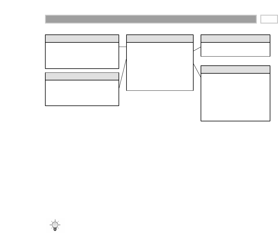
Figure 7.1 General ledger (G/L) periodic snapshot.
Year-to-Date Facts
Designers are often tempted to store to-date columns in fact tables. They think
that it would be helpful to store quarter-to-date or year-to-date totals on each
fact row so that users don’t need to calculate them. We need to remember that
numeric facts must be consistent with the grain. To-date fields are not true to
the grain and are fraught with peril. When fact rows are queried and summa-
rized in arbitrary ways, these untrue-to-the-grain facts produce nonsensical,
overstated results. They should be left out of the relational schema design and
calculated in the data access application instead.
In general, to-date totals should be calculated, not stored in the fact table.
Multiple Currencies Revisited
If the general ledger consolidates data that has been captured in multiple curren-
cies, we would handle it much as we discussed in Chapter 5. With financial data,
we typically want to represent the facts in terms of both the local currency and a
standardized corporate currency. In this case, each row in the fact table would
represent one set of fact amounts expressed in local currency and a separate set of
fact amounts expressed in the equivalent corporate currency. Doing so allows us
to summarize the facts in a common corporate currency easily without jumping
through hoops in our access applications. Of course, we’d also add a currency
dimension as a foreign key in the fact table to identify the local currency type.
General Ledger Journal Transactions
While the end-of-period snapshot addresses a multitude of financial analyses,
many users need to dive into the underlying details. If the periodic snapshot
Accounting Period Key (PK)
Accounting Period Number
Accounting Period Description
Accounting Period Fiscal Year
Accounting Period Dimension
Accounting Period Key (FK)
G/L Key (FK)
G/L Account Key (FK)
G/L Organization Key (FK)
Period End Balance Amount
Period Debit Amount
Period Credit Amount
Period Net Change Amount
G/L Snapshot Fact
G/L Organization Key (PK)
Cost Center Name
Cost Center Number
Department Name
Department Number
Division Name
Business Unit Name
Company Name
G/L Organization Dimension
G/L Key (PK)
G/L Book Name
G/L Dimension
G/L Account Key (PK)
G/L Account Name
G/L Account Category
G/L Account Type
G/L Account Dimension
Accounting 177
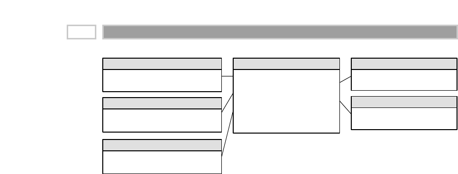
Figure 7.2 General ledger (G/L) journal entry transactions.
data appears unusual or not as expected, analysts will want to look at the
detailed transactions to sort through the issue. Others will want access to the
details because the summarized monthly balances may obscure large dispari-
ties at the granular transaction level. Once again, we complement the periodic
snapshot with a detailed journal entry transaction schema. Of course, the
accounts payable and receivable subledgers may contain transactions at even
lower levels of detail, which would be captured in separate fact tables with
additional dimensionality.
In this situation we’re still focused on the G/L process; however, the grain of
the fact table is now one row for every G/L journal entry transaction. The jour-
nal entry transaction identifies the G/L account and the applicable debit or
credit amount. As illustrated in Figure 7.2, we’ll reuse several dimensions from
the last schema, including the account and organization dimensions. If our
G/L tracked multiple sets of books, we’d also include the ledger dimension.
We’re capturing journal entry transactions by transaction posting date, so
we’ll use a daily-grained date table in this schema. Depending on the business
rules associated with the source data, we may need a second role-playing date
dimension to distinguish the posting date from the effective accounting date.
The journal entry number likely is a degenerate dimension with no linkage to
an associated dimension table. Depending on the source data, we may have a
journal entry transaction type and even a description. In this situation we’d
create a separate journal entry transaction dimension. Assuming that the
descriptions are not just freeform text, this dimension would have significantly
fewer rows than the fact table, which would have one row per journal entry
line. The specific journal entry number would still be treated as degenerate.
Fact Types
Each row in the journal entry fact table would be identified as either a credit or
a debit. Given this inherent sparsity, we’d likely store a single journal entry
Post Date Key (PK)
Post Date Attributes …
Post Date Dimension
Post Date Key (PK)
G/L Key (FK)
G/L Account Key (FK)
G/L Organization Key (FK)
Debit-Credit Indicator Key (FK)
Journal Entry Number (DD)
Journal Entry Amount
G/L Journal Entry Fact
G/L Organization Key (PK)
G/L Organization Attributes …
G/L Organization Dimension
G/L Key (PK)
G/L Attributes …
G/L Dimension
G/L Account Key (PK)
G/L Account Attributes …
G/L Account Dimension
Debit-Credit Indicator Key
Debit-Credit Indicator Description
Debit-Credit Indicator Dimension
CHAPTER 7
178

amount with a debit/credit indicator, unless we’re using a database platform,
such as Oracle, which supports variable-width columns so that the empty
columns take up minimal disk space. The debit/credit indicator would take on
two and only two values. We can create a two-row debit/credit decode dimen-
sion table, or if your database supports bit-mapped indices, we may just
include the industry-standard debit/credit abbreviation (DR/CR) in the fact
table with a bit-mapped index for speedy filtering or constraining. We don’t
want you to perceive that this is an excuse to bypass dimension table decode
tables for all low-cardinality dimensions. It makes sense in this case because
the abbreviations are understood universally, which isn’t usually the case with
our internal codes and abbreviations. Ninety-nine percent of the time we’ll
continue to create dimension tables that contain textual, descriptive decodes.
Multiple Fiscal Accounting Calendars
In this schema we’re capturing data by posting date, but users likely also want
the ability to summarize the data by fiscal account period. Unfortunately, fis-
cal accounting periods often do not align with standard Gregorian calendar
months. For example, a company may have 13 four-week accounting periods
in a fiscal year beginning on September 1 rather than 12 monthly periods
beginning on January 1. If we’re dealing with a single fiscal calendar, then each
day in a year corresponds to a single calendar month, as well as a single
accounting period. Given these relationships, the calendar and accounting
periods are merely hierarchical attributes on the daily date dimension, as we
saw in Chapter 2. The daily date dimension table obviously would conform to
a calendar month dimension table, as well as to a fiscal accounting period
dimension table.
In other situations we may be dealing with multiple fiscal accounting calen-
dars that vary by subsidiary or line of business. If the number of unique fiscal
calendars is a fixed, low number, then we can include each set of uniquely
labeled fiscal calendar attributes on a single date dimension. A given row in
the daily date dimension could be identified as belonging to accounting period
1 for subsidiary A, but accounting period 7 for subsidiary B.
In a more complex situation with a large number of different fiscal calendars,
we could identify the official corporate fiscal calendar in the date dimension.
We then have several options to address the subsidiary-specific fiscal calendars.
The most common approach is to create a date dimension outrigger with a mul-
tipart key consisting of the date and subsidiary keys. There would be one row
in this table for each day for each subsidiary. The attributes in this outrigger
would consist of fiscal groupings (such as fiscal week end date and fiscal period
end date). We’d need a mechanism for filtering on a specific subsidiary in the
outrigger. Doing so through a view would then allow the outrigger to be
Accounting 179

presented as if it were logically part of the date dimension table. A second
approach for tackling the subsidiary-specific calendars would be to create sep-
arate physical date dimensions, instead of views, for each subsidiary calendar
using a common set of surrogate date keys. This option likely would be used if
your fact data were decentralized by subsidiary. Depending on your data access
tool’s capabilities, it may be easier to either filter on the subsidiary outrigger as
described in the first option or ensure use of the appropriate subsidiary-specific
physical date dimension table (the second option). Finally, we could allocate
another foreign key in the fact table to a subsidiary fiscal period dimension
table. The number of rows in this table would be the number of fiscal periods
(approximately 36 for three years) times the number of unique calendars. This
approach simplifies user access but puts additional strain on the staging area
because it must insert the appropriate fiscal period key during the transforma-
tion process.
Financial Statements
One of the primary functions of a G/L system is to produce the organization’s
official financial reports, such as the balance sheet and income statement. Typ-
ically, the operational system handles the production of these reports. We
wouldn’t want the data warehouse to attempt to replace the reports published
by the operational financial system.
However, data warehouse teams sometimes create a complementary database
of aggregated data to provide simplified access to report information that can
be more widely disseminated throughout the organization. Dimensions in the
financial statement database would include the accounting period and cost
center. Rather than looking at G/L account-level data, the fact data would be
aggregated and tagged with the appropriate financial statement line number
and label. In this manner, managers could easily look at performance trends
for a given line in the financial statement over time for their organization. Sim-
ilarly, key performance indicators and financial ratios may be made available
at the same level of detail.
Budgeting Process
Modern G/L systems typically include the ability to integrate budget data into
the G/L. However, if our G/L either lacks this capability or we’ve elected not
to implement it, we need to provide an alternative mechanism for supporting
the budgeting process and variance comparisons.
Within most organizations, the budgeting process is looked at as a series of
events. Prior to the start of a fiscal year, each cost center manager typically
CHAPTER 7
180

creates a budget, broken down by budget line items, which is then approved.
In reality, budgeting is seldom simply a once-per-year event any more. Bud-
gets are becoming more dynamic because there are budget adjustments as the
year progresses, reflecting changes in business conditions or the realities of
actual spending versus the original budget. Managers want to see the current
budget’s status, as well as how the budget has been altered since the first
approved version. As the year unfolds, commitments to spend the budgeted
monies are made. Finally, payments are processed.
As dimensional modelers, we view the budgeting chain as a series of fact
tables. We’ll begin with a budget fact table. For an expense budget line item,
each row identifies what an organization in the company is allowed to spend
for what purpose during a given time frame. Similarly, if the line item reflects
an income forecast, which is just another variation of a budget, it would iden-
tify what an organization intends to earn from what source during a time
frame.
We could further identify the grain to be a status snapshot of each line item in
each budget each month. Although this grain has a familiar ring to it (because
it feels like a management report), it is a poor choice as the fact table grain.
The facts in such a status report are all semiadditive balances rather than fully
additive facts. Also, this grain makes it difficult to determine how much has
changed since the previous month or quarter because we have to obtain the
records from several time periods and then subtract them from each other.
Finally, this grain choice would require the fact table to contain many dupli-
cated records when nothing changes in successive months for a given line
item.
Instead, the grain we’re interested in is the net change of the budget line item
in a cost center that occurred during the month. While this suffices for budget
reporting purposes, the accountants eventually will need to tie to the budget
line item back to a specific G/L account that is affected, so we’ll also go down
to the G/L account level.
Given the grain, the associated dimensions would include effective month,
organization, budget line item, and G/L account, as illustrated in Figure 7.3.
The organization dimension is identical to the one used earlier with the G/L
data. The G/L dimension is also a reused dimension. The only complication
regarding the G/L account dimension is that sometimes a single budget line
item has an impact on more than one G/L account. In such a case, we would
need to allocate the budget line to the individual G/L accounts. Since the grain
of the budget fact table is by G/L account, a single budget line for a cost center
may be represented as several rows in the fact table.
Accounting 181

Figure 7.3 Annual budget schema.
The budget line item identifies the purpose of the proposed spending, such as
employee wages or office supplies. Typically, several levels of summarization
categories are associated with a budget line item. As we discussed in Chapter 5,
all the budget line items may not have the same number of levels in their sum-
marization hierarchy, such as when some have only a category roll-up but not
a subcategory. In this case we may populate the dimension attributes by repli-
cating the category name in the subcategory column to avoid having line items
roll up to a “Not Applicable” subcategory bucket. The budget line-item dimen-
sion also would identify the budget year and budget version.
The effective month is the month during which the budget changes are posted.
The first entries for a given budget year would show the effective month when
the budget is first approved. If the budget is updated or modified as the bud-
get year gets underway, the effective months would occur during the budget
year. If we don’t adjust the budget at all throughout the year, then the only
entries would be the first ones when the budget is approved. This is what we
meant when we specified the grain to be the net change. It is critical that you
understand this point, or you won’t understand what is in this budget fact
table or how it is used.
Sometimes budgets are created as annual spending plans; at other times
they’re broken down by month or by quarter. The schema in Figure 7.3
assumes that the budget is an annual figure, with the budget year identified in
the budget line-item dimension. If we need to express the budget data by
spending month, we would need to include a second month dimension table
that plays the role of spending month.
The budget fact table has a single budget amount fact that is fully additive. If
we’re budgeting for a multinational organization, the budget amount may be
tagged with the expected currency conversion factor for planning purposes.
If the budget amount for a given budget line and G/L account is modified
Budget Effective Date Key (PK)
Budget Effective Date Month
Budget Effective Date Year
… and more
Effective Date Dimension
Budget Effective Date Key (FK)
Budget Line Item Key (FK)
G/L Account Key (FK)
G/L Organization Key (FK)
Budget Amount
Budget Fact
G/L Organization Key (PK)
G/L Organization Attributes …
G/L Organization Dimension
Budget Line Item Key (PK)
Budget Line Description
Budget Year
Budget Line Subcategory Description
Budget Line Category Description
Budget Line Item Dimension
G/L Account Key (PK)
G/L Account Attributes …
G/L Account Dimension
CHAPTER 7
182

during the year, an additional row is added to the budget fact table represent-
ing the net change. For example, if the original budget was $200,000, we might
have another row in June for a $40,000 increase and then another in October
for a negative $25,000 as we tighten our belts going into year-end.
Once the budget year begins, managers make commitments to spend the bud-
get through purchase orders, work orders, or other forms of contracts. Man-
agers are keenly interested in monitoring their commitments and comparing
them with the annual budget in order to manage their spending. We can envi-
sion a second fact table for the commitments that shares the same dimensions,
in addition to dimensions identifying the specific commitment document
(purchase order, work order, or contract) and commitment party. In this case
the fact would be the committed amount.
Finally, payments are made as monies are transferred to the party named in
the commitment. From a practical point of view, the money is no longer avail-
able in the budget when the commitment is made. However, the finance
department is interested in the relationship between commitments and pay-
ments because it manages the company’s cash. The dimensions associated
with the payments fact table would include the commitment fact table dimen-
sions plus a payment dimension to identify the type of payment and the
payee to whom the payment actually was made. In the budgeting chain we
expand the list of dimensions as we move from the budget to commitments to
payments.
With this design, we can create a number of interesting analyses. To look at the
current budgeted amount by department and line item, we constrain on all
dates up to the present, adding the amounts by department and line item.
Because the grain is the net change in the line items, adding up all the entries
over time does exactly the right thing. We end up with the current approved
budget amount, and we get exactly those line items in the given departments
which have a budget.
To ask for all the changes to the budget for various line items, we simply con-
strain on a single month. We’ll report only those line items which experienced
a change during the month.
To compare current commitments with the current budget, we separately sum
the commitment amounts and budget amounts from the beginning of time to
the current date (or any date of interest). We then combine the two answer sets
on the row headers. This is a standard drill-across application using multipass
SQL. Similarly, we could drill across commitments and payments.
If you’re interested in reading more about building and using the budgeting
chain, we recommend Data Warehouse Design Solutions (Wiley 1998) by Chris
Adamson and Mike Venerable.
Accounting 183

Consolidated Fact Tables
In the last section we discussed users comparing metrics generated by sepa-
rate business processes by drilling across fact tables, such as budget and com-
mitments. If this type of drill-across analysis is extremely common in the user
community, it likely makes sense to create a single fact table that combines the
metrics once rather than relying on users or their reporting applications to
stitch together result sets, especially given the inherent issues of complexity,
accuracy, tool capabilities, and performance.
Most typically, business managers are interested in comparing actual to bud-
get variances. At this point we presume that our annual budgets and/or fore-
casts have been broken down by accounting period. In Figure 7.4 we see the
actual and budget amounts, as well as the variance (which is a calculated dif-
ference) by the common dimensions. As we discussed earlier, we deliver the
to-date fields by leveraging the roll-up attributes on the accounting period
dimension.
Again, if we’re working for a multinational organization, we likely would see
the actual amounts in both local and equivalent standard currency, based on
the effective conversion rate. In addition, we may convert the actual results
based on the planned currency conversion factor (as described during the
budget process). Given the unpredictable nature of currency fluctuations, it is
useful to monitor performance based on both the effective and planned con-
version rates. In this manner, remote managers aren’t penalized for currency
rate changes outside their control. Likewise, the finance department can bet-
ter understand the big-picture impact of unexpected currency conversion
fluctuations on the organization’s annual plan.
As we introduced in Chapter 3, we refer to fact tables that combine metrics at
a common granularity as consolidated or second-level fact tables (or consolidated
data marts). While consolidated fact tables can be very useful in terms of both
performance and usability, they often represent a dimensionality compromise
because they consolidate facts at the least common denominator set of dimen-
sions. One potential risk associated with consolidated fact tables is that proj-
ect teams sometimes base their designs solely on the granularity of the
consolidated fact table while failing to meet user requirements that demand
the ability to dive into more granular data. These schemas also run into seri-
ous problems if project teams attempt to force a one-to-one correspondence in
order to consolidate data with different granularity or dimensionality.
CHAPTER 7
184
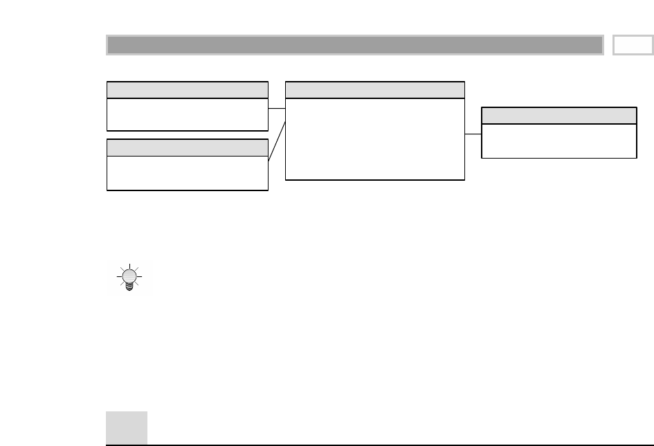
Figure 7.4 Actual versus budget consolidated fact table.
When facts from multiple business processes are combined in a consolidated fact
table, they must live at the same level of granularity and dimensionality. Optimally, the
separate facts naturally live at a common grain. Otherwise, we are forced to eliminate
or aggregate some dimensions to support the one-to-one correspondence or keep
them in separate fact tables. Project teams should not create artificial facts or dimen-
sions in an attempt to force fit the consolidation of differently grained fact data.
Role of OLAP and Packaged Analytic Solutions
While we’ve been discussing financial data warehouses in the context of
relational databases, it is worth noting that multidimensional OLAP vendors
have long played a role in this arena. OLAP products have been used exten-
sively for financial reporting, budgeting, and consolidation applications. We
often see relational dimensional models feeding financial OLAP data cubes.
OLAP cubes are precalculated, which results in fast query performance that
is critical for executive use. The data volumes, especially for the G/L bal-
ances or financial statement aggregates, typically do not overwhelm the
practical size constraints of a multidimensional product. OLAP is well suited
to handle complicated organizational roll-ups, as well as complex calcula-
tions, including interrow manipulations. Most multidimensional OLAP ven-
dors provide finance-specific capabilities, such as financial functions (for
example, net present value or compound growth), the appropriate handling
of financial statement data (in the expected sequential order, such as income
before expenses), and the proper treatment of debits and credits depending
on the account type, as well as more advanced functions such as financial
consolidation.
Accounting Period Key (PK)
Accounting Period Attributes …
Accounting Period Dimension
Accounting Period Key (FK)
G/L Account Key (FK)
G/L Organization Key (FK)
Accounting Period Actual Amount
Accounting Period Budget Amount
Accounting Period Budget Variance
Budget Variance Fact
G/L Organization Key (PK)
G/L Organization Attributes …
G/L Organization Dimension
G/L Account Key (PK)
G/L Account Attributes …
G/L Account Dimension
Accounting 185

Given the standard nature of G/L processing, purchasing a G/L package
rather than attempting to build one from scratch has been a popular route for
years. Nearly all the operational package providers also offer a complemen-
tary analytic solution, sometimes in partnership with one of the multidimen-
sional OLAP vendors. In many cases these canned analyses based on the
cumulative experience of the vendor are a sound way to jump-start a financial
data warehouse implementation with potentially reduced cost and risk. The
analytic solutions often have tools to assist with the extraction and staging of
operational financial data, as well as tools to assist with analysis and interpre-
tation. However, as we discussed in Chapter 6, when leveraging packaged
solutions, we need to be cautious about avoiding stovepipe applications. One
could easily find oneself in a situation with separate financial, CRM, human
resources, and ERP packaged analytic solutions from as many different ven-
dors, none of which integrates with other internal data. We need to conform
dimensions across the entire data warehouse environment regardless of
whether we’re building our own solution or implementing packages. Pack-
aged analytic solutions can turbocharge your data warehouse implementa-
tion; however, they do not alleviate the need for conformance. Most
organizations inevitably will rely on a combination of building, buying, and
integrating for a complete solution.
Summary
In this chapter we focused primarily on financial G/L data in terms of both
periodic snapshots and journal entry transactions. We discussed the handling
of common G/L data challenges, including multiple currencies, multiple fiscal
years, unbalanced organizational trees, and the urge to create to-date totals.
We explored the series of events in a budgeting process chain. We described
the use of net-change granularity in this situation rather than creating snap-
shots of the budget data totals. We also discussed the concept of consolidated
fact tables that combine the results of separate business processes when they
are analyzed together frequently.
Finally, we discussed the natural fit of multidimensional OLAP products for
financial analysis. We also stressed the importance of integrating analytic
packages into the overall data warehouse through the use of conformed
dimensions.
CHAPTER 7
186
TEAMFLY
Team-Fly®

Human Resources Management
CHAPTER 8
187
This chapter, which focuses on human resources (HR) data, is the last in the
series that deals with cross-industry business applications. Similar to the
accounting and finance data described in Chapter 7, HR information is dis-
seminated broadly throughout the organization. Unlike finance, however, we
typically don’t find a cadre of tech-savvy HR analysts in many organizations.
Most of us operate in a rapidly changing, competitive business environment.
We need to better understand our employees’ demographics, skills, earnings,
and performance in order to maximize their impact. In this chapter we’ll
explore several dimensional modeling techniques in the context of HR data.
Chapter 8 discusses the following concepts:
■■ Dimension tables to track employee transaction facts
■■ Audit dimension
■■ Skill-set keyword dimension outrigger
■■ Handling of survey questionnaire data

Time-Stamped Transaction Tracking
in a Dimension
Thus far the dimensional models we have designed closely resemble each other
in that the fact tables have contained key performance metrics that typically can
be added across all the dimensions. It is easy for dimensional modelers to get
lulled into a kind of additive complacency. In most cases, this is exactly how it is
supposed to work. However, with HR employee data, many of the facts aren’t
additive. Most of the facts aren’t even numbers, yet they are changing all the time.
To frame the problem with a business vignette, let’s assume that we work in
the HR department of a large enterprise with more than 100,000 employees.
Each employee has a detailed HR profile with at least 100 attributes, including
date of hire, job grade, salary, review dates, review outcomes, vacation entitle-
ment, organization, education, address, insurance plan, and many others. In
our organization there is a stream of transactions against this employee data.
Employees are constantly being hired, transferred, and promoted, as well as
adjusting their profiles in a variety of ways.
The highest-priority business requirement is to track and analyze these
employee transaction events accurately. This detailed transaction history is the
fundamental truth of HR data; it should provide the answer to every possible
employee profile inquiry. While these unanticipated questions may be com-
plex, we must be confident the data is available and waiting to be analyzed.
We immediately visualize a schema as depicted in Figure 8.1 where each
employee transaction event is captured in a transaction-grained fact table. The
granularity of this fact table would be one row per employee transaction. Since
no numeric metrics are associated with the transaction, the fact table is factless.
The measurements associated with employee transactions are the changes
made to the employee profile, such as a new address or job grade promotion.
Figure 8.1 Initial draft for tracking employee change transactions.
Each change to the
employee dimension
handled as a SCD type 2
Employee Key (PK)
Employee ID (Natural Key)
Employee Attributes …
Employee Dimension
Grain: one row per
employee transaction
Transaction Date Key (FK)
Transaction Time Key (FK)
Employee Key (FK)
Employee Transaction Type Key (FK)
Employee Transaction Fact Table
Employee Transaction Type Key (PK)
Employee Transaction Type Description
Employee Transaction Type Dimension
Transaction Date Dimension
Transaction Time Dimension
CHAPTER 8
188

In this initial draft schema, the dimensions include the transaction date and
time, transaction type, and employee. The transaction date and time dimen-
sions refer to the exact date and time of the employee transaction. We assume
that these dates and times are fine-grained enough that they guarantee
uniqueness of the transaction row for a given employee. The transaction type
dimension refers to the variety of transaction that caused the creation of this
particular row, such as a promotion or address change. The employee dimen-
sion is extremely wide with many attribute columns. The employee identifier
used in the HR production system as a constant identifier for the employee is
included in this dimension table as an attribute.
We envision using the type 2 slowly changing dimension technique for track-
ing changed profile attributes in the employee dimension. Consequently,
with every employee transaction in the fact table in Figure 8.1, we also create
a new type 2 row in the employee dimension that represents the employee’s
profile as a result of the transaction event. It continues to accurately describe
the employee until the next employee transaction occurs at some indetermi-
nate time in the future. The alert reader is quick to point out that we’ve
designed an employee transaction fact table and a type 2 employee dimen-
sion table with the exact same number of rows, which are almost always
joined to one another. At this point dimensional modeling alarms should be
going off. We certainly don’t want to have as many rows in a fact table as we
do in a related dimension table.
Instead of using the initial schema, we can simplify the design by embellishing
the employee dimension table to make it more powerful and thereby doing
away with the transaction event fact table. As depicted in Figure 8.2, the
employee transaction dimension contains a snapshot of the employee profile
following each individual employee transaction. We included the transaction
type description in the employee dimension to track the reason for the profile
change. There is no numeric metric associated with a profile transaction; the
transaction merely results in a new set of employee profile characteristics. In
some cases, the affected characteristics are numeric. If the numeric attributes
are summarized rather than simply constrained upon, they belong in a fact
table instead.
As you’d expect, the surrogate employee transaction key is the primary key of
the dimension table, although the natural key is the constant employee ID. We
resist the urge to rely on a smart key consisting of the employee ID, transaction
code, and transaction date/time. All these attributes are valuable, but they are
simply columns in the employee transaction row that participate in queries
and constraints like all the other attribute columns.
Human Resources Management 189

Figure 8.2 Employee transaction dimension.
A crucial component of this design is the second date and time entry, the trans-
action expiration date/time. This date/time represents the date/time of the
next transaction to occur for this employee, whenever that may be. In this way
these two date/times in each row define a span during which the employee
profile is accurate. The two date/times can be one second apart (if a rapid
sequence of transactions is being processed against an employee profile) or
many months apart. The transaction expiration date/time in the most current
employee profile must be set to an arbitrary time in the future. Although it
would seem more elegant to set the expiration date for this row to null, this
probably would make the query and reporting applications more complex
because they might have to test separately for the null value.
The most recent transaction indicator identifies the latest transaction made
against an employee profile. This column allows the most recent or final status
of any employee to be retrieved quickly. If a new profile transaction occurs for
this employee, the indicator in the former profile row needs to be updated to
indicate that it is no longer the latest transaction.
Even in a large organization, this approach doesn’t require significant storage.
Assume that we have 100,000 employees and perform an average of 10 HR
profile transactions on each employee each year. Even if we have a verbose
2,000-byte transaction row, 5 years of profile data only adds up to 10 GB (5
years x 100,000 employees x 2,000 bytes x 10 transactions per year) of raw data
in the employee transaction dimension.
Employee Transaction Key (PK)
Employee ID (Natural Key)
Employee Name …
Employee Address …
Job Grade …
Salary …
Education …
Original Hire Date (FK)
Last Review Date (FK)
Appraisal Rating …
Health Insurance Plan …
Vacation Plan …
Employee Transaction Type Description
Employee Transaction Date
Employee Transaction Time
Employee Transaction Expiration Date
Employee Transaction Expiration Time
Most Recent Transaction Indicator
Employee Transaction Dimension
Indicates the transaction that caused
another Employee row to be created
CHAPTER 8
190

On its own, this time-stamped type 2 employee transaction dimension can
answer a number of interesting HR inquiries. We obviously can use this table
to look in detail at the sequence of transactions against any given employee.
We can easily profile the employee population at any precise instant in time.
We can choose an exact date at any historical point in time and ask how many
employees we have and what their detailed profiles were on that date by con-
straining the date and time to be equal to or greater than the transaction
date/time and less than the transaction expiration date/time. The query can
perform counts and constraints against all the rows returned from these date
constraints. Given that the dimension rows are snapshots in their own right,
we avoid sifting through a complex set of transactions in sequence to construct
a snapshot for a particular date in the past.
Adding effective and expiration date/time stamps, along with a transaction descrip-
tion, on each row can embellish the design of a type 2 slowly changing dimension to
allow very precise time slicing of the dimension by itself.
Before rushing into this design for an HR application, we need to be thought-
ful about the transaction dimension. The underlying HR source system may
have a very complex notion of a transaction that isn’t really what we want in
the data warehouse. For instance, an employee promotion may be imple-
mented in the source system by many microtransactions corresponding to
each change in an individual field on the employee record. We don’t want to
see this detail in the data warehouse. Rather, we want to encapsulate the whole
series of microtransactions from the underlying source system and treat them
all as a super transaction called employee promotion. The new record in our type
2 employee dimension reflects all the relevant changed fields in one step. Iden-
tifying these supertransactions may be tricky. Perhaps the best way to identify
them is to make sure that there is a field on the HR operational application that
captures the high-level action.
Time-Stamped Dimension with
Periodic Snapshot Facts
Some of you may be wondering if the employee transaction dimension table
isn’t really a kind of fact table because it is time-stamped. While technically
this may be true, this employee transaction table mainly contains textual val-
ues; it is the primary source of query constraints and report labels. Thus it is
proper to think of this table as a dimension table that serves as the entry point
into the HR fact tables. The employee transaction table can be used with any
fact table that requires an employee dimension as long as the employee surro-
gate key is extended to be the employee transaction surrogate key.
Human Resources Management 191

In addition to profiling the employee base in HR, we also need to report sum-
mary statuses of the employee base on a regular, monthly basis. We’re inter-
ested in counts, statistics, and totals, including such things as number of
employees, total salary paid during the month, vacation days taken, vacation
days accrued, number of new hires, and number of promotions. We want to
analyze the data by all possible slices, including time and organization. We
need to access totals at the end of each month, even when there is no transac-
tion activity in a given employee’s profile during that month.
As shown in Figure 8.3, the HR periodic snapshot consists of a fairly ordinary
looking fact table with three dimensions: month, employee transaction, and
organization. The month dimension table contains the usual descriptors for
the corporate calendar at the month grain. The employee transaction key in a
fact table row is the employee transaction key that was effective on the last day
of the given reporting month. This guarantees that the month-end report is a
correct depiction of all the employee profiles. The organization dimension
contains a description of the organization to which the employee belongs at
the close of the relevant month.
The facts in this HR snapshot consist of monthly numeric summaries that are
difficult to calculate from the underlying transactions. These monthly counts
and totals satisfy the bulk of management’s inquiries regarding monthly
employee statistics. All the facts are additive across all the dimensions or
dimension attributes, except for the facts labeled as balances. These balances,
like all balances, are semiadditive and must be averaged across the time
dimension after adding across the other dimensions.
Figure 8.3 HR periodic snapshot with employee transaction dimension.
Employee Transaction Key (PK)
Employee ID (Natural Key)
Employee Attributes …
Employee Transaction Type Description
Employee Transaction Date
Employee Transaction Time
Employee Transaction Expiration Date
Employee Transaction Expiration Time
Most Recent Transaction Indicator
Employee Transaction Dimension
Employee Transaction and Organization
foreign keys are those valid at month end
Month Key (FK)
Employee Transaction Key (FK)
Organization Key (FK)
Salary Paid
Overtime Paid
Overtime Hours
Retirement Fund Paid
Retirement Fund Employee Contribution
Vacation Days Accrued
Vacation Days Taken
Vacation Day Balance
Employee Count
New Hire Count
Transfer Count
Promotion Count
Human Resources Snapshot Fact
Month Key (PK)
Month Attributes …
Month Dimension
Organization Key (PK)
Organization Attributes ...
Organization Dimension
CHAPTER 8
192

Audit Dimension
Whenever we build a fact table containing measurements of our business, we
surround the fact table with everything we know to be true. We can extend this
everything-we-know approach to our fact tables by including key pieces of
metadata that are known to be true when an individual fact row is created. For
instance, when we create a fact table row, we know the following:
■■ What source system supplied the fact data
■■ What version of the extract software created the row
■■ What version of allocation logic, if any, was used to create the row
■■ Whether a specific “Not Applicable” fact column is unknown, impossible,
corrupted, or not available yet
■■ Whether a specific fact was altered after the initial load and, if so, why
■■ Whether the row contains facts more than 2, 3, or 4 standard deviations
from the mean or, equivalently, outside various bounds of confidence
derived from some other statistical analysis
The first three items describe the lineage of the fact table row; in other words,
where did the data come from? The last three items describe our confidence
in the quality of data for that fact table row. As illustrated in Figure 8.4, the
most efficient way to add this information to a fact table is to create a single
audit foreign key in the fact table. The beauty of this design is that the data
staging lineage and confidence metadata has now become regular data,
which can be queried and analyzed along with the other more familiar
dimensions.
The indicators in the audit dimension consist of textual decodes. We are
going to constrain and report on these various audit attributes, so we want
them to appear as understandable text. Perhaps the extract software
attribute might contain the value “Employee extract version 5 using ETL
vendorABC release 6.4.” The altered status attribute might contain values
such as “Not altered” or “Altered due to restatement.” In our staging
extract-transformation-load (ETL) process, we track these indicators and
have them ready when the fact table row is being assembled in its final state.
If we are loading a large number of rows each day, almost all the rows will
have the same audit foreign key because presumably nearly all the rows
will be normal.
Human Resources Management 193

Figure 8.4 HR periodic snapshot with audit dimension.
Keyword Outrigger Dimension
Let’s assume that the IT department wants to supplement the employee
dimension with descriptive technical skill-set information. The department
wants to be able to determine any and all of the key technical skills in which an
employee is proficient. It is highly likely that many IT employees have exper-
tise in a wide variety of skills. We can consider these technical skills to be key-
words that describe our employees. There will be a number of different
keywords, but there will be predictability or structure to them. Some key-
words will describe programming languages (for example, Cobol, C++, and
Pascal), whereas others will describe operating systems (for example, Unix,
Windows, and Linux) or database platforms. We want to search the IT
employee population by these descriptive keywords, which we will label as
skills in our design.
Since each employee will have a variable, unpredictable number of skills, the
skills dimension is a prime candidate to be a multivalued dimension. Key-
words, by their nature, usually are open-ended. New keywords are created
regularly and added to the database. We’ll show two logically equivalent
modeling schemes for handling open-ended sets of keywords while at the
same time keeping both querying and administration simple. Figure 8.5 shows
a multivalued dimension design for handling the skills keywords as an
Employee Transaction Key (PK)
Employee Transaction Attributes …
Employee Attributes …
Employee Transaction Dimension
Audit Key (PK)
Extract Completion Date
Extract Completion Time
Extract Status
Number of Records Extracted
Transformation Completion Date
Transformation Completion Time
Transformation Status
Number of Records Transformed
Number of Transform Records Rejected
Load Completion Date
Load Completion Time
Load Status
Number of Records Loaded
Number of Load Records Rejected
Audit Dimension
Month Key (FK)
Employee Transaction Key (FK)
Organization Key (FK)
Audit Key (FK)
Salary Paid
Overtime Paid
Overtime Hours
Retirement Fund Paid
Retirement Fund Employee Contribution
Vacation Days Accrued
Vacation Days Taken
Vacation Day Balance
Employee Count
New Hire Count
Transfer Count
Promotion Count
Human Resources Snapshot Fact
Month Key (PK)
Month Attributes …
Month Dimension
Organization Key (PK)
Organization Attributes ...
Organization Dimension
CHAPTER 8
194

Figure 8.5 Skills group keyword dimension outrigger.
outrigger to the employee dimension table. As we’ll see in Chapter 13 when
we further elaborate on multivalued dimension attributes, sometimes the mul-
tivalued dimension is joined directly to a fact table.
The skills group identifies a given set of skills keywords. All IT employees
who are proficient in Oracle, Unix, and SQL would be assigned the same skills
group key. In the skills group outrigger, there would be three rows for this par-
ticular group, one for each of the associated keyword skills (Oracle, Unix, and
SQL). In this case, just two attributes are associated with each skill, description
and category, so we include these attributes in the outrigger directly.
AND/OR Dilemma
Assuming that we have built the schema as shown in Figure 8.5, we are still
left with a serious query problem. Query requests against the technical skill-
set keywords likely will fall into two categories. The OR queries (for example,
Unix OR Linux experience) can be satisfied by a simple OR constraint on the
skills description column in the outrigger. However, AND queries (for exam-
ple, Unix AND Linux experience) are difficult because the AND constraint is a
constraint across two rows in the skills outrigger. SQL is notoriously poor at
handling constraints across rows. The answer is to create SQL code using
unions and intersections, probably in a custom interface that hides the com-
plex logic from the business user. The SQL code would look like this:
(SELECT EMPLOYEE_ID, EMPLOYEE_NAME
FROM EMPLOYEE, SKILLS
WHERE EMPLOYEE.SKILLSGROUP = SKILLS.SKILLSGROUP AND SKILL = “UNIX”)
UNION / INTERSECTION
(SELECT EMPLOYEE_ID, EMPLOYEE_NAME
FROM EMPLOYEE, SKILLS
WHERE EMPLOYEE.SKILLSGROUP = SKILLS.SKILLSGROUP AND SKILL = “LINUX”)
Using the UNION lists employees with Unix OR Linux experience, whereas
using INTERSECTION identifies employees with Unix AND Linux experience.
Employee Key (FK)
More Foreign Keys …
Human Resources Facts …
Human Resources Fact
Employee Key (PK)
Employee Attributes …
Employee Skill Group Key (FK)
Employee Dimension
Employee Skill Group Key (PK)
Employee Skill Key (PK)
Employee Skill Description
Employee Skill Category
Employee Skill Group Outrigger
Human Resources Management 195

Searching for Substrings
We can remove the many-to-many join and the need for UNION/
INTERSECTION SQL by changing the design to a simpler form, as shown in
Figure 8.6. Now each row in the skills list outrigger contains one long text
string with all the skills keywords for that list key. We use a special delimiter
such as a backslash at the beginning of the skills list column and after each
skill in the list. Thus the skills list string containing Unix and C++ would look
like \Unix\C++\. We presume that a number of employees share a common
list of skills. If the lists are not reused frequently, we could collapse the skills
list outrigger into the employee dimension merely by including the skills list
string as we just described directly in the employee dimension.
String searches can be challenging because of the ambiguity caused by search-
ing on upper or lower case. Is it UNIX or Unix or unix? We can resolve this
either by changing all the keywords to one case or by using a special database
text string search function that is case-insensitive.
With the design in Figure 8.6, the AND/OR dilemma can be addressed in a
single SELECT statement. The OR constraint looks like this:
SKILL_LIST LIKE ‘%\UNIX\% OR SKILL_LIST LIKE ‘%\LINUX\%’
Meanwhile, the AND constraint has exactly the same structure:
SKILL_LIST LIKE ‘%\UNIX\%’ AND SKILL_LIST LIKE ‘%\LINUX\%’
The % symbol is a wildcard pattern-matching character defined in SQL that
matches zero or more characters. The backslash delimiter is used explicitly in
the constraints to exactly match the desired keywords and not get erroneous
matches.
The keyword list approach shown in Figure 8.6 will work in any relational
database because it is based on standard SQL. However, leading wildcard
searches are notorious for being slow when the keyword dimension table gets
large. If performance becomes objectionable, you can pursue two approaches
if your database allows. First, you can pin the keyword list outrigger in mem-
ory so that even though the constraint may invoke an exhaustive search of the
dimension, it may be pretty fast. Second, you can build a special pattern index
on the keyword list column that provides an index lookup to every conceiv-
able substring, provided that your database can support this type of index.
CHAPTER 8
196
TEAMFLY
Team-Fly®
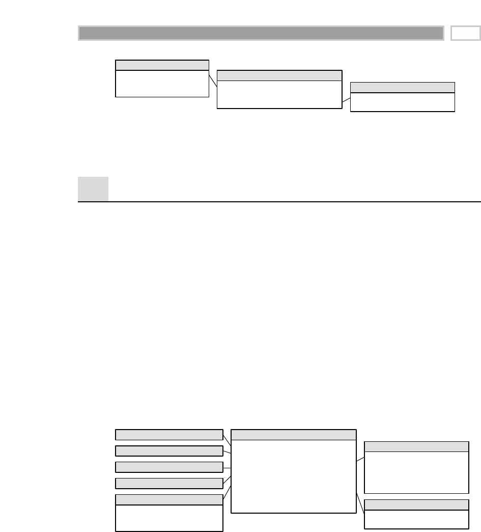
Figure 8.6 Delimited skills list dimension outrigger.
Survey Questionnaire Data
The HR department often collects survey data from the entire employee base,
especially when gathering peer and/or management review data. The depart-
ment wants to analyze these questionnaire responses to determine the average
rating for a reviewed employee and the average rating within a department.
In order to analyze questionnaire data, we create a fact table with one row for
each question on a respondent’s survey, as illustrated in Figure 8.7. There
would be two role-playing employee dimensions in the schema corresponding
to the responding employee and the reviewed employee. The survey dimen-
sion consists of descriptors about the survey instrument. The question dimen-
sion would provide the question and its categorization. Presumably, the same
question is asked on multiple surveys. The survey and question dimensions
can be useful handles for searching for specific topics in a broad database of
questionnaires. The response dimension contains the responses and perhaps
categories of responses, such as favorable or hostile.
Figure 8.7 HR survey schema.
Survey Sent Date Dimension
Survey Sent Date Key (FK)
Survey Received Date Key (FK)
Survey Key (FK)
Responding Employee Key (FK)
Reviewed Employee Key (FK)
Question Key (FK)
Response Category Key (FK)
Survey Number (DD)
Response
Employee Evaluation Survey Fact
Survey Key (PK)
Survey Title
Survey Type
Survey Objective
Review Year
Survey Dimension
Response Category Key (PK)
Response Category Description
Response Category Dimension
Survey Received Date Dimension
Responding Employee Dimension
Reviewed Employee Dimension
Question Key (PK)
Question Label
Question Category
Question Dimension
Employee Key (FK)
More Foreign Keys …
Human Resources Facts …
Human Resources Fact
Employee Key (PK)
Employee Attributes …
Employee Skill Group Key (FK)
Employee Dimension
Employee Skill List Key (PK)
Employee Skill List
Employee Skill Group Outrigger
Human Resources Management 197

Creating the simple schema in Figure 8.7 supports robust slicing and dicing of
survey data. Variations of this schema design would be useful for analyzing all
types of survey data, including customer satisfaction and product usage feed-
back.
Summary
In this chapter we discussed several concepts in the context of HR data. First,
we further elaborated on the advantages of embellishing a dimension table so
that it not only captures all the relevant attributes but also tracks transactions
that cause profile changes. In the world of HR, this single table will be used to
address a number of questions regarding the status and profile of the
employee base at any point in time. We described the use of an audit dimen-
sion to track data lineage and quality metadata within an HR fact table. This
technique obviously is broadly applicable beyond the HR arena. We intro-
duced the use of keyword group or delimited list dimension outriggers to sup-
port analysis on multivalued attributes. Finally, we provided a brief overview
regarding the analysis of data collected from surveys or questionnaires.
CHAPTER 8
198

Financial Services
CHAPTER 9
199
The financial services industry encompasses a wide variety of businesses,
including credit card companies, brokerage firms, and mortgage providers.
This chapter will focus primarily on retail banks given that most readers have
some degree of personal familiarity with this type of financial institution. A
full-service bank offers a breadth of products, including checking accounts,
savings accounts, mortgage loans, personal loans, credit cards, and safe
deposit boxes. This chapter begins with a very simplistic schema. We then
explore several schema extensions, including handling of the bank’s broad
portfolio of heterogeneous products that vary significantly by line of business.
As we embark on a series of industry-focused chapters, we want to remind
you that they are not intended to provide full-scale industry solutions. While
various dimensional modeling techniques will be discussed in the context of a
given industry, the techniques certainly are applicable to other businesses. If
you don’t work in financial services, you still need to read this chapter. If you
do work in financial services, remember that the schemas in this chapter
should not be viewed as complete.
Chapter 9 discusses the following concepts:
■■ Dimension triage to avoid the “too few dimensions” trap
■■ Household dimensions
■■ Associating individual customers with accounts using a bridge table
■■ Multiple minidimensions in a single fact table

■■ Value banding of facts for reporting purposes
■■ Point-in-time balances using transaction data
■■ Handling heterogeneous products, each with unique metrics and dimension attributes,
across lines of business
Banking Case Study
The bank’s initial goal is to build the capability to better analyze the bank’s
accounts. Users want the ability to slice and dice individual accounts, as well
as the residential household groupings to which they belong. One of the
bank’s major objectives is to market more effectively by offering additional
products to households that already have one or more accounts with the bank.
After conducting interviews with managers and analysts around the bank, we
develop the following set of requirements:
1. Business users want to see 5 years of historical monthly snapshot data on
every account.
2. Every account has a primary balance. The business wants to group differ-
ent types of accounts in the same analyses and compare primary balances.
3. Every type of account (known as products within the bank) has a set of
custom dimension attributes and numeric facts that tend to be quite dif-
ferent from product to product.
4. Every account is deemed to belong to a single household. There is a sur-
prising amount of volatility in account-household relationships due to
changes in marital status and other life-stage factors.
5. In addition to the household identification, users are interested in demo-
graphic information as it pertains to both individual customers and
households. In addition, the bank captures and stores behavior scores
relating to the activity or characteristics of each account and household.
Dimension Triage
Based on the business requirements just listed, the grain and dimensionality of
the initial model begin to emerge. We start with a core fact table that records
the primary balances of every account at the end of each month. Clearly, the
grain of the fact table is one row for each account at the end of each month.
Based on this grain declaration, we initially envision a design with only two
CHAPTER 9
200

dimensions—month and account. These two foreign keys form the fact table
primary key, as shown in Figure 9.1. A data-centric designer might argue that
all the other description information, such as household, branch, and product
characteristics, should be embedded as descriptive attributes of the account
dimension because each account has only one household, branch, and product
associated with it.
While this schema accurately represents the many-to-one and many-to-many
relationships in the snapshot data, it does not adequately reflect the natural
business dimensions. Rather than collapsing everything into the huge
account dimension table, additional analytic dimensions such as product and
branch mirror the instinctive way that banking users think about their busi-
nesses. These supplemental dimensions provide much smaller points of entry
to the fact table. Thus they address both the performance and usability objec-
tives of a dimensional model. Finally, given that the master account dimen-
sion in a big bank may approach 10 million members, we worry about type 2
slowly changing dimension (SCD) effects mushrooming this huge dimension
into something unworkable. The product and branch attributes are conve-
nient groups of attributes to remove from the account dimension in order to
cut down on the type 2 SCD effects. Later in this chapter we’ll squeeze the
changing demographics and behavioral attributes out of the account dimen-
sion for the same reasons.
The product and branch dimensions are two separate dimensions because
there is a many-to-many relationship between products and branches. They
both change slowly but on different rhythms. Most important, business users
think of them as basic, distinct dimensions of the banking business.
In general, most dimensional models end up with between 5 and 15 or so
dimensions. If we find ourselves at or below the low end of this range, we
should be suspicious that dimensions may have been left out of the design
inadvertently. In this case we should consider carefully whether any of the fol-
lowing kinds of dimensions are appropriate supplements to a draft dimen-
sional model:
Figure 9.1 Balance snapshot with too few dimensions.
Month End Date Key (PK)
Month Attributes …
Month Dimension
Month End Date Key (FK)
Account Key (FK)
Primary Month Ending Balance
Monthly Account Snapshot Fact
Account Key (PK)
Account Attributes …
Product Attributes …
Household Attributes …
Status Attributes …
Branch Attributes …
Account Dimension
Financial Services 201

Causal dimensions. These dimensions, such as promotion, contract, deal,
store condition, or even weather, provide additional insight into the cause
of an event.
Multiple date or time-stamp dimensions. Refer to Chapter 5 for sample fact
tables with multiple date stamps, especially when the fact table is an accu-
mulating snapshot.
Degenerate dimensions. These dimensions identify operational transaction
control numbers, such as an order, invoice, bill of lading, or ticket, as illus-
trated initially in Chapter 2.
Role-playing dimensions. Role-playing occurs when a single physical
dimension appears several times in a fact table, each represented as a
separate logical table with unique column names through views.
Status dimensions. These dimensions identify the current status of a transac-
tion or monthly snapshot within some larger context, such as an account
status.
Audit dimension. As discussed in Chapter 8, this dimension is designed to
track data lineage and quality.
Junk dimensions.These consist of correlated indicators and flags, as
described in Chapter 5.
These supplemental dimensions typically can be added gracefully to a design,
even after the data warehouse has gone into production, because they do not
change the grain of the fact table. The addition of these dimensions usually
does not alter the existing dimension keys or measured facts in the fact table.
All existing applications should continue to run without change.
Any descriptive attribute that is single-valued in the presence of the measurements
in the fact table is a good candidate to be added to an existing dimension or to be
its own dimension.
Based on further study of the bank’s requirements, we ultimately choose the
following dimensions for our initial schema: month end date, account, house-
hold, branch, product, and status. As illustrated in Figure 9.2, at the intersec-
tion of these six dimensions, we take a monthly snapshot and record the
primary balance and any other metrics that make sense across all products,
such as interest paid, interest charged, and transaction count. Remember that
account balances are just like inventory balances in that they are not additive
across any measure of time. Instead, we must average the account balances by
dividing the balance sum by the number of months.
CHAPTER 9
202
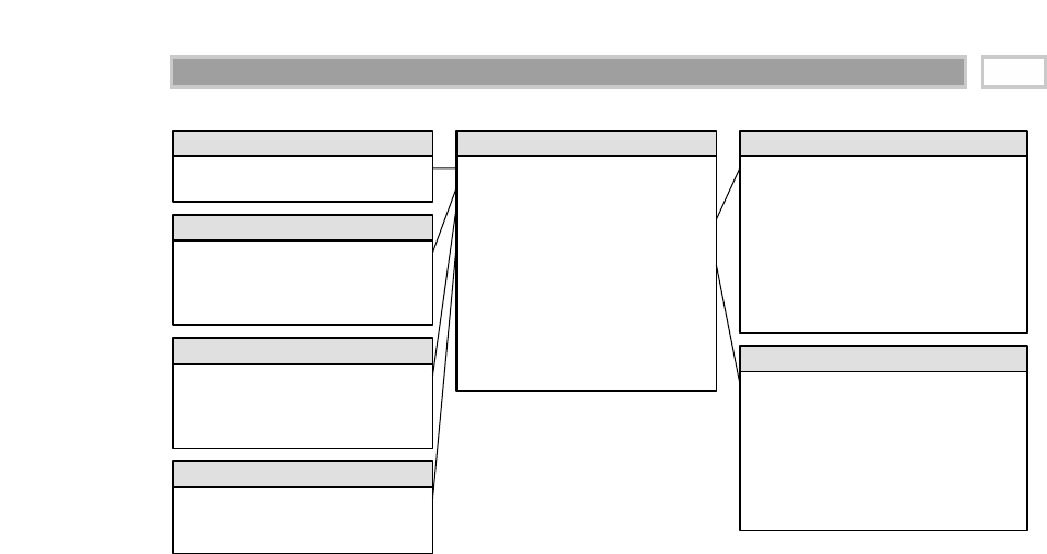
Figure 9.2 Core snapshot fact table for all accounts.
The product dimension consists of a simple product hierarchy that describes
all the bank’s products, including the name of the product, type, and category.
The need to construct a generic product categorization in the bank is the same
need that causes grocery stores to construct a generic merchandise hierarchy.
The main difference between the bank and grocery store examples is that the
bank also develops a large number of custom product attributes for each prod-
uct type. We’ll defer discussion regarding the handling of these custom attrib-
utes until the end of this chapter.
The branch dimension is similar to the facility or location dimensions we
discussed earlier in this book, such as the retail store or distribution center
warehouse.
The account status dimension is a useful dimension to record the condition of
the account at the end of each month. The status records whether the account
is active or inactive or whether a status change occurred during the month,
such as a new account opening or an account closure. Rather than whipsawing
the large account dimension or merely embedding a cryptic status code or
abbreviation directly in the fact table, we treat status as a full-fledged dimen-
sion with descriptive status decodes, groupings, and status reason descrip-
tions as appropriate. In many ways we could consider the account status
dimension to be another example of a minidimension, as we introduced in
Chapter 6.
Month End Date Key (PK)
Month Attributes …
Month Dimension
Branch Key (PK)
Branch Address Attributes …
Branch Rollup Attributes …
Branch Format Description
Branch Dimension
Product Key (PK)
Product Description
Product Type
Product Category
Product Dimension
Account Status Key (PK)
Account Status Description
Account Status Group
Account Status Dimension
Month End Date Key (FK)
Branch Key (FK)
Product Key (FK)
Account Key (FK)
Account Status Key (FK)
Household Key (FK)
Primary Month Ending Balance
Average Daily Balance
Number of Transactions
Interest Paid
Interest Charged
Fees Charged
Monthly Account Snapshot Fact
Account Key (PK)
Account Number (Natural Key)
Primary Account Holder Name
Secondary Account Holder Name
Account Address Attributes …
Account Open Date
Account Type Description
Account Type Category
… and more
Account Dimension
Household Key (PK)
Head of Household Name
Household Address Attributes …
Household Type
Household Income
Household Homeownership Indicator
Household Presence of Children
… and more
Household Dimension
Financial Services 203

Household Dimension
Rather than focusing solely on the bank’s accounts, users also want the ability
to analyze the bank’s relationship with an entire economic unit, or household.
They are interested in understanding the overall profile of a household, the
magnitude of the existing relationship with the household, and what addi-
tional products should be sold to the household. They also want to capture key
demographics regarding the household, such as household income, whether
the household owns or rents the home, and whether there are children in the
household. These demographic attributes change over time; as you might sus-
pect, the users want to track the changes. If the bank focuses on accounts for
commercial entities rather than consumers, it likely has similar requirements
to identify and link corporate families.
From the bank’s perspective, a household may be comprised of several
accounts and individual account holders. For example, consider John and
Mary Smith as a single household. John has a checking account, and Mary has
a savings account. In addition, John and Mary have a joint checking account,
credit card, and mortgage with the bank. All five of these accounts are consid-
ered to be a part of the same Smith household despite the fact that minor
inconsistencies may exist in the operational name and address information.
The process of relating individual accounts to households (or the commercial
business equivalent of a residential household) is not to be taken lightly.
Householding requires the development of business rules and algorithms to
assign accounts to households. As we discussed in Chapter 6, there are spe-
cialized products and services to do the matching necessary to determine
household assignments. It is very common for a large financial services orga-
nization to invest significant resources in specialized capabilities to support its
householding needs.
The decision to treat accounts and households as separate dimensions is some-
what a matter of the designer’s prerogative. Despite the fact that accounts and
households are correlated intuitively, we decide to treat them separately
because of the size of the account dimension and the volatility of the account
constituents within a household dimension, as referenced earlier. In a large
bank, the account dimension is huge, with easily over 10 million rows that
group into several million households. The household dimension provides
a somewhat smaller point of entry into the fact table without traversing a
10-million-row account dimension table. In addition, given the changing
nature of the relationship between accounts and households, we elect to use
the fact table to capture the relationship rather than merely including the
household attributes on each account dimension row. In this way we avoid
using the type 2 SCD approach with the large account dimension.
CHAPTER 9
204

Multivalued Dimensions
As we just saw in the John and Mary Smith example, an account can have one,
two, or more individual account holders, or customers, associated with it.
Obviously, we cannot merely include the customer as an account attribute;
doing so violates the granularity of the dimension table because more than one
individual can be associated with an account. Likewise, we cannot include
customer as an additional dimension in the fact table; doing so violates the
granularity of the fact table (one row per account per month) again because
more than one individual can be associated with any given account. This is a
classic example of a multivalued dimension, which we’ll develop fully in
Chapter 13. For now, suffice it to say that to link an individual customer
dimension to an account-grained fact table requires the use of an account-to-
customer bridge table, as shown in Figure 9.3. At a minimum, the primary key
of the bridge table consists of the surrogate account and customer foreign
keys. We’ll discuss date/time stamping of bridge table rows in Chapter 13 to
capture relationship changes. In addition, we’ll elaborate on the use of a
weighting factor in the bridge table to enable both correctly weighted reports
and impact reports.
An open-ended many-valued attribute can be associated with a dimension row by
using a bridge table to associate the many-valued attributes with the dimension.
In some financial services companies, the individual customer is identified and
associated with each transaction. For example, credit card companies often
issue unique card numbers to each cardholder. John and Mary Smith may have
a joint credit card account, but the numbers on their respective pieces of plastic
are unique. In this case there is no need for an account-to-customer bridge table
because the atomic transaction facts are at the discrete customer grain. Account
and customer would both be foreign keys in this fact table.
Figure 9.3 Account-to-customer bridge table to associate multiple customers with account-level facts.
Month End Date Key (FK)
Branch Key (FK)
Product Key (FK)
Account Key (FK)
Account Status Key (FK)
Household Key (FK)
Primary Month Ending Balance
Average Daily Balance
Number of Transactions
Interest Paid
Interest Charged
Fees Charged
Month Account Snapshot Fact
Account Key (PK)
Account Number (Natural Key)
Primary Account Holder Name
Secondary Account Holder Name
Account Address Attributes …
Account Open Date
Account Type Description
… and more
Account Dimension
Account Key (FK)
Customer Key (FK)
Weighting Factor
Account-to-
Customer Bridge
Customer Key (PK)
Customer Name
Customer Date of Birth
… and more
Customer Dimension
Financial Services 205

Minidimensions Revisited
Similar to our Chapter 6 discussion regarding the customer dimension, there
are a wide variety of attributes to describe the bank’s accounts, customers, and
households, including monthly credit bureau attributes, external demo-
graphic data, and calculated scores to identify their behavior, retention, prof-
itability, and delinquency characteristics. Financial services organizations
typically are interested in understanding and responding to changes in these
attributes over time.
It is unreasonable to rely on the type 2 SCD technique to track changes in the
account dimension given the dimension row count and attribute volatility,
such as the monthly update of credit bureau attributes. Instead, we break off
the browseable and changeable attributes into multiple minidimensions, such
as credit bureau and demographics minidimensions, whose keys are included
in the fact table. This recommendation was illustrated in Figure 6.4. The mini-
dimensions allow us to slice and dice the fact data based on a lengthy list of
attributes while readily tracking attribute changes over time, even though they
may be updated at different frequencies. While minidimensions are extremely
powerful, we need to be careful that we don’t overuse the technique. However,
account-oriented financial services are a good environment for using the mini-
dimension technique because the primary fact table is a very long-running
periodic snapshot. Thus a fact table row exists for every account every month.
This fact row provides a home for all the foreign keys and links them together
so that we can always see the account together with all the other minidimen-
sions for any month.
Minidimensions should consist of correlated clumps of attributes; each attribute
shouldn’t be its own minidimension or we’d end up with too many dimensions
in the fact table.
As described in Chapter 6, one of the compromises associated with minidi-
mensions is the need to band attribute values in order to maintain reasonable
minidimension row counts. Rather than storing extremely discrete income
amounts, such as $31,257.98, we store income ranges, such as $30,000-$34,999
in the minidimension. Similarly, the profitability scores may range from 1
through 1,200, which we band into fixed ranges such as less than or equal to
100, 101-150, 151-200, and so on in the minidimension.
Most organizations find that these banded attribute values support their rou-
tine analytic requirements; however, there are two situations where banded
values may be inadequate. First, data mining analysis often requires discrete
values rather than fixed bands to be most effective. Second, a limited number
CHAPTER 9
206
TEAMFLY
Team-Fly®

of power analysts may want to analyze the discrete values to determine if the
selected bands are appropriate. In this case we still maintain our banded-value
minidimension attributes to support consistent day-to-day analytic reporting,
but we also store the key discrete numeric values as facts in the fact table. For
example, if each account’s profitability score is recalculated each month, we
assign the appropriate profitability-range minidimension for that score each
month. In addition, we capture the discrete profitability score as a fact in the
monthly account snapshot fact table. Finally, if needed, we could include the
most recent profitability range or score in the account dimension, where any
changes are handled by deliberately overwriting the attribute. Each of these
data elements in a schema should be uniquely labeled so that they are distin-
guishable. Designers always must carefully balance the incremental value of
including somewhat redundant facts and attributes versus the cost in terms of
additional complexity for both the staging application and user presentation.
Arbitrary Value Banding of Facts
Suppose that business users want the ability to perform value-band reporting
on a standard numeric fact, such as the account balance, but are not willing to
live with predefined bands. They may want to create a report that looks simi-
lar to the following based on the account balance snapshot:
Balance Range Number of Accounts Total of Balances
0-1,000 45,678 $10,222,543
1,001-2,000 36,788 $45,777,216
2,001-5,000 11,775 $31,553,884
5,001-10,000 2,566 $22,438,287
10,001 and up 477 $8,336,728
Using the schema in Figure 9.2, it is difficult to create this report directly from
the fact table. SQL has no generalization of the GROUP BY clause that clumps
additive values into ranges. To further complicate matters, the ranges are of
unequal size and have textual names like “10,001 and up”. Also, users typically
need the flexibility to redefine the bands at query time with different bound-
aries or levels of precision.
The schema design shown in Figure 9.4 allows us to do flexible value-band
reporting. The band definition table can contain as many sets of different
reporting bands as desired. The name of a particular group of bands is stored
in the band group column. The band definition table is joined to the balance
fact using a pair of less-than and greater-than joins. The report uses the band
range name as the row header and sorts the report on the band sort column.
Financial Services 207
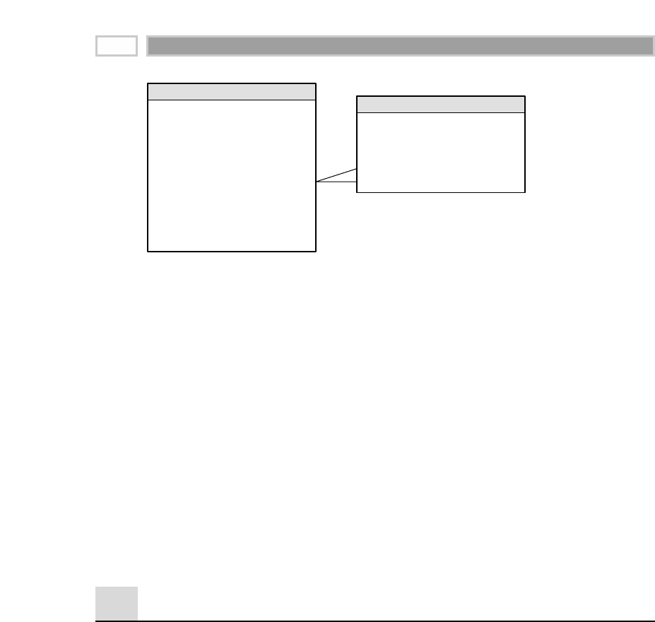
Figure 9.4 Arbitrary value-band reporting using a band definition table.
Controlling the performance of this query can be a challenge. By definition, a
value-band query is very lightly constrained. Our example report needed to
scan the balances of more than 90,000 accounts. Perhaps only the date dimen-
sion was constrained to the current month. Furthermore, the unconventional
join to the banding definition table is not the basis of a nice restricting con-
straint; all it is doing is grouping the 90,000 balances. In this situation you may
need to place an index directly on the balance fact. The performance of a query
that constrains or groups on the value of a fact, such as balance, will be
improved enormously if the database management system (DBMS) can sort
and compress the individual fact efficiently. Such an approach was pioneered
by the Sybase IQ product in the early 1990s and is now becoming a standard
indexing option on several of the competing DBMSs.
Point-in-Time Balances
So far we’ve restricted our discussions in this financial services chapter to
month-end balance snapshots because this level of detail typically is sufficient
for analysis. If required, we could supplement the monthly-grained snapshot
fact table with a second fact table that provides merely the most current snap-
shot as of the last nightly update or perhaps is extended to provide daily-balance
snapshots for the last week or month. However, what if we face the requirement
to report an account’s balance at any arbitrarily picked historical point in time?
Creating daily-balance snapshots for a large bank over a lengthy historical
time span would be overwhelming given the density of the snapshot data. If
the bank has 10 million accounts, daily snapshots translate into approximately
3.65 billion fact rows per year.
Month End Date Key (FK)
Branch Key (FK)
Product Key (FK)
Account Key (FK)
Account Status Key (FK)
Household Key (FK)
Primary Month Ending Balance
Average Daily Balance
Number of Transactions
Interest Paid
Interest Charged
Fees Charged
Month Account Snapshot Fact
Band Group Key (PK)
Band Group Sort Order (PK)
Band Group Name
Band Range Name
Band Lower Value
Band Upper Value
Band Definition Table
>=
<
CHAPTER 9
208

Assuming that business requirements already have driven the need to make
transaction detail data available for analysis, we could leverage this transac-
tion detail to determine an arbitrary point-in-time balance. To simplify mat-
ters, we’ll boil the account transaction fact table down to an extremely simple
design, as illustrated in Figure 9.5. The transaction type key joins to a small
dimension table of permissible transaction types. The transaction sequence
number is a continuously increasing numeric number running for the
lifetime of the account. The final flag indicates whether this is the last
transaction for an account on a given day. The transaction amount is self-
explanatory. The balance fact is the ending account balance following the
transaction event.
Like all transaction-grained fact tables, we add a row to the fact table in
Figure 9.5 only if a transaction occurs. If an account were quiet for two weeks,
perhaps January 1 through 14, there would be no rows in the fact table for the
account during that time span. However, suppose that we want to know what
all the account balances were on January 5? In this case we need to look for the
most recent previous transaction fact row for each account on or before our
requested date. Here’s sample SQL code that does the trick:
SELECT A.ACCTNUM, F.BALANCE
FROM FACT F, ACCOUNT A
WHERE F.ACCOUNT_KEY = A.ACCOUNT_KEY
AND F.DATE_KEY
(SELECT MAX(G.DATE_KEY)
FROM FACT G
WHERE G.ACCOUNT_KEY = F.ACCOUNT_KEY
AND G.DATE_KEY IN
(SELECT D.DATE_KEY
FROM DATE D
WHERE D.FULLDATE <= ‘January 5, 2002’))
In this example we are taking advantage of a special situation that exists with
the surrogate date key. As we discussed in Chapter 2, the date key is a set of
integers running from 1 to N with a meaningful, predictable sequence. We
assign consecutive integers to the date surrogate key so that we can physically
partition a large fact table based on the date. This neatly segments the fact
table so that we can perform discrete administrative actions on certain date
ranges, such as moving archived data to offline storage or dropping and
rebuilding indexes. The date dimension is the only dimension whose surro-
gate keys have any embedded semi-intelligence. Due to its predictable
sequence, it is the only dimension on which we dare place application con-
straints. We used this ordering in the preceding SQL code to locate the most
recent prior end-of-day transaction.
Financial Services 209
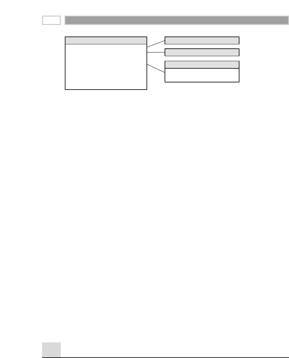
Figure 9.5 Using a transaction fact table for point-in-time balances.
Leveraging the transaction fact table for dual purposes requires that the fact
table is absolutely complete and accurate. Every transaction against the
account must appear in this fact table, or else the running balance will not be
accurate. A late-arriving transaction row would require sweeping forward
from the point of insertion in that account and incrementing all the balances
and transaction sequence numbers. Note that we haven’t explicitly used the
transaction sequence number in this discussion, although it is needed in this
design to reconstruct the true sequence of transactions reliably and to provide
the basis of the fact table’s primary key, which is the date, account, and
sequence number. We prefer using the sequence number rather than a time-of-
day stamp because differences between the sequence numbers are a valid mea-
sure of account activity.
This technique is viable in some part because the transaction processing sys-
tem can readily hand off the current balance metric to the warehouse with each
transaction record. Unlike the year-to-date facts we discussed in Chapter 8, in
this case of account balances we have no way to determine the balances merely
by summarizing recent transactions alone. Rather, we’d need to study the
impact of all transactions from the beginning of the account’s existence to cal-
culate valid account balances. For some businesses within the financial ser-
vices arena, even if balances are provided following each transaction, they still
may not be valid for point-in-time balance reporting. For example, in the case
of a brokerage firm, if a valuation balance is updated following each invest-
ment transaction, we cannot rely on that balance for point-in-time reporting
because the valuation changes constantly. In this case we’d likely create a
snapshot fact table to provide users with regular end-of-period investment
valuation balances.
Heterogeneous Product Schemas
In many financial service businesses, a dilemma arises because of the hetero-
geneous nature of the products or services offered by the institution. As we
Transaction Date Key (FK)
Account Key (FK)
More Foreign Keys …
Transaction Type Key (FK)
Transaction Sequence Number (DD)
Final Flag
Transaction Amount
Transaction Ending Balance
Balance Transaction Fact Table
Transaction Type Key (PK)
Transaction Type Description
Transaction Type Dimension
Transaction Date Dimension
Account Dimension
CHAPTER 9
210

mentioned in the introduction to this chapter, a typical retail bank offers a myr-
iad of dissimilar products, from checking accounts to mortgages, to the same
customers. Although every account at the bank has a primary balance and
interest amount associated with it, each product type has a number of special
attributes and measured facts that are not shared by other products. For
instance, checking accounts have minimum balances, overdraft limits, and ser-
vice charges; time deposits such as certificates of deposit have few attribute
overlaps with checking but instead have maturity dates, compounding fre-
quencies, and current interest rate.
Business users typically require two different perspectives that are difficult to
present in a single fact table. The first perspective is the global view, including
the ability to slice and dice all accounts simultaneously, regardless of their
product type. As we described in Chapter 6, this global view is needed to plan
appropriate customer relationship management (CRM) cross-sell and up-sell
strategies against the aggregate customer base spanning all possible products.
In this situation we need the single core fact table crossing all the lines of busi-
ness to provide insight into the complete account portfolio, as illustrated ear-
lier in Figure 9.2. Note, however, that the core fact table can present only a
limited number of facts that make sense for virtually every line of business. We
are unable to accommodate incompatible facts in the core fact table because, in
the case of banking, there may be several hundred of these facts when all the
possible account types are considered. Similarly, the core product dimension
provides an extremely useful analytical point of entry to the facts but is limited
to the subset of common product attributes.
The second perspective required by users is the specific line-of-business view
that focuses on the in-depth details of one business, such as checking. As we
described, there is a long list of special facts and attributes that only make
sense for the checking business. These special facts cannot be included in the
core fact table; if we did this for each line of business in a retail bank, we would
end up with a hundred special facts, most of which would have null values in
any specific row. Likewise, if we attempted to include specific line-of-business
attributes in the product dimension table, it would have hundreds of special
attributes, almost all of which would be empty for any given row. The result-
ing tables would resemble Swiss cheese, littered with data holes. The solution
to this dilemma is to create a custom schema for the checking line of business
that is limited to just checking accounts, as shown in Figure 9.6.
Now both the custom checking fact table and the corresponding checking
product dimension are widened to describe all the specific facts and attrib-
utes that only make sense for checking products. These custom schemas also
contain the core facts and attributes so that we can avoid joining tables from
the core and custom schemas in order to get the complete set of facts and
Financial Services 211

attributes. Likewise, we would build custom fact and product tables for the
other lines of business to support their in-depth analysis requirements.
Although creating product-specific schemas sounds complex, only the DBA
sees all the tables at once. From the perspective of users, either it’s a cross-
product analysis that relies on the core fact table and its attendant core prod-
uct table or the analysis focuses on a particular product type, in which case
one of the custom line-of-business subschemas is used. In general, it does not
make sense to combine data from one or more custom subschemas because,
by definition, the facts and attributes are disjoint (or nearly so).
The keys of the custom product dimensions are the same keys used in the core
product dimension, which contains all possible product keys. For example, if
the bank offers a $500 minimum balance with no per-check charge checking
product, the product would have the same surrogate key in both the core and
custom checking product dimensions. As we discussed in Chapter 3, estab-
lishing conformed dimensions is essential to an extensible data warehouse
architecture. Each custom product dimension is a subset of rows from the core
product dimension table. Each custom product dimension contains attributes
specific to a particular product type.
This heterogeneous product technique obviously applies to any business that
offers widely varied products through multiple lines of business. If we worked
for a technology company that sells hardware, software, and services, we can
imagine building core sales fact and product dimension tables to deliver the
global customer perspective. The core tables would include all facts and
dimension attributes that are common across lines of business. The core tables
would then be supplemented with schemas that do a deep dive into custom
facts and attributes that vary by business. Again, a specific product would be
assigned the same surrogate product key in both the core and custom product
dimensions.
Figure 9.6 Specific line-of-business custom schema for checking products.
Month End Date Key (FK)
Account Key (FK)
Product Key (FK)
More Core Foreign Keys …
Core Facts …
Number of Checks Cleared
Number of Electronic Transactions
Number of Overdrafts
Number of ATM Usages
Number of Deposits
Monthly Checking Snapshot Fact
Product Key (PK)
Core Product Attributes …
Minimum Checking Balance Requirement
Per Check Fee Indicator
Per Check Fee Amount
Monthly Fee Indicator
Monthly Fee Basis
Monthly Fee Amount
Free Check Printing Indicator
Debit Card Eligible Indicator
Checking-Specific Product Dimension
CHAPTER 9
212

A family of core and custom fact tables is needed when a business has heteroge-
neous products that have naturally different facts and descriptors but a single
customer base that demands an integrated view.
We can consider handling the specific line-of-business attributes as a context-
dependent outrigger to the product dimension, as illustrated in Figure 9.7. We
have isolated the core attributes in the base-product dimension table, and we
can include a snowflake key in each base record that points to its proper
extended-product outrigger. The snowflake key must connect to the particular
outrigger table that a specific product type defines. Usually, you can accom-
plish this task by constructing a relational view for each product type that
hardwires the correct join path.
In the case of account-oriented financial services, when a product is sold to a
customer, a new account is opened. In the case of some banking products, such
as mortgages, more account-specific descriptive information is collected when
the account opening occurs. For example, the bank may offer a 15-year fixed-
rate mortgage at a given rate. When the mortgage originates, the bank will
know more about the specific property, including the address, appraised
value, square footage, home type (for example, single-family, townhouse, con-
dominium, trailer), construction type (for example, wood frame, brick,
stucco), date of construction, and acreage. These attribute values differ by
account, so they don’t belong in the what-the-bank-sells product dimension.
As shown in Figure 9.7, we can envision an account dimension outrigger for
some account types.
If the lines of business in our retail bank are physically separated so that each
has its own data mart, the custom fact and dimension tables likely will not
Figure 9.7 Context-dependent dimension outriggers.
Account Key (PK)
Core Account Attributes …
Account Dimensions Month End Date Key (FK)
Account Key (FK)
Product Key (FK)
More Core Foreign Keys …
Core Facts …
Original Loan Amount
Outstanding Loan Amount
Interest Amount
Property Tax Escrow Amount
Insurance Escrow Amount
Property Mortgage Insurance Amount
Property Tax Escrow Paid
Insurance Escrow Paid
Property Mortgage Insurance Paid
Escrow Overage/Shortage Amount
Late Payment Fee
Additional Principal Paid
Monthly Mortgage Snapshot Fact
Product Key (PK)
Core Product Attributes …
Product Dimension
Mortgage-Specific Account Key (PK)
Property Address …
Appraised Value
Square Footage
Home Type
Construction Type
Year Constructed Completed
Acreage
Mortgage-Specific
Account Outrigger Mortgage-Specific Product Key (PK)
Fixed / Adjustable
Conventional / Jumbo
Rate
Term
FHA Compliant / Eligible
VA Compliant / Eligible
Mortgage-Specific
Product Outrigger
Financial Services 213

Figure 9.8 Heterogeneous products schema using an extended fact table.
reside in the same space as the core fact and dimension tables. In this case the
data in the core fact table would be duplicated exactly once to implement all
the custom tables. Remember that the custom tables provide a disjoint parti-
tioning of the products so that there is no overlap between the custom
schemas.
If the lines of business share the same physical table space, we can avoid dupli-
cating both the core fact keys and core facts in the custom line-of-business fact
tables. We do so by assigning a special join key to each core fact row that
uniquely identifies a single account in a single month. Using this join key, we
physically link the extended custom facts to the core fact table, as shown in
Figure 9.8. When using this technique, we need to ensure that the optimizer
resolves the constraints on the core fact table prior to joining to the extended
fact table using the special join key.
The query tool or application must know to use this special join key to link to
the correct extended fact table for each line of business. While this sounds
complicated, it is actually quite natural. By definition with heterogeneous
facts, it almost never makes sense to join to more than one extended fact table
representing one line of business in a single SQL expression. The names of the
facts in the separate extended fact tables, by definition, are different; no single
SQL expression can talk to multiple extended fact tables. Thus a requesting
application analyzing a specific line of business, such as checking, always
would be hard-coded to link to the correct extended fact table.
Month End Date Key (FK)
Account Key (FK)
Product Key (FK)
More Foreign Keys …
Core Facts …
Checking-Specific Fact Key (FK)
Fact Table Restricted to Checking Accts
Checking-Specific Fact Key (PK)
Number of Checks Cleared
Number of Electronic Transactions
Number of Overdrafts
Number of ATM Usages
Number of Deposits
More Checking-Specific Facts …
Custom Checking Extended Fact Table
CHAPTER 9
214

Heterogeneous Products with
Transaction Facts
The heterogeneous product technique just discussed is appropriate for fact
tables in which a single logical row contains many product-specific facts.
Snapshots usually fit this pattern.
On the other hand, transaction-grained fact tables often have a single fact that
is generically the target of a particular transaction. In such cases the fact table
has an associated transaction dimension that interprets the amount column. In
the case of transaction-grained fact tables, we typically do not need specific
line-of-business fact tables. We get by with only one core fact table because
there is only one fact. However, we still can have a rich set of heterogeneous
products with diverse attributes. In this case we would generate the complete
portfolio of custom product dimension tables and use them as appropriate,
depending on the nature of the application. In a cross-product analysis, we
would use the core product dimension table because it is capable of spanning
any group of products. In a single-product analysis, we optionally could use
the custom-product dimension table instead of the core dimension if we
wanted to take advantage of the custom attributes specific to that product type.
Summary
We began this chapter by discussing the situation in which a fact table has too
few dimensions. We provided suggestions for ferreting out additional dimen-
sions using a triage process. Approaches for handling the often complex rela-
tionship between accounts, customers, and households were described. We
also discussed the use of multiple minidimensions in a single fact table, which
is fairly common in financial services schemas.
We illustrated a technique for clustering numeric facts into arbitrary value
bands for reporting purposes through the use of a separate band table. We also
touched on an approach for leveraging an existing transaction fact table to
supply point-in-time balances.
Finally, we provided recommendations for any organization that offers het-
erogeneous products to the same set of customers. In this case we create a core
fact table that contains performance metrics that are common across all lines of
business. The companion core dimension table contains rows for the complete
product portfolio, but the attributes are limited to those that are applicable
across all products. Multiple custom schemas, one for each line of business,
complement this core schema with product-specific facts and attributes.
Financial Services 215

TEAMFLY
Team-Fly®

Telecommunications and Utilities
CHAPTER
10
217
This chapter will flow a bit differently than preceding chapters. We’ll still begin
with a case study overview, but we won’t be designing a dimensional model
from scratch this time. Instead, we’ll step into a project midstream to conduct
a design review, looking for opportunities to improve the initial draft schema.
Do you recall reading Highlights for Children magazine in your dentist’s waiting
room long ago? If so, do you remember the what’s wrong with this picture work-
sheets where you identified all the out-of-place items, like the chicken driving
a car or a snowman on the beach? The bulk of this chapter will focus on a
dimensional modeling what’s wrong with this picture exercise where we’ll iden-
tify out-of-place design flaws.
We’ll use a billing vignette drawn from the telecommunications industry as
the basis for the case study; however, it shares similar characteristics with the
billing data generated by a utilities company. At the end of this chapter we’ll
elaborate on managing and leveraging the geographic location information in
the warehouse, regardless of the industry.
Chapter 10 discusses the following concepts:
■■ Design review exercise
■■ Common design mistakes to look for in a review
■■ Geographic location dimension, including its treatment as a snowflaked outrigger
and its interaction with geographic information systems

Telecommunications Case Study
Given your extensive experience in dimensional modeling (nine chapters so
far), you’ve been recruited to a new position as a dimensional modeler on the
data warehouse team for a large wireless telecommunications company. On
your first day, after a few hours of human resources paperwork and orienta-
tion (including the location of the nearest coffee machine), you’re ready to get
to work.
The data warehouse team is anxious to pick your brain regarding its initial
dimensional design. So far it seems that the project is off to a good start. The
company has a strong business and IT sponsorship committee that embraced
the concept that a data warehouse must be business-driven; as such, the com-
mittee was fully supportive of the business requirements gathering process.
Based on the requirements initiative, the team drafted an initial data ware-
house bus matrix. It is the first flip chart, as illustrated in Figure 10.1, to hit the
wall during the design walk-through with you. The team identified several
core business processes and a number of common dimensions. Of course, the
complete enterprise-wide matrix would be much larger in terms of both
the number of rows and the number of columns, but you’re comfortable that the
key constituencies’ major data requirements have been captured.
The sponsorship committee jointly decided to focus on the first row of the
matrix, the customer billing process, for the initial phase of the data warehouse.
Business management determined that better access to the metrics resulting
from the billing process would have significant impact on the business, espe-
cially given the business’s recent focus on CRM, as we discussed in Chapter 6.
Management wants the ability to see monthly usage and billing metrics
(otherwise known as revenue) by customer, sales organization, and rate plan to
perform sales rep and channel performance analysis and the rate plan analy-
sis. Fortunately, the IT team felt that it was feasible to tackle this business
process during the first warehouse iteration.
Some people in the IT organization thought it would be preferable to tackle
individual call detail records, such as every call initiated or received by every
phone. While this level of highly granular data would provide interesting
insights, it was determined by the joint business and IT sponsorship commit-
tee that the associated data presents more feasibility challenges while not
delivering as much short-term business value.
CHAPTER 10
218

Figure 10.1 Subset of the data warehouse bus matrix.
Based on the direction provided by the sponsorship committee, the team pro-
ceeded to look more closely at the customer billing data. Each month, the oper-
ational billing system generates a bill for each phone number, also known as
service line. Since the wireless company has millions of service lines, this repre-
sents a significant amount of data. Each service line is associated with a single
customer. However, a customer can have multiple wireless service lines, which
appear as separate line items on the same bill; each service line has its own set
of billing metrics, such as the number of minutes used and monthly service
charge. There is a single rate plan associated with each service line on a given
bill; this plan can change as customers’ usage habits evolve. Finally, a sales rep
(and his or her respective sales organization and channel) is associated with
each service line in order to evaluate the ongoing billing revenue stream gen-
erated by each rep and channel partner.
The team designed a fact table with the grain being one row per bill each
month. The data warehouse team proudly unrolls its draft dimensional mod-
eling masterpiece, as shown in Figure 10.2, and looks at you expectantly.
What do you think? Before we move on, please spend several minutes studying
the design in Figure 10.2. Try to identify the design flaws and suggest improve-
ments in this “what’s wrong with this picture” exercise before reading ahead.
Customer Billing
Call Detail Traffic
Purchasing
Distributor Inventory
Channel Sales
Service Calls
Repair Items
Date
Customer
Product
Rate Plan
Sales Channel
Service Line #
Switch
Vendor
GL Account
Organization
Employee
Service Call Type
Service Call Status
Telecommunications and Utilities 219
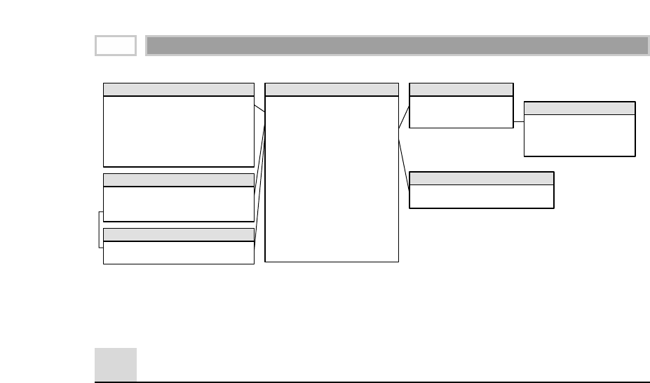
Figure 10.2 Draft schema prior to design review.
General Design Review Considerations
Before we discuss the specific issues and potential recommendations for Fig-
ure 10.2, we’ll take a moment to outline the design issues we commonly
encounter when conducting a design review. Not to insinuate that the data
warehouse team in our case study has stepped into all these traps, but it may
be guilty of violating several. Again, the design review exercise will be a more
effective learning tool if you take a moment to jot down your personal ideas
regarding Figure 10.2 before proceeding.
Granularity
One of the first questions we always ask during a design review is, What’s the
grain of the fact table? Surprisingly, we often get inconsistent answers to this
inquiry from the project team. Declaring a clear and concise definition of the
grain of the fact table is critical to a productive modeling effort. Likewise, the
project team and business liaisons should share a common understanding of
this grain declaration.
Of course, if you’ve read this far, you’re aware that we strongly believe that
you should build your fact table at the lowest level of granularity possible.
However, the definition of the lowest level of granularity possible depends on
the business process you are modeling.
In this case study we don’t need call-level detail with the granularity of one row
for every call to address the business requirements. Instead, a billing fact table
is more appropriate. We want to implement the most granular data available
Customer ID (PK and Natural Key)
Customer Name
Customer City
Customer State
Customer Zip
Date of 1st Service
Original Authorization Credit Score
Customer Dimension
Sales Rep Number (PK and Natural Key)
Sales Rep Name
Sales Org ID
Sales Rep Dimension
Sales Org ID
Sales Channel ID
Sales Org Dimension
Bill # (FK)
Customer ID (FK)
Sales Rep Number (FK)
Sales Org ID (FK)
Rate Plan Code (FK)
Rate Plan Type Code
Number of Calls
Number of Total Minutes
Number of Roam Minutes
Number of Long-Distance Minutes
Monthly Service Charge
Prior Month Service Charge
Year-to-Date Service Charges
Roaming Charge
Long-Distance Charge
Taxes
Regulatory Charges
Billing Fact
Bill # (PK)
Bill Date
Service Line Number (FK)
Bill Dimension
Rate Plan Code (PK and Natural Key)
Rate Plan Abbreviation
Rate Plan Dimension
Service Line Number (PK)
Area Code
Area Code and Prefix
Service Line Activation Date
Service Line Dimension
CHAPTER 10
220

for the selected billing process, not just the most granular data available in the
enterprise. Of course, if the high-priority business requirements focused on
switching network traffic and capacity analysis, then low-level call detail data
would be appropriate.
Going to the lowest level of granularity does not imply finding the greatest amount
of detailed data available in the organization.
Fact Granularity
Once the fact table granularity has been established, facts should be identified
that are consistent with the grain declaration. In an effort to improve perfor-
mance or reduce query complexity, aggregated facts such as year-to-date totals
sometimes sneak into the fact row. These totals are dangerous because they are
not perfectly additive. While a year-to-date total reduces the complexity and
run time of a few specific queries, having it in the fact table invites a query to
double count the year-to-date column (or worse) when more than one bill date
is included in a query. It is very important that once the grain of a fact table is
chosen, all the additive facts are presented at a uniform grain.
Dimension Granularity
Each of the dimensions associated with a fact table should take on a single
value with each row of fact table measurements. Likewise, each of the dimen-
sion attributes should take on one value for a given dimension row. If the
attributes have a one-to-many relationship, then this hierarchical relationship
can be represented within a single dimension. We generally should look for
opportunities to collapse dimension hierarchies whenever possible.
In general, we discourage the snowflaking or normalization of dimension
tables. While snowflaking may reduce the disk space consumed by dimension
tables, the savings are usually insignificant when compared with the entire
data warehouse and seldom offset the disadvantages in ease of use or query
performance.
Throughout this book we have occasionally discussed outriggers as permissi-
ble snowflakes. Outriggers can play a useful role in your dimensional designs,
but keep in mind that the use of outriggers for a cluster of relatively low-
cardinality or frequently reused attributes should be the exception rather than
the rule. Be careful to avoid abusing the outrigger technique by overusing
them in your schemas.
Telecommunications and Utilities 221

Date Dimension
Design teams sometimes join a generic date dimension to their fact table
because they know it’s the most common dimension but then can’t articulate
what the date refers to. Needless to say, this presents real challenges for the
data staging team. While we discourage superfluous date dimensions, we
encourage the inclusion of robust date roll-up and filter attributes in a mean-
ingful date dimension table.
Fixed Time-Series Buckets Instead of
Date Dimension
Other designers sometimes avoid a date dimension table altogether by repre-
senting a time series of monthly buckets of facts on a single fact table row.
Older operational systems may contain metric sets that are repeated 12 times
on a single record to represent month 1, month 2, and so on. There are several
problems with this approach. First, the hard-coded identity of the time slots is
inflexible. When you fill up all the buckets, you are left with unpleasant
choices. You could alter the table to expand the row. Otherwise, you could shift
everything over by one column, dropping the oldest data, but this wreaks
havoc with your existing query applications. The second problem with this
approach is that all the attributes of the date itself are now the responsibility of
the application, not the database. There is no date dimension in which to place
calendar event descriptions for constraining. Finally, the fixed-slot approach is
inefficient if measurements are only taken in a particular time period, resulting
in null columns in many rows. Instead, these recurring time buckets should be
presented as separate rows in the dimensional fact table.
Degenerate Dimensions
Rather than treating operational transaction numbers, such as the invoice or
order number, as degenerate dimensions, teams sometimes want to create a
separate dimension for the transaction number. Attributes of the transaction
number dimension then include elements from the transaction header record,
such as the invoice date, invoice type, and invoice terms.
Remember, transaction numbers are best treated as degenerate dimensions. In
your design reviews, be on the lookout for a dimension table that has as many
(or nearly as many) rows as the fact table. This should be a warning sign that
there may be a degenerate dimension lurking within a dimension table.
Dimension Decodes and Descriptions
All identifiers and codes in the dimension tables should be accompanied by
descriptive decodes. We simply need to dismiss the misperception that business
CHAPTER 10
222

users prefer to work with codes. To convince yourself, you should stroll down
to their offices to see the decode listings filling their bulletin boards or lining
their computer monitors. Most users do not memorize the codes outside of a
few favorites. New hires are rendered helpless when assaulted with a lengthy
list of meaningless codes.
The good news is that we usually can source decodes from operational systems
with minimal additional effort or overhead. Occasionally, the descriptions are
not available from an operational system but need to be provided by business
partners. In these cases, it is important to determine an ongoing maintenance
strategy to maintain data quality.
Finally, we sometimes work with project teams that opt to embed complex fil-
tering or labeling logic in the data access application rather than supporting it
via a dimension table. While access tools may provide the ability to decode
within the query or reporting application, we recommend that decodes be
stored as data elements instead. Applications should be data-driven in order
to minimize the impact of decode additions and changes. Of course, decodes
that reside in the database also ensure greater report labeling consistency.
Surrogate Keys
Instead of relying on operational keys or identifiers, we recommend the use of
surrogate keys throughout your dimensional design. If you are unclear about
the reasons for pursuing this strategy, we suggest you backtrack to Chapter 2
to refresh your memory.
Too Many (or Too Few) Dimensions
As we have mentioned, a dimensional model typically has 5 to 15 dimensions.
If your design has only two or three dimensions, then you should revisit Chap-
ter 9 for a discussion on dimension triage considerations. If your design has 25
or 30 dimensions, we suggest you review the centipede design in Chapter 2 or
the junk dimension in Chapter 5 for ideas to reduce the number of dimensions
in your schema.
Draft Design Exercise Discussion
Now that we’ve reviewed several common dimensional modeling pitfalls that
we encounter frequently during design reviews, let’s look back to the draft
design in Figure 10.2. Several items immediately jump out at us—perhaps so
many that it’s hard to know where to start.
Telecommunications and Utilities 223

The first thing we focus on is the grain of the fact table. The design team stated
that the grain is one row for each bill each month. However, based on our
understanding from the data discovery effort, the lowest level of billing data
would be one row per service line on a bill. When we point this out to the proj-
ect team, the team directs us to the bill number dimension, which includes the
service line number. When reminded that each service line has its own set of
billing metrics, the team agrees that the more appropriate grain declaration
would be one row per service line per bill. We move the service line key into
the fact table as a foreign key to the service line dimension.
While discussing the granularity, the bill number dimension is scrutinized,
especially since we just moved the service line key into the fact table. As the
draft model was originally drawn in Figure 10.2, every time a bill row is loaded
into the fact table, a row also would be loaded into the bill number dimension
table. It doesn’t take much to convince the team that something is wrong with
this picture. Even with the modified granularity to include service line, we
would still end up with nearly as many rows in both the fact and bill number
dimension tables. Instead, we opt to treat the bill number as a degenerate
dimension. At the same time, we move the bill date into the fact table and join
it to a robust date dimension, which plays the role of a bill date in this schema.
We’ve been bothered since first looking at the design by the double joins on the
sales rep organization dimension table. First of all, the sales rep organizational
hierarchy has been snowflaked unnecessarily. We opt to collapse the hierarchy
by including the sales rep organization and channel identifiers (along with
more meaningful descriptors, hopefully) as additional attributes in the sales
rep dimension table. In addition, we can eliminate the unneeded sales rep
organization foreign key in the fact table.
The design inappropriately treats the rate-plan type code as a textual fact. Tex-
tual facts are seldom a sound design choice. They almost always take up more
space in our fact tables than a surrogate key. More important, users generally
want to query, constrain, and report against these textual facts. We can provide
quicker response and more flexible access by handling these textual values in
a dimension table. In addition, additional descriptive attributes usually are
associated with the textual fact. In this case study, the rate plan type code and
its decode can be treated as roll-up attributes in the rate plan dimension table.
The team spent some time discussing the relationship between the service line
and the customer, sales rep, and rate plan dimensions. Since there is a single
customer, sales rep, and rate plan associated with a service line number, the
dimensions theoretically could be collapsed and modeled as service line attrib-
utes. However, collapsing the dimensions would result in a schema with just
two dimensions (bill date and service line). Besides, the service line dimension
already has millions of rows in it and is growing rapidly. In the end, we opt to
CHAPTER 10
224

treat the customer, sales rep, and rate plan as minidimensions of the service
line, as we described in Chapter 6.
We notice that surrogate keys are used inconsistently throughout the design.
Many of the draft dimension tables use operational identifiers or system keys
as primary keys. We encourage the team to implement surrogate keys for all
the dimension primary keys and fact table foreign keys.
The original design was riddled with operational codes and identifiers. In gen-
eral, adding descriptive names will make the data more legible to the business
users. If required by the business, the operational codes can continue to
accompany the descriptors as dimension attributes, but they should not be the
dimension primary keys.
Finally, we see that there is a year-to-date fact stored in the fact table. While the
team felt that this would enable users to report year-to-date figures more eas-
ily, in reality, year-to-date facts can be confusing and prone to error. We opt to
remove the year-to-date fact. Instead, users can calculate year-to-date amounts
on the fly by using a constraint on year in the date dimension or by leveraging
the data access tool’s capabilities.
After a taxing day, our initial review of the design is complete. Of course,
there’s more ground to cover, including the handling of changes to the dimen-
sion attributes. In the meantime, everyone on the team agrees that the
revamped design, illustrated in Figure 10.3, is a vast improvement. We feel
that we’ve earned our first week’s pay at our new employer.
Figure 10.3 Schema following the design review.
Customer Key (PK)
Customer ID (Natural Key)
Customer Name
Customer City
Customer State
Customer Zip
Date of 1st Service
Original Authorization Credit Score
… more attributes
Customer Dimension
Sales Rep Key (PK)
Sales Rep Number (Natural Key)
Sales Rep Name
Sales Organization ID
Sales Organization Name
Sales Channel ID
Sales Channel Name
Sales Rep Dimension
Bill Date Key (FK)
Customer Key (FK)
Service Line Key (FK)
Sales Rep Key (FK)
Rate Plan Key (FK)
Bill Number (DD)
Number of Calls
Number of Total Minutes
Number of Roam Minutes
Number of Long-Distance Minutes
Monthly Service Charge
Roaming Charge
Long-Distance Charge
Taxes
Regulatory Charge
Billing Fact
Bill Date Key (PK)
Bill Date
Bill Date Year
… more attributes
Bill Date Dimension
Service Line Key (PK)
Service Line Number (Natural Key)
Service Line Area Code
Service Line Area Code and Prefix
Service Line Prefix
Service Line Activation Date
Service Line Dimension
Rate Plan Key (PK)
Rate Plan Code (Natural Key)
Rate Plan Abbreviation
Rate Plan Description
Rate Plan Type Code
Rate Plan Type Description
Rate Plan Dimension
Telecommunications and Utilities 225

Geographic Location Dimension
Let’s shift gears and presume that we’re now working for a phone company
with land lines tied to a specific physical location. In general, the telecommu-
nications industry has a very well-developed notion of location. The same
could be said for the utilities industry. Many of its dimensions contain a precise
geographic location as part of the attribute set. The location may be resolved to
a physical street, city, state, and ZIP code or even to a specific latitude and lon-
gitude. Using our dimension role-playing technique, we imagine building a
single master location table where data is standardized once and then reused.
The location table could be part of the service line telephone number, equip-
ment inventory, network inventory (including poles and switch boxes), real
estate inventory, service location, dispatch location, right of way, and even cus-
tomer entities. Each row in the master location table is a specific point in space
that rolls up to every conceivable geographic grouping, such as census tracts
and counties. A location could roll up to multiple unique geographic group-
ings simultaneously.
Location Outrigger
Location more naturally is thought of as a component of a dimension, not as
a standalone dimension. The use of an embedded role, such as location, in a
variety of unrelated larger dimensions is one of the few places where we
support snowflaked outriggers. We recommend creating a join from each of
the primary dimension tables that need to describe location to a clone of the
location subdimension table. The issues in creating location clones are
exactly the same as the ones we described in Chapter 5 for creating date role-
playing dimensions. We need separate views for each use of the location
table, being careful to create distinguishable column names. A possible
advantage of this approach is that if we later embellish the geographic
dimensions with census or demographic information, we do so in one place,
without touching all the primary dimensions that include a location descrip-
tion. On the other hand, we haven’t gained much with this approach if there
is little overlap between the geographic locations embedded in various
dimensions. In this situation we would pay a performance price for consoli-
dating all the disparate addresses into a single dimension. Likewise, we
should check with our database management system to determine its treat-
ment (and associated penalty, if applicable) of the view construct. Ultimately,
we need to remain focused on our two driving design principles: ease of use
and performance.
CHAPTER 10
226
TEAMFLY
Team-Fly®

Leveraging Geographic
Information Systems
While we’re on the topic of location dimensions, very few conventional data
warehouses currently make the most of their data with a map-driven approach
to visualization and presentation. The data warehouse can take advantage of
interesting geographic information system (GIS) tools to deliver the informa-
tion and insights contained in spatially oriented address or route data. This
actually may encourage design enhancements and extensions to include attrib-
utes that enable richer analysis of our warehouse data via a GIS capability.
Using GIS tools, we can effectively exploit the millions of addresses we already
store. We can invoke new graphic presentation tools that allow us to see two-
dimensional patterns on a map that simply can’t be detected in spreadsheets
and conventional reports. In addition, we can attach some new verbs to our
existing databases that let us ask spatially enabled questions, such as “Find all
the service lines or switches that are within or near a group of counties,” with-
out modifying the underlying data.
The process for integrating the warehouse data with a GIS capability will vary
depending on which GIS tool is used. Essentially, in order for the GIS to inter-
pret ordinary street addresses, it first standardizes the raw address informa-
tion from the location dimension into a parsed form. The GIS tool’s geocoder
then attempts to match the parsed addresses with a standard street network
database of geographic points. If all goes well, you get back a set of location
objects that can be plotted visually. In other cases you may choose to physically
alter and populate the underlying location dimension with geospecific attrib-
utes such as points, lines, and polygons. You also may want to consider the
spatial capabilities that are implemented within some DBMSs.
If you are a GIS professional sitting on top of mounds of geospatial data, this
approach is probably not for you; you likely need to use a mainline GIS solu-
tion instead. However, if you are a text-and-numbers data warehouse manager
already storing millions of addresses and other attributes of physical locations,
then consider this technique to pick the low-hanging fruit that our GIS col-
leagues have generously provided without modifying your existing data
warehouse applications or data architecture.
Summary
This chapter provided the opportunity to conduct a design review using an
example case study. We provided a laundry list of common design flaws to
Telecommunications and Utilities 227

scout for when performing a review. We encourage you to use this laundry list
to review your own draft schemas in search of potential improvements.
We also discussed the geographic location as a permissible outrigger if it is
used repeatedly in dimensional designs. Finally, we suggested opportunities
to further leverage this geographic information through the use of a GIS tool.
CHAPTER 10
228

Transportation
CHAPTER
11
229
Voyages occur whenever a person or thing travels from one point to another,
perhaps with stops in the middle. Obviously, this applies directly to organiza-
tions involved in the travel industry. Shippers, as well as internal logistical
functions, also will relate to the discussion, as will package delivery services
and car rental agencies. Somewhat unexpectedly, many of the characteristics
in this chapter’s schema are also applicable to telecommunications network
route analysis. A phone network can be thought of as a map of possible voy-
ages that a call makes between origin and destination phone numbers.
In this chapter we’ll draw on an airline frequent flyer case study to explore
voyages and routes because many readers are familiar (perhaps too familiar)
with the subject matter. The case study lends itself to a discussion of multiple
fact tables at different granularities. We’ll also expand on several concepts,
such as dimension role-playing and additional date and time dimension con-
siderations. As usual, the intended audience for this chapter should not be lim-
ited to the industries just listed.
Chapter 11 discusses the following concepts:
■■ Fact tables at different levels of granularity
■■ Combining role-playing dimensions into a superdimension in certain situations
■■ Country-specific date dimensions
■■ Time of day as a fact versus dimension
■■ Dates and times in multiple time zones

Airline Frequent Flyer Case Study
In this case the airline’s marketing department wants to analyze the flight
activity of each member of its frequent flyer program. The department is inter-
ested in seeing what flights the company’s frequent flyers take, which planes
they fly, what fare basis they pay, how often they upgrade, how they earn and
redeem their frequent flyer miles, whether they respond to special fare pro-
motions, how long their overnight stays are, and what proportion of these
frequent flyers have titanium, platinum, gold, or aluminum status.
As usual, we work through the four-step process to tackle the design of this
frequent flyer schema. For this case study, the business process would be
actual flight activity. We are not focusing on reservation or ticketing activity
data that didn’t result in a frequent flyer boarding a plane. The data warehouse
team will contend with those other sources of data in subsequent phases.
Multiple Fact Table Granularities
When it comes to the grain, we encounter a situation in this case where we are
presented with multiple potential levels of fact table granularity. Each of these
levels of granularity has different metrics associated with them.
At the most granular level, the airline captures data at the leg level. The leg
represents an aircraft taking off at one airport and landing at another without
any intermediate stops. Capacity planning and flight scheduling analysts are
very interested in this discrete level of information because they’re able to look
at the number of seats to calculate load factors by leg. We also can include facts
regarding the leg’s flight duration as well as the number of minutes late at
departure and arrival. Perhaps there’s even a dimension to easily identify
on-time arrivals.
The next level of granularity corresponds to a segment. In this case we’re
looking at the portion of a trip on a single aircraft. Segments may have one or
more legs associated with them. If you take a flight from San Francisco to
Minneapolis with a stop in Denver but no aircraft change, you have flown one
segment (SFO-MSP) but two legs (SFO-DEN and DEN-MSP). Conversely, if
the flight flew nonstop from San Francisco to Minneapolis, you would have
flown one segment as well as one leg. The segment represents the line item on
an airline ticket coupon; revenue and mileage credit is generated at the seg-
ment level.
Next, we can analyze flight activity by trip. The trip provides an accurate pic-
ture of customer demand. In our prior example, assume that the flights from
San Francisco to Minneapolis required the flyer to change aircraft in Denver. In
CHAPTER 11
230

this case the trip from San Francisco to Minneapolis would entail two seg-
ments corresponding to the two aircraft involved. In reality, the passenger just
asked to go from San Francisco to Minneapolis; the fact that he or she needed
to stop in Denver was merely a necessary evil but certainly wasn’t requested.
For this reason, sales and marketing analysts are interested in trip-level data.
Finally, the airline collects data for the itinerary, which is equivalent to the
entire airline ticket or reservation confirmation number.
The data warehouse team and business representatives decide to begin at the
segment-level grain to satisfy the need for improved frequent flyer analysis.
This represents the lowest level of data with meaningful metrics for the mar-
keting department. The data warehouse team inevitably will tackle the more
granular leg-level data for the capacity planners and flight schedulers at some
future point. The conforming dimensions built during this first iteration cer-
tainly will be leveraged at that time.
There will be one row in the fact table for each boarding pass collected from
frequent flyers. The dimensionality associated with this data is quite extensive,
as illustrated in Figure 11.1. If we had instead chosen the grain to be the trip as a
multiple-segment event, all the specific details regarding the aircraft, fare basis,
class, and other circumstances of each flight would have been suppressed.
We see that the schema uses the role-playing technique extensively. The multi-
ple date, time, and airport dimensions link to views of a single underlying
physical date, time, and airport dimension table, respectively, as we discussed
originally in Chapter 5.
Figure 11.1 Initial segment-level flight activity schema.
Scheduled Departure Date Key (FK)
Scheduled Departure Time Key (FK)
Actual Departure Date Key (FK)
Actual Departure Time Key (FK)
Frequent Flyer Key (FK)
Frequent Flyer Profile Key (FK)
Segment Origin Airport Key (FK)
Segment Destination Airport Key (FK)
Flight Key (FK)
Aircraft Key (FK)
Class Key (FK)
Fare Basis Key (FK)
Sales Channel Key (FK)
Itinerary Number (DD)
Ticket Number (DD)
Segment Sequence Number (DD)
Gross Segment Revenue
Segment Miles Flown
Segment Miles Earned
Segment Flight Duration
Number of Minutes Late at Departure
Number of Minutes Late at Arrival
Net Number of Minutes Late
Segment-Level Flight Activity Fact
Time-of-Day Dimension
(view for 2 roles)
Date Dimension (views for 2 roles)
Airport Dimension
(views for 2 roles)
Frequent Flyer Dimension
Aircraft Dimension
Flight Dimension
Fare Basis Dimension
Class Dimension
Sales Channel Dimension
Frequent Flyer Profile Dimension
Transportation 231

The frequent flyer dimension is a garden-variety customer dimension with all
the attributes captured about our most valuable flyers. Interestingly, in this
case the frequent flyers are motivated to help you maintain this dimension
accurately because they want to ensure that they’re receiving appropriate
mileage credit. For a large airline, this dimension would have tens of millions
of rows in it. Marketing wants to analyze activity by frequent flyer tier, which
can change during the course of a year. In addition, we learned during the
requirements process that the users are interested in slicing and dicing based
on the flyers’ home airports and whether they belong to the airline’s airport
club. Therefore, we opt to create a separate frequent flyer profile minidimen-
sion, as we discussed in Chapter 6, with one row for each unique combination
of frequent flyer elite tier, home airport, and club membership status.
The flight dimension contains information about each flight, such as the air-
craft used. Although there is a specific origin and destination associated with
each flight, we call these key airport dimensions out separately to simplify the
user’s view of the data and make access more efficient.
The class of service flown describes whether the passenger sat in coach, busi-
ness, or first class. The fare basis dimension describes the terms surrounding
the fare. It would identify whether it’s a full fare, an unrestricted fare, a 21-day
advanced-purchase fare with change and cancellation penalties, or a 10 per-
cent off fare due to a special promotion available for tickets purchased at the
company’s Web site during a given time period. In this case study we decide
not to separate the notion of promotion from fare basis. After interviewing
business users at the airline, we conclude that fare basis and promotion are
inextricably linked and that it does not make sense to separate them in the
data.
The sales channel dimension identifies how the ticket was purchased, whether
through a travel agency, directly from the airline’s toll-free phone number or
city ticket office, from the airline’s Web site, or via another Internet travel ser-
vices provider. In addition, several operational numbers are associated with
the flight activity data, including the itinerary number, the ticket number, and
the segment sequence number.
The facts captured at the segment level of granularity include the gross seg-
ment revenue, segment miles flown, and segment miles awarded (in those
cases where a minimum number of miles are awarded regardless of the flight
distance). To monitor customer service levels, we also might include such facts
as the minutes late at departure and arrival, which would be summarized in
the case of a multileg segment.
CHAPTER 11
232
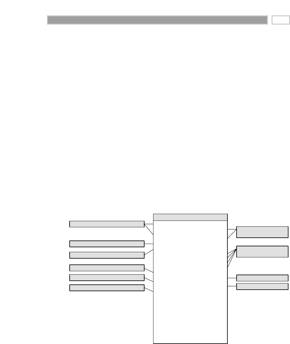
Linking Segments into Trips
Despite the powerful dimensional framework we just designed, we are unable
to easily answer one of the most important questions about our frequent fly-
ers, namely, where are they going? The segment grain masks the true nature of
the trip. If we fetch all the segments of the airline voyage and sequence them
by segment number, it is still nearly impossible to discern the trip start and end
points. Most complete itineraries start and end at the same airport. If a lengthy
stop were used as a criterion for a meaningful trip destination, it would
require extensive and tricky processing whenever we tried to summarize a
number of voyages by the meaningful stops.
The answer is to introduce two more airport role-playing dimensions: trip ori-
gin and trip destination, while keeping the grain at the flight segment level.
These are determined during data extraction by looking on the ticket for any
stop of more than four hours, which is the airline’s official definition of a
stopover. The enhanced schema looks like Figure 11.2. We would need to exer-
cise some caution when summarizing data by trip in this schema. Some of the
dimensions, such as fare basis or class of service flown, don’t apply at the trip
level. On the other hand, it may be useful to see how many trips from San
Francisco to Minneapolis included an unrestricted fare on a segment.
Figure 11.2 Trip-level flight activity schema.
Scheduled Departure Date Key (FK)
Scheduled Departure Time Key (FK)
Actual Departure Date Key (FK)
Actual Departure Time Key (FK)
Frequent Flyer Key (FK)
Frequent Flyer Profile Key (FK)
Segment Origin Airport Key (FK)
Segment Destination Airport Key (FK)
Trip Origin Airport Key (FK)
Trip Destination Airport Key (FK)
Flight Key (FK)
Aircraft Key (FK)
Class Key (FK)
Fare Basis Key (FK)
Sales Channel Key (FK)
Itinerary Number (DD)
Ticket Number (DD)
Segment Sequence Number (DD)
Gross Segment Revenue
Segment Miles Flown
Segment Miles Earned
Segment Flight Duration
Number of Minutes Late at Departure
Number of Minutes Late at Arrival
Net Number of Minutes Late
Segment-Level Flight Activity Fact
Time-of-Day Dimension
(view for 2 roles)
Date Dimension (views for 2 roles)
Airport Dimension
(views for 4 roles)
Frequent Flyer Dimension
Aircraft Dimension
Flight Dimension
Fare Basis Dimension
Class Dimension
Sales Channel Dimension
Frequent Flyer Profile Dimension
Transportation 233

In addition to linking segments into trips as Figure 11.2 illustrates, if the business
users are constantly looking at information at the trip level, rather than by seg-
ment, we might be tempted to create an aggregate fact table at the trip grain.
Some of the earlier dimensions discussed, such as class of service, fare basis, and
flight, obviously would not be applicable. The facts would include such metrics
as trip gross revenue and additional facts that would appear only in this com-
plementary trip summary table, such as the number of segments in the trip.
However, we would only go to the trouble of creating such an aggregate table if
there were obvious performance or usability issues when we used the segment-
level table as the basis for rolling up the same reports. If a typical trip consisted
of three segments, then we might barely see a three times performance improve-
ment with such an aggregate table, meaning that it may not be worth the bother.
Extensions to Other Industries
Using the frequent flyer case study to illustrate a voyage schema makes intu-
itive sense because most of us have boarded a plane at one time or another.
We’ll briefly touch on several other variations on this theme.
Cargo Shipper
The schema for a cargo shipper looks quite similar to the frequent flyer schemas
just developed. Suppose that a transoceanic shipping company transports bulk
goods in containers from foreign to domestic ports. The items in the containers
are shipped from an original shipper to a final consignor. The trip can have mul-
tiple stops at intermediate ports. It is possible that the containers may be off-
loaded from one ship to another at a port. Likewise, it is possible that one or
more of the legs may be by truck rather than ship.
As illustrated in Figure 11.3, the grain of the fact table is the container on a spe-
cific bill-of-lading number on a particular leg of its trip.
The ship mode dimension identifies the type of shipping company and specific
vessel. The item dimension contains a description of the items in a container.
The container dimension describes the size of the container and whether it
requires electrical power or refrigeration. The commodity dimension describes
one type of item in the container. Almost anything that can be shipped can be
described by harmonized commodity codes, which are a kind of master con-
formed dimension used by agencies, including U.S. Customs. The consignor,
CHAPTER 11
234
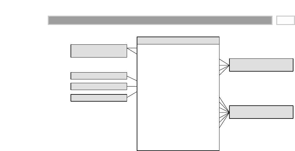
Figure 11.3 Shipper schema.
foreign transporter, foreign consolidator, shipper, domestic consolidator,
domestic transporter, and consignee are all roles played by a master business
entity dimension that contains all the possible business parties associated with
a voyage. The bill-of-lading number is a degenerate dimension. We assume that
the fees and tariffs are applicable to the individual leg of the voyage.
Shipping transport schemas like this one characteristically have a large num-
ber of dimensions. When all the parties to the voyage have been added, the
design can swell to 15 or even 20 dimensions.
Travel Services
If we work for a travel services company, we can envision complementing the
customer flight activity schema with fact tables to track associated hotel stays
and rental car usage. These schemas would share several common dimen-
sions, such as the date, customer, and itinerary number, along with ticket and
segment number, as applicable, to allow hotel stays and car rentals to be inter-
leaved correctly into a airline trip. For hotel stays, the grain of the fact table is
the entire stay, as illustrated in Figure 11.4. The grain of a similar car rental fact
table would be the entire rental episode. Of course, if we were constructing a
fact table for a hotel chain rather than a travel services company, the schema
would be much more robust because we’d know far more about the hotel prop-
erty characteristics, the guest’s use of services, and associated detailed charges.
Voyage Departure Date Key (FK)
Leg Departure Date Key (FK)
Voyage Origin Port Key (FK)
Voyage Destination Port Key (FK)
Leg Origin Port Key (FK)
Leg Destination Port Key (FK)
Ship Mode Key (FK)
Container Key (FK)
Commodity Key (FK)
Consigner Key (FK)
Foreign Transporter Key (FK)
Foreign Consolidator Key (FK)
Shipper Key (FK)
Domestic Consolidator Key (FK)
Domestic Transporter Key (FK)
Consignee Key (FK)
Leg Fee
Leg Tariffs
Leg Miles
Shipping Transport Fact
Port Dimension
(view for 4 roles)
Date Dimension
(views for 2 roles)
Business Entity Dimension
(views for 7 roles)
Ship Mode Dimension
Container Dimension
Commodity Dimension
Transportation 235
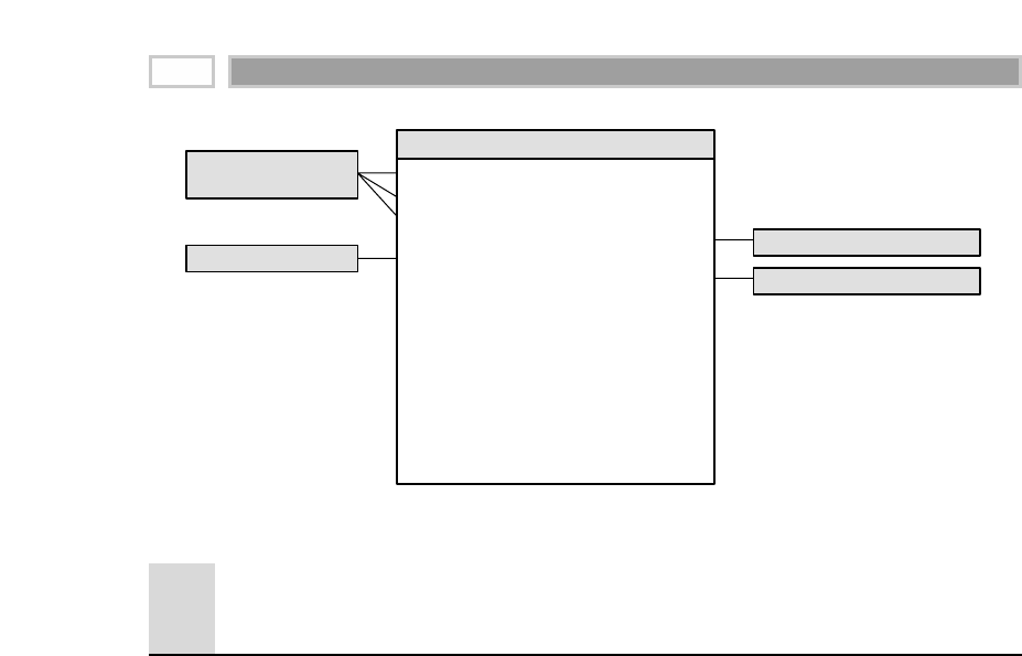
Figure 11.4 Travel services hotel stay schema.
Combining Small Dimensions
into a Superdimension
We stated previously that if a many-to-many relationship exists between two
groups of dimension attributes, then they should be modeled as separate
dimensions with separate foreign keys in the fact table. Sometimes, however,
we’ll encounter a situation where these dimensions can be combined into a
single superdimension rather than treating them as two separate dimensions
with two separate foreign keys in the fact table.
Class of Service
The Figure 11.1 draft schema included the class of service flown dimension. Fol-
lowing our first design checkpoint with the business community, we learn that
the business users want to analyze the class of service purchased, as well as the
class flown. Unfortunately, we’re unable to reliably determine the class of ser-
vice actually used from the original fare basis because the customer may do a
last-minute upgrade. In addition, the business users want to easily filter and
report on activity based on whether an upgrade or downgrade occurred. Our
initial reaction is to include a second role-playing dimension and foreign key in
the fact table to support access to both the purchased and flown class of service,
along with a third foreign key for the upgrade indicator. In this situation, how-
ever, there are only three rows in each class dimension table to indicate first,
business, and coach classes. Likewise, the upgrade indicator dimension also
would have just three rows in it, corresponding to upgrade, downgrade, or no
class change. Since the row counts are so small, we elect instead to combine the
dimensions into a single class of service dimension, as illustrated in Figure 11.5.
Date of Arrival Key (FK)
Date of Departure Key (FK)
Date of Reservation Key (FK)
Customer Key (FK)
Hotel Key (FK)
Sales Channel Key (FK)
Itinerary Number (DD)
Ticket Number (DD)
Segment Number (DD)
Number of Nights
Room Dollar Charge
Meal Dollar Charge
Phone Dollar Charge
Miscellaneous Charge
Tax Charge
Travel Services Hotel Stay Fact
Customer Dimension
Date Dimension
(views for 3 roles)
Sales Channel Dimension
Hotel Dimension
CHAPTER 11
236
TEAMFLY
Team-Fly®

Figure 11.5 Sample rows from the combined class dimension.
The Cartesian product of the separate class dimensions only results in a nine-
row dimension table (three class purchased rows, three class flown rows). We
also have the opportunity in this superdimension to describe the relationship
between the purchased and flown classes, such as the class group and class
change indicator. In some ways, we can think of this combined class of service
superdimension as a type of junk dimension, which we introduced in Chapter 5.
Origin and Destination
Likewise, we can consider the pros and cons of combining the origin and des-
tination airport dimensions. In this situation the data volumes are more signif-
icant, so separate role-playing origin and destination dimensions seem more
practical. However, the users may need additional attributes that depend on
the combination of origin and destination. In addition to accessing the charac-
teristics of each airport, business users also want to analyze flight activity data
by the distance between the city-pair airports, as well as the type of city pair
(such as domestic or trans-Atlantic). Even the seemingly simple question
regarding the total activity between San Francisco (SFO) and Denver (DEN),
regardless of whether the flights originated in SFO or DEN, would be chal-
lenging with separate origin and destination dimensions. Sure, SQL experts
may be able to answer the question programmatically, but what about the less
empowered? In addition, even if we’re able to derive the correct answer, we
lack a standard label for that city-pair route. Some applications may label it
SFO-DEN, whereas others might opt for DEN-SFO, San Fran-Denver, Den-SF,
and so on. Rather than embedding inconsistent labels in application code, we
should put them in a dimension table so that common, standardized labels can
be used throughout the organization. It would be a shame to go to the bother
of creating a data warehouse and then allow application code to implement
inconsistent reporting labels. The business sponsors of the data warehouse
won’t tolerate that for long.
1
2
3
4
5
6
7
8
9
Coach
Coach
Coach
Business
Business
Business
First
First
First
Coach
Business
First
Coach
Business
First
Coach
Business
First
Coach-Coach
Coach-Business
Coach-First
Business-Coach
Business-Business
Business-First
First-Coach
First-Business
First-First
No Class Change
Upgrade
Upgrade
Downgrade
No Class Change
Upgrade
Downgrade
Downgrade
No Class Change
Class of
Service Key Class Purchased Class Flown
Purchased-Flown
Class Group
Class Change
Indicator
Transportation 237

Figure 11.6 Sample rows from the city-pair (route) dimension.
To satisfy the need to access additional city-pair attributes, we have two
options. One is merely to add another dimension to the fact table for the city-
pair descriptors, including the city-pair name, city-pair type, and distance. The
other alternative, as shown in Figure 11.6, is to combine the origin and desti-
nation airport attributes in addition to including the supplemental city-pair
attributes. In this case, the number of rows in the combined dimension table
will grow significantly. Theoretically, the combined dimension could have as
many rows as the Cartesian product of the origin and destination airports. For-
tunately, in real life the number of rows is much smaller than this theoretical
limit. More to the point, we’re willing to live with this compromise because the
combined city-pair dimension reflects the way the business thinks about the
data. We could use this same table as a role-play for a trip city-pair dimension.
As we mentioned, if the actual row counts prohibited a combined dimension,
then we could continue to use the separate origin and destination dimensions
but include a third dimension in the fact table to support the city-pair attrib-
utes rather than relying on the access application for the combination city-pair
logic. Besides large data volumes, the other motivation for maintaining sepa-
rate dimension tables occurs if other business processes require the separate
dimensions, although one could argue that the separate dimensions merely
must conform to the combined superdimension.
In most cases, role-playing dimensions should be treated as separate logical dimen-
sions created via views on a single physical table, as we’ve seen earlier with date
dimensions. In isolated situations it may make sense to combine the separate
dimensions into a superdimension, notably when the data volumes are extremely
small or there is a need for additional attributes that depend on the combined
underlying roles for context and meaning.
More Date and Time Considerations
From the earliest chapters in this book we’ve discussed the importance of hav-
ing a verbose date dimension, whether it’s at the individual day, week, or
month granularity, that contains descriptive attributes about the date and
private labels for fiscal periods and work holidays. In this final section we’ll
introduce several additional considerations when dealing with date and time
dimensions.
City-Pair
Key
City-Pair
Name
Origin
Airport Origin City
Destination
Airport
Destination
City
Distance
(Miles) Distance Band City-Pair Type
1
2
3
4
5
BOS-JFK
BOS-JFK
BOS-LGW
BOS-LGW
BOS-NRT
BOS
JFK
BOS
LGW
BOS
Boston, MA
New York, NY
Boston, MA
London, UK
Boston, MA
JFK
BOS
LGW
BOS
NRT
New York, NY
Boston, MA
London, UK
Boston, MA
Tokyo, Japan
191
191
3267
3267
6737
Less than 200 miles
Less than 200 miles
3,000 to 3,500 miles
3,000 to 3,500 miles
More than 6,000 miles
Domestic
Domestic
Trans-Atlantic
Trans-Atlantic
Trans-Pacific
CHAPTER 11
238

Country-Specific Calendars
If the data warehouse serves multinational needs, we must generalize the
standard date dimension to handle multinational calendars in an open-ended
number of countries. The primary date dimension contains generic attributes
about the date, regardless of the country. If your multinational business spans
Gregorian, Hebrew, Islamic, and Chinese calendars, then we would include
four sets of days, months, and years in this primary dimension.
Country-specific date dimensions supplement the primary date table. The key
to the supplemental dimension is the primary date key, along with the country
name. The table would include country-specific date attributes, such as holiday
or season names, as illustrated in Figure 11.7. This approach is similar to the
handling of multiple fiscal accounting calendars, as described in Chapter 7.
We can join this table to the main calendar dimension or to the fact table
directly. If we provide an interface that requires the user to specify a country
name, then the attributes of the country-specific supplement can be viewed as
logically appended to the primary date table, allowing you to view the calendar
through the eyes of a single country at a time. Country-specific calendars can be
messy to build in their own right. Things get even messier if we need to deal
with local holidays that occur on different days in different parts of a country.
Figure 11.7 Country-specific calendar outrigger.
Date Key (FK)
More Foreign Keys …
Facts …
Fact
Date Key (PK)
Date
Day of Week
Day Number in Epoch
Week Number in Epoch
Month Number in Epoch
Day Number in Calendar Month
Day Number in Calendar Year
Day Number in Fiscal Month
Day Number in Fiscal Year
Last Day in Week Indicator
Last Day in Month Indicator
Calendar Week Ending Date
Calendar Week Number in Year
Calendar Month
Calendar Month Number in Year
Calendar Year-Month (YYYY-MM)
Calendar Quarter
Calendar Year-Quarter
Calendar Half Year
Calendar Year
Fiscal Week
Fiscal Week Number in Year
Fiscal Month
Fiscal Month Number in Year
Fiscal Year-Month
Fiscal Quarter
Fiscal Year-Quarter
Fiscal Half Year
Fiscal Year
SQL Date Stamp
… and more
Date Dimension
Date Key (FK)
Country Key (PK)
Country Name
Civil Holiday Flag
Civil Holiday Name
Religious Holiday Flag
Religious Holiday Name
Workday Indicator
Season Name
Country-Specific Date Outrigger
Transportation 239

Time of Day as a Dimension or Fact
We strongly encourage designers to separate time of day from the date dimen-
sion to avoid an explosion in the date dimension row count. In earlier examples
we’ve illustrated the time of day as a full-fledged dimension table with one row
per discrete time period (for example, each second or minute within a 24-hour
period). This is the preferred route if we need to support the roll-up of time peri-
ods into more summarized groupings for reporting and analysis, such as
15-minute intervals, hours, or AM/PM. They also could reflect business-specific
time groupings, such as the weekday morning rush period for flight activity.
If there’s no need to roll up or filter on time-of-day groups, then we have the
option to treat time as a simple numeric fact instead. In this situation, the time
of day would be expressed as a number of minutes or number of seconds since
midnight, as shown in Figure 11.8.
Date and Time in Multiple
Time Zones
When operating in multiple countries or even just multiple time zones, we’re
faced with a quandary concerning transaction dates and times. Do we capture
the date and time relative to local midnight in each time zone, or do we express
the time period relative to a standard, such as the corporate headquarters
date/time or Greenwich Mean Time (GMT)? To fully satisfy users’ require-
ments, the correct answer is probably both. The standard time allows us to see
the simultaneous nature of transactions across the business, whereas the local
time allows us to understand transaction timing relative to the time of day.
Contrary to popular belief, there are more than 24 time zones (corresponding
to the 24 hours of the day) in the world. For example, there is a single time
zone in India, offset from GMT by 5.5 or 6.5 hours depending on the time of
year. The situation gets even more unpleasant when you consider the com-
plexities of switching to and from daylight saving time. As such, it’s unrea-
sonable to think that merely providing an offset in a fact table can support
Figure 11.8 Fact table with time of day as a fact.
Date Dimension Departure Date Key (FK)
Frequent Flyer Key (FK)
More Foreign Keys …
Degenerate Dimensions …
Departure Time of Day
More Facts …
Flight Activity Fact
Frequent Flyer Dimension
Time of day as a fact
CHAPTER 11
240
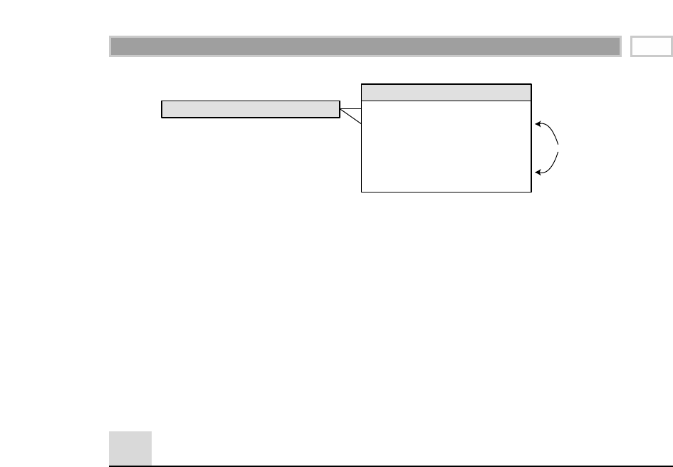
Figure 11.9 Localized and equalized date/time across time zones.
equivalized dates and times. Likewise, the offset can’t reside in a time or air-
port dimension table. The recommended approach for expressing dates and
times in multiple time zones is to include separate date and time-of-day
dimensions (or time-of-day facts, as we just discussed) corresponding to the
local and equivalized dates, as shown in Figure 11.9.
We’ll elaborate further on multiple date and time dimension tables to capture
both the absolute standard and local clock-on-the-wall dates and times when
we discuss a multinational Web retailer in Chapter 14.
Summary
In this chapter we turned our attention to the concept of trips or routes. The
expanded case study focused on an airline frequent flyer example, and we
briefly touched on similar scenarios drawn from the shipping and travel
services industries. We examined the situation in which we have multiple fact
tables at multiple granularities with multiple grain-specific facts. We also dis-
cussed the possibility of combining dimensions into a single dimension table
in cases where the row count volumes are extremely small or when there are
additional attributes that depend on the combined dimensions. Again, com-
bining dimensions should be viewed as the exception rather than the rule.
We wrapped up this chapter by discussing several date and time dimension
techniques, including country-specific calendar outriggers, treatment of time
as a fact versus a separate dimension, and the handling of absolute and rela-
tive dates and times.
Date Dimension (playing 2 roles) Departure Date Key (FK)
GMT Departure Date Key (FK)
More Foreign Keys …
Degenerate Dimensions …
Departure Time of Day
GMT Departure Time of Day
More Facts …
Flight Activity Fact
Comparing across time
zones requires 2 dates
and times of day
Transportation 241


Education
CHAPTER
12
243
We step into the world of an educational institution in this chapter. We’ll first
look at the applicant student pipeline as an accumulating snapshot. When we
introduced the accumulating snapshot-grained fact table in Chapter 5, we
used an order fulfillment pipeline to illustrate the concept. In this chapter,
rather than watching orders move through various states prior to completion,
the accumulating snapshot is used to monitor prospective student applicants
as they move through standard admissions milestones. The other primary
concept discussed in this chapter is the factless fact table. We’ll explore several
case study illustrations drawn from education to further elaborate on these
special fact tables, and we will discuss the analysis of events that didn’t occur.
Chapter 12 discusses the following concepts:
■■ Admission’s applicant tracking as an accumulating snapshot
■■ Factless fact table for student registration and facilities management data
■■ Handling of nonexistent events, including promotion events from the retail industry

University Case Study
In this chapter we’ll pretend that we work for a university, college, or other
type of educational institution. Traditionally, there has been less focus on rev-
enue and profit in this arena, but with the ever-escalating costs and competi-
tion associated with higher education, universities and colleges are very
interested in attracting and retaining high-quality students. In fact, there’s a
strong interest in understanding and maintaining a relationship well beyond
graduation. There’s also a dominant need to understand what our student cus-
tomers are buying in terms of courses each term. Finally, we’ll take a look at
maximizing the use of the university’s capital-intensive facilities.
Accumulating Snapshot for
Admissions Tracking
In Chapter 5 we treated the order fulfillment pipeline as an accumulating
snapshot. We also described the use of an accumulating snapshot to track a
specific item, uniquely identified by a serial or lot number, as it moves through
the manufacturing and test pipeline. Let’s take a moment to recall the distin-
guishing characteristics of an accumulating snapshot fact table:
■■ A single row represents the complete history of something.
■■ Such a fact table is most appropriate for short-lived processes, such as
orders and bills.
■■ Multiple dates represent the standard scenario milestones of each row.
■■ Open-ended sets of facts accumulate the interesting measures.
■■ Each row is revisited and changed whenever something happens.
■■ Both foreign keys and measured facts may be changed during the revisit.
We can envision these same characteristics applied to the prospective student
admissions pipeline. For those who work in other industries, there are obvious
similarities to tracking job applicants as they move through the hiring process,
and tracking sales prospects as they become customers.
In the case of applicant tracking, prospective students progress through a
standard set of admissions hurdles or milestones. Perhaps we’re interested in
tracking activities around key dates, such as receipt of preliminary admissions
test scores, information requested (via Web or otherwise), information sent,
interview conducted, on-site campus visit, application received, transcript
received, test scores received, recommendations received, first pass review by
admissions, review for financial aid, final decision from admissions, accepted,
CHAPTER 12
244

admitted, and enrolled. At any point in time, people in the admissions and
enrollment management area are interested in how many applicants are at
each stage in the pipeline. The process is much like a funnel, where many
applicants enter the pipeline, but far fewer progress through to the final stage.
Admission personnel also would like to analyze the applicant pool by a vari-
ety of characteristics.
The grain of the accumulating snapshot to track the applicant’s lifecycle is one
row per prospective student. This granularity represents the lowest level of
detail captured when the prospect enters the pipeline. As more information is
collected while the prospect progresses toward application, acceptance, and
admission, we continue to revisit and update the prospect’s status in the fact
table row, as illustrated in Figure 12.1.
Figure 12.1 Student applicant pipeline as an accumulating snapshot.
Preliminary Test Score Receipt Date Key (FK)
Information Requested Date Key (FK)
Information Sent Date Key (FK)
Interview Conducted Date Key (FK)
On-Site Campus Visit Date Key (FK)
Application Submitted Date Key (FK)
Transcript Received Date Key (FK)
Test Scores Received Date Key (FK)
Recommendations Received Date Key (FK)
Admissions First Pass Review Date Key (FK)
Reviewed for Financial Aid Date Key (FK)
Admissions Final Decision Date Key (FK)
Applicant Decision Received Date Key (FK)
Admitted Date Key (FK)
Enrolled Date Key (FK)
Admissions Decision Key (FK)
Applicant Key (FK)
Preliminary Test Score Receipt Quantity
Information Requested Quantity
Information Sent Quantity
Information Requested-Sent Lag
Interview Conducted Quantity
On-Site Campus Visit Quantity
Application Submitted Quantity
Transcript Received Quantity
Test Scores Received Quantity
Recommendations Received Quantity
Application Complete Quantity
Application Submitted-Complete Lag
Admissions First Pass Review Quantity
Reviewed for Financial Aid Quantity
Admissions Final Decision Quantity
Application Submitted-Final Decision Lag
Accepted Quantity
Decline Quantity
Final Decision-Accepted/Decline Lag
Admitted Quantity
Enrolled Quantity
Admissions Decision Key (PK)
Admissions Decision Description
Admissions Decision Category
Applicant Pipeline Accumulating Fact
Date Dimension (views for 15 roles)
Admissions Decision Dimension
Applicant Key (PK)
Applicant Name
Applicant Address Attributes …
Applicant High School GPA
Applicant High School
Applicant SAT Math Score
Applicant SAT Verbal Score
Number of Advanced Placement Credits
Gender
Date of Birth
Ethnicity
Preliminary School
Preliminary College Major
… and more
Applicant Dimension
Education 245

Like other accumulating snapshots we’ve discussed, there are multiple dates
in the fact table corresponding to the standard process milestones. We want to
analyze the prospect’s progress by these dates to determine the pace of move-
ment through the pipeline, and we also want to spot bottlenecks. This is espe-
cially important if we see a significant lag involving a candidate whom we’re
interested in attracting. Each of these dates is treated as a role-playing dimen-
sion, using surrogate keys to handle the inevitable unknown dates when we
first load the row.
The applicant dimension contains many interesting attributes about our
prospective students. Admissions analysts are interested in slicing and dicing
these applicant characteristics by geography, incoming credentials (grade
point average, college admissions test scores, advanced placement credits, and
high school), gender, date of birth, ethnicity, and preliminary major. Analyzing
these characteristics at various stages of the pipeline will help admissions per-
sonnel adjust their strategies to encourage more (or fewer) students to proceed
to the next mile marker.
As we saw previously, accumulating snapshots are appropriate for short-lived
processes, such as the applicant pipeline, that have a defined start and end, as
well as standard intermediate milestones. This type of fact table allows us to
see an updated status and ultimately final disposition of each prospective
applicant. We could include a fact for the estimated probability that the
prospect will become a student. By adding all these probabilities together, we
would see an instantaneous prediction of the following year’s enrollment.
Another education-based example of an accumulating snapshot focuses on
research proposal activities. Some user constituencies may be interested in view-
ing the lifecycle of a research grant proposal as it progresses through the grant
pipeline from preliminary proposal to grant approval and award receipt. This
would support analysis of the number of outstanding proposals in each stage of
the pipeline by faculty, department, research topic area, or research funding
source. Likewise, we could see success rates by the various dimensions. Having
this information in a common repository such as the data warehouse would
allow it to be leveraged more readily by a broader university population.
Factless Fact Tables
So far we’ve designed fact tables that have had a very characteristic structure.
Each fact table typically has three to approximately 15 to 20 key columns, fol-
lowed by one to potentially several dozen numeric, continuously valued,
preferably additive facts. The facts can be regarded as measurements taken at
the intersection of the dimension key values. From this perspective, the facts
are the justification for the fact table, and the key values are simply adminis-
trative structure to identify the facts.
CHAPTER 12
246
TEAMFLY
Team-Fly®
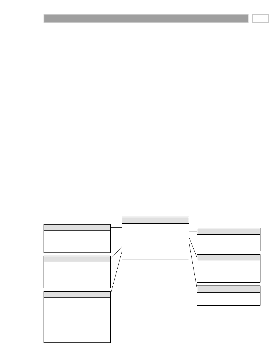
There are, however, a number of business processes whose fact tables are sim-
ilar to those we’ve been designing with one major distinction: There are no
measured facts! We call these factless fact tables. In the following examples we’ll
discuss both event tracking and coverage factless fact tables. We briefly intro-
duced the factless coverage table in Chapter 2 while discussing retail promo-
tion coverage, as well as in Chapter 5 to describe sales rep territory coverage.
Student Registration Events
There are many situations in which events need to be recorded as the simulta-
neous coming together of a number of dimensional entities. For example, we
can track student registrations by term. The grain of the fact table would be
one row for each registered course by student and term. As illustrated in Fig-
ure 12.2, the fact table has the following dimensionality: term, student, student
major and attainment, course, and faculty.
In this scenario we’re dealing with fact data at the term level rather than at the
more typical calendar day, week, or month granularity. Term is the lowest level
available for the registration events. The term dimension still should conform
to the calendar date dimension. In other words, each date in our daily calendar
dimension should identify the term (for example, Fall AY2002), academic year
(for example, AY2002), and term season (for example, Winter). The column
labels and values must be identical for the attributes common to both the
calendar date and term dimensions.
Figure 12.2 Student registration events as a factless fact table.
Term Key (FK)
Student Key (FK)
Declared Major Key (FK)
Credit Attainment Key (FK)
Course Key (FK)
Faculty (FK)
Registration Count (always = 1)
Faculty Key (PK)
Faculty Employee ID (Natural Key)
Faculty Name
Faculty Address Attributes …
Faculty Type
Faculty Tenure Indicator
Faculty Original Hire Date
Faculty Years of Service
Faculty School
Student Registration Event Fact
Faculty Dimension
Term Key (PK)
Term Description
Academic Year
Term/Season
Term Year Dimension
Course Key (PK)
Course Name
Course School
Course Format
Course Credit Hours
Course Dimension
Student Key (PK)
Student ID (Natural Key)
Student Attributes …
Student Dimension
Declared Major Key (PK)
Declared Major Description
Declared Major School
Interdisciplinary Indicator
Credit Attainment Key (PK)
Class Level Description
Declared Major Dimension
Credit Attainment Dimension
Education 247

The student dimension is an expanded version of the applicant dimension that
we discussed in the last scenario. We still want to retain all the information we
garnered from the application process (for example, geography, credentials,
and preliminary major) but supplement it with on-campus information, such
as part-time/full-time status, residence, involvement in athletics, declared
major, and class level status (for example, sophomore). As we discussed in
Chapter 6, we imagine treating some of these attributes as a minidimension(s)
because factions throughout the university are interested in tracking changes
to them over time, especially when it comes to declared major, class level, and
graduation attainment. People in administration and academia are keenly
interested in academic progress and retention rates by class, school, depart-
ment, and major.
A fact table is a reasonable place to represent the robust set of many-to-many
relationships among these dimensions. It records the collision of dimensions at
a point in time and space. This table could be queried to answer a number of
interesting questions regarding registration for the college’s academic offer-
ings, such as which students registered for which courses? How many
declared engineering majors are taking an out-of-major finance course? How
many students have registered for a given faculty member’s courses during
the last three years? How many students have registered for more than one
course from a given faculty member? The only peculiarity in this example is
that we don’t have a numeric fact tied to this registration data. As such, analy-
ses of this data will be based largely on counts.
Events often are modeled as a fact table containing a series of keys, each representing
a participating dimension in the event. Event tables often have no obvious numeric
facts associated with them and hence are called factless fact tables.
The SQL for performing counts in this factless fact is asymmetric because of
the absence of any facts. When counting the number of registrations for a fac-
ulty member, any key can be used as the argument to the COUNT function.
For example:
SELECT FACULTY, COUNT(TERM_KEY)... GROUP BY FACULTY
This gives the simple count of the number of student registrations by faculty,
subject to any constraints that may exist in the WHERE clause. An oddity of
SQL is that you can count any key and still get the same answer because you
are counting the number of keys that fly by the query, not their distinct values.
We would need to use a COUNT DISTINCT if we wanted to count the unique
instances of a key rather than the number of keys encountered.
The inevitable confusion surrounding the SQL statement, while not a serious
semantic problem, causes some designers to create an artificial implied fact,
CHAPTER 12
248

perhaps called registration count (as opposed to dummy), that is always popu-
lated by the value 1. While this fact does not add any information to the fact
table, it makes the SQL more readable, such as:
SELECT FACULTY, SUM(REGISTRATION_COUNT)... GROUP BY FACULTY
At this point the table is no longer strictly factless, but most would agree that
the 1 is nothing more than an artifact. The SQL will be a bit cleaner and more
expressive with the registration artifact. Perhaps query tools will have an easier
time constructing the query with a few simple user gestures. More important,
if we build a summarized aggregate table above this fact table, we will need a
real column to roll up to meaningful aggregate registration counts.
If a measurable fact does surface during the design, it can be added to the
schema, assuming that it is consistent with the grain of student registrations
by term. For example, if we have the ability to track tuition revenue, earned
credit hours, and grade scores, we could add them to this fact table, but then
it’s no longer a factless fact table. The addition of these facts would definitely
enable more interesting analyses. For example, what is the revenue generated
by course or faculty? What is the average grade per class by faculty?
Facilities Utilization Coverage
The second type of factless fact table is the coverage table. We’ll draw on a sce-
nario dealing with facility management to serve as an illustration. Universities
invest a tremendous amount of capital in their physical plant and facilities. It
would be helpful to understand which facilities were being used for what
purpose during every hour of the day during each term. For example, which
facilities were used most heavily? What was the average occupancy rate of the
facilities as a function of time of day? Does use drop off significantly on Fri-
days when no one wants to teach (or attend) classes?
Once again, the factless fact table comes to the rescue. In this case we’d include
one row in the fact table for each facility for standard hourly time blocks dur-
ing each day of the week during a term regardless of whether the facility is
being used or not. We’ve illustrated the schema in Figure 12.3.
The facility dimension would include all types of descriptive attributes about
the facility, such as the building, facility type (for example, classroom, lab, or
office), square footage, capacity, and amenities (for example, white board or
built-in projector). The utilization status dimension obviously would include a
text descriptor with values of “Available” or “Utilized.” Meanwhile, multiple
organizations may be involved in facilities utilization. Such would be the case
if one organization owned the facility during a time block, whereas the same
or a different organization was assigned as the facility user.
Education 249
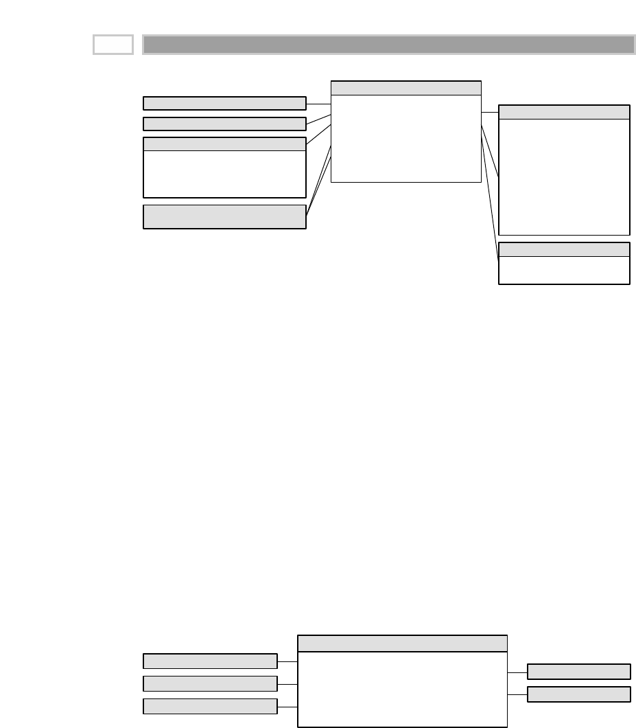
Figure 12.3 Facilities utilization as a coverage factless fact table.
Student Attendance Events
We can visualize a similar schema to track student attendance in a course. In
this case the grain would be one row for each student who walks through the
course’s classroom door each day. This factless fact table would share a num-
ber of the same dimensions we discussed with respect to registration events.
The primary difference would be that the granularity is by calendar date in
this schema rather than merely term. This dimensional model, as illustrated in
Figure 12.4, would allow us to answer such questions as which courses were
the most heavily attended? Which courses suffered the least attendance attri-
tion over the term? Which students attended which courses? Which faculty
member taught the most students?
Figure 12.4 Student attendance fact table.
Date Key (FK)
Student Key (FK)
Facility Key (FK)
Faculty Key (FK)
Course Key (FK)
Attendance Count (0 or 1)
Student Attendance Event Fact
Date Dimension
Facility Dimension
Course Dimension
Student Dimension
Faculty Dimension
Term Year Key (FK)
Day of Week Key (FK)
Time-of-Day Hour Key (FK)
Facility Key (FK)
Owner Organization Key (FK)
Assigned Organization Key (FK)
Utilization Status Key (FK)
Utilization Count (always = 1)
Time-of-Day Hour Key (PK)
Time-of-Day Description
Time-of-Day AM/PM Indicator
Time-of-Day Day Part
Facility Utilization Coverage Fact
Time-of-Day Hour Dimension
Term Year Dimension
Organization Dimension
(views for 2 roles)
Day of Week Dimension Facility Key (PK)
Facility Building Name
Facility Building Address
Facility Room Number
Facility Type
Facility Floor
Facility Square Footage
Facility Capacity
White Board Indicator
PC Monitor Indicator
… and more
Facility Dimension
Utilization Status Key (PK)
Utilization Status Description
Utilization Status Dimension
CHAPTER 12
250

Explicit Rows for What Didn’t Happen
Perhaps people are interested in monitoring students who were registered for
a course but didn’t show up. In this example we can envision adding explicit
rows to the fact table for attendance events that didn’t occur. Adding rows is
viable in this scenario because the nonattendance events have the same exact
dimensionality as the attendance events. Likewise, the fact table won’t grow at
an alarming rate, presuming (or perhaps hoping) that the no shows are a small
percentage of the total students registered for a course. In this situation we’re
no longer dealing with a factless fact table because now the attendance fact
would equal either 1 or 0.
While this approach is reasonable in this scenario, creating rows for events that
didn’t happen is ridiculous in many situations. For example, if we think back
to our transportation case study, we certainly don’t want to build fact table
rows for each flight not taken by a frequent flyer on a given day.
Other Relational Options for What
Didn’t Happen
In many cases the primary transaction fact table, such as the sales in a grocery
store, is very sparsely populated. Only a fraction of the total product portfolio
sells in each store each day in most retail environments. There would be over-
whelming overhead associated with storing explicit rows for products that
didn’t sell. The transaction sales fact table is already very large; the last thing
we want to do is to spend more money on the resources and disk space to store
a bunch of zeroes. As we recall from Chapter 2, we can use a promotion cover-
age factless fact table to help answer the question of what was being promoted
but didn’t sell. A row is placed in the coverage table for each product in each
store that is on promotion in each time period. This table would be much
smaller than adding explicit rows to the existing transaction fact table because
it only contains the items on promotion; those not being promoted would be
excluded. In addition, perhaps we could substitute a weekly granularity
instead of a daily grain if promotions run on a weekly basis. To answer the
question regarding what was on promotion but didn’t sell, we’d first consult
the coverage table for the products on promotion at a given time in that store.
We’d then consult the sales fact table to determine what did sell; the set differ-
ence between these two lists of products is our answer.
Education 251

In a relational database environment, we also have the option of using the
NOT EXISTS construct in SQL to identify rows that don’t exist in a database,
such as nonexistent facts or dimension attributes. While this approach allevi-
ates the need for upfront planning and design work to either include explicit
rows or construct coverage tables, it’s not as pain free as it appears initially. We
must ask very specifically what doesn’t exist by framing the NOT EXISTS
within a larger query. For example, to answer the question about nonexistent
sales for promoted products, we must first determine all products sold during
a given extended time frame and then issue a subquery within the NOT EXISTS
construct to determine all products sold on promotion during a smaller time
frame. The danger in using this SQL correlated subquery approach is that we’ll
miss products that didn’t sell at all during the extended time frame. Also, the
query is bound to perform slowly because of the complexity. Finally, data
access tools may prohibit the use of this construct within their interface. Using
the factless promotion coverage table in Figure 12.5, here is the SQL for finding
all the products that did not sell on a particular promotion (“Active Promo-
tion”) on January 15, 2002 that otherwise sold in the San Antonio Main Outlet
sometime during January 2002. If you can understand this SQL, then you are
qualified to support this application!
SELECT P1.PRODUCT_DESCRIPTION
FROM SALES_FACT F1, PRODUCT P1, STORE S1, DATE D1, PROMOTION R1
WHERE F1.PROD_KEY = P1.PROD_KEY
AND F1.STORE_KEY = S1.STORE_KEY
AND F1.DATE_KEY = D1.DATE_KEY
AND F1.PROMO_KEY = R1.PROMO_KEY
AND S1.STORE_LOCATION = ‘San Antonio Main Outlet’
AND D1.MONTH = ‘January, 2002’
AND NOT EXISTS
(SELECT R2.PROMO_KEY
FROM SALES_FACT F2, PROMOTION R2, DATE D2
WHERE F2.PROMO_KEY = R2.PROMO_KEY
AND F2.PROD_KEY = F1.PROD_KEY
AND F2.STORE_KEY = F1.STORE_KEY
AND F2.DATE_KEY = D2.DATE_KEY
AND R2.PROMOTION_TYPE = ‘Active Promotion’
AND D2.FULL_DATE = ‘January 15, 2002’)
CHAPTER 12
252

Figure 12.5 Promotion coverage as a factless fact table.
Multidimensional Handling of What
Didn’t Happen
Multidimensional online analytical processing (OLAP) databases do an excel-
lent job of helping users understand what didn’t happen. When the data cube
is constructed, the multidimensional database handles the sparsity of the
transaction data while minimizing the overhead burden of storing explicit
zeroes. As such, at least for fact cubes that are not too sparse, the event and
nonevent data is available for user analysis while reducing some of the com-
plexities we just discussed in the relational world.
Other Areas of Analytic Interest
Now that we’ve taken a tangent to discuss the analysis of what didn’t happen,
let’s return to the world of higher education to bring this chapter to an orderly
conclusion. Many of the analytic processes described earlier in this book, such
as procurement and human resources, are obviously applicable to the univer-
sity environment given the desire to better monitor and manage costs. When
we focus on the revenue side of the equation, research grants and alumni con-
tributions are key sources, in addition to the tuition revenue.
The majority of research grant analysis is a variation of financial analysis, as
we discussed in Chapter 7, but at a lower level of detail, much like a subledger.
The grain would include additional dimensions to further describe the
research grant, such as the corporate or governmental funding source,
research topic, grant duration, and faculty researcher. There is a strong need to
Date Key (FK)
Product Key (FK)
Store Key (FK)
Promotion Key (FK)
Promotion Count (always = 1)
Date Key (PK)
Date Attributes…
Promotion Coverage Fact
Date Dimension
Store Key (PK)
Store Attributes…
Store Dimension
Product Key (PK)
Product Attributes…
Product Dimension
Promotion Key (PK)
Promotion Attributes…
Promotion Dimension
Education 253

better understand and manage the budgeted and actual spending associated
with each research project. The objective is to optimize the spending so that a
surplus or deficit situation is avoided, while funds are deployed where they
will be most productive. Likewise, understanding research spending rolled up
by various dimensions is necessary to ensure proper institutional control of
such monies.
Better understanding the university’s alumni is much like better understand-
ing a customer base, as we described in Chapter 6 regarding CRM. Obviously,
there are many interesting characteristics that would be helpful in maintaining
a mutually beneficial relationship with our alumni, such as geographic, demo-
graphic, employment, interests, and behavioral information, in addition to the
data we collected about them as students (for example, incoming credentials,
affiliations, school, major, length of time to graduate, and honors). Improved
access to a broad range of attributes about the alumni population would allow
the university to better target messages and allocate resources. In addition to
alumni contributions, we can leverage the information for potential recruiting,
job placement, and research opportunities. To this end, we can envision a full-
scale CRM operational system to track all the university’s touch points with its
alumni, working in conjunction with the warehouse’s analytic foundation.
Summary
In this chapter we focused on two primary concepts. First, we looked at the
accumulating snapshot used to track the application pipeline (or conversely,
the research grant activity pipeline). Even though the accumulating snapshot
is used much less frequently than the more common transaction and periodic
snapshot fact tables, it is very useful in situations where we want to track the
current status of a short-lived process with generally accepted standard
progress milestones.
Second, we explored several examples of the factless fact table. These fact
tables capture the relationship between dimensions in the case of an event or
coverage but are unique in that no measurements are collected to serve as
actual facts. We also discussed the handling of situations where we want to
track events that didn’t occur.
CHAPTER 12
254

Health Care
CHAPTER
13
255
Health care presents several interesting data warehouse design situations. In
this chapter we will imagine first that we work for a large health care consor-
tium, then that we work for a billing organization for care providers and
hospitals, and finally that we work for a large clinic with millions of complex
patient treatment records. Each of these situations will suggest important
design techniques applicable to health care and other industries.
Chapter 13 discusses the following concepts:
■■ Value circle within health care, centered on the patient treatment records
■■ Accumulating snapshot fact table to handle medical bill line items
■■ More dimension role-playing as applied to multiple dates and providers
■■ Multivalued dimensions, such as an open-ended number of diagnoses along with
effective dates and weighting factors to support allocations
■■ Extended fact set to support profitability analysis
■■ Handling of complex medical events
■■ Fact dimension to organize extremely sparse, heterogeneous measurements

Health Care Value Circle
A typical large health care consortium is a network of providers, clinics,
hospitals, pharmacies, pharmaceutical manufacturers, laboratories, employers,
insurance companies, and government agencies. Unlike the value chain we
described in Chapter 3, a health care consortium resembles more of a value
circle, as illustrated in Figure 13.1. This figure is not a schema diagram! It is a
picture of how all these diverse organizations need to share the same critical
data: the patient treatment record.
There are two main types of patient treatment records. The treatment billing
record corresponds to a line item on a patient bill from a provider’s office, a
clinic, a hospital, or a laboratory. The treatment medical record, on the other
hand, is more comprehensive and includes not only the treatments that result
in charges but also all the laboratory tests, findings, and provider’s notes dur-
ing the course of treatment. The issues involved in these two kinds of records
are quite different, and we will look at them in separate sections.
Our large health care consortium must be able to share treatment billing
records smoothly from organization to organization. Billing records from all
the different kinds of providers must have a complete set of common dimen-
sions in order to be processed by the insurance companies and medical bill
payers. As individuals move from location to location, employer to employer,
and insurance company to government health care program, a coherent pic-
ture of that individual’s history needs to be creatable at any time. And finally,
on the scrimmage line of health care delivery, the medical records of a patient
need to be available on short notice for legitimate medical use by any of the
primary providers.
Figure 13.1 Typical health care value circle.
Patient
Treatment
Long Term
Care Facilities Physician
Offices
Pharmacies
Pharmaceutical
Manufacturers
Laboratories
Employers
Insurance
Companies
Government
Agencies
Hospitals
Clinics
CHAPTER 13
256
TEAMFLY
Team-Fly®

The health care value circle differs from the classic linear value chain because
there is no obvious ordering in time. However, the issues of conforming the
common dimensions remain exactly the same. The health care consortium will
be able to function if and only if it can implement a set of conformed dimen-
sions. A representative set of dimensions that must be conformed by the health
care consortium include:
■■ Calendar date
■■ Patient
■■ Responsible party (parent, guardian, employee)
■■ Employer
■■ Health plan
■■ Payer (primary, secondary)
■■ Provider (all forms of health care professionals who administer
treatments)
■■ Treatment (billable procedure, lab test, examination)
■■ Drug
■■ Diagnosis
■■ Outcome
■■ Location (office, clinic, outpatient facility, hospital)
A billing row probably would need all these dimensions except for the out-
come dimension. A medical row would not always identify the employer,
health plan, or payer dimensions. And insurance claims processing would
need even more dimensions relating to claimants, accidents, lawyers, and the
transaction types needed for claims processing. We’ll suppress the insurance
aspect of health care data warehouses because we will deal with those kinds of
subjects in Chapter 15.
In the health care business, some of these dimensions are very hard to con-
form, whereas others are easier than they look at first glance. The patient and
responsible party dimensions are the hardest, at least in the United States,
because of the lack of a reliable national identity number and because people
are signed up separately in doctors’ offices and hospitals and employment
situations. The problems with the patient and responsible party dimensions
are very similar to the issues we discussed in Chapter 6 regarding the consoli-
dation of multiple sources for customer information. The same customer
matching, householding, merge-purge software, and service providers offer
similar services to the health care industry. To find out more about these com-
panies, search for name householding or merge-purge on an Internet search
engine such as Google (www.google.com).
Health Care 257

The diagnosis and treatment dimensions are considerably more structured
and predictable than one might expect because the insurance industry and
government have mandated their content. Diagnoses usually follow the Inter-
national Classification of Diseases, 9th Revision: Clinical Modification, Volumes 1
and 2 (ICD-9-CM) standard. The U.S. Department of Health and Human Ser-
vices (HHS) maintains this standard as far as the United States is concerned.
The ICD-9-CM standard, Volume 3, defines treatment and management codes.
The Health Care Financing Administration Common Procedure Coding System
(HCPCS) standard, also updated and distributed by HHS; and Current Proce-
dural Terminology, 4th Edition (CPT-4), as updated and distributed by the
American Medical Association, cover health-related services and other items,
including:
■■ Physician services
■■ Physical and occupational therapy services
■■ Radiological procedures
■■ Clinical laboratory tests
■■ Other medical diagnostic procedures
■■ Hearing and vision services
■■ Transportation services (including ambulance)
■■ Medical supplies
■■ Orthotic and prosthetic devices
■■ Durable medical equipment
Dentists are able to use the Code on Dental Procedures and Nomenclature, as
updated and distributed by the American Dental Association, for dental
services.
When all the dimensions in our list have been conformed, then any organiza-
tion with appropriate access privileges can drill across the separate fact tables,
linking together the information by matching the row headers of each row. The
use of conformed dimensions guarantees that this matching process is well
defined. We described this process in Chapter 3 in a product movement con-
text, but the principles are exactly the same when applied to the health care
value circle.
Health Care Bill
Let us imagine that we work for a billing organization for health care
providers and hospitals. We receive the primary billing transactions from the
CHAPTER 13
258

providers and hospitals, prepare and send the bills to all the responsible
payers, and track the progress of the payments made.
Our health care billing data warehouse must meet a number of business objec-
tives. We want to analyze the counts and dollar amounts of all the bills by
every dimension available to us, including by patient, provider, diagnosis,
treatment, date, and any combinations of all these. We want to see how these
bills have been paid and what percentage of the bills have not been collected.
We want to see how long it takes to get paid, and we want to see the current
status of all unpaid bills, updated every 24 hours. And of course, the queries
need to be simple, and the response time must be instantaneous!
As we discussed in Chapter 5, whenever we consider a data source for inclu-
sion in the data warehouse, we have three fundamental choices of grain for the
fact table. Remember that the grain of the fact table is the fundamental defini-
tion of what constitutes a fact table row. In other words, what is the measure-
ment that we are recording?
The transaction grain is the most fundamental. In the health care bill example,
the transaction grain would include every input transaction from the
providers and the hospitals, as well as every payment transaction resulting
from the bill being sent. Although the world can be reconstructed from indi-
vidual transactions, this grain may not be the best grain to begin with to meet
our business reporting objectives because many of the queries would require
rolling the transactions forward from the beginning of the patient’s treatment.
The periodic snapshot grain is the grain of choice for long-running time-series
processes such as bank accounts and insurance policies. However, the periodic
snapshot doesn’t do a good job of capturing the behavior of a quickly moving,
short-lived process such as orders or medical bills. Most of the interesting
activity surrounding a medical bill takes place quickly in one or two months.
Also, if the periodic snapshot is available only at month-end, we cannot see the
current status of the unpaid bills.
We will choose the accumulating snapshot grain for our health care bill. A sin-
gle row in our fact table will represent a single line item on a health care bill.
Furthermore, this single row will represent the accumulated history of that
line item from the moment of creation of the row to the current day. When any-
thing about the line item changes, we revisit the unique accumulating row and
modify the row appropriately. From the point of view of the billing organiza-
tion, we’ll assume that the standard scenario of a bill includes:
■■ Treatment date
■■ Primary insurance billing date
■■ Secondary insurance billing date
Health Care 259
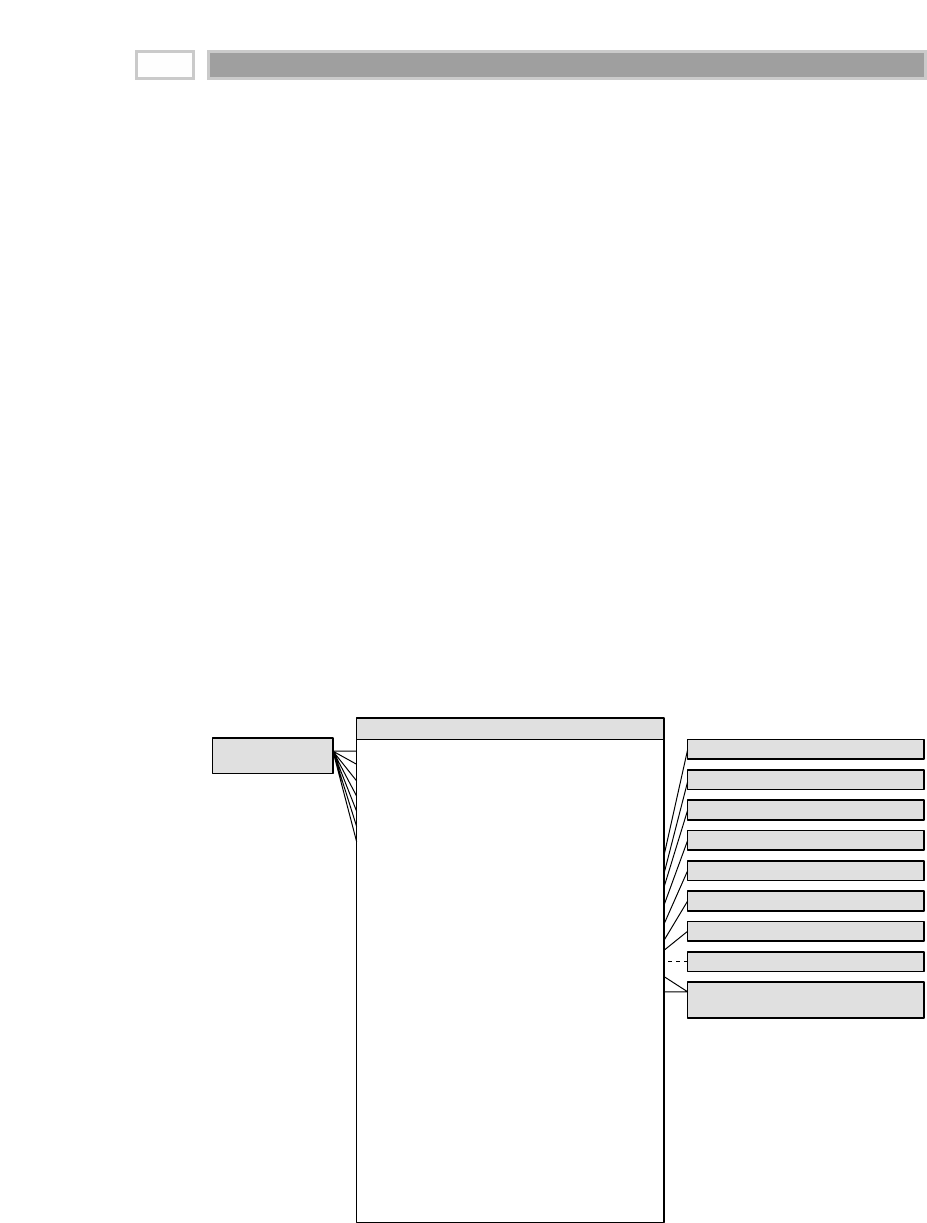
■■ Responsible party billing date
■■ Last primary insurance payment date
■■ Last secondary insurance payment date
■■ Last responsible party payment date
We choose these dates to be an adequate description of a normal bill. An accu-
mulating snapshot does not attempt to describe unusual situations fully. If the
business users occasionally need to see all the details of a particularly messy
bill payment situation, then a companion transaction grained fact table would
be needed. The purpose of the accumulating snapshot grain is to place every
health care bill into a uniform framework so that the business objectives we
described earlier can be satisfied easily.
Now that we have a clear idea of what an individual fact table row represents
(for example, the accumulated history of a line item on a health care bill), we
can complete the list of dimensions by carefully listing everything we know to
be true in the context of this row. In our hypothetical billing organization, we
know the responsible party, employer, patient, provider, provider organiza-
tion, treatment performed, treatment location, diagnosis, primary insurance
organization, secondary insurance organization, and master bill ID number.
These become our dimensions, as shown in Figure 13.2.
Figure 13.2 Accumulating snapshot fact table for health care billing.
Treatment Date Key (FK)
Primary Insurance Billing Date Key (FK)
Secondary Insurance Billing Date Key (FK)
Responsible Party Billing Date Key (FK)
Last Primary Insurance Payment Date Key (FK)
Last Secondary Insurance Payment Date Key (FK)
Last Responsible Party Payment Date Key (FK)
Responsible Party Key (FK)
Employer Key (FK)
Patient Key (FK)
Provider Key (FK)
Provider Organization (FK)
Treatment Key (FK)
Treatment Location Key (FK)
Diagnosis Keys (multi-valued)
Primary Insurance Organization Key (FK)
Secondary Insurance Organization Key (FK)
Master Bill ID (DD)
Billed Amount
Primary Insurance Paid Amount
Secondary Insurance Paid Amount
Responsible Party Paid Amount
Total Paid Amount (calculated)
Sent to Collections Amount
Written Off Amount
Remaining to be Paid Amount (calculated)
Number of Treatment Units
Treatment Duration
Days to First Primary Insurance Payment
Days to First Secondary Insurance Payment
Days to First Responsible Party Payment
Health Care Billing Line Item Fact
Date Dimension
(views for 7 roles)
Responsible Party Dimension
Employer Dimension
Patient Dimension
Provider Dimension
Provider Organization Dimension
Treatment Dimension
Treatment Location Dimension
Diagnosis Dimension (see Fig 13.3)
Insurance Organization Dimension
(views for 2 roles)
CHAPTER 13
260

The interesting facts that we choose to accumulate over the history of the line
item on the health care bill include the billed amount, primary insurance paid
amount, secondary insurance paid amount, responsible party paid amount,
total paid amount (calculated), amount sent to collections, amount written off,
amount remaining to be paid (calculated), number of treatment units (depend-
ing on treatment type), treatment duration, number of days from billing to first
primary insurance payment, number of days from billing to first secondary
insurance payment, and number of days from billing to first responsible party
payment.
We’ll assume that a row is created in this fact table when the activity transac-
tions are first received from the providers and hospitals and the initial bills are
sent. On a given bill, perhaps the primary insurance company is billed, but the
secondary insurance and the responsible party are not billed, pending a
response from the primary insurance company. For a period of time after the
row is first entered into the database, the last five dates are not applicable. The
surrogate date key in the fact table must not be null, but the full date descrip-
tion in the corresponding date dimension table row can indeed be null.
In the next few days and weeks after creation of the row, payments are
received, and bills are sent to the secondary insurance company and responsi-
ble party. Each time these events take place, the same fact table row is revis-
ited, and the appropriate keys and facts are destructively updated. This
destructive updating poses some challenges for the database administrator.
The row widths in databases such as Oracle will grow each time an update
occurs because numeric facts may be changed from a small number to a larger
number. This can cause block splits and fragmentation if enough space is not
available at the disk block level to accommodate this growth. If most of these
accumulating rows stabilize and stop changing within 90 days (for instance),
then a physical reorganization of the database at that time can recover disk
storage and improve performance. If the fact table is partitioned on the treat-
ment date key, then the physical clustering (partitioning) probably will be well
preserved throughout these changes because we assume that the treatment
date is not normally revisited and changed.
Roles Played By the Date Dimension
Accumulating snapshot fact tables always involve multiple date stamps. Our
example, which is typical, has seven foreign keys pointing to the date dimen-
sion. This is a good place to reiterate several important points:
■■ The foreign keys in the fact table cannot be actual date stamps because
they have to handle the “Not Applicable” case. The foreign keys should
be simple integers serving as surrogate keys.
Health Care 261

■■ The surrogate keys assigned in the date dimension should be assigned
consecutively in order of date. This is the only dimension where the
surrogate keys have any relationship to the underlying semantics of the
dimension. We do this so that physical partitioning of a fact table can be
accomplished by using one of the date-based foreign keys. In our example
we recommend that the treatment date key be used as the basis for physi-
cally partitioning the fact table.
■■ Surrogate keys corresponding to special conditions such as “Not Applica-
ble,” “Corrupted,” or “Hasn’t Happened Yet” should be assigned to the
top end of the numeric range so that these rows are physically partitioned
together in the hot partition with the most recent data. We do this if these
rows are ones that are expected to change.
■■ We do not join the seven date-based foreign keys to a single instance of
the date dimension table. Such a join would demand that all seven dates
were the same date. Instead, we create seven views on the single underly-
ing date dimension table, and we join the fact table separately to these
seven views, just as if they were seven independent date dimension
tables. This allows the seven dates to be independent. We refer to these
seven views as roles played by the date dimension table.
■■ The seven view definitions using the date dimension table should cosmet-
ically relabel the column names of each view to be distinguishable so that
query tools directly accessing the views will present the column names
through the user interface in a way that is understandable to the end user.
Although the role-playing behavior of the date dimension is very characteris-
tic of accumulating snapshot fact tables, other dimensions often play roles in
similar ways, such as the payer dimension in Figure 13.2. Later in this chapter
we will see how the physician dimension needs to have several roles in com-
plex surgical procedures depending on whether the physician is the primary
responsible physician, working in a consulting capacity, or working in an
assisting capacity.
Multivalued Diagnosis Dimension
Normally we choose the dimensions surrounding a fact table row by asking,
what do we know to be true in the context of the measurement? Almost always
we mean, what takes on a single value in the context of the measurement? If
something has many values in the context of the measurement, we almost
always disqualify that dimension because the many-valuedness means that
the offending dimension belongs at a lower grain of measurement.
CHAPTER 13
262

However, there are a few situations in which the many-valuedness is natural
and unavoidable, and we do want to include such a dimension in our design,
such as the case when we associated multiple customers with an account in
Chapter 9. The diagnosis dimension in our health care billing fact table is
another good example. At the moment of treatment, the patient has one or
more diagnoses, which are well known. Furthermore, there is good incentive
for keeping these diagnoses along with the billing row.
If there were always a maximum of three diagnoses, for instance, we might be
tempted to create three diagnosis dimensions, almost as if they were roles.
However, diagnoses don’t behave like roles. Unfortunately, there are often
more than three diagnoses, especially for elderly patients who are hospital-
ized. Real medical bill-paying organizations sometimes encounter patients
with more than 50 diagnoses! Also, the diagnoses don’t fit into well-defined
roles other than possibly admitting diagnosis and discharging diagnosis. The
role-playing dimensions we talked about in the preceding section are catego-
rized much more naturally and disjointly. Finally, the multiple-slots style of
design makes for very inefficient applications because the query doesn’t know
a priori which dimensional slot to constrain for a particular diagnosis.
We handle the open-ended nature of multiple diagnoses with the design
shown in Figure 13.3. We replace the diagnosis foreign key in the fact table
with a diagnosis group key. This diagnosis group key is connected by a many-
to-many join to a diagnosis group bridge table, which contains a separate row
for each diagnosis in a particular group.
Figure 13.3 Design for a multivalued diagnosis dimension.
Treatment Date Key (FK)
Primary Insurance Billing Date Key (FK)
Secondary Insurance Billing Date Key (FK)
Responsible Party Billing Date Key (FK)
Last Primary Insurance Payment Date Key (FK)
Last Secondary Insurance Payment Date Key (FK)
Responsible Party Key (FK)
Employer Key (FK)
Patient Key (FK)
Provider Key (FK)
Provider Organization (FK)
Treatment Key (FK)
Treatment Location Key (FK)
Diagnosis Group (FK)
Primary Insurance Organization Key (FK)
Secondary Insurance Organization Key (FK)
Master Bill ID (DD)
Facts …
Health Care Billing Line Item Fact
Diagnosis Group Key (FK)
Diagnosis Key (FK)
Weighting Factor
Diagnosis Group Bridge
Diagnosis Key (PK)
ICD-9 Code
Full Diagnosis Description
Diagnosis Type
Diagnosis Category
Diagnosis Dimension
Health Care 263

If a patient has three diagnoses, then that patient is assigned a diagnosis group
with three diagnoses. We assign a numerical weighting factor to each diagnosis
in the group such that the sum of all the weighting factors in the group is exactly
1.00. We can then use the weighting factors to allocate any of the numeric addi-
tive facts across individual diagnoses. In this way we can add up all billed
amounts by diagnosis, and the grand total will be the correct grand total billed
amount. This kind of report would be called a correctly weighted report.
We see that the weighting factors are simply a way to allocate the numeric
additive facts across the diagnoses. Some would suggest that we change the
grain of the fact table to be line item by diagnosis rather than just line item. In
this case we would take the weighting factors and physically multiply them
against the original numeric facts. This is done rarely, for three reasons. First,
the size of the fact table would be multiplied by the average number of diag-
noses. Second, in some fact tables we have more than one multivalued dimen-
sion. The number of rows would get out of hand in this situation, and we
would start to question the physical significance of an individual row. Finally,
we may want to see the unallocated numbers, and it is hard to reconstruct
these if the allocations have been combined physically with the numeric facts.
If we choose not to apply the weighting factors in a given query, we can still
summarize billed amounts by diagnosis, but in this case we get what is called
an impact report. A question such as “What is the total billed amount across all
possible treatments in any way involving the diagnosis of XYZ?” would be an
example of an impact report.
In Figure 13.3, an SQL view could be defined combining the fact table and the
diagnosis group bridge table so that these two tables, when combined, would
appear to data access tools as a standard fact table with a normal diagnosis
foreign key. Two views could be defined, one using the weighting factors and
one not using the weighting factors.
Finally, if the many-to-many join in Figure 13.3 causes problems for your mod-
eling tool that insists on proper foreign-key-to-primary-key relationships, the
equivalent design of Figure 13.4 can be used. In this case an extra table whose
primary key is diagnosis group is inserted between the fact table and the bridge
Figure 13.4 Diagnosis group dimension to create a primary key relationship.
Diagnosis Group Key (PK)
Diagnosis Group
Dimension
Foreign Keys …
Diagnosis Group (FK)
Master Bill ID (DD)
Facts …
Health Care Billing
Line Item Fact
Diagnosis Group Key (FK)
Diagnosis Key (FK)
Weighting Factor
Diagnosis Group Bridge
Diagnosis Key (PK)
ICD-9 Code
Full Diagnosis Description
Diagnosis Type
Diagnosis Category
Diagnosis Dimension
CHAPTER 13
264

table. Now both the fact table and the bridge table have conventional many-to-
one joins in all directions. There is no new information in this extra table.
In the real world, a bill-paying organization would decide how to administer
the diagnosis groups. If a unique diagnosis group were created for every out-
patient treatment, the number of rows could become astronomical and
unworkable. Probably the best approach is to have a standard portfolio of
diagnosis groups that are used repeatedly. This requires that each set of diag-
noses be looked up in the master diagnosis group table. If the existing group is
found, it is used. If it is not found, then a new diagnosis group is created.
In a hospital stay situation, however, the diagnosis group probably should be
unique to the patient because it is going to evolve over time as a type 2 slowly
changing dimension (SCD). In this case we would supplement the bridge table
with two date stamps to capture begin and end dates. While the twin date
stamps complicate the update administration of the diagnosis group bridge
table, they are very useful for querying and change tracking. They also allow
us to perform time-span queries, such as identifying all patients who pre-
sented a given diagnosis at any time between two dates.
To summarize this discussion of multivalued dimensions, we can list the issues
surrounding a multivalued dimension design:
■■ In the context of the fact table measurement, the multivalued dimension
takes on a small but variable number of well-defined values.
■■ Correctly allocated reports can be created only if weighting factors can be
agreed to.
■■ Weighting factors can be omitted, but then only impact reports can be
generated using the multivalued dimension.
■■ In high-volume situations such as medical bills and bank accounts, a
system of recognizing and reusing groups should be used.
■■ In cases where the relationship represented in the bridge table changes
over time, we embellish the bridge table with begin and end dates.
Extending a Billing Fact Table
to Show Profitability
Figure 13.5 shows an extended set of facts that might be added to the basic
billing schema of Figure 13.2. These include the consumables cost, provider
cost, assistant cost, equipment cost, location cost, and net profit before general
and administrative (G&A) expenses, which is a calculated fact. If these addi-
tional facts can be added to the billing schema, the power of the fact table
grows enormously. It now becomes a full-fledged profit-and-loss (P&L) view
of the health care business.
Health Care 265

Figure 13.5 Billing line-item fact table extended at the same grain with activity-based
costs for profit and loss.
These costs are not part of the billing process and normally would not be col-
lected at the same time as the billing data. Each of these costs potentially arises
from a separate source system. In order to bring this data into the billing fact
table, the separately sourced data would have to be allocated down to the
billing line item. For activity-based costs such as the ones we have included in
the list, it may be worth the effort to do this allocation. All allocations are con-
troversial and to an extent arbitrary, but if agreement can be reached on the set
of allocations, the P&L database that results is incredibly powerful. Now the
health care organization can analyze profitability by all the dimensions!
Dimensions for Billed Hospital Stays
The first part of this chapter described a comprehensive and flexible design for
billed health care treatments that would cover both inpatient and outpatient
bills. If an organization wished to focus exclusively on hospital stays, it would
be reasonable to tweak the dimensional structure of Figure 13.2 to provide
more hospital-specific information. Figure 13.6 shows a revised set of dimen-
sions specialized for hospital stays, with the new dimensions set in bold type.
In Figure 13.6 we show two roles for provider: admitting provider and attend-
ing provider. We show provider organizations for both roles because providers
may represent different organizations in a hospital setting.
We also have three multivalued diagnosis dimensions on each billed treatment
row. The admitting diagnosis is determined at the beginning of the hospital
stay and should be the same for every treatment row that is part of the same
hospital stay. The current diagnosis describes the state of knowledge of the
patient at the time of the treatment. The discharge diagnosis is not known until
the patient is discharged and is applied retroactively to all the rows that have
been entered as part of the hospital stay.
Existing 17 Foreign Keys …
Master Bill ID (DD)
Existing 13 Facts …
Consumables Cost
Provider Cost
Assistant Cost
Equipment Cost
Location Cost
Net Profit before G&A (calculated)
Health Care Billing Line Item Fact
CHAPTER 13
266
TEAMFLY
Team-Fly®

Figure 13.6 Accumulating snapshot for hospital stays billing.
Complex Health Care Events
In a hospital setting, we may want to model certain very complex events, such
as major surgical procedures. In a heart-transplant operation, whole teams of
specialists and assistants are assembled for this one event. A different heart
transplant may involve a team with a different makeup.
We can model these complex events with the design shown in Figure 13.7. We
combine the techniques of role-playing dimensions and multivalued dimen-
sions. We assume that a surgical procedure involves a single responsible
physician and variable numbers of attending physicians, assisting profession-
als, procedures, and equipment types. We also assume that the patient has a
multivalued diagnosis before the surgery and a separate multivalued diagno-
sis after the surgery.
Thus we have six multivalued dimensions, indicated by the bold type in Fig-
ure 13.7. The responsible physician, attending physician, and assisting profes-
sional dimensions are all roles played by an overall provider dimension. The
presurgery and postsurgery multivalued diagnosis dimensions are roles
played by a single diagnosis dimension.
Treatment Date Key (FK)
Primary Insurance Billing Date Key (FK)
Secondary Insurance Billing Date Key (FK)
Responsible Party Billing Date Key (FK)
Last Primary Insurance Payment Date Key (FK)
Last Secondary Insurance Payment Date Key (FK)
Last Responsible Party Payment Date Key (FK)
Responsible Party Key (FK)
Employer Key (FK)
Patient Key (FK)
Admitting Provider Key (FK)
Attending Provider Key (FK)
Admitting Provider Organization (FK)
Attending Provider Organization (FK)
Treatment Key (FK)
Treatment Location Key (FK)
Admitting Diagnosis Keys (multivalued)
Current Diagnosis Keys (multivalued)
Discharge Diagnosis Keys (multivalued)
Primary Insurance Organization Key (FK)
Secondary Insurance Organization Key (FK)
Hospital Stay ID (DD)
Facts …
Hospital Stay Billing Fact
Health Care 267

Figure 13.7 Surgical events transaction fact table extended to show profit and loss.
Since the grain of the fact table is the surgical procedure itself, it is natural to
supply a comprehensive set of facts. We show the extended set of facts that
would allow a complete P&L analysis to be done on surgical procedures,
assuming that the various costs can be allocated to each surgical event.
We leave out the weighting factors on all the multivalued dimensions in this
design. If we tried to provide weighting factors for the multivalued dimen-
sions, we would be implicitly supporting all the complex combinations of
weighting values, some of which would be nonsensical. It doesn’t seem worth
the trouble to claim that the correctly allocated portion of the total billed
amount of the surgery conjointly assigned to each possible assistant and each
possible piece of equipment has much meaning. Our technique of placing the
weighting factors independently in each dimension is only part of the prob-
lem. A more practical concern is that most organizations would not be willing
to assign dozens or hundreds of weighting factors.
Without the weighting factors, we nevertheless can create many useful impact
reports. For instance, what is the total value of all surgeries performed that used
a heart-lung machine? We also can ask which physicians, which assisting pro-
fessionals, and which pieces of equipment were involved in various kinds of
surgery. And finally, if we have allocated the costs to each surgery in a rational
way, we can ask which types of surgery are profitable or nonprofitable and why.
Treatment Date Key (FK)
Treatment Time of Day Key (FK)
Patient Key (FK)
Responsible Physician Key (FK)
Attending Physician Keys (multivalued)
Assisting Professionals Keys (multivalued)
Location Key (FK)
Procedure Keys (multivalued)
Equipment Keys (multivalued)
Pre-Surgery Diagnosis Keys (multivalued)
Post-Surgery Diagnosis Keys (multivalued)
Outcome
Total Billed Amount
Total Paid Amount (accumulating overwrite)
Consummables Cost
Provider Cost
Assistant Cost
Equipment Cost
Location Cost
Net Profit before G&A (calculated)
Surgical Events Transaction Fact
CHAPTER 13
268

Medical Records
General medical records are challenging for the data warehouse because of
their extreme variability. The records in a patient file take many different
forms, ranging from standard-format numeric data captured online, to one-of-
a-kind laboratory test results, to free-text comments entered by a health care
professional, to graphs and photographs. Given this extreme variability, we
don’t attempt to do queries and reports simultaneously analyzing every data
type. However, we still would like to provide a standard, simple framework
for all the records for a given patient. We are driven by the suspicion that if the
grain could be defined as an individual record entry for a patient, we should
be able to capture most of a medical record in a single fact table.
In such a fact table we might be tempted to provide a fact field for each type of
measurement. Some fields would be numeric, and some fields would be flags
(or foreign keys to junk dimensions consisting of groups of flags, as described
in Chapter 5). However, the sheer variety of possible medical record entries
defeats us. We would soon end up with a ridiculously wide fact table row with
too many fact fields, almost all of which would be null or zero for any specific
medical entry. In addition, this fixed-slot style of design is very inflexible
because new measurement types could be added only by physically altering
the fact table with the addition of a new field.
Fact Dimension for Sparse Facts
We handle the extreme variability of the medical record entry with a special
dimension we call a fact dimension. In Figure 13.8 the entry type is a fact dimen-
sion that describes what the row means or, in other words, what the fact
represents. The entry type dimension also determines which of the four kinds
of fact fields (amount, flag, comment, and JPEG file name) are valid for the
specific entry and how to interpret each field. For example, the generic amount
column is used for every numeric entry. The unit of measure for a given
numeric entry is found in the attached entry type dimension row, along with
any additivity restrictions. If the entry is a flag (for example, Yes/No or High/
Medium/Low), the types of flag values are found in the entry type dimension.
If the entry is a free-text comment or a multimedia object such as JPEG graphic
image or photograph, the entry type dimension alerts the requesting applica-
tion to look in these fact table fields.
Health Care 269

Figure 13.8 Transaction table with sparse, heterogeneous medical record facts and a fact
dimension.
This approach is elegant because it is superbly flexible. We can add new mea-
surement types just by adding new rows in the fact dimension, not by altering
the structure of the fact table. We also eliminate the nulls in the classic posi-
tional fact table design because a row exists only if the measurement exists.
However, there are some significant tradeoffs. Using a fact dimension may
generate lots of new fact table rows. If an event resulted in 10 numeric mea-
surements, we now have 10 rows in the fact table rather than a single row in
the classic design. For extremely sparse situations, such as clinical/laboratory
or manufacturing test environments, this is a reasonable compromise. How-
ever, as the density of the facts grows, we end up spewing out too many fact
rows. At this point we no longer have sparse facts and should return to the
classic fact table approach.
Moreover, we must be aware that this approach typically complicates data
access applications. Combining two numbers that have been taken as part of a
single event is more difficult because now we must fetch two rows from the
fact table. SQL likes to perform arithmetic functions within a row, not across
rows. In addition, we must be careful not to mix incompatible amounts in a
calculation because all the numeric measures reside in a single amount column.
The other dimensions in Figure 13.8 should be fairly obvious. The patient,
responsible provider, attending provider, location, equipment, and diagnosis
dimensions were all present in various forms in our earlier designs. The test
panel ID is a standard degenerate dimension because it probably is just a sim-
ple natural key that ties together multiple medical record entries that were all
part of a particular test panel.
Entry Date Key (FK)
Patient Key (FK)
Responsible Provider Key (FK)
Attending Provider Key (FK)
Assisting Professionals Keys (Multivalued)
Location Key (FK)
Equipment Key (FK)
Diagnosis Keys (Multivalued, time varying)
Comment (FK)
Entry Type (FK)
Test Panel ID (DD)
Amount
Flag
JPEG File Name
Medical Record Entries Fact Table
Foreign key to free text from procedure/lab test
Fact dimension to identify which facts are populated in
this row and what they mean
Measured value from procedure/lab test
Bounded set of categorical values from procedure/lab test
Pointer to graph or photo from procedure/lab test
CHAPTER 13
270

Free text comments should not be stored in a fact table directly because they
waste space and rarely participate in queries. Presumably, the free text com-
ments occur only on some records. Rather, the fact table should have a foreign
key that points to a comment dimension, as shown in Figure 13.8.
The use of a JPEG file name to refer to an image, rather than embedding the
image as a blob directly in the database, is somewhat of an arbitrary decision.
The advantage of using a JPEG file name is that other image creation, viewing,
and editing programs can access the image freely. The disadvantage is that a
separate database of graphic files must be maintained in synchrony with the
fact table.
Going Back in Time
As data warehouse practitioners, we have developed powerful techniques for
accurately capturing the historical flow of data from our enterprises. Our
numeric measurements go into fact tables, and we surround these fact tables
with contemporary descriptions of what we know is true at the time of the
measurements. These contemporary descriptions are packaged as dimension
tables in our dimensional schemas. In our health care data warehouse, we
allow the descriptions of patient, provider, and payer to evolve whenever
these entities change their descriptions. Since these changes occur unpredictably
and sporadically, we have called these slowly changing dimensions (SCDs).
In Chapter 4 we developed specific techniques for processing overwrites (type
1 SCDs), true changes in the entities at points in time (type 2 SCDs), and
changes in the labels we attach to entities (type 3 SCDs). These procedures are
an important part of our extract-transform-load (ETL) procedures with every
update.
However, what do we do when we receive late-arriving data that should have
been loaded into the data warehouse weeks or months ago? Some of our pro-
cedures won’t work. There are two interesting cases that need to be discussed
separately.
Late-Arriving Fact Rows
Using our patient treatment scenario, suppose that we receive today a treat-
ment row that is several months old. In most operational data warehouses we
are willing to insert this late-arriving row into its correct historical position,
even though our summaries for the prior month will now change. How-
ever, we must choose the old contemporary dimension rows that apply to this
Health Care 271

treatment carefully. If we have been date stamping the dimension rows in our
type 2 SCDs, then our processing involves the following steps:
1. For each dimension, find the corresponding dimension row whose date
stamp is the latest date stamp less than or equal to the date of the treatment.
2. Using the surrogate keys found in the each of the dimension rows from
step 1, replace the natural keys of the late-arriving fact row with the
surrogate keys.
3. Insert the late-arriving fact row into the correct physical partition of the
database containing the other fact rows from the time of the late-arriving
treatment.
There are a few subtle points here. First, we assume that all of our dimension
rows contain twin date stamps that indicate the span of time when that partic-
ular detailed description was valid. We need to be careful to have an unbroken
chain of nonoverlapping begin and end dates for each patient, provider, and
payer because we must find the right dimension rows for the new fact row
about to be inserted.
A second subtle point goes back to our assumption that we have an opera-
tional data warehouse that is willing to insert these late-arriving rows into old
months. If your data warehouse has to tie to the books, then you can’t change
an old monthly total, even if that old total was incorrect. Now you have a
tricky situation in which the date dimension on the treatment record is for a
booking date, which may be today, but the other patient, provider, and payer
dimensions nevertheless should refer to the old descriptions in the way we
described earlier. If you are in this situation, you should have a discussion
with your finance department manager to make sure that he or she under-
stands what you are doing. An interesting compromise is to carry two date
dimensions on treatment records. One refers to the actual treatment date, and
the other refers to the booking date. Now we can roll up the treatment records
either operationally or by the books.
The third subtle point is the requirement to insert the late-arriving treatment
row into the correct physical partition of the database containing its contem-
porary brothers and sisters. In this way, when you move a physical partition
from one form of storage to another or when you perform a backup or restore
operation, you will be affecting all the treatment rows from a particular span
of time. In most cases this is what you want to do. You can guarantee that all
fact rows in a time span occupy the same physical partition if you declare the
physical partitioning of the fact table to be based on the date dimension, where
the surrogate date keys are assigned in a predictable sequence order.
CHAPTER 13
272

Late-Arriving Dimension Rows
A late-arriving dimension row presents an entirely different set of issues that,
in some ways, are more complex than a late-arriving fact row. Suppose that
John Doe’s patient dimension row contains a marital flag attribute that always
contained the value “Single.” We have a number of patient rows for John Doe
because this is a slowly changing dimension and other attributes such as
John’s address and employment status have changed over the past year or two.
Today we are notified that John Doe was married on July 15, 1999 and has been
married ever since. To add this new information to the data warehouse
requires the following steps:
■■ Insert a fresh row, with a new surrogate key, for John Doe into the patient
dimension with the marital status attribute set to “Married” and the effec-
tive date set to “July 15, 1999.”
■■ Scan forward in the patient dimension table from July 15, 1999, finding
any other rows for John Doe, and destructively overwrite the marital
status field to “Married.”
■■ Find all fact rows involving John Doe from July 15, 1999 to the first next
change for him in the dimension after July 15, 1999 and destructively
change the patient foreign key in those fact rows to the new surrogate key
created in step 1.
This is a fairly messy change, but you should be able to automate these steps
in a good programmable ETL environment. We have some subtle issues in this
case, too. First, we need to check to see if some other change took place for
John Doe on July 15, 1999. If so, then we only need to perform step 2. We don’t
need a new dimension row in this special case.
Second, since we are using a pair of date stamps in each product dimension
row, we need to find the closest previous to July 15 patient row for John Doe
and change its end date to July 15, 1999, and we also need to find the closest
subsequent to July 15 patient row for John Doe and set the end date for the July
15, 1999 entry to the begin date of that next row. Got it?
Finally, we see from this example why the surrogate keys for all dimensions
except date or time cannot be ordered in any way. You never know when you
are going to have to assign a surrogate key for a late-arriving row. And since
surrogate keys are just assigned in numeric order without any logic or struc-
ture, you can easily have a high-valued surrogate key representing a dimen-
sion row that is very old.
Health Care 273

Hopefully, these late-arriving fact and dimension rows are unusual in most of
our data warehouses. If nothing else, they are bothersome because they change
the counts and totals for prior history. However, we have taken a pledge as
keepers of the data warehouse to present the history of our enterprise as accu-
rately as possible, so we should welcome the old rows because they are mak-
ing our databases more complete.
Some industries, such as health care, have huge numbers of late-arriving rows.
In such cases, these techniques, rather than being specialized techniques for
the unusual case, may be the dominant mode of processing.
Summary
Health care not only is an important application area in its own right, but it also
provides the data warehouse designer with a number of clear design examples
that can be used in many other situations. In this chapter we have seen:
The value circle, where a large number of organizations need to look at the
same data in parallel without any strong sense of time sequencing. How-
ever, the issues of building a value-circle data warehouse bus architecture
with conformed dimensions and conformed facts are exactly the same as
the more conventional value chains.
The accumulating snapshot grain of fact table applied to a medical bill line
item. This grain was appropriate because of the relatively brief duration of
a medical bill compared with something like a bank account, where the
periodic snapshot is more appropriate.
Roles played by the date dimension in the accumulating snapshot grain, as
well as roles played by the provider and payer dimensions in other fact
tables of this chapter. Roles are implemented as separate, specifically
named views on a single underlying master dimension.
Multivalued dimensions, especially the diagnosis dimension. In many
cases we are able to associate a weighting factor with each of the values in
a multivalued dimension entry so as to allow allocations to be calculated
on numeric facts in the fact table. We would call this kind of report a cor-
rectly weighted report. However, in some cases where we are unwilling to
assign weighting factors, the multivalued dimension still lets us produce
impact reports.
An extended set of cost-based facts that allow us to implement a P&L
schema. Adding these cost-based facts is very attractive, but it is a lot of
work. The best costs to add to a design are activity-based costs because
these are not too controversial to associate with individual fact rows such
as our medical bill line items.
CHAPTER 13
274

Complex events modeled as single fact table rows containing several multi-
valued dimensions. In these cases we often do not build weighting factors
into all the multivalued dimensions because the interaction between the
weighting factors becomes nonsensical.
Fact dimensions used to organize extremely sparse, heterogeneous measure-
ments into a single, uniform framework. Our example plausibly covered
general medical records consisting of standardized numeric measures,
one-of-a-kind lab results, categorical textual measurements, free-text
comments, and image data.
Health Care 275

TEAMFLY
Team-Fly®

Electronic Commerce
CHAPTER
14
277
Web-intensive businesses have access to a new kind of data source that literally
records the gestures of every Web site visitor. We call it the clickstream. In its
most elemental form, the clickstream is every page event recorded by each of
the company’s Web servers. The clickstream contains a number of new dimen-
sions—such as page, session, and referrer—that are unknown in our conven-
tional data marts. The clickstream is a torrent of data, easily being the largest
text and number data set we have ever considered for a data warehouse.
Although the clickstream is the most exciting new development in data ware-
housing, at the same time it can be the most difficult and most exasperating.
Does it connect to the rest of the warehouse? Can its dimensions and facts be
conformed in a data warehouse bus architecture?
The full story of the clickstream data source and its implementation by com-
panies, such as those involved in electronic commerce, is told in the complete
book on this subject, The Data Webhouse Toolkit, by Ralph Kimball and Richard
Merz (Wiley, 2000). This chapter is a lightning tour of the central ideas drawn
from The Data Webhouse Toolkit. We start by describing the raw clickstream data
source. We show how to design a data mart around the clickstream data.
Finally, we integrate this data mart into a larger matrix of more conventional
data marts for a large Web retailer and argue that the profitability of the Web
sales channel can be measured if you allocate the right costs back to the indi-
vidual sales of the retailer.

Chapter 14 discusses the following concepts:
■■ Brief tutorial on Web client-server interactions
■■ Unique characteristics of clickstream data, including the challenges of identifying
the visitors, their origin, and their complete session
■■ Clickstream-specific dimensions, such as the page, event, session, and referral
dimensions
■■ Clickstream fact tables for the complete session, individual page event, and an
aggregated summary
■■ Integrating the clickstream data mart into the rest of the enterprise data warehouse
■■ Web profitability data mart
Web Client-Server Interactions Tutorial
Understanding the interactions between a Web client (browser) and a Web
server (Web site) is essential for understanding the source and meaning of the
data in the clickstream. In Figure 14.1 we show a browser, designated “Visitor
Browser.” We’ll look at what happens in a typical interaction from the per-
spective of a browser user. The browser and Web site interact with each other
across the Internet using the Web’s communication protocol—the HyperText
Transfer Protocol (HTTP).
First, the visitor clicks a button or hypertext link containing a Uniform
Resource Locator (URL) to access a particular Web site, shown as black-circled
action 1 in Figure 14.1. When this HTTP request reaches the Web site, the server
returns the requested item (action 2). In our illustration, this fetches a docu-
ment in HyperText Markup Language (HTML) format—websitepage.html.
Once the document is entirely retrieved, the visitor’s browser scans web-
sitepage.html and notices several references to other Web documents that it
must fulfill before its work is completed; the browser must retrieve other com-
ponents of this document in separate requests. Note that the only human
action taken here is to click on the original link. All the rest of the actions that
follow in this example are computer-to-computer interactions triggered by the
click and managed, for the most part, by instructions carried in the initially
downloaded HTML document, websitepage.html. In order to speed up Web
page responsiveness, most browsers will execute these consequential actions
in parallel, typically with up to 4 or more HTTP requests being serviced
concurrently.
The visitor’s browser finds a reference to an image—a logo perhaps—that,
from its URL, is located at Website.com, the same place it retrieved the initial
HTML document. The browser issues a second request to the server (action 3),
and the server responds by returning the specified image.
CHAPTER 14
278
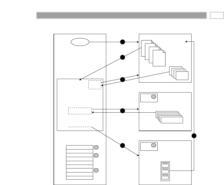
Figure 14.1 Interactions between Web client (browser) and Web server (Web site).
The browser continues to the next reference in websitepage.html and finds an
instruction to retrieve another image from Banner-ad.com. The browser makes
this request (action 4), and the server at Banner-ad.com interprets a request for
the image in a special way. Rather than immediately sending back an image,
the banner-ad server first issues a cookie request to the visitor’s browser
requesting the contents of any cookie that might have been placed previously
in the visitor’s PC by Banner-ad.com. The banner-ad Web site retrieves this
cookie, examines its contents, and uses the contents as a key to determine
which banner ad the visitor should receive. This decision is based on the visi-
tor’s interests or on previous ads the visitor had been sent by this particular ad
server. Once the banner-ad server makes a determination of the optimal ad, it
returns the selected image to the visitor. The banner-ad server then logs which
Visitor Browser Website.com
HTML Pages
Banner-ad.com
Profiler.com
Demographic Detail
User
Profile
Images
Click Link
websitepage.html
Hidden Link
Image
Banner Ad
Cookie File
Website.com
Banner-ad.com
Profiler.com
Reads
Cookie
Reads
Cookie
Advertisements
1
2
3
4
5
6
Electronic Commerce 279

ad it has placed along with the date and the clickstream data from the visitor’s
request. Had the banner-ad server not found its own cookie, it would have
sent a new persistent cookie to the visitor’s browser for future reference, sent
a random banner ad, and started a history in its database of interactions with
the visitor’s browser.
The HTTP request from the visitor’s browser to the banner-ad server carried
with it a key piece of information known as the referrer. The referrer is the URL
of the agent responsible for placing the link on the page. In our example the
referrer is Website.com/websitepage.html. The referrer is not the user’s
browser but rather is the HTML context in which the link to Banner-ad.com
was embedded. Because Banner-ad.com now knows who the referrer was, it
can credit Website.com for having placed an advertisement on a browser
window. This is a single impression. The advertiser can be billed for this
impression, with the revenue being shared by the referrer (Website.com) and
the advertising server (Banner-ad.com).
If the Web site is sharing Web log information with the referring site, it will be
valuable to share page attributes as well. In other words, not only do we want
the URL of the referring page, but we also want to know what the purpose of
the page was. Was it a navigation page, a partner’s page, or a general search
page?
While the ad server deals primarily with placing appropriate content, the pro-
filer deals with supplying demographic information about Web site visitors. In
our original HTML document, websitepage.html had a hidden field that con-
tained a request to retrieve a specific document from Profiler.com (action 5).
When this request reached the profiler server, Profiler.com immediately tried
to find its cookie in the visitor’s browser. This cookie would contain a user ID
placed previously by the profiler that is used to identify the visitor and serves
as a key to personal information contained in the profiler’s database. The pro-
filer might either return its profile data to the visitor’s browser to be sent back
to the initial Web site or send a real-time notification to the referrer, Website.com,
via an alternative path alerting Website.com that the visitor is currently logged
onto Website.com and viewing a specific page (action 6). This information also
could be returned to the HTML document to be returned to the referrer as part
of a query string the next time an HTTP request is sent to Website.com.
Although Figure 14.1 shows three different sites involved in serving the con-
tents of one document, it is possible, indeed likely, that these functions will be
combined into fewer servers. It is likely that advertising and profiling will be
done within the same enterprise, so a single request (and cookie) would suffice
to retrieve personal information that would more precisely target the ads that
are returned. However, it is equally possible that a Web page could contain ref-
erences to different ad/profile services, providing revenue to the referrer from
multiple sources.
CHAPTER 14
280

Why the Clickstream Is Not
Just Another Data Source
The clickstream is not just another data source that is extracted, cleaned, and
dumped into the data warehouse. The clickstream is really an evolving collec-
tion of data sources. There are more than a dozen Web server log file formats
for capturing clickstream data. These log file formats have optional data com-
ponents that, if used, can be very helpful in identifying visitors, sessions, and
the true meaning of behavior. We are in the infancy of this clickstream game,
and it is a sure bet that new logging capabilities and new logging formats will
become available on a regular basis. Extensible Markup Language (XML) has
the potential for making the structure of our Web pages far more expressive,
which is bound to affect the clickstream data source.
Because of the distributed nature of the Web, clickstream data is often collected
simultaneously by different physical servers, even when the visitor thinks that
he or she is interacting with a single Web site. Even if the log files being col-
lected by these separate servers are compatible, a very interesting problem
arises in synchronizing the log files after the fact. Remember that a busy Web
server may be processing hundreds of page events per second. It is unlikely
that the clocks on separate servers will be in synchrony to a hundredth of a
second. The Data Webhouse Toolkit explores various technical approaches to
solving this synchronization problem.
We also get clickstream data from different parties. Besides our own log files,
we may get clickstream data from referring partners or from Internet service
providers (ISPs). We also may get clickstream data from Web-watcher services
that we have hired to place a special control on certain Web pages that alert
them to a visitor opening the page.
Another important form of clickstream data is the search specification given to
a search engine that then directs the visitor to the Web site.
Finally, if we are an ISP providing Web access to directly connected customers,
we have a unique perspective because we see every click of our familiar cap-
tive visitors that may allow much more powerful and invasive analysis of the
end visitor’s sessions.
The most basic form of clickstream data from a normal Web site is stateless. That
is, the log shows an isolated page retrieval event but does not provide a clear tie
to other page events elsewhere in the log. Without some other kind of context
help, it is difficult or impossible to reliably identify a complete visitor session.
The other big frustration with basic clickstream data is the anonymity of the
session. Unless the visitor agrees to reveal his or her identity in some way, we
often cannot be sure who he or she is or if we have ever seen the visitor before.
Electronic Commerce 281

In certain situations we may not even be able to distinguish the clicks of two
visitors who are browsing our Web site simultaneously.
Challenges of Tracking with
Clickstream Data
Clickstream data contains many ambiguities. Identifying visitor origins, visitor
sessions, and visitor identities is something of an interpretive art. Browser
caches and proxy servers make these identifications even more challenging.
Identifying the Visitor Origin
If we are very lucky, our site is the default home page for the visitor’s browser.
Every time the visitor opens his or her browser, our home page is the first
thing he or she sees. This is pretty unlikely unless we are the Webmaster for a
portal site or an intranet home page, but many sites have buttons that, when
clicked, prompt the visitor to set his or her URL as the browser’s home page.
Unfortunately, there is no easy way to determine from a log whether or not our
site is set as a browser’s home page.
A visitor may be directed to our site from a search at a portal such as Yahoo! or
Alta Vista. Such referrals can come either from the portal’s index or table of
contents, for which you may have paid a placement fee, or from a word or con-
tent search.
For many Web sites, the most common source of visitors is from a browser
bookmark. In order for this to happen, the visitor will have to have previously
bookmarked the site, and this will occur only after the site’s interest and trust
levels cross the visitor’s bookmark threshold. Unfortunately, when a visitor
uses a bookmark, the referrer field is empty, just as if the visitor had typed in
the URL by hand.
Finally, the site may be reached as a result of a click-through—a deliberate
click on a text or graphic link from another site. This may be a paid-for referral
as via a banner ad or a free referral from an individual or cooperating site. In
the case of click-throughs, the referring site almost always will be identifiable
in the Web site’s referrer log data. Capturing this crucial clickstream data is
important to verify the efficacy of marketing programs. It also provides crucial
data for auditing invoices you may receive from click-through advertising
charges.
Identifying the Session
Most web-centric data warehouse applications will require every visitor
session (visit) to have its own unique identity tag, similar to a grocery store
CHAPTER 14
282

point-of-sale ticket ID. We call this the session ID. The rows of every individual
visitor action in a session, whether derived from the clickstream or from an
application interaction, must contain this tag. Keep in mind, however, that the
operational application generates this session ID, not the Web server.
The basic protocol for the World Wide Web, HTTP, is stateless—that is, it lacks
the concept of a session. There are no intrinsic login or logout actions built into
the HTTP, so session identity must be established in some other way. There are
several ways to do this:
1. In many cases, the individual hits comprising a session can be consoli-
dated by collating time-contiguous log entries from the same host (Inter-
net Protocol, or IP, address). If the log contains a number of entries with
the same host ID in a short period of time (for example, one hour), one
can reasonably assume that the entries are for the same session. This
method breaks down for visitors from large ISPs because different visitors
may reuse dynamically assigned IP addresses over a brief time period. In
addition, different IP addresses may be used within the same session for
the same visitor. This approach also presents problems when dealing with
browsers that are behind some firewalls. Notwithstanding these prob-
lems, many commercial log analysis products use this method of session
tracking, which requires no cookies or special Web server features.
2. Another, much more satisfactory method is to let the Web browser place a
session-level cookie into the visitor’s Web browser. This cookie will last as
long as the browser is open and, in general, won’t be available in subse-
quent browser sessions. The cookie value can serve as a temporary session
ID not only to the browser but also to any application that requests the
session cookie from the browser. This request must come from the same
Web server (actually, the same domain) that placed the cookie in the first
place. Using a transient cookie value as a temporary session ID for both
the clickstream and application logging allows a straightforward approach
to associating the data from both these sources during postsession log
processing. However, using a transient cookie has the disadvantage that
you can’t tell when the visitor returns to the site at a later time in a new
session.
3. HTTP’s secure sockets layer (SSL) offers an opportunity to track a visitor
session because it may include a login action by the visitor and the
exchange of encryption keys. The downside to using this method is that
to track the session, the entire information exchange needs to be in high-
overhead SSL, and the visitor may be put off by security advisories that
can pop up when certain browsers are used. In addition, each host server
must have its own unique security certificate.
4. If page generation is dynamic, you can try to maintain visitor state by
placing a session ID in a hidden field of each page returned to the visitor.
Electronic Commerce 283

This session ID can be returned to the Web server as a query string
appended to a subsequent URL. This method of session tracking requires
a great deal of control over the Web site’s page-generation methods to
ensure that the thread of session ID is not broken. If the visitor clicks on
links that don’t support this session ID ping-pong, a single session will
appear to be multiple sessions. This approach also breaks down if multi-
ple vendors are supplying content in a single session.
5. Finally, the Web site may establish a persistent cookie in the visitor’s PC
that is not deleted by the browser when the session ends. Of course, it’s
possible that the visitor will have his or her browser set to refuse cookies
or may clean out his or her cookie file manually, so there is no absolute
guarantee that even a persistent cookie will survive. Although any given
cookie can be read only by the Web site that caused it to be created, cer-
tain groups of Web sites can agree to store a common ID tag that would
let these sites combine their separate notions of a visitor session into a
supersession.
In summary, the most powerful method of session tracking from Web server
log records is to set a persistent cookie in the visitor’s browser. Other less pow-
erful methods include setting a session-level nonpersistent cookie or nearly
associating time-contiguous log entries from the same host. The latter method
requires a robust algorithm in the log postprocessor to ensure satisfactory
results, in part by deciding when not to take the results seriously.
Identifying the Visitor
Identifying a specific visitor who logs onto our site presents some of the most
challenging problems facing a site designer, Webmaster, or manager of data
warehousing for the following reasons:
Web visitors wish to be anonymous. They may have no reason to trust us, the
Internet, or their PC with personal identification or credit card information.
If we request a visitor’s identity, he or she is likely to lie about it. It is
believed that when asked their name on an Internet form, men will enter
a pseudonym 50 percent of the time and women will use a pseudonym
80 percent of the time.
We can’t be sure which family member is visiting our site. If we obtain an
identity by association, for instance, from a persistent cookie left during a
previous visit, the identification is only for the computer, not for the spe-
cific visitor. Any family member or company employee may have been
using that particular computer at that moment in time.
CHAPTER 14
284

We can’t assume that an individual is always at the same computer. Server-
provided cookies identify a computer, not an individual. If someone accesses
the same Web site from an office computer, a home PC, and a laptop com-
puter, a different Web site cookie is probably put into each machine.
Proxy Servers
When a browser makes an HTTP request, that request is not always served
from the server specified in a URL. Many ISPs make use of proxy servers to
reduce Internet traffic. Proxy servers are used to cache frequently requested
content at a location between its intended source and an end visitor. Such prox-
ies are employed commonly by large ISPs such as America Online and Earth-
link, and in some cases, an HTTP request may not even leave the visitor’s PC. It
may be satisfied from the browser’s local cache of recently accessed objects.
Proxy servers can introduce three problems, as illustrated in Figure 14.2. First,
a proxy may deliver outdated content. Although Web pages can include tags
that tell proxy servers whether or not the content may be cached and when
content expires, these tags often are omitted by Webmasters or ignored by
proxy servers.
Second, proxies may satisfy a content request without properly notifying the
originating server that the request has been served by the proxy. When a proxy
handles a request, convention dictates that it should forward a message that
indicates that a proxy response has been made to the intended server, but this
is not reliable. As a consequence, our Webhouse may miss key events that are
otherwise required to make sense of the events that comprise a browser/Web
site session. Third, if the visitor has come though a proxy, the Web site will not
know who made the page request unless a cookie is present.
It is important, therefore, to make liberal use of expiration dates and no-proxy
tags in the HTML content of your Web site. This will help ensure that we are
getting as much data as possible for our warehouse.
The type of proxy we are referring to in this discussion is called a forward proxy.
It is outside of our control because it belongs to a networking company or an
ISP. Another type of proxy server, called a reverse proxy, can be placed in front
of our enterprise’s Web servers to help them offload requests for frequently
accessed content. This kind of proxy is entirely within our control and usually
presents no impediment to Webhouse data collection. It should be able to sup-
ply the same kind of log information as that produced by a Web server and
discussed in the following section.
Electronic Commerce 285

Figure 14.2 Proxy architectures.
Browser Caches
Browser caches also introduce uncertainties in our attempts to track all the
events that occur during a visitor session. Most browsers store a copy of
Normal (non-proxy) HTTP Interaction
ISP The Internet
Request
Response
Web log
captured
here!
Web Server
Web log
captured
here! Forward Proxy HTTP Interaction
ISP
The Internet
Request Acknowledgement
Response
Web Server
Reverse Proxy HTTP Interaction
ISP The Internet
Request
Response
Web log
captured
here!
Web Server
Proxy
Servers
ISP Proxy Server
CHAPTER 14
286
TEAMFLY
Team-Fly®

recently retrieved objects such as HTML pages and images in a local object
cache in the PC’s file system. If the visitor returns to a page already in his or
her local browser cache (for example, by clicking the Back button), no record of
this event will be sent to the server, and the event will not be recorded. This
means that we can never be certain that we have a full map of the visitor’s
actions.
As with proxies, we can attempt to force the browser to always obtain objects
from a server rather than from cache by including appropriate “No Cache”
HTML tags, but we may not choose to do this because of performance or other
content-related reasons.
A similar uncertainty can be introduced when a visitor opens multiple
browser windows to the same Web site. The visitor may have multiple views
of different pages of the site available on his or her PC screen, but there isn’t
any way for the Web server to know this.
Specific Dimensions for
the Clickstream
Before we design specific clickstream data marts, let’s collect together as many
dimensions as we can think of that may have relevance in a clickstream envi-
ronment. Any single dimensional schema will not use all the dimensions at
once, but it is nice to have a portfolio of dimensions waiting to be used. The
complete list of dimensions for a Web retailer could include:
■■ Date
■■ Time of day
■■ Part
■■ Vendor
■■ Transaction
■■ Status
■■ Type
■■ Carrier
■■ Facilities location
■■ Product
■■ Customer
■■ Media
■■ Causal
Electronic Commerce 287

■■ Service policy
■■ Internal organization
■■ Employee
■■ Page
■■ Event
■■ Session
■■ Referral
All the dimensions in the list, except for the last four, are familiar data ware-
house dimensions, most of which we have used already in earlier chapters of
this book. The last four, however, are the unique dimensions of the clickstream
and warrant some careful attention. We’ll also provide preliminary sizing esti-
mates to give a sense of their magnitude.
Page Dimension
The page dimension describes the page context for a Web page event, as
shown in Table 14.1. The grain of this dimension is the individual page. Our
definition of page must be flexible enough to handle the evolution of Web
pages from the current, mostly static page delivery to highly dynamic page
delivery in which the exact page the customer sees is unique at that instant in
time. We will assume even in the case of the dynamic page that there is a well-
defined function that characterizes the page, and we will use this to describe
the page. We will not create a page row for every instance of a dynamic page
because that would yield a dimension with an astronomical number of rows,
yet the rows would not differ in interesting ways. What we want is a row in
this dimension for each interesting, distinguishable type of page. Static pages
probably get their own row, but dynamic pages would be grouped by similar
function and type.
When the definition of a static page changes because the Webmaster alters it,
the row in the page dimension either can be overwritten or can be treated as a
slowly changing dimension. This decision is a matter of policy for the data
Webhouse, and it depends on whether the old and new descriptions of the
page differ materially and whether the old definition should be kept for his-
torical analysis purposes.
Web site designers and Webhouse developers need to collaborate to assign
descriptive codes and attributes to each page served by the Web server,
whether the page is dynamic or static. Ideally, Web page developers supply
descriptive codes and attributes with each page they create and embed these
CHAPTER 14
288

Table 14.1 Recommended Design for the Page Dimension
ATTRIBUTE SAMPLE VALUES
Page Key Surrogate values, 1-N
Page Source Static, Dynamic, Unknown, Corrupted, Inapplicable
Page Function Portal, Search, Product Description, Corporate Information
Page Template Sparse, Dense
Item Type Product SKU, Book ISBN Number, Telco Rate Type
Graphics Type GIF, JPG, Progressive Disclosure, Size Pre-Declared,
Combination
Animation Type Similar to Graphics Type
Sound Type Similar to Graphics Type
Page File Name File Name
codes and attributes into the optional fields of the Web log files. This crucial
step is at the foundation of the implementation of this page dimension.
The page dimension is small. If the nominal width of a single row is 100 bytes
and we have a big Web site with 100,000 pages, then the unindexed data size is
100 x 100,000 = 10 MB. If indexing adds a factor of 3, then the total size of this
dimension is about 40 MB.
Event Dimension
The event dimension describes what happened on a particular page at a par-
ticular point in time. The main interesting events are open page, refresh page,
click link, and enter data. As dynamic pages based on XML become more com-
mon, the event dimension will get much more interesting because the seman-
tics of the page will be much more obvious to the Web server. Each field in an
XML document can be labeled with a visitor-defined tag. We will want to cap-
ture this information in this event dimension, as shown in Table 14.2
Table 14.2 Recommended Design for the Event Dimension
ATTRIBUTE SAMPLE VALUES
Event Key Surrogate values, 1-N
Event Type Open Page, Refresh Page, Click Link, Enter Data, Unknown,
Inapplicable
Event Content Application-dependent fields eventually driven from
XML tags
Electronic Commerce 289

The event dimension is tiny. If the nominal width of a single row is 40 bytes and
we have 1,000 distinct events, then the indexed data size is 40 x 1,000 = 0.04 MB.
If indexing adds a factor of 3, then the total size of this dimension is only about
0.16 MB.
Session Dimension
The session dimension, illustrated in Table 14.3, provides one or more levels of
diagnosis for the visitor’s session as a whole. For example, the local context of
the session might be requesting product information, but the overall session
context might be ordering a product. The success status would diagnose
whether the mission was completed. The local context may be decidable from
just the identity of the current page, but the overall session context probably
can be judged only by processing the visitor’s complete session at data extract
time. The customer status attribute is a convenient place to label the customer
for periods of time, with labels that are not clear immediately either from the
page or from the immediate session. Useful statuses include high-value reli-
able customer, new customer, about to cancel, or in default. All these statuses
may be derived from auxiliary data marts in the data Webhouse, but by plac-
ing these labels deep within the clickstream, we are able to study the behavior
of certain types of customers directly. We do not put these labels in the cus-
tomer dimension because they may change over very short periods of time. If
there were a large number of these statuses, then we would consider creating
a separate customer status dimension rather than embedding this information
in the session dimension.
This dimension is extremely important because it provides a way to group ses-
sions for insightful analysis. For example, this dimension would be used to ask:
■■ How many customers consulted our product information before ordering?
■■ How many customers looked at our product information and never
ordered?
■■ How many customers began the ordering process but did not finish?
And where did they stop?
The session dimension is tiny. If the nominal width of a single row is 80 bytes
and we have 10,000 identified session combinations, then the indexed data
size is 80 x 10,000 = 0.8 MB. If indexing adds a factor of 3, then the total size of
this dimension is about 3 MB.
CHAPTER 14
290

Table 14.3 Recommended Design for the Session Dimension
ATTRIBUTE SAMPLE VALUES
Session Key Surrogate values, 1-N
Session Type Classified, Unclassified, Corrupted, Inapplicable
Local Content Page-derived context, such as requesting product
information
Session Context Trajectory-derived context, such as ordering a product
Action Sequence Summary label for overall action sequence during
session
Success Status Whether the overall session mission was achieved
Customer Status High Value, Reliable, In Default
Referral Dimension
Shown in Table 14.4, the referral dimension describes how the customer
arrived at the current page. Web server logs usually provide this information.
The URL of the previous page is identified, and in some cases, additional infor-
mation is present. If the referrer was a search engine, then usually the search
string is specified. It is not worthwhile to put the raw search specification into
our database because the search specifications are so complicated and idio-
syncratic that an analyst couldn’t usefully query them. We assume that some
kind of simplified and cleaned specification is placed in the specification field.
Table 14.4 Recommended Design for the Referral Dimension
ATTRIBUTE SAMPLE VALUES
Referral Key Surrogate values, 1-N
Referral Type Intra Site, Remote Site, Search Engine, Corrupted,
Inapplicable
Referring URL www.organization.site.com/linkspage
Referring Site www.organization.site.com
Referring Domain Site.com
Search Type Simple Text Match, Complex Match Logic
Specification Actual spec used; useful if simple text, questionable
otherwise
Target Where the search found its match, for example,
Meta Tags, Body Text, Title
Electronic Commerce 291

The referral dimension may be fairly large. If the average width of a single row
is 100 bytes and if we have 1 million referral rows, then the indexed data size
is 100 x 1,000,000 = 100 MB. If indexing adds a factor of 3, then the total size of
this dimension is about 400 MB. This is a hard dimension to estimate without
actual data because the variability in size comes from the length of the refer-
ring URL and the search specification, which may not be present.
Now that we have a portfolio of useful clickstream dimensions, we can first
build the primary clickstream data mart directly off the server log files. Then
we will integrate this data mart into the family of other data marts in our Web
retailer.
Clickstream Fact Table for Complete Sessions
The first fact table in our clickstream data mart will be based solely on the
clickstream data derived from our own Web site logs. With an eye toward
keeping the first fact table from growing astronomically, we choose the grain
to be one row for each completed customer session. This grain is significantly
higher than the underlying Web server logs, which record each microscopic
page event. However, perhaps we have a big site recording more than 100 mil-
lion raw page events per day, and we want to start with a more manageable
number of rows to be loaded each day. We assume for the sake of argument
that the 100 million page events boil down to 5 million complete visitor ses-
sions. This could arise if an average visitor session touched five pages, and
there was an average of four basic events recorded per page, including
requests for GIF and JPEG graphic images.
The dimensions that are appropriate for this first fact table are calendar date,
time of day, customer, page, session, and referrer. Finally, we add a set of
measured facts for this session that includes session seconds, pages visited,
orders placed, order quantity, and order dollar amount. The completed design
is shown in Figure 14.3.
There are a number of interesting aspects to the design shown in Figure 14.3.
You may be wondering why the date and time-of-day dimensions play two
different roles, identified by semantically independent views, in this schema,
as we introduced in Chapter 11. Because we are interested in measuring the
precise times of sessions, we must make sure we meet two conflicting require-
ments. First, we want to make sure that we can synchronize all session dates
and times across multiple time zones internationally. Perhaps we have other
date and time stamps from other Web servers or from non-Web systems
elsewhere in our data warehouse. To achieve true synchronization of events
across multiple servers and processes, we must record all session dates and
CHAPTER 14
292
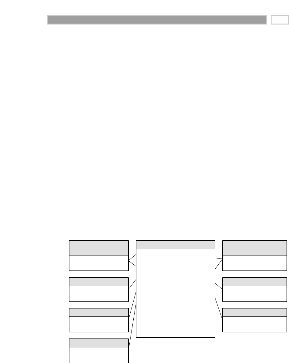
times uniformly in a single time zone such as Greenwich Mean Time (GMT).
We interpret the session date and time combinations as the beginning of the
session. Since we have the dwell time of the session as a numeric fact, we can
tell when the session ended if this is of interest.
The other requirement we will meet with this design is to record the date and
time of the session relative to the visitor’s wall clock. The best way to represent
this information is with a second pair of calendar date and time-of-day foreign
keys. Theoretically, we could represent the time zone of the customer in the
customer dimension table, but constraints to determine the correct wall clock
time would be horrendously complicated. The time difference between two
cities (such as London and Sydney) can change by as much as 2 hours at dif-
ferent times of the year depending on when these cities go on and off daylight
savings time. This is not the business of the end-user application to work out;
it is the business of the database to store this information so that it can be con-
strained in a simple and direct way.
Inclusion of the page dimension in Figure 14.3 may seem surprising given that
the grain of the design is the customer session. However, in a given session, an
interesting page is the entry page. We interpret the page dimension in this
design as the page with which the session started. In other words, how did the
customer hop onto our bus just now? Coupled with the referrer dimension, we
now have an interesting ability to analyze how and why the customer accessed
our Web site. A more elaborate design also would add an exit page dimension.
Figure 14.3 Clickstream schema at the session grain.
Universal Date Key (FK)
Universal Time of Day Key (FK)
Local Date Key (FK)
Local Time of Day Key (FK)
Customer Key (FK)
Entry Page Key (FK)
Session Key (FK)
Referrer Key (FK)
Causal Key (FK)
Session Seconds
Pages Visited
Orders Placed
Order Quantity
Order Dollar Amount
Clickstream Page Event Fact
Date Key (PK)
Date Attributes…
Date Dimension
(views for 2 roles)
Time of Day Key (PK)
Time of Day Attributes…
Time of Day Dimension
(views for 2 roles)
Customer Key (PK)
Customer Attributes…
Customer Dimension
Session Key (PK)
Session Attributes…
Session Dimension
Entry Page Key (PK)
Page Attributes…
Entry Page Dimension
Referrer Key (PK)
Referrer Attributes…
Referrer Dimension
Causal Key (PK)
Causal Attributes…
Causal Dimension
Electronic Commerce 293

We may be tempted to add the causal dimension to this design, but if the
causal dimension were intended to focus on individual products, it would be
inappropriate to add to this design. The symptom that the causal dimension
does not mesh with this design is the multivalued nature of the causal factors
for a given complete session. If we are running ad campaigns or special deals
for several products, how do we represent this multivalued situation if the
customer’s session involves several products? The right place for a product-
oriented causal dimension will be in the more fine-grained table we build in
the next fact table example. Conversely, a more broadly focused market causal
dimension that described market conditions affecting all products would be
appropriate for a session-grained fact table.
The session seconds fact is the total number of seconds the customer spent on
the site during this session. There will be many cases where we can’t tell when
the customer left. Perhaps the customer typed in a new URL. Conventional
Web server logs won’t detect this (although if the data is being collected by an
ISP that can see every click across sessions, then this particular issue goes
away). Or perhaps the customer got up out of the chair and didn’t return for
an hour. Or perhaps the customer just closed the browser without making any
more clicks. In all these cases our extract software needs to assign a small and
nominal number of seconds to this part of the session so that the analysis is not
distorted unrealistically.
The fact table shown in Figure 14.3 has 13 fields. Since all the foreign key fields
are surrogate keys, none of them needs to be represented in more than 4 bytes.
Similarly, all the measured facts are either integers or scaled integers. Again,
4-byte fields are reasonable for estimation purposes. Thus our fact table is about
52 bytes wide. If we collect 5 million new fact rows each day for our hypothet-
ical large Web site example, then we are adding 260 MB of data (before index-
ing) to the fact table each day. Over the course of a year, this would amount to
260 MB x 365 = 94.9 GB of unindexed data. This is big, but not ridiculously so.
Three years of data, together with indexing overhead, perhaps would consume
600 GB of disk space. Given the pace of Web marketing and Web technology, it
seems reasonable to plan on keeping only 3 years of data.
Note that the dimension tables, with the possible exception of the customer
dimension, are small by comparison with the main fact table. A fully indexed 50-
million-row customer table could occupy 200 GB of storage, about one-third the
size of the fact table. All the other dimension tables are negligible by comparison.
We purposely built this first fact table in our clickstream data mart to focus on
complete visitor sessions and to keep the size of the data mart under control.
The next table we design drops down to the lowest practical granularity we
can support in the data Webhouse: the individual page event.
CHAPTER 14
294
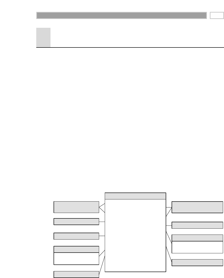
Clickstream Fact Table for
Individual Page Events
In this second fact table we will define the granularity to be the individual
page event in each customer session. With simple, static HTML pages, we may
be able to record only one interesting event per page view, namely, the page
view itself. As Web sites employ dynamically created XML-based pages with
the ability to establish an ongoing dialogue through the page, the number and
types of events will grow.
It is likely that this fact table will become astronomical in size. We will resist
the urge to aggregate the table up to a coarser granularity because such a step
inevitably involves eliminating dimensions. Actually, the first fact table we
built for this data mart represents just such an aggregation. It is a worthwhile
fact table, but the analyst cannot ask questions about visitor behavior or indi-
vidual pages. When the individual page-oriented data set gets too large, then
in order to preserve the ability to analyze detailed behavior, either the time
span of the data must be restricted or statistical sampling techniques must be
used to reduce data size. Although disk storage capacity has been doubling
even faster (every 12 months, supposedly) than processing power, our propen-
sity to collect reams of data seems to be doubling at an even faster pace.
Having chosen the grain, we can choose the appropriate dimensions. Our list
of dimensions includes calendar date, time of day, customer, page, event, ses-
sion, session ID, product, causal, and referrer. The completed design is shown
in Figure 14.4.
Figure 14.4 Clickstream schema at the page-event grain.
Universal Date Key (FK)
Universal Time of Day Key (FK)
Local Date Key (FK)
Local Time of Day Key (FK)
Customer Key (FK)
Page Key (FK)
Event Key (FK)
Session Key (FK)
Session ID (DD)
Referrer Key (FK)
Product Key (FK)
Causal Key (FK)
Page Seconds
Order Quantity
Order Dollar Amount
Clickstream Page Event Fact
Date Dimension
(views for 2 roles)
Time of Day Dimension
(views for 2 roles)
Customer Dimension
Session Dimension
Causal Dimension
Page Dimension
Referrer Dimension
Event Key (PK)
Event Attributes…
Event Dimension
Product Key (PK)
Product Attributes…
Product Dimension
Electronic Commerce 295

The design in Figure 14.4 looks rather similar to our first design. This similar-
ity between fact tables is typical of dimensional models. One of the charms of
dimensional modeling is the boring similarity of the designs. However, this is
where they get their power. When the designs have a predictable structure, all
the software up and down the data warehouse chain, from extraction, to data-
base querying, to the end-user tools, can exploit this similarity to great advan-
tage. Query and reporting tools, for example, may be able to adapt to a whole
family of dimensional designs without any reprogramming.
The two roles played by the calendar date and time-of-day dimensions have the
same interpretation as in the first design; one role is the universal synchronized
time, probably expressed in GMT, and the other role is the local wall clock time
as measured by the customer. In this fact table the date/time combinations refer
to the individual page event that is being described by the row we are building.
The page dimension refers to the individual page whose events we are record-
ing. This is the main difference in grain between this fact table and the first one
we built. In this fact table we will be able to see all the pages accessed by the
customers.
The event dimension describes what happened on the page, as we described
earlier in this chapter.
The session dimension describes the outcome of the session. A companion field,
the session ID, is a degenerate dimension that does not have a join to a dimension
table. The session ID is simply a unique identifier with no semantic content that
serves to group together the page events of each customer session in an unam-
biguous way. We did not need a session ID degenerate dimension in our first fact
table because each row in that table already represented a complete session. We
recommend that the session dimension be at a higher level of granularity than the
session ID because the session dimension is intended to describe classes and cat-
egories of sessions, not the characteristics of each individual session.
We show a product dimension in this design under the assumption that this
Web site is owned by a Web retailer. A financial services site probably would
have a similar dimension. A consulting services site would have a service
dimension. An auction site would have a subject or category dimension
describing the nature of the items being auctioned. A news site would have a
subject dimension, although with different content than an auction site.
We accompany the product dimension with a causal dimension so that we can
attach useful marketplace interpretations to the changes in demand we may
see for certain products.
CHAPTER 14
296
TEAMFLY
Team-Fly®

For each page event we record the number of seconds that we believe elapse
before the next page event. We call this page seconds to contrast it with session
seconds that we used in the first fact table. This is a simple example of paying
attention to conformed facts. If we called both these measures simply seconds,
then we would run the risk of having these seconds added or combined inap-
propriately. Since these seconds are not precisely equivalent, we name them
differently as a warning. In this particular case we would expect the page sec-
onds for a session in this second fact table to add up to the session seconds in
the first fact table.
Our final facts are order quantity and order dollar amount. These fields will be
zero or null for many of the rows in this fact table simply because the specific
page event is not the event that places the order. Nevertheless, it is highly
attractive to provide these fields because they tie all-important Web revenue
directly to behavior. If the order quantity and dollar amount were only avail-
able through the production order-entry system elsewhere in the data Web-
house, it would be inefficient to perform the revenue-to-behavior analysis
across multiple large tables. In many database management systems the exis-
tence of these kinds of null fields is handled efficiently and may take up liter-
ally zero space in the fact table.
We can quickly estimate the size of this fact table. If we use the earlier example
of 100 million raw Web log events each day, we probably end up with about 20
million meaningful page events per day after we discard the requests for GIF
and JPEG images. Each row in the page-event fact table has 15 fields, which we
estimate occupies 15 x 4 bytes = 60 bytes. Thus the total fact table data to be
added each day is 20 million x 60 bytes = about 1.2 GB per day. This would
amount to 365 x 1.2 GB = 438 GB per year, before indexing. Again, while this is
a large number, it is within reach of today’s technology.
As we move to more dynamic page delivery with better semantic labels on
each of the actions (thanks to XML), undoubtedly we will increase the volume
of data available. Perhaps we keep the granularity of the present table at
approximately one page view per row rather than making a row for each dis-
crete customer gesture. It is too early at this time to make a definitive predic-
tion of whether we will descend all the way to the individual gesture level
with a third and even more granular fact table. Even if our storage and query
technologies keep up with the increased volume of data, we need to wait to see
if there is sufficient analysis content in the lowest-level behavior data to make
it worthwhile. Hopefully, you can see how to extend the techniques of this
chapter to handle this case.
Electronic Commerce 297

Aggregate Clickstream Fact Tables
Both the fact tables we have built thus far in our clickstream data mart are
large. There are many business questions we would like to ask that would be
forced to summarize millions of rows from these tables. For example, if we
want to track the total visits and revenue from major demographic groups of
customers accessing our Web site on a month-by-month basis, we certainly can
do this with either fact table. In the session-grained fact table we would con-
strain the calendar date dimension to the appropriate time span (say, January,
February, and March of the current year). We would then create row headers
from the demographics type field in the customer dimension and the month
field in the calendar dimension (to separately label the three months in the out-
put). Finally, we would sum over the total order dollars and count the number
of sessions. This all works just fine. However, it is likely to be slow without
help from an aggregate table. If this kind of query is frequent, the DBA will be
encouraged to build an aggregate table such as shown in Figure 14.5.
We can build this table directly from our first fact table, whose grain is the indi-
vidual session. To build this aggregate table, we group by month, demographic
type, entry page, and session outcome. We count the number of sessions and
sum all the other additive facts. This results in a drastically smaller fact table,
almost certainly less than 1 percent of the original session-grained fact table.
This reduction in size translates directly to a corresponding increase in perfor-
mance for most queries. In other words, we would expect queries directed to
this aggregate table to run at least 100 times faster.
Although it may not have been obvious, we followed a careful discipline in build-
ing the aggregate table. This aggregate fact table is connected to a set of shrunken
dimensions directly related to the original dimensions in the session-grained fact
table. The month table is a conformed subset of the calendar-day table. The
demographic table is a conformed subset of the customer table. We assume that
the page and session tables are unchanged, although a careful design of the
aggregation logic could suggest a conformed shrinking of these tables as well.
Figure 14.5 Aggregated clickstream schema summarized by session characteristics.
Universal Month Key (FK)
Demographic Key (FK)
Entry Page Key (FK)
Session Outcome Key (FK)
Number of Sessions
Session Seconds
Pages Visited
Orders Placed
Order Quantity
Order Dollar Amount
Session Characteristics
Aggregate Fact
Month Dimension
Entry Page Dimension
Demographic Dimension
Session Outcome Dimension
CHAPTER 14
298

Integrating the Clickstream Data Mart
into the Enterprise Data Warehouse
In this section we look at the overall design of a series of data marts implemented
for a Web-based computer retailer. The data marts correspond to all the business
processes needed by this retailer to run its business. We could illustrate this
design by showing each schema as we have done in the preceding examples, but
the synergy among the designs would be difficult to see clearly. Instead, we use
the data warehouse bus matrix, which we introduced in Chapter 3.
The matrix method lists the data marts down the left side of the matrix and the
dimensions used by the data marts across the top of the matrix. The cells of the
matrix contain Xs if the particular data mart uses a particular dimension. Note
that the matrix describes data marts, not individual fact tables. Typically, a
data mart consists of a suite of closely associated fact tables all describing a
particular business process. A good way to start the design of a series of data
marts is to define first-level data marts that are, as much as possible, related to
single sources of data. Once several of these first-level data marts have been
implemented, then second-level consolidated data marts, such as profitability,
can be built that require data from the first-level marts to be combined. Thus the
entries in a given row of the matrix represent the existence of a dimension some-
where in the closely associated suite of tables defining a particular data mart.
Figure 14.6 shows the completed bus matrix for a Web retailer. The matrix has
a number of striking characteristics. There are a lot of Xs. An X in a given
matrix column is, in effect, an invitation to the meeting for conforming that
dimension. The average data mart uses six to eight dimensions. Some of the
dimensions, such as date/time, transaction, status/type, organization, and
employee, appear in almost every data mart. The product and customer
dimensions dominate the whole middle part of the matrix, where they are
attached to the data marts that describe customer-oriented activities. At the
top of the matrix, suppliers and parts dominate the processes of acquiring the
parts that make up products and building them to order for the customer. At
the bottom of the matrix we have classic infrastructure and cost-driver data
marts that are not tied directly to customer behavior.
We see the Web visitor clickstream data mart sitting squarely among the
customer-oriented data marts. It shares the date/time, transaction, product,
customer, media, causal, and service policy dimensions with several other
data marts nearby. In this sense it should be obvious that the Web visitor click-
stream data mart is well integrated into the fabric of the overall data ware-
house for this retailer. Applications tying the Web visitor clickstream will be
easy to integrate across all these data marts sharing these conformed dimen-
sions because the separate queries to each data mart will be able to be com-
bined across individual rows of the report.
Electronic Commerce 299
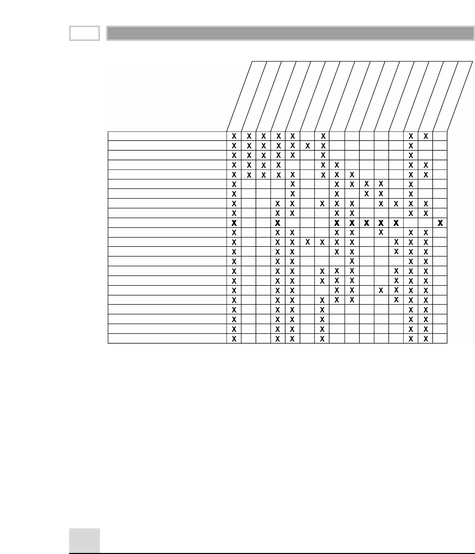
Figure 14.6 Data warehouse bus matrix for a Web retailer.
The Web visitor clickstream data mart contains the four special clickstream
dimensions not found in the other data marts. These dimensions do not pose a
problem for applications. Instead, the ability of the Web visitor clickstream
data mart to bridge between the Web world and the brick-and-mortar world is
exactly the advantage that we are looking for. We can constrain and group on
attributes from the four Web dimensions and explore the effect on the other
business processes. For example, we can see what kinds of Web experiences
produce customers who purchase certain kinds of service policies and then
invoke certain levels of service demands.
Electronic Commerce Profitability Data Mart
After the data Webhouse team successfully brings up the initial clickstream
data mart and ties this data mart to the sales transaction and customer
Supplier Purchase Orders
Supplier Deliveries
Part Inventories
Product Assembly Bill of Materials
Product Assembly to Order
Product Promotions
Advertising
Customer Inquiries
Customer Communications
Web Visitor Clickstream
Product Sales Transactions
Product Shipments
Customer Billing
Customer Payments
Product Returns
Product Support
Service Policy Orders
Service Policy Responses
Employee Labor
Human Resources
Facilities Operations
Web Site Operations
Date and Time
Part
Vendor
Transaction
Status and Type
Carrier
Facilities Location
Product
Customer
Media
Causal
Service Policy
Internal Organization
Employee
Clickstream (4 dims)
CHAPTER 14
300

communication data marts, the team may be ready to tackle the most chal-
lenging data mart of all: the Web profitability data mart.
We can build the Web profitability data mart as an extension of the sales trans-
action data mart. Fundamentally, we are going to allocate all the activity costs
and infrastructure costs down to each sales transaction. We could, as an alter-
native, try to build the Web profitability data mart on top of the clickstream,
but this would involve an even more controversial allocation process in which
we allocated costs down to each session. It would be hard to assign activity
and infrastructure costs to a session that had no obvious product involvement
and led to no immediate sale.
A big benefit of extending the sales transaction fact table is that we will get a
view of profitability over all our sales channels, not just the Web. In a way, this
should be obvious, because we know that we have to sort out the costs and
assign them to the various channels anyway. For this reason, we will call the
main fact table in our new data mart simply profitability.
Thus the grain of the profitability fact table is each individual product sold on
a sales ticket to a customer at a point in time. This sounds familiar, doesn’t it?
This grain is nearly identical to the grain of the first dimensional model we
designed. The primary difference is that Chapter 2’s schema was limited to the
grocer’s brick-and-mortar store. In this section the model will include profitabil-
ity metrics across all channels, including store sales, telesales, and Web sales.
We explored a profitability data mart extensively in Chapter 5. We enumerated
a lengthy list of profit and loss (P&L) facts from gross revenue to contribution
profit. Figure 14.7 illustrates these same facts in a somewhat broader context.
As we saw in Chapter 5, the fact table is organized as a simple P&L statement.
The first fact is our now-familiar quantity sold. The rest of the facts are dollar
values, beginning with gross revenue, which is the value of the item as if it
were sold at list or catalog price. We account for allowances and promotions to
arrive at net revenue, which is the true net price the customer pays times the
quantity purchased.
The rest of the P&L table consists of a series of subtractions, where we calcu-
late progressively for more far-reaching versions of profit. We begin by sub-
tracting the product manufacturing cost (if we manufacture it) or, equivalently,
the product acquisition cost (if we acquire it from a supplier). We then subtract
the product storage cost. At this point many enterprises refer to this partial
result as the gross profit. One can divide this gross profit by the gross revenue
to get the gross margin ratio.
Electronic Commerce 301
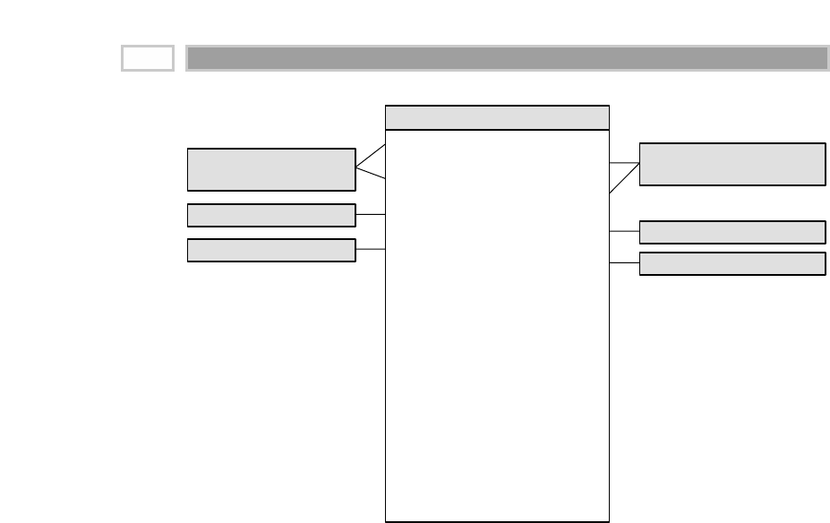
Figure 14.7 Electronic commerce profitability schema.
Obviously, the columns called “Net Revenue” and “Gross Profit” are calculated
directly from the fields immediately preceding them in the P&L table. However,
should we explicitly store these fields in the database? The answer depends on
whether you provide access to this fact table through a view or allow users or
applications to access the physical fact table directly. The structure of the P&L
table is sufficiently complex that, as the data warehouse provider, you don’t
want to risk having important measures such as net revenue and gross profit
computed incorrectly. If you provide all access through views, you can easily
supply the computed columns without physically storing them. However, if
your users are allowed to access the underlying physical table, then you should
include net revenue, gross profit, and net profit as physical fields.
Below the gross profit we continue subtracting various costs. Typically, the
warehouse team must source or estimate each of these costs separately.
Remember that the actual entries in any given fact table row are the fractions
of these total costs allocated all the way down to the individual fact row grain.
Often there is significant pressure on the warehouse team to finish the prof-
itability data mart. To put this another way, there is tremendous pressure to
source all these costs. But how good are the costs in the various underlying
Universal Date Key (FK)
Universal Time of Day Key (FK)
Local Date Key (FK)
Local Time of Day Key (FK)
Customer Key (FK)
Channel Key (FK)
Product Key (FK)
Promotion Key (FK)
Ticket Number (DD)
Quantity Sold
Gross Revenue
Manufacturing Allowance
Marketing Promotion
Sales Markdown
Net Revenue
Manufacturing Cost
Storage Cost
Gross Profit
Freight Cost
Special Deal Cost
Other Overhead Cost
Net Profit
Profitability Fact
Date Dimension
(views for 2 roles)
Customer Dimension
Product Dimension
Time of Day Dimension
(views for 2 roles)
Channel Dimension
Promotion Dimension
CHAPTER 14
302

data sets? Sometimes a cost is only available as a national average, computed
for an entire year. Any allocation scheme is going to assign a kind of pro forma
value that has no real texture to it. Other costs will be broken down a little bet-
ter, perhaps to the calendar quarter and by geographic region (if this is rele-
vant). Finally, some costs may be truly activity-based and vary in a highly
dynamic, responsive, and realistic way over time.
Web site system costs are an important cost driver in electronic commerce-
oriented businesses. Although Web site costs are classic infrastructure costs and
therefore are difficult to allocate directly to the product and customer activity,
this is a key step in developing a Web-oriented P&L statement. Various alloca-
tion schemes are possible, including allocating the Web site costs to various
product lines by the number of pages devoted to each product, allocating the
costs by pages visited, or allocating the costs by actual Web-based purchases.
Before leaving this design, it is worthwhile to reiterate that Figure 14.7’s prof-
itability fact table within a rich dimensional framework is immensely power-
ful. We can see the breakdown of all the components of revenue, cost, and
profit for every conceivable slice and dice supported by the dimensions. We
can ask, “How profitable are each of our channels (for example, Web sales,
telesales, and store sales) and why?” or “How profitable are all our possible
customer segmentations and why?” Of course, the symmetric dimensional
approach allows us to combine constraints from as many dimensions as we
can. This gives us compound versions of profitability analyses, such as, “Who
are the profitable customers in each channel and why?” or “Which promotions
work well on the Web but do not work well in other channels and why?”
Summary
The Web retailer example we used in this chapter is illustrative of any business
with a significant Web presence. Besides building the clickstream data mart,
the central challenge is to integrate the clickstream data effectively into the rest
of the business. In this chapter the key concepts included:
The challenge of identifying the Web visitor’s origin. In some cases we can
look backward through the referral information in the Web log, but in
many other cases this information is not supplied.
The challenge of identifying a complete session. HTTP sessions are stateless.
The use of cookies is the best mechanism for defining a session, bearing in
mind that we cannot explain all the time intervals between page requests.
The challenge of identifying the Web visitor. Even with a cookie, we cannot
be sure who the individual is at the other end.
Electronic Commerce 303

How to deal with proxy servers. A proxy server intercepts the visitor’s page
requests. We can inhibit the use of proxy servers, or in some cases we can
collect the logs.
The design of the page dimension. The key step is to get the Web page
designer to assign content codes and attributes to each page and then
embed these codes and attributes into the Web server logs.
The design of the session dimension. The key step is to use the record of the
complete session, together with some simple criteria, to provide a session
diagnosis that can be used to look for sessions of different types.
The design of a clickstream fact table for complete sessions. This fact table
is an interesting compromise between a high-level summary of Web site
activity and the overwhelming detail provided by a fact table for each page
event.
The design of a clickstream fact table for each page event. This ultimate
level of detail is the most accurate and complete record of customer behav-
ior. The size problems with this table can be addressed by sampling.
The design of aggregate clickstream fact tables. Much smaller (and faster)
fact tables can usefully summarize visitor behavior, such as correlating
demographics with productive sessions.
How to integrate the clickstream data mart into the rest of the data ware-
house. Using the bus matrix design method, we see which dimensions
must be conformed across all the data marts, and we see that the click-
stream data mart has a significant overlap with the other data marts.
How to add profitability measures to the product sales data mart so that
the contribution of the Web channel can be isolated and analyzed.
CHAPTER 14
304

Insurance
CHAPTER
15
305
We will bring together concepts from nearly all the previous chapters to build a
data warehouse for a property and casualty insurance company in this final
case study. If you are from the insurance industry and jumped directly to this
chapter for a quick fix, please accept our apology, but this material depends
heavily on ideas from the earlier chapters. You’ll need to turn back to the
beginning of the book to have this chapter make any sense.
As has been our standard procedure, this chapter is launched with back-
ground information for a business case. While the requirements unfold, we’ll
draft the data warehouse bus matrix, much like we would in a real-life require-
ments analysis effort. We’ll then design a series of dimensional models by
overlaying the core techniques learned thus far in a manner similar to the
overlay of overhead transparencies.
Chapter 15 reviews the following concepts:
■■ Requirements-driven approach to dimensional design
■■ Value-chain implications
■■ Data warehouse bus matrix
■■ Complementary transaction, periodic snapshot, and accumulating snapshot
schemas
■■ Four-step design process for dimensional models
■■ Dimension role-playing
■■ Handling of slowly changing dimension attributes
■■ Minidimensions for dealing with large, more rapidly changing dimension
attributes

■■ Multivalued dimension attributes
■■ Degenerate dimensions for operational control numbers
■■ Audit dimensions to track data lineage
■■ Heterogeneous products with attributes and facts that vary by line of business
■■ Conformed dimensions and facts
■■ Consolidated fact tables that combine metrics from separate business
processes
■■ Factless fact tables
■■ Common mistakes to avoid when designing dimensional models
Insurance Case Study
Let’s imagine that we work for a $5 billion property and casualty insurer that
offers automobile, homeowners’, and personal property insurance. We con-
duct extensive interviews with representatives and senior management from
the claims, field operations, actuarial, finance, and marketing departments.
Based on these interviews, we learn that the insurance industry is in a state of
flux. New, nontraditional players are entering by leveraging alternative chan-
nels, such as the Internet. In the meantime, the industry is consolidating due to
globalization, deregulation, and demutualization challenges. Markets are
changing, along with customer needs. Numerous interviewees tell us that
information is becoming an even more important strategic asset. Regardless of
the functional groups, there is a strong desire to use information more effec-
tively to identify opportunities more quickly and respond most appropriately.
The good news is that internal systems and processes already capture the bulk
of the data required. Most insurance companies generate tons of nitty-gritty
operational data. The bad news is that the data is not integrated. Over the
years, political and data-processing boundaries have encouraged the con-
struction of tall barriers around these isolated islands of data. There are multi-
ple disparate sources for information about the company’s products,
customers, and distribution channels. In the legacy operational systems, the
same policyholder may be identified several times in separate automobile,
home, and personal property applications. Traditionally, this segmented
approach to data was acceptable because the different lines of business func-
tioned largely autonomously. There was little interest in sharing data across
units for cross-selling and collaboration in the past. Now we’re attempting to
better leverage an enormous amount of inconsistent yet somewhat redundant
data.
Besides the inherent issues surrounding data integration, business users lack
the ability to access data easily when needed. In an attempt to address this
CHAPTER 15
306
TEAMFLY
Team-Fly®

shortcoming, several organizations within the insurance company rallied their
own resources and hired consultants to solve their individual short-term data
needs. In many cases the same data was extracted from the same source sys-
tems to be accessed by separate organizations without any strategic overall
information-delivery strategy. Unfortunately, no one had the courage to pro-
actively inform senior management of the negative consequences of this
approach.
It didn’t take long for management to recognize the negative ramifications
associated with separate data warehouses because performance results pre-
sented at executive meetings differed depending on the analytic source. Man-
agement understood that this independent route was not viable as a long-term
solution because of the lack of integration, large volumes of redundant data,
and difficulty in accessing and interpreting the results. Given the importance
of information in this brave new insurance world, management was moti-
vated to deal with the cost implications surrounding the development, sup-
port, and analytic inefficiencies of these supposed data warehouses that
merely proliferated the operational data islands.
A new chief information officer (CIO) was hired to lead the information
charge. Senior management chartered the CIO with the responsibility and
authority to break down the historical data silos to “achieve information nir-
vana.” They charged the CIO with the fiduciary responsibility to manage and
leverage the organization’s information assets more effectively. The CIO
developed an overall vision that wed an enterprise strategy for dealing with
massive amounts of data, with a response to the immediate need to become an
information-rich organization. In the meantime, an enterprise data warehouse
team was created to begin designing and implementing the vision.
Senior management has been preaching about a transformation to a more
customer-centric focus instead of the traditional product-centric approach in an
effort to gain competitive advantage. The CIO jumped on that bandwagon as a
catalyst for change and already has had an impact. The message has reached
the folks in the trenches. They pledge intent to share data rather than squirrel-
ing it away for a single purpose. There is a strong desire for everyone to have
a common understanding of the state of the business. They’re clamoring to get
rid of the isolated pockets of data while ensuring that they have access to
detail and summary data at both the enterprise and line-of-business levels.
Insurance Value Chain
The primary value chain of an insurance company is seemingly short and
simple. The core processes are to issue policies, collect premium payments,
and process claims. The organization is interested in better understanding the
Insurance 307

metrics spawned by each of these processes. Users want to analyze detailed
transactions relating to the formulation of policies, as well as transactions
generated by claims processing. They want to measure profit over time by
coverage, covered item type (that is, which kinds of houses and automobiles),
geographic, demographic, and sales distribution channel characteristics. Of
course, the desire to monitor profit implies that both revenues and costs can
be identified and tracked. While users are interested in the enterprise per-
spective, they also want to analyze the heterogeneous nature of the insurance
company’s lines of business.
Obviously, an insurance company is engaged in many other external
processes, such as the investment of premium payments, as well as a host of
internally focused activities, such as human resources, finance, and purchas-
ing. For now, we’ll focus on the core business related to policies and claims.
The insurance value chain begins with a variety of policy transactions. Based
on our current understanding of the requirements and underlying data, we opt
to handle all the transactions having an impact on a policy as a single business
process (and fact table). If this perspective is too simplistic to accommodate the
metrics, dimensionality, or analytics required, we have the option to split the
transaction activities into separate fact tables (for example, separate fact tables
for quoting, rating, and underwriting). As we discussed in Chapter 3, there are
tradeoffs between creating separate fact tables for each natural cluster of trans-
action types versus lumping the transactions into a single fact table.
While we’re on the topic of policies, there is also a need to better understand the
premium revenue associated with each policy on a monthly basis. This will be
key input into the overall profit picture. In the case of insurance, the business is
very transaction-intensive, but the transactions themselves do not represent lit-
tle pieces of revenue, as was the case with retail or manufacturing sales. We can-
not merely add up insurance transactions to determine the revenue amount. The
picture is further complicated in insurance because customers pay in advance
for services. We encounter this same advance-payment model in organizations
that offer magazine subscriptions or extended warranty contracts. Premium
payments must be spread out across multiple reporting periods because the
organization earns the revenue over time as it provides insurance coverage. The
complex relationship between individual transactions and the basic measures of
revenue often makes it impossible to answer revenue questions by crawling
through the individual transactions. Not only is such crawling time-consuming,
but the logic required to interpret the effect of different transaction types on rev-
enue also can be horrendously complicated. The natural conflict between the
detailed transaction view and the monthly snapshot perspective almost always
requires that we build both kinds of fact tables in the warehouse. In this case, the
premium snapshot is not merely a summarization of the policy transactions; it is
quite a separate thing that comes from a separate source.
CHAPTER 15
308

Figure 15.1 Initial draft bus matrix.
Draft Insurance Bus Matrix
Based on the interview findings, along with an understanding of the key
source systems, the team begins to draft a data warehouse bus matrix with the
core business processes as rows and core dimensions as columns. At this point
we’re focused on the policy-based processes. We put two rows in the matrix,
one corresponding to the policy transactions and another for the monthly pol-
icy premium snapshot.
As illustrated in Figure 15.1, the core dimensions include date, policyholder,
employee, coverage, covered item, and policy. When drafting the matrix, we
don’t attempt to include all the dimensions because the matrix could end up
with 100 columns or more. Instead, we try to focus on the core common
dimensions that are reused in more than one schema.
Policy Transactions
Now let’s turn our attention to the first row of the matrix by focusing on the
transactions for creating and altering a policy. We assume that the policy is the
header for a set of coverages sold to the policyholder. Coverages can be con-
sidered the products sold by the insurance company. Homeowner coverages
include fire, flood, theft, and personal liability. Automobile coverages include
comprehensive, collision damage, uninsured motorist, and personal liability.
In a property and casualty insurance company, coverages typically apply to a
specific covered item, such as a particular house or car. Both the coverage and
covered item are identified carefully in the policy. A particular covered item
usually will have several coverages listed in the policy. We assume that a pol-
icy can contain multiple covered items.
Just to keep things reasonably simple, an agent sells the policy to the policy-
holder in this case. Before the policy can be created, a pricing actuary deter-
mines the premium rate that will be charged given the specific coverages,
covered items, and qualifications of the policyholder. An underwriter, who
Policy Transactions
Policy Premium Snapshot
Date
Policyholder
Coverage
Covered Item
Employee
Policy
BUSINESS PROCESSES
COMMON DIMENSIONS
Insurance 309

takes ultimate responsibility for doing business with the policyholder, makes
the final approval.
The operational policy transaction system captures the following types of
transactions:
■■ Create policy, alter policy, cancel policy (with reason)
■■ Create coverage on covered item, alter coverage, cancel coverage
(with reason)
■■ Rate coverage, decline to rate coverage (with reason)
■■ Underwrite policy, decline to underwrite policy (with reason)
The grain of the policy transaction fact table would be one row for each indi-
vidual policy transaction. Each atomic transaction should be embellished with
as much context as possible to create a complete dimensional description
of the transaction. The dimensions associated with the policy transaction
business process include the transaction date, effective date, policyholder,
employee, coverage, covered item, policy number, and policy transaction type.
Dimension Details and Techniques
Now let’s further discuss the dimensions in this schema while taking the
opportunity to reinforce concepts from earlier chapters.
Dimension Role-Playing
There are two dates associated with each policy transaction. The policy trans-
action date is the date when the transaction was entered into the operational
system, whereas the policy transaction effective date is when the transaction
legally takes effect. These two independent dimensions can be implemented
using a single physical date table. Multiple logically distinct tables are then
presented to the user through views with unique column names, as described
originally in Chapter 5.
The policyholder is the customer in this schema. The policyholder can be multi-
ple people, such as a person and his or her spouse, or the policyholder can be a
business entity. The policyholder dimension often qualifies as a large dimension,
as is the case with our $5 billion insurer that caters to millions of policyholders.
Slowly Changing Dimensions
Insurance companies typically are very interested in tracking changes to dimen-
sions over time. We’ll apply the three basic techniques for handling slowly
changing dimension attributes that we introduced in Chapter 4 to the policy-
holder dimension.
CHAPTER 15
310

With the type 1 approach, we simply overwrite the preceding dimension
attribute value. This is the simplest approach to dealing with attribute changes
because the attributes always represent the most current descriptors. For
example, perhaps the business agrees to handle changes to the policyholder’s
date of birth as a type 1 change based on the assumption that any changes to
this attribute are intended as corrections. In this manner, all fact table history
for this policyholder appears to have always been associated with the updated
date-of-birth value.
Since the policyholder’s ZIP code is key input to the insurer’s pricing and risk
algorithms, users are very interested in tracking ZIP code changes, so we opt
to use a type 2 approach to this attribute. Type 2 is the most common slowly
changing dimension (SCD) approach when there’s a requirement for accurate
change tracking over time. In this case, when the ZIP code changes, we create
a new policyholder dimension row with a new surrogate key and updated
geographic attributes. We do not go back and revisit the fact table. Historical
fact table rows, prior to the ZIP code change, still reflect the old surrogate key.
Going forward, we use the policyholder’s new surrogate key so that new fact
table rows join to the postchange profile. While this technique is extremely
graceful and powerful, it places more burdens on the data staging application.
Also, the number of rows in the dimension table grows with each type 2 SCD
change. Given that there are already well over 1 million rows in our policy-
holder dimension table, we may opt to use a minidimension for tracking ZIP
code changes, which we’ll review shortly.
Finally, let’s assume that each policyholder is classified as belonging to a par-
ticular segment. Perhaps we historically tagged our nonresidential policy-
holders as either commercial or government entities. Going forward, the
business users want more detailed customer classifications. For instance, the
new policyholder segments may differentiate between large multinational,
middle market, and small business commercial customers, in addition to
nonprofit organizations and governmental agencies. For a period of time,
users want the ability to analyze results by either the historical or new seg-
ment classifications. In this case we could use a type 3 approach to track the
change for a period of time. We add a column to the dimension table, labeled
“Historical Policyholder Segment Type,” to retain the old classifications. The
new classification values would populate the segment attribute that has been
a permanent fixture on the policyholder dimension. This approach, while
not extremely common, allows us to see performance by either the current or
historical segment maps. This is useful when there’s been an en masse
change, such as the customer classification realignment. Obviously, the type
3 technique becomes overly complex if we need to track more than one ver-
sion of the historical map or if we need to track before and after changes for
multiple dimension attributes.
Insurance 311

Minidimensions for Large or Rapidly
Changing Dimensions
As we referenced earlier, the policyholder dimension qualifies as a large
dimension with more than 1 million rows. The covered item dimension likely
also falls into this category because most policyholders insure more than one
specific item. In both cases, it is often important to track content values accu-
rately for a subset of attributes. For example, we need an accurate description
of some policyholder and covered item attributes at the time the policy was
created, as well as at the time of any adjustment or claim. We saw in Chapter 6
that the practical way to track changing attributes in large dimensions was to
split the closely monitored, more rapidly changing attributes into one or more
minidimensions directly linked to the fact table with a separate surrogate key.
The use of minidimensions has an impact on the efficiency of attribute brows-
ing because users typically want to browse and constrain on these changeable
attributes, as well as on updating. If all possible combinations of the attribute
values in the minidimension have been created already, handling a mini-
dimension change simply means placing a different key in the fact table row
from a certain point in time forward. Nothing else needs to be changed or
added to the database.
Multivalued Dimension Attributes
We discussed multivalued dimension attributes in Chapter 9 when we associ-
ated multiple customers with an account and then again in Chapter 13 when a
patient encounter involved multiple diagnoses. We certainly could duplicate
the multiple customers per account design for each policy, but in this case
study we’ll look at yet another multivalued modeling situation: the relation-
ship between commercial customers and their industry classifications.
Each commercial customer may be associated with one or more standard
industry classification (SIC) codes. A large, diversified commercial customer
could be represented by a dozen or more SIC codes. Much like we did with
Chapter 13’s diagnosis group, we build an SIC group bridge table to tie
together all the SIC codes within an SIC group. This SIC bridge table joins to the
customer dimension as an outrigger. It allows us to report fact table metrics by
any attribute in the SIC table, either correctly weighted or as an impact report.
To handle the case where no valid SIC code is associated with a given customer,
we simply create a special SIC dimension row that represents “Unknown.”
Let’s move on to the coverage dimension. Large insurance companies will
have dozens or even hundreds of separate coverage products available to sell
for a given type of covered item. If the coverage has specific limits or
deductibles, we generally treat these numeric parameters as facts rather than
CHAPTER 15
312

creating a distinct coverage for every different possible value. For example, a
basic limit on homeowner’s fire protection is the appraised value of the house.
Since the appraised value can be thought of as a continuously valued numeric
quantity that is measured each time we look at a different policy and can even
vary for a given policy over time, we treat limits as legitimate facts.
The covered item is the house, the car, or other specific insured item. The cov-
ered item dimension contains one row for each actual covered item. As we men-
tioned earlier, the covered item dimension is usually somewhat larger than the
policyholder dimension, so it’s a good place to consider deploying a mini-
dimension. In general, it is not desirable to capture the variable descriptions of
the physical covered objects as facts because most are textual and are not
numeric or continuously valued. In most cases a textual measurement is a
description of something drawn from a discrete list of alternatives. The designer
should make every effort to put textual measures into dimension tables because
they can be correlated more effectively with the other textual attributes in a
dimension and require much less space, especially if the proposed fact table text
column is a wide, fixed-width field that is often empty. Textual facts can be
counted and constrained on, but if they are unpredictable free text, the usual
dimensional activities of constraining and grouping on these text values will be
of little value. A true text fact is not a very good thing to have in a fact table.
The employee is the individual responsible for creating the transaction. For
create policy and create coverage transactions, the responsible employee is the
agent. For rating transactions, the employee is the rater. Likewise, the under-
writer is the employee involved in underwriting transactions.
Degenerate Dimension
The policy number will be treated as a degenerate dimension if we have
extracted all the header information associated with the policy into the other
dimensions. We obviously want to avoid creating a policy transaction fact table
with just several keys while embedding all the descriptive details (including the
policyholder, dates, and coverages) in a policy dimension. In some cases there
may be one or two attributes that still belong to the policy and not to another
dimension. For example, if the underwriter establishes an overall risk grade for
the policy, based on the totality of the coverages and covered items, then this risk
grade probably belongs in a policy dimension. Of course, in this scenario we no
longer have a degenerate dimension.
The policy transaction type dimension is a small dimension consisting of the
transaction types listed earlier together with all the possible reason descrip-
tions for the applicable transactions. Usually, a transaction type dimension
contains less than 100 entries, although not always.
Insurance 313

Audit Dimension
We always have the option to add keylike information to the transaction fact
row, such as an audit key that links to a dimension row created by the extract
process. As we described in Chapter 8, each audit dimension row can describe
the data lineage of the fact row, including the time of the extract, the source
table, and the version of the extract software.
We are now able to present the policy transaction schema, as illustrated in Fig-
ure 15.2. The resulting fact table illustrates several characteristics of a classic
transaction-grain fact table. First of all, the fact table consists almost entirely of
keys. Transaction-level schemas allow us to analyze behavior in extreme detail.
As we descend to lower granularity with atomic data, the fact table naturally
sprouts more dimensionality. In this case the fact table has a single numeric fact,
called policy transaction amount. Interpretation of the amount column depends
on the type of transaction, as identified in the transaction type dimension.
Because there are different kinds of transactions in the same fact table, we usu-
ally cannot label the fact with anything more specific. If the transaction-
processing system introduces additional types of transactions, they represent a
change to the data content but don’t necessitate a schema modification.
Heterogeneous Products
While there is strong support for an enterprise-wide perspective at our insur-
ance company, the business users don’t want to lose sight of their line-of-
business specifics. Insurance companies typically are involved in multiple yet
very different lines of business. For example, the detailed parameters of home-
owners’ coverages differ significantly from automobile coverages. And these
both differ substantially from personal property coverage, general liability
coverage, and other types of insurance. Although all coverages can be coded
into the generic structures we have used so far in this chapter, insurance com-
panies want to track numerous specific attributes (and perhaps facts) that only
make sense for a particular coverage and covered item. We can generalize the
initial schema developed in Figure 15.2 by using the heterogeneous products
technique we discussed in Chapter 9.
Figure 15.2 Policy-creation transaction schema.
Policy Transaction Date Key (FK)
Policy Effective Date Key (FK)
Policyholder Key (FK)
Employee Key (FK)
Coverage Key (FK)
Covered Item Key (FK)
Policy Transaction Type Key (FK)
Policy Transaction Audit Key (FK)
Policy Number (DD)
Policy Transaction Amount
Policy Transaction Fact
Date Dimension (views for 2 roles)
Policyholder Dimension
Employee Dimension Covered Item Dimension
Policy Transaction Type Dimension
Policy Transaction Audit Dimension
Coverage Dimension
CHAPTER 15
314

In Figure 15.3 we show a schema to handle the specific attributes that describe
automobiles and their coverages. For each line of business (or coverage type),
we create custom dimension tables for both the covered item and the coverage.
When an access application needs the specific attributes of a single coverage
type, it uses the appropriate custom dimension tables.
Notice in this transactional schema that we don’t need a custom fact table. We
only introduce custom dimension tables to handle the special automobile
attributes. No new keys need to be generated; logically, all we are doing is
extending existing dimension rows.
Alternative (or Complementary)
Policy Accumulating Snapshot
Finally, before we leave policy transactions, we want to mention briefly the
use of an accumulating snapshot to capture the cumulative effect of the trans-
actions. In this case the grain of the fact table likely would be one row for each
coverage/covered item on a policy. We can envision including the following
policy-centric dates in the fact table: quoted, rated, underwritten, effective,
renewed, and expiration. Many of the other dimensions we discussed also
would be applicable to this schema, with the exception of the transaction type
dimension. The accumulating snapshot likely would have an expanded fact
set. As we discussed in Chapter 5, an accumulating snapshot is effective for
collecting information about the key milestones of the policy transaction
process. It represents the cumulative lifespan of a policy, covered items, and
coverages; however, it does not capture information about each and every
transaction that occurred. Unusual transactional events or unexpected out-
liers from the standard process could be masked with an accumulating per-
spective. On the other hand, this type of snapshot, sourced from the
transactions, provides a clear picture of the durations or lag times between
key process events.
Figure 15.3 Policy transaction schema with custom automobile dimension tables.
Coverage Key (PK)
Coverage Description
Line of Business Description
Automobile Deductible
Windshield Coverage Included
Rental Car Coverage Included
Automobile Coverage
Dimension Policy Transaction Date Key (FK)
Policy Effective Date Key (FK)
Policyholder Key (FK)
Employee Key (FK)
Coverage Key (FK)
Covered Item Key (FK)
Policy Transaction Type Key (FK)
Policy Transaction Audit Key (FK)
Policy Number (DD)
Policy Transaction Amount
Policy Transaction Fact
Covered Item Key (PK)
Covered Item Description
Vehicle Manufacturer
Vehicle Make
Vehicle Year
Vehicle Classification
Engine Size
Number of Passenger Capacity
Driver's Airbag Indicator
Automobile Covered
Item Dimension
Insurance 315

Policy Periodic Snapshot
The policy transaction schema is very useful for answering a wide range of ques-
tions. However, the blizzard of transactions makes it difficult to quickly deter-
mine the status or financial value of a policy at a given point in time. Even if all
the necessary detail lies in the transaction data, a snapshot perspective would
require rolling the transactions forward from the beginning of history. Not only is
this nearly impractical on a single policy, but it is ridiculous to think about gener-
ating summary top-line views of key performance metrics in this way.
The answer to this dilemma is to create a second fact table that operates as a
companion to the policy transaction table. In this case the business process is
the monthly policy premium snapshot. The granularity of the fact table is one
row per coverage and covered item on a policy each month.
Conformed Dimensions
Of course, when we approach this second business process within our insur-
ance company, we strive to reuse as many dimensions as makes sense at the
periodic snapshot granularity. Hopefully, you have become a conformed
dimension enthusiast by now. As we indicated in Chapter 3, conformed
dimensions used in separate fact tables either must be identical or must repre-
sent a subset of the most granular version of the dimension.
The policyholder, covered item, and coverage dimensions would be identical.
We replace the daily date dimension with a conformed month dimension
table. We don’t need to track all the employees that were somehow involved in
policy transactions on a monthly basis, although it may be useful to retain the
involved agent, especially since field operations are so focused on ongoing
revenue performance analysis. The transaction type dimension would not be
used because it does not apply at the periodic snapshot granularity. Instead,
we introduce a status dimension so that users can discern quickly the current
state of a coverage or policy, such as new policies or cancellations this month
and over time.
Conformed Facts
While we’re on the topic of conformity, we also need to use conformed facts. If
the same facts appear in multiple fact tables, such as some facts that are com-
mon to this snapshot fact table as well as the consolidated fact table we’ll dis-
cuss later in this chapter, then they must have consistent definitions and labels.
If the facts are not identical, then they need to be given different names.
CHAPTER 15
316
TEAMFLY
Team-Fly®

Pay-in-Advance Metrics
Business management wants to know how much premium revenue was written
(or sold) each month, as well as how much revenue was earned. In this case we
can’t derive revenue metrics merely by summarizing the detailed policy trans-
actions. While a policyholder may contract and pay for specific coverages on
specific covered items for a period of time, the revenue is not earned until the
service is provided. In the case of the insurance company, the revenue from a
policy is earned month by month as long as the customer doesn’t cancel the pol-
icy. A correct calculation of a metric such as earned premium would mean fully
replicating all the business rules of the operational revenue-recognition system
within the data warehouse access application. Typically, the rules for converting
a transaction amount into its monthly revenue impact are very complex, espe-
cially with coverage upgrades and downgrades. Fortunately, these metrics can
be sourced from a separate operational revenue-recognition system.
As we see in the periodic snapshot in Figure 15.4, we include two premium
revenue metrics in the fact table to handle the different definitions of written
versus earned revenue. Simplistically, if an annual policy for a given coverage
and covered item was written on January 1 for a cost of $600, then the written
premium for January would be $600, whereas the earned premium is $50 ($600
divided by 12 months). In February, the written premium is zero, whereas the
earned premium is still $50. If the policy is canceled on March 31, the earned
premium for March is $50, whereas the written premium is a negative $450.
Obviously, at this point the earned-revenue stream comes to a crashing halt.
Pay-in-advance business scenarios typically require the combination of a
transaction-grained fact table and a monthly snapshot-grained fact table in
order to answer questions of transaction frequency and timing, as well as
questions of earned income in a given month. We can almost never add
enough facts to a snapshot schema to do away with the need for a transaction
schema, or vice versa.
Figure 15.4 Periodic policy snapshot schema.
Month End Snapshot Date Key (FK)
Policyholder Key (FK)
Coverage Key (FK)
Covered Item Key (FK)
Agent Key (FK)
Policy Status Key (FK)
Policy Number (DD)
Written Premium Revenue Amount
Earned Premium Revenue Amount
Policy Premium Snapshot Fact
Month End Dimension
Policyholder Dimension
Coverage Dimension
Covered Item Dimension
Agent Dimension
Policy Status Dimension
Insurance 317

Heterogeneous Products Again
We are again confronted with the need to look at snapshot data by more spe-
cific line-of-business attributes. In this case we also need to grapple with
snapshot facts that vary by line of business. Because the custom facts for each
line are incompatible with each other, for any given snapshot row, most of
the fact table would be filled with nulls. In this scenario, the answer is to sep-
arate the monthly snapshot fact table physically by line of business. We end
up with the single core monthly snapshot schema and a series of custom
monthly snapshots, one for each line of business or coverage type. Each of
the custom snapshot fact tables is a copy of a segment of the core fact table
for just those coverage keys and covered item keys belonging to a particular
line of business. We include the core facts as a convenience so that analyses
within a coverage type can use both the core and custom facts without hav-
ing to access two large fact tables. Alternatively, we could handle the
extended fact set by adding a special join key to each fact table row, as
described in Chapter 9.
Multivalued Dimensions Again
Automobile insurance provides us with another opportunity to discuss multi-
valued dimensions. Often multiple insured drivers are associated with a poli-
cyholder. We can construct a bridge table, as illustrated in Figure 15.5, to
capture the relationship between the insured drivers and the policyholder. In
this case the insurance company can calculate the weighting factor more real-
istically based on each driver’s share of the total premium cost. We also can
assign begin and end dates to the bridge table rows to capture relationship
changes over time, as required.
Figure 15.5 Handling multiple drivers associated with a policy.
Month End Snapshot Date Key (FK)
Policyholder Key (FK)
More Foreign Keys …
Written Premium Revenue Amount
Earned Premium Revenue Amount
Policy Premium Snapshot Fact
Policyholder Key (FK)
Insured Driver Key (FK)
Weighting Factor
Policyholder-Insured
Driver Bridge
Insured Driver Key (PK)
Insured Driver Name
Insured Driver Address Attributes ...
Insured Driver Date of Birth
Insured Driver Occupation
Insured Driver Accident History Attributes ...
Insured Driver Dimension
CHAPTER 15
318

More Insurance Case Study Background
Unfortunately, the insurance business has a downside. We learn from the inter-
viewees that there’s more to life than collecting premium payments. The costs in
this industry predominantly result from claims or losses. After a policy with its
associated coverages and covered items is in effect, then a claim can be made
against a specific coverage and covered item. A claimant, who may be the policy-
holder or perhaps a new party not previously known to the insurance company,
makes the claim. The claimant provides a description of the loss in the claim. The
nature of the claim obviously depends on the coverage and covered item.
When the insurance company opens a new claim, a reserve is usually estab-
lished at this time. The reserve is a preliminary estimate of the insurance com-
pany’s eventual liability for the claim. As further information becomes known,
this reserve can be adjusted.
Before the insurance company pays any claim, there is usually an investigative
phase where the insurance company sends out an adjuster to examine the cov-
ered item and interview the claimant, policyholder, or other individuals
involved. The investigative phase produces a stream of transactions. In com-
plex claims, various outside experts may be required to pass judgment on the
claim or the extent of the damage.
In most cases, after the investigative phase, the insurance company issues a
number of payments. Many of these payments go to third parties such as doc-
tors, lawyers, or automotive body shop operators. Some payments may go
directly to the claimant. A large insurance company may have more than
1,000 individuals who are authorized to issue payments against open claims.
For this reason, it is important to clearly identify the employee responsible for
every payment made against an open claim.
The insurance company may take possession of the covered item after replac-
ing it for the policyholder or claimant. In many such cases there is a salvage
value to the item, which is realized eventually by the insurance company. Sal-
vage payments received are a credit against the claim accounting.
Eventually, the payments are completed, and the claim is closed. If nothing
unusual happens, this is the end of the transaction stream generated by the
claim. However, in complex cases, further claims are made at later times or
claimant lawsuits may force a claim to be reopened. In this case the reserve usu-
ally is reset as well. An important measure for an insurance company is how
often and under what circumstances claims are reopened and reserves are reset.
Toward the tail end of processing a complex claim, the insurance company
may believe that further money will flow back to the insurance company when
Insurance 319

pending lawsuits or counterclaims are resolved eventually. The insurance
company may choose to sell the rights to all such further recoveries to special-
ists who are prepared to wait out the resolution of the lawsuits or counter-
claims. Although such sales take place at a discount, they allow the insurance
company to get cash immediately and close its books on the claim. This option
is known as subrogation and generates its own special transaction.
In addition to analyzing the detailed transactions, the insurance company also
wants to understand what happens during the life of a claim. For example, the
time lag between the claim open date and the first payment date is an impor-
tant measure of claims processing efficiency.
Updated Insurance Bus Matrix
With a better understanding of the claims side of the house, we’ll revisit the
draft matrix from Figure 15.1. Based on the new requirements we’ve uncov-
ered, we add another row to the matrix to accommodate claims transactions,
as shown in Figure 15.6. Many of the dimensions identified earlier in the proj-
ect will be reused; we added new columns to the matrix for the claim,
claimant, and third party.
Project teams sometimes struggle with the level of detail captured in a bus
matrix. In the planning phase of an architected data warehouse project, it
makes sense to stick with rather high-level business processes (or sources).
Multiple fact tables may result from each of these business process rows. As
we delve into the implementation phase, we sometimes take a subset of the
matrix to a lower level of detail by reflecting all the fact tables resulting from
the process as separate matrix rows. At this point the matrix can be enhanced
in several ways. We can add columns to reflect the granularity and metrics
associated with each fact table. Likewise, we can indicate the use of more sum-
marized conformed dimensions, especially when documenting an aggregated
schema. We’ve illustrated this lower implementation bus matrix in Figure 15.7.
Figure 15.6 Updated insurance bus matrix.
Policy Transactions
Policy Premium Snapshot
Claims Transactions
Date
Policyholder
Coverage
Claim
Claimant
3rd Party
Covered Item
Employee
Policy
CHAPTER 15
320
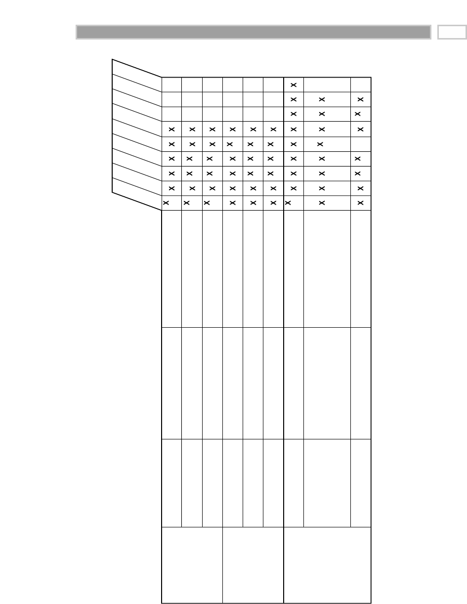
Figure 15.7 Implementation bus matrix detailing fact tables for each business process.
Business Process Fact Table Granularity Facts
Date
Policyholder
Coverage
Claim
Claimant
3rd Party
Covered Item
Employee
Policy
Trxn
Eff
Trxn
Eff
Trxn
Eff
Trxn
Eff
Auto
Home Home
Auto
Home
Auto
Auto
Auto
Home
Auto
Agent
Agent
Agent
Agent
Auto
Original Reserve Amount, Assessed
Damage Amount, Reserve Adjustment
Amount, Current Reserve Amount, Open
Reserve Amount, Claim Amount Paid,
Payments Received, Salvage Received,
Number of Transactions
Claim Transaction Amount
Implied Accident Count
Written Premium Revenue Amount,
Earned Premium Revenue Amount
Written Premium Revenue Amount,
Earned Premium Revenue Amount
Written Premium Revenue Amount,
Earned Premium Revenue Amount
Policy Transaction Amount
Policy Transaction Amount
Policy Transaction Amount
1 row per covered item and
coverage on a claim
1 row for every claim transaction
1 row per loss party and affiliation
in an auto claim
1 row per home policy, home covered
item, and home coverage each month
1 row per auto policy, auto covered
item, and auto coverage each month
1 row for every policy, covered item,
and coverage each month
1 row per home policy transaction
1 row per auto policy transaction
1 row for every policy transaction
Claim Accumulating Snapshot
Claim Transactions
Accident Event
Home Policy Premiums
Auto Policy Premiums
Corporate Policy Premiums
Home Policy Transactions
Auto Policy Transactions
Corporate Policy Transactions
Claims Transactions
Policy Premium Snapshot
Policy Transactions
Insurance 321

Claims Transactions
As we learned earlier, the operational claims processing system generates a
slew of transactions, including the following transaction types:
■■ Open claim, reopen claim, close claim
■■ Set reserve, reset reserve, close reserve
■■ Set salvage estimate, receive salvage payment
■■ Adjuster inspection, adjuster interview
■■ Open lawsuit, close lawsuit
■■ Make payment, receive payment
■■ Subrogate claim
We discovered when updating the Figure 15.6 bus matrix that this schema
uses a number of dimensions developed for the policy world. We again have
two role-playing dates associated with the claims transactions. Unique col-
umn labels should distinguish the claims transaction and effective dates
from those associated with policy transactions. The employee is the
employee involved in the transactional event. As mentioned in the business
case, this is particularly interesting for payment authorization transactions.
The claims transaction type dimension would include the transaction types
and groupings just listed.
As shown in Figure 15.8, there are several new dimensions in the claims
transaction fact table. The claim dimension contains a codified description of
the claim. Generally, it must map to the coverage and covered item in order
to be valid and make sense. The claimant is the party making the claim, typ-
ically an individual. The third party is a witness, expert, or payee. The
claimant and third-party dimensions usually are dirty dimensions because
of the difficulty of reliably identifying and tracking them across different
claims, although there certainly would be value in doing so. Unscrupulous
potential payees may go out of their way not to identify themselves in a way
that would make it easy to tie them to other claims in the insurance com-
pany’s system.
The heterogeneous product techniques discussed earlier in this chapter are
also applicable to claims data. The only difference is that we probably want to
extend the claim dimension table, in addition to the covered item and cover-
age dimension tables, because it seems plausible that there could be special
claims attributes that depend on the coverage type.
CHAPTER 15
322

Figure 15.8 Claims transaction schema.
Claims Accumulating Snapshot
As we’ve seen in the past, even with a robust transaction-level schema, there is
a whole class of urgent business questions that can’t be answered using only
transaction detail. It is difficult to derive claim-to-date performance measures
by traversing through every detailed transaction from the beginning of the
claim’s history and applying the transactions appropriately.
On a periodic basis, perhaps at the close of each day, we can roll forward all the
transactions to update an accumulating claims snapshot incrementally. The
granularity is one row for each unique combination of policy, coverage, cov-
ered item, and claim. The row is created once when the claim is opened and
then is updated throughout the life of a claim until it is finally closed.
Many of the dimensions are reusable, conformed dimensions, as illustrated in
Figure 15.9. We include more dates in this fact table to track the key milestones
in the life of a claim. The dates allow us to observe time lags easily. We’ve also
added a status dimension to quickly identify all open, closed, or reopened
claims, for example. Transaction-specific dimensions such as employee,
claimant, third party, and claim transaction type are suppressed, whereas the
list of additive, numeric measures has been expanded.
In cases where a claim is not so short-lived, such as with long-term disability
or care claims that have a multiyear life span, we may represent the snapshot
as a periodic monthly snapshot rather than an accumulating variety. The grain
of the periodic snapshot would be one row for every working claim each
month. The facts would represent numeric, additive facts that occurred during
the month, such as amount claimed, amount paid, and change in reserve. In
some situations we find ourselves building all three types of fact tables for the
same business process.
Claim Transaction Date Key (FK)
Claim Effective Date Key (FK)
Policyholder Key (FK)
Employee Key (FK)
Coverage Key (FK)
Covered Item Key (FK)
Claimant Key (FK)
Claim 3rd Party Key (FK)
Claim Transaction Type Key (FK)
Claim Key (FK)
Policy Number (DD)
Claim Transaction Amount
Claims Transaction Fact
Date Dimension (views for 2 roles)
Policyholder Dimension
Employee Dimension
Coverage Dimension
Covered Item Dimension
Claimant Dimension
Claim 3rd Party Dimension
Claim Transaction Type Dimension
Claim Dimension
Insurance 323
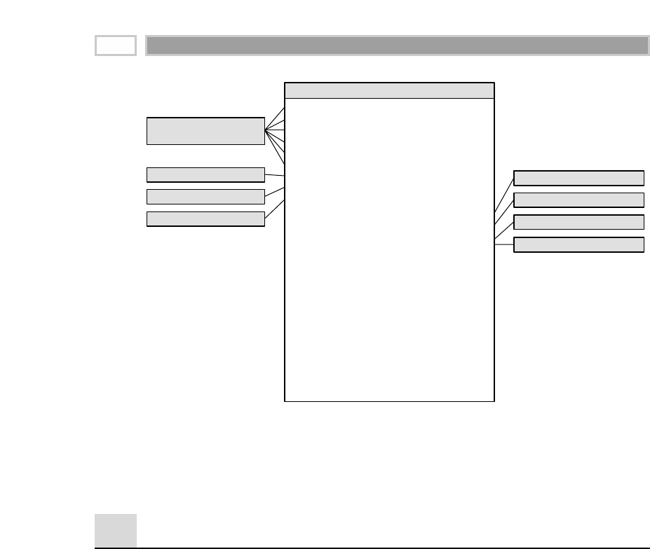
Figure 15.9 Claims accumulating snapshot schema.
Policy/Claims Consolidated Snapshot
With the four fact tables designed thus far (in addition to the heterogeneous
extensions), we deliver a robust perspective of the policy and claims transac-
tions, in addition to snapshots from both processes. However, recall that the
users expressed a strong interest in profit metrics. While premium and claim
financial metrics could be derived by separately querying two fact tables and
then combining the result set, we opt to go the next step in the spirit of ease of
use and performance. We can construct another fact table to bring the pre-
mium revenue and claim loss metrics together, as shown in Figure 15.10. This
table has a reduced set of dimensions corresponding to its slightly summa-
rized monthly granularity. As you recall from Chapter 7, we refer to this as a
consolidated fact table because it combines data from multiple business
processes. It is best to develop consolidated fact tables after the base metrics
have been delivered in separate dimensional models.
Claim Open Date Key (FK)
Claim Assessment Completion Date Key (FK)
Claim 1st Payment Date Key (FK)
Claim Most Recent Payment Date Key (FK)
Claim Most Recent Transaction Date Key (FK)
Claim Close Date Key (FK)
Policyholder Key (FK)
Agent Key (FK)
Coverage Key (FK)
Covered Item Key (FK)
Claimant Key (FK)
Claim Status Key (FK)
Claim Key (FK)
Policy Number (DD)
Original Reserve Amount
Assessed Damage Amount
Reserve Adjustment Amount
Current Reserve Amount
Open Reserve Amount
Claim Amount Paid
Payment Received
Salvage Received
Number of Transactions
Claim Open Date to Assessment Lag
Claim Open Date to 1st Payment Lag
Claim Open Date to Close Lag
Claims Accumulating Snapshot Fact
Date Dimension
(views for 6 roles)
Policyholder Dimension
Agent Dimension
Coverage Dimension
Covered Item Dimension
Claimant Dimension
Claim Status Dimension
Claim Dimension
CHAPTER 15
324
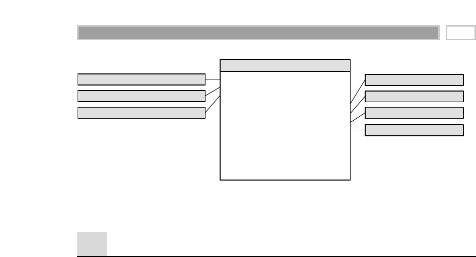
Figure 15.10 Policy/claims consolidated schema.
Factless Accident Events
When we discussed factless fact tables in Chapter 12, we referred to them as the
collision of keys at a point in space and time. In the case of an automobile
insurer, we can record literal collisions using a factless fact table. In this situation
the fact table registers the many-to-many correlations between the loss parties
and loss items or, to put it less euphemistically, all the correlations between the
people and vehicles involved in an accident.
Several new dimensions appear in the factless fact table shown in Figure 15.11.
The loss party describes other individuals who were involved in the accident,
possibly as passengers, witnesses, or in another capacity. If the loss party was
not associated with a vehicle in the accident, then the loss vehicle key would
join to a “No Vehicle” entry in that dimension. The loss affiliation explains the
role of the loss party (and loss vehicle, if applicable) to the claim. Again, as we
did in Chapter 12, we include a fact that is always valued at 1 to facilitate
counting and aggregation. This factless fact table can represent complex acci-
dents involving many individuals and vehicles because the number of
involved parties with various roles is open-ended. When there is more than
one claimant or loss party associated with an accident, we can optionally treat
these dimensions as multivalued dimensions using claimant group and loss
party group bridge tables. This has the advantage that the grain of the fact
table is preserved as one record per accident claim. Either schema variation
could answer questions such as “How many bodily injury claims did we han-
dle where ABC Legal Partners represented the claimant and EZ-Dent-B-Gone
body shop performed the repair?”
Month End Snapshot Date Key (FK)
Policyholder Key (FK)
Coverage Key (FK)
Covered Item Key (FK)
Agent Key (FK)
Policy Status Key (FK)
Claim Status Key (FK)
Policy Number (DD)
Written Premium Revenue Amount
Earned Premium Revenue Amount
Claim Paid Amount
Claim Receipt Amount
Consolidated Policy/Claims Fact
Month End Dimension
Policyholder Dimension
Coverage Dimension
Covered Item Dimension
Agent Dimension
Policy Status Dimension
Claim Status Dimension
Insurance 325
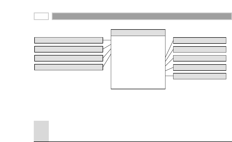
Figure 15.11 Factless fact table for accident events.
Common Dimensional Modeling
Mistakes to Avoid
As we close this final chapter on dimensional modeling techniques, we
thought it would be helpful to establish boundaries beyond which designers
should not go. Thus far in this book we’ve presented concepts by positively
stating that you should use technique A in situation X. Now, rather than focus-
ing on to-dos, we turn our attention to not-to-dos by elaborating on dimen-
sional modeling techniques that should be avoided. As we did with Chapter
1’s list of pitfalls, we’ve listed the not-to-dos in reverse order of importance. Be
aware, however, that even the less important mistakes can seriously compro-
mise your data warehouse.
Mistake 10: Place text attributes used for constraining and grouping in a
fact table. The process of creating a dimensional model is always a kind of
triage. The numeric measurements delivered from an operational business
process source belong in the fact table. The descriptive textual attributes
from the context of the measurements go in dimension tables. Finally, we
make a field-by-field decision about the leftover codes and pseudonumeric
items, placing them in the fact table if they are more like measurements
and in the dimension table if they are more like physical descriptions of
something. You shouldn’t lose your nerve and leave true text, expecially
comment fields, in the fact table. We need to get these text attributes off the
main runway of your data warehouse and into dimension tables.
Mistake 9: Limit verbose descriptive attributes in dimensions to save
space. You might think that you are being a good, conservative designer by
keeping the size of your dimensions under control. However, in virtually
Accident Date Key
Policyholder Key (FK)
Coverage Key (FK)
Covered Item Key (FK)
Claimant Key (FK)
Claim Key (FK)
Loss Party Key (FK)
Loss Vehicle Key (FK)
Loss Affiliation Key (FK)
Policy Number (DD)
Accident Count (always 1)
Accident Event Fact
Date Dimension
Policyholder Dimension
Coverage Dimension
Covered Item Dimension
Claimant Dimension
Claim Dimension
Loss Party Dimension
Loss Vehicle Dimension
Loss Affiliation Dimension
CHAPTER 15
326
TEAMFLY
Team-Fly®

every data warehouse, the dimension tables are geometrically smaller than
the fact tables. Having a 100-MB product dimension table is insignificant if
the fact table is 100 times as large! Your job as designer of an easy-to-use
data warehouse is to supply as much verbose descriptive context in each
dimension as you can. Make sure every code is augmented with readable
descriptive text. Better yet, you probably can remove the codes entirely.
Remember that the textual attributes in the dimension tables provide the
user interface to data browsing, constraining, or filtering, as well as the
content for the row and column headers in your final reports.
Mistake 8: Split hierarchies and hierarchy levels into multiple dimensions.
A hierarchy is a cascaded series of many-to-one relationships. For example,
many products may roll up to a single brand; and many brands may roll
up to a single category. If your dimension is expressed at the lowest level
of granularity (for example, product), then all the higher levels of the hier-
archy can be expressed as unique values in the product row. Users under-
stand hierarchies. Your job is to present the hierarchies in the most natural
and efficient manner. A hierarchy belongs together in a single physical flat
dimension table. Resist the urge to snowflake a hierarchy by generating a
set of progressively smaller subdimension tables. In this case you would be
confusing backroom data staging with front room data presentation!
Finally, if more than one roll-up exists simultaneously for a dimension, in
most cases it’s perfectly reasonable to include multiple hierarchies in the
same dimension, as long as the dimension has been defined at the lowest
possible grain (and the hierarchies are uniquely labeled).
Mistake 7: Ignore the need to track dimension attribute changes. Contrary
to popular belief, business users often want to understand the impact of
changes to a subset of the dimension tables’ attributes. It is unlikely that
your users will settle for dimension tables with attributes that always reflect
the current state of the world. We have three techniques for tracking slowly
moving attribute changes; don’t rely on type 1 exclusively. Likewise, if a
group of attributes changes rapidly, don’t delay splitting a dimension to
allow for a more volatile minidimension. You can’t always understand the
volatility of your data when you first design the dimensions. Suppose that
your product dimension contains a set of attributes called standard parame-
ters. At the beginning of the design process you are assured that these stan-
dard parameters are fixed for the life of the product. However, after rolling
out your data warehouse, you discover that these attributes change several
times per year for each product. Sooner, rather than later, you probably
should separate your product dimension into two dimensions. The new
product standard parameter dimension will keep your original product
dimension from burgeoning disastrously if you tried to model it as slowly
changing.
Insurance 327

Mistake 6: Solve all query performance problems by adding more hard-
ware. Aggregates, or derived summary tables, are the most cost-effective
way to improve query performance. Most query tool vendors have explicit
support for the use of aggregates, which depend on explicit dimensional
modeling constructs. Adding expensive hardware should be done as part
of a balanced program that includes building aggregates, creating indices,
choosing query-efficient DBMS software, increasing real memory size,
increasing CPU speed, and finally, adding parallelism at the hardware
level.
Mistake 5: Use operational or smart keys to join dimension tables to a fact
table. Novice data warehouse designers are sometimes too literal minded
when designing the dimension tables’ primary keys that connect to the for-
eign keys of the fact table. It is counterproductive to declare a whole suite
of dimension attributes as the dimension table key and then use them all as
the basis of the physical join to the fact table. This includes the unfortunate
practice of declaring the dimension key to be the operational key, along
with an effective date. All types of ugly problems will arise eventually. You
should replace the smart physical key with a simple integer surrogate key
that is numbered sequentially from 1 to N, where Nis the total number of
rows in the dimension table.
Mistake 4: Neglect to declare and then comply with the fact table’s grain.
All dimensional designs should begin with the business process that gen-
erates the numeric performance measurements. Second, specify the exact
granularity of that data. Building fact tables at the most atomic, granular
level will gracefully resist the ad hoc attack. Third, surround these mea-
surements with dimensions that are true to that grain. Staying true to the
grain is a crucial step in the design of a dimensional data model. A subtle
but serious error in a dimensional design is to add helpful facts to a fact
table, such as rows that describe totals for an extended time span or a large
geographic area. Although these extra facts are well known at the time of
the individual measurement and would seem to make some applications
simpler, they cause havoc because all the automatic summations across
dimensions overcount these higher-level facts, producing incorrect results.
Each different measurement grain demands its own fact table.
Mistake 3: Design the dimensional model based on a specific report. A
dimensional model has nothing to do with an intended report! Rather, it is
a model of a measurement process. Numeric measurements form the basis
of fact tables. The dimensions that are appropriate for a given fact table are
the physical context that describes the circumstances of the measurements.
We see that a dimensional model is based solidly on the physics of a mea-
surement process and is quite independent of how a user chooses to define
CHAPTER 15
328

a report. A project team once confessed to us that they had built several
hundred fact tables to deliver order management data to their users. It
turned out that each fact table had been constructed to address a specific
report request. The same data was being extracted many, many times to
populate all these fact tables. Not surprisingly, the team was struggling to
update the databases within the nightly batch window. Rather than
designing a quagmire of report-centric schemas, they should have focused
on the measurement process(es). The users’ requirements could have been
handled with a well-designed schema for the atomic data along with a
handful (not hundreds) of performance-enhancing aggregations.
Mistake 2: Expect users to query the lowest-level atomic data in a normal-
ized format. The lowest-level data is always the most dimensional and
should be the foundation of your dimensional design. Data that has been
aggregated in any way has been deprived of some of its dimensions. You
can’t build a data mart with aggregated data and expect your users and
their tools to seamlessly drill down to third normal form data for the
atomic details. Normalized models may be helpful for staging the data, but
they should never be used for presenting the data to business users.
Mistake 1: Fail to conform facts and dimensions across separate fact tables.
This final not-to-do should be presented as two separate mistakes because
they are both so dangerous to a successful data warehouse environment,
but we’ve run out of mistake numbers to assign, so we’ve lumped them
into one.
It would be a shame to get this far and then build isolated data stovepipes.
We refer to this as snatching defeat from the jaws of victory. If you have a
numeric measured fact, such as revenue, in two or more data marts
sourced from different underlying systems, then you need to take special
care to ensure that the technical definitions of these facts match exactly. If
the definitions do not match exactly, then they shouldn’t both be referred
to as revenue. This is called conforming the facts.
Finally, the single most important design technique in the dimensional
modeling arsenal is conforming your dimensions. If two or more fact
tables have the same dimension, then you must be fanatical about making
these dimensions identical or carefully chosen subsets of each other. When
you conform your dimensions across fact tables, you will be able to drill
across separate data sources because the constraints and row headers mean
the same thing and match at the data level. Conformed dimensions are the
secret sauce needed for building distributed data warehouses, adding
unexpected new data sources to an existing warehouse, and making
multiple incompatible technologies function together harmoniously.
Insurance 329

Summary
In this final case study we designed a series of insurance dimensional models
representing the culmination of many important concepts developed through-
out this book. Hopefully, now you feel comfortable and confident using the
vocabulary and tools of a dimensional modeler. With dimensional modeling
mastered, we turn our attention to all the other activities that occur during the
lifecycle of a successful data warehouse project in the next chapter. Before you
go forth and be dimensional, it’s useful to have this holistic perspective and
understanding, even if your job focus is limited to modeling.
CHAPTER 15
330

Building the Data Warehouse
CHAPTER
16
331
The gears shift rather dramatically in this chapter. Rather than focusing on
dimensional modeling techniques, we turn our attention to everything else
that occurs during the course of a data warehouse design and implementation
project. We’ll walk through the life of a data warehouse project from inception
through ongoing maintenance, identifying best practices at each step, as well
as potential vulnerabilities. More comprehensive coverage of the data ware-
house lifecycle is available in The Data Warehouse Lifecycle Toolkit, by Ralph
Kimball, Laura Reeves, Margy Ross, and Warren Thornthwaite (Wiley, 1998).
This chapter is a crash course drawn from the complete text, which weighs in
at a hefty 750+ pages.
Some may perceive that this chapter’s content is applicable only to data ware-
house project managers. We certainly don’t feel that this is the case. Imple-
menting a data warehouse requires tightly integrated activities. We believe
that everyone on the project team, including the business analyst, architect,
database designer, data stager, and analytic application developer, needs a
high-level understanding of the complete lifecycle of a data warehouse. Like
the rest of the book, we’ve written this chapter so that it’s accessible to a broad
audience.
Chapter 16 covers the following concepts:
■■ Business dimensional lifecycle overview
■■ Data warehouse project planning and ongoing communication and management
■■ Tactics for collecting business requirements, including prioritization

■■ Process for developing the technical architecture and then selecting products
■■ Dimensional design workshops
■■ Physical design considerations, including aggregation and indexing
■■ Data staging recommendations
■■ Analytic application design and development
■■ Recommendations for deployment, ongoing maintenance, and future growth
■■ Common mistakes to avoid when building and managing a data warehouse
Business Dimensional Lifecycle Road Map
When driving to a place we’ve never been to before, most of us rely on a road
map. Similarly, a road map is extremely useful if we’re about to embark on the
unfamiliar journey of data warehousing. The authors of The Data Warehouse
Lifecycle Toolkit drew on decades of experience to develop the business dimen-
sional lifecycle approach. We chose the name because it reinforced several of
our key tenets for successful data warehousing. First and foremost, data ware-
house projects must focus on the needs of the business. Second, the data pre-
sented to the business users must be dimensional. Hopefully, this comes as no
surprise to any readers at this point! Finally, while data warehousing is an
ongoing process, each implementation project should have a finite cycle with
a specific beginning and end.
We use the diagram in Figure 16.1 to encapsulate the major activities of the
business dimensional lifecycle. The diagram illustrates task sequence, depen-
dency, and concurrency. It serves as a road map to help teams do the right
thing at the right time. The diagram does not reflect an absolute timeline.
While the boxes are equally wide, there’s a vast difference in the time and
effort required for each major activity.
Figure 16.1 Business dimensional lifecycle diagram.
Technical
Architecture
Design
Product
Selection &
Installation
Dimensional
Modeling
Business
Requirements
Definition
Project Management
Project
Planning
Physical
Design
Data Staging
Design &
Development
Deployment
Maintenance
and
Growth
Analytic
Application
Specification
Analytic
Application
Development
CHAPTER 16
332

Road Map Major Points of Interest
Before we dive into specifics, let’s take a moment to orient ourselves to the
road map. The data warehouse lifecycle begins with project planning, as one
would expect. During this module we assess the organization’s readiness for a
data warehouse initiative, establish the preliminary scope and justification,
obtain resources, and launch the project. Ongoing project management serves
as a foundation to keep the remainder of the lifecycle on track.
The second major task in Figure 16.1 focuses on business requirements defini-
tion. Notice the two-way arrow between project planning and business
requirements definition because there’s much interplay between these two
activities. Aligning the data warehouse with business requirements is
absolutely crucial. Best-of-breed technologies won’t salvage a data warehouse
that fails to focus on the business. Data warehouse designers must understand
the needs of the business and translate them into design considerations. Busi-
ness users and their requirements have an impact on almost every design and
implementation decision made during the course of a warehouse project. In
Figure’s 16.1 road map, this is reflected by the three parallel tracks that follow.
The top track of Figure 16.1 deals with technology. Technical architecture
design establishes the overall framework to support the integration of multi-
ple technologies. Using the capabilities identified in the architecture design as
a shopping list, we then evaluate and select specific products. Notice that
product selection is not the first box on the road map. One of the most frequent
mistakes made by novice teams is to select products without a clear under-
standing of what they’re trying to accomplish. This is akin to grabbing a ham-
mer whether you need to pound a nail or tighten a screw.
The middle track emanating from business requirements definition focuses on
data. We begin by translating the requirements into a dimensional model, as
we’ve been practicing. The dimensional model is then transformed into a
physical structure. We focus on performance tuning strategies, such as aggre-
gation, indexing, and partitioning, during the physical design activities. Last
but not least, data staging extract-transformation-load (ETL) processes are
designed and developed. As we mentioned earlier, the equally sized boxes
don’t represent equally sized efforts; this is obvious when we think about the
workload differential between physical design and data staging activities.
The final set of tasks spawned by the business requirements definition is
the design and development of analytic applications. The data warehouse
project isn’t done when we deliver data. Analytic applications, in the form of
parameter-driven templates and analyses, will satisfy a large percentage of
the analytic needs of business users.
Building the Data Warehouse 333

We bring together the technology, data, and analytic application tracks, along
with a good dose of education and support, for a well-orchestrated deploy-
ment. From there, ongoing maintenance is needed to ensure that the data
warehouse and its user community remain healthy and poised to leverage the
investment. Finally, we handle future data warehouse growth by initiating
subsequent projects, each returning to the beginning of the lifecycle all over
again.
Now that we have a high-level understanding of the road map’s overall struc-
ture, we’ll delve into each of the boxes of Figure 16.1 for more details.
Project Planning and Management
Not surprisingly, we launch the data warehouse with a series of project planning
activities. We sometimes refer to these as marshmallow tasks because they’re soft,
sticky, and can gum up the works of a data warehouse project seriously.
Assessing Readiness
Before moving full-steam ahead with significant data warehouse expenditures,
it is prudent to take a moment to assess the organization’s readiness to proceed.
Based on our cumulative experience from hundreds of data warehouses, we’ve
identified five factors that differentiate projects that were predominantly
smooth sailing versus those which entailed a constant struggle. These factors
are leading indicators of data warehouse success. You don’t need high marks
on every factor to move forward, but any shortfalls represent risks or vulnera-
bilities. We’ll describe the characteristics in rank order of importance.
The most critical factor for successful data warehousing is to have a strong
business sponsor. Business sponsors should have a vision for the potential
impact of a data warehouse on the organization. They should be passionate
and personally convinced of the project's value while realistic at the same time.
Optimally, the business sponsor has a track record of success with other inter-
nal initiatives. He or she should be a politically astute leader who can convince
his or her peers to support the warehouse.
Sometimes there’s strong demand for a data warehouse coming from a single
sponsor. Even if this person and his or her opportunity encompass the ware-
house characteristics we’re looking for, we can still encounter trouble in this
scenario because lone sponsors tend to move on, either internally or externally.
This is the most common cause for data warehouse stagnation. Some teams are
confronted with too much demand coming from all corners of the organiza-
tion. Assuming that you (or your management) do not attempt to tackle all the
CHAPTER 16
334

demand in one fell swoop, this is a great way to start. Finally, the business
sponsor may be missing in action, but this doesn’t stop the IT organization
from moving forward, nearly guaranteeing a data warehouse false start. This
is the riskiest scenario; the project should slow down until the right business
sponsor has been identified (or perhaps recruited) and has voiced a commit-
ment to the project.
The second readiness factor is having a strong, compelling business motiva-
tion for building a data warehouse. This factor often goes hand in hand with
sponsorship. A data warehouse project can’t merely deliver a nice-to-have
capability; it needs to solve critical business problems in order to garner the
resources required for a successful launch and healthy lifespan. Compelling
motivation typically creates a sense of urgency, whether the motivation is from
external (for example, competitive factors) or internal (for example, inability to
analyze cross-organization performance following acquisitions) sources.
The third factor when assessing readiness is feasibility. There are several
aspects of feasibility, such as technical or resource feasibility, but data feasibil-
ity is the most crucial. Are we collecting real data in real operational source
systems to support the business requirements? Data feasibility is a major con-
cern because there is no short-term fix if we’re not already collecting reason-
ably clean source data at the right granularity.
The next factors are not project showstoppers but still influence your probabil-
ity for success. The fourth factor focuses on the relationship between the busi-
ness and IT organizations. In your company, does the IT organization
understand and respect the business? Conversely, does the business under-
stand and respect the IT organization? The inability to honestly answer yes to
these questions doesn’t mean that you can’t proceed. Rather, it implies that
you need to vigilantly keep the business and IT representatives marching to
the same drum. In many ways the data warehouse initiative can be an oppor-
tunity to mend the fence between these organizations, assuming that you both
deliver.
The final aspect of readiness is the current analytic culture within your com-
pany. Do business analysts make decisions based on facts and figures, or are
their decisions based on intuition, anecdotal evidence, and gut reactions? The
businesspeople already immersed in numbers likely will be more receptive to
a data warehouse. However, you can be successful with either scenario as long
as you prepare for the increased burden of shifting the cultural mindset (with
the help of the business sponsor), as well as the need for additional analytic
application development, education, and support resources.
If your project is not ready to proceed, typically due to a business sponsor
shortfall, we suggest two approaches for shoring up your readiness. The first
Building the Data Warehouse 335

is to conduct a high-level business requirements analysis and prioritization.
We’ll talk more about this process in the next major section, so stay tuned. The
other alternative is to create a proof of concept. Proofs of concept are quick and
dirty demonstrations of the potential capabilities of a data warehouse. They
are a sales tool rather than a technical proof of design. Teams use this tech-
nique because business users supposedly can’t describe what they want with-
out seeing something to react to. While the proof of concept can establish a
common understanding, we don’t suggest that it be the first tool pulled from
your toolbox. Proofs of concept often require more effort than quick and dirty
implies. Typically, they’re held together with duct tape yet have a tendency to
morph into a production system without the requisite rework. It is challenging
to manage user expectations appropriately. Those who like to play with tools
gravitate to this technique, but you should be aware that there might be more
effective and efficient methods to reach the same objective.
Scoping
Once you’re comfortable with the organization’s readiness, it’s time to put
boundaries around an initial project. Scoping requires the joint input of both
the IT organization and business management. The scope of your data ware-
house project should be both meaningful in terms of its value to the organiza-
tion and manageable. When you are first getting started, you should focus on
data from a single business process. Save the more challenging, cross-process
projects for a later phase. Sometimes scopes are driven by a target completion
date, such as the end of the fiscal year. You can manage the scope to a due date
effectively, but doing so may present additional risks. Even with a set time
frame, you need to maintain your focus on scoping a project that is both com-
pelling and doable. Sometimes project teams feel that the delivery schedule is
cast in concrete before project planning is even initiated. The prioritization
process, which we’ll describe during business requirements definition, can be
used to convince IT and business management that adjustments are required.
Finally, remember to avoid the law of too when scoping—too firm of a commit-
ment to too brief of a timeline involving too many source systems and too
many users in too many locations with too diverse analytic requirements.
Justification
A slew of acronyms surrounds the justification process, but don’t let them
intimidate you. Justification requires an estimation of the benefits and costs
associated with a data warehouse; hopefully, the anticipated benefits grossly
outweigh the costs. IT usually is responsible for deriving the expenses. You
need to determine approximate costs for the requisite hardware and software.
Data warehouses tend to expand rapidly, so be sure the estimates allow some
CHAPTER 16
336
TEAMFLY
Team-Fly®

room for short-term growth. Unlike operational system development, where
resource requirements tail off after production, ongoing warehouse support
needs will not decline appreciably over time.
We rely on the business to determine the financial benefits of a data ware-
house. Warehouses typically are justified based on increased revenue or profit
opportunities rather than merely focusing on expense reduction. Delivering a
single version of the truth or flexible access to information isn’t sufficient financial
justification. You need to peel back the layers to determine the quantifiable
impact of improved decision making made possible by these sound bites. If
you are struggling with warehouse justification, this is likely a symptom that
you are focused on the wrong business sponsor or problem.
Staffing
Data warehouse projects require the integration of a cross-functional team
with resources from both the business and IT communities. It is common for
the same person to fill more than one role, especially as the cost of entry for
data warehousing has fallen. The assignment of named resources to roles
depends on the project’s magnitude and scope, as well as the individual’s
availability, capacity, and experience.
From the business side of the house, you’ll need representatives to fill the fol-
lowing roles:
Business sponsor. The business sponsor is the warehouse’s ultimate client, as
well as its strongest advocate. Sponsorship sometimes takes the form of an
executive steering committee, especially for cross-enterprise initiatives.
Business driver. If you work in a large organization, the sponsor may be too
far removed or inaccessible to the project team. In this case the sponsor
sometimes delegates his or her less strategic warehouse responsibilities to
a middle manager in the organization. This driver should possess the same
characteristics as the sponsor.
Business lead. The business project lead is a well-respected person who is
highly involved in the project, likely communicating with the project man-
ager on a daily basis. The same person serving as the business driver or
subject matter expert sometimes fills this role.
Business users. Optimally, the business users are the enthusiastic fans of the
data warehouse. You need to involve them early and often, beginning with
the project scope and business requirements. From there, you must find
creative ways to maintain their interest and involvement throughout the
lifecycle. Remember, user involvement is critical to data warehouse accep-
tance. Without business users, the data warehouse is a technical exercise
in futility.
Building the Data Warehouse 337

Several other positions are staffed from either the business or IT organizations.
These straddlers can be technical resources that understand the business
or business resources that understand technology. Straddler roles include the
following:
Business system analyst. This person is responsible for determining the busi-
ness needs and translating them into architectural, data, and analytic
application requirements.
Business subject matter expert. This person is often the current go-to
resource for ad hoc analysis. He or she understands what the data means,
how it is used, and where data inconsistencies are lurking. Their analytic
and data insights are extremely useful, especially during the modeling and
analytic application processes.
Analytic application developer. Analytic application developers are respon-
sible for designing and developing the starter set of analytic templates, as
well as providing ongoing application support.
Data warehouse educator. The educator(s) must be confident of their data,
applications, and access tool knowledge because the business community
does not differentiate between these warehouse deliverables.
The following roles typically are staffed from the IT organization (or an
external consulting firm). If you are working with consultants due to
resource or expertise constraints, you should retain internal ownership of the
project. Insist on coaching and extensive skills/knowledge transfer so that
you can function more independently on the next project. Finally, you must
clearly understand whether you’re buying meaningful experience rather
than staff augmentation (perhaps with consultants who merely know how to
spell OLAP).
Project manager. The project manager is a critical position. He or she should
be comfortable with and respected by business executives, as well as tech-
nical analysts. The project manager’s communication and project manage-
ment skills must be stellar.
Technical architect. The architect is responsible for the overall technical and
security architecture. He or she develops the plan that ties together the
required technical functionality and helps evaluate products on the basis of
the overall architecture.
Technical support specialists. Technical specialists tend to be nearly encyclo-
pedic about a relatively narrow spectrum of technology.
Data modeler. The data modeler likely comes from a transactional data mod-
eling background with heavy emphasis on normalization. He or she
should embrace dimensional modeling concepts and be empathetic to the
CHAPTER 16
338

requirements of the business rather than focused strictly on saving space
or reducing the staging workload.
Database administrator. Like the data modeler, the database administrator
must be willing to set aside some traditional database administration tru-
isms, such as having only one index on a relational table.
Metadata coordinator. This person ensures that all the metadata is collected,
managed, and disseminated. As a watchdog role, the coordinator is
responsible for reminding others of their metadata-centric duties.
Data steward. The data steward is responsible for enterprise agreement on
the warehouse’s conformed dimensions and facts. Clearly, this is a politi-
cally challenging role.
Data staging designer. The staging designer is responsible for designing the
data staging ETL processes. He or she typically is involved in the make
versus buy decision regarding staging software.
Data staging developer. Based on direction from the staging designer, the
staging developer delivers and automates the staging processes using
either a staging tool or manually programmed routines.
Data warehouse support. Last, but not least, the data warehouse requires
ongoing backroom and front room support resources. Most often this role
is assigned to individuals who have been involved in the project in an
earlier capacity.
Developing and Maintaining
the Project Plan
Developing the data warehouse project plan involves identification of all the
tasks necessary to implement the data warehouse. Resources are available in
the marketplace to help you compile a project task list. For example, the
CD-ROM that comes with The Data Warehouse Lifecycle Toolkit includes a nearly
200-item task listing.
Any good project manager knows that key team members, such as the data
staging designer, should develop the effort estimates for their tasks. The proj-
ect manager can’t dictate the amount of time allowed and expect conformance.
The project plan should identify a user acceptance checkpoint after every
major milestone and deliverable to ensure that the project is still on track and
that the business is still intimately involved.
The data warehouse project demands broad communication. During the proj-
ect planning phase, we suggest that the project manager establish a communi-
cation matrix, such as Table 16.1 illustrates, to help make certain that the
communication strategy is executed.
Building the Data Warehouse 339

Table 16.1 Example Data Warehouse Communication Plan
CONSTITUENCY FREQUENCY FORUM KEY MESSAGES
Business sponsors Bimonthly Face-to-face Issue resolution,
briefing expectation management,
funding
Business Monthly Web site Requisite involvement,
community expectation management,
critical dates
Project team Weekly Status Progress, issue
meetings identification and
resolution
IT colleagues Bimonthly Existing IT Expectation management,
staff meeting resource needs
Data warehouse projects are vulnerable to scope creep largely due to our
strong desire to satisfy users’ requirements. We need to be most watchful
about the accumulation of minor changes that snowball. While no single
request is too arduous, taken in total, they may represent a significant change
to the project’s scope. We have several options when confronted with changes.
First, we can increase the scope by adding time, resources, or money to accom-
modate the change. Otherwise, the total effort can remain unchanged if the
users relinquish something that had been in scope to accommodate the
change. Finally, we can just say no without really saying no by handling the
change as an enhancement request. The most important thing to remember
about scope changes is that they shouldn’t be made in an IT vacuum. The right
answer depends on the situation. Now is the time to leverage your partnership
with the business to arrive at an answer with which everyone can live.
The keys to data warehouse project planning and management include:
1. Having a solid business sponsor
2. Balancing high value and doability to define the scope
3. Working with the best team possible to develop a detailed project plan
4. Being an excellent project manager by motivating, managing, and communicating
up, down, and across the organization
Business Requirements Definition
Embracing the business users to understand their requirements and garner
their buy-in is absolutely essential to successful data warehousing. This sec-
tion focuses on back-to-basics techniques for accomplishing just that.
CHAPTER 16
340

Requirements Preplanning
Before sitting down with the business community to gather requirements, we
suggest that you set yourself up for a productive session by considering the
following:
Choose the Forum
We gather requirements by meeting with business user representatives while
interweaving data sessions with source system gurus and subject matter
experts. This dual-pronged approach gives us insight into the needs of the
business in conjunction with the realities of the data. However, we can’t ask
business managers about the granularity or dimensionality of their critical
data. We need to talk to them about what they do, why they do it, how they
make decisions, and how they hope to make decisions in the future. Like orga-
nizational therapy, we’re trying to detect the issues and opportunities.
There are two primary techniques for gathering requirements—interviews or
facilitated sessions. Both have their advantages and disadvantages. Interviews
encourage lots of individual participation. They are also easier to schedule.
Facilitated sessions may reduce the elapsed time to gather requirements,
although they require more time commitment from each participant.
Based on our experience, surveys are not a reasonable tool for gathering
requirements because they are flat and two-dimensional. The self-selected
respondents only answer the questions we’ve asked in advance. There’s no
option to probe more deeply, such as when we’re face to face. In addition,
don’t forget that a secondary outcome of gathering requirements is to create a
bond between users and the warehousing initiative. This is just not going to
happen with surveys.
We generally use a hybrid approach with interviews to gather the gory details
and then facilitation to bring the group to consensus. While we’ll describe this
hybrid approach in more detail, much of the discussion applies to pure facili-
tation as well. The forum choice depends on the team’s skills, the organiza-
tion’s culture, and what you’ve already subjected your users to. This is a case
in which one size definitely does not fit all.
Identify and Prepare
the Requirements Team
Regardless of the approach, you need to identify and prepare the project team
members who are involved. If you’re doing interviews, you need to identify a
lead interviewer whose primary responsibility is to ask the great open-ended
questions. Meanwhile, the interview scribe takes copious notes. While a tape
Building the Data Warehouse 341

recorder may provide more complete coverage of each interview, we don’t use
one because it changes the meeting dynamics. Our preference is to have a sec-
ond person in the room with another brain and sets of eyes and ears rather
than relying on a whirling machine. We often invite one or two additional proj-
ect members (depending on the number of interviewees) as observers so that
they can hear the users’ input directly.
Before you sit down with users, you need to make sure you’re approaching
the sessions with the right mindset. You shouldn’t presume that you already
know it all. If done correctly, you will definitely learn during these require-
ments interviews. On the other hand, you should do some homework by
researching available sources, such as the annual report, Web site, and inter-
nal organization chart.
Since the key to getting the right answers is asking the right questions, we rec-
ommend that questionnaires be formulated before user meetings. The ques-
tionnaire should not be viewed as a script. It is a tool to organize your thoughts
and serve as a fallback device in case your mind goes blank during the inter-
view session.
Select, Schedule, and Prepare Business
Representatives
If this is your first foray into data warehousing (or your first attempt to rescue
data stovepipes), you should talk to businesspeople who represent horizontal
breadth across the organization. This coverage is critical to formulating the
data warehouse bus matrix blueprint. You need to have an early understand-
ing of the common data and vocabulary across the core business functions to
build an extensible environment.
Within the target user community, you should cover the organization verti-
cally. Data warehouse project teams naturally gravitate toward the super-
power analysts in the business. While their insight is valuable, you can’t
ignore senior executives and middle management. Otherwise, you are vulner-
able to being overly focused on the tactical here-and-now but lose sight of the
organization’s future strategic direction.
Scheduling the business representatives can be the most onerous requirements
task. Be especially nice to your administrator (or your boss’s administrator is
you’re attempting to schedule sessions with executive staff). We prefer to meet
with executives on their own, whereas we can meet with a homogeneous
group of two to three people for those lower on the organization chart. We
allow 1 hour for individual meetings and 11⁄2hours for the small groups. The
scheduler needs to allow 1⁄2hour between meetings for debriefing and other
necessities. Interviewing is extremely taxing because you must be completely
CHAPTER 16
342

focused for the duration of the session. Consequently, we only schedule three
to four sessions in a day because our brains turn mushy after that.
When it comes to preparing the interviewees, the optimal approach is to con-
duct a project launch meeting with the users. The business sponsor plays a
critical role, stressing his or her commitment and the importance of everyone’s
participation. The launch meeting disseminates a consistent message about
the project. It also generates a sense of the business’s ownership of the project.
If the launch meeting is a logistical nightmare, the sponsor should distribute a
launch memo covering the same topics. Likewise, the interview team must
prepare the interviewees by highlighting the topics to be covered in the
upcoming session. We do not include a copy of the questionnaire, which is not
intended for public dissemination. We do ask the interviewees to bring copies
of their key reports and analyses.
Collecting the Business Requirements
It’s time to sit down face to face to collect the business requirements. The
process usually flows from an introduction through structured questioning to
a final wrap-up, as we’ll discuss.
Launch
Responsibility for introducing the interview should be established prior to
gathering in a conference room. The designated kickoff person should script
the primary points to be conveyed in the first couple minutes when you set the
tone of the interview meeting. You should focus on the project and interview
objectives but not ramble on about the hardware, software, and other technical
jargon. The introduction should convey a crisp, business-centric message.
Interview Flow
The objective of an interview is to get business users to talk about what they do
and why they do it. A simple, nonthreatening place to begin is to ask about
their job responsibilities and organizational fit. This is a lob ball that intervie-
wees can respond to easily. From there, we typically ask about their key per-
formance metrics. Determining how they track progress and success translates
directly into the dimensional model. They’re telling us about their key busi-
ness processes and facts without us asking those questions directly.
If we’re meeting with a person who has more hands-on data experience, we
indirectly probe to better understand the dimensionality of the business,
along with hierarchical roll-ups. Again, we go to their world rather than ask-
ing them to meet on our turf. Such questions as “How do you distinguish
Building the Data Warehouse 343

between products (or agents, providers, or facilities)?” or “How do you
naturally categorize products?” help identify key dimension attributes and
hierarchies.
If the interviewee is more analytic, we ask about the types of analyses he or
she currently performs. Understanding the nature of these analyses and
whether they are ad hoc or standardized provides input into the data access
tool requirements, as well as the application template design process. Hope-
fully, the interviewee has brought along copies of their key spreadsheets and
reports. Rather than stashing them in a folder, it is helpful to understand
how the interviewee uses the analysis today, as well as opportunities for
improvement. Contrary to the advice of some industry pundits, you cannot
design an extensible analytic environment merely by getting users to agree
on the top five reports or queries. The users’ questions are bound to change.
Consequently, we must resist the temptation to narrow our design focus to a
supposed top five.
If we’re meeting with business executives, we usually don’t delve into the
details just described. Instead, we ask them about their vision for better lever-
aging information in the organization. Perhaps the project team is envisioning
a totally ad hoc environment, whereas business management is more inter-
ested in the delivery of standardized analysis. We need to make sure the data
warehouse deliverable matches the business demand and expectations.
We ask each interviewee about the impact of improved access to information.
We’ve likely already received preliminary funding for the project, but it never
hurts to capture more potential, quantifiable benefits.
Ground rules for effective interviewing include:
■■ Remember your interview role; listen and absorb like a sponge.
■■ Strive for a conversational flow; don’t dive too quickly (or pull out a copy of poten-
tial data elements).
■■ Verify communication and capture terminology precisely because most organiza-
tions use terminology inconsistently.
■■ Establish a peer basis with the interviewee; use his or her vocabulary.
Wrap-Up
As the interview is coming to a conclusion, we ask each interviewee about his
or her success criteria for the project. Of course, each criterion should be mea-
surable. Easy to use and fast mean something different to everyone, so you
should get the interviewees to articulate specifics, such as their expectations
regarding the amount of training required to run a predefined report.
CHAPTER 16
344

At this point in the interview we make a broad disclaimer. The interviewees
must understand that just because we discussed a capability in the meeting
doesn’t guarantee that it’ll be included in the first phase of the project. We
thank interviewees for their brilliant insights and let them know what’s hap-
pening next and what their involvement will be. We also take advantage of
this opportunity to manage expectations.
Conducting Data-Centric Interviews
While we’re focused on understanding the requirements of the business, it is
helpful to intersperse sessions with the source system data gurus or subject
matter experts to evaluate the feasibility of supporting the business needs.
These data-focused interviews are quite different from the ones just described.
The goal is to assess that the necessary core data exists before momentum
builds behind the requirements. A more complete data audit will occur during
the dimensional modeling process. We’re trying to learn enough at this point
to manage the organization’s expectations appropriately.
Postcollection Documentation
and Follow-up
Immediately following the interview, the interview team should debrief. You
want to ensure that you’re on the same page about what was learned, as well
as being prepared for any surprises or inconsistencies. It is also helpful to
review your notes quickly to fill in any gaps while the interview is still fresh in
your memory. Likewise, you should examine the reports gathered to gain fur-
ther offline insight into the dimensionality that must be supported in the data
warehouse.
At this point it is time to document what you heard. While documentation is
everyone’s least favorite activity, it is critical for both user validation and project
team reference materials. There are two levels of documentation that typically
result from the requirements process. The first is to write up each individual
interview. This activity can be quite time-consuming because the write-up
should not be merely a stream-of-consciousness transcript but should make
sense to someone who wasn’t in the interview. The second level of documenta-
tion is a consolidated findings document. We organize the document by first
identifying the key business processes. As we mentioned earlier, we tackle the
initial phases of a data warehouse on a process-by-process basis. Consequently,
it is logical to organize the requirements of the business into the same buckets
that will, in turn, become implementation efforts. Notes from all the interviews
are reviewed to capture the findings associated with each of the core business
processes.
Building the Data Warehouse 345

When writing up the findings document, we typically begin with an executive
summary, followed by a project overview that discusses the process used and
participants involved. The bulk of the report centers on our requirements find-
ings. For each major business process discussed, we describe why business
users want to analyze the process results, what capabilities they desire, their
current limitations, and potential benefits or impact. We include a list of sam-
ple questions that could be answered once the process metrics are available in
the data warehouse. Commentary about the feasibility of tackling the data
generated by each process is also documented.
We sometimes bring the processes together in a matrix to convey the oppor-
tunities across the organization. In this case we’re not referring to a data ware-
house bus matrix. The rows of the opportunity matrix still identify the
business processes. However, in the opportunity matrix, rather than identify-
ing common dimensions as the columns, we instead identify the organiza-
tional groups or functions. Surprisingly, the matrix will be quite dense
because many groups need access to the same core business process perfor-
mance metrics.
Prioritization and Consensus
The requirements findings document serves as the basis for presentations back
to senior management representatives, as well as for others who participated.
Inevitably we’ve uncovered more than can be tackled in a single iteration, so
we need to prioritize our efforts. As we discussed with project scope, you
shouldn’t make this decision in a vacuum. You need to leverage (or foster)
your partnership with the business community to arrive at priorities with
which everyone can live.
The requirements wrap-up presentation is positioned as a findings review and
prioritization meeting. Participants include relatively high-level business rep-
resentatives, as well as the data warehouse manager and other involved IT
management. The session begins with an overview of each identified business
process. You want everyone in the room to have a common understanding of
the range of opportunities, as well as what is meant when we say “sales book-
ings analysis,” for example.
Once the findings have been reviewed, it is time to prioritize. The four-cell quad-
rant technique, illustrated in Figure 16.2, is an effective tool for reaching consen-
sus on a data warehouse development plan that focuses on the right initial
opportunities. The quadrant’s vertical axis refers to the potential impact or value
to the business. The horizontal axis conveys feasibility. Each of the finding’s
CHAPTER 16
346
TEAMFLY
Team-Fly®
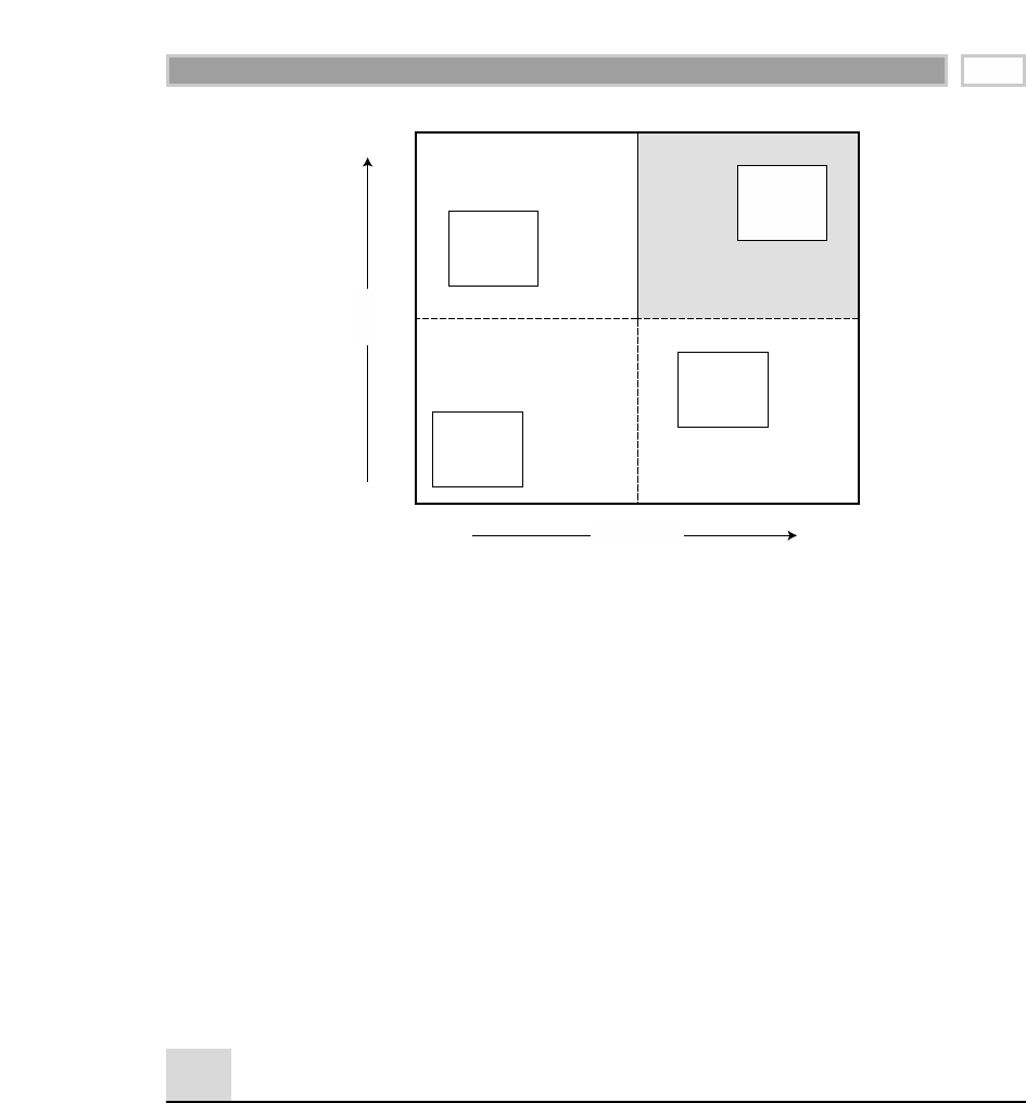
Figure 16.2 Prioritization quadrant analysis.
business process themes is placed in a quadrant based on the representatives’
composite agreement on impact and feasibility. The projects that warrant
immediate attention are located in the upper right corner because they’re high-
impact projects, as well as highly feasible. Projects in the lower left cell should
be avoided like the plague—they’re missions impossible that do little for the
business. Likewise, projects in the lower right cell don’t justify short-term
attention, although project teams sometimes gravitate here because these pro-
jects are doable but not very crucial. In other words, no one will notice if the
project doesn’t go well. Finally, projects in the upper left cell represent mean-
ingful opportunities. These projects have large potential business payback but
are currently infeasible. While the data warehouse project team is focused on
projects in the shaded upper right cell, other IT teams should address the cur-
rent feasibility limitations of those in the upper left cell.
Lifecycle Technology Track
The business requirements definition is followed immediately by three con-
current tracks focused on technology, data, and analytic applications, respec-
tively. In the next several sections we’ll zero in on the technology track, which
includes design of the technical architecture and selection of products that
bring the architecture to reality.
Business
Process
B
Business
Process
D
Business
Process
C
High
High
Business
Impact
Low
Low
Business
Process
A
Feasibility
Building the Data Warehouse 347

Technical Architecture Design
Much like a blueprint for a new home, the technical architecture is the blue-
print for the warehouse’s technical services and elements. The architecture
plan serves as an organizing framework to support the integration of tech-
nologies. Like housing blueprints, the technical architecture consists of a series
of models that delve into greater detail regarding each of the major compo-
nents. In both situations, the architecture allows us to catch problems on paper
(such as having the dishwasher too far from the sink) and minimize midpro-
ject surprises. It supports the coordination of parallel efforts while speeding
development through the reuse of modular components. The architecture
identifies the immediately required components versus those which will be
incorporated at a later date (such as the deck and screened porch). Most
important, the architecture serves as a communication tool. Home construc-
tion blueprints allow the architect, general contractor, subcontractors, and
homeowner to communicate from a common document. The plumber knows
that the electrician has power in place for the garbage disposal. Likewise, the
data warehouse technical architecture supports communication regarding a
consistent set of technical requirements within the team, upward to manage-
ment, and outward to vendors.
In Chapter 1 we discussed several major components of the technical architec-
ture, including data staging services, data access services, and metadata. In the
following section we turn our attention to the process of creating the technical
architecture design.
Eight-Step Process for Creating
the Technical Architecture
Data warehouse teams approach the technical architecture design process
from opposite ends of the spectrum. Some teams simply don’t understand the
benefits of an architecture and feel that the topic and tasks are too nebulous.
They’re so focused on data warehouse delivery that the architectures feels like
a distraction and impediment to progress, so they opt to bypass architecture
design. Instead, they piece together the technical components required for the
first iteration with bailing twine and chewing gum, but the integration and
interfaces get taxed as we add more data, more users, or more functionality.
Eventually, these teams often end up rebuilding because the nonarchitectured
structure couldn’t withstand the stresses. At the other extreme, some teams
want to invest two years designing the architecture while forgetting that the
primary purpose of a data warehouse is to solve business problems, not
address any plausible (and not so plausible) technical challenge.
CHAPTER 16
348

Neither end of the architecture spectrum is healthy; the most appropriate
response lies somewhere in the middle. We’ve identified an eight-step process
to help you navigate these architectural design waters. Remember, every data
warehouse has a technical architecture. The question is whether yours is
planned and explicit or merely implicit.
Establish an Architecture Task Force
Based on our experience, it is most useful to have a small task force of two to
three people focus on architecture design. Typically, it is the technical architect,
working in conjunction with the data staging designer and analytic applica-
tion developer, to ensure both backroom and front room representation on the
task force. This group needs to establish its charter and deliverables time line.
It also needs to educate the rest of the team (and perhaps others in the IT orga-
nization) about the importance of an architecture.
Collect Architecture-Related Requirements
As you recall from Figure 16.1, defining the technical architecture is not the
first box in the lifecycle diagram. The architecture is created to support high-
value business needs; it’s not meant to be an excuse to purchase the latest,
greatest products. Consequently, key input into the design process should
come from the business requirements definition findings. However, we listen
to the business’s requirements with a slightly different filter to drive the archi-
tecture design. Our primary focus is to uncover the architectural implications
associated with the business’s critical needs. We also listen closely for any tim-
ing, availability, and performance needs.
In addition to leveraging the business requirements definition process, we
also conduct additional interviews within the IT organization. These are
purely technology-focused sessions to understand current standards,
planned technical directions, and nonnegotiable boundaries. In addition, we
can uncover lessons learned from prior information delivery projects, as well
as the organization’s willingness to accommodate operational change on
behalf of the warehouse, such as identifying updated transactions in the
source system.
Document Architecture Requirements
Once we leveraged the business requirements definition process and con-
ducted supplemental IT interviews, we need to document our findings. At this
point we opt to use a simplistic tabular format. We simply list each business
requirement that has an impact on the architecture, along with a laundry list of
Building the Data Warehouse 349

architectural implications. For example, if there is a need to deliver global sales
performance data on a nightly basis following the recent acquisition of several
companies, the technical implications might include 24/7 worldwide avail-
ability, data mirroring for loads, robust metadata to support global access, ade-
quate network bandwidth, and sufficient staging horsepower to handle the
complex integration of operational data.
Develop a High-Level Architectural Model
After the architecture requirements have been documented, we begin formu-
lating models to support the identified needs. At this point the architecture
task force often sequesters itself in a conference room for several days of heavy
thinking. The team groups the architecture requirements into major compo-
nents, such as data staging, data access, metadata, and infrastructure. From
there the team drafts and refines the high-level architectural model. This
drawing is similar to the front elevation page on housing blueprints. It illus-
trates what the warehouse architecture will look like from the street, but it is
dangerously simplistic because significant details are embedded in the pages
that follow.
Design and Specify the Subsystems
Now that we understand how the major pieces will coexist, it is time to do a
detailed design of the subsystems. For each component, such as data staging
services, the task force will document a laundry list of requisite capabilities.
The more specific, the better, because what’s important to your data ware-
house is not necessarily critical to mine. This effort often requires preliminary
research to better understand the market. Fortunately, there is no shortage of
information and resources available on the Internet, as well as from network-
ing with peers. The subsystem specification results in additional detailed
graphic models.
In addition to documenting the capabilities of the primary subsystems, we
also must consider our security requirements, as well as the physical infra-
structure and configuration needs. Often, we can leverage enterprise-level
resources to assist with the security strategy. In some cases the infrastructure
choices, such as the server hardware and database software, are predeter-
mined. However, if you’re building a large data warehouse, over 1 TB in size,
you should revisit these infrastructure platform decisions to ensure that they
can scale as required. Size, scalability, performance, and flexibility are also key
factors to consider when determining the role of OLAP cubes in your overall
technical architecture.
CHAPTER 16
350

Determine Architecture
Implementation Phases
Like the homeowner’s dream house, you likely can’t implement all aspects of
the technical architecture at once. Some are nonnegotiable mandatory capabil-
ities, whereas others are nice-to-haves that can be deferred until a later date.
Again, we refer back to the business requirements to establish architecture pri-
orities. We must provide sufficient elements of the architecture to support the
end-to-end requirements of the initial project iteration. It would be ineffective
to focus solely on data staging services while ignoring the capabilities required
for metadata and access services.
Document the Technical Architecture
We need to document the technical architecture, including the planned imple-
mentation phases, for those who were not sequestered in the conference room.
The technical architecture plan document should include adequate detail so
that skilled professionals can proceed with construction of the framework,
much like carpenters frame a house based on the blueprint.
Review and Finalize the
Technical Architecture
Eventually we come full circle with the architecture design process. With a
draft plan in hand, the architecture task force is back to educating the organi-
zation and managing expectations. The architecture plan should be communi-
cated, at varying levels of detail, to the project team, IT colleagues, business
sponsors, and business leads. Following the review, documentation should be
updated and put to use immediately in the product selection process.
Product Selection and Installation
In many ways the architecture plan is similar to a shopping list. We then select
products that fit into the plan’s framework to deliver the necessary functional-
ity. We’ll describe the tasks associated with product selection at a rather rapid
pace because many of these evaluation concepts are applicable to any technol-
ogy selection. The tasks include:
Understand the corporate purchasing process. The first step before selecting
new products is to understand the internal hardware and software purchase-
approval processes, whether we like them or not. Perhaps expenditures need
Building the Data Warehouse 351

to be approved by the capital appropriations committee (which just met last
week and won’t reconvene for 2 months).
Develop a product evaluation matrix. Using the architecture plan as a start-
ing point, we develop a spreadsheet-based evaluation matrix that identi-
fies the evaluation criteria, along with weighting factors to indicate
importance. The more specific the criteria, the better. If the criteria are too
vague or generic, every vendor will say it can satisfy our needs. Common
criteria might include functionality, technical architecture, software design
characteristics, infrastructure impact, and vendor viability.
Conduct market research. We must be informed buyers when selecting prod-
ucts, which means more extensive market research to better understand
the players and their offerings. Potential research sources include the Inter-
net, industry publications, colleagues, conferences, vendors, and analysts
(although be aware that analyst opinions may not be as objective as we’re
lead to believe). A request for information or request for proposal (RFP) is
a classic product-evaluation tool. While some organizations have no choice
about their use, we avoid this technique, if possible. Constructing the
instrument and evaluating responses are tremendously time-consuming
for the team. Likewise, responding to the request is very time-consuming
for the vendor. Besides, vendors are motivated to respond to the questions
in the most positive light, so the response evaluation is often more of a
beauty contest. In the end, the value of the expenditure may not warrant
the effort.
Narrow options to a short list and perform detailed evaluations. Despite
the plethora of products available in the market, usually only a small num-
ber of vendors can meet both our functionality and technical requirements.
By comparing preliminary scores from the evaluation matrix, we should
focus on a narrow list of vendors about whom we are serious and disqual-
ify the rest. Once we’re dealing with a limited number of vendors, we can
begin the detailed evaluations. Business representatives should be
involved in this process if we’re evaluating data access tools. As evalua-
tors, we should drive the process rather than allow the vendors to do the
driving (which inevitably will include a drive-by picture of their headquar-
ters building). We share relevant information from the architecture plan so
that the sessions focus on our needs rather than on product bells and whis-
tles. Be sure to talk with vendor references, both those provided formally
and those elicited from your informal network. If possible, the references
should represent similarly sized installations.
Conduct prototype, if necessary. After performing the detailed evaluations,
sometimes a clear winner bubbles to the top, often based on the team’s
prior experience or relationships. In other cases, the leader emerges due to
existing corporate commitments. In either case, when a sole candidate
CHAPTER 16
352

emerges as the winner, we can bypass the prototype step (and the associ-
ated investment in both time and money). If no vendor is the apparent
winner, we conduct a prototype with no more than two products. Again,
take charge of the process by developing a limited yet realistic business
case study. Ask the vendors to demonstrate their solution using a small
sample set of data provided via a flat file format. Watch over their shoul-
ders as they’re building the solution so that you understand what it takes.
As we advised earlier with proof of concepts, be sure to manage organiza-
tional expectations appropriately.
Select product, install on trial, and negotiate. It is time to select a product.
Rather than immediately signing on the dotted line, preserve your negoti-
ating power by making a private, not public, commitment to a single ven-
dor. In other words, make your choice but don’t let the vendor know that
you’re completely sold. Instead, embark on a trial period where you have
the opportunity to put the product to real use in your environment. It takes
significant energy to install a product, get trained, and begin using it, so
you should walk down this path only with the vendor from whom you
fully intend to buy; a trial should not be pursued as another tire-kicking
exercise. As the trial draws to a close, you have the opportunity to negoti-
ate a purchase that’s beneficial to all parties involved.
Lifecycle Data Track
In the lifecycle diagram found in Figure 16.1, the middle track following the
business requirements definition focuses on data. We turn our attention in that
direction throughout the next several sections.
Dimensional Modeling
Given the focus of the first 15 chapters of this book, we won’t spend much time
discussing dimensional modeling techniques here. This is merely a place-
holder for all we’ve discussed earlier. We will, however, take a moment to
review the overall dimensional modeling process. We stressed the four-step
process previously, but here we’ll discuss those steps within a larger project
context.
Immediately following the business requirements definition, we should draft
(or revisit) the data warehouse bus matrix, as introduced in Chapter 3. We
already drafted the matrix rows when documenting and presenting the user’s
requirements in the context of business processes. Canvassing the core data
sources by talking with IT veterans can further flesh out the rows. Likewise,
Building the Data Warehouse 353

we generate an impressive list of potential dimensions and then mark the
intersections.
The final prioritization step of the business requirements activities identified
the specific business process that will be tackled first. This, of course, corre-
sponds to a row of the matrix. It also addresses the first question of our four-
step dimensional modeling approach: identify the business process.
At this point it’s time to do a more thorough analysis of the data generated by
this process. While we conducted a high-level audit during the business
requirements definition, we need to dig into the nitty-gritty to evaluate granu-
larity, historical consistency, valid values, and attribute availability. Often busi-
ness subject matter experts or power analysts from the business community
can shed light quickly on data inconsistencies or idiosyncrasies based on the
challenges they’ve encountered while attempting to analyze the data.
Once our data-analysis homework is complete, we conduct design workshops
to create the dimensional schema. In our experience, it is more effective and
efficient to have a small team (consisting minimally of the business system
analyst, business subject matter expert, business power analyst, and data mod-
eler) work through the design rather than relying on a solo modeler sitting in
his or her ivory tower to design independently. The facilitated group work-
shop approach seems to arrive at the right design more rapidly. During the
earlier case studies, steps 2 through 4 (that is, grain, dimensions, and facts)
were tackled in an orderly sequence. In real life, don’t be surprised if the
design team revisits the granularity declaration once it is immersed in dimen-
sions or facts. While progress is made in each workshop, issues also are iden-
tified inevitably. Responsibility for resolving the design issues needs to be
assigned. Someone also must be responsible for logging and documenting the
complete set of issues and their resolutions. Obviously, the team should lever-
age the business requirements findings to ensure that the model can support
the key needs and questions.
Once the modeling team is reasonably confident about its work product, we
communicate and validate the design with a broader audience, first within the
IT and data warehouse team and then with others in the business community.
To start, the matrix is a prime communication tool with both audiences so that
everyone gains an appreciation of the larger, integrated vision and plan. From
there, we focus on the specific schema.
We can expect the IT-centric meetings potentially to identify but also hopefully
to resolve data issues. The business-user sessions initially will involve a small
group of users identified to validate the design. This group should focus on
CHAPTER 16
354

the types of analyses and questions it hopes to ask of the data. When we’re
ready to present the dimensional design to a larger group of business users, it
is often helpful to simplify the schema to hide the join keys and many-to-one
crow’s feet that have been known to overwhelm users. Simplified illustrations
help spoon-feed the design to people who aren’t already comfortable with a
modeling tool’s output.
Documentation on the validated model should identify the table and column
names, definitions, and either calculation rules for facts or slowly changing
dimension rules for dimension attributes. Typically captured in a modeling
tool, this information is some of the first input (or link) to a metadata catalog.
As tools and partnerships mature, information will flow more readily between
the modeling, staging, access, and metadata tools. The schema documentation
is further supplemented by adding the specific source system, fields, and
transformation rules to derive the source-to-target mapping in conjunction
with the staging team. It is helpful to adopt standard naming conventions for
the data elements early in the process.
Physical Design
The dimensional models developed in the preceding section need to be trans-
lated into a physical design. In dimensional modeling, the logical and physical
designs bear a very close resemblance. We certainly don’t want the database
administrator to convert our lovely dimensional schema into a normalized
structure during the physical design. The physical model will differ from the
logical model in terms of the details specified for the physical database,
including physical column names (don’t be afraid to use lengthy names), data
types, key declarations (if appropriate), and the permissibility of nulls. At this
point the physical design also contends with such nuts-and-bolts activities as
performance tuning, partitioning, and the file layout.
Contrary to public belief, adding more hardware isn’t the only weapon in our
arsenal for performance tuning. Creating indexes and aggregate tables are far
more cost-effective alternatives. We’ll briefly review recommendations in both
areas, understanding that physical design considerations quickly descend into
platform specifics, which are changing rapidly. Also, be aware that aggregation
and indexing strategies are bound to evolve as we better understand actual use.
However, don’t use inevitable change as an excuse to procrastinate on these top-
ics. We must deliver appropriately indexed and aggregated data with the initial
rollout to ensure that the warehouse delivers adequate query performance.
Building the Data Warehouse 355

Aggregation Strategy
Every data warehouse should contain precalculated and prestored aggrega-
tion tables. Given our stringent rules about avoiding mixed fact table granu-
larity, each distinct fact table aggregation should occupy its own physical fact
table. When we aggregate facts, we either eliminate dimensionality or associ-
ate the facts with a rolled-up dimension. These rolled-up, aggregated dimen-
sion tables should be shrunken versions of the dimensions associated with the
granular base fact table. In this way, aggregated dimension tables conform to
the base dimension tables.
It is impractical to think about building all potential aggregation combina-
tions. If we have a very simple fact table with just four dimensions and each
dimension has three attributes that are candidates for aggregation, there are
256 different potential aggregate fact tables. Since we can’t possibly build,
store, and administer all these aggregates, we need to consider two primary
factors when designing our aggregation strategy. First, we need to think
about the business users’ access patterns. In other words, what data are they
frequently summarizing on the fly? The answer to this question can be
derived from business requirements analysis insights, as well as from input
gained by monitoring actual usage patterns. Second, we need to assess the
statistical distribution of the data. For example, how many unique instances
do we have at each level of the hierarchy, and what’s the compression as we
move from one level to the next? If our 50 products roll up into 10 brands,
we’re only summarizing 5 base rows (on average) to calculate the brand
aggregate. In this case it’s not worth the effort to physically prestore the
aggregate. On the other hand, if we can avoid touching 100 base rows by
accessing the aggregate instead, it makes much more sense. The aggregation
game boils down to reducing input-output. In general, the disk space
required by aggregate tables should be approximately two times the space
consumed by the base-level data.
The availability of an aggregate navigator is another consideration in our over-
all aggregation strategy. Without an aggregate navigator, the number of aggre-
gate schemas for analytic users to manually choose from is very
limited—probably no more than two aggregates per base fact table. Aggregate
navigator functionality sits between the requesting client and relational data-
base management system. The navigator intercepts the client’s SQL request
and, wherever possible, modifies it so that it accesses the most appropriate
performance-enhancing aggregates. The aggregate navigator makes produc-
tive use of the aggregate tables while buffering the client applications. Clients
don’t need to specifically write their query to access a specific base versus
aggregated fact table, requiring that queries be rewritten when aggregates are
CHAPTER 16
356
TEAMFLY
Team-Fly®

added or dropped. The navigator handles changes to the aggregate portfolio
behind the scenes so that the client can remain oblivious, as it should be.
Finally, we should consider the role of OLAP cubes as part of our aggregation
strategy because they are especially well suited for rapid response to summa-
rized data. Some products allow a seamless integration between the aggre-
gated data in the cubes and the detailed schema in a relational structure.
Initial Indexing Strategy
Database administrators may hyperventilate when they learn that dimen-
sion tables frequently have more than just one index. Dimension tables will
have a unique index on the single-column primary key. In addition, we rec-
ommend a B-tree index on high-cardinality attribute columns used for con-
straints. Bit-mapped indexes should be placed on all medium- and
low-cardinality attributes.
Meanwhile, fact tables are the behemoths of the data warehouse, so we need to
index them more carefully. The primary key of the fact table is almost always
a subset of the foreign keys. We typically place a single, concatenated index on
the primary dimensions of the fact table. Since many dimensional queries are
constrained on the date dimension, the date foreign key should be the leading
index term. In addition, having the date key in the first position speeds the
data loading process where incremental data is clumped by date. Since most
optimizers now permit more than one index to be used at the same time in
resolving a query, we can build separate indexes on the other independent
dimension foreign keys in the fact table. Much less frequently, indexes are
placed on the facts if they are used for range or banding constraints.
Creating the physical storage plan for the data warehouse is not dissimilar to
that for other relational databases. The database administrator will want to
consider the database file layout, including striping to minimize input-output
contention. Large fact tables typically are partitioned by date, with data seg-
mented by month, quarter, or year into separate storage partitions while
appearing to the users as a single table. The advantages of partitioning by date
are twofold. Queries will perform better because they only access the parti-
tions required to resolve the query. Likewise, in most cases data loads will run
more quickly because we only need to rebuild the index for a partition, not for
the entire table. Partitions also can be archived easily. Finally, the database
administrator should implement a usage monitoring system as early as possi-
ble. Usage monitoring will be important for ongoing performance tuning, as
well as for user support, capacity planning, and internal marketing.
Building the Data Warehouse 357

Data Staging Design and Development
The final activity in the data track is the design and development of the stag-
ing or ETL system. We sometimes refer to staging as the iceberg of the data
warehouse project. While the iceberg looks formidable from the ship’s helm,
we often don’t gain a full appreciation of its magnitude until we collide with it
and discover the mass that’s lurking beneath the water’s surface.
As we described in Chapter 1, data staging takes the raw data from opera-
tional systems and prepares it for the dimensional model in the data presenta-
tion area. It is a backroom service, not a query service, that requires a robust
system application. Unfortunately, many teams focus solely on the E and the L
of the ETL acronym. Much of the heavy lifting occurs in the transform (T) step,
where we combine data, deal with quality issues, identify updated data, man-
age surrogate keys, build aggregates, and handle errors.
As has been our mantra throughout this chapter, you must first formulate a
staging plan. Similar to the technical architecture, we design the staging appli-
cations using a series of schematics that start at the high level and then drill
into the specifics for each table. You need to decide whether we’re buying a
data staging tool or building the capabilities on our own. We generally recom-
mend using a commercially available product. While you can’t expect to
recoup your investment on the first iteration due to the learning curve, a tool
will provide greater metadata integration and enhanced flexibility, reusability,
and maintainability in the long run.
The other fundamental decision to be made concerns the structure of the data
stores that result from or are used to support the staging activities, as we dis-
cussed in Chapter 1. Normalizing the source data before it is denormalized for
the dimensional model may be appropriate for a particularly thorny relation-
ship or if the source is already normalized, but often is unnecessary. For some,
it is unfathomable to think about tackling the staging activities without the use
of a normalized structure despite the additional storage space and effort
required. In this case the normalized data satisfies a comfort zone need rather
than an absolute requirement.
Dimension Table Staging
Since dimensions need to conform and be reused across dimensional models,
typically they are the responsibility of a more centralized authority. The
dimension authority is responsible for defining, maintaining, and publishing a
particular dimension for the appropriate data marts. The act of publishing is
CHAPTER 16
358

actually a kind of synchronous replication because all the downstream marts
should have an identical copy of the dimension at the same time.
While the dimension authority has centralized responsibility, there are likely
multiple authorities in our organization, each responsible for one or more core
dimensions. Dimensions can be processed concurrently. However, all the dimen-
sions involved in a schema must be published prior to staging of the fact data.
Dimension table staging involves the following steps. Staging tools can deliver
much of this functionality.
Extract dimensional data from operational source system. The extracted
data can be moved to the dimension staging area by either outputting to a
file and using File Transfer Protocol (FTP) or doing a stream transfer. Audit
statistics from the extract should be collected.
Cleanse attribute values. Appropriate action should be taken to handle the
following situations, along with many others: name and address parsing,
inconsistent descriptive values, missing decodes, overloaded codes with
multiple meanings over time, invalid data, and missing data.
Manage surrogate key assignments. Since we use surrogate keys in the data
warehouse, we must maintain a persistent master cross-reference table in
the staging area for each dimension. The cross-reference table keeps track of
the surrogate key assigned to an operational key at a point in time, along
with the attribute profile. If the master cross-reference data were handled as
a flat table, the fields would include those identified in Figure 16.3.
As shown in Figure 16.4, we interrogate the extracted dimensional source
data to determine whether it is a new dimension row, an update to an exist-
ing row, or neither. New records from the operational source are identified
easily on the initial pass because the operational source key isn’t located in
the master cross-reference table. In this case the staging application assigns
a new surrogate key and inserts a new row into the master table.
Figure 16.3 Fields for the Staging Master Dimension Cross-Reference Table
Surrogate Dimension Key
Operational Source Key
Dimension Attributes 1-N
Dimension Row Effective Date
Dimension Row Expiration Date
Most Recent Dimension Row Indicator
Most Recent Cyclic Redundancy Checksum (CRC)
If combining data from
multiple sources, there
would be additional
columns for the other
operational sources.
Master Dimension Cross-Reference Table
Building the Data Warehouse 359
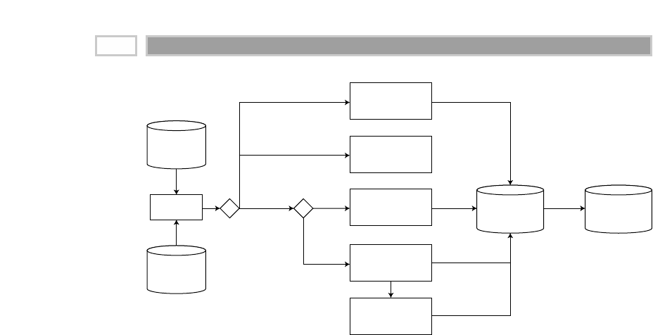
Figure 16.4 Dimension table surrogate key management.
To quickly determine if rows have changed, we rely on a cyclic redun-
dancy checksum (CRC) algorithm. If the CRC is identical for the extracted
record and the most recent row in the master table, then we ignore the
extracted record. We don’t need to check every column to be certain that
the two rows match exactly.
If the CRC for the extracted record differs from the most recent CRC in the
cross-reference table, then we need to study each column to determine
what’s changed and then how the change will be handled. If the changed
column is a type 1 attribute, then we merely overwrite the attribute value. If
the column is to be handled with a type 3 response, changes are made
solely in the existing row. However, the processing is a bit trickier with a
type 2 change. In this case we add a new row to the master cross-reference
table with a new surrogate key reflecting the new attributes values, as well
as the appropriate effective date, expiration date, and most recent indicator.
The expiration date and most recent indicator on the prior version need to
be updated to reflect that the prior row is no longer in effect. If we’re using
a combination of SCD techniques within a single table, we must establish
business rules to determine which change technique takes precedence.
The final step in Figure 16.4 is to update the most recent surrogate key
assignment table. This table consists of two columns—the operational
source key and its most recent assigned surrogate key. If we’ve handled
changes using the type 2 technique, this table will contain only the most
recent row. We create this table to provide fast lookups when assigning fact
table surrogate keys.
Most Recent
Key
Assignment
Master
Dimension
Cross-Ref
Source
Extract
Master
Dimension
Cross-Ref
Changed
Rows
No CRC
Change
New Source
Rows
Insert
Type
1 or 3
Type
2
Update
Insert
Update
Update
CRC
Compare
Update
dimension
attribute
Ignore
Assign surrogate
keys & set
dates/indicator
Update
prior "most
recent" row
Assign surrogate
keys & set
dates/indicator
CHAPTER 16
360

Build dimension row load images and publish revised dimensions. Once
the dimension table reflects the most recent extract (and has been confi-
dently quality assured), it is published to all data marts that use that
dimension.
Fact Table Staging
While the dimension tables are replicated to all the appropriate date marts,
fact table data is explicitly not duplicated. With the data warehouse bus archi-
tecture, the boundaries around a fact table are based on the source business
process(es), not on organizational lines. Consequently, fact tables are isolated
at unique locations but available to all who need access. Unlike dimension
tables that require a centralized authority to guarantee consistency across the
organization, fact tables can be managed on a more distributed basis, assum-
ing that each promises to use the dimension authority’s conformed dimension
and not replicate the same fact table data in multiple locations. We briefly out-
lined the steps required to stage the fact table data:
1. Extract fact data from operational source system.
2. Receive updated dimensions from the dimension authorities. We want
to ensure that we have the complete set of dimension rows that might be
encountered in the fact data.
3. Separate the fact data by granularity as required. Operational source sys-
tems sometimes include data at different levels of detail within the same
file. The granularities should be separated early in the staging process.
4. Transform the fact data as required. Common transformations include
arithmetic calculations, time conversions, equivalization of currencies or
units of measure, normalization of facts (such as the treatment of 12 date-
defined buckets on a single operational record), and handling of nulls.
5. Replace operational source keys with surrogate keys. To replace the oper-
ational keys with surrogate keys, we use the most recent surrogate key
assignment table created by the dimension authority. Making one pass over
the fact table for each dimension, we quickly substitute the most recent sur-
rogate key for each operational key encountered. We should ensure referen-
tial integrity at this point rather than waiting for the data load process. If
the fact table’s operational key does not locate a match in the surrogate key
assignment table, we have several options. The process could be halted. The
questionable rows could be written to a reloadable suspense file. Otherwise,
we could automatically create a new surrogate key and dimension row for
the unmatched operational key. Rather than assigning a single unknown
dummy key for all the troublesome operational keys encountered, we
assign a different surrogate key for each nonlocated operational key. The
Building the Data Warehouse 361

descriptive attribute for this newly assigned surrogate key might read
something like “Description Unknown for Operational Key XYZ.” In this
manner, when the new operational key is described properly, you often can
avoid revisiting the surrogate keys in the fact table.
6. Add additional keys for known context. We sometimes add surrogate
keys that aren’t available on the operational record, such as the appropri-
ate promotion key for the point-of-sale transactions or the demographics
minidimension key that identifies the customer’s current profile. Surro-
gate keys to indicate “Not Applicable” or “Date to Be Determined”
would be assigned as appropriate.
7. Quality-assure the fact table data. Of course, we should be generating
more row counts and cross-foots to compare with the extract statistics.
8. Construct or update aggregation fact tables. The aggregate tables typi-
cally are created outside the relational database platform because their
construction depends heavily on sort-and-sum sequential processing.
Be aware that reversals or prior-period adjustments can wreak havoc
on aggregation subsystems.
9. Bulk load the data. If fact table key collisions occur during the load,
we again have several options. We can halt the process, write the rows
to a reloadable suspense file, or additively update the target row.
10. Alert the users. Finally, inform the business community that the fact
table has been published and is ready for action.
Lifecycle Analytic Applications Track
The final set of parallel activities following the business requirements defini-
tion in Figure 16.1 is the analytic application track, where we design and
develop the applications that address a portion of the users’ analytic require-
ments. As a well-respected application developer once told us, “Remember,
this is the fun part!” We’re finally using the investment in technology and data
to help users make better decisions. The applications provide a key mecha-
nism for strengthening the relationship between the project team and the busi-
ness community. They serve to present the data warehouse’s face to its
business users, and they bring the business needs back into the team of appli-
cation developers.
While some may feel that the data warehouse should be a completely ad hoc
query environment, delivering parameter-driven analytic applications will sat-
isfy a large percentage of the business community’s needs. There’s no sense
CHAPTER 16
362

making every user start from scratch. Constructing a set of analytic applications
establishes a consistent analytic framework for the organization rather than
allowing each Excel macro to tell a slightly different story. Analytic applications
also serve to encapsulate the analytic expertise of the organization, providing a
jump-start for the less analytically inclined.
Analytic Application Specification
Following the business requirements definition, we need to review the find-
ings and collected sample reports to identify a starter set of approximately 10
to 15 analytic applications. We want to narrow our initial focus to the most crit-
ical capabilities so that we can manage expectations and ensure on-time deliv-
ery. Business community input will be critical to this prioritization process.
While 15 applications may not sound like much, the number of specific analy-
ses that can be created from a single template merely by changing variables
will surprise you.
Before we start designing the initial applications, it’s helpful to establish stan-
dards for the applications, such as common pull-down menus and consistent
output look and feel. Using the standards, we specify each application tem-
plate, capturing sufficient information about the layout, input variables, calcu-
lations, and breaks so that both the application developer and business
representatives share a common understanding.
During the application specification activity, we also must give consideration
to the organization of the applications. We need to identify structured naviga-
tional paths to access the applications, reflecting the way users think about
their business. Leveraging the Web and customizable information portals are
the dominant strategies for disseminating application access.
Analytic Application Development
When we move into the development phase for the analytic applications, we
again need to focus on standards. Standards for naming conventions, calcula-
tions, libraries, and coding should be established to minimize future rework.
The application development activity can begin once the database design is
complete, the data access tools and metadata are installed, and a subset of his-
torical data has been loaded. The application template specifications should be
revisited to account for the inevitable changes to the data model since the spec-
ifications were completed.
Each tool on the market has product-specific tricks that can cause it to jump
through hoops backwards. Rather than trying to learn the techniques via trial
Building the Data Warehouse 363

and error, you should invest in appropriate tool-specific education or supple-
mental resources for the development team.
While the applications are being developed, several ancillary benefits result.
Application developers, armed with a robust data access tool, quickly will find
needling problems in the data haystack despite the quality assurance per-
formed by the staging application. This is one reason why we prefer to get
started on the application development activity prior to the supposed comple-
tion of staging. Of course, we need to allow time in the schedule to address any
flaws identified by the analytic applications. The developers also will be the
first to realistically test query response times. Now is the time to begin review-
ing our performance-tuning strategies.
The application development quality-assurance activities cannot be com-
pleted until the data is stabilized. We need to make sure that there is adequate
time in the schedule beyond the final data staging cutoff to allow for an
orderly wrap-up of the application development tasks.
Deployment
The technology, data, and analytic application tracks converge at deployment.
Unfortunately, this convergence does not happen naturally but requires sub-
stantial preplanning. Perhaps more important, a successful deployment
demands the courage and willpower to assess the project’s preparedness
to deploy honestly. Deployment is similar to serving a large holiday meal to
friends and relatives. It can be difficult to predict exactly how long it will take
to cook the turkey. Of course, if the turkey’s thermometer doesn’t indicate done-
ness, the cook is forced to slow down the side dishes to compensate for the lag.
In the case of data warehouse deployment, the data is the main entrée, analo-
gous to the turkey. Cooking (or staging) the data is the most unpredictable task.
Unfortunately, in data warehousing, even if the data isn’t fully cooked, we often
still proceed with deployment because we told the warehouse guests they’d be
served on a specific date and time. Because we’re unwilling to slow down the
pace of deployment, we march into their offices with undercooked data. No
wonder users sometimes refrain from coming back for a second helping.
In addition to critically assessing the readiness of the data warehouse deliver-
able, we also need to package it with education and support for deployment.
Since the user community must accept the warehouse for it to be deemed suc-
cessful, education is critical. The education program needs to focus on the
complete warehouse deliverable: data, analytic applications, and the data
access tool (as appropriate). If we elect to develop educational materials
inhouse, we must allow at least 1 to 2 days of development for each hour of
education.
CHAPTER 16
364

Consider the following for an effective education program:
■■ Understand your target audience; don’t overwhelm.
■■ Don’t train the business community early prior to the availability of data and ana-
lytic applications.
■■ Postpone the education (and deployment) if the data warehouse is not ready to be
released.
■■ Gain the sponsor’s commitment to a “no education, no access” policy.
The data warehouse support strategy depends on a combination of manage-
ment’s expectations and the realities of the data warehouse deliverables. Sup-
port is often organized into a two-tier structure—the first line of expertise
resides within the business area, whereas centralized support provides a sec-
ondary line of defense. In addition to identifying support resources and pro-
cedures, we also need to determine the application maintenance and release
plan, as well as ongoing communication strategies.
Much like a software product release goes through a series of phases prior to
general availability, so should the data warehouse. The alpha test phase con-
sists of the core project team performing an end-to-end system test. As with
any system test, you’re bound to encounter problems, so make sure there’s
adequate time in the schedule for the inevitable rework. With the beta test, we
involve a limited set of business users to perform a user acceptance test, espe-
cially as it applies to the business relevance and quality of the warehouse
deliverables. Finally, the data warehouse is released for general availability,
albeit as a controlled rollout.
Maintenance and Growth
We’ve made it through deployment, so now we’re ready to kick back and
relax. Not so quickly! Our job is far from complete once we’ve deployed. We
need to continue to invest resources in the following areas:
Support. User support is crucial immediately following the deployment in
order to ensure that the business community gets hooked. For the first
several weeks following user education, the support team should be
working proactively with the users. We can’t sit back in our cubicles and
assume that no news from the business community is good news. If we’re
not hearing from them, then chances are that no one is using the data
warehouse. Relocate (at least temporarily) to the business community so
that the users have easy access to support resources. If problems with the
data or applications are uncovered, be honest with the business to build
Building the Data Warehouse 365

credibility while taking immediate action to correct the problems. Again,
if your warehouse deliverable is not of high quality, the unanticipated
support demands for data reconciliation and application rework can be
overwhelming.
Education. We need to provide a continuing education program for the data
warehouse. The curriculum should include formal refresher and advanced
courses, as well as repeat introductory courses. More informal education
can be offered to the developers and power users to encourage the inter-
change of ideas.
Technical support. The data warehouse is no longer a nice-to-have but needs
to be treated as a production environment, complete with service level
agreements. Of course, technical support should proactively monitor per-
formance and system capacity trends. We don’t want to rely on the busi-
ness community to tell us that performance has degraded.
Program support. While the implementation of a specific phase of the data
warehouse may be winding down, the data warehouse program lives on.
We need to continue monitoring progress against the agreed-on success
criteria. We need to market our success. We also need to ensure that the
existing implementations remain on track and continue to address the
needs of the business. Ongoing checkpoint reviews are a key tool to assess
and identify opportunities for improvement with prior deliverables. Data
warehouses most often fall off track when they lose their focus on serving
the information needs of the business users.
If we’ve done our job correctly, inevitably there will be demand for growth,
either for new users, new data, new applications, or major enhancements
to existing deliverables. As we advised earlier when discussing scoping,
the data warehouse team should not make decisions about these growth
options in a vacuum. The business needs to be involved in the prioritiza-
tion process. Again, this may be a good time to leverage the prioritization
quadrant analysis illustrated in Figure 16.2. If you haven’t done so already,
it is helpful to have an executive business sponsorship committee in place
to share responsibility for the prioritization. Once new priorities have been
established, then we go back to the beginning of this chapter and do it all
over again! Hopefully, we can leverage much of the earlier work, especially
regarding the technical and data architectures.
Common Data Warehousing Mistakes to Avoid
We’ve told you what to do throughout this chapter; now we’ll balance those rec-
ommendations with a list of what not to do. We closed Chapter 15 with a list of
common dimensional modeling mistakes. Here we’ve listed mistakes to avoid
CHAPTER 16
366
TEAMFLY
Team-Fly®

when building and managing a data warehouse. The mistakes are described as
a series of negative caricatures. Please forgive any trace of cynicism you might
detect. Our goal is for you to learn from these caricatures based on mistakes
made by unnamed data warehouse teams. As George Santayana said, “Those
who cannot remember the past are condemned to repeat it.” Let’s all agree not
to repeat any of these mistakes.
As in Chapter 15’s list of dimensional modeling mistakes, we’ve listed these
mistakes in reverse order, ending with the most important. However, any of
these could be show-stoppers.
Mistake 10: Accept the premise that those responsible for the enterprise's major
source systems are too important and busy to spend time with the data warehouse
team. Certainly, they cannot alter their operational procedures significantly for
passing data to or from the warehouse. If your organization really understands
and values the data warehouse, then the operational source systems
should be effective partners with you in downloading the data needed and
in uploading cleaned data as appropriate.
Mistake 9: After the data warehouse has been rolled out, set up a planning meeting
to discuss communications with the business users, if the budget allows. Newslet-
ters, training sessions, and ongoing personal support of the business com-
munity should be gating items for the first rollout of the data warehouse.
Mistake 8: Make sure the data warehouse support personnel have nice offices in the
IT building, which is only a short drive from the business users, and set up a data
warehouse support number with lots of touch-tone options. Data warehouse
support people should be physically located in the business departments,
and while on assignment, they should spend all their waking hours
devoted to the business content of the departments they serve. Such a rela-
tionship engenders trust and credibility with the business users.
Mistake 7: Train every user on every feature of the data access tool in the first train-
ing class, defer data content education because the class uses dummy data (the real
data won’t be ready for another couple of months), and declare success at the com-
pletion of the first training class because the data warehouse has been rolled out to
business users. Delay training until your first data mart is ready to go live
on real data. Keep the first training session short, and focus only on the
simple uses of the access tool. Allocate more time to the data content and
analytic applications rather than to the tool. Plan on a permanent series of
beginning training classes, as well as follow-up training classes. Take credit
for the user acceptance milestone when your users are still using the data
warehouse six months after they have been trained.
Mistake 6: Assume that business users naturally will gravitate toward robust data
and develop their own killer analytic applications. Business users are not appli-
cation developers. They will embrace the data warehouse only if a set of
prebuilt analytic applications is beckoning them.
Building the Data Warehouse 367

Mistake 5: Before implementing the data warehouse, do a comprehensive analysis
describing all possible data assets of the enterprise and all intended uses of infor-
mation, and avoid the seductive illusion of iterative development, which is only
an excuse for not getting it right the first time. Very few organizations and
human beings can develop the perfect comprehensive plan for a data
warehouse upfront. Not only are the data assets of an organization too vast
and complex to describe completely, but also the urgent business drivers
will change significantly over the life of the data warehouse. Start with a
lightweight data warehouse bus architecture of conformed dimensions and
conformed facts, and then build your data warehouse iteratively. You will
keep altering and building it forever.
Mistake 4: Don’t bother the senior executives of your organization with the data
warehouse until you have implemented it and can point to a significant success.
The senior executives must support the data warehouse effort from the
very beginning. If they don’t, your organization likely will not be able to
use the data warehouse effectively. Get their support prior to launching
the project.
Mistake 3: Encourage the business users to give you continuous feedback through-
out the development cycle about new data sources and key performance metrics
they would like to access, and make sure to include these requirements in the in-
process release. You need to think like a software developer and manage
three very visible stages of developing each data mart: (1) the business
requirements gathering stage, where every suggestion is considered seri-
ously, (2) the implementation stage, where changes can be accommodated
but must be negotiated and generally will cause the schedule to slip, and
(3) the rollout stage, where project features are frozen. In the second and
third stages, you must avoid insidious scope creep (and stop being such
an accommodating person).
Mistake 2: Agree to deliver a high-profile customer-centric data mart, ideally cus-
tomer profitability or customer satisfaction, as your first deliverable. These kinds of
data marts are consolidated, second-level marts with serious dependencies
on multiple sources of data. Customer profitability requires all the sources of
revenue and all the sources of cost, as well as an allocation scheme to map
costs onto the revenue! For the first deliverable, focus instead on a single
source of data, and do the more ambitious data marts later.
Mistake 1: Don’t talk to the business users; rather, rely on consultants or internal
experts to give you their interpretation of the users’ data warehouse requirements.
Your job is to be the publisher of the right data. To achieve your job objec-
tives, you must listen to the business users, who are always right. Nothing
substitutes for direct interaction with the users. Develop the ability to listen.
CHAPTER 16
368

The business users, not you, define the suitability and usability of the data
warehouse deliverable. You will be successful only if you serve the business
users’ needs.
Summary
This chapter provided a high-speed tour of the lifecycle of a data warehouse
project. We briefly touched on the key processes and best practices of a data
warehouse design and implementation effort. While each project is a bit dif-
ferent from the next, inevitably you’ll need to focus attention on each of the
major tasks we discussed to ensure a successful initiative.
Building the Data Warehouse 369


Present Imperatives and
Future Outlook
CHAPTER
17
371
Despite the dot-com meltdown and the collapse of the Internet hype, it is safe to
say that we are still in the middle of a revolution in computing and communi-
cations. A majority of the citizens in the United States, Europe, and parts of
Asia are using computers directly or are affected directly by them in various
ways. The speed and capacities of our computers continue to double every
18 months, and we are aggressively rewiring our infrastructure to support
high-bandwidth communications.
The unabated pace of this information revolution has profound implications
for data warehousing. Remember, data warehousing (or whatever it may be
called in the future) simply means publishing the right data. Data warehousing
is the central responsibility for doing something useful with all the data we
collect. Thus perhaps the good news is that we will all have jobs forever
because data warehousing is at the core of IT’s responsibility. But the bad news
is that data warehousing will be a moving target because our information
environment is evolving so rapidly and surely will continue to evolve for
many decades.
To try to get a grip on what the next 10 or 20 years may have in store us, let’s
first lay out as much as we can about what other industry pundits have said
recently regarding the next directions of technology. Although this may seem
to go counter to the biases in this book (that is, start with the business user’s
needs, not with technology), in the large sense of the marketplace, the new

technology is indeed a reflection of what the users want. Viewed from the per-
spective of the data warehouse, the entire world is being educated in the new
medium of the computer, and a whole set of powerful expectations will define
and drive what is a data warehouse.
Second, we must acknowledge and anticipate powerful political forces at
work in the world today affecting what we think a computer is and how infor-
mation should be used. The operative words are security and privacy. The data
warehouse is absolutely in the thick of both security and privacy issues, and if
anything, the data warehouse community has been slow to articulate security
and privacy solutions. Instead, we have had solutions handed to us by non-
data warehouse interests, including infrastructure groups in IT as well as
politicians.
Finally, we will try to describe the big cultural trends within data warehous-
ing, including the shake-out of the vendor community, the use of packaged
applications and outsourced application service providers, and the trends
toward and away from data warehouse centralization.
Ongoing Technology Advances
Let’s start with a fun topic: new technology. Did we say gadgets?
Internet appliance. Wafer thin, high performance, always on, real-time audio
and video with 24-bit color. Today’s personal computers connected to digi-
tal subscriber line (DSL) or cable modems already approach these specifi-
cations. Increasingly, people will demand portable devices with wireless
wideband connections to the Internet. The Internet appliance will become
an even more potent combination of information manipulation and com-
munication than it is today. Many data warehouse-driven services will be
delivered through this medium, and much data will be collected as a result
of the end user’s gestures made while using the appliance. The applica-
tions of the Internet appliance will include:
All forms of information search and retrieval. These will feature search
engines that do a much better job of understanding meaning, both in the
search specifications and in document contents.
Electronic mail. Always-on e-mail will encourage a flood of tiny e-mails
consisting of single sentence fragments as people converse casually and as
parents check on the locations of children, as well as countless other infor-
mal types of communication. This behavior is already common with the
Japanese DoCoMo device.
CHAPTER 17
372

Telephony. The Internet appliance will be a full-powered telephone, avail-
able anywhere at all times.
Mobile teleconferencing. Two-way and N-way face-to-face and voice-to-
voice communications will become a significant and valuable mode of
using the Internet appliance.
Television. Television will be widely available via the Internet appliance,
although it will not replace the standard living room TV.
Movies, literature, and games. The Internet appliance, coupled with wire-
less access, will be used increasingly for leisure and entertainment, espe-
cially on the road. Entertainment, of course, blends into education.
e-Learning. Electronic education will continue to be delivered on demand
more and more to remote students.
Radio. Conventional radio broadcasts from all over the world will grow in
popularity. The Internet is the successor to shortwave radio.
Shopping. Shopping on the Internet will continue to grow. Consumers
increasingly will configure the options they want and arrange delivery of
their built-to-order products. Dell provides a case study in a built-to-order,
no-intermediary business. eBay will grow to become the worldwide mar-
ketplace for person-to-person sales.
Navigation. Since the Internet appliance is portable, always connected, and
probably Global Positioning System (GPS)-enabled, it will be an increas-
ingly useful navigation aid, whether for driving or for walking.
Language translation. Slowly but surely, automatic language translation
services accessed via the Internet appliance will become accurate and useful.
4000 x 3000 pixel two-page monitors. Large-format, high-resolution display
technologies are coming out of the labs today that will increase the usable
area and resolution of our desktop PC systems dramatically.
Integration of cameras, video cameras, personal video recorders (PVRs),
and PCs. Disk storage and processor bandwidths are very close to being
ready at consumer prices for a grand synthesis of high-resolution photog-
raphy, full video capture, PVRs, and video libraries.
Spoken-language interfaces. Speech recognition is good enough already for
voice control of computer commands. A related capability will be voice
annotations in documents, a technology that has been waiting in the wings
for enough microphones attached to PCs to achieve critical mass.
GPS integration. GPS devices will permeate everything from our automo-
biles to our portable PCs to our smart credit cards. These devices not only
Present Imperatives and Future Outlook 373

will give end users feedback about where on the surface of the earth they
are but also frequently will record and save the locations of important
events, such as phone calls and transactions. The increased geocoding of
much of our data warehouse data will bring the data warehouse and GPS
communities somewhat closer together.
Secure, pervasive e-wallet. Today’s uncertainties about revealing your credit
card numbers will be forgotten. All of us will have the ability to reliably
authenticate ourselves (see the next item) and pay for products and ser-
vices in any situation. Coincidentally, this will hasten the financial crisis of
the conventional post office because paying bills by first class mail will be
one of the biggest categories switching over to the electronic form.
Reliable biometric identification. The window of opportunity for smart
tokens, such as automatic teller machine (ATM) cards, has passed by
already. Especially in these days of concern about making sure the person
at the PC is really who he or she says he or she is, there will be widespread
use of virtually foolproof biometric devices for personal identification.
Today, in 2002, fingerprint recognition seems to be the leader, but retinal
recognition seems to be the best long-term technology, assuming that the
retinal recognition devices can be built cheaply.
Personal data-collecting transducers everywhere. Over the next several
decades, it will be hard to resist the gradually increased use of data-
collecting transducers that will record our every move and every gesture.
Some of the pressure will come from security cameras or transducers in
sensitive public areas. Some of the pressure will come from protective par-
ents needing to track the whereabouts of their children. Criminals perhaps
may be released early from jail if they agree to wear a tracking device at all
times. Helpful household appliances will turn on the lights and heat up the
coffee when we stumble out of bed. Our pantries will keep a running
inventory and will generate a pick list for the next grocery store visit. The
grocery store itself can interact with this list and optimize our visit. It’s a
brave new world.
If all 300 million people in the United States generate one record each
second 24 hours per day 365 days per year, and assuming that the
records thus generated are 40 bytes wide, this would require 378,432 TB
of raw data storage each year. And this is a conservative design consisting
of only text and numbers, no images or maps.
Micropayments for content. A side effect of the e-wallet may well be the
introduction of added-value services in exchange for micropayments of a
few cents or fractions of a cent. Our hesitation here is not with the technol-
ogy but with the culture of the Internet that demands free access to every-
thing. Of course, content providers have to make money somehow, and
unless it’s advertising, it may have to be micropayments.
CHAPTER 17
374

Political Forces Demanding Security
and Affecting Privacy
At the time of this writing we are in the early stages of responding to the chal-
lenges of international terrorism. At the moment, most Americans would be
willing give up a little of their civil liberties and privacy in exchange for
significantly increased safety. If significant time goes by before another major
terrorist assault, the demand for a national ID card or other forms of secure
authentication of all persons will fade away. However, if another assault takes
place soon, it seems likely that we will want to track everyone, everywhere, at
least when they are using public infrastructure. The likely authentication tech-
nologies include forgery-proof ID cards with embedded biometric informa-
tion, as well as camera recognition systems that can identify anyone passing
through a security barrier.
In the face of terrorist threats, it is likely that we will tolerate a certain level of
tapping of our e-mails as well as our phone calls. It is not likely that we will
impose significant new constraints on the use of encryption simply because
strong encryption technology is already widely available both in the United
States and from foreign countries.
The existence of a national ID number and the encouragement to tie an indi-
vidual’s behavior together with the use of that number is, of course, the familiar
use of a conformed dimension on a very grand scale.
Conflict between Beneficial Uses
and Insidious Abuses
We often allow our personal information to be gathered only when we consider
the beneficial uses. And we usually don’t understand or anticipate the insidious
abuses of that same gathering of information when we approve it. Consider
the following examples:
Personal medical information. The beneficial uses are obvious and com-
pelling. We want our doctors to have complete information about us so
that they can provide the most informed care. We recognize that insurance
companies need access to our medical records so that they can reimburse
the health care providers. Most of us agree that aggregated data about
symptoms, diagnoses, treatments, and outcomes is valuable for society as a
whole. Furthermore, we see the need to tie these medical records to fairly
detailed demographic and behavioral information. Is the patient a smoker?
How old is the patient? However, the insidious abuses are nearly as rivet-
ing as the benefits. Most of us don’t want our personal medical details to
be available to anyone other than our doctors. Preferably, insurance claims
Present Imperatives and Future Outlook 375

processing clerks should not be able to view our names, but this is proba-
bly unrealistic. We certainly don’t want our personal medical information
to be sold to marketing-oriented third parties. We don’t want to be discrimi-
nated against because of our health status, age, or genetic predispositions.
Purchase behavior. The beneficial uses of purchase behavior data allow our
favorite retailers to give us personalized service. In fact, when we trust a
retailer, we are quite happy to provide a customization profile listing our
interests if this focuses the choices down to a manageable number and alerts
us to new products in which we would be interested. We want the retailer
to know us enough to handle questions, payment issues, delivery problems,
and product returns in a low-stress way. However, insidious abuses of our
purchase behavior drive us ballistic. We do not wish to be solicited by any
third party through junk mail or e-mail or over the telephone.
Safety and security in public facilities. In this day and age, all of us are
grateful for a feeling of security in airports, in front of bank teller machines,
and in parking garages. We wish the people who deliberately run red traffic
lights would stop endangering the rest of us. Most of us accept the presence
of cameras and license plate recognition systems in these public places as
an effective compromise that increases our safety and security. The legal
system, which ultimately reflects our society’s values, has solidly supported
the use of these kinds of surveillance technologies. However, the insidious
abuses of cameras and citizen tracking systems are scary and controversial.
We have the technical ability to create a national image database of every
citizen and identify most of the faces that cross through airport security
gates. How is the accumulated record of our travels going to be used and
by whom?
Who Owns Your Personal Data?
There is a natural inclination to believe that each of us owns and has an
inalienable right to control all our personal information. However, let’s face
the harsh reality. This view is naive and impractical in today’s society. The
forces that collect and share personal information are so pervasive and grow-
ing so quickly that we can’t even make comprehensive lists of the information-
gathering systems, much less define what kinds of collecting and sharing are
acceptable.
Think about the three examples discussed earlier. We all routinely sign the
waivers that allow providers and insurance companies to share our medical
records. Have you read one of these waivers? Usually they allow all forms of
records to be used for any purpose for an indefinite period. Just try objecting
to the wording on the waiver, especially if you are in the emergency room.
CHAPTER 17
376
TEAMFLY
Team-Fly®

And, honestly, the providers and the insurance companies have a right to own
the information because they have committed their resources and exposed
themselves to liability on your behalf.
Similarly, the retailer has a right to know who you are and what you bought if
you expect any form of credit or delivery relationship with the retailer. If you
don’t want personalized service, then only engage in anonymous cash trans-
actions at traditional brick-and-mortar stores.
And finally, if you use airports, teller machines, or roads, you implicitly agree
to accept the surveillance compromise. Any images collected belong to the
government or the bank, at least as far as current law is concerned. An odd
corollary of being filmed in a public place is the experience we all have had of
walking through a scene being filmed by an amateur photographer. Since a
third party has innocently captured our image, do we have any rights of own-
ership in that image?
What Is Likely to Happen?
Watching the Watchers . . .
In our opinion, there are two major ways in which privacy laws and practices
will be developed. Either our lawmakers will lead the way with innovative
and insightful legislation such as the Health Insurance Portability and
Accountability Act (HIPAA) and the Children’s On-Line Privacy Protection
Act (COPPA) or the marketplace and media will force organizations to adapt
to the perceived privacy concerns of our citizens. It should be said that the
government moves slowly, even when it does its job well. HIPAA was enacted
in 1996, and COPPA was enacted in 1998. The requirements of these laws still
have not been implemented fully in 2002.
Much has been written about the threats to privacy and the impact of new
technologies, but a pragmatic and compelling perspective that seems to be
gaining a significant following can be found in David Brin’s The Transparent
Society: Will Technology Force Us to Choose Between Privacy and Freedom? (Perseus
Books, 1999). Brin argues that an effective compromise between freedom and
privacy can be struck by watching the watchers. In other words, we accept the
inevitability of the beneficial applications of personal information gathering,
but we make the whole process much more visible and transparent. In this
way we can curb many of the insidious uses of the information. We insist on
very visible notifications of information gathering wherever it occurs. We
insist on honesty and ethical consistency in following the stated policies. And
significantly, we insist on being notified whenever our personal information is
used by anyone.
Present Imperatives and Future Outlook 377

Simson Garfinkel, in Database Nation (O’Reilly, 2000), agrees with many of the
points raised in Brin’s book and further insists that citizens should be able to
access, challenge, and correct all instances of their personal information, even
if they don’t have the absolute right to inhibit its use.
How Watching the Watchers Affects
Data Warehouse Architecture
The privacy movement is a potent force that may develop quickly. As data
warehouse designers, we may be asked suddenly by management to respond
to an array of privacy concerns. How is our data warehouse architecture likely
to be affected? Here is a likely list, in our opinion:
■■ All personal information scattered around our organization will need to
be consolidated and centralized into a single database. There should only
be one consistent, cleaned set of data about individuals, and any data that
is not being used for any identified purpose should be removed from all
databases.
■■ Security roles and policies surrounding this centralized personal informa-
tion database will need to be defined, enforced, and audited.
■■ The server containing the centralized personal information database will
be need to be physically isolated on its own segment of a local-area net-
work behind a packet filtering gateway that only accepts packets from
trusted application servers on the outside.
■■ Backup and recovery of the centralized personal information server will
need a strong form of physical and logical security.
■■ At least two levels of security sensitivity will need to be defined to imple-
ment a new privacy standard in your organization. General demographic
information will be assigned a lower level of security. Names, account
numbers, and selected financial and health-related information will be
assigned a higher level of security.
■■ An audit database that tracks every use of the personal information must
accompany the main database. This audit database must implement the
requirement to notify every individual of all uses of his or her personal
information, including who the requestor of the information is and what
the application is. The audit database may have different access require-
ments compared with the main database. If the audit database is used in a
batch mode, it pumps out usage reports that are e-mailed (or postal mailed)
to the affected individual whose information is being used. If the affected
individual can query the audit database online, then it is inherently less
CHAPTER 17
378

secure than the main database and probably needs to sit on a different,
more public server. It is important that the audit database contains as little
compromising content as possible but is focused simply on disclosing the
final uses of information.
■■ An interface must be provided that authenticates the individual requestor
and then provides a copy of all his or her personal information stored on
the database. A second interface must allow the individual to challenge,
comment on, or correct the information.
■■ A mechanism must exist for the effective expunging of information that is
deemed to be incorrect, legally inadmissible, or outdated. Expunged
information must be truly expunged so that it cannot surface again at a
later time.
Although the data warehouse community traditionally hasn’t led the way in
advocating social change, we think that it may be a canny look into the future
if we each consider whether the preceding list of changes could be imple-
mented in our organizations. Consider it a reasonable future scenario that
merits a little advanced planning. If you are more daring, and if you think the
privacy debate will end up as the kind of compromise described in Brin’s and
Garfinkel’s books, then have a talk with your CIO and your marketing man-
agement about some of these ideas.
Designing to Avoid Catastrophic Failure
We have been used to thinking that our big, important, visible buildings and
computers are intrinsically secure just because they are big, important, and vis-
ible. This myth has been shattered. If anything, these kinds of buildings
and computers are the most vulnerable.
The devastating assault on our infrastructure also has come at a time when the
data warehouse has evolved to a near production-like status in many of our
companies. The data warehouse now drives customer relationship manage-
ment and provides near-real-time status tracking of orders, deliveries, and pay-
ments. The data warehouse is often the only place where a view of customer
and product profitability can be assembled. The data warehouse has become
an indispensable tool for running many of our businesses.
Is it possible to do a better job of protecting our data warehouses? Is there a
kind of data warehouse that is intrinsically secure and less vulnerable to cata-
strophic loss?
Present Imperatives and Future Outlook 379

Catastrophic Failures
Let us list some important threats that can result in a sustained catastrophic
failure of a data warehouse, followed by potential practical responses:
Destruction of the facility. A terrorist attack can level a building or damage
it seriously through fire or flooding. In these extreme cases, everything on
site may be lost, including tape vaults and administrative environments.
Painful as it is to discuss, such a loss may include the IT personnel who
know passwords and understand the structure of the data warehouse.
Deliberate sabotage by a determined insider. The events of September 11,
2001 showed that the tactics of terrorism include the infiltration of our
systems by skilled individuals who gain access to the most sensitive points
of control. Once in the position of control, the terrorist can destroy the
system, logically and physically.
Cyberwarfare. It is not news that hackers can break into systems and wreak
havoc. The events of September 11 should remove any remaining naive
assumptions that these incursions are harmless or constructive because
they expose security flaws in our systems. There are skilled computer
users among our enemies who are actively attempting today to access
unauthorized information, alter information, and disable our systems.
How many times in recent months have we witnessed denial-of-service
attacks from software worms that have taken over servers or personal
computers? We do not believe for a minute that these are solely the work
of script kiddies. We suspect that some of these efforts are practice runs by
cyberterrorists.
Single-point failures (deliberate or not). A final general category of cata-
strophic loss comes from undue exposure to single-point failures, whether
the failures are caused deliberately or not. If the loss of a single piece of
hardware, a single communication line, or a single person brings the data
warehouse down for an extended period of time, then we have a problem
with the architecture.
Countering Catastrophic Failures
Now that we’ve identified several potential catastrophic failures, let’s turn our
attention to possible responses:
Profoundly distributed systems. The single most effective and powerful
approach to avoiding catastrophic failure of the data warehouse is a pro-
foundly distributed architecture. The enterprise data warehouse must be
made up of multiple computers, operating systems, database technologies,
CHAPTER 17
380

analytic applications, communications paths, locations, personnel, and
online copies of the data. The physical computers must be located in
widely separated locations, ideally in different parts of the United States
or across the world. Spreading out the physical hardware with many inde-
pendent nodes greatly reduces the vulnerability of the warehouse to sabo-
tage and single-point failures. Implementing the data warehouse
simultaneously with diverse operating systems (for example, Linux, Unix,
and NT) greatly reduces the vulnerability of the warehouse to worms,
social engineering attacks, and skilled hackers exploiting specific vulnera-
bilities. Over the next 20 years, many of the interesting architectural
advances in data warehousing will be in building profoundly distributed
systems. Although building and administering a profoundly distributed
data warehouse sound difficult, we have been arguing for years that we all
do this anyway! Very few large enterprise data warehouses are centralized
on a single monolithic machine.
Parallel communication paths. Even a distributed data warehouse implemen-
tation can be compromised if it depends on too few communication paths.
Fortunately, the Internet is a robust communications network that is highly
parallelized and adapts itself continuously to its own changing topology.
Our impression is that the architects of the Internet are very concerned
about system-wide failures due to denial-of-service attacks and other inten-
tional disruptions. Collapse of the overall Internet is probably not the
biggest worry. The Internet is locally vulnerable if key switching centers
(where high-performance Web servers attach directly to the Internet back-
bone) are attacked. Each local data warehouse team should have a plan for
connecting to the Internet if the local switching center is compromised. Pro-
viding redundant multimode access paths such as dedicated lines and satel-
lite links from your building to the Internet further reduces vulnerability.
Extended storage-area networks (SANs). A SAN is typically a cluster of
high-performance disk drives and backup devices connected together via
very high-speed fiber channel technology. Rather than being a file server,
this cluster of disk drives exposes a block-level interface to computers
accessing the SAN that makes the drives appear to be connected to the
backplane of each computer. SANs offer at least three huge benefits to a
hardened data warehouse. A single physical SAN can be 10 kilometers in
extent. This means that disk drives, archive systems, and backup devices
can be located in separate buildings on a fairly big campus. Second,
backup and copying can be performed disk to disk at extraordinary speeds
across the SAN. And third, since all the disks on a SAN are a shared
resource for attached processors, multiple application systems can be con-
figured to access the data in parallel. This is especially compelling in a true
read-only environment.
Present Imperatives and Future Outlook 381

Daily backups to removable media taken to secure storage. We’ve known
about this one for years, but now it’s time to take all this more seriously.
No matter what other protections we put in place, nothing provides the
bedrock security that offline and securely stored physical media provide.
However, before rushing into buying the latest high-density device, give
considerable thought as to how hard it will be to read the data from the
storage medium one, five, and even ten years into the future.
Strategically placed packet-filtering gateways. We need to isolate the key
servers of our data warehouse so that they are not directly accessible from
the local-area networks used within our buildings. In a typical configura-
tion, an application server composes queries, which are passed to a separate
database server. If the database server is isolated behind a packet-filtering
gateway, the database server can only receive packets from the outside
world coming from the trusted application server. This means that all other
forms of access are either prohibited or must be connected locally to the
database server behind the gateway. This means that database administra-
tors with system privileges must have their terminals connected to this
inner network so that their administrative actions and passwords typed in
the clear cannot be detected by packet sniffers on the regular network in
the building.
Role-enabled bottleneck authentication and access. Data warehouses can be
compromised if there are too many different ways to access them and if
security is not centrally controlled. Note that we didn’t say centrally located;
rather, we said centrally controlled. An appropriate solution would be a
Lightweight Directory Access Protocol (LDAP) server controlling all out-
side-the-gateway access to the data warehouse. The LDAP server allows
all requesting users to be authenticated in a uniform way regardless of
whether they are inside the building or coming in over the Internet from
a remote location. Once authenticated, the directory server associates the
user with a named role. The application server then makes the decision on
a screen-by-screen basis as to whether the authenticated user is entitled to
see the information based on his or her role. As our data warehouses grow
to thousands of users and hundreds of distinct roles, the advantages of this
bottleneck architecture become significant.
There is much we can do to fortify our data warehouses. In the past few years
our data warehouses have become too critical to the operations of our organi-
zations to remain as exposed as they have been. We have had the wakeup call.
CHAPTER 17
382

Intellectual Property and Fair Use
Organizations who create information have tremendous political power and
largely have succeeded in asserting permanent ownership rights to the informa-
tion they create. This kind of information includes recordings of works of art,
such as songs, movies, and video productions, as well as news and sports broad-
casts, and copyrighted expressions of opinion, such as financial newsletters.
All of this has a pretty significant impact on the data warehouse. One must be
extraordinarily careful about collecting information from an outside source.
Since most of our organizations have deep pockets, we must be very risk-
averse to avoid a lawsuit based on the claim that we appropriated information
that did not belong to us or was under license. Because of this, and because
media copying technology is being made much more restrictive, the original
concept of fair use of information found in a purchased copyrighted work
such as a book largely has been eviscerated. Fair use may be still legally valid
for an individual, but it may not be possible for a large enterprise.
Although the general public may have felt that Napster was harmless or even
beneficial, the courts took an extremely negative view of Napster’s file sharing
and cut off Napster’s air completely. Unless there is some significant change in
the law or a successful constitutional challenge, the writing on the wall is clear.
Created information belongs to the owner, who has very long-term rights to
the absolute control of that information. If you are lucky, you can rent the
information, but you won’t own it, and there is no practical way to make fair
use of that information, at least with the technology we know about today.
Cultural Trends in Data Warehousing
We’ll close this chapter by describing the significant cultural trends going on
and having an impact on data warehousing.
Managing by the Numbers
across the Enterprise
In the past 20 years the business world shifted noticeably to managing by the
numbers rather than managing by instinct or by walking the aisles. The whole
current generation of business managers has been educated in data-driven
Present Imperatives and Future Outlook 383

analysis and the importance of key performance indicators. The sheer size and
complexity of large businesses demand detailed measurements. And finally,
micromanaging individual store locations, product subcategories, and even
individual customers can result in significant economies.
All this requires a biblical flood of numbers and measurements. Although
marketing managers and the other strategic analysts in the business world
have been quantitatively oriented for most of the last 20 years, only recently
have the rank-and-file operations managers embraced the full potential of the
data warehouse. Much of the recent move comes from the new emphasis on
integrating all the customer-facing processes of the business into a seamless
whole so that both operations people and the customer can see all the
processes at once in a single understandable framework. However, achieving
full enterprise application integration (EAI) is a very complex process that
usually involves replacing the primary online transaction processing (OLTP)
operational systems. We are only partway through this process on a global
scale. However, competitive and financial pressures to achieve this integration
will only increase in the next 20 years. Thus, although this continued evolution
of managing by the numbers (you can call it data warehousing, CRM, or EAI)
may not be the most high-tech trend in the next 20 years, it is in some ways the
most important and pervasive trend we will have to deal with.
Increased Reliance on Sophisticated
Key Performance Indicators
Business managers always have had a love-hate relationship with powerful
key performance indicators (KPIs), especially those derived from sophisti-
cated mathematical models. If they work, they’re fantastic, but as soon as they
produce an inexplicable or wrong result, they suffer a disastrous drop in cred-
ibility. Data mining and sophisticated forecasting models gradually are gain-
ing a critical mass of respect, especially in certain application areas, such as
economic forecasting, promotions analysis, optimal pricing algorithms, fraud
detection, and threat analysis. The data mining community seems to have
learned the lesson not to oversell their sophisticated techniques but rather to
focus on successes that bring money to the bottom line. Generally, we feel that
the sophisticated analytic tools are natural clients of the data warehouse. In
many cases, the data warehouse serves to hand off observation sets as physi-
cal files to these tools, where they are processed and analyzed repeatedly
while the main data warehouse is busy serving other clients. The key issues for
the data warehouse manager supporting these sophisticated clients are to
(1) make sure that these clients actually use the data warehouse as the platform
for cleaned data rather than performing primary data extraction themselves,
CHAPTER 17
384

(2) educate these clients on how to drill across the conformed dimensions of
the enterprise to assemble broad and powerful observations, and (3) develop
an effective partnership for handing off data in both directions—to the data
mining tool and from the data mining tool.
Behavior Is the New Marquee
Application
In the 1980s, the dominant data warehouse application was shipments and
share. We were delighted just to see how much product went out the door to
various markets. In the 1990s, profitability was the dominant data warehouse
application. We discovered that with the proper data warehouse design, we
could slice and dice the profitability of our businesses by products, customers,
promotional events, time, and many other dimensions.
Although shipments, share and profitability certainly remain important, in the
2000s it appears that we have a new marquee application—behavior. Like the
earlier applications, behavior means many things and reaches to all corners of
our business. Customers have purchase behavior, payment behavior, product
return behavior, repurchase behavior, support request behavior, and recom-
mendation behavior. Products have reliability behavior, market appeal behav-
ior, and ordering season behavior. Employees have productivity behavior,
selling behavior, vacation taking behavior, and leadership behavior. Web site
visitors have click-through behavior, site navigation behavior, privacy behav-
ior, and trust behavior. Behavior is a powerful perspective to add to the ship-
ments and share and profitability applications we already know how to do.
Clearly, however, behavior is a more elusive concept. If profitability equals
revenue minus expenses, then what is behavior?
Packaged Applications Have Hit
Their High Point
During the go-go days of the Internet hype, many IT shops were overwhelmed
by the new demands of e-business. Most IT shops knew that they lacked the
skills to build their own Web- and CRM-oriented data warehouse systems.
This paved the way for application package vendors to address this need with
load-and-go packages for Web and CRM analysis. However, with e-business
pausing and taking a deep breath, IT shops now have the time to consider
more thoughtfully the tradeoffs in relying on an outside vendor’s proprietary
package for a portion of the data warehouse. We are not taking the position
here that packaged applications are bad, but we respectfully suggest that
package providers and IT shops need to reach a better middle ground. Here’s
Present Imperatives and Future Outlook 385

the main issue: Application package providers cannot be the data warehouse.
And this includes the biggest Enterprise Resource Planning (ERP) vendors.
The proprietary barriers of most of the application packages defeat the ability
of IT to control and publish its enterprise data in an open way. Application
packages instead should focus on performing their specific tasks very well and
then provide the most flexible and high performance possible way for the IT
organization to extract all the data from the package for housing in a separate
data warehouse.
Application Integration Has to
Be Done by Someone
We mentioned earlier that integrating the enterprise’s applications in order to
achieve a consistent customer-facing view often requires replacing the pro-
duction OLTP systems. This is not a cop-out in an effort to get the data ware-
house off the hook. Like data quality issues, it is almost impossible to clean up
incompatible data issues downstream from the source. Information has been
lost. In many cases the matching of data from incompatible systems is not log-
ically possible. In the long run, the data warehouse must follow, not lead, the
EAI effort. We do not mean by this to give up on creating conformed dimen-
sions and conformed facts. We are trying to warn you that this task will be far
easier if it starts with the production systems. Finally, you should be very con-
cerned if you (the data warehouse manager) are not invited to be on the EAI
architecture board of your organization. You are one of the most important
clients of this process, and senior management of your organization should
understand this.
Data Warehouse Outsourcing Needs
a Sober Risk Assessment
At the height of the Internet hype there was a hope that application service
providers (ASPs) could take off much of the load of developing and support-
ing the new kinds of data warehouses required for e-business. Some of these
also were affiliated with application package providers (discussed earlier).
The potential attraction of a data warehouse ASP remains very real, but again,
with the benefit of the pause we are all experiencing, we are assessing the risks
of the ASP model as well as the advantages. If we are no longer in a desperate
hurry to implement our e-business and our e-warehouse, why are we willing
to trust a strategic responsibility to an outsider? Before we throw the baby out
with the bath water, let’s list the advantages of the ASP model for data ware-
housing:
CHAPTER 17
386
TEAMFLY
Team-Fly®

■■ The ASP already has skills that the IT shop does not have and perhaps
cannot obtain easily.
■■ The ASP has configured a complete set of hardware and software compo-
nents that are known to work well together.
■■ The ASP has spare hardware capacity to respond to explosive demands
from the Web or for disaster recovery.
■■ The ASP has centralized economies of scale for backup and recovery.
■■ The costs of the ASP can be isolated and managed in a more visible way
than an internal department.
■■ The ASP takes care of its own personnel management.
Countering these very compelling potential advantages are the risks:
■■ Defining a data warehouse level-of-service agreement is a sophisticated
task, and there isn’t a lot of industry experience doing this. No matter
what, this agreement should come from your organization, not from the
lawyers working for the ASP!
■■ An ASP can go out of business. A source code escrow agreement is not
much consolation in such a case.
■■ An ASP may upgrade its software on its own schedule. In any case, the
ASP probably will not want to make custom modifications to standard
software offerings if it is supporting many clients across many applications.
■■ An ASP may support your competitors. You don’t have direct visibility
of the security procedures of an ASP.
At this point we are betting against the pure business model of the remote ASP
for data warehousing applications. Rather, we think a more viable model giv-
ing both parties what they need is for an ASP-like entity to run an inhouse data
warehouse implementation where there is significant skills sharing with the
local IT staff. In this way, many of the advantages of the ASP model can be real-
ized while lessening the risks.
In Closing
The best way to end this book is to return to the beginning. Sweeping away all
the details and techniques, the gold coin for the data warehouse professional
is to listen to the business. Consistently listening to the users brings us back to
what we are supposed to do. Over the next 20 years, we can navigate through
all the technical, organizational, and political changes that will happen if we
keep our eyes on the horizon. After all, our job is to publish the right data.
Present Imperatives and Future Outlook 387


Glossary
389
24/7 Operational availability 24 hours a day, 7 days a week.
3NF See Third normal form.
Accumulating snapshot fact table Type of fact table with multiple dates
representing the major milestones of a relatively short-lived process or
pipeline. The fact table is revisited and updated as activity occurs. A record
is placed in an accumulating snapshot fact table just once, when the item
that it represents is first created. Contrast with Periodic snapshot fact table
and Transaction-grain fact table.
Activity-based costs Costs that are reported as a measure of the activity
required rather than on an unchanging standard value. See Allocations.
Additive (facts) Measurements in a fact table that can be added across all
the dimensions. Ratios and unit prices are not generally additive.
Ad hoc queries Queries that are formulated by the user on the spur of the
moment. The ad hoc attack refers to the difficulty a database has in antici-
pating the pattern of queries. The more that queries are ad hoc, the more
symmetric the database model must be so that all queries look the same.
This is one of the strengths of the dimensional modeling approach.

Aggregate navigator Layer of software between the client and the relational
data that intercepts the client’s Structured Query Language (SQL) and
transforms that SQL, if it can, to use aggregates that are present somewhere
in the data warehouse. The aggregate navigator, by definition, shields the
user application from needing to know if an aggregate is present. In this
sense, an aggregate behaves like an index. Some relational database suppli-
ers have incorporated aggregate navigation capabilities into their database
management systems (DBMSs).
Aggregates Physical rows in a database, almost always created by sum-
ming other records in the database for the purpose of improving query
performance. Sometimes referred to as precalculated summary data. See
Aggregate navigator.
Algorithm Standard method for computing something; essentially a
mathematical recipe.
Alias (SQL) A short alphanumeric identifier in an SQL expression that
stands for a physical table name.
Allocated inventory Inventory that has been assigned for shipment to a
particular customer or store before it has actually been shipped.
Allocations Assignment or proration of measured values (usually costs) to
several accounts, customers, products, or transactions. For instance, the
overhead costs in a manufacturing plant are often allocated to the various
product lines made in the plant.
Allowance Amount subtracted from the list price of a product, typically as
a result of a promotion or a deal. Usually shown on the invoice but called
an off-invoice allowance.
Analytic application Prebuilt data access applications intended for less
frequent users of the data warehouse. Typically parameter-driven with
flexibility to analyze countless permutations. Such an application repre-
sents an opportunity to encapsulate the analytic best practices of an
organization.
Analytic processing Using data for analytic purposes to support business
decision-making, versus operational processing, where data is used to run
the business. Analytic processing often involves trend analysis, period-to-
period comparisons, and drilling.
ANSI American National Standards Institute, the recognized standards-
publishing body for a range of businesses, professions, and industries.
GLOSSARY
390

Answer set Rows returned to the end user as a result of an SQL expression
presented to a relational DBMS.
Application constraint (SQL) Portion of the WHERE clause in SQL that
defines a constraint on values, usually within a dimension table. To be
contrasted with a join constraint.
Architected data marts See Data warehouse bus architecture.
ASCII American Standard Code for Information Interchange. An 8-bit
character set encoding. ASCII can only support 127 characters, which is
not enough for international usage. See Extended ASCII and UNICODE.
Asset Item that appears on the balance sheet of a company that represents
something owned by the company or something owed to the company by
someone else. Bank loans are assets from the bank’s point of view because
they are owed to the bank.
Associative table See Bridge table.
Atomic data The most detailed granular data captured by a business
process. Atomic data must be made available in the data presentation area
to respond to unpredictable ad hoc queries.
Attribute A column (field) in a dimension table.
Audit dimension A special dimension that tags each fact table row with
operational meta data (for example, data lineage and confidence) when the
row is created.
Authentication The step of determining the identity of the requesting
client. Single-factor authentication usually is based on a simple password
and is the least secure authentication scheme. Two-factor authentication
may involve What-You-Know (a password) with What-You-Possess (a
plastic card) and is secure enough for banks’ automated teller machines.
Other two-factor authentication schemes involve What-You-Know with
Who-You-Are, using biometric scanning devices, such as fingerprint-,
retina-, or voice-based systems.
Average order backlog Average length of time that orders have been
waiting to be fulfilled.
B-tree index A relational index that is particularly useful for high-cardinality
columns. The B-tree index builds a tree of values with a list of row IDs that
have the leaf value. B-tree indexes are almost worthless for low-cardinality
columns because they take a lot of space and they usually cannot be com-
bined with other indexes at the same time to increase the focus of the
constraints. Contrast with Bitmap index.
GLOSSARY 391

Baseline sales (of a promotion) Sales volume that would have occurred if
there had been no promotion in effect.
Behavior score Figure of merit that is assigned to a customer based on pur-
chase patterns or credit patterns. Also referred to as a segmentation score.
Behavior scores can range from simple segmentation labels such as high,
medium, or low to complex numerical results of a data-mining application.
Behavior study group Large group of customers or products that is used in
a user analysis or report but which cannot be defined by constraining on
dimensional attributes and is too large to be enumerated by an SQL IN
clause. The behavioral study group often is defined from an original
analysis that isolates interesting purchase behavior or credit behavior.
BI See Business intelligence.
Bitmap index A relational indexing technique most appropriate for
columns with a limited number of potential values (low cardinality). Most
optimizers can combine more than one bitmapped index in a single query.
Contrast with B-tree index.
Brick and mortar A physically tangible business, such as a store, as
opposed to virtual or Web-based businesses. See also Click and mortar.
Bridge table A table with a multipart key capturing a many-to-many rela-
tionship that can’t be accommodated by the natural granularity of a single-
fact table or single-dimension table. Serves to bridge between the fact table
and the dimension table in order to allow many-valued dimensions or
ragged hierarchies. Sometimes referred to as a helper or associative table.
Browse query SELECT DISTINCT query on a single-dimension table to
show the user the values of an attribute or combination of attributes.
Browser Personal computer (PC) client software that communicates with
Web servers and displays Web content (text, image, audio, video) on the
PC. The main function of the browser is to execute the HyperText Markup
Language (HTML) program downloaded from the remote Web server.
Bus Originally used in the electrical power industry to refer to the common
structure providing power; then used in the computer industry to refer to a
standard interface specification. In the data warehouse, the bus refers to
the standard interface that allows separate data marts to coexist usefully.
See Data warehouse bus architecture.
GLOSSARY
392

Business dimensional lifecycle A methodology for planning, designing,
implementing, and maintaining data warehouses, as described in The Data
Warehouse Lifecycle Toolkit (Wiley, 1998).
Business intelligence (BI) A generic term to describe leveraging the organi-
zation’s internal and external information assets for making better business
decisions.
Business measure Business performance metric captured by an operational
system and represented as a fact in a dimensional model.
Business process Major operational activities or processes supported by
a source system, such as orders, from which data can be collected for the
analytic purposes of the data warehouse. Choosing the business process is
the first of four key steps in the design of a dimensional model.
Byte (B) Unit of measure, consisting of 8 bits of data.
Cache In a Web browser, disk space set aside to store temporary copies of
Web objects so that if they are requested again, they need not be fetched
from the Web but can be obtained locally. More generally, a cache is a tem-
porary storage space for objects or data expected to be used in the near
future.
Cannibalization Growth of sales of one product causing the slowing of
sales of another product. Usually referring to two products made by the
same manufacturer.
Cardinality The number of unique values for a given column in a relational
table. Low cardinality refers to a limited number of values, relative to the
overall number of rows in the table.
Cartesian product A set comprised of all the possible combinations from
multiple constraints.
Causal (factor or dimension) Something that is thought to be the cause of
something else. Causal factors in retail sales usually refer to ads, displays,
coupons, and price reductions. A causal dimension describes these causal
factors.
Centipede fact table A fact table with too many dimensions (often more
than 20), leading to a schema that resembles a centipede with numerous
foreign keys joined to numerous dimension tables. Centipedes typically
GLOSSARY 393

result when designers attempt to represent hierarchical relationships with
a proliferation of separate dimensions rather than nested within a single
dimension.
Chart of accounts List of accounts used by the general ledger. A uniform
chart of accounts is a chart of accounts applied consistently across an
organization.
Churn In a subscription service, the ratio of customers lost to customers
gained.
CIO Chief information officer within an organization.
Click and mortar A hybrid business with both a Web-based and a physically
tangible presence. Contrast with Brick and mortar.
Clickstream The composite body of actions taken by a user at a Web browser.
The clickstream can include both the actual clicks (browser requests) and
the server responses to those requests. The clickstream takes the form of
Web server logs, where each Web server log record corresponds to a single
page event.
Click-through The action of arriving at a Uniform Resource Locator (URL;
Web page) by clicking on a button or link, usually located on a different
Web site.
Column Data structure that contains an individual data item within a row
(record). Equivalent to a database field.
Composite key Key in a database table made up of several columns. Same
as Concatenated key. The overall key in a typical fact table is a subset of the
foreign keys in the fact table. In other words, it usually does not require
every foreign key to guarantee uniqueness of a fact table row.
Concatenated key See Composite key.
Conformed dimensions Dimensions are conformed when they are either
exactly the same (including the keys) or one is a perfect subset of the other.
Most important, the row headers produced in answer sets from two differ-
ent conformed dimensions must be able to be matched perfectly.
Conformed facts Facts from multiple fact tables are conformed when the
technical definitions of the facts are equivalent. Conformed facts are
allowed to have the same name in separate tables and can be combined
and compared mathematically. If facts do not conform, then the different
interpretations must be given different names.
GLOSSARY
394

Consolidated data mart Data marts that combine business measurements
from multiple business processes. Sometimes called a second-level data
mart. Contrast with First-level data mart.
Constraint Phrase in the SQL WHERE clause. A constraint is either a join
constraint or an application constraint.
Continuously valued (facts) Numeric measurement that usually is differ-
ent every time it is measured. Continuously valued measurements should
be facts in the fact table as opposed to discrete attributes that belong in a
dimension table.
Contribution Profit in a business measured by subtracting the allowances,
discounts, costs of manufacturing, and costs of sales from the gross revenue.
See Profit and loss.
Cookie A small text file placed on a user’s PC by a Web browser in response
to a specific request from a remote Web server. The cookie contents are
specified by the Web server and can only be read from Web servers belong-
ing to the domain that is specified in the cookie.
Copybook Traditional COBOL header file that describes all the columns in
an underlying data file.
Core table The fact table or the dimension table in a heterogeneous product
situation that is meant to span all the products at once. Contrast with
Custom line-of-business tables. See also Heterogeneous products.
Cost based optimizer Software in a relational database that tries to deter-
mine how to process the query by assigning estimated costs to various
table lookup alternatives.
Coverage table for a promotion A fact table, typically factless, that records
all the products that are on a promotion in a given store, regardless of
whether they sold or not.
CRC See Cyclic redundancy checksum.
CRM See Customer relationship management.
Cross-selling The technique of increasing sales by selling a new product
line to existing customers. See also Up-selling.
Cube Name for a dimensional structure on a multidimensional or online
analytical processing (OLAP) database platform, originally referring to the
simple three-dimension case of product, market, and time.
GLOSSARY 395

Custom line-of-business table The fact table or the dimension table in a
heterogeneous product situation that contains facts or attributes specific to
one set of products, where those facts or attributes are incompatible with
the other sets of products. Contrast with Core tables. See also Heterogeneous
products.
Customer master file Company’s master list of customers, usually
maintained by the order-processing operational system of record.
Customer matching The effort to identify an individual human customer
across multiple systems by Social Security Number, address, or other
indicators.
Customer relationship management (CRM) Operational and analytic
processes that focus on better understanding and servicing customers in
order to maximize mutually beneficial relationships with each customer.
Cyclic redundancy checksum (CRC) An algorithm that is useful for check-
ing two complex items, such as customer records, to see if anything has
changed. The CRC can be stored with an existing record, and then the CRC
can be computed on an incoming record. If there are any differences, the
CRCs will be different. This eliminates the requirement to check each con-
stituent field in the record.
Data access tool A client tool that queries, fetches, or manipulates data
stored on a relational database, preferably a dimensional model located in
the data presentation area. Contrast with a Data staging tool.
Data cube See Cube.
Data extract Process of copying data from an operational system in order to
load it into a data warehouse.
Data mart A logical and physical subset of the data warehouse’s presentation
area. Originally, data marts were defined as highly aggregated subsets of
data, often chosen to answer a specific business question. This definition
was unworkable because it led to stovepipe data marts that were inflexible
and could not be combined with each other. This first definition has been
replaced, and the data mart is now defined as a flexible set of data, ideally
based on the most atomic (granular) data possible to extract from an opera-
tional source, and presented in a symmetric (dimensional) model that is
most resilient when faced with unexpected user queries. Data marts can
be tied together using drill-across techniques when their dimensions are
conformed. We say these data marts are connected to the data warehouse
bus. In its most simplistic form, a data mart represents data from a single
business process.
GLOSSARY
396
TEAMFLY
Team-Fly®

Data mining A class of undirected queries, often against the most atomic
data, that seek to find unexpected patterns in the data. The most valuable
results from data mining are clustering, classifying, estimating, predicting,
and finding things that occur together. There are many kinds of tools that
play a role in data mining. The principal tools include decision trees,
neural networks, memory- and cased-based reasoning tools, visualization
tools, genetic algorithms, fuzzy logic, and classical statistics. Generally,
data mining is a client of the data warehouse.
Data presentation area The place where warehouse data is organized,
stored, and available for direct querying by users, data access tools, and
other analytical applications. All querying takes place on the data presen-
tation area. The data in the presentation area must be dimensional and
atomic (and possibly summarized, as appropriate) and adhere to the data
warehouse bus architecture. Typically referred to as a series of integrated
data marts. Contrast with the Data staging area.
Data quality assurance The step during the production data staging
process where the data is tested for consistency, completeness, and fitness
to publish to the user community.
Data staging area A storage area and set of processes that clean, transform,
combine, deduplicate, household, archive, and prepare source data for use
in the data warehouse. The data staging area is everything in between the
source system and the data presentation server. No querying should be
done in the data staging area because the data staging area normally is not
set up to handle fine-grained security, indexing or aggregations for perfor-
mance, or broad data integration across multiple data sources. Contrast
with the Data presentation area.
Data staging tool A software application typically resident on both the
client and the server that assists in the production data extract-transform-
load processes. Contrast with Data access tools.
Data stovepipe Occurs when data is available in isolated application-
specific databases, where little investment has been made to sharing
common data, such as customer or product, with other operational systems.
Unarchitected, stovepipe data marts are disastrous as they merely perpetu-
ate isolated, incompatible views of the organization.
Data warehouse The conglomeration of an organization’s data warehouse
staging and presentation areas, where operational data is specifically struc-
tured for query and analysis performance and ease-of-use. See Enterprise
data warehouse.
GLOSSARY 397

Data warehouse bus architecture The architecture for the data warehouse’s
presentation area based on conformed dimensions and facts. Without
adherence to the bus architecture, a data mart is a standalone stovepipe
application.
Data warehouse bus matrix Tool used to create, document, and communi-
cate the bus architecture, where the rows of the matrix identify the organi-
zation’s business processes and the columns represent the conformed
dimensions. The intersection of relevant dimensions applicable to each
business process is then marked.
Database management system (DBMS) A computer application whose
sole purpose is to store, retrieve, and modify data in a highly structured
way. Data in a DBMS usually is shared by a variety of applications.
Days’ supply (inventory) The number of days the current inventory level
would last at the current rate of sales.
DBA Database administrator, a senior IT position requiring extensive
understanding of database and data warehouse technology, as well as the
uses of corporate data.
DD See Degenerate dimension.
Decision support system (DSS) The original name for data warehousing.
In our opinion, it’s still the best name because it’s the business rationale for
the data warehouse—using data to make decisions in an organization. See
also Business intelligence.
Decode The textual description associated with an operational code, flag,
or indicator.
Degenerate dimension A dimension key, such as a transaction number,
invoice number, ticket number, or bill-of-lading number, that has no
attributes and hence does not join to an actual dimension table.
Demand side Flow of processes in a business starting with finished goods
inventory and progressing through to customer sales. Contrast with the
Supply side.
Demographic minidimension See Minidimensions.
Denormalize Allowing redundancy in a table so that the table can remain
flat, rather than snowflaked or normalized, in order to optimize perfor-
mance and ease-of-use. Equivalent to Second normal form (2NF).
Depletions Same as Shipments. Usually refers to a warehouse drawing
down inventory in response to customer orders.
GLOSSARY
398

Dimension An independent entity in a dimensional model that serves as
an entry point or as a mechanism for slicing and dicing the additive
measures located in the fact table of the dimensional model.
Dimension table A table in a dimensional model with a single-part primary
key and descriptive attribute columns.
Dimensional data warehouse Set of tables for decision support designed as
star-joined schemas.
Dimensional modeling A methodology for logically modeling data for
query performance and ease of use that starts from a set of base measure-
ment events. In the relational DBMS environment, a fact table is constructed
generally with one record for each discrete measurement. This fact table is
then surrounded by a set of dimension tables describing precisely what is
known in the context of each measurement record. Because of the charac-
teristic structure of a dimensional model, it is often called a star schema.
Dimensional models have proved to be understandable, predictable,
extendable, and highly resistant to the ad hoc attack from groups of busi-
ness users because of their predictable symmetric nature. Dimensional
models are the basis of many DBMS performance enhancements, including
powerful indexing approaches and aggregations. Dimensional models are
the basis for the incremental and distributed development of data ware-
houses through the use of conformed dimensions and conformed facts.
Dimensional models are also the logical foundation for all OLAP systems.
Directory server A server, which can be viewed as a little data warehouse,
that keeps track of all the users of a system as well as all the resources
available on the system, such as database servers, file servers, printers, and
communications resources. The industry standard way to communicate
with a directory server is the Lightweight Directory Access Protocol (LDAP).
Dirty customer dimension Customer dimension in which the same person
can appear multiple times, probably not with exactly the same name
spellings or other attributes.
Discrete (dimension attributes) Data, usually textual, that takes on a fixed
set of values, such as the flavor of a product. Discrete textual data always
should be handled as attributes in a dimension table as opposed to contin-
uously valued numeric data that belongs in a fact table.
Domain (1) A specific range of Internet addresses assigned to a single Inter-
net user. The domain name is a unique text name, often ending in .com,
.org, .gov, or .net. (2) In a dimension, the complete set of legal values from
which actual values are derived for an attribute.
GLOSSARY 399

Double-barreled joins Multiple parallel joins between a single dimension
table and a fact table.
Drill across The act of requesting similarly labeled data from two or more
fact tables in a single report, almost always involving separate queries that
are merged together in a second pass by matching row headers.
Drill down The act of adding a row header or replacing a row header in a
report to break down the rows of the answer set more finely.
Drill up The act of removing a row header or replacing a row header in a
report to summarize the rows of the answer set. Sometimes called dynamic
aggregation.
DSS See Decision support system.
Dwell time The length of time that a specific Web page is available for
viewing on a user’s browser.
Earned income The income that a company is allowed to report in a given
time period based on providing a service during that time period. Money
paid in advance cannot be reported as income until it is earned.
End-aisle displays A form of promotion in grocery and drug stores.
Enterprise application integration (EAI) In a general sense, the reengineer-
ing of operational source systems to deliver enterprise consistency. In a
product sense, a set of products that attempt to facilitate transaction-level
communication among potentially incompatible operational source systems.
Enterprise data warehouse (EDW) The conglomeration of an organization’s
data warehouse staging and presentation areas. Others in the industry
refer to the EDW as an centralized, atomic, and normalized layer of the
data warehouse, without making it clear if such a system is available for
end-user querying and drill-down. We discourage this interpretation of the
EDW, preferring to think of the EDW as the largest possible union of stag-
ing and presentation services, taken as a whole.
Enterprise resource planning (ERP) application A class of applications
aimed at spanning some or all of the business functions of a complete
enterprise. ERP applications often are deployed on relational databases,
and the data dictionaries for these applications may contain thousands of
tables. An organization acquiring a major ERP application usually must
shut down existing legacy applications and restructure fundamental busi-
ness processes around the ERP system. ERP systems often contain the
equivalent of an operational data store (ODS) because they usually are
GLOSSARY
400

capable of real-time or near-real-time operational reporting, but ERP systems
until 2002 have not made good data warehouses because they have not
provided acceptable end-user query performance or a flexible environment
for importing third-party data.
Entity-relationship (ER) diagram (ERD) Drawings of boxes and lines to
communicate the relationship between tables. Both third normal form
(3NF) and dimensional models can be represented as ER diagrams because
both consist of joined relational tables. The key difference between the
models is the degree of dimension normalization. A dimensional model is
a second normal form (2NF) model.
Equal access The original promise of relational databases: the ability to
retrieve data based on any criteria present in the data.
ETL See Extract-transform-load.
Event See Page event.
Event-tracking table A fact table, frequently factless, where the dimensions
of the table are brought together to describe an event, such as an insurance
description of an automobile accident.
Extended ASCII The extension of the American Standard Code for Infor-
mation Interchange to include European accented characters and other
special characters. This encoding uses the high 128 characters in the 8-bit
ASCII format. See ASCII and UNICODE.
Extended cost The unit cost multiplied by a quantity to give an additive
value.
Extensible Markup Language (XML) A cousin of HTML that provides
structured data exchange between parties. XML contains data and meta
data but no formatting information. Contrast with HTML. XML is a flexible,
strongly hierarchical framework for assigning tags to fields within a docu-
ment. XML does not specify what the tags should be. It is up to various
organizations or industry groups to define and use consistent sets of tags,
and this effort is the main gating factor slowing the widespread use of XML.
Extract-transform-load (ETL) Set of processes by which the operational
source data is prepared for the data warehouse. The primary processes of
the backroom data staging area of the data warehouse, prior to any presen-
tation or querying. Consists of extracting operational data from a source
application, transforming it, loading and indexing it, quality-assuring it,
and publishing it.
GLOSSARY 401

Fact A business performance measurement, typically numeric and additive,
that is stored in a fact table.
Fact dimension A special dimension used to identify extremely sparse,
dissimilar measurements in a single fact table.
Fact table In a star schema (dimensional model), the central table with
numeric performance measurements characterized by a composite key,
each of whose elements is a foreign key drawn from a dimension table.
Factless fact table A fact table that has no facts but captures certain many-
to-many relationships between the dimension keys. Most often used to
represent events or provide coverage information that does not appear in
other fact tables.
File Transfer Protocol (FTP) TCP/IP protocol that is used for transferring
files between computers.
Filter on fact rows A type of application constraint that constrains on the
numeric values of one or more facts. Used for value banding.
First-level data mart A data mart that is derived from a single primary
source system. Contrast with Consolidated data mart.
Fixed depth hierarchy A highly predictable hierarchy with a fixed number
of levels. Contrast with Ragged hierarchy.
FK See Foreign key.
Flat file A simple data structure, often implemented on a mainframe, that
relies on nonrelational files, such as IBM VSAM files.
Foreign key (FK) A column in a relational database table whose values are
drawn from the values of a primary key in another table. In a star-join
schema, the components of a composite fact table key are foreign keys with
respect to each of the dimension tables.
Framework Unifying, guiding architectural approach, as in the data ware-
house bus architecture.
FROM clause (SQL) SQL clause that lists the tables required by the query.
General ledger (G/L) Ledger that represents the organization’s assets,
liabilities, equity, income, and expense. The G/L remains balanced through
offsetting transactions to debit and credit accounts.
GLOSSARY
402

Geographic information system (GIS) A hybrid application combining
database and mapping technology. Typically, in a GIS, queries can be con-
structed from maps, and maps can be delivered as a result of a query.
Gigabyte (GB) One billion bytes.
GIS See Geographic information system.
GMROI Gross margin return on inventory, equal to the number of turns of
inventory multiplied by the gross margin percent. A measure of the return
on each dollar invested in inventory.
Grain The meaning of a single row in a fact table. The declaration of the
grain of a fact table is the second of four key steps in the design of a
dimensional model.
Granularity The level of detail captured in the data warehouse. See Grain.
Greenwich Mean Time (GMT) The local standard time at zero degrees
longitude, which runs through the Royal Navy Observatory near London.
Gross margin percent The gross profit expressed as a percentage of gross
revenue.
Gross profit The gross revenue less the cost of the goods.
Gross revenue The total revenue paid to a company by its customers. If the
gross revenue is calculated before applicable discounts, then the actual
amount paid by the customers is called the net revenue.
GROUP BY clause (SQL) SQL clause that uniquely lists the unaggregated
items in the SELECT list, that is, everything that is not a SUM, COUNT,
MIN, MAX, or AVG.
GUI Graphic user interface. A style of computer interface characterized by
windows, icons, the use of graphics, and the use of a mouse pointing
device.
Helper table See Bridge table.
Heterogeneous products A set of products typically characterized by many
incompatible product attributes and measurable facts. A characteristic
design challenge in financial service environments. See Core table and
Custom line-of-business table.
Hierarchical relationship A relationship where data rolls up into higher
levels of summarization in a series of strict many-to-one relationships.
GLOSSARY 403

Hierarchies are reflected by additional columns on the atomic dimension
table.
Householding The effort to assign an account or an individual to a house-
hold of accounts or individuals for marketing purposes.
HyperText Markup Language (HTML) A standard markup language for
defining the presentation characteristics of Web documents. HTML con-
tains data and formatting but does not contain meta data. Contrast with
XML. HTML is not a general programming language.
HyperText Transfer Protocol (HTTP) The communications protocol of the
Web. HTTP specifies the way in which a browser and Web site exchange
information.
Impact report When reporting with a bridge table, the weighting factor
assigned to the multivalued dimension is ignored. The resulting totals pro-
vide a summarization for any case in which the multivalued dimension
was involved, regardless of the extent of the involvement. Contrast with
Weighted report.
Implementation bus matrix A more detailed version of the data warehouse
bus matrix where fact tables are identified for each business process, as well
as the fact table granularity and measurements.
Index A data structure associated with a table that is logically ordered by
the values of a key and used to improve database performance and query
access speed. B-tree indexes are used for high-cardinality fields, and
bitmap indexes are used for medium- and low-cardinality fields.
Internet The worldwide collection of communication links and services
that are tied together using the Internet Protocol (IP).
Internet service provider (ISP) A company or organization that provides
Internet connectivity to the public through the use of telephone lines,
cable, or satellites. ISPs often offer a range of services, such as electronic
mail, Web hosting, and application access, and provide connectivity to the
customer’s personal computer using TCP/IP protocols.
IP address The numeric address of a particular host or subnet on the Internet.
Join constraint (SQL) The portion of the SQL WHERE clause that book-
keeps the join relationships between the fact table and the dimension
tables.
GLOSSARY
404

JPEG, JPG An image-compression format standardized by the Joint Photo-
graphic Experts Group. It is particularly suited to complex images such as
photographs. A JPEG image can be adjusted to offer high compression with
resulting loss of image quality or low compression with high image quality.
Julian day number A representation of a calendar date as the simple count
of days from the beginning of an epoch, such as January 1, 1900. True Julian
dates are numbered in the millions and are not used often as the literal
basis of date values.
Junk dimension An abstract dimension with the decodes for a group of
low-cardinality flags and indicators, thereby removing the flags from the
fact table.
LDAP Lightweight Directory Access Protocol, a standard currently agreed
to by most of the major systems vendors for describing the users of a net-
work and the resources available on a network. See Directory server.
Liability An item that appears on the balance sheet of a company that
represents money the company owes to someone else. Bank deposits are
liabilities from a bank’s point of view because they must be paid back.
Lift of a promotion The increase of sales over the baseline value that can be
attributed to the effects of a promotion.
Line item An individual line of a control document such as an invoice usu-
ally identifying a single product within the invoice. Most often used as the
grain of the associated fact table.
Logical design The phase of a database design concerned with identifying
the relationships among the data elements. Contrast with Physical design.
Loss party (insurance) Any individual or entity associated with a claim
(a loss), including injured parties, witnesses, lawyers, and other service
providers.
Low-cardinality attribute set A set of attributes that have a very low cardi-
nality relative to the number of rows in the base dimension, such as external
demographic data for a set of customers. May be handled as a dimension
outrigger. See also Cardinality.
Many-to-many relationship A logical data relationship in which the value
of one data element can exist in combination with many values of another
data element, and vice versa.
Many-to-one relationship See One-to-many relationship.
GLOSSARY 405

Many-valued dimensions Normally, a fact table possesses only connec-
tions to dimensions representing a single value, such as a single time or a
single product. But occasionally, it is valid to connect a fact table record to
a dimension representing an open-ended number of values, such as the
number of simultaneous diagnoses a patient may have at the moment of a
single treatment. In this case we say that the fact table has a many-valued
dimension. Also referred to as Multivalued dimensions. Typically handled
using a bridge table.
Market basket analysis A kind of analysis in retail environments that seeks
to understand all the products purchased by a customer in a single shop-
ping event. Market basket analysis is an example of affinity grouping that
seeks to find things that happen together.
Market growth A desirable outcome of a promotion that causes overall
sales of a product category to grow instead of causing cannibalization.
MBA Master of Business Administration, a graduate college or university
degree requiring extensive understanding of how commercial businesses
are organized and managed.
Merchandise hierarchy A set of attributes in the product dimension that
define an ascending many-to-one relationship. Common to all manufactur-
ing and retail environments.
Meta data Any data maintained to support the operations or use of a data
warehouse, similar to an encyclopedia for the data warehouse. Nearly all
data staging and access tools require some private meta data in the form
of specifications or status. There are few coherent standards for meta data
viewed in a broader sense. Distinguished from the primary data in the
dimension and fact tables.
Migrate Moving data from one computer to another or from one file format
to another.
Minidimensions Subsets of a large dimension, such as customer, that are
broken off into separate, smaller artificial dimensions to control the explo-
sive growth of a large, rapidly changing dimension. The continuously
changing demographic attributes of a customer are often modeled as a
separate minidimension.
Mirrored database A physical organization of data where the entire data-
base is duplicated on separate disk drives. Mirrored databases offer a
number of performance and administrative advantages.
GLOSSARY
406
TEAMFLY
Team-Fly®

Modeling applications A sophisticated data warehouse client with analytic
capabilities that transform or digest the output from the data warehouse.
Modeling applications include forecasting models, behavior scoring mod-
els that cluster and classify customer purchase behavior or customer credit
behavior, allocation models that take cost data from the data warehouse
and spread the costs across product groupings or customer groupings, and
most data mining tools.
Most recent indicator An attribute, typically used in conjunction with
type 2 slowly changing dimensions, that indicates the most current profile.
Multidimensional database Database in which the data is presented in
data cubes, as opposed to tables in a relational database platform.
Multidimensional OLAP (MOLAP) Dedicated online analytical processing
implementations not dependent on relational databases. Although
MOLAP systems do not scale to the sizes that relational databases systems
can, they typically offer better performance and more tightly integrated
tools than their relational counterparts.
Multipass SQL Query capability supported by some data access tools in
which the results of separate star-schema queries are combined column
by column via the conformed dimensions. Not the same thing as a union,
which is a row-by-row combination of separate queries.
Multitable join query One of the two characteristic types of queries in a
data warehouse environment. Involves the joining of one or more dimen-
sion tables to a single fact table. Contrast with Browse queries.
Multivalued dimensions See Many-valued dimensions.
Natural key The identifier used by the operational systems. Natural keys
often have embedded meaning. They may appear as dimension attributes
in dimensional models but should not serve as the dimension table primary
key, which always should be a surrogate key.
Nonadditive (facts) A fact that cannot logically be added between rows.
May be numeric and therefore usually must be combined in a computation
with other facts before being added across rows. If nonnumeric, can only
be used in constraints, counts, or groupings.
Normalize A logical modeling technique that removes data redundancy by
separating the data into many discrete entities, each of which becomes a
table in a relational DBMS.
GLOSSARY 407

Null A data field or record for which no value exists. We avoid null keys
in the fact table by assigning a dimension surrogate key to identify “Not
Applicable,” “To Be Determined,” or other “Empty” conditions.
ODS See Operational data store.
Off-invoice allowances Typically deal- or promotion-related subtractions
from the list price shown on the invoice. Part of deriving the net invoice
amount, which is what the customer is supposed to pay on this line item.
Off-invoice discounts Typically financial terms-related subtractions from
the list price shown on the invoice. Part of deriving the net invoice amount,
which is what the customer is supposed to pay on this line item.
One-to-many relationship A logical data relationship in which the value
of one data element can exist in combination with many values of another
data element, but not vice versa.
Online analytic processing (OLAP) OLAP is a loosely defined set of princi-
ples that provide a dimensional framework for decision support.
The term OLAP also is used to define a confederation of vendors who offer
nonrelational, multidimensional database products aimed at decision
support. Contrast with Online transaction processing.
Online transaction processing (OLTP) The original description for all the
activities and systems associated with entering data reliably into a data-
base. Most frequently used with reference to relational databases, although
OLTP can be used generically to describe any transaction-processing envi-
ronment. Contrast with Online analytic processing.
Operational data store (ODS) A physical set of tables sitting between the
operational systems and the data warehouse or a specially administered
hot partition of the data warehouse itself. The main reason for an ODS is
to provide immediate reporting of operational results if neither the opera-
tional system nor the regular data warehouse can provide satisfactory
access. Because an ODS is necessarily an extract of the operational data,
it also may play the role of source for the data warehouse.
Operational system of record An operational system for capturing data
about a company’s operations and business processes. May not necessarily
be a transaction system or a relational system.
ORDER BY clause (SQL) SQL clause that determines the ordering of rows
in the answer set.
GLOSSARY
408

Outrigger table A secondary dimension table attached to a dimension
table. An outrigger table is a physical design interpretation of a single
logical dimension table. Occurs when a dimension table is snowflaked.
P&L See Profit-and-loss schema.
Page (1) A Web page is a document in HTML format that can be displayed
by a browser. The term page also is used to describe a compound document
consisting of the HTML document itself and ancillary objects such as
images or sounds that are downloaded to the browser as directed by the
page’s HTML. (2) Basic unit of stored data.
Page event Refers to a Web page or frame downloaded from a Web server
to a browser, exclusive of any ancillary content.
Parent-child database Hierarchical organization of data typically involving
a header and set of line items. The dimensional modeling approach strips
all the information out of the header (parent) into separate dimensions and
leaves the original parent natural key as a degenerate dimension.
Parsing Decomposing operational fields, such as a name or address, into
standard elemental parts.
Partitioned tables Tables (and their associated indices) that are managed as
physically separate tables but appear logically as a single table. Large fact
tables are candidates for partitioning, often by date. Partitioning can
improve both query and maintenance performance.
Partitioning of history The natural correspondence between dimension
table entries and fact table rows when a type 2 slowly changing dimension
has been implemented. A type 2 slowly changing dimension partitions his-
tory because each value of its surrogate key is administered correctly to
connect to the correct contemporary span of fact records.
Periodic snapshot fact table A type of fact table that represents business
performance at the end of each regular, predictable time period. Daily
snapshots and monthly snapshots are common. Snapshots are required in
a number of businesses, such as insurance, where the transaction history is
too complicated to be used as the basis for computing snapshots on the fly.
A separate record is placed in a periodic snapshot fact table each period
regardless of whether any activity has taken place in the underlying
account. Contrast with Transaction fact table and Accumulating snapshot
fact table.
GLOSSARY 409

Physical design The phase of a database design following the logical
design that identifies the actual database tables and index structures used
to implement the logical design.
PK See Primary key.
Point-of-sale (POS) system The cash registers and associated in-store
computers in a retail environment.
Portal A Web site designed to be the first point of entry for visitors to the
Web. Portal sites usually feature a wide variety of contents and search
capabilities in order to entice visitors to use them. Portals are often selected
as browser home pages.
Price-point analysis The breakdown of product sales by each discrete
transaction price. Requires a fact table with fine enough grain to represent
each price point separately.
Primary key (PK) A column in a database table that is uniquely different
for each row in the table.
Product master file A company’s master list of products, usually main-
tained by a manufacturing or purchase order operational application.
Profit-and-loss (P&L) schema The P&L, also known as an income statement,
is the classic logical ordering of revenues and costs to represent a progres-
sion from gross revenues down to a bottom line that represents net profit.
The profitability schema often is called the most powerful dimensional
schema because it allows the business to slice and dice revenue, cost, and
profit by their primary dimensions, such as customer and product.
Promotion An event, usually planned by marketing, that features one or
more causal items such as ads, displays, or price reductions. Also thought
of as a deal or sometimes as a contract.
Proxy An alternate Web server that responds to a Web page request in order
to reduce the load on a primary Web server or network.
Pseudotransaction A step needed in some production data extract systems
where a nontransactional legacy system is analyzed to see what changed
from the previous extract. These changes are then made into artificial
(pseudo) transactions in order to be loaded into the data warehouse.
Publishing the right data The most succinct way to describe the overall
responsibility of the data warehouse. The data is right if it satisfies the
GLOSSARY
410

business’s requirements. The act of publishing is driven ultimately by the
business user’s needs.
Pull-down list A user-interface effect in a data access tool that displays a
list of options for the user. The most interesting pull-down lists in a data
warehouse come from browse queries on a dimension attribute.
Query User request for information stored in a data warehouse. With a
relational DBMS, the query is an SQL SELECT statement passed from the
data access application (typically on the end user’s client machine).
Ragged hierarchy A hierarchy with an unbalanced and arbitrarily deep
structure that usually cannot be described in advance of loading the data.
Sometimes referred to as a variable-depth hierarchy. Organization charts
often are ragged hierarchies. See Bridge table.
Real time partitions A physically separate and specially administered set
of tables, apart from the conventional data warehouse, to support more
real-time access requirements. See also Operational data store.
Reason code A field used in conjunction with a transaction dimension to
describe why the transaction took place. Reason codes are valuable for
returns and cancellations and for describing why something changed.
Redundancy Storing more than one occurrence of the data.
Referential integrity (RI) Mandatory condition in a data warehouse where
all the keys in the fact tables are legitimate foreign keys relative to the
dimension tables. In other words, all the fact key components are subsets
of the primary keys found in the dimension tables at all times.
Referral The identity of the previous context of a URL. In other words, if
you click on a link in page A and wind up on page B, page B’s Web server
sees page A as the referral. Web servers can log referrals automatically,
which is a very useful way to see why a visitor came to your Web site.
Relational database management system (RDBMS) Database management
system based on the relational model that supports the full range of stan-
dard SQL. Uses a series of joined tables with rows and columns to organize
and store data.
RI See Referential integrity.
ROI Return on investment, usually expressed as a rate describing the
growth of an investment during its lifetime.
GLOSSARY 411

Role-playing dimensions The situation where a single physical dimension
table appears several times in a single fact table. Each of the dimension
roles is represented as a separate logical table with unique column names
through views.
Roll up To present higher levels of summarization. See Drill up.
Row A record in a relational table.
Row header The nonaggregated components of the SQL select list. Always
listed in the SQL group by clause.
Sales invoice The operational control document that describes a sale.
Usually contains multiple line items that each represent a separate product
sold.
Scalability The ability to accommodate future growth requirements.
SCD See Slowly changing dimensions.
Schema The logical or physical design of a set of database tables, indicating
the relationship among the tables.
Second-level mart See Consolidated data mart.
SELECT DISTINCT (SQL) SQL statement that suppresses duplicate rows
in the answer set.
SELECT list (SQL) List of column specifications that follows SELECT and
comes before FROM in an SQL query. Each item in the select list generates
a column in the answer set.
Semantic layer An interface layer placed between the user and the physical
database structure.
Semiadditive (fact) Numeric fact that can be added along some dimensions
in a fact table but not others. Inventory levels and balances cannot be
added along the time dimension but can be averaged usefully over the time
dimension.
Session The collection of actions taken by a Web site visitor while visiting
the Web site without leaving it. Also called a visit.
Shelf displays Tags, racks, or other promotional mechanisms used in a
retail environment.
GLOSSARY
412

SKU See Stock keeping unit.
Slice and dice Ability to access a data warehouse through any of its dimen-
sions equally. Slicing and dicing is the process of separating and combining
warehouse data in seemingly endless combinations.
Slowly changing dimensions (SCD) The tendency of dimension rows to
change gradually or occasionally over time. A type 1 SCD is a dimension
whose attributes are overwritten when the value of an attribute changes.
A type 2 SCD is a dimension where a new row is created when the value
of an attribute changes. A type 3 SCD is a dimension where an alternate
old column is created when an attribute changes.
Snapshot See either Accumulating snapshot fact table or Periodic snapshot
fact table.
Snowflake A normalized dimension where a flat, single-table dimension is
decomposed into a tree structure with potentially many nesting levels. In
dimensional modeling, the fact tables in both a snowflake and star schema
would be identical, but the dimensions in a snowflake are presented in
third normal form, usually under the guise of space savings and maintain-
ability. Although snowflaking can be regarded as an embellishment to the
dimensional model, snowflaking generally compromises user understand-
ability and browsing performance. Space savings typically are insignificant
relative to the overall size of the data warehouse. Snowflaked normalized
dimension tables may exist in the staging area to facilitate dimension
maintenance.
Sort To sequence data according to designated criteria.
Source system An operational system of record whose function it is to
capture the transactions or other performance metrics from a business’s
processes. Alternatively, the source system may be external to the organiza-
tion but is still capturing information that is needed in the data warehouse.
Sparse A fact table that has relatively few of all the possible combinations
of key values. A grocery store product movement database is considered
sparse because only 5 to 10 percent of all the key combinations for product,
store, and day will be present. An airline’s frequent-flyer database is
extremely sparse because very few of the customer, flight number, and day
combinations actually appear in the database.
Sparsity failure A situation that occurs when an aggregate table is created
that is not appreciably smaller than the table on which it is based. For
GLOSSARY 413

instance, if only one SKU in each brand is sold on a given day, then a brand
aggregate for a day will be the same size as the base table.
SQL Structured Query Language, the standard language for accessing
relational databases.
Star-join schema The generic representation of a dimensional model in a
relational database in which a fact table with a composite key is joined to a
number of dimension tables, each with a single primary key.
Star schema See Star-join schema.
Stock keeping unit (SKU) A standard term in manufacturing and retail
environments to describe an individual product.
Subrogation The act of an insurance company selling the rights remaining
in a claim, such as the right to sue someone for damages.
Supply side The part of the value chain in a manufacturing company that
starts with purchase orders for ingredients and parts and ends with fin-
ished goods inventory. Physically, the supply side is the manufacturing
operation. Contrast with Demand side.
Surrogate key Integer keys that are sequentially assigned as needed in
the staging area to populate a dimension table and join to the fact table.
In the dimension table, the surrogate key is the primary key. In the fact
table, the surrogate key is a foreign key to a specific dimension and may
be part of the fact table’s primary key, although this is not required. A
surrogate key usually cannot be interpreted by itself. That is, it is not a
smart key in any way. Surrogate keys are required in many data ware-
house situations to handle slowly changing dimensions, as well as
missing or inapplicable data. Also known as artificial keys, integer keys,
meaningless keys, nonnatural keys, and synthetic keys.
Syndicated data suppliers Companies that collect data, clean it, package it,
and resell it. A.C. Nielsen and IRI are the principal syndicated data suppli-
ers for grocery and drug store scanner data, and IMS Health and Source
Informatics (Walsh America) are the principal syndicated data suppliers
for pharmaceutical data.
Table Collection of rows (records) that have associated columns (fields).
Takeaway Consumer purchases.
TCP/IP Transmission Control Protocol/Internet Protocol, the basic commu-
nication protocol of the Internet, consisting of a transport layer (IP) and an
application layer (TCP).
GLOSSARY
414

Temporal inconsistency Tendency of an OLTP database to change its
primary data relationships from moment to moment as transactions are
processed. This inconsistency has an impact on users in two primary ways:
(1) the database is changing constantly as they query it, and (2) old history
is not necessarily preserved.
Temporary price reduction (TPR) Promotional technique in retail
environments.
Terabyte (TB) One trillion (1012) bytes.
Textual (dimension attributes) Dimension attributes that are actually text
or behave like text.
Third normal form (3NF) Database design approach that eliminates redun-
dancy and therefore facilitates insertion of new rows into tables in an
OLTP application without introducing excessive data locking problems.
Sometimes referred to as normalized.
3NF See Third normal form.
Time shifting of a promotion Tendency of some promotions to cause the
customer to defer purchases until the promotion is on and then not make
purchases after the promotion for a prolonged period. In the most serious
cases, the promotion accomplishes nothing except to allow the customer to
buy products cheaply.
Time stamping Tagging each record with the time the data was processed
or stored.
Topology The organization of physical devices and connections in a system.
TPR See Temporary price reduction.
Transaction Indivisible unit of work. A transaction processing system
either performs an entire transaction or it doesn’t perform any part of the
transaction.
Transaction fact table Type of fact table in which the fact table granularity
is one row for the lowest level of detail captured by a transaction. A record
in a transaction fact table is present only if a transaction event actually
occurs. Contrast with Periodic snapshot fact table and Accumulating snapshot
fact table.
Transshipments Shipments of product that occur between the warehouses
belonging to the manufacturer or retailer.
GLOSSARY 415

Trending Analyzing data representing multiple occurrences in a time series.
Turns (inventory) Number of times in a given period (usually a year) that
the inventory must be completely replenished in order to keep up with the
observed rate of sales.
24/7 Operational availability 24 hours a day, 7 days a week.
Twinkling database The tendency of a transaction-processing database to
constantly be changing the data the user is attempting to query.
Type 1 A slowly changing dimension (SCD) technique where the changed
attribute is overwritten.
Type 2 A slowly changing dimension (SCD) technique where a new dimen-
sion record with a new surrogate key is created to reflect the change.
Type 3 A slowly changing dimension (SCD) technique where a new column
is added to the dimension table to capture the change.
UNICODE The UNICODE worldwide character standard is a character
coding system designed to support the interchange, processing, and dis-
play of the written texts of the diverse languages of the modern world,
including Japanese, Chinese, Arabic, Hebrew, Cyrillic, and many others.
In addition, it supports classical and historical texts of many written lan-
guages. UNICODE is a 16-bit implementation, which means that 65,535
characters can be supported, unlike ASCII, which can support only 127,
or extended ASCII, which supports 255. Release 2.1, the current release
of UNICODE, defines 38,887 of the possible characters.
Universal Product Code (UPC) Standard bar-coded value found on most
grocery and drug store merchandise.
Universal Resource Locator (URL) The text address of a specific object on
the World Wide Web. It usually consists of three parts: a prefix describing
the TCP protocol to use to retrieve it (for example, HTTP), a domain name
(for example, webcom.com), and a document name (for example, index.
html). Such a URL would be formatted as http://www.webcom.com/
index.html.
UPC See Universal product code.
Up-selling Selling a product or service to an existing customer, where the
goal is to get the customer to purchase a more expensive or higher-value
version than previously purchased. See Cross-selling.
GLOSSARY
416
TEAMFLY
Team-Fly®

URL See Universal resource locator.
Value banding (facts) Grouping facts into flexible value bands as specified
in a band definition table.
Value chain Sequence of processes that describe the movement of products
or services through a pipeline from original creation to final sales.
Value circle In some organizations, the sequence of events or processes
more closely resembles a circle, rather than a chain, centered on core data,
such as the patient treatment record in health care.
Variable-depth hierarchy See Ragged hierarchy.
Variable-width attribute set The situation where a varied number of dimen-
sion attributes are known, depending on the duration of the relationship,
such as the case with prospects who evolve into customers.
VIEW (SQL) SQL statement that creates logical copies of a table or a com-
plete query that can be used separately in a SELECT statement. Views are
semantically independent, so the separate roles of a dimension usually are
implemented as views.
Virgin territory Portion of disk storage that is unoccupied prior to a data
load. In a static database experiencing no in-place updates or inserts and
with a primary sort order with time as the leading term in the sort, all data
loading takes place in virgin territory.
Web Short for the World Wide Web, the collection of servers and browsers
that talk to each other using the HTTP protocol.
Webhouse The data warehouse evolved to a new form because of the
existence of the Web.
Web site A Web server, or collection of Web servers, that appears to users as
an integrated entity with a well-defined system of hyperlinks connecting
its components.
Weighted report When using a bridge table, the facts in the fact table are
multiplied by the bridge table’s weighting factor to appropriately allocate
the facts to the multivalued dimension. Contrast with Impact report.
XML See Extensible Markup Language.
GLOSSARY 417


INDEX
419
A
accounting, 173–186
about, 173
budgeting process, 180–185
case study, 174
general ledger data, 175–180
OLAP, 185–186
packaged analytic solutions,
185–186
account status dimension, financial
services, 203
accumulating snapshot fact tables,
134–135. See also periodic
snapshot fact tables; transaction
grain fact tables
accumulating snapshot for
admissions tracking, 244–246
accumulating snapshot for order
fulfillment pipeline
lag calculations, 130
multiple units of measure, 130–132
order management, 128–132
rear-view mirror metrics, 132
accumulating snapshot grain fact
tables, 18
accumulating snapshot real-time
partition, 138–139
AC Nielsen, 16
Adamson, Chris, 183
additive (facts), 17
additive complacency, 188
address parsing, CRM, 147–150
affinity grouping. See market basket
analysis
aggregate clickstream fact table, 298
aggregated facts as attributes,
CRM, 152
aggregate navigators, 390
aggregates, 390
aggregation strategy, data ware-
house building, 356–357
airline frequent flyer case study
multiple fact table granularities,
230–232
transportation, 230–234
algorithms, 390
alias (SQL), 390
allocated inventory, 390
allocations, 390
header facts to line item, 121–122
allowance, 390
alternate reality, 101
alternative (or complementary)
policy accumulating snapshot,
insurance, 315
America Online, 285
analytic application, 390
development, 338
development, lifecycle analytic
applications track, 363–364
specification, lifecycle analytic
applications track, 362–364
analytic CRM, 143–145
analytic processing, 390

Index
420
AND/OR dilemma, 195
anonymous Web visitors, 284
ANSI, 390
answer set, 391
application constraint (SQL), 391
application integration, data ware-
housing cultural trends, 386
application service providers
(ASPs), 386–387
architected data marts. See data
warehouse bus architecture
architectural requirements, data
staging area, 8
artificial keys. See surrogate keys
ASCII, 391
asset, 391
associative tables, 163. See also
bridge tables
Atkinson, Toby, 150
atomic data, 22–23, 391
dimensional modeling, 12
attribute hierarchies, order
transactions, 111
attributes, 20, 391
audit dimension, 391
financial services, 202
human resources management,
193–194
insurance policy transactions, 314
authentication, 391
average order backlog, 391
B
backups, 382
banking case study, 20
baseline sales (of a promotion), 392
behavior score, 392
behavior study group, 160, 392
BI. See business intelligence (BI)
billing fact table extension to show
profitability, 265–266
biometric identification, 374
bitmap indexes, 392. See also B-tree
indexes
snowflaking and, 56
branch dimension, financial
services, 203
brick and mortar, 392. See also click
and mortar
bridge tables, 163, 392
joining, 166
Brin, David, 377
browse queries, 392
browser caches, data tracking,
286–287
browsers, 392
browsing
key attributes, 157
snowflaking and, 56
B-tree indexes, 391. See also bitmap
indexes
budgeting process, 180–185
consolidated fact tables, 184–185
bus, 78, 392. See also data warehouse
bus architecture
bus architecture, 13
business dimensional lifecycle, 393
data warehouse building, 332–334
business intelligence (BI), 393
business measure, 393
business process, 393
selection, retail sales, 33–34
business representatives, 342–343
business requirements
data warehouse building, 340–347
postcollection documentation and
follow-up, 345–347
prioritization and consensus,
346–347
business requirements collecting
data-centric interviews, 345
interview flow, 343–344
launch, 343
wrap-up, 344–345

Index 421
business requirements preplanning
business representatives, 342–343
forum choice, 341
prepare requirements team,
341–342
business subject matter experts, 338
business system analysts, 338
bytes (B), 393
C
cache, 393
cannibalization, 393
cardinality, 393
cargo shippers, transportation,
234–235
Cartesian product, 393
catastrophic failure prevention,
379–382
causal dimensions, 393
financial services, 202
retail sales, 46–48
causal factors, 393
centipede fact tables, 393–394
with too many dimensions, 58
centipedes, 57
chart of accounts, 394
general ledger periodic snapshot,
175–176
chief operating officer (CIO),
307, 394
Children’s On-Line Privacy
Protection Act (COPPA), 377
churn, 394
claims accumulating snapshot,
insurance, 323–324
claims transactions, insurance,
321–323
class of service, transportation,
236–237
click and mortar, 394. See also brick
and mortar
clickstream, 277, 281–292, 394
data tracking, 282–287
clickstream data mart, enterprise
data warehouse and, 299–300
clickstream dimensions, 287–292
event dimension, 289–290
page dimension, 288–289
referral dimension, 291–292
session dimension, 290–291
clickstream fact tables, 292–294
aggregate, 298
page events, 295–297
click-through, 394
closed-loop analytic CRM, 145
Code on Dental Procedures and
Nomenclature, 258
columns, 394
commercial customer hierarchies,
161–168
fixed-depth hierarchies, 162
variable depth hierarchies, 162–168
complementary procurement
snapshot, 93–94
complex schemas, dimensional
modeling and, 10–12
composite keys, 18, 394
compound keys, 61
concatenated keys, 18, 61. See also
composite keys
confidential information, data
warehouse, 4
conformed dimensions, 394
data warehouse bus architecture,
82–87
insurance policy periodic
snapshot, 316
conformed facts, 394
data warehouse bus
architecture, 87
insurance policy periodic snapshot,
316–317
conforming the facts, 329
