R And Data Mining Zhao_R_and_data_mining Zhao
User Manual: Zhao_R_and_data_mining
Open the PDF directly: View PDF ![]() .
.
Page Count: 160 [warning: Documents this large are best viewed by clicking the View PDF Link!]
- List of Figures
- List of Abbreviations
- Introduction
- Data Import and Export
- Data Exploration
- Decision Trees and Random Forest
- Regression
- Clustering
- Outlier Detection
- Time Series Analysis and Mining
- Association Rules
- Text Mining
- Social Network Analysis
- Case Study I: Analysis and Forecasting of House Price Indices
- Case Study II: Customer Response Prediction and Profit Optimization
- Case Study III: Predictive Modeling of Big Data with Limited Memory
- Online Resources
- Bibliography
- General Index
- Package Index
- Function Index
- New Book Promotion

Messages from the Author
Case studies: The case studies are not included in this oneline version. They are reserved ex-
clusively for a book version.
Latest version: The latest online version is available at http://www.rdatamining.com. See the
website also for an R Reference Card for Data Mining.
R code, data and FAQs: R code, data and FAQs are provided at http://www.rdatamining.
com/books/rdm.
Chapters/sections to add: topic modelling and stream graph; spatial data analysis. Please let
me know if some topics are interesting to you but not covered yet by this document/book.
Questions and feedback: If you have any questions or comments, or come across any problems
with this document or its book version, please feel free to post them to the RDataMining group
below or email them to me. Thanks.
Discussion forum: Please join our discussions on R and data mining at the RDataMining group
<http://group.rdatamining.com>.
Twitter: Follow @RDataMining on Twitter.
A sister book: See our upcoming book titled Data Mining Application with R at http://www.
rdatamining.com/books/dmar.
Contents
List of Figures v
List of Abbreviations vii
1 Introduction 1
1.1 DataMining ....................................... 1
1.2 R.............................................. 1
1.3 Datasets.......................................... 2
1.3.1 The Iris Dataset . . . . . . . . . . . . . . . . . . . . . . . . . . . . . . . . . 2
1.3.2 The Bodyfat Dataset . . . . . . . . . . . . . . . . . . . . . . . . . . . . . . . 3
2 Data Import and Export 5
2.1 Save and Load R Data . . . . . . . . . . . . . . . . . . . . . . . . . . . . . . . . . . 5
2.2 Import from and Export to .CSV Files ......................... 5
2.3 Import Data from SAS . . . . . . . . . . . . . . . . . . . . . . . . . . . . . . . . . . 6
2.4 Import/Export via ODBC . . . . . . . . . . . . . . . . . . . . . . . . . . . . . . . . 7
2.4.1 Read from Databases . . . . . . . . . . . . . . . . . . . . . . . . . . . . . . 7
2.4.2 Output to and Input from EXCEL Files . . . . . . . . . . . . . . . . . . . . 7
3 Data Exploration 9
3.1 HaveaLookatData................................... 9
3.2 Explore Individual Variables . . . . . . . . . . . . . . . . . . . . . . . . . . . . . . . 11
3.3 Explore Multiple Variables . . . . . . . . . . . . . . . . . . . . . . . . . . . . . . . . 15
3.4 MoreExplorations .................................... 19
3.5 Save Charts into Files . . . . . . . . . . . . . . . . . . . . . . . . . . . . . . . . . . 27
4 Decision Trees and Random Forest 29
4.1 Decision Trees with Package party ........................... 29
4.2 Decision Trees with Package rpart ........................... 32
4.3 RandomForest ...................................... 36
5 Regression 41
5.1 LinearRegression..................................... 41
5.2 Logistic Regression . . . . . . . . . . . . . . . . . . . . . . . . . . . . . . . . . . . . 46
5.3 Generalized Linear Regression . . . . . . . . . . . . . . . . . . . . . . . . . . . . . . 47
5.4 Non-linear Regression . . . . . . . . . . . . . . . . . . . . . . . . . . . . . . . . . . 48
6 Clustering 49
6.1 The k-Means Clustering . . . . . . . . . . . . . . . . . . . . . . . . . . . . . . . . . 49
6.2 The k-Medoids Clustering . . . . . . . . . . . . . . . . . . . . . . . . . . . . . . . . 51
6.3 Hierarchical Clustering . . . . . . . . . . . . . . . . . . . . . . . . . . . . . . . . . . 53
6.4 Density-based Clustering . . . . . . . . . . . . . . . . . . . . . . . . . . . . . . . . . 54
i
ii CONTENTS
7 Outlier Detection 59
7.1 Univariate Outlier Detection . . . . . . . . . . . . . . . . . . . . . . . . . . . . . . 59
7.2 Outlier Detection with LOF . . . . . . . . . . . . . . . . . . . . . . . . . . . . . . . 62
7.3 Outlier Detection by Clustering . . . . . . . . . . . . . . . . . . . . . . . . . . . . . 66
7.4 Outlier Detection from Time Series . . . . . . . . . . . . . . . . . . . . . . . . . . . 67
7.5 Discussions ........................................ 68
8 Time Series Analysis and Mining 71
8.1 Time Series Data in R . . . . . . . . . . . . . . . . . . . . . . . . . . . . . . . . . . 71
8.2 Time Series Decomposition . . . . . . . . . . . . . . . . . . . . . . . . . . . . . . . 72
8.3 Time Series Forecasting . . . . . . . . . . . . . . . . . . . . . . . . . . . . . . . . . 74
8.4 Time Series Clustering . . . . . . . . . . . . . . . . . . . . . . . . . . . . . . . . . . 75
8.4.1 Dynamic Time Warping . . . . . . . . . . . . . . . . . . . . . . . . . . . . . 75
8.4.2 Synthetic Control Chart Time Series Data . . . . . . . . . . . . . . . . . . . 76
8.4.3 Hierarchical Clustering with Euclidean Distance . . . . . . . . . . . . . . . 77
8.4.4 Hierarchical Clustering with DTW Distance . . . . . . . . . . . . . . . . . . 79
8.5 Time Series Classification . . . . . . . . . . . . . . . . . . . . . . . . . . . . . . . . 81
8.5.1 Classification with Original Data . . . . . . . . . . . . . . . . . . . . . . . . 81
8.5.2 Classification with Extracted Features . . . . . . . . . . . . . . . . . . . . . 82
8.5.3 k-NN Classification . . . . . . . . . . . . . . . . . . . . . . . . . . . . . . . . 84
8.6 Discussions ........................................ 84
8.7 FurtherReadings..................................... 84
9 Association Rules 85
9.1 Basics of Association Rules . . . . . . . . . . . . . . . . . . . . . . . . . . . . . . . 85
9.2 The Titanic Dataset . . . . . . . . . . . . . . . . . . . . . . . . . . . . . . . . . . . 85
9.3 Association Rule Mining . . . . . . . . . . . . . . . . . . . . . . . . . . . . . . . . . 87
9.4 Removing Redundancy . . . . . . . . . . . . . . . . . . . . . . . . . . . . . . . . . . 90
9.5 Interpreting Rules . . . . . . . . . . . . . . . . . . . . . . . . . . . . . . . . . . . . 91
9.6 Visualizing Association Rules . . . . . . . . . . . . . . . . . . . . . . . . . . . . . . 91
9.7 Discussions and Further Readings . . . . . . . . . . . . . . . . . . . . . . . . . . . . 96
10 Text Mining 97
10.1 Retrieving Text from Twitter . . . . . . . . . . . . . . . . . . . . . . . . . . . . . . 97
10.2 Transforming Text . . . . . . . . . . . . . . . . . . . . . . . . . . . . . . . . . . . . 98
10.3StemmingWords..................................... 99
10.4 Building a Term-Document Matrix . . . . . . . . . . . . . . . . . . . . . . . . . . . 100
10.5 Frequent Terms and Associations . . . . . . . . . . . . . . . . . . . . . . . . . . . . 101
10.6WordCloud........................................ 103
10.7ClusteringWords..................................... 104
10.8 Clustering Tweets . . . . . . . . . . . . . . . . . . . . . . . . . . . . . . . . . . . . 105
10.8.1 Clustering Tweets with the k-means Algorithm . . . . . . . . . . . . . . . . 106
10.8.2 Clustering Tweets with the k-medoids Algorithm . . . . . . . . . . . . . . . 107
10.9 Packages, Further Readings and Discussions . . . . . . . . . . . . . . . . . . . . . . 109
11 Social Network Analysis 111
11.1 Network of Terms . . . . . . . . . . . . . . . . . . . . . . . . . . . . . . . . . . . . . 111
11.2 Network of Tweets . . . . . . . . . . . . . . . . . . . . . . . . . . . . . . . . . . . . 114
11.3 Two-Mode Network . . . . . . . . . . . . . . . . . . . . . . . . . . . . . . . . . . . 119
11.4 Discussions and Further Readings . . . . . . . . . . . . . . . . . . . . . . . . . . . . 122
12 Case Study I: Analysis and Forecasting of House Price Indices 125
13 Case Study II: Customer Response Prediction and Profit Optimization 127
CONTENTS iii
14 Case Study III: Predictive Modeling of Big Data with Limited Memory 129
15 Online Resources 131
15.1 R Reference Cards . . . . . . . . . . . . . . . . . . . . . . . . . . . . . . . . . . . . 131
15.2R.............................................. 131
15.3DataMining ....................................... 132
15.4 Data Mining with R . . . . . . . . . . . . . . . . . . . . . . . . . . . . . . . . . . . 133
15.5 Classification/Prediction with R . . . . . . . . . . . . . . . . . . . . . . . . . . . . 133
15.6 Time Series Analysis with R . . . . . . . . . . . . . . . . . . . . . . . . . . . . . . . 134
15.7 Association Rule Mining with R . . . . . . . . . . . . . . . . . . . . . . . . . . . . 134
15.8 Spatial Data Analysis with R . . . . . . . . . . . . . . . . . . . . . . . . . . . . . . 134
15.9 Text Mining with R . . . . . . . . . . . . . . . . . . . . . . . . . . . . . . . . . . . 134
15.10Social Network Analysis with R . . . . . . . . . . . . . . . . . . . . . . . . . . . . . 134
15.11Data Cleansing and Transformation with R . . . . . . . . . . . . . . . . . . . . . . 135
15.12Big Data and Parallel Computing with R . . . . . . . . . . . . . . . . . . . . . . . 135
Bibliography 137
General Index 143
Package Index 145
Function Index 147
New Book Promotion 149
iv CONTENTS
List of Figures
3.1 Histogram......................................... 12
3.2 Density .......................................... 13
3.3 PieChart ......................................... 14
3.4 BarChart......................................... 15
3.5 Boxplot .......................................... 16
3.6 ScatterPlot........................................ 17
3.7 Scatter Plot with Jitter . . . . . . . . . . . . . . . . . . . . . . . . . . . . . . . . . 18
3.8 A Matrix of Scatter Plots . . . . . . . . . . . . . . . . . . . . . . . . . . . . . . . . 19
3.9 3DScatterplot...................................... 20
3.10HeatMap......................................... 21
3.11LevelPlot......................................... 22
3.12Contour .......................................... 23
3.133DSurface ........................................ 24
3.14 Parallel Coordinates . . . . . . . . . . . . . . . . . . . . . . . . . . . . . . . . . . . 25
3.15 Parallel Coordinates with Package lattice ....................... 26
3.16 Scatter Plot with Package ggplot2 ........................... 27
4.1 DecisionTree ....................................... 30
4.2 Decision Tree (Simple Style) . . . . . . . . . . . . . . . . . . . . . . . . . . . . . . . 31
4.3 Decision Tree with Package rpart ............................ 34
4.4 Selected Decision Tree . . . . . . . . . . . . . . . . . . . . . . . . . . . . . . . . . . 35
4.5 PredictionResult..................................... 36
4.6 Error Rate of Random Forest . . . . . . . . . . . . . . . . . . . . . . . . . . . . . . 38
4.7 Variable Importance . . . . . . . . . . . . . . . . . . . . . . . . . . . . . . . . . . . 39
4.8 Margin of Predictions . . . . . . . . . . . . . . . . . . . . . . . . . . . . . . . . . . 40
5.1 Australian CPIs in Year 2008 to 2010 . . . . . . . . . . . . . . . . . . . . . . . . . 42
5.2 Prediction with Linear Regression Model - 1 . . . . . . . . . . . . . . . . . . . . . . 44
5.3 A 3D Plot of the Fitted Model . . . . . . . . . . . . . . . . . . . . . . . . . . . . . 45
5.4 Prediction of CPIs in 2011 with Linear Regression Model . . . . . . . . . . . . . . 46
5.5 Prediction with Generalized Linear Regression Model . . . . . . . . . . . . . . . . . 48
6.1 Results of k-Means Clustering . . . . . . . . . . . . . . . . . . . . . . . . . . . . . . 50
6.2 Clustering with the k-medoids Algorithm - I . . . . . . . . . . . . . . . . . . . . . . 52
6.3 Clustering with the k-medoids Algorithm - II . . . . . . . . . . . . . . . . . . . . . 53
6.4 Cluster Dendrogram . . . . . . . . . . . . . . . . . . . . . . . . . . . . . . . . . . . 54
6.5 Density-based Clustering - I . . . . . . . . . . . . . . . . . . . . . . . . . . . . . . . 55
6.6 Density-based Clustering - II . . . . . . . . . . . . . . . . . . . . . . . . . . . . . . 56
6.7 Density-based Clustering - III . . . . . . . . . . . . . . . . . . . . . . . . . . . . . . 56
6.8 Prediction with Clustering Model . . . . . . . . . . . . . . . . . . . . . . . . . . . . 57
7.1 Univariate Outlier Detection with Boxplot . . . . . . . . . . . . . . . . . . . . . . . 60
v
vi LIST OF FIGURES
7.2 Outlier Detection - I . . . . . . . . . . . . . . . . . . . . . . . . . . . . . . . . . . . 61
7.3 Outlier Detection - II . . . . . . . . . . . . . . . . . . . . . . . . . . . . . . . . . . . 62
7.4 Density of outlier factors . . . . . . . . . . . . . . . . . . . . . . . . . . . . . . . . . 63
7.5 Outliers in a Biplot of First Two Principal Components . . . . . . . . . . . . . . . 64
7.6 Outliers in a Matrix of Scatter Plots . . . . . . . . . . . . . . . . . . . . . . . . . . 65
7.7 Outliers with k-Means Clustering . . . . . . . . . . . . . . . . . . . . . . . . . . . . 67
7.8 Outliers in Time Series Data . . . . . . . . . . . . . . . . . . . . . . . . . . . . . . 68
8.1 A Time Series of AirPassengers ............................ 72
8.2 Seasonal Component . . . . . . . . . . . . . . . . . . . . . . . . . . . . . . . . . . . 73
8.3 Time Series Decomposition . . . . . . . . . . . . . . . . . . . . . . . . . . . . . . . 74
8.4 Time Series Forecast . . . . . . . . . . . . . . . . . . . . . . . . . . . . . . . . . . . 75
8.5 Alignment with Dynamic Time Warping . . . . . . . . . . . . . . . . . . . . . . . . 76
8.6 Six Classes in Synthetic Control Chart Time Series . . . . . . . . . . . . . . . . . . 77
8.7 Hierarchical Clustering with Euclidean Distance . . . . . . . . . . . . . . . . . . . . 78
8.8 Hierarchical Clustering with DTW Distance . . . . . . . . . . . . . . . . . . . . . . 80
8.9 DecisionTree ....................................... 82
8.10 Decision Tree with DWT . . . . . . . . . . . . . . . . . . . . . . . . . . . . . . . . 83
9.1 A Scatter Plot of Association Rules . . . . . . . . . . . . . . . . . . . . . . . . . . . 92
9.2 A Balloon Plot of Association Rules . . . . . . . . . . . . . . . . . . . . . . . . . . 93
9.3 A Graph of Association Rules . . . . . . . . . . . . . . . . . . . . . . . . . . . . . . 94
9.4 AGraphofItems..................................... 95
9.5 A Parallel Coordinates Plot of Association Rules . . . . . . . . . . . . . . . . . . . 96
10.1FrequentTerms...................................... 102
10.2WordCloud........................................ 104
10.3 Clustering of Words . . . . . . . . . . . . . . . . . . . . . . . . . . . . . . . . . . . 105
10.4 Clusters of Tweets . . . . . . . . . . . . . . . . . . . . . . . . . . . . . . . . . . . . 108
11.1 A Network of Terms - I . . . . . . . . . . . . . . . . . . . . . . . . . . . . . . . . . 113
11.2 A Network of Terms - II . . . . . . . . . . . . . . . . . . . . . . . . . . . . . . . . . 114
11.3 Distribution of Degree . . . . . . . . . . . . . . . . . . . . . . . . . . . . . . . . . . 115
11.4 A Network of Tweets - I . . . . . . . . . . . . . . . . . . . . . . . . . . . . . . . . . 116
11.5 A Network of Tweets - II . . . . . . . . . . . . . . . . . . . . . . . . . . . . . . . . 117
11.6 A Network of Tweets - III . . . . . . . . . . . . . . . . . . . . . . . . . . . . . . . . 118
11.7 A Two-Mode Network of Terms and Tweets - I . . . . . . . . . . . . . . . . . . . . 120
11.8 A Two-Mode Network of Terms and Tweets - II . . . . . . . . . . . . . . . . . . . . 122
List of Abbreviations
ARIMA Autoregressive integrated moving average
ARMA Autoregressive moving average
AVF Attribute value frequency
CLARA Clustering for large applications
CRISP-DM Cross industry standard process for data mining
DBSCAN Density-based spatial clustering of applications with noise
DTW Dynamic time warping
DWT Discrete wavelet transform
GLM Generalized linear model
IQR Interquartile range, i.e., the range between the first and third quartiles
LOF Local outlier factor
PAM Partitioning around medoids
PCA Principal component analysis
STL Seasonal-trend decomposition based on Loess
TF-IDF Term frequency-inverse document frequency
vii
viii LIST OF FIGURES

Chapter 1
Introduction
This book introduces into using R for data mining. It presents many examples of various data
mining functionalities in R and three case studies of real world applications. The supposed audience
of this book are postgraduate students, researchers and data miners who are interested in using R
to do their data mining research and projects. We assume that readers already have a basic idea
of data mining and also have some basic experience with R. We hope that this book will encourage
more and more people to use R to do data mining work in their research and applications.
This chapter introduces basic concepts and techniques for data mining, including a data mining
process and popular data mining techniques. It also presents R and its packages, functions and
task views for data mining. At last, some datasets used in this book are described.
1.1 Data Mining
Data mining is the process to discover interesting knowledge from large amounts of data [Han
and Kamber, 2000]. It is an interdisciplinary field with contributions from many areas, such as
statistics, machine learning, information retrieval, pattern recognition and bioinformatics. Data
mining is widely used in many domains, such as retail, finance, telecommunication and social
media.
The main techniques for data mining include classification and prediction, clustering, outlier
detection, association rules, sequence analysis, time series analysis and text mining, and also some
new techniques such as social network analysis and sentiment analysis. Detailed introduction of
data mining techniques can be found in text books on data mining [Han and Kamber, 2000,Hand
et al., 2001, Witten and Frank, 2005]. In real world applications, a data mining process can
be broken into six major phases: business understanding, data understanding, data preparation,
modeling, evaluation and deployment, as defined by the CRISP-DM (Cross Industry Standard
Process for Data Mining)1. This book focuses on the modeling phase, with data exploration and
model evaluation involved in some chapters. Readers who want more information on data mining
are referred to online resources in Chapter 15.
1.2 R
R2[R Development Core Team, 2012] is a free software environment for statistical computing and
graphics. It provides a wide variety of statistical and graphical techniques. R can be extended
easily via packages. There are around 4000 packages available in the CRAN package repository 3,
as on August 1, 2012. More details about R are available in An Introduction to R 4[Venables et al.,
1http://www.crisp-dm.org/
2http://www.r-project.org/
3http://cran.r-project.org/
4http://cran.r-project.org/doc/manuals/R-intro.pdf
1
2CHAPTER 1. INTRODUCTION
2010] and R Language Definition 5[R Development Core Team, 2010b] at the CRAN website. R
is widely used in both academia and industry.
To help users to find our which R packages to use, the CRAN Task Views 6are a good guidance.
They provide collections of packages for different tasks. Some task views related to data mining
are:
Machine Learning & Statistical Learning;
Cluster Analysis & Finite Mixture Models;
Time Series Analysis;
Multivariate Statistics; and
Analysis of Spatial Data.
Another guide to R for data mining is an R Reference Card for Data Mining (see page ??),
which provides a comprehensive indexing of R packages and functions for data mining, categorized
by their functionalities. Its latest version is available at http://www.rdatamining.com/docs
Readers who want more information on R are referred to online resources in Chapter 15.
1.3 Datasets
The datasets used in this book are briefly described in this section.
1.3.1 The Iris Dataset
The iris dataset has been used for classification in many research publications. It consists of 50
samples from each of three classes of iris flowers [Frank and Asuncion, 2010]. One class is linearly
separable from the other two, while the latter are not linearly separable from each other. There
are five attributes in the dataset:
sepal length in cm,
sepal width in cm,
petal length in cm,
petal width in cm, and
class: Iris Setosa, Iris Versicolour, and Iris Virginica.
> str(iris)
data.frame : 150 obs. of 5 variables:
$ Sepal.Length: num 5.1 4.9 4.7 4.6 5 5.4 4.6 5 4.4 4.9 ...
$ Sepal.Width : num 3.5 3 3.2 3.1 3.6 3.9 3.4 3.4 2.9 3.1 ...
$ Petal.Length: num 1.4 1.4 1.3 1.5 1.4 1.7 1.4 1.5 1.4 1.5 ...
$ Petal.Width : num 0.2 0.2 0.2 0.2 0.2 0.4 0.3 0.2 0.2 0.1 ...
$ Species : Factor w/ 3 levels "setosa","versicolor",..: 1 1 1 1 1 1 1 1 1 1 ...
5http://cran.r-project.org/doc/manuals/R-lang.pdf
6http://cran.r-project.org/web/views/

1.3. DATASETS 3
1.3.2 The Bodyfat Dataset
Bodyfat is a dataset available in package mboost [Hothorn et al., 2012]. It has 71 rows, and each
row contains information of one person. It contains the following 10 numeric columns.
age: age in years.
DEXfat: body fat measured by DXA, response variable.
waistcirc: waist circumference.
hipcirc: hip circumference.
elbowbreadth: breadth of the elbow.
kneebreadth: breadth of the knee.
anthro3a: sum of logarithm of three anthropometric measurements.
anthro3b: sum of logarithm of three anthropometric measurements.
anthro3c: sum of logarithm of three anthropometric measurements.
anthro4: sum of logarithm of three anthropometric measurements.
The value of DEXfat is to be predicted by the other variables.
> data("bodyfat", package = "mboost")
> str(bodyfat)
data.frame : 71 obs. of 10 variables:
$ age : num 57 65 59 58 60 61 56 60 58 62 ...
$ DEXfat : num 41.7 43.3 35.4 22.8 36.4 ...
$ waistcirc : num 100 99.5 96 72 89.5 83.5 81 89 80 79 ...
$ hipcirc : num 112 116.5 108.5 96.5 100.5 ...
$ elbowbreadth: num 7.1 6.5 6.2 6.1 7.1 6.5 6.9 6.2 6.4 7 ...
$ kneebreadth : num 9.4 8.9 8.9 9.2 10 8.8 8.9 8.5 8.8 8.8 ...
$ anthro3a : num 4.42 4.63 4.12 4.03 4.24 3.55 4.14 4.04 3.91 3.66 ...
$ anthro3b : num 4.95 5.01 4.74 4.48 4.68 4.06 4.52 4.7 4.32 4.21 ...
$ anthro3c : num 4.5 4.48 4.6 3.91 4.15 3.64 4.31 4.47 3.47 3.6 ...
$ anthro4 : num 6.13 6.37 5.82 5.66 5.91 5.14 5.69 5.7 5.49 5.25 ...
4CHAPTER 1. INTRODUCTION

Chapter 2
Data Import and Export
This chapter shows how to import foreign data into R and export R objects to other formats. At
first, examples are given to demonstrate saving R objects to and loading them from .Rdata files.
After that, it demonstrates importing data from and exporting data to .CSV files, SAS databases,
ODBC databases and EXCEL files. For more details on data import and export, please refer to
R Data Import/Export 1[R Development Core Team, 2010a].
2.1 Save and Load R Data
Data in R can be saved as .Rdata files with function save(). After that, they can then be loaded
into R with load(). In the code below, function rm() removes object afrom R.
> a <- 1:10
> save(a, file="./data/dumData.Rdata")
> rm(a)
> load("./data/dumData.Rdata")
> print(a)
[1]12345678910
2.2 Import from and Export to .CSV Files
The example below creates a dataframe df1 and save it as a .CSV file with write.csv(). And
then, the dataframe is loaded from file to df2 with read.csv().
> var1 <- 1:5
> var2 <- (1:5) / 10
> var3 <- c("R", "and", "Data Mining", "Examples", "Case Studies")
> df1 <- data.frame(var1, var2, var3)
> names(df1) <- c("VariableInt", "VariableReal", "VariableChar")
> write.csv(df1, "./data/dummmyData.csv", row.names = FALSE)
> df2 <- read.csv("./data/dummmyData.csv")
> print(df2)
VariableInt VariableReal VariableChar
1 1 0.1 R
2 2 0.2 and
3 3 0.3 Data Mining
4 4 0.4 Examples
5 5 0.5 Case Studies
1http://cran.r-project.org/doc/manuals/R-data.pdf
5

6CHAPTER 2. DATA IMPORT AND EXPORT
2.3 Import Data from SAS
Package foreign [R-core, 2012] provides function read.ssd() for importing SAS datasets (.sas7bdat
files) into R. However, the following points are essential to make importing successful.
SAS must be available on your computer, and read.ssd() will call SAS to read SAS datasets
and import them into R.
The file name of a SAS dataset has to be no longer than eight characters. Otherwise, the
importing would fail. There is no such a limit when importing from a .CSV file.
During importing, variable names longer than eight characters are truncated to eight char-
acters, which often makes it difficult to know the meanings of variables. One way to get
around this issue is to import variable names separately from a .CSV file, which keeps full
names of variables.
An empty .CSV file with variable names can be generated with the following method.
1. Create an empty SAS table dumVariables from dumData as follows.
data work.dumVariables;
set work.dumData(obs=0);
run;
2. Export table dumVariables as a .CSV file.
The example below demonstrates importing data from a SAS dataset. Assume that there is a
SAS data file dumData.sas7bdat and a .CSV file dumVariables.csv in folder “Current working
directory/data”.
> library(foreign) # for importing SAS data
> # the path of SAS on your computer
> sashome <- "C:/Program Files/SAS/SASFoundation/9.2"
> filepath <- "./data"
> # filename should be no more than 8 characters, without extension
> fileName <- "dumData"
> # read data from a SAS dataset
> a <- read.ssd(file.path(filepath), fileName, sascmd=file.path(sashome, "sas.exe"))
> print(a)
VARIABLE VARIABL2 VARIABL3
1 1 0.1 R
2 2 0.2 and
3 3 0.3 Data Mining
4 4 0.4 Examples
5 5 0.5 Case Studies
Note that the variable names above are truncated. The full names can be imported from a
.CSV file with the following code.
> # read variable names from a .CSV file
> variableFileName <- "dumVariables.csv"
> myNames <- read.csv(paste(filepath, variableFileName, sep="/"))
> names(a) <- names(myNames)
> print(a)
2.4. IMPORT/EXPORT VIA ODBC 7
VariableInt VariableReal VariableChar
1 1 0.1 R
2 2 0.2 and
3 3 0.3 Data Mining
4 4 0.4 Examples
5 5 0.5 Case Studies
Although one can export a SAS dataset to a .CSV file and then import data from it, there are
problems when there are special formats in the data, such as a value of “$100,000” for a numeric
variable. In this case, it would be better to import from a .sas7bdat file. However, variable
names may need to be imported into R separately as above.
Another way to import data from a SAS dataset is to use function read.xport() to read a
file in SAS Transport (XPORT) format.
2.4 Import/Export via ODBC
Package RODBC provides connection to ODBC databases [Ripley and from 1999 to Oct 2002
Michael Lapsley, 2012].
2.4.1 Read from Databases
Below is an example of reading from an ODBC database. Function odbcConnect() sets up a
connection to database, sqlQuery() sends an SQL query to the database, and odbcClose()
closes the connection.
> library(RODBC)
> connection <- odbcConnect(dsn="servername",uid="userid",pwd="******")
> query <- "SELECT * FROM lib.table WHERE ..."
> # or read query from file
> # query <- readChar("data/myQuery.sql", nchars=99999)
> myData <- sqlQuery(connection, query, errors=TRUE)
> odbcClose(connection)
There are also sqlSave() and sqlUpdate() for writing or updating a table in an ODBC database.
2.4.2 Output to and Input from EXCEL Files
An example of writing data to and reading data from EXCEL files is shown below.
> library(RODBC)
> filename <- "data/dummmyData.xls"
> xlsFile <- odbcConnectExcel(filename, readOnly = FALSE)
> sqlSave(xlsFile, a, rownames = FALSE)
> b <- sqlFetch(xlsFile, "a")
> odbcClose(xlsFile)
Note that there might be a limit of 65,536 rows to write to an EXCEL file.
8CHAPTER 2. DATA IMPORT AND EXPORT

Chapter 3
Data Exploration
This chapter shows examples on data exploration with R. It starts with inspecting the dimen-
sionality, structure and data of an R object, followed by basic statistics and various charts like
pie charts and histograms. Exploration of multiple variables are then demonstrated, including
grouped distribution, grouped boxplots, scattered plot and pairs plot. After that, examples are
given on level plot, contour plot and 3D plot. It also shows how to saving charts into files of
various formats.
3.1 Have a Look at Data
The iris data is used in this chapter for demonstration of data exploration with R. See Sec-
tion 1.3.1 for details of the iris data.
We first check the size and structure of data. The dimension and names of data can be obtained
respectively with dim() and names(). Functions str() and attributes() return the structure
and attributes of data.
> dim(iris)
[1] 150 5
> names(iris)
[1] "Sepal.Length" "Sepal.Width" "Petal.Length" "Petal.Width" "Species"
> str(iris)
data.frame : 150 obs. of 5 variables:
$ Sepal.Length: num 5.1 4.9 4.7 4.6 5 5.4 4.6 5 4.4 4.9 ...
$ Sepal.Width : num 3.5 3 3.2 3.1 3.6 3.9 3.4 3.4 2.9 3.1 ...
$ Petal.Length: num 1.4 1.4 1.3 1.5 1.4 1.7 1.4 1.5 1.4 1.5 ...
$ Petal.Width : num 0.2 0.2 0.2 0.2 0.2 0.4 0.3 0.2 0.2 0.1 ...
$ Species : Factor w/ 3 levels "setosa","versicolor",..: 1 1 1 1 1 1 1 1 1 1 ...
> attributes(iris)
$names
[1] "Sepal.Length" "Sepal.Width" "Petal.Length" "Petal.Width" "Species"
$row.names
[1] 1 2 3 4 5 6 7 8 9 10 11 12 13 14 15 16 17 18 19
[20] 20 21 22 23 24 25 26 27 28 29 30 31 32 33 34 35 36 37 38
9
10 CHAPTER 3. DATA EXPLORATION
[39] 39 40 41 42 43 44 45 46 47 48 49 50 51 52 53 54 55 56 57
[58] 58 59 60 61 62 63 64 65 66 67 68 69 70 71 72 73 74 75 76
[77] 77 78 79 80 81 82 83 84 85 86 87 88 89 90 91 92 93 94 95
[96] 96 97 98 99 100 101 102 103 104 105 106 107 108 109 110 111 112 113 114
[115] 115 116 117 118 119 120 121 122 123 124 125 126 127 128 129 130 131 132 133
[134] 134 135 136 137 138 139 140 141 142 143 144 145 146 147 148 149 150
$class
[1] "data.frame"
Next, we have a look at the first five rows of data. The first or last rows of data can be retrieved
with head() or tail().
> iris[1:5,]
Sepal.Length Sepal.Width Petal.Length Petal.Width Species
1 5.1 3.5 1.4 0.2 setosa
2 4.9 3.0 1.4 0.2 setosa
3 4.7 3.2 1.3 0.2 setosa
4 4.6 3.1 1.5 0.2 setosa
5 5.0 3.6 1.4 0.2 setosa
> head(iris)
Sepal.Length Sepal.Width Petal.Length Petal.Width Species
1 5.1 3.5 1.4 0.2 setosa
2 4.9 3.0 1.4 0.2 setosa
3 4.7 3.2 1.3 0.2 setosa
4 4.6 3.1 1.5 0.2 setosa
5 5.0 3.6 1.4 0.2 setosa
6 5.4 3.9 1.7 0.4 setosa
> tail(iris)
Sepal.Length Sepal.Width Petal.Length Petal.Width Species
145 6.7 3.3 5.7 2.5 virginica
146 6.7 3.0 5.2 2.3 virginica
147 6.3 2.5 5.0 1.9 virginica
148 6.5 3.0 5.2 2.0 virginica
149 6.2 3.4 5.4 2.3 virginica
150 5.9 3.0 5.1 1.8 virginica
We can also retrieve the values of a single column. For example, the first 10 values of
Sepal.Length can be fetched with either of the codes below.
> iris[1:10, "Sepal.Length"]
[1] 5.1 4.9 4.7 4.6 5.0 5.4 4.6 5.0 4.4 4.9
> iris$Sepal.Length[1:10]
[1] 5.1 4.9 4.7 4.6 5.0 5.4 4.6 5.0 4.4 4.9
3.2. EXPLORE INDIVIDUAL VARIABLES 11
3.2 Explore Individual Variables
Distribution of every numeric variable can be checked with function summary(), which returns the
minimum, maximum, mean, median, and the first (25%) and third (75%) quartiles. For factors
(or categorical variables), it shows the frequency of every level.
> summary(iris)
Sepal.Length Sepal.Width Petal.Length Petal.Width Species
Min. :4.300 Min. :2.000 Min. :1.000 Min. :0.100 setosa :50
1st Qu.:5.100 1st Qu.:2.800 1st Qu.:1.600 1st Qu.:0.300 versicolor:50
Median :5.800 Median :3.000 Median :4.350 Median :1.300 virginica :50
Mean :5.843 Mean :3.057 Mean :3.758 Mean :1.199
3rd Qu.:6.400 3rd Qu.:3.300 3rd Qu.:5.100 3rd Qu.:1.800
Max. :7.900 Max. :4.400 Max. :6.900 Max. :2.500
The mean, median and range can also be obtained with functions with mean(),median() and
range(). Quartiles and percentiles are supported by function quantile() as below.
> quantile(iris$Sepal.Length)
0% 25% 50% 75% 100%
4.3 5.1 5.8 6.4 7.9
> quantile(iris$Sepal.Length, c(.1, .3, .65))
10% 30% 65%
4.80 5.27 6.20
12 CHAPTER 3. DATA EXPLORATION
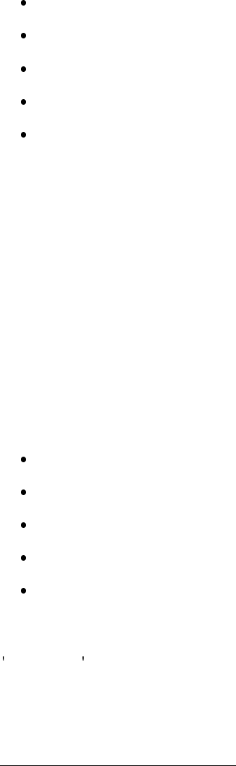
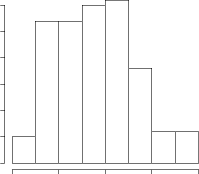
Then we check the variance of Sepal.Length with var(), and also check its distribution with
histogram and density using functions hist() and density().
> var(iris$Sepal.Length)
[1] 0.6856935
> hist(iris$Sepal.Length)
Histogram of iris$Sepal.Length
iris$Sepal.Length
Frequency
45678
0 5 10 15 20 25 30
Figure 3.1: Histogram
3.2. EXPLORE INDIVIDUAL VARIABLES 13
> plot(density(iris$Sepal.Length))
45678
0.0 0.1 0.2 0.3 0.4
density.default(x = iris$Sepal.Length)
N = 150 Bandwidth = 0.2736
Density
Figure 3.2: Density
14 CHAPTER 3. DATA EXPLORATION
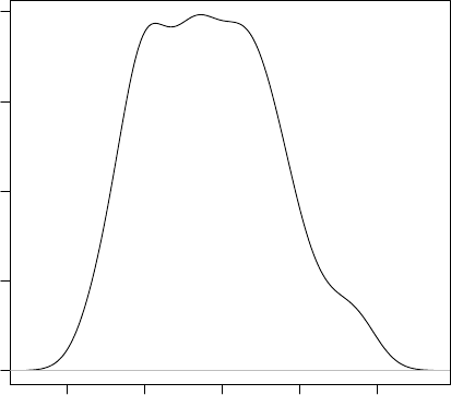
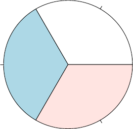
The frequency of factors can be calculated with function table(), and then plotted as a pie
chart with pie() or a bar chart with barplot().
> table(iris$Species)
setosa versicolor virginica
50 50 50
> pie(table(iris$Species))
setosa
versicolor
virginica
Figure 3.3: Pie Chart
3.3. EXPLORE MULTIPLE VARIABLES 15
> barplot(table(iris$Species))
setosa versicolor virginica
0 10 20 30 40 50
Figure 3.4: Bar Chart
3.3 Explore Multiple Variables
After checking the distributions of individual variables, we then investigate the relationships be-
tween two variables. Below we calculate covariance and correlation between variables with cov()
and cor().
> cov(iris$Sepal.Length, iris$Petal.Length)
[1] 1.274315
> cov(iris[,1:4])
Sepal.Length Sepal.Width Petal.Length Petal.Width
Sepal.Length 0.6856935 -0.0424340 1.2743154 0.5162707
Sepal.Width -0.0424340 0.1899794 -0.3296564 -0.1216394
Petal.Length 1.2743154 -0.3296564 3.1162779 1.2956094
Petal.Width 0.5162707 -0.1216394 1.2956094 0.5810063
> cor(iris$Sepal.Length, iris$Petal.Length)
[1] 0.8717538
> cor(iris[,1:4])
Sepal.Length Sepal.Width Petal.Length Petal.Width
Sepal.Length 1.0000000 -0.1175698 0.8717538 0.8179411
Sepal.Width -0.1175698 1.0000000 -0.4284401 -0.3661259
Petal.Length 0.8717538 -0.4284401 1.0000000 0.9628654
Petal.Width 0.8179411 -0.3661259 0.9628654 1.0000000
16 CHAPTER 3. DATA EXPLORATION
Next, we compute the stats of Sepal.Length of every Species with aggregate().
> aggregate(Sepal.Length ~ Species, summary, data=iris)
Species Sepal.Length.Min. Sepal.Length.1st Qu. Sepal.Length.Median
1 setosa 4.300 4.800 5.000
2 versicolor 4.900 5.600 5.900
3 virginica 4.900 6.225 6.500
Sepal.Length.Mean Sepal.Length.3rd Qu. Sepal.Length.Max.
1 5.006 5.200 5.800
2 5.936 6.300 7.000
3 6.588 6.900 7.900
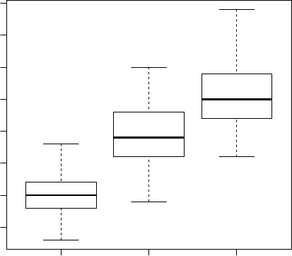
We then use function boxplot() to plot a box plot, also known as box-and-whisker plot, to
show the median, first and third quartile of a distribution (i.e., the 50%, 25% and 75% points in
cumulative distribution), and outliers. The bar in the middle is the median. The box shows the
interquartile range (IQR), which is the range between the 75% and 25% observation.
> boxplot(Sepal.Length~Species, data=iris)
●
setosa versicolor virginica
4.5 5.0 5.5 6.0 6.5 7.0 7.5 8.0
Figure 3.5: Boxplot
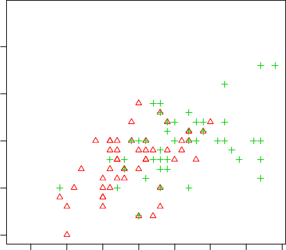
A scatter plot can be drawn for two numeric variables with plot() as below. Using function
with(), we don’t need to add “iris$” before variable names. In the code below, the colors (col)
3.3. EXPLORE MULTIPLE VARIABLES 17
and symbols (pch) of points are set to Species.
> with(iris, plot(Sepal.Length, Sepal.Width, col=Species, pch=as.numeric(Species)))
●
●
●
●
●
●
● ●
●
●
●
●
●●
●
●
●
●
●●
●
●
●
●
●
●
●
●
●
●
●
●
●
●
●
●
●
●
●
●
●
●
●
●
●
●
●
●
●
●
4.5 5.0 5.5 6.0 6.5 7.0 7.5 8.0
2.0 2.5 3.0 3.5 4.0
Sepal.Length
Sepal.Width
Figure 3.6: Scatter Plot
18 CHAPTER 3. DATA EXPLORATION
When there are many points, some of them may overlap. We can use jitter() to add a small
amount of noise to the data before plotting.
> plot(jitter(iris$Sepal.Length), jitter(iris$Sepal.Width))
●
●
●
●
●
●
●●
●
●
●
●
●
●
●
●
●
●
●
●
●
●
●
●
●
●
●
●
●
●
●
●
●
●
●
●
●
●
●
●
●
●
●
●
●
●
●
●
●
●
●
●
●
●
●
●
●
●
●
●
●
●
●
●
●
●
●
●
●
●
●
●
●
●
●
●
●
●
●
●
●
●
●●
●
●
●
●
●
●
●
●
●
●
●
●
●●
●
●
●
●
●
●
●●
●
●
●
●
●
●
●
●
●
●
●
●
●
●
●
●●
●
●
●
●
●
●
●
●
●
●
●
●
●
●
●
●
●
●●
●
●
●
●
●
●
●
●
5 6 7 8
2.0 2.5 3.0 3.5 4.0
jitter(iris$Sepal.Length)
jitter(iris$Sepal.Width)
Figure 3.7: Scatter Plot with Jitter
3.4. MORE EXPLORATIONS 19
A matrix of scatter plots can be produced with function pairs().
> pairs(iris)
Sepal.Length
2.0 3.0 4.0
●
●●
●
●
●
●
●
●
●
●
●●
●
●●
●
●
●
●
●
●
●
●
●
● ●
●●
●
●
●●
●
●
●
●
●
●
●
●
●●
●●
●
●
●
●
●
●
●
●
●
●
●
●
●
●
●
●
●
●●
●
●
●
●
●
●
●
●
●●
●
●
●●
●
●
●●
●
●
●
●
●
●
●
●●
●
●
●
●●●
●
●
●
●
●
●
●
●
●
●
●
●
●
●
●
●
●●
●
●
●●
●
●
●
●
●
●
●
●●
●
●
●
●
●
●
●
●
●
●
●
●
●
●
●
●
●●
●●
●
●
●
●
●
●
●
●
●
●
●
●
●
●●
●
●
●
●
●
●
●
●
●
●
●
●
●●
●●
●
●
●
●
●
●
●
●
●
●
●
●
●
●
●
●
●
●
●
●
●
●
●
●
●
●
●
●
●
●
●
●
●
●●
●
●
●
●
●
●
●
●●
●
●
●●
●
●
●
●●
●●
●
●
●
●
●
●●
●
●
●
●
●●
●
●
●
●
●
●
●
●
●
●
●
●
●
●
●
●
●
●
●
●
●●
●
●
●
●
●
●
●
●
●
●
●
●
●
●
●●
●
●
●
●
●
●
●
●
●
●●
●
●
●
●
0.5 1.5 2.5
●
●
●
●
●
●
●
●
●
●
●
●●
●
●●
●
●
●
●
●
●
●
●
●
● ●
●●
●
●
●
●
●
●
●
●
●
●
●
●
●
●
●
●
●
●
●
●
●
●
●
●
●
●
●
●
●
●
●
●
●
●●
●
●
●
●
●
●
●
●●
●
●
●
●●
●
●
●●
●●
●
●
●
●
●
●●
●
●
●
●
●●
●
●
●
●
●
●
●●
●
●
●
●
●
●
●
●
●●
●
●
●●
●
●
●
●
●
●
●
●
●
●
●●
●
●
●
●
●
●
●
●
●●
●
●
●●●
●
●
●
●
4.5 6.0 7.5
●
●
●
●
●
●
●
●
●
●
●
●●
●
●
●
●
●
●
●
●
●
●
●
●
●●
●●
●
●
●
●
●
●
●
●
●
●
●
●
●
●
●
●
●
●
●
●
●
●
●
●
●
●
●
●
●
●
●
●
●
●
●
●
●
●
●
●
●
●
●
●
●
●
●
●
●
●
●
●●
●
●
●
●
●
●
●
●●
●
●
●
●
●●
●
●
●
●
●
●
●
●
●
●
●
●
●
●
●
●
●
●
●
●
●●
●
●
●
●
●
●
●
●
●
●
●
●
●
●
●
●
●
●
●
●
●
●
●
●
●
●●
●
●
●
●
2.0 3.0 4.0
●
●
●
●
●
●
● ●
●
●
●
●
●●
●
●
●
●
●●
●
●
●
●
●
●
●
●
●
●
●
●
●●
●
●
●
●
●
●
●
●
●
●
●
●
●
●
●
●●● ●
●
●●
●
●
●
●
●
●
●
●●
●
●
●
●
●
●
●
●
●●
●
●
●
●
●
●●
●●
●
●
●
●
●
●
●
●
●
●
●
●
● ●
●
●
●
●
●
●
● ●
●
●
●
●
●
●
●
●
●
●
●
●
●
●
●
● ●
●
●●
●
●
●
●
●
●
●●
●
●
●
●
●●●●
●
●
●
●
●
●
●
●
Sepal.Width
●
●
●
●
●
●
●●
●
●
●
●
●●
●
●
●
●
●●
●
●
●
●
●
●
●
●
●
●
●
●
●
●
●
●
●
●
●
●
●
●
●
●
●
●
●
●
●
●●●●
●
●●
●
●
●
●
●
●
●
●●
●
●
●
●
●
●
●
●
●
●
●
●
●
●
●
●●
● ●
●
●
●
●
●
●●
●
●
●
●
●
●●
●
●
●
●
●
●
● ●
●
●
●
●
●
●
●
●
●
●
●
●
●
●
●
● ●
●
●
●
●
●
●
●
●
●
●●
●
●
●
●
●●●●
●
●
●
●
●
●
●
●
●
●
●
●
●
●
●●
●
●
●
●
●●
●
●
●
●
●●
●
●
●
●
●
●
●
●
●
●
●
●
●
●
●
●
●
●
●
●
●
●
●
●
●
●
●
●
●
●●●
●
●
●●
●
●
●
●
●
●
●
●●
●
●
●
●
●
●
●
●
●
●
●
●
●
●
●
●●
● ●
●
●
●
●
●
●
●
●
●
●
●
●
●●
●
●
●
●
●
●●●
●
●
●
●
●
●
●
●
●
●
●
●
●
●
●
●●
●
●
●
●
●
●
●
●
●
●●
●
●
●
●
●● ●●
●
●●
●
●
●
●
●
●
●
●
●
●
●
●●
●
●
●
●
●●
●
●
●
●
●●
●
●
●
●
●
●
●
●
●
●
●
●
●
●
●
●
●
●
●
●
●
●
●
●
●
●
●
●
●
●●●
●
●
●●
●
●
●
●
●
●
●
●●
●
●
●
●
●
●
●
●
●
●
●
●
●
●
●
●●
●●
●
●
●
●
●
●
●
●
●
●
●
●
●●
●
●
●
●
●
●
●●
●
●
●
●
●
●
●
●
●
●
●
●
●
●
●
●●
●
●
●
●
●
●
●
●
●
●●
●
●
●
●
●
●●●
●
●
●
●
●
●
●
●
●●
●
●●●
●●
●● ●
●
●
●●
●
●
●●
●●
●
●
●
●
●●
●
●
●● ●● ●
●
●●
●
●●
●●● ●
●
●●
●●
●
●
●●
●
●
●●
●
●
●
●
●
●
●
●
●
●
●●
●
●
●
●
●●
●
●
●
●
●
●
●●
●
● ● ●
●
●
●
●●
●
●
●●● ●
●
●
●
●
●
●
●
●
●
●
●●
●
●●
●
●●
●
●
●
●
●
●
●
●
●●
●
●
●●
●●
●
●
●
●
●
●
●
●
●
●●
●
●
●
●
●
●
●
●● ●
●●●
●
●
●● ●
●
●
●●●
●
●●
●
●●
●
●
●
● ●
●
●
●● ● ●
●
●
●●
●
●●
●● ● ●●
●●
●●
●
●
●
●
●
●
●●
●
●
●
●
●
●
●
●
●
●
●
●
●
●
●
●●
●
●
●●
●
●
●
●●
●
● ●
●
●●
●
●●
●
●
● ●●
●
●
●
●
●
●
●
●
●
●
●
●●
●
●●
●●●
●
●
●
●
●
●
●
●
●
●
●●
●●
●●
●
●
●
●
●
●
●
●
●
●●
●
●
●
●●●
●
Petal.Length
●●
●
●
●●
●
●
●
●●
●
●
●
●●
●
●
●
●
●●
●
●
●
● ●
●
●
●● ●●
●
●
●
●
●
●
●
●●● ●
●
●
●
●
●
●
●
●
●
●
●
●●
●
●
●
●
●
●
●
●
●
●
●●
●
●
●
●
●
●
●
●●
●
●
●
●●
●
●●
●
●
●
●
●●
●
●
●●●
●
●
●
●
●
●
●●
●
●
●
●●
●
●●
●●
●
●
●
●
●
●
●
●
●
●
●
●
●
●
●●
●
●
●
●
●
●
●
●
●●
●●
●●
●
●
●●
●
1357
●●
●
●
●
●
●
●
●
●●
●
●
●
●
●
●
●
●
●
●
●
●
●
●
●●
●
●
●●
●●
●
●
●
●
●
●
●
●●●
●
●
●
●
●
●
●
●
●
●
●
●
●
●
●
●
●
●
●
●
●
●
●
●
●
●
●
●
●
●
●
●
●
●
●
●
●
●
●
●
●
●●
●
●
●
●
●
●
●
●
●●●
●
●
●
●
●
●
●
●
●
●
●
●
●
●
●
●
●
●
●
●
●
●
●
●
●
●
●
●
●
●
●
●
●
●
●
●
●
●
●
●
●
●
●
●
●●
●
●
●
●
●
●
●
0.5 1.5 2.5
●●●● ●
●
●●● ●●●
●● ●
●●
● ●● ●
●
●
●
●●
●
●●●●
●
●●●● ●
●
● ●
●●
●
●
●
●●● ●●
●
● ●
●
●
●
●
●
●
●
●
●
●
●
●●
●
●
●
●
●
●
●
●●
●●
●
●
●
●
●
●
●
●●●
●●●
●
●
●
●
●
●
● ●
●
●
●
●
●
●
●●
●●●
●
●
●
●
●
●●
●
●
●
●
●
● ●
●
●
●●●
●
●
●●
●
●
●
●
●
●●
●
●
●
●
●
●
●
●
●
●
●
●● ●● ●
●
●
●● ●●●
●● ●
●●
● ●●
●
●
●
●
●●
●
●●●●
●
●
●●● ●
●
● ●
●● ●
●
●
●●● ●●
●
●●
●
●
●
●
●
●
●
●
●
●
●
●●
●
●
●
●
●
●
●
●
●
●●
●
●
●
●
●
●
●●●
●
● ●●
●
●
●
●
●●
●●
●
●
●
●
●
●
●
●
●●●
●
●
●
●
●
●●
●
●
●
●
●
●●
●
●
●● ●
●
●
●●
●
●
●
●●
●●
●
●
●
●
●
●
●
●●
●
●
●●●●●
●
●
●●
●
●●
●●
●
●●
●●●
●
●
●
●
●●
●
●●●●
●
●
●●●●
●
●●
●●
●
●
●
●
●●●●
●
●●
●
●
●
●
●
●
●
●
●
●
●
●●
●
●
●
●
●
●
●
●
●
●●
●
●
●
●
●
●
●
●
●
●
●●●●
●
●
●
●
●
●●
●
●
●
●
●
●
●●
●●●
●
●
●
●
●
●
●
●
●
●
●
●
● ●
●
●
●●●
●
●
●
●
●
●●
●
●
●●
●
●
●
●
●
●
●
●
●
●
●
Petal.Width
●●●●●
●
●
●●
●
●●
●●
●
●●
●●●
●
●
●
●
●●
●
●●●●
●
●
●●●●
●
●●
●●
●
●
●
●
●●●●
●
●●
●
●
●
●
●
●
●
●
●
●
●
●
●
●
●
●
●
●
●
●
●
●
●●
●
●
●
●
●
●
●
●
●
●
●●●
●
●
●
●
●
●
●●
●
●
●
●
●
●
●
●
●
●●
●
●
●
●
●
●
●
●
●
●
●
●
●●
●
●
●●●
●
●
●
●
●
●
●
●
●
●●
●
●
●
●
●
●
●
●
●
●
●
4.5 6.0 7.5
●●●● ● ●● ●● ● ●●●● ●●●● ●● ●●● ●●●●●●●● ●● ●●● ●●● ●●●● ●●● ●● ●●
●● ●● ●● ●● ●●● ●●●● ●●● ●● ●●●● ●●●●●●●● ●●● ● ●●●●● ●●● ●●● ●● ●
●● ●●● ●● ●● ●●● ●●● ●● ●●● ●● ●● ● ●●● ● ●● ●●●● ●●●● ●●●● ●●●●●●●
●● ●● ● ●●●● ● ●●●● ● ●●● ●●● ●●●●● ●●●●● ● ●●●● ●●● ●●● ● ● ●● ●● ●●
●●●● ●● ●● ●●● ●● ●● ●●●● ● ●●● ●●●● ●●●●● ●● ● ●●● ●●● ●●● ● ●●●● ●
●● ●●●●● ●● ●●● ●● ● ●● ●●● ●●●● ●●● ●● ●● ●●●● ● ●●●●●●● ●●●● ● ●●
1357
●●●●●●●●●●●●●●●●●●●●●●● ●●●●●●●●●●●●●●●●●●●●●●●●●●●
●●●● ●●●● ●●● ●● ●● ●●●●● ●● ●●●●●●●●●●● ●●●●●●●●●●● ●●●●● ●
●● ●●● ●● ●●●●●●●●●● ●●● ●● ●● ●●●● ●●●●●● ● ●●●● ●●●● ●●●●●●●
●●●●● ●●●●●●●●●● ●●●●●● ●● ●●● ●●●●● ●●●●●●●●●●●● ●●●●●●●
●●●● ●● ●● ●●● ●● ●●●●● ●● ●● ●●●●● ●●●●● ● ●●●●●●●● ●●● ●●●●● ●
●● ●● ●●●●● ●●● ●● ●●● ●●● ●●●● ●●●● ●● ●● ●●● ●●●● ● ●●● ● ●●●● ●●
1.0 2.0 3.0
1.0 2.0 3.0
Species
Figure 3.8: A Matrix of Scatter Plots
3.4 More Explorations
This section presents some fancy graphs, including 3D plots, level plots, contour plots, interactive
plots and parallel coordinates.
20 CHAPTER 3. DATA EXPLORATION
A 3D scatter plot can be produced with package scatterplot3d [Ligges and M¨
achler, 2003].
> library(scatterplot3d)
> scatterplot3d(iris$Petal.Width, iris$Sepal.Length, iris$Sepal.Width)
0.0 0.5 1.0 1.5 2.0 2.5
2.0 2.5 3.0 3.5 4.0 4.5
4
5
6
7
8
iris$Petal.Width
iris$Sepal.Length
iris$Sepal.Width
●
●
●
●
●
●
●
●
●
●
●
●
●
●●
●
●●
●
●
●
●
●
●
●
●
●
●
●
●●●
●
●
●
●
●●
●
●
●
●
●
●
●
●
●
●
●
●
●●
●
●
●
●
●●
● ●
●●
●
●
●
●
●
●
●
●
●
●
●
●
●●
●
●
●
●
●
●
●
●
●
●
●
●
●
●
●
●
●
● ●
●
●
●
●
●●
●
●
●
●
●
●
●
●
●
● ●
●
●
●
●
●●
●
●
●
●●
●
●
●
●
●
●
●
●
●●
●●
●
●
●
●
●●
●
●
●
●
●
●
●
●
●
Figure 3.9: 3D Scatter plot
Package rgl [Adler and Murdoch, 2012] supports interactive 3D scatter plot with plot3d().
> library(rgl)
> plot3d(iris$Petal.Width, iris$Sepal.Length, iris$Sepal.Width)
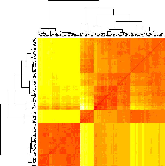
A heat map presents a 2D display of a data matrix, which can be generated with heatmap()
in R. With the code below, we calculate the similarity between different flowers in the iris data
3.4. MORE EXPLORATIONS 21
with dist() and then plot it with a heat map.
> distMatrix <- as.matrix(dist(iris[,1:4]))
> heatmap(distMatrix)
42
23
14
9
43
39
4
13
2
46
36
7
48
3
16
34
15
45
6
19
21
32
24
25
27
44
17
33
37
49
11
22
47
20
26
31
30
35
10
38
5
41
12
50
28
40
8
29
18
1
119
106
123
132
118
131
108
110
136
130
103
126
101
144
121
145
61
99
94
58
65
80
81
82
63
83
93
68
60
70
90
54
107
85
56
67
62
72
91
89
97
96
100
95
52
76
66
57
55
59
88
69
98
75
86
79
74
92
64
109
137
105
125
141
146
142
140
113
104
138
117
116
149
129
133
115
135
112
111
148
78
53
51
87
77
84
150
147
124
134
127
128
139
71
73
120
122
114
102
143
Figure 3.10: Heat Map
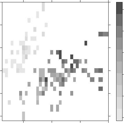
A level plot can be produced with function levelplot() in package lattice [Sarkar, 2008].
Function grey.colors() creates a vector of gamma-corrected gray colors. A similar function is
22 CHAPTER 3. DATA EXPLORATION
rainbow(), which creates a vector of contiguous colors.
> library(lattice)
> levelplot(Petal.Width~Sepal.Length*Sepal.Width, iris, cuts=9,
+ col.regions=grey.colors(10)[10:1])
Sepal.Length
Sepal.Width
2.0
2.5
3.0
3.5
4.0
567
0.0
0.5
1.0
1.5
2.0
2.5
Figure 3.11: Level Plot
Contour plots can be plotted with contour() and filled.contour() in package graphics, and
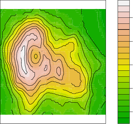
3.4. MORE EXPLORATIONS 23
with contourplot() in package lattice.
> filled.contour(volcano, color=terrain.colors, asp=1,
+ plot.axes=contour(volcano, add=T))
100
120
140
160
180
100
100
100
110
110
110
110
120
130
140
150
160
160
170
180
190
Figure 3.12: Contour
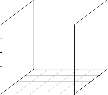
Another way to illustrate a numeric matrix is a 3D surface plot shown as below, which is
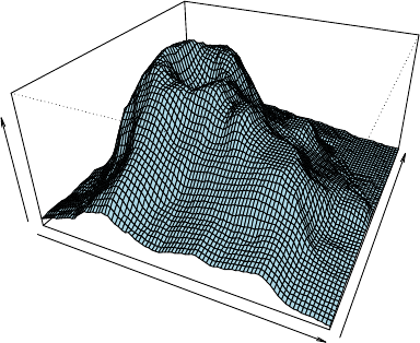
24 CHAPTER 3. DATA EXPLORATION
generated with function persp().
> persp(volcano, theta=25, phi=30, expand=0.5, col="lightblue")
volcano
Y
Z
Figure 3.13: 3D Surface
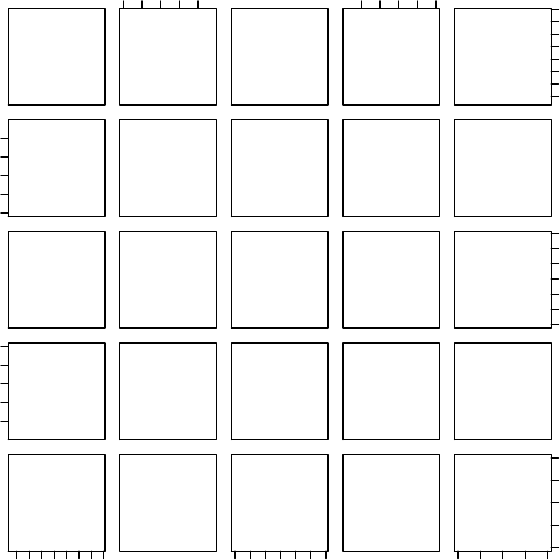
Parallel coordinates provide nice visualization of multiple dimensional data. A parallel coor-
dinates plot can be produced with parcoord() in package MASS , and with parallelplot() in
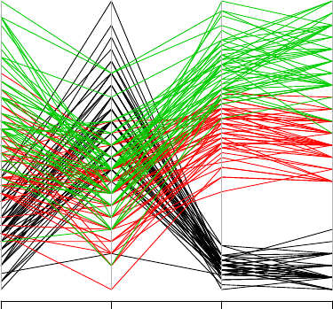
3.4. MORE EXPLORATIONS 25
package lattice.
> library(MASS)
> parcoord(iris[1:4], col=iris$Species)
Sepal.Length Sepal.Width Petal.Length Petal.Width
Figure 3.14: Parallel Coordinates
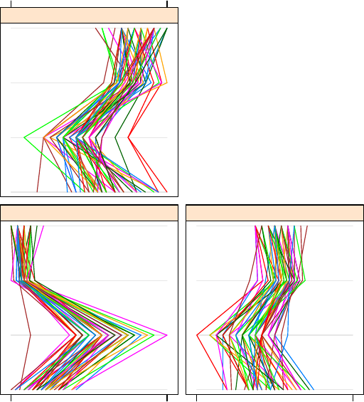
26 CHAPTER 3. DATA EXPLORATION
> library(lattice)
> parallelplot(~iris[1:4] | Species, data=iris)
Sepal.Length
Sepal.Width
Petal.Length
Petal.Width
Min Max
setosa
versicolor
Sepal.Length
Sepal.Width
Petal.Length
Petal.Width
virginica
Figure 3.15: Parallel Coordinates with Package lattice
Package ggplot2 [Wickham, 2009] supports complex graphics, which are very useful for ex-
ploring data. A simple example is given below. More examples on that package can be found at
http://had.co.nz/ggplot2/.
3.5. SAVE CHARTS INTO FILES 27
> library(ggplot2)
> qplot(Sepal.Length, Sepal.Width, data=iris, facets=Species ~.)
●
●
●
●
●
●
● ●
●
●
●
●
●●
●
●
●
●
●●
●
●
●
●
●
●
●●
●
●●
●
●●
●●
●
●
●
●
●
●
●
●
●
●
●
●
●
●
●● ●
●
●●
●
●
●
●
●
●
●
●●
●
●
●
●
●
●
●
●
●●●
●
●
●
●
●●
● ●
●
●
●
●
●
●
●
●
●
●
●
●
● ●
●
●
●
●
●
●● ●
●
●
●
●
●
●
●
●
●
●
●
●
●
●
●
● ●
●
●●
●
●
●
●
●
●
●●
●
●
●
●
●●● ●
●
●
●
●
●
●
●
●
2.0
2.5
3.0
3.5
4.0
4.5
2.0
2.5
3.0
3.5
4.0
4.5
2.0
2.5
3.0
3.5
4.0
4.5
setosa
versicolor
virginica
5678
Sepal.Length
Sepal.Width
Figure 3.16: Scatter Plot with Package ggplot2
3.5 Save Charts into Files
If there are many graphs produced in data exploration, a good practice is to save them into files.
R provides a variety of functions for that purpose. Below are examples of saving charts into PDF
and PS files respectively with pdf() and postscript(). Picture files of BMP, JPEG, PNG and
TIFF formats can be generated respectively with bmp(),jpeg(),png() and tiff(). Note that
the files (or graphics devices) need be closed with graphics.off() or dev.off() after plotting.
> # save as a PDF file
> pdf("myPlot.pdf")
> x <- 1:50
> plot(x, log(x))
> graphics.off()
> #
> # Save as a postscript file
> postscript("myPlot2.ps")
> x <- -20:20
> plot(x, x^2)
> graphics.off()
28 CHAPTER 3. DATA EXPLORATION

Chapter 4
Decision Trees and Random Forest
This chapter shows how to build predictive models with packages party,rpart and randomForest.
It starts with building decision trees with package party and using the built tree for classification,
followed by another way to build decision trees with package rpart. After that, it presents an
example on training a random forest model with package randomForest.
4.1 Decision Trees with Package party
This section shows how to build a decision tree for the iris data with function ctree() in package
party [Hothorn et al., 2010]. Details of the data can be found in Section 1.3.1. Sepal.Length,
Sepal.Width,Petal.Length and Petal.Width are used to predict the Species of flowers. In the
package, function ctree() builds a decision tree, and predict() makes prediction for new data.
Before modeling, the iris data is split below into two subsets: training (70%) and test (30%).
The random seed is set to a fixed value below to make the results reproducible.
> str(iris)
data.frame : 150 obs. of 5 variables:
$ Sepal.Length: num 5.1 4.9 4.7 4.6 5 5.4 4.6 5 4.4 4.9 ...
$ Sepal.Width : num 3.5 3 3.2 3.1 3.6 3.9 3.4 3.4 2.9 3.1 ...
$ Petal.Length: num 1.4 1.4 1.3 1.5 1.4 1.7 1.4 1.5 1.4 1.5 ...
$ Petal.Width : num 0.2 0.2 0.2 0.2 0.2 0.4 0.3 0.2 0.2 0.1 ...
$ Species : Factor w/ 3 levels "setosa","versicolor",..: 1 1 1 1 1 1 1 1 1 1 ...
> set.seed(1234)
> ind <- sample(2, nrow(iris), replace=TRUE, prob=c(0.7, 0.3))
> trainData <- iris[ind==1,]
> testData <- iris[ind==2,]
We then load package party, build a decision tree, and check the prediction result. Function
ctree() provides some parameters, such as MinSplit,MinBusket,MaxSurrogate and MaxDepth,
to control the training of decision trees. Below we use default settings to build a decision tree. Ex-
amples of setting the above parameters are available in Chapter 13. In the code below, myFormula
specifies that Species is the target variable and all other variables are independent variables.
> library(party)
> myFormula <- Species ~ Sepal.Length + Sepal.Width + Petal.Length + Petal.Width
> iris_ctree <- ctree(myFormula, data=trainData)
> # check the prediction
> table(predict(iris_ctree), trainData$Species)
29
30 CHAPTER 4. DECISION TREES AND RANDOM FOREST
setosa versicolor virginica
setosa 40 0 0
versicolor 0 37 3
virginica 0 1 31
After that, we can have a look at the built tree by printing the rules and plotting the tree.
> print(iris_ctree)
Conditional inference tree with 4 terminal nodes
Response: Species
Inputs: Sepal.Length, Sepal.Width, Petal.Length, Petal.Width
Number of observations: 112
1) Petal.Length <= 1.9; criterion = 1, statistic = 104.643
2)* weights = 40
1) Petal.Length > 1.9
3) Petal.Width <= 1.7; criterion = 1, statistic = 48.939
4) Petal.Length <= 4.4; criterion = 0.974, statistic = 7.397
5)* weights = 21
4) Petal.Length > 4.4
6)* weights = 19
3) Petal.Width > 1.7
7)* weights = 32
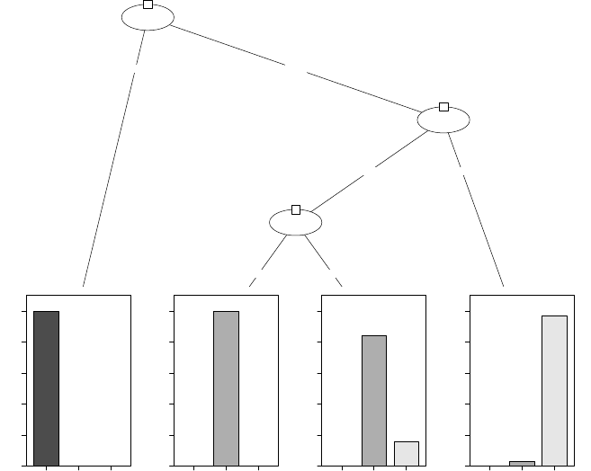
> plot(iris_ctree)
Petal.Length
p < 0.001
1
≤1.9 >1.9
Node 2 (n = 40)
setosa versicolor virginica
0
0.2
0.4
0.6
0.8
1
Petal.Width
p < 0.001
3
≤1.7 >1.7
Petal.Length
p = 0.026
4
≤4.4 >4.4
Node 5 (n = 21)
setosa versicolor virginica
0
0.2
0.4
0.6
0.8
1
Node 6 (n = 19)
setosa versicolor virginica
0
0.2
0.4
0.6
0.8
1
Node 7 (n = 32)
setosa versicolor virginica
0
0.2
0.4
0.6
0.8
1
Figure 4.1: Decision Tree
4.1. DECISION TREES WITH PACKAGE PARTY 31
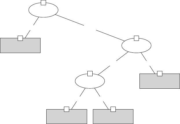
> plot(iris_ctree, type="simple")
Petal.Length
p < 0.001
1
≤1.9 >1.9
n = 40
y = (1, 0, 0)
2Petal.Width
p < 0.001
3
≤1.7 >1.7
Petal.Length
p = 0.026
4
≤4.4 >4.4
n = 21
y = (0, 1, 0)
5n = 19
y = (0, 0.842, 0.158)
6
n = 32
y = (0, 0.031, 0.969)
7
Figure 4.2: Decision Tree (Simple Style)
In the above Figure 4.1, the barplot for each leaf node shows the probabilities of an instance
falling into the three species. In Figure 4.2, they are shown as “y” in leaf nodes. For example,
node 2 is labeled with “n=40, y=(1, 0, 0)”, which means that it contains 40 training instances and
all of them belong to the first class “setosa”.
After that, the built tree needs to be tested with test data.
> # predict on test data
> testPred <- predict(iris_ctree, newdata = testData)
> table(testPred, testData$Species)
testPred setosa versicolor virginica
setosa 10 0 0
versicolor 0 12 2
virginica 0 0 14
The current version of ctree() (i.e. version 0.9-9995) does not handle missing values well, in
that an instance with a missing value may sometimes go to the left sub-tree and sometimes to the
right. This might be caused by surrogate rules.
Another issue is that, when a variable exists in training data and is fed into ctree() but does
not appear in the built decision tree, the test data must also have that variable to make prediction.
Otherwise, a call to predict() would fail. Moreover, if the value levels of a categorical variable in
test data are different from that in training data, it would also fail to make prediction on the test
data. One way to get around the above issue is, after building a decision tree, to call ctree() to
build a new decision tree with data containing only those variables existing in the first tree, and
to explicitly set the levels of categorical variables in test data to the levels of the corresponding
variables in training data. An example on that can be found in ??.
32 CHAPTER 4. DECISION TREES AND RANDOM FOREST
4.2 Decision Trees with Package rpart
Package rpart [Therneau et al., 2010] is used in this section to build a decision tree on the bodyfat
data (see Section 1.3.2 for details of the data). Function rpart() is used to build a decision tree,
and the tree with the minimum prediction error is selected. After that, it is applied to new data
to make prediction with function predict().
At first, we load the bodyfat data and have a look at it.
> data("bodyfat", package = "mboost")
> dim(bodyfat)
[1] 71 10
> attributes(bodyfat)
$names
[1] "age" "DEXfat" "waistcirc" "hipcirc" "elbowbreadth"
[6] "kneebreadth" "anthro3a" "anthro3b" "anthro3c" "anthro4"
$row.names
[1] "47" "48" "49" "50" "51" "52" "53" "54" "55" "56" "57" "58" "59"
[14] "60" "61" "62" "63" "64" "65" "66" "67" "68" "69" "70" "71" "72"
[27] "73" "74" "75" "76" "77" "78" "79" "80" "81" "82" "83" "84" "85"
[40] "86" "87" "88" "89" "90" "91" "92" "93" "94" "95" "96" "97" "98"
[53] "99" "100" "101" "102" "103" "104" "105" "106" "107" "108" "109" "110" "111"
[66] "112" "113" "114" "115" "116" "117"
$class
[1] "data.frame"
> bodyfat[1:5,]
age DEXfat waistcirc hipcirc elbowbreadth kneebreadth anthro3a anthro3b
47 57 41.68 100.0 112.0 7.1 9.4 4.42 4.95
48 65 43.29 99.5 116.5 6.5 8.9 4.63 5.01
49 59 35.41 96.0 108.5 6.2 8.9 4.12 4.74
50 58 22.79 72.0 96.5 6.1 9.2 4.03 4.48
51 60 36.42 89.5 100.5 7.1 10.0 4.24 4.68
anthro3c anthro4
47 4.50 6.13
48 4.48 6.37
49 4.60 5.82
50 3.91 5.66
51 4.15 5.91
Next, the data is split into training and test subsets, and a decision tree is built on the training
data.
> set.seed(1234)
> ind <- sample(2, nrow(bodyfat), replace=TRUE, prob=c(0.7, 0.3))
> bodyfat.train <- bodyfat[ind==1,]
> bodyfat.test <- bodyfat[ind==2,]
> # train a decision tree
> library(rpart)
> myFormula <- DEXfat ~ age + waistcirc + hipcirc + elbowbreadth + kneebreadth
> bodyfat_rpart <- rpart(myFormula, data = bodyfat.train,
+ control = rpart.control(minsplit = 10))
> attributes(bodyfat_rpart)
4.2. DECISION TREES WITH PACKAGE RPART 33
$names
[1] "frame" "where" "call"
[4] "terms" "cptable" "method"
[7] "parms" "control" "functions"
[10] "numresp" "splits" "variable.importance"
[13] "y" "ordered"
$xlevels
named list()
$class
[1] "rpart"
> print(bodyfat_rpart$cptable)
CP nsplit rel error xerror xstd
1 0.67272638 0 1.00000000 1.0194546 0.18724382
2 0.09390665 1 0.32727362 0.4415438 0.10853044
3 0.06037503 2 0.23336696 0.4271241 0.09362895
4 0.03420446 3 0.17299193 0.3842206 0.09030539
5 0.01708278 4 0.13878747 0.3038187 0.07295556
6 0.01695763 5 0.12170469 0.2739808 0.06599642
7 0.01007079 6 0.10474706 0.2693702 0.06613618
8 0.01000000 7 0.09467627 0.2695358 0.06620732
> print(bodyfat_rpart)
n= 56
node), split, n, deviance, yval
* denotes terminal node
1) root 56 7265.0290000 30.94589
2) waistcirc< 88.4 31 960.5381000 22.55645
4) hipcirc< 96.25 14 222.2648000 18.41143
8) age< 60.5 9 66.8809600 16.19222 *
9) age>=60.5 5 31.2769200 22.40600 *
5) hipcirc>=96.25 17 299.6470000 25.97000
10) waistcirc< 77.75 6 30.7345500 22.32500 *
11) waistcirc>=77.75 11 145.7148000 27.95818
22) hipcirc< 99.5 3 0.2568667 23.74667 *
23) hipcirc>=99.5 8 72.2933500 29.53750 *
3) waistcirc>=88.4 25 1417.1140000 41.34880
6) waistcirc< 104.75 18 330.5792000 38.09111
12) hipcirc< 109.9 9 68.9996200 34.37556 *
13) hipcirc>=109.9 9 13.0832000 41.80667 *
7) waistcirc>=104.75 7 404.3004000 49.72571 *
With the code below, the built tree is plotted (see Figure 4.3).
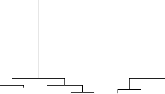
34 CHAPTER 4. DECISION TREES AND RANDOM FOREST
> plot(bodyfat_rpart)
> text(bodyfat_rpart, use.n=T)
|
waistcirc< 88.4
hipcirc< 96.25
age< 60.5 waistcirc< 77.75
hipcirc< 99.5
waistcirc< 104.8
hipcirc< 109.9
16.19
n=9 22.41
n=5 22.32
n=6 23.75
n=3 29.54
n=8
34.38
n=9 41.81
n=9
49.73
n=7
Figure 4.3: Decision Tree with Package rpart
Then we select the tree with the minimum prediction error (see Figure 4.4).
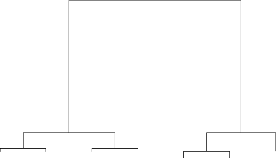
4.2. DECISION TREES WITH PACKAGE RPART 35
> opt <- which.min(bodyfat_rpart$cptable[,"xerror"])
> cp <- bodyfat_rpart$cptable[opt, "CP"]
> bodyfat_prune <- prune(bodyfat_rpart, cp = cp)
> print(bodyfat_prune)
n= 56
node), split, n, deviance, yval
* denotes terminal node
1) root 56 7265.02900 30.94589
2) waistcirc< 88.4 31 960.53810 22.55645
4) hipcirc< 96.25 14 222.26480 18.41143
8) age< 60.5 9 66.88096 16.19222 *
9) age>=60.5 5 31.27692 22.40600 *
5) hipcirc>=96.25 17 299.64700 25.97000
10) waistcirc< 77.75 6 30.73455 22.32500 *
11) waistcirc>=77.75 11 145.71480 27.95818 *
3) waistcirc>=88.4 25 1417.11400 41.34880
6) waistcirc< 104.75 18 330.57920 38.09111
12) hipcirc< 109.9 9 68.99962 34.37556 *
13) hipcirc>=109.9 9 13.08320 41.80667 *
7) waistcirc>=104.75 7 404.30040 49.72571 *
> plot(bodyfat_prune)
> text(bodyfat_prune, use.n=T)
|
waistcirc< 88.4
hipcirc< 96.25
age< 60.5 waistcirc< 77.75
waistcirc< 104.8
hipcirc< 109.9
16.19
n=9 22.41
n=5 22.32
n=6 27.96
n=11 34.38
n=9 41.81
n=9
49.73
n=7
Figure 4.4: Selected Decision Tree
After that, the selected tree is used to make prediction and the predicted values are compared
with actual labels. In the code below, function abline() draws a diagonal line. The predictions
of a good model are expected to be equal or very close to their actual values, that is, most points
should be on or close to the diagonal line.
36 CHAPTER 4. DECISION TREES AND RANDOM FOREST
> DEXfat_pred <- predict(bodyfat_prune, newdata=bodyfat.test)
> xlim <- range(bodyfat$DEXfat)
> plot(DEXfat_pred ~ DEXfat, data=bodyfat.test, xlab="Observed",
+ ylab="Predicted", ylim=xlim, xlim=xlim)
> abline(a=0, b=1)
●
●
●
●●
●
●●
●
●
● ●
●
●●
10 20 30 40 50 60
10 20 30 40 50 60
Observed
Predicted
Figure 4.5: Prediction Result
4.3 Random Forest
Package randomForest [Liaw and Wiener, 2002] is used below to build a predictive model for
the iris data (see Section 1.3.1 for details of the data). There are two limitations with function
randomForest(). First, it cannot handle data with missing values, and users have to impute data
before feeding them into the function. Second, there is a limit of 32 to the maximum number of
levels of each categorical attribute. Attributes with more than 32 levels have to be transformed
first before using randomForest().
An alternative way to build a random forest is to use function cforest() from package party,
which is not limited to the above maximum levels. However, generally speaking, categorical
variables with more levels will make it require more memory and take longer time to build a
random forest.
Again, the iris data is first split into two subsets: training (70%) and test (30%).
> ind <- sample(2, nrow(iris), replace=TRUE, prob=c(0.7, 0.3))
> trainData <- iris[ind==1,]
> testData <- iris[ind==2,]
Then we load package randomForest and train a random forest. In the code below, the formula
is set to “Species ∼.”, which means to predict Species with all other variables in the data.
> library(randomForest)
> rf <- randomForest(Species ~ ., data=trainData, ntree=100, proximity=TRUE)
> table(predict(rf), trainData$Species)
4.3. RANDOM FOREST 37
setosa versicolor virginica
setosa 36 0 0
versicolor 0 31 1
virginica 0 1 35
> print(rf)
Call:
randomForest(formula = Species ~ ., data = trainData, ntree = 100, proximity = TRUE)
Type of random forest: classification
Number of trees: 100
No. of variables tried at each split: 2
OOB estimate of error rate: 1.92%
Confusion matrix:
setosa versicolor virginica class.error
setosa 36 0 0 0.00000000
versicolor 0 31 1 0.03125000
virginica 0 1 35 0.02777778
> attributes(rf)
$names
[1] "call" "type" "predicted" "err.rate"
[5] "confusion" "votes" "oob.times" "classes"
[9] "importance" "importanceSD" "localImportance" "proximity"
[13] "ntree" "mtry" "forest" "y"
[17] "test" "inbag" "terms"
$class
[1] "randomForest.formula" "randomForest"
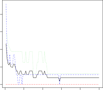
38 CHAPTER 4. DECISION TREES AND RANDOM FOREST
After that, we plot the error rates with various number of trees.
> plot(rf)
0 20 40 60 80 100
0.00 0.05 0.10 0.15 0.20
rf
trees
Error
Figure 4.6: Error Rate of Random Forest
The importance of variables can be obtained with functions importance() and varImpPlot().
4.3. RANDOM FOREST 39
> importance(rf)
MeanDecreaseGini
Sepal.Length 6.485090
Sepal.Width 1.380624
Petal.Length 32.498074
Petal.Width 28.250058
> varImpPlot(rf)
Sepal.Width
Sepal.Length
Petal.Width
Petal.Length
●
●
●
●
0 5 10 15 20 25 30
rf
MeanDecreaseGini
Figure 4.7: Variable Importance
Finally, the built random forest is tested on test data, and the result is checked with functions
table() and margin(). The margin of a data point is as the proportion of votes for the correct
class minus maximum proportion of votes for other classes. Generally speaking, positive margin
40 CHAPTER 4. DECISION TREES AND RANDOM FOREST
means correct classification.
> irisPred <- predict(rf, newdata=testData)
> table(irisPred, testData$Species)
irisPred setosa versicolor virginica
setosa 14 0 0
versicolor 0 17 3
virginica 0 1 11
> plot(margin(rf, testData$Species))
●
●
●
●
●
●
●
●
●
●
●
●●
●
●
●●
●
●●
●
●
●
●●
●
●●
●
●●
●●●●●●●●●●●●●●●●●●●●●●●●●●●●●●●●●●●●●●●●●●●●●●●●●●●●●●●●●●●●●●●●●●●●●●●●●
0 20 40 60 80 100
0.0 0.2 0.4 0.6 0.8 1.0
Index
x
Figure 4.8: Margin of Predictions

Chapter 5
Regression
Regression is to build a function of independent variables (also known as predictors) to predict
adependent variable (also called response). For example, banks assess the risk of home-loan
applicants based on their age, income, expenses, occupation, number of dependents, total credit
limit, etc.
This chapter introduces basic concepts and presents examples of various regression techniques.
At first, it shows an example on building a linear regression model to predict CPI data. After that,
it introduces logistic regression. The generalized linear model (GLM) is then presented, followed
by a brief introduction of non-linear regression.
A collection of some helpful R functions for regression analysis is available as a reference card
on R Functions for Regression Analysis 1.
5.1 Linear Regression
Linear regression is to predict response with a linear function of predictors as follows:
y=c0+c1x1+c2x2+· · · +ckxk,
where x1, x2,· · · , xkare predictors and yis the response to predict.
Linear regression is demonstrated below with function lm() on the Australian CPI (Consumer
Price Index) data, which are quarterly CPIs from 2008 to 2010 2.
At first, the data is created and plotted. In the code below, an x-axis is added manually with
function axis(), where las=3 makes text vertical.
1http://cran.r-project.org/doc/contrib/Ricci-refcard-regression.pdf
2From Australian Bureau of Statistics <http://www.abs.gov.au>
41
42 CHAPTER 5. REGRESSION
> year <- rep(2008:2010, each=4)
> quarter <- rep(1:4, 3)
> cpi <- c(162.2, 164.6, 166.5, 166.0,
+ 166.2, 167.0, 168.6, 169.5,
+ 171.0, 172.1, 173.3, 174.0)
> plot(cpi, xaxt="n", ylab="CPI", xlab="")
> # draw x-axis
> axis(1, labels=paste(year,quarter,sep="Q"), at=1:12, las=3)
●
●
●
●●
●
●
●
●
●
●
●
162 164 166 168 170 172 174
CPI
2008Q1
2008Q2
2008Q3
2008Q4
2009Q1
2009Q2
2009Q3
2009Q4
2010Q1
2010Q2
2010Q3
2010Q4
Figure 5.1: Australian CPIs in Year 2008 to 2010
We then check the correlation between CPI and the other variables, year and quarter.
> cor(year,cpi)
[1] 0.9096316
> cor(quarter,cpi)
[1] 0.3738028
Then a linear regression model is built with function lm() on the above data, using year and
quarter as predictors and CPI as response.
> fit <- lm(cpi ~ year + quarter)
> fit
Call:
lm(formula = cpi ~ year + quarter)
Coefficients:
(Intercept) year quarter
-7644.487 3.887 1.167
5.1. LINEAR REGRESSION 43
With the above linear model, CPI is calculated as
cpi = c0+c1∗year + c2∗quarter,
where c0,c1and c2are coefficients from model fit. Therefore, the CPIs in 2011 can be get as
follows. An easier way for this is using function predict(), which will be demonstrated at the
end of this subsection.
> (cpi2011 <- fit$coefficients[[1]] + fit$coefficients[[2]]*2011 +
+ fit$coefficients[[3]]*(1:4))
[1] 174.4417 175.6083 176.7750 177.9417
More details of the model can be obtained with the code below.
> attributes(fit)
$names
[1] "coefficients" "residuals" "effects" "rank"
[5] "fitted.values" "assign" "qr" "df.residual"
[9] "xlevels" "call" "terms" "model"
$class
[1] "lm"
> fit$coefficients
(Intercept) year quarter
-7644.487500 3.887500 1.166667
The differences between observed values and fitted values can be obtained with function resid-
uals().
> # differences between observed values and fitted values
> residuals(fit)
123456
-0.57916667 0.65416667 1.38750000 -0.27916667 -0.46666667 -0.83333333
7 8 9 10 11 12
-0.40000000 -0.66666667 0.44583333 0.37916667 0.41250000 -0.05416667
> summary(fit)
Call:
lm(formula = cpi ~ year + quarter)
Residuals:
Min 1Q Median 3Q Max
-0.8333 -0.4948 -0.1667 0.4208 1.3875
Coefficients:
Estimate Std. Error t value Pr(>|t|)
(Intercept) -7644.4875 518.6543 -14.739 1.31e-07 ***
year 3.8875 0.2582 15.058 1.09e-07 ***
quarter 1.1667 0.1885 6.188 0.000161 ***
---
Signif. codes: 0 ´
S***ˇ
S 0.001 ´
S**ˇ
S 0.01 ´
S*ˇ
S 0.05 ´
S.ˇ
S 0.1 ´
Sˇ
S 1
Residual standard error: 0.7302 on 9 degrees of freedom
Multiple R-squared: 0.9672, Adjusted R-squared: 0.9599
F-statistic: 132.5 on 2 and 9 DF, p-value: 2.108e-07
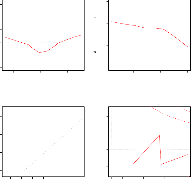
44 CHAPTER 5. REGRESSION
We then plot the fitted model as below.
> plot(fit)
164 166 168 170 172 174
−1.0 −0.5 0.0 0.5 1.0 1.5
Fitted values
Residuals
●
●
●
●
●
●
●
●
●●●
●
Residuals vs Fitted
3
6
8
●
●
●
●
●
●
●
●
●
●●
●
−1.5 −1.0 −0.5 0.0 0.5 1.0 1.5
−1 0 1 2
Theoretical Quantiles
Standardized residuals
Normal Q−Q
3
6
8
164 166 168 170 172 174
0.0 0.5 1.0 1.5
Fitted values
Standardized residuals
●●
●
●
●
●
●
●
●
●●
●
Scale−Location
3
6
8
0.00 0.05 0.10 0.15 0.20 0.25 0.30 0.35
−1 0 1 2
Leverage
Standardized residuals
●
●
●
●
●
●
●
●
●
●
●
●
Cook's distance
0.5
0.5
1
Residuals vs Leverage
3
1
8
Figure 5.2: Prediction with Linear Regression Model - 1
We can also plot the model in a 3D plot as below, where function scatterplot3d() creates
a 3D scatter plot and plane3d() draws the fitted plane. Parameter lab specifies the number of
tickmarks on the x- and y-axes.
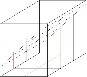
5.1. LINEAR REGRESSION 45
> library(scatterplot3d)
> s3d <- scatterplot3d(year, quarter, cpi, highlight.3d=T, type="h", lab=c(2,3))
> s3d$plane3d(fit)
2008 2009 2010
160 165 170 175
1
2
3
4
year
quarter
cpi
●
●
●
●
●
●
●
●
●
●
●
●
Figure 5.3: A 3D Plot of the Fitted Model
With the model, the CPIs in year 2011 can be predicted as follows, and the predicted values
are shown as red triangles in Figure 5.4.
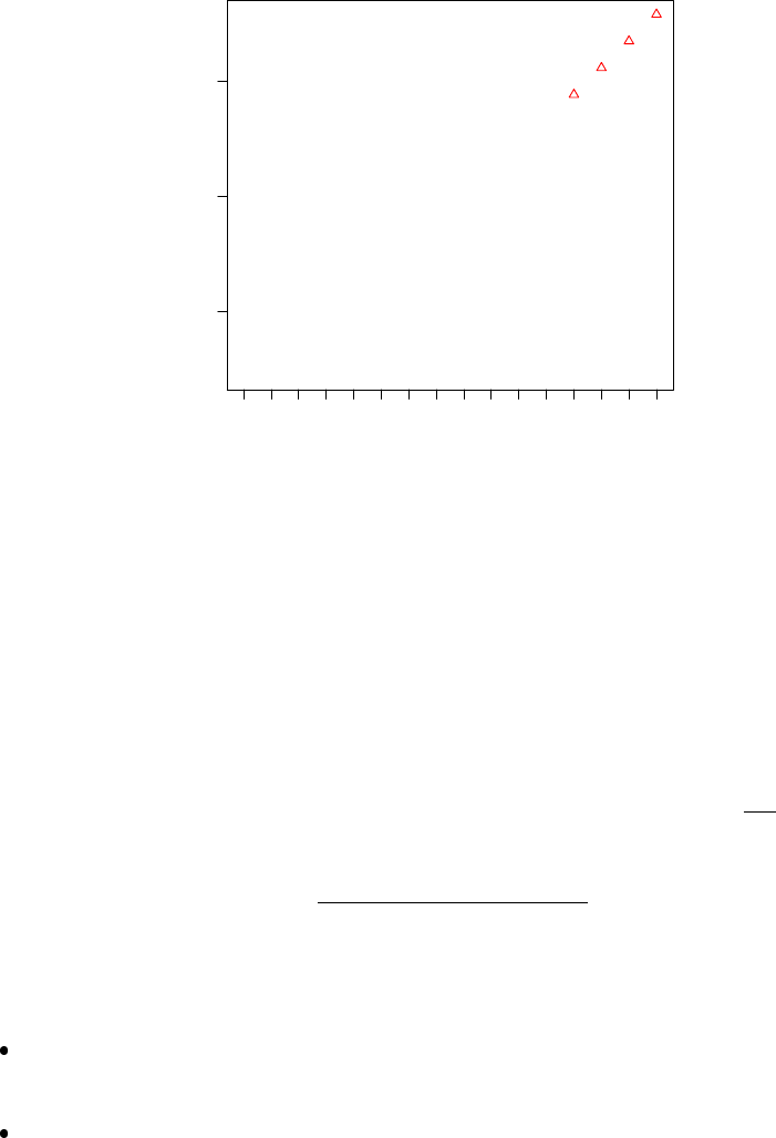
46 CHAPTER 5. REGRESSION
> data2011 <- data.frame(year=2011, quarter=1:4)
> cpi2011 <- predict(fit, newdata=data2011)
> style <- c(rep(1,12), rep(2,4))
> plot(c(cpi, cpi2011), xaxt="n", ylab="CPI", xlab="", pch=style, col=style)
> axis(1, at=1:16, las=3,
+ labels=c(paste(year,quarter,sep="Q"), "2011Q1", "2011Q2", "2011Q3", "2011Q4"))
●
●
●
●●
●
●
●
●
●
●
●
165 170 175
CPI
2008Q1
2008Q2
2008Q3
2008Q4
2009Q1
2009Q2
2009Q3
2009Q4
2010Q1
2010Q2
2010Q3
2010Q4
2011Q1
2011Q2
2011Q3
2011Q4
Figure 5.4: Prediction of CPIs in 2011 with Linear Regression Model
5.2 Logistic Regression
Logistic regression is used to predict the probability of occurrence of an event by fitting data to a
logistic curve. A logistic regression model is built as the following equation:
logit(y) = c0+c1x1+c2x2+· · · +ckxk,
where x1, x2,· · · , xkare predictors, yis a response to predict, and logit(y) = ln(y
1−y). The above
equation can also be written as
y=1
1 + e−(c0+c1x1+c2x2+···+ckxk).
Logistic regression can be built with function glm() by setting family to binomial(link="logit").
Detailed introductions on logistic regression can be found at the following links.
R Data Analysis Examples - Logit Regression
http://www.ats.ucla.edu/stat/r/dae/logit.htm
Logistic Regression (with R)
http://nlp.stanford.edu/~manning/courses/ling289/logistic.pdf
5.3. GENERALIZED LINEAR REGRESSION 47
5.3 Generalized Linear Regression
The generalized linear model (GLM) generalizes linear regression by allowing the linear model to
be related to the response variable via a link function and allowing the magnitude of the variance
of each measurement to be a function of its predicted value. It unifies various other statistical
models, including linear regression, logistic regression and Poisson regression. Function glm()
is used to fit generalized linear models, specified by giving a symbolic description of the linear
predictor and a description of the error distribution.
A generalized linear model is built below with glm() on the bodyfat data (see Section 1.3.2
for details of the data).
> data("bodyfat", package="mboost")
> myFormula <- DEXfat ~ age + waistcirc + hipcirc + elbowbreadth + kneebreadth
> bodyfat.glm <- glm(myFormula, family = gaussian("log"), data = bodyfat)
> summary(bodyfat.glm)
Call:
glm(formula = myFormula, family = gaussian("log"), data = bodyfat)
Deviance Residuals:
Min 1Q Median 3Q Max
-11.5688 -3.0065 0.1266 2.8310 10.0966
Coefficients:
Estimate Std. Error t value Pr(>|t|)
(Intercept) 0.734293 0.308949 2.377 0.02042 *
age 0.002129 0.001446 1.473 0.14560
waistcirc 0.010489 0.002479 4.231 7.44e-05 ***
hipcirc 0.009702 0.003231 3.003 0.00379 **
elbowbreadth 0.002355 0.045686 0.052 0.95905
kneebreadth 0.063188 0.028193 2.241 0.02843 *
---
Signif. codes: 0 ´
S***ˇ
S 0.001 ´
S**ˇ
S 0.01 ´
S*ˇ
S 0.05 ´
S.ˇ
S 0.1 ´
Sˇ
S 1
(Dispersion parameter for gaussian family taken to be 20.31433)
Null deviance: 8536.0 on 70 degrees of freedom
Residual deviance: 1320.4 on 65 degrees of freedom
AIC: 423.02
Number of Fisher Scoring iterations: 5
> pred <- predict(bodyfat.glm, type="response")
In the code above, type indicates the type of prediction required. The default is on the scale of
the linear predictors, and the alternative "response" is on the scale of the response variable.
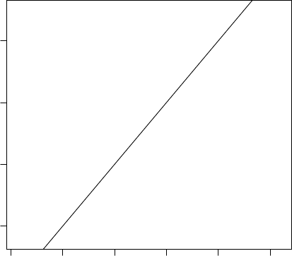
48 CHAPTER 5. REGRESSION
> plot(bodyfat$DEXfat, pred, xlab="Observed Values", ylab="Predicted Values")
> abline(a=0, b=1)
●●
●
●
●
●●
●
●
●
●
●
●
●
●
●
●
●
●
●
●
●
●
●
●
●
●
●
●
●
●
●
●
●
●●
●
●
●
●
●
●
●
●
●
●
●
●
●
●
●
●
●
●
●
●
●
●
●
●
●
●
●
●
●
●
●●
●
●
●
10 20 30 40 50 60
20 30 40 50
Observed Values
Predicted Values
Figure 5.5: Prediction with Generalized Linear Regression Model
In the above code, if family=gaussian("identity") is used, the built model would be sim-
ilar to linear regression. One can also make it a logistic regression by setting family to bino-
mial("logit").
5.4 Non-linear Regression
While linear regression is to find the line that comes closest to data, non-linear regression is to
fit a curve through data. Function nls() provides nonlinear regression. Examples of nls() can be
found by running “?nls” under R.
Chapter 6
Clustering
This chapter presents examples of various clustering techniques in R, including k-means clustering,
k-medoids clustering, hierarchical clustering and density-based clustering. The first two sections
demonstrate how to use the k-means and k-medoids algorithms to cluster the iris data. The third
section shows an example on hierarchical clustering on the same data. The last section describes
the idea of density-based clustering and the DBSCAN algorithm, and shows how to cluster with
DBSCAN and then label new data with the clustering model. For readers who are not familiar
with clustering, introductions of various clustering techniques can be found in [Zhao et al., 2009a]
and [Jain et al., 1999].
6.1 The k-Means Clustering
This section shows k-means clustering of iris data (see Section 1.3.1 for details of the data).
At first, we remove species from the data to cluster. After that, we apply function kmeans() to
iris2, and store the clustering result in kmeans.result. The cluster number is set to 3 in the
code below.
> iris2 <- iris
> iris2$Species <- NULL
> (kmeans.result <- kmeans(iris2, 3))
K-means clustering with 3 clusters of sizes 38, 50, 62
Cluster means:
Sepal.Length Sepal.Width Petal.Length Petal.Width
1 6.850000 3.073684 5.742105 2.071053
2 5.006000 3.428000 1.462000 0.246000
3 5.901613 2.748387 4.393548 1.433871
Clustering vector:
[1]222222222222222222222222222222222222222
[40]222222222223313333333333333333333333331
[79]333333333333333333333313111131111113311
[118]113131311331111131111311131113113
Within cluster sum of squares by cluster:
[1] 23.87947 15.15100 39.82097
(between_SS / total_SS = 88.4 %)
Available components:
49
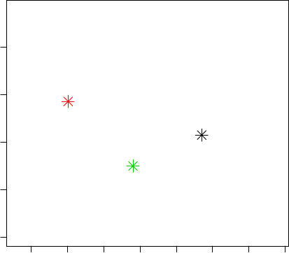
50 CHAPTER 6. CLUSTERING
[1] "cluster" "centers" "totss" "withinss" "tot.withinss"
[6] "betweenss" "size"
The clustering result is then compared with the class label (Species) to check whether similar
objects are grouped together.
> table(iris$Species, kmeans.result$cluster)
123
setosa 0 50 0
versicolor 2 0 48
virginica 36 0 14
The above result shows that cluster “setosa” can be easily separated from the other clusters, and
that clusters “versicolor” and “virginica” are to a small degree overlapped with each other.
Next, the clusters and their centers are plotted (see Figure 6.1). Note that there are four
dimensions in the data and that only the first two dimensions are used to draw the plot below.
Some black points close to the green center (asterisk) are actually closer to the black center in the
four dimensional space. We also need to be aware that the results of k-means clustering may vary
from run to run, due to random selection of initial cluster centers.
> plot(iris2[c("Sepal.Length", "Sepal.Width")], col = kmeans.result$cluster)
> # plot cluster centers
> points(kmeans.result$centers[,c("Sepal.Length", "Sepal.Width")], col = 1:3,
+ pch = 8, cex=2)
●
●
●
●
●
●
● ●
●
●
●
●
●●
●
●
●
●
●●
●
●
●
●
●
●
●
●
●
●
●
●
●
●
●
●
●
●
●
●
●
●
●
●
●
●
●
●
●
●
●●
●
●
●●
●
●
●
●
●
●
●
●●
●
●
●
●
●
●
●
●
●
●
●
●
●
●
●
●●
● ●
●
●
●
●
●
●
●
●
●
●
●
●
● ●
●
●
●
●
●
●
● ●
●
●
●
●
●
●
●
●
●
●
●
●
●
●
●
●●
●
●
●
●
●
●
●
●
●
●●
●
●
●
●
●
●● ●
●
●
●
●
●
●
●
●
4.5 5.0 5.5 6.0 6.5 7.0 7.5 8.0
2.0 2.5 3.0 3.5 4.0
Sepal.Length
Sepal.Width
Figure 6.1: Results of k-Means Clustering
More examples of k-means clustering can be found in Section 7.3 and Section 10.8.1.
6.2. THE K-MEDOIDS CLUSTERING 51
6.2 The k-Medoids Clustering
This sections shows k-medoids clustering with functions pam() and pamk(). The k-medoids clus-
tering is very similar to k-means, and the major difference between them is that: while a cluster
is represented with its center in the k-means algorithm, it is represented with the object closest to
the center of the cluster in the k-medoids clustering. The k-medoids clustering is more robust than
k-means in presence of outliers. PAM (Partitioning Around Medoids) is a classic algorithm for
k-medoids clustering. While the PAM algorithm is inefficient for clustering large data, the CLARA
algorithm is an enhanced technique of PAM by drawing multiple samples of data, applying PAM
on each sample and then returning the best clustering. It performs better than PAM on larger
data. Functions pam() and clara() in package cluster [Maechler et al., 2012] are respectively im-
plementations of PAM and CLARA in R. For both algorithms, a user has to specify k, the number
of clusters to find. As an enhanced version of pam(), function pamk() in package fpc [Hennig, 2010]
does not require a user to choose k. Instead, it calls the function pam() or clara() to perform a
partitioning around medoids clustering with the number of clusters estimated by optimum average
silhouette width.
With the code below, we demonstrate how to find clusters with pam() and pamk().
> library(fpc)
> pamk.result <- pamk(iris2)
> # number of clusters
> pamk.result$nc
[1] 2
> # check clustering against actual species
> table(pamk.result$pamobject$clustering, iris$Species)
setosa versicolor virginica
1 50 1 0
2 0 49 50
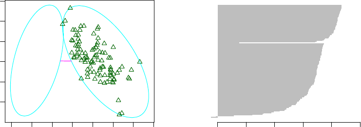
52 CHAPTER 6. CLUSTERING
> layout(matrix(c(1,2),1,2)) # 2 graphs per page
> plot(pamk.result$pamobject)
> layout(matrix(1)) # change back to one graph per page
−3 −2 −1 0 1 2 3 4
−2 −1 0 1 2 3
clusplot(pam(x = sdata, k = k, diss = diss))
Component 1
Component 2
These two components explain 95.81 % of the point variability.
●
●
●
●
●
●
●●
●
●
●
●
●
●
●
●
●
●
●
●
●
●
●
●
●
●
●
●
●
●
●
●
●
●
●
●
●
●
●
●
●
●
●
●
●
●
●
●
●
●
●
Silhouette width si
0.0 0.2 0.4 0.6 0.8 1.0
Silhouette plot of pam(x = sdata, k = k, diss = diss)
Average silhouette width : 0.69
n = 150 2 clusters Cj
j : nj | avei∈Cj si
1 : 51 | 0.81
2 : 99 | 0.62
Figure 6.2: Clustering with the k-medoids Algorithm - I
In the above example, pamk() produces two clusters: one is “setosa”, and the other is a mixture
of “versicolor” and “virginica”. In Figure 6.2, the left chart is a 2-dimensional “clusplot” (clustering
plot) of the two clusters and the lines show the distance between clusters. The right one shows their
silhouettes. In the silhouette, a large si(almost 1) suggests that the corresponding observations
are very well clustered, a small si(around 0) means that the observation lies between two clusters,
and observations with a negative siare probably placed in the wrong cluster. Since the average Si
are respectively 0.81 and 0.62 in the above silhouette, the identified two clusters are well clustered.
Next, we try pam() with k= 3.
> pam.result <- pam(iris2, 3)
> table(pam.result$clustering, iris$Species)
setosa versicolor virginica
1 50 0 0
2 0 48 14
3 0 2 36
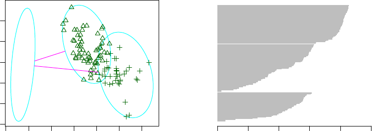
6.3. HIERARCHICAL CLUSTERING 53
> layout(matrix(c(1,2),1,2)) # 2 graphs per page
> plot(pam.result)
> layout(matrix(1)) # change back to one graph per page
−3 −2 −1 0 1 2 3
−3 −2 −1 0 1 2
clusplot(pam(x = iris2, k = 3))
Component 1
Component 2
These two components explain 95.81 % of the point variability.
●
●
●
●
●
●
●●
●
●
●
●
●
●
●
●
●
●
●
●
●
●
●
●
●
●
●
●
●
●
●
●
●
●
●
●
●
●
●
●
●
●
●
●
●
●
●
●
●
●
Silhouette width si
0.0 0.2 0.4 0.6 0.8 1.0
Silhouette plot of pam(x = iris2, k = 3)
Average silhouette width : 0.55
n = 150 3 clusters Cj
j : nj | avei∈Cj si
1 : 50 | 0.80
2 : 62 | 0.42
3 : 38 | 0.45
Figure 6.3: Clustering with the k-medoids Algorithm - II
With the above result produced with pam(), there are three clusters: 1) cluster 1 is species
“setosa” and is well separated from the other two; 2) cluster 2 is mainly composed of “versicolor”,
plus some cases from “virginica”; and 3) the majority of cluster 3 are “virginica”, with two cases
from “versicolor”.
It’s hard to say which one is better out of the above two clusterings produced respectively with
pamk() and pam(). It depends on the target problem and domain knowledge and experience. In
this example, the result of pam() seems better, because it identifies three clusters, corresponding
to three species. Therefore, the heuristic way to identify the number of clusters in pamk() does
not necessarily produce the best result. Note that we cheated by setting k= 3 when using pam(),
which is already known to us as the number of species.
More examples of k-medoids clustering can be found in Section 10.8.2.
6.3 Hierarchical Clustering
This section demonstrates hierarchical clustering with hclust() on iris data (see Section 1.3.1
for details of the data).
We first draw a sample of 40 records from the iris data, so that the clustering plot will not be
over crowded. Same as before, variable Species is removed from the data. After that, we apply
hierarchical clustering to the data.
> idx <- sample(1:dim(iris)[1], 40)
> irisSample <- iris[idx,]
> irisSample$Species <- NULL
> hc <- hclust(dist(irisSample), method="ave")
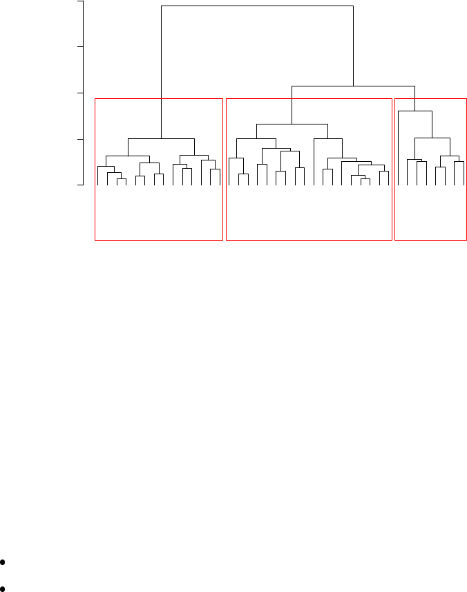
54 CHAPTER 6. CLUSTERING
> plot(hc, hang = -1, labels=iris$Species[idx])
> # cut tree into 3 clusters
> rect.hclust(hc, k=3)
> groups <- cutree(hc, k=3)
setosa
setosa
setosa
setosa
setosa
setosa
setosa
setosa
setosa
setosa
setosa
setosa
setosa
setosa
versicolor
versicolor
versicolor
virginica
virginica
versicolor
versicolor
versicolor
versicolor
versicolor
versicolor
versicolor
versicolor
versicolor
versicolor
versicolor
versicolor
versicolor
virginica
virginica
virginica
virginica
virginica
virginica
virginica
virginica
01234
Cluster Dendrogram
hclust (*, "average")
dist(irisSample)
Height
Figure 6.4: Cluster Dendrogram
Similar to the above clustering of k-means, Figure 6.4 also shows that cluster “setosa” can be
easily separated from the other two clusters, and that clusters “versicolor” and “virginica” are to a
small degree overlapped with each other.
More examples of hierarchical clustering can be found in Section 8.4 and Section 10.7.
6.4 Density-based Clustering
The DBSCAN algorithm [Ester et al., 1996] from package fpc [Hennig, 2010] provides a density-
based clustering for numeric data. The idea of density-based clustering is to group objects into
one cluster if they are connected to one another by densely populated area. There are two key
parameters in DBSCAN :
eps: reachability distance, which defines the size of neighborhood; and
MinPts: minimum number of points.
If the number of points in the neighborhood of point αis no less than MinPts, then αis a dense
point. All the points in its neighborhood are density-reachable from αand are put into the same
cluster as α.
The strengths of density-based clustering are that it can discover clusters with various shapes
and sizes and is insensitive to noise. As a comparison, the k-means algorithm tends to find clusters
with sphere shape and with similar sizes.
Below is an example of density-based clustering of the iris data.
> library(fpc)
> iris2 <- iris[-5] # remove class tags
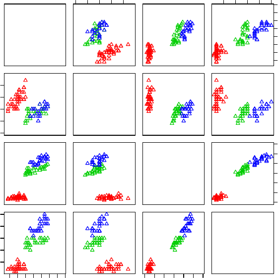
6.4. DENSITY-BASED CLUSTERING 55
> ds <- dbscan(iris2, eps=0.42, MinPts=5)
> # compare clusters with original class labels
> table(ds$cluster, iris$Species)
setosa versicolor virginica
0 2 10 17
1 48 0 0
2 0 37 0
3 0 3 33
In the above table, “1” to “3” in the first column are three identified clusters, while “0” stands for
noises or outliers, i.e., objects that are not assigned to any clusters. The noises are shown as black
circles in Figure 6.5.
> plot(ds, iris2)
Sepal.Length
2.0 3.0 4.0
●
●●●
●
●
●
●
●
●
●
●
●
●
●●
●
●
●
●●
●
●
●●
●
●
●
●●
●
●
●
●
●
●
●
●
●●
●●
●
●
●
●●
●
●
●
●
●
●
●
●
●
●
●
●●●
●●
●
●
●
●
●
●
●
●
●●
●
●
●
●
●
●
●
●●
●
●
●
●
●
●
●
●
●
●
●
●
●
●
●
●●
●
●
●
●●●
●
●
●●
●
●
●
●
●
0.5 1.5 2.5
4.5 5.5 6.5 7.5
●
●●●
●
●
●
●
●
●
●
●
●
●
●●
●
●
●
●
●
●
●
●●
●
●
●
●
●
●
●
●
●
●
●
●
●
●●
●●
●
●
●
●● ●
●
●
●
●
●
●
●
●
●
2.0 3.0 4.0
●
●
●
●
●
●
●
●
●
●
●
●
●
●
●
●●
●
●
●
●
●
●
●
●
●
●
●
●
●
●
●●
●
●
●
●
●
●
●
●
●
●
●●
●
●
●
●
●●
●
●
●
● ●
●
Sepal.Width
●
●
●
●
●
●
●
●
●
●
●
●
●
●
●
●●
●
●
●
●
●
●
●
●
●
●
●
●
●
●
●●
●
●
●
●
●
●
●
●
●
●
●●
●
●
●
●
●●
●
●
●
●●
●
●
●
●
●
●
●
●
●
●
●
●
●
●
●
●
●●
●
●
●
●
●
●
●
●
●
●
●
●
●
●
●●
●
●
●
●
●
●
●
●
●
●
●●
●
●
●
●
●●
●
●
●
● ●
●
●●
●
●
●
●
●
●
●
●
●
●
●
●
●
●
●
●
●●
●●
●
●
●●●●
●
●
●●
●
●
●
●●
●
●
●
●
●
●
●
●
●
●●●
●
●
●
●
●
●
●
●
●●●
●
●
●
●
●
●
●
●
●
●
●
●
●
●
●●
●●●
●
●
●●
●●
●●
●
●
●
●
●
●●
●
●●
●
●
●●
●
●
●
●●
●
●
●
●
●
●
●●
Petal.Length
1 2 3 4 5 6 7
●
●●
●
●
●
●●
●
●
●
●
●
●
●
●
●
●●
●
●●
●
●
●●
●●
●
●
●
●
●
●
●
●●
●
●●
●
●
●●
●
●
●●
●
●
●
●
●
●
●
●
●
4.5 5.5 6.5 7.5
0.5 1.5 2.5
●●
●
●
●●●
●
●
●
●
●
●
● ●
●
●
●
●
●
●
●
●●
●●
●
●
●
●
●
●●
●●●
●
●●
●
●
●
●
●●
●
●
●●
●
●
●
●
●
●
●●
●●
●
●
●●●
●
●
●
●
●
●
● ●
●
●
●
●
●
●
●
●●
●●
●●
●●
●
●●
●●●
●
●●
●
●
●
●
●●
●
●
●●
●
●
●
●●
●
● ●
1 2 3 4 5 6 7
●
●
●
●
●●
●
●
●
●
●
●
●
● ●
●
●
●
●
●
●
●
●●
●
●
●
●
●
●
●
●●
●●●
●
●●
●
●
●
●
●●
●
●
●●
●
●●
●
●
●
●●
Petal.Width
Figure 6.5: Density-based Clustering - I
The clusters are shown below in a scatter plot using the first and fourth columns of the data.
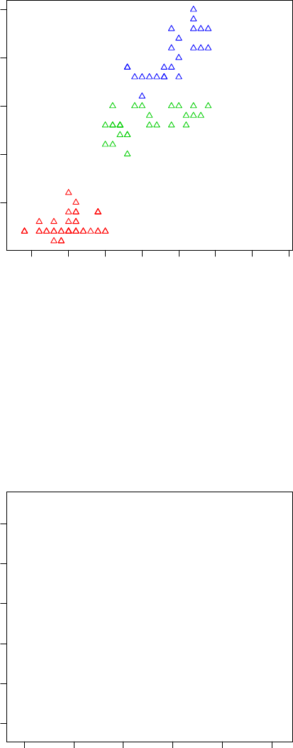
56 CHAPTER 6. CLUSTERING
> plot(ds, iris2[c(1,4)])
●
●
●
●
●●
●
●
●
●
●
●
●
● ●
●
●
●
●
●
●
●
●●
●
●
●
●
●
●
●
●●
●
●●
●
●●
●
●
●
●
●●
●
●
●
●
●
●
●
●
●
●
●●
4.5 5.0 5.5 6.0 6.5 7.0 7.5 8.0
0.5 1.0 1.5 2.0 2.5
Sepal.Length
Petal.Width
Figure 6.6: Density-based Clustering - II
Another way to show the clusters is using function plotcluster() in package fpc. Note that
the data are projected to distinguish classes.
> plotcluster(iris2, ds$cluster)
1
1
1
1
1
11
11
1
11
1
1
1
11
1
1
1
1
1
0
1
11
1
1
11
1
1
1
1
1
1
1
11
1
1
0
1
1
1
1
11
11
2
2
22
2
2
2
0
2
2
0
2
0
2
0
2
2
2
0
2
3
2
3
2
2
2
2
2
2
02
2
23
2
0
2
0
2
2
2
2
2
02
2
2
2
0
2
0
3
3
3
3
0
0
0
0
0
3
3
33
0
3
3
0
0
0
3
3
0
3
3
0
3
33
0
0
0
3
3
0
0
3
3
33
3
3
3
3
3
3
3
3
3
3
−8 −6 −4 −2 0 2
−2 −1 0 1 2 3
dc 1
dc 2
Figure 6.7: Density-based Clustering - III
6.4. DENSITY-BASED CLUSTERING 57
The clustering model can be used to label new data, based on the similarity between new
data and the clusters. The following example draws a sample of 10 objects from iris and adds
small noises to them to make a new dataset for labeling. The random noises are generated with
a uniform distribution using function runif().
> # create a new dataset for labeling
> set.seed(435)
> idx <- sample(1:nrow(iris), 10)
> newData <- iris[idx,-5]
> newData <- newData + matrix(runif(10*4, min=0, max=0.2), nrow=10, ncol=4)
> # label new data
> myPred <- predict(ds, iris2, newData)
> # plot result
> plot(iris2[c(1,4)], col=1+ds$cluster)
> points(newData[c(1,4)], pch="*", col=1+myPred, cex=3)
> # check cluster labels
> table(myPred, iris$Species[idx])
myPred setosa versicolor virginica
0 0 0 1
1 3 0 0
2 0 3 0
3 0 1 2
●●●● ●
●
●
●●
●
●●
●●
●
●●
● ●●
●
●
●
●
● ●
●
●●● ●
●
●
●● ● ●
●
● ●
●●
●
●
●
●
●● ●●
●
● ●
●
●
●
●
●
●
●
●
●
●
●
●
●
●
●
●
●
●
●
●
●
●
● ●
●
●
●
●
●
●
●
●
●
●
●●●
●
●
●
●
●
●
● ●
●
●
●
●
●
●
●
●
●
●●
●
●
●
●
●
●
●
●
●
●
●
●
●●
●
●
●●●
●
●
●
●
●
●
●
●
●
●●
●
●
●
●
●
●
●
●
●
●
●
4.5 5.0 5.5 6.0 6.5 7.0 7.5 8.0
0.5 1.0 1.5 2.0 2.5
Sepal.Length
Petal.Width
**
*
*
*
*
*
*
**
Figure 6.8: Prediction with Clustering Model
As we can see from the above result, out of the 10 new unlabeled data, 8(=3+3+2) are assigned
with correct class labels. The new data are shown as asterisk(“*”) in the above figure and the colors
stand for cluster labels in Figure 6.8.
58 CHAPTER 6. CLUSTERING
Chapter 7
Outlier Detection
This chapter presents examples of outlier detection with R. At first, it demonstrates univariate
outlier detection. After that, an example of outlier detection with LOF (Local Outlier Factor) is
given, followed by examples on outlier detection by clustering. At last, it demonstrates outlier
detection from time series data.
7.1 Univariate Outlier Detection
This section shows an example of univariate outlier detection, and demonstrates how to ap-
ply it to multivariate data. In the example, univariate outlier detection is done with function
boxplot.stats(), which returns the statistics for producing boxplots. In the result returned by
the above function, one component is out, which gives a list of outliers. More specifically, it lists
data points lying beyond the extremes of the whiskers. An argument of coef can be used to
control how far the whiskers extend out from the box of a boxplot. More details on that can be
obtained by running ?boxplot.stats in R. Figure 7.1 shows a boxplot, where the four circles are
outliers.
59
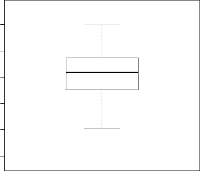
60 CHAPTER 7. OUTLIER DETECTION
> set.seed(3147)
> x <- rnorm(100)
> summary(x)
Min. 1st Qu. Median Mean 3rd Qu. Max.
-3.3150 -0.4837 0.1867 0.1098 0.7120 2.6860
> # outliers
> boxplot.stats(x)$out
[1] -3.315391 2.685922 -3.055717 2.571203
> boxplot(x)
●
●
●
●
−3 −2 −1 0 1 2
Figure 7.1: Univariate Outlier Detection with Boxplot
The above univariate outlier detection can be used to find outliers in multivariate data in a
simple ensemble way. In the example below, we first generate a dataframe df, which has two
columns, xand y. After that, outliers are detected separately from xand y. We then take outliers
as those data which are outliers for both columns. In Figure 7.2, outliers are labeled with “+” in
red.
> y <- rnorm(100)
> df <- data.frame(x, y)
> rm(x, y)
> head(df)
x y
1 -3.31539150 0.7619774
2 -0.04765067 -0.6404403
3 0.69720806 0.7645655
4 0.35979073 0.3131930
5 0.18644193 0.1709528
6 0.27493834 -0.8441813
7.1. UNIVARIATE OUTLIER DETECTION 61
> attach(df)
> # find the index of outliers from x
> (a <- which(x %in% boxplot.stats(x)$out))
[1] 1 33 64 74
> # find the index of outliers from y
> (b <- which(y %in% boxplot.stats(y)$out))
[1] 24 25 49 64 74
> detach(df)
> # outliers in both x and y
> (outlier.list1 <- intersect(a,b))
[1] 64 74
> plot(df)
> points(df[outlier.list1,], col="red", pch="+", cex=2.5)
●
●
●
●
●
●
●
●
●
●
●
●
●
●
●●
●
●
●
●
●
●
●
●
●
●
●
●
●
●
●
●
●
●
●
●
●
●
●
●
●
●
●
●
●
●
●
●
●
●
●
●
●
●
●
●
●
●
●
●
●
●
●
●
●
●
●●
●
●
●
●
●
●
●
●
●
●
●
●
●
●
●
●
●
●
●
●
●
●
●●
●
●
●
●
●
●
●
●
−3 −2 −1 0 1 2
−3 −2 −1 0 1 2
x
y
+
+
Figure 7.2: Outlier Detection - I
Similarly, we can also take outliers as those data which are outliers in either xor y. In
Figure 7.3, outliers are labeled with “x” in blue.
62 CHAPTER 7. OUTLIER DETECTION
> # outliers in either x or y
> (outlier.list2 <- union(a,b))
[1] 1 33 64 74 24 25 49
> plot(df)
> points(df[outlier.list2,], col="blue", pch="x", cex=2)
●
●
●
●
●
●
●
●
●
●
●
●
●
●
●●
●
●
●
●
●
●
●
●
●
●
●
●
●
●
●
●
●
●
●
●
●
●
●
●
●
●
●
●
●
●
●
●
●
●
●
●
●
●
●
●
●
●
●
●
●
●
●
●
●
●
●●
●
●
●
●
●
●
●
●
●
●
●
●
●
●
●
●
●
●
●
●
●
●
●●
●
●
●
●
●
●
●
●
−3 −2 −1 0 1 2
−3 −2 −1 0 1 2
x
y
xx
x
x
x
x
x
Figure 7.3: Outlier Detection - II
When there are three or more variables in an application, a final list of outliers might be
produced with majority voting of outliers detected from individual variables. Domain knowledge
should be involved when choosing the optimal way to ensemble in real-world applications.
7.2 Outlier Detection with LOF
LOF (Local Outlier Factor) is an algorithm for identifying density-based local outliers [Breunig
et al., 2000]. With LOF, the local density of a point is compared with that of its neighbors. If
the former is significantly lower than the latter (with an LOF value greater than one), the point
is in a sparser region than its neighbors, which suggests it be an outlier. A shortcoming of LOF
is that it works on numeric data only.
Function lofactor() calculates local outlier factors using the LOF algorithm, and it is available
in packages DMwR [Torgo, 2010] and dprep. An example of outlier detection with LOF is given
below, where kis the number of neighbors used for calculating local outlier factors. Figure 7.4
shows a density plot of outlier scores.
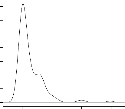
7.2. OUTLIER DETECTION WITH LOF 63
> library(DMwR)
> # remove "Species", which is a categorical column
> iris2 <- iris[,1:4]
> outlier.scores <- lofactor(iris2, k=5)
> plot(density(outlier.scores))
1.0 1.5 2.0 2.5
0.0 0.5 1.0 1.5 2.0 2.5 3.0 3.5
density.default(x = outlier.scores)
N = 150 Bandwidth = 0.05627
Density
Figure 7.4: Density of outlier factors
> # pick top 5 as outliers
> outliers <- order(outlier.scores, decreasing=T)[1:5]
> # who are outliers
> print(outliers)
[1] 42 107 23 110 63
> print(iris2[outliers,])
Sepal.Length Sepal.Width Petal.Length Petal.Width
42 4.5 2.3 1.3 0.3
107 4.9 2.5 4.5 1.7
23 4.6 3.6 1.0 0.2
110 7.2 3.6 6.1 2.5
63 6.0 2.2 4.0 1.0
Next, we show outliers with a biplot of the first two principal components (see Figure 7.5).
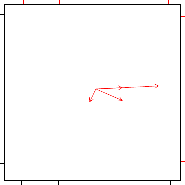
64 CHAPTER 7. OUTLIER DETECTION
> n <- nrow(iris2)
> labels <- 1:n
> labels[-outliers] <- "."
> biplot(prcomp(iris2), cex=.8, xlabs=labels)
−0.2 −0.1 0.0 0.1 0.2
−0.2 −0.1 0.0 0.1 0.2
PC1
PC2
.
.
.
.
.
.
.
.
.
.
.
.
.
.
.
.
.
.
.
.
.
.
23 .
.
.
.
.
.
.
.
.
.
.
.
.
.
.
.
.
.
42
.
.
.
.
.
.
.
.
.
.
.
.
.
.
.
.
.
.
.
.
63
.
.
.
.
.
.
.
.
.
.
.
.
...
.
.
.
.
..
.
.
.
.
.
..
.
.
.
.
.
.
.
.
.
.
.
.
.
.
.
107
.
.
110
.
.
.
.
.
.
.
.
.
.
.
.
.
.
.
.
.
..
..
.
.
.
.
.
.
.
.
.
.
.
.
.
.
.
.
..
.
−20 −10 0 10 20
−20 −10 0 10 20
Sepal.Length
Sepal.Width
Petal.Length
Petal.Width
Figure 7.5: Outliers in a Biplot of First Two Principal Components
In the above code, prcomp() performs a principal component analysis, and biplot() plots the
data with its first two principal components. In Figure 7.5, the x- and y-axis are respectively the
first and second principal components, the arrows show the original columns (variables), and the
five outliers are labeled with their row numbers.
We can also show outliers with a pairs plot as below, where outliers are labeled with “+” in
red.
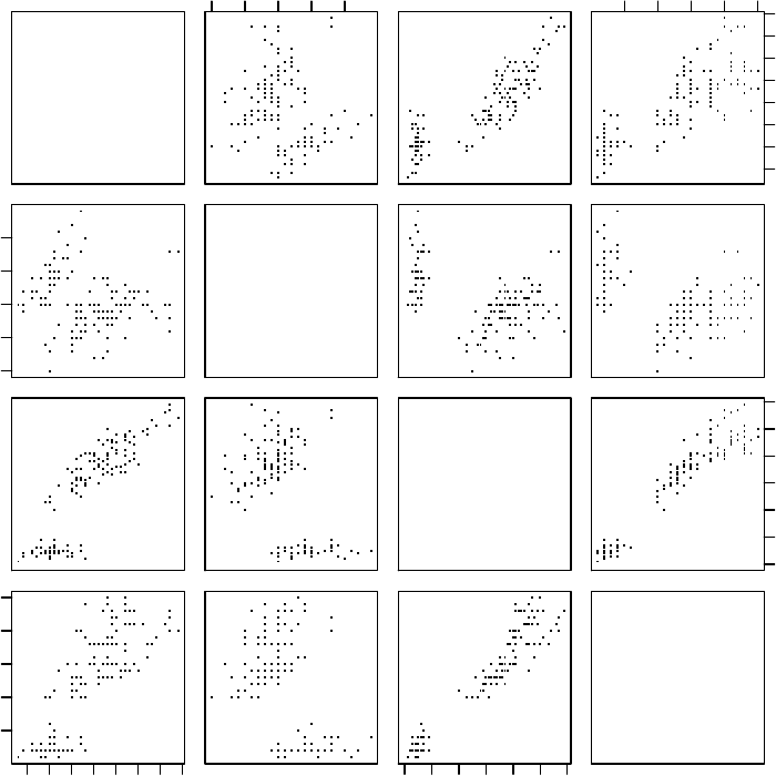
7.2. OUTLIER DETECTION WITH LOF 65
> pch <- rep(".", n)
> pch[outliers] <- "+"
> col <- rep("black", n)
> col[outliers] <- "red"
> pairs(iris2, pch=pch, col=col)
Sepal.Length
2.0 3.0 4.0
+
+
+
+
+
++
+
+
+
0.5 1.5 2.5
4.5 5.5 6.5 7.5
+
+
+
+
+
2.0 3.0 4.0
+
++
+
+
Sepal.Width
+
+++
+
+
+++
+
+
+
+
+
+
+
+
++
+
Petal.Length
1 2 3 4 5 6 7
+
+
++
+
4.5 5.5 6.5 7.5
0.5 1.5 2.5
+
+
+
+
+
+
+
+
+
+
1 2 3 4 5 6 7
++
+
+
+
Petal.Width
Figure 7.6: Outliers in a Matrix of Scatter Plots
Package Rlof [Hu et al., 2011] provides function lof(), a parallel implementation of the LOF
algorithm. Its usage is similar to lofactor(), but lof() has two additional features of supporting
multiple values of kand several choices of distance metrics. Below is an example of lof(). After
computing outlier scores, outliers can be detected by selecting the top ones. Note that the current
version of package Rlof (v1.0.0) works under MacOS X and Linux, but does not work under
Windows, because it depends on package multicore for parallel computing.
> library(Rlof)
> outlier.scores <- lof(iris2, k=5)
66 CHAPTER 7. OUTLIER DETECTION
> # try with different number of neighbors (k = 5,6,7,8,9 and 10)
> outlier.scores <- lof(iris2, k=c(5:10))
7.3 Outlier Detection by Clustering
Another way to detect outliers is clustering. By grouping data into clusters, those data not
assigned to any clusters are taken as outliers. For example, with density-based clustering such as
DBSCAN [Ester et al., 1996], objects are grouped into one cluster if they are connected to one
another by densely populated area. Therefore, objects not assigned to any clusters are isolated
from other objects and are taken as outliers. An example of DBSCAN be found in Section 6.4
Density-based Clustering.
We can also detect outliers with the k-means algorithm. With k-means, the data are partitioned
into kgroups by assigning them to the closest cluster centers. After that, we can calculate the
distance (or dissimilarity) between each object and its cluster center, and pick those with largest
distances as outliers. An example of outlier detection with k-means from the iris data (see
Section 1.3.1 for details of the data) is given below.
> # remove species from the data to cluster
> iris2 <- iris[,1:4]
> kmeans.result <- kmeans(iris2, centers=3)
> # cluster centers
> kmeans.result$centers
Sepal.Length Sepal.Width Petal.Length Petal.Width
1 5.006000 3.428000 1.462000 0.246000
2 6.850000 3.073684 5.742105 2.071053
3 5.901613 2.748387 4.393548 1.433871
> # cluster IDs
> kmeans.result$cluster
[1]111111111111111111111111111111111111111
[40]111111111113323333333333333333333333332
[79]333333333333333333333323222232222223322
[118]223232322332222232222322232223223
> # calculate distances between objects and cluster centers
> centers <- kmeans.result$centers[kmeans.result$cluster, ]
> distances <- sqrt(rowSums((iris2 - centers)^2))
> # pick top 5 largest distances
> outliers <- order(distances, decreasing=T)[1:5]
> # who are outliers
> print(outliers)
[1] 99 58 94 61 119
> print(iris2[outliers,])
Sepal.Length Sepal.Width Petal.Length Petal.Width
99 5.1 2.5 3.0 1.1
58 4.9 2.4 3.3 1.0
94 5.0 2.3 3.3 1.0
61 5.0 2.0 3.5 1.0
119 7.7 2.6 6.9 2.3
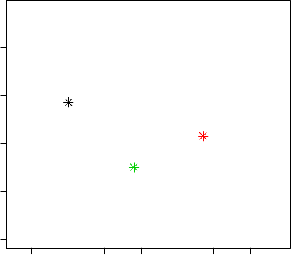
7.4. OUTLIER DETECTION FROM TIME SERIES 67
> # plot clusters
> plot(iris2[,c("Sepal.Length", "Sepal.Width")], pch="o",
+ col=kmeans.result$cluster, cex=0.3)
> # plot cluster centers
> points(kmeans.result$centers[,c("Sepal.Length", "Sepal.Width")], col=1:3,
+ pch=8, cex=1.5)
> # plot outliers
> points(iris2[outliers, c("Sepal.Length", "Sepal.Width")], pch="+", col=4, cex=1.5)
o
o
o
o
o
o
o o
o
o
o
o
oo
o
o
o
o
oo
o
o
o
o
o
o
o
o
o
o
o
o
o
o
o
o
o
o
o
o
o
o
o
o
o
o
o
o
o
o
oo
o
o
oo
o
o
o
o
o
o
o
oo
o
o
o
o
o
o
o
o
o
o
o
o
o
o
o
oo
o o
o
o
o
o
o
o
o
o
o
o
o
o
o o
o
o
o
o
o
o
o o
o
o
o
o
o
o
o
o
o
o
o
o
o
o
o
oo
o
o
o
o
o
o
o
o
o
oo
o
o
o
o
o
oo o
o
o
o
o
o
o
o
o
4.5 5.0 5.5 6.0 6.5 7.0 7.5 8.0
2.0 2.5 3.0 3.5 4.0
Sepal.Length
Sepal.Width
+
++
+
+
Figure 7.7: Outliers with k-Means Clustering
In the above figure, cluster centers are labeled with asterisks and outliers with “+”.
7.4 Outlier Detection from Time Series
This section presents an example of outlier detection from time series data. In the example, the
time series data are first decomposed with robust regression using function stl() and then outliers
are identified. An introduction of STL (Seasonal-trend decomposition based on Loess) [Cleveland
et al., 1990] is available at http://cs.wellesley.edu/~cs315/Papers/stl%20statistical%20model.
pdf. More examples of time series decomposition can be found in Section 8.2.
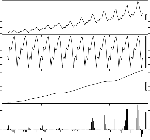
68 CHAPTER 7. OUTLIER DETECTION
> # use robust fitting
> f <- stl(AirPassengers, "periodic", robust=TRUE)
> (outliers <- which(f$weights<1e-8))
[1] 79 91 92 102 103 104 114 115 116 126 127 128 138 139 140
> # set layout
> op <- par(mar=c(0, 4, 0, 3), oma=c(5, 0, 4, 0), mfcol=c(4, 1))
> plot(f, set.pars=NULL)
> sts <- f$time.series
> # plot outliers
> points(time(sts)[outliers], 0.8*sts[,"remainder"][outliers], pch="x", col="red")
> par(op) # reset layout
100 300 500
data
−40 0 20 40
seasonal
150 250 350 450
trend
0 50 100
1950 1952 1954 1956 1958 1960
remainder
time
xx
xx
x
xx
x
x
x
x
x
x
x
x
Figure 7.8: Outliers in Time Series Data
In above figure, outliers are labeled with “x” in red.
7.5 Discussions
The LOF algorithm is good at detecting local outliers, but it works on numeric data only. Package
Rlof relies on the multicore package, which does not work under Windows. A fast and scalable
outlier detection strategy for categorical data is the Attribute Value Frequency (AVF) algorithm
[Koufakou et al., 2007].

7.5. DISCUSSIONS 69
Some other R packages for outlier detection are:
Package extremevalues [van der Loo, 2010]: univariate outlier detection;
Package mvoutlier [Filzmoser and Gschwandtner, 2012]: multivariate outlier detection based
on robust methods; and
Package outliers [Komsta, 2011]: tests for outliers.
70 CHAPTER 7. OUTLIER DETECTION
Chapter 8
Time Series Analysis and Mining
This chapter presents examples on time series decomposition, forecasting, clustering and classi-
fication. The first section introduces briefly time series data in R. The second section shows an
example on decomposing time series into trend, seasonal and random components. The third sec-
tion presents how to build an autoregressive integrated moving average (ARIMA) model in R and
use it to predict future values. The fourth section introduces Dynamic Time Warping (DTW) and
hierarchical clustering of time series data with Euclidean distance and with DTW distance. The
fifth section shows three examples on time series classification: one with original data, the other
with DWT (Discrete Wavelet Transform) transformed data, and another with k-NN classification.
The chapter ends with discussions and further readings.
8.1 Time Series Data in R
Class ts represents data which has been sampled at equispaced points in time. A frequency of
7 indicates that a time series is composed of weekly data, and 12 and 4 are used respectively for
monthly and quarterly series. An example below shows the construction of a time series with 30
values (1 to 30). Frequency=12 and start=c(2011,3) specify that it is a monthly series starting
from March 2011.
> a <- ts(1:30, frequency=12, start=c(2011,3))
> print(a)
Jan Feb Mar Apr May Jun Jul Aug Sep Oct Nov Dec
2011 12345678910
2012 11 12 13 14 15 16 17 18 19 20 21 22
2013 23 24 25 26 27 28 29 30
> str(a)
Time-Series [1:30] from 2011 to 2014: 1 2 3 4 5 6 7 8 9 10 ...
> attributes(a)
$tsp
[1] 2011.167 2013.583 12.000
$class
[1] "ts"
71
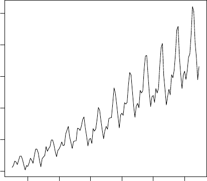
72 CHAPTER 8. TIME SERIES ANALYSIS AND MINING
8.2 Time Series Decomposition
Time Series Decomposition is to decompose a time series into trend, seasonal, cyclical and irregular
components. The trend component stands for long term trend, the seasonal component is seasonal
variation, the cyclical component is repeated but non-periodic fluctuations, and the residuals are
irregular component.
A time series of AirPassengers is used below as an example to demonstrate time series de-
composition. It is composed of monthly totals of Box & Jenkins international airline passengers
from 1949 to 1960. It has 144(=12*12) values.
> plot(AirPassengers)
Time
AirPassengers
1950 1952 1954 1956 1958 1960
100 200 300 400 500 600
Figure 8.1: A Time Series of AirPassengers
Function decompose() is applied below to AirPassengers to break it into various components.
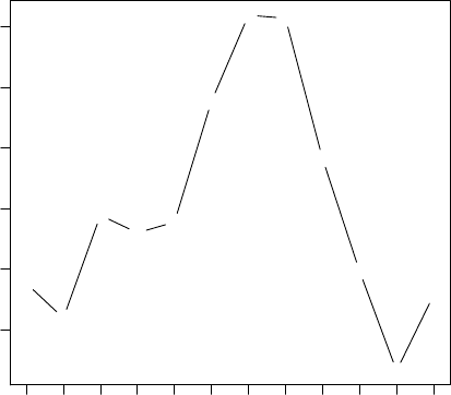
8.2. TIME SERIES DECOMPOSITION 73
> # decompose time series
> apts <- ts(AirPassengers, frequency=12)
> f <- decompose(apts)
> # seasonal figures
> f$figure
[1] -24.748737 -36.188131 -2.241162 -8.036616 -4.506313 35.402778 63.830808
[8] 62.823232 16.520202 -20.642677 -53.593434 -28.619949
> plot(f$figure, type="b", xaxt="n", xlab="")
> # get names of 12 months in English words
> monthNames <- months(ISOdate(2011,1:12,1))
> # label x-axis with month names
> # las is set to 2 for vertical label orientation
> axis(1, at=1:12, labels=monthNames, las=2)
●
●
●
●
●
●
●●
●
●
●
●
−40 −20 0 20 40 60
f$figure
January
February
March
April
May
June
July
August
September
October
November
December
Figure 8.2: Seasonal Component
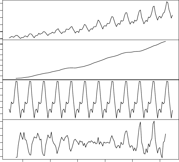
74 CHAPTER 8. TIME SERIES ANALYSIS AND MINING
> plot(f)
100 300 500
observed
150 250 350 450
trend
−40 0 40
seasonal
−40 0 20 60
2 4 6 8 10 12
random
Time
Decomposition of additive time series
Figure 8.3: Time Series Decomposition
In Figure 8.3, the first chart is the original time series. The second is trend of the data, the
third shows seasonal factors, and the last chart is the remaining components after removing trend
and seasonal factors.
Some other functions for time series decomposition are stl() in package stats [R Development
Core Team, 2012], decomp() in package timsac [The Institute of Statistical Mathematics, 2012],
and tsr() in package ast.
8.3 Time Series Forecasting
Time series forecasting is to forecast future events based on historical data. One example is
to predict the opening price of a stock based on its past performance. Two popular models for
time series forecasting are autoregressive moving average (ARMA) and autoregressive integrated
moving average (ARIMA).
Here is an example to fit an ARIMA model to a univariate time series and then use it for
forecasting.
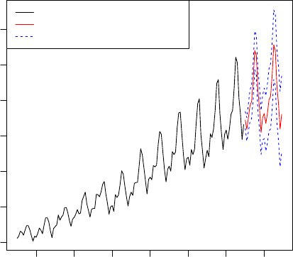
8.4. TIME SERIES CLUSTERING 75
> fit <- arima(AirPassengers, order=c(1,0,0), list(order=c(2,1,0), period=12))
> fore <- predict(fit, n.ahead=24)
> # error bounds at 95% confidence level
> U <- fore$pred + 2*fore$se
> L <- fore$pred - 2*fore$se
> ts.plot(AirPassengers, fore$pred, U, L, col=c(1,2,4,4), lty = c(1,1,2,2))
> legend("topleft", c("Actual", "Forecast", "Error Bounds (95% Confidence)"),
+ col=c(1,2,4), lty=c(1,1,2))
Time
1950 1952 1954 1956 1958 1960 1962
100 200 300 400 500 600 700
Actual
Forecast
Error Bounds (95% Confidence)
Figure 8.4: Time Series Forecast
In Figure 8.4, the red solid line shows the forecasted values, and the blue dotted lines are error
bounds at a confidence level of 95%.
8.4 Time Series Clustering
Time series clustering is to partition time series data into groups based on similarity or distance,
so that time series in the same cluster are similar to each other. There are various measures
of distance or dissimilarity, such as Euclidean distance, Manhattan distance, Maximum norm,
Hamming distance, the angle between two vectors (inner product), and Dynamic Time Warping
(DTW) distance.
8.4.1 Dynamic Time Warping
Dynamic Time Warping (DTW) finds optimal alignment between two time series [Keogh and
Pazzani, 2001] and an implement of it in R is package dtw [Giorgino, 2009]. In that package,
function dtw(x, y, ...) computes dynamic time warp and finds optimal alignment between two
time series xand y, and dtwDist(mx, my=mx, ...) or dist(mx, my=mx, method="DTW", ...)
calculates the distances between time series mx and my.
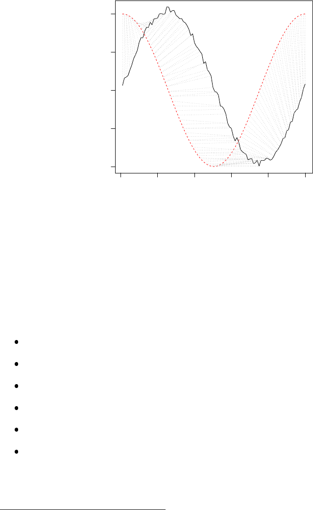
76 CHAPTER 8. TIME SERIES ANALYSIS AND MINING
> library(dtw)
> idx <- seq(0, 2*pi, len=100)
> a <- sin(idx) + runif(100)/10
> b <- cos(idx)
> align <- dtw(a, b, step=asymmetricP1, keep=T)
> dtwPlotTwoWay(align)
Index
Query value
0 20 40 60 80 100
−1.0 −0.5 0.0 0.5 1.0
Figure 8.5: Alignment with Dynamic Time Warping
8.4.2 Synthetic Control Chart Time Series Data
The synthetic control chart time series 1is used in the examples in the following sections. The
dataset contains 600 examples of control charts synthetically generated by the process in Alcock
and Manolopoulos (1999). Each control chart is a time series with 60 values, and there are six
classes:
1-100: Normal;
101-200: Cyclic;
201-300: Increasing trend;
301-400: Decreasing trend;
401-500: Upward shift; and
501-600: Downward shift.
Firstly, the data is read into R with read.table(). Parameter sep is set to "" (no space
between double quotation marks), which is used when the separator is white space, i.e., one or
more spaces, tabs, newlines or carriage returns.
1http://kdd.ics.uci.edu/databases/synthetic_control/synthetic_control.html
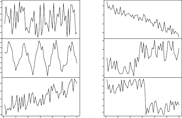
8.4. TIME SERIES CLUSTERING 77
> sc <- read.table("./data/synthetic_control.data", header=F, sep="")
> # show one sample from each class
> idx <- c(1,101,201,301,401,501)
> sample1 <- t(sc[idx,])
> plot.ts(sample1, main="")
24 26 28 30 32 34 36
1
15 25 35 45
101
25 30 35 40 45
0 10 20 30 40 50 60
201
Time
0 10 20 30
301
25 30 35 40 45
401
10 15 20 25 30 35
0 10 20 30 40 50 60
501
Time
Figure 8.6: Six Classes in Synthetic Control Chart Time Series
8.4.3 Hierarchical Clustering with Euclidean Distance
At first, we select 10 cases randomly from each class. Otherwise, there will be too many cases and
the plot of hierarchical clustering will be over crowded.
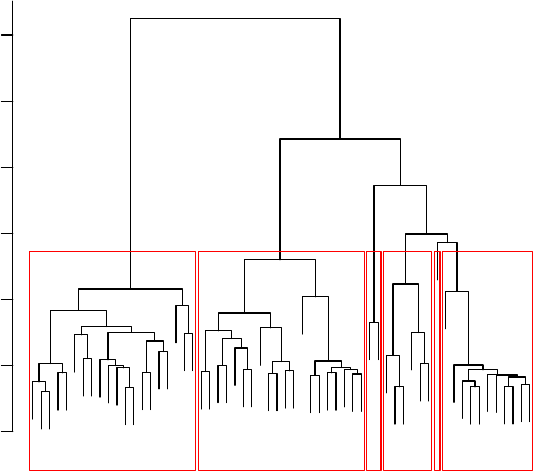
78 CHAPTER 8. TIME SERIES ANALYSIS AND MINING
> set.seed(6218)
> n <- 10
> s <- sample(1:100, n)
> idx <- c(s, 100+s, 200+s, 300+s, 400+s, 500+s)
> sample2 <- sc[idx,]
> observedLabels <- rep(1:6, each=n)
> # hierarchical clustering with Euclidean distance
> hc <- hclust(dist(sample2), method="average")
> plot(hc, labels=observedLabels, main="")
> # cut tree to get 6 clusters
> rect.hclust(hc, k=6)
> memb <- cutree(hc, k=6)
> table(observedLabels, memb)
memb
observedLabels 1 2 3 4 5 6
11000000
2162100
30000100
40000010
50000100
60000010
3
3
33
35
5
5
3
3
3
3
35
55
55
5
5
6
6
6
66
6
66
4
4
4
66
4
4
4
4
4
4
42
2
2
2
22
2
22
2
1
1
1
11
1
1
1
1
1
20 40 60 80 100 120 140
hclust (*, "average")
dist(sample2)
Height
Figure 8.7: Hierarchical Clustering with Euclidean Distance
8.4. TIME SERIES CLUSTERING 79
The clustering result in Figure 8.7 shows that, increasing trend (class 3) and upward shift
(class 5) are not well separated, and decreasing trend (class 4) and downward shift (class 6) are
also mixed.
8.4.4 Hierarchical Clustering with DTW Distance
Next, we try hierarchical clustering with the DTW distance.
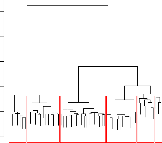
80 CHAPTER 8. TIME SERIES ANALYSIS AND MINING
> library(dtw)
> distMatrix <- dist(sample2, method="DTW")
> hc <- hclust(distMatrix, method="average")
> plot(hc, labels=observedLabels, main="")
> # cut tree to get 6 clusters
> rect.hclust(hc, k=6)
> memb <- cutree(hc, k=6)
> table(observedLabels, memb)
memb
observedLabels 1 2 3 4 5 6
11000000
2073000
30001000
4000073
5200800
60000010
4
4
4
4
4
4
46
6
6
4
4
46
6
6
6
6
6
6
5
5
5
5
5
5
5
5
3
3
3
3
3
3
3
3
3
3
1
1
1
1
1
11
1
1
15
52
2
2
22
2
22
2
2
0 200 400 600 800 1000
hclust (*, "average")
distMatrix
Height
Figure 8.8: Hierarchical Clustering with DTW Distance
By comparing Figure 8.8 with Figure 8.7, we can see that the DTW distance are better than
the Euclidean distance for measuring the similarity between time series.
8.5. TIME SERIES CLASSIFICATION 81
8.5 Time Series Classification
Time series classification is to build a classification model based on labeled time series and then
use the model to predict the label of unlabeled time series. New features extracted from time series
may help to improve the performance of classification models. Techniques for feature extraction
include Singular Value Decomposition (SVD), Discrete Fourier Transform (DFT), Discrete Wavelet
Transform (DWT), Piecewise Aggregate Approximation (PAA), Perpetually Important Points
(PIP), Piecewise Linear Representation, and Symbolic Representation.
8.5.1 Classification with Original Data
We use ctree() from package party [Hothorn et al., 2010] to demonstrate classification of time
series with the original data. The class labels are changed into categorical values before feeding
the data into ctree(), so that we won’t get class labels as a real number like 1.35. The built
decision tree is shown in Figure 8.9.
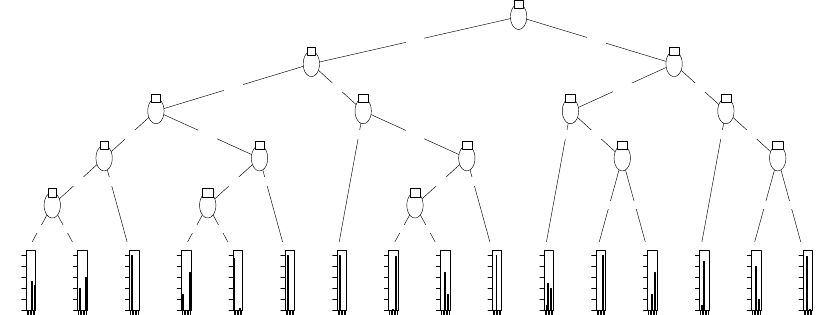
82 CHAPTER 8. TIME SERIES ANALYSIS AND MINING
> classId <- rep(as.character(1:6), each=100)
> newSc <- data.frame(cbind(classId, sc))
> library(party)
> ct <- ctree(classId ~ ., data=newSc,
+ controls = ctree_control(minsplit=30, minbucket=10, maxdepth=5))
> pClassId <- predict(ct)
> table(classId, pClassId)
pClassId
classId 1 2 3 4 5 6
19700003
21932004
30096040
400010000
5 4 0 10 0 86 0
6 0 0 0 87 0 13
> # accuracy
> (sum(classId==pClassId)) / nrow(sc)
[1] 0.8083333
> plot(ct, ip_args=list(pval=FALSE), ep_args=list(digits=0))
V59
1
≤46 >46
V59
2
≤36 >36
V59
3
≤24 >24
V54
4
≤27 >27
V19
5
≤35 >35
Node 6 (n = 187)
14
0
0.2
0.4
0.6
0.8
1
Node 7 (n = 10)
14
0
0.2
0.4
0.6
0.8
1
Node 8 (n = 21)
14
0
0.2
0.4
0.6
0.8
1
V4
9
≤36 >36
V51
10
≤25 >25
Node 11 (n = 10)
14
0
0.2
0.4
0.6
0.8
1
Node 12 (n = 102)
14
0
0.2
0.4
0.6
0.8
1
Node 13 (n = 41)
14
0
0.2
0.4
0.6
0.8
1
V54
14
≤32 >32
Node 15 (n = 31)
14
0
0.2
0.4
0.6
0.8
1
V19
16
≤36 >36
V15
17
≤36 >36
Node 18 (n = 59)
14
0
0.2
0.4
0.6
0.8
1
Node 19 (n = 10)
14
0
0.2
0.4
0.6
0.8
1
Node 20 (n = 13)
14
0
0.2
0.4
0.6
0.8
1
V20
21
≤33 >33
V41
22
≤42 >42
Node 23 (n = 10)
14
0
0.2
0.4
0.6
0.8
1
V57
24
≤49 >49
Node 25 (n = 21)
14
0
0.2
0.4
0.6
0.8
1
Node 26 (n = 10)
14
0
0.2
0.4
0.6
0.8
1
V39
27
≤39 >39
Node 28 (n = 10)
14
0
0.2
0.4
0.6
0.8
1
V15
29
≤31 >31
Node 30 (n = 10)
14
0
0.2
0.4
0.6
0.8
1
Node 31 (n = 55)
14
0
0.2
0.4
0.6
0.8
1
Figure 8.9: Decision Tree
8.5.2 Classification with Extracted Features
Next, we use DWT (Discrete Wavelet Transform) [Burrus et al., 1998] to extract features from
time series and then build a classification model. Wavelet transform provides a multi-resolution
representation using wavelets. An example of Haar Wavelet Transform, the simplest DWT, is
available at http://dmr.ath.cx/gfx/haar/. Another popular feature extraction technique is
Discrete Fourier Transform (DFT) [Agrawal et al., 1993].
An example on extracting DWT (with Haar filter) coefficients is shown below. Package wavelets
[Aldrich, 2010] is used for discrete wavelet transform. In the package, function dwt(X, filter,
n.levels, ...) computes the discrete wavelet transform coefficients, where Xis a univariate or
multi-variate time series, filter indicates which wavelet filter to use, and n.levels specifies the
level of decomposition. It returns an object of class dwt, whose slot Wcontains wavelet coefficients
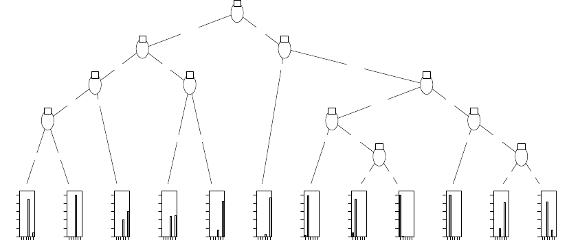
8.5. TIME SERIES CLASSIFICATION 83
and Vcontains scaling coefficients. The original time series can be reconstructed via an inverse
discrete wavelet transform with function idwt() in the same package. The produced model is
shown in Figure 8.10.
> library(wavelets)
> wtData <- NULL
> for (i in 1:nrow(sc)) {
+ a <- t(sc[i,])
+ wt <- dwt(a, filter="haar", boundary="periodic")
+ wtData <- rbind(wtData, unlist(c(wt@W, wt@V[[wt@level]])))
+ }
> wtData <- as.data.frame(wtData)
> wtSc <- data.frame(cbind(classId, wtData))
> # build a decision tree with DWT coefficients
> ct <- ctree(classId ~ ., data=wtSc,
+ controls = ctree_control(minsplit=30, minbucket=10, maxdepth=5))
> pClassId <- predict(ct)
> table(classId, pClassId)
pClassId
classId 1 2 3 4 5 6
19730000
21990000
3 0 0 81 0 19 0
4 0 0 0 63 0 37
5 0 0 16 0 84 0
60001099
> (sum(classId==pClassId)) / nrow(wtSc)
[1] 0.8716667
> plot(ct, ip_args=list(pval=FALSE), ep_args=list(digits=0))
V57
1
≤117 >117
W43
2
≤−4 >−4
W5
3
≤−9 >−9
W42
4
≤−10 >−10
Node 5 (n = 10)
135
0
0.2
0.4
0.6
0.8
1
Node 6 (n = 54)
135
0
0.2
0.4
0.6
0.8
1
Node 7 (n = 10)
135
0
0.2
0.4
0.6
0.8
1
W31
8
≤−1 >−1
Node 9 (n = 49)
135
0
0.2
0.4
0.6
0.8
1
Node 10 (n = 46)
135
0
0.2
0.4
0.6
0.8
1
V57
11
≤140 >140
Node 12 (n = 31)
135
0
0.2
0.4
0.6
0.8
1
V57
13
≤178 >178
W22
14
≤−6 >−6
Node 15 (n = 80)
135
0
0.2
0.4
0.6
0.8
1
W31
16
≤−9 >−9
Node 17 (n = 10)
135
0
0.2
0.4
0.6
0.8
1
Node 18 (n = 98)
135
0
0.2
0.4
0.6
0.8
1
W31
19
≤−15 >−15
Node 20 (n = 12)
135
0
0.2
0.4
0.6
0.8
1
W43
21
≤3>3
Node 22 (n = 103)
135
0
0.2
0.4
0.6
0.8
1
Node 23 (n = 97)
135
0
0.2
0.4
0.6
0.8
1
Figure 8.10: Decision Tree with DWT

84 CHAPTER 8. TIME SERIES ANALYSIS AND MINING
8.5.3 k-NN Classification
The k-NN classification can also be used for time series classification. It finds out the knearest
neighbors of a new instance and then labels it by majority voting. However, the time complexity of
a naive way to find knearest neighbors is O(n2), where nis the size of data. Therefore, an efficient
indexing structure is needed for large datasets. Package RANN supports fast nearest neighbor
search with a time complexity of O(nlog n) using Arya and Mount’s ANN library (v1.1.1) 2. Below
is an example of k-NN classification of time series without indexing.
> k <- 20
> # create a new time series by adding noise to time series 501
> newTS <- sc[501,] + runif(100)*15
> distances <- dist(newTS, sc, method="DTW")
> s <- sort(as.vector(distances), index.return=TRUE)
> # class IDs of k nearest neighbors
> table(classId[s$ix[1:k]])
4 6
3 17
For the 20 nearest neighbors of the new time series, three of them are of class 4, and 17 are of
class 6. With majority voting, that is, taking the more frequent label as winner, the label of the
new time series is set to class 6.
8.6 Discussions
There are many R functions and packages available for time series decomposition and forecasting.
However, there are no R functions or packages specially for time series classification and clustering.
There are a lot of research publications on techniques specially for classifying/clustering time series
data, but there are no R implementations for them (as far as I know).
To do time series classification, one is suggested to extract and build features first, and then ap-
ply existing classification techniques, such as SVM, k-NN, neural networks, regression and decision
trees, to the feature set.
For time series clustering, one needs to work out his/her own distance or similarity metrics,
and then use existing clustering techniques, such as k-means or hierarchical clustering, to find
clusters.
8.7 Further Readings
An introduction of R functions and packages for time series is available as CRAN Task View:
Time Series Analysis at http://cran.r-project.org/web/views/TimeSeries.html.
R code examples for time series can be found in slides Time Series Analysis and Mining with
Rat http://www.rdatamining.com/docs.
Some further readings on time series representation, similarity, clustering and classification
are [Agrawal et al., 1993, Burrus et al., 1998, Chan and Fu, 1999, Chan et al., 2003, Keogh and
Pazzani, 1998,Keogh et al., 2000, Keogh and Pazzani, 2000, M¨
orchen, 2003,Rafiei and Mendelzon,
1998, Vlachos et al., 2003, Wu et al., 2000, Zhao and Zhang, 2006].
2http://www.cs.umd.edu/~mount/ANN/

Chapter 9
Association Rules
This chapter presents examples of association rule mining with R. It starts with basic concepts of
association rules, and then demonstrates association rules mining with R. After that, it presents
examples of pruning redundant rules and interpreting and visualizing association rules. The chap-
ter concludes with discussions and recommended readings.
9.1 Basics of Association Rules
Association rules are rules presenting association or correlation between itemsets. An association
rule is in the form of A⇒B, where Aand Bare two disjoint itemsets, referred to respectively
as the lhs (left-hand side) and rhs (right-hand side) of the rule. The three most widely-used
measures for selecting interesting rules are support,confidence and lift.Support is the percentage
of cases in the data that contains both Aand B,confidence is the percentage of cases containing
Athat also contain B, and lift is the ratio of confidence to the percentage of cases containing B.
The formulae to calculate them are:
support(A⇒B) = P(A∪B) (9.1)
confidence(A⇒B) = P(B|A) (9.2)
=P(A∪B)
P(A)(9.3)
lift(A⇒B) = confidence(A⇒B)
P(B)(9.4)
=P(A∪B)
P(A)P(B)(9.5)
where P(A) is the percentage (or probability) of cases containing A.
In addition to support, confidence and lift, there are many other interestingness measures, such
as chi-square, conviction, gini and leverage. An introduction to over 20 measures can be found in
Tan et al.’s work [Tan et al., 2002].
9.2 The Titanic Dataset
The Titanic dataset in the datasets package is a 4-dimensional table with summarized information
on the fate of passengers on the Titanic according to social class, sex, age and survival. To make it
suitable for association rule mining, we reconstruct the raw data as titanic.raw, where each row
represents a person. The reconstructed raw data can also be downloaded as file “titanic.raw.rdata”
at http://www.rdatamining.com/data.
85

86 CHAPTER 9. ASSOCIATION RULES
> str(Titanic)
table [1:4, 1:2, 1:2, 1:2] 0 0 35 0 0 0 17 0 118 154 ...
- attr(*, "dimnames")=List of 4
..$ Class : chr [1:4] "1st" "2nd" "3rd" "Crew"
..$ Sex : chr [1:2] "Male" "Female"
..$ Age : chr [1:2] "Child" "Adult"
..$ Survived: chr [1:2] "No" "Yes"
> df <- as.data.frame(Titanic)
> head(df)
Class Sex Age Survived Freq
1 1st Male Child No 0
2 2nd Male Child No 0
3 3rd Male Child No 35
4 Crew Male Child No 0
5 1st Female Child No 0
6 2nd Female Child No 0
> titanic.raw <- NULL
> for(i in 1:4) {
+ titanic.raw <- cbind(titanic.raw, rep(as.character(df[,i]), df$Freq))
+ }
> titanic.raw <- as.data.frame(titanic.raw)
> names(titanic.raw) <- names(df)[1:4]
> dim(titanic.raw)
[1] 2201 4
> str(titanic.raw)
data.frame : 2201 obs. of 4 variables:
$ Class : Factor w/ 4 levels "1st","2nd","3rd",..: 3 3 3 3 3 3 3 3 3 3 ...
$ Sex : Factor w/ 2 levels "Female","Male": 2 2 2 2 2 2 2 2 2 2 ...
$ Age : Factor w/ 2 levels "Adult","Child": 2 2 2 2 2 2 2 2 2 2 ...
$ Survived: Factor w/ 2 levels "No","Yes": 1 1 1 1 1 1 1 1 1 1 ...
> head(titanic.raw)
Class Sex Age Survived
1 3rd Male Child No
2 3rd Male Child No
3 3rd Male Child No
4 3rd Male Child No
5 3rd Male Child No
6 3rd Male Child No
> summary(titanic.raw)
Class Sex Age Survived
1st :325 Female: 470 Adult:2092 No :1490
2nd :285 Male :1731 Child: 109 Yes: 711
3rd :706
Crew:885
9.3. ASSOCIATION RULE MINING 87
Now we have a dataset where each row stands for a person, and it can be used for association
rule mining.
The raw Titanic dataset can also be downloaded from http://www.cs.toronto.edu/~delve/
data/titanic/desc.html. The data is file“Dataset.data”in the compressed archive“titanic.tar.gz”.
It can be read into R with the code below.
> # have a look at the 1st 5 lines
> readLines("./data/Dataset.data", n=5)
[1] "1st adult male yes" "1st adult male yes" "1st adult male yes"
[4] "1st adult male yes" "1st adult male yes"
> # read it into R
> titanic <- read.table("./data/Dataset.data", header=F)
> names(titanic) <- c("Class", "Sex", "Age", "Survived")
9.3 Association Rule Mining
A classic algorithm for association rule mining is APRIORI [Agrawal and Srikant, 1994]. It is a
level-wise, breadth-first algorithm which counts transactions to find frequent itemsets and then
derive association rules from them. An implementation of it is function apriori() in package
arules [Hahsler et al., 2011]. Another algorithm for association rule mining is the ECLAT algorithm
[Zaki, 2000], which finds frequent itemsets with equivalence classes, depth-first search and set
intersection instead of counting. It is implemented as function eclat() in the same package.
Below we demonstrate association rule mining with apriori(). With the function, the default
settings are: 1) supp=0.1, which is the minimum support of rules; 2) conf=0.8, which is the
minimum confidence of rules; and 3) maxlen=10, which is the maximum length of rules.
> library(arules)
> # find association rules with default settings
> rules.all <- apriori(titanic.raw)
parameter specification:
confidence minval smax arem aval originalSupport support minlen maxlen target
0.8 0.1 1 none FALSE TRUE 0.1 1 10 rules
ext
FALSE
algorithmic control:
filter tree heap memopt load sort verbose
0.1 TRUE TRUE FALSE TRUE 2 TRUE
apriori - find association rules with the apriori algorithm
version 4.21 (2004.05.09) (c) 1996-2004 Christian Borgelt
set item appearances ...[0 item(s)] done [0.00s].
set transactions ...[10 item(s), 2201 transaction(s)] done [0.00s].
sorting and recoding items ... [9 item(s)] done [0.00s].
creating transaction tree ... done [0.00s].
checking subsets of size 1 2 3 4 done [0.00s].
writing ... [27 rule(s)] done [0.00s].
creating S4 object ... done [0.00s].
> rules.all
set of 27 rules
88 CHAPTER 9. ASSOCIATION RULES
> inspect(rules.all)
lhs rhs support confidence lift
1 {} => {Age=Adult} 0.9504771 0.9504771 1.0000000
2 {Class=2nd} => {Age=Adult} 0.1185825 0.9157895 0.9635051
3 {Class=1st} => {Age=Adult} 0.1449341 0.9815385 1.0326798
4 {Sex=Female} => {Age=Adult} 0.1930940 0.9042553 0.9513700
5 {Class=3rd} => {Age=Adult} 0.2848705 0.8881020 0.9343750
6 {Survived=Yes} => {Age=Adult} 0.2971377 0.9198312 0.9677574
7 {Class=Crew} => {Sex=Male} 0.3916402 0.9740113 1.2384742
8 {Class=Crew} => {Age=Adult} 0.4020900 1.0000000 1.0521033
9 {Survived=No} => {Sex=Male} 0.6197183 0.9154362 1.1639949
10 {Survived=No} => {Age=Adult} 0.6533394 0.9651007 1.0153856
11 {Sex=Male} => {Age=Adult} 0.7573830 0.9630272 1.0132040
12 {Sex=Female,
Survived=Yes} => {Age=Adult} 0.1435711 0.9186047 0.9664669
13 {Class=3rd,
Sex=Male} => {Survived=No} 0.1917310 0.8274510 1.2222950
14 {Class=3rd,
Survived=No} => {Age=Adult} 0.2162653 0.9015152 0.9484870
15 {Class=3rd,
Sex=Male} => {Age=Adult} 0.2099046 0.9058824 0.9530818
16 {Sex=Male,
Survived=Yes} => {Age=Adult} 0.1535666 0.9209809 0.9689670
17 {Class=Crew,
Survived=No} => {Sex=Male} 0.3044071 0.9955423 1.2658514
18 {Class=Crew,
Survived=No} => {Age=Adult} 0.3057701 1.0000000 1.0521033
19 {Class=Crew,
Sex=Male} => {Age=Adult} 0.3916402 1.0000000 1.0521033
20 {Class=Crew,
Age=Adult} => {Sex=Male} 0.3916402 0.9740113 1.2384742
21 {Sex=Male,
Survived=No} => {Age=Adult} 0.6038164 0.9743402 1.0251065
22 {Age=Adult,
Survived=No} => {Sex=Male} 0.6038164 0.9242003 1.1751385
23 {Class=3rd,
Sex=Male,
Survived=No} => {Age=Adult} 0.1758292 0.9170616 0.9648435
24 {Class=3rd,
Age=Adult,
Survived=No} => {Sex=Male} 0.1758292 0.8130252 1.0337773
25 {Class=3rd,
Sex=Male,
Age=Adult} => {Survived=No} 0.1758292 0.8376623 1.2373791
26 {Class=Crew,
Sex=Male,
Survived=No} => {Age=Adult} 0.3044071 1.0000000 1.0521033
27 {Class=Crew,
Age=Adult,
Survived=No} => {Sex=Male} 0.3044071 0.9955423 1.2658514
As a common phenomenon for association rule mining, many rules generated above are un-
interesting. Suppose that we are interested in only rules with rhs indicating survival, so we set
9.3. ASSOCIATION RULE MINING 89
rhs=c("Survived=No", "Survived=Yes") in appearance to make sure that only “Survived=No”
and “Survived=Yes” will appear in the rhs of rules. All other items can appear in the lhs, as set
with default="lhs". In the above result rules.all, we can also see that the left-hand side (lhs)
of the first rule is empty. To exclude such rules, we set minlen to 2 in the code below. Moreover,
the details of progress are suppressed with verbose=F. After association rule mining, rules are
sorted by lift to make high-lift rules appear first.
> # rules with rhs containing "Survived" only
> rules <- apriori(titanic.raw, control = list(verbose=F),
+ parameter = list(minlen=2, supp=0.005, conf=0.8),
+ appearance = list(rhs=c("Survived=No", "Survived=Yes"),
+ default="lhs"))
> quality(rules) <- round(quality(rules), digits=3)
> rules.sorted <- sort(rules, by="lift")
> inspect(rules.sorted)
lhs rhs support confidence lift
1 {Class=2nd,
Age=Child} => {Survived=Yes} 0.011 1.000 3.096
2 {Class=2nd,
Sex=Female,
Age=Child} => {Survived=Yes} 0.006 1.000 3.096
3 {Class=1st,
Sex=Female} => {Survived=Yes} 0.064 0.972 3.010
4 {Class=1st,
Sex=Female,
Age=Adult} => {Survived=Yes} 0.064 0.972 3.010
5 {Class=2nd,
Sex=Female} => {Survived=Yes} 0.042 0.877 2.716
6 {Class=Crew,
Sex=Female} => {Survived=Yes} 0.009 0.870 2.692
7 {Class=Crew,
Sex=Female,
Age=Adult} => {Survived=Yes} 0.009 0.870 2.692
8 {Class=2nd,
Sex=Female,
Age=Adult} => {Survived=Yes} 0.036 0.860 2.663
9 {Class=2nd,
Sex=Male,
Age=Adult} => {Survived=No} 0.070 0.917 1.354
10 {Class=2nd,
Sex=Male} => {Survived=No} 0.070 0.860 1.271
11 {Class=3rd,
Sex=Male,
Age=Adult} => {Survived=No} 0.176 0.838 1.237
12 {Class=3rd,
Sex=Male} => {Survived=No} 0.192 0.827 1.222
When other settings are unchanged, with a lower minimum support, more rules will be pro-
duced, and the associations between itemsets shown in the rules will be more likely to be by
chance. In the above code, the minimum support is set to 0.005, so each rule is supported at least
by 12 (=ceiling(0.005 * 2201)) cases, which is acceptable for a population of 2201.
Support, confidence and lift are three common measures for selecting interesting association
rules. Besides them, there are many other interestingness measures, such as chi-square, conviction,
90 CHAPTER 9. ASSOCIATION RULES
gini and leverage [Tan et al., 2002]. More than twenty measures can be calculated with function
interestMeasure() in the arules package.
9.4 Removing Redundancy
Some rules generated in the previous section (see rules.sorted, page 89) provide little or no
extra information when some other rules are in the result. For example, the above rule 2 provides
no extra knowledge in addition to rule 1, since rules 1 tells us that all 2nd-class children survived.
Generally speaking, when a rule (such as rule 2) is a super rule of another rule (such as rule 1)
and the former has the same or a lower lift, the former rule (rule 2) is considered to be redundant.
Other redundant rules in the above result are rules 4, 7 and 8, compared respectively with rules
3, 6 and 5.
Below we prune redundant rules. Note that the rules have already been sorted descendingly
by lift.
> # find redundant rules
> subset.matrix <- is.subset(rules.sorted, rules.sorted)
> subset.matrix[lower.tri(subset.matrix, diag=T)] <- NA
> redundant <- colSums(subset.matrix, na.rm=T) >= 1
> which(redundant)
[1]2478
> # remove redundant rules
> rules.pruned <- rules.sorted[!redundant]
> inspect(rules.pruned)
lhs rhs support confidence lift
1 {Class=2nd,
Age=Child} => {Survived=Yes} 0.011 1.000 3.096
2 {Class=1st,
Sex=Female} => {Survived=Yes} 0.064 0.972 3.010
3 {Class=2nd,
Sex=Female} => {Survived=Yes} 0.042 0.877 2.716
4 {Class=Crew,
Sex=Female} => {Survived=Yes} 0.009 0.870 2.692
5 {Class=2nd,
Sex=Male,
Age=Adult} => {Survived=No} 0.070 0.917 1.354
6 {Class=2nd,
Sex=Male} => {Survived=No} 0.070 0.860 1.271
7 {Class=3rd,
Sex=Male,
Age=Adult} => {Survived=No} 0.176 0.838 1.237
8 {Class=3rd,
Sex=Male} => {Survived=No} 0.192 0.827 1.222
In the code above, function is.subset(r1, r2) checks whether r1 is a subset of r2 (i.e., whether
r2 is a superset of r1). Function lower.tri() returns a logical matrix with TURE in lower triangle.
From the above results, we can see that rules 2, 4, 7 and 8 (before redundancy removal) are
successfully pruned.
9.5. INTERPRETING RULES 91
9.5 Interpreting Rules
While it is easy to find high-lift rules from data, it is not an easy job to understand the identified
rules. It is not uncommon that the association rules are misinterpreted to find their business mean-
ings. For instance, in the above rule list rules.pruned, the first rule "{Class=2nd, Age=Child}
=> {Survived=Yes}" has a confidence of one and a lift of three and there are no rules on chil-
dren of the 1st or 3rd classes. Therefore, it might be interpreted by users as children of the 2nd
class had a higher survival rate than other children. This is wrong! The rule states only that all
children of class 2 survived, but provides no information at all to compare the survival rates of
different classes. To investigate the above issue, we run the code below to find rules whose rhs is
"Survived=Yes" and lhs contains "Class=1st","Class=2nd","Class=3rd","Age=Child" and
"Age=Adult" only, and which contains no other items (default="none"). We use lower thresholds
for both support and confidence than before to find all rules for children of different classes.
> rules <- apriori(titanic.raw,
+ parameter = list(minlen=3, supp=0.002, conf=0.2),
+ appearance = list(rhs=c("Survived=Yes"),
+ lhs=c("Class=1st", "Class=2nd", "Class=3rd",
+ "Age=Child", "Age=Adult"),
+ default="none"),
+ control = list(verbose=F))
> rules.sorted <- sort(rules, by="confidence")
> inspect(rules.sorted)
lhs rhs support confidence lift
1 {Class=2nd,
Age=Child} => {Survived=Yes} 0.010904134 1.0000000 3.0956399
2 {Class=1st,
Age=Child} => {Survived=Yes} 0.002726034 1.0000000 3.0956399
3 {Class=1st,
Age=Adult} => {Survived=Yes} 0.089504771 0.6175549 1.9117275
4 {Class=2nd,
Age=Adult} => {Survived=Yes} 0.042707860 0.3601533 1.1149048
5 {Class=3rd,
Age=Child} => {Survived=Yes} 0.012267151 0.3417722 1.0580035
6 {Class=3rd,
Age=Adult} => {Survived=Yes} 0.068605179 0.2408293 0.7455209
In the above result, the first two rules show that children of the 1st class are of the same survival
rate as children of the 2nd class and that all of them survived. The rule of 1st-class children didn’t
appear before, simply because of its support was below the threshold specified in Section 9.3. Rule
5 presents a sad fact that children of class 3 had a low survival rate of 34%, which is comparable
with that of 2nd-class adults (see rule 4) and much lower than 1st-class adults (see rule 3).
9.6 Visualizing Association Rules
Next we show some ways to visualize association rules, including scatter plot, balloon plot, graph
and parallel coordinates plot. More examples on visualizing association rules can be found in
the vignettes of package arulesViz [Hahsler and Chelluboina, 2012] on CRAN at http://cran.
r-project.org/web/packages/arulesViz/vignettes/arulesViz.pdf.
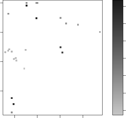
92 CHAPTER 9. ASSOCIATION RULES
> library(arulesViz)
> plot(rules.all)
Scatter plot for 27 rules
0.95
1
1.05
1.1
1.15
1.2
1.25
lift
0.2 0.4 0.6 0.8
0.85
0.9
0.95
1
support
confidence
Figure 9.1: A Scatter Plot of Association Rules
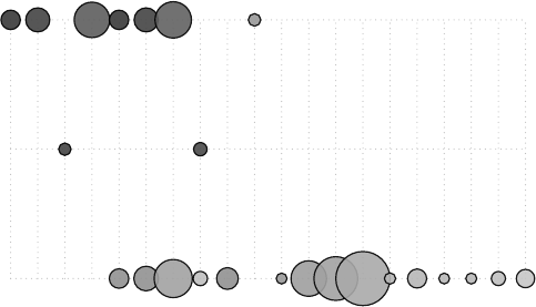
9.6. VISUALIZING ASSOCIATION RULES 93
> plot(rules.all, method="grouped")
Grouped matrix for 27 rules
size: support
color: lift
1 (Class=Crew +2)
1 (Class=Crew +1)
1 (Class=3rd +2)
1 (Age=Adult +1)
2 (Class=Crew +1)
2 (Class=Crew +0)
2 (Survived=No +0)
2 (Class=3rd +1)
2 (Class=Crew +2)
1 (Class=3rd +2)
1 (Class=1st +0)
1 (Sex=Male +1)
1 (Sex=Male +0)
1 (Class=1st +−1)
1 (Sex=Male +1)
1 (Survived=Yes +0)
1 (Sex=Female +1)
2 (Class=2nd +3)
2 (Class=3rd +2)
1 (Class=3rd +0)
{Age=Adult}
{Survived=No}
{Sex=Male}
LHS
RHS
Figure 9.2: A Balloon Plot of Association Rules
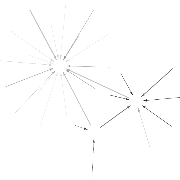
94 CHAPTER 9. ASSOCIATION RULES
> plot(rules.all, method="graph")
Graph for 27 rules
{}
{Age=Adult,Survived=No}
{Age=Adult}
{Class=1st}
{Class=2nd}
{Class=3rd,Age=Adult,Survived=No}
{Class=3rd,Sex=Male,Age=Adult}
{Class=3rd,Sex=Male,Survived=No}
{Class=3rd,Sex=Male}
{Class=3rd,Survived=No}
{Class=3rd}
{Class=Crew,Age=Adult,Survived=No}
{Class=Crew,Age=Adult}
{Class=Crew,Sex=Male,Survived=No}
{Class=Crew,Sex=Male}
{Class=Crew,Survived=No}
{Class=Crew}
{Sex=Female,Survived=Yes}
{Sex=Female}
{Sex=Male,Survived=No}
{Sex=Male,Survived=Yes}
{Sex=Male}
{Survived=No}
{Survived=Yes}
width: support (0.119 − 0.95)
color: lift (0.934 − 1.266)
Figure 9.3: A Graph of Association Rules
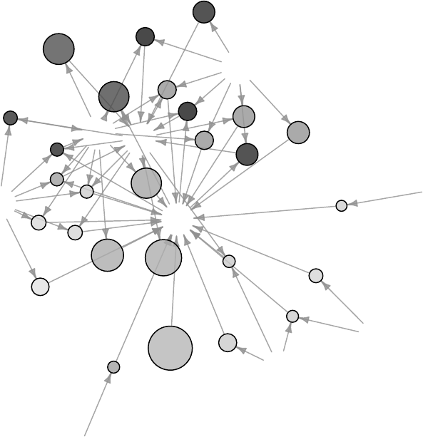
9.6. VISUALIZING ASSOCIATION RULES 95
> plot(rules.all, method="graph", control=list(type="items"))
Graph for 27 rules
Class=1st
Class=2nd
Class=3rd
Class=Crew
Sex=Female
Sex=Male
Age=Adult
Survived=No
Survived=Yes
size: support (0.119 − 0.95)
color: lift (0.934 − 1.266)
Figure 9.4: A Graph of Items
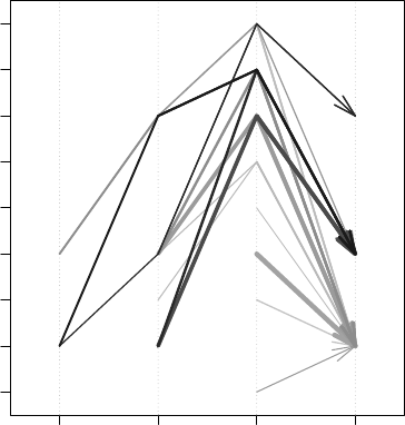
96 CHAPTER 9. ASSOCIATION RULES
> plot(rules.all, method="paracoord", control=list(reorder=TRUE))
Parallel coordinates plot for 27 rules
3 2 1 rhs
Class=Crew
Class=1st
Sex=Female
Sex=Male
Class=2nd
Survived=Yes
Class=3rd
Survived=No
Age=Adult
Position
Figure 9.5: A Parallel Coordinates Plot of Association Rules
9.7 Discussions and Further Readings
In this chapter, we have demonstrated association rule mining with package arules [Hahsler et al.,
2011]. More examples on that package can be found in Hahsler et al.’s work [Hahsler et al., 2005].
Two other packages related to association rules are arulesSequences and arulesNBMiner. Package
arulesSequences provides functions for mining sequential patterns [Buchta et al., 2012]. Package
arulesNBMiner implements an algorithm for mining negative binomial (NB) frequent itemsets and
NB-precise rules [Hahsler, 2012].
More techniques on post mining of association rules, such as selecting interesting association
rules, visualization of association rules and using association rules for classification, can be found
in Zhao et al’s work [Zhao et al., 2009b].

Chapter 10
Text Mining
This chapter presents examples of text mining with R. Twitter1text of @RDataMining is used
as the data to analyze. It starts with extracting text from Twitter. The extracted text is then
transformed to build a document-term matrix. After that, frequent words and associations are
found from the matrix. A word cloud is used to present important words in documents. In the
end, words and tweets are clustered to find groups of words and also groups of tweets. In this
chapter, “tweet” and “document” will be used interchangeably, so are “word” and “term”.
There are three important packages used in the examples: twitteR,tm and wordcloud. Package
twitteR [Gentry, 2012] provides access to Twitter data, tm [Feinerer, 2012] provides functions for
text mining, and wordcloud [Fellows, 2012] visualizes the result with a word cloud 2.
10.1 Retrieving Text from Twitter
Twitter text is used in this chapter to demonstrate text mining. Tweets are extracted from Twitter
with the code below using userTimeline() in package twitteR [Gentry, 2012]. Package twitteR
depends on package RCurl [Lang, 2012a], which is available at http://www.stats.ox.ac.uk/
pub/RWin/bin/windows/contrib/. Another way to retrieve text from Twitter is using package
XML [Lang, 2012b], and an example on that is given at http://heuristically.wordpress.com/
2011/04/08/text-data-mining-twitter-r/.
For readers who have no access to Twitter, the tweets data “rdmTweets.RData” can be down-
loaded at http://www.rdatamining.com/data. Then readers can skip this section and proceed
directly to Section 10.2.
Note that the Twitter API requires authentication since March 2013. Before running the code
below, please complete authentication by following instructions in “Section 3: Authentication
with OAuth” in the twitteR vignettes (http://cran.r-project.org/web/packages/twitteR/
vignettes/twitteR.pdf).
> library(twitteR)
> # retrieve the first 200 tweets (or all tweets if fewer than 200) from the
> # user timeline of @rdatammining
> rdmTweets <- userTimeline("rdatamining", n=200)
> (nDocs <- length(rdmTweets))
[1] 154
Next, we have a look at the five tweets numbered 11 to 15.
> rdmTweets[11:15]
1http://www.twitter.com
2http://en.wikipedia.org/wiki/Word_cloud
97

98 CHAPTER 10. TEXT MINING
With the above code, each tweet is printed in one single line, which may exceed the boundary
of paper. Therefore, the following code is used in this book to print the five tweets by wrapping
the text to fit the width of paper. The same method is used to print tweets in other codes in this
chapter.
> for (i in 11:15) {
+ cat(paste("[[", i, "]] ", sep=""))
+ writeLines(strwrap(rdmTweets[[i]]$getText(), width=73))
+ }
[[11]] Slides on massive data, shared and distributed memory,and concurrent
programming: bigmemory and foreach http://t.co/a6bQzxj5
[[12]] The R Reference Card for Data Mining is updated with functions &
packages for handling big data & parallel computing.
http://t.co/FHoVZCyk
[[13]] Post-doc on Optimizing a Cloud for Data Mining primitives, INRIA, France
http://t.co/cA28STPO
[[14]] Chief Scientist - Data Intensive Analytics, Pacific Northwest National
Laboratory (PNNL), US http://t.co/0Gdzq1Nt
[[15]] Top 10 in Data Mining http://t.co/7kAuNvuf
10.2 Transforming Text
The tweets are first converted to a data frame and then to a corpus, which is a collection of
text documents. After that, the corpus can be processed with functions provided in package
tm [Feinerer, 2012].
> # convert tweets to a data frame
> df <- do.call("rbind", lapply(rdmTweets, as.data.frame))
> dim(df)
[1] 154 10
> library(tm)
> # build a corpus, and specify the source to be character vectors
> myCorpus <- Corpus(VectorSource(df$text))
After that, the corpus needs a couple of transformations, including changing letters to lower
case, and removing punctuations, numbers and stop words. The general English stop-word list is
tailored here by adding “available” and “via” and removing “r” and “big” (for big data). Hyperlinks
are also removed in the example below.
> # convert to lower case
> myCorpus <- tm_map(myCorpus, tolower)
> # remove punctuation
> myCorpus <- tm_map(myCorpus, removePunctuation)
> # remove numbers
> myCorpus <- tm_map(myCorpus, removeNumbers)
> # remove URLs
> removeURL <- function(x) gsub("http[[:alnum:]]*", "", x)
> myCorpus <- tm_map(myCorpus, removeURL)
> # add two extra stop words: "available" and "via"
> myStopwords <- c(stopwords( english ), "available", "via")
> # remove "r" and "big" from stopwords
> myStopwords <- setdiff(myStopwords, c("r", "big"))
> # remove stopwords from corpus
> myCorpus <- tm_map(myCorpus, removeWords, myStopwords)
10.3. STEMMING WORDS 99
In the above code, tm_map() is an interface to apply transformations (mappings) to corpora. A
list of available transformations can be obtained with getTransformations(), and the mostly used
ones are as.PlainTextDocument(),removeNumbers(),removePunctuation(),removeWords(),
stemDocument() and stripWhitespace(). A function removeURL() is defined above to remove
hypelinks, where pattern "http[[:alnum:]]*" matches strings starting with “http” and then
followed by any number of alphabetic characters and digits. Strings matching this pattern are
removed with gsub(). The above pattern is specified as an regular expression, and detail about
that can be found by running ?regex in R.
10.3 Stemming Words
In many applications, words need to be stemmed to retrieve their radicals, so that various forms
derived from a stem would be taken as the same when counting word frequency. For instance,
words “update”, “updated” and “updating” would all be stemmed to “updat”. Word stemming
can be done with the snowball stemmer, which requires packages Snowball,RWeka,rJava and
RWekajars. After that, we can complete the stems to their original forms, i.e., “update” for
the above example, so that the words would look normal. This can be achieved with function
stemCompletion().
> # keep a copy of corpus to use later as a dictionary for stem completion
> myCorpusCopy <- myCorpus
> # stem words
> myCorpus <- tm_map(myCorpus, stemDocument)
> # inspect documents (tweets) numbered 11 to 15
> # inspect(myCorpus[11:15])
> # The code below is used for to make text fit for paper width
> for (i in 11:15) {
+ cat(paste("[[", i, "]] ", sep=""))
+ writeLines(strwrap(myCorpus[[i]], width=73))
+ }
[[11]] slide massiv data share distribut memoryand concurr program bigmemori
foreach
[[12]] r refer card data mine updat function packag handl big data parallel
comput
[[13]] postdoc optim cloud data mine primit inria franc
[[14]] chief scientist data intens analyt pacif northwest nation laboratori
pnnl
[[15]] top data mine
After that, we use stemCompletion() to complete the stems with the unstemmed corpus
myCorpusCopy as a dictionary. With the default setting, it takes the most frequent match in
dictionary as completion.
> # stem completion
> myCorpus <- tm_map(myCorpus, stemCompletion, dictionary=myCorpusCopy)
Then we have a look at the documents numbered 11 to 15 in the built corpus.
> inspect(myCorpus[11:15])
[[11]] slides massive data share distributed memoryand concurrent programming
foreach
[[12]] r reference card data miners updated functions package handling big data
parallel computing
100 CHAPTER 10. TEXT MINING
[[13]] postdoctoral optimizing cloud data miners primitives inria france
[[14]] chief scientist data intensive analytics pacific northwest national pnnl
[[15]] top data miners
As we can see from the above results, there are something unexpected in the above stemming
and completion.
1. In both the stemmed corpus and the completed one, “memoryand” is derived from “... mem-
ory,and ...” in the original tweet 11.
2. In tweet 11, word “bigmemory” is stemmed to “bigmemori”, and then is removed during stem
completion.
3. Word “mining” in tweets 12, 13 & 15 is first stemmed to “mine” and then completed to
“miners”.
4. “Laboratory” in tweet 14 is stemmed to “laboratori” and then also disappears after comple-
tion.
In the above issues, point 1 is caused by the missing of a space after the comma. It can be
easily fixed by replacing comma with space before removing punctuation marks in Section 10.2.
For points 2 & 4, we haven’t figured out why it happened like that. Fortunately, the words involved
in points 1, 2 & 4 are not important in @RDataMining tweets and ignoring them would not bring
any harm to this demonstration of text mining.
Below we focus on point 3, where word “mining” is first stemmed to “mine” and then completed
to “miners”, instead of “mining”, although there are many instances of “mining” in the tweets,
compared to only two instances of “miners”. There might be a solution for the above problem by
changing the parameters and/or dictionaries for stemming and completion, but we failed to find
one due to limitation of time and efforts. Instead, we chose a simple way to get around of that
by replacing “miners” with “mining”, since the latter has many more cases than the former in the
corpus. The code for the replacement is given below.
> # count frequency of "mining"
> miningCases <- tm_map(myCorpusCopy, grep, pattern="\\<mining")
> sum(unlist(miningCases))
[1] 47
> # count frequency of "miners"
> minerCases <- tm_map(myCorpusCopy, grep, pattern="\\<miners")
> sum(unlist(minerCases))
[1] 2
> # replace "miners" with "mining"
> myCorpus <- tm_map(myCorpus, gsub, pattern="miners", replacement="mining")
In the first call of function tm_map() in the above code, grep() is applied to every document
(tweet) with argument “pattern="\\<mining"”. The pattern matches words starting with “min-
ing”, where “\<” matches the empty string at the beginning of a word. This ensures that text
“rdatamining” would not contribute to the above counting of “mining”.
10.4 Building a Term-Document Matrix
A term-document matrix represents the relationship between terms and documents, where each
row stands for a term and each column for a document, and an entry is the number of occurrences of
10.5. FREQUENT TERMS AND ASSOCIATIONS 101
the term in the document. Alternatively, one can also build a document-term matrix by swapping
row and column. In this section, we build a term-document matrix from the above processed
corpus with function TermDocumentMatrix(). With its default setting, terms with less than three
characters are discarded. To keep “r” in the matrix, we set the range of wordLengths in the
example below.
> myTdm <- TermDocumentMatrix(myCorpus, control=list(wordLengths=c(1,Inf)))
> myTdm
A term-document matrix (444 terms, 154 documents)
Non-/sparse entries: 1085/67291
Sparsity : 98%
Maximal term length: 27
Weighting : term frequency (tf)
As we can see from the above result, the term-document matrix is composed of 444 terms and
154 documents. It is very sparse, with 98% of the entries being zero. We then have a look at the
first six terms starting with “r” and tweets numbered 101 to 110.
> idx <- which(dimnames(myTdm)$Terms == "r")
> inspect(myTdm[idx+(0:5),101:110])
A term-document matrix (6 terms, 10 documents)
Non-/sparse entries: 9/51
Sparsity : 85%
Maximal term length: 12
Weighting : term frequency (tf)
Docs
Terms 101 102 103 104 105 106 107 108 109 110
r 1100200111
ramachandran 0 0 0 0 0 0 0 0 0 0
random 0000000000
ranked 0000000010
rapidminer 1 0 0 0 0 0 0 0 0 0
rdatamining 0 0 0 0 0 0 0 1 0 0
Note that the parameter to control word length used to be minWordLength prior to version
0.5-7 of package tm. The code to set the minimum word length for old versions of tm is below.
> myTdm <- TermDocumentMatrix(myCorpus, control=list(minWordLength=1))
The list of terms can be retrieved with rownames(myTdm). Based on the above matrix, many
data mining tasks can be done, for example, clustering, classification and association analysis.
When there are too many terms, the size of a term-document matrix can be reduced by
selecting terms that appear in a minimum number of documents, or filtering terms with TF-IDF
(term frequency-inverse document frequency) [Wu et al., 2008].
10.5 Frequent Terms and Associations
We have a look at the popular words and the association between words. Note that there are 154
tweets in total.
> # inspect frequent words
> findFreqTerms(myTdm, lowfreq=10)
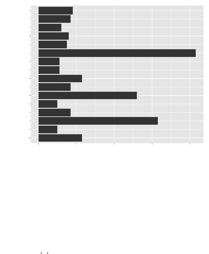
102 CHAPTER 10. TEXT MINING
[1] "analysis" "computing" "data" "examples" "introduction"
[6] "mining" "network" "package" "positions" "postdoctoral"
[11] "r" "research" "slides" "social" "tutorial"
[16] "users"
In the code above, findFreqTerms() finds frequent terms with frequency no less than ten.
Note that they are ordered alphabetically, instead of by frequency or popularity.
To show the top frequent words visually, we next make a barplot for them. From the term-
document matrix, we can derive the frequency of terms with rowSums(). Then we select terms that
appears in ten or more documents and shown them with a barplot using package ggplot2 [Wickham,
2009]. In the code below, geom="bar" specifies a barplot and coord_flip() swaps x- and y-axis.
The barplot in Figure 10.1 clearly shows that the three most frequent words are “r”, “data” and
“mining”.
> termFrequency <- rowSums(as.matrix(myTdm))
> termFrequency <- subset(termFrequency, termFrequency>=10)
> library(ggplot2)
> qplot(names(termFrequency), termFrequency, geom="bar", xlab="Terms") + coord_flip()
analysis
computing
data
examples
introduction
mining
network
package
positions
postdoctoral
r
research
slides
social
tutorial
users
0 20 40 60 80
termFrequency
Terms
Figure 10.1: Frequent Terms
Alternatively, the above plot can also be drawn with barplot() as below, where las sets the
direction of x-axis labels to be vertical.
> barplot(termFrequency, las=2)
We can also find what are highly associated with a word with function findAssocs(). Below
we try to find terms associated with “r” (or “mining”) with correlation no less than 0.25, and the
words are ordered by their correlation with “r” (or “mining”).
> # which words are associated with "r"?
> findAssocs(myTdm, r , 0.25)

10.6. WORD CLOUD 103
users canberra cran list examples
0.32 0.26 0.26 0.26 0.25
> # which words are associated with "mining"?
> findAssocs(myTdm, mining , 0.25)
data mahout recommendation sets supports
0.55 0.39 0.39 0.39 0.39
frequent itemset card functions reference
0.35 0.34 0.29 0.29 0.29
text
0.26
10.6 Word Cloud
After building a term-document matrix, we can show the importance of words with a word cloud
(also known as a tag cloud), which can be easily produced with package wordcloud [Fellows,
2012]. In the code below, we first convert the term-document matrix to a normal matrix, and
then calculate word frequencies. After that, we set gray levels based on word frequency and use
wordcloud() to make a plot for it. With wordcloud(), the first two parameters give a list of
words and their frequencies. Words with frequency below three are not plotted, as specified by
min.freq=3. By setting random.order=F, frequent words are plotted first, which makes them
appear in the center of cloud. We also set the colors to gray levels based on frequency. A colorful
cloud can be generated by setting colors with rainbow().
> library(wordcloud)
> m <- as.matrix(myTdm)
> # calculate the frequency of words and sort it descendingly by frequency
> wordFreq <- sort(rowSums(m), decreasing=TRUE)
> # word cloud
> set.seed(375) # to make it reproducible
> grayLevels <- gray( (wordFreq+10) / (max(wordFreq)+10) )
> wordcloud(words=names(wordFreq), freq=wordFreq, min.freq=3, random.order=F,
+ colors=grayLevels)
104 CHAPTER 10. TEXT MINING
r
data
mining
analysis
package
users
examples network
tutorial
slides
research
social
positionspostdoctoral
computing
introduction
applications
code
clustering
parallel
series
time
graphics
pdf
statistics
talk
text
free
learn
advanced
australia
card
detection
functions
information
lecture
modelling
rdatamining
reference
scientist
spatial
techniques
tools
university
analyst
book
classification
datasets
distributed
experience
fast
frequent
job
join
outlier
performance
programming
snowfall
tried
twitter
vacancy
website
wwwrdataminingcom
access
analytics
answers
association
big
charts
china
comments
databases
details
documents
followed
itemset
melbourne
notes
poll
presentations
processing
published
recent short
technology
views visits
visualizing
Figure 10.2: Word Cloud
The above word cloud clearly shows again that “r”, “data” and “mining” are the top three
words, which validates that the @RDataMining tweets present information on R and data mining.
Some other important words are “analysis”, “examples”, “slides”, “tutorial” and “package”, which
shows that it focuses on documents and examples on analysis and R packages. Another set of
frequent words, “research”, “postdoctoral” and “positions”, are from tweets about vacancies on
post-doctoral and research positions. There are also some tweets on the topic of social network
analysis, as indicated by words “network” and “social” in the cloud.
10.7 Clustering Words
We then try to find clusters of words with hierarchical clustering. Sparse terms are removed, so
that the plot of clustering will not be crowded with words. Then the distances between terms are
calculated with dist() after scaling. After that, the terms are clustered with hclust() and the
dendrogram is cut into 10 clusters. The agglomeration method is set to ward, which denotes the
increase in variance when two clusters are merged. Some other options are single linkage, complete
linkage, average linkage, median and centroid. Details about different agglomeration methods can
be found in data mining textbooks [Han and Kamber, 2000, Hand et al., 2001, Witten and Frank,
2005].
> # remove sparse terms
> myTdm2 <- removeSparseTerms(myTdm, sparse=0.95)
> m2 <- as.matrix(myTdm2)
> # cluster terms
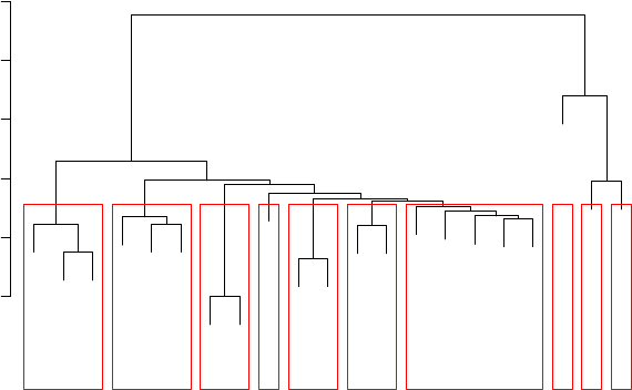
10.8. CLUSTERING TWEETS 105
> distMatrix <- dist(scale(m2))
> fit <- hclust(distMatrix, method="ward")
> plot(fit)
> # cut tree into 10 clusters
> rect.hclust(fit, k=10)
> (groups <- cutree(fit, k=10))
analysis applications code computing data examples
123453
introduction mining network package parallel positions
261748
postdoctoral r research series slides social
8981021
time tutorial users
10 2 2
analysis
network
social
positions
postdoctoral
research
series
time
package
computing
parallel
code
examples
tutorial
slides
applications
introduction
users
r
data
mining
0 10 20 30 40 50
Cluster Dendrogram
hclust (*, "ward")
distMatrix
Height
Figure 10.3: Clustering of Words
In the above dendrogram, we can see the topics in the tweets. Words “analysis”, “network”
and “social” are clustered into one group, because there are a couple of tweets on social network
analysis. The second cluster from left comprises “positions”, “postdoctoral” and “research”, and
they are clustered into one group because of tweets on vacancies of research and postdoctoral
positions. We can also see cluster on time series, R packages, parallel computing, R codes and
examples, and tutorial and slides. The rightmost three clusters consists of“r”, “data” and“mining”,
which are the keywords of @RDataMining tweets.
10.8 Clustering Tweets
Tweets are clustered below with the k-means and the k-medoids algorithms.
106 CHAPTER 10. TEXT MINING
10.8.1 Clustering Tweets with the k-means Algorithm
We first try k-means clustering, which takes the values in the matrix as numeric. We transpose
the term-document matrix to a document-term one. The tweets are then clustered with kmeans()
with the number of clusters set to eight. After that, we check the popular words in every cluster
and also the cluster centers. Note that a fixed random seed is set with set.seed() before running
kmeans(), so that the clustering result can be reproduced. It is for the convenience of book writing,
and it is unnecessary for readers to set a random seed in their code.
> # transpose the matrix to cluster documents (tweets)
> m3 <- t(m2)
> # set a fixed random seed
> set.seed(122)
> # k-means clustering of tweets
>k<-8
> kmeansResult <- kmeans(m3, k)
> # cluster centers
> round(kmeansResult$centers, digits=3)
analysis applications code computing data examples introduction mining network
1 0.040 0.040 0.240 0.000 0.040 0.320 0.040 0.120 0.080
2 0.000 0.158 0.053 0.053 1.526 0.105 0.053 1.158 0.000
3 0.857 0.000 0.000 0.000 0.000 0.071 0.143 0.071 1.000
4 0.000 0.000 0.000 1.000 0.000 0.000 0.000 0.000 0.000
5 0.037 0.074 0.019 0.019 0.426 0.037 0.093 0.407 0.000
6 0.000 0.000 0.000 0.000 0.000 0.100 0.000 0.000 0.000
7 0.533 0.000 0.067 0.000 0.333 0.200 0.067 0.200 0.067
8 0.000 0.111 0.000 0.000 0.556 0.000 0.000 0.111 0.000
package parallel positions postdoctoral r research series slides social
1 0.080 0.000 0.000 0.000 1.320 0.000 0.040 0.000 0.000
2 0.368 0.053 0.000 0.000 0.947 0.053 0.000 0.053 0.000
3 0.071 0.000 0.143 0.143 0.214 0.071 0.000 0.071 0.786
4 0.125 0.750 0.000 0.000 1.000 0.000 0.000 0.125 0.000
5 0.000 0.000 0.093 0.093 0.000 0.000 0.019 0.074 0.000
6 1.200 0.100 0.000 0.000 0.600 0.100 0.000 0.100 0.000
7 0.000 0.000 0.000 0.000 1.000 0.000 0.400 0.533 0.000
8 0.000 0.000 0.444 0.444 0.000 1.333 0.000 0.000 0.111
time tutorial users
1 0.040 0.200 0.160
2 0.000 0.000 0.158
3 0.000 0.286 0.071
4 0.000 0.125 0.250
5 0.019 0.111 0.019
6 0.000 0.100 0.100
7 0.400 0.000 0.400
8 0.000 0.000 0.000
To make it easy to find what the clusters are about, we then check the top three words in every
cluster.
> for (i in 1:k) {
+ cat(paste("cluster ", i, ": ", sep=""))
+ s <- sort(kmeansResult$centers[i,], decreasing=T)
+ cat(names(s)[1:3], "\n")
+ # print the tweets of every cluster
10.8. CLUSTERING TWEETS 107
+ # print(rdmTweets[which(kmeansResult$cluster==i)])
+ }
cluster 1: r examples code
cluster 2: data mining r
cluster 3: network analysis social
cluster 4: computing r parallel
cluster 5: data mining tutorial
cluster 6: package r examples
cluster 7: r analysis slides
cluster 8: research data positions
From the above top words and centers of clusters, we can see that the clusters are of different
topics. For instance, cluster 1 focuses on R codes and examples, cluster 2 on data mining with
R, cluster 4 on parallel computing in R, cluster 6 on R packages and cluster 7 on slides of time
series analysis with R. We can also see that, all clusters, except for cluster 3, 5 & 8, focus on R.
Cluster 3, 5 & 8 are about general information on data mining and are not limited to R. Cluster
3 is on social network analysis, cluster 5 on data mining tutorials, and cluster 8 on positions for
data mining research.
10.8.2 Clustering Tweets with the k-medoids Algorithm
We then try k-medoids clustering with the Partitioning Around Medoids (PAM) algorithm, which
uses medoids (representative objects) instead of means to represent clusters. It is more robust to
noise and outliers than k-means clustering, and provides a display of the silhouette plot to show
the quality of clustering. In the example below, we use function pamk() from package fpc [Hennig,
2010], which calls the function pam() with the number of clusters estimated by optimum average
silhouette.
> library(fpc)
> # partitioning around medoids with estimation of number of clusters
> pamResult <- pamk(m3, metric="manhattan")
> # number of clusters identified
> (k <- pamResult$nc)
[1] 9
> pamResult <- pamResult$pamobject
> # print cluster medoids
> for (i in 1:k) {
+ cat(paste("cluster", i, ": "))
+ cat(colnames(pamResult$medoids)[which(pamResult$medoids[i,]==1)], "\n")
+ # print tweets in cluster i
+ # print(rdmTweets[pamResult$clustering==i])
+ }
cluster 1 : data positions research
cluster 2 : computing parallel r
cluster 3 : mining package r
cluster 4 : data mining
cluster 5 : analysis network social tutorial
cluster 6 : r
cluster 7 :
cluster 8 : examples r
cluster 9 : analysis mining series time users
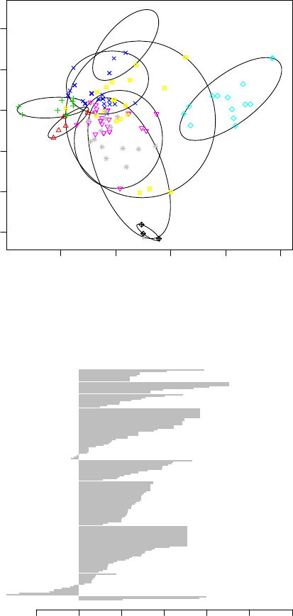
108 CHAPTER 10. TEXT MINING
> # plot clustering result
> layout(matrix(c(1,2),2,1)) # set to two graphs per page
> plot(pamResult, color=F, labels=4, lines=0, cex=.8, col.clus=1,
+ col.p=pamResult$clustering)
> layout(matrix(1)) # change back to one graph per page
−2 0 2 4 6
−6 −4 −2 0 2 4
clusplot(pam(x = sdata, k = k, diss = diss, metric = "manhattan"))
Component 1
Component 2
These two components explain 24.81 % of the point variability.
●
●
●
●
●
●
●
●
1
2
3
45
6
7
8
9
Silhouette width si
−0.2 0.0 0.2 0.4 0.6 0.8 1.0
Silhouette plot of pam(x = sdata, k = k, diss = diss, metric = "manhattan")
Average silhouette width : 0.29
n = 154 9 clusters Cj
j : nj | avei∈Cj si
1 : 8 | 0.32
2 : 8 | 0.54
3 : 9 | 0.26
4 : 35 | 0.29
5 : 14 | 0.32
6 : 30 | 0.26
7 : 32 | 0.35
8 : 15 | −0.03
9 : 3 | 0.46
Figure 10.4: Clusters of Tweets
In Figure 10.4, the first chart is a 2D “clusplot” (clustering plot) of the k clusters, and the
second one shows their silhouettes. With the silhouette, a large si(almost 1) suggests that

10.9. PACKAGES, FURTHER READINGS AND DISCUSSIONS 109
the corresponding observations are very well clustered, a small si(around 0) means that the
observation lies between two clusters, and observations with a negative siare probably placed in
the wrong cluster. The average silhouette width is 0.29, which suggests that the clusters are not
well separated from one another.
The above results and Figure 10.4 show that there are nine clusters of tweets. Clusters 1, 2,
3, 5 and 9 are well separated groups, with each of them focusing on a specific topic. Cluster 7
is composed of tweets not fitted well into other clusters, and it overlaps all other clusters. There
is also a big overlap between cluster 6 and 8, which is understandable from their medoids. Some
observations in cluster 8 are of negative silhouette width, which means that they may fit better in
other clusters than cluster 8.
To improve the clustering quality, we have also tried to set the range of cluster numbers
krange=2:8 when calling pamk(), and in the new clustering result, there are eight clusters, with
the observations in the above cluster 8 assigned to other clusters, mostly to cluster 6. The results
are not shown in this book, and readers can try it with the code below.
> pamResult2 <- pamk(m3, krange=2:8, metric="manhattan")
10.9 Packages, Further Readings and Discussions
In addition to frequent terms, associations and clustering demonstrated in this chapter, some
other possible analysis on the above Twitter text is graph mining and social network analysis. For
example, a graph of words can be derived from a document-term matrix, and then we can use
techniques for graph mining to find links between words and groups of words. A graph of tweets
(documents) can also be generated and analyzed in a similar way. It can also be presented and
analyzed as a bipartite graph with two disjoint sets of vertices, that is, words and tweets. We will
demonstrate social network analysis on the Twitter data in Chapter 11: Social Network Analysis.
Some R packages for text mining are listed below.
Package tm [Feinerer, 2012]: A framework for text mining applications within R.
Package tm.plugin.mail [Feinerer, 2010]: Text Mining E-Mail Plug-In. A plug-in for the tm
text mining framework providing mail handling functionality.
package textcat [Hornik et al., 2012] provides n-Gram Based Text Categorization.
lda [Chang, 2011] fit topic models with LDA (latent Dirichlet allocation)
topicmodels [Gr¨
un and Hornik, 2011] fit topic models with LDA and CTM (correlated topics
model)
For more information and examples on text mining with R, some online resources are:
Introduction to the tm Package – Text Mining in R
http://cran.r-project.org/web/packages/tm/vignettes/tm.pdf
Text Mining Infrastructure in R [Feinerer et al., 2008]
http://www.jstatsoft.org/v25/i05
Text Mining Handbook
http://www.casact.org/pubs/forum/10spforum/Francis_Flynn.pdf
Distributed Text Mining in R
http://epub.wu.ac.at/3034/
Text mining with Twitter and R
http://heuristically.wordpress.com/2011/04/08/text-data-mining-twitter-r/
110 CHAPTER 10. TEXT MINING

Chapter 11
Social Network Analysis
This chapter presents examples of social network analysis with R, specifically, with package igraph
[Csardi and Nepusz, 2006]. The data to analyze is Twitter text data used in Chapter 10 Text
Mining. Putting it in a general scenario of social networks, the terms can be taken as people and
the tweets as groups on LinkedIn1, and the term-document matrix can then be taken as the group
membership of people.
In this chapter, we first build a network of terms based on their co-occurrence in the same
tweets, and then build a network of tweets based on the terms shared by them. At last, we
build a two-mode network composed of both terms and tweets. We also demonstrate some tricks
to plot nice network graphs. Some codes in this chapter are based on the examples at http:
//www.stanford.edu/~messing/Affiliation%20Data.html.
11.1 Network of Terms
In this section, we will build a network of terms based on their co-occurrence in tweets. At first,
a term-document matrix, termDocMatrix, is loaded into R, which is actually a copy of m2, an R
object from Chapter 10 Text Mining (see page 105). After that, it is transformed into a term-term
adjacency matrix, based on which a graph is built. Then we plot the graph to show the relationship
between frequent terms, and also make the graph more readable by setting colors, font sizes and
transparency of vertices and edges.
> # load termDocMatrix
> load("./data/termDocMatrix.rdata")
> # inspect part of the matrix
> termDocMatrix[5:10,1:20]
Docs
Terms 1234567891011121314151617181920
data 1 1 0 0 2 0 0 0 0 0 1 2 1 1 1 0 1 0 0 0
examples 0 0 0 0 0 0 0 0 0 0 0 0 0 0 0 0 0 0 0 0
introduction 0 0 0 0 0 0 0 0 0 0 0 0 0 0 0 0 0 0 0 1
mining 0 0 0 0 0 0 0 0 0 0 0 1 1 0 1 0 0 0 0 0
network 0 0 0 0 0 0 0 0 0 0 0 0 0 0 0 1 0 1 1 1
package 0 0 0 1 1 0 0 0 0 0 0 1 0 0 0 0 0 0 0 0
> # change it to a Boolean matrix
> termDocMatrix[termDocMatrix>=1] <- 1
> # transform into a term-term adjacency matrix
> termMatrix <- termDocMatrix %*% t(termDocMatrix)
1http://www.linkedin.com
111
112 CHAPTER 11. SOCIAL NETWORK ANALYSIS
> # inspect terms numbered 5 to 10
> termMatrix[5:10,5:10]
Terms
Terms data examples introduction mining network package
data 53 5 2 34 0 7
examples 5 17 2 5 2 2
introduction 2 2 10 2 2 0
mining 34 5 2 47 1 5
network 0 2 2 1 17 1
package 7 2 0 5 1 21
In the above code, %*% is an operator for the product of two matrices, and t() transposes a
matrix. Now we have built a term-term adjacency matrix, where the rows and columns represent
terms, and every entry is the number of concurrences of two terms. Next we can build a graph
with graph.adjacency() from package igraph.
> library(igraph)
> # build a graph from the above matrix
> g <- graph.adjacency(termMatrix, weighted=T, mode="undirected")
> # remove loops
> g <- simplify(g)
> # set labels and degrees of vertices
> V(g)$label <- V(g)$name
> V(g)$degree <- degree(g)
After that, we plot the network with layout.fruchterman.reingold (see Figure 11.1).
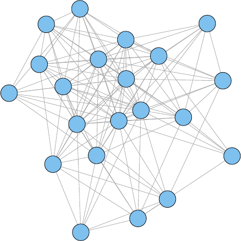
11.1. NETWORK OF TERMS 113
> # set seed to make the layout reproducible
> set.seed(3952)
> layout1 <- layout.fruchterman.reingold(g)
> plot(g, layout=layout1)
analysis
applications
code
computing
data
examples
introduction
mining
network
package
parallel
positions
postdoctoral
r
research
series
slides
social
time
tutorial users
Figure 11.1: A Network of Terms - I
In the above code, the layout is kept as layout1, so that we can plot the graph in the same
layout later.
A different layout can be generated with the first line of code below. The second line produces
an interactive plot, which allows us to manually rearrange the layout. Details about other layout
options can be obtained by running ?igraph::layout in R.
> plot(g, layout=layout.kamada.kawai)
> tkplot(g, layout=layout.kamada.kawai)
We can also save the network graph into a .PDF file with the code below.
> pdf("term-network.pdf")
> plot(g, layout=layout.fruchterman.reingold)
> dev.off()
Next, we set the label size of vertices based on their degrees, to make important terms stand
out. Similarly, we also set the width and transparency of edges based on their weights. This is
useful in applications where graphs are crowded with many vertices and edges. In the code below,
the vertices and edges are accessed with V() and E(). Function rgb(red, green, blue, alpha)
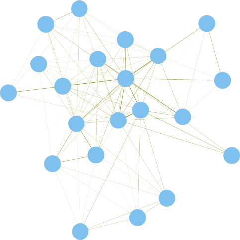
114 CHAPTER 11. SOCIAL NETWORK ANALYSIS
defines a color, with an alpha transparency. With the same layout as Figure 11.1, we plot the
graph again (see Figure 11.2).
> V(g)$label.cex <- 2.2 * V(g)$degree / max(V(g)$degree)+ .2
> V(g)$label.color <- rgb(0, 0, .2, .8)
> V(g)$frame.color <- NA
> egam <- (log(E(g)$weight)+.4) / max(log(E(g)$weight)+.4)
> E(g)$color <- rgb(.5, .5, 0, egam)
> E(g)$width <- egam
> # plot the graph in layout1
> plot(g, layout=layout1)
analysis
applications
code
computing
data
examples
introduction
mining
network
package
parallel
positions
postdoctoral
r
research
series
slides
social
time
tutorial users
Figure 11.2: A Network of Terms - II
11.2 Network of Tweets
Similar to the previous section, we can also build a graph of tweets base on the number of terms
that they have in common. Because most tweets contain one or more words from “r”, “data” and
“mining”, most tweets are connected with others and the graph of tweets is very crowded. To
simplify the graph and find relationship between tweets beyond the above three keywords, we
remove the three words before building a graph.
> # remove "r", "data" and "mining"
> idx <- which(dimnames(termDocMatrix)$Terms %in% c("r", "data", "mining"))
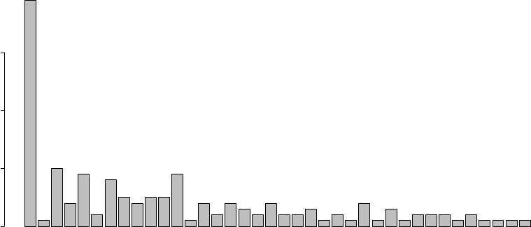
11.2. NETWORK OF TWEETS 115
> M <- termDocMatrix[-idx,]
> # build a tweet-tweet adjacency matrix
> tweetMatrix <- t(M) %*% M
> library(igraph)
> g <- graph.adjacency(tweetMatrix, weighted=T, mode = "undirected")
> V(g)$degree <- degree(g)
> g <- simplify(g)
> # set labels of vertices to tweet IDs
> V(g)$label <- V(g)$name
> V(g)$label.cex <- 1
> V(g)$label.color <- rgb(.4, 0, 0, .7)
> V(g)$size <- 2
> V(g)$frame.color <- NA
Next, we have a look at the distribution of degree of vertices and the result is shown in
Figure 11.3. We can see that there are around 40 isolated vertices (with a degree of zero). Note
that most of them are caused by the removal of the three keywords, “r”, “data” and “mining”.
> barplot(table(V(g)$degree))
0 9 10 11 12 13 17 18 19 20 21 22 23 24 25 27 28 29 30 31 32 33 34 35 36 37 39 40 41 42 43 44 45 50 53 55 56 71
0 10 20 30
Figure 11.3: Distribution of Degree
With the code below, we set vertex colors based on degree, and set labels of isolated vertices to
tweet IDs and the first 20 characters of every tweet. The labels of other vertices are set to tweet
IDs only, so that the graph will not be overcrowded with labels. We also set the color and width
of edges based on their weights. The produced graph is shown in Figure 11.4.
> idx <- V(g)$degree == 0
> V(g)$label.color[idx] <- rgb(0, 0, .3, .7)
> # load twitter text
> library(twitteR)
> load(file = "data/rdmTweets.RData")
> # convert tweets to a data frame
> df <- do.call("rbind", lapply(rdmTweets, as.data.frame))
> # set labels to the IDs and the first 20 characters of tweets
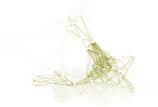
116 CHAPTER 11. SOCIAL NETWORK ANALYSIS
> V(g)$label[idx] <- paste(V(g)$name[idx], substr(df$text[idx], 1, 20), sep=": ")
> egam <- (log(E(g)$weight)+.2) / max(log(E(g)$weight)+.2)
> E(g)$color <- rgb(.5, .5, 0, egam)
> E(g)$width <- egam
> set.seed(3152)
> layout2 <- layout.fruchterman.reingold(g)
> plot(g, layout=layout2)
●
●
●
●
●
●
●●
●
●
●
●
●
●
●
●
●
●
●
●
●
●
●
●
●
●●
●
●
●
●
●
●
●
●
●
●
●
●●
●
●
●
●●
●
●
●
●
●
●
●
●
●
●
●
●
●
●
●
●
●
●
●
●
●
●
●
●
●
●
●
●
●
●●●
●
●
●
●
●
●
●
●
●
●
●
●
●
●
●
●
●
●
●
●
●
●
●
●
●
●
●
●
●
●
●
●
●
●
●
●
●
●
●
●
●
●
●
●
●
●
●
●
●
●
●
●●
●
●
●
●
●
●
●
●
●
●
●
●
●
●
●
●
●●
●
●
●
●
●
●
1
2
3
4
5
6
78
9
10
11
12
13
14: Chief Scientist − Da
15: Top 10 in Data Minin
16
17
18
19 20
21
22
23
24
25
26 27 28
29
30
31
32
33
34: Lecturer in Statisti
35
36: Several functions fo
37
38
3940
41
42
43
44 45
46
47
48: Join our discussion
49: My edited book title
50: Vacancy of Data Mini
51: Sub−domains (group &
52
53
54
55 56
57
58
59
60
61
62
63
64
65: Data Mining Job Open
66: A prize of $3,000,00
67: Statistics with R: a
68: A nice short article
69
70: Data Mining Job Open
71
72: A vacancy of Bioinfo
73 74
75 76 77
78
79
80
81: @MMiiina It is worki
82
83
84
85: OpenData + R + Googl
86: Frequent Itemset Min
87: A C++ Frequent Items
88
89
90: An overview of data
91: fastcluster: fast hi
92
93
94
95: Resources to help yo
96
97
98
99: I created group RDat
100
101
102
103
104
105
106: Mahout: mining large
107
108
109: R ranked no. 1 in a
110
111: ACM SIGKDD Innovatio
112
113: Learn R Toolkit −− Q
114
115: @emilopezcano thanks
116
117
118
119
120: Distributed Text Min
121
122
123
124
125
126
127
128
129 130
131
132: Free PDF book: Minin
133: Data Mining Lecture
134: A Complete Guide to
135: Visits to RDataMinin
136
137
138: Text Data Mining wit
139
140
141
142
143: A recent poll shows
144: What is clustering?
145
146
147: RStudio − a free IDE
148: Comments are enabled
149
150: There are more than
151: R Reference Card for
152
153
154
Figure 11.4: A Network of Tweets - I
The vertices in crescent are isolated from all others, and next we remove them from graph with
function delete.vertices() and re-plot the graph (see Figure 11.5).
> g2 <- delete.vertices(g, V(g)[degree(g)==0])
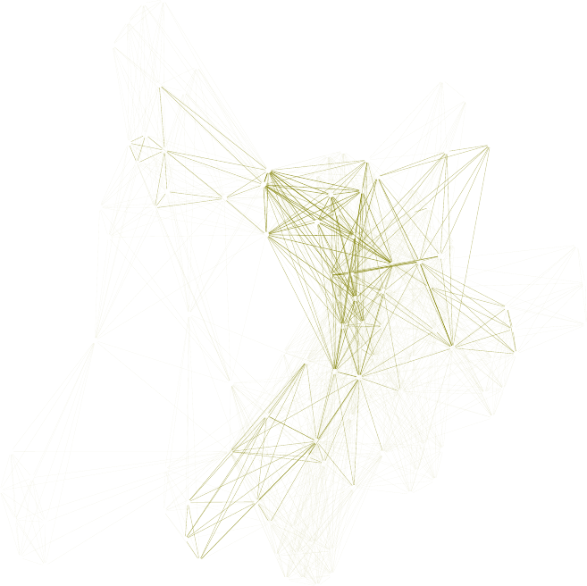
11.2. NETWORK OF TWEETS 117
> plot(g2, layout=layout.fruchterman.reingold)
●
●
●
●
●
●
●
●
●
●
●
●
●
●
●
●
●
●
●
●
●●
●
●
●
●
●
●
●
●
●
●
●
●
●
●
●
●
●
●
●
●
●
●
●
●
●
●
●
●
●
●
●
●
●
●
●
●
●
●
●
●
●
●
●
●
●
●
●
●
●
●
●
●
●
●
●
●
●
●
●
●
●
●
●
●
●
●
●
●
●
●
●
●
●
●
●
●
●
●
●
●
●
●
●
●
●
●
●
●
●
●
●
●
●
1
2
3
4
5
6
7
8
9
10
11
12
13
16
17
18
19
20
21
22
23 24
25
26
27
28
29
30
31
32
33
35
37
38
39
40
41
42
43
44
45
46
47
52
53
54
55
56
57
58
59
60
61
62
63
64
69
71
73
74
75
76
77
78
79
80
82
83
84
88
89
92
93
94
96
97
98
100
101
102
103
104
105
107
108
110
112
114
116
117
118
119
121
122
123
124
125
126
127
128
129
130
131
136
137
139
140
141
142
145
146
149
152
153
154
Figure 11.5: A Network of Tweets - II
Similarly, we can also remove edges with low degrees to simplify the graph. Below with function
delete.edges(), we remove edges which have weight of one. After removing edges, some vertices
become isolated and are also removed. The produced graph is shown in Figure 11.6.
> g3 <- delete.edges(g, E(g)[E(g)$weight <= 1])
> g3 <- delete.vertices(g3, V(g3)[degree(g3) == 0])
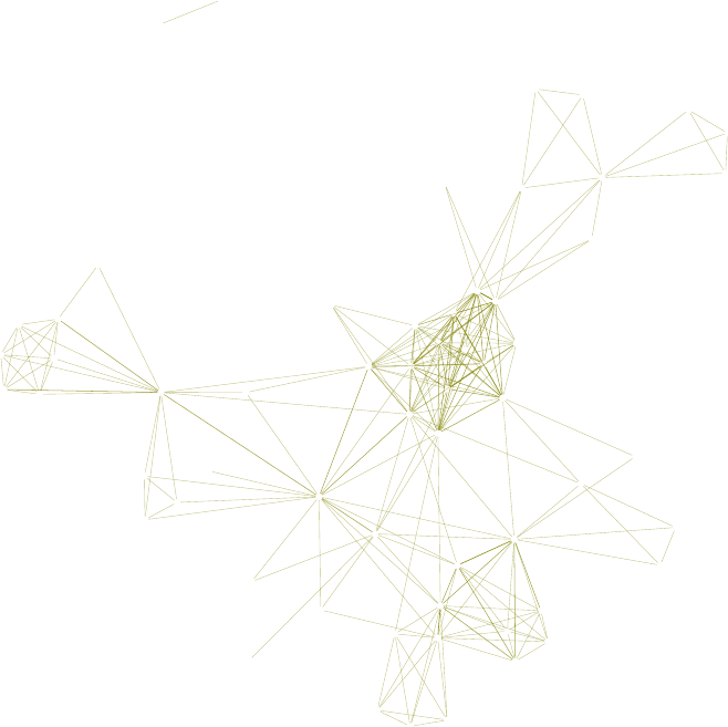
118 CHAPTER 11. SOCIAL NETWORK ANALYSIS
> plot(g3, layout=layout.fruchterman.reingold)
●
●●
●
●
●
●
●
●
●
●
●
●
●
●
●
●
●
●
●
●
●
●
●
●
●
●
●
●
●
●
●
●
●
●
●
●
●
●
●
●
●
●
●
●
●
●●
●
●
●●
●
●
●
●
●
●
●
●
2
34
5
6
7
8
9
12
16
18
19
20
21
22
23
24
26
27
29
30
31
33
37
38
44
45
52
53
58
59
60
69
71
73
79
80
92
94
96
100
101
102
105
107
108
112 114
116
119
121 122
126
127
128
129
136
139
153
154
Figure 11.6: A Network of Tweets - III
In Figure 11.6, there are some groups (or cliques) of tweets. Let’s have a look at the group in
the middle left of the figure.
> df$text[c(7,12,6,9,8,3,4)]
[7] State of the Art in Parallel Computing with R http://t.co/zmClglqi
[12] The R Reference Card for Data Mining is updated with functions & packages
for handling big data & parallel computing. http://t.co/FHoVZCyk
[6] Parallel Computing with R using snow and snowfall http://t.co/nxp8EZpv
[9] R with High Performance Computing: Parallel processing and large memory
http://t.co/XZ3ZZBRF
[8] Slides on Parallel Computing in R http://t.co/AdDVxbOY
[3] Easier Parallel Computing in R with snowfall and sfCluster

11.3. TWO-MODE NETWORK 119
http://t.co/BPcinvzK
[4] Tutorial: Parallel computing using R package snowfall http://t.co/CHBCyr76
We can see that tweets 7, 12, 6, 9, 8, 3, 4 are on parallel Computing with R. We can also see
some other groups below:
Tweets 4, 33, 94, 29, 18 and 92: tutorials for R;
Tweets 4, 5, 154 and 71: R packages;
Tweets 126, 128, 108, 136, 127, 116, 114 and 96: time series analysis;
Tweets 112, 129, 119, 105, 108 and 136: R code examples; and
Tweets 27, 24, 22,153, 79, 69, 31, 80, 21, 29, 16, 20, 18, 19 and 30: social network analysis.
Tweet 4 lies between multiple groups, because it contains keywords“parallel computing”, “tutorial”
and “package”.
11.3 Two-Mode Network
In this section, we will build a two-mode network, which is composed of two types of vertices: tweets
and terms. At first, we generate a graph gdirectly from termDocMatrix. After that, different
colors and sizes are assigned to term vertices and tweet vertices. We also set the width and color
of edges. The graph is then plotted with layout.fruchterman.reingold (see Figure 11.7).
> # create a graph
> g <- graph.incidence(termDocMatrix, mode=c("all"))
> # get index for term vertices and tweet vertices
> nTerms <- nrow(M)
> nDocs <- ncol(M)
> idx.terms <- 1:nTerms
> idx.docs <- (nTerms+1):(nTerms+nDocs)
> # set colors and sizes for vertices
> V(g)$degree <- degree(g)
> V(g)$color[idx.terms] <- rgb(0, 1, 0, .5)
> V(g)$size[idx.terms] <- 6
> V(g)$color[idx.docs] <- rgb(1, 0, 0, .4)
> V(g)$size[idx.docs] <- 4
> V(g)$frame.color <- NA
> # set vertex labels and their colors and sizes
> V(g)$label <- V(g)$name
> V(g)$label.color <- rgb(0, 0, 0, 0.5)
> V(g)$label.cex <- 1.4*V(g)$degree/max(V(g)$degree) + 1
> # set edge width and color
> E(g)$width <- .3
> E(g)$color <- rgb(.5, .5, 0, .3)
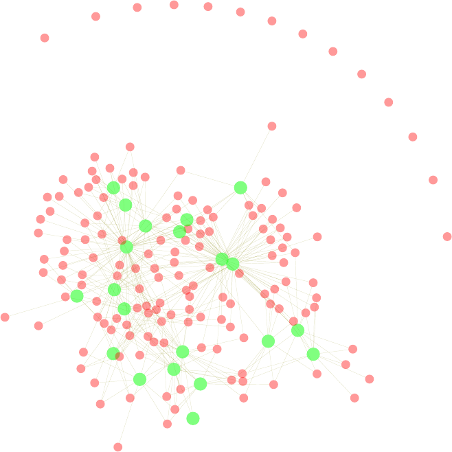
120 CHAPTER 11. SOCIAL NETWORK ANALYSIS
> set.seed(958)
> plot(g, layout=layout.fruchterman.reingold)
analysis
applications
code
computing
data
examples
introduction
mining
network
package
parallel
positions
postdoctoral
r
research
series
slides
social
time
tutorial
users
1
2
3
45
6
7
8
9
10
11
12
13
14
15
16
17
18
19
20
21
22
23
24
25
26
27
28
29
30
31
32
33
34
35
36
37
38
39
40
41
42
43
44
45
46
47
48
49
50
51
52
53
54
55
56
57
58
59
60
61
62
63
64 65
66
67
68
69
70
71
72
73
74
75
76
77
78
79
80
81
82
83
84
85
86
87
88
89
90
91
92
93
94
95
96
97
98
99
100
101
102
103
104
105
106
107
108
109
110
111
112
113
114
115
116
117
118
119
120
121
122
123
124
125
126
127
128
129
130
131 132
133
134
135
136
137
138
139
140
141
142
143
144
145
146
147
148
149
150
151
152
153
154
Figure 11.7: A Two-Mode Network of Terms and Tweets - I
Figure 11.7 shows that most tweets are around two centers, “r” and “data mining”. Next, let’s
have a look at which tweets are about “r”. In the code below, nei("r") returns all vertices which
are neighbors of vertex “r”.
> V(g)[nei("r")]
Vertex sequence:
[1] "3" "4" "5" "6" "7" "8" "9" "10" "12" "19" "21" "22" "25"
[14] "28" "30" "33" "35" "36" "41" "42" "55" "64" "67" "68" "73" "74"
[27] "75" "77" "78" "82" "84" "85" "91" "92" "94" "95" "100" "101" "102"
[40] "105" "108" "109" "110" "112" "113" "114" "117" "118" "119" "120" "121" "122"
[53] "126" "128" "129" "131" "136" "137" "138" "140" "141" "142" "143" "145" "146"
[66] "147" "149" "151" "152" "154"
11.3. TWO-MODE NETWORK 121
An alternative way is using function neighborhood() as below.
> V(g)[neighborhood(g, order=1, "r")[[1]]]
We can also have a further look at which tweets contain all three terms: “r”, “data” and
“mining”.
> (rdmVertices <- V(g)[nei("r") & nei("data") & nei("mining")])
Vertex sequence:
[1] "12" "35" "36" "42" "55" "78" "117" "119" "138" "143" "149" "151" "152"
[14] "154"
> df$text[as.numeric(rdmVertices$label)]
[12] The R Reference Card for Data Mining is updated with functions & packages
for handling big data & parallel computing. http://t.co/FHoVZCyk
[35] Call for reviewers: Data Mining Applications with R. Pls contact me if you
have experience on the topic. See details at http://t.co/rcYIXfnp
[36] Several functions for evaluating performance of classification models added
to R Reference Card for Data Mining: http://t.co/FHoVZCyk
[42] Call for chapters: Data Mining Applications with R, an edited book to be
published by Elsevier. Proposal due 30 April. http://t.co/HPaBSbRa
[55] Some R functions and packages for outlier detection have been added to R
Reference Card for Data Mining at http://t.co/FHoVZCyk.
[78] Access large amounts of Twitter data for data mining and other tasks within
R via the twitteR package. http://t.co/ApbAbnxs
[117] My document, R and Data Mining - Examples and Case Studies, is scheduled to
be published by Elsevier in mid 2012. http://t.co/BcqwQ1n
[119] Lecture Notes on data mining course at CMU, some of which contain R code
examples. http://t.co/7YY73OW
[138] Text Data Mining with Twitter and R. http://t.co/a50ySNq
[143] A recent poll shows that R is the 2nd popular tool used for data mining.
See Poll: Data Mining/Analytic Tools Used http://t.co/ghpbQXq
To make it short, only the first 10 tweets are displayed in the above result. In the above
code, df is a data frame which keeps tweets of RDataMining, and details of it can be found in
Section 10.2.
Next, we remove “r”, “data” and “mining” to show the relationship between tweets with other
words. Isolated vertices are also deleted from graph.
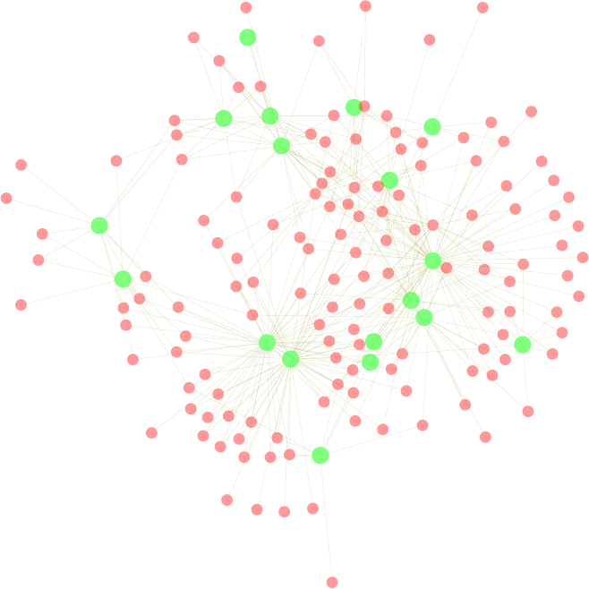
122 CHAPTER 11. SOCIAL NETWORK ANALYSIS
> idx <- which(V(g)$name %in% c("r", "data", "mining"))
> g2 <- delete.vertices(g, V(g)[idx-1])
> g2 <- delete.vertices(g2, V(g2)[degree(g2)==0])
> set.seed(209)
> plot(g2, layout=layout.fruchterman.reingold)
analysis
applications
code
data
examples
mining
network
package
parallel
positions
r
research
series
slides
social time
tutorial
users
123
4
5
6
7
8
9
10
11
12
13
14 15
16
17
18
19
20
21 22
23
24 25
26
27
28
29
30
31
32
33
35
36
37
38
39
40
41
42
43
44
45
46
47
50
52
53
54
55
56
58
59
60
61
62
63
64
65
66
67
68
69
70
71
73
74
75
76
77
78
79
80
82
83
84
85
86
87
88
89
90
91
92
93
94 95
96
97
98
100
101
102
103
104
105
106
107
108
109 110
112
113
114
116
117
118
119
120
121 122
123
124
126
127
128
129
130
131
132
133
136
137
138
139
140
141
142
143
145
146
147
149
151
152
153
154
Figure 11.8: A Two-Mode Network of Terms and Tweets - II
From Figure 11.8, we can clearly see groups of tweets and their keywords, such as time series,
social network analysis, parallel computing and postdoctoral and research positions, which are
similar to the result presented at the end of Section 11.2.
11.4 Discussions and Further Readings
In this chapter, we have demonstrated how to find groups of tweets and some topics in the tweets
with package igraph. Similar analysis can also be achieved with package sna [Butts, 2010]. There
11.4. DISCUSSIONS AND FURTHER READINGS 123
are also packages designed for topic modeling, such as packages lda [Chang, 2011] and topicmodels
[Gr¨
un and Hornik, 2011].
For readers interested in social network analysis with R, there are some further readings.
Some examples on social network analysis with the igraph package [Csardi and Nepusz, 2006] are
available as tutorial on Network Analysis with Package igraph at http://igraph.sourceforge.
net/igraphbook/ and R for Social Network Analysis at http://www.stanford.edu/~messing/
RforSNA.html. There is a detailed introduction to Social Network Analysis with package sna
[Butts, 2010] at http://www.jstatsoft.org/v24/i06/paper. A statnet Tutorial is available
at http://www.jstatsoft.org/v24/i09/paper and more resources on using statnet [Handcock
et al., 2003] for network analysis can be found at http://csde.washington.edu/statnet/resources.
shtml. There is a short tutorial on package network [Butts et al., 2012] at http://sites.stat.
psu.edu/~dhunter/Rnetworks/. Slides on Social network analysis with R sna package can be
found at http://user2010.org/slides/Zhang.pdf. slides on Social Network Analysis in R can
be found at http://files.meetup.com/1406240/sna_in_R.pdf. Some R codes for community
detection are available at http://igraph.wikidot.com/community-detection-in-r.
124 CHAPTER 11. SOCIAL NETWORK ANALYSIS
Chapter 12
Case Study I: Analysis and
Forecasting of House Price Indices
This chapter and the other case studies are not available in this online version. They are reserved
exclusively for a book version published by Elsevier in December 2012. Below is abstract of this
chapter.
Abstract: This chapter presents a case study on analyzing and forecasting of House Price Indices
(HPI). It demonstrates data import from a .CSVfile, descriptive analysis of HPI time series data,
and decomposition and forecasting of the data.
Keywords: Time series, decomposition, forecasting, seasonal component
Table of Contents:
12.1 Importing HPI Data
12.2 Exploration of HPI Data
12.3 Trend and Seasonal Components of HPI
12.4 HPI Forecasting
12.5 The Estimated Price of a Property
12.6 Discussion
125
126 CHAPTER 12. CASE STUDY I: ANALYSIS OF HOUSE PRICE INDICES
Chapter 13
Case Study II: Customer
Response Prediction and Profit
Optimization
This chapter and the other case studies are not available in this online version. They are reserved
exclusively for a book version published by Elsevier in December 2012. Below is abstract of this
chapter.
Abstract: This chapter presents a case study on using decision trees to predict customer response
and optimize profit. To improve customer contact process and maximize the amount of profit,
decision trees were built with R to model customer contact history and predict the response of
customers. And then the customers can be prioritized to contact based on the prediction, so that
profit can be maximized, given a limited amount of time, cost and human resources.
Keywords: Decision tree, prediction, profit optimization
Table of Contents:
13.1 Introduction
13.2 The Data of KDD Cup 1998
13.3 Data Exploration
13.4 Training Decision Trees
13.5 Model Evaluation
13.6 Selecting the Best Tree
13.7 Scoring
13.8 Discussions and Conclusions
127
128 CHAPTER 13. CASE STUDY II: CUSTOMER RESPONSE PREDICTION
Chapter 14
Case Study III: Predictive
Modeling of Big Data with
Limited Memory
This chapter and the other case studies are not available in this online version. They are reserved
exclusively for a book version published by Elsevier in December 2012. Below is abstract of this
chapter.
Abstract: This chapter shows a case study on building a predictive model with limited memory.
Because the training dataset was large and not easy to build decision trees within R, multiple
subsets were drawn from it by random sampling, and a decision tree was built for each subset.
After that, the variables appearing in any one of the built trees were used for variable selection
from the original training dataset to reduce data size. In the scoring process, the scoring dataset
was also split into subsets, so that the scoring could be done with limited memory. R codes for
printing rules in plain English and in SAS format are also presented in this chapter.
Keywords: Predictive model, limited memory, large data, training, scoring
Table of Contents:
14.1 Introduction
14.2 Methodology
14.3 Data and Variables
14.4 Random Forest
14.5 Memory Issue
14.6 Train Models on Sample Data
14.7 Build Models with Selected Variables
14.8 Scoring
14.9 Print Rules
14.9.1 Print Rules in Text
14.9.2 Print Rules for Scoring with SAS
14.10 Conclusions and Discussion
129
130 CHAPTER 14. CASE STUDY III: PREDICTIVE MODELING OF BIG DATA

Chapter 15
Online Resources
This chapter presents links to online resources on R and data mining, includes books, documents,
tutorials and slides. A list of links is also available at http://www.rdatamining.com/resources/
onlinedocs.
15.1 R Reference Cards
R Reference Card, by Tom Short
http://cran.r-project.org/doc/contrib/Short-refcard.pdf
R Reference Card for Data Mining, by Yanchang Zhao
http://www.rdatamining.com/docs
R Reference Card, by Jonathan Baron
http://cran.r-project.org/doc/contrib/refcard.pdf
R Functions for Regression Analysis, by Vito Ricci
http://cran.r-project.org/doc/contrib/Ricci-refcard-regression.pdf
R Functions for Time Series Analysis, by Vito Ricci
http://cran.r-project.org/doc/contrib/Ricci-refcard-ts.pdf
15.2 R
Quick-R
http://www.statmethods.net/
R Tips: lots of tips for R programming
http://pj.freefaculty.org/R/Rtips.html
R Tutorial
http://www.cyclismo.org/tutorial/R/index.html
The R Manuals, including an Introduction to R,R Language Definition,R Data Import/Export,
and other R manuals
http://cran.r-project.org/manuals.html
R You Ready?
http://pj.freefaculty.org/R/RUReady.pdf
R for Beginners
http://cran.r-project.org/doc/contrib/Paradis-rdebuts_en.pdf
131

132 CHAPTER 15. ONLINE RESOURCES
Econometrics in R
http://cran.r-project.org/doc/contrib/Farnsworth-EconometricsInR.pdf
Using R for Data Analysis and Graphics - Introduction, Examples and Commentary
http://www.cran.r-project.org/doc/contrib/usingR.pdf
Lots of R Contributed Documents, including non-English ones
http://cran.r-project.org/other-docs.html
The R Journal
http://journal.r-project.org/current.html
Learn R Toolkit
http://processtrends.com/Learn_R_Toolkit.htm
Resources to help you learn and use R at UCLA
http://www.ats.ucla.edu/stat/r/
R Tutorial - An R Introduction to Statistics
http://www.r-tutor.com/
Cookbook for R
http://wiki.stdout.org/rcookbook/
Slides for a couple of R short courses
http://courses.had.co.nz/
Tips on memory in R
http://www.matthewckeller.com/html/memory.html
15.3 Data Mining
Introduction to Data Mining, by Pang-Ning Tan, Michael Steinbach and Vipin Kumar
Lecture slides (in both PPT and PDF formats) and three sample chapters on classification,
association and clustering available at the link below.
http://www-users.cs.umn.edu/%7Ekumar/dmbook
Tutorial on Data Mining Algorithms by Ian Witten
http://www.cs.waikato.ac.nz/~ihw/DataMiningTalk/
Mining of Massive Datasets, by Anand Rajaraman and Jeff Ullman
The whole book and lecture slides are free and downloadable in PDF format.
http://infolab.stanford.edu/%7Eullman/mmds.html
Lecture notes of data mining course, by Cosma Shalizi at CMU
R code examples are provided in some lecture notes, and also in solutions to home works.
http://www.stat.cmu.edu/%7Ecshalizi/350/
Introduction to Information Retrieval, by Christopher D. Manning, Prabhakar Raghavan
and Hinrich Sch¨
utze at Stanford University
It covers text classification, clustering, web search, link analysis, etc. The book and lecture
slides are free and downloadable in PDF format.
http://nlp.stanford.edu/IR-book/
Statistical Data Mining Tutorials, by Andrew Moore
http://www.autonlab.org/tutorials/
Tutorial on Spatial and Spatio-Temporal Data Mining
http://www.inf.ufsc.br/%7Evania/tutorial_icdm.html

15.4. DATA MINING WITH R 133
Tutorial on Discovering Multiple Clustering Solutions
http://dme.rwth-aachen.de/en/DMCS
Time-Critical Decision Making for Business Administration
http://home.ubalt.edu/ntsbarsh/stat-data/Forecast.htm
A paper on Open-Source Tools for Data Mining, published in 2008
http://eprints.fri.uni-lj.si/893/1/2008-OpenSourceDataMining.pdf
An overview of data mining tools
http://onlinelibrary.wiley.com/doi/10.1002/widm.24/pdf
Textbook on Introduction to social network methods
http://www.faculty.ucr.edu/~hanneman/nettext/
Information Diffusion In Social Networks: Observing and Influencing Societal Interests, a
tutorial at VLDB’11
http://www.cs.ucsb.edu/~cbudak/vldb_tutorial.pdf
Tools for large graph mining: structure and diffusion, a tutorial at WWW2008
http://cs.stanford.edu/people/jure/talks/www08tutorial/
Graph Mining: Laws, Generators and Tools
http://www.stanford.edu/group/mmds/slides2008/faloutsos.pdf
A tutorial on outlier detection techniques at ACM SIGKDD’10
http://www.dbs.ifi.lmu.de/~zimek/publications/KDD2010/kdd10-outlier-tutorial.
pdf
A Taste of Sentiment Analysis - 105-page slides in PDF format
http://statmath.wu.ac.at/research/talks/resources/sentimentanalysis.pdf
15.4 Data Mining with R
Data Mining with R - Learning by Case Studies
http://www.liaad.up.pt/~ltorgo/DataMiningWithR/
Data Mining Algorithms In R
http://en.wikibooks.org/wiki/Data_Mining_Algorithms_In_R
Statistics with R
http://zoonek2.free.fr/UNIX/48_R/all.html
Data Mining Desktop Survival Guide
http://www.togaware.com/datamining/survivor/
15.5 Classification/Prediction with R
An Introduction to Recursive Partitioning Using the RPART Routines
http://www.mayo.edu/hsr/techrpt/61.pdf
Visualizing classifier performance with package ROCR
http://rocr.bioinf.mpi-sb.mpg.de/ROCR_Talk_Tobias_Sing.ppt

134 CHAPTER 15. ONLINE RESOURCES
15.6 Time Series Analysis with R
An R Time Series Tutorial
http://www.stat.pitt.edu/stoffer/tsa2/R_time_series_quick_fix.htm
Time Series Analysis with R
http://www.statoek.wiso.uni-goettingen.de/veranstaltungen/zeitreihen/sommer03/
ts_r_intro.pdf
Using R (with applications in Time Series Analysis)
http://people.bath.ac.uk/masgs/time%20series/TimeSeriesR2004.pdf
CRAN Task View: Time Series Analysis
http://cran.r-project.org/web/views/TimeSeries.html
15.7 Association Rule Mining with R
Introduction to arules: A computational environment for mining association rules and fre-
quent item sets
http://cran.csiro.au/web/packages/arules/vignettes/arules.pdf
Visualizing Association Rules: Introduction to arulesViz
http://cran.csiro.au/web/packages/arulesViz/vignettes/arulesViz.pdf
Association Rule Algorithms In R
http://en.wikibooks.org/wiki/Data_Mining_Algorithms_In_R/Frequent_Pattern_Mining
15.8 Spatial Data Analysis with R
Applied Spatio-temporal Data Analysis with FOSS: R+OSGeo
http://www.geostat-course.org/GeoSciences_AU_2011
Spatial Regression Analysis in R - A Workbook
http://geodacenter.asu.edu/system/files/rex1.pdf
15.9 Text Mining with R
Text Mining Infrastructure in R
http://www.jstatsoft.org/v25/i05
Introduction to the tm Package Text Mining in R
http://cran.r-project.org/web/packages/tm/vignettes/tm.pdf
Text Mining Handbook with R code examples
http://www.casact.org/pubs/forum/10spforum/Francis_Flynn.pdf
Distributed Text Mining in R
http://epub.wu.ac.at/3034/
15.10 Social Network Analysis with R
R for networks: a short tutorial
http://sites.stat.psu.edu/~dhunter/Rnetworks/

15.11. DATA CLEANSING AND TRANSFORMATION WITH R 135
Social Network Analysis in R
http://files.meetup.com/1406240/sna_in_R.pdf
A detailed introduction to Social Network Analysis with package sna
http://www.jstatsoft.org/v24/i06/paper
A statnet Tutorial
http://www.jstatsoft.org/v24/i09/paper
Slides on Social network analysis with R
http://user2010.org/slides/Zhang.pdf
Tutorials on using statnet for network analysis
http://csde.washington.edu/statnet/resources.shtml
15.11 Data Cleansing and Transformation with R
Tidy Data and Tidy Tools
http://vita.had.co.nz/papers/tidy-data-pres.pdf
The data.table package in R
http://files.meetup.com/1677477/R_Group_June_2011.pdf
15.12 Big Data and Parallel Computing with R
State of the Art in Parallel Computing with R
http://www.jstatsoft.org/v31/i01/paper
Taking R to the Limit, Part I - Parallelization in R
http://www.bytemining.com/2010/07/taking-r-to-the-limit-part-i-parallelization-in-r/
Taking R to the Limit, Part II - Large Datasets in R
http://www.bytemining.com/2010/08/taking-r-to-the-limit-part-ii-large-datasets-in-r/
Tutorial on MapReduce programming in R with package rmr
https://github.com/RevolutionAnalytics/RHadoop/wiki/Tutorial
Distributed Data Analysis with Hadoop and R
http://www.infoq.com/presentations/Distributed-Data-Analysis-with-Hadoop-and-R
Massive data, shared and distributed memory, and concurrent programming: bigmemory and
foreach
http://sites.google.com/site/bigmemoryorg/research/documentation/bigmemorypresentation.
pdf
High Performance Computing with R
http://igmcs.utk.edu/sites/igmcs/files/Patel-High-Performance-Computing-with-R-2011-10-20.
pdf
R with High Performance Computing: Parallel processing and large memory
http://files.meetup.com/1781511/HighPerformanceComputingR-Szczepanski.pdf
Parallel Computing in R
http://blog.revolutionanalytics.com/downloads/BioC2009%20ParallelR.pdf
Parallel Computing with R using snow and snowfall
http://www.ics.uci.edu/~vqnguyen/talks/ParallelComputingSeminaR.pdf

136 CHAPTER 15. ONLINE RESOURCES
Interacting with Data using the filehash Package for R
http://cran.r-project.org/web/packages/filehash/vignettes/filehash.pdf
Tutorial: Parallel computing using R package snowfall
http://www.imbi.uni-freiburg.de/parallel/docs/Reisensburg2009_TutParallelComputing_
Knaus_Porzelius.pdf
Easier Parallel Computing in R with snowfall and sfCluster
http://journal.r-project.org/2009-1/RJournal_2009-1_Knaus+et+al.pdf
Bibliography
[Adler and Murdoch, 2012] Adler, D. and Murdoch, D. (2012). rgl: 3D visualization device system
(OpenGL). R package version 0.92.879.
[Agrawal et al., 1993] Agrawal, R., Faloutsos, C., and Swami, A. N. (1993). Efficient similarity
search in sequence databases. In Lomet, D., editor, Proceedings of the 4th International Con-
ference of Foundations of Data Organization and Algorithms (FODO), pages 69–84, Chicago,
Illinois. Springer Verlag.
[Agrawal and Srikant, 1994] Agrawal, R. and Srikant, R. (1994). Fast algorithms for mining as-
sociation rules in large databases. In Proc. of the 20th International Conference on Very Large
Data Bases, pages 487–499, Santiago, Chile.
[Aldrich, 2010] Aldrich, E. (2010). wavelets: A package of funtions for comput-
ing wavelet filters, wavelet transforms and multiresolution analyses. http://cran.r-
project.org/web/packages/wavelets/index.html.
[Breunig et al., 2000] Breunig, M. M., Kriegel, H.-P., Ng, R. T., and Sander, J. (2000). LOF:
identifying density-based local outliers. In SIGMOD ’00: Proceedings of the 2000 ACM SIG-
MOD international conference on Management of data, pages 93–104, New York, NY, USA.
ACM Press.
[Buchta et al., 2012] Buchta, C., Hahsler, M., and with contributions from Daniel Diaz (2012).
arulesSequences: Mining frequent sequences. R package version 0.2-1.
[Burrus et al., 1998] Burrus, C. S., Gopinath, R. A., and Guo, H. (1998). Introduction to Wavelets
and Wavelet Transforms: A Primer. Prentice-Hall, Inc.
[Butts, 2010] Butts, C. T. (2010). sna: Tools for Social Network Analysis. R package version
2.2-0.
[Butts et al., 2012] Butts, C. T., Handcock, M. S., and Hunter, D. R. (March 1, 2012). network:
Classes for Relational Data. Irvine, CA. R package version 1.7-1.
[Chan et al., 2003] Chan, F. K., Fu, A. W., and Yu, C. (2003). Harr wavelets for efficient similarity
search of time-series: with and without time warping. IEEE Trans. on Knowledge and Data
Engineering, 15(3):686–705.
[Chan and Fu, 1999] Chan, K.-p. and Fu, A. W.-c. (1999). Efficient time series matching by
wavelets. In Internation Conference on Data Engineering (ICDE ’99), Sydney.
[Chang, 2011] Chang, J. (2011). lda: Collapsed Gibbs sampling methods for topic models. R
package version 1.3.1.
[Cleveland et al., 1990] Cleveland, R. B., Cleveland, W. S., McRae, J. E., and Terpenning, I.
(1990). Stl: a seasonal-trend decomposition procedure based on loess. Journal of Official
Statistics, 6(1):3–73.
137
138 BIBLIOGRAPHY
[Csardi and Nepusz, 2006] Csardi, G. and Nepusz, T. (2006). The igraph software package for
complex network research. InterJournal, Complex Systems:1695.
[Ester et al., 1996] Ester, M., Kriegel, H.-P., Sander, J., and Xu, X. (1996). A density-based
algorithm for discovering clusters in large spatial databases with noise. In KDD, pages 226–231.
[Feinerer, 2010] Feinerer, I. (2010). tm.plugin.mail: Text Mining E-Mail Plug-In. R package
version 0.0-4.
[Feinerer, 2012] Feinerer, I. (2012). tm: Text Mining Package. R package version 0.5-7.1.
[Feinerer et al., 2008] Feinerer, I., Hornik, K., and Meyer, D. (2008). Text mining infrastructure
in r. Journal of Statistical Software, 25(5).
[Fellows, 2012] Fellows, I. (2012). wordcloud: Word Clouds. R package version 2.0.
[Filzmoser and Gschwandtner, 2012] Filzmoser, P. and Gschwandtner, M. (2012). mvoutlier: Mul-
tivariate outlier detection based on robust methods. R package version 1.9.7.
[Frank and Asuncion, 2010] Frank, A. and Asuncion, A. (2010). UCI machine learning
repository. university of california, irvine, school of information and computer sciences.
http://archive.ics.uci.edu/ml.
[Gentry, 2012] Gentry, J. (2012). twitteR: R based Twitter client. R package version 0.99.19.
[Giorgino, 2009] Giorgino, T. (2009). Computing and visualizing dynamic timewarping alignments
in R: The dtw package. Journal of Statistical Software, 31(7):1–24.
[Gr¨
un and Hornik, 2011] Gr¨
un, B. and Hornik, K. (2011). topicmodels: An R package for fitting
topic models. Journal of Statistical Software, 40(13):1–30.
[Hahsler, 2012] Hahsler, M. (2012). arulesNBMiner: Mining NB-Frequent Itemsets and NB-
Precise Rules. R package version 0.1-2.
[Hahsler and Chelluboina, 2012] Hahsler, M. and Chelluboina, S. (2012). arulesViz: Visualizing
Association Rules and Frequent Itemsets. R package version 0.1-5.
[Hahsler et al., 2005] Hahsler, M., Gruen, B., and Hornik, K. (2005). arules – a computational
environment for mining association rules and frequent item sets. Journal of Statistical Software,
14(15).
[Hahsler et al., 2011] Hahsler, M., Gruen, B., and Hornik, K. (2011). arules: Mining Association
Rules and Frequent Itemsets. R package version 1.0-8.
[Han and Kamber, 2000] Han, J. and Kamber, M. (2000). Data Mining: Concepts and Techniques.
Morgan Kaufmann Publishers Inc., San Francisco, CA, USA.
[Hand et al., 2001] Hand, D. J., Mannila, H., and Smyth, P. (2001). Principles of Data Mining
(Adaptive Computation and Machine Learning). The MIT Press.
[Handcock et al., 2003] Handcock, M. S., Hunter, D. R., Butts, C. T., Goodreau, S. M., and
Morris, M. (2003). statnet: Software tools for the Statistical Modeling of Network Data. Seattle,
WA. Version 2.0.
[Hennig, 2010] Hennig, C. (2010). fpc: Flexible procedures for clustering. R package version 2.0-3.
[Hornik et al., 2012] Hornik, K., Rauch, J., Buchta, C., and Feinerer, I. (2012). textcat: N-Gram
Based Text Categorization. R package version 0.1-1.
[Hothorn et al., 2012] Hothorn, T., Buehlmann, P., Kneib, T., Schmid, M., and Hofner, B. (2012).
mboost: Model-Based Boosting. R package version 2.1-2.
BIBLIOGRAPHY 139
[Hothorn et al., 2010] Hothorn, T., Hornik, K., Strobl, C., and Zeileis, A. (2010). Party: A
laboratory for recursive partytioning. http://cran.r-project.org/web/packages/party/.
[Hu et al., 2011] Hu, Y., Murray, W., and Shan, Y. (2011). Rlof: R parallel implementation of
Local Outlier Factor(LOF). R package version 1.0.0.
[Jain et al., 1999] Jain, A. K., Murty, M. N., and Flynn, P. J. (1999). Data clustering: a review.
ACM Computing Surveys, 31(3):264–323.
[Keogh et al., 2000] Keogh, E., Chakrabarti, K., Pazzani, M., and Mehrotra, S. (2000). Dimen-
sionality reduction for fast similarity search in large time series databases. Knowledge and
Information Systems, 3(3):263–286.
[Keogh and Pazzani, 1998] Keogh, E. J. and Pazzani, M. J. (1998). An enhanced representation
of time series which allows fast and accurate classification, clustering and relevance feedback.
In KDD 1998, pages 239–243.
[Keogh and Pazzani, 2000] Keogh, E. J. and Pazzani, M. J. (2000). A simple dimensionality
reduction technique for fast similarity search in large time series databases. In PAKDD, pages
122–133.
[Keogh and Pazzani, 2001] Keogh, E. J. and Pazzani, M. J. (2001). Derivative dynamic time
warping. In the 1st SIAM Int. Conf. on Data Mining (SDM-2001), Chicago, IL, USA.
[Komsta, 2011] Komsta, L. (2011). outliers: Tests for outliers. R package version 0.14.
[Koufakou et al., 2007] Koufakou, A., Ortiz, E. G., Georgiopoulos, M., Anagnostopoulos, G. C.,
and Reynolds, K. M. (2007). A scalable and efficient outlier detection strategy for categori-
cal data. In Proceedings of the 19th IEEE International Conference on Tools with Artificial
Intelligence - Volume 02, ICTAI ’07, pages 210–217, Washington, DC, USA. IEEE Computer
Society.
[Lang, 2012a] Lang, D. T. (2012a). RCurl: General network (HTTP/FTP/...) client interface for
R. R package version 1.91-1.1.
[Lang, 2012b] Lang, D. T. (2012b). XML: Tools for parsing and generating XML within R and
S-Plus. R package version 3.9-4.1.
[Liaw and Wiener, 2002] Liaw, A. and Wiener, M. (2002). Classification and regression by ran-
domforest. R News, 2(3):18–22.
[Ligges and M¨
achler, 2003] Ligges, U. and M¨
achler, M. (2003). Scatterplot3d - an r package for
visualizing multivariate data. Journal of Statistical Software, 8(11):1–20.
[Maechler et al., 2012] Maechler, M., Rousseeuw, P., Struyf, A., Hubert, M., and Hornik, K.
(2012). cluster: Cluster Analysis Basics and Extensions. R package version 1.14.2.
[M¨
orchen, 2003] M¨
orchen, F. (2003). Time series feature extraction for data mining using DWT
and DFT. Technical report, Departement of Mathematics and Computer Science Philipps-
University Marburg. DWT & DFT.
[R-core, 2012] R-core (2012). foreign: Read Data Stored by Minitab, S, SAS, SPSS, Stata, Systat,
dBase, ... R package version 0.8-49.
[R Development Core Team, 2010a] R Development Core Team (2010a). R Data Import/Export.
R Foundation for Statistical Computing, Vienna, Austria. ISBN 3-900051-10-0.
[R Development Core Team, 2010b] R Development Core Team (2010b). R Language Definition.
R Foundation for Statistical Computing, Vienna, Austria. ISBN 3-900051-13-5.
140 BIBLIOGRAPHY
[R Development Core Team, 2012] R Development Core Team (2012). R: A Language and Envi-
ronment for Statistical Computing. R Foundation for Statistical Computing, Vienna, Austria.
ISBN 3-900051-07-0.
[Rafiei and Mendelzon, 1998] Rafiei, D. and Mendelzon, A. O. (1998). Efficient retrieval of similar
time sequences using DFT. In Tanaka, K. and Ghandeharizadeh, S., editors, FODO, pages 249–
257.
[Ripley and from 1999 to Oct 2002 Michael Lapsley, 2012] Ripley, B. and from 1999 to Oct 2002
Michael Lapsley (2012). RODBC: ODBC Database Access. R package version 1.3-5.
[Sarkar, 2008] Sarkar, D. (2008). Lattice: Multivariate Data Visualization with R. Springer, New
York. ISBN 978-0-387-75968-5.
[Tan et al., 2002] Tan, P.-N., Kumar, V., and Srivastava, J. (2002). Selecting the right interest-
ingness measure for association patterns. In KDD ’02: Proceedings of the 8th ACM SIGKDD
International Conference on Knowledge Discovery and Data Mining, pages 32–41, New York,
NY, USA. ACM Press.
[The Institute of Statistical Mathematics, 2012] The Institute of Statistical Mathematics (2012).
timsac: TIMe Series Analysis and Control package. R package version 1.2.7.
[Therneau et al., 2010] Therneau, T. M., Atkinson, B., and Ripley, B. (2010). rpart: Recursive
Partitioning. R package version 3.1-46.
[Torgo, 2010] Torgo, L. (2010). Data Mining with R, learning with case studies. Chapman and
Hall/CRC.
[van der Loo, 2010] van der Loo, M. (2010). extremevalues, an R package for outlier detection in
univariate data. R package version 2.0.
[Venables et al., 2010] Venables, W. N., Smith, D. M., and R Development Core Team (2010). An
Introduction to R. R Foundation for Statistical Computing, Vienna, Austria. ISBN 3-900051-
12-7.
[Vlachos et al., 2003] Vlachos, M., Lin, J., Keogh, E., and Gunopulos, D. (2003). A wavelet-
based anytime algorithm for k-means clustering of time series. In Workshop on Clustering High
Dimensionality Data and Its Applications, at the 3rd SIAM International Conference on Data
Mining, San Francisco, CA, USA.
[Wickham, 2009] Wickham, H. (2009). ggplot2: elegant graphics for data analysis. Springer New
York.
[Witten and Frank, 2005] Witten, I. and Frank, E. (2005). Data mining: Practical machine learn-
ing tools and techniques. Morgan Kaufmann, San Francisco, CA., USA, second edition.
[Wu et al., 2008] Wu, H. C., Luk, R. W. P., Wong, K. F., and Kwok, K. L. (2008). Interpreting
tf-idf term weights as making relevance decisions. ACM Transactions on Information Systems,
26(3):13:1–13:37.
[Wu et al., 2000] Wu, Y.-l., Agrawal, D., and Abbadi, A. E. (2000). A comparison of DFT and
DWT based similarity search in time-series databases. In Proceedings of the 9th ACM CIKM
Int’l Conference on Informationand Knowledge Management, pages 488–495, McLean, VA.
[Zaki, 2000] Zaki, M. J. (2000). Scalable algorithms for association mining. IEEE Transactions
on Knowledge and Data Engineering, 12(3):372–390.
[Zhao et al., 2009a] Zhao, Y., Cao, L., Zhang, H., and Zhang, C. (2009a). Handbook of Research
on Innovations in Database Technologies and Applications: Current and Future Trends. ISBN:
978-1-60566-242-8, chapter Data Clustering, pages 562–572. Information Science Reference.
BIBLIOGRAPHY 141
[Zhao et al., 2009b] Zhao, Y., Zhang, C., and Cao, L., editors (2009b). Post-Mining of Association
Rules: Techniques for Effective Knowledge Extraction, ISBN 978-1-60566-404-0. Information
Science Reference, Hershey, PA.
[Zhao and Zhang, 2006] Zhao, Y. and Zhang, S. (2006). Generalized dimension-reduction frame-
work for recent-biased time series analysis. IEEE Transactions on Knowledge and Data Engi-
neering, 18(2):231–244.
142 BIBLIOGRAPHY
General Index
3D surface plot, 23
APRIORI, 87
ARIMA, 74
association rule, 85, 134
AVF, 68
bar chart, 14
big data, 129, 135
box plot, 16, 60
CLARA, 51
classification, 133
clustering, 49, 66, 104, 105
confidence, 85, 87
contour plot, 22
corpus, 98
CRISP-DM, 1
data cleansing, 135
data exploration, 9
data mining, 1, 132
data transformation, 135
DBSCAN, 54, 66
decision tree, 29
density-based clustering, 54
discrete wavelet transform, 82
document-term matrix, see term-document
matrix
DTW, see dynamic time warping, 79
DWT, see discrete wavelet transform
dynamic time warping, 75
ECLAT, 87
forecasting, 74
generalized linear model, 47
generalized linear regression, 47
heat map, 20
hierarchical clustering, 53, 77, 79, 104
histogram, 12
IQR, 16
k-means clustering, 49, 66, 106
k-medoids clustering, 51, 107
k-NN classification, 84
level plot, 21
lift, 85, 89
linear regression, 41
local outlier factor, 62
LOF, 62
logistic regression, 46
non-linear regression, 48
ODBC, 7
outlier, 55
PAM, 51, 107
parallel computing, 135
parallel coordinates, 24, 91
pie chart, 14
prediction, 133
principal component, 63
R, 1, 131
random forest, 36
redundancy, 90
reference card, 131
regression, 41, 131
SAS, 6
scatter plot, 16
seasonal component, 72
silhouette, 52, 108
snowball stemmer, 99
social network analysis, 111, 134
spatial data, 134
stemming, see word stemming
STL, 67
support, 85, 87
tag cloud, see word cloud
term-document matrix, 100
text mining, 97, 134
143
Package Index
arules, 87, 90, 96, 134
arulesNBMiner, 96
arulesSequences, 96
arulesViz, 91, 134
ast, 74
bigmemory, 135
cluster, 51
data.table, 135
datasets, 85
DMwR, 62
dprep, 62
dtw, 75
extremevalues, 69
filehash, 136
foreach, 135
foreign, 6
fpc, 51, 54, 56, 107
ggplot2, 26, 102
graphics, 22
igraph, 111, 112, 122, 123
lattice, 21, 23, 25
lda, 109, 123
MASS, 24
mboost, 3
multicore, 65, 68
mvoutlier, 69
network, 123
outliers, 69
party, 29, 36, 81
randomForest, 29, 36
RANN, 84
RCurl, 97
rgl, 20
rJava, 99
Rlof, 65, 68
rmr, 135
ROCR, 133
RODBC, 7
rpart, 29, 32, 133
RWeka, 99
RWekajars, 99
scatterplot3d, 20
sfCluster, 136
sna, 122, 123, 135
snow, 135
Snowball, 99
snowfall, 135, 136
statnet, 123, 135
stats, 74
textcat, 109
timsac, 74
tm, 97, 98, 101, 109, 134
tm.plugin.mail, 109
topicmodels, 109, 123
twitteR, 97
wavelets, 82
wordcloud, 97, 103
XML, 97
145
146 PACKAGE INDEX

Function Index
abline(), 35
aggregate(), 16
apriori(), 87
as.PlainTextDocument(), 99
attributes(), 9
axis(), 41
barplot(), 14, 102
biplot(), 64
bmp(), 27
boxplot(), 16
boxplot.stats(), 59
cforest(), 36
clara(), 51
contour(), 22
contourplot(), 23
coord flip(), 102
cor(), 15
cov(), 15
ctree(), 29, 31, 81
decomp(), 74
decompose(), 72
delete.edges(), 117
delete.vertices(), 116
density(), 12
dev.off(), 27
dim(), 9
dist(), 21, 75, 104
dtw(), 75
dtwDist(), 75
dwt(), 82
E(), 113
eclat(), 87
filled.contour(), 22
findAssocs(), 102
findFreqTerms(), 102
getTransformations(), 99
glm(), 46, 47
graph.adjacency(), 112
graphics.off(), 27
grep(), 100
grey.colors(), 21
gsub(), 99
hclust(), 53, 104
head(), 10
heatmap(), 20
hist(), 12
idwt(), 83
importance(), 38
interestMeasure(), 90
is.subset(), 90
jitter(), 18
jpeg(), 27
kmeans(), 49, 106
levelplot(), 21
lm(), 41, 42
load(), 5
lof(), 65
lofactor(), 62, 65
lower.tri(), 90
margin(), 39
mean(), 11
median(), 11
names(), 9
nei(), 120
neighborhood(), 121
nls(), 48
odbcClose(), 7
odbcConnect(), 7
pairs(), 19
pam(), 51–53, 107
pamk(), 51–53, 107, 109
147

148 FUNCTION INDEX
parallelplot(), 24
parcoord(), 24
pdf(), 27
persp(), 24
pie(), 14
plane3d(), 44
plot(), 16
plot3d(), 20
plotcluster(), 56
png(), 27
postscript(), 27
prcomp(), 64
predict(), 29, 31, 32, 43
quantile(), 11
rainbow(), 22, 103
randomForest(), 36
range(), 11
read.csv(), 5
read.ssd(), 6
read.table(), 76
read.xport(), 7
removeNumbers(), 99
removePunctuation(), 99
removeURL(), 99
removeWords(), 99
residuals(), 43
rgb(), 113
rm(), 5
rownames(), 101
rowSums(), 102
rpart(), 32
runif(), 57
save(), 5
scatterplot3d(), 20, 44
set.seed(), 106
sqlQuery(), 7
sqlSave(), 7
sqlUpdate(), 7
stemCompletion(), 99
stemDocument(), 99
stl(), 67, 74
str(), 9
stripWhitespace(), 99
summary(), 11
t(), 112
table(), 14, 39
tail(), 10
TermDocumentMatrix(), 101
tiff(), 27
tm map(), 99, 100
tsr(), 74
userTimeline(), 97
V(), 113
var(), 12
varImpPlot(), 38
with(), 16
wordcloud(), 103
write.csv(), 5

Data Mining Applications with R
- an upcoming book
Book title: Data Mining Applications with R
Publisher: Elsevier
Publish date: September 2013
Editors: Yanchang Zhao, Yonghua Cen
URL: http://www.rdatamining.com/books/dmar
Abstract: This book presents 16 real-world applications on data mining with R. Each application
is presented as one chapter, covering business background and problems, data extraction and
exploration, data preprocessing, modeling, model evaluation, findings and model deployment.
R code and data for the book will be provided soon at the RDataMining.com website, so that
readers can easily learn the techniques by running the code themselves.
Table of Contents:
Foreword
Graham Williams
Chapter 1 Power Grid Data Analysis with R and Hadoop
Terence Critchlow, Ryan Hafen, Tara Gibson and Kerstin Kleese van Dam
Chapter 2 Picturing Bayesian Classifiers: A Visual Data Mining Approach to Parameters
Optimization
Giorgio Maria Di Nunzio and Alessandro Sordoni
Chapter 3 Discovery of emergent issues and controversies in Anthropology using text mining,
topic modeling and social network analysis of microblog content
Ben Marwick
Chapter 4 Text Mining and Network Analysis of Digital Libraries in R
Eric Nguyen
Chapter 5 Recommendation systems in R
Saurabh Bhatnagar
Chapter 6 Response Modeling in Direct Marketing: A Data Mining Based Approach for
Target Selection
Sadaf Hossein Javaheri, Mohammad Mehdi Sepehri and Babak Teimourpour
Chapter 7 Caravan Insurance Policy Customer Profile Modeling with R Mining
Mukesh Patel and Mudit Gupta
Chapter 8 Selecting Best Features for Predicting Bank Loan Default
Zahra Yazdani, Mohammad Mehdi Sepehri and Babak Teimourpour
149

150 FUNCTION INDEX
Chapter 9 A Choquet Ingtegral Toolbox and its Application in Customer’s Preference Anal-
ysis
Huy Quan Vu, Gleb Beliakov and Gang Li
Chapter 10 A Real-Time Property Value Index based on Web Data
Fernando Tusell, Maria Blanca Palacios, Mar´ıa Jes´us B´arcena and Patricia Men´endez
Chapter 11 Predicting Seabed Hardness Using Random Forest in R
Jin Li, Justy Siwabessy, Zhi Huang, Maggie Tran and Andrew Heap
Chapter 12 Generalized Linear Mixed Model with Spatial Covariates
Alex Zolotovitski
Chapter 13 Supervised classification of images, applied to plankton samples using R and
zooimage
Kevin Denis and Philippe Grosjean
Chapter 14 Crime analyses using R
Madhav Kumar, Anindya Sengupta and Shreyes Upadhyay
Chapter 15 Football Mining with R
Maurizio Carpita, Marco Sandri, Anna Simonetto and Paola Zuccolotto
Chapter 16 Analyzing Internet DNS(SEC) Traffic with R for Resolving Platform Optimiza-
tion
Emmanuel Herbert, Daniel Migault, Stephane Senecal, Stanislas Francfort and Maryline
Laurent
