PWLZO.dvi A Gentle Guide To Constraint Logic Programming Via Eclipse
User Manual:
Open the PDF directly: View PDF ![]() .
.
Page Count: 545 [warning: Documents this large are best viewed by clicking the View PDF Link!]


Antoni Niederli´nski
Chair of Knowledge Engineering
Department of Informatics and Communication
Economic University
PL 40-226 Katowice, Poland
e-mail: antoni.niederlinski@ae.katowice.pl
Limited Copyright c
Antoni Niederli´nski
A secured PDF file of this publication may be reproduced, transmitted,
or stored in computer systems without written permission of the author.
It is freely downloadable from http://www.anclp.pl.
No part of this publication may be printed in any form or by any means.
This is a translation of the revised and extended Polish book ”Programowanie
w logice z ograniczeniami. Lagodne wprowadzenie dla platformy ECLiPSe”,
Third Edition, published by pkjs.com.pl, Gliwice, 2014.
Published from PDF file provided by Antoni Niederli´nski
Text design: Antoni Niederli´nski
Text illustrations: Antoni Niederli´nski
Cover design: Antoni Niederli´nski
Cover illustration: Gantt charts for MT6 Job-Shop
ISBN 978-83-62652-08-2
Published by
Jacek Skalmierski Computer Studio
PL-44-100 Gliwice
ul. Pszczy´nska 44
tel. +48 (0)32 7298097, (0)506132960
fax +48 (0)32 7298549,
pkjs@pkjs.com.pl
Gliwice, 2014
Printed and bound in Poland
”Sweet are the uses of adversity!”
William Shakespeare (1564-1616), ”As You Like It”
”Alle Beschr˝ankung begl˝uckt.”
Arthur Schopenhauer (1788-1860), ”Parerga und Paralipomena”
”What good are books without pictures and stories?”
Lewis Carroll (1832-1898), ”Alice in Wonderland”
” Three friends, a Politician, a Doctor and a Mathemati-
cian, started on a summer walk-out in the enchanting Sile-
sian Beskidy Mountains, when the Politician noticed a sin-
gle black sheep in the middle of a grassland. ’All Silesian
sheep are black’, he remarked. ’No, my friend’, replied the
Doctor, ’Some Silesian sheep are black’. At which point the
Mathematician, after a few second’s thought, said blandly:
’In the Silesian Beskidy Mountains, there exists at least
one grassland, in which there exists at least one sheep, at
least one side of which is black.’”
Anonymouse
Contents
Forwor d i
0.1 Mainassumptions .......................... i
0.2 Whatisinthebook?......................... iii
0.3 Howtousethebook? ........................ viii
0.4 Acknowledgments........................... xi
1 Introduction 1
1.1 WhatisConstraintLogicProgramming?.............. 1
1.2 Why use Constraint Logic Programming? . . . . . . . . . . . . . 2
1.3 Whatdowemeanby’constraints’?................. 5
1.4 Constraint logic programming and
artificial intelligence . . . . . . . . . . . . . . . . . . . . . . . . . 6
1.5 Constraint logic programming and
operationsresearch.......................... 8
1.6 Constraint logic programming and
knowledgeengineering ........................ 9
1.7 Classifyingproblems ......................... 10
2 In the beginning was Prolog 13
2.1 Prologbasics ............................. 13
2.1.1 Domainofinference ..................... 14
2.1.2 PrologandCLPprograms.................. 17
2.1.3 Modesofvariables ...................... 19
2.1.4 Operations .......................... 21
2.1.5 Constraint propagation . . . . . . . . . . . . . . . . . . . 23
2.1.6 Treesearchwithnotrees .................. 24
2.1.7 Failing usefully . . . . . . . . . . . . . . . . . . . . . . . . 28
2.1.8 Recursivedefinitions..................... 30
2.1.9 Basiclistoperations ..................... 32
2.1.10 Generatinglists........................ 34
2.1.11 Controlling backtracking with ’cut’ . . . . . . . . . . . . . 36
2.1.12 Lameness of Prolog’s logic . . . . . . . . . . . . . . . . . . 39
2.2 Configurationproblems ....................... 40
2.2.1 Configuringa3-elementsystem............... 40
2.2.2 Exhaustivesearch ...................... 41
2.2.3 Backtrackingsearch ..................... 44
2.3 Optimumconfigurationproblems.................. 47
2.3.1 Branch-and-bound for optimum configuration . . . . . . . 47
2.4 Assignmentproblems......................... 50
2.4.1 Golfers............................. 50
2.4.2 Threecubes.......................... 53
2.4.3 Who is the killer? . . . . . . . . . . . . . . . . . . . . . . 55
2.4.4 Placing queens - defining variables . . . . . . . . . . . . . 57
2.4.5 Exhaustivesearchforqueens ................ 58
2.4.6 Backtrackingsearchforqueens ............... 59
2.4.7 Examination - backtracking search . . . . . . . . . . . . . 66
2.4.8 ParadoxesinProlog ..................... 68
2.4.9 Howtobecomeyourowngrandfather?........... 69
2.4.10 Using conditional predicates . . . . . . . . . . . . . . . . . 71
2.5 Sequencingproblems......................... 75
2.5.1 Farmer-wolf-goat-cabbage . . . . . . . . . . . . . . . . . . 75
2.5.2 Missionariesandcannibals.................. 80
2.5.3 TowersofHanoi ....................... 87
2.6 Optimumsequencingproblems ................... 90
2.6.1 Asimplemaze ........................ 90
2.6.2 Minefield........................... 92
2.6.3 HamptonCourtmaze .................... 95
2.6.4 Waterjugsproblem ..................... 99
2.7 Exercises ...............................102
3 CLP with elementary predicates for feasible solutions 113
3.1 Elementarypredicates ........................113
3.2 How CLP languages differ from Prolog? . . . . . . . . . . . . . . 114
3.2.1 Basicdifferences .......................114
3.2.2 Similarity ...........................116
3.2.3 Queens-CLPapproaches..................116
3.2.4 Forward Checking forqueens ................117
3.2.5 Looking Ahead+Forward Checking forqueens.......119
3.3 Searchheuristics ...........................120
3.4 Consistencytechniques........................123
3.5 Propagating constraints with failure . . . . . . . . . . . . . . . . 124
3.6 Successful propagation of constraints . . . . . . . . . . . . . . . . 129
3.6.1 Asimpleexample ......................129
3.6.2 Whowithwhom? ......................131
3.6.3 Studentsandlanguages ...................133
3.6.4 Righteous Oppositionists and Secret
Collaborators.........................138
3.7 Propagation is most often not enough . . . . . . . . . . . . . . . 143
3.7.1 Threeequations .......................144
3.7.2 Golfers.............................145
3.7.3 Watchtowers .........................147
3.7.4 Examination .........................148
3.7.5 Queens ............................149
3.7.6 Configuration.........................151
3.8 Exercises ...............................152
4 CLP with global constraints for feasible solutions 159
4.1 Introductoryremarks.........................159
4.2 The’alldifferent/1’built-in .....................160
4.3 The’element/3’built-in .......................162
4.4 Feasibleassignmentproblems ....................164
4.4.1 SendMoreMoney ......................164
4.4.2 FIFTEEN...........................165
4.4.3 Who with whom again . . . . . . . . . . . . . . . . . . . . 167
4.4.4 Golfers again . . . . . . . . . . . . . . . . . . . . . . . . . 169
4.4.5 Three cubes again . . . . . . . . . . . . . . . . . . . . . . 172
4.4.6 Queens again . . . . . . . . . . . . . . . . . . . . . . . . . 174
4.4.7 Sevenmachines-seventasks ................175
4.4.8 Threemachines-threefromfivetasks...........178
4.4.9 Threemachines-fivetasks .................179
4.5 Feasibletimetabling .........................181
4.5.1 Fiverooms ..........................181
4.5.2 Tenrooms...........................184
4.5.3 AllThingstoAllPeople...................192
4.6 Datahandling.............................195
4.6.1 Structuresandarrays ....................196
4.6.2 How to get hold of matrix elements? . . . . . . . . . . . . 199
4.6.3 Recursions and iterations - bye, bye declarativity! . . . . . 200
4.6.4 Queensonemoretime....................207
4.6.5 Scalarproduct ........................208
4.7 Morefeasibleassignmentproblems .................208
4.7.1 Sudoku . . . . . . . . . . . . . . . . . . . . . . . . . . . . 208
4.7.2 Queensforthelasttime...................211
4.7.3 Implicit domain declaration - lectures again . . . . . . . . 212
4.7.4 Stablemarriages .......................214
4.8 Feasiblesequencing..........................222
4.8.1 Carassemblylinesequencing ................222
4.8.2 Bob’sShishKebab......................226
4.8.3 Dinnercalamity .......................233
4.9 Exercises ...............................236
5 CLP with elementary constraints for optimal solutions 245
5.1 General optimization approaches . . . . . . . . . . . . . . . . . . 245
5.2 Branch-and-bound ..........................246
5.3 Upgrading Branch-and-Bound ....................247
5.3.1 Optimum queens - standard Branch-and-Bound ......247
5.3.2 Optimum queens - Forward Checking ...........249
5.3.3 Optimum queens - Looking Ahead +Forward
Checking ...........................249
5.4 Basicbuilt-ins.............................251
5.4.1 The’bbmin/3’built-in ...................251
5.4.2 The’search/6’built-in....................252
5.5 Asimpleexample...........................254
5.6 Optimumconfigurationproblems..................256
5.6.1 Optimum configuration - OR approach . . . . . . . . . . . 256
5.6.2 Optimum configuration - CLP approach . . . . . . . . . . 259
5.6.3 Knapsackproblem1.....................261
5.6.4 Reifiedconstraints ......................263
5.6.5 Constraintsforsets......................265
5.6.6 Knapsackproblem2.....................268
5.6.7 Howtocutoptimally?....................269
5.6.8 Appointing a parliamentary committee . . . . . . . . . . . 271
5.6.9 AmbulanceServiceStations.................274
5.7 Optimumassignmentproblems ...................280
5.7.1 Tasks allocation for 7 machines - OR approach . . . . . . 280
5.7.2 Tasks allocation for 7 machines - CLP approach . . . . . 284
5.7.3 Deliveringminingoutput1 .................286
5.7.4 Deliveringminingoutput2 .................289
5.7.5 Deliveringminingoutput3 .................291
5.7.6 Deliveringminingoutput4 .................293
5.7.7 Mapcoloring .........................295
5.7.8 Fightingforrainfalljustice .................297
5.7.9 SendMostMoney ......................300
5.8 Advancedoptimumassignmentproblems..............302
5.8.1 Warehouse location problem - OR . . . . . . . . . . . . . 302
5.8.2 Warehouse location problem 1 CLP . . . . . . . . . . . . 304
5.8.3 Warehouse location problem 2 CLP . . . . . . . . . . . . 307
5.8.4 Warehouse location problem 3 CLP . . . . . . . . . . . . 311
5.8.5 Real-valuedobjectivefunctions...............314
5.9 Optimumtimetablingproblems...................317
5.9.1 Fastfoodbarcrewroster ..................317
5.9.2 The power and misery of optimization . . . . . . . . . . . 320
5.9.3 Tollcollectorsroster .....................320
5.9.4 DogService..........................324
5.9.5 Policeofficers.........................328
5.10Optimumsequencingproblems ...................333
5.10.1 Precedence constraints - building a house . . . . . . . . . 334
5.10.2 Disjunctive constraints - limited resources . . . . . . . . . 339
5.10.3 Sequencing with conflicting constraints - a photo . . . . . 341
5.11Exercises ...............................346
6 CLP with global constraints for optimal solutions 357
6.1 Introduction..............................357
6.2 The’cumulative/4’built-in .....................358
6.3 Cumulativescheduling1.......................360
6.4 Cumulativescheduling2.......................361
6.5 Cumulativesequencing........................363
6.6 The’disjunctive/2’built-in .....................366
6.7 Disjunctivesequencing........................367
6.8 Disjunctivescheduling ........................370
6.9 The’disjoint2(Rectangles)’built-in.................371
6.10Assemblylinebalancing .......................373
6.11Readingnewspapers1 ........................376
6.12Readingnewspapers2 ........................380
6.13Readingnewspapers3 ........................385
6.14Assemblingbicycles .........................389
6.15Shipunloadingandloading .....................403
6.16Whatisajob-shop? .........................408
6.17 A job-shop scheduling problem - benchmark MT6 . . . . . . . . . 412
6.18 A difficult job-shop scheduling problem - benchmark MT10 . . . 416
6.19TravelingSalesmanProblems ....................430
6.19.1 Hamiltoniancircuits .....................431
6.19.2 Schedulingaprocessline ..................433
6.19.3 Schedulingasalesman ....................436
6.20Appendices ..............................441
6.20.1 The”circuit.ecl”module...................441
6.20.2 The ”distance matrix.ecl” module . . . . . . . . . . . . . 442
6.21Exercises ...............................442
7 CLP for continuous variables 447
7.1 CCSPandCCOP...........................447
7.2 The blessing and curse of compound interest . . . . . . . . . . . 449
7.2.1 Basic..............................449
7.2.2 Calculating compound interest in CLP . . . . . . . . . . . 450
7.2.3 To retire as millionaire - 1 . . . . . . . . . . . . . . . . . . 451
7.2.4 To retire as millionaire - 2 . . . . . . . . . . . . . . . . . . 452
7.2.5 Those cursed mortgages! . . . . . . . . . . . . . . . . . . . 453
7.2.6 Net Present Value or how much we make (or loose) really? 454
7.3 Warehouses-suppliers........................457
7.4 Refiningandblendingoils......................461
7.5 Howtomakeeasymoney?......................463
7.6 Makingshrewdinvestments .....................466
7.7 Yet another financial Perpetuum Mobile!..............471
7.8 Exercises ...............................479
Afterword 488
Glossary 490
Bibliography 500
Index 506
List of Figures
1TheTKECL
iPSeicon ....................... viii
2 Main Window of ECLiPSe..................... ix
3File menu............................... ix
4Help menu............................... x
5 Documents available through Full documentation... ....... xi
6 Running ECLiPSeincommandmode............... xii
1.1 Simple CSP example with non-unique solution. . . . . . . . . . . 2
1.2 Simple CSP example with unique solution. . . . . . . . . . . . . . 3
1.3 SimpleCOPexample. ........................ 4
1.4 Apassiveconstraintexample .................... 5
1.5 Anactiveconstraintexample .................... 6
2.1 Venn diagram for input variables . . . . . . . . . . . . . . . . . . 21
2.2 Search tree for simple Prolog program ............... 27
2.3 Propertiesofcut(!/0) ........................ 37
2.4 Search tree for exhaustive search .................. 42
2.5 Search tree for depth-first search with standard backtracking ... 44
2.6 Search tree for branch-and-bound search.............. 47
2.7 Lastbutoneplacementof8queens................. 60
2.8 Exhaustivesearchtreefor4queens................. 60
2.9 Depth-firstbacktrackingsearchfor4queens. ........... 63
2.10 Animation of search for 4 queens search tree, part 1 . . . . . . . 64
2.11 Animation of search for 4 queens search tree, part 2 . . . . . . . 65
2.12 State of the system farmer-wolf-goat-cabbage ........... 76
2.13 First solution river crossings for farmer, wolf, goat and cabbage . 79
2.14 Second solution river crossings for farmer, wolf, goat and cabbage 80
2.15 State of the system missionaries-cannibals ............. 81
2.16 River crossings for missionaries and canibals by solution 1 . . . . 86
2.17TowerofHanoisolutionfor3disks................. 89
2.18Asimplemaze ............................ 90
2.19Asimpleminefield.......................... 92
2.20HamptonCourtmaze ........................ 95
2.21HamptonCourtMazecoordinates ................. 97
2.22HamptonCourtMazesolution ................... 99
2.23 Filling of three jugs . . . . . . . . . . . . . . . . . . . . . . . . . . 102
2.24 Dragon-dinosaur maze . . . . . . . . . . . . . . . . . . . . . . . . 110
3.1 Partial queens placement generating trashing ...........116
3.2 Forward Checking forfourqueens..................118
3.3 Search tree for Forward Checking forfourqueens.........119
3.4 A queen placement that invokes Forward Checking in vain . . . . 120
3.5 Looking Ahead+Forward Checking forfourqueens ........121
3.6 Search tree for Looking Ahead+Forward Checkingfor four queens 122
3.7 Initial domains for variables X, Y iZ ................126
3.8 Results of successful propagation for Y<Z ............127
3.9 Results of successful propagation for X=Y+Z.........127
3.10 Results of successful propagation for X=Z+3..........128
3.11 Results of successful propagation for X>2+Z..........128
3.12 Results of unsuccessful propagation for Y=2∗Z.........129
3.13 Truth table for the state space of the RO-SC story . . . . . . . . 140
4.1 Fiveroomstimetable.........................184
4.2 Tenroomstimetable-solution1and2...............190
4.3 Tenroomstimetable-solution3and4...............191
4.4 Examplesofstableandunstablemarriages ............215
4.5 The meaning of workstation capacity constraints . . . . . . . . . 224
4.6 Carassemblylinesequencing ....................226
4.7 Dinnercalamitysolution.......................236
4.8 Killer Sudoku problem a) and solution b) . . . . . . . . . . . . . 242
4.9 Pi-Day Sudoku problem a) and solution b) . . . . . . . . . . . . 243
5.1 Analogy between standard Depth-First Backtracking Search and
standard Branch-and-Bound .....................246
5.2 Twofeasibleplacementsforfourqueens ..............248
5.3 Search tree for standard Branch-and-Bound for4queens.....248
5.4 Search tree for Branch-and-Bound+Forward Checking for 4 queens249
5.5 Search tree for Branch-and-Bound+Looking Ahead+Forward Check-
ing for4queens............................250
5.6 Graphical solution to the simple optimization problem . . . . . . 255
5.7 Feasible cutting strategies for a 100 cm long rod . . . . . . . . . 270
5.8 Districtmaps .............................274
5.9 OptimumlocationofASS ......................277
5.10 The administrative map of Absurdoland . . . . . . . . . . . . . . 295
5.11 Coloring the administrative map of Absurdoland . . . . . . . . . 297
5.12Crewrosterforfastfoodbar ....................319
5.13Crewrosterfortollcollectors ....................324
5.14 Dog roster for Great Southern Boarder Crossing . . . . . . . . . 329
5.15Optimumtime-tablesforpoliceofficers...............333
5.16 AoA network of precedence constraints for house building . . . . 335
5.17Ganttchartsforsimplesequencingproblem ............340
5.18 Candidates for a commemorative photo and their preferences . . 342
5.19Alignmentwithnoconstraints6and11...............343
5.20 Alignments minimizing the number of violated constraints . . . . 346
6.1 Tasks satisfying a cumulative/4 constraint.............359
6.2 Ganttchartforcumulativescheduling ...............363
6.3 Gantt charts of some optimum assembly sequences . . . . . . . . 367
6.4 Properties of the disjunctive/2 constraint .............368
6.5 Three examples of ’disjoint2(Rectangles)’ application . . . . . . . 372
6.6 Solution of ’cumulative’ for assembly line balancing . . . . . . . . 375
6.7 Gantt diagram for assembly line balancing . . . . . . . . . . . . . 375
6.8 Ganttchartforstudents........................381
6.9 Ganttchartforpapers.........................381
6.10 First (customary) schedule for bicycle assembling . . . . . . . . . 391
6.11 Second (optimum) schedule for bicycle assembling . . . . . . . . 392
6.12Thirdscheduleforbicycleassembling................393
6.13Fourthscheduleforbicycleassembling ...............394
6.14Fifthscheduleforbicycleassembling................395
6.15Sixthscheduleforbicycleassembling................396
6.16Seventhscheduleforbicycleassembling ..............396
6.17 Gantt chart for optimum unloading and loading of a ship . . . . 409
6.18Job-shopMT6definition.......................413
6.19MT6Ganttcharts ..........................417
6.20Job-shopMT10definition ......................418
6.21GanttchartsforMT10jobs.....................428
6.22 Machine coloring codes for the jobs Gantt chart . . . . . . . . . . 428
6.23GanttchartsforMT10machines ..................429
6.24 Job coloring codes for the machines Gantt charts . . . . . . . . . 429
6.25 A graph that is a Hamiltonian circuit for nodes 1,2,3,4,5,6,7. . . 431
6.26 A graph that is not a Hamiltonian circuit for nodes 1,2,3,4,5,6,7. 432
6.27 Hamiltonian circuit for optimum sequencing of set-ups. . . . . . . 435
6.28 Hamiltonian circuit for the TSP solution for Absurdoland’s dis-
trictcapitals. .............................439
6.29Job-shopABZ5definition ......................446
7.1 Warehouses-suppliersdata.....................458
7.2 Timestructureofbusinessevents..................481
List of Tables
2.1 Definition of implication in Prolog ................. 18
2.2 Definitionofimplicationinlogic .................. 18
2.3 Modesofvariables .......................... 20
2.4 Standardarithmeticoperations................... 21
2.5 Standardorderofoperations .................... 22
2.6 Operatorclassesandtheirassociativity .............. 23
2.7 Second-handcarsaledata...................... 35
2.8 Examinationroomlayout ...................... 66
3.1 Definition of implication in logic as used in ECLiPSe......142
4.1 Taskcostsformachines .......................176
4.2 Taskcostsformachines .......................178
4.3 Taskcostsformachinesandtheirdoubles .............179
4.4 Womenarerankingmen.......................216
4.5 Menarerankingwomen .......................216
4.6 Capacity constraints for car assembly line: x - option required, -
-optionnotrequired.........................223
5.1 Parliamentarians, their affiliation to parties and contributions to
mainstreams .............................272
5.2 Taskcostsformachines .......................280
5.3 Delivercostsformineoutputs....................287
5.4 Proposals to organize and run Rain Agencies . . . . . . . . . . . 299
5.5 Delivery and building costs for 3 warehouses and 5 customers . . 303
5.6 Delivery and building costs for 4 warehouses and 10 customers . 308
5.7 Happy Town student population and traveling distances . . . . . 314
5.8 Minimumnumberofrequiredpoliceofficers ............328
5.9 Housebuildingdata .........................335
5.10Textbooksdata............................346
5.11Glueproductiondata ........................349
5.12Machinesdata ............................349
5.13Ordersdata..............................349
5.14Projectsdata .............................350
5.15Dataforallocatingbenefitstonapoleonides ............352
5.16Carmanufacturingdata .......................353
5.17Fastfoodprojectdata ........................353
5.18Committeecandidates ........................355
5.19 Pizzeria construction activities . . . . . . . . . . . . . . . . . . . 356
6.1 Dataforsimplecumulativescheduling ...............361
6.2 Reading order duration for students and papers . . . . . . . . . . 377
6.3 Tasksforshipunloadingandloading................404
6.4 Increaseofjob-shopschedulenumbers ...............412
6.5 Set-up times for gasoline production changes . . . . . . . . . . . 434
6.6 Taskdurations ............................443
6.7 Threemachines-threejobsdata ..................443
6.8 Fivetasksdata ............................444
6.9 Projectdata..............................444
6.10Holecoordinates ...........................445
6.11Jobdurationsandduedates.....................445
6.12 Job durations, due dates and late penalties . . . . . . . . . . . . 446
7.1 Financial parameters for investment options . . . . . . . . . . . . 456
7.2 Oildata................................461
7.3 Cashrequirementsforconsecutiveyears ..............467
7.4 Resultsforinvestmentoptions....................470
7.5 Results for investment options - continuation . . . . . . . . . . . 471
7.6 Currency exchange rates for March 10, 2010 . . . . . . . . . . . . 472
7.7 Assemblylinedata..........................482
7.8 Computerproductiondata .....................483
7.9 Construction costs each year and interest rates for bonds . . . . 483
7.10Busallocationdata..........................484
7.11 Revenues and bills for for six months . . . . . . . . . . . . . . . . 484
7.12Loantypesdata ...........................485

Foreword
0.1 Main assumptions
This is to be a painless introduction into an exciting software technology named
Constraint Logic Programming, in the sequel abbreviated by CLP.Thebook
aims to teach modeling decision problems and solving them using CLP. It ad-
dresses the needs of all interested in quickly finding feasible and optimum solu-
tions to combinatorial and continuous decision problems using a well-established
tool. It serves to create a basic foothold on CLP for all those wishing to get
some operational experience of using it before eventually dwelling into more
advanced realms of theory. Therefore:
•it starts with an introduction to CLP’s predecessor - the Prolog language.
It is the first language containing in a nutshell the basic ideas of declarative
programming later developed and extended in CLP languages;
•the book is based on a series of extensively commented examples of increa-
sing difficulty. The Author strongly believes that an ounce of application
is worth a ton of abstraction1. He believes that the best way to learn
and master advanced abstractions (Prolog and CLP are full of them) is
by seeing them applied to concrete examples. Examples - especially in
a logic-saturated discipline - are easier to understand by beginners than
theories;
•the book presents basic ideas and methods of CLP, the emphasis being
not on theory but on intuitive understanding. Obviously, not each student
with interest in CLP intends to make a M.Sc. or Ph.D. in CLP. Most of
them just want to know what can be done with CLP, and how. So this
1This is sometimes referred to as Booker’s Law.
i

ii Foreword
book is not addressed to Ph.D candidates, although it seems that most
of them could profit from reading it before plunging into more advanced,
mathematically-saturated texts;
•all examples discussed are running under one of the most popular and
intensively supported CLP platforms, the
ECLiPSeConstraint P rogramming System (ECLiPSeCPS)
platform (see [ECLiPSe-10]), freely available under Cisco-style Mozilla
Public License from http://www.eclipseclp.org/.
A survey of some of the earlier tools for solving CSP and OCSP may be found
in [From-94].
The impetus of this book goes back to a series of lectures and projects on
Prolog and CLP, run in the years 1984-2007 at the Faculty of Automatic Control,
Electronics and Computer Science of the Silesian University of Technology in
Gliwice, Poland, and in the years 2008-2013 at the Faculty of Informatics and
Communication of the University of Economics in Katowice, Poland. The first
teaching assignments made use of the platforms Visual Prolog and CHIP,the
last one - of ECLiPSe.
The authors educational experience in teaching Prolog and CLP convinces
him that a major stumbling block for those learning it is modelling, i.e. trans-
lating verbal problem statements into Prolog or CLP programs. This can be
dealt with by a series of stepping stones leading the learner through a broad
range of verbal problems of increasing complexity, translated into Prolog or
CLP programs. To practice the art of translation, sets of unsolved problems are
provided as well. Thus the core of the book are examples: most of the book is
devoted to presenting them, discussing them and solving them. The programs
that solve them are build using a broad range of various powerful ”black boxes”
referred to as built-in predicates and embedded into the ECLiPSeplatform:
they have a precisely defined functionality, the user always knows what to feed
them and what to obtain in return, but their algorithmic mechanism - being part
of the excluded theory - is hidden. The interested reader may find it in a num-
ber of theoretically-oriented books and publications, e.g. [Apt-03], [Apt-07],
[Bartak-10], [Bratko-01], [Dechter-03], [Jaffar-94], [Marriott-98], [Rossi-06], to
mentions just a few. An extensive in-depth animated and multi-version digital
CLP lecture series for the ECLiPSeplatform has been presented by Simonis
([Simonis-10]). It provides as well a number of interesting examples.

0.2 What is in the book? iii
The art of translating real-world problems into Prolog or CLP programs is
best learned using puzzles. However, solving puzzles using Prolog or CLP is not
only an excellent exercise in learning modelling. The Author fully agrees with
the ideas advocated by Michalewicz (see [Michalewicz-07] and [Michalewicz-08]):
1. Puzzles are educational, as they illustrate many useful (and powerful)
problem-solving rules in a very entertaining way.
2. Puzzles are engaging and thought-provoking.
3. It is possible to talk about different techniques (e.g. simulation, opti-
mization), or application areas (e.g. business, management, industrial
engineering, finance) and illustrate their significance by discussing some
simple puzzles.
What is perhaps more important is that some of the main business, manage-
ment and industrial combinatorial applications of CLP languages, like resource
allocation, timetabling, crew rostering, scheduling, planning, vehicle routing and
a multitude of others, are just mega-puzzles or giga-puzzles with a very large
number of variables; to get a sure foothold for starting to solve them, it seems
necessary to learn the CLP-way-of-thinking and master some basic techniques
by solving a series of micro-puzzles first.
Last but not least, nowadays a student textbook has to compete for the
students time and attention with the Internet, computer games, social activ-
ities, and a number of other distractions. So it should not bore the student
stiff. A good lecturer is expected to say from time to time something unusual,
something paradoxical, some joke, just for the sake of keeping students from
falling asleep and alerting their minds. I think the same applies to textbooks.
They should not be dull. Here puzzles come in handy as excellent vehicles for
introducing moments of relaxation into prolonged intellectual exertions.
0.2 What is in the book?
The contents of the book are organized as follows:
The initial Chapter 1 presents an introduction to general ideas underlying
CLP. There the basic notions of Constraint Satisfaction Problems (CSP) and
Constraint Optimization Problems (COP) are defined and illustrated. The con-
cept of constraint as used in the book is explained. Attention is drawn to

iv Foreword
the relations between CLP and Operation Research, Artificial Intelligence and
Knowledge Engineering.
Chapter 2 (In the beginning was Prolog) presents Prolog - the predecessor
of all CLP languages. It was the first language that allowed the programmer to
specify only what is known about the problem and what goal is to be pursued,
while abstracting from mechanisms used to exploit the knowledge. The emphasis
is on ideas that were later on developed and extended in CLP languages, but
which are perhaps easier to grasp in a more simple setting. The examples
presented there belong to four categories, like all other CLP programs:
1. Examples of determining a feasible state (FS) in the problem state-space,
or simply said, at determining a full descriptions of some situations on the
basis of partial but sufficient data. They include a.o. a set of examples
about configuring a system consisting of three different components with
different costs and different compatibility requirements. Their purpose
is to introduce the reader to the basic mechanisms of tree search and
constraint propagation as unification. The examples illustrate exhaustive
search and backtracking search for finding feasible configurations.
2. Examples of determining an optimum state (OS) in the problem state
space. This is illustrated by determining the least expensive feasible con-
figuration using branch-and-bound search.
3. Examples of determining a feasible state trajectory (FST) in the state-
space from some well-defined initial states to some well-defined final states.
This is illustrated by the well-known Towers of Hanoi problem.
4. Examples of determining an optimum state trajectory (OST) in the state-
space. This is illustrated by a number of well-known maze-walking, river-
crossing and jug filling puzzles.
The classes seem to exhaust all possible Prolog and CLP applications. The
Author never came across Prolog or CLP problems that could not be accom-
modated in one of those categories.
All examples in Chapter 2 are using Prolog as provided by the ECLiPSe
platform, referred to as ECLiPSeP rolog. Prolog programs have the extension
.pl. Compiling any Prolog program makes ECLiPSeuse only those mechanisms
and standard constraints that belong to standard Prolog.

0.2 What is in the book? v
The question may well be asked, ”Why start with ECLiPSeP rolog,why
not with the much more powerful ECLiPSeCLP?” All the more so because
the mechanism of Prolog (standard backtracking with constraint propagation
via unification) differs from the mechanism of CLP (enhanced backtracking
with constraint propagation via consistency techniques). The answers to those
objections concentrate on purely tutorial reasons and are as follows:
1. Ideas that were later on developed and extended in CLP languages (like
declarativity, constraint propagation, logical inference by search with back-
tracking, branch-and-bound) have their roots in Prolog, and are easier to
grasp in the more simple Prolog settings2.
2. The basic elements of Prolog programs are the same as those for CLP
programs.
3. Prolog programs structure closely resembles CLP programs structure.
4. Prolog (in contrast to CLP) may be used to easily program exhaustive
search, which is a rather inefficient search method and may be used only
for simple problems, but is the ancestor of all other search methods and
the knowledge of its mechanism promotes understanding of more efficient
and advanced search methods.
5. Last but not least - Prolog is readily available on the ECLiPSeplatform.
Many examples solved in Chapter 2 are again invoked in later chapters to
show their solution with the help of more advanced CLP mechanisms.
All examples in Chapters 3,...,6 are using CLP as provided by the ECLiPSe
platform, referred to as ECLiPSeCLP. CLP programs have the extension .ecl.
Compiling any CLP program makes ECLiPSeuse only those mechanisms and
standard constraints, which are supported by the CLP libraries declared at the
head of the program.
The topics presented in Chapters 3,...,6 have been dichotomized into follow-
ing categories:
1. Goal-dependent categories:
•the goal is to determine feasible solutions,whichmaybegivenby
either feasible states (FS) or feasible state trajectories (FST) ;
2Thew idea is: ”Start with the simple, gain mastery, move gradually to the complex”.

vi Foreword
•the goal is to determine optimum solutions, which may be given by
either optimum states (OS) or optimum state trajectories (OST) .
2. Built-in-dependent categories:
•only elementary built-ins are used;
•global built-ins are used as well.
Because both dichotomizations are independent, they give rise to four chap-
ters:
1. Chapter 3 (CLP with elementary constraints for feasible solutions)starts
with discussing basic differences between Prolog and CLP languages, like
differences in domain declarations, differences of backtracking strategies
and differences of constraint propagation. Problems that can be solved
using constraint propagation only, and problems that need to supplement
constraint propagation with search, have been presented, explained and
solved. Some of the problems solved in Chapter 2 using Prolog have now
been solved using CLP; some new problems, for which a Prolog solution
would be quite expensive, are solved as well.
2. Chapter 4 (CLP with global constraints for feasible solutions) introduces
the notion of global constraints and presents properties and applications of
three important global constraint used for finding feasible solutions. They
are the alldifferent/1,element/3 and occurrences/3 built-ins. The
chapter presents also a discussion of data handling in ECLiPSeCLP,
with special attention to iterations, practically not used in any Prolog but
being of great importance in ECLiPSeCLP. The application of data
handling predicates for a range of problems has been presented.
3. Chapter 5 (CLP with elementary constraints for optimum solutions)shows
that the solution of rather varied optimization problems can be obtained
using elementary constraints only. Upgrades of the standard branch-and-
bound approach (as used for Prolog programs) are presented. Basic built-
ins (bb_min/3 -bb_min/5 and search/6), used for implementing branch-
and-bound in ECLiPSeCLP, are presented and applied to range of op-
timization problems.
4. Chapter 6 (CLP with global constraints for optimum solutions)presents
properties and applications of two important global constraints used for
finding optimum solutions of complex scheduling problems: cumulative/4

0.2 What is in the book? vii
(cumulative/5)anddisjunctive/2 built-ins. They are applied to a
range of scheduling problems, starting with job-shop problems (includ-
ing the famous MT10 benchmark), and ending with traveling salesman
problems.
Chapter 7 (CLP for continuous variables) is a departure from combina-
torial problems considered in previous chapters. Now an extension of CLP
to continuous variables is presented, and all problems discussed are defined
for continuous domains. They are either Continuous Constraint Satisfaction
Problems (CCSP), or Continuous Constraint Optimization Problems (CCOP).
The chapter starts with highlighting the basic differences between them and
the CSP/COP discussed so far. This is followed by a set of CCSP examples
concerned with compound interest problems. Next, a set of CCOP examples
concerned with linear programming problems is presented. The examples are
chosen so as to highlight the fact that - contrary to OR approaches - CCOP
does not need problems to be cast into some canonical form.
Each chapter, save the first one, terminates with a set of exercises. Most
exercises concerned with solving CSPs are Internet-born. They seem to belong
to the folklore of puzzle-lovers and most of them have not (to the best of the
Authors knowledge) been solved using CLP approaches. Some of them may be
found on so many puzzle websites, that to state their whereabouts would be
pointless. Most exercises concerned with solving COPs are good old Operation
Research problems, well known from a number of excellent textbooks and web-
sites. Although most of them have not been solved using CLP approaches, their
origins are always cited.
Some remarks concerning semantic discipline and parsimony of vocabulary
have to be made at this place. The Author tried hard to avoid any synonyms,
well aware that they are a curse for any diligently studying beginner. This
approach may even be defended by such fundamental principle as Ockham’s
razor 3.
Unfortunately, this inclination brought the Author sometimes into conflict
with established ECLiPSeterminology. The most important case is perhaps
the one involving terms ”predicate”, ”function”, and ”compound term”. Any
function is a relation (although not all relations are functions), relations are de-
3The following Latin saying ”Entia non sunt multiplicanda praeter neccessitatem ” meaning
”Entities should not be multiplied beyond necessity”, attributed to the 14th-century English
logician, theologian and Franciscan friar Father William of Ockham (1285–1349), is known as
Ockham’s razor. The saying is often used as a heuristics to choose between two hypotheses
explaining the same observations equally well, but having different ”degrees of complication”.

viii Foreword
scribed by predicates, so the term ”predicate” seems to obliviate the term ”func-
tion”: there are no discernable operational differences between their meaning.
So the term ”function” will not be used further. Similarly, the name ”compound
term” denotes either a ”predicate” or a ”structure”. No ”compound terms” may
be found that are not defined as ”predicates” or ”structures”.
0.3 How to use the book?
The reader is encouraged to solve all examples discussed in the book, in their
original version and in any conceivable modification, as well as examples pro-
vided in the Exercise sections. While doing this it should be remembered that
learning CLP is essentially a mix of trial and error with explorations aimed at
finding why something doesn’t work. While learning CLP the old ”ski prin-
ciple” holds: if you don’t fall, you won’t learn! Learning CLP gives ample
opportunities for making mistakes, from simple formal mistakes detected by
ECLiPSe/, CLP , to sophisticated, difficult to diagnose, logical mistakes.
The basic software needed, available on the ECLiPSewebsite
http://www.eclipseclp.org/,
has to be downloaded. At the time of writing this book (2013), the software
available was in the Release 6.0_201 file dated 19-Feb-2013. The user is en-
couraged to read the installation notes, README_UNIX for Unix/Linux systems,
or README_WIN.TXT for Windows systems. The download results (for Windows
systems) in the directory
Program Files\ECLiPSe6.0,
in the Ccatalogue, and from the ECLiPSe6.0 directory the TKEclipse6.0 icon
may be put onto the desktop, (Figure 1).
Figure 1: The TKECL
iPSeicon
A click on the icon makes the Main Window of ECLiPSeto appear, see Figure
2.
0.3 How to use the book? ix
Figure 2: Main Window of ECLiPSe
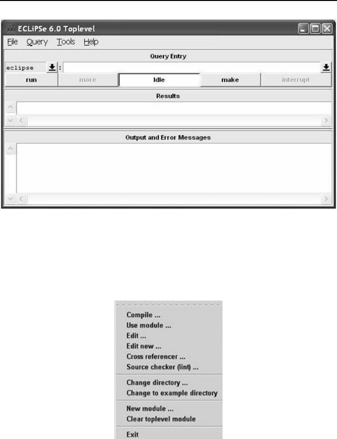
The option File makes available the menu from Figure 3
Figure 3: File menu

xForeword
The Compile option from this menu enables the loading and compilation of
any program with extension .pl (a Prolog program) or with extension .ecl (a
CLP program). All programs presented in this book are activated by inputting
the universal query top. Because top is used for all programs, it is worthwhile
to clean the memory before using it for another program. This can be done by
activating the option Clear toplevel module.
The option Help makes available the menu from Figure 4.
Figure 4: Help menu
Its most often used sub-option is Full documentation..., which makes available
a broad range of documents as shown in Figure 5.
Here the user may find a full list of all standard predicates or built-ins (option
Alphabetical Predicate Index ), libraries (option Constraint Library Manual), a
tutorial (ECLiPSe Tutorial Introduction)andUser Manual. Easy immediate
access to all definitions is the reason standard predicates won’t be defined (save
some important and difficult ones) in this book. The compilation of any .ecl
program makes use of ECLiPSeCPS libraries declared in the program head.
For all standard predicates the Alphabetical Predicate Index documentation pro-
vides data about libraries needed for supporting those predicates.
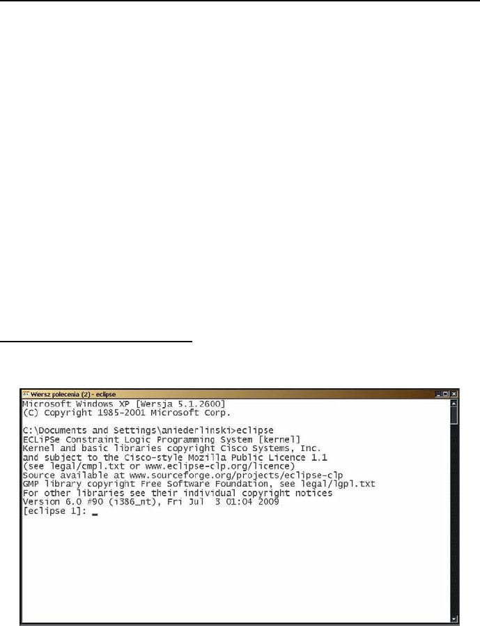
Short CLP programs may also be run using the command mode with the
path leading to eclipse.exe. Then entering the command eclipse in the
command window invokes the command mode (see Figure 6), prompting the

0.4 Acknowledgments xi
user to paste a small CLP program and activate it with ENTER. The command
mode may be also used to run any CLP program by clicking its .ecl name.
Figure 5: Documents available through Full documentation...
0.4 Acknowledgments
The Author did not have the good luck to meet - early in his career - people
knowledgeable in Prolog or CLP, and enthusiastic about them. Having a control-
engineering academic background and position, his education on Prolog and
CLP was entirely self-inflicted, with the help of books and papers he read, and
software he used; they were authored mostly by people he has never even met.
Nevertheless, it seems they deserve to be given credit for the inspiration they
provided by their writing and their software.
The first and most influential book to be mentioned was authored by K.L.
Clark and F.G. McCabe (see [Clark-84]). It was a splendid tutorial, which
caused the Author to get Prolog-infected. He went through all their examples
in the early 80-ties, using a SINCLAIR ZX Spectrum microcomputer for a
microProlog interpreter running under CP/M, and distributed on audio cassette
tapes. It was with the help of this software that the Author started running
courses on Prolog for students at the ”Automation and Robotics” stream at the
xii Foreword
Faculty of Automatic Control, Electronics and Computer Science of the Silesian
University of Technology in Gliwice, Poland.
Later, the Author started to use Turbo-Prolog and its PDC 4- developed
descendants, PDC Prolog and Visual Prolog.Visual Prolog v. 5.2 has been
used to design four expert system shells rmes, which are the subject of another
book. The Author had innumerable opportunities to marvel at the quality of
software produced by PDC people while working on rmes and while teaching
Prolog.
Next, while staying with Professor Mietek Brdy´s at the University of Birm-
ingham, UK, the Author first came across CLP by reading the excellent and
inspiring book by van Hentenryck ([van Hentenryck-89]). This was followed
by using the CHIP v.5.2 software for a course on CLP for students majoring
in ”Computer Controlled Systems”. The Author continued to use CHIP for a
number of years and was always impressed by its elegance and power. It’s main
drawback is the price of the software and lack of public-domain or educational
versions.
In 1997 the Author came across two excellent websites by Roman Bart´ak
from Charles University, Praha, Czech Republic, see [Bartak-10] and [Bartak-10a].
4PDC stands for Prolog Development Center, a Copenhagen based software company.
Figure 6: Running ECLiPSein command mode

0.4 Acknowledgments xiii
That was the beginning of fruitful and inspiring friendly contacts. Professor
Bart´aks insightful talks at a series of ”Workshops on Constraint Programming
for Decision and Control”, run at the Institute of Automation of the Silesian
University of Technology in Gliwice, Poland, during years 1999-2005, was an im-
portant boost to the Authors work and the work of some of his Ph.D students
as well.
Thanks to the initiative of Professor Jerzy Goluchowski from the Economic
University (EU) in Katowice, the Author had the good chance to pursue his
CLP interest at the Chair of Knowledge Engineering (EU), starting 2009 with a
series of CLP lectures based on ECLiPSeCPS. The Author is indebted to Pro-
fessor Goluchowski for relieving him from chores like attending meetings about
planning, proposals and policy, and from activities like fund raising, consulting,
interviewing. The writing of this book has been also inspired by the interest
shown by colleagues from the Chair.
The Author is grateful to his former Ph.D. students, especially Dr. Lukasz
Domagala and Dr. Wojciech Legierski, for many fruitful discussions on CLP
and interesting examples of CLP.
His former colleagues from the Computer Control Group at the Faculty of
Automatic Control, Electronics and Computer Science of the Silesian University
of Technology in Gliwice, Poland: Drs. Jerzy Mo´sci´nski, Dariusz Bismor and
Krzysztof Czy˙z, helped him a lot by explaining peculiarities of Miktex used for
writing this book. He owe thanks to Dr. Jacek Loska for constantly keeping his
hardware and software alive and up-to-date.
The Author is grateful to Hakan Kjellerstrand from Sweden, who - at a
rather short notice - read the typescript of the first edition of the book and
provided valuable feedback on many topics of importance.
Last but not least, the work done on this book would be unthinkable but
for the understanding and support of the Author’s Wife Teresa, who patiently
tolerated for years his prolonged spiritual absence at home.
Obviously, the Author is solely responsible for all mistakes and misrepresen-
tations that may eventually be found in this book.
Finally, the Author offers his deepest apologies to whomever he has neglected
to mention.
Gliwice, January 2014


Chapter 1
Introduction
1.1 What is Constraint Logic Programming?
Constraint Logic Programming (CLP) is a tool for solving constraint satisfaction
problems(CSP). For the important combinatorial case CSP is characterized by
following features1:
•a finite set Sof integer variables X1, ..., Xn, with values from finite do-
mains D1, ..., Dn;
•a set of constraints between variables. The i-th constraint Ci(Xi1, ..., Xik)
between kvariables from Sis given by a relation defined as subset of the
Cartesian product Di1×, ..., ×Dikthat determines variable values corres-
ponding to each other in a sense defined by the problem considered .
Quite often the constraints may not be stated as relations, but by equa-
tions, inequalities, subroutines etc. The number of variables present in
a constraint is named arity of this constraint. A constraint for a single
variable is unary,fortwo-binary,fork>2-k-ary;
•aCSPsolution is given by any assignment of domain values to variables
that satisfies all constraints. It may be non-unique or unique.
•aCSPsolution may additionally minimize or maximize an objective func-
tion. Then it is usually referred to as constraint optimization problem
1This not so gentle (but general and precise) definition will hopefully be more obvious and
lucid after working through some examples from chapters 3,...,6.
1
2Introduction
(COP), and its solution as optimum solution.
Let us spend a moment unpacking these features. This is best done by
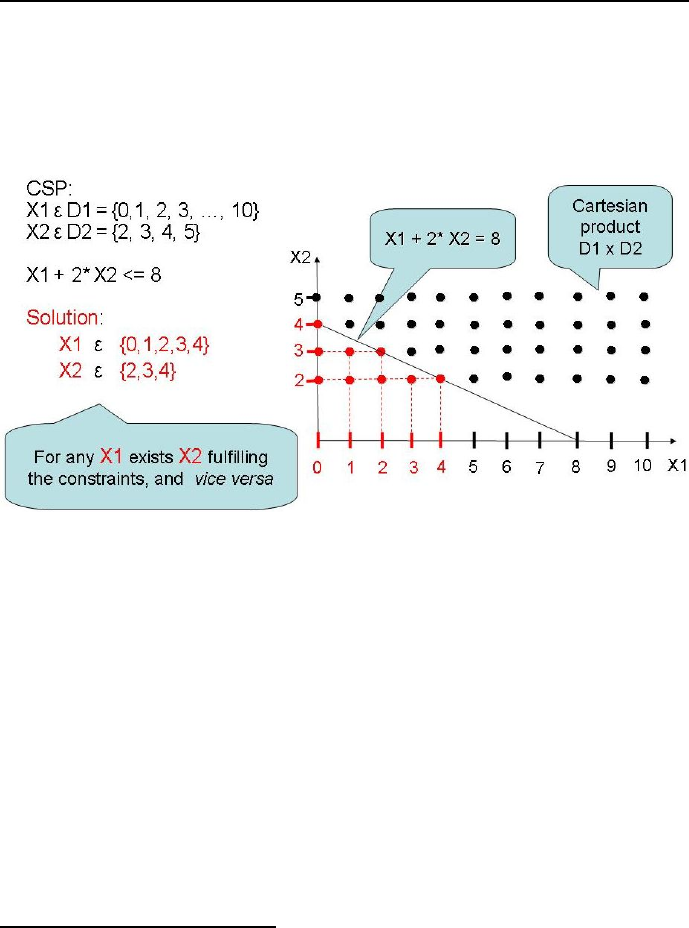
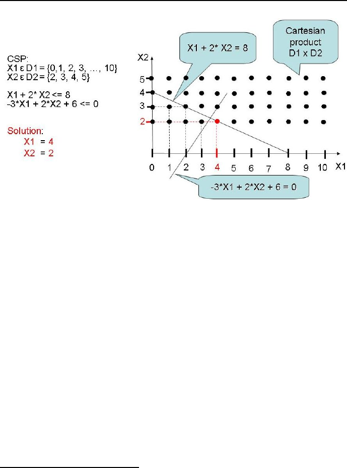
simple examples, see Figure 1.1 for a non-unique solution, Figure 1.2 for a
unique solution and Figure 1.3 for an optimum solution.
Figure 1.1: Simple CSP example with non-unique solution.
Readers familiar with Integer Programming will recognize the problem from
Figure 1.3 as such, see chapters 5 and 6.
1.2 Why use Constraint Logic Programming?
A salient feature of combinatorial CSP and COP is that all variables take values
from finite domains. It follows that in theory any CSP and COP can either be
shown to have no solution or be solved using an algorithmically simple exhaustive
search or direct enumeration2approach. Therefore the wisdom of developing
special tools for such problems may be questioned. Why are present-day tools
for solving combinatorial CSP and COP, outlined in this book, better than
exhaustive search? The answer to this question is as follows:
2I.e. generating one by one all n-tuples of the Cartesian product of variable domains and
testing whether they satisfy all constraints of the problem.
1.2 Why use Constraint Logic Programming? 3
Figure 1.2: Simple CSP example with unique solution.
1. Because of the numerical effectiveness of determining CSP and COP so-
lutions, which for exhaustive search and large numbers of variables is very
bad indeed. It means that the number of enumerations needed to get those
solutions may be exorbitant. E.g. consider a particular case of 30 vari-
ables, each one of them assuming 100 different values3. The total number
of 30-variable sets (constituting what is usually called the state space)
amounts to 10030 =10
60. Because humans are notoriously bad at under-
standing how large is a large number 4, it is worthwhile to convert such
numbers into time. Suppose that the evaluation of a particular set of con-
straints for any of the 30 variable sets will take a microsecond. Evaluating
all sets will take 1054 seconds or 1054/3600 hours or 1054/(3600 ∗24 ∗365)
years. Obviously:
1054/(3600 ∗24 ∗365) >1054/(10000 ∗100 ∗1000) = 1045,
so exhaustive search would need more than 1045 years, i.e. a time consider-
ably in excess of the estimated age of the universe ( 1.4∗1010 years). This
is what we mean by combinatorial explosion, or what Richard Bellman
(see [Bellman-61]) referred to as the curse of dimensionality.CLPlan-
3This is really a small problem compared with e.g. average university timetabling problems.
4This is best seen while watching budgetary discussions in any Parliament.
4Introduction
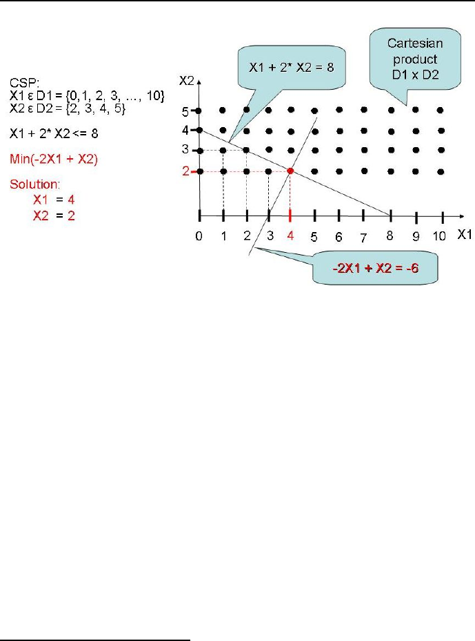
Figure 1.3: Simple COP example.
guages cope (to some extent, not entirely) with such problem by early and
judicious use of problem constraints5and use of implicit feasible problem-
specific heuristics in order to substantially decrease the number of sets to
be tested.
2. Because of the declarativity of Prolog and CLP programs. Declarativity
means that a properly formalized description of the solved problem is tan-
tamount to the program solving the problem. It is contrasted with im-
perativity (procedurality) based on designing algorithms needed to solve
problems. Declarativity means further that while using Prolog or CLP
languages no algorithms for problem solving need to be designed. The al-
gorithms, which are of course necessary for any computer-based problem
solving, have been embedded into Prolog or CLP compilers. To simplify
a bit, it may be stated that the art of Prolog and CLP consists in de-
signing such problem descriptions that are understood by Prolog or CLP
language compilers, and that ensure an efficient determination of the solu-
tion6. However, it should be kept in mind that non-trivial complete Prolog
5Those are the Shakespearean sweet uses of adversity.
6Although thinking declaratively is considered to be much easier than thinking procedurally
1.3Whatdowemeanby’constraints’? 5
and CLP programs cannot entirely get rid of imperativity since they need
to some extent the fixing of order for clauses to be executed, and need
commands for data to be imported and messages to be generated.
1.3 What do we mean by ’constraints’?
The term ’constraints” deserves some attention. It is understood to mean any-
thing that limits the freedom of action. Constraints are ubiquitous: any program
we write in any language is full of them. However, their meaning in impera-
tive languages (like Pascal, C, C++) differs considerably from their meaning
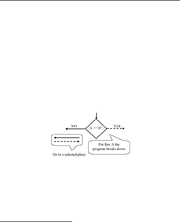
in CLP languages. In imperative languages constraints are passive; that means
they may be used only if all their variables are grounded, and they are used as
tests for choosing the next step taken, see Figure 1.4.
Figure 1.4: A passive constraint example
Constraints in CLP languages are active; that means they may be used also
if some or all of their variables are free. Active constraints (denoted by various
symbols like #for finite domains or $for real or symbolic domains) are used for
initiating a search for such variable groundings that satisfies them, see Figure
1.5.
(see e.g. [Apt-07]), and declarative programs are easier to understand, develop and modify,
it does not mean that using Prolog or CLP techniques is always plain sailing. It simply
means that difficulties experienced while producing efficient algorithms are no longer present,
but instead a new set of difficulties (luckily less formidable) appear while attempting to
design efficient declarative programs making judicious use of available built-ins. We never
get something for nothing.

6Introduction
Figure 1.5: An active constraint example
1.4 Constraint logic programming and
artificial intelligence
Artificial Intelligence (AI) is usually understood to be this branch of computer
science that deals with creating tools for jobs usually considered to need con-
siderable human intelligence, see [Poole-98], [Luger-98] and [Russel-03]. E.g. a
time-tabling program for a large university department (see e.g. [Legierski-06])
surely deserves to be considered as such, as it needs to satisfy a variety of cur-
ricula, balance a large number of conflicting demands by staff and students, and
make best use of facilities available. The label AI is also relevant for programs
that support the design of complicated vehicle routing tasks for a set of vehicles
located in one or more depots, operated by a crew of drivers, having to deliver
an assortment of goods from some spatially dispersed warehouses to some spa-
tially dispersed clients in a way that minimizes the total cost of delivery, see e.g.
Toth-Vigo [Toth-02]. Solving timetable or vehicle routing problems manually
can put a high demand on the intelligence of humans doing it, because they
need to take into account a huge number of relations, conflicting factors, and
trade-offs.
Some authors (e.g. Puget [Puget-08]) are of the opinion that constraint
programming is one of the most successful application of Artificial Intelligence.
Puget quotes the following achievements of constraint programming for one of
the most often met application field, which is scheduling.:
•scheduling operations of a paint shop in a car assembly plant. The paint
shop is one of the most critical zones in the process, because whenever a
paint color is changed, the shop’s machinery must be completely purged;

1.4 Constraint logic programming and
artificial intelligence 7
this is an operation costing both time and money. The developed appli-
cation has minimized the number of times paints need to be changed in
filling customer orders, resulting in considerable savings;
•scheduling production at a large manufacture and marketer of home ap-
pliances in order to better match customer demand and reduce response
time, while keeping low inventories of finished goods;
•designing multi-constrained time-tables for engineers monitoring on a 24-
hour basis all computer and telecommunication systems in a large financial
institution.
This set of examples has been considerably extended by Simonis (see [Simonis-10]),
who quotes the following interesting applications:
•assembly line scheduling for Mirage 2000 fighter aircraft production;
•various crew rostering systems like personnel planning for the guards in
jails or nurses in hospitals;
•production of Belgian chocolates;
•design of advanced signal processing chips;
•design of print engine controller in Xerox copiers;
•assigning ships to berths in container harbor;
•scheduling Bandwidth on Demand.
Researchers, designers and users of AI products have always been confronted
with the need to solve difficult complex problems, see e.g. [Luger-98]. Exactly
the same problems are solved using constraint programming technology.
It is also worthwhile to note that the closeness of the connection between
Prolog/CLP and AI has deeper, more fundamental roots. This is so because AI
as known today may be dated from the failure of the General Problem Solver
(GPS) project7.The critical step in solving a problem with GPS was the definition
of the problem space in terms of the initial state, the goal state to be achieved,
and the transformation rules defining feasible moves from state to state. Us-
ing an inference method called means-end-analysis,GPS would determine the
7GPS was a computer program created in 1959 by Herbert A. Simon, J.C. Shaw, and Allen
Newell at the Carnegie-Mellon University in Pittsburgh, PA, USA.

8Introduction
so called syntactic difference between any initial state and the final state, as
well as determine a logical operator that decreases this difference. This strategy
proved successful for solving formalized symbolic problem, like e.g. theorems
proofs, geometric problems and chess playing. Encouraged by initial success,
Newell and Simon made attempts to increase the prowess of GPS by incorpo-
rating smarter reasoning techniques using more clever search algorithms, and
hoping it will eventually allow them to solve real-world problems outside the
”find a trajectory in problem space” scheme. By and large, it proved a failure:
developing programs that could prove theorems of logic did not seem to pro-
vide techniques that could be readily adapted to other tasks. At the end of the
day these programs were very smart at logic, but still stupid when it came to
anything else. It was then widely recognized that a main characteristic of in-
telligent behavior was not so much general principles of reasoning applicable to
any field of human activity, but rather detailed concrete knowledge of the very
narrow areas relevant to the problem solved. It turned out that for solving real-
world problems plenty of relevant problem knowledge is needed, but the necessary
logical instrumentation is rather modest. Because it was impossible to model
intelligent behaviour which did not rely both upon specific domain knowledge
and sound reasoning, an AI paradigm emerged based on the requirement to put
both components in any AI programs. An obvious next step was to separate
(logically, structurally) in AI programs those two crucial components: domain
knowledge (usually presented in some declarative form and residing in one part
of the program) and reasoning available as a service provided by some other
program or another part of the entire program8.
1.5 Constraint logic programming and
operations research
Operations Research (OR) is a discipline that aims to calculate optimum or
sub-optimum solutions to complex decision-making problems, characterized by
some clearly defined objective function and limited resources. It is basically
concerned with optimizing the objective function, i.e. determining its maxi-
mum (in case it represents profit or yield) or minimum (in case it represents
loss or cost). The objective function depends upon some decision variables that
8This type of programming, known as knowledge based programming, is typical for Prolog
and CLP: the program contains domain knowledge relevant to the problem solved, the compiler
contains the reasoning system.

1.6 Constraint logic programming and
knowledge engineering 9
can be manipulated to achieve the aim, see [Winston-94], [Williams-99], and
[Taha-08]. Originating in military efforts before World War II, its techniques
have developed and turned useful for problems in a variety of industries. The
most widely used numerical tools of operations research are known as various
kinds (linear,integer,mixed)ofprogramming; the term has no connection with
computer programming, but has its roots in the history of the discipline. The
techniques usually stipulate and need the existence of a canonical form of the
decision problem: determine
min
x
cTx
under constraints:
Ax =b
where xis an n-dimensional column vector of real or 0-1 decision variables, A
is an m×nmatrix of reals or 0-1 elements, and cis an m-dimensional column
vector of reals or 0-1 elements. Modern CLP platforms (including ECLiPSe)
provide efficient solvers for this type of problems. What’s more, CLP mod-
elling and solving of operation research problems usually do not need the prior
transformation of those problems into some canonical form, and provide a large
number of global constraints that simplify both problem formulation and so-
lution. The CLP- and OR- approaches to solving optimization problems have
been compared in a number of insightful publications, see e.g. [Hansen-03] and
[Milano-04]. A trend to integrate traditional OR techniques with CLP is also
clearly visible, see [Hooker-00] and [Hooker-07].
1.6 Constraint logic programming and
knowledge engineering
What do we mean by knowledge while speaking about knowledge engineering?
To explain this lets start with some more simple concepts like data and infor-
mation. Quite often they are defined as follows:
•data is given by sets of 0-1 vectors staying for numbers, letters, signs,
words, pictures, sounds. They originate usually as results of some mea-
surements, human actions or processing of other data. They are repre-
sented as bits,bytes,words,lists,arrays,records ;

10 Introduction
•information =data +meaning of data +purpose of data. Information
is thus a purpose-oriented meaningful set of data. Information appears as
the result of some target-oriented human action. It is stored in data bases
and data warehouses;
•knowledge =information +goal +ability to use information to reach the
goal. Knowledge consists thus of information relevant to some goal and
the ability to process the information in a way that procures the goal. The
goal is usually given as some state estimation or decision. Knowledge is
represented by facts,rules and mathematical models.
Not so long ago knowledge was considered to be an exclusively human attribute.
However, in the last 30 years more and more inroads into the realm of knowl-
edge have been struck by computer technology. They cover knowledge discov-
ery (data mining), knowledge storing (knowledge bases), knowledge represen-
tation and knowledge application (reasoning) for some small and well-defined
domains. It also became obvious that computer-assisted knowledge discovery
and computer-assisted knowledge application may be a source of large economic
and social benefits. Those circumstance cumulated in the raise and development
of Knowledge Engineering as a discipline that forms an umbrella covering all
computer-assisted knowledge activities and presents a set of basic concepts to
speak about them, see e.g. [Brachman-04] and [Goluchowski-07].
It so happens that Prolog and CLP excel in almost all those features and ac-
tivities that are crucial for knowledge engineering. Perhaps the most important
is the ability to present knowledge in a declarative form using logic and mathe-
matics, and apply this form for computer assisted reasoning, aiming at proving
or disproving some statements. This is behind one of the widespread knowledge
engineering applications, namely expert systems (see e.g. [Niederli´nski-06])
and business rule management systems (see e.g. [Morgan-08], [Ross-03], and
[von Halle-02]).
1.7 Classifying problems
From a tutorial point of view similarities between verbally different problems
and the resulting similarities of programs that solve them are important. In
order to exploit them effectively a classification of problems solved in this book
is introduced. Prolog problems (and CLP problems as well) may be classified
as belonging to one of the following four categories:

1.7 Classifying problems 11
1. FS-type problems concerned with finding feasible states i.e. states satis-
fying all constraints of the problem. To this category belong most puzzles
and mind-teasers, for which partial data describing some situation is given
and the solver is expected to provide the missing facts so as to get a con-
sistent situation. The importance of such puzzles for learning Prolog is
well illustrated by a number of specialized Prolog-Puzzle websites (see
e.g. [Edmund-10] or http://brownbuffalo.sourceforge.net/). They convey
in simple form problems that are present in such complicated real-world
applications as university time-tabling and industrial time-tabling. Unfor-
tunately, those real-world applications are so complex and need so many
variables that they are hardly suitable for learning Prolog and CLP.FS-
type problems may be farther divided into:
•Feasible configuration problems , which aim at selecting - from some
set - subsets meeting constraints of belongness and compatibility con-
straints .
•Feasible assignment problems, aiming at finding - for any element of
some set - elements of another sets so as to fulfill some constraints.
A type of assignment problems is often referred to as transportation
problems.
•Feasible timetabling problems, aiming at pairing elements of some set
with elements of a set of time intervals.
2. FST-type problems concerned with finding feasible state trajectories i.e.
sequences of feasible states from some well defined feasible initial state to
some well-defined feasible final state. This class of problems is generally
more difficult than the previous one. To this category belong puzzles
and mind-teasers, for which some moves need to be accomplished, e.g.
finding the way out of a maze, bringing people across a river or finding
the shortest path a traveling salesman has to take. They convey in simple
form problems that are present in many important industrial and business
applications. like scheduling of operations or routing of vehicles. FST-type
problems may be farther divided into:
•Feasible sequencing problems, aiming at ordering elements of some
set so as to fulfill some precedence constraints.
•Feasible scheduling problems, aiming at ordering elements of some
set so as to fulfill some precedence constraints and constraints on
available resources.

12 Introduction
3. OS-type problems concerned with finding optimum states i.e. feasible
states optimizing some objective function. Those problems have a number
of feasible states, and therefore it is possible to find such feasible state that
is best from some point of view. To this category belong optimum configu-
ration problems,optimum assignment problems and optimum timetabling
problems, which differ from FS-type problems by aiming additionally at
minimizing some objective function , most often a cost function.
4. OST-type problems concerned with finding optimum state trajectories i.e.
feasible state trajectories optimizing some objective function. Those prob-
lems have a number of feasible state trajectories, and therefore are open to
select such feasible state trajectory that is best from some point of view. To
this category belong optimum sequencing problems and optimum schedul-
ing problems, which differ from FST-type problems by aiming additionally
at minimizing some objective function , most often a cost function.
This classification seems to be exhaustive and all-encompassing. The Author
never came across Prolog or CLP applications with goals that could not be put
into one of those four categories.

Chapter 2
In the beginning was Prolog
The first programming language offering basic CLP methods (like backtracking
search and propagation of constraints) was Prolog1. Because of the simplicity
and transparency of CLP methods used, it is worthwhile to start the discussion
with Prolog. The more so that it is implemented as option in ECLiPSeCPS.
2.1 Prolog basics
Prolog2(an acronym meaning Programming in logic) is based on a fruitful and
inspiring ideas of writing programs consisting neither of instructions (like pro-
cedural,imperative languages) nor of functions (like functional languages), but
of relations (expressed bypredicates) between logical variables.Thismakesthe
language declarative: relations (predicates) and variables cannot be used to for-
mulate commands, i.e. to formulate algorithms, but can be used to describe the
problem under consideration. This makes Prolog (and CLP, which is inheriting
those properties) an excellent tool for presenting problem-relevant knowledge.
However, for Prolog to be a useful tool for solving problems, a system capable
of drawing inferences from this knowledge is needed. Such a system, referred
farther as inference system, is embedded in the Prolog/CLP compiler and is
1Prolog was conceived as joint effort by a group around Alain Colmerauer in Marseille,
France, and Robert Kowalski in Edinburgh, UK, in the period 1971-1974.
2The word ’prologue’ of Greek origin denotes originally an introduction to some large entity
like a book or play. This coincidence is rather uncanny because the computer language Prolog
happened to be an introduction to a large computing paradigm, described in this book.
13

14 Chapter 2. In the beginning was Prolog
(for a limited set of predicates) of universal character. This means that prob-
lem descriptions are in Prolog separated (in a conceptual and in a software
sense) from techniques needed to solve the problems. This means also that
Prolog/CLP are declarative:theproblem description is the problem model is
the problem modeling program is the problem solving program.Byproblem de-
scription is meant a description understandable for the Prolog/CLP compiler
and assuring an efficient determination of the solution. Once more, the art of
Prolog/CLP programming consists of formulating such descriptions.
2.1.1 Domain of inference
Prolog’s domain of inference is the domain of terms. A term is defined by its
type: it may be an atom,avariable,anumber,apredicate,astructure or a list:
•an atom is given as any sequence of characters starting with a lower case
letter, or starting with lower or upper case letter but put between dou-
ble or single quotes3. Atoms are non-numerical (i.e. logical or symbolic)
constants. E.g. blu_sky is a logical constant, because in a given situa-
tionitmaybetrueorfalse,and"Antoni Niederlinski" is a symbolic
constant because no logical value can be assigned to it. The use of quotes
distinguishes atoms that start with upper case letters from variables;
•avariable given as any sequence of characters starting with an upper case
letter or underscore, e.g. X, A, John, Who, _who, _how_much.Variables
in Prolog and CLP are used as unknowns, similar as in logic and algebra.
This is contrasted with variables in procedural programs, where they are
place-holders for varying but known entities. A discussion of modes of
variables is presented in Section 2.1.3. A single underscore (_) denotes
an anonymous variable and means ”any term”; it is used to preserve the
defined predicate arity in case the value of the variable occupying the place
of the anonymous variable is of no interest;
•anumber is given as any integer constant (like -10,-6,0,2,8) or floating-
point constant (like 2.71, 3.14) with decimal points only4;
3Single (straight) quotes will be avoided in programs discussed in this book. This is so
because they are converted in text files (e.g. PDF files) into lexicographic (curly) quotes that
are not recognized by ECLiPS
e. So a scan of a PDF-file program with such quotes cannot
be activated.
4No decimal commas are allowed.

2.1 Prolog basics 15
•apredicate is a relation between variables, e.g.
likes(Somebody, Something),
where likes is the predicate name (always starting with a lower case
letter), while (Somebody, Something) is a tuple i.e. an ordered sequence
of the predicate arguments. The number of arguments is referred to as
arity of predicate, to be used in references like name/arity (likes/2 in
our example). For the relation to be meaningful, sets (or in CLP-parlance:
domains) for both variables have to be defined: e.g. the variable Somebody
may take values from the set of names of 20 students attending my lecture,
and the variable Something may take values from the set of names of 5
popular programming languages.
The above predicate is a formalized prefix version of the colloquial infix
sentence
"Somebody likes Something";
the predicate prefix form, although awkward for colloquial use, has the
undeniable advantage of providing easy access to the subject (Somebody),
object (Something) and predicate (likes) of the sentence. What’s more,
the prefix form can easily accommodate a large number of arguments.
Having defined the predicate arguments as variables Somebody and Some-
thing, a predicate as such has no logical value: it is neither true nor false,
but ambiguous. However, it forms a blueprint for a grounded predicate,
with variables bounded to some constants, e.g.
likes("John Smith","Prolog and CLP")
that may be either a false (unsatisfied) statement or a true (satisfied) state-
ment for some particular "John Smith" from my group of 20 students5.
It should be stressed that predicate arguments form a tuple, i.e. their
order matters; it must be the same for any usage of the predicate. This is
so because Prolog and CLP identify variables across clauses not by their
names, but by their position in the tuple. Thus
likes("John Smith","Prolog and CLP")
and
likes("Prolog and CLP","John Smith"),
should not appear in the same program, although they may mean (from
the programmers point of view) exactly the same thing.
Predicates may be nested: any predicate may serve as argument of another
5Because any bounding of the predicate arguments to some constants produces a proposi-
tion that is either true or false, a predicate is sometimes referred to as propositional function.

16 Chapter 2. In the beginning was Prolog
predicate, e.g.:
likes(graduate_student(Somebody),
computer_science_subject(Something)).
A special case of predicates are functions6: all functions are predicates,
but not all predicates are functions. Therefore no distinction will further
be made between them. Because for some functions infix notation with
standard operators is normally used (e.g. X1 + X2,where"+" is the stan-
dard operator), such infix notation is also accepted by Prolog and CLP.
Predicates may be divided into:
1. Standard predicates (built-in predicates), defined and designed by
Prolog or CLP language designers, and made available to users.
They are farther divided into elementary predicates, defining basic
relations as given in libraries ic and branch_and_bound,withargu-
ments contained at most in one list,andglobal predicates, defining
advanced relations as given in libraries ic_global,ic_cumulative,
ic_edge_finder,ic_edge_finder3, with arguments usually con-
tained in many lists.
2. Private predicates, defined and designed by Prolog or CLP program
designers, with names different from those of standard predicates,
and with arbitrary number of lists.
•astructure is presenting a tuple of a fixed number of atoms, called its
arguments. Any structure has a name (which looks like an atom). The
number of arguments of a structure is called its arity. The name and
arity of a structure are together called its functor andisoftenwrittenas
name/arity. Functors could be seen as general data types, arguments as
defining instances of those data types. Structures correspond to records
in other languages. Although structures look deceivably like predicates,
they differ from them because they do not contain variables; therefore are
always true.
•alist of terms, including an empty list. A (nonempty) list may look like:
[a, b, "CDE", 5, F], an empty list is denoted by []. For details see
Section 2.1.8.
6For a set of n variables with declared domains, a function is declaring - for some subset of
values of n-1 variables (called arguments) a unique value of the n-th variable, called (called
outputs)

2.1 Prolog basics 17
2.1.2 Prolog and CLP programs
Prolog and CLP programs are declarations of constraints. Constraints in Prolog
(and CLP) programs have the form of clauses, which are either facts or rules,
ended with a full stop:
1. Facts are structures or predicates with all arguments grounded, considered
by the program designer to be true. The following is a clause representing
afact:
likes("John Smith","Prolog and CLP").
It means that "John Smith" from my group of students does indeed likes
"Prolog and CLP". Facts are, by their very nature, singular and specific.
2. Rules are conditional statements of the form:
conclusion(_) :-
condition_1(_),
condition_2(_),
...,
condition_n(_).,
where conclusion(_) is a predicate with some free arguments referred to
as head of the rule, the sequence condition_1(_), condition_2(_),...
condition_n(_) being a conjunction of predicates with some free argu-
ments referred to as the body of the rule, the comma (,) is the conjunction
operator read and,thesymbol(:-), being a way to write the rule impli-
cation arrow ←, denotes Prolog implication and is read if.Thustherule
is read like this:
if condition_1(_) and condition_2(_) and...condition_n(_)
are satisfied, then conclusion(_) is satisfied.
The presence of variables in the head and body of rules makes rules gen-
eral: they are valid for a set of variables, as contrasted with facts. The
indentation in the rule expression has no logical meaning: it is used to
18 Chapter 2. In the beginning was Prolog
enhance the readability of rules.
It should be remembered that Prolog implication differs from the better
known implication of logic: if any condition of the Prolog implication is
false (unsatisfied), the conclusion is considered as false (unsatisfied), see
Table 2.1. This assumption is known as Closed World Assumption7.Its
aim is twofold:
Condition Conclusion Conclusion :- Condition
True True True
False False True
False True False
True False False
Table 2.1: Definition of implication in Prolog
Condition Conclusion Condition ⇒Conclusion
True True True
False False True
False True True
True False False
Table 2.2: Definition of implication in logic
•to avoid the nondeterminism existing for the implication of logic for
which, if any condition is false (unsatisfied), the conclusion may be
true (satisfied) or false (unsatisfied), see Table 2.2;
•to force the program designer to put all available relevant knowledge
into the Prolog (or CLP) program.
Prolog naming conventions deserve some comments:
7The ”world” that is subject of the programs reasoning is ”closed” in the sense that
everything that matters for the problem has been taken care of in the program, or can be
inferred from the program.

2.1 Prolog basics 19
1. The naming of private predicates8is entirely arbitrary save they are dif-
ferent from names of built-ins9.
2. Private predicate names may not convey any meanings, e.g. instead of
writing:
likes(Somebody, Something)
we could write as well:
blah_blah(Somebody, Something)
swapping likes in the entire program by blah_blah without affecting the
functioning of the program. However, humans inspecting such program
may have problems in guessing what it’s all about. For the sake of program
readability, modifiability and maintenance, it pays to use predicate names
that correspond to the predicate meaning.
3. The naming of variables needs to be consistent only in rules, but not out-
side rules. The same variable may bear different names in different rules
without affecting the program functioning. Prolog (and CLP) recognizes
variables not by their names, but by their position in predicates. How-
ever, for the sake of program readability, modifiability, and maintenance,
it pays to use the same variable names in different rules.
The described features have an advantage and a disadvantage:
•the advantage is the ease of incorporating third party programs into our
own programs: it suffices to paste them and provide calls from within our
program. No name adjustment is necessary;
•the disadvantage is the possible muddle caused by using inappropriate
names for variables and predicates. In extreme cases it may make the
understanding of a Prolog (or CLP) program a really tough job.
2.1.3 Modes of variables
The word ”mode” denotes the role played by a variable as argument of a built-in
predicate: the variable may be:
•an input, i.e. it is determined outside the predicate considered: it must be
declared as bounded to some other predicate, or list, or atom or number;
8Private predicates are predicates defined and designed by the user.
9Built-ins are predicates defined and designed by Prolog/CLP language designers and made
available for users of those languages.

20 Chapter 2. In the beginning was Prolog
•an output, i.e. it is determined by the predicate considered.
In order to avoid mode errors while using standard predicates, their variables
are distinguished in the documentation by attribute names and corresponding
symbols:
•Input variables that are (by program statements) bounded to some other
predicate, a list, an atom or number, are referred to as instantiated and
denoted by a plus prefix, like +X, in the standard predicate definitions.
•Input variables that are (by program statements) bounded to some grounded
predicate, grounded lists, atoms or numbers are referred to as grounded
and denoted by a double plus prefix, like ++X, in the standard predicate
definitions.
•Output variables are denoted by a minus prefix, like -X. They are of course
not bound to anything.
•A distinctive (rather valuable) feature of Prolog and CLP is the existence
of predicates with variables serving as either inputs or outputs. They are
then in the predicates definition distinguished by a question mark, like ?X.
The definitions are summarized in Table 2.3.
Variable Variable Variable Variable
instantiated grounded free any mode
(+X) (++X) (-X) (?X)
An input An input An output An input or
bounded to any bounded to a bounded to output, bounded
predicate or grounded predicate nothing or free
list, to an or list, to
atom or number an atom or number
Table 2.3: Modes of variables
The differences between various variables are additionally illustrated by Fi-
gure 2.1: any grounded variable is instantiated, but some instantiated variables
may not be grounded.
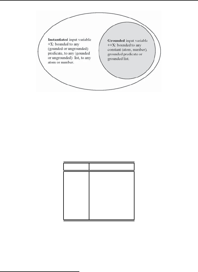
2.1 Prolog basics 21
Figure 2.1: Venn diagram for input variables
2.1.4 Operations
The basic arithmetical operations available in Prolog are shown in Table 2.4.
Theymaybeusedineitherinfix form or prefix form, see Full documentation...
in Figure 5.
Symbol Operation
+addition
-subtraction
multiplication
/real division
// integer division
mod modulus
^power
Table 2.4: Standard arithmetic operations
The standard order of operations (strength of binding, precedence) are expressed
in Table 2.510.
This means that if a number or other symbol, or an expression grouped by
one or more symbols of grouping, is preceded by one operator and followed by
10 What follows in this section may be omitted while first reading.

22 Chapter 2. In the beginning was Prolog
Operation Binding strength Precedence value
terms inside brackets strong low
exponents and roots |
multiplication and division |
addition and subtraction weak high
Table 2.5: Standard order of operations
another, the operator higher in the table should be applied first. As in Edin-
burgh Prolog, a lower precedence value means that the operator binds stronger
(1 strongest, 1200 weakest)11. Arrows in Table 2.5 indicate directions of in-
crease.
In Prolog, the user is able to modify the syntax dynamically by explicitly
declaring new operators. The built-in op/3 performs this task. Its structure is:
op(+Precedence, +Associativity, ++Name)
where Precedence is an integer from the range 1to 1200,Name is the operator
with the chosen Precedence,andAssociativity is an argument that distin-
guishes between different classes of operators. Denoting by:
f - an operator with declared precedence,
x - an argument whose precedence must be strictly lower than
that of the operator
y - an argument whose precedence is lower or equal to that
of the operator,
and farther assuming that:
- arguments enclosed in parentheses or unstructured arguments have precedence
equal zero,
- structured arguments have precedence equal to the precedence of the operator,
then possible operator classes and their associativity are shown in Table 2.6
These concepts may be illustrated by a following simple example: consider the
expression
u-v-w,
with operator ’-’ having the precedence 500. It is understood as
11 This terminology is indeed unfortunate, since a higher precedence value in Prolog indi-
cates lower precedence (in normal English). The lowest precedence value in Prolog binds the
strongest.
2.1 Prolog basics 23
Operator class Associativities
prefix fx, fy (unary) or fxx, fxy (binary)
infix xfx, xfy, yfx
postfix xf, yf
Table 2.6: Operator classes and their associativity
(u-v)-w,
and not as:
u-(v-w).
To get the correct interpretation, the operator ’-’ has to have the associativity
yfx. For a more advanced example see Section 5.8.3.
2.1.5 Constraint propagation
Constraint propagation is a process initiated by grounding a free variable from
some constraint. The propagation aimes at letting know about this event all to
which it may concern and at performing all operations relevant to the mentioned
grounding. In Prolog it is performed by two actions:
1. Value spreading.
2. Unification.
Value spreading denotes the process by which the grounding done for a variable
from some constraint is repeated for all instances of this variable in the body of
this rule and for all other instances of the constraint in bodies of other rules.
Unification denotes the process of matching values of other instances of
the grounded variable in order to obtain equality of terms. The principles of
unification are:
•in the Herbrand domain unification my be done only for syntactically
equivalent terms. Two terms are syntactically equivalent if:
- they are of the same type and format, e.g.
"likes(A,B)" and "likes(X,Y)",
or "[X,Y,Z]" and "[P,_,R]",
- one of the unified terms is a free variable;
•free variables can be unified with anything, including other free variables.
This is consistent with the property that variable names have meaning
only inside rules;

24 Chapter 2. In the beginning was Prolog
•different atoms are not unifiable;
•different numbers are not unifiable.
Unification is invoked by the built-in infix predicate =/2. E.g. the unification:
likes(Somebody, Something) = likes("John Smith",prolog)
is feasible and results in
Somebody = "John Smith"
Something = prolog
So in Prolog 1+1=2does not hold because the left hand term and the right
hand term are not syntactically equivalent. Instead the built-in is has to be
used and the equation is written as 1+1is2. Of course not all syntactically
equivalent terms may be unified (are unifiable). E.g.:
likes(Somebody,pascal) = likes("John Smith",prolog)
is false, because the different constants pascal and prolog are not unifiable.
This is also the case for:
likes("Jim Taylor",prolog) = likes("John Smith",prolog)
because the different constants "Jim Taylor" and "John Smith" are not unifi-
able. The equality sign (=) is thus meaningful only between unifiable terms.
The outcome of propagation may be twofold:
1. For a successful propagation the next free variable is grounded.
2. For an unsuccessful propagation the last grounded variable is degrounded
and backtracking starts.
Constraint propagation in Prolog is not an autonomouse activity: it can only
be used in conjunction with search.
2.1.6 Tree search with no trees
To proceed, it would be handy to introduce the concepts of state,state space,
feasible state and contracted state.State means any grounding of domain values

2.1 Prolog basics 25
to all decision variables, the state space is given by all groundings of domain
values to all decision variables, a feasible state is a state for which all constraints
are satisfied, a contracted state means any grounding of domain values to some
decision variables12.
The goal of any Prolog (and CLP) program is to satisfy a query that is the
head of some rule. The Prolog (CLP) compiler contains an inference system
that searches the state space for a feasible state that will satisfy the query. This
is done by generating sequences of contracted states leading to the feasible state,
provided a feasible state exists. If so, Yes is followed by some detailed messages.
If no feasible state exists, No will be printed. All Prolog (and CLP) programs
discussed farther will always have the query top; this makes for convenient
testing.
Search denotes the following sequence of steps:
1. Selecting adecision variable from the body of the rule defining the query;
2. Grounding the selected decision variable, i.e. assigning to it a value from
its domain. Thereby a contracted state is generated and the selected de-
cision variable is termed grounded;
3. Spreading the value of the grounded decision variable to all its instances
in the body of the rule;
4. Testing the satisfaction of all predicates in the body of the rule using
unification:
•if this is not possible because some predicates are not grounded, steps
1, 2 and 3 are repeated for the next nearest variable or for the rule
defining this predicate, until eventually all predicates are grounded
and satisfied;
•if all predicates in the body of the query are grounded and satisfied,
the query is satisfied and the variable values used for grounding are
displayed as the program solution;
•if some predicate in the body of the query fails, the latest selected
variable is degrounded, a return is performed leftwards to the nearest
tested predicate with variables not yet grounded to some values from
12 The concept of state is - to the best knowledge of the Author - not particularly en
vogue in the CLP community. The Author, because of his control-engineering and dynamic
system background, is missing it from ever since, and uses this opportunity to show its broad
usefulness while discussing CLP.

26 Chapter 2. In the beginning was Prolog
their domains, and one of the variables is regrounded. While return-
ing, all variables that have been successfully grounded between the
said nearest tested predicate and the failed predicate, are degrounded
as well. The return, the degrounding, and the regrounding is named
backtracking, and the predicate with variables of yet untested values
to which the return was performed, is named choice point.
It should be emphasized that any variable grounded to some value may
be grounded to another value only as the result of backtracking.
This is illustrated by the following simple Prolog program 2_1_search.pl:
/*1*/ a(X,Y) :-
/*2*/ b(X),
/*3*/ c(X,Y).
/*4*/ b(1).
/*5*/ b(&).
/*6*/ c(&,"A").
The programs query is a(X,Y). This means that the program aims at find-
ing such values for decision variables Xand Ythat satisfy a(X,Y). The program
contains one rule (lines /*1*/,/*2*/,and/*3*/) and three facts (lines /*4*/,
/*5*/,and/*6*/). The indentation for lines /*2*/ and /*3*/ is used to make
the rule better readable. The domains for variables Xand Yare defined implic-
itly by the facts: the domain of Xis (1,&), the domain of Yis "A".
The rule states that in order to satisfy a(X,Y) such value for Xhas to be
found that satisfies b(X),andsuchvalueforYhas to be found that together
with the value for Xsatisfies c(X,Y). The conditions for the rule are queried in a
top-down fashion, so the first value found for Xis X=1. Because the domain of X
contains another value &, a choice point is created for b(X). Next, the value X=1
is spread to line /*3*/ resulting in c(1,Y), which does not unify with c(&,"A")
from line /*6*/.Soc(1,Y) is unsatisfied, Xis degrounded from its value 1and
areturntothechoicepointforb(X) follows. Now Xis regrounded with &,the
regrounding is spread to line /*3*/ resulting in c(&,Y) that successfully unifies
with c(&,"A") from line /*6*/ giving the solution X=&,Y = "A".
The process described may be interpreted as running according to the search
tree from Figure 2.2 that reflects the program structure.
For obvious reasons the search from Figure 2.2 is known as top-down search
or depth-first search. The way returns are generated (as the result of violating
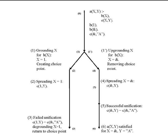
2.1 Prolog basics 27
Figure 2.2: Search tree for simple Prolog program
some constraint) is known as standard backtracking. Therefore the full name
of this search is Depth-First Backtracking Search or Top-Down Backtracking
Search.
The search tree is defined by all states of the decision variables that consti-
tute the leaves of the search tree. For this example they are (X,Y) = (1,"A")
and (X,Y) = (&,"A"). The intermediate node (there is only one node for this
example) of the search tree corresponds to the choice point, where the value of
Xis chosen.
The amazing thing is that search trees are never explicitly present in its
entirety, but simply generated piecewise, on-the-fly. In the discussed example
the left-hand branch from Figure 2.2 is generated first, but after the failed
unification in line /*3*/ it is dropped save the choice point (1)- (1’),tobe
used for generating the right-hand branch. The mechanism of making search

28 Chapter 2. In the beginning was Prolog
trees with no trees present in its entirety is of great practical significance because
it allows Prolog and CLP languages to deal with problems corresponding to
search trees of exorbitant sizes.
An important regularity from the example deserves to be emphasized:
•grounding of free variables occurs in top-down search any time a predicate
with free variables is encountered;
•degrounding of grounded variables occurs when the last grounding results
in some constraint to be unsatisfied and a return to the nearest choice
point is done, where this (or some other free variable) may be regrounded.
There is no other way for grounded variables to change their values.
It should be emphasized, that Prologs search and unifications constitute a
complete inference method. It means that if a solution to a CSP modelled in
Prolog exists, it will be determined13.
2.1.7 Failing usefully
As it had been already stressed, backtracking is initiated when some grounded
predicate fails. However, there are situation when backtracking is forced by
deliberately using an ”always false” atom called fail/0. This is illustrated by
program 2_2_fail.pl:
/*1*/ top:-
/*2a*/ who_are_your_friends_1.
/*2b*/ % who_are_your_friends_2.
/*2c*/ % who_are_your_friends_3.
/*3*/ friend("Mark").
/*4*/ friend("Jack").
/*5*/ friend("Andrew").
% For ’who_are_your_friends_1’ there is no backtracking,
% just one solution (the first one from top) is given:
/*6*/ who_are_your_friends_1:-
/*7*/ friend(Who),
/*8*/ write("Friend: "),write(Who), nl.
% For ’who_are_your_friends_2’, ’fail’ generates backtracking,
% all friends are displayed but eventually the program fails with a ’No’:
13 Well, it may sometimes take quite a time!

2.1 Prolog basics 29
/*9*/ who_are_your_friends_2:-
/*10*/ friend(Who),
/*11*/ write("Friend: "),write(Who),nl,
/*12*/ fail.
% For ’who_are_your_friends_3’, ’fail’ generates backtracking,
% but when no backtracking can be performed any more, the second
% definition of ’who_are_your_friends_3’i invoked
% and the program end with a Y’es’
/*13*/ who_are_your_friends_3:-
/*14*/ friend(Who),
/*15*/ write("Friend: "),write(Who), nl,
/*16*/ fail.
/*17*/ who_are_your_friends_3:-
/*18*/ write("Those are all my friends."),nl.
The messages are:
Message for who_are_your_friends_1:Friend: Mark.
Yes.
After clicking twice ”more” in the Main Window from Figure 2 (to enforce other
solutions), the message is:
Friend: Jack
Yes.
Friend: Andrew
Yes.
Message for who_are_your_friends_2:
Friend: Mark
Friend: Jack
Friend: Andrew
No.
Message for who_are_your_friends_3:
Friend: Mark
Friend: Jack
Friend: Andrew
Those are all my friends.
Yes.
Well, obviously fail/0 is an explicitly procedural operator that clearly

30 Chapter 2. In the beginning was Prolog
shows the impossibility of writing declarative programs that work without some
procedural crutches. It is worth remembering that fail/0 is functioning like
any predicate which is always false, e.g. 2is3.
2.1.8 Recursive definitions
Arecursive predicate definition is given by:
1) a rule with the head being the defined predicate and the body containing this
very predicate with different argument structure;
2) a fact, most often the grounded predicate.
The conciseness, declarativity and power of Prolog (and CLP as well) is largely
due to the widespread usage of recursive definitions of predicates. As example
may serve the list definition. Lists are basic Prolog data structures. They are
n-tuples of elements, beginning with a left-hand square bracket and closing with
a right-hand square bracket:
List = [Element_1, Element_2,...,Element_n] .
It may be decomposed as follows:
List = [Head|Tail]
where Head is the first element of the list List,andTail is the list that remains
after removing the first element. Because Tail is a list, it must obviously con-
tain a Head_of_Tail and a Tail_of_Tail. The last one is a list, therefore we
can speak about the Head_of_Tail_of_Tail and the Tail_of_Tail_of_Tail,
and so on, until the empty list [] is reached, which has no head. So the list
concept is in fact defined recursively. And most predicates with lists as argu-
ments use recursion as well. The most simple illustration is provided by defining
a predicate that determines list membership. It has the structure:
membership(Member,List),
which is intended to mean that Member is an element of List. It is defined by
stating the fact that the head of the list is a list member, no matter what the
tail is:
/*1*/ membership(Member,[Member|_]).

2.1 Prolog basics 31
and stating the recursive rule that a list member is the member of the list tail,
no matter what the head is:
/*2*/ membership(Member,[_|O]) :-
/*3*/ membership(Member,O).
The underscore _denotes an anonymous variable; it means we do not care
about the value it may be grounded with and are not interested in knowing
this value. Let’s have a look at how this definition is working. The program
2_3_list.pl:
/*1*/ top:-
/*2*/ membership(E,[1,2,3,4]),
/*3*/ writeln(E),
/*4*/ fail.
/*5*/ top:-
/*6*/ writeln("Those are all elements of the list.").
/*7*/ membership(Member,[Member|_]).
/*8*/ membership(Member,[_|O]) :-
/*9*/ membership(Member,O).
generates the message:
1
2
3
4
Those are all elements of the list.
The programs query is top. The logical constant top will be used in the
sequel for all Prolog/CLP programs in the book. Prolog compiler attempts
to satisfy the query, i.e. make top true. In order to do it, it has to satisfy
the predicate in line /*2*/. This invokes the definition from line /*7*/,Eis
grounded to /*1*/, and because of the other part of the definition (lines /*8*/
and /*9*/, a choice point is created for the predicate membership().The
predicate fail/0 is a built-in that cannot be satisfied, so a backtrack to the
choice point is made generating the next element of the list and another choice
point, and so on, until (thanks to removing head after head by the action of line
/*7*/,/*8*/ and /*9*/ predicates) the list becomes empty.

32 Chapter 2. In the beginning was Prolog
The example presented is more general than it seems: Prolog recursion is
always defined between a list (in the head of the recursive rule) and the tail of
this list (in the body of the recursive rule).
For ECLiPSeP rolog the built-in predicate member(?Member,?List) functions
exactly as the above membership() predicate: while using it instead of mem-
bership in line /*2*/, lines /*7*/,/*8*/,and/*9*/ are not needed, see top1
in 2_3_list.pl.
2.1.9 Basic list operations
There are only two such operations:
1. Removing successive heads from a non-empty list and constraining them.
This is continued until the list is empty, as shown in the following example:
recursive_predicate([H|T],....):-
% The head is removed and processed:
constraining_the_head(H),
........................
recursive_predicate(O,....).
% Removing of heads leads to an empty list:
recursive_predicate([],....).
The recursion with heads removal starts with a [H|T] list, the heads of
which are successively removed and processed, until the list is empty. The
recursion occurs between the list [H|T] (in the head of the rule) and the
tail of the list T(in the recurred predicate in the rule body).
2. Adding - as heads - successive elements, generated by some constraints,
to a list which is initially entirely or partially empty. This is continued
until some special list is generated, as shown in the following example:
recursive_predicate(Tail_of_list,....):-
% The head is determined and added:
determine_the_head(Head),
........................
recursive_predicate([Head|Tail_of_list],....).

2.1 Prolog basics 33
% Adding heads leads to some Special_list:
recursive_predicate(Special_list,,....).
The recursion with adding heads start with an entirely or partially empty
Tail_of_list, to which are successively added Heads generated by some
constraints, until the list is some Special_list. The recursion occurs
between the Tail_of_list (in the head of the rule) and the head-added-
list [Head|Tail_of_list] in the recurred predicate in the rule body.
The important thing to remember is that only heads may be removed from a
list, and only heads me be added to a list.
This is illustrated by program 2_4_reversal.pl that reverses the order of
list elements using two private predicates:
1. my_reverse(Initial_list, Reversed_list)
2. my_reverse(Initial_list, Reversed_list,
Accumulator_of_reversed_list)
The name my_reverse was chosen to distinguish it from the built-in reverse/2,
which does exactly the same job.
The program is removing successively heads from the the Initial_list
and adding the removed heads successively to the initially empty list named
Accumulator_of_reversed_list. When the Initial_list is empty (i.e. when
all its elements have been transferred in reverse order to the Accumulator_of_
reversed_list), the Reversed_list is unified with the accumulator.
The program looks like this:
/*1*/ top:-
/*2*/ my_reverse([a,b,c,d],Reversed_list),
/*3*/ write(Reversed_list).
/*4*/ my_reverse(Initial_list,Reversed_list):-
/*5*/ my_reverse(Initial_list,Reversed_list,[]).
/*6*/ my_reverse([],A,A).
/*7*/ my_reverse([H|T],Reversed_list,A):-
/*8*/ my_reverse(T,Reversed_list,[H|A]).

34 Chapter 2. In the beginning was Prolog
The message generated is:
Reversed list = [d, c, b, a]
The program uses two predicates with the same name but different arity
(my_reverse/2 and my_reverse/3), which is perfectly O.K. Different arities
make the names distinguishable to the compiler.
The basic rule is in lines /*7*/ and /*8*/:theretheheadHof the initial
list [H|T] is removed from this list and added as head to the list A, resulting in
[H|A].
The use of accumulator deserves some comments. In Prolog/CLP accumu-
lators are artificial variables14 that allow to write so-called tail-recursive rules,
i.e. rules with the head calling itself at the end of the body; the rule in lines
/*7*/ and /*8*/ is just a trivial example of a tail-recursive rule. Tail-recursion
is the most parsimonious type of recursion as far as stack space is concerned: it
does not need any stack at all.
2.1.10 Generating lists
To do anything in Prolog/CLP, lists have to be used. Lists are usually generated
from data sets. This can be done using the findall/3 built-in with following
mode structure:
findall(?Term, +Goal, -List)
where List is the list of all values of Term for which Goal is satisfied. Consider
the following example:
The Backyard Used Car company has widely advertised an attractive sale of
the following second-hand but relatively new and well-kept models produced by
the renowned Clunker Motors Company: Clunker SUV,Clunker Great Tour,
Clunkerlac,Clunker Family,Clunkerdes,Clunker Electric and Clunker Green.
The details are given by Table 2.7.
The aim is to determine the mean price of all cars and the mean mileage of
cars costing less than 1900 and not of red color and not older than 2006. To
14 Artificial in this sense that they do not correspond to any of the original problem variables.

2.1 Prolog basics 35
Model Mileage Year Price Color
Clunker SUV 29000 2008 1500 Black
Clunker Great Tour 60000 2009 1900 Green
Clunkerlac 47000 2007 1200 Champagne
Clunker Family 38000 2009 2200 Blue
Clunkerdes 46000 2008 3100 Silver
Clunker Electric 75000 2005 1100 Red
Clunker Green 52000 2006 1300 Silver
Table 2.7: Second-hand car sale data
use this data in a Prolog program, a private predicate
offer(Model, Mileage, Year, Price, Color)
is defined. The program 2_5_clunkers.pl shows the usage of findall/3 to ex-
tract the needed information from the data:
/*1*/ top:-
/*2*/ mean_price_for_all_cars,
/*3*/ mean_mileage_for_selected_cars.
/*4*/ mean_price_for_all_cars:-
/*5*/ findall(Price,offer(_,_,_,Price,_),List),
/*6*/ writeln("List of prices for all cars":List),
/*7*/ length(List, N),
/*8*/ Sum is sum(List),
/*9*/ MeanPrice is Sum/N,
/*10*/ writeln("Mean car price":MeanPrice),nl.
/*11*/ mean_mileage_for_selected_cars:-
/*12*/ findall(Mileage,selected_cars(Mileage),List),
/*12*/ writeln("List of mileage for cars costing less than 1900 and "),
writeln("not of red color and not older than 2006":List),
/*14*/ length(List, N),
/*15*/ Sum is sum(List),
/*16*/ MeanMileage is Sum/N,
/*17*/ writeln("Mean mileage for cars costing less than 1900 and "),
writeln("not of red color and not older than 2006":MeanMileage).
/*18*/ selected_cars(Mileage):-
/*19*/ offer(_,Mileage,Year,Price,Color),
/*20*/ Year > 2006,

36 Chapter 2. In the beginning was Prolog
/*21*/ Price < 1900,
/*22*/ Color \== "Red".
/*23*/ offer("Clunker SUV", 29000, 2008, 1500, "Black").
/*24*/ offer("Clunker Great Tour", 60000, 2009, 1900, "Green").
/*25*/ offer("Clunkerlac", 47000, 2007, 1200, "Champagne").
/*26*/ offer("Clunker Family", 38000 , 2009, 2200, "Blue").
/*27*/ offer("Clunkerdes", 46000, 2008, 3100, "Silver").
/*28*/ offer("Clunker Electric", 75000, 2005, 1100, "Red").
/*29*/ offer("Clunker Green", 52000, 2006, 1300, "Silver").
The program generates following messages:
List of prices for all cars : [1500, 1900, 1200, 2200, 3100, 1100, 1300]
Mean car price : 1757.14285714286
List of mileage for cars costing less than 1900 and
not of red color and not older than 2006 : [29000, 47000]
Mean mileage for cars costing less than 1900 and
not of red color and not older than 2006 : 38000.0
Notice the presence of anonymous variables in line /*5*/, due to the cir-
cumstance that we need only values of the Price variable.
Readers familiar with database languages may notice that Prolog is also an
elegant language for database queries, equivalent to a powerful subset of SQL.
2.1.11 Controlling backtracking with ’cut’
Backtracking in Prolog is ”automatic”. That means each time the search for
solution needs backtracking (i.e. each time some predicate fails), Prolog back-
tracks. This is both advantageous and disadvantageous: the advantage consists
of relieving programmers from coding backtracking into Prolog programs; the
disadvantage is that backtracking may sometimes be not quite desirable because
it increases the time to get a solution or generates partial solutions of no interest.
This can be avoided using the built-in !/0 referred to as cut. The properties
of cut are summarized in Figure 2.3, were black arrows denote possible back-
tracking. Program 2_6_playing_with_cut.pl illustrates all usages of cut/0:
/*1*/ top:-
/*2*/ a.
/*3*/ a :-
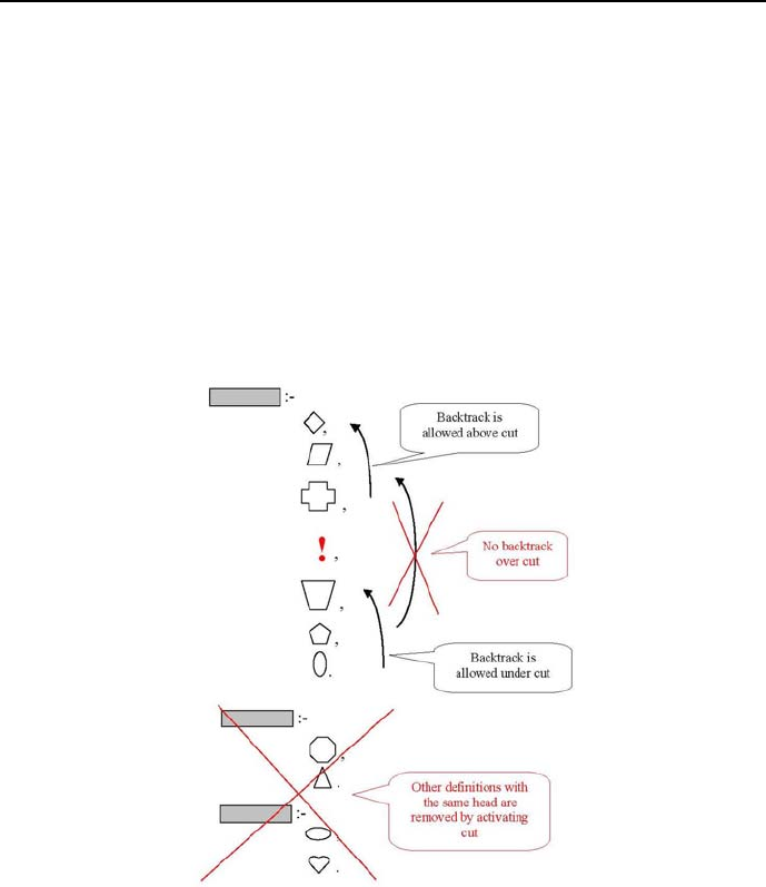
2.1 Prolog basics 37
/*4*/ b, write(" The Prolog compiler did not call the ’cut’."),nl,
/*5*/ write(" Thanks to that, because the first clause for ’b’ "),nl,
/*6*/ write(" could not be fulfilled, ’a’ is true "),nl,
/*7*/ write(" because the second clause for ’b’ was fulfilled."),nl,nl.
/*8*/ a :-
/*9*/ write("We are here 4!"),nl,
/*10*/ write(" Because the Prolog compiler called the ’cut’ in"),nl,
/*11*/ write(" the first clause for ’b’, it is not possible to "),nl,
/*12*/ write(" call the second clause for ’b’. The first clause for "),nl,
/*13*/ write(" ’a’ thus remains unfulfilled. However, the second clause "),nl,
/*14*/ write(" for ’a’ is fulfilled, because it can be called anyway."),nl,nl.
Figure 2.3: Properties of cut (!/0)
/*15*/ b :-
/*16*/ c(X),
/*17*/ d(X),
/*18*/ !,

38 Chapter 2. In the beginning was Prolog
/*19*/ e(Y),
/*20*/ f(Y),
/*21*/ g(X).
/*22*/ b:-
/*23*/ write(" We are here 0!"),nl.
/*24*/ c(1).
/*25*/ c(2):-
/*26*/ write("We are here 1!"),nl,
/*27*/ write(" Backtrack is possible before the ’cut’!"),nl,nl.
/*28*/ c(3).
/*29*/ d(2).
/*30*/ e(1).
/*31*/ e(2) :-
/*32*/ write("We are here 2!"),nl,
/*33*/ write(" Backtrack is possible after the ’cut’!"),nl,nl.
/*34*/ f(2) :-
/*35*/ write("We are here 3!"),nl,
/*36*/ write(" However, no backtrack is possible from below the place "),nl,
/*37*/ write(" cut has been placed in the first clause for ’b’ up above "),nl,
/*38*/ write(" the place ’cut’ has been placed in this clause."),nl,nl.
/*39*/ g(3).
The message while lines /*25*/,/*26*/ and /*27*/ are present:
We are here 1!
Backtrack is possible before the ’cut’!
We are here 2!
Backtrack is possible after the ’cut’!
We are here 3!
However, no backtrack is possible from below the place
cut has been placed in the first clause for ’b’ up above
the place ’cut’ has been placed in this clause.
We are here 4!
Because the Prolog compiler called the ’cut’ in
the first clause for ’b’, it is not possible to

2.1 Prolog basics 39
call the second clause for ’b’. The first clause for
’a’ thus remains unfulfilled. However, the second clause
for ’a’ is fulfilled, because it can be called anyway.
The message while lines /*25*/,/*26*/ and /*27*/ are removed:
We are here 0!
The Prolog compiler did not call the ’cut’.
Thanks to that, because the first clause for ’b’
could not be fulfilled, ’a’ is true
because the second clause for ’b’ was fulfilled.
So cut/0 is another (besides fail/0) explicitly procedural operator we need
to make partially declarative programs to work.
2.1.12 Lameness of Prolog’s logic
The Reader has perhaps already noticed that there is rather little logic in Prolog,
considering the massive stock of knowledge covered by the name logic.What’s
more, this little logic used in Prolog is sometimes strangely twisted to account
for the fact that Prolog (and CLP ) programs are running on single proces-
sors, that process the program clauses and the body predicates sequentially in
time, from programs top to programs bottom, and from body left to body right.
Consider the rule structure. The sequence of predicates in the rule’s body
had been referred to as conjunction. As we know from logic, conjunction is com-
mutative; that is changing the order of conjuncted arguments does not change
the logical value of the conjunction. However, this does not always hold for
rules. The program 2_5_clunkers.pl gives a good opportunity to demonstrate
this limitation of logic as used in Prolog. Suppose the line /*5*/ was put after
line /*8*/. The program compiles but when queried produces the message:
"instantiation fault in (0, _347, _355)".
The reason is obvious: predicates in the rules body are (because of the single
processor limitation) tested in the order they appear, from left to right. There-
fore we can’t use (in lines /*7*/ and /*8*/) data for the ungrounded variable
List: it has not yet been grounded by the moved predicate from line /*5*/.

40 Chapter 2. In the beginning was Prolog
Hence in Prolog it is up to the program designer to put the body predicates in
proper order.
2.2 Configuration problems
2.2.1 Configuring a 3-element system
To build some system, elements belonging to three classes are needed: a single
A-class element, a single B-class element, and a single C-class element. Each
class contains a number of different types of elements:
•A-classelementsmaybeoftypea1,a2,anda3;
•B-class elements may be of type b1,b2,b3,andb4;
•C-classelementsmaybeoftypec1 and c2,
with different prices (in Monetary Units,MU):
•a1 price is 1900; a2 price is 750; a3 price is 900;
•b1 price is 300; b2 price is 500; b3 price is 450; b4 price is 600;
•c1 price is 700; c2 price is 850,
and different compatibility restrictions:
•c1 is not compatible with a2;
•b2 is not compatible with c2;
•c2 is not compatible with b3;
•b4 is not compatible with a2;
•b3 is not compatible with a1;
•a3 is not compatible with b3;
There are two problems to be solved: (1) determine all configurations consisting
of three compatible elements A,B,andCwith overall price not larger than 2100
MU15, ( 2) determine all optimum configurations consisting of three compatible
15 This is an FS-type problem.

2.2 Configuration problems 41
elements A,B,andCwith overall minimum price16. Such problems are generic,
which means they are representatives of a group of concrete problems of similar
logical structure, like configuring a lunch menu, configuring a leisure outfit,
configuring computer hardware.
2.2.2 Exhaustive search
The most naive approach to solving the configuring problem is exhaustive search:
it amounts to generating consecutively all states (A,B,C) of the state space and
only then testing whether they satisfy all constraints of the problem. This is
done notwithstanding the fact that with luck the feasible solution may be found
for the first state generated and with no luck it may be found after generating
some substantial number of states. However, with bad luck it may be found
for the last state generated, and to play safe, the entire state space has to be
tested. For the configuration example 3 ×4×2 = 24 tests have to be performed.
Assuming further that Ais grounded first, Bnext, and Clast, the search may be
depicted for - the sake of compatibility with backtracking search - by the search
tree from Figure 2.4.
Exhaustive search starts (according to the assumption made) with variable A
bounded to a1, variable Bbounded to b1,andvariableCbounded to c1.There-
sulting configuration (a1,b1,c1) is too expensive, so the next state is generated
and so on. The system may be configured in 24 ways (that’s the dimension of
the state space) from which 13 configuration contain non-compatible elements,
and 7configurations costs more than the threshold price of 2100. Following
four configurations are feasible:
•Configuration(a2,b1,c2) priced at 1900;
•Configuration(a3,b1,c1) priced at 1900;
•Configuration(a3,b1,c2) priced at 2050;
•Configuration(a3,b2,c1) priced at 2100.
The exhaustive search may be performed by program 2_7_conf_es.pl:
/*1*/ top:-
/*2*/ assert(upper_price_limit(2100)),
/*3*/ upper_price_limit(Upper_price_limit),
16 This is an OS-type problem.
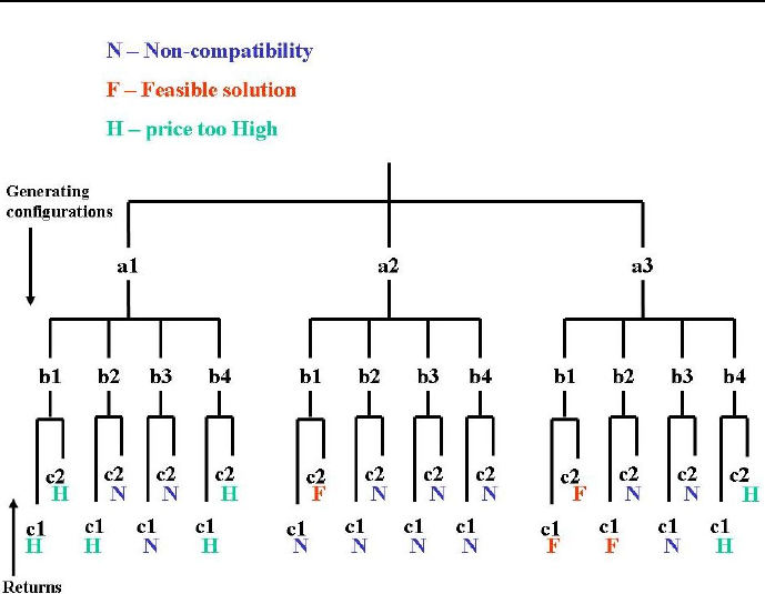
42 Chapter 2. In the beginning was Prolog
Figure 2.4: Search tree for exhaustive search
/*4*/ configuration(Upper_price_limit).
/*5*/ configuration(Upper_price_limit):-
/*6*/ member(A,[a1,a2,a3]),
/*7*/ member(B,[b1,b2,b3,b4]),
/*8*/ member(C,[c1,c2]),
/*9*/ not(incompatibility([A,B])),
/*10*/ not(incompatibility([A,C])),
/*11*/ not(incompatibility([B,C])),
/*12*/ price(A,Price_of_A),
/*13*/ price(B,Price_of_B),
/*14*/ price(C,Price_of_C),
/*15*/ Total_price is Price_of_A+Price_of_B+Price_of_C,
/*16*/ Upper_price_limit>=Total_price,
/*17*/ write("Configuration("),write(A),write(","),
/*18*/ write(B),write(","),write(C),write(")"),
/*19*/ write(" priced at "),write(Total_price),

2.2 Configuration problems 43
/*20*/ nl,fail.
/*21*/ configuration(Upper_price_limit):-
/*22*/ write("Those are all configurations "),
/*23*/ write("priced at no more than "),
/*24*/ write(Upper_price_limit),write(".").
/*25*/ price(a1,1900). price(a2,750). price(a3,900).
/*26*/ price(b1,300). price(b2,500). price(b3,450).
/*27*/ price(b4,600). price(c1,700). price(c2,850).
/*28*/ incompatible(c1,a2).
/*29*/ incompatible(b2,c2).
/*30*/ incompatible(c2,b3).
/*31*/ incompatible(b4,a2).
/*32*/ incompatible(b3,a1).
/*33*/ incompatible(a3,b3).
/*34*/ incompatibility([X,Y]):-incompatible(X,Y).
/*35*/ incompatibility([X,Y]):-incompatible(Y,X).
The message generated by the program is:
Configuration(a2,b1,c2) priced at 1900
Configuration(a3,b1,c1) priced at 1900
Configuration(a3,b1,c2) priced at 2050
Configuration(a3,b2,c1) priced at 2100
Those are all configurations priced at no more than 2100.
It should be noted that:
1) The domains for variables A,Band Chave been declared using the member/2
predicate in lines /*6*/,/*7*/ and /*8*/. The predicates from these lines
always generate a full state (A,B,C) that is next tested for compatibility and
price. The number of such states is 24.
2) Because being incompatible is a commutative relation, instead of defining it
once more for changed order of arguments, the predicate incompatibility/1
has been introduced to take care of this.
3) The number of facts stating incompatibility is less than would be the number
of facts stating compatibility. Therefore in lines /*9*/,/*10*/ and /*11*/
negated incompatibility is tested.
3) The built-in predicate fail/0 is a predicate that always fails. It is used to
force backtracking in order to find all solutions.
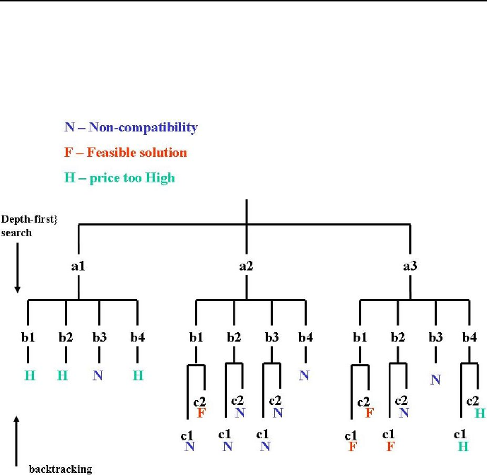
44 Chapter 2. In the beginning was Prolog
2.2.3 Backtracking search
The poor performance of exhaustive search is due to testing constraints only for
complete states. It is obvious that some constraints may be tested earlier, for
contracted states. This has been shown on Figure 2.5.
Figure 2.5: Search tree for depth-first search with standard backtracking
As can be seen from Figure 2.5, variable Ais first grounded to a1. Because
this is not the only possibility of grounding A(that may be grounded also to a2
and a3), so a choice point for Ahas to be created. Next, variable Bis grounded
to b1 while another choice point is created for Bthat may be grounded to b2,
b3,andb4 as well. The contracted state (A,B) = (a1,b1) corresponds to a
partial configuration that costs more than the threshold price, so there is no
point in going deeper in the search tree: backtracking is initiated consisting of:
•degrounding the last bounded variable B=b1;

2.2 Configuration problems 45
•returning upward to the nearest choice point which is for B;
•because the choice point contains the untested value b2, variable Bis
grounded to b2;
•the choice point for Bis retained with b2 being removed from the set of
untested values;
•the contracted state (A,B) = (a1,b3) corresponds to a partial configura-
tion that contains incompatible elements. Therefore another backtracking
is initiated.
A return may sometimes reach higher in the search tree, and therefore
more grounded variables may be degrounded. E.g. for the contracted state
(A,B) = (a2,b4) non-compatibility appears, so - as before - there is no rea-
son in going deeper in the search tree: however, this time there is no choice
point for Bbecause all values for Bhave been tested. Therefore both grounded
variables A=a2and B=b4have to be degrounded and a return to choice
point for A, accompanied with restoring all domain values for Band C,hasto
be made. It results in grounding A=a3. This is not violating any constraints.
So next Bis grounded to b1; the contracted state (A,B) = (a3,b1) is satis-
fying all constraints so far and therefore Cis grounded to c1; the full state
(A,B,C) = (a3,b1,c1) is a feasible solution: the (a3,b1,c1) configuration
fulfills all constraint. The discussed backtracking search for a feasible configu-
ration is performed by program 2_8_conf_bs.pl:
/*1*/ top:-
/*2*/ assert(upper_price_limit(2100)),
/*3*/ upper_price_limit(Upper_price_limit),
/*4*/ configuration(Upper_price_limit).
/*5*/ configuration(Upper_price_limit):-
/*6*/ member(A,[a1,a2,a3]),
/*7*/ price(A,Price_of_A),
/*8*/ Price_of_A =< Upper_price_limit,
/*9*/ member(B,[b1,b2,b3,b4]),
/*10*/ not(incompatibility([A,B])),
/*11*/ price(B,Price_of_B),
/*12*/ Price_of_AB is Price_of_A+Price_of_B,
/*13*/ Price_of_AB =< Upper_price_limit,
/*14*/ member(C,[c1,c2]),
/*15*/ not(incompatibility([A,C])),
/*16*/ not(incompatibility([B,C])),
/*17*/ price(C,Price_of_C),

46 Chapter 2. In the beginning was Prolog
/*18*/ Total_price is Price_of_A+Price_of_B+Price_of_C,
/*16*/ Total_price =< Upper_price_limit,
/*17*/ write("Configuration("),write(A),write(","),
/*18*/ write(B),write(","),write(C),write(")"),
/*19*/ write(" priced at "),write(Total_price),
/*20*/ nl,fail.
/*21*/ configuration(Upper_price_limit):-
/*22*/ write("Those are all configurations "),
/*23*/ write("priced at no more than "),
/*24*/ write(Upper_price_limit),write(".").
/*25*/ price(a1,1900). price(a2,750). price(a3,900).
/*26*/ price(b1,300). price(b2,500). price(b3,450).
/*27*/ price(b4,600). price(c1,700). price(c2,850).
/*28*/ incompatible(c1,a2).
/*29*/ incompatible(b2,c2).
/*30*/ incompatible(c2,b3).
/*31*/ incompatible(b4,a2).
/*32*/ incompatible(b3,a1).
/*33*/ incompatible(a3,b3).
/*34*/ incompatibility([X,Y]):- incompatible(X,Y),!.
/*35*/ incompatibility([X,Y]):- incompatible(Y,X),!.
The message generated by the program is:
Configuration(a2,b1,c2) priced at 1900
Configuration(a3,b1,c1) priced at 1900
Configuration(a3,b1,c2) priced at 2050
Configuration(a3,b2,c1) priced at 2100
Those are all configurations priced at no more than 2100.
This is a good place to point at the effectiveness of depth-first backtracking
search as compared with exhaustive search: for the latter the search tree had 24
leaves and therefore 24 backtrackings had to be made, whereas for the former
there are 18 leaves and that many backtrackings to be performed. For larger
state-spaces the savings due to depth-first backtracking are most often relatively
larger.
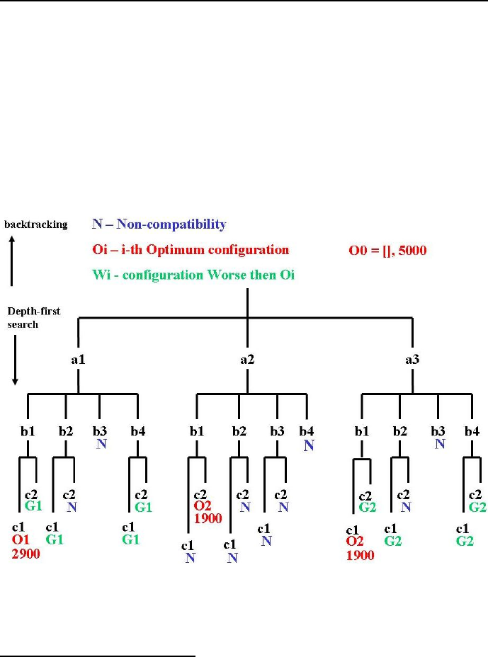
2.3 Optimum configuration problems 47
2.3 Optimum configuration problems
2.3.1 Branch-and-bound for optimum configuration
Quite often we are interested in finding only an17 optimum configuration for
which the configuration price (considered to be the objective function) is min-
imized. This can be done by a slight modification of the 2_7_conf_es.pl pro-
gram that transforms it into a branch-and-bound search program. Branch-and-
bound performs also depth-first search with backtracking, but does it differently,
as shown in Figure 2.6.
Figure 2.6: Search tree for branch-and-bound search
The idea of branch-and-bound (which is a general method for finding optimum
17 There may be more than one optimum solution; Therefore we speak about an optimum
solution rather than the optimum solution.

48 Chapter 2. In the beginning was Prolog
solutions for combinatorial optimization problems) may be described as follows:
1. A provisional lower bound for the objective function and associated opti-
mum configuration is declared . This has been done by invoking a dynamic
data base optimum_configuration(Configuration,Price) and assert-
ing into it the initial lower bound, e.g. as optimum_configuration([],
5000). I.e. the initial provisional optimum configuration is an empty one
but quite expensive;
2. Next a depth-first search is started with constraints handled similarly as
for depth-first backtracking search, but additionally:
•all contracted states, for which the objective function is already larger
than for the provisional lower bound, are handled like unsatisfied
constraint, i.e. result in backtracking while the provisional lower
bound remains unchanged;
•all full states, for which the objective function is smaller or equal
than for the provisional lower bound, are used to update this bound,
which is followed by backtracking in order to search for (perhaps) a
yet better configuration.
3. The sequence of those steps is repeated for all branches of the search tree.
This most simple version of branch-and-bound will be further referred to as
standard. It is built into program 2_9_conf_opt.pl:
/*1*/ top:-
/*2*/ assert(optimum_configuration([],5000)),
/*3*/ fail.
/*4*/ top:-
/*5*/ member(A,[a1,a2,a3]),
/*6*/ member(B,[b1,b2,b3,b4]),
/*7*/ not(incompatibility([A,B])),
/*8*/ price(A,Price_A),
/*9*/ price(B,Price_B),
/*10*/ optimum_configuration(_,Smallest_price_so_far),
/*11*/ Price_AB is Price_A+Price_B,
/*12*/ Price_AB<Smallest_price_so_far,
/*13*/ member(C,[c1,c2]),
/*14*/ not(incompatibility([A,C])),
/*15*/ not(incompatibility([B,C])),
/*16*/ price(C,Price_C),

2.3 Optimum configuration problems 49
/*17*/ Price is Price_AB+Price_C,
/*18*/ update_optimum_configuration([A,B,C],Price),
/*19*/ fail.
/*20*/ top:-
/*21*/ write("The least expensive configuration is: "),nl,
/*22*/ optimum_configuration([A,B,C],Price),
/*23*/ write("Configuration("),write(A),write(","),
/*24*/ write(B),write(", "),write(C),write(")"),
/*25*/ write(" priced at "),write(Price), nl,
/*26*/ fail.
/*27*/ top:-
/*28*/ write("Those are all optimum configurations.").
/*29*/ update_optimum_configuration([A,B,C],Price):-
/*30*/ optimum_configuration(_,Smallest_price_so_far),
/*31*/ Smallest_price_so_far > Price,
/*32*/ retract_all(optimum_configuration(_,_)),
/*33*/ assert(optimum_configuration([A,B,C],Price)),!.
/*34*/ update_optimum_configuration([A,B,C],Price):-
/*35*/ optimum_configuration(_,Smallest_price_so_far),
/*36*/ Smallest_price_so_far = Price,
/*37*/ assert(optimum_configuration([A,B,C],Price)),!.
/*38*/ update_optimum_configuration(_,Price):-
/*39*/ optimum_configuration(_,Smallest_price_so_far),
/*40*/ Smallest_price_so_far<Price,!.
/*41*/ price(a1,1900). price(a2,750). price(a3,900).
/*42*/ price(b1,300). price(b2,500). price(b3,450).
/*43*/ price(b4,600). price(c1,700). price(c2,850).
/*44*/ incompatible(c1,a2).
/*45*/ incompatible(b2,c2).
/*46*/ incompatible(c2,b3).
/*47*/ incompatible(b4,a2).
/*48*/ incompatible(b3,a1).
/*49*/ incompatible(a3,b3).
/*50*/ incompatibility([X,Y]):- incompatible(X,Y),!.
/*51*/ incompatibility([X,Y]):- incompatible(Y,X),!.
The message generated by the program is:
The least expensive configuration is:

50 Chapter 2. In the beginning was Prolog
Configuration(a2,b1, c2) priced at 1900
Configuration(a3,b1, c1) priced at 1900
Those are all optimum configurations.
2.4 Assignment problems
2.4.1 Golfers
Problems with negative information (i.e. stating that something is not true)
may be quite cumbersome to solve, even if the negative information is scarce.
A good illustration of such problems is given by the following example18:
A foursome of golfers (Fred, Joe, Bob, Tom) is standing at a tee, in a line
from left to right. Each golfer wears different colored pants:
•one is wearing red pants;
•the golfer to Fred’s immediate right is wearing blue pants;
•Joe is second in line;
•Bob is wearing plaid pants;
•Tom isn’t in position one or four, and he isn’t wearing the hideous orange
pants.
In what order are the four golfers standing at the tee, and what color are
each golfer’s pants? This is a good opportunity to demonstrate ECLiPSemus-
cles!
The modeling starts with defining a number of private predicates. They may
be the following:
•conditions(Golfers_position,Golfers_name, Color_of_golfers_pants)
•all_positions_are_different(Position_1,Position_2,Position_3,Position_4)
•all_colors_are_different(Color_1, Color_2, Color_3,Color_4)
18 This FS-type problem has been first formulated and solved using the Jess Rule Engine
for the Java Platform, see [Friedman-Hill-03].

2.4 Assignment problems 51
•wearing_red_pants(Position_1, Pants_color_for_golfer_on_position_1,
Position_2, Pants_color_for_golfer_on_position_2,
Position_3, Pants_color_for_golfer_on_position_3,
Position_4, Pants_color_for_golfer_on_position_4)
•blue_pants_right_on_Fred(Position_1, Pants_color_for_golfer_on_position_1,
Position_2, Pants_color_for_golfer_on_position_2,
Position_3, Pants_color_for_golfer_on_position_3,
Position_4, Pants_color_for_golfer_on_position_4)
•colors(colors_name)
•position(positions_number).
They are used in the 2_10_golfers.pl program :
/*1*/ top:-
% Fred is standing somewhere (position P1) and has pants of some color (color C1):
/*2*/ conditions(P1,"Fred",C1),
% 3)Joe is second in line (position P2, color of pants C2):
/*3*/ conditions(P2, "Joe",C2),
/*4*/ P2 is 2,
% 4)Bob is wearing plaid pants (and stands at position P4):
/*5*/ conditions(P4, "Bob", C4),
/*6*/ C4 = plaid,
% 5)Tom isn’t in position one or four, and he isn’t
% wearing the hideous orange pants (stands at position P3 and has pants of color C3) :
/*7*/ conditions(P3,"Tom", C3),
/*8*/ C3 \== orange,
/*9*/ P3 =\= 2,
/*10*/ P3 =\= 4,
/*11*/ all_positions_are_different(P1, P2, P3, P4),
/*12*/ all_colors_are_different(C1, C2, C3, C4),
% 1)someone is wearing red pants:
/*13*/ wearing_red_pants(P1, C1, P2, C2, P3, C3, P4, C4),
% 2)the golfer to Fred’s immediate right is wearing blue pants:
/*14*/ blue_pants_right_on_Fred(P1, C1, P2, C2, P3, C3, P4, C4),
/*15*/ write("Fred is in position "),write(P1),
write(" and wears "),write(C1), write(" pants."),nl,
/*16*/ write("Joe is in position "), write(P2),
write(" and wears "),write(C2), write(" pants."),nl,
/*17*/ write("Tom is in position "), write(P3),
write(" and wears "),write(C3), write(" pants."),nl,

52 Chapter 2. In the beginning was Prolog
/*18*/ write("Bob is in position "), write(P4),
write(" and wears "),write(C4), write(" pants."),nl,nl,fail.
/*19*/ top:-
/*20*/ write("That is all!"),nl.
/*21*/ conditions(Number,_,Color) :-
/*22*/ position(Number),
/*23*/ color(Color).
/*24*/ wearing_red_pants(_,C1,_,_,_,_,_,_) :-
/*25*/ C1 = red,!.
/*26*/ wearing_red_pants(_,_,_,C2,_,_,_,_) :-
/*27*/ C2 = red,!.
/*28*/ wearing_red_pants(_,_,_,_,_,C3,_,_) :-
/*29*/ C3 = red,!.
/*30*/ wearing_red_pants(_,_,_,_,_,_,_,C4) :-
/*31*/ C4 = red,!.
/*32*/ blue_pants_right_on_Fred(P1,_,P2,C2,_,_,_,_) :-
/*33*/ P2 is P1 + 1,
/*34*/ C2 = blue,!.
/*35*/ blue_pants_right_on_Fred(P1,_,_,_,P3,C3,_,_) :-
/*36*/ P3 is P1 + 1,
/*37*/ C3 = blue,!.
/*38*/ blue_pants_right_on_Fred(P1,_,_,_,_,_,P4,C4) :-
/*39*/ P4 is P1 + 1,
/*40*/ C4 = blue,!.
/*41*/ all_positions_are_different(X1, X2, X3, X4) :-
/*42*/ X1 =\= X2, X1 =\= X3, X1 =\= X4,
/*43*/ X2 =\= X3, X2 =\= X4, X3 =\= X4.
/*44*/ all_colors_are_different(X1, X2, X3, X4) :-
/*45*/ X1 \== X2, X1 \== X3, X1 \== X4,
/*46*/ X2 \== X3, X2 \== X4, X3 \== X4.
/*47*/ color(orange).
/*48*/ color(blue).
/*49*/ color(red).
/*50*/ color(plaid).
/*51*/ position(1).
/*52*/ position(2).
/*53*/ position(3).
/*54*/ position(4).

2.4 Assignment problems 53
The solution is as follows:
Fred is in position 1 and wears orange pants.
Joe is in position 2 and wears blue pants.
Tom is in position 3 and wears red pants.
Bob is in position 4 and wears plaid pants.
2.4.2 Three cubes
Determining attributes for items described by different types of attributes is
sometimes problem-ridden. In the following example three cube sizes should
be determined while different cube attributes are disclosed such as number and
color19.
The three cubes are of different sizes (small, large, medium), of different
colors (black,grey, white) and have different numbers (1,2,3). It is known that:
(1) The large cube is brighter than the medium cube;
(2) The small cube has number 2;
(3) The number of the black cube is greater than the number on the white cube;
(4) The size of cube with number 3 is smaller than the size of the grey cube.
What are the sizes, colors and numbers of all cubes? To solve the problem the
following private predicates are defined:
•cube(Color, Size, Number),
•smaller_size(Smaller_size, Larger_size),
•brighter(Brighter_color, Darker_color).
The program solving the puzzle (2_11_three_cubes.pl) is as follows:
/*1*/ top:-
%(1) The large cube is brighter than the medium cube:
/*2*/ cube(Color_of_large_cube,large,Number_of_large_cube),
/*3*/ cube(Color_of_medium_cube,medium,Number_of_medium_cube),
/*4*/ brighter(Color_of_large_cube,Color_of_medium_cube),
%(2) The small cube has number 2:
/*5*/ cube(Color_of_small_cube,small,2),
19 This is an FS-type problem.

54 Chapter 2. In the beginning was Prolog
%(3) The number of the black cube is greater than the number on the white cube:
/*6*/ cube(black,_,Number_of_black_cube),
/*7*/ cube(white,_,Number_of_white_cube),
/*8*/ Number_of_black_cube > Number_of_white_cube,
%(4) The size of cube with number 3 is smaller than the size of the grey cube:
/*9*/ cube(_,Size_3, 3),
/*10*/ cube(grey,Size_of_grey_cube,Number_of_grey_cube),
/*11*/ smaller_size(Size_3,Size_of_grey_cube),
% The numbers are different:
/*12*/ Number_of_grey_cube =\= Number_of_white_cube,
/*13*/ Number_of_grey_cube =\= Number_of_black_cube,
/*14*/ Number_of_white_cube =\= Number_of_black_cube,
/*15*/ 2 =\= Number_of_large_cube,
/*16*/ 2 =\= Number_of_medium_cube,
/*17*/ Number_of_large_cube=\=Number_of_medium_cube,
% The colors are different:
/*18*/ Color_of_large_cube\==Color_of_medium_cube,
/*19*/ Color_of_large_cube\==Color_of_small_cube,
/*20*/ Color_of_small_cube\==Color_of_medium_cube,
/*21*/ writeln("Color of_large_cube": Color_of_large_cube),
/*22*/ writeln("Number of_large_cube": Number_of_large_cube),nl,
/*23*/ writeln("Color of_medium_cube": Color_of_medium_cube),
/*24*/ writeln("Number of_medium_cube": Number_of_medium_cube),nl,
/*25*/ writeln("Color of_small_cube": Color_of_small_cube),
/*26*/ writeln("Number of_small_cube": "2"),nl.
/*27*/ cube(Color,Size,Number):-
/*28*/ member(Color,[black,grey, white]),
/*29*/ member(Size,[small, large, medium]),
/*30*/ member(Number,[1,2,3]).
/*31*/ smaller_size(small, large).
/*32*/ smaller_size(small, medium).
/*33*/ smaller_size(medium, large).
/*34*/ brighter(white,grey).
/*35*/ brighter(white,black).
/*36*/ brighter(grey,black).
The program generates following solution:
Color of_large_cube : grey
Number of_large_cube : 1

2.4 Assignment problems 55
Color of_medium_cube : black
Number of_medium_cube : 3
Color of_small_cube : white
Number of_small_cube : 2
2.4.3 Who is the killer?
A substantial difficulty while modeling problems in Prolog (or CLP) is the de-
sign of relevant private predicates. This is best seen for the next example, where
the private predicates chosen are far from obvious. They are of course not the
only choice that may be used for modeling the problem.
The following criminal puzzle20 has to be solved21:
Mike has been murdered. Alex, Ben and Colin are the only suspects. While
interrogated:
Alex said he is innocent, Ben was Mike’s friend but Colin hated Mike.
Ben said that he was out of town on the day of the murder, besides he didn’t
even know Mike.
Colin said he is innocent but he saw Alex and Ben with Mike just before the
murder.
Who killed Mark assuming that all except possibly the murderer are telling
the truth? The suspects’ statements are formalized using the private predicate:
statements_of_suspect(List_of_statements ).
The question is answered by program 2_12_who_killed.pl that uses the well-
known Sherlock Holmes principle: connect facts in a consistent system and the
solution follows.
/*1*/ top:-
/*2*/ find_murderer.
/*3*/ statements_of_Alex([innocent("Alex"),friends("Ben","Mike"),
hates("Colin","Mike")]).
20 This example is from http://www.binding-time.co.uk/whodunit.html
21 This is an FS-type problem.

56 Chapter 2. In the beginning was Prolog
/*4*/ statements_of_Ben([alibi("Ben"),did_not_know("Ben","Mike")]).
/*5*/ statements_of_Colin([innocent("Colin"),together("Colin","Mike"),
together("Ben","Mike"),together("Alex","Mike")]).
/*6*/ find_murderer:-
/*7*/ statements_of_Alex(Statements_of_Alex),
/*8*/ statements_of_Ben(Statements_of_Ben),
/*9*/ statements_of_Colin(Statements_of_Colin),
/*10*/ consistent_statements(Statements_of_Ben,Statements_of_Colin),
/*11*/ inconsistent_statements(Statements_of_Alex,Statements_of_Ben),
/*12*/ inconsistent_statements(Statements_of_Alex,Statements_of_Colin),
/*13*/ write("Alex is the murderer."),nl,!.
/*14*/ find_murderer:-
/*15*/ statements_of_Alex(Statements_of_Alex),
/*16*/ statements_of_Ben(Statements_of_Ben),
/*17*/ statements_of_Colin(Statements_of_Colin),
/*18*/ consistent_statements(Statements_of_Alex,Statements_of_Colin),
/*19*/ inconsistent_statements(Statements_of_Alex,Statements_of_Ben),
/*20*/ inconsistent_statements(Statements_of_Ben,Statements_of_Colin),
/*21*/ write("Ben is the murderer."),nl,!.
/*22*/ find_murderer:-
/*23*/ statements_of_Alex(Statements_of_Alex),
/*24*/ statements_of_Ben(Statements_of_Ben),
/*25*/ statements_of_Colin(Statements_of_Colin),
/*26*/ consistent_statements(Statements_of_Alex,Statements_of_Ben),
/*27*/ inconsistent_statements(Statements_of_Alex,Statements_of_Colin),
/*28*/ inconsistent_statements(Statements_of_Ben,Statements_of_Colin),
/*29*/ write("Colin is the murderer."),nl,!.
/*30*/ consistent_statements(Statement_1,Statement_2):-
/*31*/ not(inconsistent_statements(Statement_1,Statement_2)).
/*32*/ inconsistent_statements(Statement_1,Statement_2):-
/*33*/ cartesian_product(Statement_1,Statement_2,Cartesian_product),
/*34*/ test_pairwise_inconsistency(Cartesian_product).
/*35*/ cartesian_product([], _, []).
/*36*/ cartesian_product([H|T], L, M) :-
/*37*/ generate_pairs(H,L,M1),
/*38*/ cartesian_product(T, L, M2),
/*39*/ append(M1, M2, M).
/*40*/ generate_pairs(_, [], []).
/*41*/ generate_pairs(A, [B|L], [[A,B]|N] ) :-
/*42*/ generate_pairs(A, L, N).
/*43*/ test_pairwise_inconsistency([[H1,H2]|T]):-

2.4 Assignment problems 57
/*44*/ not(inconsistent_pairs(H1,H2)),
/*45*/ test_pairwise_inconsistency(T).
/*46*/ test_pairwise_inconsistency([[H1,H2]|_]):-
/*47*/ inconsistent_pairs(H1,H2),
/*48*/ !.
/*49*/ inconsistent_pairs(P1,P2):-
/*50*/ inconsistency([P1,P2]).
/*51*/ inconsistent_pairs(P1,P2):-
/*52*/ inconsistency([P2,P1]).
/*53*/ inconsistency([hates("Ben","Mike"),friends("Ben","Mike")]).
/*54*/ inconsistency([friends("Ben","Mike"),did_not_know("Ben","Mike")]).
/*55*/ inconsistency([together("Ben","Mike"),did_not_know("Ben","Mike")]).
/*55*/ inconsistency([friends("Colin","Mike"),hates("Colin","Mike")]).
/*56*/ inconsistency([innocent("Alex"),guilty("Alex")]).
/*57*/ inconsistency([innocent("Colin"),guilty("Colin")]).
/*58*/ inconsistency([alibi("Ben"),together("Ben","Mike")]).
/*59*/ inconsistency([alibi("Ben"),guilty("Ben")]).
/*60*/ inconsistency([alibi("Colin"),together("Colin","Mike")]).
The solution is:
Ben is the murderer.
2.4.4 Placing queens - defining variables
The queens placement problem22 is a favorite AI benchmark: it aims at finding
all placements of Nqueens on an N×Nchessboard in a way that no single
queen must be able to attack the other23. As often happens in Prolog,the
way variables are defined is crucial for the search effectiveness. For an 8 ×8
chessboard, variables are defined by the list:
[X1,X2,...,Xi,...,X8]
where Xi is the number of the chessboard row, for which the queen is placed in
the ith column. This definition alone satisfies two constraints:
1. No two queens will ever appear in the same column because each list
position is unique.
22 This is an FS-type problem.
23 Advanced cases of the benchmark operate for chessboards accommodating hundreds of
queens.

58 Chapter 2. In the beginning was Prolog
2. No two queens will ever appear in the same row provided the 8-tuple
X1,X2,...,X8 is equal to a permutation of the 8-tuple 1,2,3,4,5,6,7,8.
2.4.5 Exhaustive search for queens
To program exhaustive search for queens, following private predicate are intro-
duced:
•eight_queens([X1,X2,...,X8]) with argument given by the list of queens
is the main predicate.
•permutations(Permutation_List,Initial_List), which calculates con-
secutive permutations of the initial list [1,2,3,4,5,6,7,8].
•save([New_queen_to_be_placed|List_of_queens_already_placed]),
which is fulfilled if the new queen to be placed is not attacking any queen
on the list of already placed queens.
•no_attack(New_Queen_to_be_placed,List_of_queens_already_placed)
that initiates the checks of conflicts between the New_Queen_to_be_placed
and the List_of_queens_already_placed.
•no_attack(New_Queen_to_be_placed,List_of_queens_already_placed,
Shift_of_New_Queen_to_be_placed_on_the_diagonal)
that actually checks for the absence of conflicts for feasible shifts of the new
queen to consecutive columns along the upward and downward diagonal,
starting with shift 1.
The exhaustive search generates consecutively all permutations of the 8-tuple
1,2,3,4,5,6,7,8, and next checks, whether it corresponds to a safe placement.
This is done by the 2_13_queens_es.pl program:
/*1*/ top:-
/*2*/ all_solutions.
/*3*/ eight_queens([X1,X2,X3,X4,X5,X6,X7,X8]):-
/*4*/ permutations([X1,X2,X3,X4,X5,X6,X7,X8],[1,2,3,4,5,6,7,8]),
/*5*/ safe([X1,X2,X3,X4,X5,X6,X7,X8]).
/*6*/ permutations([],[]).
/*7*/ permutations([X|Xs],Ls):-
/*8*/ remove(X,Ls,Rs),
/*9*/ permutations(Xs,Rs).

2.4 Assignment problems 59
/*10*/ remove(X,[X|Xs],Xs).
/*11*/ remove(X,[Y|Ys],[Y|Rs]):-
/*12*/ remove(X,Ys,Rs).
/*13*/ safe([]).
/*14*/ safe([X|Xs]):-
/*15*/ no_attack(X,Xs),
/*16*/ safe(Xs).
/*17*/ no_attack(X,Xs):-
/*18*/ no_attack(X,Xs,1).
/*19*/ no_attack(_,[],_).
/*20*/ no_attack(X,[Y|Ys],Nb):-
/*21*/ X=\=Y-Nb,
/*22*/ X=\=Y+Nb,
/*23*/ Nb1 is Nb+1,
/*24*/ no_attack(X,Ys,Nb1).
/*25*/ all_solutions:-
/*26*/ eight_queens(X),
/*27*/ write(X),nl,
/*28*/ fail.
/*29*/ all_solutions:-
/*30*/ write("That’s all!").
There are 92 placements, from which only the first and last two are pre-
sented:
[1, 5, 8, 6, 3, 7, 2, 4]
[1, 6, 8, 3, 7, 4, 2, 5]
........................
[8, 3, 1, 6, 2, 5, 7, 4]
[8, 4, 1, 3, 6, 2, 7, 5]
That’s all!
The last but one placement is shown in Figure 2.7.
The exhaustive search tree for 8 trees is just too large to be presented.
Instead a smaller exhaustive search tree for 4 queens is shown in Figure 2.8.
2.4.6 Backtracking search for queens
Exhaustive search has an obvious shortcoming discussed already in Sections 1.2
and 2.2.2. Assume that already the placement of the first two queens is unsafe.
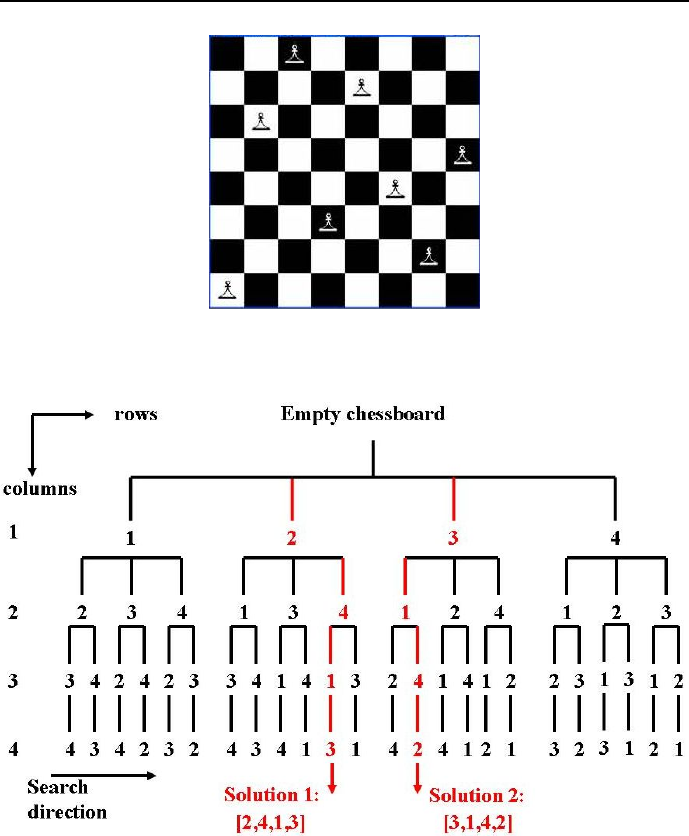
60 Chapter 2. In the beginning was Prolog
Figure 2.7: Last but one placement of 8 queens
Figure 2.8: Exhaustive search tree for 4 queens

2.4 Assignment problems 61
Then, instead canceling the last placement and returning to the nearest safe
placement, the placement of queens is continued, and only after all queens have
been placed, the safety of the placement is checked.
Exhaustive search could be improved upon by a following search strategy:
let the list [x1,x2,..xi] corresponds to a safe placement of the first iqueens.
Another queen is added to the list and a safety check is performed. If the
placement remains safe, yet another queen is added. If the safety check fails, a
return is initiated to such previous placement, for which some untested queen
choice is still possible. Such search strategy, recognized as depth-first search
with standard backtracking, is performed by the program 2_13_queens_bs.pl.
The search may be made yet more effective by noticing that the used modeling
of placements defined by the list:
[X1,X2,...,Xi,...,X8]
where Xi is the number of the chessboard row, for which the queen is placed in
the ith column, has yet another important benefits. It is, by its very nature,
fulfilling two constraints:
1. No two queens will ever be placed in the same column, because any Xi
occupies the unique ith position in the list.
2. No two queens will ever be placed in the same row, because the value of
any Xi is uniquely determined from a list of integers [1,2,3,4,5,6,7,8].
So search for safe placements has to be done only along the upward and down-
ward diagonal of the chessboard.
To program depth-first search with backtracking for queens, following private
predicate are introduced:
•queens(List_of_queens_added_to_queens_placed,
List_of_queens_already_placed,
List_of_available_queens)
that is extracting queens from the List_of_available_queens using vari-
ables from the List_of_queens_added_to_queens_placed and testing
safety for the chosen queen to be added. Only if the new placement would
be safe, the chosen queen is actually added to the List_of_queens_already
_placed.
•no_attack/2 has been defined in Section 2.4.5.
•no_attack/3 has been defined in Section 2.4.5.

62 Chapter 2. In the beginning was Prolog
•remove(Head,[Head|Tail],Tail) that removes the Head of the list
[Head|Tail] returning Tail.
The program 2_14_queens_bs.pl is as follows:
/*1*/ top:-
/*2*/ all_solutions.
/*3*/ eight_queens(X):-
/*4*/ queens(X,[],[1,2,3,4,5,6,7,8]).
/*5*/ queens([],_,[]).
/*6*/ queens([X|Xs],Placed,List_of_available_queens):-
/*7*/ remove(X,List_of_available_queens,New_list_of_available_queens),
/*8*/ no_attack(X,Placed),
/*9*/ queens(Xs,[X|Placed],New_list_of_available_queens).
/*10*/ remove(X,[X|Xs],Xs).
/*11*/ remove(X,[Y|Ys],[Y|Rs]):-
/*12*/ remove(X,Ys,Rs).
/*13*/ no_attack(X,Placed):-
/*14*/ no_attack(X,Placed,1).
/*15*/ no_attack(_,[],_).
/*16*/ no_attack(X,[Y|Ys],Nb):-
/*17*/ X=\=Y-Nb,
/*18*/ X=\=Y + Nb,
/*19*/ Nb1 is Nb + 1,
/*20*/ no_attack(X,Ys,Nb1).
/*21*/ all_solutions:-
/*22*/ eight_queens(X),
/*23*/ write(X),nl,
/*24*/ fail.
/*25*/ all_solutions:-
/*26*/ write("That’s all!").
The message generated by this program is the same as for the 2_13_queens_es.pl
program.
The recursive beauty of the definitions for no_attack/3 and queens/3 is
worth contemplating for a while. The role of variable Xfor determining the
queen to be added is worth noting: if the no_attack/2 predicate in line /*8*/
fails, backtracking is performed to line /*7*/ where a new value Xis picked from
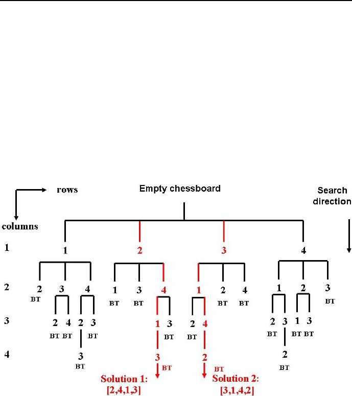
2.4 Assignment problems 63
the List_of_available_ queens. The new queens row position Xis checked
against consecutively placed queens for consecutively shifting columns alongside
the upward and downward diagonal in line /*8*/. Notice also in line /*9*/ how
the approved Xis added as head of a list of queens already placed.
The same reason as given for exhaustive search makes it impossible to picture
the depth-first backtracking search tree for /*8*/ queens. Instead a more simple
case for 4 queens is illustrated by Figure 2.9. Obviously, depth-first backtracking
search is again more effective than exhaustive search: instead of 24 leaves, the
tree has now only 18 leaves.
Figure 2.9: Depth-first backtracking search for 4 queens.
Additionally an animation of search for this search tree is shown in Figures
2.10 and 2.11, where the abbreviation BT means BackTrack.
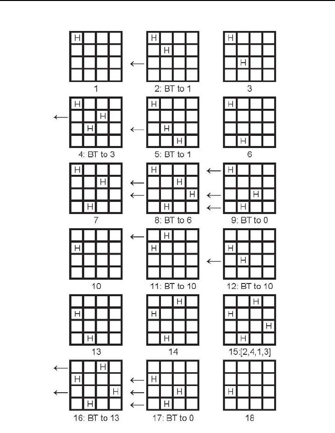
64 Chapter 2. In the beginning was Prolog
Figure 2.10: Animation of search for 4 queens search tree, part 1
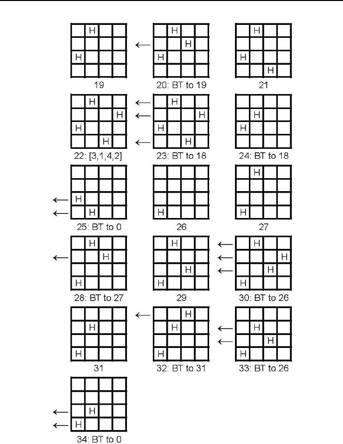
2.4 Assignment problems 65
Figure 2.11: Animation of search for 4 queens search tree, part 2
66 Chapter 2. In the beginning was Prolog
2.4.7 Examination - backtracking search
Quite often puzzles are saturated with negative knowledge i.e. knowledge about
what should not be done. Such puzzles present no special problem to Prolog as
shown by the following problem:
An examination room has 17 places arranged as shown in Table 2.8.
M1 M2 M3 M4
M5 M6 M7 M8 M9
M10 M11 M12 M13 M14
M15 M16 M17
Table 2.8: Examination room layout
This room will be used for a written examination taken by 17 students who
are expected to solve problems in one of four different examination papers,
numbered 1,2,3and 4. The teaching staff wants to secure themselves against
cheating. So students writing the same paper had to be completely isolated from
each other - so much so that their places were not adjacent in any way (hori-
zontally, vertically or at corners). How to distribute the papers among places
to achieve this? Could it be done if there were only three different examination
papers24?
The first question is answered by program 2_15_exzamination.pl:
/*0*/ top:-
/*1*/ L=[1,2,3,4],
/*2*/ member(M1,L), /*3*/ member(M2,L),
/*4*/ member(M3,L), /*5*/ member(M4,L),
/*6*/ member(M5,L), /*7*/ member(M6,L),
/*8*/ member(M7,L), /*9*/ member(M8,L),
/*10*/ member(M9,L), /*11*/ member(M10,L),
/*12*/ member(M11,L), /*13*/ member(M12,L),
/*14*/ member(M13,L), /*15*/ member(M14,L),
/*16*/ member(M15,L), /*17*/ member(M16,L),
/*18*/ member(M17,L),
/*19*/ M1 =\= M2, /*20*/ M1 =\= M5,
/*21*/ M1 =\= M6, /*22*/ M1 =\= M7,
/*23*/ M2 =\= M6, /*24*/ M2 =\= M7,
24 This is an FS-type problem.

2.4 Assignment problems 67
/*25*/ M2 =\= M3, /*26*/ M2 =\= M8,
/*27*/ M3 =\= M7, /*28*/ M3 =\= M8,
/*29*/ M3 =\= M9, /*30*/ M3 =\= M4,
/*31*/ M4 =\= M8, /*32*/ M4 =\= M9,
/*33*/ M5 =\= M6, /*34*/ M5 =\= M10,
/*35*/ M5 =\= M11, /*36*/ M6 =\= M10,
/*37*/ M6 =\= M11, /*38*/ M6 =\= M7,
/*39*/ M6 =\= M12, /*40*/ M7 =\= M11,
/*41*/ M7 =\= M12, /*42*/ M7 =\= M8,
/*43*/ M7 =\= M13, /*44*/ M8 =\= M12,
/*45*/ M8 =\= M13, /*46*/ M8 =\= M14,
/*47*/ M8 =\= M9, /*48*/ M9 =\= M13,
/*49*/ M9 =\= M14, /*50*/ M10 =\= M11,
/*51*/ M11 =\= M15, /*52*/ M11 =\= M12,
/*53*/ M12 =\= M15, /*54*/ M12 =\= M16,
/*55*/ M12 =\= M13, /*56*/ M13 =\= M15,
/*57*/ M13 =\= M16, /*58*/ M13 =\= M17,
/*59*/ M13 =\= M14, /*60*/ M14 =\= M16,
/*61*/ M14 =\= M17, /*62*/ M15 =\= M16,
/*63*/ M16 =\= M17,
/*64*/ write(" "),write(M1),write(", "), write(M2),
write(", "),write(M3),write(", "), write(M4),nl,
/*65*/ write(M5),write(", "),write(M6),write(", "), write(M7),
write(", "),write(M8),write(", "), write(M9),nl,
/*66*/ write(M10),write(", "),write(M11),write(", "), write(M12),
write(", "), write(M13),write(", "), write(M14),nl,
/*67*/ write(" "),write(M15),write(", "), write(M16),
write(", "),write(M17), nl.
One possible solution is as follows:
1, 2, 1, 2
2, 3, 4, 3, 4
4, 1, 2, 1, 2
3, 4, 3
It took quite a long time (203 seconds on a na 2.0 GHz notebook running
under Windows XP). In Section 3.7.4 another more efficient way to solve the
problem as CLP problem will be presented.

68 Chapter 2. In the beginning was Prolog
It is easy to show that for three different examination papers there is no
feasible assignment of papers to places: it suffices to change the lists in lines
/*2*/,...,/*18*/ for [1,2,3] to get the message No. The discussed problem is a
demonstration of the famous four color theorem, which states that the minimum
number of colors needed to color any planar map (or nodes of a corresponding
planar graph), in a way that all adjacent colors are different, is four25.
2.4.8 Paradoxes in Prolog
A paradox is a self-contradictory or counter-intuitive statement or argument
in logic. Most often it cannot be true but also cannot be false. Consider the
famous Bertrand Russel barber paradox : a small-town barber is ordered to shave
all those male inhabitants, and those only, who do not shave themselves. The
question is, may the barber shave himself?
It can be shown that whatever does the barber, the imposed order is violated:
•if he shaves himself then, as a shaving himself male inhabitant, he should
not be shaved by the barber, i.e. by himself;
•if he does not shave himself then, as a not shaving himself male inhabitant,
he should be shaved by the barber i.e. by himself.
So we have a vicious circle: it results because the barber is also this small-town
inhabitant. Any barber coming from a neighborhood town could easily shave
himself or use the services provided by the small-town barber.
Any attempt to solve this paradox using Prolog is bound to lead to stack overflow
no matter how large the stack. This is illustrate by program 2_16_barber.pl:
/*1*/ top:-
/*2*/ shaves(barber,barber).
/*3*/ shaves(barber,X):-
/*4*/ not(shaves(X,X)).
25 It is interesting to know that this apparently simple theorem resisted a long series of at-
tempts to prove it using mathematics. It finally succumbed to a computer-assisted proof (sort
of exhaustive search), which demonstrated the non-existence of plenary graphs that would
need five colors to color them in the sense of the theorem, see [Lines-92]. The mathematicians
weren’t quite happy about it.

2.4 Assignment problems 69
The message generated is:
Overflow of the local/control stack!
You can use the "-l kBytes" (LOCALSIZE) option to have a larger stack.
Peak sizes were: local stack 40384 kbytes, control stack 90688 kbytes
The stack overflow is caused because to satisfy the predicate shaves(barber,
barber), the negated predicate not(shaves(barber,barber)) has to be satis-
fied, but to achieve this the predicate shaves(barber,barber) has to fail, and
a backtrack occurs to line /*3*/, etc. etc., the viciousness is there. What’s
more, any backtrack to the predicate shaves(barber,barber) is accompanied
by saving some information on the internal Prolog stack that sooner or latter
is overfilled. The advice provided automatically for such cases about increasing
the stack sizes is - for the discussed situation - entirely inadequate.
It may be added that the rule in lines /*3*/ and /*4*/ is not a recursive
Prolog rule, because it is not defined between a list ( in the head of the recursive
rule) and the tail of this list (in the body of the recursive rule).
Because Prolog (exactly like human reasoning) is powerless against vicious
circles resulting from paradoxes, they should be avoided exactly like avoiding
division by 0. A consolations is provided by the circumstance that properly
and completely defined real-world problems are free of vicious circles. E.g. if
the problem was: 1)The barber shaves himself, and 2)The barber shaves all
remaining small-town male inhabitants who do not shave themselves, then -
contrasted with intellectual puns - no vicious circle will appear.
2.4.9 How to become your own grandfather?
Nicklaus Wirth in his popular textbook [Wirth-75] presented the following story
(sometimes attributed also to Mark Twain) of a man complaining about the
wretchedness of his life26:
I married a widow with a grown daughter. My father, who visited us fre-
quently, fell in love with the daughter and took her as his wife. This made my
father my adopted son, and my adopted daughter became my stepmother.
After a year my wife gave birth to a son, who became the adopted brother
26 This is an FS-type problem.

70 Chapter 2. In the beginning was Prolog
of my father and at the same time my uncle, since he was my stepmother’s
brother.
But my father’s wife, i.e. my adopted daughter, also gave birth to a son. So
this was my brother and also my grandson, since he was the son of my daughter.
This meant I’d married my grandmother, since she was the mother of my
mother. As my wife’s husband, I was also her adopted grandson.
Our friends say that I am my own grandfather, Is it true?
Let’s prove it using Prolog under assumption that an adopted family rela-
tion is to be treated as a normal one, e.g. adopted daughter = daughter,adopted
brother = brother, etc. The following order of arguments is assumed for private
predicates:
father(Father,Son),
mother(Mother,Son/Daughter),
grandfather(Grandfather,Grandson),
grandmother(Grandmother,Grandson),
brother(Father,Brother_1,Brother_2),
uncle(Father,Uncle,Nephew).
The program (2_17_grandfather.pl) is as follows:
/*1*/ top:-
% My and my_wifes son is the adopted brother of my father:
/*2*/ brother(_,my_father,my_and_my_wifes_son),
% My and my_wifes son is my uncle:
/*3*/ uncle(my_and_my_wifes_son,my_father,me),
% Son of my adopted_daughter is my brother:
/*4*/ brother(_,son_of_my_adopted_daughter,me),
% Son of my adopted_daughter is my grandson:
/*5*/ grandfather(me,son_of_my_adopted_daughter),
% my wife is my grandmother;
/*6*/ grandmother(my_wife,me),
% I am my own grandfather:
/*7*/ grandfather(me,me),nl,

2.4 Assignment problems 71
/*8*/ write("Everything is O.K.").
/*9*/ grandfather(Grandfather,Grandson):-
/*10*/ father(Grandfather,Grandfathers_son),
/*11*/ father(Grandfathers_son,Grandson).
/*12*/ grandmother(Grandmother,Grandson):-
/*13*/ mother(Grandmother,Grandmothers_daughter),
/*14*/ mother(Grandmothers_daughter,Grandson).
% I am the son of my father:
/*15*/ father(my_father,me).
% my father is my adopted son:
/*16*/ father(me,my_father).
% I am the father of my wife’s son:
/*17*/ father(me,my_and_my_wifes_son).
% my father is the father of the son of my adopted_daughter:
/*18*/ father(my_father,son_of_my_adopted_daughter).
% My adopted_daughter is my stepmother:
/*19*/ mother(my_adopted_daughter,me).
% My wife is the mother of my adopted daughter:
/*20*/ mother(my_wife,my_adopted_daughter).
/*21*/ brother(Father,Brother_1,Brother_2):-
/*22*/ father(Father,Brother_1),
/*23*/ father(Father,Brother_2).
/*24*/ uncle(Father,Uncle,Nephew):-
/*25*/ brother(_,Father,Uncle),
/*26*/ father(Uncle,Nephew).
The message generated is
Everything is O.K.
meaning that all postulated family relations are true.
2.4.10 Using conditional predicates
The basic conditional built-in:
+Condition -> +Then ; +Else.
has following properties:

72 Chapter 2. In the beginning was Prolog
•First Condition is called and if it succeeds any further solutions of Condi-
tion are cut and Then is called. Else is never called in this case regardless
of the outcome of Then.
•If Condition fails, Else is called. In this case, Then is never called.
In Prolog programs for Else often stands True with obvious meaning. The
predicate may be used to simplify some Prolog programs as shown by the ex-
ample:
Andrew, Barbara and Christopher have decided to attend some extracurri-
cular lectures. Each one choose a different lecture, in different days, on different
hours, namely:
1) Andrew will attend the lecture by Professor Paul.
2) Tuesdays lecture does not start at 2:00 p.m.
3) The lecture on ”Knowledge engineering” does not start at 5:30 p.m.
4) Thursdays lecture start at 3:45 p.m.
5) Christopher will attend the lecture on ”Econometric models”.
6) Barbara would like to attend the Tuesday lecture.
7) The lecture on ”Artificial Intelligence” is delivered in Building D3.
8) Wednesdays lecture are delivered in Room 104.
9) Professor Smith is not delivering the lecture ”Econometric models”.
10)Professor Jones is not delivering his lecture in Room K2.
A program that determines who will attend which lecture, where, when and
delivered by whom, is given by 2_25_lectures.pl:
/*1*/ top:-
/*2*/ students(Name_1,Name_2,Name_3),
/*3*/ lectures(Lecture_1,Lecture_2,Lecture_3),
/*4*/ professors(Professor_1,Professor_2,Professor_3),
/*5*/ rooms(Room_1,Room_2,Room_3),
/*6*/ days(Day_1,Day_2,Day_3),
/*7*/ hours(Hour_1,Hour_2,Hour_3),
/*8*/ constraints(Name_1,Lecture_1,Professor_1,Room_1,Day_1,Hour_1),
/*9*/ constraints(Name_2,Lecture_2,Professor_2,Room_2,Day_2,Hour_2),
/*10*/ constraints(Name_3,Lecture_3,Professor_3,Room_3,Day_3,Hour_3),
/*11*/ write(Name_1),write(" will attend a lecture on "),write(Lecture_1),
write(" by Professor "),write(Professor_1), write(" in Room "),
write(Room_1), write(" on "), write(Day_1), write(" at "),
write(Hour_1), nl,

2.4 Assignment problems 73
/*12*/ write(Name_2),write(" will attend a lecture on "),write(Lecture_2),
write(" by Professor "),write(Professor_2), write(" in Room "),
write(Room_2), write(" on "), write(Day_2), write(" at "),
write(Hour_2),nl,
/*13*/ write(Name_3),write(" will attend a lecture on "),write(Lecture_3),
write(" by Professor "),write(Professor_3), write(" in Room "),
write(Room_3), write(" on "), write(Day_3), write(" at "),
write(Hour_3),nl.
/*14*/ students(Name_1,Name_2,Name_3):-
/*15*/ name(Name_1),
/*16*/ name(Name_2),
/*17*/ name(Name_3),
/*18*/ all_different(Name_1,Name_2,Name_3).
/*19*/ lectures(Lecture_1,Lecture_2,Lecture_3):-
/*20*/ lecture(Lecture_1),
/*21*/ lecture(Lecture_2),
/*22*/ lecture(Lecture_3),
/*23*/ all_different(Lecture_1,Lecture_2,Lecture_3).
/*24*/ professors(Professor_1,Professor_2,Professor_3):-
/*25*/ professor(Professor_1),
/*26*/ professor(Professor_2),
/*27*/ professor(Professor_3),
/*28*/ all_different(Professor_1,Professor_2,Professor_3).
/*29*/ rooms(Room_1,Room_2,Room_3):-
/*30*/ room(Room_1),
/*31*/ room(Room_2),
/*32*/ room(Room_3),
/*33*/ all_different(Room_1,Room_2,Room_3).
/*34*/ days(Day_1,Day_2,Day_3):-
/*35*/ day(Day_1),
/*36*/ day(Day_2),
/*37*/ day(Day_3),
/*38*/ all_different(Day_1,Day_2,Day_3).
/*39*/ hours(Hour_1,Hour_2,Hour_3):-
/*40*/ hour(Hour_1),
/*41*/ hour(Hour_2),
/*42*/ hour(Hour_3),
/*43*/ all_different(Hour_1,Hour_2,Hour_3).
/*44*/ constraints(Name,Lecture,Professor,Room,Day,Hour):-
/*45*/ ( (Name == "Andrew")-> Professor = "Paul"
/*46*/ ; true ),

74 Chapter 2. In the beginning was Prolog
/*47*/ ( (Day == "Tuesday")-> Hour \== "2:00 p.m."
/*48*/ ; true ),
/*49*/ ( ( Lecture == "Knowledge Engineering")-> Hour \== "5:30 p.m."
/*50*/ ; true ),
/*51*/ ( ( Day == "Thursday")-> Hour = "3:45 p.m."
/*52*/ ; true ),
/*53*/ ( ( Name == "Christopher")-> Lecture = "Econometric Models"
/*54*/ ; true ),
/*55*/ ( ( Name == "Barbara") -> Day = "Tuesday"
/*56*/ ; true ),
/*57*/ ( ( Lecture == "Artificial Intelligence") -> Room = "D3"
/*59*/ ; true ),
/*59*/ ( ( Day == "Wednesday") -> Room \== "104"
/*60*/ ; true ),
/*61*/ ( ( Professor == "Smith") -> Lecture \== "Econometric Models"
/*62*/ ; true ),
/*63*/ ( ( Professor == "Jones") -> Room \== "K2"
/*64*/ ; true ).
/*65*/ all_different(Variable_1,Variable_2,Variable_3):-
/*66*/ Variable_1 \== Variable_2,
/*67*/ Variable_1 \== Variable_3,
/*68*/ Variable_2 \== Variable_3.
/*69*/ name("Andrew").
/*70*/ name("Barbara").
/*71*/ name("Christopher").
/*72*/ lecture("Knowledge Engineering").
/*73*/ lecture("Econometric Models").
/*74*/ lecture("Artificial Intelligence").
/*75*/ professor("Paul").
/*76*/ professor("Smith").
/*77*/ professor("Jones").
/*78*/ room("D3").
/*79*/ room("104").
/*80*/ room("K2").

2.5 Sequencing problems 75
/*81*/ day("Tuesday").
/*82*/ day("Wednesday").
/*83*/ day("Thursdays").
/*84*/ hour("2:00 p.m.").
/*85*/ hour("5:30 p.m.").
/*86*/ hour("3:45 p.m.").
The solution is:
Andrew will attend a lecture on Knowledge Engineering by
Professor Paul in Room K2 on Wednesday at 2:00 p.m.
Barbara will attend a lecture on Artificial Intelligence by
Professor Smith in Room D3 on Tuesday at 5:30 p.m.
Christopher will attend a lecture on Econometric Models by
Professor Jones in Room 104 on Thursdays at 3:45 p.m.
2.5 Sequencing problems
2.5.1 Farmer-wolf-goat-cabbage
This popular puzzle is a nice example of finding trajectories in the state space:
A farmer is standing on the west side of the river and with him are a wolf,
a goat and a cabbage. In the river there is a small boat. The farmer wants to
cross the river with all the three items that are with him. There are no bridges
and in the boat there is only room for the farmer and one item. However, the
crossings are danger-ridden:
•If the farmer leaves the goat with the cabbages alone on the same side of
the river, the goat will eat the cabbages.
•If the farmer leaves the wolf and the goat on the same side of the river,
the wolf will eat the goat.
Only the farmer can separate the wolf from the goat and the goat from the
cabbage. How can the farmer cross the river with all three items, without one
eating the other27?
27 This OST-type problem is attributed to Alcuin of York (730 - 804), an English scholar,
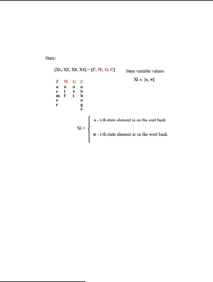
76 Chapter 2. In the beginning was Prolog
The first thing needed is to define a state that accumulates all data needed
to properly determine the next move. The state of the system farmer-wolf-goat-
cabbage is given by declaring their whereabouts, see Figure 2.12. While crossing
the river no state may appear twice.
Figure 2.12: State of the system farmer-wolf-goat-cabbage
The solution is given by program 2_18_fwgc.pl:
/*1*/ top:-
/*2*/ cross_the_river(state(w,w,w,w),state(e,e,e,e)).
/*3*/ cross_the_river(Initial_state,Final_state):-
/*4*/ feasible_crossing(Initial_state,Final_state,
[Initial_state],Final_sequence),nl,
/*5*/ reverse(Final_sequence,Final_sequence_r),
/*6*/ write_feasible_crossing(Final_sequence_r),
/*7*/ fail.
/*8*/ cross_the_river(_,_):- nl, write("Those are all solutions!").
/*9*/ feasible_crossing(Current_state,Final_state,
Final_sequence_accu,Final_sequence):-
/*10*/ crossing(Current_state,Next_state),
/*11*/ not(unsafe(Next_state)),
ecclesiastic, poet, mathematician and teacher from York, Northumbria. He wrote a textbook
Propositiones ad Acuendos Juvenes (in English: Problems to Sharpen the Young) containing
53 puzzles, some of them of the ”river crossing” type.

2.5 Sequencing problems 77
/*12*/ not(member(Next_state,Final_sequence_accu)),
/*13*/ feasible_crossing(Next_state,Final_state,
[Next_state|Final_sequence_accu],Final_sequence).
/*14*/ feasible_crossing(Final_state,Final_state,
Final_sequence,Final_sequence):- !.
% Farmer and wolf change river bank,
% goat and cabbage stay put in their places:
/*15*/ crossing(state(X,X,Go,Ca),state(Y,Y,Go,Ca)):-
/*16*/ opposite_banks(X,Y).
% Farmer and goat change river bank,
% wolf and cabbage stay put in their places:
/*17*/ crossing(state(X,W,X,Ca),state(Y,W,Y,Ca)):-
/*18*/ opposite_banks(X,Y).
% Farmer and cabbage change river bank,
% wolf and goat stay put in their places:
/*19*/ crossing(state(X,W,Go,X),state(Y,W,Go,Y)):-
/*20*/ opposite_banks(X,Y).
% Farmer only changes river bank,
% wolf, goat and cabbage stay put in their places:
/*21*/ crossing(state(X,W,Go,Ca),state(Y,W,Go,Ca)):-
/*22*/ opposite_banks(X,Y).
% Wolf and goat cannot be left with no farmers supervision:
/*23*/ unsafe( state(Y,X,X,_) ):-
/*24*/ opposite_banks(Y,X).
% Goat and cabbage cannot be left with no farmers supervision:
/*25*/ unsafe( state(Y,_,X,X) ):-
/*26*/ opposite_banks(Y,X).
/*27*/ opposite_banks(w,e).
/*28*/ opposite_banks(e,w).
/*29*/ write_feasible_crossing([H1,H2|T]) :-
/*30*/ write_crossing(H1,H2),
/*31*/ write_feasible_crossing([H2|T]).
/*32*/ write_feasible_crossing([_|[]]):-
/*33*/ writeln("All safely crossed the river.").
/*34*/ write_crossing(state(X,W,G,C), state(Y,W,G,C)):-
/*35*/ translate(X,X_translated),
/*36*/ translate(Y,Y_translated),
/*37*/ write("Farmer moves from "),write(X_translated),write(" to "),

78 Chapter 2. In the beginning was Prolog
write(Y_translated),write("."),nl.
/*38*/ write_crossing(state(X,X,G,C), state(Y,Y,G,C)):-
/*39*/ translate(X,X_translated),
/*40*/ translate(Y,Y_translated),
/*41*/ write("Farmer moves with wolf from "),write(X_translated),
write(" to "),write(Y_translated),write("."),nl.
/*42*/ write_crossing(state(X,W,X,C), state(Y,W,Y,C)) :-
/*43*/ translate(X,X_translated),
/*44*/ translate(Y,Y_translated),
/*45*/ write("Farmer moves with goat from "),write(X_translated),
write(" to "),write(Y_translated),write("."),nl.
/*46*/ write_crossing(state(X,W,G,X), state(Y,W,G,Y)) :-
/*47*/ translate(X,X_translated),
/*48*/ translate(Y,Y_translated),
/*49*/ write("Farmer moves with cabbage from "),write(X_translated),
write(" to "),write(Y_translated),write("."),nl.
/*50*/ translate(w,"west bank").
/*51*/ translate(e,"east bank").
There are two solutions to this problem. The first one is:
Farmer moves with goat from west bank to east bank.
Farmer moves from east bank to west bank.
Farmer moves with wolf from west bank to east bank.
Farmer moves with goat from east bank to west bank.
Farmer moves with cabbage from west bank to east bank.
Farmer moves from east bank to west bank.
Farmer moves with goat from west bank to east bank.
All safely crossed the river,
depicted on Figure 2.13.
As can be seen, the farmer must first take the goat across the river. He then
returns and picks up the wolf. He leaves the wolf off and takes the goat back
across the river with him. Then he leaves the goat at the starting point and
takes the cabbage over to where the wolf is. He returns and picks up the goat,
and then lands where the wolf and the cabbage are.
The second solution is:
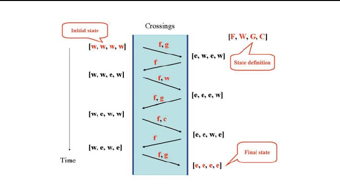
2.5 Sequencing problems 79
Figure 2.13: First solution river crossings for farmer, wolf, goat and cabbage
Farmer moves with goat from west bank to east bank.
Farmer moves from east bank to west bank.
Farmer moves with cabbage from west bank to east bank.
Farmer moves with goat from east bank to west bank.
Farmer moves with wolf from west bank to east bank.
Farmer moves from east bank to west bank.
Farmer moves with goat from west bank to east bank.
All safely crossed the river,
Those are all solutions!
It is depicted on Figure 2.14.
This time the farmer also starts with taking the goat across the river. He
then returns and picks up the cabbage. He leaves the cabbage off and takes the
goat back across the river with him. Then he leaves the goat at the starting
point and takes the wolf over to where the cabbage is. He returns and picks up
the goat, and then lands where the wolf and the cabbage are.
The program contains an interesting feature: the number of crossings is
implicitly minimized by demanding that no state ever appears twice. This is
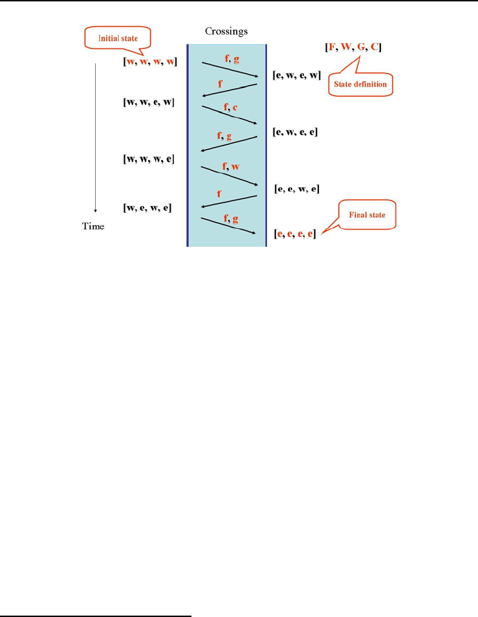
80 Chapter 2. In the beginning was Prolog
Figure 2.14: Second solution river crossings for farmer, wolf, goat and cabbage
done in line /*12*/: any new state Next_State may not belong to the list
Final_sequence_accu of states already accumulated. Unfortunately, this fea-
ture is only a fortuitous heuristics that just works for the example discussed,
but is not of general nature and does not work for all conceivable optimum state
trajectory problems.
2.5.2 Missionaries and cannibals
The missionaries and cannibals problem is a more complicated state trajectory
determination problem. It is usually stated as follows:
Three missionaries and three cannibals must cross a river using a boat that can
carry at most two people. The crossings must be done so that if on any bank
missionaries are present, they cannot be outnumbered by cannibals. Otherwise
the cannibals would eat the missionaries28. The state of the system is defined
in Figure 2.15.
The problem is solved by program 2_19_mac.pl. Its basic private predicates
28 Obviously, this is a politically incorrect puzzle. Those who object to its incorrectness
may easily formulate a politically correct version: if on any bank missionaries are present,
they must be outnumbered by cannibals, because otherwise the missionaries would convert
the cannibals.
2.5 Sequencing problems 81
Figure 2.15: State of the system missionaries-cannibals
are:
cross_the_river(Inital_state,Final_state,Boat_location)
feasible_crossing(Initial_state,Final_state,
Path_accumulator,Path,Boat_location)
The program is:
/*1*/ top:-
/*2*/ assert(counter(0)), % for counting solutions
/*3*/ cross_the_river(state(3,3,blb), state(0,0,brb),blb).
/*4*/ cross_the_river(Inital_state,Final_state,Boat_location):-
/*5*/ feasible_crossing(Inital_state,Final_state,[Inital_state],
Crossings,Boat_location), nl,
/*6*/ write_feasible_crossing(Crossings),
/*7*/ fail.
/*8*/ cross_the_river(_,_,_):-
/*9*/ write("Those are all solutions.").
/*10*/ feasible_crossing(Present_state,Final_state,Accu_of_crossings,
Crossings,Boat_location_before):-
/*11*/ crossing(Present_state,Next_state,Boat_location_before),
/*12*/ check_feasability(Next_state,Accu_of_crossings),
/*13*/ change_boat_location(Boat_location_before,Boat_location_after),
/*14*/ feasible_crossing( Next_state,Final_state,
[Next_state|Accu_of_crossings],Crossings,Boat_location_after).

82 Chapter 2. In the beginning was Prolog
% Final state reached:
/*15*/ feasible_crossing(Final_state,Final_state,Crossings,Crossings,_):- nl,
/*16*/ enumerate,
/*17*/ counter(Number_of_solutions),
/*18*/ write("Solution number "),write(Number_of_solutions),write(":"),nl,
/*19*/ write("Crossings = "),write(Crossings),nl.
% A single missionary moves to the right bank:
/*20*/ crossing(state(X,K,_),state(Y,K,brb),blb):-
/*21*/ Y is X-1.
% Two missionaries move to the right bank:
/*22*/ crossing(state(X,K,_),state(Y,K,brb),blb):-
/*23*/ Y is X-2.
% A single cannibal moves to the right bank:
/*24*/ crossing(state(M,X,_),state(M,Y,brb),blb):-
/*25*/ Y is X-1.
% Two cannibals move to the right bank:
/*26*/ crossing(state(M,X,_),state(M,Y,brb),blb):-
/*27*/ Y is X-2.
% A missionary and a cannibal move to the right bank:
/*28*/ crossing(state(X,X1,_),state(Y,Y1,brb),blb):-
/*29*/ Y is X-1,
/*30*/ Y1 is X1-1.
% Two missionaries move to the left bank:
/*31*/ crossing(state(X,K,_),state(Y,K,blb),brb):-
/*32*/ Y is X+2.
% A single missionary moves to the left bank:
/*33*/ crossing(state(X,K,_),state(Y,K,blb),brb):-
/*34*/ Y is X+1.
% A single cannibal moves to the left bank:
/*35*/ crossing(state(M,X,_),state(M,Y,blb),brb):-
/*36*/ Y is X+1.
% Two cannibals move to the left bank:
/*37*/ crossing(state(M,X,_),state(M,Y,blb),brb):-
/*38*/ Y is X+2.
% A missionary and a cannibal move to the left bank:
/*39*/ crossing(state(X,X1,_),state(Y,Y1,blb),brb):-
/*40*/ Y is X+1,

2.5 Sequencing problems 83
/*41*/ Y1 is X1+1.
/*42*/ check_feasability(S1,Crossings):-
/*43*/ not(unsafe(S1)),
/*44*/ not(unfeasible(S1)),
/*45*/ not(member(S1,Crossings)).
/*46*/ change_boat_location(brb,blb).
/*47*/ change_boat_location(blb,brb).
% On the left bank the cannibals will be in majority:
/*48*/ unsafe(state(M,K,_)):-
/*49*/ M>0,
/*50*/ M<K.
% On the right bank the cannibals will be in majority:
/*51*/ unsafe(state(M,K,_)):-
/*52*/ M<3,
/*53*/ K<M.
/*54*/ unfeasible( state(M,_,_)):-
/*55*/ M<0.
/*56*/ unfeasible(state(_,K,_)):-
/*57*/ K<0.
/*58*/ unfeasible(state(M,_,_)):-
/*59*/ M>3.
/*60*/ unfeasible(state(_,K,_)):-
/*61*/ K>3.
/*62*/ write_feasible_crossing([H1,H2|T]):-
/*63*/ write_crossing(H1,H2),
/*64*/ write_feasible_crossing([H2|T]).
/*65*/ write_feasible_crossing([_|[]]) :-
/*66*/ writeln("All safely crossed the river.").
/*67*/ write_crossing(state(X,K,_),state(Y,K,_)):-
/*68*/ Y is X+1,
/*69*/ write("A missionary moved from left bank to right bank."),nl.
/*70*/ write_crossing( state(M,X,_),state(M,Y,_)):-
/*71*/ Y is X+1,
/*72*/ write("A cannibal moved from left bank to right bank."),nl.
/*73*/ write_crossing(state(X,K,_),state(Y,K,_)):-
/*74*/ Y is X+2,

84 Chapter 2. In the beginning was Prolog
/*75*/ write("Two missionaries moved from left bank to right bank."),nl.
/*76*/ write_crossing(state(M,X,_),state(M,Y,_)):-
/*77*/ Y is X+2,
/*78*/ write("Two cannibals moved from left bank to right bank."),nl.
/*79*/ write_crossing(state(X,X1,_),state(Y,Y1,_)):-
/*80*/ Y is X+1,
/*81*/ Y1 is X1+1,
/*82*/ write("A missionary and a cannibal moved from left bank to "),
write("right bank."),nl.
/*83*/ write_crossing(state(X,K,_),state(Y,K,_)):-
/*84*/ Y is X-1,
/*85*/ write("A missionary moved from right bank to left bank."),nl.
/*86*/ write_crossing(state(M,X,_),state(M,Y,_)):-
/*87*/ Y is X-1,
/*88*/ write("A cannibal moved from right bank to left bank."),nl.
/*89*/ write_crossing(state(X,K,_),state(Y,K,_)):-
/*90*/ Y is X-2,
/*91*/ write("Two missionaries moved from right bank to left bank."),nl.
/*92*/ write_crossing(state(M,X,_),state(M,Y,_)):-
/*93*/ Y is X-2,
/*94*/ write("Two cannibals moved from right bank to left bank."),nl.
/*95*/ write_crossing(state(X,X1,_),state(Y,Y1,_)) :-
/*96*/ Y is X-1,
/*97*/ Y1 is X1-1,
/*98*/ write("A missionary and a cannibal moved from right bank to "),
write("left bank."),nl.
/*99*/ enumerate:-
/*100*/ retract(counter(Old)),
/*101*/ New is Old 1, +
/*102*/ assert(counter(New)).
The problem has 4 solutions:
Solution number 1:
Crossings = [state(0, 0, brb), state(1, 1, blb), state(0, 1, brb),
state(0, 3, blb), state(0, 2, brb), state(2, 2, blb),
state(1, 1, brb), state(3, 1, blb), state(3, 0, brb),
state(3, 2, blb), state(3, 1, brb), state(3, 3, blb)]
A missionary and a cannibal moved from left bank to right bank.
A missionary moved from right bank to left bank.

2.5 Sequencing problems 85
Two cannibals moved from left bank to right bank.
A cannibal moved from right bank to left bank.
Two missionaries moved from left bank to right bank.
A missionary and a cannibal moved from right bank to left bank.
Two missionaries moved from left bank to right bank.
A cannibal moved from right bank to left bank.
Two cannibals moved from left bank to right bank.
A cannibal moved from right bank to left bank.
Two cannibals moved from left bank to right bank.
All safely crossed the river.
Solution number 2:
Crossings = [state(0, 0, brb), state(0, 2, blb), state(0, 1, brb),
state(0, 3, blb), state(0, 2, brb), state(2, 2, blb),
state(1, 1, brb), state(3, 1, blb), state(3, 0, brb),
state(3, 2, blb), state(3, 1, brb), state(3, 3, blb)]
Two cannibals moved from left bank to right bank.
A cannibal moved from right bank to left bank.
Two cannibals moved from left bank to right bank.
A cannibal moved from right bank to left bank.
Two missionaries moved from left bank to right bank.
A missionary and a cannibal moved from right bank to left bank.
Two missionaries moved from left bank to right bank.
A cannibal moved from right bank to left bank.
Two cannibals moved from left bank to right bank.
A cannibal moved from right bank to left bank.
Two cannibals moved from left bank to right bank.
All safely crossed the river.
Solution number 3:
Crossings = [state(0, 0, brb), state(1, 1, blb), state(0, 1, brb),
state(0, 3, blb), state(0, 2, brb), state(2, 2, blb),
state(1, 1, brb), state(3, 1, blb), state(3, 0, brb),
state(3, 2, blb), state(2, 2, brb), state(3, 3, blb)]
A missionary and a cannibal moved from left bank to right bank.
A missionary moved from right bank to left bank.
Two cannibals moved from left bank to right bank.
A cannibal moved from right bank to left bank.
Two missionaries moved from left bank to right bank.
A missionary and a cannibal moved from right bank to left bank.
Two missionaries moved from left bank to right bank.
A cannibal moved from right bank to left bank.
Two cannibals moved from left bank to right bank.
A missionary moved from right bank to left bank.
A missionary and a cannibal moved from left bank to right bank.
All safely crossed the river.
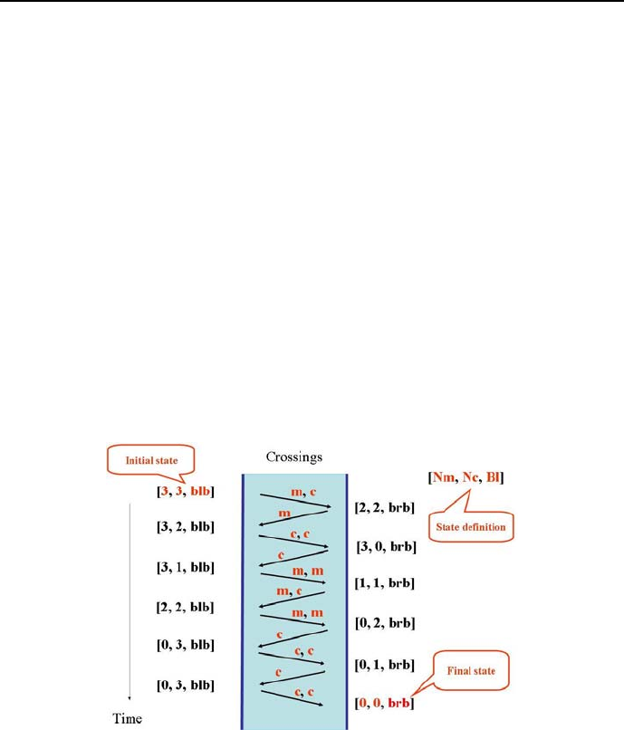
86 Chapter 2. In the beginning was Prolog
Solution number 4:
Crossings = [state(0, 0, brb), state(0, 2, blb), state(0, 1, brb),
state(0, 3, blb), state(0, 2, brb), state(2, 2, blb),
state(1, 1, brb), state(3, 1, blb), state(3, 0, brb),
state(3, 2, blb), state(2, 2, brb), state(3, 3, blb)]
Two cannibals moved from left bank to right bank.
A cannibal moved from right bank to left bank.
Two cannibals moved from left bank to right bank.
A cannibal moved from right bank to left bank.
Two missionaries moved from left bank to right bank.
A missionary and a cannibal moved from right bank to left bank.
Two missionaries moved from left bank to right bank.
A cannibal moved from right bank to left bank.
Two cannibals moved from left bank to right bank.
A missionary moved from right bank to left bank.
A missionary and a cannibal moved from left bank to right bank.
All safely crossed the river.
Those are all solutions.
Solution 1 is depicted on Figure 2.16.
Figure 2.16: River crossings for missionaries and canibals by solution 1
The general idea of missionaries and canibals is the same as for farmer-wolf-
goose-cabbage: to any sequence of states already visited (and present in the
accumulator) a new feasible state is added till the new state is equal to the final

2.5 Sequencing problems 87
state. As in Section 2.5.1, the number of river crossings is minimized implicitly
by demanding in line /*39*/ that no state may appear twice. As before, we
are fortunate that this heuristic leads to an optimum solution. Because of the
large number of solutions a counter has been added (see lines /*2*/,/*16*/,
/*17*/,/*99*/-/*102*/) to take care of the numbering.
2.5.3 Towers of Hanoi
Recursion was used for many predicates so far. Prolog people just love recursion
because of its succinctness and calculating power. A particularly convincing
argument for its virtues is given by the program solving the Towers of Hanoi
puzzle29. This puzzle is due to the French mathematician Edouard Lucas (1842-
1891). Lucas assumed the presence of three rods, onto any of them a number
of holed disks of different sizes can slide. The puzzle starts with the disks in a
stack of ascending order of diameters on one rod with the largest disk at the
bottom.
The goal is to move the entire stack disk-wise to another rod while fulfilling
the following constraints:
1. Only one disk may be moved at a time.
2. Each move consists of taking the top disk from some rod and sliding it
onto another rod.
3. No disk may be slid on top of a smaller disk.
Let’s consider the general case of Ndisks. To move Ndisks from their initial
left rod to their final right rod, it is necessary:
1. Move N−1 disks from the left rode to the middle rod using the final rod
as intermediary. Assume that it done in TN−1steps.
2. Move the last disk from the left rode to the right rode. Altogether TN−1+1
steps are needed.
Now the situation is similar to the initial one, before step 1was taken; the
difference is that now N−1 disks have to be moved from the middle rod to the
right rod using as intermediary rod left. This can be done also in TN−1steps.
All moves needed thus TN=2TN−1+ 1 steps. The difference equation:
TN=2TN−1+1
29 This is an FST-type problem.

88 Chapter 2. In the beginning was Prolog
has a solution equal to TN=2
N−1 which can be proved using mathematical
induction30.
A program solving the Tower of Hanoi puzzle (2_20_hanoi.pl)isasfollows:
/*1*/ top:-
/*2*/ write(" Declare number of disks: "),nl,
/*3*/ read_token(Number, integer),
/*4*/ write(Number),nl,
/*5*/ hanoi(Number).
/*6*/ hanoi(N) :-
/*7*/ move(N,"Left","Middle","Right").
% Move a single disk directly from
%/* position "Left" to position "Right":
/*8*/ move(1,A,_,C) :-
/*9*/ command(A,C).
% In order to move N disks from
% position "Left" to position "Right":
/*10*/ move(N,A,B,C) :-
/*12*/ N1 is N-1,
% move N-1 disks from position
% "Left" to position "Middle"
% using position "Right":
/*13*/ move(N1,A,C,B),
% move the last disk from position
% "Left" to position "Right":
/*14*/ command(A,C),
% move N-1 disks from position
% "Middle" to position "Right"
% using position "Left":
/*15*/ move(N1,B,A,C).
/*16*/ command(Position_1,Position_2):-
/*17*/ write("Move disk from position "),write(Position_1),
/*18*/ write(" to position "),write(Position_2),write(". "),nl.
The dialogue and message generated is as follows:
Declare number of disks: 3
Move disk from position Left to position Right.
Move disk from position Left to position Middle.
Move disk from position Right to position Middle.
30 For N=0isT(0) = 0. If for N−1isT(N−1) = 2N−1−1, then for T(N)=2TN−1+1 =
2(2N−1−1) + 1 = 2N−1.
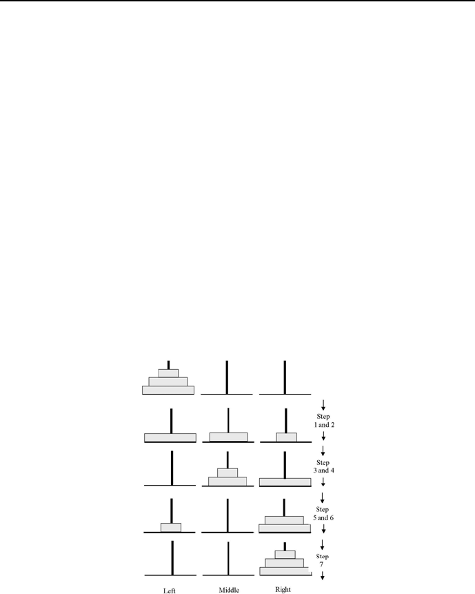
2.5 Sequencing problems 89
Move disk from position Left to position Right.
Move disk from position Middle to position Left.
Move disk from position Middle to position Right.
Move disk from position Left to position Right.
Unusual in this program is the double recursion: move(N,A,B,C) from line
/*11*/ is defined by move(N1,A,C,B) from line /*13*/ and move(N1,B,A,C)
from line /*15*/. Figure 2.17 shows the moves for 3 disks.
Lucas is supposed to enrich his 8-disc puzzle by a Tower of Brahma legend,
which states that Brahma, at the beginning of time, ordered a group of monks
to move 64 golden discs between 3diamond rods as described by the puzzle.
According to the legend, when the last move is completed, the end of the world
will occur. This legend gives justice to Lucas’ understanding of computational
complexity: assuming the monks will make a move each second, the moving of
a64-disk stack will take 264 −1 = 18446744073709551615 seconds, i.e. roughly
584 billion years to complete. Let us not forget that the estimate age of the
universe is roughly 13.7 billion years.
Figure 2.17: Tower of Hanoi solution for 3 disks

90 Chapter 2. In the beginning was Prolog
2.6 Optimum sequencing problems
2.6.1 A simple maze
The program 2_21_maze.pl finds the shortest path (measured by the number of
passed cells) from cell (0,0) to cell 6,6) for the maze from Figure 2.1831.Only
horizontal and vertical transitions between cells are feasible. To find the shortest
path, the branch-and-bound method used for finding optimum configurations
(see 2.3.1) has been applied.
Figure 2.18: A simple maze
The program 2_21_maze.pl is as follows:
/*1*/ top:-
/*2*/ assert(shortest_path([[]],80)),
/*3*/ maze.
/*4*/ from_to([0,0],[0,1]). /*5*/ from_to([0,1],[0,2]).
/*6*/ from_to([0,2],[0,3]). /*7*/ from_to([0,3],[0,4]).
/*8*/ from_to([0,4],[0,5]). /*9*/ from_to([0,5],[0,6]).
/*10*/ from_to([0,6],[1,6]). /*11*/ from_to([1,6],[2,6]).
/*12*/ from_to([0,4],[1,4]). /*13*/ from_to([1,4],[2,4]).
/*14*/ from_to([2,4],[3,4]). /*15*/ from_to([3,4],[4,4]).
/*16*/ from_to([0,1],[1,1]). /*17*/ from_to([1,1],[2,1]).
/*18*/ from_to([2,1],[2,2]). /*19*/ from_to([2,2],[2,3]).
/*20*/ from_to([2,3],[2,4]). /*21*/ from_to([4,4],[4,5]).
/*22*/ from_to([4,5],[4,6]). /*23*/ from_to([4,4],[4,3]).
/*24*/ from_to([4,3],[4,2]). /*25*/ from_to([4,2],[5,2]).
/*26*/ from_to([5,2],[6,2]). /*27*/ from_to([6,2],[6,1]).
/*28*/ from_to([6,1],[6,0]). /*29*/ from_to([6,0],[5,0]).
/*30*/ from_to([5,0],[4,0]). /*31*/ from_to([6,2],[6,3]).
31 This is an OST-type problem.

2.6 Optimum sequencing problems 91
/*32*/ from_to([6,3],[6,4]). /*33*/ from_to([6,4],[6,5]).
/*34*/ from_to([6,5],[6,6]).
/*35*/ transition(A,B):-
/*36*/ from_to(A,B).
/*37*/ transition(A,B):-
/*38*/ from_to(B,A).
/*39*/ maze:-
/*40*/ path([[6,6]],Present_solution),
/*41*/ length(Present_solution,Present_length),
/*42*/ update_shortest(Present_solution, Present_length),
/*43*/ fail.
/*44*/ maze:-
/*45*/ shortest_path(Final_solution,Final_length),
/*46*/ write("Final_solution = "),write(Final_solution),nl,
/*47*/ write("Final_length ="),write(Final_length),nl,nl,
/*48*/ fail.
/*49*/ maze:-
/*50*/ write("Those are all solutions of minimum length."),nl.
/*51*/ path([Present_state|Path_covered],Final_solution):-
/*52*/ transition(Present_state,Next_state),
/*53*/ not(member(Next_state,Path_covered)),
/*54*/ path([Next_state,Present_state|Path_covered],Final_solution).
/*55*/ path([[0,0]|Path_covered],[[0,0]|Path_covered]).
/*56*/ update_shortest(Present_solution,Present_length):-
/*57*/ shortest_path(_,Final_length),
/*58*/ Present_length<Final_length,
/*59*/ retractall(shortest_path(_,_)),
/*60*/ assert(shortest_path(Present_solution,Present_length)),!.
/*61*/ update_shortest(Present_solution, Present_length):-
/*62*/ shortest_path(_,Final_length),
/*63*/ Present_length=Final_length,
/*64*/ assert(shortest_path(Present_solution, Present_length)),!.
/*65*/ update_shortest(_,Present_length):-
/*66*/ shortest_path(_,Final_length),
/*67*/ Present_length>Final_length,!.
The solution is:
Final solution = [[0, 0], [0, 1], [0, 2], [0, 3], [0, 4], [1, 4], [2, 4],
[3, 4], [4, 4], [4, 3], [4, 2], [5, 2], [6, 2], [6, 3], [6, 4],
[6, 5], [6, 6]]
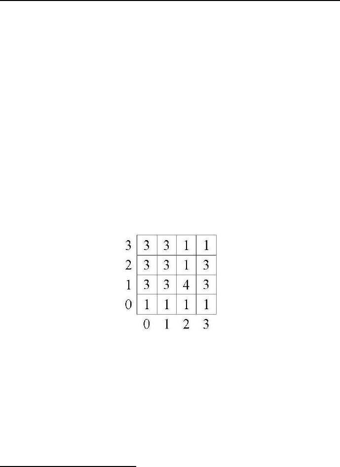
92 Chapter 2. In the beginning was Prolog
Final_Length =17
Final solution = [[0, 0], [0, 1], [1, 1], [2, 1], [2, 2], [2, 3], [2, 4],
[3, 4], [4, 4], [4, 3], [4, 2], [5, 2], [6, 2], [6, 3], [6, 4],
[6, 5], [6, 6]]
Final_Length =17
Those are all solutions of minimum length.
The domain declaration is once again implicit and given by all facts from-to/2.
The state is obviously given by cell coordinates (horizontal,vertical).
2.6.2 Mine field
More complicated maze problems are given by mine fields, for which a path that
minimizes the overall danger is to be found32. Forthesimpleminefieldfrom
Figure 2.19 with dangers declared in cells, the least dangerous path from cell
(0,0) to cell (3,3) is to be found, assuming danger being additive.
Figure 2.19: A simple mine field
The state of the mine field is - as for the maze - given by cell coordinates
(horizontal, vertical). The cell contain values of Danger associated with tran-
siting the cell. The ”dangers” do not belong to the state because they do not
influence the moves to be made. Only vertical or horizontal moves are allowed.
The Overall_danger is the sum of Dangers transited cells. The correspond-
ing program 2_22_mine_field.pl is as follows:
32 This is an OST-type problem.

2.6 Optimum sequencing problems 93
/*1*/ top:-
/*2*/ assert(safest_path([[]],50)),
/*3*/ mine_field.
/*4*/ from_to([0,0],[0,1]).% columns, from bottom to top
/*5*/ from_to([0,1],[0,2]).
/*6*/ from_to([0,2],[0,3]).
/*7*/ from_to([1,0],[1,1]).
/*8*/ from_to([1,1],[1,2]).
/*9*/ from_to([1,2],[1,3]).
/*10*/ from_to([2,0],[2,1]).
/*11*/ from_to([2,1],[2,2]).
/*13*/ from_to([2,2],[2,3]).
/*14*/ from_to([3,0],[3,1]).
/*15*/ from_to([3,1],[3,2]).
/*16*/ from_to([3,2],[3,3]).
/*17*/ from_to([0,0],[1,0]). % rows, from left to riught
/*18*/ from_to([1,0],[2,0]).
/*19*/ from_to([2,0],[3,0]).
/*20*/ from_to([0,1],[1,1]).
/*21*/ from_to([1,1],[2,1]).
/*22*/ from_to([2,1],[3,1]).
/*23*/ from_to([0,2],[1,2]).
/*24*/ from_to([1,2],[2,2]).
/*25*/ from_to([2,2],[3,2]).
/*26*/ from_to([0,3],[1,3]).
/*27*/ from_to([1,3],[2,3]).
/*28*/ from_to([2,3],[3,3]).
/*29*/ transition(A,B):-
/*30*/ from_to(A,B).
/*31*/ transition(A,B):-
/*32*/ from_to(B,A).
/*33*/ danger([0,0],1).
/*34*/ danger([0,1],3).
/*35*/ danger([0,2],3).
/*36*/ danger([0,3],3).
/*37*/ danger([1,0],1).
/*38*/ danger([1,1],3).
/*39*/ danger([1,2],3).

94 Chapter 2. In the beginning was Prolog
/*40*/ danger([1,3],3).
/*41*/ danger([2,0],1).
/*42*/ danger([2,1],4).
/*43*/ danger([2,2],1).
/*44*/ danger([2,3],1).
/*45*/ danger([3,0],1).
/*46*/ danger([3,1],3).
/*47*/ danger([3,2],3).
/*48*/ danger([3,3],1).
/*49*/ mine_field:-
/*50*/ path([[3,3]],Path),
/*51*/ overall_danger(Path,Overall_danger),
/*52*/ update_safest(Path,Overall_danger),
/*53*/ fail.
/*54*/ mine_field:-
/*55*/ safest_path(Path,Overall_danger),
/*56*/ write("Safest path = "),write(Path),nl,
/*57*/ write("Overall danger = "),write(Overall_danger),nl,nl,
/*58*/ fail.
/*59*/ mine_field:-
/*60*/ write("Those are all solutions of minimum overall danger."),nl.
/*61*/ path([Present_state|Path_covered],Path):-
/*62*/ transition(Present_state,Next_state),
/*63*/ not(member(Next_state,Path_covered)),
/*64*/ path([Next_state,Present_state|Path_covered],Path).
/*65*/ path([[0,0]|Path_covered],[[0,0]|Path_covered]).
/*66*/ overall_danger([H|T],N):-
/*67*/ overall_danger([H|T],N,0).
/*68*/ overall_danger([],N,N).
/*69*/ overall_danger([H|T],N,A):-
/*70*/ danger(H,NN),
/*71*/ A_New is A+NN,
/*72*/ overall_danger(T,N,A_New).
/*73*/ update_safest(Path, Overall_danger):-
/*74*/ safest_path(_,Present_Danger),
/*75*/ Present_Danger>Overall_danger,
/*76*/ retractall(safest_path(_,_)),
/*77*/ assert(safest_path(Path,
Overall_danger)),!.
/*78*/ update_safest(Path, Overall_danger):-

2.6 Optimum sequencing problems 95
/*79*/ safest_path(_,Present_Danger),
/*80*/ Present_Danger=Overall_danger,
/*81*/ assert(safest_path(Path, Overall_danger)),!.
/*82*/ update_safest(_,Overall_danger):-
/*83*/ safest_path(_,Present_Danger),
/*84*/ Present_Danger<Overall_danger,!.
The message is:
Safest path = [[0, 0], [1, 0], [2, 0], [2, 1], [2, 2], [2, 3], [3, 3]]
Overall danger = 10
Those are all solutions of minimum overall danger.
2.6.3 Hampton Court maze
Sometimes the distances of the mazes paths are not known. The number of forks
in the final path may then be minimized. How to do it is shown by a program
solving the famous Hampton Court Maze. This is how Jerome K. Jerome in
his book Three Man in a Boat (To Say Nothing of the Dog) described what
happened to somebody trying to find a way out of the famous hedge maze at
Hampton Court near London:
”Harris asked me if I’d ever been in the maze at Hampton Court. He said he went in once
to show somebody else the way. He had studied it up in a map, and it was so simple that it
seemed foolish - hardly worth the twopence charged for admission.
Figure 2.20: Hampton Court maze
Harris said he thought that map must have been got up as a practical joke, because it
wasn’t a bit like the real thing, and only misleading. It was a country cousin that Harris took
in. He said:

96 Chapter 2. In the beginning was Prolog
”We’ll just go in here, so that you can say you’ve been, but it’s very simple. It’s absurd
to call it a maze. You keep on taking the first turning to the right. We’ll just walk round for
ten minutes, and then go and get some lunch.”
They met some people soon after they had got inside, who said they had been there for
three-quarters of an hour, and had had about enough of it. Harris told them they could follow
him, if they liked; he was just going in, and then should turn round and come out again. They
said it was very kind of him, and fell behind, and followed.
They picked up various other people who wanted to get it over, as they went along, until
they had absorbed all the persons in the maze. People who had given up all hopes of ever
getting either in or out, or of ever seeing their home and friends again, plucked up courage
at the sight of Harris and his party, and joined the procession, blessing him. Harris said he
should judge there must have been twenty people, following him, in all; and one woman with
a baby, who had been there all the morning, insisted on taking his arm, for fear of losing him.
Harris kept on turning to the right, but it seemed a long way, and his cousin said he
supposed it was a very big maze.
”Oh, one of the largest in Europe,” said Harris.
”Yes, it must be,” replied the cousin, ”because we’ve walked a good two miles already.”
Harris began to think it rather strange himself, but he held on until, at last, they passed
the half of a penny bun on the ground that Harris’s cousin swore he had noticed there seven
minutes ago. Harris said: ”Oh, impossible!” but the woman with the baby said, ”Not at all,”
as she herself had taken it from the child, and thrown it down there, just before she met
Harris. She also added that she wished she never had met Harris, and expressed an opinion
that he was an impostor. That made Harris mad, and he produced his map, and explained
his theory.
”The map may be all right enough,” said one of the party, ”if you know whereabouts in
it we are now.”
Harris didn’t know, and suggested that the best thing to do would be to go back to the
entrance, and begin again. For the beginning again part of it there was not much enthusiasm;
but with regard to the advisability of going back to the entrance there was complete unanimity,
and so they turned, and trailed after Harris again, in the opposite direction. About ten minutes
more passed, and then they found themselves in the center.
Harris thought at first of pretending that that was what he had been aiming at; but the
crowd looked dangerous, and he decided to treat it as an accident.
Anyhow, they had got something to start from then. They did know where they were,
and the map was once more consulted, and the thing seemed simpler than ever, and off they
started for the third time.
And three minutes later they were back in the center again.
After that, they simply couldn’t get anywhere else. Whatever way they turned brought
them back to the middle. It became so regular at length, that some of the people stopped
there, and waited for the others to take a walk round, and come back to them. Harris drew
out his map again, after a while, but the sight of it only infuriated the mob, and they told
him to go and curl his hair with it. Harris said that he couldn’t help feeling that, to a certain
extent, he had become unpopular.
They all got crazy at last, and sang out for the keeper, and the man came and climbed
up the ladder outside, and shouted out directions to them. But all their heads were, by this
time, in such a confused whirl that they were incapable of grasping anything, and so the man
told them to stop where they were, and he would come to them. They huddled together, and
waited; and he climbed down, and came in.
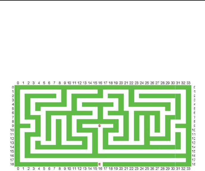
2.6 Optimum sequencing problems 97
He was a young keeper, as luck would have it, and new to the business; and when he got
in, he couldn’t find them, and he wandered about, trying to get to them, and then he got lost.
They caught sight of him, every now and then, rushing about the other side of the hedge,
and he would see them, and rush to get to them, and they would wait there for about five
minutes, and then he would reappear again in exactly the same spot, and ask them where
they had been.
They had to wait till one of the old keepers came back from his dinner before they got
out.”
In order to model the maze, it has to be presented as shown in Figure 2.21,
which clearly defines the coordinates of all forks.
Figure 2.21: Hampton Court Maze coordinates
The program 2_23_hampton_court.pl determines the shortest (by the number
of crossed forks) path from the court center (marked with S - Start) to its en-
trance (marked E):
/*1*/ top:-
/*2*/ assert(shortest_path([[]],80)),
/*3*/ maze.
% The maze model is of the form:
% ’from_to(Fork_coordinates, Adjacent_fork_coordinates)’:
/*4*/ from_to([18,16],[17,16]).
/*5*/ from_to([17,16],[17,32]).
/*6*/ from_to([17,16],[6,5]).
/*7*/ from_to([6,5],[1,15]).
/*8*/ from_to([6,5],[12,5]).

98 Chapter 2. In the beginning was Prolog
/*9*/ from_to([12,5],[13,12]).
/*10*/ from_to([12,5],[3,17]).
/*11*/ from_to([3,17],[5,22]).
/*12*/ from_to([3,17],[13,22]).
/*13*/ from_to([13,22],[7,24]).
/*14*/ from_to([13,22],[5,22]).
/*15*/ from_to([5,22],[6,28]).
/*16*/ from_to([6,28],[7,26]).
/*17*/ from_to([6,28],[10,30]).
/*18*/ from_to([10,30],[13,26]).
/*19*/ from_to([10,30],[9,16]).
/*20*/ transition(A,B):-
/*21*/ from_to(A,B).
/*22*/ transition(A,B):-
/*23*/ from_to(B,A).
/*24*/ maze:-
/*25*/ path([[18,16]],Present_solution),
/*26*/ length(Present_solution,Present_length),
/*27*/ update_shortest(Present_solution,Present_length),
/*28*/ fail.
/*29*/ maze:-
/*30*/ shortest_path(Final_solution,Final_length),
/*31*/ write("The shortest path is"),write(Final_solution),nl,
/*32*/ fail.
/*33*/ maze:-
/*34*/ write("That’s all!"),nl.
/*35*/ path([Present_state|Path_covered],Final_solution):-
/*36*/ transition(Present_state,Next_state),
/*37*/ not(member(Next_state,Path_covered)),
/*38*/ path([Next_state,Present_state|Path_covered],Final_solution).
/*39*/ path([[9,16]|Path_covered],[[9,16]|Path_covered]).
/*40*/ update_shortest(Present_solution,Present_length):-
/*41*/ shortest_path(_,Final_length),
/*42*/ Present_length<Final_length,
/*43*/ retractall(shortest_path(_,_)),
/*44*/ assert(shortest_path(Present_solution,Present_length)),!.
/*45*/ update_shortest(Present_solution, Present_length):-
/*46*/ shortest_path(_,Final_length),
/*47*/ Present_length=Final_length,
/*48*/ assert(shortest_path(Present_solution, Present_length)),!.
/*49*/ update_shortest(_,Present_length):-
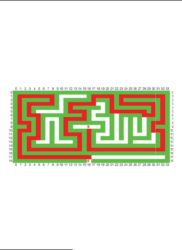
2.6 Optimum sequencing problems 99
/*50*/ shortest_path(_,Final_length),
/*51*/ Present_length>Final_length,!.
The message is:
/*10*/ The shortest path is:
/*10*/ [[9,16], [10,30], [6,28], [5,22], [3,17], [12,5], [6,5], [17,16], [18,16]]
/*10*/ It’s length (measured by the number of crossed forks) is 9
/*10*/ That’s all!
The optimum path is shown in the lower part of Figure 2.22.
Figure 2.22: Hampton Court Maze solution
2.6.4 Water jugs problem
There are many water jugs problems. The one chosen is concerned with three
jugs of capacity 8,5and 3liters. Neither has any measuring markers on it. The
8-liter jug is filled with water. How can this water be used to fill the remaining
two jugs exactly with four liters each while using only the three jugs that have
no measuring markers, and minimizing the number of pourings33?
33 This is an OST-type problem.

100 Chapter 2. In the beginning was Prolog
Defining the state of the jugs as:
state(Water_in_8_litre_jug, Water_in_5_litre_jug,
Water_in_3_litre_jug),
and using the built-in length(?List,?N), the solution is given by program
2_24_three_jugs.pl:
/*1*/ top:-
/*2*/ Initial_state = state(8,0,0),
/*3*/ pour(Initial_state,Sequence_of_states),
/*4*/ length(Sequence_of_states, N),
/*5*/ assert(sequence_of_states(N,Sequence_of_states)),
/*6*/ fail.
/*7*/ top:-
/*8*/ assert(shortest_sequence_of_states(20,[])),
/*9*/ optimize.
/*10*/ pour(Initial_state,Sequence_of_states):-
/*11*/ pour(Initial_state,[Initial_state],Sequence_of_states).
/*12*/ pour(State,Accumulator,Sequence_of_states):-
/*13*/ state_transition(State,Next_state),
/*14*/ not(member(Next_state,Accumulator)),
/*15*/ pour(Next_state,[Next_state|Accumulator],Sequence_of_states).
/*16*/ pour(Final_state,Accumulator,Accumulator):-
/*17*/ final_state(Final_state),!.
/*18*/ final_state(state(4,4,0)).
% Possible pourings:
% pouring(From_jug_A, To_jug_B,
% With_limit_for_B, New_filling_of_A, New_filling_of_B):
% pouring from jug 1 to 2, 2 may contain no more than 5 liters:
/*19*/ state_transition(state(X,Y,Z),state(K,L,Z)):-
/*20*/ pouring(X,Y,5,K,L).
% pouring from jug 2 to 1, 1 may contain no more than 8 liters:
/*21*/ state_transition(state(X,Y,Z),state(K,L,Z)):-
/*22*/ pouring(Y,X,8,L,K).
% pouring from jug 1 to 3, 3 may contain no more than 3 liters:
/*23*/ state_transition(state(X,Y,Z),state(K,Y,M)):-
/*24*/ pouring(X,Z,3,K,M).
% pouring from jug 3 to 1, 1 may contain only 8 liters:
/*25*/ state_transition(state(X,Y,Z),state(K,Y,M)):-
/*26*/ pouring(Z,X,8,M,K).

2.6 Optimum sequencing problems 101
% pouring from jug 2 to 3, w 3 may contain no more than 3 liters:
/*27*/ state_transition(state(X,Y,Z),state(X,L,M)):-
/*28*/ pouring(Y,Z,3,L,M).
% pouring from jug 3 to 2, w 2 may contain no more than 5 liters:
/*29*/ state_transition(state(X,Y,Z),state(X,L,M)):-
/*30*/ pouring(Z,Y,5,M,L).
/*31*/ pouring(X,Y,LimitY,K,L):-
/*32*/ check(X,Y,LimitY),
/*33*/ !,
/*34*/ NX is X - 1,
/*35*/ NY is Y + 1,
/*36*/ pouring(NX,NY,LimitY,K,L).
/*37*/ pouring(X,Y,_,X,Y).
/*38*/ check(X,Y,Limit):-
/*39*/ X > 0,
/*40*/ Y < Limit,!.
/*41*/ optimize:-
/*42*/ optimum_sequence_of_states,
/*43*/ shortest_sequence_of_states(N,Sequence_of_states),
/*44*/ reverse(Sequence_of_states, Reversed_sequence),
/*45*/ write("Optimum_solution : "),nl,
/*46*/ write(Reversed_sequence),nl,
/*47*/ write("Number of pourings: "),write(N).
/*48*/ optimum_sequence_of_states:-
/*49*/ sequence_of_states(X,Trajectory_X),
/*50*/ shortest_sequence_of_states(Y,Trajectory_Y),
/*51*/ update(X,Y,Trajectory_X,Trajectory_Y),
/*52*/ fail.
/*53*/ optimum_sequence_of_states.
/*54*/ update(X,Y,Trajectory_X,Trajectory_Y):-
/*55*/ X < Y,
/*56*/ !,
/*57*/ retract(shortest_sequence_of_states(Y,Trajectory_Y)),
/*58*/ assert(shortest_sequence_of_states(X,Trajectory_X)).
/*59*/ update(_,_,_,_).
The message generated is:
Optimum_solution :
[state(8,0,0), state(3,5,0), state(3,2,3), state(6,2,0),
state(6,0,2), state(1,5,2), state(1,4,3), state(4,4,0)]
102 Chapter 2. In the beginning was Prolog
Number of pourings: 8
The process of filling the three jugs is shown in Figure 2.23. Measuring markers
on jugs in Figure 2.23 have to illustrate the fillings, but are not used to control
the fillings.
Figure 2.23: Filling of three jugs
2.7 Exercises
Domains
The domain declarations in Prolog programs are usually done implicitly
and sometimes hidden in strange places. Determine the variable domains
for all Prolog examples from the present chapter.
Fibonacci numbers
Leonardo Fibonacci (c. 1170 – c. 1250) was an eminent mathematician
and mathematics teacher in the Republic of Pisa (now being part of Italy).
He is famous because of the attempt to model the growth of rabbit popu-

2.7 Exercises 103
lations, rabbits being at his time a widely craved source of meet and fur.
He assumed that a newly-born pair of rabbits of both genders are able to
mate at the age of one month so that at the end of its second month a
female can produce another pair of rabbits; assuming further that rabbits
never die and a mating pair always produces one new pair every month
from the second month on, the number of pairs of the rabbit population
increase in a month by month basis as follows:
0,1,1,2,3,5,8,13,21,34,55,89,144,...,
Denoting the number of rabbit pairs on the beginning of the nth month-
long period by Fn, the process may be described by the double recursion:
Fn=Fn−1+Fn−2
where: F0=0, ,F1=1.
Write a program for calculating Fibonacci numbers that is not tail-recursive,
and another one that is tail-recursive.
Girl friends
John has five girl friends: 1)Ann is blonde, 27 years old, is a Doctor of
Medicine, is married, has two children, a boy and a girl, likes swimming,
2)Beverly is blonde, 20 years old, is a student, single, no children, likes
cooking, 3)Colette is brunette, 24 years old, housewife, married, no chil-
dren, likes acting, 4)Diana is blonde, 21 years old, a secretary, divorced,
one child - a girl, likes being entertained, 5)Edna is blonde, 25 years old,
a nurse, divorced, no children, likes classical music. Use findal/3 to es-
tablish data of all those girl friends that are not divorced, not older than
24, and like a non-sporting activity.
Games
At the local games evening, four lads were competing in the Scrabble and
chess competitions. Liam beat Mark in chess, James came third and the
16 year old won. Liam came second in Scrabble, the 15 year old won,
James beat the 18 year old and the 19 year old came third. Kevin is 3
years younger than Mark. The person who came last in chess, came third
in Scrabble and only one lad got the same position in both games. Write
a program to determine the ages of the lads and the positions in the two
games.

104 Chapter 2. In the beginning was Prolog
Musical recital
At a musical recital five students (John, Kate, Larry, Mary and Nick)
performed five musical pieces, two by Bach, two by Mozart and one by
Vivaldi. There were three violinists and two pianists. Each student per-
formed only one piece, and played only one instrument. Find the order
of the students, their respective instruments and the composer, with the
following conditions: 1. The composers were not played consecutively.
Vivaldi was played last and Mozart was played first. 2. There was one pi-
ano piece that was played between two violin pieces, and two violin pieces
between the first and last piano piece. 3. There were no piano pieces by
Mozart. 4. Kate played third. 5. Nick played the piano, and immediately
followed John, who played a piece by Mozart. 6. Mary did not play a
piece by Vivaldi.
Master classes 34
The great mezzo-soprano Flora Nebbiacorno has retired from the inter-
national opera stage, but she still teaches master classes regularly. At a
recent class, her five students were one soprano, one mezzo-soprano, two
tenors, and one bass. (The first two voice types are women’s, and the last
two are men’s). Their first names are Chris, J.P., Lee, Pat, and Val – any
of which could belong to a man or a woman – and their last names are
Kingsley, Robinson, Robinson (the two are unrelated but have the same
last name), Ulrich, and Walker. Write a program to find the order in
which these five sang for the class, identifying each by full name and voice
type, provided that:
1. The first and second students were, in some order, Pat and the bass.
2. The second and third students included at least one tenor. 3. Kingsley
and the fifth student (who isn’t named Robinson) were, in some order, a
mezzo-soprano and a tenor. 4. Neither the third student, whose name is
Robinson, nor Walker has the first name of Chris. 5. Ulrich is not the
bass or the mezzo-soprano. 6. Neither Lee or Val (who wasn’t third) is
a tenor. 7. J.P. wasn’t third, and Chris wasn’t fifth. 8. The bass isn’t
named Robinson.
Jam making contest
At the recent inter-departmental jam making contest, four lucky candi-
dates took part to make the juiciest strawberry jam. The ages of the
contestants were 14, 17, 20, 22. As it happens the person who came last
34 This exercise is from http://brownbuffalo.sourceforge.net/

2.7 Exercises 105
was the oldest, whereas Stuart was three years older than the person who
came second. James was neither the oldest nor the youngest and Kev fin-
ished ahead of the 17 year old, but didn’t win. John was also unlucky this
time and didn’t win either. Write a program to determinate who finished
where and how old they are.
Bridge meeting
Four ladies meet each week on Thusday to play bridge. On each meeting
they decide what everyone has to bring for the next meeting. 1. Mrs.
Andrew will bring chocolate cake. 2. Neither Mrs. Brown, nor Viven,
nor Ann Clark will bring cookies. 3. Rachel, who is not from Davidson’s
family, will bring coffee. 4. Mary will not bring the wine. Write a program
to determine the whole name of each lady and what is she supposed to
bring next week.
Two jugs
You are given two jugs, a 4-gallon one and a 3-gallon one. Neither has
any measuring markers on it. There is a tap that can be used to fill the
jugs with water. Write a program to determine how can you get exactly
2 gallons of water into the 4-gallon jug.
Ships
There are 5 ships in a port35. 1. The Greek ship leaves at six and carries
coffee. 2. The ship in the middle has a black chimney. 3. The English
ship leaves at nine. 4. The French ship with a blue chimney is to the left
of a ship that carries coffee. 5. To the right of the ship carrying cocoa
is a ship going to Marseille. 6. The Brazilian ship is heading for Manila.
7. Next to the ship carrying rice is a ship with a green chimney. 8. A
ship going to Genoa leaves at five. 9. The Spanish ship leaves at seven
and is to the right of the ship going to Marseille. 10. The ship with a red
chimney goes to Hamburg. 11. Next to the ship leaving at seven is a ship
with a white chimney. 12. The ship on the border carries corn. 13. The
ship with a black chimney leaves at eight. 14. The ship carrying corn is
anchored next to the ship carrying rice. 15. The ship to Hamburg leaves
at six.
Write a program to determine which ship goes to Port Said and which
ship carries tea.
35 This exercise is from http://www.mathsisfun.com/puzzles

106 Chapter 2. In the beginning was Prolog
River crossing 1
Four adventurers (Alex, Brook, Chris and Dusty) need to cross a river in
a small canoe36. The canoe can only carry 100 kg. Alex weighs 90 kg,
Brook weighs 80 kg, Chris weighs 60 kg and Dusty weighs 40 kg, and they
have 20 kg of supplies. Write a program showing how do they get across.
River crossing 2
Three humans and three monkeys (one big, two small) need to cross a river.
But there is only one boat, and it can only hold two bodies (regardless of
their size), and only the humans or the big monkey are strong enough to
row the boat. Furthermore, the number of monkeys can never outnumber
the number of humans on the same side of the river, or the monkeys will
attack the humans. Write a program to demonstrate how can all six get
across the river without anyone getting hurt.
River crossing 3
There is a family on one side of the river: 1. Father 2. Mother 3. Son
4. Daughter 5. Maid 6. Dog They need to get to the other side of the
river. Only 1 small boat is available to bring them across. The boat is big
enough for only 2 people OR 1 person + dog. Here’s the tricky part: *
Only Father, Mother and Maid knows how to row the boat. At all times,
* Father cannot be alone with the Son, without the Mother, or else he
will hit the Son. * Mother cannot be alone with the Daughter, without
the Father, or else she will slap the Daughter * Maid MUST be with the
Dog, or else the Dog will bite anyone in sight. Write a program for the
family of 6 to get across the river, without getting hit, slapped or bitten.
River crossing 4
Three couples AA, BB and CC (the gents Andrew, Basil and Charles and
the corresponding ladies Ann, Barbara and Celine) had to cross a river in
a small boat that held only two people that. No husband would leave his
wife in the company of another man unless he himself was present. Besides
there are additional personal constraints which should not be violated:
- Andrew should not row alone because he is afraid of the river;
- Ann cannot row because of her advanced pregnancy;
- Barbara cannot row because her arm is broken;
- all other people could row;
- Andrew and Charles should not row together because the hate each
36 This exercise is from http://www.mathsisfun.com/puzzles

2.7 Exercises 107
other;
- for the same reason Andrew and Charles should not remain by them-
selves on the same river side.
Write a program for the couples o get across the river without jealousy
arising, and no personal constraint being violated.
Liars
It is known only one character is telling the truth. Mr. April says that
Mr. May tells lies. Mr. May says that Mr. June tells lies. Mr. June
says that both Mr. April and Mr. May tell lies. Write a program which
determines who is telling the truth.
Pets
At a recent Pets Anonymous reunion, the attendees were discussing which
pets they had recently owned. James used to have a dog. The person who
used to own a mouse now owns a cat, but the person who used to have a
cat does not have a mouse. Kevin has now or used to have a dog, I can’t
remember which. Becky has never owned a mouse. Only one person now
owns the pet they previously had. Rebecca said very little throughout
the meeting and nobody mentioned the hamster. Write a program to
determine who owns which pet and what they used to own.
Snail racing
After the recent Brain-Bashers snail racing contest, the four contestants
were congratulating each other. Only one snail wore the same number as
the position it finished in. Alfred’s snail wasn’t painted yellow nor blue,
and the snail who wore 3, that was painted red, beat the snail who came
in third. Arthur’s snail beat Anne’s snail, whereas Alice’s snail beat the
snail who wore 1. The snail painted green, Alice’s, came second and the
snail painted blue wore number 4. Anne’s snail wore number 1. Write a
program to work out who’s snail finished where, its number and the color
it was painted.
Professions
Messrs Butcher, Baker, Carpenter and Plumber have met for the first
time after college graduation. No-one is currently, nor ever has been in
the same profession as their name and on-one has had the same profession
twice. Charlie has never been a carpenter and Mr Butcher in now a
plumber. Dave used to be a butcher, whereas Mr Brian Baker never has.

108 Chapter 2. In the beginning was Prolog
Mr Plumber is not called Eddie and Mr Carpenter did not used to be
a butcher. Write a program to determine the full names of each of the
attendees, along with their current and previous profession.
Pre-Olympic Rehearsal
At last month’s Pre-Olympic Rehearsal, four top athletes competed in two
qualifying 400 meter races. As the results were expected to be mislaid,
various notes were taken to ensure the accuracy of the overall placing:
No-one finished both races in the same position. John beat Mr Donald in
both races. Steve Curtail came third in the second race and Dave came
last in the first race. In the second race, Mr Arnold won and Mr Bowler
came last. In the first race, Steve beat Kev, but Kev beat John. Write a
program to determine who finished where in each of the races.
Nine students
Alex, Bret, Chris, Derek, Eddie, Fred, Greg, Harold and John are nine
students who live in a three storey building, with three rooms on each
floor. A room in the West wing, one in the center, and one in the East
wing. If you look directly at the building, the left side is West and the
right side is East. Each student is assigned exactly one room. Write a
program to find where each of their room is, provided : 1. Harold does not
live on the bottom floor. 2. Fred lives directly above John and directly
next to Bret (who lives in the West wing). 3. Eddie lives in the East wing
and one floor higher than Fred. 4. Derek lives directly above Fred. 5.
Greg lives directly above Chris.
Wine barrels
A man, who recently passed away, was the owner of a winery. In his will,
he left 21 barrels (seven of which are filled with wine, seven of which are
half full, and seven of which are empty) to his three sons. However, the
wine and barrels must be split so that each son has the same number of
full barrels, the same number of half-full barrels, and the same number of
empty barrels. Note that there are no measuring devices handy. Write a
program that determines how can the barrels and wine be evenly divided.
Greetings
Kent and Hannah invited some of their friends at a dinner. Some friends
arrived with their spouses while some arrived alone. Each guest greeted
with every of the two hosts and with each other guest. When two men
greeted each other there were handshaking. When two women greeted

2.7 Exercises 109
each other there were kissing. The same was true when a man and a
woman greeted each other. It is known 6 handshakes and 12 kisses have
been done in total. Write a program to determine how many guests arrived
at the dinner, how many of them were in couples and how many of them
were alone? Obviously, when two guests arrived as a couple they didn’t
greet each other.
Politically correct missionaries and cannibals
Modify program 2_19_mac.pl so as to meet the criterium of political cor-
rectness presented by the footnote to Section 2.5.2.
Art theft
After a local art theft, six suspects were being interviewed. Below is a
summary of their statements:
Alan said: It wasn’t Brian. It wasn’t Dave. It wasn’t Eddie.
Brian said: It wasn’t Alan. It wasn’t Charlie. It wasn’t Eddie.
Charlie said: It wasn’t Brian. It wasn’t Freddie. It wasn’t Eddie.
Dave said: It wasn’t Alan. It wasn’t Freddie. It wasn’t Charlie.
Eddie said: It wasn’t Charlie. It wasn’t Dave. It wasn’t Freddie.
Freddie said: It wasn’t Charlie. It wasn’t Dave. It wasn’t Alan
Police know that exactly four of them told one lie each and all of the other
statements are true. From this information write a program to determine
who committed the theft.
Competition
Five friends were competing for jobs in the Huge International Corpora-
tion. After all interviews and examinations the results were presented to
the competitors. A bystander watching the friends overheard that:
•Art sadly confessed he has not been ranked on the first position;
•Ben admitted he has been ranked as third after Carl
•Art added that Carl has not been ranked second;
•Ben added that Ed was neither the first nor the last in the ranking;
•Dusty admitted he was ranked just after Art.
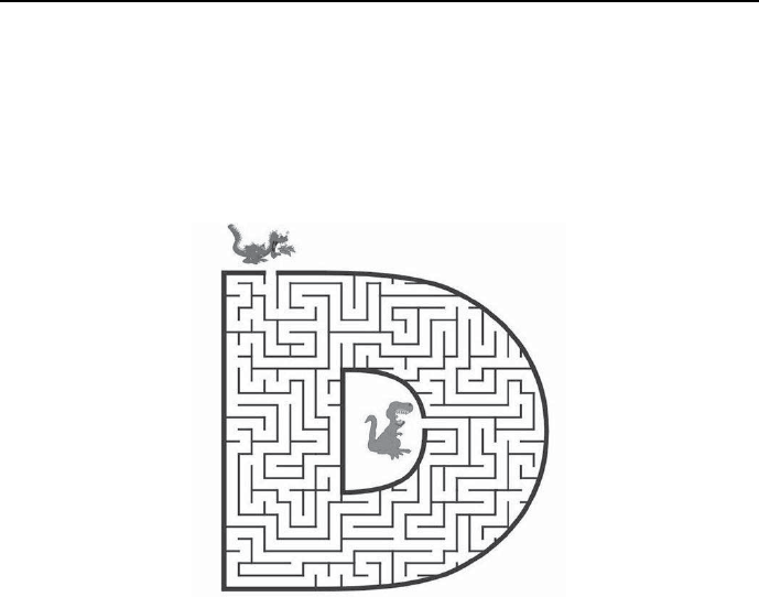
110 Chapter 2. In the beginning was Prolog
Does the bystander has enough information to rank all five friends? Write
a suitable program.
Onemoremaze
For the maze from Figure 2.24 find the shortest path (as measured by the
number of path forks) for the dragon to reach and fight the dinosaur.
Figure 2.24: Dragon-dinosaur maze
Secret Service delators
Six former Secret Service delators enjoy their retirement living in the same
six-floor Apartment House. Each gentleman delator (Al, Bob and Chase)
and each lady delator (Debi, Elsa and Fay) live on different floors. The
delator family names are Airhead, Zero, Deadbeat, Herd, Flake and Nut-
ter. Write a program to determine the names and family names of all
delators and the number of denunciation reports written by each of them,
provided that:
•they wrote altogether 280 denunciation reports, each delator at least
one report;
•Chase lives one the floor below Flake;
•the family name of Elsa is neither Herd nor Deadbeat;

2.7 Exercises 111
•Fay lives on a higher floor than Debi, but on a lower floor than Herd.
•Bob lives just above Nutter and just below this fellow who wrote 40
reports.
•Airhead lives neither on the first floor, nor on the six floor.
•Al wrote half the number of reports as the resident from the six floor,
who wrote half the number of reports as Zero;
•Debi does not live on the first floor;
•Bob wrote 20 reports more than Zero;
•Zero’s name is not Debi;
•Nutter wrote 10 reports less than Airhead.
More uses of conditional predicates
Have a look at those examples from Chapter 2 which have been solved
with no use of the basic conditional predicate from Section 2.4.10. Can
any of them be solved using the conditional predicate? Design for some
of them a program.
Chapter 3
CLP with elementary
predicates for feasible
solutions
3.1 Elementary predicates
The range of built-ins made available to users is for CLP languages much greater
and decisively more powerful than for Prolog. They may be dichotomized into:
•Elementary predicates which are predicates of fundamental functionality
over input variables contained at most in one lists. The are made available
by ic and branch_and_bound libraries.
•Global predicates which are predicates of advanced functionality over a
number of input lists. The are made available by libraries like ic_global,
ic_cumulative,ic_edge_finder,ic_edge_finder3.
Obviously, the nature and usage of elementary predicates is simpler than of
global predicates. Elementary predicates form the basic building blocks of CLP
programs and their properties as well as the way they are handled deserve close
attention. Therefore we start with using them, while leaving the discussion and
application of global predicates to latter Sections 4 and 6.
113

114 Chapter 3. CLP with elementary predicates for feasible solutions
3.2 How CLP languages differ from Prolog?
3.2.1 Basic differences
1. In Prolog programs, variable domains were declared implicitly by elements
of lists scattered in various predicates in various places of the program.
CLP programs contain, in their top part, explicitly declared domains for
all variables used in the program.
2. Prolog could handle only variables defined over domains of terms. CLP
languages are able to handle variables from a decisive broader range of
domains, e.g. integer domains, real domains, symbolic domains.
3. In Prolog constraint propagation was done via unification. CLP languages
use more efficient constraint propagation methods known as consistency
techniques.
4. CLP languages use more efficient search method compared with depth
first search with standard backtracking. The more efficient methods are
among others forward checking and forward checking-looking ahead.
5. CLP languages integrate the mentioned search methods and constraint
propagation techniques into efficient and easy-to-use search and propaga-
tion solvers.
6. In Prolog programs search is started automatically whenever a query is
invoked. For CLP languages search is started by a special predicate (usu-
ally built-in) that grounds variables in some order, most often named
labeling/1. The properties of this basic labeling predicate correspond to
the rule:
labeling([H|T]):-
indomain(H),
labeling(T).
labeling([]).,
where the built-in predicate indomain(List_of_Variables) grounds the
variables from the List_of_Variables successively to values from their
domain, in such order as they appear in the List_of_Variables,fromleft

3.2 How CLP languages differ from Prolog? 115
to right. This order is sometimes not the most efficient one, so CLP lan-
guages (including ECLiPSe) makes available a number of search heuris-
tics different from that realized by labeling/1, see 3.3.
7. While programming in ECLiPSeP rolog, no libraries need to be attached
to the program. On the other hand, while programming in ECLiPSeCLP,
the program must start with a declaration of needed libraries. The most
often needed libraries are the following:
•The ic (interval constraint) library that is a hybrid integer/real
interval arithmetic1constraint solver. Its aim is to make it conve-
nient for programmers to write hybrid solutions to problems, mixing
together integer and real constraints and variables. It is the basic
library, needed for the majority of problems discussed in chapters
3,..6.
•The lib(branch_and_bound) library that implements a highly pa-
rameterized branch and bound algorithm, see chapters 5 and 6.
•The eplex library with LP, MIP and quadratic programming solvers,
providing also the possibility of interfacing with third-party optimiza-
tion software.
•The ic_global library that implements a number of global con-
straints over lists of integer input variables.
•The cumulative library that implements the cumulative scheduling
constraint, see Chapter 6.
•The libraries ic_edge_finder and ic_edge_finder3 that imple-
ment stronger versions of the cumulative and disjunctive constraints
and cumulative scheduling constraints.
•The ic_sets library that makes available a solver for constraints over
the domain of finite sets of integers.
•The ic_symbolic library that makes available a solver for constraints
over ordered symbolic domains.
A detailed presentation of all libraries may be found in the ECLiPSe
Constraint Library Manual, available in the ECLiPSe Documentation,see
Figure 5.
1Interval arithmetic - as contrasted with ”normal” arithmetic - deals with arithmetic ope-
rations on real-valued intervals. The result of arithmetic interval operations is not given by
some set of state variable values, but by some set of state variable intervals. It will be used
intensively while discussing constraint solving for continuous variables.

116 Chapter 3. CLP with elementary predicates for feasible solutions
3.2.2 Similarity
The main similarity between Prolog and CLP is that both infer using search
and propagation
The concepts mentioned will be illustrated by a number of examples, the
first one is the queens placement problem.
3.2.3 Queens - CLP approaches
So far two solutions for the queens placement problem were presented:
1. Exhaustive search, for which all possible permutations for
[X1,X2,...,Xn] = [1,2,...,n]
were consecutively generated and their ”safety” was tested.
2. Depth first search with standard backtracking, for which a safe partial
placement [Xj,Xk,...] was extended by adding another queen and test-
ing the extended placement for safety; if it is safe we proceed with adding
yet another queen, if this test fails backtrack is done to the nearest place-
ment for which there is still an untested choice of some queen to be added.
Standard backtracking is pruning some branches of the exhaustive search
tree, thereby contributing to the efficiency of the search.
However, there are two drawbacks of depth first search with standard back-
tracking:
1)backtracking is performed only as the result of violating some constraints;
2)”trashing” i.e. repeated failure due to the appearance of similar partial solu-
tions, as shown in Figure 3.1.
Figure 3.1: Partial queens placement generating trashing
Let’s try to find a feasible solution for the queen placement problem using
elementary constraints and tools available at the ECLiPSeplatform. This

3.2 How CLP languages differ from Prolog? 117
could be done only by enhancing backtracking search: no CLP language enables
exhaustive search, offering only more advanced search methods.
3.2.4 Forward Checking for queens
Standard backtracking search may be improved using Forward Checking.Its
salient feature is to initiate backtracking before some constraint fails, but when
this failure will happen in the next search step. Strictly speaking - Forward
Checking is not only a search technique, i.e. a tool for grounding, degrounding
and regrounding variables in some order. It combines a search technique with a
consistency-based constraint propagation technique which is much more effective
than Prolog’s unification.
Forward Checking is best illustrated using the simple 4 queens placement
problem. It is assumed that:
•any queen ihas its domain given by a list:
[X1,X2,X3,X4]
of feasible Xi values, denoting the number of the chessboard row, in which
the queen is placed in the ith column;
•initially all domains are the same and given by [1, 2, 3, 4];
•to some existing safe partial placement [xi,xk,..] a new queen is added to
a position determined by her domain; this is just what Forward Checking
is about - we never place the queen on a position outside her domain, i.e.
a position which is not safe;
•adding a new queen is followed by updating the domains of all queens
not placed yet. This is a particular case of constraint propagation:the
constraint introduced by the newly placed queen is propagated across the
domains of the remaining queens;
•if some domain happens to be empty, backtracking (BT) is performed to
this nearest previous placement, for which there exists still non-empty
domains for queens not placed yet.
This is illustrated by Figure 3.2 where red ×denote places off limits for unplaced
queens, i.e. places removed from their domains.
The animation from Figure 3.2 corresponds to the search tree from Figure
3.3.
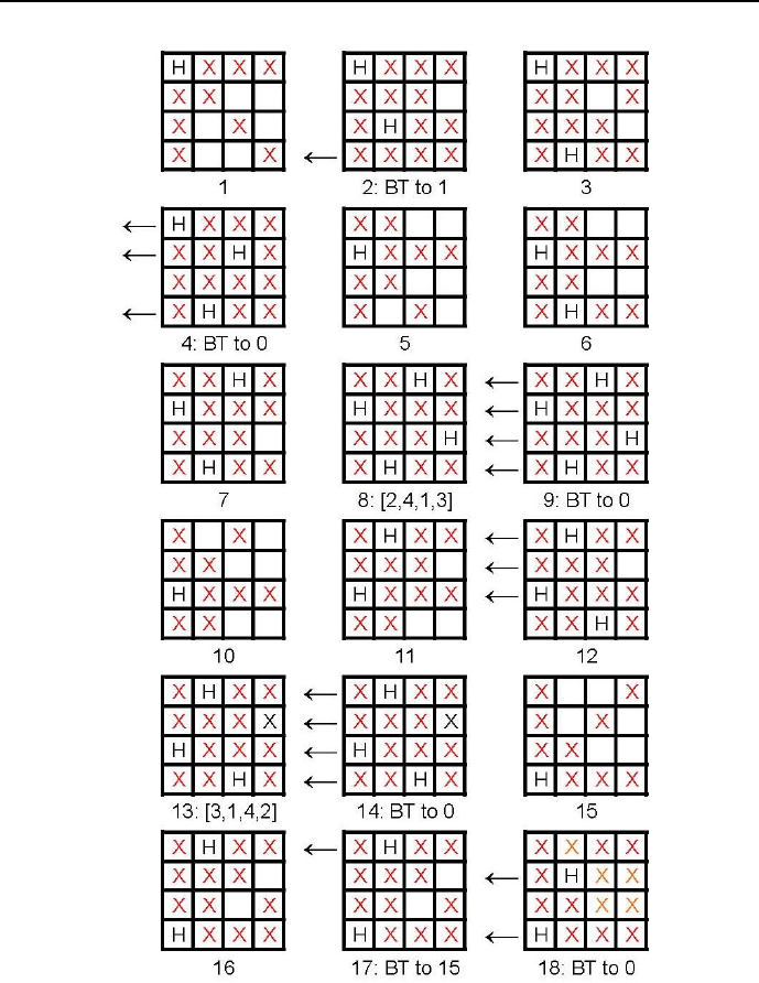
118 Chapter 3. CLP with elementary predicates for feasible solutions
Figure 3.2: Forward Checking forfourqueens
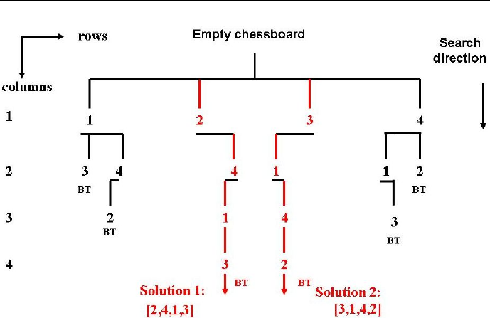
3.2 How CLP languages differ from Prolog? 119
Figure 3.3: Search tree for Forward Checking forfourqueens
It can be seen that, while Forward Checking, backtracking is not initiated by
violating some constraint, but by the inevitability of a constraint being violated
next, this being indicated by the appearance of an empty domain. Forward
Checking generates a new placement by adding the next queen to the already
existing safe placement only if the new queen has a non-empty domain. Other-
wise backtracking is performed. The result is that Forward Checking is pruning
some additional branches of the search tree as compared with depth-first search
with standard backtracking, thus increasing search effectiveness.
3.2.5 Looking Ahead +Forward Checking for queens
Forward Checking has yet some drawbacks: it is not aware of consequences more
remote then the next search step and thus attempts to place queens on places
that result in empty domains not in the next step, but in the next plus one step.
Such situation is shown in Figure 3.4.
Looking Ahead is practically always used together with Forward Checking.
It initiates backtracking as soon as the violation of some constraint in the next

120 Chapter 3. CLP with elementary predicates for feasible solutions
Figure 3.4: A queen placement that invokes Forward Checking in vain
plus one search step is to be predicted2. This is best illustrated for placing 4
queens, as shown in Figures 3.5 i 3.6.
Notice that:
•Forward Checking alone is not testing non-empty domains of queens not
placed yet;
•Looking Ahead + Forward Checking is testing whether non-empty domains
of queens not placed yet contain non-safe placements; if so, backtracking
is performed.
To end this Section, some words of consolation are due:
•the ECLiPSeuser is not expected to deal explicitly with the described
backtracking enhancements;
•they are automatically provided by the mere declaration of stating some
goal.
The above discussion just aims to give the ECLiPSeuser some idea about why
is it more efficient than Prolog.
3.3 Search heuristics
The queen placement problems shows that two decisions influence the search
effectiveness. They are answers to following questions:
1. What variable should first be chosen for grounding, what next, what af-
terwards, etc?
2Obviously, this prediction must be ”cheaper” in numerical terms than simply testing the
state for the next plus one search step.
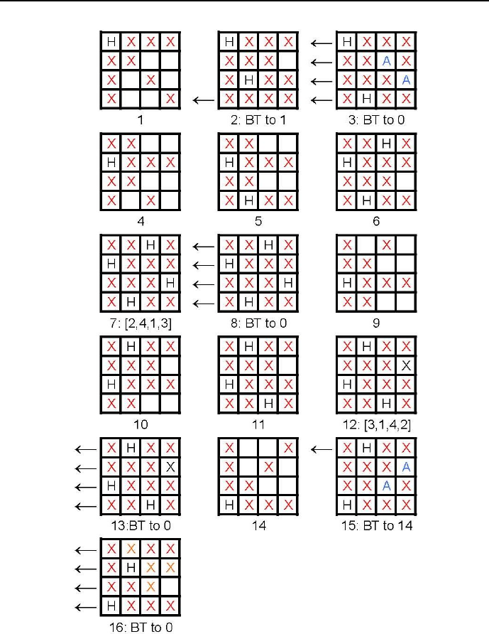
3.3 Search heuristics 121
Figure 3.5: Looking Ahead+Forward Checking forfourqueens
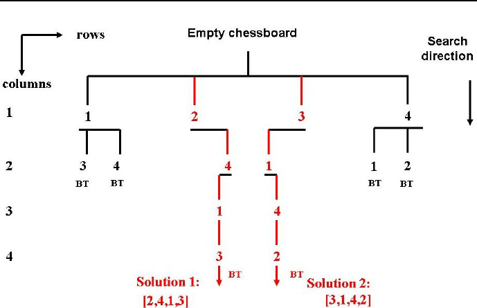
122 Chapter 3. CLP with elementary predicates for feasible solutions
Figure 3.6: Search tree for Looking Ahead+Forward Checkingfor four queens
2. What value (from the domain of the first variable chosen) should be used
for grounding, what value (from the domain of the next variable chosen)
should be used for grounding, etc? .
For the queen placement examples the variables were chosen starting with
the head of the variable list, the head of the tail was chosen next, etc. It should
be noticed that this was not the best (in terms of search efficiency) choice.
Starting near the ”middle” of the list (e.g. choosing first the second variable for
grounding), it can be seen from Figures 3.5 and 3.6 that the solution would be
obtained with a smaller number of backtracks.
For the queen placement examples the chosen variable was first grounded
to the first value from its domain, then to the second value, etc. It should be
noticed that this was also not the best choice. While starting near the middle
of the domain (e.g. grounding first the variable on value 2), it can be seen from
Figures 3.5 and 3.6 that the solution would be obtained with a smaller number
of backtracks.

3.4 Consistency techniques 123
The ways to choose the variable order and value order are covered by an
umbrella term search heuristics:
1. The order of variable to be grounded depends upon the variable choice
heuristic.
2. The order of values to which the selected variable is grounded depends
upon the value choice heuristic.
In Chapter 5 search heuristics for a more advanced search predicate than
labeling/1 will be discussed.
However, it should be emphasized already at this point that there are no
means of knowing beforehand which search heuristics to choose for some par-
ticular problem. The only feasible approach (if efficiency is of importance for
repeatedly using the same program with different data) is by exhaustively search-
ing all heuristics made available by ECLiPSe.
3.4 Consistency techniques
The name consistency techniques covers algorithms dedicated towards making
a set of integer variables, defined by names and domains, to fulfill a set of con-
straints by properly adjusting their domains. This is done be removing from
the domains values that are inconsistent. Consistency techniques are used in
CLP languages for constraint propagation, i.e. for removing inconsistent values
from variable domains each time a new constraint is tested. In CLP languages
problems with combinatorial constraints (i.e. integer constraints and symbolic
constraints) have variables defined by integer domains. There is a broad range
of consistency algorithms. Their names are derived from constraint graphs, used
for binary constraints: their nodes correspond to variables and their domains,
their arcs correspond to binary constraints. A detailed discussion of consistency
techniques may be found [Tsang-95], [Dechter-03] and [Rossi-06]. Depending
upon the number of variables present in a constraint, the following consistency
techniques are distinguished:
•Node consistency - NC for unary constraints;
•Arc consistency - AC for binary constraints;
•Path consistency - PC for tenary and higher arity constraints.

124 Chapter 3. CLP with elementary predicates for feasible solutions
Path consistency algorithms are seldom ever used, because path consistency may
be expressed in a simpler way. E.g. the case of path consistency for X=Y+Z
with corresponding domains DX,DYiDZmay be presented by a set of unary
constraints:
X>=min(DY)+min(DZ)
X<=max(DY)+max(DZ)
Y>=min(DX)−max(DZ)
Y<=max(DX)−min(DZ)
Z>=min(DX)−max(DY)
Z<=max(DX)−max(DY)
The effectiveness of existing consistency techniques has an important bear-
ing on the methodology of CSP and COP: they must be modelled using integer
variables. This is sometimes easier said than done, and occasionally may look
strange indeed. However, this is something anybody learning CLP has to mas-
ter.
Constraint propagation in CLP is an autonomous activity: it can sometimes
be used for inference purposes with no search.
3.5 Propagating constraints with failure
In ECLiPSeprograms symbols of arithmetic operations and relations for dis-
crete variables have to be prefixed by #. For better understanding of consistency
techniques let us consider a simple
example given by program 3_1_domain_0.ecl3:
/*1*/ :- lib(ic).
/*2*/ top :-
/*3*/ [X,Y,Z]::1..10,
/*4*/ get_domain(X,PX),
/*5*/ get_domain(Y,PY),
/*6*/ get_domain(Z,PZ),
/*7*/ write("X = "), write(PX),nl,
/*8*/ write("Y = "), write(PY),nl,
3This is an FS-type problem.

3.5 Propagating constraints with failure 125
/*9*/ write("Z = "), write(PZ),nl,nl,
/*10*/ write("Propagation of constraint Y < Z results in"),nl,
/*11*/ Y#<Z,
/*12*/ get_domain(X,CX),
/*13*/ get_domain(Y,CY),
/*14*/ get_domain(Z,CZ),
/*15*/ write("X = "), write(CX),nl,
/*16*/ write("Y = "), write(CY),nl,
/*17*/ write("Z = "), write(CZ),nl,nl,
/*18*/ write("Propagation of constraint X = Y + Z results in:"),nl,
/*19*/ X#=Y+Z,
/*20*/ get_domain(X,DX),
/*21*/ get_domain(Y,DY),
/*22*/ get_domain(Z,DZ),
/*23*/ write("X = "), write(DX),nl,
/*24*/ write("Y = "), write(DY),nl,
/*25*/ write("Z = "), write(DZ),nl,nl,
/*26*/ write("Propagation of constraint X = Z + 3 results in:"),nl,
/*27*/ X#=Z+3,
/*28*/ get_domain(X,TX),
/*29*/ get_domain(Y,TY),
/*30*/ get_domain(Z,TZ),
/*31*/ write("X = "), write(TX),nl,
/*32*/ write("Y = "), write(TY),nl,
/*33*/ write("Z = "), write(TZ),nl,nl,
/*34*/ write("Propagation of constraint X > 2+Z results in:"),nl,
/*35*/ X#>2+Z,
/*36*/ get_domain(X,TTX),
/*37*/ get_domain(Y,TTY),
/*38*/ get_domain(Z,TTZ),
/*39*/ write("X = "), write(TTX),nl,
/*40*/ write("Y = "), write(TTY),nl,
/*41*/ write("Z = "), write(TTZ),nl,nl,
/*42*/ write("Propagation of constraint Y = 2*Z results in:"),nl,
/*43*/ Y#=2*Z,
/*44*/ get_domain(X,SX),
/*45*/ get_domain(Y,SY),
/*46*/ get_domain(Z,SZ),
/*47*/ write("X = "), write(SX),nl,
/*48*/ write("Y = "), write(SY),nl,
/*49*/ write("Z = "), write(SZ).
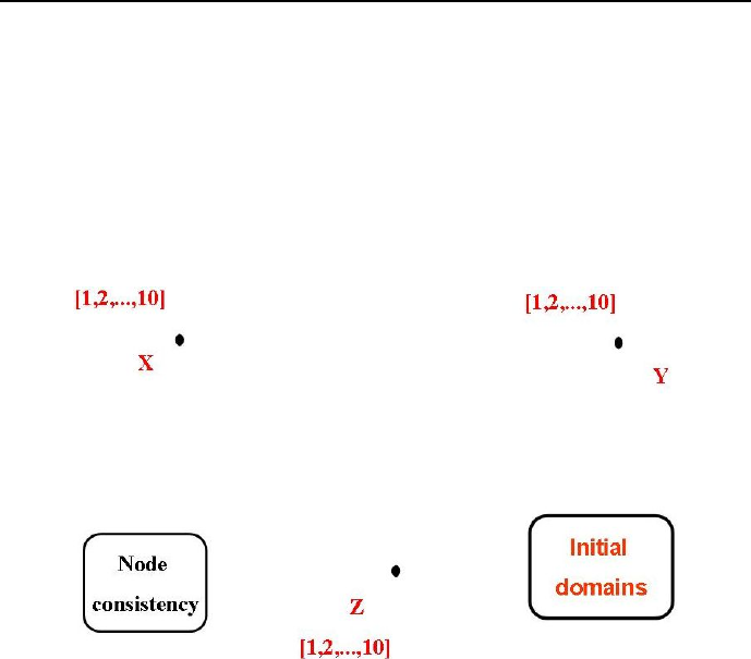
126 Chapter 3. CLP with elementary predicates for feasible solutions
The solution is as follows:
X = [1, 2, 3, 4, 5, 6, 7, 8, 9, 10]
Y = [1, 2, 3, 4, 5, 6, 7, 8, 9, 10]
Z = [1, 2, 3, 4, 5, 6, 7, 8, 9, 10]
The initial domains are shown in Figure 3.7.
Figure 3.7: Initial domains for variables X, Y iZ
Propagation of constraint Y < Z results in:
X = [1, 2, 3, 4, 5, 6, 7, 8, 9, 10]
Y = [1, 2, 3, 4, 5, 6, 7, 8, 9]
Z = [2, 3, 4, 5, 6, 7, 8, 9, 10]
Results of this propagation are shown in Figure 3.8.
Propagation of constraint X = Y + Z results in:
X = [3, 4, 5, 6, 7, 8, 9, 10]
Y = [1, 2, 3, 4, 5, 6, 7, 8]
Z = [2, 3, 4, 5, 6, 7, 8, 9]
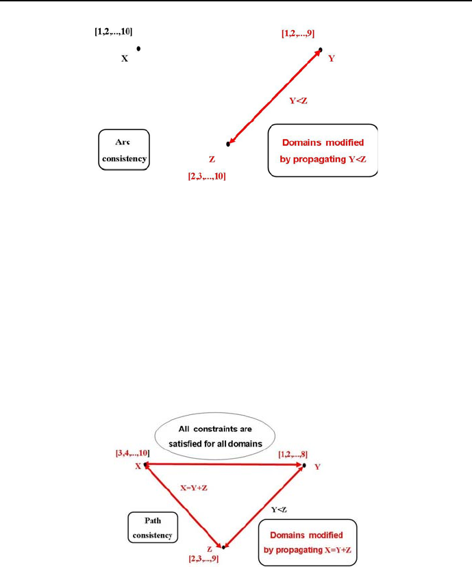
3.5 Propagating constraints with failure 127
Figure 3.8: Results of successful propagation for Y<Z
Results of this propagation are shown in Figure 3.9.
Propagation of constraint X = Z + 3 results in:
X = [5, 6, 7, 8, 9, 10]
Y = [1, 2, 3, 4, 5, 6]
Z = [2, 3, 4, 5, 6, 7]
Results of this propagation are shown in Figure 3.10.
Figure 3.9: Results of successful propagation for X=Y+Z
Propagation of constraint X > 2+Z results in:
X = [5, 6, 7, 8, 9, 10]
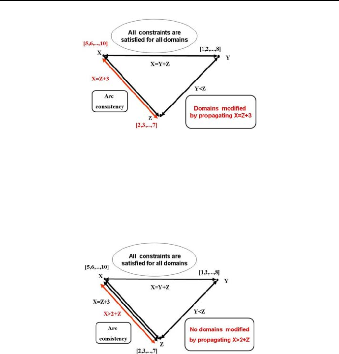
128 Chapter 3. CLP with elementary predicates for feasible solutions
Figure 3.10: Results of successful propagation for X=Z+3
Y = [1, 2, 3, 4, 5, 6]
Z = [2, 3, 4, 5, 6, 7]
Results of this propagation are shown in Figure 3.11.
Figure 3.11: Results of successful propagation for X>2+Z
Propagation of constraint Y = 2*Z results in:
This results in failure: No
Results of this propagation are shown in Figure 3.12.
Up to line /*41*/ the constraint propagation decreases the domain sizes. Line
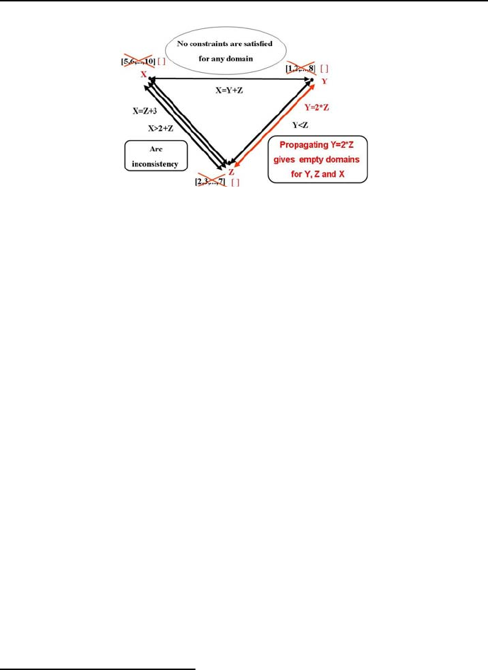
3.6 Successful propagation of constraints 129
Figure 3.12: Results of unsuccessful propagation for Y=2∗Z
/*42*/ introduces a constraint inconsistent with this from line /*10*/;this
results in the domains of Ynd Zbecoming empty. The program ends with
failure: the set of inequalities is inconsistent for the declared initial domains.
3.6 Successful propagation of constraints
Constraint propagation via consistency techniques is an incomplete inference
method. However, occasionally propagation alone may procure a unique solution
to CSP’s. This is illustrated by following programs.
3.6.1 A simple example
Consider the program 3_2_domain_1.ecl4:
/*1*/ :- lib(ic).
/*2*/ top :-
/*3*/ [X,Y,Z]::1..10,
/*4*/ get_domain(X,PX),
/*5*/ get_domain(Y,PY),
/*6*/ get_domain(Z,PZ),
/*7*/ write("X = "), write(PX),nl,
/*8*/ write("Y = "), write(PY),nl,
/*9*/ write("Z = "), write(PZ),nl,nl,
4This is an FS-type problem.

130 Chapter 3. CLP with elementary predicates for feasible solutions
/*10/ write("Propagation of constraint X = Y+3 results in:"),nl,
/*10*/ X#=Y+3,
/*11*/ get_domain(X,CX),
/*12*/ get_domain(Y,CY),
/*13*/ get_domain(Z,CZ),
/*14*/ write("X = "), write(CX),nl,
/*15*/ write("Y = "), write(CY),nl,
/*16*/ write("Z = "), write(CZ),nl,nl,
/*17/ write("Propagation of constraint Y < 3 results in:"),nl,
/*18*/ Y#<3,
/*19*/ get_domain(X,DX),
/*20*/ get_domain(Y,DY),
/*21*/ get_domain(Z,DZ),
/*22*/ write("X = "), write(DX),nl,
/*23*/ write("Y = "), write(DY),nl,
/*24*/ write("Z = "), write(DZ),nl,nl,
/*25/ write("Propagation of constraint X > 2+Z results in:"),nl,
/*26*/ X#>2+Z,
/*27*/ get_domain(X,TX),
/*28*/ get_domain(Y,TY),
/*29*/ get_domain(Z,TZ),
/*30*/ write("X = "), write(TX),nl,
/*31*/ write("Y = "), write(TY),nl,
/*32*/ write("Z = "), write(TZ),nl,nl,
/*33/ write("Propagation of constraint Y = 2*Z results in:"),nl,
/*33*/ Y#=2*Z,
/*34*/ get_domain(X,SX),
/*35*/ get_domain(Y,SY),
/*36*/ get_domain(Z,SZ),
/*37*/ write("X = "), write(SX),nl,
/*38*/ write("Y = "), write(SY),nl,
/*39*/ write("Z = "), write(SZ),nl.
The solution is as follows:
X = [1, 2, 3, 4, 5, 6, 7, 8, 9, 10]
Y = [1, 2, 3, 4, 5, 6, 7, 8, 9, 10]
Z = [1, 2, 3, 4, 5, 6, 7, 8, 9, 10]
Propagation of constraint X = Y+3 results in:
X = [4, 5, 6, 7, 8, 9, 10]
Y = [1, 2, 3, 4, 5, 6, 7]
Z = [1, 2, 3, 4, 5, 6, 7, 8, 9, 10]

3.6 Successful propagation of constraints 131
Propagation of constraint Y < 3 results in:
X = [4, 5]
Y = [1, 2]
Z = [1, 2, 3, 4, 5, 6, 7, 8, 9, 10]
Propagation of constraint X > 2+Z results in:
X = [4, 5]
Y = [1, 2]
Z = [1, 2]
Propagation of constraint Y = 2*Z results in:
X = [5]
Y = [2]
Z = [1]
Below there are some more examples for which constraint propagation alone
is sufficient for finding solutions.
3.6.2 Who with whom?
The number of different combinatorial problems that can be modeled and solved
using integer domains is all-encompassing. Some applications seem to be quite
astonishing to the beginner. Let us consider the following puzzle5:
Who went yesterday evening with whom when:
1. Andy enjoyed a concert.
2. Ben accompanied Olive.
3. Carl has not seen Eva.
4. Paula went to a cinema.
5. Eva was in a theater.
6. One boy and one girl went to an exhibition.
Dusty and Sabina belong also to the set of friends. Determine who went with
whom and where if every boy spend the evening with some girl.
The solution is given by program 3_3_who_with_whom.ecl6:
5Taken from [Bizam-75].
6This is an FS-type problem.

132 Chapter 3. CLP with elementary predicates for feasible solutions
/*1*/ :- lib(ic).
/*2*/ top:-
/*3*/ [Andy,Ben,Carl,Dusty]::[1..4],
/*4*/ [Olive, Eva,Paula,Sabina]::[1..4],
% concert=1, cinema=2, theater=3, exhibition=4
% It means: if eg. Ben=Olive=4, then
% Ben and Olive went to an exhibition
% Andy enjoyed a concert:
/*5*/ Andy#=1,
% Ben accompanied Olive:
/*6*/ Ben#=Olive,
% Carl has not seen Eva:
/*7*/ Carl#\=Eva,
% Paula went to a cinema:
/*8*/ Paula#=2,
% Eva was in a theater
/*9*/ Eva#=3,
% All persons are different:
/*10*/ Andy#\=Ben,
/*11*/ Andy#\=Carl,
/*12*/ Andy#\=Dusty,
/*13*/ Ben#\=Carl,
/*14*/ Ben#\=Dusty,
/*15*/ Carl#\=Dusty,
/*16*/ Olive#\=Eva,
/*17*/ Olive#\=Paula,
/*18*/ Olive#\=Sabina,
/*19*/ Eva#\=Paula,
/*20*/ Eva#\=Sabina,
/*21*/ Paula#\=Sabina,
/*22*/ write(Andy),write(" "),write(Ben),write(" "),
write(Carl),write(" "),write(Dusty),nl,
/*23*/ write(Olive),write(" "),write(Eva),write(" "),
write(Paula),write(" "),write(Sabina).
The program contains no labeling(_) built-in, used for initiating search. Its
use would accelerate the inference. The solution generated is poorly under-

3.6 Successful propagation of constraints 133
standable:
1423
4321
It means that:
Andy (first position on the boys list)
and Sabina (fourth position on the girls list)
enjoyed a concert (1).
Ben (second position on the boys list)
and Olive (first position on the girls list)
went to an exhibition (4).
Carl (third position on the boys list)
and Paula (third position on the girls list)
went to a cinema (2).
Dusty (fourth position on the boys list)
and Eva (second position on the girls list)
went to a theater (3).
The message readability will be improved in Section 4.4.3.
3.6.3 Students and languages
Problems where propagation alone is sufficient for obtaining a solution are some-
times astonishingly complex. This is the case for the following example taken
from [Bizam-75]:
Five students of five nationalities spend their vacation on the Masurian
Lakes. Its a Pole, a Hungarian, a Finn, a Swede and a German. Determine
who speaks what language if:
1. Each student is fluent in one o more foreign languages, but only in those
that are native for some of the remaining students.
2. There is no single language spoken by all of them.
3. Each student may speak with any other student using some language.
4. The common languages include native languages of all students.

134 Chapter 3. CLP with elementary predicates for feasible solutions
5. On average each student speaks two foreign languages.
6. The Pole and the Hungarian speak three foreign languages.
7. While the Swede has been swimming, the remaining four students could
speak a common language.
8. A common language could also be spoken while the Swede returned, but
the Finn went rowing.
9. In order to speak Swedish, two student had to leave the group.
10. Polish and Finnish is spoken (as foreign language) by only two students.
11. The Pole and Finn may communicate using two languages, none of them
being German.
12. The Hungarian and the Swede have only one common language.
This puzzle is solved by program 3_4_students_and_languages.ecl7:
/*1*/ :- lib(ic).
/*2*/ top :-
/*3*/ Students=["Pole","Hungarian","Finn","Swede","German"],
/*4*/ Languages=["Polish","Hungarian","Finnish","Swedish","German"],
/*5*/ Pole=[PP,PH,PF,PS,PG],
/*6*/ Hungarian=[HP,HH,HF,HS,HG],
/*7*/ Finn=[FP,FH,FF,FS,FG],
/*8*/ Swede=[SP,SH,SF,SS,SG],
/*9*/ German=[GP,GH,GF,GS,GG],
/*10*/ L=[Pole,Hungarian,Finn,Swede,German],
/*11*/ Pole::0..1,
/*12*/ Hungarian::0..1,
/*13*/ Finn::0..1,
/*14*/ Swede::0..1,
/*15*/ German::0..1,
% The meaning: if PF = 1, the Pole speaks Finnish;
% if PF = 0, the Pole does not speak Finnish.
% constraint_0
% Each student speaks its native language::
/*16*/ PP#=1,
/*17*/ HH#=1,
7This is an FS-type problem.

3.6 Successful propagation of constraints 135
/*18*/ FF#=1,
/*19*/ SS#=1,
/*20*/ GG#=1,
% constraint_1
% Each student speaks one or more foreign language,
% but only those that are native
% languages of the remaining students:
/*21*/ PH+PF+PS+PG#>0,
/*22*/ HP+HF+HS+HG#>0,
/*23*/ FP+FH+FS+FG#>0,
/*24*/ SP+SH+SF+SG#>0,
/*25*/ GP+GH+GF+GS#>0,
% constraint_2
% There is no language spoken by all students:
/*26*/ HP+FP+SP+GP#<4,
/*27*/ PH+FH+SH+GH#<4,
/*28*/ PF+HF+SF+GF#<4,
/*29*/ PS+HS+FS+GS#<4,
/*30*/ PG+HG+FG+SG#<4,
% constraint_3
% Each student may speak with any other
% student using some language:
/*31*/ constraint_3(Pole,Hungarian),
/*32*/ constraint_3(Pole,Finn),
/*33*/ constraint_3(Pole,Swede),
/*34*/ constraint_3(Pole,German),
/*35*/ constraint_3(Hungarian,Finn),
/*36*/ constraint_3(Hungarian,Swede),
/*37*/ constraint_3(Hungarian,German),
/*38*/ constraint_3(Finn,Swede),
/*39*/ constraint_3(Finn,German),
/*40*/ constraint_3(Swede,German),
% constraint_5
% On average each student speaks two foreign languages:
/*41*/ PH+PF+PS+PG+HP+HF+HS+HG+FP+FH+FS+FG+
SP+SH+SF+SG+GP+GH+GF+GS#=10,
% constraint_6
% The Pole and the Hungarian speak three foreign languages:
/*42*/ PH+PF+PS+PG#=3,
/*43*/ HP+HF+HS+HG#=3,
% constraint_7
% While the Swede has been swimming, the remaining
% four students could speak a common language:

136 Chapter 3. CLP with elementary predicates for feasible solutions
/*44*/ constraint_7(HP,FP,GP,PH,FH,GH,PF,HF,GF,PG,HG,FG),
% constraint_8
% A common language could also be spoken while
% the Swede returned, but the Finn went rowing:
/*45*/ constraint_8(HP,SP,GP,PH,SH,GH,PS,HS,GS,PG,HG,SG),
% constraint_9
% In order to speak Swedish,two ,
% student had to leave the group:
/*46*/ PS+HS+FS+GS#=2,
% constraint_4
% The common languages include
% native languages of all students:
/*47*/ getval(p,1),
/*48*/ getval(h,1),
/*49*/ getval(f,1),
/*50*/ getval(s,1),
/*51*/ getval(g,1),
% constraint_10
% Polish and Finnish is spoken (as foreign language)
/*52*/ HP+FP+SP+GP#=1,
/*53*/ PF+HF+SF+GF#=1,
% constraint_11
% The Pole and Finn may communicate using,
% two languages, none of them being German:
/*54*/ constraint_11(PH,FH,FP,PF,PS,FS,PG,FG),
% constraint_12
% The Hungarian and the Swede have only one common language:
/*55*/ constraint_12(Hungarian,Swede),
/*56*/ solution(Students,L,Languages),!.
/*57*/ constraint_3([A1,A2,A3,A4,A5],[B1,B2,B3,B4,B5]):-
/*58*/ 2#=A1+B1, setval(p,1); % attention: disjunction
/*59*/ 2#=A2+B2, setval(h,1);
/*60*/ 2#=A3+B3, setval(f,1);
/*61*/ 2#=A4+B4, setval(s,1);
/*62*/ 2#=A5+B5, setval(g,1).
/*63*/ constraint_7(HP,FP,GP,PH,FH,GH,PF,HF,GF,PG,HG,FG):-
/*64*/ HP#=1,FP#=1,GP#=1; % attention: disjunction
/*65*/ PH#=1,FH#=1,GH#=1;
/*66*/ PF#=1,HF#=1,GF#=1;

3.6 Successful propagation of constraints 137
/*67*/ PG#=1,HG#=1,FG#=1.
/*68*/ constraint_8(HP,SP,GP,PH,SH,GH,PS,HS,GS,PG,HG,SG):-
/*69*/ HP#=1,SP#=1,GP#=1;
/*70*/ PH#=1,SH#=1,GH#=1;
/*71*/ PS#=1,HS#=1,GS#=1;
/*72*/ PG#=1,HG#=1,SG#=1.
/*73*/ constraint_11(PH,FH,FP,PF,PS,FS,PG,FG):-
/*74*/ constraint_11b(PG,FG),
/*75*/ constraint_11a(PH,FH,FP,PF,PS,FS).
/*76*/ constraint_11a(PH,FH,FP,PF,PS,FS):-
/*77*/ PH#=1,FH#=1,FP#=1;
/*78*/ PF#=1,FP#=1;
/*79*/ PS#=1,FS#=1,FP#=1;
/*80*/ PH#=1,PF#=1,FH#=1;
/*81*/ PH#=1,PS#=1,FH#=1,FS#=1;
/*82*/ PF#=1,PS#=1,FS#=1.
/*83*/ constraint_11b(PG,FG):-
/*84*/ PG#=0;FG#=0.
/*85*/ constraint_12([G1|_],[G2|_]):-
/*86*/ G1#=1,
/*87*/ G2#=1,
/*88*/ !.
/*89*/ constraint_12([G1|O1],[G2|O2]):-
/*90*/ constraint_12a(G1,G2),
/*91*/ constraint_12(O1,O2).
/*92*/ constraint_12a(G1,G2):-
/*93*/ G1#=0; % attention: disjunction
/*94*/ G2#=0.
/*95*/ solution([G1|O1],[G2|O2],L3):-
/*96*/ write(G1),writeln(" is spoken by:"),
/*97*/ solution1(G2,L3),
/*98*/ solution(O1,O2,L3).
/*99*/ solution([],[],_).
/*100*/ solution1([1|O1],[G2|O2]):-
/*101*/ write(" "),writeln(G2),
/*102*/ solution1(O1,O2).
/*103*/ solution1([],[]).
/*104*/ solution1([0|O1],[_|O2]):-

138 Chapter 3. CLP with elementary predicates for feasible solutions
/*105*/ solution1(O1,O2).
The solution is:
Polish is spoken by:
Pole
Hungarian
Swede
German
Hungarian is spoken by:
Pole
Hungarian
Finn
German
Finnish is spoken by:
Hungarian
Finn
Swede
Swedish is spoken by:
Swede
German
German is spoken by:
Hungarian
German
As seen, despite this problem complexity, it may be solved using only constraint
propagation.
3.6.4 Righteous Oppositionists and Secret
Collaborators
ECLiPSehas a library of symbolic constraints (ic_symbolic), useful for sym-
bolic variables (defined by names). Using this library operations on set variables
have to be prefixed by &. The following example demonstrates its uses.
After the fall of communism in Absurdoland, a chain of ”Black and White”
debating clubs mushroomed across the country. They were rather exclusive: its

3.6 Successful propagation of constraints 139
membership was open only to former Secret Collaborators (of the resolved Com-
munist Security Service) or former Righteous Oppositionists (hunted in the past
by the Communist Security Service). Such a membership profile proved to be
quite successful. It provided a fertile ground for contradictory discussions, loved
by the general public, Main Stream TV media and journalists. It boosted also
the consumption of all those beverages, which have a well-earned reputation of
facilitating the understanding of complicated situations. The attractiveness of
the discussions was further enhanced by the common knowledge that Righteous
Oppositionists always tell the truth, whereas Secret Collaborators lie and tell
the truth in alteration. The Main Stream tabloid ”News from the Sewer”de-
legated to one of the clubs a Celebrated Journalist to write an in-depth report
promoting the idea of reconciliation of those foes of the past. Unfortunately,
the Celebrated Journalist had a problem: the club at the time of his arrival
was populated by just three members, of whom Member_1 and Member_2 argued
ferociously, evidently because they belonged to different groups of members.
The journalist, not wishing to disturb the adversaries, simply asked Member_3,
who did not take part in the argument, whether he was a former Righteous
Oppositionist,oraformerSecret Collaborator. Unfortunately, Member_3 had
already been drinking too much of the mentioned beverages; therefore he sim-
ply mumbled something quite unintelligible under his breath. The Celebrated
Journalist asked therefore the remaining two members about what Member_3
had said. Member_1, who perhaps thanks to some practice could understand
the reply by Member_3, maintained that Member_3 said he was a former Righ-
teous Oppositionist.Member_2 however first said that Member_3 is a former
Secret Collaborator, and next added that Member_3 had been lying. Does the
Celebrated Journalist has sufficient information to infer who is who8?
To gain some insight into the problem let’s present its state space by a truth
table as shown in Figure 3.13. There are three Boolean input variables (M1,
M21 and M22), denoting correspondingly the logical values of what Member_1
said and what Member_2 said the first and second time, with 0meaning the
corresponding member was lying and 1meaning the corresponding member
said the truth. Those three Boolean input variables can be combined in eight
ways, as shown by the map.
The numbers inside the squares of the truth table correspond to logical
values of the conjunction of all the problem constraints, 0meaning the con-
straints failed, 1meaning the constraints are satisfied:
8This is an FS-type problem.
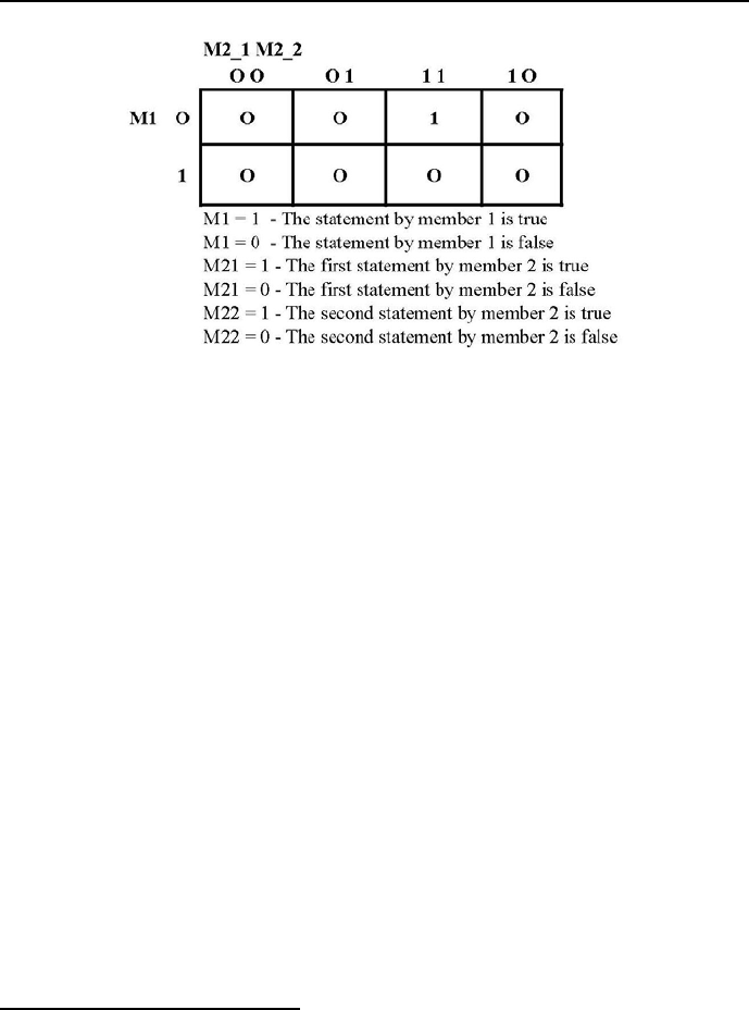
140 Chapter 3. CLP with elementary predicates for feasible solutions
Figure 3.13: Truth table for the state space of the RO-SC story
•the first column is clearly false: no club member ever tells two lies in
succession;
•the second column corresponds to a self-contradictory situation: if Member_3
lied, then the first statement by Member_2 cannot possibly by false;
•the same applies to the fourth column: if Member_3 did not lie, then of
course the first statement of Member_2 cannot possibly be true;
•consider the bottom square of the third column: if the statement by
Member_1 is true, then both statements by Member_2 cannot possibly be
true;
•what remains is the top square of third column, which corresponds to a
consistent state: if the statement by Member_1 is false, then both state-
ments of Member_2 are true;
•it follows that Member_1 and Member_3 are former Secret Collaborators,
and Member_2 is a former Righteous Oppositionist,Q.E.D.
Assured that a reasonable and unique answer exists, let’s use ECLiPSeto pro-
duce it. This is done by program 3_5_black_and_white.ecl9:
9This follows roughly the program presented by J. Schimpf to the ”Liars” problem, see
[Schimpf-10a].

3.6 Successful propagation of constraints 141
/*1*/ :- lib(ic).
/*2*/ :- lib(ic_symbolic).
/*3*/ :-local domain(club_member(righteous_oppositionist,secret_collaborator)).
/*4*/ top :-
/*5*/ solve(_).
/*6*/ solve([Member_1,Member_2,Member_3]):-
% Declaring the symbolic domain:
/*7*/ [Member_1,Member_2,Member_3] &:: club_member,
% Declaring binary variable domain:
/*8*/ [Member_3_possibly_said,Member_3_said, Member_1_possibly_said,
Member_2_said_first, Member_2_said_next] :: 0..1,
/*9*/ Member_1 &\= Member_2,
% % What Member_3 possibly said:
/*10*/ Member_3_possibly_said #= (Member_3 &=righteous_oppositionist),
/*11*/ single_utterance(Member_3, Member_3_possibly_said),
% What Member_1 possibly said:
/*12*/ Member_1_possibly_said #= (Member_3_said #=Member_3_possibly_said),
/*13*/ single_utterance(Member_1, Member_1_possibly_said),
% What Member_2 said first:
/*14*/ Member_2_said_first #= (Member_3 &=secret_collaborator),
/*15*/ single_utterance(Member_2,Member_2_said_first),
% What Memeber_2 said next:
/*16*/ Member_2_said_next #=(Member_3_said #= 0),
/*17*/ single_utterance(Member_2,Member_2_said_next),
/*18*/ consecutive_utterances(Member_2, Member_2_said_first,Member_2_said_next),
/*19*/ ic_symbolic:indomain(Member_1),
/*20*/ ic_symbolic:indomain(Member_2),
/*21*/ ic_symbolic:indomain(Member_3),
/*22*/ writeln("Member_1":Member_1),
/*23*/ writeln("Member_2":Member_2),
/*24*/ writeln("Member_3":Member_3),
/*25*/ writeln("Member_2_said_first":Member_2_said_first),
/*26*/ writeln("Member_2_said_next":Member_2_said_next).
% Righteous oppositionists always tell truth.
% Secret collaborators may tell truth or falsehood:
/*27*/ single_utterance(Member, Truth) :-
/*28*/ (Member &= righteous_oppositionist) => Truth.
% Check it using program \verb"test_TW_OE.ecl."
% Secret collaborators lie and tell the
142 Chapter 3. CLP with elementary predicates for feasible solutions
% truth in strict alteration.
% Righteous oppositionists always tell truth:
/*29*/ consecutive_utterances(Member, Truth1, Truth2) :-
/*30*/ (Member &= secret_collaborator) #= (Truth1 #\= Truth2).
% Check it using program \verb"3_12_baw_check.ecl"
Following message is generated:
Member_1 : secret_collaborator
Member_2 : righteous_oppositionist
Member_3 : secret_collaborator
Member_2_said_first : 1
Member_2_said_next : 1
It should be remembered that the symbol => denotes an implication as de-
fined in logic, see Table 3.1. It differs from the Prolog implications, see Table 2.1.
ConX ConY ConX => ConY
True True True
False True True
False False True
True False False
Table 3.1: Definition of implication in logic as used in ECLiPSe
In line /*28*/ reification is used, to be explained latter on in Section 5.6.4.
In order to better understand program 3_5_black_and_white.ecl,itisworth-
while to run program 3_6_baw_check.ecl10:
/*1*/ :- lib(ic).
/*2*/ :- lib(ic_symbolic).
/*3*/ :-local domain(club_member(righteous_oppositionist,secret_collaborator)).
/*4*/ top :-
% Consecutively one and only one of the lines /*5*/,...,/*15*/ is decommented.
% Depending upon the line decommented, the program generates an answer Yes or No.
/*5*/ % single_utterance(righteous_oppositionist, 1). % Yes
/*6*/ % single_utterance(righteous_oppositionist, 0). % No
/*7*/ % single_utterance(secret_collaborator, 0). % Yes
10 This is an FS-type problem.

3.7 Propagation is most often not enough 143
/*8*/ % single_utterance(secret_collaborator, 1). % Yes
/*9*/ % consecutive_utterances(righteous_oppositionist, 1, 0). % No
/*10*/ % consecutive_utterances(righteous_oppositionist, 1, 1). % Yes
/*11*/ % consecutive_utterances(righteous_oppositionist, 0, 1). % No
/*12*/ % consecutive_utterances(secret_collaborator, 1, 0). % Yes
/*13*/ % consecutive_utterances(secret_collaborator, 0, 0). % No
/*14*/ % consecutive_utterances(secret_collaborator, 0, 1). % Yes
/*15*/ consecutive_utterances(secret_collaborator, 1, 1). % No
% Righteous oppositionists always tell the truth.
% A single utterance by a secret collaborators may be true or false
/*16*/ single_utterance(Club_Member, Truth) :-
/*17*/ (Club_Member &= righteous_oppositionist) => Truth.
% Secret collaborators lie and tell the truth in alteration.
% Righteous oppositionists always (in alteration as well) tell the truth:
/*18*/ consecutive_utterances(Club_Member, Truth1, Truth2) :-
/*19*/ (Club_Member &= secret_collaborator) #= (Truth1 #\= Truth2).
For the decommented line /*15*/ the answer is: No.
The aim of programs in Section 3.6 was to show, that although constraint prop-
agation is an incomplete inference method, in some cases it is sufficient for
getting the solution. Because no backtracking was used, the approach rely-
ing only upon constraint propagation is sometimes denoted as backtrack-free
search. Obviously, augmenting the discussed program with search (i.e. in-
troducing labeling/1) creates no obstacle but usually accelerates the solving
process.
The remaining examples in this chapter are such that constraint propagation
alone is insufficient for getting the solution: constraint propagation has to be
supported by search.
3.7 Propagation is most often not enough
The programs presented so far, which used only propagation, are exceptional.
Normally search is needed to get a solution11. A series of example follows, for
which - despite their seemingly simplicity - search is mandatory.
11 Even for problems successfully solved with propagation only, search may be used to ac-
celerate the solution.

144 Chapter 3. CLP with elementary predicates for feasible solutions
3.7.1 Three equations
Consider program 3_7_three_equations.ecl12 for solving three linear equa-
tions in integers:
/*1*/ :- lib(ic).
/*2*/ top :-
/*3*/ [X,Y,Z]::0..6,
/*4*/ X + Y + Z #= 9,
/*5*/ write("Constraint X + Y + Z #= 9"),nl,
/*6*/ write("does not reduce domains:"),nl,
/*7*/ get_domain(X, LX),write("Domain of X ="),write(LX),nl,
/*8*/ get_domain(Y, LY),write("Domain of Y ="),write(LY),nl,
/*9*/ get_domain(Z, LZ),write("Domain of Z ="),write(LZ),nl,
/*10*/ 2*X+4*Y+3*Z #= 28,
/*11*/ write("The additional constraint 2*X + 4*Y +3* Z #= 28"),
/*12*/ nl,write("neither reduces domains:"),nl,
/*13*/ get_domain(X, LLX),write("Domain of X ="),write(LLX),nl,
/*14*/ get_domain(Y, LLY),write("Domain of Y ="),write(LLY),nl,
/*14*/ get_domain(Z, LLZ),write("Domain of Z ="),write(LLZ),nl,
/*16*/ 4*X+2*Y+Z #= 18,
/*17*/ write("At long last the constraint 4*X + 2*Y +Z #= 18"),
/*18*/ nl,write("reduces domains:"),nl,
/*19*/ get_domain(X, LLLX),write("Domain of X ="),write(LLLX),
/*20*/ nl,get_domain(Y, LLLY),write("Domain of Y ="),write(LLLY),
/*21*/ nl,get_domain(Z, LLLZ),write("Domain of Z ="),write(LLLZ),nl,
/*22*/ write("However, some values from the domains remain inconsistent."),nl,
/*23*/ labeling([X,Y,Z]),
/*24*/ write("Now,labeling is finishing the job of reducing domains:"),nl,
/*25*/ get_domain(X, KX),write("Domain of X ="),write(KX),nl,
/*26*/ get_domain(Y, KY),write("Domain of Y ="),write(KY),nl,
/*27*/ get_domain(Z, KZ),write("Domain of Z ="),write(KZ),nl,
/*28*/ write("and providing the unique solution:"),nl,
/*29*/ write("X = "),write(X),nl,
/*30*/ write("Y = "),write(Y),nl,
/*31*/ write("Z = "),write(Z),fail.
/*32*/ top:-
/*33*/ nl,write("No more solutions.").
12 This is an FS-type problem.

3.7 Propagation is most often not enough 145
The message is:
Constraint X + Y + Z ^= 9
does not reduce domains:
Domain of X =[0, 1, 2, 3, 4, 5, 6]
Domain of Y =[0, 1, 2, 3, 4, 5, 6]
Domain of Z =[0, 1, 2, 3, 4, 5, 6]
The additional constraint 2*X + 4*Y +3* Z #= 28
neither reduces domains:
Domain of X =[0, 1, 2, 3, 4, 5, 6]
Domain of Y =[0, 1, 2, 3, 4, 5, 6]
Domain of Z =[0, 1, 2, 3, 4, 5, 6]
At long last the constraint 4*X + 2*Y +Z #= 18
reduces domains:
Domain of X =[0, 1, 2, 3, 4]
Domain of Y =[1, 2, 3, 4, 5, 6]
Domain of Z =[0, 1, 2, 3, 4, 5, 6]
However, some values from the domains remain inconsistent.
Now, labeling is finishing the job of reducing domains:
Domain of X =[2]
Domain of Y =[3]
Domain of Z =[4]
and providing the unique solution:
X=2
Y=3
Z=4
No more solutions.
3.7.2 Golfers
Using integer constraints simplifies also program 3_8_golfers.pl from Section
2.4.1. This is illustrated by program 3_8_golfers.ecl13:
/*1*/ :- lib(ic).
/*2*/ top :-
/*3*/ [Fred,Joe,Tom,Bob]::1..4,
% Tom - variable denoting Tom’s position in line.
13 This is an FS-type problem.

146 Chapter 3. CLP with elementary predicates for feasible solutions
/*4*/ [Red,Orange,Blue,Plaid]::1..4,
% Blue - variable denoting the position of blue pants in line.
% 2)The golfer to Fred’s immediate right is wearing blue pants:
/*5*/ Blue#=Fred + 1,
% (3)Joe is second in line:
/*6*/ Joe#=2,
% (4)Bob is wearing plaid pants:
/*7*/ Bob#=Plaid,
% 5)Tom isn’t in position one or four, and he isn’t
% wearing the hideous orange pants:
/*8*/ Tom#\=1,
/*9*/ Tom#\=4,
/*10*/ Tom#\=Orange,
% All golfers are different:
/*11*/ Fred#\=Joe,
/*12*/ Fred#\=Tom,
/*13*/ Fred#\=Bob,
/*14*/ Joe#\=Tom,
/*15*/ Joe#\=Bob,
/*16*/ Tom#\=Bob,
% All colors are different:
/*17*/ Red#\=Orange,
/*18*/ Red#\=Blue,
/*19*/ Red#\=Plaid,
/*20*/ Orange#\=Blue,
/*21*/ Orange#\= Plaid,
/*22*/ Blue#\=Plaid,
/*13*/ labeling([Fred,Joe,Tom,Bob,Orange,
Blue,Red,Plaid]),
/*14*/ write("Fred,Joe,Tom,Bob"),nl,
/*15*/ write([Fred,Joe,Tom,Bob]),nl,
/*16*/ write("Red,Orange,Blue,Plaid"),nl,
/*17*/ write([Red,Orange,Blue,Plaid]),nl.
A following message is displayed:
Fred,Joe,Tom,Bob
[1, 2, 3, 4]

3.7 Propagation is most often not enough 147
Red,Orange,Blue,Plaid
[3, 1, 2, 4]
It means that e.g. Joe is in position 2 in the golfers list and wears pants
of a color corresponding to number 2 in the colors list, i.e. blue pants. The
readability of the message will be taken care of in Section 4.4.4.
This time labeling/1 is also needed to get the solution: constraint propa-
gation is clearly insufficient.
3.7.3 Watchtowers
The necessity of using search is not related to the number of constraints. We
already have seen example 3_4_students_and_languages.ecl were in spite of
a large number of constraints no search was needed for obtaining the solution.
The following example is an ”opposite” one: in spite of a small number of con-
straints, search has to be used to get the solution.
Consider a military base located on a square patch of land, surrounded by
a wall with corners and middle sides strengthened by multilevel watchtowers.
The guard in the corner watchtower may watch both adjacent wall sides. The
guard in the middle side watchtower may watch only his side of the wall. How
to allocate 12 guards in the watchtowers so that any side of the wall will be
watched by 5 guards?
This is solved by program 3_9_watchtowers.ecl14:
/*1*/ :- lib(ic).
/*2*/ top :-
/*3*/ Guards = [NW,N,NE,W,E,SW,S,SE],
%NW - number of guards in watchtower NorthWest
%E - number of guards in watchtower East
/*4*/ Guards :: 0..12,
/*5*/ sum(Guards) #= 12,
/*6*/ NW + N + NE #= 5,
/*7*/ NE + E + SE #= 5,
/*8*/ NW + W + SW #= 5,
/*9*/ SW + S + SE #= 5,
14 This is an FS-type problem.

148 Chapter 3. CLP with elementary predicates for feasible solutions
/*10*/ labeling(Guards),
/*11*/ printf("%3d%3d%3d\n", [NW,N,NE]),
/*12*/ printf("%3d %5d\n", [W, E]),
/*13*/ printf("%3d%3d%3d\n", [SW,S,SE]).
The solution is:
005
20
320
In spite of the examples simplicity, labeling/1 is needed to get a solution:
constraint propagation alone is not sufficient.
3.7.4 Examination
A domain declaration may simplify the examination problem from Section 2.4.7
and accelerate its solution. This is shown by the 3_10_egzamination.ecl pro-
gram15:
/*1*/ :- lib(ic).
/*2*/ top :-
/*3*/ L=[M1,M2,M3,M4,M5,M6,M7,M8,M9,M10,M11,M12,M13,M14,M15,
M16,M17],
/*4*/ L :: 1..4,
/*5*/ M1 #\= M2, /*6*/ M1 #\= M5,
/*7*/ M1 #\= M6, /*8*/ M1 #\= M7,
/*9*/ M2 #\= M6, /*10*/ M2 #\= M7,
/*11*/ M2 #\= M3, /*12*/ M2 #\= M8,
/*13*/ M3 #\= M7, /*14*/ M3 #\= M8,
/*15*/ M3 #\= M9, /*16*/ M3 #\= M4,
/*17*/ M4 #\= M8, /*18*/ M4 #\= M9,
/*19*/ M5 #\= M6, /*20*/ M5 #\= M10,
/*21*/ M5 #\= M11, /*22*/ M6 #\= M10,
/*23*/ M6 #\= M11, /*24*/ M6 #\= M7,
/*25*/ M6 #\= M12, /*26*/ M7 #\= M11,
/*27*/ M7 #\= M12, /*28*/ M7 #\= M8,
/*29*/ M7 #\= M13, /*30*/ M8 #\= M12,
/*31*/ M8 #\= M13, /*32*/ M8 #\= M14,
/*33*/ M8 #\= M9, /*34*/ M9 #\= M13,
/*35*/ M9 #\= M14, /*36*/ M10 #\= M11,
15 This is an FS-type problem.

3.7 Propagation is most often not enough 149
/*37*/ M11 #\= M15, /*38*/ M11 #\= M12,
/*39*/ M12 #\= M15, /*40*/ M12 #\= M16,
/*41*/ M12 #\= M13, /*42*/ M13 #\= M15,
/*43*/ M13 #\= M16, /*44*/ M13 #\= M17,
/*45*/ M13 #\= M14, /*46*/ M14 #\= M16,
/*47*/ M14 #\= M17, /*48*/ M15 #\= M16,
/*49*/ M16 #\= M17,
/*50*/ labeling([M1,M2,M3,M4,M5,M6,M7,M8,M9,M10,
M11,M12,M13,M14,M15,M16,M17]),
/*51*/ write(M1),write(", "),write(M2),
write(", "),write(M3),write(", "),write(M4),nl,
/*52*/ write(M5),write(", "),write(M6),write(", "),write(M7),
write(", "),write(M8),write(", "),write(M9),nl,
/*53*/ write(M10),write(", "),write(M11),write(", "),write(M12),
write(", "),write(M13),write(", "),write(M14),nl,
/*54*/ write(M15),write(", "),write(M16),
write(", "),write(M17), nl.
One of many possible solutions is given by:
1, 2, 1, 2
2, 3, 4, 3, 4
4, 1, 2, 1, 2
3, 4, 3
This time the solution was obtained immediately. This is a good example of
the efficiency of search and propagation performed by ECLiPSe−CPS as
compared with search and unifications performed by ECLiPSe−P rolog.
3.7.5 Queens
Consider now a CLP-version of the Prolog program 2_14_queens_bs.pl.The
program 3_11_queens.ecl16 determines also safe placements for 8 queens, but
seems to be more simple and readable than the former:
16 This is an FS-type problem.

150 Chapter 3. CLP with elementary predicates for feasible solutions
/*1*/ :- lib(ic).
/*2*/ top :-
/*3*/ queens(L),
/*4*/ write(L).
/*5*/ queens([X1,X2,X3,X4,X5,X6,X7,X8]):-
/*6*/ [X1,X2,X3,X4,X5,X6,X7,X8]::1..8,
/*7*/ safe([X1,X2,X3,X4,X5,X6,X7,X8]),
/*8*/ labeling([X1,X2,X3,X4,X5,X6,X7,X8]),
/*9*/ write([X1,X2,X3,X4,X5,X6,X7,X8]),nl,
/*10*/ fail.
/*11*/ queens(_):-
/*12*/ write("That’s all!"),nl.
/*13*/ safe([]).
/*14*/ safe([H|T]):-
/*15*/ no_attack(H,T),
/*16*/ safe(T).
/*17*/ no_attack(X,Xs):-
/*18*/ no_attack(X,Xs,1).
/*19*/ no_attack(_,[],_).
/*20*/ no_attack(X,[Y|Ys],Nb):-
/*21*/ X #\= Y,
/*22*/ X #\= Y + Nb,
/*23*/ Y #\= X + Nb,
/*24*/ Nb1 is Nb+1,
/*25*/ no_attack(X,Ys,Nb1).
There are 92 placements, from which only the first and last three are presented:
[1, 5, 8, 6, 3, 7, 2, 4]
[1, 6, 8, 3, 7, 4, 2, 5]
[1, 7, 4, 6, 8, 2, 5, 3]
.......................
[8, 2, 5, 3, 1, 7, 4, 6]
[8, 3, 1, 6, 2, 5, 7, 4]
[8, 4, 1, 3, 6, 2, 7, 5]
This time labeling/1 was also needed to get the solution; propagation alone
was clearly insufficient.

3.7 Propagation is most often not enough 151
3.7.6 Configuration
We should not forget about transforming the 3-element configuration program
from Section 2.2.3 into a full-grown CLP program, given by 3_12_con_CLP.ecl17:
/*1*/ :- lib(ic).
/*2*/ top :-
/*3*/ Components=[A_1,A_2,A_3,B_1,B_2,B_3,B_4,C_1,C_2],
/*4*/ Components :: 0..1,
/*5*/ Cost:: 1..2100,
% Only one A-type element is needed:
/*6*/ A_1 + A_2 + A_3 #= 1,
% Only one B-type element is needed:
/*7*/ B_1 + B_2 + B_3 + B_4 #= 1,
% Only one C-type element is needed:
/*8*/ C_1 + C_2 #= 1,
% Those are compatibility constraints:
/*9*/ C_1 + A_2 #=< 1, % C_1 and A_2 not in the same configuration
/*10*/ B_2 + C_2 #=< 1, % B_2 and C_2 not in the same configuration
/*11*/ C_2 + B_3 #=< 1, % C_2 and B_3 not in the same configuration
/*12*/ B_4 + A_2 #=< 1, % B_4 and A_2 not in the same configuration
/*13*/ B_3 + A_1 #=< 1, % B_3 and A_1 not in the same configuration
/*14*/ A_3 + B_3 #=< 1, % A_3 and B_3 not in the same configuration
/*15*/ Cost #= A_1 * 1900 + A_2 * 750 +
A_3 * 900 + B_1 * 300 + B_2 * 500 + B_3 * 450 +
B_4 * 600 + C_1 * 700 + C_2 * 850,
/*16*/ labeling(Components),
/*17*/ writeln(’Feasible configuration with cost’:Cost),,
/*18*/ write_configuration([A_1,A_2,A_3,B_1,B_2,B_3,B_4,C_1,C_2],
["A_1","A_2","A_3","B_1","B_2","B_3","B_4","C_1","C_2"]),nl,nl,
/*19*/ fail.
/*20*/ top :-
/*21*/ write("Those are all feasible configurations.").
/*22*/ write_configuration([H1|T1],[H2|T2]):-
/*23*/ H1 is 1, write(H2),write(" "),
/*24*/ write_configuration(T1,T2).
17 This is an FS-type problem.

152 Chapter 3. CLP with elementary predicates for feasible solutions
/*25*/ write_configuration([H1|T1],[_|T2]):-
/*26*/ H1 is 0,
/*27*/ write_configuration(T1,T2).
/*28*/ write_configuration([],[]).
The solution is:
Feasible configuration with cost 2100:
A_3 B_2 C_1
Feasible configuration with cost 2050:
A_3 B_1 C_2
Feasible configuration with cost 1900:
A_3 B_1 C_1
Feasible configuration with cost 1900:
A_2 B_1 C_2
Those are all feasible configurations.
This time labeling/1 was also needed.
3.8 Exercises
Equations and conditionals 1
Write a program to determine the smallest integer solution for the follow-
ing equations and conditionals:
A+E=G
C+D=10
E+F=8
A+C=6
If F <> 6thenH>F
If E <> 1thenH>B
If G <> 8thenF>B
If B <> 5thenG<> 5
If E <> 3thenC<> 4
where <> is a disequation.

3.8 Exercises 153
Solution:
A=4, B=1, C=2, D=8, E=3, F=5, G=7, H=6
Equations and conditionals 2
Write a program to determine the smallest integer solution for the follow-
ing equations and conditionals:
B+G=D
B+C=A
C+E+G=F
If D <AthenC=2
If D >= AthenE=2.
Solution:
A=5, B=4, C=1, D=7, E=2, F=6, G=3
A visit
The Smith family and their three children want to pay a visit but they do
not all have the time to do so. Following are few hints who will go and
who will not: If Mr Smith comes, his wife will come too. At least one of
their two sons Matt and John will come. Either Mrs Smith or Tim will
come, but not both. Either Tim and John will come, or neither will come.
If Matt comes, then John and his father will also come. Write a program
to determine who went and who did not.
Horse derby
At last horse derby, 10 fine horses completed the grueling 3 mile course.
Predictably, as per every year, the results mysteriously went missing. How-
ever, various marshals remembered the following snippets of information:
Sylvester lost to Zebra Wings. Zebra Wings beat Sylwester, Frogman’s
Flippers and Tweetie Pie. Fizzy Pop lost to Minty Mouse, Sylvester and
CD Player. Frogman’s Flippers beat Windy Miller, CD Player and Syl-
wester. Top Trumps lost to CD Player, Kool Kat and Tweetie Pie. CD
Player beat Top Trumps and Fizzy Pop. Tweetie pie lost to Zebra Wings
and Sylvester. Kool Kat lost to Tweetie Pie and Frogman’s Flippers. Frog-
man’s Flippers beat Fizzy Pop, Minty Mouse and CD Player. CD Player
lost to Frogman’s Flippers, Kool Kat and Tweetie Pie. Top Trumps beat
Fizzy Pop and Windy Miller. Minty Mouse lost to Windy Miller and Syl-
wester. Windy Miller lost to Tweetie Pie and CD Player. Write a program
to work out who finished where.

154 Chapter 3. CLP with elementary predicates for feasible solutions
Spring fete
At the recent spring fete, four keen gardeners were displaying their fine
roses. In total there were four colors and each rose appeared in two colors.
Mr Green had a yellow rose. Mr Yellow did not have a red one. Mr Red
had a blue rose but not a green one, whilst Mr Blue did not have a yellow
one. One person with a red rose also had a green one. One person with
a yellow rose also had a blue one. One of the persons with a green rose
had no red. Neither of the persons with a yellow rose had a green one. No
person has two roses of the same color and no two persons had the same
two color roses and their names provide no clues. Write a program which
settles who had which color roses.
Cake theft
During a recent police investigation, Chief Inspector Stone was interview-
ing five local villains to try and identify who stole Mrs Archer’s cake from
the mid-summers fair. Below is a summary of their statements:
1)Arnold: it wasn’t Edward it was Brian
2)Brian: it wasn’t Charlie it wasn’t Edward
3)Charlie: it was Edward it wasn’t Arnold
4)Derek: it was Charlie it was Brian
5)Edward:it was Derek it wasn’t Arnold
It was well known that each suspect told exactly one lie. Write a program
to determine who stole the cake.
Horse race
A gambler bet on a horse race, but the bookie wouldn’t tell him the results
of the race. The bookie gave clues as to how the five horses finished – which
may have included some ties – and wouldn’t pay the gambler off unless
the gambler could determine how the five horses finished based on the
following clues:
1. Penuche Fudge finished before Near Miss and after Whispered Promises.
2. Whispered Promises tied with Penuche Fudge if and only if Happy Go
Lucky did not tie with Skipper’s Gal.
3. Penuche Fudge finished as many places after Skipper’s Gal as Skipper’s
Gal finished after Whispered Promises if and only if Whispered Promises
finished before Near Miss.
The gambler thought for a moment, then answered correctly. Write a
program to determine how did the five horses finish the race.

3.8 Exercises 155
Grades
Five friends in the sixth form took the same combination of A-level sub-
jects. Each obtained a different grade in each subject taken, and no two
students had the same grade in the same subject. Write a program to de-
termine grades obtained for each subject by each student, provided that:
- Andrew outscored Bridget in Physics, and Neil in Math.
- Wendy was the only girl to get a ”C” grade, but she managed no ”A”
grades
- The pupil with an ”E” in Math gained a ”B” in Chemistry, but was not
awarded a ”C” in Physics.
- Paul’s Physics grade was a ”D” and his highest grade was a ”C”.
- The ”B” in Math did not go to the same student as the ”E” in Physics.
- Bridget’s best result was in Chemistry, but her Math grade was lower
than Paul’s.
The Autumn Leaves Trail
Thousands of tourists drive the Autumn Leaves Trail each fall to enjoy the
multicolored vista of changing seasons18. The Trail starts in Summerset
and goes north 10.0 miles to Fallbrook. Five scenic spots highlight the
drive, each providing parking along the narrow road with a spectacular
view of a different Trail attraction; each scenic spot is at a different mile-
post designating its distance from Summerset in tenths of a mile. Given
the road map data below, write a program to determine at what milepost
along the Autumn Leaves Trail each viewpoint is located:
1. No two consecutive scenic spots are the same distance apart; the longest
drive between any two consecutive locations (including end points) on the
Trail is 3.6 miles, while the shortest is .4 miles.
2. The distance along the Autumn Leaves Trail from Summerset to Cu-
cumber Creek equals the distance going north from Old Man Mountain
to the White Oak Inn.
3. The Amish Covered Bridge, which isn’t the last scenic spot along the
route, is 1.0 miles south of Fallbrook.
4. The Cucumber Creek spot is twice as far from the Sugar Maple Farm
stop as it is from the Old Man Mountain viewpoint.
5. The White Oak Inn and Cucumber Creek photographic opportunities
lie more than 5.0 miles apart.
6. The first scenic spot on the Trail is at milepost 1.8 north of Summerset.
18 This exercise is from http://aaa.allstarpuzzles.netdna-cdn.com/logic/00082.html

156 Chapter 3. CLP with elementary predicates for feasible solutions
Gardens
Five friends have their gardens next to one another, where they grow three
kinds of crops: fruits (apple, pear, nut, cherry), vegetables (carrot, parsley,
gourd, onion) and flowers (aster, rose, tulip, lily)19.
1. They grow 12 different varieties.
2. Everybody grows exactly 4 different varieties.
3. Each variety is at least in one garden.
4. Only one variety is in 4 gardens.
5. Only in one garden are all 3 kinds of crops.
6. Only in one garden are all 4 varieties of one kind of crops.
7. Pears are only in the two border gardens.
8. Paul’s garden is in the middle with no lily.
9. Aster grower doesn’t grow vegetables.
10. Rose grower doesn’t grow parsley.
11. Nuts grower has also gourd and parsley.
12. In the first garden are apples and cherries.
13. Only in two gardens are cherries.
14. Sam has onions and cherries.
15. Luke grows exactly two kinds of fruit.
16. Tulips are only in two gardens.
17. Apples are in a single garden.
18. Only in one garden next to the Zick’s is parsley.
19. Sam’s garden is not on the border.
20. Hank grows neither vegetables nor asters.
21. Paul has exactly three kinds of vegetable.
Write a program to determine who has which garden and what is grown
where.
Open House 20
Five students in the local ”gifted and talented” program (three girls named
Brittany, Natalie, and Olive, and two boys named Emile and Moises) or-
ganized their school’s open house this year. Each of these students is
majoring in a different area of study (geography, language, math, philos-
ophy, or sculpture). Some of these students enlisted one or more relatives
to assist with the production of the open house (mother, father, or grand-
mother), though no one enlisted more than one of any kind of relative.
Write a program to discover each student’s full name (surnames are Brad-
19 This exercise is from http://www.mathsisfun.com/puzzles
20 This exercise is from http://brownbuffalo.sourceforge.net/

3.8 Exercises 157
shaw, Henderson, Smith, Wu, and Zacher), area of study, and the relative
or relatives, if any, of each child who assisted, provided that:
1. Smith (who isn’t Moises or Olive) isn’t the philosophy major.
2. Two of Wu’s relatives assisted with the program.
3. Zacher enlisted fewer of his or her relatives to assist than at least one
other student.
4. The sculpture major is the only one who enlisted no relatives to assist.
5. Brittany and Henderson each enlisted one parent; neither of them en-
listed a grandmother, and neither of them is the math major.
6. Moises and the geography major either both enlisted their fathers’ as-
sistance, or neither of them did.
7. No two students of the same gender enlisted their mothers.
8. Bradshaw’s father didn’t assist.
9. Olive enlisted one more relative than the math major.
10. Natalie is the language major, and her father didn’t assist.
Swimming race
Five competitors - A, B, C, D and E - enter a swimming race that awards
gold, silver and bronze medals to the first three to complete it. Each of
the following compound statements about the race is false, although one
of two clauses in each may be true:
- A didn’t win the gold, B didn’t win the silver.
- D didn’t win the silver and E didn’t win the bronze.
- C won a medal, D didn’t.
- A won a medal, C didn’t.
-DandEbothwonmedals.
Write a program to determine who won each of the medals.
Queue for plane tickets 21
Five people are standing in a queue for plane tickets in Germany; each
one has a name, an age, a favorite Internet website, a place they live, a
hairstyle and a destination from the sets:
Their names are: Bob, Keeley, Rachael, Eilish and Amy, their ages: 14, 21,
46, 52 and 81, their favorite Internet websites: ”Rush Limbaugh Show”,
”Conservapedia”, ”Chronicles: A Magazine of American Culture”, ”Jeff
Rense Program” and ”American Thinker”, they live at a town, a city, a
village, a farm and a youth hostel, their hairstyle is: afro, long, straight,
curly and bald, their destinations are: France, Australia, England, Africa
21 This exercise is from http://www.mathsisfun.com/puzzles

158 Chapter 3. CLP with elementary predicates for feasible solutions
and Italy. Besides:
1. The person in the middle reads ”Jeff Rense Program”
2. Bob is the first in the queue
3. The person who reads the ”Rush Limbaugh Show” is next to the person
who lives in a youth hostel
4. The person going to Africa is behind Rachael.
5. The person who lives in a village is 52.
6. The person who is going to Australia has straight hair.
7. The person traveling to Africa reads ”Jeff Rense Program”.
8. The 14 year old is at the end of the queue.
9. Amy reads ”Chronicles: A Magazine of American Culture”.
10. The person heading to Italy has long hair.
11. Keeley lives in a village.
12. The 46 year old is bald.
13. The fourth in the queue is going to England.
14. The people with curly and straight hair are standing next to each
other.
15. The person who reads ”Conservapedia” stands next to the person
with an afro.
16. A person next to Rachael has an afro.
17. The 21 year old lives in a youth hostel.
18. The person who reads ”Conservapedia” has long hair.
19. The 81 year old lives on a farm.
20. The person who is traveling to France lives in a town.
Write a program to determine names, ages, favorite Internet website, living
places, hairstyles and destinations of all concerned.
Science Fair
Art and Bert were describing the result of the International Science Fair
Extravaganza. There were three contestants, Louis, Rene, and Johannes.
Art reported that Louis won the fair, while Rene came in second. Bert,
on the other hand, reported that Johannes won the fair, while Louis came
in second. In fact, neither Art nor Bert had given a correct report of the
results of the science fair. Each of them had given one correct statement
and one false statement. Write a program to determine what was the
actual placing of the three contestants.
Chapter 4
CLP with global constraints
for feasible solutions
4.1 Introductory remarks
The concepts introduced in this chapter and Chapter 6 are basic for modeling
and solving complicated combinatorial problems. In order to create efficient
platforms for modeling and solving CSP and COP, a set of fundamental con-
cepts and predicates corresponding to these concepts is needed. For continuous
dynamic systems, dealt with e.g. in mechanics and control engineering, the
concepts needed had been developed and had matured over ages, starting with
pioneering work by Newton and Leibnitz on differential equations. For com-
binatorial problems the concepts started to be developed with the advent of
Prolog and CLP, and culminated in defining and programming a series of ba-
sic, extremely useful high-level abstracts implemented as global constraints,see
[Baldiceanu-94] and [Baldiceanu-10]. Global constraints are constraints defining
complex relations over a number of input lists of variables. They are sup-
ported by libraries ic_global,lib(ic_cumulative),lib(ic_edge_finder),
lib(ic_edge_finder3).lib(branch_and_bound) They are contrasted with
already discussed elementary constraints with at most one input list, supported
by ic and branch_and_bound libraries. The use of global predicates enhances
program readability, declarativity and effectiveness while substantially decreas-
ing the time needed to model the problem. The ECLiPSeCPS user may
find elementary as well as global constraints in the Alphabetical Predicate Index
159

160 Chapter 4. CLP with global constraints for feasible solutions
menu ECLIPSe Documentation from Figure 5.
The global predicates alldifferent/1 and element/3 are made available
by invoking the needed library1by declaring:
:- lib(ic_global).
or
:- use_module(library(ic_global)).
4.2 The ’alldifferent/1’ built-in
The built-in:
alldifferent(?List)
is fulfilled if all elements of the List=[X1,...,Xn] are pairwise different.
This is one of the most useful and often used global constraints. Theoretically
speaking it corresponds to the following set of disequations:
X1#\=X2,
X1#\=X3,
.......
X1#\=Xn,
X2#\=X3,
.......
X2#\=Xn,
.......
X(n-1)#\=Xn,
However, the search and propagation methods for alldifferent([X1,...,Xn])
are much more efficient than those for the above definition.
1The ic library provides as well support for ’alldifferent/1’ and ’element/3’, but in a less
effective way.

4.2 The ’alldifferent/1’ built-in 161
The alldifferent/1 constraint is practically always used with indomain/1
constraints, enforcing all values considered to be from the variable domains.
Consider example 4_1_all_diff.ecl2, were it is required that X,Y,Z be a three-
element variation of the four-set [1,2,3,4]:
/*1*/ :- lib(ic).
/*2*/ top :-
/*3*/ [X,Y,Z]::1..4,
/*4*/ alldifferent([X,Y,Z]),
/*5*/ indomain(X),
/*6*/ indomain(Y),
/*7*/ indomain(Z),
/*8*/ writeln("X":X),
/*9*/ writeln("Y":Y),
/*10*/ writeln("Z":Z),
/*11*/ fail.
/*12*/ top:-
/*13*/ write("That’s it."),nl.
The message is:
X=1Y=2Z=3
X=1Y=2Z=4
X=1Y=3Z=2
X=1Y=3Z=4
X=1Y=4Z=2
X=1Y=4Z=3
X=2Y=1Z=3
X=2Y=1Z=4
X=2Y=3Z=1
X=2Y=3Z=4
X=2Y=4Z=1
X=2Y=4Z=3
X=3Y=1Z=2
X=3Y=1Z=4
X=3Y=2Z=1
X=3Y=2Z=4
X=3Y=4Z=1
2This is an FS-type problem.

162 Chapter 4. CLP with global constraints for feasible solutions
X=3Y=4Z=2
X=4Y=1Z=2
X=4Y=1Z=3
X=4Y=2Z=1
X=4Y=2Z=3
X=4Y=3Z=1
X=4Y=3Z=2
That’s it.
Thanks to fail in line /*11*/, all solutions for alldifferent([X,Y,Z]) are
determined. Obviously, if there are no solutions like for 4_2_all_diff.ecl:
/*1*/ :- lib(ic).
/*2*/ top :-
/*3*/ [V,W,X,Y,Z]::1..4,
/*4*/ alldifferent([V,W,X,Y,Z]),
/*5*/ indomain(V),
/*6*/ indomain(W),
/*7*/ indomain(X),
/*8*/ indomain(Y),
/*9*/ indomain(Z),
/*10*/ writeln(’V’:V),
/*11*/ writeln(’W’:W),
/*12*/ writeln(’X’:X),
/*13*/ writeln(’Y’:Y),
/*14*/ writeln(’Z’:Z).,
the message is:
No.
4.3 The ’element/3’ built-in
The built-in:
element(?Index, ++List, ?Value)
constraints Value to be at the position Index in the grounded integer list List.

4.3 The ’element/3’ built-in 163
This is also a very useful constraint, because it implements a relation between
two domain variables, namely between a subscripted (indexed) variable from the
List and the subscript (index) value for the variable from the List. I.e. for:
element(N, [c1,c
2..., cn],Y)
the constraint requires that:
Y=cN.
Its importance is enhanced by the fact that either one or both Index and Value
may be variables. This is illustrated by program 4_3_element.ecl3:
/*1*/ :- lib(ic).
/*2*/ top:-
/*3*/ element(Index,[20,10,41,32],41),
/*4*/ writeln("Index ":Index),
/*5*/ element(2,[](20,10,41,32),Indexed_Value),
/*6*/ writeln("Indexed_Value ":Indexed_Value),
/*7*/ element(I,[20,10,41,32],I_V),
/*8*/ writeln("I ":I),
/*9*/ writeln("I_V":I_V).
The message is:
Index : 3
Indexed_Value : 10
I : _955{1 .. 4}
I_V : _1087{[10, 20, 32, 41]}
The examples presented below are classified into the following two problem
classes:
1. Feasible assignment problems, aiming at joining elements of some sets so
as to fulfill constraints of belongness.
2. Feasible sequencing problems, aiming at ordering elements of some set so
as to fulfill constraints of precedence.
The adjective feasible is used to distinguish the problems from optimum once
discussed in Chapter 5.
3This is an FS-type problem.

164 Chapter 4. CLP with global constraints for feasible solutions
4.4 Feasible assignment problems
Their essence is to find - for any element of some set - elements from some
other sets so as to fulfill some constraints of belongness. Tie constraints define
constraints among elements of various sets.
4.4.1 Send More Money
CLP is excellent for solving cryptarithmetic puzzles in the form of equations
among unknown numbers whose digits are represented by letters. The following
puzzle4belongs to the folklore of CLP:
There is a mathematical equation:
SEND
MORE
----------
MONEY
among unknown digits 0,1,2,3,4,5,6,7,8 and 9 represented by letters S,E,N,D,M,O,R,Y.
The goal is to identify the value of each letter. The puzzle is solved by program
4_4_smm.ecl5:
/*1*/ :- lib(ic).
/*2*/ top:-
/*3*/ sendmore(_).
/*4*/ sendmore(L) :-
/*5*/ L = [S,E,N,D,M,O,R,Y],
/*6*/ L :: [0..9],
/*7*/ alldifferent(L),
/*8*/ S #\= 0,
/*9*/ M #\= 0,
/*10*/ 1000*S + 100*E + 10*N + D
+ 1000*M + 100*O + 10*R + E
#= 10000*M + 1000*O + 100*N + 10*E + Y,
/*11*/ labeling(L),
4It is attributed to Henry Dudeney who published it in the July 1924 issue of Strand
Magazine
5This is an FS-type problem.

4.4 Feasible assignment problems 165
/*12*/ write(" "),write(S),write(E),write(N),write(D),
/*13*/ write(" S E N D"),nl,
/*14*/ write(" "),write(M),write(0),write(R),write(E),
/*15*/ write(" M O R E"),nl,
/*16*/ write(" ----------------"),nl,
/*17*/ write(" "),write(M),write(0),write(N),write(E),write(Y),
/*18*/ write(" M O N E Y"),nl,nl.
The message is:
9567 S E N D
1085 M O R E
------ ----------
10652 M O N E Y
4.4.2 FIFTEEN
A more advanced cryptarithmetic puzzle is known as FIFTEEN:
In the addition sum below digits have been replaced by letters and @symbols:
@
@@@FIVE
@@FIVE@
+ @FIVE@@
-----------
FIFTEEN
Different letters stand for different digits, the same letter stands for the same
digit, an @symbol stands for any digit, which may be different in different @
positions, and leading digits cannot be zero. If FIVE is divisible by 5and ELEVEN
is divisible by 11, the program 4_5_FIFTEEN.ecl determines what number is
FIFTEEN and what digits are represented by all the symbols. However, the sym-
bols @in different positions have to be named differently, e.g. like this
A1
A4 A3 A2 F I V E
A7 A6 F I V E A5
+A10FIVEA9A8
------------------------
FIFTE E N

166 Chapter 4. CLP with global constraints for feasible solutions
The program 4_5_FIFTEEN.ecl is as follows:
/*1*/ :- lib(ic).
/*2*/ top:-
/*3*/ assert(counter(0)),
/*4*/ P = [F,I,V,E,T,N,L,A1,A2,A3,A4,A5,A6,A7,A8,A9,A10],
/*5*/ P :: [0..9],
/*6*/ alldifferent([F,I,V,T,N,L,E]),
/*7*/ F #\= 0,
/*8*/ E#\=0,
/*9*/ E #= 5,
/*10*/ A1#\=0,
/*11*/ A4#\=0,
/*12*/ A7#\=0,
/*13*/ A10#\=0,
/*14*/ my_modulo_5(F,I,V,E),
/*15*/ my_modulo_11(E,L,E,V,E,N),
/*16*/ A1 +
/*17*/ E + 10*V + 100*I + 1000*F + 10000*A2 + 100000*A3 + 1000000*A4 +
/*18*/ A5 + 10*E + 100*V + 1000*I + 10000*F + 100000*A6 + 1000000*A7 +
/*19*/ A8 + 10*A9 + 100*E + 1000*V + 10000*I + 100000*F + 1000000*A10 #=
/*19*/ 1000000*F + 100000*I+ 10000*F + 1000*T + 100*E + 10*E + N,
/*20*/ labeling(P),
/*21*/ count,
/*22*/ counter(Solution_number),
/*23*/ write("Solution "), write(Solution_number),write(":"),nl,
/*24*/ write(" "),write(" "),write(" "),write(A1),
/*25*/ write(" "),write(" "),write(" "),write(" "),write(" "),
write(" "),write(" "),write(" "),write(" A1"),nl,
/*26*/ write(A4),write(A3),write(A2),write(F),write(I),write(V),write( E),
/*27*/ write(" A4 A3 A2 F I V E"),nl,
/*28*/ write(A7),write(A6),write(F),write(I),write(V),write(E),write(A5),
/*29*/ write(" A7 A6 F I V E A5"),nl,
/*30*/ write(A10),write(F),write(I),write(V),write(E),write(A9),write(A8),
/*31*/ write(" A10 F I V E A9 A8"),nl,
/*32*/ write("------- --------------------"),nl,
/*33*/ write(F),write(I),write(F),write(T),write(E),write(E),write(N),
/*34*/ write(" FIFTEEN"),nl,nl,
/*35*/ fail.
/*36*/ top:-nl,nl,
/*37*/ write("That’s everything!").

4.4 Feasible assignment problems 167
/*38*/ my_modulo_5(F,I,V,E):-
/*39*/ integers(X),
/*40*/ E+10*V+100*I+1000*F #= X*5.
/*41*/ my_modulo_11(E,L,E,V,E,N):-
/*42*/ integers(X),
/*43*/ N+10*E+100*V+1000*E+10000*L+100000*E #= X*11.
/*44*/ count:-
/*45*/ retract(counter(Old)),
/*46*/ New is Old + 1,
/*47*/ assert(counter(New)).
The problem has 18 solution, all with the same FIFTEEN. The first and the
last one are as follows:
Solution 1:
8A1
1094085 A4 A3 A2FIVE
1540859 A7 A6FIVEA5
1408599 A10FIVEA9A8
------- --------------------
4043551 F IFTEEN
.........................
Solution 18:
9A1
1594085 A4 A3 A2FIVE
1040859 A7 A6FIVEA5
1408598 A10FIVEA9A8
------- --------------------
4043551 F IFTEEN
4.4.3 Who with whom again
Both global constraints discussed so far enable to simplify the program solving
the whowithwhompuzzle from Section 3.6.2 while at the same time enabling the
generation of a readable message. The modified program 4_6_who_with_whom_
again.ecl6is as follows:
6This is an FS-type problem.

168 Chapter 4. CLP with global constraints for feasible solutions
/*1*/ :- lib(ic).
/*2*/ top :-
/*3*/ [Andy, Ben, Carl, Dusty]::[1..4],
/*4*/ [Olive, Eva, Paula, Sabina]::[1..4],
% concert=1, cinema=2, theater=3, exhibition=4
% It means: if e. g. Ben=Olive=4, then
% Ben and Olive went to an exhibition
% Andy enjoyed a concert:
/*5*/ Andy#=1,
% Ben accompanied Olive:
/*6*/ Ben#=Olive,
% Carl has not seen Eva:
/*7*/ Carl#\=Eva,
% Paula went to a cinema:
/*8*/ Paula#=2,
% Eva went to a theater:
/*9*/ Eva#=3,
/*10*/ alldifferent([Andy,Ben,Carl,Dusty]),
/*11*/ alldifferent([Olive,Eva,Paula,Sabina]),
/*12*/ write(Andy),write(" "),write(Ben),write(" "),
/*13*/ write(Carl),write(" "),write(Dusty),nl,
/*14*/ write(Olive),write(" "),write(Eva),write(" "),
/*15*/ write(Paula),write(" "),write(Sabina),nl,nl,
% End of solution part.
% Beginning of message part:
% Determining the numbers for boys on the boy list:
/*16*/ element(Number_of_First_Boy,[Andy,Ben,Carl,Dusty],1),
/*17*/ element(Number_of_Second_Boy,[Andy,Ben,Carl,Dusty],2),
/*18*/ element(Number_of_Third_Boy,[Andy,Ben,Carl,Dusty],3),
/*19*/ element(Number_of_Fourth_Boy,[Andy,Ben,Carl,Dusty],4),
% Determining the numbers for girls on the girl list:
/*20*/ element(Number_of_First_Girl,[Olive, Eva,Paula,Sabina],1),
/*21*/ element(Number_of_Second_Girl,[Olive, Eva,Paula,Sabina],2),
/*22*/ element(Number_of_Third_Girl,[Olive, Eva,Paula,Sabina],3),
/*23*/ element(Number_of_Fourth_Girl,[Olive, Eva,Paula,Sabina],4),
% Translating numbers for boys to names:
/*24*/ name_of_boy(Number_of_First_Boy,Name_of_1_boy),
/*25*/ name_of_boy(Number_of_Second_Boy,Name_of_2_boy),
/*26*/ name_of_boy(Number_of_Third_Boy,Name_of_3_boy),

4.4 Feasible assignment problems 169
/*27*/ name_of_boy(Number_of_Fourth_Boy,Name_of_4_boy),
% Translating numbers for girls to names:
/*28*/ name_of_girl(Number_of_First_Girl,Name_of_1_girl),
/*29*/ name_of_girl(Number_of_Second_Girl,Name_of_2_girl),
/*30*/ name_of_girl(Number_of_Third_Girl,Name_of_3_girl),
/*31*/ name_of_girl(Number_of_Fourth_Girl,Name_of_4_girl),
/*32*/ write(Name_of_1_boy),write(" and "),
/*33*/ write(Name_of_1_girl), write(" enjoyed a concert."),nl,
/*34*/ write(Name_of_2_boy),write(" and "),
/*35*/ write(Name_of_2_girl), write(" went to a cinema."),nl,
/*36*/ write(Name_of_3_boy),write(" and "),
/*37*/ write(Name_of_3_girl), write(" went to a theater."),nl,
/*38*/ write(Name_of_4_boy),write(" and "),
/*39*/ write(Name_of_4_girl), write(" went to an exhibition."),nl.
/*40*/ name_of_boy(1,"Andy").
/*41*/ name_of_boy(2,"Ben").
/*42*/ name_of_boy(3,"Carl").
/*43*/ name_of_boy(4,"Dusty").
/*44*/ name_of_girl(1,"Olive").
/*45*/ name_of_girl(2,"Eva").
/*46*/ name_of_girl(3,"Paula").
/*47*/ name_of_girl(4,"Sabina").
The program generates the message:
1423
4321
Andy and Sabina enjoyed a concert.
Carl and Paula went to a cinema.
Dusty and Eva went to a theater.
Ben and Olive went to an exhibition.
4.4.4 Golfers again
Both global constraints discussed so far may also be used to simplify the program
solving the golfers puzzle from Section 3.7.2 while at the same time enabling the

170 Chapter 4. CLP with global constraints for feasible solutions
generation of a readable message. The new program 4_7_golfers_again.ecl7
is as follows:
/*1*/ :- lib(ic).
/*2*/ top :-
/*3*/ [Fred,Joe,Tom,Bob]::1..4,
% Tom - variable denoting Tom’s position in line.
/*4*/ alldifferent([Fred,Joe,Tom,Bob]),
/*5*/ [Red,Orange,Blue,Plaid]::1..4,
% Blue - variable denoting the position of blue pants in line.
% (1) Someone is wearing red pants:
/*5*/ alldifferent([Red,Orange,Blue,Plaid]),
% (2) The golfer to Fred’s immediate right is wearing blue pants:
/*6*/ Blue#=Fred+1,
% (3) Joe is second in line:
/*7*/ Joe#=2,
% (4) Bob is wearing plaid pants:
/*8*/ Bob#=Plaid,
% (5) Tom isn’t in position one or four,
% and he isn’t wearing the hideous orange pants:
/*9*/ Tom#\=1,
/*10*/ Tom#\=4,
/*11*/ Tom#\=Orange,
/*12*/ labeling([Fred,Joe,Tom,Bob,Orange,Blue,Red,Plaid]),
/*13*/ write("Fred,Joe,Tom,Bob"),nl,
/*14*/ write([Fred,Joe,Tom,Bob]),nl,
/*15*/ write("Red,Orange,Blue,Plaid"),nl,
/*16*/ write([Red,Orange,Blue,Plaid]),nl,
% End of problem solving part
% Beginning of message generating part:
% The point at issue: finding pairs (Name_of_golfer, color_of_pants)
% Number of golfer at position n, n=1,..4:
/*17*/ element(Golfer_with_number_1,[Fred,Joe,Tom,Bob],1),
/*18*/ element(Golfer_with_number_2,[Fred,Joe,Tom,Bob],2),
/*19*/ element(Golfer_with_number_3,[Fred,Joe,Tom,Bob],3),
/*20*/ element(Golfer_with_number_4,[Fred,Joe,Tom,Bob],4),
7This is an FS-type problem.

4.4 Feasible assignment problems 171
% Translating golfer numbers into golfer names
/*21*/ name_of_golfer(Golfer_with_number_1,Name_of_golfer_1),
/*22*/ name_of_golfer(Golfer_with_number_2,Name_of_golfer_2),
/*23*/ name_of_golfer(Golfer_with_number_3,Name_of_golfer_3),
/*24*/ name_of_golfer(Golfer_with_number_4,Name_of_golfer_4),
% Number of color at position n, n=1,..4:
/*25*/ element(color_with_number_1,[Red,Orange,Blue,Plaid],1),
/*26*/ element(color_with_number_2,[Red,Orange,Blue,Plaid],2),
/*27*/ element(color_with_number_3,[Red,Orange,Blue,Plaid],3),
/*28*/ element(color_with_number_4,[Red,Orange,Blue,Plaid],4),
% Translating color numbers into color names:
/*29*/ color(color_with_number_1,color_1),
/*30*/ color(color_with_number_2,color_2),
/*31*/ color(color_with_number_3,color_3),
/*32*/ color(color_with_number_4,color_4),
% Joining elements of pairs (Name_of_golfer, color_of_pants):
/*33*/write(Name_of_golfer_1),write(" wears "),write(color_1),write(" pants."),nl,
/*34*/write(Name_of_golfer_2),write(" wears "),write(color_2),write(" pants."),nl,
/*35*/write(Name_of_golfer_3),write(" wears "),write(color_3),write(" pants."),nl,
/*36*/write(Name_of_golfer_4),write(" wears "),write(color_4),write(" pants."),nl.
/*37*/ name_of_golfer(1,"Fred").
/*38*/ name_of_golfer(2,"Joe").
/*39*/ name_of_golfer(3,"Tom").
/*40*/ name_of_golfer(4,"Bob").
/*41*/ color(1,"red").
/*42*/ color(2,"orange").
/*43*/ color(3,"blue").
/*44*/ color(4,"plaid").
he following message is generated:
Fred,Joe,Tom,Bob
[1, 2, 3, 4]
Red,Orange,Blue,Plaid
[3, 1, 2, 4]
Fred wears orange pants.
Joe wears blue pants.
Tom wears red pants.
Bob wears plaid pants.

172 Chapter 4. CLP with global constraints for feasible solutions
From this program and from the previous one it can be seen that ECLiPSeCLP
is decidedly more powerful for problem solving than for generating messages
displaying solutions. For both the 4_6_who_with_whom_again.ecl and the
4_7_golfers_again.ecl program, the message generating part was more vo-
luminous and verbose than the problem solving part.
4.4.5 Three cubes again
The three cubes program from Section 2.4.2 could also be simplified with the help
of the two global constraints discussed so far. The constraints are also useful for
generating a readable message. The new program 4_8_three_cubes_again.ecl8
is as follows:
/*1*/ :-lib(ic).
/*2*/ top:-
/*3*/ color=[Black,Grey, White],
/*4*/ Size=[Small, Large, Medium],
/*5*/ [Black,Grey, White] :: [1..3],
/*6*/ [Small, Large, Medium] :: [1..3],
/*7*/ alldifferent([Black,Grey, White]),
/*8*/ alldifferent([Small, Large, Medium]),
/*9*/ Cubes = [ cube(1,_,_), cube(2,_,_), cube(3,_,_)],
% cube(Cube_number,Cube_size,Cube_color)
/*10*/ Constraints = [ cube(Black,_,black),
cube(Grey,Size_of_grey_cube,grey),
cube(White,_,white),
%(2) The small cube has number 2:
cube(2,Small,_),
% Nothing is known about the medium cube:
cube(Medium,medium,color_of_medium_cube),
% Nothing is known about the large cube:
cube(Large,large,color_of_large_cube),
cube(3,Size_3,_) ],
%(1) The large cube is brighter than the medium cube:
/*11*/ brighter(color_of_large_cube,color_of_medium_cube),
%(3) The number of the black cube is greater than the one on the white cube
/*12*/ Black#>White,
%(4) The size of cube with number 3
% is smaller than the size of the grey cube:
8This is an FS-type problem.

4.4 Feasible assignment problems 173
/*13*/ smaller_size(Size_3,Size_of_grey_cube),
% The elements of "Constraints" list must be grounded
%e xactly like corresponding elements from "Cubes" list:
/*14*/ grounding(Constraints, Cubes),
/*15*/ writeln(Color), writeln(Size),
% End of solution part.
/*The solution for this part is as follows:
[3, 1, 2]
[2, 1, 3]
for variables:
[Black, Grey, White]
[Small, Large, Medium]*/
% Beginning of message generating part. The problem: find triples
% (Number,Color,Size) with same value of elements.
% Number of color on position n, n=1,2,3:
/*16*/ element(Number_of_color_1,[Black,Grey, White],1),
/*17*/ element(Number_of_color_2,[Black,Grey, White],2),
/*18*/ element(Number_of_color_3,[Black,Grey, White],3),
% Translating number of color into name of color:
/*19*/ color(Number_of_color_1,Name_of_color_1),
/*20*/ color(Number_of_color_2,Name_of_color_2),
/*21*/ color(Number_of_color_3,Name_of_color_3),
% Number of size on position n, n=1,2,3:
/*22*/ element(Number_of_size_1,[Small,Large,Medium],1),
/*23*/ element(Number_of_size_2,[Small,Large,Medium],2),
/*24*/ element(Number_of_size_3,[Small,Large,Medium],3),
% Translating number of size into name of size:
/*25*/ size(Number_of_size_1,Name_of_size_1),
/*26*/ size(Number_of_size_2,Name_of_size_2),
/*27*/ size(Number_of_size_3,Name_of_size_3),
% Joining elements of triples (Name_of_color, Cube_number, Name_of_size):
/*28*/ write("The "),write(Name_of_color_1),write(" cube with number 1"),
write(" is "),write(Name_of_size_1),nl,
/*29*/ write("The "),write(Name_of_color_2),write(" cube with number 2"),
write(" is "),write(Name_of_size_2),nl,
/*30*/ write("The "),write(Name_of_color_3),write(" cube with number 3"),
write(" is "),write(Name_of_size_3),nl.

174 Chapter 4. CLP with global constraints for feasible solutions
/*31*/ color(1,black).
/*32*/ color(2,grey).
/*33*/ color(3,white).
/*34*/ size(1,small).
/*36*/ size(2,large).
/*36*/ size(3,medium).
/*37*/ smaller_size(small,large).
/*38*/ smaller_size(small,medium).
/*39*/ smaller_size(medium,large).
/*40*/ brighter(white,grey).
/*41*/ brighter(white,black).
/*42*/ brighter(grey,black).
/*43*/ grounding([],_).
/*44*/ grounding([H|T],List):-
/*45*/ member(H,List),
/*46*/ grounding(T,List).
The complete solution is:
[3, 1, 2]
[2, 1, 3]
The grey cube with number 1 is large
The white cube with number 2 is small
The black cube with number 3 is medium
4.4.6 Queens again
The alldifferent/1 build-in may be used for a rather original solution to the
8 queens problem. The corresponding program 4_9_queens_again.ecl9is as
follows:
/*1*/ :-lib(ic).
/*2*/ top:-
/*3*/ queens(_).
9This is an FS-type problem.

4.4 Feasible assignment problems 175
/*4*/ queens([X1,X2,X3,X4,X5,X6,X7,X8]):-
/*5*/ [X1,X2,X3,X4,X5,X6,X7,X8]::1..8,
/*6*/ [X11,X22,X33,X44,X55,X66,X77,X88]::1..16,
/*7*/ [X18,X27,X36,X45,X54,X63,X72,X81]::1..16,
/*8*/ alldifferent([X1,X2,X3,X4,X5,X6,X7,X8]),
/*9*/ X11 #= X1+1,
/*10*/ X22 #= X2+2,
/*11*/ X33 #= X3+3,
/*12*/ X44 #= X4+4,
/*13*/ X55 #= X5+5,
/*14*/ X66 #= X6+6,
/*15*/ X77 #= X7+7,
/*16*/ X88 #= X8+8,
/*17*/ alldifferent([X11,X22,X33,X44,X55,X66,X77,X88]),
/*18*/ X18 #= X1+8,
/*19*/ X27 #= X2+7,
/*20*/ X36 #= X3+6,
/*21*/ X45 #= X4+5,
/*22*/ X54 #= X5+4,
/*23*/ X63 #= X6+3,
/*24*/ X72 #= X7+2,
/*25*/ X81 #= X8+1,
/*26*/ alldifferent([X18,X27,X36,X45,X54,X63,X72,X81]),
/*27*/ labeling([X1,X2,X3,X4,X5,X6,X7,X8]),
/*28*/ write([X1,X2,X3,X4,X5,X6,X7,X8]),nl,fail.
/*29*/ queens(_):-
/*30*/ write("That’s it!").
The solution generated is the same as for program 3_11_queens.ecl,see
Section 3.7.5.
4.4.7 Seven machines - seven tasks
Allocating resources between tasks is a typical combinatorial application, suc-
cessfully solved by CLP languages. This is illustrated by the following example:
Any one of seven machines may perform any of seven different tasks, but at
different cost, as shown by Table 4.1. The tasks should be allocated between
machines so as to keep the overall cost below the threshold equal to 185.
The solution is given by program 4_10_7_machines_7_tasks.ecl10:
10 This is an FS-type problem.
176 Chapter 4. CLP with global constraints for feasible solutions
Machine Task
1 2 3 4 5 6 7
115 23 43 27 76 43 91
245 76 32 39 72 37 48
356 45 87 75 34 76 29
413 45 34 51 52 21 76
545 49 18 48 58 98 23
623 25 29 39 52 41 12
776 98 86 41 34 76 77
Table 4.1: Task costs for machines
/*1*/ :- lib(ic).
/*2*/ top :-
/*3*/ [O1,O2,O3,O4,O5,O6,O7]::1..7,
/*4*/ [K1,K2,K3,K4,K5,K6,K7]::0..100,
/*5*/ alldifferent([O1,O2,O3,O4,O5,O6,O7]),
/*6*/ element(O1,[15,23,43,27,76,43,91],K1),
/*7*/ element(O2,[45,76,32,39,72,37,48],K2),
/*8*/ element(O3,[56,45,87,75,34,76,29],K3),
/*9*/ element(O4,[13,45,34,51,52,21,76],K4),
/*10*/ element(O5,[45,49,18,48,58,98,23],K5),
/*11*/ element(O6,[23,25,29,39,52,41,12],K6),
/*12*/ element(O7,[76,98,86,41,34,76,77],K7),
/*13*/ K1+K2+K3+K4+K5+K6+K7 #< 185,
/*14*/ labeling([K1,K2,K3,K4,K5,K6,K7]),
/*15*/ display_results([O1,K1,O2,K2,O3,K3,O4,K4,
O5,K5,O6,K6,O7,K7],1),
/*16*/ K is K1+K2+K3+K4+K5+K6+K7,
/*17*/ write("Cost = "),write(K),
/*18*/ L=[O1,K1,O2,K2,O3,K3,O4,K4,O5,K5,O6,K6,O7,K7],
/*19*/ write(L).
/*20*/ display_results([],_):-
/*21*/ !.
/*22*/ display_results([A,B|R],N):-
/*23*/ write("Machine "),write(N),write(" is performing task "),write(A),
write(" costing "),write(B),write("."),nl,
/*24*/ M is N+1,
/*25*/ display_results(R,M).

4.4 Feasible assignment problems 177
Now we asked to be shown all solutions using the option more form ECLiPSe,
Main Menu. This results in:
Machine 1 is performing task 1 costing 15.
Machine 2 is performing task 4 costing 39.
Machine 3 is performing task 7 costing 29.
Machine 4 is performing task 6 costing 21.
Machine 5 is performing task 3 costing 18.
Machine 6 is performing task 2 costing 25.
Machine 7 is performing task 5 costing 34.
Overall cost = 81
[O1,K1,O2,K2,O3,K3,O4,K4,O5,K5,O6,K6,O7,K7] =
[1, 15, 4, 39, 7, 29, 6, 21, 3, 18, 2, 25, 5, 34]
Machine 1 is performing task 1 costing 15.
Machine 2 is performing task 4 costing 39.
Machine 3 is performing task 2 costing 45.
Machine 4 is performing task 6 costing 21.
Machine 5 is performing task 3 costing 18.
Machine 6 is performing task 7 costing 12.
Machine 7 is performing task 5 costing 34.
Overall cost = 184
[O1,K1,O2,K2,O3,K3,O4,K4,O5,K5,O6,K6,O7,K7] =
[1, 15, 4, 39, 2, 45, 6, 21, 3, 18, 7, 12, 5, 34]
Machine 1 is performing task 2 costing 23.
Machine 2 is performing task 6 costing 37.
Machine 3 is performing task 5 costing 34.
Machine 4 is performing task 1 costing 13.
Machine 5 is performing task 3 costing 18.
Machine 6 is performing task 7 costing 12.
Machine 7 is performing task 4 costing 41.
Overall cost = 178
[O1,K1,O2,K2,O3,K3,O4,K4,O5,K5,O6,K6,O7,K7] =
[2, 23, 6, 37, 5, 34, 1, 13, 3, 18, 7, 12, 4, 41]
Machine 1 is performing task 4 costing 27.
Machine 2 is performing task 6 costing 37.
Machine 3 is performing task 7 costing 29.
Machine 4 is performing task 1 costing 13.
Machine 5 is performing task 3 costing 18.
Machine 6 is performing task 2 costing 25.
Machine 7 is performing task 5 costing 34.
Overall cost = 183
178 Chapter 4. CLP with global constraints for feasible solutions
[O1,K1,O2,K2,O3,K3,O4,K4,O5,K5,O6,K6,O7,K7] =
[4, 27, 6, 37, 7, 29, 1, 13, 3, 18, 2, 25, 5, 34]
4.4.8 Three machines - three from five tasks
A more complicated allocation problem is the following:
Any one of three machines may be used to perform any of five tasks, but at
different cost, as shown in Table 4.2.
Machine Task
1 2 3 4 5
1 1 11 5 7 13
2 4 6 2 8 10
3 6 3 9 12 15
Table 4.2: Task costs for machines
This time three selected tasks should be allocated to three machines avai-
lable so as to keep the overall cost below the threshold of 10. The solution is
given by program 4_11_3_machines_3_from_5_tasks.ecl11:
/*1*/ :- lib(ic).
/*2*/ top :-
/*3*/ [O1,O2,O3] :: 1..5,
% The list of task numbers contains three of five task numbers.
% E.g. O2 is the task number for the task performed by machine 2.
/*4*/ [K1,K2,K3] :: 1..10,
% The list of task costs contains three of five task costs.
% E.g. K2 is the task cost for the O2 task.
/*5*/ alldifferent([O1,O2,O3]),
% [1,11,5,7,13] - list of task costs for machine 1:
/*6*/ element(O1,[1,11,5,7,13],K1),
% [4,6,2,8,10] - list of task costs for machine 2:
/*7*/ element(O2,[4,6,2,8,10],K2),
11 This is an FS-type problem.

4.4 Feasible assignment problems 179
% [6,3,9,12,15] - list of task costs for machine 23:
/*8*/ element(O3,[6,3,9,12,15],K3),
/*9*/ K1+K2+K3 #=< 10,
/*10*/ labeling([K1,K2,K3]),
/*11*/ display_results([O1,K1,O2,K2,O3,K3],1).
/*12*/ display_results([A,B|R],N):-
/*13*/ write("Machine "),write(N),write(" is performing task "),write(A),
write(" costing "),write(B),write("."),nl,
/*14*/ M is N+1,
/*15*/ display_results(R,M).
/*16*/ display_results([],_).
The message is:
Machine 1 is performing task 1 costing 1.
Machine 2 is performing task 3 costing 2.
Machine 3 is performing task 2 costing 3.
4.4.9 Three machines - five tasks
An additional complication is introduced by the following example:
Consider once more the task cost table 4.2, but this time assume that all five
tasks have to be completed by the only three machines available. To do this
we transform this problem to the already solved problem were the number of
machines was equal to the number of tasks. So each machine gets a double and
a fictitious task 6with 0cost is introduced, as shown in 4.3:
Machine Task
1 2 3 4 5 6
M1 111 5 7 13 0
M12 111 5713 0
M2 4 6 2 8 10 0
M22 462810 0
M3 6 3 9 12 15 0
M32 63912 15 0
Table 4.3: Task costs for machines and their doubles

180 Chapter 4. CLP with global constraints for feasible solutions
The solution is given by program 4_12_3_machines_5_tasks.ecl12:
/*1*/ :- lib(ic).
/*2*/ top :-
/*3*/ [M1,M2,M3,M12,M22,M32] :: 1..6,
% E.g. M12 = 4 means that machine 1 is performing task 4.
/*4*/ [K1,K2,K3,K12,K22,K32] :: 0..16,
% E.g. K12 = 7 means that machine 1 is performing task 4 with cost 7.
/*5*/ alldifferent([M1,M2,M3,M12,M22,M32]),
/*6*/ element(M1,[1,11,5,7,13,0],K1),
% E.g. M12 = 4 means that machine 1 is performing task 4 with cost 7:
/*7*/ element(M12,[1,11,5,7,13,0],K12),
/*8*/ element(M2,[4,6,2,8,10,0],K2),
/*9*/ element(M22,[4,6,2,8,10,0],K22),
/*10*/ element(M3,[6,3,9,12,15,0],K3),
/*11*/ element(M32,[6,3,9,12,15,0],K32),
/*12*/ K1+K2+K3+K12+K22+K32 #=< 25,
/*13*/ labeling([K1,K2,K3,K12,K22,K32]),
/*14*/ Cost is K1+K2+K3+K12+K22+K32,
/*15*/ write("Overall cost = "),write(Cost),nl,
/*16*/ write("[M1,K1,M2,K2,M3,K3,M12,K12,M22,K22,M32,K32]"),nl,
/*17*/ L=[M1,K1,M2,K2,M3,K3,M12,K12,M22,K22,M32,K32],
/*18*/ write(L),nl,
/*19*/ display_results(L,1),
/*20*/ !,nl.
/*21*/ display_results([],_).
/*22*/ display_results([A,B|R],N):-
/*23*/ not(B = 0),
/*24*/ N =< 3,
/*25*/ write("Machine "),write(N),write(" is performing task "),write(A),
write(" costing "),write(B),write("."),nl,
/*26*/ M is N+1,
/*27*/ display_results(R,M).
/*28*/ display_results([A,B|R],N):-
/*29*/ not(B = 0),
/*30*/ N > 3,
/*31*/ M is N - 3,
/*32*/ write("Machine "),write(M),write(" is performing task "),write(A),
write(" costing "),write(B),write("."),nl,
/*33*/ Q is N+1,
/*34*/ display_results(R,Q).
/*35*/ display_results([_,_|R],N):-
12 This is an FS-type problem.

4.5 Feasible timetabling 181
/*36*/ M is N+1,
/*37*/ display_results(R,M).
Because of the constraints in lines /*3*/,...,/*11*/, the fictitious task 6will
never be performed.
The message generated is:
Overall cost = 23
[M1,K1,M2,K2,M3,K3,M12,K12,M22,K22,M32,K32]
[1, 1, 3, 2, 6, 0, 4, 7, 5, 10, 2, 3]
Machine 1 is performing task 1 costing 1.
Machine 2 is performing task 3 costing 2.
Machine 1 is performing task 4 costing 7.
Machine 2 is performing task 5 costing 10.
Machine 3 is performing task 2 costing 3.
4.5 Feasible timetabling
4.5.1 Five rooms
Another puzzle badly in need of the alldifferent/1 built-in is the five rooms
puzzle, which may be considered as a rather simple and naive time-tabling prob-
lem. This puzzle is a modification of the well-known Zebra puzzle13,whichalso
forms part of the Prolog and CLP folklore:
To five rooms should be attributed five colors, five days, five subjects, five sub-
ject marks, and five teaching technologies. The:
room colors (red,green,blue,white,yellow),
days of the week (Monday,Tuesday,Wednesday,Thursday,Friday),
subjects (physics,mathematics,informatics,economics,English),
subject marks (dull,difficult,interesting,most_interesting,
nothing_special),
teaching technologies (computer,internet,video,chalk_blackboard,
projector)
are subject to following constraints:
(1) The physics class is in the red room.
13 It is attributed to Lewis Carrol (1832-1898), the author of Alice’s Adventures in Won-
derland and Through the Looking Glass

182 Chapter 4. CLP with global constraints for feasible solutions
(2) The English class needs a video set.
(3) Mathematics is run in the first room from the left side.
(4) The class in the yellow room is dull.
(5) The class in the room next to the computer room is
interesting.
(6) The mathematics class is in the room next to the blue room.
(7) The class considered as nothing special is run using chalk
and blackboard.
(8) The class on Thursday is most interesting.
(9) Informatics is on Tuesday.
(10) Economics is difficult.
(11) The class next to the Internet class is dull.
(12) In the green room classes are on Friday.
(13) The green room is on the right side of the white room.
(14) In the middle room classes are on Wednesdays.
First - a complete assignment has to be determined:
1)What classes, in what rooms, on what days, with what marks and
with what technologies are run throughout the week?
Next - a partial assignment has to be determined:
2a)What class is run on Monday?
2b)What class and in what room is run using the projector?
The puzzle is solved using program 4_13_five_rooms.ecl14:
/*1*/ :-lib(ic).
/*2*/ top:-
/*3*/ Days = [Monday,Tuesday,Wednesday,Thursday,Friday],
/*4*/ Colors = [Red,Green,Blue,White,Yellow],
/*5*/ Subjects = [Physics,Mathematics,Informatics,Economics,English],
/*6*/ Marks = [Dull,Difficult,Interesting,Most_Interesting,Nothing_Special],
/*7*/ Technology = [Computer,Internet,Video,ChalkBlackboard,Projector],
/*8*/ Days :: 1..5,
/*9*/ colors :: 1..5,
/*10*/ Subjects :: 1..5,
/*11*/ Marks :: 1..5,
/*12*/ Technology :: 1..5,
14 This is an FS-type problem.

4.5 Feasible timetabling 183
/*13*/ alldifferent(Days),
/*14*/ alldifferent(colors),
/*15*/ alldifferent(Subjects),
/*16*/ alldifferent(Marks),
/*17*/ alldifferent(Technology),
%(1) The physics class is in the red room:
/*18*/ Physics#=Red,
%(2) The English class needs a video set:
/*19*/ English#=Video,
%(3) Mathematics is run in the first room from the left side:
/*20*/ Mathematics is 1,
%(4) The class in the yellow room is dull:
/*21*/ Dull#=Yellow,
%(5) The class in the room next to the computer room is interesting:
/*22*/ next_to(Interesting,Computer,1),
%(6) The mathematics class is in the room next to the blue room:
/*23*/ next_to(Mathematics,Blue,1),
%(7) The class considered as nothing special is run using chalk and blackboard:
/*24*/ Nothing_Special#=ChalkBlackboard,
%(8) The class on Thursday is most interesting:
/*25*/ Most_Interesting#=Thursday,
%(9) Informatics is on Tuesday:
/*26*/ Informatics#=Tuesday,
%(10) Economics is difficult:
/*27*/ Economics#=Difficult,
%(11) The class next to the Internet class is dull:
/*28*/ next_to(Dull,Internet,1),
%(12) In the green room classes are on Friday:
/*29*/ Green#=Friday,
%(13) The green room is on the right side of the white room:
/*30*/ Green#=White+1,
%(14) In the middle room classes are on Wednesdays:
/*31*/ Wednesady#=3,
/*32*/ flatten([Days, colors, Subjects,Marks,Technology], List),
/*33*/ labeling(List),nl,nl,
/*34*/write("Complete assignment:"),nl,
/*35*/ write("Days = "),write(Days),nl,
/*36*/ write("Colors = "), write(colors),nl,
/*37*/ write("Subjects = "),write(Subjects),nl,
/*38*/ write("Marks = "),write(Marks),nl,
/*39*/ write("Technology = "),write(Technology),nl,nl,
/*40*/write("Partial assignment:"),nl,
/*41*/ SubjectsNames = [Physics-"Physics",Mathematics-"Mathematics",
Informatics-"Informatics", Economics-"Economics",English-"English"],
/*42*/ memberchk(Monday-MondayDays, SubjectsNames),
184 Chapter 4. CLP with global constraints for feasible solutions
Figure 4.1: Five rooms timetable
/*43*/ memberchk(Projector-ProjectorTechnology,SubjectsNames),
/*44*/ printf("%w is taught on Monday.", [MondayDays]),nl,
/*45*/ printf("%w is taught using the projector.",[ProjectorTechnology]).
/*46*/ next_to(X,Y,Z):-
/*47*/ X+Z#=Y.
/*48*/ next_to(X,Y,Z):-
/*49*/ X#=Y+Z.
The calculated timetable including graphics and lists are shown by Figure 4.1.
4.5.2 Ten rooms
Let us extend the size of the five rooms problem from Section 4.5.1 by consid-
ering ten rooms, to which ten colors, ten time slots, ten classes, ten marks and
ten technologies had to be attributed. The:
room colors (red, green, blue, white, yellow, pink, violet,
orange, brown, grey),
days a_m and p_m (Monday_a_m,Tuesday_a_m,Wednesady_a_m,
Thursday_a_m,Friday_a_m,Monday_p_m,

4.5 Feasible timetabling 185
Tuesday_p_m,Wednesady_p_m,Thursday_p_m,
Friday_p_m),
subjects (physics,mathematics,informatics,economics,English,
chemistry,German,history,music,electronics),
subject marks (dull,difficult,interesting,most_interesting,
nothing_special,exhausting,funny,popular,
singing,absorbing),
technology (computer,internet,video,chalk_blackboard,projector,
reagents,dictionaries,maps,piano,oscilloscope))
are subject to following constraints:
(1) The physics class is in the red room.
(2) The English class needs a video set.
(3) Mathematics is run in the first room from the left side.
(4) The class in the yellow room is dull.
(5) The class in the room next to the computer room is
interesting.
(6) The mathematics class is in the room next to the blue room.
(7) The class considered as nothing special is run using chalk
and blackboard.
(8) The class on Thursday is most interesting.
(9) Informatics is on Tuesday.
(10) Economics is difficult.
(11) The class next to the Internet class is dull.
(12) In the green room classes are on Friday.
(13) The green room is on the right side of the white room.
(14) In the middle room classes are on Wednesdays.
(15) In the pink room classes are on Monday p_m
(16) For the chemistry class reagents are used
(17) Classes on Monday p_m are exhausting
(18) The Projector is next to the room where reagent are used:
(19) On Monday p_m is a class in the pink room
(20) In the violet room are dictionaries
(21) The violet room is next to the pink room
(22) German is taught next to the room where chemistry is taught
(23) On Tuesday p_m the class is funny
(24) The room with dictionaries is on the left side of the
orange room
(25) The class run on the right side of the German class is

186 Chapter 4. CLP with global constraints for feasible solutions
popular
(26) On Wednesday p_m a class is run in the orange room
(27) For the history class maps are needed
(28) Piano is in room number 9
(29) There is much singing in the music class
(30) The piano is in the brown room
(31) A class in the brown room is run Thursday p_m
(32) Electronics is taught in the room next to the room were
music is taught
(33) For teaching electronics an oscilloscope is needed
(34) The class that makes use of the oscilloscope is absorbing
(35) On Friday p_m the class is in the grey room.
First - a complete assignment has to be determined:
1)What classes, in what rooms, on what days, with what marks and
with what technologies are run throughout the week?
Next - a partial assignment has to be determined:
2a)What class is run on Monday?
2b)What class and in what room is run using the projector?
The puzzle is solved using program 4_14_ten_rooms.ecl15:
/*1*/ :-lib(ic).
/*2*/ top:-
/*3*/ Days = [Monday_a_m,Tuesday_a_m,Wednesady_a_m,Thursday_a_m,Friday_a_m,
Monday_p_m,Tuesday_p_m,Wednesady_p_m,Thursday_p_m,Friday_p_m],
/*4*/ Colors = [Red,Green,Blue,White,Yellow,Pink,Violet,Orange,Brown,Grey],
/*5*/ Subjects = [Physics,Mathematics,Informatics,Economics,English,
Chemistry,German,History,Music,Electronics],
/*6*/ Marks = [Dull,Difficult,Interesting,Most_Interesting,Nothing_Special,
Exhausting,Funny,Popular,Singing,Absorbing],
/*7*/ Technology = [Computer,Internet,Video,ChalkBlackboard,Projector,
Reagents,Dictionaries,Maps,Piano,Oscilloscope],
/*8*/ Days :: 1..10,
/*9*/ Colors :: 1..10,
/*10*/ Subjects :: 1..10,
/*11*/ Marks :: 1..10,
/*12*/ Technology :: 1..10,
/*13*/ alldifferent(Days),
15 This is an FS-type problem.

4.5 Feasible timetabling 187
/*14*/ alldifferent(colors),
/*15*/ alldifferent(Subjects),
/*16*/ alldifferent(Marks),
/*17*/ alldifferent(Technology),
%(1) The physics class is in the red room:
/*18*/ Physics#=Red,
%(2) The English class needs a video set:
/*19*/ English#=Video,
%(3) Mathematics is run in the first room from the left side:
/*20*/ Mathematics is 1,
%(4) The class in the yellow room is dull:
/*21*/ Dull#=Yellow,
%(5) The class in the room next to the computer room is interesting:
/*22*/ adjacent(Interesting,Computer,1),
%(6) The mathematics class is in the room next to the blue room:
/*23*/ adjacent(Mathematics,Blue,1),
%(7) The class considered as nothing special is run using chalk and blackboard:
/*24*/ Nothing_Special#=ChalkBlackboard,
%(8) The class on Thursday a_m is most interesting:
/*25*/ Most_Interesting#=Thursday_a_m,
%(9) Informatics is on Tuesday a_m:
/*26*/ Informatics#=Tuesday_a_m,
%(10) Economics is difficult:
/*27*/ Economics#=Difficult,
%(11) The class is dull next to the Internet class:
/*28*/ adjacent(Dull,Internet,1),
%(12) In the green room classes are on Friday a_m:
/*29*/ Green#=Friday_a_m,
%(13) The green room is on the right side of the white room:
/*30*/ Green#=White+1,
%(14) In the middle room classes are on Wednesdays a_m:
/*31*/ Wednesady_a_m#=3,
%(15) In the pink room classes are on Monday p_m:
/*32*/ Pink#=Monday_p_m,

188 Chapter 4. CLP with global constraints for feasible solutions
%(16) For the chemistry class reagents are used:
/*33*/ Chemistry#=Reagents,
%(17) Classes on Monday p_m are exhausting:
/*34*/ Monday_p_m#=Exhausting,
%(18) The Projector is next to the room where reagent are used:
/*35*/ adjacent(Projector,Reagents,1),
%(19) On Monday p_m is a class in the pink room:
/*36*/ Monday_p_m#=Pink,
%(20) In the violet room are dictionaries:
/*37*/ Violet#=Dictionaries,
%(21) The violet room is next to the pink room:
/*38*/ adjacent(Violet,Pink,1),
%(22) German is taught next to the room where chemistry is taught:
/*39*/ adjacent(German,Chemistry,1),
%(23) On Tuesday p_m the class is funny:
/*40*/ Tuesday_p_m#=Funny,
%(24) The room with dictionaries is on the left side of the orange room:
/*41*/ Orange#=Dictionaries+1,
%(25) The class run on the right side of the German class is popular:
/*42*/ Popular#=German+1,
%(26) On Wednesday p_m a class is run in the orange room
/*43*/ Wednesady_p_m#=Orange,
%(27) For the history class maps are needed:
/*44*/ History#=Maps,
%(28) Piano is in room number 9:
/*45*/ Piano is 9,
%(29) There is much singing in the music class:
/*46*/ Music#=Singing,
%(30) The piano is in the brown room:
/*47*/ Piano#=Brown,
%(31) A class in the brown room is run Thursday p_m:
/*48*/ Brown#=Thursday_p_m,

4.5 Feasible timetabling 189
%(32) Electronics is taught in the room next to the room were music is taught:
/*49*/ adjacent(Electronics,Music,1),
%(33) For teaching electronics an oscilloscope is needed:
/*50*/ Elektronika#=Oscilloscope,
%(34) The class that makes use of the oscilloscope is absorbing:
/*51*/ Oscilloscope#=Absorbing,
%(35) On Friday p_m the class is in the grey room:
/*52*/ Friday_p_m#=Grey,
/*53*/ flatten([Days, colors, Subjects,Marks, Technology], List),
/*54*/ labeling(List),
% Complete assignment:
/*55*/ write("Complete assignment:"),nl,
/*56*/ write("Days = "),write(Days),nl,
/*57*/ write("colors = "), write(colors),nl,
/*58*/ write("Subjects = "),write(Subjects),nl,
/*59*/ write("Marks = "),write(Marks),nl,
/*60*/ write("Technology = "),write(Technology),nl,nl,
% Partial assignment:
/*61*/ write("Partial assignment:"),nl,
/*62*/ SubjectsNames = [Physics-"Physics", Mathematics-"Mathematics",
Informatics-"Informatics", Economics-"Economics",
English-"English",Chemistry-"Chemistry",
German-"German",History-"History",Music-"Music",
Electronics-"Electronics"]
/*63*/ memberchk(Monday_a_m-MondayDays,SubjectsNames),
/*64*/ memberchk(Projector-ProjectorTechnology,SubjectsNames),
/*65*/ printf("%w is taught on Monday.", [MondayDays]),nl,
/*66*/ printf("%w is taught using the projector.",[ProjectorTechnology]).
/*67*/ adjacent(X,Y,Z):-
/*68*/ X+Z#=Y.
/*69*/ adjacent(X,Y,Z):-
/*70*/ X#=Y+Z.
The timetables including graphics and lists are shown in Figures 4.2 and 4.3.
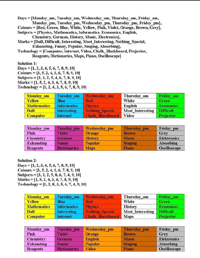
190 Chapter 4. CLP with global constraints for feasible solutions
Figure 4.2: Ten rooms timetable - solution 1 and 2
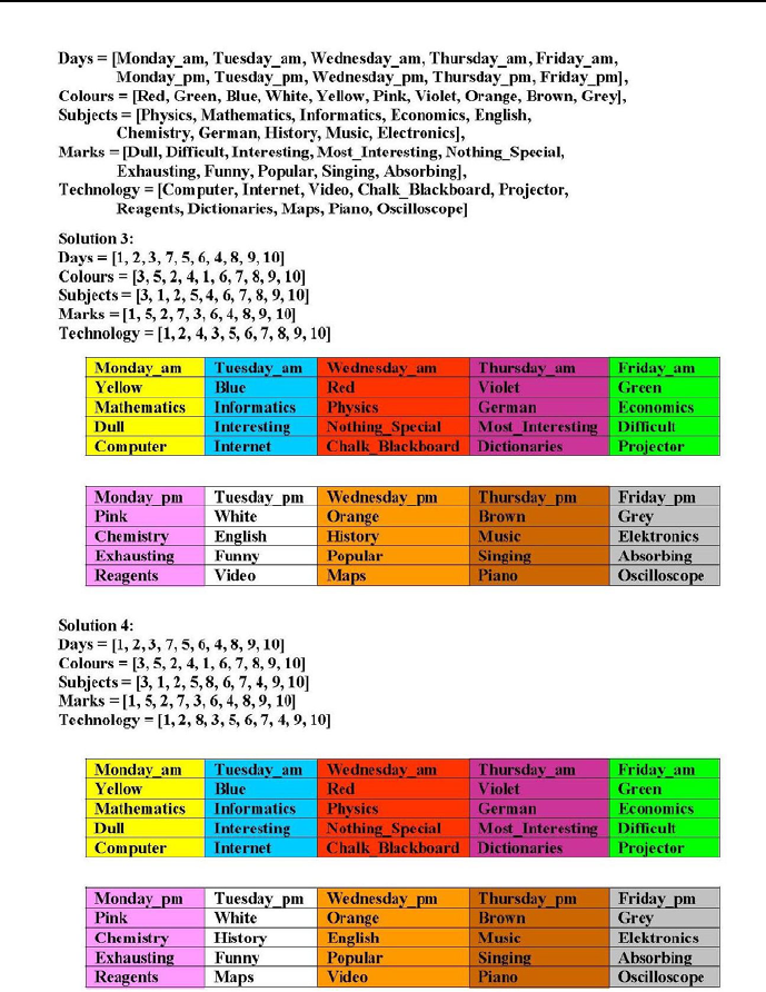
4.5 Feasible timetabling 191
Figure 4.3: Ten rooms timetable - solution 3 and 4

192 Chapter 4. CLP with global constraints for feasible solutions
4.5.3 All Things to All People
The element/3 built-in is almost always used with the alldifferent/1 built-
in. This is illustrated by the following example:
The Absurdoland’s party All Things to All People is a popular political force
to be reckoned with. At its Headquarters each Friday a meeting takes place with
the agenda devoted solely to next week dispatching of party activists to local
communities to meet with local activists, voters and supporters, and persuade
people to vote for the party candidates in the forthcoming elections. Last Friday
the discussion concentrated upon visiting three important local communities,
Lower Hole, Upper Hole and Middle Hole, by three trusted and experienced
party activists, Mr Blather, Mr Jabber and Ms Fable. The visits were supposed
to take place only on Monday, Tuesday or Wednesday, by one party activist each
day, because they were also badly needed at the Headquarters. The problem
to be settled is who should go where. Each of the party activists has special
wishes and hindrances to be taken into account:
1)Activist Blather decided never to travel again to Lower Hole, because at his
last stay there he was invited for lunch to a shabby roadside eatery pot, where
the local activists and supporters presented him with a complete set of Chinese
ball-pens; well, he did not boast about this to his party colleagues.
2)Activist Jabber has no objections for going to Lower Hole or to Upper Hole,
but not on Tuesdays, because his sponsoring benefactor, the Famous Business-
man, whom he used to meet at some randomly selected grave at the Lower-
or Upper Hole cemetery, traditionally devotes each Tuesday to one of his girl-
friends. Mr Jabber does not intend to give up those meetings because at each
of them he is presented by the Famous Businessman with a plastic bag filled
with cash and some memos about things he should take care of.
3)To Upper Hole Mr Jabber does not want to go on Monday as well, because
on Mondays all Escort Service Agencies in Upper Hole have a day off.
4)To Lower Hole nobody wants travel on Mondays because then all bars and
restaurants try to sell their Sunday left-overs.
5)Mr Blather should not be dispatched to Upper Hole because at his last stay
there he had considerable problems in explaining this item of the Party Politi-
cal Program that promises state guarantees for loans taken by any unemployed
who wishes - for a planned future business activity - to buy a new SUV of the
well-known make ”Luxus”.
6)Mr Blather may be dispatched to Lower Hole, but not on Monday, because
Mondays are traditional extensions of his customary weekends.

4.5 Feasible timetabling 193
7)Ms Fable should not be dispatched to Middle Hole, because last time there
she refused to support the request of the Middle Hole Party Chairman to be
distinguished by the widely aspired ”Pour le Fraude” golden medal that she
herself has not got yet.
Is it possible to find a dispatch solution that gives justice to all the presented
wishes and hindrances?
This problem is solved by program 4_15_delegations.ecl16:
/*1*/ :-lib(ic).
/*2*/ top:-
/*3*/ Towns=[Destination_of_Blather, Destination_of_Jabber,
Destination_of_Fable],
/*4*/ Towns::1..3,
% Visited towns: 1 - Lower Hole, 2 - Upper Hole, 3 - Middle Hole.
% If e.g Destination_of_Blather=3, then Blather is dispatched to Middle Hole.
/*5*/ alldifferent(Towns),
/*6*/ Days=[Monday,Tuesday,_],
/*7*/ Days::1..3,
% Visited Towns: 1 - Lower Hole, 2 - Upper Hole, 3 - Middle Hole.
% If e.g. Tuesday=3, then on Tuesday someone is dispatched to Middle Hole.
/*8*/ alldifferent(Days),
% 1) Mr Blather is not going to Lower Hole:
/*9*/ Destination_of_Blather #\= 1,
% 2) Mr Jabber has no objections for going to Lower Hole,
% or to Upper Hole, but not on Tuesdays:
/*10*/ constraint_2(Destination_of_Jabber,Tuesday),
% 3) Mr Jabber does not wish to travel to Upper Holes on Mondays:
/*11*/ constraint_3(Destination_of_Jabber,Monday),
% 4) To Lower Hole nobody wishes to travel on Mondays:
/*12*/ Monday #\= 1,
% 5) Mr Blather should not be dispatched to Upper Hole:
/*13*/ Destination_of_Blather #\= 2,
% 6) Mr Blather may be dispatched to Lower Hole, but not on Mondays:
/*14*/ constraint_6(Destination_of_Blather,Monday),
16 This is an FS-type problem.

194 Chapter 4. CLP with global constraints for feasible solutions
% 7) Ms Fable should not be dispatched to Middle Hole:
/*15*/ Destination_of_Fable #\= 3,
/*16*/ write("Towns = "),writeln(Towns),
/*17*/ write("Days = "),writeln(Days),nl,
% End of problem solving part
% Beginning of solution writing part:
% The idea is to determine 3-tuples (Name,Destination,Day)
% having the same number:
% Number of destination on position 1:
/*18*/ element(1,Towns,Number_of_destination_on_position_1),
% Number of day on position Number_of_destination_on_position_1:
/*19*/ element(Number_of_day_1,Days,Number_of_destination_on_position_1),
% Number of destination on position 2:
/*20*/ element(2,Towns,Number_of_destination_on_position_2),
% Number of day on position Number_of_destination_on_position_2:
/*21*/ element(Number_of_day_2,Days,Number_of_destination_on_position_2),
% Number of destination on position 3:
/*22*/ element(3,Towns,Number_of_destination_on_position_3),
% Number of day on position Number_of_destination_on_position_3:
/*23*/ element(Number_of_day_3,Days,Number_of_destination_on_position_3),
% Translating destination number into destination name:
/*24*/ destination(Number_of_destination_on_position_1,Name_of_destination_1),
/*25*/ destination(Number_of_destination_on_position_2,Name_of_destination_2),
/*26*/ destination(Number_of_destination_on_position_3,Name_of_destination_3),
% Translating day number into day name:
/*27*/ day(Number_of_day_1,Name_of_day_1),
/*28*/ day(Number_of_day_2,Name_of_day_2),
/*29*/ day(Number_of_day_3,Name_of_day_3),
% Merging elements of the 3-tuples:
/*30*/ write("Mr Blather will be dispatched to "),
write(Name_of_destination_1),write(Name_of_day_1),nl,
/*31*/ write("Mr Jabber will be dispatched to "),
write(Name_of_destination_2),write(Name_of_day_2),nl,
/*32*/ write("Ms Fable will be dispatched to "),
write(Name_of_destination_3),write(Name_of_day_3),nl.
/*33*/ constraint_2(Destination_of_Jabber,Tuesday):-
/*34*/ Destination_of_Jabber #= 1,

4.6 Data handling 195
/*35*/ Tuesday #\= 1;
/*36*/ Destination_of_Jabber #= 2,
/*37*/ Tuesday #\= 2.
/*38*/ constraint_2(_,_).
/*39*/ constraint_3(Destination_of_Jabber,Monday):-
/*40*/ Destination_of_Jabber #= 2,
/*41*/ Monday #\= 2.
/*42*/ constraint_3(_,_).
/*43*/ constraint_6(Destination_of_Blather,Monday):-
/*44*/ Destination_of_Blather #= 3,
/*45*/ Monday #\= 3.
/*46*/ constraint_6(_,_).
% Translating destination number into destination name:
/*47*/ destination(1,"Lower Hole").
/*48*/ destination(2,"Upper Hole").
/*49*/ destination(3,"Middle Hole").
% Translating day number into day name:
/*50*/ day(1," on Monday.").
/*51*/ day(2," on Tuesday.").
/*52*/ day(3," on Wednesday.").
The message generated is:
Towns = [3, 1, 2]
Days = [2, 3, 1]
Mr Blather will be dispatched to Middle Hole on Tuesday.
Mr Jabber will be dispatched to Lower Hole on Wednesday.
Ms Fable will be dispatched to Upper Hole on Monday.
4.6 Data handling
The solution of complicated and large problems may require some additional
knowledge about data structures and their handling.

196 Chapter 4. CLP with global constraints for feasible solutions
4.6.1 Structures and arrays
Structures, abbreviated by struct, are handy for presenting and processing data
from nested relational data bases. Their use is declared by local struct()
templates, like e.g.:
:- local struct(person(name, address, age)).
:- local struct(employee(p:person, salary)).
where the structure person is nested in structure employee using field p.The
following example illustrates the use of the structures. It is given by commands
in command mode, see Section 0.3, for which a response is generated:
This is a command:
[eclipse 1]:
:- local struct(person(name, address, age)).
:- local struct(employee(p:person, salary)).
Employee = employee with [name: "Jan Kowalski"", age: 26,
salary: 4000, address: "Gliwice, Kormoranow 5"],
arg(name of employee, Employee, Name),
arg(age of employee, Employee, Age),
arg(salary of employee, Employee, Salary).
This is the response:
Employee = employee(person("Jan Kowalski",
"Gliwice, Kormoranow 5", 26), 4000)
Name = "Jan Kowalski"
Age=26
Salary = 4000
Important data structures are multidimensional arrays. They are singled
out by the prefix [] and handled by following built-ins:
1)a one-dimensional array with 4 elements may be constructed by calling
dim(Array,[4]). This results in a one-dimensional array with four free ele-
ments:
This is a command:
[eclipse 2]: dim(Array,[4]).

4.6 Data handling 197
This is the response:
Array = [](_169, _170, _171, _172)
2)a 2-dimensional 3x2array may be constructed as follows:
This is a command:
[eclipse 3]: dim(Array,[3,2]).
This is the response:
Array = []([](_181, _182), [](_178, _179), [](_175, _176))
3)The dimensions of a 2-dimensional array may be calculated as follows:
This is a command:
[eclipse 4]: Array = []([](a,b,c),[](d,e,f)),dim(Array,D).
This is the response:
D = [2, 3]
4)The built-in dim/2 may also serve to determine the elements of an array:
This is a command:
[eclipse 5]: Array = [](a, b, c, d), dim(Array,D).
This is the response:
Array = [](a, b, c, d)
D = [4]
5)A 1-dimensional array may have lists as its elements. The number of elements
of such array is equal to the number of lists, e.g.:
This is a command:
[eclipse 6]: Array=[]([5 ,7 ,1 ,20 ],[14 ,8 ,100,300],
[2 ,20 ,50 ,12 ] ),
dim(Array,[M]).
This is the response:
Array = []([5, 7, 1, 20], [14, 8, 100, 300],

198 Chapter 4. CLP with global constraints for feasible solutions
[2, 20, 50, 12])
M=3
6)The number of elements of a list may be determined using the
length(?List, ?Length) built-in, e.g.:
This is a command:
[eclipse 7]: length([a,b,c,d], Length_of_list).
This is the response:
Length_of_list = 4
The length/2 built-in may also be used for list construction, e.g.:
This is a command:
[eclipse 8]: length(List, 4).
This is the response:
List = [_166, _168, _170, _172]
7)The I-th row of an array with Mcolumns can be determined by calling
Row_I is Array(I,1..M],whereRow_I is a list, e.g.:
This is a command:
[eclipse 9]: Array = []([](a,b,c),[](d,e,f)),
Second_Row is Array[2,1..3].
This is the response:
Array = []([](a, b, c), [](d, e, f))
Second_Row = [d, e, f]
8)The Jth column of an array with Nrows can be determined by calling
Column_J is Array(1..N,J],whereColumn_J is a list, e.g.:
This is a command:
[eclipse 10]: Array = []([](a,b,c),[](d,e,f)),
Third_Column is Array[1..2,3].

4.6 Data handling 199
This is the response:
Array = []([](a, b, c), [](d, e, f))
Third_Column = [c, f]
4.6.2 How to get hold of matrix elements?
If some operations have to be done on successive rows of a matrix, the presented
approach of getting hold of the rows cannot be used. Instead the built-in:
arg(Row_number,ArrayMatrix,ArrayMatrixRow)
is to be used. It determines (as an array) the matrix row of given number.
This is illustrated by program 4_16_extracting_elements.ecl17:
/*1*/ :- lib(ic).
/*2*/ array_matrix(ArrayMatrix):-
/*3*/ ArrayMatrix=[](
/*4*/ [](1,2,3,4,5),
/*5*/ [](6,7,8,9,10),
/*6*/ [](11,12,13,14,15)
/*7*/ ).
/*8*/ top:-
/*9*/ array_matrix(ArrayMatrix),
/*10*/ arg(2,ArrayMatrix,ArrayMatrixRow),
/*11*/ writeln("ArrayMatrixRow":ArrayMatrixRow),
/*12*/ ArrayMatrixRow=..[[]|ListMatrixRow],
/*13*/ writeln("ListMatrixRow":ListMatrixRow),
/*14*/ element(3,ListMatrixRow,Element_2_3),
/*15*/ writeln("Element_2_3":Element_2_3).
The message is:
ArrayMatrixRow : [](6, 7, 8, 9, 10)
ListMatrixRow : [6, 7, 8, 9, 10]
Element_2_3 : 8
While being interested only in a specific element of the matrix, a simpler ap-
proach is recommended: the element is available by calling the predicate
17 This is an FS-type problem.

200 Chapter 4. CLP with global constraints for feasible solutions
ArrayMatrix[Element_coordinates], like this:
ArrayMatrix=[](
[](1,2,3,4,5),
[](6,7,8,9,10),
[](11,12,13,14,15)
),
X is ArrayMatrix[2,3].
The message is:
ArrayMatrix = []([](1, 2, 3, 4, 5), [](6, 7, 8, 9, 10), [](11, 12, 13, 14, 15))
X=8
4.6.3 Recursions and iterations - bye, bye declarativity!
For ECLiPSeP rolog - as for any other Prolog - data is processed chiefly using
recursions. Prolog people just love recursions. E.g. consecutive elements of a
list may be obtained by the simple private predicate write_list/1 defined by
the recursion from program 4_17_write_list.ecl18:
/*1*/ top :-
/*2*/ write_list([1,2,3]).
/*3*/ write_list([X|Xs]):-
/*4*/ writeln(X),
/*5*/ write_list(Xs).
/*6*/ write_list([]).
The essence of recursion amounts to defining the write_list/1 by itself.
The program generates a message:
1
2
3
Recursive programming is functioning - as has been demonstrated many
times - also in ECLiPSeCPS.TheECLiPSedesigners decided however to
supplement recursions by iterations, the essence of which amounts to calling the
18 This is an FS-type problem.

4.6 Data handling 201
same predicate, in a loop, for changing data. Such iterations are not used in
Prolog programs; their presence in ECLiPSeCPS seems to be a concession
to programmers accustomed to procedural programming. As a result some of
Prolog programs declarativity as well as readability has been lost.
The basic iterative built-in is do/2 used as:
+iteration_definition(X) do +goal(X)
for calling goal(X) according to iteration_definition(X).
Following iteration_definitions may be used:
1) foreach(X,List) do goal(X) is iterating goal(X) for all Xfrom the list
List.Xis a local variable for goal(X). E.g.:
This is a command:
[eclipse 1]: (foreach(X, [1,2,3]) do writeln(X)).
This is the response:
1
2
3
X=X
The response is the same as that obtained by the private write_list/1 predi-
cate. However, foreach(X,List) may also be used for constructing lists:
This is a command:
[eclipse 2]: (foreach(X, [1,2,3]), foreach(Y,List) do Y is X+5).
This is the response:
X=X
Y=Y
List = [6, 7, 8]
The possibility to construct data structures is common to the majority of it-
eration definitions. It lessens somehow the burden of procedurality from those
definitions. It has been used in program 4_18_scalar_product.ecl (see 4.6.5),

202 Chapter 4. CLP with global constraints for feasible solutions
calculating the scalar products of two vectors presented as lists. This scalar
product has been in turn used in the 5_14_knapsack_1.ecl program, see 5.6.3.
2) foreacharg(X,Predicate) do goal(X) is iterating goal(X) for all Xgiven
by arguments (free or grounded) of the predicate Predicate. E.g.:
This is a command:
[eclipse 3]: (foreacharg(X, s(p,q,R,5)) do writeln(X)).
This is the response:
p
q
R
5
X=X
R=R
The built-in foreacharg(X,Predicate) cannot be used for constructing pred-
icates because of the ambiguity of this concept.
3) foreacharg(X,Predicate,I) do goal(X) is iterating goal(X) for all Xgiven
by arguments (free or grounded) of the predicate Predicate, while delivering
the numbers Iof positions Xin the predicate. E.g.:
This is a command:
[eclipse 3]: (foreacharg(X, s(p,q,R,5),I) do writeln(X),writeln(I)).
This is the response:
p
1
q
2
R
3
5
4
X=X
R=R
I=I

4.6 Data handling 203
4) param(Variable_1,Variable_2,...) is used for introducing variables into
loops of the do iterations. In other words, Variable_1,Variable_2,... are
declared as global, in contrast to other loop variables, which by default are
always local. This is illustrated by determining all pairs of list elements:
This is a command:
[eclipse 4]: List = [1,2,3],
( foreach(X, List), param(List) do
( foreach(Y,List), param(X) do
write(X),write(" "),write(Y),nl
)
).
This is the response:
11
12
13
21
22
23
31
32
33
List = [1, 2, 3]
X=X
Y=Y
Another example of using param() in a for() loop is given by the more
concise than 4_9_queens_again.ecl version of the queen placement problem
in 4_19_queens_one_more_time.ecl, see Section 4.6.4.
5)count(I,Min,Max) do goal(I) is iterating goal(I) for all integers Ifrom
the range [Min...Max].Iis (obviously) a local variable for goal(I).Thisis
illustrated by constructing a list of integers:
This is a command:
[eclipse 5]: (count(I,1,4), foreach(I,List) do true).
This is the response:
I=I

204 Chapter 4. CLP with global constraints for feasible solutions
List = [1, 2, 3 ,4]
6) for(I,MinExpr,MaxExpr)do goal(I) is iterating goal(I) for all integer
variables Ifrom the range [MinExpr...MaxExpr].Iis (obviously) a local vari-
able for goal(I),andMinExpr as well as MaxExpr may be arithmetic expres-
sions. This construct may be used only for controlling iterations, i.e. MaxExpr
must be grounded. This is illustrated by constructing a list of integers:
This is a command:
[eclipse 6]: (for(I,1,5), foreach(I,List) do true).
This is the response:
I=I
List = [1, 2, 3, 4, 5]
7) for(I,MinExpr,MaxExpr,Delta)do goal(I) is iterating goal(I) for inte-
ger variables Ifrom the range [MinExpr...MaxExpr] incremented with Delta.
Iis (obviously) a local variable for goal(I),andMinExpr as well as MaxExpr
may be arithmetic expressions. This construct may be used only for controlling
iterations, i.e. MaxExpr must be grounded. This is illustrated by constructing
a list of integers:
This is a command:
[eclipse 7]: (for(I,1,5,2), foreach(I,List) do true).
This is the response:
I=I
List = [1, 3, 5]
8) multifor(List,ListMin,ListMax)do goal(List) is a generalization for
for/3 presented in 6) when iterations have to be performed for a number of
variables. multifor is iterating goal(List) for all integer variables from the
List for ranges given by lists ListMin and ListMax.List is (obviously) a local
variable for goal(List),andMinExpr iMaxExpr may contain the same num-
ber of arithmetic expressions. This construct may be used only for controlling
iterations, i.e. MaxExpr must be grounded. The example is:
This is a command:
[eclipse 8]: (multifor([I,J],[1,2],[2,4]) do writeln([I,J]),
K is I+J, writeln([K])).

4.6 Data handling 205
This is the response:
[1, 2]
[3]
[1, 3]
[4]
[1, 4]
[5]
[2, 2]
[4]
[2, 3]
[5]
[2, 4]
[6]
I=I
J=J
K=K
An interesting application for multifor/3 is given by sudoku puzzles, see
program 4_20_sudoku.ecl in Section 4.7.1.
9) multifor(List,ListMin,ListMax,ListDelta) do goal(List) is a gen-
eralization for multifor(List,ListMin,ListMax)do goal(List) presented in
8) for integer variables incremented with ListDelta. The example is:
This is a command:
[eclipse 9]: (multifor([I,J],[1,2],[2,5],[1,2]) do writeln([I,J]),
K is I+J, writeln([K])).
This is the response:
[1, 2]
[3]
[1, 4]
[5]
[2, 2]
[4]
[2, 4]
[6]
I=I

206 Chapter 4. CLP with global constraints for feasible solutions
J=J
K=K
10) fromto(First,In,Out,Last)do goal(In,Out) is the most general itera-
tor. It iterates goal(In,Out) by starting with In = First, thus computing a
first value for Out. This value is swapped at the second iteration for In,andso
on: at each iteration the value of OUT computed from previous In is swapped
for the next In,untilOut = Last and the iteration stops. In and Out are local
variables for goal.Thefromto/4 performance is illustrated by computing the
sumofalistofintegers:
This is a command:
[eclipse 10]: (foreach(X,[10,20,30]),
fromto(0,In,Out,Sum) do Out is InX).+
This is the response:
X=X
In = In
Out = Out
Sum = 60
fromto/4 may also be used for reversing lists:
This is a command:
[eclipse 11]: (foreach(X,[10,20,30]),
fromto([],In,[X|In],Reversed_list) do true).
This is the response:
X=X
In = In
Reversed_list = [30, 20, 10]
For sophisticated applications of fromto/4 the First argument is grounded
only at the end of iterations. This occurs for various variable filtering schemes,
e.g.:
This is a command:
[eclipse 12]: (foreach(X,[5,3,8,1,4,6]),
fromto(List,In,Out,[]) do
X>3 -> In=[X|Out] ; Out=In).

4.6 Data handling 207
This is the response:
X=X
List = [5, 8, 4, 6]]
In = In
Out = Out
The 4_21_queens_for_the_last_time.ecl program (see Section 4.7.2) illus-
trates another situation, for which First is not grounded till the end of itera-
tions.
4.6.4 Queens one more time
Iterations allow to express the queens placement problem from Section 4.4.6 in
a more compact way, as shown in program 4_19_queens_one_more_time.ecl19:
/*1*/ :- lib(ic).
/*2*/ top:-
/*3*/ queens(_,_).
/*4*/ queens(N, Chessboard) :-
/*5*/ size_of_chessboard(N),
/*6*/ dim(Chessboard, [N]),
/*7*/ Chessboard[1..N] :: 1..N,
/*8*/ (for(I,1,N), param(Chessboard,N) do
/*10*/ (for(J,I+1,N), param(Chessboard,I) do
/*11*/ Chessboard[I] #\= Chessboard[J],
/*12*/ Chessboard[I] #\= Chessboard[J]+J-I,
/*13*/ Chessboard[I] #\= Chessboard[J]+I-J
/*14*/ )
/*15*/ ),
/*16*/ labeling(Chessboard),
/*17*/ writeln(Chessboard).
/*18*/ size_of_chessboard(4).
The message corresponds to the already obtained solution:
[](2, 4, 1, 3)
[](3, 1, 4, 2),
19 This is an FS-type problem.

208 Chapter 4. CLP with global constraints for feasible solutions
this time using arrays.
4.6.5 Scalar product
The scalar product (or dot product) of two vectors presented as lists:
[a1,a2,...,an] [b1,b2,...,bn]
is given by:
a1*b1 + a2*b2 + ... an*bn.
This can be computed by program 4_18_scalar_product.ecl20:
/*1*/ :- lib(ic).
/*2*/ top:-
/*3*/ scalar_product([1,2,3,4],[10,20,30,40],_).
/*4*/ scalar_product(List_1,List_2,Scalar_product):-
/*5*/ (foreach(V1, List_1),
/*6*/ foreach(V2, List_2),
/*7*/ foreach(Product,Product_list)
/*8*/ do
/*9*/ Product is V1 * V2
/*10*/ ),
/*11*/ Scalar_product #= sum(Product_list),nl,
/*12*/ write("Scalar product = "),writeln(Scalar_product),nl.
The message is:
Scalar product = 300
4.7 More feasible assignment problems
4.7.1 Sudoku
Sudoku is a combinatorial number-placement puzzle. The goal is to fill the cells
of a 9 ×9 gridded table with digits from 1to 9so that each column, each row,
and each of the nine 3 ×3 gridded sub-tables that compose the grid (called
20 This is an FS-type problem.

4.7 More feasible assignment problems 209
”boxes”) contains all of the digits from 1to 9. Initially the table is partially
completed in a way that assures a unique solution.
The program 4_20_sudoku.ecl21 is solving sudoku puzzles using the built-
in multifor/3. It is a slightly modified version of the program available at the
website [Schimpf-10]:
/*1*/ :- lib(ic).
/*2*/ top:-
/*3*/ write("Declare puzzle number (1,2 or 3):"),nl,
/*4*/ read_token(Number, integer),
/*5*/ solve(Number).
/*6*/ solve(Number):-
/*7*/ problem(Number, Board),
/*8*/ write_board(Board),
/*9*/ sudoku(Board),
/*10*/ write_board(Board).
/*11*/ sudoku(Board):-
/*12*/ Board[1..9,1..9] :: 1..9,
/*13*/ (for(I,1,9), param(Board)
/*14*/ do
/*15*/ Row is Board[I,1..9],
/*16*/ alldifferent(Row),
/*17*/ Col is Board[1..9,I],
/*18*/ alldifferent(Col)
/*19*/ ),
/*20*/ (multifor([I,J],1,9,3), param(Board)
/*21*/ do
/*22*/ (multifor([K,L],0,2),
/*23*/ param(Board,I,J),
/*24*/ foreach(X,Square)
/*25*/ do
/*26*/ X is Board[I+K,J+L]
/*26*/ ),
/*27*/ alldifferent(Square)
/*28*/ ),
/*29*/ term_variables(Board, Variables),
/*30*/ labeling(Variables).
/*31*/ write_board(Board):-
/*32*/ (for(I,1,9), param(Board)
/*33*/ do
/*34*/ (for(J,1,9), param(Board,I)
/*34*/ do
21 This is an FS-type problem.

210 Chapter 4. CLP with global constraints for feasible solutions
/*35*/ X is Board[I,J],
/*36*/ (var(X) -> write(" _") ; printf("%2d", [X]))
/*37*/ ), nl
/*38*/ ), nl.
problem(1, [](
[](_, _, 2, _, 6, _, _, _, 3),
[](_, _, _, 5, 9, _, _, 7, _),
[](_, 6, _, _, _, 4, _, _, _),
[](_, _, _, _, _, 1, _, 3, 7),
[](_, 9, 7, _, _, _, 8, 1, _),
[](4, 1, _, 7, _, _, _, _, _),
[](_, _, _, 8, _, _, _, 9, _),
[](_, 2, _, _, 7, 5, _, _, _),
[](6, _, _, _, 4, _, 3, _, _))).
problem(2, [](
[](_, _, 5, _, 7, 4, _, 6, _),
[](9, _, _, _, _, 3, _, _, _),
[](_, _, 1, _, _, _, _, 3, 2),
[](_, _, _, 9, _, _, _, _, 5),
[](_, _, _, _, _, _, _, _, _),
[](4, _, _, _, _, 6, _, _, _),
[](8, 6, _, _, _, _, 7, _, _),
[](_, _, _, 1, _, _, _, _, 8),
[](_, 2, _, 8, 6, _, 5, _, _))).
problem(3, [](
[](_, _, _, _, _, 1, 2, _, _),
[](_, _, _, _, _, _, 9, 6, _),
[](_, _, _, 7, 4, 6, _, _, 8),
[](_, 9, 3, _, 2, _, _, 1, _),
[](_, 8, _, _, _, _, _, 9, _),
[](_, 6, _, _, 5, _, 8, 2, _),
[](1, _, _, 5, 6, 7, _, _, _),
[](_, 3, 4, _, _, _, _, _, _),
[](_, _, 6, 3, _, _, _, _, _))).
The solution of problem 3 gives:
_____12__
______96_
___746__8
_93_2__1_
_8_____9_

4.7 More feasible assignment problems 211
_6__5_82_
1__567___
_34______
__63_____
658931247
347285961
912746538
493628715
285173496
761459823
129567384
534812679
876394152
4.7.2 Queens for the last time
The program 4_21_queens_for_the_last_time.ecl22 illustrates the applica-
tion of fromto/4 to the queen placement problem:
/*1*/ :- lib(ic).
/*2*/ top:-
/*3*/ four_queens(4,_).
/*4*/ four_queens(N, Chessboard):-
/*5*/ length(Chessboard, N),
/*6*/ Chessboard:: 1..N,
/*7*/ (fromto(Chessboard,[Position_1|Next_positions],
Next_positions,[])
/*8*/ do
/*9*/ (foreach(Position_2, Next_positions),
/*10*/ param(Position_1),
/*11*/ count(Distance,1,_)
/*12*/ do
/*13*/ Position_2 #\= Position_1,
/*14*/ Position_2 - Position_1 #\= Distance,
/*15*/ Position_1 - Position_2 #\= Distance
/*16*/ )
/*17*/ ),
22 This is an FS-type problem.

212 Chapter 4. CLP with global constraints for feasible solutions
/*18*/ labeling(Chessboard),
/*19*/ write("Chessboard = "),writeln(Chessboard).
The message is:
Chessboard = [2, 4, 1, 3]
Chessboard = [3, 1, 4, 2]
4.7.3 Implicit domain declaration - lectures again
Consider again the lecture example from Section 2.4.10. It may be solved by an
CLP program 4_22_lectures.ecl with implicit domain declaration:
/*1*/ :- lib(ic).
/*2*/ top :-
/*3*/ Lectures =
[
lecture(1, _, _, _, _, _, _),
lecture(2, _, _, _, _, _, _),
lecture(3, _, _, _, _, _, _)
],
% The implicit domain declaration from line /*3*/ holds
% for all lecture() predicates from the Constraints[] list below:
% From the definition of ’Lectures’ follows that integers
% Andrew, Barbara and Christopher should be grounded to values 1, 2, 3:
/*4*/ Constraints =
[
lecture(Andrew, "Andrew", _, _, _, _, _),
lecture(Barbara, "Barbara",_,_, _, _, _),
lecture(Christopher, "Christopher",_, _, _, _, _),
% From the definition of ’Lectures’ follows that integers
% Knowledge_Engineering, Econometric_Models and Artificial_Intelligence
% should be grounded to values 1, 2, 3:
lecture(Knowledge_Engineering, _, "Knowledge Engineering", _, _, _, _),
lecture(Econometric_Models, _, "Econometric Models", _, _, _, _),
lecture(Artificial_Intelligence, _, "Artificial Intelligence", _, _, _, _),
% From the definition of ’Lectures’ follows that integers
% Tuesday, Wednesday and Thursday should be grounded to values 1, 2, 3:
lecture(Tuesday, _, _, "Tuesday", _, _, _),

4.7 More feasible assignment problems 213
lecture(Wednesday, _, _, "Wednesday", _, _, _),
lecture(Thursday, _, _, "Thursday", _, _, _),
% From the definition of ’Lectures’ follows that integers
% H2_00, H3_45 and H5_30 should be grounded to values 1, 2, 3:
lecture(H2_00, _, _, _, "2:00 p.m.", _, _),
lecture(H3_45, _, _, _, "3:45 p.m.", _, _),
lecture(H5_30, _, _, _, "5:30 p.m.", _, _),
% From the definition of ’Lectures’ follows that integers
% R104, RD3 and RK2 should be grounded to values 1, 2, 3:
lecture(R104, _, _, _, _, "104", _),
lecture(RD3, _, _, _, _, "D3", _),
lecture(RK2, _, _, _, _, "K2", _),
% From the definition of ’Lectures’ follows that integers
% Paul, Jones and Smith should be grounded to values 1, 2, 3:
lecture(Paul, _, _, _, _, _, "Paul"),
lecture(Jones, _, _, _, _, _, "Jones"),
lecture(Smith, _, _, _, _, _, "Smith") ],
%1) Andrew will attend the lecture by Professor Paul:
/*5*/ Andrew #= Paul,
%2) Tuesdays lecture does not start at 2:00 p.m:
/*6*/ Tuesday #\= H2_00,
%3) The lecture on ”Knowledge Engineering” does not start at 5:30 p.m:
/*7*/ Knowledge_Engineering #\= H5_30,
%4) Thursdays lecture start at 3:45 p.m:
/*8*/ Thursday #= H3_45,
%5) Christopher will attend the lecture on ”Econometric Models”:
/*9*/ Christopher #= Econometric_Models,
%6) Barbara would like to attend the Tuesday lecture:
/*10*/ Barbara #= Tuesday,
%7) The lecture on ”Artificial Intelligence” is delivered in Room D3:
/*11*/ Artificial_Intelligence #= RD3,
%8) Wednesdays lectures are not delivered in Room 104:
/*12*/ Wednesday #\= R104,
%9) Professor Smith is not delivering the lecture ”Econometric Models”:
/*13*/ Smith #\= Econometric_Models,

214 Chapter 4. CLP with global constraints for feasible solutions
%10) Professor Jones is not delivering his lecture in Room K2:
/*14*/ Jones #\= RK2,
/*14*/ grounding(Constraints, Lectures),
/*15*/ (foreach(Lecture, Lectures) do writeln(Lecture)),!.
% All elements of the Constraints[] list must be grounded to some
% values of the elements of the Lectures[] list:
/*16*/ grounding([],_).
/*17*/ grounding([H|T],Lectures) :-
/*18*/ member(H,Lectures),
/*19*/ grounding(T,Lectures).
The message displays the solution:
lecture(1, Andrew, Knowledge Engineering, Wednesday, 2:00 p.m., K2, Paul)
lecture(2, Barbara, Artificial Intelligence, Tuesday, 5:30 p.m., D3, Smith)
lecture(3, Christopher, Econometric Models, Thursday, 3:45 p.m., 104, Jones)
4.7.4 Stable marriages
The stable marriages problem is best described by a quote from [Wirth-75]:
”Assume that two disjoint sets A and B of equal cardinality n are
given. Find a set of n pairs (a; b) such that a εAandbεB satisfy
some constraints. Many different criteria for such pairs exist; one
of them is the rule called ‘stable marriage rule.’ Assume that A is
a set of men and B is a set of women. Each man and each woman
has stated distinct preferences for their partners. If the n couples
are chosen such that there exists a man and a woman who are not
married, but who would prefer each other to their actual marriage
partners, then the assignment is said to be unstable. If no such
pair exists, it is called stable. This situation characterizes many
related problems in which assignments have to be made according to
preferences, such as, for example, the choice of a school by pupils,
the choice of recruits by different branches of the armed services, etc.
The example of marriages is particularly intuitive; note, however,
that the stated list of preferences is invariant and does not change
after a particular assignment has been made. This rule simplifies the
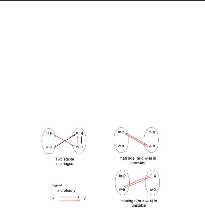
4.7 More feasible assignment problems 215
problem, but it also represents a distortion of reality.”
Niklaus Wirth, ”Algorithms + Data Structures = Programs.”
A marriage between a man m(from a set of men) and a woman w(from a
set of women) is thus considered stable if and only if for any outsider (o):
1. whenever man mranks another female outsider o(from a set of women)
higher than his current wife w, the female outsideroprefers her husband
to m,and
2. whenever women wranks another male outsider o(from a set of men)
higher than her current husband m, the male outsider oprefers his wife
to w.
This is illustrated by Figure 4.4.
Figure 4.4: Examples of stable and unstable marriages
As can be seen, the marriage (m-p, w-a) is unstable because m-p prefers w-b
more than his wife w-a,andw-b prefers m-p more than her husband m-q.
A set of marriages is stable if it does not contain unstable pairs.
Let us consider the following example with three women (woman_1, woman_2
and woman_3)andthreemen(man_1, man_2
216 Chapter 4. CLP with global constraints for feasible solutions
Women High pref...Low pref
woman_1 man_2 man_1 man_3
woman_2 man_3 man_2 man_1
woman_3 man_1 man_3 man_2
Table 4.4: Women are ranking men
Men High pref...Low pref
man_1 woman_2 woman_1 woman_3
man_2 woman_3 woman_2 woman_1
man_3 woman_1 woman_3 woman_2
Table4.5:Menarerankingwomen
and man_3r), with rankings shown in Tables 4.4 and 4.5:
The ordering in rows of Tables 4.4 and 4.5 denotes the ranking of persons
involved: e.g. the first choice of woman_1 is man_2 (woman_1 likes man_2 most),
her second choice is man_1, and her last choice is man_3.
When given a married pair, let’s say (man_r-woman_a)andman_q-woman_b),
if woman_a prefers man_q more than her current husband man_r,andman_r
prefers woman_b more than his current wife woman_a (i.e. their summary ranking
numbers may be lowered by pairing man_q-woman_a)andman_r-woman_b), then
the pair man_r-woman_a is called a dissatisfied pair. A set of marriages is said
to be stable if there are no dissatisfied pairs.
Intuitively, there are three stable solutions to this problem:
1. Men get their first choice and ladies their third:
man_1-woman_2, man_2-woman_3, man_3-woman_1,
all pairs have summary ranking 4.
2. Women get their first choice and men their third:
man_2-woman_1, man_3-woman_2, man_1-woman_3,
all pairs have summary ranking 4.

4.7 More feasible assignment problems 217
3. All participants get their second choice:
man_1-woman_1, man_2-woman_2, man_3-woman_3,
all pairs have summary ranking 4.
All three are stable because instability requires both participants to be hap-
pier (i.e. having a lower summary choice) with an alternative match. The data
shown in Tables 4.4 and 4.5 has to be (in a CLP program) put in a different
way, like this:
problem(1,
% 1=man_1, 2=man_2, 3=man_3:
/*woman_1:*/ []([](2, 1, 3), % rankByWomen:
/*woman_2:*/ [](3, 2, 1), % women are ranking men: woman_1 likes
/*woman_3:*/ [](1, 3, 2)), % most man_2, next-man_1, and least-man_3
% 1=woman_1, 2=woman_2, 3=woman_3
/*man_1:*/ []([](2, 1, 3), % rankByMen:
/*man_2:*/ [](3, 2, 1), % men are ranking women: man_1 likes most
/*man_3:*/ [](1, 3, 2))). % woman_2, next-woman_1, and least-woman_3
The problem is solved by the rather sophisticated program 4_23_stable_mar
riage.ecl due to Kjellerstrand ([Kjellerstrand-13]). It invokes a library called
Propria that implements a generalized propagation technique. If it’s not loaded
there is an instantiation fault while reading data. The program is:
/*1*/ :-lib(ic).
/*2*/ :-lib(ic_global).
/*3*/ :-lib(ic_search).
/*4*/ :-lib(propia).
/*5*/ top :-
/*6*/ all_solutions(0),
/*7*/ all_solutions(1),
/*8*/ all_solutions(2),
/*9*/ all_solutions(3),
/*10*/ all_solutions(4),
/*11*/ all_solutions(5).
/*12*/ all_solutions(Problem) :-
/*13*/ printf("\nProblem %d:\n", [Problem]),
/*14*/ findall([Husband,Wife], stable_marriage(Problem,Husband,Wife),L),
% On corresponding positions of lists
% ’Husband’ and ’Wife’ are stable marriages:
/*15*/ (foreach([H,W], L) do
/*16*/ write("Husband: "),write(H),nl,

218 Chapter 4. CLP with global constraints for feasible solutions
/*17*/ write("Wife : "),write(W),nl,nl
/*18*/ ).
/*19*/ stable_marriage(Problem,Husband,Wife) :-
/*20*/ problem(Problem, RankByWomen,RankByMen),
/*21*/ dim(RankByWomen,[NumWomen,NumMen]),
/*22*/ dim(RankByMen,[NumMen,NumWomen]),
/*23*/ dim(Wife,[NumMen]),
/*24*/ Wife #:: 1..NumWomen,
/*25*/ dim(Husband,[NumWomen]),
/*26*/ Husband #:: 1..NumMen,
/*27*/ ic_global:alldifferent(Wife),
/*28*/ ic_global:alldifferent(Husband),
% Rankings are tested on all possible pairings for men and for women:
% if the fact that any man M who ranks an outsider woman O higher
% than his wife implies that the outsider woman O prefers her husband to M:
/*29*/ ( for(M,1,NumMen) * for(O,1,NumWomen),
/*30*/ param(RankByMen,RankByWomen,Wife,Husband) do
/*31*/ (RankByMen[M,O] #< RankByMen[M, Wife[M]]) =>
/*32*/ (RankByWomen[O,Husband[O]] #< RankByWomen[O,M])
/*33*/ ),
% and if the fact that any woman W who ranks an outsider male O higher
% than her husband implies that the outsider male O prefers his wife to W:
/*34*/ ( for(W,1,NumWomen) * for(O,1,NumMen),
/*35*/ param(RankByMen,RankByWomen,Wife,Husband) do
/*36*/ (RankByWomen[W,O] #< RankByWomen[W,Husband[W]]) =>
/*37*/ (RankByMen[O,Wife[O]] #< RankByMen[O,W])
/*38*/ ),
% then the marriages are stable.
% Husbands are paired with wifes for the same lists positions:
/*39*/ ( for(W,1,NumWomen), param(Husband, Wife) do
/*40*/ Wife[Husband[W]] #= W
/*41*/ ),
% Wifes are paired with husbands for the same lists positions:
/*42*/ ( for(M,1,NumMen), param(Husband, Wife) do
/*43*/ Husband[Wife[M]] #= M
/*44*/ ),
% flatten the list of lists [Wife,Husband] for labeling purposes:
/*45*/ term_variables([Wife,Husband],Vars),

4.7 More feasible assignment problems 219
/*46*/ labeling(Vars).
problem(0,
[]([](1, 2), % rankByWomen
[](1, 2)),
[]([](2, 1), % rankByMen
[](2, 1))).
From [Wikipedia-13]:
problem(1,
[]([](2, 1, 3),% rankByWomen
[](3, 2, 1),
[](1, 3, 2)),
[]([](2, 1, 3), % rankByMen
[](3, 2, 1),
[](1, 3, 2))).
From [van Hentenryck-99]:
problem(2,
[]([](1, 2, 4, 3, 5), % rankByWomen
[](3, 5, 1, 2, 4),
[](5, 4, 2, 1, 3),
[](1, 3, 5, 4, 2),
[](4, 2, 3, 5, 1)),
[]([](5, 1, 2, 4, 3), % rankByMen
[](4, 1, 3, 2, 5),
[](5, 3, 2, 4, 1),
[](1, 5, 4, 3, 2),
[](4, 3, 2, 1, 5))).
From [Kjellerstrand-13]:
problem(3,
[]([](7, 3, 8, 9, 6, 4, 2, 1, 5), % rankByWomen
[](5, 4, 8, 3, 1, 2, 6, 7, 9),
[](4, 8, 3, 9, 7, 5, 6, 1, 2),
[](9, 7, 4, 2, 5, 8, 3, 1, 6),
[](2, 6, 4, 9, 8, 7, 5, 1, 3),
[](2, 7, 8, 6, 5, 3, 4, 1, 9),
[](1, 6, 2, 3, 8, 5, 4, 9, 7),
[](5, 6, 9, 1, 2, 8, 4, 3, 7),
[](6, 1, 4, 7, 5, 8, 3, 9, 2)),
[]([](3, 1, 5, 2, 8, 7, 6, 9, 4), % rankByMen
[](9, 4, 8, 1, 7, 6, 3, 2, 5),
[](3, 1, 8, 9, 5, 4, 2, 6, 7),
[](8, 7, 5, 3, 2, 6, 4, 9, 1),

220 Chapter 4. CLP with global constraints for feasible solutions
[](6, 9, 2, 5, 1, 4, 7, 3, 8),
[](2, 4, 5, 1, 6, 8, 3, 9, 7),
[](9, 3, 8, 2, 7, 5, 4, 6, 1),
[](6, 3, 2, 1, 8, 4, 5, 9, 7),
[](8, 2, 6, 4, 9, 1, 3, 7, 5))).
From [Hunt-13]:
problem(4,
[]([](1,2,3,4),% rankWomen
[](4,3,2,1),
[](1,2,3,4),
[](3,4,1,2)),
[]([](1,2,3,4),% rankByMen
[](2,1,3,4),
[](1,4,3,2),
[](4,3,1,2))).
From [Ahriz-13]:
problem(5,
[]([](1,5,4,6,2,3),
[](4,1,5,2,6,3),
[](6,4,2,1,5,3),
[](1,5,2,4,3,6),
[](4,2,1,5,6,3),
[](2,6,3,5,1,4)),
[]([](1,4,2,5,6,3),
[](3,4,6,1,5,2),
[](1,6,4,2,3,5),
[](6,5,3,4,2,1),
[](3,1,2,4,5,6),
[](2,3,1,6,5,4))).
The solutions are:
Problem 0:
Husband: [](2, 1)
Wife : [](2, 1)
Problem 1:
Husband: [](2, 3, 1)
Wife : [](3, 1, 2)
Husband: [](3, 1, 2)
Wife : [](2, 3, 1)

4.7 More feasible assignment problems 221
Husband: [](1, 2, 3)
Wife : [](1, 2, 3)
Problem 2:
Husband: [](4, 1, 2, 5, 3)
Wife : [](2, 3, 5, 1, 4)
Husband: [](2, 1, 4, 5, 3)
Wife : [](2, 1, 5, 3, 4)
Husband: [](2, 3, 4, 1, 5)
Wife : [](4, 1, 2, 3, 5)
Problem 3:
Husband: [](7, 5, 9, 8, 3, 6, 1, 4, 2)
Wife : [](7, 9, 5, 8, 2, 6, 1, 4, 3)
Husband: [](6, 5, 9, 8, 3, 7, 1, 4, 2)
Wife : [](7, 9, 5, 8, 2, 1, 6, 4, 3)
Husband: [](6, 4, 9, 8, 3, 7, 1, 5, 2)
Wife : [](7, 9, 5, 2, 8, 1, 6, 4, 3)
Husband: [](6, 1, 4, 8, 5, 9, 3, 2, 7)
Wife : [](2, 8, 7, 3, 5, 1, 9, 4, 6)
Husband: [](6, 4, 1, 8, 5, 7, 3, 2, 9)
Wife : [](3, 8, 7, 2, 5, 1, 6, 4, 9)
Husband: [](6, 1, 4, 8, 5, 7, 3, 2, 9)
Wife : [](2, 8, 7, 3, 5, 1, 6, 4, 9)
Problem 4:
Husband: [](1, 4, 2, 3)
Wife : [](1, 3, 4, 2)
Husband: [](1, 2, 4, 3)
Wife : [](1, 2, 4, 3)
Problem 5:
Husband: [](1, 2, 6, 3, 5, 4)
Wife : [](1, 2, 4, 6, 5, 3)
Husband: [](1, 2, 6, 3, 4, 5)
Wife : [](1, 2, 4, 5, 6, 3)
Husband: [](1, 2, 4, 3, 6, 5)
Wife : [](1, 2, 4, 3, 6, 5)

222 Chapter 4. CLP with global constraints for feasible solutions
4.8 Feasible sequencing
Feasible sequencing aims at determining the order of elements from some set so
as to fulfill neighbourhood constraints, i.e. constraints determining the position
of each element with respect to the elements.
4.8.1 Car assembly line sequencing
This example is both an opportunity to present two important global built-in
predicates and to show their application. The predicates are:
1. The sequence_total/7 predicate, defined as:
sequence_total(+Min, +Max, +Low, +High, +K, +Vars, ++Values)
where number of values taken from the list of different integers Values is between
a non-negative Low and positive High integer for all sequences of Kintegers from
the list of integers Vars, and the total occurrence of each integer in Vars is
between Min and Max
The ”strangeness” of this predicate is due to the fact that it was custom-
tailored for modelling some situation on car assembly lines.
2. The occurrences/3 predicate, defined as:
occurrences(++Value, +List, ?N)
that is fulfilled if the value Value occurs Ntimes in List.
Sequencing is the process of determining the precise order of some items, e.g.
car bodies on a car assembly line to meet a given production order. ECLiPSe
is - because of some special global constraint - well-suited for solving such prob-
lems. Consider the following example. In a car assembly line, car bodies are
moving on conveyors through different work stations, each specialized for a par-
ticular job, such as installing the engine, installing the power seats, installing
wheels etc. For each car entering a work station, a crew of assemblers from that
4.8 Feasible sequencing 223
station moves with the car while performing their jobs. The speed of the assem-
bly line is such as to allow the crews to finish their jobs while the car bodies are
in their stations. E.g. if the installation of power seats takes 16 minutes and
a new car body enters the assembly line every 4 minutes, then (assuming that
each car needs a power seats), the station for power seats installation needs a
capacity to handle 16/4 = 4 car bodies, i.e. it has to be staffed by 4 power seats
handling crews. However, because not each car requires a power seat, in order
to save instrumentation and labour, the capacity of the power seats station may
be smaller, e.g. the station may have only 3 crews to handle power seats. That
means the station can cope with no more than 3 cars requiring power seats out
of any sequence of 4 cars. In shorthand - the power seats station has a capacity
constraint 3/4. Now its up to the assembly line scheduler to assure that the
entire sequence of car bodies feed into the assembly line has no 4-bodies subse-
quences with more than 3 bodies requiring power seats. Consider the capacity
requirements for four car models to be produced with five options as shown in
Table 4.6:
Option Capacity Models produced
constraints 1 2 3 4
Sunroof 3/5 -× × -
CD changer 4/5 ×- - ×
Automatic transmission 4/5 × × -×
Power seats 3/4 × × × -
Parking assistant 1/2 ×-×-
Number of cars required 30 30 30 30
Table 4.6: Capacity constraints for car assembly line: x - option required, - -
option not required
The notion of capacity constraint is illustrated for the case of power seat
workstation in Figure 4.5.
A solution (one of a large multitude of possible solutions) for the sequence
of 120 car bodies feed into the assembly line so that the capacity constraints of all
work stations are satisfied is determined by program 4_24_car_assembling.ecl
using two powerful global constraints: occurrences/3 and sequence_total/7:
/*1*/ :- lib(ic).
/*2*/ :- lib(ic_global).
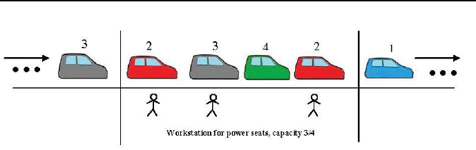
224 Chapter 4. CLP with global constraints for feasible solutions
Figure 4.5: The meaning of workstation capacity constraints
/*3*/ top:-
/*4*/ length(L,120),
/*5*/ L::1..4,
% 1 - Model 1, 2 - Model 2, 3 - Model 3, 4 - Model 4
% Constrain numbers of produced models using global constraint ’occurrences/3’:
% occurrences(++Value, +Vars, ?N)
% The integer ’Value’ occurs ’N’ times in integer list ’Vars’
% The value 1 occurs 30 times in L:
/*6*/ occurrences(1, L, 30),
% The value 2 occurs 30 times in L:
/*7*/ occurrences(2, L, 30),
% The value 3 occurs 30 times in L:
/*8*/ occurrences(3, L, 30),
% The value 4 occurs 30 times in L:
/*9*/ occurrences(4, L, 30),
% Constrain capacity of workstations using global constraint ’sequence_total/7’:
% sequence_total(+Min, +Max, +Low, +High, +K, +Vars, ++Values)
% The number of integers taken from integer list ’Values’ is between ’Low’ and
% ’High’ for all sequences of ’K’ integers in integer list ’Vars’,
% and the total occurrence of each integer in ’Vars’ is between ’Min’ and ’Max’
% Sunroofs - at least none and at most 3 of any consecutive 5 integers in L
% are from list [2,3]; at least 60 and at most 60 integers in L are
% from list [2,3]:
/*10*/ sequence_total(60, 60, 0, 3, 5, L, [2,3]),

4.8 Feasible sequencing 225
% CD changer - at least none and at most 4 of any consecutive 5 integers in L
% are from list [1,3,4]; at least 90 and at most 90 integers in L are
% from list [1,3,4]:
/*11*/ sequence_total(90, 90, 0, 4, 5, L, [1,3,4]),
% Automatic transmission - at least none and at most 4 of any consecutive
% 5 integers in L are from list [1,2,4]; at least 90 and at most 90 integers
% in L are from list [1,2,4]:
/*12*/ sequence_total(90, 90,0, 4, 5, L, [1,2,4]),
% Power seats - at least none and at most 3 of any consecutive 4 integers
% in L are from list [1,2,3]; at least 90 and at most 90 integers in L are
% from list [1,2,3]:
/*13*/ sequence_total( 90, 90, 0, 3,4, L, [1,2,3]),
% Parking assistant - at least none and at most 1 of any consecutive 2 integers
% in L are from list [1,3]; at least 60 and at most 60 integers in L are from
% list [1,3]:
/*14*/ sequence_total( 60, 60, 0, 1, 2, L, [1,3]),
/*15*/ labeling(L),
/*16*/ write_list(L).
/*17*/ write_list([H|T]):-
/*18*/ write(H),write(", "),
/*19*/ write_list(T).
/*20*/ write_list([_]).
The solution is:
L=[
1, 2, 1, 4, 3, 2, 1, 4, 2, 3, 4, 1, 2, 3, 4, 1, 2, 3, 4, 1,
2, 3, 4, 1, 2, 3, 4, 1, 2, 3, 4, 1, 2, 3, 4, 1, 2, 3, 4, 1,
2, 3, 4, 1, 2, 3, 4, 1, 2, 3, 4, 1, 2, 3, 4, 1, 2, 3, 4, 1,
2, 3, 4, 1, 2, 3, 4, 1, 2, 3, 4, 1, 2, 3, 4, 1, 2, 3, 4, 1,
2, 3, 4, 1, 2, 3, 4, 1, 2, 3, 4, 1, 2, 3, 4, 1, 2, 3, 4, 1,
2, 3, 4, 1, 2, 3, 4, 1, 2, 3, 4, 1, 2, 3, 4, 1, 2, 3, 4, 3]
To check that it satisfies the power seats capacity constraint, one has to look
at every subsequence of 4 cars, i.e.:
1, 2, 1, 4, It’s O.K
2, 1, 4, 3, It’s O.K
1, 4, 3, 2, It’s O.K
and so on, for each capacity constraint. Quite a job! So it’s worthwhile to
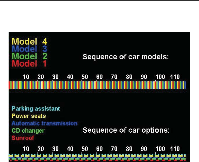
226 Chapter 4. CLP with global constraints for feasible solutions
present the solution as the sequencing diagrams from Figure 4.6, where capacity
constraints correspond to colour patterns.
Figure 4.6: Car assembly line sequencing
4.8.2 Bob’s Shish Kebab
This example is yet another opportunity to present the important built-in:
occurrences(++Value, +List, ?N)
that is fulfilled if the value Value occurs Ntimes in List, and to show its usage
for solving the Bob’s Shish Kebab example that enjoys the reputation of being
a tough one (a 5 star puzzle), see [Edmund-98]. It is befitting to end the series
of rather simple FS-type problems, solved using global built-ins, with a more
taxing problem. The Bob’s Shish Kebab problem is as follows:
Bob and Patty invited their friends Javier and Marie over for a cookout.
On the menu were grilled marinated beef cubes and four kinds of vegetables –

4.8 Feasible sequencing 227
mushrooms, onions, peppers, and tomatoes – that were put onto skewers. The
skewer that each person made had three beef cubes and one piece of three kinds
of vegetables – each person disliked a different vegetable and omitted it from
his or her skewer. The six pieces can be numbered 1 to 6 from the handle to the
point of the skewer. Can you tell what item each person had in each position,
provided that:
1. No kebab had two beef cubes right next to each other.
2. No one’s beef cubes were in the same three positions as anyone else’s.
3. One shish kebab’s first three items (numbers 1, 2, and 3 respectively) were
beef, pepper, and mushroom; this wasn’t Javier’s.
4. One skewer had beef cubes in positions 1, 3, and 5, and a tomato wedge in
position 6.
5. Bob, who loves onions and included a chunk on his skewer, had other veg-
etables in both positions 4 and 5.
6. On the four kebabs, the items in position 5 were beef, mushroom, onion, and
tomato.
7. Each onion chunk was immediately between two beef cubes.
8. No pepper was immediately between two beef cubes.
9. Marie can’t stand mushroom and left them off her skewer.
10. At least two kebabs had the same vegetable in the same position at least
once.
It contains a lot of negative conditions (i.e. conditions stating that some-
thing is not true) that may cause difficulties. A systematic way to handle them
(its essence is to use predicates defining negated conditions) is presented by
program 4_25_kebab.ecl23:
/*1*/ :- lib(ic).
/*2*/ :-lib(ic_global).
/*3*/ top:-
% Bi- element on position i of Bob’s skewer
% Pi- item on position i of Pati’s skewer
% Ji- element on position i of Javier’s skewer
% Mi- element on position i of Marie’s skewer
% 1-mushroom, 2-pepper, 3-onion, 4-tomato, 5-beef
/*4*/ Bob=[B1,B2,B3,B4,B5,B6,B7],
/*5*/ Bob::1..5,
23 This is an FS-type problem.

228 Chapter 4. CLP with global constraints for feasible solutions
/*6*/ Patty=[P1,P2,P3,P4,P5,P6,P7],
/*7*/ Patty::1..5,
/*8*/ Javier=[J1,J2,J3,J4,J5,J6,J7],
/*9*/ Javier::1..5,
/*10*/ Marie=[M1,M2,M3,M4,M5,M6,M7],
/*11*/ Marie::1..5,
% Example: J3 = 5 means Javier had beef at the third position.
% Positions 7 on each skewers denote vegetables disliked
% by the corresponding person: each person disliked a
% different vegetable and omitted it from his or her skewer:
/*12*/ [B7,P7,J7,M7]::1..4,
/*13*/ ic_global: alldifferent([B7,P7,J7,M7]),
% Constraint 1 - No kebab had two beef cubes right next to each other:
/*14*/ constraint_1([Bob,Patty,Javier,Marie]),
% Constraint 2 - No one’s beef cubes were in the same three positions
% as anyone else’s:
/*15*/ constraint_2([Bob,Patty,Javier,Marie]),
% Constraint 3 - One shish kebab’s first three items (numbers 1, 2,
% and 3 respectively) were beef, pepper, and mushroom; this wasn’t Javier’s.
/*16*/ constraint_3(Bob,Patty,Marie),
% Constraint 4 - One skewer had beef cubes in positions 1, 3, and 5, and
% a tomato wedge in position 6.
/*17*/ constraint_4(Bob,Patty,Javier,Marie),
% Constraint 5 - Bob, who loves onions and included a chunk
% on his skewer,had other vegetables in both positions 4 and 5:
/*18*/ constraint_5([_,_,_,B4,B5,_,_]),
% Constraint 6 - On the four kebabs, the items in position 5 were beef,
% mushroom, onion, and tomato:
/*19*/ constraint_6(Bob,Patty,Javier,Marie),
% Constraint 7 - Each onion chunk was immediately between two beef cubes
/*20*/ constraint_7([Bob,Patty,Javier,Marie]),
% Constraint 8 - No pepper was immediately between two beef cubes:
/*21*/ constraint_8([Bob,Patty,Javier,Marie]),
% Constraint 9 - Marie can’t stand mushroom and left them off her skewer:
/*22*/ constraint_9(Marie),
% Constraint 10 - At least two kebabs had the same vegetable in the
% same position at least once:

4.8 Feasible sequencing 229
/*23*/ constraint_10([Bob,Patty,Javier,Marie]),
% Each skewer has 3 beef cubes:
/*24*/ occurrences(5, [B1,B2,B3,B4,B5,B6], 3),
/*25*/ occurrences(5, [P1,P2,P3,P4,P5,P6], 3),
/*26*/ occurrences(5, [J1,J2,J3,J4,J5,J6], 3),
/*27*/ occurrences(5, [M1,M2,M3,M4,M5,M6], 3),
% Each skewer has one piece of three kinds of vegetables,
% the fourth vegetable rejected:
/*28*/ occurrences(1, [B1,B2,B3,B4,B5,B6,B7], 1),
/*29*/ occurrences(1, [P1,P2,P3,P4,P5,P6,P7], 1),
/*30*/ occurrences(1, [J1,J2,J3,J4,J5,J6,J7], 1),
/*31*/ occurrences(1, [M1,M2,M3,M4,M5,M6,M7], 1),
/*32*/ occurrences(2, [B1,B2,B3,B4,B5,B6,B7], 1),
/*33*/ occurrences(2, [P1,P2,P3,P4,P5,P6,P7], 1),
/*34*/ occurrences(2, [J1,J2,J3,J4,J5,J6,J7], 1),
/*35*/ occurrences(2, [M1,M2,M3,M4,M5,M6,M7], 1),
/*36*/ occurrences(3, [B1,B2,B3,B4,B5,B6,B7], 1),
/*37*/ occurrences(3, [P1,P2,P3,P4,P5,P6,P7], 1),
/*38*/ occurrences(3, [J1,J2,J3,J4,J5,J6,J7], 1),
/*39*/ occurrences(3, [M1,M2,M3,M4,M5,M6,M7], 1),
/*40*/ occurrences(4, [B1,B2,B3,B4,B5,B6,B7], 1),
/*41*/ occurrences(4, [P1,P2,P3,P4,P5,P6,P7], 1),
/*42*/ occurrences(4, [J1,J2,J3,J4,J5,J6,J7], 1),
/*43*/ occurrences(4, [M1,M2,M3,M4,M5,M6,M7], 1),
/*44*/ labeling([B1,B2,B3,B4,B5,B6,B7,P1,P2,P3,P4,P5,P6,P7,
J1,J2,J3,J4,J5,J6,J7,M1,M2,M3,M4,M5,M6,M7]),
/*45*/ write("Bob’s skewer: "),translate(B1),write(" "),translate(B2),
write(" "), translate(B3),write(" "), translate(B4),
write(" "),translate(B5),write(" "), translate(B6),nl,
/*46*/ write("Patty’s skewer: "),translate(P1),write(" "),translate(P2),
write(" "),translate(P3),write(" "), translate(P4),
write(" "),translate(P5),write(" "), translate(P6),nl,
/*47*/ write("Javier’s skewer: "),translate(J1),write(" "),translate(J2),
write(" "),translate(J3),write(" "),translate(J4),
write(" "),translate(J5),write(" "),translate(J6),nl,
/*48*/ write("Marie’s skewer: "), translate(M1),write(" "),translate(M2),
write(" "),translate(M3),write(" "), translate(M4),
write(" "), translate(M5),write(" "), translate(M6),nl,nl.

230 Chapter 4. CLP with global constraints for feasible solutions
/*49*/ translate(1):-write("mushroom").
/*50*/ translate(2):-write("pepper ").
/*51*/ translate(3):-write("onion ").
/*52*/ translate(4):-write("tomato ").
/*53*/ translate(5):-write("beef ").
% Constraint 1 - No kebab had two beef cubes right next to each other:24
/*54*/ constraint_1([H|T]):-
/*55*/ check_1(H),
/*56*/ constraint_1(T).
/*57*/ constraint_1([]).
/*58*/ check_1([A,B,C,D,E,F,_]):-
/*59*/ ~two_beef_cubes_next_to_each_other(A,B),
/*60*/ ~two_beef_cubes_next_to_each_other(B,C),
/*61*/ ~two_beef_cubes_next_to_each_other(C,D),
/*62*/ ~two_beef_cubes_next_to_each_other(D,E),
/*63*/ ~two_beef_cubes_next_to_each_other(E,F).
/*64*/ two_beef_cubes_next_to_each_other(X,Y):-
/*65*/ X#=5,Y#=5.
% Constraint 2 - No one’s beef cubes were in the same three positions
% as anyone else’s:
/*66*/ constraint_2([Bob,Patty,Javier,Marie]):-
/*67*/ check_2(Bob,Patty),check_2(Bob,Javier),check_2(Bob,Marie),
/*68*/ check_2(Patty,Javier),check_2(Patty,Marie),check_2(Javier,Marie).
/*69*/ check_2([B1,B2,B3,B4,B5,B6,_],[P1,P2,P3,P4,P5,P6,_]):-
/*70*/ ~in_the_same_positions(B1,B3,B5,P1,P3,P5),
/*71*/ ~in_the_same_positions(B1,B3,B6,P1,P3,P6),
/*72*/ ~in_the_same_positions(B1,B4,B6,P1,P4,P6),
/*73*/ ~in_the_same_positions(B2,B4,B6,P2,P4,P6).
/*74*/ in_the_same_positions(X1,X2,X3,Y1,Y2,Y3):-
/*75*/ X1#=5,
/*76*/ X2#=5,
/*77*/ X3#=5,
/*78*/ Y1#=X1,
/*79*/ Y2#=X2,
/*80*/ Y3#=X3.
% Constraint 3 - One shish kebab’s first three items (numbers 1, 2,
% and 3 respectively) were beef, pepper, and mushroom; this wasn’t Javier’s:
/*81*/ constraint_3([B1,B2,B3,_,_,_,_],[P1,P2,P3,_,_,_,_],[M1,M2,M3,_,_,_,_]):-
/*82*/ (
24 The Reader will excuse the Author for repeating the constraint statements, but this non-
redundancy makes for easier grasping the programs essence.

4.8 Feasible sequencing 231
/*83*/ (B1#=5, B2#=2, B3#=1);
/*84*/ (P1#=5, P2#=2, P3#=1);
/*85*/ (M1#=5, M2#=2, M3#=1)
/*86*/ ).
% Constraint 4 - One skewer had beef cubes in positions
% 1, 3, and 5, and a tomato wedge in position 6.
/*87*/ constraint_4(Bob,Patty,Javier,Marie):-
/*88*/ (had_beef_cubes_in_positions_1_3_5_6(Bob);
/*89*/ had_beef_cubes_in_positions_1_3_5_6(Patty);
/*90*/ had_beef_cubes_in_positions_1_3_5_6(Javier);
/*91*/ had_beef_cubes_in_positions_1_3_5_6(Marie)).
/*92*/ had_beef_cubes_in_positions_1_3_5_6([X1,_,X3,_,X5,X6,_]):-
/*93*/ X1#=5, X3#=5, X5#=5, X6#=4.
% Constraint 5 - Bob, who loves onions and included a chunk
% on his skewer, had other vegetables in both positions 4 and 5:
/*94*/ constraint_5([_,_,_,B4,B5,_,_]):-
/*95*/ B4#\=5, B5#\=5, B4#\=B5, B4#\=3, B5#\=3.
% Constraint 6 - On the four kebabs, the items in position 5 were
% beef, mushroom, onion, and tomato:
/*96*/ constraint_6([_,_,_,_,B5,_,_],[_,_,_,_,P5,_,_],[_,_,_,_,J5,_,_],
[_,_,_,_,M5,_,_]):-
/*97*/ (
/*98*/ (B5#=5; P5#=5; J5#=5; M5#=5),
/*99*/ (B5#=1; P5#=1; J5#=1; M5#=1),
/*100*/ (B5#=3; P5#=3; J5#=3; M5#=3),
/*101*/ (B5#=4; P5#=4; J5#=4; M5#=4)
/*102*/ ).
% Constraint 7 - Each onion chunk was immediately between two beef cubes:
/*103*/ constraint_7([Bob,Patty,Javier,Marie]):-
/*104*/ check_7(Bob),check_7(Patty),
/*105*/ check_7(Javier),check_7(Marie).
/*106*/ check_7([A,B,C,_,_,_,_]):-
/*107*/ A#=5,B#=3,C#=5.
/*108*/ check_7([_,B,C,D,_,_,_]):-
/*109*/ B#=5,C#=3,D#=5.
/*110*/ check_7([_,_,C,D,E,_,_]):-
/*111*/ C#=5,D#=3,E#=5.
/*112*/ check_7([_,_,_,D,E,F,_]):-
/*113*/ D#=5,E#=3,F#=5.
/*114*/ check_7([_,_,_,_,_,_,G]):-
/*115*/ G#=3.
% Constraint 8 - No pepper was immediately between two beef cubes:

232 Chapter 4. CLP with global constraints for feasible solutions
/*116*/ constraint_8([Bob,Patty,Javier,Marie]):-
/*117*/ check_8(Bob),check_8(Patty),
/*118*/ check_8(Javier),check_8(Marie).
/*119*/ check_8([A,B,C,D,E,F,_]):-
/*120*/ ~pepper_was_between_two_beef_cubes(A,B,C),
/*121*/ ~pepper_was_between_two_beef_cubes(B,C,D),
/*122*/ ~pepper_was_between_two_beef_cubes(C,D,E),
/*123*/ ~pepper_was_between_two_beef_cubes(D,E,F).
/*124*/ pepper_was_between_two_beef_cubes(X,Y,Z):-
/*125*/ X#=5,Y#=2,Z#=5.
% Constraint 9 - Marie can’t stand mushroom and left them off her skewer:
/*126*/ constraint_9([M1,M2,M3,M4,M5,M6,M7]):-
/*127*/ M7#=1,
/*128*/ M1#\=1, M2#\=1, M3#\=1,
/*129*/ M4#\=1, M5#\=1, M6#\=1.
% Constraint 10 - At least two kebabs had the same
% vegetable in the same position at least once:
/*130*/ constraint_10([Bob,Patty,Javier,Marie]):-
/*131*/ (
/*132*/ check_10(Bob,Patty);
/*133*/ check_10(Bob,Javier);
/*134*/ check_10(Bob,Marie);
/*135*/ check_10(Patty,Javier);
/*136*/ check_10(Patty,Marie);
/*137*/ check_10(Javier,Marie)
/*138*/ ).
/*139*/ check_10([X1,X2,X3,X4,X5,X6,_],[Y1,Y2,Y3,Y4,Y5,Y6,_]):-
/*140*/ (
/*141*/ (X1#\=5,X1#=Y1);
/*142*/ (X2#\=5,X2#=Y2);
/*143*/ (X3#\=5,X3#=Y3);
/*144*/ (X4#\=5,X4#=Y4);
/*145*/ (X5#\=5,X5#=Y5);
/*146*/ (X6#\=5,X6#=Y6)
/*147*/ ).
The message displays a unique solution:
Bob’s skewer: beef onion beef pepper mushroom beef
Patty’s skewer: beef pepper mushroom beef tomato beef
Javier’ skewer: beef onion beef mushroom beef tomato
Marie’s skewer: pepper beef tomato beef onion beef

4.8 Feasible sequencing 233
4.8.3 Dinner calamity
Sometimes variables have a ”cyclic” nature, like days in a week, months in a
year, places around a circle. Some care is needed to handle them, as illustrated
by the following example.
Mr and Mrs Davis invited their friends, Mr and Mrs Astor, Mr and Mrs
Blake, Mr and Mrs Crane for a dinner served on an elegant retro styled hexago-
nal table. However, their nice conversation unexpectedly turned sour because
some fundamental political differences have emerged. As the result of a heating
discussion:
1) Mrs Astor was insulted by Mr Blake, who sat next to her.
2) Mr Blake was insulted by Mrs Crane, who sat opposite him.
3) Mrs Blake was insulted by Mrs Astor, who set opposite her.
4) The hostess (Mrs Davis) was insulted by the only person to sit between two
men.
Knowing additionally that:
5)The hostess was the only person to sit between each of a married couple, and
6)Mrs Davis sat opposite to Mr Davis,
we have to determine who was sitting where and who insulted the hostess. The
problem is solved by program 4_26_dinner_calamity.ecl25:
/*1*/ :- lib(ic).
/*2*/ top :-
/*3*/ Places = [MrsAstor, MrAstor, MrBlake, MrsBlake,
MrsCrane, MrCrane, MrsDavis, MrDavis],
/*4*/ Places :: 1..8,
% The places are numbered as shown in Figure \ref{Fig.4.11}.
% Meaning of variables: if e.g. Mr Astor = 7, then Mr Astor is sitting on place 7
% The occupant of one place may be fixed:
/*5*/ MrsAstor = 1,
% Any person is occupying only one place:
/*6*/ alldifferent(Places),
% 1) Mrs Astor was insulted by Mr Blake,
% who sat next to her on her left:
25 This is an FS-type problem.

234 Chapter 4. CLP with global constraints for feasible solutions
/*7*/ MrBlake = 2,
% 2) Mr Blake was insulted by Mrs Crane, who sat opposite him:
/*8*/ opposite(2,MrsCrane),
% 3) Mrs Blake sat opposite to Mrs Astor
/*9*/ opposite(MrsBlake,1),
% 4) The hostess was insulted by the only person to sit between two men.
/*10*/ (member(Insulter,[MrsBlake,MrsCrane,MrCrane]),
in_between(MrAstor,Insulter,2);
/*11*/ member(Insulter,[MrsBlake,MrsCrane]),
in_between(MrAstor,Insulter,MrCrane);
/*12*/ member(Insulter,[MrsBlake,MrsCrane,MrCrane, MrsDavis]),
in_between(MrAstor,Insulter,MrDavis);
/*13*/ member(Insulter,[MrAstor, MrsBlake, MrsCrane,MrDavis]),
in_between(2,Insulter,MrCrane);
/*14*/ member(Insulter,[MrAstor, MrsBlake, MrsCrane, MrCrane]),
in_between(2,Insulter,MrDavis);
/*15*/ member(Insulter,[MrAstor, MrsBlake, MrsCrane]),
in_between(MrCrane,Insulter,MrDavis)),
% 5) The hostess (Mrs Davis) was the only person
% to sit between each of a married couple
/*16*/ (in_between(MrsBlake, MrsDavis, 2);
/*17*/ in_between(1, MrsDavis, MrAstor);
/*18*/ in_between(MrsCrane, MrsDavis, MrCrane)),
% 6) Mrs Davis sat opposite to Mr Davis:
/*196*/ opposite(MrsDavis,MrDavis),
/*20*/ labeling([MrsAstor, MrAstor, MrBlake, MrsBlake,
MrsCrane, MrCrane, MrsDavis, MrDavis]),
/*21*/ writeln([MrsAstor, MrAstor, MrBlake, MrsBlake,
MrsCrane, MrCrane, MrsDavis, MrDavis]),
/*22*/ List_names=["Mrs Astor","Mr Astor","Mr Blake","Mrs Blake",
"Mrs Crane","Mr Crane","Mrs Davis","Mr Davis"],
/*23*/ List_positions=[MrsAstor, MrAstor, MrBlake, MrsBlake,
MrsCrane, MrCrane, MrsDavis, MrDavis],
/*24*/ get_insulter(List_names,List_positions,Insulter,Insulter_name),
/*25*/ write("Mrs Astor was sitting at place "), write("1"),writeln("."),
/*26*/ write("Mr Astor was sitting at place "), write(MrAstor),writeln("."),
/*27*/ write("Mrs Blake was sitting at place "), write(MrsBlake),writeln("."),
/*28*/ write("Mr Blake was sitting at place "), write("2"),writeln("."),
/*29*/ write("Mrs Crane was sitting at place "), write(MrsCrane),writeln("."),
/*30*/ write("Mr Crane was sitting at place "), write(MrCrane),writeln("."),
/*31*/ write("Mrs Davis was sitting at place "), write(MrsDavis),writeln("."),

4.8 Feasible sequencing 235
/*32*/ write("Mr Davis was sitting at place "), write(MrDavis),writeln("."),
/*33*/ writeln("The hostess (Mrs Davis) was insulted by the "),
/*34*/ write("person sitting at place "),write(Insulter), write(", who was "),
/*35*/ write(Insulter_name),writeln("."),nl.
/*36*/ next_to(A,B):-
/*37*/ B #= A + 1;
/*38*/ A #= B + 1.
/*39*/ next_to(8,1).
/*40*/ next_to(1,8).
/*41*/ in_between(A,X,B):-
/*42*/ X #= A + 1,
/*43*/ X #= B - 1;
/*44*/ X #= A - 1,
/*45*/ X #= B + 1.
/*46*/ in_between(7,8,1).
/*47*/ in_between(1,8,7).
/*48*/ in_between(8,1,2).
/*49*/ in_between(2,1,8).
/*50*/ opposite(A,B):-
/*51*/ B #= A + 4;
/*52*/ A #= B + 4.
/*53*/ get_insulter([_|T_names],[H_position|T_position],X,Insulter):-
/*54*/ not(X = H_position),
/*55*/ get_insulter(T_names,T_position,X,Insulter).
/*56*/ get_insulter([H_names|_],[H_position|_],X,Insulter):-
/*57*/ X = H_position,
/*58*/ Insulter = H_names.
The solution is:
[1, 7, 2, 5, 6, 3, 8, 4]
Mrs Astor was sitting at place 1.
Mr Astor was sitting at place 7.
Mrs Blake was sitting at place 5.
Mr Blake was sitting at place 2.
Mrs Crane was sitting at place 6.
Mr Crane was sitting at place 3.
Mrs Davis was sitting at place 8.
Mr Davis was sitting at place 4.
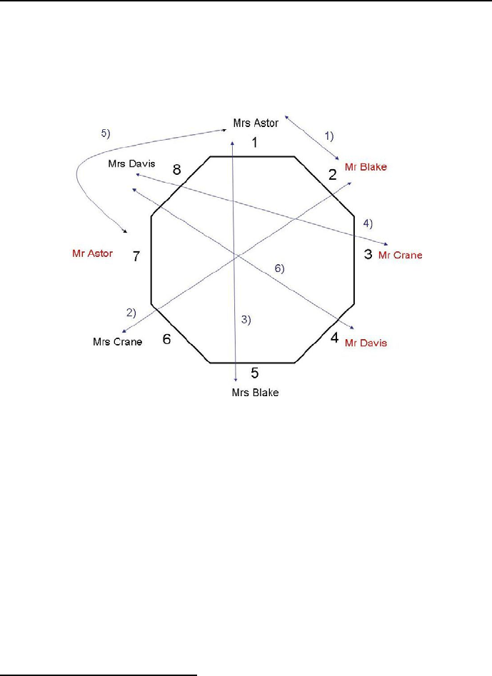
236 Chapter 4. CLP with global constraints for feasible solutions
The hostess (Mrs Davis) was insulted by the person
sitting at place 3 who was Mr Crane.
It is depicted on Figure 4.7.
Figure 4.7: Dinner calamity solution
4.9 Exercises
Stones of Heaven 26
Wan Li, a dealer in Chinese antiques and artifacts, had an excellent month
recently when he made sales to four customers from around the world –
Finland, Italy, Japan and United States – who were willing and able to pay
very good prices. The four items were rare jade figurines (a belt buckle,
dragon, grasshopper and horse), each carved from a different color of jade
(dark green, light green, red and white). Each piece dates from a different
Chinese dynasty (Ching, Ming, Sung and Tang). Write a program to
26 This exercise is from http://brownbuffalo.sourceforge.net/

4.9 Exercises 237
match each figurine with its color and dynasty, and give the home country
of each buyer, if: 1. The rare white dragon (which the American did’nt
buy) did’nt come from the Sung dynasty. 2. The exquisite belt buckle
(which was’nt any shade of green) was created in 618 A.D. for an emperor
of the Tang dynasty. 3. Three of the figurines were: the one bought by the
Finn (which was’nt the dragon), the one from the Ching dynasty (which
did’nt go to the buyer from Japan) and the light green object (which was’nt
the horse). 4. The American decided against both the grasshopper and
the piece from the Sung dynasty, neither of which she felt would match
her home decor. Determine: Item – Color – Dynasty – Country of buyer.
Lectures 27
Last week at school was made varied by a series of lectures, one each day
(Monday through Friday), in the auditorium. None of the lectures was
particularly interesting (on choosing a college, physical hygiene, modern
art, nutrition, and study habits), but the students figured that anything
that got them out of fourth period was okay. The lecturers were two
women named Alice and Bernadette, and three men named Charles, Du-
ane, and Eddie; last names were Felicidad, Garber, Haller, Itakura, and
Jeffreys. Write a program to find each day’s lecturer and subject, pro-
vided: 1. Alice lectured on Monday. 2. Charles’s lecture on physical
hygiene wasn’t given on Friday. 3. Dietician Jeffreys gave the lecture on
nutrition. 4. A man gave the lecture on modern art. 5. Ms. Itakura
and the lecturer on proper study habits spoke on consecutive days, in one
order or the other. 6. Haller gave a lecture sometime after Eddie did. 7.
Duane Felicidad gave his lecture sometime before the modern art lecture.
City council meeting
At the last meeting of the local city council, each member (Mr. Akerman,
Ms. Baird, Mr. Chatham, Ms. Duval, and Mr. Etting) had to vote on five
motions, number 1 to 5 in the clues below. Write a program to determine
how each one voted on each motion, provided that:
1. Each motion got a different number of yes votes.
2. In all, the five motions got three more yes votes than no votes.
3. No two council members voted the same way on all five motions.
4. The two women disagreed in their voting more often than they agreed.
5. Mr. Chatham never made two yes votes on consecutive motions.
6. Mr. Akerman and Ms. Baird both voted in favor of motion 4.
27 This exercise is from http://www.f1compiler.com/default.html

238 Chapter 4. CLP with global constraints for feasible solutions
7. Motion 1 received two more yes votes than motion 2 did.
8. Motion 3 received twice as many yes votes as motion 4 did.
DJ contest
During a recent music festival, four DJs entered the mixing contest. Each
wore a number, either 1, 2, 3 or 4 and their decks were different colors.
DJ Skinf Lint came first, and only one DJ wore the same number as the
position he finished in. DJ Slam Dunk wore number 1. The DJ who wore
number 2 had a red deck and DJ Jam Jar didn’t have a yellow deck. The
DJ who came last had a blue deck. DJ Park’n Ride beat DJ Slam Dunk.
The DJ who wore number 1 had a green deck and the DJ who came second
wore number 3. Can you determine who came where, which number they
wore and the color of their deck?
A knight, a knave and a spy
There are three people (Alex, Brook and Cody), one of whom is a knight,
one a knave, and one a spy28. The knight always tells the truth, the knave
always lies, and the spy can either lie or tell the truth. Alex says: ”Cody
is a knave.” Brook says: ”Alex is a knight.” Cody says: ”I am the spy.”
Who is the knight, who the knave, and who the spy?
Sum
Write a program which replaces all the letters with the respective digits
in such a way that the following sum is correct:
AND
TO
ALL
A
GOOD
-------
NIGHT
The same letters in this sum mean the same digit.
Magic square
Consider the Magic Square of order three:
ABC
DEF
GHI
28 This exercise is from http://www.mathsisfun.com/puzzles.

4.9 Exercises 239
Write a program for the following pattern of non-zero digits to be instan-
tiated to add up to the same sum along each row, column and diagonal.
Books
Eight married couples meet to land one another some books29. Couples
have the same surname, employment and a car. Eight couple has a favorite
color. Furthermore we know the following facts:
(1) Danielle Black and her husband work as Shop-Assistants. (2) The book
”The Death of the West” was brought by a couple who drive a Fiat and
love the color red. (3) Owen and his wife Victoria like the color brown. (4)
Stan Horricks and his wife Hannah like the color white. (5) Jenny Smith
and her husband work as Warehouse Managers and they drive a Ford. (6)
Monica and her husband Alexander borrowed the book ”Economy in One
Lesson”. (7) Mathew and his wife like the color pink and brought the book
”Archipelag Gulag”. (8) Irene and her husband Oto work as Accountants.
(9) The book ”The Fatal Conceit” was borrowed by a couple driving a
Chrysler. (10) The Cermaks are both Ticket-Collectors who brought the
book ”The Art of Worldly Wisdom”. (11) Mr and Mrs Kuril are both
Doctors who borrowed the book ”Atlas Shrugged”. (12) Paul and his
wife like the color green. (13) Veronica Dvorak and her husband like the
color blue. (14) Rick and his wife brought the book ”Atlas Shrugged”
and they drive a Volkswagen. (15) One couple brought the book ”The
Oxford Book of Humorouse Prose” and borrowed the book ”Archipelag
Gulag”. (16) The couple who drive a Toyota, love the color violet. (17)
The couple who work as Teachers borrowed the book ”The Oxford Book
of Humorouse Prose”. (18) The couple who work as Agriculturalists drive
a Moskvic. (19) Pamela and her husband drive a Renault and brought the
book ”Economy in One Lesson”. (20) Pamela and her husband borrowed
the book that Mr and Mrs Zajac brought. (21) Robert and his wife like the
color yellow and borrowed the book ”The Enlarged Devil’s Dictionary”.
(22) Mr and Mrs Swain work as Shoppers. (23) ”The Enlarged Devil’s
Dictionary” was brought by a couple driving a Audi.
Write a program to determine who likes violet and to find out everything
about everyone from this.
Dinner 30
Last weekend, five friends gathered for dinner at their favorite steak and
29 This exercise is from http://www.mathsisfun.com/puzzles
30 This exercise is from http://brownbuffalo.sourceforge.net/

240 Chapter 4. CLP with global constraints for feasible solutions
seafood restaurant. Each friend (two men named George and Oliver, and
three women named Colleen, Patti, and Theresa) ordered a different main
courses (crab, filet mignon, ribs, shrimp, or sirloin steak), and a different
type of potatoes (baked, French-fried, lyonnaise, mashed or scalloped). To
wash down his or her meal, each friend selected a different beverage (ginger
ale, iced tea, lemonade, root beer, or water). From the following clues,
can you match each friend with his or her surname (two of which are Gold
and Orlando), main course, side dish, and beverage? 1) The only person
with the same first-name and last-name initials ordered the ribs. 2) The
one surnamed Petroski and the person who had the shrimp are the person
who had the lyonnaise potatoes and the one who ordered the root beer,
in some order. 3) The one who selected the filet mignon didn’t have the
lemonade. 4) The one who had the scalloped potatoes (which didn’t come
with the sirloin steak) didn’t drink the water. 5) The first-name initial of
the one who had root beer is the same as George’s last-name initial. 6)
Theresa didn’t order the water. 7) The ones who chose the shrimp and
the baked potato are of opposite gender. 8) The first-name initial of the
woman who ordered the crab is the same as the last-name initial of the
person who chose the mashed potatoes. 9) The first-name initial of the
person who ordered the lemonade is the same as the last-name initial of
the one who ordered lyonnaise potatoes. 10) The one surnamed Chiasson
(who isn’t Patti) didn’t order French-fried or lyonnaise potatoes. 11) The
one surnames Truang (who didn’t order French-fried or mashed potatoes)
didn’t choose the ginger ale. 12) Colleen ordered either the filet mignon
or the sirloin steak.
Write a program to determine: First name - Last name - Main course -
Side dish - Beverage.
Soup Selections
Each of six friends who met in cooking school is now an established chef
at a different, notable restaurant in the area. Every few weeks, the friends
like to get together to trade secrets of their field and share some of their fa-
vorite creations. This past Tuesday night, each chef arrived at the group’s
favorite gathering spot with a different kind of soup that he or she had pre-
pared for the evening’s taste-test. From the following information, write a
program to match the full name of each chef (one surname is Earle) with
his or her seat (labeled one through six in the illustration) at the table at
which the group gathered and determine the restaurant where each works
and the type of soup that he or she prepared?

4.9 Exercises 241
1. Gloria (who works for either the Apple Orchard Inn or Hennigan’s
Place) prepared either the French onion or split pea soup. 2. The one
who made the minestrone sat in a lower-numbered seat than Marvin. 3.
The one surnamed Anderson sat directly across from the chef who works
at Michel’s Cafe. 4. Marvin and the one who prepared the asparagus
soup are the one who sat in seat five and the person who sat directly
across from the chef who made the chicken noodle soup, in some order. 5.
Norville sat next to the one who cooks for the Country Kitchen. 6. Quincy
and the chef who works for the Village Smorgasbord are the one surnamed
Dugan and a person who didn’t sit directly across from the chef who made
the asparagus soup, in some order. 7. The chef who works at the Pine
Cove Restaurant and the chef who sat in seat four are the one surnamed
Anderson and someone who didn’t prepare the minestrone, in some order.
8. The one surnamed Burns (who works for the Apple Orchard Inn) didn’t
prepare the split pea soup. 9. The six chefs are Jenna, the chef surnamed
Dugan, the person who works for the Pine Cove Restaurant, the person
who prepared the clam chowder, the chef who sat in seat three, and the
chef who sat directly across from the one surnamed Dugan. 10. Isabel and
the one surnamed Friedman are the chef who works at Michel’s Cafe and
the one who made the chicken noodle soup, in some order. 11. Marvin
didn’t prepare the clam chowder. 12. Jenna (who sat in an odd-numbered
seat) sat next to the one surnamed Caruso. 13. The chef who works for
the Pine Cove Restaurant didn’t occupy chair number six.
Killer Sudoku 31
Write a program to solve the Killer Sudoku from Figure 4.8a: The objec-
tive is to fill the grid with numbers from 1 to 9 in a way that the following
conditions are met:
- Each row, column, and nonet32 contains each number exactly once.
- The sum of all numbers in a cage must match the small number printed
in its corner.
- No number appears more than once in a cage. The solution of Killer
Sudoku is given by Figure 4.8b).
31 This exercise is from http://en.wikipedia.org/wiki/Killer sudoku
32 A 3 x 3 grid of cells, as outlined by the bolder lines in the diagram
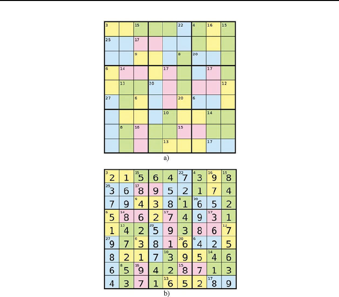
242 Chapter 4. CLP with global constraints for feasible solutions
Figure 4.8: Killer Sudoku problem a) and solution b)
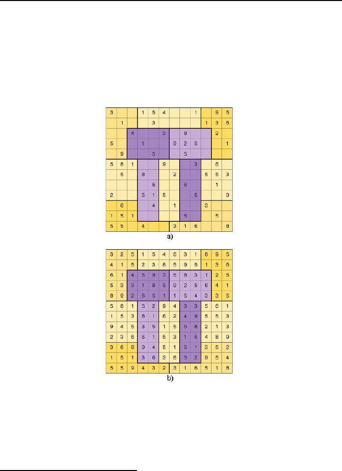
4.9 Exercises 243
Pi-Day Sudoku 33
Write a program to solve the Pi-Day Sudoku from Figure 4.9a). Each row,
column, and jigsaw region must contain exactly the first twelve digits of
pi, including repeats: 3.14159265358. Notice that each region will contain
two 1’s, two 3’s, three 5’s, and no 7’s. The solution of Pi-Day Sudoku is
given by Figure 4.9b).
Figure 4.9: Pi-Day Sudoku problem a) and solution b)
33 This exercise is from http://www.brainfreezepuzzles.com/main/piday2008.html
Chapter 5
CLP with elementary
constraints for optimal
solutions
5.1 General optimization approaches
The origin of combinatorial optimization may be traced to Operation Research
(OR). There a number of effective combinatorial optimization approaches was
developed under the heading of Integer Programming. Its distinctive feature
is the encoding of all combinatorial variables by means of 0-1binary vari-
ables. Such decoding can be used for Constraint Optimization Problems as
well, although it is not recommended because of the explosive growth of the
number of variables needed to define COP. What’s more, it may sometimes
destroy declarativity and create a troublesome semantic gap between the orig-
inal problem formulation and the program. However, for tutorial reason this
approach (termed as OR approach) will be illustrated by a number of examples,
distinguished by naming them with an OR postfix.
The CLP community has developed another approach to combinatorial op-
timization, which does the job without transforming the original (problem spe-
cific) integer variables into (more or less) vague binary variables. The approach,
preferred in the sequel, will be distinguished by naming the examples with a
CLP postfix.
245
246 Chapter 5. CLP with elementary constraints for optimal solutions
5.2 Branch-and-bound
The basic optimization method used here and in the next section is branch-
and-bound. A standard version of this method has already been used in Section
2.3.1. However, it would be worthwhile to have a closer look at that method.
To begin with, let us stress that there is a close correspondence between
standard1Depth-First Backtracking Search and standard Branch-and-Bound:
what for CSP is standard Depth-First Backtracking Search, for COP is standard
Branch-and-Bound, see Figure 5.1.
Figure 5.1: Analogy between standard Depth-First Backtracking Search and
standard Branch-and-Bound
The main difference between them is that for branch-and-bound search an
additional constraint is tested, namely the relation between the current objective
function value (COFV) and the best objective function value so far (BOFVSF).
For minimization, which is a standard optimization mode for ECLiPSeCPS,
the details are as follows:
•if COFV < BOFVSF, then the stored BOFVSF is swapped for COFV,andthe
stored set of decision variables corresponding to former BOFVSF is swapped
for the set of decision variables corresponding to COFV;
•if COFV > BOFVSF, nothing is changed;
1The backtracking discussed so far is considered to be ’standard’.

5.3 Upgrading Branch-and-Bound 247
•if COFV = BOFVSF, two approaches are used: 1)nothing is changed - this
approach is used by ECLiPSeCLP; 2)the set of decision variables corre-
sponding to COFV is stored alongside with this for BOFVSF; this enables to
find multiple optimum solutions as shown in example 2_7_conf_opt.pl.
Strictly speaking, branch-and-bound is not an optimization algorithm but a
general methodology (a paradigm) of combinatorial optimization, able in prin-
ciple to find global optima for nonlinear objective functions under nonlinear con-
straints. Practically - for numerical reasons - branch-and-bound is in most imple-
mentations (including ECLiPSe)) applicable only for linear objective functions
under linear constraints.
5.3 Upgrading Branch-and-Bound
From similarities between Standard Branch-and-Bound and Standard Depth
First Backtracking Search follows that Standard Branch-and-Bound may be
updated by introducing search mechanisms discussed in Section 3.2, i.e. Forward
Checking and Looking Ahead. The discussion of search heuristics from Section
3.3 is also relevant for Branch-and-Bound.
5.3.1 Optimum queens - standard Branch-and-Bound
In order to better understand what should be done to upgrade Branch-and-
Bound, let’s consider its standard version for the simple problem of optimally
placing four queens on a 4 ×4 chessboard. The objective function (quite artifi-
cial) is:
J = 1*X1+0*X2+1*X3+1*X4 ,
where - as previously - Xi is the row number occupied by the queen in column i.
Figure 5.2 shows two feasible placement of four queens, one of which is optimum.
Branch-and-Bound may be characterized by naming states, for which back-
tracking is initiated. For the standard Branch-and-Bound this happens:
•when a worse objective function value has been computed (Branch-and-
Bound backtracking);
•when some constraint is violated (constraint violation backtracking).
This is shown by the search tree from Figure 5.3.
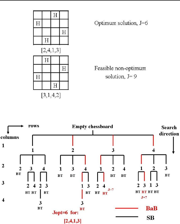
248 Chapter 5. CLP with elementary constraints for optimal solutions
Figure 5.2: Two feasible placements for four queens
Figure 5.3: Search tree for standard Branch-and-Bound for 4 queens
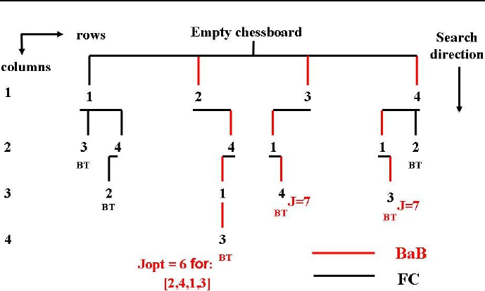
5.3 Upgrading Branch-and-Bound 249
Figure 5.4: Search tree for Branch-and-Bound+Forward Checking for 4 queens
5.3.2 Optimum queens - Forward Checking
For Branch-and-Bound + Forward Checking backtracking is initiated for follow-
ing states:
•when a worse objective function value has been computed (Branch-and-
Bound backtracking);
•when the domain of any variable is emptied (Forward Checking backtrack-
ing).
This is shown by the search tree from Figure 5.4.
5.3.3 Optimum queens - Looking Ahead +For wa rd
Checking
For Branch-and-Bound + Looking Ahead + Forward Checking backtracking is
initiated for following states:
•when a worse objective function value has been computed (Branch-and-
Bound backtracking);
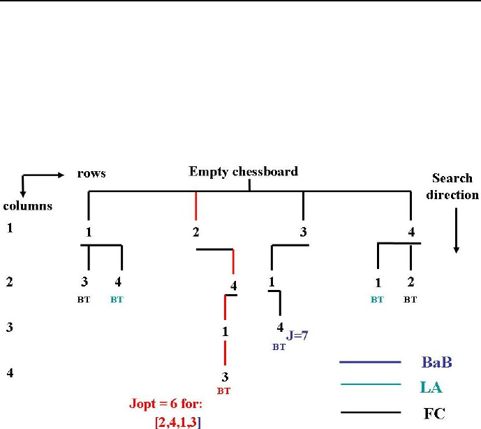
250 Chapter 5. CLP with elementary constraints for optimal solutions
•when non-empty domains contain no feasible values (Looking Ahead back-
tracking);
•when the domain of any variable is emptied (Forward Checking backtrack-
ing).
This is shown by the search tree from Figure 5.5.
Figure 5.5: Search tree for Branch-and-Bound+Looking Ahead+Forward Check-
ing for 4 queens
To end this Section, lets state this:
•the ECLiPSeuser is not expected to deal explicitly with the described
backtracking enhancements;
•they are automatically provided by the mere declaration of optimizing
some objective function.
The above discussion just aims to give the ECLiPSeuser some idea about
how to make standard branch-and-bound more efficient.

5.4 Basic built-ins 251
5.4 Basic built-ins
Now two important built-ins will be introduced:
1. bb_min/3 for Branch-and-Bound.
2. search/6 for parameterizing any search or Branch-and-Bound - related
search.
A detailed description of both built-ins is available in ECLiPSe”documenta-
tion, see Figure 5. Because of their importance, their properties will be shortly
summarized.
5.4.1 The ’bb min/3’ built-in
It is used for initiating Branch-and-Bound search. Its simplest version is:
bb_min(+Goal, ?Cost, ?Options)
where:
•Goal is a (nondeterministic) search goal, i.e, a predicate with the opti-
mization problem decision variables as arguments;
•Cost is the objective function minimized by grounding decision variables;
•Options (the most important) may be as follows:
–strategy:
∗continue (default): after finding a solution, continue search
with the newly found bound imposed on Cost;
∗restart: after finding a solution, restart the whole search with
the newly found bound imposed on Cost;
∗dichotomic: after finding a solution, split the remaining cost
range and restart search to find a solution in the lower sub-
range. If that fails, assume the upper sub-range as the remaining
cost range and split again; The new bound or the split point,
respectively, are computed from the current best solution, while
taking into account the parameters delta and factor,seebelow.
–from : number - an initial lower bound for the cost, (default -1.0Inf);
–to: number - an initial upper bound for the cost (default +1.0Inf);

252 Chapter 5. CLP with elementary constraints for optimal solutions
–delta: number - minimal absolute improvement required for each
step (default 1.0), applies to all strategies;
–factor: number - minimal improvement ratio (with respect to the
lower cost bound) for strategies ’continue’ and ’restart’ (default 1.0),
or split factor for strategy ’dichotomic’, (default 0.5);
–timeout: number - maximum seconds of cpu time to spend (default:
no limit).
5.4.2 The ’search/6’ built-in
This is a more general version of the already discussed labeling/1 built-in, see
Section 3.2. The version supported by the ic library is:
search(+List, ++Arg, ++Select, +Choice, ++Method, +Option)
where:
•List is a list of domain variables (for Arg = 0)orofterms(forArg > 0);
•Arg is an integer, which is 0if the list is a list of domain variables, or
greater than 0. If the list consists of terms of arity greater than Arg, the
value Arg indicates the selected argument of the term;
•Select is a predefined variable choice heuristic:
–input_order - the first entry in the list is selected;
–first_fail - the entry with the smallest domain size is selected;
–anti_first_fail - the entry with the largest domain size is selected;
–smallest - the entry with the smallest value in the domain is selected;
–largest - the entry with the largest value in the domain is selected;
–occurrence - the entry with the largest number of associated con-
straints is selected;
–most_constrained - the entry with the smallest domain size is se-
lected. If several entries have the same domain size, the entry with
the largest number of attached constraints is selected;
–max_regret - the entry with the largest difference between the small-
est and second smallest value in the domain is selected.

5.4 Basic built-ins 253
•Choice is a predefined value choice heuristic for variables determined by
Select:
–indomain - uses the built-in indomain/1. Values are tested in increas-
ing order. On failure, the previously tested value is not removed from
the domain;
–indomain_min - values are tested in increasing order. On failure, the
previously tested value is removed. The values are tested in the same
order as for indomain/1, but backtracking may occur earlier;
–indomain_max - values are tested in decreasing order. On failure, the
previously tested value is removed;
–indomain_reverse_min - like indomain_min, but the lues are tested
in reverse order, i.e. the smallest value is first removed from the
domain, and only if that fails, the value is assigned;
–indomain_reverse_max - like indomain_max, but the values are tested
in reverse order, i.e. the largest value is first removed from the do-
main, and only if that fails, the value is assigned;
–indomain_middle - values are tested beginning from the middle of
the domain. On failure, the previously tested value is removed;
–indomain_median - values are tested beginning from the median
value of the domain. On failure, the previously tested value is re-
moved.;
–indomain_split - values are tested by successive domain splitting,
testing the lower half of the domain first. On failure, the tested
interval is removed. This enumerates values in the same order as
indomain/1 or indomain_min, but may fail earlier;
–indomain_reverse_split - values are tested by successive domain
splitting, trying the upper half of the domain first. On failure, the
tested interval is removed. This enumerates values in the same order
as indomain/1 or indomain_max, but may fail earlier.
–indomain_random - values are tested in a random order. On back-
tracking, the previously tested value is removed;
–indomain_interval - if the domain consists of several intervals, we
first branch on the choice of the interval. For one interval, we use
indomain_split.

254 Chapter 5. CLP with elementary constraints for optimal solutions
•Method denotes one of ten search methods. The basic are:
–complete - a complete search routine, which is testing all variable
groundings;
–bbs(Backtracking_steps) - a bounded backtracking search, which
allows only Backtracking_steps steps;
–sbds - a complete search routine, which uses the SBDS symmetry
breaking library (lib(ic_sbds) or lib(fd_sbds)) to exclude sym-
metric parts of the search tree from consideration.
•Options denotes one of four options. The basic are:
–backtrack(-N) - returns the number of backtracking steps used in
the search routine;
–nodes(++N) - sets an upper limit on the number of nodes explored
in the search. If the given limit is exceeded, the search routine stops
the exploration of the search tree.
5.5 A simple example
Consider a small computer assembly plant, which has available 60 motherboards
of type A, 50 motherboards of type B and 120 SSD (solid state drives). Com-
puters with type A motherboard (which need a singleSSD) may be sold with
profit 300 JP. Computers with type B motherboard (which need a two SSDs)
may be sold with profit 500 JP. How many computers of type A and B should
be produced to maximize profit? This is an integer optimiziation problem which
luckily could be solved graphically as shown in Figure 5.6. A program doing
this (5_1_PL.ecl ) is as follows:
/*1*/ :- lib(ic).
/*2*/ :- lib(branch_and_bound).
/*3*/ top :-
/*4*/ Boards=[A,B],
/*5*/ Boards :: 1..60,
/*6*/ Profit :: 30000..40000,
/*7*/ A #=< 60,
/*8*/ B #=< 50,
/*9*/ A + 2*B #=< 120,
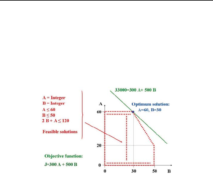
5.5 A simple example 255
/*10*/ Profit #= 300*A + 500*B,
/*11*/ Negative_profit #= - Profit,
/*12*/ minimize(labeling([A,B]),Negative_profit),
/*13*/ writeln("Maximum profit":Profit),nl,
/*14*/ write("A_opt = "), write(A), nl,
/*15*/ write("B_opt = "), write(B),nl.
Because maximization has to be done, and ECLiPSemakes available only
predicates for minimization, maximization is performed for negative profit.
Figure 5.6: Graphical solution to the simple optimization problem
The program displays all intermediate solutions from the search tree:
Found a solution with cost -30100 Found a solution with cost -30400
Found a solution with cost -30700 Found a solution with cost -31000
Found a solution with cost -31100 Found a solution with cost -31200
Found a solution with cost -31300 Found a solution with cost -31400
Found a solution with cost -31500 Found a solution with cost -31600
Found a solution with cost -31700 Found a solution with cost -31800
Found a solution with cost -31900 Found a solution with cost -32000
Found a solution with cost -32100 Found a solution with cost -32200
Found a solution with cost -32300 Found a solution with cost -32400
Found a solution with cost -32500 Found a solution with cost -32600
Found a solution with cost -32700 Found a solution with cost -32800
Found a solution with cost -32900 Found a solution with cost -33000

256 Chapter 5. CLP with elementary constraints for optimal solutions
Found no solution with cost -40000.0 .. -33001.0
Maximum profit : 33000
A_opt = 60 B_opt = 30
The problems discussed and solved below conform to the classification pre-
sented in Section 1.7.
5.6 Optimum configuration problems
5.6.1 Optimum configuration - OR approach
Next - let’s solve the optimum system configuration problem from Section 2.3.1
using an OR approach. This is done by program 5_2_configuration_OR.ecl2:
/*1*/ :- lib(ic).
/*2*/ :- lib(branch_and_bound).
/*3*/ top :-
/*4*/ Components=[A_1,A_2,A_3,B_1,B_2,B_3,B_4,C_1,C_2],
% A_1 = 1 means element A_1 belongs to the configuration
% A_1 = 0 means element A_1 does not belong to the configuration
/*5*/ Components :: 0..1,
/*6*/ Price:: 1..3000,
/*7*/ A_1 + A_2 + A_3 #= 1, % only one A-type element is needed
/*8*/ B_1 + B_2 + B_3 + B_4 #= 1, % only one B-type element is needed
/*9*/ C_1 + C_2 #= 1, % only one C-type element is needed
/*10*/ C_1 + A_2 #=< 1, % C_1 and A_2 should not appear both in a system
/*11*/ B_2 + C_2 #=< 1,
/*12*/ C_2 + B_3 #=< 1,
/*13*/ B_4 + A_2 #=< 1,
/*14*/ B_3 + A_1 #=< 1,
/*15*/ A_3 + B_3 #=< 1,
/*16*/ Price #= A_1 * 1900 + A_2 * 750 +
A_3 * 900 + B_1 * 300 + B_2 * 500 + B_3 * 450 +
B_4 * 600 + C_1 * 700 + C_2 * 850,
/*17*/ bb_min(labeling(Components),Price,bb_options with [strategy:step]),
/*18*/ writeln("Minimum configuration price":Price),nl,nl,
/*19*/ write("Optimum configuration:"),nl,
/*20*/ write([A_1,A_2,A_3,B_1,B_2,B_3,B_4,C_1,C_2]),nl,
2This is an OS-type problem.

5.6 Optimum configuration problems 257
/*21*/ write(["A_1","A_2","A_3","B_1","B_2","B_3","B_4","C_1","C_2"]),nl,
/*22*/ write_configuration([A_1,A_2,A_3,B_1,B_2,B_3,B_4,C_1,C_2],
["A_1","A_2","A_3","B_1","B_2","B_3","B_4","C_1","C_2"]),nl,nl,
/*23*/ fail.
/*24*/ top :-
/*25*/ write("Those are all optimum configurations.").
/*26*/ write_configuration([H1|T1],[H2|T2]):-
/*27*/ H1 is 1, write(H2),write(" "),
/*28*/ write_configuration(T1,T2).
/*29*/ write_configuration([H1|T1],[_|T2]):-
/*30*/ H1 is 0,
/*31*/ write_configuration(T1,T2).
/*32*/ write_configuration([],[]).
The message is:
Found a solution with cost 2350
Found a solution with cost 2200
Found a solution with cost 2100
Found a solution with cost 2050
Found a solution with cost 1900
Found no solution with cost 1.0 .. 1899.0
Minimum configuration price : 1900
Optimum configuration:
[0, 0, 1, 1, 0, 0, 0, 1, 0]
[A_1, A_2, A_3, B_1, B_2, B_3, B_4, C_1, C_2]
A_3 B_1 C_1
Those are all optimum configurations.
It can be seen that fail in line /*26*/ did not initiate backtracking to de-
termine the second optimum solution, which is known to exist as demonstrated
by program 2_9_conf_opt.pl. This is a serious limitation that however may be
bypassed as follows: in order to get all optimum solutions, a single one has to be
determined first. Next, the optimum solution data is used to constrict the do-
mains of variables (see line /*5*/ below) for a program that just determines all
feasible solutions. This program is given by 5_3_configuration_all_OR.ecl:

258 Chapter 5. CLP with elementary constraints for optimal solutions
/*1*/ :- lib(ic).
/*2*/ top :-
/*3*/ Components=[A_1,A_2,A_3,B_1,B_2,B_3,B_4,C_1,C_2],
/*4*/ Components :: 0..1,
/*5*/ Price is 1900,
/*6*/ A_1 + A_2 + A_3 #= 1,
/*7*/ B_1 + B_2 + B_3 + B_4 #= 1,
/*8*/ C_1 + C_2 #= 1,
/*9*/ C_1 + A_2 #=< 1,
/*10*/ B_2 + C_2 #=< 1,
/*11*/ C_2 + B_3 #=< 1,
/*12*/ B_4 + A_2 #=< 1,
/*13*/ B_3 + A_1 #=< 1,
/*14*/ A_3 + B_3 #=< 1,
/*15*/ Price #= A_1 * 1900 + A_2 * 750 + A_3 * 900 +
B_1 * 300 + B_2 * 500 + B_3 * 450 + B_4 * 600 +
C_1 * 700 + C_2 * 850,
/*16*/ labeling(Components),
/*17*/ writeln("Minimum configuration price": Price),nl,nl,
/*18*/ write("Search result:"),nl,
/*19*/ write([A_1,A_2,A_3,B_1,B_2,B_3,B_4,C_1,C_2]),nl,
/*20*/ write(["A_1","A_2","A_3","B_1","B_2","B_3","B_4","C_1","C_2"]),nl,
/*21*/ write("Optimum configuration:"),nl,
/*22*/ write_configuration([A_1,A_2,A_3,B_1,B_2,B_3,B_4,C_1,C_2],
["A_1","A_2","A_3","B_1","B_2","B_3","B_4","C_1","C_2"]),nl,nl,
/*23*/ fail.
/*24*/ top :-
/*25*/ write("Those are all optimum configurations.").
/*26*/ write_configuration([H1|T1],[H2|T2]):-
/*27*/ H1 is 1, write(H2),write(" "),
/*28*/ write_configuration(T1,T2).
/*29*/ write_configuration([H1|T1],[_|T2]):-
/*30*/ H1 is 0,
/*31*/ write_configuration(T1,T2).
/*32*/ write_configuration([],[]).
The message is:
Minimum configuration price:1900
Search result:

5.6 Optimum configuration problems 259
[0, 0, 1, 1, 0, 0, 0, 1, 0]
[A_1,A_2,A_3,B_1,B_2,B_3,B_4,C_1,C_2]
Optimum configuration:
A_3 B_1 C_1
Minimum configuration price:1900
Search result:
[0, 1, 0, 1, 0, 0, 0, 0, 1]
[A_1,A_2,A_3,B_1,B_2,B_3,B_4,C_1,C_2]
Optimum configuration:
A_2 B_1 C_2
Those are all optimum configurations.
5.6.2 Optimum configuration - CLP approach
Next the optimum configuration problem from Section 2.3.1 will be solved using
the CLP approach. The program 5_4_configuration_CLP.ecl3is as follows:
/*1*/ :- lib(ic).
/*2*/ :- lib(branch_and_bound).
/*4*/ top:-
% CA - cost of element A
% NA - number of element A
/*4*/ NA :: 1..3,
/*5*/ NB :: 1..4,
/*6*/ NC :: 1..2,
/*7*/ [CA,CB,CC] :: 300..1900,
/*8*/ Cost :: 1800..2600,
/*9*/ element(NA,[1900,750,900],CA),
/*10*/ element(NB,[300,500,450,600],CB),
/*11*/ element(NC,[700,850],CC),
/*12*/ ~incompatible_NB_NC(NB,NC),
/*13*/ ~incompatible_NA_NB(NA,NB),
/*14*/ ~incompatible_NA_NC(NA,NC),
% ~Goal is the sound negation operator, which delays if Goal is not grounded.+
/*15*/ Cost #= CA + CB + CC,
/*16*/ bb_min(labeling([NA,NB,NC]),Cost,bb_options with [strategy:step]),
/*17*/ writeln("Optimum configuration:"),
/*18*/ write("("),write("A"),write(NA),write(","),
/*19*/ write("B"),write(NB),write(","),write("C"),write(NC),writeln(")"),
3This is an OS-type problem.

260 Chapter 5. CLP with elementary constraints for optimal solutions
/*20*/ write("priced at "),write(Cost), writeln("."),nl,fail.
/*21*/ top:-
/*22*/ writeln("That’s all!").
/*23*/ incompatible_NA_NB(2,4).
/*24*/ incompatible_NA_NB(1,3).
/*25*/ incompatible_NA_NB(3,3).
/*26*/ incompatible_NA_NC(2,1).
/*27*/ incompatible_NB_NC(2,2).
/*28*/ incompatible_NB_NC(3,2).
The message is:
Found a solution with cost 1900
Found no solution with cost 1800.0 .. 1899.0
Optimum configuration:
(A2,B1,C2)
priced at 1900.
That’s all!
In order to generate all optimum solution the same trick as for example
5_3_configuration_all_OR.ecl has to be used. This is done in example
5_5_configuration_all_CLP.ecl4:
/*1*/ :- lib(ic).
/*2*/ :- lib(branch_and_bound).
/*3*/ top:-
/*4*/ NA :: 1..3,
/*5*/ NB :: 1..4,
/*6*/ NC :: 1..2,
/*7*/ [CA,CB,CC] :: 300..1900,
/*8*/ Cost is 1900,
/*9*/ element(NA,[1900,750,900],CA),
/*10*/ element(NB,[300,500,450,600],CB),
/*11*/ element(NC,[700,850],CC),
/*12*/ ~incompatible_NB_NC(NB,NC),
/*13*/ ~incompatible_NA_NB(NA,NB),
/*14*/ ~incompatible_NA_NC(NA,NC),
4This is an OS-type problem.

5.6 Optimum configuration problems 261
/*15*/ Cost #= CA + CB + CC,
/*16*/ labeling([NA,NB,NC]),
/*17*/ writeln("Optimum configuration:"),
/*18*/ write("("),write("A"),write(NA),write(","),
/*19*/ write("B"),write(NB),write(","),write("C"),write(NC),writeln(")"),
/*20*/ write("priced at "),write(Cost), writeln("."),nl,fail.
/*21*/ top:-
/*22*/ writeln("That’s all!").
/*23*/ incompatible_NA_NB(2,4).
/*24*/ incompatible_NA_NB(1,3).
/*25*/ incompatible_NA_NB(3,3).
/*26*/ incompatible_NA_NC(2,1).
/*27*/ incompatible_NB_NC(2,2).
/*28*/ incompatible_NB_NC(3,2).
The message is:
Optimum configuration:
(A2,B1,C2)
priced at 1900.
Optimum configuration:
(A3,B1,C1)
priced at 1900.
That’s all!
5.6.3 Knapsack problem 1
The knapsack problem is a classical optimization problem that derives its name
from a fixed-size smuggler knapsack, which must be filled with the most valuable
items. It may be formulated as follows: given a set of items, each with a
dimension (length, area, volume or weight) and a value, determine the items to
include in a collection so that the total dimension is less than a given limit and
the total value is maximized. The problem is known to exhibit combinatorial
explosion.
The most simple knapsack problem - a length-constrained knapsack problem
- can be solved using the scalar_product/3 predicate as shown in program

262 Chapter 5. CLP with elementary constraints for optimal solutions
5_6_knapsack_1.ecl5:
/*1*/ :- lib(ic).
/*2*/ :- lib(branch_and_bound).
/*3*/ top:-
/*4*/ knapsack([52,23,35,15,7],[100,60,70,15,15],60,[_,_,_,_,_]).
/*5*/ knapsack(Sizes,Values,Knapsack_size,[X1,X2,X3,X4,X5]):-
/*6*/ X = [X1,X2,X3,X4,X5],
/*7*/ X :: 0..1,
/*8*/ scalar_product(Sizes,X,Size),
/*9*/ Size #=< Knapsack_size,
/*10*/ scalar_product(Values,X,Value),
/*11*/ Cost #= -Value,
/*12*/ minimize(labeling(X),Cost),nl,
/*13*/ Value is -Cost,
/*14*/ write("Value = "),writeln(Value),
/*15*/ write("Knapsack = "), writeln(X),
/*16*/ write("Size ="),writeln(Size).
/*17*/ scalar_product(List_1,List_2,Scalar_product):-
/*18*/ (
/*19*/ foreach(V1, List_1),
/*20*/ foreach(V2, List_2),
/*21*/ foreach(Product,List_of_products)
/*22*/ do
/*232*/ Product = V1 * V2
/*24*/ ),
/*25*/ Scalar_product #= sum(List_of_products).
The message is:
Found a solution with cost 0
Found a solution with cost -15
Found a solution with cost -30
Found a solution with cost -70
Found a solution with cost -85
Found a solution with cost -100
Found a solution with cost -130
Found no solution with cost -260.0 .. -131.0
Value = 130
Knapsack = [0, 1, 1, 0, 0]
5This is an OS-type problem.

5.6 Optimum configuration problems 263
Size = 58,
So the optimum knapsack loading comprises items 2and 3from the list, of
corresponding sizes 23 and 35 amounting to 58, and of corresponding values 60
and 70 amounting to 130.
5.6.4 Reified constraints
Often it is desirable that the satisfaction of some constraint makes a Boolean
variable (further referred to as Index) bounded to 1; the failing of the constraint
makes this variable bounded to 0.TheIndex may be useful to formulate other
constraints. This may be done by reifying the constraint with respect to the
Index, as illustrated by following examples:
This is a command:
[eclipse 1]: Number = 0, #>(Number,0,Index).
This is the response:
Number = 0
Index = 0,
i.e. Number > 0 is false.
This is a command:
[eclipse 2]: Number = 6, #>(Number,0,Index).
This is the response:
Number = 6
Index = 1,
i.e. Number > 0 is true.
All elementary constraints can be changed into reified forms. E.g. the implica-
tion constraint +constraint(X) => +constraint(Y),
for which the satisfaction of ”constraint(X)” implies the satisfaction of
”constraint(Y)”, is functioning as follows:
This is a command for a non-reified form:
[eclipse 3]: X is 9, Y is 8, X#<10 => Y+2#<12.

264 Chapter 5. CLP with elementary constraints for optimal solutions
This is the response for a non-reified form:
X=9
Y=8
Yes
After reifying we get:
This is a command for a reified form:
[eclipse 4]: X is 9, Y is 8, =>(X#<10,Y+2#<12,Index).
This is the response for a reified form:
X=9
Y=8
Index = 1
If the implication is false:
This is a command:
[eclipse 5]: X is 9, Y is 8, =>(X#<10,Y+2#>15,Index).
This is the response:
X=9
Y=8
Index = 0
The implication may be true for any value from the domain, e.g.:
This is a command:
[eclipse 6]: X is 12, Y::14..18,=>(X#=5,Y+2#>15,Index).
This is the response:
X=12
Y = Y{14 .. 18}
Index = 1,
then Index is bounded to a unique value.
If the implication is true only for a subset of domain values, e.g.:

5.6 Optimum configuration problems 265
This is a command:
[eclipse 7]: X is 12, Y::12..17,=>(X#=12,Y+2#>15,Index).
This is the response:
X=12
Y = Y{12 .. 17}
Index = Index{[0, 1]},
then Index remains free.
5.6.5 Constraints for sets
AusefulfeatureofECLiPSeCPS is a the possibility of formulating constraints
for domains given by sets of integers. To use this feature the library ic_sets
needs to be loaded.
Sets of integers in ECLiPSeCPS are ordered n-tuples of unique integers, e.g.:
set_of_four_integers = [41,42,43,44], empty_set =[].
Set variables are variables that may be grounded to sets of integers. They are
declared as follows:
Set_variable :: []..[1,2,3,4,5,6]
where the empty set is the lower bound, and the set [1,2,3,4,5,6] is the upper
bound for the Set_variable. Let’s check some of its properties:
This is a command:
[eclipse 1]::-lib(ic_sets). Set_variable :: []..[1,2,3,4,5,6],
Set_variable = [3,2,1].
This is the response:
[eclipse 2]:
No (0.00s cpu)
This is a command:
[eclipse 3]::-lib(ic_sets). Set_variable :: []..[1,2,3,4,5,6],
Set_variable = [1,4,6].
This is the response:
[eclipse 4]:
Set_variable = [1, 4, 6]

266 Chapter 5. CLP with elementary constraints for optimal solutions
Yes (0.00s cpu)
This is a command:
[eclipse 5]::-lib(ic_sets). Set_variable :: []..[1,2,3,4,5,6],
Set_variable = [].
This is the response:
[eclipse 6]:
Set_variable = []
Yes (0.00s cpu)
For ECLiPSeCPS the empty set [] does not belong to the set domain if it
has not been explicitly declared:
This is a command:
[eclipse 7]::-lib(ic_sets). Set_variable :: [4]..[5,6,7],
Set_variable = [].
This is the response:
[eclipse 8]:
No (0.00s cpu)
However, the empty set [] is a subset of any set, e.g.:
This is a command:
[eclipse 9]::-lib(ic_sets). [4,5,6,7] includes X.
Set_variable = [].
This is the response:
[eclipse 8]:
X = X{([] .. [4, 5, 6, 7]) : _358{0 .. 4}},
where the _358 is the range of cardinal numbers for the Xset.
The lower bound does not belong to any set containing also elements of the
upper bound as illustrated below:
This is a command:
[eclipse 9]::-lib(ic_sets). Set_variable :: [4]..[5,6,7],

5.6 Optimum configuration problems 267
Set_variable = [4,5].
This is the response:
[eclipse 8]:
No (0.00s cpu)
In order for the lower bound to belong to some set containing (beside the lower
bound) also elements from the upper bound, it has to be included in the upper
bound:
This is a command:
[eclipse 10]: :-lib(ic_sets). Set_variable :: [4]..[4,5,6,7],
Set_variable=[4,7].
This is the response:
[eclipse 11]:
Set_variable = [4, 7]
Yes (0.00s cpu)
An important built-in for connecting sets and arrays is:
weight(?Set, ++Array_of_Set_Element_Weights, ?Weight_of_set),
for which ?Weight_of_set is the sum of all those elements from Array_of_Set_
Element_Weights that in the array are at positions given by elements of Set.
This is illustrated by program 5_7_weight_of_set_1.ecl6:
/*1*/ :- lib(ic_sets).
/*2*/ top:-
/*3*/ Set = [1,3],
/*4*/ weight(Set,[](10,20,30,40,50),Weight_of_set),
/*5*/ write("Weight of set = "),write(Weight_of_set),nl.
The message is:
Weight of set = 40
6This is an FS-type problem.

268 Chapter 5. CLP with elementary constraints for optimal solutions
The built-in weight/3 may be used to determine sets with constraint weights
as shown in the program 5_8_weight_of_set_2.ecl:
/*1*/ :- lib(ic).
/*2*/ :- lib(ic_sets).
/*3*/ top:-
/*4*/ ic_sets:(Set :: [].. [1, 2, 3, 4, 5]),
/*5*/ weight(Set,[](10,20,30,40,50),Weight_of_set),
/*6*/ Weight_of_set #=< 50,
/*7*/ Weight_of_set #>= 35,
/*8*/ insetdomain(Set,_,_,_),
/*9*/ write("Weight of set = "),write(Weight_of_set),
/*10*/ write(" Set = "),write(Set),nl.
The built-in insetdomain/4 is a set-wise correspondent of the built-in
indomain/1 for integer domains.
The message presents a number of solutions:
Weight of set = 40 Set = [1, 3]
Weight of set = 50 Set = [1, 4]
Weight of set = 50 Set = [2, 3]
Weight of set = 40 Set = [4]
Weight of set = 50 Set = [5]
5.6.6 Knapsack problem 2
The length-constrained knapsack problem may also be solved using the weight/3
built-in, as shown in 5_9_knapsack_2.ecl7:
/*1*/ :- lib(ic).
/*2*/ :- lib(ic_sets).
/*3*/ :- lib(branch_and_bound).
/*4*/ top:-
/*5*/ array_of_sizes(Sizes),
/*6*/ array_of_values(Values),
/*7*/ knapsack_size(Knapsack_size),
/*8*/ ic_sets:(Set :: [].. [1, 2, 3, 4, 5]),
/*9*/ weight(Set,Sizes,Knapsack_load),
7This is an OS-type problem.

5.6 Optimum configuration problems 269
/*10*/ Knapsack_load #=< Knapsack_size,
/*11*/ weight(Set,Values,Value),
/*12*/ Cost #= -Value,
/*13*/ minimize(insetdomain(Set,decreasing,_,_),Cost),
/*14*/ write("Value = "),writeln(Value),
/*15*/ write("Knapsack = "), writeln(Set),
/*16*/ write("Knapsack load = "),writeln(Knapsack_load).
/*17*/ array_of_sizes([](52,23,35,15,7)).
/*18*/ array_of_values([](100,60,70,15,15)).
/*19*/ knapsack_size(60).
The message is:
Found a solution with cost -90
Found a solution with cost -100
Found a solution with cost -115
Found a solution with cost -130
Found no solution with cost -260.0 .. -131.0
Value = 130
Knapsack = [2, 3]
Knapsack_load = 58,
The optimum knapsack load is thus 58, given by items z 2and 3, with overall
value 130.
5.6.7 How to cut optimally?
The range of different optimum configuration problems is broad indeed. As yet
another example may serve the one-dimensional rod-cutting problem:
Anumberof100 cm long rods should be cut into 36 rods of 28 cm and 24 rods
of 45 cm so as to minimize the total waste. There are only 3feasible cutting
strategies for a 100 cm long rod and the demanded smaller rods, illustrated
by Figure 5.7. An overall optimum cutting strategy that minimizes waste for
the given order of small rods is given by program 5_10_cutting.ecl8,where
variables Strategy_1,Strategy_2 and Strategy_3 denote numbers of 100 cm
8This is an OS-type problem.
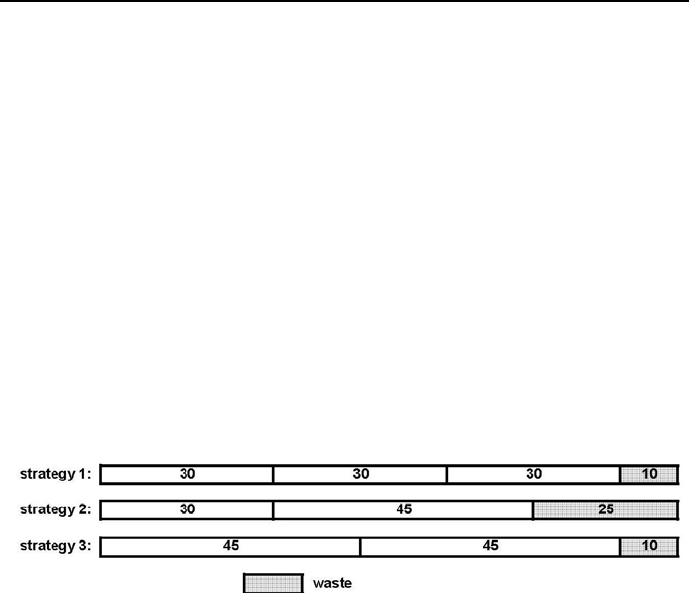
270 Chapter 5. CLP with elementary constraints for optimal solutions
rods cut using correspondingly strategy 1, strategy 2 and strategy 3:
/*1*/ :-lib(ic).
/*2*/ :-lib(branch_and_bound).
/*3*/ top :-
/*4*/ Variables = [Strategy_1,Strategy_2,Strategy_3],
/*4*/ Variables :: 0..60,
/*5*/ 3*Strategy_1 + 1*Strategy_2 + 0*Strategy_3 #>=36,
/*6*/ 0*Strategy_1 + 1*Strategy_2 + 2*Strategy_3 #>= 24,
/*7*/ Cost #= 10*Strategy_1 + 25*Strategy_2 + 10*Strategy_3,
/*8*/ minimize(search(Variables,0,first_fail,indomain,complete,[]),Cost),
/*9*/ writeln("Variables":Variables ),
/*10*/ writeln("Cost":Cost).
The message is:
Figure 5.7: Feasible cutting strategies for a 100 cm long rod
Found a solution with cost 900
Found a solution with cost 835
Found a solution with cost 770
Found a solution with cost 705
Found a solution with cost 640
Found a solution with cost 595
Found a solution with cost 540
Found a solution with cost 495
Found a solution with cost 440
Found a solution with cost 395
Found a solution with cost 340
Found a solution with cost 295
Found a solution with cost 240
Found no solution with cost 0.0 .. 239.0

5.6 Optimum configuration problems 271
Variables : [12, 0, 12]
Cost : 240
It means that 12 rods should be cut using strategy 1and 12 rods using strategy
3.
5.6.8 Appointing a parliamentary committee
A common optimization problem is concerned with set representation: find the
smallest set, which contains elements of other sets. A minimization is possible
if the sets contain some shared elements. This is illustrated by the following
example:
The ruling Absurdoland’s coalition of two immensely popular parties, ”Sprea-
ding Wealth” and ”Paradise on Earth”, is facing the problem of delegating
four parliamentarians to a newly established (under electoral pressure) parlia-
mentary committee for the investigation of illegal lobbying activities aimed at
influencing the outcome of legislative processes. Each coalition party appointed
five parliamentarians as candidates to the committee; out of the team of ten
parliamentarians available, four parliamentarians have to be finally chosen to
serve on the committee. Obviously, the parties were interested in having on
the committee parliamentarians representing all active main streams of politi-
cal and social thought cultivated in both parties. A close look at the initially
appointed ten parliamentarians (which would be referred to by numbers in or-
der not to compromise party secrets), 1,2,3,...,10, assured both parties that
they represent all active main streams of political and social thought. What’s
more, a yet closer look disclosed that some of the appointed parliamentarians
have such extraordinary high intellectual capacity to make them contribute in
the past to more than one active main stream, as shown in Table 5.1.
Therefore it was justifiably concluded that they should represent in the com-
mittee all active main streams, to which they contributed.
However, the question is still open whether a team of four parliamentarians
representing all active main streams could be selected out of the ten candidates.
To answer that question a program 5_11_committee.ecl9has been designed to
establish the minimum number of parliamentarians representing all active main
streams. The program shown below has been inspired by one presented at the
website [Kjellerstrand-13]:
9This is an OS-type problem.

272 Chapter 5. CLP with elementary constraints for optimal solutions
Parliamentarians Coalition parties
1, 2, 3, 4, 5 Spreading Wealth
6, 7, 8, 9, 10 Paradise on Earth
Main streams of political and social thought
3, 8, 9 Agents of Influence 1
1, 6, 7 Agents of Influence 2
3, 4 Mafia 1 Supporters
2, 6 Mafia 2 Supporters
7, 10 Gambling Business Advocates
3, 6 Anthropogenic Global Warming Believers
7Big Bank Advocates
2LGBT Supporters
5, 10 Useful Idiots
Table 5.1: Parliamentarians, their affiliation to parties and contributions to
main streams
/*1*/ :-lib(ic).
/*2*/ :-lib(branch_and_bound).
/*3*/ top :-
% First a single minimum number of parliamentarians is determined,
% next all lists of parliamentarians for this minimum are determined.
/*4*/ writeln("Finding a single optimum solution:"),
/*5*/ data(WhoWhere),
/*6*/ select_from_sets(WhoWhere, Minimum,_),
/*7*/ writeln("\nFinding all optimum solutions:"),
/*8*/ findall(X, select_from_sets(WhoWhere, Minimum,X), L),
/*9*/ length(L, Len),
/*10*/ printf("%d optimum solutions have been found.\n", [Len]).
/*11*/ select_from_sets(WhoWhere, Minimum, X) :-
/*12*/ dim(WhoWhere,[NumberOfGroups,NumberOfMembers]),
% Creating a list of parliamentarians:
/*13*/ dim(X,[NumberOfMembers]),
/*14*/ X :: 0..1,
% Choosing parliamentarians from each main stream:
/*15*/ (
/*16*/ for(I,1,NumberOfGroups),
/*17*/ param(NumberOfMembers,X,WhoWhere)
/*18*/ do
/*19*/ (
/*20*/ for(J,1,NumberOfMembers),
/*21*/ fromto(0,In,Out,Sum),

5.6 Optimum configuration problems 273
/*22*/ param(X,WhoWhere,I)
/*23*/ do
/*24*/ Out #= In + X[J]*WhoWhere[I,J]
/*25*/ ),
/*26*/ Sum #>= 1
/*27*/ ),
% Minimizing the number of parliamentarians:
/*28*/ flatten_array(X, Variables),
/*29*/ Z #= sum(Variables),
/*30*/ Z #= Minimum,
% Depending whether the minimum is or is not known,
% all minimal solutions are determined or
% a single minimum solution is determined:
/*31*/ (
/*32*/ ground(Minimum)
/*33*/ ->
/*34*/ search(Variables,0,first_fail,indomain,complete, [])
/*35*/ ;
/*36*/ minimize(search(Variables,0,first_fail,indomain,complete,[]),Z)
/*37*/ ),
/*38*/ writeln("Minimum number of parliamentarians":Z),
/*39*/ writeln("Selected parliamentarians":X).
/*40*/ data([](
[](1, 1, 1, 1, 1, 0, 0, 0, 0, 0), % Spreading Wealth
[](0, 0, 0, 0, 0, 1, 1, 1, 1, 1), % Paradise on Earth
[](0, 0, 1, 0, 0, 0, 0, 1, 1, 0), % Agents of Influence 1
[](1, 0, 0, 0, 0, 1, 1, 0, 0, 0), % Agents of Influence 2
[](0, 0, 1, 1, 0, 0, 0, 0, 0, 0), % Mafia 1 Supporters
[](0, 1, 0, 0, 0, 1, 0, 0, 0, 0), % Mafia 2 Supporters
[](0, 0, 0, 0, 0, 0, 1, 0, 0, 1), % Gambling Business Advocates
[](0, 0, 1, 0, 0, 1, 0, 0, 0, 0), % Anthropogenic Global Warming Believers
[](0, 0, 0, 0, 0, 0, 1, 0, 0, 0), % Big Bank Advocates
[](0, 1, 0, 0, 0, 0, 0, 0, 0, 0), % LGBT Supporters
[](0, 0, 0, 0, 1, 0, 0, 0, 0, 1))).% Useful Idiots
The message is:
Finding a single optimum solution:
Found a solution with cost 6
Found a solution with cost 4
Found no solution with cost 2.0 .. 3.0
Minimum number of parliamentarians : 4
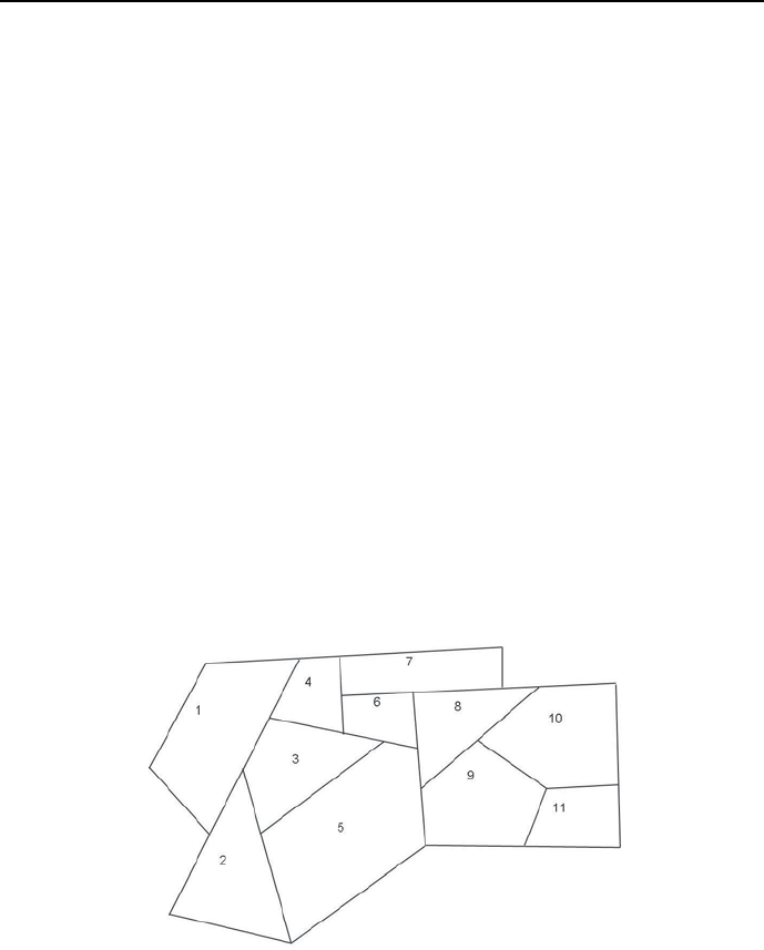
274 Chapter 5. CLP with elementary constraints for optimal solutions
Selected parliamentarians : [](0, 1, 1, 0, 0, 0, 1, 0, 0, 1)
Finding all optimum solutions:
Minimum number of parliamentarians : 4
Selected parliamentarians : [](0, 1, 1, 0, 0, 0, 1, 0, 0, 1)
Minimum number of parliamentarians : 4
Selected parliamentarians : [](0, 1, 1, 0, 1, 0, 1, 0, 0, 0)
2 optimum solutions have been found.
The meaning of this results is obvious: only if the i-th element of the one-
dimensional array Selected parliamentarians is equal 1, then the i-th par-
liamentarian may be chosen to be a committee member.
The result is both good and bad news. The good news is that there are four
parliamentarians representing all main streams of political and social thought
cultivated in both parties. The bad news is that there are two teams of such
parliamentarians, which means that there will be much arguing in the coalition.
5.6.9 Ambulance Service Stations
A Town Council is analyzing possible locations for the newly established large
and modern Ambulance Service Stations (ASS). The Town consists of 11 dis-
tricts as shown in Figure 5.8.
Figure 5.8: District maps
An Ambulance Service Station may be located in any district and provide

5.6 Optimum configuration problems 275
its services to its native and all adjacent districts. The conservative majority in
the Town Council successfully defended a motion about minimizing the number
of ASS while providing all districts with their services. It also put forward
some additional suggestions about avoiding the establishment of ASS in adjacent
districts and favoured a location plan for which any district having no ASS is
adjacent to only one district with ASS.
The program 5_12_ambulance_service.ecl explains how was it done:
/*1*/ :- lib(ic).
/*2*/ :- lib(branch_and_bound).
/*3*/ top :-
/*4*/ [S1,S2,S3,S4,S5,S6,S7,S8,S9,S10,S11] :: 0..1,
% Si = 1 - an ASS is located in i-th district
% Si = 0 - an ASS is not located in i-th district
% if an ASS is located in district 1, then no ASS is needed
% for districts 2, 3 and 4;
% if no ASS is located in district 1, then one of the
% districts 2, 3 or 4 should have an ASS:
/*5*/ S1+S2+S3+S4 #= 1,
% if an ASS is located in district 2, then no ASS is needed
% for districts 1, 3 and 5;
% if no ASS is located in district 2, then one of the
% districts 1, 3 and 5should have an ASS:
/*6*/ S1+S2+S3+ S5 #= 1,
% if an ASS is located in district 3, then no ASS is needed
% for districts 1, 2, 4, 5 and 6;
% if no ASS is located in district 3, then one of the
% districts 1, 2, 4, 5 and 6 should have an ASS:
/*7*/ S1+S2+S3+S4+S5+S6 #= 1,
% if an ASS is located in district 4, then no ASS is needed
% for districts 1, 3, 6 and 7;
% if no ASS is located in district 4, then one of the
% districts 1, 3, 6 and 7 should have an ASS:
/*8*/ S1+ S3+S4+ S6+S7 #= 1,
% if an ASS is located in district 5, then no ASS is needed
% for districts 2, 3, 6, 8 and 9;
% if no ASS is located in district 5, then one of the
% districts 2, 3, 6, 8 and 9 should have an ASS:
/*9*/ S2+S3+ S5+S6+ S8+S9 #= 1,

276 Chapter 5. CLP with elementary constraints for optimal solutions
% if an ASS is located in district 6, then no ASS is needed
% for districts 3, 4, 5, 7 and 8;
% if no ASS is located in district 6, then one of the
% districts 3, 4, 5, 7 and 8 should have an ASS:
/*10*/ S3+S4+S5+S6+S7+S8 #= 1,
% if an ASS is located in district 7, then no ASS is needed
% for districts 4, 6 and 8;
% if no ASS is located in district 7, then one of the
% districts 4, 6 and 8 should have an ASS:
/*11*/ S4+ S6+S7+S8 #= 1,
% if an ASS is located in district 8, then no ASS is needed
% for districts 5, 6, 7, 9 and 10;
% if no ASS is located in district 8, then one of the
% districts 5, 6, 7, 9 and 10 should have an ASS:
/*12*/ S5+S6+S7+S8+S9+S10 #= 1,
% if an ASS is located in district 9, then no ASS is needed
% for districts 5, 8, 10 and 11;
% if no ASS is located in district 9, then one of the
% districts 5, 8, 10 and 11 should have an ASS:
*13*/ S5+ S8+S9+S10+S11 #= 1,
% if an ASS is located in district 10, then no ASS is needed
% for districts 8, 9 and 11;
% if no ASS is located in district 10, then one of the
% districts 8, 9 and 11 should have an ASS:
/*14*/ S8+S9+S10+S11 #= 1,
% if an ASS is located in district 11, then no ASS is needed
% for districts 9 and 10;
% if no ASS is located in district 11, then one of the
% districts 9 and 10 should have an ASS:
/*15*/ S9+S10+S11 #= 1,
/*16*/ Number_of_ASS #= S1+S2+S3+S4+S5+S6+S7+S8+S9+S10+S11,
/*17*/ bb_min(search([S1,S2,S3,S4,S5,S6,S7,S8,S9,S10,S11],0,
first_fail,indomain,complete,[]),Number_of_ASS,
bb_options with [strategy:step]),
/*18*/ write([S1,S2,S3,S4,S5,S6,S7,S8,S9,S10,S11]),nl,
/*19*/ final_message([S1,S2,S3,S4,S5,S6,S7,S8,S9,S10,S11]),nl,nl.
/*20*/final_message([S1,S2,S3,S4,S5,S6,S7,S8,S9,S10,S11]):-
/*21*/ print("ASS should be located in districts:"),nl,
/*22*/ ((S1 is 1) -> print(" 1, ") ; print("")),
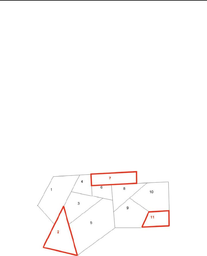
5.6 Optimum configuration problems 277
/*23*/ ((S2 is 1) -> print(" 2, ") ; print("")),
/*24*/ ((S3 is 1) -> print(" 3, ") ; print("")),
/*25*/ ((S4 is 1) -> print(" 4, ") ; print("")),
/*26*/ ((S5 is 1) -> print(" 5, ") ; print("")),
/*27*/ ((S6 is 1) -> print(" 6, ") ; print("")),
/*28*/ ((S7 is 1) -> print(" 7, ") ; print("")),
/*29*/ ((S8 is 1) -> print(" 8, ") ; print("")),
/*30*/ ((S9 is 1) -> print(" 9, ") ; print("")),
/*31*/ ((S10 is 1) -> print(" 10, ") ; print("")),
/*32*/ ((S11 is 1) -> print(" 11, ") ; print("")).
The solution is as follows:
Found a solution with cost 3
Found no solution with cost 0.0 .. 2.0
[0, 1, 0, 0, 0, 0, 1, 0, 0, 0, 1]
ASS should be located in districts:
2, 7, 11,
It is depicted on Figure 5.9.
Figure 5.9: Optimum location of ASS
Let’s check if there are other optimum solutions. This is done by program

278 Chapter 5. CLP with elementary constraints for optimal solutions
5_13_ambulance_service_all.ecl:
/*1*/ :- lib(ic).
/*2*/ :- lib(ic_global).
/*3*/ top :-
/*4*/ Stations = [S1,S2,S3,S4,S5,S6,S7,S8,S9,S10,S11] ,
/*5*/ Stations :: 0..1,
/*6*/ Number_of_stations is 3,
% Si = 1 - an ASS is located in i-th district
% Si = 0 - an ASS is not located in i-th district
% if an ASS is located in district 1, then no ASS is needed
% for districts 2, 3 and 4;
% if no ASS is located in district 1, then one of the
% districts 2, 3 or 4 should have an ASS:
/*7*/ S1+S2+S3+S4 #= 1,
% if an ASS is located in district 2, then no ASS is needed
% for districts 1, 3 and 5;
% if no ASS is located in district 2, then one of the
% districts 1, 3 and 5should have an ASS:
/*8*/ S1+S2+S3+ S5 #= 1,
% if an ASS is located in district 3, then no ASS is needed
% for districts 1, 2, 4, 5 and 6;
% if no ASS is located in district 3, then one of the
% districts 1, 2, 4, 5 and 6 should have an ASS:
/*9*/ S1+S2+S3+S4+S5+S6 #= 1,
% if an ASS is located in district 4, then no ASS is needed
% for districts 1, 3, 6 and 7;
% if no ASS is located in district 4, then one of the
% districts 1, 3, 6 and 7 should have an ASS:
/*10*/ S1+ S3+S4+ S6+S7 #= 1,
% if an ASS is located in district 5, then no ASS is needed
% for districts 2, 3, 6, 8 and 9;
% if no ASS is located in district 5, then one of the
% districts 2, 3, 6, 8 and 9 should have an ASS:
/*11*/ S2+S3+ S5+S6+ S8+S9 #= 1,
% if an ASS is located in district 6, then no ASS is needed
% for districts 3, 4, 5, 7 and 8;
% if no ASS is located in district 6, then one of the
% districts 3, 4, 5, 7 and 8 should have an ASS:
/*12*/ S3+S4+S5+S6+S7+S8 #= 1,

5.6 Optimum configuration problems 279
% if an ASS is located in district 7, then no ASS is needed
% for districts 4, 6 and 8;
% if no ASS is located in district 7, then one of the
% districts 4, 6 and 8 should have an ASS:
/*13*/ S4+ S6+S7+S8 #= 1,
% if an ASS is located in district 8, then no ASS is needed
% for districts 5, 6, 7, 9 and 10;
% if no ASS is located in district 8, then one of the
% districts 5, 6, 7, 9 and 10 should have an ASS:
/*14*/ S5+S6+S7+S8+S9+S10 #= 1,
% if an ASS is located in district 9, then no ASS is needed
% for districts 5, 8, 10 and 11;
% if no ASS is located in district 9, then one of the
% districts 5, 8, 10 and 11 should have an ASS:
*15*/ S5+ S8+S9+S10+S11 #= 1,
% if an ASS is located in district 10, then no ASS is needed
% for districts 8, 9 and 11;
% if no ASS is located in district 10, then one of the
% districts 8, 9 and 11 should have an ASS:
/*16*/ S8+S9+S10+S11 #= 1,
% if an ASS is located in district 11, then no ASS is needed
% for districts 9 and 10;
% if no ASS is located in district 11, then one of the
% districts 9 and 10 should have an ASS:
/*17*/ S9+S10+S11 #= 1,
/*18*/ Number_of_stations #= S1+S2+S3+S4+S5+S6+S7+S8+S9+S10+S11,
/*19*/ sumlist(Stations,Number_of_stations),
/*20*/ labeling(Stations),
/*21*/ write("ASS should be located in districts:"),
/*22*/ (foreach(Station,Stations),
/*23*/ count(I,1,11)
/*24*/ do
/*25*/ (Station #= 1 -> (write(" "),write(I)); true)
/*26*/ ),nl, fail.
/*27*/ top:-
/*28*/ writeln("Those are all solutions.").
The solution generated is the same as before:
280 Chapter 5. CLP with elementary constraints for optimal solutions
ASS should be located in districts: 2 7 11
Those are all solutions.
So there is only one optimum solution to the ASS location problem.
5.7 Optimum assignment problems
5.7.1 Tasks allocation for 7 machines - OR approach
Tasks allocation (as any allocation) may sometimes be also optimized, as shown
by the following example:
Any one of seven machines may perform any one of seven different tasks,
but at different costs, as shown in Table 5.2.
Machine Task
1234567
115 23 43 27 76 43 91
245 76 32 39 72 37 48
356 45 87 75 34 76 29
413 45 34 51 52 21 76
545 49 18 48 58 98 23
623 25 29 39 52 41 12
776 98 86 41 34 76 77
Table 5.2: Task costs for machines
The tasks should be allocated between machines in a way minimizing the
overall cost of performing all of them10.
A program for doing this (5_14_opty77_OR.ecl)isasfollows:
/*1*/ :- lib(ic).
/*2*/ :- lib(branch_and_bound).
% Uij - Usage of machine i for operation j:
% Uij = 1 - machine i is used for operation j.
% Uij = 0 - machine i is not used for operation j.
/*3*/ top :-
/*4*/ Machine_usage =
10 This is an OS-type problem.

5.7 Optimum assignment problems 281
[U11,U12,U13,U14,U15,U16,U17,
U21,U22,U23,U24,U25,U26,U27,
U31,U32,U33,U34,U35,U36,U37,
U41,U42,U43,U44,U45,U46,U47,
U51,U52,U53,U54,U55,U56,U57,
U61,U62,U63,U64,U65,U66,U67,
U71,U72,U73,U74,U75,U76,U77],
/*5*/ Machine_usage :: 0..1,
/*6*/ Cost :: 1..700,
/*7*/ U11+U21+U31+U41+U51+U61+U71 #= 1,
/*8*/ U12+U22+U32+U42+U52+U62+U72 #= 1,
/*9*/ U13+U23+U33+U43+U53+U63+U73 #= 1,
/*10*/ U14+U24+U34+U44+U54+U64+U74 #= 1,
/*11*/ U15+U25+U35+U45+U55+U65+U75 #= 1,
/*12*/ U16+U26+U36+U46+U56+U66+U76 #= 1,
/*13*/ U17+U27+U37+U47+U57+U67+U77 #= 1,
/*14*/ U11+U12+U13+U14+U15+U16+U17 #= 1,
/*15*/ U21+U22+U23+U24+U25+U26+U27 #= 1,
/*16*/ U31+U32+U33+U24+U35+U36+U37 #= 1,
/*17*/ U41+U42+U43+U44+U45+U46+U47 #= 1,
/*18*/ U51+U52+U53+U54+U55+U56+U57 #= 1,
/*19*/ U61+U62+U63+U64+U65+U66+U67 #= 1,
/*20*/ U71+U72+U73+U74+U75+U76+U77 #= 1,
/*21*/ Cost #= U11*15+U12*23+U13*43+U14*27+U15*76+U16*43+U17*91 +
U21*45 + U22*76 + U23*32 + U24*39 + U25*72 + U26*37 + U27*48 +
U31*56 + U32*45 + U33*87 + U34*75 + U35*34 + U36*76 + U37*29 +
U41*13 + U42*45 + U43*34 + U44*51 + U45*52 + U46*21 + U47*76 +
U51*45 + U52*49 + U53*18 + U54*48 + U55*58 + U56*98 + U57*23 +
U61*23 + U62*25 + U63*29 + U64*39 + U65*52 + U66*41 + U67*12 +
U71*76 + U72*98 + U73*86 + U74*41 + U75*34 + U76*76 + U77*77,
/*22*/ bb_min(labeling(
[U11,U12,U13,U14,U15,U16,U17,
U21,U22,U23,U24,U25,U26,U27,
U31,U32,U33,U34,U35,U36,U37,
U41,U42,U43,U44,U45,U46,U47,
U51,U52,U53,U54,U55,U56,U57,
U61,U62,U63,U64,U65,U66,U67,
U71,U72,U73,U74,U75,U76,U77]),
Cost,bb_options with [strategy:step]),
/*23*/ write("Overall cost: "),writeln(Cost),
/*24*/ display_results(1,[U11,U12,U13,U14,U15,U16,U17],[15,23,43,27,76,43,91]),
/*25*/ display_results(2,[U21,U22,U23,U24,U25,U26,U27],[45,76,32,39,72,37,48]),
/*26*/ display_results(3,[U31,U32,U33,U34,U35,U36,U37],[56,45,87,75,34,76,29]),
/*27*/ display_results(4,[U41,U42,U43,U44,U45,U46,U47],[13,45,34,51,52,21,76]),

282 Chapter 5. CLP with elementary constraints for optimal solutions
/*28*/ display_results(5,[U51,U52,U53,U54,U55,U56,U57],[45,49,18,48,58,98,23]),
/*29*/ display_results(6,[U61,U62,U63,U64,U65,U66,U67],[23,25,29,39,52,41,12]),
/*30*/ display_results(7,[U71,U72,U73,U74,U75,U76,U77],[76,98,86,41,34,76,77]),
/*31*/ fail.
/*32*/ top:-
/*33*/ writeln("That’s all!").
/*34*/ display_results(M,U,C):-
/*35*/ element(N, U, 1),
/*36*/ element(N, C, Op_Cost),
/*37*/ write("Machine "),write(M),write(" is performing operation "),write(N),
write(" costing "),write(Op_Cost),writeln(".").
The message is:
Found a solution with cost 332
Found a solution with cost 309
Found a solution with cost 307
Found a solution with cost 289
Found a solution with cost 259
Found a solution with cost 252
Found a solution with cost 222
Found a solution with cost 211
Found a solution with cost 183
Found a solution with cost 178
Found no solution with cost 1.0 .. 177.0
Overall cost: 178
Machine 1 is performing operation 2 costing 23.
Machine 2 is performing operation 6 costing 37.
Machine 3 is performing operation 5 costing 34.
Machine 4 is performing operation 1 costing 13.
Machine 5 is performing operation 3 costing 18.
Machine 6 is performing operation 7 costing 12.
Machine 7 is performing operation 4 costing 41.
That’s all!
In order to check whether there are more optimum solutions, program
5_15_opty77_all_OR.ecl may be used. The cost is fixed at the optimum cost
178 and no optimization is performed:

5.7 Optimum assignment problems 283
/*1*/ :- lib(ic).
/*2*/ :- lib(branch_and_bound).
% Uij - Usage of machine i for operation j:
% Uij = 1 - machine i is used for operation j.
% Uij = 0 - machine i is not used for operation j.
/*3*/ top :-
/*4*/ Machine_usage =
[U11,U12,U13,U14,U15,U16,U17,
U21,U22,U23,U24,U25,U26,U27,
U31,U32,U33,U34,U35,U36,U37,
U41,U42,U43,U44,U45,U46,U47,
U51,U52,U53,U54,U55,U56,U57,
U61,U62,U63,U64,U65,U66,U67,
U71,U72,U73,U74,U75,U76,U77],
/*5*/ Machine_usage :: 0..1,
/*6*/ Cost is 178,
/*7*/ U11+U21+U31+U41+U51+U61+U71 #= 1,
/*8*/ U12+U22+U32+U42+U52+U62+U72 #= 1,
/*9*/ U13+U23+U33+U43+U53+U63+U73 #= 1,
/*10*/ U14+U24+U34+U44+U54+U64+U74 #= 1,
/*11*/ U15+U25+U35+U45+U55+U65+U75 #= 1,
/*12*/ U16+U26+U36+U46+U56+U66+U76 #= 1,
/*13*/ U17+U27+U37+U47+U57+U67+U77 #= 1,
/*14*/ U11+U12+U13+U14+U15+U16+U17 #= 1,
/*15*/ U21+U22+U23+U24+U25+U26+U27 #= 1,
/*16*/ U31+U32+U33+U24+U35+U36+U37 #= 1,
/*17*/ U41+U42+U43+U44+U45+U46+U47 #= 1,
/*18*/ U51+U52+U53+U54+U55+U56+U57 #= 1,
/*19*/ U61+U62+U63+U64+U65+U66+U67 #= 1,
/*20*/ U71+U72+U73+U74+U75+U76+U77 #= 1,
/*21*/ Cost #= U11*15+U12*23+U13*43+U14*27+U15*76+U16*43+U17*91 +
U21*45 + U22*76 + U23*32 + U24*39 + U25*72 + U26*37 + U27*48 +
U31*56 + U32*45 + U33*87 + U34*75 + U35*34 + U36*76 + U37*29 +
U41*13 + U42*45 + U43*34 + U44*51 + U45*52 + U46*21 + U47*76 +
U51*45 + U52*49 + U53*18 + U54*48 + U55*58 + U56*98 + U57*23 +
U61*23 + U62*25 + U63*29 + U64*39 + U65*52 + U66*41 + U67*12 +
U71*76 + U72*98 + U73*86 + U74*41 + U75*34 + U76*76 + U77*77,
/*22*/ labeling(
[U11,U12,U13,U14,U15,U16,U17,
U21,U22,U23,U24,U25,U26,U27,
U31,U32,U33,U34,U35,U36,U37,
U41,U42,U43,U44,U45,U46,U47,
U51,U52,U53,U54,U55,U56,U57,

284 Chapter 5. CLP with elementary constraints for optimal solutions
U61,U62,U63,U64,U65,U66,U67,
U71,U72,U73,U74,U75,U76,U77]),
/*22*/ write("Overall cost: "),writeln(Cost),
/*23*/ display_results(1,[U11,U12,U13,U14,U15,U16,U17],[15,23,43,27,76,43,91]),
/*24*/ display_results(2,[U21,U22,U23,U24,U25,U26,U27],[45,76,32,39,72,37,48]),
/*25*/ display_results(3,[U31,U32,U33,U34,U35,U36,U37],[56,45,87,75,34,76,29]),
/*26*/ display_results(4,[U41,U42,U43,U44,U45,U46,U47],[13,45,34,51,52,21,76]),
/*27*/ display_results(5,[U51,U52,U53,U54,U55,U56,U57],[45,49,18,48,58,98,23]),
/*28*/ display_results(6,[U61,U62,U63,U64,U65,U66,U67],[23,25,29,39,52,41,12]),
/*29*/ display_results(7,[U71,U72,U73,U74,U75,U76,U77],[76,98,86,41,34,76,77]),
/*30*/ fail.
/*31*/ top:-
/*32*/ writeln("That’s all!").
/*33*/ display_results(M,U,C):-
/*34*/ element(N, U, 1),
/*35*/ element(N, C, Op_Cost),
/*36*/ write("Machine "),write(M),write(" is performing operation "),write(N),
write(" costing "),write(Op_Cost),writeln(".").
There is only a single optimum solution. The message generated is:
Overall cost: 178
Machine 1 is performing operation 2 costing 23.
Machine 2 is performing operation 6 costing 37.
Machine 3 is performing operation 5 costing 34.
Machine 4 is performing operation 1 costing 13.
Machine 5 is performing operation 3 costing 18.
Machine 6 is performing operation 7 costing 12.
Machine 7 is performing operation 4 costing 41.
That’s all!
5.7.2 Tasks allocation for 7 machines - CLP approach
As before, the CLP approach is more parsimonious than the OR approach with
respect to the number of variables needed to solve the problem. This is well
demonstrated by program 5_16_opty77_CLP.ecl11:
11 This is an OS-type problem.

5.7 Optimum assignment problems 285
/*1*/ :- lib(ic).
/*2*/ :- lib(branch_and_bound).
/*3*/ top :-
/*4*/ [O1,O2,O3,O4,O5,O6,O7] :: 1..7,
/*5*/ [C1,C2,C3,C4,C5,C6,C7] :: 1..100,
/*6*/ Cost :: 1..700,
/*7*/ alldifferent([O1,O2,O3,O4,O5,O6,O7]),
/*8*/ element(O1,[15,23,43,27,76,43,91],C1),
/*9*/ element(O2,[45,76,32,39,72,37,48],C2),
/*10*/ element(O3,[56,45,87,75,34,76,29],C3),
/*11*/ element(O4,[13,45,34,51,52,21,76],C4),
/*12*/ element(O5,[45,49,18,48,58,98,23],C5),
/*13*/ element(O6,[23,25,29,39,52,41,12],C6),
/*14*/ element(O7,[76,98,86,41,34,76,77],C7),
/*15*/ Cost #= C1+C2+C3+C4+C5+C6+C7,
/*16*/ bb_min(labeling([O1,O2,O3,O4,O5,O6,O7]),Cost,
bb_options with [strategy:step]),
/*17*/ display_results([O1,C1,O2,C2,O3,C3,O4,C4,O5,C5,O6,C6,O7,C7],1),
/*18*/ write("Overall cost: "),write(Cost).
/*19*/ display_results([],_).
/*20*/ display_results([A,B|R],N):-
/*21*/ write("Machine "),write(N),write(" is performing operation "),
/*22*/ write(A),write(" costing "),write(B),write("."),nl,
/*23*/ M is N1, +
/*24*/ display_results(R,M).
The message generated is exactly the same as for program 5_14_opty77_OR.ecl.
To check for multiple optimum solutions the program 5_17_opty77_all_CLP.ecl
is used:
/*1*/ :- lib(ic).
/*2*/ :- lib(branch_and_bound).
/*3*/ top :-
/*4*/ [O1,O2,O3,O4,O5,O6,O7] :: 1..7,
/*5*/ [C1,C2,C3,C4,C5,C6,C7] :: 1..100,
/*6*/ Cost is 178,
/*7*/ alldifferent([O1,O2,O3,O4,O5,O6,O7]),

286 Chapter 5. CLP with elementary constraints for optimal solutions
/*8*/ element(O1,[15,23,43,27,76,43,91],C1),
/*9*/ element(O2,[45,76,32,39,72,37,48],C2),
/*10*/ element(O3,[56,45,87,75,34,76,29],C3),
/*11*/ element(O4,[13,45,34,51,52,21,76],C4),
/*12*/ element(O5,[45,49,18,48,58,98,23],C5),
/*13*/ element(O6,[23,25,29,39,52,41,12],C6),
/*14*/ element(O7,[76,98,86,41,34,76,77],C7),
/*15*/ Cost #= C1+C2+C3+C4+C5+C6+C7,
/*16*/ labeling([O1,O2,O3,O4,O5,O6,O7]),
/*17*/ display_results([O1,C1,O2,C2,O3,C3,O4,C4,O5,C5,O6,C6,O7,C7],1),
/*18*/ write("Overall cost: "),write(Cost),
/*19*/ fail.
/*20*/ top:-
/*21*/ writeln("That’s all!").
/*22*/ display_results([],_).
/*23*/ display_results([A,B|R],N):-
/*24*/ write("Machine "),write(N),write(" is performing operation "),
/*25*/ write(A),write(" costing "),write(B),write("."),nl,
/*26*/ M is N+1,
/*27*/ display_results(R,M).
Obviously, the message generated is exactly the same as for the already discussed
program 5_14_opty77_all_OR.ecl.
5.7.3 Delivering mining output 1
Transport- and production problems, which have been from the beginning of
OR successfully solved by OR techniques, are also rewarding problems for CLP
techniques. Consider the following example:
Three mines m1, m2 and m3 deliver their output to five stockyards s1, s2, s3,
s4 i s5 at different locations. The capacity of each stockyard equals 400 ton
of output per month, while the monthly outputs equals 600 ton for mine m1
and 700 ton for mines m2 and m3. The production cost for one ton of output
are respectively 108, 96 i 102 MU. The delivery costs for one ton of output are
shown in Table 5.3.
How large should the output of mines be and how much output should the
mines deliver to the stockyard in order to minimize the overall cost of production
and transportation? This problem is solved by program 5_18_mines_1.ecl12:
12 This is an OS-type problem.

5.7 Optimum assignment problems 287
Mine Stockyard
s1 s2 s3 s4 s5
m1 14 5 9 24 15
m2 30 24 11 819
m3 922 15 718
Table 5.3: Deliver costs for mine outputs
/*1*/ :- lib(ic).
/*2*/ :- lib(branch_and_bound).
/*3*/ top :-
% Mine m1 is delivering A1 tons of output to stockyard s1,
% A2 ton to stockyard s2,...:
/*4*/ [A1,A2,A3,A4,A5] :: 0..600,
% Mine m2 is delivering B1 tons of output to stockyard s1,
% B2 ton to stockyard s2,...:
/*5*/ [B1,B2,B3,B4,B5] :: 0..700,
% Mine m3 is delivering C1 tons of output to stockyard s1,
% C2 ton to stockyard s2,...:
/*6*/ [C1,C2,C3,C4,C5] :: 0..700,
/*7*/ Cost :: 0..300000,
/*8*/ A1+A2+A3+A4+A5 #=600, % Output of mine m1
/*9*/ B1+B2+B3+B4+B5 #=700, % Output of mine m2
/*10*/ C1+C2+C3+C4+C5 #=700, % Output of mine m3
/*11*/ A1+B1+C1 #=400, % Capacity of stockyard s1
/*12*/ A2+B2+C2 #=400, % Capacity of stockyard s2
/*13*/ A3+B3+C3 #=400, % Capacity of stockyard s3
/*14*/ A4+B4+C4 #=400, % Capacity of stockyard s4
/*15*/ A5+B5+C5 #=400, % Capacity of stockyard s5
% Overall cost (sum of production and deliver costs):
/*16*/ Cost #= 14*A1+5*A2+9*A3+24*A4+15*A5+
30*B1+24*B2+11*B3+8*B4+19*B5+
9*C1+22*C2+15*C3+7*C4+18*C5+
108*A1+108*A2+108*A3+108*A4+108*A5+
96*B1+96*B2+96*B3+96*B4+96*B5+
102*C1+102*C2+102*C3+102*C4+102*C5,
/*17*/ bb_min(search([A1,A2,A3,A4,A5,B1,B2,B3,B4,B5,
C1,C2,C3,C4,C5],0,first_fail,indomain,complete,[]),

288 Chapter 5. CLP with elementary constraints for optimal solutions
Cost,bb_options with [strategy:continue]),
/*18*/write("Mine m1 has to deliver to:"),nl,
/*19*/ write("stockyard s1 "),write(A1),write(" tons of output."),nl,
/*20*/ write("stockyard s2 "),write(A2),write(" tons of output."),nl,
/*21*/ write("stockyard s3 "),write(A3),write(" tons of output."),nl,
/*22*/ write("stockyard s4 "),write(A4),write(" tons of output."),nl,
/*23*/ write("stockyard s5 "),write(A5),write(" tons of output."),nl,nl,
/*24*/write("Mine m2 has to deliver to:"),nl,
/*25*/ write("stockyard s1 "),write(B1),write(" tons of output."),nl,
/*26*/ write("stockyard s2 "),write(B2),write(" tons of output."),nl,
/*27*/ write("stockyard s3 "),write(B3),write(" tons of output."),nl,
/*28*/ write("stockyard s4 "),write(B4),write(" tons of output."),nl,
/*29*/ write("stockyard s5 "),write(B5),write(" tons of output."),nl,nl,
/*30*/write("Mine m3 has to deliver to:"),nl,
/*31*/ write("stockyard s1 "),write(C1),write(" tons of output."),nl,
/*32*/ write("stockyard s2 "),write(C2),write(" tons of output."),nl,
/*33*/ write("stockyard s3 "),write(C3),write(" tons of output."),nl,
/*34*/ write("stockyard s4 "),write(C4),write(" tons of output."),nl,
/*35*/ write("stockyard s5 "),write(C5),write(" tons of output."),nl,nl,
/*36*/write("Overall minimum cost of production and delivery:"),
write(Cost),nl,nl.
The (slowly) generated message is:
Found a solution with cost 233000
Found a solution with cost 232999
Found a solution with cost 232998
Found a solution with cost 232997
...
Found a solution with cost 232964
Found a solution with cost 232963
Found a solution with cost 232962
Found a solution with cost 232961
Found a solution with cost 232960
...
It takes a long time to et the solution:
...
Found a solution with cost 223100
Found no solution with cost 0.0 .. 223000.0
Mine m1 has to deliver to:
stockyard s1 000 tons of output.
stockyard s2 400 tons of output.

5.7 Optimum assignment problems 289
stockyard s3 000 tons of output.
stockyard s4 000 tons of output.
stockyard s5 200 tons of output.
Mine m2 has to deliver to:
stockyard s1 000 tons of output.
stockyard s2 000 tons of output.
stockyard s3 400 tons of output.
stockyard s4 100 tons of output.
stockyard s5 200 tons of output.
Mine m3 has to deliver to:
stockyard s1 400 tons of output.
stockyard s2 000 tons of output.
stockyard s3 000 tons of output.
stockyard s4 300 tons of output.
stockyard s5 000 tons of output.
Overall minimum cost of production and delivery: 223100
5.7.4 Delivering mining output 2
The slowness of the 5_18_mines_1.ecl is partially due to the extent of domains
declared in lines /*4*/,/*5*/ and /*6*/. To accelerate the computations we
could express the domains in hundreds of tons, swapping the lines /*4*/,...,
/*15*/ by the following:
% Mine m1 is delivering A1 hundred tons to stockyard s1,
% A2 hundred tons to stockyard s2,...:
/*4*/ [A1,A2,A3,A4,A5] :: 0..6,
% Mine m2 is delivering B1 hundred tons to stockyard s1,
% B2 hundred tons to stockyard s2,...:
/*5*/ [B1,B2,B3,B4,B5] :: 0..7,
% Mine m3 is delivering C1 hundred tons to stockyard s1,
% C2 hundred tons to stockyard s2,...:
/*6*/ [C1,C2,C3,C4,C5] :: 0..7,
/*7*/ Cost :: 0..2500,
/*8*/ A1+A2+A3+A4+A5 #=6, % Output of mine m1
/*9*/ B1+B2+B3+B4+B5 #=7, % Output of mine m2
/*10*/ C1+C2+C3+C4+C5 #=7, % Output of mine m3
/*11*/ A1+B1+C1 #=4, % Capacity of stockyard s1
/*12*/ A2+B2+C2 #=4, % Capacity of stockyard s2

290 Chapter 5. CLP with elementary constraints for optimal solutions
/*13*/ A3+B3+C3 #=4, % Capacity of stockyard s3
/*14*/ A4+B4+C4 #=4, % Capacity of stockyard s4
/*15*/ A5+B5+C5 #=4, % Capacity of stockyard s5
The cost domain is also expressed for hundreds of tons and decreased in
view of the results obtained by program 5_18_mines_1.ecl. Introducing ob-
vious changes to lines /*18*/,...,/*36*/, the program 5_19_mines_2.ecl13 is
obtained, which solves the problem in a jiffy generating the message:
Found a solution with cost 2328
Found a solution with cost 2310
Found a solution with cost 2292
...
Found a solution with cost 2241
Found a solution with cost 2236
Found a solution with cost 2231
Found no solution with cost 0.0 .. 2230.0
Mine m1 has to deliver to:
stockyard s1 000 tons of output.
stockyard s2 400 tons of output.
stockyard s3 000 tons of output.
stockyard s4 000 tons of output.
stockyard s5 200 tons of output.
Mine m2 has to deliver to:
stockyard s1 000 tons of output.
stockyard s2 000 tons of output.
stockyard s3 400 tons of output.
stockyard s4 100 tons of output.
stockyard s5 200 tons of output.
Mine m3 has to deliver to:
stockyard s1 400 tons of output.
stockyard s2 000 tons of output.
stockyard s3 000 tons of output.
stockyard s4 300 tons of output.
stockyard s5 000 tons of output.
Overall minimum cost of production and delivery: 223100
13 This is an OS-type problem.

5.7 Optimum assignment problems 291
5.7.5 Delivering mining output 3
Examples discussed in Sections 5.7.3 and 5.7.4 are integer programming ex-
amples: the objective function is linear in integer decision variables, and the
constraints are equations or inequalities linear in integer decision variables as
well. For such problems ECLiPSeCPS makes available an efficient solver
named eplex.Ineplex symbols of arithmetic operations and relations have to
be prefixed by $. Its application will be illustrated by the already discussed mine
production and transportation problem using program 5_20_mines_3.ecl14:
/*1*/ :- lib(eplex).
/*2*/ top :-
/*3*/ solve(_,_).
/*4*/ solve(Cost,Variables):-
/*5*/ Variables = [A1,A2,A3,A4,A5,B1,B2,B3,B4,B5,C1,C2,C3,C4,C5],
/*6*/ Variables $:: 0.0..1.0Inf,
% A default domain for all variables of problems
% solved with the \emph{eplex} solver is -1.0Inf..1.0Inf.
% An integer solution is to be determined:
/*7*/ integers(Variables),
% Output of mine m1:
/*8*/ A1+A2+A3+A4+A5 $=600,
% Output of mine m2:
/*9*/ B1+B2+B3+B4+B5 $=700,
% Output of mine m3:
/*10*/ C1+C2+C3+C4+C5 $=700,
% Stockyard capacities:
/*11*/ A1+B1+C1 $=400,
/*12*/ A2+B2+C2 $=400,
/*13*/ A3+B3+C3 $=400,
/*14*/ A4+B4+C4 $=400,
/*15*/ A5+B5+C5 $=400,
/*16*/ Cost $= 14*A1+5*A2+9*A3+24*A4+15*A5+
30*B1+24*B2+11*B3+8*B4+19*B5+9*C1+22*C2+15*C3+7*C4+18*C5+
108*A1+108*A2+108*A3+108*A4+108*A5+96*B1+96*B2+96*B3+96*B4+
96*B5+102*C1+102*C2+102*C3+102*C4+102*C5,
/*17*/ eplex_solver_setup(min(Cost),
/*18*/ eplex_solve(Cost),
/*19*/ write("Mine m1 has to deliver to:"),nl,
/*29*/ write("stockyard s1 = "),write(A1),write(" tons of output."),nl,
14 This is an OS-type problem.

292 Chapter 5. CLP with elementary constraints for optimal solutions
/*21*/ write("stockyard s2 = "),write(A2),write(" tons of output."),nl,
/*22*/ write("stockyard s3 = "),write(A3),write(" tons of output."),nl,
/*23*/ write("stockyard s4 = "),write(A4),write(" tons of output."),nl,
/*24*/ write("stockyard s5 = "),write(A5),write(" tons of output."),nl,nl,
/*25*/ write("Mine m2 has to deliver to:"),nl,
/*26*/ write("stockyard s1 = "),write(B1),write(" tons of output."),nl,
/*27*/ write("stockyard s2 = "),write(B2),write(" tons of output."),nl,
/*28*/ write("stockyard s3 = "),write(B3),write(" tons of output."),nl,
/*29*/ write("stockyard s4 = "),write(B4),write(" tons of output."),nl,
/*30*/ write("stockyard s5 = "),write(B5),write(" tons of output."),nl,nl,
/*31*/ write("Mine m3 has to deliver to:"),nl,
/*32*/ write("stockyard s1 = "),write(C1),write(" tons of output."),nl,
/*33*/ write("stockyard s2 = "),write(C2),write(" tons of output."),nl,
/*34*/ write("stockyard s3 = "),write(C3),write(" tons of output."),nl,
/*35*/ write("stockyard s4 = "),write(C4),write(" tons of output."),nl,
/*36*/ write("stockyard s5 = "),write(C5),write(" tons of output."),nl,nl,
/*37*/ write("Overall minimum cost of production and delivery: "),write(Cost).
The solution obtained after 0.12 s contains triples:
Lower_bound..Upper_bound..@ Value of Variable,
the last one only being of interest:
Mine m1 has to deliver to:
stockyard s1 = _6066{0.0 .. 1.79769313486232e+308 @ 0.0} tons of output.
stockyard s2 = _6050{0.0 .. 1.79769313486232e+308 @ 400.0} tons of output.
stockyard s3 = _6034{0.0 .. 1.79769313486232e+308 @ 0.0} tons of output.
stockyard s4 = _6018{0.0 .. 1.79769313486232e+308 @ 0.0} tons of output.
stockyard s5 = _6002{0.0 .. 1.79769313486232e+308 @ 200.0}tons of output.
Mine m2 has to deliver to:
stockyard s1 = _5986{0.0 .. 1.79769313486232e+308 @ 0.0} tons of output.
stockyard s2 = _5970{0.0 .. 1.79769313486232e+308 @ 0.0} tons of output.
stockyard s3 = _5954{0.0 .. 1.79769313486232e+308 @ 400.0} tons of output.
stockyard s4 = _5938{0.0 .. 1.79769313486232e+308 @ 300.0} tons of output.
stockyard s5 = _5922{0.0 .. 1.79769313486232e+308 @ 0.0} tons of output.
Mine m3 has to deliver to:
stockyard s1 = _5906{0.0 .. 1.79769313486232e+308 @ 400.0} tons of output.
stockyard s2 = _5890{0.0 .. 1.79769313486232e+308 @ 0.0} tons of output.
stockyard s3 = _5874{0.0 .. 1.79769313486232e+308 @ 0.0} tons of output.
stockyard s4 = _5858{0.0 .. 1.79769313486232e+308 @ 100.0} tons of output.
stockyard s5 = _5842{0.0 .. 1.79769313486232e+308 @ 200.0}00 tons of output.

5.7 Optimum assignment problems 293
Overall minimum cost of production and delivery:
223100.000
5.7.6 Delivering mining output 4
The final massage from programs 5_20_mines_3.ecl was rather awkward. It
could be made better as shown by program 5_21_mines_4.ecl:
/*1*/ :- lib(eplex).
/*2*/ top :-
/*3*/ Variables = [A1,A2,A3,A4,A5,B1,B2,B3,B4,B5,C1,C2,C3,C4,C5],
/*4*/ Variables $:: 0.0..1.0Inf,
/*5*/ integers(Variables),
% Output of mine m1:
/*6*/ A1+A2+A3+A4+A5 $=600,
% Output of mine m2:
/*7*/ B1+B2+B3+B4+B5 $=700,
% Output of mine m3:
/*8*/ C1+C2+C3+C4+C5 $=700,
/*9*/ A1+B1+C1 $=400,
/*10*/ A2+B2+C2 $=400,
/*11*/ A3+B3+C3 $=400,
/*12*/ A4+B4+C4 $=400,
/*13*/ A5+B5+C5 $=400,
/*14*/ Cost $=
14*A1+5*A2+9*A3+24*A4+15*A5+
30*B1+24*B2+11*B3+8*B4+19*B5+
9*C1+22*C2+15*C3+7*C4+18*C5+
108*A1+108*A2+108*A3+108*A4+108*A5+
96*B1+96*B2+96*B3+96*B4+96*B5+
102*C1+102*C2+102*C3+102*C4+102*C5,
/*15*/ eplex_solver_setup(min(Cost)),
/*16*/ eplex_solve(Cost),
/*17*/ eplex_get(vars,Vars),
/*18*/ eplex_get(typed_solution,Vals),
/*19*/ Vars = Vals,nl,
/*20*/ write("Mine m1 has to deliver to:"),nl,
write("stockyard s1 = "),write(A1),write(" tons of output."),nl,
write("stockyard s2 = "),write(A2),write(" tons of output."),nl,

294 Chapter 5. CLP with elementary constraints for optimal solutions
write("stockyard s3 = "),write(A3),write(" tons of output."),nl,
write("stockyard s4 = "),write(A4),write(" tons of output."),nl,
write("stockyard s5 = "),write(A5),write(" tons of output."),nl,nl,
/*21*/ write("Mine m2 has to deliver to:"),nl,
write("stockyard s1 = "),write(B1),write(" tons of output."),nl,
write("stockyard s2 = "),write(B2),write(" tons of output."),nl,
write("stockyard s3 = "),write(B3),write(" tons of output."),nl,
write("stockyard s4 = "),write(B4),write(" tons of output."),nl,
write("stockyard s5 = "),write(B5),write(" tons of output."),nl,nl,
/*22*/ write("Mine m3 has to deliver to:"),nl,
write("stockyard s1 = "),write(C1),write(" tons of output."),nl,
write("stockyard s2 = "),write(C2),write(" tons of output."),nl,
write("stockyard s3 = "),write(C3),write(" tons of output."),nl,
write("stockyard s4 = "),write(C4),write(" tons of output."),nl,
write("stockyard s5 = "),write(C5),write(" tons of output."),nl,nl,
/*23*/ write("Overall minimum cost of production and delivery: "),write(Cost).
The message is:
Mine m1 has to deliver to:
stockyard s1 = 0 tons of output.
stockyard s2 = 400 tons of output.
stockyard s3 = 0 tons of output.
stockyard s4 = 0 tons of output.
stockyard s5 = 200 tons of output.
Mine m2 has to deliver to:
stockyard s1 = 0 tons of output.
stockyard s2 = 0 tons of output.
stockyard s3 = 400 tons of output.
stockyard s4 = 300 tons of output.
stockyard s5 = 0 tons of output.
Mine m3 has to deliver to:
stockyard s1 = 400 tons of output.
stockyard s2 = 0 tons of output.
stockyard s3 = 0 tons of output.
stockyard s4 = 100 tons of output.
stockyard s5 = 200 tons of output.
Overall minimum cost of production and delivery: 223100.0
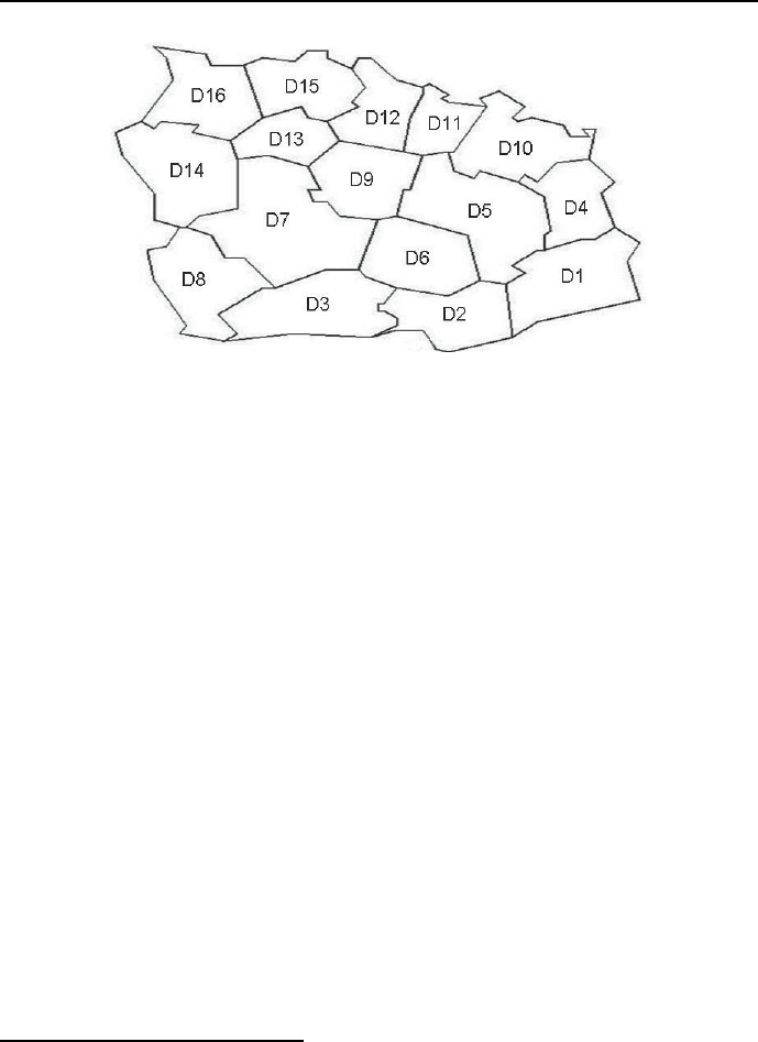
5.7 Optimum assignment problems 295
Figure 5.10: The administrative map of Absurdoland
5.7.7 Map coloring
Let’s try to test the Graph Coloring Theorem (see Sections 2.4.7 and 3.7.4) for
coloring a map.
This has to be done for the administrative map of Absurdoland showing
the country’s division into districts, see Figure 5.10 where districts are denoted
by alphanumeric Di symbols, so that a minimum number of colors is used and
adjacent districts have different colors.
This is done by program 5_22_map_coloring.ecl15:
/*1*/ :- lib(ic).
/*2*/ :- lib(ic_edge_finder3).
/*3*/ :- lib(branch_and_bound).
/*4*/ top:-
/*5*/ Districts = [D1,D2,D3,D4,D5,D6,D7,D8,D9,D10,D11,D12,D13,D14,D15,D16],
/*6*/ Districts :: 1..16,
/*7*/ L :: 1..16,
/*8*/ color([D1,D2,D3,D4,D5,D6,D7,D8,D9,D10,D11,D12,D13,D14,D15,D16]),
/*9*/ maxlist([D1,D2,D3,D4,D5,D6,D7,D8,D9,D10,D11,D12,D13,D14,D15,D16],L),
/*10*/ minimize(labeling([D1,D2,D3,D4,D5,D6,D7,D8,D9,D10,D11,D12,D13,D14,
D15,D16]),L),nl,nl,
/*11*/ write("Minimum number of colors = "),write(L),nl,
15 This is an OS-type problem.

296 Chapter 5. CLP with elementary constraints for optimal solutions
/*12*/ write("Districts = "),write("D1,D2,D3,D4,D5,D6,D7,D8,D9,D10,
D11,D12,D13,D14,D15,D16"),nl,
/*13*/ write("Colors = "), write(Districts).
/*14*/ color([D1,D2,D3,D4,D5,D6,D7,D8,D9,D10,D11,D12,D13,D14,D15,D16]):-
/*15*/ D1 #\= D4, /*16*/ D1 #\= D5,
/*17*/ D1 #\= D2, /*18*/ D2 #\= D5,
/*19*/ D2 #\= D6, /*20*/ D2 #\= D3,
/*21*/ D3 #\= D6, /*22*/ D3 #\= D7,
/*23*/ D3 #\= D8, /*24*/ D4 #\= D10,
/*25*/ D4 #\= D5, /*26*/ D5 #\= D10,
/*27*/ D5 #\= D11, /*28*/ D5 #\= D9,
/*29*/ D5 #\= D6, /*30*/ D6 #\= D9,
/*31*/ D6 #\= D7, /*32*/ D7 #\= D9,
/*33*/ D7 #\= D13, /*34*/ D7 #\= D14,
/*35*/ D7 #\= D8, /*36*/ D8 #\= D14,
/*37*/ D9 #\= D11, /*38*/ D9 #\= D12,
/*39*/ D9 #\= D13, /*40*/ D10 #\= D11,
/*41*/ D11 #\= D12, /*42*/ D12 #\= D15,
/*43*/ D12 #\= D13, /*44*/ D13 #\= D15,
/*45*/ D13 #\= D16, /*46*/ D13 #\= D14,
/*47*/ D14 #\= D16, /*48*/ D15 #\= D16,
/*49*/ D14 #\= D8.
The solution is given by:
Found a solution with cost 4
Found no solution with cost 1.0 .. 3.0
Minimum number of colors = 4
Districts = D1,D2,D3,D4,D5,D6,D7,D8,D9,D10,D11,D12,D13,D14,D15,D16
Colours = [1, 2, 1, 2, 3, 4, 2, 3, 1, 1, 2, 3, 4, 1, 1, 2]
The outcome is difficult to understand. It means e.g. that the district D1
(which corresponds on the list of districts to the first integer 1) is of different
color than the district D2 (which corresponds on the list of districts to the first
integer 2). If the following coloring code is assumed:
1 = pink 2 = yellow
3 = white 4 = blue-green,
then the map looks as shown in Figure 5.11.
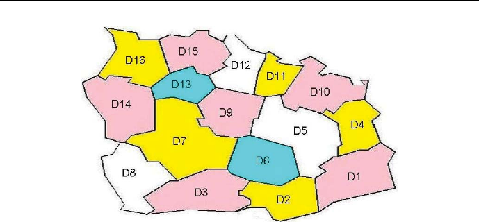
5.7 Optimum assignment problems 297
Figure 5.11: Coloring the administrative map of Absurdoland
5.7.8 Fighting for rainfall justice
Another problem of set representations consists in finding such set of elements
from other sets that minimizes the cost of elements included. The problem sim-
plest formulation is an OR formulation, corresponding in fact to the canonical
form of integer programming problems. This is best illustrated by the following
example:
The World Organization for Total Justice considers the struggle with unequal
rainfalls as one of its basic missions. Rainfall diversity is - as viewed by the Or-
ganization - a basic injustice towards Mother Earth and its inhabitants, because
to it may eventually be traced all other forms of injustice. However, the Orga-
nizations accomplishments on this particular field are - considering 15 years of
activity - rather modest. The reason for this was rightly attributed to the lack
of funds, the scarcity of which enabled only the most primitive forms of rainfall
justice restoration, like rain pipelines transporting rainwater from regions of its
abundance to those of its scarcity. Only after the World Government introduced
a Common Rain Tax paid by all countries, those with heavy rainfalls as well as
those with no rainfalls at all, a fundamental restructuring of the struggle with
rainfall diversity could be accomplished. In particular it was deemed necessary
to establish the following Rain Agencies:1)International Rain Fund, collecting
taxes and donations and financing projects, 2)Airborne Rain Flotilla, consist-
ing of Rainfall Causing Airplanes and Rainfall Stopping Airplanes,3)Rainfall
Satellite Monitoring,4)Local Air Ionizers to provoke intensive rainfalls, 5)Rain

298 Chapter 5. CLP with elementary constraints for optimal solutions
Education Agency, to coordinate rain education at all levels, starting with ju-
nior classes on Rainfall Justice, through senior classes on Rain Management,
up to chains of Educational and Correctional Institutions (to convince and win
over the most ardent opponents of rainfall justice), 6)Rain Lobbying Agency to
encourage the leaders of nations to contribute additionally to rain funds as well
as supporting groups of Rainpeace activists, 7)World Rain Institute, to manage
and finance rain research, to provide Young Researcher Rain Grants and to
organize Scientific Rain Summits on selected football stadiums.
Obviously, to successfully implement such broad range of complicated ac-
tions, highly qualified experts are needed. Luckily, three world-reputable rain
activists, Professor Hoaxman, Professor Luftmensch and Colonel Baron Fraud
of Bluffbury - have been blessed with a progeny that from their earliest days,
while listening to discussions at the Family Tables, had acquired such deep
knowledge and understanding of rainfall theory and practice, which would be
impossible to get at the best universities. Luckily as well, this progeny is - for
different reasons - busily looking for new jobs:
So the two daughters of the Colonel Baron had to vacate the posts of vice-
chairwoman of the Silly Initiative Monetary Fund. The elderly - it turned out
- did not quite understood the meaning of percentages, thereby causing huge
financial losses16, the younger one had problems with grasping the difference
between European and Anglo-American billions, causing a number of quite em-
barrassing and costly blunders17.
Professors Hoaxman son, after being dismissed from a Sport Academy, was
employed as caddy by an exclusive Golf Club. There, listening for some time to
the palaver of playing bank officials, it occurred to him rightly that he would
surely be successful in this profession. Hence he started dreaming about asser-
ting himself in some banking business.
The young Luftmensch in his wildest dreams envisaged himself in uniforms,
of course some elegant ones, dark blue or white, with golden braids and multi-
colored ribbons, and of course with the inseparable personal power and adoring
girls all around. In such uniforms he could well manage the Rain Flotilla, e.g.
using the white uniform to command the Rainfall Stopping Planes,andthe
blue uniform to command the Rainfall Causing Planes. Strongly believing that
16 The dear one should not be blamed: she could not take - because of acute drug-and-booze
poisoning - Home Math classes on percentages at her beloved Quick Results College.
17 This should really be excused because the poor girl - while studying at the renowned
Quick Results College - could not attend Home Math classes on large numbers; this was due
to the urgent need to get rid of the fruit of some exciting night spend with somebody she
can’t remember.
5.7 Optimum assignment problems 299
hard work never hurt anybody, he aspired to simultaneously commanding the
Educational and Correctional Institutions. Unfortunately, because of advanced
emotional instability, his application to the Famous Military Academy has been
rejected.
Now, all four of them saw their chance. Following their daddies advice, they
submitted applications to organize and run rain agencies. Their applications
were quite laconic, containing just the names of agencies and the expected salary
in billions of MU; after all the names speak for themselves. All applicants, on
the wave of drug-and-booze generated enthusiasm, declared the praiseworthy
willingness to organize and run more than one agency. However, the daddies did
not harmonize their applications, so there was some overlap: the same agencies
were considered worthwhile for more than one applicant, as can be seen from
Table 5.9.
Applicants
Agenda Hoaxman Luftmensch Older Ms Younger Ms
Jr Jr Bluffbury Bluffbury
Int. Rain Fund × ×
Rain Flotilla × ×
Satellite Monitoring × ×
Air Ionizers × ×
Education × ×
Lobbing × ×
Rain Research × ×
Salaries 65512
(MM MU)
Table 5.4: Proposals to organize and run Rain Agencies
The Illuminati Management of the Organization did not mind this overlap,
because - like any other management - it liked nothing so much as resolving
competence conflicts among their subordinates; if there are no conflicts, the
pleasure to resolve them is obviously lost. However, to keep appearances of
competitiveness, it was decided that the least expensive applications will be
accepted. For this end the program 5_23_rainfall_justice_OR.ecl18 may
be useful:
18 This is an OS-type problem.

300 Chapter 5. CLP with elementary constraints for optimal solutions
/*1*/ :-lib(ic).
/*2*/ :-lib(branch_and_bound).
/*3*/ top :-
% Xj = 1 - the application of candidate j has been accepted.
% Xj = 0 - the application of candidate j has been rejected.
/*4*/ Variables=[X1,X2,X3,X4],
/*5*/ Variables :: 0..1,
/*6*/ X1 + X4 #>= 1,
/*7*/ X2 + X3 #>= 1,
/*8*/ X3 + X4 #>= 1,
/*9*/ X2 + X4 #>= 1,
/*10*/ X3 + X4 #>= 1,
/*11*/ X1 + X4 #>= 1,
/*12*/ X1 + X2 #>= 1,
/*13*/ Cost #= 6*X1 + 5*X2 + 5*X3 + 12*X4,
/*14*/ minimize(search(Variables,0,first_fail,indomain,
complete,[]),Cost),
/*15*/ writeln("Variables":Variables ),
/*16*/ writeln("Cost":Cost).
The message is:
Found a solution with cost 17
Found a solution with cost 16
Found no solution with cost 0.0 .. 15.0
Variables : [1, 1, 1, 0]
Cost : 16
Luckily only one application (of younger Ms Bluffbury) has been rejected.
Notice the discrepancy between the length of the story and the shortness
of the program. Well, there is no iunctim between the length of a story (i.e.
between the complex circumstances giving raise to the problem) and the length
of its program: sometimes to explain the background knowledge of some simple
integer programming programs, a lot of things needs to be presented.
5.7.9 Send Most Money
For the popular puzzle Send More Money (see Section 4.4.1) an optimization
version known as Send Most Money may be found, see Kjellerstrand’s website
[Kjellerstrand-13], which aims at maximizing the value of Money.Itisgivenby

5.7 Optimum assignment problems 301
program 5_24_smm.ecl19 :
/*1*/ :-lib(ic).
/*2*/ :-lib(branch_and_bound).
/*3*/ top :-
% 1) Finding a single solution that maximizes MONEY:
% a)A list LD with 8 variables is created. The variables
% correspond to the eight letters in "Send Most Money":
/*4*/ length(LD, 8),
% b)The domain of LD must include all single-position digits,
% because it is not known, which of them will be finally needed:
/*5*/ LD :: 0..9,
% c)This is the main constraint:
/*6*/ send_most_money(LD, MONEY),
% Maximization is needed, but only the built-in minimize/2
% is available, so negative MONEY is to be minimized:
/*7*/ MONEY_NEGATIVE #= -MONEY,
/*8*/ writeln("Determining a single solution for maximum value of MONEY:"),
/*9*/ minimize(search(LD,0,first_fail,indomain,complete,[]),MONEY_NEGATIVE),
/*10*/ writeln([MONEY, LD]),
% 2) Determining all solutions for maximum value of MONEY:
/*11*/ length(LD2, 8),
/*12*/ LD2 :: 0..9,
/*13*/ findall(LD2, (send_most_money(LD2, MONEY),
labeling(LD2)), Everything),
/*14*/ length(Everything, Length),
/*15*/ printf("%d solutions for the maximum value of MONEY = %d:\n",
[Length, MONEY]),
/*16*/ writeln("[S, E, N, D, M, O, T, Y]"),
/*17*/ write_list(Everything).
/*18*/ send_most_money([S,E,N,D,M,O,T,Y], MONEY) :-
/*19*/ MONEY #= 10000 * M + 1000 * O + 100 * N + 10 * E + Y,
/*20*/ alldifferent([S,E,N,D,M,O,T,Y]),
/*21*/ M #\= 0,
/*22*/ S #\= 0,
/*23*/ 1000 * S + 100 * E + 10 * N + D +
1000 * M + 100 * O + 10 * S + T #= MONEY.
/*24*/ write_list(Everything):-
/*25*/ member(L,Everything),
/*26*/ writeln(L),
/*27*/ fail.
/*28*/ write_list([]).
19 This is an OS-type problem.

302 Chapter 5. CLP with elementary constraints for optimal solutions
The message is:
Determining a single solution for maximum value of MONEY:
Found a solution with cost -10437
Found a solution with cost -10438
Found a solution with cost -10548
Found a solution with cost -10657
Found a solution with cost -10765
Found a solution with cost -10768
Found a solution with cost -10875
Found a solution with cost -10876
Found no solution with cost -10878.0 .. -10877.0
[10876, [9, 7, 8, 2, 1, 0, 4, 6]]
2 solutions for the maximum value of MONEY = 10876:
[S, E, N, D, M, O, T, Y]
[9, 7, 8, 2, 1, 0, 4, 6]
[9, 7, 8, 4, 1, 0, 2, 6]
The nesting of labeling(LD2) into the findall built-in in line /*13*/ for the
purpose of finding all optimum solutions is worth noticing. It may also be
applied to other optimum-seeking problems.
5.8 Advanced optimum assignment problems
5.8.1 Warehouse location problem - OR
The basic classical warehouse location problem (WLP) can be formulated as
follows: given a number of customers and a number of warehouse locations,
which warehouses should be build in order to minimize the costs of building the
warehouses and delivering the demanded goods to the customers20. Finding the
optimum location for warehouses is of crucial importance from investors’ point
of view. Therefore many variants of this problem have been solved in OR. Let’s
start with a rather simple WLP: There are 3 potential locations for warehouses
serving 5 customers. The building costs and delivery costs are presented by
Table 5.5. The solution is given by program 5_25_warehouses_OR.ecl21:
20 A CLP approach to this problem has been first presented in [van Hentenryck-89].
21 This is an OS-type problem.
5.8 Advanced optimum assignment problems 303
Customer Warehouse
1 2 3
1 5 7 20
2 4 20 1
320 2 5
420 20 4
5 3 20 8
Building cost 18 20 28
Table 5.5: Delivery and building costs for 3 warehouses and 5 customers
/*1*/ :- lib(ic).
/*2*/ :- lib(branch_and_bound).
/*3*/ top:-
/*4*/ warehouses(_,_).
/*5*/ warehouses(Z,Cost):-
% Wj = 1 - warehouse j is built
% Wj = 0 - warehouse j is not built
% Tij = 1 - customer i is serviced by warehouse j
% Tij = 0 - customer i is not serviced by warehouse j
/*6*/ Z=[W1,W2,W3,T11,T12,T13,T21,T22,T23,T31,T32,T33,T41,T42,T43,T51,T52,T53],
/*7*/ Z::0..1,
/*8*/ T11 + T12 + T13 #= 1, % customer 1 is serviced just by one warehouse
/*9*/ T21 + T22 + T23 #= 1, % customer 2 is serviced just by one warehouse
/*10*/ T31 + T32 + T33 #= 1, % customer 3 is serviced just by one warehouse
/*11*/ T41 + T42 + T43 #= 1, % customer 4 is serviced just by one warehouse
/*12*/ T51 + T52 + T53 #= 1, % customer 5 is serviced just by one warehouse
/*13*/ T11 #=< W1, % if warehouse 1 is built, it may service customer 1
/*14*/ T21 #=< W1, % if warehouse 1 is built, it may service customer 2
/*15*/ T31 #=< W1, % if warehouse 1 is built, it may service customer 3
/*16*/ T41 #=< W1, % if warehouse 1 is built, it may service customer 4
/*17*/ T51 #=< W1, % if warehouse 1 is built, it may service customer 5
/*18*/ T12 #=< W2, % if warehouse 2 is built, it may service customer 1
/*19*/ T22 #=< W2, % if warehouse 2 is built, it may service customer 2
/*20*/ T32 #=< W2, % if warehouse 2 is built, it may service customer 3
/*21*/ T42 #=< W2, % if warehouse 2 is built, it may service customer 4
/*22*/ T52 #=< W2, % if warehouse 2 is built, it may service customer 5
/*23*/ T13 #=< W3, % if warehouse 3 is built, it may service customer 1
/*24*/ T23 #=< W3, % if warehouse 3 is built, it may service customer 2

304 Chapter 5. CLP with elementary constraints for optimal solutions
/*25*/ T33 #=< W3, % if warehouse 3 is built, it may service customer 3
/*26*/ T43 #=< W3, % if warehouse 3 is built, it may service customer 4
/*27*/ T53 #=< W3, % if warehouse 3 is built, it may service customer 5
/*28*/ Cost #= 18*W1+10*W2+28*W3+5*T11+7*T12+100*T13+4*T21+100*T22+1*T23+
100*T31+2*T32+5*T33+100*T41+100*T42 +4*T43+3*T51+100*T52+8*T53 ,
/*29*/ bb_min(labeling([W1,W2,W3,T11,T12,T13,T21,T22,T23,T31,T32,T33,
T41,T42,T43,T51,T52,T53]),Cost, bb_options{strategy:restart}), nl,
/*30*/ write("List of warehouses: "),writeln([W1,W2,W3]),nl,
/*31*/ write("List of customers and warehouses:"),nl,
/*32*/ writeln("[T11,T12,T13,T21,T22,T23,T31,T32,T33,T41,T42,T43,T51,T52,T53]"),
/*32*/ writeln([T11,T12,T13,T21,T22,T23,T31,T32,T33,T41,T42,T43,T51,T52,T53]),
/*33*/ write("Cost: "),writeln(Cost),nl.
The message is:
Found a solution with cost 66
Found a solution with cost 64
Found no solution with cost 0.0 .. 63.0
List of warehouses: [1, 0, 1]
List of customers and warehouses:
[T11,T12,T13,T21,T22,T23,T31,T32,T33,T41,T42,T43,T51,T52,T53]
[1, 0, 0, 0, 0, 1, 0, 0, 1, 0, 0, 1, 1, 0, 0]
Cost: 64
The meaning of the list of customers and warehouses is as follows:
T11 = 1, i.e. customer 1 is served from warehouse 1;
T23 = 1, i.e. customer 2 is served from warehouse 3;
T33 = 1, i.e. customer 3 is served from warehouse 3;
T43 = 1, i.e. customer 4 is served from warehouse 3;
T51 = 1, i.e. customer 5 is served from warehouse 1;
5.8.2 Warehouse location problem 1 CLP
The warehouse location problem may be solved using a number of different
CLP approaches. A CLP version using data from Table 5.5 is given by program

5.8 Advanced optimum assignment problems 305
5_26_warehouses_CLP_1.ecl22:
/*1*/ :- lib(ic).
/*2*/ :- lib(branch_and_bound).
%op(Precedence, +Associativity, ++Name)+
/*3*/ :- op(960, fx, if).
/*4*/ :- op(950,xfx, then).
/*5*/ top:-
/*6*/ warehouses(_,_,_).
/*7*/ warehouses(Ws,Cs,Cost):-
/*8*/ Ws=[W1,W2,W3],
% if Wi=0, warehouse "i" is not build
% if Wi=1, warehouse "i" is build
/*9*/ Ws::0..1,
/*10*/ Cs=[C1,C2,C3,C4,C5],
/*11*/ Cs::1..3,
% Cj - number of warehouse serving the "j"-th customer
/*12*/ element(C1,[5,7,20],Cost_1),
/*13*/ element(C2,[4,20,1],Cost_2),
/*14*/ element(C3,[20,2,5],Cost_3),
/*15*/ element(C4,[20,20,4],Cost_4),
/*16*/ element(C5,[3, 20,8],Cost_5),
% if warehouse "i" is not established, it won’t appear in list Cs:
/*17*/ if (W1 #= 0) then outof(Cs,1),
/*18*/ if (W2 #= 0) then outof(Cs,2),
/*19*/ if (W3 #= 0) then outof(Cs,3),
/*20*/ Cost #= 18*W1+20*W2+28*W3+Cost_1+Cost_2+Cost_3+Cost_4+Cost_5,
/*21*/ bb_min((labeling(Ws),labeling(Cs)),Cost,
bb_options{strategy:restart}),
/*22*/ write(" List of warehouses: "),
writeln([W1,W2,W3]),
/*23*/ write(" List of customers and warehouses: "),
writeln([C1,C2,C3,C4,C5]),
/*24*/ write(" Cost: "),
writeln(Cost).
/*25*/ outof([],_).
/*26*/ outof([K|Ks],N):-
22 This is an OS-type problem.

306 Chapter 5. CLP with elementary constraints for optimal solutions
/*27*/ K #\= N,
/*28*/ outof(Ks,N).
/*29*/ if Cond then Goal :-
/*30*/ Cond =.. CList,
/*31*/ append(CList, [Bool], RList),
/*32*/ Reified =.. RList,
/*33*/ call(Reified),
/*34*/ call_if(Goal, Bool).
/*35*/ delay call_if(_Goal, Bool) if var(Bool).
/*36*/ call_if(_Goal, 0).
/*37*/ call_if(Goal, 1) :-
/*38*/ call(Goal).
The message is:
Found a solution with cost 66
Found a solution with cost 64
Found no solution with cost 15.0 .. 63.0
List of warehouses: [1, 0, 1]
List of customers and warehouses: [1, 3, 3, 3, 1]
Cost: 64
The meaning of the list of customers and warehouses ([1, 3, 3, 3, 1])isas
follows:
-customer1is served from warehouse 1,
- customers verb”2”, 3and 4are served from warehouse 3,
-customer5is served from warehouse 1. The meaning of the list of warehouses
([1, 0, 1]) is as follows:
only warehouses 1and 3will be established.
The use of following built-ins deserves some comments:
•?Term =.. ?List succeeds if List is the list, which has the name of pred-
icate Term as its first element and the predicates arguments, if any, as its
successive elements. E.g.:
Term =.. [likes,"John",play].
gives
Term = likes("John",play),
and:

5.8 Advanced optimum assignment problems 307
s([1,4,5,6]) =.. List.
gives
List = [s,[1,4,5,6]].
•call(+Goal) succeeds if Goal succeeds: it calls the goal Goal. This built-
in is used to call goals that are grounded only at the time they are called.
For lines /*35*/,..,/*38*/ wait until Bool is grounded, then call Goal,
or simply succeed.
•op(960, fx, if) and op(950,xfx, then) mean that the ”then”part
from lines */17*/,*/18*/ and */19*/ is evaluated after the ”if”part
was, see Section 2.1.4.
As before, the number of variables needed to model the warehouse location
problem OR-wise is decisively larger than the number needed to model it CLP-
wise.
5.8.3 Warehouse location problem 2 CLP
The program 5_26_warehouses_CLP_1.ecl discussed so far has weak propa-
gation properties23, which is due to multiple callings of the element/3 built-
in. The next program 5_27_warehouses_CLP_2.ecl, which is a slightly mod-
ified version of the Warehouse location program authored by J. Schimpfa (see
[Schimpf-10]), has better propagation properties . It uses a heuristic which or-
ders - for each client - warehouses according the the rising delivery cost. This
is illustrated for a more complicated problem given by table 5.6:
As before we would like to know, which warehouses should be built, and for
which customers, in order to minimize the overall delivery and building cost.
The program 5_26_warehouses_CLP_1 discussed before has rather poor
propagation properties, mainly due to the multiple use of the element/3 built-
in. As result, to solve more complicated problems takes long times. The next
program 5_27_warehouses__CLP_2.ecl24, which is a slightly modified version
of the Warehouse location program by Schimpf (see [Schimpf-10]), is much bet-
ter. It is based on a following heuristic: for each customer the warehouses have
to be ordered according to rising delivery costs. The program is as follows:
23 This mean slow convergence for larger problems.
24 This is an OS-type problem.
308 Chapter 5. CLP with elementary constraints for optimal solutions
Customers Warehouses
1 2 3 4
1 5 7 1 20
214 8100 300
3 2 20 50 12
4110 2200 5
5300 300 8200
6 3 100 8 5
730 40 20 80
8230 50 70 8
920 350 70 98
10 30 450 370 250
Building cost 18 10 28 20
Table 5.6: Delivery and building costs for 4 warehouses and 10 customers
/*1*/ :- lib(ic).
/*2*/ :- lib(ic_sets).
/*3*/ :- lib(branch_and_bound).
/*4*/ top:-
% declare the data:
/*5*/ building_cost_array(BuildingCostArray),
/*6*/ delivery_cost_array(DeliveryCostArray),
/*7*/ dim(DeliveryCostArray,[NumberOfClients,NumberOfHouses]),
/*8*/ dim(BuildingCostArray,[NumberOfHouses]),
% declare constraints:
/*9*/ intset(ListOfBuildHouses,1,NumberOfHouses),
/*10*/ (
/*11*/ for(ClientsId, 1, NumberOfClients),
/*12*/ foreach(NumberOfHouseForClient,HousesForClients),
/*13*/ foreach(DeliveryCostForClient,ListOfDeliveryCostsForClients),
/*14*/ param(ListOfBuildHouses,DeliveryCostArray,NumberOfHouses)
/*15*/ do
/*16*/ ListOfDeliveryCosts is
DeliveryCostArray[ClientsId,1..NumberOfHouses],
/*17*/ element(NumberOfHouseForClient,ListOfDeliveryCosts,DeliveryCostForClient),
/*18*/ NumberOfHouseForClient in ListOfBuildHouses
/*19*/ ),
/*20*/ weight(ListOfBuildHouses,BuildingCostArray,BuildingCost),
% objective function:
/*21*/ OverallCost #= BuildingCost + sum(ListOfDeliveryCostsForClients),

5.8 Advanced optimum assignment problems 309
% search and propagation:
/*22*/sort_houses(DeliveryCostArray,SortedListsOfHousesForClients),
/*23*/ minimize(
/*24*/ (
/*25*/ insetdomain(ListOfBuildHouses, increasing, _, _),
/*26*/ labeling(HousesForClients,SortedListsOfHousesForClients),
% displaying intermediate results:
/*27*/ write("List of constructed warehouses = "),
writeln(ListOfBuildHouses),
/*28*/ write("Warehouses associated to clients = "),
writeln(HousesForClients),
/*29*/ write("List of delivery costs for clients = "),
writeln(ListOfDeliveryCostsForClients)
/*30*/ ),
/*31*/ OverallCost),nl,
% displaying final results:
/*32*/ write("List of built warehouses = "),writeln(ListOfBuildHouses),
/*33*/ write("Warehouses associated with clients = "),
writeln(HousesForClients),
/*34*/ write("Sorted lists of warehouses for clients = "),
writeln(SortedListsOfHousesForClients),
/*35*/ write("List of delivery costs for clients = "),
writeln(ListOfDeliveryCostsForClients),
/*36*/ write("Overall cost: "),writeln(OverallCost).
% heuristics: sort warehouses for all clients in order of increasing delivery cost:
/*37*/ sort_houses(DeliveryCostArray,SortedListsOfHousesForClients) :-
/*38*/ dim(DeliveryCostArray,[NumberOfClients,NumberOfHouses]),
/*39*/ ( for(I,1,NumberOfHouses),
/*40*/ foreach(I,ListOfHouseId)
/*41*/ do
/*42*/ true
/*43*/ ),
/*44*/ (
/*45*/ for(ClientsId, 1, NumberOfClients),
/*46*/ foreach(SortedListOfHousesForClient,SortedListsOfHousesForClients),
/*47*/ param(DeliveryCostArray,NumberOfHouses,ListOfHouseId)
/*48*/ do
/*49*/ DeliveryCosts is DeliveryCostArray[ClientsId,1..NumberOfHouses],
/*50*/ sorting(DeliveryCosts,ListOfHouseId,SortedListOfHousesForClient)
/*51*/ ).
% bounding variables "HousesForClients"
% according to the heuristic
/*52*/ labeling(HousesForClients,SortedListsOfHousesForClients) :-

310 Chapter 5. CLP with elementary constraints for optimal solutions
/*53*/ (
/*54*/ foreach(NumberOfHouseForClient,HousesForClients),
/*55*/ foreach(SortedListOfHousesForClient,SortedListsOfHousesForClients)
/*56*/ do
/*57*/ member(NumberOfHouseForClient,SortedListOfHousesForClient)
/*58*/ ).
% intermediate constraint: sorting heuristic
/*59*/ sorting(Keys, Values, SortedValues):-
/*60*/ (foreach(K,Keys),
/*61*/ foreach(W,Values),
/*62*/ foreach(K-W,KeyValues)
/*63*/ do
/*64*/ true),
/*65*/ keysort(KeyValues, SortedKeyValues),
/*66*/ (foreach(W,SortedValues),
/*67*/ foreach(_K-W,SortedKeyValues)
/*68*/ do
/*69*/ true).
/*70*/ delivery_cost_array([](
/*71*/ [](5,7,1,20),
/*72*/ [](14,8,100,300),
/*73*/ [](2,20,50,12),
/*74*/ [](110,2,200,5),
/*75*/ [](300,300,8,200),
/*76*/ [](3,100,8,5),
/*77*/ [](30,40,20,80),
/*78*/ [](230,50,70,8),
/*79*/ [](20,350,70,98),
/*80*/ [](30,450,370,250)
/*81*/ )).
/*81*/ building_cost_array([](18,10,28,20)).
The message is:
List of built warehouses = [1]
Warehouses associated to clients = [1,1,1,1,1,1,1,1,1,1]
List of delivery costs for clients = [5,14,2,110,300,3,30,230,20,30]
Found a solution with cost 762
List of built warehouses = [1, 2]
Warehouses associated to clients = [1,2,1,2,1,1,1,2,1,1]
List of delivery costs for clients = [5,8,2,2,300,3,30,50,20,30]
Found a solution with cost 478
List of built warehouses = [1, 3]

5.8 Advanced optimum assignment problems 311
Warehouses associated to clients = [3,1,1,1,3,1,3,3,1,1]
List of delivery costs for clients = [1,14,2,110,8,3,20,70,20,30]
Found a solution with cost 324
List of built warehouses = [1,2,3]
Warehouses associated to clients = [3,2,1,2,3,1,3,2,1,1]
List of delivery costs for clients = [1,8,2,2,8,3,20,50,20,30]
Found a solution with cost 200
List of built warehouses = [1,3,4]
Warehouses associated to clients = [3,1,1,4,3,1,3,4,1,1]
List of delivery costs for clients = [1,14,2,5,8,3,20,8,20,30]
Found a solution with cost 177
Found no solution with cost 102.0 .. 176.0
List of built warehouses = [1, 3, 4]
Warehouses associated to clients = [3,1,1,4,3,1,3,4,1,1]
Sorted lists of warehouses for clients =
[[3,1,2,4],[2,1,3,4],[1,4,2,3],[2,4,1,3],[3,4,1,2],
[1,4,3,2],[3,1,2,4],[4,2,3,1],[1,3,4,2],[1,4,3,2]]
List of delivery costs for clients = [1,14,2,5,8,3,20,8,20,30]
Overall cost: 177
5.8.4 Warehouse location problem 3 CLP
An efficient program comparable to the one from Section 5.8.3 may also be
designed by not using sets but using the built-in fromto/4. Thisisdemonstrated
by example 5_28_warehouses_CLP_3.ecl25, where the following variables have
been used:
•ListOfClientHouses - list of variables corresponding to warehouse num-
bers associated with consecutive customers, e.g. ListOfClientHouses =
[3, 1, 1, 4, 3, 1, 3, 4, 1, 1] means that customer 5will be served
by warehouse 3.
•ListOfHousesBuild - list of variables denoting warehouses that will be
build. E.g. ListOfHousesBuild = [1,0,1, 1] means that warehouse 2
is not going to be build.
•DeliveryCostArray - one-dimensional array of delivery costs for consec-
utive clients.
25 This program has been proposed by Lukasz Domagala.

312 Chapter 5. CLP with elementary constraints for optimal solutions
•BuildingCostList - list of building costs for consecutive warehouses.
•OverallCost - the sum of building costs and delivery costs.
Program 5_28_warehouses_3.ecl26 is:
/*1*/ :-lib(ic).
/*2*/ :-lib(ic_global).
/*3*/ :-lib(branch_and_bound).
/*4*/ top:-
/*5*/ declare_data(DeliveryCostArray,BuildingCostList),
/*6*/ constrain(ListOfClientHouses,
ListOfHousesBuild,DeliveryCostArray,
BuildingCostList,OverallCost),
/*7*/ find_optimum_solution(ListOfClientHouses,
OverallCost),
/*8*/ display_results(ListOfClientHouses,
ListOfHousesBuild,OverallCost).
/*9*/ declare_data(DeliveryCostArray,BuildingCostList):-
/*10*/ DeliveryCostArray=[](
/* H1 H2 H3 H4 */
/*11*/ /* K1 */ [5 ,7 ,1 ,20 ],
/*12*/ /* K2 */ [14 ,8 ,100,300],
/*13*/ /* K3 */ [2 ,20 ,50 ,12 ],
/*14*/ /* K4 */ [110,2 ,200,5 ],
/*15*/ /* K5 */ [300,300,8 ,200],
/*16*/ /* K6 */ [3 ,100,8 ,5 ],
/*17*/ /* K7 */ [30 ,40 ,20 ,80],
/*18*/ /* K8 */ [230,50 ,70 ,8 ],
/*19*/ /* K9 */ [20 ,350,70 ,98 ],
/*20*/ /* K10*/ [30 ,450,370,250]
/*21*/ ),
/*22*/ BuildingCostList=[18,10,28,20].
/*23*/ constrain(ListOfClientHouses,
ListOfHousesBuild,DeliveryCostArray,
BuildingCostList,OverallCost):-
/*24*/ dim(DeliveryCostArray,[NumberOfClients]),
/*25*/ length(BuildingCostList,MaxNumberOfHouses),
% Knowing "NumberOfClients" the unbounded
% "ListOfClientHouses" is created:
/*26*/ length(ListOfClientHouses,NumberOfClients),
% Its domain includes all warehouses under consideration
/*27*/ ListOfClientHouses#::[1..MaxNumberOfHouses],
26 This is an OS-type problem.

5.8 Advanced optimum assignment problems 313
% Warehous building costs:
/*28*/ (foreach(HouseBuildingCost,BuildingCostList),
/*29*/ foreach(HouseBuild,ListOfHousesBuild),
/*30*/ fromto(ListOfCosts,[
HouseBuildingCostOr0|ListOfCostsOut],
ListOfCostsOut,ListOfCostsForClient),
/*31*/ count(HouseId,1,MaxNumberOfHouses),
/*32*/ param(ListOfClientHouses)
/*33*/ do
% Number of clients for warehouse number HouseId:
/*34*/ occurrences(HouseId, ListOfClientHouses,
NumberOfClientsForHouseiNr),
/*35*/ #>(NumberOfClientsForHouseiNr,0,HouseBuild),
/*36*/ HouseBuildingCostOr0#=
HouseBuild * HouseBuildingCost
/*37*/ ),
% Warehous delivery costs:
/*38*/ (foreach(ClientsHouse,ListOfClientHouses),
/*39*/ foreacharg(ListOfDeliveryCosts,DeliveryCostArray),
/*40*/ foreach(CostForClient,ListOfCostsForClient)
/*41*/ do
/*42*/ element(ClientsHouse,ListOfDeliveryCosts,CostForClient)
/*43*/ ),
% Overall cost determination:
/*44*/ sumlist(ListOfCosts, OverallCost).
/*45*/ find_optimum_solution(ListOfClientHouses,OverallCost):-
/*46*/ BBOptions=bb_options{strategy:continue, from:0},
/*47*/ bb_min(labeling(ListOfClientHouses),OverallCost,BBOptions).
/*48*/ display_results(ListOfClientHouses,ListOfHousesBuild,OverallCost):-
/*49*/ write("Overall Cost = "),write(OverallCost),nl,
/*50*/ write("List of built warehouses = "),write(ListOfHousesBuild),nl,
/*51*/ write("Warehouses associated with clients = "),write(ListOfClientHouses),nl.
The message is:
Found a solution with cost 762
Found a solution with cost 592
Found a solution with cost 560
Found a solution with cost 498
Found a solution with cost 328
Found a solution with cost 296
314 Chapter 5. CLP with elementary constraints for optimal solutions
Found a solution with cost 286
Found a solution with cost 220
Found a solution with cost 198
Found a solution with cost 188
Found a solution with cost 181
Found a solution with cost 177
Found no solution with cost 102.0 .. 176.0
Overall Cost=177
List warehouses to be built:[1,0,1,1]
Warehouses associated with clients:[3,1,1,4,3,1,3,4,1,1]
5.8.5 Real-valued objective functions
For real-valued objective functions, even if the decision variables are integers,
branch-and-bound is not delivering: we have to resort to eplex. This is illus-
trated by the following example:
In order to promote tolerance and fight discrimination, the Absurdoland’s Min-
istry of National Brainwashing, after analyzing a number of public surveys, has
ordered that the enrollment to any High School in Absurdoland must be at least
10% gay or lesbian. As a result of this, the Happy Town School Authorities are
facing a following problem: there are five High School Districts with numbers of
straight and gay/lesbian students as shown by Table 5.7, and two High Schools
(HS), with mean distances from the districts shown by the same Table.
District Straight Gay/lesbian Distance to HS 1 Distance to HS 2
180 15 3 6
270 13 11.5
390 8 2 0.8
450 20 2.6 1.8
560 15 31.2
Table 5.7: Happy Town student population and traveling distances
The School Board policy requires all students from a given district attend
the same High School. Assuming that each High School must have an enroll-
ment of at least 130 students, write a program that will minimize the mean total
distance student must travel to High Schools while respecting the enrollment
restrictions.

5.8 Advanced optimum assignment problems 315
Introducing the following notation:
Di_HS1 = 1 students from district i travel to HS1
Di_HS2 = 1 students from district i travel to HS2 Di_HS1 = 0 students from
district i do not travel to HS1 Di_HS2 = 0 students from district i do not travel
to HS2 it is possible to formulate the balances:
1) Balance of all students enrolled in HS1:
D1_HS1 * 80 + D2_HS1 * 70 + D3_HS1 * 90 + D4_HS1 * 50+
D5_HS1 * 60 >= 130
2) Balance of all students enrolled in HS2:
D1_HS2 * 80 + D2_HS2 * 70 + D3_HS2 * 90 + D4_HS2 * 50+
D5_HS2 * 60 >= 130
3) Balance of gay/lesbian students enrolled in HS1:
D1_HS1 * 15 + D2_HS1 * 13 + D3_HS1 * 8 + D4_HS1 * 20 +
D5_HS1 * 15 >= 0.1 *(D1_HS1 * 80 + D2_HS1 * 70 + D3_HS1 * 90 +
D4_HS1 * 50+ D5_HS1 * 60)
4) Balance of gay/lesbian students enrolled in HS2:
D1_HS2 * 15 + D2_HS2 * 13 + D3_HS2 * 8 + D4_HS2 * 20 +
D5_HS2 * 15 >= 0.1 *(D1_HS2 * 80 + D2_HS2 * 70 + D3_HS2 * 90 +
D4_HS2 * 50+ D5_HS2 * 60)
The balances 3) and 4) may be put into a more simple form:
3a) D1_HS1*7 + D2_HS1*6 - D3_HS1 + D4_HS1*15 + D5_HS1 *9 >= 0
4a) D1_HS2*7 + D2_HS2*6 - D3_HS2 + D4_HS2*15 + D5_HS2 *9 >= 0
Now we can formulate program 5_29_school_enrollment.ecl for solving this
problem:
/*1*/ :- lib(eplex).
/*2*/ top:-+
/*3*/ Variables=[D1_HS1,D1_HS2,D2_HS1,D2_HS2,D3_HS1,D3_HS2,
D4_HS1,D4_HS2,D5_HS1,D5_HS2],
/*4*/ Variables $:: 0.0..1.0Inf,
/*5*/ integers(Variables),
/*6*/ D1_HS1 + D1_HS2 $= 1,
/*7*/ D2_HS1 + D2_HS2 $= 1,
/*8*/ D3_HS1 + D3_HS2 $= 1,
/*9*/ D4_HS1 + D4_HS2 $= 1,
/*10*/ D5_HS1 + D5_HS2 $= 1,
/*11*/ D1_HS1*80 + D2_HS1*70 + D3_HS1*90 + D4_HS1*50+ D5_HS1 *60 $>= 130,
/*12*/ D1_HS2*80 + D2_HS2*70 + D3_HS2*90 + D4_HS2*50 + D5_HS2 *60 $>= 130,

316 Chapter 5. CLP with elementary constraints for optimal solutions
/*13*/ D1_HS1*7 + D2_HS1*6 - D3_HS1 + D4_HS1*15 + D5_HS1 *9 $>= 0,
/*14*/ D1_HS2*7 + D2_HS2*6 + - D3_HS2 + D4_HS2*15 + D5_HS2 *9 $>= 0,
/*15*/ Distance $= D1_HS1 * 3 + D1_HS2 * 6 +
D2_HS1 * 1 + D2_HS2 * 1.5 +
D3_HS1 * 2 + D3_HS2 * 0.8 +
D4_HS1 * 2.6 + D4_HS2 * 1.8 +
D5_HS1 * 3 + D5_HS2 * 1.2,
/*16*/ eplex_solver_setup(min(Distance)),
/*17*/ eplex_solve(Distance),
/*18*/ eplex_get(vars,Vars),
/*19*/ eplex_get(typed_solution,Vals),
/*20*/ Vars = Vals,nl,
/*21*/ write(Variables),nl,
/*22*/ (foreach(A,["D1_HS1","D1_HS2","D2_HS1","D2_HS2","D3_HS1","D3_HS2",
"D4_HS1","D4_HS2","D5_HS1","D5_HS2"]),
/*23*/ foreach(X,[D1_HS1,D1_HS2,D2_HS1,D2_HS2,D3_HS1,D3_HS2,
D4_HS1,D4_HS2,D5_HS1,D5_HS2])
/*24*/ do
/*25*/ write(A),write(" = "),write(X),nl).
The solution is:
[1, 0, 1, 0, 0, 1, 0, 1, 0, 1]
D1_HS1 = 1
D1_HS2 = 0
D2_HS1 = 1
D2_HS2 = 0
D3_HS1 = 0
D3_HS2 = 1
D4_HS1 = 0
D4_HS2 = 1
D5_HS1 = 0
D5_HS2 = 1

5.9 Optimum timetabling problems 317
5.9 Optimum timetabling problems
Timetabling is the process of deciding who should act (or what should happen)
in a well-defined time span in order to satisfy a number of constraints and
minimize some performance index. In the most elementary case it is the process
of defining on the Cartesian product of two sets (the set of actors or actions and
the set of time intervals) a subset satisfying constraints and minimizing some
objective function, and known as timetable.
5.9.1 Fast food bar crew roster
A roster is a list showing the order in which people are to perform a set of
duty. A crew roster problem aims at determining an allocation of the duties
into rosters satisfying constraints of job regulations and minimizing the number
of people involved.
A large fast food bar operate seven days each week and faces the problem
of deciding how many employees to use on what day. The bar has a reliable
forecast of the number of employees needed for each day of the week, which
shows that for Monday 20 employees are needed, for Tuesday – 16, Wednesday
- 13, for Thursday – 16, for Friday - 19, Saturday – 14 and for Sunday - 12. The
bar hires employees to work at five consecutive days with two consecutive days
off. How many employees need to start work each day of the week to minimize
the total number of employees hired? The solution is presented by program
5_30_crew_rostering.ecl27:
/*1*/ :- lib(ic).
/*2*/ :- lib(branch_and_bound).
/*3*/ top:-
% Demand for employees working on consecutive days starting with Monday:
/*4*/ Demand = [20,16,13,16,19,14,12],
% Domains for variables:
% Mon - number of employees starting work on Monday, etc.
/*5*/ [Mon,Tue,Wed,Thu,Fri,Sat,Sun] :: 0..50,
% On Mondays are working employees who started on Monday,
% or on Thursday, or on Friday, or on Saturday, or on Sunday.
% Monday is a day off for those who started on Tuesday and Wednesday.
/*6*/ Monday #= Mon + Thu + Fri + Sat + Sun,
% The number of employees working on Monday should meet the demand:
/*7*/ element(1,Demand,D1),
/*8*/ Monday #>= D1,
27 This is an OST-type problem.

318 Chapter 5. CLP with elementary constraints for optimal solutions
% Similar constraints are defined for the remaining days:
/*9*/ Tuesday #= Tue + Fri + Sat + Sun + Mon,
/*10*/ element(2,Demand,D2),
/*11*/ Tuesday #>= D2,
/*12*/ Wednesday #= Wed + Sat + Sun + Mon + Tue,
/*13*/ element(3,Demand,D3),
/*14*/ Wednesday #>= D3,
/*15*/ Thursday #= Thu + Sun + Mon + Tue + Wed,
/*16*/ element(4,Demand,D4),
/*17*/ Thursday #>= D4,
/*18*/ Friday #= Fri + Mon + Tue + Wed + Thu,
/*19*/ element(5,Demand,D5),
/*20*/ Friday #>= D5,
/*21*/ Saturday #= Sat + Tue + Wed + Thu + Fri,
/*22*/ element(6,Demand,D6),
/*23*/ Saturday #>= D6,
/*24*/ Sunday #= Sun + Wed + Thu + Fri + Sat,
/*25*/ element(7,Demand,D7),
/*26*/ Sunday #>= D7,
% The "bb_min(_)" predicate is used to minimize the number of
% employees needed to meet the weekly schedule. This is done by
% simply labeling the variables Mon,Tue,Wed,Thu,Fri,Sat,Sun:
/*27*/ NumberOfEmployees #= Mon+Tue+Wed+Thu+Fri+Sat+Sun,
/*28*/ bb_min(labeling([Mon,Tue,Wed,Thu,Fri,Sat,Sun]),NumberOfEmployees,
bb_options with [strategy:step]),
write("On Mondays "),write(Mon),write(" employees start working."),nl,
write("On Tuesdays "),write(Tue),write(" employees start working."),nl,
write("On Wednesday "),write(Wed),write(" employees start working."),nl,
write("On Thursday "),write(Thu),write(" employees start working."),nl,
write("On Friday "),write(Fri),write(" employees start working."),nl,
write("On Saturday "),write(Sat),write(" employees start working."),nl,
write("On Sunday "),write(Sun),write(" employees start working."),nl,
write("All together "),write(NumberOfEmployees),write(" employees are needed.")
The message is:
Found a solution with cost 35
Found a solution with cost 34
...
Found a solution with cost 22
Found no solution with cost 0.0 ..21.0
On Mondays 8 employees start working.
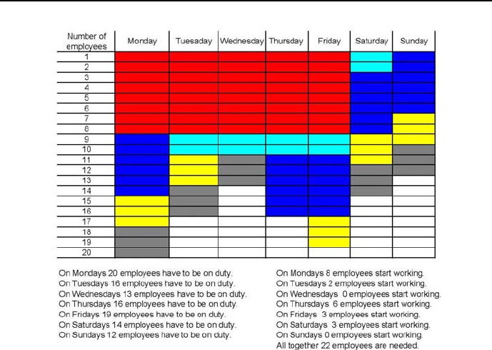
5.9 Optimum timetabling problems 319
Figure 5.12: Crew roster for fast food bar
On Tuesdays 2 employees start working.
On Wednesday 0 employees start working.
On Thursday 6 employees start working.
On Friday 3 employees start working.
On Saturday 3 employees start working.
On Sunday 0 employees start working.
All together 22 employees are needed.
The solution has been depicted by Figure 5.12.
The Cartesian product from the timetable definition is the product of the
set of days (Monday,Tuesday, Wednesday, Thursday. Friday, Saturday, Sunday)
and the employee set of employees (employee_1, employee_2, ..., employee_22).
The product corresponds to all ”boxes” from Figure 5.15. The solution is given
by subsets of the Cartesian product, marked by colours:

320 Chapter 5. CLP with elementary constraints for optimal solutions
•red (employees starting work on Monday and working up to Friday);
•green (employees starting work on Tuesday and working up to Saturday));
•blue (employees starting work on Thursday and working up to Monday);
•yellow (employees starting work on Friday and working up to Tuesday);
•grey (employees starting work on Saturday and working up to Wednesday).
5.9.2 The power and misery of optimization
Optimality (in the strict sense used in this book) means just that the solution
optimizes some objective function. The practical value of such optimum solution
may (in some cases) be at odds with the theoretical result. To bridge the gap
between both notions of optimality, a reformulation of the problem or a change
of objective function may often be needed. This is illustrated by the following
crew roster problem for toll collectors.
5.9.3 Toll collectors roster
A tollway has a toll plaza with the following staffing demands for each 24-hour
period:
from 24 to6-2collectors
from 6 to 10 - 8 collectors
from 10 to 12 - 4 collectors
from 12 to 16 - 3 collectors
from 16 to 18 - 6 collectors
from 18 to 22 - 5 collectors
from 22 to 24 - 3 collectors28
Each collector works four hours, is off one hour, and then works another four
hours. A collector may start the work at any hour. How many collectors should
start work at each hour in order to minimize the number of collectors hired?
The following variables are needed:
X1 - number of collectors that start work at 1
X2 - number of collectors that start work at 2
X3 - number of collectors that start work at 3
28 Well, the 24-hour clock system, although not popular in English-speaking countries, is
decidedly more CLP-friendly and less error-prone for around the clock time-tabling tasks.

5.9 Optimum timetabling problems 321
X4 - number of collectors that start work at 4
...
X24 -number of collectors that start work at 24.
The solution is given by 5_31_toll_collectors.ecl29:
/*1*/ :- lib(eplex).
/*2*/ top:-
/*3*/ Variables = [X1,X2,X3,X4,X5,X6,X7,X8,X9,X10,X11,X12,
X13,X14,X15,X16,X17,X18,X19,X20,X21,X22,X23,X24],
/*4*/ Variables $:: 0.0..1.0Inf,
/*5*/ integers(Variables),
% Number of collectors on duty from 24 to 1:
/*6*/ X24+X23+X22+X21+X19+X18+X17+X16 $>= 2,
% Number of collectors on duty from 1 to 2:
/*7*/ X1+X24+X23+X22+X20+X19+X18+X17 $>= 2,
% Number of collectors on duty from 2 to 3:
/*8*/ X2+X1+X24+X23+X21+X20+X19+X18 $>= 2,
% Number of collectors on duty from 3 to 4:
/*9*/ X3+X2+X1+X24+X22+X21+X20+X19 $>= 2,
% Number of collectors on duty from 4 to 5:
/*10*/ X4+X3+X2+X1+X23+X22+X21+X20 $>= ),
% Number of collectors on duty from 5 to 6:
/*11*/ X5+X4+X3+X2+X24+X23+X22+X21 $>= 2,
% Number of collectors on duty from 6 to 7:
/*12*/ X6+X5+X4+X3+X1+X24+X23+X22 $>= 8,
% Number of collectors on duty from 7 to 8:
/*13*/ X7+X6+X5+X4+X2+X1+X24+X23 $>= 8,
% Number of collectors on duty from 8 to 9:
/*14*/ X8+X7+X6+X5+X3+X2+X1+X24 $>= 8,
% Number of collectors on duty from 9 to 10:
/*15*/ X9+X8+X7+X6+X4+X3+X2+X1 $>= 8),
% Number of collectors on duty from 10 to 11:
/*16*/ X10+X9+X8+X7+X5+X4+X3+X2 $>= 4,
29 This is an OST-type problem.

322 Chapter 5. CLP with elementary constraints for optimal solutions
% Number of collectors on duty from 11 to 12:
/*17*/ X11+X10+X9+X8+X6+X5+X4+X3 $>= 4,
% Number of collectors on duty from 12 to 13:
/*18*/ X12+X11+X10+X9+X7+X6+X5+X4 $>= 3,
% Number of collectors on duty from 13 to 14:
/*19*/ X13+X12+X11+X10+X8+X7+X6+X5 $>= 3,
% Number of collectors on duty from 14 to 15:
/*20*/ X14+X13+X12+X11+X9+X8+X7+X6 $>= 3,
% Number of collectors on duty from 15 to 16:
/*21*/ X15+X14+X13+X12+X10+X9+X8+X7 $>= 3,
% Number of collectors on duty from 16 to 17:
/*22*/ X16+X15+X14+X13+X11+X10+X9+X8 $>= 6,
% Number of collectors on duty from 17 to 18:
/*23*/ X17+X16+X15+X14+X12+X11+X10+X9 $>= 6,
% Number of collectors on duty from 18 to 19:
/*24*/ X18+X17+X16+X15+X13+X12+X11+X10 $>= 5,
% Number of collectors on duty from 19 to 20:
/*25*/ X19+X18+X17+X16+X14+X13+X12+X11 $>= 5,
% Number of collectors on duty from 20 to 21:
/*26*/ X20+X19+X18+X17+X15+X14+X13+X12 $>= 5,
% Number of collectors on duty from 21 to 22:
/*27*/ X21+X20+X19+X18+X16+X15+X14+X13+X12 $>= 5,
% Number of collectors on duty from 22 to 23:
/*28*/ X22+X21+X20+X19+X17+X16+X15+X14 $>= 3,
% Number of collectors on duty from 23 to 24:
/*29*/ X23+X22+X21+X20+X18+X17+X16+X15 $>= 3,
/*30*/ NumberOfCollectors $= X1+X2+X3+X4+X5+X6+X7+X8+X9+X10+
X11+X12+X13+X14+X15+X16+X17+X18+X19+X20+X21+X22+X23+X24,
/*31*/ eplex_solver_setup(min(NumberOfCollectors)),
/*32*/ eplex_solve(NumberOfCollectors),
/*33*/ eplex_get(vars,Vars),
/*34*/ eplex_get(typed_solution,Vals),
/*35*/ Vars = Vals,nl,

5.9 Optimum timetabling problems 323
/*36*/ Number is X1+X2+X3+X4+X5+X6+X7+X8+X9+X10+X11+X12+
X13+X14+X15+X16+X17+X18+X19+X20+X21+X22+X23+X24,
/*37*/ write("Overall number of collectors = "),write(Number),nl,nl,
/*38*/ (foreach(A,["1","2","3","4","5","6","7","8","9","10","11","12",
"13","14","15","16","17","18","19","20","21","22","23","24"]),
/*39*/ foreach(X,[X1,X2,X3,X4,X5,X6,X7,X8,X9,X10,X11,X12,
X13,X14,X15,X16,X17,X18,X19,X20,X21,X22,X23,X24])
/*40*/ do
/*41*/ write("Number of collectors starting work at "),
write(A),write(" o’clock = "),write(X),nl).
As can be seen, the collector balances (lines /*6*/ -/*29*/) are formulated
so as to fulfill the main constraint: each collector works 4hours, has an hour
break, and works for another 4hours.
The solution obtained is as follows:
Overall number of collectors = 16
Number of collectors staring to work at 1 o’clock = 2
Number of collectors staring to work at 2 o’clock = 1
Number of collectors staring to work at 3 o’clock = 1
Number of collectors staring to work at 4 o’clock = 1
Number of collectors staring to work at 5 o’clock = 1
Number of collectors staring to work at 6 o’clock = 3
Number of collectors staring to work at 7 o’clock = 0
Number of collectors staring to work at 8 o’clock = 0
Number of collectors staring to work at 9 o’clock = 0
Number of collectors staring to work at 10 o’clock = 0
Number of collectors staring to work at 11 o’clock = 0
Number of collectors staring to work at 12 o’clock = 0
Number of collectors staring to work at 13 o’clock = 1
Number of collectors staring to work at 14 o’clock = 2
Number of collectors staring to work at 15 o’clock = 2
Number of collectors staring to work at 16 o’clock = 2
Number of collectors staring to work at 17 o’clock = 0
Number of collectors staring to work at 18 o’clock = 0
Number of collectors staring to work at 19 o’clock = 0
Number of collectors staring to work at 20 o’clock = 0
Number of collectors staring to work at 21 o’clock = 0
Number of collectors staring to work at 22 o’clock = 0
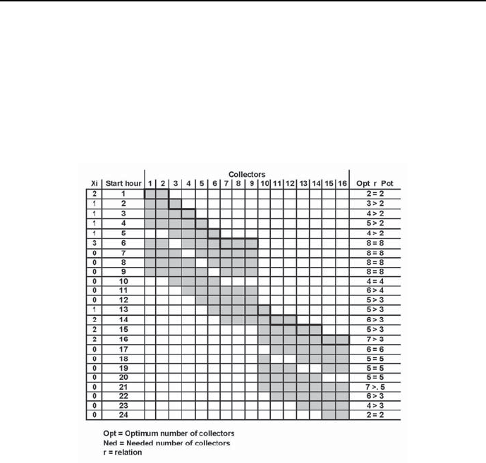
324 Chapter 5. CLP with elementary constraints for optimal solutions
Number of collectors staring to work at 23 o’clock = 0
Number of collectors staring to work at 24 o’clock = 0
The solution is depicted by Figure 5.13. Although it is optimum, it is not
parsimonious: for many hours the number of collectors on duty is larger then
the needed number. This shows that some rethinking and reformulation of the
problem is needed.
Figure 5.13: Crew roster for toll collectors
5.9.4 Dog Service
The ”Dog Service Company” is well-known as breeder, trainer and provider of
dogs being experts in discovering smuggled alcohol, tobacco, drugs, explosives
and ammunition. The ”Great Southern Boarder Crossing” is an important cus-
tomer of the company. Dogs made available to the crossings authorities may
be working any day and night no longer than 6 hours, and after any hour enjoy
an hourly rest. A thorough data mining discovered the following pattern of

5.9 Optimum timetabling problems 325
dog-demand throughout any day and night:
from 12 a.m. to 4 a.m. - 2 dogs
from 4 a.m. to 8 a.m. - 4 dogs
from 8 a.m. to 10 p.m. - 6 dogs
from 10 p.m. to 12 p.m. - 8 dogs
from 12 p.m. to 4 a.m. - 6 dogs
from 4 a.m. to 6 a.m. - 4 dogs
from 6 a.m. to 10 a.m. - 2 dogs
from 10 a.m. to 12 a.m. - 3 dogs
How many dogs should start working at any hour throughout day and night in
order to minimize the overall number of dogs working around the clock?
The following variables are needed;
X1 - number of dogs that start working at 1
X2 - number of dogs that start working at 2
...
X24 -number of dogs that start working at 24.
The dog balances for each hour are formulated so as to fulfill the main
constraint: each each dog works one hour with an hour long break afterwards.
The program 5_32_dogs.ecl looks like this:
/*1*/ :- lib(eplex).
/*2*/ top:-
/*3*/ Dogs = [X1,X2,X3,X4,X5,X6,X7,X8,X9,X10,X11,X12,
X13,X14,X15,X16,X17,X18,X19,X20,X21,X22,X23,X24],
/*4*/ Dogs $:: 0.0..1.0Inf,
/*5*/ integers(Dogs),
% Number of dogs working from 24 to 1:
/*6*/ X24+X22+X20+X18+X16+X14 $>= 2,
% Number of dogs working from 1 to 2:
/*7*/ X1+X23+X21+X19+X17+X15 $>= 2,
% Number of dogs working from 2 to 3:
/*8*/ X2+X24+X22+X20+X18+X16 $>= 2,

326 Chapter 5. CLP with elementary constraints for optimal solutions
% Number of dogs working from 3 to 4:
/*9*/ X3+X1+X23+X21+X19+X17 $>= 2,
% Number of dogs working from 4 to 5:
/*10*/ X4+X2+X24+X22+X20+X18 $>= 4,
% Number of dogs working from 5 to 6:
/*11*/ X5+X3+X1+X23+X21+X19 $>= 4,
% Number of dogs working from 6 to 7:
/*12*/ X6+X4+X2+X24+X22+X20 $>= 4,
% Number of dogs working from 7 to 8:
/*13*/ X7+X5+X3+X1+X23+X21 $>= 4,
% Number of dogs working from 8 to 9:
/*14*/ X8+X6+X4+X2+X24+X22 $>= 6,
% Number of dogs working from 9 to 10:
/*15*/ X9+X7+X5+X3+X1+X23 $>= 6,
% Number of dogs working from 10 to 11:
/*16*/ X10+X8+X6+X4+X2+X24 $>= 8,
% Number of dogs working from 11 to 12:
/*17*/ X11+X9+X7+X5+X3+X1 $>= 8,
% Number of dogs working from 12 to 13:
/*18*/ X12+X10+X8+X6+X4+X2 $>= 6,
% Number of dogs working from 13 to 14:
/*19*/ X13+X11+X9+X7+X5+X3 $>= 6,
% Number of dogs working from 14 to 15:
/*20*/ X14+X12+X10+X8+X6+X4 $>= 6,
% Number of dogs working from 15 to 16:
/*21*/ X15+X13+X11+X9+X7+X5 $>= 6,
% Number of dogs working from 16 to 17:
/*22*/ X16+X14+X12+X10+X8+X6 $>= 4,
% Number of dogs working from 17 to 18:
/*23*/ X17+X15+X13+X11+X9+X7 $>= 4,
% Number of dogs working from 18 to 19:
/*24*/ X18+X16+X14+X12+X10+X8 $>= 2,

5.9 Optimum timetabling problems 327
% Number of dogs working from 19 to 20:
/*25*/ X19+X17+X15+X13+X11+X9 $>= 2,
% Number of dogs working from 20 to 21:
/*26*/ X20+X18+X16+X14+X12+X10 $>= 2,
% Number of dogs working from 21 to 22:
/*27*/ X21+X19+X17+X15+X13+X11 $>= 2,
% Number of dogs working from 22 to 23:
/*28*/ X22+X20+X18+X16+X14+X12 $>= 3,
% Number of dogs working from 23 to 24:
/*29*/ X23+X21+X19+X17+X15+X13 $>= 3,
/*30*/ Number_of_dogs $= X1+X2+X3+X4+X5+X6+X7+X8+X9+X10+X11+X12+
X13+X14+X15+X16+X17+X18+X19+X20+X21+X22+X23+X24,
/*31*/ eplex_solver_setup(min(Number_of_dogs)),
/*32*/ eplex_solve(Number_of_dogs),
/*33*/ eplex_get(vars,Vars),
/*34*/ eplex_get(typed_solution,Vals),
/*35*/ Vars = Vals,nl,
/*36*/ Number is X1+X2+X3+X4+X5+X6+X7+X8+X9+X10+X11+X12+
X13+X14+X15+X16+X17+X18+X19+X20+X21+X22+X23+X24,
/*37*/ write("Minimum number of dogs needed = "),write(Number),nl,nl,
/*38*/ (foreach(A,["1","2","3","4","5","6","7","8","9","10","11","12",
"13","14","15","16","17","18","19","20","21","22","23","24"]),
/*39*/ foreach(X,[X1,X2,X3,X4,X5,X6,X7,X8,X9,X10,X11,X12,
X13,X14,X15,X16,X17,X18,X19,X20,X21,X22,X23,X24])
/*40*/ do
/*41*/ write("Number of dogs starting work at "),write(A),
write(" o’clock is "),write(X),nl).
The solution is as follows:
Minimum number of dogs needed = 22
Number of dogs starting work at 1 o’clock is 0
Number of dogs starting work at 2 o’clock is 5
Number of dogs starting work at 3 o’clock is 0
Number of dogs starting work at 4 o’clock is 2
Number of dogs starting work at 5 o’clock is 4
Number of dogs starting work at 6 o’clock is 1
Number of dogs starting work at 7 o’clock is 4
Number of dogs starting work at 8 o’clock is 0
Number of dogs starting work at 9 o’clock is 0
328 Chapter 5. CLP with elementary constraints for optimal solutions
Number of dogs starting work at 10 o’clock is 0
Number of dogs starting work at 11 o’clock is 0
Number of dogs starting work at 12 o’clock is 0
Number of dogs starting work at 13 o’clock is 0
Number of dogs starting work at 14 o’clock is 3
Number of dogs starting work at 15 o’clock is 0
Number of dogs starting work at 16 o’clock is 0
Number of dogs starting work at 17 o’clock is 3
Number of dogs starting work at 18 o’clock is 0
Number of dogs starting work at 19 o’clock is 0
Number of dogs starting work at 20 o’clock is 0
Number of dogs starting work at 21 o’clock is 0
Number of dogs starting work at 22 o’clock is 0
Number of dogs starting work at 23 o’clock is 0
Number of dogs starting work at 24 o’clock is 0
It is depicted by the roster from Figure 5.14.
5.9.5 Police officers
The number of optimum solutions with the same value of objective function
could - for some problems - be large indeed. Consider the following example:
The City Police Station30 needs at least, for successive 4-hour intervals around-
the-clock, the number of police officers on duty as given by Table 5.8:
Time (hours) Interval Number of officers
required
2-6 122
6-10 255
10 - 14 388
14 - 18 4110
18 - 22 544
22 - 2 633
Table 5.8: Minimum number of required police officers
Each officer is on duty for 8 consecutive hours, starting at the beginning of
some 4-hour interval. The minimum number of police officers needed to meet
the schedule is determined by program 5_33_police_officers.ecl:
/*1*/ :-lib(ic).
/*2*/ :-lib(branch_and_bound).
30 This example is from [Wagner-75].
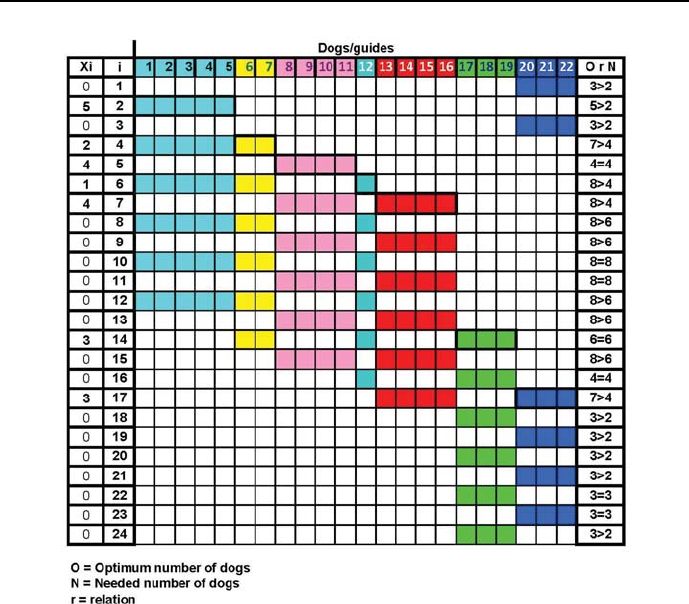
5.9 Optimum timetabling problems 329
Figure 5.14: Dog roster for Great Southern Boarder Crossing
/*3*/ top :-
% Officers_i - the number of officers starting their service
% at the beginning of interval i
/*4*/ [Officers_1,Officers_2,Officers_3,Officers_4,Officers_5,Officers_6]
::0..100,
/*5*/ Officers_on_duty_at_interval_1 #= Officers_6 + Officers_1,
/*6*/ Officers_on_duty_at_interval_1 #>= 22,
/*7*/ Officers_on_duty_at_interval_2 #= Officers_1 + Officers_2,
/*8*/ Officers_on_duty_at_interval_2 #>= 55,
/*8*/ Officers_on_duty_at_interval_3 #= Officers_2 + Officers_3,

330 Chapter 5. CLP with elementary constraints for optimal solutions
/*9*/ Officers_on_duty_at_interval_3 #>= 88,
/*10*/ Officers_on_duty_at_interval_4 #= Officers_3 + Officers_4,
/*11*/ Officers_on_duty_at_interval_4 #>= 110,
/*12*/ Officers_on_duty_at_interval_5 #= Officers_4 + Officers_5,
/*13*/ Officers_on_duty_at_interval_5 #>= 44,
/*14*/ Officers_on_duty_at_interval_6 #= Officers_5 + Officers_6,
/*15*/ Officers_on_duty_at_interval_6 #>= 33,
/*16*/ Sum #= Officers_1+Officers_2+Officers_3+Officers_4+Officers_5+Officers_6,
/*17*/ bb_min(labeling([Officers_1,Officers_2,Officers_3,
Officers_4,Officers_5,Officers_6]),
Sum,bb_options with [strategy:step]), nl,
/*18*/ write("Number of officers starting service at the beginning of :"),nl,
/*19*/ write("interval_ 1: "),write(Officers_1),nl,
/*20*/ write("interval_ 2: "),write(Officers_2),nl,
/*21*/ write("interval_ 3: "),write(Officers_3),nl,
/*22*/ write("interval_ 4: "),write(Officers_4),nl,
/*23*/ write("interval_ 5: "),write(Officers_5),nl,
/*24*/ write("interval_ 6: "),write(Officers_6),nl,nl,
/*25*/ write("Minimum number of police officers needed: "),write(Sum),nl,nl,
/*26*/ fail.
/*28*/ top:-
/*28*/ write("That’s all!"),nl,nl.
The message generated is:
Found a solution with cost 198
Found no solution with cost 20.0 .. 197.0
Number of officers starting their service at the beginning of :
interval_ 1: 0
interval_ 2: 55
interval_ 3: 33
interval_ 4: 77
interval_ 5: 0
interval_ 6: 33
Minimum number of police officers needed: 198
That’s all!

5.9 Optimum timetabling problems 331
As before, ”fail” is impotent for ”branch-and-bound”. However, a strong
suspicion is nurtured about the existence of many more optimum solutions. To
dispel any doubt, the approach already presented in Section 5.6.1 is applied
once more: the known minimum number of police officers is used to constrict
the domain of variable Sum for the program 5_34_all_police_officers.ecl
that just determines all feasible solutions for the optimum number 198 of police
officers:
/*1*/ :-lib(ic).
/*2*/ top :-
/*3*/ assert(counter(0)),
% Officers_i - the number of officers starting their service
at the beginning of interval i
/*4*/ [Officers_1,Officers_2,Officers_3,
Officers_4,Officers_5,Officers_6]::0..100,
/*5*/ Officers_on_duty_at_interval_1 #= Officers_6 + Officers_1,
/*6*/ Officers_on_duty_at_interval_1 #>= 22,
/*7*/ Officers_on_duty_at_interval_2 #= Officers_1 + Officers_2,
/*8*/ Officers_on_duty_at_interval_2 #>= 55,
/*8*/ Officers_on_duty_at_interval_3 #= Officers_2 + Officers_3,
/*9*/ Officers_on_duty_at_interval_3 #>= 88,
/*10*/ Officers_on_duty_at_interval_4 #= Officers_3 + Officers_4,
/*11*/ Officers_on_duty_at_interval_4 #>= 110,
/*12*/ Officers_on_duty_at_interval_5 #= Officers_4 + Officers_5,
/*13*/ Officers_on_duty_at_interval_5 #>= 44,
/*14*/ Officers_on_duty_at_interval_6 #= Officers_5 + Officers_6,
/*15*/ Officers_on_duty_at_interval_6 #>= 33,
/*16*/ Officers_1+Officers_2+Officers_3+Officers_4+Officers_5+
Officers_6 #= 198,
/*17*/ labeling([Officers_1,Officers_2,Officers_3,
Officers_4,Officers_5,Officers_6]),
/*18*/ count(Number),
/*19*/ write("Number of solution: ),write(Number),nl,
/*20*/ write("Number of officers starting service at the beginning of:"),nl,
/*21*/ write("interval_ 1: "),write(Officers_1),nl,
/*22*/ write("interval_ 2: "),write(Officers_2),nl,
/*23*/ write("interval_ 3: "),write(Officers_3),nl,
/*24*/ write("interval_ 4: "),write(Officers_4),nl,

332 Chapter 5. CLP with elementary constraints for optimal solutions
/*25*/ write("interval_ 5: "),write(Officers_5),nl,
/*26*/ write("interval_ 6: "),write(Officers_6),nl,nl,
/*27*/ write("Minimum number of police officers needed: "),write(Sum),nl,nl,
/*28*/ fail.
/*29*/ top:-
/*30*/ write("That’s all!"),nl,nl.
/*31*/ count:-
/*32*/ retract(counter(Old)),
/*33*/ New is Old 1, +
/*34*/ assert(counter(New)).
This time the program generates 32154 solutions; only the first and last is shown
below:
Number of solution: 1
Number of officers starting their service at the beginning of
interval_ 1: 0
interval_ 2: 55
interval_ 3: 33
interval_ 4: 77
interval_ 5: 0
interval_ 6: 33
Minimum number of police officers needed: 198
......
Number of solution: 32154:
Number of officers starting their service at the beginning of:
interval_ 1: 55
interval_ 2: 0
interval_ 3: 99
interval_ 4: 11
interval_ 5: 33
interval_ 6: 0
Minimum number of police officers needed: 198
The solutions are depicted in Figure 5.15.
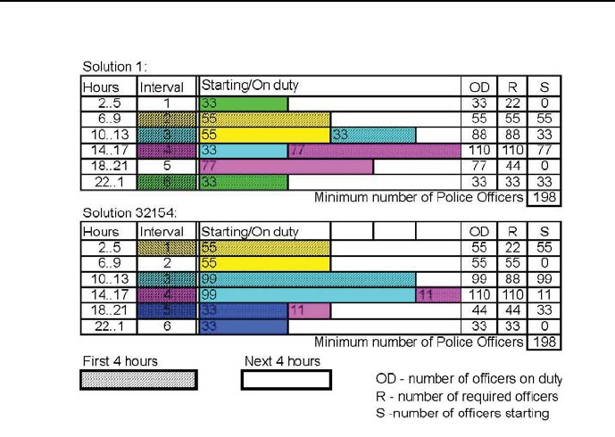
5.10 Optimum sequencing problems 333
Figure 5.15: Optimum time-tables for police officers
5.10 Optimum sequencing problems
One of the more important applications of ECLiPSeis sequencing. Sequencing
means determining the order of elements from some set so as to fulfill precedence
constraints and disjunctive constraints for those elements while minimizing some
objective function.
The meaning of those constraints is as follows:
•precedence constraints in the time-domain, which state that some tasks
may begin only after some other task of known duration has been com-
pleted:
Start_of_task_i #>= Start_of_task_j + Duration_of_task_j.
•precedence constraints on the order-line, which state that some tasks may

334 Chapter 5. CLP with elementary constraints for optimal solutions
may have higher position on some order-line than other tasks:
Position_of_task_i #> Position_of_task_j
•disjunctive constraints, which state that two or more tasks using the same
resource must be performed sequentially. For the simple case of two tasks
(say task iand task j), either task imust start after task jhas been
completed, or task jmust start after task ihas been completed, which
can be expressed as:
disjunctive(Start_of_task_i,Duration_of_task_i,
Start_of_task_j, Duration_of_task_j):-
Start_of_task_i #>= Start_of_task_j + Duration_of_task_j.
disjunctive(Start_of_task_i,Duration_of_task_i,
Start_of_task_j, Duration_of_task_j):-
Start_of_task_j #>= Start_of_task_i + Duration_of_task_i.
5.10.1 Precedence constraints - building a house
Precedence constraints are typical for a variety of projects, where something
must be done before something else may begin. As example may serve building
a house. The table of precedence constraints and duration of activities are
presented in Table 5.9
The network of precedence constraints for all activities and the activity dura-
tions are presented in Figure 5.16. This is an Activities on Arc (AoA) network:
it uses directed arcs to represent activities.
Assuming that the project begins at time 0, the problem is to find the
shortest duration for the project, i.e, the earliest time of completion. It would
be also desirable to determine the critical path of the project, i.e. the shortest
sequence of activities starting from the initial activity and ending with the
final activity. Knowing the critical path of a project is important because the
only way to shorten the projects duration is to shorten the duration of critical
path activities31. The modest house building example is solved by program
5_35_house.ecl, which offers three options:
31 The goals mentioned are pursued in OR under the heading PERT (Program Evaluation
and Review Technique)orCPM (Critical Path Method), developed to assist managers in
tracking the progress of large projects. Its first application was to the Polaris submarine
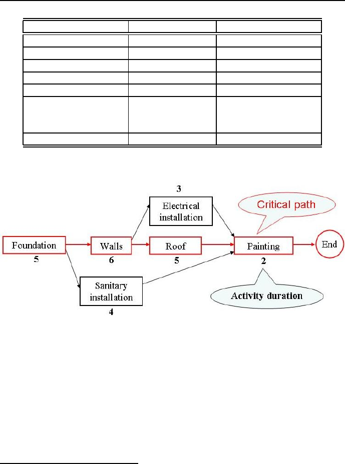
5.10 Optimum sequencing problems 335
Activity name Activity duration Precedence
Foundation 5Nothing
Walls 6 Foundation
Sanitary installation 3Foundation
Roof 5 Walls
Electrical installation 3 Walls
Painting 2Electrical installation
Sanitary installation
Roof
End 0Painting
Table 5.9: House building data
Figure 5.16: AoA network of precedence constraints for house building
1. To find a single optimum solution. For this option lines singled out by
/*?a*/ have to be decommented and lines singled out by /*?b*/ have to
be commented, as shown in the program.
2. To find for a known single optimum solution all other optimum solutions.
For this option lines singled out by /*?b*/ have to be decommented and
lines singled out by /*?a*/ have to be commented.
ballistic missile project; thanks to PERT the project is believed to be completed 18 month
ahead of schedule.

336 Chapter 5. CLP with elementary constraints for optimal solutions
3. To determine the critical path, for the last change additionally lines /*x*/
have to be decommented and lines /*17b,/*18*/,/*19*/,...,/*24*/ have
to be commented.
The program 5_35_house.ecl32 is as follows:
/*1*/ :-lib(ic).
% for a single minimum-time solution:
/*2a*/ :-lib(branch_and_bound).
/*3*/ top:-
% for a single minimum-time solution:
/*4a*/ house(_).
% for all minimum-time solutions:
/*4b*/% findall(Operations, house(Operations),_).
/*5*/ house(Operations):-
/*6*/ Operations = [Foundation,Walls,SanitaryInstallation,Roof,
ElectricalInstallation,Painting,End],
% for a single minimum-time solution:
/*7a*/ Operations :: 0..25,
% for all minimum-time solutions:
/*7b*/% Operations :: 0..18,
/*8*/ Walls #>= Foundation + 5,
/*9*/ SanitaryInstallation #>= Foundation + 5,
/*10*/ Roof #>= Walls + 6,
/*11*/ ElectricalInstallation #>= Walls + 6,
/*12*/ Painting #>= ElectricalInstallation + 3,
/*13*/ Painting #>= SanitaryInstallation + 4,
/*14*/ Painting #>= Roof + 5,
/*15*/ End #>= Painting + 2,
% for a single minimum-time solution:
/*16a*/ End #=< 25,
% for all minimum-time solutions:
/*16b*/% End #= 18,
% for a single minimum-time solution:
/*17a*/ minimize(labeling(Operations),End),nl,
32 This is an OST-type problem.

5.10 Optimum sequencing problems 337
/*x*/% get_domain(Foundation,DFoundation),
/*x*/% get_domain(Walls,DWalls),
/*x*/% get_domain(SanitaryInstallation,DSanitaryInstallation),
/*x*/% get_domain(Roof,DRoof),
/*x*/% get_domain(ElectricalInstallation,DElectricalInstallation),
/*x*/% get_domain(Painting,DPainting),
/*x*/% get_domain(End,DEnd),
/*x*/% write("Domain of foundation: "),write(DFoundation),nl,
/*x*/% write("Domain of walls: "),write(DWalls),nl,
/*x*/% write("Domain of sanitary installation: "),
/*x*/% write(DSanitaryInstallation),nl,
/*x*/% write("Domain of roof: "),write(DRoof),nl,
/*x*/% write("Domain of electrical installation: "),
/*x*/% write(DElectricalInstallation),nl,
/*x*/% write("Domain of painting: "),write(DPainting),nl,
/*x*/% write("Domain of end: "),write(DEnd),nl.
% for all minimum-time solutions:
/*17b*/% labeling(Operations),
/*18*/ write("Starting time for foundation: "),write(Foundation),
/*19*/ nl,write("Starting time for walls: "),write(Walls),nl,
/*20*/ write("Starting time for sanitary installation: "),
write(SanitaryInstallation),nl,
/*21*/ write("Starting time for roof: "),write(Roof),nl,
/*22*/ write("Starting time for electrical installation: "),
write(ElectricalInstallation),
/*23*/ nl,write("Starting time for painting: "),write(Painting),nl,
/*24*/ write("End: "),write(End),nl.
For the case of single optimum solution the message is:
Found a solution with cost 18
Starting time for foundation: 0
Starting time for walls: 5
Starting time for sanitary installation: 5
Starting time for roof: 11
Starting time for electrical installation: 11
Starting time for painting: 16
End: 18
In case all optimum solutions are to be determined, all lines numbered by

338 Chapter 5. CLP with elementary constraints for optimal solutions
/*?b*/ have to be decommented, lines numbered by /*?a*/ have to be com-
mented, and the shortest duration (End: 18) is used as the upper bound of
the Operations domain in line /*7b*/. The modified program (referred to as
5_36_house_all.ecl) then generates 24 optimum solutions, from which the
following three are presented:
Starting time for foundation: 0
Starting time for walls: 5
Starting time for sanitary installation: 5
Starting time for roof: 11
Starting time for electrical installation: 11
Starting time for painting: 16
End: 18
Starting time for foundation: 0
Starting time for walls: 5
Starting time for sanitary installation: 5
Starting time for roof: 11
Starting time for electrical installation: 12
Starting time for painting: 16
End: 18
Starting time for foundation: 0
Starting time for walls: 5
Starting time for sanitary installation: 5
Starting time for roof: 11
Starting time for electrical installation: 13
Starting time for painting: 16
End: 18
Now, if for the last change the xlines are additionally decommented, and
the lines /*17b*/,/*18*/,/*19*/,...,/*24*/ are commented, then the modified
program (referred to as 5_37_house_crit_path.ecl) generates the following
result:
Domain of foundation: 0
Domain of walls: 5
Domain of sanitary installation: 5 .. 12
Domain of Roof: 11
Domain of electrical installation: 11 .. 13
Domain of painting: 16
Domain of End: 18
Single value domains indicate that the corresponding activities (for founda-

5.10 Optimum sequencing problems 339
tion, walls, roof and painting) determine the critical path: in order to decrease
the projects duration, durations of critical path activities must be decreased.
5.10.2 Disjunctive constraints - limited resources
All resources are limited33. Simple scheduling with disjunctive constraints is
presented by the program 5_38_disjunctive_sequencing.ecl34 forfourtasks
with variable start times Z1,..Z4. The tasks with start times Z2 and Z3 are
disjunctive because they use a common resource, which is just large enough for
servicing one of the tasks only. The program is as follows:
/*1*/ :-lib(ic).
/*2*/ :-lib(branch_and_bound).
/*3*/ top :-
/*4*/ schedule(_).
/*5*/ schedule([Z1,Z2,Z3,Z4,End]):-
/*6*/ [Z1,Z2,Z3,Z4,End] :: 0..15,
/*7*/ Z1 + 3 #=< Z2,
/*8*/ Z1 + 3 #=< Z3,
/*9*/ Z2 + 4 #=< Z4,
/*10*/ Z3 + 2 #=< Z4,
/*11*/ Z4 + 1 #= End,
/*12*/ disjunctive([Z2,4,Z3,2]),
/*13*/ minimize(labeling([Z1,Z2,Z3,Z4,End]),End),
/*14*/ writeln("Z1 ":Z1),
/*15*/ writeln("Z2 ":Z2),
/*16*/ writeln("Z3 ":Z3),
/*17*/ writeln("Z4 ":Z4),
/*18*/ writeln("End ":End).
/*19*/ disjunctive([Z1,D1,Z2,_]):-
/*20*/ Z1 + D1 #=< Z2.
/*21*/ disjunctive([Z1,_,Z2,D2]):-
/*22*/ Z2 + D2 #=< Z1.
The message is:
Found a solution with cost 10
Z1 : 0
33 Well, resources of some banks seem to be an exception.
34 This is an OST-type problem.
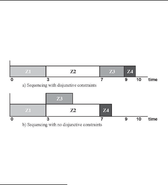
340 Chapter 5. CLP with elementary constraints for optimal solutions
Z2 : 3
Z3 : 7
Z4 : 9
End : 10
This solution is best presented by a Gantt chart35 from Figure 5.17a).
Figure 5.17: Gantt charts for simple sequencing problem
If the disjunctive constraint is removed (i.e. if line /*12*/ is removed, which
means the common resource is large enough to service simultaneously tasks Z2
and Z3), the message is:
35 A Gantt chart is a graphical representation of resource allocation over time for con-
currently performed tasks. It is named after Henry Gantt (1861-1919), a mechanical en-
gineer and management consultant who, in the second decade of the 20th century, de-
veloped this visual tool to show the progress of concurrent activities in time, see e.g.
http://www.ganttchart.com/History.html). Gantt charts were first used on large construc-
tion projects like the Hoover Dam, which started in 1931, and the interstate highway network,
which started in 1956.
It should be noted that the Patron of the Economic University in Katowice (Poland),
Karol Adamiecki (1866-1933), presented in 1903 a similar technique of describing scheduling
programs and applied it to steel mill scheduling at the Iron Works he was employed as Chief
Technical Officer.

5.10 Optimum sequencing problems 341
Found a solution with cost 8
Z1 : 0
Z2 : 3
Z3 : 3
Z4 : 7
End : 8
This corresponds to the Gantt chart from Figure 5.17b).
It should be noticed that the number of disjunctions growth rapidly with
the number of tasks: for the discussed example with 2 disjunctive tasks there
are 2 disjunctions, for 3 tasks there will be 3 ∗2 = 6 disjunctions, for 4 tasks
-4∗6 = 24 disjunctions, and for ntasks there will be xndisjunctions with
xn=n∗xn−1. This is the reason that solving problems with disjunctions us-
ing the approach just presented is numerically inefficient. Therefore, although
the model used is easily readable and strongly declarative, in the next chap-
ter a more efficient approach to modeling disjunctions with global constraints
cumulative/4,cumulative/5,anddisjunctive/2 will be presented
5.10.3 Sequencing with conflicting constraints - a photo
Conflicting constraints are constraints that cannot be fulfilled simultaneously.
They are common in most real-world applications. Any academic teacher is
well-acquainted with having the preferred lecture room at the preferred day
and preferred time slice already reserved by a colleague. A simple case of con-
flicting constraints, inspired by an example from the Mozart/Oz system website
([Mozart/Oz-10]) may be stated as follows:
Anna, Ben, Charles, Derek, Eva, Fred, Gary line up for a commemorative
photo. Some of them have preferences next to whom they want to stand: :
1. Anna wants to stand next to Eva and Fred.
2. Ben wants to stand next to Anna and Eva.
3. Derek wants to stand next to Fred and Charles.
4. Garry wants to stand next to Derek and Charles,
seeFigure5.18.
It is easy to demonstrate that the preferences are contradictory. This is done
by the program 5_39_photo_1.ecl36 :
36 This is an FS-type problem.
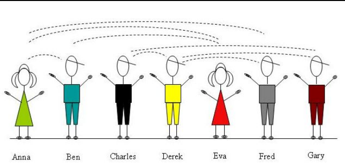
342 Chapter 5. CLP with elementary constraints for optimal solutions
Figure 5.18: Candidates for a commemorative photo and their preferences
/*1*/ :-lib(ic).
/*2*/ top :-
/*3*/ Persons = [Anna, Ben, Charles, Derek, Eva, Fred, Gary],
% The meaning of variables is as follows: Anna is the position number
% (counting from left) occupied by person "Anna", etc.
/*4*/ Persons :: 1..7,
/*5*/ alldifferent(Persons),
/*6*/ next_to(Anna,Eva),
/*7*/ next_to(Anna,Fred),
/*8*/ next_to(Ben,Anna),
/*9*/ next_to(Ben,Eva),
/*10*/ next_to(Derek,Fred),
/*11*/ next_to(Derek,Charles),
/*12*/ next_to(Gary,Derek),
/*13*/ next_to(Gary,Charles),
/*14*/ search(Persons,0,first_fail,indomain,complete,[]),
/*15*/ writeln("Persons ":Persons).
/*16*/ next_to(X,Y):-
/*17*/ X #= Y + 1.
/*18*/ next_to(X,Y):-
/*19*/ Y #= X + 1.
The message generated is No. However, if lines /*6*/ and /*11*/ are removed
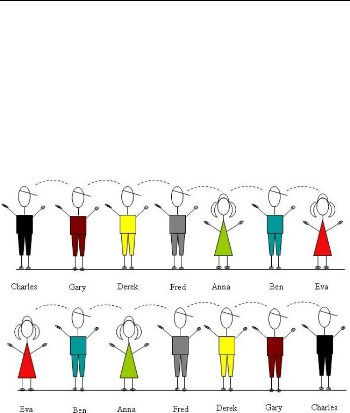
5.10 Optimum sequencing problems 343
(no attention is payed to one preference by Anna and one by Derek), the solu-
tion obtained is:
Persons : [5, 6, 1, 3, 7, 4, 2]
Persons : [3, 2, 7, 5, 1, 4, 6]
and this corresponds to two alignments (see Figure 5.19:
Charles - Gary - Derek - Fred - Anna - Ben - Eva
Eva - Ben - Anna - Fred - Derek - Gary - Charles
Figure 5.19: Alignment with no constraints 6 and 11.
The question may well be asked how many of the declared preferences may
be satisfied at most, if all of them cannot. The maximum number of satisfied

344 Chapter 5. CLP with elementary constraints for optimal solutions
preferences is determined by program 5_40_photo_2.ecl37 :
/*1*/ :-lib(ic).
/*2*/ :-lib(branch_and_bound).
/*3*/ top :-
/*4*/ preferences(Preferences),
/*5*/ dim(Preferences,[NumberOfPreferences,2]),
/*5*/ dim(Positions, [7]),
/*6*/ Positions :: 1..7,
/*7*/ alldifferent(Positions),
/*8*/ length(Differences, NumberOfPreferences),
/*9*/ (for(I,1,NumberOfPreferences),
/*10*/ fromto(Differences,Out,In,[]), % collect reifications
/*11*/ param(Preferences,Positions)
/*12*/ do
/*13*/ P1 #= Positions[Preferences[I,1]],
/*14*/ P2 #= Positions[Preferences[I,2]],
/*15*/ Difference #= P1-P2,
% reifying the condition that the modulus of variable Difference be equal 1:
/*16*/ Reif #= (Difference #= 1 or Difference #= -1),
/*17*/ Out = [Reif|In]
/*18*/ ),
/*19*/ flatten_array(Preferences, FlattenedPreferences),
/*20*/ NumberOfFlattenedPreferences #= sum(FlattenedPreferences),
/*21*/ Z :: 0..NumberOfFlattenedPreferences,
% Z - number of preferences fulfilled:
/*22*/ Z #= sum(Differences),
/*23*/ flatten_array(Positions, Variables),
/*24*/ ZNeg #= -Z,
/*25*/ minimize(search(Variables,0,first_fail,
indomain,complete,[]),ZNeg),
/*26*/ writeln("Names: Anna, Ben, Charles, Derek, Eva, Fred, Gary"),
/*27*/ writeln("Positions":Positions),
/*28*/ writeln("Number of preferences claimed":
NumberOfPreferences),
/*29*/ writeln("Number of preferences fulfilled":Z).
% Remainder about preferences:
% [Anna, Ben, Charles, Derek, Eva, Fred, Gary]
% 1. Anna wishes to stand next to Eva and Fred:
% 1 next to 5, 1 next to 6
% 2. Ben wishes to stand next to Anna and Eva:
% 2 next to 1, 2 next to 5
% 3. Derek wishes to stand next to Fred and Charles:
37 This is an OS-type problem.

5.10 Optimum sequencing problems 345
% 4 next to 6, 4 next to 3
% 4. Gary wishes to stand next to Derek and Charles:
% 7 next to 4, 7 next to 3
/*30*/ preferences([](
[](1,5),
[](1,6),
[](2,1),
[](2,5),
[](4,6),
[](4,3),
[](7,4),
[](7,3))).
The message is:
Found a solution with cost -2
Found a solution with cost -3
Found a solution with cost -4
Found a solution with cost -5
Found a solution with cost -6
Found no solution with cost -8.0 .. -7.0
Names: Anna, Ben, Charles, Derek, Eva, Fred, Gary
Positions : [](3, 1, 6, 5, 2, 4, 7)
Number of preferences claimed : 8
Number of preferences fulfilled : 6
The solution corresponds to the alignment:
Ben,Eva,Anna,Fred,Derek,Charles,Gary
The alignment is shown in Figure 5.20. There are two preferences not fulfilled.
Obviously, this is not a unique optimum solution: program 5_39_photo_1.ecl,
with lines /*6*/ and /*11*/ removed, generated two solutions with different 6
preferences fulfilled.
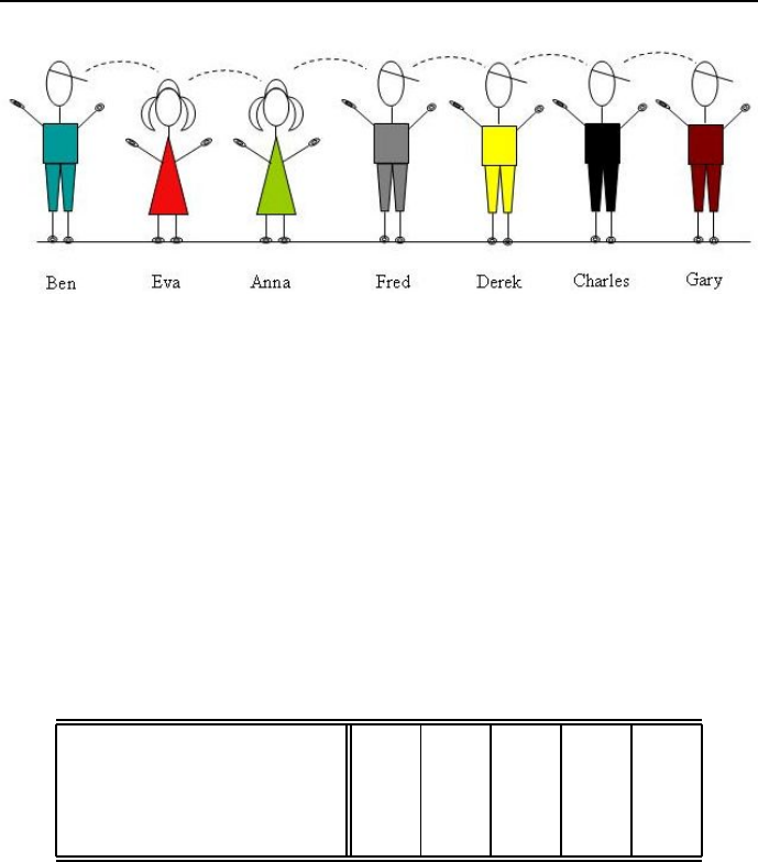
346 Chapter 5. CLP with elementary constraints for optimal solutions
Figure 5.20: Alignments minimizing the number of violated constraints
5.11 Exercises
Five textbooks
Find the optimum solution to the following problem: Bookco Publishers is
considering publishing five textbooks. The maximum number of copies of
each textbook that can be sold, the variable cost of producing each text-
book, the sales price of each textbook, and the fixed cost of a production
run for each book are given in Table 5.10. Thus for example, producing
2000 copies of book l brings in a revenue of 2000*50 = 100000 but costs
80000 + 25*2000 = 130000 MU. Bookco can produce at most 10 thousand
books. How can they maximize profit?
Textbooks 1 2 3 4 5
Maximum demand 5000 4000 3000 4000 3000
Variable cost (MU) 25 20 15 18 22
Sales price (MU) 50 40 38 32 40
Fixed cost (thousands MU) 80 50 60 30 40
Table 5.10: Textbooks data
Increasing the pension fund while going green at the same time
The increasing number of childless young couples parenting dogs i.e. de-
voting their attention and love to them, prompted the Absurdoland’s Par-
liament (worried about future declining tax revenues that could accelerate
the collapse of the non-sustainable financial pyramid of state-guaranteed

5.11 Exercises 347
pensions) to look for a mechanism that could make the dogs to generate
some income towards the retiree benefits of their masters. A hastily cre-
ated Think Tank considered a number of proposals, but its Final Scrutiny
Report presented in detail just one recommendation referred to by the
acronym TET, meaning Tail Energy Taps. The idea was to convert the
dogs natural (and pretty useless) tail-wagging into useful energy by means
of a small computer-controlled and tail-driven electrical power generator
loading a small battery. Such TET’s would be attached to the dogs be-
hind and interfaced with their tails. All dog masters would be obliged
by law to download the energy stored in the battery once per week at
the local Dog Energy Sink (DES), were it would be used to drive pumps
rising water to a cascade of elevated reservoirs, thus converting dogs en-
ergy into stored gravitational potential energy for future uses. For lazy
dogs an enhanced TET model was envisaged, allowing to control the dogs
tail-wagging through Internet, and prompt the dogs declining activity by
a series of gentle randomly changing mechanical and acoustical signals.
The submitted proposal was enthusiastically supported by the overwhel-
ming majority of parliamentarians. The environmentalists could not praise
enough the brilliant idea of tapping a hitherto untouched source of green
energy, its sustainability and renewability. Some of them even envisaged
TET’s to tail-wag the way to energy independence. Parliamentarian do-
gooders of all stripes were just enthralled by the bright prospect of creating
a number of green technical jobs in newly created branches of TET pro-
duction, TET maintenance, DES building, and DES maintenance, as well as
green management jobs in the newly created District Dog Energy Coordi-
nation Outlets (DDECO), the National Department of Dog Energy (NDDE,in
the Ministry of Energy), and the Dog Energy Police Task Force (DEPTF,
in the Ministry of Interior) for chasing dogs with no TET’s attached to
their behinds. The objections raised by a small group of TET-sceptics,
who argued that without massive taxpayer funded subsidies dog-energy
is unsustainable, were brushed aside, and a Dog Energy Bill was passed
quickly. This was welcomed by a number of companies thinking about
downloading on the market some of their outdated mechanical and elec-
tronic hardware that still gathered dust on the shelves, and give something
to do to their underemployed and overpaid unionized manpower. The Bill
had plenty of gaps, which could be profitably exploited by shrewd compa-
nies. The most important gap was the lack of canigraphic38 data; nobody
38 A doggie equivalent of ”demographic”.

348 Chapter 5. CLP with elementary constraints for optimal solutions
in Absurdoland knew how many large dogs and how many small dogs
live there, but the Bill distinguished those groups of dogs, prescribing for
each group a unique TET contraption. The reasonable approach by all
companies engaged was to stop worrying about the dog canilation 39 and
start maximizing profit, pretty sure that their output will be bought by
state-controlled NDDE outlets at state-established prices.
So did the renowned Junk Techno Company, which saw the opportunity to
get rid of two of their dust gathering mechanical appliances, Type_A and
Type_B, rejected by both Army and Navy. Both appliances could prac-
tically at small cost be converted into correspondingly small dog TET’s
(Type_B appliance only) and large dog TET’s (Type_A plus Type_B appli-
ances). What’s more, they constitute the main cost factor of the TET’s,
the needed accompanying electronics being practically freely available at
various electronics graveyards. The daily conversion of Type_A appliances
could not be larger than 60 items, the daily conversion of Type_B appli-
ances could not be larger than 50 items. The furnishing of all produced
appliances with electronics could be done at the pace of 120 appliances
daily.
On the basis of NDDE-approved purchasing prices for small and large dog
TET’s, the Company estimated its daily profit from getting rid of a single
Type_A appliance as being no less than 300 MU, and from getting rid of
a single Type_B appliance - 500 MU. Write a program that determines
the number of appliances produced to maximize the daily profit of the
company.
Glue
Glueco produces three types of glue on two different production lines.
Each line can be utilized by up to seven workers at a time. Workers are
paid 500 MU per week on production line l, and 900 MU per week on
production line 2. For a week of production it costs 1000 MU to set up
production line l and 2000 MU to set up production line 2. During a week
on a production line, each worker produces the number of units of glue
shown in Table 5.11. Each week, at least 120 units of glue l, at least 150
units of glue 2, and at least 200 units of glue 3 must be produced. Write
a program to minimize the total cost of meeting weekly demands.
Allocating machines
A product can be produced on four different machines. Each machine
39 A doggie equivalent of ”population”.
5.11 Exercises 349
Production lines Glue 1 Glue 2 Glue 3
Production line l 20 30 40
Production line 2 50 35 45
Table 5.11: Glue production data
has a fixed setup cost, variable production costs per-unit-processed, and
a production capacity given in Table 5.12. A total of 2000 units of the
product must be produced. Write a program that determines machine
loads that minimize total costs.
Machine Fixed cost (MU) Variable cost per unit (MU) Capacity
l1000 20 900
2920 24 1000
3800 16 1200
4700 28 1600
Table 5.12: Machines data
Paper rolls
A paper factory manufactures large rolls of paper that have a width of
105cm. However, retailers demand rolls of smaller width, which have to
be cut from the large ones. For instance, a standard width roll could be
cut into two rolls of 35cm each and one roll of 30cm. The factory received
orders shown in Table 5.13.
Width Number of
cm rolls
25 100
30 125
35 80
Table 5.13: Orders data
Write a program minimizing the number of produced large rolls needed to
satisfy the order.
350 Chapter 5. CLP with elementary constraints for optimal solutions
Five projects
Five projects are being evaluated over a 3-year planning horizon. Table
5.1440 gives the expected returns and the associated yearly expenditure
for each project.
Expenditure
Project (million MU per year) Returns
year 1 year 2 year 3 (million MU)
1 5 1 8 20
2 4 7 10 40
3 3 9 2 20
4 7 4 1 15
5 8 6 10 30
Available
funds 25 25 25
(milion MU)
Table 5.14: Projects data
Write a program to determine, which project should be selected over the
3-year horizon to maximize the overall returns. Modify the program to
take into account the following constraint: project 5 must be selected if
either project 1 or project 3 is selected. Modify the program to take into
account the following constraint: project 2 and project 3 are mutually
exclusive.
Allocating benefits to Napoleonides
Napoleonism means, in respect of an individual, the individual’s deeply
felt internal and personal experience of being Napoleon Bonaparte,which
may not exactly correspond to the role assigned to the individual by the
oppressive society.
This sad discrepancy is a source of enormous sufferings of all those per-
sons considering themselves to be Napoleon Bonaparte. It is therefore
not surprising that the World Institute for Wellness has finally taken se-
riously into consideration the plight of those persons, referred to officially
as Napoleonides. As a result a series of directives was issued urging Local
Governments to consider Napoleonism not as a mental disorder, but as a
40 This exercise is from [Taha-08].

5.11 Exercises 351
normal state of health that contributes substantially to the diversification
of society (Diversity is our strength! ), and deserves not only widespread
respect and some intelligent publicity (lets say establishing a. o. The
World Napoleonides Day as Public Holiday, with ”Napoleonides Parades”
and TV campaigns), but also parity in employment, wages and member-
ship in representative organs as well as special financial support from the
public purse. The directives also incorporated napoleonophobia into the
constantly increasing spectrum of heavily punished hate speeches, phobias
and descriminatory practices, forbidding therapy to turn people away from
thinking they are Napoleon Bonaparte, and introducing sensitivity train-
ing for napoleonism into syllabuses of elementary education.
The Parliament of Absurdoland, always in the vanguard of legislative or-
gans eager to quickly implement any whim of the World Institute for Well-
ness, ordered its Commission on Discrimination and Exclusion to solve
the problem as soon as possible. The Commission started with inviting
a number of Napoleonide activists to present their grievances and was
deeply shocked by what they heard. The activists complained bitterly
about them being addressed simply as ’Mr. Smith’, and not by ”Your
Imperial Highness”, about the necessity to go to work by tram or buss
instead of riding on horses or in a horse-drawn carriage, with the assis-
tance of some generals and adjutants as well as a small bunch of Chevaux
L´egeres, all in proper uniforms. They complained about haters calling
them bonacrazies or bonacranks. Their main complaints were about the
cost of making them as similar as possible to their archetype: the cost
of face matching surgery - although quite substantial - happened to be
negligible compared to the costs of height matching surgery. A number of
activists presented arguments in favour of providing them with small-sized
servants-staffed manor houses to enable them to lead a truly Napoleon-like
everyday existence. However, the straw that broke the camel’s neck was
given by tales of tragic institutionalizations, incarcerations and persecu-
tions of Napoleonides in Closed Mental Institutions. The Commission im-
mediately changed all laws handicapping or force-medicating Napoleonides
and started to work on optimizing benefits to ameliorate their fortune.
The activists provided a list of 150 well-known declared Absurdoland’s
Napoleonides (their number increased substantially on the aftermath of
the World Institute for Wellness directives). The Government of Ab-
surdoland quickly changed its budget by taking 10 MM MU out of the
Social Security Fund to provide deserving and decent living conditions
for Napoleonides. In the meantime the activists presented Happiness Val-
352 Chapter 5. CLP with elementary constraints for optimal solutions
ues for their most wanted benefits, and suggested that the Commission
should do its job by maximizing Happines over all entitled beneficiaries
by selecting the number of different benefits granted. Next the Commis-
sion established prices for those benefits, the Ministry of Medical Tech-
nology informed, that - because of technological constraints - no more
than 30 height-matching and 15 face-matching operations could be per-
formed yearly, and the Ministry of Cultural Heritage declared that the
number of small-sized servants-staffed manor houses available for manor-
less Napoleonides is (unfortunately, at least for the time being) limited to
6. It was also considered reasonable that (in view of the sorry state of
economy) Napoleonides equipped with horses for riding should not claim
horse-driven carriages. The basic problem data is presented by Table 5.15.
Number of Type of Happiness Cost of benefit
beneficiaries benefit Value per beneficiary
N1 Napoleon-like outfit 640
N2 Horse for riding 25 300
N3 Horse-drawn carriage 50 1500
N4 Face matching 180 2000
N5 Height matching 200 6500
N6 Manor house 500 13000
Table 5.15: Data for allocating benefits to napoleonides
Determine the numbers of various beneficiaries to maximize the happiness
value for the napoleonide population.
Producing cars
Clunker Motors Co has four car manufacturing plants. Each is capable
of producing any of the company’s three flagships (Clunker SUV, Clunker
Electric and Clunker Green), but only one of them. The main economic
data for the production are shown in Table 5.16.
They include the fixed cost of running each plant for a year and the variable
costs of producing a single car. The constraints are:
1. Each plant can produce only one type of car. 2. The total production
of each type must be located at a single plant. 3. If plants 3 and 4 are
producing cars, then plant 1 must also produce cars.
Clunker Motors Co must produce 600000 cars of each type per year. Write
5.11 Exercises 353
Variable cost
Plant Fixed cost SUV Electric Green
1 7 billion MU 15000 MU 19000 MU 15000 MU
2 6 billion MU 12000 MU 18000 MU 11000 MU
3 4 billion MU 17000 MU 16000 MU 12000 MU
4 2 billion MU 19000 MU 22000 MU 9000 MU
Table 5.16: Car manufacturing data
a program that determines how to minimize the annual overall cost of
producing cars while meeting production quotas.
Fast food outlets
The well-known chain of popular fast food outlets ”Tasty Poison” is con-
quering the Absurdoland’s fast food market after the collapse of the com-
munist state-owned-and-run ”Eating Joints”. A set of specialist ana-
lyzed possible locations in the Ancient Capital, proposing 6 locations were
”Tasty Poison” outlets could be placed. Those outlets served a number
of Ancient Capital districts, the ”Tasty Poison” policy being to serve any
district by at least one outlet. The specialists provided - after some hard
work - trusted estimates of cost for building any of the six fast food outlets,
shown in Table 5.17.
Fast food outlet
District 1 2 3 4 5 6
1× × ×
2× ×
3× ×
4× ×
5× ×
6× × ×
7× ×
8× × ×
Cost of building (MM MU) 10 15 12 812 13
Table 5.17: Fast food project data
Write a program that determines what outlets to build in order to mini-

354 Chapter 5. CLP with elementary constraints for optimal solutions
mize cost and serve all districts.
Hot buttered toasts 41
There is an old toaster with two hinged doors on each side. It can take
two pieces of toast at a time, and it only toasts one side of a piece at
a time. The times for the activities are: 1)It takes 30 seconds to toast
one side of a piece of bred (the toaster can take up two pieces at a time).
2)It takes 3 seconds to put a piece of bread in the toaster. 3)It takes
3 seconds to take out a piece of bread from the toaster. 4) It takes 3
seconds to reverse a piece of bread without removing it from the toaster.
5) It takes 12 seconds to butter a side of toast. In addition, the activities
of inserting, reversing, removing and buttering a slice require both hands,
so the cannot be performed at the same time. Each piece is only buttered
on one side and the butter can only be applied after that side has been
toasted. When we begin, the three pieces of bread are out of the toaster,
and we have to complete the toasting with the three pieces also being out
of the toaster. Develop such schedule that the three pieces of bread are
toasted and buttered in the shortest time.
Crossing a bridge 42
Four travelers (Mr. A, B, C and D) have to cross a bridge over a deep
ravine. It is a very dark night and the travelers only have one oil lamp.
The lamp is essential for successfully crossing the ravine because the bridge
is very old and has plenty of holes and loose boards. What is worse, its
construction is quite weak and it can only support two men at any time.
It turns out that each traveler needs a different amount of time to cross
the bridge. Mr. A is young and fast, and only needs a minute to cross
the bridge. Mr. D, on the other hand, is an old man who recently had a
hip replacement and will need 10 minutes to get across the bridge. Mr B
and Mr C need two and five minutes, respectively. And since each traveler
needs the light to cross, it is the slower man in a pair who determines the
total time required to make the crossing. Write a program to determine
a crossing schedule that minimizes the overall crossing time.
41 This exercise is from [Michalewicz-07].
42 This exercise is from [Michalewicz-07].
5.11 Exercises 355
Students grievances 43
A University is in the process of forming a committee to handle students
grievances. The administration wants the committee to include at least
one female, one male, one students, one administrator and one faculty
member. Ten individuals a,b,c,...,j have been nominated to serve on the
committee, see Table 5.18.
Category Individuals
Females a,b,c,d,e
Males f,g,h,i,j
Students a,b,c,j
Administrators e,f
Faculty d,g,h,i
Table 5.18: Committee candidates
The administration wants to formulate the smallest committee with rep-
resentation of each of the five categories of persons. Write a program to
solve this problem.
Constructing a pizzeria
Given data from Table 5.19 write a program to find the shortest duration
for constructing the pizzeria and to determine the critical path activities44.
43 This exercise is from [Taha-08].
44 This exercise is from http://faculty.ksu.edu.sa/ialharkan/default.aspx
356 Chapter 5. CLP with elementary constraints for optimal solutions
No Activity Predecessor Days
1Design layout 1
2Select contractor 1 5
3Cleaning area 2 5
4Plumbing 3 5
5Install electricity 312
6Install AC 3 7
7Tile floors 4 7
8Install walk-in cooler 7 1
9Make partition 8 6
10 Tile walls and partitions 9 7
11 Ceiling, lighting, AC 5, 6, 7 4
12 Equipment installation 10, 11 2
13 Paste 12 3
14 Design store front 3 5
15 Install store front 14 5
16 Paint 1 and 2 13, 15 2
17 Install counters 16 4
18 Install electricity sockets 13 1
19 Install frames 16 1
20 Paint 3 17, 19 1
21 Final decoration 20 1
22 Prepare sign board 3 2
23 Install sign board 22 2
24 Print new store opening 2
25 Final test 18, 21, 23 1
Table 5.19: Pizzeria construction activities
Chapter 6
CLP with global constraints
for optimal solutions
6.1 Introduction
Some global predicates were already introduced and applied in Chapter 4 for
finding feasible solutions. Some of them (like cumulative/4,cumulative/5,
disjunctive/2) and some new ones (like disjoint/1 and cycle/3) are indis-
pensable for solving a group of new optimization problems:
1. Optimum scheduling problems. Scheduling is an extension of sequencing:
scheduling is sequencing with the additional constraint on available resources
and the aim of minimizing an objective function, given most often by the time
to complete the schedule, known as makespan. Resource constraints may be
defined as follows:
Demand_A_for_shared_resource + ... +
Demand_Z_for_shared_resource <=
Maximum_amount_of_shared_resource_available.
This constraint is fundamental and universal, almost like the Law of Gravita-
tion (toutes proportion gard´ee): no rational decision-making is possible while
abstracting from the finiteness of resources.
2. Optimum bin packing problems. The aim of those problems is most often to
pack the highest-value number of objects of different values into a bin of fixed
357

358 Chapter 6. CLP with global constraints for optimal solutions
volume. An elementary bin-packing problem is the knapsack problem, discussed
in sections 5.6.3 and 5.6.3.
3. Optimum vehicle routing problems. The aim of those problems is to service
a number of spatially distributed customers with a fleet of vehicles in the most
parsimonious manner. The basic vehicle routing problem is the celebrated trav-
elling salesman problem, discussed in Section 6.19.
The mentioned predicates have found application also for solving some of the
already discussed problems, like optimum sequencing problems.
Global predicates are useful for combinatorial optimization problems because
they:
•are rich enough to capture substantial parts of the optimization problem
structure;
•provide major abstractions common to a broad range of combinatorial
optimization problems;
•provide exceptional custom-tailored computing power for some optimization-
relevant constraints;
•enhance the program declarativity and readability by introducing names
highly relevant to the functionality of the constraints.
The discussed and applied global constraints (cumulative/4,cumulative/5,
disjunctive/2,circuit/1,cycle/3) are just a tiny subset of all global con-
straints available for optimization purposes.
6.2 The ’cumulative/4’ built-in
The cumulative constraint:
cumulative(+StartTimes, +Durations,+Resources,++Limit)
expresses the fact that the total of a shared resource used by many tasks may
not, at any time instant, exceed a given limit. Its arguments have the following
meaning (see Figure 6.1):
•StartTimes = [S1,...,Sn] is a list of domain variables representing
start times for ntasks;
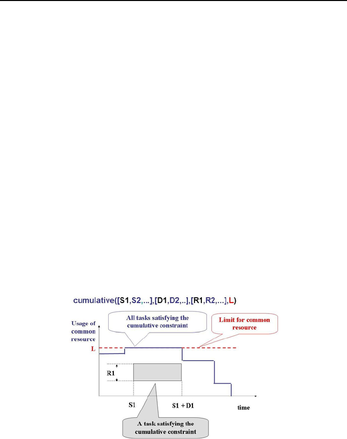
6.2 The ’cumulative/4’ built-in 359
•Durations = [D1,...,Dn] is a list of domain variables representing task
durations;
•Resources = [R1,...,Rn] is a list of domain variables representing amounts
of shared resource needed by tasks;
•End Times Ej for all tasks 1<=j<=n are given by Sj+Dj=Ej;
•Limit is the maximum amount of the available shared resource at any
time instant isuch that for a<=i<=b:
max(Sum Rj) <= Limit
for all such jthat Sj <= i <= Sj+Dj-1, where:
a = min(min(S1),...,min(Sn))
is the earliest beginning of all tasks, and
b = max((max(S1)+max(D1)),...,(max(Sn)+max(Dn)))
is the latest end of all tasks, with:
min(X) being the minimum value of Xin its domain, and
max(X) being the minimum value of Xin its domain.
•The end time of all tasks is equal End = max(Sj+Dj).
Figure 6.1: Tasks satisfying a cumulative/4 constraint

360 Chapter 6. CLP with global constraints for optimal solutions
6.3 Cumulative scheduling 1
Let’s apply the cumulative/4 built-in to data from Section 5.10.2. This can be
done as shown in program 6_1_cumu_schedule_1.ecl1:
/*1*/ :-lib(ic).
/*2*/ :- lib(ic_edge_finder3).
/*3*/ :-lib(branch_and_bound).
/*4*/ top :-
/*5*/ schedule(_).
/*6*/ schedule([Z1,Z2,Z3,Z4,End]):-
/*7*/ [Z1,Z2,Z3,Z4,End] :: 0..15,
/*8*/ Z1 + 3 #=< Z2,
/*9*/ Z1 + 3 #=< Z3,
/*10*/ Z2 + 4 #=< Z4,
/*11*/ Z3 + 2 #=< Z4,
/*12*/ Z4 + 1 #= End,
/*13*/ cumulative([Z2,Z3],[4,2],[1,1],1),
/*14*/ minimize(labeling([Z1,Z2,Z3,Z4,End]),End),
/*15*/ writeln("Z1 ":Z1),
/*16*/ writeln("Z2 ":Z2),
/*17*/ writeln("Z3 ":Z3),
/*18*/ writeln("Z4 ":Z4),
/*19*/ writeln("End ":End).
The message is:
Found a solution with cost 10
Found no solution with cost 8.0 .. 9.0
Z1 : 0
Z2 : 3
Z3 : 7
Z4 : 9
End : 10.
It corresponds to the already presented Gantt chart from Figure 5.17a).
If line /*13*/ is removed and line /*13a*/ activated, then the message gener-
1This is an OST-type problem.
6.4 Cumulative scheduling 2 361
ated is:
Found a solution with cost 8
Z1 : 0
Z2 : 3
Z3 : 3
Z4 : 7
End : 8.
It corresponds to the already presented Gantt chart from Figure 5.17b).
6.4 Cumulative scheduling 2
Consider a slightly more complicated cumulative scheduling, see [Baldiceanu-94]:
There are seven tasks, each of them characterized by its duration and the
amount of shared resource needed, see Table 6.1:
Task Duration Resource
116 2
2 6 9
313 3
4 7 7
5 5 10
618 1
7 4 11
Table 6.1: Data for simple cumulative scheduling
A schedule is to be found that minimizes the overall end of all tasks while not
exceeding the resource capacity equal 13. This can be done as shown in program
6_2_cumu_schedule_2.ecl2:
/*1*/ :- lib(ic).
/*2*/ :- lib(ic_edge_finder3).
/*3*/ :- lib(branch_and_bound).
2This is an OST-type problem.

362 Chapter 6. CLP with global constraints for optimal solutions
/*4*/top:-
/*5*/ LS = [S1,S2,S3,S4,S5,S6,S7], %list of task start times
/*6*/ LD = [16, 6,13, 7, 5,18, 4], %list of task durations
/*7*/ LE = [E1,E2,E3,E4,E5,E6,E7], %list of task end times
/*8*/ LR = [2,9,3,7,10,1,11], %list of task resource requirements
/*9*/ LS :: 1..100,
/*10*/ End :: 1..100,
/*11*/ LE :: 1..100,
/*12*/ Limit :: 1..13,
/*13*/ cumulative(LS,LD,LR,Limit),
/*14*/ E1 #= S1 + 16,
/*15*/ E2 #= S2 + 6,
/*16*/ E3 #= S3 + 13,
/*17*/ E4 #= S4 + 7,
/*18*/ E5 #= S5 + 5,
/*19*/ E6 #= S6 + 18,
/*20*/ E7 #= S7 + 4,
/*21*/ maxlist([E1,E2,E3,E4,E5,E6,E7],End),
/*22*/ minimize(labeling([S1,S2,S3,S4,S5,S6,S7,
E1,E2,E3,E4,E5,E6,E7]),End),
/*23*/ write("LS = "), writeln(LS),
/*24*/ write("LE = "), writeln(LE),
/*25*/ write("Limit = "), writeln(Limit),
/*26*/ write("End = "), writeln(End).
The message is:
LS=[ 1,17,10,10, 5, 5,1]
LE=[17,23,23,17,10,23,5]
Limit=13
End=23
A Gantt chart illustrating this schedule is given by Figure 6.2. The numbers
inside rectangles are task numbers. This figure may also be interpreted as a
solution for a bin-packing problem, namely the problem of cutting a rectangle
with dimension 13 ×23 into smaller rectangles given by the tasks.
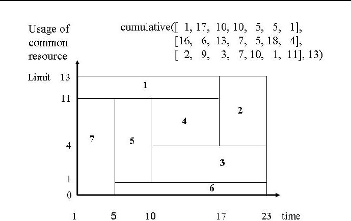
6.5 Cumulative sequencing 363
Figure 6.2: Gantt chart for cumulative scheduling
6.5 Cumulative sequencing
The cumulative/4 predicate may be used also for optimum sequencing prob-
lems. This is illustrated by the following assembly line example: a sequence of
tasks should be determined that fulfills precedence and time constraints as well
as minimizes the overall assembly time. The following set of tasks and their
duration is given:
jobs: A B C D E F G H I J K
duration: 45 11 9 50 15 12 12 12 12 8 9 .
The precedence constraints are:
first_next(predecessor, successor)
first_next(A,B).
first_next(B,C).
first_next(C,F).
first_next(C,G).
first_next(F,J).

364 Chapter 6. CLP with global constraints for optimal solutions
first_next(G,J).
first_next(J,K).
first_next(D,E).
first_next(E,H).
first_next(E,I).
first_next(H,J).
first_next(I,J).
For any pair (predecessor-successor),predecessor cannot start be-
fore successor has ended. Program 6_3_sequencing_opti_cum.ecl uses the
cumulative/4 global built-in to determine a sequence of jobs that minimizes
the overall assembly time:
/*1*/ :- lib(ic).
/*2*/ :- lib(ic_edge_finder3).
/*3*/ :- lib(branch_and_bound).
/*4*/ top:-
% task start times:
/*5*/ LS=[As,Bs,Cs,Ds,Es,Fs,Gs,Hs,Is,Js,Ks],
/*6*/ LS :: 0..250,
/*7*/ End :: 0..250,
% precedence and time constraints:
/*8*/ As + 45 #=< Bs,
/*9*/ Bs + 15 #=< Cs,
/*10*/ Cs + 9 #=< Fs,
/*11*/ Cs + 9 #=< Gs,
/*12*/ Fs + 12 #=< Js,
/*13*/ Gs + 12 #=< Js,
/*14*/ Js + 8 #=< Ks,
/*15*/ Ds + 50 #=< Es,
/*16*/ Es + 15 #=< Hs,
/*17*/ Es + 15 #=< Is,
/*18*/ Hs + 12 #=< Js,
/*19*/ Is + 12 #=< Js,
/*20*/ Ks + 9 #= End,
/*21*/ cumulative([As,Bs,Cs,Ds,Es,Fs,Gs,Hs,Is,Js,Ks],
[45,15,9,50,15,12,12,12,12,8,9],
[ 1, 1, 1, 1, 1, 1, 1, 1, 1, 1, 1],1),
/*22*/ minimize(labeling([As,Bs,Cs,Ds,Es,Fs,Gs,Hs,Is,Js,Ks]),End),
/*23*/ writeln([As,Bs,Cs,Ds,Es,Fs,Gs,Hs,Is,Js,Ks,End]).

6.5 Cumulative sequencing 365
A single solution generated by ECLiPSe) is as follows:
Found a solution with cost 199
Found no solution with cost 98.0 .. 198.0
[0, 45, 60, 69, 119, 134, 146, 158, 170, 182, 190, 199]
Our intuition suggest however that there may be more solutions. This is to
be verified using program 6_4_sequencing_opti_cum_all.ecl, with variable
End grounded on optimum value 199:
/*1*/ :- lib(ic).
/*2*/ :- lib(ic_edge_finder3).
/*3*/ top:-
/*4*/ assert(counter(0)),
% task start times:
/*5*/ LS=[As,Bs,Cs,Ds,Es,Fs,Gs,Hs,Is,Js,Ks],
/*6*/ LS :: 0..250,
% precedence and time constraints:
/*7*/ As + 45 #=< Bs,
/*8*/ Bs + 15 #=< Cs,
/*9*/ Cs + 9 #=< Fs,
/*10*/ Cs + 9 #=< Gs,
/*11*/ Fs + 12 #=< Js,
/*12*/ Gs + 12 #=< Js,
/*13*/ Js + 8 #=< Ks,
/*14*/ Ds + 50 #=< Es,
/*15*/ Es + 15 #=< Hs,
/*16*/ Es + 15 #=< Is,
/*17*/ Hs + 12 #=< Js,
/*18*/ Is + 12 #=< Js,
/*19*/ Ks + 9 #= End,
/*20*/ End is 199,
/*21*/ cumulative([As,Bs,Cs,Ds,Es,Fs,Gs,Hs,Is,Js,Ks],
[45,15,9,50,15,12,12,12,12,8,9],
[ 1, 1, 1, 1, 1, 1, 1, 1, 1, 1, 1],1),
/*22*/ labeling([As,Bs,Cs,Ds,Es,Fs,Gs,Hs,Is,Js,Ks]),
/*23*/ my_count,
/*24*/ counter(Number),
/*25*/ write("Optimum solution "), write(Number),write(":"),nl,
/*26*/ writeln([As,Bs,Cs,Ds,Es,Fs,Gs,Hs,Is,Js,Ks,End]),

366 Chapter 6. CLP with global constraints for optimal solutions
/*27*/ fail.
/*28*/ top:-
/*29*/ write("Those are all optimum solutions.").
/*30*/ my_count:-
/*31*/ retract(counter(Old)),
/*32*/ New is Old 1, +
/*33*/ assert(counter(New)).
Our intuition was well-founded: there are 504 optimum solutions. Only some
of them are shown below:
Optimum solution 1:
[0, 45, 60, 69, 119, 134, 146, 158, 170, 182, 190, 199]
.................................................................
Optimum solution 61:
[0, 45, 110, 60, 119, 134, 146, 158, 170, 182, 190, 199]
.................................................................
Optimum solution 141:
[0, 95, 110, 45, 119, 134, 146, 158, 170, 182, 190, 199]
.................................................................
Optimum solution 504:
[89, 134, 149, 0, 50, 170, 158, 77, 65, 182, 190, 199]
Those are all optimum solutions.
The Gantt chart for those solutions shown in Figure 6.3 presents a proper
interpretation of the above numerical results.
6.6 The ’disjunctive/2’ built-in
The disjunctive constraint:
disjunctive(+Start_Times, +Durations)
is fulfilled if there is no overlap of tasks with start times from the list Start_Times
and corresponding durations from the list Durations, as shown in Figure 6.4.
Both lists must have equal numbers of elements.
In contrast with cumulative/3, which constraints the task along the re-
source coordinate (on Gantt charts - vertically), disjunctive/2 constraints
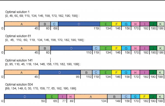
6.7 Disjunctive sequencing 367
Figure 6.3: Gantt charts of some optimum assembly sequences
tasks along the time coordinate (on Gantt charts - horizontally). However - as
shown by the following example - disjunctive/2 may sometimes fulfill the role
of cumulative/3.
6.7 Disjunctive sequencing
The disjunctive/2 built-in is most often used for sequencing problems. This
is illustrated by example 6_5_opti_dis.ecl dealing with the already solved
problem from Section 6.5:
/*1*/ :- lib(ic).
/*2*/ :- lib(ic_edge_finder3).
/*3*/ :- lib(branch_and_bound).
/*4*/ top:-
% task start times:
/*5*/ LS=[As,Bs,Cs,Ds,Es,Fs,Gs,Hs,Is,Js,Ks],
/*6*/ LS :: 0..250,
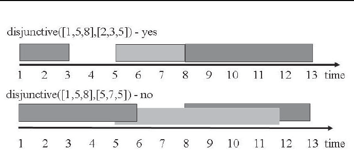
368 Chapter 6. CLP with global constraints for optimal solutions
Figure 6.4: Properties of the disjunctive/2 constraint
/*7*/ End :: 0..250,
% precedence and time constraints:
/*8*/ As + 45 #=< Bs,
/*9*/ Bs + 15 #=< Cs,
/*10*/ Cs + 9 #=< Fs,
/*11*/ Cs + 9 #=< Gs,
/*12*/ Fs + 12 #=< Js,
/*13*/ Gs + 12 #=< Js,
/*14*/ Js + 8 #=< Ks,
/*15*/ Ds + 50 #=< Es,
/*16*/ Es + 15 #=< Hs,
/*17*/ Es + 15 #=< Is,
/*18*/ Hs + 12 #=< Js,
/*19*/ Is + 12 #=< Js,
/*20*/ Ks + 9 #= End,
/*21*/ disjunctive([As,Bs,Cs,Ds,Es,Fs,Gs,Hs,Is,Js,Ks],
[45,15,9,50,15,12,12,12,12,8,9]),
/*22*/ minimize(labeling([As,Bs,Cs,Ds,Es,Fs,Gs,Hs,Is,Js,Ks]),End),
/*23*/ writeln([As,Bs,Cs,Ds,Es,Fs,Gs,Hs,Is,Js,Ks,End]).
The solution is identical with that obtained for 6_3_sequencing_opti_cum.ecl.
Multiple optimum solutions are given by 6_6_sequencing_opti_dis_all.ecl:
/*1*/ :- lib(ic).
/*2*/ :- lib(ic_edge_finder3).

6.7 Disjunctive sequencing 369
/*3*/ top:-
/*4*/ assert(counter(0)),
% task start times:
/*5*/ LS=[As,Bs,Cs,Ds,Es,Fs,Gs,Hs,Is,Js,Ks],
/*6*/ LS :: 0..250,
% precedence and time constraints:
/*7*/ As + 45 #=< Bs,
/*8*/ Bs + 15 #=< Cs,
/*9*/ Cs + 9 #=< Fs,
/*10*/ Cs + 9 #=< Gs,
/*11*/ Fs + 12 #=< Js,
/*12*/ Gs + 12 #=< Js,
/*13*/ Js + 8 #=< Ks,
/*14*/ Ds + 50 #=< Es,
/*15*/ Es + 15 #=< Hs,
/*16*/ Es + 15 #=< Is,
/*17*/ Hs + 12 #=< Js,
/*18*/ Is + 12 #=< Js,
/*19*/ Ks + 9 #= End,
/*20*/ End is 199,
/*21*/ disjunctive([As,Bs,Cs,Ds,Es,Fs,Gs,Hs,Is,Js,Ks],
[45,15,9,50,15,12,12,12,12,8,9]),
/*22*/ labeling([As,Bs,Cs,Ds,Es,Fs,Gs,Hs,Is,Js,Ks]),
/*23*/ my_count,
/*24*/ counter(Number),
/*25*/ write("Optimum solution "), write(Number),write(":"),nl,
/*26*/ writeln([As,Bs,Cs,Ds,Es,Fs,Gs,Hs,Is,Js,Ks,End]),
/*27*/ fail.
/*28*/ top:-
/*29*/ write("Those are all optimum solutions. ").
/*30*/ my_count:-
/*31*/ retract(counter(Old)),
/*32*/ New is Old 1, +
/*33*/ assert(counter(New)).
There are 504 optimum solutions, exactly the same as for program 6_4_sequencing_
opti_cum_all.ecl. See also Figure 6.3

370 Chapter 6. CLP with global constraints for optimal solutions
6.8 Disjunctive scheduling
Let’s solve the example from Section 5.10.2 using disjunctive/2.Thisisdone
by program 6_7_dis_schedule.ecl3:
/*1*/ :- lib(ic).
/*2*/ :- lib(ic_edge_finder3).
/*3*/ :- lib(branch_and_bound).
/*4*/ top :-
/*5*/ schedule(_).
/*6*/ schedule([Z1,Z2,Z3,Z4,End]):-
/*7*/ [Z1,Z2,Z3,Z4,End] :: 0..15,
/*8*/ Z1 + 3 #=< Z2,
/*9*/ Z1 + 3 #=< Z3,
/*10*/ Z2 + 4 #=< Z4,
/*11*/ Z3 + 2 #=< Z4,
/*12*/ Z4 + 1 #= End,
/*13*/ disjunctive([Z2,Z3],[4,2]),
/*14*/ minimize(labeling([Z1,Z2,Z3,Z4,End]),End),
/*15*/ writeln("Z1 ":Z1),
/*16*/ writeln("Z2 ":Z2),
/*17*/ writeln("Z3 ":Z3),
/*18*/ writeln("Z4 ":Z4),
/*19*/ writeln("End ":End).
The message is:
Found a solution with cost 10
Found no solution with cost 8.0 .. 9.0
Z1 : 0
Z2 : 3
Z3 : 7
Z4 : 9
End : 10,
depicted by the already generated Gantt chart from Figure 6.14a).
3This is an OST-type problem.

6.9 The ’disjoint2(Rectangles)’ built-in 371
6.9 The ’disjoint2(Rectangles)’ built-in
This is a generalization of the disjunctive/2 predicate for the case of two di-
mensions. It constrains the position (and possibly size) of rectangles in Rectangles
so that none overlaps. The rectangles are defined by structures:
rect{x:X,y:Y,w:W,h:H}
using the following fields:
•constant x: The x co-ordinate of the left side of the rectangle, equal to
variable X;
•constant y: The y co-ordinate of the bottom side of the rectangle, equal
to variable Y;
•constant w: The width of the rectangle equal to variable W;
•constant h: The height of the rectangle equal to variable H.
Its basic usage is illustrated by program 6_8_disjoint.ecl:
:- lib(gfd).
top_1:-
disjoint2([rect{x:1,y:2,w:1,h:1}, rect{x:3,y:1,w:2,h:1},rect{x:4,y:3,w:3,h:1}]).
top_2:-
disjoint2([rect{x:1,y:2,w:1,h:1},rect{x:3,y:1,w:2,h:1},rect{x:4,y:2,w:3,h:3}]).
top_3:-
disjoint2([rect{x:1,y:2,w:1,h:1},rect{x:3,y:1,w:2,h:3},rect{x:4,y:2,w:3,h:3}]).
The solution to top_1 and top_2 is yes, the solution to top_3 is no. Figure 6.5
depicts the rectangles involved in this program.
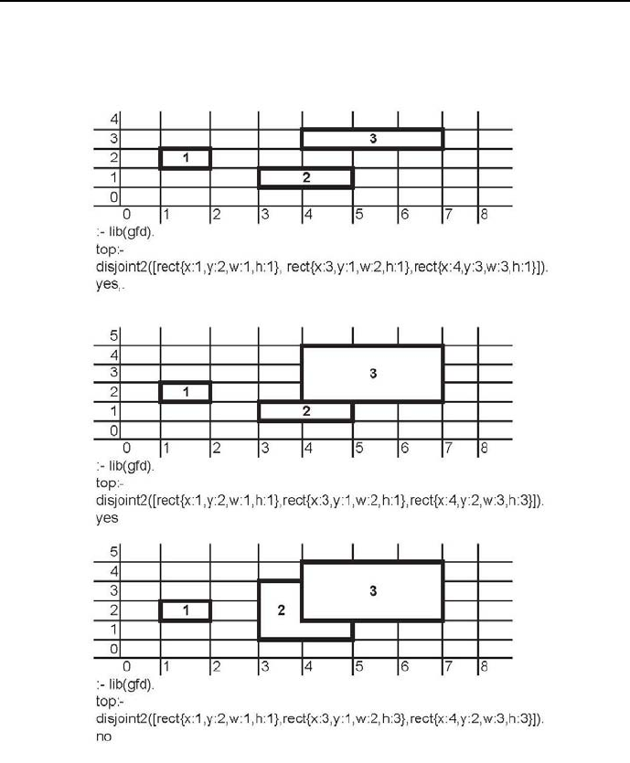
372 Chapter 6. CLP with global constraints for optimal solutions
Figure 6.5: Three examples of ’disjoint2(Rectangles)’ application

6.10 Assembly line balancing 373
6.10 Assembly line balancing
Assembly line balancing is the assignment of tasks to workstations so that, while
fulfilling precedence constraints, each workstation has approximately the same
amount of work to accomplish as measured by the time to complete it. The
largest time to complete all tasks at some workstation is referred to as cycle
time. Optimum line balancing aims at minimizing the cycle time.
Let us consider the 141 optimum solution to the cumulative sequencing
problem from Chapter as shown in Figure 6.3. It is used for balancing a 4-
workstations assembly line as shown by program 6_9_disjoint_balance.ecl:
/*1*/ :-lib(gfd).
/*2*/ :- lib(branch_and_bound).
/*3*/ top:-
%task start times:
/*4*/ LSZ=[ A, B, C, D, E, F, G, H, I, J, K],
%workstations for tasks A,B,...
/*5*/ Lst=[Ast,Bst,Cst,Dst,Est,Fst,Gst,Hst,Ist,Jst,Kst],
%task duration times:
/*6*/ LD=[Ad,Bd,Cd,Dd,Ed,Fd,Gd,Hd,Id,Jd,Kd],
%task end times:
/*4*/ LE=[EA,EB,EC,ED,EE,EF,EG,EH,EI,EJ,EK],
%task resource requirements:
/*8*/ LR=[ 1, 1, 1, 1, 1, 1, 1, 1, 1, 1, 1],
%domain declaration
/*9*/ LSZ #:: 0..100,
/*10*/ Lst #:: 1..4,
/*11*/ LE #:: 0..100,
/*12*/ Limit #:: 1..4,
%task duration times declaration:
/*13*/ Ad is 45, Bd is 15, Cd is 9, Dd is 50, Ed is 15, Fd is 12,
Gd is 12, Hd is 12, Id is 12, Jd is 8, Kd is 9,
%tasks assignment to workstations:
/*14*/ Ast is 1, Bst is 3, Cst is 3, Dst is 2, Est is 3, Fst is 3,
Gst is 4, Hst is 4, Ist is 4, Jst is 4, Kst is 4,
% constraints for tasks end times::
/*15*/ gfd_gac: (EA #>= A + Ad),
/*16*/ gfd_gac: (EB #>= B + Bd),
/*17*/ gfd_gac: (EC #>= C + Cd),
/*18*/ gfd_gac: (ED #>= D + Dd),
/*19*/ gfd_gac: (EE #>= E + Ed),
/*20*/ gfd_gac: (EF #>= F + Fd),

374 Chapter 6. CLP with global constraints for optimal solutions
/*21*/ gfd_gac: (EG #>= G + Gd),
/*22*/ gfd_gac: (EH #>= H + Hd),
/*23*/ gfd_gac: (EI #>= I + Id),
/*24*/ gfd_gac: (EJ #>= J + Jd),
/*25*/ gfd_gac: (EK #>= K + Kd),
%non-overlapping of tasks constraints:
/*26*/ disjoint2([
rect{x:A,y:Ast,w:Ad,h:1},rect{x:B,y:Bst,w:Bd,h:1},
rect{x:C,y:Cst,w:Cd,h:1},rect{x:D,y:Dst,w:Dd,h:1},
rect{x:E,y:Est,w:Ed,h:1},rect{x:F,y:Fst,w:Fd,h:1},
rect{x:G,y:Gst,w:Gd,h:1},rect{x:H,y:Hst,w:Hd,h:1},
rect{x:I,y:Ist,w:Id,h:1}, rect{x:J,y:Jst,w:Jd,h:1},
rect{x:K,y:Kst,w:Kd,h:1}]),
%constraining the usage of resources
/*27*/ cumulative(LSZ,LD,LR,Limit),
/*28*/ append(LSZ,LE,LSZ_E),
/*29*/ append(LSZ_E, Lst,LSZ_E_Lst),
%minimizing
/*30*/ gfd_gac: (max(LE, M)),
/*31*/ bb_min(labeling(LSZ_E_Lst), M, bb_options with
[strategy:continue,from:0,to:100]),
/*32*/ write("End times of tasks = "),write(LE),nl,
/*33*/ write("Minimum cycle time = "),write(M),nl,nl,
/*34*/write("Workstation for A: "),write(Ast),write(", Start A = "),write(A),nl,
/*35*/write("Workstation for B: "),write(Bst),write(", Start B = "),write(B),nl,
/*36*/write("Workstation for C: "),write(Cst),write(", Start C = "),write(C),nl,
/*37*/write("Workstation for D: "),write(Dst),write(", Start D = "),write(D),nl,
/*38*/write("Workstation for E: "),write(Est),write(", Start E = "),write(E),nl,
/*39*/write("Workstation for F: "),write(Fst),write(", Start F = "),write(F),nl,
/*40*/write("Workstation for G: "),write(Gst),write(", Start G = "),write(G),nl,
/*41*/write("Workstation for H: "),write(Hst),write(", Start H = "),write(H),nl,
/*42*/write("Workstation for I: "),write(Ist),write(", Start I = "),write(I),nl,
/*43*/write("Workstation for J: "),write(Jst),write(", Start J = "),write(J),nl,
/*43*/write("Workstation for K: "),write(Kst),write(", Start K = "),write(K),nl.
The solution is:
Found a solution with cost 53
Found no solution with cost 50.0 .. 52.0
End times of tasks = [45, 15, 24, 50, 39, 51, 12, 24, 36, 44, 53]
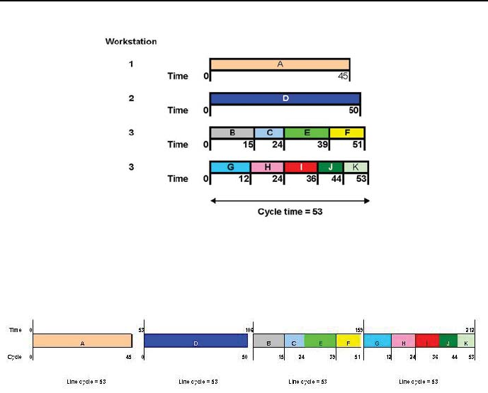
6.10 Assembly line balancing 375
Figure 6.6: Solution of ’cumulative’ for assembly line balancing
Figure 6.7: Gantt diagram for assembly line balancing
Minimum cycle time = 53
Workstation for A: 1 Start A = 0
Workstation for B: 3 Start B = 0
Workstation for C: 3 Start C = 15
Workstation for D: 2 Start D = 0
Workstation for E: 3 Start E = 24
Workstation for F: 3 Start F = 39
Workstation for G: 4 Start G = 0
Workstation for H: 4 Start H = 12
Workstation for I: 4 Start I = 24
Workstation for J: 4 Start J = 36
Workstation for K: 4 Start K = 44
Delayed goals:
gfd : gfd_do_propagate(gfd_prob(nvars(35)))
Yes (1258.02s cpu)

376 Chapter 6. CLP with global constraints for optimal solutions
6.11 Reading newspapers 1
Let’s have a look at a more complicated scheduling example. Its purpose is to
show how to solve scheduling problems were cumulative and precedence con-
straints occur:
Four bright youngsters (Andy, Ben, Carl and Dusty) are studying Commu-
nity Organizing, with a major in Deceptions,Tensions and Scares,atthebest
Absurdoland’s university. They share a flat to which each morning the Univer-
sity Administration delivers four of the most influential Absurdoland’s newspa-
pers. They are: Mainstream Drivel (MD), Daily Absurdities (DA), Morning
Brainwasher (MB) and Gutter News (GN). The students get up at different
times and are ready to start reading at different times, as shown in Table 6.2.
There also the reading orders and reading durations for all students may be
found. The problem is to determine the earliest time they can all - after having
read all newspapers - set off to the University4.
Actually, the problem is one of finding the start times for reading each newspa-
per by each student in a non-conflicting way. The solution is given by program
6_4_newspapers_1.ecl,where:
1) the non-overlapping constraint for reading newspapers is declared using
disjunctive/1;
2) the availability of only a single copy of each newspaper is declared using
cumulative/4;
3) time is divided into minutes with 08.00 taken as zero.
The program 6_4_newspapers_1.ecl5readsasfollows:
/*1*/ :- lib(ic).
/*2*/ :- lib(ic_edge_finder3).
/*3*/ :- lib(branch_and_bound).
/*4*/ top:-
/*5*/ A=[AMD,ADA,AMB,AGN], % reading start times for Andy
/*6*/ B=[BDA,BMB,BMD,BGN], % reading start times for Ben
/*7*/ C=[CMB,CDA,CMD,CGN], % reading start times for Carl
4The subject has been inspired by the report of [Duncan-90], who quotes French
([French-82]) as the author who originally posed the problem.
5This is an OST-type problem.

6.11 Reading newspapers 1 377
Students Task 1 Task 2 Task 3 Task 4
Andy starts To To To To
at 8.30 with read read read read
reading order: MD DA MB GN
and duration: 60 mins 30 mins 2 mins 5 mins
Ben starts To To To To
at 8.45 with read read read read
reading order: DA MB MD GN
and duration: 75 mins 3 mins 25 mins 10 mins
Carl starts To To To To
at 8.45 with read read read read
reading order: MB DA MD GN
and duration: 5 mins 15 mins 10 mins 30 mins
Dusty starts To To To To
at 9.30 with read read read read
reading order GN MD DA MB
and duration: 90 mins 5 mins 5 mins 5 mins
Table 6.2: Reading order duration for students and papers
/*8*/ D=[DGN,DMD,DDA,DMB], % reading start times for Dusty
/*9*/ End=[A_end,B_end,C_end,D_end],
/*10*/ % end of reading times for students
/*11*/ A :: 30..360,
/*12*/ B :: 45..360,
/*13*/ C :: 45..360,
/*14*/ D :: 105..360,
/*15*/ End :: 90..360,
/*16*/ End_of_Ends :: 90..360,
/*17*/ AMD#>=30,
/*18*/ ADA#>=AMD+60, % order constraints for Andy
/*19*/ AMB#>=ADA+30,
/*20*/ AGN#>=AMB+2,
/*21*/ A_end#>=AGN+5,
/*22*/ BDA#>=45,
/*23*/ BMB#>=BDA+75, % order constraints for Ben
/*24*/ BMD#>=BMB+3,
/*25*/ BGN#>=BMD+25,
/*26*/ B_end#>=BGN+10,

378 Chapter 6. CLP with global constraints for optimal solutions
/*27*/ CMB#>=45,
/*28*/ CDA#>=CMB+5, % order constraints for Carl
/*29*/ CMD#>=CDA+15,
/*30*/ CGN#>=CMD+10,
/*31*/ C_end#>=CGN+30,
/*32*/ DGN#>=105,
/*33*/ DMD#>=DGN+90, % order constraints for Dusty
/*34*/ DDA#>=DMD+5,
/*35*/ DMB#>=DDA+5,
/*36*/ D_end#>=DMB+5,
% Constraining the number of students reading a paper.
% Any paper may be read by one student only:
% reading "Mainstream Drivel":
/*37*/ disjunctive([AMD,BMD,CMD,DMD],[60,25,10,5]),
% reading "Daily Absurdities":
/*38*/ disjunctive([ADA,BDA,CDA,DDA],[30,75,15,5]),
% reading "Morning Brainwasher":
/*39*/ disjunctive([AMB,BMB,CMB,DMB],[2,3,5,9]),
% reading "Gutter Newsu":
/*40*/ disjunctive([AGN,BGN,CGN,DGN],[5,10,30,90]),
% Constraining the number of papers read by student.
% Any student may read only a single paper.
% reads Andy:
/*41*/ cumulative([AMD,ADA,AMB,AGN],[60,30,2,5],[1,1,1,1],1),
% reads Ben:
/*42*/ cumulative([BDA,BMB,BMD,BGN],[75,3,25,10],[1,1,1,1],1),
% reads Carl:
/*43*/ cumulative([CMB,CDA,CMD,CGN],[5,15,10,30],[1,1,1,1],1),
% reads Dusty:
/*44*/ cumulative([DGN,DMD,DDA,DMB],[90,5,5,5],[1,1,1,1],1),
/*45*/ maxlist(End,End_of_Ends),
/*46*/ minimize(labeling([AMD,ADA,AMB,AGN,BDA,BMB,BMD,BGN,
CMB,CDA,CMD,CGN,DGN,DMD,DDA,DMB,A_end,B_end,
C_end,D_end]), End_of_Ends),nl,
/*47*/ write("A = "),write(A),nl,
/*48*/ write("B = "),write(B),nl,
/*49*/ write("C = "),write(C),nl,
/*50*/ write("D = "),write(D),nl,
/*51*/ present_schedule([AMD,ADA,AMB,AGN,BDA,BMB,BMD,BGN,
CMB,CDA,CMD,CGN,DGN,DMD,DDA,DMB],
["Andy","Mainstream Drivel",60,
"Andy","Daily Absurdities",30,

6.11 Reading newspapers 1 379
"Andy","Morning Brainwasher",2,
"Andy","Gutter News",5,
"Ben","Daily Absurdities",75,
"Ben","Morning Brainwasher",3,
"Ben","Mainstream Drivel",25,
"Ben","Gutter News",10,
"Carl","Morning Brainwasher",5,
"Carl","Daily Absurdities",15,
"Carl","Mainstream Drivel",10,
"Carl","Gutter News",10,
"Dusty","Gutter News",90,
"Dusty","Mainstream Drivel",5,
"Dusty","Daily Absurdities",5,
"Dusty","Morning Brainwasher",5]).
/*52*/ present_schedule([],[]):-nl.
/*53*/ present_schedule([H1|T1],[H21,H22,H23|T2]) :-
/*54*/ convert_time(H1, FG, FM),
/*55*/ HH is H1+H23,
/*56*/ convert_time(HH, TG, TM),nl,
/*57*/ write(H21),write(" reads "),write(H22),write(" from "),
/*58*/ write(FG),write(":"),write(FM),
/*59*/ write(" to "),write(TG),write(":"),write(TM),
/*60*/ present_schedule(T1,T2).
/*61*/ convert_time(Time,Hours,Minutes) :-
/*62*/ div(Time, 60, G),
/*63*/ Hours is G + 8,
/*64*/ mod(Time,60,Minutes).
The message is:
Found a solution with cost 338
Found a solution with cost 263
Found a solution with cost 262
Found a solution with cost 257
Found a solution with cost 240
Found a solution with cost 238
Found a solution with cost 235
Found a solution with cost 210
A = [75, 140, 170, 195]
B = [65, 140, 143, 200]
C = [45, 50, 65, 75]
D = [105, 195, 200, 205]

380 Chapter 6. CLP with global constraints for optimal solutions
Andy reads "Mainstream Drivel" from 9:15 to 10:15
Andy reads "Daily Absurdities" from 10:20 to 10:50
Andy reads "Morning Brainwasher" from 10:50 to 10:52
Andy reads "Gutter News" from 11:15 to 11:20
Ben reads "Daily Absurdities" from 9:5 to 10:20
Ben reads "Morning Brainwasher" from 10:20 to 10:23
Ben reads "Mainstream Drivel" from 10:23 to 10:48
Ben reads "Gutter News" from 11:20 to 11:30
Carl reads "Morning Brainwasher" from 8:45 to 8:50
Carl reads "Daily Absurdities" from 8:50 to 9:5
Carl reads "Mainstream Drivel" from 9:5 to 9:15
Carl reads "Gutter News" from 9:15 to 9:25
Dusty reads "Gutter News" from 9:45 to 11:15
Dusty reads "Mainstream Drivel" from 11:15 to 11:20
Dusty reads "Daily Absurdities" from 11:20 to 11:25
Dusty reads "Morning Brainwasher" from 11:25 to 11:30
As can be seen, the readings finish at 11:25 and then all students may set-off to
the University.
The above message makes for hard reading. It is better presented as Gantt
charts, one for presenting student activities (see Figure 6.8), the other one pre-
senting the reading histories of papers (see Figure 6.9). The color codes for
boxes of the Gantt chart for papers are necessarily different from those of the
Gantt chart for students. Sticking to the same color codes would result in all
boxes of the Gantt chart for papers to have the same color for the same paper,
which would be rather uninformative.
It is obvious from those charts that the optimum reading order is not unique:
e.g. reading of MB by Andy, MD by Ben and GN by Carl could start a little
latter with no change to the minimum final time.
6.12 Reading newspapers 2
The problem could also be solved by a program that uses only the cumulative/4
global constraint, as shown in 6_5_newspapers_2.ecl6:
6This is an OST-type problem.
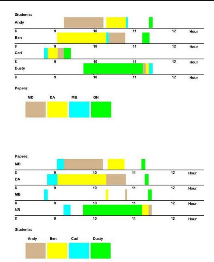
6.12 Reading newspapers 2 381
Figure 6.8: Gantt chart for students.
Figure 6.9: Gantt chart for papers.

382 Chapter 6. CLP with global constraints for optimal solutions
/*1*/ :- lib(ic).
/*2*/ :- lib(ic_edge_finder3).
/*3*/ :- lib(branch_and_bound).
/*4*/ top:-
/*5*/ A=[AMD,ADA,AMB,AGN], % reading start times for Andy
/*6*/ B=[BDA,BMB,BMD,BGN], % reading start times for Ben
/*7*/ C=[CMB,CDA,CMD,CGN], % reading start times for Carl
/*8*/ D=[DGN,DMD,DDA,DMB], % reading start times for Dusty
/*9*/ End=[A_end,B_end,C_end,D_end],
% end of reading times for students
/*10*/ A :: 30..360,
/*11*/ B :: 45..360,
/*12*/ C :: 45..360,
/*13*/ D :: 105..360,
/*14*/ End :: 90..360,
/*15*/ End_of_Ends :: 90..360,
/*16*/ AMD#>=30,
/*17*/ ADA#>=AMD+60, % order constraints for Andy
/*18*/ AMB#>=ADA+30,
/*19*/ AGN#>=AMB+2,
/*20*/ A_end#>=AGN+5,
/*21*/ BDA#>=45,
/*22*/ BMB#>=BDA+75, % order constraints for Ben
/*23*/ BMD#>=BMB+3,
/*24*/ BGN#>=BMD+25,
/*25*/ B_end#>=BGN+10,
/*26*/ CMB#>=45,
/*27*/ CDA#>=CMB+5, % order constraints for Carl
/*28*/ CMD#>=CDA+15,
/*29*/ CGN#>=CMD+10,
/*30*/ C_end#>=CGN+30,
/*31*/ DGN#>=105,
/*32*/ DMD#>=DGN+90, % order constraints for Dusty
/*33*/ DDA#>=DMD+5,
/*34*/ DMB#>=DDA+5,
/*35*/ D_end#>=DMB+5,
% Constraining the number of students reading a paper.
% Any paper may be read by one student only:
% reading "Mainstream Drivel":
/*36*/ cumulative([AMD,BMD,CMD,DMD],[60,25,10,5],[1,1,1,1],1),
% reading "Daily Absurdities":
/*37*/ cumulative([ADA,BDA,CDA,DDA],[30,75,15,5],[1,1,1,1],1),

6.12 Reading newspapers 2 383
% reading "Morning Brainwasher":
/*38*/ cumulative([AMB,BMB,CMB,DMB],[2,3,5,5],[1,1,1,1],1),
% reading "Gutter News":
/*39*/ cumulative([AGN,BGN,CGN,DGN],[5,10,30,90],[1,1,1,1],1),
% Constraining the number of papers read by student.
% Any student may read only a single paper.
% reads Andy:
/*40*/ cumulative([AMD,ADA,AMB,AGN],[60,30,2,5],[1,1,1,1],1),
% reads Ben:
/*41*/ cumulative([BDA,BMB,BMD,BGN],[75,3,25,10],[1,1,1,1],1),
% reads Carl:
/*42*/ cumulative([CMB,CDA,CMD,CGN],[5,15,10,30],[1,1,1,1],1),
% reads Dusty:
/*43*/ cumulative([DGN,DMD,DDA,DMB],[90,5,5,5],[1,1,1,1],1),
/*44*/ maxlist(End,End_of_Ends),
/*45*/ minimize(labeling([AMD,ADA,AMB,AGN,BDA,BMB,BMD,BGN,
CMB,CDA,CMD,CGN,DGN,DMD,DDA,DMB,A_end,B_end,
C_end,D_end]), End_of_Ends),nl,
/*46*/ write("A = "),write(A),nl,
/*47*/ write("B = "),write(B),nl,
/*48*/ write("C = "),write(C),nl,
/*49*/ write("D = "),write(D),nl,
/*50*/ present_schedule([AMD,ADA,AMB,AGN,BDA,BMB,BMD,BGN,
CMB,CDA,CMD,CGN,DGN,DMD,DDA,DMB],
["Andy","Mainstream Drivel",60,
"Andy","Daily Absurdities",30,
"Andy","Morning Brainwasher",2,
"Andy","Gutter News",5,
"Ben","Daily Absurdities",75,
"Ben","Morning Brainwasher",3,
"Ben","Mainstream Drivel",25,
"Ben","Gutter News",10,
"Carl","Morning Brainwasher",5,
"Carl","Daily Absurdities",15,
"Carl","Mainstream Drivel",10,
"Carl","Gutter News",10,
"Dusty","Gutter News",90,
"Dusty","Mainstream Drivel",5,
"Dusty","Daily Absurdities",5,
"Dusty","Morning Brainwasher",5]).
/*51*/ present_schedule([],[]):-nl.
/*52*/ present_schedule([H1|T1],[H21,H22,H23|T2]) :-
/*53*/ convert_time(H1, FG, FM),
/*54*/ HH is H1+H23,

384 Chapter 6. CLP with global constraints for optimal solutions
/*55*/ convert_time(HH, TG, TM),nl,
/*56*/ write(H21),write(" reads "),write(H22),write(" from "),
/*57*/ write(FG),write(":"),write(FM),
/*58*/ write(" to "),write(TG),write(":"),write(TM),
/*59*/ present_schedule(T1,T2).
%% Czasy przedstawiaja minuty po godzinie 08:00
/*60*/ convert_time(Time,Hours,Minutes) :-
/*61*/ div(Time, 60, G),
/*62*/ Hours is G + 8,
/*63*/ mod(Time,60,Minutes).
The message is:
Found a solution with cost 338
Found a solution with cost 263
Found a solution with cost 262
Found a solution with cost 257
Found a solution with cost 240
Found a solution with cost 238
Found a solution with cost 235
Found a solution with cost 210
A = [75, 140, 170, 195]
B = [65, 140, 143, 200]
C = [45, 50, 65, 75]
D = [105, 195, 200, 205]
Andy reads "Mainstream Drivel" from 9:15 to 10:15
Andy reads "Daily Absurdities" from 10:20 to 10:50
Andy reads "Morning Brainwasher" from 10:50 to 10:52
Andy reads "Gutter News" from 11:15 to 11:20
Ben reads "Daily Absurdities" from 9:5 to 10:20
Ben reads "Morning Brainwasher" from 10:20 to 10:23
Ben reads "Mainstream Drivel" from 10:23 to 10:48
Ben reads "Gutter News" from 11:20 to 11:30
Carl reads "Morning Brainwasher" from 8:45 to 8:50
Carl reads "Daily Absurdities" from 8:50 to 9:5
Carl reads "Mainstream Drivel" from 9:5 to 9:15
Carl reads "Gutter News" from 9:15 to 9:25
Dusty reads "Gutter News" from 9:45 to 11:15
Dusty reads "Mainstream Drivel" from 11:15 to 11:20

6.13 Reading newspapers 3 385
Dusty reads "Daily Absurdities" from 11:20 to 11:25
Dusty reads "Morning Brainwasher" from 11:25 to 11:30
The reading order is this time slightly different from what we got before.
Because of the non-uniqueness of the optimum solution, for the same minimum
final reading time 11:30 , Andy and Ben swapped their readings of ”Gutter
News”. As can be seen from the Gantt diagrams, this does not violate any
constraint.
6.13 Reading newspapers 3
The way data was introduced in the previous two programs was unwieldy and
and made their change difficult to handle.
Program 6_6_newspapers_3.ecl7presents a more professional approach to
data declaring; however, the price paid for this is poorer readability. The fol-
lowing important private predicates are used:
data(Data))
Data = [student(Name,Getting_ready_time,Papers)|Rest]
Papers = [Paper,Reading_time|Rest] =
= [Paper_1, Reading_time1,
Paper_2, Reading_time2, etc.]
constrain(Data,Readings,Start_times,End)
Readings = [reading(Name,Paper,Start,Reading_time)|Rest]
constrain_single_paper(Paper,Readings)
constrain_with_accu(Data,Reading_accu,Readings,
Start_times_accu,Start_times,End)
make_reading(Papers,Name,Getting_ready_time,Reading_accu,Readings,
Start_times_accu,Start_times)
collect_papers(Readings,Paper,Start_times_accu,Start_times,
Start_times_accu,Reading_times)
labeling(Start_times,End) - a private labeling predicate
The name accu denotes an accumulator for the relevant list.
The program 6_6_newspapers_3.ecl readsasfollows:
7This is an OST-type problem.

386 Chapter 6. CLP with global constraints for optimal solutions
/*1*/ :- lib(ic).
/*2*/ :- lib(ic_edge_finder3).
/*3*/ :- lib(branch_and_bound).
/*4*/ top:-
/*5*/ data(Data),
/*6*/ constrain(Data,Readings,Start_times,End),
/*7*/ minimize(labeling(Start_times,End),End),
/*8*/ present_schedule(Readings).
% Getting_ready_time in "Data"
% is given by minutes after 08:00:
/*9*/ data([
student("Andy",30,["MD",60,"DA",30,"MB",2,"GN",5]),
student("Ben",45,["DA",75,"MB",3,"MD",25,"GN",10]),
student("Carl",45,["MB",5,"DA",15,"MD",10,"GN",30]),
student("Dusty",104,["GN",90,"MD",5,"DA",5,"MB",5])]).
/*10*/constrain(Data,Readings,Start_times,End):-
/*11*/ End :: 0..363,
/*12*/ constrain_with_accu(Data,[],Readings,[],Start_times,End),
/*13*/ constrain_single_paper("MD",Readings),
/*14*/ constrain_single_paper("DA",Readings),
/*15*/ constrain_single_paper("MB",Readings),
/*16*/ constrain_single_paper("GN",Readings).
% Make a series of "readings" for all students:
/*17*/constrain_with_accu([],Readings,Readings,Start_times,
Start_times,_).
/*18*/constrain_with_accu([student(Name,Getting_ready_time,
[Paper,Reading_time|Rest])|Remaining],Reading_accu,
Readings,Start_times_accu,Start_times,End):-
% Make readings for "Name":
/*19*/ Start :: Getting_ready_time..363,
/*20*/ Next_time is Getting_ready_time + Reading_time,
/*21*/ make_reading(Rest,Name,Next_time,
[reading(Name,Paper,Start,Reading_time)|Reading_accu],
Read1,[Start|Start_times_accu],Start1),
/*22*/ Read1 = [reading(Name,_,S1,D1)|_],
% Make "End" not less than the end_time for the
% last reading of the student. Hence "End" will finally be equal
% to the end of the last reading of the latest student:
/*23*/ End #>= S1+D1,
/*24*/ constrain_with_accu(Remaining,Read1,Readings,Start1,
Start_times,End).
% Make a "reading" for the student "Name"

6.13 Reading newspapers 3 387
% and constrain his sequence of readings:
/*25*/make_reading([],_,_,Readings,Readings,Start_times,
Start_times).
/*26*/make_reading([Paper,Reading_time|Rest],Name,
Next_time,Reading_accu,Read,Start_times_accu,Starts):-
/*27*/ Start :: Next_time..363,
/*28*/ Reading_accu = [reading(Name,_,S1,D1)|_],
/*29*/ Start #>= S1+D1,
/*30*/ Next_End is Next_time+Reading_time,
/*31*/ make_reading(Rest,Name,Next_End,
[reading(Name,Paper,Start,Reading_time)|Reading_accu],
Read,[Start|Start_times_accu],Starts).
% Collect all "readings" for "Paper"
% and enforce non-overlapping of readings
% using the global constraint "cumulative/4":
/*32*/constrain_single_paper(Paper,Readings):-
/*33*/ collect_papers(Readings,Paper,[],Starts,[],
Reading_times),
/*34*/ cumulative(Starts,Reading_times,[1,1,1,1],1).
% Collect all start times and reading times for "Paper":
/*35*/collect_papers([],_,S,S,D,D).
/*36*/collect_papers([reading(_,Paper,S,D)|Rest],
Paper,S0,S1,D0,D1):- !,
/*37*/ collect_papers(Rest,Paper,[S|S0],S1,[D|D0],D1).
/*38*/collect_papers([_|Rest],Paper,S0,S1,D0,D1):-
/*39*/ collect_papers(Rest,Paper,S0,S1,D0,D1).
% Instantiate variables using the "firts fail" heuristic:
/*40*/labeling([],End):-
/*41*/ indomain(End,min),
/*42*/ convert_time(End,Hours,Minutes),
/*43*/ write("Readings are found for final time "),write(Hours),
write(":"),write(Minutes),nl.
/*44*/labeling(Start_times,End):-
/*45*/ select(Variable,Start_times,Rest,0,first_fail),
/*46*/ indomain(Variable),
/*47*/ labeling(Rest,End).
% The private predicate "select(Variable,List,Rest,Flag,Heuristic)"
% uses the standard constraint "delete/5".
% If "List" is not empty, backtrackings are possible:
/*48*/select(_, [], _, _, _):-
/*49*/ !,
/*50*/ fail.
/*51*/select(Variable, List, Rest, Flag, Heuristic):-
/*52*/ delete(Variable,List,Rest,Flag, Heuristic).

388 Chapter 6. CLP with global constraints for optimal solutions
% Present schedule:
/*53*/present_schedule([]).
/*54*/present_schedule([reading(Name,Paper,Start,
Reading_time)|Rest]):-
/*55*/ convert_time(Start, FH, FM),
/*56*/ HH is Start+Reading_time,
/*57*/ convert_time(HH, TH, TM),
/*58*/ write(Name),write(" reads "),write(Paper),write(" from "),
write(FH),write(":"),write(FM),
/*59*/ write(" to "),write(TH),write(":"),write(TM),nl,
/*60*/ present_schedule(Rest).
% Convert time:
/*61*/convert_time(Time,Hours,Minutes) :-
/*62*/ div(Time, 60, G),
/*63*/ Hours is G + 8,
/*64*/ mod(Time,60,Minutes).
The following message is generated:
Readings are found for final time 11:45
Found a solution with cost 225
Readings are found for final time 11:30
Found a solution with cost 210
Found no solution with cost 195.0 .. 209.0
Dusty reads MB from 11:25 till 11:30
Dusty reads DA from 11:20 till 11:25
Dusty reads MD from 11:15 till 11:20
Dusty reads GN from 9:45 till 11:15
Carl reads GN from 9:15 till 9:45
Carl reads MD from 9:5 till 9:15
Carl reads DA from 8:50 till 9:5
Carl reads MB from 8:45 till 8:50
Ben reads GN from 11:15 till 11:25
Ben reads MD from 10:23 till 10:48
Ben reads MB from 10:20 till 10:23
Ben reads DA from 9:5 till 10:20
Andy reads GN from 11:25 till 11:30
Andy reads MB from 10:50 till 10:52
Andy reads DA from 10:20 till 10:50

6.14 Assembling bicycles 389
Andy reads MD from 9:15 till 10:15
The schedule differs from what was obtained by 6_4_newspapers_1.ecl
and 6_5_newspapers_2.ecl, the minimum reading time remains unchanged;
this being a proof of multiple optimum solutions.
6.14 Assembling bicycles
This is yet another example of scheduling with cumulative and precedence con-
straints. It was inspired by the distinguished discrete mathematician Ronald
Graham who wrote an enlightened essay on a fictitious bicycle assembly plant
named ACME , see [Graham-78]. This essay will form the basis of an instruc-
tive scheduling program; ’instructive’ means that it shows the unreliability and
weakness of human intuition even if confronted with a simple scheduling prob-
lem. What follows is a large quote from Graham, slightly modified to make the
problem more difficult and interesting:
”Things have not been going too well in the assembling section of the ACME
Bicycle Company. For the past six month, the section had consistently failed to
meet its quota and heads were beginning to roll. A newly appointed foreman of
the assembling section has been brought in to remedy this sad state of affairs.
He realizes that this is his big chance the catch the eye of upper management,
so that the first day on the job he rolls up his sleeves and begins finding out
everything about what goes on in the section.
The first thing he learns is that the overall job of assembling a bicycle is usually
broken up into a number of specific smaller tasks:
A - Frame preparation which includes installation of the
front fork and fenders.
B - Mounting and aligning front wheel.
C - Mounting and aligning back wheel.
D - Attaching the derailleur to the frame.
E - Installing the gear cluster.
F - Attaching the chain wheel to the crank.
G - Attaching the crank and chain wheel to the frame.
H - Mounting right pedal and toe clip.
I - Mounting left pedal and toe clip.
J - Final attachments which includes mounting and adjusting

390 Chapter 6. CLP with global constraints for optimal solutions
handlebars, seat, brakes, etc.8
He also learns that his recently departed predecessor had collected reams of
data on how long (in the mean, in minutes) each of these various tasks takes
a trained assembler to perform, which he had conveniently summarized in the
following table:
Tasks: A B CDEFGHIJ
Time: 7 7 722228818
Because of space and equipment constraints in the shop, the 20 assemblers in
the section are usually paired up into 10 teams of 2assemblers each, with each
team assembling one bicycle at a time. The foreman made a quick calculation:
one bicycle requires altogether 63 minutes of total assembly time, so a team of
two should manage this in 31.5 minutes. This means that in an eight-hour day,
each team could assemble 15.23 bicycles and with all 10 teams doing this, the
quota of 152 bicycles per day can be met. The new foreman can already taste
his next year promotion.
His enthusiasm dwindles considerably, however, when he realizes that bicycles
can’t be put together in a random order. Certain tasks must be done before
certain others. For example, it is extremely awkward to mount the front fork to
the frame of a bicycle, if the handlebars have already been attached to the fork.
Similarly, the crank must be mounted on the frame before the pedals can be
attached. After lengthy discussion with several of the experienced assemblers,
the new foreman prepares the following chart showing which tasks must be done
before others during assembly:
A, B, C, D, E must be done before J
D, E, A must be done before C
D must be done before E, F
E, F, G must be done before H, I
F must be done before G
A must be done before B
In addition to this mechanical constraints on the work schedule, there are
8To paraphrase Benedykt Chmielowski (1700-1763), who in the first Polish encyclopedia
”New Athens” for the entry ”Horse” included only one short sentence: ”Everybody knows
what a horse is like”, it can be said that ”Everybody knows what a bicycle is like”andrefrain
from displaying the nice picture of the ACME bicycle, to be found in the original Graham
publication.
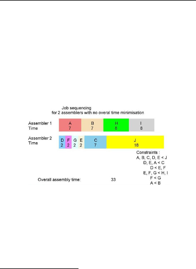
6.14 Assembling bicycles 391
also two rules (known locally as ”busy” rules) that management requires to
observe during working hours:
Rule 1: No assembler can be idle if there is some task he or she can be doing.
Rule 2: Once an assembler starts a task, he or she must continue working on
the task until it is completed.
The customary order of assembling bicycles at Acme Bicycles has always
been the following one:
Task A BCDEFGHIJ
Start time 1, 8, 9, 1, 7, 3, 5, 15, 23, 16,
shown in the Gantt chart in Figure 6.10.
Figure 6.10: First (customary) schedule for bicycle assembling
The schedule shows the activity of each assembler of the team beginning at
time 1and progressing to the time of completed assembly, called the overall
assembling time,some33 minutes latter. Although this schedule obeys all
the required order-of-assembly constraints given above, it allows each team to
complete only 14.5 bicycles per day. Thus the total output of the section is 145
bicycles per day, well under the quota of 152.”9.
After wasting numerous pieces of paper trying out various alternative sched-
ules with no success, the foreman decided to ask a well-known CLP specialist for
9This ends for the time being the quotation from [Graham-78].
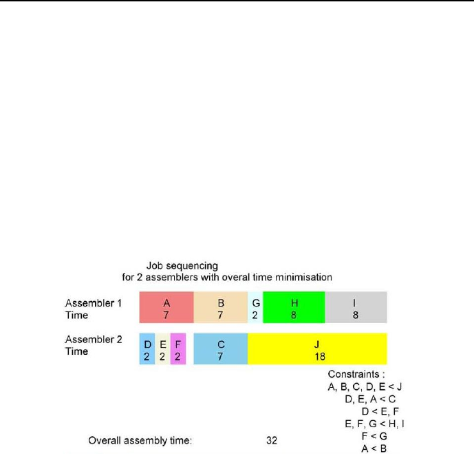
392 Chapter 6. CLP with global constraints for optimal solutions
help. This specialist presented many solutions included in the 6_7_bicycles.clp.
The first solution generates a schedule that minimizes the overall assembling
time. It is called by the query top1. This schedule (referred to as second
schedule) may be described by the following lists, with consecutive positions
corresponding to jobs A,B,...J:
Start times = [1, 8, 8, 1, 3, 5, 15, 17, 25, 15]
Durations = [7, 7, 7, 2, 2, 2, 2, 8, 8, 18]
End times = [8, 15, 15, 3, 5, 7, 17, 25, 33, 33]
End = 33
Assembling time = 32,
and visualized by the Gantt chart from Figure 6.11.
Figure 6.11: Second (optimum) schedule for bicycle assembling
Unfortunately, the overall assembling time is still over the expected 31.5 min-
utes. What’s more - Rule 1 has been violated because between job Fand job C
an illegal 1-minute long inactivity is found. The foreman wants to eliminate it
by changing the objective function: instead of minimizing the overall assembling
time, the sum of end times for all jobs should be minimized. The CLP specialist
wrote a program called by top2 from 6_7_bicycles.clp. The result is:
Start times = [1, 8, 9, 1, 3, 5, 7, 15, 16, 23]
Durations = [7, 7, 7, 2, 2, 2, 2, 8, 8, 18]
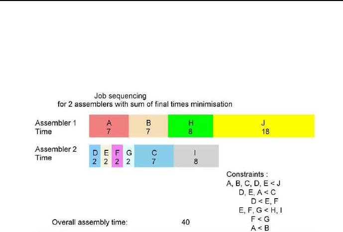
6.14 Assembling bicycles 393
End times = [8, 15, 16, 3, 5, 7, 9, 23, 24, 41]
End = 41
Assembling time = 40,
visualized by the Gantt chart from Figure 6.12.
Figure 6.12: Third schedule for bicycle assembling
Obviously, this schedule is a calamity. Let us return to quoting from [Graham-78]:
”The foreman decides, in haste, to furnish all the assemblers with rented electric
powertools. This decreases the time of each of the jobs by exactly one minute, so
the total time required for all jobs is only 53 minutes.” Now the CLP specialist
is checking what happens if - in order to eliminate idle times, the sum of end
times for all jobs should be once more minimized. The CLP specialist wrote a
program called by top3 from 6_7_bicycles.clp. The result is:
Start times = [1, 7, 12, 1, 2, 3, 4, 5, 13, 18]
Durations = [6, 6, 6, 1, 1, 1, 1, 7, 7, 17]
End times = [7, 13, 18, 2, 3, 4, 5, 12, 20, 35]
End = 35
Assembling time = 34,
visualized by the Gantt chart from Figure 6.13.
This is rather bad. The assembling time is 35 minutes, to say nothing about
the 17 minuteslongidletimeattheendofjobI.
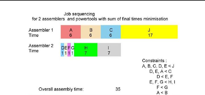
394 Chapter 6. CLP with global constraints for optimal solutions
Figure 6.13: Fourth schedule for bicycle assembling
If instead the overall assembling time is minimized, the result is given by
the top4 part of the program, which generates the schedule:
Start times = [1, 7, 7, 1, 2, 3, 4, 13, 20, 13]
Durations = [6, 6, 6, 1, 1, 1, 1, 7, 7, 17]
End times = [7, 13, 13, 2, 3, 4, 5, 20, 27, 30]
End = 30
Assembling time = 29,
visualized by the Gantt chart from Figure 6.14.
Unfortunately, it contains a 2-minute long idle time between jobs Gand C.
The foreman resorts to a brute -force approach: he hires 10 extra assemblers
and decree that from now on, each of the 10 teams will consists of three assem-
blers working together to put the miserable bicycle together. He realized that
this increases the labor cost by 50%, but he is determined to meet the quota.
However, the CLP specialist warns him that additional 10 assemblers would not
increase the production because of the order-of-assembly constraints. This he
demonstrates by the top4 part of this program, which generates a schedule:
Start times = [1, 8, 8, 1, 3, 3, 5, 7, 15, 15]
Durations = [7, 7, 7, 2, 2, 2, 2, 8, 8, 18]
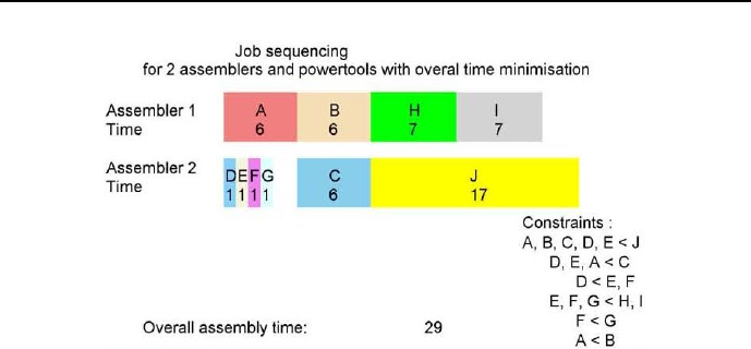
6.14 Assembling bicycles 395
Figure 6.14: Fifth schedule for bicycle assembling
End times = [8, 15, 15, 3, 5, 5, 7, 15, 23, 33]
End = 33
Assembling time = 32,
visualized by the Gantt chart from Figure 6.15.
It happens that the minimum assembling time for 3assemblers is exactly
the same as for two assemblers, see Figure 6.10. The foreman - desperate as
he is - hires another 10 assemblers and decrees that from now on, each of the
10 teams will consists of four assemblers working together. The CLP specialist
warns him again that this will be of no avail and demonstrates that by writing
the top5 part of his program, which generates the schedule:
Start times = [1, 8, 8, 1, 3, 3, 5, 7, 7, 15]
Durations = [7, 7, 7, 2, 2, 2, 2, 8, 8, 18]
End times = [8, 15, 15, 3, 5, 5, 7, 15, 15, 33]
End = 33
Assembling time = 32,
visualized by the Gantt chart from Figure 6.16.
The foreman, which brought ACME to the verge of bankruptcy, was fired on
short notice: the termination notice arrived at the end of the week. I have been
informed that after a number of sleepless nights he decided to offer his services
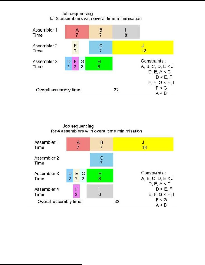
396 Chapter 6. CLP with global constraints for optimal solutions
Figure 6.15: Sixth schedule for bicycle assembling
Figure 6.16: Seventh schedule for bicycle assembling
to the popular All Things to All People political party10 which enthusiastically
commissioned him - because of his industrial expertise - to create a lobbying
service for providing manufacturing industries with financial bailouts by the
10 A long time ago Alexis de Tocqueville (1805–1859) remarked in his famous ”Democracy
in America” book that ”In America there are so many ways of making a living that a man
doesn’t usually enter politics until he has failed at everything else”. Does it happen only in
America? And only in such remote ages?

6.14 Assembling bicycles 397
Absurdoland Government.
The conclusion is that getting more man-power to even such menial job as
bicycle assembling is no guarantee of success. Let’s quote [Graham-78] the last
time: ”One might well ask just where it was that our hypothetical foreman at
ACME Bicycle did go wrong. It will turn out that he was a victim of Rules 1
and 2(and a little bad luck). The short-sighted greediness resulted, as it often
does, in an overall loss of performance of the system as a whole. In each case,
assemblers were forced (by Rule 1) to start working on jobs that they couldn’t
interrupt (by Rule 2) when a more urgent job eventually cam up.”
The program 6_7_bicycles.ecl11 is as follows:
/*1*/ :- lib(ic).
/*2*/ :- lib(ic_edge_finder3).
/*3*/ :- lib(branch_and_bound).
/*4*/ top:-
/*5*/ top1,
/*6*/ top2,
/*7*/ top3,
/*8*/ top4,
/*9*/ top5,
/*10*/ top6.
% Minimizing assembly time for two assemblers:
/*11*/ top1:-
/*12*/ declare_domains(Start_Times,Resources),
/*13*/ Assembling_Times = [7, 7, 7, 2, 2, 2, 2, 8, 8,18],
/*14*/ End_Times = [_, _, _, _, _, _, _, _, _, _],
/*15*/ End_Times :: 1..200,
/*16*/ Limit :: 2,
/*17*/ constraints(Start_Times),
/*18*/ cumulative(Start_Times,Assembling_Times,Resources,Limit),
/*19*/ end_times(Start_Times,Assembling_Times,End_Times,
End),
/*20*/ bb_min(search(Start_Times,0,smallest,indomain_min,
bbs(1),[]),End, bb_options{delta:1,timeout:60}),
/*21*/ Assembling_Time is End - 1,
/*22*/ write("Minimizing assembly time for two assemblers:"),
/*23*/ write_results(Start_Times,Assembling_Times,End_Times,
11 This is an OST-type problem.

398 Chapter 6. CLP with global constraints for optimal solutions
End,Assembling_Time).
% Minimizing sum of end times for two assemblers:
/*24*/ top2:-
/*25*/ declare_domains(Start_Times,Resources),
/*26*/ Assembling_Times = [7, 7, 7, 2, 2, 2, 2, 8, 8, 18],
/*27*/ End_Times = [K1,K2,K3,K4,K5,K6,K7,K8,K9,K10],
/*28*/ End_Times :: 1..200,
/*29*/ Limit :: 2,
/*30*/ constraints(Start_Times),
/*31*/ cumulative(Start_Times,Assembling_Times,Resources,Limit),
/*32*/ end_times(Start_Times,Assembling_Times,End_Times,
End),
/*33*/ Sum_of_End_Times #= K1+K2+K3+K4+K5+K6+K7+K8+K9+K10,
/*34*/ bb_min(search(Start_Times,0,smallest,indomain_min,
bbs(1),[]),Sum_of_End_Times, bb_options{delta:1,timeout:60}),
/*35*/ Assembling_Time is End - 1,
/*36*/ write("Minimizing sum of end times for two assemblers:"),
/*37*/ write_results(Start_Times,Assembling_Times,End_Times,
End,Assembling_Time).
% Minimizing sum of end times for two assemblers and power tools:
/*38*/ top3:-
/*39*/ declare_domains(Start_Times,Resources),
/*40*/ Assembling_Times = [6, 6, 6, 1, 1, 1, 1, 7, 7, 17],
/*41*/ End_Times = [K1,K2,K3,K4,K5,K6,K7,K8,K9,K10],
/*42*/ End_Times :: 1..200,
/*43*/ Limit :: 2,
/*44*/ constraints_for_power_tools(Start_Times),
/*45*/ cumulative(Start_Times,Assembling_Times,Resources,Limit),
/*46*/ end_times(Start_Times,Assembling_Times,End_Times,
End),
/*47*/ Sum_of_End_Times #= K1+K2+K3+K4+K5+K6+K7+K8+K9+K10,
/*48*/ bb_min(search(Start_Times,0,smallest,indomain_min,
bbs(1),[]),Sum_of_End_Times, bb_options{delta:1,timeout:60}),
/*49*/ Assembling_Time is End - 1,
/*50*/ write("Minimizing sum of end times for two assemblers
and power tools:"),
/*51*/ write_results(Start_Times,Assembling_Times,End_Times,
End,Assembling_Time).

6.14 Assembling bicycles 399
% Minimizing assembly time for two assemblers and power tools:
/*52*/ top4:-
/*53*/ declare_domains(Start_Times,Resources),
/*54*/ Assembling_Times = [6, 6, 6, 1, 1, 1, 1, 7, 7, 17],
/*55*/ End_Times = [_, _, _, _, _, _, _, _, _, _],
/*56*/ End_Times :: 1..200,
/*57*/ Limit :: 2,
/*58*/ constraints_for_power_tools(Start_Times),
/*59*/ cumulative(Start_Times,Assembling_Times,Resources,Limit),
/*60*/ end_times(Start_Times,Assembling_Times,End_Times,
End),
/*61*/ bb_min(search(Start_Times,0,first_fail,indomain,
bbs(1),[]),End, bb_options{delta:1,timeout:60}),
/*62*/ Assembling_Time is End - 1,
/*63*/ write("Minimizing assembly time for two assemblers
and power tools:"),
/*64*/ write_results(Start_Times,Assembling_Times,End_Times,
End,Assembling_Time).
% Minimizing assembly time for three assemblers:
/*65*/ top5:-
/*66*/ declare_domains(Start_Times,Resources),
/*67*/ Assembling_Times = [7, 7, 7, 2, 2, 2, 2, 8, 8,18],
/*68*/ End_Times = [_, _, _, _, _, _, _, _, _, _],
/*69*/ End_Times :: 1..200,
/*70*/ Limit :: 3,
/*71*/ constraints(Start_Times),
/*72*/ cumulative(Start_Times,Assembling_Times,Resources,Limit),
/*73*/ end_times(Start_Times,Assembling_Times,End_Times,
End),
/*74*/ bb_min(search(Start_Times,0,first_fail,indomain,
bbs(1),[]),End, bb_options{delta:1,timeout:60}),
/*75*/ Assembling_Time is End - 1,
/*76*/ write("Minimizing assembly time for three assemblers:"),
/*77*/ write_results(Start_Times,Assembling_Times,End_Times,
End,Assembling_Time).
% Minimizing assembly time for four assemblers:
/*78*/ top6:-
/*79*/ declare_domains(Start_Times,Resources),
/*80*/ Assembling_Times = [7, 7, 7, 2, 2, 2, 2, 8, 8,18],
/*81*/ End_Times = [_, _, _, _, _, _, _, _, _, _],
/*82*/ End_Times :: 1..200,

400 Chapter 6. CLP with global constraints for optimal solutions
/*83*/ Limit :: 4,
/*84*/ constraints(Start_Times),
/*85*/ cumulative(Start_Times,Assembling_Times,Resources,Limit),
/*86*/ end_times(Start_Times,Assembling_Times,End_Times,
End),
/*87*/ bb_min(search(Start_Times,0,first_fail,indomain,
bbs(1),[]),End, bb_options{delta:1,timeout:60}),
/*88*/ Assembling_Time is End - 1,
/*89*/ write("Minimizing assembly time for four assemblers:"),
/*90*/ write_results(Start_Times,Assembling_Times,End_Times,
End,Assembling_Time).
/*91*/ declare_domains(Start_Times,Resources):-
/*92*/ Start_Times = [_, _, _, _, _, _, _, _, _, _],
/*93*/ Resources = [_, _, _, _, _, _, _, _, _, _],
/*94*/ Start_Times :: 1..100,
/*95*/ Resources :: 1.
/*96*/ constraints([A,B,C,D,E,F,G,H,I,J]):-
/*97*/ A + 7 #=< J,
/*98*/ B + 7 #=< J,
/*99*/ C + 7 #=< J,
/*100*/ D + 2 #=< J,
/*101*/ E + 2 #=< J,
/*102*/ A + 7 #=< C,
/*103*/ D + 2 #=< C,
/*104*/ E + 2 #=< C,
/*105*/ D + 2 #=< E,
/*106*/ D + 2 #=< F,
/*107*/ E + 2 #=< H,
/*108*/ F + 2 #=< H,
/*109*/ G + 2 #=< H,
/*110*/ E + 2 #=< I,
/*111*/ F + 2 #=< I,
/*112*/ G + 2 #=< I,
/*113*/ F + 2 #=< G,
/*114*/ A + 7 #=< B.
/*115*/ constraints_for_power_tools([A,B,C,D,E,F,G,H,I,J]):-
/*116*/ A + 6 #=< J,
/*117*/ B + 6 #=< J,
/*118*/ C + 6 #=< J,
/*119*/ D + 1 #=< J,
/*120*/ E + 1 #=< J,
/*121*/ A + 6 #=< C,
/*122*/ D + 1 #=< C,

6.14 Assembling bicycles 401
/*123*/ E + 1 #=< C,
/*124*/ D + 1 #=< E,
/*125*/ D + 1 #=< F,
/*126*/ E + 1 #=< H,
/*127*/ F + 1 #=< H,
/*128*/ G + 1 #=< H,
/*129*/ E + 1 #=< I,
/*130*/ F + 1 #=< I,
/*131*/ G + 1 #=< I,
/*132*/ F + 1 #=< G,
/*133*/ A + 6 #=< B.
/*134*/ end_times(Start_Times,Assembling_Times,End_Times,End):-
/*135*/ ( foreach(S,Start_Times),
/*136*/ foreach(D,Assembling_Times),
/*137*/ foreach(K,End_Times)
/*138*/ do
/*139*/ K #= S + D
/*140*/ ),
/*141*/ End #= max(End_Times).
/*142*/ write_results(Start_Times,Assembling_Times,End_Times,
End,Assembling_Time):-
/*143*/ printf("%2n Start times =
[%d, %d, %d, %d, %d, %d, %d, %d, %d, %d].%n", Start_Times),
/*144*/ printf(" Assembling times =
[%d, %d, %d, %d, %d, %d, %d, %d, %d, %d].%n", Assembling_Times),
/*145*/ printf(" End times =
[%d, %d, %d, %d, %d, %d, %d, %d, %d, %d].%n", End_Times),
/*146*/ printf(" End = %d%2n", End),
/*147*/ printf(" Overall assembling time: =
%d%2n", Assembling_Time).
The message is:
Found a solution with cost 41
Found a solution with cost 34
Found a solution with cost 33
Minimizing assembly time for two assemblers:
Start times = [1, 8, 8, 1, 3, 5, 15, 17, 25, 15].
Assembling times = [7, 7, 7, 2, 2, 2, 2, 8, 8, 18].
End times = [8, 15, 15, 3, 5, 7, 17, 25, 33, 33].
End=33
Overall assembling time: = 32
Found a solution with cost 151

402 Chapter 6. CLP with global constraints for optimal solutions
Found no solution with cost 121.0 .. 150.0
Minimizing sum of end times for two assemblers::
Start times = [1, 8, 9, 1, 3, 5, 7, 15, 16, 23].
Assembling times = [7, 7, 7, 2, 2, 2, 2, 8, 8, 18].
End times = [8, 15, 16, 3, 5, 7, 9, 23, 24, 41].
End=41
Overall assembling time: = 40
Found a solution with cost 119
Found no solution with cost 97.0 .. 118.0
Minimizing sum of end times for two assemblers
and power_tools:
Start times = [1, 7, 12, 1, 2, 3, 4, 5, 13, 18].
Assembling times = [6, 6, 6, 1, 1, 1, 1, 7, 7, 17].
End times = [7, 13, 18, 2, 3, 4, 5, 12, 20, 35].
End=35
Overall assembling time: = 34
Found a solution with cost 37
Found a solution with cost 30
Minimizing assembly time for two assemblers and power tools:
Start times = [1, 7, 7, 1, 2, 3, 4, 13, 20, 13].
Assembling times = [6, 6, 6, 1, 1, 1, 1, 7, 7, 17].
End times = [7, 13, 13, 2, 3, 4, 5, 20, 27, 30].
End=30
Overall assembling time: = 29
Found a solution with cost 33
Minimizing assembly time for three assemblers:
Start times = [1, 8, 8, 1, 3, 3, 5, 7, 15, 15].
Assembling times = [7, 7, 7, 2, 2, 2, 2, 8, 8, 18].
End times = [8, 15, 15, 3, 5, 5, 7, 15, 23, 33].
End=33
Overall assembling time: = 32
Found a solution with cost 33
Minimizing assembly time for four assemblers:
Start times = [1, 8, 8, 1, 3, 3, 5, 7, 7, 15].
Assembling times = [7, 7, 7, 2, 2, 2, 2, 8, 8, 18].
End times = [8, 15, 15, 3, 5, 5, 7, 15, 15, 33].
End=33
Overall assembling time: = 32

6.15 Ship unloading and loading 403
6.15 Ship unloading and loading
The built-in cumulative is also available with 5arguments as cumulative/5:
cumulative(+StartTimes,+Durations,+Resources,+Areas,++Limit)
where Areas is a list of areas covered by tasks. The areas are given as products
of duration and resource usage for all tasks. If:
Durations = [D1,...,Dn],and
Resources = [R1,...,Rn],then
Areas = [A1,...,An] with:
Ai = Di*Ri .
To program those products is up to the user. This global constraint will be
useful to solve the following example first solved using CHIP by [Aggoun-93]:
The problem is to determine a schedule that minimizes the time to unload
and load a ship. The work consists of 34 tasks, each one to be handled by a
number of dockers during a given period of time. For each task the product of
the number of dockers and time needed, expressed as man-hours12, is given, see
Table 6.3.
These man-hours correspond to the areas in cumulative/5. The constraint
for man-hours is quite natural for this kind of tasks.
The job of unloading and loading should be done by a team of 12 dockers,
each one to be employed no longer than 8 hours. The minimum-time schedule
is determined by program 6_8_ship.ecl13:
/*1*/ :- lib(ic).
/*2*/ :- lib(ic_edge_finder3).
/*3*/ :- lib(branch_and_bound).
/*4*/ top:-
% List of task start times:
/*5*/ LS = [S1,S2,S3,S4,S5,S6,S7,S8,S9,S10,S11,
S12,S13,S14,S15,S16,S17,S18,S19,S20,S21,S22,
S23,S24,S25,S26,S27,S28,S29,S30,S31,S32,S33,S34],
% List of task durations:
/*6*/ LD = [D1,D2,D3,D4,D5,D6,D7,D8,D9,D10,D11,
12 A man-hour - the amount of work performed by an average docker in an hour.
13 This is an OST-type problem.
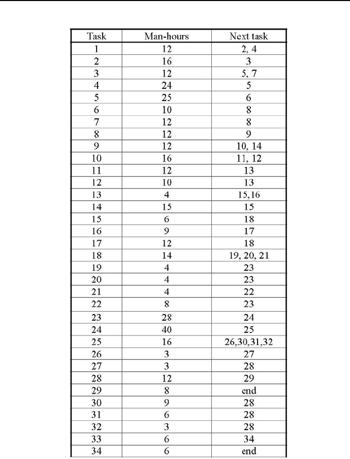
404 Chapter 6. CLP with global constraints for optimal solutions
Table 6.3: Tasks for ship unloading and loading

6.15 Ship unloading and loading 405
D12,D13,D14,D15,D16,D17,D18,D19,D20,D21,D22,
D23,D24,D25,D26,D27,D28,D29,D30,D31,D32,D33,D34],
% List of task manpower requirements - list of number of dockers
% needed to accomplish the tasks:
/*7*/ LR = [R1,R2,R3,R4,R5,R6,R7,R8,R9,R10,R11,
R12,R13,R14,R15,R16,R17,R18,R19,R20,R21,R22,
R23,R24,R25,R26,R27,R28,R29,R30,R31,R32,R33,R34],
% List of task surfaces - list of man-hours needed to accomplish the tasks:
/*8*/ LF = [12,16,12,24,25,10,12,12,12,16,12,
10,4,15,6,9,12,14,4,4,4,8,
28,40,16,3,3,12,8,9,6,3,6,6],
/*9*/ LS :: 1..400,
/*10*/ LD :: 1..40,
/*11*/ LR :: 1..12,
/*12*/ End :: 1..400,
/*13*/ Limit :: 1..12,
/*14*/ cumulative(LS,LD,[R1,R2,R3,R4,R5,R6,R7,R8,R9,R10,R11,
R12,R13,R14,R15,R16,R17,R18,R19,R20,R21,R22,
R23,R24,R25,R26,R27,R28,R29,R30,R31,R32,R33,R34],
LF,Limit),
/*15*/ S1 + D1 #=< S2,
/*16*/ S1 + D1 #=< S4,
/*17*/ S2 + D2 #=< S3,
/*18*/ S3 + D3 #=< S5,
/*19*/ S3 + D3 #=< S7,
/*20*/ S4 + D4 #=< S5,
/*21*/ S5 + D5 #=< S6,
/*22*/ S6 + D6 #=< S8,
/*23*/ S7 + D7 #=< S8,
/*24*/ S8 + D8 #=< S9,
/*25*/ S9 + D9 #=< S10,
/*26*/ S9 + D9 #=< S14,
/*27*/ S10 + D10 #=< S11,
/*28*/ S10 + D10 #=< S12,
/*29*/ S11 + D11 #=< S13,
/*30*/ S12 + D12 #=< S13,
/*31*/ S13 + D13 #=< S15,
/*32*/ S13 + D13 #=< S16,
/*33*/ S14 + D14 #=< S15,
/*34*/ S15 + D15 #=< S18,
/*35*/ S16 + D16 #=< S17,
/*36*/ S17 + D17 #=< S18,
/*37*/ S18 + D18 #=< S19,
/*38*/ S18 + D18 #=< S20,

406 Chapter 6. CLP with global constraints for optimal solutions
/*39*/ S18 + D18 #=< S21,
/*40*/ S19 + D19 #=< S23,
/*41*/ S20 + D20 #=< S23,
/*42*/ S21 + D21 #=< S22,
/*43*/ S22 + D22 #=< S23,
/*44*/ S23 + D23 #=< S24,
/*45*/ S24 + D24 #=< S25,
/*46*/ S25 + D25 #=< S26,
/*47*/ S25 + D25 #=< S30,
/*48*/ S25 + D25 #=< S31,
/*49*/ S25 + D25 #=< S32,
/*50*/ S26 + D26 #=< S27,
/*51*/ S27 + D27 #=< S28,
/*52*/ S28 + D28 #=< S29,
/*53*/ S29 + D29 #=< 400,
/*54*/ S30 + D30 #=< S28,
/*55*/ S31 + D31 #=< S28,
/*56*/ S32 + D32 #=< S33,
/*57*/ S33 + D33 #=< S34,
/*58*/ S34 + D34 #=< 400,
% Calculating list of task completion times:
/*59*/ (
/*60*/ foreach(I,LS),
/*61*/ foreach(J,LD),
/*62*/ foreach(K,LK)
/*63*/ do
/*64*/ K #= I + J
/*65*/ ),
% Calculating list of task surfaces:
/*66*/ (
/*67*/ foreach(I,LD),
/*68*/ foreach(J,LR),
/*69*/ foreach(F,LF)
/*70*/ do
/*71*/ F #= I * J
/*72*/ ),
/*73*/ maxlist(LK,End),
/*74*/ minimize(labeling(LS,LD,LR),End),nl,
/*75*/ writeln("Number of dockers ":Limit),
/*76*/ writeln("End of unloading and loading ":End),nl,
/*77*/ writeln("Task Start Duration Dockers End"),
/*78*/ present_results(LS,LD,LR,LK,01).
/*79*/ labeling([X1|X],[Y1|Y],[Z1|Z]):-
/*80*/ indomain(X1),

6.15 Ship unloading and loading 407
/*81*/ indomain(Y1),
/*82*/ indomain(Z1),
/*83*/ labeling(X,Y,Z).
/*84*/ labeling([],[],[]).
/*85*/ present_results([Sg|Sk],[Dg|Dk],[Rg|Rk],[Kg|Kk],N):-
/*86*/ printf("%d\t%d\t%d\t%d\t%d\t",[N,Sg,Dg,Rg,Kg]),nl,
/*87*/ N1 is N+1,
/*88*/ present_results(Sk,Dk,Rk,Kk,N1).
/*89*/ present_results([],[],[],[],_).
The message is:
Found a solution with objective 54
Found a solution with cost 53
Found a solution with cost 44
Found a solution with cost 43
Found no solution with cost 37.0 .. 42.0
Number of dockers : 12
End of unloading and loading : 43
Task Start Duration Dockers End
11 1122
22 2 84
34 1125
45 2127
57 5 512
6 12 1 10 13
77 2 69
8 13 1 12 14
9 14 1 12 15
10 15 2 8 17
11 17 1 12 18
12 18 1 10 19
13 19 1 4 20
14 19 3 5 22
15 22 1 6 23
16 20 3 3 23
17 23 1 12 24
18 24 2 7 26
19 26 1 4 27

408 Chapter 6. CLP with global constraints for optimal solutions
20 26 1 4 27
21 26 1 4 27
22 27 1 8 28
23 28 4 7 32
24 32 4 10 36
25 36 2 8 38
26 38 1 3 39
27 39 1 3 40
28 40 1 12 41
29 41 2 4 43
30 38 1 9 39
31 39 1 6 40
32 39 1 3 40
33 41 1 6 42
34 42 1 6 43,
where Start means the time to start the task, Duration is the time needed
to accomplish the task, Dockers is the number of dockers employed for a task
and End is the time the tasks is accomplished. This message is difficult to
understand. Therefore its content is presented as Gantt chart in Figure 6.17.
To check for surface declarations and usage, see e.g. that for task 24 the
number of man-hours is 40; it amounts to 10 dockers working 4hours.
6.16 What is a job-shop?
The newspaper reading problem from Sections 6.11, 6.12 and 6.13 belongs to
a category of scheduling problems known as job-shop scheduling. It could be
defined as follows: njobs have to be done, each one consisting of mtasks per-
formed in prescribed order by mmachines on the workshop floor. It is assumed
that:
•at any time, a machine can perform only one task;
•for all tasks on all machines the durations are known;
•for all jobs there is a prescribed order of tasks to be performed;
•the task performance cannot be interrupted;
•any machine is either available or unavailable;
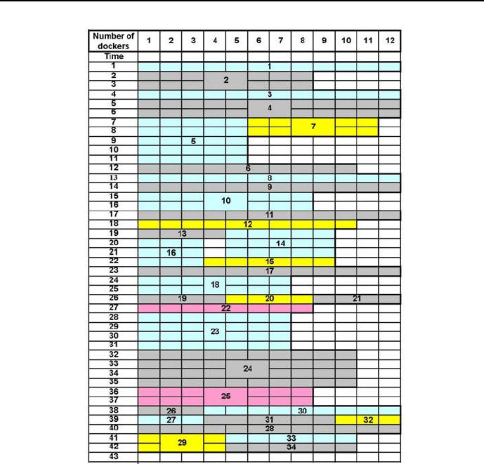
6.16 What is a job-shop? 409
Figure 6.17: Gantt chart for optimum unloading and loading of a ship
•pauses between two consecutive tasks of a job are allowed;
•no machine can be swaped for any other;
•each machine functioning is independent from other machines functioning;
•each job is independent from other jobs.
The goal of job-shop problems is most often the determination of starting times
for tasks of all jobs so that, under constraints of order and duration, the overall

410 Chapter 6. CLP with global constraints for optimal solutions
time of performing all jobs (usually referred to as makespan) is minimized.
The terminology used above is due to early developments in the field of
scheduling, which took place in manufacturing, done on some job floors in some
job shops using some machines. Now, although scheduling is still a most impor-
tant activity in managing manufacturing processes, especially in facilities that
generate a variety of products in relatively low numbers and in batch lots, a great
number of non-manufacturing (like business and military) scheduling applica-
tions have emerged, for which the old terminology (because of its relevance to
any scheduling) is still used. So e.g. underwriters processing insurance policies
could be considered as an insurance ”shop” where underwriters (”machines”)
are processing policies (”jobs”) by filling a number of documents (”tasks”).
Let’s attempt to define the job-shop problem in a more general way. Let
M={M1,M
2,...,M
i,...,M
m}
be the set of machines, and
J={J1,J
2,...,J
j,...,J
n}
be the set of jobs. Any job Jjconsists of a sequence of msequentially performed
tasks:
Tj={Tj,1,T
j,2,...,T
j,i,...,T
j,m},
each one needing a different machine:
Tj,1→Mj,1
Tj,2→Mj,2
.......................
Tj,i →Mj,i
.......................
Tj,m →Mj,m

6.16 What is a job-shop? 411
where
Mj,i ∈M,
and each one having a known duration:
Tj,1→Dj,1
Tj,2→Dj,2
.......................
Tj,i →Dj,i
.......................
Tj,m →Dj,m.
Let
T={1,2,...,i,...,m}
be an ordered set of natural numbers corresponding to prescribed order of
tasks. Associating with any element (j, i) of the Cartesian product J×Ta
pair Mj,i,D
j,i, leads to two functions defining a job-shop problem: a machine
function and a duration function.
For an illustration of these concept the Reader is kindly asked to have an-
other look at Table 6.2, where those two functions were defined for the newspa-
per reading problem: the rows correspond to student readings (i.e. to ”jobs”),
the columns correspond to reading order (i.e. to a prescribed order of ”tasks”),
and inside each cell of the table names of newspapers to be read (i.e. ”machines”
to be used) and durations of reading them (durations of ”tasks” on those ”ma-
chines”) may be found.
Let us return to the general definition. Assume that all njobs are performed
using all mmachines, and forget for a while the precedence constraints. Then
the number of possible schedules is equal (n!)m. It means that, while trying to
solve the problem using exhaustive search, it is necessary to generate all (n!)m
schedules, testing the precedence of tasks and when they are fulfilled - calculate
the makespan14.
Table 6.4 demonstrates how quickly the number of schedules increases.
14 It is emphasized that all those schedules have to be generated and tested: one never knows
whether the optimum makespan will occur for the last schedule generated.

412 Chapter 6. CLP with global constraints for optimal solutions
mmachines njobs (n!)m
1 5 120
3 5 1.7 million
5 5 25000 million
Table 6.4: Increase of job-shop schedule numbers
6.17 A job-shop scheduling problem - bench-
mark MT6
The benchmark MT6 is defined by the table from Figure 6.18. The problem
has 6jobs that have to be done, each one consisting of 6tasks, performed
in the order given by task numbers, by 6machines. It is solved by program
6_13_MT6.ecl:
/*1*/ :- lib(ic).
/*2*/ :- lib(ic_edge_finder3).
/*3*/ :- lib(branch_and_bound).
/*4*/ :- lib(lists).
/*5*/ top:-
% Sji - start time for task i of job j:
/*5*/ S = [S00, S01, S02, S03, S04, S05,
S10, S11, S12, S13, S14, S15,
S20, S21, S22, S23, S24, S25,
S30, S31, S32, S33, S34, S35,
S40, S41, S42, S43, S44, S45,
S50, S51, S52, S53, S54, S55 ],
/*6*/ S :: 0..70,
% End of job times:
/*6*/ E = [E0, E1, E2, E3, E4, E5],
/*7*/ E :: 0..100,
% Resources available for tasks:
/*8*/ R = [1, 1, 1, 1, 1, 1],
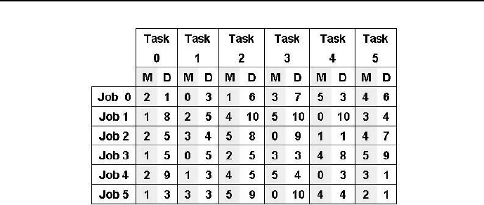
6.17 A job-shop scheduling problem - benchmark MT6 413
Figure 6.18: Job-shop MT6 definition
% Precedence constraints for tasks:
/*9*/ S01 #>= S00 + 1, S02 #>= S01 + 3, S03 #>= S02 + 6, S04 #>= S03 + 7,
/*10*/ S05 #>= S04 + 3, E0 #>= S05 + 6,
/*11*/ S11 #>= S10 + 8, S12 #>= S11 + 5, S13 #>= S12 + 10, S14 #>= S13 + 10,
/*12*/ S15 #>= S14 + 10, E1 #>= S15 + 4,
/*13*/ S21 #>= S20 + 5, S22 #>= S21 + 4, S23 #>= S22 + 8, S24 #>= S23 + 9,
/*14*/ S25 #>= S24 + 1, E2 #>= S25 + 7,
/*15*/ S31 #>= S30 + 5, S32 #>= S31 + 5, S33 #>= S32 + 5, S34 #>= S33 + 3,
/*16*/ S35 #>= S34 + 8, E3 #>= S35 + 9,
/*17*/ S41 #>= S40 + 9, S42 #>= S41 + 3, S43 #>= S42 + 5, S44 #>= S43 + 4,
/*18*/ S45 #>= S44 + 3, E4 #>= S45 + 1,
/*19*/ S51 #>= S50 + 3, S52 #>= S51 + 3, S53 #>= S52 + 9, S54 #>= S53 + 10,
/*20*/ S55 #>= S54 + 4, E5 #>= S55 + 1,
% Each machine is unique. Therefore it may
% perform at any time only a single task:
% machine 0 may perform at any time only a single task:
/*21*/ cumulative([S01, S14, S23, S31, S44, S53], [3, 10, 9, 5, 3, 10], R, 1),
% machine 1 may perform at any time only a single task:
/*22*/ cumulative([S02, S10, S24, S30, S41, S50],[6, 8, 1, 5, 3, 3], R, 1),
% machine 2 may perform at any time only a single task:
/*23*/ cumulative([S00, S11, S20, S32, S40, S55],[1, 5, 5, 5, 9, 1], R, 1),
% machine 3 may perform at any time only a single task:
/*24*/ cumulative([S03, S15, S21, S33, S45, S51],[7, 4, 4, 3, 1, 3], R, 1),
% machine 4 may perform at any time only a single task:

414 Chapter 6. CLP with global constraints for optimal solutions
/*25*/ cumulative([S05, S12, S25, S34, S42, S54],[6, 10, 7, 8, 5, 4], R, 1),
% machine 5 may perform at any time only a single task:
/*26*/ cumulative([S04, S13, S22, S35, S43, S52],[3, 10, 8, 9, 4, 9], R, 1),
% Each job is a unique sequence of consecutive tasks.
% Therefore at any time only one of its tasks may ne performed:
% job 0 is done by performing one of its task at any time:
/*27*/ cumulative([S00, S01, S02, S03, S04, S05],[1, 3, 6, 7, 3, 6], R, 1),
% job 1 is done by performing one of its task at any time:
/*28*/ cumulative([S10, S11, S12, S13, S14, S15],[8, 5, 10, 10, 10, 4], R, 1),
% job 2 is done by performing one of its task at any time:
/*29*/ cumulative([S20, S21, S22, S23, S24, S25],[5, 4, 8, 9, 1, 7], R, 1),
% job 3 is done by performing one of its task at any time:
/*30*/ cumulative([S30, S31, S32, S33, S34, S35],[5, 5, 5, 3, 8, 9], R, 1),
% job 4 is done by performing one of its task at any time:
/*31*/ cumulative([S40, S41, S42, S43, S44, S45],[9, 3, 5, 4, 3, 1], R, 1),
% job 5 is done by performing one of its task at any time:
/*32*/ cumulative([S50, S51, S52, S53, S54, S55],[3, 3, 9, 10, 4, 1], R, 1),
/*33*/ append(S, E, SE),
/*34*/ maxlist(E, M),
/*35*/ bb_min(grounding(SE), M, bb_options with [strategy:continue,
from:0,to:100]),
/*36*/ write("End of job times = "),write(E),nl,
/*37*/ write("Minimal makespan = "),write(M),nl,nl,
/*38*/ write(" S00="),write(S00),
/*39*/ write(" S01="),write(S01),
/*40*/ write(" S02="),write(S02),
/*40*/ write(" S03="),write(S03),
/*41*/ write(" S04="),write(S04),
/*42*/ write(" S05="),write(S05),nl,
/*43*/ write(" S10="),write(S10),
/*44*/ write(" S11="),write(S11),
/*45*/ write(" S12="),write(S12),
/*46*/ write(" S13="),write(S13),
/*47*/ write(" S14="),write(S14),
/*48*/ write(" S15="),write(S15),nl,
/*49*/ write(" S20="),write(S20),
/*50*/ write(" S21="),write(S21),

6.17 A job-shop scheduling problem - benchmark MT6 415
/*51*/ write(" S22="),write(S22),
/*52*/ write(" S23="),write(S23),
/*53*/ write(" S24="),write(S24),
/*54*/ write(" S25="),write(S25),nl,
/*55*/ write(" S30="),write(S30),
/*56*/ write(" S31="),write(S31),
/*57*/ write(" S32="),write(S32),
/*58*/ write(" S33="),write(S33),
/*59*/ write(" S34="),write(S34),
/*60*/ write(" S35="),write(S35),nl,
/*61*/ write(" S40="),write(S40),
/*62*/ write(" S41="),write(S41),
/*63*/ write(" S42="),write(S42),
/*64*/ write(" S43="),write(S43),
/*65*/ write(" S44="),write(S44),
/*66*/ write(" S45="),write(S45),nl,
/*37*/ write(" S50="),write(S50),
/*68*/ write(" S51="),write(S51),
/*69*/ write(" S52="),write(S52),
/*70*/ write(" S53="),write(S53),
/*71*/ write(" S54="),write(S54),
/*72*/ write(" S55="),write(S55),nl.
/*73*/ grounding(All_Variables):-
/*74*/ middle_first(All_Variables, All_VariablesP),
/*75*/ (fromto(All_VariablesP, Variables, VariablesRem, []) do
/*76*/ delete(Variable, Variables, VariablesRem, 0, max_regret),
/*77*/ indomain(Variable, min)
/*78*/ ).
/*79*/ middle_first(List, Ord):-
/*80*/ halve(List, F, B),
/*81*/ reverse(F, RF),
/*82*/ splice(B, RF, Ord).
The message is:

416 Chapter 6. CLP with global constraints for optimal solutions
Found a solution with cost 67
Found a solution with cost 64
Found a solution with cost 61
Found a solution with cost 60
Found a solution with cost 59
Found a solution with cost 58
Found a solution with cost 57
Found a solution with cost 56
Found a solution with cost 55
Found no solution with cost 47.0 .. 54.0
E = [55, 52, 45, 54, 53, 50]
Minimal makespan = 55
S00=5 S01=6 S02=16 S03=30 S04=42 S05=49
S10=0 S11=8 S12=13 S13=28 S14=38 S15=48
S20=0 S21=5 S22=9 S23=18 S24=27 S25=38
S30=8 S31=13 S32=22 S33=27 S34=30 S35=45
S40=13 S41=22 S42=25 S43=38 S44=48 S45=52
S50=13 S51=16 S52=19 S53=28 S54=45 S55=49
The solution is given by the Gantt charts from Figure 6.19.
6.18 A difficult job-shop scheduling problem -
benchmark MT10
Obviously, solving job-shop problems must be a challenge to OR and CLP
people. This is best shown by a range of job-shop benchmarks, more or less
difficult, used over years to test various algorithms. One of the more celebrated
and famous benchmark is the 10 jobs 10 machines job-shop benchmark known
as MT10. It is defined by the table from Figure 6.20, where Mdenotes machines
and Dtask durations. It was proposed in 1963 by J.F. Muth and G.L. Thompson
in the book [Muth-63]. The problem has 100 integer variables - the start times
for 10 tasks on 10 machines. Finding its solution was an open problem for more
than 20 years. Until 1982 the best available upper bound for the makespan was
equal 935 with no reasonable lower bound known. Using a highly specialized
search algorithm the minimum makespan equal 930 was determined in 1987 by
Carlier and Pinson, see [Carlier-89]. The problem is still considered as one of
the most rewarding benchmarks for job-shop scheduling methods and constantly
challenges designers of integer programming algorithms and CLP programs.
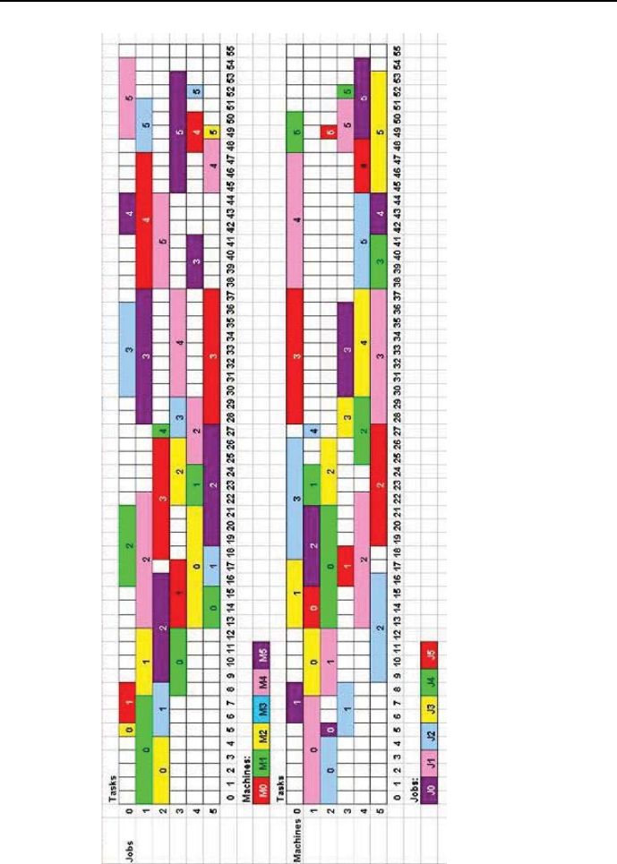
6.18 A difficult job-shop scheduling problem - benchmark MT10 417
Figure 6.19: MT6 Gantt charts
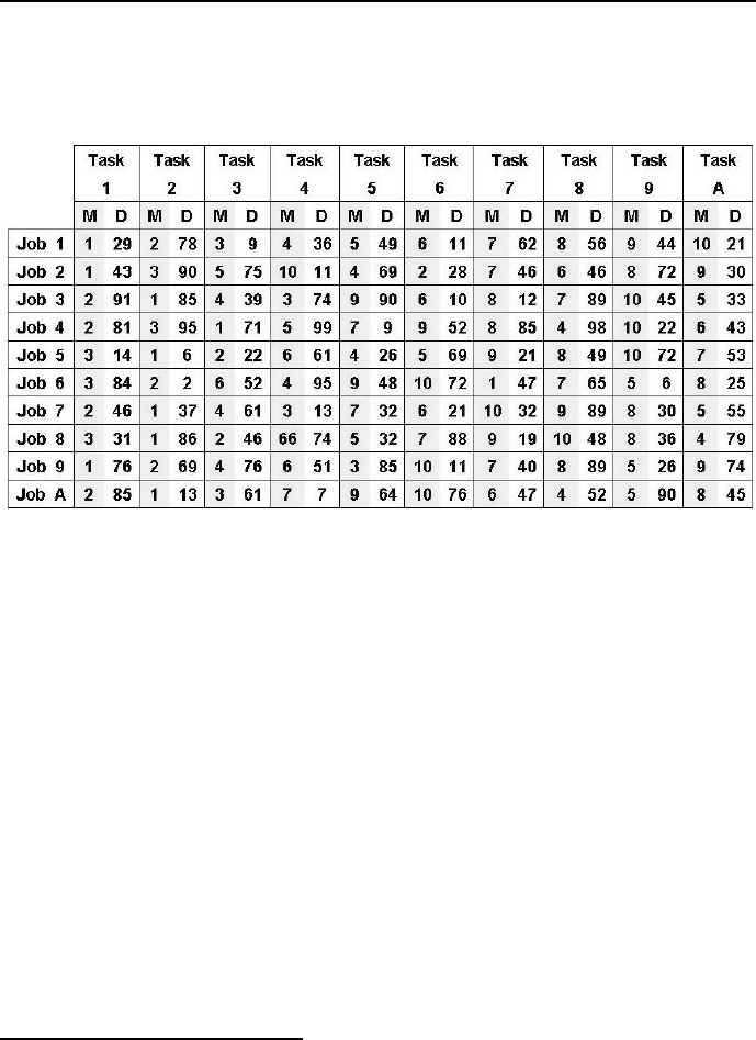
418 Chapter 6. CLP with global constraints for optimal solutions
The complexity of MT10 is the reason to first of all test the existence of a fea-
sible solution. This may be done with the help of program 6_9_mt10_tes.ecl15:
Figure 6.20: Job-shop MT10 definition
/*1*/ :- lib(ic).
/*2*/ top:-
/*3*/ S = [S11,S12,S13,S14,S15,S16,S17,S18,S19,S1A,
S21,S22,S23,S24,S25,S26,S27,S28,S29,S2A,
S31,S32,S33,S34,S35,S36,S37,S38,S39,S3A,
S41,S42,S43,S44,S45,S46,S47,S48,S49,S4A,
S51,S52,S53,S54,S55,S56,S57,S58,S59,S5A,
S61,S62,S63,S64,S65,S66,S67,S68,S69,S6A,
S71,S72,S73,S74,S75,S76,S77,S78,S79,S7A,
S81,S82,S83,S84,S85,S86,S87,S88,S89,S8A,
S91,S92,S93,S94,S95,S96,S97,S98,S99,S9A,
SA1,SA2,SA3,SA4,SA5,SA6,SA7,SA8,SA9,SAA],
% Sji - start time for task i of job j
/*4*/ E = [E1,E2,E3,E4,E5,E6,E7,E8,E9,EA],
/*5*/ E :: 655..1000,
/*6*/ S :: 0..1000,
15 This is an FS-type problem.

6.18 A difficult job-shop scheduling problem - benchmark MT10 419
% Precedence constraints for operations: for all jobs,
/*7*/ S12 #>= S11+29, /*8*/ S13 #>= S12+78,
/*9*/ S14 #>= S13+9, /*10*/ S15 #>= S14+36,
/*11*/ S16 #>= S15+49, /*12*/ S17 #>= S16+11,
/*13*/ S18 #>= S17+62, /*14*/ S19 #>= S18+56,
/*15*/ S1A #>= S19+44, /*16*/ E1 #>= S1A+21,
/*17*/ S22 #>= S21+43, /*18*/ S23 #>= S22+90,
/*19*/ S24 #>= S23+75, /*20*/ S25 #>= S24+11,
/*21*/ S26 #>= S25+69, /*22*/ S27 #>= S26+28,
/*23*/ S28 #>= S27+46, /*24*/ S29 #>= S28+46,
/*25*/ S2A #>= S29+72, /*26*/ E2 #>= S2A+30,
/*27*/ S32 #>= S31+91, /*28*/ S33 #>= S32+85,
/*29*/ S34 #>= S33+39, /*30*/ S35 #>= S34+74,
/*31*/ S36 #>= S35+90, /*32*/ S37 #>= S36+10,
/*33*/ S38 #>= S37+12, /*34*/ S39 #>= S38+89,
/*35*/ S3A #>= S39+45, /*36*/ E3 #>= S3A+33,
/*37*/ S42 #>= S41+81, /*38*/ S43 #>= S42+95,
/*39*/ S44 #>= S43+71, /*40*/ S45 #>= S44+99,
/*41*/ S46 #>= S45+9, /*42*/ S47 #>= S46+52,
/*43*/ S48 #>= S47+85, /*44*/ S49 #>= S48+98,
/*45*/ S4A #>= S49+22, /*46*/ E4 #>= S4A+43,
/*47*/ S52 #>= S51+14, /*48*/ S53 #>= S52+6,
/*49*/ S54 #>= S53+22, /*50*/ S55 #>= S54+61,
/*51*/ S56 #>= S55+26, /*52*/ S57 #>= S56+69,
/*53*/ S58 #>= S57+21, /*54*/ S59 #>= S58+49,
/*55*/ S5A #>= S59+72, /*56*/ E5 #>= S5A+53,
/*57*/ S62 #>= S61+84, /*58*/ S63 #>= S62+2,
/*59*/ S64 #>= S63+52, /*60*/ S65 #>= S64+95,
/*61*/ S66 #>= S65+48, /*62*/ S67 #>= S66+72,
/*63*/ S68 #>= S67+47, /*64*/ S69 #>= S68+65,
/*65*/ S6A #>= S69+6, /*66*/ E6 #>= S6A+25,
/*67*/ S72 #>= S71+46, /*68*/ S73 #>= S72+37,
/*69*/ S74 #>= S73+61, /*70*/ S75 #>= S74+13,
/*71*/ S76 #>= S75+32, /*72*/ S77 #>= S76+21,
/*73*/ S78 #>= S77+32, /*74*/ S79 #>= S78+89,
/*75*/ S7A #>= S79+30, /*76*/ E7 #>= S7A+55,
/*77*/ S82 #>= S81+31, /*78*/ S83 #>= S82+86,
/*79*/ S84 #>= S83+46, /*80*/ S85 #>= S84+74,
/*81*/ S86 #>= S85+32, /*82*/ S87 #>= S86+88,
/*83*/ S88 #>= S87+19, /*84*/ S89 #>= S88+48,

420 Chapter 6. CLP with global constraints for optimal solutions
/*85*/ S8A #>= S89+36, /*86*/ E8 #>= S8A+79,
/*87*/ S92 #>= S91+76, /*88*/ S93 #>= S92+69,
/*89*/ S94 #>= S93+76, /*90*/ S95 #>= S94+51,
/*91*/ S96 #>= S95+85, /*92*/ S97 #>= S96+11,
/*93*/ S98 #>= S97+40, /*94*/ S99 #>= S98+89,
/*95*/ S9A #>= S99+26, /*96*/ E9 #>= S9A+74,
/*97*/ SA2 #>= SA1+85, /*98*/ SA3 #>= SA2+13,
/*99*/ SA4 #>= SA3+61, /*100*/ SA5 #>= SA4+7,
/*101*/ SA6 #>= SA5+64, /*102*/ SA7 #>= SA6+76,
/*103*/ SA8 #>= SA7+47, /*104*/ SA9 #>= SA8+52,
/*105*/ SAA #>= SA9+90, /*106*/ EA #>= SAA+45,
/*107*/ append(S,E,SE),
/*108*/ labeling(SE).
The program contains only precedence constraints and duration data. It
generates the assuring message”
Yes (0.02s cpu, solution 1, maybe more),
indicating the existence of feasible solutions. So an optimum solution must exist
as well.
An efficient, general and rather complex program for solving MT10 and
other similar job-shop benchmarks using ECLiPSe, developed by J. Schimpf
(see [Schimpf-10]) using algorithms presented in [Baptiste-95], is available on the
website http://www.eclipse-clp.org/eclipse/examples, Section Planning
and Scheduling, Subsection Jobshop Scheduling.
Considering the introductory nature of this book, the 6_10_mt10.ecl pro-
gram presented below is solely aimed at proofing the correctness of the minimal
makespan being equal to 930, while using elementary modeling and trying to
get results quickly. This has been done using some apriori information about
domains of start times. It has been obtained by calculating (outside of the pro-
gram discussed) the earliest and latest start times of all tasks16. However, it
was not sufficient to decrease the time needed to get the solution, so some man-
16 The earliest start time for a task was calculated as the sum of durations of all tasks
preceding it in the job. The latest start time was calculated as the difference between the
upper bound of the End domain and the sum of durations of all following tasks in the job.

6.18 A difficult job-shop scheduling problem - benchmark MT10 421
ual corrections were introduced for some domains to make them yet smaller.
Obviously, a program tailored that way has no generality at all: any change of
data will require fine tuning of domains. This makeshift brute-force approach
conveys however an important and general principle: themoreweknowabout
the variable domains, and the smaller they can be declared, the quicker solutions
are obtained. The program 6_10_mt10.ecl17 is as follows:
/*1*/ :- lib(ic).
/*2*/ :- lib(ic_edge_finder3).
/*3*/ :- lib(branch_and_bound).
/*4*/ :- lib(lists).
/*5*/ top:-
/*6*/ S = [S11,S12,S13,S14,S15,S16,S17,S18,S19,S1A,
S21,S22,S23,S24,S25,S26,S27,S28,S29,S2A,
S31,S32,S33,S34,S35,S36,S37,S38,S39,S3A,
S41,S42,S43,S44,S45,S46,S47,S48,S49,S4A,
S51,S52,S53,S54,S55,S56,S57,S58,S59,S5A,
S61,S62,S63,S64,S65,S66,S67,S68,S69,S6A,
S71,S72,S73,S74,S75,S76,S77,S78,S79,S7A,
S81,S82,S83,S84,S85,S86,S87,S88,S89,S8A,
S91,S92,S93,S94,S95,S96,S97,S98,S99,S9A,
SA1,SA2,SA3,SA4,SA5,SA6,SA7,SA8,SA9,SAA],
% Sji - start time for task i of job j
/*7*/ E = [E1,E2,E3,E4,E5,E6,E7,E8,E9,EA],
/*8*/ E :: 655..1000,
/*9*/ R = [1,1,1,1,1,1,1,1,1,1],
/*10*/ S11 :: 0..605, /*11*/ S21 :: 0..490,
/*12*/ S31 :: 0..432, /*13*/ S41 :: 0..345,
/*14*/ S51 :: 0..607, /*15*/ S61 :: 0..504,
/*16*/ S71 :: 0..584, /*17*/ S81 :: 0..461,
/*18*/ S91 :: 0..403, /*19*/ SA1 :: 0..460,
/*20*/ S12 :: 29..634, /*21*/ S22 :: 43..533,
/*22*/ S32 :: 91..523, /*23*/ S42 :: 81..426,
/*24*/ S52 :: 14..621, /*25*/ S62 :: 84..588,
/*26*/ S72 :: 46..630, /*27*/ S82 :: 31..492,
/*28*/ S92 :: 76..479, /*29*/ SA2 :: 85..370,
/*30*/ S13 :: 107..712, /*31*/ S23 :: 133..628,
/*32*/ S33 :: 176..608, /*33*/ S43 :: 176..521,
/*34*/ S53 :: 20..627, /*35*/ S63 :: 86..590,
17 This is an OST-type problem.

422 Chapter 6. CLP with global constraints for optimal solutions
/*36*/ S73 :: 83..667, /*37*/ S83 :: 117..578,
/*38*/ S93 :: 145..548, /*39*/ SA3 :: 98..548,
/*40*/ S14 :: 116..721, /*41*/ S24 :: 208..698,
/*42*/ S34 :: 215..647, /*43*/ S44 :: 247..592,
/*44*/ S54 :: 42..649, /*45*/ S64 :: 138..642,
% correction: % correction:
/*46*/ S74 :: 100..450, /*47*/ S84 :: 100..450,
/*48*/ S94 :: 221..624, /*49*/ SA4 :: 159..619,
/*50*/ S15 ::152..757, /*51*/ S25 ::219..709,
/*52*/ S35 ::289..721, /*53*/ S45 ::346..691,
/*54*/ S55 ::103..710, /*55*/ S65 ::233..737,
/*56*/ S75 ::157..741, /*57*/ S85 ::237..698,
/*58*/ S95 ::272..675, /*59*/ SA5 ::166..626,
/*60*/ S16 ::201..806, /*61*/ S26 ::288..778,
/*62*/ S36 ::300..700, /*63*/ S46 ::355..700,
/*64*/ S56 ::129..736, /*65*/ S66 ::281..736,
/*66*/ S76 ::189..736, /*67*/ S86 ::269..730,
/*68*/ S96 ::250..600, /*69*/ SA6 ::230..690,
/*70*/ S17 :: 212..817, /*71*/ S27 :: 316..806,
/*72*/ S37 :: 389..821, /*73*/ S47 :: 407..821,
/*74*/ S57 :: 198..805, /*75*/ S67 :: 353..857,
/*76*/ S77 :: 210..793, /*77*/ S87 :: 357..818,
/*78*/ S97 :: 368..771, /*79*/ SA7 :: 306..766,
/*80*/ S18 :: 274..879, /*81*/ S28 :: 362..852,
/*82*/ S38 :: 401..833, /*83*/ S48 :: 492..837,
% correction:
/*84*/ S58 :: 450..800, /*85*/ S68 :: 400..904,
/*86*/ S78 :: 242..826, /*87*/ S88 :: 376..837,
/*88*/ S98 :: 408..811, /*89*/ SA8 :: 353..813,
/*90*/ S19 :: 330..935, /*91*/ S29 :: 408..898,
/*92*/ S39 :: 490..922, /*93*/ S49 :: 590..935,
/*94*/ S59 :: 268..875, /*95*/ S69 :: 450..800,
/*96*/ S79 :: 450..800, /*97*/ S89 :: 424..885,
/*98*/ S99 :: 497..900, /*99*/ SA9 :: 405..865,
/*100*/ S1A :: 374..979, /*101*/ S2A :: 480..970,
/*102*/ S3A :: 535..967, /*103*/ S4A :: 612..957,
/*104*/ S5A :: 340..947, /*105*/ S6A :: 471..975,
/*106*/ S7A :: 361..945, /*107*/ S8A :: 460..921,
/*108*/ S9A :: 523..921, /*109*/ SAA :: 495..955,

6.18 A difficult job-shop scheduling problem - benchmark MT10 423
% Each machine is unique. Therefore it may
% perform at any time only a single task:
% Machine 1 may perform at any time only a single task:
/*110*/ cumulative([S11,S21,S32,S43,S52,S67,S72,S82,S91,SA2],
[29,43,85,71,6,47,37,86,76,13],R,1),
% Machine 2 may perform at any time only a single task:
/*111*/ cumulative([S12,S26,S31,S41,S53,S62,S71,S83,S92,SA1],
[78,28,91,81,22,2,46,46,69,85],R,1),
/*112*/ cumulative([S13,S22,S34,S42,S51,S61,S74,S81,S95,SA3],
[9,90,74,95,14,84,13,31,85,61],R,1),
/*113*/ cumulative([S14,S25,S33,S48,S55,S64,S73,S8A,S93,SA8],
[36,69,39,98,26,95,61,79,76,52],R,1),
/*114*/ cumulative([S15,S23,S3A,S44,S56,S69,S7A,S85,S99,SA9],
[49,75,33,99,69,6,55,32,26,90],R,1),
/*115*/ cumulative([S16,S28,S36,S4A,S54,S63,S76,S84,S94,SA7],
[11,46,10,43,61,52,21,74,51,47],R,1),
/*116*/ cumulative([S17,S27,S38,S45,S5A,S68,S75,S86,S97,SA4],
[62,46,89,9,53,65,32,88,40,7],R,1),
/*117*/ cumulative([S18,S29,S37,S47,S58,S6A,S79,S89,S98,SAA],
[56,72,12,85,49,25,30,36,89,45],R,1),
/*118*/ cumulative([S19,S2A,S35,S46,S57,S65,S78,S87,S9A,SA5],
[44,30,90,52,21,48,89,19,74,64],R,1),
/*119*/ cumulative([S1A,S24,S39,S49,S59,S66,S77,S88,S96,SA6],
[21,11,45,22,72,72,32,48,11,76],R,1),
% Precedence constraints for tasks: for all jobs,
% the next task may start no sooner than the previous
% task is completed:
/*120*/ S12 #>= S11+29, /*121*/ S13 #>= S12+78,
/*122*/ S14 #>= S13+9, /*123*/ S15 #>= S14+36,
/*124*/ S16 #>= S15+49, /*125*/ S17 #>= S16+11,
/*126*/ S18 #>= S17+62, /*127*/ S19 #>= S18+56,
/*128*/ S1A #>= S19+44, /*129*/ E1 #>= S1A+21,
/*130*/ S22 #>= S21+43, /*131*/ S23 #>= S22+90,
/*132*/ S24 #>= S23+75, /*133*/ S25 #>= S24+11,
/*134*/ S26 #>= S25+69, /*135*/ S27 #>= S26+28,
/*136*/ S28 #>= S27+46, /*137*/ S29 #>= S28+46,
/*138*/ S2A #>= S29+72, /*139*/ E2 #>= S2A+30,
/*140*/ S32 #>= S31+91, /*141*/ S33 #>= S32+85,
/*142*/ S34 #>= S33+39, /*143*/ S35 #>= S34+74,
/*144*/ S36 #>= S35+90, /*145*/ S37 #>= S36+10,
/*146*/ S38 #>= S37+12, /*147*/ S39 #>= S38+89,
/*148*/ S3A #>= S39+45, /*149*/ E3 #>= S3A+33,

424 Chapter 6. CLP with global constraints for optimal solutions
/*150*/ S42 #>= S41+81, /*151*/ S43 #>= S42+95,
/*152*/ S44 #>= S43+71, /*153*/ S45 #>= S44+99,
/*154*/ S46 #>= S45+9, /*155*/ S47 #>= S46+52,
/*156*/ S48 #>= S47+85, /*157*/ S49 #>= S48+98,
/*158*/ S4A #>= S49+22, /*159*/ E4 #>= S4A+43,
/*160*/ S52 #>= S51+14, /*161*/ S53 #>= S52+6,
/*162*/ S54 #>= S53+22, /*163*/ S55 #>= S54+61,
/*164*/ S56 #>= S55+26, /*165*/ S57 #>= S56+69,
/*166*/ S58 #>= S57+21, /*167*/ S59 #>= S58+49,
/*168*/ S5A #>= S59+72, /*169*/ E5 #>= S5A+53,
/*170*/ S62 #>= S61+84, /*171*/ S63 #>= S62+2,
/*172*/ S64 #>= S63+52, /*173*/ S65 #>= S64+95,
/*174*/ S66 #>= S65+48, /*175*/ S67 #>= S66+72,
/*176*/ S68 #>= S67+47, /*177*/ S69 #>= S68+65,
/*178*/ S6A #>= S69+6, /*179*/ E6 #>= S6A+25,
/*180*/ S72 #>= S71+46, /*181*/ S73 #>= S72+37,
/*182*/ S74 #>= S73+61, /*183*/ S75 #>= S74+13,
/*184*/ S76 #>= S75+32, /*185*/ S77 #>= S76+21,
/*186*/ S78 #>= S77+32, /*187*/ S79 #>= S78+89,
/*188*/ S7A #>= S79+30, /*189*/ E7 #>= S7A+55,
/*190*/ S82 #>= S81+31, /*191*/ S83 #>= S82+86,
/*192*/ S84 #>= S83+46, /*193*/ S85 #>= S84+74,
/*194*/ S86 #>= S85+32, /*195*/ S87 #>= S86+88,
/*196*/ S88 #>= S87+19, /*197*/ S89 #>= S88+48,
/*198*/ S8A #>= S89+36, /*199*/ E8 #>= S8A+79,
/*200*/ S92 #>= S91+76, /*201*/ S93 #>= S92+69,
/*202*/ S94 #>= S93+76, /*203*/ S95 #>= S94+51,
/*204*/ S96 #>= S95+85, /*205*/ S97 #>= S96+11,
/*206*/ S98 #>= S97+40, /*207*/ S99 #>= S98+89,
/*208*/ S9A #>= S99+26, /*209*/ E9 #>= S9A+74,
/*210*/ SA2 #>= SA1+85, /*211*/ SA3 #>= SA2+13,
/*212*/ SA4 #>= SA3+61, /*213*/ SA5 #>= SA4+7,
/*214*/ SA6 #>= SA5+64, /*215*/ SA7 #>= SA6+76,
/*216*/ SA8 #>= SA7+47, /*217*/ SA9 #>= SA8+52,
/*218*/ SAA #>= SA9+90, /*219*/ EA #>= SAA+45,
% Each job is unique. Therefore at any time
% only one of its task may be performed:

6.18 A difficult job-shop scheduling problem - benchmark MT10 425
/*219*/ cumulative([S11,S12,S13,S14,S15,S16,S17,S18,S19,S1A],
[29,78,9,36,49,11,62,56,44,21],R,1),
/*220*/ cumulative([S21,S22,S23,S24,S25,S26,S27,S28,S29,S2A],
[43,90,75,11,69,28,46,46,72,30],R,1),
/*221*/ cumulative([S31,S32,S33,S34,S35,S36,S37,S38,S39,S3A],
[91,85,39,74,90,10,12,89,45,33],R,1),
/*222*/ cumulative([S41,S42,S43,S44,S45,S46,S47,S48,S49,S4A],
[81,95,71,99,9,52,85,98,22,43],R,1),
/*223*/ cumulative([S51,S52,S53,S54,S55,S56,S57,S58,S59,S5A],
[14,6,22,61,26,69,21,49,72,53],R,1),
/*224*/ cumulative([S61,S62,S63,S64,S65,S66,S67,S68,S69,S6A],
[84,2,52,95,48,72,47,65,6,25],R,1),
/*225*/ cumulative([S71,S72,S73,S74,S75,S76,S77,S78,S79,S7A],
[46,37,61,13,32,21,32,89,30,55],R,1),
/*226*/ cumulative([S81,S82,S83,S84,S85,S86,S87,S88,S89,S8A],
[31,86,46,74,32,88,19,48,36,79],R,1),
/*227*/ cumulative([S91,S92,S93,S94,S95,S96,S97,S98,S99,S9A],
[76,69,76,51,85,11,40,89,26,74],R,1),
/*228*/ cumulative([SA1,SA2,SA3,SA4,SA5,SA6,SA7,SA8,SA9,SAA],
[85,13,61,7,64,76,47,52,90,45],R,1),
/*229*/ append(S,E,SE),
/*230*/ maxlist(E,M),
/*231*/ bb_min(my_labeling(SE), M, bb_options with
[strategy:continue,from:900,to:930]),
/*232*/ write("E = "),write(E),nl,
/*233*/ write("Minimum makespan = "),write(M),nl,nl,
/*234*/ write("S11="),write(S11),write(" S12="),write(S12),
write(" S13="),write(S13),write(" S14="),write(S14),
write(" S15="),write(S15),nl,write("S16="),write(S16),
write(" S17="),write(S17),write(" S18="),write(S18),
write(" S19="),write(S19),write(" S1A="),write(S1A),nl,nl,
/*235*/ write("S21="),write(S21),write(" S22="),write(S22),
write(" S23="),write(S23),write(" S24="),write(S24),
write(" S25="),write(S25),nl,write("S26="),write(S26),
write(" S27="),write(S27),write(" S28="),write(S28),
write(" S29="),write(S29),write(" S2A="),write(S2A),nl,nl,
/*236*/ write("S31="),write(S31),write(" S32="),write(S32),
write(" S33="),write(S33),write(" S34="),write(S34),
write(" S35="),write(S35),nl,write("S36="),write(S36),
write(" S37="),write(S37),write(" S38="),write(S38),
write(" S39="),write(S39),write(" S3A="),write(S3A),nl,nl,

426 Chapter 6. CLP with global constraints for optimal solutions
/*237*/ write("S41="),write(S41),write(" S42="),write(S42),
write(" S43="),write(S43),write(" S44="),write(S44),
write(" S45="),write(S45),nl,write("S46="),write(S46),
write(" S47="),write(S47),write(" S48="),write(S48),
write(" S49="),write(S49),write(" S4A="),write(S4A),nl,nl,
/*238*/ write("S51="),write(S51),write(" S52="),write(S52),
write(" S53="),write(S53),write(" S54="),write(S54),
write(" S55="),write(S55),nl,write("S56="),write(S56),
write(" S57="),write(S57),write(" S58="),write(S58),
write(" S59="),write(S59),write(" S5A="),write(S5A),nl,nl,
/*239*/ write("S61="),write(S61),write(" S62="),write(S62),
write(" S63="),write(S63),write(" S64="),write(S64),
write(" S65="),write(S65),nl,write("S66="),write(S66),
write(" S67="),write(S67),write(" S68="),write(S68),
write(" S69="),write(S69),write(" S6A="),write(S6A),nl,nl,
/*240*/ write("S71="),write(S71),write(" S72="),write(S72),
write(" S73="),write(S73),write(" S74="),write(S74),
write(" S75="),write(S75),nl,write("S76="),write(S76),
write(" S77="),write(S77),write(" S78="),write(S78),
write(" S79="),write(S79),write(" S7A="),write(S7A),nl,nl,
/*241*/ write("S81="),write(S81),write(" S82="),write(S82),
write(" S83="),write(S83),write(" S84="),write(S84),
write(" S85="),write(S85),nl,write("S86="),write(S86),
write(" S87="),write(S87),write(" S88="),write(S88),
write(" S89="),write(S89),write(" S8A="),write(S8A),nl,nl,
/*242*/ write("S91="),write(S92),write(" S92="),write(S92),
write(" S93="),write(S93),write(" S94="),write(S94),
write(" S95="),write(S95),nl,write("S96="),write(S96),
write(" S97="),write(S97),write(" S98="),write(S98),
write(" S99="),write(S99),write(" S9A="),write(S9A),nl,nl,
/*243*/ write("SA1="),write(SA1),write(" SA2="),write(SA2),
write(" SA3="),write(SA3),write(" SA4="),write(SA4),
write(" SA5="),write(SA5),nl,write("SA6="),write(SA6),
write(" SA7="),write(SA7),write(" SA8="),write(SA8),
write(" SA9="),write(SA9),write(" SAA="),write(SAA),nl.
/*244*/ my_labeling(All_Variables):-
/*245*/ middle_first(All_Variables,All_VariablesP),
/*246*/ ( fromto(All_VariablesP, Variables, VariablesRem, []) do
/*247*/ delete(Variable, Variables, VariablesRem, 0, max_regret),
/*248*/ indomain(Variable,min)
/*249*/ ).

6.18 A difficult job-shop scheduling problem - benchmark MT10 427
/*250*/ middle_first(List,Ord):-
/*251*/ halve(List,F,B),
/*252*/ reverse(F,RF),
/*253*/ splice(B,RF,Ord).
The message is:
Found a solution with cost 930
Found no solution with cost 900.0 .. 929.0
E = [908, 915, 920, 842, 895, 655, 753, 892, 792, 930]
Minimum makespan = 930
S11=119 S12=445 S13=523 S14=532 S15=568
S16=617 S17=645 S18=721 S19=792 S1A=887
S21=76 S22=224 S23=355 S24=430 S25=568
S26=637 S27=707 S28=753 S29=813 S2A=885
S31=308 S32=408 S33=493 S34=532 S35=609
S36=699 S37=709 S38=753 S39=842 S3A=887
S41=0 S42=84 S43=185 S44=256 S45=359
S46=368 S47=420 S48=637 S49=766 S4A=799
S51=179 S52=256 S53=286 S54=308 S55=370
S56=430 S57=499 S58=530 S59=593 S5A=842
S61=0 S62=84 S63=86 S64=138 S65=233
S66=281 S67=361 S68=408 S69=499 S6A=505
S71=86 S72=148 S73=233 S74=314 S75=327
S76=421 S77=442 S78=520 S79=668 S7A=698
S81=193 S82=275 S83=399 S84=445 S85=519
S86=557 S87=699 S88=718 S89=777 S8A=813
S91=217 S92=217 S93=294 S94=370 S95=421
S96=506 S97=517 S98=579 S99=668 S9A=718
SA1=132 SA2=262 SA3=327 SA4=388 SA5=420
SA6=517 SA7=628 SA8=735 SA9=787 SAA=885
This message is highly uninformative. It has to be converted to Gantt charts,
as was previously done in Section 6.11.
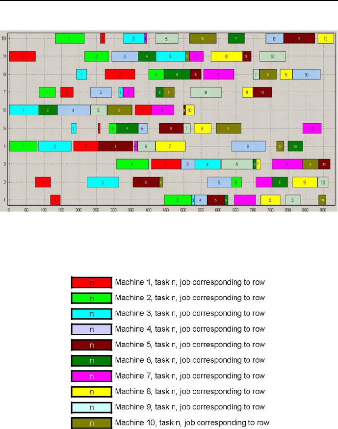
428 Chapter 6. CLP with global constraints for optimal solutions
Figure 6.21: Gantt charts for MT10 jobs
Figure 6.22: Machine coloring codes for the jobs Gantt chart
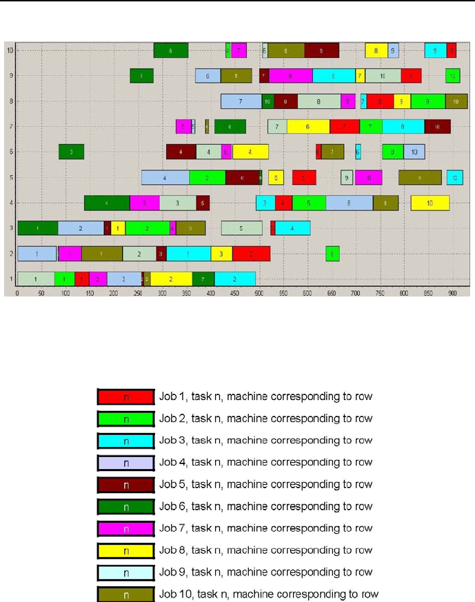
6.18 A difficult job-shop scheduling problem - benchmark MT10 429
Figure 6.23: Gantt charts for MT10 machines
Figure 6.24: Job coloring codes for the machines Gantt charts

430 Chapter 6. CLP with global constraints for optimal solutions
Figure 6.21 is the Gantt chart for jobs, with Figure 6.22 explaining the colour
coding for machines.
On Figure 6.21 it may be difficult to spot task 2for job 6, because - as
follows from line /*170*/ of the program, he duration of this task is equal 2,
and this cannot be properly shown for the scale used. The meaning of Figure
6.21 is obvious. E.g. for job 4the consecutive tasks are the tasks performed
by the: light-green machine (machine 2), light-blue machine (machine 3), red
machine (machine 1) etc. etc.
In order to make the Gantt chart for machines communicative, the color
coding used for the job Gantt chart cannot be used any longer: otherwise all
boxes in a row will be of the same color. Figure 6.23 is the Gantt chart for
machines and Figure 6.24 shows the color coding used for jobs18.
The meaning of Figure 6.23 is as follows, e.g. the red box for machine 1corre-
sponds to task 1for job 1in Figure 6.21 (also a red box ), the red box formachine
2corresponds to task 2 from job 1 in Figure 6.21 (light-green box ), the red box
(quite narrow) for machine 3 corresponds to task 3 of job 1 in Figure 6.21,
depicted by an also rather narrow light-blue box, etc. etc.
Scheduling problems are rightly considered to belong to the most difficult
combinatorial decision problems. They are ubiquitous. There is hardly any
human activity where they may not be found. They are important as being one
of the tools to control cost and time. Sometimes they may be of exorbitant size:
the Viking NASA mission to Mars is believed to be based on scheduling activ-
ities of over 20.000 people. The techniques to solve them evolved considerably
over time, starting with classical, often heuristic approaches (see [Muth-63]),
but still used (see e.g. [Baker-09]), to constraint programming techniques, see
[Baptiste-95] and [Baptiste-01].
6.19 Traveling Salesman Problems
The Traveling Salesman Problem (TSP) can be stated as follows: a salesman
based at some city (say, city 1) must travel to cities 2,3,...,n visiting each
city only once and then return to city 1. The person wishes to do it in the most
efficient way, i.e. covering the minimum total distance. No general method
(i.e. for any n) of solving this problem is known, and the problem exhibits a
18 The charts from Figures 6.21 and 6.23 have been generated using a program developed in
the M.Sc. thesis by my student Bartosz W´ojcik, presented in [W´ojcik-05].
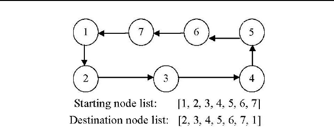
6.19 Traveling Salesman Problems 431
Figure 6.25: A graph that is a Hamiltonian circuit for nodes 1,2,3,4,5,6,7.
strong combinatorial explosion, or - as theoreticians prefer to call it - is NP-
hard: the second city may be chosen in n−1ways,thethirdcityinn−2
ways, so for the second and third cities we have (n−1) ×(n−2) choices, added
the fourth city we arrive at (n−1) ×(n−2) ×(n−3) choices etc. So any
attempt to solve the problem by exhaustive search requires generally (i.e. while
between cities iand jis a different distance than between cities jand i)(n−1)!
distance evaluations, which seems practical for no more than 10 cities. However,
a large number of heuristics and exact methods are known at present (most of
them utilizing parallel computations), which solve TSP instances with tens of
thousands of cities.
6.19.1 Hamiltonian circuits
A basic concept in TSP is the concept of Hamiltonian circuit, defined as such
circuit (i.e., closed loop) through a set of nodes that visits each node exactly
once. This is illustrated by Figure 6.25.
To discuss Hamiltonian circuits in the CLP perspective, it pays to consider
two lists:
1. Starting node list that is a list of numbers for all relevant nodes, each node
represented only once. For the sake of convenience it may be an ordered
list.
2. Destination node list that is a list of numbers of those nodes that are
visited from nodes occupying the same position in the starting node list.
So, in Figure 6.25, the node 3is the destination node for starting node 2.
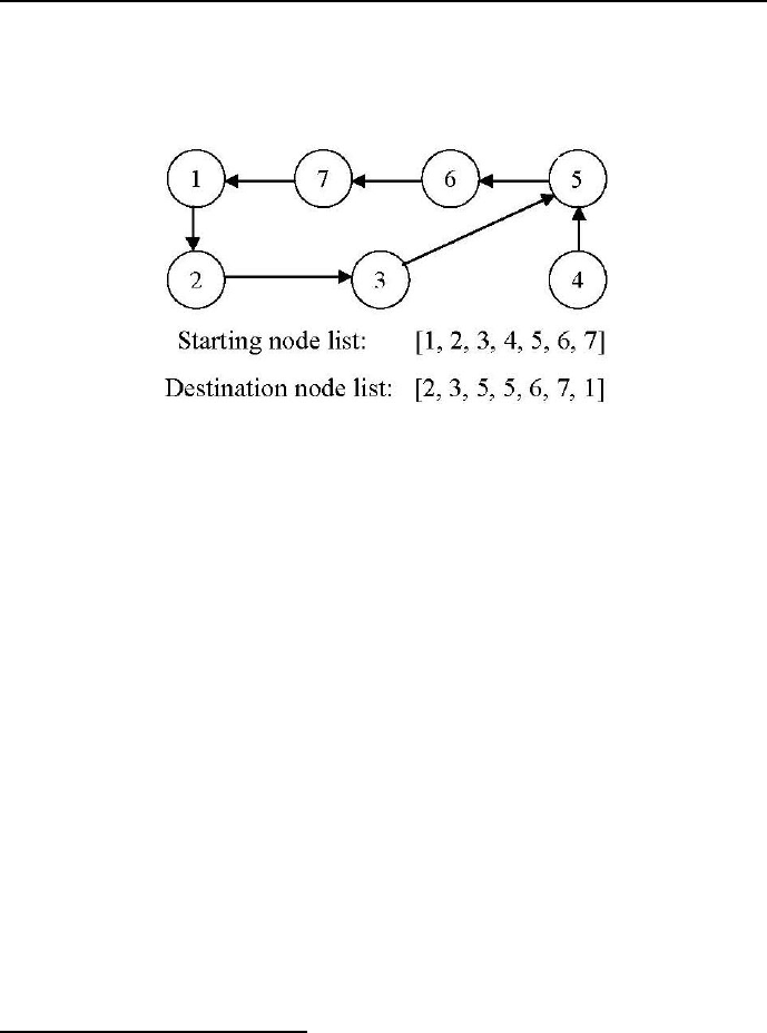
432 Chapter 6. CLP with global constraints for optimal solutions
To sharpen the concept, Figure 6.26 presents a graph that is not a Hamilto-
nian circuit: the destination node list is not a permutation of the starting node
list.
Figure 6.26: A graph that is not a Hamiltonian circuit for nodes 1,2,3,4,5,6,7.
The program 6_11_hamilton.ecl19 maybeusedtoverifythenatureof
both graphs using the built-in circuit/1:
/*1*/ :-lib(ic).
/*2*/ top:-
/*3*/ circuit([2, 3, 4, 5, 6, 7, 1]),
/*4*/ ~(circuit([2, 3, 5, 5, 6, 7, 1])).
%~Goal is the sound negation operator, which delays if +Goal is not grounded.+
/*5*/ circuit(DestinationNodeList):-
/*6*/ length(DestinationNodeList,NodeCount),
/*7*/ dim(DestinationNodeArray,[NodeCount]),
/*8*/ DestinationNodeArray=..[[]|DestinationNodeList],
/*9*/ (
/*10*/ count(StartingNodeNr,1,NodeCount),
/*11*/ param(DestinationNodeArray,NodeCount)
/*12*/ do
/*13*/ arg(StartingNodeNr,DestinationNodeArray,DestinationNode),
/*14*/ CycleLength is NodeCount -2 ,
/*15*/ (
/*16*/ count(_,1,CycleLength),
/*17*/ fromto(DestinationNode,DestinationNodeIn,DestinationNodeOut,_),
19 This program and the program defining the built-in circuit/1 that forces a Hamiltonian
cycle in a directed graph, has been proposed by Lukasz Domagala.

6.19 Traveling Salesman Problems 433
/*18*/ param(StartingNodeNr,DestinationNodeArray)
/*19*/ do
/*20*/ arr_element(DestinationNodeIn, DestinationNodeArray,
DestinationNodeOut),
/*21*/ DestinationNodeOut #\= StartingNodeNr
/*22*/ )
/*23*/ ).
/*24*/ arr_element(Index,Array,Value):-
/*25*/ (
/*26*/ ground(Index)->
/*27*/ arg(Index,Array,Value)
/*28*/ ;
/*29*/ suspend(
/*30*/ arg(Index,Array,Value),
/*31*/ 0,
/*32*/ [Index->inst],
/*33*/ _ThisSusp
/*34*/ )
/*35*/ ).
The program describes an FS-type problem. It generates a Yes message.
6.19.2 Scheduling a process line
The TSP has several applications that seem far removed from the original sales-
man problem. They are to be found in planning and scheduling various produc-
tion installations, in the manufacture of microchips and even in DNA sequenc-
ing. In these applications, the concept city (or more generally - node) represents,
for example, installation set-ups, soldering points, or DNA fragments, and the
concept distance represents set-up times or set-up costs, or a similarity measure
between DNA fragments.
To start with a small-size problem, an installation set-up will be considered
first. A process line may manufacture any of 7 types of gasoline, provided it
is properly set-up. The set-up time depends upon the sequence in which these
fuels are produced. In a full production cycle, during which one batch is devoted
to each product, the amount of non-productive time (the set-up time)is given
by Table 6.520.
20 The example was inspired by a simpler one presented by [Baker-09]. There it was solved
434 Chapter 6. CLP with global constraints for optimal solutions
Gasoline 1 2 3 4 5 6 7
Diesel 1 030 67 50 60 70 90
Regular 2 20 088 43 39 11 74
Premium 3 47 88 042 32 20 47
Ethanol_5% 438 43 62 041 59 57
Racing 5 46 39 32 41 052 29
Unleaded 6 40 11 20 59 52 069
Aviation 7 30 45 37 40 19 55 0
Table 6.5: Set-up times for gasoline production changes
The table means that e.g. to switch from producing Premium to producing
Aviation, the installation has to be properly set-up which takes 47 time units.
Similar problems may be found in different industries, e.g. in car body paint-
shops at car assembling lines.
Consider a simple program (6_12_TSP_small.ecl21 )thatdoesthejobof
sequencing the gasoline manufacturing processing using the circuit() predicate
embedded in the module circuit.ecl:
/*1*/ :-use_module(circuit).
/*2*/ :-lib(ic).
/*3*/ :-lib(branch_and_bound).
/*4*/ top:-
/*5*/ DestinationNodeList = [X1, X2, X3, X4, X5, X6, X7],
% Xi - number of instalation setup following installation setup i
/*6*/ DestinationNodeList :: 1..7,
/*7*/ element(X1, [ 0, 30, 67, 50, 60, 70, 90], C1),
/*8*/ element(X2, [20, 0, 88, 43, 39, 11, 74], C2),
/*9*/ element(X3, [47, 88, 0, 42, 32, 20, 47], C3),
/*10*/ element(X4, [38, 43, 62, 0, 41, 59, 57], C4),
/*11*/ element(X5, [46, 39, 32, 41, 0, 52, 29], C5),
/*12*/ element(X6, [40, 11, 20, 59, 52, 0, 69], C6),
/*13*/ element(X7, [30, 45, 37, 40, 19, 55, 0], C7),
/*14*/ circuit(DestinationNodeList),
/*15*/ Sum_of_setup_times #= C1+C2+C3+C4+C5+C6+C7,
/*16*/ SearchGoal=search(DestinationNodeList, 0, most_constrained,
using classical OR techniques.
21 This is an OST-type problem.
6.19 Traveling Salesman Problems 435
indomain_split, complete, []),
/*17*/ BBOptions=bb_options{strategy:dichotomic, timeout:_},
/*18*/ bb_min(SearchGoal, Sum_of_setup_times, BBOptions),
/*19*/ writeln(" Starting installation setup list ":
[ 1, 2, 3, 4, 5, 6, 7]),
/*20*/ writeln(" Destination installation setup list":
[X1, X2, X3, X4, X5, X6, X7]),
/*21*/ writeln(" Minimum overall setup time ": Sum_of_setup_times).
The program generates the following message:
Found a solution with cost 352
Found no solution with cost 0.0 .. 176.0
Found a solution with cost 263
Found a solution with cost 203
Found no solution with cost 176.0 .. 189.5
Found no solution with cost 189.5 .. 196.25
Found no solution with cost 196.25 .. 199.625
Found a solution with cost 200
Starting installation setup list : [1, 2, 3, 4, 5, 6, 7]
Destination installation setup list : [2, 6, 5, 1, 7, 3, 4]
Minimum overall setup time : 200
The solution corresponds to the Hamiltonian circuit from Figure 6.27.
Figure 6.27: Hamiltonian circuit for optimum sequencing of set-ups.

436 Chapter 6. CLP with global constraints for optimal solutions
6.19.3 Scheduling a salesman
Consider the problem of optimal scheduling a salesman visiting all 16 Absur-
doland’s district capitals. For this problem the approach used in the already
presented example 6_12_TSP_small.ecl turns out to be hopelessly inefficient.
This is mostly due to the bad propagation properties of the element/3 predicate.
A more efficient solution is given by program 6_13_TSP_large.ecl22,where
the module circuit.ecl has been evoked once more, but where no element/3
built-ins where used to define the geometry of places to be visited. The program
6_13_TSP_large.eclis as follows :
/*1*/ :-use_module(circuit).
/*2*/ :-lib(ic).
/*3*/ :-lib(branch_and_bound).
/*4*/ :-lib(ic_global).
% Absurdoland’s district capitals are named by numbers 1,2,...16.
% The ’Distance_matrix’ below has rows assigned to starting district capitals,
% and columns assigned to destination district capitals. It is symmetric,
% but this is just a happy coincidence. The program works equally well for
% non-symmetric distance matrices.
/*5*/ distance_matrix(Distance_matrix):-
/*6*/ Distance_matrix=[](
22 This is an OST-type problem.

6.19 Traveling Salesman Problems 437
%Destination district capitals:
%12345678910111113141516
% Starting
% district
% capitals:
/*7, 1*/ []( 0,384,484,214,234,267,524,656,446,371,459,561,585,683,634,751),
/*8, 2*/ [](384, 0,156,411,296,167,339,379,340,432,485,545,483,500,565,642),
/*9, 3*/ [](484,156, 0,453,323,217,213,223,281,442,452,479,394,370,500,516),
/*10, 4*/ [](214,411,453, 0,130,259,413,601,303,157,245,356,422,542,427,585),
/*11, 5*/ [](234,296,323,130, 0,129,310,491,212,178,261,335,354,465,403,517),
/*12, 6*/ [](267,167,217,259,129, 0,255,389,205,265,318,391,348,421,430,516),
/*13, 7*/ [](524,339,213,413,310,255, 0,188,134,344,319,297,181,161,295,303),
/*14, 8*/ [](656,379,223,601,491,389,188, 0,322,532,507,485,363,260,477,430),
/*15, 9*/ [](446,340,281,303,212,205,134,322, 0,204,181,196,143,242,220,306),
/*16, 10*/ [](371,432,442,157,178,265,344,532,204, 0, 86,199,300,428,268,433),
/*17, 11*/ [](459,485,452,245,261,318,319,507,181, 86, 0,113,220,382,182,347),
/*18, 12*/ [](561,545,479,356,335,391,297,485,196,199,113, 0,156,323, 75,244),
/*19, 13*/ [](585,483,394,422,354,348,181,363,143,300,220,156, 0,167,114,163),
/*20, 14*/ [](683,500,370,542,465,421,161,260,242,428,382,323,167, 0,269,170),
/*21, 15*/ [](634,565,500,427,403,430,295,477,220,268,182, 75,114,269, 0,165),
/*22, 16*/ [](751,642,516,585,517,516,303,430,306,433,347,244,163,170,165, 0)
/*23*/ ).
/*24*/ top:-
/*25*/ distance_matrix(Distance_matrix),
/*26*/ dim(Distance_matrix,[CityCount,CityCount]),
% A variable corresponds to each destination city,
% its domain is given by the numbers of all cities:
/*27*/ length(DestinationCityList,CityCount),
/*28*/ DestinationCityList#::1..CityCount,
/*29*/ (foreach(DestinationCity,DestinationCityList),
% construct a distance array and distance list for pairs
% StartingCity - DestinationCity:
/*30*/ count(StartingCity,1,CityCount),
% construct a list of all distances:
/*31*/ foreach(Distance,DistanceList),
% construct a list of all starting city numbers:
/*32*/ foreach(StartingCity,StartingCityList),
/*33*/ param(Distance_matrix) do
% Destination city must be different from starting city:
/*34*/ DestinationCity#\=StartingCity,
% The distance between starting city and destination city:
/*35*/ arg(StartingCity,Distance_matrix,DistanceArray),
/*36*/ DistanceArray=..[[]|DistanceList],
/*37*/ element(DestinationCity, DistanceList, Distance)
/*38*/ ),

438 Chapter 6. CLP with global constraints for optimal solutions
% Each destination city must be visited only once:
/*39*/ ic_global: alldifferent(DestinationCityList),
% This is an implementation with the same semantics as the standard
% alldifferent/1 constraint, but with stronger propagation properties.
% A destination city must exist for each starting city:
/*40*/ sorted(DestinationCityList, StartingCityList),
% sum of distances between corresponding starting and destination cities:
/*41*/ sumlist(DistanceList,SumOfDistances),
/*42*/ circuit(DestinationCityList),
/*43*/ SearchGoal=search(DestinationCityList, 0, most_constrained,
indomain_split, complete, []),
/*44*/ BBOptions=bb_options{strategy:dichotomic, timeout:_},
/*45*/ bb_min(SearchGoal, SumOfDistances, BBOptions),
/*46*/ write("Overall distance = "),writeln(SumOfDistances),
/*47*/ write("Starting capitals = "), writeln([1,2,3,4,5,6,7,8,9,10,
11,12,13,14,15,16]),
/*48*/ write("Destination capitals = "),writeln(DestinationCityList).
The program solves the problem in 1.75 seconds and generates the message:
Found a solution with cost 3928
Found a solution with cost 3021
Found a solution with cost 2565
Found no solution with cost 2130.0 .. 2347.5
Found no solution with cost 2347.5 .. 2456.25
Found no solution with cost 2456.25 .. 2510.625
Found a solution with cost 2521
Found no solution with cost 2510.625 .. 2515.8125
Found no solution with cost 2515.8125 .. 2518.40625
Found no solution with cost 2518.40625 .. 2519.703125
Found no solution with cost 2519.703125 .. 2520.3515625
Overall distance = 2521
Starting capitals: [1, 2, 3, 4, 5, 6, 7, 8, 9, 10, 11, 12, 13, 14, 15, 16]
Destination capitals:[4, 6, 2,10, 1, 5, 8, 3, 7, 11, 12, 15, 9, 13, 16, 14]
Search time = 1.75
The optimum Hamiltonian circuit is presented in Figure 6.28.
6.19 Traveling Salesman Problems 439
Figure 6.28: Hamiltonian circuit for the TSP solution for Absurdoland’s district
capitals.
We may improve the propagation properties for this problem by using a
global cycle/3 predicate23:
cycle(+DestinationCityList,++Distance_matrix,-SumOfDistances)
It forces a Hamiltonian cycle in a directed graph, but does it more efficiently than
circuit/1. This is shown by example 6_14_TSP_with_cycle.ecl24,wherethe
distance matrix has been put into the module distance_matrix:
/*1*/ :-use_module(distance_matrix).
/*2*/ :-lib(ic).
/*3*/ :-lib(branch_and_bound).
/*4*/ :-lib(cycle).
/*5*/ top:-
/*6*/ distance_matrix(Distance_matrix),
/*7*/ dim(Distance_matrix,[CityCount,CityCount]),
/*8*/ length(DestinationCityList,CityCount),
/*9*/ DestinationCityList#::1..CityCount,
23 This global predicate has been designed by Lukasz Domagala.
24 This is an OST-type problem.

440 Chapter 6. CLP with global constraints for optimal solutions
/*10*/ cycle(DestinationCityList,Distance_matrix,SumOfDistances),
/*11*/ cputime(StartTime),
/*11*/ SearchGoal=search(DestinationCityList, 0, most_constrained,
indomain_max, complete, []),
/*12*/ bb_min(SearchGoal, SumOfDistances, bb_options{strategy:dichotomic}),
/*13*/ cputime(EndTime),
/*14*/ SearchTime is EndTime - StartTime,
/*15*/ write("Overall distance = "),writeln(SumOfDistances),
/*16*/ write("Starting capitals = "), writeln([1,2,3,4,5,6,7,8,9,10,
11,12,13,14,15,16]),
/*17*/ write("Destination capitals = "),writeln(DestinationCityList),
/*18*/ write("Search time = "),writeln(SearchTime).
This time the program solves the problem in in shorter time (0.906) seconds
and generates the message:
Found a solution with cost 4914
Found a solution with cost 3701
Found a solution with cost 3072
Found a solution with cost 2781
Found a solution with cost 2644
Found a solution with cost 2521
Overall distance = 2521
Starting capitals = [1, 2, 3, 4, 5, 6, 7, 8, 9, 10, 11, 12, 13, 14, 15, 16]
Destination capitals = [4, 6, 2,10, 1, 5, 8, 3, 7, 11, 12, 15, 9, 13, 16, 14]
Search time = 0.906

6.20 Appendices 441
6.20 Appendices
The definition of modules circuit.ecl and distance matrix.ecl needed in
programs 6_12_TSP_small.ecl and 6_14_TSP_with_cycle.ecl respectively are
given below.
6.20.1 The ”circuit.ecl” module
/*1*/ :- module(circuit).
/*2*/ :- export(circuit/1).
/*3*/ :- lib(ic).
/*4*/ circuit(DestinationNodeList):-
/*5*/ length(DestinationNodeList,NodeCount),
/*6*/ dim(DestinationNodeArray,[NodeCount]),
/*7*/ DestinationNodeArray=..[[]|DestinationNodeList],
/*8*/ (
/*9*/ count(StartingNodeNr,1,NodeCount),
/*10*/ param(DestinationNodeArray,NodeCount)
/*11*/ do
/*12*/ arg(StartingNodeNr,DestinationNodeArray,DestinationNode),
/*13*/ CycleLength is NodeCount -2 ,
/*14*/ (
/*15*/ count(_,1,CycleLength),
/*16*/ fromto(DestinationNode,DestinationNodeIn,
DestinationNodeOut,_),
/*17*/ param(StartingNodeNr,DestinationNodeArray)
/*18*/ do
/*19*/ arr_element(DestinationNodeIn, DestinationNodeArray,
DestinationNodeOut),
/*20*/ DestinationNodeOut #\= StartingNodeNr
/*21*/ )
/*22*/ ).
/*23*/ arr_element(Index,Array,Value):-
/*24*/ (
/*25*/ ground(Index)->
/*26*/ arg(Index,Array,Value)
/*27*/ ;
/*28*/ suspend(
/*29*/ arg(Index,Array,Value),
/*30*/ 0,
/*31*/ [Index->inst],
/*32*/ _ThisSusp

442 Chapter 6. CLP with global constraints for optimal solutions
/*33*/ )
/*34*/ ).
6.20.2 The ”distance matrix.ecl” module
/*1*/ :- module(distance_matrix).
/*2*/ :- export(distance_matrix/1).
/*3*/ :- lib(ic).
/*4*/ distance_matrix(Distance_matrix):-
/*5*/ Distance_matrix=[](
[]( 0,384,484,214,234,267,524,656,446,371,459,561,585,683,634,751),
[](384, 0,156,411,296,167,339,379,340,432,485,545,483,500,565,642),
[](484,156, 0,453,323,217,213,223,281,442,452,479,394,370,500,516),
[](214,411,453, 0,130,259,413,601,303,157,245,356,422,542,427,585),
[](234,296,323,130, 0,129,310,491,212,178,261,335,354,465,403,517),
[](267,167,217,259,129, 0,255,389,205,265,318,391,348,421,430,516),
[](524,339,213,413,310,255, 0,188,134,344,319,297,181,161,295,303),
[](656,379,223,601,491,389,188, 0,322,532,507,485,363,260,477,430),
[](446,340,281,303,212,205,134,322, 0,204,181,196,143,242,220,306),
[](371,432,442,157,178,265,344,532,204, 0, 86,199,300,428,268,433),
[](459,485,452,245,261,318,319,507,181, 86, 0,113,220,382,182,347),
[](561,545,479,356,335,391,297,485,196,199,113, 0,156,323, 75,244),
[](585,483,394,422,354,348,181,363,143,300,220,156, 0,167,114,163),
[](683,500,370,542,465,421,161,260,242,428,382,323,167, 0,269,170),
[](634,565,500,427,403,430,295,477,220,268,182, 75,114,269, 0,165),
[](751,642,516,585,517,516,303,430,306,433,347,244,163,170,165, 0)
).
6.21 Exercises
Simple scheduling
There are 4 identical machines, on which seven tasks should be performed
with durations given in Table 6.625. Write a program for a minimum
makespan schedule provided there are no precedence constraints among
tasks.
25 This exercise is from [Baker-09].
6.21 Exercises 443
Task 1234567
Duration 3 3 3 1 1 1 4
Table 6.6: Task durations
More complicated scheduling
Three machines, one of type M1 and two of type M2, have to process four
jobs Ja, Jb, Jc and Jd. Each job is different and is broken up into one
or more tasks that must be performed on various machines, in the order
determined by the task number, as shown in Table 7.7.
Job Task Machine Duration
Ja Ta1 M1 2
Ja Ta2 M2 6
Jb Tb1 M2 5
Jb Tb2 M1 3
Jb Tb3 M2 3
Jc Tc M2 4
Jd Td1 M1 5
Jd Td2 M2 2
Table 6.7: Three machines - three jobs data
E.g. task Tb3 may begin only when task Tb2 is completed. Write a
program to determine a minimum makespan schedule.
Constructing a pizzeria once more
Consider once more table 5.19 for pizzeria constructing activities. The
data presented there tacitly assumed that there are unlimited resources
available for the construction. Now it is assumed that there is only a 6-man
strong workforce available for all activities of the job. Write a program to
determine a schedule that minimizes the time to construct the pizzeria.
Five tasks
Consider a five tasks problem, in which each task is characterized by
release time, duration and delivery time, as shown in Table 6.826.
26 This exercise is from [Baker-09].
444 Chapter 6. CLP with global constraints for optimal solutions
Task 1 2 3 4 5
Release time 0 2 3 0 6
Duration 2 1 2 3 2
Delivery time 5 2 6 3 1
Table 6.8: Five tasks data
Write a program for a minimum makespan schedule provided there are no
precedence constraints among tasks.
Project
Consider the project described in Table 6.927.
Task Duration Predecessors Resource requirement
A 6 - 2
B 8 - 3
C 4 - 3
D 4 A 4
E 4 A 2
F12 B,E 3
G14 B,E 1
H 6 B,C,E 4
I 8 D,F 2
J16 D,F,G 1
K 2 D,F,G 1
L12 H,K 3
Table 6.9: Project data
For each task its duration is known as well as its predecessors and shared
resource requirement. The total number of resource units available is 5.
Write a program to minimize the project makespan.
Drilling holes
A manufacturer of printed circuit boards uses programmable drill ma-
chines to drill six holes in each board. The xand ycoordinates of each
hole are given in Table 6.1028.
27 This exercise is from [Baker-09].
28 This exercise is from [Winston-94].
6.21 Exercises 445
x y Hole
1 2 1
3 1 2
5 3 3
7 2 4
8 3 5
Table 6.10: Hole coordinates
The time (in seconds) it takes the drill machine to move from one hole
to the next is equal to the distance between the points. Write a program
to determine the drilling order that minimizes the total time the drilling
machine spends moving between holes.
Four jobs
Four jobs must be processed on a single machine. The time required to
process each job and the date the job is due are shown in Table 7.1029.
Job number Job duration (in days) Due date
1 6 End of day 8
2 4 End of day 4
3 5 End of day 12
4 8 End of day 16
Table 6.11: Job durations and due dates
The delay of a job is the number of days after the due date that a job
is completed. If a job is completed on time or early, the jobs delay is
zero. Write a program that determines the order the jobs be processed to
minimize the total delay of the four jobs.
Duedatejobs30
JobCo uses a single machine to process three jobs. The job durations, due
date and late penalties are given in Table 6.12.
Determine a schedule that minimizes the overall late penalty.
29 This exercise is from [Winston-94].
30 This exercise is from [Taha-08].
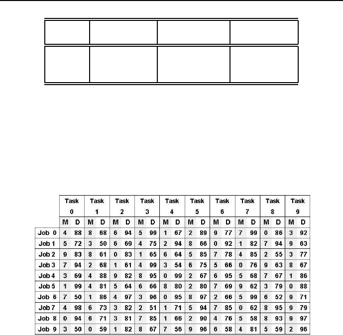
446 Chapter 6. CLP with global constraints for optimal solutions
Job Job duration Due date Late penalty
number (in days) (in days) (in MU/day)
1 5 End of day 25 19
220 End of day 20 12
315 End of day 35 34
Table 6.12: Job durations, due dates and late penalties
ABZ5 benchmark
Check whether for the ABZ5 job-shop benchmark defined in Figure 6.29
there is a feasible solution. If the check is positive, write a program to solve
the job-shop problem using an approach similar to that used in Section
6.18.
Figure 6.29: Job-shop ABZ5 definition
Chapter 7
CLP for continuous
variables
7.1 CCSP and CCOP
All examples discussed so far were for discrete variables. The search trees were
of finite depth and the state spaces had a finite number of points, which could
be explored state after state, to search for feasible states.
ECLiPSeprovides also tools for solving constraint satisfaction problems
and constraint optimization problems for continuous variables, i.e. variables
having continuous domains, like e.g. 0 ≤X≤150;
1. A continuous constraint satisfaction problem (CCSP) is defined by:
•a finite set Sof continuous decision variables X1, ..., Xn, with values
from continuous domains D1, ..., Dn,whereDi=MaxiXiMini,
∈{<, ≤,=};
•a set of constraints between variables. The constraint Ci(Xi1, ..., Xik)
between kvariables from Sis given by a relation defined as subset of
the Cartesian product Di1×, ..., ×Dikthat determines variable val-
ues corresponding to each other in a sense defined by the problem.
Constraints for continuous variables are most often stated by means
of equations and inequalities.
447

448 Chapter 7. CLP for continuous variables
Continuous domains would make the search tree infinitely deep if the ap-
proach used for discrete domains as we know it from Chapters 2,..., 6
would be applied. To avoid this, the depth of search trees is limited by us-
ing constraint propagation methods that successfully narrow the variable
domains, e.g. for some initial domain 10 ≤X≤90 the next domain may
be 5 ≤X≤65, etc. Such narrowing never results in a single value, but in
a comparatively narrow domain. Therefore the results obtained have the
form:
X = Lower_bound__Upper_bound,
e.g.:
X = 36345.099404108__36345.099448266.
So bounded real results are written as two floating point bounds separated
by a double underscore__. They may also be written as:
X{Lower_bound .. Upper_bound}
e.g.:
X{36345.099404108 .. 36345.099448266},
with two floating point bounds separated by a double full stop ...The
apparatus needed to accomplish this is known as interval arithmetic1.So
a CCSP solution is given by any assignment of domain subintervals to
variables so that all constraints are satisfied. It may be non-unique or
unique. As for discrete CSP, CCSP’s may be divided into feasible state
determination problems and feasible trajectory determination problems.
For CCSP problems there is no need to evoke the eplex library, the library
ic being just right. However, symbols of arithmetic operations and rela-
tions for continuous variables have to be prefixed by $.
1Interval arithmetic - as contrasted with ”normal” arithmetic - deals with arithmetic ope-
rations on intervals. The result of arithmetic interval operations is not given by some set of
state variable values, but by some set of state variable intervals.

7.2 The blessing and curse of compound interest 449
2. A continuous constraint optimization problem (CCOP) is defined by:
•a finite set Sof continuous and discrete decision variables X1, ..., Xn,
with values often from a standard domain declared as 0.0..1.0Inf;
•a set of constraints between variables, often stated by means of equa-
tions and inequalities;
•an objective function, expressed as linear function of decision vari-
ables with not necessarily integer coefficients, to be minimized or
maximized by choosing proper values for the decision variables from
their domains;
•a set of declaration for parameterizing the solver and the [print-out.
For solving CCOP’s, the ECLiPSeplatform is integrated with incre-
mental interval solvers of linear equations, of linear programming, integer
programming and mixed programming problems. They may be used by
evoking the ECLiPSelibrary named eplex. This library enables the use of
ECLiPSefor the design of interfaces to commercial solvers like XPRESS-
MP by Dash Optimization or CPLEX by ILOG. Although both companies
provide students with free academic versions, the following examples will
makes use of only ECLiPSe-provided eplex solver.
Similar to discrete COP, CCOP may be divided into optimum state de-
termination problems and optimum trajectory determination problems.
As for discrete domains, it is worthwhile to start the discussion of ECLiPSe
applications to continuous domains with feasible state determination prob-
lems.
7.2 The blessing and curse of compound interest
7.2.1 Basic
Compound interest arises when interest is added to the principal of a deposit or
loan, so that, from that moment on, the interest that has been added also earns
interest. This addition of interest to the principal is called compounding.
Assume that some initial capital Cois deposited on a bank account with
interest rate 0 <i<1 compounded yearly. After the first year the value of
the deposit equals C1=C+i∗Co=Co(1+i). After the second year the
value is C2=C1+i∗C1=C1∗(1 + i)=Co∗(1 + i)2.Soafternears the

450 Chapter 7. CLP for continuous variables
deposit is worth Cn=Co∗(1+1)
n. Of course, if a loan of Cois made at a bank
under the same conditions, after nyears the debt increases to Cn=Co∗(1+i)n.
What does it mean? Suppose that in the year 1 A.D. our forefather bor-
rowed 1MU with 1%interest rate compounded yearly, and he as well as all
his descendants forgot about it, but the bank survived all historical calamities
keeping account of this loan, we would - in year 2010 - inherit a debt equal
485245261.49 MU2.
7.2.2 Calculating compound interest in CLP
Mariott [Marriott-98] presented a useful recursive predicate defining compound
interest. It is used in the 7_1_compound_interest.clp program:
/*1*/ :- lib(ic).
/*2*/ top :-
/*3*/ List = [PV,T,I],
/*4*/ List :: 0.0..1000000.0,
/*5*/ T $= 24, % Number of periods
/*6*/ I $= 8/100, % Interest rate per period
/*7*/ PV $= 1000, % Initial prinicple
/*8*/ compound_interest(PV,T,I).
/*9*/ compound_interest(PV,T,I):-
/*10*/ T $>= 1, % There are still some periods of payments,
/*11*/ NT $= T-1, % but each period it is one period less.
/*12*/ FV $= PV + (PV * I), % Updated principle
/*13*/ compound_interest(FV,NT,I).
/*14*/ compound_interest(FV,T,_):- %
/*15*/ T $= 0,
/*16*/ write("Future Value = "),write(FV), nl.
It essence is to define recursively compound_interest/3 by itself with updated
number of periods and updated principle, and continuing this process until we
run out of time periods. The result is given i interval arithmetic:
2May be this explosion is responsible for the known fact of politicians not minding much
about paying national debts, but simply waiting until it reaches exorbitant ”unpayable” pro-
portions. May be this is the reason banks like nurturing creditors debts to wait for the moment
the debt is sufficiently high but still payable by the debtor.

7.2 The blessing and curse of compound interest 451
Principle = 6341.18073133441__6341.18073724012
So the domain of the variable Principle has been reduced to a suitably small
interval.
7.2.3 To retire as millionaire - 1
Consider the following example: assume that while being 20 years old we de-
cided to retire at 65 being a millionaire. How large should the initial (and only)
deposit be at our personal account with a yearly compounded interest of 6% to
achieve this goal?
The solution is given by program 7_2_millionaire_1.ecl3:
/*1*/ :- lib(ic).
/*2*/ top :-
/*3*/ LD = [K,T,I],
/*4*/ LD :: 0.0..100000,
/*5*/ T $= 45.0, % Number of saving years
/*6*/ I $= 6/100, % Interest rate per year
/*7*/ pension(K,T,I),
/*8*/ write("First and only deposit (present value) = "), write(K), nl.
/*9*/ pension(K,T,I) :-
/*10*/ T $>= 1.0,
/*11*/ NK $= K + (K * I), % New state of pensioners account
/*12*/ NT $= T-1, % Yearly decrease of saving years
/*13*/ pension(NK, NT, I).
/*14*/ pension(K,T,_):-
/*15*/ T $= 0.0,
/*16*/ K $= 1000000. % State of pensioners account after 45 years.
The message is:
First and only deposit (present value) = 72650.0743490985__72650.0743562801
So a one-time deposit of 72650 MU at the age of 20 years will give - at 6%
3This is an FS-type problem.

452 Chapter 7. CLP for continuous variables
compound yearly interest - a pension equal 1 million MU at the age of 654.
The most important part of the program is the elegant recursive defini-
tion in lines /*9*/...\verb/*16*/+: with each recursion the number of years
decreases by 1 i and correspondingly our account increases until the number
of saving years equal 0 (line /*15*/), when the account reaches the value of
1000000, see line /*16*/.
7.2.4 To retire as millionaire - 2
Assume now that we can’t afford to make a deposit of 72650 MU at the age
of 20, but in order to retire as millionaire at 65 we will deposit each year for
45 years a fixed amount on our personal account with a yearly compounded
interest of 6%. How large must that yearly deposit be?
This is settled by program 7_3_millionaire_2.ecl5:
/*1*/ :- lib(ic).
/*2*/ top:-
/*3*/ LD = [K,T,I,R],
/*4*/ LD :: 0.0..1000000,
/*5*/ K $= 0.0, % Initial state of pensioners account
/*6*/ T $= 45.0, % Number of saving years
/*7*/ I $= 6/100, % Interest rate per year
/*8*/ R =< 4701, % Yearly payment
/*9*/ pension(K,T,I,R),
/*10*/ write("Yearly payment = "), write(R), nl.
/*11*/ pension(K,T,I,R):-
/*12*/ T $>= 1.0,
/*13*/ NK $= K + (K * I) + R, % New state of pensioners account
/*14*/ NT $= T-1, % Yearly decrease of saving years
/*15*/ pension(NK, NT,I,R).
/*16*/ pension(K,T,_,_):-
/*17*/ T $= 0.0,
/*18*/ K $= 1000000.0.
The private predicate pension(K,T,I,R) has - compared with the version from
Section 7.2.3 - one more argument. This is the yearly payment Rthat according
4Of course providing we enjoy political and economic stability.
5This is an FS-type problem.

7.2 The blessing and curse of compound interest 453
to line /*13*/ augments yearly our account. Because the problem is nonlinear,
ECLiPSehas to be helped by a trial and error determination of the bound in
line /*8*/.
The message generated is:
Yearly payment = _11419{4696.74977810691 .. 4701.0}
The variable _11419 is an internal variable used by ECLiPSeto store the final
result. Rounding up a little bit, the yearly deposit is between 4696.75 and
4701.0. So depositing yearly 4701 MU, which corresponds roughly to 392 MU
per month, we could retire after 45 years of toil having at our pensioners account
one million of MU6.
Notice that your overall payments would be this time 45 ×4701 = 211545,
which is roughly three times as much as for the one-time deposit from Section
7.2.3.
7.2.5 Those cursed mortgages!
We got a mortgage to be payed for the next 24 years, the yearly payment be-
ing 12000 MU, the mortgage being at yearly interest 8%7. How large was the
mortgage we got? What is the price of this mortgage? This will be clarified by
program 7_4_mortgage.ecl8:
/*1*/ :- lib(ic).
/*2*/ top:-
/*3*/ List = [K,T,I,R],
/*4*/ List :: 0.0..1000000.0,
/*5*/ T $= 24.0, % Number of paying years
/*6*/ I $= 8/100, % Interest rate per year
/*7*/ R $= 12000.0, % Yearly mortgage payments
/*8*/ mortgage(K,T,I,R),
/*9*/ Cost $= T * R,
/*10*/ write("Principle = "),write(K),nl,
/*11*/ write("Cost of mortgage = "),write(Cost),nl.
6It would be really nice if governments stopped looking after our well-fare and stopped
being good to us.
7Being young, healthy and having a secure academic employment, we surly can afford a
mortgage like this!
8This is an FS-type problem.

454 Chapter 7. CLP for continuous variables
/*12*/ mortgage(K,T,I,R):-
/*13*/ T $>= 1.0, % There are still some years of payments,
/*14*/ NT $= T-1, % but each year it is one year less.
/*15*/ NK $= K + (K * I) - R, % Updated principal or amount of loan
/*16*/ mortgage(NK,NT,I,R).
/*17*/ mortgage(K,T,_,_):- % uf! - finally the end of the ordeal!
/*18*/ T $= 0,
/*19*/ K $= 0.
The message is:
Principle = 126345.099404108__126345.099448266
Cost of mortgage = 288000.0__288000.0
So for a mortgage of roughly 126346 MU we have to pay over 24 years 288000
MU. Nothing better illustrates the saying ”Time is Money”.
The lines /*12*/,...,/*19*/ correspond this time to the recursive decrease
of our principal as the result of yearly payments, up to the final principal equal
0. According to line /*15*/ the current principal to be repaid increases yearly
by the interest rate term, and decreases yearly by the payment term.
7.2.6 Net Present Value or how much we make (or loose)
really?
While making business it is sometimes worthwhile to remember lost opportuni-
ties. Lost, because we could not engage in them just because of this business.
But in order to make a true balance of what has been gained (or lost), we better
take those lost opportunities into account. This is done by a concept known
as Net Present Value (NPV), which is estimating our future gains (or loses) in
terms of its present values, while considering the most likely (and most certain)
lost opportunity. The basic fact underlying NPV is that the value of money
changes in time because it may be invested and bring profit. So some mMU
gained (or lost) a year from now have a different present value, equal to:
m
(1 + r),
referred to as Net Present Value of those mMU gained (or lost) a year from now.
This means that m
(1+r)MU invested now will yield (with certainty) mMU a year

7.2 The blessing and curse of compound interest 455
later, rbeing the annual rate of return (or discount rate) . The words ”with
certainty” mean that there is a market commodity (e.g. government bonds)
guaranteeing an annual rate of return equal to r. A simple extension fo this
reasoning shows that m
(1+r)kMU invested now will yield (with certainty) mMU
kyears later. The concept is readily generalized to any future cash flows, and
therefore is used for comparing the desirability of different investments. Let’s
consider the following example of two investments:
1. Investment A requires a cash outlay of 8 million MU at time 0, will yield
a return of 26 million MU a year from now and requires yet another cash
outlay of 18 million MU two years from now in order to clear some envi-
ronmental damage due to our business activities. The net cash flow for
this investment is:
−8+26−18=0,
and that looks rather discouraging. Suppose there are government bonds
guaranteeing an annual rate of return equal to 0.25. This makes the NPV
of our investment equal to:
−8+ 26
(1+0.25) −18
(1 + 0.25)2=−8+20.8−11.52 = 1.2,
and that is not so bad, because it means investment A will increase the
company’s value expressed in time 0 by 1.2 million MU.
2. Investment B requires a cash outlay of 6 million MU at time 0, will yield
a return of 8 million MU a year from now and requires yet another cash
outlay of 18 million MU two years from now in order to clear some envi-
ronmental damage due to our business activities. The net cash flow for
this investment is:
−6+8−1=1,
however its NPV is
−6+ 8
(1 + 0.25) −1
(1+0.25)2=−6+6.4−0.65=−0.25,
So investment B, in spite of the positive cash flow, will decrease the com-
pany’s value expressed in time by 0 by 0.25 million MU.

456 Chapter 7. CLP for continuous variables
Consider the following example highlighting the concept9:
Star Oil Company is considering five different investment opportunities.The cash
outflows and NPV-s (in milliones of MU) are given by Table 7.1:
Financial parameters Inv. 1 Inv. 2 Inv. 3 Inv. 4 Inv. 5
Time 0 cash outflow 11 53 5 5 29
Time 1 cash outflow 3 6 5 1 14
NPV 13 10 16 14 39
Table 7.1: Financial parameters for investment options
Star Oil has 40 million MU available for investment at the present time (time
0), it estimates that one year from now (time 1) 20 million MU will be available
for investment. Star Oil may purchase any fraction of each investment. In this
case, cash outflows and NPV are adjusted accordingly. For example, if Star Oil
purchases one fifth of investment 3, then a cash outflow of 1
55=1millionMU
would be required at time 0, and a cash outflow of 1
55=1millionMU would
be required at time 1. The one-fifth of investment 3would yield an NPV of
1
516 = 3.2millionMU. Star Oil wants to maximize the NPV that can be ob-
tained by investing in investment 1-5, while assuming that any funds left over
at time 0 cannot be used at time 1. This is done by program 7_5_NPV.ecl:
/*1*/ :- lib(eplex).
/*2*/ top :-
% Xn - fraction of investment n purchased
/*3*/ Variables = [X1,X2,X3,X4,X5],
/*4*/ Variables $:: 0.0..1.0Inf,
/*5* X1 $=< 1,
/*6*/ X2 $=< 1,
/*7*/ X3 $=< 1,
/*8*/ X4 $=< 1,
/*9*/ X5 $=< 1,
/*10*/ 11*X1 + 53*X2 + 5*X3 + 5*X4 + 29*X5 $=< 40, % time 0 constraint
/*11*/ 3*X1 + 6*X2 + 5*X3 + X4 + 34*X5 $=< 20, % time 1 constraint
/*12*/ eplex_solver_setup(max(13*X1 + 16*X2 + 16*X3 +14*X4 + 39*X5)),
/*13*/ eplex_solve(Profit),
/*14*/ (foreach(Name,["X1","X2","X3","X4","X5"]),
/*15*/ foreach(V, Variables) do
9This example is from [Winston-94].

7.3 Warehouses - suppliers 457
/*16*/ eplex_var_get(V, typed_solution, V),
/*17*/ write(Name),write(" = "),write(V),nl),
/*18*/ write("Profit = "),write(Profit).
The solution is:
X1 = 1.0 X2 = 0.200859950859951
X3 = 1.0 X4 = 1.0
X5 = 0.288083538083538 Profit = 57.4490171990172
7.3 Warehouses - suppliers
Linear programming problems are problems of minimizing an objective function
being a linear form of decision variables under constraints being linear forms of
decision variables. They are ubiquitous in OR applications. Their solution using
ECLiPSemay be illustrated by the transportation problem for 3warehouses
and 4suppliers:
Some volumes of Important Raw Material (IRM) have been contracted from
four suppliers S1, S2, S3 and S4. The material should be delivered to three
warehouses W1, W2 and W3 of limited capacity and different delivery costs due
to different delivery distances, see Figure 7.1.
The following data is known:
Contracts signed with supplier j:
Contract_j, j=1,2,3,4
Delivery cost for a unit of IRM to warehouse ifrom supplier j:
Cost_i_j, i=1,2,3, j=1,2,3,4
Space available in warehouse i:
Capacity_i, i=1,2,3
The delivery sizes:
Delivery_i_j, i=1,2,3, j=1,2,3,4
to each warehouse ifrom each supplier jshould be determined in a way minimiz-
ing the entire delivery cost while fulfilling the contracted quotas and respecting
available warehouse capacities.
The solution is given by program 7_4_warehouses_clients_1.ecl10 :
10 This is an OS-type problem.
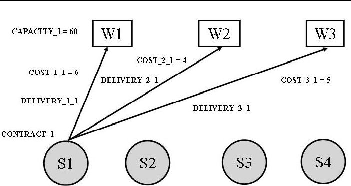
458 Chapter 7. CLP for continuous variables
Figure 7.1: Warehouses - suppliers data
/*1*/ :- lib(eplex).
/*2*/ top :-
/*3*/ solve(_,_).
/*4*/ solve(Cost,Variables):-
% Declaring variables and their domains:
/*5*/ Variables = [Delivery_1_1,Delivery_2_1,Delivery_3_1,
Delivery_1_2,Delivery_2_2,Delivery_3_2,
Delivery_1_3,Delivery_2_3,Delivery_3_3,
Delivery_1_4,Delivery_2_4,Delivery_3_4],
/*6*/ Variables $:: 0.0..1.0Inf,
/*7*/ % (integers(Variables)),
/*8*/ Cost_1_1 is 6.5,
/*9*/ Cost_1_2 is 2,
/*10*/ Cost_1_3 is 6.3,
/*11*/ Cost_1_4 is 7.3,
/*12*/ Cost_2_1 is 4,
/*13*/ Cost_2_2 is 9.7,
/*14*/ Cost_2_3 is 5.2,
/*15*/ Cost_2_4 is 3,
/*16*/ Cost_3_1 is 5.8,
/*17*/ Cost_3_2 is 2.4,
/*18*/ Cost_3_3 is 1.7,
/*19*/ Cost_3_4 is 9,
/*20*/ Capacity_1 is 60,

7.3 Warehouses - suppliers 459
/*21*/ Capacity_2 is 55,
/*22*/ Capacity_3 is 51,
/*23*/ Contract_1 is 35.5,
/*24*/ Contract_2 is 37,
/*25*/ Contract_3 is 22.7,
/*26*/ Contract_4 is 32,
% Contract constraints for clients:
/*27*/ Delivery_1_1 + Delivery_2_1 + Delivery_3_1 $=
Contract_1,
/*28*/ Delivery_1_2 + Delivery_2_2 + Delivery_3_2 $=
Contract_2,
/*29*/ Delivery_1_3 + Delivery_2_3 + Delivery_3_3 $=
Contract_3,
/*30*/ Delivery_1_4 + Delivery_2_4 + Delivery_3_4 $=
Contract_4,
% Space constraints for warehouses:
/*31*/ Delivery_1_1 + Delivery_1_2 + Delivery_1_3 +
Delivery_1_4 $=< Capacity_1,
/*32*/ Delivery_2_1 + Delivery_2_2 + Delivery_2_3 +
Delivery_2_4 $=< Capacity_2,
/*33*/ Delivery_3_1 + Delivery_3_2 + Delivery_3_3 +
Delivery_3_4 $=< Capacity_3,
% Configuring eplex solver for
% minimizing the performance index:
/*34*/ eplex_solver_setup(min(
Cost_1_1 * Delivery_1_1 + Cost_2_1 * Delivery_2_1 +
Cost_3_1 * Delivery_3_1 + Cost_1_2 * Delivery_1_2 +
Cost_2_2 * Delivery_2_2 + Cost_3_2 * Delivery_3_2 +
Cost_1_3 * Delivery_1_3 + Cost_2_3 * Delivery_2_3 +
Cost_3_3 * Delivery_3_3 + Cost_1_4 * Delivery_1_4 +
Cost_2_4 * Delivery_2_4 + Cost_3_4 * Delivery_3_4
)),
% % Solving the problem:
/*35*/ eplex_solveCost),
% Displaying results:
/*36*/ (foreach(Name,[
"Delivery_1_1","Delivery_2_1","Delivery_3_1",
"Delivery_1_2","Delivery_2_2","Delivery_3_2",
"Delivery_1_3","Delivery_2_3","Delivery_3_3",
"Delivery_1_4","Delivery_2_4","Delivery_3_4"]),
/*37*/ foreach(V, Variables)
/*38*/ do
/*39*/ eplex_var_get(V, typed_solution, V),

460 Chapter 7. CLP for continuous variables
/*40*/ write(Name),write(" = "),write(V),nl
/*41*/ ),
/*42*/ write("Cost"),write(" = "),writeCost),nl.
The message is:
Delivery_1_1 = 0.0
Delivery_2_1 = 23.0
Delivery_3_1 = 12.5
Delivery_1_2 = 37.0
Delivery_2_2 = 0.0
Delivery_3_2 = 0.0
Delivery_1_3 = 0.0
Delivery_2_3 = 0.0
Delivery_3_3 = 22.7
Delivery_1_4 = 0.0
Delivery_2_4 = 32.0
Delivery_3_4 = 0.0
Cost = 373.09
Decommenting the code in line /*7*/ makes the solver an integer program-
ming solver. If additionally in lines /*27*/,/*28*/,/*29*/ and /*30*/ the
relations ”$= are swapped for ”$>= (i.e. some over-realization of contracts will
be acceptable), the programm changes into 7_5_warehouses_clients _2.ecl
giving the solution:
Delivery_1_1 = 0
Delivery_2_1 = 23
Delivery_3_1 = 13
Delivery_1_2 = 37
Delivery_2_2 = 0
Delivery_3_2 = 0
Delivery_1_3 = 0
Delivery_2_3 = 0
Delivery_3_3 = 23
Delivery_1_4 = 0
Delivery_2_4 = 32
Delivery_3_4 = 0
Cost = 376.5
7.4 Refining and blending oils 461
This solution is intuitively obvious. Because in order to get an integer so-
lution the constraints in lines /*27*/,/*28*/,/*29*/ and /*30*/ have been
relaxed (contracts could be over-realized), the minimum cost has to increase.
7.4 Refining and blending oils
Consider another classical OR problem traditionally solved using linear pro-
gramming:
To manufacture some food, refining and blending of five oils: two common
vegetable oils (C1 and C2) and three tropical oils ( T1, T2 and T3), must be
performed. The blend must maximize profit under constraint of hardiness.
To refine common vegetable oils, a different production line is needed than
for tropical oil refining.
The monthly refinery lines production cannot exceed 200 ton of common
plant oil and 250 ton tropical oils. The production losses are negligible.
The purchase costs, refinery costs and hardiness for 1 ton of oils may be
found in Table 7.2.
Oils
Parameters C1 C2 T1 T2 T3
Cost 110 120 130 110 115
Hardness 8.8 6.1 2.0 4.2 5.0
Table 7.2: Oil data
The hardiness of the blend is a linear function of the component hardiness
and should be in the range [3,...,6]. A ton of the food may be sold for 150 MU.
The amount of monthly purchased oils and the monthly food production should
be determined so as to maximize the objective function given by the monthly
profit.
Following variables are defined:
XC1, XC2, XT1, XT2, XT3 - amount (in tons) of oils purchased monthly,
Y– amount (in tons) of food produced monthly.

462 Chapter 7. CLP for continuous variables
The solution is given by program 7_6_mixing_oils_1.ecl11 :
/*1*/ :- lib(eplex).
/*2*/ top :-
/*3*/ oils_1(_,_).
/*4*/ oils_1(Profit, Variables) :-
% Declaring variables and their domains:
/*5*/ Variables = [XC1,XC2,XT1,XT2,XT3,Y],
/*6*/ % integers(Variables),
/*7*/ Variables $:: 0.0..1.0Inf,
% Declaring constraints for the eplex instance:
/*8*/ XC1 + XC2 $=< 200,
/*9*/ XT1 + XT2 + XT3 $=< 250,
/*10*/ 8.8*XC1 + 6.1*XC2 + 2*XT1 + 4.2*XT2 +5*XT3 $=< 6*Y,
/*11*/ 8.8*XC1 + 6.1*XC2 + 2*XT1 + 4.2*XT2 +5*XT3 $>= 3*Y,
/*12*/ XC1 + XC2 + XT1 + XT2 + XT3 $= Y,
% Configuring eplex solver for
% maximizing the performance index:
+
/*13*/ eplex_solver_setup(max(
150*Y - 110*XC1 - 120*XC2 -130*XT1 - 110*XT2 - 115*XT3),
% Solving the problem:
/*14*/ eplex_solve(Profit),
% Displaying results:
/*15*/ (foreach(Name,["XC1","XC2","XT1","XT2","XT3","Y"]),
/*16*/ foreach(V, Variables) do
/*17*/ prob: eplex_var_get(V, typed_solution, V),
/*18*/ write(Name),write(" = "),write(V),nl
/*19*/ ),
/*20*/ write("Profit = "),write(Profit).
The message is:
XC1 = 159.259259259259 XC2 = 40.7407407407409
XT1 = 0.0 XT2 = 250.0
XT3 = 0.0 Y = 450.0
Profit = 17592.5925925926
11 This is an OS-type problem.

7.5 How to make easy money? 463
If the code in line /*6*/ is decommented, the resulting program
7_7_mixing_oils_2.ecl gives an integer solution:
XC1 = 159 XC2 = 41
XT1 = 0 XT2 = 250
XT3=0 Y=450
Profit = 17590.0
7.5 How to make easy money?
The previous examples show that ECLiPSeis tolerating LP models that do
not exactly conform to the classical LP canonical form. This tolerance is really
far reaching, as demonstrated by the next example:
A tireless public servant and distinguished member of the Absurdoland’s Up-
per House of Parliament, the Celebrated Senator, firmly convinced that ethanol
in automotive fuels would save the Earth, for a number of years did all he
could to satisfy the legislating wishes and suggestions of the well-known ethanol
producer Corny Fuels. Appreciating his relentless efforts, the friendly CEO of
Corny Fuels ordered its Banking Outlet to provide to the company of the Ce-
lebrated Senators Wife a 100 million MU loan for some shady investment, for 4
years at very decent interests of 2% per year12.
The Friendly Manager of the Banking Outlet suggested the Celebrated Sen-
ators Wife should herself determine the yearly payments provided they are not
lower than 10 million MU. The Celebrated Senators Wife very wisely did not
pursue the shady investment, but deposited the entire loan in a Less Friendly
Bank, where yearly deposits could be kept at a yearly compound interest, always
2% higher than the forecasted inflation. The yearly inflation was forecasted for
the first year to be 5%, for the second year - 4%, for the third year 3%,andfor
the fourth year - 2%.
However the Celebrated Senators Wife had quite a headache with managing
the loan. Her Financial Advisor suggested two different investment strategies:
1. To maximize the profit from the deposit while sticking to the Friendly Man-
agers suggestions.
2. To minimize the forecasted real costs of the loan while sticking to the Friend ly
12 The CEO was firmly convinced that it is always cheaper to buy legislatures than to buy
the majority of voters.

464 Chapter 7. CLP for continuous variables
Managers suggestions.
The Financial Advisor could not satisfactory explain the difference in out-
come (if any) of both strategies. In appreciation of services rendered to the Soci-
ety by the Celebrated Senator, a befriended CLP programmer wrote a program
(7_8_getting_rich.ecl13 ) designed to dispel any doubts about the outcomes
of both strategies:
/*1*/ :- lib(eplex).
/*2*/ top:-
/*4*/ write("Choose the version (1 or 2):"),nl,
/*4*/ read_token(Number, integer),
/*5*/ solve(Number).
/*6*/ solve(1):-
/*7*/ A $>= 10, % payment after first year
/*8*/ B $>= 10, % payment after second year
/*9*/ C $>= 10, % payment after third year
/*10*/ D $>= 10, % payment after fourth year
/*11*/ payments([A,B,C,D], 100),
/*12*/ Profit_A $= 100*(1.07)-A,
/*13*/ Profit_B $= Profit_A*(1.06)-B,
/*14*/ Profit_C $= Profit_B*(1.05)-C,
/*15*/ Profit_D $= Profit_C*(1.04)-D,
/*16*/ Profit_D $:: 0..250,
/*17*/ eplex_solver_setup(max(Profit_D)),
/*18*/ eplex_solve(Profit_D),
/*19*/ eplex_get(vars, Vars),
/*20*/ eplex_get(typed_solution, Vals),
/*21*/ Vars = Vals,
/*22*/ Cost_of_credit is
A*0.95+B*0.95*0.96+C*0.95*0.96*0.97+
D*0.95*0.96*0.97*0.98,
/*23*/ write("Payment after first year = "),write(A),write(" MM."),nl,
/*24*/ write("Payment after second year = "),write(B),write(" MM."),nl,
/*25*/ write("Payment after third year = "),write(C),write(" MM."),nl,
/*26*/ write("Payment after fourth year = "),write(D),write(" MM."),nl,
/*27*/ write("Projected real cost of credit = "), write(Cost_of_credit),
write(" MM. "),nl,
/*28*/ write("Maximum profit after 4 years = "), write(Profit_D),
write(" MM. "),nl,nl.
13 This is an OST-type problem.

7.5 How to make easy money? 465
/*29*/ solve(2):-
/*39*/ A $>= 10, % payment after firts year
/*31*/ B $>= 10, % payment after second year
/*32*/ C $>= 10, % payment after third year
/*33*/ D $>= 10, % payment after fourth year
/*34*/ payments([A,B,C,D], 100),
/*35*/ Cost_of_credit $=
A*0.95+B*0.95*0.96+C*0.95*0.96*0.97+
D*0.95*0.96*0.97*0.98,
/*36*/ eplex_solver_setup(min(Cost_of_credit)),
/*37*/ eplex_solve(Cost_of_credit),
/*38*/ eplex_get(vars, Vars),
/*39*/ eplex_get(typed_solution, Vals),
/*40*/ Vars = Vals,
/*41*/ Profit_A is 100*(1.07)-A,
/*42*/ Profit_B is Profit_A*(1.06)-B,
/*43*/ Profit_C is Profit_B*1.05-C,
/*44*/ Profit_D is Profit_C*1.04-D,
/*45*/ write("Payment after first year = "),write(A),write(" MM."),nl,
/*46*/ write("Payment after second year = "),write(B),write(" MM."),nl,
/*47*/ write("Payment after third year = "),write(C),write(" MM."),nl,
/*48*/ write("Payment after fourth year = "),write(D),write(" MM."),nl,
/*49*/ write("Minimum projected cost of credit = "), write(Cost_of_credit),
write(" MM."),nl,
/*50*/ write("Profit after 4 years ="),write(Profit_D),write(" MM."),nl.
/*51*/ payments([],Loan) :-
/*52*/ Loan $=0.
/*53*/ payments([Payment|List_of_payments],Loan) :-
/*54*/ Updated_principal $=(1+2/100)*Loan-Payment,
/*55*/ payments(List_of_payments,Updated_principal).
The message is:
Choose the version (1 or 2): choice 1
Payment after first year = 10.0 MM.
Payment after second year = 10.0 MM.
Payment after third year = 10.0 MM.
Payment after fourth year = 77.027136 MM.
Projected real cost of credit =
94.2448598792192 MM.
Maximum profit after 4 years: 13.932304 MM.
Choose the version (1 or 2): choice 2

466 Chapter 7. CLP for continuous variables
Payment after first year = 10.0 MM.
Payment after second year = 10.0 MM.
Payment after third year = 10.0 MM.
Payment after fourth year = 77.027136 MM.
Minimum projected cost of credit =
94.2448598792192 MM.
Profit after 4 years: 13.932304 MM.
It follows that no matter what strategy the Celebrated Senators Wife will
opt for, the profit (a nice 13.932304 MM MU) and the payment strategy will
always be the same.
7.6 Making shrewd investments
ECLiPSeformulations of LP problems may be far, far removed from the con-
ventional LP canonical form. This is illustrated by the following example:
The chief accountant of some small company has forecast the cash require-
ments for the next five years. It turned out that the company would have some
free cash in the future. He considered the following investments options:
1. Short term (one-year bonds) with interest rates (return after a year) 20%.
2. Intermediate term (two-year bonds) with interest rates (return after two
years) 47%.
3. Long term (three-year bonds) with interest rates (return after three years)
78%.
He wishes to plan the investments over five years taking into account the cash
requirements and one of the following three investment options, given the initial
cash of 100000 MU:
Option 1: satisfy yearly demands and maximize the amount of cash at the end
of the five years period.
Option 2: satisfy yearly demands and minimize initial cash.
Option 3: satisfy yearly demands and determine the minimum initial cash
needed to have at the end of the five years period the same amount of
cash.

7.6 Making shrewd investments 467
Cash requirements at the beginnings of each year are given by Table 7.3:
Year Amount Variable
110000 Crx1
210000 Crx2
320000 Crx3
420000 Crx4
520000 Crx5
Table 7.3: Cash requirements for consecutive years
To model the problem, following variables are defined :
Sinx : Short term investment at the beginning of year x
Iinx : Intermediate term investment at the beginning of year x
Linx : Long term investment at the beginning of year x
Tinx : Total investment at the beginning of year x
Srex : Short term revenue at the beginning of year x
Irex : Intermediate term revenue at the beginning of year x
Lrex : Long term revenue at the beginning of year x
Trex : Total revenue at the beginning of year x
Crx : cash requirement at the beginning of year x
Ebcx: ending cash balance at the beginning of year x
What decisions with respect to forms of investment have to be made each year?
The answer is given by 7_9_inwestments.ecl14 :
/*1*/ :- lib(eplex).
/*2*/ top:-
/*3*/ writeln("Option 1:"),
/*4*/ not( not(top(100000.0,_))),
/*5*/ writeln("Option 2:"),
/*6*/ not( not(top(_,150000.0))),
/*7*/ writeln("Option 3:"),
/*8*/ not( not(top(X,X))).
14 This is an OST-type problem.

468 Chapter 7. CLP for continuous variables
/*9*/ top(Initial_cash,Final_cash):-
% we start with a dummy performance index:
/*10*/ eplex_solver_setup(max(0)),
/*11*/ investments(Initial_cash, Variables, Names, Final_cash),
% find minimum Initial_cash and fix it:
/*12*/ eplex_probe(min(Initial_cash), Initial_cash),
% find maximum Final_cash and fix it:
/*13*/ eplex_probe(max(Final_cash), Final_cash),
/*14*/ eplex_get(typed_solution, Vs), eplex_get(vars, Vs),
/*15*/ writelist(Names, Variables),
/*16*/ write("Initial cash: "),writeln(Initial_cash),
/*17*/ write("Final cash: "),writeln(Final_cash),nl.
/*18*/ investments(Initial_cash, Variables, Names, Final_cash) :-
/*19*/ Variables = [
Sin1,Sin2,Sin3,Sin4,Sin5,
Iin1,Iin2,Iin3,Iin4,Iin5,
Lin1,Lin2,Lin3,Lin4,Lin5,
Tin1,Tin2,Tin3,Tin4,Tin5,
Sre2,Sre3,Sre4,Sre5,Sre6,
Ire3,Ire4,Ire5,Ire6,
Lre4,Lre5,LreC,
Tre2,Tre3,Tre4,Tre5,Tre6,
Ebc1,Ebc2,Ebc3,Ebc4,Ebc5
],
/*20*/ Names = [
"Sin1","Sin2","Sin3","Sin4","Sin5",
"Iin1","Iin2","Iin3","Iin4","Iin5",
"Lin1","Lin2","Lin3","Lin4","Lin5",
"Tin1","Tin2","Tin3","Tin4","Tin5",
"Sre2","Sre3","Sre4","Sre5","Sre6",
"Ire3","Ire4","Ire5","Ire6",
"Lre4","Lre5","LreC",
"Tre2","Tre3","Tre4","Tre5","Tre6",
"Ebc1","Ebc2","Ebc3","Ebc4","Ebc5"
],
/*21*/ Variables $:: 0..inf,
/*22*/ Tin1 $= Iin1 + Sin1 + Lin1,
/*23*/ Tin2 $= Iin2 + Sin2 + Lin2,
/*24*/ Tin3 $= Iin3 + Sin3 + Lin3,
/*25*/ Tin4 $= Iin4 + Sin4 + Lin4,
/*26*/ Tin5 $= Iin5 + Sin5 + Lin5,
/*27*/ Ire3 $= 1.47 * Iin1,
/*28*/ Ire4 $= 1.47 * Iin2,

7.6 Making shrewd investments 469
/*29*/ Ire5 $= 1.47 * Iin3,
/*30*/ Ire6 $= 1.47 * Iin4,
/*31*/ Lre4 $= 1.78 * Lin1,
/*32*/ Lre5 $= 1.78 * Lin2,
/*33*/ Lre6 $= 1.78 * Lin3,
/*34*/ Sre2 $= 1.2 * Sin1,
/*35*/ Sre3 $= 1.2 * Sin2,
/*36*/ Sre4 $= 1.2 * Sin3,
/*37*/ Sre5 $= 1.2 * Sin4,
/*38*/ Sre6 $= 1.2 * Sin5,
/*39*/ Tre2 $= Sre2,
/*40*/ Tre3 $= Sre3 + Ire3,
/*41*/ Tre4 $= Sre4 + Ire4 + Lre4,
/*42*/ Tre5 $= Sre5 + Ire5 + Lre5,
/*43*/ Tre6 $= Sre6 + Ire6 + Lre6,
/*44*/ Cr1 $>= 10000,
/*45*/ Cr2 $>= 10000,
/*46*/ Cr3 $>= 20000,
/*47*/ Cr4 $>= 20000,
/*48*/ Cr5 $>= 20000,
/*49*/ Ebc1 $= Initial_cash - Tin1 - Cr1,
/*50*/ Ebc2 $= Ebc1 + Tre2 - Tin2 - Cr2,
/*51*/ Ebc3 $= Ebc2 + Tre3 - Tin3 - Cr3,
/*52*/ Ebc4 $= Ebc3 + Tre4 - Tin4 - Cr4,
/*53*/ Ebc5 $= Ebc4 + Tre5 - Tin5 - Cr5,
/*54*/ Final_cash $= Ebc5 + Tre6.
/*55*/ writelist([], []).
/*56*/ writelist([FN|RN], [FV|RV]) :-
/*57*/ write(FN), write(" = "), writeln(FV),
/*58*/ writelist(RN, RV).
To enhance the expressive power of the results they are presented in table 7.4,
which makes it easy to compare various investment options. The ”double nega-
tions” in lines /*4*/,/*6*/ and /*8*/ may be astonishing at first sight.

470 Chapter 7. CLP for continuous variables
Variable Option 1 Option 2 Option 3
Sin1 8333.33333333333 8333.33333333333 8333.33333333333
Sin2 0.0 0.0 0.0
Sin3 0.0 0.0 0.0
Sin4 0.0 0.0 0.0
Sin5 0.0 0.0 0.0
Iin1 22860.8450182794 80187.1463253183 55293.192790018
Iin2 0.0 0.0 0.0
Iin3 13605.4421768707 13605.4421768696 13605.4421768707
Iin4 84674.3625341293 0.0 0.0
Iin5 0.0 0.0 0.0
Lin1 58805.8216483872 11235.9550561798 11235.9550561798
Lin2 0.0 0.0 0.0
Lin3 0.0 84269.6629213483 47675.5512244557
Lin4 0.0 0.0 0.0
Lin5 0.0 0.0 0.0
Tin1 90000.0 99756.4347148322 74862.4811795311
Tin2 0.0 0.0 0.0
Tin3 13605.4421768707 97875.105098218 61280.9934013264
Tin4 84674.3625341293 0.0 0.0
Tin5 0.0 0.0 0.0
Sre2 10000.0 10000.0 10000.0
Sre3 0.0 0.0 0.0
Sre4 0.0 0.0 0.0
Sre5 0.0 0.0 0.0
Sre6 0.0 0.0 0.0
Ire3 33605.4421768707 117875.105098218 81280.9934013264
Ire4 0.0 0.0 0.0
Ire5 20000.0 19999.9999999984 20000.0
Ire6 124471.31292517 0.0 0.0
Lre4 104674.362534129 20000.0 20000.0
Lre5 0.0 0.0 0.0
Lre6 0.0 150000.0 84862.4811795311
Table 7.4: Results for investment options

7.7 Yet another financial Perpetuum Mobile!471
Variable Option 1 Option 2 Option 3
Tre2 10000.0 10000.0 10000.0
Tre3 33605.4421768707 117875.105098218 81280.9934013264
Tre4 104674.362534129 20000.0 20000.0
Tre5 20000.0 19999.9999999984 20000.0
Tre6 124471.31292517 150000.0 84862.4811795311
Gnad1 0.0 0.0 0.0
Gnad2 0.0 0.0 0.0
Gnad3 0.0 0.0 0.0
Gnad4 0.0 0.0 0.0
Gnad5 0.0 0.0 0.0
Initial cash 100000.0 109756.434714832 84862.4811795311
Final cash 124471.31292517 150000.0 84862.4811795311
Table 7.5: Results for investment options - continuation
However, it is an old Prolog trick15 that serves to call the same predicate with
changing data: the satisfaction of the first top(_,_) predicate makes the in-
ternal negation fail. That removes all results got so far, which in turn makes
the external negation true, and enables the second top(_,_) predicate to be
activated, and so on.
The basic model is given by cash balance equations and investment updates
equations from lines /*22*/ -/*54*/. They correspond directly to the invest-
ment options as stated in the problem and are - by all standards - far removed
from the conventional LP canonical form.
7.7 Yet another financial Perpetuum Mobile!
The mathematical model used for LP are mainly various balances. The nature
of those balances may sometimes be strange indeed. This is illustrated by the
following example. inspired by one presented by [Taha-08]:
Clever Young, a computer prodigy as well as a mathematical and business
whiz-kid, has been thinking a long time about how to make money on-line.
He finally decided to make some currency speculations using general available
15 Thanks are due to Joachim Schimpf from ECLiPSe for drawing the Authors attention to
this trick.
472 Chapter 7. CLP for continuous variables
real-time currency sites information and on-line facilities of foreign exchange
spot trading. He started with simulating speculations on five currencies: the
USD, EUR, GBP, JPY and PLN (that’s Polish Zloty). The exchange rates he
assembled for this purpose are mid-market rates derived from the mid-point
between the ”buy” and ”sell” rates from global currency markets for some day
and hour, and are given by Table 7.6.
USD EUR GBP JPY PLN
USD 10.8353 0.692 91.89 3.4872
EUR 1.1972 10.8283 110.03 4.181
GBP 1.445 1.2073 1132 5.0414
JPY 0.01088 0.009088 0.007575 13.7950
PLN 0.2867 0.2392 0.1983 0.2635 1
Table 7.6: Currency exchange rates for March 10, 2010
The meaning of this table is obvious: e.g. 1 EUR could be sold (bought)
for 1.1972 USD. Clever Young thinks it is possible to increase the USD hold-
ings (above some initial AMM USD) by circulating currencies throughout the
currency market. The problem is what and how much to buy, and what and
how much to sell in order to maximize the profit from the initial investment of
AMM USD?
The speculation is constrained by the regulation that sets the following limits
on the amount of any single transaction: USD ¡= 5, EUR ¡= 3, GBP ¡= 3.5,
JPY ¡= 100, PLN ¡= 40 (in millions)
Transaction are denoted by by variables of type:
CURRENCYitoCURRENCYj
denoting the amount in CURRENCYi converted to CURRENCYj. Exchange rates
from Table 7.6 are presented using variables:
Ex_rate_CURRENCYi_to_CURRENCYj.
Variable Adenotes the initial USD amount (in MM), variable Z- the final USD
holdings (in MM).
The program to test the speculation effectiveness is based on currency balances
for all currencies. They have the form:
Currency accumulation + Currency out = Currency in

7.7 Yet another financial Perpetuum Mobile!473
The program 7_10_currency_speculations.ecl16 is as follows:
/*1*/ :- lib(eplex).
/*2*/ top:-
/*3*/ % A = 5.0,
/*3a*/ A = 0.0,
% what currencies are USD converted to:
/*4*/ USD = [USDtoEUR,USDtoGBP,USDtoJPY,USDtoPLN],
/*5*/ USD :: 0.0..5.0,
/*6*/ Z :: 0.0..6.0,
% what currencies are EUR converted to:
/*7*/ EUR = [EURtoUSD,EURtoGBP,EURtoJPY,EURtoPLN],
/*8*/ EUR :: 0.0..3.0,
% what currencies are GBP converted to:
/*9*/ GBP = [GBPtoUSD,GBPtoEUR,GBPtoJPY,GBPtoPLN],
/*10*/ GBP :: 0.0..3.5,
% what currencies are JPY converted to:
/*11*/ JPY = [JPYtoUSD,JPYtoEUR,JPYtoGBP,JPYtoPLN],
/*12*/ JPY :: 0.0..100.0,
% what currencies are PLN converted to:
/*13*/ PLN = [PLNtoUSD,PLNtoEUR,PLNtoGBP,PLNtoJPY],
/*14*/ PLN :: 0.0..40.0,
/*15*/ Ex_rate_USD_to_EUR = 0.8353,
/*16*/ Ex_rate_USD_to_GBP = 0.692,
/*17*/ Ex_rate_USD_to_JPY = 91.89,
/*18*/ Ex_rate_USD_to_PLN = 3.4872,
/*19*/ Ex_rate_EUR_to_GBP = 0.8283 ,
/*20*/ Ex_rate_EUR_to_JPY = 110.03,
/*21*/ Ex_rate_EUR_to_PLN = 4.181,
/*22*/ Ex_rate_GBP_to_JPY = 132,
/*23*/ Ex_rate_GBP_to_PLN = 5.0414,
/*24*/ Ex_rate_JPY_to_PLN = 3.7950,
/*25*/ Ex_rate_EUR_to_USD is 1/(Ex_rate_USD_to_EUR),
/*26*/ Ex_rate_GBP_to_USD is 1/(Ex_rate_USD_to_GBP),
/*27*/ Ex_rate_JPY_to_USD is 1/(Ex_rate_USD_to_JPY),
/*28*/ Ex_rate_PLN_to_USD is 1/(Ex_rate_USD_to_PLN),
/*29*/ Ex_rate_GBP_to_EUR is 1/(Ex_rate_EUR_to_GBP),
/*30*/ Ex_rate_JPY_to_EUR is 1/(Ex_rate_EUR_to_JPY),
/*31*/ Ex_rate_PLN_to_EUR is 1/(Ex_rate_EUR_to_PLN),
16 This is an OS-type problem.

474 Chapter 7. CLP for continuous variables
/*33*/ Ex_rate_JPY_to_GBP is 1/(Ex_rate_GBP_to_JPY),
/*33*/ Ex_rate_PLN_to_GBP is 1/(Ex_rate_GBP_to_PLN),
/*34*/ Ex_rate_PLN_to_JPY is 1/(Ex_rate_JPY_to_PLN),
% USD balance:
/*35*/ Z + USDtoEUR + USDtoGBP + USDtoJPY + USDtoPLN $=
A + (Ex_rate_EUR_to_USD)*EURtoUSD + (Ex_rate_GBP_to_USD)*GBPtoUSD +
(Ex_rate_JPY_to_USD)*JPYtoUSD + (Ex_rate_PLN_to_USD)*PLNtoUSD,
% EUR balance:
/*36*/ EURtoUSD + EURtoGBP + EURtoJPY + EURtoPLN $=
(Ex_rate_USD_to_EUR)*USDtoEUR + (Ex_rate_GBP_to_EUR)*GBPtoEUR +
(Ex_rate_JPY_to_EUR)*JPYtoEUR + (Ex_rate_PLN_to_EUR)*PLNtoEUR,
% GBP balance:
/*37*/ GBPtoUSD + GBPtoEUR + GBPtoJPY + GBPtoPLN $=
(Ex_rate_USD_to_GBP)*USDtoGBP + (Ex_rate_EUR_to_GBP)*EURtoGBP +
(Ex_rate_JPY_to_GBP)*JPYtoGBP + (Ex_rate_PLN_to_GBP)*PLNtoGBP,
% JPY balance:
/*38*/ JPYtoUSD + JPYtoEUR + JPYtoGBP + JPYtoPLN $=
(Ex_rate_USD_to_JPY)*USDtoJPY + (Ex_rate_EUR_to_JPY)*EURtoJPY +
(Ex_rate_GBP_to_JPY)*GBPtoJPY + (Ex_rate_PLN_to_JPY)*PLNtoJPY,
% PLN balance:
/*39*/ PLNtoUSD + PLNtoEUR + PLNtoGBP + PLNtoJPY $=
(Ex_rate_USD_to_PLN)*USDtoPLN + (Ex_rate_EUR_to_PLN)*EURtoPLN +
(Ex_rate_GBP_to_PLN)*GBPtoPLN + (Ex_rate_JPY_to_PLN)*JPYtoPLN,
/*40*/ eplex_solver_setup(max(Z)),
/*41*/ eplex_solve(Z),
/*42*/ eplex_get(vars, Vars),
/*43*/ eplex_get(typed_solution, Vals),
/*44*/ Vars = Vals,
/*45*/ writeln("A ": A),
/*46*/ writeln("Final USD holdings (in MM)) ": Z),
/*47*/ write_positive("USDtoEUR", USDtoGBP),
/*48*/ write_positive("USDtoGBP", USDtoGBP),
/*49*/ write_positive("USDtoJPY", USDtoJPY),
/*50*/ write_positive("USDtoPLN", USDtoPLN),
/*51*/ write_positive("EURtoUSD", EURtoUSD),
/*52*/ write_positive("EURtoGBP", EURtoGBP),
/*53*/ write_positive("EURtoJPY", EURtoJPY),
/*54*/ write_positive("EURtoPLN", EURtoPLN),
/*55*/ write_positive("GBPtoUSD", GBPtoUSD),
/*56*/ write_positive("GBPtoEUR", GBPtoEUR),
/*57*/ write_positive("GBPtoJPY", GBPtoJPY),
/*58*/ write_positive("GBPtoPLN", GBPtoPLN),

7.7 Yet another financial Perpetuum Mobile!475
/*59*/ write_positive("JPYtoUSD", JPYtoUSD),
/*60*/ write_positive("JPYtoEUR", JPYtoEUR),
/*61*/ write_positive("JPYtoGBP", JPYtoGBP),
/*62*/ write_positive("JPYtoPLN", JPYtoPLN),
/*63*/ write_positive("PLNtoUSD", PLNtoUSD),
/*64*/ write_positive("PLNtoEUR", PLNtoEUR),
/*65*/ write_positive("PLNtoGBP", PLNtoGBP),
/*66*/ write_positive("PLNtoJPY", PLNtoJPY),
/*67*/ writeln("Ex_rate_USD_to_EUR":Ex_rate_USD_to_EUR),
/*68*/ writeln("Ex_rate_USD_to_GBP":Ex_rate_USD_to_GBP),
/*69*/ writeln("Ex_rate_USD_to_JPY":Ex_rate_USD_to_JPY),
/*70*/ writeln("Ex_rate_USD_to_PLN":Ex_rate_USD_to_PLN),
/*71*/ writeln("Ex_rate_EUR_to_USD":Ex_rate_EUR_to_USD),
/*72*/ writeln("Ex_rate_EUR_to_GBP":Ex_rate_EUR_to_GBP),
/*73*/ writeln("Ex_rate_EUR_to_JPY":Ex_rate_EUR_to_JPY),
/*74*/ writeln("Ex_rate_EUR_to_PLN":Ex_rate_EUR_to_PLN),
/*75*/ writeln("Ex_rate_GBP_to_USD":Ex_rate_GBP_to_USD),
/*76*/ writeln("Ex_rate_GBP_to_EUR":Ex_rate_GBP_to_EUR),
/*77*/ writeln("Ex_rate_GBP_to_JPY":Ex_rate_GBP_to_JPY),
/*78*/ writeln("Ex_rate_GBP_to_PLN":Ex_rate_GBP_to_PLN),
/*79*/ writeln("Ex_rate_JPY_to_USD":Ex_rate_JPY_to_USD),
/*80*/ writeln("Ex_rate_JPY_to_EUR":Ex_rate_JPY_to_EUR),
/*81*/ writeln("Ex_rate_JPY_to_GBP":Ex_rate_JPY_to_GBP),
/*82*/ writeln("Ex_rate_JPY_to_PLN":Ex_rate_JPY_to_PLN),
/*83*/ writeln("Ex_rate_PLN_to_USD":Ex_rate_PLN_to_USD),
/*84*/ writeln("Ex_rate_PLN_to_EUR":Ex_rate_PLN_to_EUR),
/*85*/ writeln("Ex_rate_PLN_to_GBP":Ex_rate_PLN_to_GBP),
/*86*/ writeln("Ex_rate_PLN_to_JPY":Ex_rate_PLN_to_JPY).
/*87*/ write_positive(A, B):-
/*88*/ (B > 0 -> writeln(A:B); true).
The message is:
A : 5.0
Final USD holdings (in MM)) : 6.0
EURtoJPY : 0.00843576360267486
JPYtoPLN : 0.928187069202315
PLNtoUSD : 3.4872
PLNtoEUR : 0.0352699276227836
Ex_rate_USD_to_EUR : 0.8353
Ex_rate_USD_to_GBP : 0.692
Ex_rate_USD_to_JPY : 91.89
Ex_rate_USD_to_PLN : 3.4872
Ex_rate_EUR_to_USD : 1.19717466778403
Ex_rate_EUR_to_GBP : 0.8283

476 Chapter 7. CLP for continuous variables
Ex_rate_EUR_to_JPY : 110.03
Ex_rate_EUR_to_PLN : 4.181
Ex_rate_GBP_to_USD : 1.44508670520231
Ex_rate_GBP_to_EUR : 1.20729204394543
Ex_rate_GBP_to_JPY : 132
Ex_rate_GBP_to_PLN : 5.0414
Ex_rate_JPY_to_USD : 0.0108825769942322
Ex_rate_JPY_to_EUR : 0.00908843042806507
Ex_rate_JPY_to_GBP : 0.00757575757575758
Ex_rate_JPY_to_PLN : 3.795
Ex_rate_PLN_to_USD : 0.286763019041064
Ex_rate_PLN_to_EUR : 0.239177230327673
Ex_rate_PLN_to_GBP : 0.198357599079621
Ex_rate_PLN_to_JPY : 0.263504611330698
The result was so astonishing that Clever Young decided to check all bal-
ances:
The USD check:
6+0+0+0+0 = 5+0+0+0+0.286763019041064*3.4872
gives:
6=6
The EUR check:
0+0+0.00843576360267486+0 = 0+0+0+
0.239177230327673*0.0352699276227836
gives:
0.008435763602674869 = 0.008435763602674869
The GBP check is trivial:
0+0+0+0 = 0+0+0+0
The JPY check:
0+0+0+0.928187069202315 = 0+110.03*0.00843576360267486+0+0
gives:
0.928187069202315 = 0.9281870692023148458
The PLN check:
3.4872+0.0352699276227836+0+0 = 0+0+0+3.795*0.928187069202315

7.7 Yet another financial Perpetuum Mobile!477
gives:
3.5224699 = 3.5224699
So everything is O.K.! If the obtained solution is submitted to the currency
dealer as one order, there is no need for waiting until some other currencies are
accumulated to make a buy. However the problem remains: where to get the
5MM of USD from in order to convert them to 6MM USD. Clever Young,
having an enterprising nature, made one more try, this time with A=0, i.e. with
no initial USD at all. The result was as follows, the exchange rates messages
being omitted:
A : 0.0
Final USD holdings (in MM)) : 6.0
EURtoJPY : 0.0506145816160492
JPYtoPLN : 5.56912241521389
PLNtoUSD : 20.9232
PLNtoEUR : 0.211619565736702
with GBP not participating in the deal.
Clever Young just couldn’t believe his eyes. To get 6 million USD just out
of thin air, starting with nothing at all! He made a check of balances:
The USD check:
6+0+0+0+0 = 0+0+0+0+20.9232*3.4872
gives:
6=6
The EUR check:
0+0+0.0506145816160492+0 = 0+0+0+
0.239177230327673*0.211619565736702
gives:
0.0506145816160492 = 0.0506145816160492
The GBP check is trivial:
0+0+0+0 = 0+0+0+0
The JPY check:
0+0+0+5.56912241521389 = 0+110.03*0.0506145816160492+0+0
gives:

478 Chapter 7. CLP for continuous variables
5.56912241521389 = 5.56912241521389
The PLN check:
20.9232+0.211619565736702+0+0 = 0+0+0+3.795*5.56912241521389
gives:
21.13481956573 = 21.1348195657
So everything is O.K. one more time. However, Clever Young still wondered
about getting the same 6 MM USD as before. Because those 6 MM USD were
equal to the (somewhat arbitrarily) upper level in line /*6*/ (domain definition
for Z), he decided to make yet one more simulation, but this time with the
upper level equal to 120 MM USD. he result was as follows wit the exchange
rates messages being omitted:
A : 0.0
Final USD holdings (in MM)) : 21.208105932626
EURtoUSD : 3.0
EURtoJPY : 1.08782427718034
GBPtoUSD : 3.5
JPYtoUSD : 100.0
JPYtoPLN : 19.6933052181531
PLNtoUSD : 40.0
PLNtoEUR : 17.091193302891
PLNtoGBP : 17.6449
with all currencies participating in the deal.
This time Clever Young got more than 21 million USD. Another check proves
everything is O.K.: a new financial Perpetuum Mobile17 has been invented! The
only problem Clever Young is facing now is to find a currency dealer willing to
accept such order from someone having no money at all18.
17 A hypothetical machine that produces more energy than it consumes, no matter how long
it operates. Scientists agree that a Perpetuum Mobile is unfeasible: its existence would violate
fundamental laws of physics.
18 Well, the mathematics used by Clever Young was O.K., but his data was faulty. He
inputed wrong numbers for the JPYtoPLN and PLNtoJPY exchange rates into Table 7.6.

7.8 Exercises 479
7.8 Exercises
Building a factory
An enterprizing businessman decided to build a factory producing XYZ
Gizmos, which - he believed - will be much in demand the moment they
appear on the market. The first thing to do was to get financing. To
secure a loan of 6 MM MU costs him 0.1 MM MU and took 4 months to
arrange. The loan was at a bargain-basement price of 7% per year, to be
repaid in 3 years. If defaulted, the balance after three years had to be
repaid at 12% per year. Next, he bought a piece of property for 1 MM
MU. To arrange the purchase took an unbelievable short time of 4 months.
He began to pay property taxes on it immediately, which goes to pay for
fire, police and roads, etc., to the amount of 0.01 MM MU per month.
Next he had to get an environmental impact study done, which normally
may take as long as 1.5 years. Unfortunately, he was challenged by an
Environmental Group claiming that his property is the habitat of some
very rare micro-rodents, now on the verge of extinction. The businessman
had to defend himself in a court of law for 2 years, and finally settled with
the Environmental Group to drop their charges by paying them 0.2 MM
MU for resettling the entire micro-rodent population from his property.
He also needed to place microphones and cameras in his grass to monitor
if some remnants of the micro-rodent population did not remain there and
are not disturbed by business activities. This contributed a yearly cost of
0.05 MM MU to the budget. Only then could he provide electric, water
and sewage hookups for his property. It took 3 month at the cost of 0.2
MM MU. At the same time he started to design and pay for sidewalks,
roads, drainage swales, green belts; because his property was near an
established road, he had to pay to have it widened. This took 5 months
and costed 0.2 MM MU. Next he hired an architect to do the drawings.
They were submitted for approval, and rejected because of protests from
the religious community of Boo-Woo Worshipers demanding a Room for
Prayer at the factory for their Brothers/Sisters in Faith (in case they
are employed at the factory), and because of protests from the Nursing
Mother Association demanding a Nursing Mother Rest-and-Care Room
at the factory for nursing mothers to be surely employed at the factory.
Ultimately, after 3 months and multiple checks and revisions, at the overall
cost of 0.5 MM MU, the drawings were approved by proper Authorities.
Only then (i.e. 3 years after getting the loan, for which no nickel has
been repaid yet) the businessman hired a general contractor who agreed

480 Chapter 7. CLP for continuous variables
to build the factory in 7 months (at the overall cost of 3.2 MM MU),
and at the same time the businessman started to buy several permits:
building permit, electrical permit, plumbing permit, and had multiple
inspections all along the way, each inspection costing him a fee; all the
fees for permits and inspections amount to 0.3 MM MU; unfortunately,
they have to be renewed at 3-months intervals. Once the factory was
built, the businessman began outfitting it with necessary tools, machines
and office equipment, which took 3 month and costed 1.2 MM MU). At
the same time he started to staff his factory with employees; because
of the large percentage of unemployable unemployed in the working age
population, and because of the local LGBT Community accusing him of
discriminatory hiring practices, it was quite a job and took 6 month at the
cost of 0.1 MM MUs. Now, everything was ready to start producing those
XYZ Gizmos. However, by chance entirely, the businessman visited a local
World Market Mall outlet, and found that the Famous Eastern Global
Company has already flooded the market with a large spectrum of various
XYZ Gizmos at ridiculously low prices. In seeing that, the businessman
suffered a fatal heart attack. Write a program to determine how long did
it take and how much did it cost to arrive at this situation, assuming no
payment of the purchase loan (neither the principal nor the interest rate)
has ever been made and any money needed by the businessman above the
initial loan of 6 MM has been granted by the loan provider but at 12% per
year. In order to make the time-structure of events evident, it has been
shown in Figure 7.2.
Private investments
A private investor wishes to invest 15000 MU over the next year in two
types of investment: investment I1 yields 5% and investment I2 yields 9%.
The broker advises to allocate at least 30% in I1 and at most 55% in I2.
Besides, the investment in I1 should be at least half the investment in I2.
How to invest to maximize the yearly return?
PR campaign
The well-known party All Things to All People is misleading the electorate
by a well-organized PR campaign on radio and television. Its PR budget
is limited to 15000 MU per month. Each minute of radio hype costs 15
MU, and each minute of TV hype costs 300 MU. The party likes radio
hype at least twice as much as it likes TV hype. Research indicates that
it is not practical to broadcast party hype on radio more than 400 minutes
7.8 Exercises 481
Figure 7.2: Time structure of business events
per month. The same research show that TV hype is 25 times more
effective than radio hype. How to allocate the PR budget to maximize
effectiveness of the PR campaign?
Assembling phones
An assembling line, consisting of four consecutive workstations, is used to
assemble 2 phones, Handy_1 and Handy_2. The assembly data is given by
Table 7.7. The shift-wise maintenance of workstations consumes a given
percentage of the overall 480 minutes work-time on a shift. Write a pro-
gram to determine the optimum numbers of Handy_1 and Handy_2 phones
produced at a shift that will minimize the overall idle time for a shift.

482 Chapter 7. CLP for continuous variables
Assembly time Assembly time Daily maintenance
Station in minutes in minutes in %of
number per unit per unit 480 minutes
for Handy_1 for Handy_2
l 6 4 10
2 4 6 12
3 5 5 14
4 7 8 16
Table 7.7: Assembly line data
Homes and apartments
The Lotus Point Condo Project will contain both homes and apartments.
The site can accommodate up to 10.000 dwelling units. The project must
contain a recreation project: either a swimming-tennis complex or a sail-
boat marina, but not both. If a marina is built, the number of homes in
the project must be at least triple the number of apartments in the project.
A marina will cost 1.2 MM MU, and a swimming-tennis complex will cost
2.8 MM MU. The developers believe that each apartment will yield rev-
enues with an net present value (NPV) of 48000 MU, and each home will
yield revenues with an NPV 46000 MU. Each home (or apartment) costs
40000 MU to build. Write a program to maximize profits.
Personal computers
Orange Co owns four production plants at which personal computers are
produced. The Company can sell up to 20.000 computers per year at a
price of 3500 MU per computer. For each plant the production capacity,
the production cost per computer, and the fixed cost of operating a plant
for a year are given in Table.
Write a program to determine how Orange Co can maximize its yearly
profit from computer production.
Constructing a bridge
For the construction of a new bridge over the Large River a financing plan
has to be established. Table 7.9 gives the estimated cost over the 6 years
of construction. The City of Riverside plans to raise the funds needed to
pay these costs by issuing bonds. Such a bond is valid up to 6 years. It
can be taken out every 1st of January and is due on the 31st December
of the year that it is due—the validity period is fixed beforehand. Of
7.8 Exercises 483
Plant Production Plant fixed Cost per
number capacity cost (MM MU) computer (MU)
l10000 91000
28000 51700
39000 32300
46000 12900
Table 7.8: Computer production data
course, interest has to be paid on bonds when they are due, depending
on how long they are valid, see Table 7.919. Money that is not used for
construction can be invested at the National Bank at an interest rate of
6.8% annually. Write a program to find out how many bonds to which
terms should be issued each year to keep the outstanding debts at the end
as low as possible.
Year Cost Length of Overall interest
MM MU validity, years rate, %
l20 1 7
217 215
323 323
424 432
525 541
621 650
Table 7.9: Construction costs each year and interest rates for bonds
Buses
Two Bus Depots (D1 and D2) are dispatching buses to four Bus Stations
(S1, S2, S3 and S4). Table 7.10 shows the distances between the depots
and stations, the number of buses available at the depots and the demands
of the bus stations. Write a program allocating buses from depots to
stations so as to minimize the overall distance traveled between depots
and stations.
19 This exercise is from ftp.math.tu-berlin.de/pub/Lehre/LinOpt/WS09/linoptWS09-08.pdf
484 Chapter 7. CLP for continuous variables
Depot Station Buses available
S1 S2 S3 S4
D1 15 12 10 17 100
D2 518 24 7150
Demand 40 65 45 60
Table 7.10: Bus allocation data
Farmland management
A farmer can choose to grow wheat or corn in his fields, each crop produces
a different yield per hectare but also requires a different amount of time
for its care20. There is a limit to the maximum number of working days
the farmer has available for these crops. Write a program to determine
the maximum yield achievable from his 100 hectares and 40 working days.
The yield of wheat pro acre is 2.5, while that of corn is 3.5. The time
necessary for cultivating wheat compared with that for corn is 1:2.
Paying bills on time
E.J.Korvair Department Store has 10000 MU in available cash.21 At the
beginning of each of the next six month, E.J. will receive revenues and
pay bills as shown in Table 7.11:
Month Revenues (in MU) Bills (in MU)
July 10000 50000
August 20000 50000
September 20000 60000
October 40000 20000
November 70000 20000
December 90000 10000
Table 7.11: Revenues and bills for for six months
It is clear that E.J. will have a short-term cash flow problem until the
store receives revenues from the Christmas shopping season. To solve this
problem, E.J. must borrow money.
20 This exercise is from http://www.ifcomputer.com/IFProlog/
21 This exercise is from [Winston-94].
7.8 Exercises 485
At the beginning of July, E.J. may take out a six-month loan. Any money
borrowed for a six-month period must be paid back at the end of December
along with 9% interest (early payback does not reduce the the interest
cost of the loan). E.J. may also meet cash needs through month-to-month
borrowing. Any money borrowed for a one-month period incurs an interest
cost of 4% per month. Write a program to determine how E.J. can minimize
the cost of paying its bills on time.
Loan policy
The Famous Bank is in the process of designing a loan policy for maximum
12 million MU. Table 7.1222 provides pertinent data about types of loans
available at the bank.
Type of loan Interest rate Bad-debt ratio
Personal 0.140 0.1
Car 0.130 0.07
Home 0.120 0.03
Farm 0.125 0.05
Commercial 0.100 0.02
Table 7.12: Loan types data
It is assumed that bad debts are unrecoverable and produce no interest
revenue. Competition with other financial institutions requires that the
bank allocate at least 40% of the funds to farm and commercial loans. To
assist the housing industry in the region, home loans must equal at least
50% of the personal, car and home loans. The bank also has a stated policy
of not allowing the overall ratio of bad debts on all loans to exceed 4%.
Write a program to maximize the net return of the Famous Bank, i.e. the
difference between interest revenue and lost bad debts.
Healing the No Symptoms Disorder
Researchers at the famous BigPharma company, working around the clock
to make a pill for every ill, have eventually designed a breakthrough habit-
forming drug (BHFD), which does not generate any pleasant sensations
and has no proven healing effects, but - after a few usages - creates a
formidable craving for more and more, which - if not satisfied - is the
source of acute discomfort bordering on suffering, but if satisfied leads
22 This exercise is from [Taha-08].

486 Chapter 7. CLP for continuous variables
to a number of degenerative illnesses. The BigPharma Board of Direc-
tors had analyzed in depth a number of possible strategies to market
this stuff and had finally decided to sell it for supposedly healing the in-
vented (by their marketing people) disease named No Symptoms Disorder
(NSD). The marketing people have described NSD as a fatal-outcome dis-
ease to be endemic in Normal People, i.e. people who seem to be quite
healthy, enjoy their life, family and work, lead a healthy life style with
no cigarettes, recreational drugs or alcohol, devote some time to risk-free
sporting activities, steer clear of high-carb low-fat nutrition and prefer
natural saturated fat food over industry-manufactured concoctions, avoid
ridiculous expenses and stressful occupations, are strong proponents of
various natural healing methods (including legally banned hydrotherapy
cures designed by Sebastian Kneipp). Now the job was to convince Normal
People they need pharmaceuticals to treat their disorder, the best being
obviously BHFD. Therefore Main-Stream Media, generously financed by
BigPharma, started a hysterical campaign highlighting all No Symptoms
Disorder fatalities, usually forgetting to mention the rather advanced age
of those who died, but praising the healing-power of BHFD. This has been
supported financially by the Department of Longevity of the World Insti-
tute for Wellness, worried about the constantly rising number of ageing
Normal People, being a drain on all pension schemes and not contributing
enough to any taxing schemes. The cynical quotation from one of its high-
level functionaries: ”How can you control a population if you don’t keep
them medicated?” was quickly and thoroughly swept under the carpet.
To use its monopoly on BHFD,BigPharma started to work on BHFD tech-
nologies, aiming at producing BHFD pills, suppositories, syrups, vaccines
and patches, so as to satisfy the preferences of a wide range of customers.
However, the production of all those BHFD articles was hampered by
some constraints:
•The Basic Raw Material (BRM )forBHFD turned out to be an
extract from some tropical plant found only in the Famous Tropical
(Forest), which - for the time being - could be harvested at no more
than 1000 kg monthly.
•The production of pills and suppositories run - for the time being -
on the same production line, which constraints the overall monthly
output of pills and suppositories to 1000 standard packages;
•The production of patches needed a special textile fabric which was

7.8 Exercises 487
available up to 10 m2monthly;
•The production of vaccines and syrups depended upon the same sol-
vent available up to 100 liters monthly.
Write a program determining the monthly production volume of all BHFD
articles in order to maximize BigPharma profit provided that:
•for producing a single pill package 0.01 kg BRM was needed, for
producing a single suppository package 0.015 kg BRM was needed,
for producing a single syrup bottle 0.01 kg BRM was needed, for
producing a single vaccine package 0.02 kg BRM was needed, and for
producing a single package of patches - 0.012 kg BRM was needed,;
•for producing a single package of patches 10 cm2special textile fabric
was needed;
•for producing a single syrup container 0.001 liters, and for producing
a single package of vaccines 0.01 liters of solvent was needed.
and that:
•selling a single pill package gives profit equal to 1.5 MU;
•selling a single suppository package gives profit equal to 1.8 MU;
•selling a single sirup bottle gives profit equal to 2.0 MU;
•selling a single vaccine package gives profit equal to 3.5 MU;
•selling a single package of patches gives profit equal to 2.5 MU.
Afterword
”Well, in our country,” said Alice, still panting a little, ”you’d generally get
to somewhere else – if you ran very fast for a long time, as we’ve been doing.”
”A slow sort of country!” said the Queen. ”Now, here, you see, it takes all the
running you can do, to keep in the same place. If you want to get somewhere
else, you must run at least twice as fast as that!”
Lewis Carroll, ”Through the Looking Glass”
In spite of the territory covered in this book in what seems to be a fast and
long run, we have barely scratched the surface of ECLiPSeCPS.
The ECLiPSeplatform is offering to knowledgeable users much, much more
than could be described in this elementary introduction, which concentrated on
basic ideas only. The doubting Reader is kindly asked to have a close look
at all the standard predicates listed in the Alphabetical Predicate Index,see
Figure 5. A number of advanced topics has been presented rather cursorily (e.g.
controlling search), a number of important features has not been presented at all
like graphics, and interfacing with procedural languages. Finally the important
subject of finding sub-optimum solutions by means of heuristics like local search
including Hill Climbing,Tabu Search and Simulated Annealing, has simply been
omitted.
The interested Reader may find more about it on the continuously updated
ECLiPSewebsite and on the ECLiPSediscussion forum.
The books aim was educating ECLiPSe(and CLP) novices. The Author
always believed that education in anything is not like filling a vessel, but rather
like igniting a fire. It’s up to the Reader to judge to what extend this book
meets those claims. However, it’s up to the Author to state that writing this
book was a source of personal satisfaction and enjoyment.
489
Glossary
Absurdoland - a totally fictitious country, being a place where unusual, unbelievable and
extraordinary things are happening, as recounted in many problem stories of this book.
Accumulator - an initially empty list (or zero variable) to which head (or values) are added
on each recursion of the predicate containing the accumulator.
AI -Artificial Intelligence.
Algorithm - a solution method guaranteeing success.
Anonymous variable - a variable which does not need to be grounded.
AoA - Activity on Arcs network: uses directed arcs to represent activities.
Appearance of variable - the presence of some predicate variable in many places of the
body of a rule, or in the same predicate in other rules.
Argument -avariable associated with a predicate.
Argument -anatom associated with a structure.
Argument - free - an argument with no assigned value from its domain. item[Argument -
ground] - an argument with assigned value from its domain.
Arity - the number of arguments to a term. The notation Name/Arity is used to specify a
term by giving its name and arity.
Arity - of predicate - number of variables in a predicate.
Arity - of relation - number of variables in Cartesian product.
Array - a generalization of variable, capable of storing multiple values as vectors or matrices.
Artificial Intelligence - a branch of computer science trying to emulate human performance
usually deemed to be intelligent.
Assert - to save a grounded predicate in a database.
Assigning - pairing elements of some set with elements of another sets so as to fulfill belong-
ness constraints.
Atom - a Prolog/CLP non-numerical (i.e. logical or symbolic) constant with zero arity,
presented by a sequence of characters starting with a lower case letter or by any sequence
of characters put between double quotes or single quotes.
491

492 Glossary
Backtracking - the process of degrounding the recently grounded variable followed by mak-
ing the contracted state equal to one corresponding to the nearest choice point.
Backtracking - Forward Checking -backtracking in CLP, initiated when, as the result
of the last variable grounding, an empty domain appears.
Backtracking - Looking Ahead -backtracking in CLP, initiated when, as the result of the
last variable grounding, for the next search step the appearance of an empty domain
is predicted.
Backtracking - Standard -backtracking in Prolog, initiated when a grounded predicate
fails.
Belongness constraint - a constraint stating that some items belong together as parts of
some entity.
Body -seerule.
Boolean -seeVariable - Boolean.
Built-in -seePredicate - built-in.
Branch and bound - a form of backtracking search with the additional constraint to find
a state that minimizes some objective function.
Cartesian product -ofnsets - the set of all possible n-tuples, each element of which belongs
to a different set.
CCOP - continuous constraint optimization problem.
CCSP - continuous constraint satisfaction problem.
Choice point - a predicate having at least one variable with value not yet grounded to
some value of its domain, serving as point of return when - during search - a recently
grounded variable results in failure.
Clause - a basic building block of Prolog and CLP programs, being either a fact or a rule.
Closed World Assumption - - the assumption that the head of a not satisfied rule is
considered to be false.
Combinatorial variable -seeVariable - discrete.
Combinatorial explosion - - the effect of rapid state space growth caused by increasing
number of decision variables.
Command mode - an execution mode for CLP programs, run in DOS-like command win-
dow.
Compound interest - addition of interest to the principal before next interest is calculated.
Configuring - selecting, from some sets, subsets fulfilling constraints of belongness and com-
patibility constraints.
Conjunction - an operation on logical operands that produces a true value if and only if all
of its operands are true.
Consistency techniques - algorithms making a set of integer variables, defined by names
and domains, to fulfill a set of constraints by properly adjusting the initial variable
domains.Usedforconstraint propagation in CLP. Consistency techniques are not
complete inference method.

Glossary 493
Constant - an atom (starting with a small letter), an integer number, a real number, a list
or array of atoms, of integer numbers, of real numbers.
Constraint -arelation over a set of domain variables, which constricts the combination
of domain values to which the variables may be grounded. A constraint represents
conditions which these variables must satisfy.
Constraint - active - a constraint that could initiate search in case it is either not consistent
or not all of its variables have been grounded.
Constraint - consistent - a constraint with variables grounded in a way the constraint is
satisfied.
Constraint - passive - a constraint that is used as a test in case all its variables are
grounded.
Constraint propagation - a process initiated by making a constraint consistent by ground-
ing its variables.
Constraint propagation in CLP - a process by which the value of a grounded constraint
variable is modifying domains of relevant variables so that their constraints are satisfied.
The modification consists of removing those values from all domains that violate the
constraint. Constraint propagation in CLP may be performed without search, but it is
s not a complete inference method.
Constraint propagation in Prolog - a process by which the grounding done by unification
for a constraint variable in some rule is spread i.e. repeated for all instances of this
variable in the body of this rule and for all other instances of the predicates in other
rules. Constraint propagation in Prolog cannot be performed without search.
Continuous variable -seeVariable - continuous.
COP constraint optimization problem.
Critical path - the shortest sequence of projects activities starting from the initial activity
and ending with the final activity.
CSP - constraint satisfaction problem.
Decision variable -seeVariable - decision.
Declarative programming - a programming paradigm based on describing problems to be
solved, rather than describing how to go about solving them.
Decomment -remove%comment lines.
Degrounding a variable -makingagrounded variable free.
Delayed goals - goals that could not have been instantiated because of insufficient informa-
tion.
Direct enumeration -seeSearch - exhaustive.
Discrete variable -seeVariable - discrete.
Disequation -?Term1 \== ?Term2 - succeeds if Term1 and Term2 are not identical terms,
?ExprX \= ?ExprY - succeeds if ExprX is not equal to ExprY where Expr - an integer
arithmetic expression.
Disjunction - an operation on logical operands that produces a value of true if at least one
of its operands is true.

494 Glossary
Domain, continuous -arangeofvalues a continuous variable may take.
Domain. discrete -asetofvalues a discrete variable may take.
Domain, finite -seeDomain. discrete.
eplex -asolverforLP,IP and MP problems, integrated into ECLiPS
e.
Exhaustive search -seeSearch - exhaustive.
Fac t -apredicate with no arguments or with all arguments grounded, considered to be
satisfied. Facts are used to express constraints.
fail - a predicate that always fails, used in Prolog to force backtracking in order to find
alternate solutions.
Failure - a grounded predicate is not satisfied, i.e. results in a false clause.
Feasible solution - any solution satisfying all constraints of the problem.
Function - a special case of relation for n sets of variables. A function assigns a unique
element (or none) of one set (the ”output” set) to each n-1 tuple of the remaining n-1
sets (the ”input” sets).
For wa rd ch eck i n g - initiate backtracking for failures to be unavoidable in the next search
step.
Free - argument -seeArgument - free.
Free predicate -seePredicate - free.
Free va r i a bl e -seeVariable - free.
Function - a special case of relation for n sets of variables. A function assigns a unique
element (or none) of one set (the ”output” set) to each n-1 tuple of the remaining n-1
sets (the ”input” sets).
FS - feasible state, see state - feasible.
FST - feasible state trajectory, see state trajectory, feasible.
Functor -asynonymforpredicate, not used in this book.
Gantt chart - a graphical representation of resource allocation over time for concurrently
performed tasks.
General Problem Solver - the ancestor of AI computer programs which separate its knowl-
edge of problems (rules represented as input data) from its strategy of how to solve
problems (a generic solver engine).
Goal - a query initiating the logical flow of a Prolog/CLP program. Goals have a boolean
result of yes or no, succeed or fail.
Grounded predicate -seePredicate - grounded.
Grounded variable -seeVariable - grounded.
Grounding of variable - assigning to the variable avalue from its domain.Seealsolabel-
ing.
Head -seerule.
Heuristic - a problem-solving approach with no guarantee of success.

Glossary 495
Identity of variables -seevariables - identity.
Imperative programming - a programming paradigm based on declaring algorithms needed
to solve problems.
Implication in logic - a logical operation with two variables called Conclusion and Con-
dition. It returns false, if and only if the Conclusion is true, and the Condition is
false.
Implication in rules - a logical operation with two variables called Conclusion and Condi-
tion. It returns false, if and only if the Conclusion and Condition have opposite logical
values.
Inconsistency - the appearance of an empty domain for some variable in the process of
constraint propagation.
Inference methods - methods used to discover information implied by data.
Inference methods - complete - methods guaranteeing that if a solution for a CSP exists,
it will be determined.
Inference methods - incomplete - methods that sometimes may not manage to find a
solution for a CSP, although such solution exists.
Inference system - part of the Prolog or CLP compiler used to infer conclusions from
knowledge bases.
Infix notation - predicate names are written in between arguments.
Input of predicate - a variable determined outside the predicate in which it appears.
Input of program - a variable determined by the user of the Prolog or CLP program in
which it appears.
Instantiated - a variable to which a predicate or list has been assigned.
Integer Programming - a set of numerical technique for the optimization of integer-valued
linear objective functions subject to integer-valued linear equality and/or inequality
constraints.
IP -seeInteger Programming.
Iteration - applying a predicate repeatedly for consecutive data in a loop.
Job -aseriesoftasks to be performed in some order.
Job-shop - a specific environment of scheduling problems with a number of jobs consisting
of tasks performed concurrently on the same set of machines.
Knowledge - an understanding of a subject needed to make rational decisions.
Knowledge base - a text file containing (in proper syntactic form) the entire knowledge
needed by the inference system to solve the decision problem under consideration.
Labeling - consecutively grounding a set of variables to their domain values.
Linear Programming - a set of numerical technique for the optimization of real-valued
linear objective functions subject to real-valued linear equality and/or real-valued linear
inequality constraints.
List -a tuple starting with left-hand square bracket ([) and ending wit right-hand square
bracket (]).

496 Glossary
Logic - a science about what follows from what.
Logical values - constants true or false.
Logical variable -avariable that can be grounded to a logical value.
Looking ahead - initiate backtracking for failures to be unavoidable in the second next
search step.
LP -seeLinear Programming.
Makespan - the difference between start time and finish time for a sequence of jobs or tasks.
Mathematical programming problems -linear programming problems, integer program-
ming problems or mixed programming problems.
Mixed Programming - a set of numerical technique for the optimization of real-valued lin-
ear objective functions subject to real-valued and integer-valued linear equality and/or
linear inequality constraints.
MM - an abbreviation that represents one million (M stands for ”a thousand”, MM being
”thousand thousands”.).
Mode of variable - the role played by the variable as argument of built-in predicate (input,
output,input instantiated, input grounded)
Modelling - translating verbal problem statements into Prolog or CLP programs.
MP -seeMixed Programming.
MU - Monetary Unit, a fictitious currency unit used throughout this book.
Name of variable - any series of letters starting with a capital letter or underscore.
Name of predicate - any series of letters and symbols, starting with a non-capital letter.
Neighbourhood constraints - constraints determining the position of each element of some
set with respect to the remaining elements.
Nested predicate -seepredicate - nested.
Non-numerical - logical or symbolic.
Number - an integer constant (like 9 or 123) or floating-point constant (like 3.14, 2.79) with
decimal points only.
Objective function - a function of decision variables to be optimized while solving COP’s
or CCOP’s.
Operation Research - an interdisciplinary system science technology that uses mathemat-
ical modeling, statistical analysis, and mathematical optimization to arrive at optimal
or near-optimal solutions to complex decision-making problems.
Optimization - the best way to utilize limited resources (money, production capacity,time).
Finding the best solution from all feasible solutions.
OS - optimum state, see sstate - optimum.
OST - optimum state trajectory, see sstate - optimum trajectory.
Output of predicate - a variable determined by the predicate in which it appears.
Output of program - a variable determined by the Prolog or CLP program in which it
appears.

Glossary 497
Permutation - any arrangement of a tuple of different values into a particular order.
Precedence constraint - a constraint stating the relative order of some items in space or
in time.
Predicate -arelation between ordered variables referred to as arguments, declared by nam-
ing it, naming their arguments, arranging their order and defining them either by other
predicates or by declaring their domains. Predicates are used to express constraints.
Predicate - built-in - a predicate designed by Prolog/CLP language designers and made
available for ECLiPS
eusers.
Predicate - elementary - built-in predicates of elementary functionality provided by li-
braries ic and branch_and_bound, usually having no more than a single input list.
Predicate - free - a predicate with some free variables.
Predicate - global - built-in predicates of advanced functionality provided by libraries ic_global,
ic_cumulative,ic_edge_finder,ic_edge_finder3, usually having many input lists.
Predicate - grounded - a predicate with all variables grounded.
Predicate - nested - a predicate that serves as argument of another predicate.
Predicate - private - a predicate defined by user, with a name different from names of
ECLiPS
ebuilt-ins.
Predicate - satisfied - a grounded predicate that is a true clause.
Predicate - unsatisfied - a grounded predicate that is a false clause.
Prefix notation - predicate names are written in front of its arguments.
Procedural programming -seeImperative programming.
Propagation -seeConstraint - propagation.
Q.E.D. - an initialization of the Latin phrase Quod errat demonstrandum meaning what has
been proved ; an abbreviation used to conclude proofs or arguments.
Quadratic programming - a set of numerical technique for the optimization of quadratic
objective functions subject to real-valued linear equality and/or real-valued linear in-
equality constraints.
Query - the head of some rule, invoked to be satisfied. Queries are used to activate Pro-
log/CLP programs.
Reification - associating a constraint with a Boolean variable grounded to 1if the constraint
is satisfied, and grounded to 0otherwise.
Recursion - defining a predicate by applying it as part of its definition.
Recursion- tail - the last thing a tail-recursive predicate does is to call itself.
Regrounding a variable - assigning to a degrounded variable a new (untested) value from
its domain.
Relation - a subset of the Cartesian product of some sets.
Resource - anything necessary for performing some action. item[Resource constraint] - a
constraint limiting the overall amount of resource available.
Retract - to remove a grounded predicate from a database.

498 Glossary
Rule - a conditional statement with the meaning: If conditions are true, then conclusion is
true,theconclusion being an ungrounded predicate referred to as the head of the rule,
the conditions being a conjunction of grounded or ungrounded predicates referred to as
the body of the rule. Rules are written in the form conclusion:- conditions,thesymbol
(:-) being a convenient way of writing the rule implication arrow (←).
Satisfied - having the logical value true.
Scheduling - ordering elements of some set so as to fulfill precedence constraints and resource
constraints.
Search - the following sequence of steps: 1)grounding a selected decision variable, and 2)tes-
ting the satisfaction of relevant constraints: if some constraint fails, backtracking is
initiated. Otherwise another decision variable is selected and grounded. Search is a
complete inference method.
Search and propagation - a process of searchand propagation performed alternately.
Search - exhaustive - generating consecutively all states of the state space and testing
whether they satisfy all constraints of the problem.
Search space -seestate space.
Solver - software for solving optimization problems.
Sequencing - ordering elements of some set so as to fulfill precedence constraints.
Semantics - meaning of symbols and clauses of a language.
Spreading a variable value - the grounding done for a predicate variable in some rule is
repeated by unification for all instances of this variable in the body of this rule and for
all other instances of the predicates in other rules.
State - complete - any grounding of domain values to all decision variables.
State - contracted - any grounding of domain values to some decision variables.
State - feasible - such assignment of domain values to decision variables that satisfies all
constraints.
State - optimal - a feasible state for which some objective function achieves its optimum.
State - optimal trajectory - a feasible state trajectory, for which some objective function
achieves its optimum.
State space - all groundings of domain values to all decision variables.
State space - contracted - all groundings of domain values to some decision variables.
State trajectory, feasible - a sequence of feasible states leading from some initial feasible
state to some final feasible state of the state space.
State trajectory, optimal - a sequence of feasible states leading from some initial feasible
state to some final feasible state of the state space, while optimizing some cost function.
State - unfeasible - an grounding of domain values to decision variables for which at lest
one constraint is unsatisfied.
String - any sequence of characters enclosed in double quotes.
Structure - a tuple of a fixed number of atoms with a name.
Success - a grounded predicate is satisfied, i.e. corresponds to a true clause.

Glossary 499
Syntax - feasible arrangements of symbols of a language.
Tail-recursion - recursive rules with the head calling itself at the end of the body.
Task - an elementary indivisible activity recognized in a job.
Tautology - a statement that is true just by the meaning of the words in it.
Ter m - a basic data type in Prolog and CLP: an atom,avariable,anumber,apredicate,a
structure,alist.
Timetabling - pairing elements of some set with elements of a set of time intervals.
top. -themainquery used throughout this book.
Tuple - an ordered sequence of elements.
Unification - the process of matching elements in a way that makes two syntactically equiv-
alent terms (most often predicates) equal
Unsatisfied - having the logical value false.
Va l u e -aconstant
Value choice heuristic - a heuristic that determines the order of domain values used for
grounding variables while searching.
Value spreading -seeSpreading a variable value.
Va r i a b l e - an unknown that has a name staring with a small letter or underscore and a
domain.
Variable - anonymous - a variable that do not need to be grounded.
Variable - Boolean - a variable with domain [0,1].
Variable - combinatorial -seeVariable - discrete.
Variable - continuous - a variable with continuous domain.
Variable - decision - a variable used to formulate CSP, COP, CCSP and CCOP.
Variable - degrounded -agrounded variable that has been made again free.
Variable - degrounding - making a grounded variable free while restoring its value to its
domain.
Variable - discrete - a variable with finite domain.
Variable - free - a variable with no assigned value from its domain.
Variable - grounded - a variable with assigned value from its domain.
Variable - grounding - assigning to a free variable a value from its domain.
Variable - identity - the sameness of a predicate variable is assured by assigning to it the
same name in a rule and by assigning it to the same argument position in the predicate
in other rules.
Variable - meaning - to make Prolog/CLP programs understandable, the meaning of all
variables used should be precisely defined.
Variable - regrounded - a variable to which is assigned at least a second value from its
domain in turn.
Variable - regrounding - assigning to a degrounded variable at least a second value from
its domain.
Variable choice heuristic - a heuristic that determines the order of variables to be grounded
while searching.
Bibliography
[Aggoun-93] Aggoun, A. and N. Baldiceanu, Extending CHIP in Order to Solve Complex
Scheduling and Placement Problems, Mathl. Comput. Modelling, Vol. 17, No. 7, pp.
57-73, 1993.
[Apt-03] Apt, K. R., Principles of Constraint Programming, Cambridge University Press,
Cambridge 2003.
[Apt-07] Apt, K. R. and M. G. Wallace, Constraint Logic Programming using ECLiPS
e,
Cambridge University Press, Cambridge 2007.
[Ahriz-13] Ahriz, H., Z models for constraint and optimisation problems
http://www.comp.rgu.ac.uk/staff/ha/ZCSP/, 2013.
[Baker-09] Baker, K. R. and D. Trietsvch, Principles of Sequencing and Scheduling,John
Wiley and Sons, Hoboken, 2009.
[Baldiceanu-94] Baldiceanu, N. and Contejean E., Introducing Global Constraints in CHIP
Math.Comput.Modelling, Vol. 20, No. 12, pp. 97-123, 1994.
[Baldiceanu-10] Baldiceanu, N., Global Constraints Catalog
http://www.emn.fr/x-info/sdemasse/gccat/, 2010.
[Baptiste-95] Baptiste, Ph., C. Le Pape and W. Nuijten, Constraint-Based Optimization and
Approximation for Job-Shop Scheduling, Proceedings of the AAAI-SIGMAN Workshop
on Intelligent Manufacturing Systems, IJCAI-95, Montreal, Canada, 1995.
[Baptiste-01] Baptiste, Ph., C. Le Pape and W. Nuijten, Constraint-Based Scheduling,
Kluwer Academic Publishers, Boston, 2001.
[Bartak-10] Bart´ak, R., On-Line Guide to Prolog Programming,
http://kti.mff.cuni.cz/ bartak/prolog/, 2010.
[Bartak-10a] Bart´ak, R., On-Line Guide to Constraint Programming,
http://kti.mff.cuni.cz/ bartak/constraints/, 2010.
[Bellman-61] Bellman, R., Adaptive Control Processes,
Princeton University Press, Princeton 1961.
501

502 BIBLIOGRAPHY
[Bizam-75] Biz´am, G. and J. Herczeg, Games and logic, A Polish translation (Gry i logika)
from the Hungarian original, Wydawnictwa Naukowo-Techniczne, Warszawa, 1975.
[Brachman-04] Brachman, R. J. and H. J. Levesque, Knowledge Representation and Reason-
ing, Elsevier - Morgan Kaufmann, Amsterdam, 2004.
[Bratko-01] Bratko, I., Prolog programming for Artificial Intelligence, Addison Wesley, Har-
low, 3rd ed., 2001.
[Carlier-89] Carlier, J. and E. Pinson, An algorithm for solving the job-shop problem,Man-
agement Science, 35(2), 164-176, 1989.
[Clark-84] Clark K.L. and F.G. McCabe. Micro-PROLOG: programming in logic.
Prentice Hall, 1984.
[CHIP-07] COSYTEC Complex Systems Technologies. CHIP V5.
http://www.cosytec.com/.
[Dechter-03] Dechter, R., Constraint Processing, Morgan Kaufmann, San Francisco, 2003.
[Duncan-90] Duncan, T., Scheduling Problems and Constraint Logic Programmingf: A Sim-
ple Example and its Solution, AIAI-TR-120,AIAI University of Edinburgh, 1990.
[ECLiPSe-10] CISCO, The ECLiPSe Constraint Programming System,
http://www.eclipse-clp.org/, 2010.
[Edmund-98] Edmund, D., Bob’s Shish Kebabs,
Dell Logic Puzzles, June, 1998, p. 24.
[Edmund-10] Edmund, D., Dough Edmund’s Puzzle Page,
http://www.eclipse-clp.org/eclipse/examples, 2010.
[French-82] French, S., Sequencing and Scheduling: An Introduction to the Mathematics of
Job-Shop, Ellis Horwood, 1982.
[Friedman-Hill-03] Friedman-Hill, E., Jess in Action. Rule-Based Systems in Java, Manning
Publ. Co., Greewich, 2003.
[From-94] From, A., Programmation par Contraintes, Addison-Wesley, Paris, 1994.
[Goluchowski-07] Goluchowski, J., Technologie informatyczne w zarz¸adzaniu wiedz¸aworga-
nizacji, (Information Technologies in Kowledge Management), Wydawnictwo Akademii
Ekonomicznej, Katowice, wyd. 2, 2007.
[Graham-78] Graham, R. L., Combinatorial Scheduling Theory, In L. A. Steen (Ed.), Math-
ematics Today: Twelve Informal Essays, Springer-Verlag, New York, 1978, pp. 183-211.
[Hansen-03] Hansen, J., Constraint Programming versus Mathematical Programming,Orbit,
Vol. 3, Feb. 2003.
[Hooker-00] Hooker, J.N., Logic-Based Methods for Optimization: Combining Optimization
and Constraint Satisfaction, John Wiley and Sons, New York, 2000.

BIBLIOGRAPHY 503
[Hooker-07] Hooker, J.N., Integrated Methods for Optimization, Springer, Pittsburgh, 2007.
[Hunt-13] Hunt, W., The Stable Marriage Problem,
http://www.csee.wvu.edu/ ksmani/courses/fa01/random/lecnotes/lecture5.pdf, 2013.
[Jaffar-94] Jaffar, J. and M. J. Maher, Constraint Logic Programming: A Survey, Journal of
Logic Programming, 1994, 19-20, str. 503-581.
[Kjellerstrand-13] Kjellerstrand, H., Constraint Programming Blog,
http://www.hakank.org/ECLiPSe/, 2013.
[Legierski-06] Legierski, W., Automated Timetabling via Constraint Programming,
J. Skalmierski CS, Gliwice, 2006.
[Lines-92] Lines, M.E., Think of a number, IOP Publishing Ltd, London, 1992.
[Luger-98] Luger, G. F. and Stubblefield, W.A., Artificial Intelligence. Structures and Strate-
gies for Complex Problem Solving, Addison Wesley Longman, Inc, Harlow, 3rd ed., 1998.
[Mackworth-92] Mackworth, A.K., Constraint Satisfaction, W: Shapiro S.C. (Ed.) Encyclo-
pedia of Artificial Intelligence John Wiley and Sons, New York, 1992.
[Marriott-98] Marriott, K. and P. J. Stuckey, Programming with Constraints: An Introduc-
tion, The MIT Press, Cambridge Mass., 1998.
[Michalewicz-07] Michalewicz, Z. and M. Michalewicz, Puzzle Based Learning, Proceedings
of the 2007 AaeE Conference, Melbourne, 2007.
[Michalewicz-08] Michalewicz, Z. and M. Michalewicz, Puzzle-Based Learning: Introduction
to Critical Thinking, Mathematics, and Problem Solving, Hybrid Publishers, Melbourne,
2008.
[Milano-04] Milano, M.,(ed.) Constrained and Integere Programming. Towards a Unified
Methodology, Kluwer Academic Publishers, Boston, 2004.
[Morgan-08] Morgan, T., Business Rules and Information Systems.Aligning IT with Business
Goals, Addison-Wesley, Boston, 4th Printing, 2008.
[Mozart/Oz-10] Mozart/Oz multi-paradigm language,
http://www.mozart-oz.org/home/doc/fdt/node37.html, 2010.
[Muth-63] Muth, J.F. and G. L. Thompson, Industrial Scheduling, Prentice-Hall, Inc., En-
glewood Cliffs, 1963.
[Niederli´nski-99] Niederli´nski, A., Constraint Logic Programming - from Prolog to CHIP,Pro-
ceedings of the Workshop on Constraint Programming for Decision and Control,Editor
J. Figwer, Institute of Automation, Silesian University of Technology, Gliwice, 1999, str.
27-34.
[Niederli´nski-06] Niederli´nski, A., rmes - Rule- and Model-Based Expert Systems,
PKJS.com.pl, Gliwice, 2008.

504 BIBLIOGRAPHY
[Poole-98] Poole, D., A. Mackworth and R. Goebel, Computational Intelligence. A Logical
Approach, Oxford University Press, New York, 1998.
[Puget-08] Puget, J-F., Constraint Programming: A Great AI Success,InPrade,H.(Ed.),
Proceedings of the 13th European Conference on Atrtificial Intelligence ECAI98, pp.
698-705. John Wiley and Sons, 1998.
[Ross-03] Ross, R. G., Principles of the Business Rule Approach, Addison-Wesley, Boston,
2003.
[Rossi-06] Rossi, F., P. van Beek and T. Walsh, Handbook of Constraint Programming,
Elsevier, Amsterdam, 2006.
[Russel-03] Russel, S. and O. Norvig, Artificial Intelligence. A Modern Approach,Prentice
Hall, II-nd edition, Upper Saddle Roiver, 2003.
[Schimpf-10] Schimpf, J., Sudoku,
http://www.eclipse-clp.org/eclipse/examples, 2010.
[Schimpf-10a] Schimpf, J., Liars,
http://www.eclipse-clp.org/eclipse/examples, 2010.
[Simonis-10] Simonis, H., ECLiPSE ELearning Website,
http://www.eclipse-clp.org/eclipse/examples, 2010.
[Steen-83] Steen, L. A. (Ed.), Contemporary mathematics. Twelve essays, Polish translation,
WNT, Warszawa, 1983.
[Szczygiel-03] Szczygiel, T., Angle Packing Problems: Constraint Logic Programming versus
Classical Approaches, JSCS, Gliwice, 2003.
[Taha-08] Taha, H. A.,Operations Research: An Introduction, Operations Research: An
Introduction, Prentice Hall, Upper Saddle River, 8th. Edition, 2008.
[Toth-02] Toth, P. and D. Vigo, The Vehicle Routing Problem, SIAM, Philadelphia, 2002.
[Tsang-95] Tsang, E., Foundation of Constraint Satisfaction, Academic Press, London 1995.
[van Hentenryck-89] van Hentenryck, P., Constraint Satisfaction in Logic Pogramming,The
MIT Press, Cambridge Mass., 1989.
[van Hentenryck-99] van Hentenryck, P., The OPL Optimization Programming Language,
The MIT Press, Cambridge Mass., 1999.
[Visual Prolog-98] Visual Prolog 5.1. Prolog Development Center, Copenhagen, 1998,
http//www.pdc.dk/vip.
[von Halle-02] von Halle, B., Business Rules Applied, John Wiley and Sons, New York, 2002.
[Wagner-75] Wagner, H. M., Principles of Operations Resaerch, Prentice Hall, Englewood
Cliffs, 1975.

BIBLIOGRAPHY 505
[Wikipedia-13] Stable marriage problem, http://en.wikipedia.org/wiki/Stable_marriage_problem,
2013
[Williams-99] Williams, H. P., Model Building in Mathematical Programming, John Wiley
and Sons, Chichester, 4th ed., 1999.
[Winston-94] Winston, W.L., Operations Research, Duxbury Press, Belmont, 3rd ed., 1994.
[Wirth-75] Wirth, N., ”Algorithms + Data Structures = Programs”, Prentice Hall, Engle-
wood Cliffs, 1975.
[Wojcik-05] W´ojcik, B., Szeregowanie zada´n metodami CLP,(Scheduling with CLP),MSc
thesis, Institute of Automation, Silesian University of Technology, Gliwice, 2005.
Index
=/2, 24
#, 5, 124
$, 5, 291, 448
&, 138
0.0..1.0Inf, 449
accumulator, 34
algorithm, 4
All Things to All People, 192
alldifferent/1, 160, 192
annual rate of return, 455
arg/3, 199
array, 196
Artificial Intelligence, 6
assembly line, 363, 373, 481
assembly plant, 254
assignment, feasible, 11, 72, 163, 164
assignment, optimum, 12, 280
associativity, 22
atom, 14
backtracking, 26, 27, 45, 59, 66, 116, 246
backtracking, forward checking, 117
backtracking, looking ahead + forward check-
ing, 119
bb_min/3, 251
belongness constraint, 164
bicycle assembling, 389
Black and White, 138
Bob’s Shish Kebab, 226
body, 17
branch-and-bound, 48, 246, 247
branch-and-bound, forward checking, 249
branch-and-bound, looking ahead, 249
capacity constraint, 223
CCOP, 449
CCSP, 447
choice point, 26
circuit/1, 434
clause, 17
Closed World Assumption, 18
combinatorial explosion, 3
compatibility, 11
compound interest, 449
conclusion, 17
condition, 17
Condition -¿ Then ; Else, 72
configuration, feasible, 11, 40, 44, 151
configuration, optimum, 12, 47, 256, 259
conjunction, rules, 39
consistency techniques, 114, 117, 123
constant, logical, 14
constant, symbolic, 14
constraint, 1, 5
constraint optimization problem, continuous,
449
constraint optimization problem, discrete, 2
constraint propagation, 114, 123
constraint satisfaction problem, continuous,
447
constraint satisfaction problem, discrete, 1
constraint, active, 5
constraint, disjunctive, 334
constraint, passive, 5
constraint, precedence, 333, 334
constraint, reified, 263
constraint, sets, 265
constraints, conflicting, 341
constraints, disjunctive, 339
constraints, elementary, 159
constraints, global, 159
COP, 2
count/3, 203
506

INDEX 507
crew roster, 320
CSP, 1
cumulative, 115
cumulative/4, 358
cumulative/5, 403
cut, 36
cycle/3, 439
cyclic constraints, 233
data, 9
declarativity, 4, 13
degrounding, 28
destination node list, 431
dinner calamity, 233
direct enumeration, 2
discount rate, 455
disequality, 371
disequation, 160
disjunctive/2, 366
do/2, 201
dog service, 324
domain, 2
domain of inference, Prolog, 14
domain, continuous, 447
domain, discrete, 1
domain, implicit, 212
domain, narrowing, 448
domains, CLP, 114, 289
domains, Prolog, 114
element/3, 163, 192
eplex, 115, 291, 314, 448, 449
examination, 66, 148
exhaustive search, 2, 41, 58, 116
facts, 17
fail/0, 162
feasible state, continuous, 448
feasible state, discrete, 11
feasible states, 11
FIFTEEN, 167
findall/3, 34, 217, 272, 301, 302, 336
fire and rescue stations location, 274
five rooms, 181
for/3, 204
for/4, 204
foreach/2, 201
foreacharg/2, 202
fromto/4, 206
FS-type problems, 11
FST-type problems, 11
functions, 16
Gantt chart, 340, 362, 366, 375, 380, 391–393,
395, 408, 416, 430
golfers, 50, 145, 169
grounding, 28
Hamiltonian circuit, 431
Hampton Court maze, 95
head of list, 30
head of rule, 17
ic, 115
imperativity, 4, 13
implication, logic, 18
implication, Prolog, 17
indomain/1, 114, 161
inference, complete, 28
inference, incomplete, 129
inference, system, 13, 25
infix notation, 15, 16
information, 10
input, 19
insetdomain/4, 268
interval arithmetic, 115
is, 24
iteration, 200
job-shop, 408
job-shop, benchmark MT10, 416
job-shop, benchmark MT6, 412
job-shop, jobs, 410
job-shop, machines, 410
job-shop, tasks, 410
Killer Sudoku, 241
knapsack problem, 261, 268
knowledge, 10
knowledge based programming, 8
knowledge engineering, 9
knowledge, domain, 8
labeling/1, 114
lectures, 72, 212
lib(branch_and_bound), 159, 254, 256, 259,
260, 262, 268, 270, 271, 275, 278,
280, 283, 285, 287, 295, 299, 301,

508 INDEX
302, 305, 308, 312, 317, 328, 336,
339, 344, 360, 361, 364, 367, 370,
376, 380, 385, 397, 403, 412, 421
lib(eplex), 291, 293, 315, 321, 325, 456, 458,
462, 464, 467, 473
lib(ic_cumulative), 115, 159
lib(ic_edge_finder), 115
lib(ic_edge_finder3), 115, 159, 295, 360,
361, 364, 365, 367, 368, 370, 376,
380, 385, 397, 403, 412, 421
lib(ic_global), 115, 159, 160, 217, 223, 227,
312
lib(ic_search), 217
lib(ic_sets), 115, 265, 267, 268, 308
lib(ic_symbolic), 115, 140, 142
lib(propia), 217
libraries, 115
list, 16, 30
list, operations, 32
lists, 412, 421
makespan, 357, 410
map coloring, 295
matrix, elements, 199
maze, 90, 92, 95
mine field, 92
mode, 19
modelling, ii, 9
modelling, integer variables, 124
MT10 benchmark, 416
MT6 benchmark, 412
multifor/3, 204
name/arity, 15, 16
newspapers reading, 376, 380, 385
number, 14
objective function, 1, 8, 449
occurrences/3, 222, 226
op/2, 22
operation, order, 21
operation, standard, 21
Operations Research, 8
optimization, advanced assignment, 302
optimization, CLP approach, 259, 284, 307,
311
optimization, OR approach, 256, 280, 283,
302
optimization, rod cutting, 269
optimization, sets size, 271
optimization, simple example, 254
optimization, task allocation, 280
optimum solutions, non unique, 257
optimum solutions, non-unique, 44, 328
optimum state trajectory, continuous, 449
optimum state trajectory, discrete, 12
optimum state, continuous, 449
optimum state, discrete, 12
OS-type problems, 12
OST-type problems, 12
output, 19
paradox, Prolog, 68
param/..., 203
parliamentary committee, 271
photo, 341, 344
Pi-Day Sudoku, 243
placement problem, 274
precedence, 22
predicate, 13, 15
predicate, built-in, 19
predicate, grounded, 15
predicate, private, 19
predicate, recursive, 30
predicate,elementary, 16
predicate,global, 16
predicate,private, 16
predicate,standard, 16
predicates, elementary, 113
predicates, global, 113
predicates, nested, 15
prefix notation, 15
problem description, 14
procedurality, 4
Prolog, 13
propositional function, 15
queens, 57, 116, 117, 119, 149, 174, 207, 211
query, 25, 31
rainfall justice, 297
recursion, 30, 200
regrounding, 28
relation, 1, 13
resources, allocation, 175, 178, 179
river crossing, Farmer,Wolf,..., 75
river crossing, Missionaries and..., 80
rod cutting, 269

INDEX 509
roster, dog service, 324
roster, fast foods bar, 317
roster, police station, 328
roster, toll collector, 320
roster, toll collectors, 321
rule, tail-recursive, 34
rules, 17
scalar product, 208
scheduling, a salesman, 436
scheduling, cumulative, 360, 361
scheduling, disjunctive, 370
scheduling, feasible, 11
scheduling, optimum, 12
scheduling, process line, 433
search, 25, 114
search tree, 26
search, depth-first, 26
search, heuristics, 120, 123
search, in CLP, 114
search, in Prolog, 114
search, methods, 254
search, top-down, 26
search/6, 252
Send More Money, 164
Send Most Money, 301
sequencing, car assembly line, 222
sequencing, feasible, 11, 75, 80, 87, 163, 222
sequencing, optimum, 12, 90, 92, 95, 99, 333,
341
seven machines - seven tasks, 175
ship loading, 403
stable marriage, 215
starting node list, 431
state, 24
state trajectory, feasible, 11
state, contracted, 24
state, feasible, 24
state, space, 24
structures, 196
students and languages, 133
sudoku, 209
tail, 30
ten rooms, 184
term, 14
terms, syntactically equivalent, 23
three cubes, 53, 172
three machines, five tasks, 179
three machines, three from five tasks, 178
timetabling, feasible, 11, 181, 184, 192
timetabling, optimum, 12, 317, 320, 324, 328
top, 31
towers of Hanoi, 87
transport- and production problem, 286, 289,
291
transportation problems, 11
traveling salesman problem, 431, 433, 436
tuple, 15
unification, 23, 117
value choice heuristic, 122, 253
value spreading, 23
variable, 14
variable choice heuristic, 123, 252
variable, anonymous, 14
variable, grounded, 20, 25
variable, instantiated, 20
variable, naming, 19
variable. mode, 19
warehouse location, CLP approach, 304, 307,
311
warehouse location, OR approach, 302
water jugs, 99
who with whom, 131, 167