A Concise Guide To Compositional Data Analysis

User Manual:

Open the PDF directly: View PDF .
Page Count: 134 [warning: Documents this large are best viewed by clicking the View PDF Link!]

A Concise Guide to

Compositional Data Analysis

John Aitchison

Honorary Senior Research Fellow

Department of Statistics University of Glasgow

Address for correspondence: Rosemount, Carrick Castle, Lochgoilhead

Cairndow, Argyll, PA24 8AF, United Kingdom

Email: john.aitchison@btinternet.com

A Concise Guide to

Compositional Data Analysis

Contents

Preface

Why a course on compositional data analysis?

1. The nature of compositional problems

1.1 Some typical compositional problems

1.2 A little bit of history: the perceived difficulties of compositional data

1.3 An intuitive approach to compositional data analysis

1.4 The principle of scale invariance

1.5 Subcompositions: the marginals of compositional data analysis

1.6 Compositional classes and the search for a suitable sample space

1.7 Subcompositional coherence

1.8 Perturbation as the operation of compositional change

1.9 Power as a subsidiary operation of compositional change

1.10 Limitations in the interpretability of compositional data

2. The simplex sample space and principles of compositional data analysis

2.1 Logratio analysis: a statistical methodology for compositional data analysis

2.2 The unit simplex sample space and the staying-in the-simplex approach

2.3 The algebraic-geometric structure of the simplex

2.4 Useful parametric classes of distributions on the simplex

2.5 Logratio analysis and the role of logcontrasts

2.6 Simple estimation

2.7 Simple hypothesis testing: the lattice approach

2.8 Compositional regression, residual analysis and regression diagnostics

2.9 Some other useful tools.

3. From theory to practice: some simple applications

3.1 Simple hypothesis testing: comparison of hongite and kongite

3.2 Compositional regression analysis: the dependence of Arctic lake

sediments on depth

3.3 Compositional invariance: economic aspects of household budget patterns

3.4 Testing perturbation hypotheses: an application to change in cows’ milk

3.5 Testing for distributional form

3.6 Related types of data

4. Developing appropriate methodology for more complex compositional

problems

4.1 Dimension reducing techniques: logcontrast principal components:

application to hongite

4.2 Simplicial singular value decomposition

4.3 Compositional biplots and their interpretation

4.4 The Hardy-Weinberg law: an application of biplot and logcontrast

principal component analysis

4.5 A geological example: interpretation of the biplot of goilite

4.6 Abstract art: the biplot search for understanding

4.7 Tektite mineral and oxide compositions

4.8 Subcompositional analysis

4.9 Compositions in an explanatory role

4.10 Experiments with mixtures

4.11 Forms of independence

5. A Compositional processes: a statistical search for understanding

5.1 Introduction

5.2 Differential perturbation processes

5.3 A simple example: Arctic lake sediment

5.4 Exploration for possible differential processes

5.5 Convex linear mixing processes

5.6 Distinguishing between alternative hypothesis

Postlude

Pockets of resistance and confusion

Appendix Tables

Preface

Why a course in compositional data analysis? Compositional data consist of vectors

whose components are the proportion or percentages of some whole. Their peculiarity

is that their sum is constrained to the be some constant, equal to 1 for proportions, 100

for percentages or possibly some other constant c for other situations such as parts

per million (ppm) in trace element compositions. Unfortunately a cursory look at such

vectors gives the appearance of vectors of real numbers with the consequence that

over the last century all sorts of sophisticated statistical methods designed for

unconstrained data have been applied to compositional data with inappropriate

inferences. All this despite the fact that many workers have been, or should have

been, aware that the sample space for compositional vectors is radically different from

the real Euclidean space associated with unconstrained data. Several substantial

warnings had been given, even as early as 1897 by Karl Pearson in his seminal paper

on spurious correlations and then repeatedly in the 1960’s by geologist Felix Chayes.

Unfortunately little heed was paid to such warnings and within the small circle who

did pay attention the approach was essentially pathological, attempting to answer the

question: what goes wrong when we apply multivariate statistical methodology

designed for unconstrained data to our constrained data and how can the

unconstrained methodology be adjusted to give meaningful inferences.

Throughout all my teaching career I have emphasised to my students the importance

of the first step in an statistical problem, the recognition and definition of a sensible

sample space. The early modern statisticians concentrated their efforts on statistical

methodology associated with the all-too-familiar real Euclidean space. The algebraic-

geometric structure was familiar, at the time of development almost intuitive, and a

huge array of meaningful, appropriate methods developed. After some hesitation the

special problems of directional data, with the unit sphere as the natural sample space,

were resolved mainly by Fisher and Watson, who recognised again the algebraic-

geometric structure of the sphere and its implications for the design and

implementation of an appropriate methodology. A remaining awkward problem of

spherical regression was eventually solved by Chang, again recognising the special

algebraic-geometric structure of the sphere.

Strangely statisticians have been slow to take a similar approach to the problems of

compositional data and the associated sample space, the unit simplex. This course is

designed to draw attention to its special form, to principles which are based on logical

necessities for meaningful interpretation of compositional data and to the simple

forms of statistical methodology for analysing real compositional data.

Chapter 1 The nature of compositional problems

1.1 Some typical compositional problems

In this section we present the reader with a series of challenging problems in

compositional data analysis, with typical data sets and questions posed. These come

from a number of different disciplines and will be used to motivate the concepts and

principles of compositional data analysis, and will eventually be fully analysed to

provide answers to the questions posed. The full data sets associated with these

problems are set out in Appendix A.

Problem 1 Geochemical compositions of rocks

The statistical analysis of geochemical compositions of rocks is fundamental to

petrology. Commonly such compositions are expressed as percentages by weight of

ten or more major oxides or as percentages by weight of some basic minerals. As an

illustration of the nature of such problems we present in Table 1.1.1a the 5-part

mineral (A, B, C, D, E) compositions of 25 specimens of rock type hongite. Even a

cursory examination of this table shows that there is substantial variation from

specimen to specimen, and first questions are: In what way should we describe such

variability? Is there some central composition around which this variability can be

simply expressed?

A further rock specimen has composition

[A, B, C, D, E] = [44.0, 20.4, 13.9, 9.1, 12.6]

and is claimed to be hongite. Can we say whether this is fairly typical of hongite? If

not, can we place some measure on its atypicality?

Chapter 1 The nature of compositional problems

Table 1.1.1b presents a set of 5-part (A, B, C, D, E) compositions for 25 specimens of

rock type kongite. Some obvious questions are as follows. Do the mineral

compositions of hongite and kongite differ and if so in what way? For a new

specimen can a convenient form of classification be devised on the basis of the

composition? If so, can we investigate whether a rule of classification based on only a

selection of the compositional parts would be as effective as use of the full

composition?

Problem 2 Arctic lake sediments at different depths

In sedimentology, specimens of sediments are traditionally separated into three

mutually exclusive and exhaustive constituents -sand, silt and clay- and the

proportions of these parts by weight are quoted as (sand, silt, clay) compositions.

Table 1.1.2 records the (sand, silt, clay) compositions of 39 sediment samples at

different water depths in an Arctic lake. Again we recognise substantial variability

between compositions. Questions of obvious interest here are the following. Is

sediment composition dependent on water depth? If so, how can we quantify the

extent of the dependence? If we regard sedimentation as a process, do these data

provide any information on the nature of the process? Even at this stage of

investigation we can see that this may be a question of compositional regression.

Problem 3 Household budget patterns

An important aspect of the study of consumer demand is the analysis of household

budget surveys, in which attention often focuses on the expenditures of a sample of

households on a number of mutually exclusive and exhaustive commodity groups and

their relation to total expenditure, income, type of housing, household composition

and so on. In the investigation of such data the pattern or composition of expenditures,

the proportions of total expenditure allocated to the commodity groups, can be shown

to play a central role in a form of budget share approach to the analysis. Assurances

of confidentiality and limitations of space preclude the publication of individual

budgets from an actual survey, but we can present a reduced version of the problem,

which retains its key characteristics.

Chapter 1 The nature of compositional problems

In a sample survey of single persons living alone in rented accommodation, twenty

men and twenty women were randomly selected and asked to record over a period of

one month their expenditures on the following four mutually exclusive and exhaustive

commodity groups:

1. Housing, including fuel and light.

2. Foodstuffs, including alcohol and tobacco.

3. Other goods, including clothing, footwear and durable goods.

4. Services, including transport and vehicles.

The results are recorded in Table 1.1.3.

Interesting questions are readily formulated. To what extent does the pattern of budget

share of expenditures for men depend on the total amount spent? Are there differences

between men and women in their expenditure patterns? Are there some commodity

groups which are given priority in the allocation of expenditure?

Problem 4 Milk composition study

In an attempt to improve the quality of cow milk, milk from each of thirty cows was

assessed by dietary composition before and after a strictly controlled dietary and

hormonal regime over a period of eight weeks. Although seasonal variations in milk

quality might have been regarded as negligible over this period it was decided to have

a control group of thirty cows kept under the same conditions but on a regular

established regime. The sixty cows were of course allocated to control and treatment

groups at random. Table 1.1.4 provides the complete set of before and after milk

compositions for the sixty cows, showing the protein, milk fat, carbohydrate, calcium,

sodium, potassium proportions by weight of total dietary content. The purpose of the

experiment was to determine whether the new regime has produced any significant

change in the milk composition so it is essential to have a clear idea of how change in

compositional data is characterised by some meaningful operation. A main question

here is therefore how to formulate hypotheses of change of compositions, and indeed

how we may investigate the full lattice of such hypotheses. Meanwhile we note that

because of the before and after nature of the data within each experimental unit we

have for compositional data the analogue of a paired comparison situation for real

Chapter 1 The nature of compositional problems

measurements where traditionally the differences in pairs of measurements are

considered. We have thus to find the counterpart of difference for paired

compositions.

Problem 5 Analysis of an abstract artist

The data of Table 1.1.5 show six-part colour compositions in 22 paintings created by

an abstract artist. Each painting was in the form of a square, divided into a number of

rectangles, in the style of a Mondrian abstract painting and the rectangles were each

coloured in one of six colours: black and white, the primary colours blue, red and

yellow, and one further colour, labelled ‘other’, which varied from painting to

painting. An interesting question posed here is to attempt to see whether there is any

pattern discernible in the construction of the paintings. There is considerable

variability from painting to painting and the challenge is to describe the pattern of

variability appropriately in as simple terms as possible.

Problem 6 A statistician’s time budget

Time budgets, how a day or a period of work is divided up into different activities,

have become a popular source of data in psychology and sociology. To illustrate such

problems we consider six daily activities of an academic statistician: T, teaching; C,

consultation; A, administration; R, research; O, other wakeful activities; S, sleep.

Table 1.1.6 records the proportions of the 24 hours devoted to each activity, recorded

on each of 20 days, selected randomly from working days in alternate weeks so as to

avoid possible carry-over effects such as a short-sleep day being compensated by

make-up sleep on the succeeding day. The six activities may be divided into two

categories: ‘work’ comprising activities T, C, A, R, and ‘leisure’ comprising activities

O, S. Our analysis may then be directed towards the work pattern consisting of the

relative times spent in the four work activities, the leisure pattern, and the division of

the day into work time and leisure time. Two obvious questions are as follows. To

what extent, if any, do the patterns of work and of leisure depend on the times

allocated to these major divisions of the day? Is the ratio of sleep to other wakeful

activities dependent on the times spent in the various work activities?

Chapter 1 The nature of compositional problems

Problem 7 Sources of pollution in a Scottish loch

A Scottish loch is supplied by three rivers, here labelled 1, 2, 3. At the mouth of each

10 water samples have been taken at random times and analysed into 4-part

compositions of pollutants a, b, c, d. Also available are 20 samples, again taken at

random times, at each of three fishing locations A, B, C. Space does not allow the

publication of the full data set of 90 4-part compositions but Table 1.1.7, which

records the first and last compositions in each of the rivers and fishing locations, gives

a picture of the variability and the statistical nature of the problem. The problem here

is to determine whether the compositions at a fishing location may be regarded as

mixtures of compositions from the three sources, and what can be inferred about the

nature of such a mixture.

Other typical problems in different disciplines

The above seven problems are sufficient to demonstrate that compositional problems

arise in many different forms in many different disciplines, and as we develop

statistical methodology for this particular form of variability we shall meet a number

of other compositional problems to illustrate a variety of forms of statistical analysis.

We list below a number of disciplines and some examples of compositional data sets

within these disciplines. The list is in no way complete.

Agriculture and farming

Fruit (skin, stone, flesh) compositions

Land use compositions

Effects of GM

Archaeology

Ceramic compositions

Developmental biology

Shape analysis: (head, trunk, leg) composition relative to height

Economics

Household budget compositions and income elasticities of demand

Portfolio compositions

Chapter 1 The nature of compositional problems

Environometrics

Pollutant compositions

Geography

US state ethnic compositions, urban-rural compositions

Land use compositions

Geology

Mineral compositions of rocks

Major oxide compositions of rocks

Trace element compositions of rocks

Major oxide and trace element compositions of rocks

Sediment compositions such as (sand, silt, clay) compositions

Literary studies

Sentence compositions

Manufacturing

Global car production compositions

Medicine

Blood compositions

Renal calculi compositions

Urine compositions

Ornithology

Sea bird time budgets

Plumage colour compositions of greater bower birds

Palaeontology

Foraminifera compositions

Zonal pollen compositions

Psephology

US Presidential election voting proportions

Chapter 1 The nature of compositional problems

Psychology

Time budgets of various groups

Waste disposal

Waste composition

1.2 A little bit of history: the perceived difficulties of compositional analysis

We must look back to 1897 for our starting point. Over a century ago Karl Pearson

published one of the clearest warnings (Pearson, 1897) ever issued to statisticians and

other scientists beset with uncertainty and variability: Beware of attempts to interpret

correlations between ratios whose numerators and denominators contain common

parts. And of such is the world of compositional data, where for example some rock

specimen, of total weight w, is broken down into mutually exclusive and exhaustive

parts with component weights w1 , . . . , wD and then transformed into a composition

(x1, . . . , xD ) = (w1, . . . , wD )/(w1 + . . . + wD ).

Our reason for forming such a composition is that in many problems composition is

the relevant entity. For example the comparison of rock specimens of different

weights can only be achieved by some form of standardization and composition (per

unit weight) is a simple and obvious concept for achieving this. Equivalently we could

say that any meaningful statement about the rock specimens should not depend on the

largely accidental weights of the specimens.

It appears that Pearson’s warning went unheeded, with raw components of

compositional data being subjected to product moment correlation analysis with

unsound interpretation based on methods of ‘standard’ multivariate analysis designed

for unconstrained multivariate data. In the 1960’s there emerged a number of

scientists who warned against such methodology and interpretation, in geology

mainly Chayes, Krumbein, Sarmanov and Vistelius, and in biology mainly

Mosimann: see, for example, Chayes (1956, 1960, 1962, 1971), Krumbein (1962),

Chapter 1 The nature of compositional problems

Sarmanov and Vistelius (1959), Mosimann (1962,1963). The main problem was

perceived as the impossibility of interpreting the product moment correlation

coefficients between the raw components and was commonly referred to as the

negative bias problem. For a D-part composition

[

]

D1 with the component

sum

, since

cov(

)

D1 1

we have

)var(),cov(...),cov( 1121 xxxxx D−=++ .

The right hand side here is negative except for the trivial case where the first

component is constant. Thus at least one of the covariances on the left must be

negative or, equivalently, there must be at least one negative element in the first row

of the raw covariance matrix. The same negative bias must similarly occur in each of

the other rows so that at least D of the elements of the raw covariance matrix. Hence

correlations are not free to range over the usual interval (-1, 1) subject only to the

non-negative definiteness of the covariance or correlation matrix, and there are bound

to problems of interpretation.

The problem was described under different headings: the constant-sum problem, the

closure problem, the negative bias problem, the null correlation difficulty. Strangely

no attempt was made to try and establish principles of compositional data analysis.

The approach was essentially pathological with attempts to see what went wrong

when standard multivariate analysis was applied to compositional data in the hope

that some corrective treatments could be applied; see, for example, Butler (1979),

Chayes (1971, 1972), Chayes and Kruskal (1966), Chayes and Trochimczyk (1978),

Darroch and James (1975), Darroch and Ratcliff (1970, 1978).

An appropriate methodology, taking account of some logically necessary principles of

compositional data analysis and the special nature of compositional sample spaces,

began to emerge in the 1980’s with, for example, contributions from Aitchison and

Shen (1980), Aitchison (1982, 1983, 1985), culminating in the methodological

Chapter 1 The nature of compositional problems

monograph Aitchison (1986) on The Statistical Analysis of Compositional Data. This

course is largely based on that monograph and the many subsequent developments of

the subject.

1.3 An intuitive approach to compositional data analysis

A typical composition is a (sand, silt, clay) sediment composition such as the

percentages [77.5 19.5 3.0] of the first sediment in Table 1.1.2. Standard terminology

is to refer to sand, silt and clay as the labels of the three parts of the composition and

the elements 77.5, 19.5, 3.0 of the vector as the components of the composition. A

typical or generic composition

[

]

D1 2 will therefore consist D parts with labels

1, . . , D and components

D1 2

The components will have a constant sum, 1

when the components are proportions of some unit, 100 when these are expressed as

percentages, and so on. We shall find that the particular value of constant sum is of no

relevance in compositional data analysis and in much of our theoretical development

we shall standardise to a constant sum of 1. Note that we have set out a typical

composition as a row vector. This seems a sensible convention and is common in

much modern practice as, for example, in MSExcel where the practice is to have rows

as cases.

In the early 1980’s it seemed to the writer that there was an obvious way of analysing

compositional data. Since compositional data provide information only about the

relative magnitudes of the parts, not their absolute values, then the information

provided is essentially about ratios of the components. Therefore it seemed to make

sense to think in terms of ratios. There is clearly a one-to-one correspondence

between compositions and a full set of ratios. Moreover, since ratios are awkward to

handle mathematically and statistically (for example there is no exact relationship

between var( /)x x

i j and var( /)x x

j i ) it seems sensible to work in terms of logratios,

for example reaping the benefit of simple relationships such as

var{log( /)} var{log( /)}x x x x

i j j i

Chapter 1 The nature of compositional problems

Since there is also a one-to-one correspondence between compositions and a full set

of logratios, for example,

[

]

[log(

)

log(

)]

D D D D1 1 1 1− −

with inverse

[

]

[exp(

)

exp(

)

]

{exp(

)

exp(

)

}

D D D1 2 1 1 1 1

− −

any problem or hypothesis concerning compositions can be fully expressed in terms

of logratios and vice versa. Therefore, since a logratio transformation of compositions

takes the logratio vector onto the whole of real space we have available, with a little

caution, the whole gamut of unconstrained multivariate analysis. The conclusions of

the unconstrained multivariate analysis can then be translated back into conclusions

about the compositions, and the analysis is complete.

This proposed methodology, essentially a transformation technique, is in line with a

long tradition of statistical methodology, starting with McAlister (1879) and his

logarithmic transformation, the lognormal distribution and the importance of the

geometric mean, and more recently the Box-Cox transformations and the

transformations involved in the general linear model approach to statistical analysis.

There has always been opposition, sometimes fierce, to transformation techniques.

For example, Karl Pearson became involved in a heated controversy with Kapteyn on

the relative merits of his system of curves and the lognormal curve; see Kapteyn

(1903, 1905), Pearson (1905, 1906). With a general mistrust of the technique of

transformations Pearson would pose such questions as: what is the meaning of the

logarithm of weight? History has clearly come down on the side of Wicksell and the

logarithmic transformation and the lognormal distribution are long established useful

tools of statistical modelling.

One might therefore have expected the logratio transformation technique to have been

an immediate happy and successful end of story. While it has eventually become so,

immediate opposition along Pearsonian lines undoubtedly came to the fore. The

Chapter 1 The nature of compositional problems

reader interested in pursuing the kinds of anti-transformation and other arguments

against logratio analysis may find some entertainment in the following sequence of

references published in the Mathematical Geology: Watson and Philip (1989),

Aitchison (1990a), Watson (1990), Aitchison (1990b), Watson (1991), Aitchison

(1991, 1992), Woronow (1997a, 1997b), Aitchison (1999), Zier and Rehder (1998),

Aitchison et al (2000), Rehder and Zier (2001), Aitchison et al (2001).

While much of this argumentative activity has been unnecessary and time-consuming,

there have been episodes of progress. While the transformation techniques of

Aitchison (1986) are still valid and provide a comprehensive methodology for

compositional data analysis, there is now a better understanding of the fundamental

principles which any compositional data methodology must adhere to. Moreover,

there is now an alternative approach to compositional data analysis which could be

termed the staying-in-the-simplex approach, whereby the tools introduced by

Aitchison (1986) are adapted to defining a simple algebraic-geometric structure on the

simplex, so that all analysis may be conducted entirely within this framework. This

makes the analysis independent of transformations and results in unconstrained

multivariate analysis. It should be said, however, that inferences will be identical

whether a transformation technique or a staying-in-the-simplex approach is adopted.

Which approach a compositional data analyst adopts will largely depend on the

analyst’s technical understanding of the algebraic-geometric structure of the simplex.

In this guide we will adopt a bilateral approach ensuring that we provide examples of

interpretations in both ways.

1.4 The principle of scale invariance

One of the disputed principles of compositional data analysis in the early part of the

sequence above is that of scale invariance. When we say that a problem is

compositional we are recognizing that the sizes of our specimens are irrelevant. This

trivial admission has far-reaching consequences.

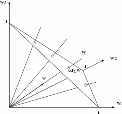
A simple example can illustrate the argument. Consider two specimen vectors

Chapter 1 The nature of compositional problems

w = (1.6, 2.4, 4.0) and W = (3.0, 4.5, 7.5)

in R+

3 as in Figure 1.4, representing the weights of the three parts (a, b, c) of two

specimens of total weight 8g and 15g, respectively. If we are interested in

compositional problems we recognize that these are of the same composition, the

difference in weight being taken account of by the scale relationship W =(15/8) w.

More generally two specimen vectors w and W in RD

+ are compositionally equivalent,

written W ∼ w, when there exists a positive proportionality constant p such that W=

pw. The fundamental requirement of compositional data analysis can then be stated as

follows: any meaningful function f of a specimen vector must be such that f(W)=f(w)

when W∼w, or equivalently

f(pw) = f(w), for every p>0.

In other words, the function f must be invariant under the group of scale

transformations. Since any group invariant function can be expressed as a function of

any maximal invariant h and since

h(w) = (w1 / wD , . . . , wD-1 / wD)

is such a maximal invariant we have the following important consequence:

Any meaningful (scale-invariant) function of a composition can be expressed

in terms of ratios of the components of the composition.

Note that there are many equivalent sets of ratios which may be used for the purpose

of creating meaningful functions of compositions. For example, a more symmetric set

of ratios such as w/g(w), where g(w) = (w1 . . . wD )

1/D is the geometric mean of the

components of w, would equally meet the scale-invariant requirement.

Chapter 1 The nature of compositional problems

Fig. 1.4 Representation of equivalent specimen vectors as points on rays of the positive orthant

1.5 Subcompositions: the marginals of compositional data analysis

The marginal or projection concept for simplicial data is slightly more complex than

that for unconstrained vectors in RD , where a marginal vector is simply a subvector of

the full D-dimensional vector. For example, a geologist interested only in the parts

(Na2O, K2O, Al2O3) of a ten-part major oxide composition of a rock commonly forms

the subcomposition based on these parts. Formally the subcomposition based on parts

(1, 2, . . . ,C) of a D-part composition [x1 , ... , xD ] is the (1, 2, . . . ,C)-subcomposition

[s1, . . . , sC ] defined by

[s1, . . . , sC ] = [x1 , . . . , xC ] / (x1 + . . . + xC).

Note that this operation is a projection from a subsimplex to another subsimplex. See,

for example, Aitchison (1986, Section 2.5).

1.6 Compositional classes and the search for a suitable sample space

In my own teaching over the last 45 years I have issued a warning to all my students,

similar to that of Pearson. Ignore the clear definition of your sample space at your

Chapter 1 The nature of compositional problems

peril. When faced with a new situation the first thing you must resolve before you do

anything else is an appropriate sample space. On occasions when I have found some

dispute between students over some statistical issue the question of which of them had

appropriate sample spaces has almost always determined which students are correct in

their conclusions. If, for example, it is a question of association between the directions

of departure and return of migrating New York swallows then an appropriate sample

space is a doughnut.

We must surely recognize that a rectangular box, a tetrahedron, a sphere and a

doughnut look rather different. It should come as no surprise to us therefore that

problems with four different sample spaces might require completely different

statistical methodologies. It has always seemed surprising to this writer that the

direction data analysts had little difficulty in seeing that the sphere and the torus

require their own special methodology, whereas for so long statisticians and scientists

seemed to think that what was good enough for a box was good enough for a

tetrahedron.

In the first step of statistical modelling, namely specifying a sample space, the choice

is with the modeller. It is how the sample space is used or exploited to answer

relevant problems that is important. We might, as in our study of scale invariance

above, take the set of rays through the origin and in the positive orthant as our sample

space. The awkwardness here is that the notion of placing a probability measure on a

set of rays is less familiar than on a set of points. Moreover we know that as far as the

study of compositions is concerned any point on a ray can be used to represent the

corresponding composition. The selection of each representative point x where the

rays meet the unit hyperplane w1 + . . . + wD = 1 with x = w/(w1 + . . . + wD) is surely

the simplest form of standardization possible. We shall thus adopt the unit simplex

SD = { [x1 , . . . , xD

]: xi>0 (i = 1, . . . , D) , x1 + . . . + xD = 1}.

To avoid any confusion on terminology for our generic composition x we reiterate

that we refer to the labels 1, . . . , D of the parts and the proportions x1 , ... , xD as the

components of the composition x. With this representation we shall continue to ensure

Chapter 1 The nature of compositional problems

scale invariance by formulating all our statements concerning compositions in terms

of ratios of components.

Note the one-to-one correspondence between the components of x and a set of

independent and exhaustive ratios such as

ri = xi /(x1 + . . . + xD ) (i = 1, ... , D-1),

rD = 1 /(x1 + . . . + xD ),

with the components of x determined by these ratios as

xi = ri /(r1 + . . . + rD-1 +1) (i = 1, ... , D-1),

xD = 1/(r1 + . . . + rD-1 +1).

Our next logical requirement will reinforce the good sense of this formulation in

terms of ratios.

1.7 Subcomposional coherence

Less familiar than scale invariance is another logical necessity of compositional

analysis, namely subcompositional coherence. Consider two scientists A and B

interested in soil samples, which have been divided into aliquots For each aliquot A

records a 4-part composition (animal, vegetable, mineral, water); B first dries each

aliquot without recording the water content and arrives at a 3-part composition

(animal, vegetable, mineral). Let us further assume for simplicity the ideal situation

where the aliquots in each pair are identical and where the two scientists are accurate

in their determinations. Then clearly B's 3-part composition [s1 , s2 , s3 ] for an aliquot

will be a subcomposition of A's 4-part composition [x1 , x2 , x3 , x

4 ] for the

corresponding aliquot related as in the definition of subcomposition in Section 1.5

above with C = 3, D = 4. It is then obvious that any compositional statements that A

and B make about the common parts, animal, vegetable and mineral, must agree. This

is the nature of subcompositional coherence.

Chapter 1 The nature of compositional problems

The ignoring of this principle of subcompositional coherence has been a source of

great confusion in compositional data analysis, The literature, even currently, is full of

attempts to explain the dependence of components of compositions in terms of

product moment correlation of raw components. Consider the simple data set:

Full compositions

[

]

1 2 3 4 Subcompositions

[

]

123

[0.1, 0.2, 0.1, 0.6] [0.25, 0.50, 0.25]

[0.2, 0.1, 0.1, 0.6] [0.50, 0.25, 0.25]

[0.3, 0.3, 0.2, 0.2] [0.375, 0.375, 0.25]

Scientist A would report the correlation between animal and vegetable as corr(x1 , x2 )

= 0.5 whereas B would report corr(s1 , s2 ) = -1. There is thus incoherence of the

product-moment correlation between raw components as a measure of dependence.

Note, however, that the ratio of two components remains unchanged when we move

from full composition to subcomposition: s s x x

i j i j

/ /

, so that as long as we work

with scale invariant functions, or equivalently express all our statements about

compositions in terms of ratios, we shall be subcompositionally coherent.

1.8 Perturbation as the operation of compositional change

1.8.1 The role of group operations in statistics

For every sample space there are basic group operations which, when recognized,

dominate clear thinking about data analysis. In RD the two operations, translation (or

displacement) and scalar multiplication, are so familiar that their fundamental role is

often overlooked. Yet the change from y to Y = y + t by the translation t or to Y = ay

by the scalar multiple a are at the heart of statistical methodology for RD sample

spaces. For example, since the translation relationship between y1 and Y1 is the same

as that between y2 and Y2 if and only if Y1 and Y2 are equal translations t of y1 and y2 ,

any definition of a difference or a distance measure must be such that the measure is

the same for (y1 , Y1 ) as for (y1 + t, Y1 + t) for every translation t. Technically this is a

Chapter 1 The nature of compositional problems

requirement of invariance under the group of translations. This is the reason, though

seldom expressed because of its obviousness in this simple space, for the use of the

mean vector ?

(

)

and the covariance matrix Σ= = − −cov( ){( )( ) }yEy y T

µ µ

as meaningful measures of ‘central tendency’ and ‘dispersion’. Recall also, for further

reference, two basic properties: for a fixed translation t,

E( y + t) = E(y) + t ; V(y + t) = V(y).

The second operation, that of scalar multiplication, also plays a substantial role in, for

example, linear forms of statistical analysis such as principal component analysis,

where linear combinations

D D1 1

with certain properties are sought.

Recall, again for further reference, that for a fixed scalar multiple a,

E(ay) = aE(y) ; V(ay) = a2V(y).

Similar considerations of groups of fundamental operations are essential for other

sample spaces. For example, in the analysis of directional data, as in the study of the

movement of tectonic plates, it was recognition that the group of rotations on the

sphere plays a central role and the use of a satisfactory representation of that group

that led Chang (1988) to the production of the essential statistical tool for spherical

regression.

1.8.2 Perturbation: a fundamental group operation in the simplex

By analogy with the group operation arguments for RD the obvious questions for a

simplex sample space are whether there is an operation on a composition x, analogous

to translation in D

, which transforms it into X, and whether this can be used to

characterize ‘difference’ between compositions or change from one composition to

another. The answer is to be found in the perturbation operator as defined in

Aitchison (1986, Section 2.8).

The perturbation operator can be motivated by the following observation within the

positive orthant representation of compositions. For any two equivalent compositions

w and W on the same ray there is a scale relationship W = pw for some p > 0, where

Chapter 1 The nature of compositional problems

each component of w is scaled by the same factor p to obtain the corresponding

component of W. For any two non-equivalent compositions w and W on different rays

a similar, but differential, scaling relationship W 1= p1 w1, . . . , WD = pDwD reflects

the change from w to W. Such a unique differential scaling can always be found by

taking pi = Wi / wi (i = 1, . . . , D). We can translate this into terms of the

compositional representations x and X within the unit simplex sample space

If we define a perturbation p as a differential scaling operator p p p S

=∈[.. . ]

and denote by

⊕

the perturbation operation, then we can define the perturbation

operation in the following way. The perturbation p applied to the composition

[

]

1 produces the composition X given by

],...[

).../(]...[

1111

DDDD

xpxpC

xpxpxpxpxpX

++=⊕=

where C is the so-called closure operation which divides each component of a vector

by the sum of the components, thus scaling the vector to the constant sum 1. Note that

because of the nature of the scaling in this relationship it is not strictly necessary for

the perturbation p to be a vector in

In mathematical terms the set of perturbations in

D form a group with the identity

perturbation

[

]

and the inverse of a perturbation p being the closure

]...[11

1−−− =D

ppCp. We use the notation

to denote the operation of this inverse

on x giving

D D

[

]

1 1 . The relation between any two

compositions x and X can always be expressed as a perturbation operation

⊕

(

)

, where

is a perturbation in the group of perturbations in the

the simplex

D. Similarly the change from X to x is expressed by the perturbation

. Thus any measure of difference between compositions x and X must be

expressible in terms of one or other of these perturbations. A consequence of this is

that if we wish to define any scalar measure of distance between two compositions x

and X , say

∆

(

)

then we must ensure that it is a function of the ratios x1/X1. . . . ,

xD/XD . As we shall see later this, together with attention to the need for scale

Chapter 1 The nature of compositional problems

invariance, subcompositional coherence and some other simple requirements, has led

Aitchison (1992) to advocate the follolowing definition:

∆2

(,)log logxXx

i j

= −













∑

as a simplicial metric, reinforcing an intuitive equivalent choice in Aitchison (1986,

Section 8.3).

1.8.3 Some familiar perturbations

In relation to probability statements the perturbation operation is a standard process.

Bayesians perturb the prior probability assessment x on a finite number D of

hypotheses by the likelihood p to obtain the posterior assessment X through the use of

Bayes’s formula. Again, in genetic selection, the population composition x of

genotypes of one generation is perturbed by differential survival probabilities

represented by a perturbation p to obtain the composition X at the next generation,

again by the perturbation probabilistic mechanism. In certain geological processes,

such as metamorphic change, sedimentation, crushing in relation to particle size

distributions, change may be best modelled by such perturbation mechanisms, where

an initial specimen of composition x0 is subjected to a sequence of perturbations p1, . .

. , pn in reaching its current state n

x :

n n n1 1 0 2 2 1 1

⊕

−

so that

n n

⊕

(

)

1 2 0 .

It is clear that in this mechanism we have the makings of some form of central limit

theorem but we delay consideration of this until we have completed the more

mathematical aspects of the simplex sample space.

A further role which perturbation plays in simplicial inference is in characterizing

Chapter 1 The nature of compositional problems

imprecision or error. A simple example will suffice for the moment. In the process of

replicate analyses of aliquots of some specimen in an attempt to determine its

composition

? we may obtain different compositions x1, . . . , xN because of the

imprecision of the analytic process. In such a situation we can model by setting

xp n N

n n

=⊕=ξ(,..., )1,

where the pn are independent error perturbations characterizing the imprecision.

1.9 Power as a subsidiary operation in the simplex

The simplicial operation analogous to scalar multiplication in real space is the power

operation. First we define the power operation and then consider its relevance in

compositional data analysis. For any real number

∈

1 and any composition

∈

we define

]...[1a

axxCxaX=⊗=

as the a-power transform of x. Such an operation arises in compositional data analysis

in two distinct ways. First it may be of relevance directly because of the nature of the

sampling process. For example, in grain size studies of sediments, sediment samples

may be successively sieved through meshes of different diameters and the weights of

these successive separations converted into compositions based on proportions by

weight. Thus though separation is based on the linear measurement diameter the

composition is based essentially on a weight, or equivalently a volume measurement,

with a power transformation being the natural connecting concept. More indirectly the

power transformation can be useful in describing regression relations for

compositions. For example, the finding of Aitchison (1986, Section 7.7) of the

relationship of a (sand, silt, clay) sediment x to depth d can be expressed in the form

⊕

⊗

⊕

}

{log

Chapter 1 The nature of compositional problems

where β is a composition playing the counterpart of regression coefficients and p is a

perturbation playing the role of error in more familiar regression situations.

It must be clear that together the operations perturbation

⊕

and power

⊗

play roles

in the geometry of

D analogous to translation and scalar multiplication in D

and

indeed can be used to define a vector space in

D. We shall take up the full algebraic-

geometric structure of the simplex sample space later in this guide.

1.10 Limitations in the interpretability of compositional data

There is a tendency in some compositional data analysts to expect too much in their

inferences from compositional data. For these the following situation may show the

nature of the limitations of compositional data.

Outside my home I have a planter consisting of water, soil and seed. One evening

before bedtime I analyse a sample and determine its (water, soil, seed) composition as

x = [3/6 2/6 1/6]. I sleep soundly and in the morning again analyse a sample finding

X = [6/9 2/9 1/9]. I measure the change as the perturbation

[(

)

(

)

(

)

(

)

(

)

(

)]

[

]

Now I can picture two simple scenarios which could describe this change. Suppose

that the planter last evening actually contained [18 12 6] kilos of (water, soil, seed),

corresponding to the evening composition [3/6 2/6 1/6], and it rained during the

night increasing the water content only so that the morning content was [36 12 6]

kilos, corresponding to the morning composition [6/9 2/9 1/9]. Although this rain

only explanation may be true, is it the only explanation? Obviously not, because the

change could equally be explained by a wind only scenario, in which the overnight

wind has swept away soil and seed resulting in content of [18 6 3] kilos and the same

morning composition [6/9 2/9 1/9]. Even more complicated scenarios will produce a

similar change. For example a combination of rain and wind might have resulted in a

Chapter 1 The nature of compositional problems

combination of increased water and decreased soil and seed, say to a content of [27 9

4.5] kilos, again with morning composition [6/9 2/9 1/9].

The point here is that compositions provide information only about the relative

magnitudes of the compositional components and so interpretations involving absolute

values as in the above example cannot be justified. Only if there is evidence external

to the compositional information would such inferences be justified. For example, if I

had been wakened by my bedroom windows rattling during the night and I found my

rain gauge empty in the morning would I be justified in painting the wind only

scenario. But I slept soundly during the night.

A consequence of this example is that we must learn to phrase our inferences from

compositional data in terms which are meaningful and we have seen that the

meaningful operations are perturbation and power. In subsequent chapters we shall

how we may use these operations successfully.

Chapter 2 The simplex sample space

Chapter 2 The simplex sample space and principles of compositional

data analysis

2.1 Logratio analysis: a statistical methodology for compositional data analysis

What has come to be known as logratio analysis for compositional data problems

arose in the 1980’s out of the realisation of the importance of the principle of scale

invariance and that its practical implementation required working with ratios of

components, This, together with an awareness that logarithms of ratios are

mathematically more tractable than ratios led to the advocacy of a transformation

technique involving logratios of the components. There were two obvious contenders

for this. Let x x x S

=∈[.. . ]

1be a typical D-part composition. Then the so-called

additive logratio transformation alr SR

D D

:→−1 is defined by

)]/log(...)/log()/[log()( 121 DDDD xxxxxxxalry−

== ,

where the ratios involve the division of each of the first D – 1 components by the final

component. The inverse transformation DD SRalr →

−− 11:is

]1)exp(...)exp()[exp()( 121

1−

−== D

yyyCyalrx,

where C denotes the closure operation. Note that this transformation takes the

composition into the whole of

D−1 and so we have the prospect of using standard

unconstrained multivariate analysis on the transformed data, and because of the one-

to-one nature of the transformation transferring any inferences back to the simplex

and to the components of the composition.

One apparent drawback with this technique is the choice of the final component as

divisor, with a much asked question. Would we obtain the same inference if we chose

Chapter 2 The simplex sample space

another component as divisor, or more generally if we permuted the parts? The

answer to this question is yes. We shall not go into any details of the proofs of this

assertion, but the interested reader may find these in Aitchison (1986, Chapter 5).

The alr transformation is asymmetric in the parts and it is sometimes convenient to

treat the parts symmetrically. This can be achieved by the so-called centred logratio

transformation clr SU

D D

:→:

)}](/log{...)}(/[log{)( 1xgxxgxxclrzD

== ,

where

}0...:]...{[ 11 =+= DD

DuuuuU.

a hyperplane of

D.The inverse transformation DD SUclr →

−:

1 takes the form

)]exp(...)[exp( 1D

zzCx=.

This transformation to a real space again opens up the possibility of using standard

unconstrained multivariate methods.

We note here that the mean vector

alr

{

(

)}

and covariance matrix

cov{

(

)}

alr

of the logratio vector

alr

(

)

will play an important role in our

compositional data analysis, as will do the centred logratio analogues

clr

{

(

)}

and

cov{

(

)}

clr

So the philosophy of logratio analysis can be stated simply.

1. Formulate the compositional problem in terms of the components of the

composition.

2. Translate this formulation into terms of the logratio vector of the

composition.

Chapter 2 The simplex sample space

3. Transform the compositional data into logratio vectors.

4. Analyse the logratio data by an appropriate standard multivariate statistical

method.

5. Translate back into terms of the compositions the inference obtained at

step 4.

We shall see later many examples of this compositional methodology.

2.2 The unit simplex sample space and the staying-in the-simplex approach

Logratio analysis emerged in the 1980’s in a series of papers Aitchison (1981a,

1981b, 1981c, 1982, 1983, 1984a, 1984b, 1985), Aitchison and Bacon-Shone (1984),

Aitchison and Lauder (1985), Aitchison and Shen (1980, 1984) and in the monograph

Aitchison (1986); and has been successfully applied in a wide variety of disciplines.

Since, however, there seem an appreciable number of statisticians and scientists who

seem, for whatever reason, uncomfortable with transformation techniques it seems

worth considering what are the alternatives. In the discussion of Aitchion (1982),

Fisher made the following comment:

Clearly the speaker has been very successful in fitting simple models to normal

transformed data, the counterpart to the simplicity of these models is the

complexity of corresponding relationships among the untransformed components.

This is hardly an original observation. Yet there are certain aromas rising from the

murky potage of compositional data problems which are redolent of some aspects

of problems with directional data, and herein lies the point. When attacking these

latter problems, one is ultimately better off working within the confines of the

original geometry (of the circle, sphere cylinder, . . .) and with techniques

particular thereto (vector methods, etc), in terms of perceiving simple underlying

ideas and modelling them in a natural way. Mapping from, say, the sphere into the

plane, and then back, rarely produces these elements, and usually introduces

unfortunate distortion. I still hold out some hope that simple models of dependence

can be found, peculiar to the simplex. . . . Meanwhile, I shall analyse data with the

normal transform method.

Chapter 2 The simplex sample space

The lack of success in transforming the sphere into the plane is that the spaces are

topologically different whereas the simplex and real space are topologically

equivalent. Nevertheless there is a challenge to confine the statistical argument to the

geometry of the simplex, and this approach has been emerging over the last decade,

based on the operations of perturbation and power and on the already indicated

simplicial metric. It is now certainly possible to analyse compositional data entirely

within simplicial geometry. Clearly the success of such an approach must depend

largely on the mathematical sophistication of the user. In the remainder of this guide

we shall adopt a bilateral approach, attempting to interpret inferences from our

compositional data problems both from the logratio analysis approach and the

staying-in-the-simplex approach.

First in the next section we give a concise account of the algebraic-geometric

structure of the simplex.

2.3 The algebraic-geometric structure of the simplex

2.3.1 Introduction

The purpose of this section is to provide a reasonably agreed account in terms of

terminology and notation of the algebraic-geometric structure of the unit simplex as a

standard sample space for those compositional data analysts wishing to adopt a

staying-in-the-simplex approach as an alternative to logratio transformation

techniques. Emphasis is placed on the metric vector space structure of the simplex,

with perturbation and power operations, the associated metric, the importance of

bases, power-perturbation combinations, and simplicial subspaces in range and null

space terms. Concepts of rates of compositional change, including compositional

differentiation and integration are also considered. For compositional data sets, some

basic ideas are discussed including concepts of distributional centre and dispersion,

and the fundamental simplicial singular value decomposition. The sources of the ideas

are dispersed through the References and will not be cited throughout the text.

Chapter 2 The simplex sample space

2.3.2 Compositional vectors

Compositions, positive vectors with unit, 100 per cent or some other constant sum, are

a familiar, important data source for geologists. Since in compositional problems the

magnitude of the constant sum is irrelevant we assume that the data vectors have been

standardised to be of unit sum; we then regard a generic D-part composition, such as

ten major oxides or sedimental sand, silt, clay, to take the form of a row vector

[

1 where the

(

)

are the components, proportions of the

available unit, and the integers 1, . . . D act as labels for the parts. We have chosen

the convention of recording compositions as row vectors since this conforms with the

common practice of setting out compositional data with cases set out in rows and

parts such as major oxides in columns. Such a convention also conforms with practice

in such software as MSExcel. Thus a data set consisting of N D-part compositions x1,

. . . , xN may be set out as an

matrix X = [x1; . . . ; xN], where the semi-colon

is used to indicate that the next vector occurs in the next row.

As in standard multivariate analysis marginal concepts are important. For

compositions and the simplex the marginal concept is a subcomposition, such as the

CNK (CaO, N2O, K2O)-subcomposition of a major oxide composition. For example

the (1, . . . C)-subcomposition of a D-part composition

[

]

D1is defined as

)..../(],...,[],...,[ C],...,[1111 CCCC xxxxxxss ++==

Note that the ‘closure’ operator C standardises the contained vector by dividing by the

sum of its components so that a subcomposition consists of components summing to

unity. In geometric terms formation of a subcomposition is geometrically a projection.

2.3.3 The algebraic-geometric structure of the unit simplex

The sample space associated with D-part compositions is the unit simplex:

}.1...),,...,1(0:],...,{[ 11 =++=>= DiC

DxxDixxxS

The fundamental operations of change in the simplex are those of perturbation and

power transformation. In their simplest forms these can be defined as follows. Given

Chapter 2 The simplex sample space

any two D-part compositions D

Syx ∈, their perturbation is

where C is the well known closure or normalizing operation in which the elements of

a positive vector are divided by their sum; and given a D-part composition x ∈ D

and a real number, a the power transformed composition is

Note that we have used the operator symbols ⊕ and ⊗ to emphasize the analogy with

the operations of displacement or translation and scalar multiplication of vectors in

D. It is trivial to establish that the internal ⊕ operation and the external ⊗ ?operation

?define a vector or linear space structure on D

S. In particular the

⊕

operation defines

an abelian group with identity

[

]

. We record a few of the simple

properties of

⊕

and

⊗

⊕

⊗

⊕

⊗

⊕

⊗

(

)

(

)

(

)

(

The operator

, the inverse of

⊕

, is simply defined by

]/,...,/[11 DD yxyxCyx =Θ

and plays an important role in compositional data analysis, for example in the

construction of compositional residuals.

The structure can be extended by the introduction of the simplicial metric

∆: S D × S D → 0≥

defined as follows:

),,(loglog

)(

log

)(

log),(

2/1

ji j

ii Syx

yx ∈































−=























−=∆∑∑ <=

],,...,[11 DD yxyxCyx =⊕

],...,[1a

axxCxa=⊗

Chapter 2 The simplex sample space

where

(

)

is the geometric mean of the components of the composition. The metric

∆

satisfies the usual metric axioms:

M1 Positivity :

)

(

)

(

)

(

∆

≠

∆

M2 Symmetry : ),(),(xyyx ∆=∆

M3 Power relationship:

)

(

)

(

∆

⊗

∆

M4 Triangular inequality: ),(),(),(yxyzzx∆≥∆+∆

The fact that this metric has also desirable properties relevant and logically necessary,

such as scale, permutation and perturbation invariance and subcompositional

dominance, for meaningful statistical analysis of compositional data is now well

established and the relevant properties are recorded briefly here:

M5 Permutation invariance: ),(),(yxyPxP ∆=∆, for any permutation matrix P.

M6 Perturbation invariance:

)

(

)

(

∆

⊕

∆

, where p is any

perturbation.

M7 Subcompositional dominance: if sx and sy are similar, say (1, . . . , C)-

subcompositions of x and y, then ),(),(yxss DCS

S∆≤∆.

It is possible to go to even more mathematical sophistication for the unit simplex if

either theoretical or practical requirements demand it. For example, consistent with

the metric

∆

is the norm ||x||, defined by

and the inner product, defined by

〈 〉 ==

∑

x y x

,log ( ) log ( )

where e is the identity perturbation [1, . . . , 1]/D. An interesting aspect of these

extensions is that an inner product

〈

〉

can be expressed as

)(

log),(|||| ∑

=













=∆=D

exx

Chapter 2 The simplex sample space

where

)}

(

log{

and so

. Thus inner products play the role of

logcontrasts, well established as the compositional ‘linear combinations’ required in

many forms of compositional data analysis such as principal component analysis and

investigation of subcompositions as concomitant or explanatory vectors.

2.3.4 Generators, orthonormal basis and subspaces

As for any vector space generating vectors, bases, linear dependence, orthonormal

bases and subspaces play a fundamental role and this is equally true for the simplex

vector space. In such concepts the counterpart of ‘linear combination’ is a power-

perturbation combination such as

)(...)( 11 CC

uuxββ ⊗⊕⊕⊗=

and such combinations play a central role. In such a specification the

’s are

compositions regarded as generators, and the combination generates some subspace of

the unit simplex as the real number u-coefficient vary. When this subspace is the

whole of the unit simplex then the

’s form a basis. Generally a basis should be

chosen such that the generators are ‘linearly independent’ in the sense that C

ββ ,...,

are linearly independent if and only if

0...)(...)( 111 ===⇒=⊗⊕⊕⊗ CCC uueuu ββ .

For

D, which is essentially a (D –1)-dimensional space, a linearly independent basis

has D –1 generators, and important among such basis are those which form an

orthonormal basis, say with generators 11 ,..., −D

ββ which have unit norm

)1,...,1(1|||| −== Di

β, and are orthogonal in the sense that )(0,ji

ji ≠=〉〈 ββ .

As on any vector space a set of C orthonormal generators can be easily extended to

form an orthonormal basis of

D. Later in Section 2.3.7 we shall see that orthonormal

ii xa

blog

)(

log

)(

log

1 1

∑ ∑

= =

Chapter 2 The simplex sample space

bases a central role in a data-analytic sense in terms of the simplicial singular value

decomposition of a compositional data set.

As in standard multivariate analysis range and null spaces play an important and

complementary role in such areas of data investigation as compositional regression ,

principal logcontrast component analysis and in the study of compositional processes.

The set ];...;[1C

ββ=Β of linearly independent generators identifies a range space

)},...,1(),(...)(:{)( 1

11 CiRuuuxxrange iCC =∈⊗⊕⊕⊗==Βββ

namely the subspace of dimension C generated by the compositions in

. Similarly

associated with

can be defined a null space

}0,,...,0,:{)( 1=〉〈=〉〈=Βxxxnull C

ββ

a subspace of dimension D – C – 1. Range and null spaces are essentially equivalent

ways of expressing certain constraints which may apply to compositions. The

relationship of these equivalences is simple. For example, the null space

corresponding to

range

(

)

above is null( )Β⊥where

⊥ is the completion of a basis

orthogonal to

; similarly null range( ) ( )Β Β=⊥. As defined, these range and null

spaces contain the identity e of

D. It is often convenient to allow a displacement so

that they contain a specified compositionξ: all that this requires is the specification of

the range space above to start with

-i.e.,

)

(

range

⊕

-, and the zero values of

the inner products in the specification of the null space to be replaced by

〉−〈〉−〈ξβξβxx C,,...,,

2.3.5 Differentiation, integration, rates of change

Clearly in compositional processes rates of change of compositions are important and

here we define the basic ideas. Suppose that a composition

)

(

depends on some

continuous variable t such as time or depth. Then the rate of change of the

composition with respect to t can be defined as the limit

Chapter 2 The simplex sample space

)))(log

(exp(C=x(t)))((

lim)( 0tx

dttx

tDx dt Θ+⊗=>−

where d/dt denotes ‘ordinary’ derivation with respect to t. Thus, for example, if

xtht( ) ( )=⊕ ⊗ξβ, then

(

)

(

)

⊗

. There are obvious extensions through

partial differentiation to compositional functions of more than one variable. We note

also that the inverse operation of integration of a compositional function

)

(

over an

interval (t0, t) can be expressed as

2.3.6 Distributional concepts in the simplex

For statistical modelling we have to consider distributions on the simplex and their

characteristics. The well-established ‘measure of central tendency’ ξ∈SD which

minimizes E(∆(x, ξ)) is

satisfying certain necessary requirements, such as

cen

(

)

(

)

⊗

and

cen

(

)

(

)

(

⊕

There are a number of criteria which dictate the choice of any measure V(x) of

dispersion and dependence which forms the basis of characteristics of compositional

variability in terms of second order moments:

(a) Is the measure interpretable in relation to the specific hypotheses and

problems of interest in fields of application?

(b) Is the measure conformable with the definition of center associated with the

sample space and basic algebraic operation?

group of perturbations? Is

)

(

)

(

dis

⊕

for every constant perturbation

)).)(log(exp()(

∫ ∫

tdttxCdttx

)))

(log

(exp(

)

(

cen

Chapter 2 The simplex sample space

p? (Recall the result in Section 1.8.1 that for D

Ry∈ the covariance matrix V

is invariant under translation: V(t + y) = V(y)).

(d) Is the measure tractable mathematically?

To ensure a positive answer to (a) we must clearly work in terms of ratios of the

components of compositions to ensure scale invariance. At first thought this might

suggest the use of variances and covariances of the form

var(xi/xj) and cov(xi /xj , xk / xl ).

Unfortunately these are mathematically intractable because, for example, there is no

exact or even simple approximate relationship between var(xi/xj) and var(xj/xi).

Fortunately we already have a clue as to how to overcome this difficulty in the

appearance of logarithms of ratios of components both in the central limit theorem at

Section 1.8.3 and in the definition of the center of compositional variability. It seems

worth the risk therefore of apparently complicating the definition of dispersion and

dependence by considering such dispersion characteristics as

var{log(xi /xj )}, cov{log(xi /xj )} , log(xk /xl ) .

Obvious advantages of this are simple relationships such as

var{log(xi/xj)} = var{log(xj/xi)}

cov{log(xi /xj ) , log(xl /xk )} = cov{log(xi /xj ) , log(xl /xk ).

There are a number of useful and equivalent ways (Aitchison, 1986, Chapter 4) in

which to summarize such a sufficient set of second-order moment characteristics. For

example, the logratio covariance matrix?

])}/log(),/[cov{log())(cov()( DjDixxxxxalrx==Σ

using only the final component xD as the common ratio divisor, or the centered

Chapter 2 The simplex sample space

logratio covariance matrix

G(x) = cov{clr(x)} = [cov{log(xi /g(x)), log(xj /g(x))}].

My preferred summarizing characteristic is what I have termed the variation matrix

T(x) = [t ij] = [var{log(xi /xj )}].

Note that T is symmetric, has zero diagonal elements, and cannot be expressed as the

standard covariance matrix of some vector. It is a fact, however, that S, G and T are

equivalent: each can be derived from any other by simple matrix operations

(Aitchison, 1986, Chapter 4). A first reaction to this variation matrix characterization

is surprise because it is defined in terms of variances only. The simplest statistical

analogue is in the use of a completely randomized block design in, say, an industrial

experiment . From such a situation information about var(yi - yj) for all i, j is a

sufficient description of the variability for purposes of inference.

So far we have emphasized criteria (a), (b) and (d). Fortunately criterion (c) is

automatically satisfied since, for each of the dispersion measures

)

(

)

(

dis

⊕

for any constant perturbation p. We should also note here that the dimensionality of

the covariance parameter is ½ D(D -1) and so is as parsimonious as corresponding

definitions in other essentially (D-1)-dimensional spaces.

To sum up, importantly these dispersion characteristics are consistent with the

simplicial metric defined above and satisfy the following properties:

dis axadis x( ) | | ( )⊗=2, for any scalar a in R;

dis

(

)

(

)

⊕

, for any constant perturbation p;

dis

(

)

(

)

(

)

⊕

, for independent x, y.

2.3.7 Relevance to compositional data sets

Chapter 2 The simplex sample space

There are substantial implications in the above development for the analysis of a

compositional data set

[

;

]

1. A main feature is that the estimate

of the centre ξ is given by $(,..., )ξ=Cg gD1, gi is the geometric mean of the ith

component of the N compositions. Measures of dispersion are simply estimated from

the estimated variances of the appropriate logratios.

There is for the simplex a central result, analogous to the singular value

decomposition for data sets associated with the sample space RD, which plays a

central role. Any N x D compositional data matrix X with nth row composition xn can

be decomposed in a perturbation-power form as follows

where ξ is the centre of the data set, the s’s are positive ‘singular values’ in

descending order of magnitude, the β ’s are compositions, m (

−

≤

) is a readily

defined rank of the compositional data set, and the u’s are power components specific

to each composition. In a way similar to that for data sets in RD we may consider an

approximation of order r <m to the compositional data set given by

Such an approximation retains a proportion

of the total variability of the N × D compositional data matrix as measured by the

trace of the centered logratio covariance matrix or equivalently in terms of total

mutual distances as

We may also note here that the power-perturbation expression of the singular value

decomposition has exactly the same form as regression of a composition on some set

)(...)( 111 mmnmnn susuxββξ⊗⊕⊕⊗⊕=

).(...)( 111

)( rrnrn

nsusuxββξ⊗⊕⊕⊗⊕=

).../()...(22

1mrssss ++++

).,())1(( '

21 n

xxNN ∑

−∆−

Chapter 2 The simplex sample space

of variables. The form is exactly that of what would obtained if the logratio form of

regression analysis in Aitchison (1986, Chapter 7) were transformed back into terms

of the simplex.

2.4 Useful parametric classes of distributions on the simplex

2.4.1 Introduction

In this section we first present some results in distributional calculus leading to a

central limit theorem analogous to the role of the multivariate normal limit in real

space. This leads us to the definition of a number of useful parametric classes of

distributions on the simplex sample space.

2.4.2 Generating functions for simplicial distributions

The characteristic and moment generating functions for distributions in RD are

familiar useful tools of distributional analysis. It is relatively easy to design the

analogous tools for the study of simplicial distributions in S D. The transform which

seems to be most suited to this purpose is a multivariate adaptation of the Mellin

transform. Let

Uu u u u

DD D

= + + ={[ .. . ]: . .. }

1 1 0 .

Suppose that a composition

∈

has density function

(

)

. Then define its Mellin

generating function MUR

:→+

1 by the relationship

Mux x fxdx

( ) . .. ( )=∫11.

Note that the restriction of the vector u to the hyperplane

D rather than

D is

dictated by the need to meet the requirement of scale invariance, here ensured by the

fact that integrand is expressible in terms of ratios of the components of x. The Mellin

generating function has perturbation, power and limit properties similar to additive

Chapter 2 The simplex sample space

and scale properties of characteristic and moment generating functions for

distributions in RD.

Property M1.

(

)

Property M2. If x and y are independent compositions then

MuMuMu

x y x y⊕

() () ().

Property M3. If

∈

1 is a scalar then MuMau

ax x⊗=( ) ( ).

Property M4. If b is a fixed perturbation then

Mu b b Mu

⊕=( ) .. . ().

Property M5. Combining M2 and M3, if x and y are independent compositions

then

).()(

)()( buMauMM yxybxa=

⊗⊕⊗

Property M6. Moment generating properties. In a manner similar to the use of

moment-generating functions in RD we can obtain expansions which produce

moments of any order

log ( ) logMu u uTu

= − +

∑

ξterms of higher order,

where ξ and

are the centre and

variation matrix with (i, j) element

var{log( /)}x x

i j of the distribution. Moments can also be found through a

differentiation process but we shall not pursue that here; see Aitchison (2001,

Section 6) for details.

Property M7. A limit property. Let {xn} be a sequence of compositions with density

functions {fn} and Mellin transforms {Mn}. If

(

)

(

)

→

and M(u) is the

Mellin transform of f(x) then fn converges in distribution to f.

Chapter 2 The simplex sample space

2.4.3 Central limit theorem for compositions

An obvious question to ask about compositional variability is whether there is an

analogue of the well known limiting results for sequences of additive and

multiplicative changes leading to normal and lognormal variability through the central

limit theorems. As we have already noted the relationship in Section 1.8.3 depicts the

result of a sequence of independent perturbations. In exactly the same way as moment

generating functions can be used to establish central limit theorems in RD so we could

use the above properties of the Mellin generating function to establish a similar result

for xn in (???). A simple version for the case where pr (r = 1, 2, . . . ) are

independently and identically distributed with centre cen prD

( ) [ .. . ]= =ξ ξ ξ

1 and

variation matrix

(

)

leads to the following limiting Mellin generating function

for ynx

n n

=−1 2/:

Mu u uTu

ii T

( ) exp log= −











∑

ξ.

Alternatively we can very simply use transformation techniques to obtain an additive

central limit theorem by rewriting the perturbation sequence it in terms of logratios:

log(xni/xnD) = {log(p1i/p1D) + . . . + log(pni/pnD)} + log(x0i/x0D) (i = 1, ..., D - 1).

If the perturbations are random then the sum within the brackets will, under certain

regularity conditions which need not divert us here, tend for large n towards a

multivariate normal pattern of variability. It is a simple application of distribution

theory to deduce the form of the probability density function

(

)

on the unit

simplex as

}))(())((exp{)...()2det()( 1

2/1T

Dxalrxalrxxxfµµπ−Σ−−Σ=−−−

where

is (D – 1) row vector,

a positive definite square matrix of order D-1. This

Chapter 2 The simplex sample space

is the parametric class of additive logistic normal distributions LD−1(,)µΣdescribed

by Aitchison and Shen (1980). This result differs from the Mellin transform result

only in the parameterization of the parameters. We use the notation LD(,)ξΤ to

denote the distribution in this parameterization.

2.4.4 Parametric classes of distributions

The emergence of the logistic normal distribution LD−1(,)µΣ or LD(,)ξΤ in a central

limit theorem ensures for this parametric class of distributions a central role in the

study of distributions on the simplex in a way similar to the multivariate normal and

lognormal distributions in D

and D

R+. In particular, in addition to simple logistic

normal subcompositional and conditional properties, this class of distributions has the

essential and useful properties of being closed under the basic simplex operations of

perturbation and power; see Aitchison (1986, Chapter 6) for details.

In contrast the popular Dirichlet class

(

)

on the simplex with density function

fx x x x X

( ) , , , ( )∝ ∈

α α

has so many drawbacks that it has virtually no role to play in simplicial inference. For

example, it has no simple perturbation or power transformation properties and so is

ill-suited to the basic operations of the simplex. Moreover, it has so many inbuilt

independence properties that, apart from being a model of extreme independence, it

has almost no role to play in the investigation of the nature of the dependence

structure of compositional variability.

There are other classes of distributions on

D. The fact that the LD−1(,)µΣ class is

simply related to the multivariate normal class in

D−1 by way of the alr

transformation led Aitchison (1986) to consider other transformations from

D to

D−1to define other logistic-normal classes of distributions, the multiplicative and

partitioned classes, which are directed at specific practical problems in compositional

data analysis; see Aitchison (1986, Sections 6.14, 6.18) for details. Also Aitchison

)

(

∝

Chapter 2 The simplex sample space

(1985, 1986, Section 13.4) extends the LD−1(,)µΣ class by the introduction of a

single parameter to produce a generalization which includes both the Dirichlet class

and the logistic normal class. While this is a useful extension it is somewhat restricted

by computational problems involving multiple integrals. A more promising

generalization, which is simpler computationally, is an extension based on the

recently introduced multivariate skew normal class of distributions (Azzalini and

Della Valle, 1997). In terms of a class of distributions on the simplex a composition x

can be said to have a logistic skew normal distribution if alr(x) has a multivariate

skew normal distribution. For recent applications of this class to compositional data

problems, see Mateu-Figueres, Barceló-Vidal and Pawlowsky-Glahn (1998),

Aitchison and Bacon-Shone (1999).

For comparison with the fitting of parametric distributions to simplicial data or for use

when there is no satisfactory parametric class, resort may be made to a non-parametric

approach through kernel density estimation (Aitchison and Lauder, 1985).

2.5 Logratio analysis and the role of logcontrasts

In unconstrained multivariate analysis with sample space RD substantial use is made

of properties of linear combinations (transformations) of the components of vector

observations, for example in all techniques involving eigen-analysis. Inspection of the

forms involved in the definitions of geometric centre, dispersion matrices, Mellin

generating function, and the distribution emerging from the central limit theorem

suggest that the simplex analogue of a linear combination is a logcontrast (Aitchison,

1983) of a composition x defined by

D D1 1

log

, where

Such linear contrasts have also emerged naturally as inner product in our study of the

algebraic-geometric structure of the simplex space. Just as linear combinations can be

used to define subspaces of the vector space RD by way of null spaces or range spaces,

so logcontrasts can be used to identify subspaces of the already identified vector

Chapter 2 The simplex sample space

space

D through, for example, logcontrast principal component analysis. We shall

see later the role that such logcontrasts play in statistical analysis. The main

distributional result for logcontrasts can be expressed as follows.

Property L1. If composition x has geometric center ? and variation matrix ? then the

vector l = [l1, . . . , lC]

∈

RC , where

has moment generating function G(t), where t = [t1, . . . , tC], given by Gl (t) =

Mx(tAT ), where A = [ari]. A corollary of this result is that, if x follows a LD(?,?)

distribution, then l follows a NA A A

{(log ),}ξ−1

2Τ distribution.

We may comment here on the negative signs that appear in this last result. This is

because of the nature of the variation matrix ?. This can easily be shown to have a

restricted form of negative definiteness in the sense that, for any

∈

, u?uT , so

that the covariance matrix −1

2A A

TΤ in the above result is positive definite.

2.6 Simple estimation

Compositional data, in the form of N compositions each with D parts can be set out in

the form of a

matrix

[

]

, where

ni is the ith component of the nth

composition. In such a compositional data matrix compositions are set out in the rows

and the part components are set out in the columns. We shall denote the nth row of the

matrix, the nth composition, by

The estimation of such central characteristics as

and dispersion matrices

straightforward. The transformation alr and clr produce vectors in real space so that

mean vectors and covariance matrices are estimated exactly as in standard

unconstrained multivariate statistics. In matrix notation, with

N denoting a N-row

vector with unit elements, we have estimates as follows:

),,1(log

CrxalD

irirK== ∑

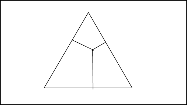
Chapter 2 The simplex sample space

∧=(/) ( ),1Njalr X

∧∧ ∧

= − −{/( )}{ ( ) ( ) }1 1Nalr Xalr XN

µ µ ,

∧∧ ∧

= − −{/( )}{ ( ) ( ) }1 1Nclr Xclr XN

λ λ .

Considerable insight can be given to the transformation technique by considering a

simple application. We choose as a data set the (A, B, C) subcomposition of the

hongite data of Table 1.1.1a. Such three-part compositions can be plotted in a

triangular or ternary diagram in the following way. Figure 2.6.a shows an equilateral

triangle with vertices 1, 2, 3 and with unit altitude. In such a diagram a three-part

composition such as

[

]

1 2 3 can be represented by a point P in the triangle where

123

are the lengths of the perpendiculars from P to the sides 23, 31, and 12, the

sides opposite the vertices 1, 2 and 3. The sum of such perpendiculars for any point

within the triangle is always 1 (this result is apparently known as Viciani’s theorem)

and roughly speaking the nearer the point P is to any vertex the greater is the

corresponding component. The triangle and its four-part counterpart have proved

useful in giving some visual insight into compositional variability. Triangular graph

paper is available commercially for such purposes.

2 3

Fig. 2.6.a Representation of a 3-part composition

[

]

1 2 3 in the reference triangle 123

∧=(/) ( ),1Njclr X

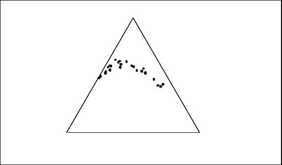
Chapter 2 The simplex sample space

Figure 2.6.b shows the 25 (A, B, C) subcompositions of hongite as 25 points within a

ternary diagram. Note the apparent curved nature of the data points; this curvature in

the naïve geometry of the simple is quite common, and is another reason why linear

methods such as product-moment correlations are unsuccessful. Figure 2.6.d shows

the plot of the additive logratio vectors in the two-dimensional plane. Note that the

curved nature of the data set in the triangle has been changed to a more elliptical

scatter in the real space.

Albita

Blandita Cornita

Fig. 2.6.b ABC subcompositions for 25 hongite specimens

Let us now consider the estimation process with the alr transformation. The estimate

∧ of

alr

{

(

)}

is [1.600 0.799], and this is shown as the point Q (red) in

Figure 2.6.d. The question of interest is how this point transforms back into the

appropriate simplex sample space, in this case triangle ABC. This is achieved by

computing

alr-1[1.600 0.799] = [0.606 0.272 0.122],

and this composition is shown as the point G (red) in the triangle ABC of Figure

2.6.c. It clearly lies within the cluster of data points within the triangle.

This estimated centre is in sharp contrast to what is almost universally quoted in raw

compositional data analysis, namely the arithmetic mean vector of the compositional

data set:(/)1NjX

t, which, for the (A, B, C) subcomposition of hongite, is [0.443

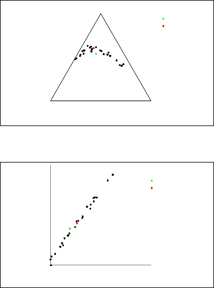
Chapter 2 The simplex sample space

0.229 0.148], substantially different from the centre arrived at through the

transformation process. This composition is plotted as the point A (green) in the

triangle ABC of Figure 2.6.c, and compared with centre G is more like an outlier than

a central characteristic.

Albita

Blandita Cornita

Arithmetic Mean

Geometric Mean

Fig. 2.6.c Arithmetic average composition (A = green) and the geometric centre (G = red) for 3-part

compositional data set in a ternary diagram

-2 -

-1 -

log(Albita/Cornita)

log(Blandita/Cornita)

Arithmetic Mean

Geometric Mean

Fig. 2.6.d Arithmetic average composition (A = green) and the geometric centre (G = red) for 3-part

compositional data set in the logratio diagram.

Chapter 2 The simplex sample space

This estimation by alr and alr-1 transformation leads to an estimate of ξ=cen x(). If

[

]

D1 denote the geometric means of the D columns of the compositional data

matrix X then it is easy to show that

)]/log(...)/[log( 11 DDD gggg −

∧=µ

and then

]...[)( 1

ggCalr =

∧

−µ,

which is the estimate of centre.

For the set of full hongite compositions this centre

[0.489 0.220 0.099 0.104 0.088],

compared with an incorrect use of the arithmetic mean

[0.443 0.230 0.148 0.096 0.083],

again showing a substantial discrepancy.

We give below the estimates of

for the hongite compositional data matrix:

∧

0.1386 0.2641 -0.2233 0.1214

0.2641 0.6490 -0.7020 0.1444

-0.2233 -0.7020 0.9476 0.0116

0.1214 0.1444 0.0116 0.1871

∧

0.0644 0.1791 -0.2441 0.0145 -0.0140

0.1791 0.5530 -0.7337 0.0266 -0.0249

-0.2441 -0.7337 0.9803 -0.0419 0.0394

0.0145 0.0266 -0.0419 0.0475 -0.0467

-0.0140 -0.0249 0.0394 -0.0467 0.0462

Chapter 2 The simplex sample space

∧

0 0.2593 1.5329 0.0828 0.1386

0.2593 0 3.0007 0.5473 0.6490

1.5329 3.0007 0 1.1115 0.9476

0.0828 0.5473 1.1115 0 0.1871

0.1386 0.6490 0.9476 0.1871 0

We shall see later as we develop our methodology the various ways in which these

measures of dispersion come into play. For the moment we concentrate on a simple

point. Hopefully by now early warners of the fallacy of using raw product-moment

correlations such as Chayes (1960, 1962), Krumbein (1962), Sarmanov and Vistelius

(1959) have reinforced Karl Pearson’s century-old warning and have at least raised

uneasiness about interpretations of product-moment correlations cov(xi , xj). Relative

variances such as var{log(xi /xj )} provide some compensation for such deprivation of

correlation interpretations. For example, var{log( /)}x x

i j

0 means a perfect

relationship between

iand xjin the sense that the ratio x x

i j

/ is constant, replacing

the unusable idea of perfect positive correlation between

i and xj by one of perfect

proportionality. Again, the larger the value of var{log( /)}x x

i j the more the

departure from proportionality with var{log( /)}x x

i j

∞

replacing the unusable

idea of zero correlation or independence between xi and xj. For scientists who are

uneasy about scales that stretch to infinity we can easily provide a finite scale by

considering 1− −exp( )τij as a measure of relationship between components

and xj. The scale is now from 0 (corresponding to lack of proportional relationship )

and 1 (corresponding to perfect proportional relationship). Note that if we are really

interested in hypotheses of independence these are most appropriately expressed in

terms of independence of subcompositions. For example independence of the (1, 2,

3)- and (4, 5)-subcompositions would be reflected in the following statements:

cov{log(x1/x3), log(x4/x5)}= 0, cov{log(x2/x3), log(x4/x5)} = 0.

Finally we can provide an analogue of the rough-and-ready normal 95 percent range

of mean plus and minus two standard deviations. This is expressed in terms of ratios

xi/xj and a signed version of a coefficient of variation:

Chapter 2 The simplex sample space

cv x x

Ex x

i j

=var{log( /)}

|{log( /)}|

giving













≤ ≤ 











− +1 2 1 2

where ji gg , are the geometric means of the ith and jth components.

In the study of unconstrained variability in RD it is often convenient to have available

a measure of total variability, for example in principal component analysis and in

biplots. For such a sample space the trace of the covariance matrix is the appropriate

measure. Here we might consider trace(G) the trace of the symmetric centered

logratio covariance matrix. Equally we might argue on common sense grounds that

the sum of all the possible relative variances in

, namely

var{log( /)}x x

i j j

∑

would be equally good. These two measures indeed differ only by a constant factor

and so we can define totvar(x), a measure of total variability, as

totvar ∑

<































=Γ=

ji j

tracexlogvar

)()(

We may also note here that our scalar measure of distance, the simplicial metric, is

compatible with the above definitions of covariance analogous to the compatibility of

Euclidean distance with the covariance matrix of an unconstrained vector. As an

illustration of this consider how we might construct a measure of the total variability

for a

compositional data set . The above definition suggests that we may

Chapter 2 The simplex sample space

obtain such a total measure, totvar1 say, by replacing each var{log( /)}x x

i j in the

definition of totvar its standard estimate. An alternative intuitive measure of total

variation is surely the sum of all the possible distances between the N compositions,

namely

totvar2 ),()( 2nm

xxx

∑

∆=,

where here

denote the mth and nth compositions in X. The easily established

proportional relationship totvar1 = [D/{N(N-1)}] totvar2 confirms the compatibility

of the defined covariance structures and scalar measures of distance for compositional

variability.

Note on subcomposional analysis. If interest may be in subcompositions of the full

composition then the relative variation array is particularly useful. This is because the

variation array of any subcomposition is simply obtained by picking out all the

logratio variances associated with the parts of the subcomposition.

A caveat on the use of the centred logratio covariance matrix. Because of the

symmetry of the centred logratio covariance

there is a temptation to imagine that

corr xgx x gx

i j

[log{ /()}, log{ /()}] is somehow a sound measure of a relationship

between x x

i j

,. Although the centred logratio covariance and correlation matrices

possess scale invariance, any correlation interpretation is subcompositionally

incoherent. This is because the geometric mean divisor changes with the move from

full composition to subcomposition. A simple example can illustrate this. For hongite,

the centred correlation matrix associated with the (A, B, D, E) subcompositions is

A B D E

A 1,00000 0,74025 -0,86129 -0,02096

B 0,74025 1,00000 -0,89208 -0,34832

D -0,86129 -0,89208 1,00000 -0,08899

E -0,02096 -0,34832 -0,08899 1,00000

whereas the (A, B, D, E) correlations extracted from the centred logratio correlation

matrix for the full composition (A, B, C, D, E) is

Chapter 2 The simplex sample space

A B c D E

A 1,00000 0,94865 -0,97117 0,26291 -0,25602

B 0,94865 1,00000 -0,99656 0,16410 -0,15593

C -0,97117 -0,99656 1,00000 -0,19412 0,18519

D 0,26291 0,16410 -0,19412 1,00000 -0,99765

E -0,25602 -0,15593 0,18519 -0,99765 1,00000

Notice the substantial differences, particularly in the correlation between A and D,

from 0.26291 in the full composition to –0.86129 in the subcomposition. It is clear

that two scientists, one working with full compositions and the other with the (A, B,

D, E) subcompositions will not agree using centred logratio correlations. Despite this

we shall see that the centred logratio covariance matrix does have a useful role to play

in compositional data analysis.

2.7 Simple hypothesis testing: the lattice approach

2.7.1 Introduction

In most of our applications we shall be assuming that there is a sufficiently general

parametric model which is the most complex we would consider as capable of

explaining, or useful in explaining, the experienced pattern of variability. We are

hesitant, however, to believe that the complexity of the model with its many

parameters is really necessary and so postulate a number of hypotheses which provide

a simpler explanation of the variability than the model. These hypotheses place

constraints on the parameters of the model or equivalently allow a reparametrisation

of the situation in terms of fewer parameters than in the model. We can then usually

show the hypotheses of interest and their relations of implication with respect to each

other and the model in a diagrammatic form in a lattice. The idea is most simply

conveyed by a simple example.

2.7.2 Example

Suppose that our data set consists of the measurements of some characteristic of a

sediment, such as specific gravity or, in a compositional problem, logratio of sand to

clay components, at different depths in a lake bed. Suppose that our aim is to explore

the nature of the dependence, if any, of characteristic y on depth u, and that we are

prepared to assume that the most complex possible dependence is with expected

Chapter 2 The simplex sample space

characteristic of the form αβγδ+ + +u u u

2log . The lattice of Figure 2.7.a provides

a number of possible hypotheses for investigation. Note the following features of such

a lattice. The hypotheses and model have been arranged in a series of levels. At the

highest level is the model with its four parameters; at the lowest level is the

hypothesis of no dependence on depth, of essentially random unexplained variation of

the characteristic with only one parameter

representing the mean of the random

variation. At intermediate levels are hypotheses of the same intermediate complexity,

requiring the same number of parameters for their description: for example, the two

hypotheses at level 2 correspond to a logarithmic dependence and lineard dependence

on depth. When a hypothesis at a lower level implies one at a higher level,

the lattice shows a line joining the two hypotheses: for example, the hypothesis

at level 2 implies

and implies

0 at level 3 and so the associated

joins are made, whereas

at level 2 does not imply

0 at level 3 and so no

join is made. In short, the lattice displays clearly the relative simplicities and the

hierarchy of implication of the hypotheses and their relation to the model.

There is much to be said for having a clear picture of the lattice of hypotheses of

interest before attempting any statistic analysis of data and indeed before embarking

on any experimental or observational exercise.

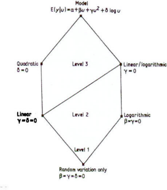
Chapter 2 The simplex sample space

Fig. 2.7.a Lattice of hypotheses within the model with expected characteristic of the form

αβγ+ + +u u u

2log .

2.7.3 Testing within a lattice

Once the model and relevant hypotheses have been set out in a lattice how should we

proceed to test the various hypotheses? The problem is clearly one of multiple

hypotheses testing with no optimum solution unless we can frame it as a decision

problem with a complete loss structure, a situation seldom realised for such problems.

Some more ad hoc procedure is usually adopted. In our approach we adopt the

simplicity postulate of Jeffreys (1961), which within our context maybe expressed as

follows: we prefer a simple explanation, with few parameters, to a more complicated

explanation, with many parameters. In terms of the lattice of hypotheses, therefore,

we will want to see positive evidence before we are prepared to move from a lower

level to one at a higher level. In terms of standard Neyman-Parson testing the setting

of the significance level

at some low value may be viewed as placing some kind of

protection on the hypothesis under investigation: if the hypotheses is true our test has

only a small probability, at most

, of rejecting it. With this protection, rejection of a

hypothesis is a fairly positive act: we believe we really have evidence against it. This

Chapter 2 The simplex sample space

is ideal for our view of hypothesis testing within a lattice under the simplicity

postulate. In moving from a lower level to a higher level we are seeking a mandate to

complicate the explanation, to introduce further parameters. The rejection of a

hypothesis gives us a positive reassurance that we have reasonable grounds for

moving to this more complicated explanation.

Our lattice testing procedure can then be expressed in terms of the following rules.

1. In every test of a hypothesis within the lattice, regard the model as the

alternative hypothesis.

2. Start the testing procedure at the lowest level, by testing each hypothesis at

that level within the model.

3. Move from one level to the next higher level only if all hypotheses at the

lower level are rejected.

4. Stop testing at the level at which the first non-rejection of a hypothesis occurs.

All non-rejected hypotheses at that level are acceptable as ‘working models’

on which further analysis such as estimation and prediction may be based.

2.7.4 Construction of tests

For the construction of ha hypothesis h within a model m in an unfamiliar situation,

we shall adopt the generalised likelihood ratio principle. In simple terms let

(

)

denote the likelihood of the parameter

for data and θ

∧

hX( ) and θ

∧

mX( ) denote the

maximum likelihood estimates, and

LXLX X

( ) {()| )=∧

θ and LXLX X

( ) {()| )=∧

denote the maximised likelihood under the hypothesis (h) and the model (m),

respectively. The generalised likelihood ratio test statistic is then

(

)

(

)

(

)

Chapter 2 The simplex sample space

and the larger this is the more critical of the hypothesis h we shall be. When the exact

distribution of this test statistic under the hypothesis h is not known, we shall make

use of the Wilks (1938) asymptotic approximation under the hypothesis h which

palaces c constraints on the parameters, the test statistic

(

)

log{

(

)}

is distributed approximately as χ2( )c.

2.8 Compositional regression, residual analysis and regression diagnostics

In terms of the transformation technique of logratio analysis little need be said.

Transformation from compositional vectors to logratio vectors places the analyst in

the position of facing a multivariate linear modelling situation which can be proceed

with in a standard way, with standard unconstained multivariate tests and the usual

forms of residual analysis. We shall see an example of this for the Arctic lake

sediment data in the next chapter.

For the staying in the simplex approach compositional regression uses the power and

perturbation operations in the following way: for a composition x regressing on a real

concomitant u we would set

xu p=⊕ ⊗ ⊕ξβ( ) ,

where ξβ, , p are all compositions, ξ playing the role of ‘constant’,

the role of

‘regression coefficient’ and p the role of the ‘error term’. The relation to the

transformation version is simply seen since

alr xalr ualr( ) ( ) ( )= + +ξβerror,

which could obviously be reparametrised as

Chapter 2 The simplex sample space

alr

(

)

error.

Obviously the estimation of ξβ, can be obtained as )(),(11 γα−− alralr from an

application of the transformation technique.

Although the staying-in-the-simplex and the transformation technique lead to the

same inferences a main difference will lie in the nature of the interpretation. In the

staying-in-the-simplex approach, for example, the definition of residual will be

$, where )(ˆ ∧∧ ⊗⊕=βξux. We shall see in the next chapter through an example

how all these ideas fit into place.

2.9 Some other useful tools

2.9.1 The predictive distribution as the fitted distribution

In much of statistical work we fit models to describe patterns of variability of our

observed data and there has been much discussion in statistical circles as to what the

appropriate distribution should be. It is clearly beyond the scope of this guide to argue

any case here but let us direct our attention to the use of what have become known as

the predictive distributions. Instead of simply inserting the maximum-likelihood

estimates in the logistic-normal LD(,)µΣ density function (the estimative method), as

it were putting all our eggs in one basket, we average all the possible logistic-normal

density functions taking account of the relative plausibilities of the various

(

)

parametric combinations. The resulting predictive distribution is what can be termed a

logistic-Student distribution with density function

fxdata x x alr xNNalr x

(|) ( .. ) [ {( ) }[( )( ) ] {( ) }/

∝+ − − + −

−∧−∧−∧

11 1 1 2

1 1 1µ µΣ

for compositional data matrix X. For large data sets there is little difference between

estimative and predictive fitted distributions, but for moderate compositional data sets

the difference can be substantial. The fact that geological sets often have N small (a

Chapter 2 The simplex sample space

few rock specimens) and D large (ten or more major oxides) should recommend the

use of the predictive distribution in applications to compositional geology.

2.9.2 Atypicality indices

The fitted density function assigns different plausibilities to different compositions.

Figure 2.9.1 shows a 3-part compositional data set in a ternary diagram with some

contour lines of the fitted predicative distribution. A composition such as C near the

center is clearly more probable than one such as B in the less dense area: B is more

atypical than C of the past experience. We can express this in terms of an atypicality

index, which is, roughly speaking, the probability that a future composition will be

more typical (be associated with a higher probability density) than the considered

composition. Technically the atypicality index Ax( )

*of a composition

* is given by

∫

=RdxdataxfxA)|()( *, where Rxfxdata fxdata= >{:(|) ( |)}

and this is easily evaluated in terms of standard incomplete beta functions; for details

see Aitchison (1986, Section 7.10). Atypicality indices lie between 0 and 1, with near-

zero corresponding to a composition near the center of the distribution and near 1

corresponding to an extremely atypical composition lying in a region of very low

density. Atypicality indices are therefore useful in detecting possible outliers or

anomalous compositions. For inspection of a given data set it is advisable to use the

now standard jackknife or leaving-one-out technique to avoid resubstitution bias in

assessing the atypicality index of any composition in the data set. Again atypicality

indices for such a procedures are readily computable.

Chapter 3 From theory to practice: some simple apllications

Chapter 3 From theory to practice: some simple applications

3.1 Simple hypothesis testing: comparison of hongite and kongite

A general question that we asked in Example 1 of Section 1.1 was whether any

differences could be detected between the hongite and kongite compositional

experience. After an alr logratio transformation of the compositional vectors we are

then faced with two multivariate normal samples with questions about equality of

mean vectors and covariance matrices. We have already obtained the estimates for

hongite in Section 2.6. The corresponding estimations for kongite are as follows.

The kongite centre is [0.486 0.201 0.114 0.105 0.094], again quite different from

the arithmetic mean [0.438 0.214 0.165 0.097 0.086].

The estimates of

for the kongite compositional data matrix are:

∧

0.1131 0.2352 -0.2008 0.0961

0.2352 0.6554 -0.7231 0.1061

-0.2008 -0.7231 1.0504 0.0911

0.0961 0.1061 0.0911 0.1951

∧

0.0646 0.1807 -0.2441 -0.0014 0.0002

0.1807 0.5949 -0.7724 0.0026 -0.0058

0.2441 -0.7724 1.0123 -0.0012 0.0054

-0.0014 0.0026 -0.0012 0.0487 -0.0487

0.0002 -0.0058 0.0054 -0.0487 0.0489

∧

0 0.2981 1.5652 0.1161 0.1131

0.2981 0 3.1520 0.6384 0.6554

1.5652 3.1520 0 1.0634 1.0504

0.1161 0.6384 1.0634 0 0.1951

0.1131 0.6554 1.0504 0.1951 0

Following the lattice strategy we can set out the model of two completely different

distributions and the hypotheses within that model in a self explanatory lattice

diagram (Figure 3.1). We are now within the structure of standard multivariate

Chapter 3 From theory to practice: some simple apllications

analysis apart from the constraints of the simplicity postulate in the order and nature

of the hypothesis testing within the model. To simplify matters here we use the

asymptotic forms of the generalised likelihood ratio test statistics, the Q of Section

2.7, to be compared against appropriate chi-squared percentiles.. The computational

procedures are uninteresting and can be found in Aitchison (1986, Section 7.5). The

only unusual feature is the computation for the hypothesis

1 2

with different

covariance matrices, commonly referred to as the Fisher-Behrens problem.

Model

51 1

2 2

(,)

No of parameters 28

1 2

No of parameters 24 Level 2 No of parameters 18

Test statistic 160.8 Test statistic 10.7

Level 1

µ µ

1 2

=Σ Σ

Test statistic 46.7

Fig. 3.1 Lattice of hypotheses for comparison of hongite and kongite compositions

Chapter 3 From theory to practice: some simple apllications

The sequence of tests are then as follows. The hypothesis at level 1, that the hongite

and kongite distributions are identical compares the value of the Q-statistic 46.7

against the 95 percentile of χ214( ) , namely 23.7, and so we reject this hypothesis and

move up to testing the hypotheses at level 2. The hypotheses that the mean vectors are

equal, allowing different covariance matrices, has a Q-statistic value of 160.8, to be

compared with the 95 percentile of χ234( ) , namely 36.4, and so again this

hypothesis has to be rejected. Finally the hypothesis that the covariance matrices are

equal but that the mean vectors are different has a Q-statistic value of 10.7 to be

compared with the 95 percentile of χ26( ) , namely 12.6. Thus we cannot reject this

hypothesis and so would conclude that a reasonable working model would assume

equal covariance structure for hongite and kongite but with different mean vectors.

Along the lines of Section 2.9 we could apply the leaving-one-out technique to

compute the atypicality indices of the hongite and kongite sets. For example, for the

hongite set theses are:

Speciment A B C D E Atypicality

index

48,8

31,7

3,8

6,4

9,3

0,7122

48,2

23,8

9,0

9,2

9,8

0,0171

37,0

9,1

34,2

9,5

10,2

0,1990

50,9

23,8

7,2

10,1

8,0

0,0318

44,2

38,3

2,9

7,7

6,9

0,7086

52,3

26,2

4,2

12,5

4,8

0,8284

44,6

33,0

4,6

12,2

5,6

0,8822

34,6

5,2

42,9

9,6

7,7

0,9689

41,2

11,7

26,7

9,6

10,8

0,1000

42,6

46,6

0,7

5,6

4,5

0,9873

49,9

19,5

11,4

9,5

9,7

0,1678

45,2

37,3

2,7

5,5

9,3

0,7012

32,7

8,5

38,9

8,0

11,9

0,8148

41,4

12,9

23,4

15,8

6,5

0,7405

46,2

17,5

15,8

8,3

12,2

0,2679

32,3

7,3

40,9

12,9

6,6

0,7508

43,2

44,3

1,0

7,8

3,7

0,7298

49,5

32,3

3,1

8,7

6,3

0,1454

42,3

15,8

20,4

8,3

13,2

0,5135

44,6

11,5

23,8

11,6

8,5

0,3501

45,8

16,6

16,8

12,0

8,8

0,0990

49,9

25,0

6,8

10,9

7,4

0,0739

48,6

34,0

2,5

9,4

5,5

0,8282

45,5

16,6

17,6

9,6

10,7

0,2800

45,9

24,9

9,7

9,8

9,7

0,2864

Chapter 3 From theory to practice: some simple apllications

The hongite specimens with atypicality index in excess of 0.95 are specimens no 8

(0.97) and no 10 (0.99). From inspection of the components we can see that for no 8

the atypicality probably arises from the relatively low value of the B component, and

for no 10 the relatively low value of the C component. Clearly we should place these

in a possible outlier category and refer the question of possible reasons to the

geologist.

What remains is to answer the question as to whether the new composition [44.0,

20.4, 13.9, 9.1, 12.6] can be regarded as typical of the hongite experience. Here a

straightforward application of the new case atypicality computation of Section 2.9

produces an atypicality index of 0.997, raising substantial doubt as to the hongiteness

of this new specimen.

3.2 Compositional regression analysis: the dependence of Arctic lake sediments on

depth

We asked the question in Example 2 of Section 1.1 whether the Arctic lake sediments

of Table 1.1.2 were dependent of depth and, if so, what is the nature of the

dependence. Again the alr transformation of the 3-part sediment compositions

produces two-dimensional vectors in real space and we can then consider a

straightforward multivariate (bivariate) regression on some function of depth. In this

respect we follow the two-dimensional counterpart of the lattice used as an

introductory example in Section 2.7. This is shown in Fig 3.2.a in which the various

hypotheses on the functional form of the regressand and their relationships to each

other are detailed. The tests of these hypotheses within the model (based on ratios of

determinants of residual matrices) are a familiar part of unconstrained multivariate

analysis and need not be dwelt on here; details can be found in Aitchison (1986,

Sections 7.6-7.9).

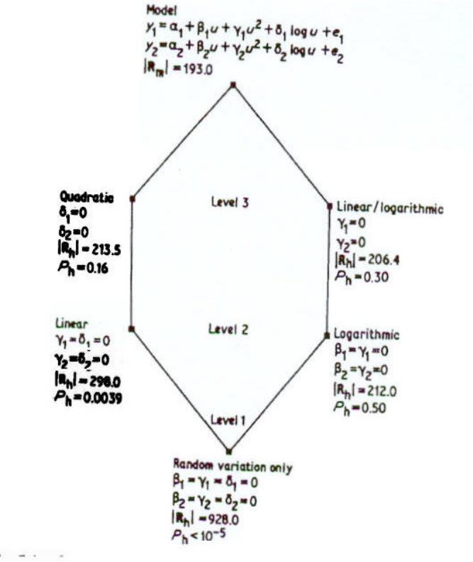
Chapter 3 From theory to practice: some simple apllications

Fig. 3.2.a Lattice of hypotheses for investigation of the dependence of Arctic lake sediments on water

depth, showing residual determinants |Rh| and significance probabilities Ph.

The test at level 1 dismisses the hypothesis of no dependence on depth. Stepping up to

level 2 the linear hypothesis is dismissed, but the simple logarithmic hypothesis

cannot be dismissed. If we had in fact reached level 3 we would have found the

quadratic and linear-logarithmic dependence hypotheses also acceptable. Lattice

testing prefers the logarithmic dependence because it provides a simpler working

model with only four regression parameters, compared with the six parameters of the

hypotheses at level 3.

The working model in alr logratio terms can thus be expressed in the following terms:

log( /)log( )

sand clay depth error

silt clay depth error

= + +

αδ

1 1 1

2 2 2

Chapter 3 From theory to practice: some simple apllications

with fitted model:

log(

)

log(

)

log( /). . log( )

sand

clay

depth

silt clay depth

−

= −

4 80 110 .

It should be emphasised here that this compositional regression is permutation

invariant. In particular, a different choice of divisor in the alr transformation would

have led to compatible results. Indeed the log(sand/silt) regression expression can be

obtained by a simple subtraction of the two forms above, giving

log(

)

log(

)

sand

silt

depth

−

The working model here clearly conforms to theories that as depth increases sand

gives way to silt and more so to clay with these differential effects decreasing with

depth. It would be interesting to compare the rates of change associated with such

processes for different locations.

The stay-in-the-simplex versions of these are the compositional regression

compositio

depth

⊕

⊗

[

]

log(

)

[

]

9928

0071

0001

046

238

716

This provides the same interpretation of the regression as the transformation

regression: as depth increases sand gives way to silt and more so to clay with

differential effects decreasing with depth. Which characterisation of the regression is

chosen may well depend on personal choice.

Here we can show the regression line within the [sand silt clay] ternary diagram as

in Figure 3.2.b. The fit is obviously reasonably convincing.

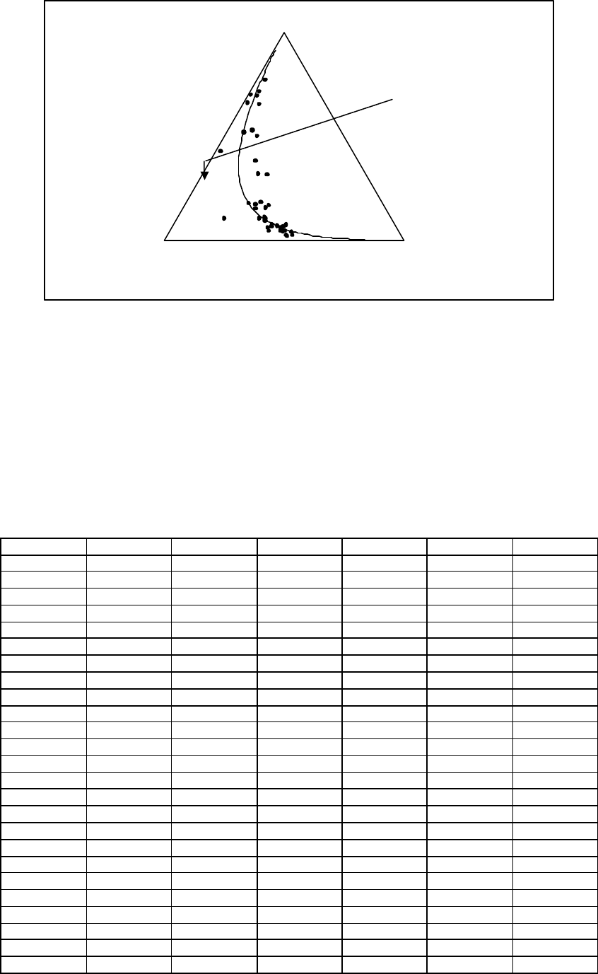
Chapter 3 From theory to practice: some simple apllications

Sand

Silt Clay

Fig. 3.2.b Arctic sediments and regression line of sediment on logarithm of depth.

Residual analysis can obviously be carried out either in terms of the transformed

regression or in a stay-in-the simplex format. Since the latter is less familiar we

demonstrate it briefly. This simply involves computation and investigation of the

residual compositions, namely

compositio

fitted

compositio

. The residual

compositions here are:

sediment sand silt clay res_sand

res_silt res_clay

1 77,5

19,5

3,0

0,3661

0,2596

0,3744

2 71,9

24,9

3,2

0,3766

0,3028

0,3206

3 50,7

36,1

13,2

0,1583

0,2257

0,6160

4 52,2

40,9

6,6

0,2304

0,3523

0,4173

5 70,0

26,5

3,5

0,5081

0,2751

0,2168

6 66,5

32,2

1,3

0,5550

0,3614

0,0836

7 43,1

55,3

1,6

0,3727

0,5461

0,0812

8 53,4

36,8

9,8

0,3692

0,2728

0,3580

9 15,5

54,4

30,1

0,0837

0,2665

0,6499

10 31,7

41,5

26,8

0,2044

0,2180

0,5776

11 65,7

27,8

6,5

0,6040

0,2036

0,1924

12 70,4

29,0

0,6

0,7652

0,2181

0,0166

13 17,4

53,6

29,0

0,1518

0,2952

0,5530

14 10,6

69,8

19,6

0,1670

0,4747

0,3583

15 38,2

43,1

18,7

0,5052

0,2329

0,2619

16 10,8

52,7

36,5

0,1816

0,3118

0,5066

17 18,4

50,7

30,9

0,3110

0,2885

0,4005

18 4,6

47,4

48,0

0,0760

0,2743

0,6497

19 15,6

50,4

34,0

0,3182

0,2887

0,3931

20 31,9

45,1

23,0

0,6110

0,2031

0,1858

21 9,5

53,5

37,0

0,2530

0,3338

0,4132

22 17,1

48,0

34,9

0,4127

0,2595

0,3278

23 10,5

55,4

34,1

0,2996

0,3424

0,3580

24 4,8

54,7

41,0

0,1518

0,3736

0,4746

25 2,6

45,2

52,2

0,1206

0,3371

0,5423

Direction of

increasing depth

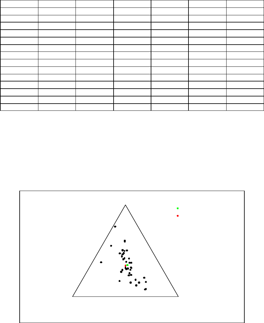
Chapter 3 From theory to practice: some simple apllications

sediment sand silt clay res_sand

res_silt res_clay

26 11,4

52,7

35,9

0,4164

0,3019

0,2818

27 6,7

46,9

46,4

0,2910

0,3060

0,4030

28 6,9

49,7

43,4

0,3047

0,3236

0,3716

29 4,0

44,9

51,1

0,2353

0,3277

0,4371

30 7,4

51,6

40,9

0,4057

0,3178

0,2764

31 4,8

49,5

45,7

0,3051

0,3473

0,3476

32 4,5

48,5

47,0

0,3157

0,3438

0,3406

33 6,6

52,1

41,3

0,4375

0,3190

0,2435

34 6,7

47,3

45,9

0,4725

0,2808

0,2467

35 7,4

45,6

46,9

0,5020

0,2585

0,2395

36 6,0

48,9

45,1

0,4587

0,2994

0,2418

37 6,3

53,8

39,9

0,4711

0,3210

0,2080

38 2,5

48,0

49,5

0,2877

0,3893

0,3229

39 2,0

47,8

50,2

0,2677

0,4088

0,3235

These should be spread around the centre of a ternary diagram, as in Figure 3.2.c. The

question of outliers among these residuals obviously arises. We report that there are

two sediment compositions -S12 and S7- with residual atypicality indices of 0.9998

and 0.9990, respectively.

sand

silt clay

Arithmetic Mean

Geometric Mean

Fig. 3.2.c Residuals of the Arctic sediments fitted by the regression line of sediment on logarithm of

depth

Chapter 3 From theory to practice: some simple apllications

3.3 Compositional invariance: Economic aspects of household budget patterns

In the literature of consumer demand analysis there have been only a few attempts to

incorporate compositional analysis directly into the analysis of household budgets.

This technique has many advantages and provides opportunities for new forms of

investigation. Suppose the w is a record of household expenditure on D mutually

exclusive and exhaustive commodity groups so that

is total

expenditure and

(

)

is the proportional pattern of allocation to the groups.

Logcontrast linear modelling with

(

)

of Lt

D(log ,)αβ+Σform has interesting

consequences. First, the sometimes troublesome budget constraint or Engel

aggregation (Brown and Deaton, 1972, 1163), that for each household total

expenditure should equal the sum of all commodity expenditures, is automatically

satisfied. Secondly, the hypothesis of compositional invariance

, that

composition is independent of size, has a direct interpretation in terms of the income

elasticities

∂

i i

wt i D

log /log (, .. , )1 of demand, if for the moment and for

simplicity we identify household total expenditure with household income. In

expectation terms

iiD

−

(

)

so that compositional invariance, not surprisingly, corresponds to equality of all D

income elasticities. Thirdly, whether or not there is compositional invariance, the

modelling can clearly be extended to a full consumer demand analysis by the

incorporation of commodity prices and other covariates such as household type and

household composition into the mean parameter of the logistic normal distribution.

Indeed, such an extension can be shown to be identical with the Houthakker (1960)

indirect addilog model of consumer demand (Brown and Deaton, 1972, Equation

115),

In the above discussion we have identified household total expenditure t with

household income s. This is not an essential feature of the modelling since we could

approach it through the conditioning

(

)

(

)

(

)

(

)

with perhaps a

Chapter 3 From theory to practice: some simple apllications

reasonable assumption that, for given total expenditure t, the pattern x is independent

of income s, leading to the above concentration on

(

)

As a simple start to our analysis of the household budgets of Table 1.1.3 let us first

apply tests of compositional invariance separately to the 20 single male households

and to the 20 single female households. Estimation and testing follows standard

unconstrained multivariate analysis, with the result that we reject the hypothesis of

compositional invariance for both single male and single female households. Thus for

each set there is strong evidence against the hypothesis of compositional invariance:

in other words, the patterns of expenditures do appear to depend on total expenditure.

From the relationship above we see that although the D ‘income’ elasticities are not

determined by the D – 1 regression coefficients they can at least be placed in order of

magnitude. The commodity groups arranged in increasing order of elasticity, that is,

in conventional economic terminology from necessity to increasing luxury groups are

(for each gender):

1. Foodstuffs, including alcohol and tobacco

2. Housing, including fuel and light

3. Services, including transport and vehicles

4. Other goods, including clothing, footwear and durable goods

The fact that the ordering is the same for males and females raises the question of

whether the dependence of pattern on total expenditure is really different for males

and females. This suggests that it might have been more fruitful to consider

hypotheses expressed in terms of the parameters of the model

M M

log

+ error, for males;

F F

log

+ error, for females.

Note that the separate compositional invariance hypotheses tested above are the

hypotheses

and

at level 2. All the hypotheses of the lattice can be

tested within the standard framework of multivariate linear modelling. We omit the

Chapter 3 From theory to practice: some simple apllications

details here but show on the lattice the significance probabilities associated with each

hypothesis, noting that we can move up the lattice by rejection until level 3 where we

would fail to reject the hypothesis

Before we leave this example we point out that it would be straightforward to

introduce some concomitant feature such as age on which pattern may depend and test

hypotheses within the associated more general model.

3.4 Testing perturbation hypotheses: Change in cows’ milk

The data of Table 1.1.4 are of a before- and after-nature. Each cow has had milk

composition determined at the beginning and at the end of the trial and so we have

essentially, in standard statistical analysis terms, paired comparisons. The major

difference is that we require to use a measure of difference appropriate to

compositional change and we have seen this to be perturbation. Thus for each cow we

record the set of perturbations below.

Control group: compositional change

Ident_cow pr mf ch Ca Na K

C1 0,1389

0,2278

0,1553

0,1699

0,1400

0,1680

C2 0,1377

0,1661

0,1540

0,2066

0,1549

0,1807

C3 0,1464

0,1525

0,1672

0,1976

0,1572

0,1792

C4 0,1950

0,1564

0,1562

0,1993

0,1163

0,1768

C5 0,1988

0,1423

0,1507

0,1869

0,1470

0,1742

C6 0,1498

0,1979

0,1858

0,1782

0,1237

0,1645

C7 0,1467

0,1552

0,1828

0,1778

0,1564

0,1812

C8 0,1109

0,2690

0,1466

0,2046

0,0996

0,1693

C9 0,1198

0,2005

0,1351

0,1984

0,1654

0,1807

C10 0,2164

0,1624

0,1687

0,1818

0,1111

0,1597

C11 0,1792

0,1585

0,1358

0,1907

0,1645

0,1713

C12 0,1650

0,1836

0,1401

0,1896

0,1477

0,1740

C13 0,1744

0,1999

0,1742

0,1608

0,1310

0,1597

C14 0,1319

0,1689

0,1338

0,2055

0,1713

0,1886

C15 0,1482

0,2426

0,1544

0,1524

0,1476

0,1549

C16 0,1857

0,1891

0,1810

0,1829

0,1042

0,1571

C17 0,1497

0,1552

0,1419

0,2027

0,1623

0,1883

C18 0,1518

0,1703

0,1412

0,1656

0,2064

0,1646

Ident_cow pr mf ch Ca Na K

C19 0,1582

0,1437

0,1682

0,1852

0,1733

0,1713

Chapter 3 From theory to practice: some simple apllications

C20 0,1683

0,1832

0,1618

0,1659

0,1643

0,1565

C21 0,1394

0,2128

0,1999

0,1619

0,1336

0,1523

C22 0,1687

0,1570

0,1399

0,1883

0,1632

0,1829

C23 0,1988

0,1436

0,1529

0,1809

0,1537

0,1700

C24 0,1870

0,1770

0,1561

0,1754

0,1424

0,1622

C25 0,1243

0,2008

0,1520

0,2043

0,1346

0,1840

C26 0,1686

0,2286

0,1465

0,1641

0,1373

0,1549

C27 0,1512

0,1692

0,1658

0,1865

0,1508

0,1766

C28 0,2033

0,2042

0,1676

0,1460

0,1344

0,1445

C29 0,1455

0,1817

0,1783

0,1519

0,1798

0,1628

C30 0,1451

0,2350

0,1886

0,1696

0,1195

0,1422

Treatment group: compositional change

Ident_cow pr mf ch Ca Na K

T1 0,1753

0,1459

0,1552

0,2122

0,1642

0,1473

T2 0,2090

0,0937

0,1313

0,2341

0,1717

0,1603

T3 0,2387

0,1207

0,1497

0,1832

0,1652

0,1426

T4 0,2398

0,1345

0,1726

0,2310

0,0896

0,1326

T5 0,1173

0,1647

0,1535

0,2482

0,1577

0,1586

T6 0,1701

0,1063

0,1524

0,2508

0,1826

0,1379

T7 0,2018

0,1109

0,1166

0,2800

0,1471

0,1436

T8 0,2142

0,0944

0,1472

0,2488

0,1536

0,1418

T9 0,1890

0,1622

0,2066

0,2182

0,0965

0,1274

T10 0,2097

0,1431

0,1706

0,2082

0,1435

0,1249

T11 0,1562

0,1611

0,1901

0,2452

0,1126

0,1349

T12 0,1292

0,2046

0,1977

0,2104

0,1313

0,1268

T13 0,2538

0,1314

0,1499

0,1665

0,1655

0,1328

T14 0,1959

0,1289

0,1612

0,2324

0,1370

0,1448

T15 0,2154

0,1707

0,1713

0,2456

0,0875

0,1095

T16 0,1748

0,1715

0,1458

0,1959

0,1795

0,1326

T17 0,1446

0,1634

0,1757

0,2265

0,1375

0,1523

T18 0,1690

0,1918

0,1625

0,2510

0,0992

0,1264

T19 0,1791

0,1607

0,1792

0,1990

0,1221

0,1599

T20 0,2149

0,1210

0,1446

0,2589

0,1090

0,1516

T21 0,1799

0,1545

0,1605

0,2272

0,1408

0,1371

T22 0,1723

0,1566

0,1638

0,2460

0,1299

0,1314

T23 0,1778

0,1285

0,1905

0,2468

0,1161

0,1403

T24 0,2045

0,1670

0,1612

0,2124

0,1248

0,1301

T25 0,2063

0,1206

0,1428

0,2287

0,1461

0,1555

T26 0,2709

0,1018

0,1207

0,2491

0,1226

0,1349

T27 0,2099

0,1188

0,1450

0,2617

0,1047

0,1598

T28 0,2046

0,1370

0,1325

0,2779

0,1111

0,1369

T29 0,2808

0,1252

0,1390

0,1813

0,1328

0,1408

T30 0,1245

0,1871

0,1554

0,2084

0,1573

0,1672

Chapter 3 From theory to practice: some simple apllications

We can address the problems that we face here in three stages by posing three

questions.

Question 1. Is there any evidence of seasonal change in milk composition. In other

words is there any evidence of differences in the milk compositions of the control

group between the beginning and end of the trial? Phrased as a compositional

hypothesis this is simply a question of whether the centre of the control group

perturbations is the identity perturbation. Transformed into logratio terms this is

simply asking whether the mean of the alr vectors is a zero vector, a hypothesis

easily tested under standard multivariate analysis. The Q-statistic value is 32.5, which

when compared with the 95 percentile of χ215( ) , namely 25.0, shows significant

departure from the identity perturbation. We thus conclude that there is some

evidence of a seasonal change which justifies the insistence of having a control group.

The centre of the control group perturbations is

[pr mf ch Ca Na K]control = [0.1595 0.1835 0.1599 0.1818 0.1458 0.1695].

Question 2. Is there similar evidence of a change in the treatment group? Here the Q-

statistic value is even larger, 75.6, again to be compared against the same percentile

value, and so we have real evidence of change, with the centre of the treatment group

perturbations being

[pr mf ch Ca Na K]treat = [0.1928 0.1416 0.1589 0.2309 0.1338 0.1420].

Question 3. The remaining question is to ask whether there are differences between

the control and treatment group perturbations and this question can be answered by

using a separate sample lattice identical to that for the hongite-kongite comparison of

Section 3.1. The three Q-statistics in the same order as for the previous example are

153.7, 45.6 and 212.0 to be compared against 95 percentiles of the chi-squared

distribution at 20, 15 and 5 degrees of freedom, all giving significant differences.

Thus there is strong evidence of differences between control and treatment changes.

Chapter 3 From theory to practice: some simple apllications

A good indication of what the nature of this change is can be obtained by computing

the perturbation difference between the control and treatment perturbation centres,

namely

[pr mf ch Ca Na K]treat-control = [0.2015 0.1286 0.1656 0.2117 0.1529 0.1397].

Thus we can see that relatively there is enhancement of protein, carbohydrate and

calcium, presumably a successful nutritional result.

3.5 Testing for distributional form

3.5.1 Introduction

For compositional problems in which the analysis depends in an assumption of

distributional form tests can be applied to assess the multivariate normality of the

transformed logratio vectors. For this purpose there is a whole battery of such tests:

univariate marginal tests, bivariate angle tests, multivariate radius tests, with different

forms of test statistics: Anderson-Darling, Cramer-von Mises, Watson, with

accompanying useful graphical plots. All of these are examined in great detail in

Aitchison (1986) and need not divert us here from the main task of presenting

principles and practice of compositional data analysis. There has been discussion of

whether the choice of divisor in the alr transformation is crucial to the result. So here

we present a simple alternative avoiding this problem and which may also provide

some measure of the degree of success of the normality assumption.

3.5.2 A useful characterisation of compositional distributional forms

The form of the simplicial singular value decomposition suggests a useful way in

which to characterise compositional distributions. Suppose that we express a generic

D-part composition x in the form

xu uDDD

=⊕ ⊗ ⊕ ⊕ − − −

ξπ β π β( ) . .. ( )

1 1 1 1 1 1

Chapter 3 From theory to practice: some simple apllications

Now if we assume that u = [u1 . . . uD-1] follows a (D-1)-dimensional normal

distribution N D-1(0, ID-1), then it is simple to establish that x follows a logistic

normal distribution with center

and centred logratio covariance matrix

expressible in terms of

)

(

diag

and

as ,)()( T

clrclr ΒΠΒ=Γwhere clr denotes

the operation of forming centred logratios from the rows of

. Similarly a logistic-

Student distribution is obtained with the same centre and covariance matrix and with

degrees of freedom when u follows a ),0,(1

1−

−D

DISt νdistribution. Further a

logistic skew normal distribution for x is obtained if u follows a multivariate skew

normal distribution with density function ).(),0|(1

DuIuγφΦ

−

We note at this point that this characterisation in terms of the u-distribution is useful

for simulation purposes since it requires only simple simulation algorithms for

standardised distributions. Simulated data is here useful for testing the effectiveness

of the distributional form tests.

3.5.3 Testing procedures

The remaining problem is how to exploit these characterisations for the purpose of

testing distributional forms. We shall have available a compositional data set, a

matrix

whose rows N

xx ,...,

1 are N D-part compositions and the first step

in testing is to arrive at the appropriate N (D-1)-real vectors u on which to base the

tests. This is easily done through the compositional singular value decomposition of

The first step is to estimate the parameters in the above characterisation. This is easily

done from the standard singular value decomposition of the doubly centred matrix Z

constructed form the log X. Suppose that the standard singular value decomposition of

Z is T

UPVZ=, where U and V have zero-sum orthonormal columns and

),...,(11 −

ppdiagP, where 11 ,..., −D

pp are the singular values in descending

order of magnitude. Then it is easy to see that our estimates of the parameters ξ, ,ΠΒ

in the power-perturbation characterization are cen(X), 1/−NP and

)(

Vclr −. Also, and importantly for our distributional form testing here the u

vectors for the individual compositions are given as the rows of .1−NU

Chapter 3 From theory to practice: some simple apllications

The aim is then to test these uni (i = 1, . . . , D; n = 1, . . . , N) for compositional form.

Let us take the specific case of testing the compositional data set for additive logistic

normality. The philosophy behind the testing procedure described below is that

through the singular value decomposition we have a picture of the dimensionaly of

the data set with known proportions of the total variability explained by increasing

degrees of approximation. We would surely be reasonably happy if we were sure that

for 99 percent of the variability we had satisfied ourselves of additive logistic

normality. In this procedure the first column of $

represents the first order

approximations with a proportion p1 explained, the first two columns of $

the second

order approximation with a proportion

2explained, and so on. Thus in terms of the

marginal, bivariate and radius tests as described in Aitchison (1986, Section 7.3) the

sequence of testing proceeds as follows.

First order tests. Subject the first column of $

to marginal tests.

Second order tests. Subject the second column of $

to marginal tests; columns 1, 2

to bivariate angle tests; and columns 1, 2 to radius test.

Third order tests. Subject the third column of $

to marginal tests; columns 1,3

and 2, 3 to bivariate angle tests; and columns 1, 2, 3 to radius tests.

And so on until the desired degree of approximation is achieved.

3.6 Related types of data

3.6.1 Probability statement data

Statisticians will readily recognize that all the above arguments relating to

compositional data equally apply to probabilistic statements. It is clear that the

standard practice of measuring probabilities on the scale of 0 to 1 is merely a

convention and that any meaningful probabilistic statement can be expressed in terms

of ratios, equivalently odds.

Chapter 3 From theory to practice: some simple apllications

For example, subcompositional coherence is simply conditional probability

coherence. A clinician may be faced with a differential diagnostic problem among

five forms (1, 2, 3, 4, 5) of which 1, 2, 3, are malignant and 4, 5 benign. At a stage in

the diagnostic process the clinician, having ruled out the benign forms 4 and 5, may

wish to make a conditional probabilistic statement involving only the malignant states

1, 2, 3. The process of moving from the full probabilistic statement to the conditional

probability statement is exactly analogous to the closure operation of forming a

subcomposition from a full composition. Moreover, clearly there is also a principle of

conditional coherence, analogous to the subcompositional coherence principle, that

must apply here.

In relation to probability statements the perturbation operation is a standard process.

Bayesians perturb the prior probability assessment x on a finite number D of

hypotheses by the likelihood p to obtain the posterior assessment X through the use

of Bayes’s formula. Again, in genetic selection, the population composition x of

genotypes of one generation is perturbed by differential survival probabilities

represented by a perturbation p to obtain the composition X at the next generation,

again by the perturbation probabilistic mechanism .

3.6.2 Granulometric data

Granulometric data obtained by sieving techniques are not histograms, as commonly

defined, but are weight (or volume)_x_diameter profiles. Mathematically they are

third moment distributions of the basic grain diameter distribution, a fact apparently

first noted by Hatch (1933); see also Aitchison and Brown (1956) for further details

and its relation to the Kolmogorov (1941) breakage model. Thus it could be argued

that fitting a probability distribution to such an object is every bit as weird as

considering the profile as a composition. Indeed to move from a weight_x_diameter

profile to a diameter histogram is nothing more than a perturbation operation. For

example if the weight_ x_diameter profile has H diameter intervals I1 , . . . , IH , with

centers d1, . . . , dH and with associated proportional weights p1 , . . . , pH, then on the

assumption of uniform specific gravity, the diameter histogram q

1 , . . . , q

H is

approximated by the perturbation [d1-3, . . . , dH -3]

⊕

[p1 , . . . , pH]. A consequence of

the perturbation invariance property of the compositional metric is that the distance

between profiles is the same as between histograms, a clearly desirable property.

Chapter 3 From theory to practice: some simple apllications

Whether grain-size data is considered as grouped ordinal data and some class of

univariate distributions is used to characterize each such ‘histogram’ or each

histogram is considered a compositional vector is certainly an open question. In

situations where the objective is to compare a number of weight_x_diameter profiles,

until a satisfactory class of distributions giving good fits to the histogram emerges, the

treatment of such data as compositional is certainly viable, with possibilities of

inferring the nature of an underlying process through the study of possible differential

perturbation processes.

Chapter 4 More complex compositional problems

Chapter 4 Developing appropriate methodology for more complex

compositional problems

4.1 Dimension reducing techniques: logcontrast principal components

In unconstrained multivariate analysis principal component analysis is a popular

means of investigating the dimension of the variability and of hopefully arriving at

linear combinations of variables, which may have some interpretation within the

particular discipline. In variation in

D principal components are the natural

algebraic form as the inner product of the vector space, namely linear combinations of

the components. As we have seen in Section 2.3.3 the inner product takes the form of

a logcontrast of the components of the form:

D D1 1

log

, where

The variance of such a logcontrast is

, where

is the centred logratio

covariance matrix, and the successive principal logcontrasts are obtained from the

eigenvectors (corresponding to the non-zero eigenvalues) of the estimate of

, and

have the usual properties of orthogonality and with variances simply related to the

eigenvalues.

Applied to the hongite experience of Table 1.1.1a we have 51,...,aa coefficients as

rows of

log A log B log C log D log E

-----------------------------------------------

1st logcontrast 0.1945 0.5876 -0.7840 0.0341 -0.0322

2nd logcontrast -0.0672 0.0867 -0.0112 -0.7069 0.6986

3rd logcontrast 0.7899 -0.5598 -0.2295 -0.0707 0.0701

4th logcontrast -0.3656 -0.3658 -0.3640 0.5423 0.5531

with eigenvalues 38.26, 2.186, 0.142, 0.004. The measure of total variability is 1.69

and the first principal logcontrast ‘explains’ 94.2 percent of this variability, the second

bringing this to 99.6 percent. Thus we would be justified in regarding the variability

Chapter 4 More complex compositional problems

of hongite as being largely two-dimensional. Inspection of the first two logcontrasts

suggests that the first is involved largely in explaining variability within the (A, B, C)

subcomposition and the second variability within the (D, E) subcomposition, and that

these variations are orthogonal to each other. The writer can divulge that he had

forgotten how he had simulated the hongite data set and that this analysis reminded

him exactly of the details of the simulation.

4.2 Simplicial singular value decomposition

For the record we give the staying-in-the-simplex version of logcontrast principal

component analysis. This is by way of the simplicial singular value decomposition. It

could reasonably be argued that the major statistical tool in the analysis of

multivariate data associated with a metric vector space such as R R S

D D D

, ,

+must be

the associated singular value decomposition. For a

compositional data matrix

X with nth composition

n this, as we have already seen in Chapter 2, takes the form

xu u

n n nR R R

=⊕ ⊗ ⊕ ⊕ ⊗ξπ β π β( ) .. . ( )

1 1 1 .

It is interesting to apply this to a simple compositional data set such as hongite. The

details of the process of estimation will be taken up in the next section. Here we

simply record the results.

ξ= [0.489 0.220 0.099 0.104 0.088],

=]ˆ...ˆ[ 41 ππ [6.185 1.478 0.377 0.066],

∧

























0 222 0329 0189 0189 0177

0169 0198 0179 0 089 0364

0 395 0103 0143 0167 0192

0125 0125 0125 0310 0314

. . . . .

with the

−

(

)

set of u coefficients given by

Chapter 4 More complex compositional problems

Specimen u1 u2 u3 u4

1 0,1529

0,2871

0,1325

-0,2833

2 0,0177

0,1155

-0,0512

0,0403

3 -0,2512

0,0646

0,0109

0,0705

4 0,0493

-0,0258

0,1437

0,0351

5 0,2046

0,0752

-0,2816

-0,2748

6 0,1314

-0,3607

0,2511

-0,2053

7 0,1359

-0,2561

-0,4477

-0,0110

8 -0,3336

-0,1047

0,5093

0,0235

9 -0,1928

0,0984

0,0224

0,0122

10 0,4027

0,0494

0,1957

0,4844

11 -0,0298

0,0803

0,1656

-0,1737

12 0,2084

0,3751

-0,0332

-0,1205

13 -0,2796

0,2203

-0,1642

0,3033

14 -0,1612

-0,3733

-0,2201

0,0101

15 -0,0858

0,2479

0,0340

-0,1349

16 -0,2951

-0,2955

-0,1939

-0,0771

17 0,3560

-0,2078

-0,0156

-0,1994

18 0,1847

-0,0418

0,1284

-0,0841

19 -0,1311

0,2812

-0,1400

0,1719

20 -0,1750

-0,1090

0,2042

-0,1500

21 -0,0952

-0,0859

-0,0731

0,1594

22 0,0614

-0,0949

0,0350

0,1608

23 0,2174

-0,1375

0,1050

0,4186

24 -0,1035

0,1131

-0,0370

-0,2569

25 0,0114

0,0848

-0,2802

0,0808

The connection between this and the logcontrast principal components is simply that

the eigenvalues correspond to the squares of the

’s, and that the a-coefficients of the

logcontrast approach are the clr transforms of the

’s. The interpretation remains the

same.

4.3 Compositional biplots and their interpretation

The biplot (Gabriel, 1971, 1981) is a well established graphical aid in other branches

of statistical analysis. Its adaptation for compositional data is simple and can prove a

useful exploratory and expository tool. For a compositional data matrix X the biplot is

based on a singular value decomposition of the doubly centered logratio matrix Z =

[zri], where

∑

−

−= N

rrirriri xgxNxgxz

1)}..(/log{)}(/log{

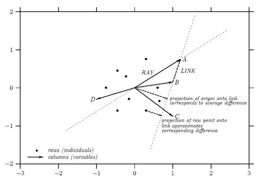
Chapter 4 More complex compositional problems

Let Z = U diag(k1, . . . , kR) V t be the singular value decomposition, where m is the

rank of Z, in practice usually m = D – 1, and where the singular values k1`, . . . , km are

in descending order of magnitude. The biplot (Figure 4.3.a) then converts the second

order approximation to Z given by the singular value decomposition into a graphical

display. Figure 4.3.a consists of an origin O which represents the centre of the

compositional data set, a vertex at position (k1vi1, k2 vi2)/(N – 1)1/2 for each of the parts,

labelled 1, . . . , D, and a case marker at position at (N – 1)1/2 (ur1, ur2) for each of the

N cases, labelled c1, . . . , cN . We term the join of O to a vertex i the ray Oi, and the

join of two vertices i and j the link ij. These features constitute a biplot with the

following main properties for the interpretation of the compositional variability.

Fig. 4.3.a The basic elements of a compositional biplot

Links, rays and covariance structure. The links and rays provide information on the

covariance structure of the compositional data set.

| | var{log( /)}ij x x

i j

2≈,

)}](/var[log{|| 2xgxOi i

≈,

)}](/log{)},(/[log{)cos( xgxxgxcorriOj ii

Chapter 4 More complex compositional problems

It is tempting to imagine that this last relation can be used to replace discredited

corr(xi, xj) as a measure of the dependence between two components. Unfortunately

this measure does not have subcompositional coherence.

A more useful result is the following. If links ij and kl intersect in M then

cos( ){log( /),log( /)}iMk corr x x x x

i j kl

≈

A particular case of this is when the two links are at right angles so implying that

cos(

)

iMk

≈

and there is zero correlation of the two logratios. This is useful in

investigation of subcompositions for possible independence.

Subcompositional analysis. The center O is the centroid (center of gravity) of the D

vertices 1, . . ., D. Since ratios are preserved under formation of subcompositions it

follows that the biplot for any subcomposition s is simply formed by selecting the

vertices corresponding to the parts of the subcomposition and taking the center Os of

the subcompositional biplot as the centroid of these vertices.

Coincident vertices. If vertices i and j coincide or nearly so this means that

var{log(xi/xj)} is zero or nearly so, so that the ratio xi /xj is constant or nearly so.

Collinear vertices. If a subset of vertices, say 1, . . . , C is collinear then we know

from our comment on subcompositional analysis that the associated subcomposition

has a biplot that is one-dimensional, and then a technical argument leads us to the

conclusion that the subcomposition has one-dimensional variability. Technically this

one-dimensionality is described by the constancy of C–2 logcontrasts of the

components x1, . . . , xC . Inspection of these constant logcontrasts may then give

further insights into the nature of the compositional variability.

Case markers and recovery of data. Such markers have the easily established property

that Ocn . ji represents the departure of log(xi /xj) for case cn from the average of this

logratio over all the cases. Let P and Pn in Figure 4.3.b denote the projections of the

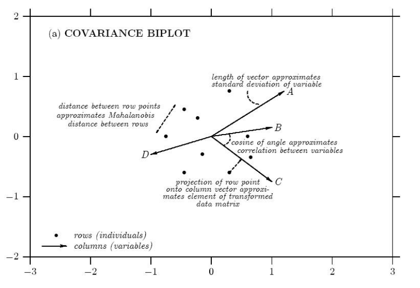
Chapter 4 More complex compositional problems

center O and the compositional marker cc on the possibly extended link ji . Then

Ocn . ji =

|PPn| | ji |,

where the positive sign is taken if the directions of PPn and ji are the same, otherwise

the negative sign is taken. A simple interpretation can be obtained as follows.

Consider the extended line ji as divided into positive and negative parts by the point

P, the positive part being in the direction of ji from P. If Pn falls on the positive

(negative) side of this line then the logratio of log(xni /xnj) of the nth composition

exceeds (falls short of) the average value of this logratio over all cases and the further

Pn is from P the greater is this excedance (shortfall); if Pn coincides with P then the

compositional logratio coincides with the average.

Fig. 4.3.b Interpretation of case markers in a compositional biplot

A similar form of interpretation can be obtained from the fact that Ocn.Oi represents

the departure of the centered logratio log{xni /g(xn)} of the nth composition from the

average of this centered logratio over all replicates.

It must be clear from the above aspects of interpretation that the fundamental

elements of a compositional biplot are the links, not the rays as in the case of variation

Chapter 4 More complex compositional problems

diagrams for unconstrained multivariate data. The complete set of links, by specifying

all the relative variances, determines the compositional covariance structure and

provides direct information about subcompositional variability and independence. It is

also obvious that interpretation of the relative variation diagram is concerned with its

internal geometry and would, for example, be unaffected by any rotation or indeed

mirror-imaging of the diagram.

Another fundamental difference between the practice of biplots for unconstrained and

compositional data is in the use of data scaling. For unconstrained data if there are

substantial differences in the variances of the components, biplot approximation may

concentrate its effort on capturing the nature of the variability of the most variable

components and fail to provide any picture of the pattern of variability within the less

variable components. Since such differences in variances may simply arise because of

scales of measurement a common technique in such biplot applications is to apply

some form of individual scaling to the components of the unconstrained vectors prior

to application of the singular value decomposition. No such individual scaling is

necessary for compositional data when the analysis involves logratio transformations.

Indeed, since for any set of constants (c1, . . . , cD), we have

cov{log(cixi /cjxj),log(ckxk /clxl)} = corr{log(xi /xj),log(xk /xl)}

it is obvious that the covariance structure and therefore the compositional biplot are

unchanged by any differential scaling or perturbation of the compositions. This, of

course, is simply an aspect of the perturbation invariance of measures of dispersion

for compositional data. Only the centering process is affected by such differential

scaling. Moreover any attempt at differential scaling of the logratios of the

components would be equivalent to applying differential power transformations to the

components of the compositions, a distortion which would prevent any compositional

interpretation from the resulting diagram.

4.4 The Hardy-Weinberg law: an application of compositional biplots and

logcontrast principal component analysis

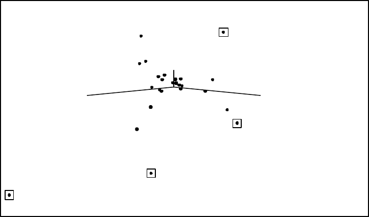
Chapter 4 More complex compositional problems

In the MN blood group system there are three genotypes, namely MN, MM, NN, and

the proportions of these genotypes within a population provide a blood group

composition for that population. Table 4.4.1 shows these compositions for 24 native

populations; the data are reconstructed from Figure 12 of Gower (1987). Let us

suppose that we know nothing about genetic theory and decide to explore this data set

by the construction of a relative variation biplot (Fig. 4.4.a) as described in Section

4.3. For such a 3-part compositional data set the biplot retains all the variability and

provides an exact representation of the pattern of variability. The approximate

collinearity of the vertices MN, MM, NN indicates that the variability is mainly one-

dimensional and suggests a logcontrast principal component analysis to determine the

form of the constant logcontrast. Such a principal component analysis (Aitchison,

1986, Section 8.3) yields the following eigenvalues and logcontrasts

, 0.0031 log MN - 0.7091 log MM + 0.706 log NN;

079

, 0.816 log MN - 0.406 log MM - 0.411 log NN.

Cumulative proportion explained:

0,97

MM NN

= Outliers

Fig. 4.4.a Biplot of the MN blood group data

The near-constant logcontrast arises from the near-zero second eigenvalue. Moreover

the fact that the coefficient 0.816 is approximately twice the coefficients 0.406 and

0.411 suggests that we can obtain a substantial simplification to our interpretation if

Chapter 4 More complex compositional problems

we consider the constant logcontrast

2 log MN - log MM - log NN = constant

We can obtain an estimate 1.348 of the constant from the average value of the

logcontrast over the sample of 24 compositions. Moreover the fact that this is

approximately log 4 encourages the following conjecture,

2 log MN - log MM - log NN = log 4,

a relationship which can be written as

MN 2 = 4MM

NN.

Thus through examination of the relative variation biplot and its clear indication of

the need for a logcontrast principal component analysis we have been led to the

rediscovery of the fundamental Hardy-Weinberg equilibrium curve.

With this set of 3-part compositions the one-dimensionality of the pattern of

variability and the Hardy-Weinberg curve are obvious from the well-known

representation of such compositional data sets in a triangular diagram as in Figure

4.4.b. Note that the three cases 1, 5 and 19, circled in the biplot of Figure 4.4.a and

having atypicality indices 0.97, 0.97 and 0.99, are the cases which appear to depart

most from the Hardy-Weinberg curve in Figure 4.4.b. Omission of any or all of these

three cases does not materially affect the form of the Hardy-Weinberg curve.

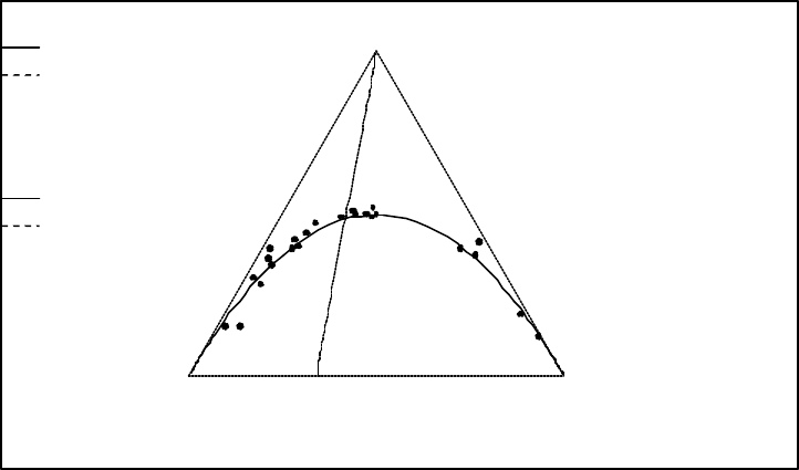
Chapter 4 More complex compositional problems

Cum. prop. expl.:

0,97

Pr. Components:

0,28 0,14 0,58

0,63 0,19 0,18

MM NN

Fig. 4.4.b The ternary plot of the MN blood group compositions and the Hardy-Weinberg ‘curve’.

We have deliberately used this simple example to demonstrate the effectiveness of

logratio analysis and its associated relative variation biplot since there seems to

remain some misunderstanding about the transformation involved. For example,

Gower (1987, p. 38) mistakenly claims that the logratio transformation fails to cope

with the curvature in the data. His confusion lies in not distinguishing between

logarithmic and logratio transformations. He correctly points out that a logarithmic

transformation, which considers logarithms of components, removes neither the

constraint nor the curvature in the data. The logarithmic transformation is, however,

not the relevant transformation for compositional data, which provide information

only on the relative values or ratios of the components. For successful analysis a

logratio transformation involving only ratios of components is required, and as we

have seen above this is highly successful not only in taking account of the unit-sum

constraint but in modelling the curvature of the Hardy-Weinberg curve.

4.5 A geological example: interpretation of the biplot of goilite

Table 4.5.1 reports a compositional data set which will be new to everyone and so no

preconceived ideas will dictate our analysis. It consists of 20 6-part mineral

compositions of goilite rocks from a site on the edge of Loch Goil near Carrick

Castle. I am told that this is an interesting site so let us see what we can discover

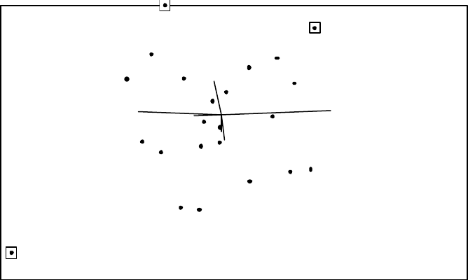
Chapter 4 More complex compositional problems

about it.

Inspection of the variation array of Table 4.5.2 provides little insight into the nature of

variability of the goilite compositions of Table 4.5.1. In contrast, the relative variation

biplot of Figure 4.5.a, retaining 98.2 per cent of the total compositional variability,

allows easy identification of a number of characteristics. For simplicity in our

interpretation we shall use only the initial letters to identify the mineral parts. First,

we see that the de link is by far the longest indicating the greatest relative variation in

the ratios of components is between d and e. Secondly, the near coincidence of the

vertices a and c implies that the a and c are in almost constant proportion with the

approximate relationship of a/c = 0.55 easily obtained from Table 4.5.1 or from the

estimate -0.605 for E{log(a/c)} in the variation array of Table 4.5.2. Note that in the

ternary diagram of the abc subcomposition in Figure 4.5.b the representative

compositional points lie roughly on a ray through the vertex b. Applying the

approximate 95 percent range formula and noting that

[ga gb gc gd ge gf ] = [0.157 0.207 0.288 0.102 0.055 0.162]

and coefficients of variation for log(e/f) and log(a/e) are -0.716 and -0.214 we obtain

the ranges

0.073 < e / f < 1.59; 0.42 < a / c < 0.71.

Cumulative proportion

0,89

0,98

0,99

Arkaigite

Broomite

Carronite

Dhuite Eckite

Fyneite

1617

= Outliers

explained:

Fig. 4.5.a Biplot of goilite mineral compositions

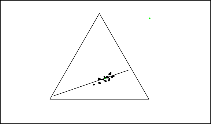
Chapter 4 More complex compositional problems

Arkaigite

Broomite Carronite

Geometric Mean

Fig. 4.5.b Ternary diagram for (arkaigite, broomite, carronite) subcompositions showing the near

proportionality of arkaigite to carronite

Thirdly and most strikingly we see the near-orthogonality of the ab (or cb) link and

the links de, df and ef. We can immediately infer that the ratios d/e, d/f and e/f are

independent of the ratio of a/b or c/b. Another way of expressing this feature is to

state that the subcompositions [c,d,e] and [a,b] are independent. A formal test of this

hypothesis of subcompositional independence (Aitchison, 1986, Section 10.3) results

in a significance probability 0.27 confirming our conclusion. Fourthly, the collinearity

of the three mineral links de, df and ef and the consequent one-dimensionality of the

pattern of variability of this (d, e, f)-subcomposition, confirmed by the corresponding

subcompositional ternary diagram of Figure 4.5.c, implies some relationship between

the proportions of the minerals d, e and f. Direct investigation by logcontrast principal

component analysis leads to the following eigenvalues and corresponding logcontrast

principal components:

.log792.0log225.0log567.0,567.0

;log194.0log785.0log587.0,79.12

fed

fef

+−−−=

+−=

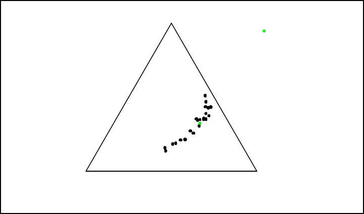
Chapter 4 More complex compositional problems

Dhuite

Eckite Fyneite

Geometric Mean

Fig. 4.5.c Ternary diagram of the (dhuite, eckite, fyneite) subcompositions showing the one-

dimensional pattern of variability of this subcomposition

The near-constant logcontrast arises from the near-zero second eigenvalue. Moreover

the fact that the coefficients are roughly in the ratios of -2 : -1 : 3 suggests that we

can make a substantial simplification to our interpretation if we consider the constant

logcontrast

-3 log d - log e + 4 log f = constant = 2.46,

where the constant value is estimated from the sample average of the logcontrast. This

can be simply converted into the approximate relationship;

e / f = 0.85

(f / d)3

Whether this suggested 'cubic hypothesis' is worth further investigation as a

geological finding is a matter for geologists not an ingeolate statistician.

As a final comment here we note that any subcomposition can be viewed as a set of

logcontrasts (Aitchison, 1984) and so are included in any logcontrast principal

component analysis for study of the dimensionalty of the pattern of compositional

variability.

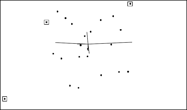
Chapter 4 More complex compositional problems

4.6 Abstract art: the biplot search for understanding

Inspection of the variation array of Table 2 provided little insight into the nature of

variability of the colour compositions of Table 1.1.5. In contrast, the relative variation

biplot of Figure 4.6.a, retaining 98.2 per cent of the total compositional variability,

allows easy identification of a number of characteristics. First, we see that the red-

yellow link is by far the longest indicating that the greatest relative variation in the

pictures is between red and yellow. Secondly, the near coincidence of the vertices

black and other implies that the artist uses black and the non-primary colour in almost

constant proportion with the approximate relationship of other/black = 1.85 easily

estimated from Table 1.1.5 or from the estimate 0.605 for E{log(other/black)} in the

variation array of Table 2. Thirdly only two compositions, those of paintings 14 and

22, have atypicality indices 0.999 and 0.953 greater than 0.95. From the position of

the marker for composition 14 in Figure 4.6.a it is clear that this atypicality is

probably due to a combination of its unusually high ratios of yellow to blue with that

of white to black, facts easily confirmed from Table 1.1.5. Composition 22 is atypical

because of its high blue to yellow, white to black and white to other ratios.

Cumulative proportion explained:

0,9

0,98

black

white

blue red

yellow other

= Outliers

Fig. 4.6.a Biplot of the 22 colour compositions of an abstract artist

Fourthly and most strikingly we see the near-orthogonality of the black-white link (or

other-white link) and the links blue-red, blue-yellow, red-yellow associated with the

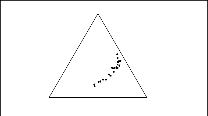
Chapter 4 More complex compositional problems

primary colours. Thus, we can immediately infer that the ratios in which the artist

uses the primary colours are independent of the ratio of black to white, or other to

white. Another way of expressing this feature is that the subcompositions (blue, red,

yellow) and (black, white) are independent; a formal test of this hypothesis of

subcompositional independence (Aitchison, 1986, Section 10.3) results in a

significance probability 0.27 confirming our conclusion. Fifthly, the collinearity of

the three primary colour links and the consequent one-dimensionality of the pattern of

variability of the primary subcomposition, confirmed by the corresponding

subcompositional triangular diagram of Figure 4.6.b implies some relationship

between the proportions of the primary colours used. Investigation along the lines of

the previous example leads to an approximate relationship

3 log(blue) + log(red) - 4 log(yellow) = constant,

or, in terms of ratios of colour use, red/yellow

∝

(yellow/blue)3. Whether this

suggested 'cubic rule' is worth further investigation as an artistic principle is

questionable, but such relationships can play an important role in compositional

analysis (Aitchison, 1998).

blue

red yellow

Fig. 4.6.b Ternary diagram of (blue,red,yellow)-subcompositions of an abstract artist

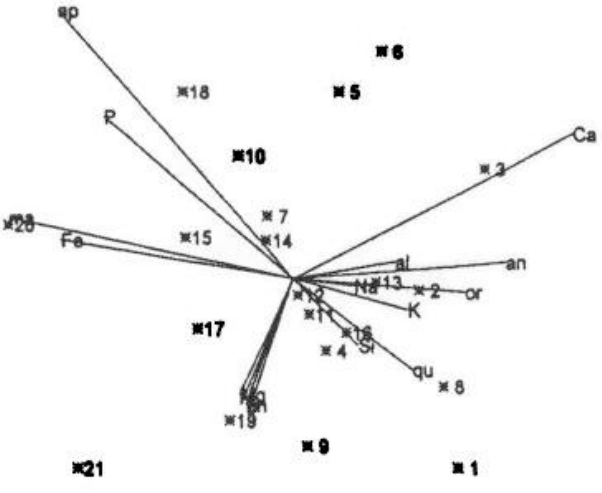
Chapter 4 More complex compositional problems

4.7 Tektite mineral and major oxide compositions

As a further example to illustrate compositional biplot technique and to provide some

unusual features which require care in interpretation we consider a data set for 21

tektites (Chao, 1963; Miesch et al, 1966), set out in Table 4.7.1, for which the two

compositions are 8-part major-oxide compositions and 8-part mineral compositions.

These are subcompositions of the original data set, this reduction being adopted for

the sake of simpler exposition. While experimentally these two types of compositions

are determined by completely different processes they are obviously chemically

related since the minerals are themselves more complicated major oxide compounds.

The challenge of the conditional biplot of Figure 4.7, with mineral composition as the

response and major-oxide composition as the covariate, is whether it can at least

identify these relationships from the compositional data alone, without any additional

information about the chemical formulae of the minerals, and hopefully provide other

meaningful interpretations of the data.

Fig. 4.7 Conditional biplot showing the dependence of the mineral composition on the major

oxide compositions for tektite compositions

A striking feature of the diagram is that it is indeed successful in identifying which

oxides are associated with which minerals. From Table 4.7.2, which provides the

Chapter 4 More complex compositional problems

chemical association between minerals and major oxides, we see that, apart from

SiO2, each of the other seven major oxides is associated with only one of the minerals,

for example MgO is contained only in enstatite. In the biplot diagram each of these

seven major oxide vertices is close to its corresponding mineral vertex. This means

that the link associated with any two of these major oxides is nearly parallel to the

link of the corresponding minerals and so the mineral logratios are all highly

correlated with the corresponding major oxide logratios. It is in this sense that the

conditional biplot identifies the chemical relationships. Moreover even SiO2, which is

a constituent of all eight minerals is nevertheless primarily identified with quartz

which is simply its oxide self.

Table 4.7.2 Oxides and associated minerals in tektite study

_________________________________________________________________

Oxide Mineral Abbreviation Formula

_________________________________________________________________

SiO2 Quartz qu SiO2

K2O Orthoclase or KAlSi

3O8

Na2O Albite al NaAlSi

3O8

CaO Anorthite an CaAl2Si2O8

MgO Enstatite en MgSiO3

Fe2O3 Magnetite ma Fe3O4

TiO Ilmenite il FeTiO3

P2O5 Apatite ap Ca5(F,Cl)(PO4)3

__________________________________________________________________

All of this seems splendid until the quality of the approximation is investigated. The

proportion of the covariance matrix G which is retained by the biplot is only 0.204.

The reason is not too difficult to detect. The singular value decomposition has

singular values 1.00, 1.00, 1.00. 0.999, 0.994. 0.868, 0,060 and it would require a

fourth order approximation and a four-dimensional biplot to raise the quality to a

reasonable 0.911 proportion retained. The reason for this disappointing quality is

easily determined. It lies in the fact that within the constraints of compositional data

each mineral is almost independently related to its major oxide, in the sense that each

mineral logratio is almost perfectly linearly related to the corresponding major-oxide

ratio. An analogous situation with unconstrained data would be the assemblage of

Chapter 4 More complex compositional problems

independent univariate regressions, each with a different response and different

covariate, into a multivariate regression. The apparent success of the conditional

biplot lies more in the strength of the individual logratio regressions than in the

quality of the biplot. It is important here to distinguish between the quality of the

biplot and the reliability of the logratio regression of mineral on major oxide

composition. The proportion of the mineral variability explained by the regression can

be shown to be 0.983.

4.8 Subcompositional analysis

A common problem in compositional data analysis appears to be marginal analysis in

the sense of locating subcompositions of greatest or of least variability. For this

purpose the measure of total variation provides for any subcomposition s of a full

compositions x the estimate of the ratio

trace

{

(

)}

{

(

)}

as the proportion of the total variation explained by the subcomposition. In such forms

of analysis it should be noted that a (1, . . . , C–1)-subcomposition is a set of C–1

particular logcontrasts and so the variability explained by a C-part subcomposition

can also be compared with that achieved by the first C–1 principal logcontrasts.

We can illustrate this simply for the hongite experience of Table 1.1.1a. For example

for 3-part subcompositions we have the 10 possible subcompositions in ascending

order of variability (where 1=A. . . . , 5=E):

Chapter 4 More complex compositional problems

Subcompositions Proportion o

variability

explained

A D E 0.08

A B D 0.17

A B E 0.20

B D E 0.27

C D E 0.44

A C E 0.51

A C D 0.53

B C E 0.90

B C D 0.91

A B C 0.94

We may note here that the (A,B,C)–subcomposition is the most variable, in

concurrence with our interpretation of the first logcontrast principal component of

Section 4.1. We may also note that this proportion 0.94 is comparable to that obtained

by the first principal logcontrast component.

4.9 Compositions in an explanatory role

Another interesting form of subcompositional analysis is where the composition plays

the role of regressor, for example in categorical regression, where we wish to examine

the extent to which, for example, type of rock depends on full major oxide

composition or some subcomposition. For binary regression a sensible approach is to

set the conditional model of type t, say 0 and 1, for given composition x as follows:

)log()|0(1)|1(1

iixFxtprxtpr ∑=

+==−== αα , where αi

∑=

10.

Hypotheses that the categorization depends only on a subcomposition, for example on

the subcomposition formed from parts 1, . . . , C is then simply specified by

CD+

, and so the whole lattice of subcompositional hypotheses can be

readily and systematically investigated.

A striking example of the use of this technique is to be found in discriminating

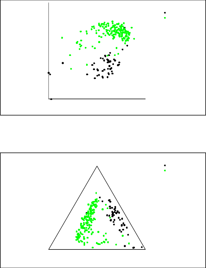
Chapter 4 More complex compositional problems

100

between two types of limestone. Thomas and Aitchison (1998) show that of the 17-

part (major-oxide, trace element) composition a simple major-oxide subcomposition

(CaO,Fe2O3,MgO) provides excellent discrimination, equal to that of the full

composition. Figures 4.9.a and 4.9.b show the separation in logratio and ternary

diagram space, respectively.

-3 -

-2 -

-1 -

log(CaO/MgO)

log(Fe2O3/MgO)

Dufftown

Inchory

Fig. 4.9.a Scattergram of logratios log(CaO / MgO) and log(Fe2O3/ MgO) for Scottish limestones

CaO

Fe2O3 MgO

Dufftown

Inchory

Fig. 4.9.b Ternary diagram of ‘centre perturbed’ (CaO, Fe2O3, MgO) subcompositions of Scottish

limestones

Chapter 4 More complex compositional problems

101

4.10 Experiments with mixtures

Another range of problems where compositional data play a role as comcomitants is

in experiments with mixtures. Here the usual aim is to determine whether and in way

a quantitative response depends on the composition of a mixture of ingredients. A

simple and typical example is where the experiment is aimed at determining how the

microhardness (kg/mm2) of glass depends on the relative proportions of Ge, Sb, Se

used in its manufacture. Such problems are quite common in many disciplines. There

is no reason why the response should be univariate. Aitchison and Bacon-Shone

(1984) give an example of an investigation into how the brilliance and vorticity of

girandole fireworks may depend on a 5-part mixture of light producing, propellent

and binding components. Indeed the response may be a composition.

The simplest model for such investigations is clearly when the expected response is a

logcontrast of the ingredients and it is clear from the discussion of the previous

section how investigation of subcompositional hypotheses would proceed. It is,

however, possible to have a more general model involving second power terms in

logratios, together with a hierarchy of hypotheses of inactivity of parts, of partition

additivity , completely additive. For full details on the motivation for such definitions,

for the practical meaning of the hypotheses and for implementation of a testing lattice,

see Aitchison and Bacon-Shone (1984) and Aitchison (1986, Sections 12.4-5).

4.11 Forms of independence

Because of the constant sum constraint, equivalently because of the nature of the

simplex sample space, independence hypotheses must clearly take radically different

forms from those associated with

D. For example, the analogue of complete

independence of components in unconstrained space is for compositional data

complete subcompositional independence, in which any subset of non-overlapping

subcompositions is independent. These, of course can be specified in terms of

associated logratios and in fact result in a particular parameterisation of the

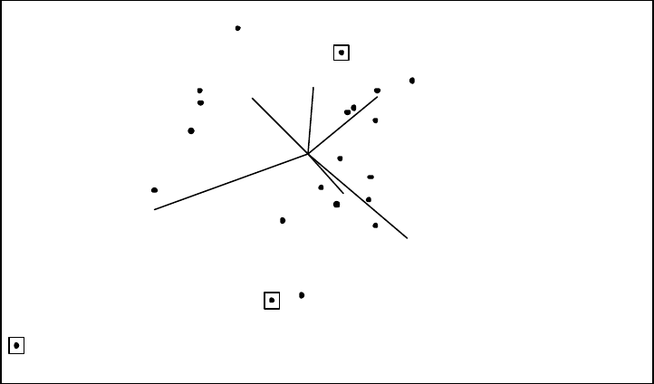
Chapter 4 More complex compositional problems

102

covariance structure. Tests of such hypotheses are readily available; see, for example,

Aitchison (1986, Chapter 10).

We use the time budgets of Table 1.1.6 to provide a very simple example, and

examine the hypothesis that the work and leisure subcompositions are independent.

This is almost clear in the biplot of Figure 4.11, in which the links of the working

parts are roughly at right angles to the links of the leisure parts, indicating lack of

correlation. The formal test involves testing whether the correlations between work

logrations and leisure logratios are all zero. This is easily assessed and results in a

significance probability of 0.56, so that we cannot reject the hypothesis of

independence of work and leisure parts of the statistician’s day.

Cumulative proportion explained:

0,42

0,65

0,82

0,95

Teaching

Consultation

Administration

Research

Other

Sleep

13 14

= Outliers

Fig. 4.11 Biplot of the time budgets of the statistician’s day

Chapter 5 Compositional processes

103

Chapter 5 Compositional processes: a statistical search for

understanding

5.1 Introduction

Most scientists are interested in the nature of the process which has led to the data

they observe, not least geologists in their search for explanations of how our planet

has developed geologically. Unfortunately they are seldom in the fortunate position of

observing a closed system where fundamental principles such as conservation of mass

and energy apply. Commonly the only data available take the form of compositional

data providing information only on relative magnitudes of the constituents of the

specimens. In some disciplines there is a wide variety of terminology associated with

such realised or hypothetical compositional processes. For example, geological

language contains many terms to describe a whole variety of envisaged geochemical

processes, such as denudation, diagenesis, erosion, gravity transport, metasomatism,

metamorphism, orogenesis, polymetamorphism, sedimentation, transportation,

weathering. Often the data for the study of such possible processes consist of variable

compositional vectors, such as major oxide compositions, major and minor element

compositions, granulometric weight by diameter profiles such as (sand, silt, clay)

sediments or palaeontological compositions such as foraminifera abundances. It is our

purpose here to study a variety of ways in which statistical analysis of the variability

in such data sets may be directed towards quantification of such processes and also,

where there may be rival hypotheses as to the nature of the geological process, the

extent to which the nature of the variability may be used to distinguish between the

hypotheses.

5.2 Differential perturbation processes

Many of the terms used by geologists to describe the processes they study appear to

envisage some kind of differential change in the components of the composition –

denudation, erosion, sedimentation, metamorphism, weathering. Since differential

Chapter 5 Compositional processes

104

change in compositions is simply characterised by the simplex operation of

perturbation this seems the sensible tool for the mathematical statistical study of such

processes. The fundamentals for such a study were set out in Aitchison and Thomas

(1998). Briefly the argument went as follows.

Consider a process which results in an observable D-part composition x(t) = [x1(t) , . .

. , xD(t)] which varies with some ordered variable such as time t. Since processes are

commonly assumed to take place continuously over time we can attempt to describe

such a process in a time-differential way by relating the composition x(t + dt) at time t

+ dt to the composition x(t) at previous time t in terms of a small perturbation. Since

such an infinitesimal perturbation will be a slight departure from the identity

perturbation (1/D, . . . , 1/D ) the process can be set out as

(

)

(

)

(

)[

(

)

(

)

]

⊕

Sometimes it is convenient to assume that such a perturbation is in the D-simplex but

since the perturbation operation is invariant with respect to scale there is strictly no

need for such a requirement. The original development then moved to a set of

differential equation in logratios for which the solution is

{

}

)],,...,1()([exp)()(

0Diduutxtxt

ti=⊕−∫δ

where

(

)

0is the known or assumed composition at time

0. With differentiation

now defined on the simplex we note that an alternative expression of the process is in

terms of the simple differential equation ],...,1:)([exp()( DitCtDx i== δ with the

known value at

0 being the ‘boundary condition’.

An interesting and important special case is where

i i

(

)

(

)

, when the

relationship takes the form of a simple compositional regression in a power-

perturbation form as

(

)

(

)

(

)

⊕

⊗

Chapter 5 Compositional processes

105

where ∫

tdtthtH

)()( and ].,...,1:)[(exp( DiCi== γβ

With actual compositional data the regression either in logratio terms or in staying in

the simplex mode is easily accomplished. The important feature here is the possibility

of alternative approaches to interpretation.

5.3 A simple example: Arctic lake sediments

We continue the example used by Aitchison and Thomas (1998) to illustrate various

ways of describing the process by which the variability of Arctic lake sediments may

depend on depth. The previous study arrived at logratio regression equations

log{sand(t) / clay(t)} = 9.70 -2.74 log t; log{silt(t) / clay(t)} = 4.80 - 1.10 log t,

and differential perturbation relationship

xtdt xt t t t( )()[./), ,/, . /].+ = ⊕− + +

31 146 1 018 1 128

The stay-in-the-simplex versions of these are the compositional regression

(

)

[

]

log

[

]

⊕

⊗

9928

0071

0001

046

238

716

and the compositional differential equation

(

)

(

)

[

]

⊗

046

238

716

All provide the same interpretation of the process: as depth increases sand gives way

to silt and more so to clay with differential effects decreasing with depth. Which

characterisation of the process is chosen may well depend on personal choice.

Chapter 5 Compositional processes

106

5.4 Exploration for possible differential processes

Given a compositional data set ];..;.,[1N

xxX=forming some possible process but

with no obvious driving variable such as time, temperature or pressure, it is of interest

to explore the possibility that there may be some unknown process at work. A suitable

tool for such an investigation is the simplicial singular value decomposition

(Aitchison et al, 2002). With each

n expressible in power-perturbation form:

xusus

n n n D D D

=⊕ ⊗ ⊕ ⊕ ⊗

− − −

ξβ β( ) .. . ( )

,1 1 1 1 1 1

where ξ is the centre of the data set. Here the hope is that the singular values are

decreasing so rapidly that the variability will be described by a low order truncation of

the power-perturbation combination.

Suppose that for the Arctic lake sediments we were unaware of the possibility of

depth as a process variable. Then the application of the singular value decomposition

gives a representation

xusus

n n n

=⊕ ⊗ ⊕ ⊗ξβ β( ) ( ),

1 1 1 2 2 2

where

].175.0629.0196.0[],560.0304.0136.0[

];258.0564.0178.0[;85..1,51,9

===

ββ

ξss

The second order approximation explains 96.3 of the total variability. This should

encourage the search for a possible driving variable. If depth is considered and plotted

against the resulting u’s a log-like scatter of points is obtained confirming the nature

of the earlier regression analysis.

The expression of a process in terms of a power-perturbation combination is in

simplicial terms a range space description. It should be realised that for any range

space description say

range

(

)

there is available a corresponding null space

Chapter 5 Compositional processes

107

description null( )Β⊥. This is convenient if the objective is to produce some law-like

description of the process. This was the situation in Aitchison and Thomas (1998) in

the study of olivines. There, for example for kimberlitess, the range space approach

would have resulted in

[, , ] ( [ ...])Fe Mg Si u=⊕ ⊗ξ0128 0461 0411

corresponding to the null space law-like description

−

log

738

log

67222

log

065

constant

or equivalently in equilibrium form

.13.1

011.0089.0

























As a further illustrative analysis of the 25 5-part hongite compositions of Aitchison

(1986) provides an interesting insight into the variability. The simplicial singular

value decomposition gives the following results

The consequence is that the second order power-perturbation approximation explains

94 percent of the total variability. Moreover the nature of

1 and

2indicate that the

first order approximation is associated with stability of the (4,5)-subcomposition with

the second order complementing this with a subprocess involving the stability of the

(1, 2, 3)-subcomposition.

[

]

[.....]

[

185

478

377

066

0489 0 220 0 099 0104 0088

0.222 0.329 0.084 0.189 0.177]

0.170 0.198 0.179 0.089 0.364]

0.395 0.103 0.143 0.167 0.192]

0.125 0.125 0.125 0.311 0.314]

Chapter 5 Compositional processes

108

5.5 Convex linear mixing processes

Another popular way of studying compositional data is in terms of convex linear

modelling processes. Such an approach is based on some such assumption as

conservation of mass There is, of course, no way that compositional data can be used

to support such a mass conservation hypothesis since compositions carry no

information about mass. Compositions can, however, be analyzed within models

which assume conservation of mass. All these models assume that there are source

compositions, say ξ ξ

1,..., C, from which a generic observed composition

arises as a

convex linear combination

xC C

= + +πξπξ

1 1 .. .

where π π π=∈[,..., ]

1CC

Sis the vector of mixing proportions. The form of

modelling obviously depends on the extent of the information about the number of

sources and the source compositions. At the ‘ignorance end’ neither the number of

sources nor their compositions are known – the so-called endmember problem as

presented, for example, in Renner (1993) and Weltje (197). At the opposite extreme

the problem may be to test a hypothesis that the sources are specified ompositions

ξ ξ

1,..., C. Many intermediate situations can be visualised: an example is the pollution

problem analysed by Aitchison and Bacon-Shone (1999), where there are not only

samples from the target set but also sampled compositions from the source.

The additive nature of such modelling does not mean that basic principles of

compositional data analysis are thereby neglected. For example an approach to the

so-called endmember problem where a set of say C endmember compositions

ξ ξ

1,..., C is sought such that each composition xn (n = 1, . . . , N) of the data set can

be expressed as a convex linear combination n

Π of ξ ξ

1,..., C , uses as criterion of

success the magnitude of

∑

∆

2),(ξ

Chapter 5 Compositional processes

109

while monitoring the magnitude of

).,(

2cb

ξξ

∑

∆

All that are required to implement such a procedure are good algorithms for the

minimisation of functions over a product of simplices. Our own, still at the testing

stage, are based on an iterative search program where each step involves perturbations

of the attained position, For the hongite data set for example on the supposition that

there are three endmembers these turn out to be

0 358 0 052 0265 0 059 0266

0507 0351 0004 0 085 0053

0 374 0055 0 392 0146 0033

[.....]

[. . . . . ]

5.6 Distinguishing between alternative hypotheses

Each of the processes – differential perturbation and convex linear mixing – will

result in fitted compositions, say xn

P and xn

C, for each of the observed compositions

The goodness of fit

Pand

Cof each of these processes may then be reasonably

judged in terms some such measures as

).,(),,(

PxxGxxG∑∑ ==

∆=∆=

In such a comparison, of course, we would be comparing processes of the same order

of complexity. We do not attempt here to develop any formal statistical test for such a

comparison. That would certainly involve many assumptions about the nature of the

residual variability and possibly lead to more argument than any simple sensible

comparison of the goodness of fit measures.

For the hongite data set we can compare these goodness of fit measures at various

orders of approximation:

Chapter 5 Compositional processes

110

Differential Convex lineal

perturbation mixing

Order

2 2.332 3.731

3 0.146 1.851

4 0.004 0.402

5 0 0

It is fairly clear that for this data set the differential perturbation model has the edge

over the convex linear model. This is in concurrence with the known method by

which the data set was originally simulated.

Postlude Pockets of resistance and confusion

111

Postlude

Pockets of resistance and confusion

There are a number of well-defined categories of response to the problems of

compositional data analysis. I hope readers do not recognize their position in any of

the categories.

The wishful thinkers

No problem exists (Gower,1987) or, at worst, it is some esoteric mathematical

statistical curiosity which has not worried our predecessors and so should not worry

us. Let us continue to calculate and interpret correlations of raw components. After

all if we omit one of the parts the constant-sum constraint no longer applies.

Someday, somehow, what we are doing will be shown by someone to have been

correct all the time.

The describers

As long as we are just describing a compositional data set we can use any

characteristics. In describing compositional data we can use arithmetic means,

covariance matrices of raw components and indeed any linear methods such as

principal components of the raw components. After all we are simply describing the

data set in summary form, not analyzing it (Le Maitre, 1982).

The openers

The fact that most compositions are recorded by first arriving experimentally at an

'open vector' of quantities of the D parts constituting some whole and then forming a

'closed vector', the composition, seems to have led to a particular form of wishful

thinking. All will be resolved if we can reopen the closed vector in some ideal way

and then perform some statistical analysis on the open vectors to reveal the inner

secrets of the compositions. The notion that there is some magic powder which can be

sprinkled on closed data to make them open and unconstrained dies hard. Most

recently Whitten (1995) takes as closed vectors major-oxide compositions of rocks

Postlude Pockets of resistance and confusion

112

expressed as percentages by weight, scales by whole rock specific gravities to obtain

'open vectors' recorded in g/100cc. His argument depends on attempts to establish that

whole rock specific gravity is independent of the composition of the rock (To

someone with virtually no knowledge of geology a seemingly naive concept) by a

series of regression studies in which whole rock specific gravities are regressed

against at most two of the constituent major oxides. Percentages of explanation of

over 50 per cent are cavalierly regarded as indications of independence. And why we

may ask was not a regression on the complete set of major oxides considered. These

would certainly have led to even higher percentages of explanation. Apart from this

statistical criticism the consequent open vectors are peculiarly placed geometrically,

being only minor displacements from a different constraining hyperplane. If only such

openers would realize that in any opened composition the ratios of components are

the same as in the closed composition so that any scale invariant procedure applied

to the opened composition will be identical to that procedure applied to the closed

composition. Opening compositions is indeed superfluous folly.

The null correlationists

Pearson was the originator of this school. The idea developed from a study of the

composition (shape) of Plymouth shrimps; see Aitchison (1986, Chapter 3) for an

account of his ingenious early bootstrap experiment. Others, in particular Chayes and

Kruskal (1966) and Darroch and Ratcliff (1970, 1978) have attempted this approach.

The basic idea here is related to the openers’ ideas. Because of the ‘negative bias’ in

correlations of raw components of compositions, zero correlation obviously does not

have its usual meaning in relation to independence. There must be some non-zero

value of such a correlation, called the null correlation, which corresponds to

‘independence’. Usually the null correlation is surmised by some opening out

procedure, as for example the oft-quoted Chayes-Kruskall method. The concept of

null correlation is spurious and indeed unnecessary. All meaningful concepts of

compositional dependence and independence can be studied within the simplex and in

relation to the logratio covariance structures already specified.

The pathologists

A study of the compositional literature suggests that much of compositional data

Postlude Pockets of resistance and confusion

113

analysis in the period 1965-85 was directed at trying to find some inspiration from

calculation of crude correlations and other linear methods. Those who were aware that

things go wrong with crude correlations attempted to describe the nature of the

disease instead of trying to find a cure. Thus we have many papers with titles such as

‘An effect of closure on the structure of principal component’ (Chayes and

Trochimczyk, 1978) and ‘The effect of closure on the measure of similarity between

samples’ (Butler, 1979).

The non-transformists

Despite his warning about the spuriousness of correlations of crude proportions,

Pearson would have been unhappy about the solution through logratio

transformations. He had bitter arguments (Pearson, 1905, 1906) with some of the

rediscoverers (for example, Kapteyn, 1903 ) of the lognormal distribution. This lay in

his distrust of transformations: what can possibly be the meaning of the logarithm of

weight? I had hoped that we were now sufficiently convinced, particularly in geology,

that the lognormal distribution has a central role to play in many geological

applications. But the mention of a logratio of components still brings forth that same

resistance. What is the meaning of such a logratio is a question posed by Fisher in the

discussion of Aitchison (1982) and even more recently by Whitten (1995). We hope

that the analogy with the lognormal distribution and the comments earlier that every

piece of compositional statistical analysis can be carried out within the simplex may

mean that this resistance will soon collapse.

The sphericists

There have been various attempts to escape from the unit simplex to what are thought

to be simpler or more familiar sample spaces. One popular idea (Atkinson and

Stephens in the discussion of Aitchison (1982), and Stephens(1982)) is to move from

the unit simplex D

S to the positive orthant of the unit hypersphere by the

transformation zi = i

u (i = 1, . . . , D) and then to use established theory of

distributions on the hypersphere. There are two insuperable difficulties about such a

transformation. First, the transformation is only onto part of the hypersphere and so

established distributional theory, associated as it is with the whole hypersphere, does

Postlude Pockets of resistance and confusion

114

not apply. There is clearly no way round this since the simplex and hypersphere are

topologically different: there is no way of transforming a triangle to the surface of a

two-dimensional sphere. As serious a difficulty is the impossibility of representing the

fundamental operation of perturbation on the simplex as something tractable on the

hypersphere. This is not surprising since the fundamental algebraic operation on the

hypersphere is rotation and this bears no relationship to the structure of perturbation.

The additional step of Stanley (1990) in transforming z to spherical polar coordinates

further complicates such issues. Although the angles involved are scale invariant

functions of the composition their relationship to the composition is bewilderingly

complicated. Moreover there would be no subcompositional coherence since in terms

of our previous discussion scientist B would be transforming onto a hypersphere of

lower dimension with impossibly complicated relationships between the angles used

by scientist A and B.

The Dirichlet extenders

Many statisticians are attempting to extend the Dirichlet class of distributions on the

simplex in the hope that greater generality will bring greater realism than the simple

Dirichlet class. Unfortunately I think they are likely to fail, since even the simple

Dirichlet class with all its elegant mathematical properties does not have any exact

perturbation properties.

Conclusion

The only sensible conclusion, it seems to me, is to reiterate my advice to my students.

Recognize your sample space for what it is. Pay attention to its properties and follow

through any logical necessities arising from these properties. The solution here to the

apparent awkwardness of the sample space is not so difficult. The difficulty is facing

up to reality and not imagining that there is some esoteric panacea.

References

115

References

AITCHISON, J.(1981a). A new approach to null correlations of proportions. J. Math. Geol. 13, 175-

189.

AITCHISON, J. (1981b). Distributions on the simplex for the analysis of neutrality, in Statistical

Distributions in Scientific Work (Taillie, C., Patil, G.P. and Baldessari, B.,eds), Vol 4, pp.147-156.

Dordrecht, Holland: D. Reidel Publishing Company.

AITCHISON, J. (1981c). Some distribution theory related to the analysis of subjective performance in

inferential tasks, in Statistical Distributions in Scientific Work (Taillie, C., Patil, G.P. and

Baldessari, B., eds), Vol 5, pp.363-385. Dordrecht, Holland: D. Reidel Publishing Company.

AITCHISON, (1982). The statistical analysis of compositional data (with discussion). J. R. Statist. Soc.

B 44, 139-177.

AITCHISON, J.(1983). Principal component analysis of compositional data. Biometrika 70, 57-65.

AITCHISON, J. (1984a). The statistical analysis of geochemical compositions. J. Math. Geol. 16, 531-

64.

AITCHISON, J. (1984b). Reducing the dimensionality of compositional data sets. J. Math. Geol. 16,

617-36.

AITCHISON, J. (1985). A general class of distributions on the simplex. J. R. Statist. Soc. B 47, 136-

146.

AITCHISON, J. (1986). The Statistical Analysis of Compositional Data. London: Chapman and Hall.

AITCHISON, J. (1989a). Letter to the editor. Reply to "Interpreting and testing compositional data" by

Alex Woronow, Karen M. Love, and John C. Butler. J. Math. Geol. 21, 65-71.

AITCHISON, J. (1989b). Letter to the Editor. Measures of location of compositional data sets. J. Math.

Geol. 21, 787-790.

AITCHISON, J. (1990a). Letter to the Editor. Comment on "Measures of Variability for Geological

Data" by D. F. Watson and G. M. Philip, J. Math. Geol. 22, 223-6.

AITCHISON, J. (1990b). Relative variation diagrams for describing patterns of variability of

compositional data. J. Math. Geol. 22, 487-512.

AITCHISON, J. (1991a). Letter to the Editor. Delusions of uniqueness and ineluctability. J. Math.

Geol. 23, 275-277.

AITCHISON, J. (1991b). A plea for precision in Mathematical Geology. J. Math, Geol. 23, 1081-1084.

AITCHISON, J. (1992a). The triangle in statistics. Chapter 8 in The Art of Statistical Science. A

Tribute to G. S. Watson (ed. K. V. Mardia), pp 89-104. New York: Wiley

AITCHISON, J. (1992b). On criteria for measures of compositional differences. J. Math. Geol. 24,

365-380.

AITCHISON, J. (1993). Principles of compositional data analysis. In Multivariate Analysis and its

Applications (eds. T.W. Anderson. I. Olkin and K.T. Fang), p.73-81. Hayward, California:

Institute of Mathematical Statistics.

References

116

AITCHISON, J. (1997). The one-hour course in compositional data analysis or compositional data

analysis is easy. In Proceedings of the Third Annual Conference of the International Association

for Mathematical Geology (ed. Vera Pawlowsky Glahn). 3-35. Barcelona: CIMNE

AITCHISON, J. (1999a). Logratios and natural laws in compositional data analysis. J. Math. Geol. 31,

563-89.

AITCHISON, J. (2002), Simplicial inference. In Algebraic Methods in Statistics and Probability, eds

M. A. G. Viana and D. St. P. Richards, 1-22. Contemporary Mathematics Series 287. Providence,

Rhode Island: American Mathematical Society.

AITCHISON, J. and BACON-SHONE, J. H. (1984). Logcontrast models for experiments with

mixtures. Biometrika 71, 323-330.

AITCHISON, J. and BACON-SHONE, J. H. (1999). Convex linear combinations of compositions.

Biometrika 86, 351-364.

AITCHISON, J., BARCELÓ-VIDAL, C., and PAWLOWSKY-GLAHN, V. (2001). Reply to Letter to

the Editor by S. Rehder and U. Zier on ‘Logratio analysis and compositional distance’ by J.

Aitchison, C. Barceló-Vidal, J. A. Martín-Fernández and V. Pawlowsky-Glahn. J. Math. Geol. 33.

AITCHISON, J., BARCELÓ-VIDAL, C., ECOZCUE, J. J., PAWLOWSKY-GLAHN, V. (2002). A

concise guide to the algebraic-geometric structure of the simplex, the sample space for

compositional data analysis, to appear in Proceedings of IAMG02.

AITCHISON, J., BARCELÓ-VIDAL, C., MARTÍN-FERNÁNDEZ, J. A. and PAWLOWSKY-

GLAHN, V. (2000). Logratio analysis and compositional distance: J. Math. Geol. 32, 271-275.

AITCHISON, J., BARCELÓ-VIDAL, C., and PAWLOWSKY-GLAHN V. (2002). Somme comments

on compositional data analysis in archeometry, in particular the fallacies in Tangri and Wright's

dismissal of logratio. Archaeometry, vol. 44, núm. 2, p. 295-304.

AITCHISON, J. and BROWN, J.A.C. (1957). The Lognormal Distribution. Cambridge University

Press.

AITCHISON, J. and GREENACRE, M. (2002) Biplots for compositional data. Applied Statistics, 51,

num. 4, pp. 375-392.

AITCHSION, J. and LAUDER, I.J. (1985). Kernel density estimation for compositional data. Applied

Statistics 34,129-137.

AITCHISON, J. and SHEN, S. M. (1980). Logistic-normal distributions: some properties and uses.

Biometrika 67, 261-272.

AITCHISON, J. and SHEN, S.M. (1984). Measurement error in compositional data. J. Math. Geol. 16,

637-50.

AITCHISON J. and THOMAS, C. W. (1998) Differential perturbation processes: a tool for the study of

compositional processes, in Buccianti A., Nardi, G. and Potenza, R., eds., Proceedings of IAMG'98

- The Fourth Annual Conference of the International Association for Mathematical Geology: De

Frede Editore, Napoli (I), p. 499-504.

AZZALINI, A. and DALLA VALLE, A. (1996). The multivariate skew-normal distribution.

Biometrika 83, 715-26.

BARCELÓ, C., PAWLOWSKY, V. and GRUNSKY, E. (1996). Some aspects of transformations of

compositional data and the identification of outliers. Mathematical Geology, vol. 28(4), pp. 501-

518.

References

117

BARCELÓ-VIDAL, C. MARTÍN-FERNÁNDEZ, J. A. and PAWLOWSKY-GLAHN, V. (2001).

Mathematical foundations of compositional data analysis. In Proceedings of IAMG01., Ed. G.

Ross. Volume CD, electronic publication.

CHAYES, F. (1956). Petrographic Modal Analysis. New York: Wiley.

BROWN, J. A. C. and DEATON, A. S. (1972). Surveys in applied economic models of consumer

demand. Econ. J. 82, 1145-236.

BUTLER, J. C. (1979). The effect of closure on the measure of similarity between samples: J. Math.

Geol. 11, 73-84.

CHANG, T. C. (1988). Spherical regression: Ann. Statist.. 14, 907-24.

CHAYES, F. (1956) Petrographic Modal Analysis. New York: Wiley.

CHAYES, F. (1960) On correlation between variables of constant sum: J. Geophys. Res. 65, 4185-

4193.

CHAYES, F. (1962) Numerical correlation and petrographic variation: J. Geology. 70, 440-552.

CHAYES, F. (1971). Ratio Correlation. University of Chicago Press.

CHAYES, F. (1972). Effect of the proportion transformation on central tendency. J. Math. Geol. 4,

269-70.

CHAYES, F. and KRUSKAL, W. (1966) An approximate statistical test for correlation between

proportions: J. Geology, 74, 692-702.

CHAYES, F. and TROCHIMCZYk, J. (1978) The effect of closure on the structure of principlal

components: J. Math. Geol. 10, 323-333.

DARROCH, J. N. (1969). Null correlations for proportions. J. Math. Geol. 1, 221-7.

DARROCH, J. N. and JAMES, J. R. (1974). F-independence and null correlations of bounded sum

positive variables. J. R. Statist. Soc. B 36, 247-52.

DARROCH, J. N. and RATCLIFF, D. (1970). Null correlations for proportions II. J. Math. Geol. 2,

307-12..

DARROCH, J. N. and RATCLIFF, D. (1978). No association of proportions.. J. Math. Geol. 10, 361-

8..

GABRIEL, K. R. (1971). The biplot-graphic display of matrices with application to principal

component analysis. Biometrika 58, 453-467.

GABRIEL, K. R. (1981). Biplot display of multivariate matrices for inspection of data and diagnosis.

In: V. Barnett, Ed., Interpreting Multivariate Data, Wiley, New York, 147-173.

GOWER, J. C. (1987). Introduction to ordination techniques, in Legendre, P. and Legendre, L., eds.,

Developments in Numerical Ecology: Springer-Verlag, Berlin, p. 3-64.

HOUTHAKKER, H. S. (1960). Additive preferences. Econometrica 28, 244-56.

KAPTEYN, J. C. (1903). Skew Frequency Curves in Biology and Statistics: Astronomical Laboratory,

Groningen, Noordhoff.

KAPTEYN, J. C. (1905). Rec. Trav. bot. néerl.

References

118

KRUMBEIN, C. (1962). Open and closed number systems: stratigraphic mapping: Bull. Amer. Assoc.

Petrol. Geologists, 46, 322-37.

MARTÍN-FERNÁNDEZ, J. A., BARCELÓ-VIDAL, C. and PAWLOWSKY-GLAHN, V. (1998).

Measures of difference for compositional data and hierarchical clustering methods. In: A.

Buccianti, G. Nardi and R. Potenza, Eds., Proceedings of IAMG'98, The Fourth Annual

Conference of the International Association for Mathematical Geology, De Frede, Naples, 526-

531.

MATEU -FIGUERAS, G., BARCELO-VIDAL, C and PAWLOWSKY-GLAHN, C. (1998). Modeling

compositional data with multivariate skew-normal distributions. In: A. Buccianti, G. Nardi and R.

Potenza, Eds., Proceedings of IAMG98, The Fourth Annual Conference of the International

Association for Mathematical Geology, De Frede, Naples, 532-537.

McALISTER, D. (1879). The law of the geometric mean: Proc. Roy. Soc. 29, 367-

MOSIMANN, J. E. (1962). On the compound multinomial distribution, the multivariate β-distribution

and correlations among proportions. Biometrika 49, 65-82.

MOSIMANN, J. E. (1963). On the compound negative binomial distribution and correlations among

inversely sampled pollen counts. Biometrika 50, 47-54.

PAWLOWSKY, V. (1986), Räumliche Strukturanalyse und Schätzung ortsabhängiger Kompositionen

mit Anwendungsbeispeilen aus der Geologie: unpublished dissertation, FB Geowissenschaften,

Freie Universität Berlin, 120.

PAWLOWSKY, V., OLEA, R. A., and DAVIS, J. C. (1995). Estimation of regionalized compositions:

a comparison of three methods: J. Math. Geol. 27, 105-48.

PAWLOWSKY-GLAHN, V and ECOZCUE, J. J. (2001). Geometric approach to statistical analysis on

the simplex. SERRA 15. 384-98.

PAWLOWSKY-GLAHN, V and ECOZCUE, J. J. (2002). BLU estimators and compositional data.

Mathematical Geology, vol. 34(3), p. 259-274.

PEARSON, K. (1897). Mathematical contributions to the theory of evolution: on a form of spurious

correlation which may arise when indices are used in the measurements of organs: Proc. Roy. Soc.

60, p.489-98.

PEARSON, K. (1905). Das Fehlergetz und seine erallgemeinerungen durch Fechner und Pearson. A

rejoinder: Biometrika. 4, 169-212..

PEARSON, K. (1906). Skew frequency curves. A rejoinder to Professor Kapteyn: Biometrika.5, 168-

71.

REHDER, U. and ZIER, S. (2001). Comment on “Logratio analysis and compositional distance by

Aitchison et al. (2000)”: J. Math. Geol. 32.

RENNER, R.M. (1993) The resolution of a compositional data set into mixtures of fixed source

components. Applied Statistics. 42, 615-311.

SARMANOV, O. V. and VISTELIUS, A. B. (1959). On the correlation of percentage values: Dokl.

Akad. Nauk. SSSR, 126, 22-5.

STANLEY, C. R. (1990). Descriptive statistics for N-dimensional closed arrays: a spherical coordinate

approach, J. Math. Geol. 22, 933-56.

STEPHENS, M.A. (1982) Use of the von Mises distribution to analyze continuous proportions,

Biometrika 69, 197-203.

References

119

THOMAS, C. W. and AITCHISON, J. (1998). The use of logratios in subcompositional analysis and

geochemical discrimination of metamorphosed limestones from the northeast and central Scottish

Highlands. In: A. Buccianti, G. Nardi and R. Potenza, Eds., Proceedings of IAMG98, The Fourth

Annual Conference of the International Association for Mathematical Geology, De Frede, Naples,

549-554.

WATSON, D. F. (1990). Reply to Comment on "Measures of variability for geological data" by D. F.

Watson and G. M. Philip: J. Math. Geol. 22..227-31.

WATSON, D. F. (1991). Reply to "Delusions of uniqueness and ineluctability" by J. Aitchison: J.

Math. Geol. 23, 279.

WATSON, D. F. and PHILIP, G. M. (1989). Measures of variability for geological data: J. Math.

Geol.. 21, 233-54.

WELTJE, G. J. (1997) End-member modelling of compositional data: numerical statistical algorithms

for solving the explicit mixing problem. Math Geology 39, 503-49.

WHITTEN, E. H. T. (1995). Open and closed compositional data in petrology: J. Math. Geol. 27, .789-

806.

WORONOW, A. (1997a). The elusive benefits of logratios. In: V. Pawlowsky-Glahn, Ed., Proceedings

of IAMG97, The Third Annual Conference of the International Association for Mathematical

Geology, CIMNE, Barcelona, 97-101.

WORONOW, A. (1997b). Regression and discrimination analysis using raw compositional data - is it

really a problem? In: V. Pawlowsky-Glahn, Ed., Proceedings of IAMG97, The Third Annual

Conference of the International Association for Mathematical Geology, CIMNE, Barcelona, 157-

162.

ZIER, U. and REHDER, S. (1998). Grain -size analysis –a closed data proble. In A. Buccianti, Nardi,

G. and Potenza, R., eds., Proceedings of IAMG'98 - The Fourth Annual Conference of the

International Association for Mathematical Geology: De Frede Editore, Napoli, p. 555-8..

120

Appendix Tables

121

Appendix Tables

Table 1.1.1a Compositions of 25 specimens of hongite

___________________________________________

Specimen Percentages by weight of minerals

no A B C D E

___________________________________________

1 48.8 31.7 3.8 6.4 9.3

2 48.2 23.8 9.0 9.2 9.8

3 37.0 9.1 34.2 9.5 10.2

4 50.9 23.8 7.2 10.1 8.0

5 44.2 38.3 2.9 7.7 6.9

6 52.3 26.2 4.2 12.5 4.8

7 44.6 33.0 4.6 12.2 5.6

8 34.6 5.2 42.9 9.6 7.7

9 41.2 11.7 26.7 9.6 10.8

10 42.6 46.6 0.7 5.6 4.5

11 49.9 19.5 11.4 9.5 9.7

12 45.2 37.3 2.7 5.5 9.3

13 32.7 8.5 38.9 8.0 11.9

14 41.4 12.9 23.4 15.8 6.5

15 46.2 17.5 15.8 8.3 12.2

16 32.3 7.3 40.9 12.9 6.6

17 43.2 44.3 1.0 7.8 3.7

18 49.5 32.3 3.1 8.7 6.3

19 42.3 15.8 20.4 8.3 13.2

20 44.6 11.5 23.8 11.6 8.5

21 45.8 16.6 16.8 12.0 8.8

22 49.9 25.0 6.8 10.9 7.4

23 48.6 34.0 2.5 9.4 5.5

24 45.5 16.6 17.6 9.6 10.7

25 45.9 24.9 9.7 9.8 9.7

___________________________________________

Appendix Tables

122

Table 1.1.1b Compositions of 25 specimens of kongite

_____________________________________________

Specimen Percentages by weight of minerals

no A B C D E

_____________________________________________

1 33.5 6.1 41.3 7.1 12.0

2 47.6 14.9 16.1 14.8 6.6

3 52.7 23.9 6.0 8.7 8.7

4 44.5 24.2 10.7 11.9 8.7

5 42.3 47.6 0.6 4.1 5.4

6 51.8 33.2 1.9 7.0 6.1

7 47.9 21.5 10.7 9.5 10.4

8 51.2 23.6 6.2 13.3 5.7

9 19.3 2.3 65.8 5.8 6.8

10 46.1 23.4 10.4 11.5 8.6

11 30.6 6.7 43.0 6.3 13.4

12 49.7 28.1 5.1 8.0 9.1

13 49.4 24.3 7.6 8.5 10.2

14 38.4 9.5 30.6 14.8 6.7

15 41.6 19.0 17.3 13.8 8.3

16 42.3 43.3 1.6 5.9 6.9

17 45.7 23.9 10.3 11.6 8.5

18 45.5 20.3 13.6 10.9 9.7

19 52.1 17.9 10.7 7.9 11.4

20 46.2 14.3 18.5 12.2 8.8

21 47.2 30.9 4.6 6.3 11.0

22 45.4 33.3 4.0 11.9 5.4

23 48.6 23.4 8.7 10.7 8.6

24 31.2 4.5 47.0 10.2 7.1

25 44.3 15.0 19.4 10.5 10.8

___________________________________________

Appendix Tables

123

Table 1.1.2 (sand, silt, clay) compositions (percentages by weight) and water depth

(m) of 39 Arctic lake sediments

_____________________________________________

Sediment Percentages by weight Water

no sand silt clay depth

_____________________________________________

1 77.5 19.5 3.0 10.4

2 71.9 24.9 3.2 11.7

3 50.7 36.1 13.2 12.8

4 52.2 40.9 6.6 13.0

5 70.0 26.5 3.5 15.7

6 66.5 32.2 1.3 16.3

7 43.1 55.3 1.6 18.0

8 53.4 36.8 9.8 18.7

9 15.5 54.4 30.1 20.7

10 31.7 41.5 26.8 22.1

11 65.7 27.8 6.5 22.4

12 70.4 29.0 0.6 24.4

13 17.4 53.6 29.0 25.8

14 10.6 69.8 19.6 32.5

15 38.2 43.1 18.7 33.6

16 10.8 52.7 36.5 36.8

17 18.4 50.7 30.9 37.8

18 4.6 47.4 48.0 36.9

19 15.6 50.4 34.0 42.2

20 31.9 45.1 23.0 47.0

21 9.5 53.5 37.0 47.1

22 17.1 48.0 34.9 48.4

23 10.5 55.4 34.1 49.4

24 4.8 54.7 41.0 49.5

25 2.6 45.2 52.2 59.2

26 11.4 52.7 35.9 60.1

27 6.7 46.9 46.4 61.7

28 6.9 49.7 43.4 62.4

29 4.0 44.9 51.1 69.3

30 7.4 51.6 40.9 73.6

31 4.8 49.5 45.7 74.4

32 4.5 48.5 47.0 78.5

33 6.6 52.1 41.3 82.9

34 6.7 47.3 45.9 87.7

35 7.4 45.6 46.9 88.1

36 6.0 48.9 45.1 90.4

37 6.3 53.8 39.9 90.6

38 2.5 48.0 49.5 97.7

39 2.0 47.8 50.2 103.7

_____________________________________________

Appendix Tables

124

Table 1.1.3 Household expenditures (HK$) on four commodity groups of 20 single

men (M) and 20 single women (W)

_________________________________________________________________

Commodity group Commodity group

ID 1 2 3 4 ID 1 2 3 4

no no

_________________________________________________________________

M1 497 591 153 291 W1 820 114 183 154

M2 839 942 302 365 W2 184 74 6 20

M3 789 1308 668 584 W3 921 66 1686 455

M4 892 842 287 395 W4 488 80 103 115

M5 1585 781 2476 1740 W5 721 83 176 104

M6 755 764 428 438 W6 614 55 441 193

M7 388 655 153 233 W7 801 56 357 214

M8 617 879 757 719 W8 396 59 61 80

M9 248 438 22 65 W9 864 65 1618 352

M10 1641 440 6471 2063 W10 845 64 1935 414

M11 1180 1243 768 813 W11 404 97 33 47

M12 619 684 99 204 W12 781 47 1906 452

M13 253 422 15 48 W13 457 103 136 108

M14 661 739 71 188 W14 1029 71 244 189

M15 1981 869 1489 1032 W15 1047 90 653 298

M16 1746 746 2662 1594 W16 552 91 185 158

M17 1865 915 5184 1767 W17 718 104 583 304

M18 238 552 29 75 W18 495 114 65 74

M19 1199 1095 261 344 W19 382 77 230 147

M20 1524 964 1739 1410 W20 1090 59 313 177

_________________________________________________________________

1 Housing, including fuel and light

2 Foodstuffs, including alcohol and tobacco

3 Other goods, including clothing, footwear and durable goods

4 Services, including transport and vehicles

Appendix Tables

125

Table 1.1.4 Dietary compositions of the milk of 60, thirty in the control group and 30

in the treatment group (pr = protein, mf = milk fat, ch = carbohydrate)

Control group before

______________________________________________

pr mf ch Ca Na K

10-2 x 10-2 x 10-2 x

____________________________________________

0.3098 0.2237 0.4410 0.0103 0.0025 0.0127

0.2679 0.3687 0.3377 0.0084 0.0030 0.0144

0.2583 0.3392 0.3747 0.0074 0.0047 0.0157

0.2450 0.2614 0.4617 0.0090 0.0090 0.0140

0.3715 0.1477 0.4514 0.0098 0.0032 0.0163

0.2451 0.2987 0.4263 0.0104 0.0032 0.0163

0.3797 0.2268 0.3660 0.0064 0.0080 0.0131

0.2286 0.2723 0.4709 0.0097 0.0026 0.0159

0.2381 0.2182 0.5199 0.0100 0.0016 0.0122

0.3731 0.1937 0.4051 0.0109 0.0020 0.0153

0.1988 0.4113 0.3632 0.0056 0.0080 0.0131

0.3178 0.1908 0.4678 0.0058 0.0067 0.0111

0.2446 0.2976 0.4272 0.0114 0.0018 0.0175

0.2680 0.2357 0.4731 0.0041 0.0085 0.0106

0.3448 0.2428 0.3840 0.0098 0.0040 0.0148

0.2107 0.4630 0.2955 0.0154 0.0016 0.0138

0.2767 0.1796 0.5177 0.0040 0.0089 0.0130

0.3286 0.2883 0.3584 0.0065 0.0038 0.0143

0.2168 0.3149 0.4421 0.0083 0.0043 0.0136

0.2325 0.2858 0.4544 0.0049 0.0066 0.0157

0.3140 0.1600 0.4967 0.0092 0.0053 0.0149

0.3007 0.2313 0.4451 0.0084 0.0016 0.0131

0.1966 0.3840 0.3933 0.0101 0.0031 0.0128

0.1207 0.5170 0.3328 0.0075 0.0042 0.0179

0.1728 0.4103 0.3892 0.0112 0.0015 0.0150

0.1655 0.5171 0.2841 0.0094 0.0066 0.0173

0.3257 0.1735 0.4761 0.0059 0.0044 0.0142

0.2177 0.3711 0.3788 0.0147 0.0021 0.0155

0.2628 0.3019 0.4022 0.0131 0.0035 0.0164

0.3754 0.1718 0.4256 0.0112 0.0009 0.0150

______________________________________________

Appendix Tables

126

Table 1.1.4 (continued)

Treatment group before

______________________________________________

pr mf ch Ca Na K

10-2 x 10-2 x 10-2 x

____________________________________________

0.3270 0.1956 0.4500 0.0068 0.0083 0.0123

0.3758 0.1720 0.4267 0.0071 0.0057 0.0125

0.2473 0.3304 0.3924 0.0086 0.0059 0.0156

0.2624 0.2719 0.4344 0.0090 0.0054 0.0169

0.2811 0.2700 0.4226 0.0042 0.0108 0.0112

0.3456 0.2318 0.4003 0.0039 0.0069 0.0115

0.4216 0.1417 0.4138 0.0080 0.0024 0.0125

0.2465 0.3286 0.3980 0.0087 0.0046 0.0135

0.2468 0.3266 0.3945 0.0092 0.0052 0.0178

0.3486 0.1670 0.4575 0.0118 0.0015 0.0135

0.3217 0.2407 0.4055 0.0069 0.0126 0.0128

0.2165 0.3268 0.4260 0.0111 0.0035 0.0161

0.3296 0.2173 0.4197 0.0092 0.0110 0.0133

0.2324 0.3370 0.4026 0.0086 0.0022 0.0172

0.2252 0.3160 0.4245 0.0099 0.0072 0.0171

0.1756 0.4177 0.3797 0.0091 0.0037 0.0143

0.3169 0.2167 0.4373 0.0051 0.0116 0.0125

0.2226 0.3809 0.3668 0.0064 0.0088 0.0145

0.2820 0.2373 0.4514 0.0085 0.0040 0.0168

0.2180 0.3414 0.4138 0.0066 0.0042 0.0161

0.3460 0.2307 0.3926 0.0106 0.0046 0.0155

0.3065 0.2337 0.4336 0.0125 0.0014 0.0122

0.2522 0.2965 0.4227 0.0141 0.0016 0.0130

0.3312 0.1541 0.4896 0.0073 0.0048 0.0130

0.2800 0.2365 0.4562 0.0115 0.0015 0.0144

0.2704 0.2809 0.4256 0.0119 0.0009 0.0104

0.5041 0.0875 0.3808 0.0104 0.0027 0.0146

0.3187 0.2490 0.4041 0.0111 0.0037 0.0134

0.2396 0.3502 0.3793 0.0106 0.0033 0.0170

0.2424 0.2725 0.4592 0.0117 0.0015 0.0127

_______________________________________________

Appendix Tables

127

Table 1.1.4 (continued)

Control group after

______________________________________________

pr mf ch Ca Na K

10-2 x 10-2 x 10-2 x

____________________________________________

0.2582 0.3057 0.4107 0.0105 0.0021 0.0128

0.2381 0.3954 0.3356 0.0112 0.0030 0.0168

0.2405 0.3291 0.3985 0.0093 0.0047 0.0179

0.2877 0.2461 0.4342 0.0108 0.0063 0.0149

0.4395 0.1251 0.4049 0.0109 0.0028 0.0169

0.2040 0.3285 0.4400 0.0103 0.0022 0.0149

0.3427 0.2165 0.4115 0.0070 0.0077 0.0146

0.1469 0.4245 0.4000 0.0115 0.0015 0.0156

0.1941 0.2976 0.4779 0.0135 0.0018 0.0150

0.4360 0.1699 0.3690 0.0107 0.0012 0.0132

0.2302 0.4212 0.3186 0.0069 0.0085 0.0145

0.3338 0.2230 0.4174 0.0070 0.0063 0.0123

0.2351 0.3279 0.4102 0.0101 0.0013 0.0154

0.2475 0.2789 0.4435 0.0059 0.0102 0.0140

0.2942 0.3392 0.3415 0.0086 0.0034 0.0132

0.2112 0.4724 0.2886 0.0152 0.0009 0.0117

0.2809 0.1890 0.4981 0.0055 0.0098 0.0166

0.3244 0.3192 0.3291 0.0070 0.0051 0.0153

0.2164 0.2855 0.4692 0.0097 0.0047 0.0147

0.2310 0.3091 0.4341 0.0048 0.0064 0.0145

0.2411 0.1875 0.5468 0.0082 0.0039 0.0125

0.3304 0.2364 0.4056 0.0103 0.0017 0.0156

0.2461 0.3472 0.3786 0.0115 0.0030 0.0137

0.1321 0.5356 0.3041 0.0077 0.0035 0.0170

0.1276 0.4896 0.3516 0.0136 0.0012 0.0164

0.1447 0.6130 0.2158 0.0080 0.0047 0.0139

0.3044 0.1814 0.4878 0.0068 0.0041 0.0155

0.2352 0.4027 0.3373 0.0114 0.0015 0.0119

0.2248 0.3225 0.4217 0.0117 0.0037 0.0157

0.3039 0.2252 0.4477 0.0106 0.0006 0.0119

_______________________________________________

Appendix Tables

128

Table 1.1.4 (continued)

Treatment group after

______________________________________________

pr mf ch Ca Na K

10-2 x 10-2 x 10-2 x

____________________________________________

0.3575 0.1780 0.4357 0.0090 0.0085 0.0113

0.5056 0.1038 0.3607 0.0107 0.0063 0.0129

0.3635 0.2455 0.3616 0.0097 0.0060 0.0137

0.3510 0.2040 0.4182 0.0116 0.0027 0.0125

0.2246 0.3028 0.4419 0.0071 0.0116 0.0121

0.3966 0.1662 0.4115 0.0066 0.0085 0.0107

0.5544 0.1024 0.3145 0.0146 0.0023 0.0117

0.3587 0.2107 0.3980 0.0147 0.0048 0.0130

0.2509 0.2850 0.4385 0.0108 0.0027 0.0122

0.4076 0.1332 0.4351 0.0137 0.0012 0.0094

0.2939 0.2268 0.4510 0.0099 0.0083 0.0101

0.1521 0.3636 0.4580 0.0127 0.0025 0.0111

0.4641 0.1584 0.3491 0.0085 0.0101 0.0098

0.2870 0.2738 0.4091 0.0126 0.0019 0.0157

0.2693 0.2995 0.4037 0.0135 0.0035 0.0104

0.1894 0.4421 0.3416 0.0110 0.0041 0.0117

0.2816 0.2176 0.4722 0.0071 0.0098 0.0117

0.2154 0.4184 0.3414 0.0092 0.0050 0.0105

0.2896 0.2187 0.4638 0.0097 0.0028 0.0154

0.3070 0.2707 0.3921 0.0112 0.0030 0.0160

0.3749 0.2146 0.3794 0.0145 0.0039 0.0128

0.3195 0.2214 0.4297 0.0186 0.0011 0.0097

0.2654 0.2255 0.4766 0.0206 0.0011 0.0108

0.3843 0.1460 0.4478 0.0088 0.0034 0.0096

0.3690 0.1822 0.4162 0.0168 0.0014 0.0143

0.4646 0.1813 0.3257 0.0188 0.0007 0.0089

0.5987 0.0588 0.3123 0.0154 0.0016 0.0132

0.4122 0.2157 0.3385 0.0195 0.0026 0.0116

0.3991 0.2600 0.3126 0.0114 0.0026 0.0143

______________________________________________

Appendix Tables

129

Table 1.1.5 Six-part colour compositions of 22 paintings by an abstract artist

________________________________________________________

Painting Proportions of total area assigned to colours

No black white blue red yellow other

________________________________________________________

1 0.125 0.243 0.153 0.031 0.181 0.266

2 0.143 0.224 0.111 0.051 0.159 0.313

3 0.147 0.231 0.058 0.129 0.133 0.303

4 0.164 0.209 0.120 0.047 0.178 0.282

5 0.197 0.151 0.132 0.033 0.188 0.299

6 0.157 0.256 0.072 0.116 0.153 0.246

7 0.153 0.232 0.101 0.062 0.170 0.282

8 0.115 0.249 0.176 0.025 0.176 0.259

9 0.178 0.167 0.048 0.143 0.118 0.347

10 0.164 0.183 0.158 0.027 0.186 0.281

11 0.175 0.211 0.070 0.104 0.157 0.283

12 0.168 0.192 0.120 0.044 0.171 0.305

13 0.155 0.251 0.091 0.085 0.161 0.257

14 0.126 0.273 0.045 0.156 0.131 0.269

15 0.199 0.170 0.080 0.076 0.158 0.318

16 0.163 0.196 0.107 0.054 0.144 0.335

17 0.136 0.185 0.162 0.020 0.193 0.304

18 0.184 0.152 0.110 0.039 0.165 0.350

19 0.169 0.207 0.111 0.057 0.156 0.300

20 0.146 0.240 0.141 0.038 0.184 0.250

21 0.200 0.172 0.059 0.120 0.136 0.313

22 0.135 0.225 0.217 0.019 0.187 0.217

_________________________________________________________

Appendix Tables

130

Table 1.1.6 Activity patterns of a statistician for 20 days

______________________________________________

Day Proportion of day in activity

No te co ad re ot sl

______________________________________________

1 0.144 0.091 0.179 0.107 0.263 0.217

2 0.162 0.079 0.107 0.132 0.265 0.254

3 0.153 0.101 0.131 0.138 0.209 0.267

4 0.177 0.087 0.140 0.132 0.155 0.310

5 0.158 0.110 0.139 0.116 0.258 0.219

6 0.165 0.079 0.113 0.113 0.275 0.255

7 0.159 0.084 0.117 0.094 0.225 0.321

8 0.161 0.105 0.123 0.110 0.267 0.234

9 0.163 0.126 0.105 0.106 0.227 0.273

10 0.169 0.102 0.104 0.104 0.235 0.286

11 0.149 0.113 0.123 0.115 0.256 0.244

12 0.118 0.100 0.145 0.096 0.192 0.349

13 0.106 0.112 0.135 0.104 0.205 0.338

14 0.163 0.142 0.109 0.115 0.260 0.211

15 0.151 0.122 0.126 0.121 0.235 0.245

16 0.163 0.101 0.126 0.142 0.232 0.237

17 0.176 0.084 0.094 0.098 0.213 0.335

18 0.104 0.093 0.148 0.090 0.269 0.295

19 0.111 0.111 0.118 0.086 0.216 0.358

20 0.105 0.090 0.135 0.117 0.168 0.385

________________________________________________

Notes: te = teaching; co = consultation; ad = administration;

re = research; ot = other wakeful activities; sl = sleep

Appendix Tables

131

Table 1.1.7 Typical river and fishing location pollutant compositions

Pollutant

a b c d

River 1 0.6541 0.1553 0.1129 0.0777

0.5420 0.3497 0.0349 0.0734

River 2 0.2450 0.2924 0.2450 0.2176

0.2503 0.0420 0.5571 0.1506

River 3 0.3334 0.1704 0.2026 0.2936

0.4332 0.1409 0.1352 0.2907

Location A 0.4014 0.1864 0.2619 0.1503

0.3820 0.1169 0.3480 0.1531

Location B 0.4033 0.2300 0.2168 0.1498

0.4706 0.2207 0.1594 0.1493

Location C 0.3140 0.1060 0.3896 0.1904

0.2460 0.2278 0.3488 0.1774

Appendix Tables

132

Table 4.5.1 Six-part mineral compositions of 22 specimens of goilite

a b c d e f

______________________________________________________________

1 0.125 0.353 0.266 0.163 0.031 0.181

2 0.143 0.224 0.313 0.111 0.051 0.159

3 0.147 0.231 0.303 0.058 0.129 0.133

4 0.164 0.209 0.282 0.120 0.047 0.178

5 0.197 0.151 0.299 0.132 0.033 0.188

6 0.157 0.256 0.246 0.072 0.116 0.153

7 0.153 0.232 0.282 0.101 0.062 0.170

8 0.115 0.249 0.259 0.176 0.025 0.176

9 0.178 0.167 0.347 0.048 0.143 0.118

10 0.164 0.183 0.281 0.158 0.027 0.186

11 0.175 0.211 0.283 0.070 0.104 0.157

12 0.168 0.192 0.305 0.120 0.044 0.171

13 0.155 0.251 0.257 0.091 0.085 0.161

14 0.126 0.273 0.269 0.045 0.156 0.131

15 0.199 0.170 0.318 0.080 0.076 0.158

16 0.163 0.196 0.335 0.107 0.054 0.144

17 0.136 0.185 0.304 0.162 0.020 0.193

18 0.184 0.152 0.350 0.110 0.039 0.165

19 0.169 0.207 0.300 0.111 0.057 0.156

20 0.146 0.240 0.250 0.141 0.038 0.184

21 0.200 0.172 0.313 0.059 0.120 0.136

22 0.135 0.225 0.217 0.217 0.019 0.187

______________________________________________________________

a: arkaigite b: broomite c: carronite

d: dhuite e: eckite f: fyneite

Table 4.5.2 Variation array for goilite compositional data set

Column j

a b c d e f

_________________________________________

a 0 0.307 0.129 0.502 0.617 0.225

b -0.275 0 0.270 0.465 0.646 0.221

Row i c -0.605 -0.330 0 0.486 0.628 0.213

d 0.432 0.706 1.037 0 1.071 0.314

e 1.047 1.322 1.652 0.615 0 0.769

f -0.027 0.247 0.578 -0.459 -1.074 0

Estimates below the diagonal are of E(log(xj /xi) and above the diagonal of )}/var{log( ji xx

Appendix Tables

133

Table 4.7.1 Major-oxide and mineral compositions of 21 tektites

Major oxide compositions

Case SiO2 K2O Na2O CaO MgO Fe2O3 TiO P2O5

_____________________________________________________

1 70.83 1.86 1.20 0.52 0.46 0.030 0.65 0.005

2 80.10 1.99 1.37 0.49 0.42 0.110 0.66 0.020

3 80.17 2.24 1.53 0.56 0.37 0.180 0.60 0.030

4 78.40 1.90 1.36 0.55 0.59 0.050 0.69 0.010

5 78.37 2.43 1.84 0.78 0.70 0.050 0.59 0.020

6 77.21 2.42 1.80 0.96 0.50 0.060 0.62 0.060

7 78.19 2.23 1.71 0.65 0.73 0.230 0.74 0.040

8 76.11 2.38 1.59 0.81 0.59 0.220 0.74 0.040

9 76.68 1.81 1.27 0.59 0.56 0.005 0.83 0.010

10 76.09 2.04 1.60 0.67 0.54 0.230 0.80 0.040

11 76.25 2.22 1.63 0.74 0.74 0.270 0.74 0.050

12 76.23 2.03 1.50 0.51 0.58 0.330 0.77 0.050

13 75.59 2.42 1.72 0.79 0.66 0.200 0.73 0.050

14 75.58 2.40 1.84 0.79 0.95 0.210 0.71 0.050

15 75.38 2.21 1.77 0.79 0.95 0.320 0.78 0.060

16 75.51 2.25 1.61 0.74 0.67 0.350 0.75 0.050

17 75.13 1.84 1.42 0.54 0.61 0.170 0.90 0.050

18 74.94 1.84 1.50 0.66 0.43 0.130 0.86 0.040

19 73.36 1.93 1.44 0.61 0.75 0.310 0.87 0.030

20 72.70 1.63 1.43 0.41 0.70 0.320 0.99 0.070

21 71.89 1.60 1.28 0.045 0.78 0.270 1.05 0.040

Minerals compositions

Case qu or al an en ma il ap

______________________________________________________

1 62.02 10.99 10.15 2.58 1.15 0.040 1.23 0.010

2 61.13 11.76 11.59 2.30 1.05 0.160 1.25 0.050

3 59.17 13.25 12.94 2.58 0.92 0.260 1.14 0.070

4 58.93 11.23 11.50 2.66 1.47 0.070 1.31 0.020

5 53.79 14.36 15.56 3.74 1.74 0.070 1.12 0.050

6 52.54 14.30 15.22 4.37 1.24 0.090 1.18 0.140

7 55.20 13.17 14.46 2.96 1.82 0.330 1.41 0.090

8 52.78 14.06 13.45 3.76 1.47 0.320 1.41 0.090

9 57.90 10.69 10.74 2.86 1.39 0.010 1.58 0.020

10 54.19 12.05 13.53 3.06 1.34 0.330 1.52 0.090

11 53.22 13.12 13.79 3.34 1.84 0.390 1.41 0.120

12 55.38 11.99 12.69 2.20 1.44 0.480 1.46 0.120

13 51.24 14.30 14.55 3.59 1.64 0.290 1.39 0.120

14 50.15 14.18 15.56 3.59 2.37 0.300 1.35 0.120

15 50.97 13.06 14.97 3.53 2.37 0.460 1.48 0.140

16 52.39 13.29 13.62 3.34 1.67 0.510 1.42 0.120

17 54.92 10.87 12.01 2.35 1.52 0.250 1.71 0.120

18 54.01 10.87 12.69 3.01 1.07 0.190 1.63 0.090

19 51.99 11.40 12.18 2.83 1.87 0.450 1.65 0.070

20 52.95 9.63 12.09 1.58 1.74 0.460 1.88 0.170

21 52.79 9.45 10.83 1.97 1.94 0.390 1.99 0.090

______________________________________________________

qu: quartz or: orthoclase al: albite an: anorthite

en: enstatite ma: magnetite il: ilmenite ap: apatite

Appendix Tables

134

Table 4.7.2 Oxides and associated minerals in tektite study

_________________________________________________________________

Oxide Mineral Abbreviation Formula

_________________________________________________________________

SiO2 Quartz qu SiO2

K2O Orthoclase or KAlSi

3O8

Na2O Albite al NaAlSi

3O8

CaO Anorthite an CaAl2Si2O8

MgO Enstatite en MgSiO3

Fe2O3 Magnetite ma Fe3O4

TiO Ilmenite il FeTiO3

P2O5 Apatite ap Ca5(F,Cl)(PO4)3

__________________________________________________________________

A Concise Guide To Compositional Data Analysis

Navigation menu

Versions of this User Manual:

Views

Navigation