180625 Antares general reference guide

Last Rev. 25 JUN 2018

1/57

Antares_Simulator 6.0.0

GENERAL REFERENCE GUIDE

Simulation package

X

Script Editor package

Graph Editor package

Data Organizer

package

Last Rev. 25 JUN 2018

2/57

ANTARES QUICK REFERENCE GUIDE

Table of contents

1 Introduction............................................................................................................................................................................. 3

2 General content of Antares sessions ....................................................................................................................................... 3

2 Data organization .................................................................................................................................................................... 5

3 Commands............................................................................................................................................................................... 7

File ......................................................................................................................................................................................... 7

Edit ........................................................................................................................................................................................ 8

Input ...................................................................................................................................................................................... 8

Output ................................................................................................................................................................................... 9

Run ...................................................................................................................................................................................... 10

Configure ............................................................................................................................................................................. 10

Scripts.................................................................................................................................................................................. 12

Tools .................................................................................................................................................................................... 12

Window ............................................................................................................................................................................... 13

“?” Menu ............................................................................................................................................................................. 13

4 Active windows ..................................................................................................................................................................... 14

System Maps ....................................................................................................................................................................... 14

Simulation ........................................................................................................................................................................... 14

User’s Notes ........................................................................................................................................................................ 18

Load..................................................................................................................................................................................... 18

Thermal ............................................................................................................................................................................... 19

Hydro .................................................................................................................................................................................. 21

Wind .................................................................................................................................................................................... 25

Solar .................................................................................................................................................................................... 26

Misc. Gen. ........................................................................................................................................................................... 27

Reserves / DSM ................................................................................................................................................................... 28

Links .................................................................................................................................................................................... 28

Binding constraints ............................................................................................................................................................. 29

Economic Opt. ..................................................................................................................................................................... 30

Miscellaneous ..................................................................................................................................................................... 30

5 Output files ............................................................................................................................................................................ 31

Economy and Adequacy, area results ................................................................................................................................. 32

Economy and Adequacy, interconnection results ............................................................................................................... 33

Economy and Adequacy, other results ............................................................................................................................... 34

Draft, area results ............................................................................................................................................................... 34

Miscellaneous ..................................................................................................................................................................... 35

6 Time-series analysis and generation ..................................................................................................................................... 36

General................................................................................................................................................................................ 36

Time-series generation (load, wind, solar) : principles ...................................................................................................... 37

Time-series generation (load, wind, solar) : GUI ................................................................................................................ 38

Time-series analysis (load, wind, solar) ............................................................................................................................... 40

Time-series generation (thermal) ....................................................................................................................................... 42

Time-series analysis (thermal) ............................................................................................................................................ 46

Time-series generation and analysis (hydro) ...................................................................................................................... 47

7 Miscellaneous ........................................................................................................................................................................ 48

Antares at one glance ......................................................................................................................................................... 48

Operating reserves modeling .............................................................................................................................................. 49

Conventions regarding colors and names ........................................................................................................................... 51

Definition of geographic districts ........................................................................................................................................ 52

The “export mps” optimization preference ........................................................................................................................ 54

8 System requirements ............................................................................................................................................................ 55

Operating system ................................................................................................................................................................ 55

Hard drive disk .................................................................................................................................................................... 55

Memory .............................................................................................................................................................................. 55

Multi-threading ................................................................................................................................................................... 55

Last Rev. 25 JUN 2018

3/57

1 Introduction

This document describes all of the main features of the Antares_Simulator package, version 6.0.0.

It gives useful general information regarding the way data are handled and processed, as well as how

the Graphic User Interface (GUI) works. So as to keep this documentation as compact as possible,

many redundant details (how to mouse-select, etc.) are omitted.

Some features described in this guide are not fully operational in 6.0.0 version. Features not yet

available appear in grey in the GUI.

Real-life use of the software involves a learning curve process that cannot be supported by a simple

reference guide. So as to be able to address this basic issue, two kinds of resources may be used:

 The examples library, which is meant as a self-teaching way to learn how to use the software.

It is enhanced in parallel to the development of new features. The content of this library may

depend on the type of installation package it comes from (general public or members of the

users’ club).

 The https://antares.rte-france.com website

Please report misprints or other errors to:

Rte-antares@rte-france.com

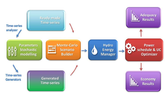
2 General content of Antares sessions

A typical Antares session involves different steps that are usually run in sequence, either automatically

or with some degree of man-in-the-loop control, depending on the kind of study to perform.

These steps most often involve:

a) GUI session dedicated to the initialization or to the updating of various input data sections

(load time-series, grid topology, wind speed probability distribution, etc.)

b) GUI session dedicated to the definition of simulation contexts (definition of the number and

consistency of the “Monte-Carlo years” to simulate)

c) Simulation session producing actual numeric scenarios following the directives defined in (b)

d) Optimization session aiming at solving all of the optimization problems associated with each of

the scenarios produced in (c).

e) GUI session dedicated to the exploitation of the detailed results yielded by (d)

The scope of this document is to describe the features of the software involved in step (a) to (e), from

the user’s standpoint

1

.

The following picture gives a functional view of all that is involved in steps (a) to (e).

1

This guide does not provide a detailed expression of the mathematical problems solved. Note, however, that a comprehensive

formulation of all optimization problems may be printed along with the simulation results if the user so requires.

Last Rev. 25 JUN 2018

4/57

The number and the size of the individual problems to solve (typically, a least-cost hydro-thermal

power schedule and unit commitment, with an hourly resolution and throughout a week, over a large

interconnected system) make optimization sessions often computer-intensive.

Depending on user-defined results accuracy requirements, various practical options allow to simplify

either the formulation of the problems or their resolution.

In terms of power studies, the different fields of application Antares has been designed for are the

following:

 Generation adequacy problems : assessment of the need for new generating plants so as to

keep the security of supply above a given critical threshold

What is most important in these studies is to survey a great number of scenarios that

represent well enough the random factors that may affect the balance between load and

generation. Economic parameters do not play as much a critical role as they do in the

other kinds of studies since the stakes are mainly to know if and when supply security is

likely to be jeopardized (detailed costs incurred in more ordinary conditions are of

comparatively lower importance). In these studies, the default Antares option to use is the

“Adequacy” simulation mode, or the “Draft” simulation mode (which is extremely fast but

which produces crude results).

 Transmission project profitability : assessment of the savings brought by a specific

reinforcement of the grid, in terms of decrease of the overall system generation cost (using an

assumption of fair and perfect market) and/or improvement of the security of supply (reduction

of the loss-of-load expectation).

In these studies, economic parameters and the physical modeling of the dynamic

constraints bearing on the generating units are of paramount importance. Though a

thorough survey of many “Monte-Carlo years” is still required, the number of scenarios to

simulate is not as large as in generation adequacy studies. In these studies, the default

Antares option to use is the “Economy” simulation mode.

The common rationale of the modeling used in all of these studies is, whenever it is possible, to

decompose the general issue (representation of the system behavior throughout many years, with a

time step of one hour) into a series of standardized smaller problems.

In Antares, the “elementary“ optimization problem resulting from this approach is that of the

minimization of the overall system operation cost over a week, taking into account all proportional and

non-proportional generation costs, as well as transmission charges and “external” costs such as that

of the unsupplied energy (generation shortage) or, conversely, that of the spilled energy (generation

excess). In this light, carrying out generation adequacy studies or transmission projects studies means

formulating and solving a series of a great many week-long operation problems (one for each week of

each Monte-Carlo year ), assumed to be independent (note that, however, issues such as the

management of hydro resources may bring some degree of coupling between the successive

problems).

Last Rev. 25 JUN 2018

5/57

2 Data organization

In Antares, all input and output data regarding a given study are located within a folder named after

the study and which should preferably be stored within a dedicated library of studies (for instance:

C/.../A_name_for_an_Antares_lib/Study-number-one).

The software has been designed so that all input data may be handled (initialized, updated, deleted)

through the simulator’s GUI. Likewise, all results in the output data can be displayed and analyzed

within the simulator: its standard GUI is actually meant to be able to provide, on a stand-alone basis,

all the features required to access input and output in a user-friendly way.

In addition to that, the Antares 6.x simulator may come

2

with or without functional extensions that

provide additional ways to handle input and output data.

These extensions take the form of companion applications whose documentation is independent from

that of the main simulator. For information regarding these tools (Graph Editor, Script Editor, Study

Manager) please refer to the specific relevant documents.

Besides, a point of notice is that most of Antares files belong to either “.txt” or “.csv” type: as an

alternative to the standard GUI, they can therefore be viewed and updated by many applications

(Windows Notepad, Excel,….). However, this is not recommended since handling data this way may

result in fatal data corruption (e.g. as a consequence of accidental insertion of special characters).

Direct access to input or output data files should therefore be reserved to very experienced users.

The input data contained in the study folder describe the whole state of development of the

interconnected power system (namely: grid, load and generating plants of every kind) for a given

future year.

As already stated, all of these data may be reviewed, updated, deleted through the GUI, whose

commands and windows are described in Sections 3 and 4.

Once the input data is ready for calculation purposes, an Antares session may start and involve any or

all of the following steps: historical time-series analysis, stochastic times-series generation, (draft)

adequacy simulation, (full) adequacy simulation and economic simulation.

The results of the session are stored within the output section of the study folder. The results obtained

in the different sessions are stored side by side and tagged. The identification tag has two

components: a user-defined session name and the time at which the session was launched.

2

Depending on the installation package

Last Rev. 25 JUN 2018

6/57

Particular cases are:

a) The outputs of the Antares time-series analyzer are not printed in the general output files but

kept within the input files structure (the reason being that they are input data for the Antares

time - series generators). The associated data may nonetheless be accessed to be reviewed,

updated and deleted at any time through the GUI.

b) Some specific input data may be located outside the study folder: this is the case of the

historical times-series to be processed by the time-series analyzer, which may be stored either

within the “user” subfolder of the study or anywhere else (for instance, on a remote “historical

data” or “Meteorological data” server).

c) The study folder contains a specific subfolder named “user”, whose status is particular:

Antares is not allowed to delete any files within it (yet files may be updated on the user’s

requirement). As a consequence, the “user” subfolder is unaffected by the “clean study”

command (see Section 3). This subfolder is therefore a “private” user space, where all kinds of

information can be stored without any kind of interference with Antares. Note that on using the

“save as” command (described further below), the choice is given to make or not a copy of this

subfolder.

d) The times-series analyzer requires the use of a temporary directory in which intermediate files

are created in the course of the analysis and deleted in the end, unless the user wishes to

keep them for further examination. Its location is user-defined and should usually be the “user”

subfolder if files are to be kept, otherwise any proper temporary space such as “C..../Temp”.

e) If the interconnected system to study is large and/or if the computer is low on RAM, it is

possible to run the Monte-Carlo adequacy simulator as well as the Monte-Carlo economic

simulator in “Swap” mode. Swap is not handled by the computer’s OS but by an Antares

specific swap manager, whose operation requires the definition of a space where the software

can store temporary files. This location is user-defined but should never be chosen within the

study folder. C/.../Temp may typically be used but an external drive may be preferred if the

computer is low on HDD.

Last Rev. 25 JUN 2018

7/57

3 Commands

The Antares GUI gives access to a general menu of commands whose name and meanings are

described hereafter.

File

New

Creates a new empty study to be defined entirely from scratch (network

topology, interconnections ratings, thermal power plants list, fuel costs, hydro

inflows stats, wind speed stats, load profiles ,etc.)

Open

Loads in memory data located in a specified Antares study folder. Once

loaded, these data may be reviewed, updated, deleted, and simulations may

be performed. If “open” is performed while a study was already opened, the

former study will be automatically closed.

Quick Open

Same action as open, with a direct access to the recently opened studies

Save

Saves the current state of the study, if necessary by replacing original files by

updated ones. After using this command the original study is no longer

available, though some original files may be kept until the ”clean” command is

used (see “clean” command )

Save as

Saves the current state of the study under a different name and / or location.

Using this command does not affect the original study. When “saving as”, the

user may choose whether he prefers to save input and output data or only

input data. Note that Antares does not perform “autosave”: Therefore, the

actions performed on the input data during an Antares session (adding an

interconnection, removing a plant,...) will have no effect until either “save” or

“save as” have been used

Export Map

Saves a picture of the current map as a PNG, JPEG or SVG file

Default background colour and storage location can be changed

Open in Windows Explorer

Opens the folder containing the study in a standard Windows Explorer window

Clean

Removes all junk files that may remain in the study folder if the Antares

session has involved lots of sequences such as “create area – add plant –

save –rename area – save - rename plant ...” (Antares performs only low level

auto-clean for the sake of GUI’s efficiency)

Close

Closes the study folder. If no “save” or “save as” commands have been

performed, all the modifications made on the input data during the Antares

session will be ignored

Quit

Exits from Antares

Last Rev. 25 JUN 2018

8/57

Edit

Copy

Prepare a copy of elements selected on the current system map. The

command is available only if the current active tab (whose name appears at

the top line of the subcommand menu) is actually that of the System maps.

Paste

Paste elements previously prepared for copy. The command is available only

if the current active tab (whose name appears at the top line of the

subcommand menu) is actually that of the System maps. Note that

copy/paste may be performed either within the same map or between two

different maps, attached to the same study or to different studies. To achieve

that, launch one instance of Antares to open the “origin” study, select

elements on the map and perform copy, launch another instance of Antares to

open the destination study, perform paste. Copied elements are stored in an

Antares clipboard that remains available for subsequent (multiple) paste as

long as the system map is used as active window.

Paste Special

Same as Paste, with a comprehensive set of parameterized actions (skip,

merge, update, import) that can be defined for each data cluster copied in the

clipboard. This gives a high level of flexibility for carrying out complex

copy/paste actions.

Reverse

The elements currently selected on the system map are no longer selected

and are replaced by those not selected beforehand.

Unselect All

Unselect all elements currently selected on the system map.

Select All

Select all elements on the system map.

Input

Name of the study

Gives a reference name to the study. The default name is identical to that of

the study’s folder but the user may modify it. The default name of a new study

is “no title”

Author(s)

Sets the study’s author(s) name. Default value is “memory”

The other “input” subcommands here below are used to move from one active window to another

System Maps

Simulation

User’s Notes

Load

Solar

Wind

Hydro

Thermal

Misc. Gen.

Reserves/DSM

Links

Binding constraints

Economic opt.

Last Rev. 25 JUN 2018

9/57

Output

For each simulation run for which results have been generated, opens a GUI

for displaying results. Results may be viewed by multiple selections made on a

number of parameters. Note that, since all simulations do not include all kinds

of results (depending on user’s choices), some parameters are not always

visible. Parameters stand as follows:

•

Antares area (node)

•

Antares interconnection (link)

•

Class of Monte-Carlo results :

o Monte-Carlo synthesis (over all years simulated)

o Year-by-Year (detailed results for one specific year)

•

Category of Monte-Carlo results :

o General values (operating cost, generation breakdown, ...)

o Thermal plants (detailed thermal generation breakdown)

o Record years (for each Antares variable, identification of

the Monte-Carlo year for which lowest and highest values

were encountered)

•

Span of Monte-Carlo results :

o Hourly

o Daily

o Weekly

o Monthly

o Annual

The interface provides a user-friendly way for the comparison of results between multiple

simulations (e.g. “before” and “after” commissioning of a new plant or interconnection) :

•

Use “new tab” button and choose a first set of simulation results

•

Use again “new tab” and choose a second set of simulation results

The results window will be automatically split so as to show the two series of results in parallel.

To the right of the “new tab” button, a symbolic (icon) button gives further means to compare

results on a split window (average, differences, minimum, maximum, sum)

Besides, when the simulation results contain the “year-by-year” class, it is possible to carry out

an extraction query on any given specific variable (e.g. “monthly amounts of CO2 tons

emitted”) throughout all available years of simulation.

The results of such queries are automatically stored within the output file structures, so as to

be available at very short notice if they have to be examined later in another session

(extractions may require a significant computer time when there are many Monte-Carlo years

to process).

Open in Windows Explorer

Displays the list of available simulation results and allows browsing through

the output files structure. The content of these files may be reviewed by tools

such as Xcel. File structures are detailed in Section 5.

Last Rev. 25 JUN 2018

10/57

Run

Monte Carlo Simulation

Runs either an economy simulation, an adequacy simulation, or a “draft”

simulation, depending on the values of the parameters set in the “simulation”

active window (see Section 4). If hardware resources and simulation settings

allow it, simulations benefit from full multi-threading (see Section 8)

Time-series generators

Runs any or all of the Antares stochastic time-series generators, depending

on the values of the parameters set in the “simulation” active window (see

Section 6)

Time-series analyzer

Runs the Antares historical time-series analyzer. The parameters of this

module are defined by a specific active window, available only on launching

the analyzer (see Section 6)

Configure

Filters on simulation results

Opens a few auxiliary windows that allow multiple selection on the results to

store at the end of a simulation: Choice of areas or geographic districts (see

below), choice of interconnections, choice of results spans (hourly, daily, etc.).

Note that in versions where the feature is not operational (grey display), an

alternative way of filtering results is available (see Section 4, “output profile”).

Geographic Districts

Allows selecting a set of areas so as to bundle them together in a “district”.

These are used in the course of simulations to aggregate results over several

areas. They can be given almost any name (a “@” prefix is automatically

added by Antares). Bypassing the GUI is possible (see Section 7).

MC Scenario builder

For each Monte-Carlo year of the simulation defined in the “Simulation”

window, this command allows to state, for each kind of time-series, whether it

should be randomly drawn from the available set (be it ready-made or

Antares-generated) OR should take a user-defined value (in the former case,

the default “rand” value should be kept; in the latter, the value should be the

reference number of the time-series to use). Multiple simulation profiles can

be defined and archived. The default active profile gives the “rand” status for

all time-series in all areas (full probabilistic simulation).

MC Scenario playlist

For each Monte-Carlo year of the simulation defined in the “Simulation” active

window, this command allows to state whether a MC year prepared for the

simulation should be actually simulated or not. This feature allows, for

instance, to refine a previous simulation by excluding a small number of “raw”

MC years whose detailed analysis may have shown that they were not

physically realistic. A different typical use consists in replaying only a small

number of years of specific interest (for instance , years in the course of which

Min or Max values of a given variable were encountered in a previous

simulation).

Last Rev. 25 JUN 2018

11/57

Object custom properties

Opens an interface that allows multiple selection of Antares objects (nodes,

links, thermal clusters,etc.) and to bind specific data to them (e.g. minimum

voltage level, maximum voltage level, etc ...).

These data are not used by Antares itself but may prove useful for external

applications

Optimization preferences

Defines a set of options related to the optimization core used in the

simulations. The set of preferences is study-specific; it can be changed at any

time and saved along with study data. Options refer to objects (binding

constraints,tec.) that are presented in subsequent sections of this document.

The values set in this menu overlay the local parameters but do not change

their value: for instance, if the LOCAL parameter “set to infinite” is activated for

some interconnections, and if the GLOBAL preference regarding transmission

capacities is “set to null”, the simulation will be carried out as if there were no

longer any grid BUT the local values will remain untouched. If the preference

is afterwards set to “local values”, the interconnections will be given back their

regular capacities (infinite for those being set on “set to infinite”).

•

Binding constraints (include / ignore)

•

Hurdle costs (include / ignore)

•

Transmission capacities (local values / set to null / set to infinite)

•

Min Up/down time of thermal plants (include / ignore)

•

Day-ahead reserve (include / ignore)

•

Primary reserve (include / ignore)

•

Strategic reserve (include / ignore)

•

Spinning reserve (include / ignore)

•

Export mps (false/true) (see Sections 7 and 8)

•

Simplex optimization range

3

(day / week)

3

Weekly optimization performs a more refined unit commitment, especially when the level selected in the “advanced

parameters” menu is “accurate”.

Last Rev. 25 JUN 2018

12/57

Advanced parameters

These parameters seldom need to be changed. The set of parameters is

study-specific; it can be updated at any time.

•

Seeds for random number generation

o Time-series draws (MC scenario builder)

o Wind time-series generation

o Solar time-series generation

o Hydro time - series generation

o Load time - series generation

o Thermal time-series generation

o Noise on thermal plants costs

o Noise on unsupplied energy costs

o Noise on spilled energy costs

o Noise on virtual hydro cost

o Initial hydro reservoir levels

•

Spatial time-series correlation

o Numeric Quality : load [standard | high]

o Numeric Quality : wind[standard | high]

o Numeric Quality : solar[standard | high]

•

Other preferences

o Power fluctuations [free modulations | minimize

excursions | minimize ramping]

o Shedding policy [shave peaks | minimize duration]

o District marginal prices : [average | weighed]

o Day-ahead reserve management [global|local]

o Unit commitment mode [fast |accurate]

o Simulation cores [minimum|low|medium|high|maximum]

Scripts

Allows execution of R- scripts edited through the “script editor” package (see

dedicated documentation for this package)

Tools

Study manager

Launches the “study manager” external package

(Please refer to dedicated documentation for this package)

Grapher

Launches the “graph editor” external package

(Please refer to dedicated documentation for this package)

CSV viewer

Opens txt or csv files, with a set of minimal data handling functions

(copy/paste, find min, max, compute average, standard deviation, etc.)

Resources monitor

Indicates the amounts of RAM and disk space currently used and those

required for a simulation in the available modes (see Section 8). Note that the

“disk requirement” amount does not include the footprint of the specific “mps”

files that may have to be written aside from the regular output (see previous §

“optimisation preferences”). Besides, the resources monitor shows the number

of CPU cores available on the machine Antares is running on.

Configure the swap folder

Defines the location that will be used by Antares to store the temporary files of

the MC simulators when the swap mode is activated (this location may also be

used by Antares GUI when handling large studies). The default setting is the

system temporary folder

Last Rev. 25 JUN 2018

13/57

Window

Toggle full window

Uses the whole window for display

Inspector

Opens a window that gives general information on the study and allows quick

browsing through various area- or interconnection-related parameters

Log viewer

Displays the log files regarding every Antares session performed on the study

“?” Menu

Reference Guide

Short-cut to this document (pdf reader software required)

System Map Editor Reference Guide

Short-cut to a guide to copy/paste features (pdf reader software required)

Continue on-line

Connects to the internet (required to participate to anonymous usage metrics

and, more generally, to get access to other services - future versions).

Privacy Policy – GDPR compliance:

When an Antares_Simulator GUI connects to the internet, it sends a signal to

a server dedicated to the gathering of anonymous usage metrics, over a

rolling period of one year.

The communication does not convey any personal data: transmitted

information is limited to three items:

• Antares_Simulator version number

• Computing power range of the machine running Antares_Simulator

(number of CPU cores)

• Signature of the running instance of Antares_Simulator

Continue off-line

Disconnects from the internet. All anonymous usage metrics that may have

been gathered so far for this instance of Antares_Simulator will be discarded.

Show signature

Displays the anonymous signature under which this instance of

Antares_Simulator will be referred to in web-based services, if it goes on-line

Check for updates

Tells if a more recent version of Antares_Simulator is available

Last Rev. 25 JUN 2018

14/57

4 Active windows

Data can be reviewed, updated, deleted by selecting different possible active windows whose list and

content are described hereafter. On launching Antares, the default active window is “System Maps”.

System Maps

This window is used to define the general structure of the system, i.e. the list of areas and that

of the interconnections. Only the area’s names, location and the topology of the grid are

defined at this stage. Different colours may be assigned to different areas. These colours may

later be used as sorting options in most windows. They are useful to edit data in a fashion that

has a geographic meaning (which the lexicographic order may not have).

This window displays copy/paste/select_all icons equivalent to the relevant EDIT menu

commands.

The top left side of the window shows a “mouse status” field with three icons. These icons

(one for nodes, one for links and one for binding constraints) indicate whether a selection

made on the map with the mouse will involve or not the related elements.

When a copy/paste action is considered, this allows for instance to copy any combination of

nodes, links and binding constraints. Status can be changed by toggling the icons. Default is

“on” for the three icons.

Two other purely graphic icons/buttons (no action on data) allow respectively to centre the

map on a given set of (x,y) coordinates, and to prune the “empty” space around the current

map.

Multiple additional maps may be defined by using the cross-shaped button located top right. A

detailed presentation of all system map editor features can be found in the document “System

Map Editor Reference Guide”.

Simulation

The main simulation window is divided up in two parts. On the left side are the general

parameters while the right side is devoted to the time-series management. These two parts

are detailed hereafter

Last Rev. 25 JUN 2018

15/57

LEFT PART : General parameters

Simulation

Mode: Economy , Adequacy, Draft

4

First day: First day of the simulation (e.g. 8 for a simulation beginning on

the second week of the first month of the year)

Last day: Last day of the simulation (e.g. 28 for a simulation ending on

the fourth week of the first month of the year)

5

Calendar

Horizon: Reference year (static tag, not used in the calculations)

Year: Actual month by which the Time-series begin (Jan to Dec, Oct

to Sep, etc.)

Leap Year: (Yes/No) indicates whether February has 28 or 29 days

Week: In economy or adequacy simulations, indicates the frame

(Mon- Sun, Sat-Fri, etc.) to use for the edition of weekly

results

1st January: First day of the year (Mon, Tue, etc.)

Monte-Carlo scenarios

Number: Number of MC years that should be prepared for the

simulation (not always the same as the Number of MC years

actually simulated, see “selection mode” below)

Building mode:

(Automatic)

For all years to simulate, all time-series will be drawn at

random

(Custom)

The simulation will be carried out on a mix of deterministic and

probabilistic conditions, with some time-series randomly drawn

and others set to user-defined values. This option allows

setting up detailed “what if” simulations that may help to

understand the phenomena at work and quantify various kinds

of risk indicators. To set up the simulation profile, choose in

the main menu: Configure/ MC scenario builder

4

”Economy” simulations make a full use of Antares optimization capabilities. They require economic as well as technical input

data and may demand a lot of computer resources. “Adequacy” simulations are faster and require only technical input data.

Their results are limited to adequacy indicators. “Draft” simulations are highly simplified adequacy simulations, in which binding

constraints (e.g. DC flow rules) are ignored, while hydro storage is assumed to be able to provide its nominal maximum power

whenever needed. As a consequence, draft simulations are biased towards optimism. They are, however, much faster than

adequacy and economic simulations.

5

In Economy an Adequacy simulations, these should be chosen so as to make the simulation span a round number of weeks.

If not, the simulation span will be

truncated

: for instance, (1, 365) will be interpreted as (1, 364), i.e. 52 weeks (the last day of

the last month will not be simulated). In Draft simulations, the simulation is always carried out on 8760 hours.

Last Rev. 25 JUN 2018

16/57

(Derated)

All time-series will be replaced by their mean and the number

of MC years is set to 1. If the TS are ready-made or Antares-

generated but are not to be stored in the INPUT folder, the

mean time-series will not be written over the original ones. If

the time-series are built by Antares and if it is specified that

they should be stored in the INPUT, the single mean-time

series will be stored instead of the whole set of time-series.

Selection mode:

(Automatic)

All prepared MC years will actually be simulated.

(Custom)

The years to simulate are defined in a list. To set up this list,

choose in the main menu: Configure/ MC scenario playlist

6

.

Output profile

Simulation synthesis: (True) Synthetic results will be stored in a directory :

Study_name/OUTPUT/simu_tag/Economy /mc-all

(False) No general synthesis will be printed out

Year-by-Year: (False) No individual results will be printed out

(True) For each simulated year, detailed results will be

printed out in an individual directory

7

:

Study_name/OUTPUT/simu_tag/Economy /mc-i-number

Results Filtering: (None) Storage of results for all areas, geographic districts,

interconnections as well as all time spans (hourly, daily, etc.)

(Custom) Storage of the results selected through “filters on

simulation results” of the Configure option in the main menu

Filters on areas, interconnections and time spans may also be

defined as follows:

a) On the map, select area(s) and/or interconnection(s)

b) Open the inspector module (Main menu, Windows)

c) Set adequate parameters in the “output print status” group

MC Scenarios: (False) No storage of the time-series numbers (either

randomly drawn or user-defined) used to set up the simulation

(True) A specific OUTPUT folder will be created to store the

time-series numbers drawn when preparing the MC years

6

c

hanging the number of MC years will reset the playlist to its default value ; not available in Draft simulations

7

Not available in Draft simulations

Last Rev. 25 JUN 2018

17/57

RIGHT PART : Time-series management

For the different kinds of time-series that Antares manages in a non-deterministic way (load, thermal

generation, hydro power, wind power, solar power):

1) Choice of the kind of time-series to use

Either « ready-made » or «stochastic » (i.e. Antares-generated), defined by setting the status

parameter to “on” or “off”

2) For stochastic TS only:

Number

Number of TS to generate

Refresh

(Yes /No)

Indicates whether a periodic renewal of TS should be performed or not

Refresh span

Number of MC years at the end of which the renewal will be performed (if so required)

Seasonal correlation

(“monthly” or “annual”)

Indicates whether the spatial correlation matrices to use are defined month by month

or if a single annual matrix for the whole year should rather be used (see Section 6)

Store in input

(Yes/No)

Yes: the generated time-series will be stored in the INPUT in replacement of the

original ones (wherever they may come from)

No: the original time-series will be kept as they were

Store in output

(Yes/No)

Yes: the generated times-series will be stored as part of the simulation results

No: no storage of the generated time-series in the results directories

3) General rules for building up the MC years

Intra-modal (Yes)

For each mode, the same number should be used for all locations (or 1 where there is

only one TS), but this number may differ from one mode to another. For instance,

solar power TS = 12 for all areas, while wind power TS number = 7 for all areas.

(No) Independent draws

Inter-modal (Yes)

For all modes, the same number should be used but may depend on the location (for

instance, solar and wind power TS = 3 for area 1, 8 for area 2, 4 for area 3, etc.)

(No) Independent draws

A full meteorological correlation (for each MC year, one single number for all modes and areas) is,

from a theoretical standpoint, accessible by activating “intramodal” and “ inter-modal” for all but the

“thermal” kind of time-series. The availability of an underlying comprehensive multi-dimensional

Meteorological data base of ready-made time-series is the crux of the matter when it comes to using

this configuration.

Last Rev. 25 JUN 2018

18/57

User’s Notes

A built-in notepad for recording comments regarding the study. Such comments typically help

to track successive input data updates (upgrading such interconnection, removing such plant,

etc.). Another simple use is to register what has been stored in the “user” subfolder and why.

Such notes may prove useful to sort and interpret the results of multiple simulations carried

out at different times on various configurations of the power system.

Load

This window is used to handle all input data regarding load. In Antares load should include

transmission losses. It should preferably not include the power absorbed by pumped storage

power plants. If it does, the user should neither use the “PSP” array (see window “Misc. Gen”)

nor the explicit modeling of PSP plants

The user may pick any area appearing in the list and is then given access to different tabs :

• The “time-series” tab display the “ready-made” 8760-hour time-series available for

simulation purposes. These data may come from any origin outside Antares, or be

data formerly generated by the Antares time-series stochastic generator, stored as

input data on the user’s request. Different ways to update data are :

o direct typing

o copy/paste a selected field to/from the clipboard

o load/save all the time-series from/to a file (usually located in the “user”

subfolder)

o Apply different functions (+,-, *, /,etc.) to the existing (possibly filtered) values

(e.g. simulate a 2% growth rate by choosing “ multiply-all-by-1.02”)

o Handle the whole (unfiltered) existing dataset to either

• Change the number of columns (function name : resize)

• Adjust the values associated with the current first day of the year

(function name : shift rows)

Versatile “Filter” functions allow quick access to user-specified sections of data (e.g.

display only the load expected in the Wednesdays of January, at 09:00, for time-series

#12 to #19). Hourly load is expressed in round numbers and in MW. If a smaller unit

has to be used, the user should define accordingly ALL the data of the study (size of

thermal plants, interconnection capacities, etc.)

Note that:

 If the “intra-modal correlated draws” option has not been selected in

the simulation window, MC adequacy or economy simulations can

take place even if the number of time-series is not the same in all

areas (e.g. 2 , 5 , 1 , 45 ,...)

 If the “intra-modal correlated draws” option has been selected in the

simulation window, every area should have either one single time-

series or the same given number (e.g. 25 , 25 , 1 , 25...)

Last Rev. 25 JUN 2018

19/57

• The “spatial correlation” tab gives access to the inter-area correlation matrices that will

be used by the stochastic generator if it is activated. Different sub-tabs are available

for the definition of 12 monthly correlation matrices and of an overall annual

correlation matrix.

A matrix A must meet three conditions to be a valid correlation matrix:

for all i and j { Aii= 100 , -100<= Aij <=100 } ; A symmetric ; A positive semi-definite

When given invalid matrices, the TS generator emits an unfeasibility diagnosis

• The “local data” tab is used to set the parameters of the stochastic generator. These

parameters are presented in four sub-tabs whose content is presented in Section 6.

• The “digest” tab displays for all areas a short account of the local data

Thermal

This window is used to handle all input data regarding thermal dispatchable power.

The user may pick any area appearing in the area list and is then given access to the list of

thermal plants clusters defined for the area (e.g. “CCG 300 MW”, “coal 600”,...). Once a given

cluster has been selected, a choice can be made between different tabs:

• The “time-series” tab displays the “ready-made” 8760-hour time-series available for

simulation purposes. These data may come from any origin outside Antares, or be

data formerly generated by the Antares time-series stochastic generator, stored as

input data on the user’s request. Different ways to update data are :

o direct typing

o copy/paste a selected field to/from the clipboard

o load/save all the time-series from/to a file (usually located in the “user”

subfolder)

o Apply different functions (+,-, *, /,etc.) to the existing (possibly filtered) values

(e.g. simulate a 2% growth rate by choosing “ multiply-all-by-1.02”)

o Handle the whole (unfiltered) existing dataset to either

• Change the number of columns (function name : resize)

• Adjust the values associated with the current first day of the year

(function name : shift rows)

Versatile “Filter” functions allow quick access to user-specified sections of data (e.g.

display only the generation expected on Sundays at midnight, for all time-series).

Hourly thermal generation is expressed in round numbers and in MW. If a smaller unit

has to be used, the user should define accordingly ALL the data of the study (Wind

generation, interconnection capacities, load, hydro generation, solar, etc.)

Note that:

 If the “intra-modal correlated draws” option has not been selected in

the simulation window, MC adequacy or economy simulations can

take place even if the number of time-series is not the same in all

areas (e.g. 2, 5, 1, 45,etc.)

 If the “intra-modal correlated draws” option has been selected in the

simulation window, every area should have either one single time-

series or the same given number (e.g. 25, 25, 1, 25, etc.). Note that,

unlike the other time-series (load, hydro, etc.), which depend on

meteorological conditions and are therefore inter-area-correlated, the

thermal plants time-series should usually be considered as

uncorrelated. Using the “correlated draws” feature makes sense only

in the event of having to play predefined scenarios (outside regular

MC scope)

Last Rev. 25 JUN 2018

20/57

• The “TS generator” tab is used to set the parameters of the stochastic generator.

These parameters are defined at the daily scale and are namely, for each day : the

average duration of forced outages (beginning on that day), the forced outage rate,

the duration of planned outages (beginning on that day), the planned outage rate,

planned outages minimum and maximum numbers. Durations are expressed in days

and rates belong to [0 , 1].

• The “Common” tab is used to define the cluster’s techno-economic characteristics :

 Name

 Fuel used

 Location (Area)

 Activity status

• false: not yet commissioned,moth-balled, ...

• true : the plant may generate

 Number of units

 Nominal capacity

 Full Must-run status

• false: above a partial “must-run level” (that may exist or not, see

infra) plants will be dispatched on the basis of their market bids.

• true: plants will generate at their maximum capacity, regardless of

market conditions

 Minimum stable power (MW)

 Minimum Up time (hours)

 Minimum Down time (hours)

 Default contribution to the spinning reserve (% of nominal capacity)

 CO2 tons emitted per electric MWh

 Marginal operating cost (€/MWh)

 Fixed cost (No-Load heat cost) (€ / hour of operation )

 Start-up cost (€/start-up)

 Market bid (€/MWh)

 Random spread on the market bid (€/MWh)

 Seasonal marginal cost variations (gas more expensive in winter, ...)

 Seasonal market bid modulations (assets costs charging strategy )

 Nominal capacity modulations (seasonal thermodynamic efficiencies, special

over-generation allowances, etc). These modulations are taken into account

during the generation of available power time-series

 Minimal generation commitment (partial must-run level) set for the cluster

Note that:

 The optimal dispatch plan as well as locational marginal prices are based

on market bids, while the assessment of the operating costs associated

with this optimum are based on cost parameters. (In standard “perfect”

market modeling, there is no difference of approaches because market bids

are equal to marginal costs)

Last Rev. 25 JUN 2018

21/57

Hydro

This window is used to handle all input data regarding hydro power

The user may pick any area appearing in the list and is then given access to different tabs:

• The “time-series” tab displays the “ready-made” time-series already available for

simulation purposes. There are two categories of time-series (displayed in two

different subtabs): the Run Of River (ROR) time-series on the one hand and the

Storage power (SP) time-series on the other hand.

ROR time-series are defined at the hourly scale; each of the 8760 values represents

the ROR power expected at a given hour, expressed in round number and in MW. The

SP time-series are defined at the monthly scale; each of the 12 values represents the

overall SP energy expected in the month, expressed in round number and in MWh.

These data may come from any origin outside Antares, or be data formerly generated

by the Antares time-series stochastic generator, stored as input data on the user’s

request. Different ways to update data are:

o direct typing

o copy/paste a selected field to/from the clipboard

o load/save all the time-series from/to a file (usually located in the “user”

subfolder)

o Apply different functions (+,-, *, /,etc.) to the existing (possibly filtered) values

(e.g. simulate a 2% growth rate by choosing “ multiply-all-by-1.02”)

o Handle the whole (unfiltered) existing dataset to either

• Change the number of columns (function name : resize)

• Adjust the values associated with the current first day of the year

(function name : shift rows)

Note that:

 For a given area, the number of ROR time-series and SP times-

series must be identical

 If the “intra-modal correlated draws” option has not been selected in

the simulation window, MC adequacy or economy simulations can

take place even if the number of hydro time-series is not the same in

all areas (e.g. 2 , 5 , 1 , 45 ,...)

 If the “intra-modal correlated draws” option has been selected in the

simulation window, every area should have either one single time-

series or the same given number (e.g. 25 , 25 , 1 , 25...)

• The “spatial correlation” tab gives access to an annual inter-area correlation matrix

that will be used by the stochastic generator if it is activated. Correlations are

expressed in percentages, hence to be valid this matrix must be symmetric, p.s.d,

with a main diagonal of 100s and all terms lying between (-100 ,+100)

• The “Allocation” tab gives access to an annual inter-area allocation matrix A(i,j) that is

used during the optimization process, regardless of whether the stochastic time-series

generator is used or not. This matrix describes the weights that are given to the loads

of areas (i) in the definition of the monthly and weekly hydro storage generation

profiles of areas (j).

Last Rev. 25 JUN 2018

22/57

More precisely, if there are Z zones z = 1,…,Z, and if M(z) denotes the overall “must-run”

generation of every kind in zone z (thermal, wind power, solar, run of river,…), one can

define successively :

a) L(z), “natural” load in zone z

b) L*(z) = L(z) - M(z), “net” load in zone z (in that sense that it has to be satisfied by

either imports or dispatchable thermal generation or hydro storage power).

c) L**(z) = sigma {i=1, Z} A(i,z) x L*(i) , “weighed” load in zone z. This weighed load

is the signal used in the hydro storage monthly and weekly energy profiles

adjustment stage, along with other parameters described further below.

Extreme cases are :

A is the identity matrix

The hydro storage energy monthly and weekly profiles of each zone z depend

only on the local demand and must-run generation in z

A has a main diagonal of zeroes

The hydro storage energy monthly and weekly profiles of each zone z do not

depend at all on the local demand and must-run generation in z

• The “local data” tab is used to set up the parameters of the stochastic generator AND

to define techno-economic characteristics of the hydro system that are used in

Economy and Adequacy optimizations.

 The parameters of the stochastic generator are the expectations,

standard deviations, minimum and maximum values of monthly energies

(expressed in GWh), monthly shares of Run of River within the overall

hydro monthly credit, and correlation between the energy of a month and

that of the next month (inter-monthly correlation).

These monthly energies will be considered either as amounts of energy to

generate or as amounts of energy inflows that may be partly stored in a

reservoir (i.e. net storable hydro energy = overall energy - ROR share)

 The techno-economic characteristics used in optimizations are namely :

o A “reservoir management” parameter that can take two values

(No / Yes). In the first case, the monthly SP time-series are

considered as energies to generate, while in the second they are

inflows to manage at best.

o The reservoir capacity (or size S), in GWh. This parameter is not

used if “reservoir management” is set to No. If “reservoir

management” is set to Yes , the capacity must be strictly positive

o 12 x 3 values for the monthly reservoir levels at the beginning of

the month : low, average, high (expressed in percentage of

reservoir size : Ll, La,Lh)

Last Rev. 25 JUN 2018

23/57

o 365 x 3 values for the daily maximum available hydro SP Power,

in MW, deemed to be consistent with the three assumptions

regarding the level of the reservoirs: low, average, high

(Pl,Pa,Ph)

o An “inter-monthly generation breakdown” parameter

α

, which is

used to split the hydro energy allocated for the whole year (sum

of inflows) into monthly energies, depending on the conditions

encountered at medium term (load level, wind generation,

etc...).This parameter is heuristically fitted and allows to simulate

different hydro management strategies. It is used only if the

hydro-time series are considered as inflows (otherwise, the time-

series are assumed to be direct estimates of monthly generated

energies)

The heuristic used comprises three steps:

a) Assessment of 12 monthly hydro storage energy targets H(m)

defined for each zone as follows : if H denotes the annual sum of

the 12 storable parts of the monthly inflows, L**(m) is the weighed

load during month m, then for all m and n :

H(m)/H(n) =( L**(m) / L**(n)) ^

α

Sigma {m=1,12} H(m) = H

b) Assessment of 12 monthly hydro storage energies H**(m) that

can actually be generated, by solving a linear problem in which

the objective function to minimize is a cost proportional to the

absolute deviations to the targets identified in step (a), while the

energies generated are variables submitted to two kinds of

constraints :

i. Energy conservation (monthly) : for any month ,

inflow - generation = monthly reservoir levels

variation

ii. Energy conservation (annual) : the energy

generated throughout the year is equal to the

sum of inflows

8

iii. Reservoir constraints (soft) : the “low” and “high”

levels boundaries should not be crossed, or only

at a very high cost

iv. Reservoir constraints (hard) : reservoir level

always lies between (0, reservoir size)

c) Assessment of 365 daily maximum hydro-storage power levels

that will actually be used in the course of the simulations. These

power levels are the result of an interpolation between the low,

average and high arrays (Pl,Pa,Ph) made on the basis of the

reservoir levels that are secondary results of step (b)

8

This is equivalent to stating that the reservoir level at the end of the year is the same as at the beginning.

In the simulations, the initial reservoir level is randomly drawn between “L(low)” and “L(high)”, with average “L(average)”

Last Rev. 25 JUN 2018

24/57

o An “inter-daily generation breakdown” parameter

β

, which is used

to split the hydro storage energy H**(m) to generate during the

whole month into daily energies, depending on the conditions

encountered at short term (load level, wind generation, etc...).This

parameter is heuristically fitted and allows to simulate different

hydro management strategies

The heuristic used comprises two steps :

a) Assessment of daily hydro storage energy targets h(i) defined for

each zone as follows: if H**(m) is the hydro storage energy to

generate during month m, l**(i) is the weighed load during day i,

then for all i and j :

h(i) / h(j) =( l**(i) / l**(j)) ^

β

Sigma {i=1,28>31} h(i) = H**(m)

b) Assessment of daily hydro storage energies h**(i) that can

actually be generated, by solving a linear problem in which the

objective function to minimize is a cost proportional to the

absolute deviations to the targets identified in step (a), while the

energies generated are variables submitted to two kinds of

constraints :

i. Energy conservation (monthly, soft) : The energy

generated throughout the month should be equal

to the sum of the daily targets. If it is lower (some

energy is spilled), the spillage cost translates as

a high penalty in the objective function

ii. Power constraints (hard) : for each day , the

energy generated lies between (0, P max x 24)

o An “intra-daily modulation” parameter, which represents, for the

storage power, the maximum authorized value for the ratio of the

daily peak to the mean power generated throughout the day. This

parameter is heuristically fitted and allows to simulate different

hydro management strategies.

Extreme values are :

1 : Hydro storage power is constant throughout the day

24: If the maximum hydro power is high enough, the

whole daily energy credit can be spent in one hour

Last Rev. 25 JUN 2018

25/57

Wind

This window is used to handle all input data regarding Wind power

The user may pick any area appearing in the list and is then given access to different tabs:

• The “time-series” tab display the “ready-made” 8760-hour time-series already

available for simulation purposes. These data may come from any origin outside

Antares, or be data formerly generated by the Antares time-series stochastic

generator, stored as input data on user’s request. Different ways to update data are :

o direct typing

o copy/paste a selected field to/from the clipboard

o load/save all the time-series from/to a file (usually located in the “user”

subfolder)

o Apply different functions (+,-, *, /,etc.) to the existing (possibly filtered) values

(e.g. simulate a 2% growth rate by choosing “ multiply-all-by-1.02”)

o Handle the whole (unfiltered) existing dataset to either

• Change the number of columns (function name : resize)

• Adjust the values associated with the current first day of the year

(function name : shift rows)

Versatile “Filter” functions allow quick access to user-specified sections of data (e.g.

display only the wind generation expected between 17:00 and 21:00 in February, for

time-series 1 to 100).

Hourly wind generation is expressed in round numbers and in MW. If a smaller unit

has to be used, the user should define accordingly ALL the data of the study (size of

thermal plants, interconnection capacities, load, etc.)

Note that:

 If the “intra-modal correlated draws” option has not been selected in

the simulation window, MC adequacy or economy simulations can

take place even if the number of time-series is not the same in all

areas (e.g. 2 , 5 , 1 , 45 ,...)

 If the “intra-modal correlated draws” option has been selected in the

simulation window, every area should have either one single time-

series or the same given number (e.g. 25 , 25 , 1 , 25...)

• The “spatial correlation” tab gives access to the inter-area correlation matrices that will

be used by the stochastic generator if it is activated. Different sub-tabs are available

for the definition of 12 monthly correlation matrices and an overall annual correlation

matrix.

A matrix A must meet three conditions to be a valid correlation matrix:

for all i and j { Aii= 100 , -100<= Aij <=100 } ; A symmetric ; A positive semi-definite

When given invalid matrices, the TS generator emits an unfeasibility diagnosis

• The “local data” tab is used to set the parameters of the stochastic generator. These

parameters are presented in four subtabs whose content is presented in Section 6.

• The “digest” tab displays for all areas a short account of the local data

Last Rev. 25 JUN 2018

26/57

Solar

This window is used to handle all input data regarding Solar power. Both thermal generation

and PV generation are assumed to be bundled in this data section.

The user may pick any area appearing in the list and is then given access to different tabs :

• The “time-series” tab display the “ready-made” 8760-hour time-series available for

simulation purposes. These data may come from any origin outside Antares, or be

data formerly generated by the Antares time-series stochastic generator, stored as

input data on the user’s request. Different ways to update data are :

o direct typing

o copy/paste a selected field to/from the clipboard

o load/save all the time-series from/to a file (usually located in the “user”

subfolder)

o Apply different functions (+,-, *, /,etc.) to the existing (possibly filtered) values

(e.g. simulate a 2% growth rate by choosing “ multiply-all-by-1.02”)

o Handle the whole (unfiltered) existing dataset to either

• Change the number of columns (function name : resize)

• Adjust the values associated with the current first day of the year

(function name : shift rows)

Versatile “Filter” functions allow quick access to user-specified sections of data (e.g.

display only the solar power expected in August at noon, for all time-series).

Hourly solar power is expressed in round numbers and in MW. If a smaller unit has to

be used, the user should define accordingly ALL the data of the study (size of thermal

plants, interconnection capacities, etc.)

Note that:

 If the “intra-modal correlated draws” option has not been selected in

the simulation window, MC adequacy or economy simulations can

take place even if the number of time-series is not the same in all

areas (e.g. 2 , 5 , 1 , 45 ,...)

 If the “intra-modal correlated draws” option has been selected in the

simulation window, every area should have either one single time-

series or the same given number (e.g. 25 , 25 , 1 , 25...)

• The “spatial correlation” tab gives access to the inter-area correlation matrices that will

be used by the stochastic generator if it is activated. Different sub-tabs are available

for the definition of 12 monthly correlation matrices and of an overall annual

correlation matrix.

A matrix A must meet three conditions to be a valid correlation matrix:

for all i and j { Aii= 100 , -100<= Aij <=100 } ; A symmetric ; A positive semi-definite

When given invalid matrices, the TS generator emits an unfeasibility diagnosis

• The “local data” tab is used to set the parameters of the stochastic generator. These

parameters are presented in four subtabs whose content is presented in Section 6.

• The “digest” tab displays for all areas a short account of the local data

Last Rev. 25 JUN 2018

27/57

Misc. Gen.

This window is used to handle all input data regarding miscellaneous non dispatchable

generation.

On picking any area in the primary list, the user gets direct access to all data regarding the

area, which amount to 8 ready-made 8760-hour time-series (expressed in MW) :

• CHP generation

• Bio Mass generation

• Bio-gas generation

• Waste generation

• Geothermal generation

• Any other kind of non dispatchable generation

• A predefined time-series for the operation of Pumped Storage Power plants, if they

are not explicitly modeled. A positive value is considered as an output (generating) to

the grid, a negative value is an input (pumping) to the station.

Note that the sum of the 8760 values must be negative, since the pumping to

generating efficiency is lower than 1. The user may also use only the negative values

(prescribed pumping), while transferring at the same time the matching generating

credit on the regular hydro storage energy credit.

• ROW balance: the balance with the rest of the world. A negative value is an export to

ROW, a positive value is an import from ROW. These values acts as boundary

conditions for the model

Different ways to update data are:

o direct typing

o copy/paste a selected field to/from the clipboard

o load/save all the time-series from/to a file (usually located in the “user”

subfolder)

o Apply different functions (+,-, *, /,etc.) to the existing (possibly filtered) values

(e.g. simulate a 2% growth rate by choosing “ multiply-all-by-1.02”)

o Handle the whole (unfiltered) existing dataset to either

• Change the number of columns (function name : resize)

• Adjust the values associated with the current first day of the year

(function name : shift rows)

Last Rev. 25 JUN 2018

28/57

Reserves / DSM

This window is used to handle all input data regarding reserves and the potential of “smart”

load management (when not modeled using “fake” thermal dispatchable plants). On picking

any area in the primary list, the user gets direct access to all data regarding the area, which

amount to four ready-made 8760-hour time-series (expressed in MW). The first two are used

only in “draft” simulations, while the last two are available in either “adequacy” or “economy”

simulations:

• Primary reserve: must be provided whatever the circumstances, even at the price of

some unsupplied energy (Draft simulations only)

• Strategic reserve: sets a limit on the backup power that an area is supposed to be

able to export to its neighbours. This reserve may represent an actual generation

reserve, an energy constraint too complex to model by standard means (e.g. energy

policy regarding special reservoirs) or can also be justified by simplifications made in

grid modeling. (Draft simulations only).

• Day-ahead reserve: power accounted for in setting up the optimal unit-commitment

and schedule of the following day(s), which must consider possible forecasting errors

or last-minute incidents. If the optimization range is of one day, the reserve will be

actually seen as “day-ahead”. If the optimization range is of one week, the need for

reserve will be interpreted as “week-ahead”. (Adequacy and Economy simulations)

• DSM: power (decrease or increase) to add to the load. A negative value is a load

decrease, a positive value is a load increase. Note that an efficient demand side

management scheme may result in a negative overall sum (All simulation modes).

Links

This window is used to handle all input data regarding the interconnections. On picking any

interconnection in the primary list, the user gets direct access to all data regarding the link,

which are two annual parameters and a set of five ready-made 8760-hour time-series

The two parameters, used in economy or adequacy simulations (not in draft), are namely:

• “ Hurdle cost ”, which is used to state whether (linear) transmission fees

should be taken into account or not in economy and adequacy simulations

• “ Transmission capacities ”, which is used to state whether the capacities to

consider are those indicated in 8760-hour arrays or if zero or infinite values

should be used instead (actual values / set to zero / set to infinite)

The five times-series are:

• NTC direct : the upstream-to-downstream capacity, in MW

• NTC indirect : the downstream-to-upstream capacity, in MW

• Impedances: virtual impedances that are used in economy simulations to give a

physical meaning to raw outputs, when no binding constraints have been defined to

enforce Kirchhoff’s laws (see “Output” section, variable “Flow quad”).

• Hurdle cost direct : an upstream-to-downstream transmission fee, in €/MWh

• Hurdle cost indirect : a downstream-to-upstream transmission fee, in €/MWh

Last Rev. 25 JUN 2018

29/57

Binding constraints

This window is used to input all data regarding linear constraints that may have to be taken

into account in optimizations tasks.

In standard simulations, power is assumed to be able to flow freely within the grid without any

kind of constraints, aside from limits resulting from the interconnections capacities. This

modeling of the grid’s behavior allows the assessment of a rough adequacy/economic

diagnosis, in which all the theoretical potential of both grid and park are used to the end (say

that ad hoc FACTS come into action whenever needed to “abolish” Kirchhoff’s’ laws)

In more refined simulations, where the power system is simulated on an everyday “regular”

basis, the previous “emergency” modeling may be fitting no longer and, if enough data are

available, can be improved. For that purpose, Antares gives the possibility to define linear

constraints that are to be met by power flows while seeking the optimal solution of the

economic problem.

These constraints are freely defined by the user and can be arbitrarily mixed.

For instance, if meaningful estimates of physical impedance 



are available for the

interconnections  , Kirchhoff’s laws can be enforced by defining, for each element of a set of

cycles  forming a basis of the system’s graph, the binding constraint:

 







= 0

∈

Constraints serving different objectives may be defined, such as enforcing commercial-

contract-related flow patterns.

Antares allows to define three categories of binding constraints:

• “hourly” binding constraints, which are applied to instant power and which are typically

used for Kirchhoff’s laws enforcement

• “daily” binding constraints, that are applied to daily energies. This class makes more

sense for commercial modeling (say : imports and exports from/to such and such

area should be comprised between such and such lower bound and upper bound).

Daily binding constraints may also be used to model more complex configurations,

such as setting up a virtual pumped storage power facility operated on a daily cycle

• “weekly” binding constraints, that are applied to weekly energies. Like the previous

ones, these constraints may be used to model commercial contracts or various

phenomena, such as the operation of a pumped storage power plant operated on a

weekly cycle.

The main window is divided into six tabs whose purpose is:

• “summary” : creates, edits or deletes a binding constraint of a given name (e.g.

“northern mesh”) and numerical class ( upper-bounded , lower-bounded, equality)

• “weights” : defines how much each interconnection contributes to the constraint

(e.g. in the constraint 3 X(t) + 5.2 Y(t+4 ) = RHS, weights are 3 and 5.2)

• “offsets” : defines whether the time-dependent variable X involved in the constraint is

related to time t or to another reference

(e.g. in the constraint 3 X(t) + 5.2 Y(t+4) =RHS, offsets are 0 and 4)

• “=” defines the 8760-hour or 365- day right-hand side of the equality constraints

• “>”defines the 8760-hour or 365-day right-hand side of the lower-bounded constraints

•

“<”defines the 8760-hour or 365-day right-hand side of the upper-bounded constraints

Last Rev. 25 JUN 2018

30/57

Note that the terms of the right-hand sides of the daily and weekly constraints are both defined

at the daily scale. For each simulation week, the terms , = 1,7 are interpreted as

follows:

a) If the type of the constraint is “daily” each  is the right-hand side value for the

daily constraint

b) If the type of constraint is “weekly” , the value used for week  is ∑

∈

When defining binding constraints between (hourly) power, daily or weekly (energy) flows,

attention should be paid to potential conflicts between them, since it is possible to create

situations for which the load/generation equilibrium problem has no solution, e.g.

( T1+T2 > 5 ; T2 < -3 ; T3 > 0 ; T1+T3 < 7)

On running the economic simulator, such situations will produce an unfeasibility diagnosis.

Economic Opt.

This window is used to set the value of a number of area-related parameters that, aside from

the costs of each generating plant, define the optimal solution that Antares has to find in

economic simulations. These parameters are namely, for each area of the system :

• The value of the unsupplied energy (also commonly denoted Value Of Lost Load,VOLL) , in

€/MWh. This value should usually be set much higher than the cost of the most expensive

generating plant of the area

• The random spread within which the nominal unsupplied energy value is assumed to vary

• The value of the spilled energy, in € /MWh. This value reflects the specific penalty that should

be added to the economic function for each wasted MWh, if any. Note that even if this value

is set to zero no energy will be shed needlessly

• The random spread within which the nominal unsupplied energy value is assumed to vary

• Three parameters named “shedding status” and related to different kinds of generation. If the

system cannot be balanced without shedding some generation, these parameters give control

on how each kind of generation ("Non dispatchable power", ”Dispatchable hydropower” and

“Other dispatchable generating plants”) should contribute to the shedding. Depending on the

value chosen for the status, the generation can or cannot be shed to find a solution to the

load/generation balance problem. Note that enforcing a negative status for all types of plants

may lead to simulations scenarios for which there are no mathematical solutions.

On running the economic simulator, such situations produce an unfeasibility diagnosis.

Miscellaneous

In all previous windows showing Input data, the content can be filtered so as to reflect only items that

are associated with Areas and Links defined as “visible” in a particular map. In that regard, binding

constraints are considered as visible if and only if all of their non-zero weight associated objects are

visible on the map.

Last Rev. 25 JUN 2018

31/57

5 Output files

The general file organization is the same for Economy, Adequacy and Draft simulations.

• Economy and Adequacy results may be displayed in the GUI ( “Output” in main menu)

• Draft results are available only as flat .txt files. They can be viewed with “Tool /csv viewer” in

the main menu (As well as any other files, they can also be accessed by Xcel or suchlike)

Economy :

OUTPUT/ Simu id / Economy /mc-all / grid /... contains a summary file "digest.txt"

/areas/name/... contains area-related results

/links / name/... contains interconnection-related results

/mc-ind /<year number>

/areas/name/... contains area-related results

/links / name/... contains interconnection-related results

(“mc-all” files contain synthetic results over all years, “year-number” files contain results for a single year

The variables present in each file are detailed in the following sections

In “Economy” simulations, all variables have a techno-economic meaning

Adequacy:

OUTPUT/ Simu id / Adequacy /mc-all / grid /... contains a summary file "digest.txt"

/areas/name/... contains area-related results

/links / name/... contains interconnection-related results

/mc-ind /<year number>

/areas/name/... contains area-related results

/links / name/... contains interconnection-related results

(“mc-all” files contain synthetic results over all years, “year-number” files contain results for a single year

The variables present in each file bear exactly the same name as in Economy simulations but do not have the same values

The only variables that have a techno-economic meaning are the “Adequacy” indicators (unsupplied energy,LOLD,LOLP)

Draft:

OUTPUT / Simu id / Adequacy-Draft / mc-all /grid/... contains a condensed file "digest.txt"

/areas/name/... contains area-related results

(“mc-all” files contains mostly synthetic results over all years ; However, there is (for each area) a “mc-annual.txt” file that gives

a short view of local results for each simulated year)

IMPORTANT Adequacy and Economy files look the same but their content are specific

In “Economy” and “Adequacy” simulations, the optimization ignores the “primary” and “strategic”

reserves (however, it may include the [other] spinning and day-ahead reserves, depending on the

settings made in “optimization preferences”).

In “Adequacy” simulations, all dispatchable thermal units are given the “must-run” status (hence, they

will generate at Pmax, regardless of the demand). As a consequence the only variables that are

actually meaningful are the adequacy indicators (unsupplied energy, LOLD,LOLP), that may depend

on assumptions made regarding the economic values of Unsupplied and spilled energies, and on

hurdle costs on interconnections.

As a consequence, both “Adequacy” and “Economy” simulations yield the same values for the

adequacy indicators under the following conditions: if hurdle costs on interconnections are higher than

the difference between the maximum VOLL and the minimum VOLL assigned to the different areas of

the system.

The files and their content are hereafter described.

Last Rev. 25 JUN 2018

32/57

Economy and Adequacy, area results

9

15 files resulting from the combination of the following attributes :

• The second attribute defines the time span over which the results are assessed : hourly detail,

daily bundle, weekly bundle, monthly bundle, annual bundle.

• The first attribute defines the nature of the results presented in the file :

Values Values of different variables (price, load, overall generation issued from coal, etc.),

the list of which is common to all areas of the interconnected system. Files of type

"values" have therefore the same size for all areas.

These results appear under the label “ general values” in the output GUI

details Values regarding the different dispatchable thermal generating plants of each area

(e.g. “older 300 MW coal from the south coast”). The sizes of these files differ from

one area to another.

These results appear under the label “ thermal plants ” in the output GUI

id Identifier (number) of the Monte-Carlo years for which were observed the extreme

values of the different variables presented in the « values » files

These results appear under the label “record years” in the output GUI

The area files that belong to the « values » class display 98 fields corresponding to the expectation ,

standard deviation, minimal and maximal values of the variables whose list is given hereafter.

OV.COST Overall cost = operating cost + unsupplied energy cost+ spilled energy cost

OP.COST Operating cost = Proportional costs + Non- proportional costs

MRG. PRICE LMP : overall economic effect of a local 1MW load increase

CO2 EMIS. Amount of CO2 emitted by all dispatchable thermal plants

BALANCE Overall Import/export balance of the area (positive value : export)

ROW BAL Import/export with areas outside the modeled system (positive value: import)

10

PSP User-defined settings for pumping and subsequent generating

MISC. NDG Miscellaneous non dispatchable generation

LOAD Demand (including DSM potential if relevant)

H.ROR Hydro generation, Run-of-river share

WIND Wind generation

SOLAR Solar generation (thermal and PV)

NUCLEAR Overall generation of nuclear clusters

LIGNITE Overall generation of dispatchable thermal clusters burning brown coal

COAL Overall generation of dispatchable thermal clusters burning hard coal

GAS Overall generation of dispatchable thermal clusters burning gas

OIL Overall generation of dispatchable thermal clusters using petroleum products

MIX.FUEL Overall gen. of disp. thermal clusters using a mix of the previous fuels

MISC.DTG Overall gen. of disp. thermal clusters using other fuels

H.STOR Hydro generation, storage share

UNSP. ENRG Unsupplied energy : adequacy indicator (Expected Energy Not Served–EENS)

SPIL. ENRG Spilled energy (energy that cannot be used and has to be wasted)

LOLD Loss of load duration : adequacy indicator (length of shortfalls)

LOLP Loss of Load probability : adequacy indicator (probability of shortfalls)

AVL DTG Available dispatchable thermal generation (sum of av. power over all plants)

DTG MRG Disp. Ther. Gen. (AVL DTG – sum of all dispatched thermal generation)

MAX MRG Maximum margin : operational margin obtained if the hydro storage energy of

the week were used to maximise margins instead of minimizing costs

NP COST Non-proportional costs of the dispatchable plants (start-up and fixed costs)

NODU Number Of Dispatched Units

11

9

This description applies to both « MC synthesis » files and “Year-by-Year” files, with some simplifications in the latter case

10

Value identical to that defined under the same name in the “Misc Gen” input section.

11

NODU and NP Cost do not appear in “Adequacy” results since these variables are irrelevant in that context

Last Rev. 25 JUN 2018

33/57

Economy and Adequacy, interconnection results

12

10 files resulting from the combination of the following attributes :

• The second attribute defines the period of time over which the results are assessed : hourly

detail, daily bundle, weekly bundle, monthly bundle, annual bundle.

• The first attribute defines the nature of the results presented in the file

values values of different variables (flow, congestion rent) the list of which is common to all

interconnections. The files of type "values" have therefore the same size everywhere

These results appear under the label “ general values” in the output GUI

id identifier (number) of the Monte-Carlo years for which were observed the extreme

values of the different variables presented in the « values » files

These results appear under the label “record years” in the output GUI

The area files that belong to the « values » class display 27 fields corresponding to the expectation ,

standard deviation, minimal and maximal values of the variables whose list is given hereafter.

FLOW LIN. Flow (signed + from upstream to downstream) assessed by the linear optimization.

These flows follow Kirchhoff’s law only if these laws have been explicitly enforced by the means of

suitable binding constraints

UCAP Used capacity: absolute value of FLOW LIN. This indicator may be of interest

to differentiate the behavior of interconnectors showing low average flows: in

some cases this may indicate that the line is little used, while in others this

may be the outcome of high symmetric flows

FLOW QUAD. Flow computed anew, starting from the linear optimum, by minimizing a

quadratic function equivalent to an amount of Joule losses, while staying

within the transmission capacity limits. This calculation uses for this purpose

the impedances found in the “Links” Input data. If congestions occur on the

grid, these results are not equivalent to those of a DC load flow

CONG. FEE ALG Algebraic congestion rent = linear flow * (downstream price – upstream price)

CONG. FEE ABS Absolute congestion rent = linear flow* abs(downstream price–upstream price)

MARG. COST Decrease of the system’s overall cost that would be brought by the optimal

use of an additional 1 MW transmission capacity (in both directions)

CONG PROB + Up>Dwn Congestion probability = (NC+) / (total number of MC years) with:

NC+ = number of years during which the interconnection was congested in the

Up>Dwn way for any length of time within the time frame relevant with the file

CONG PROB - Dwn>Up Congestion probability = (NC-) / (total number of MC years) with:

NC- = number of years during which the interconnection was congested in the

Dwn>Up way for any length of time within the time frame relevant with the file

HURD. COST Contribution of the flows to the overall economic function through the “hurdles

costs” component. For each hour :

if FLOW.LIN > 0

HURD. COST = (hourly direct hurdle cost) * (FLOW LIN.)

else HURD.COST = (hourly indirect hurdle cost) * (-1)* (FLOW LIN.)

12

This description applies to both « MC synthesis » files and “Year-by-Year” files, with some simplifications in the latter case

Last Rev. 25 JUN 2018

34/57

Economy and Adequacy, other results

Depending on the options chosen in the main simulation window, the output folders may

include either, both or none of the following sections :

• OUTPUT/ Simu Id / ts-numbers / Load /area names / ...

/ Thermal /area names / ...

/ Hydro /area names / ...

/ Wind /area names / ...

/ Solar /area names / ...

These files contain, for each kind of time-series, the number drawn (randomly or not) in each

Monte-Carlo year (files are present if “output profile / MC scenarios” was set to “true”)

• OUTPUT/ Simu Id / ts-generator / Load / batch number /area names / ...

/ Thermal / batch number /area names / ...

/ Hydro / batch number /area names / ...

/ Wind / batch number /area names / ...

/ Solar / batch number /area names / ...

These files contain, for each kind of Antares-generated time-series, copies of the whole set of

time-series generated. Batch numbers depend on the values set for the “refresh span”

parameters of the stochastic generators (files are present if “store in output” was set to “true”)

Draft, area results

1 file « annual » + 6 files resulting from the combination of the following attributes :

[with-network | without-network | id] X [ hourly | annual]

• The second attribute defines the period of time over which the results are assessed : hourly

detail or annual summary.

• The first attribute defines the nature of the results presented in the file

with network values of adequacy indices (shortfall duration, loss of load probability)

assessed while taking into account the effective grid capacities. The results in

these files bear the suffix –CN (connex)

without network values of adequacy indices (shortfall duration, loss of load probability)

assessed without taking into account any interconnection. The results in these

files bear the suffix –IS (isolated areas)

id identifiers (numbers) of the MC years for which were observed the extreme

values of the different variables presented in the « w/net » and “wo/net” files

Last Rev. 25 JUN 2018

35/57

Files « with network » et « without network » present the expectations and extreme values observed

for the variables whose list is given hereafter :

LOLD Overall length of time for which there were shortfalls (Loss of Load Duration)

(note : the commonly used LOLE index is equivalent to LOLD expectation )

LOLP Loss of Load Probability

EENS Energy Not Supplied

MARG Margin = available generation – (load + primary reserve)

When MARG>0, MARG is a security margin

When MARG <0 , MARG is a curtailment depth

The file « annual » has one line per simulated Monte-Carlo year and gives, for each year, the following

information :

LOLD IS Load shedding duration, if the grid capacities are not considered as available

LOLD CN Load shedding duration, if the grid capacities are actually available

MAX DEPTH IS Margin available at the most critical hour of the whole MC year, w/o grid

When MAX DEPTH >0 , MAX DEPTH is a security margin

When MAX DEPTH <0,MAX DEPTH is a shortfall depth

MAX DEPTH CN Margin available at the most critical hour of the whole MC year, w/ grid

When MAX DEPTH >0 , MAX DEPTH is a security margin

When MAX DEPTH <0,MAX DEPTH is a shortfall depth

Remark : In spite of their likenesses, the fields « MARG » of the files w/net, wo/net and the fields

« MAX DEPTH » of the file mc-details are not identical (hence different names):

• MARG (expectation, min, max) is related to the whole set of MC years

• MAX DEPTH regards one single year.

Note that the following relations hold :

Min { MC years } MAX DEPTH IS = Min { hours} MARG IS [MIN]

Min { MC years } MAX DEPTH CN = Min { hours} MARG CN [MIN]

Miscellaneous

Alike Input data, output results can be filtered so as to include only items that are associated with

Areas and Links defined as “visible” in the current map. In addition, the output filtering dialog box

makes it possible to filter according to two special categories (Districts and Unknown) that are not

related to standard maps:

• Districts displays only results obtained for spatial aggregates

•

Unknown displays only results attached to Areas or Links that no longer

exist in the Input dataset (i.e. study has changed since the last simulation)

Last Rev. 25 JUN 2018

36/57

6 Time-series analysis and generation

General

When ready-made time-series are not available or are too scarce for building the required number of

Monte-Carlo annual simulation scenarios, Antares provides means to generate sets of stochastic time-

series to use instead.

The different categories of time-series call for wholly different generation processes :

• For thermal power, the generator is based on the animation of a daily three-state Markov

chain (available – planned outage – forced outage ) attached to each plant.

• For Hydro-power, the generator works out monthly time-series of energies, based on the

assumption that they can be modeled by Log Normal variables with known correlations

through space and time. So as to keep the model simple, for an interconnected system made

of N areas, the user defines, along with the N expectations and N standard deviations of the

monthly energies, the N X N correlation matrix R(n,m) of the logs of the annual hydro

energies between the areas n,m, and the N average auto-correlations r(k) between one

month and the next in each area k. The correlation C(n,i,m,j) between the logs of hydro

energies in area n, month i and area m, month j is taken to be

C(n,i,m,j)=

R(n,m)*sqrt((r(n)*r(m))^abs(j-i))

This most simplified model asks for considerably fewer data

than a comprehensive 12N X 12N time-space matrix. Note that if R is positive semi-definite

but C is not, matrix C is automatically transformed into a fitting p.s.d matrix and the data

generation keeps going on (however, the log report will show a warning message). If the

primary matrix R is not p.s.d, data are considered as corrupted, the generation stops and a

fatal error message will be displayed in the log report

• For Wind power, Solar power and Load, the required time-series are 8760-hour long and

have to emulate as closely as possible the response of the system to variations of wind

speed, sunshine and temperature. In all three cases, the rationale of the model is to offer the

possibility to consider either the final variable to model (wind power output, solar power

output, load) or an underlying intermediate variable (wind speed, nebulosity, deviation

between load and the level expected in standard temperature conditions) as a stationary

stochastic process, with given marginal laws, given auto-correlation functions and given

spatial correlations (eventually, the values of the final variables and those of the core

stationary process are tied by diurnal/seasonal rhythms and scaling functions).

The identification of all relevant parameters can be made outside Antares by any appropriate

means but can also be made automatically by the time-series analyzer, which is then to be fed

with the largest available set of historical time-series. Note however that, using the time-series

analyzer, one has to consider whether the time-series at hand are statistically meaningful or

whether they need some pre-processing (for instance, if wind power time-series are gathered

for a period within which the park has increased, the time-series to analyze should be

expressed in % of installed power rather than in MW. For Solar power, the relevant variable to

model as a stationary stochastic process is certainly not the raw output of solar power but

rather a meteorological indicator related to the sky clarity (for instance , time-series of

nebulosity expressed on a 0-100 scale may be used).

Once generated by appropriate algorithms, the values of the stationary processes are turned

into final values by using a number of parameters that put back in the series the diurnal and

seasonal patterns that may have been observed in the course of the historical data analysis

and that were temporarily removed to identify the core stationary processes.

Last Rev. 25 JUN 2018

37/57

Time-series generation (load, wind, solar) : principles

For the generation of wind, solar and load time-series, Antares gives access to different marginal laws

and autocorrelation functions presented hereafter. Note that wind speed modeling should usually be

based upon a Weibull modeling, while almost all other situations are likely to be best modeled by Beta

variables.

The stationary processes are defined at a monthly scale. For each month, there are :

• Four parameters for the definition of the marginal law

TS Gen. Parameters

Law α β γ δ

Expectation

Variance

Uniform N/A N/A < δ >γ

(δ−γ)/2

(δ−γ)

^

2 /12

Beta >0 >0 < δ >γ

γ + α(δ−γ)/(α+β)

[αβ(δ−γ)

^

2] / [(α+β+1)(α+β)

^

2 ]

Normal Any >0 N/A N/A

α

β

^2

Weibull

>=1 <50

>0 N/A N/A

β Γ(1+1/α)

β

^2

[ Γ(1+2/α)

−Γ(1+1/α)

^2

)]

Gamma

>=1 <50

>0 N/A N/A

α∗β

^2

Uniform : uniform defined on

(γ,δ)

Beta : Beta

(α,β

) defined on

(γ,δ)

Normal : expectation

α

, standard deviation

β

Weibull : shape

α

, scale

β

, defined on (0,+inf.)

Gamma : shape

α

, scale

β,

defined on (0, +inf.)

In the expressions of expectation and variance,

Γ

(x) is the standard Euler Function

• Two parameters for the definition of the autocorrelation function

TS Gen. Parameters

Law θ µ

Corr (Xt,Xt+h)

Pure exponential decay θ > 0 µ =1 exp( - θh)

Smoothed exponential

decay(*)

θ > 0 1 < µ < 24 Phi(θ,µ,h)

Phi(θ,µ,h)= (1/A) *sigma {i=0,µ} [sigma {j=h,h+µ} (exp(-θ|j-i|))]

with A= µ + 2 sigma{i=1,µ ;j=1,µ ; j>i } (exp(-θ(j-i))

(*) Obtained by the generation of purely exponentially autocorrelated values (parameter

θ

) followed

by a moving average transformation (parameter

µ

).

θ

and

µ

should be carefully chosen so as to

accommodate at best the experimental data at hand. If meaningful historical data are available, this

identification may be directly made using the Antares time-series analyzer

Last Rev. 25 JUN 2018

38/57

Time-series generation (load, wind, solar) : GUI

The section of the GUI specific to the generation of wind, solar and load time-series comprises :

1. Spatial correlation matrices that are located within the “spatial correlation” tab of

each path “ Wind | Solar | Load / <area_name >”

This tab contains a workspace for the description of 12 monthly spatial correlation matrices

Ξ

and one annual correlation matrix. For the stochastic generators to work properly, these

matrices must meet the usual requirements (matrices must be p.s.d, symmetric, with all terms

between -100 and +100, and a main diagonal made of 100s). If this is not the case,

generators will emit an unfeasibility diagnosis. Matrices can be either set up manually OR

automatically filled out by the time-series analyzer (see next paragraph).

Depending on the choices made in the main “simulation” window, the matrices used will be

either the 12 monthly matrices or the annual matrix. Whether to use the first or the second

option depends on the quality of the statistical data at hand: with high quality data (for

instance, that derived from the analysis of a very large pool of historical data), use of monthly

correlations is recommended because monthly differences between matrices have a physical

meaning ; with less robust data (derived from a handful of historical data,…), use of the single

annual correlation matrix should be preferred because it smoothes out the numeric noise

which impairs the monthly matrices.

2. Four parameters and four subtabs that are located within the “local” tab of each path

“Wind | Solar | Load / <area_name >”

FOUR PARAMETERS

• Capacity : This first parameter is used to scale up time-series generated on the basis of the

(

α,β,γ,δ,θ,µ

) parameters described previously in the “principles” paragraph, together with

coefficients characterizing the diurnal pattern (see below)

• Distribution : This second parameter gives the type of marginal distribution of the stationary

stochastic processes to generate (Beta, Weibull, Normal, Gamma, Uniform)

• Translation : This third parameter has three possible values :

o Do not use : parameter ignored

o Add before scaling : A specific 8760-hour array is added to the time-series produced

by the primary stochastic generator, BEFORE use of the conversion table (optional)

followed by the final multiplication by the capacity factor

o Add after scaling : A specific 8760-hour array is added to the time-series produced

by the primary stochastic generator, AFTER use of the conversion table (optional)

followed by the final multiplication by the capacity factor

Last Rev. 25 JUN 2018

39/57

• Conversion : This fourth parameter has two possible values :

o Do not use : Any transfer function that may be described in the “conversion” subtab

(see below) should not be used for the final stage of data elaboration (for instance, if

the primary parameters describe the physics of wind speeds, the time-series

eventually produced should remain wind speeds and not wind power).

o Use : The time-series produced by the stochastic generators (wind speeds, for

instance) are turned into other values (wind power) by using the transfer function

described in the “conversion” subtab.

FOUR SUBTABS

• Subtab “Coefficients”

A twelve-month table of values for the primary parameters

α,β,γ,δ,θ,µ

This table may be either filled out manually or automatically (use of the time-series analyzer)

• Subtab “Translation”

Contains a 8760-hour array T to add to the time-series generated, prior or after scaling. This

array can be either filled out manually or by the time-series analyzer

• Subtab “Daily profile”

A 24*12 table of hourly / monthly coefficients K(hm) that are used to modulate the values of

the stationary stochastic process by which the actual process is approximated. This table can

be either filled out manually or by the time-series analyzer

• Subtab “Conversion”

A table of 2 * N values (with 1<=N<=50 ) that is used to turn the initial time-series produced by

the generators (for instance, wind speeds) into final data (for instance , wind power). The

transfer function (speed to power,…) is approximated by N discrete points whose abscises

X(N) an ordinates Y(N) are given by the table.

Last Rev. 25 JUN 2018

40/57

Time-series analysis (load, wind, solar)

The time-series analyzer module available in Antares is meant to identify the values that should be

given to the parameters used in the time-series generators (load, solar power, wind power) so as to fit

best historical time-series at hand

IMPORTANT

When the time-series analyzer is used, it automatically updates the parameters relevant to the

analysis (for instance: analysis of “wind” time-series will overwrite all local and global “wind”

parameters [correlation matrices] that may have been previously set manually)

The primary TS analyzer window shows two tabs:

1. Tab “Time-series and areas”

o Time-series (load, wind, solar) : class of parameters to be assessed by the analyzer

o Browse: location of the historical time-series files. These are txt files in which 8760-

hour time-series must be stored in adjacent columns separated by a tabulation

o For each area :

 Activity status

• yes : parameters will be assessed and updated by the analyzer

• no : the area will be skipped (local parameters for the area will

remain unchanged, however spatial correlation with other areas will

be reset to zero)

 Distribution

• Type of distribution to fit (beta, normal, etc.)

 Data

• Raw : data to analyze are the actual historical time-series

• Detrended : data to analyze are the time-series of the deviations to

average (for instance: load time-series need to be analyzed in

“detrended” mode while wind speeds can be analyzed in “raw” mode)

 File to analyze

• Name of the file that should contain historical time-series to analyze

 Status

• Ready (a file bearing the expected name was found)

• Not found (no file found with the expected name)

IMPORTANT : To generate stochastic data similar to the historical data analyzed, generation

parameters must be kept consistent with the results of the analysis , which means, in the generators :

Keep the same:

Type of distribution

Values for

α,β,γ,δ

and for the diurnal–seasonal pattern (table of 12 X 24 values)

Value for the “capacity” parameter (the analyzer automatically sets it to 1)

Besides: “Conversion” option must be set to “no”

“Translation” option must be set to “do not use “ if data were analyzed as “raw”

and to “add after scaling” or “add before scaling” if data were analyzed as

“detrended” (both options give the same value in this case because the scaling is 1:1)

Last Rev. 25 JUN 2018

41/57

2. Tab “Global settings”

o Temporary folder : workspace that can be used for the analysis (cleaned after use)

o Analyzer settings

 Short- term autocorrelation adjustment (%)

 Long – term autocorrelation adjustment (%)

These two parameters are used by Antares as targets for the fitting of

θ

and

µ

parameters. For instance, if the historical time-series autocorrelation function is

such that Corr(T,T+ 18 hours)=90 % and Corr(T,T+60 hours)= 50%, and if the

parameters in the analyzer are (ST = 90%,LT = 50%) , then it will search values of

θ

and

µ

matching the historical autocorr.function in two points(18 hours, 60 hours)

 Trimming threshold (%)

In the spatial correlation matrices, terms lower than the threshold will be

replaced by zeroes

o Input data

 Time-series per area (n)

limits the analysis to the first n historical time-series at hand

 Upper-bound (Max)

In the analysis, all values above Max in the historical files will be

replaced by Max

 Lower-bound (Min)

In the analysis, all values below Min in the historical files will be

replaced by Min

Last Rev. 25 JUN 2018

42/57

Time-series generation (thermal)

The stochastic generator for time-series of available dispatchable power generation works, for

each plant of each set (cluster), with the following parameters :

• The nominal plant capacity and a 8760-hour array of modulation

coefficients to apply to it (default value : 1)

• A 365-day array of forced outages rates (“FOR” , lies in [0,1] )

• A 365-day array of planned outages rates (“POR” , lies in [0,1])

• A 365-day array of forced outages average durations

(“FOD” in days, integer, lies in [1,365])

• A 365-day array of planned outages average durations

(“POD” in days, integer,lies in [1,365] )

• A 365-day array of planned outages minimum number (PO Min Nb)

(integer, lies in [0, PO Max Nb])

• A 365-day array of planned outages maximum number (PO Max Nb)

(integer, lies in [PO Min Nb, Nb of units in the cluster]

• Two parameters describing how forced outages durations may

randomly deviate from their average value (law : uniform or geometric

, volatility : lie in [0,1])

• Two parameters describing how planned outages durations may

randomly deviate from their average value (law : uniform or geometric

, volatility : lie in [0,1])

1. Outage duration : meaning and modeling

In the thermal time-series generator, the concept of outage duration (either forced or planned)

is simple enough : for any given plant affected by such an event, it is the duration of a single

outage, expressed in days.

The fact that 365 different values can be used to describe what may happen in the course of a

year (for each kind of outages) means that the average outage duration may depend on the

day the outage begins on. For instance, very short outages may be sometimes be planned on

week-ends. Likewise, historical statistics can show that forced outages do not last the same

average time in winter and summer, etc.

In complement to the average value of the duration D of outages beginning on a particular

day, the time-series generator allows to set two parameters that describe how the actual

outage durations may deviate from the calendar-related average value.

Last Rev. 25 JUN 2018

43/57

o The first parameter (law) can take either the value “uniform” or “geometric” :

Uniform : the actual outage duration will be randomly drawn (one draw per

outage), according to a uniform distribution centered on the average value

D. The width of the interval [min duration, max duration] will depend on the

value of the second parameter (volatility)

Geometric : the actual outage duration will be expressed as the sum of a

fixed value F and a randomly drawn (one draw per outage) variable following

a geometric distribution of expectation G, with F+G=D. The ratio of F to G

will depend on the value of the second parameter (volatility).

o The second parameter (volatility) can take any value within [0,1]

0 : The outage duration does not show any stochastic fluctuation at all.

Therefore, regardless of the chosen distribution law :

actual duration = D

1 : The variability of the actual outage duration is as high as the chosen

distribution law makes it possible, which means respectively that :

If choice = “uniform” : 1 <= actual duration <= 2D-1

If choice = “geometric” : F=0 and G = D

(which in turn implies 1<=actual duration <= #4D )

0<V<1: The variability of the actual outage duration is such that the ratio

σ /

D

of its standard deviation to its expectation has a value that depends on

V , on D and on the chosen distribution law. More precisely :

If choice = “uniform” :

σ /

D = [1/3^0.5] * V * (D-1) / D

and

Duration min = D (1-V) + V

Duration max = D (1+V) - V

If choice = “geometric” :

σ /

D = V * [ (D-1) / D ]^0.5

and

Duration min = F

Duration max # 4D-3F

with F = D – G

G = 2z /[ (1+4z)^0.5 - 1]

z = (V^2) * D * (D-1)

NOTE : The calculation time required for the generation of time-series does not depend of the

kind of chosen law but depends on the fact that the volatility is null or not (it is minimal for

zero-volatility).

NOTE : A geometric law associated with a volatility parameter V yielding a characteristic

parameter F (according to the previous formulas) will produce a distribution summarized by :

 63 % of values in the interval [ F , D]

 23 % of values in the interval [ D , 2D-F]

 12 % of values in the interval [2D-F , 4D-3F]

 2 % of values in the interval [4D-3F , infinite )

Remark : Antares is able to provide these options because it involves more than a simple

Markov chain mechanism (intrinsically limited to : law = geometric, volatility = 1)

Last Rev. 25 JUN 2018

44/57

2. Outage rates : meaning and modeling

The concept of outage rate is not always clearly distinguished from the notion of failure rate,

to which it is closely related.

Outage rates OR represent the average proportion of time during which a plant is unavailable

(for instance, OR = 5.2%).

Failure rates FR represent the average number of outages starting during a period of time

of a given length. (for instance, FR = 1.5 per year). If the time step is short enough (typically

one day, which is the value used in Antares), the failure rates are always lower than 1 (for

instance, FR = (1.5 / 365) per day).

When this condition is met and if the physical outage process can be modeled by a Poisson

process, failure rates can be interpreted as probabilities.

In Antares the following relation between failure rates FR, outage rates OR and outage

durations OD is used:

FR = OR / [OR+ OD * ( 1 – OR )]

To determine whether a plant available on day D is still available on day D+1, the Antares

stochastic generator therefore makes draws based on the failure rates equivalent to the data

provided in the form of outage rates and outage durations.

Since two processes may be described in the GUI, consecutive draws are made for each

process so as to determine whether :

 An outage of the first category begins (it will last for the specified duration)

 An outage of the second category begins (it will last for the specified duration)

 No outage occurs, the plant is still available on D+1

Whether to describe the “planned outage” process as a random process or not depends of the

kind of data at hand, which is often related to the horizon of the studies to carry out : when

actual overhauls plans are known, the PO rates can be set at 1 when the plant is deemed to

be unavailable and to zero on the other days.

For long term studies in which only general patterns are known, season-, month- or week-

modulated rates and duration may be used to describe the “planned” process as a stochastic

one. Another possible use of the model is to incorporate the overhauls plans in the “nominal

capacity modulation” array, and consider the stochastic “planned outage” processor as a

simulator for a second modality of forced outage (longer or shorter than the main component)

NOTE : Once the outage duration and outage rate are defined, the failure rate is completely

determined. For the sake of clarity, the Antares GUI displays still another parameter often

used in reliability analysis, which is the MTBF (Mean Time Between Failure). Relations

between MTBF,FR and OR are :

FR= 1 / ( MTBF+1 ) OR = OD / ( MTBF+OD )

Last Rev. 25 JUN 2018

45/57

NOTE : When two stochastic processes of outages (forced and planned, or forced-type-1 and

forced-type-2) are used, the overall resulting outage rate OOR is not equal to the sum of the

two rates FOR and POR. Instead, the following relation holds:

OOR = ( FOR + POR – 2*FOR*POR ) / (1 - FOR*POR)

The explanation of this formula lies in the definition of the different outages rates:

Over a long period of operation, FOR represents the ratio of the time spent in forced outages

to the overall time not spent in planned outages.

Likewise, POR represents the ratio of the time spent in planned outages to the overall time not

spent in forced outages.

OOR represents the ratio of the time spent in either forced or planned outages to the overall

operation period.

The period of operation can be broken down into three categories of hours :

F hours spent in forced outages

P hours spent in planned outages

A hours of availability

The following relations hold and explain the previous formula:

FOR = F/(A+F)

POR=P/(A+P)

OOR=(F+P)/(A+F+P)

3. Planned Outages Minimum and Maximum Numbers

In the description given so far regarding how outages are modeled, no true difference was

made between “forced” and “planned” outages, i.e. both relied on unconstrained random

draws. This is satisfactory only if the process to model through the “planned” data is actually

little constrained, or not at all.

In all other occurences, it makes sense to define a general framework for the maintenance

schedule. In Antares this is defined at the cluster scale by two specific 365-day arrays :

PO Min Nb and PO Max Nb.

These parameters are used by the time-series generator as constraints that cannot be

violated, regardless of the raw outcome of regular random draws. To meet these constraints,

the generator may have to anticipate or delay “planned” outages yielded by the primary

random draws stage. If data regarding planned outage rates and planned outage Max and Min

numbers are not consistent, the Max and Min Numbers take precedence.

Exemples (for simplicity’sake, they are described here with only one value instead of 365) :

Cluster size = 100 PO rate =10% PO Min Nb=0 PO Max Nb= 100

 Actual number in [0,100], average = 10, wide fluctuations (unconstrained)

Cluster size = 100 PO rate =10% PO Min Nb=7 PO Max Nb= 11

 Actual number in [7,11], average = 10 (to remain within the bounds, some

outages will be anticipated, while others will be delayed)

Cluster size = 100 PO rate =0% PO Min Nb=10 PO Max Nb= 10

 Actual number =10 (to remain within the bounds, outages are set up even if

none come from random draws)

Last Rev. 25 JUN 2018

46/57

Time-series analysis (thermal)

The stochastic generator for time-series of available dispatchable power generation needs to

be given assumptions regarding forced & planned outages rates & durations. Depending on

the quality and quantity of statistics at hand, these estimates can be either described as “flat”

(same constant values used from the beginning to the end of the year) or as more or less

modulated signals, with the possibility of choosing different values for each day of the year.

Different ways can be considered to work out values for FOR,POR,FOD,POD from historical

data regarding outages. For any (family of ) plant(s) to study, notations have to be defined with

respect to the “calendar accuracy” chosen by the user. For the sake of clarity, assume from

now on that the user wants to assess weekly rates and durations, that is to say : describe the

whole year with 52 values for rates and durations, for both forced and planned outages (within

any given week, identical values will therefore be assigned to the seven days of the week).

With the following notations :

D(w) = Overall cumulated statistical observation time available for week (w)

for instance, for w = 1= first week of January : D(w) = 3500 days

coming from 10 years of observation of 50 identical plants

Df(w) = Within D(w), overall time spent in forced outages, either beginning

during week w or before (for instance , Df(1) = 163 days)

Dp(w) = Within D(w), overall time spent in planned outages, either beginning

during week w or before (for instance, Dp(1) = 22 days)

Kf(w) = Number of forced outages beginning during week (w)

(for instance, Kf(1) = 26)

Kp(w) = Number of planned outages beginning during week (w)

(for instance, Kp(1) = 3)

FOT(w) = Overall cumulated time (expressed in days) spent in forced outages

beginning during week (w) (for instance, FOT(1)= 260)

Note that if outages last more than one week FOT(w) necessarily

includes days from weeks w+1, w+2,…

POT(w)= Overall cumulated time (expressed in days) spent in planned

outages beginning during week (w) (for instance, POT(1) = 84)

Note that if outages last more than one week POT(w) necessarily

includes days from weeks w+1, w+2,…

The following formulas can be used :

FOD (w) = FOT(w) / Kf(w)

POD (w) = POT(w) / Kp(w)

FOR(w) = FOD(w) / [ FOD(w) + ( (D(w) - Dp(w)) / Kf(w)) ]

POR(w) = POD(w) /[ POD(w) + ( (D(w) - Df(w))) / Kp(w)) ]

For the examples given above, the estimated parameters would therefore be :

FOD(1) = 10 (days)

POD(1) = 28 (days)

FOR(1) = 0.0695 # 7 %

POR(1) = 0.0245 # 2.5 %

These values should eventually (using the GUI or other means) be assigned to the first

seven days of January.

Last Rev. 25 JUN 2018

47/57

Time-series generation and analysis (hydro)

The stochastic hydro generator assesses monthly time-series of energies, based on the

assumption that they can be modeled by Log Normal variables. The values generated are

interpreted as monthly amounts of hydro energies generated (sum of Run of River – ROR –

and hydro storage – HS) or as amounts of hydro inflows, depending on the modeling chosen

for the area (straightforward estimate of energies generated or explicit management of

reservoirs).

The historical data to work from depend on the kind of modeling chosen (statistics of monthly

generation in the first case, or statistics of monthly inflows in the second case).

In both cases , assuming that a large number of historical time-series of energies are

available, the rationale of the assessment of parameters is the following (from now on,

“energies” mean either “ROR and HS energies generated” or “inflows to ROR and HS”),

a) For each area n , build up annual energy time-series A(n) by aggregation of the original

monthly energy time-series M(n). For each pair of areas (n,m) , assess the correlation

R(n,m) between the random variables Log(A(n)) and Log(A(m)). Expressed in

percentage, matrix R should be used to fill out the “spatial correlation tab” of in the active

window “hydro”

b) For each area n, build up two monthly time-series derived from the original array M(n), by

proceeding as follows. Assuming that M(n) has K elements (for instance, K= 180 if 15

years of statistics are available):

• M’(n) = time-series of K-1 elements obtained by deleting the first

element of the time-series Log(M(n))

• M’’(n) = time-series of K-1 elements obtained by deleting the last

element of the time-series Log(M(n))

Assess the correlation IMC(n) between the random variables M’(n) and M’’(n). This value

(lying in [-1,1]) should be used to fill out the field “inter-monthly correlation value” of the

“local data” tab in the “hydro” active window

c) For each area n, build up 12 monthly energy time-series derived from the original array

M(n) by extracting from M(n) the values related to each month of the year ( M1(n) = time-

series of energies in January,…, M12(n) = time-series of energies in December.)

Assess the expectations and standard deviations of the 12 random variables

M1(n),…,M12(n). These values should be used to fill out the fields “expectation” and “std

deviation” of the “local data” tab in the “hydro” active window.

Aside from expectation and standard deviations, minimum and maximum bounds can be

freely set on the monthly overall energies (ROR + HS). Whether to assess these bounds

by examination of historical data or on the basis of other considerations depends on the

context of the studies to carry out

d) For each area n, extract from the 12 monthly overall energy time-series M1(n),…,M12(n)

the contribution of the 12 monthly time-series of ROR energies R1(n),…, R12(n).

Assess the expectations of the 12 random variables R1(n)/M1(n),…., R12(n)/M12(n).

These values should be used to fill out the fields “ROR share” of the “local data” tab in the

“hydro” active window.

Last Rev. 25 JUN 2018

48/57

7 Miscellaneous

Antares at one glance

This section gives a summary of the whole simulation process followed by Antares in Economy

simulations (Adequacy and Draft simulations being simplified variants of it)

a) Load or Generate [stochastic generators] Time-series of every kind for all system areas

b) For each Monte-Carlo year , pick up at random or not [scenario builder] one time-series of

each kind for each area

c) For each area and each reservoir :

a. Split up the annual overall hydro storage inflows into monthly hydro storage

generation, taking into account reservoir constraints, hydro management policy and

operation conditions (demand, must-run generation, etc.) [heuristic + optimizer ]

b. For every day of each month, break down the monthly hydro energy into daily blocks,

taking into account hydro management policy and operation conditions (demand,

must-run generation, etc.) [heuristic + optimizer ]. Aggregate daily blocks back into

weekly hydro storage energy credits (used if the final optimization is run with full

weekly 168-hour span)

c. For each week of the year (daily/weekly hydro energy credits are now known in every

area), run a three-stage 168-hour optimization cycle (or seven 24-hour optimizations,

if the optimization preference is set to “daily”). This aim of this cycle is to minimize the

sum of all costs throughout the optimization period. This sum may include regular

proportional fuel costs, start-up and no-load heat costs, unsupplied and spilled energy

costs, and hurdle costs on interconnection. The solution has to respect minimum and

maximum limits on the power output of each plant, minimum up and down durations,

as well as interconnection capacity limits and “binding constraints” at large (which may

be technical – e.g. DC flow rules – or commercial – e.g. contracts). Note that an

accurate resolution of this problem requires mixed integer linear programming

(because of dynamic constraints on thermal units). A simplified implementation of this

approach is used when the advanced parameter “Unit commitment” is set on

“accurate”. This high quality option may imply long calculation times. This is why,

when “Unit commitment” is set on “fast”, Antares makes further simplifications that

save a lot of time (starting costs are not taken into account within the optimization step

but are simply added afterwards, units within a thermal cluster are subject to starting

up/shutting down constraints more stringent than the minimum up/down durations). In

both cases, the general optimization sequence is as follows:

i. Minimization of the overall system cost throughout the week in a continuous

relaxed linear optimization. Prior to the optimization, a 8760-hourly vector of

operating reserve R3 (see next section) may be added to the load vector (this

will lead in step (ii) to identify plants that would not be called if there were no

reserve requirements. Their actual output will be that found in step (iii),

wherein the load used in the computations takes back its original value)

ii. So as to accommodate the schedule resulting from (i), search for integer

values of the on/off variables that satisfy the dynamic constraints with the

smallest possible cost increase.

iii. Take into account the integer variables found in (ii) and solve again the

optimal schedule problem for the week.

Last Rev. 25 JUN 2018

49/57

Operating reserves modeling

Many definitions may be encountered regarding the different operating reserves (spinning / non

spinning, fast / delayed, primary-secondary-tertiary, frequency containment reserve - frequency

restoration reserve – replacement reserve, etc.).

Besides, all of them need not be modeled with the same level of accuracy in a simulator such as

Antares. Furthermore, the best way to use the concept is not always quite the same in pure Adequacy

studies and in Economy studies.

Several classes of reserves may therefore be used in Antares ; how to use them at best depend on

the kind and quality of operational data at hand, and on the aim of the studies to carry out ; though all

kinds of reserves may always be defined in the INPUT dataset, the set of reserves that will effectively

be used depends on the kind of simulations to run. Note that any or all classes of reserves may be

ignored in a given simulation (without being removed from the INPUT dataset) by setting the matching

“optimization preference” to “ignore reserve X”:

 Pre-allocated reserve on dispatchable thermal plants (R0)

This reserve (which corresponds to the parameter “spinning” attached to the

thermal plants) is expressed as a percentage of the nominal capacity of the

plants. It is simply used as a derating parameter: for instance, a 1000 MW

plant with a 2.5% spinning parameter will not be able to generate more than

975 MW. It is important to notice that, if the plant is not scheduled on, it will

NOT contribute to the spinning reserve (to be effectively available, the 25 MW

of reserve would need the plant to be started). This first class of reserve is

available for Adequacy as well as for Economy simulations but is not taken

into account in Draft simulations.

 Primary and strategic reserves (R1,R2):

These two reserves may be used in Draft simulations, with the following

meaning:

• Primary reserve must be supplied by local generation and has a

higher priority than load: for instance, if overall load L=43.6 GW,

overall generation G=44.0 GW, primary reserve = 0.7 GW, then an

adequacy analysis will show 300 MW of unsupplied energy. The

primary reserve is in essence a frequency containment reserve.

• The strategic reserve is an amount of power that should remain

available for balancing domestic load, i.e. cannot be exported

regardless of the load/generation balance of the neighbouring areas.

For instance, if loads in area A and B are LA= 45 GW and LB= 50

GW, if available generations are GA= 49 GW and GB = 47 GW, and if

there is a 1.5 GW strategic reserve to be kept in A, then an adequacy

analysis will show 500 MW of unsupplied energy in B. The strategic

reserve may include amounts of power known to be unavailable for

actual exports (for instance, because of grid limitations not thoroughly

modeled in the Antares study dataset).

Last Rev. 25 JUN 2018

50/57

 Day-ahead reserve (R3):

This reserve is available in Adequacy and Economy simulations, with the

following meaning :

“For any day D, so as to be able to accommodate last-minute random

variations of the expected demand and/or generation (as they were seen from

day D -1), a certain amount of power (R3) should be ready to be available at

short notice”

In actual operating terms, R3 is a complex (spinning/non spinning) mix as well

as (hydro/thermal) mix. It may involve or not part of the primary and secondary

power/frequency regulation reserves. R3 may represent as much as the

overall amount of frequency containment reserve, frequency restoration

reserve and replacement reserve required for operation on day D, as seen

from day D-1.

In the simulations, R3 is construed as a “virtual” increase of the load to serve,

which influences the optimal unit commitment and dispatch (because of

minimum stable power levels and minimum On / Down times).

IMPORTANT:

The optimization makes sure that, should the need arise, reserve R3 will

actually be available where it is needed BUT there is no commitment

regarding whether this service should be provided by an increase of local

generation, a decrease of exports or even an increase of imports: the

optimizer will choose the mix leading to the minimal cost for the system.

Note that this “standard” feature of Antares makes it possible to assess the

potential value of keeping some headroom in interconnections for the purpose

of transferring operating reserves, when “remote” reserves are less expensive

than domestic ones.

The table below gives an overview of the different reserves available in

Antares

Economy Adequacy Draft

R0 Yes Yes No

R1 No No Yes

R2 No No Yes

R3 Yes Yes No

Last Rev. 25 JUN 2018

51/57

Conventions regarding colors and names

• Names for areas, thermal plants, etc.

Name length should not exceed 256 characters.

Characters must belong to :

{ A-Z , a-z , 0-9 , - , _ , ( , ) , & , comma , space }

• Colors:

After being entered in the GUI, some numeric fields can see their color

change. The meaning of that is:

 Turn to red: invalid value. Saving the study in this

state is possible, but the field will have to be

corrected at some point in the future. Should the

simulator be launched on the dataset, it will detect an

error and stop.

 Turn to orange: value is valid, though unusual (user

may want to double-check data).

• Abbreviations :

Fields requiring to be filled out with “YES” or “NO” can alternatively

accept “Y” , “1” or “N” , ”0”

Fields requiring to be filled out with “ON” or “ OFF” can alternatively

accept “true”, “1” or “false”, ”0”

Fields requiring to be filled out with “annual” or “monthly” can

alternatively accept “a” or “m”

Fields requiring to be filled out with :

“Raw” ,“Detrended”,” Beta”, ”Normal”, ”Uniform”, “ Gamma”, “ Weibull”

can alternatively accept: “R”, “D”, “ B”, “N”, “U”, “G”, “W”

Last Rev. 25 JUN 2018

52/57

Definition of geographic districts

In versions 4.x of Antares in which it is not possible to define districts through the GUI,

districts may yet be defined in a file that has to be edited by notepad (or suchlike)

Typical uses of the “district” feature are :

1) On a large system, define an "all system" zone to get an overall synthesis on all of the

system nodes

2) In a study involving different countries modeled by different regions, define "country"

macro-nodes to aggregate regional results to the national level.

3) In a study using some specific modeling such as PSP modeling with fake nodes,

define a local cluster involving all the relevant real and fake nodes to simplify the

edition of results.

Hereafter is described the process to follow to bypass the GUI for the definition of districts.

It is based on the edition of a special "sets.ini" file.

IMPORTANT :

 Make sure that the sets.ini file is ready for use before opening the Antares

study. Attempts to update the sets.ini file while the study is opened will not be

effective

 Definition of meaningless districts (references to nodes that do not exist,…)

will generate warnings in the GUI log files

HOW TO UPDATE / CREATE the file : Use Notepad (or equivalent)

WHERE TO FIND / STORE THE FILE : INPUT/areas/sets.ini

PRINCIPLE:

The file is divided in consecutive sections, one for each district to define.

A section contents :

a) A header line that gives its name to the district. The header syntax is : [district_name]

To avoid confusion with the real area names, the results regarding this macro-area will

later be found in the OUTPUT files under a name bearing the prefix "@", i.e.

@district_name

b) A list of parametrized building rules to be processed in their apparition order

The different elementary rules are :

+= area_name : add the area "area_name" to the district

-= area_name : remove the area "area_name" from the district

apply-filter = add-all : add all areas to the district

apply-filter = remove-all : remove all areas (clear the district)

c) A special "output" parameter that defines whether the results for the district will

actually be computed or not. (this latter option allows to inactivate parts of the sets.ini

without altering the file)

The syntax is : "output=false" or "output= true"

Last Rev. 25 JUN 2018

53/57

EXAMPLES OF SETS.INI FILES

a) File defining a single district named "set1" involving three areas named "area1, area3,

area42":

[set1]

+ = area1

+ = area3

+ = area42

output = true

b) File defining a district gathering all areas but five :

[most of the system]

apply-filter = add-all

- = country 1

- = neighbour 2

- = fake antenna 12

- = region 1

- = region 32

output = true

c) File defining two districts, the current simulation will ignore the second one :

[All countries]

apply-filter= add-all

output=true

[All but one ]

apply-filter = add-all

-= special region 12

output=false

Last Rev. 25 JUN 2018

54/57

The “export mps” optimization preference

This preference can be set either on “false” or “true”. Choosing either value does not influence

the way calculations are carried out, nor does it change their results.

The effect of this preference is that, if the “true” value is selected, Antares will produce and

store in the simulation output folder two files for every linear problem solved in the whole

simulation.

The first file (“problem” file) contains a standardized description of the mathematical problem

solved by Antares’ built-in linear solver. The format standard used in this file is known as “mps”.

The second file (“criterion” file) contains the value of the optimal (minimum) value found for the

objective function of the optimization problem (overall system cost throughout a day or a week)

All commercial as well as free linear solvers are able to process mps files. As a consequence,

tests aiming at comparing Antares’ solver with other commercial solutions can be easily carried

out: all that has to be done is to submit the mps problem to the solver at hand and measure its

performances (calculation time, criterion value) with those of Antares.

Note that this way of running benchmarks is a clean way to remove issues regarding how the

system is modeled from the physical standpoint (the comparison is made here only on purely

mathematical grounds)

File names are structured as follows:

• When the optimization preference “simplex range” is set on “week”:

Problem-MC year-week number-date-time.mps

Criterion-MC year-week number-date-time.txt

• When the optimization preference “simplex range” is set on “day”:

Problem-MC year-week number-date-time-day number.mps

Criterion-MC year-week number-date-time-day number.txt

Besides, each economic problem generally demands to be solved through two successive

optimization problems. Files related to these two problems will bear almost the same name, the

only difference being the “time” suffix. The files related to the second optimization (final Antares

results) are those that bear the latest tag.

Finally, it is possible that, on special occasions (very small files), the files attached to the two

optimization rounds begin to be printed within the same second. In that case, an additional

suffix is added before the mps or txt extension.

Note that:



The disk space used to store mps file is not included in the disk resources

assessment displayed in the resources monitor menu



The extra runtime and disk space resulting from the activation of the “mps”

option may be quite significant. This option should therefore be used only

when a comparison of results with those of other solvers is actually intended.

Last Rev. 25 JUN 2018

55/57

8 System requirements

Operating system

Antares installation packages are available for Windows XP, Vista, 7, 8 and 10, as well as for

Windows TS 2008 and Windows TS 2012. Linux distributions are not standard but are

available on a case-by-case basis.

Hard drive disk

Installed alone, the Antares simulator does not require a lot of HDD space (less than 1 GB).

Installation packages including companion tools (study manager, graph editor) are however

significantly heavier. The proper storage of data (i.e. both Input and Output folders of Antares

studies) may require a large amount of space. The disk footprint of any individual study mainly

depends on:

 The size of the power system modeled (number of Areas, Links, Thermal

clusters, etc.)

 The number of ready-made Time-Series and the number of Time-Series to be

generated at runtime and stored afterwards

 The activation of output filters (storage of results for all Areas and links or

only for a carefully delimited subset)

 The number of Monte-Carlo years involved in the simulation session (if the

storage of detailed year-by-year results is requested)

 The status of the “export mps” optimization preference

At any moment, the amount of disk resources required for a simulation is accessible through

the Tools/resources monitor menu

Memory

The amount of RAM required for a simulation depends on:

 The size of the power system modeled (number of Areas, Links, Thermal

clusters, etc.)

 The number of ready-made Time-Series and that of Time-Series to be

generated at runtime

 The simulation mode (draft, adequacy, economy with “fast” or “accurate” unit

commitment)

 The execution mode (swap, default, parallel)

At any moment, the amount of RAM resources required for a simulation is accessible through

the Tools/resources monitor menu

Multi-threading

The GUI of Antares and all I/O operations on Input / Output files automatically benefit from full

multi-threading on the local machine’s CPU cores. Multi-threading is also available on the

proper calculation side, on a user-defined basis.

Provided that hardware resources are large enough, this mode may reduce significantly the

overall runtime of heavy simulations.

To benefit from multi-threading, the simulation must be run in the following context:

 In the “run” window, the option “parallel” must be selected

13

 The simulation mode must be either “Adequacy” or “Economy”

14

When the “parallel” solver option is used, each Monte-Carlo year is dispatched as an individual

process on the available CPU cores.

13

Options « default » and « swap » do not perform multi-threaded optimizations

14

The « draft » mode is not multi-threaded

Last Rev. 25 JUN 2018

56/57

The number of such individual processes depends on the characteristics of the local hardware

and on the value given to the study-dependent “simulation cores” advanced parameter. This

parameter can take five different values (Minimum, Low, Medium, High, Maximum). The

number of independent processes resulting from the combination (local hardware + study

settings) is given in the following table, which shows the CPU allowances granted in the

different configurations.

Machine

Size

15

Simulation Cores

Minimum Low Medium Large Maximum

1 1 1 1 1 1

2 1 1 1 2 2

3 1 2 2 2 3

4 1 2 2 3 4

5 1 2 3 4 5

6 1 2 3 4 6

7 1 2 3 5 7

8 1 2 4 6 8

9 1 3 5 7 8

10 1 3 5 8 9

11 1 3 6 8 10

12 1 3 6 9 11

S >12 1 Ceil(S/4) Ceil(S/2) Ceil(3S/4) S-1

CPU allowances in parallel mode

Note: The number of independent threads actually launched by Antares in parallel mode may

appear smaller than that shown in the table above. In this case, the resources monitor menu

and the dashboard displayed on starting the simulation indicates:

simulation cores: nn reduced to pp

nn is the regular allowance and pp is the practical value that the solver has to work with.

Allowance reduction may occur if the built-in Time-Series generators are activated, their

“refresh” status is set to “Yes” and the values given to the “refresh span” parameters are not

appropriate (parallel execution demand that refresh operations do not take place within a

bundle of parallel years). Optimal use of the “parallel” execution mode is obtained when all

activated built-in time –series generators are set up in either of the two following ways:

 Refresh status : No

 Refresh status : Yes, refresh span = Ki * (CPU allowance) , with Ki >=1

Examples of reduction from an initial allowance of 12 cores are given hereafter. The reduced

allowance is the size of the smallest bundle of parallel years between two consecutive

“refresh” (it indicates the slowest point of the simulation

16

). Note that RAM requirements

displayed in the resources monitor are, contrariwise, assessed on the basis on the largest

bundle of parallel years encountered in the simulation).

Built-in TS generators status / refresh span

17

Reduced Allowance (from 12)

Load Thermal Hydro Wind Solar MC Years : 80 MC years: 400

50 1 50 50 50 1 1

No 10 50 No No 10 10

No 11 50 No No 5 1

No 100 100 100 100 No reduction 4

18

No 12 12 12 No No reduction

12 24 48 48 36 No reduction

15

This hardware characteristic, independent from Antares general parameters and from study parameters, can be checked with the Resources

monitor tool (Section 3)

16

When the number of MC years to run is smaller than the allowance, the parallel run includes all of these years in a single bundle and there

is no “reduced allowance” message

17

The Table indicates either the refresh status (No) or the refresh span (the associated refresh status “yes” is implicit)

18

The smallest bundle in this case is the ninth (year number 97 to year number 100). The first 8 bundles involve 12 MC years each

Last Rev. 25 JUN 2018

57/57

APPENDIX : ATTRIBUTION NOTICES

Antares_Simulator

Antares_Simulator is free software: you can redistribute it and/or modify it under the terms of

the GNU General Public License as published by the Free Software Foundation, either version

3 of the License, or (at your option) any later version.

There are special exceptions to the terms and conditions of the license as they are applied to

this software. View the full text of the exceptions in file COPYING.txt in the directory of a

distribution of this software in source form.

Antares_Simulator is distributed in the hope that it will be useful, but WITHOUT ANY

WARRANTY; without even the implied warranty of MERCHANTABILITY or FITNESS FOR A

PARTICULAR PURPOSE. See the GNU General Public License for more details.

You should have received a copy of the GNU General Public License along with

Antares_Simulator. If not, see <http://www.gnu.org/licenses/>.

Antares_Simulator 6.0.0 uses external libraries and makes extensive use of the

following persons' or companies code. Source and binary forms of these programs are

distributed along with Antares_Simulator with NO WARRANTY:

license: wxWindows Library License,V3.1 https://spdx.org/licenses/wxWindows.html

license: curl license https://spdx.org/licenses/curl.html

"This product includes software developed by the OpenSSL Project

for use in the OpenSSL Toolkit (http://www.openssl.org/)"

"This product includes software written by Tim Hudson (tjh@cryptsoft.com)"

license: OpenSSL license and SSLeay license https://spdx.org/licenses/OpenSSL.html

libYuni 1.1.0 https://github.com/libyuni

license: Mozilla Public License 2.0 https://spdx.org/licenses/MPL-2.0.html

license: 3-clause BSD https://spdx.org/licenses/BSD-3-Clause.html

license: ISC license https://spdx.org/licenses/ISC.html

license: EPL 2.0 https://spdx.org/licenses/EPL-2.0.html

180625 Antares General Reference Guide

Antares-general-reference-guide

Navigation menu

Versions of this User Manual:

Views

Navigation