A Beginner’s Guide To Image Preprocessing Techniques Beginners
User Manual:
Open the PDF directly: View PDF ![]() .
.
Page Count: 115 [warning: Documents this large are best viewed by clicking the View PDF Link!]
- Cover������������
- Half Title�����������������
- Series Page
- Title Page�����������������
- Copright Page��������������������
- Contents���������������
- Preface��������������
- Authors��������������
- 1. Perspective of Image Preprocessing on Image Processing����������������������������������������������������������������
- 1.1 Introduction to Image Preprocessing����������������������������������������������
- 1.2 Complications to Resolve Using Image Preprocessing�������������������������������������������������������������
- 1.3 Effect of Image Preprocessing on Image Recognition�������������������������������������������������������������
- 1.4 Summary������������������
- References�����������������
- 2. Pixel Brightness Transformation Techniques����������������������������������������������������
- 3. Geometric Transformation Techniques���������������������������������������������
- 4. Filtering Techniques������������������������������
- 4.1 Spatial Filter�������������������������
- 4.2 Frequency Filter���������������������������
- 4.3 Summary������������������
- References�����������������
- 5. Segmentation Techniques���������������������������������
- 5.1 Thresholding�����������������������
- 5.2 Edge-Based Segmentation����������������������������������
- 5.2.1 Roberts Edge Detector����������������������������������
- 5.2.2 Sobel Edge Detector��������������������������������
- 5.2.3 Prewitt Edge Detector����������������������������������
- 5.2.4 Kirsch Edge Detector���������������������������������
- 5.2.5 Robinson Edge Detector�����������������������������������
- 5.2.6 Canny Edge Detector��������������������������������
- 5.2.7 Laplacian of Gaussian (LoG) Edge Detector������������������������������������������������������
- 5.2.8 Marr-Hildreth Edge Detection�����������������������������������������
- 5.3 Region-Based Segmentation������������������������������������
- 5.4 Summary������������������
- References�����������������
- 6. Mathematical Morphology Techniques��������������������������������������������
- 7. Other Applications of Image Preprocessing���������������������������������������������������
- Index������������
A Beginner’s Guide to
Image Preprocessing
Techniques
Intelligent Signal Processing and Data Analysis
SERIES EDITOR
Nilanjan Dey
Department of Information Technology, Techno India College of Technology,
Kolkata, India
Proposals for the series should be sent directly to one of the series editors
above, or submitted to:
Chapman & Hall/CRC
Taylor and Francis Group
3 Park Square, Milton Park
Abingdon, OX14 4RN, UK
Bio-Inspired Algorithms in PID Controller Optimization
Jagatheesan Kaliannan, Anand Baskaran, Nilanjan Dey and Amira S. Ashour
A Beginner’s Guide to Image Preprocessing Techniques
Jyotismita Chaki and Nilanjan Dey
https://www.crcpress.com/Intelligent-Signal-Processing-and-Data-
Analysis/book-series/INSPDA

A Beginner’s Guide to
Image Preprocessing
Techniques
Jyotismita Chaki
Nilanjan Dey

MATLAB® is a trademark of The MathWorks, Inc. and is used with permission. The MathWorks
does not warrant the accuracy of the text or exercises in this book. This book’s use or discussion
of MATLAB® software or related products does not constitute endorsement or sponsorship by The
MathWorks of a particular pedagogical approach or particular use of the MATLAB® software.
CRC Press
Taylor & Francis Group
6000 Broken Sound Parkway NW, Suite 300
Boca Raton, FL 33487-2742
© 2019 by Taylor & Francis Group, LLC
CRC Press is an imprint of Taylor & Francis Group, an Informa business
No claim to original U.S. Government works
Printed on acid-free paper
International Standard Book Number-13: 978-1-138-33931-6 (Hardback)
This book contains information obtained from authentic and highly regarded sources. Reasonable
efforts have been made to publish reliable data and information, but the author and publisher cannot
assume responsibility for the validity of all materials or the consequences of their use. The authors
and publishers have attempted to trace the copyright holders of all material reproduced in this
publication and apologize to copyright holders if permission to publish in this form has not been
obtained. If any copyright material has not been acknowledged please write and let us know so we
may rectify in any future reprint.
Except as permitted under U.S. Copyright Law, no part of this book may be reprinted, reproduced,
transmitted, or utilized in any form by any electronic, mechanical, or other means, now known or
hereafter invented, including photocopying, microfilming, and recording, or in any information
storage or retrieval system, without written permission from the publishers.
For permission to photocopy or use material electronically from this work, please access www.copy-
right.com (http://www.copyright.com/) or contact the Copyright Clearance Center, Inc. (CCC),
222 Rosewood Drive, Danvers, MA 01923, 978-750-8400. CCC is a not-for-profit organization that
provides licenses and registration for a variety of users. For organizations that have been granted a
photocopy license by the CCC, a separate system of payment has been arranged.
Trademark Notice: Product or corporate names may be trademarks or registered trademarks, and
are used only for identification and explanation without intent to infringe.
Library of Congress Cataloging-in-Publication Data
Names: Chaki, Jyotismita, author. | Dey, Nilanjan, 1984- author.
Title: A beginner’s guide to image preprocessing techniques / Jyotismita
Chaki and Nilanjan Dey.
Description: Boca Raton : Taylor & Francis, a CRC title, part of the Taylor &
Francis imprint, a member of the Taylor & Francis Group, the academic
division of T&F Informa, plc, 2019. | Series: Intelligent signal
processing and data analysis | Includes bibliographical references and index.
Identifiers: LCCN 2018029684| ISBN 9781138339316 (hardback : alk. paper) |
ISBN 9780429441134 (ebook)
Subjects: LCSH: Image processing--Digital techniques.
Classification: LCC TA1637 .C7745 2019 | DDC 006.6--dc23
LC record available at https://lccn.loc.gov/2018029684
Visit the Taylor & Francis Web site at
http://www.taylorandfrancis.com
and the CRC Press Web site at
http://www.crcpress.com

v
Contents
Preface ......................................................................................................................ix
Authors ................................................................................................................. xiii
1. Perspective of Image Preprocessing on Image Processing ....................1
1.1 Introduction to Image Preprocessing .................................................1
1.2 Complications to Resolve Using Image Preprocessing ...................1
1.2.1 Image Correction .....................................................................2
1.2.2 Image Enhancement ................................................................ 4
1.2.3 Image Restoration ....................................................................6
1.2.4 Image Compression ................................................................. 7
1.3 Effect of Image Preprocessing on Image Recognition ..................... 9
1.4 Summary .............................................................................................. 10
References ....................................................................................................... 11
2. Pixel Brightness Transformation Techniques ........................................13
2.1 Position-Dependent Brightness Correction .....................................13
2.2 Grayscale Transformations ................................................................ 14
2.2.1 Linear Transformation .......................................................... 14
2.2.2 Logarithmic Transformation ................................................ 17
2.2.3 Power-Law Transformation .................................................. 19
2.3 Summary ..............................................................................................23
References .......................................................................................................23
3. Geometric Transformation Techniques ................................................... 25
3.1 Pixel Coordinate Transformation or Spatial Transformation ....... 25
3.1.1 Simple Mapping Techniques ................................................26
3.1.2 Afne Mapping ...................................................................... 29
3.1.3 Nonlinear Mapping ...............................................................29
3.2 Brightness Interpolation ..................................................................... 31
3.2.1 Nearest Neighbor Interpolation...........................................32
3.2.2 Bilinear Interpolation ............................................................34
3.2.3 Bicubic Interpolation .............................................................35
3.3 Summary ..............................................................................................36
References .......................................................................................................37
4. Filtering Techniques ....................................................................................39
4.1 Spatial Filter .........................................................................................39
4.1.1 Linear Filter (Convolution) ................................................... 39
4.1.2 Nonlinear Filter ......................................................................40
4.1.3 Smoothing Filter.....................................................................40
4.1.4 Sharpening Filter ...................................................................42
vi Contents
4.2 Frequency Filter ...................................................................................43
4.2.1 Low-Pass Filter .......................................................................44
4.2.1.1 Ideal Low-Pass Filter (ILP) ....................................44
4.2.1.2 Butterworth Low-Pass Filter (BLP) ......................45
4.2.1.3 Gaussian Low-Pass Filter (GLP) ...........................46
4.2.2 High Pass Filter ......................................................................47
4.2.2.1 Ideal High-Pass Filter (IHP) ..................................48
4.2.2.2 Butterworth High-Pass Filter (BHP) .................... 49
4.2.2.3 Gaussian High-Pass Filter (GHP) ......................... 49
4.2.3 Band Pass Filter ...................................................................... 50
4.2.3.1 Ideal Band Pass Filter (IBP) ................................... 50
4.2.3.2 Butterworth Band Pass Filter (BBP) ..................... 51
4.2.3.3 Gaussian Band Pass Filter (GBP) .......................... 51
4.2.4 Band Reject Filter ...................................................................52
4.2.4.1 Ideal Band Reject Filter (IBR) ................................ 52
4.2.4.2 Butterworth Band Reject Filter (BBR) .................. 52
4.2.4.3 Gaussian Band Reject Filter (GBR) ....................... 53
4.3 Summary ..............................................................................................53
References .......................................................................................................53
5. Segmentation Techniques ........................................................................... 57
5.1 Thresholding........................................................................................ 57
5.1.1 Histogram Shape-Based Thresholding...............................57
5.1.2 Clustering-Based Thresholding ...........................................59
5.1.3 Entropy-Based Thresholding ............................................... 62
5.2 Edge-Based Segmentation .................................................................63
5.2.1 Roberts Edge Detector ...........................................................63
5.2.2 Sobel Edge Detector ...............................................................64
5.2.3 Prewitt Edge Detector ...........................................................64
5.2.4 Kirsch Edge Detector.............................................................64
5.2.5 Robinson Edge Detector .......................................................65
5.2.6 Canny Edge Detector ............................................................66
5.2.7 Laplacian of Gaussian (LoG) Edge Detector ...................... 67
5.2.8 Marr-Hildreth Edge Detection.............................................68
5.3 Region-Based Segmentation .............................................................. 69
5.3.1 Region Growing or Region Merging ..................................69
5.3.2 Region Splitting ...................................................................... 69
5.4 Summary .............................................................................................. 69
References .......................................................................................................70
6. Mathematical Morphology Techniques ...................................................73
6.1 Binary Morphology ............................................................................73
6.1.1 Erosion ..................................................................................... 73
6.1.2 Dilation .................................................................................... 75
6.1.3 Opening ................................................................................... 76
viiContents
6.1.4 Closing ..................................................................................... 76
6.1.5 Hit and Miss ...........................................................................77
6.1.6 Thinning .................................................................................77
6.1.7 Thickening .............................................................................. 78
6.2 Grayscale Morphology ....................................................................... 78
6.2.1 Erosion ..................................................................................... 79
6.2.2 Dilation .................................................................................... 79
6.2.3 Opening ...................................................................................79
6.2.4 Closing .....................................................................................80
6.3 Summary ..............................................................................................80
References .......................................................................................................81
7. Other Applications of Image Preprocessing ...........................................83
7.1 Preprocessing of Color Images ..........................................................83
7.2 Image Preprocessing for Neural Networks and
Deep Learning .....................................................................................90
7.3 Summary ..............................................................................................94
References .......................................................................................................95
Index .......................................................................................................................99


ix
Preface
Digital image processing is a widespread subject and is progressing
continuously. The development of digital image processing has been driven
by technological improvements in computer processors, digital imaging, and
mass storage devices. Digital image processing is used to extract valuable
information from images. In this procedure, it additionally deals with
(1) enhancement of the quality of an image, (2) image representation, (3)
restoration of the original image from its corrupted form, and (4) compression
of the bulk amounts of data in the images to increase the efciency of image
retrieval. Digital image processing can be categorized into three different
categories. The rst category involves the algorithm directly dealing with the
raw pixel values like edge detection, image denoising, and so on. The second
category involves the algorithm that employs results obtained from the rst
category for further processing such as edge linking, segmentation, and so
forth. The third and last category involves the algorithm that tries to extract
semantic information from those delivered by the lower levels such as face
recognition, handwriting recognition, and so on. This book covers different
image preprocessing techniques, which are essential for the enhancement of
image data in order to reduce reluctant falsications or to improves certain
image features vital for additional processing and image retrieval. This book
presents the different techniques of image transformation, enhancement,
segmentation, morphological techniques, ltering, preprocessing of color
images, and preprocessing for Deep Learning in detail. The aim of this book
is not only to present different perceptions of digital image preprocessing to
undergraduate and postgraduate students, but also to serve as a handbook
for practicing engineers. Simulation is an important tool in any engineering
eld. In this book, the image preprocessing algorithms are simulated using
MATLAB®. It has been the attempt of the authors to present detailed examples
to demonstrate the various digital image preprocessing techniques.
This book is organized as follows:
• Chapter 1 gives an overview of image preprocessing. The different
fundamentals of image preprocessing methods like image correction,
image enhancement, image restoration, image compression, and the
effect of image preprocessing on image recognition are covered in this
chapter. Preprocessing techniques, used to correct the radiometric or
geometric aberrations, are introduced in this chapter. The examples
related to image correction, image enhancement, image restoration,
image compression, and the effect of image preprocessing on image
recognition are illustrated through MATLAB examples.
xPreface
• Chapter 2 deals with pixel brightness transformation techniques.
Position-dependent brightness correction is introduced in this chapter.
This chapter also gives an overview of different techniques used for
grayscale transformation like linear, logarithmic, and power–law or
gamma correction. Different types of linear transformations such as
identity transformation and negative transformation, different types
of logarithmic transformation like log transformations, and inverse
log transformations are also included in this chapter. Different image
enhancement techniques such as contrast stretching, histogram
equalization, and histogram specication are also discussed in this
chapter. The examples related to pixel brightness transformation
techniques are illustrated through MATLAB examples.
• Chapter 3 is devoted to geometric transformation techniques. Two
basic steps in geometric transformations like pixel coordinate
transformation or spatial transformation and brightness interpolation
are discussed in this chapter. Different simple mapping techniques
like translation, scaling, rotation, and shearing are included in this
chapter. Also, the afne mapping and different nonlinear mapping
techniques such as twirl, ripple, and spherical transformation are
discussed step by step. Various brightness interpolation methods like
nearest neighbor interpolation, bilinear interpolation, and bicubic
interpolation are included in this chapter. The examples related
to geometric transformation techniques are illustrated through
MATLAB examples.
• Chapter 4 discusses different spatial and frequency ltering
techniques. We explain in this chapter different spatial ltering
methods such as linear lter, nonlinear lter, and sharpening lter
smoothing, which includes smoothing linear lters and order-
statistics lters. Various frequency lters like low-pass lter, high-
pass lter, bandpass lter, and band-reject lter are also included. In
each category of frequency lter, three types of lters are explained:
Ideal, Butterworth, and Gaussian. The examples related to different
spatial and frequency-ltering techniques are illustrated through
MATLAB examples.
• The focus of Chapter 5 is on image segmentation. Different
segmentation techniques such as thresholding-based segmentation,
edge-based segmentation, and region-based segmentation are
explained in this chapter. Different methods to select the threshold
value like the histogram shape-based method, entropy-based
method, and clustering-based method—which includes k-means
and Otsu—are discussed in this chapter. Various edge-based
segmentations like Sobel, Canny, Prewitt, Robinson, Robert, kirsch,
LoG, and Marr-Hildreth are also explained step by step. Region
growing or merging, and region splitting methods are included
xiPreface
in region-based segmentation. The examples related to image
segmentation techniques are illustrated through MATLAB examples.
• Chapter 6 provides an overview of mathematical morphology
techniques. Different methods of binary morphology and grayscale
morphology are discussed in this chapter. Binary morphology
techniques including erosion, dilation, opening, closing, hit-and-
miss, thinning and thickening, as well as grayscale morphology
techniques including erosion, dilation, opening and closing are
explained. The examples related to mathematical morphology
techniques are illustrated through MATLAB examples.
• Chapter 7 deals with preprocessing of color images and preprocessing
for neural networks and Deep Learning. Preprocessing of color
images includes pseudo color processing, true color processing,
different color models, intensity modication, color complement, color
slicing, and tone correction. Other types of color image preprocessing
involve histogram equalization, segmentation of color image, and so
on. Preprocessing for neural networks and Deep Learning includes
unvarying aspect ratio, scaling of images, normalization of image
inputs, reduction of data dimension, and augmentation of image
data. The examples related of preprocessing techniques of color
images are illustrated through MATLAB examples.
Dr. Jyotismita Chaki
Jadavpur University
Dr. Nilanjan Dey
Techno India College of Technology
MATLAB® is a registered trademark of The MathWorks, Inc. For product
information, please contact:
The MathWorks, Inc.
3 Apple Hill Drive
Natick, MA 01760-2098 USA
Tel: 508 647 7000
Fax: 508-647-7001
E-mail: info@mathworks.com
Web: www.mathworks.com

xiii
Authors
Jyotismita Chaki, PhD, was appointed
as an Assistant Professor in the School of
Computer Engineering at Kalinga Institute
of Industrial Technology (KIIT) deemed to be
university, India. From 2012 to 2017, she was
a Research Fellow at Jadavpur University. Her
research interest includes image processing,
pattern recognition, computer vision and
machine learning. Dr. Chaki is a reviewer
of Journal of Visual Communication and
Image Representation, Elsevier; Biosystems
Engineering, Elsevier; Signal, Image and Video
Processing, Springer; Pattern Recognition
Letters, Elsevier; Applied Soft Computing, Elsevier and Computers and
Electronics in Agriculture, Elsevier.
Nilanjan Dey, PhD, is currently associated
with Department of Information Technology,
TechnoIndia College of Technology, Kolkata,
W.B., India. He holds an honorary position
of visiting scientist at Global Biomedical
Technologies Inc., California, and is a
research scientist at the Laboratory of Applied
Mathematical Modeling in Human Physiology,
Territorial Organization of Scientific and
Engineering Unions, Bulgaria. He is also an
associate researcher of Laboratoire RIADI,
University of Manouba, TUNISIA. He is an
associated member of Wearable Computing
Research lab, University of Reading, London,
in the United Kingdom.
His research topics are medical imaging, soft computing, data mining,
machine learning, rough sets, computer aided diagnosis, and atherosclerosis.
He has authored 35 books and 170 journals and 100 international conference
papers. He is the editor-in-chief of the International Journal of Ambient
Computing and Intelligence, US (Scopus, ESCI, ACM dl and DBLP listed), the
International Journal of Rough Sets and Data Analysis, and is the U.S. co-editor-
in-chief of the International Journal of Synthetic Emotions and the International
Journal of Natural Computing Research. He also is the U.S. series editor of
Advances in Geospatial Technologies (AGT) book series, and the U.S. series editor
xiv Authors
of Advances in Ubiquitous Sensing Applications for Healthcare (AUSAH). He is
also the executive editor of the International Journal of Image Mining (IJIM) and
the associated editor of IEEE Access journal and the International Journal of
Service Science, Management, Engineering and Technology. He is a life member of
IE, UACEE, and ISOC. He has chaired many international conferences such as
the ITITS 2017—China, WS4 2017—London, INDIA 2017—Vietnam etc.

1
1
Perspective of Image Preprocessing
on Image Processing
1.1 Introduction to Image Preprocessing
Preprocessing is a typical name for procedures applied to both input and
output intensity images. These images are indistinguishable from the original
data taken by the sensors. Basically, image preprocessing is a method to
transform raw image data into a clean image data, as most of the raw image
data contain noise and contain some missing values or incomplete values,
inconsistent values, and false values [1]. Missing information means lacking
of certain attributes of interest or lacking of attribute values. Inconsistent
information means there are some discrepancies in the image. False
value means error in the image value. The purpose of preprocessing is an
enhancement of the image data to reduce reluctant falsications or to improve
some image features vital for additional processing [2]. Some will contend that
image preprocessing is not a smart idea, as it alters or modies the true nature
of the raw data. Nevertheless, smart application of image preprocessing can
offer benets and take care of issues that nally produce improved global and
local feature detection [3]. Image preprocessing may have benecial effects
on the excellence of feature extraction and the outcomes of image analysis
[4]. Image preprocessing is similar to the scientic standardization of a data
set, which is a general step in many feature descriptor techniques. Image
preprocessing is used to correct the degradation of an image. In that case, some
prior data or information is important such as information about the nature of
the degradation, information about the features of the image capturing device,
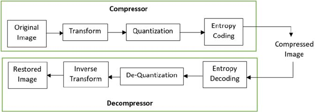
and the conditions under which the image was obtained. Figure 1.1 shows the
steps of image preprocessing during digital image processing.
1.2 Complications to Resolve Using Image Preprocessing
The following complications can be resolved by using image preprocessing
techniques.
2A Beginner’s Guide to Image Preprocessing Techniques
1.2.1 Image Correction
Image corrections are generally grouped into radiometric and geometric
corrections. Some standard correction methods might be completed prior to the
data being delivered to the user [5]. These techniques incorporate a radiometric
correction to correct for the irregular sensor reaction over the entire image, and
a geometric correction to correct for the geometric misrepresentation owing to
different imaging settings such as oblique viewing [6]. Radiometric correction
means correcting the radiometric error caused owing to the noise in the
brightness values of the image. Some common radiometric errors are random
bad pixels or shot noise, line start/stop problems, line or column dropouts,
and line or column striping [7]. Radiometric correction is a preprocessing
method to rebuild physically aligned values by altering the spectral faults and
falsications caused by the sensors themselves when the individual detectors
do not function properly, or are not properly calibrated for the sun’s direction
and or landscape [8]. For example, shot noise, which is generated when random
pixels are not recorded for one or more band, can be corrected by identifying
missing pixels. Missing pixel values can be regenerated by taking the average
of the neighboring pixels and lling in the value of the missing pixel. Figure
1.2 shows the preprocessed output.
Line start/stop problems occur when scanning detectors fail to start or are
out of sequence with other detectors, which results in displaced rows with the
pixel data at inappropriate locations along the scan line [9]. This can be solved
by determining the rows affected and offsetting and scripting a standard
offset for the affected rows. Figure 1.3 shows the preprocessing output.
Line or column dropout error occurs when an entire line does not contain
any information and results in blank lines or lines of same gray level value.
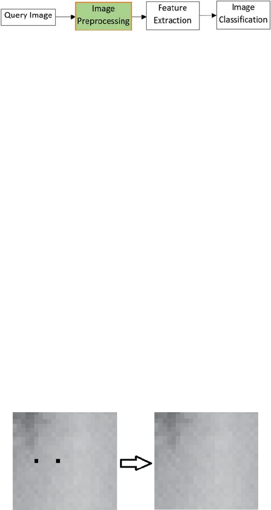
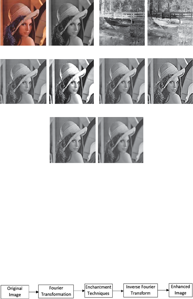
FIGURE 1.1
Image preprocessing step in digital image processing.
(A) (B)
FIGURE 1.2
(A) Image with shot noise, (B) Preprocessed output.
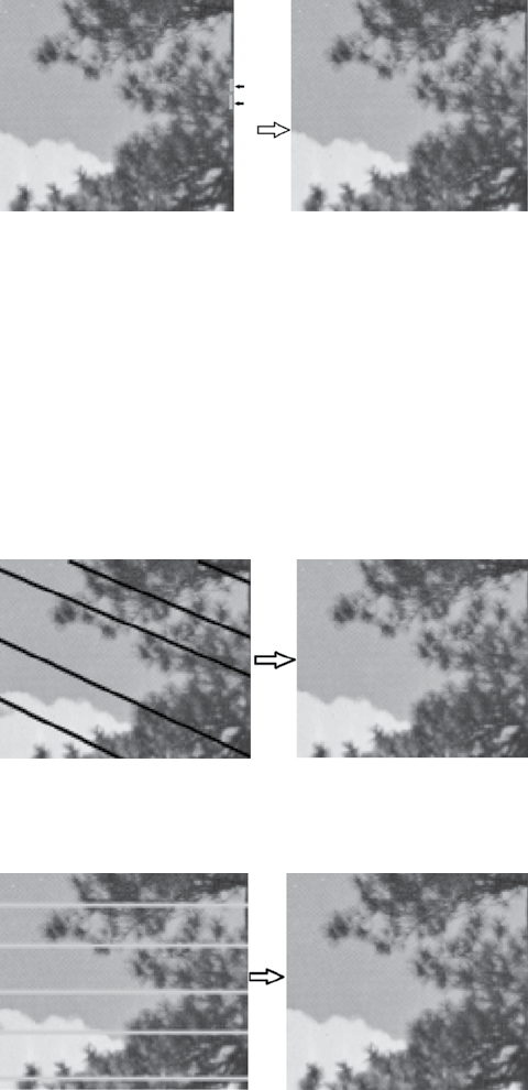
3Perspective of Image Preprocessing on Image Processing
This error can be corrected by averaging above and below pixel values to
record in each missing pixels, or ll in values from another image. Figure 1.4
shows the preprocessing output.
Line or column striping occurs when there are some stripes throughout the
entire image. This can be resolved by identifying the rows impacted through
analysis of a latitudinal geographic prole for the affected band. Figure 1.5
shows the preprocessing output.
(A) (B)
FIGURE 1.3
(A) Image with line start/stop problem, (B) Preprocessed image.
(A) (B)
FIGURE 1.4
(A) Image with line or column dropout, (B) Preprocessed output.
(A) (B)
FIGURE 1.5
(A) Image with line striping, (B) Preprocessed output.
4A Beginner’s Guide to Image Preprocessing Techniques
Geometric corrections contain modications of geometric distortions
caused by sensor–Earth geometry differences, translation of the data to
real-world latitude and longitude on the Earth’s surface, motion of platform,
Earth curvature, and so on [10]. Geometric correction means putting the
pixels in their proper location. This type of correction is generally needed
to coregister images for change detection, make accurate distance and area
measurements, and correct the imagery distortion. Sometimes the scale of
the same object varies due to some change in capturing the image. Geometric
error also involves perspective distortion. Fixing these types of distortion
involves resampling of the image data [11]. This can be done by determining
the correct geometric model, which tells how to transform images, in order
to compute the geometric transformations and basically how to analyze the
geometric error and resample to produce new output image data. Image
row/column coordinates are transformed to real-world coordinates using
polynomials [12]. One must choose the proper order of the polynomial. The
higher the transformation order, the greater the number of variables in the
polynomials and the more the warping stretches and twists in the dataset.
The higher order polynomial can provide misleading RMS errors. First order
polynomials, called afne transforms, are the linear conversion used to shift
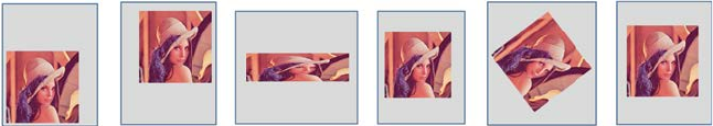
the origin of the image, as well as rescale and rotate it. Figure 1.6 shows the
outputs of afne transformation.
Second order polynomial is the nonlinear conversion used to correct the
camera lens distortion and correct for the Earth’s curvature. Figure 1.7 shows
the outputs of nonlinear transformation.
1.2.2 Image Enhancement
Image enhancement is mostly rening the sensitivity of information in
images for an improved input for automated image processing methods [13].
The primary goal of image enhancement is to adjust image attributes to make
them more appropriate for a given task. Through this method, one or more
attributes of the image are revised. Image enhancement is used to highlight
interesting details in images, remove noise from images, make images
more visually appealing, enhance otherwise hidden information, lter
(1A) (1B) (2A) (2B) (3A) (3B)
FIGURE 1.6
(1A) Original position of the image, (1B) Shift of origin of the image, (2A) Original scaling of
the image, (2B) Rescaling output of the image, (3A) Original orientation of the image, and (3B)
Change of orientation of the image.
5Perspective of Image Preprocessing on Image Processing
important image features, and discard unimportant image features [14]. The
enhancement approaches are generally divided into the following two types:
spatial domain methods and frequency domain methods. In spatial domain
methods, image pixels are enhanced directly. The pixel values are altered to
obtain the desired enhancements. The spatial domain image enhancement
operation is expressed by using Equation 1.1:
Sxy TIxy(, )[(, )],=
(1.1)
where
Ixy(, )
is the input image,
Sxy(, )
is the processed image, and T is an
operator on I dened over some neighborhood of
( ),xy
.
Some spatial domain image enhancement includes point processing, mask
processing, and so on. In point processing a neighborhood of 1 × 1 pixel is
considered. This is generally used to convert a color image to grayscale or
binary image and so forth. In mask processing, the neighborhood is larger
than a 1 × 1 pixel area. This is generally used in image sharpening, image
smoothing, and so on. Some of the spatial domain enhancements are shown
in Figure 1.8.
With frequency domain methods, rst the image is transmitted into the
frequency domain. The enhancement procedures are performed on the
frequency domain of the image, and then it is again transferred to the spatial
domain. Figure 1.9 illustrates the procedure.
The frequency domain image enhancement operation is expressed by using
Equation 1.2:
FuvHuvIuv(,)(,)(,),=
(1.2)
where
Iuv(,)
is the input image in the frequency domain,
Huv(,)
is the transfer
function, and
Fuv(,)
is the enhanced image. These enhancement processes are
done in order to enhance some frequency parts of the image. Some frequency
domain image enhancements are shown in Figure 1.10.
Through image enhancement, the pixel intensity values of the input image
are altered according to the enhancement function applied to the input
values.
(1A)(1B)(2A)(2B)
FIGURE 1.7
(1A) Ripple effect, (1B) Nonlinear correction output, (2A) Spherical effect, and (2B) Nonlinear
correction output.
6A Beginner’s Guide to Image Preprocessing Techniques
1.2.3 Image Restoration
The goal of image restoration methods is to decrease the noise effect or
corruption from the image and improve resolution loss. Image preprocessing
methods are done both in the image domain and the frequency domain.
Corruption may arise in many ways such as noise, motion blur, camera
misfocus, and so on [15]. Image restoration is not the same as image
enhancement, as the latter one is used to highlight features of the image used
FIGURE 1.9
Steps of enhancement of images in the frequency domain.
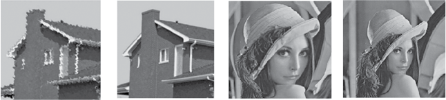
(I) (II)
(III)
(IV)
(V)
(A) (B) (A) (B)
(A) (B) (A) (B)
(
A
)(
B
)
FIGURE 1.8
Enhancement outputs in the spatial domain. (I) Conversion of true color image to grayscale
image: (A) True color image, (B) Grayscale Image; (II) Negative Transformation of a grayscale
image: (A) Original image, (B) Negative transformed image; (III) Contrast Enhancement: (A)
Original image, (B) Contrast enhanced image; (IV) Sharpening an image: (A) Original Image,
(B) Sharpen Image; (V) Smoothing an image: (A) Original image, (B) Smoothed image.
7Perspective of Image Preprocessing on Image Processing
to make it more attractive to the viewer, but it is not essential in obtaining
representative data from a scientic point of view. With image enhancement
noise can be efciently suppressed by losing some resolution, but this is not
satisfactory in many applications. Image restoration is useful in these cases.
Distorted pixels can be restored by the average value of the neighboring
pixels. Some outputs of the restored images are shown in Figure 1.11.
1.2.4 Image Compression
Image compression can be described as the procedure of encoding data using
a method that decreases the overall size of the image [16]. This reduction of
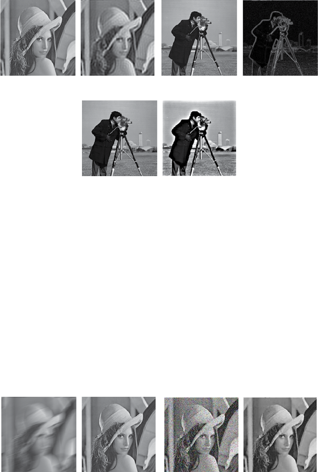
(I) (II)
(III)
(A) (B) (A) (B)
(A) (B)
FIGURE 1.10
Enhancement outputs in the frequency domain. (I) The output of low pass lter: (A) Original
image, (B) Filtered image; (II) The output of high pass lter: (A) Original image, (B) Filtered
image; (III) The output of bandpass lter: (A) Original image, (B) Filtered image.
(I) (II)
(A)(B)(A)(B)
FIGURE 1.11
Outputs of restored images. (I) Output of restoration of blurred image: (A) Blurred image,
(B)Restored image; (II) Noise reduction: (A) Noisy image, (B) Image after noise removal.
8A Beginner’s Guide to Image Preprocessing Techniques
data can be done when the original dataset holds some type of redundancy.
Image compression is used to reduce the total number of bits needed to
characterize an image. This can be accomplished by removing different
types of redundancy that occur in the pixel values. Generally, three basic
redundancies occur in digital images: (1) psycho-visual redundancy, which
corresponds to different intensities from image signals sensed by human
eyes. Therefore, removing some less important intensities may not be sensed
by human eyes; (2) interpixel redundancy, which corresponds to statistical
reliance among pixels, particularly between neighboring pixels; and (3)
coding redundancy, which occurs when the image is coded with every pixel
by a xed length. There are many methods to deal with these aforementioned
redundancies. Compression methods can be classied into two categories:
lossy compression and lossless compression. Lossy compression can attain
high compression ratios such as 60:1 or higher as it permits some tolerable
degradation, but lossless compression can attain very low compression ratios
such as 2:1 as it can completely recover the original data. In applications
where the image quality is the ultimate requirement, lossless compression
is used—such as in medical applications in which no degradation on the
original image data are permitted owing to the accuracy requirements for
diagnosis. Figure 1.12 shows the block diagram of lossy compression.
Lossy compression is basically a three-stage compression technique
to remove the three types of redundancies discussed above. First, a
transformation is applied to remove the interpixel redundancy to pack
information effectively. Then quantization is applied to eliminate psycho-
visual redundancy to characterize the packed information with the fewest
bits. The quantized bits are then prociently encoded to get much more
compression from the coding redundancy. Lossy decompression is a perfect
inverse technique of lossy compression.
Figure 1.13 shows the block diagram of lossless compression.
Lossless compression is usually a two-step compression technique. First,
transformation is applied to the original image to convert it to some other
format to reduce the interpixel redundancy. Then an entropy encoder is used
FIGURE 1.12
Block diagram of lossy compression.
9Perspective of Image Preprocessing on Image Processing
to eliminate the coding redundancy. Lossless decompression is a perfect
inverse technique of lossless compression.
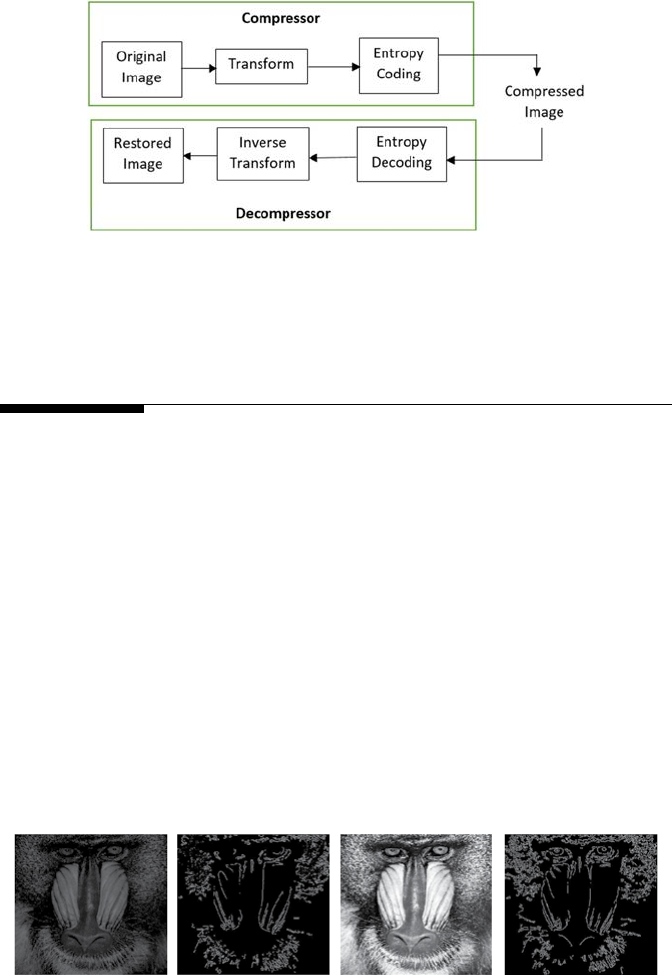
1.3 Effect of Image Preprocessing on Image Recognition
Image preprocessing is used to enhance the image data so that useful features
can be extracted for image recognition. Image cropping is used to crop the
irrelevant parts from the image so that the region of interest of the image
is focused. Image morphological operations can be applied in some cases.
Image ltering is used to create new intensity values in the output image.
Smoothing methods are used to remove noise or other small irrelevant data
in the image [17]. Filters are also used to highlight the edges of an image.
Brightness and contrast of the image can also be adjusted to enhance the
useful features of the image [18]. The unwanted areas can be removed from
the binary image by using a polygonal mask. Images can also be transformed
to different color modes for extraction of different types of features. If the
whole scene is rotated, or the image is taken from the wrong perspective,
it is required to correct the geometry prior to feature extraction, as many
features are dependent on geometric variation [19]. Figure 1.14 shows that
(1A)(1B)(2A)(2B)
FIGURE 1.14
(1A) Raw image, (1B) Extracted edge information from raw image, (2A) Preprocessed image,
and (2B) Extracted edge information from preprocessed image.
FIGURE 1.13
Block diagram of lossless compression.
10 A Beginner’s Guide to Image Preprocessing Techniques
more edge information can be obtained from a preprocessed image than
from a raw image.
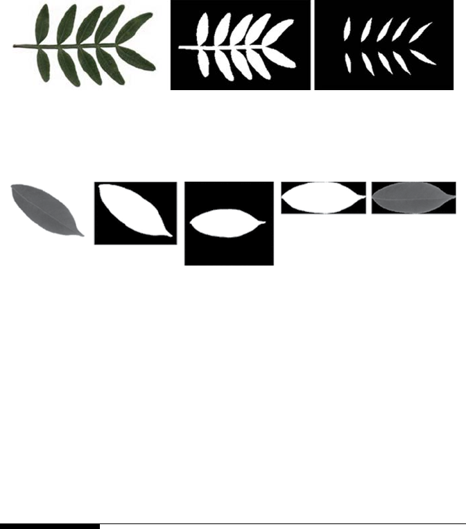
Suppose we have to count the number of leaets from a compound leaf
image [20]. In this particular example, the preprocessing steps involve
binarization and some morphological operations. Figure 1.15 illustrates this.
To correct the orientation and translation factor, preprocessing can be applied
as shown in Figure 1.16.
1.4 Summary
Image preprocessing is an enhancement of the image data to reduce reluctant
falsications or improve some image features vital for additional processing.
Preprocessing is generally used to correct the radiometric or geometric
errors, enhance the image, restore the image, and compress the image data.
Radiometric correction is used to correct for the irregular sensor reaction
over the entire image, and geometric correction is used to compensate for
the geometric misrepresentation due to different imaging settings such
as oblique viewing. Image enhancement is mainly used to adjust image
attributes to make it more appropriate for a given task. The goal of image
restoration methods is to decrease the noise effect or corruption from the
(A)(B)(C)(D)(E)
FIGURE 1.16
(A) The original image, (B) Binarized image, (C) Corrected orientation, (D) Corrected translation
factor, and (E) Preprocessed image after correcting the orientation and translation.
(A) (B) (C)
FIGURE 1.15
(A) Original gray image, (B) Binarized image, and (C) Separation of leaets using morphological
erosion operation.

11Perspective of Image Preprocessing on Image Processing
image and improve resolution loss. Image compression is used to decrease
the overall size of the image. Image preprocessing is used to enhance the
image data so that useful features can be extracted for image recognition.
References
1. Chatterjee, S., Ghosh, S., Dawn, S., Hore, S., & Dey, N. 2016. Forest type
classication: A hybrid NN-GA model based approach. In Information Systems
Design and Intelligent Applications (pp. 227–236). Springer, New Delhi.
2. Santosh, K. C., & Nattee, C. 2009. A comprehensive survey on on-line
handwriting recognition technology and its real application to the Nepalese
natural handwriting. Kathmandu University Journal of Science, Engineering, and
Technology, 5(I), 31–55.
3. Hore, S., Chakroborty, S., Ashour, A. S., Dey, N., Ashour, A. S., Sifaki-Pistolla,
D., Bhattacharya, T., & Chaudhuri, S. R. 2015. Finding contours of hippocampus
brain cell using microscopic image analysis. Journal of Advanced Microscopy
Research, 10(2), 93–103.
4. Dey, N., Roy, A. B., Das, P., Das, A., & Chaudhuri, S. S. 2012, November. Detection
and measurement of arc of lumen calcication from intravascular ultrasound
using harris corner detection. In Computing and Communication Systems (NCCCS),
2012 National Conference on (pp. 1–6). IEEE.
5. Santosh, K. C., Lamiroy, B., & Wendling, L. 2012. Symbol recognition using
spatial relations. Pattern Recognition Letters, 33(3), 331–341.
6. Dey, N., Ahmed, S. S., Chakraborty, S., Maji, P., Das, A., & Chaudhuri, S. S.
2017. Effect of trigonometric functions-based watermarking on blood vessel
extraction: An application in ophthalmology imaging. International Journal of
Embedded Systems, 9(1), 90–100.
7. Saha, M., Chaki, J., & Parekh, R. 2013. Fingerprint recognition using texture
features. International Journal of Science and Research, 2, 12.
8. Chakraborty, S., Mukherjee, A., Chatterjee, D., Maji, P., Acharjee, S., & Dey, N.
2014, December. A semi-automated system for optic nerve head segmentation
in digital retinal images. In Information Technology (ICIT), 2014 International
Conference on (pp. 112–117). IEEE.
9. Hossain, K., Chaki, J., & Parekh, R. 2014. Translation and retrieval of image
information to and from sound. International Journal of Computer Applications,
97(21), 24–29.
10. Dey, N., Roy, A. B., & Das, A. 2012, August. Detection and measurement of
bimalleolar fractures using Harris corner. In Proceedings of the International
Conference on Advances in Computing, Communications and Informatics (pp. 45–51).
ACM, Chennai, India.
11. Belaïd, A., Santosh, K. C., & d’Andecy, V. P. 2013. Handwritten and printed text
separation in real document. arXiv preprint arXiv:1303.4614.
12. Dey, N., Nandi, P., Barman, N., Das, D., & Chakraborty, S. 2012. A comparative
study between Moravec and Harris corner detection of noisy images using
adaptive wavelet thresholding technique. arXiv preprint arXiv:1209.1558.
12 A Beginner’s Guide to Image Preprocessing Techniques
13. Russ, J. C. 2016. The Image Processing handbook. CRC Press, Boca Raton, FL.
14. Araki, T., Ikeda, N., Dey, N., Acharjee, S., Molinari, F., Saba, L., Godia, E.,
Nicolaides, A., & Suri, J. S. 2015. Shape-based approach for coronary calcium
lesion volume measurement on intravascular ultrasound imaging and its
association with carotid intima-media thickness. Journal of Ultrasound in
Medicine, 34(3), 469–482.
15. Ashour, A. S., Samanta, S., Dey, N., Kausar, N., Abdessalemkaraa, W. B., &
Hassanien, A. E. 2015. Computed tomography image enhancement using
cuckoo search: A log transform based approach. Journal of Signal and Information
Processing, 6(03), 244.
16. Nandi, D., Ashour, A. S., Samanta, S., Chakraborty, S., Salem, M. A., & Dey,N.
2015. Principal component analysis in medical image processing: A study.
International Journal of Image Mining, 1(1), 65–86.
17. Hangarge, M., Santosh, K. C., Doddamani, S., & Pardeshi, R. 2013. Statistical
texture features based handwritten and printed text classication in south
indian documents. arXiv preprint arXiv:1303.3087.
18. Chaki, J., Parekh, R., & Bhattacharya, S. 2016. Plant leaf recognition using ridge
lter and curvelet transform with neuro-fuzzy classier. In Proceedings of 3rd
International Conference on Advanced Computing, Networking and Informatics
(pp.37–44). Springer, New Delhi.
19. Chaki, J., Parekh, R., & Bhattacharya, S. 2015. Plant leaf recognition using
texture and shape features with neural classiers. Pattern Recognition Letters,
58, 61– 68.
20. Chaki, J., Parekh, R., & Bhattacharya, S. In press. Plant leaf classication using
multiple descriptors: A hierarchical approach. Journal of King Saud University-
Computer and Information Sciences, doi:10.1016/j.jksuci.2018.01.007.

13
2
Pixel Brightness Transformation Techniques
Pixel brightness can be revised by using pixel brightness techniques. The
transformation relies on the characteristics of a pixel itself. There are two
types of pixel brightness transformations: Position-dependent brightness
correction and grayscale transformation [1]. The position-dependent
brightness correction, or simply brightness correction, modies the pixel
brightness value by considering the original brightness of the pixel and its
position in the image. Grayscale transformation modies the brightness of
the pixel regardless of the position of the pixel.
2.1 Position-Dependent Brightness Correction
The quality of acquisition and digitization of an image is not dependent on the
pixel position in the image, however, in many practical cases this theory is not
valid [2]. There are different reasons for the degradation of the image quality:
rst, the uneven sensitivity of the light sensors such as CCD camera elements,
vacuum-tube cameras, and so on; second, the nonhomogeneous property of
the optical system, that is, if the lens passes farther from the optical lens,
the lens decreases light more; and last, the uneven object illumination. With
brightness correction, the systematic degradation can be suppressed. The
ideal identity transfer function can be described by a multiplicative error
coefcient E(p, q). Let the original undegraded, or desired, image be G(p, q)
and the image containing degradation F(p, q)
Fp qEpqGp q(, )(,)(, ).=
(2.1)
If the reference image G(p, q) is captured with a known constant brightness
C, then the error coefcient E(p, q) can be obtained. If the image containing
degradation is Fc(p, q), the systematic brightness errors can be suppressed by
Equation 2.2:
G
pq
Fp q
Ep q
CFpq
Fpq
c
(, )
(, )
(, )
(, )
(, )
.
==
×
(2.2)
This technique can be adopted if the degradation process of the image is stable.
Periodic calibration is needed for the device to nd the error coefcient E(p, q).

14 A Beginner’s Guide to Image Preprocessing Techniques
This method indirectly adopts linearity of the transformation [3]. But as the
brightness scale is restricted to some interval, this technique is not true in
reality. Equation 2.1 can overow. This indicates that the best reference image
has brightness that is far from both the minimum and maximum limits of the
brightness. If the gray scale has 256 levels of brightness, then the best image
has a persistent brightness level of 128. Most TV cameras permit us to control
the varying illumination settings, as they have automatic gain controllers.
This automatic gain control should be switched off rst if systematic errors
are suppressed using error coefcients.
2.2 Grayscale Transformations
This transformation is not dependent on the pixel position in the image
[4]. Here, an input image I is transformed into G by using T. Where T is the
transformation. Let the pixel value of I and G be represented as PI and PG,
respectively. So, the pixel values are related by Equation 2.3:
P P
GI
=T.
(2.3)
Using Equation 2.3, the pixel value PI is mapped to PG by the transformation
function T. As we are dealing only with the grayscale transformation, the
output of this transformation is mapped to a grayscale range. The output is
mapped to the range [0, L − 1], where L = 2m, m is the number of bits in the
image. For example, the range of pixel values of an 8-bit image will be [0, 255].
The following are three basic gray level transformations used in image
enhancement:
• Linear transformation
• Logarithmic transformation
• Powerlaw transformation.
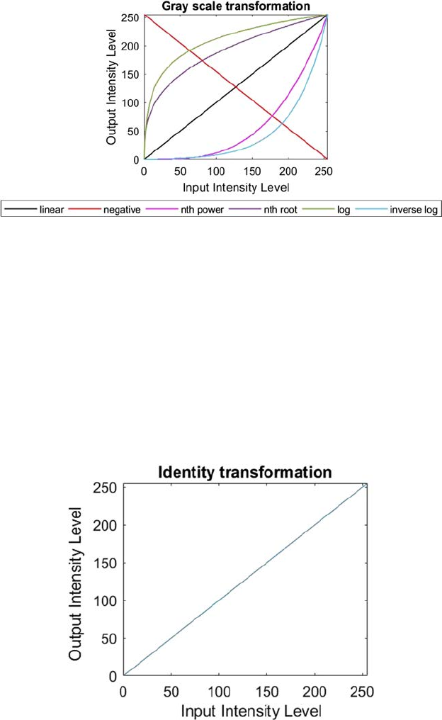
Figure 2.1 shows the plots of different grayscale transformation functions.
Here, L represents the number of gray levels. The identity and negative
transformation function plots are the types of linear transformations; log
and inverse log transformation function plots are the types of logarithmic
transformation plots, and nth root and nth power transformation function
plots are the types of power-law transformations.
2.2.1 Linear Transformation
There are two types of linear transformation: identity transformation and
negative transformation [5]. In identity transformation each pixel value of
the input image is directly mapped to the pixel value of the output image. So
15Pixel Brightness Transformation Techniques
the result is same in the input and output image. Hence, it is called identity
transformation. The graph of identity transformation is shown in Figure 2.2.
This particular graph shows that between the input and output image there
is a straight transition line. This represents that for each input pixel value,
the output pixel value will remain the same. So, here the output image is the
replica of the input image. Linear transformation can be used to convert a
color image into gray scale. Let I(p, q) be the input image and G(p, q) the output
image. Then the linear transformation can be represented by Equation 2.4:
Gpq Ipq(, )(,).=
(2.4)
FIGURE 2.1
Different grayscale transformation functions.
FIGURE 2.2
Identity transformation plot.
16 A Beginner’s Guide to Image Preprocessing Techniques
Figure 2.3 shows the input and output of linear transformation.
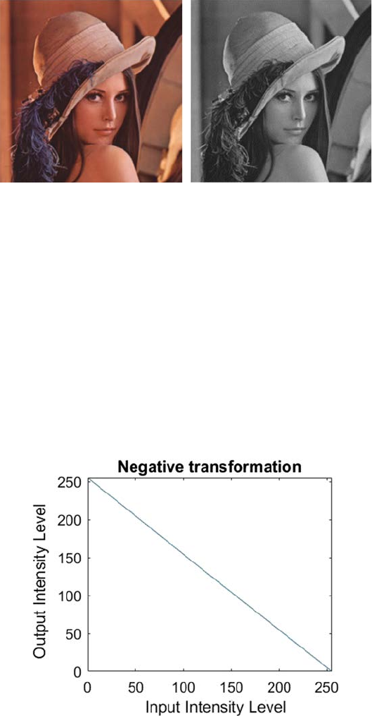
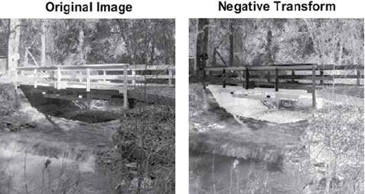
The second type of linear transformation is negative transformation
[6]. This is basically the inverse of the linear transformation. The negative
transformation of an image with gray levels within the range [0, L − 1] can be
obtained by subtracting each input pixel value from [L − 1] and mapping it
into the output image, which can be expressed by the Equation 2.5:
PLP
GI
=−−1.
(2.5)
This expression indicates the reversing of the gray level intensities of the
input pixels, therefore producing a negative image. The graph of negative
transformation is shown in Figure 2.4.
(A) (B)
FIGURE 2.3
(A) Input image, (B) Linear transformed image.
FIGURE 2.4
Negative transformation plot.
17Pixel Brightness Transformation Techniques
This technique is benecial for improving gray or white details implanted
in the dark regions of an image. Figure 2.5 shows the input and output of
negative transformation.
In the above example, the input image is an 8-bit image. So, there are 256
levels of variations of gray. Putting this in Equation 2.6, we get
PPP
GII
=−−= −256 1 255 .
(2.6)
So, by applying the negative transformation, lighter pixels become dark and
darker pixels become light.
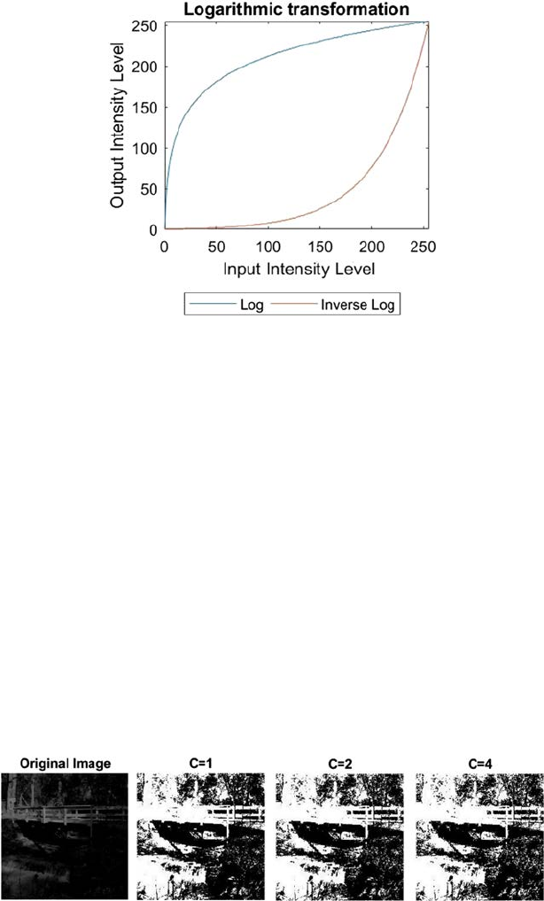
2.2.2 Logarithmic Transformation
This transformation can be used to brighten the intensity of a pixel in an
image [7]. There are various reasons to work with logarithmic intensities
rather than with the actual pixel intensity: the logged intensity values are
comparatively less dependent on the magnitude of the pixel values, the
skewness of the highly skewed values reduces while considering the logs,
and the variance estimation increases when using logarithmic values.
The visual inspection of data becomes easier by using logged intensities.
The raw data are frequently severely clomped together at low intensities
followed by a very long tail. Over 75% of the image information may lie in
the least 10% values of intensities. The details of such parts are difcult to
recognize. After the logarithmic transformation, the change of intensity
information is spread out more equally making it simpler to analyze. There
are two types of logarithmic transformation: log transformation and inverse
log transformation. The graph for log and inverse log transformation is
shown in Figure 2.6.
(A) (B)
FIGURE 2.5
(A) Input image, (B) Negative transformed image.
18 A Beginner’s Guide to Image Preprocessing Techniques
The log transformation is used to brighten or increase the detail of the
lower intensity values of an image. This can be expressed by the Equation 2.7:
PcP
GI
=× +log( ),1
(2.7)
where c is a constant which is normally used to scale the scope of the log
transformation function to match the input area. For a 8-bit image, c = 255/
log(1 + 255). It can be used to additionally increase the contrast—the higher
the c, the brighter the image will appear.
The value 1 is added to every one of the pixel values of the input image in light
of the fact that if there is a pixel intensity of 0 in the image, at that point log (0) is
equivalent to innity. So 1 is included, to make the minimum value no less than1.
During log transformation, the dark pixels in an image are extended compared
to the higher pixel values. The higher pixel values are somewhat compressed in
log transformation. This makes for the improvement of the image.
Figure 2.7 demonstrates the outcomes of log transformation of the original
image. We can see that when c = 4, the image is the brightest and the
FIGURE 2.6
Logarithmic transformation plot.
FIGURE 2.7
Results of log transformation.
19Pixel Brightness Transformation Techniques
outspread lines are visible within the tree. These lines are not visible in the
original image, as there isn’t sufcient contrast in the lower intensities.
Inverse log transformation is opposite of the log transformation. It expands
bright regions and compresses the darker intensity level values.
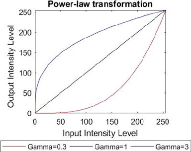
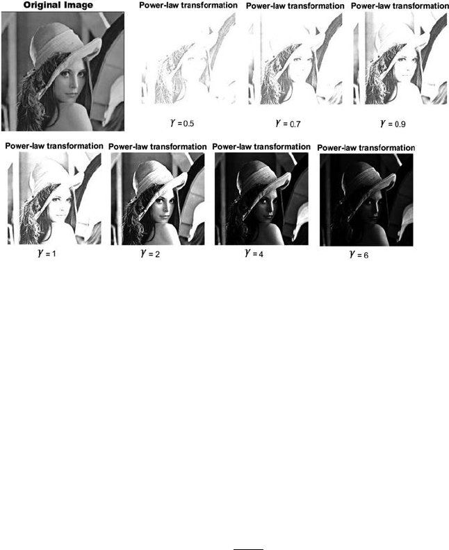
2.2.3 Power-Law Transformation
This transformation is used to increase the contrast of the image [8]. There
are two types of power-law transformations: n-th power and n-th root
transformation. These transformations can be expressed by Equation 2.8:
PCP
GI
=×
γ.
(2.8)
The symbol γ is called gamma and this transformation is also called
gamma correction. For different values of γ, various levels of enhancement of
the image can be obtained. The graph of power-law transformation is shown
in Figure 2.8.
Different monitors or display devices have their own gamma correction.
That is the reason they display their image at various intensity. This sort of
transformation is used for improving images for various kinds of monitors.
The gamma of various monitors is different. For instance, the gamma of
monitors lies between 1.8 and 2.5, which implies the image displayed on
monitor is dark. The same image with different γ values is shown in Figure2.9.
Digital images have a nite number of gray levels [9]. Thus, grayscale
transformations should be possible using look-up tables. Grayscale
transformations are mostly used if the outcome is seen by a human. One
way to improve the contrast of the image is contrast stretching (also known
as normalization) [10]. Contrast stretching is a linear normalization that
expands an arbitrary interval of the intensities of an image and ts this
FIGURE 2.8
Power-law transformation plot.
20 A Beginner’s Guide to Image Preprocessing Techniques
interval to another arbitrary interval. The initial step is to decide the limits
over which image intensity values will be expanded. These lower and upper
limits will be known as p and q, individually. For standard 8-bit grayscale
images, these limits are normally 0 and 255. Next, the histogram of the input
or original image is examined to decide the possible value limits (lower = a,
upper = b) in the unmodied image. If the input image covers the entire
possible set of values, direct contrast stretching will achieve nothing, but,
even then sometimes the majority of the picture information is contained
within a restricted range. This restricted range can be extended linearly with
original values, which lie outside the range, being set to the appropriate limit
of the extended output range. Then for every pixel, the original value PI is
mapped to output PG by using Equation 2.9:
P
Pa
qp
ba
p
GI
=−
−
−
+()
.
(2.9)
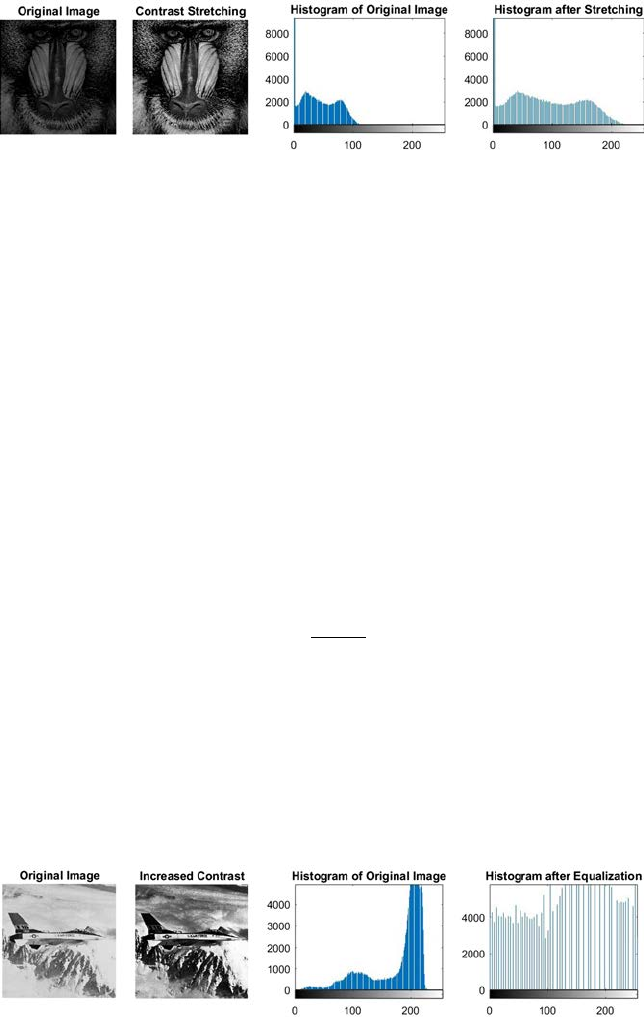
Figure 2.10 shows the result after contrast stretching. In contrast stretching,
there exists a one-to-one relationship of the intensity values between the
original or input image and the output image; that is, after contrast stretching
the input image can be restored from the output image.
Another transformation for contrast improvement is usually applied
automatically using histogram equalization, which is a nonlinear
normalization, expanding the range of the histogram with high intensities
and compressing the areas with low intensities [11]. The point is to discover
an image with equally distributed brightness levels over the whole brightness
scale. Histogram equalization improves contrast for brightness values close
FIGURE 2.9
Results of Gamma variation where C = 2.
21Pixel Brightness Transformation Techniques
to histogram maxima, and decreases contrast near the minima. Figure 2.11
shows the result after histogram equalization. Once histogram equalization
is executed, there is no technique for getting back the original image.
Let the input histogram be denoted by Hp where p0 ≤ p ≤ pt. The intention
is to nd a monotonic transform of grayscale q = T(p), for which the output
histogram Gq will remain uniform for the whole input brightness domain,
where q0 ≤ q ≤ qt. This monotonic property of T can be expressed by
Equation2.10:
k
t
qk
k
t
pk
GH
==
∑∑
=
00
.
(2.10)
The equalized histogram Gqk corresponds to a uniform distribution function
F whose value is constant and can be expressed by Equation 2.11 for a N × N
image,
F
=−
N
qq
t
2
0
.
(2.11)
In the continuous case, the ideal continuous histogram is available and can
be expressed by Equation 2.12:
q
q
p
p
Gsds Hsds
00
∫∫
=() ()
.
(2.12)
FIGURE 2.10
Contrast stretching results.
FIGURE 2.11
Histogram equalization result.
22 A Beginner’s Guide to Image Preprocessing Techniques
Substituting Equation 2.11 in Equation 2.12 we get
Nqq
ds Hsds
Nq q
qq Hsds
qp
q
q
q
tp
p
tp
p
t
2
0
20
0
00
0
1
∫∫
∫
−=
−
−=
==
()
()
()
()
T−− +
∫
q
NHsds q
p
p
0
20
0
()
.
(2.13)
For discrete case, this is called cumulative histogram, which is approximated
by the sum in the digital images and can be expressed by Equation 2.14:
qp
qq
NHk q
t
kp
p
==
−+
=
∑
T() ()
.
0
20
0
(2.14)
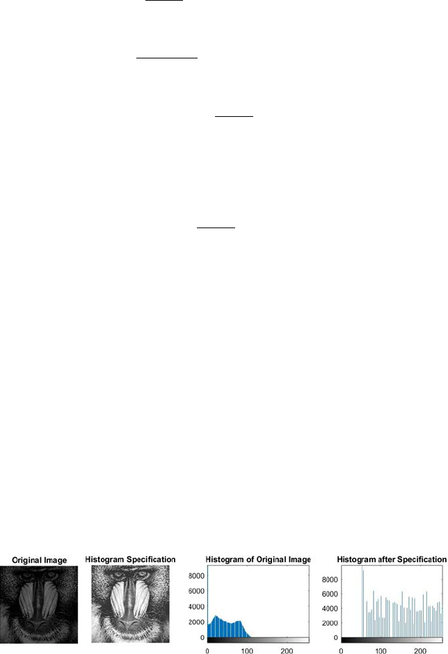
Histogram specication, or histogram matching, can also be used to enhance
the contrast of an image [12]. Histogram specication, or histogram matching,
is a method that changes the histogram of one image into the histogram of
another image. This change can be effortlessly done by perceiving that if as
opposed to using an equally separated perfect histogram (as in histogram
equalization), one is specied explicitly. By this method, it is possible to impose
an arbitrary histogram of an image to another. First, choose the template
histogram. This can be done by determining a specic histogram shape, or
by calculating the histogram of a target image. Then, the histogram of the
image to be transformed is calculated. Afterwards, calculate the cumulative
aggregate of the template histogram. Then, calculate the cumulative aggregate
of the histogram of the image to be changed. Finally, map pixels from one
bin to another bin, as per the guidelines of histogram equalization. The
essential rule is that the actual cumulative aggregate cannot be less than the
cumulative aggregate of the template image. Figure2.12 shows the result of
histogram specication.
FIGURE 2.12
Result of histogram specication.

23Pixel Brightness Transformation Techniques
2.3 Summary
In image preprocessing, image information captured by sensors on a satellite
contains faults associated with geometry and brightness information of the
pixels. These errors are improved using suitable techniques. Image enhancement
is the adjustment of an image by altering the pixel brightness values to enhance
its visual effect. Image enhancement includes a collection of methods used to
improve the visual presence of an image, or to alter the image to a form better
matched for human or machine understanding. This chapter describes the image
enhancement methods by using pixel brightness transformation techniques.
Two types of pixel brightness transformation techniques are discussed in this
chapter: position dependent and independent, or grayscale transformation. The
position-dependent brightness correction modies the pixel brightness value by
considering the original brightness of the pixel and its position in the image. But,
grayscale transformation alters the brightness of the pixel regardless the position
of the pixel. There are different variations in gray level transformation techniques:
linear, logarithmic, and power-law. The identity transformation, which is a type
of linear transformation, is mainly used to convert the color image into gray
scale. The second type of linear transformation, that is, negative transformation
can be used to enhance the gray or white details embedded into the dark region
of the image. By using this transformation lighter pixels become dark and
darker pixels become light. The logarithmic transformation is used to brighten
the intensity of a pixel in an image. The log transformation, which is a type of
logarithmic transformation, is used to brighten or increase the detail of the lower
intensity values of an image. The second type of logarithmic transformation,
that is, inverse log transformation is opposite to the log transformation. Power-
law transformation, also known as gamma correction transformation, is used to
increase the contrast of an image. For different values of gamma, various levels
of enhancement of the image can be obtained. This sort of transformation is
used for improving images for various kinds of monitors. To enhance the image
contrast, different types of methods can be adopted like contrast stretching,
histogram equalization, and histogram specication. Contrast stretching is a
linear transformation and the original image can be retrieved from the contrast-
stretched image. Histogram equalization is a nonlinear transformation and
doesn’t allow for the retrieval of the original image from the histogram-equalized
image. In case of histogram specication, the histogram of a template image can
be applied to the input image to enhance the contrast of the input image.
References
1. Umbaugh, S. E. 2016. Digital Image Processing and Analysis: Human and Computer
Vision Applications with CVIPtools. CRC Press, Boca Raton, FL.
2. Russ, J. C. 2016. The Image Processing Handbook. CRC Press, Boca Raton, FL.
24 A Beginner’s Guide to Image Preprocessing Techniques
3. Saba, L., Dey, N., Ashour, A. S., Samanta, S., Nath, S. S., Chakraborty, S.,
Sanches,J., Kumar, D., Marinho, R., & Suri, J. S. 2016. Automated stratication of
liver disease in ultrasound: An online accurate feature classication paradigm.
Computer Methods and Programs in Biomedicine, 130, 118–134.
4. Chaki, J., Parekh, R., & Bhattacharya, S. In press. Plant leaf classication using
multiple descriptors: A hierarchical approach. Journal of King Saud University-
Computer and Information Sciences, doi:10.1016/j.jksuci.2018.01.007.
5. Bhattacharya, T., Dey, N., & Chaudhuri, S. R. 2012. A session based multiple
image hiding technique using DWT and DCT. arXiv preprint arXiv:1208.0950.
6. Kotyk, T., Ashour, A. S., Chakraborty, S., Dey, N., & Balas, V. E. 2015. Apoptosis
analysis in classication paradigm: A neural network based approach. In Healthy
World Conference—A Healthy World for a Happy Life (pp. 17–22). Kakinada (AP), India.
7. Ashour, A. S., Samanta, S., Dey, N., Kausar, N., Abdessalemkaraa, W. B., &
Hassanien, A. E. 2015. Computed tomography image enhancement using
cuckoo search: A log transform based approach. Journal of Signal and Information
Processing, 6(03), 244.
8. Francisco, L., & Campos, C. 2017, October. Learning digital image processing
concepts with simple scilab graphical user interfaces. In European Congress on
Computational Methods in Applied Sciences and Engineering (pp. 548–559). Springer,
Cham.
9. Chakraborty, S., Chatterjee, S., Ashour, A. S., Mali, K., & Dey, N. 2018. Intelligent
computing in medical imaging: A study. In Advancements in Applied Metaheuristic
Computing (pp. 143–163). IGI Global, Hershey, Pennsylvania.
10. Negi, S. S., & Bhandari, Y. S. 2014, May. A hybrid approach to image enhancement
using contrast stretching on image sharpening and the analysis of various
cases arising using histogram. In Recent Advances and Innovations in Engineering
(ICRAIE), 2014 (pp. 1–6). IEEE.
11. Dey, N., Roy, A. B., Pal, M., & Das, A. 2012. FCM based blood vessel segmentation
method for retinal images. arXiv preprint arXiv:1209.1181.
12. Wegner, D., & Repasi, E. 2016, May. Image based performance analysis of thermal
imagers. In Infrared Imaging Systems: Design, Analysis, Modeling, and Testing
XXVII (Vol. 9820, p. 982016). International Society for Optics and Photonics.

25
3
Geometric Transformation Techniques
Geometric transformations allow the removal of geometric distortion that
happens when an image is captured. For example, if one wants to match images
of a similar location taken after one year when the later image was perhaps
not taken from exactly the same location. To assess changes throughout the
year, it is required initially to accomplish a geometric transformation, and
afterward, subtract one image from the other. Geometric transformations are
often required where the digitized image may be misaligned [1].
There are two basic steps in geometric transformations:
• Pixel coordinate transformation or spatial transformation
• Brightness interpolation.
3.1 Pixel Coordinate Transformation or Spatial Transformation
Pixel coordinate transformation or spatial transformation of an image is a
geometric transformation of the image coordinate system, that is, the mapping
of one coordinate system onto another. This is characterized by methods of
spatial transformation which are mapping functions that builds up a spatial
correspondences between every point in the input and output images. Each
point in the output adopts the value of its equivalent point in the input image
[2]. The correspondence is established via the spatial transformation mapping
function to assign the output point onto the input image. It is frequently
required to do a spatial transformation to (1) align images captured with
different types of sensors or at different times, (2) correct the image distortion
caused by the lens and camera orientations, and (3) image morphing or other
special effects and so on [3].
An input image comprises known coordinate reference points. The output
image consists of the distorted data. The general mapping function can either
relate the output coordinate system to that of the input, or vice versa. Let
G(x′,y′) denote the input or original image, and I(x, y) be the deformed (or
distorted) image. We can relate corresponding pixels in the two images by
Equation 3.1:
I G.
(3.1)
26 A Beginner’s Guide to Image Preprocessing Techniques
Two types of mapping can be done here:
• Forward Mapping: Map pixels of input image onto output image,
which can be represented by Equation 3.2:
Gxy Ixy(, )(,).
′′
=
(3.2)
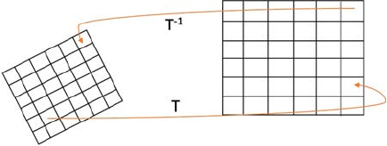
• Inverse Mapping: Map pixels of output image onto the input image,
which can be represented by Equation 3.3:
Ixy Gx y(, )(,).=′′
(3.3)
General mapping example is shown in Figure 3.1.
3.1.1 Simple Mapping Techniques
Translation: Translation means moving the image from one position to another
[4]. Let the translation amount in the x and y-direction be tx and ty respectively.
Translation can be dened by the Equation 3.4:
′
′
=+
=+
′
′
=
+
xxt
yyt
x
y
x
y
t
t
x
y
x
y
OR
.
(3.4)
Translation of a geometric shape, as well as an image, is shown in
Figure3.2.
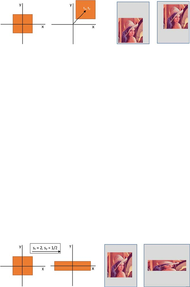
Scaling: Scaling means stretching or contracting an image based on some
scaling factors [5,6,7]. Let, sx and sy be the scaling factor in the x and y-direction.
Scaling can be dened by Equation 3.5:
FIGURE 3.1
T: Forward mapping; T−1: Inverse mapping.
27Geometric Transformation Techniques
′
′
=⋅
=⋅
′
′
=
⋅
xxs
yys
x
y
s
s
x
y
x
y
x
y
OR
0
0
,
(3.5)
sx > 1 represents stretching, sx < 1 represents contracting or shrinking, and
sx = 1 means that the size will remain the same.
Scaling of a geometric shape, as well as an image, is shown in Figure 3.3.
Rotation: Rotation means [5,6,7] to change the orientation of an image by an
angle of θ, which is dened by Equation 3.6:
′
′
=⋅ −⋅
=⋅ +⋅
′
′
xx y
yx y
x
y
cos( )sin()
sin( )cos()
θθ
θθ
OR
== −
⋅
cos( )sin()
sin( )cos()
.
θθ
θθ
x
y
(3.6)
Rotation of a geometric shape as well as of an image is shown in Figure 3.4.
(A) (B) (C) (D)
FIGURE 3.2
(A) Original position of the rectangle, (B) Final position of the rectangle after translation,
(C)Original position of an image, and (D) Final position of an image after translation.
(A) (B) (C) (D)
FIGURE 3.3
(A) The original size of the rectangle, (B) Modied size of the rectangle, (C) Original size of the
image, and (D) Modied size of the image.
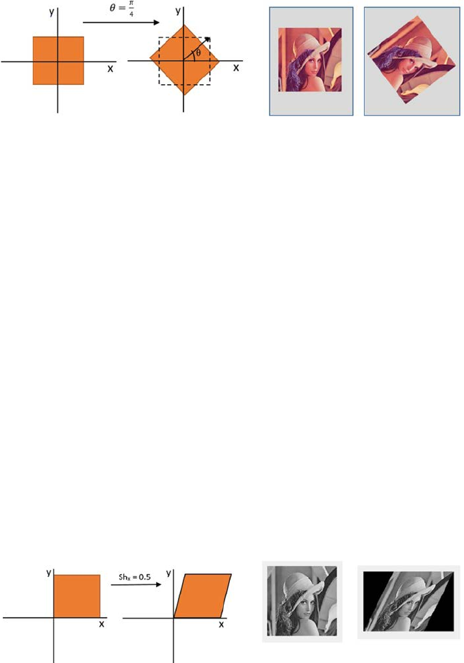
28 A Beginner’s Guide to Image Preprocessing Techniques
Shearing: Images can be sheared along horizontal and vertical direction
[8]. For horizontal shears, pixels are relocated horizontally by a distance
increasing linearly with the (vertical) distance from the horizontal line,
moving to the right above the line and to the left below the line for positive
angles. Likewise, for vertical shear, pixels are relocated vertically by a distance
that increases linearly with the (horizontal) distance from the vertical line,
moving downward to the right of the line, and upward to the left of the
line for positive angles. Let, Shx and Shy be the shear amount in the x and
y-direction. Shear can be represented by Equation 3.7:
′
′
=+ ⋅
=+ ⋅
′
′
=
xx y
yy x
x
y
x
y
x
y
Sh
Sh
OR
Sh
Sh
1
1⋅
x
y
.
(3.7)
Shear of a geometric shape, as well as an image, is shown in Figure 3.5.
(A) (B) (C) (D)
FIGURE 3.4
(A) Original orientation of rectangle, (B) Modied orientation of rectangle, (C) Original
orientation of image, and (D) Modied orientation of image.
(A) (B)
(C)(D)
FIGURE 3.5
(A) Original rectangle, (B) Horizontal sheared rectangle, (C) Original image, and (D) Horizontal
sheared image.
29Geometric Transformation Techniques
3.1.2 Affine Mapping
All possible simple mapping or transformations are special cases of afne
mapping [9,10]. The afne transformation is the combination of simple
transformations. Afne mapping is a linear mapping method, which
conserves straight lines, planes, and points. Sets of parallel lines stay parallel
after an afne transformation.
The overall afne transformation is normally written in homogeneous
coordinates, as shown in Equation 3.8:
′
′
=×
+
x
yP
x
yQ
.
(3.8)
By dening only the Q matrix, this transformation turns to a pure translation
transformation, as shown in Equation 3.9:
P
Q
t
t
x
y
=
=
10
01
,.
(3.9)
By dening only the P matrix, this transformation turns into a pure rotation
transformation (for positive or clockwise rotation), as shown in Equation 3.10:
P
Q=
−
=
cos( )sin()
sin( )cos()
,.
θθ
θθ
0
0
(3.10)
Similarly, pure scaling can be dened by Equation 3.11:
Ps
sQ
x
y
=
=
0
0
0
0
,.
(3.11)
Since the general afne transformation is characterized by six constants, it
is conceivable to express this transformation by determining the new output
image locations (x′, y′) of any three input image coordinate (x, y) pairs. In
general, several points are estimated and a least squares technique is used to
nd the nest tting transform.
3.1.3 Nonlinear Mapping
Twirl: In case of twirl, rather than using image color at (x′, y′), use image
colors at twirled (x, y) position [11]. Rotate or turn the image by an angle
θ at the anchor point or center (xc, yc). Progressively, turn the image as the
spiral distance S from the center increases up to Smax. The image remains
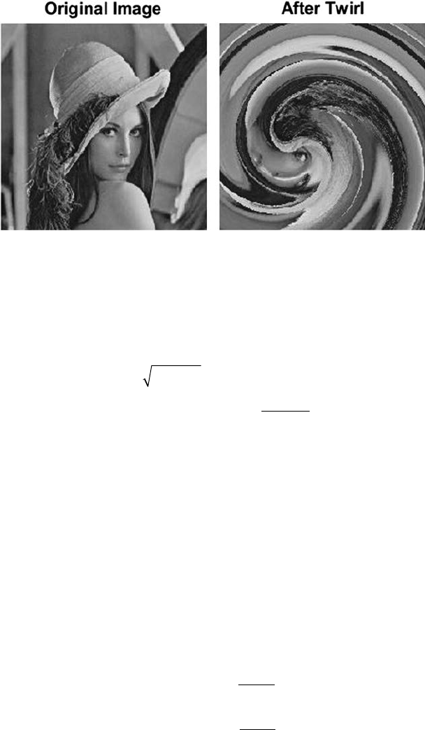
30 A Beginner’s Guide to Image Preprocessing Techniques
unaffected outside of the radial distance Smax. Twirl can be dened by
Equation 3.12:
Dxx Dyy
SDD
DD
SS
S
xc
yc
xy
yx
=− =−
=+
=+
⋅−
′′
,
(,)max
max
22
αθ
arctan
=+⋅ ≤
>
=+⋅
′
xxr SS
xS
S
yyr
c
c
cos( )
sin
max
max
αif
if
(()
.
max
max
αif
if
SS
yS
S
≤
>
′
(3.12)
The twirl effect of an image is shown in Figure 3.6.
Ripple: Ripple effects are like wave patterns, which are introduced in the
image along both the x and y-directions [12]. Let the amplitude of the wave
pattern in the x and y-direction is dened as Ax and Ay, respectively, and
the frequency of the wave in the x and y-direction is dened as Fx and Fy,
respectively. So, this effect can be expressed by the sinusoidal function, as
shown in Equation 3.13:
xx
Ay
F
yy
Ax
F
x
x
y
y
=+
′
=+ ′
′⋅⋅
′⋅⋅
sin
sin
2
2
π
π
.
(3.13)
FIGURE 3.6
Twirl effect of an image.
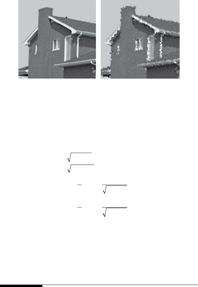
31Geometric Transformation Techniques
The ripple effect of an image is shown in Figure 3.7.
Spherical Transformation: This transformation zooms in the center of the
image. Let the center of the lens be (xc, yc), Lmax the lens radius, and τ is the
refraction index [13]. The spherical transformation is dened by Equation 3.14:
Dxx Dyy
SDD
ZL S
xcyc
xy
x
=− =−
=+
=+
=−
⋅
′′
−
,
sin
max
22
22
11
ατ
11
22
1
22
11
D
DZ
D
DZ
x
x
y
y
y
+
=−
⋅+
−
ατsin
=−
⋅≤
>
=
′
′
xx
ZS
L
SL
yy
x
tan( )max
max
αif
if 0
−−
⋅≤
>
ZS
L
SL
y
tan( )
.
max
max
αif
if 0
(3.14)
The spherical transformation effect of an image is shown in Figure 3.8.
3.2 Brightness Interpolation
New pixel coordinates were found after the geometric transformation has
been performed [14]. The location of the new coordinate point usually does
(A) (B)
FIGURE 3.7
(A) Original image, (B) Ripple effect.
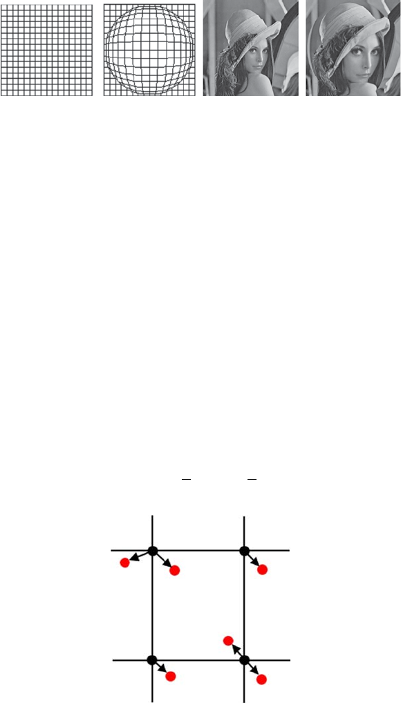
32 A Beginner’s Guide to Image Preprocessing Techniques
not get tted on the discrete raster output image. Integer grid values are
required. Every pixel value in the output raster image can be obtained by
brightness interpolation of some noninteger neighboring samples. The
brightness interpolation is generally done by dening the brightness of
the original pixel in the input image that resembles the pixel in the output
discrete raster image. Interpolation is used when we need to estimate the
value of an unknown pixel by using some known data.
3.2.1 Nearest Neighbor Interpolation
This is the simplest interpolation approach [15]. This technique basically
determines the nearest neighboring pixel value and adopts its intensity value,
as shown in Figure 3.9.
Consider the following example (Figure 3.10).
Figure 3.9 shows that the 2D input matrix is 3 × 3 and it is interpolated
to 6 × 6. First, we must nd the ratio of the input and output matrix size, as
shown in Equation 3.15:
R
R
ro
wc
ol
==
3
6
3
6
,.
(3.15)
(A) (B) (C) (D)
FIGURE 3.8
(A) Original graph, (B) Spherical effect of graph, (C) Original image, and (D) Spherical effect
of image.
FIGURE 3.9
Black pixels: Original pixels, Red pixels: Interpolated pixels.
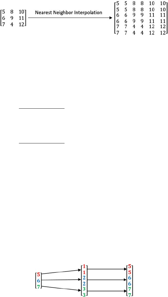
33Geometric Transformation Techniques
Then, based on the output matrix size the row-wise and column-wise pixel
positions are normalized.
R
owposition
row
== =
[]
[. ..]
123456 05 1152253
1
1
2
2
3
3
R
== =Colposition
col
[]
[. ..][
123456 05 1152253 11
R
22233]
.
(3.16)
After that, the row-wise interpolation is performed on all columns. The
output of the rst column after interpolation is shown in Figure 3.11.
The row-wise interpolation output is shown below:
5810
581
0
6911
6911
7412
7412
FIGURE 3.10
Nearest neighbor interpolation output.
FIGURE 3.11
Row-wise interpolation of the rst column of the input matrix.
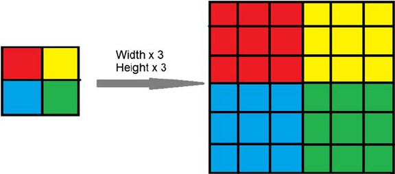
34 A Beginner’s Guide to Image Preprocessing Techniques
Similarly, the column-wise interpolation for all rows is shown below:
558810 10
66991
11
1
774412 12
The nal nearest neighbor interpolated output matrix is shown below:
558810 10
558810 10
66991
11
1
66991
11
1
774412 12
874412 12
The nearest neighbor interpolation output of an image is shown in Figure3.12.
The position error of the nearest neighborhood interpolation is at most half
a pixel. This error is perceptible on objects with straight-line boundaries,
which may appear step-like after the transformation.
In nearest neighbor interpolation, each nearby pixel has similar
characteristics, hence, it becomes easier to add or remove the pixels as per
requirement. The major drawback of this method is unwanted artifacts, like
the sharpening of edges that may appear in an image while resizing, hence,
it is generally not preferred.
3.2.2 Bilinear Interpolation
This type of interpolation searches four neighboring points of the interpolated
point (x, y), as shown in Figure 3.13, and assumes that the brightness function
is linear in this neighborhood [16].
FIGURE 3.12
Nearest neighbor interpolation of an image.
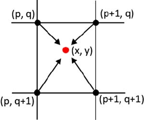
35Geometric Transformation Techniques
Consider a discrete image function. The black circles represents the
known pixels of the image I, and the red circle is lying outside the known
samples. This interpolation is not linear but the product of two linear
functions. If the interpolated point lies on one of the edges of the cell
[(I(p,q) → I(p + 1, q)), (I(p + 1, q) → I(p + 1, q + 1)), (I(p + 1, q + 1) → I(p,
q + 1)), (I(p, q + 1) → I(p,q))], the function becomes linear. Otherwise, the
bilinear interpolation function is quadratic. The interpolated value of
(x,y) is considered as a linear combination of four known sample values,
that is, I(p, q), I(p + 1,q), I(p + 1, q + 1), I(p, q + 1). The inuence of each
samples depends on the proximity to the interpolated point in the linear
combination.
Ixy tx ty IpqtxtyIpq
ty tx I
(, )( )
*
()
*
(,)
*
()
*
(,)
*()
*
=− −+−+
+−
11 11
1((, )**
(,),pq tx ty Ip q++ ++111
(3.17)
where = x − p, ty = y − q.
A minor reduction in resolution and blurring can happen while using
bilinear interpolation due to its averaging nature. The problem of step-like
straight boundaries with the nearest neighborhood interpolation is reduced
when using bilinear interpolation. The main advantage of using bilinear
interpolation is that it is fast and simple to implement.
3.2.3 Bicubic Interpolation
Improves the model of the brightness function by using sixteen neighboring
points for interpolation [17]. This interpolation ts a series of cubic polynomials
to the brightness values contained in the 4 × 4 array of pixels surrounding the
calculated address. First, interpolation is done along the x-direction using the
16 grid samples (black), as shown in Figure 3.14. Then, interpolation is done
along the other dimension (blue line) by using the interpolated pixels from
the previous step.
FIGURE 3.13
Black pixels: Original pixels, Red pixel: Interpolated pixel.
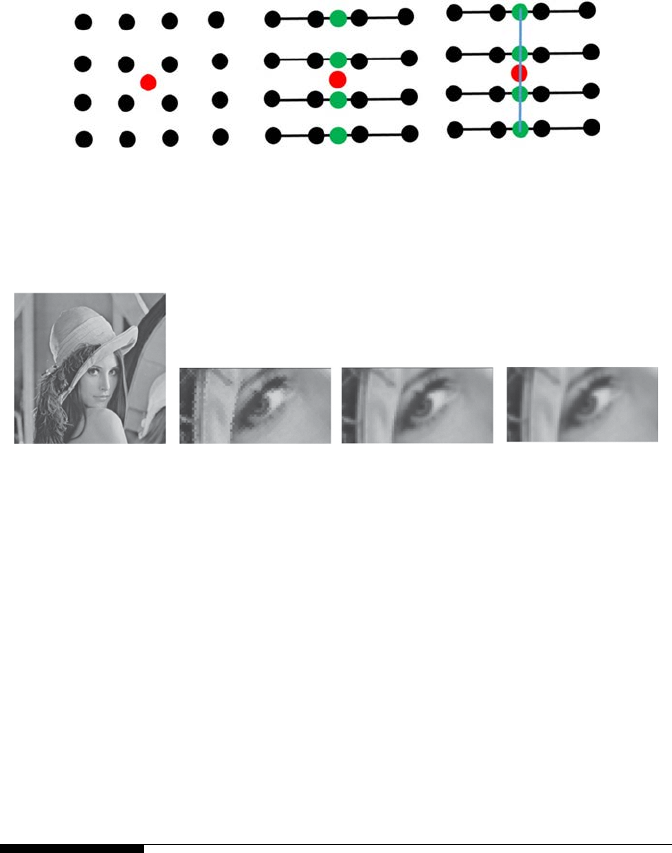
36 A Beginner’s Guide to Image Preprocessing Techniques
Bicubic interpolation does not suffer from the step-like boundary problem
of nearest neighborhood interpolation and copes with linear interpolation
blurring as well. Bicubic interpolation is often used in raster displays
that enable zooming with respect to an arbitrary point—if the nearest
neighborhood method were used, areas of the same brightness would
increase. Bicubic interpolation preserves ne details in the image very well.
The comparison between nearest-neighbor, bilinear, and bicubic
interpolation is shown in Figure 3.15.
3.3 Summary
Geometric transformation is actually the rearrangement of pixels of the
image. Coordinates of the input image is transformed into the coordinates
of the output image using some transformation function. The output
pixel intensity of a specied pixel position may not depend on the pixel
intensity of that particular input pixel, but is dependent on the position as
specied in the transformation matrix. There are two types of geometric
(A) (B) (C)
FIGURE 3.14
(A) known pixel (black) and interpolated pixel (red), (B) x-direction interpolation, (C) y-direction
interpolation.
(A) (B) (C) (D)
FIGURE 3.15
(A) Original image, (B) Nearest-neighbor interpolation, (C) Bilinear interpolation, and
(D)Bicubic interpolation.

37Geometric Transformation Techniques
transformation: pixel coordinate transformation and brightness interpolation.
Pixel coordinate transformation, or spatial transformation, of an image
is a geometric transformation of the image coordinate system, that is, the
mapping of one coordinate system onto another. Mapping can be forward
(map pixels of an input image onto an output image) or backward (map pixels
of an output image onto an input image). This type of transformation involves
some linear mapping like translation, scaling, rotation, shearing, and afne
transformation. Nonlinear mapping involves twirl, ripple, and spherical
transformation. The brightness interpolation is generally done by dening
the brightness of the original pixel in the input image that resembles the pixel
in the output discrete raster image. Brightness interpolation involves nearest
neighbor interpolation, bilinear interpolation, and bicubic interpolation.
References
1. Candemir, S., Borovikov, E., Santosh, K. C., Antani, S., & Thoma, G. 2015. Rsilc:
Rotation-and scale-invariant, line-based color-aware descriptor. Image and Vision
Computing, 42, 1–12.
2. Chaki, J., Parekh, R., & Bhattacharya, S. 2015. Plant leaf recognition using texture
and shape features with neural classiers. Pattern Recognition Letters, 58, 61–68.
3. Gonzalez, R. C., Woods, R. E. 2016. Digital Image Processing 3rd edition,
Prentice-Hall, New Jersey. ISBN-9789332570320, 9332570329.
4. Chaki, J., Parekh, R., & Bhattacharya, S. In press. Plant leaf classication using
multiple descriptors: A hierarchical approach. Journal of King Saud University-
Computer and Information Sciences, doi:10.1016/j.jksuci.2018.01.007.
5. Li, J., Yu, C., Gupta, B. B., & Ren, X. 2018. Color image watermarking scheme based
on quaternion Hadamard transform and Schur decomposition. Multimedia Tools
and Applications, 77(4), 4545–4561.
6. Chakraborty, S., Chatterjee, S., Ashour, A. S., Mali, K., & Dey, N. 2018. Intelligent
computing in medical imaging: A study. In Advancements in Applied Metaheuristic
Computing (pp. 143–163). IGI Global.
7. Chaki, J., Parekh, R., & Bhattacharya, S. 2016, December. Recognition of plant
leaves with major fragmentation. In Computational Science and Engineering:
Proceedings of the International Conference on Computational Science and
Engineering (Beliaghata, Kolkata, India, October 4–6, 2016) (p. 111). CRC Press,
Boca Raton, FL.
8. Chaki, J., Parekh, R., & Bhattacharya, S. 2015, July. Recognition of whole and
deformed plant leaves using statistical shape features and neuro-fuzzy classier.
In Recent Trends in Information Systems (ReTIS), 2015 IEEE 2nd International
Conference on (pp. 189–194). IEEE, Kolkata, India.
9. Vučković, V., Arizanović, B., & Le Blond, S. 2018. Ultra-fast basic geometrical
transformations on linear image data structure. Expert Systems with Applications,
91, 322–346.
38 A Beginner’s Guide to Image Preprocessing Techniques
10. Santosh, K. C., Lamiroy, B., & Wendling, L. 2011, August. DTW for matching
radon features: A pattern recognition and retrieval method. In International
Conference on Advanced Concepts for Intelligent Vision Systems (pp. 249–260).
Springer, Berlin, Heidelberg.
11. Sonka, M., Hlavac, V., & Boyle, R. 2014. Image Processing, Analysis, and Machine
Vision. Cengage Learning, Stamford, USA.
12. Fu, K. S. 2018. Special Computer Architectures for Pattern Processing. CRC Press,
Boca Raton, FL.
13. Gilliam, C., & Blu, T. 2018. Local all-pass geometric deformations. IEEE
Transactions on Image Processing, 27(2), 1010–1025.
14. Chaki, J., Parekh, R., & Bhattacharya, S. 2016. Plant leaf recognition using ridge
lter and curvelet transform with neuro-fuzzy classier. In Proceedings of 3rd
International Conference on Advanced Computing, Networking and Informatics (pp.
37–44). Springer, New Delhi.
15. Jiang, N., & Wang, L. 2015. Quantum image scaling using nearest neighbor
interpolation. Quantum Information Processing, 14(5), 1559–1571.
16. Wegner, D., & Repasi, E. 2016, May. Image based performance analysis of thermal
imagers. In Infrared Imaging Systems: Design, Analysis, Modeling, and Testing XXVII
(Vol. 9820, p. 982016). International Society for Optics and Photonics, Baltimore,
Maryland, United States.
17. Dong, C., Loy, C. C., He, K., & Tang, X. 2016. Image super-resolution using
deep convolutional networks. IEEE Transactions on Pattern Analysis and
Machine Intelligence, 38(2), 295–307.

39
4
Filtering Techniques
Filtering is a method for enhancing or altering an image [1]. There are mainly
two types of ltering:
• Spatial Filtering
• Frequency Filtering
4.1 Spatial Filter
In spatial ltering, the processed pixel value for the existing pixel is
dependent on both itself and neighboring pixels [2]. Therefore, spatial
ltering is a neighboring procedure, where the value of any particular pixel
in the output image is calculated by applying some algorithm to the values
of the neighboring pixels of the corresponding input pixel [3]. A pixel’s
neighborhood is dened by a set of surrounding pixels relative to that pixel.
Some types of spatial ltering are discussed below.
4.1.1 Linear Filter (Convolution)
The result of the linear ltering [4] is the summation of products of the mask
coefcients with the equivalent pixels exactly beneath the mask, as shown in
Figure 4.1.
Linear ltering can be expressed by Equation 4.1:
IxyM Ix y
MIxy MIx
(,)[(,)
*
(, )]
[(,)
*(, )] [(,)
*(
=− −+
++++
11 11
01 111111
10 100
10 1
,)
]
[( ,)
*(,)] [(,)
*(,)]
[(,)
*(,
y
MIxy MIxy
MIx
+
+− −+
++yyM Ix y
MIxy MIx
)] [( ,)
*(,)]
[(,)
*
(, )] [(,)
*
(
+−−−−
+− −+ −
11
11
01 111+
+−11
,)].y (4.1)
The mask coefcient M(0, 0) overlaps with image pixel value I(x, y),
representing that the mask center is at (x, y) when the calculation of the sum
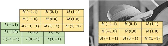
40 A Beginner’s Guide to Image Preprocessing Techniques
of products occurred. For a mask of size p × q, p and q are odd numbers
and represented as p = 2m + 1, q = 2n + 1, where m and n are nonnegative
integers. Linear ltering of an image I of size p × q, with a lter mask of size
p × q, is given by the Equation 4.2:
LF xy Mab Ix ay b
am
m
bn
n
(,)(,) (,).
=∗++
=− =−
∑∑
(4.2)
4.1.2 Nonlinear Filter
Nonlinear spatial ltering also works on neighborhoods, as discussed in the
case of linear ltering [5]. The only difference is the nonlinear ltering is
based conditionally on the values of the neighboring pixels of a relative pixel.
4.1.3 Smoothing Filter
Smoothing lters are mainly used to reduce noise of an image and for blurring
[6,7]. Blurring is used to remove unimportant information from an image
prior to feature extraction, and is used to connect small breaks in curves or
lines. Blurring is also used to reduce noise from an image. A smoothing lter
is also useful for highlighting gross details. Two types of smoothing spatial
lters exist:
• Smoothing Linear Filters
• Order-Statistics Filters
A smoothing linear lter is basically the mean of the neighborhood pixels
of the lter mask. Therefore, this lter is sometimes called “mean lter” or
“averaging lter.” The concept entails substituting the value of every single
pixel in an image with the mean of the neighborhood pixels dened by the
lter mask. Figure 4.2 shows a 3 × 3 standard mean and weighted mean
smoothing linear lter:
(A) (B)
FIGURE 4.1
(A) I: Image pixel positions and M: Mask Coefcients, (B) Mask of image pixels.
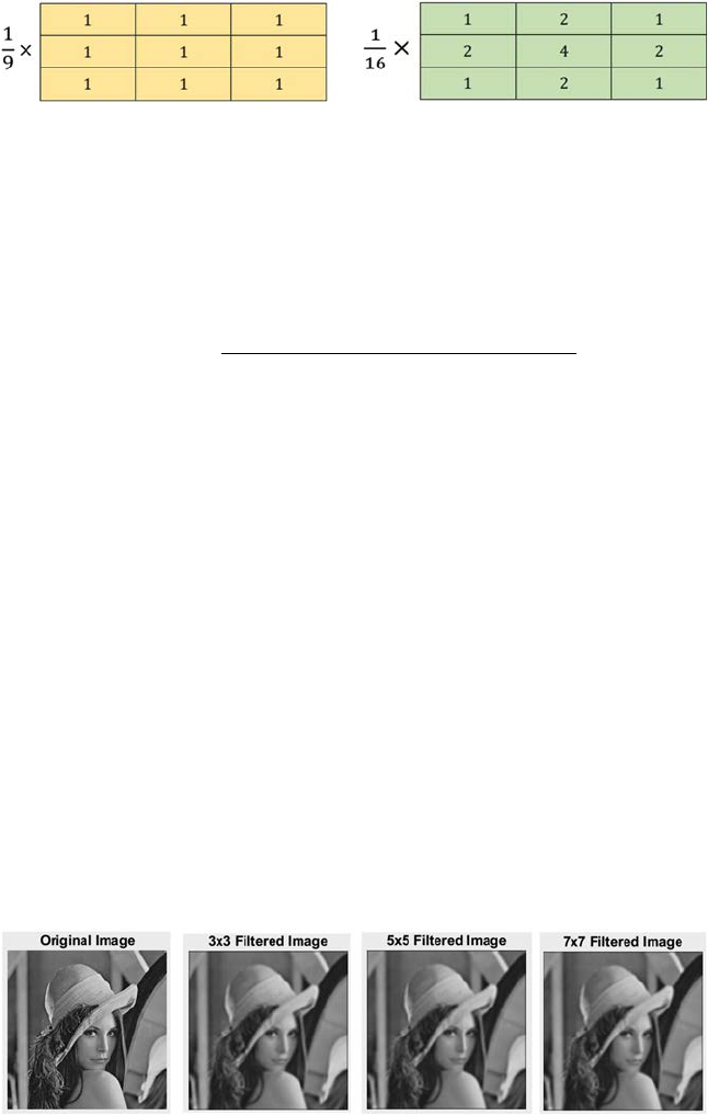
41Filtering Techniques
Filtering an I(m × n) image with a weighted averaging lter of size m × n
is given by Equation 4.3:
SF xy
Mab Ix ay b
Mab
am
m
bn
n
am
m
bn
n
(,)(,)*(,)
(,)
.=
++
=− =−
=− =−
∑∑
∑∑
(4.3)
The output of a smoothing linear lter is shown in Figure 4.3.
Order-statistics smoothing lters are basically nonlinear spatial lter
[8 –10]. The response of this lter is constructed by ordering or ranking the
pixels enclosed in the image area covered by the lter. Then, the value of
the center pixel is replaced with the value calculated by the ordering or
ranking result. This type of lter is also known as “median lter.” The
median lter is used to reduce the salt and pepper type noise from an image
while preserving edges [11–13]. This lter works by moving a window of a
particular size over each and every pixel of the image, and replaces each
pixel value with the median of the neighboring pixel values. To calculate the
median, rst the pixel values beneath the window are sorted into numerical
order and then the considered pixel value is replaced with the median pixel
value of the sorted list.
Consider the example shown in Figure 4.4. A 3 × 3 window is used in this
example.
Figure 4.5 shows the output of a median lter when applied to salt and
pepper noise image.
(A) (B)
FIGURE 4.2
(A) Standard mean smoothing linear lter, (B) Weighted mean smoothing linear lter.
FIGURE 4.3
Smoothing linear lter output.
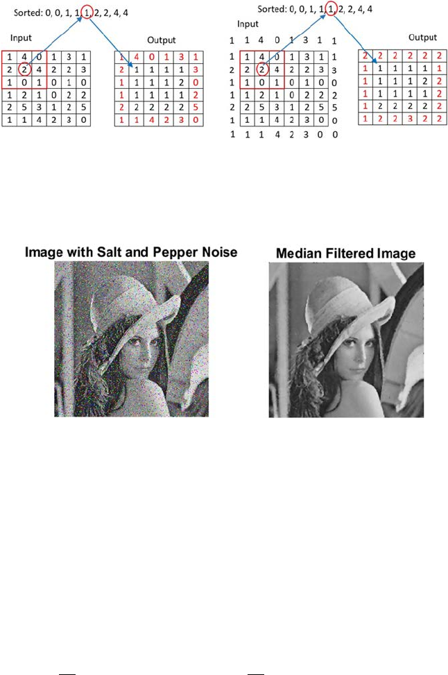
42 A Beginner’s Guide to Image Preprocessing Techniques
4.1.4 Sharpening Filter
The primary goal of this lter is to enhance the ne detail in an image or to
highlight the blurred detail [14]. Sharpening can be performed by using spatial
derivatives, which can be applied in areas of at regions or constant gray level
regions, at the step and end of discontinuities or ramp discontinuities, and
along gray-level discontinuities or ramps. These discontinuities can be lines,
noise points, and edges.
The rst order partial spatial derivatives of a digital image I(x, y) can be
expressed by using Equation 4.4:
∂
∂=+ −
∂
∂=+−
I
xIx yIxy I
yIx
yI
xy(,)(,) (, )(
,)
.
11
and
(4.4)
First order partial derivative must be (1) zero in at regions, (2) nonzero at
the step and gray level ramp discontinuities, and (3) nonzero along ramps.
(1A) (1B) (2A) (2B)
FIGURE 4.4
(1) Keeping the border value unchanged: (1A) Input Image values, (1B) Output after smoothing;
(2) Boundary values are also ltered by extending the border values: (2A) Input Image values,
(2B) Output after smoothing.
FIGURE 4.5
Median lter output.
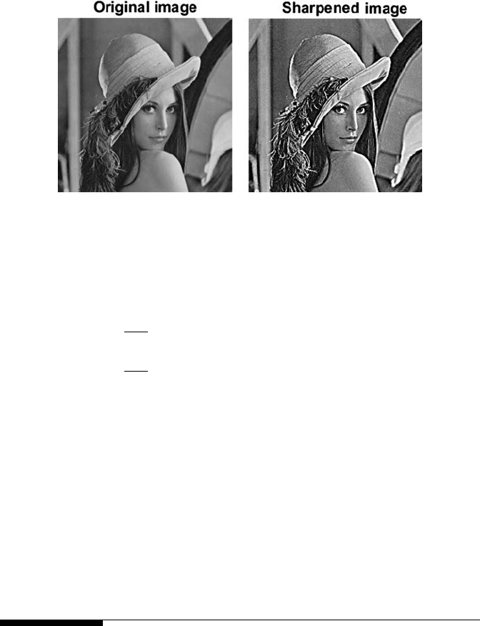
43Filtering Techniques
The second order partial spatial derivatives of a digital image I(x, y) can be
expressed by using Equation 4.5:
∂
∂=+ +− −
∂
∂=++−−
2
2
2
2
112
112
I
xIx yIxyIxy
I
yIxyIxy
(,)( ,) (,)
(, )(,)IIxy(,).
(4.5)
Second order partial derivative must be: (1) zero in at regions, (2) nonzero at
the step and gray level ramp discontinuities, (3) zero along ramps of constant
slope.
The rst order derivative is nonzero along the entire discontinuity or ramp,
but the second order derivative is nonzero only at the step and gray level
ramp discontinuities. A rst order derivative is used to make the edge thick,
and a second-order derivative is used to enhance or highlight ne details
such as thin edges and lines, including noise.
Figure 4.6 shows the result of a sharpening lter.
4.2 Frequency Filter
Frequency lters are used to process an image in the frequency domain [15].
The image is converted to frequency domain by using a Fourier transform
function. After frequency domain processing, the image is retransformed into
the spatial domain by inverse Fourier transform. Reducing high frequencies
in the spatial domain converts the image into a smoother one, while reducing
low frequencies highlights the edges of the image [16]. All frequency lters
FIGURE 4.6
Sharpen image output.

44 A Beginner’s Guide to Image Preprocessing Techniques
can also be implemented in the spatial domain, and frequency lters are
computationally not costly to accomplish ltering in the spatial domain.
Frequency ltering is also more suitable if there is no direct kernel that can be
created in the spatial domain, in which case they may also be more effective.
All spatial domain images have an equivalent frequency representation.
The high frequency corresponds to pixel values that rapidly vary across the
image like leaves, text, texture, and so forth. Low frequency corresponds to
the homogeneous part of the image.
Frequency ltering is founded on the Fourier Transform. The operator
generally takes a lter function and an image in the Fourier domain. This
image is then multiplied in a pixel-by-pixel fashion with the lter function,
and can be expressed by Equation 4.6:
FuvPQ Ixye
x
P
y
Qjux
P
vy
Q
(,)(,) .=
=
−
=
−
−+
∑∑
1
0
1
0
12π
(4.6)
Here I(x, y) is the input image of dimension P × Q in the Fourier domain and
F(u, v) is the ltered image [u = 0, … , P − 1 and v = 0, …, Q − 1]. To convert
the frequency domain image into the spatial domain,
Fuv(,)
is retransformed
by using the inverse Fourier Transform, as shown in Equation 4.7:
IxyPQ Fuve
x
P
y
Qjux
P
vy
Q
(,
)(
,) .=
=
−
=
−
−+
∑∑
1
0
1
0
12π
(4.7)
Since the multiplication in the Fourier space is identical to convolution in
the spatial domain, all frequency lters can be implemented theoretically
as a spatial lter. Different types of frequency lters are discussed in the
following subsections.
4.2.1 Low-Pass Filter
A low-pass lter is a lter that passes or allows low-frequency signals, and
suppresses signals with higher frequencies than the cutoff or threshold
frequency [17]. Based on the specic lter design, the actual amount of
suppression varies for each frequency. A low-pass lter is generally used
to smooth an image. The standard forms of low-pass lters are Ideal,
Butterworth, and Gaussian low-pass lters.
4.2.1.1 Ideal Low-Pass Filter (ILP)
This is the simplest low-pass lter that suppresses all high-frequency
components of the Fourier Transform that are greater than a specied
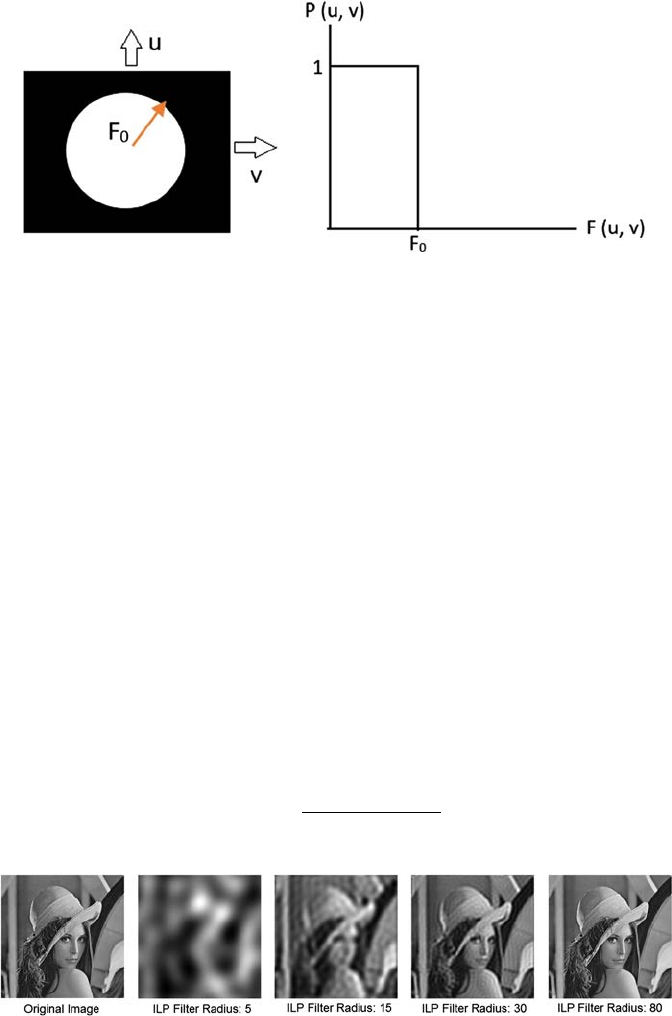
45Filtering Techniques
cutoff frequency F0. This transfer function of the lter can be dened by
Equation4.8:
PuvFu
vF
Fu
vF
(,)(,)
(,).=≤
>
1
0
0
0
if
if
(4.8)
The image and graphical representation of an ideal low-pass lter are shown
in Figure 4.7.
Because of the structure of the ILP mask, ringing occurs in the image when
an ILP lter is applied to an image. ILP lter yields a blurred image, as shown
in Figure 4.8.
4.2.1.2 Butterworth Low-Pass Filter (BLP)
This lter is used to eliminate high frequency noise with the least loss of
image data in the specied pass band with order d. The transfer function of
order d and with cutoff frequency F0 can be expressed by using Equation 4.9:
PuvFuvFd
(,)(,).=+
[]
1
10
2
/
(4.9)
(A) (B)
FIGURE 4.7
(A) Filter displayed as an image, (B) Graphical representation of ideal low-pass lter.
FIGURE 4.8
ILP lter output with different values of F0.
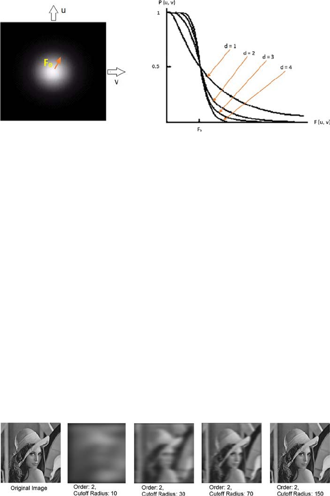
46 A Beginner’s Guide to Image Preprocessing Techniques
The image and graphical representation of a BLP lter are shown in Figure4.9.
The output of the BLP lter is shown in Figure 4.10.
4.2.1.3 Gaussian Low-Pass Filter (GLP)
The transfer function of a GLP lter is expressed in Equation 4.10:
Puve
Fuv
(,
).
(,)
=−
22
2/ σ
(4.10)
Here, σ is the standard deviation and a measure of spread of the Gaussian
curve. If σ is replaced with the cutoff radius F0, then the transfer function of
GLP is expressed as in Equation 4.11:
Puve
Fu
vF
(,
).
(,)/
=−20
2
2
(4.11)
The image and graphical representation of a GLP lter is shown in
Figure4.11.
The output of the GLP lter is shown in Figure 4.12.
(A) (B)
FIGURE 4.9
(A) Filter displayed as an image, (B) Graphical representation of BLP lter.
FIGURE 4.10
Output of BLP lter with various cutoff radii.
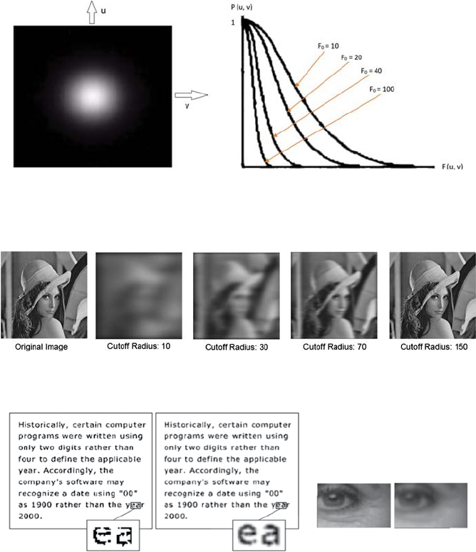
47Filtering Techniques
A low-pass lter can be used to connect broken text as well as reduce
blemishes [18], as shown in Figure 4.13.
4.2.2 High Pass Filter
A high-pass lter suppresses frequencies lower than the cutoff frequency, but
allows or passes high frequencies well [19]. A high-pass lter is generally used
(A) (B)
FIGURE 4.11
(A) Filter displayed as an image, (B) Graphical representation of GLP lter.
FIGURE 4.12
Output of GLP lter at different cutoff radius.
(1A) (1B)
(2A) (2B)
FIGURE 4.13
(1) Connecting text input-output: (1A) Input Image, (1B) Output of low-pass lter; (2) Blemishes
reduction input–output: (2A) Input Image, (2B) Output of low-pass lter.
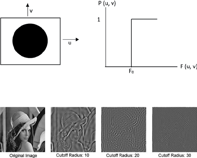
48 A Beginner’s Guide to Image Preprocessing Techniques
to sharpen an image and to highlight the edges and ne details associated
with the image. Different types of high-pass lters are Ideal, Butterworth,
and Gaussian high-pass lter. All high-pass lters (HPF) can be represented
by their relationship to the low-pass lters (LPF), as shown in Equation 4.12:
HPFLPF.=−1
(4.12)
4.2.2.1 Ideal High-Pass Filter (IHP)
The transfer function of an IHP lter can be expressed by Equation 4.13,
where F0 is the cutoff frequency or cutoff radius:
PuvFu
vF
Fu
vF
(,)(,)
(,).=≤
>
0
1
0
0
if
if
(4.13)
The image and graphical representation of an IHP lter is shown in Figure4.14.
The output of the IHP lter is shown in Figure 4.15.
(A) (B)
FIGURE 4.14
(A) Filter displayed as an image, (B) Graphical representation of IHP lter.
FIGURE 4.15
Output of IHP lter.
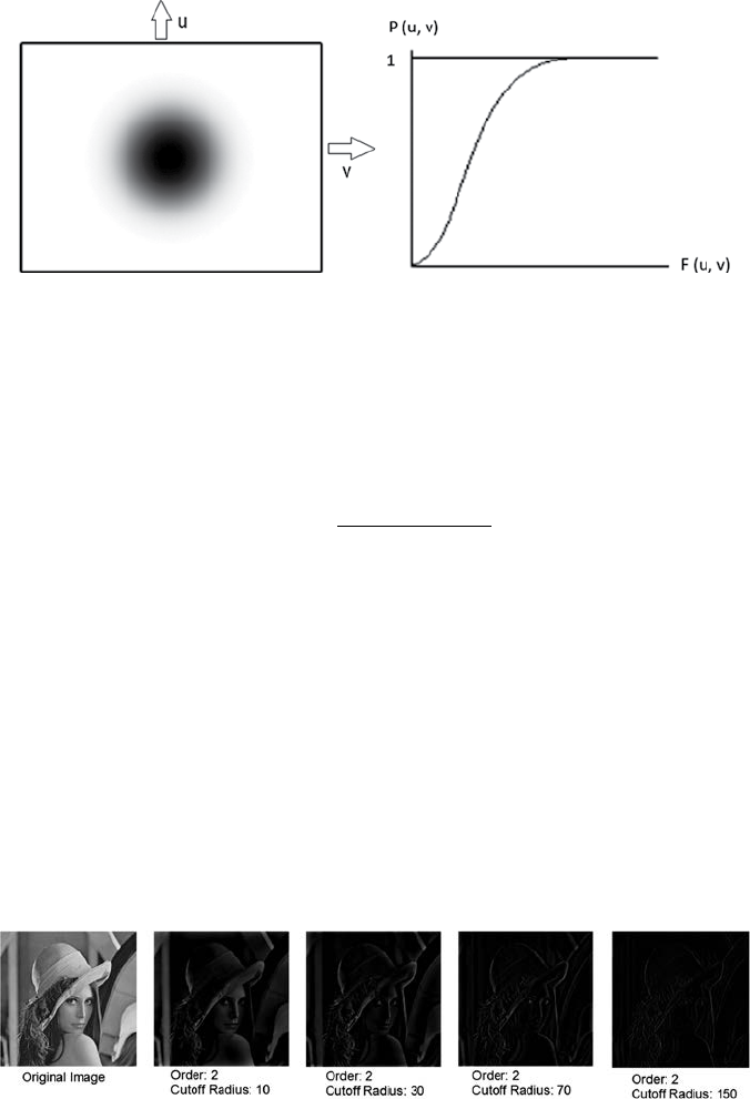
49Filtering Techniques
4.2.2.2 Butterworth High-Pass Filter (BHP)
The transfer function of BHP lter can be dened by Equation 4.14 where p is
the order and F0 is the cutoff frequency or cutoff radius:
PuvFFuv n
(,)(,).=+
[]
1
10
2
/
(4.14)
The image and graphical representation of BHP lter is shown in Figure4.16.
The output of the BHP lter is shown in Figure 4.17.
4.2.2.3 Gaussian High-Pass Filter (GHP)
The transfer function of GLP lter is expressed in Equation 4.15, with the
cutoff radius F0:
Puve
Fu
vF
(,
).
(,)/
=−
−
120
2
2
(4.15)
The image and graphical representation of GLP lter is shown in Figure4.18.
The output of the GHP lter is shown in Figure 4.19.
(A) (B)
FIGURE 4.16
(A) Image representation of BHP, (B) Graphical representation of BHP.
FIGURE 4.17
Output of BHP lter.
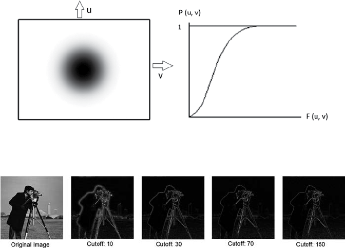
50 A Beginner’s Guide to Image Preprocessing Techniques
4.2.3 Band Pass Filter
A band pass suppresses very high and very low frequencies, but preserves an
intermediate range band of frequencies [20]. Band pass ltering can be used to
highlight edges (attenuating low frequencies) while decreasing the noise amount
at the same time (suppressing high frequencies). To obtain the band pass lter
function, the low-pass lter function is multiplied with the high-pass lter
function in the frequency domain, where the cutoff frequency of the high pass
is lower than that of the low pass. So, in theory, a band pass lter function can be
developed if the low-pass lter function is available. The different types of band
pass lter are Ideal band pass, Butterworth band pass, and Gaussian band pass.
4.2.3.1 Ideal Band Pass Filter (IBP)
The IBP allows the frequency within the pass band and removes the very
high and very low frequency. An IBP lter within a frequency range FL, … ,
FH is dened by Equation 4.16:
PuvFFuv F
LH
(,)(,).=
≤≤
1
0
if
otherwise
(4.16)
Figure 4.20 shows the image and the effect of applying the IBP lter with
different pass bands.
FIGURE 4.19
Output of GHP lter.
(A) (B)
FIGURE 4.18
(A) Image representation of GHP, (B) Graphical representation of GHP.
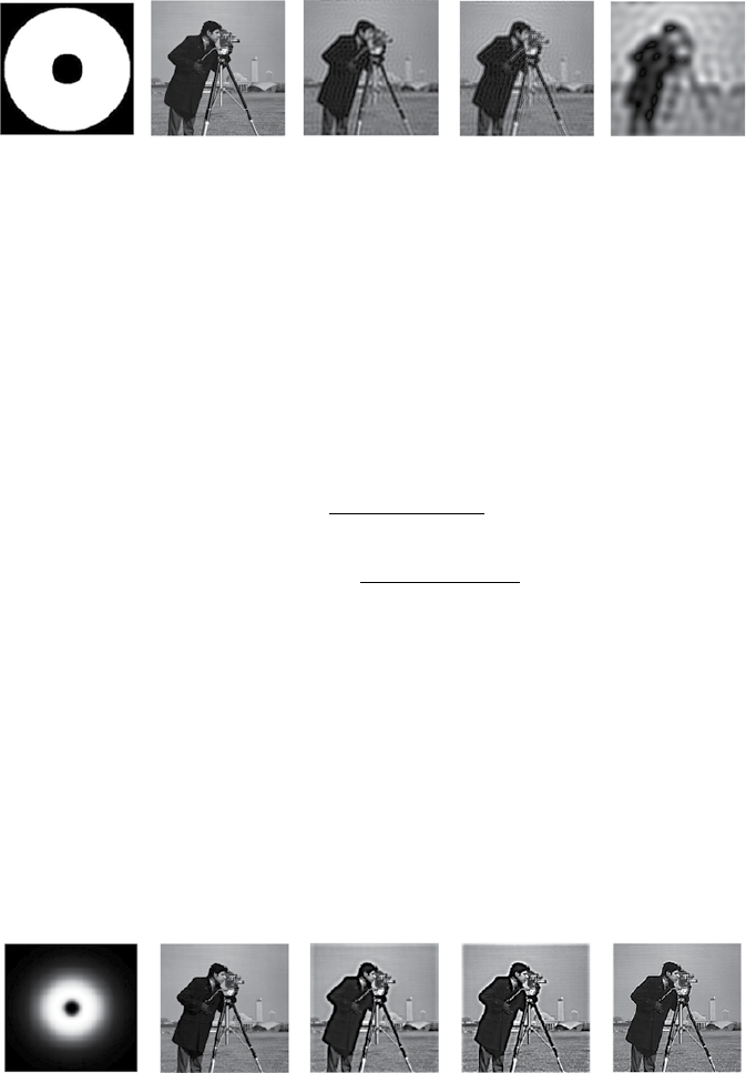
51Filtering Techniques
4.2.3.2 Butterworth Band Pass Filter (BBP)
This lter can be obtained by multiplying the transfer function of a low
and high Butterworth lter. If FL is the low cutoff frequency, FH is the high
cutoff frequency, and p is the order of the lter then the BBP lter can be
dened by Equation 4.17. The range of frequency is dependent on the order
of the lter:
BuvFuvF
BuvFuvF
Bu
L
p
H
p
LP
HP
BP
/
/
(),(,)
(,)(,)
(,
=+
[]
=−+
[]
1
1
11
1
2
2
vvBuv Buv
LP
)(,)
*(,).=HP
(4.17)
Figure 4.21 shows the image and the effect of applying the BBP lter with
different pass bands and order = 2.
4.2.3.3 Gaussian Band Pass Filter (GBP)
This lter can be obtained by multiplying the transfer function of a low and
high Gaussian lter. If FL is the low cutoff frequency, FH is the high cutoff
frequency, and p is the order of the lter then the GBP lter can be dened
by Equation 4.18:
(A)(B) (C)(D) (E)
FIGURE 4.20
(A) Image of IBP lter, (B) Original image, (C) Output of IBP lter (FL = 30, FH = 100), (D) Output
of IBP lter (FL = 30, FH = 50), and (E) Output of IBP lter (FL = 10, FH = 90).
(A)
(B) (C)(D) (E)
FIGURE 4.21
(A) Image of BBP lter, (B) Original image, (C) Output of BBP lter (FL = 30, FH = 50), (D) Output
of BBP lter (FL = 30, FH = 150), and (E) Output of BBP lter (FL = 70, FH = 200).

52 A Beginner’s Guide to Image Preprocessing Techniques
Guve
Guve
GGu
FuvF
FuvF
LP
HP
BP LP
()
()
(
,
,
,
(,)/
(,)/
=
=−
=
−
−
20
2
20
2
2
2
1
vvG uv
FF
LH
).
(,)
∗>
HP where
(4.18)
Figure 4.22 shows the image and the effect of applying the GBP lter with
different pass bands.
4.2.4 Band Reject Filter
Band-reject lter (also called band-stop lter) is just the opposite of the
bandpass lter [21]. It attenuates frequencies within a range of a higher and
lower cutoff frequency. Different types of band reject lters are Ideal band
reject, Butterworth band reject, and Gaussian band reject.
4.2.4.1 Ideal Band Reject Filter (IBR)
In this lter, the frequencies within the pass band are attenuated and the
frequencies outside of the given range are passed without attenuation.
Equation 4.19 denes an IBR lter with a frequency cutoff F0, which is the
center of the frequency band, and where W is the width of the frequency band:
PuvFWFuvFW
(,)(,).=−≤ ≤+
0
22
1
00
if
otherwise
(4.19)
4.2.4.2 Butterworth Band Reject Filter (BBR)
In a BBR lter, frequencies at the center of the band are completely blocked.
Frequencies at the edge of the frequency band are suppressed by a fraction
of maximum value. If F0 is the center of the frequency, W is the width of the
(A) (B) (C)(D) (E)
FIGURE 4.22
(A) Image of GBP lter, (B) Original image, (C) Output of GBP lter (FL = 30, FH = 50), (D) Output
of GBP lter (FL = 10, FH = 90), and (E) Output of GBP lter (FL = 70, FH = 90).

53Filtering Techniques
frequency band, and p is the order of the lter, then a BBR lter can be dened
by Equation 4.20:
Puv
FuvW FuvF
p
(,)
(,)((,
))
.=
+−
1
120
22
/
(4.20)
4.2.4.3 Gaussian Band Reject Filter (GBR)
Here, the transition between the ltered and unltered frequency is very
smooth. If F0 is the center of the frequency and W is the width of the frequency
band, then GBR lter can be dened by Equation 4.21:
Puve
FuvFFuvW
(,
).
[(,) (,
)]()
=−−
20
22
/
(4.21)
4.3 Summary
Filtering is generally used to enhance the image detail. Several types of lters
are discussed in this chapter. Mainly there are two types of lter: spatial
and frequency. Spatial ltering is used to process the pixel value for the
existing pixel, which is dependent on both itself and neighboring pixels.
There are several types of spatial lter like linear, nonlinear, smoothing, and
sharpening. Smoothing lter is used to blur the image and sharpening lter
is used to highlight the blurred detail. Frequency lters are used to process
the image in frequency domain. Different types of frequency lters are low-
pass lters, which are used to blur the image, or high pass lters, which are
used to highlight edges and sharpening. Band pass ltering can be used to
highlight edges (attenuating low frequencies) and decrease the noise amount
at the same time (suppressing high frequencies), while band reject lters are
the opposite of band pass lters.
References
1. Araki, T., Ikeda, N., Dey, N., Acharjee, S., Molinari, F., Saba, L., Godia, E.,
Nicolaides, A., & Suri, J. S. 2015. Shape-based approach for coronary calcium
lesion volume measurement on intravascular ultrasound imaging and its
association with carotid intima-media thickness. Journal of Ultrasound in
Medicine, 34(3), 469–482.
54 A Beginner’s Guide to Image Preprocessing Techniques
2. Gonzalez, R. C., Woods, R. E. 2016. Digital Image Processing 3rd edition,
Prentice-Hall, New Jersey. ISBN-9789332570320, 9332570329.
3. Chaki, J., Parekh, R., & Bhattacharya, S. 2016. Plant leaf recognition using ridge
lter and curvelet transform with neuro-fuzzy classier. In Proceedings of 3rd
International Conference on Advanced Computing, Networking and Informatics (pp.
37–44). Springer, New Delhi.
4. Santosh, K. C., Candemir, S., Jaeger, S., Karargyris, A., Antani, S., Thoma,G.R.,&
Folio, L. 2015. Automatically detecting rotation in chest radiographs using
principal rib-orientation measure for quality control. International Journal of
Pattern Recognition and Articial Intelligence, 29(02), 1557001.
5. Ashour, A. S., Beagum, S., Dey, N., Ashour, A. S., Pistolla, D. S., Nguyen, G. N.,
et al. 2018. Light microscopy image de-noising using optimized LPA-ICI lter.
Neural Computing and Applications, 29(12), 1517–1533.
6. Hangarge, M., Santosh, K. C., Doddamani, S., & Pardeshi, R. 2013. Statistical
texture features based handwritten and printed text classication in south
indian documents. arXiv preprint arXiv:1303.3087.
7. Dey, N., Ashour, A. S., Beagum, S., Pistola, D. S., Gospodinov, M., Gospodinova,
Е. P., & Tavares, J. M. R. 2015. Parameter optimization for local polynomial
approximation based intersection condence interval lter using genetic
algorithm: An application for brain MRI image de-noising. Journal of Imaging,
1(1), 60 –84.
8. Santosh, K. C., & Mukherjee, A. 2016, April. On the temporal dynamics of
opinion spamming: Case studies on yelp. In Proceedings of the 25th International
Conference on World Wide Web (pp. 369–379). International World Wide Web
Conferences Steering Committee, Montréal, Québec, Canada.
9. Garg, A., & Khandelwal, V. 2018. Combination of spatial domain lters for
speckle noise reduction in ultrasound medical images. Advances in Electrical
and Electronic Engineering, 15(5), 857–865.
10. Nandi, D., Ashour, A. S., Samanta, S., Chakraborty, S., Salem, M. A., & Dey,N.
2015. Principal component analysis in medical image processing: A study.
International Journal of Image Mining, 1(1), 65–86.
11. Kotyk, T., Ashour, A. S., Chakraborty, S., Dey, N., & Balas, V. E. 2015. Apoptosis
analysis in classication paradigm: A neural network based approach. In
Healthy World Conference—A Healthy World for a Happy Life (pp. 17–22). Kakinada
(AP), India.
12. Santosh, K. C. 2010. Use of dynamic time warping for object shape classication
through signature. Kathmandu University Journal of Science, Engineering and
Technology, 6(1), 33–49.
13. Dhanachandra, N., Manglem, K., & Chanu, Y. J. 2015. Image segmentation using
K-means clustering algorithm and subtractive clustering algorithm. Procedia
Computer Science, 54(2015), 764–771.
14. Chakraborty, S., Chatterjee, S., Ashour, A. S., Mali, K., & Dey, N. 2018. Intelligent
computing in medical imaging: A study. In Advancements in Applied Metaheuristic
Computing (pp. 143–163). IGI Global, doi:10.4018/978-1-5225-4151-6.ch006.
15. Pardeshi, R., Chaudhuri, B. B., Hangarge, M., & Santosh, K. C. 2014, September.
Automatic handwritten Indian scripts identification. In 14th International
Conferenceon Frontiers in Handwriting Recognition (ICFHR), 2014 (pp. 375–380). IEEE.
16. Santosh, K. C., & Nattee, C. 2007. Template-based nepali natural handwritten
alphanumeric character recognition. Science & Technology Asia, 12(1), 20–30.
55Filtering Techniques
17. Najarian, K., & Splinter, R. 2016. Biomedical signal and image processing. CRC Press,
Boca Raton, FL.
18. Low-pass lter example [https://www.slideshare.net/SuhailaAfzana/image-
smoothing-using-frequency-domain-lters (Last access date: June 10, 2018)]
19. Makandar, A., & Halalli, B. 2015. Image enhancement techniques using highpass
and lowpass lters. International Journal of Computer Applications, 109(14).
20. Semmlow, J. L., & Griffel, B. 2014. Biosignal and medical image processing. CRC
Press, Boca Raton, FL.
21. Konstantinides, K., & Rasure, J. R. 1994. The Khoros software development
environment for image and signal processing. IEEE Transactions on Image
Processing, 3(3), 243–252.


57
5
Segmentation Techniques
Image segmentation is the procedure of separating an image into several
parts [1–3]. This is normally used to nd objects or other signicant
information in digital images. There are various techniques to accomplish
image segmentation discussed here.
5.1 Thresholding
Thresholding is a procedure of transforming an input grayscale image
into a binarized image, or image with a new range of gray level, by using a
particular threshold value [4,5]. The goal of thresholding is to extract some
pixels from the image while removing others. The purpose of thresholding is
to mark pixels that belong to foreground pixels with the same intensity and
background pixels with different intensities.
Threshold is not only related to the image processing eld. Rather threshold
has the same meaning in any arena. A threshold is basically a value having
two set of regions on its either side, that is, above the threshold or below the
threshold. Any function can have a threshold value [6]. The function has
different expressions for below the threshold value and for above the threshold
value. For an image, if the pixel value of the original image is less than or
below a particular threshold value it will follow a specic transformation or
conversion function, if not, it will follow another. Threshold can be global or
local. Global threshold means the threshold is selected from the whole image.
Local or adaptive threshold is used when the image has uneven illumination,
which makes it difcult to segment using a single threshold. In that case, the
original image is divided into subimages, and for each subimage a particular
threshold is used for segmentation [7]. Figure 5.1 shows the segmentation
output with local and global threshold.
5.1.1 Histogram Shape-Based Thresholding
The histogram method presumes that there is some average value for the
foreground or object pixels and background, but the reality is that the real
pixel values have some deviation around these average values [8,9]. In that case,
selecting an accurate image threshold value is difcult and computationally

58 A Beginner’s Guide to Image Preprocessing Techniques
expensive. One comparatively simple technique is the iterative method to nd
a specic image threshold, which is also robust against noise. The steps of the
iterative method is as follows:
Step 1: An initial threshold (T) is selected arbitrarily by any other
desired method.
Step 2: The image I(x, y) is segmented into foreground or object pixels
and background pixels:
Object pixels OP
Backgroundpixels BP
(){( ,):(,) }
(){
←≥
←
IxyIxy T
I((, ): (, )}.xy IxyT
< (5.1)
Step 3: The average of each pixel set is calculated.
AOP AverageofOP←
ABP AverageofBP←
Step 4: A new threshold is formed, which is the average of AOP and ABP:
TAA
newOP BP
←
+()
.
2
(5.2)
Step 5: In step 2, use the new threshold obtained in step 4. Repeat till
the new threshold matches the one before it.
Assume that the gray level image I(x, y) is composed of a light object in a
dark background, in such a way that background and object, or foreground
gray level pixels, can be grouped into two dominant modes. One clear way to
extract the object pixels from the background is to select a threshold T, which
divides these two modes. Then any pixel (x, y) where I(x, y) ≥ T is called an
object pixel, otherwise, the pixel is called a background pixel. Example:
If two dominant modes describe the image histogram, it is called a
bimodal histogram. Here, only one threshold is sufcient for segmenting or
partitioning the image. Figure 5.2 shows the bimodal histogram of an image
and the segmented image.
(A) (B) (C)(D)
FIGURE 5.1
(A) Input image with uneven illumination, (B) and (C) Global thresholding result, (D) Local
thresholding result.
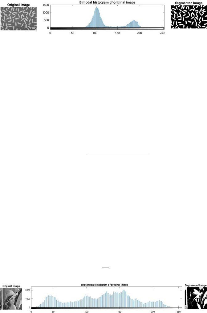
59Segmentation Techniques
If for instance, an image is composed of two or more types of dark objects in
a light background, three or more dominant modes are used to characterize
the image histogram, which is denoted as a multimodal histogram. Figure5.3
shows the multimodal histogram of an image and the segmented image.
5.1.2 Clustering-Based Thresholding
K-means Thresholding Method: The steps of K-means algorithm for selecting the
threshold is as follows [10]:
Step 1: Class centers (K) are initialized:
C
G
jj GG
k
j0
2
=+
−−
minma
xm
in
((/))( )
, (5.3)
where j = 1,2,…,k; Cj0 is the rst class center of jth class; Gmin and Gmax
are the minimum and maximum gray value of the sample space.
Step 2: Assign every point of the sample space to its nearest class center
based on Euclidean Distance:
DGC
ji
ij
,
(),=−abs
(5.4)
where j = 1,2,…,k; i = 1,2,…,P; Dj,i is the distance from an ith point to
the jth class, and P is the total number of points in the sample space.
Step 3: Compute the (K) new class centers from the average of the points
that are assigned to it:
CPi
Gjnew
=∑
1,
(5.5)
FIGURE 5.2
The bimodal histogram and the segmented image.
FIGURE 5.3
The multimodal histogram and the segmented image.
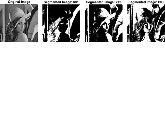
60 A Beginner’s Guide to Image Preprocessing Techniques
where j = 1,2,…,k and Pi is the total number of points that are assigned
to the ith class in step 2.
Step 4: Repeat step 2 for change in the class center; otherwise stop the
iteration.
Step 5: The threshold is calculated by the mean of the kth class center
and (k − 1) class center:
TC
C
kk
=+
−
1
2
1
().
(5.6)
The result of the image segmentation is shown in Figure 5.4.
Otsu-Clustering Thresholding Method: This method is used to select a threshold
value by minimizing the within class variances of two clusters [11,12]. The
within-class variance can be expressed by Equation 5.7:
σσσ
wbbff
TPTTPT T
222
() () () () (),=+
(5.7)
where Pf and Pb are the probability of foreground and background class
occurrences; T is the initial threshold value, which is randomly selected
by some algorithm, and
σ
f
2
and
σb
2
are the variances of foreground and
background clusters.
The probability of foreground and background class occurrences can be
denoted by Equation 5.8:
PT pG
PTp
G
b
G
T
f
GT
L
()
()
()
()
,
=
=
=
=+
−
∑
∑
0
1
1
(5.8)
where G is the gray level values {0,1,…,L − 1} and p(G) is the probability mass
function of G.
FIGURE 5.4
The output of image segmentation with different k values.

61Segmentation Techniques
The variances of foreground and background clusters are dened by
Equation 5.9:
σ
σ
b
G
T
b
b
f
GT
L
f
TGMT pG
PT
TGMT p
2
0
2
2
1
1
2
() (()) ()
()
(())()
=−
=−
=
=+
−
∑
∑(
()
()
,
G
PT
f
(5.9)
where Mb and Mf are the means of background and foreground clusters
respectively and can be dened by Equation 5.10:
MTGpG
MT GpG
f
G
T
b
GT
L
()
()
()
().
=×
=×
=
=+
−
∑
∑
0
1
1
(5.10)
A lot of computations are involved in computing the within class variance
for each of the two classes for every possible threshold. Thus, the between-
class variance is computed by subtracting the within class variance from the
total variance:
σσσ
µ
between total
total
222
2
() () ()
() () ()[[]
TTT
PT TM PT
w
bb f
=−
=−+µµ
f
TM()
].
−
total
2
(5.11)
σtotal
2
and Mtotal can be expressed by the Equation 5.12:
σtota
lt
otal
total
2
0
1
2
0
1
=−
=×
=
−
=
−
∑
∑
G
L
G
L
GM
pG
M
GpG
()()
().
(5.12)
The main advantage of this method is its simple computation.
Figure 5.5 shows the segmented output using a different number of clusters.
FIGURE 5.5
Segmented output using the Otsu clustering thresholding method.
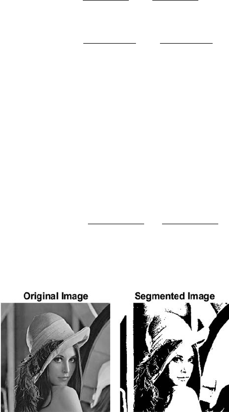
62 A Beginner’s Guide to Image Preprocessing Techniques
5.1.3 Entropy-Based Thresholding
This method is created based on the probability distribution function of the
gray level histogram [13,14]. Two entropies can be calculated: one for black
pixels and the other for white pixels:
i
b
i
t
j
t
j
t
w
gi
Et gi
gj
gi
gj
E
=
=
==
∑
∑
∑∑
=
=−
0
255
0
00
1()
() ()
()
*()
()
(
log
tt gi
gj
gi
gj
it
jt jt
)()
()
*()
()
,=−
=+
=+ =+
∑
∑∑
1
255
1
255
1
255
log
(5.13)
where g(i) is the normalized histogram.
The optimal single threshold value is selected by maximizing the entropy
of black and white pixels, and can be depicted by Equation 5.14:
TEtEt
tbw
=+
=…
Argmax () ().
0 255
(5.14)
p optimal threshold values can be found by Equation 5.15:
{, ,} max( ,) (, )(,),TT EtEt tEt
ptt p
p
11
12
1
1 255…= −+ ++
<<
Arg
(5.15)
where
E
tt gi
gj
gi
nn
it
t
jt
t
jt
t
n
n
n
n
n
n
(, )()
()
()
+
=+
=+ =+
=−
+
++
∑
∑
1
1
11
1
1log11
∑
gj
()
.
Figure 5.6 shows the output of the segmented image using an entropy-
based method.
FIGURE 5.6
Segmented output using entropy-based method.
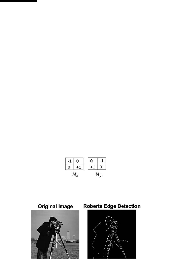
63Segmentation Techniques
5.2 Edge-Based Segmentation
Edge segmentation is a vital area of research, as it helps higher-level image
exploration [15]. Detection of edges is an important tool for image segmentation.
The representation of the edge of an image meaningfully decreases the
amount of data to be processed, however, it holds vital information about
the shapes of objects in the scene [16]. Edges are basically local variations in
image intensity. Edge detection approaches convert original images into edge
images depending on the variations of gray tones in the image. Image edge
detection is used in many applications like object shape identication, medical
image processing, biometrics, and so on [17,18]. There are three different types
of discontinuities in the gray level such as points, lines, and edges. Spatial
masks can be used to identify these three types of image discontinuities.
5.2.1 Roberts Edge Detector
The Roberts edge detection technique is used to highlight high spatial
frequency regions of the image, which corresponds to edges. The input to
the operator is a grayscale image [19]. A mask is used to compute the output,
which operates on each pixel values of the input image. Figure 5.7 shows the
values of the mask. Here, Mx is the mask used in the horizontal direction and
My is the mask used in the vertical direction.
Figure 5.8 shows the detected edge output using a Roberts edge detector.
FIGURE 5.7
Masks used in Roberts edge detection.
FIGURE 5.8
Edge detection using the Roberts edge detector.
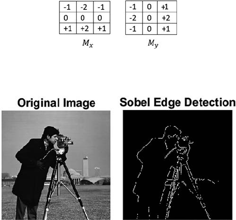
64 A Beginner’s Guide to Image Preprocessing Techniques
5.2.2 Sobel Edge Detector
The Sobel edge detection method uses the Sobel approximation to the
derivative to highlight edges [19,20]. It leads the edges at those points where
the gradient is highest. The operator comprises of a pair of 3 × 3 kernels, or
masks, as shown in Figure 5.9. One kernel is simply the 90° rotated version
of other. Here, Mx is the mask used in the horizontal direction and My is the
mask used in the vertical direction.
Figure 5.10 shows the detected edge output using a Sobel edge detector.
5.2.3 Prewitt Edge Detector
The Prewitt edge detection is used to assess the orientation and magnitude
of an edge [19]. The operator comprises of a pair of 3 × 3 kernels, or masks,
as shown in Figure 5.11. Like the Sobel operator, one kernel is simply the
90°-rotated version of the other. Here, Mx is the mask used in the horizontal
direction and My is the mask used in the vertical direction.
Figure 5.12 shows the detected edge output using a Prewitt edge detector.
5.2.4 Kirsch Edge Detector
Kirsch edge detection uses a single mask and rotates it to eight directions:
North, West, East, South, Northwest, Southwest, Southeast, and Northeast [21].
FIGURE 5.9
Masks used in Sobel edge detection.
FIGURE 5.10
Edge detection using the Sobel edge detector.
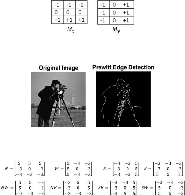
65Segmentation Techniques
The edge magnitude is denoted as the maximum value found by convolution
of each mask with the image. The masks are dened as shown in Figure 5.13.
Figure 5.14 shows the detected edge output using a Kirsch edge detector.
5.2.5 Robinson Edge Detector
The Robinson method is implemented by using coefcients of 0, 1, and 2
[22]. The masks are symmetrical around their directional axis, which is
composed of zeros. The edge magnitude is the maximum value obtained by
convolving the mask with the image pixel neighborhood, and the edge angle
can be obtained by the angle of the line of zeroes in the mask containing the
maximum response. The masks are shown in Figure 5.15.
Figure 5.16 shows the detected edge output using a Robinson edge detector.
FIGURE 5.11
Masks used in Prewitt edge detection.
FIGURE 5.12
Edge detection using the Prewitt edge detector.
FIGURE 5.13
Masks used in Kirsch edge detection.
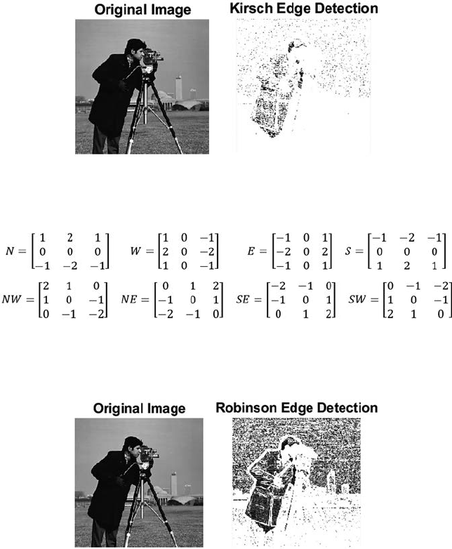
66 A Beginner’s Guide to Image Preprocessing Techniques
5.2.6 Canny Edge Detector
A canny edge detector is used to nd the edge of an image by separating
noise from the image prior to edge extraction [23,24]. The steps are as follows:
Step 1: The image I(x, y) is convolved with a Gaussian function G to
reduce the noise and to get a smooth version of the image:
Sxy IxyG(, )(,) .←∗
(5.16)
FIGURE 5.14
Edge detection using the Kirsch edge detector.
FIGURE 5.15
Masks used in Robinson edge detection.
FIGURE 5.16
Edge detection using the Robinson edge detector.
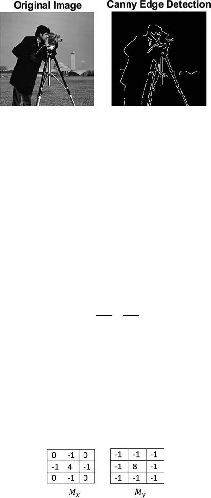
67Segmentation Techniques
Step 2: Gradient magnitude and direction is calculated for every pixel
of S(x, y), as obtained before.
Step 3: Nonmaximal suppression is applied to the gradient magnitude.
Step 4: Finally, a threshold is applied to the nonmaximal suppression
image.
Figure 5.17 shows the detected edge output using Canny edge detector.
5.2.7 Laplacian of Gaussian (LoG) Edge Detector
LoG of an image I(x, y) is dened [25] by a second order derivative dened as:
∇=
∂
∂+
∂
∂
2
2
2
2
2
II
x
I
y
.
(5.17)
It smoothes the image and the Laplacian is also calculated. This results
in a double edge image. Zero crossings are found out from the ltered
image to nd the edge. This operator is used to nd a pixel in the light
or dark side of the edge. The masks used in this operation are shown in
Figure 5.18 where Mx and My are the masks used in the horizontal and
vertical direction.
Figure 5.19 shows the detected edge output using an LoG edge detector.
FIGURE 5.17
Edge detection using a Canny edge detector.
FIGURE 5.18
Masks used in LoG edge detection.
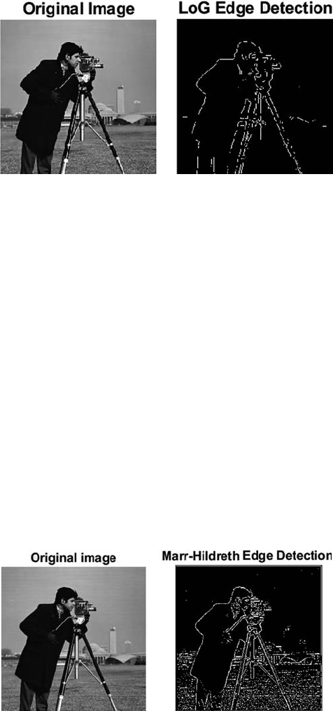
68 A Beginner’s Guide to Image Preprocessing Techniques
5.2.8 Marr-Hildreth Edge Detection
The Marr-Hildreth method is a technique of highlighting edges in continuous
curves wherever there are quick variations in image brightness [26]. The LoG
function is used as the convolution function. Then zero-crossings are found
in the ltered result to nd the edges. Algorithmic steps for the Marr-Hildreth
edge detector are as follows:
Step 1: The image is convolved with the Gaussian function for smoothing
Step 2: 2D Laplacian is applied to the smoothed image
Step 3: Analyze the sign change by looping through the result
Step 4: If a sign change occurs, and if the slope across the sign change is
greater than a threshold, then consider it as an edge.
Figure 5.20 shows the detected edge output using a Marr-Hildreth edge
detector.
FIGURE 5.19
Edge detection using the LoG edge detector.
FIGURE 5.20
Edge detection using the Marr-Hildreth edge detector.

69Segmentation Techniques
5.3 Region-Based Segmentation
Region-based segmentation is used to split or merge regions in the image
based on some similar or common image properties such as intensity values
of the region, texture, or pattern of the region and so on [27,28]. This can be
divided into two main types: region growing or region merging and region
splitting.
5.3.1 Region Growing or Region Merging
This is a method to group, or merge, pixels or subregions into larger regions
based on some property or image attributes [29]. This method starts with a
set of seed points and is based on some similar properties such as texture,
gray level, shape, color, and so forth; the neighboring pixels are appended
or added with the seed region. One such method is to divide the image into
2 × 2 or 4 × 4 regions and check each one. In the worst case the seed can be
a single pixel. Merging is done until no neighboring pixels are left with the
same property. Finally, the region is extracted from the image and a new seed
is dened to merge other similar regions. If the homogeneous regions are
small, region growing or merging is preferred.
5.3.2 Region Splitting
This method is just the opposite of region growing [30]. Region splitting starts
with the whole image and is divided until a uniform subregion is found.
The main drawback of this method is that it is very difcult to nd a proper
location to make the partition. If the homogeneous regions are large, region
splitting is preferred.
5.4 Summary
Image segmentation is generally used to separate an image into different
parts, or to extract signicant information from the image. Thresholding
is one of the procedures for image segmentation. The goal of thresholding
is to extract some pixels from the image while removing others. There are
different methods to select the threshold value like a histogram shape-
based method, clustering-based method, and entropy-based method.
In the histogram shape-based method peaks, valleys, and curvatures of
the histogram are analyzed. In a clustering-based method, the image is
clustered into different parts based on the pixel values. There are different
clustering-based methods like k-means, or Otsu. The entropy-based method

70 A Beginner’s Guide to Image Preprocessing Techniques
is developed based on the probability distribution function of the gray level
histogram. There are different edge-based segmentations like Sobel, Canny,
Prewitt, Robinson, Robert, Kirsch, LoG, and Marr-Hildreth. The Roberts
edge detection technique is used to highlight high spatial frequency regions
of the image, which corresponds to edges. The Sobel edge detection method
uses the Sobel approximation to the derivative to highlight edges. The
Prewitt edge detection is used to assess the orientation and magnitude of
an edge. The Kirsch edge detection use a single mask and rotates it to eight
directions: North, West, East, South, Northwest, Southwest, Southeast, and
Northeast. The Robinson method is same as the Kirsch method but the only
difference is that it is implemented by using the coefcients of 0, 1, and 2.
A Canny edge detector is used to nd the edge of the image by separating
noise from the image prior to edge extraction. The LoG operator is used
to nd a pixel in the light or the dark side of the edge. The Marr-Hildreth
method is a technique of highlighting edges in continuous curves wherever
there are fast variations in image brightness. Segmentation can be done
based on region properties. In region growing, or merging, rst a small
region is taken, then based on some similar property the neighboring pixels
are added to that region. In region splitting, the whole image is split into
sun regions that satisfy the predened similarity or homogeneity property.
References
1. Santosh, K. C., Xue, Z., Antani, S. K., & Thoma, G. R. 2015. NLM at imageCLEF2015:
Biomedical multipanel gure separation. In CLEF (Working Notes), 1391, 1–8.
ISSN 1613-0073.
2. Roy, P., Goswami, S., Chakraborty, S., Azar, A. T., & Dey, N. 2014. Image
segmentation using rough set theory: A review. International Journal of Rough
Sets and Data Analysis (IJRSDA), 1(2), 62–74.
3. Obaidullah, S. M., Halder, C., Santosh, K. C., Das, N., & Roy, K. 2018. PHDIndic_11:
Page-level handwritten document image dataset of 11 ofcial Indic scripts for
script identication. Multimedia Tools and Applications, 77(2), 1643–1678.
4. Araki, T., Ikeda, N., Dey, N., Acharjee, S., Molinari, F., Saba, L., Godia, E.,
Nicolaides, A., & Suri, J. S. 2015. Shape-based approach for coronary calcium
lesion volume measurement on intravascular ultrasound imaging and its
association with carotid intima-media thickness. Journal of Ultrasound in
Medicine, 34(3), 469–482.
5. Chaki, J., & Parekh, R. 2011. Plant leaf recognition using shape based features
and neural network classiers. International Journal of Advanced Computer Science
and Applications, 2(10), 41–47.
6. Chaki, J., Parekh, R., & Bhattacharya, S. 2015, July. Recognition of whole and
deformed plant leaves using statistical shape features and neuro-fuzzy classier.
In Recent Trends in Information Systems (ReTIS), 2015 IEEE 2nd International
Conference on (pp. 189–194). IEEE, Kolkata, India.
71Segmentation Techniques
7. Santosh, K. C., & Antani, S. 2018. Automated chest x-ray screening: Can lung
region symmetry help detect pulmonary abnormalities? IEEE Transactions on
Medical Imaging, 37(5), 1168–1177.
8. Roy, P., Dutta, S., Dey, N., Dey, G., Chakraborty, S., & Ray, R. 2014, July. Adaptive
thresholding: A comparative study. In Control, Instrumentation, Communication
and Computational Technologies (ICCICCT), 2014 International Conference on (pp.
1182–1186). IEEE.
9. Chaki, J., Parekh, R., & Bhattacharya, S. 2015. Plant leaf recognition using texture
and shape features with neural classiers. Pattern Recognition Letters, 58, 61–68.
10. Dhanachandra, N., Manglem, K., & Chanu, Y. J. 2015. Image segmentation using
K-means clustering algorithm and subtractive clustering algorithm. Procedia
Computer Science, 54(2015), 764–771.
11. Satapathy, S. C., Raja, N. S. M., Rajinikanth, V., Ashour, A. S., & Dey, N. 2016.
Multi-level image thresholding using Otsu and chaotic bat algorithm. Neural
Computing and Applications, 29(12), 1–23.
12. Chaki, J., Parekh, R., & Bhattacharya, S. 2016, January. Plant leaf recognition
using a layered approach. In Microelectronics, Computing and Communications
(MicroCom), 2016 International Conference on (pp. 1–6). IEEE, Durgapur, India.
13. Shriranjani, D., Tebby, S. G., Satapathy, S. C., Dey, N., & Rajinikanth, V. 2018.
Kapur’sentropy and active contour-based segmentation and analysis of retinal
optic disc. In Computational Signal Processing and Analysis (pp. 287–295). Springer,
Singapore.
14. Chakraborty, S., Chatterjee, S., Dey, N., Ashour, A. S., Ashour, A. S., Shi, F., & Mali, K.
2017. Modied cuckoo search algorithm in microscopic image segmentation of
hippocampus. Microscopy Research and Technique, 80(10), 1051–1072.
15. Chaki, J., & Parekh, R. 2012. Designing an automated system for plant leaf
recognition. International Journal of Advances in Engineering & Technology, 2(1), 149.
16. Dey, N., Pal, M., & Das, A. 2012. A session based blind watermarking technique
within the NROI of retinal fundus images for authentication using DWT, spread
spectrum and harris corner detection. arXiv preprint arXiv:1209.0053.
17. Santosh, K. C., & Nattee, C. 2007. Template-based nepali natural handwritten
alphanumeric character recognition. Science & Technology Asia, 12(1), 20–30.
18. Samanta, S., Acharjee, S., Mukherjee, A., Das, D., & Dey, N. 2013, December. Ant
weight lifting algorithm for image segmentation. In Computational Intelligence and
Computing Research (ICCIC), 2013 IEEE International Conference on (pp. 1–5). IEEE.
19. Ganesan, P., & Sajiv, G. 2017, March. A comprehensive study of edge detection
for image processing applications. In Innovations in Information, Embedded and
Communication Systems (ICIIECS), 2017 International Conference on (pp. 1–6). IEEE.
20. Biswas, D., Das, P., Maji, P., Dey, N., & Chaudhuri, S. S. 2013. Visible watermarking
within the region of noninterest of medical images based on fuzzy C-means
andHarris corner detection. Computer Science & Information Technology, 161–168.
21. Melin, P., Gonzalez, C. I., Castro, J. R., Mendoza, O., & Castillo, O. 2014. Edge-
detection method for image processing based on generalized type-2 fuzzy logic.
IEEE Transactions on Fuzzy Systems, 22(6), 1515–1525.
22. Russ, J. C. 2016. The Image Processing Handbook. CRC Press, Boca Raton, FL.
23. Chaki, J., Parekh, R., & Bhattacharya, S. 2016. Plant leaf recognition using ridge
lter and curvelet transform with neuro-fuzzy classier. In Proceedings of 3rd
International Conference on Advanced Computing, Networking and Informatics (pp.
37–44). Springer, New Delhi.
72 A Beginner’s Guide to Image Preprocessing Techniques
24. Dey, N., Maji, P., Das, P., Biswas, S., Das, A., & Chaudhuri, S. S. 2013, January.
An edge based blind watermarking technique of medical images without
devalorizing diagnostic parameters. In Advances in Technology and Engineering
(ICATE), 2013 International Conference on (pp. 1–5). IEEE.
25. Thamotharan, B., Venkatraman, B., Anusuya, A., Ramakrishnan, S., &
Karthikeyan, M. P. 2017. Analysis of various edge detection techniques for
dosimeter bubble detector images. Biomedical Research, 28(20), 8635–8639.
26. Hemalatha, R., Santhiyakumari, N., Madheswaran, M., & Suresh, S. 2017,
March. Intima-media segmentation using marr-hildreth method and its
implementation on unied technology learning platform. In Emerging Devices
and Smart Systems (ICEDSS), 2017 Conference on (pp. 32–36). IEEE.
27. Chakraborty, S., Chatterjee, S., Ashour, A. S., Mali, K., & Dey, N. 2018. Intelligent
computing in medical imaging: A study. In Advancements in Applied Metaheuristic
Computing (pp. 143–163). IGI Global.
28. Dey, N., Rajinikanth, V., Ashour, A. S., & Tavares, J. M. R. 2018. Social group
optimization supported segmentation and evaluation of skin melanoma images.
Symmetry, 10(2), 51.
29. Hore, S., Chakraborty, S., Chatterjee, S., Dey, N., Ashour, A. S., Van Chung, L.,&
Le, D. N. 2016. An integrated interactive technique for image segmentation
using stack based seeded region growing and thresholding. International Journal
of Electrical and Computer Engineering, 6(6), 2773.
30. Ohlander, R., Price, K., & Reddy, D. R. 1978. Picture segmentation using a
recursive region splitting method. Computer Graphics and Image Processing, 8(3),
313–333.

73
6
Mathematical Morphology Techniques
6.1 Binary Morphology
Binary images generally contain several aws [1]. The binary regions which
are created by simple thresholding can contain noise. Morphological image
processing is used to remove these imperfections of the image. Morphological
techniques use a small shape or template called a structuring element. The
structuring element is placed in all possible positions in the image and is
compared with the corresponding neighborhood of pixels. Some procedures
check whether the structuring element “ts” inside the neighborhood, while
others check whether it intersects or “hits” the neighborhood. Figure 6.1
shows the effect of a structuring element on image pixel.
Through the binary morphological operation on a binary image [2], another
new binary image is created which contains nonzero pixel values only if
the test is successful for that particular location of the input image. The
structuring element is a small matrix of pixels, that is, a small binary image,
with values of either zero or one. The arrangement of zeroes and ones denotes
the shape of the structuring element. The origin of the structuring element is
generally one of its pixels. The size of the structuring element is usually odd in
dimension, and the center pixel is considered as the origin of the structuring
element. Figure 6.2 shows some examples of structuring elements.
When a structuring element is positioned onto a binary image, each pixel
of the binary image is associated with the pixels of the structuring element.
The structuring element is considered to t the image if, for all of its pixels
containing the value 1, the associated image pixel is also 1. Likewise, a
structuring element is considered to intersect or hit an image if at least for
one of its pixels containing the value 1 the associated image pixel is also 1.
Figure 6.3 demonstrates the effect of hit and t.
The structuring elements having zero valued pixels are ignored.
6.1.1 Erosion
The erosion operation [3,4] (denoted by ) between a binary image I(x, y) and
a structuring element S, creates a new binary image E(x, y) with ones in each
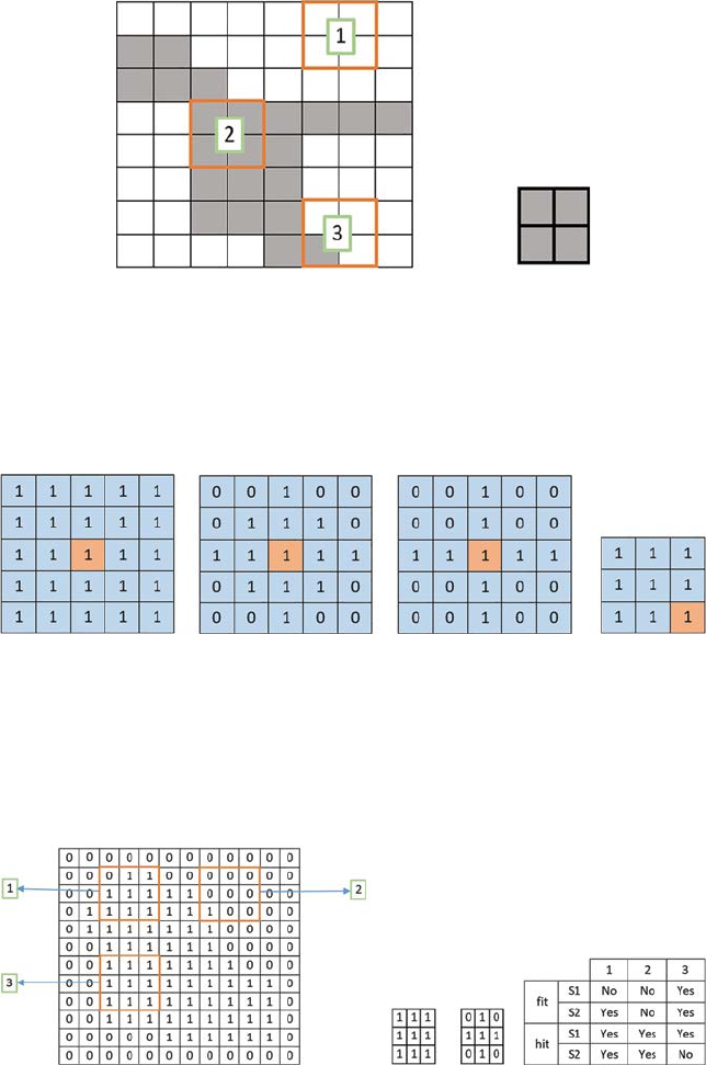
74 A Beginner’s Guide to Image Preprocessing Techniques
(A) (B)
FIGURE 6.1
(A) White pixels contain zero value, and nonzero pixels contain nonzero value, (1) The
structuring element neither ts, nor hits the image, (2) The structuring element ts the image,
(3) The structuring element hits the image; (B) structuring element.
(A)
(B) (C)(D)
FIGURE 6.2
Orange pixel is the origin of the structuring element, (A) 5 × 5 square-shaped structuring
element, (B) 5 × 5 diamond-shaped structuring element, (C) 5 × 5 cross-shaped structuring
element, (D) 3 × 3 square-shaped structuring element.
(A) (B) (C
)(
D)
FIGURE 6.3
(A) Superimposing of structuring element, (B) Structuring element S1, (C) Structuring element
S2, and (D) Fitting and hitting of a binary image with structuring elements S1 and S2.

75Mathematical Morphology Techniques
and every locations (x, y) at which that structuring element S ts the input
image I and zero otherwise:
Exy IS(,).=
(6.1)
Erosion with a small (e.g., 3 × 3 or 5 × 5) structuring element shrinks an
image by removing a pixel layer from both the outer and inner boundaries of
image regions. So, image details are removed and different gaps and holes of
the image regions become larger. Figure 6.4 shows the output of erosion with
a 5 × 5 structuring element.
Erosion with a large structuring element has a more prominent effect. The
erosion result with a large structuring element can be the same if a smaller
structuring element of the same shape is iteratively applied to an image. For
example, if S1 and S2 are two structuring elements duplicate in shape, but the
size of S2 is twice that of S1, then
ISISS211=().
(6.2)
By using erosion small details of the image can be removed, and thus the
size of the region of interest can be reduced. The boundary (B) of an image
region can be obtained by subtracting the eroded image from the original
image:
BIIS=−().
(6.3)
6.1.2 Dilation
The dilation operation [5,6] (denoted by ⊕ ) between a binary image I(x, y)
and a structuring element S, creates a new binary image D(x, y) with ones in
each and every location (x, y) where that structuring element S hits the input
image I and 0:
Exy IS(,).=⊕
(6.4)
Thus, dilation is just the opposite of erosion. It adds a pixel layer to both the
outer and inner boundaries of image regions. Figure 6.5 shows the output of
dilation with a 5 × 5 structuring element.
FIGURE 6.4
Output of erosion of a binary image.

76 A Beginner’s Guide to Image Preprocessing Techniques
By using dilation, the holes of a binary image can be lled and gaps between
different regions can be reduced.
6.1.3 Opening
The opening operation [7] (denoted by ) between a binary image I(x, y) and a
structuring element S, creates a new binary image O(x, y), which is basically
erosion followed by dilation:
ISISS=().⊕
(6.5)
The opening is used to open up gaps between connected regions within
the image. Figure 6.6 shows the output of opening with 7 × 7 structuring
element.
Once the connected regions within the image are opened by using a
structuring element, there is no further opening effect on that image using
that particular structuring element:
ISISS=().
(6.6)
6.1.4 Closing
The closing operation [7] (denoted by ·) between a binary image I(x, y) and a
structuring element S, creates a new binary image C(x, y), which is basically
dilation followed by erosion:
ISISS⋅=().⊕
(6.7)
A closing operation is used to connect or ll holes in the image regions
while maintaining the initial region sizes. Figure 6.7 shows the output of
closing with a 7 × 7 structuring element.
FIGURE 6.6
Output of opening of a binary image.
FIGURE 6.5
Output of dilation of a binary image.

77Mathematical Morphology Techniques
Once the holes are connected within the image by using a structuring
element, there is no further closing effect on that image using that particular
structuring element:
ISISS⋅= ⋅⋅().
(6.8)
6.1.5 Hit and Miss
The hit and miss operation [8] (denoted as ⊙) permits to develop information
on how objects in a binary image are associated to their neighbors. The
operation calls for a matched pair of structuring elements, {S1, S2}, that
investigate the outside and inside, individually, of objects in the image:
ISS IS IS
C
{, }( )( ).12 12=∩
(6.9)
Here, IC is the complement of I.
An object pixel is conserved by this operation if and most effective if S1
transformed to that pixel ts inside the object and S2 transformed to that pixel
ts outside the object. Figure 6.8 shows the output of a hit and miss operation.
It is assumed that S1 ∩ S2 = NULL. This operation is generally used for
detecting particular shapes where two structuring elements present that
particular shape.
6.1.6 Thinning
The thinning operation is to some extent like opening or erosion [8], which
is used to eliminate selected foreground pixels from binary images. It is
generally used for skeletonization. Thinning is usually particularly applied
to binary images, and results in another binary image as output. Thinning
FIGURE 6.8
Output of hit and miss of a binary image.
FIGURE 6.7
Output of closing of a binary image.

78 A Beginner’s Guide to Image Preprocessing Techniques
operations can be expressed by hit and miss operations. The thinning of an
image I by a structuring element S is:
Thinhit_and_miss(, )(,),IS IIS=−
(6.10)
where “−” is a logical subtraction and can be denoted by two binary images
A and B:
AB AB−= ∩
. Figure 6.9 shows the output of a thinning operation.
6.1.7 Thickening
Thinning operation is to some extent like closing or dilation [8], which is used
to grow selected foreground pixels from binary images. It is usually used to
determine the estimated convex hull of a shape. Thickening is normally only
applied to binary images, and it produces another binary image as output.
A thickening operation can be expressed by a hit and miss operation. The
thickening of an image I by a structuring element S is:
Thick hit_and_miss(, )(,).IS IIS=∪
(6.11)
Thus, the thickened image consists of the original image and additional
foreground pixels produced by the hit-and-miss operation. Figure 6.10 shows
the output of a thickening operation.
6.2 Grayscale Morphology
Grayscale morphology [9] is basically a multidimensional simplication of
the binary morphology.
FIGURE 6.9
Output of thinning of a binary image.
FIGURE 6.10
Output of thickening of a binary image.
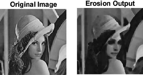
79Mathematical Morphology Techniques
6.2.1 Erosion
The erosion of a grayscale image I(x, y) by the structuring element S(x, y) can
be expressed as:
ISIxsyt Sxy
st B
=++−
∈
min( ,)(,){}.
,
(6.12)
Here, B is the space in which S(x, y) is dened. In grayscale erosion, the
local minimum grey level in the image is considered over the region dened
by the structuring element [10]. The image becomes darker with the erosion
operation and light details are reduced. Figure 6.11 shows the output of an
erosion operation.
6.2.2 Dilation
The dilation of a grayscale image I(x, y) by the structuring element S(x, y) can
be expressed as:
ISIxsyt Sxy
st B
⊕=−−+
∈
max( ,)(, ){}.
,
(6.13)
Here, B is the space in which S(x, y) is dened. In grayscale dilation, the
local maximum gray level in the image is considered over the region dened
by the structuring element [11]. The image become brighter by the dilation
operation and dark details are reduced. Figure 6.12 shows the output of a
dilation operation.
6.2.3 Opening
The opening of a grayscale image I(x, y) by the structuring element S(x, y) can
be expressed as:
ISISS=().⊕
(6.14)
FIGURE 6.11
Output of erosion of a grayscale image.
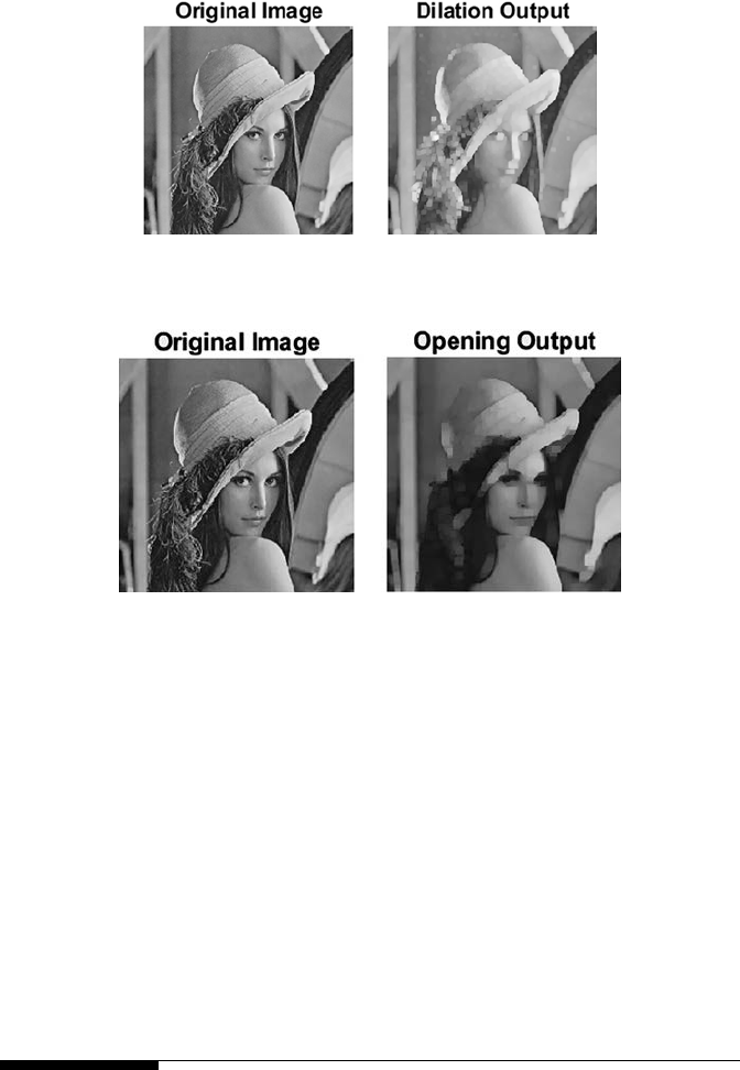
80 A Beginner’s Guide to Image Preprocessing Techniques
In the grayscale opening, bright details are reduced. Figure 6.13 shows the
output of the opening operation.
6.2.4 Closing
The closing of a grayscale image I(x, y) by the structuring element S(x, y) can
be expressed as:
ISISS⋅=().⊕
(6.15)
In grayscale closing, the dark details are reduced. Figure 6.14 shows the
output of the closing operation.
6.3 Summary
Morphology is used to remove the imperfections of the image. The output
of morphology is generated by using a structuring element. Morphology
FIGURE 6.13
Output of opening of a grayscale image.
FIGURE 6.12
Output of dilation of a grayscale image.
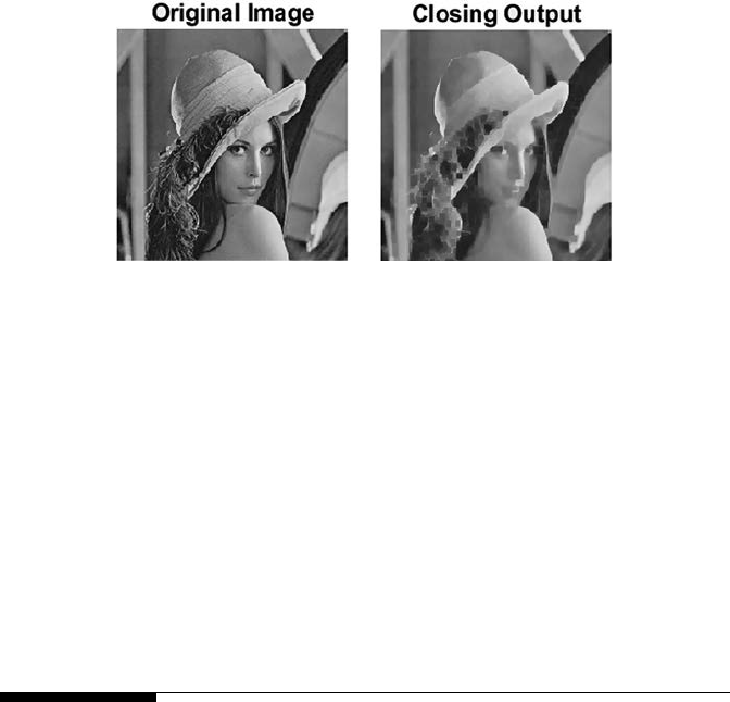
81Mathematical Morphology Techniques
operations are applicable in binary as well as grayscale images. Some
examples of morphological operations are erosion, which is used to shrink
binary images and darken grayscale images; dilation, which is used to ll
up gaps in binary images and lighten grayscale images; opening, which is
used to open up gaps between connected regions within binary images and
where bright details of grayscale images are reduced; closing, which is used
to connect or ll holes in binary image regions and where dark details of
grayscale images are reduced; thinning, which is mainly applied to binary
image for thinning and thickening, and is used to determine the estimated
convex hull of a binary shape.
References
1. Kotyk, T., Ashour, A. S., Chakraborty, S., Dey, N., & Balas, V. E. 2015. Apoptosis
analysis in classication paradigm: A neural network based approach. In Healthy
World Conference—A Healthy World for a Happy Life (pp. 17–22). Kakinada(AP),
India.
2. Shih, F. Y. 2009. Image Processing and Mathematical Morphology: Fundamentals and
Applications. CRC Press, Boca Raton, FL.
3. Chaki, J., Parekh, R., & Bhattacharya, S. 2016, January. Plant leaf recognition
using a layered approach. In Microelectronics, Computing and Communications
(MicroCom), 2016 International Conference on (pp. 1–6). IEEE, Durgapur, India.
4. Chaki, J., Parekh, R., & Bhattacharya, S. In press. Plant leaf classication using
multiple descriptors: A hierarchical approach. Journal of King Saud University-
Computer and Information Sciences, doi:10.1016/j.jksuci.2018.01.007.
5. Ravi, S., & Khan, A. M. 2013. Morphological operations for image processing:
Understanding and its applications. In NCVSComs-13 Conference Proceedings
(pp.17–19).
6. Pardeshi, R., Chaudhuri, B. B., Hangarge, M., & Santosh, K. C. 2014, September.
Automatic handwritten Indian scripts identication. In Frontiers in Handwriting
FIGURE 6.14
Output of closing of a grayscale image.
82 A Beginner’s Guide to Image Preprocessing Techniques
Recognition (ICFHR), 2014 14th International Conference on (pp. 375–380). IEEE,
Heraklion, Greece.
7. Benavent, X., Dura, E., Vegara, F., & Domingo, J. 2012. Mathematical morphology
for color images: An image-dependent approach. Mathematical Problems in
Engineering, 2012(678326), 1–18.
8. Sonka, M., Hlavac, V., & Boyle, R. 2014. Image Processing, Analysis, and Machine
Vision. Cengage Learning, Stamford, USA.
9. Sternberg, S. R. 1986. Grayscale morphology. Computer Vision, Graphics, and Image
Processing, 35(3), 333–355.
10. Ćurić, V., Landström, A., Thurley, M. J., & Hendriks, C. L. L. 2014. Adaptive
mathematical morphology—A survey of the eld. Pattern Recognition Letters, 47,
18–28.
11. Wang, Y., Shi, F., Cao, L., Dey, N., Wu, Q., Ashour, A. S., & Wu, L. In press.
Morphological segmentation analysis and texture-based support vector
machines classication on mice liver brosis microscopic images. Current
Bioinformatics.

83
7
Other Applications of Image Preprocessing
7.1 Preprocessing of Color Images
A color image has a huge quantity of information. If the color information is
hidden, human eyes may fail to analyze it [1]. Moreover, small alterations in
image features such as color, intensity, texture, and so forth are truly hard
to accomplish. Thus, preprocessing of color images is needed to preserve
the reliability of edges and other detailed information needed for further
processing.
There are two types of color image processing: pseudo color or false color
processing, and full color or true color processing. The purpose of pseudo
color processing is to color a grayscale image by assigning different colors
in different intensity ranges of a gray level image [2]. Pseudo color is also
called false color, as the colors are not originally present in the grayscale
image. The human eye can interpret about two dozens of gray shades in
a grayscale image, whereas it can interpret nearly 1000 variations of colors
in a color image [3]. Thus, if a given grayscale image is converted to color
by using pseudo color processing, the interpretation of different intensities
becomes much more convenient, as compared to an ordinary grayscale
image. Pseudo coloring can be done by an intensity slicing method. Suppose
there are L number of intensity values in a grayscale image I(x, y), which
varies from 0,…,(L − 1). In this case, l0 represents black where I(x, y) = 0 and
lL−1 represents white where I(x, y) = L − 1. Suppose there are P number of
planes perpendicular to the intensity plane where 0 < P < L − 1. These
planes are placed to the intensity levels l1,l2… , lP . P number of planes divide
the intensities to P + 1 number of intervals. So, the color Ck is assigned to the
gray level intensity at position (x, y) can be denoted by f(x, y) = Ck if I(x, y) ∈ Dk
where Dk is the intensity range between lk and lk+1. Thus, it can be said that P
number of planes divide the intensities to P + 1 number of intervals denoted
by D1,D2,… , DP+1. By using this concept the gray level intensity range can be
divided into some intervals, and for each interval a particular color can be
assigned. In this way a grayscale image can be colored—this procedure is
known as pseudo coloring. F ig u r e 7.1 shows the pseudo coloring image of
a grayscale image [4]. In the pseudo color image we can visualize different
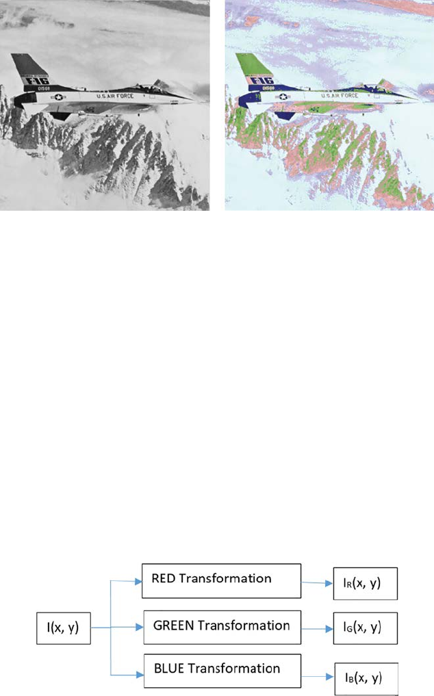
84 A Beginner’s Guide to Image Preprocessing Techniques
intensities of the image region with different colors, which are almost at in
the grayscale image. So, using a pseudo color image, intensities of the image
are much more interpretable or distinguishable than in a grayscale image. In
case of an RGB image, colors are added to R, G, and B channels separately
and the combination of R, G, and B channels enables the interpretation of
pseudo color images [5].
Grayscale to color image conversion can be done by the transformations
shown in F ig u r e 7.2.
In Fig u r e 7.2 I(x, y) is the grayscale image, which is transformed by three
different transformations: RED transformation, GREEN transformation,
and BLUE transformation [6]. RED, GREEN, and BLUE transformations give
the red, green, and blue plane output of the input grayscale image, which is
given by IR(x, y), IG(x, y), and IB(x, y). When these three planes are combined
together and displayed in a color display system it is known as a pseudo color
(A) (B)
FIGURE 7.1
(A) Grayscale image, (B) Pseudo color image.
FIGURE 7.2
Grayscale to color transformation.
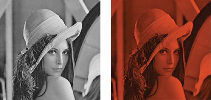
85Other Applications of Image Preprocessing
image. For example, Equation 7.1 denotes the transformation functions used
to generate the color image, and Fig u r e 7.3 shows the color transformation of
a grayscale image by using Equation 7.1:
IxyIxy
Ix
yI
xy
IxyIxy
R
G
B
()
()
()
,(,)
,.(, )
,.(, ).
=
=×
=×
033
011
(7.1)
In this example, to convert the grayscale image to color, the exact intensities
of the grayscale image are copied to the red plane, but the degraded version
of intensities of the original grayscale image are used in the green and
blue plane. The combination of this red, green, and blue plane is shown in
Figure7.3.
In the full color, or true color image preprocessing, the actual color of the
image is considered [7]. In such types of images, the colors can be specied
by using different color models like RGB (Red-Green-Blue), HSI (Hue-
Saturation-Intensity), CMY (Cyan-Magenta-Yellow), and so on. In some cases,
color image processing can be more convenient in a particular color model
while less convenient in some other color model. In such cases, the image is
converted from one color model to another color model. Fig u r e 7.4 shows the
representation of different color components, or color planes, of an image in
the RGB color model.
Fi g u r e 7. 5 shows the representation of different color components, or color
planes, of an image in the HSI color model.
Figure 7.6 shows the representation of different color components, or color
planes, of an image in the CMY color model.
(A) (B)
FIGURE 7.3
(A) Grayscale image, (B) Pseudo color transformed image.
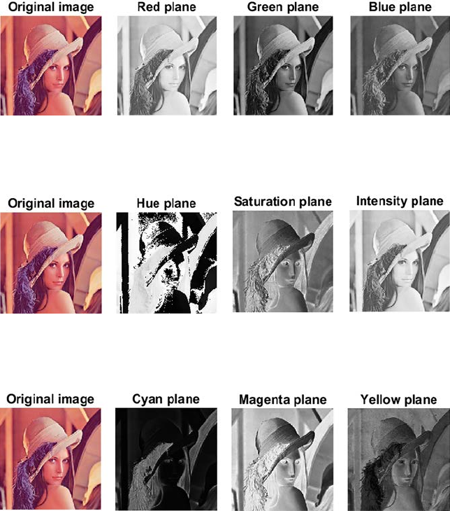
86 A Beginner’s Guide to Image Preprocessing Techniques
Different preprocessing transformation [8] operations can be done in these
color models, such as intensity modication represented by Equation 7.2:
fxyTOxy(, )(,),=×
( 7. 2)
where 0 < T < 1, O(x, y) is the input image and f(x, y) is the processed image.
So, if the image in the RGB color space is considered, then Equation 7.2 can
be rewritten, as shown in Equation 7.3:
fxyTOxy
ii
(),(,),=×
( 7. 3)
FIGURE 7.4
Red, Green, and Blue plane of RGB color image.
FIGURE 7.5
Hue, Saturation and Intensity plane of HSI color image.
FIGURE 7.6
Cyan, Magenta, and Yellow plane of CMY color image.
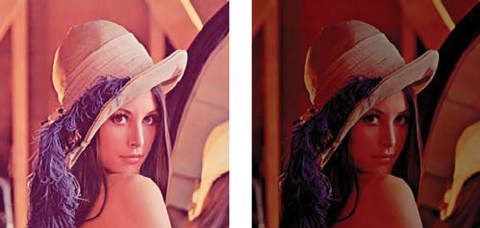
87Other Applications of Image Preprocessing
where i = 1,2, and 3, which represents the red, green, and blue planes of the
RGB color model, respectively. From Equation 7.3 it can be said that in case
of an RGB color image, all the three planes are scaled by the same scaling
factor, T.
If intensity modication is done for an HSI color image, then the scaling
is done only in the I plane of the input image, as this is the only plane of the
HSI color model representing the intensity. The hue and saturation of the
processed image will remain the same as in the input image. Thus, in this
case Equation 7.2 can be rewritten, as shown in Equation 7.4:
fxyOxy
fxyOxy
fxyTOxy
11
22
33
()
()
() ().
,(,)
,(,)
,,
=
=
=×
(7.4)
Similarly, the intensity modication in CMY color space can be represented
by Equation 7.5:
fxyTOxyT
ii
() (),,(),=× +−1
( 7. 5)
where i = 1,2, and 3, which represents the cyan, magenta, and yellow planes
of the CMY color model, respectively.
From these intensity transformations it can be said that the computation
using the HSI color space is minimum, as compared to RGB and CMY color
space, because in the RGB and CMY color space the scaling is done in all three
color planes. Fig u r e 7.7 shows the intensity-modied output for the HSI color
image with a scaling factor of 0.5.
Color complement is another preprocessing [9] transformation, which can
be done in true color image. Let us rst take a look at the color wheel, or color
circle, which is shown in Fi g u r e 7. 8.
In Fig u re 7. 8, it can be seen that the colors diagonally opposite in the color
wheel are complementary colors, such as cyan which is the complementary
(A)
(B)
FIGURE 7.7
(A) Original Image, (B) Intensity modied image.
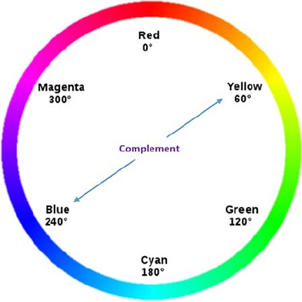
88 A Beginner’s Guide to Image Preprocessing Techniques
color of red and vice versa, or yellow which is the complementary color of
blue and vice versa, and so on. Color complement is analogous to grayscale
negative. Thus, if the same transform function, which is used to generate
grayscale negative, is applied in different planes of the color image, a color
complement image is generated. This can be represented by Equation 7.6 and
Fi g u r e 7.9, which shows the color complement image of an RGB color input
image:
fxyL Oxy
ii
() (),,,=−−1
(7. 6)
where i = 1,2, and 3, Oi(x, y) is the input image, L is the maximum number
of color shades (in case of RGB L = 256), and fi(x, y) is the processed image.
From Fig u r e 7.9 it can be seen that the complement of an input image looks
like the photographic negative of a color image.
Color slicing is the next preprocessing [10] transformation that can be
applied to the true color or full color image. Color slicing is used to highlight
a certain color range in an image, and thus it is useful to nd an object of a
certain color in an image. In this method, it is assumed that all the colors of
interest lie within a cube of width, say W, centered at the prototypical color
whose components are given by some vector say C1, C2, and C3, as shown in
Fi g u r e 7.10.
FIGURE 7.8
Color wheel.
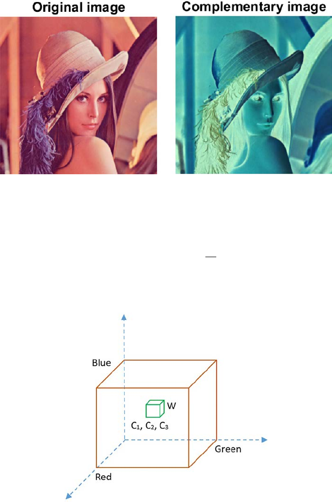
89Other Applications of Image Preprocessing
The color slicing transformation can be denoted by Equation 7.7:
fxyOxyC Wi
Oxy
i
ii
i
(),.|(, )| .
(, ),
=−>
∀≤≤05 2
13
if
otherwisse
( 7.7 )
FIGURE 7.9
Complementary image output.
FIGURE 7.10
Cube of width W.
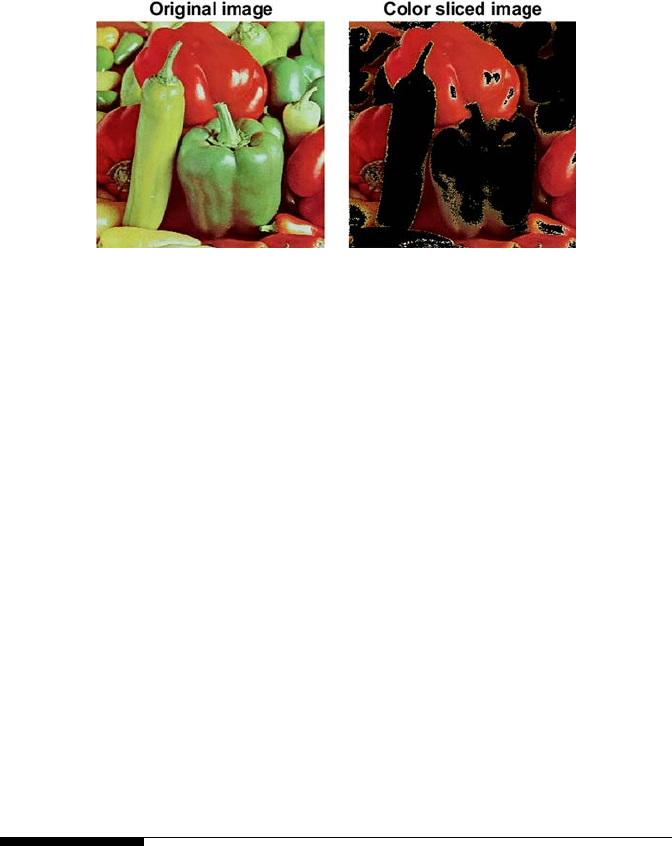
90 A Beginner’s Guide to Image Preprocessing Techniques
This means all the colors outside the cube of width W will be represented by
some insignicant color, but inside the cube the original colors are retained.
Fi g u r e 7.11 shows the output of the color slicing where only the red shades
are kept.
The next type of preprocessing transformation of the color image is tone
correction [11]. This is again analogous with the intensity enhancement, or
contrast enhancement, of the grayscale image. A color image may have a
at tone, light tone, or dark tone. These tones represent the distribution of
different color intensities within the color image or RGB image. The form of
transformation function used to correct the tone of at, light, and bark-toned
image is shown in Fi g u r e 7.12 .
In case of light tone image wide range of intensities in the input image is
mapped to narrow range intensities in the output image so that the output
image become dark. In case of dark tone image narrow range of intensities in
the input image is mapped to wide range intensities in the output image so
that the output image become light.
Other types of color image preprocessing involve histogram equalization,
segmentation of color images, and so on F ig u r e 7.13 through 7.16.
7.2 Image Preprocessing for Neural
Networks and Deep Learning
Deep learning has really become a main research area in the past few
years[12]. Deep learning uses neural networks, which need a large number
of training data and are comprised of many of hidden layers. These models
are used in speech, vision, image, video, language processing, and so forth.
For an image, providing the image pixel values directly into a neural network
may cause numerical overows [13,14]. Also, some objective and activation
FIGURE 7.11
Output of color slicing.
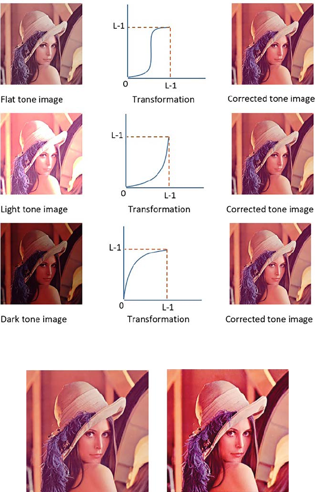
91Other Applications of Image Preprocessing
FIGURE 7.12
Tone correction.
(A) (B)
FIGURE 7.13
(A) Original image, (B) Image output after histogram equalization.
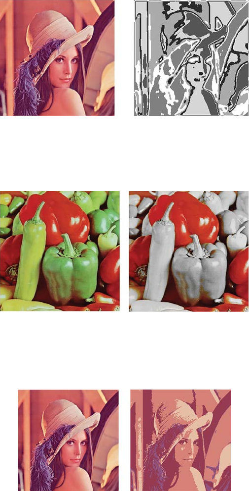
92 A Beginner’s Guide to Image Preprocessing Techniques
(A) (B)
FIGURE 7.14
(A) Original image, (B) Segmented output using 5 bins.
(A) (B)
FIGURE 7.15
(A) Original Image, (B) Image output after ltering or masking. Here only the red shades are
kept in color and rest of the image is desaturated.
(A) (B)
FIGURE 7.16
(A) Original image, (B) Image Otsu thresholding output.

93Other Applications of Image Preprocessing
functions are not compatible with all kinds of input. The wrong arrangement
produces a poor result during the learning phase of a neural network [15–17].
To construct an efcient neural network model, cautious attention is required
to build the network architecture as well as the input data format. The most
common image data input factors are the number of images, image width,
image height, number of levels per pixel, and number of channels. For an RGB
image, there are three channels of data representing the colors (pixel intensity
values) in Red, Green, and Blue channels, which range between 0 and 255 [18,19].
A number of preprocessing steps are needed prior to using this in any
Deep Learning project. Some of the most common preprocessing steps are
discussed below.
Unvarying Aspect Ratio: Most of the neural networks presume that the input
image is square in shape. So, it is essential to check every image to ensure
it is square or not [20], and cropped properly, as shown in Figure 7.17. While
cropping, usually the center part is kept.
Scaling of Images: After making all images square in shape, scaling of each
image is properly done [21,22]. For example, suppose the image is of size
250 × 250 pixels and we have to obtain an image with a height and width
of 100 pixels. Therefore, the height and width of each image are scaled by a
factor of 0.4 (100/250). The same applies for up-scaling.
Normalization of Image Inputs: Image data normalization [23,24] is a vital
step, which conrms a similar data distribution for every input data. This
helps to converge the network faster while training it. In image processing,
normalization helps to change the pixel intensity range. There are three types
of normalization: data rescaling, data standardization, and data stretching.
Data rescaling is further divided into linear and nonlinear rescaling.
The linear data scaling can be represented by Equation 7.8:
I
II
II
II
I
Norm MinNewMax NewMin
MaxMin
NewMin
=−
−
−
+() ,
(7. 8)
where IMax and IMin are the maximum and minimum intensities of the original
image, and INewMax and INewMin are the maximum and minimum intensities
of the normalized image. For example, suppose the image has the intensity
FIGURE 7.17
Cropping of image data.

94 A Beginner’s Guide to Image Preprocessing Techniques
range 30–120 and the desired range is 0–255. First, 30 is subtracted from every
pixel intensity. Then each pixel intensity is multiplied with 255/90, making
the range between 0 and 255.
The nonlinear data scaling is represented by Equation 7.9, which follows a
sigmoid function:
I
II
e
I
Norm NewMax NewMin NewMin
=−
+
+
−−
()
,
(( )/ )
1
1
1βα
(7.9)
where β denotes the intensity around which the range is centered, and α
denotes the width of the input intensity.
Data standardization is the second way to normalize image data, where the
average of the data is subtracted from the image and divided by its standard
deviation. The spreading of such data looks like a Gaussian curve with
mean = 0, and a standard deviation (std) = 1. Data standardization can be
represented by Equation 7.10:
III
I
Norm Mean
Std
=
−.
(7.10)
Data stretching is the third way to normalize image data, where the data
are braced to a maximum and minimum value, and can be represented by
using Equation 7.11:
IIcc
I
Id d
Norm
Norm
[]
[].
<=
>=
(7.11)
Here, image data values greater than d are set to d, and the same occurs
inversely with c.
Reduction in Dimension: Sometimes the three channels of an RGB image [25]
are collapsed into a single grayscale channel. Reduction in the dimension
of image data is often needed when the neural network performance is
permitted to be dimension-invariant.
Augmentation of Image Data: The next preprocessing technique [26] includes
augmenting the image data with disturbed versions of the present images.
Rotation, scaling, and other afne transformations are usually used to
augment image data. This prevents the neural network from recognizing
unwanted characteristics present in the disturbed version of image data.
7.3 Summar y
The need of preprocessing of color images in the eld of Deep Learning is
discussed in this chapter. Color image processing includes pseudo color and
full color or true color processing. The purpose of pseudo color processing is

95Other Applications of Image Preprocessing
to color a grayscale image by assigning different colors to different intensity
ranges of a gray level image. In the case of an RGB image, colors are added
to the R, G, and B channels separately, and the combination of R, G, and
B channels allows for the interpretation of a pseudo color image. Through
pseudo color images, we can visualize different intensities of the image region
with a different color, which would be almost at in the grayscale image.
Thus, using the pseudo color image, intensities of the image are much more
interpretable or distinguishable than for a grayscale image. In the full-color
image, the actual color of the image is considered. In such types of images, the
colors can be specied by using different color models like RGB (Red-Green-
Blue), HSI (Hue-Saturation-Intensity), CMY (Cyan-Magenta-Yellow), and so
on. Different preprocessing transformation operations can be performed on
these color models such as intensity modication, color complement, color
slicing, tone correction, histogram equalization, segmentation of the color
image, and so forth.
References
1. Ghosh, A., Sarkar, A., Ashour, A. S., Balas-Timar, D., Dey, N., & Balas, V. E. 2015.
Grid color moment features in glaucoma classication. Int J Adv Comput Sci Appl,
6(9), 1–14.
2. Dey, N., Ashour, A. S., Chakraborty, S., Samanta, S., Sifaki-Pistolla, D., Ashour,
A. S., & Nguyen, G. N. 2016. Healthy and unhealthy rat hippocampus cells
classication: A neural based automated system for Alzheimer disease
classication. Journal of Advanced Microscopy Research, 11(1), 1–10.
3. Chaki, J., Parekh, R., & Bhattacharya, S. 2017, March. An efcient fragmented
plant leaf classication using color edge directivity descriptor. In International
Conference on Computational Intelligence, Communications, and Business Analytics
(pp. 197–211). Springer, Singapore.
4. Li, Z., Shi, K., Dey, N., Ashour, A. S., Wang, D., Balas, V. E., … & Shi, F. 2017.
Rule-based back propagation neural networks for various precision rough set
presented KANSEI knowledge prediction: A case study on shoe product form
features extraction. Neural Computing and Applications, 28(3), 613–630.
5. Bhattacharya, T., Dey, N., & Chaudhuri, S. R. 2012. A session based multiple
image hiding technique using DWT and DCT. arXiv preprint arXiv:1208.0950.
6. Candemir, S., Borovikov, E., Santosh, K. C., Antani, S., & Thoma, G. 2015. Rsilc:
Rotation-and scale-invariant, line-based color-aware descriptor. Image and Vision
Computing, 42, 1–12.
7. Chaki, J., & Parekh, R. 2011. Plant leaf recognition using shape based features
and neural network classiers. International Journal of Advanced Computer Science
and Applications, 2(10) 41–47.
8. Benavent, X., Dura, E., Vegara, F., & Domingo, J. 2012. Mathematical morphology
for color images: An image-dependent approach. Mathematical Problems in
Engineering, 2012(678326) 1–18.
96 A Beginner’s Guide to Image Preprocessing Techniques
9. Sonka, M., Hlavac, V., & Boyle, R. 2014. Image Processing, Analysis, and Machine
Vision. Cengage Learning, Stamford, USA.
10. Fu, K. S. 2018. Special Computer Architectures for Pattern Processing. CRC Press,
Boca Raton, FL.
11. Kotyk, T., Ashour, A. S., Chakraborty, S., Dey, N., & Balas, V. E. 2015. Apoptosis
analysis in classication paradigm: A neural network based approach. In Healthy
World Conference—A Healthy World for a Happy Life (pp.17–22). Kakinada(AP),
India.
12. Dong, C., Loy, C. C., He, K., & Tang, X. 2016. Image super-resolution using
deep convolutional networks. IEEE Transactions on Pattern Analysis and Machine
Intelligence, 38(2), 295–307.
13. Nimmy, S. F., Sarowar, M. G., Dey, N., Ashour, A. S., & Santosh, K. C. 2018.
Investigation of DNA discontinuity for detecting tuberculosis. Journal of Ambient
Intelligence and Humanized Computing, 1–15.
14. Chaki, J., Parekh, R., & Bhattacharya, S. 2015. Plant leaf recognition using texture
and shape features with neural classiers. Pattern Recognition Letters, 58, 61–68.
15. Li, Z., Dey, N., Ashour, A. S., Cao, L., Wang, Y., Wang, D., & Shi, F. 2017.
Convolutional neural network based clustering and manifold learning method
for diabetic plantar pressure imaging dataset. Journal of Medical Imaging and
Health Informatics, 7(3), 639–652.
16. Chaki, J., Parekh, R., & Bhattacharya, S. In press. Plant leaf classication using
multiple descriptors: A hierarchical approach. Journal of King Saud University-
Computer and Information Sciences, doi:10.1016/j.jksuci.2018.01.007.
17. Halder, C., Obaidullah, S. M., Santosh, K. C., & Roy, K. 2018. Content independent
writer identication on Bangla script: A document level approach. International
Journal of Pattern Recognition and Articial Intelligence, 32(9), 1856011.
18. Chatterjee, S., Sarkar, S., Hore, S., Dey, N., Ashour, A. S., Shi, F., & Le, D. N. 2017.
Structural failure classication for reinforced concrete buildings using trained
neural network based multi-objective genetic algorithm. Structural Engineering
and Mechanics, 63(4), 429–438.
19. Chaki, J., Parekh, R., & Bhattacharya, S. 2016, January. Plant leaf recognition
using a layered approach. In Microelectronics, Computing and Communications
(MicroCom), 2016 International Conference on (pp. 1–6). IEEE.
20. Chatterjee, S., Hore, S., Dey, N., Chakraborty, S., & Ashour, A. S. 2017. Dengue
fever classication using gene expression data: A PSO based articial neural
network approach. In Proceedings of the 5th International Conference on Frontiers
in Intelligent Computing: Theory and Applications (pp. 331–341). Springer,
Singapore.
21. Chaki, J., Parekh, R., & Bhattacharya, S. 2015, July. Recognition of whole and
deformed plant leaves using statistical shape features and neuro-fuzzy classier.
In Recent Trends in Information Systems (ReTIS), 2015 IEEE 2nd International
Conference on (pp. 189–194). IEEE.
22. Samanta, S., Ahmed, S. S., Salem, M. A. M. M., Nath, S. S., Dey, N., & Chowdhury,
S. S. 2015. Haralick features based automated glaucoma classication using back
propagation neural network. In Proceedings of the 3rd International Conference on
Frontiers of Intelligent Computing: Theory and Applications (FICTA) 2014 (pp.351–
358). Springer, Cham.
23. Santosh, K. C., & Nattee, C. 2007. Template-based nepali natural handwritten
alphanumeric character recognition. Science & Technology Asia, 12(1), 20–30.
97Other Applications of Image Preprocessing
24. Hore, S., Chatterjee, S., Sarkar, S., Dey, N., Ashour, A. S., Balas-Timar, D., &
Balas, V. E. 2016. Neural-based prediction of structural failure of multistoried
RC buildings. Structural Engineering and Mechanics, 58(3), 459–473.
25. Maji, P., Chatterjee, S., Chakraborty, S., Kausar, N., Samanta, S., & Dey, N.
2015, March. Effect of Euler number as a feature in gender recognition system
from ofine handwritten signature using neural networks. In Computing for
Sustainable Global Development (INDIACom), 2015 2nd International Conference on
(pp. 1869–1873). IEEE.
26. Bhattacherjee, A., Roy, S., Paul, S., Roy, P., Kausar, N., & Dey, N. 2016. Classication
approach for breast cancer detection using back propagation neural network:
A study. In Biomedical Image Analysis and Mining Techniques for Improved Health
Outcomes (pp. 210–221). IGI Global, Hershey, Pennsylvania.


99
Index
B
Binarized Image, 57
Binary Morphology, 73
closing, 76
dilation, 75
erosion, 73
hit and miss, 77
opening, 76
thickening, 78
thinning, 77
Brightness Interpolation, 31
bicubic, 35
bilinear, 34
nearest neighbor, 32
C
Clustering, 59
k-means, 59
otsu, 60
CM Y, 85
Color Image, 83
complement, 87
pseudo color, 83
slicing, 88
tone correction, 90
true color, 85
Compression, 7
lossless, 8
los sy, 8
Contrast Stretching, 19
D
Deep Learning, 90
data augmentation, 94
data normalization, 93
E
Edge Detection, 63
canny edge detector, 66
kirsch edge detector, 64
laplacian of gaussian (LoG) edge
detector, 67
marr-hildreth edge detection, 68
prewitt edge detector, 64
roberts edge detector, 63
robinson edge detector, 65
sobel edge detector, 64
F
Filter, 39
frequenc y, 43
band pass, 50
band reject, 52
high pass, 47
low pass, 44
spatial, 39
linear, 39
non-linear, 40
sharpening, 42
smoothing, 40
G
Gamma Correction, 19
Grayscale Morphology, 78
closing, 80
dilation, 79
erosion, 79
opening, 79
H
Histogram Equalization, 20
Histogram Matching, 22
HSI, 85
I
Image Correction, 2
Image Enhancement, 4
Image Restoration, 6
Intensity Modication, 86
100 Index
L
Line or Column Dropout Error, 2
Line or Column Striping, 3
Line Start/Stop Problem, 2
M
Mapping, 26
forward, 26
inverse, 26
P
Pixel Brightness, 13
Pixel Coordinate Transformation, 25
Position-Dependent Brightness
Correction, 13
R
Radiometric Correction, 2
Region-Based Segmentation, 69
RGB, 84
T
Thresholding, 57
clustering based, 59
entropy-based, 62
histogram shape-based, 57
Transformation, 13, 25
afne, 29
grayscale, 14
linear, 14
logarithmic, 17
power – law, 19
red, green, blue, 84
ripple, 30
rotation, 27
scaling, 26
shearing, 28
spatial, 25
spherical, 31
translation, 26
twirl, 29
