Bfm V5.1.0 Manual R1.1 201508
User Manual:
Open the PDF directly: View PDF ![]() .
.
Page Count: 104 [warning: Documents this large are best viewed by clicking the View PDF Link!]
- The BFM Equations
- The formalism of the BFM equations
- The pelagic plankton model
- The environmental parameters affecting biological rates
- Phytoplankton
- Bacterioplankton
- Zooplankton
- Non-living components
- The sea ice biogeochemical model
- BFM code description

The Biogeochemical Flux Model (BFM)
Equation Description and User Manual
BFM version 5.1
The BFM System Team
Release 1.1, August 2015
—– BFM Report series N. 1 —–
http://bfm-community.eu
info@bfm-community.eu
This document should be cited as:
Vichi M., Lovato T., Lazzari P., Cossarini G., Gutierrez Mlot E., Mattia G., Masina S., McK-
iver W. J., Pinardi N., Solidoro C., Tedesco L., Zavatarelli M. (2015). The Biogeochemical
Flux Model (BFM): Equation Description and User Manual. BFM version 5.1. BFM Report
series N. 1, Release 1.1, August 2015, Bologna, Italy, http://bfm-community.eu, pp. 104
Copyright 2015, The BFM System Team. This work is licensed under the Creative Commons
Attribution-Noncommercial-No Derivative Works 2.5 License. To view a copy of this license, visit
http://creativecommons.org/licenses/by-nc-nd/2.5/ or send a letter to Creative Commons, 171 Second Street, Suite 300,
San Francisco, California, 94105, USA.
2
Contents
I. The BFM Equations 13
1. The formalism of the BFM equations 15
2. The pelagic plankton model 19
2.1. The environmental parameters affecting biological rates . . . . . . . . . . . . . . . . 19
2.2. Phytoplankton . . . . . . . . . . . . . . . . . . . . . . . . . . . . . . . . . . . . . . 20
2.2.1. Photosynthesis and carbon dynamics . . . . . . . . . . . . . . . . . . . . . . 22
2.2.2. Multiple nutrient limitation . . . . . . . . . . . . . . . . . . . . . . . . . . . 24
2.2.3. Nutrient uptake . . . . . . . . . . . . . . . . . . . . . . . . . . . . . . . . . 25
2.2.3.1. Nitrogen . . . . . . . . . . . . . . . . . . . . . . . . . . . . . . . 25
2.2.3.2. Phosphorus . . . . . . . . . . . . . . . . . . . . . . . . . . . . . 25
2.2.3.3. Silicate . . . . . . . . . . . . . . . . . . . . . . . . . . . . . . . . 26
2.2.4. Nutrient loss associated with lysis . . . . . . . . . . . . . . . . . . . . . . . 26
2.2.5. Exudation of carbohydrates . . . . . . . . . . . . . . . . . . . . . . . . . . 26
2.2.6. Chlorophyll synthesis and photoacclimation . . . . . . . . . . . . . . . . . . 27
2.2.7. Light limitation and photoacclimation based on optimal light . . . . . . . . . 28
2.2.8. Iron in phytoplankton . . . . . . . . . . . . . . . . . . . . . . . . . . . . . . 29
2.2.9. Phytoplankton sinking . . . . . . . . . . . . . . . . . . . . . . . . . . . . . 29
2.3. Bacterioplankton . . . . . . . . . . . . . . . . . . . . . . . . . . . . . . . . . . . . 29
2.3.1. Regulating factors . . . . . . . . . . . . . . . . . . . . . . . . . . . . . . . 31
2.3.2. Respiration . . . . . . . . . . . . . . . . . . . . . . . . . . . . . . . . . . . 31
2.3.3. Mortality . . . . . . . . . . . . . . . . . . . . . . . . . . . . . . . . . . . . 31
2.3.4. BACT1 parameterization . . . . . . . . . . . . . . . . . . . . . . . . . . . 33
2.3.4.1. Substrate uptake . . . . . . . . . . . . . . . . . . . . . . . . . . . 33
2.3.4.2. Nutrient release and uptake . . . . . . . . . . . . . . . . . . . . . 33
2.3.4.3. Excretion . . . . . . . . . . . . . . . . . . . . . . . . . . . . . . . 34
2.3.5. BACT2 parameterization . . . . . . . . . . . . . . . . . . . . . . . . . . . . 34
2.3.5.1. Substrate uptake . . . . . . . . . . . . . . . . . . . . . . . . . . . 34
2.3.5.2. Nutrient release and uptake . . . . . . . . . . . . . . . . . . . . . 34
2.3.6. BACT3 parameterization . . . . . . . . . . . . . . . . . . . . . . . . . . . 34
2.3.6.1. Substrate uptake . . . . . . . . . . . . . . . . . . . . . . . . . . . 34
2.3.6.2. Nutrient release and uptake . . . . . . . . . . . . . . . . . . . . . 35
2.3.6.3. Excretion . . . . . . . . . . . . . . . . . . . . . . . . . . . . . . . 35
2.4. Zooplankton . . . . . . . . . . . . . . . . . . . . . . . . . . . . . . . . . . . . . . . 35
2.4.1. Food availability . . . . . . . . . . . . . . . . . . . . . . . . . . . . . . . . 35
2.4.2. Ingestion . . . . . . . . . . . . . . . . . . . . . . . . . . . . . . . . . . . . 37
2.4.3. Excretion/egestion . . . . . . . . . . . . . . . . . . . . . . . . . . . . . . . 37
3
Contents
2.4.4. Respiration . . . . . . . . . . . . . . . . . . . . . . . . . . . . . . . . . . . 38
2.4.5. Excretion/egestion of organic nutrients . . . . . . . . . . . . . . . . . . . . 39
2.4.6. Inorganic nutrients . . . . . . . . . . . . . . . . . . . . . . . . . . . . . . . 39
2.5. Non-living components . . . . . . . . . . . . . . . . . . . . . . . . . . . . . . . . . 40
2.5.1. Oxygen and anoxic processes . . . . . . . . . . . . . . . . . . . . . . . . . 40
2.5.2. Dissolved inorganic nutrients . . . . . . . . . . . . . . . . . . . . . . . . . . 41
2.5.3. Dissolved and particulate organic matter . . . . . . . . . . . . . . . . . . . . 43
2.5.4. The carbonate system . . . . . . . . . . . . . . . . . . . . . . . . . . . . . . 44
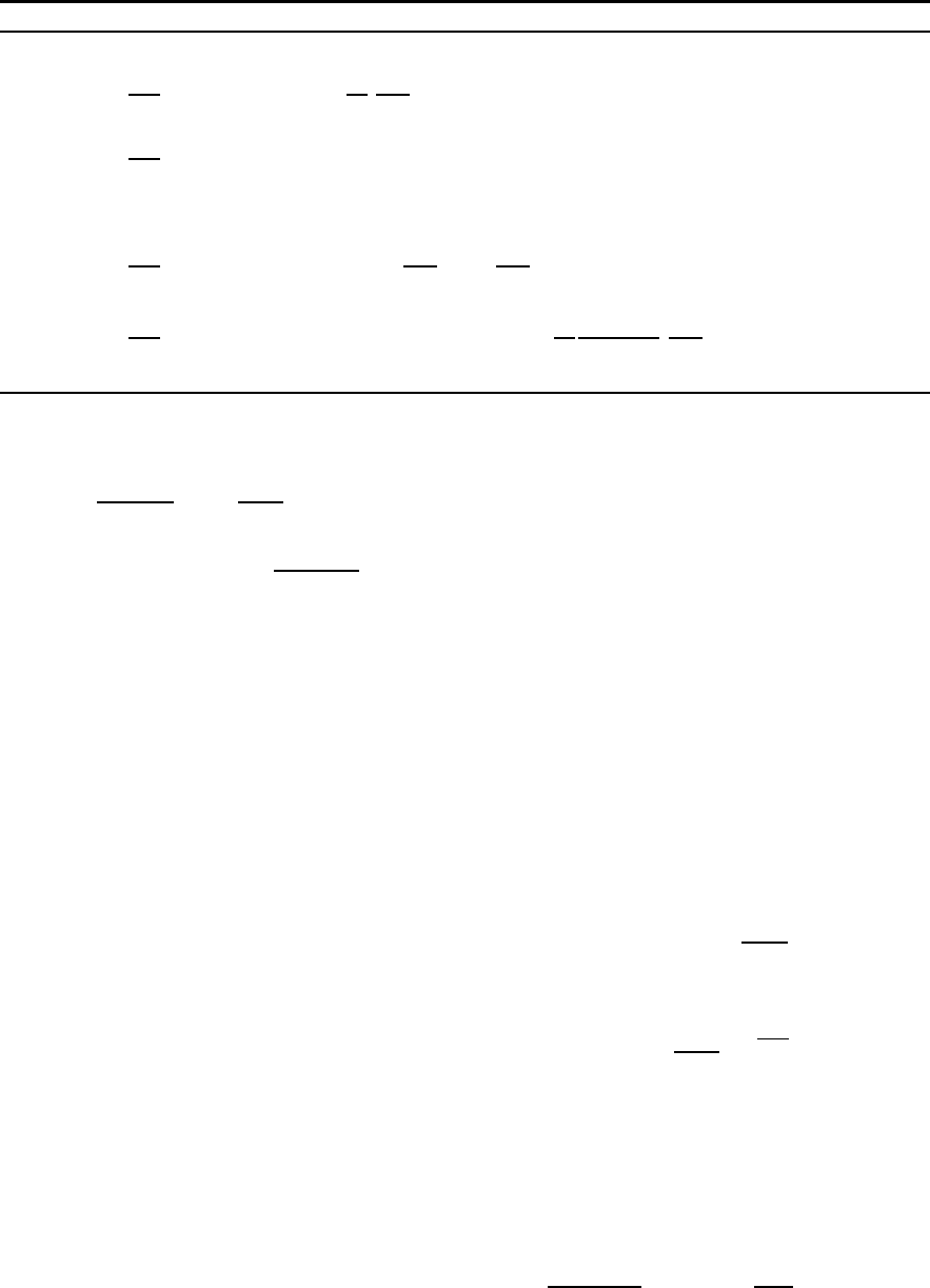
3. The sea ice biogeochemical model 49
3.1. A model for sea ice biogeochemistry . . . . . . . . . . . . . . . . . . . . . . . . . . 49
3.2. Model structure . . . . . . . . . . . . . . . . . . . . . . . . . . . . . . . . . . . . . 49
3.3. Sea ice Algae Dynamics . . . . . . . . . . . . . . . . . . . . . . . . . . . . . . . . 50
3.4. Nutrient Supply and Dynamics . . . . . . . . . . . . . . . . . . . . . . . . . . . . . 55
3.5. Gases and Detritus . . . . . . . . . . . . . . . . . . . . . . . . . . . . . . . . . . . 56
3.6. The coupling strategy . . . . . . . . . . . . . . . . . . . . . . . . . . . . . . . . . . 56
3.6.1. Boundary fluxes: the sea ice-ocean interface . . . . . . . . . . . . . . . . . . 57
3.6.2. Boundary fluxes: the sea ice-atmosphere interface . . . . . . . . . . . . . . 59
II. BFM code description 61
4. Installation, configuration and compilation 63
4.1. Installation . . . . . . . . . . . . . . . . . . . . . . . . . . . . . . . . . . . . . . . 63
4.1.1. System Requirements . . . . . . . . . . . . . . . . . . . . . . . . . . . . . 63
4.2. Configuration: BFM Presets . . . . . . . . . . . . . . . . . . . . . . . . . . . . . . 65
4.3. Compiling the BFM STANDALONE . . . . . . . . . . . . . . . . . . . . . . . . . 67
5. Running the STANDALONE model 69
5.1. Description . . . . . . . . . . . . . . . . . . . . . . . . . . . . . . . . . . . . . . . 69
5.2. State variables initial conditions (IC) . . . . . . . . . . . . . . . . . . . . . . . . . . 69
5.3. Numerical integration . . . . . . . . . . . . . . . . . . . . . . . . . . . . . . . . . . 69
5.4. Forcing functions . . . . . . . . . . . . . . . . . . . . . . . . . . . . . . . . . . . . 71
5.4.1. Analytical forcing functions . . . . . . . . . . . . . . . . . . . . . . . . . . 71
5.4.2. Boundary forcing for atmospheric CO2. . . . . . . . . . . . . . . . . . . . 73
5.4.3. Environmental data from file . . . . . . . . . . . . . . . . . . . . . . . . . . 73
5.4.4. External event data . . . . . . . . . . . . . . . . . . . . . . . . . . . . . . . 73
5.5. Test cases . . . . . . . . . . . . . . . . . . . . . . . . . . . . . . . . . . . . . . . . 73
5.5.1. STANDALONE_CO2TEST: carbonate system model . . . . . . . . . . . . 73
5.5.2. STANDALONE_PELAGIC: the full pelagic BFM . . . . . . . . . . . . . . 76
5.5.3. STANDALONE_SEAICE: sea ice biogeochemistry . . . . . . . . . . . . . . 76
5.6. Output visualization . . . . . . . . . . . . . . . . . . . . . . . . . . . . . . . . . . . 76
6. Structure of the code 81
6.1. Coding rules . . . . . . . . . . . . . . . . . . . . . . . . . . . . . . . . . . . . . . . 81
6.2. Memory layout and variable definition . . . . . . . . . . . . . . . . . . . . . . . . . 81
4
Contents
6.3. The BFM flow-chart . . . . . . . . . . . . . . . . . . . . . . . . . . . . . . . . . . 83
6.3.1. Initialization procedures . . . . . . . . . . . . . . . . . . . . . . . . . . . . 83
6.3.2. Time marching . . . . . . . . . . . . . . . . . . . . . . . . . . . . . . . . . 84
6.3.3. Computation of pelagic reaction terms . . . . . . . . . . . . . . . . . . . . . 87
7. Design model layout components 89
7.1. Layout syntax and modular structure . . . . . . . . . . . . . . . . . . . . . . . . . . 89
7.2. Example 1. Adding a subgroup . . . . . . . . . . . . . . . . . . . . . . . . . . . . . 92
7.3. Example 2. Adding a biochemical component and a group . . . . . . . . . . . . . . 94
7.4. Example 3. Removing components from zooplankton . . . . . . . . . . . . . . . . . 95
8. Model outputs 97
8.1. Output . . . . . . . . . . . . . . . . . . . . . . . . . . . . . . . . . . . . . . . . . . 97
8.2. Restart . . . . . . . . . . . . . . . . . . . . . . . . . . . . . . . . . . . . . . . . . . 97
8.3. Aggregated diagnostics and rates . . . . . . . . . . . . . . . . . . . . . . . . . . . . 97
8.4. Mass conservation . . . . . . . . . . . . . . . . . . . . . . . . . . . . . . . . . . . . 99
Bibliography 101
5
List of Equation Boxes
2.1. Phytoplankton . . . . . . . . . . . . . . . . . . . . . . . . . . . . . . . . . . . . . . 21
2.2. Chlorophyll synthesis . . . . . . . . . . . . . . . . . . . . . . . . . . . . . . . . . . 28
2.3. Bacteria . . . . . . . . . . . . . . . . . . . . . . . . . . . . . . . . . . . . . . . . . 33
2.4. Zooplankton . . . . . . . . . . . . . . . . . . . . . . . . . . . . . . . . . . . . . . . 36
2.5. Dissolved inorganic nutrient equations. . . . . . . . . . . . . . . . . . . . . . . . . . 42
2.6. Dissolved organic matter . . . . . . . . . . . . . . . . . . . . . . . . . . . . . . . . 43
2.7. Particulate organic detritus equations. . . . . . . . . . . . . . . . . . . . . . . . . . 45
3.1. Sea ice algae . . . . . . . . . . . . . . . . . . . . . . . . . . . . . . . . . . . . . . 54
7
List of Tables
1.1. BFM reference state variables . . . . . . . . . . . . . . . . . . . . . . . . . . . . . 17
1.2. List of abbreviations . . . . . . . . . . . . . . . . . . . . . . . . . . . . . . . . . . 18
2.1. Environmental variables . . . . . . . . . . . . . . . . . . . . . . . . . . . . . . . . 21
2.2. Phytoplankton parameters . . . . . . . . . . . . . . . . . . . . . . . . . . . . . . . 23
2.3. Iron cycle parameters . . . . . . . . . . . . . . . . . . . . . . . . . . . . . . . . . . 30
2.4. Bacterioplankton . . . . . . . . . . . . . . . . . . . . . . . . . . . . . . . . . . . . 32
2.5. Microzooplankton . . . . . . . . . . . . . . . . . . . . . . . . . . . . . . . . . . . . 36
2.6. Mesozooplankton . . . . . . . . . . . . . . . . . . . . . . . . . . . . . . . . . . . . 37
2.7. Switches for mesozooplankton food limitation . . . . . . . . . . . . . . . . . . . . . 39
2.8. Chemical parameters . . . . . . . . . . . . . . . . . . . . . . . . . . . . . . . . . . 42
2.9. Carbonate system . . . . . . . . . . . . . . . . . . . . . . . . . . . . . . . . . . . . 47
3.1. List of the sea ice model state variables . . . . . . . . . . . . . . . . . . . . . . . . 52
3.2. Ecological and physiological parameters in BFM-SI. . . . . . . . . . . . . . . . . . 53
4.1. List of optional arguments for bfm_configure . . . . . . . . . . . . . . . . . . . . . 68
5.1. namelist bfm_nml in BFM_General.nml . . . . . . . . . . . . . . . . . . . . . . . . 70
5.2. namelist Param_parameters in BFM_General.nml . . . . . . . . . . . . . . . . . . . 70
5.3. namelist PAR_parameters in Pelagic_Environment.nml . . . . . . . . . . . . . . . . 71
5.4. namelist standalone_nml in Standalone.nml . . . . . . . . . . . . . . . . . . . . . . 72
5.5. namelist time_nml in Standalone.nml . . . . . . . . . . . . . . . . . . . . . . . . . 72
5.6. namelist forcings_nml in Standalone.nml . . . . . . . . . . . . . . . . . . . . . . . 74
7.1. Example of model layout . . . . . . . . . . . . . . . . . . . . . . . . . . . . . . . . 90
9
Introduction
Synopsis
This report is divided in two main parts. The first
part contains an extended description of the Bio-
geochemical Flux Model (BFM version 5) equa-
tions and as such it describes different parame-
terizations that can be used to simulate biogeo-
chemical processes in the marine system. Part II
describes the model set-up, compilation and exe-
cution of the standard test cases. It also provides
the major technical implementation of the model
and information to understand the code structure.
This part gives examples of the possible diagnos-
tics that can be activated and illustrates advanced
features that allow the user to modify the model
adding new state variables and components.
The BFM is a direct descendant of the Euro-
pean Regional Seas Ecosystem Model (ERSEM)
and shares most of its characteristics with
the original formulations (Baretta et al., 1995;
Baretta-Bekker et al., 1997). The major differ-
ence is that BFM focuses more on the bio-
geochemistry of lower trophic levels in marine
ecosystems than on trophic food webs, which
is where it takes its name. The philosophy
of the BFM and the mathematical formulation
applied throughout the book are described in
Vichi et al. (2007b). The users familiar with
ERSEM will find that the code notation de-
scribed by Blackford and Radford (1995) has not
changed substantially and that the state variables
are indicated with the same naming convention.
Vichi et al. (2007b) have extended this notation
making it formally consistent and additional vari-
ables have been named accordingly.
The structure of the code was instead ex-
tensively modified with respect to the original
ERSEM code. The major reason for a full rewrit-
ing lied in the growing need to couple biogeo-
chemical processes with hydrodynamical model
of various forms and to allow a modular expan-
sion of the number and type of state variables in
modern coding standards. The necessity to have
a flexible system which can be embedded in the
existing state-of-the-art ocean general circulation
models (OGCM) required a re-organization of the
structure, yet the fundamentals of the coupling
strategy are very similar to the first coupled im-
plementations. From BFM version 5.1 the cou-
pled configurations are publicly supported. The
BFM module can be easily coupled with differ-
ent ocean models and an example of the cou-
pled configuration with the NEMO ocean model
(http://nemo-ocean.eu) is given in the company-
ing manual of this release Vichi et al. (2015).
The BFM module
This report documents the BFM equations for the
standalone pelagic configuration of the code that
solves the reaction part of the general equations
for biogeochemical tracers in the marine envi-
ronment. The state variables presented in Part I
are historically derived from the pelagic compo-
nent of ERSEM and represent the standard set
of transformations for the major chemical con-
stituents. The BFM by construction solves the
cycles of C, O, N, P, Si in the lower trophic levels
of marine ecosystems and it also allows the inclu-
sion of the Fe cycle and carbonate system chem-
istry by means of user-controlled flags. Differ-
ent parameterizations are proposed for the various
functional groups as they have been demonstrated
valid in certain model applications. Given the in-
herent empirical nature of biogeochemical model-
ling, the proposed parameterizations are given “as
they are” and it is up to the user to decide which
one to use given the specific application. The
modular implementation of the BFM allows to
implement new parameterizations and new state
variables.
11
List of Tables
The equations of Part I consider no vertical or
horizontal processes and the system is solved as a
set of ordinary differential equations. At the heart
of the BFM module is the possibility to increase
the number of components, as for instance im-
plementing any number of phytoplankton groups
that share the same dynamical terms but differ in
term of parameter and parameterization choices.
The user interested in this feature, in the modifi-
cation of the model layout and in the definition of
specific diagnostics will find in Part II all the re-
quired information. The reference test cases will
be presented in the STANDALONE implementa-
tion, which is a time-dependent box model with a
given depth where pelagic processes are assumed
homogeneous.
Licensing
The BFM is free software and is pro-
tected by the GNU Public License
http://www.gnu.org/licenses/gpl.html. All
files of the BFM contain the following statement:
Copyright 2013, The BFM System
Team (info@bfm-community.eu)
<Past Copyrights>
This file is part of the BFM.
The BFM is free software: you can re-
distribute it and/or modify it under the
terms of the GNU General Public Li-
cense as published by the Free Soft-
ware Foundation, either version 3 of
the License, or (at your option) any
later version. The BFM is distributed
in the hope that it will be useful, but
WITHOUT ANY WARRANTY; with-
out even the implied warranty of MER-
CHANTABILITY or FITNESS FOR
A PARTICULAR PURPOSE. See the
GNU General Public License for more
details.You should have received a copy
of the GNU General Public License
along with the BFM core. If not, see
<http://www.gnu.org/licenses/>.
Acknowledgments
The code support and development is currently
done by the BFM System Team whose mem-
bers are listed on the BFM web site (http://bfm-
community.eu). The initial core of the BFM sys-
tem software was developed by Piet Ruardij and
Marcello Vichi. The BFM system team is grateful
to Job Baretta, Hanneke Baretta-Bekker, Piet Ru-
ardij and Wolfgang Ebenhoeh for their contribu-
tion to the science of biogeochemical modeling.
12
Part I.
The BFM Equations
13

1. The formalism of the BFM equations
The BFM equations are written following the
notation proposed by Vichi et al. (2007b), which
is briefly summarized in this section. The reader
is referred to Vichi et al. (2007b) for a more theo-
retical viewpoint on the extension of the ERSEM
approach to the system state variables of the
plankton ecosystem. As shown in Tab. 1.1,
each variable is mathematically expressed by a
multi-dimensional array that contains the concen-
trations of reference chemical constituents. We
use a superscript indicating the CFF for a specific
living functional group and a subscript for the ba-
sic constituent. For instance, diatoms are LFG of
producers and comprise 6 living CFFs written as
P(1)
i≡P(1)
c,P(1)
n,P(1)
p,P(1)
s,P(1)
f,P(1)
l.
The standard model resolves 4 different groups
for phytoplankton P(j),j=1,2,3,4 (diatoms, au-
totrophic nanoflagellates, picophytoplankton and
large phytoplankton), 4 for zooplankton Z(j),j=
3,4,5,6 (carnivorous and omnivorous mesozoo-
plankton, microzooplankton and heterotrophic
nanoflagellates), 1 for bacteria, 7 inorganic vari-
ables for nutrients and gases (phosphate, nitrate,
ammonium, silicate, reduction equivalents, oxy-
gen, carbon dioxide) and 10 organic non-living
components for dissolved and particulate detritus
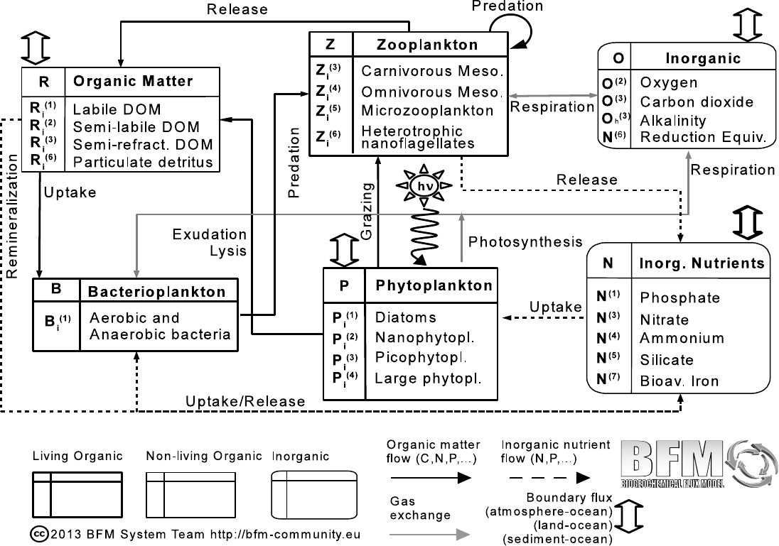
(cf.. Tab. 1.1 and Fig. 1.1). The state variable ni-
trate is assumed here to be the sum of both nitrate
and nitrite. Reduction equivalents represent all
the reduced ions produced under anaerobic con-
ditions. This variable was originally used only
in the benthic nutrient regeneration module of
ERSEM (Ruardij and Van Raaphorst, 1995) but
was extended to the water column in Vichi et al.
(2004). In this approach, all the nutrient-carbon
and chlorophyll-carbon ratios are allowed to vary
within their given ranges and each component has
a distinct biological time rate of change.
Following Vichi et al. (2007b) the dynamical
equations are written in two forms: 1) rates of
change form; and 2) explicit functional form. In
“rates of change form”, the biogeochemical reac-
tion term a generic state variable Cis written as:
dC
dt bio
=∑
i=1,n∑
j=1,m
dC
dt
ej
Vi
,(1.0.1)
where the right hand side contains the terms rep-
resenting significant processes for each living or
non-living component. The superscripts ejare
the abbreviations indicating the process which de-
termines the variation. In Table 1.2 we report
the acronyms of the processes used in the super-
scripts. The subscripts Viindicate the state vari-
able involved in the process. If V=C, we refer to
intra-group interactions such as cannibalism.
When a term is present as a source in one equa-
tion and as a sink in another, we refer to it follow-
ing this equivalent notation:
dC
dt
e
V
=−dV
dt
e
C
.(1.0.2)
In “functional process form”, the formulation
of the dynamic dependencies on other variables
is made explicit, i.e.: all the rates of change in
eq. (1.0.1) are given in the complete functional
parameterization. Although this is the more com-
plete mathematical form, it is more difficult to
read and interpret at a glance, especially when try-
ing to distinguish which processes affect the dy-
namics of which variable . All equations in this
Part will be presented both in rate of change and
in functional process forms.
15
1. The formalism of the BFM equations
Figure 1.1.: Scheme of the state variables and pelagic interactions of the reference STANDALONE
model. Living components are indicated with bold-line square boxes, non-living organic
components with thin-line square boxes and inorganic components with rounded boxes
(modified after Blackford and Radford (1995) and Vichi et al. (2007b)).
16

Variable Code Type Const. Units Description
N(1)N1p IO P mmol P m−3Phosphate
N(3)N3n IO N mmol N m−3Nitrate
N(4)N4n IO N mmol N m−3Ammonium
N(5)N5s IO Si mmol Si m−3Silicate
N(6)N6r IO R mmol S m−3Reduction equivalents, HS−
N(7)N7f IO Fe
µ
mol Fe m−3Dissolved Iron
O(2)O2o IO O mmol O2m−3Dissolved Oxygen
O(3)O3c IO C mg C m−3Dissolved Inorganic Carbon
O(5)O3h IO -mmol Eq m−3Total Alkalinity
P(1)
iP1[cnpslf] LO C N P Si
Chl Fe
mg C m−3, mmol
N-P-Si m−3, mg
Chl-am−3,
µ
mol
Fe m−3
Diatoms
P(2)
iP2[cnplf] LO C N P Chl
Fe
mg C m−3, mmol
N-P m−3, mg Chl-a
m−3,
µ
mol Fe m−3
NanoFlagellates
P(3)
iP3[cnplf] LO C N P Chl
Fe
mg C m−3, mmol
N-P m−3, mg Chl-a
m−3,
µ
mol Fe m−3
Picophytoplankton
P(4)
iP4[cnplf] LO C N P Chl
Fe
mg C m−3, mmol
N-P m−3, mg Chl-a
m−3,
µ
mol Fe m−3
Large phytoplankton
BiB1[cnp] LO C N P mg C m−3, mmol
N-P m−3
Pelagic Bacteria
Z(3)
iZ3[cnp] LO C N P mg C m−3, mmol
N-P m−3
Carnivorous Mesozooplankton
Z(4)
iZ4[cnp] LO C N P mg C m−3, mmol
N-P m−3
Omnivorous Mesozooplankton
Z(5)
iZ5[cnp] LO C N P mg C m−3, mmol
N-P m−3
Microzooplankton
Z(6)
iZ6[cnp] LO C N P mg C m−3, mmol
N-P m−3
Heterotrophic Flagellates
R(1)
iR1[cnpf] NO C N P Fe mg C m−3, mmol
N-P m−3,
µ
mol Fe
m−3
Labile Dissolved Organic Matter
R(2)
cR2c NO C mg C m−3Semi-labile Dissolved Organic Carbon
R(3)
iR3c NO C mg C m−3Semi-refractory Dissolved Organic Carbon
R(6)
iR6[cnpsf] NO C N P Si Fe mg C m−3, mmol
N-P-Si m−3,
µ
mol
Fe m−3
Particulate Organic Detritus
Table 1.1.: List of the reference state variables for the pelagic model. Type legend: IO = Inorganic; LO
= Living organic; NO = Non-living organic. The subscript iindicates the basic components
(if any) of the variable, e.g. P(1)
i≡P(1)
c,P(1)
n,P(1)
p,P(1)
s,P(1)
l,P(1)
f.
17

1. The formalism of the BFM equations
Abbreviation Process
gpp Gross primary production
rsp Respiration
prd Predation
rel Biological release: Egestion, Excretion
exu Exudation
lys Lysis
syn Biochemical synthesis
nit/denit Nitrification, denitrification
scv Scavenging
rmn Biochemical remineralization
Table 1.2.: List of all the abbreviations used to indicate the physiological and ecological processes in
the equations
18

2. The pelagic plankton model
2.1. The environmental
parameters affecting
biological rates
This section describes the dependencies of the
pelagic biogeochemical processes from the phys-
ical environment. The BFM has defined a set of
environmental variables that are provided by ex-
ternal data or by a physical model (Tab.2.1). The
local coupling between physics and biogeochem-
istry is realized explicitly through surface irradi-
ance and temperature. Temperature regulates all
physiological processes in the model and its ef-
fect, denoted by fT, is parameterized in this non-
dimensional form
fT=Q
T−10
10
10 (2.1.1)
where the Q10 coefficient is different for each
functional process considered.
Light is fundamental for primary producers
and the energy source for photosynthesis is the
downwelling amount of the incident solar radi-
ation at the sea surface. Only a portion of the
downwelling irradiance is used for growth, the
Photosynthetic Available Radiation (PAR) EPAR
(the notation of Sakshaug et al. (1997) is used
here). The BFM only computes the propagation
of PAR as a function of the attenuation coeffi-
cient of sea water, which is determined by the
concentration of suspended and dissolved com-
ponents. The BFM considers two cases con-
trolled by the parameters described in Tab.5.3: 1)
a broadband mean attenuation coefficient and 2) a
3-band attenuation coefficient for chlorophyll as
proposed by Morel (1988) and tabulated accord-
ing to Lengaigne et al. (2007).
In the default case we assume that PAR is prop-
agated according to the Lambert-Beer formula-
tion with broadband, depth-dependent extinction
coefficients
EPAR (z) =
ε
PAR QSe
λ
wz+R0
z
λ
bio(z′)dz′(2.1.2)
where
ε
PAR is the coefficient determining the frac-
tion of PAR in QS. Light propagation takes into
account the extinction due to suspended particles,
λ
bio, and
λ
was the background extinction of wa-
ter. The biological extinction is written as
λ
bio =
4
∑
j=1
cP(j)P(j)
l+cR(6)R(6)
c(2.1.3)
where the extinctions due to the concentration of
phytoplankton chlorophyll and particulate detri-
tus are considered (see Sec. 2.2 and 2.5). The c
constants are the specific absorption coefficients
of each suspended substance (Tab. 2.2 and 2.8),
which may also include extinction by suspended
sediments (not currently resolved by the BFM but
can be included from an external model).
With the 4-band wavelength parameterization
the model considers differential attenuation of
light divided in red, green and blue coefficients
(RGB) that are functions of the chlorophyll con-
centration. The visible portion is divided equally
in the 3 bands such as
EPAR (z) =
ε
PAR
3QSeR0
z
λ
R(Chl,z′)dz′+eR0
z
λ
G(Chl,z′)dz′+eR0
z
λ
B(Chl,z′)dz′
(2.1.4)
where the
λ
coefficients are obtained with a look-
up table dependng on the local total chlorophyll
concentration Chl =∑4
j=1P(j)
l. In this parameter-
ization both the background attenuation of water
and the specific attenuation of chlorophyll are not
used.
The short-wave surface irradiance flux QS
is obtained generally from data or from an
atmospheric radiative transfer model. Three
types of forcings are allowed depending
on the value of LightPeriodFlag in
Pelagic_Environment.nml:
19

2. The pelagic plankton model
1. Instantaneous irradiance
(LightPeriodFlag=1)
2. Daily average (LightPeriodFlag=2)
3. Daylight average (with explicit photoperiod,
LightPeriodFlag=3)
The discretized irradiance Ek
PAR is located
at the top of each layer k, and three dif-
ferent choices are available according to
the parameter LightLocationFlag in
Pelagic_Ecology.nml:
1. light at the upper interface EPAR =Ek
PAR
(LightLocationFlag=1),
2. light in the middle of the
cell as in Lazzari et al. (2012)
(LightLocationFlag=2),
EPAR =Ek
PAR exp−
λ
k∆zk
2(2.1.5)
3. integrated light over the level
depth as in Vichi et al. (2007b)
(LightLocationFlag=3),
EPAR =Ek
PAR
λ
k∆zk1−exp−
λ
k∆zk
(2.1.6)
When needed for physiological computations, the
value is converted from W m−2to the unit of
µ
E m−2s−1with the constant factor 1/0.215
(Reinart et al., 1998).
2.2. Phytoplankton
Primary producers are divided in four principal
sub-groups coarsely representing the functional
spectrum of phytoplankton in marine systems.
The operational model definitions of the phyto-
plankton groups are:
•diatoms (P(1)
i), ESD = 20-200
µ
, unicellular
eukaryotes enclosed by a silica frustule eaten
by micro- and mesozooplankton;
•autotrophic nanoflagellates (P(2)
i), ESD =
2-20
µ
, motile unicellular eukaryotes com-
prising smaller dinoflagellates and other au-
totrophic microplanktonic flagellates eaten
by heterotrophic nanoflagellates, micro- and
mesozooplankton;
•picophytoplankton (P(3)
i), ESD = 0.2-2
µ
,
prokaryotic organism generally indicated
as non-diazotrophic autotrophic bacteria
such as Prochlorococcus and Synechococ-
cus, but also mixed eukaryotic species
(Worden et al., 2004), mostly preyed by het-
erotrophic nanoflagellates;
•large, slow-growing phytoplankton (P(4)
i),
ESD > 100
µ
, that represents a wide group
of phytoplankton species, also comprising
larger species belonging to the previous
groups (for instance dinoflagellates) but also
those that during some period of the year de-
velop a form of (chemo)defense to preda-
tor attack. This group generally has low
growth rates and small food matrix values
with respect to micro- and mesozooplankton
groups.
The processes parameterized in the biological
source term are gross primary production (gpp),
respiration (rsp), exudation (exu), cell lysis (lys),
nutrient uptake (upt), predation (prd) and bio-
chemical synthesis (syn). All the phytoplankton
groups share the same form of primitive equa-
tions, but are differentiated in terms of the values
of the physiological parameters.
Phytoplankton in the model is composed of
several constituents and the related dynamical
equations (Box 2.1): some of them are manda-
tory (C, N, P), that is they are required to compute
physiological terms, and some others are required
for specific groups (like Si in diatoms) or they
are optional such as the Chl and Fe constituents.
The inclusion of Fe is a typical example of the
model flexibility as it allows to have an additional
multiple-nutrient limitation term without affect-
ing the other parameterizations (see Sec. 2.2.8).
When Chl constituent is not used (see Sec.
2.2.7), light acclimation in phytoplankton can be
20

2.2. Phytoplankton
Symbol Code Unit Description
TETW oC Sea water salinity
SESW (-) Sea water temperature
ρ
ERHO Kg m−3Sea water density
EPAR EIR
µ
E m−2s−1Photosynthetically available radiation
SSESS g m−3Suspended sediment load
Watm EWIND m s−1Wind speed
Fice EICE (-) Sea ice fraction
ΦSUNQ hours Daylight length
Table 2.1.: Mathematical and code symbols, units and description of the environmental state variables
defined in the model.
Equation Box 2.1 Phytoplankton equations
dPc
dt bio
=dPc
dt
gpp
O(3)
−dPc
dt
exu
R(2)
c
−dPc
dt
rsp
O(3)
−∑
j=1,6
dPc
dt
lys
R(j)
c
−∑
k=4,5,6
dPc
dt
prd
Z(k)
c
(2.2.1a)
dPn
dt bio
=∑
i=3,4
dPn
dt
upt
N(i)
−∑
j=1,6
dPn
dt
lys
R(j)
n
−Pn
Pc∑
k=4,5,6
dPc
dt
prd
Z(k)
c
(2.2.1b)
dPp
dt bio
=dPp
dt
upt
N(1)
−∑
j=1,6
dPp
dt
lys
R(i)
p
−Pp
Pc∑
k=4,5,6
dPc
dt
prd
Z(k)
c
(2.2.1c)
dPl
dt bio
=dPl
dt
syn
−Pl
Pc∑
j
dPc
dt
prd
Z(j)
c
(2.2.1d)
dPs
dt bio
=dPs
dt
upt
N(5)
−dPs
dt
lys
R(6)
s
−Ps
Pc∑
k=4,5,6
dPc
dt
prd
Z(k)
c
(2.2.1e)
if Ps∃,otherwise dPs
dt bio
=0
dPf
dt bio
=dPf
dt
upt
N(7)
−dPf
dt
lys
R(6)
f
−Pf
Pc∑
j
dPc
dt
prd
Z(j)
c
(2.2.1f)
if Pf∃,otherwise dPf
dt bio
=0 (2.2.1g)
21

2. The pelagic plankton model
described by means of the optimal light property
as proposed by Ebenhöh et al. (1997). The no-
tation remains mostly unchanged but in this case
the variable ˆ
Plindicates the optimal light level to
which phytoplankton is acclimated and the alter-
native equation to (2.2.1d) is given in Sec. 2.2.7.
2.2.1. Photosynthesis and carbon
dynamics
Photosynthesis is primarily controlled by light
by means of the non-dimensional light regulation
factor proposed by Jassby and Platt (1976)
fE
P=1−exp−EPAR
EK(2.2.2)
where EKis the optimal irradiance, defined as
Ek=P∗
m/
α
∗
P∗
m=fT
PfPP
Pr0
P
Pc
Pl
(2.2.3)
α
∗=fT
PfPP
P
α
0
chl
The maximum chl-specific photosynthetic rate P∗
m
is controlled by the non-storable nutrients that
control primary production fPP
P(Sec. 2.2.2). It
is assumed that both
α
∗and P∗
mare controlled
by the same regulating factors (Jassby and Platt,
1976; Behrenfeld et al., 2004). When instanta-
neous light is used, the equation is written in the
following form:
fE
P=1−exp−
α
0
chl EPARPl
r0
PPc(2.2.4)
while in case the length of the photoperiod is con-
sidered, this is implicitly done in P∗
mthat becomes.
P∗
m=fT
PfPP
Pr0
P
Pc
Pl
Φ
24 (2.2.5)
where Φis the daylight length in hours
(Lazzari et al., 2012). The final form of gross pri-
mary production also depends on the choice of the
daylight availability. In the case of instantaneous
or average daily irradiance (Vichi et al., 2007a), it
is written as
dPc
dt
gpp
O(3)
=fT
PfE
PfPP
Pr0
PPc.(2.2.6)
Note that it is possible to further control tem-
perature limitation with a cut-off value cT
Papplied
to the temperature regulating factor as done in
(Vichi et al., 2007a) to control the growth of pi-
cophytoplankton at high latitudes:
fT=max0,fT−cT
P.(2.2.7)
Respiration is defined as the sum of the basal res-
piration, which is independent of the production
rate, and the activity respiration:
dPc
dt
rsp
O(3)
=bPfT
PPc+
γ
P
dPc
dt
gpp
O(3)
.(2.2.8)
Basal respiration is only a function of the car-
bon biomass, temperature (through the regulating
factor fT
P) and the specific constant rate bP. The
activity respiration is a constant fraction (
γ
P) of
the total gross primary production.
The term lysis includes all the non-resolved
mortality processes that disrupt the cell mem-
brane, such as mechanical causes, virus and
yeasts. It is assumed that the lysis rate is parti-
tioned between particulate and dissolved detritus
and tends towards the maximum specific rate d0
P
with a saturation function of the nutrient stress as:
dPc
dt
lys
R(6)
c
=
ε
n,p
Php,n
P
fp,n
P+hp,n
P
d0
PPc+
χ
lys(2.2.9)
dPc
dt
lys
R(1)
c
=1−
ε
n,p
P(2.2.10)
hp,n
P
fp,n
P+hp,n
P
d0
PPc+
χ
lys
The lysis of cells generates both dissolved and
particulate detritus; the structural parts of the cell
are not as easily degradable as the cytoplasm,
therefore the percentage going to DOC is in-
versely proportional to the internal nutrient con-
tent and constrained by the minimum structural
content in the following way:
ε
n,p
P=min 1,pmin
P
Pp/Pc
,nmin
P
Pn/Pc!.(2.2.11)
22

2.2. Phytoplankton
Symbol Code Unit Description
Q10Pp_q10 - Characteristic Q10 coefficient
cT
Pp_temp - Cut-off threshold for temperature regulating factor
r0Pp_sum d−1Maximum specific photosynthetic rate
bPp_srs d−1Basal specific respiration rate
d0Pp_sdmo d−1Maximum specific nutrient-stress lysis rate
hp,n,s
Pp_thdo - Nutrient stress threshold
dx
Pp_seo d−1Extra lysis rate
hx
Pp_sheo mg C m−3Half saturation constant for extra lysis
β
Pp_pu_ea - Excreted fraction of primary production
γ
Pp_pu_ra - Activity respiration fraction
p_switchDOC 1-3 Switch for the type of DOC excretion. Choice consistent with bacteria parame-
terization in Sec. 2.3. 1. All DOC is released as R(1)
c(BACT1); 2. Activity DOC
is released as R(2)
c(BACT2); 3. All DOC is released as R(2)
c(BACT3)
p_netgrowth logical Switch for parameterization of nutrient limited growth (T or F)
p_limnut 0-2 Switch for parameterization of nutrient co-limitation
a4p_qun m3mg C−1d−1Specific affinity constant for N
hn
Pp_lN4 mmol
N-NH4 m−3
Half saturation constant for ammonium uptake preference over ammonium
nmin
P,nopt
P,nmax
Pp_qnlc,
p_qncPPY,
p_xqn*p_qncPPY
mmolN mgC−1Minimum, optimal and maximum nitrogen quota
a1p_qup m3mg C−1d−1Specific affinity constant for P
pmin
P,popt
P,pmax
Pp_qplc,
p_qpcPPY,
p_xqp*p_qpcPPY
mmolP mgC−1Minimum, optimal and maximum phosphorus quota
p_switchSi 1,2 Switch for parameterization of silicate limitation (1=external, 2=internal)
hs
Pp_chPs mmol Si m−3Half saturation constant for Si-limitation
ρ
s
Pp_Contois - Variable half saturation constant for Si-limitation of Contois (like Monod if 0)
a5p_qus m3mg C−1d−1Specific affinity constant for Si
smin
P,sopt
Pp_qslc
p_qscPPY
mmolSi mg C−1Minimum and optimal Si:C ratio in silicifiers
ω
sink
Pp_res m d−1Maximum sedimentation rate
lsink
Pp_esNI - Nutrient stress threshold for sinking
p_switchChl Choice of the Chl synthesis parameterization
dchl
Pp_sdchl d−1Chlorophyll turn-over rate
α
0
chl p_alpha_chl mgC (mg chl)−1
µ
E−1m2
Maximum light utilization coefficient
θ
0
chl p_qlcPPY mg chl mg C−1Maximum chl:C quotum
cPp_epsChla m2(mg chl)−1Chl-specific light absorption coefficient
ε
opt p_EpEk_or - Optimal value of EPAR /EK
τ
opt p_tochl_relt d−1Relaxation rate toward the optimal Chl:C value
p_iswLtyp 0-6 Shape of the productivity function (diagnostic Chl, ChlDynamicsFlag=1)
Emax
P,Emin
Pp_chELiPPY
p_clELiPPY
W m−2Maximum and minimum thresholds for light adaptation
vI
Pp_ruELiPPY d−1Relaxation rate toward the optimal light
p_rPIm m d−1Additional background sinking rate
Table 2.2.: Mathematical and code symbols, units and description of the phytoplankton parameters
(namelist Pelagic_Ecology.nml: Phyto_parameters). 23

2. The pelagic plankton model
This equation ensures that the carbon and nutri-
ents in the supportive structures, which are as-
sumed to have pmin
Pand nmin
Pnutrient ratios, are
always released as particulate components.
The model also implements and extra lysis rate
in the last term of eq. (2.2.9-2.2.10), which is de-
pendent on the population density. This term is
controlled by an optional specific lysis rate
χ
lys =dx
P
Pc
Pc+hx
P
Pc(2.2.12)
which is usually included for those phytoplankton
population that are indedible and therefore acts as
an additional mortality term to regulate the popu-
lation dynamics.
2.2.2. Multiple nutrient limitation
The BFM inherits the treatment of nutri-
ent limitation from the original work by
Baretta-Bekker et al. (1997) which has similari-
ties to the Caperon and Meyer equation, with
some specific extensions. Nutrients are divided
in two main groups, the ones that directly con-
trol carbon phosynthesis (as silicate, since dupli-
cation can only occur with Si deposition) and the
ones that are decoupled from carbon uptake be-
cause of the existence of cellular storage capabili-
ties. Limiting factors for nutrients can be both in-
ternal (i.e. based on the internal nutrient quota) or
external (based on dissolved inorganic concentra-
tion). The internal limitation is only partly based
on Droop (1973), with the concepts of nutrient
surge and storage by Baretta-Bekker et al. (1997)
and the possibility to apply the parameterization
of net growth described in Vichi et al. (2004) by
means of the parameter p_netgrowth in the
namelist (Tab. 2.2). The regulating factors for
internal limitation are controlled by the optimal
and minimum values for the existence of struc-
tural components (nopt
P,nmin
P), and they are imple-
mented for N, P and Fe (Sec. 2.2.8) and also for
Si (Lazzari et al., 2012), although in this case it is
not possible to have luxury uptake because there
is no storage for dissolved silicate in the cell:
fn
P=min1,max0,Pn/Pc−nmin
P
nopt
P−nmin
P (2.2.13)
fp
P=min1,max0,Pp/Pc−pmin
P
popt
P−pmin
P
(2.2.14)
ff
P=Pf/Pc−
φ
min
P
φ
opt
P−
φ
min
P
(2.2.15)
ˆ
fs
P=Ps/Pc−smin
P
sopt
P−smin
P
(2.2.16)
fp
P=min1,max0,Pp/Pc−pmin
P
popt
P−pmin
P
(2.2.17)
Note that the ratios between brackets can be larger
than 1 because the nutrient quota are allowed to
reach the maximum values (cf. Sec. 2.2.3) but
the regulating factor has to be limited to 1 because
above the optimal quotum there is no limitation to
physiological processes.
There is a flag (Tab. 2.2) for the choice of
external and internal silicon limitation in case
of diatoms. External dissolved silicate control
should be preferable (Flynn, 2003) and it im-
plements a Monod regulation with variable half-
saturation constant hs
P, modified according to
Contois (1959):
fs
P(1)=N(5)
N(5)+ (hs
P+
ρ
s
PP(1)
s)(2.2.18)
fs
P(j)=1,j6=1
The Contois formulation implements a control on
dissolved nutrient uptake that is dependent on the
size of the population, in this case it is applied
to biogenic silica as suggested by Tsiaras et al.
(2008). If the Contois parameter is zero a clas-
sical Monod function is obtained, while if
ρ
s
P6=0
the half-saturation constant is increased and the
resulting silicate control factor is smaller.
Multiple nutrient limitation is different for nu-
trients that can be stored in the cell and nutrients
that cannot. The threshold combination (Liebig-
like) is usually preferred to the multiplicative ap-
proach (Flynn, 2003): the BFM allows the three
24

2.2. Phytoplankton
alternative ways implemented in ERSEM-II to
combine N and P limitation (that can be selected
differently for each phytoplankton group, Tab.
2.2),
fn,p
P=minfn
P,fp
P(2.2.19)
fn,p
P=2
1/fn
P+1/fp
P
(2.2.20)
fn,p
P=qfn
Pfp
P(2.2.21)
and a simple multiplicative approach for the ef-
fect of nutrients that directly control photosyn-
thesis (eq. 2.2.6), such as fPP =ˆ
fs
Pas done by
Lazzari et al. (2012) or fPP =ff
Pfs
Pwhen iron dy-
namics is included (Sec. 2.3) as in Vichi et al.
(2007b). The co-limitation from all nutrients is
always done with a threshold method
fnut
P=minfn,p
P,ff
P,fs
P(2.2.22)
and it is considered in the parameterization of
some processes such as chlorophyll synthesis and
sinking (Secs. 2.2.6 and 2.2.9).
2.2.3. Nutrient uptake
A major problem in modelling nutrient up-
take is to deal with unbalanced growth condi-
tions, and any realistic application is expected
to produce transient environmental conditions re-
sulting in uncoupled assimilation rates of car-
bon and nutrients. The Droop (intracellular
quota approach) and Monod (external concentra-
tion approach) equations produce consistent re-
sults when applied in balanced growth condi-
tions (Morel, 1987). The BFM approach, largely
derived from Baretta-Bekker et al. (1997), com-
bines both mechanisms with a threshold control.
2.2.3.1. Nitrogen
The uptake of DIN is the sum of the uptake of dis-
solved nitrate and ammonium and is the minimum
between a diffusion-dependent uptake rate (when
internal nutrient quota are low and nutrients are
only structural), and a rate based on considera-
tions of balanced growth and luxury uptake:
∑
j=3,4
dPn
dt
upt
N(j)
=
minan
P
hn
P
hn
P+N(4)N(3)+an
PN(4)Pc,
nopt
PGP+
ν
Pnmax
P−Pn
PcPc(2.2.23)
A preference for ammonium is parameterized
through a saturation function that modulates the
affinity constant for dissolved nitrate. Balanced
uptake is a function of the net primary production
Gp, which is computed as:
GP=max 0,dPc
dt
gpp
O(3)
−dPc
dt
exu
R(i)
c
−dPc
dt
rsp
O(3)
−dPc
dt
lys
R(i)
c!
(2.2.24)
and
ν
P=max0.05,GP
Pc.
When the nitrogen uptake rate in eq. (2.2.23)
is positive, the partitioning between N(3)and
N(4)uptake is done by multiplying the rate by the
fractions:
ε
(3)
P=
an
P
hn
P
hn
P+N(4)N(3)
an
PN(4)+an
P
hn
P
hn
P+N(4)N(3)(2.2.25)
ε
(4)
P=an
PN(4)
an
PN(4)+an
P
hn
P
hn
P+N(4)N(3)(2.2.26)
When it is negative, the whole flux is directed to
the DON pool R(1)
n.
2.2.3.2. Phosphorus
Phosphate uptake is simpler than N uptake as one
single species is considered:
dPp
dt
upt
N(1)
=mina(1)
PN(1)Pc,popt
PGP+
+
ν
Ppmax
P−Pp
PcPc(2.2.27)
25

2. The pelagic plankton model
2.2.3.3. Silicate
Silicate is not stored in the cell and therefore the
uptake is directly proportional to the net carbon
growth (see eq. 2.2.24):
dPs
dt
upt
N(5)
=sopt
PGP(2.2.28)
2.2.4. Nutrient loss associated with
lysis
Nutrients in the cell are not evenly distributed be-
tween cytoplasm and structural parts. When the
cell wall is disrupted, part of the nutrients are re-
leased as dissolved organic matter (the nutrients
in the cytoplasm) and part as particulate organic
matter (the nutrients in the structural parts, such
as the cell wall).
The redistribution of the cellular elements C,
N and P over the excretion variables reflects the
preferential remineralization of P and to a lesser
extent of N, with respect to C. This parameter val-
ues are based on the ERSEM-II parameterizations
(Baretta-Bekker et al., 1997).
dPp
dt
lys
R(6)
i
=
ε
i
P
hp,n
P
fp,n
P+hp,n
P
d0
PPii=n,p(2.2.29)
dPp
dt
lys
R(1)
i
=1−
ε
i
Php,n
P
fp,n
P+hp,n
P
d0
PPii=n,p
(2.2.30)
In the case of Si, the release is always in partic-
ulate form and thus is a constant fraction of the
particulate carbon lysis
dP(1)
s
dt
lys
R(6)
s
=sopt
P
dP(1)
c
dt
lys
R(6)
c
(2.2.31)
2.2.5. Exudation of carbohydrates
In the case of intra-cellular nutrient shortage,
not all photosynthesized carbon can be assimi-
lated into biomass, and the non-assimilated part
is released in the form of dissolved carbohy-
drates. The model considers three different types
of DOC (Tab. 1.1) and phytoplankton excretion
must be consistent with the bacteria parameter-
ization (Sec. 2.3). Carbohydrates are excreted
when phytoplankton cannot equilibrate the fixed
C with sufficient nutrients to maintain the min-
imum quotum needed for the synthesis of new
biomass. The choice of the parametrization for
DOC exudation is controlled by the flag parame-
ters p_netgrowth and p_switchDOC in the
phytoplankton namelist (Tab. 2.2), which can
be set differently for each sub-group. There
is a runtime check that controls the consis-
tency between the two parameters. When the
flag is false, the ERSEM-II parameterization
(Baretta-Bekker et al., 1997) as implemented in
Vichi et al. (2007b) is used,
dPc
dt
exu
R(1)
c
=
β
P+ (1−
β
P)1−fn,p
PdPc
dt
gpp
O(3)
(2.2.32)
where exudation (and thus carbon biomass
loss) increases when phytoplankton has low nu-
trient:carbon ratios. The nutrient-stress ex-
cretion can also be partly directed to semi-
refractory DOC (R(2)
c) by setting the parameter
p_switchDOC=3:
dPc
dt
exu
R(1)
c
=
β
P
dPc
dt
gpp
O(3)
(2.2.33)
dPc
dt
exu
R(2)
c
= (1−
β
P)1−fn,p
PdPc
dt
gpp
O(3)
(2.2.34)
However, the ERSEM-II parameterization not
only leads to the desired extra release of C-
enriched DOM but also to a decrease of the pop-
ulation biomass. It has been shown by Vichi et al.
(2004) that the use of a different parameteriza-
tion results in the maintenance of higher stand-
ing stocks in the post bloom period with a con-
sequently enhanced consumption of the non-
limiting nutrients. This parameterization is also
used by Lazzari et al. (2012) to allow the con-
sumption of N species in a P-depleted environ-
ment.
When the p_netgrowth flag is true, total ex-
udation is directed to the state variable R(2)
c(see
26

2.2. Phytoplankton
also Sec. 2.3 for a detailed explanation of DOM
in the BFM), and it is written as the sum of an ac-
tivity exudation linked to the gross primary pro-
duction and a balance term
dPc
dt
exu
R(2)
c
=
β
P
dPc
dt
gpp
O(3)
+GP−Gbal
P(2.2.35)
where
Gbal
P=max 0,min GP,1
nmin
P∑
j=3,4
dPn
dt
upt
N(j)
,
(2.2.36)
1
pmin
P
dPp
dt
upt
N(1)
2.2.6. Chlorophyll synthesis and
photoacclimation
The chlorophyll equation in (2.2.1d) is composed
of two terms. The first one is net chlorophyll syn-
thesis, which is mostly derived from Geider et al.
(1996, 1997) with some adaptations, and the sec-
ond one represents the losses due to grazing.
Net chlorophyll synthesis is namely a function
of acclimation to light conditions, nutrient avail-
ability and turnover rate. The former process is
taken into account by Geider’s parameterization,
while the latter is generally parameterized with
different formulations, for instance by assuming a
dependence on gross carbon uptake (Geider et al.,
1997; Blackford et al., 2004) and/or on nitro-
gen assimilation (Geider et al., 1998; Flynn et al.,
2001). To integrate the variety of processes
into our formulations, we consider three differ-
ent parameterizations presented in 2.2 that have
been used in different applications of the BFM
(Vichi and Masina (2009), Lazzari et al. (2012),
Clementi et al., in preparation). The synthesis
part is rather similar as it is controlled by the dy-
namical chl:C ratio
ρ
chl proposed by Geider et al.
(1997), which regulates the amount of chloro-
phyll in the cell according to a non-dimensional
ratio between the realized photosynthetic rate in
eq. (2.2.6) and the maximum potential photosyn-
thesis:
ρ
chl =
θ
0
chl
dPc
dt
gpp
O(3)
α
∗EPARPl
(2.2.38)
and multiplying by a maximum chl:C ratio
θ
0
chl
which is different for each phytoplankton func-
tional group (Tab. 2.2). The major difference in
eq. (2.2.37b) proposed by Lazzari et al. (2012) is
the presence of the combined nutrient regulating
factor, which implies that chl synthesis is reduced
in regions limited by phosphorus like for instance
the Mediterranean.
Following the notation shown in Sec. 2.2.3,
Geider’s original formulation is rewritten after
some algebra as:
ρ
chl =
θ
0
chl
fE
Pr0
PPc
α
0
chl EPARPl
(2.2.39)
The ratio is down-regulated when the rate of light
absorption (governed by the quantum efficiency
and the amount of light-harvesting pigments) ex-
ceeds the rate of utilization of photons for car-
bon fixation, as explained in detail in Geider et al.
(1996). Also here it is assumed that both
α
∗and
P∗
mare controlled by the same regulating factors
(Jassby and Platt, 1976; Behrenfeld et al., 2004).
The formulation of the lysis term is still un-
known and this is reflected in the diversity
of parameterizations that are available in the
model and controlled by the namelist parameter
p_switchChl (Tab. 2.2). The user should con-
sider the different assumptions and use them ac-
cordingly. A different parameterization can be
used for each phytoplankton group to allow their
testing. In eq. (2.2.37a) it is assumed that chl lysis
is simply linked to the carbon term, while in eq.
(2.2.37b) there is a relaxation to the optimal chl:C
ratio with an additional lysis term linked to back-
ground mortality. The parameterization proposed
in eq. (2.2.37c) is slightly more elaborated as it
considers an optimal cell acclimation to light that
corresponds to an optimal value EPAR/EK=
ε
opt
of the exponential in eq. (2.2.4).
The theoretical chlorophyll concentration cor-
responding to optimal light acclimation in eq.
(2.2.37c) is computed as follows:
27
2. The pelagic plankton model
Equation Box 2.2 Different parameterizations for the chlorophyll synthesis.
dPl
dt
syn
=
ρ
chl GP−Pl
Pc
dPc
dt
lys
(2.2.37a)
dPl
dt
syn
=fp,n
P
ρ
chl GP−max0,d◦
P(1−fp,n
P)Pl−(2.2.37b)
min(0,GP)∗max0,Pl−
θ
0
chl Pc
dPl
dt
syn
=
ρ
chl GP−
θ
chl dPc
dt
lys
+dPc
dt
rsp!−max0,Pl−Popt
l
τ
chl (2.2.37c)
dPl
dt
syn
=
ρ
chl GP−dchl
PPlhp,n,s
P−fnut
P−Pl
Pc
1
1+EPAR
dPc
dt
rsp
(2.2.37d)
r0
PPc
Popt
l
α
0
chl
=EPAR
ε
opt
Popt
l=
ε
opt r0
PPc
α
0
chl EPAR
(2.2.40)
and the chl content in (2.2.37c) is relaxed to this
optimal value with a specific time scale parameter
τ
chl .
The parameterization presented in eq.
(2.2.37d) has instead an explicit term for
the turn-over rate of chl, dchl
P. The losses of
chlorophyll are not considered as mass losses in
the model because we have currently not imple-
mented a chl component in detritus and dissolved
organic matter. The same consideration applies to
the ingested chl fraction in zooplankton. All these
terms are presently collected into a generic sink
term used for mass conservation purposes, which
can be easily split into its major components once
it is deemed necessary to follow the degradation
products of chl (phaeopigments).
2.2.7. Light limitation and
photoacclimation based on
optimal light
This parameterization is alternative to the one
above and is consistent with the one originally im-
plemented in ERSEM-II (Ebenhöh et al., 1997).
It assumes that phytoplankton is acclimated to the
prevailing light in a few days and that the C:chl
ratio is constant.
The state variable Iopt in the original ERSEM-
II formulation represented the light intensity at
which production saturated for the whole phyto-
plankton community. We consider here an opti-
mal light for each phytoplankton group indicated
with ˆ
P(j)
l, which has the same meaning as the
light saturation parameter Ekused in the alter-
native formulation of chlorophyll dynamics (Sec.
2.2.3).
A note of caution on the application of this
parameterization: the model was formulated to
simulate the daily production, therefore it is sug-
gested to apply it with the daylight-averaged irra-
diance, possibly modulated by the duration of the
daylight period (see Sec. 2.1). Several forms of
the P-E curve are available:
prod =fT
Pfs
Pr0Pmin1,EPAR
ˆ
Pl(ramp)
prod =fT
Pfs
Pr0P
EPAR
ˆ
Pl
e1−EPAR
ˆ
P
l(Steele)
The light regulating factor is computed by inte-
grating the P-E curve over the depth of the con-
sidered layer, therefore the irradiance at the top of
the layer is used
fE
P=1
fT
Pfs
Pr0PDZ0
−D
prod EPAR
ˆ
Pldz (2.2.41)
28

2.3. Bacterioplankton
The time rate of change of ˆ
Plis computed with
a relaxation term
dˆ
Pl
dt bio
=
ν
I
PEopt
P−ˆ
Pl(2.2.42)
where Eopt
Pis the reference light saturation param-
eter to which the phytoplankton adapt with fre-
quency
ν
I
P(generally 4 days for a full acclima-
tion).
The irradiance level to which phytoplankton
may adapt is
Eopt
P=minEmax
P,maxEmin
P,EPAR
which is a constrained ramp function over the
range of saturating irradiance.
2.2.8. Iron in phytoplankton
The iron (Fe) constituent in phytoplankton shown
in eq. (2.2.1f) is not activated by default in
the model. It is available as a compilation
key INCLUDE_PELFE and implements the iron
dynamics proposed by Vichi et al. (2007b) de-
scribed by the parameters of Tab. 2.3. The iron
cycle involves phytoplankton, particulate and dis-
solved component (Sec. ), while the zooplankton
and bacteria fraction is neglected.
The equation (2.2.1f) for iron in phytoplank-
ton Pfcontains a term for the uptake of Fe, a
loss term related to turnover/cell lysis and a pre-
dation term. Similarly to N and P content, intra-
cellular Fe:C quota are allowed to vary between
a maximum and a minimum thresholds (
φ
max
Pand
φ
min
P, Tab. 2.3), and the realized quotum is used
to derive a non-dimensional regulating factor as
in eq. (2.2.19). The allowed minimum ratio
φ
min
P
represents the evolutive adaptation of each func-
tional group at the prevailing iron concentrations,
and the optimal value
φ
opt
Pindicates the cellular
requirement for optimal growth. This regulating
factor modulates the actual photosynthetic rate in
eq. (2.2.6), since there is a clear decrease in the
activity of PSUs due to insufficient cellular Fe
(Sunda and Huntsman, 1997).
The regulating factor inhibits carbon fixation,
but iron can still be taken up in the cell, progres-
sively increasing the internal quotum. Iron uptake
from dissolved pools is computed as for N and P
(Sec. 2.2.3) by taking the minimum of two rates, a
linear function of the ambient concentration simu-
lating the membrane through-flow at low external
Fe concentration, and the balancing flux accord-
ing to the carbon assimilation:
∂
Pf
∂
t
upt
N(7)
=mina7
PN(7)Pc,
φ
opt
PGP+(2.2.43)
+fT
Pr0
P
φ
max
P−Pf
PcPc
It is assumed that the only physiological iron loss
from phytoplankton is linked to cell disruption,
computed according to carbon lysis and assuming
that particulate material has the minimum struc-
tural Fe:C ratio:
∂
Pf
∂
t
lys
R(6)
f
=
φ
min
P
∂
Pc
∂
t
lys
R(6)
c
.(2.2.44)
2.2.9. Phytoplankton sinking
The sinking of biogenic material is a fundamental
process for the simulation of carbon sequestration
in the interior of the ocean. However, the estima-
tion of the sinking velocity wBis still parameter-
ized in a very simplified way in the model. Any
phytoplankton group is allowed to have a sinking
velocity using the original ERSEM formulation
(Varela et al., 1995). This is generally valid only
for diatoms, which reach their maximum veloc-
ity
ω
sink as a function of the total nutrient stress
(2.2.22) as follows:
wP(1)=
ω
sink max0,lsink −fnut
P(2.2.45)
where lsink is the nutrient regulating factor value
below which the mechanism is effective.
2.3. Bacterioplankton
Bacterioplankton is included in the standard BFM
with one single state variable representing a wide
29

2. The pelagic plankton model
Symbol Code Unit Description
a7p_quf m−3mg C−1
d−1
Specific affinity constant for Fe in phytoplank-
ton
φ
min
P,
φ
opt
P,
φ
max
Pp_qflc,
p_qfcPPY,
p_xqf*p_qfcPPY
µ
mol
Fe mgC−1
Minimum, optimal and maximum iron quota in
phytoplankton
Λ1rmn
fp_sR1N7 d−1Specific remineralization rate of dissolved bio-
genic iron
Λ6rmn
fp_sR6N7 d−1Specific remineralization rate of particulate bio-
genic iron
Q10fp_q10R6N7 (-) Characteristic Q10 coefficient for Fe remineral-
ization
ϕ
scv
fp_N7fsol
µ
mol Fe m−3Solubility concentration
Λscv
fp_scavN7f d−1Specific scavenging rate of dissolved iron
Λdep
fp_qflc (-) Specific dissolution fraction of dust iron
Table 2.3.: Mathematical and code symbols, units and description of the iron cycle pa-
rameters (namelist Pelagic_Ecology.nml:Phyto_parameters_iron
Pelagic_environment.nml:PelChem_parameters_iron).
group of aerobic and anaerobic bacteria. The
user can eventually expand the number of bacte-
ria group using the modular facilities described in
Part II of this document and by providing new dy-
namical equations in the code. The main source of
carbon for bacterioplankton is the organic matter
pool that is composed of particulate detritus (vari-
ables R(6)) and dissolved organic matter (DOM,
variables R(1)and R(2)).
In addition to the original ERSEM parameter-
ization (Baretta-Bekker et al., 1995) further ex-
panded in Vichi et al. (2007b), the code con-
tains also two alternative parameterizations pro-
posed by Vichi et al. (2004) and Polimene et al.
(2006). We will refer to BACT1 when indicating
the standard most simple parameterization and to
BACT2 and BACT3 for theVichi et al. (2004) and
Polimene et al. (2006) parameterizations, respec-
tively. BACT1 set of equations is the default
choice but all parameterizations are deemed equal
and can be activated at run time.
The different parameterizations consider that
dissolved organic matter (DOM) available to
pelagic bacteria may have different degrees of la-
bility/refractivity (see Tab. 1.1). The lability/re-
fractivity characteristics of DOM are dependent
on two factors: the C:N and C:P ratios of bac-
teria and the structure of organic molecules con-
stituting the DOM matrix. DOM is assumed to be
partitioned into three broad and distinct state vari-
ables, each of them corresponding to different de-
grees of lability/refractivity and having different
production pathways. The parameterizations de-
scribed below consider only one, two or all of the
3 classes. It is important to remark that the DOC
fraction considered by the model covers only the
labile and the semi-labile DOC part. Therefore, in
the following we define, as “semi-refractory” the
DOC fraction more slowly remineralized by bac-
teria only to avoid confusion with the truly refrac-
tory DOC (with turnover time of 100-1000 years)
that is not considered at all in the model.
The most labile fraction of the total DOM
pool R(1)
i,i=c,n,pis produced by phytoplank-
ton, zooplankton and bacteria via the lysis, mor-
tality and sloppy feeding (mesozooplankton only)
processes. This DOM variable is character-
ized by C:N and C:P ratios identical to those
of the producing functional groups. The char-
acteristic turnover time-scale is assumed to be 1
day. The semi-labile DOM fraction R(2)
cis pro-
duced through excretion by phytoplankton and
30

2.3. Bacterioplankton
bacteria in order to achieve/maintain their inter-
nal “optimal” stoichiometry (this part is consid-
ered only in BACT2 and BACT3 parameteriza-
tions). The production process of semi-labile
DOM can be thought as release of excess car-
bon and, therefore, negligible N and P pools are
assumed. The characteristic turnover time-scale
is assumed to be 10 days. DOM released by
bacteria as capsular material R(3)
cis also intro-
duced in BACT2 and BACT3, and it represents
the semi-refractory fraction of the DOM, but it is
only considered as a source of carbon in BACT3
(Polimene et al., 2006). This component of the
DOM pool is also assumed (as for the semi-
labile fraction) to be DOC only and to be formed
by high molecular weight substances such as
polysaccharid fibrils (Heissenberger et al., 1996),
which are quite resistant to enzymatic attack
(Stoderegger and Herndl, 1998). Therefore, the
characteristic turnover time-scale is assumed to
be longer (100 days), as this material is only
degradable by bacteria at time-scales of 2-3 or-
ders of magnitude longer with respect to the labile
DOC (Stoderegger and Herndl, 1998).
Bacteria have 3 free-varying constituents C, N,
P, and the fundamental equations shown in Eq.
Box 2.3 are common to all parameterizations. In
all versions, pelagic bacteria behave as remineral-
izers or phytoplankton competitors depending on
their internal nutrient quota, taking up inorganic
nutrients directly from the water. Before provid-
ing a detailed description of the three versions the
common processes are described.
2.3.1. Regulating factors
The oxygen non dimensional regulating factor fo
B
(eq. 2.3.2) is parameterized with a type III control
formulation as:
fo
B=O(2)3
O(2)3+ho
B3(2.3.2)
where the dissolved oxygen concentration O(2)is
considered, and ho
Bis the oxygen concentration at
which metabolic functionalities are halved. This
steep sigmoid has been proposed by Vichi et al.
(2004) to efficiently switch between bacteria
metabolism under aerobic conditions and anaer-
obic metabolism.
The non dimensional regulating factor based on
the nutritional content of bacterial cells is given
by:
fn,p
B=min1,Bp/Bc
popt ,Bn/Bc
nopt ; (2.3.3)
nopt
Band popt
Bare the “optimal” N:Cand P:C
bacterial internal quota (Goldman and McCarthy,
1978).
2.3.2. Respiration
The respiration sink term is composed of basal
and activity respiration as:
dBc
dt
rsp
O(3)
=bBfT
BBc+(2.3.4)
γ
a
B+
γ
o
B(1−fo
B)∑
j=1,2,6
dBc
dt
upt
R(j)
c
The basal respiration is parameterized as for
phytoplankton with a constant specific respiration
rate bBand the regulating factor for temperature
given in eq. (2.1.1).
γ
a
Band
γ
O
Bare the fraction of
production that is used for activity respiration un-
der oxic and low oxygen conditions respectively.
Since the BFM pelagic bacteria parameterization
encompasses both aerobic and anaerobic bacte-
rial activities, we consider here the differences in
the energetics of the metabolic pathways in re-
lation to oxygen availability. Anaerobic bacteria
have a lower efficiency because they need to con-
sume (respire) more carbon in order to produce
the same amount of energy.
2.3.3. Mortality
The mortality (lysis) process is given by
dBc
dt
lys
R(1)
i
=d0BfT
B+dd
BBcBci=c,n,p
(2.3.5)
31

2. The pelagic plankton model
Symbol Code Units Description Parameterization
Q10Bp_q10 (-) Characteristic Q10 coefficient All
ho
Bp_chdo mmolO2m−3Half saturation value for oxygen limitation All
r0Bp_sum d−1Potential specific growth rate All
bBp_srs d−1Basal specific respiration rate All
γ
a
Bp_pu_ra (-) Activity respiration fraction All
γ
o
Bp_pu_ra_o (-) Additional respiration fraction under anoxic
conditions
All
d0Bp_sd d−1Specific mortality rate All
dd
Bp_sd2 d−1mgC−1m3Density-dependent specific mortality rate All
ν
R(2)
Bp_suR2 d−1Specific potential R(2)uptake (semi-labile) BACT2,BACT3
ν
R(3)
Bp_suR3 d−1Specific potential R(3)uptake (semi-refractory) BACT3
ν
R(6)
Bp_suR6 d−1Specific potential R(6)uptake (particulate) All
ν
R(1)
Bp_suhR1 d−1Specific quality-dependent potential R(1)up-
take (nutrient-rich labile)
All
ν
R(1)
0Bp_sulR1 d−1Specific quality-independent potential R(1)up-
take (nutrient-poor labile)
BACT1
a1Bp_qup m−3mg C−1
d−1
Specific affinity constant for P BACT2
a4Bp_qun m−3mg C−1
d−1
Specific affinity constant for N BACT2
ν
n
B,
ν
p
Bp_ruen, p_ruep d−1Relaxation time scales for N and P uptake or
remineralization
All
ν
c
Bp_rec d−1Relaxation time scale for semi-labile carbon re-
lease
BACT3
nopt
B,popt
Bp_qncPBA
p_qpcPBA
mmolN mgC−1,
mmolP mgC−1
Optimal nutrient quota All
nmin
B,pmin
Bp_qlnc, p_qlpc mmolN mgC−1,
mmolP mgC−1
Minimum nutrient quota BACT2
hn
B,hp
Bp_chn, p_chp mmolN mgC−1,
mmolP mgC−1
Half saturation for nutrient uptake All
β
Bp_pu_ea_R3 (-) Fractional excretion of R(3)(semi-refractory) BACT3
-p_version Switch for bacteria parameterization:
1=BACT1; 2=BACT2; 3=BACT3
Table 2.4.: Mathematical and code symbols, units and description of the bacterioplankton parameters
(namelist Pelagic_Ecology.nml: PelBac_parameters).
32

2.3. Bacterioplankton
Equation Box 2.3 Bacteria equations
dBc
dt bio
=∑
j=1,6
dBc
dt
upt
R(j)
c
−dBc
dt
rsp
O(3)
−dBc
dt
lys
R(1)
c
−∑
k=5,6
dBc
dt
prd
Z(k)
c
(2.3.1a)
dBn
dt bio
=∑
j=1,6
R(j)
n
R(j)
c
dBc
dt
upt
R(j)
c
+∑
i=3,4
dBn
dt
upt
N(i)
−dBn
dt
rel
N(4)
−Bn
Bc
dBc
dt
lys
R(1)
c
+(2.3.1b)
−Bn
Bc∑
k=5,6
dBc
dt
prd
Z(k)
c
(2.3.1c)
dBp
dt bio
=∑
j=1,6
R(j)
p
R(j)
c
dBc
dt
upt
R(j)
c
+fp
B
dBp
dt
upt,rel
N(1)
−Bp
Bc
dBc
dt
lys
R(1)
c
−Bp
Bc∑
k=5,6
dBc
dt
prd
Z(k)
c
(2.3.1d)
where d0Bis a temperature enhanced background
mortality specific rate and dd
Bis a density depen-
dent mortality specific rate assumed to be depen-
dent on virus infection.
2.3.4. BACT1 parameterization
In this parameterization labile DOC (R(1)
c,n,p) is the
only class of dissolved organic matter resolved by
the model and, together with Particulate Organic
Detritus (R(6)
c,n,p), constitute the organic substrate
available to bacteria.
2.3.4.1. Substrate uptake
The total carbon uptake rate of organic substrate
in (2.3.1a) is regulated by environmental factors
and substrate availability with a threshold formu-
lation:
∑
j=1,6
dBc
dt
upt
R(j)
c
=minfn,p
BfT
Br0BBc,(2.3.6)
∑
j=1,6
ν
R(j)
Bfn,p
R(j)R(j)
c+
ν
R(1)
0B1−fn,p
R(1)R(1)
c!
where r0Bis the maximum potential specific
growth rate,
ν
R(j)
Bis the specific quality-dependent
uptake rate for substrate,
ν
R(1)
0Bis the specific,
quality-independent uptake rate for semi-labile
organic matter and fn,p
R(j)is the non-dimensional
regulating factor based on the of organic substrate
fn,p
R(j)=min 1,R(j)
p/R(j)
c
popt ,R(j)
p/R(j)
c
nopt !j=1,6fn,p
R(j)
(2.3.7)
The uptake of the nutrient components in the
dissolved and particulate fractions is then derived
from the actual nutrient ratios in the organic mat-
ter as:
dBi
dt
upt
R(j)
i
=R(j)
i
R(j)
c
dBc
dt
upt
R(j)
c
,i=n,p;j=1,6
(2.3.8)
2.3.4.2. Nutrient release and uptake
The mineralizers/phytoplankton competitors be-
havior is controlled by the non-dimensional fac-
tors fp
Band fn
Band by the specific relaxation rates
ν
p
Band
ν
n
Btowards the optimal internal quota. The
process it involves only phosphate and ammo-
nium components:
dBp
dt
upt,rel
N(1)
=fp
B
ν
p
B
Bp
Bc
−popt
B
Bc(2.3.9)
dBn
dt
upt,rel
N(4)
=fn
B
ν
n
B
Bn
Bc
−nopt
B
Bc(2.3.10)
dBn
dt
upt
N(3)
=0 (2.3.11)
33

2. The pelagic plankton model
In the case of phosphorus as in eq. (2.3.9), for
instance, if there is an excess of nutrients in the
cell, Bp
Bc−popt
B>0, the non-dimensional parame-
ter fp
B=−1, and if Bp
Bc−popt
B<0 there is direct
uptake from the water as a function of the nu-
trient concentration in a Michaelis-Menten form,
fp
B=N(1)
N(1)+hp
B
. The same applies to nitrogen,
and the direct uptake is regulated by the factor
fn
B=N(4)
N(4)+hn
B
.
2.3.4.3. Excretion
In this parameterization the release term appear-
ing in eq. (2.3.1a) is nil.
2.3.5. BACT2 parameterization
In this parameterization originally proposed by
Vichi et al. (2004), the substrate available for up-
take is composed of R(1,6)
c,n,pand R(2)
c.
2.3.5.1. Substrate uptake
The R(1,6)
cuptake is parameterized as in BACT1
(see eq.2.3.6) and the R(2)
cuptake is added.
∑
j=1,2,6
dBc
dt
upt
R(j)
c
=minfn,p
BfT
Br0BBc,(2.3.12)
∑
j=1,6
ν
R(j)
Bfn,p
R(j)R(j)
c+
ν
R(1)
0B1−fn,p
R(1)R(1)
c+
ν
R(2)
BR(2)
c!
where
ν
R(2)
Bis the R(2)
cspecific uptake rate. The
uptake of the nutrient components in the dissolved
and particulate fractions is the same defined for
BACT1 in eq. (2.3.8).
2.3.5.2. Nutrient release and uptake
The uptake dynamics is similar to the one for phy-
toplankton, with affinity constants for phosphate
and ammonia (a1Band a4Brespectively) and also
nitrate with a inhibition factor due to ammonium.
This flux regulates the direct uptake and the activ-
ity uptake based on the optimal quota and the net
carbon uptake
GB=∑
j=1,2,6
dBc
dt
upt
R(j)
c
−dBc
dt
rsp
O(3)
.(2.3.13)
Remineralization dynamics occur only when in-
ternal quotas are in excess with respect to the “op-
timal” value and the dissolved nutrient uptake is
linearly dependent on the membrane affinity as
follows:
dBp
dt
upt
N(1)
=(2.3.14)
min"a1
BN(1)Bc,max 0,popt
BGB−
∑
j=1,6
dBp
dt
upt
R(j)
p!#
dBp
dt
rel
N(1)
=max 0,∑
j=1,6
dBp
dt
upt
R(j)
p
−popt
PGB!
(2.3.15)
dBn
dt
rel
N(4)
=max 0,∑
j=1,6
dBn
dt
upt
R(j)
n
−nopt
BGB!
(2.3.16)
∑
i=3,4
dBn
dt
upt
N(i)
=mina4B
hn
B
hn
B+N(4)N(3)+a4BN(4)
Bn,
max 0,nopt
BGB−∑
j=1,6
dBn
dt
upt
R(j)
n!!
(2.3.17)
2.3.6. BACT3 parameterization
2.3.6.1. Substrate uptake
The organic substrate uptake differs from the
BACT1 and BACT2 parameterizations not only
for the wider resolution of the DOM lability/re-
fractivity characteristics given in the introduction,
but also because the DOC uptake is not con-
strained by the nutritional content of bacterial
cells (see eq. 2.3.3)
∑
j=1,2,3,6
dBc
dt
upt
R(j)
c
=min fT
Bfo
Br0BBc,∑
j=1,2,3,6
ν
R(j)
BR(j)
c!
(2.3.18)
The uptake of the nutrient components in the
dissolved and particulate fractions is instead the
same defined for BACT1 (eq. 2.3.8).
34

2.4. Zooplankton
2.3.6.2. Nutrient release and uptake
The Nutrient release and uptake parameterization
is the same described for the BACT1 version (see
Sec. 2.3.4.2)
2.3.6.3. Excretion
This version also defines a bacterial first-order ex-
cretion of carbohydrates
dBc
dt
rel
R(2)
c
=max0,1−Bp/Bc
popt
B
,1−Bn/Bc
nopt
B
ν
BBc
(2.3.19)
based on the optimal nutrient content and the con-
stant relaxation time scale
ν
B. The release of semi
refractory DOC is assumed to be at constant rate
(d−1), assumed to be proportional to the activity
respiration rates:
dBc
dt
rel
R(3)
c
=
β
B∑
j=1,2,3,6
dBc
dt
upt
R(j)
c
(2.3.20)
where
β
Bis the constant fraction of renewal of
capsular material, usually equivalent to about 1/4
of the respiration rate (Stoderegger and Herndl,
1998). Note that this parameter must be set by
the user and a warning is issued if the resulting
bacterial growth efficiency is too low.
2.4. Zooplankton
Zooplankton is subdivided into microzooplankton
and mesozooplankton with 2 sub-groups defined
for each component:
•carnivorous mesozooplankton Z(3)
i;
•omnivorous mesozooplankton Z(4)
i, mainly
comprising calanoid copepods ;
•microzooplankton Z(5)
i, representing the
biomass concentration of microzooplankton
with a ESD in the range 20-200
µ
m, exclud-
ing flagellates and naupliar/larval stages of
multicellular zooplankton or meroplanktonic
larvae of benthic organisms;
•heterotrophic nanoflagellates Z(6)
i, protozoa
with dimensions between 2 and 20
µ
m,
mainly grazing upon picophytoplankton and
bacteria.
Mesozooplankton is operationally defined in the
model as any zooplankter between 200
µ
m and
3 to 4 cm long as an adult, also embrac-
ing many species that are traditionally consid-
ered part of the microzooplankton when in ju-
veniles stages (Broekhuizen et al., 1995). The
BFM core contains a specific parameteriza-
tion for microzooplankton and mesozooplank-
ton, but the formal description is presented
for the generic zooplankton as in Vichi et al.
(2007b). The zooplankton parameterization is
modified from Baretta-Bekker et al. (1995) and
Broekhuizen et al. (1995) and it includes the pro-
cesses of growth due to ingestion and the loss
terms due to excretion/egestion, mortality, respi-
ration and predation. Each zooplankton group
comprises 3 constituents for C, N and P content
as shown in Eq. Box 2.4, however the model
is constructed to reduce the parameterizations to
C-based dynamics assuming constant nutrient to
carbon ratios (see Sec. 7.4).
Si and chl are currently not included as con-
stituents for zooplankton, because biogenic silica
in the form of frustules is directly egested by zoo-
plankters and chl is a negligible part of C and N
in the total biomass of preys.
2.4.1. Food availability
The total amount of food available to zooplank-
ton is computed considering the set of possi-
ble preys Xi∈nP(j)
i,Bi,Z(j)
ioas the vector Fi=
∑X
δ
Z,XeZ,XXi, where
δ
Z,Xis the availability of prey
Xifor predator Z and eZ,Xis the capture efficiency.
The product of the latter terms gives the total pref-
erence. There are many definitions of preferences
in the literature, and we have used concepts from
Gentleman et al. (2003) and Gibson et al. (2005)
to combine the parameterizations described in
Baretta-Bekker et al. (1995) for microzooplank-
ton and in Broekhuizen et al. (1995) for mesozoo-
plankton. Availability represents the suitability
35

2. The pelagic plankton model
Equation Box 2.4 Zooplankton equations.
dZc
dt bio
=∑
X=P,Z
dZc
dt
prd
Xc
−∑
j=1,6
dZc
dt
rel
R(j)
c
−dZc
dt
rsp
O(3)
−∑
k=4,5,6
dZc
dt
prd
Z(k)
c
(2.4.1a)
dZn
dt bio
=Fn
Fc∑
X=P,Z
dZc
dt
prd
Xc
−∑
j=1,6
dZn
dt
rel
R(j)
n
−dZn
dt
rel
N(4)
−Zn
Zc∑
k=4,5,6
dZc
dt
prd
Z(k)
c
(2.4.1b)
dZp
dt bio
=Fp
Fc∑
X=P,Z
dZc
dt
prd
Xc
−∑
j=1,6
dZp
dt
rel
R(j)
p
−dZp
dt
rel
N(1)
−Zp
Zc∑
k=4,5,6
dZc
dt
prd
Z(k)
c
(2.4.1c)
Symbol Code Units Description
Q10Zp_q10 (-) Characteristic Q10 coefficient
hF
Zp_chuc mg C m−3Michaelis constant for total food ingestion
µ
Zp_minfood mg C m−3Feeding threshold
r0Zp_sum d−1Potential specific growth rate
δ
Z,Bp_paPBA(z,p) (-) Availability of pelagic bacteria Bto zooplankton Z
δ
Z,Pp_paPPY(z,p) (-) Availability of phytoplankton Pto zooplankton Z
δ
Z,Zp_paMIZ(z,p) (-) Availability of microzooplankton Pto zooplankton Z
bZp_srs d−1Basal specific respiration rate
η
Zp_pu (-) Assimilation efficency
β
Zp_pu_ea (-) Excreted fraction of uptake
ε
c
Zp_pe_R1c (-) Partition between dissolved and particulate excretion of C
ε
n
Zp_pe_R1n (-) Partition between dissolved and particulate excretion of N
ε
p
Zp_pe_R1p (-) Partition between dissolved and particulate excretion of P
nopt
Z,popt
Zp_qncMIZ,
p_qpcMIZ
mmolN mgC−1,
mmolP mgC−1
Maximum nutrient quota
ν
Z1 d−1Specific rate of nutrients and carbon excretion
d0Zp_sd d−1Specific mortality rate
do
Zp_sdo d−1Oxygen-dependent specific mortality rate
p_chro mmolO2 m−3Half saturation value for oxygen
Table 2.5.: Mathematical and code symbols, units and description of the microzooplankton parameters
(namelist Pelagic_Ecology.nml: MicroZoo_parameters).
36

2.4. Zooplankton
Symbol Code Units Description
Q10Zp_q10 (-) Characteristic Q10 coefficient
r0Zp_sum d−1Potential specific growth rate
vZp_vum m3mg C −1d−1Specific search volume
δ
Z,Pp_paPPY(z,p) (-) Availability of phytoplankton Pto zooplankton Z
δ
Z,Zp_paMIZ(z,p) (-) Availability of microzooplankton Pto zooplankton Z
δ
Z,Zp_paMEZ(z,p) (-) Availability of mesozooplankton Pto zooplankton Z
bZp_srs d−1Basal specific respiration rate
η
Zp_puI (-) Assimilation efficency
β
Zp_peI (-) Excreted fraction of uptake (faeces production)
nopt
Z,popt
Zp_qncMEZ,
p_qpcMEZ
mmolN mgC−1,
mmolP mgC−1
Maximum nutrient quota
ν
Z1 d−1Specific rate of nutrients and carbon excretion
d0Zp_sd d−1Specific mortality rate
ddns
Zp_sdo m3mgC−1d−1Density-dependent specific mortality rate
γ
Zp_sds (-) Exponent for density dependent mortality
p_clO2o mmolO2 m−3Half saturation value for oxygen
Table 2.6.: Mathematical and code symbols, units and description of the mesozooplankton parameters
(namelist Pelagic_Ecology.nml: MesoZoo_parameters).
of the prey and is assumed to be mostly depen-
dent on the prey’s nominal dimensions. Capture
efficiency (or relative preference) is also a non-
dimensional factor which is set to 1 for mesozoo-
plankton and it is density-dependent in microzoo-
plankton, eZ,X=Xc
Xc+
µ
Z, according to the threshold
half-saturation density
µ
Z(
µ
Z=0 for mesozoo-
plankton).
2.4.2. Ingestion
The first term on the right hand side of eq.
(2.4.1a) is the total carbon ingestion, which cor-
responds to the sum of all the predation loss
terms in the carbon equations of the other func-
tional groups preyed by zooplankton. Applying
the inter-functional group conversion defined in
eq. (1.0.2), the rate term for each predation pro-
cesses is parameterized with a Type 2 formulation
(Gentleman et al., 2003),
dZc
dt
prd
Xc
=−dXc
dt
prd
Zc
=fT
Zr0
Z
δ
Z,XeZ,XXc
Fc
Fc
Fc+hF
Z
Zc
(2.4.2)
which is traditionally rewritten in terms of the
specific search volume in the case of mesozoo-
plankton (hF
Z=r0Z
vZ), because this parameter is
generally available in the literature. For brevity,
in the zooplankton equations we will use the fol-
lowing notation to indicate the total ingestion rate
in units of each constituent:
Ij=∑
X
dZj
dt
prd
Xj
j=c,n,p.(2.4.3)
2.4.3. Excretion/egestion
Metabolic rates in zooplankton are assumed to
be closely coupled to growth, therefore total in-
gested carbon is used part for net production,
part for respiration and the remainder is egest-
ed/excreted. The parameters that can be mea-
sured in laboratory experiments are net growth
efficiency
η
Zand the egested portion of ingested
material
β
Z. The ingestion rate in eq. (2.4.3)
is not directly affected by prey quality in our
present formulation, although this process ap-
pears to modulate zooplankton feeding rates sub-
stantially (cf. Mitra and Flynn, 2005). Neverthe-
less, the definition of constant (optimal) nutri-
ent quota in zooplankton (Baretta-Bekker et al.,
37

2. The pelagic plankton model
1997), equivalent to the Threshold Elemental Ra-
tios of Andersen et al. (2004, TER), implies that
the ingestion of low-quality (i.e. nutrient-poor)
food lead to the disposal of the ingested carbon in
excess, thus effectively limiting biomass growth.
On the other hand, an excess of nutrients, as
for instance due to the ingestion of phytoplank-
ton under “luxury uptake” conditions, leads to an
increase of the nutrient remineralization rates as
shown below in eqs. (2.4.14-2.4.15). The release
of extra C is parameterized as an increase of the
egestion rates of organic carbon compounds or,
alternatively, by increasing the respiration rates.
Both processes are well documented in freshwater
zooplankton (Frost et al., 2004; Anderson, 2005)
and we have decided to parameterize increased
excretion rates. The two pathways are equivalent
from the point of view of internal element regula-
tion in zooplankton, but the consequences of one
choice or another on the biogeochemical cycling
of carbon are still to be investigated both experi-
mentally and in model studies.
The carbon loss term in (2.4.1a) thus represents
the sum of the activity excretion/egestion (higher
for mesozooplankton because of sloppy feeding),
the mortality rates and the nutrient-limited excre-
tion of organic carbon. For the microzooplankton
the carbon loos term reads:
∑
j=1,6
dZc
dt
rel
R(j)
c
=
β
ZIc+ (d0Z+do
Z(1−fo
Z)) fT
ZZc
(2.4.4)
for mesozooplankton the carbon loss term
reads:
dZc
dt
rel
R(6)
c
=
β
ZIc+(d0Z+doxy0Z(1−fo
Z)) fT
ZZc+ddns
ZZ
γ
Z
c+Qc
Z
(2.4.5)
The released fraction is further divided into
particulate (faecal pellets) and dissolved organic
forms using a constant percentage
ε
c
Z(mesozoo-
plankton is assumed to have no dissolved prod-
ucts). Mortality is parameterized as senescence
with a first-order rate based on a constant d0Z,
as oxygen regulated component doxy0Z, and as
a grazing closure by higher trophic levels not re-
solved in the model, which is a power function of
density valid only for mesozooplankton (ddns
Z=0
for microzooplankton).
The balancing flows of C, N, P, Qc,n,p
Zare com-
puted from the actual elemental ratios of ingested
material:
Γi
Z=(1−
β
Z)Ii
η
ZIc
,i=n,p(2.4.6)
the (1−
β
Z)factor is the assimilation fraction of
element uptake. The SWITCH (see Tab. 2.7)
indicates which is the limiting element, default
is carbon, if the Γi
Zis lower than the internal
quota Zi/Zcindicates that i is limiting. The ra-
tios between the Γi
Zand the respective zooplank-
ton internal elemental quota of Zi/Zcare cross-
compared, the lowest defines the most limiting el-
ement i. For example in the case of nitrogen limi-
tation (N column Tab.2) the correction on carbon
(Qc
Z) is the difference between effective ingestion
of carbon (
η
ZIc) and the effective ingestion of ni-
trogen scaled by the nitrogen TER (nopt
Z):
Qc
Z=
η
ZIc−(1−
β
Z)
nopt
Z
In,(2.4.7)
2.4.4. Respiration
Taking into account the energy cost of ingestion
(1 - assimilation - egestion) and basal metabolism
the total respiration rate can be written as:
dZc
dt
rsp
O(3)
= (1−
η
Z−
β
Z)Ic+bZfT
ZZc(2.4.8)
where the constant basal respiration rate bZis also
considered. The energy cost of ingestion is com-
puted considering the following metabolic bal-
ance:
Ic=Gc+Ec+Rc(2.4.9)
where Ingestion (I) is partitioned in Growth (G),
Excretion (E) and Respiration (R). Assimilation
efficiency
η
Zis:
η
Z=Gc
Ic
(2.4.10)
and excretion is:
38

2.4. Zooplankton
Limiting
Element -> C N P
SWITCH default if Γn
Z
ZN/ZC<Γp
Z
Zp/ZCand Γn
Z
ZN/ZC<1 if Γp
Z
Zp/ZC<Γn
Z
Zn/ZCand Γp
Z
Zp/ZC<1
Qc
Z0
η
ZIc−(1−
β
Z)
nopt
Z
In
η
ZIc−(1−
β
Z)
popt
Z
Ip
Qn
Z(1−
β
Z)In−nopt
Z
η
ZIc0(1−
β
Z)In−nopt
Z
η
Z(Ic−Qc
Z)
Qp
Z(1−
β
Z)Ip−popt
Z
η
ZIc(1−
β
Z)Ip−popt
Z
η
Z(Ic−Qc
Z)0
Table 2.7.: Mesozooplankton formulation to eliminate the excess of the non-limiting constituent. The
SWITCH control determines whether C, P or N is the limiting element.
η
Zis the net
growth efficiency factor,
β
Zis the egested portion of ingested material, nopt
Zand popt
Zare
the optimal Threshold Elemental Ratios (TERs).
Ec=
β
ZIc(2.4.11)
after some algebra we can express R in term of I:
Rc= (1−
η
Z−
β
Z)Ic(2.4.12)
2.4.5. Excretion/egestion of organic
nutrients
The nutrient dynamics for zooplankton given in
eqs. (2.4.1b) and (2.4.1c) are mainly derived from
carbon dynamics taking into account the nutri-
ent content of the total food uptake. The excre-
tion/egestion rate of organic nutrients is obtained
from eq. (2.4.4):
∑
j=1,6
dZi
dt
rel
R(j)
i
=Zi
Zc
β
ZIc+d0ZfT
ZZc+ddns
ZZ
γ
Z
c
i=n,p(2.4.13)
for microzooplankton is subsequently partitioned
between particulate and dissolved matter accord-
ing to the non-dimensional fraction
ε
i
Z, which pa-
rameterizes the different distribution of nutrients
between structural parts and cytoplasm. Meso-
zooplankton only releases particulate organic de-
tritus.
2.4.6. Inorganic nutrients
The third terms on the right hand side of eqs.
(2.4.1b) and (2.4.1c) parameterize the zooplank-
ton excretion of inorganic nutrients, which occur
only when the internal nutrient quota exceed the
optimal quota for P and N, popt
Zand nopt
Z, respec-
tively. The following formulation is applied to
microzooplankton:
dZp
dt
rel
N(1)
=
ν
p
Zmax0,Zp
Zc
−popt
ZZp
(2.4.14)
dZn
dt
rel
N(4)
=
ν
n
Zmax0,Zn
Zc
−nopt
ZZn
(2.4.15)
and the time scales of excretion are controlled by
the specific constant rates
ν
p
Zand
ν
n
Z. The excre-
tion is in the form of phosphate and urea, but the
latter in the model is assumed to be as labile as
the ammonium, therefore the rate is directed to
the N(4)pool. In the case of mesozooplankton the
inorganic excretion is congruent with the formu-
lation for carbon excretion (Tab.2):
dZp
dt
rel
N(1)
=d0Zfo
ZfT
ZZp+Qp
Z(2.4.16)
39

2. The pelagic plankton model
dZn
dt
rel
N(4)
=d0Zfo
ZfT
ZZn+Qn
Z(2.4.17)
2.5. Non-living components
2.5.1. Oxygen and anoxic processes
The dynamics of dissolved oxygen and carbon
dioxide are important closures of global biogeo-
chemical cycles. We do not describe here the
exchange of gases at the air sea interface which
is assumed to be a purely physical process and
has been thoroughly investigated elsewhere, es-
pecially for CO2(Olsen et al., 2005).
Anaerobic processes and denitrification dy-
namics are a consequence of oxygen dynamics
and are described here for completeness, although
they are of limited impact in the well-oxygenated
euphotic zones of the open ocean. Nevertheless,
these processes are important for the sulfur cycle
and for the fate of exported carbon in the meso-
and bathypelagic layers of the ocean, where bac-
teria are the major drivers of these processes. To
account for hypoxic and anoxic remineralization
in the water, the original ERSEM parameteriza-
tion of anaerobic processes in the sediments pro-
posed by Ruardij and Van Raaphorst (1995) was
extended to the pelagic system by Vichi et al.
(2004). The state variable “reduction equivalents”
N(6)(Table 1.1 and Fig. 1.1) is an inorganic
state variable containing all the reduced chemi-
cal species and assumed to be chemically equiv-
alent to the sulphide ion HS−. The basic con-
stituent is indicated with the letter R because this
variable account for all the reduced biochemical
products, although it should be mostly regarded
as sulphur S. Reduction equivalents are produced
as a result of bacterial anoxic respiration and are
partly used for the parameterization of denitrifica-
tion processes and partly for direct sulphide pro-
duction.
The pelagic net production of oxygen is derived
from the sum of gross primary production and
community respiration rates from phytoplankton,
zooplankton and bacteria, also subtracting the
losses due to pelagic chemical reactions:
dO(2)
dt bio
=Ωo
c
3
∑
j=1 dP(j)
c
dt
gpp
O(3)
−dP(j)
c
dt
rsp
O(3)!+
−Ωo
cfo
B
dBc
dt
rsp
O(3)
+
−Ωo
c
6
∑
j=4
dZ(j)
c
dt
rsp
O(3)
+
−Ωo
n
dN(4)
dt
nit
N(3)
−1
Ωr
o
dN(6)
dt
reox
sinkr
(2.5.1)
All the rates are converted into oxygen units
by means of constant stoichiometric coefficients.
Since bacteria are active both under aerobic and
anaerobic conditions the bacterial oxygen de-
mand (eq. 2.3.4) is partitioned into oxygen con-
sumption and reduction equivalent production by
using the oxygen regulating factor fo
Bin (2.3.2).
The nitrification rate is a source term of the nitrate
equation (2.5.6b), and a sink term for ammonium
(eq. 2.5.6c) and oxygen (eq.2.5.1). Nitrification
is not explicitly resolved but parameterized with a
simple first-order dependence on ammonium and
oxygen concentrations:
dN(4)
dt
nit
N(3)
=Λnit
N(4)fT
n
O(2)
O(2)+ho
N(4)(2.5.2)
where Λnit
N4is the constant specific nitrification rate
and fT
na temperature regulating factor with the
Q10 formulation shown in (eq. 2.1.1).
The formation of reduction equivalents is pa-
rameterized converting the biological oxygen de-
mand of bacteria (under low oxygen conditions)
into sulphide ions by using the stoichiometric co-
efficient Ωr
oas:
dN(6)
dt bio
=Ωr
oΩo
c1−fo
B1dBc
dt
rsp
O(3)
+
−Ωr
oe
Ωo
n
dN(3)
dt
denit
sinkn
−dN(6)
dt
reox
sinkr
(2.5.3)
40

2.5. Non-living components
The utilization of nitrate as an electron accep-
tor in microbial metabolic reactions is parameter-
ized in an indirect way. Firstly, when the oxygen
level falls below the threshold level and fo
B<1
(eq. 2.3.2), the metabolic formation of reduction
equivalents begins according to the carbon miner-
alization rate (eq. 2.3.4). The denitrification reac-
tion is favored with respect to the strictly anaero-
bic sulphate reduction, therefore a portion of this
oxygen demand is redirected towards the denitri-
fication process. In order to achieve this net ef-
fect, the changes in the redox conditions enhance
the denitrification flux in the following way:
dN(3)
dt
denit
=Λdenit
N(3)fT
n1
M∗
o
Ωo
c1−fo
BdBc
dt
rsp
O(3)N(3)·
(2.5.4)
where Λdenit
N(3)is the specific denitrification rate at a
reference anoxic mineralization M∗
o. If nitrate is
still present in the water, the bacterial rate of pro-
duction of reduction equivalents N(6)is converted
to nitrate consumption, mimicking the bacteria-
mediated denitrification reactions. This chemical
rate leads to a direct production of gaseous N2in
the water, which is the only time rate of change
for state variable O(4)in the model.
Furthermore, as long as there is some oxygen
left, reduction equivalents are also quickly re-
oxidized at the following rate:
dN(6)
dt
reox
sinkr
=Λreox
N(6)
O(2)
O(2)+ho
N(6)(2.5.5)
where Λreox
N(6)is the (constant) specific daily re-
oxidation rate, and hois the half-saturation oxy-
gen concentration. When oxygen and nitrate are
completely depleted the last two terms in (2.5.3)
become zero and the process turns to a strict
anaerobic formation of sulphide ions coupled to
the availability of the organic substrate.
2.5.2. Dissolved inorganic nutrients
The pelagic cycles of dissolved inorganic nutri-
ents are essential components of any biogeochem-
ical model of the marine ecosystem. Five inor-
ganic CFFs for dissolved compounds are consid-
ered here (Fig. 1.1): phosphate, nitrate (nitrate
+ nitrite), ammonium and silicate with the equa-
tions shown in Box 2.5 and derived from the pro-
cesses described in the previous sections.
The pelagic cycle of phosphate N(1)in (eq.
2.5.6a) is affected by phytoplankton uptake (eq.
2.2.23), bacterial uptake/release (eq. 2.3.9) and
excretion from zooplankton groups (eq. 2.4.14).
The pelagic processes for nitrate N(3)shown
in eq. (2.5.6b), involve phytoplankton uptake
described in eq. (2.2.1b) and the nitrification
and denitrification process parameterizations de-
scribed in equations (2.5.2) and (2.5.4), respec-
tively.
Ammonium (eq. 2.5.6c) is consumed by phy-
toplankton as described in eq. (2.2.23) and rem-
ineralized (or utilized) by bacteria according to
the quality of the substrate and their internal con-
tent of nitrogen according to eq. (2.3.10). Zoo-
plankton participates in the ammonium dynamics
through the excretion of urea, which is assumed
to be directly available in the form of ammonium,
as shown in eq. (2.4.15).
The pelagic cycle of silicate is quite simple
in the model because of the many uncertainties
linked to the complex dynamics of this element
in the water. Silicate concentration was originally
only affected by diatom uptake (eq. 2.2.1e), but
a simple first-order reaction parameterizing bac-
terial dissolution (e.g. Bidle and Azam, 2001) has
been introduced accounting for the dissolution of
silicate frustules as:
dR(6)
s
dt
rmn
N(5)
=Λrmn
sfT
R(6)R(6)
s(2.5.7)
where Λrmn
sis the constant specific dissolution
rate and fT
R(6)is the temperature regulating factor
as in eq. (2.1.1), mimicking bacterial activity en-
hancement at higher temperatures.
Iron is made available in dissolved form
through remineralization of biogenic particles
produced by phytoplankton and zooplankton. The
biochemical pathways of the remineralization
process are not completely clear and involve
both siderophores and photochemical reactions.
41

2. The pelagic plankton model
Symbol Code Units Description
Ωo
cMW_C mmolO2mgC−1Unit conversion factor and stoichiometric coefficient
Ωo
np_qon_nitri mmolO2mmolN−1Stoichiometric coefficient for nitrification reaction
e
Ωo
np_qon_dentri mmolO2mmolN−1Stoichiometric coefficient for denitrification reaction
Ωr
op_qro mmolHS −mmolO2−1Stoichiometric coefficient for oxic-anoxic reaction
Ωr
np_qro * p_qon_dentri mmolHS −mmolN−1Stoichiometric coefficient nitrogen-anoxic reaction
Λnit
N4p_sN4N3 d−1Specific nitrification rate at 10oC
Q10np_q10N4N3 (-) Q10 factor for nitrification/denitrification reaction
hop_clO2o mmolO2m−3Half saturation for chemical processes
hrp_clN6r mmolHS −m−3Half saturation oxygen concentration for anoxic pro-
cesses
Λdenit
N3p_sN3O4n d−1Specific denitrification rate
M∗
op_rPAo mmol O2m−3d−1Reference anoxic mineralization rate
Λreox
N6p_rOS d−1Specific reoxidation rate of reduction equivalents
Q10N5p_q10R6N5 (-) Q10 factor for dissolution of biogenic silica
Λrmn
sp_sR6N5 d−1Specific dissolution rate of biogenic silica
ε
PAR p_PAR (-) Fraction of Photosynthetically Available Radiation
λ
Wp_eps0 m−1Background attenuation coefficient
cR(6)p_epsR6 m2mg C−1C-specific attenuation coefficient of particulate detritus
vsed
R6p_sediR6 m d−1Settling velocity of particulate detritus
Table 2.8.: Chemical stoichiometric coefficients and general parameters involving pelagic
components.
Equation Box 2.5 Dissolved inorganic nutrient equations.
dN(1)
dt bio
=−
4
∑
j=1
dP(j)
p
dt
upt
N(1)
+fp
B
dBp
dt
upt,rel
N(1)
+∑
k=4,5,6
dZ(k)
p
dt
rel
N(1)
(2.5.6a)
dN(3)
dt bio
=−
4
∑
j=1
dP(j)
n
dt
upt
N(3)
+dN(3)
dt
nit
N(4)
−dN(3)
dt
denit
sinkn
(2.5.6b)
dN(4)
dt bio
=−
4
∑
j=1
dP(j)
n
dt
upt
N(4)
+fp
B
dBn
dt
upt,rel
N(4)
+∑
k=4,5,6
dZ(k)
n
dt
rel
N(4)
−dN(4)
dt
nit
N3
(2.5.6c)
dN(5)
dt bio
=−dP(1)
s
dt
upt
N(5)
+dR(6)
s
dt
rmn
N(5)
(2.5.6d)
42

2.5. Non-living components
Equation Box 2.6 Dissolved organic matter equations
dR(1)
c
dt bio
=
3
∑
j=1
dP(j)
c
dt
exu
R(1)
c
−dBc
dt
upt
R(1)
c
+∑
k=5,6
dZ(k)
c
dt
rel
R(1)
c
(2.5.8a)
dR(1)
i
dt bio
=
3
∑
j=1
dP(j)
i
dt
exu
R(1)
i
−R(1)
i
R(1)
c
dBc
dt
upt
R(1)
c
+∑
k=5,6
Z(k)
i
Z(k)
c
dZ(k)
c
dt
rel
R(1)
c
i=n,p(2.5.8b)
dR(2)
c
dt bio
=dPc
dt
exu
R(2)
c
−dBc
dt
upt
R(2)
c +dBc
dt
rel
R(2)
c!(2.5.8c)
Since all these processes are primarily bacterial-
mediated, it is assumed here that dissolved Fe is
released from detritus according to a first-order
relationship as for silicate (2.5.7):
dR(6)
f
dt
rmn
N(5)
=Λrmn
ffT
R(6)R(6)
f(2.5.9)
where Λrmn
fis a constant specific dissolution rate
and fT
R(6)is the temperature dependence. Both
numbers are currently unknown, and therefore
they need to be adjusted by trial-and-error for bal-
ancing the iron cycle in the ocean. The inclusion
of iron as an explicit component of zooplankton
and bacteria may link this process to the direct
excretion of organisms and bacterial regeneration
activity, once the important pathways and time-
scales have been properly assessed by laboratory
and in situ experiments.
Dissolved inorganic iron species are scavenged
onto particle surfaces owing to hydroxide precip-
itation. Since the concentration of iron ligands
is about 0.6 nM in the deep ocean, Johnson et al.
(1997) suggested that iron scavenging can be pa-
rameterized with a constant rate when the iron
is above this threshold. Ligand dynamics have
been further investigated by Archer and Johnson
(2000); Parekh et al. (2004); Lefevre and Watson
(1999), but the simplest approach as proposed
by Johnson et al. (1997) and Aumont et al. (2003)
has been used here:
dN(7)
dt
scv
sinkf
=Λscv
fmin0,N(7)−0.6(2.5.10)
with a given time constant Λscv
f=1
40 years−1and
with the further assumption that scavenging re-
sults in adsorption onto sinking particles and con-
sequently sequestration in the deeper layers.
2.5.3. Dissolved and particulate
organic matter
The state variables describing dissolved organic
matter shown in Box 2.6 have been introduced in
Sec. 2.3 because they are tightly linked to the pa-
rameterizations of pelagic bacteria. Three biogeo-
chemical basic constituents C, N and P and are
thus described by 3 equations shown in. DOM is
produced by phytoplankton, bacteria and micro-
zooplankton and used as organic substrate by bac-
teria. The different degrees of lability of DOM are
reflected in the nutrient content of R(1)
j, which reg-
ulates bacterial uptake as shown in eq. (2.3.18),
while variables R(2)
cand R(3)
conly contains the
carbon constituent. The equation (2.5.8c) for
semi-labile DOC (carbohydrates) is derived from
the production terms implemented in the different
bacteria parameterizations (Secs. 2.3.4, 2.3.5 and
2.3.6). Bacteria are allowed to release carbohy-
drates only in BACT2 and BACT3 parameteriza-
tions.
Particulate detritus is instead described by 4
equations, one for each biogeochemical basic
constituent C, N, P, Si as in Box 2.7. The carbon,
nitrogen and phosphorus component of particu-
late detritus in equations (2.5.11a) and (2.5.11b),
43

2. The pelagic plankton model
respectively, are produced by all the members of
the planktonic community except bacteria, which
are the only utilizers of this component according
to eq. (2.3.18).
The pelagic cycle of biogenic silica is in-
stead restricted to the release of diatom frustules
through mortality and other lysis processes as in
eq. (2.2.28) and via micro/mesozooplankton pre-
dation (including sloppy feeding) with the ad-
dition of the chemical dissolution shown in eq.
(2.5.7).
Particulate iron dynamics are the consequence
of processes described in equations (2.2.9),
(2.5.9) and (2.5.10). Particulate organic Fe is also
derived from zooplankton egestion and mortal-
ity. It is assumed that zooplankton is never iron-
limited and the iron fraction of the ingested phyto-
plankton is directly egested as particulate detritus.
2.5.4. The carbonate system
The aquatic chemistry of inorganic carbon forms
(state variable O(3)) is a further extension to the
original ERSEM formulation and it is activated
with the key INCLUDE_PELCO2. The theory
of dissolved inorganic carbon chemical reactions
is well understood (Zeebe and Wolf-Gladrow,
2001) and we propose here a slightly revised for-
mulation with respect to Blackford and Burkill
(2002), which also takes into account the algo-
rithms proposed by the Ocean Carbon Model In-
tercomparison Project (Doney et al., 2004).
In the ocean, inorganic carbon is present
in three different forms: free carbon dioxide
([CO2] = [CO2]aq + [H2CO3]),bicarbonate ion
(HCO−
3)and carbonate ion (CO2−
3). These car-
bonate species reach the following equilibrium:
CO2+H2O⇋HCO−
3+H+⇋CO2−
3+2H+
(2.5.12)
defined by the equilibrium constants K1and K2
for the first and second reaction, respectively. The
carbonate system in seawater is described in terms
of 7 chemical species, i.e., free carbon dioxide
(CO2), bicarbonate ion (HCO−
3), carbonate ion
(CO2−
3), carbon dioxide partial pressure in seawa-
ter (pCO2), hydrogen ion concentration (pH =
−log10([H+])), dissolved inorganic carbon con-
centration (DIC) and total alkalinity (TA). These
species are governed by the following relations:
K1=[HCO−
3]·[H+]
[CO2](2.5.13)
K2=[CO2−
3]·[H+]
[HCO−
3](2.5.14)
DIC = [CO2] + [HCO−
3] + [CO2−
3](2.5.15)
pCO2=[CO2]
K0
(2.5.16)
TA = [HCO−
3] + 2[CO2−
3] + [B(OH)−
4] +
+[OH−] + [HPO2−
4] + 2[PO3−
4] +(2.5.17)
+[H3SiO−
4]−[H+]F−[HSO−
4] +
−[HF]−[H3PO4](2.5.18)
The species appearing in this latter equation are
expressed in terms of their equilibrium constants
and their total elemental concentrations. Total al-
kalinity is therefore computed as a function of:
TA =f([H+],DIC,K1,K2,Kw,Kb,
K1p,K2p,K3p,Ksi,Ks,Kf,bt,st,f t,
(2.5.19)
O(3),O(5),N(5),N(1))(2.5.20)
where K1and K2are the previously seen equilib-
rium constants for carbonic acid (H2CO3)and bi-
carbonate ion (HCO−
3),K0is the Henry’s con-
stant which regulates CO2solubility in seawater,
Kwis the ion product of water, Kbis the dissoci-
ation constant for boric acid (B(OH)3),K1p,K2p
and K3pare the dissociation constants for phos-
phoric acid (H3PO4), di-hydrogen phosphate ion
(H2PO−
4)and hydrogen phosphate ion (HPO2−
4)
respectively, Ksi is the dissociation constant for
silicic acid (Si(OH)4),Ksis the dissociation con-
stant for bisulfate ion (HSO−
4),Kfis the dis-
sociation constant for hydrogen fluoride (HF),
44

2.5. Non-living components
Equation Box 2.7 Particulate organic detritus equations.
dR(6)
c
dt bio
=
4
∑
j=1
dP(j)
c
dt
lys
R(6)
c
−dBc
dt
upt
R(6)
c
+
6
∑
k=4
dZ(k)
c
dt
rel
R(6)
c
(2.5.11a)
dR(6)
i
dt bio
=
4
∑
j=1
dP(j)
i
dt
lys
R(6)
i
−R(6)
i
R(6)
c
dBc
dt
upt
R(6)
c
+
6
∑
k=4
Z(k)
i
Z(k)
c
dZ(k)
c
dt
rel
R(6)
c
i=n,p(2.5.11b)
dR(6)
s
dt bio
=dP(1)
s
dt
lys
R(6)
s
+P(1)
s
P(1)
c
6
∑
j=4
dP(1)
c
dt
prd
Z(j)
c
−dR(6)
s
dt
rmn
N(5)
(2.5.11c)
bt is the total boron concentration ([B(OH)3+
[B(OH)−
4]),st is the total sulfate concentration
([HSO−
4] + [SO2−
4]),f t is the total fluoride con-
centration ([HF] + [F−]), and O(3),O(5),N(1)
and N(5)are the model state variables for DIC,
total alkalinity, total phosphorus concentration
([H3PO4] + [H2PO−
4] + [HPO2−
4] + [PO3−
4]), and
total silica concentration ([Si(OH)4]+[H3SiO−
4]),
respectively. Note that total fluoride, sulfate and
boron concentrations (f t,st and bt)are given as
dependent on the temperature and salinity only.
Currently, the model does not take into account
changes of alkalinity due to calcification.
The effects of biogeochemical processes on al-
kalinity linked to the N cycle are taken into ac-
count with a correction to the total alkalinity value
after Wolf-Gladrow et al. (2007). The uptake of
1 mole of N leads to (i) an increase of alkalinity
by 1 mole when nitrate is the source, (ii) to a de-
crease of alkalinity by 1 mole when ammonia is
used. Nitrification leads to a decrease of TA by
2 moles per mole of nitrate formed and denitrifi-
cation leads to an increase of TA by 1 mole per
mole of nitrate converted. Thus, considering the
equations in (2.5.6b) and (2.5.6c), the source form
equation for TA reads:
dO(5)
dt bio
=
4
∑
j=1
dP(j)
n
dt
upt
N(3)
−
4
∑
j=1
dP(j)
n
dt
upt
N(4)
+
−2dN(3)
dt
nit
N(4)
+dN(3)
dt
denit
sinkn
(2.5.21)
The equilibrium constants are also computed
from temperature and salinity according to the
methods described in Zeebe and Wolf-Gladrow
(2001) where the total pH scale is used. The
carbonate equilibrium calculation is done in units
of mol ·kg−1, therefore conversions from model
units are done by taking into account the actual
seawater density.
This is a five equation system (eqs. 2.5.13-
2.5.17) with seven unknown variables: the sys-
tem is therefore determined when two of the seven
variables are known, which in this case are DIC
and TA. Total alkalinity equation is used to com-
pute [H+]by means of the Newton-Raphson con-
vergence method. A dedicated diagnostic variable
is also introduced to store the total hydrogen ions
and to allow the restart of the model from pre-
vious simulations. The other carbon species are
eventually computed from the carbonate equilib-
rium equations.
Alternatively, the model allows the usage of a
simplified computation of DIC equilibria as sug-
gested by Follows et al. (2006), which does not
imply an iterative procedure. This solution is sug-
gested for coupled configurations because in that
case the inaccuracy of the computation is less im-
portant due to the presence of advective and dif-
fusive processes.
Finally, the biological production and con-
sumption of CO2considered in the model can be
easily derived by collecting the first 4 terms on the
right hand side of eq. (2.5.1) without considering
the stoichiometric factor Ωo
cand taking the total
45

2. The pelagic plankton model
bacterial respiration as
dO(3)
dt bio
=
3
∑
j=1 dP(j)
c
dt
gpp
O(3)
−dP(j)
c
dt
rsp
O(3)!+
−dBc
dt
rsp
O(3)
−∑
k=4,5,6
dZ(k)
c
dt
rsp
O(3)
(2.5.22)
The parameters of the carbonate system are
controlled with a specific namelist found in file
Carbonate_Dynamics.nml and listed in Tab. 2.9.
The namelist also allows to read an external file
containing data for atmospheric concentration of
inorganic carbon or to set it constant to a certain
value of the mixing ratio. Atmospheric partial
pressure can also be computed or read from an
external file.
46

2.5. Non-living components
Parameter Units Description
pCO2Method Integer Switch Methods for computing pCO2
1 = AtmCO20* sea level pressure (slp0 in Param.nml
or external input AtmSLP_N),
2 = Compute the pCO2 using the Magnus formula:
Sea Level Pressure and Dew Point Temperature have
to be provided
AtmCO20 ppmv Set constant atmospheric CO2 concentration (ppm),
also referred as the CO2 mixing ratio
calcAtmpCO2 Logical Compute the atmospheric pCO2
phstart pH Initial guess of the seawater pH.
K1K2 Integer Switch Acidity constants parameterization
1- Roy et al. (1993); DOE (1994); pH on total scale;
2- Mehrbach et al. (1973) refit by Dickson & Millero
(1987); pH on Sea Water Scale;
3 - Mehrbach et al.(1973) refit by Lueker et al.
(2000), pH on total scale;
4 - Hansson (1973b) data as refitted by Dickson and
Millero (1987), pH on Sea Water Scale.
MethodCalcCO2 Integer Switch Method for Carbonate System computation: 1 -
Approximate static solution; 2 - Standard OCMIP
iteration; 3 - Approximation by Follows et al. (2006).
CalcBioAlkFlag Logical Compute the corrections of alkalinity due to
biogeochemical processes
M2XACC Threshold Accuracy of the iterative scheme for OCMIP (with
MethodCalcCO2=2)
M2PHDELT pH pH range for the root search in the OCMIP scheme
(with MethodCalcCO2=2)
M2MAXIT Integer maximum number of iterations for OCMIP (with
MethodCalcCO2=2)
Caconc0 mol m−3Calcium ion concentration (In "Seawater : Its
composition, properties and behaviour", Open
University Course Team, 1995)
Canorm Logical Normalize Calcium ion concentration by sea water
salinity
AtmCO2_N ppmv Read external file with atmospheric CO2mixing
ratio data.
AtmSLP_N Pa Read external file with Sea Level Pressure data (with
pCO2Method=1 and 2).
AtmTDP_N oC Read external file with atmospheric Dew Point
Temperature data (with pCO2Method = 2).
Table 2.9.: Parameters controlling the carbonate system (from namelist Carbonate_Dynamics.nml)
47
2. The pelagic plankton model
48
3. The sea ice biogeochemical model
3.1. A model for sea ice
biogeochemistry
Sea ice is a rich habitat for microbial community.
The most abundant species found are unicellular
microalgae, mostly diatoms. When sea ice forms,
many organisms are either passively or actively
entrapped in the salty brines. Their rate of sur-
vival in the new habitat depends on their adapta-
tion and/or acclimation to the new environmen-
tal conditions (low temperature, high salinity and
low light intensities) and on the external supply of
nutrients and gases from seawater. Some organ-
isms may die in isolated brines, some may sur-
vive or encyst, some may find a favorable habi-
tat and actively grow. Concentrations up to 1000
mg m−3of diatom chlorophyll have been found
in Antarctic sea ice (Thomas and Dieckmann,
2002).
The sea ice biogeochemical cycle is also
strongly related to its oceanic counterpart. This is
of extreme biological importance at the end of the
ice season, when sea ice starts melting and a sea
ice algae bloom occurs. The fate of this biomass
depends on the rate of melting and on the vertical
stability of the water column. If the stratification
is high and the rate of melting is low, sea ice algae
may stay long time in the upper part of the wa-
ter column and may seed a pelagic phytoplankton
bloom. Polar blooms represent a relevant fraction
of the carbon production in some regions of the
world, such as the Ross Sea and the Weddell Sea
in Antarctica, and the Barents Sea in the Arctic.
If the rate of melting is high and the stratification
is low, the sea ice biomass may rapidly sink to the
bottom of the ocean and likely become a sink for
the atmospheric CO2. In both cases, the size and
weight of the organisms affect the sinking veloc-
ity.
Sea ice biota has been studied for only a few
decades. Few regions have been highly character-
ized, but sea ice biological variability at different
temporal and spatial scales is still lacking. Sea
ice is one of the largest ecosystem on earth, but
is also one of the less sampled: sampling sea ice
biota is in fact not an easy task. It is costly and
time-consuming and often it is done in severe en-
vironmental conditions. In absence of data and
remote sensing facilities, modelling can help un-
derstanding the sea ice ecosystem, as well as it
can provide the wider picture of its qualitative and
quantitative importance, which is still missing.
The sea ice extension of the BFM de-
scribed here (BFM-SI) has been published in
a series of papers (Tedesco et al., 2010, 2012;
Tedesco and Vichi, 2014) and this chapter is a
modified version of Tedesco and Vichi (2010).
The reader interested in a full theoretical descrip-
tion and a review of the existing techniques for
sea ice biogeochemical modelling is addressed to
Tedesco and Vichi (2014). This latter paper also
describes the default example available as part of
the BFM presets, STANDALONE_SEAICE.
3.2. Model structure
This implementation focuses on primary produc-
ers, which are the most abundant group of organ-
isms found in sea ice and the most relevant group
in terms of export of biomass to the ocean. The
biogeochemical equations of the sea ice algae dy-
namics are written according to the formulation
explained in Chapter 1.
The model layout (Fig. 3.1) takes advantage of
the same biological processes of the pelagic BFM.
The focus is here on primary producers, which
are assumed to differently adapt to the new phys-
ical environment. The main differences between
BFM and BFM-SI stand in the type and number
of functional groups (Table 3.1), in the parameters
assigned to several physiological and ecological
49
3. The sea ice biogeochemical model
processes (Table 3.2) and in the dimensional form
they represent. While pelagic state variables are
expressed in terms of their constituent per cubic
meters, the BFM-SI state variables are expressed
in terms of constituent per square meters. The
strategy of coupling will be further described.
BFM-SI totally resolves 28 state variables (Fig.
3.1, Table 3.1):
•2 sea ice algae functional groups (adapted
diatoms and surviving sea ice algae, mostly
represented by autotrophic nanoflagellates)
•6 inorganic variables for nutrients and gases
(phosphate, nitrate, ammonium, silicate,
oxygen and carbon dioxide)
•2 organic non-living groups for dissolved
and particulate detritus
•1 generic group of aerobic and anaerobic sea
ice bacteria
•1 generic group of sea ice fauna
Each state variable interacts with the others
through the universal physiological and ecolog-
ical processes depicted in Fig. 3.1. This com-
ponent already includes parameterizations of sea
ice bacteria and fauna, which follow the same dy-
namics as their counterpart in the pelagic realm.
Nonetheless, both groups are technically avail-
able for future studies.
As for the pelagic model, nitrate is assumed
here to be the sum of both nitrite and nitrate.
All the nutrient:carbon ratios in chemical organic
and living functional groups are allowed to vary
within their given range and each component has
a distinct biological time rate of change. This
kind of parametrization is meant to mimic the
adaptation of organisms to the diverse availabil-
ity of nutrients and light observed in nature, and
also allow to recycle organic matter depending on
the actual nutrient content.
3.3. Sea ice Algae Dynamics
As a first implementation of the BFM in sea ice, 2
distinct subgroups have been chosen as represen-
tative of sea ice primary producers:
•Adapted diatoms, which are meant to be
highly adapted to the environment and also
show distinct skills in acclimation. They are
supposed to be first light-limited and, later
in the bloom, dependent on nutrient avail-
ability. They have an Equivalent Spherical
Diameter (ESD) of 20-200
µ
m and preyed
by adult mesozooplankton (> 200
µ
m) and
microzooplankton of larger dimensions (20-
200
µ
m), which are not currently present
in the sea ice system, but act in the pelagic
BFM when sea ice melts and algae are re-
leased in the water column. Sea ice diatoms
are the main source of biogenic silica and
differ from the other subgroup being their
growth limited by dissolved silicate.
•Surviving sea ice algae, which may be
mostly represented by autotrophic nanoflag-
ellates, are meant to only survive in the sea
ice environment, being less adapted to it and
showing lower skills of acclimation. How-
ever, they may be able to grow in sea ice if
the diatoms bloom is quickly exhausted - for
instance, for depletion of silicate - and a suf-
ficient amount of nutrients is still available
for their growth. Their ESD is 2-20
µ
m and
are mainly externally preyed by pelagic mi-
crozooplankton.
The mathematical notation used here is the same
defined for the pelagic BFM (Chap 1). Sea ice
algae are involved in several processes: gross pri-
mary production (gpp), respiration (rsp), exuda-
tion (exu), cell lysis (lys), nutrient uptake (upt),
predation (prd) and biochemical synthesis (syn).
Both subgroups share the same form of primi-
tive equations, but are differentiated in terms of
the values of the physiological parameters (Table
3.2). There are 5 living CFFs that describe the
constituents of the generic variable sea ice algae
A(with constituents C, N, P, Si and Chl, see Ta-
ble 3.1) and thus for each group we have 4 or 5
equations as shown in Equation Box 3.1:
50
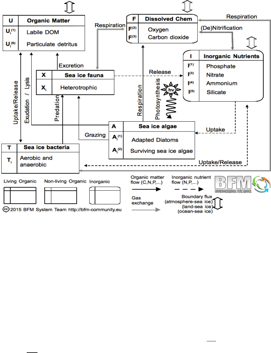
3.3. Sea ice Algae Dynamics
Figure 3.1.: Scheme of the state variables of BFM-SI and interactions within BFM-SI and with exter-
nal systems.
The rate of change of carbon in sea ice al-
gae depends on gross primary production, exuda-
tion, respiration, lysis and predation (Eq. 3.3.1a).
Gross primary production is the rate of change
of sea ice algae carbon Acdue to photosynthe-
sis, which involves an uptake of dissolved carbon
dioxide F(3).It is written as:
dAc
dt
gpp
F(3)
=fT
AfE
Afs
Ar0
AAc(3.3.2)
where the r0
Ais the maximum specific photosyn-
thetic rate under nutrient-replete, light saturated
conditions (Table 3.2). The ffunctions are mul-
tiplicative, non-dimensional regulating factors for
temperature, light and silicate, which vary from 0
to 1.
Temperature is regulating several physiologi-
cal processes. Its effect is expressed in a non-
dimensional form by fT
A:
fT
A=QA
10
T−10
10 (3.3.3)
where QA
10 is the characteristic doubling tempera-
ture parameter (Table 3.2).
Many relevant biological processes, such as po-
tential photosynthesis, are also affected by the
51

3. The sea ice biogeochemical model
Table 3.1.: List of the sea ice model state variables. Legend: IO = Inorganic; LO = Living organic;
NO = Non-living organic. The subscript iindicates the basic components of the group, e.g.
A(1)
i≡(A(1)
c;A(1)
n;A(1)
p;A(1)
s;A(1)
l).
Variable Type Components Description
I(1)IO P Phosphate (mmol P m−2)
I(3)IO N Nitrate (mmol N m−2)
I(4)IO N Ammonium (mmol N m−2)
I(5)IO Si Silicate (mmol Si m−2)
F(2)IO O Dissolved oxygen (mg C m−2)
F(3)IO C Carbon dioxide (mg C m−2)
A(1)
iLO C N P Si Chl Adapted diatoms (mg C m−2, mmol N-P-Si m−2, mg Chl-a m−2)
A(2)
iLO C N P Chl Surviving sea ice algae (mg C m−2, mmol N-P m−2,mg Chl-a m−2)
TiLO C N P Sea ice bacteria (mg C m−2, mmol N-P m−2)
XiLO C N P Sea ice fauna (mg C m−2, mmol N-P m−2)
U(1)
iNO C N P Dissolved organic detritus (mg C m−2, mmol N-P m−2)
U(6)
iNO C N P Si Particulate organic detritus (mg C m−2, mmol N-P-Si m−2)
non-dimensional light regulating factor fE
A:
fE
A=1−exp −EPAR
EK!(3.3.4)
where EPAR is the Photosynthetic Available Ra-
diation (PAR). EPAR is parametrized according
to the Lambert-Beer formulation with depth-
dependent extinction coefficients:
EPAR(z) =
ε
PARFswe(
λ
s+
λ
i)z+R0
z
λ
bio(z′)dz′(3.3.5)
where Fsw is the short-wave surface irradiance
flux and may be derived from data or from
a coupled physical model, such as the one of
Tedesco et al. (2009, 2010). The irradiance flux
is then converted by BFM-SI from W m−2to the
units of
µ
E m−2s−1as done in the pelagic model.
ε
PAR is the coefficient determining the portion of
PAR in Fsw. Light propagation takes into account
the extinction due to the background extinction of
snow/sea ice
λ
s,iand due to particles in the sea ice
λ
bio, where:
λ
bio =
2
∑
j
cAA(j)
l+cU(6)U(6)
c.(3.3.6)
Thus,
λ
bio takes into consideration the extinction
due to sea ice algae chlorophyll and to particu-
late detritus, while dissolved substances and other
inorganic matter are not currently taken into ac-
count. The cAand cUconstants are the specific
absorption coefficients of each suspended sub-
stance (Table 3.2).
EKis the light saturation parameter, that is the
ratio between the maximum chl-
a
specific photo-
synthetic rate and the maximum light utilization
coefficient, i.e.:
EK=P∗
m
α
∗.(3.3.7)
As for pelagic phytoplankton of BFM:
P∗
m=fT
Afs
Ar0
A
Ac
Al
(3.3.8)
52

3.3. Sea ice Algae Dynamics
Table 3.2.: Ecological and physiological parameters in BFM-SI.
Symbol A(1)A(2)Description
rA
01.5 2.0 Maximum specific photosynthetic rate (d−1)
QA
10 2.0 2.0 Characteristic Q10 coefficient (-)
θ
0
chl 0.035 0.03 Optimal quotum chl-a:C (mg chl mg C−1)
α
0
chl 1.8 e−33.8 e−6Maximum light utilization coefficient (mg C (mg chl)−1mE−1m2s)
ds0.1 - Half saturation value for Si-limitation (mmol Si m−2)
bA0.05 0.1 Basal specific respiration rate (d−1)
γ
A0.10 0.10 Activity respiration fraction (-)
β
A0.05 0.20 Excreted fraction of primary production (-)
dp,n,s
A0.1 0.2 Nutrient stress threshold (-)
dOA0.1 0.1 Maximum specific lysis rate (d−1)
a12.5 10−32.5 10−3Specific affinity constant for P (m−2mg C−1d−1)
a32.5 10−32.5 10−3Specific affinity constant for N-NO3(m−2mg C−1d−1)
a42.5 10−32.5 10−3Specific affinity constant for N-NH4(m−2mg C−1d−1)
sopt
A(1)0.03 - Standard Si:C ratio in sea ice diatoms (mmol Si mg C−1)
smax
A(1)0.085 - Maximum Si:C ratio in sea ice diatoms (mmol Si mg C−1)
pmin
A1.97 10−41.97 10−4Minimum phosphorus quota (mmol P mgC−1)
popt
A7.86 10−47.86 10−4Optimal phosphorus quota (mmol P mgC−1)
pmax
A1.57 10−31.5710−3Maximum phosphorus quota (mmol P mgC−1)
nmin
A3.78 10−43.78 10−4Minimum nitrogen quota (mmol N mgC−1)
nopt
A1.26 10−31.26 10−3Optimal nitrogen quota (mmol N mgC−1)
nmax
A2.52 10−32.52 10−3Maximum nitrogen quota (mmol N mgC−1)
cA10.0 e−310.0−3Specific absorption coefficient for chlorophyll-a(m2(mg Chl-a)−1)
cU0.1 e−30.1e−3Specific absorption coefficient for detritus (m2(mg C)−1)
Ωo
c1
12
1
12 Unit converison factor and stochiometric coefficient (mmol O2mgC)−1
53

3. The sea ice biogeochemical model
Equation Box 3.1 Sea ice algae equations
dAc
dt = = −∑
j=1,6
dAc
dt
lys
U(j)
c
dAc
dt
gpp
F(3)
−dAc
dt
exu
U(1)
c
−dAc
dt
resp
F(3)
(3.3.1a)
dAn
dt =∑
j=3,4
dAn
dt
upt
I(j)
−∑
j=1,6
dAn
dt
lys
U(j)
n
(3.3.1b)
dAp
dt =dAp
dt
upt
I(1)
−∑
j=1,6
dAp
dt
lys
U(j)
p
(3.3.1c)
dA(1)
s
dt =dA(1)
s
dt
upt
I(5)
−dA(1)
s
dt
lys
U(6)
s
(3.3.1d)
dAl
dt =
θ
chl dAc
dt
gpp
F(3)
−dAc
dt
exu
U(1)
c!− dAc
dt
rsp
F(3)
+dAc
dt
lys
U(6)
c!Al
Ac
(3.3.1e)
α
∗=fT
Afs
A
α
0
chl (3.3.9)
where fT
Ais the regulating factor for temper-
ature, fs
Ais the regulating factor for silicate,
r0
Ais the maximum specific photosynthetic rate
under nutrient-replete, light-saturated conditions
and
α
0
chl is the maximum slope of the production-
irradiance curve at optimal conditions (Table 3.2).
The fs
Ais parametrized as an external limiting
factor with a Michaelis-Menten form:
fs
A=I(5)
I(5)+ds
(3.3.10)
where dsis the Michaelis-Menten constant for
SiO2uptake inhibition (Table 3.2).
The exudation rate of Eq. (3.3.1a) reads:
dAc
dt
exu
U(1)
c
= [
β
A+
(1−
β
A)(1−fn,p
A)]dAc
dt
gpp
F(3)
(3.3.11)
where
β
Ais a constant fraction of carbon uptake
(Table 3.2) and fn,p
Ais a Liebig-like regulating
factor for internal nutrient ratio:
fn,p
A=min An/Ac−nmin
A
nopt
A−nmin
A
,
Ap/Ac−pmin
A
popt
A−pmin
A!(3.3.12)
where n(p)opt
Ais the nitrate(phosphate) optimal
ratio, while n(p)min
Ais the nitrate(phosphate) min-
imum quota (Table 3.2).
The respiration rate of Eq. (3.3.1a) is written
as:
dAc
dt
rsp
F(3)
=fT
AbAAc+
γ
A dAc
dt
gpp
F(3)
−dAc
dt
exu
U(1)
c!(3.3.13)
where fT
Ais the metabolic regulating factor for
temperature, bAis a constant specific rate of res-
piration and
γ
Ais a fraction of the assimilated pro-
duction (Table 3.2).
The loss of carbon via lysis of Eq. (3.3.1a) is
written as:
∑
j=1,6
dAc
dt
lys
U(j)
c
=1
fp,n
A+dp,n
A
dOAAc(3.3.14)
where dp,n
Ais the nutrient stress threshold and dOA
is the maximum specific lysis rate (Table 3.2).
54

3.4. Nutrient Supply and Dynamics
The chlorophyll rate of change of Eq. (3.3.1e)
is due to chlorophyll synthesis. The net chloro-
phyll synthesis is a function of acclimation to
light conditions, nutrient availability and turnover
rate. As in BFM, it is assumed that nutrient-
stressed cells releasing substantial amounts of dis-
solved organic carbon tend to regulate their inter-
nal chl:C ratio in order to avoid unconstrained de-
creases.
The rate of change of net photosynthesis is thus
primarily controlled by the dynamical chl:C ratio
θ
chl proposed by Geider et al. (1998), which reg-
ulates the amount of chl-
a
in the cell according to
a non-dimensional ratio between the realized pho-
tosynthetic rate in Eq. (3.3.1e) and the maximum
potential photosynthesis, i.e.:
θ
chl =
θ
0
chl
fE
Ar0
AAc
α
0
chl EPARAl
(3.3.15)
where
θ
0
chl is the maximum quotum chl-
a
:C and
α
0
chl is the maximum slope of the production-
irradiance curve at optimal growth conditions (Ta-
ble 3.2). The same considerations about down-
regulation and chlorophyll losses as detailed in
Sec. 2.2.6 for phytoplankton are valid for sea ice
algae.
3.4. Nutrient Supply and
Dynamics
Nutrients supply for algal growth comes from the
mixed layer up to the ice sheet for sustaining bot-
tom communities, but also from snow deposition
through brine drainage for surface communities
and from
in situ
regeneration processes.
Even in isolated brine pockets, bacteria,
heterotrophic protozoa and small metazoans
have been shown to regenerate the major
nutrients (Arrigo et al., 1995), but not sili-
cate. Silicate dissolution and regeneration
may be slower than demand and can be
the major limiting factor for diatoms growth
(Lizotte and Sullivan, 1991), shifting the commu-
nity from being diatom-dominated to flagellates-
dominated (Dieckmann et al., 1991). The slow
regeneration of silicate in sea ice is parametrized
in BFM-SI as a smaller value for the half satura-
tion of silica and a larger value for the standard
Si:C quotum in adapted diatoms (Table 3.2).
The boundary fluxes are currently added as ad-
ditional source terms to the biogeochemical equa-
tions and solved explicitly. For instance, in the
case of an inorganic nutrient in sea ice (e.g. ni-
trate, I(3)), the complete equation is written as
dI(3)
dt =dA(1)
n
dt
upt
I(3)
+dA(2)
n
dt
upt
I(3)
+dI(3)
dt
f lux
N(3)
(3.4.1)
where the first two terms on the right hand side
represent the uptake from sea ice algae and the
last one is the flux of nutrient at the boundaries.
The external mechanisms of nutrients replenish-
ment (exchange with the ocean and atmospheric
deposition) will be analyzed in the next sections.
The uptake of nitrogen and phosphorous by al-
gae (Eq. 3.4.1) is regulated by a Droop kinetics:
∑
i=3,4
dAn
dt
upt
I(i)
=min a3
AI(3)
+a4
AI(4)Ac,nopt
AGA
+fT
Ar0
Anmax
A−An
AcAc!(3.4.2)
dAp
dt
upt
I(1)
=min a1
AI(1)Ac,popt
AGA
+fT
Ar0
Apmax
A−Ap
AcAc!(3.4.3)
where the aconstants are the membrane affinity
for nitrate, ammonium and phosphate (Table 3.2).
The uptake of silicate is, instead, only function
of the maximum Si:C ratio smax
A(1)and of the net pro-
duction GA(1)of Eq. (3.3.1a):
dAs
dt
upt
I(5)
=smax
A(1)GA(1)(3.4.4)
Whenever sea ice algae carbon is lost by lysis,
a proportional loss is found for algae nutrient con-
tent and is distributed between a dissolved and a
55

3. The sea ice biogeochemical model
particulate fraction. For instance, the equations of
the lysis rate for phosphorous are:
dAp
dt
lys
U(6)
p
=pmin
A
∂
Ac
∂
t
lys
U(6)
c
(3.4.5)
dAp
dt
lys
U(1)
p
=Ap
Ac∑
j=1,6
∂
Ac
∂
t
lys
U(j)
c
−
∂
Ap
∂
t
lys
U(6)
p
.(3.4.6)
Silicate is instead only released in particulate
form:
∂
A(1)
s
dt
lys
U(6)
s
=A(1)
s
A(1)
c
∂
A(1)
c
∂
t
lys
U(6)
c
.(3.4.7)
3.5. Gases and Detritus
The following equations are derived by combin-
ing terms from the previous sections in order to
ensure mass conservation. The net production of
oxygen is due to the gross primary production and
to algae respiration rates:
∂
F(2)
∂
tbio
=Ωo
c
2
∑
j=1
∂
A(j)
c
∂
t
gpp
F(3)
−
∂
Aj
c
∂
t
rsp
F(3)!
where Ωo
cis the stoichiometric conversion factor
to oxygen units in respiration and photosynthesis
(Table 3.2).
Dissolved organic matter (DOM, U(1)
iin BFM-
SI) is a non-living functional group including C,
N and P constituents. In this current implemen-
tation, DOM is produced by sea ice algae (Eq.
3.3.11), though in the complete setup shown in
Fig. 3.1 , DOM will be produced also by sea ice
bacteria and microzooplankton:
∂
U(1)
c
∂
tbio
=
2
∑
j=1
∂
A(j)
c
∂
t
exu
U(1)
c
(3.5.1)
∂
U(1)
i
∂
tbio
=
2
∑
j=1
∂
A(j)
i
∂
t
exu
U(1)
i
i=n,p.(3.5.2)
Particulate organic matter (POM, U(6)
iin BFM-
SI) is made of C, N, P and Si:
∂
U(6)
c
∂
tbio
=
2
∑
j=1
∂
A(j)
c
∂
t
lys
U(6)
c
(3.5.3)
∂
U(6)
i
∂
tbio
=
2
∑
j=1
∂
A(j)
i
∂
t
lys
U(6)
i
i=n,p,s(3.5.4)
where the silicate component of POM is only
valid for the release of sea ice diatoms frustules.
3.6. The coupling strategy
A full description of the coupling issues is given
in Tedesco and Vichi (2014); here we briefly
mention some major aspects. The construction of
a biological system in sea ice implies the coupling
with the underlying biology of the ocean. BFM-
SI is in fact coupled to a simplified version of the
pelagic lower trophic levels in a surface layer of
ice-covered oceans. The standard pelagic BFM
has been simplified in a way that every sea ice
group has its own pelagic counterpart and there is
no loss of material between the two systems (Fig.
3.2). The number of functional groups is reduced
and the total number of state variables computed
are 34. The included groups and subgroups in the
pelagic BFM are:
•2 phytoplankton (diatoms and autotrophic
nanoflagellates)
•3 zooplankton (omnivorous mesozooplank-
ton, microzooplankton and heterotrophic
nanoflagellates)
•1 pelagic bacteria
•9 inorganic variables for nutrients and
gases (phosphate, nitrate, ammonium, sili-
cate,oxygen, carbon dioxide)
•2 organic non-living variables for dissolved
and particulate detritus.
56
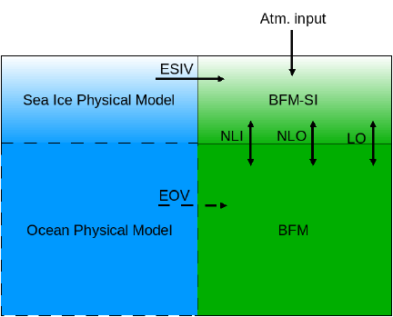
3.6. The coupling strategy
Figure 3.2.: Structure of the current coupling between physics and biogeochemistry (boxes with con-
tinuos line). The sea ice physical model passes offline the Environmental Sea Ice Vari-
ables (ESIV) to BFM-SI. BFM-SI is online coupled to BFM through the exchange of
Non Living Inorganic (NLI), Non Living Organic (NLO) and Living Organic (LO) mat-
ter. Boxes with dashed lines represent the possibility for the sea ice physical model to
be also coupled to an ocean physical model, which would pass the Environmental Ocean
Variables (EOV) to BFM.
Differently to BFM-SI, the pelagic zooplank-
ton includes 3 different subgroups and mesozoo-
plankton may effectively control the fate of the
sea ice algae released into the water and the
magnitude of the phytoplankton bloom. Conse-
quently, the diversity of feeding behaviors of zoo-
plankton is maintained.
The exchange of matter between the ocean sys-
tem and the sea ice system will be the subject
of the next section. We focus here on the cou-
pling strategy. BFM-SI has been built as a layer
model, in a similar way as the benthic compo-
nent of BFM is designed. A layer model means
that the model is two-dimensional (concentrations
are expressed in units of mass per square meters):
all the members of a generic layer of the system,
as for instance the benthic oxic layer, have to be
thought as their constituents are homogeneously
distributed on a stratum at the interface with the
ocean. However, the state variables of the pelagic
BFM are expressed as concentrations in a vol-
ume of sea water. The thickness of the consid-
ered layer is taken into account in order to have
every CFF of both systems (pelagic ad benthic) in
the same units per cubic meters. This concept can
be applied also to the coupling between BFM and
BFM-SI, considering that the sea ice biology is
distributed in a certain layer of sea ice (the sea ice
bio, BAL of Fig. 3.3). The thickness of the layer
is computed by a physical sea ice model, such as
the one developed by Tedesco et al. (2010), which
is a time-varying layer whose thickness depends
on the physical properties of sea ice (temperature,
salinity and brine volume).
3.6.1. Boundary fluxes: the sea
ice-ocean interface
The major exchanges between the sea ice and the
pelagic systems are the fluxes of organic and in-
organic matter at the interface. Ice structure de-
termines the porosity and therefore the rate of ex-
change: frazil ice is less porous than congelation
ice and algae may experience, for instance, nutri-
ent depletion in the former.
The rates of advection and diffusion of dis-
solved and particulate substances from seawater
into the porous bottom layer of ice may also de-
pend on under-ice current velocities, tides and
57
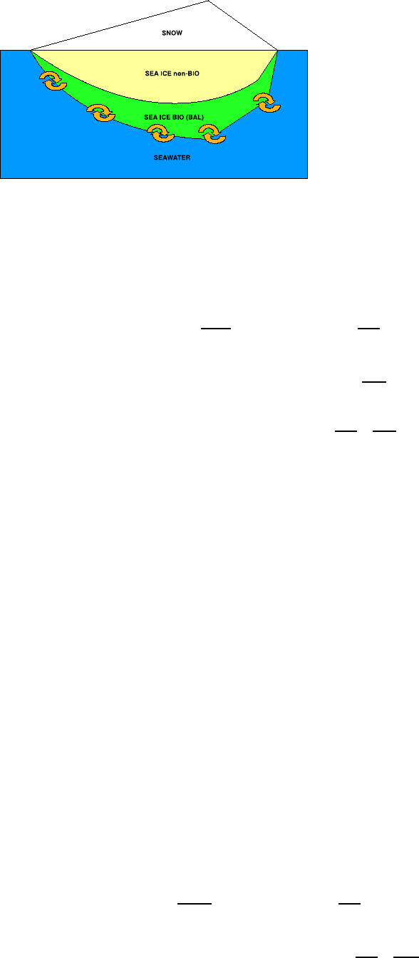
3. The sea ice biogeochemical model
Figure 3.3.: Model representation of the sea ice and pelagic coupling during a generic ice season. The
pelagic BFM exchange matter and gases with the SEA ICE BIO layer.
atmospheric pressure cycles (Cota et al., 1991).
Additionally, high algal biomass in the platelet
layer has been found to reduce the flux of nu-
trients to algae communities of the upper con-
gelation layer in Antarctica Lizotte and Sullivan
(1991).
High biomass is usually found in area of slow
ice growth rate (Legendre et al., 1992). During
the growth season, convection in the skeletal layer
enhances nutrient fluxes (Cota et al., 1991). Dur-
ing the melting season, the supply of freshwater
increases the stratification just below the ice and
reduces the flux of nutrients upward by reduc-
ing mixing and friction velocity (Gosselin et al.,
1985). Even if the enlargement and intercon-
nections of the brine channels allows a greater
biomass accumulation and nutrient supply, it also
leads to an increase in the biological loss by cells
sinking in the water column.
It is assumed here that the entrapment of dis-
solved matter follows the same partitioning of
salt in sea ice, that is the dynamics of dissolved
constituents is treated as the salinity dynamics,
as proposed by Tedesco et al. (2009), considering
the concentration of dissolved matter in seawa-
ter and sea ice growth rate. Fluxes are defined
positive upward, i.e. towards sea ice in Fig. 3.2.
The nitrate flux is described here as an example of
an inorganic nutrient exchange. The flux is com-
posed of a positive part (entrapment) during sea
ice formation when sea ice growth is positive, and
of a negative part during the melting phase:
dI(3)
dt
f lux−oce
N(3)
=max0,
∂
hi
∂
t·
max 0,N(3)−I(3)
hbio !
+min0,
∂
hi
∂
tI(3)
hbio
(3.6.1)
where N(3)is the nitrate concentration in seawa-
ter, hiis the ice thickness and hbio is the thickness
of the biologically active layer in sea ice. When
ice starts melting (the last term in the equation
above), the release to the water column depends
only on the sea ice melting rate and on the sea ice
concentration. The same flux, converted into units
of volume concentration, is included with oppo-
site sign in the dynamical equation for pelagic nu-
trients.
The entrapment of particulate matter is as-
sumed to be only a function of the seawater con-
centration, the sea ice growth rate and the actual
available space in the sea ice matrix (brine vol-
ume, Vbio), while the release during the melting
phase is parametrized as function of the sea ice
melting rate and sea ice concentrations, as in Eq.
(3.6.1). For instance, the flux of the chlorophyll
component of sea ice algae A(1)
l, from the pelagic
variable P(1)
lto sea ice is defined as:
dA(1)
l
dt
f lux−oce
P(1)
=max0,
∂
hi
∂
tP(1)
lVbio
+min0,
∂
hi
∂
tA(1)
l
hbio
.(3.6.2)
58

3.6. The coupling strategy
3.6.2. Boundary fluxes: the sea
ice-atmosphere interface
Nutrient content in snow and liquid precipitation
may directly lead to additional nutrient availabil-
ity for surface communities, and indirectly to in-
ternal and bottom communities, and finally to sur-
face waters once sea ice has totally melted away.
In the Baltic Sea, for instance, 5% of the total
annual flux of N and P and 20–40% of lead and
cadmium are deposited as snow: due to the in-
tense stratification of most of the Baltic waters,
sea ice is the major source of nutrients and trace
elements to the surface Baltic waters during the
melting season (Granskog et al., 2006).
The physical processes responsible of the
bioavailability of atmospheric nutrients to the sea
ice community are snow ice formation and snow
flushing. When snow ice forms the fraction of
snow that mixes with flooding seawater may bring
an additional source of nutrients for internal com-
munities, while during snow flushing episodes
the accumulated nutrients in the melting snow
may become available also for bottom commu-
nities, if brines are permeable. This latter pro-
cess is the one that it is currently considered in
the model for the parametrization of the flux of
atmospheric nutrients to bottom sea ice, as shown
in Fig. 3.2. Phosphate and nitrogen concentra-
tion in snow may be derived from an atmospheric
model or may be prescribed using available obser-
vations. The flux of nutrients due to precipitation
becomes then a linear function of the snow melt-
ing rate, similarly to the flux of matter from sea
ice to the ocean during melting of sea ice, i.e. for
nitrate:
dI(3)
dt
f lux−atm
Nsnow
=min0,
∂
hs
∂
tNsnow (3.6.3)
where Nsnow is the nitrate concentration in snow
and hsis the snow thickness.
59
3. The sea ice biogeochemical model
60
Part II.
BFM code description
61
4. Installation, configuration and
compilation
The default basic configuration of BFM is the STANDALONE model, which simulates the biogeo-
chemistry of a water volume with given depth. The typical example is a micro- or mesocosm batch
culture. Only the pelagic system can be currently simulated with this configuration. The model is
forced with prescribed or analytical functions of temperature, salinity and light and can be integrated
for any desired period with three different numerical schemes. The model output is in NetCDF.
4.1. Installation
The BFM code repository is made available through a distributed git repository, which requires access
authentication by using the username and password provided in the registration to the BFM website
(http://www.bfm-community.eu/). The code can be downloaded using the following git instruction
% git clone http://username:password@dev.cmcc.it/git/bfm.git
Alternatively, it is possible to retrieve a tarball archive from the website. After downloading the
tarball file, create a directory for the BFM and move into that directory. Uncompress and extract the
contents of the tarball. The downloaded file will have a different name based on the version. For
example:
% mkdir $HOME/BFM
% cd $HOME/BFM
% gunzip bfm-release-<version>.tgz
% tar xvf bfm-release-<version>.tar
This operation will create and populate the directory bfm containing the source files and the direc-
tory run for running the various test cases which are described in Sec. 5.5. The full directory tree of
the BFM core is given in Fig. 4.1.
The minimal user local settings to use BFM configuration/compilation tools is provided by means
of the environmental shell variable:
•BFMDIR The root directory of the BFM model (the path to the installed bfm-<version> direc-
tory).
4.1.1. System Requirements
The BFM can be run on any UNIX-based architecture and it has been tested on linux, Mac OSX and
IBM-iDataplex systems.
The software requirements are:
•PERL (version 5.8.2 and above), used automatically during compilation time to generate the
code from the model template (see Sec. 7).
63
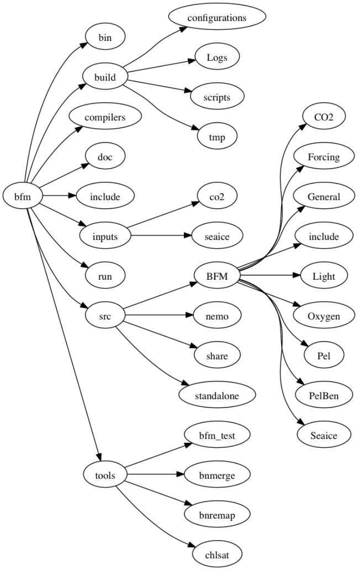
4. Installation, configuration and compilation
Figure 4.1.: Directory tree of the current BFM version.
64
4.2. Configuration: BFM Presets
•FORTRAN 90/95 compiler. Under linux and Mac OSX the model can be currently compiled
with gfortran (version 4.5 and above) and ifort (version 12 and above).
•NetCDF library (version 4 and above are recommended,
http://www.unidata.ucar.edu/software/netcdf) . It is mandatory that the library has been
compiled with the same compiler used for the model compilation since the F90 netcdf module is
used.
4.2. Configuration: BFM Presets
An experiment is defined by a model layout structure, namelists, and initial input values. These
definitions put together with compilation and run options is what is called a PRESET. A preset is
contained together in a folder and it is all you need to create a particular experiment.
The basic operations for configuration, compilation, and deployment of the model are performed
automatically by the script bfm_configure.sh in the folder ${BFMDIR}/build/, while the folder con-
taining the presets is ${BFMDIR}/build/configurations/.
Execute the following command to show a list of all available presets:
./bfm_configure.sh -P
Presets are composed of three different main files:
-configuration (compilation and deployment options)
This file uses the F90 namelist format to set values. Below is reported an example of the configuration
file format:
&BFM_conf
MODE = ’STANDALONE’,
CPPDEFS = ’BFM_STANDALONE INCLUDE_PELCO2 INCLUDE_DIAG’,
ARCH = ’gfortran.inc’,
PROC = 1,
EXP = ’standalone.pelagic’, /
...
<option>=<value>
/
Not all the options available in Tab. 4.1 can be specified in the configuration file and all the values
are overridden by the command line options. Available options are: MODE, CPPDEFS, BFMDIR,
NEMODIR, ARCH, CLEAN, PROC, NETCDF, EXP, NMLDIR, PROC and QUEUE. Do not use the
character " to surround values, but use ’ instead.
There are 2 major macros that belong to the core of the BFM source code and additional compilation
keywords that activates model components. The first 2 macros are “negative”, which means that their
options are activated by default and needs to be deactivated when desired.
Note that, the MODE field is used to specify if the code is compiled for standalone or coupled
execution, thus meaning that specific settings of the script generator will be used. Beside the STAN-
DALONE mode, additional fields will be made available following the release of the official coupling
support for external hydrodynamic models.
65

4. Installation, configuration and compilation
BFM_STANDALONE:This macro controls the main memory structure of the BFM. In default con-
figuration the BFM allocates its own memory array. When the macro is defined at compilation
(-DBFM_STANDALONE) all the variables belonging to the main memory are defined as pointers
and are not allocated during the initialization phase.
BFM_NOPOINTERS:by default, all the F90 symbols of the BFM state variables are defined as point-
ers to the main memory (cf. Sec. 6.2). By defining this macro, it is possible to substitute all
the pointers with the actual memory location. For instance, all the occurrences of the keyword
P1c(:) which are pointers to the memory address of phytoplankton carbon content, are substi-
tuted with the name D3STATE(ppP1c,:). To facilitate this feature, it is requested that all the
references to the pointers in the code are written with the indication of the number of dimensions:
P1c should always be indicated as P1c(:), otherwise a pre-compiler error is generated when
BFM_NOPOINTERS is defined. This macro is strongly recommended when BFM is coupled to
hydrodynamical models.
INCLUDE_PELCO2: Define and activate the pelagic variables of the carbonate system.
INCLUDE_PELFE: Add iron component and activate the related dynamics in the system.
INCLUDE_DIAG: Activate the computation and storage of user-defined diagnostics described in
Chap. 8.
EXPLICIT_SINK: Activate the explicit usage of serapate source and sinks arrays (Sec. 6.2).
-layout (memory layout configuration file)
This file is the template to define the model components layout (Sec. 7) and user-defined diagnostics
(Sec. 8.3). For a detailed description of the BFM memory layout content refer to Sec. 6.2.
-namelists_bfm (namelist file with standard values)
This file contains all the standard values of the namelists1used for the experiment. Namelists are
checked for consistency against the source code at generation time and the files effectively used for
the simulation will be copied in the $BFMDIR/run/<PRESETNAME> directory.
During this phase the BFM named constants corresponding to state variables (O2o, N1p, P1c,
...) are substituted by the progressive number which is a function of the chosen layout file. This
check will guarantee an executable file compatible with the namelists provided. The regular user will
generally work with generated namelists and usually there is no need to change any keyword in this
file besides the values in case there is the willingness to generate a new standard set of values.
After running the experiments, it is possible to modify generated namelists in the deployed experi-
ment folder ( $BFMDIR/run/$EXP ). If you want to preserve these changes into a new "preset" you
can use the tool "nmlcreator". This is for instance desired when a new group is added as in Sec.
7.2 and the parameters of the new group have to become default for the preset. To execute this tool do
the following steps
cd $BFMDIR/build/scripts/conf
./nmlcreator.pl -i NAMELIST_IN -o NAMELIST_OUT
where
1BFM input namelists follows F90 namelist standard
66

4.3. Compiling the BFM STANDALONE
•NAMELIST_IN: Complete path of the file containing namelist/s to read (e.g.. $BFMDIR/run/s-
tandalone.pelagic/Pelagic_Ecology.nml)
•NAMELIST_OUT: Complete path of the "namelist" file of
the preset where to append at the end of the input (e.g.:
$BFMDIR/build/configurations/STANDALONE_PELAGIC_Z/namelists).
Basically, nmlcreator adds the "filename_nml_conf" key with the name of the file at the end
of each namelist read. It is important to note that it will not delete the existing namelists in the target
preset, it will only append the new namelist at the end. In this case, an autimatic back substitution of
variables numerical indexes with the corresponding variable names (e.g. O2o, N1p) is not possible
and it has to be done manually by the user if required.
4.3. Compiling the BFM STANDALONE
Configuration and deployment of the model is done automatically by the script bfm_configure.sh. Af-
ter setting-up $BFMDIR variable in your shell environment, you can go to $BFMDIR/build directory
and execute bfm_configure.sh using default preset, namely the STANDALONE_PELAGIC:
./bfm_configure.sh -gcd
bfm_configure.sh generates, compiles and/or deploys files needed for the BFM model, as specified
in the preset folder. There are three different steps to have an executable model (see Fig. 4.2):
g (Generation) generate fortran files (.h , .f90) based on layout information and the single
namelist files (.nml) from namelists_bfm in $BFMDIR/build/tmp/<PRESETNAME> and
also place fortran files in the main code tree ($BFMDIR/src);
c (Compilation) compile the fortran code usig files of the main code tree ($BFMDIR/src)
and create the executable file (.x) in $BFMDIR/bin;
d (Deployment) create experiment folder in $BFMDIR/run/<PRESETNAME> and copy
namelists and executable for the simulation.
At least one of these three basic instruction is mandatory.
An execution without errors2will show the output directory for running the experiment and the
command to execute. Output after successful compilation should end with:
.................................. Makefile is ready.
STANDALONE_PELAGIC generation done!
Starting STANDALONE_PELAGIC compilation...
STANDALONE_PELAGIC compilation done!
Go to $BFMDIR/run/standalone.pelagic and execute command: ./bfm_standalone.x
Presets are loaded using option “-p” followed by the preset name, e.g.:
./bfm_configure.sh -gcd -p CO2TEST
For a full description of the script usage and available options, see Tab. 4.1 or execute the following
command:
./bfm_configure.sh -h
2If you experience problems during the generation or compilation, visit http://bfm-community.eu/
documentation for help
67
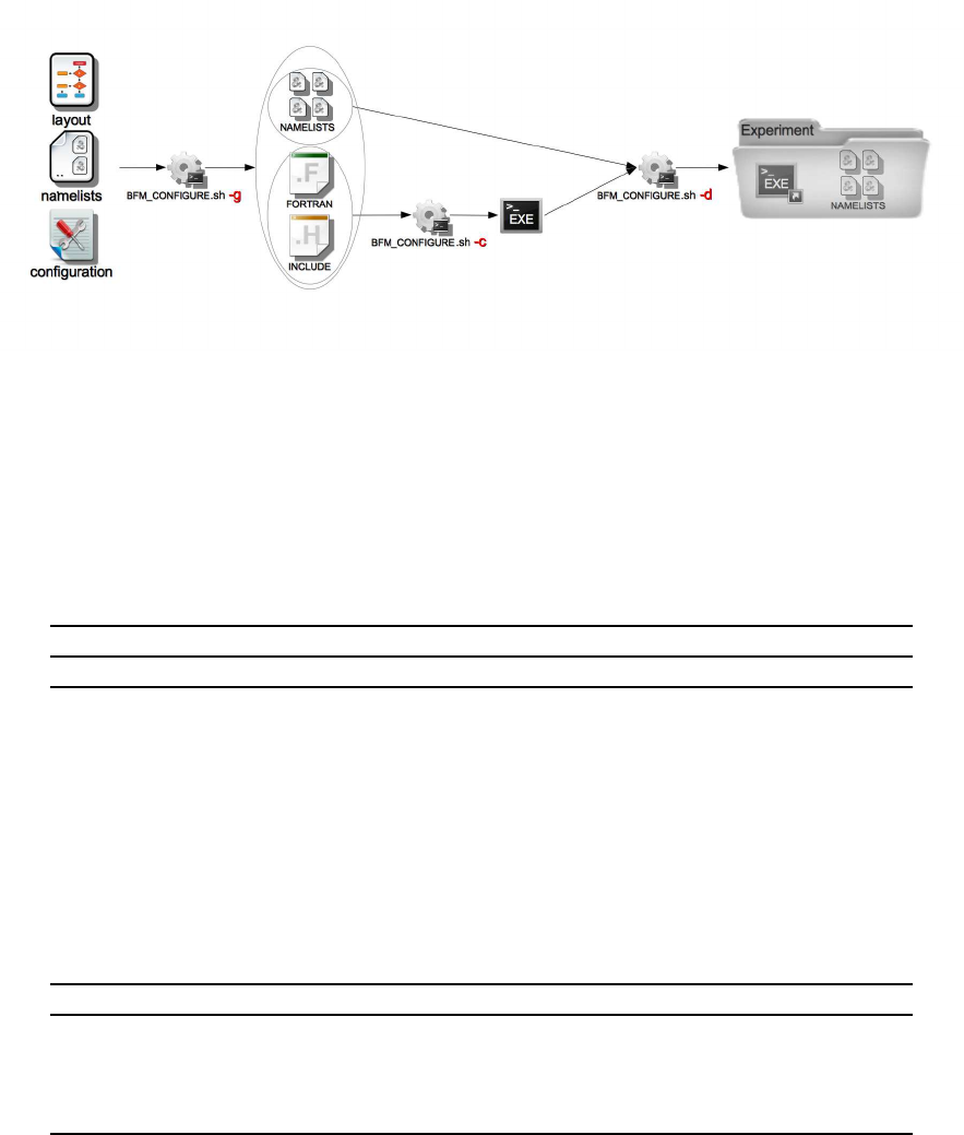
4. Installation, configuration and compilation
Figure 4.2.: Steps for experiment deployment
Option Argument Description
Compilation options
VERBOSE -v Verbose mode to print all messages
PRESET -p Preset to generate the configuration
MODE -m Mode for compilation and deployment
CPPDEFS -k Key options to configure the model
BFMDIR -b path to root directory of BFM
NEMODIR -n path to root directory of NEMO (only for NEMO coupling)
ARCH -a Specify compilation Architecture file
PROC -r Number of procs used for compilation (and execution)
FAST -f Fast mode. Don’t execute "clean" command in compilation
NETCDF -t Path to netcdf library and header files
Deployment options
EXP -x Name of the experiment for generation of the output folder
NMLDIR -l Input dir where are the namelists to run the experiment
PROC -r Number of procs used for running (same as compilation)
QUEUE -q Name of the queue number of procs used for running
Table 4.1.: List of optional arguments for bfm_configure
68
5. Running the STANDALONE model
5.1. Description
The execution of the configuration script described in the previous section creates the exe-
cutable and the running environment for the default preset of the STANDALONE model (called
STANDALONE_PELAGIC). The list of the available presets is obtained with the command
bfm_configure.sh -P and the results of the test cases are detailed in Sec. 5.5. The gener-
ated namelists are copied to the directory $BFMDIR/run/standalone.pelagic and the model
is run by executing ./bfm_standalone.x or ./bfm_standalone.x &> outputfile to
redirect the output messages to a file in bash.
Most of the BFM settings can be controlled via namelists. The STANDALONE model behaviour
is controlled with 2 major namelist files BFM_General.nml and Standalone.nml. The first
file contains the namelist to control the model setup (Tab. 5.1), model formulation (Tab. 5.2) and the
initial conditions for all the functional groups declared in the preset layout file (see also 1.1). The
second file control the simulation environment of the standalone model, like e.g., simulation setup
(Tab. 5.4), time settings (Tab. 5.5), and environmental forcing (Tab. 5.6).
5.2. State variables initial conditions (IC)
The initial conditions of the model state variables are declared in the file BFM_General.nml within
the bfm_init_nml namelist. As a general rule, the IC of each state variable is indicated with its
code abbreviation and 0, for example Phosphate initial value will be declared as N1p0 = 1.0.
ICs for living and non-living components of the model (see Tab. 1.1) has to be treated as follow:
•Dissolved Inorganic (IO) components require the specification of the initial value;
•Living organic (LO) components require only the initial content of carbon (e.g., P1c0, Z3c0),
while the other constituents are automatically set by the model using the optimal ratios to carbon
set in the specific namelists;
•Non-living organic (NO) components require only the initial content of carbon (e.g., R1c0) and
for those groups with more than one constituent, these are set using the Redfield ratios.
5.3. Numerical integration
Three integration schemes are implemented in the STANDALONE model. They can be chosen by the
parameter method in the namelist file standalone.nml. They are all explicit and use a time step
cutting approach to avoid negative concentrations. In detail, indicating with S(cn)the right-hand-side
source term computed with concentration cn, they are written as:
•the Euler scheme (method=1):
cn+1=cn+S(cn)∆t
69

5. Running the STANDALONE model
name kind description
bio_setup integer STANDALONE configuration:
1. pelagic
2. benthic (not yet available)
3. pelagic and benthic (not yet avail-
able)
bfm_rstctl string Save initial state in the output file
out_fname string Name of NetCDF output file
out_dir string Path to the output file
out_title string Name of the experiment in NetCDF
file
out_delta integer Output is saved every out_delta
timesteps
Table 5.1.: Parameters that control the model setup and output file (bfm_nml in
BFM_General.nml)
name kind description
CalcPelagic logical Switch on off the pelagic system
CalcBenthicFlag integer
Switch for the benthic model (only option 1. is
currently allowed)
1. no benthic model;
2. simple benthic return;
3. benthic organisms and intermediate
complexity nutrient regeneration;
4. benthic organisms and full nutrient
regeneration (early diagenesis)
CalcPhytoplankton(P) logical Switch for phytoplankton (P=1,2,3,4)
CalcPelBacteria(B) logical Switch for pelagic bacteria (B=1)
CalcMesoZooplankton(Z) logical Switch for mesozooplankton (Z=1 for Z3, Z=2
for Z4)
CalcMicroZooplankton(Z) logical Switch for microzooplankton (Z=1 for Z5, Z=2
for Z6)
CalcPelChemistry logical Switch for pelagic chemistry
AssignPelBenFluxesInBFMFlag logical
Switch to turn on/off the fluxes between the
pelagic and the benthic system. Fluxes are
always computed but not integrated if the flag
is false
AssignAirPelFluxesInBFMFlag logical
Switch to turn on/off the fluxes between the
atmosphere and the pelagic system. Fluxes are
always computed but not integrated if the flag
is false
ChlDynamicsFlag integer
Switch for chlorophyll parameterization in
phytoplankton
1. constant chl:C ratio and acclimation through
optimal light (ERSEM-II). Note: the variable
for chl content P1l is used to store optimal
irradiance in W m−2
2. Chlorophyll is a phytoplankton constituent
and variable chl:C ratio. Note: P1l is in mg
chl m−3
Table 5.2.: Parameters that control model formulation and execution (Param_paramteres in
BFM_General.nml)
70

5.4. Forcing functions
name kind description
LightPeriodFlag integer
Provide the light averaging period of the
external irradiance:
1. Instantaneous irradiance
2. Daylight average with explicit photoperiod
3. Daily average
LightLocationFlag integer
Choose the parameterization of light location
in the discrete grid:
1. Light at the top of the cell
2. Light in the middle of the cell
3. Average Light in the cell
ChlAttenFlag integer
Choose the PAR attenuation due to Chl:
1. broadband linear attenuation
2. 3-band tabulated attenuation coefficients
Table 5.3.: Parameters that control light properties in the water column (PAR_paramteres in
Pelagic_Environment.nml)
•the Runge-Kutta scheme of 2nd order (method=2):
cn+1=cn+1
2[S(cn) + S(cn+S(cn)∆t)] ∆t
•the leap-frog scheme (method=3):
cn+1=cn−1+S(cn)2∆twith the Asselin-filter: cn=cn+
γ
(cn−1−cn+cn+1)
5.4. Forcing functions
The STANDALONE model can be forced with different kind of forcing functions to provide the
physical information for the aquatic system (e.g. temperature, irradiance, etc.). Two options are
currently available: analytical forcing functions and data from an external file. All external data
formats and time interpolations are derived from the code provided by GOTM under the GPL.
5.4.1. Analytical forcing functions
This option is activated by setting forcing_method=1 in the namelist forcings_nml (Tab. 5.5).
The simple analytical forcing functions give the user a easily accessible and quickly usable basic set-
up of the physical forcing fields. The basic concept behind all forcing functions is the interpolation of
some (northern hemisphere) summer and winter values by a sine wave, considering them as the two
extreme values. This simple case is used for salinity forcing data (sw and ss in Table 5.6), while for
temperature, in addition to the sine wave, it is possible to superimpose a daily excursion (constant all
over the year).
Light forcing is interpolated with a sine wave from a winter minimum value to a summer maximum
value (lw and sw in Table 5.6) to obtain the actual value of average daylight for each day of the year.
These variables are as well intended as the placeholders for instantaneous light values and average
daylight, i. e. the mean value of light energy over the light period:
1
daylength Z
τ
dusk
τ
dawn
light(t)dt
The daylength is computed by the model as a function of the latitude value given in the namelist
. In case of the instantaneous light option (ltype=1) the average daylight is distributed in a sine
71

5. Running the STANDALONE model
name kind description
nboxes integer Number of water volumes
(boxes)
indepth real Depth of each box (m)
latitude real Latitude of each box
longitude real Longitude of each box
maxdelt real Maximum timestep duration (s)
mindelt real Minimum timestep duration (s)
method integer Integration method
1. Euler forward
2. Runge-Kutta 2nd order
3. Leap-frog
Table 5.4.: Main parameters for controlling time marching and integration in the STANDALONE
(standalone_nml in Standalone.nml)
name kind description
timefmt integer Format of the time limits and loop:
1. MaxN only. Give number of iterations,
fake start time is used.
2. start and stop dates. MaxN calcu-
lated.
3. start and MaxN.stop time calcu-
lated.
4. simdays only. Give number of simula-
tion days, fake start time used and MaxN
calculated.
MaxN integer Number of iterations in time-loop
simdays integer Number of simulation days
start string
“yyyy-mm-dd hh:mm:ss”
Start date
stop string
“yyyy-mm-dd hh:mm:ss”
Stop date
Table 5.5.: Main parameters for time management and integration length (time_nml in
Standalone.nml))
72
5.5. Test cases
wave over the daylight period reaching thus a maximum of twice the average daylight while being
zero at the beginning and in the end of the light period. In the case of constant light (ltype=2) the
mean daylight is smoothed out over the whole day by the factor daylength/24. In the case of
rectangular light distribution (ltype=3) the light equals the average daylight value over the whole
daylight period and is zero at night time. In order to setup a constant-light experiment, it is sufficient
to put the winter value equal to the summer value and set ltype=2.
5.4.2. Boundary forcing for atmospheric CO2
The STANDALONE model (but also any other coupled configuration that does not provide a connec-
tion with the atmosphere) has the possibility to turn on the prescription of an atmospheric CO2con-
centration for computing the surface fluxes. A time series can be specified as input to the atmospheric
mixing ratio by setting the file name in Carbonate_Dynamics.nml parameters listed in Tab. 2.9.
This is activated only if pelagic CO2is turned on in the model with the macros INCLUDE_PELCO2
in the file configuration. The atmospheric value found in Carbonate_Dynamics.nml is given
in units of partial pressure (
µ
atm) and not in ppm. A simple annual increase of this initial value can be
turned on by giving a percentage constant rate in the variable CO2inc found in Standalone.nml
(Table 5.6, set to 0 by default, if set to 1.0 gives the typical 1% annual increase).
5.4.3. Environmental data from file
The forcing_method=2 option allows the user to input the environmental data directly from a
file. The required input data are seawater temperature (variable ETW,oC), salinity (ESW), irradiance
(in W m−2, converted directly into the model variable EIR) and wind velocity (EWIND, m s−1). Any
other parameter can be included by modifying the file standalone/external_forcing.F90.
This file is a template for the input of external forcing data and must be modified by the user. The data
input file format is an ASCII file with a first column indicating the date (yyyy-mm-dd hh:mm:ss)
and one column for each parameter separated by space(s).
5.4.4. External event data
The model allows to input event data that force the state variables to certain values. This is useful to
simualte the case of a laboratory experiment, when for instance phytoplankton is inoculated at given
time interval or nutrients are restored to certain values. The syntax of the input file is the same as the
environmental data file above and the template file standalone/external_data.F90. must
be modified by the user according to the state variables that have to be modified. The subroutine is
implemented to overwrite any obtained value of the selected state variable(s) with the input value(s)
at the prescribed time(s).
5.5. Test cases
5.5.1. STANDALONE_CO2TEST: carbonate system model
The most simple test case is STANDALONE_CO2TEST that generates the run directory
run/standalone.co2test. if the BFM is configured with bfm_configure.sh -gcd
-p CO2TEST. It simulates a simple carbonate system equilibrium using the routines developed by
OCMIP (CalcCO2Method=2 in Carbonate_Dynamics.nml). Initial conditions are set for a
73

5. Running the STANDALONE model
name kind description
forcing_method integer Choice of the external forcing functions
1. analytical forcings
2. from file
3. interactive fluxes (not yet imple-
mented)
ltype integer Light forcing options:
1. instantaneous light description
2. constant light over 24h
3. rectangular light distribution (on/off)
according to photoperiod
4. Constant light averaged over the pho-
toperiod
lw real Sinusoidal light intensity (boreal win-
ter) W m−2
ls real Sinusoidal light intensity (boreal sum-
mer) W m−2
sw real Sinusoidal salinity (boreal winter)
ss real Sinusoidal salinity (boreal summer)
tw real Sinusoidal temperature (boreal winter)
degC
ts real Sinusoidal temperature (boreal sum-
mer) degC
tde real Sinusoidal temperature daily excursion
degC
ww real Sinusoidal wind (boreal winter) m s−1
ws real Sinusoidal wind (boreal summer) m s−1
CO2inc real Linear increase in CO2air partial pres-
sure [% per year]
forcing_file char Filename for external forcings (forc-
ing_method = 2)
use_external_data logical Read external data (user defined)
data_file char Filename for external data
Table 5.6.: Parameters for the external forcing functions (forcings_nml in Standalone.nml
74
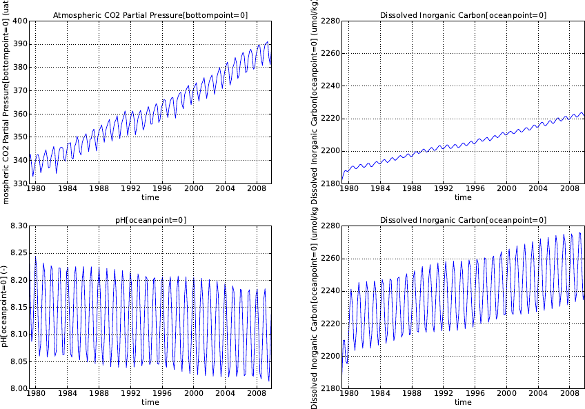
5.5. Test cases
Figure 5.1.: Examples from the CO2TEST simulation. Top panels: atmospheric CO2
partial pressure from the NOAA marine boundary layer data at 33N
(http://www.esrl.noaa.gov/gmd/ccgg/mbl/) and DIC with temperature set to the
constant value of 25 oC(default run). Bottom panels: pH and DIC values obtained with
seasonally varying temperature (tw=14, ts=27 in Standalone.nml)
75
5. Running the STANDALONE model
Mediterranean station with high alkalinity value and output is created every 60 days. The system is
forced with observed atmospheric CO2increase over the period 1979-2009. The default simulation
prescribes a constant temperature value and it is interesting to note the differences shown in Fig. 5.1
when seasonal variability of temperature is turned on. The seasonal cycle in temperature can be pre-
scribed by changing the winter and summer temperature minima and maxima of the analytical forcing
functions (Sec. 5.6).
5.5.2. STANDALONE_PELAGIC: the full pelagic BFM
The standard test case for the full BFM is created in directory run/standalone.pelagic and
it is the default preset when the code is generated and compiled without any option. It simulates
the seasonal cycle of a well-mixed temperate coastal sea, with mean depth 5 m. This example is
to be considered as a template for other applications, as it is not meant to describe any real-world
application. The simulation starts in January 2000 and terminates in 2010 with a maximum time step
of 8640 s in the adaptive Runge-Kutta solver and with the output stored every 30 days (see namelists
in Tab. 5.5, 5.4 and 5.1). The time evolutions of temperature, irradiance, nutrients (the system is
sustained with regenerated nutrients only, therefore nitrate plot is logarithmic and goes very close to
0), chlorophyll and gross primary production are shown in Figs. 5.2-5.4 for comparison.
5.5.3. STANDALONE_SEAICE: sea ice biogeochemistry
This configuration is the standard preset for the sea ice model described in Chap. 3. It describes the
evolution of a sea ice season using external forcing data from a sea ice model (the data are copied
from the directory inputs/seaice into the running directory by the configurator). The forcing functions
and model output are fully described in Tedesco and Vichi (2014).
5.6. Output visualization
Output values are stored in netCDF according to the CF convention (http://www.cgd.ucar.
edu/cms/eaton/cf-metadata/). The STANDALONE test cases output can be visualized with
the all-round ncview software (http://meteora.ucsd.edu/~pierce/ncview_home_
page.html), with the Python utility PyNcview https://sourceforge.net/projects/
pyncview/ or with ncbrowse. Matlab users can use the bfm_ncload.m utility available in the
tools directory. The figures presented in Sec. 5.5 have been produced with pyncview.
76
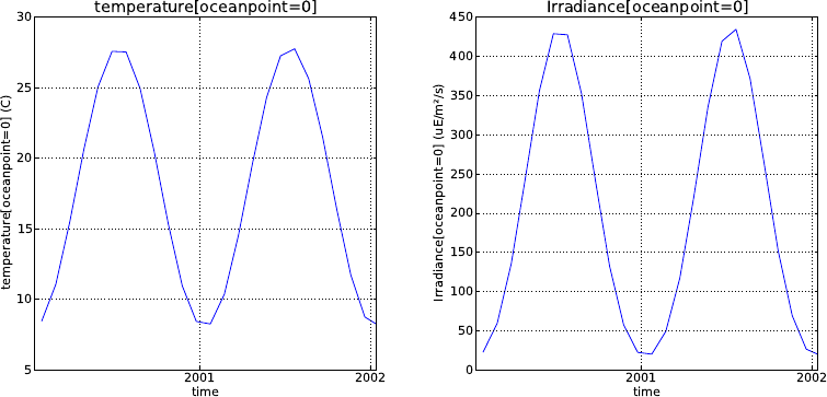
5.6. Output visualization
Figure 5.2.: Sample output of the STANDALONE_PELAGIC test case: temperature (left) and irradi-
ance (right)
77
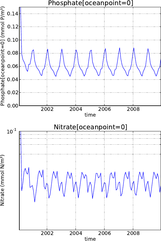
5. Running the STANDALONE model
Figure 5.3.: Sample output of the STANDALONE_PELAGIC test case: phosphate (top) and nitrate
(bottom)
78
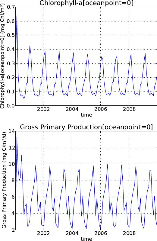
5.6. Output visualization
Figure 5.4.: Sample output of the STANDALONE_PELAGIC test case: Chlorophyll-a (top) and gross
primary production (bottom)
79
5. Running the STANDALONE model
80
6. Structure of the code
6.1. Coding rules
The BFM is written in plain F90 and it can generally be compiled with any F90 (and above) com-
piler. There are no fixed coding rules apart from standard clean programming. For historical reasons,
the subroutine and symbols of the BFM biogeochemistry module are indicated with C-style capital-
ized long-names (e.g. EcologyDynamics), even if F90 does not distinguish capital letters. Constants
and main memory arrays are generally indicated with capital names, to highlight their global static
behavior. It is recommended to follow this style when possible.
6.2. Memory layout and variable definition
The BFM is structured similarly as the original ERSEM used to be. Pelagic variables are defined as
virtually 3-dimensional, while benthic and sea ice variables are 2-dimensional. Only the sea-points are
stored in memory, and thus the BFM has no knowledge of any land-sea mask or spatial relationships
between grid-points in general. The number of bottom points is the same as the number of surface
points, therefore the 2-D arrays can also be used for the surface variables and/or surface fluxes. These
definitions are also maintained when the model is applied to a 1-D vertical setup. In that case, the
pelagic variables have the spatial dimension of the number of vertical layers while the benthic and
surface variables have dimension 1 (the bottom and surface levels, with the index depending on the
definitions of the physical model). In a 0-D setup (as in the STANDALONE test cases described in
Chap. 5), the same grid-point is at the same time a bottom, surface and ocean layer.
Fig. 6.1 illustrates the memory layout of pelagic variables. They are gathered in a single 2-
dimensional array holding the number of different variables and the number of ocean grid-points:
D3STATE(NO_D3_BOX_STATES,NO_BOXES)
and the same is done for the 2-dimensional variables (defined for the benthic and sea ice ecosystem
models):
D2STATE(NO_D2_BOX_STATES,NO_BOXES_XY)
Each variable memory is accessed by means of a pointer to the corresponding row containing all
the grid-point values. This pointer array has the same naming convention of ERSEM. The rows
are numbered with named constants starting with the letters pp (ppP1c for phytoplankton carbon,
ppN1n for nitrate or ppR1p for dissolved organic phosphorus, etc.). When the BFM is coupled to
a 3-D model, then a mapping function must be taken into account as shown in Fig. 6.1 in order to
compute the transport terms.
In addition to this direct mechanism, the memory can be accessed by means of group functions.
These functions have been created to allow the addition of any number of sub-groups in the same
trophic compartment, such as diatoms, nanoflagellates, picoplankton, etc. in the group of phy-
toplankton. The group function is in this case called PhytoPlankton(no_of_subgroups,
no_of_components), and allows to access the memory P1c by writing
81
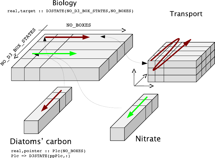
6. Structure of the code
Figure 6.1.: Layout of the main memory array for the pelagic variables (D3STATE) and schematic of
the remapping into a three-dimensional ocean grid for transport processes.
PhytoPlankton(iiP1,iiC)
The model state variables and components are defined in the model layout file of each preset (Sec.
4.2) which will be detailed in Chap. 7. It is now only sufficient to list the constants indicating the con-
stituents, namely iiC,iiN,iiP and iiSi. For each defined group there is a named constant starting
with the letters ii which holds the total number of existing subgroups (e.g. iiPhytoPlankton).
A typical example of the use of groups is to compute the total amount of food available to micro-
zooplankton (from MicroZoo.F90):
do i = 1 ,iiPhytoPlankton
PPYc(:,i) = p_paPPY(zoo,i)*PhytoPlankton(i,iiC)*&
MM_vector(PhytoPlankton(i,iiC), p_minfood(zoo))
rumc = rumc + PPYc(:,i)
rumn = rumn + PPYc(:,i)*qncPPY(i,:)
rump = rump + PPYc(:,i)*qpcPPY(i,:)
end do
Compare this code with the equation for food availability and capture efficiency presented in Sec.
2.4.1 of the BFM description and it will show how it is simple to cycle over all the phytoplankton
variables, independently of the number and type of the defined subgroups.
The other basic arrays of the memory are the ones containing the time rates of change due to each
physiological or ecological interaction. The rate of mass exchange between two state variables is an
82
6.3. The BFM flow-chart
element of an array D3SOURCE, if it is a production term, and D3SINK if it is a loss term, both
with dimensions NO_D3_BOX_STATES ×NO_D3_BOX_STATES ×NO_BOXES (Fig. 6.2). It is
clear that the two matrices are symmetrical and a predation (negative) rate from variable P1c to Z4c
is equivalent to an ingestion rate (positive) of Z4c over P1c. All the rates are defined positive by
convention, so that to obtain the net rate of change for variable of row j, it is sufficient to compute
sum(D3SOURCE(j,:,:)-D3SINK(j,:,:))
Fluxes which involve a variable not defined in the model, such as oxygen production from water
during photosynthesis can be taken into account by using the diagonal of the matrix. There is a
positive flow from O2o to itself computed stoichiometrically from the gross carbon production rate
and inserted in (D3SOURCE(O2o,O2o,:), cf. Fig. 6.2).
The same definitions apply for the 2-dimensional system, and the arrays are called D2SOURCE and
D2SINK with dimensions NO_D2_BOX_STATES ×NO_D2_BOX_STATES ×NO_BOXES_XY.
This separation between positive and negative terms allow to use more sophisticated positive-
definite integration schemes, but it may result in an excessive memory usage. Thus, the default setting
of BFM make use of a shrank version of D3SOURCE (NO_D3_BOX_STATES ×NO_BOXES), which
is the result of the addition of all the terms after the combination of the two symmetrical matrices into
one that contains all the source (upper-left part) and sink (lower-right part) terms. It is possible to use
the two separated matrices for source and sinks terms through the inclusion of the compilation macro
EXPLICIT_SINK in the preset configuration file.
No direct mass exchanges are allowed between variables from different realms (like for instance
between pelagic and benthic variables), and therefore those fluxes are defined as diagonal fluxes
each one within its own realm taking into account any change of units. Specialized functions
have been written to take into account all the possible kind of exchanges and are collected in
General/FluxFunctions.F90.
6.3. The BFM flow-chart
The BFM core will be described in its STANDALONE configuration. The main program (Fig. 6.3)
consists of 3 subroutines, one for initialization, one for the time-loop and one for closing all active
processes. The same structure is likely to be maintained also for all the coupled configurations, but
the calls are going to be distributed differently according to the structure of the general circulation
model.
6.3.1. Initialization procedures
The initialization of the BFM requires 4 different phases:
1. Initialization of geometric domain (number of boxes/gridpoints). This part de-
pends on the configuration: in the STANDALONE case, this is done in
standalone/standalone.F90[init_standalone] while in the other coupled
configuration there are specific interface subroutines;
2. Initialization of the set-up via namelist and definition of variable information
(share/api_bfm.F90[init_bfm] for the STANDALONE case);
3. Definition of variable information and allocation/initialization of variables;
4. Initialization of the NetCDF output.
83
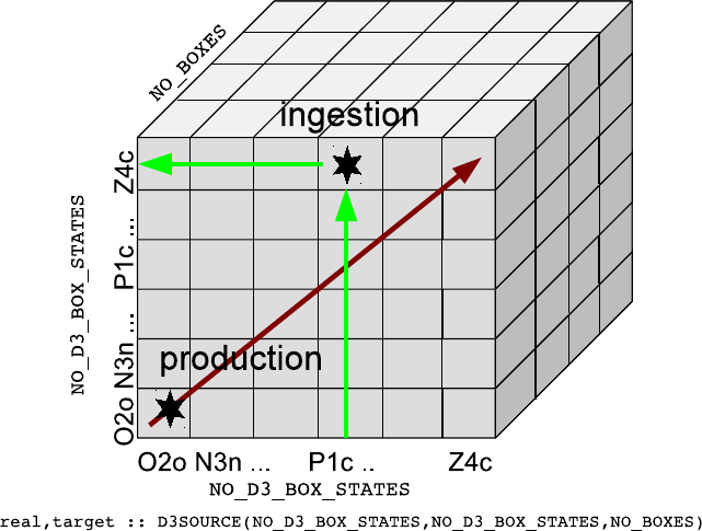
6. Structure of the code
Figure 6.2.: Schematic of the D3SOURCE array collecting the source terms.
6.3.2. Time marching
The time marching is driven by the host hydrodynamical model, or in the case of the STANDALONE
model, by a specific built-in routine. The phases of the time stepping shown in Fig. 6.3 are the
following:
1. update of the physical forcing functions needed by the biogeochemical model (temperature, ir-
radiance, wind, etc.). This is done by subroutine envforcing_bfm, which in the case of the
STANDALONE model computes the analytical values based on the time of the day/year. When
coupled with an ocean model, this routine is the contact point between the two models. Note
that information may flow in two directions because the light attenuation coefficient might also
be passed back to the physical model via this routine.
2. computation of the reaction term for the BFM module. This is done in EcologyDynamics,
which is further explained in the next section.
3. numerical integration of the biogeochemical terms. In the Standalone model there are three
different numerical schemes that can be used (see Sec. 5.3). Note that EcologyDynamics
can be called more than one time by this routine when the integration scheme is of higher-order.
4. preparation and writing of the NetCDF output, routines calcmean_bfm and save_bfm (the
names of the routines can be different for each coupling according to the ocean model structure
and naming conventions).
84
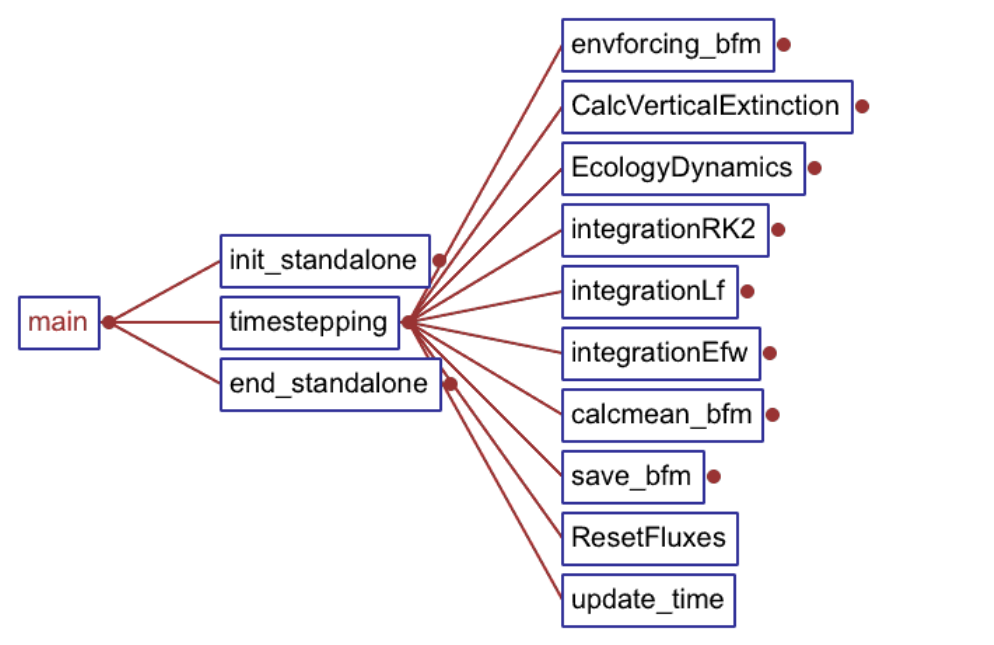
6.3. The BFM flow-chart
Figure 6.3.: Invocation tree of the Standalone main.
85
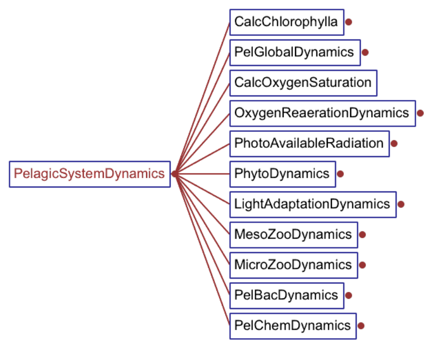
6. Structure of the code
Figure 6.4.: Invocation tree for PelagicSystemDynamics
86
6.3. The BFM flow-chart
6.3.3. Computation of pelagic reaction terms
The pelagic components are computed in PelagicSystemDynamics, which invokes the rou-
tines shown in Fig. 6.4. It first sets the diagnostic values for total chlorophyll (sum of all the
chlorophyll components in phytoplankton) and for the nutrient:carbon ratios in all the components
(PelGlobalDynamics) and for oxygen saturation and surface fluxes with the atmosphere.
The routines for the computation of light availability are only used when the parameterization of
optimal irradiance is activated (as in ERSEM-II, Ebenhöh et al., 1997), see Sec. 2.2.7, which is done
in Param_parameters (Tab. 5.2) by setting ChlDynamicsFlag=1.
The standard groups, phytoplankton, meso- and micro-zooplankton and bacteria are computed
in PhytoDynamics,Meso- MicroZooDynamics and PelBacDynamics, respectively. The
same routine is modularly used for each sub-group, as
!-=-=-=-=-=-=-=-=-=-=-=-=-=-=-=-=-=-=-=-=-=-=-=-=-=-=-=-=-=
! Compute phytoplankton dynamics
!-=-=-=-=-=-=-=-=-=-=-=-=-=-=-=-=-=-=-=-=-=-=-=-=-=-=-=-=-=
do i =1,iiPhytoPlankton
if ( CalcPhytoPlankton(i)) call PhytoDynamics( i )
end do
...
!-=-=-=-=-=-=-=-=-=-=-=-=-=-=-=-=-=-=-=-=-=-=-=-=-=-=-=-=-=
! Compute MesoZooPlankton dynamics
!-=-=-=-=-=-=-=-=-=-=-=-=-=-=-=-=-=-=-=-=-=-=-=-=-=-=-=-=-=
do i =1,iiMesoZooPlankton
if ( CalcMesoZooPlankton(i)) call MesoZooDynamics( i )
end do
PhytoDynamics has the declaration structure depicted in Fig. 6.5. This is an example
of how the memory layout presented in Sec. 6.2 is accessed by each submodel of the BFM.
To refer to the pointer of each phytoplankton component, one can use the placeholder function
ppPhytoPlankton(i,j), where iis the phytoplankton subgroup number (up to 4 in the reference
model) and jis the component (c, n, p, etc). Using ppPhytoPlankton(1,iiC) is equivalent to
writing ppP1c.
The function flux_vector is invoked many times by PhytoDynamics (Fig. 6.5) because it is
used to fill in the source/sink term arrays described in Sec. 6.2. This function is used throughout the
BFM modules. In case of a mass exchange term such as the excretion of dissolved carbon we have
call flux_vector(iiPel,ppphytoc,ppR1c,rr1c)
where the flux is pelagic (iiPel), from phytoplankton carbon to dissolved organic carbon
(ppphytoc, ppR1c) and the value is rr1c, which will be assigned both to D3SINK and
D3SOURCE in the appropriate element. The oxygen production rate is instead assigned as
call flux_vector(iiPel,ppO2o,ppO2o,rugc/MW_C)
which concerns a pelagic flux (iiPel), on the oxygen diagonal (from ppO2o to ppO2o) and MW_C
is the mass weight of carbon to convert gross primary production (rugc). Since the last term is
positive, this flux will be assigned to D3SOURCE.
The same methodology is applied for all the other pelagic fluxes and also in the benthic and sea
ice system. After the computation of all the reaction terms for pelagic organisms, there is the call
87
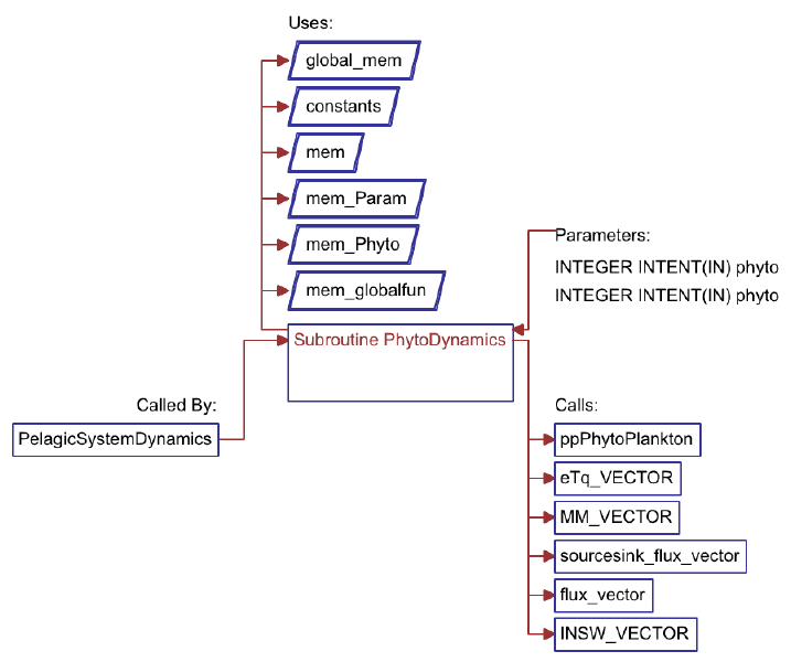
6. Structure of the code
Figure 6.5.: Declaration scheme of PhytoDynamics.
to pelagic chemistry (PelChemDynamics, see Fig. 6.4). This part computes all the parameter-
ized bacteria-mediated biochemical processes such as nitrification and denitrification, re-oxidation of
reduction equivalents and dissolution of biogenic silica.
88
7. Design model layout components
7.1. Layout syntax and modular structure
The BFM is conceived in a modular way and the number of state variables and biogeo-
chemical basic components can be modified according to the modelling needs. In fact, each
state variable is not defined directly in the code, but through a model template layout
found in the PRESET directories (Sec. 4.2, $BFMDIR/build/configurations). All the
ancillary F90 memory layout files (AllocateMem.F90, INCLUDE.h, ModuleMem.f90,
set_var_info_bfm.f90) are automatically generated from this meta-data structure by way of
a perl script ($BFMDIR/build/script). The prototypes of these files are found in directory
$BFMDIR/BFM/proto and filled in with the user-defined state variables and diagnostics.
The structure of the model template given in Tab. 7.1 is divided in sections with specific headings.
Sections can be repeated many times in the file. For clarity, it is suggested to follow a conceptual
construction of the model, by grouping all the state variables and diagnostics as done in the standard
released structure.
3d-state: this section is used for all the state variables, which are defined as being virtually three-
dimensional. This means that they exist in the whole domain, be it 0-, 1- or 3-dimensional. An
example of state variable definition is shown in Box 7.1.
According to the theoretical model description, variables are defined as functional families and
identified by their main biochemical components, which are indicated according to the classi-
cal ERSEM syntax (Blackford and Radford, 1995). State variable definitions require 3 pieces of
information, separated by colons: code symbol with components, long name and units. Com-
ponents are indicated by one single letter and currently the following are reserved: c=carbon,
n=nitrogen, p=phosphorus, s=silica, l=chlorophyll, f=iron. Any other new component (ei-
ther atomic or molecular) can be added, provided that the user include the relative dynamics
in an appropriate piece of code. The syntax for a multi-component variable is detailed be-
low varname[cnp...], and it is also possible to define group of state variables, such as
PhytoPlankton or PelDetritus as shown in Box 7.1. This feature gives the advantage to
cycle over all the group components with one single index (see the example in Sec. 6.2).
2d-state: all the features described above are also valid for the state variables belonging to the
benthic or sea ice 2-D system.
1d-variable: this section defines the variable without a spatial component (more appropriately de-
fined as 0-D variables). These are only function of time and defined as scalars.
2d-variable: this section includes the surface variables, originally identified as benthic variables.
However, this section is also used to define surface variables such as wind velocity. In a 1D
coupled model, this is a scalar, while it is a one-dimensional array holding all the surface (bottom)
points in a coupled 3D model.
89
7. Design model layout components
...
#-=-=-=-=-=-=-=-=-=-=-=-=-=-=-=-=-=-=-=-=-=-=-=-=-=-=-=-=-=-=-=-=-=-=-=-
# PELAGIC STATE VARIABLES (volume)
#-=-=-=-=-=-=-=-=-=-=-=-=-=-=-=-=-=-=-=-=-=-=-=-=-=-=-=-=-=-=-=-=-=-=-=-
3d-state
#-=-=-=-=-=-=-=-=-=-=-=-=-=-=-=-=-=-=-=-=-=-=-=-=-=-=-=-=-=-=-=-=-=-=-=-
# State Variable(s) for Nutrients
#-=-=-=-=-=-=-=-=-=-=-=-=-=-=-=-=-=-=-=-=-=-=-=-=-=-=-=-=-=-=-=-=-=-=-=-
N1p : Phosphate : mmol P/m3
N3n : Nitrate : mmol N/m3
N4n : Ammonium : mmol N/m3
#-=-=-=-=-=-=-=-=-=-=-=-=-=-=-=-=-=-=-=-=-=-=-=-=-=-=-=-=-=-=-=-=-=-=-=-
# State Variable(s) for Phytoplankton
#-=-=-=-=-=-=-=-=-=-=-=-=-=-=-=-=-=-=-=-=-=-=-=-=-=-=-=-=-=-=-=-=-=-=-=-
group PhytoPlankton[cnpls] (PPY) : mg C/m3 : mmol N/m3 : mmol P/m3 :
mg Chl/m3 : mmol Si/m3
P1 : Diatoms
P2[-s] : Flagellates
P3[-s] : PicoPhytoplankton
P4[-s] : Large Phytoplankton
end
#-=-=-=-=-=-=-=-=-=-=-=-=-=-=-=-=-=-=-=-=-=-=-=-=-=-=-=-=-=-=-=-=-=-=-=-
# State Variable(s) for Mesozooplankton
#-=-=-=-=-=-=-=-=-=-=-=-=-=-=-=-=-=-=-=-=-=-=-=-=-=-=-=-=-=-=-=-=-=-=-=-
group MesoZooPlankton[cnp] (MEZ) : mg C/m3 : mmol N/m3 : mmol P/m3
Z3 : Carnivorous Mesozooplankton
Z4 : Omnivorous Mesozooplankton
end
end
Table 7.1.: Example of the model template file layout with the definition of pelagic state variables.
90
7.1. Layout syntax and modular structure
3d-variable: this section is used for all the ancillary diagnostic variables defined in the whole do-
main. Typically, this section is used for temperature, salinity, and other environmental or diag-
nostic variables. Environmental variables obtained from external data files or hydrodynamical
models are indicated with capital symbols starting with E (e.g. ETW = environmental temperature
of water).
The syntax of the allowed layout elements is the following
[dim]d-state [-if-exist]
GROUP
VARNAME
end
[dim]d-variable [-if-exist]
VARNAME
ARRAYNAME
QUOTUM
end
[dim]d-flux [-if-exist]
FLUXNAME
end
•GROUP, like PhytoPlankton
group name[constituents] (acronym) : constituent_units
VARNAME
end
•VARNAME, like N1p or P2[-s] (if present, the constituent within brackets are removed from
the group list of elements)
name[-constituents] : description : units
•ARRAYNAME, a variable that is defined for each element of a group, like the specific uptake
for each phytoplankton suPPY(PhytoPlankton)
name(groupname) : description : units
•QUOTUM, like qncPPY(PhytoPlankton) (quotum N:C for each phytoplankton group)
q+constituent+constituent+acronym() : description : units
•FLUXNAME, the named entity for a user-defined flux like ruPPYc (Sec. 8.3)
name = FLUX : description : units
•FLUX, an expression combining several variables to store fluxes between components (Sec. 8.3)
(var[+|-]var)[<-|->](var[+|-]var)
with the following fundamental elements
91
7. Design model layout components
•name: an alphanumeric string starting with a non-numeric character
•constituents: one or several from the list: c(Carbon), n(nitrogen), p(phosphorus), s(sili-
con), f(iron), l(chlorophyll). They have to be written in lower case and without any separation
•description: phrase describing the variable, quota or flux
•units: units in which the variable, quota or flux are measured
•constituents_units: units separated by “:”. Have to be same number of units as con-
stituents have been specified
•groupname: name of a group, also name of the function to access the group components
•var: variable name (e.g. R6c) or first letter of group with constituents for naming all (e.g. P.c)
•acronym: acronym representing the group. Currently accepted acronyms are: PPY
(PhytoPlankton), PBA (PelBacteria), MEZ (MesoZooPlankton), MIZ
(MicroZooPlankton), OMT (PelDetritus), CAR (Inorganic)
•dim: dimension of the layout elements inside. Allowed values are: 1,2and 3
The configuration can be also modified at compilation time by means of the set of macros listed in
Sec. 4.2. The statement -if-exist found after one of the layout declarations indicates that the
following set of variables will be defined only when the macro is included in the compilation:
3d-variable -if-exist INCLUDE_PELCO2
DIC : Dissolved Inorganic Carbon : umol/kg
CO2 : CO2(aq) : umol/kg
pCO2 : Oceanic pCO2 : uatm
HCO3 : Bicarbonate : umol/kg
CO3 : Carbonate : umol/kg
Ac : Alkalinity : umol eq/kg
pH : pH : -
end
7.2. Example 1. Adding a subgroup
This is the most simple example, because it involves a small number of changes. Let us assume we
want to add another mesozooplankton component to the zooplankton group , such as macrozooplank-
ton (as done for instance by Berline et al., 2011). It is also assumed that this group will have exactly
the same dynamics as the other two subgroups, but different parameter values. It is first suggested to
create a new preset by copying the directory STANDALONE_PELAGIC to a new name
cd $BFMDIR/build/configurations
cp -r STANDALONE_PELAGIC STANDALONE_PELAGIC_Z
and then edit the appropriate line in the template file layout by adding the new variable name and
long name:
92
7.2. Example 1. Adding a subgroup
#-=-=-=-=-=-=-=-=-=-=-=-=-=-=-=-=-=-=-=-=-=-=-=-=-=-=-=-=-=-=-=-=-=-=-=-
# State Variable(s) for Mesozooplankton
#-=-=-=-=-=-=-=-=-=-=-=-=-=-=-=-=-=-=-=-=-=-=-=-=-=-=-=-=-=-=-=-=-=-=-=-
group MesoZooPlankton[cnp] (MEZ) : mg C/m3 : mmol N/m3 : mmol P/m3
Z3 : Carnivorous Mesozooplankton
Z4 : Omnivorous Mesozooplankton
Z2 : Macrozooplankton
end
It is also suggested to edit the name of the run directory where the namelists will be copied. This is
done in the configuration file $BFMDIR/build/configurations/configuration and change
EXP = ’standalone.macrozoo’
Now the configuration can be generated by compiling the new preset
cd $BFMDIR/build
./bfm_configure.sh -gcd -p STANDALONE_PELAGIC_Z
and the script will take care of the automatic generation of the new memory layout with the required
named constants, pointers, initial value, run directory and namelists. A new Z2 element will be added
to the group MesoZooPlankton (in this case Z2 will be the third element as it comes after Z3 and
Z4). Particularly, a new column will be added in the mesozooplankton namelist and filled in with
zero. A warning is issued for each added column or row of parameters:
WARNING: (2 < 3) adding zero values to element p_q10 in namelist MesoZoo
WARNING: (2 < 3) adding zero values to element p_srs in namelist MesoZoo
WARNING: (2 < 3) adding zero values to element p_sum in namelist MesoZoo
...
WARNING: (2 < 3) adding new predator term p_paMIZ(3,:) in namelist MesoZoo
WARNING: (2 < 3) adding new predator term p_paPPY(3,:) in namelist MesoZoo
Check the updated file tmp/STANDALONE_PELAGIC_Z/ModuleMem.F90 and search for the
new variable Z2 to see the added pieces of code.
The final steps before running the new model are the addition of the proper parameter values
in place of zeros in the new column/rows corresponding to Z2 of MesoZoo_parameters in
run/STANDALONE_PELAGIC_Z/Pelagic_Ecology.nml
&MesoZoo_parameters
! Z3 Z4 Z2
p_q10 = 2.0 2.0 0.0
p_srs = 0.01 0.02 0.0
p_sum = 2.0 2.0 0.0
p_vum = 0.025 0.025 0.0
p_puI = 0.6 0.6 0.0
p_peI = 0.3 0.35 0.0
p_sdo = 0.01 0.01 0.0
p_sd = 0.02 0.02 0.0
p_sds = 2.0 2.0 0.0
p_qpcMEZ = 1.67d-3 1.67d-3 0.0
p_qncMEZ = 0.015 0.015 0.0
p_clO2o = 30.0 30.0 0.0
! P1 P2 P3 P4
! Z3
p_paPPY(1,:) = 0.0 0.0 0.0 0.0
93
7. Design model layout components
! Z4
p_paPPY(2,:) = 1.0 0.0 0.0 0.7
! Z5 Z6
! Z3
p_paMIZ(1,:) = 0.0 0.0
! Z4
p_paMIZ(2,:) = 1.0 0.0
! Z3 Z4 Z2
! Z3
p_paMEZ(1,:) = 1.0 1.0 0.0
! Z4
p_paMEZ(2,:) = 0.0 1.0 0.0
! Z5 Z6
! Z2
p_paMIZ(3,:) = 0.0 0.0
! P1 P2 P3 P4
! Z2
p_paPPY(3,:) = 0.0 0.0 0.0 0.0
! Z3 Z4 Z2
! Z2
p_paMEZ(3,:) = 0.0 0.0 0.0
/
and to turn on the flag CalcMesoZooPlankton(3)=.TRUE. in Param_parameters and add
initial value(s) by adding a line Z2c0=<value> in bfm_init_nml, both found in file
run/STANDALONE_PELAGIC_Z/BFM_General.nml.
7.3. Example 2. Adding a biochemical component and a group
The BFM application in the global ocean is called PELAGOS (PELAgic biogeochemistry for Global
Ocean Simulations) and the climatological simulations were described in Vichi et al. (2007a). A ma-
jor requirement to simulate the global ocean ecosystem is the introduction of iron control on phyto-
plankton growth (Sec. 2.2.8), particularly to capture the high-nutrient low-chlorophyll regions. The
example below shows how the iron component of phytoplankton and detritus have been added to the
model structure template. Additional coding from the user is then required to parameterize the fluxes
between these components and the regulations of plankton physiology (this is already included in
the GYRE_BFM preset that requires the usage of the NEMO model and activated with the keyword
INCLUDE_PELFE).
To add an iron constituent to a group, it is sufficient to specify a unique single-character constant
between the square brackets in the layout file as shown below:
#-=-=-=-=-=-=-=-=-=-=-=-=-=-=-=-=-=-=-=-=-=-=-=-=-=-=-=-=-=
# State Variable(s) for Phytoplankton
#-=-=-=-=-=-=-=-=-=-=-=-=-=-=-=-=-=-=-=-=-=-=-=-=-=-=-=-=-=
group PhytoPlankton[cnplsf] (PPY) : mg C/m3 : mmol N/m3 : mmol P/m3 :
mg Chl/m3 : mmol Si/m3 : umol Fe/m3
P1 : Diatoms
P2[-s] : Flagellates
P3[-s] : PicoPhytoPlankton
end
94
7.4. Example 3. Removing components from zooplankton
It is also necessary to provide units separated by colons, in this case
µ
mol Fe m−3. Remember
that the [-s] syntax in some phytoplankton groups indicates that this constituent, although being a
component of the group vector, is not computed for that specific sub-group.
The preprocessing script will take care during compilation to generate an adequate entry in the main
memory module and the definitions of the named constants (ppP1f, . . . ) and pointers (P1f, . . . ) to
access the new variables from the model code.
New groups can also be defined in order to use the facilities shown in Sec. 6.3.3. All the detritus
variables can be grouped together with the following syntax:
#-=-=-=-=-=-=-=-=-=-=-=-=-=-=-=-=-=-=-=-=-=-=-=-=-=-=-=-=-=-=-=-=-=-=-=-
# State Variable(s) for Detritus (Biogenic Organic Material)
#-=-=-=-=-=-=-=-=-=-=-=-=-=-=-=-=-=-=-=-=-=-=-=-=-=-=-=-=-=-=-=-=-=-=-=-
group PelDetritus[cnpsf] (OMT) : mg C/m3 : mmol N/m3: mmol P/m3:
mmol Si/m3 : umol Fe/m3
R1[-s] : Labile Dissolved Organic Matter
R2[-npsf] : Semi-labile Dissolved Organic Carbon
R3[-npsf] : Semi-refractory Dissolved Organic Carbon
R6 : Particulate Organic Matter
end
7.4. Example 3. Removing components from zooplankton
For certain purposes it is not needed to carry out the computation of variable nutrient:carbon quota
in selected Functional Groups (for instance, in the case of the new macrozooplankton group added in
example 1). This can be done to save computational resources in the case of low-resolution long-term
global ocean simulations or with high-resolution coastal models. A possible example is the assump-
tion of a fixed quota in zooplankton which allows one to reduce the number of standard components
of up to 8 state variables. The zooplankton group definitions are equal to the one shown in the code
of Box 7.1 for MesoZooplankton but with the removal of the nand pconstituents:
#−=−=−=−=−=−=−=−=−=−=−=−=−=−=−=−=−=−=−=−=−=−=−=−=−=−=−=−=−=−=−=−=−=−=−=−
# S t a t e V a r i a b l e ( s ) f o r Mes oz oopl ankton
#−=−=−=−=−=−=−=−=−=−=−=−=−=−=−=−=−=−=−=−=−=−=−=−=−=−=−=−=−=−=−=−=−=−=−=−
grou p MesoZ ooPlankto n [ cnp ] (MEZ) : mg C / m3 : mmol N / m3 : mmol P / m3
Z3[−np ] : C a r n i v o r o u s M es oz oo plan kt on
Z4[−np ] : Omnivorous Mesoz ooplankton
end
The additional requirement is the change of value in parameter check_fixed_quota from 0 to 1
in the Param_parameters namelist. Test experiments have shown that the simulation times can
be reduced up to 30%. The physiological assumption is that zooplankton release in inorganic form
the nutrients in excess of the given fixed quota.
95
7. Design model layout components
96
8. Model outputs
8.1. Output
The variables that can be stored in the output file are the ones defined in file layout. All the
state variables can be stored (provided that they have a long name and units), both as instantaneous
values and as means over the chosen output period. This behavior is controlled via the namelist
bfm_save_nml contained in the BFM_General.nml file when running the STANDALONE
model. Other couplings may have different names. Additionally, a set of other variables can be saved,
such as the ones obtained from the physical model and other diagnostics such as total chlorophyll,
nutrient quota or aggregated rates.
8.2. Restart
The length of each BFM simulation is controlled by the physical transport model except for the STAN-
DALONE model which has its own time marching. It is common practice in modeling to split the
simulation in several chunks and to continue the simulation from the end values of each state variable
at the end of a previous run. The BFM stores this information in a NetCDF file which is always gen-
erated at the end of each simulation. There is no automatic control on the date (neither it is stored as
an attribute inside the NetCDF file), so it is totally up to the user to check that the initial restart file is
the proper one. The input/output restart file names and the restart switch (bfm_init) are set in the
BFM_General.nml file within the namelist bfm_init_nml.
8.3. Aggregated diagnostics and rates
All the ancillary 2D and 3D variables (like wind velocity or temperature, for instance) and diagnostics
are grouped in two memory arrays, D3DIAGNOS and D2DIAGNOS, which are accessed by means of
pointers. The dimensions of these arrays change according to the number of model elements in the
layout file, and any diagnostic rate can be easily defined thanks to the automatic generation of the
memory layout. Some fluxes are already defined by default, such as the gross/net primary production
rates, total respiration rates and (de)nitrification rates.
Any exchange of mass between every state variable can be tracked by means of a special
syntax that allows the user to access and combine the elements of the D3(D2)SOURCE and
D3(D2)SINK arrays where all the rates are stored. Some examples are already included at the
end of the STANDALONE_PELAGIC/layout file and are activated with the compilation macros
INCLUDE_DIAG:
#
-=-=-=-=-=-=-=-=-=-=-=-=-=-=-=-=-=-=-=-=-=-=-=-=-=-=-=-=-=-=-=-=-=-=-=-=-
# DIAGNOSTIC RATES
97
8. Model outputs
#
-=-=-=-=-=-=-=-=-=-=-=-=-=-=-=-=-=-=-=-=-=-=-=-=-=-=-=-=-=-=-=-=-=-=-=-=-
3d-flux -if-exist INCLUDE_DIAG INCLUDE_PELCO2
ruPPYc=P.c <- O3c : Gross Primary Production : mg C/m3/d
resPPYc=P.c -> O3c : Phytoplankton Respiration : mg C/m3/d
resPBAc=B.c -> O3c : Bacterial Respiration : mg C/m3/d
resZOOc=Z.c -> O3c : Zooplankton Respiration : mg C/m3/d
end
3d-flux -if-exist INCLUDE_DIAG
ruPPYn=P.n <- N3n+N4n: Net Nitrogen Uptake:mmol N/m3/d
ruPPYp=P.p <- N1p : Net Phosphate Uptake : mmol P/m3/d
ruPPYs=P.s <- N5s : Net Silicate Uptake : mmol Si/m3/d
exPPYc=(P.c->R1c+R2c+R3c+R6c): C excretion from phytoplankton :mg C/m3/
d
ruZOOc=(Z.c<-P.c+B.c+Z.c): Gross Secondary Production:mg C/m3/d
resPELo=(O2o->*): Pelagic Oxygen Demand : mmol O2/m3/d
remZOOn=(N4n<-B.n+Z.n): Zooplankton N Remineralization : mmol N/m3/d
remZOOp=(N1p<-B.p+Z.p): Zooplankton P Remineralization : mmol P/m3/d
remPBAn=(N4n<-B.n): Bacterial N Uptake/Remineralization : mmol N/m3/d
remPBAp=(N1p<-B.p): bacterial P Uptake/Remineralization : mmol P/m3/d
end
The names used for the diagnostics are derived from the short names of the groups defined above
in the layout file (see Sec. 7), preceded by the letter rfor rate and the identifier of the chemical
constituent. This is not mandatory, but it is suggested to follow the convention derived from the
original ERSEM code (Blackford and Radford, 1995) to easily identify the type of rate. The first
line, for instance, defines the combined rate of gross primary production ruPPYc (rate of uptake of
pelagic phytoplankton PPY expressed in carbon), which is the sum of all the carbon fluxes to all the
phytoplankton groups (notice the syntax using the wildcard “.” to indicate all sub-groups).
An example of aggregated flux is the carbon excretion from phytoplankton exPPYc or gross sec-
ondary production ruZOOc, which is defined as the sum of carbon ingestion by all zooplankton
groups. The diagnostics also define the long_name and units attributes for the NetCDF output.
Diagnostics can be included in the output just by adding the name to the bfm_save_nml namelist
in BFM_General.nml.
Boundary fluxes are defined by default for each pelagic state variable. The variables
PELSURFACE(NO_D3_BOX_STATES,NO_BOXES_XY)
PELBOTTOM(NO_D3_BOX_STATES,NO_BOXES_XY)
are also pointers to the main diagnostic memory D2DIAGNOS and store the surface and bottom
boundary flux for any state variable. They can be accessed by means of specific pointers allocated
in the generated subroutine BFM/General/AllocateMem.F90 (notice that the integer constants
change at every code generation and are only reported here as an example of the code):
PELSURFACE => D2DIAGNOS(17+1:17+50,:); PELSURFACE=ZERO
jsurO2o => D2DIAGNOS(17+ppO2o,:); jsurO2o=ZERO
jsurN1p => D2DIAGNOS(17+ppN1p,:); jsurN1p=ZERO
jsurN3n => D2DIAGNOS(17+ppN3n,:); jsurN3n=ZERO
jsurN4n => D2DIAGNOS(17+ppN4n,:); jsurN4n=ZERO
The boundary rates (always in units per day) are accessed in the code by means of both the direct
98
8.4. Mass conservation
value PELSURFACE(ppO2o,:) or the pointer jsurO2o(:), but can be added to the output in the
bfm_save_nml section of BFM_General.nml only with the pointer name (e.g. jsurO2o).
8.4. Mass conservation
The total mass in the system (mass units m−2) can be checked by means of built-in diagnostic vari-
ables. There is a variable for each biogeochemical component (C, N, P, Si, etc.) both for the pelagic
and the benthic systems. To activate the diagnostic it is necessary to add the following lines to the
output namelist in the var_save section:
var_save = ’totpeln’,
’totpelp’,
’totpels’
The actual computation is done in General/CheckMassConservation.F90. Note that for
technical reasons the total mass variables are multidimensional but the value is stored in the first
element of the array. When checking a coupling with an OGCM, it is also important to turn off any
additional boundary flux (e.g. dilution, atmospheric deposition, river input, etc.) because they are not
taken into account by the standard BFM.
99
8. Model outputs
100
Bibliography
Andersen, T., Elser, J. J., Hessen, D. O., 2004.
Stoichiometry and population dynamics. Ecol.
Lett. 7, 884–900.
Anderson, T. R., 2005. Plankton functional type
modelling: running before we can walk? J.
Plankt. Res. 27, 1073–1081.
Archer, D. E., Johnson, K. S., 2000. A Model of
the iron cycle in the ocean. Glob. Biogeochem.
Cy. 14, 269–279.
Arrigo, K. R., Dieckmann, G., Gosselin, M.,
Robinson, D. H., Fritsen, C. H., Sullivan,
C. W., 1995. High resolution study of the
platelet ice ecosystem in McMurdo Sound,
Antarctica: biomass, nutrient, and production
profiles within a dense microalgal bloom. Mar.
Ecol. Prog. Ser. 127, 255–268.
Aumont, O., Maier-Reimer, E., Monfray, P.,
Blain, S., 2003. An ecosystem model of the
global ocean including Fe, Si, P co-limitations.
Glob. Biogeochem. Cy. 17 (2), 1060.
Baretta, J., Ebenhöh, W., Ruardij, P., 1995. The
European Regional Seas Ecosystem Model, a
complex marine ecosystem model. J. Sea Res.
33 (3-4), 233–246.
Baretta-Bekker, J., Baretta, J., Ebenhoeh, W.,
1997. Microbial dynamics in the marine
ecosystem model ERSEM II with decoupled
carbon assimilation and nutrient uptake. J. Sea
Res. 38 (3/4), 195–212.
Baretta-Bekker, J., Baretta, J., Rasmussen, E.,
1995. The microbial food web in the European
Regional Seas Ecosystem Model. J. Sea Res.
33 (3-4), 363–379.
Behrenfeld, M. J., Prasil, O., Babin, M., Bruyant,
F., 2004. In search of a physiological basis for
covariations in light-limited and light-saturated
photosynthesis. J. Phycol. 40, 4–25.
Berline, L., Stemmann, L., Vichi, M., Lombard,
F., Gorsky, G., 06 2011. Impact of appendic-
ularians on detritus and export fluxes: a model
approach at dyfamed site. J. Plankt. Res. 33 (6),
855–872.
Bidle, K. D., Azam, F., 2001. Bacterial con-
trol of silicon regeneration from diatom detri-
tus: Significance of bacterial ectohydrolases
and species identity. Limnol. Oceanogr. 46 (7),
1606–1623.
Blackford, J., Radford, P., 1995. A structure and
methodology for marine ecosystem modelling.
J. Sea Res. 33 (3-4), 247–260.
Blackford, J. C., Allen, J. I., Gilbert, F. J., 2004.
Ecosystem dynamics at six contrasting sites: a
generic modelling study. J. Mar. Sys. 52, 191–
215.
Blackford, J. C., Burkill, P. H., 2002. Planktonic
community structure and carbon cycling in the
Arabian Sea as a result of monsoonal forcing:
the application of a generic model. J. Mar. Sys.
36 (3), 239–267.
Broekhuizen, N., Heath, M., Hay, S., Gurney,
W., 1995. Modelling the dynamics of the North
Sea’s mesozooplankton. J. Sea Res. 33 (3-4),
381–406.
Contois, D., 1959. Kinetics of bacterial growth:
relationship between population density and
specific growth rate of continuous cultures.
Journal of general microbiology 21 (1), 40–50.
Cota, G. F., Legendre, L., Gosselin, M., Ingram,
R. G., 1991. Ecology of bottom ice algae: I
Environmental controls and variability. J. Mar.
Syst. 2, 257–277.
101
Bibliography
Dieckmann, G. S., Lange, M. A., Ackley, S. F.,
Jennings, J. C., 1991. The Nutrient Status in
Sea Ice of the Weddell Sea During Winter: Ef-
fects of Sea Ice Texture and Algae. Polar Biol-
ogy 11, 449–456.
Doney, S. C., Lindsay, K., Caldeira, K., Campin,
J. M., Drange, H., Dutay, J. C., Follows, M.,
Gao, Y., Gnanadesikan, A., Gruber, N., Ishida,
A., Joos, F., Madec, G., Maier-reimer, E.,
Marshall, J. C., Matear, R. J., Monfray, P.,
Mouchet, A., Najjar, R., Orr, J. C., Plattner,
G. K., Sarmiento, J., Schlitzer, R., Slater, R.,
Totterdell, I. J., Weirig, M. F., Yamanaka, Y.,
Yool, A., 2004. Evaluating global ocean carbon
models: The importance of realistic physics.
Glob. Biogeochem. Cy. 18, 3017.
Droop, M., 1973. Some thoughts on nutrient lim-
itation in algae. J. Phycol. 9, 264–272.
Ebenhöh, W., Baretta-Bekker, J., Baretta, J.,
1997. The primary production module in the
marine ecosystem model ERSEM II with em-
phasis on the light forcing. J. Sea Res. 38, 173–
193.
Flynn, K. J., 2 2003. Modelling multi-nutrient in-
teractions in phytoplankton; balancing simplic-
ity and realism. Prog. Oceanogr. 56 (2), 249–
279.
Flynn, K. J., Marshall, H., Geider, R. J., 2001.
A comparison of two N-irradiance interac-
tion models of phytoplankton growth. Limnol.
Oceanogr. 46, 1794–1802.
Follows, M. J., Ito, T., Dutkiewicz, S., 2006. On
the solution of the carbonate chemistry system
in ocean biogeochemistry models. Ocean Mod-
elling 12 (3-4), 290–301.
Frost, P. C., Xenopoulos, M. A., Larson, J. H.,
2004. The stoichiometry of dissolved organic
carbon, nitrogen, and phosphorus release by a
planktonic grazer, Daphnia. Limnol. Oceanogr.
49, 1802–1808.
Geider, R., MacIntyre, H., Kana, T., 1996. A
dynamic model of photoadaptation in phyto-
plankton. Limnol. Oceanogr. 41 (1), 1–15.
Geider, R., MacIntyre, H., Kana, T., 1997. A dy-
namic model of phytoplankton growth and ac-
climation: responses of the balanced growth
rate and chlorophyll a:carbon ratio to light, nu-
trient limitation and temperature. Mar. Ecol.
Prog. Ser. 148, 187–200.
Geider, R., MacIntyre, H., Kana, T., 1998. A dy-
namic regulatory model of phytoplanktonic ac-
climation to light, nutrients, and temperature.
Limnol. Oceanogr. 43 (3), 679–694.
Gentleman, W., Leising, A., Frost, B., Strom, S.,
Murray, J., 2003. Functional responses for zoo-
plankton feeding on multiple resources: a re-
view of assumptions and biological dynamics.
Deep-Sea Res. Pt. II 50, 2847–2875.
Gibson, G. A., Musgrave, D. L., Hinckley, S.,
2005. Non-linear dynamics of a pelagic ecosys-
tem model with multiple predator and prey
types. J. Plankt. Res. 27, 427–447.
Goldman, J., McCarthy, J., 1978. Steady
state growth and ammonium uptake of a
fast-growing marine diatom. Limnology and
oceanography 23 (4), 695–703.
Gosselin, M., Legendre, L., Demers, S., Ingram,
R. G., 1985. Responses of Sea-Ice Microalgae
to Climatic and Fortnightly Tidal Energy Inputs
(Manitounuk Sound, Hudson Bay). Canadian
Journal of Fisheries and Aquatic Sciences 42,
5, 999–1006, doi:10.1139/CJFAS–42–5–999.
Granskog, M. A., Kaartokallio, H., Kuosa, H.,
Thomas, D. N., Vainio, J., 2006. Sea ice in
the baltic sea: A review. Estuarine, Coastal and
Shelf Science 70, 145–160.
Heissenberger, A., Leppard, G. G., Herndl, G. J.,
1996. Relationship between the intracellular in-
tegrity and the morphology of the capsular en-
velope in attached and free-living marine bac-
teria. Applied and environmental microbiology
62 (12), 4521–4528.
102
Bibliography
Jassby, A., Platt, T., 1976. Mathematical formula-
tion of the relationship between photosynthesis
and light for phytoplankton. Limnol. Oceanogr.
21, 540–547.
Johnson, K. S., Gordon, R. M., Coale, K. H.,
1997. What controls dissolved iron concentra-
tions in the world ocean? Mar. Chem. 57, 137–
161.
Lazzari, P., Solidoro, C., Ibello, V., Salon, S.,
Teruzzi, A., Béranger, K., Colella, S., Crise,
A., 2012. Seasonal and inter-annual variabil-
ity of plankton chlorophyll and primary pro-
duction in the mediterranean sea: a modelling
approach. Biogeosciences 9 (1), 217–233.
Lefevre, N., Watson, A. J., 1999. Modeling the
geochemical cycle of iron in the oceans and
its impact on atmospheric CO2 concentrations.
Global Biogeochem Cy 13, 727–736.
Legendre, L., Ackley, S. F., Dieckmann, G. S.,
Gulliksen, B., Horner, R., Hoshiai, T., Mel-
nikov, I. A., Reeburgh, W. S., Spindler, M.,
Sullivan, C. W., 1992. Ecology of sea ice biota:
2. global significance. Polar Biology 12, 429–
444.
Lengaigne, M., Menkes, C., Aumont, O.,
Gorgues, T., Bopp, L., Madec, J.-M. A. G.,
2007. Bio-physical feedbacks on the tropical
pacific climate in a coupled general circulation
model. Clim. Dyn. 28, 503–516.
Lizotte, M. P., Sullivan, C. W., 1991.
Photosynthesis-irradiance relationships in
microalgae associated with Antarctic pack ice:
evidence for in situ activity. Mar. Ecol. Prog.
Ser. 71, 175–184.
Mitra, A., Flynn, K. J., 2005. Predator-prey inter-
actions: is ’ecological stoichiometry’ sufficient
when good food goes bad? J. Plankt. Res. 27,
393–399.
Morel, A., 1988. Optical modeling of the up-
per ocean in relation to its biogenous matter
content (case i waters). J. Geophys. Res. 93,
10,749–10,768.
Morel, F., 1987. Kinetics of uptake and growth in
phytoplankton. J. Phycol. 23, 137–150.
Olsen, A., Wanninkhof, R., Trinanes, J. A., Jo-
hannessen, T., 2005. The effect of wind speed
products and wind speed-gas exchange rela-
tionships on interannual variability of the air-
sea CO2 gas transfer velocity. Tellus B 57, 95–
106.
Parekh, P., Follows, M. J., Boyle, E., 2004. Mod-
eling the global ocean iron cycle. Glob. Bio-
geochem. Cy. 18, GB1002.
Polimene, L., Allen, J. I., Zavatarelli, M., Jun
2006. Model of interactions between dissolved
organic carbon and bacteria in marine systems.
Aquat. Microb. Ecol. 43 (2), 127–138.
Reinart, A., Arst, H., Blanco-Sequeiros, A., Her-
levi, A., 1998. Relation between underwater
irradiance and quantum irradiance in depen-
dence on water transparency at different depths
in the water bodies. J. Geophys. Res. 103 (C4),
7759–7752.
Ruardij, P., Van Raaphorst, W., 1995. Benthic nu-
trient regeneration in the ERSEM ecosystem
model of the North Sea. J. Sea Res. 33 (3-4),
453–483.
Sakshaug, E., Bricaud, A., Dandonneau, Y.,
Falkowski, P. G., Kiefer, D. A., Legendre, L.,
Morel, A., Parslow, J., Takahashi, M., 1997.
Parameters of photosynthesis: definitions, the-
ory and interpretation of results. J. Plankt. Res.
19, 1637–1670.
Stoderegger, K., Herndl, G., 1998. Production
and release of bacterial capsular material and
its subsequent utilization by marine bacterio-
plankton. Limnol. Oceanogr. 43 (5), 877–884.
Sunda, W. G., Huntsman, S. A., 1997. Interrelated
influence of iron, light and cell size on marine
phytoplankton growth. Nature 390, 389–392.
Tedesco, L., Vichi, M., 2010. BFM-SI: A new im-
plementation of the biogeochemical flux model
in sea ice. Research Papers 81, CMCC.
103
Bibliography
Tedesco, L., Vichi, M., 2014. Sea ice biogeo-
chemistry: A guide for modellers. PLoS ONE
9(2) (e89217).
Tedesco, L., Vichi, M., Haapala, J., Stipa, T.,
2009. An enhanced sea-ice thermodynamic
model applied to the Baltic Sea. Boreal Envi-
ronmental Research 14, 68–80.
Tedesco, L., Vichi, M., Haapala, J., Stipa, T.,
2010. A dynamic biologically-active layer for
numerical studies of the sea ice ecosystem.
Ocean Modelling 35, 89–104.
Tedesco, L., Vichi, M., Thomas, D. N., 2012. Pro-
cess studies on the ecological coupling between
sea ice algae and phytoplankton. Ecol. Mod.
226, 120–138.
Thomas, D., Dieckmann, G., 2002. Antartic sea
ice - a habitat for extremophiles. Science 295,
5555, 641–644.
Tsiaras, K. P., Kourafalou, V. H., Davidov, A.,
Staneva, J., 2008. A three-dimensional coupled
model of the western black sea plankton dy-
namics: Seasonal variability and comparison
to seawifs data. J. Geophys. Res. 113 (C7),
C07007.
Varela, R., Cruzado, A., Gabaldon, J., 1995. Mod-
elling primary production in the North Sea
using the European Regional Seas Ecosystem
Model. J. Sea Res. 33 (3-4), 337–361.
Vichi, M., Lovato, T., Gutierrez Mlot, E., McK-
iver, W., April 2015. Coupling BFM with ocean
models: the NEMO model (Nucleus for the Eu-
ropean Modelling of the Ocean). Release 1.0.
BFM Report Series 2, Bologna, Italy.
URL http://bfm-community.eu
Vichi, M., Masina, S., 11 2009. Skill assessment
of the PELAGOS global ocean biogeochem-
istry model over the period 1980-2000. Biogeo-
sciences 6 (11), 2333–2353.
Vichi, M., Masina, S., Navarra, A., 2007a. A gen-
eralized model of pelagic biogeochemistry for
the global ocean ecosystem. Part II: numerical
simulations. J. Mar. Sys. 64, 110–134.
Vichi, M., Pinardi, N., Masina, S., 2007b. A gen-
eralized model of pelagic biogeochemistry for
the global ocean ecosystem. Part I: theory. J.
Mar. Sys. 64, 89–109.
Vichi, M., Ruardij, P., Baretta, J. W., 2004. Link
or sink: a modelling interpretation of the open
Baltic biogeochemistry. Biogeosciences 1, 79–
100.
Wolf-Gladrow, D. A., Zeebe, R. E., Klaas, C.,
Körtzinger, A., Dickson, A. G., 2007. Total
alkalinity: The explicit conservative expres-
sion and its application to biogeochemical pro-
cesses. Marine chemistry 106 (1), 287–300.
Worden, A. Z., Nolan, J. K., Palenik, B., 2004.
Assessing the dynamics and ecology of ma-
rine picophytoplankton: The importance of the
eukaryotic component. Limnol. Oceanogr. 49,
168–179.
Zeebe, R. E., Wolf-Gladrow, D. A., 2001. CO2
in Seawater: Equilibrium, Kinetics, Isotopes.
Vol. 65 of Oceanography Book Series. Elsevier,
Amsterdam.
104
