World Real Interest Rates RWD 1002 C10972

This PDF is a selection from an out-of-print volume from the National

Bureau of Economic Research

Volume Title: NBER Macroeconomics Annual 1990, Volume 5

Volume Author/Editor: Olivier Jean Blanchard and Stanley Fischer, editors

Volume Publisher: MIT Press

Volume ISBN: 0-262-02312-1

Volume URL: http://www.nber.org/books/blan90-1

Conference Date: March 9-10, 1990

Publication Date: January 1990

Chapter Title: World Real Interest Rates

Chapter Author: Robert J. Barro, Xavier Sala-i-Martin

Chapter URL: http://www.nber.org/chapters/c10972

Chapter pages in book: (p. 15 - 74)

Robert

J. Barro

and Xavier Sala-i-Martin

HARVARD

UNIVERSITY

World

Real

Interest

Rates*

1. Introduction

This study began with the challenge to explain why real interest rates

were so high in the 1980s in the major industrialized countries. In order

to address this challenge we expanded the question to the determination

of real interest rates over a longer sample, which turned out to be 1959-

88. In considering how real interest rates were determined we focused

on the interaction between investment demand and desired saving in an

economy (ten OECD countries viewed as operating on an integrated

capital market) that was large enough to justify closed-economy assump-

tions. Within this "world" setting, high real interest rates reflect positive

shocks to investment demand (such as improvements in the expected

profitability of investment) or negative shocks to desired saving (such as

temporary reductions in world income). Our main analysis ends up

measuring the first kind of effect mainly by stock returns and the second

kind primarily by oil prices and monetary growth.

We think we have partial answers to how world real interest rates

have been determined, and, more specifically, to why real interest rates

were as high as they were in the 1980s. The key elements in the period

1981-86 appear to be favorable stock returns (which raised real interest

rates and stimulated investment) combined with high oil prices (which

also raised real interest rates, but discouraged investment).

In this paper we focus on the behavior of short-term real interest rates

since 1959 in nine OECD countries: Belgium (BE), Canada (CA), France

(FR), Germany (GE), Japan (JA), the Netherlands (NE), Sweden (SW),

the United Kingdom (UK), and the United States (US). These countries

*We are grateful for comments from Jason Barro, Olivier Blanchard, Bill Brainard, Bob

Lucas, Greg Mankiw, Larry Summers, and Andrew Warner. We appreciate the research

assistance of Casey Mulligan. The statistical analysis in this paper was carried out with

Micro TSP

16 *

BARRO & SALA-I-MARTIN

constitute the set of industrialized market economies for which we have

been able to obtain data since the late 1950s on relatively open-market

interest rates for assets that are analogous to U.S. Treasury bills. For

France and Japan, the available data are money-market rates. We were

unable to obtain satisfactory data on interest rates for Italy (IT) prior to

the early 1970s, but we included Italian data on other variables; there-

fore, parts of the analysis deal with ten OECD countries. These countries

accounted in 1960 for 65.4% of the overall real GDP for 114 market

economies, according to the PPP-adjusted data that were constructed by

Summers and Heston (1988). In 1985, the share was 63.4%. Thus, the

sample of ten countries represents a substantial fraction of the world's

real GDP.

We have concentrated thus far on short-term interest rates because of

the difficulty in measuring medium- or long-term expected inflation and,

hence, expected real interest rates. The quantification of expected infla-

tion is difficult even for short horizons, although the results in this paper

are robust to these problems. The patterns in short-term expected real

interest rates reveal a good deal of persistence; for example, the rates are

much higher for 1981-86 than for 1974-79, with the rates in the 1960s

falling in between. Given the ease with which participants in financial

markets can switch among maturities, the persisting patterns in ex-

pected real short-term rates would also be reflected in medium- and

long-term rates. Therefore, we doubt that the limitation of the present

analysis to short-term rates will be a serious drawback. We plan, how-

ever, to apply the approach also to longer-term rates.

2. Expected Inflation

and Expected

Real Interest

Rates

Investment demand and desired saving depend on expected real interest

rates. The data provide measures of nominal interest rates and realized

real rates. We could carry out the analysis with the realized real rates,

relying on a rational-expectations condition to argue that the difference

between the realized and expected real rates, which corresponds to the

negative of the difference between the actual and expected inflation rate,

involves a serially uncorrelated random error. Because the divergences

between actual and expected inflation are likely to be large in some peri-

ods, much more precise estimates could be attained by constructing rea-

sonably accurate measures of expected inflation and expected real interest

rates. Thus, we begin by estimating expected inflation rates.

We have quarterly, seasonally unadjusted data on an index of con-

sumer prices for each country beginning in 1952:1. (For the United

States, we used the CPI less shelter to avoid problems with the treat-

World Real Interest Rates

?

17

ment of housing costs in the data prior to 1983.) The results reported in

this paper compute expected inflation for dates t = 1958:1 to 1989:4

based on regression forecasts for CPI inflation. (Quarter 1 represents the

annualized inflation rate from January to April, and so on.) Each regres-

sion uses data on inflation for country i from 1952:2 up to the quarter

prior to date t. That is, the data before date t are equally weighted, but

later data are not used to calculate forecasts.

The functional form for the inflation regressions is an ARMA (1,1)

with deterministic seasonals for each quarter; thus, expected inflation is

based solely on the history of inflation. We considered forms in which

inflation depended also on past values of M1 growth and nominal inter-

est rates, but the effects on the computed values of expected real interest

rates were minor. (The nature of the relation between inflation and past

monetary growth and interest rates also varied considerably across the

countries.) Within the ARMA (1,1) form, the results look broadly similar

across the nine OECD countries; typically, the estimated AR(1) coeffi-

cient is close to 0.9 and the estimated MA(1) coefficient ranges between

-0.4 and -0.8. Q-statistics for serial correlation are typically insignifi-

cant at the 5% level, although they are significant in some cases. The

pattern of seasonality varies a good deal across the countries. Appendix

Table Al shows the estimated equations that apply for the nine countries

over the sample 1952:2-1989:3.

We computed annual measures of expected inflation by averaging the

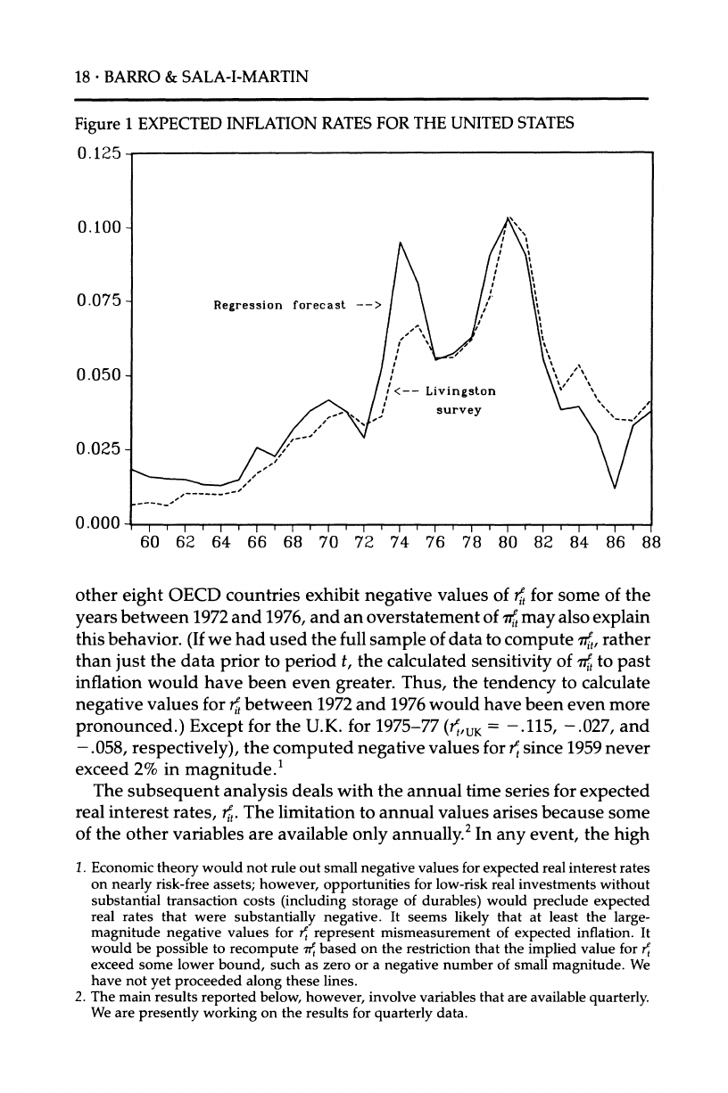
four quarterly values from the regression forecasts. Figure 1 compares

the constructed annual time series for U.S. expected inflation, 7us,t, with

values derived from the six-month-ahead forecasts from the Livingston

survey (obtained from the Federal Reserve Bank of Philadelphia). The

two series move closely together, with a correlation of .92 from 1959 to

1988. The main discrepancies are the more rapid adjustment of the

regression-based series to actual inflation in the periods 1973-75 (when

inflation rose) and 1985-86 (when inflation fell).

We calculated expected real interest rates, t, for country i in quarter t

by subtracting the constructed value for Tie

from the corresponding nomi-

nal interest rate, Rit (The three-month Treasury bill rate in January

matches up with the expected inflation rate for January to April, and so

on.) We then formed an annual series for rit

by averaging the four quar-

terly values.

The calculated values for U.S. expected real interest rates for 1974-77

are negative and average -1.2%, whereas the values based on the Living-

ston survey average 0.1% and are negative only for 1975-77. A plausible

explanation is that the regression estimates overstate the responsiveness

of expected inflation to actual inflation in the early 1970s. Many of the

18 *

BARRO

& SALA-I-MARTIN

Figure

1 EXPECTED

INFLATION

RATES

FOR

THE UNITED

STATES

60 62 64 66 68 70 72 74 76 78 80 82 84 86

other eight OECD countries exhibit negative values of i for some of the

years between 1972 and 1976, and an overstatement of die

may also explain

this behavior. (If

we had used the full sample of data to compute ~it, rather

than just the data prior to period t, the calculated sensitivity of ~it to past

inflation would have been even greater. Thus, the tendency to calculate

negative values for it between 1972 and 1976 would have been even more

pronounced.) Except for the U.K. for 1975-77 (r,UK = -.115, -.027, and

-.058, respectively), the computed negative values for r since 1959 never

exceed 2% in magnitude.1

The subsequent analysis deals with the annual time series for expected

real interest rates, t. The limitation to annual values arises because some

of the other variables are available only annually.2 In any event, the high

1. Economic theory would not rule out small negative values for expected real interest rates

on nearly risk-free assets; however, opportunities for low-risk real investments without

substantial transaction costs (including storage of durables) would preclude expected

real rates that were substantially negative. It seems likely that at least the large-

magnitude negative values for rt represent mismeasurement of expected inflation. It

would be possible to recompute dt based on the restriction that the implied value for r4

exceed some lower bound, such as zero or a negative number of small magnitude. We

have not yet proceeded along these lines.

2. The main results reported below, however, involve variables that are available quarterly.

We are presently working on the results for quarterly data.

World Real Interest Rates *

19

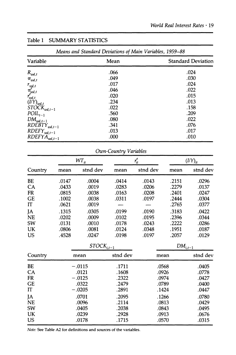
Table 1 SUMMARY STATISTICS

Means and Standard Deviations of Main Variables,

1959-88

Variable Mean Standard Deviation

Rwd,

t .066 .024

rrwd,

t .049 .030

rwd t .017 .024

erwa, .046 .022

wd,t .020 .015

(I/Y)wd,t .234 .013

STOCKwd,t_1 .022 .158

POIL_i1 .560 .209

DMWd,t-1 .080 .022

RDEBTYWd,t_ .341 .076

RDEFYwd,t1 .013 .017

RDEFYA, t_1 .000 .010

Own-Country

Variables

WTit ri (I/Y)it

Country mean stnd dev mean stnd dev mean stnd dev

BE .0147 .0004 .0414 .0143 .2151 .0296

CA .0433 .0019 .0283 .0206 .2279 .0137

FR .0815 .0038 .0163 .0208 .2401 .0247

GE .1002 .0038 .0311 .0197 .2444 .0304

IT .0621 .0019 .2765 .0377

JA .1315 .0305 .0199 .0190 .3183 .0422

NE .0202 .0009 .0102 .0195 .2396 .0344

SW .0131 .0010 .0178 .0243 .2222 .0286

UK .0806 .0081 .0124 .0348 .1951 .0187

US .4528 .0247 .0198 .0197 .2057 .0129

STOCKi,

t- DMi,,t

Country mean stnd dev mean stnd dev

BE -.0115 .1711 .0568 .0405

CA .0121 .1608 .0926 .0778

FR - .0125 .2322 .0974 .0427

GE .0322 .2479 .0789 .0400

IT -.0205 .2891 .1424 .0447

JA .0701 .2095 .1266 .0780

NE .0096 .2114 .0813 .0429

SW .0405 .2038 .0843 .0495

UK .0239 .2928 .0913 .0676

US .0178 .1715 .0570 .0315

Note: See Table

A2 for definitions and sources of the variables.

20 *

BARRO & SALA-I-MARTIN

serial correlation in the quarterly series on ri suggests that we may not

lose a lot of information by confining ourselves to the annual observa-

tions. The use of annual data means also that we do not have to deal

with possible seasonal variations in expected real interest rates.

We constructed a world index of a variable for year t by weighting the

value for country i in year t by the share of that country's real GDP for

year t in the aggregate real GDP of the nine- or ten-country sample.

(Henceforth, "world" signifies the aggregate of the nine- or ten-country

OECD sample.) In computing the weights, we used the PPP-adjusted

numbers for real GDP reported by Summers and Heston (1988). (For

1986-89, we used the shares for 1985, the final year of their data set.)

None of our results changed significantly if we weighted instead by

shares in world investment. Table 1 shows the average of each country's

Summers-Heston GDP weight (WT) from 1959 to 1988. Note that the

average share for the United States was .45, that for Japan was .13, and

so on. (In 1985, the U.S. share was .44 and the Japanese was .17.)

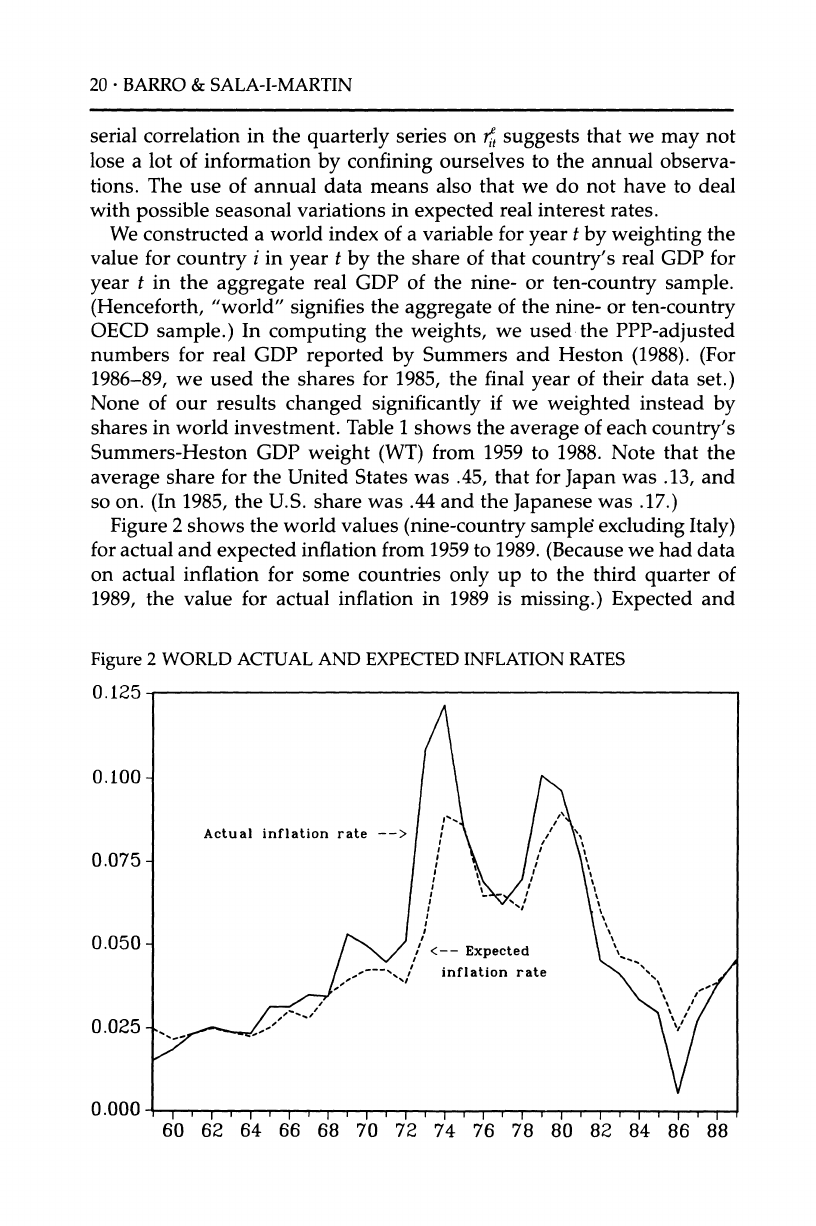
Figure 2 shows the world values (nine-country sample excluding Italy)

for actual and expected inflation from 1959 to 1989. (Because we had data

on actual inflation for some countries only up to the third quarter of

1989, the value for actual inflation in 1989 is missing.) Expected and

Figure

2 WORLD ACTUAL

AND EXPECTED INFLATION RATES

0.125

60 62 64 66 68 70 72 74 76 78 80 82 84 86 88

World Real

Interest Rates ?

21

actual inflation move together in a broad sense, but the expected values

lag behind the increases in inflation in 1969, 1972-74, and 1979-80, and

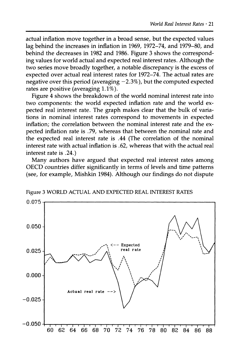
behind the decreases in 1982 and 1986. Figure 3 shows the correspond-

ing values for world actual and expected real interest rates. Although the

two series move broadly together, a notable discrepancy is the excess of

expected over actual real interest rates for 1972-74. The actual rates are

negative over this period (averaging -2.3%), but the computed expected

rates are positive (averaging 1.1%).

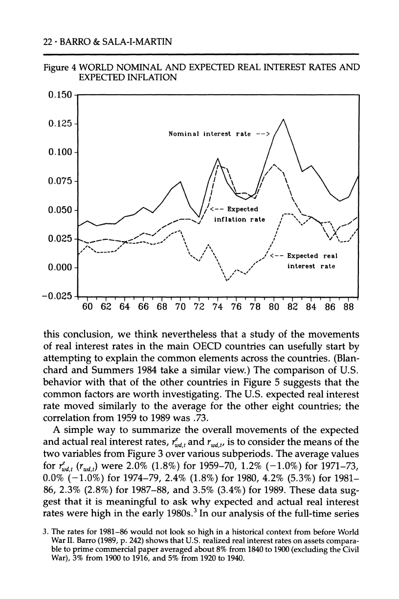
Figure 4 shows the breakdown of the world nominal interest rate into

two components: the world expected inflation rate and the world ex-

pected real interest rate. The graph makes clear that the bulk of varia-

tions in nominal interest rates correspond to movements in expected

inflation; the correlation between the nominal interest rate and the ex-

pected inflation rate is .79, whereas that between the.nominal rate and

the expected real interest rate is .44 (The correlation of the nominal

interest rate with actual inflation is .62, whereas that with the actual real

interest rate is .24.)

Many authors have argued that expected real interest rates among

OECD countries differ significantly in terms of levels and time patterns

(see, for example, Mishkin 1984). Although our findings do not dispute

Figure

3 WORLD

ACTUAL

AND EXPECTED

REAL

INTEREST RATES

70 72 74 76 78 80 82 84 86 88

22 *

BARRO

& SALA-I-MARTIN

Figure

4 WORLD NOMINAL

AND EXPECTED REAL INTEREST

RATES

AND

EXPECTED

INFLATION

0.150

0.125 -

Nominal interest rate -

0.100 -

0.075 - - xxxx

.,. / \/ .

0 /

2\ /

'<-- Expected real

0.000_- '

,, interest rate

-0.025 , , I , , i ,

60 62 64 66 68 70 72 74 76 78 80 82 84 86 88

this conclusion, we think nevertheless that a study of the movements

of real interest rates in the main OECD countries can usefully start by

attempting to explain the common elements across the countries. (Blan-

chard and Summers 1984 take a similar view.) The comparison of U.S.

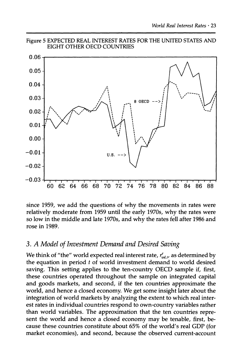
behavior with that of the other countries in Figure 5 suggests that the

common factors are worth investigating. The U.S. expected real interest

rate moved similarly to the average for the other eight countries; the

correlation from 1959 to 1989 was .73.

A simple way to summarize the overall movements of the expected

and actual real interest rates, id,t and rw,,, is to consider the means of the

two variables from Figure 3 over various subperiods. The average values

for rd,t (rwd,t)

were 2.0% (1.8%) for 1959-70, 1.2% (-1.0%) for 1971-73,

0.0% (-1.0%) for 1974-79, 2.4% (1.8%) for 1980, 4.2% (5.3%) for 1981-

86, 2.3% (2.8%) for 1987-88, and 3.5% (3.4%) for 1989. These data sug-

gest that it is meaningful to ask why expected and actual real interest

rates were high in the early 1980s.3 In our analysis of the full-time series

3. The rates for 1981-86 would not look so high in a historical context from before World

War

II. Barro (1989, p. 242) shows that U.S. realized real interest rates on assets compara-

ble to prime commercial paper averaged about 8% from 1840 to 1900 (excluding the Civil

War), 3% from 1900 to 1916, and 5% from 1920 to 1940.

World Real Interest

Rates *

23

Figure

5 EXPECTED

REAL INTEREST

RATES FOR

THE

UNITED

STATES

AND

EIGHT

OTHER

OECD COUNTRIES

0.06 -

0.05 -

0.04 - A \

0.03-

0.00- I

I

-0.01- .S.

-->' /

-0.02- -

-0.03 ,, ., , ,, , ,,,

60 62 64 66 68 70 72 74 76 78 80 82 84 86 88

since 1959, we add the questions of why the movements in rates were

relatively moderate from 1959 until the early 1970s, why the rates were

so low in the middle and late 1970s, and why the rates fell after 1986 and

rose in 1989.

3. A Model

of

Investment

Demand and

Desired

Saving

We think of "the" world expected real interest rate, r-,, as determined by

the equation in period t of world investment demand to world desired

saving. This setting applies to the ten-country OECD sample if, first,

these countries operated throughout the sample on integrated capital

and goods markets, and second, if the ten countries approximate the

world, and hence a closed economy. We get some insight later about the

integration of world markets by analyzing the extent to which real inter-

est rates in individual countries respond to own-country variables rather

than world variables. The approximation that the ten countries repre-

sent the world and hence a closed economy may be tenable, first, be-

cause these countries constitute about 65% of the world's real GDP (for

market economies), and second, because the observed current-account

24 *

BARRO & SALA-I-MARTIN

balance for the ten-country aggregate has been very small. We added up

each country's nominal current-account balance (expressed via current

exchange rates in terms of U.S. dollars) from 1960 to 1987 and divided by

the total nominal GDP (also converted by exchange rates into U.S. dol-

lars). The average value of the ratio of the aggregated current-account

balance to overall GDP was 0.1%. Moreover, the largest value from 1960

to 1987 (1971) was only 0.5% and the smallest (1984) was only -0.7%.

We now construct a simple model of investment demand and desired

saving. Although this model is used to interpret some of the empirical

findings, the general nature of the reduced-form results does not depend

on this particular framework. Hence, readers who are unimpressed by

our theory may nevertheless be interested in the empirical evidence.

We measure real investment, It, by gross domestic capital formation

(private plus public, nonresidential plus residential, fixed plus changes

in stocks). Thus, It excludes purchases of consumer durables and expen-

ditures on human capital. Investment demand, expressed as a ratio to

GDP, is determined by a q-type variable:

(IIY)t

= ao + a,1 log[PROF7/(r?+p,)]

+ u, (1)

where PROF' is expected profitability per unit of capital, r< is the ex-

pected real interest rate on assets like Treasury bills, Pt

is a risk premium,

and a1>0. The error term ut

is likely to be highly persistent because, first,

time-to-build considerations imply that current investment demand de-

pends on lagged variables that influenced past investment decisions,

and second, there may be permanent shifts in the nature of adjustment

costs, which determine the relation between investment demand and

the q variable. In first-difference form, equation (1) becomes

(I/Y)t

= a,

' Alog[PROFt/(+pt)] + (I/Y)t_1

+ Ut-Ut-1. (2)

Our analysis treats the error term, ut-ut_ , as roughly white noise.

We use the world real rate of return on the stock market through

December of the previous year STOCKt_i,

to proxy for the first difference

of the q variable, Alog[PROF/(<+pt)].4 This proxying is imperfect because

4. The stock-return

variable

for each country is the nominal rate of return

for the year

implied by the IFS December index for industrial-share prices less the December-to-

December inflation rate based on the consumer price index. We had broader stock-

return measures readily available for three countries-Canada, the United Kingdom,

and the United States-which together comprised 57% on average of the ten-country

GDP. The substitution of these numbers for the IFS values had a negligible impact on the

regression results we report later. We took this result as an indication that the IFS data

are probably satisfactory indicators of stock-market returns.

World

Real Interest Rates

*

25

of distinctions between average and marginal q,5 because of failure to

adjust for changes in the market value of bonds and depreciation of

capital stocks, and because the stock market values only a portion of the

capital that relates to our measure of investment. (The investment num-

bers include residential construction, noncorporate business invest-

ment, and public investment.) For these reasons, the best estimate of

Alog[PROFI/(re+pt)] would depend inversely on the change in rt, for a

given value of STOCKt_

.6 Therefore, we approximate the relation for

investment demand as

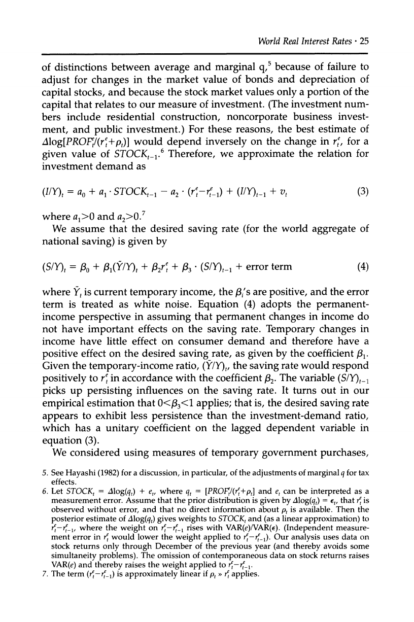
(IIY)t = ao + a1 *

STOCKt,1 - a, (r~-_1) + (I/Y)t_ + vt (3)

where a1>0 and a2>0.7

We assume that the desired saving rate (for the world aggregate of

national saving) is given by

(S/Y), = o + Pl(Y/Y)t + 32r~

+

+3 *

(S/Y)t-1 + error term (4)

where Yt

is current temporary income, the 3i's

are positive, and the error

term is treated as white noise. Equation (4) adopts the permanent-

income perspective in assuming that permanent changes in income do

not have important effects on the saving rate. Temporary changes in

income have little effect on consumer demand and therefore have a

positive effect on the desired saving rate, as given by the coefficient ,1.

Given the temporary-income ratio, (Y/Y)t,

the saving rate would respond

positively to r' in accordance with the coefficient /2. The variable (S/Y)t_

picks up persisting influences on the saving rate. It turns out in our

empirical estimation that 0<33<1 applies; that is, the desired saving rate

appears to exhibit less persistence than the investment-demand ratio,

which has a unitary coefficient on the lagged dependent variable in

equation (3).

We considered using measures of temporary government purchases,

5. See Hayashi (1982) for a discussion, in particular, of the adjustments of marginal q for tax

effects.

6. Let STOCKt = Alog(qt) + et, where qt = [PROFt(t+pt] and et can be interpreted as a

measurement error. Assume that the prior distribution is given by Alog(qt)

= et, that 4r

is

observed without error, and that no direct information about Pt is available. Then the

posterior estimate of Alog(qt)

gives weights to STOCKt

and (as a linear approximation) to

-rt_l, where the weight on -

t-_ rises with VAR(e)/AR(E). (Independent measure-

ment error in 4t

would lower the weight applied to 4-et-_). Our analysis uses data on

stock returns only through December of the previous year (and thereby avoids some

simultaneity problems). The omission of contemporaneous data on stock returns raises

VAR(e)

and thereby raises the weight applied to t-rte,.

7. The term (t-rte_ ) is approximately linear if pt >> applies.

26 *

BARRO

& SALA-I-MARTIN

especially defense expenditures, as influences on temporary income and

hence desired national saving rates. Up to this point, however, we have

been unable to isolate important temporary variations in the ratios of

real government purchases to real GDP over the period since 1959 for

the ten OECD countries we are studying.

We have had more success by thinking of the relative price of oil as an

indicator of world temporary income. Higher oil prices are bad for oil

importers, which predominate in the ten-country OECD sample. Be-

cause higher oil prices tend to reflect more effective cartelization of the

market for oil, an increase in prices also represents a global distortion

that is bad for the world as a whole. Moreover, high oil prices may be a

signal of disruption of international markets in a sense that goes beyond

oil; therefore, the effects on world income may be substantially greater

than those attributable to oil, per se.

Our subsequent analysis of real interest rates provides some indica-

tion that the level of the relative price of oil, rather than the change in

this relative price, is the variable that proxies for temporary income. This

result is reasonable if the relative price of oil is perceived to be stationary;

in this case, a high level for the current relative price signals a temporar-

ily high level. In the actual time series, the relative price of oil did

happen to return after 1985 to values close to those applying before 1973.

But our direct analysis of the time-series properties of the relative oil

price is inconclusive about stationarity.8

The empirical analysis uses the variable POILt,_, which is the relative

price of crude petroleum for December of the previous year from the

U.S. producer price index. The results do not change significantly if we

use instead a weighted average of relative petroleum prices for each

country. The precise concepts for these prices varied across the countries

and the data for some countries were unavailable for parts of the sample.

For these reasons, we used the U.S. variable in the main analysis.9

Thinking of POILt_1

as an inverse measure of the temporary income

ratio, (Y/Y)t,

the equation for the saving rate becomes

(S/Y)t = bo

- bi *

POILt - + b2 r + b3 (S/Y)t 1 + error term (5)

8. Even if the relative price of oil is nonstationary, the consequences of a change in the price

of oil for world income are likely to be partly transitory. In particular, the effects on

income would tend to diminish as methods of production adjusted to the new configura-

tion of relative prices.

9. The results are also similar if we use the dollar price for Venezuelan crude instead of the

U.S. PPI for crude petroleum. (The Saudi Arabian price is very close to the Venezuelan

price, but the IFS does not report the Saudi Arabian values after 1984.) The main

difference between the Venezuelan and U.S. series is that the Venezuelan one shows a

much larger proportionate increase in 1973.

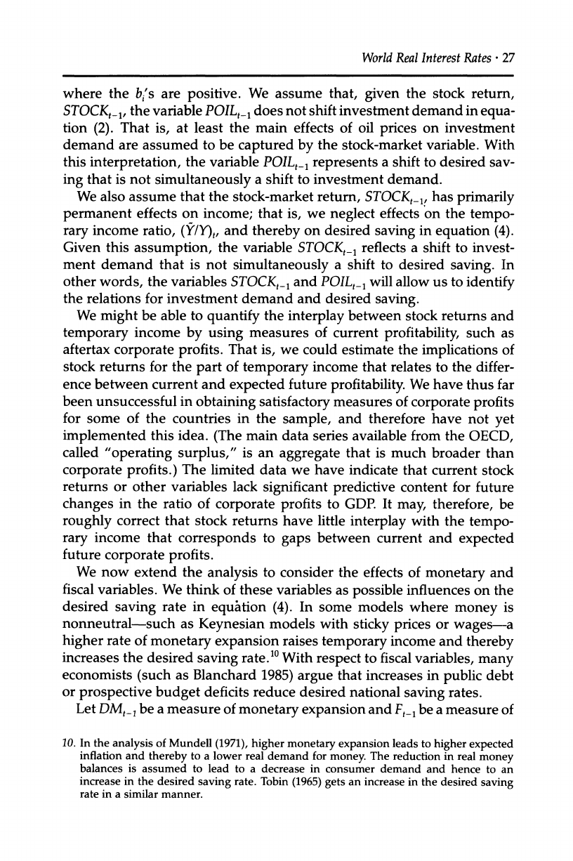
World Real Interest Rates

*

27

where the bi's are positive. We assume that, given the stock return,

STOCKt_,,

the variable POILt_,

does not shift investment demand in equa-

tion (2). That is, at least the main effects of oil prices on investment

demand are assumed to be captured by the stock-market variable. With

this interpretation, the variable POILt, represents a shift to desired sav-

ing that is not simultaneously a shift to investment demand.

We also assume that the stock-market return, STOCKt_l,

has primarily

permanent effects on income; that is, we neglect effects on the tempo-

rary income ratio, (Y/Y)t, and thereby on desired saving in equation (4).

Given this assumption, the variable STOCKt_,

reflects a shift to invest-

ment demand that is not simultaneously a shift to desired saving. In

other words, the variables STOCKt_1

and POILt_1

will allow us to identify

the relations for investment demand and desired saving.

We might be able to quantify the interplay between stock returns and

temporary income by using measures of current profitability, such as

aftertax corporate profits. That is, we could estimate the implications of

stock returns for the part of temporary income that relates to the differ-

ence between current and expected future profitability. We have thus far

been unsuccessful in obtaining satisfactory measures of corporate profits

for some of the countries in the sample, and therefore have not yet

implemented this idea. (The main data series available from the OECD,

called "operating surplus," is an aggregate that is much broader than

corporate profits.) The limited data we have indicate that current stock

returns or other variables lack significant predictive content for future

changes in the ratio of corporate profits to GDP. It may, therefore, be

roughly correct that stock returns have little interplay with the tempo-

rary income that corresponds to gaps between current and expected

future corporate profits.

We now extend the analysis to consider the effects of monetary and

fiscal variables. We think of these variables as possible influences on the

desired saving rate in equation (4). In some models where money is

nonneutral-such as Keynesian models with sticky prices or wages-a

higher rate of monetary expansion raises temporary income and thereby

increases the desired saving rate.10

With respect to fiscal variables, many

economists (such as Blanchard 1985) argue that increases in public debt

or prospective budget deficits reduce desired national saving rates.

Let DMt_1

be a measure of monetary expansion and Ft_-

be a measure of

10. In the analysis

of Mundell

(1971),

higher monetary

expansion

leads to higher

expected

inflation and thereby

to a lower real demand for money. The reduction

in real

money

balances is assumed to lead to a decrease in consumer demand and hence to an

increase

in the desired saving rate. Tobin

(1965)

gets an increase in the desired

saving

rate

in a similar manner.

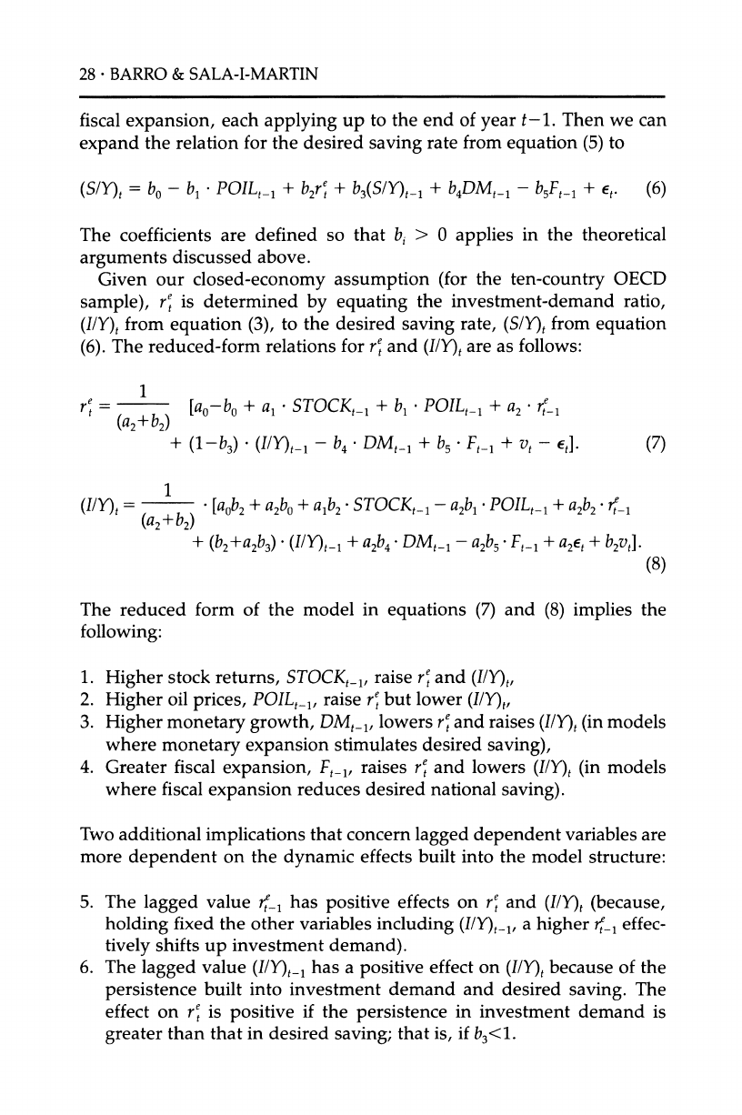
28 *

BARRO

& SALA-I-MARTIN

fiscal expansion, each applying up to the end of year t- 1. Then we can

expand the relation for the desired saving rate from equation (5) to

(S/Y), = bo - b, *

POILt,_ + b2re + b3(S/Y)t_, + b4DMt-_ - bFt,_, + et. (6)

The coefficients are defined so that bi > 0 applies in the theoretical

arguments discussed above.

Given our closed-economy assumption (for the ten-country OECD

sample), r' is determined by equating the investment-demand ratio,

(IIY)t

from equation (3), to the desired saving rate, (S/Y)t

from equation

(6). The reduced-form relations for r' and (I/Y)t

are as follows:

rt = b)[a0-b0 + a, *

STOCKt, + b, POILt_1

+ a2

' rt1

(a2+b2)

+ (1-b3) . (I/Y)t_ - b * DMt 1 + b5 Ft-, + vt - e,]. (7)

1

(IIY)t

= *

[a b2+ + ab a1b2

*

STOCKt-,

- a2b1,

POILt, + a2b2

* 1

(a2+b2)

+ (b2+a2b3)

(IIY),_ + a2b4 DM,t- - a2b5

Ft- + a2et

+ b2vt. (8)

The reduced form of the model in equations (7) and (8) implies the

following:

1. Higher stock returns, STOCKt 1, raise r\ and (I/Y)t,

2. Higher oil prices, POIL,_ , raise ri but lower (I/Y)t,

3. Higher monetary growth, DMt_ , lowers ri and raises (IIY)t

(in models

where monetary expansion stimulates desired saving),

4. Greater fiscal expansion, Ft,,, raises ri and lowers (IIY)t

(in models

where fiscal expansion reduces desired national saving).

Two additional implications that concern lagged dependent variables are

more dependent on the dynamic effects built into the model structure:

5. The lagged value ri-, has positive effects on ri and (IIY), (because,

holding fixed the other variables including (IIY)t_

, a higher ft_,

effec-

tively shifts up investment demand).

6. The lagged value (I/Y)t_1

has a positive effect on (IIY)t

because of the

persistence built into investment demand and desired saving. The

effect on re is positive if the persistence in investment demand is

greater than that in desired saving; that is, if b3<l.

World Real Interest Rates

?

29

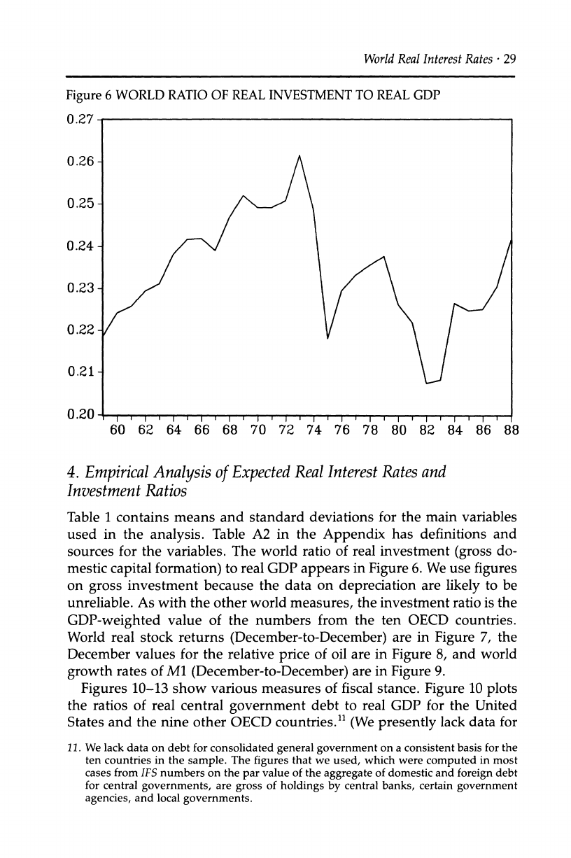
Figure

6 WORLD

RATIO OF REAL INVESTMENT

TO REAL

GDP

0.27

0.26 -

0.25-

0.24 -

0.23 -

0.22 -

0.21-

0.20 ,

, , ,

, ,

60 62 64 66 68 70 72 74 76 78 80 82 84 86 88

4. Empirical

Analysis

of Expected

Real Interest Rates

and

Investment Ratios

Table 1 contains means and standard deviations for the main variables

used in the analysis. Table A2 in the Appendix has definitions and

sources for the variables. The world ratio of real investment (gross do-

mestic capital formation) to real GDP appears in Figure 6. We use figures

on gross investment because the data on depreciation are likely to be

unreliable. As with the other world measures, the investment ratio is the

GDP-weighted value of the numbers from the ten OECD countries.

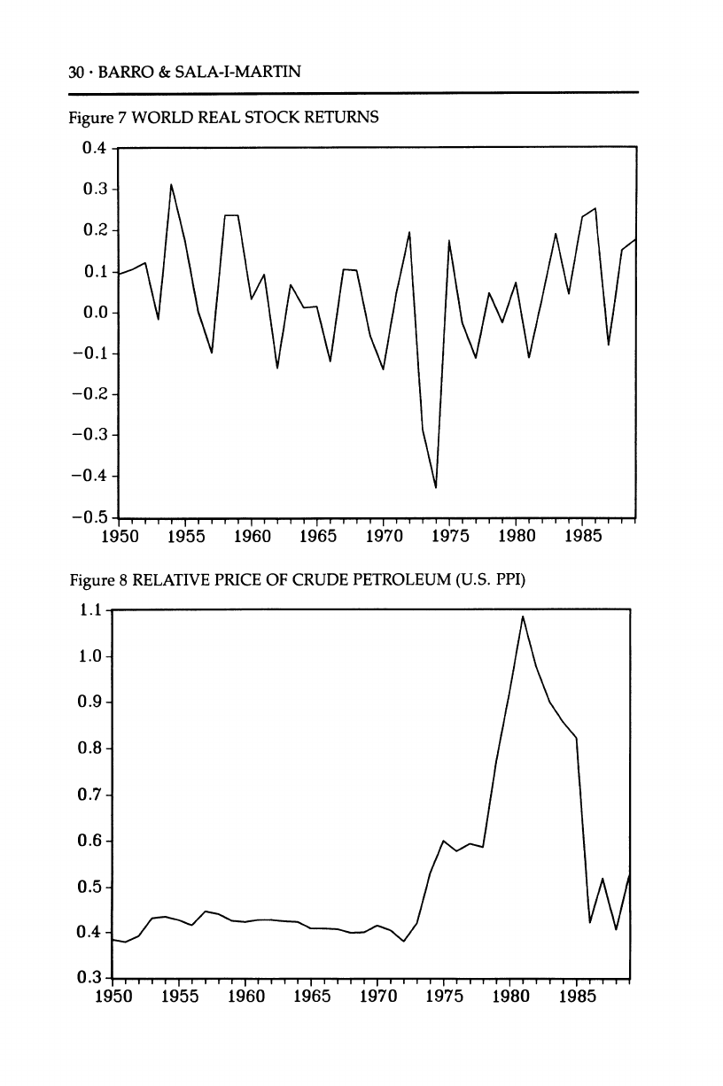
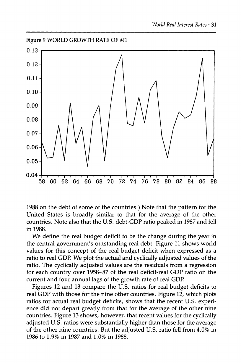
World real stock returns (December-to-December) are in Figure 7, the

December values for the relative price of oil are in Figure 8, and world

growth rates of M1 (December-to-December) are in Figure 9.

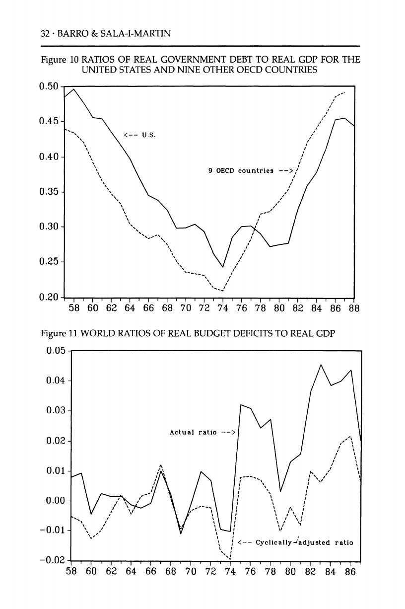
Figures 10-13 show various measures of fiscal stance. Figure 10 plots

the ratios of real central government debt to real GDP for the United

States and the nine other OECD countries.1 (We presently lack data for

11. We lack data on debt for consolidated general government on a consistent basis for the

ten countries in the sample. The figures that we used, which were computed in most

cases from IFS numbers on the par value of the aggregate of domestic and foreign debt

for central governments, are gross of holdings by central banks, certain government

agencies, and local governments.

30 ?

BARRO & SALA-I-MARTIN

Figure

7 WORLD

REAL STOCK

RETURNS

0.4

0.3 -

0.2-

0.1

0.0-

-0.1 -

-0.2-

-0.3-

-0.4 -

-0.5 ,,,, ,,,

1950 1955 1960 1965 1970 1975 1980 1985

Figure

8 RELATIVE PRICE OF CRUDE PETROLEUM

(U.S. PPI)

1.1

1.0-

0.9-

0.8-

0.7-

0.6-

0.5- /

0.4 -~~

0

.3-

. . . . . . . . . . . . . . . . . . . . . . . . . . . . . . . . . . . . . .

1950 1955 1960 1965 1970 1975 1980 1985

World Real

Interest Rates

*

31

Figure

9 WORLD GROWTH

RATE

OF

M1

1988 on the debt of some of the countries.) Note that the pattern for the

United States is broadly similar to that for the average of the other

countries. Note also that the U.S. debt-GDP ratio peaked in 1987 and fell

in 1988.

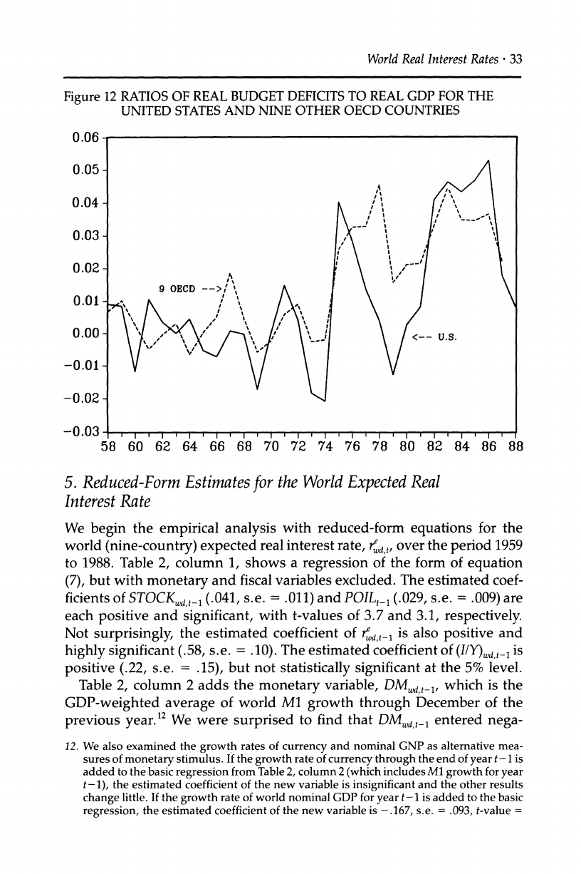
We define the real budget deficit to be the change during the year in

the central government's outstanding real debt. Figure 11 shows world

values for this concept of the real budget deficit when expressed as a

ratio to real GDP. We plot the actual and cyclically adjusted values of the

ratio. The cyclically adjusted values are the residuals from a regression

for each country over 1958-87 of the real deficit-real GDP ratio on the

current and four annual lags of the growth rate of real GDP.

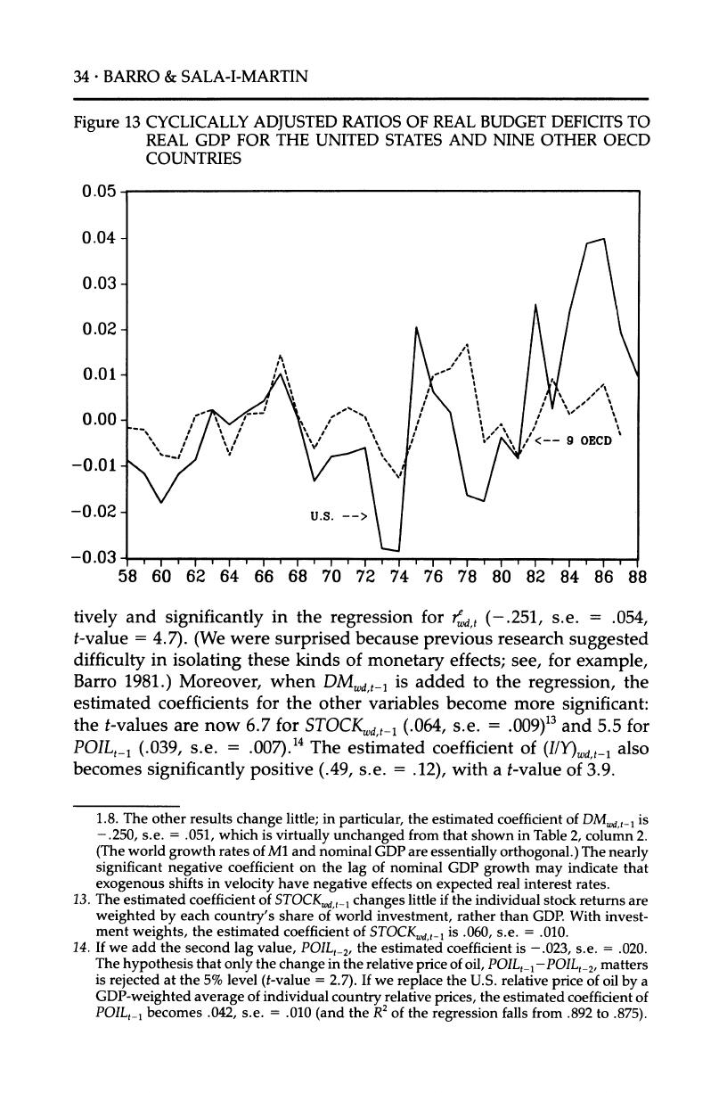
Figures 12 and 13 compare the U.S. ratios for real budget deficits to

real GDP with those for the nine other countries. Figure 12, which plots

ratios for actual real budget deficits, shows that the recent U.S. experi-

ence did not depart greatly from that for the average of the other nine

countries. Figure 13 shows, however, that recent values for the cyclically

adjusted U.S. ratios were substantially higher than those for the average

of the other nine countries. But the adjusted U.S. ratio fell from 4.0% in

1986 to 1.9% in 1987 and 1.0% in 1988.

32 *

BARRO & SALA-I-MARTIN

Figure 10 RATIOS OF REAL

GOVERNMENT

DEBT

TO REAL

GDP FOR

THE

UNITED STATES AND NINE OTHER OECD COUNTRIES

I

0.20 - I I

I, I , I

I,I

. I, ,, ,, ,

I, I I I

,

58 60 62 64 66 68 70 72 74 76 78 80 82 84 86 88

Figure

11 WORLD

RATIOS

OF REAL

BUDGET DEFICITS TO REAL GDP

0.05

World Real Interest Rates

. 33

Figure

12 RATIOS OF REAL BUDGET

DEFICITS

TO REAL

GDP

FOR

THE

UNITED

STATES

AND NINE OTHER OECD

COUNTRIES

58 60 62 64 66 68 70 72 74 76 78 80 82 84 86 88

5. Reduced-Form Estimates

for

the World

Expected

Real

Interest Rate

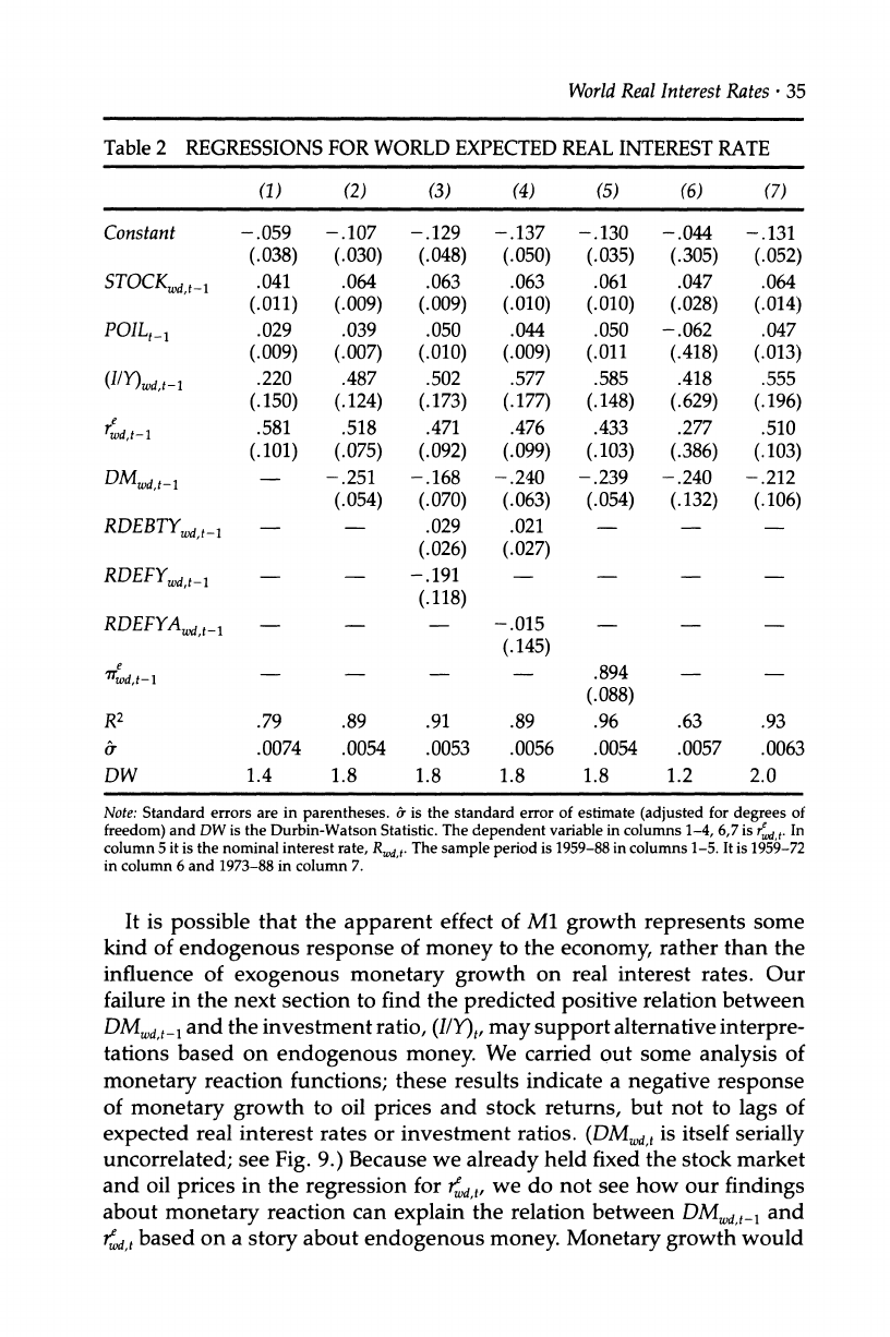
We begin the empirical analysis with reduced-form equations for the

world (nine-country) expected real interest rate, ,t, over the period 1959

to 1988. Table 2, column 1, shows a regression of the form of equation

(7), but with monetary and fiscal variables excluded. The estimated coef-

ficients of STOCKd,

t_ (.041, s.e. = .011) and POILt_1

(.029, s.e. = .009) are

each positive and significant, with t-values of 3.7 and 3.1, respectively.

Not surprisingly, the estimated coefficient of td,t-1 is also positive and

highly significant (.58, s.e. = .10). The estimated coefficient of (I/Y)d t-_1

is

positive (.22, s.e. = .15), but not statistically significant at the 5% level.

Table 2, column 2 adds the monetary variable, DMd, t-, which is the

GDP-weighted average of world M1 growth through December of the

previous year.12

We were surprised to find that DMWdt 1 entered nega-

12. We also examined the growth rates of currency and nominal GNP as alternative mea-

sures of monetary stimulus. If the growth rate of currency through the end of year t- 1 is

added to the basic regression from Table 2, column 2 (which includes M1 growth for year

t-1), the estimated coefficient of the new variable is insignificant and the other results

change little. If the growth rate of world nominal GDP for year t- 1 is added to the basic

regression, the estimated coefficient of the new variable is -.167, s.e. = .093, t-value =

34 *

BARRO & SALA-I-MARTIN

Figure

13 CYCLICALLY

ADJUSTED

RATIOS OF REAL

BUDGET DEFICITS

TO

REAL

GDP FOR THE UNITED

STATES AND NINE OTHER

OECD

COUNTRIES

0.05

0.04 -

0.03 -

0.02 -

0.01- /

= /

\/ \V ?

/< 9 OECD

-

''

-0.03-, ,, ,, ,, , , ,, , ,

I , , , , ,

58 60 62 64 66 68 70 72 74 76 78 80 82 84 86 88

tively and significantly in the regression for r,t (-.251, s.e. = .054,

t-value = 4.7). (We were surprised because previous research suggested

difficulty in isolating these kinds of monetary effects; see, for example,

Barro 1981.) Moreover, when DMWd,t1

is added to the regression, the

estimated coefficients for the other variables become more significant:

the t-values are now 6.7 for STOCKwd,

t_ (.064, s.e. = .009)13

and 5.5 for

POILt-_

(.039, s.e. = .007).14

The estimated coefficient of (IlY)wdt-1 also

becomes significantly positive (.49, s.e. = .12), with a t-value of 3.9.

1.8. The other results change little; in particular, the estimated coefficient of DMw,d

t- is

-.250, s.e. = .051, which is virtually unchanged from that shown in Table 2, column 2.

(The world growth rates of Ml and nominal GDP are essentially orthogonal.) The nearly

significant negative coefficient on the lag of nominal GDP growth may indicate that

exogenous shifts in velocity have negative effects on expected real interest rates.

13. The estimated coefficient of STOCKw,

t-l changes little if the individual stock returns are

weighted by each country's share of world investment, rather than GDP. With invest-

ment weights, the estimated coefficient of STOCK

wd,t_1

is .060, s.e. = .010.

14. If we add the second lag value, POILt_2,

the estimated coefficient is -.023, s.e. = .020.

The hypothesis that only the change in the relative price of oil, POILt_l-POILt_2, matters

is rejected at the 5% level (t-value = 2.7). If we replace the U.S. relative price of oil by a

GDP-weighted average of individual country relative prices, the estimated coefficient of

POILt_L

becomes .042, s.e. = .010 (and the R2

of the regression falls from .892 to .875).

World

Real Interest Rates - 35

Table

2 REGRESSIONS

FOR

WORLD EXPECTED REAL

INTEREST RATE

(1) (2) (3) (4) (5) (6) (7)

Constant

(.

STOCKWd,t_1 (.

POIL,t_ (.

(I/Y)wd,t-l

r (-

M

.dt-1

--RDEBT,t-i

RDEBTYw,t-

RDEFYWd,t-1

RDEFYAWd,t-_

e

'7rwd,

t-

1_

.79

.0074

1.4

R2

DW

059 -.107 -.129

038) (.030) (.048)

041 .064 .063

011) (.009) (.009)

029 .039 .050

009) (.007) (.010)

220 .487 .502

150) (.124) (.173)

581 .518 .471

101) (.075) (.092)

- -.251 -.168

(.054) (.070)

- .029

(.026)

- - .191

(.118)

.89

.0054

1.8

.91

.0053

1.8

Note:

Standard

errors are in parentheses.

a is the standard error

of estimate

(adjusted

for degrees of

freedom)

and DW is the Durbin-Watson Statistic. The

dependent

variable

in columns

1-4, 6,7 is r4,t. In

column

5 it is the nominal

interest

rate,

Rwd,t.

The

sample period

is 1959-88

in columns

1-5. It is 1959-72

in column

6 and 1973-88

in column

7.

It is possible that the apparent effect of M1 growth represents some

kind of endogenous response of money to the economy, rather than the

influence of exogenous monetary growth on real interest rates. Our

failure in the next section to find the predicted positive relation between

DMwd,t- and the investment ratio, (I/Y)t,

may support alternative interpre-

tations based on endogenous money. We carried out some analysis of

monetary reaction functions; these results indicate a negative response

of monetary growth to oil prices and stock returns, but not to lags of

expected real interest rates or investment ratios. (DMwd t is itself serially

uncorrelated; see Fig. 9.) Because we already held fixed the stock market

and oil prices in the regression for 4rd,,

we do not see how our findings

about monetary reaction can explain the relation between DMwd,t- and

wd,t based on a story about endogenous money. Monetary growth would

-.137

(.050)

.063

(.010)

.044

(.009)

.577

(.177)

.476

(.099)

-.240

(.063)

.021

(.027)

-.130

(.035)

.061

(.010)

.050

(.011

.585

(.148)

.433

(.103)

-.239

(.054)

.894

(.088)

.96

.0054

1.8

-.044

(.305)

.047

(.028)

-.062

(.418)

.418

(.629)

.277

(.386)

-.240

(.132)

.63

.0057

1.2

-.131

(.052)

.064

(.014)

.047

(.013)

.555

(.196)

.510

(.103)

-.212

(.106)

.93

.0063

2.0

(.145)

.89

.0056

1.8

-n15.

36 *

BARRO & SALA-I-MARTIN

have to be reflecting information about future real interest rates not

already contained in the other explanatory variables.

The explanatory power of DMWdt_- for wd,t reflects in part the well-

known cutback in world M1 growth in 1979 and 1980 (6.8% and 5.3%,

respectively, compared with a mean of 8.0% for 1959-88). This monetary

contraction matches up well with the increase in r,d, from 0.9% in 1979 to

2.4% in 1980 and 4.7% in 1981. (With the monetary variable excluded in

Table 2, column 1, the fitted values of ed,t for 1980 and 1981 are 2.0% and

3.4%, respectively. With the monetary variable included in column 2,

these fitted values become 2.5% and 4.4%.) The significance of DM,d, t_

in the regression for red,

, however, does not depend on the inclusion of

the observations for 1980-81. If these two years are omitted, the esti-

mated coefficient of DMwd,t-1 becomes -.233, s.e. = .066, and the other

results do not change much from those shown in column 2.

We have carried out the estimation using the realized real interest rate,

rwd,, rather than our constructed measure of the expected rate, wd

t. The

error term in the regression can then be viewed as including the discrep-

ancy between the actual and expected real rate. Under rational expecta-

tions, this expectational error would be independent of the explanatory

variables, which are all lagged values. The estimates would therefore be

consistent, but inefficient relative to a situation where rd,t is observed

directly and used as the dependent variable. Although the standard

errors of the estimated coefficients are substantially higher when rw,

replaces 4d,t as the dependent variable, the basic pattern of the results

remains the same. Thus, the findings do not depend on our particular

measure for expected inflation.

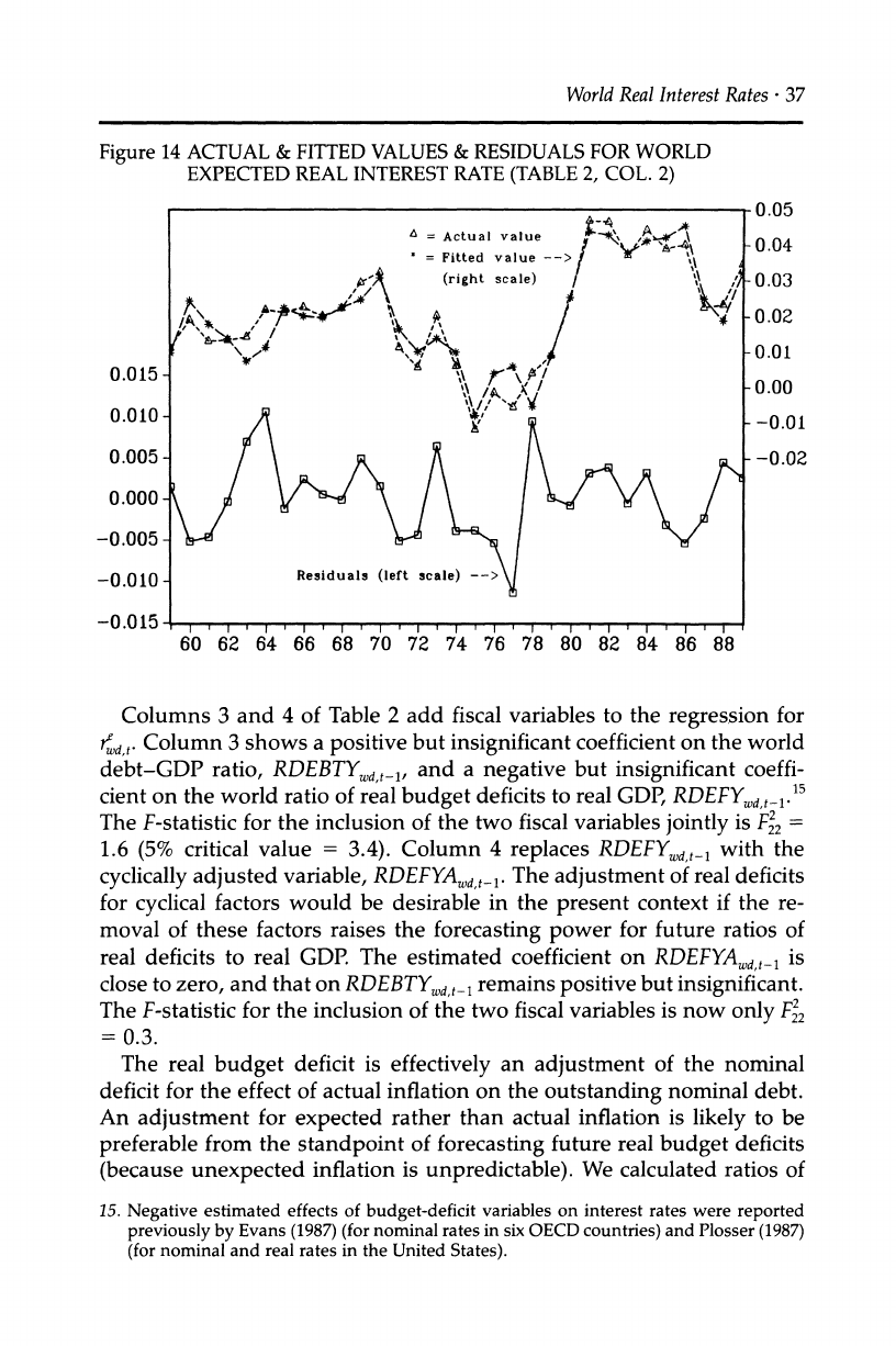
Overall, the regression equation in Table 2, column 2 does a remark-

able job of explaining the variations in expected real interest rates from

1959 to 1988; see Figure 14 for a plot of actual values against fitted values

and residuals. Note that the out-of-sample forecast of rd,t for 1989 is 3.2%

compared to an actual of 3.5%; for 1988, the estimated value was 1.9%

and the actual was 2.3%. (We promise that we generated the forecast for

1989 before finding the data on the actual value.)

We will discuss more features of the results later, but some key ele-

ments for the 1980s are the generally favorable stock-market returns

combined with high oil prices. (Blanchard and Summers 1984, argue that

improved prospects for profitability-which we pick up in the stock-

market returns-were an important element in the high real interest

rates of the 1980s.) The experience for the 1980s contrasts with the ex-

tremely poor stock returns and lower oil prices that prevailed in the mid-

1970s. The 1960s featured still lower oil prices, but better stock returns

than in the mid-1970s.

World

Real Interest

Rates *

37

Figure

14 ACTUAL & FITTED VALUES

& RESIDUALS FOR WORLD

EXPECTED REAL INTEREST

RATE

(TABLE

2, COL.

2)

0.05

= Actual value f -0.04

= Fitted value -> / '

\

(right scale) / ' 0.03

'8 /^

^/~' I A

^ o.o2

.t' - ',s. .

/** / -0.01

0.015- \

,'00 -0-00

/0.010 y,

--0

0.005 - / A /\ -0.02

0.000

-0.005 -

-0.010- Residuals (left scale) -->

-0 .015 , I, I,

I, , , , , , ,

60 62 64 66 68 70 72 74 76 78 80 82 84 86 88

Columns 3 and 4 of Table 2 add fiscal variables to the regression for

wd,t. Column 3 shows a positive but insignificant coefficient on the world

debt-GDP ratio, RDEBTYW,t-, and a negative but insignificant coeffi-

cient on the world ratio of real budget deficits to real GDP, RDEFYd, t-.15

The F-statistic for the inclusion of the two fiscal variables jointly is F2 =

1.6 (5% critical value = 3.4). Column 4 replaces RDEFYd,t 1 with the

cyclically adjusted variable, RDEFYAd, t-. The adjustment of real deficits

for cyclical factors would be desirable in the present context if the re-

moval of these factors raises the forecasting power for future ratios of

real deficits to real GDP. The estimated coefficient on RDEFYAWdt

_ is

close to zero, and that on RDEBTYWd

_1 remains positive but insignificant.

The F-statistic for the inclusion of the two fiscal variables is now only F2

=0.3.

The real budget deficit is effectively an adjustment of the nominal

deficit for the effect of actual inflation on the outstanding nominal debt.

An adjustment for expected rather than actual inflation is likely to be

preferable from the standpoint of forecasting future real budget deficits

(because unexpected inflation is unpredictable). We calculated ratios of

15. Negative estimated effects of budget-deficit

variables

on interest rates were reported

previously by Evans

(1987) (for

nominal rates

in six OECD

countries)

and Plosser

(1987)

(for

nominal and real rates

in the United

States).

38 *

BARRO

& SALA-I-MARTIN

real budget deficits to real GDP (adjusted or unadjusted for cyclical

fluctuations) in this manner, but the results differed negligibly from

those found with actual inflation.

We also held fixed the ratio of government consumption purchases to

GDP (which entered insignificantly) and experimented with the inclu-

sion of current or future real budget deficits. In all cases we obtained

similar results; the measures of fiscal stance that we have considered do

not help significantly in explaining the time series for expected real

interest rates. We are forced to conclude that the evidence supports the

Ricardian view, which deemphasizes the roles of public debt and budget

deficits in the determination of real interest rates.

Column 5 in Table 2 uses the world nominal interest rate, R, t, as the

dependent variable and adds the constructed measure of world expected

inflation, Td,

, on the right side. Measurement error

in 7ed,t would bias the

estimated coefficient toward zero, but the estimated value (.89, s.e. =

.09) differs insignificantly from one. Of course, to the extent that coun-

tries levy taxes on nominal interest payments, the predicted coefficient

would be somewhat above unity.

We tested for the stability of the relation between 4d,t and the explana-

tory variables by estimating the specification from Table 2, column 2

separately for 1959-72 and 1973-88. Thus, we split the sample before the

oil crises and the main changes in the international monetary system.

The estimates for the two subperiods appear in columns 6 and 7 of the

table. The test for stability leads to the statistic F18 = 0.2; thus, we do not

reject the hypothesis that the same equation applies over both periods.

To some extent, the failure to reject reflects the high standard errors that

apply to the estimated coefficients for 1959-72 (column 6). For example,

the standard error for the estimated coefficient of POILt_ is enormous

because of the small variations in relative oil prices from 1958 to 1971 (see

Fig. 8).16

The data for 1959-72, however, do generate marginally signifi-

cant estimated coefficients on STOCKd,

t_ (.047, s.e. = .028) and DMWdt,,-

(-.240, s.e. = .132).

6. Reduced-Form Estimates

for

World Investment Ratio

We now consider the reduced form for the investment ratio in equation

(8). Table 3 shows regressions over 1959-88 for the world ratio of real

16. The estimated coefficient of POILt_, differs insignificantly from zero for samples that

begin in 1959 and end as recently as 1979; for the 1959-79 sample, the estimated

coefficient is -.003, s.e. = .034. If the sample ends in 1980, the estimated coefficient

becomes .029, s.e. = .018. For samples that end between 1981 and 1988, the estimated

coefficient is very stable, varying between .038 and .040 with a standard error between

.007 and .010.

World Real Interest Rates *

39

Table

3. REGRESSIONS FOR WORLD

INVESTMENT

RATIO

(1) (2) (3) (4) (5) (6)

Constant .053 .057 .066 .076 -.016 .133

(.031) (.033) (.051) (.051) (.125) (.059)

STOCKwd,t-1 .036 .034 .034 .031 .018 .045

(.009) (.011) (.010) (.010) (.011) (.016)

POILt_1 -.016 -.017 -.030 -.020 .077 -.033

(.008) (.008) (.010) (.009) (.172) (.015)

(I/Y)wd,t- .814 .791 .848 .770 .92 .57

(.122) (.139) (.183) (.181) (.26) (.23)

wd,t- -.005 .000 .037 -.011 .043 -.057

(.082) (.085) (.097) (.101) (.158) (.118)

DMwd,t- .022 -.104 -.049 .064 -.127

(.060) (.075) (.064) (.054) (.122)

RDEBTYw,t-1 - -.029 -.021

(.027) (.027)

RDEFYwd,tl .306

(.125)

RDEFYAWd,t_1 .331

(.148)

R2 .82 .82 .86 .86 .97 .82

& .0060 .0061 .0056 .0057 .0023 .0073

DW 1.6 1.7 1.9 1.8 1.5 1.7

Note:

The

dependent

variable is (I/Y)wd,.

The sample period

in columns

1-4 is 1959-88. It is 1959-72 in

column 5 and 1973-88

in column 6.

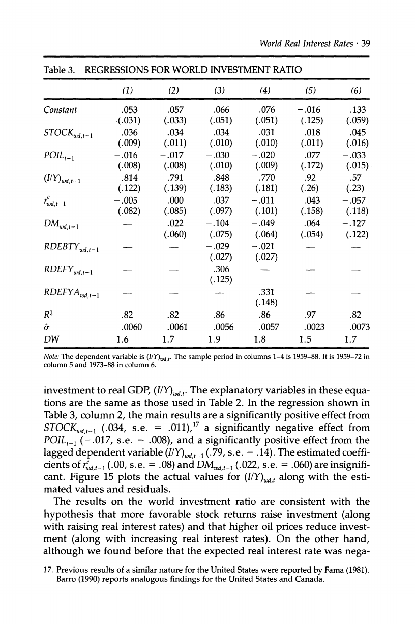
investment to real GDP, (I/Y)d,t. The explanatory variables in these equa-

tions are the same as those used in Table 2. In the regression shown in

Table 3, column 2, the main results are a significantly positive effect from

STOCKWdt,_

(.034, s.e. = .011),17 a significantly negative effect from

POILt_1

(-.017, s.e. = .008), and a significantly positive effect from the

lagged dependent variable (I/Y)wd,

t- (.79, s.e. = .14). The estimated coeffi-

cients of rd,t-1 (.00, s.e. = .08) and DMWd,t- (.022, s.e. = .060) are insignifi-

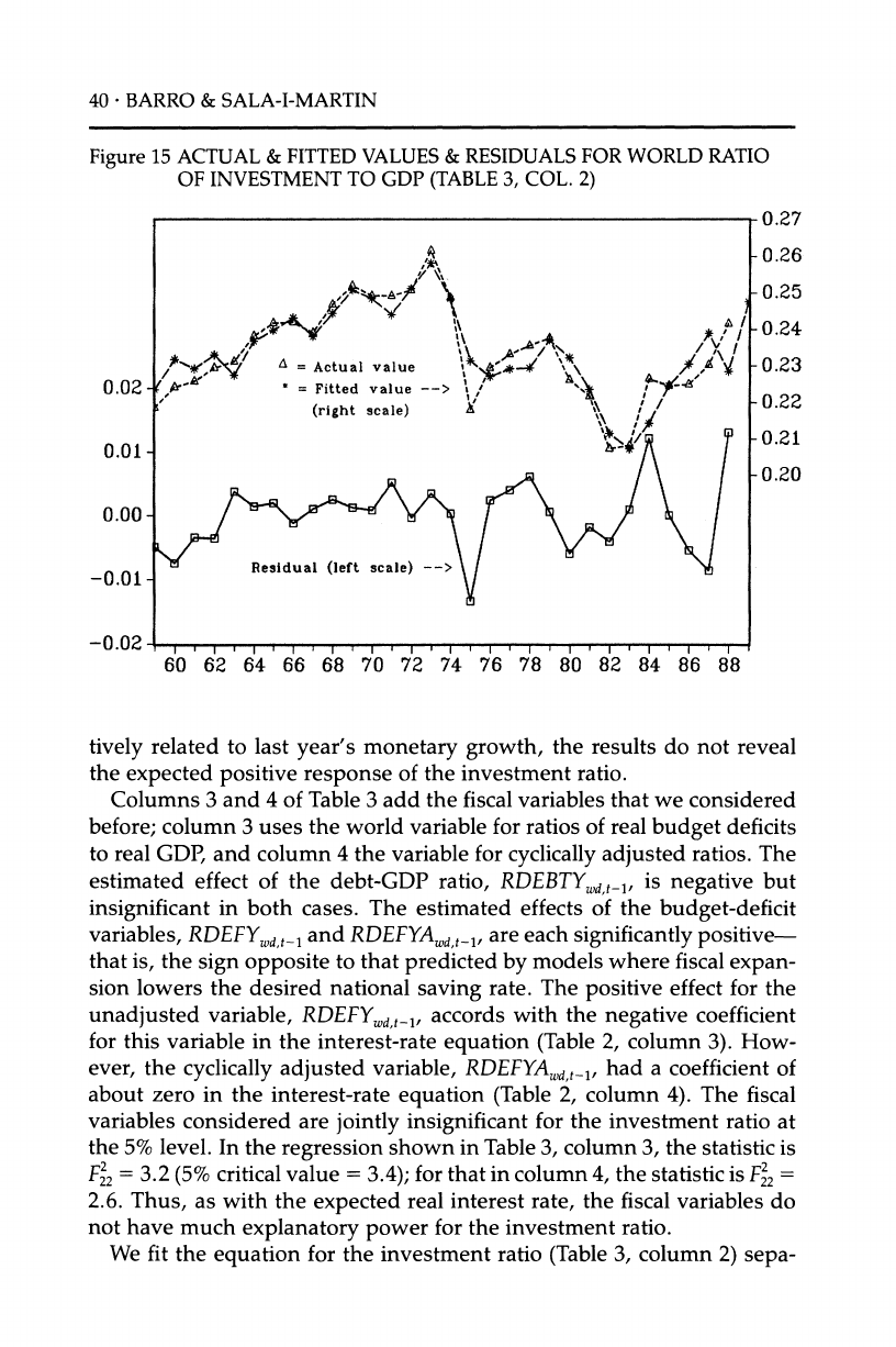
cant. Figure 15 plots the actual values for (I/Y)Wdt

along with the esti-

mated values and residuals.

The results on the world investment ratio are consistent with the

hypothesis that more favorable stock returns raise investment (along

with raising real interest rates) and that higher oil prices reduce invest-

ment (along with increasing real interest rates). On the other hand,

although we found before that the expected real interest rate was nega-

17. Previous results of a similar nature for the United States were reported by Fama (1981).

Barro (1990) reports analogous findings for the United States and Canada.

40 *

BARRO

& SALA-I-MARTIN

Figure

15 ACTUAL & FITTED

VALUES & RESIDUALS

FOR WORLD RATIO

OF INVESTMENT TO GDP (TABLE

3, COL.

2)

0.27

A$~ -~ ~

~-0.26

X\ - / t-0.25

- Actual value -0.23

0.02 X,* * =- Fitted value --> -.' \23 - 0.2

esidual

(lefright

scale) -->0.22

0.01- -0.20

-0.02 ,

60 62 64 66 68 7

772 74 76 78 80 82 84 86 88

tively related to last year's monetary growth, the results do not reveal

the expected positive response of the investment ratio.

Columns 3 and 4 of Table 3 add the fiscal variables that we considered

before; column 3 uses the world variable for ratios of real budget deficits

to real GDP, and column 4 the variable for cyclically adjusted ratios. The

estimated effect of the debt-GDP ratio, RDEBTYwd,t , is negative but

insignificant in both cases. The estimated effects of the budget-deficit

variables, RDEFYd,t-1 and RDEFYAwd,t_, are each significantly positive-

that is, the sign opposite to that predicted by models where fiscal expan-

sion lowers the desired national saving rate. The positive effect for the

unadjusted variable, RDEFYd,,_,, accords with the negative coefficient

for this variable in the interest-rate equation (Table 2, column 3). How-

ever, the cyclically adjusted variable, RDEFYAwd,

-, had a coefficient of

about zero in the interest-rate equation (Table 2, column 4). The fiscal

variables considered are jointly insignificant for the investment ratio at

the 5% level. In the regression shown in Table 3, column 3, the statistic is

F2 = 3.2 (5%

critical value = 3.4); for that in column 4, the statistic is F2 =

2.6. Thus, as with the expected real interest rate, the fiscal variables do

not have much explanatory power for the investment ratio.

We fit the equation for the investment ratio (Table 3, column 2) sepa-

World Real Interest

Rates ?

41

rately over 1959-72 and 1973-88. A test of stability for the coefficients

yields the statistic F% = 1.7 (5% critical value = 2.7). Columns 5 and 6

show the estimates obtained over the two subperiods. The standard

errors for the estimated coefficients from the 1959-72 sample tend to be

high; however, the estimated coefficient of STOCKd, t-_ is positive (.018,

s.e. = .011).

7. System

Estimates

for World

Expected

Real Interest Rate

and

Investment

Ratio

The structural model in equations (3) and (6) led to the reduced-form

equations (7) and (8) for the expected real interest rate and investment

ratio. In the previous sections, we estimated the two reduced-form equa-

tions separately, ignoring the overidentifying restrictions that came from

the structure. In this section, we estimate the two equations as a joint

system, allowing for the imposition of the model's restrictions as well as

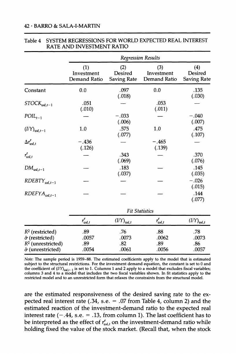
for correlation of the error terms across the equations. Table 4 shows the

resulting estimates for the structural coefficients that appear in equation

(3) for investment demand and in equation (6) for desired saving. Col-

umns 1 and 2 apply to a system that includes monetary growth but

excludes fiscal variables. Columns 3 and 4 add two fiscal variables: the

debt-GDP ratio, RDEBTYd, t_, and the cyclically adjusted real deficit-real

GDP ratio, RDEFYAwd,t-.

We also fit the joint systems for the expected real interest rate and the

investment ratio without the restrictions imposed by the structural

model. Thereby we were able to compute likelihood-ratio tests of the

overidentifying restrictions. For the model without fiscal variables, the

test statistic (for -2 ? log[likelihood ratio]) of 9.9 compared to a 5%

critical value from the X2

distribution with 5 degrees of freedom of 11.1.

In the model with fiscal variables, the test statistic of 13.7 compared to

the 5% critical value (with 7 d.f.) of 14.1. Thus, the model's restrictions

were not rejected at the 5% level in either case. Table 4 also compares the

fits (in terms of R2

and -a

values) for restricted and unrestricted forms of

each equation separately. The fits for the investment equation appear

substantially more sensitive than those for the interest-rate equation to

the imposition of the model's overidentifying restrictions.

The two fiscal variables are jointly insignificant when added to the

restricted joint system (likelihood-ratio statistic of 5.3 compared to a 5%

critical value of 6.0). Since the other results are not sensitive to the

exclusion of the fiscal variables, we focus now on the estimates from the

model that excludes the fiscal variables (columns 1 and 2 of Table 4).

If one takes the structural model seriously, then two interesting results

42 *

BARRO & SALA-I-MARTIN

Table 4 SYSTEM REGRESSIONS FOR WORLD EXPECTED REAL INTEREST

RATE AND INVESTMENT RATIO

Regression

Results

(1) (2) (3) (4)

Investment Desired Investment Desired

Demand Ratio Saving Rate Demand Ratio Saving Rate

Constant 0.0 .097 0.0 .135

(.018) (.030)

STOCK,d

t_1 .051 .053

(.010) (.011)

POILt1 - -.033 -.040

(.006) (.007)

(I/Y)w,t-1 1.0 .575 1.0 .475

(.077) (.107)

Arwd,t -.436 -.465

(.126) (.139)

rwd,t - 343 -.370

(.069) (.076)

DMWd,t-1 .183 .145

(.037) (.035)

RDEBTYWd,t_1 -.026

(.015)

RDEFYAwd,t_1 .144

(.077)

Fit Statistics

rew,t

(I/Y)wd,t rwd,t (I/Y)wd,

R2

(restricted) .89 .76 .88 .78

a (restricted) .0057 .0073 .0062 .0073

R2

(unrestricted) .89 .82 .89 .86

r (unrestricted) .0054 .0061 .0056 .0057

Note: The sample period is 1959-88. The estimated coefficients

apply to the model that is estimated

subject

to the structural restrictions.

For the investment demand

equation,

the constant is set to 0 and

the coefficient

of (I/Y)wd,-_1

is set to 1. Columns

1 and 2 apply

to a model that

excludes fiscal

variables;

columns 3 and 4 to a model that includes the two fiscal variables shown. In fit statistics

apply to the

restricted model and to an unrestricted form

that

relaxes

the constraints from

the structural model.

are the estimated responsiveness of the desired saving rate to the ex-

pected real interest rate (.34, s.e. = .07 from Table 4, column 2) and the

estimated reaction of the investment-demand ratio to the expected real

interest rate (-.44, s.e. = .13, from column 1). The last coefficient has to

be interpreted as the effect of 4d,t on the investment-demand ratio while

holding fixed the value of the stock market. (Recall that, when the stock

World Real Interest Rates

*

43

return is an imperfect measure of Aq,,

the variable <-rt-1 provides some

independent information about Aqt.)

The dependence of the stock return

on d,t- wd,t- suggests that the estimated coefficient -.44 would underes-

timate the magnitude of the response of the investment-demand ratio to

id,t while holding fixed expected profitability, PROFg,

and the risk pre-

mium, Pt, but not the value of the stock market.18

The estimated model implies that desired national (gross) saving rates

rise by .34 percentage points for each percentage-point increase in ?r.

Although this form provides a natural unit for thinking of the responsive-

ness of saving rates to real interest rates, it appears to be more common

to think in terms of elasticities. Because the sample mean of (I/Y)wd,t

is .23,

whereas that for wd,t

is only .020, the implied elasticities are small-only

.03 at the sample means. The calculated elasticities would, however,

tend to be substantially greater for net saving rates.

Column 1 of Table 4 shows that the estimated effect of STOCKWd,

_ on

the investment-demand ratio is .051, s.e. = .010. Since the sample stan-

dard deviation of STOCKWd,

t is .16, the result means that a 1 s.d. move in

the stock market changes the investment-demand ratio by .008 com-

pared to a sample s.d. for (I/Y)wdt

of .013. The estimated effect of POILt,_

on the desired saving rate in col. 2 is -.033, s.e. = .006. Given the

sample s.d. for POIL_ 1 of .21, a 1 s.d. move in the relative oil price

implies a shift in the desired saving rate by .007.

Columns 1 and 2 show that the estimated effects of the lagged depen-

dent variable, (I/Y)wd,t_, are 1 for the investment-demand ratio (as con-

strained by the model) and .58, s.e. = .08, for the desired saving rate.

The greater persistence of investment demand than of desired saving

generates the positive relation in the reduced form between 4,dt and

(I/Y)wd,t-. If the coefficient on (I/Y)d, t_ in the investment-demand equa-

tion is freed up, the estimated value is .93, s.e. = .11. In this case, the

estimated coefficient of (IIY)d, t in the saving-rate equation becomes .55,

s.e. = .09. Thus, this unrestricted version of the model does indicate

significantly greater persistence in investment demand than in desired

saving.

Column 2 shows the positive estimated effect for DMWd,t- on the de-

sired saving rate (.183, s.e. = .037). The previous discussion of the

reduced form indicated that this estimate stems from the negative rela-

tion between d,t

and DMd, tl, and not from any relation between (I/Y)wdt

and DMw, _.

Column 4 of Table 4 shows that the estimated effect of the debt-GDP

18. Serial correlation of the error term in the equation for r4,, would, however, likely lead

to an overestimate of the sensitivity of investment demand to a change in the expected

real interest rate; see the coefficient a2

in equations (3) and (7).

44 *

BARRO & SALA-I-MARTIN

ratio on the desired saving rate is negative but insignificant (-.026, s.e.

= .015). The cyclically adjusted deficit variable has a positive and margin-

ally significant estimated effect on desired saving (.144, s.e. = .077). This

"wrong" sign accords with the results discussed before in Table 3.

8. Simulations

for Expected

Real

Interest

Rates and

Investment Ratios

8.1 WHY WERE

EXPECTED

REAL INTEREST

RATES

SO HIGH IN

1981-86?

We can use the estimated model for the expected real interest rate and

the investment ratio to assess the frequently asked question: Why have

real interest rates been so high in the 1980s? We approach this question

Table 5 SIMULATED

EFFECTS ON EXPECTED

REAL

INTEREST RATES

AND INVESTMENT RATIOS

(RESULTS

REFER

TO

MEANS

FOR

THE PERIODS INDICATED)

Simulated Initial

Actual Total STOCK POIL DM Conditions

I. Study period:

1981-86; reference period:

1975-80

Restricted model

Arwd,t .039 .038 .025 .019 .003 -.009

A(I/Y)d,t -.011 -.009 .014 -.009 -.002 -.012

Unrestricted Model

Arwd,t .039 .031 .021 .014 .005 -.009

A(IY)wdt -.011 -.015 .012 -.015 -.001 -.011

II. Study period:

1975-80; reference

period:

1965-70

Restricted model

Ard, t -.022 -.013 -.018 .011 -.007 .001

A(I/Y)wd,t -.015 -.010 -.011 -.005 .003 .003

Unrestricted model

Ared

t -.022 -.011 -.015 .009 -.008 .003

A(I/Y)wd,t -.015 -.010 -.008 -.008 .001 .005

III. Study period:

1987-88; reference period:

1985-86

Restricted model

Arwd,t -.017 -.021 .002 -.019 -.001 -.003

A(I/Y)wdt .011 .009 .002 .008 .001 -.002

Unrestricted model

Are d,t -.017 -.020 .002 -.017 -.002 -.003

A(I/Y)d,t .011 .010 .001 .009 .000 -.001

World

Real

Interest Rates *

45

Table

5 SIMULATED EFFECTS ON EXPECTED

REAL

INTEREST

RATES

AND INVESTMENT RATIOS

(RESULTS

REFER TO MEANS

FOR

THE PERIODS

INDICATED)

(CONTINUED)

Simulated Initial

Actual Total STOCK POIL DM Conditions

IV. Study period:

1989; reference

period:

1988

Restricted model

Ard,t .011 .014 .015 -.005 -.003 .007

A(IlY)wd,t .017 .005 .002 .001 .009

Unrestricted model

Arwd,t .011 .013 .015 -.004 -.003 .006

A(I/Y)W - .019 .008 .002 .000 .009

Means of Variables Initial Conditions

Period rwd,t (IlY)d,t STOCKWd,t-l POILt-1 DMwd,t- rwd,t- (Y)wd,t-1

1989 .0347 (.247) .1484 .406 .0661 .0233 .242

1988 .0233 .242 -.0817 .519 .0541 .0225 .230

1987-88 .0229 .236 .0847 .470 .0895 .0401 .225

1985-86 .0395 .225 .1370 .839 .0906 .0443 .226

1981-86 .0424 .219 .0769 .927 .0791 .0245 .226

1975-80 .0031 .230 -.0624 .601 .0880 .0061 .249

1965-70 .0247 .245 .0092 .407 .0677 .0219 .238

Note: The column labeled "Simulated Total" refers to the change in the average simulated value of rd, t

or (IIY)Wd,t

from the reference period to the study period. These dynamic simulations use the actual

values of STOCKwd

t 1, POILt_1,

and DMWd,t_l,

and the actual initial values of re, t-_ and (I/Y)wd

t- at the

beginnings of the reference and study periods. The column labeled "STOCK" shows the part of the

change in the simulated values attributable to differences in the time series of STOCKWd,

t_ for the study

and reference periods. The other columns give the corresponding information for differences in the

time series of POIL_1, DMWd,t-_1 and the values for rwdt-l and (I/Y)wd,t-l at the start of the study and

reference periods. The value (I/Y)d,t for 1989 is based on incomplete data.

by comparing the period 1981-86, during which the average value of rd,t

was 4.2%, with an earlier reference period of equal length, 1975-80,

during which the average of wd,t

was 0.3%. Hence, we seek to explain the

increase in the average expected real interest rate from 1975-80 to 1981-

86 by 3.9 percentage points.

According to the model, the differences in averages of expected real

interest rates should be explicable mainly in terms of differences in

stock-market returns, oil prices, and monetary growth. Some role would

also be played by differences in initial conditions for rd,t- and (I/Y)wd,t-l

(in

1981 compared to 1975). Note from Table 5 that the averages for

STOCKWdt

- were 7.7% in 1981-86 versus -6.2% in 1975-80, those for

POILt_ were 0.93 in 1981-86 versus 0.61 in 1975-80, and those for

46 *

BARRO

& SALA-I-MARTIN

DMd,t-l were 7.91% in 1981-86 versus 8.80% in 1975-80. The difference

in initial conditions were .0245 for 4d,t-1 in 1981 versus .0061 in 1975, and

.226 for (I/Y)wd,t- in 1981 versus .249 in 1975.

We can simulate the estimated model to estimate the extent to which

the higher average for r1dt in 1981-86 than in 1975-80 can be attributed to

differences in STOCKwd, t_, POIL,_

, DMWdt-,,

and the initial conditions for

4d,t-l and (I/Y)wd,t_. We consider the restricted version of the joint model

as reported in Table 4 and also the unrestricted version that does not

impose the overidentifying restrictions from the structure. We also ne-

glect any interplay among STOCK,, t, POILt,

and DMd, ; that is, we treat

the time paths of these three variables as exogenous.19

Given the actual time paths for STOCKwd,B

POILt,

and DMWd,t,

and the

actual values for w

,t- and (IY)wd,t- in 1981 and 1975, dynamic simulations

of the restricted model for 1981-86 and 1975-80 predict an increase in

the average of wd,t

of 3.8 percentage points compared to the actual in-

crease of 3.9 points (see the columns labeled "Simulated Total" and

"Actual" in section I of Table 5). We then dynamically simulated the

restricted model for 1981-86 with the values of STOCKWd,

t- from 1975-80

substituted year by year for those in 1981-86. This simulation implied

that 2.5 percentage points of the increase in the average of rwdt from 1975-

80 to 1981-86 derived from the higher average for stock returns in the

latter period (see the column labeled "STOCK"

in the table).20

Similarly,

we found that 1.9 percentage points of the rise in the average of rwd,

resulted from the increase in average oil prices (the column "POIL"),

0.3

points from the lower average monetary growth (the column "DM"),

and -0.9 points from the differences in initial conditions. The main

change in the initial conditions is the much lower value for (IIY)w

,_1 in

1981 than in 1975; this effect by itself would have lowered real interest

rates for 1981-86. The results from simulations of the unrestricted

model, shown in Table 5, are basically similar.

Table 5 also indicates the simulated results for investment ratios. The

restricted model predicts that the average of (IIY)w,t

for 1981-86 would be

19. We do find a significant negative relation between stock returns for year t and the

change in oil prices during year t. Also, M1 growth has significant negative reactions to

the contemporaneous change in oil prices and to lagged stock returns. We can filter the

stock returns to compute the component exogenous to oil-price changes, and we can

filter M1 growth to calculate the part exogenous to oil-price changes and lagged stock

returns. In the discussion below we attribute changes in expected real interest rates

and investment ratios to the behavior of stock returns, oil prices, and monetary

growth. The breakdown among these three variables would change if we shifted from

gross numbers to the filtered values.

20. The results depend not only on differences in the average value of STOCK., _,, but on

differences in the time pattern. It is possible for the simulated effects to go in the

direction opposite to that suggested just from a comparison of means.

World Real Interest Rates *

47

0.9 percentage points below the average for 1975-80, compared to the

actual shortfall of 1.1 points. The simulations attribute 0.9 percentage

points of the decline in the average investment ratio to higher oil prices,

-1.4 points to the more favorable stock returns (which, by themselves,

would have raised the investment ratio), 0.2 points to lower monetary

growth, and 1.2 points to differences in initial conditions. The main

element in the initial conditions is again the lower value for (I/Y)d,,t- in

1981 than in 1975. The results from the unrestricted model are again

similar.

8.2 WHY

WERE EXPECTED REAL

INTEREST RATES SO LOW

IN

1975-80?

We now compare the low average for rWd,t

in 1975-80, 0.3%, with the

higher value, 2.5%, that prevailed during an earlier reference period of

the same length, 1965-70. (The results are similar if we pick alternative

six-year reference periods in the 1960s or early 1970s.) Section II of Table

5 shows that simulations of the restricted model predict a decline of only

1.3 percentage points in the average of 7d, from 1965-70 to 1975-80

compared with the actual decrease of 2.2 points. The model attributes

1.8 percentage points of the decline to lower stock returns, -1.1 points

to higher oil prices (which, by themselves, would have raised expected

real interest rates), 0.7 points to higher monetary growth, and -0.1

points to differences in initial conditions. The results from the unre-

stricted model are similar.

Overall, the largest factor behind the differences in expected real inter-

est rates among the three periods, 1965-70, 1975-80, and 1981-86, is the

variation in stock returns. The fall in real interest rates from 1965-70 to

1975-80 goes along with a worsening of stock returns (from 0.9% to

-6.2%), and the steep rise in rates in 1981-86 reflects sharply higher

stock returns (7.7%). The movements in oil prices are also important,

although higher oil prices in 1975-80 compared to 1965-70 partially

counteract the movement to lower real interest rates. The increase in oil

prices in 1981-86 compared to 1975-80 reinforces the stock market in

generating a shift toward higher real interest rates.

8.3 WHY DID EXPECTED REAL INTEREST RATES FALL IN 1987-88

AND RISE IN 1989?

The average of 4dt fell by 1.7 percentage points from 1985-86 to 1987-88

and then rose by 1.1 percentage points from 1988 to 1989. Sections III

and IV of Table 5 contain simulations for these periods. The dominant

factor behind the decline in real interest rates in 1987-88 is the fall in oil

prices. The main element underlying the rise in real rates in 1989 is the

48 *

BARRO

& SALA-I-MARTIN

much more favorable stock return in 1988 (15.0%) compared to 1987

(-8.2%).

We have assembled nearly complete data for 1989 on the variables

STOCKw,

t, POILt,

DMwd,t,

(IIY)wd,,t

and wd,t-

Using these values, we can use

the model to forecast the expected real interest rate and investment ratio

for 1990. Remarkably, the restricted model implies a predicted value for

4d,t of 5.6% (5.5% from the unrestricted model). The forecast from the

restricted model for 1990 not only constitutes an increase by 2.1 percent-

age points in red from the value prevailing in 1989, it also represents a

level that is almost a full percentage point above the highest value of the

entire previous sample, 1958-89. The five determinants of rd, in the

model all point in the direction of higher real interest rates in 1990: the

favorable stock return (17.4% in 1989 versus 14.8% in 1988) accounts for

0.1 percentage point, the increase in oil prices (.525 versus .406) for 0.5

percentage point, reduced monetary growth (3.2% versus 6.6%) for 0.8

percentage point, and the change in initial conditions (the rise in (IY)wd,t

from .242 in 1988 to .247 in 1989 and the increase in 4wt from .023 in 1988

to .035 in 1989) accounts for 0.9 percentage point. Needless to say, this

prediction of a rise in the expected real interest rate to a range not seen at

least in the last 30 years will provide a severe test of the model. With

respect to the investment ratio, the restricted model predicts little

change from 1989 (.246 in 1990 versus .247 in 1989), whereas the unre-

stricted model projects an increase by 0.3 percentage point.

Given the stress on fluctuations in the stock market, we would like to

know what fundamental factors underlie these fluctuations. (We would,

of course, also like to understand the forces that lead to changes in oil

prices and monetary growth.) We interpret stock returns as reflecting

changes in the expected profitability of investment, PROFt,

and in the risk

premium, Pt. We plan to use data on actual profitability to separate the

influences from these two channels. At this point, we can only note that

the fluctuations in stock prices could derive from technological innova-

tions, changing conditions of labor markets or international competition,

shifts in government policies with regard to taxation and regulation, and

so on. Although we have not isolated the main forces that influence stock

returns, the findings suggest that these forces are crucial for the determi-

nation of expected real interest rates and investment ratios.

9. Systems

for Individual

Countries'

Expected

Real

Interest

Rates

In the world model with an integrated capital market, "the" expected

real interest rate depends on world variables, which include world aggre-

World Real Interest Rates

. 49

gates of stock returns and monetary growth and the world price of oil.

Thus, the reduced form in equation (7) gives an expression for ft in terms

of these world variables. In practice, we observe individual time series,

4, for each country i. In the previous analysis we combined these obser-

vations into a world index, '4d,

t that gives more weight to countries with

higher shares in world real GDP. Then we related this world index to the

world influences suggested by the structural model.

We can think of each country's expected real interest rate as determined

by the hypothetical world rate-which depends on world variables in the

manner suggested by the structural model-plus some own-country fac-

tors. That is,

I = t + it (11)

where xit represents variables particular to country i and i depends on

the world variables as in the previous analysis. Unless the xt are random

errors that are perfectly correlated across the countries, we would get

more efficient estimates of the determinants of i by using all the individ-

ual observations on the r for the nine countries, instead of combining

everything into the world weighted average, rd,t. That is, we can think of

equation (11) as a system of nine equations, and we can estimate the

variance-covariance structure of the error terms, xi, along with the esti-

mation of the coefficients for the variables that determine rt.

When we look empirically at the values of r for an individual country,

we typically find a good deal of serial persistence about the rate, 4, that

can be explained by worldwide forces. We can allow for this effect more

or less equivalently by including (t-1 as an element of xt or by treating xi

as an error term that is serially correlated. Because it is simpler in the

systems discussed below and also delivers somewhat better fits (at least

relative to an AR(1) model for the xt), we take the approach of including

rt-I as a regressor.21 We do not make any structural interpretations for

the statistical significance of this lagged dependent variable. It could

reflect a variety of own-country forces that we do not hold constant,

including serially correlated measurement error in nominal interest rates

or expected inflation and persisting differences across countries in riski-

ness of real returns or the tax treatment of these returns.

If the world capital and goods markets are fully integrated, shifts to a

single country's investment demand or desired saving affect the ex-

pected real interest rate only to the extent that these shifts affect the

21. Once we hold fixed rt_1, the determinants of rt, (which are second lags of the world

variables) are insignificant in the equations for ri.

50 *

BARRO & SALA-I-MARTIN

world aggregate of investment demand or desired saving. Therefore,

own-country variables like country i's stock return and monetary growth

would matter for i only to the extent that they contribute to the world

aggregates of stock returns and monetary growth. With the world vari-

ables held constant, the importance of these own-country variables for r

will provide some evidence about the extent of country i's integration

into world markets. If the own-country variables are unimportant for

country i, we cannot conclude unambiguously that country i is well

integrated; that is, country i could be isolated from the rest of the world,

but rt may nevertheless be insensitive to the own-country explanatory

variables we consider. We get clearer evidence from observations in the

reverse direction; if i depends in an important way on the own-country

variables for country i, then we have an indication that the country is not

well integrated into world markets.

Table 6 contains system estimates for rt for nine countries over 1959-

88. The estimation is by generalized least squares, which allows for

estimation of each country's error variance and of contemporaneous

covariances across the countries. Roughly speaking, the method of esti-

mation differs from that in Table 2 in that the weight for each country

now depends mainly on the estimated error variance, rather than on the

relative GDP.

We begin with a model that, aside from f,t- and individual constants for

each country, includes only the world variables we considered before:

STOCKwd,t-_

POILt,_, (I/Y)wd,t-_ and DMWd,

t,. These results are in column 1

of Table 6. The estimated coefficients on each of the independent vari-

ables, including the lagged dependent variable, are constrained to be the

same for each country. In this form, the estimates are similar to those from

the comparable equation for wd,t (Table 2, column 2). The main difference

(with the increase in the overall number of observations from 30 to 270) is

the reduction in the standard errors for the estimated coefficients.

Column 2 of Table 6 adds three own-country variables: STOCKit_l,

(I/Y)i,_l, and DMi, _,. (We assume that POILt_1

takes on the same value for

each country; therefore, we cannot distinguish world from own-country

values in this case.) We constrain the coefficients of the three own vari-

ables to be the same across the nine countries. In this form, a test of the

hypothesis that the coefficients on the three own-country variables are

all zero leads to the likelihood-ratio statistic 2.7 compared to the 5%

critical value of 7.8. Thus, we accept the hypothesis that own-country

expected real interest rates depend on the world variables and not own-

country variables (aside from the individual constant and the lagged

dependent variable).

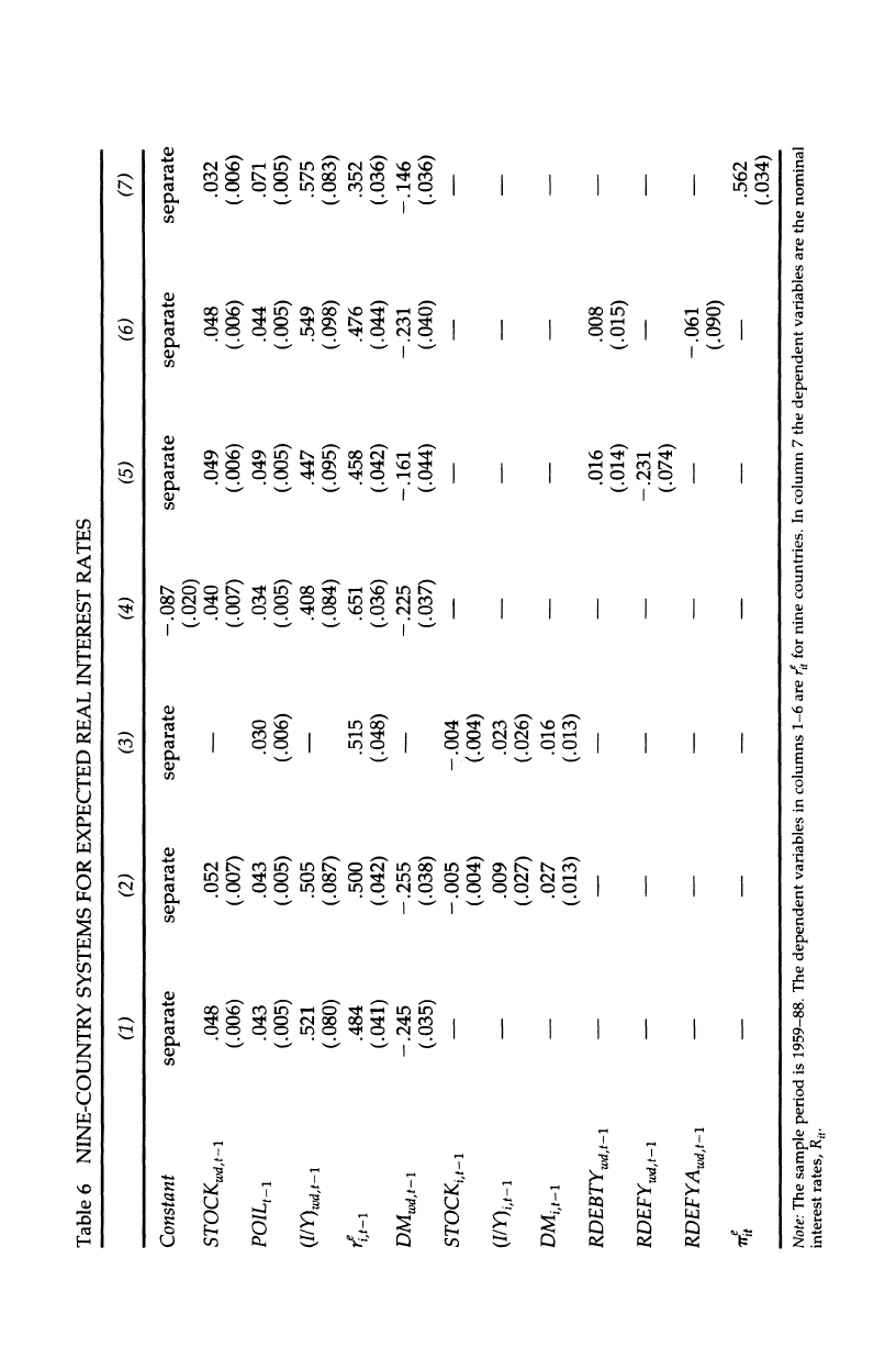
Table 6 NINE-COUNTRY SYSTEMS FOR EXPECTED REAL INTEREST RATES

(1) (2) (3) (4) (5) (6) (7)

Constant separate separate separate -.087 separate separate separate

(.020)

STOCKwd,t- .048 .052 - .040 .049 .048 .032

(.006) (.007) (.007) (.006) (.006) (.006)

POIL,_1 .043 .043 .030 .034 .049 .044 .071

(.005) (.005) (.006) (.005) (.005) (.005) (.005)

(IY)wt .521 .505 - .408 .447 .549 .575

(.080) (.087) (.084) (.095) (.098) (.083)

ri .

.484 .500 .515 .651 .458 .476 .352

(.041) (.042) (.048) (.036) (.042) (.044) (.036)

DMwd,t-1 -.245 -.255 - -.225 -.161 -.231 -.146

(.035) (.038) (.037) (.044) (.040) (.036)

STOCKi,

t1 -.005 -.004 - -

(.004) (.004)

(IY)it-1 - .009 .023

(.027) (.026)

DMi,t_ - .027 .016 -

(.013) (.013)

RDEBTYw,t - - .016 .008

(.014) (.015)

RDEFYt_ - -.231 -

(.074)

RDEFYAwd,,

t- - -- -.061

(.090)

_- -_ - .562

(.034)

Note: The sample period is 1959-88. The dependent variables in columns 1-6 are ri for nine countries. In column 7 the dependent variables are the nominal

interest rates, Ri,.

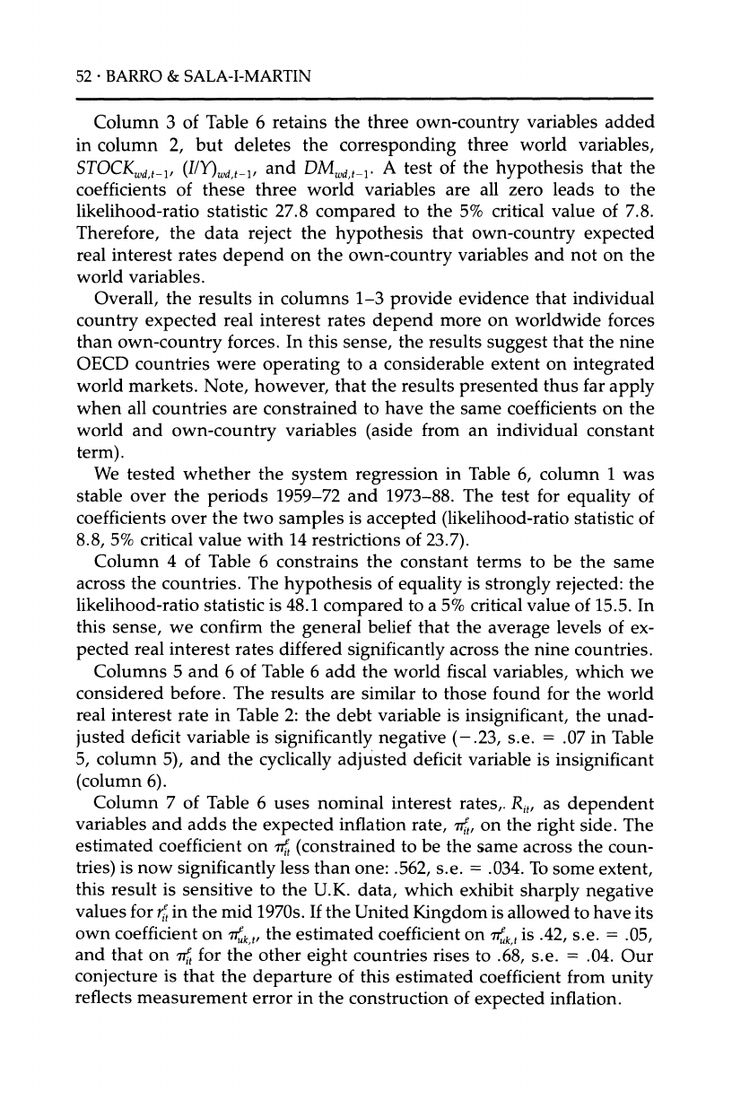
52 *

BARRO

& SALA-I-MARTIN

Column 3 of Table 6 retains the three own-country variables added

in column 2, but deletes the corresponding three world variables,

STOCKwd,t_l (I/Y)wdt_l, and DMdt _1. A test of the hypothesis that the

coefficients of these three world variables are all zero leads to the

likelihood-ratio statistic 27.8 compared to the 5% critical value of 7.8.

Therefore, the data reject the hypothesis that own-country expected

real interest rates depend on the own-country variables and not on the

world variables.

Overall, the results in columns 1-3 provide evidence that individual

country expected real interest rates depend more on worldwide forces

than own-country forces. In this sense, the results suggest that the nine

OECD countries were operating to a considerable extent on integrated

world markets. Note, however, that the results presented thus far apply

when all countries are constrained to have the same coefficients on the

world and own-country variables (aside from an individual constant

term).

We tested whether the system regression in Table 6, column 1 was

stable over the periods 1959-72 and 1973-88. The test for equality of

coefficients over the two samples is accepted (likelihood-ratio statistic of

8.8, 5% critical value with 14 restrictions of 23.7).

Column 4 of Table 6 constrains the constant terms to be the same

across the countries. The hypothesis of equality is strongly rejected: the

likelihood-ratio statistic is 48.1 compared to a 5% critical value of 15.5. In

this sense, we confirm the general belief that the average levels of ex-

pected real interest rates differed significantly across the nine countries.

Columns 5 and 6 of Table 6 add the world fiscal variables, which we

considered before. The results are similar to those found for the world

real interest rate in Table 2: the debt variable is insignificant, the unad-

justed deficit variable is significantly negative (-.23, s.e. = .07 in Table

5, column 5), and the cyclically adjusted deficit variable is insignificant

(column 6).

Column 7 of Table 6 uses nominal interest rates,. Rit, as dependent

variables and adds the expected inflation rate, 7it, on the right side. The

estimated coefficient on 77i

(constrained to be the same across the coun-

tries) is now significantly less than one: .562, s.e. = .034. To some extent,

this result is sensitive to the U.K. data, which exhibit sharply negative

values for rt

in the mid 1970s. If the United Kingdom is allowed to have its

own coefficient on 7rk,t the estimated coefficient on k

t is .42, s.e. = .05,

and that on ift for the other eight countries rises to .68, s.e. = .04. Our

conjecture is that the departure of this estimated coefficient from unity

reflects measurement error in the construction of expected inflation.

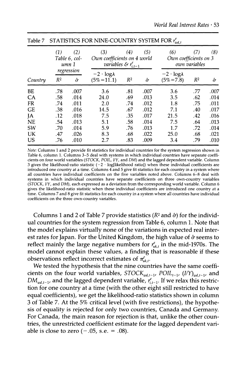
World

Real Interest Rates

. 53

Table

7 STATISTICS FOR NINE-COUNTRY

SYSTEM FOR

red,t

(1) (2) (3) (4) (5) (6) (7) (8)

Table

6, col- Own

coefficients

on

4 world Own

coefficients

on

3

umn

1 variables

&

r_t-1 own variables

regression

regresn -2 ?

logA -2 ?

logA

Country R2 a (5%=11.1) R2 & (5%=7.8) R2 &

BE .78 .007 3.6 .81 .007 3.6 .77 .007

CA .58 .014 24.0 .69 .013 3.5 .62 .014

FR .74 .011 2.0 .74 .012 1.8 .75 .011

GE .38 .016 14.5 .67 .012 7.1 .40 .017

JA .12 .018 7.5 .35 .017 21.5 .42 .016

NE .54 .013 5.1 .58 .014 7.5 .64 .013

SW .70 .014 5.9 .76 .013 1.7 .72 .014

UK .47 .026 8.3 .68 .022 25.0 .68 .021

US .76 .010 2.7 .83 .009 3.4 .79 .010

Note: Columns 1 and 2 provide fit statistics for individual countries for the system regression shown in

Table 6, column 1. Columns 3-5 deal with systems in which individual countries have separate coeffi-

cients on four world variables (STOCK,

POIL, I/Y, and DM) and the lagged dependent variable. Column

3 gives the likelihood-ratio statistic (-2 ? log[likelihood ratio]) when these individual coefficients are

introduced one country at a time. Columns 4 and 5 give fit statistics for each country in a system where

all countries have individual coefficients on the five variables noted above. Columns 6-8 deal with

systems in which individual countries have separate coefficients on three own-country variables

(STOCK,

IIY, and DM), each expressed as a deviation from the corresponding world variable. Column 6

gives the likelihood-ratio statistic when these individual coefficients are introduced one country at a

time. Columns 7 and 8 give fit statistics for each country in a system where all countries have individual

coefficients on the three own-country variables.

Columns 1 and 2 of Table 7 provide statistics (R2

and &)

for the individ-

ual countries for the system regression from Table 6, column 1. Note that

the model explains virtually none of the variations in expected real inter-

est rates for Japan. For the United Kingdom, the high value of 6r

seems to

reflect mainly the large negative numbers for rk,t in the mid-1970s. The

model cannot explain these values, a finding that is reasonable if these

observations reflect incorrect estimates of Tk,t.

We tested the hypothesis that the nine countries have the same coeffi-

cients on the four world variables, STOCKw,t

_, POIL,_1, (I/Y)wd,t

_ and

DM d,

t_, and the lagged dependent variable, _t-. If we relax this restric-

tion for one country at a time (with the other eight still restricted to have

equal coefficients), we get the likelihood-ratio statistics shown in column

3 of Table 7. At the 5% critical level (with five restrictions), the hypothe-

sis of equality is rejected for only two countries, Canada and Germany.

For Canada, the main reason for rejection is that, unlike the other coun-

tries, the unrestricted coefficient estimate for the lagged dependent vari-

able is close to zero (-.05, s.e. = .08).

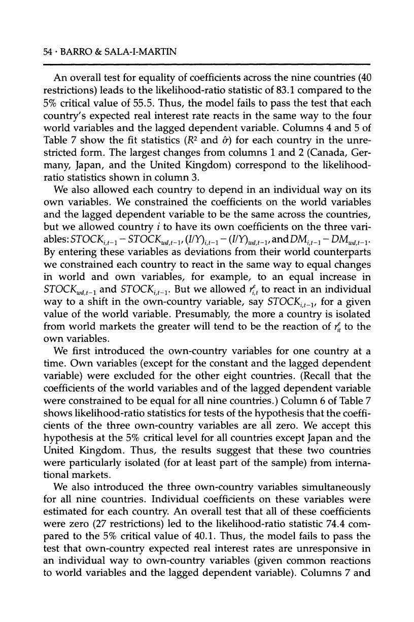
54 *

BARRO & SALA-I-MARTIN

An overall test for equality of coefficients across the nine countries (40

restrictions) leads to the likelihood-ratio statistic of 83.1 compared to the

5% critical value of 55.5. Thus, the model fails to pass the test that each

country's expected real interest rate reacts in the same way to the four

world variables and the lagged dependent variable. Columns 4 and 5 of

Table 7 show the fit statistics (R2 and 6) for each country in the unre-

stricted form. The largest changes from columns 1 and 2 (Canada, Ger-

many, Japan, and the United Kingdom) correspond to the likelihood-

ratio statistics shown in column 3.

We also allowed each country to depend in an individual way on its

own variables. We constrained the coefficients on the world variables

and the lagged dependent variable to be the same across the countries,

but we allowed country i to have its own coefficients on the three vari-

ables: STOCKi, t_ - STOCKd, t l, (I/Y)i,t_l - (I/Y)Wd,t-l,

andDMi,t_ - DMwd,t-l

By entering these variables as deviations from their world counterparts

we constrained each country to react in the same way to equal changes

in world and own variables, for example, to an equal increase in

STOCKd,

t1 and STOCK,

t_. But we allowed /,t

to react in an individual

way to a shift in the own-country variable, say STOCK,

_l, for a given

value of the world variable. Presumably, the more a country is isolated

from world markets the greater will tend to be the reaction of it to the

own variables.

We first introduced the own-country variables for one country at a

time. Own variables (except for the constant and the lagged dependent

variable) were excluded for the other eight countries. (Recall that the

coefficients of the world variables and of the lagged dependent variable

were constrained to be equal for all nine countries.) Column 6 of Table 7

shows likelihood-ratio statistics for tests of the hypothesis that the coeffi-

cients of the three own-country variables are all zero. We accept this

hypothesis at the 5% critical level for all countries except Japan and the

United Kingdom. Thus, the results suggest that these two countries

were particularly isolated (for at least part of the sample) from interna-

tional markets.

We also introduced the three own-country variables simultaneously

for all nine countries. Individual coefficients on these variables were

estimated for each country. An overall test that all of these coefficients

were zero (27 restrictions) led to the likelihood-ratio statistic 74.4 com-

pared to the 5% critical value of 40.1. Thus, the model fails to pass the

test that own-country expected real interest rates are unresponsive in

an individual way to own-country variables (given common reactions

to world variables and the lagged dependent variable). Columns 7 and

World Real Interest Rates

*

55

8 of Table 7 show fit statistics (R2

and &)

for each country in the model

that allows individual coefficients for all countries on the three own

variables. The largest changes from columns 1 and 2 (Japan and the

United Kingdom) correspond to the likelihood-ratio statistics shown in

column 6.

10. System for Individual Countries' Investment

Ratios

We now relate the investment ratio for each of the ten countries, (I/Y),, to

world and own-country variables. Unlike for the expected real interest

rate, r, the null hypothesis under integrated world markets is not that

(I/Y)it

depends only on world variables. (IIY),i would depend on any

variable that influences own-country investment demand-notably, the

own-country stock return, STOCKi,

_, and the lagged investment ratio,

(I/Y)i,,_1-and on world variables through their influence on the world

expected real interest rate. Given the world variables (and hence the

world expected real interest rate), (I/Y)i,

would be independent of influ-

ences on country i's desired saving rate. Because POILt_1 is a common

influence across countries, the only variable of this type in the previous

analysis was own-country monetary growth, DMi,

_. (The own-country

fiscal variables would also be in this category, but the fiscal variables

were found to be unimportant in general.)

Table 8 shows the results for (I/Y)it

for the ten-country system of invest-

ment ratios over the period 1959-88. The independent variables are

POIL,_l;

the world and own-country lagged values of STOCK,

(IIY),

and

DM; 4d,t-,;22 and individual constant terms. The regression in column 1

shows a significant, positive effect for STOCKi,, (.017, s.e. = .003). This

result can be interpreted as an effect from changes in the expected profit-

ability of investment in country i (or possibly changes in the risk pre-

mium applicable to these investments). The estimated coefficient of

STOCKW,t 1, however, is also positive: .017, s.e. = .008. If the own-

country stock return holds constant the expected profitability of invest-

ment (risk-adjusted), then the world stock return would influence (I/Y)t

only through its effect on world expected real interest rates; that is, the

effect of STOCKWd, on (I/Y)i would be negative. It is possible, however,

that stock returns in other countries provide information about the profit-

ability of investment in country i, even for a given value of country i's

22. Because the expected real interest rate is unavailable for Italy we entered rd ,t- for each

country. The results change little if we also include rt-i in the nine-country system that

excludes Italy. That is, lags of expected real interest rates are unimportant in general for

the investment ratios.

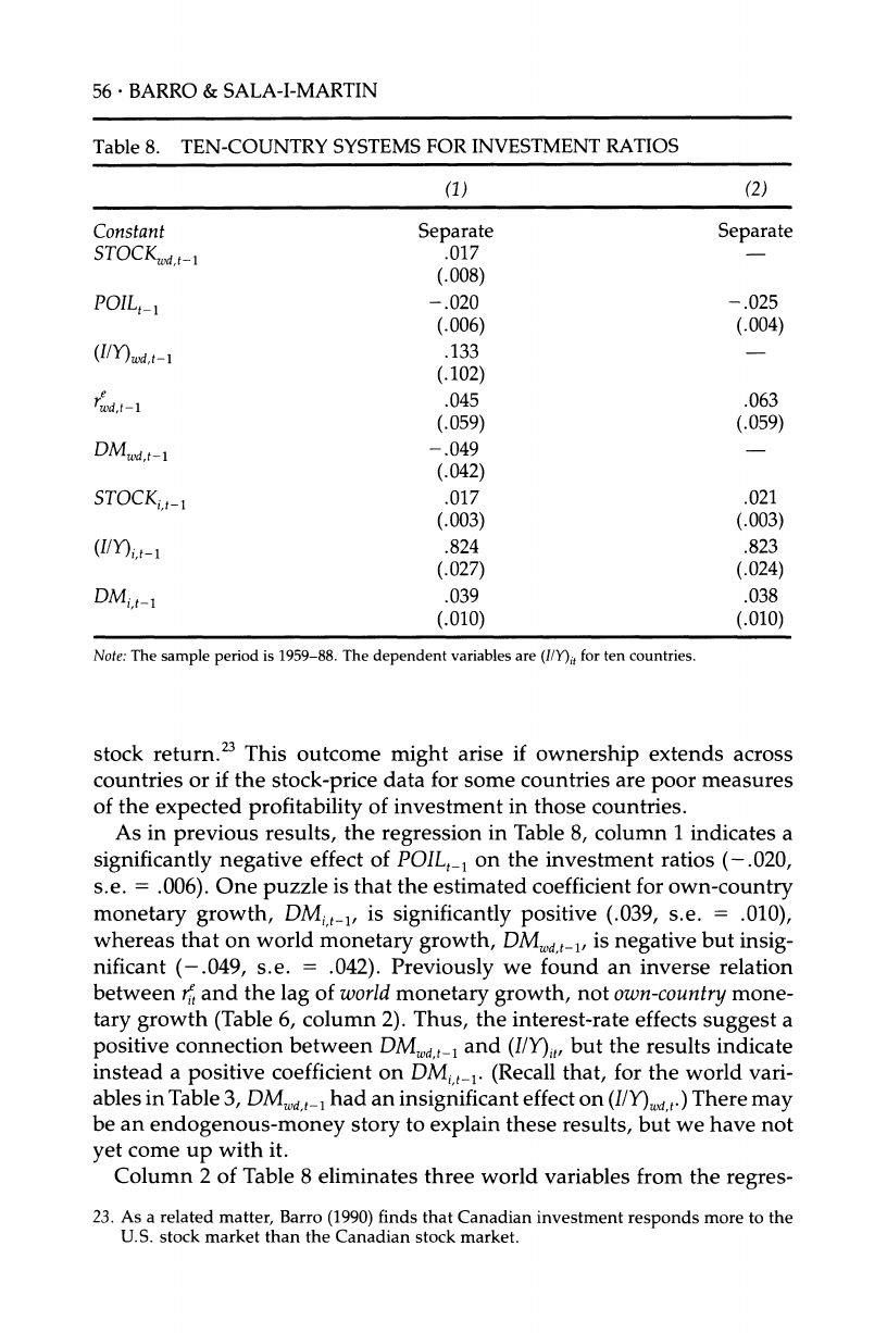
56 *

BARRO & SALA-I-MARTIN

Table

8. TEN-COUNTRY

SYSTEMS

FOR INVESTMENT

RATIOS

(1)

Constant

STOCKWd,t-1

POILt_1

(I/Y)wd,t-l

rwd,t-l

DM ,t-1

STOCKit-1

(I/Y)it-1

DMi,t-I

Separate

.017

(.008)

-.020

(.006)

.133

(.102)

.045

(.059)

-.049

(.042)

.017

(.003)

.824

(.027)

.039

(.010)

(2)

Separate

-.025

(.004)

.063

(.059)

.021

(.003)

.823

(.024)

.038

(.010)

Note: The sample period

is 1959-88. The dependent

variables

are

(I/Y)it

for

ten countries.

stock return.23 This outcome might arise if ownership extends across

countries or if the stock-price data for some countries are poor measures

of the expected profitability of investment in those countries.

As in previous results, the regression in Table 8, column 1 indicates a

significantly negative effect of POILt_1

on the investment ratios (-.020,

s.e. = .006). One puzzle is that the estimated coefficient for own-country

monetary growth, DMi,t,, is significantly positive (.039, s.e. = .010),

whereas that on world monetary growth, DMwd t-_, is negative but insig-

nificant (-.049, s.e. = .042). Previously we found an inverse relation

between i and the lag of world

monetary growth, not own-country

mone-

tary growth (Table 6, column 2). Thus, the interest-rate effects suggest a

positive connection between DMWd,

t- and (I/Y)it,

but the results indicate

instead a positive coefficient on DMi, _. (Recall that, for the world vari-

ables in Table 3, DMd,t-l had an insignificant effect on (IY)wd,t.) There may

be an endogenous-money story to explain these results, but we have not

yet come up with it.

Column 2 of Table 8 eliminates three world variables from the regres-

23. As a related matter, Barro (1990) finds that Canadian investment responds more to the

U.S. stock market than the Canadian stock market.

World

Real

Interest Rates

*

57

sion: STOCKw t-l, (I/Y)w,

t-, and DM,dt-_. Theoretically (abstracting from

the possible informational role of world stock prices for own-country

profitability), these variables would affect (I/Y)it

only through their ef-

fects on the world expected real interest rate. The three world variables

prove to be jointly insignificant; the likelihood-ratio statistic is 2.9 com-

pared to the 5% critical value of 7.8.

It would be possible to consider the system of equations for invest-

ment ratios jointly with the system for expected real interest rates. The

restrictions imposed by the structural model could be imposed on this

overall joint system. We plan eventually to undertake this grand-system

estimation.

11. Summary

of

Main

Results

We thought of the expected real interest rate for the major industrialized

countries as determined by the equation of aggregate investment de-

mand to the aggregate of desired national saving. We used stock-market

returns to isolate shifts to expected profitability of investment (or risk

premia) and, hence, to investment demand. We used oil prices to cap-

ture shifts to temporary income and, hence, to desired national saving.

In some models, monetary expansion would appear as a positive shock

to desired national saving, and in others, fiscal expansion would enter as

a negative shock.

We used the structural model to determine a reduced form for the

"world" expected real interest rate and ratio of investment to GDP. The

main predictions are that more favorable stock returns raise the real

interest rate and investment, higher oil prices increase the real interest

rate but decrease investment, higher monetary growth lowers the real

interest rate and stimulates investment, and greater fiscal expansion

raises the real interest rate and reduces investment.

We estimated the reduced form of the model on data for ten OECD

countries over the period 1959-88. Thus far, the results pertain to an-

nual data on short-term interest rates. (Because of data problems with

Italy we included only nine countries in the equations for interest

rates.) The results for world (GDP-weighted) expected real interest

rates reveal significant effects in the predicted directions for world

stock returns, oil prices, and world monetary growth. Fiscal variables

turned out to be unimportant. The behavior of the world investment

ratio was also consistent with the model, except that the hypothesized

positive effect from monetary growth did not show up and fiscal vari-

ables were unimportant.

58 - BARRO

& SALA-I-MARTIN

Estimates of the reduced form that were constrained by the structural

restrictions led to estimates of structural coefficients, such as the respon-

siveness of desired national saving rates to the expected real interest

rate. We find that an increase in the expected real interest rate by one

percentage point raises the desired saving rate by about one-third of a

percentage point.

We simulated the model to try to explain why expected real interest

rates were high for 1981-86 (averaging 4.2%) and low for 1975-80

(averaging 0.3%). The dominant influence was the variation in stock

returns; these returns were very low for 1974-79 and much higher for

1980-85. The increase in oil prices from the early 1970s until 1986 is also

an important factor. We attributed the drop in expected real interest

rates for 1987-88 (to an average of 2.3%) mainly to the decline in oil

prices, and the rise in the rate for 1989 (to 3.5%) mainly to the im-

proved stock market in 1988. The model also forecasts a dramatic rise

in the expected real interest rate to 5.6% in 1990. This value is almost a

full percentage point above the highest value that occurred during the

period 1958-89.

We estimated systems of equations for expected real interest rates for

nine OECD countries. (We also estimated systems of equations for invest-

ment ratios for ten OECD countries, including Italy.) These systems

include world and own-country variables as regressors. One finding is

that each country's expected real interest rate depends primarily on

world factors, thereby suggesting a good deal of integration of world

markets. We do find, however, significant effects of own-country vari-

ables for Japan and the United Kingdom. Our interpretation is that these

countries were significantly isolated from international markets, at least

over part of the period 1959-88.

The research carried out thus far suggests a number of avenues for

future work. The possibilities that we are presently pursuing are the

analysis of longer-term interest rates, the inclusion of measures of the

profitability of investment, the addition of variables such as defense

expenditures that represent exogenous shifts to desired saving, consider-

ation of tax effects related to interest income and expenses, and the

estimation of equations for expected real interest rates and investment

ratios with quarterly data. We are also considering a division of invest-

ment into components that would be especially sensitive to the stock

market (business nonresidential investment) and those that would be

less sensitive (residential investment, public investment, and purchases

of consumer durables). Finally, we are looking into the possibilities for

adding more countries; Switzerland and Australia appear to be the most

promising in terms of the availability of data.

World Real Interest Rates

. 59

REFERENCES

Barro, R. J. 1981. Intertemporal substitution and the business cycle. Carnegie-

Rochester

Conference

Series

on Public Policy 14 (Spring): 237-68.

1989. Macroeconomics,

3d ed. New York;

John Wiley & Sons.

. 1990. The stock market and investment. The Review of Financial Studies.

Spring.

Blanchard, O. J. 1985. Debt, deficits, and finite horizons. Journal

of Political

Econ-

omy 93 (2): 223-47.

,and L. H. Summers. 1984. Perspectives on high world real interest rates.

Brookings Papers

on Economic

Activity (2): 273-324.

Evans, P. 1985. Do budget deficits raise nominal interest rates? Evidence from six

countries. Journal

of Monetary

Economics 20 (5): 281-300.

Fama, E. F 1981. Stock returns, real activity, inflation, and money. American

Economic Review 71 (4): 545-65.

Hayashi, F 1982. Tobin's marginal q and average q: A neoclassical interpretation.

Econometrica 50 (1): 213-24.

Mishkin, F S. 1984. Are real interest rates equal across countries? An empirical

investigation of international parity conditions. Journal

of Finance 39 (6): 1345-

57.

Mundell, R. A. 1971. Inflation, saving, and the real rate of interest. In Monetary

Theory,

edited by R. A. Mundell. Pacific Palisades, Calif.: Goodyear.

Plosser, C. I. 1987. Fiscal policy and the term structure. Journal of Monetary

Economics 20 (5): 343-67.

Summers, R., and A. Heston. 1988. A new set of international comparisons of

real product and price levels. Estimates for 130 countries. The

Review

of Income

and Wealth 34 (1): 1-25.

Tobin, J. 1965. Money and economic growth. Econometrica

33 (3): 671-84.

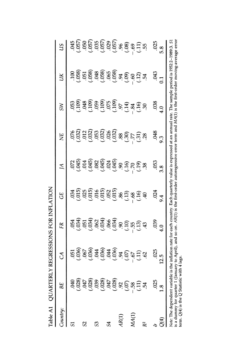
Table Al QUARTERLY REGRESSIONS FOR INFLATION

Country: BE CA FR GE JA NE SW UK US

S1

52

53

S4

AR(1)

MA(1)

R2

Q(4)

.040

(.028)

.047

(.028)

.039

(.028)

.047

(.028)

.92

(.07)

-.58

(.11)

.54

.025

1.8

.051

(.036)

.067

(.036)

.044

(.036)

.044

(.036)

.94

(.07)

-.67

(.11)

.62

.025

12.5

.054

(.034)

.051

(.034)

.062

(.034)

.066

(.034)

.90

(.10)

-.55

(.13)

.43

.039

4.0

.034

(.015)

.025

(.015)

.016

(.015)

.052

(.015)

.86

(.13)

-.68

(.16)

.40

.024

9.4

.072

(.045)

.014

(.045)

.082

(.045)

.024

(.045)

.90

(.16)

-.70

(.19)

.38

.053

3.8

.076

(.032)

.012

(.032)

.053

(.032)

.026

(.032)

.88

(.30)

-.77

(.31)

.28

.048

9.3

.053

(.109)

.048

(.109)

.059

(.109)

.075

(.109)

.97

(.14)

-.84

(.16)

.30

.038

4.0

.100

(.058)

.051

(.058)

.048

(.058)

.065

(.058)

.94

(.09)

-.60

(.12)

.54

.043

0.1

.045

(.057)

.050

(.057)

.035

(.057)

.029

(.057)

.96

(.08)

-.69

(.11)

.55

.025

5.8

Note: The dependent variable is the inflation rate for each country. Each quarterly value is expressed at an annual rate. The sample period is 1952:2-1989:3. S1

is a dummy for quarter 1 (January to April), and so on. AR(1) is the first-order autoregressive error term and MA(1) is the first-order moving-average error

term. Q(4) is the Q Statistic with 4 lags.

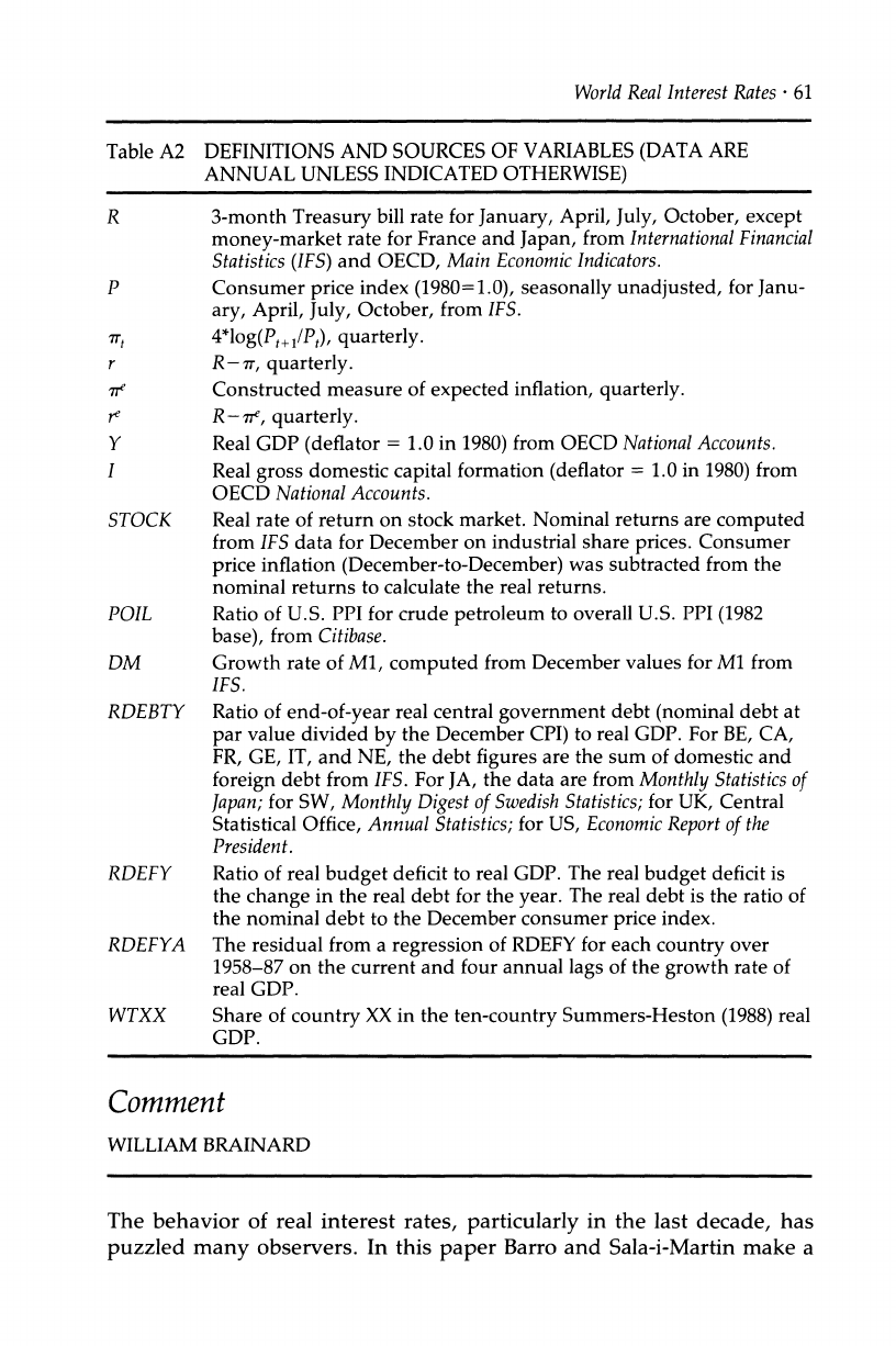
World

Real Interest Rates *

61

Table A2 DEFINITIONS AND SOURCES OF VARIABLES

(DATA ARE

ANNUAL UNLESS INDICATED OTHERWISE)

R 3-month Treasury bill rate for January, April, July, October, except

money-market rate for France and Japan, from International

Financial

Statistics (IFS) and OECD, Main Economic

Indicators.

P Consumer price index (1980=1.0), seasonally unadjusted, for Janu-

ary, April, July, October, from IFS.

%t 4*log(Pt+ /Pt), quarterly.

r R- r, quarterly.

Tef Constructed measure of expected inflation, quarterly.

re R- e, quarterly.

Y Real GDP (deflator = 1.0 in 1980) from OECD National Accounts.

I Real gross domestic capital formation (deflator = 1.0 in 1980) from

OECD National Accounts.

STOCK Real rate of return on stock market. Nominal returns are computed

from IFS data for December on industrial share prices. Consumer

price inflation (December-to-December) was subtracted from the

nominal returns to calculate the real returns.

POIL Ratio of U.S. PPI for crude petroleum to overall U.S. PPI (1982

base), from Citibase.

DM Growth rate of M1, computed from December values for M1 from

IFS.

RDEBTY Ratio of end-of-year real central government debt (nominal debt at

par value divided by the December CPI) to real GDP. For BE, CA,

FR, GE, IT, and NE, the debt figures are the sum of domestic and

foreign debt from IFS. For JA, the data are from Monthly Statistics

of

Japan;

for SW, Monthly Digest of Swedish

Statistics;

for UK, Central

Statistical Office, Annual Statistics;

for US, Economic

Report of the

President.

RDEFY Ratio of real budget deficit to real GDP. The real budget deficit is

the change in the real debt for the year. The real debt is the ratio of

the nominal debt to the December consumer price index.

RDEFYA The residual from a regression of RDEFY for each country over

1958-87 on the current and four annual lags of the growth rate of

real GDP.

WTXX Share of country XX in the ten-country Summers-Heston (1988) real

GDP.

Comment

WILLIAM BRAINARD

World

Real Interest Rates *

61

Table A2 DEFINITIONS AND SOURCES OF VARIABLES

(DATA ARE

ANNUAL UNLESS INDICATED OTHERWISE)

R 3-month Treasury bill rate for January, April, July, October, except

money-market rate for France and Japan, from International

Financial

Statistics (IFS) and OECD, Main Economic

Indicators.

P Consumer price index (1980=1.0), seasonally unadjusted, for Janu-

ary, April, July, October, from IFS.

%t 4*log(Pt+ /Pt), quarterly.

r R- r, quarterly.

Tef Constructed measure of expected inflation, quarterly.

re R- e, quarterly.

Y Real GDP (deflator = 1.0 in 1980) from OECD National Accounts.

I Real gross domestic capital formation (deflator = 1.0 in 1980) from

OECD National Accounts.

STOCK Real rate of return on stock market. Nominal returns are computed

from IFS data for December on industrial share prices. Consumer

price inflation (December-to-December) was subtracted from the

nominal returns to calculate the real returns.

POIL Ratio of U.S. PPI for crude petroleum to overall U.S. PPI (1982

base), from Citibase.

DM Growth rate of M1, computed from December values for M1 from

IFS.

RDEBTY Ratio of end-of-year real central government debt (nominal debt at

par value divided by the December CPI) to real GDP. For BE, CA,

FR, GE, IT, and NE, the debt figures are the sum of domestic and

foreign debt from IFS. For JA, the data are from Monthly Statistics

of

Japan;

for SW, Monthly Digest of Swedish

Statistics;

for UK, Central

Statistical Office, Annual Statistics;

for US, Economic

Report of the

President.

RDEFY Ratio of real budget deficit to real GDP. The real budget deficit is

the change in the real debt for the year. The real debt is the ratio of

the nominal debt to the December consumer price index.

RDEFYA The residual from a regression of RDEFY for each country over

1958-87 on the current and four annual lags of the growth rate of

real GDP.

WTXX Share of country XX in the ten-country Summers-Heston (1988) real

GDP.

Comment

WILLIAM BRAINARD

The behavior of real interest rates, particularly in the last decade, has

puzzled many observers. In this paper Barro and Sala-i-Martin make a

The behavior of real interest rates, particularly in the last decade, has

puzzled many observers. In this paper Barro and Sala-i-Martin make a

62 *

BARRO & SALA-I-MARTIN

bold attempt to explain the "world" real interest rate with a simple

model in which that rate is determined by the condition that world

investment be equal to world saving. The paper is stimulating to read

and rich with information and puzzles. It is written in a commendable

style-clear about the data, candid about contradictory results. Artful in

the specification of the model, Barro and Sala-i-Martin are at the same

time disarmingly diffident about the theory. Although I have reserva-

tions about both the theory and some of the authors' conclusions, I

admire their willingness to tackle an inherently difficult problem and

their resourcefulness in creating a coherent picture of the experience of

the last 30 years.

1. Overview

of

the

Model

The authors' model is "classical," consisting simply of an investment

equation and a saving equation, plus the condition that saving and

investment be equal. Each equation contains only one right-hand-side

endogenous variable, the real interest rate. Since nothing else is free to

give, the real interest rate is determined by the equilibrium condition.

Hence the real rate is determined by exogenous factors shifting invest-

ment or saving. In the authors' specification these are few in number;

investment depends on a "q-like

variable" and saving depends on transi-

tory income and the real rate of interest.

The theoretical framework the authors use for organizing their investi-

gation has the virtue of simplicity, but its very simplicity precludes exami-

nation of some major hypotheses about the movements of the real rates

during their sample period. The classical model usually comes with the

assumption that income is always at full employment. The authors do

not make that assumption explicit, and indeed they allow changes in

transitory income to affect the saving ratio. But, as in the classical full-

employment model, adjustments in income play no role in transmitting

shocks to interest rates or investment ratios and they do not test the

validity of that assumption. Hence, for example, they do not examine

the role that a worldwide recession may have played in explaining why

real rates appear to fall following OPEC 1. Indeed the reader will not find

a figure or time series for income in the paper.

Similarly, the interplay of inflation, income, money, and nominal rates

is not modeled. Prices are gotten out of the way early, for most of the

analysis an estimate of inflationary expectations is used simply to calcu-

late the expected real rate from nominal rate. The classical role of prices

in maintaining full employment, and their success in doing so, is not

examined. The transmission mechanism for monetary policy is missing.

World Real Interest

Rates *

63

The authors do allow the possibility of non-neutrality of money in the

short run, but in their model money enters directly in the saving sched-

ule, with monetary expansion presumed to increase saving at a given

real rate of interest. The suppression of the demand and supply for

money obscures the way in which monetary events may affect invest-

ment, saving, and interest rates. Placing money in the saving function,

with income exogenous, in my view does not do justice to the possible

role of money. In the usual story, an increase in the expected rate of

growth of money and associated inflation shifts downward the stock

demand for money and decreases the required rate of return on bonds or

capital. In the short run easy money, in the level or expected rate of

change, lowers real rates as well as nominal because price changes do

not fully offset the nominal changes. Hence, expansionary monetary

encourages investment and increases income. These effects can be pres-

ent even if saving is inelastic with respect to interest rates and real

balances. According to the authors' model the reason tight money raised

real rates in 1979 was because it decreased desired saving, not because

reduction of the money supply forced up nominal rates in the money

markets much more rapidly than inflation could possibly subside.

While I am somewhat skeptical about the meaningfulness of a "world"

rate, particularly early in the sample period, focusing on an average of real

rates for a number of countries can be a useful enterprise even if world

capital markets are not perfectly integrated and the assets of different

countries are not perfect substitutes. Averaging real rates, investment

ratios and explanatory variables across countries wash out idiosyncratic

fluctuations, giving the investigator a better chance at detecting the impor-

tance of common factors such as oil-price shocks. Such shocks to the

world economy could have similar affects on many countries even if

capital markets are not integrated. But the authors' analysis does provides

them some evidence on the extent of integration.

How many countries need to be considered in analyzing the world

interest rate is another question. The authors assume their ten countries

are the entire world; hence they do not need to worry about an external

sector and the role that export demand and capital flows may play in the

determination of investment and interest rates. They argue that this is

not an unreasonable assumption since the countries represent approxi-

mately two-thirds of world output and because the observed current-

the account balance of the ten country aggregate has been small. As a

theoretical matter the fact that the current account balance tends to be

small is not a sufficient condition for treating a group of countries as

"closed"; on the empirical level the assumption rules out a major issue

surrounding the effect of the OPEC oil price increases, namely the extent

64

. BARRO & SALA-I-MARTIN

to which the OPEC nations increased their demand for imports from the

oil-consuming nations, and "recycled" their increased income. In the

authors' model these oil-price increases are treated simply as a transitory

reduction in income, with a negative effect on saving.

IMPLEMENTATION

Like any empirical investigation, implementation of the authors' model

requires a multitude of judgments about specification and about the

empirical counterparts of the variables appearing in the theoretical

model. I found most of the authors' decisions sensible. Furthermore, the

authors are well aware of many of the potential difficulties with the

particular choices they have made. Nevertheless several specification

issues are worth mentioning.

2. "The"

Real Interest Rate

The expected real rate of interest is taken to be a short-term rate minus

expected inflation. The authors' recognize that it would be desirable to

extend the analysis to the rates on assets of longer maturities and differ-

ent risks. Longer rates are probably a better approximation to the cost of

capital than the short rate and its behavior is, if anything, more puzzling

than that of the short rate. The required rate of return on equity, presum-

ably more relevant to investment than the required rate on nominal

assets, not only contains a substantial risk premia but appears to vary

relative to the rates on nominal assets. A second concern is the authors'

use of consumer price indexes in converting to a real rate. Because of

OPEC and exchange rate fluctuations during the 1970s there was a sub-

stantial difference between the inflation in consumer prices and the

inflation of capital goods prices relevant to the cost of capital. Most firms

were not experiencing increases in their product or capital goods prices

as large as those faced by consumers. Hence, the authors may substan-

tially overstate the decline in the real rate relevant to investment-

expected and actual-during that period. The authors do report two

regressions with the nominal rate as the dependent variable and ex-

pected inflation as an additional explanatory variable. In these equations

the coefficients on the other variables are essentially the same as in

expected real rate equations, but the estimate on expected inflation is

less than one. In the case of the country rate equations the point estimate

is .562, over ten standard errors away from one. Taken at face value this

result suggests that the expected real rate is highly negatively correlated

with the level of inflation. The authors suggest that the result is likely to

World

Real Interest Rates

?

65

reflect measurement error in expected inflation, but it should be noted

that studies not subject to that problem, using the nominal rate to pre-

dict future inflation, get essentially the same result.

3. The

Investment

Equation

The investment equation is determined by "a q-like variable"; prior stock

returns and the change in the real rate are used to proxy for the change

in q. Investment demand is expressed as a ratio to GDP. Hence, the

elasticity of investment with respect to income is assumed to be one with

adjustments of investment to income entirely within the year. This as-

sumption is inconsistent with the results of most empirical work. Since

the authors use gross, not net investment, depreciation is implausibly

assumed to be a fixed proportion of income.

Stock returns are taken to be a proxy for future expected profits. Em-

pirically, stock returns do not do well in forecasting profits. For example,

a simple regression of the net rate of return on capital (private, nonfarm)

on two lags of the annual stock return yields insignificant coefficients

and an R2 of less than 4%. The stock market is forward looking, and it

seems likely market returns reflect expectations about a variety of factors

other than profits relevant to investment-including future monetary

policy, income, and inflation. Hence, the interpretation of the positive

coefficient on the market return is open to a wide variety of interpreta-

tions. For example, if the stock market does a good job forecasting infla-

tion and nominal rates do not fully adjust to inflation, then periods of

low market returns will be followed by low real rates (assuming inflation

is bad for the market for at a given real rate). While relating investment

to market returns is itself an achievement, it leaves us with an even

greater need to explain the market itself.

Investment is taken to be gross domestic capital formation, which

includes both residential and public investment. It does not seem likely

that stock returns are a good explanatory variable for either. The inclu-

sion of public investment also implicitly treats public investment as a

perfect substitute for private. This specification could help explain why

the authors find a significantly positive relationship between investment

and government deficits, a result they believe is opposite that predicted

by models where fiscal deficits lower national saving. If, in fact, govern-

ment investment is less than a perfect substitute for private, as seems

likely, then exogenous increases in public investment, correlated with

the deficit, would create a positive correlation between gross capital

formation and the deficit even with crowding out.

66 *

BARRO

& SALA-I-MARTIN

4. The

Saving Equation

Saving, like investment, is gross of depreciation and expressed as a ratio

to income. Hence, the elasticity of saving with respect to current income

is one for a given ratio of transitory to permanent income. A conse-

quence of the assumption that both the investment and saving equations

are expressed in ratio form is that fluctuations in income can have sub-

stantial effects on investment and saving.

The relative price of oil is used as a measure of transitory income in the

saving equation and excluded from the investment equation, providing

identification. It could just as well be argued that it belongs in the invest-

ment equation. Some of the effect of changes in oil prices may be cap-

tured by stock market returns; however it can be argued that changes in

the relative price of oil may change the relationship between marginal

and average q. Stock returns are excluded from the saving equation,

thereby providing identification. For both wealth and rate of return rea-

sons it could be argued they belong.

Although their theoretical specification distinguishes between transi-

tory and permanent income, in their estimation the authors simply take

the relative price of oil as a measure of transitory income. The authors

make no attempt to econometrically distinguish between transitory and

permanent changes in income.

The authors test for Ricardian equivalence by introducing the real value

of government debt and its change (the "real deficit"), both cyclically

adjusted and unadjusted, in the saving function. These tests are not the

centerpiece of their study, but I would have preferred a more extensive

investigation of possible fiscal effects, particularly since some observers

have argued that fiscal deficits are partly responsible for the current high

level of real rates. There are a number of issues. I am skeptical that this

measure of the deficit is an adequate summary of the effect of government

fiscal policy on saving; it attempts to capture rather different fiscal events

in single a variable. First, in principle government consumption, govern-

ment investment, and taxes could have quite different effects. Indeed,

Ricardian theory itself distinguishes among these three. The authors do

report that an attempt to find effects of government consumption were

unsuccessful. Second, whether it is called money illusion or a distribution

effect, there is empirical evidence that the effect of a tax increase on saving

is different from that of a capital loss of the same dollar value. Further-

more, changes in real wealth due to changes in the price level may have a

different effect than changes in market value associated with changes in

interest rates. Lastly, it would be desirable to distinguish, for any of these

variables, between expected and unexpected changes.

World Real

Interest Rates

*

67

For testing Ricardian equivalence I would also have preferred a more

inclusive measure of government. The authors' fiscal measures do not

include state and local governments. For the United States, at any rate,

the combined government deficit is substantially different from the fed-

eral deficit in the latter part of the sample, with state and local surpluses

partially offsetting central deficits.

As I believe Lucas will discuss, the model gives no role to the rate of

growth of income or consumption in the determination of real rates.

Such differences, in theory, should be important in explaining differ-

ences in rates across countries.

5. Results

Notwithstanding these concerns about the econometric specification,

world stock returns and oil prices are estimated to have positive and

significant effects on world real interest rates. The reduced form equa-

tions explain approximately 90% of the fluctuations of interest rates and

85% of investment during the 1959-1988 period. The equations do un-

derpredict the decline in the expected real rate by approximately 1% for

the period 1975-80. Unexpected inflation was positive during most of

the period so the equations underpredict the actual real rate by more.

(The difference between expected and actual real rates was dramatic in

1973-74.) The equations do better in predicting the rise in the expected

real rate in the 1980s. The model's forecast of inflation, however, are

typically low during this period; hence actual real rates average about a

percent below the expected real rate.

Stock returns are the most important variable in explaining variations

in the real rate over the sample. For example, the estimates attribute

about 2.5% points of the approximately 4% rise in the expected real

rate between 1975 to 1980 and 1981 to 1986 to higher stock returns

during the later period. Oil prices are also important, their increase in

1975-1980 over the late 1960s partially offsets the increase attributed to

stock prices, and further increases are estimated to add 1.9% to the

expected real rate in the 1980s. Although monetary growth is signifi-

cant in the rate equations, world monetary contraction explains only a

small portion of the increase in real rate during the 1980s. Fiscal vari-

ables are not significant.

Investment is positively related to stock returns and negatively related

to oil prices, consistent with both the theory and the rate equations.

However, inconsistent with the predicted effect of monetary growth on

the real rate, it appears to have no effect on investment. Similarly, the

budget deficit variables appear to have substantial and significant posi-

68 *

BARRO

& SALA-I-MARTIN

tive effects on investment even though they appear to have essentially

no effect on rates. The authors suggest the positive coefficients are incon-

sistent with the view that fiscal expansion lowers desired national sav-

ing. They need not be for at least two reasons. First, proponents of the

view that government deficits crowd out private investment are refer-

ring to the effect on national saving with output constant, either because

monetary policy offsets fiscal expansion or because the economy is oper-

ating at capacity. The authors do not control for output; endogenous

increases in output in response to fiscal stimulus would be expected to

increase saving, and could even induce increases in private investment.

Second, as discussed above, the fact that the authors have included

government investment in their investment series could explain a posi-

tive coefficient.

It is hard to argue against the proposition that nominal short-term rates

and expected exchange rate changes are tied together in international

financial markets. But given the poor performance of purchasing power

parity it would be more of a surprise if real rates were tightly tied together.

The authors investigate the degree of integration by introducing country

variables in the various estimated equations. If capital markets are well

integrated and assets close substitutes, individual countries' real rates

and investment should primarily reflect world variables rather than coun-

try variables; country saving, however, should reflect individual country

effects even if markets are integrated.

The authors' specification provides only a weak test of the integra-

tion hypothesis. Separate intercepts and the own-country lagged depen-

dent variable are included in both the rate and investment equations.

Hence, systematic differences in real rates are not taken as evidence

against the hypothesis and differences in average values of explanatory

variables across countries are not allowed to explain cross-country dif-

ferences in investment or interest rates. For example, high average

investment in Japan is not credited to a low-average real rate or high-

average stock return. The country intercepts and coefficients on lagged

own-country dependent variables that soak up these country effects are

highly significant.

In the rate equations world stock returns do hold up quite well in

competition with country returns. The coefficient (when constrained to

be equal across countries) is roughly the same as in the world rate

equation and own returns are insignificant. World money growth contin-

ues to be highly significant, whereas own money is marginally signifi-

cant and of the "wrong" sign. These results suggest a high degree of

integration and substitution between different countries assets; however

if the markets are well integrated and the assets close substitutes, the

World Real

Interest Rates

?

69

magnitude of the responses should also be equal. The authors' reject the

hypothesis of equality but find the rejection reflects significant differ-

ences for only two of the nine countries.

The integration hypothesis does less well in the case of investment.

The coefficients on world and country stock returns are about equal and

half the magnitude of world returns in the world rate equation. World

money, lagged world investment and real rates are all insignificant.

Tested jointly, world variables are insignificant; yet all three country-

specific variables are highly significant. The authors are puzzled by the

importance of own-country monetary expansion given the world rate is

insignificant and own money has the wrong sign in the rate equation.

One possible explanation is that investment shocks, with resultant in-

creases in the country's income, are partially accommodated by the

monetary authority. The significant, and "wrong" signed coefficient on

own money in the rate equation could be similarly explained; since own

investment does not appear to affect interest rates the shocks to income

would have to be from another source.

In some respects the paper is quite successful. The authors have

clearly identified important comovements of real rates, investment,

stock returns, and oil prices during this 30-year period. Furthermore,

they have shown that salient features of economic performance during

this period are worldwide, and that some phenomena are best explained

from a world perspective. The results, however, do not give strong

confirmation of the model. As the authors suggest, there is room to

interpret the coefficients on the two major "exogenous" variables-stock

prices and the relative price of oil-in alternative ways. Their work does

add to the evidence that the movements of the stock market are inti-

mately connected with investment and real rates-further whetting the

profession's appetite for a satisfying explanation of the market's own

behavior. The authors promise to continue working in this fruitful area

and I look with anticipation to reading their future work.

Comment

ROBERT

E. LUCAS,

JR.

The paper by Barro and Sala-i-Martin deals with the determination of

interest rates in nine OECD countries over the period 1959 to 1988, with

particular emphasis on the question of why real rates in all these coun-

tries were so high in the 1980s and so low in the 1970s. The authors

construct time series on real interest rates and other variables for each