Courses Instructions
User Manual:
Open the PDF directly: View PDF ![]() .
.
Page Count: 46

UW Courses Instructions
水卢课程指南
Instructor: Sibelius
Last update: January 3, 2019

Copyright ©2017–2019 Sibelius Peng
Permission is NOT granted to copy, distribute and/or modify this document.

Contents
I. MATH 5
1. Basic Math 7
1.1. Calculus .......................................... 7
1.1.1. other faculties’ calculus . . . . . . . . . . . . . . . . . . . . . . . . . . . . . 7
1.1.2. MATH 137 . . . . . . . . . . . . . . . . . . . . . . . . . . . . . . . . . . . . 8
1.1.2.1. Topics . . . . . . . . . . . . . . . . . . . . . . . . . . . . . . . . . 8
1.1.2.2. Final Note . . . . . . . . . . . . . . . . . . . . . . . . . . . . . . . 9
1.1.3. MATH 138 . . . . . . . . . . . . . . . . . . . . . . . . . . . . . . . . . . . . 9
1.1.3.1. Topics . . . . . . . . . . . . . . . . . . . . . . . . . . . . . . . . . 9
1.1.3.2. Final Note . . . . . . . . . . . . . . . . . . . . . . . . . . . . . . . 10
1.1.4. MATH 147 . . . . . . . . . . . . . . . . . . . . . . . . . . . . . . . . . . . . 10
1.1.4.1. Topics . . . . . . . . . . . . . . . . . . . . . . . . . . . . . . . . . 10
1.1.5. MATH 237 . . . . . . . . . . . . . . . . . . . . . . . . . . . . . . . . . . . . 10
1.1.5.1. Selected Proofs . . . . . . . . . . . . . . . . . . . . . . . . . . . . 10
1.2. Algebra........................................... 12
1.2.1. other faculties’ algebra . . . . . . . . . . . . . . . . . . . . . . . . . . . . . 12
1.2.2. MATH 135 . . . . . . . . . . . . . . . . . . . . . . . . . . . . . . . . . . . . 13
1.2.2.1. Topics . . . . . . . . . . . . . . . . . . . . . . . . . . . . . . . . . 13
1.2.3. MATH 136 . . . . . . . . . . . . . . . . . . . . . . . . . . . . . . . . . . . . 13
1.2.3.1. Topics . . . . . . . . . . . . . . . . . . . . . . . . . . . . . . . . . 13
1.2.4. MATH 145 . . . . . . . . . . . . . . . . . . . . . . . . . . . . . . . . . . . . 13
1.2.4.1. Topics . . . . . . . . . . . . . . . . . . . . . . . . . . . . . . . . . 13
2. STAT 15
2.1. STAT 220/230 . . . . . . . . . . . . . . . . . . . . . . . . . . . . . . . . . . . . . . 15
2.2. ACTSC........................................... 15
3. AMATH 16
3.1. AMATH231 ....................................... 16
3.1.1. Topics....................................... 16
3.1.2. Selected Proof . . . . . . . . . . . . . . . . . . . . . . . . . . . . . . . . . . 19
3.2. AMATH251 ....................................... 21
3.2.1. Topics....................................... 21
3.3. AMATH390 ....................................... 30
3.3.1. Topics....................................... 30
3.4. AMATH391 ....................................... 30
3

Contents
4. PMATH 31
5. CO 32
5.1. Overview.......................................... 33
II. CS 34
6. Basic 35
6.1. CS135 ........................................... 35
6.1.1. Overview . . . . . . . . . . . . . . . . . . . . . . . . . . . . . . . . . . . . . 35
6.2. CS136 ........................................... 35
6.2.1. Overview . . . . . . . . . . . . . . . . . . . . . . . . . . . . . . . . . . . . . 35
7. Major 36
7.1. CS246 ........................................... 36
7.1.1. Summary . . . . . . . . . . . . . . . . . . . . . . . . . . . . . . . . . . . . . 36
7.2. CS251 ........................................... 37
7.2.1. Topics....................................... 37
7.2.2. Diary ....................................... 37
8. Minor 38
9. Beyond 39
III. MUSIC 40
10.Music Theory 41
10.1.MUSIC111 ........................................ 41
11.Music Ensemble 42
IV. OTHER 44
12.Science 45
13.Arts 46
4

Part I.
MATH
1. Basic Math 7
1.1. Calculus .......................................... 7
1.1.1. other faculties’ calculus . . . . . . . . . . . . . . . . . . . . . . . . . . . . . 7
1.1.2. MATH 137 . . . . . . . . . . . . . . . . . . . . . . . . . . . . . . . . . . . . 8
1.1.2.1. Topics . . . . . . . . . . . . . . . . . . . . . . . . . . . . . . . . . 8
1.1.2.2. Final Note . . . . . . . . . . . . . . . . . . . . . . . . . . . . . . . 9
1.1.3. MATH 138 . . . . . . . . . . . . . . . . . . . . . . . . . . . . . . . . . . . . 9
1.1.3.1. Topics . . . . . . . . . . . . . . . . . . . . . . . . . . . . . . . . . 9
1.1.3.2. Final Note . . . . . . . . . . . . . . . . . . . . . . . . . . . . . . . 10
1.1.4. MATH 147 . . . . . . . . . . . . . . . . . . . . . . . . . . . . . . . . . . . . 10
1.1.4.1. Topics . . . . . . . . . . . . . . . . . . . . . . . . . . . . . . . . . 10
1.1.5. MATH 237 . . . . . . . . . . . . . . . . . . . . . . . . . . . . . . . . . . . . 10
1.1.5.1. Selected Proofs . . . . . . . . . . . . . . . . . . . . . . . . . . . . 10
1.2. Algebra........................................... 12
1.2.1. other faculties’ algebra . . . . . . . . . . . . . . . . . . . . . . . . . . . . . 12
1.2.2. MATH 135 . . . . . . . . . . . . . . . . . . . . . . . . . . . . . . . . . . . . 13
1.2.2.1. Topics . . . . . . . . . . . . . . . . . . . . . . . . . . . . . . . . . 13
1.2.3. MATH 136 . . . . . . . . . . . . . . . . . . . . . . . . . . . . . . . . . . . . 13
1.2.3.1. Topics . . . . . . . . . . . . . . . . . . . . . . . . . . . . . . . . . 13
1.2.4. MATH 145 . . . . . . . . . . . . . . . . . . . . . . . . . . . . . . . . . . . . 13
1.2.4.1. Topics . . . . . . . . . . . . . . . . . . . . . . . . . . . . . . . . . 13
2. STAT 15
2.1. STAT 220/230 . . . . . . . . . . . . . . . . . . . . . . . . . . . . . . . . . . . . . . 15
2.2. ACTSC........................................... 15
3. AMATH 16
3.1. AMATH231 ....................................... 16
3.1.1. Topics....................................... 16
3.1.2. Selected Proof . . . . . . . . . . . . . . . . . . . . . . . . . . . . . . . . . . 19
3.2. AMATH251 ....................................... 21
3.2.1. Topics....................................... 21


1
Basic Math
顾名思义,这部分主要是一些数学的基础课。水卢的基础课划分的比国内清楚一些。国
内大学有些时候把国内的基础课直接合并在一起,把数学分析和高代作为基础,其中其实包
括很多分支。我们这边一般把基础课分作微积分和代数两个 (Calculus and Algebra) 。当然
往后面学完全看个人兴趣和专业需求,接下来我们就来详尽分析一下这些基础课吧。
为了连续性,我这里不会按照学期的顺序,而是按照课程的连贯性,比如我会将微积分
单独作为一个部分来详尽阐述。
1.1. Calculus
什么是微积分呢?这个问题大概在学math 237 的时候Professor Spiro Karigiannis 讲
了一下 — How things change. 就是事物如何变化的。学了一年微积分也不明白学的是什
么. . . . . .
1.1.1. other faculties’ calculus
详尽的课程介绍可以自己去官网或者uwflow进行查找。这个课我也没上过,不过听了其
他系的人上的人说也不难. . . . . .
MATH 104 Introductory Calculus for Arts and Social Science
MATH 116 Calculus 1 for Engineering
MATH 117 Calculus 1 for Engineering
上面两门课虽然名字一样,但是受众不一样。116 Open to students in Engineering
excluding Electrical and Computer Eng, Nanotechnology Eng, Software Eng and Systems
Design Eng. 117 Open only to students in Electrical and Computer Engineering or Software
Engineering or Nanotechnology Engineering.
MATH 118 Calculus 2 for Engineering
MATH 119 Calculus 2 for Engineering
跟上面一样的,也是受众不一样。118 Open only to students in Engineering excluding
students in Electrical and Computer Eng, Nanotechnology Eng, Software Eng and Systems
Design Eng. 119 Open only to students in Electrical and Computer Engineering or Software
Engineering or Nanotechnology Engineering.
7

1. Basic Math
MATH 124 Calculus and Vector Algebra for Kinesiology.
这个专业其实是很有意思的一个专业,有兴趣的同学可以研究一下。
MATH 127 Calculus 1 for the Sciences.
虽然是for Science, 很多数学系的学不下去137也会来上127,而且也是可以接受的(具
体的请查询calendar 或者询问advisor)。
MATH 128 Calculus 2 for the Sciences.
跟上面一样,很137 failed 的人或者说达不到138的要求就会来上这个课,其实难度上并
无太大差别。
虽然其他有些低级别的课也可以是math major 的课,不过正常来说接下来才是真正的
数学系的课。
1.1.2. MATH 137
这门课对于作为大学第一门入门微积分课一定要好好学,为以后的知识打好基础。其实
我觉得这门课太简单了,没什么好多说的,不过还是多说一下吧,因为很多新生刚来难以适
应大学的课程模式和结构,当然大佬除外。
这门课之前是由作业构成的,然后也一直在2017 fall 改版了,增加了proof的部分,当然
难度跟math147当然不能比。2018 fall 把原有的作业全部改成weekly quiz。虽然难度不大,
但是quiz的目的就是督促人及时复习,而不是拖到考试再复习。
1.1.2.1. Topics
•Absolute Values
•Sequence and their limits
•Squeeze Theorem, Induction, MCT
•Function and Limits
•Infinite Limits, Continuity
•IVT, EVT, Instantaneous Velocity
•Derivatives, Differentiation Rules
•Tangent Lines, Newton’s Method, IFT
•Implicit Differentiation, Extrema, MVT
•Application of MVT, l’Hopital’s Rule
•Curve Sketching
•Taylor Polynomials and Taylor’s Theorem
最难的应该就是泰勒那里了,但是实际上不需要很懂原理,会用就好了。很大可能
最后有些prof讲得慢,然后泰勒后面的一些定理就不考了,还有big O notation等等,但
是Jordan讲得还是很快的,所以应该能在他的课上学习到这些不会考的知识点。
还有一点就是证明要写清楚,不要伪证或者跳步骤。本来就不是很难的证明,一定要尽
量拿满分。
8

1. Basic Math
1.1.2.2. Final Note
这门课的好prof应该挺多的,不过elas分配的prof据说是真的差,上课都不能自圆其
说,然后Jordan讲得又太好了,导致很多人都去蹭Jordan的课。如果教室大还好,教室
小了很多enroll的人就只能站着,所以很多人在第一学期蹭课就遭遇查ID的情况。我建议
最好能抢到他的课,抢不到的话就蹭吧,查ID的话就蹭别的好prof吧,像Eddie等等。当
然Jordan的review session还是非常值得去的,很多情况下都是类似的题目,如果有机会蹭的
话可以去蹭一下。
这门课还有一个physics-based section,很多地方都应用到物理上了。如果不感兴趣物理
不建议上这个。当然有些人可能专业需要,那还是上吧,难度也不会大的离谱。
1.1.3. MATH 138
传说中难度陡然增大的课。相比137确实难了不少。1137很多同学都在吃老本,138讲积
分很多同学也吃一点老本,后面讲级数series就没得吃了。下个学期怎么改我不太清楚,我
就先说说我这个学期吧。
1.1.3.1. Topics
•Area Under Curves, Riemann Sums, Definite Integrals
•Definite Integrals, Average Value, FTC I, FTC II
•Change of Variable, Trigonometric Substitution, Integration By Parts (IBP)
•Partial Fractions, Improper Integrals
•Areas, Volumes, Arclength
•DEs, IVPs
•Qualitative Solutions
•Series
–Convergence
–Integral Test
–Ratio Test
–Alternating Series
–Positive Series
–Binomial Series
–Taylor Series
–Power Series
•Curves
•Parametrization
所以这门课两大theme:Integrals & Series. 积分有的很需要技巧,然后DE的难度是很
小的,因为只是intro,最后series的难度会陡然增大,建议就是多做题吧,然后考试应该就
还好了。
1当然有人也觉得是很简单的。
9

1. Basic Math
1.1.3.2. Final Note
很多人上完这门课,微积分就结束了,因为general cs不需要后面的微积分了。微积分
相比线代对cs的作用不是那么大,但是还是看选择的cs方向。如果选择computer graphics的
话,建议接着往下学微积分(math237)。cs370(Numerical Computation)是cs488(computer
graphics)的preq。如果要上cs370,微积分的底子就显得尤为重要了。
很久以前cs是必修4门微积分的(amath231)2。后来cs考虑到要上更多的cs课,就把微
积分必修的要求减轻了,只用两门了。当然从现在的水平来看,微积分确实没有很大的用
处,所以先学着备着吧,假如将来真的做computer graphics,微积分的用处就显现出来了。
再说一个用处,当然这是建立在对数学很感兴趣的前提下,如今很多人对数学也就
是专业需要就学一下,并没有很大兴趣。好了,进入正题。pmath365(differential geome-
try,微分几何)也是很有趣的一个数学subject,preq:amath231/math247,这是很需要微
积分做底子的,不过更多的是从分析、理论的层面上,不是像math137/138 或者amath等等
从应用的层面上。学完这个,就能感受到数学之美了3。还有pmath467(Algebraic Topol-
ogy),preq:pmath347/351。这个偏代数,但是学起来一定是很有趣的。
还有以后如果想学习real/complex analysis, 微积分也是尤为重要的。当然如果137/138上
过来,要pmath333过渡一下到pmath351/352,或者图简单,上pmath331/332也行,但是这
个简单的版本偏应用,理论相对较少,所以难度也是降低了很多。
如果从amath专业来考虑的话,微积分要学好,然后real/complex analysis学baby ver-
sion 就够了,多学点应用便好。相反的,pmath专业或者enthusiasts 学351/352 就比较好
了,见识和学习到更多数学好玩的地方。
1.1.4. MATH 147
1.1.4.1. Topics
•The real numbers
•Sequences and limits
•Logarithms, exponentials and other important functions
•Functions, limits and continuity
•Intermediate Value and Extreme Value Theorems
•Derivatives and curve sketching
•The Mean Value Theorem and applications
•Taylor’s theorem
1.1.5. MATH 237
1.1.5.1. Selected Proofs
Theorem 1.1.1
Suppose fis in C1at
a, then fis differentiable at
a.
Proof
▸(for n=2, but the proof is identical for any n.)
Denote the function by f(x, y), and the point
a=(a, b).
2一个amath prof告诉我的......
3我将来打算上,不知道有没有机会[捂脸]
10

1. Basic Math
Our hypothesis: fx, fyboth exist near (a, b)and are continuous at (a, b)
The linear approximation is
L(x, y)=f(
a)+(∇f)(
a)⋅(
x−
a)=f(a, b)+fx(a, b)(x−a)+fy(a, b)(y−b)
We want to show
lim
(x,y)→(a,b)f(x, y)−L(x, y)
(x−a)2+(y−b)2=0
f(x, y)−L(x, y)=f(x, y)−f(a, b)−fx(a, b)(x−a)−fy(a, b)(y−b)
=f(x, y)−f(a, y)
fx(x0,y)(x−a)by (2) +f(a, y)−f(a, b)
fy(a,y0)(y−b)by (3) −fx(a, b)(x−a)−fy(a, b)(y−b)(1)
Consider the function
h(t)=f(t, y)on [a, x] (yis fixed )
h′(t)=fx(t, y). By hypothesis, fxexists near (a, b), so his differentiable on [a.x]fo xclose
to a.
Apply MVT to this situation: there exists x0between aand xsuch that
h(x
t2)−h(a
t1)=h′(x0
t0)(x−a
t2−t1)
f(x, y)−f(a, y)=fx(x0, y)(x−a)(2)
Consider the function
k(s)=f(a, s)on [y, b] (ais fixed )
k′(s)=fy(a, s)exists near (a, b), so kis differentiable on [y, b]for yclose to b.
Let s1=y, s2=b. Apply MVT, there exist y0between band ysuch that
k(s0)−k(s1)=k′(y0)(s2−s1)
f(a, y)−f(a, b)=fy(a, y0)(y−b)(3)
We’ve shown that: there exists x0between aand xand there exists y0between band ysuch
that
f(x, y)−L(x, y)
(x−a)2+(y−b)2=(x−a)[fx(x0, y)−fx(a, b)]
(x−a)2+(y−b)2+(y−b)[fy(a, y0)−fy(a, b)]
(x−a)2+(y−b)2
We want to show this →0as (x, y)→(a, b).
A+B≤A+Balso
x−a
(x−a)2+(y−b)2≤1y−b
(x−a)2+(y−b)2≤1
11

1. Basic Math
Then f(x, y)−L(x, y)
(x−a)2+(y−b)2≤fx(x0, y)−fx(a, b)
→0as (x,y)→(a,b)
since fxis continuous
at (a,b)
+fy(a, y0)−fy(a, b)
→0as (x,y)→(a,b)
since fyis continuous
at (a,b)
So by Squeeze Theorem
lim
(x,y)→(a,b)
f(x, y)−L(x, y)
(x−a)2+(y−b)2=0
So fis differentiable at (a, b)
Example Prove that ˆ∞
0
e−x2dx converges, and find the value N.
Proof
▸2N=ˆ∞
−∞
e−x2dx =ˆ∞
−∞
e−y2dy
4N2=ˆ∞
−∞
e−x2dx ˆ∞
−∞
e−y2dy
=ˆ∞
−∞ ˆ∞
−∞
e−x2dxe−y2dy
=ˆ∞
−∞ ˆ∞
−∞
e−(x2+y2)dA
=¨R2
e−(x2+y2)dA
Change to polar coordinates 0≤r≤∞
0≤θ≤2π
4N2=ˆ2π
0ˆ∞
0
e−r2r drdθ
dA
=2πˆ∞
0
e−r2r dr =2π−1
2e−r2∞
0=π
Hence N=√π
2
1.2. Algebra
1.2.1. other faculties’ algebra
详尽的课程介绍可以自己去官网或者uwflow进行查找。这个课我也没上过,不过听了其
他系的人上的人说也不难. . . . . .
MATH 103 Introductory Algebra for Arts and Social Science
MATH 106 Applied Linear Algebra 1
MATH 114 Linear Algebra for Science
12

1. Basic Math
MATH 115 Linear Algebra for Engineering
1.2.2. MATH 135
1.2.2.1. Topics
To develop the vocabulary, techniques and analytical skills associated with reading and
writing proofs, and to gain practice in formulating conjectures and discovering proofs. Em-
phasis will be placed on understanding basic logical structures, recognition and command over
common proof techniques, and precision in language. These skills will be developed through
working with number theory, complex numbers and polynomials.
1.2.3. MATH 136
1.2.3.1. Topics
•Vectors in Rn, Spanning
•Linear Independence, Bases, Subspaces
•Dot/ Cross Product, Projections
•Matrix
•Linear Mappings
•Vector Spaces
•Dimension
•Matrix Inverse
•Determinants
•Cramer’s Rule
•Similar Matrices
•Eigenvalues, Diagonalization
•Power of Matrices
1.2.4. MATH 145
1.2.4.1. Topics
•Chap 1. Sets and Mathematical Statements
•Chap 2. Mathematical Proof
•Chap 3. Rings, Fields and Orders
•Chap 4. Recursion and Induction
•Chap 5. Factorization of Integers
•Chap 6. Congruence and Modular Arithmetic
•Chap 7. Cryptography
13

1. Basic Math
•Chap 8. Complex Numbers
•Chap 9. Cardinality
•Chap 10. Factorization in Rings.
14

2
STAT
这部分是很多人不 喜欢的......因为stat不像其他数学那么有趣(可能以后会改变看
法)。整个stat的课给人的感觉就是很多概念讲不明白,讲不透,但是会做题,套公式
就可以了,明白什么题套什么模型,这门课也就完了。当然如果真的对这个领域感兴趣,可
以深入研究,有很多好的课本,像概率论之类的可以自行研究,来弥补上课讲不透的东西。
2.1. STAT 220/230
这两门课我干脆丢在一起了,好像并无太 大 差别,可能220相对简单一些 。230作
为stat的第一门入门课,很多人把它当作水课。但是从这几个学期开始(18winter),这
门课的难度逐渐加大了,考试的内容也在变难,有些出的题目非常恶心,不是那种很容易就
做出来的,跟几年前学长学姐说的水课完全不一样。
2.2. ACTSC
这部分留给学姐来写好啦,因为这部分我感兴趣的也不多,也没有机会上了。
15

3
AMATH
3.1. AMATH 231
3.1.1. Topics
Before you brush your teeth,
parametrize your curves.
Edward R. Vrscay
•Vector Calculus
–gradient vector field
–Conservation in physics
–line (path) integral
ˆC
f ds =ˆb
a
f(g(t))g′(t)dt
W=ˆC
F⋅dx=ˆb
a
F(g(t))⋅g′(t)dt
–Path-independence and the Fundamental Theorems of Calculus for Line Integrals
ˆCAB
F⋅dx=ˆCAB
∇f⋅dx=f(B)−f(A)
–First Fundamental Theorem for Line Integrals
f(x)=ˆx
x0
F⋅dyÔ⇒
∇f(x)=F(x)
–over closed curves ‰C
F⋅dx
‰C
F⋅dx=ˆb
a
F(g(t))⋅g′(t)dt =‰f ds
where the scalar valued function f(g(t))=F(g(t))⋅̂
T(t)
16

3. AMATH
–Green’s Theorem
ˆ∂D
F⋅dx=¨D∂F2
∂x −∂F1
∂y dA =¨D(∇ × F)zdA
–divergence
divF=
∇⋅F=∂F1
∂x +∂F2
∂y +∂F3
∂z
–divergence of position vector
∇⋅ 1
r3r=0(x, y, z)≠0
–curl
curlF=∇ × F=
∇×F=∂F2
∂x −∂F1
∂y k
∇ × F=0Ô⇒Fis gradient
–vorticity
v(x, y)=(v1(x, y), v2(x, y)), then vorticity is
Ω(x, y)=∂v2
∂x −∂v1
∂y
–Mean value theorem for (double) integrals
f(x∗, y∗)=fD=1
A(D)¨D
f(x, y)dA
[curlF(p1, p2)]z=Ω(p1, p2)=lim
ε→0
1
πε2‰Cε
F⋅dx
–Total outward flux
‰C
F⋅̂
Nds =ˆb
a
F(g(t))⋅̂
N(t)ds =ˆb
a
F(g(t))⋅̂
N(t)g′(t)dt
–Divergence Theorem
‰C
F⋅̂
Nds =¨D∂F1
∂x +∂F2
∂y dA =¨D
∇⋅FdA
∇⋅F(p)=lim
ε→0
1
πε2‰Cε
F⋅̂
Nds
∇⋅F(p)=lim
ε→0
1
4
3πε3¨Sε
F⋅̂
Nds
–Circulation integrals/Outward flux integrals around singularities
–Surface integration
∗Surface parametrizations
∗Normal vectors to surfaces from parameterizations
N(u0, v0)=±Tu(u0, v0)×Tv(u0, v0)
where Tu=∂g(u,v)
∂u .
17

3. AMATH
∗surface integrals of scalar functions
ˆS
f dS =¨u,v
f(g(u, v))N(u, v)dudv
∗surface area
S=¨Duv ∂g
∂u ×∂g
∂v dudv
∗flux integral
¨S
F⋅̂
NdS =¨Duv
F(g(u, v))⋅N(u, v)dA
∗Gauss Divergence Theorem in R3
¨S
F⋅̂
NdS
surface integral =˚D
divFdV
volume integral
–Let U(t)denote the total amount of substance X in region Dat time t.u(x, t)
denote the concentration of substance X at a point x∈R⊂R3.
U(t)=˚D
u(x, t)dV Ô⇒U′(t)=˚D
∂u
∂t (x, t)dV
–The flow of X is defined by the flux density vector j(x, t). The net outward sub-
stance Xthrough an infinitesimal element of surface area dS centered at point
x∈∂D is given by j(x, t)⋅̂
N(x)dS. The total outward flux: ¨∂D
j(x, t)⋅̂
N(x)dS.
By Divergence Theorem, we have
¨∂D
j(x, t)⋅̂
N(x)dS =˚D
∇⋅j(x, t)dV
and U′(t)=−˚D
∇⋅j(x, t)dV , then integral form of the conservation law
for substance X: ˚D∂u
∂t (x, t)+
∇⋅j(x, t)dV =0
–∇operator
∇×F=
i j k
∂
∂x
∂
∂y
∂
∂z
F1F2F3
∂u
∂v1=∂u
∂x
∂x
∂v1+∂u
∂y
∂y
∂v1=∇u⋅∂x
∂v1
∇in polar/cylindrical/spherical coordinates in R3
–Stoke’s Theorem ˆC
F⋅dx=¨S(∇ × F)⋅̂
NdS
–final calculation (using spherical polar coordinate is easiest)
F=1
rnr=1
(x2+y2+z2)n/2[xi+yj+zk]Ô⇒
∇⋅F=3−n
rn
18

3. AMATH
•Fourier Series
f(x)=a0
2+∞
∑
n=1
ancos nx +∞
∑
n=1
bnsin nx, x ∈[−π, π]
–piecewise C1
–pointwise convergence for a Fourier series (2π-period and piecewise C1)
–even & odd extension of a function defined on (0, π)
–fn, fn=a2
0
2π+π
n
∑
k=1[a2
k+b2
k]≤f2
2
–{fn}converges pointwise to f:lim
n→∞fn(x)−f(x)=0,for all x∈[a, b].
–Series
∞
∑
k=1
akin C[a, b]converges uniformly to fmeans that the sequence {Sn}of
partial sums converges uniformly to f
lim
n→∞f−∞
∑
k=1
ak∞=0
–Series
∞
∑
k=1
akin C[a, b]converges in the mean to fmeans that the sequence {Sn}
of partial sums converges in the mean to f
lim
n→∞f−∞
∑
k=1
ak2=0
–Weierstrass M-test (also covered in MATH 148): If an(x)<Mn,∀x∈[a, b],
∞
∑
n=1
Mnconverges, then
∞
∑
n=1
an(x)converges absolutely for each x∈[a, b], with sum
f(x), it converges uniformly to f(x)on [a, b].
–∗fppiecewise continuous Ô⇒ converges in the mean to fpon any finite interval
∗fppiecewise C1Ô⇒ converges pointwise to fpfor all x∈R
∗fppiecewise C1and continuous Ô⇒ converges uniformly to fpon any finite
interval
–Complex Fourier series of a τ-periodic function
–Parseval’s formula: f, f =f2
2=ˆ
τ
2
−τ
2
f(t)2dt =τ
∞
∑
−∞ cn2
–Fourier Transform: F{f(t)}=F(ω)=ˆ∞
−∞
f(t)e−iωtdt
3.1.2. Selected Proof
Conservation of Energy Assumptions: F∶Rn→Rnis conservative.
Proof
▸E(t)=1
2mv(t)2+V(x(t))
19

3. AMATH
E′(t)=m
2
d
dt[v(t)⋅v(t)]+d
dtV(x1(t),...,xn(t))
d
dt[v(t)⋅v(t)]=v′(t)⋅v(t)+v(t)⋅v′(t)=2a(t)⋅v(t)
By chain rule:
d
dtV(x1(t),...,xn(t))=∂V
∂x1
dx1
dt +...+∂V
∂xn
dxn
dt =
∇V⋅v
Put together,
E′(t)=v(t)⋅[ma(t)]+v(t)⋅
∇V=v(t)⋅[ma(t)+
∇V]=v(t)⋅[ma(t)−F(x(t))]=v(t)⋅0=0
Work Integrals
F=−
∇V
Proof
▸W=ˆCAB
F⋅dx=ˆCAB
∇V⋅dx=−[V(B)−V(A)]=V(A)−V(B)=−∆V
Second Fundamental Theorem of Line Integrals Let F∶U→Rnbe a continuous vector
field on a connected open set U⊂Rn, and let x1,x2be two points in U. If F=∇f, where
f∶U→Ris a C1scalar field, and Cis any curve in Ujoining x1to x2, then
ˆC
F⋅dx=f(x2)−f(x1)
Proof
▸Let Cbe given by x=g(t), t1≤t≤t2, so that x1=g(t1),x2=g(t2). Bt the hypothesis,
ˆC
F⋅dx=ˆC(∇f)⋅dx
=ˆt2
t1∇f(g(t))⋅g′(t)dt by definition of line integral
=ˆt2
t1
d
dt[f(g(t))]dt Chain rule
=f(g(t2))−f(g(t1)) second FTC
=f(x2)−f(x1)
Proposition 5.1
f2
2=ˆb
a
f(x)2dx
≤max
a≤x≤b[f(x)]2(b−a)
=max
a≤x≤bf(x)2(b−a)
=(b−a)f2
∞
20

3. AMATH
Proposition 5.2 If fnconverges uniformly in piecewise continuous [a, b], then converges in
(i) mean and (ii) pointwise. Proof
▸For (i), use prop 5.1 and squeeze theorem. For (ii) by definition, fn(x)−f(x)≤fn−f∞,
then...
3.2. AMATH 251
3.2.1. Topics
•First-order DEs
–An equation relating an unknown function and one or more of its derivatives is
called a differential equation.
–The order of a differential equation is the order of the highest derivative that
appears in it.
–IVP & IC
–Ordinary differential equations: the unknown function (dependent variable) de-
pends on only a single independent variable.
–If the dependent variable is a function of two or more independent variables, then
partial derivatives are likely to be involved; if they are, the equation is called a
partial differential equation.
–general & particular solution
–Slope fields & solution curves
– Theorem Existence and Uniqueness of Solutions
dy
dx =f(x, y), y(a)=b. has only one solution is defined on I, if f(x, y)&∂f
∂y are
continuous on some rectangle Rin the xy-plane that contains the point (a, b)in
its interior.
–Separable Equations
–Linear First-Order dy
dx +P(x)y=Q(x), y(x0)=y0
Integrating factor: ρ(x)=e´P(x)dx
– Theorem Unique solution for linear first-order equation
P(x)and Q(x)are continuous on the open interval Icontaining x0
–Substitution Methods
∗dy
dx =Fy
xÐ→v=y
x
∗Bernoulli Equation
dy
dx +P(x)y=Q(x)ynÐ→v(x)=y1−n
–Exactness (will not be tested on the final)
M(x, y)+N(x.y)dy
dx =0∂M
∂y =∂N
∂x ⇐⇒ exact in an open rectangle R
–Reducible Second-Order Equations
21

3. AMATH
∗Dependent variable ymissing
∗Independent variable xmissing
•Models in Chapter 1
–Natural Growth and Decay dx
dt =kx
–Newton’s Cooling dT
dt =k[A(t)−T]
–Torricelli’s Law
Suppose that a water tank has a hole with area aat its bottom, from which water
is leaking. Denote by y(t)the depth of water in the tank at time t, and by V(t)the
volume of water in the tank then. It is plausible – and true, under ideal conditions
– that the velocity of water exiting through the hole is v=√2gy, which is the
velocity a drop of water would acquire in falling freely from the surface of the
water to the hole. As a consequence,
dV
dt =−av =−a2gy Ð→dV
dt =−k√ywhere k=a2g
Alternatively, Let A(y)denote the horizontal cross-sectional area of the tank at
height y.
dV
dt =dV
dy ⋅dy
dt =A(y)dy
dt Ô⇒A(y)dy
dt =−a2gy =−k√y
–Mixture Problem:
dp
dt =Rate of change of pin time = rate pollution in −rate pollution out
= (rate water in)(concentration pollutions in) −(rate water out) (concentration
pollution out)
•Mathematical Models and Numerical Methods
–Population Models:
β(t)δ(t)- # of births/deaths per unit of per population per unit time at time t
dP
dt =[β(t)−δ(t)]P
∗Logistic equation dP
dt =kP (M−P), P (0)=P0
Ô⇒P(t)=MP0
P0+(M−P0)e−kM t lim
t→+∞ P(t)=MP0
P0+0=M
M: limiting population / carrying capacity
∗A constant solution of a differential equation is sometimes called an equilib-
rium solution.
∗the critical point cis stable if, for each ε>0, there exists δ>0such that
x0−c<δÔ⇒x(t)−c<ε
for all t>0. Otherwise it is unstable.
∗Logistic Population with Harvest dx
dt =kx(M−x)−h
22

3. AMATH
–Acceleration-Velocity Models
∗Resistance Proportional to Velocity
FR=−kv.mdv
dt =−kv −mg.vτ=mg
k.
∗Resistance Proportional to Square of Velocity
FR=−kvv.mdv
dt =−mg −kvv.vτ=v=mg
k
–Newton’s Law of Gravitation: F=GMm
r2
dv
dt =d2r
dt2=−GM
(R+y)2=−GM
r2
d2r
dt2=dv
dt =dv
dr
dr
dt =vdv
dr
Ô⇒vdv
dr =−GM
r2Ô⇒v=v2
0+2GM 1
r−1
R
Consider the interval of existence, we must have the radicand >0. Thus we can
find the escape velocity v=2GM
R.
–Numerical Approximation
∗dy
dx =f(x, y), y(x0)=y0. Step size h.yn+1=yn+hf(xn, yn).
∗Improved Euler Method
k1=f(xn, yn)
un+1=yn+h⋅k1predictor
k2=f(xn+1, un+1)
yn+1=y+h⋅1
2(k1+k2)corrector
•Dimensional Analysis
–Two principles
1. One can only add, subtract or equate physical quantities with the same physical
dimensions.
2. Quantities with different dimensions may be combined by multiplication with
dimensions.
–Dimensionless Variables
–Buckingham-πTheorem
Qn=f(Q1,...,Qn−1)is equivalent to πk=h(π1,...,πk−1)
rindependent fundamental physical dimensions. k=n−r.
–Pendulum Model
•Linear Equations of Higher order
–boundary value problem / initial value problem
– Theorem Principle of Superposition for Homogeneous Equations: y=c1y1+c2y2
is also a solution on I.
– Theorem Existence and Uniqueness for Linear Equations: y′′ +p(x)y′+q(x)y=
f(x)has unique solution on Ithat satisfies y(a)=b0, y′(a)=b1.
23

3. AMATH
–homogeneous & nonhomogeneous (associated homogeneous)
–linear independence of functions
–Wronskian. Suppose the functions f1,...,fnare n−1times differentiable on some
interval I:
W(f1,...,fn)=det
f1. . . fn
⋮⋱⋮
f(n−1)
1. . . f(n−1)
n
f1,...,fnlinearly independent Ô⇒W(f1,...,fn)≡0on I.
– Theorem General Solution for a Linear Homogeneous Equation.
y(n)+P1(x)y(n−1)+...+Pn(x)y=0(3.1)
Let φ(x)be any solution of (3.1), y1,...,ynbe linearly independent solutions on
I, then there exists c1,...,cnsuch that
φ(x)=n
∑
i=1
ciyi(x),∀x∈I
Note the difference from Superposition Theorem... I got no marks on proving this
in midterm...
Proof (n=2) Let φ(x)be a solution of (3.1) on I. Let a∈I. Consider the linear
system.
(∗) y1(a)y2(a)
y′
1(a)y′
2(a)c1
c2=φ(a)
φ′(a)
Since y1, y2are linearly independent on I,W(y1, y2)≠0on I. Thus det(M)≠0
and (∗)has a solution c1
c2=M−1φ(a)
φ′(a)
Using these values of c1, c2define
y(x)=c1y1(x)+c2y2(x)
Then y(x)satisfies the IVP on Iconsisting of (3.1) and y(a)=φ(a), y′(a)=φ′(a).
But φ(a)also satisfies this IVP on I. So by E/U we must have:
φ(x)=y(x)=c1y1(x)+c2y2(x)x∈I
In other words, given y1,...,ynlinearly independent solutions of (3.1), and arbi-
trary constants c1,...,cn
c1y1(x)+...+cnyn(x)
is a general solution of (3.1).
–General Solution for a Linear Non-Homogeneous Equation.
–Homogeneous, linear ODEs with constant coefficients
∗characteristic equation/polynomial: anrn+...+a1r+a0=0
∗Three cases: (ciare arbitrary constants)
- Linear independence verification uses Wronskian.
- Proofs of the last two involve differential operator D
1. distinct real roots: y=c1er1x+...+cnernx
24
3. AMATH
2. repeated real roots (multiplicity k): erx, xerx,...,xk−1erx
3. complex roots (α±iβ): eαx cos(βx), eαx sin(βx)
2 & 3. Repeated complex roots:
eαx cos(βx), eαx sin(βx),...,xk−1eαx cos(βx), xk−1eαx sin(βx)
–Application
∗Mass spring damp: mx′′ +cx′+kx =0
∗pendulum: s=lθ,mlθ′′ =−mg sin(θ)
Two models are of the same form y′′ +b1y+b0y=0
b1=0simple harmonic motion
b2
1−4b0<0two complex root underdamped oscillatory with amplitude decaying
b2
1−4b0=0one real repeated root critically damped not oscillatory
b2
1−4b0>0two real roots overdamped not oscillatory
–Non-homogeneous DE
∗Undetermined Coefficients
∗Variation of Parameters
∗Application
·Forced, undamped motion: resonance and beating
·Forced, damped motion: practical resonance
•Linear Systems of DEs
–definition x′=P(t)
coefficient
matrix
x+f(t),x(t0)=x0
–E/U: P(t),f(t)are continuous on an open interval Icontaining point t0, then there
exists a unique solution on I.
–Superposition
–Wronskian of x1,...,xn(which are solutions of x′=P(t)x) is
W(x1,...,xn)=det(M)=det x1(t)... xn(t)=det
x11(t). . . xn1(t)
⋮ ⋱ ⋮
x1n(t). . . xnn(t)
dependent, W≡0; independent, W≠0,∀t∈I.
–General Solution of Homogeneous/Non-Homogeneous Linear Systems
x′=P(t)
x(3.2)
Proof of Homogeneous one (responsible for final)
Proof
▸Let
x(t)be any solution on Iof (3.2). Let t0∈I, and M(t)be as in the definition
of the Wronskian. Since
x1,...,
xnare linearly independent on I,
det(M(t0))=W(
x1(t0),...,
xn(t0))≠0
Thus the linear system M(t0)
c=
x(t0) (∗)
has a unique solution
c=M−1(t0)
x(t0)=
c1
c2
⋮
cn
25
3. AMATH
Define
y(t)=c1
x1(t)+...+cn
xn(t). This is a solution of (3.2) by the Superposition
Principle and satisfies the initial condition
y(t0)=
x(t0). But
x(t)is also a solution
of (3.2) satisfying the same IC. By the E/U Theorem we must have
x(t)=
y(t)=c1
x1(t)+...+cn
xn(t)∀t∈I
–Eigenvalue Method 1
λ1, λ2∈Rv1,v2c1eλ1tv1+c2eλ2tv2
λv,uc1eλtv+c2eλtu+teλtv
λ1,2=α±iβ v1,2=u±iwc1eαt (cos(βt)u−sin(βt)w)+c2eαt (sin(βt)u+cos(βt)w)
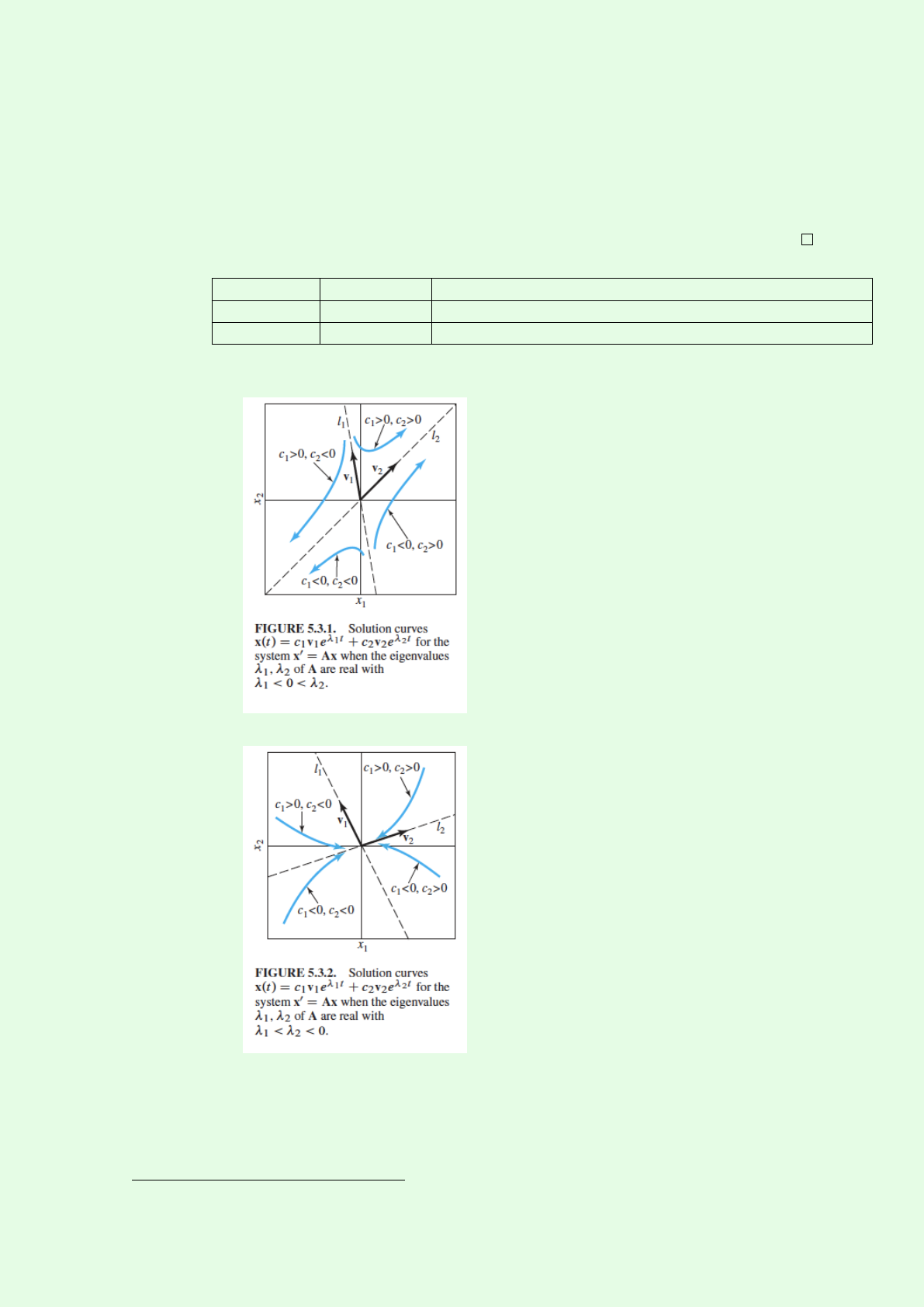
–solution curves
∗saddle point: nonzero distinct eigenvalues of opposite sign
∗Nodes (sink): distinct negative eigenvalues. Origin: improper nodal sink
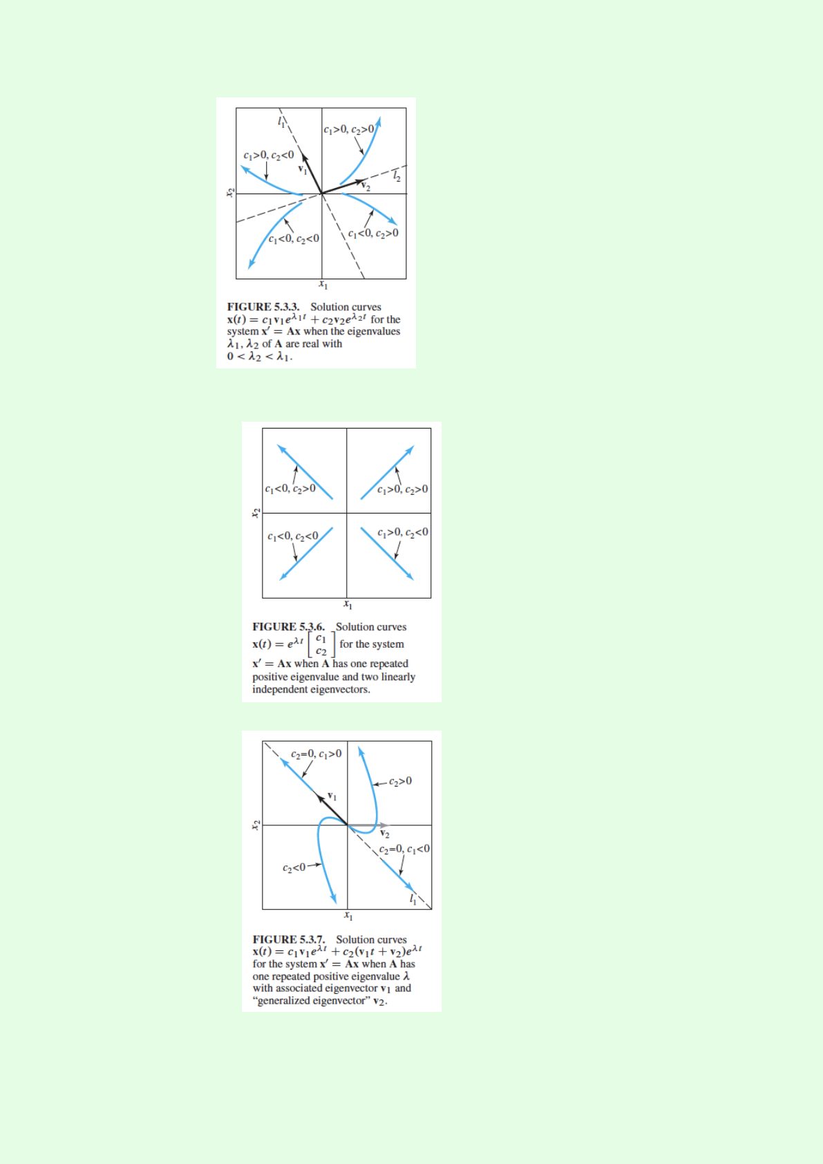
∗Nodes (source): distinct positive eigenvalues. Origin: improper nodal source
1(A−λI)u=v,uis a generalized eigenvector of λ
26
3. AMATH
∗Repeated positive eigenvalue.
·with two independent eigenvectors. Origin: proper nodal source
·without two independent eigenvectors. Origin: improper nodal source
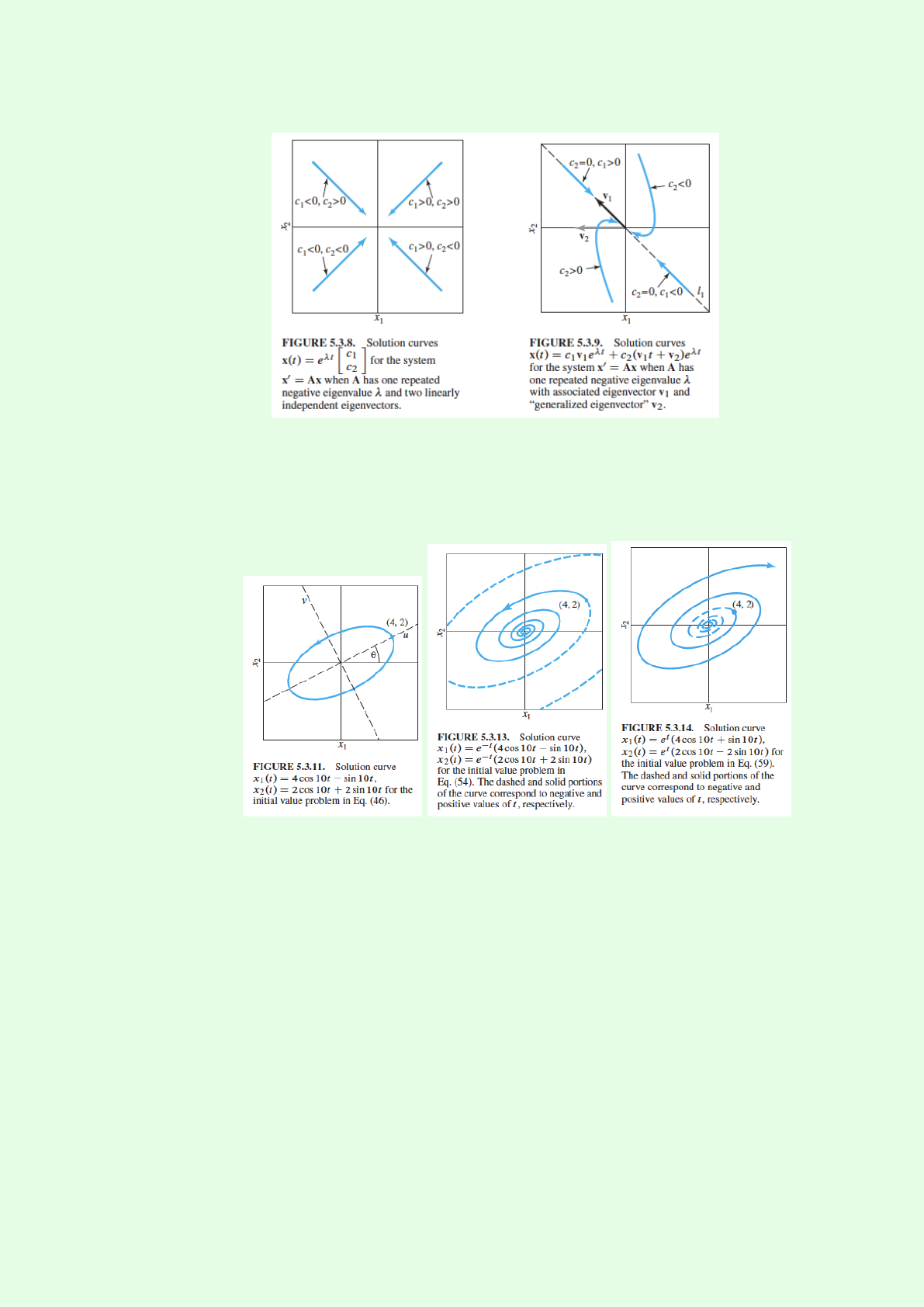
∗Repeated negative eigenvalue.
·with two independent eigenvectors. Origin: proper nodal sink (5.3.8)
27
3. AMATH
·without two independent eigenvectors. Origin: improper nodal sink (5.3.9)
∗Complex conjugate eigenvalues and eigenvectors
·pure imaginary: center
·negative real part: spiral sink
·positive real part: spiral source
–Fundamental Matrix: Φ(t)=x1(t)... xn(t), where x1,...,xn∈Rnare n
linearly independent solutions of x′=P(t)xon I.
●Propositions
∗Every solution x(t)can be written x(t)=Φ(t)cwhere c∈Rn.
∗invertible
∗Φ′(t)=P(t)Φ(t)
●Theorem (Fundamental Matrix Solution)
x′=P(t)x,x(t0)=x0unique solution is x(t)=Φ(t)Φ−1(t0)x0, t ∈I
–Nonhomogeneous Linear Systems: Variation of Parameters. x′=P(t)x+f(t)
x(t)=xh(t)+xp(t)=Φ(t)c+Φ(t)ˆΦ(t)−1f(t)dt
•Laplace Transforms
28

3. AMATH
–Definitions: F(s)=L{f(t)}=ˆ∞
0
e−stf(t)dt
–Unit step: ua(t)=u(t−a)=
0t<a
1t≥a
–exponential order: f(t)≤M ect,for t≥T(2)
–Existence of the Laplace Transform (responsible for final): If fis piecewise con-
tinuous on t≥0and of exponential order as t→∞with constant cin eq(2), then
L{f(t)}=F(s)exists for s>c.
converge absolutely Ô⇒ converges Ô⇒ exists for s>c
Proof
▸Since fis piecewise continuous on t≥0, we can find M≥0such that (2)is
satisfied with T=0. i.e.
f(t)≤M ect,for t≥0
´∞
0Mecte−stdt converges if s>c. Thus using a comparison theorem ´∞
0f(t)e−stdt
converges for s>c.
It follows that ´∞
0f(t)e−stdt converges.
–Gamma function
–Uniqueness of the Inverse Laplace Transform
–Transform of Derivatives L{f′(t)}=sL{f(t)}−f(0)=sF (s)−f(0)
–Corollary
Lf(n)(t)=snL{f(t)}−sn−1f(0)−sn−2f′(0)−...−f(n−1)(0)=F(s)
– Theorem (Laplace Transform of Integrals) responsible for final
If f(t)is piecewise continuous on t≥0and is of exponential order as t→∞(with
constants c, T, M) then
Lˆt
0
f(τ)dτ=1
sL{f(t)}=F(s)
sfor s>c
equivalently:
L−1F(s)
s=ˆt
0
f(τ)dτ
Proof
▸Since fis piecewise continuous, on t≥0.g(t)=´t
0f(t)dt is continuous on t≥0,
g′is piecewise continuous on t≥0.
Further,
g(t)=ˆt
0
f(τ)dτ≤ˆt
0f(τ)dτ≤ˆt
0
Mecτdτ=M
c(ect −1)≤M
cect t≥0
So g(t)is of exponential order as t→∞and we can apply the Theorem on Laplace
Transform of Derivatives.
L{f(t)}=Lg′(t)=sL{g(t)}−g(0)=sL{g(t)} for s>c
Ô⇒Lˆt
0
f(τ)dτ=L{g(t)}=1
sL{f(t)} for s>c
29

3. AMATH
–Translation: Leatf(t)=F(s−a), s >a+c
–differentiation of transforms: L{−tf(t)}=F′(s)
–convolution: L{f(t)∗g(t)}=F(s)⋅G(s)
–translation: L{u(t−a)f(t−a)}=e−asF(s)for s>c
•Appendix
–Method of Successive Approximations: dy
dx =f(x, y), then yn(x)=y0+ˆx
x0
f(t, yn−1(t))dt.
–Existence for Linear Systems. The IVP has a solution on the entire interval I.
x′=P(t)x+f(t),x(a)=b
3.3. AMATH 390
3.3.1. Topics
This course provides an introduction to some of the deep connections between mathemat-
ics and music; mathematics will be used to provide insights into several important aspects of
music. Topics covered include: modelling the acoustics of string, wind and percussion instru-
ments with 1D and 2D partial differential equations, pitch and harmonics, frequency response
and signal sampling with Fourier transforms, and the advantages and disadvantages of various
scales and tuning systems (Pythagorean and just intonation, equal and well temperament).
3.4. AMATH 391
30

4
PMATH
31

5
CO
来到了我最喜欢的部分之一. . . . . . 其实math 2x9 按照课程编码应该算到basic math里面
的,不过鉴于课程内容,我还是把它们都放在这里。
其实CO是两个学科的组合:Combinatorics and Optimization, 组合和优化。两个是有一
定关联的,但还是分开讲了。就像math229/239/249 是introduction to combinatorics,
co227/250/255 是introduction to optimization。当时一开始我没弄清楚这两个的差别,慢慢
等到上了这些课就明白了,在intro这个部分,两门课的联系不是很大。1
1收回刚才说的话......今天(2018.10.22)math249刚讲了introduction to graph theory,然后下午co255就
讲了totally unimodular matrix在bipartite graph等的应用。这个是在advanced讲了,不知道250会不会
讲. . . . . . anyway,我得补习一下什么是matching and perfect matching了。今天(10.23)又讲了cover。
32
5. CO
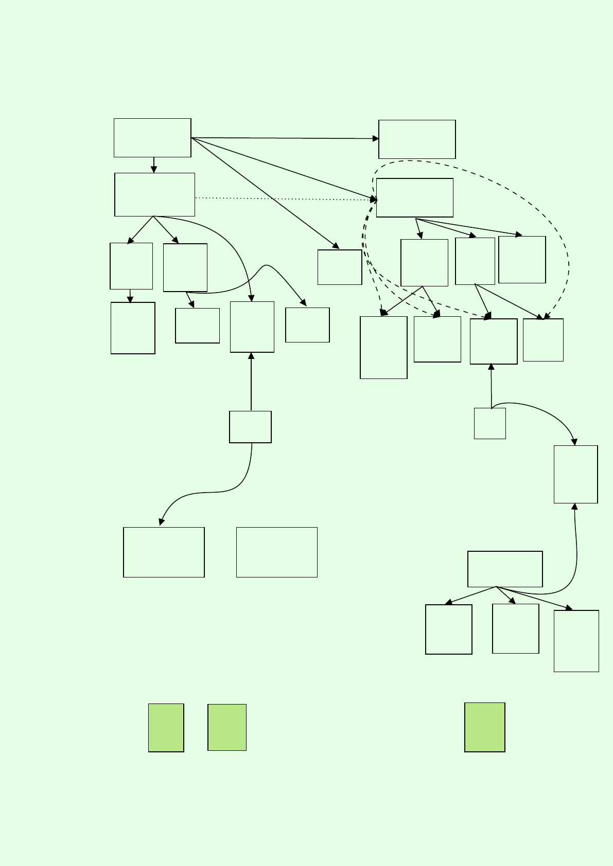
5.1. Overview
linear
algebra
math 239/249
Intro Comb.
co 255 (adv)
co 250
Intro Optim.
330
comb.
enum
Intro Optim.
342
intro
graph
331
coding
351
network
flow
353
discrete
optim.
367
non-
linear
430
algebra
enum
439
topic:
enum
440
topic:
graph
442
graph
444
algebra
graph
446
matroid 450
combin-
atorial
optim.
pmath
346/347
452
int.
optim.
math239/249
co250/255
459
topic:
optim.
453
network
design
454
schdul-
ing
456
intro
game
theory
463
convex
optim.
pmath
351
466
cont.
optim.
471
semi-
definite
optim.
485
Public-Key
Cryptography
487
Applied
Cryptography
33

Part II.
CS
6. Basic 35
6.1. CS135 ........................................... 35
6.1.1. Overview . . . . . . . . . . . . . . . . . . . . . . . . . . . . . . . . . . . . . 35
6.2. CS136 ........................................... 35
6.2.1. Overview . . . . . . . . . . . . . . . . . . . . . . . . . . . . . . . . . . . . . 35
7. Major 36
7.1. CS246 ........................................... 36
7.1.1. Summary . . . . . . . . . . . . . . . . . . . . . . . . . . . . . . . . . . . . . 36
7.2. CS251 ........................................... 37
7.2.1. Topics....................................... 37
7.2.2. Diary ....................................... 37
8. Minor 38
9. Beyond 39
6
Basic
6.1. CS 135
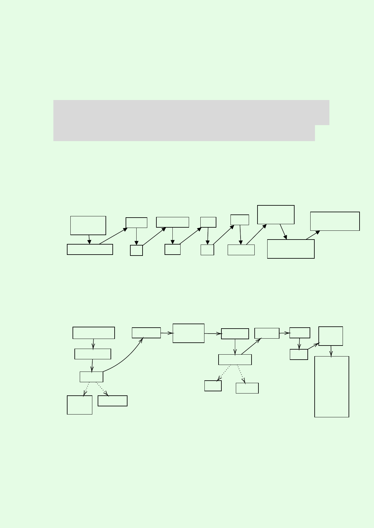
6.1.1. Overview
CS 135
syntax &
semantics
design recipe
struct
list
recursion
sort
tree
bst
local
lambda
generative
recursion
Graph Theory
(just joking...)
CS history
(will be tested)
6.2. CS 136
6.2.1. Overview
Dave’s CS 136 (before Nomair)
Racket→C
imperative
Model
control
flow
memory
pointers modular-
ization !arrays!
efficiency
time space
strings Heap
ADT
linked
list
ADT:
stack
sequence
queue
tree
bst
dictionary
35

7
Major
先说一下CS的big three。452(小火车),444(compiler),488(graphics)。然后
还有一门也很有意思442(Principles of Programming Languages)。大二公认比较难的就
是246,241。大三就是350,349。
然后是算法big three(不知道他们怎么叫),341→466(666)→761。三门课越往后越抽
象。但是很多工作其实用不到很多666,761的算法,因为已经超越到一个境界了. . . . . .
7.1. CS 246
7.1.1. Summary
Note that it is NOT guaranteed that all the topics covered in class are listed here.
•linux shell (bash)
–commands
–globbing
–script
•C++
–basic
–stream
–reference
–overloading
–include guard
–Classes
∗Big 5
∗MIL
∗copy-and-
swap
∗rvalue and
lvalue
∗linked lists
∗encapsulations
–inheritance
–Design patterns
∗UML
∗factory
∗observer
∗singeleton
∗tempalte
∗decorator
∗visitor
∗iterator
∗bridge
•STL
–vector
–stack
–queue
–set
–maps
•idiom
–NVI
–RAII
–piml
–MVC
•Other
–makefile
–debugging
∗gdb
∗valgrind
–exception
–smart ptrs
–vtable, vptr
–cast
–forward declara-
tion
–template
–STL algorithms
∗for each
∗transform
–lambda
36

7. Major
7.2. CS 251
7.2.1. Topics
A mess
7.2.2. Diary
Midterm
2018.10.22
现在终于弄懂了fsm是怎么表示的了。1明天下午4点考,现在真的很慌,因为真的学的
不是很认真,上课也没好好听,现在就在临时抱佛脚。但愿今晚能多复习一点,虽然现在已
经快12点了. . . . . .
突然回想到上次考试前几乎什么都不会的还是phys111,那会还好应付,而且还是期
末。大概是下午4点考,然后从晚上睡不着,大概从凌晨4点一直看到考试前。现在没那么好
应付了,然后我现在还在typesetting L
A
T
EX. . . . . .
Midterm
2018.10.23
转点了,先睡了,早起复习,再git push2一下.
After mid, 感觉凉透了. . . . . . 考试有很多东西感觉没复习到位,就像在学习新知识一
样。回忆起来上次,考前一小时还在复习的是stat231 mid1,不过那个好歹我每节课都去听
了,虽然不是每节课都完全能接受,相比251已经是一个巨大的比例了。上课能大大减少我
在课外花的时间。学长的建议:
前期比较简单,但老师讲的不是很清楚,slide很混乱,后面有点加大难度。但
是这门课没什么逻辑可言,只要把该背的都背了,背好简单的逻辑,上课好好听
课,然后不懂的就去问prof,还是可以熬过这门课的。课还是挺水的。
真的每个人都说这门课水,从某种角度来说确实是这样的。所以还是慢慢学吧,更多的
等再学一段时间再说吧。我其实更希望整个slide能像cs135/136那样明确,有很明确的划分,
有很明显的重点,和考点。ppt给我的感觉就是一个页面一个标题,然后想到啥写啥,该明
确的地方可能一句话带过了。可能是这门课的course coordinator对这门课的维护不是很到
位,只是想着把改覆盖的东西一股脑的丢上去就完了。但愿这门课几年后能有所改变,不过
现在这个教授已经教了好像有好几年了,slide也是一直没有变化。但是她人挺好的,经常会
在课上复习,也会经常回答同学的问题。
After Mid
2018.10.25
成绩出了,果然炸了。前几个学期是比这学期期中简单不少,唉. . . . . . 现在又在讲single
cycle啥的,越来越迷了,slide也越来越乱了. . . . . .
1如果你早就会了,不要嘲笑学长,学长好菜......
2cs246(e)会稍微讲一讲
37

8
Minor
38

9
Beyond
39


10
Music Theory
这个地方是我最喜欢的部分之一。乐理是作曲的基础,也是很多学习乐器中的必修课。
难点肯定是有的,但是学起来不会很枯燥,会很有趣。相比较pmath的课肯定有趣不少,也
不会枯燥的,当然这样比较其实没有太大价值. . . . . .
10.1. MUSIC 111
这门课的title叫做Fundamentals of Music Theory,就是rudiment,非常基本的乐理知
识,是给那些几乎没有基础的人上的,因为它真的是从最基本的音符,五线谱到最后的3和
弦和一些调式为止。可能对于那些从来没学过乐理的人信息量有点大,不过紧跟步伐,认真
做作业还是很好理解内容的。否则的话,我就不建议学乐理了. . . . . .
41

11
Music Ensemble
顾名思义,这个课就是一个小型乐团课,一门课排练一学期,然后最后汇报演出。课号
为MUSIC 116 117 216 217 316 317。上完一门如果还想上下一门就接着上。如果你不想要
学分,不enroll这门课也没有关系。接下来为了让整体格式整齐,我先用FAQ的格式来回答
一些问题。
乐乐乐团团团有有有哪哪哪些些些选选选择择择呢呢呢???
Answer: 根据官网所列的,大概有以下几种
•Chamber Choir 室内合唱团
•Chapel Choir 教堂唱诗班
•University Choir 大学合唱团,全称叫UW Choir
•Vocal Techniques 声乐技巧
•Instrumental Chamber Ensembles 室内乐团
•orchestra@uwaterlo 管弦乐团
•Jazz Ensemble 爵士乐队
•World Music Ensemble: Balinese Gamelan 世界音乐乐团:甘美兰1
如如如何何何才才才能能能进进进入入入这这这些些些乐乐乐团团团呢呢呢?
可以去官网的每个乐 团的网站,里面有详尽的介绍。一般来说都是需要试音的
(audition)。但是对于有些乐团,如果你之前在这个乐团里,下学期如果你还想
来,只需要跟instructor发邮件就好,表明你的意愿。
听听听说说说可可可以以以拿拿拿学学学分分分!!!!!!!!!??????
是的,这门课有0.25学分,而且不用交学费(曲谱的费用除外,当然不会超过100刀
的)。而且这门课是直接可以加在正常的course load 里面的,有些时候加不上去可以
找advisor帮忙调整。当然前提是你enroll了乐团课,然后也过了audition,然后缺勤太
多次,最后会在成绩单上有0.25学分,听来是不是很酷!!
那那那instructor是是是谁谁谁呢呢呢???
每个乐团的我会详尽在后面每个chapter说明,不过他们都是非常有经验的音乐家,一
定会让你好好享受音乐的。
排排排练练练会会会不不不会会会占占占用用用太太太多多多时时时间间间呢呢呢???
如果课程不是非常满的话是不会的,除非你每天像学长一样一堆due,赶mid、quiz等。
一般来说都是每周排练一次,大概3-4小时,具体的时间我会在接下来的章节详尽说
明。
1印度尼西亚历史最悠久的一种民族音乐
42

11. Music Ensemble
一一一般般般在在在哪哪哪里里里排排排练练练呢呢呢???乐乐乐器器器会会会不不不会会会很很很水水水???
不会的. . . . . . 这是我们学校的音乐系组织的乐团,在Renison旁边有个专门的附属学校
就是它—Conrad Grebel College. 一般在那里排练。钢琴都是大三角雅马哈,虽然不是
施坦威,但是也是非常不错的琴,毕竟很多教授都是从Laurier直接过来的,配置当然
不能低。当然像小提琴这种还是自己带啦。
43


12
Science
45

13
Arts
46
