DCG User Manual
User Manual:
Open the PDF directly: View PDF ![]() .
.
Page Count: 5

DCG user manual
McCowan Lab & Fushing Lab
December 28, 2015
Introduction
The R code for data cloud geometry is designed to find multi-level structure in undirected
network data (e.g. edgelist or matrix)[Chen and Fushing 2012]. This multi-level structure is equivalent to
finding community structure, similar to the Girvan-Newman method of finding network modularity [Newman
and Girvan 2004]. This method begins with a similarity matrix, where the entries of the matrix are a measure
of how similar a pair of individuals is with respect to a particular feature. Similarity can be measured based
on grooming relationships (where the strength of grooming per dyad is the measure of similarity) or other
affiliative relationships. Similarity can also be measured using physical traits or genetic code. The data cloud
geometry method involves performing a random walk across all nodes in the network. The probability of
making a step from one node to another is based upon their strength of similarity (i.e. from the value in the
similarity matrix). Such random walks proceed locally, going to and from a local subset of nodes. Once a
subset of nodes has been visited sufficiently (e.g. when one node from that community has been visited at
least 5 times,
m=5
) that node is removed from the network such that it may no longer be visited. Once all
nodes from a community have been removed in this manner, the random walk is forced to jump to another
community. This is how communities are defined – the subset of nodes that is each visited 5 times before
jumping to a new set of nodes is one community.
Installing the package
To install “DCG” package in R, you need to put the package file in your working
directory and run install.packages("./DCG_0.12.tar.gz", repos = NULL, type = "source").
Importing data
DCG package works on similarity matrices. It required the raw data to be an edgelist or
a matrix. DCG is designed for undirected networks, i.e. where the direction of the interaction doesn’t matter.
The function
as.simMat
is used to convert the raw data to a similarity matrix whose values range from 0 to
1 by dividing values in the raw matrix by the maximum value of the matrix. You could assess help for all
functions by running ?functionName, for example, ?as.simMat.
library(DCG)
head(myData)
## Initiator Recipient
## 1 35281 35510
## 2 35281 35510
## 3 35281 36003
## 4 35281 36003
## 5 35281 36003
## 6 35281 36182
Sim <- as.simMat(myData)
Selecting temperatures
Because the random walk proceeds based upon similarity, the range of variance
in similarity will influence how close two nodes appear to be. Therefore, the similarity matrix must be
evaluated at several different ‘temperatures’. For example, the similarity matrix Sim can be transformed to
Simˆ0.5, Simˆ2, Simˆ5, and Simˆ10; the scale of variance within each matrix will allow the random walk to
assess similarity at different levels.
1
To generate several different temperatures, we use the function
temperatureSample
with arguments
start
and
end
which define the lowest and highest temperatuers respectively. The argument
n
defined the
number of temperatures you want to sample, with default being 20. It is recommended to use at least
20-30 different temperatures. Because the number of distinct clusters in the network may be different at
each temperature, and these values can be plotted to note which cluster numbers hold stable for multiple
temperatures (meaning this number is likely a logical division of the network) and which cluster numbers are
ephemeral. The
method
argument of
temperatureSample
allows you to choose how you want to sample the
temperatures: randomly ("random") or based on fixed intervals ("fixedInterval").
set.seed(1)# This ensure we get the same results when sampling temperares. It is not required.
temperatures <- temperatureSample(start = 0.01,end = 20,n=20,method = 'random')
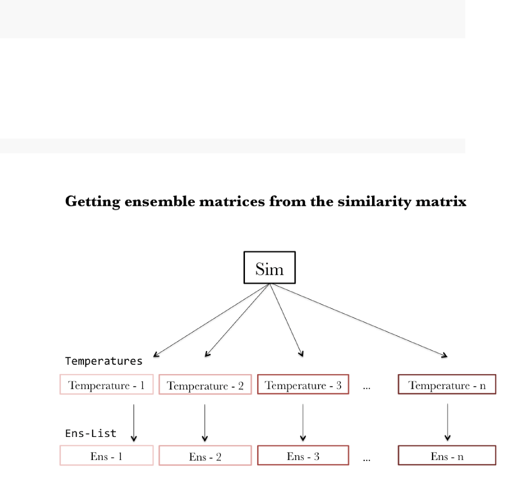
Generating ensemble matrices
The function
getEnsList
involves two steps. It first transforms the
similarity matrix Sim into a list of matrices of different scaled variances based on temperatures. Then it
performed n-times of consecutive regulated random walks (defined by
MaxIt
,
MaxIt = 1000
by default) with
the node removal parameter m (m = 5 by default) on each matrix in the list. It returned a list of ensemble
matrices which is used later on in determining clusters. We used
MaxIt = 5
for illustration purpose only
because it ran quickly.
Ens_list <- getEnsList(simMat = Sim, temperatures = temperatures, MaxIt = 5,m=5)
The process of transforming similarity matrix into a list of ensemble matrices is illustrated in the following
flow chart.
Generating eigenvalue plots
The appropriate number of clusters is determined by examining the
eigenvalue plots. The function
plotMultiEigenvalues
is used to plot eigenvalues corresponding to each
2
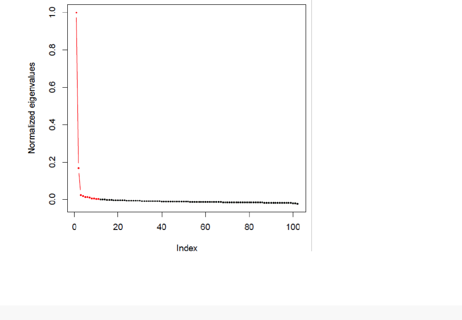
ensemble matrix in the list of ensemble matrix (
Ens_List
). These plots show the approximate number of
clusters. Red dots connected by a red line represent a cluster. The plot below shows two red lines that
connect three red dots on the left, which indicates the presence of two clusters.
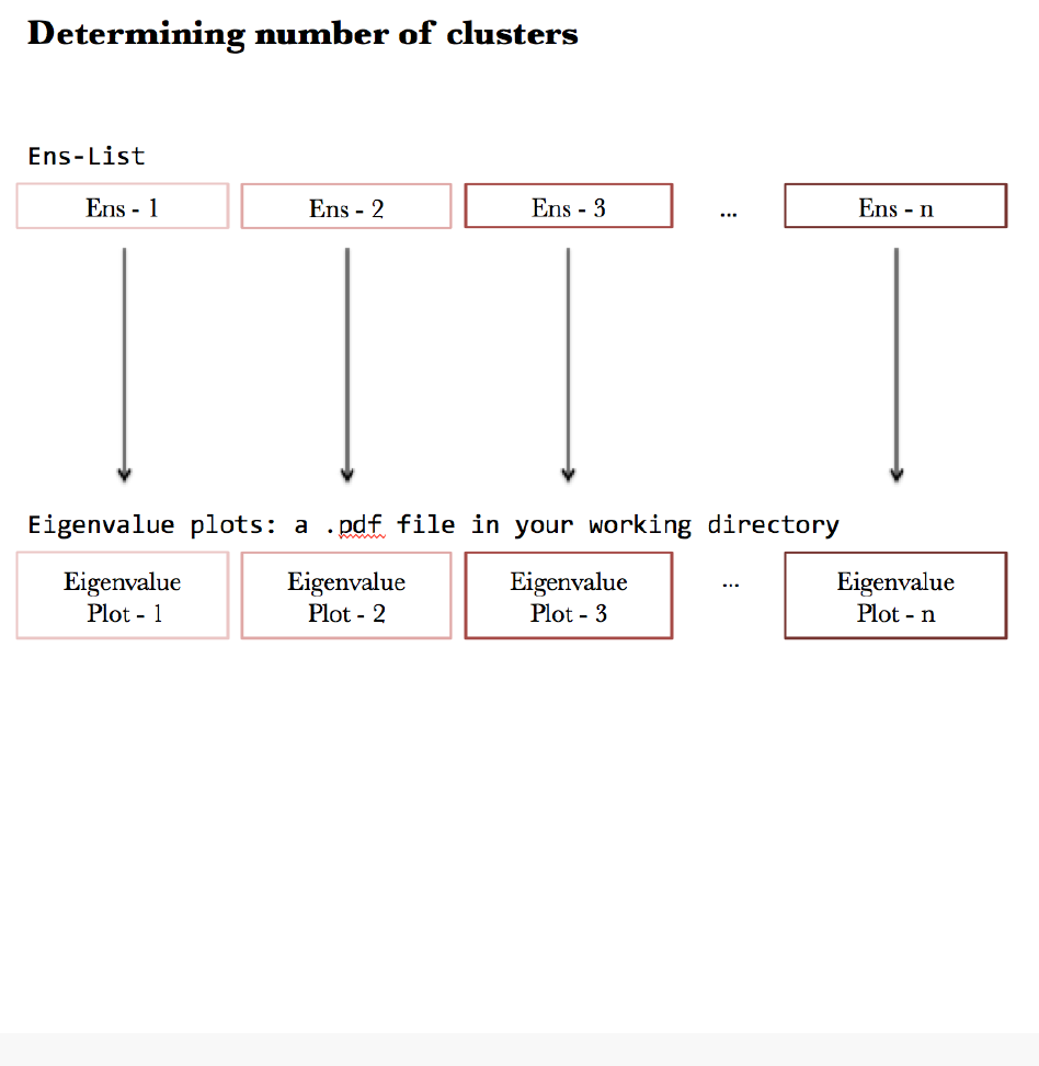
The function
plotEnsList
takes two arguments,
Enslist
and
name
, and exported a .pdf file in your
working directory containing all eigenvalue plots. The argument
Enslist
is the output from the function
getEnsList. The argument name is the name given to the exported .pdf file.
plotEnsList(Ens_list, name = "eigenvalue_plots")
## eigen value plots can be found at './eigenvalue_plots.pdf'
Note, the plots in your “
eigenvalue_plots.pdf
” file look messy because we ran only 5 iterations
(MaxIt = 5) in getEnsList. Try using MaxIt = 1000 and see if your plots are of any difference.
The process generating eigenvalue plots from ensemble matrices is shown in the flow chart below.
3
After inspecting the eigen plots, choose an ensemble matrix (Ens1, Ens2. . . .Ens20) whose number of
clusters appears to be stable across multiple temperatures. For example, if matrices Ens1 – Ens4 all show
two clusters, Ens5 shows three clusters, and Ens6 – Ens20 all show four clusters, then the divisions of two
or four clusters are likely reasonable divisions of your network. Once you know which ensemble matrix to
choose, you’ll need to generate tree plots to examine clusters.
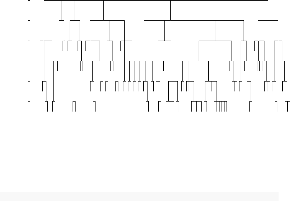
Generating tree plots
To generate tree plot of specific ensemble matrix, you could use
plotTheTree
function. For example, if you want to create the tree plot from only the first ensemble matrix, you’ll need to
run the following codes:
plotTheTree(Ens_list, index = 1)
4
41685
41705
41627
41721 40025
41785
42040 40768
41173 38908
41243
41880
40599
36504
36828 41784
36879
40757 40123
36511
36657
36406
40769 42080
36420
39753
38809
39873 40638
39243
36114
38891 40625
39967
40628
36369
40536
40941
41930
40598
40627
39843
36449
40667 36861
41537
39643
39999
40026 40902
42131
38993
36341
36973
36379
40626 36374
40792
35694
35421
40888
40207
36605
35281
35510
38686
41838 36473
36182
39874
39800
39110
36518
36011
36384 41625
41863
36892
41225
36003
41734 38877
36285
36196
39111 39668
35692
36308
40564
41217
36394
36415
40074
40800
40889 36501
41062
41932
39687
41084
0.0 0.2 0.4 0.6 0.8 1.0
Cluster Dendrogram
hclust (*, "complete")
as.dist(1 − ens)
Height
The function
plotTrees
is used to plot tree plots from a list of ensemble matrices and export the
plots in a .pdf file in your working directory. Its first argument
EnsList
is the output from the function
getEnsList
. Its second argument
name
is the name given to the .pdf file. These plots allow you to examine
the differences between cluster divisions corresponding to each of the ensemble matrix. You could find the
exported .pdf file in your working directory.
plotTrees(EnsList = Ens_list, name = "myTrees")
## tree plots can be found at './myTrees.pdf'
In addition, the Ens matices contains valuable information as well. These values range from 0 to 1 and
represent the proportion of the 1000 iterations in which each pair of nodes appeared in the same cluster. To
examine ensemble matrices of your choice, you could pull the matrix from the list by running
Ens_list[[n]]
,
with n being the index of the matrix you choose. For example, if you want to examine the first one, simply
run
Ens_list[[1]]
. If you want to save the first matrix into an Excel file, run ‘write.csv(Ens_list[[1]],
“myFirstEnsembleMatrix.csv”).
Feel free play with it and let me know what you think! Happy New Year!
5
