Main Rev.dvi Derive Lab Manual
User Manual: manual pdf -FilePursuit
Open the PDF directly: View PDF ![]() .
.
Page Count: 248 [warning: Documents this large are best viewed by clicking the View PDF Link!]
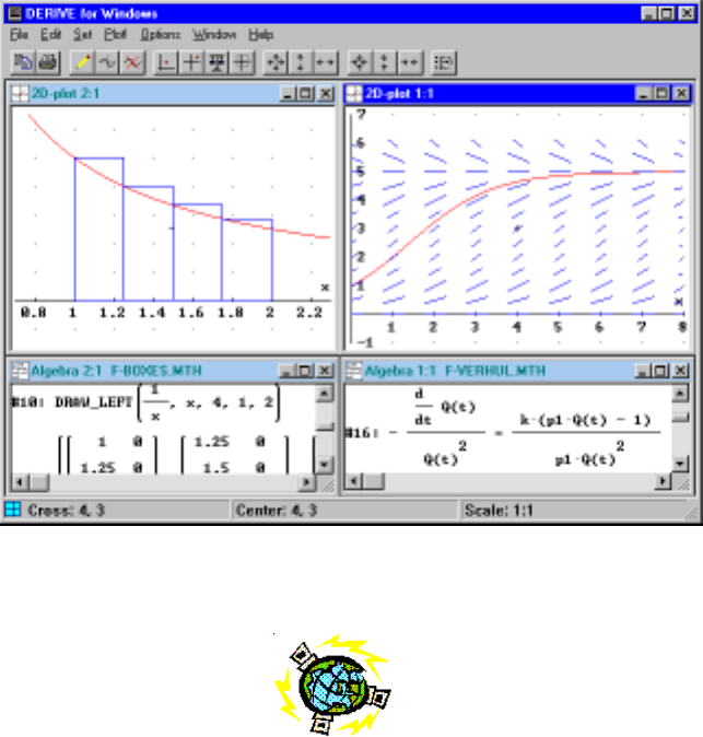
Calculus Concepts
Using Derive For Windows
Ralph S. Freese and David A. Stegenga
Professors of Mathematics, University of Hawaii
R & D Publishing
The procedures and applications presented in this supplement have been
included for their instructional value. They have been tested with care but
are not guaranteed for any purpose. The authors do not offer any warranties
or representations, nor do they accept any liabilities with respect to the
programs or applications.
c
Copyright 2000 by the Authors.
All rights reserved.
No part of this publication may be reproduced, stored in a retrieval system,
or transmitted, in any form or by any means, electronic, mechanical, photo-
copying, recording, or otherwise, without the prior written permission of the
authors.
Printed in the United States of America.
This publication was typeset using AMS-L
A
T
E
X, the American Mathematical
Society’s T
EX macro system, and L
A
T
EX2
ε.
For information on obtaining this book see
http://www.math.hawaii.edu/CalcLabBook/
and to see our class web page containing our syllabus, assignments and gen-
eral information for students see
http://www.math.hawaii.edu/lab/
Honolulu, Hawaii
May 7, 2001
Contents
Preface ix
CalculusReformandComputers ................... ix
HowToTeachFromTheManual................... x
AdviceForTheStudents .......................xiii
SettingUpTheComputerLab ....................xiii
World-WideWebSiteForOurLab .................. xv
0 Introduction and Derive Basics 1
0.1 Overview.............................. 1
0.2 StartingDerive .......................... 2
0.3 EnteringanExpression...................... 3
0.4 SpecialConstantsandFunctions................. 4
0.5 Editing............................... 5
0.6 SimplifyingandApproximating ................. 6
0.7 SolvingEquations......................... 6
0.8 Substituting ............................ 8
0.9 Calculus.............................. 9
0.10Plotting .............................. 12
0.11DefiningFunctionsandConstants................ 14
0.12DefiningTheDerivativeFunction ................ 16
0.13FunctionsDescribedByTables ................. 17
0.14Vectors............................... 18
0.15PrintingandSavingtoaDisk .................. 20
0.16Help ................................ 21
0.17CommonMistakes ........................ 22
iii
1 Curve Sketching 25
1.1 Introduction............................ 25
1.2 WorkingwithGraphs....................... 26
1.3 ExponentialvsPolynomialGrowth ............... 29
1.4 LaboratoryExercises ....................... 32
2TheDerivative 37
2.1 TheDerivativeasaLimitofSecantLines............ 37
2.2 LocalLinearityandApproximation ............... 41
2.3 LaboratoryExercises ....................... 44
3 Basic Algebra and Graphics 47
3.1 Introduction............................ 47
3.2 FindingExtremePoints ..................... 47
3.3 Max-MinProblems ........................ 49
3.4 ZoomingandAsymptotes .................... 50
3.5 LaboratoryExercises ....................... 52
4 Curve Fitting 55
4.1 Introduction............................ 55
4.2 FittingPolynomialstoDataPoints ............... 55
4.3 Exponential Functions and
PopulationGrowth ........................ 60
4.4 Approximation Using Spline Functions∗............ 61
4.5 LaboratoryExercises ....................... 63
5 Finding Roots Using Computers 69
5.1 Introduction............................ 69
5.2 Newton’sMethod......................... 69
5.3 WhenDoTheseMethodsWork ................. 73
5.4 Complex Numbers, Fractals and Chaos∗............ 78
5.5 Bisection Method∗........................ 86
5.6 LaboratoryExercises ....................... 89
6 Numerical Integration Techniques 95
6.1 Introduction............................ 95
6.2 AnExample............................ 96
6.3 Theorem on Error Estimates∗..................100
6.4 More on Error Estimates∗....................102
6.5 Deriving Simpson’s Rule∗....................104
6.6 LaboratoryExercises .......................105
7 Taylor Polynomials 109
7.1 PolynomialApproximations ...................109
7.2 Examples .............................110
7.3 Taylor’sTheoremwithRemainder................115
7.4 ComputingtheSineFunction ..................116
7.5 ComputingtheExponentialFunction...............118
7.6 Taylor Expansions About x=c.................120
7.7 IntervalofConvergence......................122
7.8 LaboratoryExercises .......................124
8 Series 131
8.1 Introduction............................131
8.2 GeometricSeries .........................132
8.3 Applications............................133
8.4 Approximating Infinite Series ..................137
8.5 LaboratoryExercises .......................147
9 Approximating Integrals 153
9.1 Introduction............................153
9.2 TheBasicErrorEstimate ....................154
9.3 The Logarithm Series . ......................154
9.4 AnIntegralApproximation....................156
9.5 LaboratoryExercises .......................158
10 Polar and Parametric Graphs 161
10.1Introduction............................161
10.2PolarCoordinates.........................161
10.3RotatingPolarCurves ......................164
10.4ComplexNumbers ........................166
10.5ParametricCurves ........................167
10.6LaboratoryExercises .......................172
11 Differential Equations 177
11.1Introduction............................177
11.2Examples .............................177
11.3ApproximationofSolutions ...................182
11.4 Euler’s Approximation Method∗.................186
11.5LinearFirstOrderDifferentialEquations............187
11.6LaboratoryExercises .......................191
12 Harmonic Motion 195
12.1Introduction............................195
12.2Examples .............................196
12.3SolvingLinearDifferentialEquations ..............198
12.4SystemsofDifferentialEquations ................206
12.5LaboratoryExercises .......................211
A Utility Files 217
A.1 TheFunctions...........................218
A.2 Listings of the Utility Files ....................223
B DfW Version 5 227
B.1 What’sNewInDfW5.......................227

List of Figures
Part of M206L World-Wide Web page . . . ...........xvi
0.1 Authorentryformwithspecialsymbols............. 4
0.2 Using the Calculusmenu..................... 10
0.3 Examples of Limits, Products and Sums ............ 11
0.4 Using Plotforgraphics...................... 14
0.5 Examples of Declare, Simplifyandapproximating ....... 15
0.6 Functionsdefinedbytablesofexpressions ........... 18
0.7 Using the Calculus/Vectorcommand .............. 19
1.1 Using vector toplotseveralgraphs............... 26
1.2 The functions x4and ex..................... 30
1.3 The functions x4and ex,rescaled ................ 31
2.1 Secantlinesapproximatingthetangentline........... 38
2.2 Approximatingderivativesusingthedifferencequotient.... 43
3.1 Findingcriticalpoints ...................... 48
3.2 Zoomingtofindthehorizontalasymptote ........... 51
4.1 Fittingapolynomialtodatapoints............... 57
4.2 Thealgebrabehindfittingpolynomialstodatapoints..... 59
4.3 Approximationusingsplinefunctions.............. 64
5.1 Newton’s method for finding roots ................ 70
5.2 Eachiterationgivestwiceasmanydigits ............ 73
5.3 Newton’smethodwithcomplexstartingpoint ......... 82
5.4 Chaos ............................... 83
5.5 Basins of attraction of x3−1inthecomplexplane ...... 84
5.6 Bad Newton starting points for x3−3x=0inthecomplex
plane................................ 85
vii
5.7 Basins of attraction for x3−3x=0............... 86
5.8 Bisection method for finding roots ................ 88
6.1 Approximatingln2withleftendpointmethod ......... 98
6.2 Rectangularvstrapezoidalapproximation ...........100
6.3 Trapezoidandmidpointruleforconcavefunctions.......104
7.1 BasicexamplesofTaylorpolynomials..............111
7.2 Taylor polynomials for sin x...................113
7.3 Approximating sin xwithitsTaylorpolynomials........114
7.4 Approximatingsin100within6decimals ............118
7.5 Approximating e5within6decimals...............120
7.6 Taylor expansion of the logarithm function ...........122
7.7 Graphically finding the radius of convergence ..........123
8.1 Ratiotestexample ........................140
8.2 Thegeometricestimateusedintheintegraltest ........143
8.3 Summing the series P1/i2....................146
9.1 UsingTaylorseriestoapproximateintegrals ..........158
10.1PolarCoordinates.........................162
10.2Plottingpointsinpolarcoordinates...............163
10.3 Showing that y=1/x isahyperbola ..............165
10.4 Parametric plot of a semi-ellipse . ................168
10.5Moreparametricplots ......................171
10.6 The cycloid curve and the rolling wheel .............175
11.1SlopefieldfortheNewtoncoolingproblem...........183
11.2AgraphofaVerhulstpopulationcurve.............185
11.3Euler’smethodforapproximatingsolutions...........187
11.4SolvingNewton’scoolingequation................189
12.1 The pendulum ...........................197
12.2Springmotionstartingatdifferentpositions ..........203
12.3 Under Damped Oscillations . . . ................205
12.4 Euler and the 2nd Runge-Kuttamethods ............208
12.5RabbitsandFoxes ........................210
12.6 Pendulums . . ...........................212
B.1 ThenewlookofDfW5......................228
Preface
Calculus Reform and Computers
This lab manual is the result of more than a decade of experimenting with the
use of computers as an enhancement to learning calculus. In the beginning we
were working with Albert Rich and David Stoutemyer, founders of the Soft
Warehouse Inc. here in Honolulu, and their muMATH computer program.
This program was the precursor to Derive. It was a PC-version of the big
mainframe computer program macsyma. They could symbolically integrate,
differentiate and do other calculus type problems. There were no menus or
graphics at that time, so we developed a small enhancement program which
included these features and distributed it to several university mathematics
departments in the United States and elsewhere.
This effort took place in the middle to late 1980’s. Since then, there has
been a national movement to include computers in the teaching of calculus
and in fact to reform the teaching of calculus by discussing new ideas using
not only the traditional algebraic approach but also by exploring the ideas
graphically and numerically. In response to this movement, new computer
programs were written such as Derive,Mathematica and Maple.Com-
puter calculus labs were created at most universities and colleges to take
advantage of this new technology and to start experimenting with new ideas
for teaching calculus.
Calculus textbooks are now starting to include substantial supplements
on computer experiments and some have been completely rewritten to involve
computers as an integral component of the course. It is hard to say right now
what calculus instruction will look like in ten years but there is no doubt that
computers are completely changing the teaching approach to certain topics
with intensive use graphics or computation components.
In this book we try to highlight those areas of calculus, which are best
ix
studied by using the computer to explore, to visualize and to suggest further
directions to study. We also try to convey that studying calculus can be
fun to do and that it is very important in understanding other topics in
mathematics and other fields.
This manual uses Derive because of its ease of use. Students enter ex-
pressions by filling out a form which includes special mathematical symbols
such as πand ∞. Then, at the click of a button one can differentiate, inte-
grate or plot the expressions. This calculator type interface is very easy for
students to learn and after about 15 minutes of introduction during the first
visit to the lab the students are ready to start using the program. There
are also functions that are equivalent to the various buttons and menu com-
mands. Knowing these functions enables one to write programs that extend
the power of Derive. We will give numerous examples demonstrating both
the simple calculator mode and the powerful programming language.
HowToTeachFromTheManual
We have been incorporating computers in our calculus curriculum for over a
decade. Originally, this was done as an experimental section of our regular
calculus classes and was taught by the two of us. But for the last four years
this computer component has been a required lab course for all of calculus
students. The typical class session starts with a discussion from the lecturer,
who uses both the chalkboard and the projected image of a computer to
present the material, which includes a combination of theory along with
computer graphics and computations. One of the students has his computer
monitor projected on a screen for the whole class to see and follows the
instructions given by the lecturer. The rest of the class follows along on their
own computers and consults the screen to make sure that they are doing it
correctly. Each class session allows for a time period after the lecture during
which the students can work on their assignments and ask questions.
Each course will include several labs involving selected topics from calcu-
lus and differential equations. Typically, first semester students do the first
several chapters focusing on graphing, properties of the derivative and per-
haps a brief introductory treatment of Chapter 6 on approximating definite
integrals. Second semester students generally do 7-8 chapters covering inte-
gration, series and differential equations. Second year students would study
parametric curves, series and differential equations more thoroughly. There
is also a good deal of extra material such as an introductory treatment of
chaos theory and complex dynamics, approximations with spline functions,
and the Runge-Kutta approximation methods which can be added when-
ever appropriate. Several of the chapters would require more than one lab
depending on the level of understanding that is desired.
The material in each chapter is for the most part self-contained and does
not rely on any of the others. This allows considerable flexibility in planning
a syllabus. For example, while we recommend reading the first four chapters
in order, this is not necessary. Chapter 5 and Chapter 6 can be done in either
order; however, Chapter 6 does use some material from Chapter 4 to derive
the algorithm for Simpson’s Rule.
Chapter 7 on Taylor polynomials and Chapter 8 on Series can also be
done in either order; however, Chapter 9 assumes a knowledge of those two
chapters. Likewise, Chapter 12 on harmonic motion assumes that the student
has read Chapter 11 on differential equations.
•Chapter 1 covers basic graphs and manipulation of graphs by trans-
lations and rescalings. A graphical comparison of exponential growth
with polynomial growth is a prelude to later discussions of population
growth models.
•Chapter 2 covers the local linearity of the derivative using computer
zooming techniques and the limit of secant lines. One of the exercises
requires approximating a function by its tangent line.
•Chapter 3 is a further discussion of the derivative including critical
point theory, inflection points and max-min problems.
•Chapter 4 shows how to fit a polynomial through a set of data points.
This includes a discussion of how to solve a system of linear equations
using the computer. A more advanced discussion on spline functions is
given in the last section. There are exercises which explore the growth
in the US population, over the last two centuries, viewed as empirical
data.
•Chapter 5 covers the Newton method for finding real roots to equations.
Emphasis is given to both the speed at which the method converges and
the care which is required in the selection of the starting point. There
is also a brief review of the algebra of complex numbers and applica-
tions of Newton’s method to finding complex roots to polynomials. A
discussion of fractals and chaos is given toward the end of the chapter.
•Chapter 6 discusses the various methods for numerically approximating
integral and a comparison of the rates of convergence. The last section
shows how to derive Simpson’s method using the tools from Chapter 4.
•Chapter 7 introduces Taylor polynomials as a means of approximating
trigonometric and exponential functions. Pattern recognition is used to
suggest infinite series representations. Emphasis is given to the analysis
of the error and how many terms are needed to achieve a given accuracy.
Graphical methods are used to discuss the interval of convergence in
an elementary manner.
•Chapter 8 introduces infinite series and gives several applications of the
geometric series. There are discussions of the error that results when a
series is approximated by its partial sums.
•Chapter 9 combines the techniques of both Taylor polynomials and
infinite series to discuss on the approximation of integrals using Taylor
polynomials. As an application, the representation and approximation
of the logarithm function is studied.
•Chapter 10 shows how to plot polar and parametric curves. There are
discussions of rotations of graphs, speed of particles traveling along a
parametric curve and some connections with complex numbers.
•Chapter 11 is a basic treatment of first order differential equations.
Population growth models and Newton cooling are used as motivating
examples. Graphical representations using slope fields and the Euler
approximation method are discussed.
•Chapter 12 discusses second order linear differential equations with
constant coefficients such as the mass-spring system. The chapter ends
with a treatment of the Runge-Kutta method of approximation.
Advice For The Students
The students should read the designated chapter in the manual and then
complete the laboratory exercises for that chapter. Some of the sections are
marked with a star which means that they are either optional or a little more
advanced than the other sections. For example, many of the theorems and
proofs that provide rigorous explanations for the material in these sections
can be found in the starred sections. This same principle applies to the
starred exercises, which generally contain problems that are a little more
involved than the others or contain material that is not generally presented
in a first year calculus course.
We recommend reading the un-starred sections first and skimming over
the starred sections before attempting the exercises. After becoming more
familiar with the material by working several exercises, the starred sections
should be more accessible and interesting.
The text material and the labs assume that you are using the computer
software Derive for Windows which we denote by DfW. As mentioned
above, it is easy to learn how to use Derive because its design reminds you
of an elaborate calculator. The buttons and nested menus at the top of the
screen lead the student along.
Chapter 0 contains a tutorial and reference on using Derive.Thereare
many interesting features that will be explored in the labs. In the beginning
we recommend that the students just skim over this chapter, while at the
computer, so that they can do the basics, such as entering an expression,
graphing it and so on. As the students progress through the text there will
be frequent references to this chapter, so we recommend that they go back
over the material that was skimmed the first time.
Setting Up The Computer Lab
Our computer lab has modified the basic installation of DfW in three ways.
First of all, we added a subfolder which contains all of the files referred to in
the manual and make this folder the default directory (see your DfW manual
for doing this). These files include the Derive files which correspond to
every demonstration figure in the manual. For example, in Figure 1.2 on
page 30 there is a reference to the file F-EXP1.MTH which can be seen by
looking at the header stripe for the algebra window in the figure. Loading the

file F-EXP1 (the extension is unnecessary) allows the students to practice on
the material that is being explained. The demonstration files are completely
optional but the students occasionally find them quite useful. They can be
downloaded from our web site.
In addition to these optional files there are two required Derive files
which implement the manual’s utility functions. These are ADD-HEAD and
ADD-UTIL. We recommend that the students start each new lab session by
loading the small file ADD-HEAD and then using the File/Save Asmenuto
save this file using a new name such as H:LAB1. Here we have designated the
student’s network harddrive as the H: drive. The ADD-HEAD file quietly
loads the definitions, from the ADD-UTIL file, of all the utility functions that
are used in the manual. For example, in Chapter 6 we explain how to enter
from scatch and use the formula for the left endpoint method in numerical
integration. But for the exercises and further discussion we introduce special
utility functions such as LEFT, TRAP and SIMP that have the formula
built-in. This allows the instructor to either emphasize the programming
features or to simply demonstrate them and then allow the students to use
a ready-made formula for the exercises.
Thelastchangewemakeisusethemixed output mode. This is done by
selecting the menu option Declare/Algebra State/Output and then changing
the notation option to mixed. With this option set then decimals are saved
as decimals instead of being converted to fractions which is Derive’s default
mode. When exiting Derive after making this change you will be asked to
save the State Variables. You should accept this change for it then makes an
entry in the initialization file DFW.INI.
However, after everything is set up and working properly we recommend
setting the permissions on the DFW folder to read and execute only. This
will prevent the students from saving their lab files to the default directory
(the one containing ADD-HEAD and the demonstration files) which is a
common problem. In addition, this will prevent the students for changing
the file DFW.INI that contains the basic settings mentioned above.
These restrictions are easily done if you are using the Windows NT work-
station operating system with the NTFS file system or if you are using a
network installation of DfW. If you have Derive installed locally on a Win-
dows 95/98 PCs then you should probably download the three files: ADD-
HEAD, ADD-UTIL and DFW.INI every time the student logs onto the sys-
tem. This can be done with a login script.
See Appendix A for a more detailed explanation of all of these issues.

The latest versions of these files are available for downloading from our
web site at: http://www.math.hawaii.edu/CalcLabBook/
World-Wide Web Site For Our Lab
We maintain a web site on our lab for the students here at the University of
Hawaii. This includes course information such as lab schedules and assign-
ments but it also has several pages of general interest. The web address is
http://www.math.hawaii.edu/lab/
There is a link to M241, which is our first semester Calculus class, and
M242 is the second semester class. For example, let’s suppose that we click
on the M242 button.
You will notice that there are many links on the left border that will
take you to different parts of the site. Just click on any of the underlined
words and a new page will be displayed with addition information on that
topic. For example, by clicking on the Utility Functions link you go to a
page where the utility functions which we have added to the system, in the
ADD-HEAD and ADD-UTIL files, are explained. Scrolling down there are
explanations of functions like LEFT and SIMP which can be used for doing
numerical integration in Chapter 6. The latest version of these files can also
be downloaded from this web page.
The picture on the following page shows part of our web site. It is a
demonstration of Newton’s method that is explained in Chapter 5. You can
flip back and forth between the web pages and Derive while you are reading
the online material. In the Window’s desktop, this is simply a matter of
clicking the DfW button on the task tray or you can use cascading windows.
Another quick method is to press and hold the Alt key and then press the
Tab until DfW is selected. The same procedure will take you back to the
browser. You may have to experiment with this or ask a PC-friend for help,
but it works very nicely and allows you to view the web page and then flip
to the Derive screen and practice.
Ralph S. Freese
David A. Stegenga
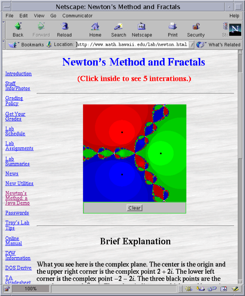
Part of our web page
Chapter 0
Introduction and Derive Basics
0.1 Overview
In this course you will learn to use the computer mathematics program De-
rive. This program, along with others such as Maple and Mathematica,
are very powerful tools for doing calculus. They are capable of doing exact
computations with arbitrary precision. This means that you can work with
numbers of any size or number of decimal places (most spreadsheets only
use 10-20 significant digits). These programs can simplify mathematical ex-
pressions by canceling common factors and doing other algebraic operations.
They can do symbolic calculus such as differentiation and integration, solve
equations and factor polynomials. When possible these programs solve these
problems exactly and when exact solutions do not exist, such as factoring
high degree polynomials or integration of some non-polynomial expressions,
then numerical methods are applied to obtain approximate results.
Probably the most important numerical technique is to graph and com-
pare functions. This will be a key feature of the labs. Typically we will
explore a topic by first graphing the functions involved and then trying to
do symbolic calculus on them using the insight gained from the picture. If
the problem is too difficult algebraically we then try numerical techniques
to gain further insight into the problem. It is this combination of graphics,
algebra and numerical approximation that we want to emphasize in these
labs.
Calculus is a hard subject to learn because it involves many ideas such as
slopes of curves, areas under graphs, finding maximums and minimums, ana-
1

2CHAPTER 0. INTRODUCTION AND DERIVE BASICS
lyzing dynamic behavior and so on. On the other hand, many computations
involve algebraic manipulations, simplifying powers, dealing with basic trig
expressions, solving equations and other techniques. Our goal is to help you
understand calculus better by concentrating on the ideas and applications in
the labs and let the computer do the algebra, simplifying and graphing.
Another important goal of the lab is to teach you a tool which can used
from now on to help you understand advanced work, both in mathematics
and in subjects which use mathematics. There are many features such as
matrices and vector calculus which we will not discuss but can be learned
later as you continue with your studies in mathematics, physics, engineering,
economics or whatever. Any time you have a problem to analyze you can
use the computer to more thoroughly explore the fundamental concepts of
the problem, by looking at graphs and freeing you from tedious calculations.
This chapter contains a brief introduction on how to use Derive.We
suggest you sit down at the computer and experiment as you look over the
material. Derive is very easy to learn thanks to its system of menus. The
few special things you need to remember are discussed below and can also
be found using the help feature in Derive.
This manual assumes that you will be using Derive for Windows (DfW)
Version 4. The recently released DfW Version 5 (DfW5) can also be used but
there have been some changes to the menus and buttons that we try to point
out using footnotes. See also Appendix B for more information on Version 5.
0.2 Starting Derive
To start DfW look for
on the Windows desktop and double click it.
In DfW we use the drop down menus on the top strip or else click an
appropriate button. If you move the cursor onto a button and leave it there
a brief explanation of what the button does will appear. All possible options
can be found on the drop down menus but the buttons provide a quick way
of doing most common operations. For example, to enter a mathematical
expression you click the button which represents a pencil. Alternately,

0.3. ENTERING AN EXPRESSION 3
you click the Author menu and then click Expression. In this manual we will
indicate that two step combination by simply Author/Expression.1
In this manual we use a typewriter like font, eg., a(b + c) to indicate
something you might type in. We use a sans serif font for special keys on the
keyboard like Enter (the return key) and Tab.MostofDerive has easy to
use menus and buttons which we will described below. It only takes a few
minutes of practice to become capable at using DfW. You can skim over this
section now or then come back to it later as the need arises.
0.3 Entering an Expression
After clicking the button, you enter a mathematical expression, i.e., you
type it in and then press the Enter key or else click OK. You enter an expres-
sion using the customary syntax: addition +-key, subtraction --key, division
/-key, powers ^-key and multiplication *-key (however; multiplication does
not require a *, i.e., 2x is the same as 2*x). Derive then displays it on the
screen in two-dimensional form with raised superscripts, displayed fractions,
and so forth. You should always check to make sure the two-dimensional
form agrees with what you thought you entered (see Editing below to see
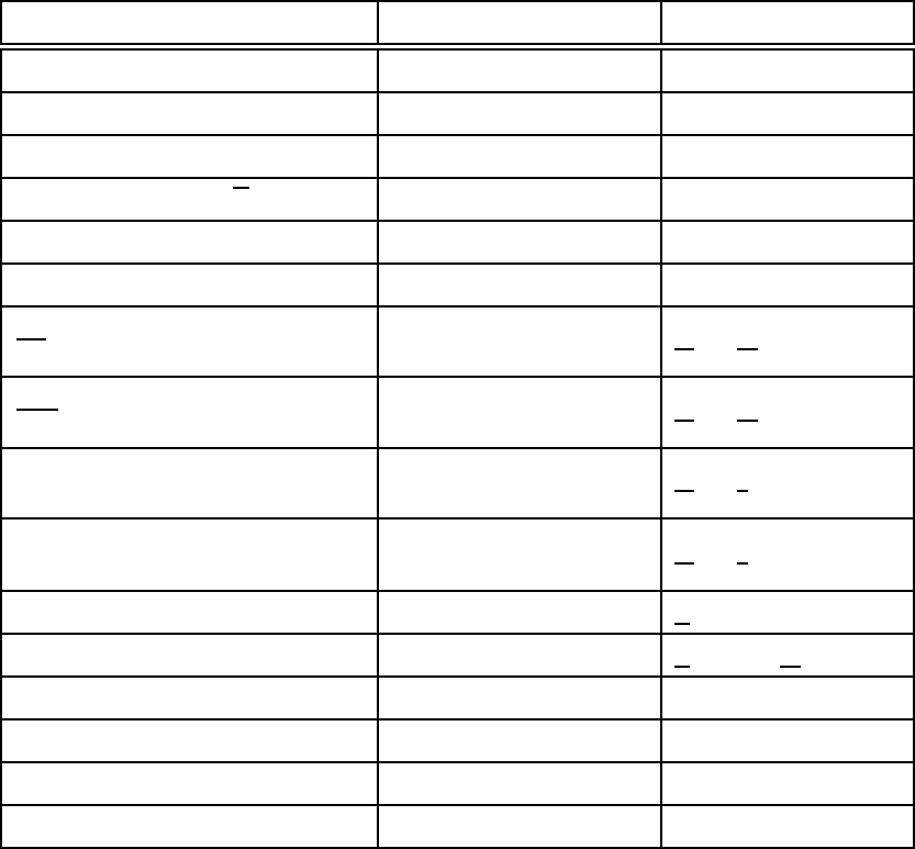
how to correct typing errors). Table 1 gives some examples.
If you get a syntax error when you press enter (or click OK) the problem
is usually mismatched parentheses. Carefully check that each left parenthe-
sis is matched with a corresponding right one. Also be careful to use the
round parentheses and not the square brackets since they are used for vector
notation; see Section 0.14 on page 18.
Note from (3) and (4) and from (6) and (7) of Table 1 that it is sometimes
necessary to use parentheses. Also note in (8), that to get the fraction you
want, it is necessary to put parentheses around the numerator and denomi-
nator. See what happens if you enter (8) without the parentheses. Also try
entering some expressions of your own. There are two ways to enter square
roots. One way is using the 0.5 or 1/2 power as in (9) and the other is to
enter the special square root character as in (10).
1In DfW5, authoring has been improved and simplified but the above methods still
works. See Appendix B for details.
4CHAPTER 0. INTRODUCTION AND DERIVE BASICS
Table 1:
You enter: You get:
(1) 25 25
(2) x^2 x2
(3) a^2x a2x
(4) a^(2x) a2x
(5) sin x sin(x)
(6) sinax sin(a)x
(7) sin(a x) sin(ax)
(8) (5x^2 - x)/(4x^3 - 7) 5x2−x
4x3−7
(9) (a + b)^(1/2) (a+b)1/2
(10) √(a+b) √
(a+b)
0.4 Special Constants and Functions
In DfW all the special characters are on the author form and you just click
on them to enter them in an expression. There are also key equivalent such
as pi for πand #e for Euler’s constant2ewhich is displayed by Derive as
ˆe.
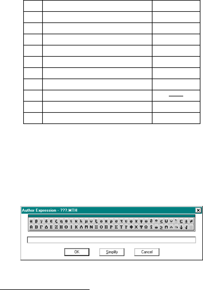
Figure 0.1: Author entry form with special symbols
2Leonhard Euler (oi’lar)wasa18
th century Swiss mathematician.

0.5. EDITING 5
It is important to distinguish ˆefrom just e.Derive takes eto just be some
constant like a.
To get the functions tan−1x= arctan(x), sin−1x=arcsin(x), etc., you
type atan x and asin x. If you forget how a particular function is entered
just use the Help menu.
0.5 Editing
Suppose that you author an expression, click OK and then observe that you
typed something wrong. To enter a correction you would click the
button again and then click the right mouse button.Amenuopensupwith
several options, one of which is Insert Expression.3Clicking this option puts
the highlighted expression of the current algebra window into the author box.
You edit this expression as you would in any windows program. That is you
position the cursor either by clicking or using the arrow keys. By highlighting
or selecting a subexpression and typing you replace the selected text with the
new text. One can use the Edit/Copy Expressions4menu or Cntl-C to place
a highlighed expression from any algebra window onto the clipboard and
then in the authoring form right click the mouse and click Paste to copy the
clipboard contents. The simpler method of just right clicking the mouse and
then Insert is the best way as long as your expressions are in a single window.
There is also an option for inserting the expression enclosed in parenthesis.
A key equivalent to these techniques is to press either the F3 or the F4 key.
You select or highlight expressions in the algebra window by clicking on
them. For more complicated expressions you can click several times until the
desired subexpression is selected. This requires a little practice but you can,
for example, select the x+ 2 part of the expression sin x2
x(x+2) by clicking on
it 4 times (each click takes you deeper into the expression).
The displayed expressions are numbered. You can refer to them as #n.
So, for example, with the expressions in Table 1, you could get sin(x)/x2by
Authoring #5/#2.
When you start Derive it is in a character mode. This means it treats
each single character as a variable, so if you type ax Derive takes this to
3In DfW5 you click in the Author box first and then right click Insert. A new feature
is to right click the erroneous expression, choose Edit and press the Enter key after you
make the corrections.
4This is simply Copy in DfW5.

6CHAPTER 0. INTRODUCTION AND DERIVE BASICS
be atimes x. This mode is what is best for calculus. The exception to this
are the functions Derive knows about. If you type xsinx,Derive knows
you want xsin(x). Actually on the screen you will see xSIN(x): Derive
displays all variables in lower case and all functions in upper case.
0.6 Simplifying and Approximating
After you enter an expression, Derive displays it in two-dimensional form,
but does not simplify it. Thus, integrals are displayed with the integral sign
and derivatives are displayed using the usual notation. To simplify (that is
evaluate) the expression, click the button. The alternate method is
the Simplify/Basic drop down menu.
Derive uses exact calculations. If you Author the square root of eight,
√8 will be displayed in the algebra window. If you simplify this, you get
2√2. If you want to see a decimal approximation, you click the but-
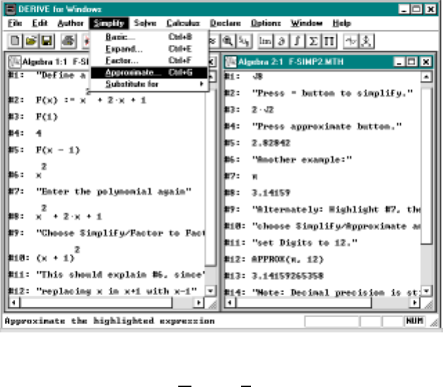
ton. See Figure 0.5 on page 15 for several examples. The number of decimal
places used can be changed to any number. You choose Declare/Algebra
State/Simplification5and then reset the value of Digits on this form. This re-
sults in a change in the State variables for Derive and you will be prompted
on whether you want to save these changes when you exit the program. Since
you shouldn’t change files on the system directory you click No.
An alternate way to do this for a single computation is to select the
Simplify menu. Then, choose Approximate from the drop down menus and
enter a new number of decimals. The only trouble with this method is that
if you save your file the extra decimals will be ignored unless you set the
Output decimal places appropriately. When you open the file later you will
also need to reset the Output decimal place accuracy.
0.7 Solving Equations
An important problem is to find all solutions to the equation f(x)=0. If
f(x) is a quadratic polynomial such as x2−x−2, then this can be done using
the quadratic formula or by factoring. To factor you choose Simplify/Factor
from the menu bar and click Simplify on the entry form. The result is
5In DfW5 you choose Declare/Simplification Settings.
0.7. SOLVING EQUATIONS 7
Table 2: Special Keys and Function Names
Expression/Action Type: Menu:
e#e Author entry form
πpi Author entry form
∞,−∞ inf,-inf Author entry form
The square sign: √xsqrt(x) Author entry form
ln x,log
bxlnx,log(x, b)
Inverse trigonometric functions asin x, atan x, etc.
d
dxf(x)dif(f(x), x) Calc/Differentiate
dn
dxnf(x)dif(f(x), x, n) Calc/Differentiate
Zf(x)dx int(f(x), x) Calc/Integrate
Zb
a
f(x)dx int(f(x), x, a, b) Calc/Integrate
Simplify an expression Simplify
Approximate Simplify/Approx
Cancel a menu choice Esc-key
Move around in a menu Tab-key
Change highlighted expression N,H-key Click expression
Insert highlighted expression F3 ,F4 with ( )’s Right mouse button

8CHAPTER 0. INTRODUCTION AND DERIVE BASICS
(x+1)(x−2). This means that the roots of f(x)arex=−1, 2, i.e., these
are the only solutions to f(x)=0.
WecanalsodothisbyusingtheSOLVE function. To do this we highlight
the equation, say x2−x−2 = 0 and click the . If you forget the function
of a button just hold the cursor on it and a brief explanation will appear.
An alternate method is to choose Solve/Algebraically from the drop down
menu. The quadratic formula is used to solve for the roots so it is possible
the answer will involve square roots (and even complex solution, e.g., x2+1
has no real roots but it does have two complex ones, namely, x=±i).
If f(x) is not a quadratic polynomial then Derive may not be able to
factor it; nevertheless, it may be able to solve the equation f(x)=0. As
an example, sin x= 0 has infinitely many solution x=mπ where mis
any integer. If we use Derive to solve this equation it gives the 3 solutions
corresponding to m=−1,0,1 (these are the principle solutions and all others
are obtained by adding or subtracting multiples of 2π).
Finally, the simple equation sin x−x2= 0 cannot be solved exactly in
Derive although it is obvious that x= 0 is one solution and by viewing
the graph we see another one with x≈1. In order to approximate this
solution we need to choose Solve/Numerically.6You will then be asked for a
range of x’s (initially it is the interval [−10,10]). Since there are (at least)
2 solutions in [−10,10], you should restrict the interval to say [.5,1] which
seems reasonable based on the graphical evidence. The result is that Derive
gives the solution x=.876626. We will discuss how this computation is done
later in Chapter 5.
Note that Solve/Numerically will only give one solution (or none if there
are none) even if the interval you choose cantains several solutions. To find
additional solutions you need to use Solve/Numerically again but with an
interval avoiding the first solution.
0.8 Substituting
If you have an expression like √x2+1/x and you want to evaluate this
with say x= 3 or if you solved an equation f(x)=0andyouwantto
substitute that value of xback into f(x), you start by highlighting the desired
6In DfW5 you choose Solve/Expression and then select the Numerically solution
method option.
0.9. CALCULUS 9
expression. Next you click the button and the substitution form opens
up. You need to fill in the substitution value so you would just type 3 in the
first example. On the other hand, if the substitution value is large, say lots
of digits or some other complicated expression in the algebra window, the
easiest way is to move the form out of the way (just hold down the left mouse
button in the top strip and drag to another location) and select the desired
expression by clicking on it. Then, paste it into the form by right clicking
and choosing Insert. If there happen to be other variables in the expression
you may have to change the variable in the variable list box.
0.9 Calculus
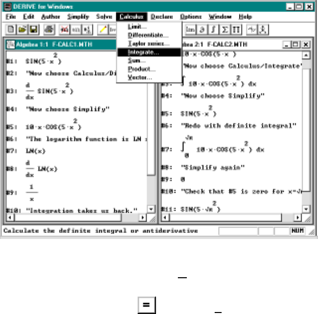
This menu item is very important for us. After choosing the Calculus drop
down menu, you get a submenu with Limit, Differentiate, Taylor series,
Integrate, Sum, Product, and Vector. There are also buttons for most of
these operators. After you have authored an expression, you can differenti-
ate it by either clicking the button or choosing Calculus/Differentiate
from the drop down menu. The form will have entries for what variable to
use and how many times to differentiate, but it usually guesses right so you
can just click OK. Then simplify.
To integrate an expression, first author it or highlight it if it is already
in the algebra window, then either click the button or else choose
Calculus/Integrate. The form will have entries for what expression to inte-
grate; it will guess you want to integrate the highlighted expression. It will
have an entry for what variable you what to integrate with; again it will prob-
ably guess right. It will also have entries for the limits of integration. If you
want an indefinite integral, just click the appropriate button and click OK.
For a definite integral click the appropriate button, type in the upper/lower
limit, then click OK. See Figure 0.2 on the next page for several examples
using Differentiate and Integrate on the Calculus menu.
The options Calculus/Limits is similar to the above. To find
lim
x→−1
x2−1
x+1
you enter the expression, then either click or choose Limits from the
Calculus menu. You fill in the variable (which is x) and the limit point which
10 CHAPTER 0. INTRODUCTION AND DERIVE BASICS
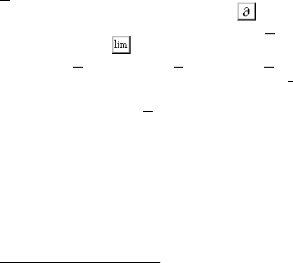
Figure 0.2: Using the Calculus menu
is −1sincex→−1. Then click or choose Simplify to get the answer.
In a similar manner Derive does summation and product problems. Special
notations are used; namely,
n
X
i=1
ai=a1+···+a
nand
n
Y
i=1
ai=a1···a
n.
Let us discuss the summation notation which may be new to you. If
a1,...,a
nare numbers then
n
X
i=1
ai=a1+···+a
n.
The symbol on the left, Pn
i=1 ai,isreadas“thesumofa
ias iruns from 1
to n.” Often aiis a formula involving i.So
5
X
i=0
i2=0
2+1
2+2
2+3
2+4
2+5
2= 55.
0.9. CALCULUS 11
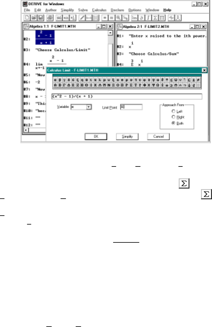
Figure 0.3: Examples of Limits, Products and Sums
You can do this computation in Derive by clicking the or using the
Sum option on the Calculus menu. Just author i^2 then click . Fill
in the required variable ialong with the starting value 0 and end value 5.
Simplify to get 55. As an interesting aside, edit the above sum and have
Derive Simplify Pn
i=1 ito get the formula:
n
X
i=1
i=n(n+1)
2.
This formula is used in many calculus texts to evaluate certain Riemann
sums.
See Figure 0.3 for some examples. Note that in Figure 0.3
3
Y
i=1
xi=x·x2·x3=x6.
The option Calculus/Taylor will be explained in Chapter 7.

12 CHAPTER 0. INTRODUCTION AND DERIVE BASICS
0.10 Plotting
Supposed you want to graph the function xsin x. You simply author the
expression, by clicking the pencil button , to be plotted and then
click the button. A plot window will then opens up and the icon-
bar will change to a new set of buttons. You then click the button
again (it’s position is different in the plot window) and the graph will be
drawn. There are several different ways to view the algebra and plot window
together. The one we used to produce the pictures in the manual is to first
select the algebra window (if you are currently in the plot window you can
go to the algebra window by clicking the button) and then choose
Window/Tile Vertically from the menus. This will split the screen into two
windows: an algebra window on the left and a plotting window on the right.
These windows each have a number in their upper left hand corner. You can
have several plot windows associated with a single algebra window but you
cannot plot together expressions from different algebra windows. You can
switch windows by either clicking the top strip of the window or clicking the
or buttons. Actually you can click anywhere in the window to
select it but the top strip avoids changing the highlighted expression in the
algebra window or moving the cross in the plot window.
You can plot several functions in the same plot window. Move to the
algebra window, highlight the expression you want to plot, switch to the plot
window and then click the in the plot window. Now both expressions
will be graphed. You can plot as many as you want this way. The plot
window also has a menu option, Edit/Delete Plot, for removing some or all
of the expressions to be plotted. Pressing the Delete-key also removes the
current plot.
When you plot, there is a small crosshair in the plot window, initially at
the (1,1) position. You can move the cross around using the arrow keys or
by clicking at a new location. The coordinates of the cross are give at the
bottom of the screen. This is useful for such things as finding the coordinates
of a maximum or a minimum, or where two graphs meet. In order to center
the graph so that the cross is in the center of the window, click the
button. This is useful for zooming in and out to get a better view of the
graph. There are several buttons for doing this in the plot window. Take a
look and you will see a button for zooming in, namely , and for zooming

0.10. PLOTTING 13
out and various ways of changing just the x-scale or just the y-scale.
You should try clicking these buttons to see exactly what happens.
In general, these buttons change the scale of the plot window by either
doubling or halving it. You can customize these by using the button7
(that’s a picture of a balance scale). Just click this button and fill out the
form the appears with your own numbers. You can see the current scale at
the bottom of the screen.
We mentioned above how to plot any number of graphs simultaneously by
repeatedly switching between the algebra window and the graphics window.
Another technique for plotting three or more functions is to plot a vector
of functions. This just means authoring a collection of functions, separated
by commas and surrounded by square brackets. For example, plotting the
expression [x, x^2, x^3] will graph the three functions: x,x2,andx
3
.
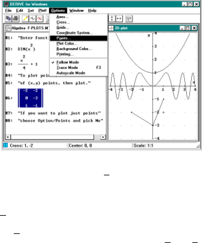
In order to plot a collection of individual points one enters the points as a
matrix, for example authoring the expression [[-2,-2], [0,-3], [1,-1]]
and then plotting it will graph the 3 points: (−2,−2), (0,−3) and (1,−1).
A quick way of authoring a vector is to use the button and a quick
way to enter a matrix is to use the button. One then just fills out the
form that opens up. So for example with the 3 points above we would click
the matrix button and select 3 rows and 2 columns. The form will
open up and we then fill in the 6 numbers above in the obvious order. You
move between fields by either clicking or using the Tab-key.
When plotting points you have a choice of connecting the points with a
line segment so that it appear like the graph of a function. You do this by
choosing Options from the menu bar. There are lots of interesting items on
this menu that will allow you to customize plotting colors, the size points are
plotted, axes and so on. To connect points we choose Points and then check
the Yes button.8We can also modify the size of the points by clicking the
appropriate button. See the Figure 0.4 on the next page where each of these
techniques is demonstrated. Choosing Option/Plot Color controls the color
of a plot and whether the colors should rotate with each new graph.
7This functionality has been replaced in DfW5 with the Set/Plot Region and Set/Plot
Range menu options.
8The default is for points to be connected but if data points are to be plotted then it
is usually best to select No.
14 CHAPTER 0. INTRODUCTION AND DERIVE BASICS
Figure 0.4: Using Plot for graphics
0.11 Defining Functions and Constants
If you Author f(x),Derive will put fxon the screen because it thinks both
xand fare variables. If you wish to define f(x)=x
2+2x+ 1, for example,
you could Author f(x) := x^2 + 2x + 1. Note that we use := for assign-
ments and = for equations. Alternately, you could choose Declare/Function,
and then fill in the form with f(x) for the function name and x^2+2x+
1for its value. Derive will then enter this as above with the :=-sign. See
Figure 0.5 on the facing page.
Constant are treated just like functions except there are no arguments.
In order to set a=2πfor example you type a:=2pi. Then, whenever you
simplify an expression containing a, each occurrence is replaced with 2π.
In many problems you find it useful to have constant names with more
than one letter or symbol, which is the default in Derive. For example
variables with names like x1,y2, etc. will be used frequently as are names
like “gravity”. This can be done by declaring the variable, for example, to
use the variable x1 we author x1:=. Now any use of these letters will be
0.11. DEFINING FUNCTIONS AND CONSTANTS 15
Figure 0.5: Examples of Declare, Simplify and approximating
treated as the single variable x1.
An interesting function defining technique is provided by the factorials.
For n=1,2,... we define n-factorial, denoted by n!, as
n!=n·(n−1) ···2·1n=1,2,...
and for completeness we define 0! = 1. These numbers are important in many
formulas, e.g., the binomial theorem. One observes the important recursive
relationship n!=n(n−1)! which gives the value of n! in terms of the previous
one (n−1)!. Thus, since 5! = 120 we see immediately that 6! = 720 without
multiplying all 6 numbers together.
In Derive we can recursively define a function F(n) satisfying F(n)=n!
by simply typing
F(n) := IF(n=0, 1, n F(n-1))
where the properties of the Derive function IF(test, true, false) should
be pretty obvious. The definition forces the function to circle back over and
16 CHAPTER 0. INTRODUCTION AND DERIVE BASICS
over again until we get to the beginning value at n= 0, i.e.,
F(n)=n·F(n−1) = ···=n·(n−1) ···2·1·F(0) = n!
We will give several other examples of this technique in the text.
0.12 Defining The Derivative Function
A common application of defining functions is to have f(x) defined but the
calculus problem requires a formula involving both f(x)andf
0
(x). For ex-
ample, the equation of the tangent line at the point (a, f(a)) is given by
y=f(a)+f0(a)(x−a).
If you try to define the derivative of f(x)byg(x) := dif(f(x), x) and
then evaluate g(2), you get DIF(F(2), 2), which is not what you want. Of
course, we could also just compute the derivative and define g(x) := to
be that expression. The advantage of defining it as a function is that if we
change the definition of f(x), then g(x) will also change to the derivative of
the new f(x). Thus, we get to use the formula for more than one application.
Here’s a way to define the derivative as a function correctly: Start by
Authoring f(x):= and we can enter the specific definition of f(x)nowor
wait until later. Next, click the derivative button and enter f(u) in
the form (note the variable is unot x). Select the Variable uand press OK.
Now click the limit button (with the previous expression highlighted)
and enter the Variable uand the Point x. Finally, Author g(x):= and insert
the previous expression by right-clicking and selecting Insert.
The result is the expression G(x):= LIM( DIF( F(u), u), u, x).Ac-
tually, you could have just Authored this expression directly but the syntax
and the number of parentheses is a little confusing in the beginning so the
above method is easier and probably faster.
The above technique is a little confusing and so to simplify matters we
have included a function SUBST(u,x,a)9in the ADD-HEAD file (we’ll discuss
this file in more detail later). This function simplifies its argument ubefore
it substitutes afor x. Thus, an alternate definition to the derivative function
is given by
G(x):= SUBST( DIF( F(u), u), u, x)
See Chapter 2 where more discussion of this issue is given.
9This function was added to DfW5.
0.13. FUNCTIONS DESCRIBED BY TABLES 17
0.13 Functions Described By Tables
In calculus functions are typically described by giving a formula like f(x)=
2x
3+ 5 but another technique is to describe the values restricted to certain
intervals or with different formulas on different ranges of x-values. As an
example, consider the function
f(x)=
2x+ 1 for x<1
x
2for 1 ≤x≤2
4 for 4 <x
which defines a unique value f(x) for each value of x. The problem is how
do we define such a function using Derive?
One basic technique is to use the logical IF statement. The syntax is
IF(test, true, false). For example, if we enter and simplify IF(1 < 2,
0, 1) we get 0 whereas IF(1 = 2, 0, 1) simplifies to 1. Now our function
above is entered as:
f(x):= IF(x < 1, 2x + 1, IF(x <= 2, x^2, 4))
Notice how we use nested IF statements to deal with the three conditions
and that with four conditions even more nesting would be required. Now once
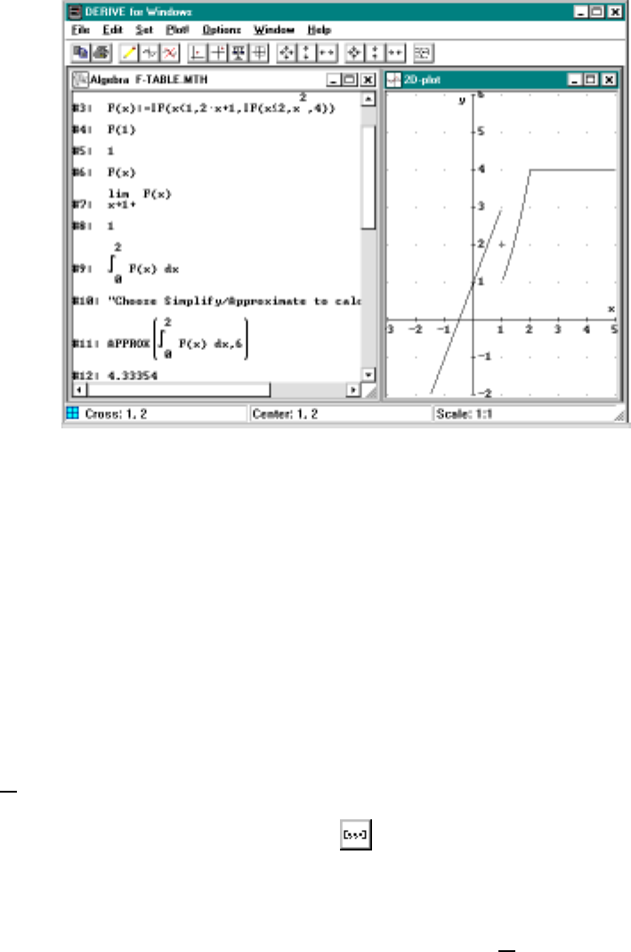
f(x) has been defined we can make computations such as Simplifying F(1)
(should get 1), computing limits such as the right-hand limit limx→1+ f(x)
(should get x2evaluated at x= 1) or definite integrals using approXto
simplify. We can also plot f(x) in the usual manner described in the previous
section.
Notice from Figure 0.6 that the function y=f(x) is continuous at all
x6=1. Atx= 1, both left and right limits exist but they are not equal so
the graph has a jump discontinuity.
As the number of table entries increases we are forced into using nested IF
statements and the formulas become quite difficult to read and understand.
An alternate approach is to use the Derive function CHI(a,x,b) which is
simply
CHI(a, x, b)=
0 for x≤a
1 for a<x<b
0 for b≤x
Then except for x= 1 our function f(x) above satisfies:
18 CHAPTER 0. INTRODUCTION AND DERIVE BASICS
Figure 0.6: Functions defined by tables of expressions
F(x):=(2x+1) CHI(-inf,x,1) + x^2 CHI(1,x,2) + 4 CHI(2,x,inf)
This technique works for graphing and limit problems and moreover gives
the exact result at each point where the function is continuous.
0.14 Vectors
Vectors are quite useful in Derive, even for calculus. They are also useful
in plotting. To enter the 3 element vector with entries a,b,andc,wecan
A
uthor [a, b, c] directly. It is important to note the square brackets which
are used in Derive for vectors; commas are used to separate the elements.
An easier approach is just click the button and fill in the three values
on the vector input form.
Derive also provides a useful function for constructing vectors whose
elements follow a specific pattern. The vector function is a good way to
make lists and tables in Derive. For example, if you Author vector(n^2,
n, 1, 3), it will simplify to [1, 4, 9]. The form of the vector function is
0.14. VECTORS 19
vector(u,i,k,m) where uis an expression containing i. This will produce
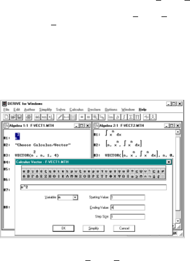
the vector [u(k),u(k+1),... ,u(m)]. You can also use the Calculus/Vector
menu option to create a vector. So, for example, to obtain the same vector
as before, you start by authoring n^2.NowchooseC
alculus/Vector and fill
in the form setting the Variable to n(not x), the start value to 1, the end
value to 3 and the step size to 1 (that’s the default value).
A table (or matrix) can be produced by making a vector with vector en-
tries. If we modify the previous example slightly by replacing the expression
n^2 with [n, n^2] and then repeating the above we get [[1, 1], [2, 4],
[3, 9]] which displays as a table with the first column containing the value
of the index nand the second column containing the value of the expression
n2. This is a good technique for studying patterns in data. See Figure 0.7
for some examples.
Figure 0.7: Using the Calculus/Vector command
We have already seen two important applications of vectors in Section 0.10;
namely,
•Plotting a vector of 3 or more functions [f(x),g(x),h(x),...]plotseach
20 CHAPTER 0. INTRODUCTION AND DERIVE BASICS
of these functions in order.
•Plotting a vector of 2-vectors [[x1,y
1],[x
2,y
2],...] will plot the individ-
ual points (x1,y
1), (x2,y
2),....
We will have other application that will require us to refer to the individ-
ual expression inside of a vector. This is done with the Derive SUB function
(which is short for subscript). Thus, for example, [a,b,c] SUB 2 simplifies
to the second element b.Derive will display this as [a, b, c]2which explains
the name. For a matrix or vector of vectors then double subscripting is used
so that, for example, if
y:= 12
34
then Authoring y SUB 2 SUB 1 will be displayed as y2,1and simplify to 3
(because it’s on row 2 and column 1).
0.15 Printing and Saving to a Disk
You can save the expressions in an algebra window to either a floppy disk
or the hard drive and come back later to continue working on them. Unfor-
tunately, the plot windows are not saved10 but the pictures can be put on
the clip board and saved as graphics files using suitable graphics software.
To save to a floppy, put a the diskette in say the A: drive and activate the
algebra window that you want to save. Click File/Save As and fill out the
menu of options with the drive A: and a file name such as Lab5 or just save
to A:LAB5 and enter. Derive will add the extension .MTH11 to indicate
that this is a file consisting of Derive expressions. After the file has been
saved you can update it by simply pressing the button.
You will most likely save your files to the network harddisk. For example,
suppose your network harddisk is the H:-drive. To save a file, just refer to it
as say H:LAB5 or switch to the H:-drive and view your files.
Later, you can recall these expressions by using either the File/Open
or File/Load/Math options. The second method is used primarily to add
10In DfW5 plots can be embedded in the algebra window and are saved along with the
expressions using the new DFW file format.
11DfW5 has added a new file format with the DFW extension. The MTH files can still
be used.

0.16. HELP 21
expressions to an existing window. If you forget the name of your files just
type either A: or H: and press the enter–key to see a listing of your files.
During the course of your session with the computer you will make lots of
typing and mathematical mistakes. Before saving your work to a file or before
printing and turning your lab in for grading you should erase the unneeded
entries and clean up the file. The three buttons canbeusedfor
this purpose. For example, if you select several expressions by say dragging
the mouse pointer over them with the left button held down and then press
the button these expression will be removed. Clicking will undo
the last delete. You can move a block of highlights lines by holding down
the right mouse button and dragging the block to a new location. Of course,
when you delete or move some lines then the line numbers will no longer be
in a proper sequence of #1, #2, ... . You can correct this by pressing the
renumbering button . You should practice these commands on some
scratch work to make certain you understand them.12
One way to use the move command is to write comments in the file and
placing them before computation. Many of the *.MTH files that we wrote
for this lab manual use this technique. To do it, just author a line of text
enclosed in double quotes, for example, "Now substitute x=0.". Then,
move this comment to the appropriate location.
You can print all the expressions in the algebra window (even the ones
you can’t see) by pressing the button. You do the same thing to
print a graph. Just activate the plot window and press . Typically,
students turn in the labs by printing out the algebra window and penciling in
remarks and simple graphs. More extensive graphs can be printed out. Some
combination of hand writing and printouts should be the most efficient.13
0.16 Help
You can obtain on-line help by choosing Help. This help feature provides
information on all Derive functions and symbols. Suppose that you want
to know how to enter the second derivative of a functions f(x)bytyping.
12DfW5 has changed the methods for moving expressions, correcting expressions and
adding comments. See Appendix B for details.
13The new functionality of embedded graphics in DfW5 allows for more flexibility in
these matters.

22 CHAPTER 0. INTRODUCTION AND DERIVE BASICS
For example, maybe this expression is to be used as part of another function.
There are three techniques for learning how to do this.
The first method starts by authoring F(x):= to declare f(x)tobea
function of x. NextweusethemenuswithC
alculus/Differentiate to calculate
the second derivative by entering F(x) for the function and 2 for the order.
Then, press Author followed by the pull-down key F3 or right click in the
author box and select Insert. This will enter Derive’s way of typing the
expression, in this case it’s DIF(f(x),x,2). The second method is to use
the online help by choosing Help on the main menu. One then searches for
a topic like differentiation or vector to get further information.
0.17 Common Mistakes
Here are a few common mistakes that everyone makes, including the authors,
every once in a while. It just takes practice and discipline to avoid these
problems, although, it is human nature to blame the computer for your
own mistakes. Fortunately, the computer never takes insults personally and
it never takes revenge by creating sticky keys, erasing files, locking up, or
anything else like that ... or does it?
Q1. I tried to plot the line ax +band instead I got an error message about
“too many variables”. What did I do wrong? You must define a,b
to have numerical values, otherwise Derive treats your function as
f(a, b, x) which it cannot plot.
Q2. I tried to plot the family of parabolas x2+cand I got an error about too
many variables. What did I do wrong? Same problem as above, except
now Derive is trying to plot a surface z=f(x, c)in 2-dimensional
space. You probably want to enter and Simplify a vector of functions
such as
VECTOR(x^2 + c, c, 0, 4).
Now Plot this vector of 5 functions: x2,x2+1, x
2+2, x
2+3, and x
2+4.
Q3. I entered the expression √5−xcorrectly, but when I substituted x=9
and simplified I got 2ˆ
i. What happened? You took the square root of
a negative number which is not allowed when you are working with the

0.17. COMMON MISTAKES 23
real number system. Derive treats this as a computation with complex
numbers and uses the complex number i(where i2=−1).
Q4. I solved for the 3 roots of the cubic x3−2x2+x−2 and I got x=2which
I guessed from the graph but the other two solutions were x=ˆ
iand −ˆ
i.
Where do these last two come from? If you factor the cubic instead of
using Solve you would get (x−2)(x2+ 1). The complex solutions come
from that quadratic term. In calculus, we just ignore those complex
solutions. For example, numerically solving the above cubic will give
only real solutions.
Q5. I differentiated exand I got exln e, what’s wrong? Nothing, Derive is
treating the letter eas an ordinary symbol like aor b. You probably
wanted Euler’s constant ewhich can be entered using the symbol bar or
with #e.
Q6. I tried to author the inverse tangent function arctan x and I got a·r·
c·tan xinstead. What’s wrong? Derive recognized the tan x part but
treated the other symbols as individual constants. Use atan x.
Q7. I entered the vector [v1,v
2,v
3]bytyping[v1,v2,v3] and I got [v·1,v·
2,v·3] instead. What happened? You must declare these multi-letter
variables first before they can be treated as a single variable. To do this
just author v1:=,v2:= and v3:=. A quick way to do this is to simply
author the vector [v1:=, v2:=, v3:=].
Q8. I tried to author x^n and I got a syntax error! How was this possible?
The problem here is that either xor nis previously defined as a function.
For example, maybe you had authored x(t):=sint. You can check on
this by scrolling up to find the definition. If instead, you know the
problem is that x(t) is defined and you want to remove that definition,
then just author x:=. In extreme cases you might just open a new
window and copy over some of your expressions using the Copy and
Paste technique.
Q9. I entered and simplified sin(2π) and I got SIN([2π]) instead, what hap-
pened? You authored sin[2pi] instead of sin(2pi).Derive treats
square brackets not as parenthesis but as a device for defining vectors,
see Section 0.14.

24 CHAPTER 0. INTRODUCTION AND DERIVE BASICS
Q10. I tried to show that limn→∞(1 + 1
n)n=e,insteadDerive returns a
question mark indicating that it can’t do this problem. What’s wrong?
Same as above, check that your parenthesis are not brackets.
Chapter 1
Curve Sketching
1.1 Introduction
Before the widespread use of computers and graphing calculators, graphing
a function f(x) was done by a combination of techniques including:
•Plotting some judiciously chosen points.
•Locating the intercepts on the x-axis by finding solutions to the equa-
tion: f(x)=0.
•Using Calculus to finding the local minima and maxima and where f(x)
is increasing and decreasing.
•Finding the points where the graph is curving upward and where it
is curving downward. The transition point in between is called an
inflection point.
•Finding the horizontal and vertical asymptotes.
Graphing is easier with a computer algebra system. In order to under-
stand the behavior of a function f(x) we can plot it using Derive’s plot
window (see Section 0.10 for instructions on plotting.). Moreover, we can
also find the local minima and maxima and the other items above if we need
them. We do this in Chapter 3. It is also possible to make a small change in
the function f(x) and then plot that change to see how the graph is affected.
We can also see important aspects of the graph by zooming in or out and
moving around to different parts of the graph. In this lab you will develop
your skills at graphing with the computer.
25
26 CHAPTER 1. CURVE SKETCHING
1.2 Working with Graphs
In many problems involving periodic behavior, such as oscillating springs,
pendulums, planetary motion and others, the solutions generally have the
form
asin(b(x−x0))
where a,band x0are given numbers. This raises the question of how the
graph of a function, such as sin x, changes when subject to the above mod-
ifications. You should observe the changes by comparing with the original
function but you should also think about why the changes make sense, for
example, what does changing ado, what is the geometrical significance of
the point x=x0on the x-axis.
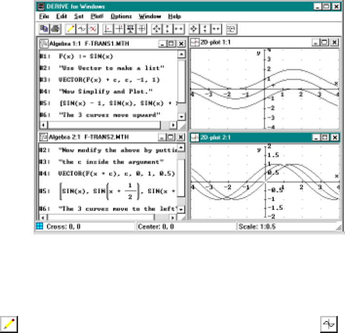
Figure 1.1: Using vector to plot several graphs
As our first task, lets plot y=f(x)+cwhere f(x)=sinxand where c
varies over the range −2, −1,..., +2. We start by clicking the pencil button
,enteringsin x + (-2) and pressing OK. Next, click the button
1.2. WORKING WITH GRAPHS 27
and the Plot Window appears. Notice that there are a different set of buttons
at the top. The most important ones are the plot button ,thevarious
zoom buttons such as which doubles the scale in each direction and
the cross buttons such as which centers the plot on the cross. The
cross is the little reference point whose coordinates are shown in the lower
left corner of the DfW window. You move the cross by either pointing and
clicking or else using the arrow keys.
Clicking the button will plot expression that is highlighted in the
Algebra Window. We return to the Algebra Window by clicking the
button and then entering the next expression sin x + (-1). Pressing
puts us back in the Plot Window and by clicking again we plot the
second expression in the same window as the first so that we can compare
them. The second graph appears to be the same as the first except that it
is shifted up one unit. We proceed in a similar manner with the remaining
three expressions with each successive graph shifting up another unit.
We like to have the Algebra Window and the Plot Window visible at
the same time. We do this by splitting the screen using the Window/Tile
Vertically command. Of course, you can work with only one window at a
time but it is easy to change the active window by simply clicking on the
name strip. You can actually click anywhere in the window to activate it
but this is not a good idea in the Plot Window since this will also move the
cross. Typically, the cross is carefully located at some important feature of
the graph and you don’t want to move it unnecessarily.
There are a few shortcuts that we can do to make this task a little easier.
First of all it’s not necessary to retype each expression over and over again.
Instead, we click on the expression we want to modify (this causes it to be
highlighted) and then we press .Wethenright click in the author
form and a menu opens up. We choose the Insert expression option and the
highlighted expression appears in the author box. We then just change the
-2 to -1 and press OK. That does it and we can now plot the new expression.
A very fast way of plotting similar expressions all at once is to uses
vectors1. Select the Calculus/Vector menu and enter sinx+cin the form.
Click the Variable list box and select the variable c. For this example, set
the Starting value to -2 and the Ending value to 2. The Step Size can be left
1See Section 0.14 on page 18 for more information about the vector function

28 CHAPTER 1. CURVE SKETCHING
at 1 although in other examples you might want to change this. Press OK.
Next we need to simplify the resulting expression
VECTOR( SIN(x) + c, c, -2, 2)
by clicking the button or by using the Simplify menu. The button
method is faster. With the vector of five expressions highlighted, click the
button twice and all five graphs are plotted. One problem with this
technique is that you can’t see the pattern, i.e., each successive graph is
shifted up one unit. On the other hand, we can compute the 5-vector above
and plot the individual elements in the vector by clicking on them and then
plotting. This way you can plot say the first two or three until you see the
pattern and then plot the entire vector to plot the rest.
Another interesting technique is to define our function f(x)=sinx.But
unlike a Calculus text that uses the equal sign both for equations and defi-
nitions in Derive we need to make a distinction. You must remember that
the := symbol is for assignment whereas the =sign is used for equations and
comparisons. To make a definition we author f(x):=sin x.Wecanthen
enter expressions such as f(x)+c which clearly shows the modifications we
have in mind. Many other options are also possible; for example, editing
the vector formula above by replacing the expression with f(x+c)gives
an interesting result upon graphing. See if you can see a traveling wave in
the plot window. Is it traveling from left to right or right to left?
Warning You can change the function definition by simply Authoring f(x)
:= with a new expression. One problem with making definitions is that you
tend to forget them, especially as you move on to a new problem. Thus, if you
use the same letter f(x) in every problem you will definitely have problems
and get confused as to the current definition of the expression f(x). A good
strategy is to use definitions as little as possible and only when necessary.
Use different letters, say f1(x):= for the first problem and f2(x):= for the
second, and so on. You might also want to eliminate a definition as soon
as you are done with it. It is important to note that once you define a
function by this method it will not go away if you simply erase that line
from your algebra window because it is in the computer’s memory. The
way to completely remove a definition using the letter fis to author the
expression f:=.Thisgivesfan empty definition.
1.3. EXPONENTIAL VS POLYNOMIAL GROWTH 29
You might note that after you have defined a function in Derive it
thereafter is displayed with uppercase letters. This is just a visual cue and
it is not necessary to type expressions using uppercase letters2
1.3 Exponential vs Polynomial Growth
Suppose we want to compare the behavior of the function x4andwiththe
exponential ex. For example, suppose we want to know which function grows
the most as xgets large. If we graph x4we see it has the same basic shape
as the parabola x2(you probably guessed this). It is a little flatter than the
parabola between −1 and 1 and it grows more quickly for |x|>1.
If we now graph ex(besuretousethespecialsymbolˆeand not the
letter e) on the same graph and zoom out once, we see that the graph seems
to get close to the x–axis as xgets larger in the negative direction (as x
approaches −∞); that it crosses x4at least twice; and it grows quickly when x
is positive, but not as quickly as x4; see Figure 1.2 on the next page. One
waytoverifythatthex–axis is a horizontal asymptote of exis to highlight
exin the algebra window and choose Calculus/Limit and enter -inf for the
‘Point,’ as we did in Figure 1.2.
To see where the curves cross we need to solve the equation x4=ex.There
are several ways to attack this problem. The most obvious is to simply look at
the graph and estimate the coordinates of the intersection points. Using the
cross is most helpful for this because we can click on the point of intersection
and read off the coordinates in the Plot Window. The arrow keys can also be
used to more precisely position the cross. Further accuracy can be obtained
by centering on the cross by clicking the button and then zooming in
several times by pressing the button.
In order to get an exact solution to an equation we return to the Algebra
Window and use the button. Note that the little icon is a magnifying
glass. For example, a simple quadratic equation such as x2+x−2=0can
solved in this manner by entering the equation in the solve form and setting
the variable to x. Pressing OK and then simplifying by clicking the
button yields the two answers in a vector:
[x=1,x=-2].
2
Derive does have a special mode in which case matters but we don’t use it in the
lab.
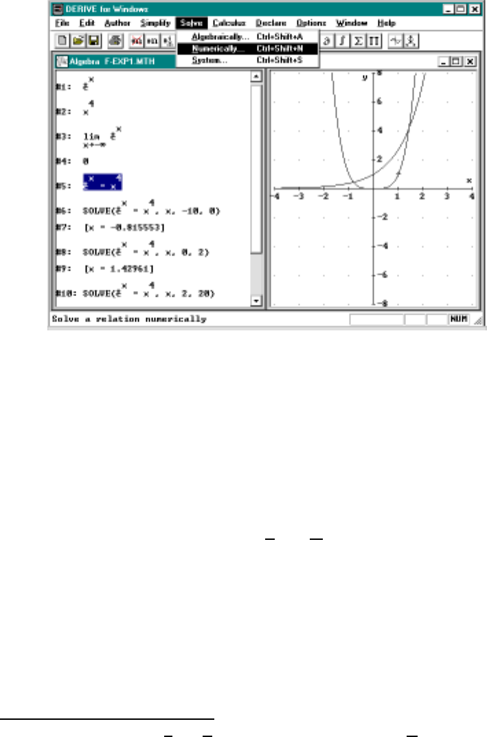
30 CHAPTER 1. CURVE SKETCHING
Figure 1.2: The functions x4and ex
Unfortunately, Derive can not solve all equations (nor can anybody else!)
and so we need to also consider approximate numerical solutions. The tech-
nique for doing this uses calculus and will be discussed in Chapter 5.
For example, our equation x4=excannot be solved exactly. If you
try then Derive just returns the empty solution vector []. We can get
approximate solutions if we use the Solve/Numerically3menu. You enter
the equation x^4 = e^x and then choose an appropriate interval which you
believe contains the desired solution. This choice is usually made by looking
at the graph. For example, the negative solution in Figure 1.2 appears to
be in the interval [−1,0]. Making the interval larger will not increase the
number of solutions since the answer, unlike exact equation solving, has at
most one answer. If there are no solutions in the interval, then you need to
specify a new interval. In our example, the other solution in Figure 1.2 can
be found if we choose the interval from 0 to 2.
3In DfW5 you choose Solve/Expression and then select the Numerically solution
method option.
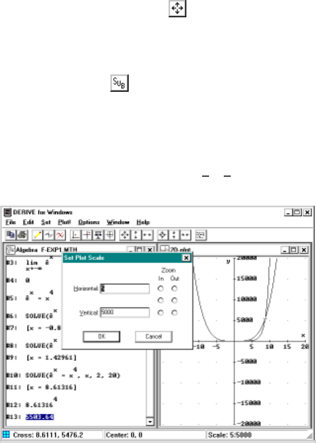
1.3. EXPONENTIAL VS POLYNOMIAL GROWTH 31
Are there any other solutions? It is pretty clear that there are no other
solutions for x<0 but what about large x? From the graph it appears that
x4grows much faster than ex. But of course exhas “exponential growth” so
perhaps ex>x
4for large enough x. To test this we try zooming out several
times in the Plot Window by clicking . But both functions grow very
quickly and it is a little difficult to be successful with this method. Back in
the Algebra Window we can try to numerically solve x4=exfor larger x.
If we choose the interval to be 2 to 20, we get the solution x=8.61316.
So the graphs cross at this point. To find the yvalue of this point, we
use the substitute button to substitute 8.61316 into x4.Theresult
approximates to 5503.64.
To see this on the graph we need to zoom out once so that the x–scale
includes x=8.61316. Then we need to zoom out on the y–axis without
zooming out on the x–axis. The need to do this is why there are those
extra zoom buttons. After zooming out several times we obtain the graph
of Figure 1.3. Another approach is to use the Set/Scale menu and enter an
x-scaleof5anday-scale of 5000.
Figure 1.3: The functions x4and ex, rescaled
32 CHAPTER 1. CURVE SKETCHING
There are a couple things this demonstration shows. First that in order
to see the important features of a graph it may take some skill at moving
around and manipulating the scale of the graph. Moreover, even though we
can clearly see the two graphs intersecting at x=8.61316 in Figure 1.3, we
can no longer see the other two solutions. So it may not be possible to see
all the important features in one plot. In the exercises you will learn how to
move and scale in the plot window and to use the algebra window in order
to find all the important features of one or more graphs.
1.4 Laboratory Exercises
1. Use the author button and the approximate button (or
Simplify/Approximate) to get decimal approximations for each of the
following.
a. 81/2
b. sin(π
4)
c. sin(π
4)/51/2
2. Let f(x)=1/(1 + 2x2).
a. Graph each of the following f(x)−1, f(x), f(x) + 1, and f(x)+2
in a plot window. Then, use the Window/New 2D-Plot Window
command to open another plot window and plot f(x−1), f(x),
f(x+1) andf(x+ 2) in that window. (Hint: The Vector menu
can be used to simplify the typing.)
b. What does the transformation f(x)→f(x)+ado to the shape
of the graph? to the position of the graph?
c. What does the transformation f(x)→f(x+a)dototheshape
and position of the graph?
3. Graph cos x,2cosx,andcos(2x) and explain what the transformations
f(x)→f(ax)andf(x)→af (x) do to the graph of f(x).
4. What do the transformations f(x)→f(−x)andf(x)→−f(x)do?
Graph f(x)=x
5−x
2+1andf(−x)and−f(x).

1.4. LABORATORY EXERCISES 33
5. Let g(t)=sint+cost.
a. Graph g(t).
b. What sort of transformations should be applied to sin tto make
its graph look like the graph of g(t)?
c. Use Derive’s crosshair to find the maximum value of g(t)andto
find the first root of g(t) to the left of zero.
d. Use these numbers to find aand bso that g(t)=asin(t+b), at
least approximately.
*e. Find exact values of aand bso that
sin t+cost=asin(t+b).
Hint: Set the simplification of trigonometry functions to “Ex-
pand” using the Declare/Algebra State/Simplification menu. Then
evaluate asin(t+b).
6. Let f(x)=e
−ax2where ais a constant.
a. Plot f(x) for a=−2, −1, 0, 1, and 2. You can use the vector
function if you like but plot each expression one at a time so you
can see its graph.
b. For each of the five values of adetermine whether the graph is
curving upward, curving downward, no curving at all or curving
both ways. If the graph has both upward and downward curving
graphically approximate the points where there is a transition
between upward and downward curving. These are the inflection
points. Print out the Plot Window and mark it up with your
pencil indicating which graph corresponds to which value of a,
inflection points, etc.
7. Find the points where the curves ln xand x1/4intersect. Make two (or
more) graphs with different scales showing the places where the curves
intersect.
8. Make separate graphs of each of the following functions. Using some
of the graphing techniques such as zooming, centering, etc. Make sure

34 CHAPTER 1. CURVE SKETCHING
your graphs show the main features such as the xand y–intercepts, the
critical points, and the inflection points.
a. sin(x)cos(20x)b. 3x
√4x2+1
c. 1
1 + 5000(x−1)2d. xsin(1/x)
*9. Enter the rational function
x6+3x
5+x
4+1
2x
4−1
(1)
a. Choose Simplify/Expand and select Rational. This gives a partial
fractions decomposition of the function. (Partial fraction decom-
positions are used in integrating rational functions) Notice that
the partial fraction decomposition consists of (a sum of) one or
more proper rational functions (where the denominator has higher
degree than the numerator) and a polynomial. What is the poly-
nomial?
b. Graph the rational function given by (1) and the polynomial you
found in the first part. Zoom out a few times. How are the two
graphs related when |x|is large? Explain why this is.
*10. Let
g(x)=−2x
3+6x
2−3x+5
4x
2−6x−7
a. Graph g(x) so that your graph shows the main features of this
function.
b. This graph has a slant asymptote, i.e., an asymptote which is a
line with nonzero slope. Zoom out a few times until you can see
this slant asymptote.
c. Find the formula for the slant asymptote by using Simplify/Expand.
*11. In reading this chapter you might have wondered if exand x4intersect
some place beyond c=8.61316 ···.YoucoulduseDerive to verify
1.4. LABORATORY EXERCISES 35
that there is no solution say between 8.7 and 100 and this would be
strong evidence that they don’t intersect beyond c, but not a proof. So
in this problem you are to find a proof that exand x4don’t intersect
beyond c(without using Derive). Hint: By taking 4th roots we must
show ex/4>xfor all large x. Now using Calculus, show that the slope
of ex/4−xis positive for all x≥8, i.e., the derivative is positive.Use
this to show ex>x
4for all x>c.
36 CHAPTER 1. CURVE SKETCHING

Chapter 2
The Derivative
2.1 The Derivative as a Limit of Secant Lines
Geometrically the derivative of a function f(x)atapointais the slope of the
tangent line of f(x) going through the point (a, f(a)). We can approximate
the tangent line by the ‘secant’ line which goes through the points (a, f(a))
and (a+h, f(a+h)). The slope of this line, the rise over the run, is (f(a+
h)−f(a))/h, and so, by the usual point-slope formula for a line, the equation
of this secant line is
y−f(a)=f(a+h)−f(a)
h(x−a).
As a+hgets closer to a, i.e., as hgets smaller, this secant line approximates
the tangent line at abetter and better, and so its slope approaches the
derivative f0(a). We can visualize this with Derive by entering the following
expressions:
F(x) := x^3/3
SL(a, h) := f(a) + (f(a+h) - f(a))/h (x - a)
The first step defines f(x) to be the function x3/3. The second defines a
function SL(a, h) which gives the secant line through the points (a, f(a))
and (a+h, f(a+h)). For example, if we Simplify SL(1,1) we get 7x−6
3so
that the equation of the secant line determined by the points (1,f(1)) and
(2,f(2)) is y=7x−6
3.
37
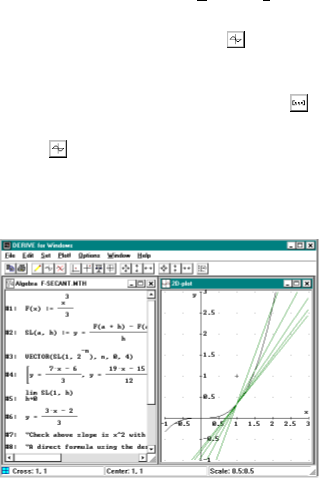
38 CHAPTER 2. THE DERIVATIVE
Now we want to fix a= 1 and plot several secant lines corresponding
to different h’s. We can, for example, just Author and Simplify SL(1,1),
SL(1,1/2), SL(1,1/4), SL(1,1/8), and SL(1,1/16), and plot these lines and
f(x) on the same graph. This simply means you highlight each of the sim-
plified expression and then click the plot button in the plot window,
see Section 0.10 on page 12 in Chapter 0 for the details on how to do this.
This is illustrated in Figure 2.1.
A nice way to calculate and plot these secant lines is to use vector tech-
niques. Here’s how you would do it: Click the vector button and set
the number of elements to 5. Now enter the 5 expressions above starting
with SL(1,1) and using the Tab to move from entry to entry. Finally, sim-
plify and click on the resulting vector [SL(1,1),...,SL(1/16)]. All
five lines will be plotted one at a time. It all happens very quickly and it’s
difficult to see the pattern of the plots. Actually, if you stare at the screen
carefully just as you click the plot button you possibly can see (depending
on the speed of your computer) an animation-like effect.
Figure 2.1: Secant lines approximating the tangent line

2.1. THE DERIVATIVE AS A LIMIT OF SECANT LINES 39
If the drawing is too quick to see the animation, try the following method
instead. Erase the 5 secant lines in the plot window by pressing the Del key
5 times. In the algebra window select an individual line in the vector by
repeatedly clicking on it. Then, activate the plot window and press .
Finally, repeat this process several times to see the pattern evolving in the
plot window; namely, that the lines are rotating about the point (1,1
3)on
the graph. Moreover, the lines appear to be tending to the tangent line.
In Figure 2.1 on the preceding page this pattern is clearly shown: the
secant lines tend to the tangent line by rotating in a clockwise manner, i.e.,
with decreasing slope. We can use Derive to illustrate this effect using
calculus. That is, as htends to 0, the secant line tends to the tangent line
by taking the limit: Author SL(1,h) and choose Calculus/Limit, taking the
variable to be h(not x). After Simplifying we get
lim
h→0SL(1,h)=3x−2
3=x−2
3
.
which, in fact, yields the tangent line to x3/3atx= 1. Check this out for
yourself by plotting this function on your previous graph. Since the slope
ofthesecantlineis(f(a+h)−f(a))/h, this explains why we define the
derivative as
f0(a) = lim
h→0
f(a+h)−f(a)
h
(1)
and why the derivative is the slope of the tangent line.
A quicker way of entering the 5 lines above is to observe that there is
a pattern to the values 1,1
2,1
4,...;namely 1
2
nfor n=0,1,...,4. We can
use this fact and the VECTOR function on the Calculus menu to simplify this
task. Select Calculus/Vector and enter SL(1,1/2^n) in the form. Note that
using uppercase letters is not necessary and that the highlighted expression
will be replaced with whatever you type. For the Variable, scroll down and
select n. NextwetaketheS
tartingvaluetobe0since2
0=1andtheEnding
valuetobe4since2
4= 16. Click OK and simplify the resulting expression
VECTOR(SL(1, 2^-n), n, 0, 4). The result is a vector of five secant lines
as above. You will find that this is a convenient method of producing a large
number of expressions without typing them individually.
We can later change the definition of f(x) to a different function and
use the SL(a, h) function to get secant lines to the new function. The file
F-SECANT.MTH contains the definitions of SL(a, h) and the tangent line
function, TL(a), discussed below.
40 CHAPTER 2. THE DERIVATIVE
Tangent Lines In order to get a function TL(a) for the tangent line at a
analogous to the secant line function SL(a,h), we need to be a little careful
since the most obvious definition; namely,
TL(a) := F(a) + DIF(F(a),a) (x - a)
doesn’t work. This is because the order of evaluation is wrong. Consider
what would happen if we evaluated TL(5). First 5 would be substituted for
aand then the resulting expression,
F(5) + DIF(F(5),5) (x - 5),
would be evaluated. But DIF(F(5),5) doesn’t make sense.
To solve this problem and to keep thing as simple as possible we use a
special utility file ADD-UTIL.MTH. This file contains several new functions
that we will be using for now on and so we suggest adding a few lines to start
of every DfW session. This can be done by Opening or using Load/Math on
the file ADD-HEAD1Once this has been done, these new functions can be
used. See Appendix A for a more detailed explanation.
For example, the function SUBST(u, x, a)2simplifies the expression u
and then substitutes the value afor xin u. The three variables in the SUBST
function are the expression,thevariable and the evaluation point.Ithasthe
same effect as first Simplifying uand then using the button to replace
xwith a.
To define the TL function we first make a function DF(x) of the derivative
using the SUBST function. Click and enter F(u) with the variable set to
u. With this expression highlighted click and type in SUBST(). Then,
click in-between the parenthesis and insert the derivative by right-clicking and
selecting Insert from the menu. Finally, type in next two arguments uand
xseparated by commas to complete the three arguments for this function.
1All DfW4 files have the MTH extension although sometimes Windows doesn’t explic-
itly show the file extensions. However, DfW5 has added a new file format with the DFW
extension which allows for the inclusion of graphics. The MTH files can still be used. The
default extension used when Saving or Opening files depends on the version with DfW5
using the newer format. In this manual we usually drop the reference to the extension
since it is assumed to be MTH.
2This function was added to DfW5.

2.2. LOCAL LINEARITY AND APPROXIMATION 41
Pressing OK, you should get the first expression below:
DF(x):= SUBST(DIF(F(u), u), u, x)(2)
TL(a) := F(a) + DF(a)(x - a)(3)
The TL function can then be defined as above.
The utility file contains two more functions which you can use for the
exercises and that eliminate the need to reproduce the definitions we’ve been
discussing. To find the tangent line of say x3/3atx=5youenterandsim-
plify the expression TANGENT(x^3/3, x, 5). Here again, the three variables
in the TANGENT function are the expression,thevariable and the evaluation
point. Similarly, the secant line computed earlier can be obtained by entering
SECANT(x^3/3, x, 1, 1/16). Here the last variable is the h-increment.
When you Simplify either of these functions you get an expression of the
form y=mx +brather than just mx +b. You can still plot the entire
equation and get the right result since DfW knows how to plot equations in
addition to functions. You can test this by plotting the familiar equation
x2+y2=1togettheunit circle.Tryit!
Notice that using these functions it is not necessary to define any functions
such as F(x):= or DF(x):= in order to get an answer. This is usually a better
approach because the use of variables or definitions causes problem when you
forget that something is defined. As a result you get some strange answers
to your problems and you don’t know why. This difficulty is particularly
common as you go from problem to problem in the exercises. Just remember
to start off your labs by doing Load/Math to the ADD-HEAD file.
2.2 Local Linearity and Approximation
One of the important properties of a function is that its graph can be ap-
proximated near a value x=a, or more precisely near the point (a, f(a)) on
its graph, by the tangent line at that point. This means that as you zoom
in closer to the point, the graph appears to be getting closer to the tangent
line. Typically, the graph and the tangent line are eventually so close to-
gether that they are plotted as the same curves. This ‘local linearity’ is very
useful in many applications. To see this local flatness in action, move the
crosshair in the plot window we obtained above to the point (1,1/3) where
all the lines intersect, then center on the cross by clicking the button.

42 CHAPTER 2. THE DERIVATIVE
Now we want to zoom in several times by clicking the zoomin button.
Notice how flat the curve appears. Try clicking The zoom out button
several times and then repeating to completely visualize this process.
Approximating the Sine Function One of the most important functions
in calculus is sin xand yet, with the exception of a handful of points such as:
sin 0 = 0,sin π
2=1,sin π
4=√2
2, ...
we need either a calculator or Derive to obtain approximate numerical
values. For example, Author sin(1
3) and press the button. Derive
does nothing with this expression other than to repeat it. On the other
hand, pressing the button and we get the approximate numerical value
sin(1
3)≈0.327194.
To use local linearity we need to compute the tangent line at say a=0
by authoring (make sure you Loaded ADD-HEAD) our new function
TANGENT(sin x, x, 0) .
The answer is y=x. You should verify this visually by plotting sin xand x
together on the same graph. Now center the cross at the origin and zoom in
several times. On the other hand, using the formulas
d
dx sin x=cosxand sin 0 = 0,cos 0 = 1
we can easily derive the above formula for the tangent line.
The point is that we now have a powerful tool for approximating the
values of sin xas long as xis small; namely,
sin x≈xfor x≈0.
Looking back at our sin(1
3) example above, we see that this simple technique
has given a result which is accurate to roughly 2 decimal places.
We can also use the above approach to approximate the derivative of a
function and plot the result. For example, we know that the derivative of
f(x)=x
3is 3x2by using the standard formulas. On the other hand, the
function of x,g(x, h)=f(x+h)−f(x)
hwith hfixed at some value like h=.01
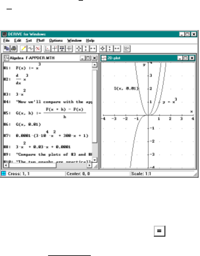
2.2. LOCAL LINEARITY AND APPROXIMATION 43
is a good approximation to 3x2as one can see from Figure 2.2. The figure
actually shows both plots although they appear to be only one curve. In
Derive you should enter and Simplify the above expression (it sometimes
helps to Expand the result to further simplify it). Then compare the graph
with 3x2by plotting both expressions together.
Figure 2.2: Approximating derivatives using the difference quotient
In this case, we can easily estimate how the close the two graphs are by
algebraically simplifying (enter in Derive and press )toget:
(x+h)
3−x
3
h−3x
2=3hx +h2.
Now for h=.01, the right hand side above no larger than .03|x|+.0001 and
as long as we take −1≤x≤1 then this error term is approximately .03 and
our accuracy is nearly 2 decimal places.
Let us try this technique with sin x. Maybe you haven’t learned yet that
the derivative of sin xis cos x. Here is way to strongly suggest this result
44 CHAPTER 2. THE DERIVATIVE
visually: plot the functions
sin(x+h)−sin(x)
hand cos x
for some small value of h,sayh=.01. Can you tell the difference in the
graphs?
2.3 Laboratory Exercises
Start off your lab by Loading the ADD-HEAD file (use File/Load/Math).
Note that the syntax of the SECANT and TANGENT functions are displayed on
the second line of the ADD-HEAD file.
1. For each functions f(x)below
(i) Plot the graph y=f(x).
(ii) Use the function TANGENT(u,x,a) to calculate the tangent lines
at the points a=0,2.
(iii) Plot these tangent lines and turn in a sketch. Label the approxi-
mate slope of each tangent line by visual inspection.
(iv) In the Algebra Window, compute the derivative f0(x) and use the
buttontopluginthevaluesa=0,2.
(v) Determine the exact slope of each of these tangent lines using part
(v) and compare with your estimate for part (iii).
a. 1−x
2b. 2x−1
2x2
c. 1
2x2−xd. sin x
2. a. Using the TANGENT(u,x,a) function find the equation of the tan-
gent line for f(x)= 3
√
x(enter cube roots as x^(1/3))atthepoint
a= 8 and plot it along with the graph of f(x).
b. In part ayou found the tangent line to 3
√xat a=8. Estimate
3
√
9 by finding the y–value of this line when x= 9. Compare your
answers with DfW’s own approximation to this quantity obtained
by clicking the button.
2.3. LABORATORY EXERCISES 45
c. Using the plot window again give a reasonably accurate interval
[c,d] containing the point x= 8 for which the tangent line approx-
imates the function to 2 decimal place accuracy. (Hint: Plot the
difference between the function and the tangent line and rescale
to get a good picture. It is also helpful to use the Trace Mode
which can be set from the Options menu of the graphics window.)
3. The acceleration due to gravity, a, varies with the height above the
surface of the earth. If you go down below the surface of the earth, a
varies in a different way. It can be shown that, as a function of r,the
distance from the center of the earth, ais given by
a(r)=
GM r
RAD3for r<RAD
GM
r2for r≥RAD
where RAD is the radius of the earth, Mis the mass of the earth, and
Gis the gravitational constant. All three of these are constants. In
order to define the function a(r) and examine its graph, we’ll use the
numerical values3:GM:=4.002 ×10¹⁴ and RAD := 6.4×10⁶meters.
a. Define a(r) using the technique in Section 0.13 and plot its graph.
Rescale as necessary to give a good picture4.
b. Is aa continuous function of r?
c. Is aa differentiable function of r? Explain your answer.
d. Refine your answer to Part aso that the domain of a(r)isr≥0.
*4. Γ(x) is a differentiable function for x>0 which is very important in
applications. Derive knows this function but not how to differentiate
it. You can get Γ in either version of Derive by typing gamma but in
DfW you can also just click on the Γ in the Author Dialog Box.
a. Graph Γ(x) and the four secant lines to Γ(x) through the points
(3,Γ(3)) and (3 + h, Γ(3 + h)), for h=1/2, 1/4, 1/8, and 1/16.
[It is known that Γ(3) = 2, but you don’t really need this here.]
3Simply Author the expression GM:=4.002 10^14 and similarly for RAD.
4The horizontal scale should reflect the value of RAD and the vertical scale can be
determined from the numerical value of a(RAD)
46 CHAPTER 2. THE DERIVATIVE
b. Use the secant line you obtained in part awith h=1/16 to
approximate Γ(3.1).
c. Have Derive approximate Γ(3.1).
d. Use the graph to verify that Γ(n+1)=n!=1·2···nwhenever
n=0,1,..., 5. (Since factorials play an important role in many
applications this explain why the Γ function is important.)
*5. Let f(x)=x
2sin(1/x) for x6=0andf(0) = 0. In this problem you will
show that f(x) is continuous and differentiable for all xbut f0(x)isnot
continuous at 0. This means to find f0(0) you must use the definition of
the derivative; you cannot just find f0(x) and take the limit as x→0.
a. Define f(x)asabovebyA
uthoring F(x) := x^2 sin(1/x) (don’t
worry about x= 0 for now). Show limx→0f(x) = 0. (Hint: Click
and fill in the form.)
b. Graph f(x), x2,and−x
2
, setting the plot scale to 0.1 horizon-
tal and 0.01 vertical. Zoom in several times towards the origin
by clicking the button and convince yourself that f(x)is
continuous at x= 0. But notice that the curve oscillates up and
down slightly.
c. Find f0(0) by finding limh→0f(0+h)−f(0)
h.
d. Find the derivative of f(x)usingthe button.
e. Make a new graph of f0(x) and by zooming in several times con-
vince yourself that f0(x) oscillates wildly between approximately
±1asxapproachs zero.
Chapter 3
Basic Algebra and Graphics
3.1 Introduction
Calculus is a beautiful and important subject. It derives its importance
from its ability to describe and model basic phenomena in so many fields.
Besides physics, chemistry and engineering, it is used in biology, economics,
and probability. In order for calculus to be useful to you, you will need
to understand calculus graphically and numerically as well as algebraically.
Algebraically you learn how to differentiate functions given as complicated
expressions. But you also need to understand the derivative visually as the
slope of the tangent line and physically as a rate of change of ywith respect
to x.
With Derive it is easy to learn all three of these aspects and to see the
relations between them.
3.2 Finding Extreme Points
As an example, consider the function f(x)=2x
4−3x
3
. In order to under-
stand the behavior of this function we can plot it using Derive’s plot window
(see Section 0.10 for instructions on plotting.). The resulting graph can be
seen in Figure 3.1 on the next page. The graph suggests f(x) has one local
minimum which is the absolute minimum. Using the crosshair in the plot
window (see Section 0.10) we can determine that the location of the minimum
point has coordinates approximately given by x=1.125 and y=−1.0625.
We can get exact results by switching to the algebra window and doing some
47
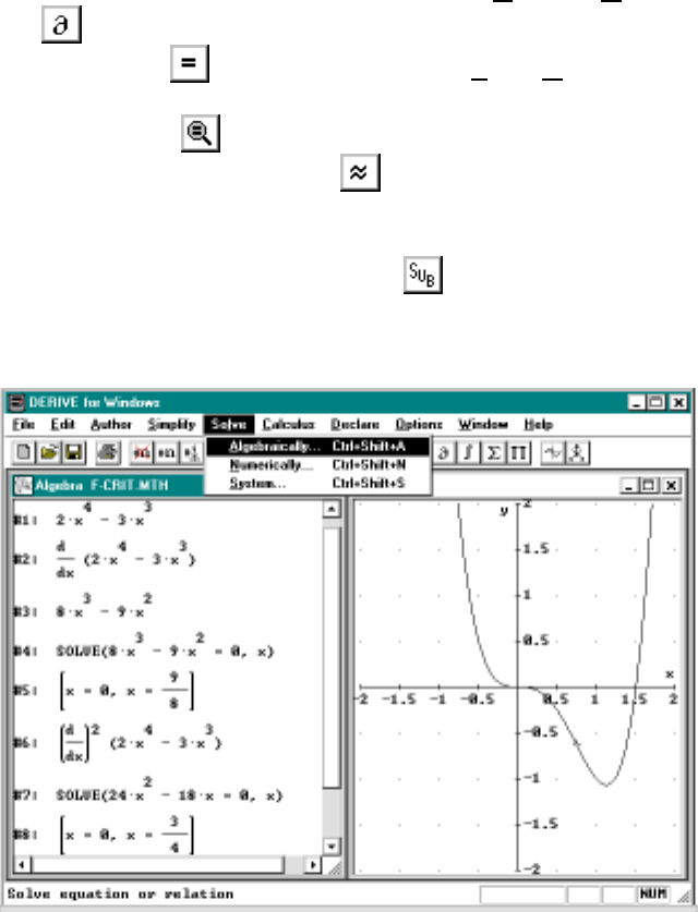
48 CHAPTER 3. BASIC ALGEBRA AND GRAPHICS
calculus. In Derive’s algebra window we choose Calculus/Differentiate or
click the button to find the derivative. You get the answer by clicking
the simplify button .WecanthenchooseSolve/Algebraically to find
where the derivative is 0, i.e., these are the critical points. Alternately, just
click the solve button . The critical points occurs when x=0andwhen
x=9/8. Pressing the approximate button to get decimal answers we
see that approximately 9/8=1.125, which is exact equality in this case.
Now if we substitute this value for xinto f(x) by highlighting the expression
2x4−3x3and then using the substitution button to replace xwith 9/8
we get, after approximating, that y=−1.06787 which is close to our first
estimate.
Figure 3.1: Finding critical points
Looking further at the graph we can see that f(x) does not have a local
minimum or maximum at x= 0; in fact f0(x)<0 on both sides of 0. The
graph also shows that x=9/8 is where the minimum occurs and that f(x)is
decreasing on (−∞,9/8] and increasing on [9/8,∞). If we highlight the first
3.3. MAX-MIN PROBLEMS 49
derivative and clcik (or choose Calculus/Differentiate), then we get
the second derivative. We can then solve to find the points of inflection, i.e.,
the places where the bending in the graph changes. The second derivative
must be zero at these points but this criteria alone is not sufficient. Solving
f00(x)=0yieldsx=0andx=3/4. Again looking at the graph we see that
both of these are indeed points of inflection since the graph is concave up on
(−∞,0], concave down on [0,3/4], and concave up on [3/4,∞).
Insertion Tip In a typical problem the critical point will be complicated
and retyping the expression in the substitution form is difficult and slow.
A quicker method is to highlight the f(x) expression, 2x4−3x3in our ex-
ample, and then click the button. Now click on parts of the answer
vector several times until the desired quantity, say 9/8 is highlighted. In the
Substitution box click the right mouse button and select Insert. The high-
lighted quantity will be inserted in the form. You will find this a particularly
useful technique when doing critical point problems algebraically instead of
numerically. For example, f(x)=ax2+bx +c. In this case the critical point
is a large expression involving the parameters a,b,andc.
3.3 Max-Min Problems
The typical max-min problems requires finding either the absolute maximum
value or the absolute minimum value of a function, f(x), on an interval
a≤x≤b. Our first step is plot the graph. We want the x-values to contain
the interval [a, b] but not much larger. The y-values need to scaled in such
a way that we get a clear picture of the largest and smallest values. If the
function takes on negative values then the absolute minimum will be the
largest negative value (the lowest point on the graph in any case).
Using either the crosshair for precise approximations or just using the
labels on the y-axis to obtain a rough answer are both good first steps to
solving the problem. To obtain exact answers we need calculus and critical
point theory. In the Algebra Window we use the button to calculate
f0(x). Next we use the button to find the critical points from the
equation f0(x) = 0. Once that value is found it can be substituted back into
the expression for f(x) by pressing the button.
Three problems arise:

50 CHAPTER 3. BASIC ALGEBRA AND GRAPHICS
•First we are only interested in those points xwhich lie on our interval
[a, b]. It probably will be necessary to obtain decimal approximations
to our critical points xto see if they satisfy a≤x≤b.
•The second problem is that the absolute maximum may not occur at
the critical points at all. Instead, it occurs at either the left or right
endpoint, i.e., x=aor x=b. This situation should be clear from the
graph.
•The third problem is that perhaps Derive can not solve the equation
f0(x) = 0. As you look at the graph, you should be able to guess the
critical point, at least approximately. Then you can ask Derive to
approximate the critical point by using the Solve/Numerically1menu.
You will need to specify an interval on which Derive will search for
a solution. But this should be obtained by again looking the graph
and choosing a convenient interval containing the approximate critical
point. Choosing too big of an interval can get you into trouble because
Derive may end up finding a solution which is not the one you want.
You would then need to refine your interval to exclude the undesired
critical points.
3.4 Zooming and Asymptotes
As another example of using both plotting and calculus operations, consider
the problem does the function g(x)=3x
3
+5x2−x+1
x3−1have a horizontal asymp-
tote? In other words, we are interested in the behavior of the graph y=g(x)
for very large values of xand we want to know whether the y-values tend to
a limit. To solve this you begin by entering the function by choosing Author
and typing
(3x^3 + 5x^2 - x + 1)/(x^3 - 1).
Now plot this. Zoom out by clicking and see if it appears that g(x)has
a horizontal asymptote. A nice technique to do this is to leave the vertical
scale alone and zoom out in the horizontal direction. There are several ways
to do this; one way is use the zoom buttons on the menu bar. Can you guess
1In DfW5 you choose Solve/Expression and then select the Numerically solution
method option.
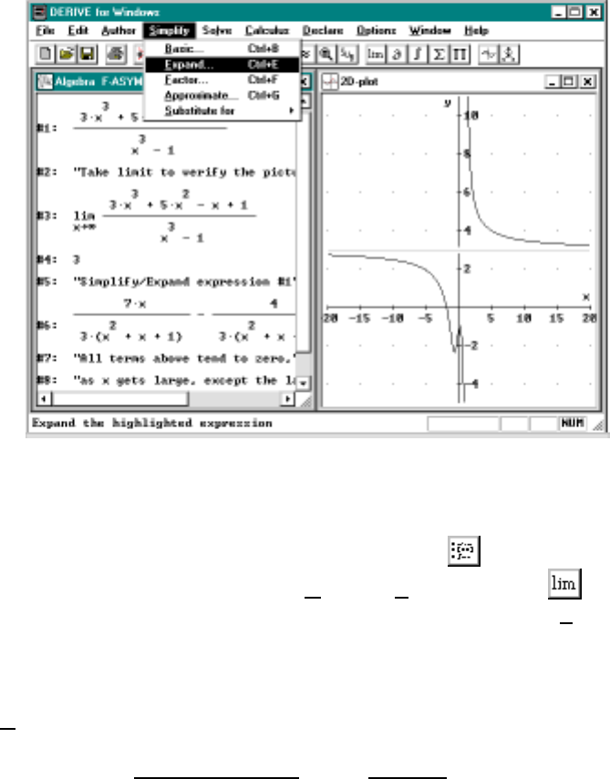
3.4. ZOOMING AND ASYMPTOTES 51
which button does this? Another way is change the scale, say x= 100 (click
the button with the balance scale on it). Use the cross-hair to estimate the
value of ythat g(x) is tending to for large x. You should get y=3(see
Figure 3.2).
Figure 3.2: Zooming to find the horizontal asymptote
Now return to the algebra window by clicking .Wewanttoverify
that limx→∞ g(x) = 3. Now choose Calculus/Limit or click . When
asked for the “point,” type in inf or click ∞symbol on the form. Simplify the
answer; you should get 3. This means that as xgets large, g(x) approaches 3,
i.e., the line y= 3 is a horizontal asymptote. We can check this calculation
by the method of polynomial division which is accomplished in Derive using
the Expand option. As we see at the bottom of Figure 3.2,
3x3+5x
2−x+1
x
3−1=3+ 8
3(x−1) +···
where all the terms other than the 3 are small near x=∞. Thisisbecause
the denominator of each term has a larger power of xthan the numerator.

52 CHAPTER 3. BASIC ALGEBRA AND GRAPHICS
(The answer above is too wide for the window to display completely so you
will need to scroll to see the 3. Use the horizontal scroll bar at the bottom
of the window to do this.)
3.5 Laboratory Exercises
1. For each functions f(x)below
(i) Plot the graph y=f(x) on the interval 0 ≤x≤2.
(ii) By looking at the graph, estimate the x-value and y-value where
the function obtains its absolute maximum value on the interval
[0,2].
(iii) In the Algebra Window, compute the derivative f0(x) and use the
button to find the critical points on the interval [0,2].
(iv) Study the graph to see if the endpoints need to be considered as
possible extreme points.
(v) Determine the absolute maximum value on [0,2] by substituting
into f(x)thex-value where the maximum is obtained.
a. 1−x
2b. 2x−1
2x2
c. 1
2x2−xd. sin x
2. Consider the function f(x)=x
3−x+ 1. You do not need to declare a
function, just enter and work the expression itself.
a. Enter the expression for f(x) and plot it. Using the crosshair as
described in Section 0.10, find an approximation for the both the x
and y–coordinates of the local minimum of f(x).
b. Using the same method find an approximation for the unique x
satisfying the equation f(x) = 0, i.e., the value of xwhere the
graph crosses the x–axis.
c. In the algebra window click or use Solve to find the root
exactly. Approximate this as a decimal and see how it compares
with your answer in Part (b).
3.5. LABORATORY EXERCISES 53
d. In the algebra window find the derivative f0(x) and use it to find
the exact coordinates of the local minimum you approximated in
Part (a). (This will give you the critical value x;togetthey–
coordinate substitute the value of the x–coordinate into f(x)by
clicking or by using the Simplify/Substitute/Variable menu;
see Section 0.8.)
3. Consider the class of all function of the form f(x)=x
3+bx2+cx.
a. Author the expression form x3+bx2+cx. Click the
substitution button and enter some specific values for b,
c, then plot the result2. Do this for several different choices for b
and cand observe the critical points and inflection points of the
different graphs.
b. Using Derive’s calculus facilities in the algebra window, show
that the function f(x)=x
3+bx2+cx always has exactly one
inflection point, regardless of the values of b,c.
c. Again using Derive’s calculus facilities, show that f(x)canhave
either 0, 1 or 2 critical points. Determine for what values of band
cdoes f(x) have no critical point?
d. Choose values b,cwhich demonstrate that f(x) may have either
0, 1 or 2 critical points and plot their graphs.
4. Graph the function f(x)=( x
1+x2)7. Atfirstthereappearstobeno
part of the graph showing in the graphics window but this can not be
since f(0) = 0. Try replotting the graph in another color by either just
clicking several times or using the Options/Plot Color menu.
Now the graph appears to the horizontal line y= 0 but this can not be
since clearly f(x) = 0 only for x=0.
a. In the Algebra window, find the critical points of f(x)byusing
the and buttons.
b. Determine the xand ycoordinates of the local maximums and
local minimums by using the button to substitute the values
in part (a) into the function.
2Derive can’t plot the function unless the values are provided.

54 CHAPTER 3. BASIC ALGEBRA AND GRAPHICS
c. In the Graphics window, use the Zoom buttons or else the Set/Range
menu in such a way that both the local maximum and local min-
imum points are visible. Furthermore, make the y-scale compara-
ble to the y-coordinate of the local maximum.
d. After you get a good looking graph, print out the result.
5. ThevolumeofatincanisV=πr2hwhere ris the radius of the
top (and the bottom) and his the height. The surface area is A=
2πrh +2πr2. (The first term is the area of the side and the second is
the area of the top and bottom.)
a. A manufacturing company wants to make cans with volume 42 in3.
To minimize their costs they want to minimize the area of the can.
What values of rand hdo this? (Hint: Author the formula for the
area, 2πrh+2πr2; use the equation for the volume, 42 = πr2h,to
solve for hin terms of rand substitute this into you expression for
the area. Now find the value of rthat minimizes the area using
calculus techniques and use this value of rto find what his.)
b. You may have noticed that h=2rfor the can of minimum area
you found in part a. Show that this relation always holds for
the can of least surface area (not just for cans with volume 42).
(Hint: Do this just as in part aexcept don’t replace Vby 42 in
the equation for the volume.)
*6. Suppose we have the situation of the previous problem except that now
the metal for the top and the bottom of the can costs 1.5 times as much
as the metal for the side. What is h/r for the can of minimun cost?
7. Integrate each expression using the button (or Calculus/Integrate).
(See Section 0.9 for instructions.)
a. Zx2
(x3−1)2dx b. Zπ/2
0
(1 + cos x)2dx
c. Zπ/4
0
xsin(x2)dx d. Zx√1+xdx
Chapter 4
Graphing Data and Curve
Fitting
4.1 Introduction
Consider the population of a certain country, P(t), as a function of time. We
may not know exactly what P(t) is but instead just have a table of data,
for example, the population at the beginning of each year for the last few
years. We are interested in finding an appropriate curve for the data. We
might try comparing the data against a linear function ax +b, a quadratic
function ax2+bx +cor say an exponential curve of the form P(t)=aert.
Under a certain model of population growth P(t) will have this last form.
Our problem is to determine the parameters a,b,..., from the data. Once
we do this then we can use P(t) to estimate the population at times between
the data and predict the population in the future.
This kind of problem of fitting a function from a family of functions to
numerical data arises frequently in many applied areas including statistics.
In this lab we use the computer to help visualize data and fit the data to a
function from a class of functions. We begin with the class of all polynomial
functions.
4.2 Fitting Polynomials to Data Points
Given a finite set of data points:
(x1,y
1
),...,(x
n,y
n)
55

56 CHAPTER 4. CURVE FITTING
let’s consider the problem of finding a polynomial function f(x)whichgoes
through these points. That is, we want f(x) to satisfy f(xi)=y
ifor i=
1,... ,n.Ifx
i6=x
j
, for i6=j, then it turns out that we can always find a
unique polynomial of degree at most n−1 going through these points. This
is quite obvious when n= 2 since there is a unique line passing through any
2distinctpoints.
If we are given 3 points, (x1,y
1
), (x2,y
2
), and (x3,y
3), and want to find a
quadratic polynomial passing through these points, we let f(x)=ax2+bx+c
be an arbitrary quadratic. Since f(xi)=y
ifor i= 1, 2, and 3, we obtain
three (linear) equations
ax2
1+bx1+c=y1
ax2
2+bx2+c=y2
ax2
3+bx3+c=y3
(1)
in the unknowns a,b,andc. (Remember, we are given the points (xi,y
i
)so
they are known and we want to find the unknowns a,b,andc.) We then
solve this system of 3 equations for the 3 unknowns a,b,andc.
For example, suppose we want to find a quadratic polynomial f(x)=
ax2+bx+cpassing through (0,0), (1,2), and (2,8). The way to do this with
DfW is to first author f(x) := ax^2 + bx + c then choose Solve/System
from the menu bar, set the number of equation to be 3, and then enter the
three equations (you can either use the Tab-key after entering an equation
or click the next equation box)
f(0) = 0 f(1) = 2 f(2) = 8
Click on the Equation Variables box and select the variables to solve for as a,
b,andc. Click OK and then simplify the resulting expression SOLVE( [F(0)
= 0, F(1) = 2, F(2) = 8], [a, b, c]) (see Section 0.7 on page 6). De-
rive returns
[a=2 b=0 c=0]
So in this case f(x)=2x
2
.
We can double check this result by plotting the function 2x2determined
above along with the 3 ×2datamatrix
00
12
28
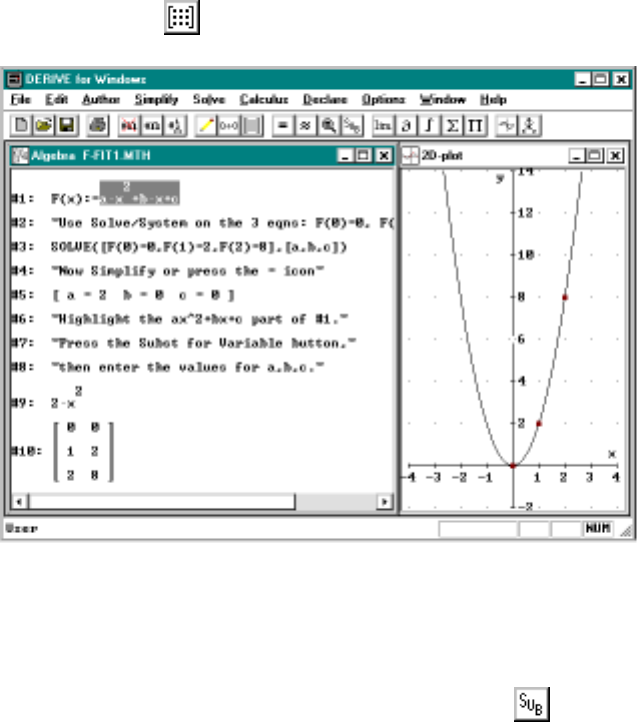
4.2. FITTING POLYNOMIALS TO DATA POINTS 57
entered by using the button. See Figure 4.1.
Figure 4.1: Fitting a polynomial to data points
For more complicated problems we would have to substitute in the values
of a, b, c into the expression ax2+bx +cusing the button. The
utility file ADD-UTIL has a function CURVEFIT(x, data) which does this
automatically. Here the xis the variable and data is the matrix of point we
want to fit the curve to. The more points we use the higher the degree of
the polynomial needs to be.
As we mentioned above, for 3 points with distinct x–coordinates there is
a unique quadratic polynomial function passing through them. We can use
Derive to demonstrate this by showing that the system of equations (1) can
always be solved for a,b,andc, regardless of the values of (xi,y
i
). To do
this we will just have Derive solve the system (1).
However, there is a slight problem. In its normal input mode, called
character input, Derive treats each letter as a separate variable. So if you
author ab Derive will read this as atimes band the algebra window will
show it as a·b. This is very convenient for calculus where we almost always

58 CHAPTER 4. CURVE FITTING
use single characters for our variables. But to solve (1) we need the variables
x1,x2, etc. When we enter x1,Derive will think of this as xtimes 1, which
is not what we want. So we need to declare that x1,x2, etc., are variables.
To declare x1 as a variable you can author x1 :=. You need to do this for
all three x’s and y’s. Besuretousetheassignmentcharacters:= and not
the equation character =.
As a convenience for the exercises the ADD-HEAD file has provided dec-
larations for x0, ...,x4andy0,..., y4. But if you need more variables or
if you use a different letter other than xor ythen you will need to declare
them.
Now enter the data matrix by clicking the button and selecting 3
rows and 2 columns. Then, enter x1 press Tab and enter y1. Continuing,
enter all the remaining xi’s and yi’s. Click the OK button and the result
should be
x1y1
x2y2
x3y3
Now we Author CURVEFIT(x,data) where data is the above matrix of
points. Simplifying yields a complicated looking answer that is a little dif-
ficult to digest. However, if you examine the denominators of each of the
expressions you will notice that they cannot be 0 since we are assuming that
x1,x2,andx
3are distinct. This is the only thing that can go wrong with the
formula in general so our assumption gives us a valid solution. See Figure 4.2
on the facing page. You might try increasing the number of points to see
that the same principle applies.
As an interesting variant on the above, suppose we want to find a,b,and
cfor a function f(x)=ax2+bx +cwhen we know
f(x1)=y
1
f(x
2
)=y
2
(2)
f0(x3)=y
3(That’s the derivative!)
In other words we specify that f(x) must pass through (x1,y
1
)and(x
2
,y
2)
and that its slope at x=x3is y3. We define f(x) as before and define g(x)
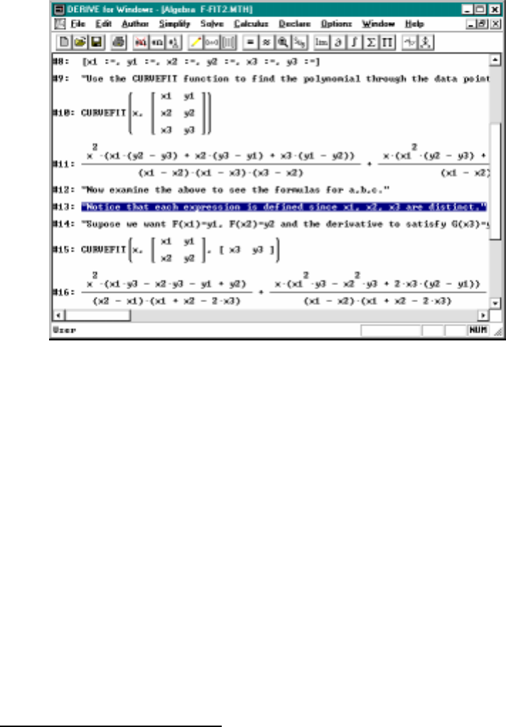
4.2. FITTING POLYNOMIALS TO DATA POINTS 59
Figure 4.2: The algebra behind fitting polynomials to data points
as the derivative1
g(x) := 2ax+b(3)
Now if we solve the system of equations
f(x1) = y1 f(x2) = y2 g(x3) = y3
as before and then factor the answer, we see that the denominator of each of
the 3 fractions is
(x1−x2)(x1+x2−2x3)
(You can do this just as in Figure 4.2 except you need to define g(x) and
use g(x3) = y3 in place of f(x3) = y3.) Of course we are assuming that
1Note that you can’t simply define g(x):=DIF(f(x),x). We ran into this problem
earlier on page 41 (see Section 0.12 on page 16 for a complete explanation). One solution
to this problem is to use the utility file and define g(x):= SUBST( DIF(f(u),u), u, x).

60 CHAPTER 4. CURVE FITTING
x16=x2so the factor x1−x2will not be 0. The other factor is 0 when
x3=x1+x2
2
This means we can always find f(x) except possibly if x3=(x
1+x
2
)/2.
This is somewhat surprising since one expects to be able to solve for 3 un-
knowns satisfying 3 equations just as one can solve for 2 unknowns satisfying
2 equations. However, in both cases there are exceptional cases that need
to be considered. In this case, the difficulty is related to the mean value
theorem and is explored in Exercise 3. Related results for cubic functions
are examined in Exercises 4 and 7.
The solution to curve fitting problems involving the derivative can also
be found using the CURVEFIT(x,data,ddata) function. As before xis the
variable and data is a matrix of points satisfied by the function. The matrix
ddata represents the points satisfied by the derivative.Intheaboveexample,
we would author
CURVEFIT(x,[[x1,y1],[x2,y2]],[[x3,y3]])
and simplify to get the answer.
4.3 Exponential Functions and
Population Growth
A good first model for population growth is
P(t)=aer(t−t0)
(4)
Population models are studied more thoroughly in Chapter 11 using the the-
ory of differential equations but for now we will just consider the exponential
model. Here P(t) is the population at time tand ais the population at the
starting time, t0. Problem 7 uses this model.
There are two parameters in (4), aand r. These parameters can be
determined if we know the population at two different times, t1and t2, i.e.,
if we know P(t1)=y
1and P(t2)=y
2
. This gives the equations
aer(t1−t0)=y1
aer(t2−t0)=y2
4.4. APPROXIMATION USING SPLINE FUNCTIONS∗61
but solving for aand ris a little more difficult since this is not a linear
system of equations. Hence, we can not solve this system using the function.
Instead, the way to do it is to use the first equation to solve for aand then
substitute that value into the second equation and then solve the resulting
equation for r.YoucanuseSOLVE on any single equation but not systems.
Another approach is to observe that the equations are linear in the quan-
tities ln aand rbecause, if we let c=lna, they are equivalent to:
c+r(t1−t0)=lny
1
c+r(t
2−t
0
)=lny
2
Of course, once we find cthen a=ec, so you’re done. Problem 6 will require
solving these equations.
4.4 Approximation Using Spline Functions∗
Suppose that, as before, we are given data points in the form of an n×2
matrix declared as data. To take a simple example let’s assume that
data :=
00
11
20
31
.
We want to find a smooth function f(x) whose graph passes through the
data points. One solution to this problem is to use CURVEFIT(x, data)
which gives us a degree n−1 polynomial passing though the given data
points. Unfortunately, for problems with a large number of data points this
can take a long time to solve because it requires solving a large system of
equations (n−1 equations and n−1 unknowns).
One simple technique that doesn’t involve solving large systems of equa-
tions is to use a piecewise quadratic polygonal approximation to the graph.
The idea is find a quadratic polynomial connecting each pair of consecutive
data points but the catch is that in order for the graph to be smooth you
need to make the derivatives match at each data point.
Here’s how we do it: We start with an arbitrary slope, say m=2,atthe
first data point, which is (0,0) in our example, and use the second form of
CURVEFIT to find a quadratic polynomial f1(x) which satisfies the equations
f1(0) = 0,f
1
(1) = 1 and f0
1(0)=2.

62 CHAPTER 4. CURVE FITTING
This solution is
CURVEFIT(x,[data SUB 1, data SUB 2],[[0,2]])
where we note that each data point can be referred to as data SUB i or
alternately, using the symbol bar as data↓i.
Now to find our second quadratic f2(x) connecting the second pair of data
points and making sure that the graph of the two functions is smooth at x=1
we simply solve for f2(x) using the equation: f0
1(1) = f0
2(1). Continuing in
this way we get quadratics f1(x), f2(x), ... ,f
n−1(x) corresponding to each of
the n−1intervals: [data
1,1
,data2,1], [data2,1,data3,1], ... ,[data
n−1,1
,datan,1].
Note that we have used the double subscript notation to get the x-values in
the first column of the data matrix.
We combine these functions into a single function using the CHI function.
Here CHI(a,x,b) is 0 unless a≤x≤bin which case it is 1. Thus, the
combined function is
f(x)=
3
X
k=1
fk(x)·CHI(datak,1,x,datak+1,1)(5)
In our example we can solve for the three quadratics and get
f1(x)=2x−x
2
,f
2
(x)=2x−x
2and f3(x)=3x
2−14x+16
Application The resulting function f(x) above is called a quadratic spline
function and is important in approximation theory and computer graphics.
One important example is in generating fonts for computer screens. Com-
puters used to view a highly stylized letter like the capital S in some fancy
font as a bitmap picture which required lots of memory to store and lots of
time to draw on the screen. The modern approach is to view the letter as
say 10-20 carefully chosen data points and then fill in the rest of the letter
using spline function techniques.
You can experiment with these techniques by using the utility function
SPLINE(x,data,m1) which gives the quadratic spline passing the data points
data and having derivative m1 at x=data
1,1
. Using our example, we enter
the above with m1 = 2 and Simplify. It’s instructive to plot the points data
as a (non-connected) set of points and then plot the spline function to make
sure that it passes through the points and that it indeed has a smooth graph.

4.5. LABORATORY EXERCISES 63
The definition behind the SPLINE function (see the file ADD-UTIL) is
fairly straightforward. The function fk(x) depends on the previous function
fk−1(x) and more specifically on the quantity f0
k−1(xk), where the kth interval
is [xk,x
k+1]. It turns out that it is more efficient to make a vector out of the
n−1slopesm=[m
1
,m
2,...] using the formula
mk=2y
k+1 −yk
xk+1 −xk−mk−1k=2,...,n−1.(6)
which can be derived using DfW(see the file F-SPLINE.MTH). Using this
formula one produces the vector of slopes using the ITERATES function. The
formula looks a little complicated at first but should look straigtforward
after some careful examination (see either the file ADD-UTIL or the SLOPE
function in the file F-SPLINE.MTH).
Using these quantities one then computes fk(x)using
CURVEFIT(x, [data↓k, data↓(k+1)], [[data↓k↓1, m↓k]])
.
See Figure 4.3 where we use this method of approximation to approximate
the function y=sinxusing n= 7, which is the smallest integer greater than
2π. Thus, based on the numbers sin 1,...,sin 7 plus the derivative at x=0,
i.e., m0= 1, we get a good approximation to the sine function.
4.5 Laboratory Exercises
Start off your lab by Loading the ADD-HEAD file (use File/Load/Math).
Note that the syntax of the CURVEFIT function is displayed on the second
line of the ADD-HEAD file. There are two possibilities: CURVEFIT(x, data)
where data is a matrix of data points satisfied by the function or CURVEFIT(x,
data, ddata) where now the derivative satisfies the matrix of data points
ddata.
1. a. Use the CURVEFIT function to find the cubic polynomial passing
through the points: (0,0), (1,1), (2,0) and (3,1).
b. What degree polynomial is required to pass through 7 points?
(Hint: Make up a 7 point data set and examine the solution.)
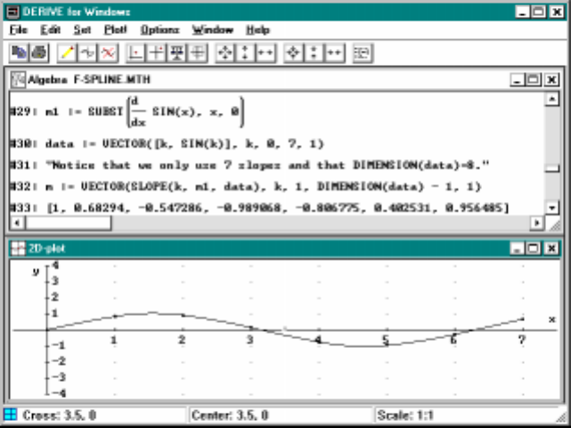
64 CHAPTER 4. CURVE FITTING
Figure 4.3: Approximation using spline functions
2. Use the CURVEFIT function to find a,b,andcif ax2+bx +cpasses
through
a. (1,1), (3,4), and (4,4).
b. (1,1), (3,4), and (4,1).
c. Show that the functions determined in part aand bboth have
the same slope at x=2.
d. Do you think it is possible that
f(1)=1
f(3)=4
f
0
(2)=2
(see equation 2). Use the second form of the CURVEFIT function to
find the solution. Note that the ddata is a 1×2matrixinthiscase.
What does Derive tell you? What if you change the derivative
to f0(2) = 3/2? Can you explain what the answer means?

4.5. LABORATORY EXERCISES 65
For the following problems you will need to use the variables x1,x2,x3,x4,
y0,y1,y2,y3,andy4. As long as you have loaded the ADD-HEAD file these
variable will be declared. On the other hand, if you use a variable such as
z0 then you will need to declare it by authoring z0:=. See the discussion on
page 57.
3. Let (x1,y
1
)and(x
2
,y
2) be two points in the plane with x16=x2.Let
m=y
2
−y
1
x
2
−x
1be the slope of the line through these points. The Mean
Value Theorem says that if f(x) is a differentiable function which passes
through these points then f0(x3)=mfor some x3between x1and x2.
Show that if f(x) has the form ax2+bx+cthen we can take x3=(x
1+
x
2
)/2, i.e., show that f0((x1+x2)/2) = mif f(x) has this form. Hint:
Solve the system f(x1)=y
1
,f(x
2
)=y
2for band cand substitute
those values back into ax2+bx +c. Then show that the derivative of
the resulting expression is mwhen x=(x
1+x
2
)/2. Of course this
means that all quadratic functions through (x1,y
1)and(x
2
,y
2)have
thesameslopeat(x
1+x
2
)/2.
4. Use the CURVEFIT function to find the quadratic function f(x)=ax2+
bx +cthat satisfies
f(x0)=y
0
f(x
1
)=y
1
f(x
2
)=y
2
Integrate the resulting function over the interval [x0,x2]. Observe that
your answer is a pretty big expression that requires scrolling to view.
Now substitute in this expression x1=(x0+x2)/2usingthe but-
ton and simplify. Note that x1isthemidpoint of the interval [x0,x2].
The answer should be a very simple formula in terms of x0,x2,y0,y1
and y2. In the next chapter this calculation will be the basis for the
Simpson Method of numerical integration.
*5. Suppose we want to find a cubic function f(x)=ax3+bx2+cx +d

66 CHAPTER 4. CURVE FITTING
such that
f(x1)=y
1
f(x
2
)=y
2
f(x
3
)=y
3
f
00(x4)=y
4
Show that this is always possible if x1,x2,andx
3are all distinct and
x46=(x
1+x
2+x
3
)/3. The algebra in this problem gets fairly messy.
6. Let (x1,y
1)and(x
2
,y
2) be two points in the plane with y1>0, y2>0,
and x16=x2.Letf(x)=aerx be an exponential function. Show that
it always possible to find aand rso that f(x) passes through these
points. Hint: you need to solve the equations
aerx1=y1
aerx2=y2
To do this first solve for ain one of these and substitute the answer
into the other and then solve for r. Make sure that your formulas for
aand ronly involve the data points.
7. Table 4.1 on page 68 shows the population of the US for every decade
from 1800–1900. Consider two models for the data: an exponential
model P(t)=aert and a linear model L(t)=bt +c.
a. Use the data for 1800 and 1810 to determine 2 linear equations in
the 2 unknowns band c.Use to find band c.
b. Do the same thing for the aand rbut this time you will need to
apply the previous exercise to solve for aand r.
c. Show that your model in Part (b) is the same as 5.3er(t−1800) where
ris the value you obtained in Part (b). Use properties of the
exponential function to explain why this is true.
d. What does each model predict for 1830?
e. How do the models compare during the first 50 years? 100 years?
Do this by graphing both functions and the population data. Ad-
just the scale to get a good picture. Note: The data in Table 4.1
can be copied from the file F-population.

4.5. LABORATORY EXERCISES 67
f. Make up your own values of aand rin the exponential model and
see if you can get a better representation of the data for the last
20 to 30 years. Do this by plotting the model and comparing with
the data.
g. The population for 1990 is 248.7 million. Use a value of aand
rfrom the previous part to estimate the population in the year
2050.
*8. Suppose that data is an n×2 matrix of data points
data :=
x1y1
x2y2
.
.
.
xnyn
.
where x1,y1,... have numerical values and x1<x
2< ....Weknow
that plotting this vector in connected mode gives a piece-wise linear
graph. You can test this using a sample value for data. Write a function
f(x) in DfW which will have the same graph, i.e., between any two
consecutive x-values, xk≤x≤xk+1,f(x) linearly interpolates the
data points. (Hint: Look at equation 5 on page 62 for doing spline
function interpolation and use the CHI function as is done there. You
will need to use subscript notation to refer to the x,yvalues. For
example, data↓1↓1is x1and data↓3↓2is y3.)
*9. Let (x1,y
1
), (x2,y
2
), and (x3,y
3) be three points in the plane
with x16=x2,x16=x3,andx
26=x
3
. Show that all cubic functions,
f(x)=ax3+bx2+cx +dwhich go through all three of these points
have the same second derivative at x1+x2+x3
3. (Hint: Just solve the 3
equations in the 3 unknowns b,c,anddin terms of the 4th unknown a.
Differentiate twice and substitute in the above value of x.Checkthat
the answer does not depend on a.)

68 CHAPTER 4. CURVE FITTING
Table 4.1: Population of the US, 1800–1990
Year Population (millions)
1800 5.3
1810 7.2
1820 9.6
1830 12.8
1840 17.0
1850 23.0
1860 31.4
1870 38.5
1880 50.0
1890 62.9
1900 76.2
1910 92.2
1920 106.0
1930 123.2
1940 132.2
1950 161.3
1960 179.3
1970 203.3
1980 226.5
1990 248.7
Chapter 5
Finding Roots Using
Computers
5.1 Introduction
This lab explains two techniques for numerically solving equations, Newton’s
famous method and the bisection method. If we have any equation we want
to solve for x, we can subtract one side from the other to get an equation of
the form f(x) = 0. Of course, in case f(x) is a polynomial then solving this
equation means finding the roots of f(x).Thus, for quadratic polynomials we
would ordinarily use the quadratic formula. However, we will be considering
very general functions which typically involve trigonometric functions, loga-
rithms and exponentials and hence algebraic methods are usually hopeless.
Newton’s method is called a dynamic process and is related to interesting
topics such as chaos and fractals. We will explore these concepts later in this
chapter.
5.2 Newton’s Method
Newton’s method for finding a solution rto the equation f(x)=0isto
start with a guess x0(presumably not too far from r) and form the tangent
line to f(x) through (x0,f(x
0)). Then find the place, call it x1, that this
tangent line crosses the x–axis. Now we repeat this process with x1in place
of x0. (See Figure 5.1 on the next page.) In this way we obtain a sequence
of numbers x0,x
1,x
2,... which, under reasonable conditions, will converge
69
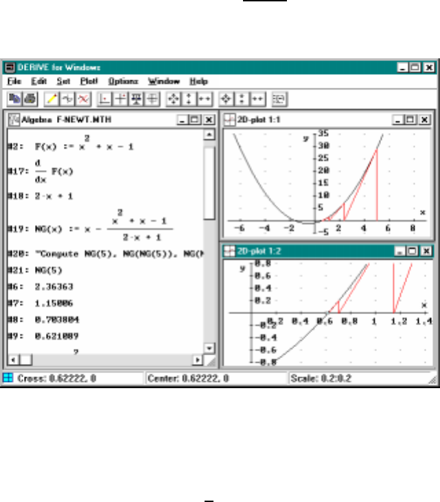
70 CHAPTER 5. FINDING ROOTS USING COMPUTERS
to r.
Since y−y0=m(x−x0) is the equation of the line through (x0,y
0)with
slope m, the equation for the tangent line of f(x) through (x0,f(x
0)) is
y−f(x0)=f
0
(x
0
)(x−x0).
Solving for xwhen y=0givesx=x
0−f(x
0
)/f0(x0). Thus we get the
(n+1)
st approximation from the nth by the formula:
xn+1 =xn−f(xn)
f0(xn)
(1)
Figure 5.1: Newton’s method for finding roots
In the graphics window of Figure 5.1 the first several approximations in
Newton’s method are shown for the equation x2+x−1 = 0 which has
the unique positive solution x=√5/2−1/2≈0.618. The initial guess is
x0=5. Fromthepoint(5,0) we go up to the curve at the point (5,f(5))
and then follow the tangent line until it intersects the x–axis at the point

5.2. NEWTON’S METHOD 71
(x1,0) ≈(2.36363,0). The process is now repeated, starting with the guess
x1.
It is convenient to view the computations as an iteration process:
NG(x)=x−f(x)
f
0
(x)
(2)
which changes a guess xinto a (hopefully) better guess NG(x). (Note that
xn+1 =NG(x
n
).) You can think of NG as standing for ‘Newton guess’ or
for ‘next guess’. To make a Derive function to do this for our function
f(x)=x
2+x−1 we define
NG(x) := x-(x^2+x-1)/(2x+1)(3)
Now starting with x0and successively applying this function to the previous
result produces a sequence of approximations:
x0
x1=NG(x
0
)
x
2=NG(x
1
)=NG(NG(x
0
))
x3=NG(x
2
)=NG(NG(x
1
)) = NG(NG(NG(x0)))
.
.
.
which we hope get closer and closer to the exact answer. In the limit we
want this sequence of approximations to converge to the root.
We can compute several approximates by first Authoring NG(5),andthen
approximating. Now we can author NG, press the right mouse button and then
click (Insert expression) or press F4. This will bring down the highlighted
expression in parentheses giving NG(2.36363) which we approximate (just
press Simplify instead of OK) again and then repeat this process.
A somewhat fancier method is to use the Derive’s ITERATES func-
tion. ITERATES(u,x,a,n) simplifies to an (n+ 1)-vector whose first en-
try is aand each subsequent entry is obtained by substituting the pre-
vious entry for xin u.Thus,ITERATES(x^2,x,2, 4) returns the vector
[2,4,16,256,65536]. (The function ITERATE is similar, but just gives the
last value, so ITERATE(x^2,x,2,4) gives 65536.) We can get the first 4
approximates by authoring ITERATES(NG(x), x, 5, 4) and approximating
the result.
72 CHAPTER 5. FINDING ROOTS USING COMPUTERS
Loading the utility file ADD-HEAD adds two functions to the system that
make computing the Newton iterations easier. The function NEWT(u,x,a)
computes the Newton guess of the expression u,inthevariablex, starting
with an initial guess at x0=a. In our previous example of f(x)=x
2+x−1
with starting point x0= 5 we would enter NEWT(x^2+x-1,x,5).Togeta
vector containing the starting point and the first 4 Newton iterates you author
and simplify NEWT(x^2+x-1,x,5,4). The general syntax is NEWT(u,x,a,k).
Looking at the algebra window in Figure 5.1 we see the above function
along with the first 4 iterates starting at x0= 5. The graphic demonstration
shows the Newton method in action by plotting a part of the tangent line
until it crosses the x-axis. The picture clearly shows how well the Newton
method works since one has to zoom-in several times near the actual root in
order to see the last two iterations. The utility function DRAW NEWT(u,x,a,k)
simplifies to a matrix which plots the figure shown in Figure 5.1.
Alternately, that file contains the necessary definition for doing the graph-
ics directly. The basic idea is to make a vector out of several triples of points
which have the form (x, 0), the initial guess on the x–axis, (x, f(x)), the cor-
responding point on the curve, and (NG(x),0), the place where the tangent
to the curve at (x, f(x)) intersects the x–axis. When we graph these points
we want the lines connecting them to be drawn. If this is not the case then
adjust the Options/Points menu.
You might note that a little trick is used in the above of DRAW Nin
the file F-NEWT. The special form of the VECTOR(u,x,v) function sets x
equal to each value in the vector v=[v
1
,...,v
n] and makes the new vector
[u(v1),...,u(v
n)].
Example. Suppose we want a numerical approximation of √2. We think
of it as a solution to the equation x2−2 = 0. Then formula (2) gives the
very simple expression:
NG(x)=x−f(x)
f
0
(x)=x−x
2−2
2x=x
2+2
2x=x
2+1
x
We get several approximates by clicking after authoring either
NEWT(x^2-2,x,2,5)(4)
or equivalently as in the file F-NEWT.MTH
ITERATES(x/2+1/x,x,2,5)(5)
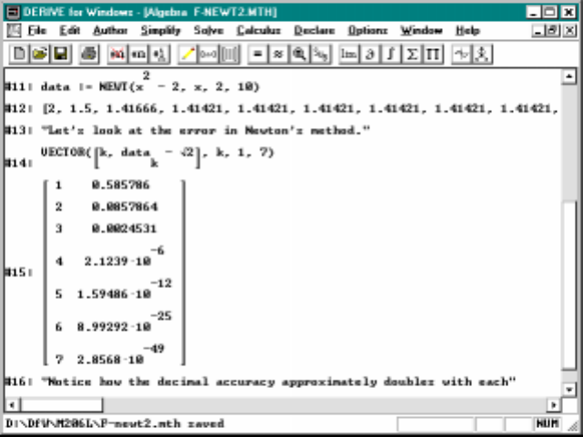
5.3. WHEN DO THESE METHODS WORK 73
with precision digits set to 10 decimal places. We get
[2,1.5,1.41666666,1.414215686,1.414213562,1.414213562](6)
which is accurate to 10 decimal places. In fact, Figure 5.2 shows a remark-
able property about Newton approximation: the number of decimal place
accuracy approximately doubles with each iteration!
Figure 5.2: Each iteration gives twice as many digits
5.3 When Do These Methods Work
In our previous examples, we have seen that by starting at a point x0which
is close to the solution r, of the equation f(x) = 0, and computing several
iterates of the NG(x) function, i.e.
x0,x
1=NG(x
0
),x
2=NG(x
1
),x
3=NG(x
2
),...
results in a sequence of approximates which get closer and closer to r.By
comparing decimals we see that the number of decimals places in common

74 CHAPTER 5. FINDING ROOTS USING COMPUTERS
increases with each new xn. More precisely, the differences |r−xn|can
be bounded by 10−mnwhere the integers mn, which are approximately the
number decimal places in common, increases with out bound. For example, in
the √2 problem above the number of decimals was approximately mn≈2n,
i.e., 2, 4, 8, 16, etc.
In order for Newton’s method to work we need at least that f(x)is
differentiable and f0(x)6= 0, since the derivative appears in the denominator
of the formula (2). We would like to find a criteria that guarantees that the
sequence xngets closer and closer to rand that the number of decimal places
in common, mn, increases without bound.
As an example, suppose that on some interval I=[r−a, r +a], with r
as a midpoint, we know that
|NG0(x)|≤λ<1 for all xin I.
Take x0in Ias our starting point and observe that NG(r)=r. By applying
the Mean Value Theorem we get that
|x1−r|=|NG(x0)−r|=|NG(x0)−NG(r)|=|NG0(c)(x0−r)|
where cis some point between x0and r. Hence, cis in the interval Iand
therefore |NG0(c)|≤λby our assumption. Thus, the above yields that
|x1−r|=λ|x0−r|<|x0−r|
and so x1is indeed closer to rthan x0.
In addition, this means that x1is in the interval Iso that we can repeat
this argument with x1as our starting point. Then, the above inequality
becomes
|x1−r|=|NG(x0)−r|≤λ|x
0−r|
|x
2−r|=|NG(x1)−r|≤λ|x
1−r|≤λ
2
|x
0−r|
.
.
.
|x
n−r|=|NG(xn−1)−r|≤λ
n
|x
0−r|
which shows that the xn’s are getting closer and closer to r.Toestimatethe
number of decimals in common take the special case that λ=0.1=10
−1
.
Then, |xn−r|≤10−n|x0−r|, i.e., mn=n, and we see that we gain one
decimal place with each computation.

5.3. WHEN DO THESE METHODS WORK 75
In general, the same sort of thing will occur with any 0 <λ<1. If λis
greater than 0.1 then the number of decimals mnwill increase at a slower rate
but nevertheless it can be shown to increase without bound. For example,
in Derive if we approximate VECTOR(1/2^n,n,1,16,3) then we get
[0.5,0.0625,0.0078125,0.000976562,0.000122070,1.5258710−5]
which suggests that mn≈n/3. In fact, if your numerically solve the equation
2−n=10
−mfor musing Derive you will get m=0.301029n.
If we assume that f00(x) exists and that f0(x)6=0onIwe can compute
NG0(x) as follows:
NG0(x)= d
dx x−f(x)
f0(x)
=1−f
0
(x)
2−f(x)f
00(x)
f0(x)2=f(x)f00(x)
f0(x)2.
Since f(r)=0weseethatNG(r) = 0! Thus, not only is |NG0(x)|less than
one near rbut it can be made as small as you like. This follows from the
continuity of the function NG(x) which in turn follows from the continuity
of f0(x) and the fact that it is never zero near r. The implication of this fact
is a much faster rate of convergence, i.e., the mnincreases much faster than
the above computations suggest.
Theorem 1. Suppose f(r)=0and that f00(x)is continuous in some open
interval Iwhich has ras its midpoint. If f0(r)6=0then the iterates of
NG(x)=x−f(x)
f
0
(x)
converge to rprovided the starting point x0is sufficiently close to r.More
precisely, the interval Ican be chosen small enough so that there is a constant
Msatisfying:
|NG(x)−r|<M|x−r|
2
(7)
whenever xis in the interval I.
Before we prove this fact, let’s see what it really means. Suppose for
example that M= 50 and we pick xin Ithat is within 2 decimals places of

76 CHAPTER 5. FINDING ROOTS USING COMPUTERS
the exact value r, i.e., |x−r|<.01. The above relationship then says that
our Newton guess starting at x,NG(x), satisfies:
|NG(x)−r|<M|x−r|
2<50(.01)2=.005
and since .005 is much smaller than .01 we have a big improvement over our
initial guess of x. Moreover, since our new guess is closer to rthan our initial
guess we see that it is also in the interval Iand hence we can repeat the same
calculation using NG(x)inplaceofx.
We could make further calculations, as above, to see how rapidly the
sequence of approximates converges to the exact root ror we could have
Derive do it for us. If we author the expression
ITERATES(50 t^2, t, .01, 5)
and simplify we get
[0.01,0.005,0.00125,7.812510−5,3.0517510−7,4.6566110−12]
which clearly shows the very rapid rate of convergence to the exact answer r.
Proof. By making the interval Ia little smaller if necessary we may assume
that both f0,f00 are continuous and bounded on I. Let us assume that
|f0(x)|≤Aand |f00(x)|≤B
for xin I. Similarly, since f0(r)6= 0 we may assume, again by making Ia
little smaller if necessary, that
|f0(x)|≥C>0orequivalently 1
|f
0
(x)|
≤
1
C
for xin I. Note that in particular this means that NG(x) is defined for xin
I.PutM=AB/C2.
We have observed that NG(r)=rand NG0(r) = 0. Hence, by using the
Mean Value Theorem twice and our formula for NG0(x)weget
NG(x)−r=NG(x)−NG(r)=NG
0
(c
1
)(x−r)
=f(c1)f00(c1)
f0(c1)2(x−r)= f
00(c1)
f0(c1)2(f(c1)−f(r))(x−r)
=f00(c1)
f0(c1)2f0(c2)(c1−r)(x−r)

5.3. WHEN DO THESE METHODS WORK 77
where c1,c2are between xand rand hence in the interval I.Usingthe
bounds for f0,f00 and 1/f0above shows that (7) holds because
|NG(x)−r|≤ A
C
2B|c
1−r||x−r|≤M|x−r|
2
which is what we needed to prove.
For another illustration of how fast the Newton method converges when
NG0(r) = 0 let us assume that the constant Min (7) is one or less. If we
make an initial guess x0which is in Iand approximates rto ndecimal places,
i.e., |x0−r|<10−nthen the first approximate x1=NG(x
0
)satifies
|x
1−r|=|NG(x0)−r|≤M|x
0−r|
2<10−2n
which means that x1approximates rto twice as many decimal places as x0.
This doubling property was observed numerically in an earlier example. The
case when M>1 is similar and is discussed in an exercise. In dynamic
systems like this, a point rwith NG0(r) = 0 is called a super attractor.
Once xgets close to a super attractor r, repeated applications of NG will
move it towards rvery quickly.
The next theorem investigates a situation where 0 <NG0(r)<1. In this
case Nk(x) still tends to rbut not nearly as fast. In this case ris no longer
a super attractor but is simply an attractor.
Theorem 2. Suppose that f(r)=0and that f(x)=(x−r)
m
g(x)where
g(x)is differentiable, mis a positive integer and g(r)6=0. Then, NG(x)is
defined for all x6=rwhich are sufficiently close to rand the iterates converge
to r.
Proof. Since f0(r) = 0 for m>1 (check!) it is not clear that we can even
define NG(x) for xnear r.But
f
0
(x)=m(x−r)
m−1
g(x)+(x−r)
m
g
0(x)
=(x−r)
m−1
[mg(x)+(x−r)g
0(x)] ≈(x−r)m−1mg(r)(8)
and since g(r)6= 0 it is easy to see that the bracketed expression above can
not be zero for all xnear to randhencethesameistrueoff
0
(x)provided
x6=r.

78 CHAPTER 5. FINDING ROOTS USING COMPUTERS
Now using (8) to simplify NG(x) (do this using Derive)weget
NG(x)−r
x−r=(m−1)g(x)+(x−r)g
0(x)
mg(x)+(x−r)g
0(x).
When x=r, the right hand side above simplifies to (m−1)/m which is less
the one. This means that we can find an interval I, with midpoint r,anda
number 0 <λ<1 such that
|NG(x)−r|≤λ|x−r|
for all xin the interval I. As we argued earlier in this section, this means
that starting at x0in Iwe get the sequence of approximates xnsatisfying
|xn−r|≤λ
n
|x
0−r|which shows that the xn’s converge to r.
5.4 Complex Numbers, Fractals and Chaos∗
Which root does Newton find? Of course f(x)=x
2−2hastworoots,
√
2and−
√
2. If our initial guess is any positive number, Newton’s method
will converge to √2 and, if it is any negative number, to −√2. If the initial
guess is 0 the method fails since NG(0) is not defined. The situation for this
f(x) is pretty simple but that is not always the case. To get a clearer picture
of what can happen we need to discuss the complex numbers .
Complex Numbers Recall that a complex number has the form a+bi,
where aand bare real numbers and iis a square root of −1, i.e., i2=−1.
In Derive we input iby using the symbol bar or by typing #i.Thisis
displayed with ˆ
i. The basic operations with complex numbers are the same
as real numbers; namely, addition, subtraction, multiplication, division and
distance.
•Addition and Subtraction. You do the real and imaginary parts sepa-
rately:
(a+bi)+(c+di)=(a+c)+(b+d)i
(a+bi)−(c+di)=(a−c)+(b−d)i

5.4. COMPLEX NUMBERS, FRACTALS AND CHAOS∗79
•Multiplication. Do this as usual except replace i2with -1:
(a+bi)(c+di)=ac +ad i +bd i +bd i2
=ac +ad i +bd i −bd =(ac −db)+(ad +bc)i
•Division: You can divide any complex number a+bi by any non-zero
complex number c+di. This means that c2+d2>0, i.e., both cand
dcan not both be zero. We define the complex conjugate ¯w=c−di.
(In Derive this is computed using CONJ(w).) Then we observe that
w¯w=(c+di)(c−di)=c
2−(di)
2=c
2+d
2
and so the formula for the reciprocal is
1
w=¯w
w¯w=c−di
c
2+d
2=c
c
2+d
2−d
c
2+d
2i.
The formula for the quotient is then given by
a+bi
c+di =(a+bi)(c−di)
(c+di)(c−di)
=(ac +bd)+(bc −ad)i
c2+d2
=ac +bd
c2+d2+bc −ad
c2+d2i
•Distance: The modulus or absolute value of a complex number z,where
z=a+bi, is defined as |z|=√a2+b2.Thedistance between two
complex numbers z,wis defined as |z−w|, i.e., the modulus of their
difference. When we plot complex numbers as points in the plane (see
below) then this distance formula is the same as the usual distance for-
mula between points in the plane. In Derive the modulus is computed
using ABS which is the absolute value function.
•Real and Imaginary Parts: In the representation of a complex number
as z=a+bi;wherea,bare real numbers, we say that ais the real part
of zand that bis the imaginary part of z. Using the complex conjugate
defined above we have the following formulas:
a=<z=z+¯z
2and b==z=z−¯z
2i.
In Derive the corresponding these are computed as RE(z) and IM(z).

80 CHAPTER 5. FINDING ROOTS USING COMPUTERS
The formulas may look a little complicated at first but nevertheless the
usual rules of algebra hold for complex numbers and we can use them just as
we would ordinary real numbers. Of course, it is easier to make computations
using Derive then it is to compute with the formulas above. You should
verify the above formulas using Derive.
You probably have already encountered complex numbers in Derive
when, for example, you try to Solve an equation such as x2+1 = 0 or
something more complicated, while trying to find extreme points. The result
is that Derive computes the two solutions x=±i. Of course, in calculus we
usually ignore complex solutions since they are not relevant to max-min the-
ory or graphics. Nevertheless, they do play an important role in algebra since
they provide a complete theory for the solution to polynomial equations.
Complex numbers can be represented as points in the plane: (a, b) for
a+bi. When we are plotting complex numbers we usually refer to the
plane as the complex plane.Derive does not directly plot complex numbers
as points in the plane but we have a utility function DRAW COMPLEX which
converts a vector of complex numbers into a matrix of points in the plane,
using the RE and IM functions, which can then be plotted as usual.
Example In order to plot the powers of i,weenter:
[#i, #i^2, #i^3, #i^4, #i^5]
and then simplify to get [i, −1,−i, 1,i]
1. Now we apply our utility function
to this vector and simplify to get the matrix
01
−10
0−1
10
01
Notice that the row entries (x, y) corresponds to the complex numbers x+yi
from the above vector. Now plotting these five (x, y)-points as usual gives us
an interesting picture of how complex multiplication is quite different from
ordinary real numbers. Notice that the powers are rotating in the counter-
clockwise direction about the origin. Also notice that the last point is the
1We could use vector(#i^n,n,1,5). to produce this vector

5.4. COMPLEX NUMBERS, FRACTALS AND CHAOS∗81
same as the first since i5=(−1)2i=i. Which real numbers xhave the
property that xn=xfor some integer n?
Using the same function f(x)=x
2−2, let’s see what happens if we start
with a complex number for x0like 3 + 2 i. The formula (1) 1 on page 70 for
Newton’s method involves arithmetic operations with the complex number
x0=3+2iand hence is valid. This time we Author
data := NEWT(x^2-2,x,3+2 #i,5)
and then we approximate this with precision set to 6 decimal places, to obtain
[3 + 2 i, 1.73076 + 0.846153 i, 1.33170 + 0.195097 i,
1.40099 −0.0101504 i, 1.41423 + 9.59747 ×10⁻⁵i, 1.41421]
so that it still converges to √2. Notice how the iparts tend to zero rapidly.
We can get a picture of this convergence by authoring
DRAW COMPLEX(data)
and then simplifying. The result will be a matrix of 6 points. We plot this
matrix to observe how the iterates converge to the point (√2,0) on the x-axis,
see Figure 5.3 on the following page.
It’s a fact that the Newton method will converge to √2 whenever we
start with x0=a+bi where a>0. We call √2anattractive fixed point
and the right half plane is called the basin of attraction for √2. If we start
with x0=a+bi where a<0 it will converge to −√2, so −√2isalsoan
attractor with the left half plane as its basin of attraction.
What happens if we start with a point on the imaginary axis (the y–axis
x0=bi? Simplify and plot the expression
DRAW COMPLEX(NEWT(x^2-2,x,#i,25))
Notice that all the values are purely imaginary (they only have an icom-
ponent) and that they seem to bounce around randomly. Moreover, if you
author
DRAW COMPLEX(NEWT(x^2-2,x,1.01#i,25))
you’ll notice that the corresponding entries of the answers are approximately
the same for the first few terms but very quickly seem to have no relation to
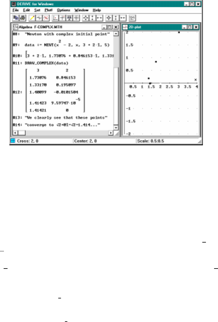
82 CHAPTER 5. FINDING ROOTS USING COMPUTERS
Figure 5.3: Newton’s method with complex starting point
each other. Here’s a nice way to do this: Define the first set of points to be
data1 and the second set to be data2. Author the vector [data1,data2]
and simplify. Then scroll though the matrix to compare entries.
In other words, even though the two starting points above; namely i
and 1.01iare quite close together their long-term behavior seem completely
different. The above phenomenon is what is known as chaos.
We can illustrate this last property graphically by looking at the equation
x2+ 2 = 0 rather than x2−2 = 0. The former equation has roots √2iand
−√2i. Just as before if we start with any point a+ib in the upper half of the
complex plane (b>0), the Newton iterates of the function x2+ 2 converge
to √2iand any point in the lower half plane (b<0) converges to −√2i.
Test this by plotting
DRAW COMPLEX(NEWT(x^2+2,x,1+#i,5))
But we get chaos on the real axis. To see this chaos plot the function x2+2
and the output to DRAW NEWT(x^2+2,x,2,4) in connected mode, see Fig-
ure 5.4 on the next page.
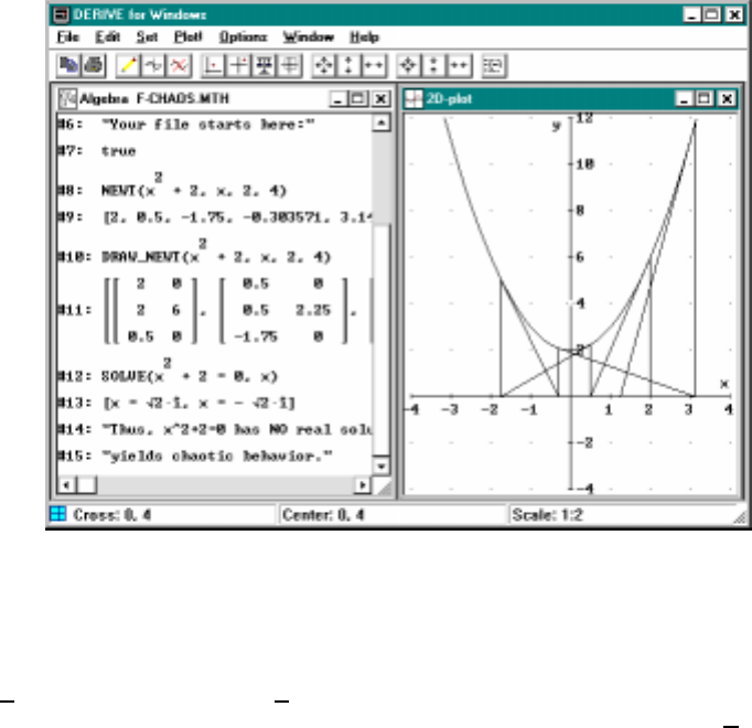
5.4. COMPLEX NUMBERS, FRACTALS AND CHAOS∗83
Figure 5.4: Chaos
Now consider f(x)=x
3−1. This has three roots: x=1,x=−1/2+
i
√
3/2, and x=−1/2−i√3/2. This is easy to do in Derive just Solve the
equation x3−1 = 0. Each of these is an attractor with a basin of attraction.
However the shapes of these basins of attraction are really quite interesting
and bizarre. Figure 5.5 on the following page shows the basin of attraction
for the root x= 1 in white. The basins of attraction of both of the other
roots are black. In Figure 5.5 the center is the origin in the complex plane
and the right hand edge has x=2. Sothepoint(1,0) (i.e., 1+0 i) is between
the center and the right hand edge.
A color version of this figure that indicates the number of iterates needed
to converge can be viewed on our World Wide Web home page at
http://www.math.hawaii.edu/lab/newton.html
This web page contains an interactive Java applet that shows the iterations in
Newton’s method. You click a complex starting point and the applet shows
the first five iterations. Try it!

84 CHAPTER 5. FINDING ROOTS USING COMPUTERS
Figure 5.5: Basins of attraction of x3−1 in the complex plane
Constructing the Julia set The set of points where Newton’s method
fails, that is, the set of points x0where the sequence
x0,NG(x0),NG(NG(x0)),...(9)
fails to converge, is called the Julia set for NG(x). In the example f(x)=
x
3
−1 these are the points on the edge or boundary of the basin of attraction.
As the picture in Figure 5.5 shows this set can be very complicated, it looks
a little like a necklace with infinitely many smaller and smaller loops coming
out in many different directions.
There are two basic methods for constructing this set. Since NG(x0)is
not even defined when f0(x0) = 0 this is a good place to start. If xis a
solution of
NG(x)=x
0
then the third term of the sequence (9) is not defined and so xwill be in
the Julia set. In the case when f(x)=x
3−1 the equation above has
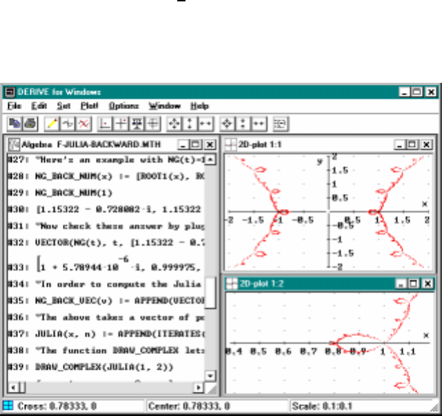
5.4. COMPLEX NUMBERS, FRACTALS AND CHAOS∗85
three solutions. For each of these there are three more obtained by solving a
similar equation or in other words finding the points where NG(NG(x)) = x0.
Continuing in this way we get a close approximation to the Julia set. The
actual set is obtained by taking limits of these points. This method is called
the backward method and is done in the file F-JULIA-BACKWARD for the
polynomial x3−3xwhich has critical points at ±1. This function has three
real roots at x=0andx=±
√
3 and the Julia set somehow has to separate
the three basins of attraction corresponding to these roots. See Figure 5.6
for a picture of it’s Julia “necklace”.
Figure 5.6: Bad Newton starting points for x3−3x= 0 in the complex plane
The trouble with the backward method is that it uses the cubic formula
for solving 3rd order equations and this formula is pretty complicated. Even
worst is the fact that there is no analogous formula for degrees 5 or greater.
To get around this problem there is the “forward method” which involves
simply looking at the sequence:
NG(x0),NG(NG(x0)),NG(NG(NG(x0))),...
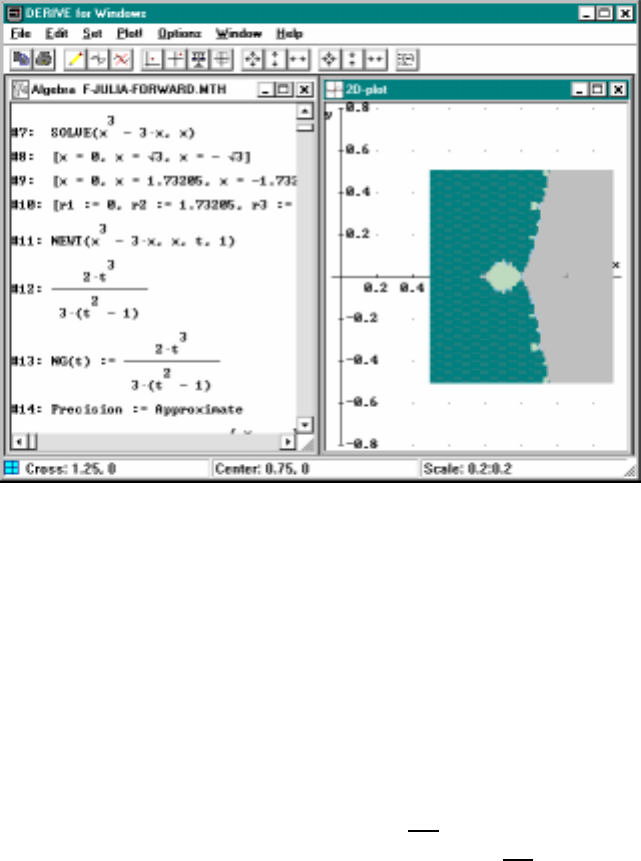
86 CHAPTER 5. FINDING ROOTS USING COMPUTERS
and checking whether it gets closer and closer to root or else just wanders
around forever. Since you have to do this for each point or pixel in the graph
this can be a very lengthy computation. A number of shortcuts and tricks
are typically employed and you can study the file F-JULIA-FORWARD to
see how we did it. Or you can just check out the pictures; see Figure 5.7.
Figure 5.7: Basins of attraction for x3−3x=0
5.5 Bisection Method∗
We now consider a very simple technique that is applicable to any continuous
function f(x). If f(x) is continuous and f(a)<0andf(b)>0, i.e., it is
below the x–axis at aand above the x–axis at b, then the Intermediate Value
Theorem tells us that f(x) must have a zero between aand b. Assume a<b.
The bisection method evaluates f(x)atx=a+b
2, the midpoint of aand b
(which is why it is called the bisection method). If f(a+b
2)>0 then there
must be a root in the interval [a, (a+b)/2]; otherwise there must be a root in
the interval [(a+b)/2,b]. In the former case we take the interval [a, (a+b)/2]

5.5. BISECTION METHOD∗87
and apply the bisection method to it; otherwise we use [(a+b)/2,b]. At each
stage the root lies in an interval that is only half the size of the previous
stage. So we can eventually find the root to any number of decimal places.
We can automate this process by authoring two functions:
F(x) :=
BIS2(a,b) := IF(f(a)f((a+b)/2)<0, [a, (a+b)/2], [(a+b)/2, b])
BIS(v) := BIS2(v SUB 1, v SUB 2).
The main function is BIS(v) and BIS2(a,b) is a helper function. The ar-
gument vto BIS is a vector with two entries, e.g., [a, b].TheDerive
function SUB, which we discussed in the previous section, returns the parts
of a vector so that [a,b] SUB 1 = a and [a,b] SUB2=b.SoBIS starts
with a vector like [a,b] and calls BIS2(a,b). This then uses the values f(a)
and f((a+b)/2) to decide if there is a root in [a, (a+b)/2] or in [(a+b)/2,b].
In the discussion above we assumed that f(x)<0andthatf(b)>0. The
way we have defined BIS it will work also in the case f(x)>0andf(b)<0.
To do this we test if the product f(a)f((a+b)/2) is negative. If it is, then
one of f(a)andf((a+b)/2) is negative and the other is positive. In this
case the points (a, f(a)) and (a+b
2,f(a+b
2)) lie on opposite sides of the x–axis
and so there must be a root in the interval [a, (a+b)/2]. In the other case,
f(a)f((a+b)/2) is positive and so they have the same sign. In this case
f((a+b)/2) and f(b) must have the opposite signs (why?) and so there is a
root in [(a+b)/2,b].
Let us try the equation ln x= 1 which has the (unique) solution x=e=
2.718 .... Of course we are finding the root of ln x−1 so we author f(x)
:= ln(x) - 1 and apply BIS. Graphing f(x) shows that there is a root
between2and3soweauthorBIS([2,3]). This returns [2.5,3], indicating
that 2.5<e<3.
Now we want to apply BIS to the answer [2.5,3]. You can do this several
times by choosing author, typing BIS, and then inserting the highlighted
vector. Once again we have an iteration process and we can use the ITERATES
function that does this for you.
Using this technique, we author
ITERATES(BIS(v),v,[2,3],10)
and then approximate it to see how well this approximates e, see Figure 5.8
on the following page.
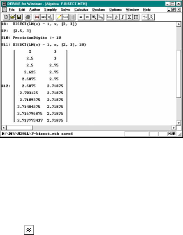
88 CHAPTER 5. FINDING ROOTS USING COMPUTERS
Figure 5.8: Bisection method for finding roots
An easier way to see the bisection method in action is to use the function
BISECT(u,x,v,k) in the utility file ADD-UTIL. To get the above results
we would simply enter BISECT(ln x-1,x,[2,3],10) and the press the ap-
proximation button. It is interesting to compare the results of the
bisection method with the Newton method of the previous section. The bi-
section method is fairly fast at getting a good approximation but not nearly
as fast as the Newton method.
The bisection method will work for any fthat is continuous on the interval
[a, b]andf(a)andf(b) have opposite signs. It is easy to see that after n
iterates the error is at most (b−a)/2n. (In fact this is the width of the
resulting interval. If we choose the midpoint as our estimate, the error will
be at most (b−a)/2n+1.)

5.6. LABORATORY EXERCISES 89
5.6 Laboratory Exercises
Start off your lab by Loading the ADD-HEAD file (use File/Load/Math).
Note that the syntax of the NEWT function is displayed on the second line
of the ADD-HEAD file. There are two possibilities: NEWT(u,x,a) where a
is the starting point in Newton’s method applied to the expression uin the
variable x. Alternately, the function NEWT(u,x,a,k) gives a vector contain-
ing the intial guess afollowed by the first kapproximates. The function
DRAW NEWT(u,x,a,k) produces the graphical demonstration of the Newton
method.
1. The equation x2= 2 has solutions x=±√2. Use the function x2−2
and NEWT to estimate √2.
a. Give the 5th iterate starting at x=10
b. Plot the graph of x2−2 and the output to DRAW NEWT(x^2-2, x,
10, 5).
c. What happens when your start at x=−10?
d. What’s wrong with the starting point x= 0? Explain this both
numerically and graphically.
2. In a manner similar to Problem 1, use NEWT to estimate 3
√7.
a. Give the 5th iterate starting at x=2.
b. By comparing with the approximate given by Derive how many
decimal places (roughly) does the Newton approximations share
with the actual answer. Note that you may need to increase the
number of digits you are working with (see Section 0.6).
3. Plot the graphs of x2and sin x.
a. Determine graphically where the two graphs intersect. Give a
rough estimate of the accuracy of this method? (Hint: If you use
the right arrow key to change the position of the crosshair, how
much does its x–coordinate change?)
b. Next use Newton’s method to find all solutions to x2−sin x=0.
Give the 5th iterate starting at x=2.
90 CHAPTER 5. FINDING ROOTS USING COMPUTERS
c. Solve this equation numerically by using Solve/Numerically2
menu. Compare the solution you get using DfW’s SOLVE function
with your approximation above using Newton’s method.
4. Let f(x)=x
3−5x.Graphf(x).
a. Use Solve to find the all roots of x3−5x=0.
b. Plot the output to DRAW NEWT(x^3-5x,x,1,5) and analyze the
first 5 iterates in the Newton approximation method starting at
x= 1. Explain in words what goes wrong when you start at x=1.
c. Do the same but with x0=1.01 and with x0=0.99.
5. Again let f(x)=x
3−5x.
a. Find the formula for NG(x) for this f.
b. Find a point x0where is NG(x) undefined. (There are two such
points; find either one.) Give the exact answer and then approxi-
mate it.
c. Use Derive’s Solve/Numerical2to solve NG(x)=x
0
.Callthe
answer x1.
*d. Do this once more, that is, Solve/Numerical2NG(x)=x
1
.Call
the answer x2. If you continued this forever what do you think
the sequence
x0,x
1,x
2,x
3...
would look like? What are their signs? What do you think
limn→∞ |xn|is?
e. Choose any numbers aand bwhich satisfy
|x2|<a<|x
1
|<b<|x
0
|
To which root does Newton’s method converge if we start with a?
with b?
2In DfW5 you choose Solve/Expression and then select the Numerically solution
method option.

5.6. LABORATORY EXERCISES 91
6. Let f(x)=x
2+1. Graphf(x). Find 10 iterates of Newton’s method
starting with x0=0.5andx
0=0.501. Explain why you think the
successive approximations don’t seem to be converging to anything.
7. Use the definitions for adding and multiplying complex numbers given
in Section 5.4 on page 78 to answer these problems using pencil and
paper and then check your computations using Derive. Recall that
the definition of the complex conjugate is a+bi =a−bi and that in
Derive you use the function CONJ. The modulus is |a+bi|=√a
2+b
2
and in Derive you use the function ABS, i.e. absolute value.
a. (1 + 2i)+(3−i)b. (1 + 2i)+(3 −i)
c. (1 + 2i)(3 −i)d. (1 + 2i)(3 −i)
e. |(1 + 2i)(3 −i)|f. |(1 + 2i)(3 −i)|
g. 1+2i
3−ih. 2+i1+2i
3−i
i. =1+2i
3−ij. <(2 + i1+2i
3−i)
8. Let z=a+bi and w=c+di,wherea,b,cand dare real numbers.
Recall that the definition of the complex conjugate is ¯z=a−biand that
the modulus is |z|=√a2+b2. Verify the equations below using pencil
and paper and then check your computations using Derive.Notethat
in Derive you use the function CONJ for the complex conjugate and
ABS for the modulus. Verify equations in Derive by authoring their
difference and simplifying. You should get zero if the two expressions
are equal.
a. z+w=¯z+¯wb. z−w=¯z−¯w
c. zw =wz d. zw =¯z¯w
e. |z|2=z¯zf. |zw|=|z||w|
Now let P(x)=x
2+2x+ 3 be a typical quadratic polynomial. Use the
above relations to show that:
g. P(z)=P(¯z)

92 CHAPTER 5. FINDING ROOTS USING COMPUTERS
The above relation implies that P(z) = 0 if and only if P(¯z)=0so
that the two roots of P(x) = 0 are conjugates to each other. Use Solve
to verify this fact by computing the roots from the quadratic formula.
9. Use the discussion about complex numbers in Section 5.4 and the utility
function DRAW COMPLEX to answer these questions.
a. Compute the first ten powers of 1 + iand plot the result.
b. Compute the first ten powers of 1
2+1
2iand plot the result.
c. Compute the first ten powers of 1
√2+1
√2iand plot the result.
d. One of the above examples spirals in toward the origin. What
geometric conditions on a complex number z=x+yi do you
think would force its powers to spiral into the origin?
The rate of the convergence of Newton’s method to a solution rof f(x)=
0 is determined by |NG0(r)|. Since NG(r)=rwe say that ris a fixed point
for NG(x). If 0 <|NG0(r)|<1thenris said to be an attractive fixed point
because nearby points are drawn to rby iterating. If NG0(r)=0,thenr
is called a super attractive fixed point. The hypotheses of Theorem 1 on
page 75 imply that NG(r)=rand NG0(r) = 0 which guarantees that the
convergence was very fast. In the following problems you explore situations
where NG0(r)6=0. Aslongas|NG0(r)|<1 Newton’s method will still
converge to rif x0is close enough to r, but not as fast as the super attractive
case.
*10. Theorem 1 had the hypothesis that f(r)=0andf
0
(r)6=0. Inthis
problem we explore what happens to a function when f0(r) = 0. Let
f(x)=x(x
2−2)2.
a. Graph f(x) and plot DRAW NEWT(x(x^2-2)^2,x,3,5) (rescale to
get a good picture).
b. Find the first 10 Newton iterates starting with x= 2. How fast
are they approaching √2 compared with the example shown in
formulas (4) and (6)? (Use 10 digits precision.)
c. Compute (exactly) NG(√2) and NG0(√2), where NG is defined
by formula (2). Is √2 a super attractor?

5.6. LABORATORY EXERCISES 93
d. Find aand bso that a6=band NG(a)=band NG(b)=a.
(Hint: Start by visualizing this situation graphically. Then try
guessing an approximate solution by looking at the graph and
experimenting with the DRAW NEWT function. Finally, use algebra
to solve the equation: NG(NG(a)) = afor aand then put b=
NG(a).)
e. Suppose now that f(x)=x(x
2−2)3.FindNG
0
(
√
2). What do
you think NG0(√2) would be for f(x)=x(x
2−2)k?(Lookup
Theorem 2 on page 77 to see if this situation is a consequence of
that result.)
11. The function f(x)=x
1/3has a root at x=0. FindNG(x), NG0(x), and
NG0(0). Find 10 iterates of Newton’s method starting with x0=0.1.
(Note: Make sure that the Precision Mode is set to Exact or else there
may be problems with this exercise.)
12. Let x1,x
2,... be the Newton iterates starting at x0, i.e.,
x1=NG(x
0
)andx
n+1 =NG(x
n
)
for n=1,2,.... In Theorem 1 on page 75, it is proved that there is an
interval I, with midpoint r, and a constant Msuch that
|xn+1 −r|≤M|x
n−r|
2
whenever xnis in the interval I.
Assume that x0is in the interval Iand satisfies
|x0−r|≤ 1
10M
where Mis the above constant. Use pencil and paper (and perhaps
mathematical induction) to prove:
a. Each xnis in the interval I.
b. The inequality
|xn−r|≤M
−1
10−2n
holds for n=0,1,2,....

94 CHAPTER 5. FINDING ROOTS USING COMPUTERS
c. Check your work above by having Derive calculate
ITERATES(mt^2, t, 1/(10m), 10).
If you Approximate the result rather than simplifying then the
answer will be expressed using powers of 10 which makes for easier
reading.
d. Interpret the above rate of convergence into the number of decimal
place accuracy achieved with each approximate xn.
13. Use the bisection method to estimate √2.
*14. The light area in Figure 5.5 on page 84 shows the basin of attraction
of the root 1 when using Newton’s method on x3−1. The origin of the
complex plane is in the middle of this figure. Note that most of the
negative real axis (the negative x–axis) is in the white area. This means
that starting with most negative real numbers, Newton’s method will
converge to 1. Try this for x0=−1and−2. If you look closely at
the figure you see that black pinches down on the negative real axis at
various points. Find the value of the first such point to the left of the
origin.
Chapter 6
Numerical Integration
Techniques
6.1 Introduction
This lab discusses numerical integration. Numerical integration is described
in most calculus books and is sometimes covered in second semester calculus.
You may want to look over this part of your calculus text.
A function is called elementary if it is made up of sums, products, powers,
and compositions of the trig functions and ln xand ex. Although the deriva-
tive of any elementary function is elementary, not all such functions have
elementary antiderivatives. For example, there is no elementary function
whose derivative is sin(x2), i.e., Rsin(x2)dx is not an elementary function.
Consider the problem
Z1
−1
sin(x2)dx
Even though sin(x2) has no elementary antiderivative, the area defined by the
integral certainly exists. So how do we find it? We use numerical integration.
Consider the integral Rb
af(x)dx, and for simplicity assume f(x)≥0and
that a<b. The idea of numerical integration is to choose intermediate points
a=x0<x
1<x
2<···<x
n=band estimate the area in the strip below
f(x) for xi≤x≤xi+1 and then add up these estimates; see Figure 6.2 on
page 100. Of course the width of this strip is xi+1 −xi. The height varies
with x. Some of the most common ways of estimating the area of the strip
95
96 CHAPTER 6. NUMERICAL INTEGRATION TECHNIQUES
are:
•Left endpoint: f(xi)(x
i+1 −xi)
•Right endpoint: f(xi+1)(x
i+1 −xi)
•Midpoint: f(xi+1 +xi
2)(x
i+1 −xi)
•Trapezoid: 1
2[f(xi+1)+f(x
i
)] (xi+1 −xi)
•Simpson’s Rule: 1
6f(xi+1)+4f(x
i+1 +xi
2)+f(x
i
)
(x
i+1 −xi)
The last one, Simpson’s Rule, is based on the best quadratic approximation
to f(x). This basic idea was derived in Exercise 4 on page 65 in Chapter 4.
Section 6.5 on page 104 has a detailed explanation.
Usually we choose the xi’s equally spaced, so that
xi=a+b−a
ni(1)
Of course, in this case, xi+1 −xi=b−a
n. Thus, if we use the left endpoint
approximation, we get
Zb
a
f(x)dx ≈b−a
n
n−1
X
i=0
f(xi)(2)
Notice that we factor out the term b−a
nand multiply by the sum rather
than multiplying every term.
6.2 An Example
Formula (2) suggests how we might do numerical integration with Derive.
Let ube the expression for f(x). We can define a Derive function for the
left endpoint method by
LEFT(u,x,n,a,b) :=
(b-a)/n * SUM(SUBST(u, x, a + k*(b-a)/n), k, 0, n-1)

6.2. AN EXAMPLE 97
(Recall that SUBST(u, x, a) substitutes afor xin uso
SUBST(u, x, a+k(b-a)/n)
really evaluates uat x=a+k(b−a)/n.) LEFT is already defined for you
in the file ADD-UTIL. All of the other methods mentioned above are also
defined in that file with the names: RIGHT,MID,TRAP,andSIMP.
Now let’s try an example. Although we would normally use these approx-
imations for integrating expressions without an elementary antiderivative, we
can test how good they are by applying them to something we do know how
to integrate:
Z2
1
1
xdx =ln2≈0.693147180559
To use the left endpoint method with n= 10 intervals, we would just author
and then approximate
LEFT(1/x, x, 10, 1, 2)
Doing this gives the answer 0.718771. Similarly if we wanted to use the
trapezoid method we would author and approximate TRAP(1/x, x, 10, 1,
2) which gives 0.693771.
We want to compare the accuracy of these methods of approximation
and also see how much the accuracy is improved by increasing n. We will
try them for n= 10, 100, 1,000 and 10,000. A fancy way to see and compare
approximation values, using the left endpoint rule for a range of nis to start
by authoring the vector
[10^n,LN(2),LEFT(1/x,x,10^n,1,2),LEFT(1/x,x,10^n,1,2)-LN(2)].
Then, use the Calculus/Vector menu to produce
vector([10^n, LN(2), LEFT(1/x,x,10^n,1,2),
LEFT(1/x,x,10^n,1,2) - LN(2)], n, 1, 4)
where the Variable nvaries from a Starting value of 1 to an End value of 4.
Approximating this expression yields a 4 ×4 matrix with the first column
being the number of partitions, the second column being the exact value, the
third column being the approximate value obtained from the left endpoint
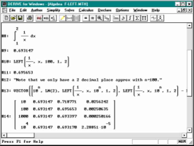
98 CHAPTER 6. NUMERICAL INTEGRATION TECHNIQUES
Figure 6.1: Approximating ln 2 with left endpoint method
method and the fourth column being the error. See Section 0.14 on page 18
for more discussion on the vector function.
Notice from Figure 6.1 that the accuracy in this method seems to be
roughly 1, 2, 3 and 4 digits respectively. This is in fact the case and it can
be proved that using 10nsubdivisions yields an accuracy of ndecimal places.
This is not very efficient since it requires a billion computations (109)to
achieve calculator accuracy of 9 digits. Try comparing computation times
for various powers of 10 to see how this rapidly becomes impractical. If we
try to obtain simple calculator accuracy of 8-12 decimal places, then this
can take hours on a PC which is impractical. It is for this reason that we
investigate the other methods for computational purposes.
By replacing the left endpoint method with the trapezoid method in the
computation in Figure 6.1 we see a remarkable difference. The accuracy now
appears to be approximately 2, 4, 6 and 8 digits respectively. Thus, the 4
decimal place accuracy achieved by the left endpoint method using 10,000
rectangles is equivalent to the trapezoid method using only 100 trapezoids.
We can summarize the theoretical error for these methods as follows. It

6.2. AN EXAMPLE 99
can be shown that error in using the left endpoint method is no greater than
(b−a)2
2max
x∈[a,b]|f0(x)|1
n.(3)
On the other hand, the error in using the trapezoid method is no greater
than
(b−a)3
12 max
x∈[a,b]|f00(x)|1
n2.(4)
In our example (with f(x)=1/x,a=1andb=2)wehavethebracketed
quantity in (4) is equal to 1/6 so that the error is no greater than n−2/6.
Thus, n= 100 indeed yields an error of less than .00002 or approximately
4 decimal digits. You might want to modify the previous table we did in
Derive to add another column displaying this theoretical error estimate
(3) (and (4) for the trapezoid method) and compare it to the actual error.
Although the trapezoid method is quite accurate and fairly efficient, the
Simpson’s Rule is vastly more efficient. The error in using the Simpson
method is no greater than
(b−a)5
180 max
x∈[a,b]|f(4)(x)|1
n4.(5)
Notice the main difference between (4) and (5) is that we now have an
error which is roughly 1/n4(the bracketed quantity in our example is 24/180).
Thus, with n= 10 we obtain the same accuracy as n= 100 in the trapezoid
method or n= 10,000 in the left endpoint method. A table illustrating these
differences can be obtain by approximating
vector([LEFT(1/x,x,10^n,1,2) - LN(2), TRAP(1/x,x,10^n,1,2)
- LN(2),SIMP(1/x,x,10^n,1,2) - LN(2)], n,1,4).
These functions are available by doing Load/Utility with the file ADD-UTIL.
Seeing the accuracy of SIMP(1/x, x, 104,1,2) requires 16 digits of accuracy.
Recall from Section 0.6 how to increase the accuracy of a calculation.
To get a geometric feeling for why the trapezoid method is so much better
than the left endpoint method one need only draw a sketch comparing the two
methods. It’s possible to graphically represent these approximations using
Derive. Recall from Chapter 4 that one can plot a collection of points,
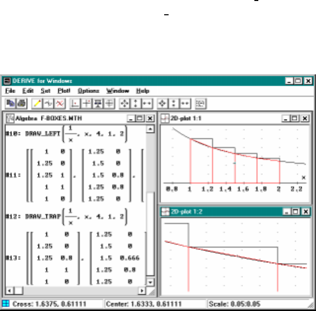
100 CHAPTER 6. NUMERICAL INTEGRATION TECHNIQUES
(x1,y
1
), (x2,y
2
), ...,(x
n
,y
n), by plotting an n×2 matrix. Thus, a rectangle
can be drawn by plotting a 5 ×2 matrix. (Note: The 5th point is the same
as the first point so that the figure is closed.) In order to draw nrectangles,
one plots an n-vector with entries corresponding to each of the rectangles.
This vector resembles a 5 ×2nmatrix but in facts its a vector with matrix
entries. To generate this vector use the function DRAW LEFT(u,x,n,a,b)
for the left endpoint method and DRAW TRAP(u,x,n,a,b) for the trapezoid
method. Both of these are defined in ADD-UTILe.
Figure 6.2 illustrates both of these. One must zoom in a bit to see that
the trapezoid is actually different from the original curve (even for n=4).
Figure 6.2: Rectangular vs trapezoidal approximation
6.3 Theorem on Error Estimates∗
Let us indicate how one obtains some of these error estimates by proving the
following theorem:

6.3. THEOREM ON ERROR ESTIMATES∗101
Theorem 1. Suppose that f(x)is a continuous function on the interval
[a, b]. The following hold:
(a) If f0(x)is bounded on the interval [a, b], then the error in approximating
Rb
af(x)dx with LEFT(f(x),x,n,a,b)is proportional to 1/n.
(b) If f00(x)is bounded on the interval [a, b], then the error in approximating
Rb
af(x)dx with TRAP(f(x),x,n,a,b)is is proportional to 1/n2.
(c) Finally, if f(4)(x)is bounded then the error in approximating the inte-
gral using Simpson’s Rule SIMP(f(x),x,n,a,b)is proportional to 1/n4.
Proof. We’ll prove parts (a),(b) and leave (c) to a more advanced text. We
first show that the error obtained by approximating a function f(x), over the
kth sub-interval [xk−1,x
k], by the constant f(xk−1) is proportional to 1/n.(x
k
is defined by (1).) This estimate uses the Mean Value Theorem as follows:
for xk−1≤x≤xkwe have
|f(x)−f(xk−1)|=|f0(cx)(x−xk−1)|≤max
x∈[a,b]|f0(x)|(b−a)
n.
This bounds how much f(x)andf(x
k−1
) can differ for xbetween xk−1and
xk; and this means the error in using the left endpoint estimate for the strip
between xk−1and xkis at most the width of the strip, (b−a)/n, times this
bound. Adding this over all nstrips gives
Zb
a
f(x)dx −LEFT(f(x),x,n,a,b)
≤(b−a)
2max
x∈[a,b]|f0(x)|1
n
which is the desired result. This completes the proof of part (a).
The proof of part (b) is similar except it uses the Mean Value Theorem
three times. We estimate the error from approximating f(x) by the linear
function obtained from the endpoints values f(xk−1)andf(x
k
). Thus, for
xk−1≤x≤xkwe have
f(x)−f(xk)−f(xk−1)
xk−xk−1·(x−xk−1)+f(x
k−1
)
=
(f(x)−f(x
k−1
)) −f(xk)−f(xk−1)
xk−xk−1·(x−xk−1)
=|f0(c1)(x−xk−1)−f0(c2)(x−xk−1)|=|f00(c3)||c1−c2||x−xk−1|
≤max
x∈[a,b]|f00(x)|b−a
n2

102 CHAPTER 6. NUMERICAL INTEGRATION TECHNIQUES
and thus at each point the error is proportional to 1/n2and so is the integral
over [a, b]. More precisely,
Zb
a
f(x)dx −TRAP(f(x),x,n,a,b)
≤(b−a)
3max
x∈[a,b]|f00(x)|1
n2
We note that the error estimates above differ from (3) and (4) only in the
constant term and not the power of n. To obtain the better constant more
careful estimation needs to done in the above argument. On the other hand,
the constants obtained above suffice for most applications.
6.4 More on Error Estimates∗
In order for any method of approximation to be useful we must know some-
thing about the error. The error estimates given in equations (4) and (5)
usually work quite well. But they do require certain boundedness assump-
tions which are not always true. Consider
Z1
0
dx
1+x
3/2
(6)
Use Derive to graph g(x)=1/(1 + x3/2). Notice that the graph is pretty
tame; there are no wild oscillations and it would appear that the trapezoid
method could be used to obtain a good approximation of (6). In fact it does
give a good approximation.
In order to use (4) to estimate the error in using the trapezoid rule to
evaluate (6) we need to find g00.UseDerive to do this. Note that g00(0)
is undefined; but that limx→0+√xg00(x)=−
3
4
. This means that g00(x)≈
−3
4x−1/2and hence is not bounded on [0,1] so that (4) gives us no information
about the error.
We can work around this problem by noticing that for each nwe can
apply (4) to the interval [ 1
n,1] instead and use a different technique for that
first interval. Thus, using |g00(1/n)|for the maximum on [1/n, 1] (check that
this is valid for all large n), we obtain from (4) that
Z1
1/n
g(x)dx −TRAP(g(x),x,n−1,1/n, 1)≤c√n·1
(n−1)2≈c
n3/2.

6.4. MORE ON ERROR ESTIMATES∗103
On the small interval we observe that g(x) is decreasing for x>0andthat
g(0) −g(x)=x
3/2
/(1 + x3/2)≤x3/2. Thus, by comparing areas we see that
Z1/n
0
g(x)dx −TRAP(g(x),x,1,0,1/n)≤1
n(g(0) −g(1
n)) ≤1
n5/2.
Combining these estimates shows that the error obtained using the trapezoid
method is proportional to n−3/2(which is the larger of the two errors). This is
a better result than 1/n but not as good as 1/n2. Actually, one can improve
the 3/2-power a little by refining these estimates.
The next question is what can you do without explicit estimates like the
above but only using monotonicity or convexity of the graph. If fis increas-
ing on [a, b] notice that the left endpoint method of estimating Rb
af(x)dx
always underestimates the integral while the right endpoint method overes-
timates it. Similarly, if fis decreasing the opposite inequalities hold. If we
let LEFT(f(x),x,n,a,b) and RIGHT(f(x),x,n,a,b) be the left and right
endpoint estimates then:
(7) LEFT(f(x),x,n,a,b)≤Zb
a
f(x)dx ≤RIGHT(f(x),x,n,a,b)
if f0(x)≥0on[a, b]
and
(8) RIGHT(f(x),x,n,a,b)≤Zb
a
f(x)dx ≤LEFT(f(x),x,n,a,b)
if f0(x)≤0on[a, b]
See Figure 8.2 on page 143 which makes these relations quite obvious.
A similar relation holds between the trapezoid and midpoint methods
but depends on the concavity, i.e., the second derivative of frather than
the slope, i.e., the first derivative of f.IfweletTRAP(f(x),x,n,a,b)and
MID(f(x),x,n,a,b) be the trapezoid and midpoint estimates then
Theorem 2. If fis concave up on [a, b], i.e., f00(x)≥0, then
MID(f(x),x,n,a,b)≤Zb
a
f(x)dx ≤TRAP(f(x),x,n,a,b)
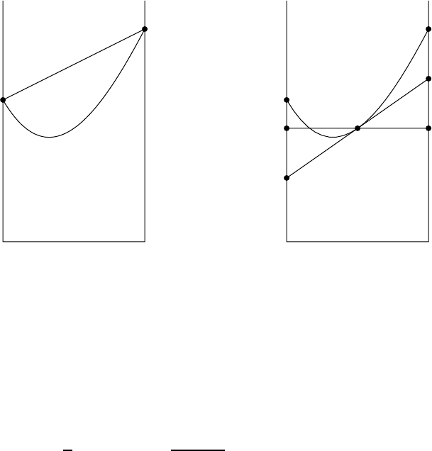
104 CHAPTER 6. NUMERICAL INTEGRATION TECHNIQUES
If fis concave down on [a, b], i.e., f00(x)≤0, then
TRAP(f(x),x,n,a,b)≤Zb
a
f(x)dx ≤MID(f(x),x,n,a,b)
Figure 6.3 shows why this is true. It has two graphs of the same function
which is concave up. the line in the left part shows the trapezoid used in the
trapezoid rule. Clearly it overestimates the integral. The midpoint rule is
illustrated in the right graph. The midpoint rule gives the area under the line
AB. The line CD is the tangent line through the midpoint. The area below
AB is the same as the area below CD (why?). So both are the midpoint
estimate. But clearly the area under CD is less than the area under the
curve.
A
C
B
D
Figure 6.3: Trapezoid and midpoint rule for concave functions
6.5 Deriving Simpson’s Rule∗
Simpson’s Rule uses the quantity
1
6f(x1)+4f(x
1+x
2
2)+f(x
2
)
(x
2−x
1
)(9)

6.6. LABORATORY EXERCISES 105
to approximate Rx2
x1f(x)dx. The can be derived by solving for the quadratic
g(x)=ax2+bx +cwhich passes through the 3 points (x1,y
1), (x2,y
2
)and
(x
3
,y
3); where yi=f(xi)andx
3=(x
1+x
2
)/2 which is simply the midpoint
or average of x1and x2. One then computes Rx2
x1g(x)dx and uses this for
our approximation. Now the algebra involved in this computation is fairly
formidable and yet the beauty of it is that the answer (given in (9)) is so
simple. That’s why the formula for Simpson’s Rule looks hardly any different
from the formula for the left endpoint rule and as a result the computation
times are approximately the same.
Now the algebra involved is the same as that of Chapter 4. We solve 3
equations for the unknowns a,band c, then we integrate the result. Al-
ternately, we can make the derivation into a two step process by using the
function CURVEFIT(x,data) where the data matrix is
data :=
x1y1
x2y2
x1+x2
2y3
The resulting quadratic polynomial contains some pretty large expressions
involving xiand yi. Nevertheless, one need only integrate this expression
over the interval x1≤x≤x2to get the desired result.
6.6 Laboratory Exercises
Start off your lab by Loading the ADD-HEAD file. After you have done this
the functions described in Section 6.2: LEFT, MID, TRAP, and SIMP, which
compute the integral approximations using respectively the left endpoint
method, the midpoint method, the trapezoid method and Simpson’s rule, will
all be defined. In addition the functions DRAW LEFT and DRAW TRAP,
which draw the rectangles and trapezoids used in the graphical demonstra-
tion of Figure 6.2 on page 100, will be defined.
1. a. Use Derive to verify the formula
π=Z1
0
4dx
1+x
2
b. Plot the graph of f(x)=4/(1 + x2) and verify that this function
is decreasing on the interval [0,1].

106 CHAPTER 6. NUMERICAL INTEGRATION TECHNIQUES
c. Evaluate LEFT(4/(1 + x2),x,1000,0,1) and the similar quantity
using the RIGHT function. Then, use part (b) along with equa-
tion 8 on page 103 to determine how accurate an approximation
either of these numbers is to π.
2. Evaluate TRAP(1/x,x,n,1,2) and SIMP(1/x,x,n,1,2) for n= 10,
100, and 1,000. Also use Derive to find ln 2 using 15 decimal place
precision. Which of the 6 approximations above (if any) gives ln 2 to
10 or more decimal places?
3. Use the trapezoid method and Simpson’s Rule to approximate each of
the following integrals. Use n= 10, 20, and 30. Derive has its own
method of doing approximate integration. Find the answer it gets.
You can do this by authoring the integral and choosing approximate.
Compare the decimal accuracy of the Simpson approximates with the
one computed by Derive above.
a. Z1
−1
sin(x2)dx b. Z3
0
1
1+x
3dx
4. Using the midpoint method MID(1/x,x,n,a,b), approximate ln 10 (=
R10
1(1/x)dx)usingn= 10, 100, 1000 and compare your answers with
Derive’s approximation.
5. For the following integrals use the error estimate (4) described above
to find an nlarge enough so that the trapezoid method will give an
approximation of the integral with error at most 0.005. Give both the
approximate value of the integral and the smallest nwhich guarantees
(using formula (4)) that you will be within this error, and also give
M2=max{|f00(x)|:a≤x≤b}.
Hints: Use Derive to find f0,f00,andf
000. For the first integral below,
you can easily see that the maximum for |f00|occurs when x=1. For
the second, solve f000(x) = 0; this tells you where the maximums of
|f00(x)|can occur, and, using this (and maybe some plotting), you can
find M2. For the third integral don’t forget that M2if the maximum of
the absolute value of f00(x)on[0,2]. Once you have M2, find nlarge
enough so that the error given in (4) is at most 0.005.

6.6. LABORATORY EXERCISES 107
a. Ze2
1
ln xdx b. Z2
1
2
1
1+x
2dx
c. Z2
0
1
1+x
2dx
6. Do the same as the last problem, but use Simpson’s Rule this time and
of course use formula (5) instead of (4).
7. Suppose that f(x)=cx +dfor some constants cand d.
a. Use the MID function to verify that
Zb
a
f(x)dx =MID(f(x),x,n,a,b)
for all n. (Hint: To show that two different looking expressions
are equal, try Simplifying their difference.)
b. Assuming that a,b,cand dare all positive use pencil and paper to
verify the result in (a) by using simple geometric considerations.
c. Explain why the area below AB is the same as the area below CD
in Figure 6.3.
8. Find where 1/(1 + x3/2) is concave up and where it is concave down in
the interval [0,1]. Use Theorem 2 to give lower and upper estimates
for
Z1
0
dx
1+x
3/2.
Use n= 20 for all numerical estimates.
9. Prove the following simple relationship between the trapezoid, mid-
point, and Simpson’s rules:
SIMP(f(x),x,n,a,b)=1
3TRAP(f(x),x,n,a,b)+2
3MID(f(x),x,n,a,b)

108 CHAPTER 6. NUMERICAL INTEGRATION TECHNIQUES
Hint: First define f(x) to an unspecified function by Authoring f(x) :=.
Now Author and Simplify the two expressions
SIMP(f(x),x,n,a,b)
(1/3) TRAP(f(x),x,n,a,b) + (2/3) MID(f(x),x,n,a,b)
Finally simplify the difference of the two resulting expressions.
10. Do the calculations needed to verify Simpson’s rule as outlined in Sec-
tion 6.5. This is the same problem as Exercise 4 in Chapter 4.
11. Suppose that f(x)=cx2+dx +efor some constants c,dand e.
a. Use the SIMP function to verify that
Zb
a
f(x)dx = SIMP(f(x),x,n,a,b)
for all n. (Hint: To show that two different looking expressions
are equal, try Simplifying their difference.)
b. Explain why Simpson’s rule gives the exact answer whenever the
integrand is a quadratic polynomial. (Hint: Study the derivation
in Section 6.5)
c. Show that part (a) holds even when f(x) is an arbitrary degree 3
polynomial.
d. Show that the error estimate (5) for Simpson’s rule implies the
result in part (c).

Chapter 7
Taylor Polynomials
7.1 Polynomial Approximations
Suppose we want to approximate a function f(x)byapolynomial
f(x)≈P
n
(x)=a
0+a
1
x+a
2
x
2+···+a
nx
n=
n
X
k=0
akxk.
Onenaturalwaytotodothisistorequirethatf(0) = Pn(0), f0(0) = P0
n(0),
f00(0) = P00
n(0), etc., i.e., f(k)(0) = P(k)
n(0) for k=0,... ,n.Thisgivesn+1
equations for the n+ 1 unknowns a0,...,a
n. If we differentiate, say P3(x),
several times these equations become quite clear:
P3(x)=a
0+a
1
x+a
2
x
2+a
3
x
3
(1)
P0
3(x)=1·a
1+2·a
2
x+3·a
3
x
2
(2)
P00
3(x)=2·1·a
2+3·2·a
3
x(3)
P000
3(x)=3·2·1·a
3
(4)
Setting x= 0 in the first of these equations gives a0=f(0). Setting x=0
in the second of these equations gives 1 ·a1=f0(0). Taking more derivatives
and setting x=0,weget2·1·a
2=f
00(0), 3 ·2·1·a3=f000(0). By thinking
about factorials, you can see the pattern evolving: the general term (solving
for ak)is
a
k=f
(k)
(0)
k!for 0 ≤k≤n(5)
109

110 CHAPTER 7. TAYLOR POLYNOMIALS
Pn(x)iswhatisknownasthen
th Taylor polynomial for f(x):
Pn(x)=
n
X
k=0
f(k)(0)
k!xk
(6)
The coefficient of xkin Pn(x)isjustf
(k)
(0)/k! (which is the same for all n
as long as n≥k). This quantity is called the kth–Taylor coefficient for f(x).
As our first application, notice that it follows from (5) that the graph of
y=P1(x)isjustthetangent line to the curve y=f(x)atthepoint(0,f(0)).
We studied this method of approximation extensively in Section 2.2. Thus,
since the tangent line yields the best degree-one approximation to the func-
tion, near the point x= 0, it is reasonable that guess that Pn(x)isthebest
n
th–degree approximation, near x=0.
To have Derive compute a Taylor polynomial for a function first select
the Calculus/Taylor menu, then enter the function in the form, enter some
integer n,sayn= 5, for the Degree and leave the Point1value at its default
value of 0. This results in the expression TAYLOR(f(x),x,0,5).Analternate
approach after becoming familiar with its syntax is to simply author this
expression. See Figure 7.1 on the facing page for some of the basic examples
and a comparison of the graph of f(x)=1/(1 −x) and it’s 5th degree Taylor
polynomial approximation. An interesting exercise is to load the file F-TAY0
which contains the expressions from Figure 7.1 and compare graphically the
various functions with their Taylor polynomials of different degrees.
7.2 Examples
As we see from Figure 7.1 on the next page, the formulas for the Taylor
polynomials for the function f(x)=1/(1 −x) are pretty easy to guess after
looking at a few examples:
Pn(x)=1+x+x
2+x
3+···+x
n.
Since the graphs of these polynomials appear to approximate the graph of
the function f(x) to a high degree of accuracy as ngets larger and larger (at
1For now we just take the Point value to be 0. Later, in Section 7.6 we discuss how to
use this variable.
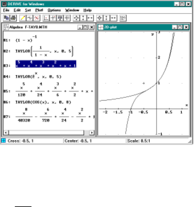
7.2. EXAMPLES 111
Figure 7.1: Basic examples of Taylor polynomials
least for values of xsatisfying −1<x<1) we conjecture that
1
1−x=1+x+x
2+x
3+···= lim
n→∞
n
X
k=0
xk=∞
X
k=0
xk.(7)
The three dots in the above formula means that you are to keep adding more
and more terms forever. Since adding an infinite list of numbers together
looks like an impossible task, we define this in terms of limits. That is what
we mean by the last expression above. More generally, we denote an infinite
series by ∞
X
k=0
ak= lim
n→∞
n
X
k=0
ak.
Of course, any time we discuss limits we need to worry about whether or
not the limit exist! When the above limit exists for an infinite series with
terms akwe then say that the series Pakis convergent. Otherwise, we say
the series is divergent. We will thoroughly discuss this topic in Chapter 8.
In case you already know something about infinite series you might notice

112 CHAPTER 7. TAYLOR POLYNOMIALS
that our conjecture in (7) above is in fact the most famous example of an
infinite series; namely, it is the geometric series.
We got the form of the Taylor polynomials above by the method of pattern
recognition, looking at lots of examples using Derive and then guessing at
the general result. To verify this result we must use (5) to compute the
Taylor coefficients. We will need to show f(k)(0) = k!. Using Derive we can
make a table of derivatives by authoring
VECTOR([k, DIF((1-x)^-1,x,k)], k, 0, 4)
and then simplifying. The answers seem to follow the pattern k!/(1 −x)k+1
which can be verified by having Derive check that:
DIF((1-x)^(-k-1) k!,x) = (1-x)^(-k-2) (k+1)!
(Try this for yourself).
Note that in Figure 7.1 the 5th degree Taylor polynomial approximation
gives a very good approximation on the interval [−.5,.5]. As we mentioned
earlier, you should Load the file F-TAY0 and experiment with higher degree
approximations to see how the interval size improves, but the graphical evi-
dence suggests the infinite series representation is only valid for −1<x<1
(even though the function appears well behaved near x=−1). We will
demonstrate this fact later.
Three other important examples are the series for ex,sinx,andcosx.If
we look carefully at Figure 7.1 we might guess the pattern for the exponential
function because the denominators 1, 1, 2, 6, 24, 120 are just k!askvaries
from 0 ≤k≤5. On the other hand, equation (5) gives the required formula
easily since all derivatives f(k)(x)=e
xandsoare1atx= 0. Thus, in this
case f(k)(0)/k!=1/k!sothen
th Taylor polynomial is simply Pn
k=0 xk/k!=
1+x+x
2/2! + ···+x
n/n!. Now, if we can also take the limit as in the case
of the geometric series, then
ex=∞
X
k=0
xk
k!=1+x+x
2
2! +···= lim
n→∞
n
X
k=0
xk
k!.(8)
In fact, the series above does converge, for all values of x, to the exponential
function. Moreover, it is this series that forms the basis for numerical calcu-
lations of the exponential function on computers and calculators. Section 7.5
will give a complete explanation of this matter.
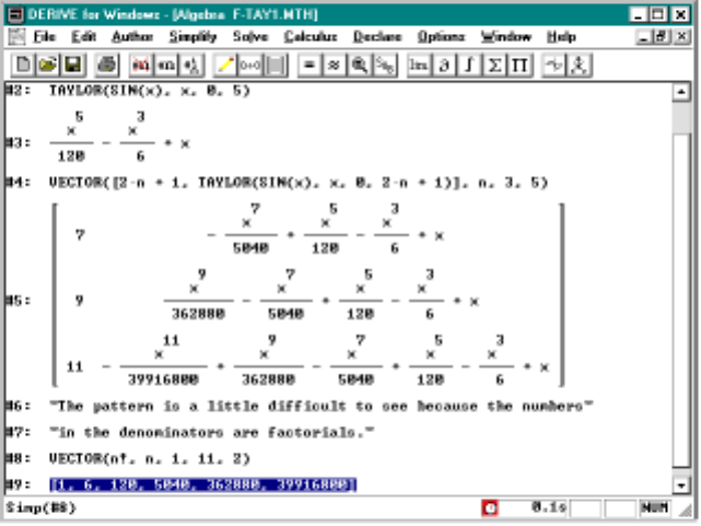
7.2. EXAMPLES 113
Figure 7.2: Taylor polynomials for sin x
We can proceed in a like manner to compute the Taylor polynomials
for the sine and cosine functions. The only problem is that the pattern
for the successive derivatives is a little trickier. Let us discuss the function
f(x)=sinxsince the analysis of the cosine function is similar. If we make a
vector of f(k)(x)with0≤k≤4 we get [sin x, cos x, −sin x, −cos x, sin x]and
it is clear that the pattern will repeat in groups of 4 with f(4k)(x)=sinx.
Substituting x= 0 gives the pattern [0,1,0,−1] and hence every even power
of x, i.e., x0,x
2,x
4,..., will have a zero coefficient; whereas, the odd power
x2k+1 will have the coefficient (−1)k/(2k+1)! by (5). See Figure 7.2 for several
Taylor polynomials of the sine function. The only unfortunate part about
making these computations in Derive is that the factorials are expanded
to their integer values which makes it difficult to recognize the patterns. On
the other hand, it’s easy to see how fast the factorials in the denominator
grow which means that the added terms are quite small in magnitude. At
any rate, the Taylor polynomials form the partial sums of an infinite series
representation of sin xwhich is convergent for all −∞ <x<∞.Thisseries
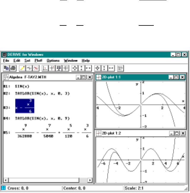
114 CHAPTER 7. TAYLOR POLYNOMIALS
and the one for cos xare given below:
sin x=x−x3
3! +x5
5! +···=∞
X
n=0
(−1)nx2n+1
(2n+1)!
(9)
cos x=1−x
2
2! +x4
4! +···=∞
X
n=0
(−1)nx2n
(2n)!
(10)
Figure 7.3: Approximating sin xwith its Taylor polynomials
Next we want to graph several of these Taylor polynomials and compare
them with the graph of sin x. This is done in Figure 7.3. Another instructive
exercise is to plot 3 or more Taylor polynomials all at once by making a vector
of the functions and then plotting the vector. As each successively higher
degree polynomial is plotted, the range of close approximation gets larger
and larger. Curiously, one sees from Figure 7.3 that the approximation
is good up to a point and then is very bad thereafter. The basic idea in
approximating is simply to take more terms; i.e., use a higher degree Taylor
polynomial, to obtain more accuracy. An example of a more precise question

7.3. TAYLOR’S THEOREM WITH REMAINDER 115
we shall be interested in is: What degree nis needed for approximating the
sine function on the interval [0,π/2] to within 6 decimal places?
7.3 Taylor’s Theorem with Remainder
We are interested in how accurately a Taylor polynomial approximates f(x)
and for what values of xdoes the Taylor series converge to f(x). The basic
result is the following theorem:
Theorem 1. Suppose that f(x)is (n+1)–times continuously differentiable
on the interval [0,b].Letthen
th degree Taylor polynomial be denoted by
Pn(x). Then, for any 0≤x≤bwe have
|f(x)−Pn(x)|≤max
0≤t≤x|f(n+1)(t)|· |x|
n+1
(n+1)! =M·|x|
n+1
(n+1)!
(11)
where we abbreviate the maximum by M.
Furthermore, the theorem also holds when the defining interval is [−b, 0]
for some positive b. The only change is that now −b≤x≤0and the
maximum in (11) is taken over the interval x≤t≤0.
Observe that the error estimate in (11) is similar to those we obtained
for the approximate integral formulas (Trapezoid method, Simpson’s rule)
in that they depend on the maximum of a high order derivative, look back
at the formulas on page 99. Also, notice that when n= 0 then (11) follows
immediately from the Mean Value Theorem and in fact, you can think of
(11) as a higher order Mean Value Theorem.
The proof is based on a simple application of the integration by parts for-
mula; namely, for any continuously differentiable function g(t) which satisfies
g(0)=0,then
Zx
0
g(t)
(x−t)
m
m!dt =Zx
0
g0(t)(x−t)m+1
(m+1)! dt m =0,1,...(12)
Just put u=g(t)andv=(x−t)
m+1/(m+ 1)! and apply the integration by
parts formula. Notice that the integrated terms, i.e., the uv|x
0terms, vanish
because g(0) = 0 at the left endpoint and (x−t)m+1 is zero when t=x.

116 CHAPTER 7. TAYLOR POLYNOMIALS
Proof. Put g(t)=f(t)−P
n
(t)letMbe the maximum of |f(n+1)|on the
interval [0,x]. By the definition of the Taylor polynomial, observe that
g(m)(0) = 0 for m=0,1,...,n and g(n+1)(t)=f
(n+1)(t)
where the second fact follows since the (n+1)
st–derivative of any degree n
polynomial is zero (look back at (1) on page 109). Now we get to apply (12)
to g0,g
00,...,g
(n)with the result that
Zx
0
g0(t)dt =Zx
0
g00(t)(x−t)dt =Zx
0
g000(t)(x−t)2
2dt
=···=Zx
0
g
(n+1)(t)(x−t)n
n!dt
and hence that
f(x)−Pn(x)=g(x)−g(0) = Zx
0
g0(t)dt
=Zx
0
g(n+1)(t)(x−t)n
n!dt =Zx
0
f(n+1)(t)(x−t)n
n!dt .
We take absolute values of the left and right-hand sides of the above to get
|f(x)−Pn(x)|≤Zx
0|f
(n+1)(t)|(x−t)n
n!dt
≤Zx
0
M(x−t)n
n!dt =Mxn+1
(n+1)!
which proves the theorem.
7.4 Computing the Sine Function
First observe that we don’t need to compute, for example, sin 100 directly
since the sine function is 2πperiodic. We just set x= 100 −2kπ where
the integer kis chosen so 0 ≤x<2π.InDerive we simplify the function
MOD(100, 2π)to get k=15andx=5.75221 approximately. Now it’s
an interesting exercise to use the properties of the sine function to reduce
the computation to the interval [0,π]. For example, if π<x<2πthen
sin x=−sin(2π−x) where now 0 ≤2π−x<π. Similarly, you can use

7.4. COMPUTING THE SINE FUNCTION 117
the identity sin(π−x)=sinxto reduce the problem to the smaller interval
[0,π/2]. It’s even possible to reduce the interval to [0,π/4].
We can use formula (11) to estimate the error in using the Taylor poly-
nomial to estimate sin x. The computation of M=max|f
(n+1)|might look
a little formidable at first but we observe that any derivative is equal to ei-
ther ±sin tor ±cos tandineithercaseM≤1. Thus, we can take M=1
and achieve 6 decimals of accuracy by determining the smallest integer n
satisfying
|x|n+1
(n+1)! ≤10−6
(13)
For approximations on the interval [0,π/2] we could just take the worst case
by setting x=π/2intheabove.
We now have reduced the problem to solving (13) for the smallest possible
integer n. Unfortunately, the factorial expression means that we can’t use
simple algebra to solve this inequality. A simple numerical approach would
be to make a table with nin the first column and the above expression in the
second column. Examining the data will result in an answer provided nis
reasonably small. We did this earlier on page 138 when we studied the ratio
test. If this fails, as with the 1/k2series, you might try testing various powers
of 10. Both of these techniques are easy to do using the vector function. (In
the next section we present another way of finding n.) In Figure 7.4, see the
file F-TAY3, we analyze sin 100 by reducing the computation to a smaller
value of x(x=0.530973), determining which nyields an error of less than
10−6(n= 7) and then computing using P7(0.530973). Observe that for the
sine function P2n+1(x)=P
2n+2(x) and so for the error computation (13) we
use the higher power 2n+3instead2n+ 2 and hence
|sin x−
n
X
k=0
(−1)kx2k+1
(2k+1)!
|≤ |x|
2n+3
(2n+3)! for n=0,1,...(14)
Lastly, let us observe that the right hand side of (14) tends to zero for
any x. After all, for xfixed, the ratio of terms above is
|x|2n+5
(2n+5)!·(2n+3)!
|x|
2n+3 =|x|2
(2n+ 5)(2n+4) ≤1
2
for all large n.Thus,|x|
2n+3/(2n+3)! ≤c
x/2
n(or for that matter |x|n/n!≤
cx/2n) for some constant cxand the sequence tends to zero because 1/2n→0.
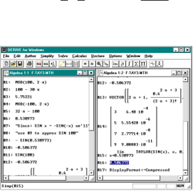
118 CHAPTER 7. TAYLOR POLYNOMIALS
By applying Theorem 1 we see that the Taylor series converges for all xand
we indeed have the representation
sin x=x−x3
3! +x5
5! +···=∞
X
n=0
(−1)nx2n+1
(2n+1)!
(15)
which is valid for all −∞ <x<∞. In a similar manner we establish (10)
on page 114.
Figure 7.4: Approximating sin 100 within 6 decimals
7.5 Computing the Exponential Function.
Now let’s repeat the above procedure for ex. We use the partial sums of
(8) for approximating and (11) for determining the number of terms to use.
Let’s assume x>0. Since f(n+1)(x)=e
xis an increasing function, we can
take M=exor more conveniently we will replace ewith the larger value 3.
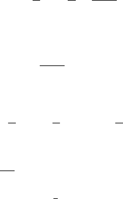
7.5. COMPUTING THE EXPONENTIAL FUNCTION. 119
Thus,
ex−(1 + x+x2
2! +···+x
n
n!)
<3
xx
n+1
(n+1)!
(16)
and so we need only find nso that the right-hand side is sufficiently small.
We would like to define a function in Derive to determine the number of
terms nnecessary to achieve 6 decimals places, rather than looking at tables.
First of all, recall from the previous section that
lim
n→∞
3xxn+1
(n+1)! =0
for all values of x. Hence we are guaranteed that there is a first nfor which
the above quantity is less than 10−6. Moreover, this proves that the Taylor
series converges for all x, by Theorem 1, to ex. Thus, as stated earlier
ex=∞
X
k=0
xk
k!=1+x+x
2
2! +···= lim
n→∞
n
X
k=0
xk
k!
for all −∞ <x<∞.
Now consider the functions
1: N1(x,k) := IF(3xxk
k!<10−6, k-1, N1(x,k+1))
2: N(x) := N1(x,1)
and consider what happens when you Simplify N(5). The N-function com-
putes the N1-function with a starting value of k= 1. The error expression
is compared to 10−6and if successful then k−1isthevalueofN(5); oth-
erwise, kis increased by one and the process continues. Eventually, we get
to a large enough kso that the comparison with 10−6is successful and that
value of k−1 is returned as the value of the function. The function N1is
called a recursive function because its definition refers to itself. Care has
to exercised with such functions to make sure that they eventually return a
value and don’t continue computing forever (press the Esc if this happens).
See Figure 7.5 and load the file F-TAY4 where these functions are used to
define a new version of the exponential function (for x≥0) which is accurate
to 6 decimal places. A comparison of this function with the built in version
obtained by approximating shows that the build in function is faster but the
accuracy is the same for the first 6 decimals using P25(x).
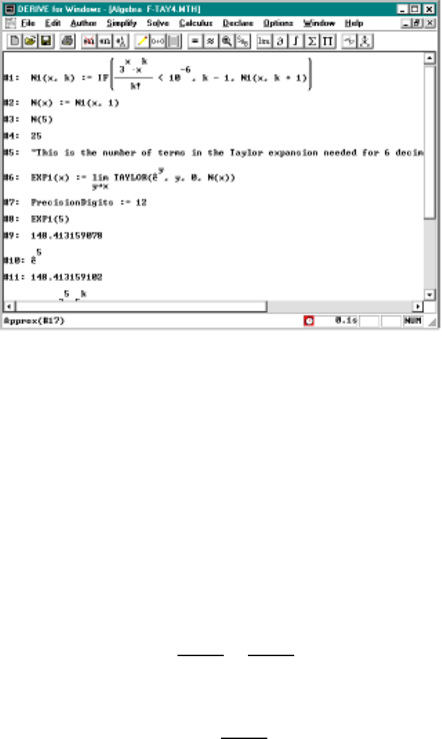
120 CHAPTER 7. TAYLOR POLYNOMIALS
Figure 7.5: Approximating e5within 6 decimals
7.6 Taylor Expansions About x=c
Up to this point we have been approximating functions near x= 0. Suppose
instead we want to approximate f(x)nearx=c. A simple approach is to
define g(x)=f(x+c) and approximate g(x)nearx= 0 as before. Observe,
that for x≈cwe then have
f(x)=g(x−c)≈P
n
(x−c)=
n
X
k=0
ak(x−c)k
where Pnis the Taylor polynomial for g(x) and hence
ak=g(k)(0)
k!=f(k)(c)
k!.
By the above observation it makes sense to define
Pn(x, c)=
n
X
k=0
f(k)(c)
k!(x−c)k

7.6. TAYLOR EXPANSIONS ABOUT X=C121
to be the nth–Taylor polynomial of f(x), expanded about the point x=c.In
Derive we just enter TAYLOR(f(x),x,c,n) or put the Point variable equal
to cif we use the menu method.
Similarly, the Taylor series expansion about the point cis
f(x)= ∞
X
k=0
f(k)(c)
k!(x−c)k
provided this series converges to f(x). To discuss convergence of the above
we use Theorem 1 applied to the function g(x)=f(x+c). We do the same
thing when we are computing with Derive. The advantage of this method
for Derive is that if the fifth Taylor polynomial of f(x) around cis say
P5
k=0 ak(x−c)k,Derive will expand the powers of x−cso you get an
expression like b5x5+b4x4+b3x3+b2x2+b1x+b0, and you won’t be able to
see what the ak’s are. Thus,
If you want a Taylor polynomial of f(x) expanded about the
point c,itisbesttofindtheTaylorpolynomialoff(x+c)
expanded about 0.
A nice illustration of this technique is to examine Figure 7.6 on the next
page where f(x)=lnxis plotted along with P5(x, 1). Since ln 0 is not even
defined it would be foolish to think about its Taylor expansion about x=0,
however, expanding about x= 1 is a reasonable alternative. Notice that
TAYLOR(ln x,x,1,5) produces a messy result in which the 6th term is hard
to guess but that there is a clear pattern in TAYLOR(ln (x+1),x,0,5).In
fact, it can be shown that
ln(1 + x)=x−x
2
2+x
3
3···=∞
X
k=1
(−1)k+1
kxk,−1<x≤1(17)
although the proof that the series converges to ln xon the interval 0 <x≤
1/2 is straightforward, see Exercise 2, is quite a bit harder than our earlier
examples to get the full interval 0 <x≤1. You can load the file F-LOG
and try approximating ln xwith higher degree Taylor polynomials to see if
you can confirm the above representation. The full convergence problem for
the logarithm function will be studied in Chapter 9.
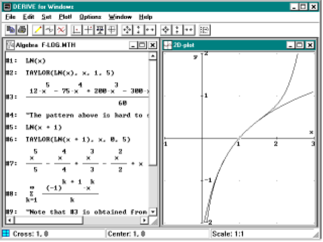
122 CHAPTER 7. TAYLOR POLYNOMIALS
Figure 7.6: Taylor expansion of the logarithm function
7.7 Interval of Convergence
The Taylor series for f(x)=sinx,cosx,ore
xconverges to f(x) for all
values of x. This means that, by taking the degree large enough, the Taylor
polynomials of these functions will approximate f(x) accurately on arbitrarily
large intervals. However, the geometric series (7) only converged for |x|<1
and so the Taylor polynomial will approximate 1/(1−x) only on this interval.
Of course, 1/(1 −x) is not continuous at x= 1 and hence it is not surprising
that the Taylor polynomials will not converge at x= 1. Surprisingly, this
divergence at x= 1 turns out to influence the convergence of the series for
negative values of x! It is an important basic theorem about the convergence
of Taylor series that if the series converges at a point x16=0,thenitalso
converges at all |x|<|x1|. Thus, any Taylor series which diverges at x=1
cannotconvergeatanyx<−1. Why? If it did converge say at x1=−2,
then it would also converge at x= 1. But it diverges for x= 1 so it cannot
possibly converge at x1=−2 (or any |x|>1). This fact also leads to the
observation that the set of points xwhere the Taylor series converges must
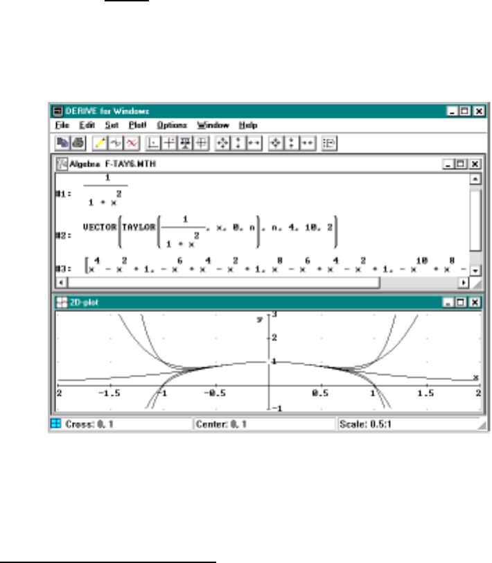
7.7. INTERVAL OF CONVERGENCE 123
be an interval which is centered about the origin. Actually, there are four
possibilities for the interval of convergence: (−r, +r), (−r, +r], [−r, +r)or
[−r, +r] for some 0 ≤r≤+∞.2This number ris called the radius of
convergence.
Now consider the function 1/(1 + x2). We can obtain the Taylor series
for this function by substituting −x2for xin (7):
1
1+x
2=1−x
2+x
4−x
6+···=∞
X
k=0
(−1)kx2k
(18)
As before we can use Derive to plot several of the Taylor polynomials for
this function; see Figure 7.7.
Figure 7.7: Graphically finding the radius of convergence
Notice that although the higher degree polynomials do a better job of
approximating the function for |x|<1, none of them work outside of this
2We need to allow the notation r=+∞so that the set of all real numbers can be
represented as the interval (−r, r).

124 CHAPTER 7. TAYLOR POLYNOMIALS
region. This strongly suggests that the radius of convergence of 1/(1 + x2)
is r= 1. This can be proved by observing the following: if the series s=
P∞
k=1 akconverges then the terms ak→0. This is because an=sn−sn−1→
s−s=0. Now,inourcase|a
k
|=|x|
2k→∞whenever |x|>1. So even
though the function 1/(1 + x2) is defined and differentiable to all orders on
the whole real line, the radius of convergence of its power series is r=1. It
is therefore impossible to deduce the radius of convergence for a function by
looking at its graph.
In the case of our example 1/(1 + x2), an interesting explanation as to
why r= 1 can be based on the fact that x2+1has a complex root at the
point x=i, which a distance one from the origin. We will not pursue this
approach here but let us say that this application of complex numbers turned
out to be one the the great triumphs for this man-made invention.
7.8 Laboratory Exercises
1. Start by declaring f(x) to be a function, i.e., Author F(x):=.Usethe
C
alculus/Taylor series menu to produce the expression TAYLOR( F(x),
x, 0, 5) and then edit this expression by replacing the 5 with n(note
that the Taylor menu requires integer values for the degree). With this
last expression highlighted, use the Calculus/Vector menu twice, with
the Variable set to n,Start value 4, End value 10 and Step size 1 to
produce the two expressions:
VECTOR(TAYLOR( F(x), x, 0, n), n, 4, 10, 1)
VECTOR([n, TAYLOR( F(x), x, 0, n)], n, 4, 10, 1)
For each of the functions below do the following:
(i) Define f(x) to be the given function and plot its graph in the color
red.
(ii) Simplify the first vector function above to make a 7–vector which
has the degree nTaylor polynomial, expanded about x= 0, for
n=4,... ,10 as its entries.
(iii) Graph this vector to plot each of these Taylor polynomial in suc-
cession. It is probably best to plot the first 2-3 polynomials indi-
vidually first and then the entire vector so that you can see how

7.8. LABORATORY EXERCISES 125
their graphs are getting closer and closer to the graph of f(x).
You might need to scale your pictures appropriately.
(iv) Simplify the second vector function to make a 7 ×2–table that
has the degrees nin the first column and Pn(x) in the second
column.
(v) Use your table to guess what the infinite Taylor series expansion
is.
*(vi) Prove that in each case, the Taylor series expansion converges to
the function and determine the interval of x’s for which it is valid.
In parts (b), (c) use the geometric series (2) on page 132 and the
fact that the series converges only for −1<x<1.
a. f(x)=x
8
8+···+x
2
2+x
b. f(x)= 1
3−x
c. f(x)= 1
x
2+2 (Hint: For the pattern recognition you will need
to change the output mode to Rational. Use the Declare/Algebra
state menu to access the Output menu.)
2. Let f(x)=−ln(1 −x). We want to determine the Taylor series for
f(x) and prove that it converges to f(x) using Theorem 1 on page 115.
a. Compute the first several derivative of f(x) and guess at a general
formula for f(n)(x) for all n=0,1,2,....
b. Use part ato establish the Taylor series of f(x) and hence if the
Taylor series converges to f(x)wewouldhave:
ln 1
1−x=∞
X
k=1
xk
k=x+x2
2+x3
3+...(19)
c. Use Theorem 1 to show that the (1) holds for any −1≤x≤1/2.
(Hint: Carefully compute the right-hand side of (11) on page 115.
Then, show that the error estimate tends to zero as n→∞only
for −1≤x≤1/2.)

126 CHAPTER 7. TAYLOR POLYNOMIALS
d. Show that taking x=−1 in (19) leads to another series represen-
tation of ln 2; namely,
ln 2 ≈1−1
2+1
3···+(−1)n+1 1
n
Analyze how quickly these approximates converge to ln 2 by mak-
ing tables of numerical computations. What value of nis needed
for 2-decimal place accuracy?
e. It turns out that (19) actually holds for all −1≤x<1andthe
radius of convergence is r= 1. By computing Pn(x) for several
nand comparing their graphs with f(x), show that the Taylor
polynomials seem to converge to f(x) on the full interval −1≤
x<1
3. For each of the functions below do the following:
(i) Do parts (i)–(iv) of Problem 1 using these functions.
(ii) By comparing the graph of the function with several Taylor poly-
nomials make a guess at the interval of x’s for which the Taylor
expansion is valid, see Section 7.7.
(iii) Give further support for your answer in (ii) by picking some nonzero
x1(where the Taylor representation is valid) and numerically com-
paring the function’s value at x1with that of several of its Taylor
polynomials. Recall that tan−1xis entered as atan x in Derive.
a. 1
(x+1)
2b. tan−1x
c. e−x2
4. Load the file F-TAY3 and following the methods of Section 7.4 compute
sin 7. Which degree Taylor polynomial should you use to get an error
of less than 10−6?
5. In this problem we approximate e5using the methods in Section 7.5.
a. Express e5using the Taylor series representation of the exponen-
tial function.

7.8. LABORATORY EXERCISES 127
b. Compare the numerical value of e5using approximate with the
value of the first several Taylor polynomials. How many terms
appear to needed for 6 decimal place accuracy?
c. We now want to use Theorem 1 on page 115 to obtain a precise
estimate of e5within 10−6. Compute an upper bound on the error
estimate on the right-hand side of (11) for several n.Dothisby
first giving an upper estimate for Mand then making a list of
several error estimates until the value becomes less than 10−6.
d. What is your estimate for e5and how many terms do you need?
6. The functions f(x)=sinxhas only odd powers in its Taylor series ex-
pansion. This property can be explained by the fact that f(x)satisfies
the equation f(−x)=−f(x)asdoalloddpowersofx. It is because of
this that we call any such f(x)anodd function. Similarly, a function is
an even function if f(−x)=f(x) holds for all x, as do all even powers
of x.
a. Prove that f(2k)(0) = 0 for k=0,1,... andanyoddfunction
f(x).
b. Prove that f(2k+1)(0) = 0 for k=0,1,... and any even function
f(x).
*7. Recall from our discussion of complex numbers in Section 5.4 on page 78
that a complex number is of the form α=a+bi where a,bare real
numbers and isatisfies i2=−1. Our goal in this exercise is define the
complex exponential eαx in such a way that the basic formula:
d
dxeαx =αeαx
(20)
is still valid. We will use Taylor polynomials as a guidepost to the
correct definition.
a. Find the 6th degree Taylor polynomial P6(x) for the function eαx
(enter the αsymbol using the symbol bar). Be sure to expand out
your answer into powers of x.

128 CHAPTER 7. TAYLOR POLYNOMIALS
b. Substitute ifor αinto P6(x) (Recall that iis entered in DfW
using the symbol bar). Compute the real and imaginary parts of
the resulting expression using the Derive functions RE(...) and
IM(...).
c. Now find the 6th Taylor polynomial for cos xand for sin x.Verify
that that 6th Taylor polynomial for cos xisthesameasthereal
part of P6(x)aboveandthe6
th Taylor polynomial for sin xis the
same as the imaginary part of P6(x). (Hint: The verification for
the Taylor polynomial for sin xis a little tricky. Try expanding
out the imaginary part of P6(x)usingtheSimplify/Expand menu.
d. Another way of obtaining the previous result is to multiply the
Taylor polynomial for sin xby iand add it to the Taylor polyno-
mial for cos xand compare the result with the Taylor polynomial
P6(x) above. Verify that these expressions are the same.
e. These computations suggest that we define the complex exponen-
tial eix by the formula
eix =cosx+isin x.(21)
In fact, this is the Euler Formula which is one of the most fun-
damental equations with complex numbers. Verify that using this
definition, (20) with α=iis valid.
f. Lastly, use the definition
eαx =e(a+bi)x=e
axeibx =eax(cos bx +isin bx)(22)
to verify (20) for general complex α. Dothisbyenteringtheright
hand side of the above definition and computing its derivative.
Then, author the expression obtained by subtracting from your
derivative computation a+bi times the right hand side above.
Now simplify and if you have done everything correctly Derive
should returns the answer zero.
g. Use the above definition to show that the complex conjugate sat-
isfies:
eix =e−ix and eαx =e¯αx
(Recall that in Derive the ¯αis entered as CONJ(α).)

7.8. LABORATORY EXERCISES 129
*8. In this problem we use the Taylor polynomials for the arc tangent
function tan−1xto estimate π. Recall that tan−1xis entered as atan x.
a. Use Derive to verify the formula
π
4=4tan
−1
(1/5) −tan−1(1/239)
b. Compute the eighth degree Taylor polynomial P8(x) for tan−1x.
c. Use P8(x) to approximate on the right side of the above formula
and use your answer to estimate π.
d. Let Mbe the maximum value of the 9th derivative of tan−1(x)on
the interval [0,1/5]. Use the error estimate (11) on page 115 to
give an upper bound for the error in your estimate of πin terms
of M. For example, give an answer like M·10−2.
e. Use graphical techniques to give an upper bound on M.
f. Combine the last two parts to give an estimate on the number
of decimal places your estimate to πvalid for. How does this
compare with Derive approximation to π?
g. Use Derive to show that the absolute maximum value for |f(9)(x)|,
where f(x)=tan
−1
(x), is achieved at x=0.
130 CHAPTER 7. TAYLOR POLYNOMIALS
Chapter 8
Series
8.1 Introduction
An infinite series is a sum with infinitely many terms:
∞
X
i=0
ai=a0+a1+a2+···
We define P∞
i=0 ai=sto mean that
lim
n→∞
n
X
i=0
ai=s,
if this limit exists. If the limit does exist we say the series converges;oth-
erwise we say it diverges. There are two basic techniques for showing that
a series is convergent. One method is to show directly that the above limit
exists. There are not many examples when we can do this but a particularly
important one is geometric series which will be discussed in the next section.
The second method for showing convergence applies to series with non-
negative terms, i.e., the case that ai≥0 for all i=1,2,.... In this case the
partial sums,
sn=a0+a1+···+a
n=
n
X
i=0
ai,n=0,1,...
form an increasing sequence, s0≤s1≤s2≤.... Hence, by a fundamen-
tal property of real numbers, the limit limn→∞ snexists if and only if the
131
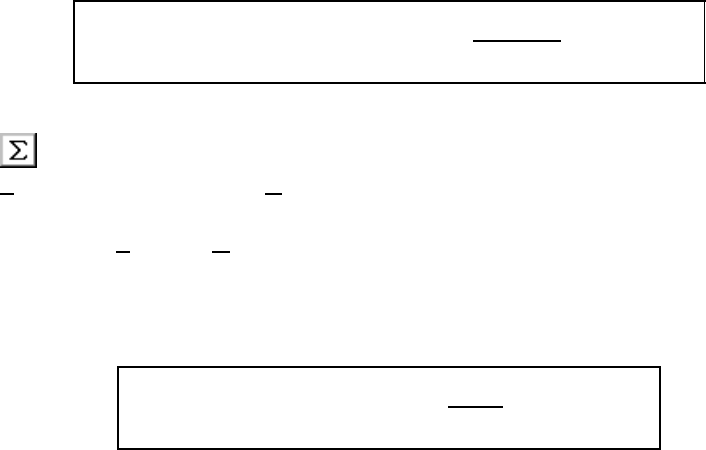
132 CHAPTER 8. SERIES
sequence {sn}is bounded. This second technique is used extensively for
proving convergence and obtaining estimates on the answer. Particular ex-
amples are the ratio test and the integral test which we will discuss in this
chapter.
8.2 Geometric Series
Ageometric series is one in which the ratio of consecutive terms is constant,
i.e., series of the form Paxi. To evaluate this series let sn=Pn
i=0 xi=1+
x+x
2
+···+x
n.Then
s
n−xsn=(1+x+x
2+···+x
n)
−(x+x
2+···+x
n+x
n+1)
=1−x
n+1
Factoring out snand solving, we get
sn=
n
X
i=0
xi=1+x+x
2+···+x
n=1−x
n+1
1−x,if x6=1
(1)
It’s instructive to verify this formula in DfW. You start by clicking the sum
button and enter x^k. Makesurethevariableisk(not x)andsetthe
S
tart value to 0and the End value to n. Click OK and edit the resulting
expression SUM( x^k, k, 0, n) by multiplying it by the factor (1 −x).
Lastly, use Simplify/Expand to get the desired 1 −xn+1.
If |x|<1, then limn→∞ xn+1 = 0. Thus, we get that limn→∞ snexists
and so the series is convergent. In addition, the following simple formula for
evaluating geometric series holds:
∞
X
i=0
axi=a+ax +ax2+···=a
1−x,if |x|<1
(2)
If |x|≥1 then the series diverges because limn→∞ sndoes not exist.
We can verify this formula in Derive by entering, as we did above or
directly, the expression SUM( ax^k, k, 0, inf) which displays as the left
hand side of (2). Now we must declare that −1<x<1. We do this using

8.3. APPLICATIONS 133
the Declare/Variable Domain menu for the variable xand the open interval
(−1,1). If you do this right the expression x:∈Real (-1,1) will be the
result. If not you should be able to edit the expression until it is right.
Finally simplify the infinite series to get a/(1 −x) which is the desired result.
8.3 Applications
Geometric series are useful in several areas, for example, business and finance.
We will give some of the important examples.
Interest. If you start with pdollars (pfor principal ) in a bank account
which earns 6% per year how much money will you have after nyears?
Assuming the interest is compounded yearly, you will be given an interest
payment of 0.06 pafter one year. You will still have the original pdollars
so that the amount of money in the account after one year will be p(1.06).
Notice that this is saying that each year the amount of money in the account
gets multiplied by 1.06. Thus after nyears the account will have p(1.06)n
dollars. If we let rdenote the interest rate, the amount after nyears is
p(1 + r)n.
An interesting alternative to this formula is obtained by focusing on the
year to year change in the savings account balance. Let sbal(k,p,r) denote
the balance after kyears, starting with an amount pwhich is compounded
annually at a rate r. This function can be defined in DfW by
sbal(k,p,r):=IF(k=0,p,(1+r)*s bal(k-1,p,r)).
Notice how we use the function IF(test,true,false). To compute say
sbal(2,p,r) the first thing that happens is the test k= 0 fails and hence we
get (1+r)*s bal(1,p,r).Butthensbal(1,p,r) is computed in a similar
manner, i.e., the test k= 0 fails again so now
sbal(2,p,r)=(1+r)*s bal(1,p,r)=(1+r)*((1+r)*s bal(0,p,r)).
Finally, sbal(0,p,r) is evaluated but this time the test k= 0 succeeds
and so the answer is p. Combining the answers we get the same result as
before (1 + r)2p. This type of computation has a fancy name; it’s called
recursive programming and it is particularly useful in situations where you
have a sequence of numbers which change one to the next by a fixed rule.

134 CHAPTER 8. SERIES
Now suppose that the bank compounds your money quarterly instead of
annually. This means that they give you 6/4=1.5% interest four times a
year. So the amount of money in your account after nyears is p(1.015)4n.
For a general rate rcompounded ktimes a year, the amount of money after n
years is
p1+ r
kkn
(3)
This can be also be expressed as sbal(kn,p,r/k).
Now suppose that you deposit adollars each year into a bank account
paying a rate rin interest, compounded annually. Suppose that you opened
theaccountwithanamountpdollars. How much money will the account
have after nyears? This is easy to do using a small modification in the sbal
function as follows:
sbal(k,p,r,a):=IF(k=0,p,(1+r)*s bal(k-1,p,r,a)+a).
In other words we need only account for the extra adollars which are de-
posited each year. We can get a nice table of values by numerically approxi-
mating
VECTOR([k,s bal(k,1000,.06,100)], k, 0, 10)
to see how an initial balance of $1000 will grow over a ten year period, at
6% annual interest, if we add an extra $100 each year.
Now if you make the same table as above using the symbolic values for
p,rand ayou get a sequence of expressions which don’t appear to follow
any clear pattern. On the other hand, if we substitute r1=1+reverything
is much clearer. In DfW you would declare a variable r1 and use r1-1 as a
replacement for r, then the table obtained by entering
VECTOR([k,s bal(k,p,r1-1,a)], k, 0, 10)
and pressing presents the following pattern for sbal(k,p,r,a):
a(rk−1
1+rk−2
1+···+r
1+1)+prk
1
=ark
1−1
r1−1+prk
1
=a(1 + r)k−1
r+p(1 + r)k

8.3. APPLICATIONS 135
Here we used (1) with x=r1=1+r. Thus, the geometric series arises nat-
urally in compound interest problems and provides us with a useful formula.
Loan repayment. Suppose we borrow pat an annual rate of R.Weare
to pay this loan back by paying a monthly amount of adollars for nyears.
Now the monthly interest is r=R
12 . Thus, at the end of the first month we
owe the pdollars plus the interest it would have earned, rp, for a total of
(1 + r)p.Wealsomakeapaymentofadollars so the net amount we owe is
(1 + r)p−A. The same computation is used month after month except that
the pis replaced with the loan balance for the previous month. Hence, if let
lbal(k,p,r,a) denote the loan balance after kmonths on a loan amount
of pdollars at a monthly interest rate rand monthly payment athen
lbal(k,p,r,a):=IF(k=0,p,(1+r)*l bal(k-1,p,r,a)-a).
which is very similar to our definition for sbal.
Now suppose we are interested in a loan of $20,000 at a monthly interest
rate of r=0.01. The problem is to compute the monthly payment awhich
will result in paying off the loan in four years. We can display a four year
history of the loan in a table when the payments are a= $500 by first
authoring the vector [k, l bal(k,20000,0.01,500)] and then using the
Calculus/Vector menu to produce the expression
VECTOR([k, l bal(k,20000,0.01,500)], k, 0, 48, 1).
We see that after 4 year (so k= 48 payments) we still have an outstanding
balance of $1633.21 (of course, we could also discover this by just simplify-
ing lbal(48,20000,0.01,500)). This means that $500 per month is not
enough to pay off the loan in 4 years. At this point we could try increas-
ing the payment aand then computing bal(48,20000,0.01,a) until we get
nearly zero. We might start by incrementing aby $10 until we get the answer
within $10 and then increment by a dollar until we get the answer within a
dollar. For repeated computations this would be a rather tedious approach.
By comparing with the formula derived for sbal using the geometric

136 CHAPTER 8. SERIES
series we get a similar formula for lbal(k,p,r,a),namely,
(1 + r)kp−a
k−1
X
i=0
(1 + r)i=(1+r)
k
p−a
1−(1 + r)k
1−(1 + r)
=(1+r)
k
p−a
(1 + r)k−1
r
(4)
Using this formula we can easily get the general formula for aby solving
lbal(k,p,r,a) = 0 for a. Thus, the monthly payments aon a loan of p
dollars at a monthly interest rate r(divide the annual rate by 12) for a period
of nyears (so k= 12npayments) is:
a=r(1 + r)kp
(1 + r)k−1where k= 12n.(5)
Thus, in our $20,000 example you need a= $526.68, i.e.,
bal(48,20000,0.01,526.68) =0.
Repeating Decimals. What exactly is meant by the decimal representa-
tion of a number x=0.d1d2d3···, where each of the digits dkare integers
0≤dk≤9? One explanation is that there is no difficulty as long as it is a
finite decimal, i.e., 0.d1=d1
10,0.d1d2=d1
10 +d2
100, etc. For the infinite case,
we can think of our decimal as the limit of an increasing sequence which is
bounded from above:
0.d1≤0.d1d2≤0.d1d2d3≤···≤1.
and hence this sequence has a limit, as mentioned above.
Another approach is to view the decimal as an infinite series as follows:
x=0.d1d2···=d
1
10 +d2
102+d3
103+···=∞
X
k=1
dk
10k
(6)
Now clearly, the partial sums form an increasing sequence since the terms
are nonnegative numbers. However, maybe it is not completely obvious that
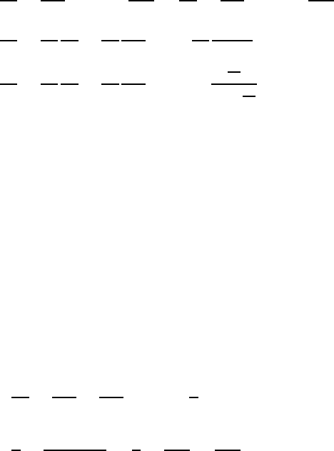
8.4. APPROXIMATING INFINITE SERIES 137
they are bounded by 1! Here’s a proof:
d1
10 +d2
102+···+d
n
10n≤9
10 +9
102+···+9
10n
=9
10 +9
10
1
10 +9
10
1
102···+9
10
1
10n−1
≤9
10 +9
10
1
10 +9
10
1
102+···=
9
10
1−1
10
=1.
Note that the key step above was recognizing that the geometric series
P∞
k=0 a(1/10)k,wherea=9/10, sums to 1 by (2) on page 132.
Of course, we also notice that repeating decimals like 0.999 ···=1and
0.333 ···=1/3 are all geometric series when represented as above. Try to
figure out the a,xin (2) in each case. This turns out to be true of any
repeating decimal and hence by the formula (2) these decimal numbers must
be fractions a/b where a,bare integers. In fact, the converse is also true,
namely, a decimal is a fraction if and only if it is eventually repeating.
Example. Consider the eventually repeating decimal x=0.5010101 ···.
We express this as
x=5
10 +1
103+1
105+···=1
2+∞
X
k=0
10−310−2k
=1
2+10−3
1−10−2=1
2+1
990 =248
495 .
We might notice that it is not possible to enter xin Derive as a decimal
but we can define it by means of the infinite series above. Then, simplifying
we get the above result.
8.4 Approximating Infinite Series
We can determine the sum of a geometric series exactly but for most conver-
gent infinite series this is impossible. If the series converges to s=P∞
k=0 ak,
then by definition scan be approximated arbitrarily closely by the partial
sums Pn
k=0 akfor large enough n. In this section we investigate two methods
for approximating infinite series, with a given precision.
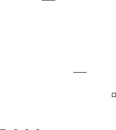
138 CHAPTER 8. SERIES
The Ratio Test. In a convergent geometric series, ak=axk, and hence
ak+1 =akx, i.e., the ratio of consecutive terms is x,where|x|<1. In this
section we consider positive series (ak>0) where the the ratio of consecutive
is approximately equal to some xwith 0 <x<1. It will turn out that all
such series converge and that we can estimate their size by comparisons with
appropriate geometric series. This technique is called the ratio test.
Theorem 1. Let aibe positive.
(a) If limi→∞ ai+1/ai=λ<1, then the series Paiconverges.
(b) Suppose that 0<x<1and that for some n,ai+1/ai≤xfor all i>n.
Then
0≤∞
X
i=1
ai−
n
X
i=1
ai≤an+1
1−x
(7)
Proof. If limi→∞ ai+1/ai=λ<1, then for any xsatisfying λ<x<1,
we know that the ratios will be less than xfor all large i.Thus,givenx
there is an nfor which ai+1 ≤xaiwhenever i>n.Soa
n+2 ≤xan+1 and
an+3 ≤xan+2 ≤x2an+1. In general, an+1+k≤xkan+1 and hence for all m>n
0≤
m
X
i=1
ai−
n
X
i=1
ai=an+1 +an+2 +···+a
m
≤a
n+1(1 + x+x2+···)= a
n+1
1−x.
Thus, the partial sums {sm}are bounded and the series is convergent. More-
over, the inequality (7) follows by taking limits as m→∞.
Example. Suppose we want to use Theorem 1 to prove that the series
∞
X
k=0
2k
k!=1
1+2
1+4
2+...
converges and estimate its value with an error of at most 10−6. The first
step is to show that limk→∞ ak+1/ai<1. We think of the terms as a

8.4. APPROXIMATING INFINITE SERIES 139
function of kby authoring term(k):=2^k/k!. Now simplifying the ratio
term(k+1)/term(k) we see that
ak+1
ak
=2
k+1 ≤1
2
for all k>2. Thus, limk→∞ ak+1/ak= limk→∞ 2/(k+1) = 0 <1sotheseries
converges and furthermore we can take x=1/2andn= 2 in Theorem 1(b).
Now we must determine nso that
an+1
1−x=2a
n+1 <10−6.
We do this by authoring
VECTOR([n,2*term(n+1)],n,2,20) ,
approximating the result and then searching the entries (by scrolling) until
we find one smaller than 10−6. It turns out n= 13 works. The last step is
to compute the partial sum s13 =P13
k=0 2k/k! giving 7.38905.
We might observe how fortunate we were that kturned out to be so small.
Recall some of our computations using the trapezoid method or Simpson’s
rule where similar accuracy required thousands or even millions of computa-
tions (using the left endpoint method, for example). It is one of the funda-
mental properties of geometric series that they converge very rapidly. Think
about it, 6–decimal place accuracy with just 15 computations!
As it turns out this series is rather special since
∞
X
k=0
2k
k!=e2=7.38905 ···
This important fact is explained in Chapter 7 equation 8. If this fact is new
to you then just try authoring the above infinite series and have Derive
simplify the result. What if the 2 is replaced with 3 or x?
Example∗.Now consider the harder problem of approximating
∞
X
k=1
k!
kk
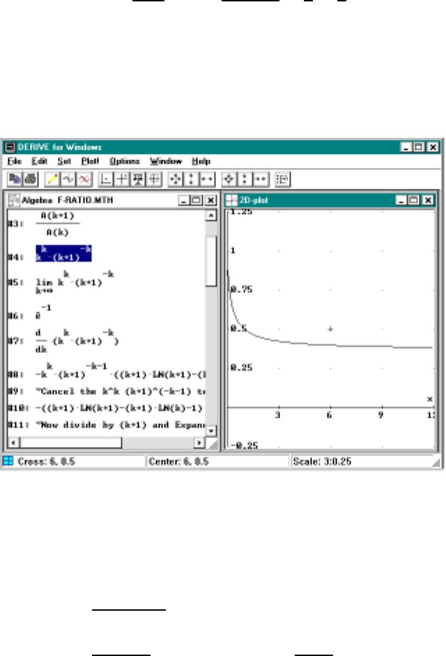
140 CHAPTER 8. SERIES
with error again of at most 10−6. Proceeding as before we author the formula
term(k):=k!/k^k. Now by first simplifying and then taking limits we see
that
lim
k→∞
ak+1
ak
= lim
k→∞
kk
(k+1)
k=1
e<1
2
since e>2. Thus, the limit is less than 1 so the series converges. Further-
more, we can take x=1/2 in Theorem 1(b). But now we need to find an
integer nso that ak+1/ak=kk/(1 + k)k<1/2 for all k>n.
This step is harder than before. If we graph f(x)=(x/(x+1))xit appears
to be decreasing for all x≥0. See Figure 8.1.
Figure 8.1: Ratio test example
In order to prove that f(x) is a decreasing function we differentiate and
show that f0(x)<0. Using Derive we get
f0(x)=−x
x
(x+1)
x+1 [(x+1)ln(x+1)−(x+1)lnx−1]
=−xx
(x+1)
xln(x+1)−ln x−1
x+1
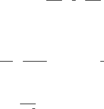
8.4. APPROXIMATING INFINITE SERIES 141
after some rearrangement (see the file F-RATIO for the step-by-step pro-
cedure). Since xx/(x+1)
xis positive for x>0, we need to show that
ln(x+1)−ln x−1/(x+ 1) is positive. At this point Derive can’t help so
we need an idea from calculus. One quick way to solve this problem is to
use the Mean Value Theorem for the function g(x)=lnx. The Mean Value
Theorem says: g(b)−g(a)=g
0
(c)(b−a) for some a<c<b.Fora=xand
b=x+1thisgivesln(x+1)−ln x=1/c for some x<c<x+1. Thus
ln(x+1)−ln x−1
x+1 =1
c−1
x+1 >0
where we obtain the desired inequality since c<x+1. Thus, f0(x)<0 for
all x>0andsofis decreasing.
Now that we have established that the ratios decrease we need to know
when they are less than 1/2. Since
ak+1
ak
=kk
(k+1)
k=f(k)≤f(1) = 1
2.
for all k≥1, it follows that we may apply the theorem for any n. Finally,
by (7), we must determine nso that
an+1
1−1
2
=2a
n+1 <10−6.
As before we author
VECTOR([n,2*term(n+1)],n,2,20) ,
approximate the result and then search the entries until we find one smaller
than 10−6. It turns out in this case that k= 16. Computing the partial sum
s15 gives 1.87985.
Now suppose that your series Paksatisfies lim ak+1/ak=λbut that
λ≥1. The case λ>1 is pretty much like the case λ<1 except that now
the series diverges. The idea is to pick 1 <x<λand observe that
∞=an+anx+anx2···≤a
n+a
n+1 +an+2 +...
for some large nsince now ak+1/ak≥xfor all k≥n.Thecaseλ=1is
much harder since, as we see in the next section, there are examples in which
the series converges and examples where it diverges.

142 CHAPTER 8. SERIES
TheIntegralTest Suppose that f(x) is a decreasing positive valued func-
tion, for x≥1. Let an=f(n). We want to approximate P∞
i=1 aiand
determine whether the series is convergent or divergent.
In Section 6.4 we saw that, for a decreasing function like f(x), the left
endpoint method of estimating a definite integral of f(x) always overesti-
mates the integral while the right endpoint method underestimates it. This
is quite obvious by looking at Figure 8.2 on the next page where we use
f(x)=1/x as our function and apply the box drawing function from Chap-
ter 6; see the file F-SERINT for a demonstration. Now, we observe that since
the interval size is one, the area of the box with height f(n)isjusta
n
.From
this we get that adding the area of boxes corresponds to partials sums of the
series Pak. Thus, for any 1 ≤n≤m
m+1
X
i=n+1
ai≤Zm
n
f(x)dx ≤
m
X
i=n
ai
(8)
The sum on the left is the right endpoint estimate and the sum on the right
is the left endpoint estimate, when we use ∆x= 1 as the subinterval size.
From this inequality, we obtain the following theorem:
Theorem 2. Suppose that f(x)is a continuous, nonnegative, decreasing
function for x≥1.Puta
n=f(n).
(a) The infinite series P∞
i=1 aiconverges if and only if the improper integral
R∞
1f(x)dx does.
(b) Moreover, the inequality
n
X
i=1
ai≤
n
X
i=1
ai+Z∞
n+1
f(x)dx ≤∞
X
i=1
ai≤
n
X
i=1
ai+Z∞
n
f(x)dx(9)
holds for all n=1,2,....
(c) The value of the series can be estimated using the following:
0≤∞
X
i=1
ai− n
X
i=1
ai+Z∞
n+1
f(x)dx!≤an
(10)
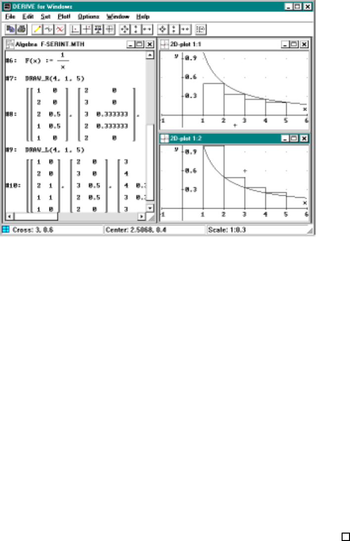
8.4. APPROXIMATING INFINITE SERIES 143
Figure 8.2: The geometric estimate used in the integral test
Proof. Suppose that the improper integral R∞
1f(x)dx is convergent so that
the total area under the curve is finite. From (8) it follows that
m+1
X
i=n+1
ai≤Zm
n
f(x)dx ≤Z∞
n
f(x)dx < ∞
and hence the partial sums {sm}are bounded (the first nterms are irrelevant).
Thus, the series converges and the second inequality in (9) follows from
∞
X
i=1
ai=
n
X
i=1
ai+∞
X
i=n+1
ai≤
n
X
i=1
ai+Z∞
n
f(x)dx .
A similar argument shows that the integral is convergent if the series is and
that the first inequality in (9) holds.
The first inequality in (10) is an immediate consequence of (9) and simi-
larly it follows that the middle expression in (10) is bounded by Rn+1
nf(x)dx.
But since f(x) is decreasing this integral is less than or equal to f(n)=a
n
and the theorem is proved.
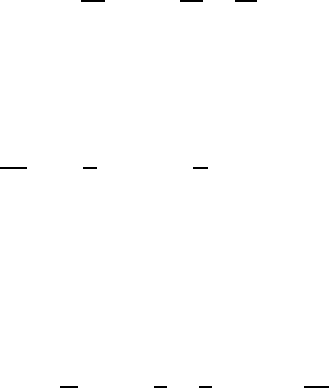
144 CHAPTER 8. SERIES
We note that (9) actually gives us two methods for approximating the
sum of a convergent series s=P∞
k=1 ak. The first technique looks more like
the one used in the ratio test:
0≤s−sn=∞
X
i=1
ai−
n
X
i=1
ai≤Z∞
n
f(x)dx
and the second one is the more refined estimate (10) which uses the quantity
n
X
i=1
ai+Z∞
n+1
f(x)dx
to approximate sinstead of the partial sum sn. As we shall see in the
examples, this more refined method has a dramatic computational advantage.
A curious formula. As our first application of the integral test let us
prove that the series
∞
X
k=1
1
k2=1+ 1
2
2+1
3
2+...
is convergent. First note that λ= 1 in the ratio test so we cannot use that
approach. Next, we take f(x)=1/x2and observe (say using Derive)that
Zn
1
dx
x2=−1
x
n
1
=1−1
n→1asn→∞
and hence the improper integral R∞
1dx/x2is convergent. Now, by the integral
test the series P1/i2<∞, that is the series is convergent. Actually, a similar
argument shows that P1/ip<∞whenever p>1.
Now it is a remarkable fact that
∞
X
i=1
1
i2=1+1
4+1
9+···=π
2
6.(11)
You have to wonder how the π–term can possibly be involved in this compu-
tation. The proof of this fact is beyond the scope of this text but Derive
can help us believe thisresult. OnewaytodothisistohaveDerive simplify
the series and get π2/6 as the answer. It works, try it. A more independent

8.4. APPROXIMATING INFINITE SERIES 145
approach would be to compute the partial sums snfor several nand compare
with a decimal approximation to π2/6. In Figure 8.3 on the following page
we have Derive make these comparisons with n= 100, 1000, and 10,000.
We also observe that Derive knows about (11) and simplifies the series
accordingly.
Problem: Compute this series to mdecimal places. We solve this
problem by using (10) which in this case says:
0≤∞
X
i=1
1
i2− n
X
i=1
1
i2+1
n+1!≤1
n
2.(12)
Thus, to solve our problem we need only find nso that right-hand side of
(12) is less than 10−m, and then use
n
X
i=1
1
i2+1
n+1 =1+1
4+1
9+···+1
n
2+1
n+1
for our estimate. For example, with m= 6 we need to take n2>10mor
n>1000.
Something rather amazing occurred in this problem. In Figure 8.3 on the
next page we used the partial sums {sn}to approximate the sum s.Thisis
the natural thing to do since s= lim sn. But the accuracy in Figure 8.3 is
only 3 or 4 decimal places with n= 1000. This error is to expected since (8)
yields
0≤s−sn=∞
X
i=n+1
1
i2≤Z∞
n
dx
x2=1
n
and the right-hand side is just less than 10−3. On the other hand, adding
theterm1/(n+ 1) (which is the integral in (10)) increases the accuracy to
1/n2=10
−6
. This accuracy is 1000 times better than the other estimate.
Put another way, suppose for example that both computations take about 3
seconds with n= 1000 on your PC, the amount of computation time needed
to produce 6 decimal place accuracy using the less efficient method is almost
an hour! See the file F-2-SER which contains a comparison of these methods.
This problem illustrates the potential value of a innovative approach to a
computation compared to the conventional solution.
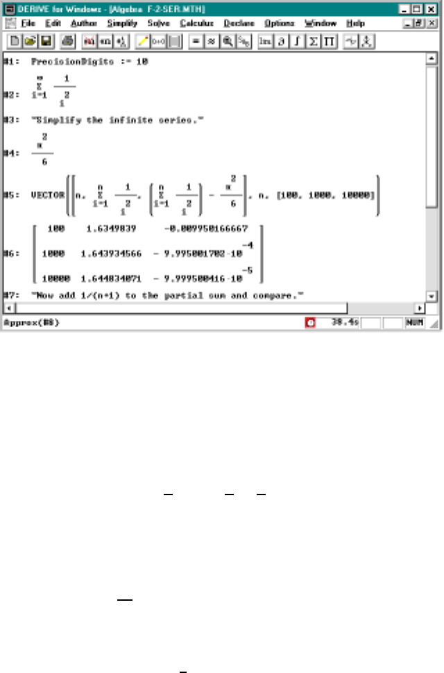
146 CHAPTER 8. SERIES
Figure 8.3: Summing the series P1/i2
The Harmonic Series Let us apply the integral test to the harmonic
series,namely,
∞
X
i=1
1
i=1+1
2+1
3+...
We take f(x)=1/x in the theorem and observe that
Zx
1
dt
t=lnx→∞ as x→∞
and hence the integral is divergent. Thus, the series is divergent. Another
way to express this is that P∞
i=1
1
i=+∞or in other words, the partials sums
are eventually larger than any given number.
Consider this: How many terms of the harmonic series are necessary
before the partial sums exceed 100? Is the answer 1000? 1,000,000? 1010?
Amazingly, none of these answers are even close to the actual result. Suppose
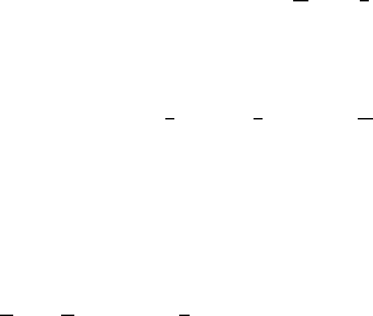
8.5. LABORATORY EXERCISES 147
that 100 <ln n,thenby(8)
100 <ln n=Zn
1
dt
t≤
n
X
1
1
i
so that any n>e
100 ≈2.6×1043 is certainly large enough. On the other
hand, using (8) again we have
100 ≤
n
X
1
1
i=1+
n
X
2
1
i≤1+Zn−1
1
dt
t<1+lnn
so that when combined with the above we see that the best nsatisfies: e99 <
n<e
100.
8.5 Laboratory Exercises
For these problems it is a good idea to have more digits of precision: choose
Declare/Algebraic State/Simplification and the Digits box to 10 or 12.
1. Formula (3) on page 134 shows the amount of money in an account
after nyears if the interest rate is r, the original amount is A,and
the interest is compounded ktimes a year. In Problem 1 on page 191
you showed that if interest is compounded continuously, the amount of
money would be Aern.
a. Show that the limit as k→∞of compounding ktimes a year is
the same as compounding continuously.
b. If you put $1000.00 into an account earning 4.5% interest, how
much money will be in the account after one year if the interest
is compounded yearly? quarterly? daily? continuously?
c. Do the previous part only assume that the bank is paying 9%.
2. Suppose you get a 30 year mortgage loan for $200,000 which is to be
repaid in 30 ·12 equal monthly payments, based on an annual interest
rate of 7.5%.
a. Find your monthly payment.
148 CHAPTER 8. SERIES
b. How much do you still owe after your first payment? How much
of your first year’s payment went to interest and how much went
to paying off the principal?
c. Formula (4) gives the amount you still owe after kmonths. Re-
place the kwith 12kin Formula (4) so that know represents years,
approximate the resulting expression and then plot. (You’ll need
to adjust the range in such a way that the visible x-axis contains
the range 0 to 30 and the y–axis contains the range 0 to 200,000.)
Notice that at the beginning the amount you owe changes slowly
but that near the end of the 30 years it changes quickly.
3. In some problems involving monthly payments or interest the monthly
interest rate is computed by dividing the annual rate by 12. But some-
times the monthly rate mis not specified and instead the effective
annual rate ris given. This means that compounding the monthly rate
m12 times gives the annual rate r, i.e. (1 + m)12 =1+r.Consider
the previous problem but now suppose that the effective annual rate is
7.5%.
a. Calculate the monthly rate for this problem.
b. Find the monthly mortgage payments using this new rate.
4. The bank says that it will give you a car loan of $6,000 provided you
make monthly payments of $135 for 5 years. What interest rate is the
bank charging? (Hint: You may need to be a little careful how you
compute this.)
5. Consider the fraction 1/7.
a. Using Derive show that 1/7appears to have a repeating decimal
expansion. What is it?
b. Express this repeating decimal from part aas an infinite series,
see the example on page 137.
c. Have Derive simplify this series.
d. Identify the aand xterms from (2) and verify using that formula
that your infinite series simplifies to 1/7.

8.5. LABORATORY EXERCISES 149
6. Have Derive evaluate the sum P∞
n=1 1/n2. (Make sure you use Exact
mode.) Evaluate the left and right sides of formula (9) in Theorem 2
for n= 1000. You should approximate the sum rather than Simplify,
otherwise the computation time is fairly long. Use these to estimate π
giving upper and lower bounds.
7. For each of the following series P∞
k=0 akfind λ= limi→∞ ak+1/akand
show that λ<1/2. Now use Theorem 1(b) with x=1/2tofindn
large enough so that Pn
k=0 akapproximates the series with error at
most 10−6.
a. ∞
X
k=0
k3
4kb. ∞
X
k=0
(k!)2
(2k)!
8. Use Theorem 2(c) to evaluate each of the following series with an
errorofatmost10
−6
. (The finite sum of Theorem 2(c) should be
Approximated but the improper integral should be evaluated exactly.)
a. ∞
X
k=2
1
k(ln k)2b. ∞
X
k=1
1
k3
c. ∞
X
k=1
1
1+k
2
9. Some of the following series converge and some diverge. Decide which
do which and state the required Theorem needed to prove your conclu-
sion.
a. ∞
X
k=0
2kb. ∞
X
k=2
1
kln k
c. ∞
X
k=0
1
ekd. ∞
X
k=1
2·4···2k
(2k)!
10. Consider the series P∞
k=0 1/k!.
a. Show that the series converges by the ratio test.

150 CHAPTER 8. SERIES
b. Have Derive simplify this series.
c. Use these results to approximate the Euler constant ewith an
accuracy of 10−6
*11. The following formula
1+2 ∞
X
k=1
e−k2/t =√tπ 1+2 ∞
X
k=1
e−k2π2t!
(13)
is known to hold for all t>0. The formula is derived from an im-
portant technique in the theory of Fourier transforms called Poisson
summation. We will not attempt to prove this formula but instead try
to use it as a method of approximating πmore efficiently than in an
earlier problem. It has a number of other useful applications too. We
will fix the value of t= 2 for the rest of this problem.
a. Using the ratio test, show that both infinite series in (13) are
convergent.
b. Use Theorem 1 with x=e−6π2and n= 1 to show that P∞
k=1 e−2k2π2
is less than 10−8. Thus, with an accuracy of 2√2π10−8or roughly
7 decimal places we can take the right hand side of equation (13)
to be √2π.
c. Using Theorem 1 again, show that
0< 1+2 ∞
X
k=1
e−k2/2!− 1+2
6
X
k=1
e−k2/2!
=2 ∞
X
k=7
e−k2/2<10−10
and hence
π≈1
2 1+2
6
X
k=1
e−k2/2!2
.
d. Approximate the above expression using Simplify/Approximate
with the number of precision digits set to 10. Compare the above
approximation of πwith Derive’s. What is the decimal place
accuracy?
8.5. LABORATORY EXERCISES 151
e. To achieve more decimal places you should increase the value of
t. Show that with t= 10, the analogous estimate in part bis
∞
X
k=1
e−10k2π2<10−42
(This problem is essentially due to George Csordas.)
152 CHAPTER 8. SERIES

Chapter 9
Approximating Integrals with
Taylor Polynomials
9.1 Introduction
In Chapter 6 we developed several techniques for approximating a definite
integral I=Rb
0f(x)dx by applying the trapezoid method or Simpson’s rule.
In the last chapter we saw that many of the important functions in Calculus
can be represented by a Taylor series and hence can be approximated by
their Taylor polynomials. This suggest another approach to approximating I;
namely, approximate the integrand f(x) by its Taylor polynomials and then
use
Zb
0
f(x)dx ≈Zb
0
Pn(x)dx =Zb
0
n
X
k=0
akxkdx =
n
X
k=0
ak
bk+1
k+1
where ak=f(k)(0)/k! to obtain the desired estimate.
The advantage to this approach was strongly suggested by Problem 3
on page 159. In that problem it was shown that approximating ln 3 using
Taylor series techniques gave 8–decimal place accuracy with approximately 8
computations. Whereas the standard approach using Simpson’s rule require
approximately 100 computations.
153

154 CHAPTER 9. APPROXIMATING INTEGRALS
9.2 The Basic Error Estimate
Recall from (11) of Chapter 7 on page 115 that if Pn
k=0 akxkis the nth Taylor
polynomial for f(x), then an upper bound for the error made in estimating
f(x) with this Taylor polynomial is given by
f(x)−
n
X
k=0
akxk≤M|x|n+1
(n+1)!
(1)
where Mis the maximum of |f(n+1)(t)|on the interval connecting 0 to x.
This can be written as
−M|x|n+1
(n+1)! ≤f(x)−
n
X
k=0
akxk≤M|x|n+1
(n+1)!
(2)
If we integrate this from 0 to b,weget
−M|b|
n+2
(n+2)! ≤Zb
0
f(x)dx −
n
X
k=0
ak
k+1b
k+1 ≤M|b|n+2
(n+2)!
(3)
Writing this with absolute values:
Zb
0
f(x)dx −
n
X
k=0
ak
k+1b
k+1≤M|b|n+2
(n+2)!
(4)
This technique works for integrals going from 0 to b.Ifyouwantto
approximate Rb
af(x)dx, you can make the substitution u=x−aso the
integral becomes Rb−a
0f(u)du.
9.3 The Logarithm Series
Consider the logarithm function f(x)=ln 1
1−xwhereweshiftthevariable
so that x= 0 yields ln 1 = 0. First of all, we have the integral representation:
ln 1
1−x=Zx
0
dt
1−tfor −∞<x<1.
which can be easily checked using Derive.
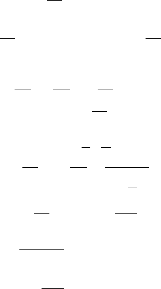
9.3. THE LOGARITHM SERIES 155
Now, the idea is to approximate the integrand by its Taylor series but in
this case we recognize the connection with the geometric series; namely,
∞
X
k=0
tk=1
1−tfor −1<x<1.
We’ll actually use the following more refined estimate from Section 8.2:
1
1−t−
n
X
k=0
tk=∞
X
k=n+1
tk=tn+1 +tn+2 +···=t
n+1
1−t
(5)
whenever |t|<1. Now we integrate this equation from 0 to x,wherewe
assume that −1≤x<1, to get
ln 1
1−x−
n
X
k=0
xk+1
k+1 =Zx
0 1
1−t−
n
X
k=0
tk!dt(6)
=Zx
0
tn+1
1−tdt .(7)
Taking absolute values of the above we need to evaluate the integral in (7).
Since this looks complicated, we instead try to obtain an upper bound. For
positive x, we uses the inequality 0 <1
1−t≤1
1−xto obtain that
Zx
0
tk+1
1−tdt≤Zx
0
tn+1
1−xdt =xn+2
(1 −x)(n+2).(8)
On the other hand, for negative x, we instead use 0 <1
1−t≤1 to get a similar
bound:
Z0
x
tk+1
1−tdt≤Z0
x|t|n+1 dt =|x|n+2
(n+2).(9)
Hence, we have the desired approximation result because
lim
n→∞
xn+2
(1 −x)(n+2) = 0 whenever 0 ≤x<1
and
lim
n→∞ |x|n+2
(n+2) = 0 whenever −1≤x≤0

156 CHAPTER 9. APPROXIMATING INTEGRALS
One small point, the polynomial approximations in (6) look a little differ-
ent from the standard Taylor polynomials because the powers are expressed
with the index k+ 1. This is just an artificial difference since
Pn+1(x)=
n+1
X
j=1
xj
j=x+x2
2+···+x
n+1
n+1 =
n
X
k=0
xk+1
k+1
and hence we ultimately obtain that
ln 1
1−x−Pn(x)≤
xn+1
(1 −x)(n+1),0≤x<1;
|x|n+1
(n+1),−1≤x≤0
(10)
which tends to zero as n→∞. This leads to the Taylor series representation
ln 1
1−x=∞
X
j=1
xj
jfor −1≤x<1.(11)
9.4 An Integral Approximation
Suppose we wanted to estimate the definite integral
Z1
0
sin x
xdx.
At first glance there appears to be a problem at x= 0 because we are
dividing by zero. However, L’Hospital rule shows that limx→0sin x/x =1.
An interesting alternative way of proving this fact is use the Taylor series
representation for the sin x, i.e.
sin x=x−x3
3! +x5
5! −···=∞
X
k=0
(−1)k
(2k+1)!x
2k+1
for all −∞ <x<+∞. Now for x6= 0 we can divide both sides by xto get
sin x
x=1−x
2
3! +x4
5! −... .
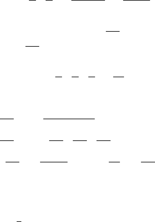
9.4. AN INTEGRAL APPROXIMATION 157
Formally then, the right-hand side above approaches 1 as x→0 because all
the xn–terms tend to zero. Of course, there is always the problem of making
estimates for infinite series, as opposed to finite sums, which can be difficult.
One way around this difficulty is use the approach we adopted for approx-
imating sin xin Section 7.4. There we used Taylor’s Theorem with remainder
to show that
sin x−x−x3
3! +x5
5! −...(−1)nx2n+1
(2n+1)!
≤|x
2n+3|
(2n+3)!
(12)
for all n=0,1,.... For example, even taking n=0intheaboveyieldsa
nice result; namely, |sin x−x|≤|x|
3
/6. Hence, |sin x
x−1|≤x
2
/6→0as
x→0 and thus limx→0
sin x
x=1.
Similarly, if we take a larger value of n,sayn=3,weget
sin x−x−x3
3! +x5
5! −x7
7! ≤|x9|
9!
(13)
and so dividing by xand integrating from 0 to 1 yields
Z1
0
sin x
xdx −
3
X
n=0
1
(2n+ 1)(2n+1)!
=
Z1
0
sin x
xdx −1−1
3·3! +1
5·5! −1
7·7!
=Z1
0 sin x
x−
3
X
n=0
(−1)nx2n
(2n+1)!!dx≤Z1
0
|x|8
9! dx
=1
9·9!.
Finally, since 1/(9 ·9!) ≈3.0619 ×10⁻⁷we get 6 decimal place accuracy by
approximating the integral using 4 terms from the series.
In Figure 9.1 on the next page we have Derive approximate our integral
using 20 digit precision. This computation, which uses Simpson’s rule, is
actually quite slow, Load the file F-SININT and try this yourself. On the
other hand, we enter the partial sums of the series solution and make a table
comparing the first several sums with the answer from Derive.Noticethat
the theoretical error that we calculated above is practically the same as the
actual error when n=3.
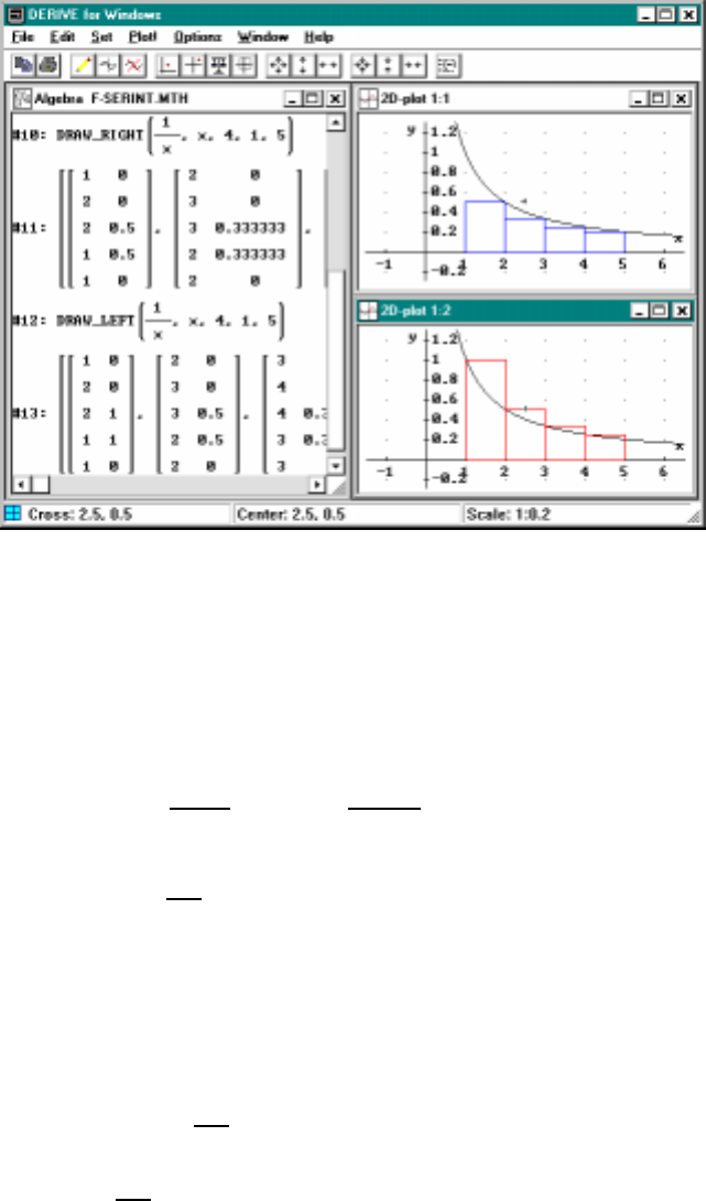
158 CHAPTER 9. APPROXIMATING INTEGRALS
Figure 9.1: Using Taylor series to approximate integrals
9.5 Laboratory Exercises
1. Use (17) on page 121 and (11) on page 156 to prove that
ln 1+x
1−x=2 ∞
X
k=0
x2k+1
2k+1 for −1<x<1(14)
2. Let f(x)=ln
1+x
1−xfor −1<x<1. In this exercise we will use the
representation (14) above to compute ln 3.
a. Determine the value of xin the standard representation of the
logarithm function (17) on page 121 that makes the left hand side
of that relation equal to ln 3. Explain why the infinite series on
the right hand side can not be used to compute ln 3.
b. Plot g(x)=1+x
1−xand show that y=g(x) is a strictly increasing
function on −1<x<1 with range 0 <y<∞.
c. Solve 1+x
1−x= 3 for x.Letx
3be your answer.

9.5. LABORATORY EXERCISES 159
d. Using (14) above, we get an infinite series for ln 3 by substituting
x=x3into (14). Show that this infinite series converges by the
ratio test on page 138.
e. Compare the numerical values of Pn(x3) for various nwith the
approximate value of ln 3.
3. If we take x=1/3 in (14) above we get
Z2
1
dt
t=ln2= ∞
X
k=0
2
(2k+1)3
2k+1 .
In Chapter 6 we studied numerical integration techniques for approxi-
mating the above integral with the most efficient method being Simp-
son’s rule. One the other hand, using the ratio test on page 138 we
approximated the infinite series similar to the above.
a. Using the error in Simpson’s rule, formula (5) on page 99, deter-
mine approximately how many subdivisions (and hence how many
computations) are needed to obtain 8 decimal place accuracy.
b. For completeness, also do part (a) using the left endpoint method
and the trapezoid method.
c. Show that the ratio of terms in the above series is less than 1/9.
d. Using formula (7) of Theorem 1 on page 138 with x=1/9, deter-
mine how many terms are needed to approximate ln 2 to 8 decimal
places.
e. Now compare all four approximation techniques. Which method
is the most efficient?
4. Use the formula
tan−1x=Zx
0
dt
1+t
2
and the techniques of this chapter to prove that the Taylor representa-
tion
tan−1x=∞
X
k=0
(−1)k
2k+1x
2k+1 =x−x3
3+x5
5−... for −1≤x≤1
holds. Look back at Problem 6 on page 129 and also Problem 3b.
What are the implications of this problem to the earlier ones?

160 CHAPTER 9. APPROXIMATING INTEGRALS
5. In this problem you are to estimate
Z2
0
e√xdx
using the method outlined in the text.
a. Define and simplify P(x):= the 8th–degree Taylor polynomial for
ex.
b. Author P(√x) and integrate the result from 0 to 2. Simplify this
integral and then express the answer as a decimal.
c. Compute the maximum value of the ninth derivative of exon the
interval 0 to √2. Denote this maximum by M. (Note: Thisisthe
Mvalue associated with the Taylor polynomial p(x) in (11) on
page 115 corresponding to the interval 0 ≤x≤√2. The reason
we use √2 and not 2 is that if |ex−p(x)|≤cfor 0 ≤x≤√2,
then |e√x−p(√x)|≤cfor 0 ≤√x≤√2, i.e., for 0 ≤x≤2.)
d. In a manner similar to what was done in Section 9.4, find the error
in the approximation you obtained in part b.
e. Have Derive evaluate R2
0e√xdx and then approximate it and
compare the answer with what you obtained in part b.
6. Do parts a. to e. but this time for
Z1
0
e−x2dx.
Instead of starting with the Taylor polynomial for ex, start with the
Taylor polynomial of e−x.

Chapter 10
Polar and Parametric Graphs
10.1 Introduction
Graphs of the form y=f(x)orx=g(y) can be used to represent a wide
variety of curves in the plane, there are many important curves, such as
circles or ellipses, that cannot be represented by a single graph of this type.
More generally, imagine the curve traced out by an ant walking on a flat
surface. In this chapter we will introduce two techniques for plotting general
curves. One is the method of polar coordinates, which is a coordinate system
based on angles and distance from the origin. The other is the method of
parametric representation, which allows one to specify completely arbitrary
curves like the motion of a particles (or the ant).
10.2 Polar Coordinates
We can specify a point in the plane by how far it is from the origin and what
angle the line from the point to the origin makes with the x–axis. If ris the
distance from the origin and θis the angle, we say that [r, θ] are the polar
coordinates of the point; see Figure 10.1 on the next page. Thus, for example,
the point with rectangular coordinates (1,1) would have polar coordinates
[√2,π/4]. The way to envision plotting a polar point [r, θ]istostandat
the origin facing out towards the positive x–axis and then turn counter-
clockwise by the angle θandthenmoverunit in the direction you are now
facing. We usually think of ras being nonnegative, but if ris negative, we
simply go backwards |r|units. Similarly, we plot negative angles by turning
161
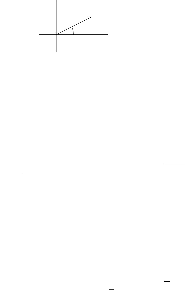
162 CHAPTER 10. POLAR AND PARAMETRIC GRAPHS
θ
[r, θ]
r
Figure 10.1: Polar Coordinates
clockwise instead of counter-clockwise. This leads to a surprising difference
compared to rectangular coordinates; namely, two different polar coordinates
can represent the same point. Thus, [−2,π/4] = [2,5π/4] = [2,−3π/4]. Note
that [0,θ] is the origin regardless of what θis. Your calculus text has a more
detailed description of polar coordinates.
A basic problem in polar graphing is to plot a function such as r=ρ(θ),
i.e., plot all points [r, θ]whereris given by the function ρ(θ). For example
the circle of radius a, centered at the origin, is the graph of r=a.Thus,
ρ(θ)=ais a constant functions. Note that to draw this circle in rectangular
coordinates you must think of this curve as two graphs, namely, y=√a2−x2
and y=−√a2−x2. This simple example already shows that some curves
are more easily represented with polar coordinates.
Let us now try something harder such as r=1+cosθ. One then graphs
the curve by computing rfor lots of θ’s by thinking about the geometry of the
angle θand the value of r. This is usually done with angles such as θ=0,
π/4, π/2, 3π/4andπwhich corresponds to 45◦increments in the angle.
By authoring vector([1+cos θ,θ], θ,0,π,π/4) and simplifying this
expression gives a table of polar points which can be plotted by hand or as
a set of points in Derive. We’ll need to plot more θ’s but this is a start.
A nice technique for viewing the data is to use the APPROX function to get
decimals for the r–values. We then get ras a decimal and θexpressed in the
usual radian notation for the angles. See Figure 10.2 on the facing page.
Derive can plot these points in polar coordinates by selecting the Option
menu and then selecting the Polar option on the Coordinates menu. Then,
plot the points just as we did in rectangular coordinates by highlighting the
matrix of points and clicking the plot button in the graphics window. After
plotting these 5 points we try to imagine the rest of the graph by interpolating
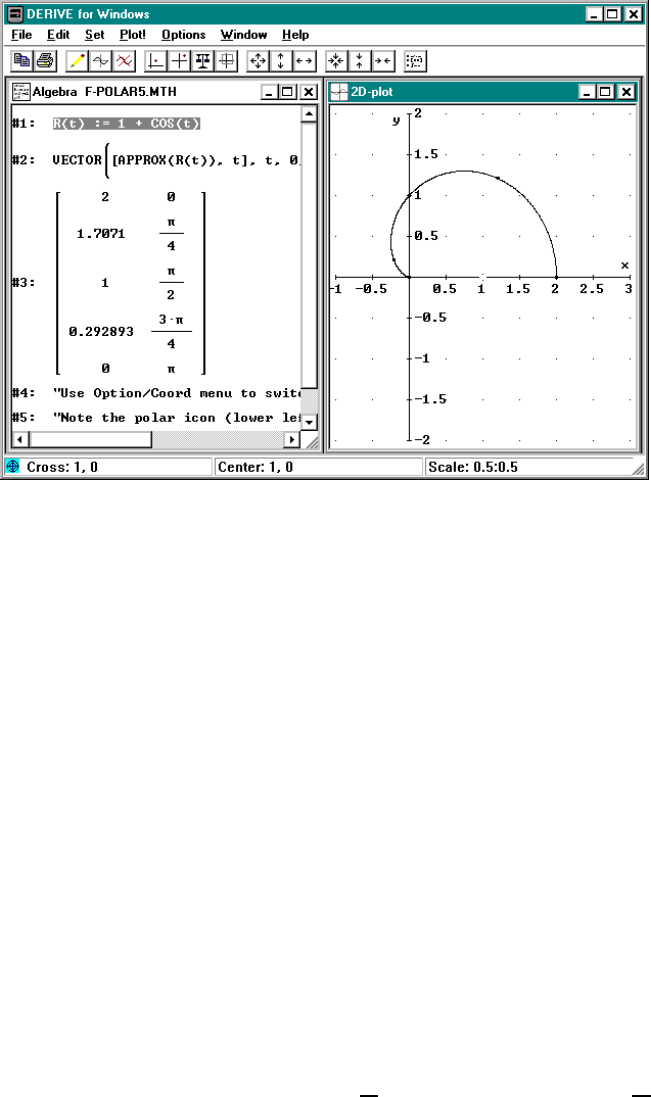
10.2. POLAR COORDINATES 163
Figure 10.2: Plotting points in polar coordinates
other values of θ.Ofcourse,Derive will plot the curve for us. We enter
either 1 + cos t or just highlight expression #1 in Figure 10.2, then click
the Plot button in the graphics window. So far, this is just like rectangular
plots except for the change in the coordinate mode. But now Derive will
prompt you for the parameter interval (interval of θ’s to use) and suggest the
default range of −π≤θ≤π. Since many of the standard examples of polar
curves involve the θ-variable only in the form of either cos θor sin θ, it usually
suffices to only consider 0 ≤θ≤2π(or as Derive prefers −π≤θ≤π).
Of course, you can change it to whatever interval you want. For example, in
Figure 10.2 the range 0 ≤θ≤πwas used. You might want to plot the full
graph at this point by using the default range. The resulting graph heart
shaped curve is called a cardioid.
Tracing. It is important to actually see the curve being plotted but the
computer plots so quickly that it is nearly impossible to see it happen. De-
rive has an approach for “driving” around a curve called tracing.After
plotting the polar curves above select the Trace Mode option on the Options

164 CHAPTER 10. POLAR AND PARAMETRIC GRAPHS
menu (or just press F3 to toggle the Trace mode) and the cross will turn into
a box and it will be moved onto the last curve plotted. Now press and hold
down the right arrow key and watch the little car drive around the curve.
Youcanseethevalueofθ, which we can also interpret as time, as it increases,
as well as the rand θcoordinates, on the lower part of the screen. If you
have more than one graph you can switch between curves by using the up or
down arrow keys.
When plotting the cardioid a= 1 pay particular attention to the way the
plotting slows down as we approach the cusp. It turns out that the only way
for cusps or corners to occur in the graph, when r(θ) is differentiable, is for
the plotting to slow to a stop and then to start up again. This notion of
speed will be discussed in Section 10.5.
10.3 Rotating Polar Curves
A nice feature of polar coordinates is the ease with which we can rotate a
figure. For example, if we plot r=ρ(θ) and we want to rotate the picture
clockwise by an angle αwe simply plot r=ρ(θ+α) instead. Try this out in
for yourself using Derive.
Here is an interesting application of this idea. Did you know that the
curve y=1/x, which is used to define the natural logarithm, is a hyperbola.
The equation does not make this apparent since using the usual convention;
namely, the axes should be chosen parallel and perpendicular to the axes of
symmetry, we are supposed to have the equation of the form:
x2
a2−y2
b2=±1.
We need to discuss converting polar graphs to rectangular graphs and
vice versa. Figure 10.1 on page 162 makes it clear how to do this. The
algebraic relationship between the polar coordinates [r, θ] and the rectangular
coordinates (x, y) is given by the right triangle formed from the 3 points:
(0,0), (x, y)and(x, 0). The equations are:
x=rcos θ, y =rsin θand r=px2+y2,θ=tan
−1
(y/x)(1)
In Figure 10.3 on the facing page we enter xy = 1, convert to polar
coordinates by using the above equations and then rotate by α=π/4inthe
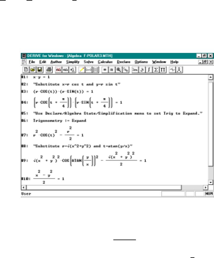
10.3. ROTATING POLAR CURVES 165
clockwise direction by substituting θ+π/4 for θ. We now what to apply the
trigonometric formulas:
sin(A+B)=sinAcos B+sinBcos A
cos(A+B)=cosAcos B−sin Asin B
but Derive does not simplify these by default. Instead we need to choose
Declare/Algebra State/Simplification and on the Trigonometry box we select
Expand. Simplifying these standard formulas will now yield the above.
Simplifying our rotated curve now yields: r2cos2t−r2/2 = 1. Converting
back to rectangular coordinates we use (1) to replace r2cos2twith x2and
r2with x2+y2. This yields the desired result; namely, rotating the graph
y=1/x by 45◦results in an equation x2−y2= 2 which is a hyperbola.
Figure 10.3: Showing that y=1/x is a hyperbola
Actually, the method used in Figure 10.3 to convert back to rectangular
coordinates is to substitute r=px2+y2and θ=tan
−1
(y/x)(Derive
denotes the inverse tangent function by ATAN). But there can be problems
with this approach. For example, consider the polar point [√2,3π/4] which

166 CHAPTER 10. POLAR AND PARAMETRIC GRAPHS
clearly corresponds to the point (−1,1) in rectangular coordinates. But
tan−1(−1) = −π/4 instead of 3π/4 because the definition of the inverse
tangent uses the principle angles −π/2<θ<π/2. Thus, for points with
x<0 we should substitute θ=tan
−1
(y/x)+πinstead.1Of course, in our
example it doesn’t cause a problem thanks to the fact that
cos2(θ+π)=cos
2θ
for all θ(check this using Derive).
10.4 Complex Numbers
Recall that we can also think of the points in the plane as complex numbers.
Thus, the point (a, b) in rectangular coordinates can also be considered to
be the complex number a+bi. This raises the question of whether the polar
coordinate representation of points in the plane might have an interesting
application to visualizing complex numbers.
The connection between these two ideas is provided by the Euler Formula
that we discussed in an earlier problem (see Problem 6 on page 127). The
formula, which essentially defines the complex exponential function, is given
by
eiθ =cosθ+isin θ
By looking at this formula we now realize that any complex number
z=x+yican be expressed as
z=|z|eiθ where |z|=px2+y2
and the angle θcomes from its polar coordinate representation. Note that
the modulus |z|is simply the rin the polar coordinate representation. Thus,
z=|z|eiθ =rcos θ+ir sin θ
so that zhas the polar coordinate representation [r, θ].
1Derive’s function ATAN has a two-variable form ATAN(y, x) which does the right
thing.
10.5. PARAMETRIC CURVES 167
Rotations and Complex Multiplication Let’s look back at rotations
from the previous section. Observe that the usual law of exponents when
applied to complex exponentials, which can be verified using the addition
formulas for sines and cosines, yields:
eiαeiθ =ei(α+θ).
Hence, the geometric effect of multiplying an arbitrary complex number zby
the complex exponential eiα is
eiαz=eiα|z|eiθ =|z|ei(α+θ)
and the point zis rotated in the counterclockwise direction through an angle
α.
Example The above formula now makes the computation of infor n=
2,3,... completely transparent from a geometric point of view. Each power
results in a counterclockwise 90◦rotation. Thus, for example the famous
formula i2=−1 can be viewed as a rotation of the point (0,1) in the plane
to the point (−1,0).
10.5 Parametric Curves
As we saw in the last section we obtain many interesting curves by plot-
ting r=ρ(θ)withα≤θ≤βin polar coordinates. However, there are
still limitations on the shape of a polar curve (just as there are limitations
on the shape of a rectangular graph) although these limitations are not as
transparent since we have seen examples of looping in the lima¸con curves.
To study general curves we need the idea of parametric curves. To specify
the motion of a particle in the plane; for example, the position of the ant
crawling around on the plane, we return to rectangular coordinates and give
the x–coordinate as a function, x=x(t), of a parameter t(which is usually
thought of as time) and similarly for y=y(t). This means that at time t0
the particle is at the point (x(t0),y(t
0)).
As an example, the equations (1) on page 164 show that the polar graph
r=ρ(θ) for α≤θ≤βcan be thought of as a parametric graph if we set
x(t)=ρ(t)cost, y(t)=ρ(t)sintwhere α≤t≤β.
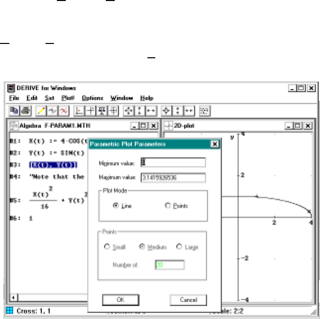
168 CHAPTER 10. POLAR AND PARAMETRIC GRAPHS
Of course, this makes the plotting problem harder since we probably wouldn’t
use the geometry of polar coordinates to plot points. The computer on the
other hand doesn’t use geometric consideration since it just plots lots of
points and connects them with line segments.
Let us consider the non-polar example
x(t)=4cost, y(t)=sint, where 0 ≤t≤π.
We can plot npoints in order by taking ti=ti−1+∆twhere ∆t=(β−α)/n
and making a n×2–matrix using the vector function. Enter [4*cos t,sin
t] andthenuseC
alculus/Vector with Start: 0, End: πand Step: .2 (this
gives 16 points). Now we can plot this as usual in rectangular coordinates
(you will need to switch back to rectangular coordinates). To draw a curve,
select Options/Points again and set plotting mode to connected. Then, replot
the points. See Figure 10.4 and Load the file F-PARAM1.MTH for a
demonstration.
Figure 10.4: Parametric plot of a semi-ellipse
As with polar curves Derive has a simplified way to plot parametric
curves. You simply plot the vector [4*cos t,sin t].Derive will ask for

10.5. PARAMETRIC CURVES 169
the parameter interval and then plot the curve. You might have thought that
Derive would plot the two functions 4 cos tand sin tsince we know that this
happens for 3 or more functions in a vector. But when a vector contains only
two functions, it is treated as a parametric curve.
Looking at the picture you might have guessed that the curve in Fig-
ure 10.4 was an ellipse (even if you didn’t read the caption) because of it’s
oval shape. Of course, not all oval shaped curves are ellipses but indeed this
example is one since one easily checks that
x(t)2
42+y(t)2
12=sin
2t+cos
2t= 1 for all t
and hence the particle travels along the ellipse x2/4+y
2= 1 centered at
the origin with semi-major axis 4 and semi-minor axis 1. Observe that this
information does not tell you how the particle travels around on this ellipse.
For instance, is it going clockwise or counterclockwise? Does it ever stop?
See Figure 10.4 again and try the slow down technique to understand
how the parametric curve can be thought of as a particle moving along a
curve (like a car traveling over a roadway). By using this technique it is
apparent that the motion is counterclockwise (as time tincreases) and it
never stops. This interpretation will be extremely important in later courses
when Newton famous F=ma law is used to analyze the forces acting on a
moving particle.
Tracing parametric curves. Let us recall the tracing technique from
Section 10.2, which we used for polar curves. We now want to “drive” around
a parametric curve and observe its speed. After plotting the parametric curve
above press F3. The cross will turn into a box on the curve and pressing and
holding down the right arrow key will move the little car drive around the
curve. You can see the time parameter as it increases, as well as the xand
ycoordinates, on the lower part of the screen.
By watching the particle move while you press and hold down the right
arrow key, you can see that the particle is traveling in the counterclockwise
direction and a careful inspection will reveal that the speed (rate of change of
distance with respect to time) is slower on the sides than the top and bottom
parts of the curve. This is actually a consequence of one of Kepler’s laws of
planetary motion. This law states that certain moving bodies revolving about
a central point (such as the origin in this example) sweep out equal area in

170 CHAPTER 10. POLAR AND PARAMETRIC GRAPHS
equal time. Assuming this fact, then the particle needs to be faster near the
top and bottom since these points are closer to the origin and hence sweep
out less area. Whereas the left and right portions of the curve are further
from the origin and hence require less time to sweep out an equal amount of
area.
One can calculate the speed directly as follows: Over a small time interval
∆tthe x-position changes by ∆x(= x(t+∆t)−x(t)) and the y-position
changes by ∆y. Thus, the distance traveled during that time interval is
approximately p∆x2+∆y
2and hence the average speed is given by
p∆x2+∆y
2
∆t=s∆x
∆t2
+∆x
∆t2
≈px
0(t)
2+y
0(t)
2
Taking limits as ∆t→0 leads to the formula:
Speed at time t=px0(t)2+y0(t)2.(2)
Derive has an alternate approach for curves described by [x(t),y(t)];
namely, one uses Calculus/Differentiate on the vector and then applies ABS
to the result. This works because ABS([a,b]) simplifies to √a2+b2.
Another use of Derive’s tracing feature is for curves that retrace them-
selves and hence make motion on the curve difficult to see. Try the example,
x=sintcos tand y=sin2tfor 0 ≤t≤2π. That is, plot the vector [sin
t cos t, sin(2t)]. Surprisingly, the picture is simply a line segment with
endpoints (−1/2,−1) and (1/2,1). But how does the particle travel around
this curve? By pressing F3 and tracing the curve we see a back and forth
motion which reminds us of a swinging pendulum. In fact, by carefully ob-
serving the motion near the endpoints we see the particle slow down and
stop. Then, it turns around and goes back in the opposite direction gaining
speed as it approaches the center of the line segment and then slowing down
as it approaches the other endpoint. A point where the speed is zero is ac-
tually the only way a smoothly parametrized curve, i.e., one for which x(t)
and y(t) are continuously differentiable, can have cusps (like the cardioid) or
corners (as in this example) or otherwise exhibit nonsmooth behavior. Check
directly the speed at the endpoints.
As a last example, enter x=2cos
2tand y=2sintcos tfor 0 ≤t≤π.In
this case we have another surprising picture of a circle, which we can verify
by showing
(x(t)−1)2+y(t)2= 1 for all t.
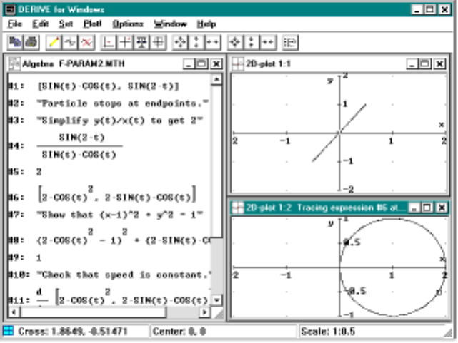
10.5. PARAMETRIC CURVES 171
Figure 10.5: More parametric plots
Two interesting features are that the complete circle is plotted with tin the
[0,π] (instead of requiring 0 ≤t≤2π) and also that a particle travels around
the curve with uniform speed. Observe this with the tracing technique and
then verify it directly using (2).

172 CHAPTER 10. POLAR AND PARAMETRIC GRAPHS
10.6 Laboratory Exercises
1. Consider the polar curve r=2cosθ.
a. Plot the curve using polar coordinates.
b. Describe how the curve is traced for 0 ≤θ≤2π.
c. Use equations (1) on page 164 to convert the polar equation to
rectangular coordinates. Use this to show that the curve is a circle
of radius 1 with center at (1,0).
2. Let r=2sinθbe a polar curve.
a. Plot the curve using polar coordinates.
b. Show that the graph is a rotation of the graph in Problem 1.
3. Let r=sec(θ−π/4) be a polar curve.
a. Plot the curve using polar coordinates.
b. Show that in rectangular coordinates the curve satisfies the equa-
tion: x+y=√2. (Hint: Use the Trigonometry Expand mode to
simplify the equation.)
4. Plot several petal curves, r=2cos(nθ) for different integer choices of n.
How many petals are there as a function of n?
5. Choose positive number dand e, then the family of polar curves
r=ed
1+ecos θ
turns out to be conic sections (see your calculus text as a reference).
We will examine this phenomenon with d=2andeset to 4 different
positive values: e=.5, e=.75, e=1ande=2.
a. Plot the first two curves (e=.5ande=.75) with −π<θ<π
and identify the conics.
b. Plot the curve with e=1with−3.10 <θ<3.10. Can you
identify this conic?
10.6. LABORATORY EXERCISES 173
c. Plot the curve with e=2with−2.09 <θ<2.09. Can you
identify this conic?
d. In the last plot, what is the significance of the number θ=2.09?
What curves do you get when −π<θ<−2.10 or 2.10 <θ<π?
(Warning: If you try plotting with the default range [−π, π] it will
eventually graph the complete conic but it takes a very long time!
Press Esc if you can’t wait.)
6. Let x=(cost)
3and y=(sint)
3for −π≤t≤π.
a. Plot the parametric curve.
b. Use Derive’s tracing method described on page 169 to find where
the speed is 0 on the graph.
c. Switch to the algebra window and verify your empirical observa-
tions by using (2) on page 170 to determine exactly where the
speed is zero.
7. Let x=tsin tand y=tcos tfor −3π/2≤t≤3π/2
a. Plot the parametric curve.
b. Use tracing to determine how a particle (ant) traverses the curve
over the given tinterval. Sketch arrows on the graph to indicate
the motion.
c. What will happen if tis allowed to exceed 3π/2? Does it go around
the curve again?
*8. Start by authoring
r(θ, a):=a(e
sin θ−2cos(4θ))
where we think of this function as a polar curve in θwith a para-
menter a.UseDerive’s vector function to make a vector of the func-
tion r(θ, a) where the parameter agoes from 1 to 2 in increments of
size 0.25. (So after you simplify it, the vector will contain 5 functions.)
Plot this vector of 5 functions using polar coordinates. Does it look
like a butterfly? (This curve is similar to one described by T. H. Fay,

174 CHAPTER 10. POLAR AND PARAMETRIC GRAPHS
The butterfly curve, Amer. Math. Monthly, vol. 96, May 1989, p. 442.)
It can be viewed on the Web as Figure 3 on our home page
http://www.math.hawaii.edu/lab/
9. Let x=t−sin tand y=1−cos tfor t≥0.
a. Plot the parametric curve.
b. Use tracing to verify that the motion stops briefly each time it
touches the x–axis.
c. Verify your observations in part bby using the formula for speed
given in (2) on page 170.
10. Imagine a circle (or wheel) of radius one rolling along the x–axis at
unit speed. Now try to picture the path followed by a fixed point on
this circle as its rolls. This is the parametric curve in problem 9,itis
called a cycloid curve. It may seem a little surprising that the speed of
the point on the wheel is 0 once every time the wheel revolves even as
the center of the wheel travels at a constant speed.
a. Make a graph of the speed function (2) and determine how fast
the point on the wheel going when it is at its highest point? (Hint:
Plot the speed function and cycloid curve together on the same
graph.)
b. Load the file F-CYCL.MTH and plot expression #8 which contains
the parametric curves for 5 positions of the rolling wheel along
with a dot marking the particle’s position on the wheel. Then
plot the cycloid expression #3, see Figure 10.6 on the facing page.
11. Plot the parametric curve x=sin(πsin t)andx=cos(πsin t) for
−π≤t≤π.
a. What geometric object does this look like? Prove that your answer
is correct.
b. Using the trace feature to see how a particle following these para-
metric equations moves along this geometric object. Describe this
motion in words.
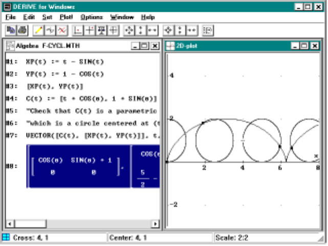
10.6. LABORATORY EXERCISES 175
Figure 10.6: The cycloid curve and the rolling wheel
c. Are there places where the point seems to have speed 0? Find a
formula for the speed of the particle at time t. Atwhattimesdoes
the particle have speed 0 and what is the position of the particle
at these times?
12. Two particles move in the plane. The motion of the first is described
by the parametric equations
x(t)=16/3−8t/3,y(t)=4t−5,t≥0
and the second one by
x(t)=2sin(πt/2),y(t)=−3cos(πt/2),t≥0
Plot both of these curves. Find where the curves intersect. But just
because the curves cross does not mean the particles collide; they might
arrive at the intersection point at different times. Where do the parti-
cles collide?
176 CHAPTER 10. POLAR AND PARAMETRIC GRAPHS
Chapter 11
Exponential Growth and
Differential Equations
11.1 Introduction
Suppose that yis a function of x. A first order differential equation is an
equation which involves x,yand its derivative y0.Ann
th order differential
equation involves x, y, y0,... ,y
(n). For example, y00 +xy0=x2+ 1 is a second
order differential equation.
Differential equations occur frequently in every field of science and engi-
neering, especially biology. Libraries have many volumes devoted to solving
differential equations (even for first order differential equations). In this
chapter we study first order differential equations and show some of the ap-
plications. One of the most important examples is population growth (of
humans, cells, radioactive substances, savings account balances, etc.)
We will show you how to get an exact solution to certain types of first
order differential equations and we will introduce slope fields and Euler’s
method for obtaining approximate solutions to more general first order dif-
ferential equations.
11.2 Examples
Population Growth. The standard model for population growth states
that the rate of change y0(x), of the population size y(x), with respect to
time xis proportional to the population size at any given time. This means
177

178 CHAPTER 11. DIFFERENTIAL EQUATIONS
that y0(x)=ky(x) for some fixed constant kand all x. Now it is easy to
check that y(x)=y
0
e
kx satisfies the relations
dy
dx =y0=ky y(0) = y0
(1)
where we simplify our notation by dropping the explicit reference to the
variable x. Thus, the exponential function provides a model for population
growth. Recall from Problem 7 on page 66 that we compared a linear model
versus the exponential model above for the population of the US and found
a significant difference in the long run behavior with the exponential model
giving a much larger growth. This comparison was also made in Section 1.3
where it was shown that exponential growth eventually exceeds the growth
of any polynomial.
We now want to show that the above solution is the only solution to (1).
Suppose that y=u(x) is a solution then
Zx1
0
u0(x)
u(x)dx =Zx1
0
kdx=kx1.
On the other hand, using the substitution y=u(x) in the integral above
yields that
Zx1
0
u0(x)
u(x)dx =Zu(x1)
y0
dy
y=ln
u(x
1
)
y
0
.
Now, if we set the right hand sides of the two equations above equal to each
other we get
u(x1)
y0
=kx1.
Finally, we observe that since u(x1)>0andy
0>0 we can remove the abso-
lute values in the above equation. Exponentiate both sides of the resulting
equation (remembering that eln a=afor a>0) we get
u(x1)
y0
=ekx1
which is equivalent to our solution above.
Less formally, this approach is quite simple. We rewrite
dy
dx =ky as dy
y=k

11.2. EXAMPLES 179
and then integrate both sides to get
ln y=Zdy
y=Zkdx=kx +c
and exponentiating yields
y=ekx+c=ekxec=c1ekx .
By using the initial conditions x=0,y=y
0we see that the arbitrary
constant c1must be y0.
This method of solving differential equations is called separation of vari-
ables and the key feature is that the equation can be rewritten with all
occurrences of yon the left side of the equation and all occurrences of xon
the right side. Thus, to solve y0=f(y)g(x) you compute the integrals
Zdy
f(y)=Zg(x)dx +c
explicitly and then solve for the constant cusing the initial conditions.
Example To solve the equation
dy
dx =xy2−4xwhere y(1) = 4
we first separate the variables and integrate:
Zdy
y2−4=Zxdx.
Now, we use Derive to solve the integrals but add in a constant of integra-
tion c. This yields
1
4ln y+2
y−2=x
2
2+c
Now using Derive, substitute in the values x=1,y= 4 and simplify. Next,
have Derive solve for the value of cto get
c=ln 3
4−1.
Finally, we substitute this value in the above equation and then have Derive
solve for yto get the answer to the differential equation.

180 CHAPTER 11. DIFFERENTIAL EQUATIONS
You should always check your answer to make sure it satisfies the differ-
ential equation and the initial conditions. In Derive you could differentiate
the answer and set that equal to xy2−4xwhereyouuseyouranswerin
place of y.NowS
implify, you should get the value true which indicates that
Derive was able to verify that the equation is an identity. You might also
try this problem with pencil and paper!They-integral part involves some
work since this is a partial fractions integration problem.
Be Careful With Logarithms Since Derive gives the answer ln y, for
the integral Rdy/y, instead of ln |y|this can cause some problems. From our
definition of the logarithm it doesn’t make sense to take the log of a negative
number. But Derive uses a more advanced definition which uses complex
numbers and might cause some confusion for you. For example, Derive uses
the formula ln(−1) = πi when it simplifies expressions. You have two choices:
use Derive to solve the equations (potentially using complex numbers) or
else change the answer to the integrals involving logarithms by inserting
absolute values.
In the previous example if we change the initial conditions to y(1) = 1
then we should change the equation resulting from the integrals above to the
following:
1
4ln y+2
2−y=x
2
2+c.
Now proceeding as before will give the solution. We’ll give several other
examples of how to do this in the following sections.
Newton’s Law of Cooling. Another important example of differential
equations is Newton’s Law of Cooling. According to this law a hot pan of tem-
perature yhot will have a temperature of y(t)attimetwhich decreases, i.e.,
will cool down, when placed in a vat of cool water of temperature ycool <y
hot.
The key point of the law is that the rate of change in the temperature, y0,is
proportional to y(t)−ycool, which is the difference in the current temperature
of the (hot) pan and the (cool) water. This says that
dy
dt =−k(y−ycool)wherey(0) = yhot >y
cool
(2)
and k>0 is a constant which depends on the physical properties of the
pan, for example, copper cools faster than iron so the corresponding k-value
11.2. EXAMPLES 181
would be larger. Notice that the derivative dy/dt above is negative since the
temperature is decreasing.
We solve (2) by separating variables and integrating:
Zdy
y−ycool
=−kZdt +c.
S
implifying this equation in Derive, we then solve for the unknown constant
cby substituting in the initial conditions x=0andy=y
hot.Notethatwe
assume the quantity y−ycool to be positive; hence, we can take its logarithm.
We now Substitute this value for cback into the relation above and solve for
y. This gives the solution
y(t)=(y
hot −ycool)e−kt +ycool.(3)
To do this computation in Derive we need to use multi-letter variables.
Typically, one uses the variables yh and yc in place of yhot and ycool.Sothat
these are treated as variables (and not as y·h)wefirstA
uthor the vector
[yh:=,yc:=] which simultaneously declares them both as variables.
Notice that the term involving the exponential e−kt tends to zero very
rapidly. Hence, y(t) tends to the water temperature ycool very rapidly.
Radioactive Decay. In certain radioactive materials some particles change
from one form to another. The number of particles decaying in this way in
a small time period is proportional to the size of the material. So that, for
example, if you have twice as much radioactive material the number of parti-
cles decaying is twice as great. If A(t) is the amount of radioactive material
at time t,thenAsatisfies the differential equation A0(t)=−kA.Herewe
have k>0 and have written it in this way to emphasize that the derivative
is negative since the amount of material decreases with time. Except for this
minus sign this is the same as the population model above. It is easy to see
the solution is
A(t)=A
0
e
−kt
(4)
The half-life of a radioactive substance is the time it takes for half of it to
decay. We can find this by solving A(t)=A
0
/2 for t. By (4) this gives the
equation A0/2=A
0
e
−kt. Cancelling the A0,wegettheequation1/2=e
−kt,
so that −kt =ln(1/2)=−ln 2 or t=ln2/k. Notice that the half-life is
independent of A0.

182 CHAPTER 11. DIFFERENTIAL EQUATIONS
11.3 Approximation of Solutions
The general first order differential equation has the form y0=f(x, y)with
initial conditions (x0,y
0), i.e., y=y0when x=x0. The separation of
variables technique for solving differential equations that we discussed in the
previous sections do not extend to all differential equations. In fact, many
important differential equations cannot be solved explicitly by any technique
what so ever. We encountered this situation earlier with integrals1and this
suggests trying to find numerical approximations to the solution. The critical
observation to make is that the equation y0=f(x, y) tells us the slope of
the tangent line to the solution y(x). Thus, by drawing many small line
segments of slope f(x, y), through the point (x, y) in the plane, we obtain an
approximate picture of the solution whose graph contains the point (x, y). By
drawing several of these partial tangent lines we get an approximate picture
of y(x) by drawing a curve which conforms to these slopes. These diagrams
are called slope or direction fields.
The file ADD-UTIL adds the function DF (for direction field) which will
make a matrix. When this matrix is plotted it draws the ‘slope field.’ The
form of DF is
DF(r,x,x0,xm,m,y,y0,yn,n)
where the first argument ris f(x, y)andx0, xm, m represent the initial
and final x-values in a rectangular grid with mx-values plotted. Similarly,
y0, yn, n represent the initial and final y-values in a rectangular grid with
ny-values. Hence, the total number of line segments plotted will be m·
n. In order that line segments are plotted, not just the endpoints, we put
the plotting window into connected mode by choosing Options/Points and
setting Connect to ‘Yes.’
As an example, we can take the cooling problem above, namely,
y0+y=1
so that f(x, y)=−(y−1) = 1 −y. We simplify the expression
df(1-y,x,0,4,8,y,0,4,8)
1Notice that the simple differential equation y0=f(x) has solution y=Rf(x)dx so
that the class of differential equations contains all integration problems.
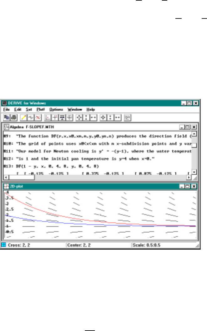
11.3. APPROXIMATION OF SOLUTIONS 183
to get the slope field. In the plot window select Option/Plot Color and set
it to ‘Off’ so that all slope lines will be in one color. Of course, if you like
colorful diagrams then you can skip that last step. Also choose Option/Points
to set the Connected Mode and to set Size to Small. Make sure to delete
all existing graphs and then plot the slope field. Try to picture the solution
though a given initial point (0,y
0
) by following the slope field. Finally, plot
some actual solutions that we obtained above using the DE function and see
how it conforms to the slope field. See Figure 11.1 where we have graphed
the solution y=3e
−x
+1, which corresponds to the initial condition y(0)=4.
Try several other initial conditions to see how the slope lines approximate
the solution.
Figure 11.1: Slope field for the Newton cooling problem
Another Population Model.∗In the model we used for population growth
we had
dP
dt =kP.

184 CHAPTER 11. DIFFERENTIAL EQUATIONS
This works well for many populations. But the population cannot continue
to grow forever. When a country no longer has room for expansion the rate of
growth slows. For example, a bacteria culture in a petri dish will satisfy the
above differential equation for awhile, but as the dish fills the above equation
becomes invalid. Verhulst, a Belgian mathematician, proposed a model using
the differential equation
dP
dt =kP 1−P
P1.(5)
Notice that when Pis small compared to P1, the derivative is approximately
kP, as before. But as Papproaches P1,P0approaches 0.
We study this equation by looking at the direction field. Let’s take a
numerical example
dP
dt =P1−P
5where P(0)=1,
so that the population starts out at a value of 1 and has a maximum value
of 5. We’ll guess as to how long of a time interval to look at, say 0 ≤t≤12.
Thus, we enter
df(p(1-p/5),t,0,12,12,p,0,6,6)
and Approximate to get a large direction field matrix. See Figure 11.2 on
the facing page for a picture of the direction field.
Looking at the picture of the direction field you should be able to see the
solution approximately by starting at the point (0,1) and “following along”
in the direction of the tangent lines. The picture makes it appears that it
takes only about 6-7 time units before the population reaches its maximum
value of 5.
To solve (5) exactly we separate variables and integrate
ZdP
P(1 −P
P1)=Zkdt+c.
In Derive we would first declare the variables P0and P1by entering [p0:=,
p1:=] and then entering each of the integrals. Then, we Author the above
equation. Notice that we added the integration constant c. After simplifying
we get
ln P−ln(P−P1)=c+kt
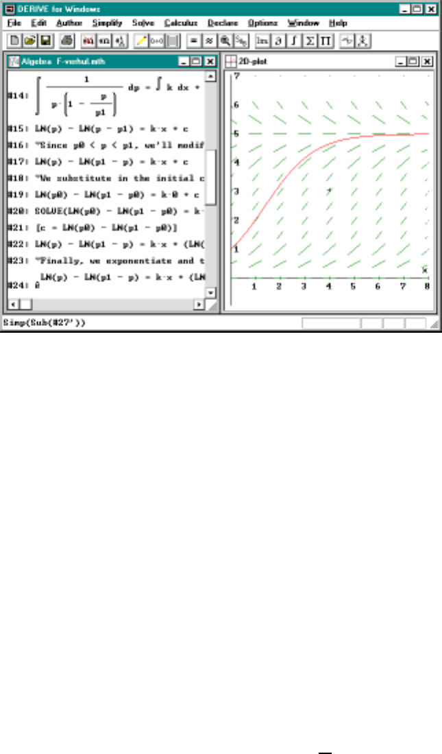
11.3. APPROXIMATION OF SOLUTIONS 185
Figure 11.2: A graph of a Verhulst population curve
We solve for cby substituting in the initial conditions t=0,P=P
0
.After
solving for cand substituting the value into our relation from above we now
try to get the solution by solving for P.
The equation we are trying to solve is
ln P−ln(P−P1)=(ln(P
0
)−ln(P0−P1))+kt .
But, there are two problems with the above equation. We assume that
0<P
0<P <P
1when t>0 and so two of the logarithm have negative
arguments. As a result we modify the above to the equation
ln P−ln(P1−P)=(ln(P
0
)−ln(P1−P0))+kt .
and then try to solve for P.
Curiously, this equation is too hard for Derive to solve and it returns no
solutions. After carefully inspecting the equation it seems like a good idea
to exponentiate both sides of the equation and use the fact that eln p=p
whenever p>0. In Derive thiscanbedonebyA
uthoring #e raised to

186 CHAPTER 11. DIFFERENTIAL EQUATIONS
a power where the power is the above equation and then Simplifying. This
yields the equation
P
P1−P=P0ekt
P1−P0
which Derive can solve for P. The result is
P=P0P1ekt
P0ekt +(P
1−P
0
)
(6)
Notice that P(0) = P0, as we would expect, and that limt→∞ P(t)=P
1
.
11.4 Euler’s Approximation Method∗
The method of slope fields suggest an approximation technique known as
Euler’s method. The idea is to approximate the solution to
y0=f(x, y)wherey(x
0
)=y
0
by a piecewise linear function passing through a sequence of points
(x0,y
0),(x
1,y
1
),... ,(x
n,y
n)
obtained by using the slope at (xi−1,y
i−1
), which is f(xi−1,y
i−1), to construct
the next point (xi,y
i), where the increment in xis a fixed amount, say
xi=xi−1+h.TheDerive function is deceptively simple:
EULER(r,x,y,x0,y0,xn,n):=
ITERATES(v+[1,LIM(r,[x,y],v)]*(xn-x0)/n,v,[x0,y0],n)
where xvaries between x0≤x≤xnand we use npoints in the approximation
scheme. This function is also in the file ADD-UTIL. It is a slight variant of
the EULER function in the utility file ODE APPR that comes with Derive.
Try the Newton cooling problem
EULER(1-y,x,y,0,4,4,16)
to see how this works. Again, you must be sure that your graphics window is
in single color, connected mode for this to plot properly. See the Figure 11.3
on the next page for a demonstration of this technique. You should try
larger and larger nto see that the approximations converge, as n→∞,to
the solution for 0 ≤x≤4.
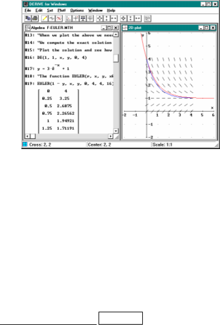
11.5. LINEAR FIRST ORDER DIFFERENTIAL EQUATIONS 187
Figure 11.3: Euler’s method for approximating solutions
11.5 Linear First Order Differential Equations
Returning to the population growth equation (1) we now describe another
method for proving that the exponential solution to equation is the only
solution to that equation. To do this we suppose that u(x) is any solution to
y0=ky that satisfies u(0) = y0. We want to show that u(x)/ekx =e−kxu(x)
is a constant, so we compute it’s derivative and observe that
(e−kxu)0=e−kxu0−ke−kxu=e−kx(u0−ku)=0(7)
holds for all x. Hence integrating gives
e−kxu(x)=c.
We solve for the constant cby substituting x= 0 in the above to get c=
u(0) = y0and then multiply both sides by ekx to obtain2
u(x)=y
0
e
kx
2In Derive you can multiply both sides of an equation by an expression by right clicking
the equation, inserting with parentheses into the author box and then multiplying.

188 CHAPTER 11. DIFFERENTIAL EQUATIONS
as we claimed.
Equation (1) is a special case of the general equation
y0+p(x)y=q(x),y(x
0
)=y
0
(8)
since (1) can be written as y0−ky = 0. Thus, in (8) the functions p(x)=−k,
q(x) = 0 and initial time x0= 0. Any differential equation with the form
of (8) is called a linear first order differential equation. We will prove that
any such equation has a unique solution which is obtained in manner a similar
to the above. See Theorem 1 below for the formula for the solution.
The formula for the solution to (8) can be made into a Derive function
quite easily. This has been done in Derive’s utility file ODE1 with the
name LINEAR1. For convenience we have added this function to our utility
file ADD-HEAD but we use the shorter name DE. It has the form
DE(p, q, x, y, x0, y0)
where pand qare expressions in the variable x. The initial conditions are
y=y0whenx=x0.
Example To solve the differential equation
y0=2ywhere y(0) = 5
simplify DE(-2,0,x,y,0,5). Note that the above equation can be rewritten
as y0−2y=0sop(x)=−2andq(x) = 0. This will yield the expression
y=5e
2xas the solution.
Example To solve the Newton Cooling equation
y0=−k(y−ycool)wherey(0) = yhot
we rewrite the equation so that it has the form of the general first order linear
differential equation in (8):
y0+ky =kycool y(0) = yhot
(9)
and thus we can solve this equation with Derive by using the DE function.
We will use the variables yh and yc in place of yhot and ycool. So that these
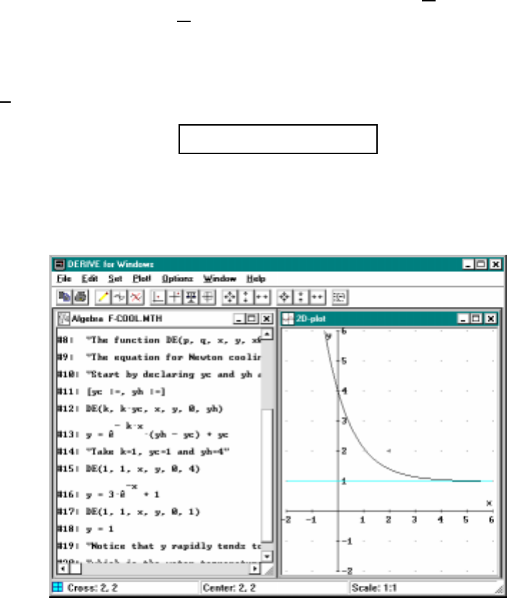
11.5. LINEAR FIRST ORDER DIFFERENTIAL EQUATIONS 189
are treated as single variables (and not as y·h)wefirstA
uthor the vector
[yh:=,yc:=].ThenweA
uthor
de(k,k*yc,t,y,0,yh)
Simplifying the expression gives the solution
y(t)=(yh −yc)e−kt +yc.(10)
See Figure 11.4 for a demonstration of these functions and observe how
rapidly the temperature y(t) tends to the water temperature yc.UseDerive
to calculate limt→∞ y(t).
Figure 11.4: Solving Newton’s cooling equation
By looking back at (7) on page 187 and making a small modification of
that argument we see how the above solution is derived; namely, by (9),
(ekxy)0=ekxy0+kekxy=ekx(y0+ky)=y
coolkekx
(11)

190 CHAPTER 11. DIFFERENTIAL EQUATIONS
and hence integrating gives
ekxy(x)=Zy
coolkekx dx =ycoolekx +c.
Now solving for cby substituting x=0intheaboveyieldsc=y
hot −ycool
and then multiplying both sides by e−kx gives the desired result above.
The argument above gives us a pretty good idea how to solve the general
differential equation y0+p(x)y=q(x). One multiplies yby an appropriate
exponential µ, differentiates and then replaces the quantity y0+p(x)yby
q(x). Integrating the result essentially solves the problem. That critical
multiplying exponential turns out to be
µ(x)=e
Rp(x)dx since µ0(x)=p(x)µ(x).
See the proof of Theorem 1 below for the details.
We now solve the general linear first order differential equation (8)
by proving the following theorem:
Theorem 1. Suppose that y(x)satisfies (8) where p(x)and q(x)are con-
tinuous functions of x.Ifysatisfies the initial condition y(x0)=y
0then
y=e−Rx
x0p(u)du ·Zx
x0
q(u)eRu
x0p(v)dv du +y0.(12)
Proof. Let h(x)=e
R
x
x
0
p(u)du. By the fundamental theorem of calculus,
d
dx Rx
x0p(u)du =p(x). So h0(x)= d
dx heRx
x0p(u)dui=p(x)h(x). Thus
(h(x)y)0=h(x)y0+h0(x)y=h(x)y0+p(x)h(x)y
If we multiply equation (8) by h(x) and use the above, we see that (h(x)y)0=
h(x)q(x). If we integrate both sides of this from x0to xand use the fact that
h(x0) = 0, we get h(x)y=Rx
x0h(u)q(u)du +C,or
y=e
−Rx
x
0p(u)du ·Zx
x0
q(u)eRu
x0p(v)dv du +C.
Since y(x0)=y
0
,weseethatC=y
0and thus (12) holds.

11.6. LABORATORY EXERCISES 191
As we said, the solution (12) to the differential equation can be made into
aDerive function quite easily. You should look at the formula above and
see if you can write a Derive function that will produce the solution. Then
compare your answer with the following definition of the function DE.3
(13) de(p,q,x,y,x0,y0):= y =
^e^(-int(p,x,x0,x)) * (int(q*^e^int(p,x,x0,x),x,x0,x)+y0)
11.6 Laboratory Exercises
The functions discussed in this chapter, DE,DF,andEULER,arealldefined
once you Load in the file ADD-HEAD.
1. If money earns interest compounded continuously and y(t) is the amount
of money at time t,thenysatisfies the differential equation y0=ry,
where ris the interest rate.
a. What is the solution to the differential equation y0=ry?
b. Find how long it takes for your money to double for r=3%,5%,
and 10%? (This means that r=0.03, 0.05, and 0.1intheabove
equation.)
2. Normal body temperature is 98.6◦F. If someone dies, then the body
cools according to Newton’s law of cooling. It is known that, if the
surrounding temperature is a constant 64◦, then the body will cool to
92◦in 3 hours.
3You might notice that the formula for the solution to the differential equation in
Theorem 1 is careful about the “dummy variables” in the integrals. This is because in
calculus we avoid integrals of the form Rx
af(x)dx because the integration variable xmight
be mistaken for the upper limit x. Since the integration variable is completely arbitrary
we usually take it to be tor uin such a situation. On the other hand, for the Derive
function de above we used expressions like int(f(x),x,0,x) because the integration is
done before the limits of integration are substituted. The computer does this correctly
but it is usually foolhardy for students to try this since it is so easy to make mistakes such
as Zx
0
xdx =xZx
0
dx =x2
when then answer should be x2/2.
192 CHAPTER 11. DIFFERENTIAL EQUATIONS
a. Use this information to compute the constant kin (10) on page 189.
b. Now suppose that a murder victim’s body is found at 12am with
a temperature of 86◦. Assuming an air temperature of 64◦, deter-
mine when the murder was committed?
3. Consider the differential equation
y0=0.1x(y
2−4) with y(1)=1.
a. Use the DF function to draw a 16 ×16 grid of slope lines using
0≤x≤8and−4≤y≤4. (You need to have the graphics
window in the connected state; see the instructions for this on
page 182.)
b. Print out the slope field graph and with your pencil draw an ap-
proximate solution to the differential equation starting at the ini-
tial condition (1,1).
c. Use the separation of variables method to find the solution to the
differential equation and plot the answer to see how it conforms
to the slope lines.
d. Verify that the solution never attains the value y=−2. Can
you explain this fact by looking at the equation itself and not the
solution?
4. Consider the differential equation
y0=sinx−ywith y(−1) = −1.
a. Use the DF function to draw a 10 ×10 grid of slope lines using
−1≤x≤3and−1≤y≤1. (You need to have the graphics
window in the connected state; see the instructions for this on
page 182.)
b. Rewrite the differential equation to have the form (8) on page 188.
Use the DE function to find the solution to the differential equation
and plot the answer to see how it conforms to the slope lines.
c. Double check that the answer you get from the DE function is in-
deed the solution by verifying that it solves the differential equa-
tion and the initial conditions.

11.6. LABORATORY EXERCISES 193
5. Suppose a body of mass mis dropped from high in the atmosphere.
Let vbe its downward velocity as a function of time t.Thereare
two forces acting on the body: gravity and wind resistance. The force
due to gravity is mg,where gis a constant; the force due to wind
resistance is −kv (the minus since it is upward). Newton’s law says
F=ma,wherea=v
0is the body’s acceleration. This leads to the
differential equation
ma =mv0=mg −kv.
Solve this equation for vwith v(0) = 0. Find limt→∞ v(t) (don’t in-
clude the v= part from above). Derive returns an expression contain-
ing SIGN(km) because it does not know that kand mare positive. Use
Declare/Variable Domain to declare that kis a positive real number,
and do the same for m. Now reevaluate the limit. Note that vnever
exceeds this value, which is called the terminal velocity.Nowindre-
sistance corresponds to k=0. Findvin this case both by solving the
differential equation with k= 0, and by taking the limit of the general
solution for vfound above as k→0.
*6. Suppose the population growth of a small country satisfies (5) with
P1=10andk=0.05 (with population in millions). Plot the direction
field for this. (There are instructions for doing this in Section 11.3.)
Suppose P(0)=2. FindP(20), P(50), and P(100). Graph P(t).
Adjust the scale of the graph so that you get a clear picture of the
nature of the population growth.
7. Carbon-14, 14C, is an unstable isotope of carbon that slowly decays
to the more stable 12C. While an organism is alive it has a constant
amount of 14C, but after it dies, the amount decreases according to (4).
If 200 years after the organism dies, the amount of 14Cis97.6% of the
original amount, what is the half-life of 14C? If the burnt wood from a
prehistoric campsite contains 29% of the original amount of 14C, how
old is the campsite?
194 CHAPTER 11. DIFFERENTIAL EQUATIONS

Chapter 12
Harmonic Motion and
Differential Equations
12.1 Introduction
In this chapter we consider second order differential equations of the form
y00 =f(t, y, y0)wherey(t
0
)=y
0and y0(t0)=y
0
0.
It is easy to see that two initial conditions are needed because in the simply
case y00 =f(t) one would simple integrate f(t) twice and that there would
be two constants of integration. Our applications involve moving physical
systems such as oscillating springs and swinging pendulums. These systems
can be analyzed using Newton’s Law of Motion: F=ma.Sincetheain this
formula is acceleration which is the second derivative with respect to time
we see that Newton’s formula is actually a second order differential equation.
Free Fall The equation for the vertical height yof a free falling particle,
in the time variable t,isgivenby
y
00 =−gwhere y(0) = y0and y0(0) = v0
where gis the force due to gravity (which we assume is constant). The initial
conditions in this case are the initial height y0and the initial velocity v0.By
integrating twice and solving for the initial conditions we get the solution
y=y0+v0t−1
2gt2. Here are the steps:
195

196 CHAPTER 12. HARMONIC MOTION
y0=Z−gdt=−gt +c1=−gt +v0
y=Z−gt +v0dt =−1
2gt2+v0t+c2=−1
2gt2+v0t+y0
Notice that the constants are obtained by substituting t=0,y=y
0and
y0=v0.
In this chapter we will mainly be interested in second order linear differ-
ential equations of the form
y00 +by0+cy =0(1)
These equations are linear differential equations because of they only involve
y00,y0and yin a linear relation. It turns out that to solve these equations
we need to use the complex exponential function eαx which was discussed
earlier in Problem 6 on page 127 in Chapter 7. Here α=a+bi is in general
a complex number (see Section 5.4 on page 78 for a brief tutorial on complex
numbers).
12.2 Examples
Springs and Hooke’s Law. Suppose we have a mass mattached to the
end of a spring hanging from the ceiling. If we pull the mass down a little it
will bounce (oscillate) up and down. We image it moving along the y–axis
with y= 0 denoting the rest position. Newton’s law says F=ma where F
is the force on the mass and a=y00 is the acceleration. A reasonably good
approximation of the force is given by Hooke’s Law which states
F=Fspring =−ky
where kis a positive constant. Since Fspring =F=ma =my00 this gives y00 =
−k
my. After transposing the yterm we get the following linear differential
equation:
y00 +k
my=0(2)
As an example suppose we pull the particle down dunits and let go.
Then, the initial condition would be: y0=−dand v0=0

12.2. EXAMPLES 197
Damped oscillation. Now suppose that we immerse our oscillating spring
into a vat of oil. The oil would cause the oscillations to be damped out and
eventually our system will come to a stop. This is basically the model for
a car’s shock absorbers. When you hit a bump you want the oscillations to
damp out at just the right rate so as to give a conformable ride. Not too
quickly nor too slowly.
The resistance force due to the oil is proportional to the velocity of the
particle so we introduce a new force Foil =−by0where bis a positive constant.
If we take this into account we get F=Fspring +Foil and our differential
equation (2) becomes
y00 +b
my0+k
my=0.(3)
Pendulums. Suppose we have a mass mat the end of a pendulum of
length l. It swings along a circular arc. When the pendulum is at rest it
hangs straight down and has velocity 0. Let s(t) denote the arc length from
this rest position as a function of time. Let θ(t) be the angle the pendulum
makes from the vertical position. Then s=lθ and so the acceleration is
d2s/dt2=ld2θ/dt2. The force on the mass due to gravity is downward and
has magnitude mg,wheregis the gravitational constant. This force can be
broken into the part in the same direction as the pendulum rod and a part
part tangent to the arc traced out by the mass; see Figure 12.1.
s
θ
Figure 12.1: The pendulum
198 CHAPTER 12. HARMONIC MOTION
The component of the force in the direction of the pendulum rod is can-
celled out by the rod. The force along the arc is −gm sin θ.Newton’slaw,
F=ma says md2s/dt2=−gm sin θ.Intermsofθwe get the differential
equation:
d2θ
dt2=−g
lsin θ(4)
This is not a linear equation because of the sin θ. But the Taylor series is
sin θ=θ−θ3/6+···,soifθis small we can approximate sin θwith θ.Using
this (4) becomes
d2θ
dt2+g
lθ=0(5)
If we start by pulling the pendulum back by an angle θ0and letting go
we get the initial conditions:
θ=θ0and dθ
dt =0 when t=0.
12.3 Solving Linear Differential Equations
Our basic technique to solving (1) is to try an exponential solution y=ert
for some choice of r. This is not such a surprising guess when one considers
the simple example y0−ry = 0 from the previous chapter. We know that
the solution would be y0ert in that case. Substituting y=ert into (1) we get
r2ert +brert +cert =(r
2+br +c)ert =0.
Since ert >0 we want to solve the quadratic equation
r2+br +c=0(6)
This equation is called the characteristic equation. Its roots are
r1=−b+√b2−4c
2and r2=−b−√b2−4c
2
(7)
and so both y=er1tand y=er2tare solutions to (1).

12.3. SOLVING LINEAR DIFFERENTIAL EQUATIONS 199
Now, we take advantage of the fact that our differential equation is linear.
We claim that if y1,y2are solutions to (1) then so is any function of the form
y=C1y1+C2y2where C1,C2are arbitrary constants. This is easy to verify:
y00 +by0+cy =(C
1
y
1+C
2
y
2
)
00 +b(C1y1+C2y2)0+c(C1y1+C2y2)
=(C
1
y
00
1+C2y00
2)+b(C
1
y
0
1+C
2
y
0
2
)+c(C
1
y
1+C
2
y
2
)
=C
1
(y
00
1+by0
1+cy1)+C
2
(y
00
2+by0
2+cy2)=C
1
0+C
2
0=0.
Finally, we take y1=er1t,y2=er2tabove and then use the two arbitrary
constants C1,C2to solve for the two initial conditions:
y(t0)=y
0and y0(t0)=y
0
0.
Example Consider the equation,
y00 −y0−2y=0 where y(0)=3,y
0
(0)=0.(8)
The characteristic equation is
r2−r−2=(r+1)(r−2) = 0 so r=−1,2.
Our general solution is therefore y=C1e−t+C2e2tand we need to solve for
the initial conditions. This leads to the pair of equations:
C1+C2=y(0) = 1
−C1+2C
2=y
0(0) = 0
which has solutions: C1=2andC
2= 1. Just to be sure, double check that
the function
y=2e
−t+e
2t
satisfies the differential equation in (8) and the initial conditions.
To simplify the process above for the general second order equation (1) we
use the utility function (we assume that you have loaded the file ADD-HEAD
as usual):
DE2(b, c, t, t0, y0, v0) .
Thus, for our example we would Simplify DE2(-1, -2, t, 0, 3, 0).

200 CHAPTER 12. HARMONIC MOTION
Example Now consider the equation,
y00 +y=0 where y(0)=3,y
0
(0) = 0 .(9)
The characteristic equation in this case is
r2+1=(r+i)(r−i)=0 so r=±i.
Thus, we should try y=C1eit +C2e−it. We don’t usually encounter expo-
nentials with complex numbers in the exponent so what does it mean? The
answer is that we use the Euler Formula the has been discussed in an earlier
exercise, see Problem 6 on page 127. Thus,
eit =cost+isin tand e−it =cost−isin t
and in general,
e(α+βi)t=e
αt(cos βt +isin βt).
It’s important to note (again from Problem 6 on page 127) that the differen-
tiation formula d
dte(α+βi)t=(α+βi)e
(α+βi)t
still holds, even for complex exponents, and hence
y0=iC1eit +(−i)C
2
e
−it .
Thus, to solve for C1,C2we need to solve the equations:
C1+C2=y(0) = 3
iC1+(−i)C
2=y
0(0) = 0
Even though these equations have complex coefficients it is pretty easy to
solve. In the second equation, just cancel the iterms. This yields the new
equations:
C1+C2=3
C
1−C
2=0
which has the solution C1=C2=3/2.
At this point it looks like our solution is going to involve complex numbers.
But this runs counter to our intuition since (9) is model for an undamped

12.3. SOLVING LINEAR DIFFERENTIAL EQUATIONS 201
mass-spring system (see (2)) and this couldn’t possibly have complex num-
bers in the solution. Let look at the computation:
y=3
2eit +3
2e−it
=3
2(cos t+isin t)+3
2
(cos t−isin t)
=3cost
and hence the i-term drops out of the solution. Although we were convinced
of this fact from a physical point of view it was far from obvious from an
algebraic point.
To see why this is always the case we make an important observation
about (1). Since we tacitly assume that the coefficients b,care real numbers
observe that if yis a solution to (1) then so are the real part <yand the
imaginary part =yof yalso solutions to this equation. Let’s verify this for
the real part (you may need to refer back to Section 5.4 and Problem 8 on
page 91). Recall that we have already shown that solutions can be combined
by multiplying them by constants and then adding them. Since <y=(y+
¯y)/2 we need only show that given a solution ythat it’s complex conjugate
¯yis also a solution. Let verify this fact:
(¯y)00 +b(¯y)0+c(¯y)=y
00 +by0+c¯y
=y00 +by0+cy =¯
0=0.
This means that instead of using complex exponentials for the two solutions
y1,y2and then solving for complex C1,C2so that C1y1+C2y2satisfies the
initial conditions we could instead solve the initial value equations
y=C1cos t+C2sin twhere y(t0)=y
0and y0(t0)=v
0
which would not involve complex numbers at all. Of course, since we ulti-
mately use Derive to do the algebra, i.e., DE2(b, c, t,t0, y0, v0) this
is mostly important for hand calculations.
Let us return to the general equation (1) with characteristic equation
r2+br +c=(r−r
1
)(r−r2)=0
with solutions r1,r2given by (7). If b2−4c≥0 then these are real solutions.
If b2−4c<0thenbothr
1and r2are complex numbers. We can write

202 CHAPTER 12. HARMONIC MOTION
r1=α+iβ where α=−b/2andβ=√
4c−b
2
/2(sinceb
2−4c<0,
4c−b2>0). Note that r2=α−iβ which is the complex conjugate of r1.
To find the real solutions corresponding to e(α+iβ)twe calculate
eα+iβ =eαteiβt =eαtcos(βt)+isin(βt)
Thus, as we showed above eαt cos(βt)ande
αt sin(βt) are both solutions. Of
course, we can easily check this fact directly by substituting eαt cos(βt) for y
in (1) and show the left side simplifies to 0. Try this yourself.
When b2−4ac =0,r
1=r
2we have a problem because we know longer
have two different solutions with which to solve for C1,C2. However, in this
case both er1tand ter1tare solutions; see Exercise 3 on page 213.
Summarizing, with r1,r2,α,andβas above, the general solution of (1)
are
y=C1er1t+C2er2tif b2−4c>0(10)
y=C1er1t+C2ter1tif b2−4c=0(11)
y=C1eαt cos(βt)+C
2
e
αt sin(βt)ifb
2
−4c<0(12)
Using this form of the general solution we solve for the two arbitrary
constants C1,C2using the initial conditions as above. Again, assuming you
have loaded the ADD-HEAD file, you can solve (1) subject to these initial
conditions by authoring
DE2(b, c, t, t0, y0, v0)
Springs and Hooke’s Law. Returning to our mass-spring example, sup-
pose we have a mass mattached to the end of a spring hanging from the
ceiling. If we pull the mass down a little it will bounce (oscillate) up and
down. We image it moving along the y–axis with y= 0 denoting the rest
position. Hooke’s Law for the spring force differential linear equation:
y00 +k
my=0.(13)
As an example suppose we pull the mass down dunits and let go. Then
y0=−dand v0= 0 so we can find the motion by authoring DE2(0, k/m,
t, 0, -d, 0) but first we need to tell Derive that the two constants k,
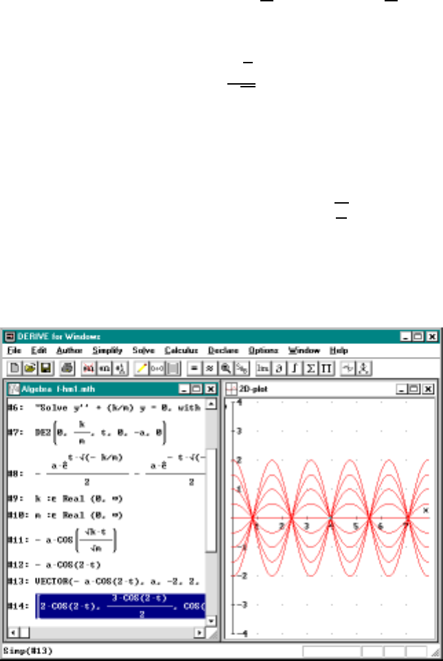
12.3. SOLVING LINEAR DIFFERENTIAL EQUATIONS 203
mare both positive numbers. You use the Declare/Variable Domain to tell
Derive that kis positive and do the same for m. Now simplifying the DE2
function gives the answer
−dcos √k
√mt!
Figure 12.2 shows the graph of this function when k=2andm=1and
dvaries between −2 and 2 in increments of 0.5. Notice all of the graphs
cross the x–axis at the same place; that is, at the same time. So it doesn’t
matter how far the spring is pulled down it will take the same amount of
time to return to its original position. If we let ω=qk
mthen time to return
to the original position is 2π/ω independent of d. This is called the period
of oscillation. ωis called the angular frequency while the reciprocal of the
period, ω/2πis the frequency. In Exercise 4 on page 213 you investigate
what happens if we start with y0= 0 but vary the velocity.
Figure 12.2: Spring motion starting at different positions

204 CHAPTER 12. HARMONIC MOTION
Damped oscillation. Recall that the frictional force due to the oil in the
vat is proportional to the velocity of the mass. This extra force changed the
differential equation (2) to
y00 +b
my0+k
my=0(14)
where b,k,mare all positive constants.
Before we analyze the roots of the characteristic equation just imagine
the effect of going from a very small value of b, close to zero, to a large
value. Since the value of brepresents how difficult it is to move in the oil
(this is essentially the viscosity of the oil) a small value would mean the
solution is similar the oscillating spring although it eventually slows down
and stops. A larger value will mean less oscillations and eventually there
will be no oscillations and the system will quickly come to a stop. Actually,
the mathematical model never actually stops, it just goes into exponential
decay!
Going back to the characteristic equation for this equation we have
r2+b
mr+k
m=0
Its roots are
−b±√b2−4km
2m
The solutions to (14) are given in (10)–(12). The sign of √b2−4km
determines which equation applies. If b2>4km we say the spring is over
damped. In this case the solutions of (14) have the form of (10) with r1and
r2the solutions to the characteristic equation given above. Notice that since
b,k,andmare all positive
0<b
2−4km < b2so √b2−4km < b
and thus, both r1and r2are negative. So the general solution is the sum of
two decaying exponentials.
If b2=4km the spring is critically damped. The solutions are given
by (11). Again r1is negative. If b2≤4km the spring is under damped.The
solutions are given by (12).
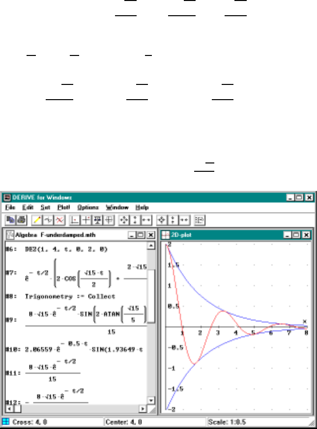
12.3. SOLVING LINEAR DIFFERENTIAL EQUATIONS 205
As an illustration we take b/m =1andk/m = 4 in (2). To solve (2)
with initial conditions t0=0,y
0=2,andv
0= 0 we author DE2(1, 4, t,
0, 2, 0). Simplifying this gives
e−t/2"2cos √15
2t!+2√15
15 sin √15
2t!#
We use the Declare/Algebra State/Simplification menu to set Trigonometry
to Collect and simplify again we get
8√15
15 e−t/2sin √15
2t+ 2 arctan √15
5!
≈2.06559e−t/2sin(1.93649 t+1.31811)
Figure 12.3 graphs this function as well as ±8√15
15 e−t/2.
Figure 12.3: Under Damped Oscillations

206 CHAPTER 12. HARMONIC MOTION
Pendulums. Lastly, let’s return to the pendulum example. We have a
mass mat the end of a pendulum of length l. It swings along a circular arc.
When the pendulum is at rest it hangs straight down and has velocity 0.
Let s(t) denote the arc length from this rest position as a function of time.
Let θ(t) be the angle the pendulum makes from the vertical position; see
Figure 12.1 on page 197.
As noted earlier the component of the force in the direction of the pen-
dulum rod is cancelled out by the rod and the force along the arc yields the
differential equation:
d2θ
dt2+g
lsin θ=0(15)
Since this is not a linear equation we approximate sin θwith θto get (5), i.e.,
d2θ
dt2+g
lθ=0(16)
In our illustration, we start by pulling the pendulum back by a small
angle θ0and letting go we can solve the equation by authoring DE2(0, g/L,
t, 0, θ0,0). This gives the solution
θ0cos rg
lt
Notice that the period depends on lbut not on θ0.Thisiswhyoldclocks
often use pendulums. As the spring runs down the pendulum will continue to
swing with the same frequency (until it stops completely of course). You can
adjust the speed by making a small change in the length of the pendulum.
Later in this chapter we will show how to find approximate solutions to
exact pendulum equation (15).
12.4 Systems of Differential Equations
Predator prey population growth. Suppose we have a population of
rabbits. Let R(t) be the population at time tand let R0=R(0) be the
initial population. In Chapter 11 we had two models for R(t). The first was
R0=kR was the standard exponential growth model. The second was the
Verhulst modification of this: R0=kR/(1 −R/R1), where R1is a constant
12.4. SYSTEMS OF DIFFERENTIAL EQUATIONS 207
representing the ideal population. But suppose we also have a population,
F(t), of foxes which prey on the rabbits. This gives us a system of differential
equations for R(t)andF(t). It is reasonable to assume that number of rabbits
eaten by foxes is proportional to R·F. Then the population of rabbits and
foxes can be modeled by the equations
R0=kR(1 −R/R1)−cRF
F0=dRF −eF
(17)
where k,c,d,andeare positive constants. If R= 0 the second equation
becomes F0=−eF . This means that if there are no rabbits the fox popula-
tion will dwindle because there is nothing to eat. If F= 0 then the rabbit
population will follow the Verhulst model.
The Runge-Kutta method of approximation. A general system of two
first order differential equations has the form
y0=r(t, y, z)
z0=s(t, y, z)
(18)
These can be solved exactly if r(t, y, z) has the form ay +bz and s(t, y, z)
has a similar form. (When rand shave this form, the system of equations
(18) is called linear.) Since the examples we are interested are not linear, we
concentrate on finding approximate solution to (18).
In Chapter 11 we described Euler’s method for finding an approximate
solution of a single first order equation y0=f(t, y) subject to the initial
conditions y(t0)=y
0
. We start with the point (t0,y
0
). Since we know the
slope of yat this point is f(t0,y
0
) we draw a short line segment from (t0,y
0)
to (t1,y
1
)=(t
0+h, y0+hf(t0,y
0)), where his a small increment. The
(n+1)
st point is obtained the nth by
(tn+1,y
n+1)=(t
n+h, yn+hf(tn,y
n))
Figure 12.4 on the following page gives the direction field for the simple
differential equation y0=−4(t−1). Of course we can find the solutions
by integration. If y(0) = 0 this gives y=2t(2 −t), which we have also
graphed. If we use Euler’s method with h=1/2 the first three points are
(0,0), (1/2,2), and (1,3). As the graph indicates these points are not very
close to the true solution.
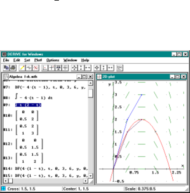
208 CHAPTER 12. HARMONIC MOTION
If instead of using the slope at (tn,y
n) we average this slope with the slope
at the next point (tn+1,y
n+1) we obtain a much more accurate approximation
of the solution. This is known as the second order Runge-Kutta method.The
precise formulae for tn+1 and yn+1 are
tn+1 =tn+h=t0+(n+1)h
y
n+1 =yn+h
2f(tn,y
n)+f(t
n+h, yn+hf(tn,y
n))
(19)
As we can see from Figure 12.4 this is much more accurate. If we also take into
account the slope at the midpoint of the two points we obtain the fourth order
Runge-Kutta method. This is usually just called the Runge-Kutta method .
Figure 12.4: Euler and the 2nd Runge-Kutta methods
If we have a system of equations like (18) we calculate triples of points
(tn,y
n,z
n) instead of pairs, but the formula is essentially the same. The
Derive utility function RK, which is included in ADD-HEAD, will calculate
approximate solutions to system of differential equations using the Runge-

12.4. SYSTEMS OF DIFFERENTIAL EQUATIONS 209
Kutta method.1To approximately solve (18) with initial conditions y(t0)=
y
0and z(t0)=z
0
, we author
RK([r(t,y,z), s(t,y,z)], [t, y, z], [t0, y0, z0], h, n)
where his the step size and nis the total number of steps you want. When we
approXimate this we get a matrix of triples. To graph y(t) we use the function
extract 2 columns(m,1,2) (where mis the matrix we got). This gives a ma-
trix of pairs which we can plot. To plot z(t)weuseextract 2 columns(m,1,3).
Returning to the predator-prey problem let’s look at the rabbits and foxes
problem with specific data for the constants in (17):2
k=.1 rabbit per month per rabbit
R1= 10000 rabbits
c=.005 rabbit per month per rabbit-fox
d=.0004 fox per month per rabbit-fox
e=.04 fox per month per fox
t0=0months
R
0= 2000 rabbits
F0=10foxes
To use the Runge-Kutta method to find an approximation of the solution
we author:
RK([.1r(1 - r/10000) - .005rf, .00004rf - .04f], [t,r,f],
[0,2000,10], 0.5, 600)
We approximate this and then use extract 2 columns for columns 1 and 2
to see R(t). The result is graphed in the upper right window of Figure 12.5
on the following page. Extracting column 1 and 3 gives the fox population
graphed in the lower right. Notice both populations oscillate with the fox
population following the rabbit population. After the rabbits increase the
foxes will then increase but when the fox population gets large the rabbit
1RK is the same as the one in Derive’s utility file ODE-APPR so the description of it
in Derive’s Help applies.
2This example is taken from J. Callahan and K. Hoffman Calculus in Context,
W. H. Freeman, 1995.
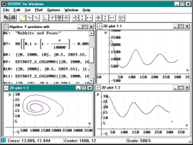
210 CHAPTER 12. HARMONIC MOTION
population will decrease which in turn will cause the fox population to de-
crease and so on.
The window in the lower left of Figure 12.5 shows the results of extracting
columns 2 and 3. The point near the crosshair in that window is (2000,10),
the initial rabbit and fox populations. At the beginning both the rabbit and
fox populations increase. When they reach the point furthest to the right
the rabbit population starts to decrease while the fox population continues
to increase. As we continue along the curve it spirals inward indicating that
the oscillation in the populations get smaller. In Exercise 6 on page 213 your
find the point to which the spiral approaches.
Figure 12.5: Rabbits and Foxes
The pendulum revisited. A second order differential equation such as (15)
can be reduced to a system of two first order equations. To do this we intro-

12.5. LABORATORY EXERCISES 211
duce a new variable w(t)=dθ/dt. Then (15) becomes
θ0=w
w0=−g
lsin θ
(20)
As an example suppose g/l = 25. Then to get an approximate solution
of (15) we author and then approximate the following.
EXTRACT 2 COLUMNS((21)
RK([w,-25 SIN(θ)], [t,θ,w], [0,θ0,0], 0.05, 60), 1, 2)
Figure 12.6 on the next page shows the resulting graphs for θ0=π/8,
π/4, π/2, and 15π/16. The graph of the solution of (15), namely θ0cos(5t), is
also shown on each graph. Looking at these graphs we can see several things.
First for θ0=π/8=22.5
◦the curves are almost identical showing that using
(5) rather than (15) works well for small and even moderate angles. Even
for θ0=π/4=45
◦
, shown in the lower left, is fairly close to the true graph.
Since we are considering a pendulum without friction (undamped) we
expect that when we release it with an initial angle of θ0it will swing to the
other side reaching the angle θ=−θ0and then return back to the original
position with θ=θ0. Then of course it will just repeat this. This means
that the solution of (15) will be periodic. The linear approximation (5) has
a shorter period than the true equation (15). This makes sense since the
magnitude of the force pushing the pendulum back towards its rest position
(θ= 0) is proportional to sin θfor the true equation and to θin the linear
approximation and sin θ≤θfor θ>0.
The lower right frame of Figure 12.6 on the following page gives the graphs
when θ0= 15π/16. This corresponds to starting the pendulum almost at the
top. Notice that not only is the true period much greater than the linear
approximation but that the shape of curve is different.
12.5 Laboratory Exercises
The functions discussed in this chapter, DE2 and RK are defined once you
Load in the file ADD-HEAD.
1. For each of the differential equations below solve the characteristic
equation and enter the general solution with constants C1,C2.Verify
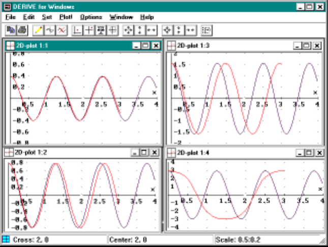
212 CHAPTER 12. HARMONIC MOTION
Figure 12.6: Pendulums
that the general solution satisfies the differential equationby computing
the first and second derivatives and substituting into the equation.
Show that Derive simplifies the resulting expression to zero. Use only
real solutions to the equations. Finally, use the DE2 function to solve
the differential equation using the same initial conditions: y(0)=1and
y
0
(0) = 2. Plot the solution.
a. y00 −2y0−8y=0 b. y00 =−4y0−4y
c. y00 =−16yd. y00 −4y0+5y=0
2. A mass, with m= 1, is attached to a vertical spring. The mass stretches
the spring by 2 feet as a result. With the mass attached, stretch the
spring another 3 feet and release it. The spring will then oscillate up
and down periodically. (Use g= 32 feet/sec2to calculate k.)
a. Find the differential equation that describes this motion.

12.5. LABORATORY EXERCISES 213
b. Find the vertical displacement function y(t)byusingDE2 to solve
the differential equation.
c. Determine the period of the motion.
3. Show that if the characteristic equation (6) has a double root, that is,
if r1=r2,thenbothy=e
r
1
tand y=ter1tsatisfy (1) on page 196.
4. Hooke’s Law is given by equation 2 on page 196.
a. Solve this with the initial conditions y0=0andv
0=v.(You
should use Derive’s Declare/Variable Domain to tell Derive
that mand kare positive.)
b. Graph your solutions with with k=2,m=1,andvvarying
between −2 and 2 in increments of 0.5.
5. A third order differential equation of the form
y000 +by00 +cy0+dy =0
has the characteristic equation r3+br2+cr +d=0. Therootsof
the characteristic equation determine the solutions of the differential
equation in the same way as for second order differential equations. The
solutions of second order differential equations involve two arbitrary
constants but for third order there are three.
a. Find the solutions to y000 −2y00 −y0+2y=0.
b. Find the solutions to y000 −2y00 +y0−2y=0.
c. Find the solutions to y000 −4y00 +5y
0−2y=0.
6. Suppose we want to find solutions to (17) such that both R(t)and
F(t) are constant. One (trivial) solution is R(t)=0=F(t) but we
would like something more interesting than this. If the populations are
constant then R0(t)=0andF
0
(t)=0.
a. Solve (17) for Rand Fwhen R0(t)=F
0
(t)=0. Hint: Use the
second equation of (17) to find R, substitute this into the first
equation and then solve for F.

214 CHAPTER 12. HARMONIC MOTION
b. The curve in the lower left window of Figure 12.5 on page 210
spirals inward. Use your answer from the previous part with the
constants on page 209 to guess where it is heading.
7. Suppose in our rabbits and foxes example instead of (17) we use the
simpler equations
R0=kR −cRF
F0=dRF −eF
without the Verhulst modification.
a. In Figure 12.5 on page 210 we used RK and EXTRACT 2 COLUMNS to
make 3 graphs. Make the same 3 graphs but using these simpler
equations. Describe the differences between your graphs and those
of Figure 12.5.
b. Find the solutions which are constant as in the previous problem.
8. We saw in the lower right frame of Figure 12.6 on page 212 on page 212
that for θ0=15π/16 the solution to (15) and to the linear approxi-
mation (5) were quite different. In this exercise we will compare the
solution to (15) with a cos function of the same amplitude and period.
a. Author the expression (21) with θ0=15π/16 and then approxi-
mate it. Then graph the result.
b. Using this graph estimate the period Pof this function
c. Graph 15π
16 cos(2π
Pt)usingthePyou found in the previous part.
d. Notice the graph you found in the first part is pretty flat at the
top and bottom compared to the cos curve. What is the solution
of (15) if θ0=π(and w0= 0, of course)? You should be able to
just guess the solution.
9. In this problem we explore what happens to a pendulum with initial
position θ0= 0 but with a nonzero value for w0. If the initial velocity
is not too large the pendulum will swing up to an angle αand then
swing back. The motion will be the same as if we started with θ0=α

12.5. LABORATORY EXERCISES 215
and w0= 0 except that starting place for the graph will be different.
That is, the curves will be the same except one will be shifted to the
right. However if w0is large enough, the pendulum will swing all the
way over the top.
a. Author
EXTRACT 2 COLUMNS(
RK([w,-25 SIN(θ)],[t,θ,w],[0,0,w0],.05,60),1,2)
Substitute w0=9.5 and approximate and then graph the result.
Do the same for w0=10andw
0= 10.5.
b. The behavior of the solutions of the previous part are quite differ-
ent depending on whether w0is large enough to send the pendulum
over the top (so it keeps spinning around and around) or it doesn’t
make it to the top and so falls back. In this problem we look for
a value of w0so that it never falls back but also never goes over
the top. We will try to choose w0so that it will have the exact
amount of energy to just get to the top. Since we are assuming our
pendulum is frictionless, there are two kinds of energy in our sys-
tem, kinetic and potential energy. Kinetic energy is 1
2mv2which
in our case is 1
2m(ds/dt)2=1
2ml(dθ/dt)2. Potential energy gained
as the pendulum swings above its rest position is mgh where his
the height above the rest position. So the potential energy at the
top is 2mgl. Use the law of conservation of energy to show that
if the kinetic energy at the bottom equals the potential energy at
the top then
w0=θ0(0) = 2rg
l
which is 10 when g/l = 25.
c. While the solution to (15) on page 206 cannot be expressed in
terms of elementary functions, the solution when θ(0) = 0 and
θ0(0) = 2pg
lcan. Show that
θ(t) = 4 arctan(e√g
lt)−π

216 CHAPTER 12. HARMONIC MOTION
is a solution of (15) and that θ0(0) = 2pg
l. You will need set
the trigonometry mode to Expand under the Declare/Algebra
StateSimplification menu. Also remember that Derive uses ATAN
for the arctan function.
d. When g/l = 25, θ(t) = 4 arctan(e5t)−π. Graph this function
and compare it with the graph you made in the first part with
w0= 10. Also graph
EXTRACT 2 COLUMNS(
RK([w,-25 SIN(θ)],[t,θ,w],[0,0,10],.01,500),1,2)
e. Why do these graphs differ?
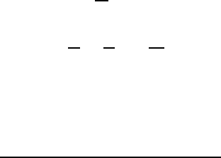
Appendix A
Utility Files
This book defines 19 Derive functions. All of these functions are defined in
the utility file ADD-UTIL which is quietly loaded; which means the formulas
are not displayed, whenever you load the file ADD-HEAD. This file and its
companion, ADD-HEAD, can be downloaded from our web page
http://www.math.hawaii.edu/lab/
Listings of these files are given at the end of this appendix in the (hopefully
unlikely) event you have trouble downloading them. Additional information
on the use of the functions as well as examples are included on the web site
above.
How to use these files. When a student first starts to work on a lab
assignment he should:
1. Enter (Author) his name and the lab number as a comment. (Com-
ments are entered using the double quotes, ".)
2. Do File/Load/Math add-head.
3. Begin working on his assignment.
The file ADD-HEAD has only four lines. Two of these are comments
and one gives the variable syntax for the commands. The other line is
LOAD("add-util"). This automatically silently loads ADD-UTIL.1.For
1
This assumes that this file is in the default directory. A default directory should be
established and all F-*.MTH files placed in that directory along with ADD-HEAD and
ADD-UTIL
217

218 APPENDIX A. UTILITY FILES
this load command directory to work correctly, ADD-HEAD and ADD-UTIL
should both be in the current directory. It is best to put them in the default
directory.
Home use of these files. If you have Derive for your own computer
you can install ADD-HEAD and ADD-UTIL. When Derive starts it has
a default directory it looks for MTH files. If you haven’t changed this it is
..\DfW\Math. That directory contains the utility files that come with the
system. You should add a new subdirectory, such as ..\DfW\Lab,usingthe
Windows file manager and then make that your default directory using the
File/Change Directory command in DfW. Next, you put both ADD-UTIL
and ADD-HEAD in this default directory and the above directions should
work fine. You should also add all the F-*.MTH files that are used in the
book’s figures to this directory. All of these files are available from our web
site.
A.1 The Functions
Table A.1 on page 221 and A.2 on page 222 list the functions defined in
ADD-UTIL. In each of the examples below it is assumed that the utility file
ADD-UTIL has been loaded as described above. Here are some examples on
their use.
Example 1. If you want to compute a tangent line for say f(x)=x
3
/3at
the point x=1youwouldA
uthor and Simplify TANGENT(x^3/3, x, 1).
The result will be y=x−2/3. We describe the variables for this and the
other functions typically as TANGENT( u, x, a) where the urefers to any
expression in the variable xand ais a parameter in the function which in
this case it is the point we are interested in.
Example 2. Suppose that you want to find the quadratic polynomial ax2+
bx +cthat passes through the three points (0,0), (1,2), and (2,8). You
Author CURVEFIT( x, [[0,1], [1,2], [2,8]]). After simplifying the re-
sult will be 2x2. Probably the best way to do this is to start by defining
the 3 ×2 matrix of points using the matrix button and then plotting
the 3 points on a graph. Next you Author the CURVEFIT(x, part and then
right click and insert the matrix of data points. Simplify and plot to make
sure the answer function does indeed pass through the 3 data points. The

A.1. THE FUNCTIONS 219
CURVEFIT function will find the appropriate degree polynomial through
the data regardless of the number of points.
Example 3. Suppose that now that you want to find the quadratic poly-
nomial ax2+bx +cthat passes through the two points: (0,0) and (1,2). In
addition, you want the derivative to be 1 when x=0. YouA
uthor CURVEFIT(
x, [[0,1], [1,2]], [[0,1]]). In other words, you enter one matrix for
the points satisfied by the function and another matrix for the points satisfied
by the derivative. The degree of the answer polynomial is always one less
than the total number of equations for both the function and its derivative.
Example 4. Let’s solve the equation x2+x−1 = 0 using Newton’s method
of Chapter 5. We’ll use x0 = 5 as our initial guess. We obtain our first
approximation by Authoring NEWT(x^2+x-1, x, 5) and then Simplifying
to get 2.63263. We repeat this process using this new value as our starting
point. After 4–5 iterations we obtain an approximation we good to 6 decimal
places.
Example 5. More generally, to approximate the solution to the equation
u=0,whereuis an expression in x, using Newton’s method with initial
guess ayou author and approximate NEWT(u, x, a). Suppose instead that
you want the first kapproximates starting with x=a, then you approximate
NEWT(u, x, a, k).The4
th argument is optional. You get a nice picture
of the Newton method in action by approximating DRAW NEWT(u, x, a, k)
and then plotting the result. Notice that the starting point can be a complex
number in which case the approximates are also complex. The function
DRAW COMPLEX(v) can be applied to the solution vector to get a matrix of
[x, y]pointswhichcanthenbeplottedina2D-plotwindow.
Example 6. Suppose that you want to approximate the integral which de-
fines the natural logarithm of 2, i.e.,
ln 2 = Z2
1
dx
x
using say the trapezoid rule or Simpson’s rule for numerical integration.
We do this for n= 100 subdivisions by Authoring either the expression
TRAP(1/x, x, 100, 1, 2) or the expression SIMP(1/x, x, 100, 1, 2).
Now since we are interested in a decimal approximation we use the
button to simplify the expression. More generally, suppose you approximate
220 APPENDIX A. UTILITY FILES
the integral of the expression u,inthevariablexover the interval [a, b], using
Simpson’s rule with nsubdivisions. You Author SIMP(u,x,n,a,b) and press
.
Example 7. Suppose that you want to solve a Newton cooling type differ-
ential equation: y0=−(y−2) with initial conditions y(0) = 4. You start by
manipulating the equation to the form y0+py =qwhere p=1andq=2.
The function DE(p,q,x,y,x0,y0) solves this equation so we just substitute
in the right values which in this case means that we Author DE(1,2,x,y,0,4)
and press .
Example 8. Suppose that you want to look at the direction field for the
equation y0=rwhere ris an expression in xand y. You use the function
DF(r,x,x0,xm,m,y,y0,yn,n))
where the grid of points is determined by x0<x<xmwith msubdivisions
and y0<y<ynwith nsubdivsions. Doing this for the previous example
would mean Authoring say DF(-(y-2),x,0,6,12,y,-2,4,12) andthenap-
proximating the expression by pressing . You get a graph with a slope
line at every half integer in an appropriate range of xand y’s by plotting the
result.

A.1. THE FUNCTIONS 221
Table A.1: Functions Defined in ADD-UTIL.MTH
SUBST(u, x, a)Substitutes x=ain the expression u.
SECANT(u, x, a, h)Secant line of u(x) through x=aand x=
a+h.
TANGENT(u, x, a)Tangent line of u(x)atx=a.
CURVEFIT(x, data)
CURVEFIT(x, data, ddata)
Fits a polynomial in the variable x, though
the points data := [[x0,y0],[x1,y1], ...]
provided ddata is either omitted or []. Oth-
erwise, the graph of the derivative must
pass through the ddata points.
NEWT(u, x, x0)
NEWT(u, x, x0,k)
Newton algorithm for root of u(x)=0with
initial guess x0. If the optional kargu-
ment is used then a vector of kiterates is
returned.
DRAW NEWT(u, x, x0,k)Draws a picture of Newton method applied
to u(x) = 0 with initial guess x0andk
iterates. Simplify expression and plot the
result.
DRAW COMPLEX(v)Converts the vector of complex numbers
[x0+iy0,x1+iy1, ...] into a matrix of
points [[x0,y0],[x1,y1], ...] which can then
be plotted in a 2D-plot window.
BISECT(u, x, v)
BISECT(u, x, v, k)
Bisection method for solving u(x)=0with
interval v=[a, b]. The answer is either the
left or right half of the interval depending
on the root. If the optional kargument is
used then a vector of kiterates is returned.
LEFT(u, x, n, a, b)Numerical approximation to the integral
of u(x)over[a, b] using the left-endpoint
method with nrectangles.
MID(u, x, n, a, b)Numerical approximation to the integral of
u(x)over[a, b] using the midpoint method
with nrectangles.

222 APPENDIX A. UTILITY FILES
Table A.2: Functions Defined in ADD-UTIL.MTH (cont.)
RIGHT(u, x, n, a, b)Numerical approximation to the integral
of u(x)over[a, b] using the right-endpoint
method with nrectangles.
TRAP(u, x, n, a, b)Numerical approximation to the integral of
u(x)over[a, b] using the trapezoid method
with ntrapezoids.
SIMP(u, x, n, a, b)Numerical approximation to the integral
of u(x)over[a, b] using Simpson’s method
with nsubdivisions.
DRAW LEFT(u, x, n, a, b)Draws graphic demonstration of the left-
endpoint method for numerically integrat-
ing u(x) over the interval [a, b]usingnrect-
angles.
DRAW RIGHT(u, x, n, a, b)Same as above except for the right-
endpoint method.
DRAW TRAP(u, x, n, a, b)Draws graphic demonstration of the trape-
zoid method for numerically integrating
u(x) over the interval [a, b]usingntrape-
zoids.
DE(p, q, x, y, x0,y0) Solves the differential equation (DE) y0+
p(x)y=q(x)withy(x0) = y0.
DF(r, x, x0, xm, m, y, y0,yn,n)The direction field (DF) for the differential
equation: y0=r(x, y) with a grid deter-
mined by x0<x<xmwith msubdivi-
sions and y0<y<ymwith nsubdivi-
sions.
EULER(r, x, y, x0,y0,xn,n)This gives an approximate solution to:
y0=r(x, y)withy(x0) = y0. The answer
is a vector of points [[x0,y0],[x1,y1], ...]
from which one makes a piecewise linear
approximating function, i.e., connect the
points with straight line segments to get
the approximating function’s graph.
A.2. LISTINGS OF THE UTILITY FILES 223
A.2 Listings of the Utility Files
In the event you are unable to download these files, you can type them in.
Probably the easiest way to do this is to start Derive and author each line.
Then save the first as add-head and the second as add-util.
A.2.1 The ADD-HEAD.MTH File
"The vector below declares all the utility functions in add-util.mth."
[SUBST(u,x,a):=,SECANT(u,x,a,h):=,TANGENT(u,x,a):=,CURVEFIT(x,data):=,SPLINE(~
x,data,m1):=,NEWT(u,x,x0,k):=,DRAW_NEWT(u,x,x0,k):=,DRAW_COMPLEX(v):=,BISECT(~
u,x,v0,k):=,LEFT(u,x,n,a,b):=,MID(u,x,n,a,b):=,RIGHT(u,x,n,a,b):=,TRAP(u,x,n,~
a,b):=,SIMP(u,x,n,a,b):=,DRAW_LEFT(u,x,n,a,b):=,DRAW_TRAP(u,x,n,a,b):=,DE(p,q~
,x,y,x0,y0):=,DF(r,x,x0,xm,m,y,y0,yn,n):=,EULER(r,x,y,x0,y0,xn,n):=]
LOAD("add-util")
"Your file starts here:"
A.2.2 The ADD-UTIL.MTH File
"File add-util.mth, (c) 1997 Ralph Freese and David Stegenga."
"See add-summary.mth for a summary of new functions defined below:"
"Substitute x=a into the expression u."
SUBST(u,x,a):=LIM(u,x,a)
"The secant line of u(x) through x = a andx=a+h."
SECANT(u,x,a,h):=y=(SUBST(u,x,a+h)-SUBST(u,x,a))/h*(x-a)+SUBST(u,x,a)
"The tangent line of u(x) at x = a."
TANGENT(u,x,a):=y=SUBST(u,x,a)+SUBST(DIF(u,x),x,a)*(x-a)
"Helper functions for CURVEFIT."
POLY(x,a,n):=SUM(a SUB (i+1)*x^i,i,0,n)
DPOLY(x,a,n):=SUM(i*a SUB (i+1)*x^(i-1),i,1,n)
EQNS(data,ddata,a,n):=APPEND(VECTOR(POLY(data SUB i SUB 1,a,n)=data SUB i SUB~
2,i,1,DIMENSION(data),1),VECTOR(DPOLY(ddata SUB i SUB 1,a,n)=ddata SUB i SUB~
2,i,1,DIMENSION(ddata),1))
UNK(n):=RHS(VECTOR(SOLVE(upsilon=upsilon,upsilon),i,1,n,1)‘ SUB 1)
224 APPENDIX A. UTILITY FILES
ANS(x,data,ddata,a,n):=IF(DIMENSION(ans_:=SOLVE(EQNS(data,ddata,a,n),[a]))=0,~
[],POLY(x,(RHS(ans_)) SUB 1,n))
"Finds the polynomial of the right degree through the nx2-data matrix."
CURVEFIT1(x,data):=ANS(x,data,[],UNK(DIMENSION(data)),DIMENSION(data)-1)
CURVEFIT2(x,data,ddata):=ANS(x,data,ddata,UNK(DIMENSION(data)+DIMENSION(ddata~
)),DIMENSION(data)+DIMENSION(ddata)-1)
CURVEFIT(x,data,ddata):=IF(DIMENSION(ddata)>0,CURVEFIT2(x,data,ddata),CURVEFI~
T1(x,data),CURVEFIT1(x,data))
"Quadratic spline function interpolating data points with initial slope m1."
SPLINE_AUX(x,data,m):=SUM(CURVEFIT(x,[data SUB k,data SUB (k+1)],[[data SUB k~
SUB 1,m SUB k SUB 2]])*CHI(data SUB k SUB 1,x,data SUB (k+1) SUB 1),k,1,DIME~
NSION(data)-1)
SLOPE(data,m1):=ITERATES([v SUB 1+1,2*(data SUB (v SUB 1+1) SUB 2-data SUB (v~
SUB 1) SUB 2)/(data SUB (v SUB 1+1) SUB 1-data SUB (v SUB 1) SUB 1)-v SUB 2]~
,v,[1,m1],DIMENSION(data)-1)
"Note that SLOPE returns the matrix [[1,m1], [2,m2], ...]."
SPLINE(x,data,m1):=SPLINE_AUX(x,data,SLOPE(data,m1))
"Newton algorithm"
NEWT_ITERATES(u,x,x0,k):=ITERATES(x-u/DIF(u,x),x,x0,k)
NEWT(u,x,x0,k):=IF(k>0,NEWT_ITERATES(u,x,x0,k),?,SUBST(x-u/DIF(u,x),x,x0))
"This produces a vector which when plotted demonstrates Newton’s method."
DRAW_NEWT(u,x,x0,k):=VECTOR([[v,0],[v,SUBST(u,x,v)],[NEWT(u,x,v),0]],v,ITERAT~
ES(NEWT(u,x,w),w,x0,k))
DRAW_COMPLEX(v):=VECTOR([RE(z),IM(z)],z,v)
"Bisection method helper"
BIS_AUX(u,x,a,b):=IF(SUBST(u,x,a)*SUBST(u,x,(a+b)/2)<0,[a,(a+b)/2],[(a+b)/2,b~
])
"Bisection method"
BISECT(u,x,v0,k):=IF(k>0,ITERATES(BIS_AUX(u,x,v SUB 1,v SUB 2),v,v0,k),?,BIS_~
AUX(u,x,v0 SUB 1,v0 SUB 2))
"Formula for the left-endpoint method for integrating u(x) over [a,b] with n ~
subdivisions."
LEFT(u,x,n,a,b):=(b-a)/n*SUM(SUBST(u,x,a+k*(b-a)/n),k,0,n-1)
"Formula for the midpoint method for integrating u(x) over [a,b] with n subdi~
A.2. LISTINGS OF THE UTILITY FILES 225
visions."
MID(u,x,n,a,b):=(b-a)/n*SUM(SUBST(u,x,a+(k+0.5)*(b-a)/n),k,0,n-1)
"Formula for the right-endpoint method for integrating u(x) over [a,b] with n~
subdivisions."
RIGHT(u,x,n,a,b):=(b-a)/n*SUM(SUBST(u,x,a+k*(b-a)/n),k,1,n)
"Formula for the trapezoid method for integrating u(x) over [a,b] with n subd~
ivisions."
TRAP(u,x,n,a,b):=(b-a)/(2*n)*(SUBST(u,x,a)+SUBST(u,x,b)+2*SUM(SUBST(u,x,a+k*(~
b-a)/n),k,1,n-1))
"Formula for Simpson’s rule for integrating u(x) over [a,b] with n subdivisio~
ns."
SIMP(u,x,n,a,b):=(b-a)/(6*n)*(SUBST(u,x,a)+SUBST(u,x,b)+2*SUM(SUBST(u,x,a+k*(~
b-a)/n),k,1,n-1)+4*SUM(SUBST(u,x,a+(k+1/2)*(b-a)/n),k,0,n-1))
"The box and trapezoid drawing functions used in the graphical demonstrations~
of numerical integration techniques."
D_BOX(x1,y1,x2,y2):=[[x1,y1],[x2,y1],[x2,y2],[x1,y2],[x1,y1]]
D_TRAP(x1,y1,x2,y2,x3,y3,x4,y4):=[[x1,y1],[x2,y2],[x3,y3],[x4,y4],[x1,y1]]
DRAW_LEFT(u,x,n,a,b):=VECTOR(D_BOX(t,0,t+(b-a)/n,SUBST(u,x,t)),t,a,b-(b-a)/n,~
(b-a)/n)
DRAW_RIGHT(u,x,n,a,b):=VECTOR(D_BOX(t,0,t+(b-a)/n,SUBST(u,x,t+(b-a)/n)),t,a,b~
-(b-a)/n,(b-a)/n)
DRAW_TRAP(u,x,n,a,b):=VECTOR(D_TRAP(t,0,t+(b-a)/n,0,t+(b-a)/n,SUBST(u,x,t+(b-~
a)/n),t,SUBST(u,x,t)),t,a,b-(b-a)/n,(b-a)/n)
"The solution to the differential equation (DE) y’+p(x)y=q(x) with y(x0)=y0."
DE(p,q,x,y,x0,y0):=y=(y0+INT(q*#e^INT(p,x,x0,x),x,x0,x))/#e^INT(p,x,x0,x)
"Direction field helper function."
SEG(rc,x,y,x,y):=IF(ABS(rc)>1 AND y<ABS(rc)*x,[[x-y/rc,y-y],[x+y/rc,y+~
y]],[[x-x,y-rc*x],[x+x,y+rc*x]])
"The direction field (DF) for the differential equation: y’=r(x,y) with a de~
termined by x0<x<xm with m subdivisions and y0<y<ym with n subdivisions."
DF(r,x,x0,xm,m,y,y0,yn,n):=VECTOR(VECTOR(SEG(LIM(r,[x,y],[x0+j*(xm-x0)/m,y0+k~
*(yn-y0)/n]),x0+j*(xm-x0)/m,y0+k*(yn-y0)/n,(xm-x0)/(4*m),(yn-y0)/(4*n)),j,0,m~
),k,0,n)
"The EULER function gives an approximate solution to: y’=r(x,y) with y(x0)=y0~
."
EULER(r,x,y,x0,y0,xn,n):=ITERATES(v+(xn-x0)/n*[1,LIM(r,[x,y],v)],v,[x0,y0],n)
226 APPENDIX A. UTILITY FILES

Appendix B
DfW Version 5
In 1999, the Soft Warehouse became a part of Texas Instruments Corpora-
tion (TI) and the business office for the Derive software in Honolulu was
moved to Texas. Nevertheless, the software itself is still being developed and
maintained by its creators and the sales and promotional aspects are done
by TI. In addition, the math engine inside of Derive is being installed into
all of TI’s calculator products.
In the year 2000, Version 5 of Derive was released. The new version
has an improved interface, embedded graphics, embedded text (for making
workbooks) and a new DFW file format to support the new features.
B.1 What’s New In DfW5
See Figure B.1 on the next page for a look at DfW5. The first thing to
notice is that the authoring form is now a permanent part of the window,
along with the special symbol bar. You can either click the button as
in Version 4 or just simply click your mouse pointer in the new author box.
You can still right-click to insert expressions (or press F3) but there are now
several options for adding expressions to the algebra window. You can return
the unsimplified expression or the simplified (or approximated) expression as
in Version 4 but there is a new option: returning the unsimplified expression
first aligned with the left side of the window and then that same expression
is returned, simplified and centered in the window. This makes it easy to
see what expressions are input and what expressions have been simplified by
Derive.
227
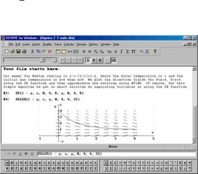
228 APPENDIX B. DFW VERSION 5
The method for correcting typos or making small changes in an expression
has been improved. Now you only need to right-click the erroneous expression
and select Edit. The expression is entered into the Author form where you
make changes. Then, pressing the Enter key results in changing the expression
at its current position rather than adding a new line as in Version 4. This
turns out to be a very useful feature.
Figure B.1: The new look of DfW5
Next, notice that the comment text is now a specially formatted object
in the window and it is no longer necessary to use double quotes to add
remarks. Inserted text can be formatted in different fonts and colors so that
the algebra window can be given the appearance of a page in a textbook.
This is a powerful feature that makes it much easier to use the printout from
your Derive session in classroom notes. In addition, the plot window can be
embedded into the algebra window and hence be included with the printout of
the expressions and comments, making for a true workbook like appearance.
You can see the embedded graphics feature in Figure B.1. Notice that there
is no Plot window showing.
B.1. WHAT’S NEW IN DFW5 229
In Version 4 you needed to simplify an expression before plotting it. For
some functions, like the ones used in Figure B.1, this will result in huge data
matrices that were of little value to look at. In Version 5 you can plot without
simplifying, which is exactly what happened in our sample session. There is
no need to plot and then erase the huge expression as in Version 4.
Lastly, observe that the complete file name is F-EULER.DFW and that
the extension is not MTH as in Version 4. The old file format can still be used
for reading and writing expressions but the new format supports all of the new
features we have been discussing. Thus, a DFW file will contain expressions
as usual, but also embedded text and graphics. Since the embedded text
can be edited along with the expressions themselves, as mentioned above,
the Version 5 algebra window is becoming similar to a mathematical word
processor.
There are many other features in Version 5 that we have not highlighted
here but the most important one is the new programming language. Pro-
gramming in Version 4 primarily consists of defining simple functions using
the IF and the ITERATE functions. Of course, more elaborate constructions
are possible as evidenced by some of the complicated examples in the ADD-
UTIL file, see Appendix A.
In Version 5 there is a complete programming language consisting of block
constructions with local variables along with loops and branching. Programs
are displayed in a specially formatted manner that makes it easy to see the
logic involved and to correct mistakes that occur. This makes building large
programs much more feasible. However, there are benefits even for simple
things like the IF function that we have used on so many occasions. For
example, the Version 4 definition of the factorial function is
FAC(n) := IF(n=0, 1, n FAC(n-1))
and it is displayed in a linear fashion. On the other hand, the same input in
Version 5 is display as
fac(n):=
If n=0
1
n·fac(n−1)
that shows the logic more clearly. This becomes a very powerful feature
for larger programs or even complicated functions that involve branching
depending on the value of a variable.
230 APPENDIX B. DFW VERSION 5
Index
angular frequency, 203
asymptote, 50
attractor, 77
super, 77
basin of attraction, 81
bisection method, 86–88
chaos, 82
character input mode, 57
characteristic equation, 198
complex conjuagate, 91
complex conjugate, 79, 128, 202
complex exponential, 127
complex numbers, 78, 166
conjugate, 79, 91, 128
exponential, 127, 166
imaginary part, 79, 91
modulus, 79, 91
multiplication, 167
real part, 79, 91
roots, 80, 92
complex plane, 80
complex roots, 8, 80
critical points, 48
damping, 204
defining variables, 14
differential equations, 60, 177–191,
195–211
linearfirstorder,188
direction field, 182
dynamic system, 77
Euler’s constant, 4
Euler’s method, 186
exponential growth, 31
fixed point, 92
attractive, 81
frequency, 203
Gamma function, 45
half-life, 181
Hooke’s Law, 196
imaginary part, 79, 91
integral test, 132, 142–147
interest, 133–135
continuous, 147
effective annual rate, 148
loan repayment, 135–136
modulus, 79, 91
Newton’s Law of Cooling, 180–181
Newton’s method, 69–83
period, 203
Poisson summation, 150
population growth, 55, 177–180, 183–
186
231
232 INDEX
radioactive decay, 181
ratio test, 132, 138–141
real part, 79, 91
recursion, 15
right mouse button, 5
Runge-Kutta method, 208
series
convergent, 131
divergent, 131
geometric, 131, 132
harmonic, 146
Simpson’s rule
derivation, 104–105
error estimate, 99
slope field, 182
solving equations, 6–8
numerically, 30
spline functions, 62
subscripts, 20
super attractor, 77
tangent line, 40
trapezoid rule
error estimate, 99
vectors, 18
web page, xv