Detrital Py Manual V1.1.2
User Manual:
Open the PDF directly: View PDF ![]() .
.
Page Count: 28
- TABLE OF CONTENTS
- INTRODUCTION
- PYTHON INSTALLATION
- DATA FORMATING
- OPENING JUPYTER NOTEBOOK
- STEPS I-III: Database import and sample selection
- DETRITALPY FUNCTIONS
- Plot detrital age distributions
- Plot rim age versus core age
- Plot detrital age distributions in comparison to another variable (e.g., Th/U)
- Plot detrital age populations as a bar graph
- Plot sample locations on an interactive map
- Plot and export maximum depositional age (MDA) calculations
- Multi-dimensional scaling
- (U-Th)/He vs U-Pb age “double dating” plot
- Export sample comparison matrices as a CSV file
- Export detrital age distributions as a CSV file
- Export ages and error in tabular format as a CSV file
- REFERENCES
1
detritalPy
A Python-based Toolset for Visualizing and Analyzing
Detrital Geo-Thermochronologic Data
Version 1.1.2
Updated October 11, 2018
Glenn R. Sharman, Jonathan P. Sharman, and Zoltan Sylvester
2
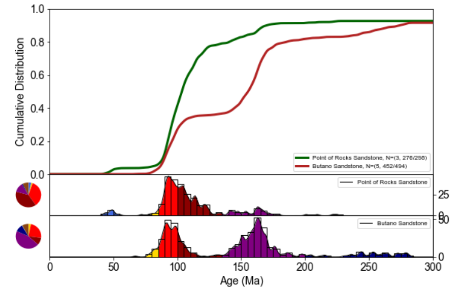
Cover page: Example visualization of detrital zircon U-Pb age distributions from two sample
groups. The top plot displays a cumulative kernel density estimate (CKDE) of all three samples
using a bandwidth of 1.5 Myr. The bottom panels display (1) kernel density estimates (KDE)
constructed using a bandwidth of 1.5 Myr and shaded according to user-defined age populations,
(2) a histogram (bin size of 5 Myr), and (3) pie diagrams showing the proportions of user-defined
age populations. Data are from Sharman et al. (2013, 2015).
3
TABLE OF CONTENTS
TABLE OF CONTENTS 3
INTRODUCTION 5
PYTHON INSTALLATION 5
DATA FORMATING 6
Samples Worksheet 6
ZrUPb Worksheet 7
OPENING JUPYTER NOTEBOOK 8
STEPS I-III: DATABASE IMPORT AND SAMPLE SELECTION 9
I. Import required modules 9
II. Import the dataset as an Excel file 9
III. Select samples 10
DETRITALPY FUNCTIONS 11
Plot detrital age distributions 11
Plot rim age versus core age 16
Plot detrital age distributions in comparison to another variable (e.g., Th/U) 17
Plot detrital age populations as a bar graph 18
Plot sample locations on an interactive map 19
Plot and export maximum depositional age (MDA) calculations 22
5
INTRODUCTION
This manual provides an overview of detritalPy, a Python-based toolset designed to
promote efficient organization, visualization, and analysis of detrital geochronologic and
thermochronologic datasets. For additional information, please refer to Sharman et al.
(submitted) and commented lines within detritalPy code
(https://github.com/grsharman/detritalPy).
PYTHON INSTALLATION
If using Python for the first time, we suggest installing the open data science platform
Anaconda by Continuum Analytics that includes the most commonly used Python packages.
detritalPy is compatible with Python 3.6 and is run through Jupyter Notebook.
Although the basic functions of detritalPy can be accessed via the packages that are installed
by default with Anaconda, it is necessary to install several additional packages to utilize the full
functionality of detritalPy.
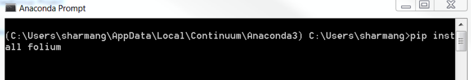
• If using Windows, launch the Anaconda Prompt and enter the following commands:
pip install folium (required for mapping sample locations)
pip install vincent (required for mapping sample locations)
pip install simplekml (required for exporting sample locations to kml)
pip install peakutils (required for plotting peak ages)
• If using a Macintosh, launch a Terminal window and activate the Anaconda environment
that you are using (e.g., ‘source activate python3’, where ‘python3’ is the name of the
environment). Then run the pip installation commands listed above.
6
DATA FORMATING
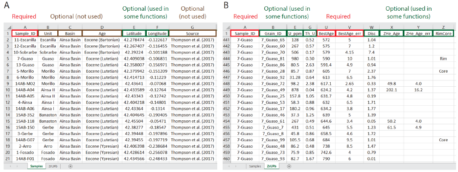
detritalPy requires that input data be organized using a specific format. The default
format is a Microsoft Excel file that contains two worksheets: (1) a worksheet that contains a row
for each unique sample in the dataset (default worksheet name is “Samples”), and (2) a data
worksheet that contains a row for each unique detrital analysis in the dataset (default worksheet
name is “ZrUPb” for zircon U-Pb and/or (U-Th)/He data) (Fig. 1). This data structure places
sample-level information within the Samples worksheet and zircon U-Pb and/or (U-Th)/He
analysis-level data within the ZrUPb worksheet. The two worksheets are linked together by a
unique sample identifier (“Sample_ID” column) that must be assigned to each individual
sample. Each sample identifier must be distinct (unique) from all others in the database. There
should be no empty rows within data in either the Samples or ZrUPb worksheets.
More than one Excel file can be loaded into detritalPy, provided that there is no
duplication of data, no duplicated sample identifiers, and the column headings are all the same.
Two example datasets are provided to illustrate how input data should be formatted.
Figure 1. Illustration of default Excel data format. (A) Samples worksheet that contains a row for
each individual sample. (B) Data worksheet (“ZrUPb”) that contains a row for each individual
analysis.
Samples Worksheet
The Samples worksheet contains information related to individual samples. The first row
of the Samples worksheet must contain column names and at a minimum must have a
7
“Sample_ID” column. Each unique sample in the database must have its own row and must be
labeled with a unique sample identifier that can be any combination of numbers, letters, and
symbols. We recommend that sample identifiers not be comprised of only numbers or contain a
backslash. “Latitude” and “Longitude” fields are required for plotting the locations of samples
on a map, and must be entered in decimal degrees format (e.g., XX.XXXX°) using a WGS84
datum. Other column headings (“Age”, “Basin”, etc.) can also be included but are not currently
used in detritalPy functions.
Required column headings:
• Sample_ID: An alpha-numeric identifier that is unique for each individual sample
Optional column headings, but used for some detritalPy functions:
• Latitude: Sample coordinates in decimal degrees format (e.g., XX.XXXX°) using a
WGS84 datum. Negative indicates southern hemisphere.
• Longitude: Sample coordinates in decimal degrees format (e.g., XX.XXXX°) using a
WGS84 datum. Negative indicates western hemisphere.
ZrUPb Worksheet
The ZrUPb worksheet contains information related to each individual detrital analysis.
Note that a single mineral grain may have multiple analyses. A minimum of three columns are
required: “Sample_ID”, “BestAge”, and “BestAge_err”. The Sample_ID column must contain
the exact, unique sample identifier that is used to identify the sample within the Samples
worksheet. The BestAge column represents the preferred U-Pb age of the grain analysis
(typically the 206Pb/238U age for young grains and the 207Pb/206Pb for older grains). The
BestAge_err column must contain the analytical uncertainty, either reported at 1σ or 2σ
confidence level. The choice of 1σ or 2σ confidence level must be used consistently throughout
the entire database, and can be specified when loading data using the sampleToData() function.
All detritalPy functions assume 1σ analytical uncertainties, and 2σ analytical uncertainties will
be converted to 1σ during data loading. In addition, both the BestAge and BestAge_err columns
must not be blank and must be a number (e.g., “DISC”, “N/A”, or other non-numeric values will
cause an error).

8
If additional numeric data types are included, such as the concentration of Uranium
(“U_ppm”) or Th:U (“Th_U”), these data can be plotted. Rim and core relationships can be
plotted if each analysis has a unique grain identifier (“Grain_ID”) and a column that identifies
rims and cores (default is “RimCore”). Other data columns (e.g., “Analysis_ID”) may be useful
but will not be used for data analysis by detritalPy.
Required column headings:
• Sample_ID: Unique sample identifier that matches the Sample_ID used in the Samples
worksheet.
• BestAge: The preferred geochronologic or thermochronologic age. Default is the U-Pb
crystallization age.
• BestAge_err: The 1σ or 2σ uncertainty associated with the BestAge
Optional column headings, but used for some detritalPy functions:
• Any numerical attribute associated with a detrital analysis (e.g., U_ppm, Th_U, or trace
element abundance).
• Grain_ID: Unique grain identifier, used for plotting rim versus core ages
• RimCore: Column that identifies rims and cores
• ZHeAge: The (U-Th)/He cooling age of the detrital analysis
• ZHeAge_err: The 1σ or 2σ uncertainty associated with the ZHeAge
OPENING JUPYTER NOTEBOOK
detritalPy is run by opening the detritalPy.ipynb file in Jupyter Notebook, a browser-
based Python application. Launch Jupyter Notebook and upload detritalPy.ipynb and the
detritalFuncs.py files. The detritalFuncs.py file contains a number of functions required by
detritalPy, but no interaction with this file is required, except to upload it to Jupyter Notebook.
Launch the detritalPy notebook by clicking on the detritalPy.ipynb file from the Home screen.
9
STEPS I-III: Database import and sample selection
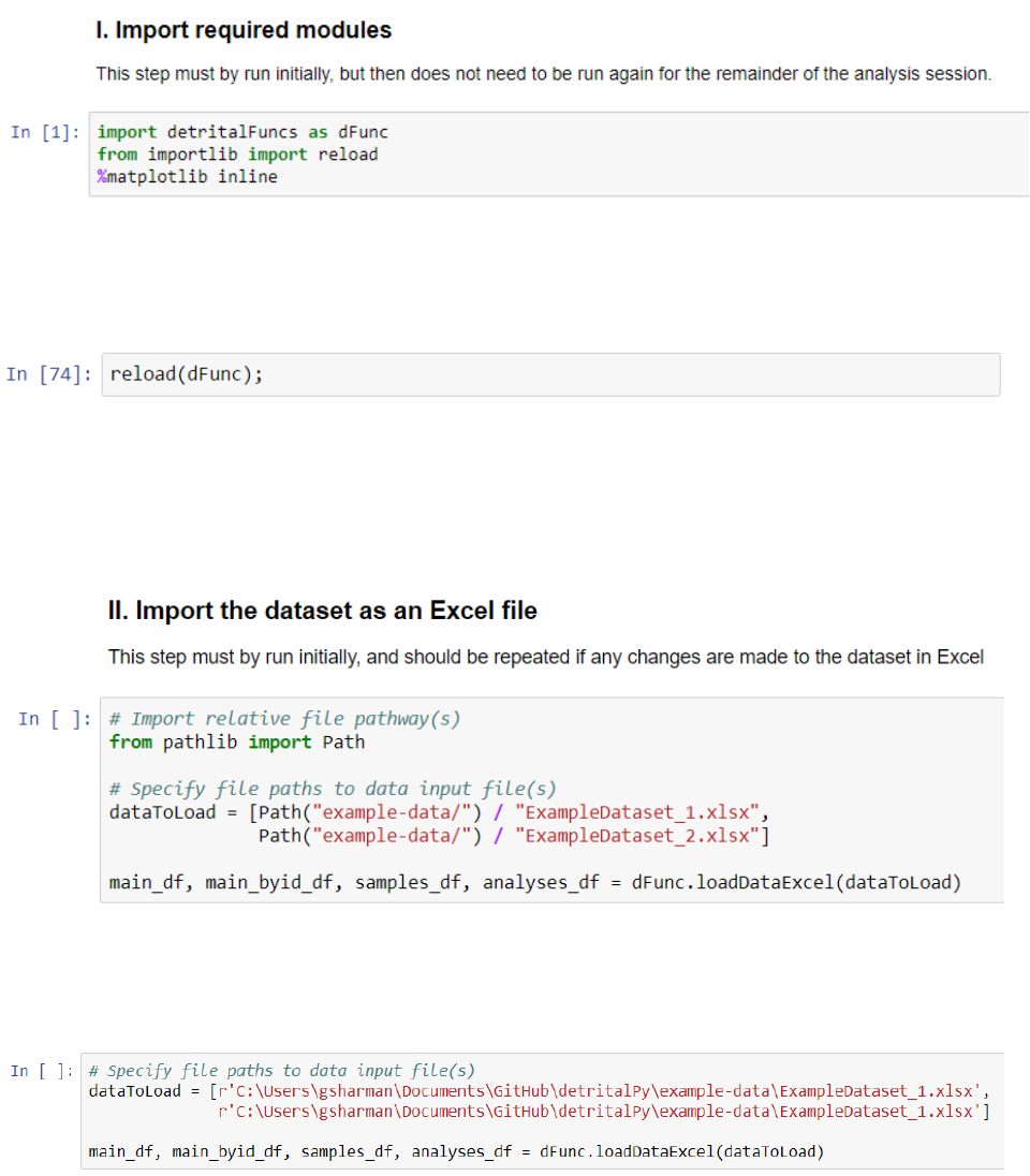
I. Import required modules
The first cell of detritalPy imports the modules that are required for the code to function.
If changes are made to the detritalFuncs.py file, these can be loaded into the notebook session by
executing the following cell:
II. Import the dataset as an Excel file
The Excel file(s) that contains the detrital age dataset(s) is/are imported in Step II.
Relative file paths can be used if the files are in the same folder directory as the detritalPy.ipynb.
Alternatively, file paths can be hard coded. If using Windows, backslashes are acceptable
provided the file path name is preceded by ‘r’ as shown below:
10
In either case, multiple Excel files can be loaded by listing the file paths in the ‘dataToLoad’
array. Data should not be duplicated if loading multiple Excel files, however.
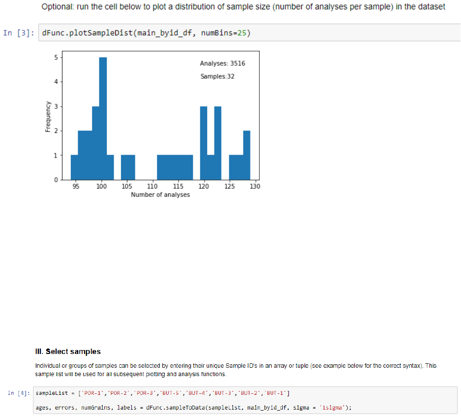
To create a plot of sample size distribution (number of grains per sample), execute the
following cell. The number of grain ages and samples are shown in the upper right portion of the
plot.
Step II should be repeated if any changes are made to the Excel file.
III. Select samples
detritalPy supports two methods of selecting samples for plotting and analysis. (1) Any
number of individual samples can be selected for plotting by entering a list of sample identifiers
in the ‘sampleList’ array, in the format shown below.
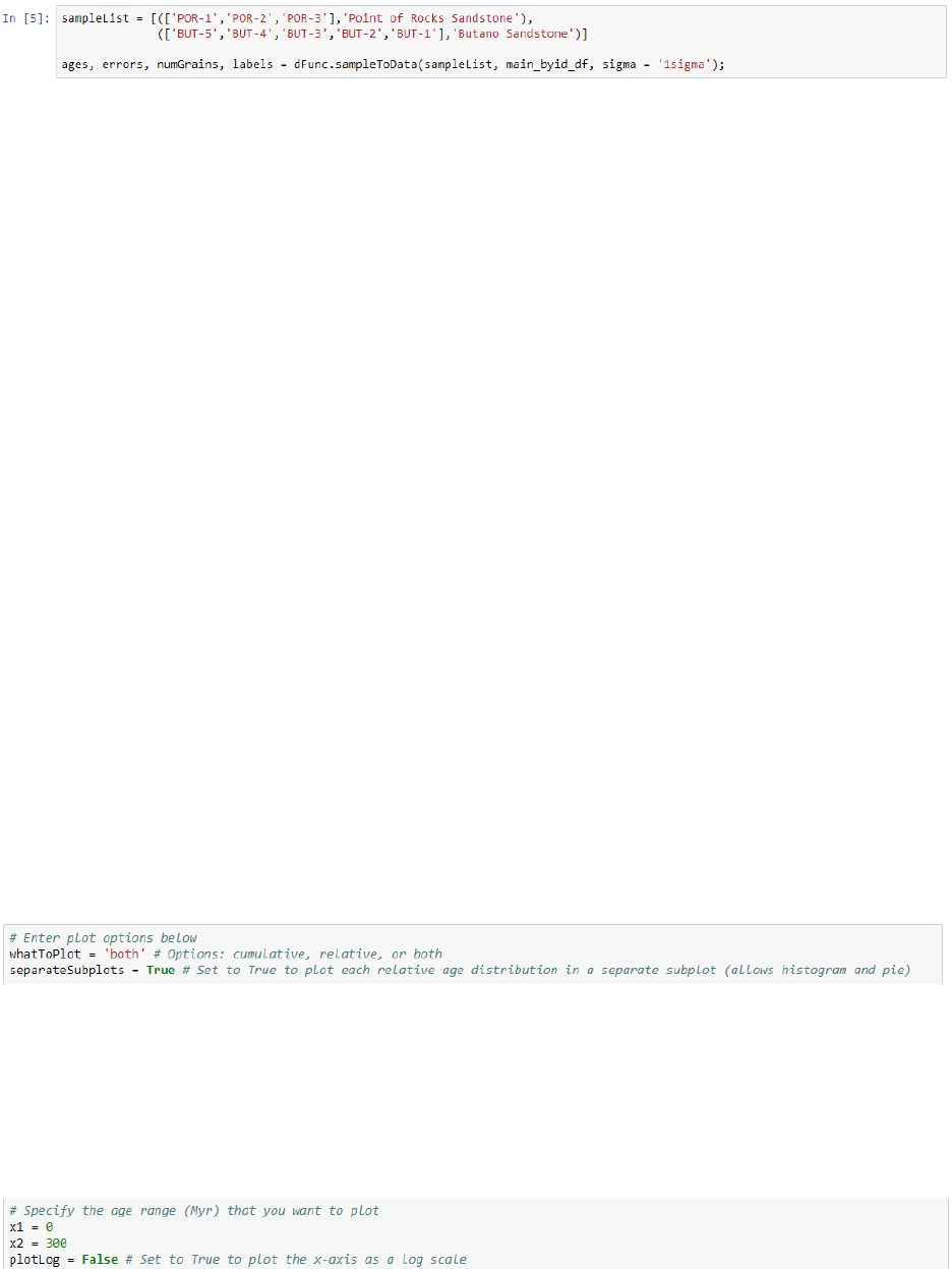
(2) Any number of groups of samples can also be selected by entering a list of sample identifiers
within a tuple data structure, using the format shown below. For each group, a label must be
provided.
11
Step III should be repeated to select a different set of samples or groups of samples for plotting
or analysis. Also, samples or groups of samples will be plotted in the order (top to bottom) that
they are entered into the array or tuple, respectively.
DETRITALPY FUNCTIONS
The primary visualization and analysis functions included with detritalPy are described
below. These functions can be executed in any order.
Plot detrital age distributions
detritalPy provides flexibility in plotting detrital age distributions using a variety of the
most common data visualization approaches. The plotting function is divided into a cumulative
distribution plot (upper panel) and one or more relative distribution plots (lower panel). The
‘whatToPlot’ variable can be set to equal ‘cumulative’, ‘relative’, or ‘both’. When set to
‘both’, the cumulative distribution is shown on top and the relative distribution for each sample
or group of samples is shown below.
Setting ‘separateSubplots’ variable equal to True results in each relative age
distribution being plotted in a separate subplot. This option allows a histogram and pie diagram
to also be plotted with relative age distributions. If ‘separateSubplots’ does not equal True,
relative age distributions will be plotted on top of each other, rather than in separate subplots.
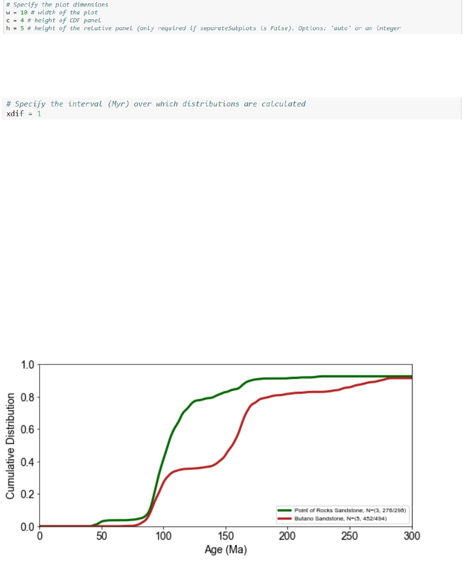
The age range of the plot in Myr can be selected by assigning the variables x1 and x2 that
specify the beginning and age of the plotted age range, respectively. To plot the x-axis on a log
scale, set ‘plotLog’ to True. Note that if x1 = 0, then it will be automatically assigned to equal
0.1.
12
Plot dimensions can be specified using the variables ‘w’, ‘c’, and ‘h’.
The variable ‘xdif’ specifies the discretization interval (in Myr) at which age distributions
are calculated. The default is 1 Myr.
There are three options for plotting a cumulative distribution. Set the variable ‘plotCDF’
to True to plot a standard cumulative distribution function that is discretized at xdif interval. Set
‘plotCPDP’ to True to plot a cumulative (summed) probability density plot (CPDP). Set
‘plotCKDE’ = to True to plot a cumulative (summed) kernel density estimate (CKDE). Both the
CPDP and CKDE produce a smoothed cumulative distribution relative to the unsmoothed CDF.
Cumulative distribution functions are automatically colored by sample or sample group.
The colors that are selected can be customized by modifying the colorMe() function within the
detritalFuncs.py file. Note that the figure legend includes the number of samples (X), the number
of analyses shown in the plotted age range (Y), and the total number of analyses in the sample or
sample group (Z) in the following notation: N=(X, Y/Z).
A 95% confidence interval about the cumulative distribution function can be estimated
based on the Dvoretsky-Kiefer-Wolfowitz inequality (Anderson et al., 2018). This option can be
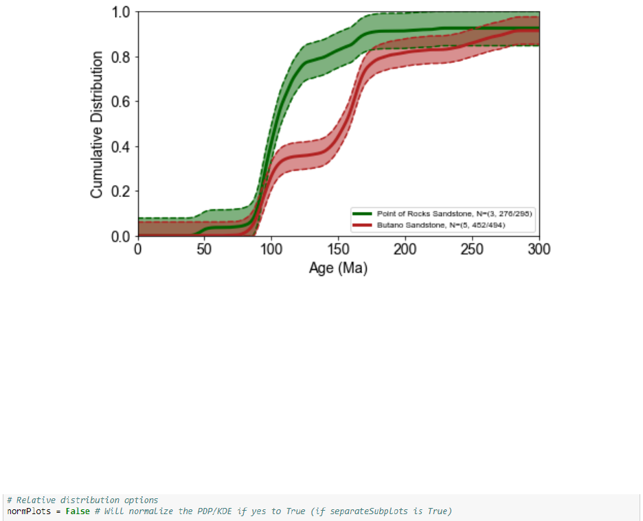
13
enabled by setting the variable variable ‘plotDFW’ to True. By default, the 95% confidence
interval is denoted by shaded lines and transparent shading that are colored the same as the
corresponding CDF.
If relative distributions are selected to be plotted (i.e., ‘whatToPlot’ = ‘relative’ or ‘both’),
then there are a number of options can be selected.
• ‘normPlots’: setting to True will result in relative distributions (i.e., PDP, KDE, and
histogram) having the same y-axis scale. This option also applies if ‘separateSubplots’
equals True; relative distributions are always normalized if ‘separateSubplots’ does not
equal True.
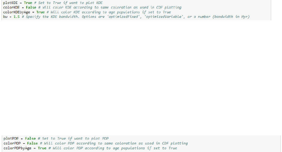
• ‘plotKDE’: setting to True will plot a KDE as a black line.
• ‘colorKDE’: setting to True will fill each KDE plot with a solid color. The color will
match the CDF, CKDE, and/or CPDP, if selected to be plotted. This will only be plotted
if ‘plotKDE’ is set to True.
• ‘colorKDEbyAge’: setting to True will fill each KDE plot with a color spectrum that
corresponds to user-specified age boundaries. The age boundaries and color choices are
specified in the ‘agebins’ and ‘agebinsc’ variables. This will only be plotted if
‘plotKDE’ is set to True.
• ‘bw’: sets the KDE bandwidth. There are three options:
14
o Setting ‘bw’ equal to a number assigns a bandwidth in Myr.
o Setting bw equal to ‘optimizedFixed’ selects an optimized bandwidth for each
sample or sample group, based on Shimazaki and Shinomoto (2010). This option
requires the ‘adaptiveKDE.py’ file to present in the default folder (i.e., same
folder as the ‘detritalFuncs.py’ file.
o Setting bw equal to ‘optimizedVariable’ assigns a bandwidth that varies
depending on the dataset characteristics for each sample or sample group, based
on Shimazaki and Shinomoto (2010). Note that this option can result in very long
processing times, particularly for large numbers of samples or sample groups.
This option requires the ‘adaptiveKDE.py’ file to present in the default folder
(i.e., same folder as the ‘detritalFuncs.py’ file.
• ‘plotPDP’: setting to True will plot a PDP as a black line.
• ‘colorPDP’: setting to True will fill each PDP plot with a solid color. The color will
match the CDF, CKDE, and/or CPDP, if selected to be plotted. This will only be plotted
if ‘plotPDP’ is set to True.
• ‘colorPDPbyAge’: setting to True will fill each PDP plot with a color spectrum that
corresponds to user-specified age boundaries. The age boundaries and color choices are
selected in the ‘agebins’ and ‘agebinsc’ variables (see below). This will only be plotted
if ‘plotPDP’ is set to True.
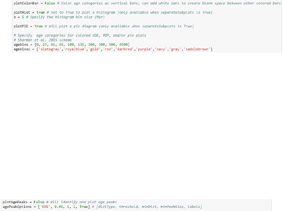
• ‘plotColorBar’: setting to True will result in a vertical color bar being shown on the
cumulative and/or relative plots. The age boundaries and color choices are selected in the
‘agebins’ and ‘agebinsc’ variables (see below).
• ‘plotHist’: setting to True will result in a histogram being plotted.
• ‘b’: specifies the histogram bin size in Myr
15
• ‘plotPIE’: setting to True will result in a pie diagram being plotted to the left of each age
distribution. The age boundaries and color choices are selected in the ‘agebins’ and
‘agebinsc’ variables (see below).
• ‘agebins’: an array that contains the age bin boundaries.
• ‘agebinsc’: an array of colors that correspond to the specified age bin boundaries.
• ‘plotAgePeaks’: setting to True will result in identification of age peaks, based on the
peakutils library that must be installed separately
(https://pypi.python.org/pypi/PeakUtils).
• ‘agePeakOptions’: specifies the parameters used to identify age peaks within an array.
‘distType’ may be set to either ‘KDE’ or ‘PDP’ and specifies which relative distribution
to select age peaks from. ‘threshold’ refers to a y-axis cutoff from which to exclude
potential age peaks. ‘minDist’ refers to an x-axis cutoff which relates to the proximity of
adjacent age peaks. ‘minPeakSize’ refers to the minimum peak height threshold for an
age peak. The age of the age peak (Ma) will be plotted if ‘labels’ is set to True. See
https://pypi.python.org/pypi/PeakUtils and the agePeak() in detritalFuncs.py for more
information.
Executing the cell results in generation of a figure, such as the one below (see also Cover
Image and caption).
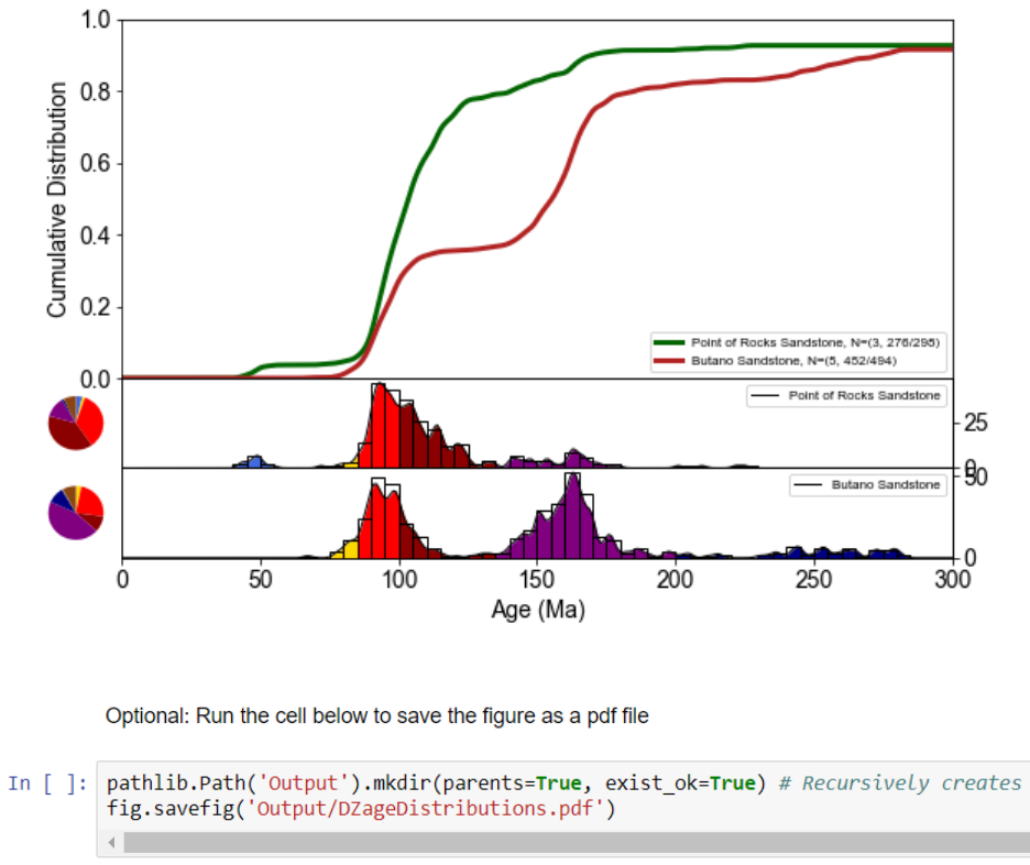
16
The resulting figure can be exported as a PDF file by executing the following cell.
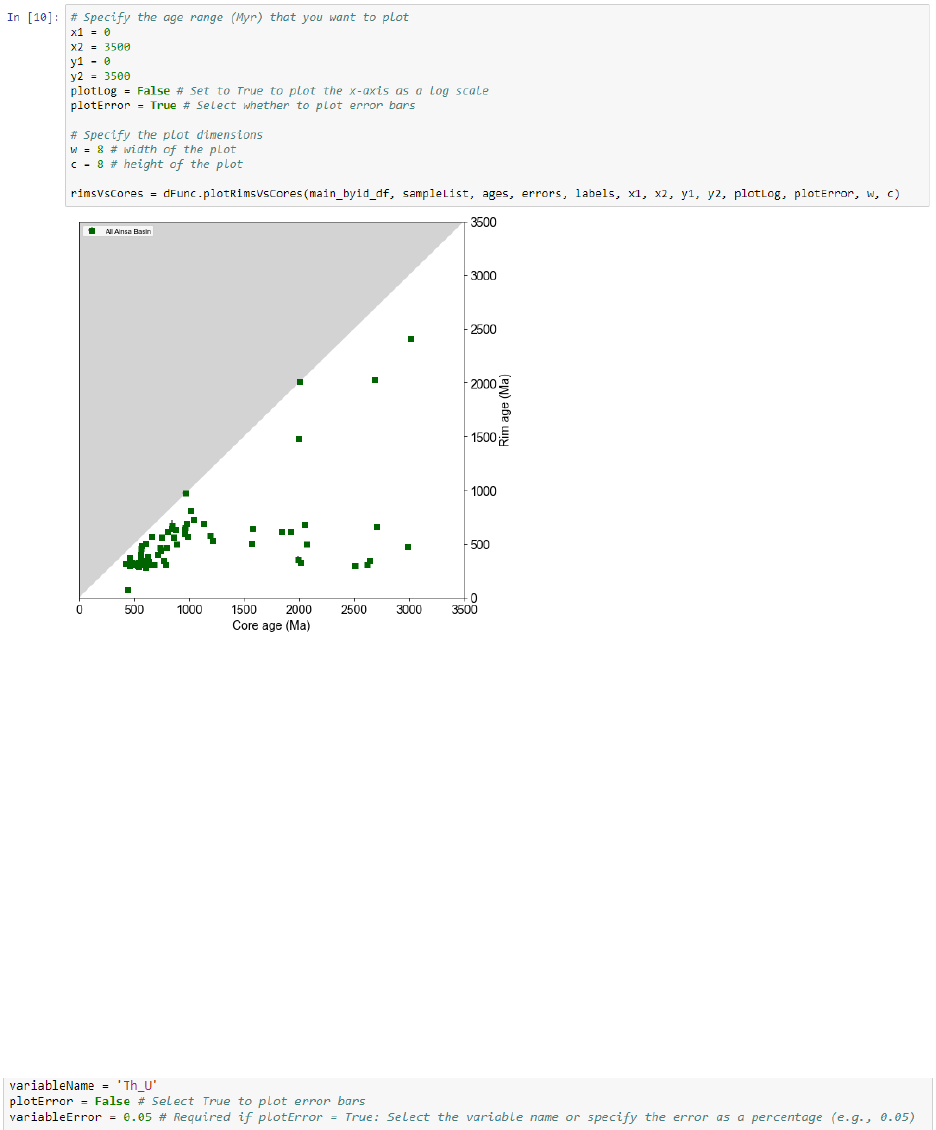
Plot rim age versus core age
Rim ages can be plotted against core ages in a scatterplot. This function requires that the
‘ZrUPb’ worksheet contains 1) a column with a unique grain identifier (default is “Grain_ID”),
and 2) a column that identifies rims and core (default is “RimCore” with “Rim” and “Core”
designations).
• ‘x1’, ‘x2’, ‘y1’, ‘y2’: These variables specify the minimum and maximum x-axis and y-
axis extents, in Ma.
• ‘plotLog’: Setting to True will plot the x-axis as a log scale.
• ‘plotError’: Setting to True will plot error bars.
• ‘w’, ‘c’: These variables specify the width and height of the plot.
17
Plot detrital age distributions in comparison to another variable (e.g., Th/U)
This function allows any numeric variable in the ‘ZrUPb’ worksheet to be plotted
adjacent (above) detrital age distributions for each sample or sample group. Examples could
include the uranium concentration (U_ppm), the thorium to uranium ratio (Th_U), the epsilon
hafnium value (eHf), or the concentration of a trace element.
The variable is selected by assigning the column heading of the desired variable to
‘variableName’. Error bars can be plotted if ‘plotError’ is set to True. ‘variableError’ must
be specified if ‘plotError’ equals True and can be set to a percentage (e.g., 5% error would be
entered as 0.05) or as a column heading that contains the error data (e.g., “Th_U_err”).
Many of the same options for plotting relative age distributions are described above in the
“Plot detrital age distributions” section. In addition, the y-axis scale of the plotted variable can
be selected automatically by setting ‘autoScaleY’ to True. Otherwise, ‘y1’ and ‘y2’ will specify
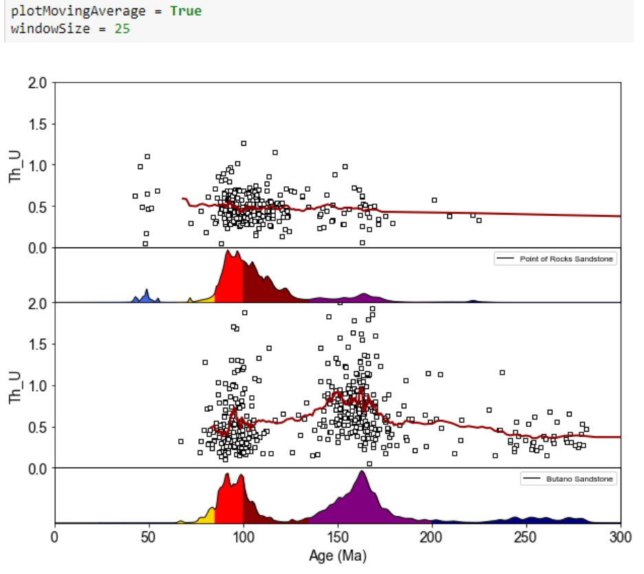
18
the y-axis extents. Plot dimensions can be specified via the ‘w’, ‘t’, and ‘l’ variables. A moving
average can be plotted by setting ‘plotMovingAverage’ to True with the ‘windowSize’ variable
indicating the number of analyses to include in the moving average.
Example plot of Th/U versus PDP plots for the Point of Rocks Sandstone and Butano Sandstone
groups (see example data).
Plot detrital age populations as a bar graph
This function allows detrital age distributions to be plotted as a bar graph, using user-
specified age categories and colors. The dimensions of the plot, bar height, and bar overlap can
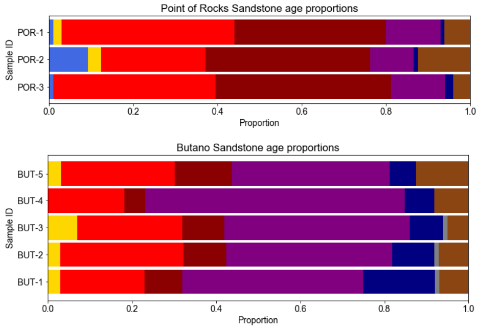
19
be specified using the ‘overlap’, ‘width’, and ‘height’ variables. Setting ‘separateGroups’
equal to True will divide sample groups into individual samples, rather than displaying each
group as a single bar graph. A file name can be assigned to the variable ‘fileName’, and a CSV
file will be automatically saved to the default project folder that contains population abundance
information. Setting ‘savePlot’ to True will automatically save each output plot as a PDF file
within an Output folder in the default project directory. If a folder named “Output” does not
already exist, one will be created.
Example output for the Point of Rocks Sandstone and Butano Sandstone groups (see example
data).
Plot sample locations on an interactive map
Samples with latitude and longitude coordinates (decimal degrees format; WGS84
datum) can be plotted on an interactive map (requires an internet connection). Sample age
distributions can be optionally plotted by clicking on a sample by setting any of the following
variables equal to True: ‘plotMapKDE’, ‘plotMapPDP’, and/or ‘plotCumulative’. If
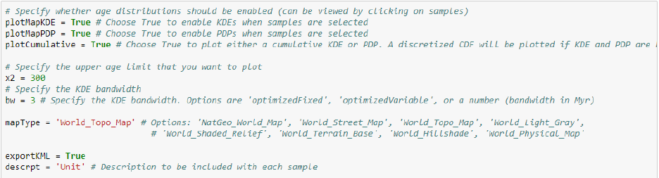
20
‘plotCumulative’ equals True, then the KDE or PDP plot will be plotted as a CKDE or CPDP
plot (provided that either ‘plotMapKDE’ or ‘plotMapPDP’ is also set to True). The upper age
limit of the plot can be specified by setting ‘x2’ equal to a number (Ma).
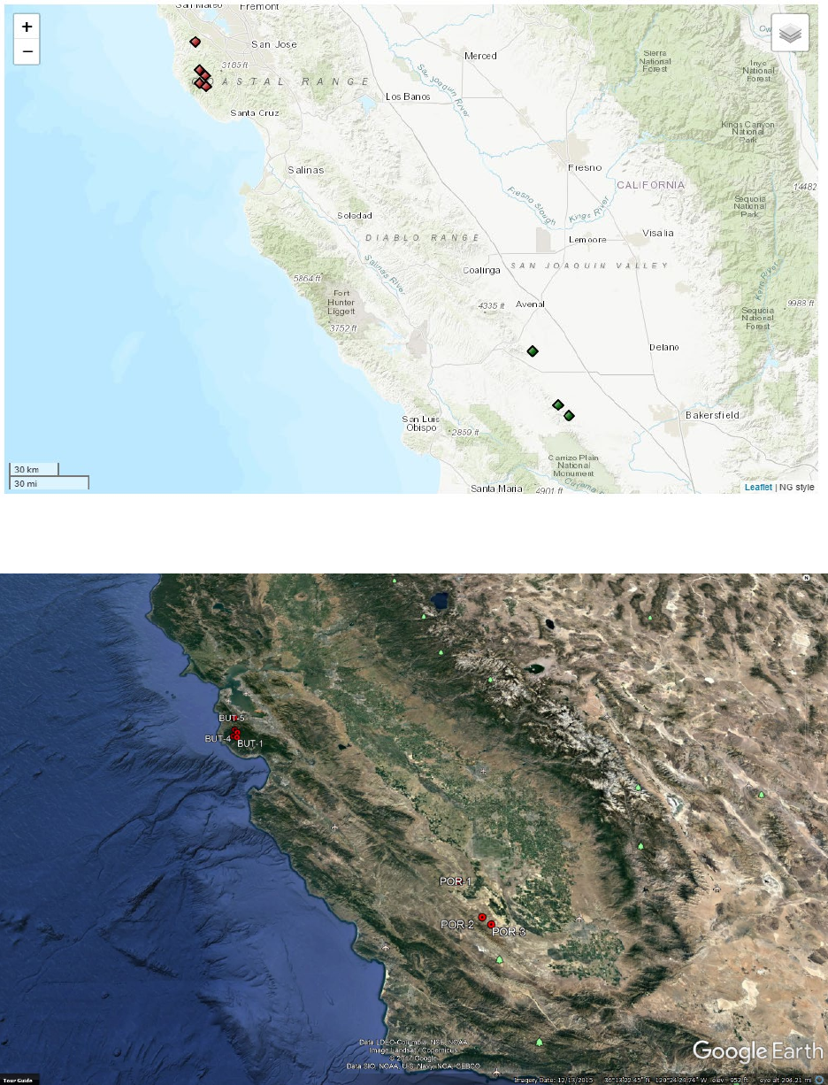
A number of different map options are available, and can be specified via the variable
‘mapType’. If ‘exportKML’ is set to True, a Google Earth KML file will be automatically
exported to the default project folder. A description can be included with each KML data point,
and can be specified via the variable ‘descrpt’ (default is ‘Unit’).
If plotting sample groups, each group will be colored according to the colorMe()
function. We recommend not selecting plotting age distributions if plotting a large number of
samples.
21
Example plot using the ‘World_Topo_Map’ option for the ‘mapType’ variable.
Example Google Earth KML file generated from detritalPy.
22
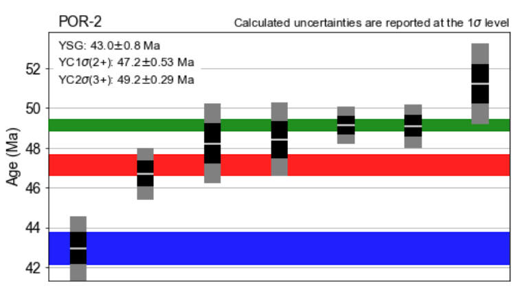
Plot and export maximum depositional age (MDA) calculations
Estimates of maximum depositional age for a sample or sample group can be calculated
and plotted. We use three metrics outlined in Dickinson and Geherls (2009): the youngest single
grain (YSG), the youngest cluster of 2 or more ages with overlapping 1σ uncertainties
(YC1σ(2+)), and the youngest cluster of 3 or more ages with overlapping 2σ uncertainties
(YC2σ(3+)) (see Sharman et al., in press, for additional details).
A CSV file will be automatically generated in the default project folder. It’s name can be
specified via the ‘fileName’ variable. Setting ‘makePlot’ to True will result in a plot of the
youngest detrital ages and each maximum depositional age estimate to be generated for each
sample or sample group. The grain analyses can be sorted by their mean age, mean age plus 1σ
uncertainty, or mean age plus 2σ uncertainty via the variable ‘sortBy’. A number of plot
parameters can be specified via the following variables: ‘plotWidth’, ‘plotHeight’, ‘barWidth’,
‘ageColors’, ‘fillMDACalc’, and ‘alpha’.
Example output showing the youngest detrital analyses and MDA calculations for a single
sample.
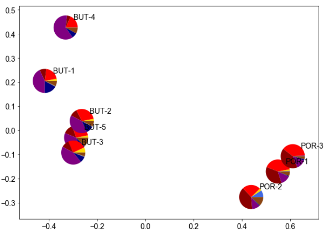
Multi-dimensional scaling
Multi-dimensional scaling (MDS) plots are a popular approach to comparing sample
similarity and dissimilarity (Vermeesch, 2013; Saylor et al., 2017). detritalPy allows plotting
samples or groups of samples using metric or non-metric MDS.
23
Setting the variable ‘metric’ to True results in metric MDS, whereas non-metric MDS
will be used if ‘metric’ does not equal True. Plot dimensions can be specified via the
‘plotWidth’ and ‘plotHeight’ variables. Setting ‘plotPie’ to True will result in pie diagrams
being used as sample markers (age categories can be specified via the ‘agebins’ and ‘agebinsc’
variables). If ‘plotPie’ equals True, then the size of each pie diagrams can be specified via the
‘pieSize’ variable.
Example output using individual samples from the Butano Sandstone and Point of Rocks
Sandstone.
24
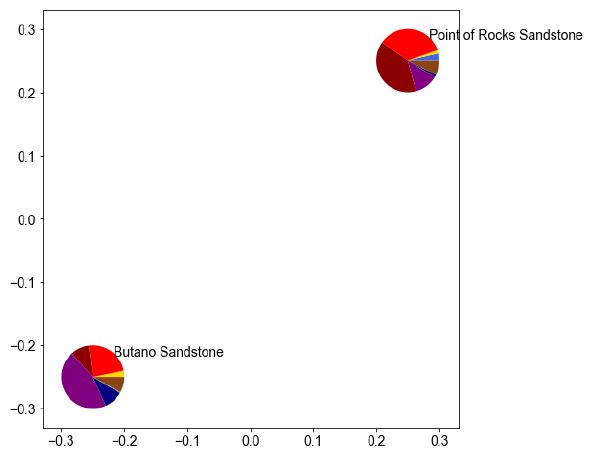
Same data as above, but here plotted as sample groups.
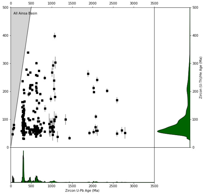
(U-Th)/He vs U-Pb age “double dating” plot
For grains that have been “double dated” (e.g., a detrital zircon having both a U-Pb
crystallization age and a (U-Th)/He cooling age), cooling ages can be plotting against grain
crystallization ages. The default column names in the “ZrUPb” worksheet for the U-Pb
crystallization age and analytical uncertainty are “BestAge” and “BestAge_err”, respectively.
The default column names for the (U-Th)/He cooling age and analytical uncertainty are
“ZHe_Age” and “ZHe_Age_err”, respectively.
The plotting extents of the x-axis and y-axis can be specified via the variables ‘x1’, ‘x2’,
‘y1’, and ‘y2’. Other plotting options are the same as described above in the “Plot detrital age
distributions” section. Set the variable ‘savePlot’ equal to True to save output plots as PDF
files in the Output folder. A separate PDF file will be created for each sample or sample group
plotted.
25
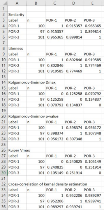
Export sample comparison matrices as a CSV file
A number of metrics have been proposed to assess the similarity and/or dissimilarity of
detrital age distributions (see Saylor and Sundell, 2016). detritalPy current allows computation of
five different metrics for a given list of samples or sample groups: similarity, likeness, the
Kolgomorov-Smirnov statistic, the Kuiper statistic, and the cross-correlation (r2) of either the
KDE or PDP. In addition, the name of the output CSV file can be specified via the ‘fileName’
variable.
The similarity, likeness, and cross-correlation (r2) metrics requires selection of the type of
relative distribution (either KDE or PDP), specified via the variable ‘distType’. By default, all
sample comparison metrics are calculated over the entire age distribution from 0 to 4500 Ma, in
1 Myr bins. Note that the cross-correlation (r2) metric is not independent of the age range it is
computed over.
26
Export detrital age distributions as a CSV file
Raw detrital age distributions can be exported as a CSV file. The ‘exportType’ variable
selects the distribution type to export: a CDF, PDP, or KDE. If ‘cumulative’ equals True, then
the a CPDP or CKDE will be exported, if ‘exportType’ equals ‘PDP’ or ‘KDE’, respectively.
The ‘normalize’ variable specifies whether to require the exported distribution to sum-
to-1. Other variables are the same as described above in the “Plot detrital age distributions”
section.
Export ages and error in tabular format as a CSV file
Some toolsets for analyzing detrital geochronologic data require ages and analytical
uncertainties to be arranged adjacent to each other (e.g., Arizona LaserChron Center Excel
worksheets). detritalPy provides a function for creating a CSV file that contains U-Pb ages and
analytical uncertainties that are automatically sorted from youngest to oldest and listed in
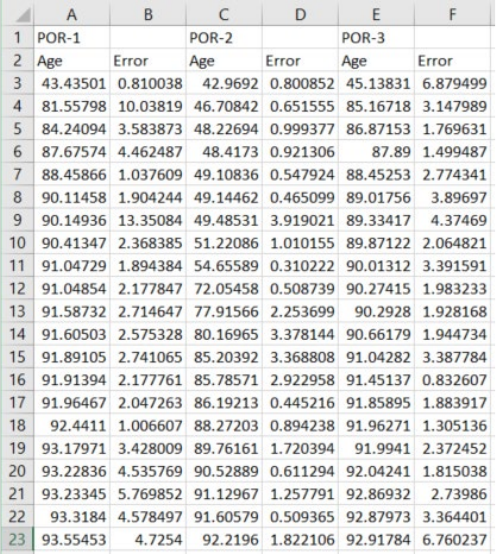
27
adjacent columns. This script can be used to quickly export sample or sample group data for use
in other software that require this data format.
An example of the first 21 detrital analyses exported for samples POR-1, POR-2, and
POR-3 (see example data).
REFERENCES
Anderson, T., Kristoffersen, M. and Elburg, M.A. (2018) Visualizing, interpreting and
comparing detrital zircon age and Hf isotope data in basin analysis – a graphical
approach: Basin Research, 30, 132-147.
Dickinson, W.R. and Gehrels, G.E. (2009) Use of U-Pb ages of detrital zircons to infer
maximum depositional ages of strata: A test against a Colorado Plateau Mesozoic
database: Earth and Planetary Science Letters, 288, 115-125.
Sharman, G.R., Graham, S.A., Grove, M. and Hourigan, J.K. (2013) A reappraisal of the
early slip history of the San Andreas fault, central California, USA: Geology, 41, 727-
730.
Sharman, G.R., Graham, S.A., Grove, M., Kimbrough, D.L. and Wright, J.E. (2015)
Detrital Zircon Provenance of the Late Cretaceous-Eocene California Forearc: Influence
28
of Laramide Low-Angle Subduction on Sediment Dispersal and Paleogeography:
Geological Society of America Bulletin, 127, 38-60.
Sharman, G.R., Sharman, J.P. and Sylvester, Z. (submitted) A Python-based Toolset for
Visualizing and Analyzing Detrital Geo-Thermochronologic Data: The Depositional
Record.
Saylor, J.E. and Sundell, K.E. (2016) Quantifying comparison of large detrital geochronology
data sets: Geosphere, 12, 203-220.
