Dynopt Guide
User Manual:
Open the PDF directly: View PDF ![]() .
.
Page Count: 59

Institute of Information Engineering, Automation, and Mathematics,
Department of Information Engineering and Process Control,
Faculty of Chemical and Food Technology,
Slovak University of Technology in Bratislava,
Radlinsk´eho 9, 812 37 Bratislava, Slovak Republic.
✗
✖
✔
✕
MATLAB DYNamic OPTimisation Code
DYNOPT
M. ˇ
Ciˇzniar
M. Fikar
M. A. Latifi
USER’S GUIDE Version 4.3, March 28, 2017

✬
✫
✩
✪
M. Fikar Institute of Information Engineering, Automation, and Mathematics, De-
partment of Information Engineering and Process Control, Faculty of Chemical
and Food Technology, Slovak University of Technology in Bratislava, Radlin-
sk´eho 9, 812 37 Bratislava, Slovak Republic.
e-mail:miroslav.fikar@stuba.sk, tel: +421 (0)2 593 25 354, fax: +421 (0)2 52 49 64
69
Contact
✬
✫
✩
✪
https://bitbucket.org/dynopt/dynopt_code
http://www.kirp.chtf.stuba.sk/publication_info.php?id_pub=271&lang=en
Internet and Download
✬
✫
✩
✪
M. ˇ
Ciˇzniar, M. Fikar, M. A. Latifi, MATLAB Dynamic Optimisation Code
DYNOPT. User’s Guide, Technical Report, KIRP FCHPT STU Bratislava, Slovak
Republic, 2006.
Reference

Contents
1 Before You Begin 1
1.1 What is dynopt .................................. 1
1.2 What is New in this Version ........................... 1
1.3 How to Use this Manual ............................. 2
1.4 Code, Documentation, and License ....................... 2
1.5 Installation .................................... 2
1.5.1 Manual Installation ............................ 2
1.5.2 Installation using tbxmanager ...................... 3
1.5.3 Optimisation Toolbox .......................... 3
2 Dynamic Optimisation 4
2.1 Optimisation Problem Statement ........................ 4
2.1.1 Cost Functional .............................. 4
2.1.2 Process Model Equations ......................... 5
2.1.3 Constraints ................................ 5
2.2 Optimal Control Problem Solutions ....................... 5
2.3 NLP Formulation Problem ............................ 6
3 Tutorial 10
3.1 ODE systems ................................... 10
3.1.1 Example 1: Unconstrained Problem ................... 10
3.1.2 Example 2: Constrained Problem with Gradients ........... 13
3.1.3 Example 3: Unconstrained Problem with Gradients and Bounds . . . 18
3.1.4 Example 4: Inequality State Path Constraint Problem ........ 21
3.1.5 Example 5: Parameter Estimation Problem .............. 24
3.1.6 Example: Minimum Time Problem ................... 27
3.2 DAE systems ................................... 30
3.2.1 Example 6: Batch Reactor Problem ................... 30
3.3 Maximisation ................................... 32
3.4 Greater than Zero Constraints .......................... 33
i

CONTENTS
4 Reference 34
4.1 Function Arguments ............................... 34
4.1.1 Input Arguments ............................. 35
4.1.2 Output Arguments ............................ 37
4.2 Function Description ............................... 38
4.2.1 Purpose .................................. 38
4.2.2 Syntax and Description .......................... 39
4.2.3 Arguments ................................. 39
4.2.4 Algorithm ................................. 43
4.3 Additional Functions ............................... 44
4.3.1 Function profiles ............................. 44
4.3.2 Function constraints ........................... 44
5 Examples 45
5.1 Problem 4 ..................................... 45
5.2 Problem 5 ..................................... 46
5.3 Problem 6 ..................................... 47
5.4 Problem 7 ..................................... 47
5.5 Problem 9 ..................................... 49
Bibliography 52
ii

List of Figures
2.1 Collocation method on finite elements ...................... 7
3.1 Tutorial example 1: control profile ........................ 13
3.2 Tutorial example 1: state profiles ........................ 13
3.3 Tutorial example 2: control profile ........................ 18
3.4 Tutorial example 2: state profiles ........................ 18
3.5 Tutorial example 3: control profile ........................ 20
3.6 Tutorial example 3: state profiles ........................ 20
3.7 Tutorial example 3: control profile ........................ 21
3.8 Tutorial example 3: state profiles ........................ 21
3.9 Tutorial example 4: control profile ........................ 25
3.10 Tutorial example 4: state profiles ........................ 25
3.11 Tutorial example 4: constraints ......................... 25
3.12 Tutorial example 5: state profiles ........................ 25
3.13 Control and state profiles for minimum time car problem ........... 29
3.14 Control and state profiles for constrained minimum time car problem . . . . 30
3.15 Tutorial example 6: control profile ........................ 32
3.16 Tutorial example 6: state profiles ........................ 32
5.1 Problem 4: Control profile ............................ 46
5.2 Problem 4: State profiles ............................. 46
5.3 Problem 5: Control profile ............................ 47
5.4 Problem 4: State profiles ............................. 47
5.5 Problem 6: Control profile ............................ 48
5.6 Problem 6: State profiles ............................. 48
5.7 Control and state profiles for problem 7 ..................... 50
5.8 Diafiltration problem: optimal α(left), concentrations (middle), and volume
(right) as functions of time ............................ 51
iii

CHAPTER 1
Before You Begin
1.1 What is dynopt
dynopt is a set of MATLAB functions for determination of optimal control trajectory by
given description of the process, the cost to be minimised, subject to equality and inequality
constraints, using orthogonal collocation on finite elements method.
The actual optimal control problem is solved by complete parametrisation both the con-
trol and the state profile vector. That is, the original continuous control and state profiles
are approximated by a sequence of linear combinations of some basis functions. It is as-
sumed that the basis functions are known and optimised are the coefficients of their linear
combinations. In addition, each segment of the control sequence is defined on a time interval
whose length itself may also be subject to optimisation. Finally, a set of time independent
parameters may influence the process model and can also be optimised.
It is assumed, that the optimised dynamic model may be described by a set of ordinary
differential equations (ODE’s) or differential-algebraic equations (DAE’s).
1.2 What is New in this Version
Version 4 introduces several new properties of the package:
•three type of constraints can be defined in the same time: constraints in t0, constraints
over full time interval [t0, tf], and constraints in tf. Previously only one of them was
possible.
•time independent parameters are introduced into the process function, objfun function
and confun.
Version 4.2 enables definition of min/max constraints on state and control independently on
each interval (see Section 3.1.3).
Version 4.3 makes possible to use different NLP solvers (see Chapter 3.1.2 for example of
use Ipopt and Chapter 4for reference).
1

1.3. HOW TO USE THIS MANUAL
1.3 How to Use this Manual
This manual has four main parts:
Chapter 2 introduces implementation of orthogonal collocation on finite elements method
into general optimisation problems.
Chapter 3 provides a tutorial for solving different optimisation problems.
Chapter 4 provides a detailed reference description of dynopt function. Reference descrip-
tions include the function syntax, detailed information about arguments to the func-
tion, including relevant optimisation options parameters.
Chapter 5 provides some more examples solved by dynopt, their definitions and solutions.
1.4 Code, Documentation, and License
Starting with the version 4.3, dynopt has been moved to bitbucket and both source code of
the toolbox and this documentation are available.
Project:
https://bitbucket.org/dynopt/
Code:
https://bitbucket.org/dynopt/dynopt_code
Documentation:
https://bitbucket.org/dynopt/dynopt_doc
dynopt is free of charge to use and is openly distributed, but note that (YALMIP license)
•Copyright is owned by Miroslav Fikar.
•dynopt must be referenced when used in a published work (give me some credit for
saving your valuable time!)
•dynopt, or forks or versions of dynopt, may not be re-distributed as a part of a com-
mercial product unless agreed upon with the copyright owner (if you make money from
dynopt, let me in first!)
•dynopt is distributed in the hope that it will be useful, but WITHOUT ANY WAR-
RANTY; without even the implied warranty of MERCHANTABILITY or FITNESS
FOR A PARTICULAR PURPOSE (if your satellite crash or you fail your Phd due to
a bug in dynopt, your loss!).
•Forks or versions of dynopt must include, and follow, this license in any distribution.
1.5 Installation
1.5.1 Manual Installation
Download dynopt from:
https://bitbucket.org/dynopt/dynopt_code/downloads/dynopt_4.3.0.zip.
2

1.5. INSTALLATION
dynopt needs fminsdp toolbox [19] to be installed. For convenience, it is packed in
the fminsdp directory, but feel free to get it from the original location. To install it, add
directories fminsdp,fminsdp/interfaces, and fminsdp/utilities to MATLAB path.
Next, install dynopt: add the directory dynoptim to MATLAB path.
Both packages can be installed by getting into dynopt directory in MATLAB and running
the following commands:
addpath([pwd ’/dynoptim’]);
addpath([pwd ’/fminsdp’]);
addpath([pwd ’/fminsdp/interfaces’]);
addpath([pwd ’/fminsdp/utilities’]);
and then saving the path for future.
1.5.2 Installation using tbxmanager
tbxmanager (https://www.tbxmanager.com) is a tool to install and manage several third
party optimisation toolboxes for MATLAB. The complete list of available packages is disponible
at its home page.
Install tbxmanager according to directions at its home page. Then, dynopt is installed
(or upgraded) as:
tbxmanager install dynopt
tbxmanager update dynopt
1.5.3 Optimisation Toolbox
dynopt is a set of functions that extend the capability of the MATLAB Optimization Toolbox.
That means, that for using dynopt this toolbox has to be provided. To determine if the
Optimization Toolbox is installed on your system, type this command at the MATLAB
prompt:
ver
After entering this command, MATLAB displays information about the version of MATLAB
you are running, including a list of all toolboxes installed on your system and their version
numbers. If the Optimization Toolbox is not installed, check the Installation Guide for
instructions on how to install it.
dynopt has been developed and tested since MATLAB 6.5 (R13). The results in this
guide are obtained with MATLAB 2015a (Linux 64b) using solvers fmincon and ipopt. It is
quite usual that results obtained and convergence criteria achieved with different versions of
MATLAB or its toolboxes can/will produce slightly different (better, worse) results.
3

CHAPTER 2
Dynamic Optimisation
This chapter deals with dynamic optimisation in general. The chapter starts with several
dynamic optimisation problem definitions. Finally, this chapter ends with the NLP problem
formulation.
2.1 Optimisation Problem Statement
The objective of dynamic optimisation is to determine, in open loop control, a set of time
dependent decision variables (pressure, temperature, flow rate, current, heat duty, . . . ) that
optimise a given performance index (or cost functional or optimisation criterion)(cost, time,
energy, selectivity, . . . ) subject to specified constraints (safety, environmental and operating
constraints). Optimal control refers to the determination of the best time-varying profiles in
closed loop control.
2.1.1 Cost Functional
The performance index (cost functional or optimisation criterion) can in general be written
in one of three forms as follows:
Bolza form
J(u(t),p, tf) = G(x(tf),p, tf) + Ztf
t0F(x(t),u(t),p, t)dt(2.1)
Lagrange form
J(u(t),p, tf) = Ztf
t0F(x(t),u(t),p, t)dt(2.2)
Mayer form
J(u(t),p, tf) = G(x(tf),p, tf) (2.3)
where
4

2.2. OPTIMAL CONTROL PROBLEM SOLUTIONS
J(·) – optimisation criterion,
G(·) – component of objective function evaluated at final conditions,
Rtf
t0F(·)dt– component of the objective function evaluated over a period of time,
x(t) – vector of state variables,
u(t) – vector of control variables,
p– vector of time independent parameters,
t0, tf– initial and final times.
Note that all three forms are interchangeable and can be derived one from another. In the
sequel, Mayer form will be used.
2.1.2 Process Model Equations
The behaviour of many of processes can in general be described either by a set of ordinary
differential equations (ODE’s) or by a set of differential-algebraic equations (DAE’s) as
follows:
M˙x(t) = f(x(t),u(t),p, t),x(t0) = x0over t0≤t≤tf(2.4)
with initial condition for states x0which may also be a function of some time independent
parameters. Here Mis a constant mass matrix. This ODE or DAE system forms equality
constraint in optimal control problem.
2.1.3 Constraints
Constraints to be accounted for typically include equality and inequality infinite dimensional,
interior-point, and terminal-point constraints [10]. Moreover, they may be written in the
following canonical form similar to the cost form (2.3):
Ji(u(t),p, ti) = Gi(x(ti),p, ti) (2.5)
where ti≤tf,i= 1,...,nc, and nc is the number of constraints.
2.2 Optimal Control Problem Solutions
There are several approaches that can solve optimal control problems. These can be divided
into analytical methods that have been used originally and numerical methods preferred
nowadays. In this work only numerical methods are considered.
The numerical methods used for the solution of dynamic optimisation problems can
then be grouped into two categories: indirect and direct methods. In this work only direct
methods are considered. In this category, there are two strategies: sequential method and
simultaneous method. The sequential strategy, often called control vector parameterisation
(CVP), consists in an approximation of the control trajectory by a function of only few
parameters and leaving the state equations in the form of the original ODE/DAE system [10].
In the simultaneous strategy often called total discretisation method, both the control and
5

2.3. NLP FORMULATION PROBLEM
state variables are discretised using polynomials (e.g., Lagrange polynomials) of which the
coefficients become the decision variables in a much larger NLP problem [4]. Implementation
of this method is subject of this work.
Next section reviews the general NLP formulation for optimal control problems using
orthogonal collocation on finite elements method.
2.3 NLP Formulation Problem
As mentioned before, the optimal control problem will be solved by complete parametrisation
of both the control and the state profile vector [13,14]. That means, that the control and state
profiles are approximated by a linear combination of some basis functions. It is expected
here, that the basis functions are known so only the coefficients of linear combination of
these fundamentals have to be optimised. In addition, each control sequence segment is
defined on time interval, which length itself can be the optimised variable. Finally, a set of
time independent parameters may influence the process model and can also be optimised.
As mentioned in section sec:pme, it is supposed that the optimised dynamic model can be
described either by an ODE system or by an DAE system.
Consider the following general control problem for t∈[t0, tf]:
min
u(t),p,tf{G(x(tf),p, tf)}(2.6)
such that
M˙x(t) = f(x(t),u(t),p, t),x(t0) = x0(p)
h(x(t),u(t),p, t) = 0
g(x(t),u(t),p, t)≤0
x(t)L≤x(t)≤x(t)U
u(t)L≤u(t)≤u(t)U
pL≤p≤pU
with following nomenclature:
h(·) – equality design constraint vector,
g(·) – inequality design constraint vector,
x(t)L,x(t)U– state profile bounds,
u(t)L,u(t)U– control profile bounds,
pL,pU– parameter bounds.
In order to derive the NLP problem the differential equations are converted into algebraic
equations using collocation on finite elements. Residual equations are then formed and solved
as a set of algebraic equations. These residuals are evaluated at the shifted roots of Legendre
polynomials. The procedure is then following: Consider the initial-value problem over a finite
element iwith time t∈[ζi, ζi+1]:
M˙x=f(x(t),u(t),p, t)t∈[t0, tf] (2.7)
6
2.3. NLP FORMULATION PROBLEM
ζi−1ζiζi+1 ζi+2
∆ζi
xi−1,0xi−1,1xi−1,2xi,0xi,1xi,2xi+1,0xi+1,1xi+1,2xi+2,0
ui−1,1ui−1,2ui,1ui,2ui+1,1ui+1,2
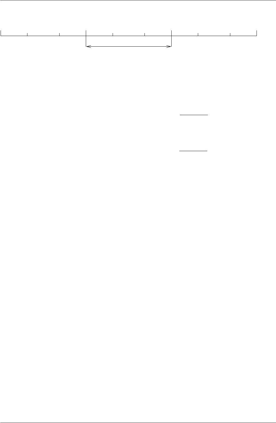
Figure 2.1: Collocation method on finite elements for state profiles, control profiles and element lengths
(Kx=Ku= 2)
The solution is approximated by Lagrange polynomials over element i, ζi≤t≤ζi+1 as
follows:
xKx(t) =
Kx
X
j=0
xij φj(t); φj(t) =
Kx
Y
k=0,j
(t−tik)
(tij −tik)(2.8)
in element i i = 1,...,NE
uKu(t) =
Ku
X
j=1
uij θj(t); θj(t) =
Ku
Y
k=1,j
(t−tik)
(tij −tik)(2.9)
in element i i = 1,...,NE
Here k= 0, j means kstarting form 0 and k6=j, NE is the number of elements. Also xKx(t)
is a (Kx+ 1)th degree piecewise polynomial and uKu(t) is piecewise polynomial of order
Ku. The polynomial approximating the state xtakes into account the initial conditions of
x(t) for each element i. Also, the Lagrange polynomial has the desirable property that (for
xKx(t), for example):
xKx(tij ) = xij (2.10)
which is due to the Lagrange condition φk(tj) = δkj , where δkj is the Kronecker delta. This
polynomial form allows the direct bounding of the states and controls, e.g., path constraints
can be imposed on the problem formulation.
Using K=Kx=Kupoint orthogonal collocation on finite elements as shown in Fig. 2.1,
and by defining the basis functions, so that they are normalised over the each element
∆ζi(τ∈[0,1]), one can write the residual equation as follows:
∆ζir(tik) = M
Kx
X
j=0
xij ˙
φj(τk)−∆ζif(tik,xik,uik,p) (2.11)
i= 1,...,NE, j = 0,...,Kx, k = 1,...,Kx
where ˙
φj(τk) = dtφj/dtτ, and together with φj(τ), θj(τ) terms (basis functions), they are
calculated beforehand, since they depend only on the Legendre root locations. Note that
tik =ζi+∆ζiτk. This form is convenient to work with when the element lengths are included
as decision variables. The element lengths are also used to find possible points of discontinuity
for the control profiles and to insure that the integration accuracy is within a numerical
tolerance. Additionally, the continuity of the states is enforced at element endpoints (interior
knots ζi, i = 2, ..., NE), but it is allowed that the control profiles to have discontinuities at
these endpoints. Here
xi
Kx(ζi) = xi−1
Kx(ζi) (2.12)
i= 2,...,NE
7

2.3. NLP FORMULATION PROBLEM
or
xi0=
Kx
X
j=0
xi−1,j φj(τ= 1) (2.13)
i= 2,...,NE, j = 0,...,Kx
These equations extrapolate the polynomial xi−1
Kx(t) to the endpoints of its element and
provide an accurate initial conditions for the next element and polynomial xi
Kx(t).
At this point a few additional comments concerning construction of the control profile
polynomials must be made. Note that these polynomials use only Kucoefficients per element
and are of lower order than the state polynomials. As a result these profiles are constrained
or bounded only at collocation points. The constraints of the control profile are carried out
by bounding the values of each control polynomial at both ends of the element. This can be
done by writing the equations:
uL
i≤ui
Ku(ζi)≤uU
ii= 1,...,NE (2.14)
uL
i≤ui
Ku(ζi+1)≤uU
ii= 1,...,NE (2.15)
Note that since the polynomial coefficients of the control exist only at collocation points,
enforcement of these bounds can be done by extrapolating the polynomial to the endpoints
of the element. This is easily done by using:
ui
Ku(ζi) =
Ku
X
j=1
uij θj(τ= 0), i = 1,...,NE (2.16)
and
ui
Ku(ζi+1) =
Ku
X
j=1
uij θj(τ= 1), i = 1,...,NE (2.17)
Adding these constraints affects the shape of the final control profile and the net effect of
these constraints is to keep the endpoint values of the control profile from varying widely
outside their ranges [uL
i,uU
i].
The NLP formulation consists of the ODE model (2.4) discretised on finite elements,
continuity equation for state variables, and any other equality and inequality constraints
that may be required. It is given by
min
xij ,uij ,p,∆ζihG(xf,p, tf)i(2.18)
8

2.3. NLP FORMULATION PROBLEM
such that
x10 −x0(p) = 0
r(tik) = 0i= 1,...,NE k= 1,...,Kx
xi0−xi−1
Kx(ζi) = 0i= 2,...,NE
xf−xNE
Kx(ζNE+1) = 0
uL
i≤ui
Ku(ζi)≤uU
ii= 1,...,NE
uL
i≤ui
Ku(ζi+1)≤uU
ii= 1,...,NE
uL
ij ≤uKu(τj)≤uU
ij i= 1,...,NE j= 1,...,Ku
xL
ij ≤xKx(τj)≤xU
ij i= 1,...,NE j= 0,...,Kx
∆ζL
i≤∆ζi≤∆ζU
ii= 1,...,NE
pL≤p≤pU
NE
X
i=1
∆ζi=tf
h(tij ,xij ,uij ,p) = 0
g(tij xij ,uij ,p)≤0
where irefers to the time-interval, j, k refers to the collocation point, ∆ζirepresents finite-
element length of each time-interval i= 1,...,NE, xf=x(tf), and xij ,uij are the colloca-
tion coefficients for the state and control profiles. Problem (2.6) can be now solved by any
large-scale nonlinear programming solver.
To solve this problem within MATLAB, default settings of dynopt use the Optimization
Toolbox and its function fmincon. This can minimise/maximise given objective function with
respect to nonlinear equality and inequality constraints. In order to use this function it was
necessary to create and program series of additional functions. These additional functions
together with fmincon are formed within dynopt which is simple for user to employ. This
function is presented in next chapter.
Alternate nonlinear programming solvers can be used thanks to interface fminsdp. This
version of dynopt was also tested with Ipopt [20].
9

CHAPTER 3
Tutorial
This chapter discusses the dynopt application. It shows, that dynopt is suitable for a quite
large variety of problems ranging from simple unconstrained problem to inequality state path
constraint problem described either by ODE’s or DAE’s. As mentioned in the title of this
chapter, it is an step by step tutorial. It shows the user how to define his problem into
dynopt by filling the input argument functions process,objfun,confun.
3.1 ODE systems
3.1.1 Example 1: Unconstrained Problem
Consider a simple integrator with LQ cost function to be optimised [17,18]:
˙x1=u, x1(0) = 1 (3.1)
˙x2=x2
1+u2, x2(0) = 0 (3.2)
The cost function is given in the Mayer form:
min
u(t)J=x2(tf) (3.3)
with x1(t), x2(t) as states and u(t) as control, such that tf= 1.
Function process,objfun definitions
Problem (3.3) is described by two differential equations which together with initial values of
state variables should be defined in process.
Step1: Write an M-file process.m
function sys = process(t,x,flag,u,p)
switch flag,
10

3.1. ODE SYSTEMS
case 0 % f(x,u,p,t)
sys = [u;x(1)^2+u^2];
case 1 % df/dx
sys = [];
case 2 % df/du
sys = [];
case 3 % df/dp
sys = [];
case 4 % df/dt
sys = [];
case 5 % x0
sys = [1;0];
case 6 % dx0/dp
sys = [];
case 7 % M
sys = [];
case 8 % unused flag
sys = [];
otherwise
error([’unhandled flag = ’,num2str(flag)]);
end
It is important to notice that in dynopt the mass matrix M(2.4) is by default a nx-by-nx
identity matrix. Here nx represents the number of state variables x.
As the performance index is given in Mayer form, dynopt optimises it at final conditions,
thus the input arguments of objfun are as follows: t- scalar value tf,x- scalar/vector of
state variable(s), u- scalar/vector of control variable(s), both evaluated at corresponding
final time tf,p- scalar/vector of time independent parameters. objfun should be defined as
follows:
Step2: Write an M-file objfun.m
function f = objfun(t,x,u,p)
f = [x(2)];
After the problem has been defined in the functions, user has to invoke the dynopt
function by writing an M-file problem1a.m as follows:
Step3: Invoke dynopt
options = optimset(’LargeScale’,’off’,’Display’,’iter’);
options = optimset(options,’MaxFunEvals’,1e6);
options = optimset(options,’TolFun’,1e-7);
options = optimset(options,’TolCon’,1e-7);
options = optimset(options,’TolX’,1e-7);
options = optimset(options,’MaxIter’,4000);
options = optimset(options,’Algorithm’,’interior-point’); %2013b
%options = optimset(options,’Algorithm’,’sqp’); %2010a
11

3.1. ODE SYSTEMS
%options = optimset(options,’Algorithm’,’active-set’); %2008b
optimparam.optvar = 3;
optimparam.objtype = [];
optimparam.ncolx = 3;
optimparam.ncolu = 2;
optimparam.li = ones(3,1)*(1/3);
optimparam.tf = 1;
optimparam.ui = zeros(1,3);
optimparam.par = [];
optimparam.bdu = [];
optimparam.bdx = [];
optimparam.bdp =[];
optimparam.objfun = @objfun;
optimparam.confun = [];
optimparam.process = @process;
optimparam.options = options;
[optimout,optimparam]=dynopt(optimparam)
save optimresults optimout optimparam
[tplot,uplot,xplot] = profiles(optimout,optimparam,50);
save optimprofiles tplot uplot xplot
graph
In this case the variables: t,uwere chosen as decision variables, so the parameter
optimparam.optvar was set to 3. As the objective is to minimise the functional in Mayer
form the parameter optimparam.objtype was left an empty matrix. Moreover 3 colloca-
tion points for state variables (optimparam.ncolx), 2 collocation points for control variables
(optimparam.ncolu), 3 time intervals with the same initial lengths (optimparam.li) equal
to 1/3 were chosen. Final time tf= 1 was given by the problem definition (optimparam.tf),
the control variable initial values (optimparam.ui) were set to 0 for each time interval.
As can be seen from the problem definition (3.3) no parameters (optimparam.par), no
bounds for the control variables (optimparam.bdu), the state variables (optimparam.bdx),
and the parameters (optimparam.bdp) are needed, so the values of this parameters have
been left an empty matrix. As mentioned before, this problem is unconstrained, so parame-
ter optimparam.confun was set to [ ].
The results returned by dynopt in optimout structure contain the vector of times t, the
vector of optimal control profile u. They are ready to be plotted.
The objective function at the optimal solution [t,u] is returned after 133 iterations in above
mentioned output structure optimout as parameter fval:
optimout.fval = 7.615959e-01
The parameter exitflag tells if the algorithm converged. An exitflag >0 means a local
minimum was found:
optimout.exitflag = 1
More details about the optimisation are given by the optimout.output structure. In this
example, the default selection of the large-scale algorithm has been turned off, so the medium-
12
3.1. ODE SYSTEMS
scale algorithm is used. Also all termination tolerances have been changed. For more infor-
mation about options and dynopt input and output arguments, see Chapter 4.
The user may want to plot also the state profiles but without integrating the process
with respect to the optimal control profile in optimout.u. It is possible to use an additional
function profiles for this reason as follows:
[tplot,uplot,xplot] = profiles(optimout,optimparam,ntimes);
where ntimes represents the density of the points plotted per interval. Note that profiles
are represented by collocation polynomials and not as a solution of the original ODE/DAE
system. Therefore, there might be slight differences with regard to the original problem. For
more precise plots, integrate the original problem with optimal control trajectories.
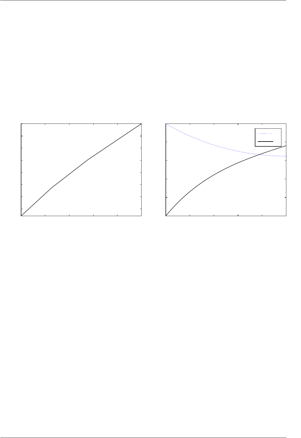
Graphical representation of the problem (3.3) solution is shown in Figs. 3.1 and 3.2.
time
0 0.2 0.4 0.6 0.8 1
u
-0.7
-0.6
-0.5
-0.4
-0.3
-0.2
-0.1
0
Figure 3.1: Control profile for unconstrained problem
time
0 0.2 0.4 0.6 0.8 1
x1, x 2
0
0.2
0.4
0.6
0.8
1
x1
x2
Figure 3.2: State profiles for unconstrained problem
3.1.2 Example 2: Constrained Problem with Gradients
A process described by the following system of 2 ODE’s [17,18]:
˙x1=u, x1(0) = 1 (3.4)
˙x2=x2
1+u2, x2(0) = 0 (3.5)
is to be optimised for u(t) with the cost function:
min
u(t)J=x2(tf) (3.6)
subject to the constraint:
x1(1) = 1 (3.7)
with x1(t), x2(t) as states, u(t) as control, such that tf= 1.
Problem (3.3) is similar to problem (3.6), it differs in constraint of state variable x1at final
time tf= 1. This example will be solved by supplying analytical gradients. Ordinarily the
medium-scale minimisation routines use numerical gradients calculated by finite-difference
approximation. This procedure systematically perturbs each of the variables in order to cal-
culate function and constraint partial derivatives. Alternatively, you can provide a function
to compute partial derivatives analytically. Typically, the problem is solved more accurately
and efficiently if such a function is provided.
13

3.1. ODE SYSTEMS
Function process,objfun,confun definitions
As mentioned before the problem (3.6) is described by the same differential equations as
problem (3.3). As we decided to supply analytical gradients, they should be defined for
all the user supplied functions: process,objfun,confun. The form of the gradients will be
explained on the function process and is valid for all above mentioned user functions.
Step1: Write an M-file process.m
function sys = process(t,x,flag,u,p)
switch flag,
case 0 % f(x,u,p,t)
sys = [u;x(1)^2+u^2];
case 1 % df/dx
sys = [0 2*x(1);0 0];
case 2 % df/du
sys = [1 2*u];
case 3 % df/dp
sys = [];
case 4 % df/dt
sys = [];
case 5 % x0
sys = [1;0];
case 6 % dx0/dp
sys = [];
case 7 % M
sys = [];
case 8 % unused flag
sys = [];
otherwise
error([’unhandled flag = ’,num2str(flag)]);
end
Definition of gradients results from problem definition (3.6). As the problem consists of
one control variable uand two states variables x1, x2just the gradients with respect to this
variables have to be supplied by filling the appropriate flag.
sys in case 1 contains the partial derivatives of the process function, defined as sys in case
0, with respect to each of the elements in x:
sys =
∂f1
∂x1
∂f2
∂x1
∂f1
∂x2
∂f2
∂x2
=0 2x1
0 0
sys in case 2 contains the partial derivatives of the process function, defined as sys in case
0, with respect to each of the elements in u:
sys =h∂f1
∂u
∂f2
∂u i=1 2u
If needed, the gradients with respect to other defined variables (t,p) are filled similarly. For
more information about process definition, and its input and output arguments see chapter
4.
14

3.1. ODE SYSTEMS
As mentioned before user has also to supply the gradients to the objective function objfun
as follows:
Step2: Write an M-file objfun.m
function [f,Df] = objfun(t,x,u,p)
% objective function
f = [x(2)]; % J
% gradients of the objective function
Df.t = []; % dJ/dt
Df.x = [0;1]; % dJ/dx
Df.u = []; % dJ/du
Df.p = []; % dJ/dp
Here they are written in the structure Df containing variables t,u,x, and pand rep-
resenting the gradients with respect to the appropriate variable. Just the variables used
in problem are filled by user. Unused variables are set to be an empty matrix. For more
information about objfun definition, and its input and output arguments see chapter 4.
dynopt optimises a given performance index, subject to the constraints defined at the
beginning t=t0(flag = 0), over the full time interval t∈[t0, tf] (flag = 1), and at the end
t=tf(flag = 2). Thus the input arguments of confun are the same as of process but it is
necessary to tell dynopt by defining the constraints and their gradients with respect to the
appropriate variables in the corresponding flag in which time should they be evaluated. How
the gradients have to seem like, was explained before. confun should be defined as follows:
Step3: Write an M-file confun.m
function [c,ceq,Dc,Dceq] = confun(t,x,flag,u,p)
switch flag
case 0 % constraints in t0
c = [];
ceq = [];
% gradient calculus
if nargout == 4
Dc.t = [];
Dc.x = [];
Dc.u = [];
Dc.p = [];
Dceq.t = [];
Dceq.x = [];
Dceq.u = [];
Dceq.p = [];
end
case 1 % constraints over interval [t0,tf]
c = [];
ceq = [];
15

3.1. ODE SYSTEMS
% gradient calculus
if nargout == 4
Dc.t = [];
Dc.x = [];
Dc.u = [];
Dc.p = [];
Dceq.t = [];
Dceq.x = [];
Dceq.u = [];
Dceq.p = [];
end
case 2 % constraints in tf
c = [];
ceq = [x(1)-1];
% gradient calculus
if nargout == 4
Dc.t = [];
Dc.x = [];
Dc.u = [];
Dc.p = [];
Dceq.t = [];
Dceq.x = [1;0];
Dceq.u = [];
Dceq.p = [];
end
end
Here the gradients are written into the structures Dc,Dceq similar to those, described in
objfun. For more information about confun definition, and its input and output arguments
see chapter 4.
Since you are providing the gradients of the objective function in objfun.m and the
gradients of the constraints in confun.m, you must tell dynopt that these M-files contain this
additional information. Use optimset to turn the parameters GradObj and GradConstr to
’on’ in our already existing options structure
options = optimset(options,’GradObj’,’on’,’GradConstr’,’on’);
If you do not set these parameters to ’on’ in the options structure, dynopt will not use the
analytic gradients.
After the problem has been defined in the functions, user has to invoke the dynopt
function by writing an M-file problem1b.m as follows :
Step4: Invoke dynopt
options = optimset(’LargeScale’,’off’,’Display’,’iter’);
options = optimset(options,’GradObj’,’on’,’GradConstr’,’on’);
options = optimset(options,’MaxFunEvals’,1e4);
options = optimset(options,’MaxIter’,2e3);
16

3.1. ODE SYSTEMS
options = optimset(options,’TolFun’,1e-7);
options = optimset(options,’TolCon’,1e-6);
options = optimset(options,’TolX’,1e-7);
options = optimset(options,’Algorithm’,’interior-point’); %2013b
%options = optimset(options,’Algorithm’,’sqp’); %2010a
%options = optimset(options,’Algorithm’,’active-set’); %2008b
%options.NLPsolver=’ipopt’;
optimparam.optvar = 3;
optimparam.objtype = [];
optimparam.ncolx = 6;
optimparam.ncolu = 2;
optimparam.li = ones(4,1)*(1/4);
optimparam.tf = 1;
optimparam.ui = zeros(1,4);
optimparam.par = [];
optimparam.bdu = [];
optimparam.bdx = [0 1;0 1];
optimparam.bdp =[];
optimparam.objfun = @objfun;
optimparam.confun = @confun;
optimparam.process = @process;
optimparam.options = options;
[optimout,optimparam]=dynopt(optimparam)
save optimresults optimout optimparam
[tplot,uplot,xplot] = profiles(optimout,optimparam,50);
save optimprofiles tplot uplot xplot
%graph
As this problem differs from the problem (3.3) in the constraint applied in final time
tf= 1, the input parameter optimparam.confun is set to the constraint function name
@confun. Next, 6 collocation points for state variables, 4 intervals with the same initial
lengths of intervals equal to 1/4 have been chosen. Other parameters are as same as in
problem (3.3).
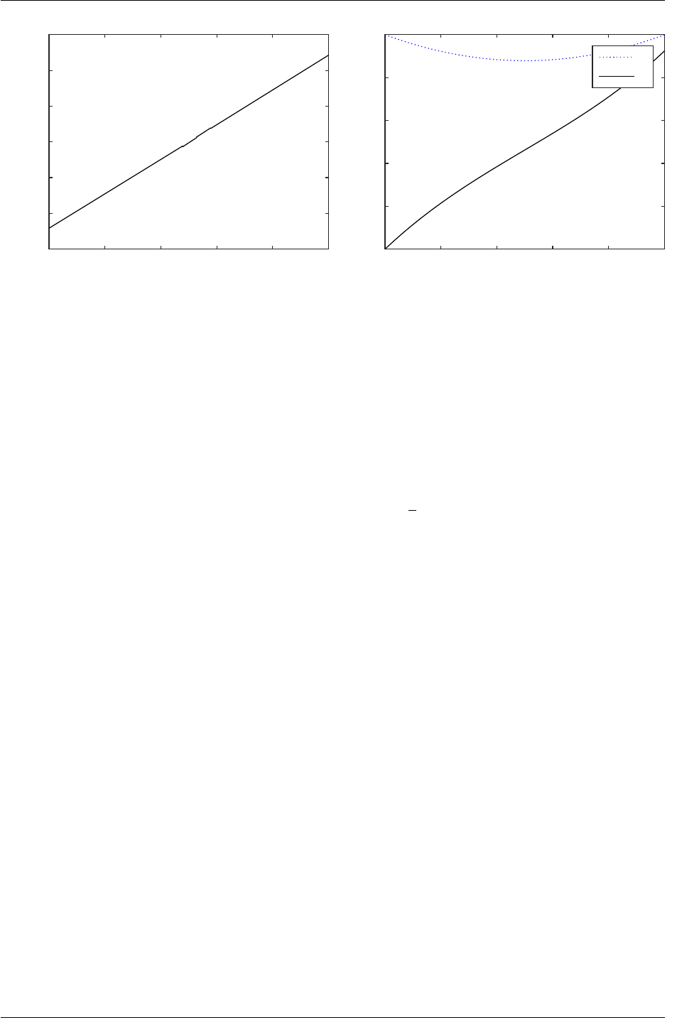
The optimal solution is shown in Figs. 3.3 and 3.4. The value of the objective function
at this solution is 9.245704e-01 after 1440 iterations and with exitflag equal to 2.
Alternative NLP solver Ipopt can be invoked when uncommenting the line
options.NLPsolver=’ipopt’;
in the main file. A slightly better value of the optimum is found in 622 iterations and the
value of the objective function is 9.242380-01. More about alternate NLP solvers can be
found in Chapter 4.
17
3.1. ODE SYSTEMS
time
0 0.2 0.4 0.6 0.8 1
u
-0.6
-0.4
-0.2
0
0.2
0.4
Figure 3.3: Control profile for constrained problem
with gradients
time
0 0.2 0.4 0.6 0.8 1
x1, x 2
0
0.2
0.4
0.6
0.8
1
x1
x2
Figure 3.4: State profiles for constrained problem with
gradients
3.1.3 Example 3: Unconstrained Problem with Gradients and
Bounds
Following mathematical problem [16,18] with system of four ODE’s:
˙x1=x2, x1(0) = 0 (3.8)
˙x2=−x3u+ 16t−8, x2(0) = −1 (3.9)
˙x3=u, x3(0) = −√5 (3.10)
˙x4=x2
1+x2
2+ 0.0005(x2+ 16t−8−0.1x3u2)2, x4(0) = 0 (3.11)
is to be optimised for −4≤u(t)≤10 with the cost function:
min
u(t)J=x4(tf) (3.12)
with x1(t)−x4(t) as states, u(t) as control, such that tf= 1.
Function process,objfun,confun definitions
Step1: Write an M-file process.m
function sys = process(t,x,flag,u,p)
switch flag,
case 0 % f(x,u,p,t)
sys = [x(2);
-x(3)*u+16*t-8;
u;
x(1)^2+x(2)^2+0.0005*(x(2)+16*t-8-0.1*x(3)*u^2)^2];
case 1 % df/dx
sys = [0 0 0 2*x(1);
1 0 0 (2*x(2)+2*0.0005*(x(2)+16*t-8-0.1*x(3)*u^2));
0 -u 0 2*0.0005*(x(2)+16*t-8-0.1*x(3)*u^2)*(-0.1*u^2);
18

3.1. ODE SYSTEMS
0 0 0 0];
case 2 % df/du
sys = [0 -x(3) 1 (2*0.0005*(x(2)+16*t-8-0.1*x(3)*u^2)*(-2*0.1*x(3)*u))];
case 3 % df/dp
sys = [];
case 4 % df/dt
sys = [0 16 0 2*0.0005*(x(2)+16*t-8-0.1*x(3)*u^2)*16];
case 5 % x0
sys = [0;-1;-sqrt(5);0];
case 6 % dx0/dp
sys = [];
case 7 % M
sys = [];
case 8 % unused flag
sys = [];
otherwise
error([’unhandled flag = ’,num2str(flag)]);
end
Step2: Write an M-file objfun
function [f,Df] = objfun(t,x,u,p)
% objective function
f = [x(4)]; % J
% gradients of the objective function
Df.t = []; % dJ/dt
Df.x = [0;0;0;1]; % dJ/dx
Df.u = []; % dJ/du
Df.p = []; % dJ/dp
Step3: Invoke dynopt writing an M-file problem2.m as follows:
options = optimset(’LargeScale’,’off’,’Display’,’iter’);
options = optimset(options,’GradObj’,’on’,’GradConstr’,’on’);
options = optimset(options,’MaxFunEvals’,1e5);
options = optimset(options,’MaxIter’,1e5);
options = optimset (options,’TolFun’,1e-7);
options = optimset (options,’TolCon’,1e-7);
options = optimset (options,’TolX’,1e-7);
options = optimset(options,’Algorithm’,’sqp’); %2010a
%options = optimset(options,’Algorithm’,’active-set’); %2008b
% options.NLPsolver=’ipopt’;
optimparam.optvar = 3;
optimparam.objtype = [];
optimparam.ncolx = 6;
optimparam.ncolu = 2;
19
3.1. ODE SYSTEMS
optimparam.li = ones(4,1)*(1/4);
optimparam.tf = 1;
optimparam.ui = ones(1,4)*7;
optimparam.par = [];
optimparam.bdu = [-4 10];
optimparam.bdx = [];
optimparam.bdp =[];
optimparam.objfun = @objfun;
optimparam.confun = [];
optimparam.process = @process;
optimparam.options = options;
[optimout,optimparam]=dynopt(optimparam)
save optimresults optimout optimparam
[tplot,uplot,xplot] = profiles(optimout,optimparam,50);
save optimprofiles tplot uplot xplot
%graph
The value of the objective function evaluated for optimal control profile is of value of
1.202688e-01 after 175 iterations with exitflag equal to 1 (using default NLP solver fmincon).
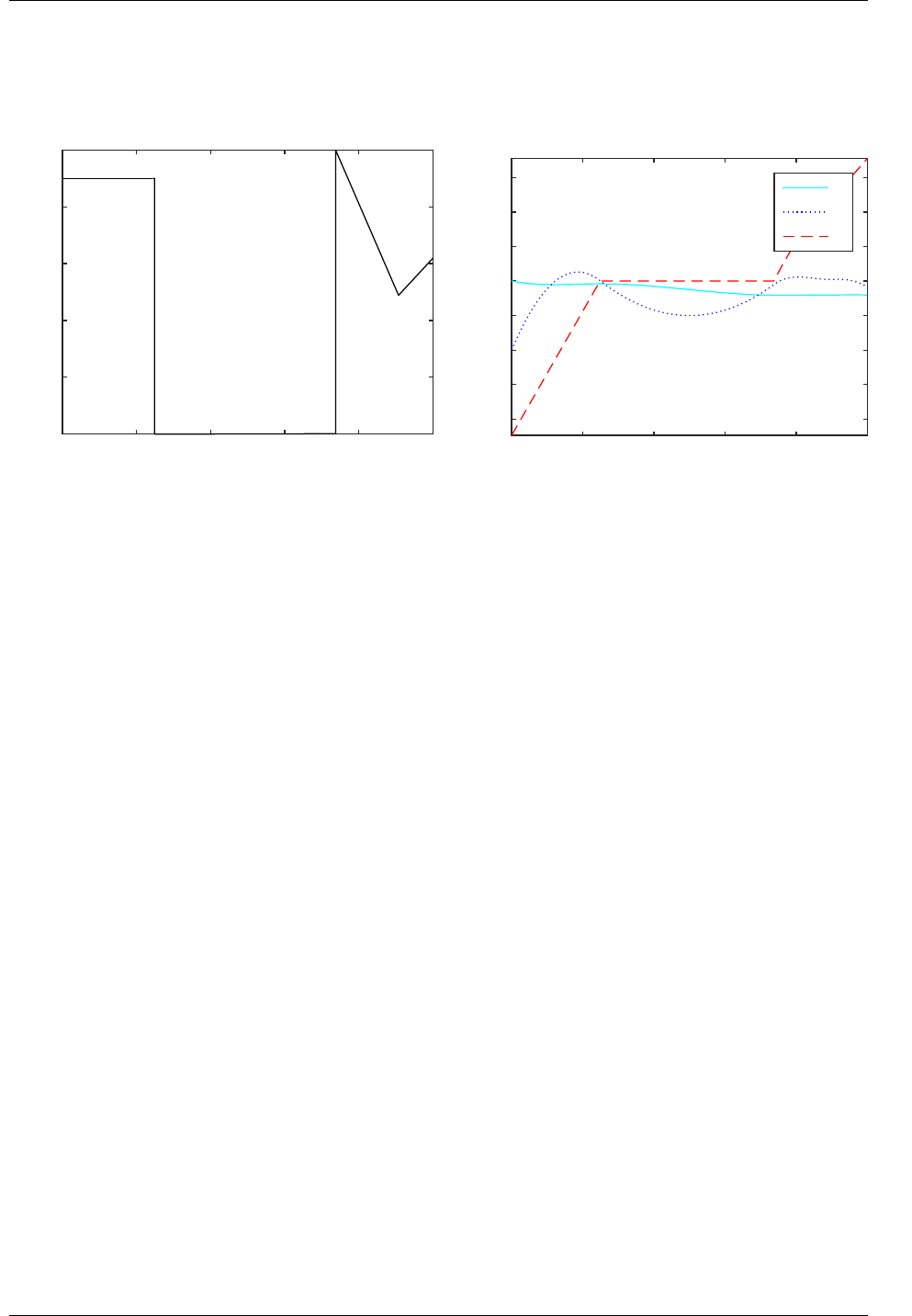
Graphical representation of the solution of the problem (3.12) is shown in Figs. 3.5 and 3.6.
Ipopt solver finished after 1366 iterations with the cost function value of 1.2047839e-01.
time
0 0.2 0.4 0.6 0.8 1
u
0
2
4
6
8
10
Figure 3.5: Control profile for unconstrained problem
with gradients and bounds
time
0 0.2 0.4 0.6 0.8 1
x1, x 2, x 3
-2
-1.5
-1
-0.5
0
0.5
1
1.5 x1
x2
x3
Figure 3.6: State profiles for unconstrained problem
with gradients and bounds
Control Constrained on Intervals
If we would like to constrain control on the first interval to be at most 9, we will redefine
variable bdu (problem2_bdu/problem2bdu.m). Now it will be a matrix composed of lower
and upper bounds on every interval as follows
optimparam.bdu = [-4 9 -4 10 -4 10 -4 10];
20
3.1. ODE SYSTEMS
The value of the objective function evaluated for optimal control profile has increased
to 0.1249686 after 153 iterations with exitflag equal to 1. Graphical representation of the
modified solution is shown in Figs. 3.7 and 3.8.
time
0 0.2 0.4 0.6 0.8 1
u
0
2
4
6
8
10
Figure 3.7: Control profile for unconstrained problem
with gradients and bounds on intervals
time
0 0.2 0.4 0.6 0.8 1
x1, x 2, x 3
-2
-1.5
-1
-0.5
0
0.5
1
1.5 x1
x2
x3
Figure 3.8: State profiles for unconstrained problem
with gradients and bounds on intervals
3.1.4 Example 4: Inequality State Path Constraint Problem
A process described by the following system of 2 ODE’s [6,12]:
˙x1=x2, x1(0) = 0 (3.13)
˙x2=−x2+u, x2(0) = −1 (3.14)
is to be optimised for u(t) with the cost function:
min
u(t)J=Z1
0
(x2
1+x2
2+ 0.005u2)dt(3.15)
subject to state path constraint:
x2−8(t−0.5)2+ 0.5≤0, t ∈[0,1] (3.16)
with x1(t), x2(t) as states, u(t) as control, such that tf= 1.
As the objective function is not in the Mayer form as required by dynopt, we define an
additional differential equation
˙x3=x2
1+x2
2+ 0.005u2, x3(0) = 0 (3.17)
and rewrite the cost as
min
u(t)J=x3(tf) (3.18)
21

3.1. ODE SYSTEMS
Function process,objfun,confun definitions
Step1: Write an M-file process.m
function sys = process(t,x,flag,u,p)
switch flag,
case 0 % f(x,u,p,t)
sys = [x(2);
-x(2)+u;
x(1)^2+x(2)^2+0.005*u^2];
case 1 % df/dx
sys = [0 0 2*x(1);
1 -1 2*x(2);
0 0 0];
case 2 % df/du
sys = [0 1 0.01*u];
case 3 % df/dp
sys = [];
case 4 % df/dt
sys = [];
case 5 % x0
sys = [0;-1;0];
case 6 % dx0/dp
sys = [];
case 7 % M
sys = [];
case 8 % unused flag
sys = [];
otherwise
error([’unhandled flag = ’,num2str(flag)]);
end
Step2: Write an M-file objfun
function [f,Df] = objfun(t,x,u,p)
% objective function
f = [x(3)]; % J
% gradients of the objective function
Df.t = []; % dJ/dt
Df.x = [0;0;1]; % dJ/dx
Df.u = []; % dJ/du
Df.p = []; % dJ/dp
Step3: Write an M-file confun
function [c,ceq,Dc,Dceq] = confun(t,x,flag,u,p)
switch flag
22

3.1. ODE SYSTEMS
case 0 % constraints in t0
c = [];
ceq = [];
% gradient calculus
if nargout == 4
Dc.t = [];
Dc.x = [];
Dc.u = [];
Dc.p = [];
Dceq.t = [];
Dceq.x = [];
Dceq.u = [];
Dceq.p = [];
end
case 1 % constraints over interval [t0,tf]
c = [x(2)-8*(t-0.5)^2+0.5];
ceq = [];
% gradient calculus
if nargout == 4
Dc.t = [-16*t+8];
Dc.x = [0;1;0];
Dc.u = [];
Dc.p = [];
Dceq.t = [];
Dceq.x = [];
Dceq.u = [];
Dceq.p = [];
end
case 2 % constraints in tf
c = [];
ceq = [];
% gradient calculus
if nargout == 4
Dc.t = [];
Dc.x = [];
Dc.u = [];
Dc.p = [];
Dceq.t = [];
Dceq.x = [];
Dceq.u = [];
Dceq.p = [];
end
end
Step4: Invoke dynopt writing an M-file problem3.m as follows:
options = optimset(’LargeScale’,’off’,’Display’,’iter’);
23

3.1. ODE SYSTEMS
options = optimset(options,’GradObj’,’on’,’GradConstr’,’on’);
options = optimset(options,’MaxFunEvals’,1e5);
options = optimset(options,’MaxIter’,1e5);
options = optimset(options,’TolFun’,1e-7);
options = optimset(options,’TolCon’,1e-7);
options = optimset(options,’TolX’,1e-7);
options = optimset(options,’Algorithm’,’sqp’); %2010a
%options = optimset(options,’Algorithm’,’active-set’); %2008b
% options.NLPsolver=’ipopt’;
optimparam.optvar = 3;
optimparam.objtype = [];
optimparam.ncolx = 6;
optimparam.ncolu = 2;
optimparam.li = [ones(7,1)*(1/7)];
optimparam.tf = 1;
optimparam.ui = zeros(1,7);
optimparam.par = [];
optimparam.bdu = [];
optimparam.bdx = [];
optimparam.bdp =[];
optimparam.objfun = @objfun;
optimparam.confun = @confun;
optimparam.process = @process;
optimparam.options = options;
[optimout,optimparam]=dynopt(optimparam)
save optimresults optimout optimparam
[tplot,uplot,xplot] = profiles(optimout,optimparam,50);
[tp,cp,ceqp] = constraints(optimout,optimparam,50);
save optimprofiles tplot uplot xplot tp cp ceqp
%graph
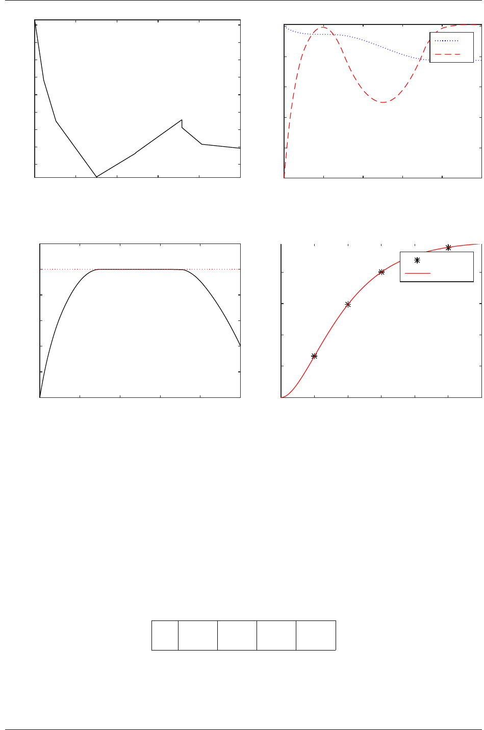
An optimal value of x3(tf) = 0.1701564 was computed after 3069 iterations with exitflag
equal to 1 (using fmincon). Graphical representation of the solution of the problem (3.18)
is shown in Figs. 3.9,3.10, and 3.11.
3.1.5 Example 5: Parameter Estimation Problem
Consider a state estimation problem [8] where the cost functional is defined as the sum of
squares of deviations between the model and measured outputs as follows:
min
pJ=X
i=1,2,3,5
(x1(ti)−xm
1(ti))2(3.19)
24
3.1. ODE SYSTEMS
time
0 0.2 0.4 0.6 0.8 1
u
-2
0
2
4
6
8
10
12
14
Figure 3.9: Control profile for inequality state path
constraint problem
time
0 0.2 0.4 0.6 0.8 1
x1, x 2
-1
-0.8
-0.6
-0.4
-0.2
0
x1
x2
Figure 3.10: State profiles for inequality state path
constraint problem
time
0 0.2 0.4 0.6 0.8 1
c
-2.5
-2
-1.5
-1
-0.5
0
0.5
Figure 3.11: Constraint profile for inequality state
path constraint problem
time
0123456
x1
0
0.2
0.4
0.6
0.8
x1,measured
x1,estimated
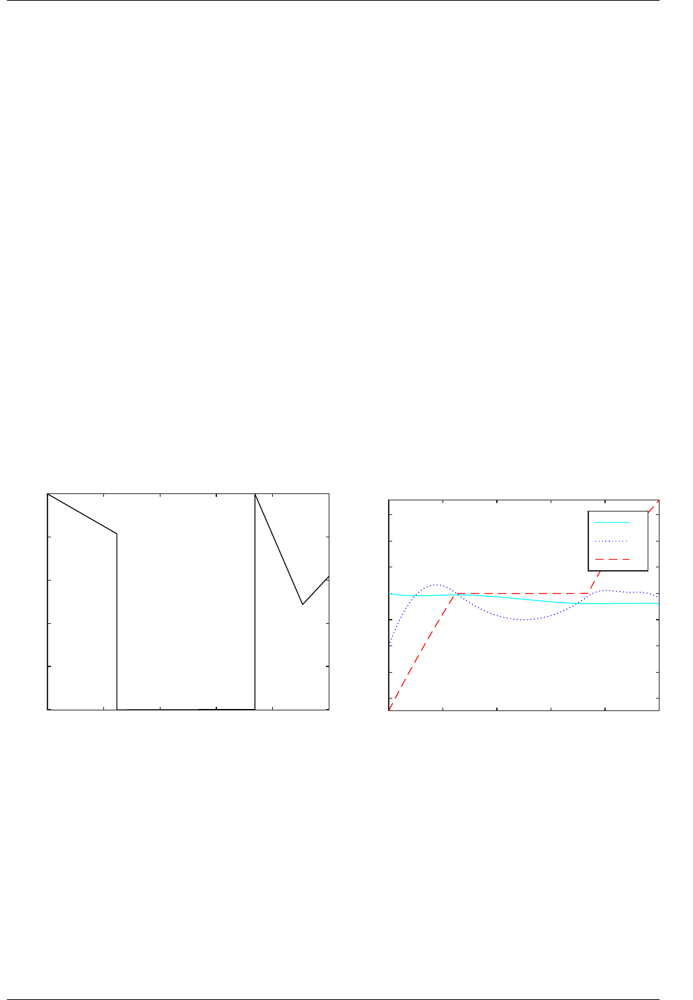
Figure 3.12: Comparison of estimated and measured
state trajectory for state x1in parameter
estimation problem
subject to the following ODE’s:
˙x1=x2, x1(0) = p1(3.20)
˙x2= 1 −2x2−x1, x2(0) = p2(3.21)
with x1, x2as states and tf= 6. The task is to find initial conditions denoted by the
parameters p1, p2∈[−1.5,1.5], if the input to the system is equal to 1. Measured outputs
xm
1and times of measurements are specified in Tab. 3.1.
t1 2 3 5
xm
10.264 0.594 0.801 0.959
Table 3.1: Measured data for parameter estimation problem
25

3.1. ODE SYSTEMS
Function process,objfun,confun definitions
Step1: Write an M-file process.m
function sys = process(t,x,flag,u,p)
switch flag
case 0 % f(x,u,p,t)
sys = [x(2);
1-2*x(2)-x(1)];
case 1 % df/dx
sys = [0 -1;
1 -2];
case 2 % df/du
sys = [];
case 3 % df/dp
sys = [0 0;
0 0];
case 4 % df/dt
sys = [];
case 5 % x0
sys = [p(1);p(2)];
case 6 % dx0dp
sys = [1 0;
0 1];
case 7 % M
sys = [];
case 8 % unused flag
sys = [];
otherwise
error([’unhandled flag = ’,num2str(flag)]);
end
Step2: Write an M-file objfun
function [f,Df] = objfun(t,x,u,p,xm)
% objective function
f = [(x(1)-xm(1))^2]; % J
% gradients of the objective function
Df.t = []; % dJ/dt
Df.x = [2*(x(1)-xm(1));0]; % dJ/dx
Df.u = []; % dJ/du
Df.p = []; % dJ/dp
Step3: Write an M-file confun
Step4: Invoke dynopt writing an M-file problem8.m as follows:
26

3.1. ODE SYSTEMS
options = optimset(’LargeScale’,’off’,’Display’,’iter’);
options = optimset(options,’GradObj’,’on’,’GradConstr’,’on’);
options = optimset(options,’TolFun’,1e-7);
options = optimset(options,’TolCon’,1e-7);
options = optimset(options,’TolX’,1e-7);
options = optimset(options,’Algorithm’,’sqp’); %2010a
%options = optimset(options,’Algorithm’,’active-set’); %2008b
objtype.tm = [1;2;3;5];
objtype.xm = [0.264 0.594 0.801 0.958;
NaN NaN NaN NaN];
optimparam.optvar = 4;
optimparam.objtype = objtype;
optimparam.ncolx = 4;
optimparam.ncolu = [];
optimparam.li = ones(6,1);
optimparam.tf = [];
optimparam.ui = [];
optimparam.par = [0;0];
optimparam.bdu = [];
optimparam.bdx = [];
optimparam.bdp = [-1.5 1.5;-1.5 1.5];
optimparam.objfun = @objfun;
optimparam.confun = [];
optimparam.process = @process;
optimparam.options = options;
[optimout,optimparam]=dynopt(optimparam)
save optimresults optimout optimparam
[tplot,uplot,xplot] = profiles(optimout,optimparam,50);
save optimprofiles tplot uplot xplot
graph
The results obtained by dynopt are the same as those published in [8]. Fig. 3.12 shows
the comparison of estimated and measured state trajectory.
3.1.6 Example: Minimum Time Problem
Consider a following problem optimising a car that has to be moved from origin and stopped
at a distance of 300 m in a minimum time
˙x1=u, x1(0) = 0, x1(tf) = 0 (3.22)
˙x2=x1, x2(0) = 0, x2(tf) = 300 (3.23)
optimised for −2≤u(t)≤1 with the cost function:
min
u(t)J=tf(3.24)
with x1(t) – velocity, x2(t) – distance, u(t) control – acceleration.
27

3.1. ODE SYSTEMS
Function process,objfun,confun definitions
Step1: Write an M-file process.m
function sys = process(t,x,flag,u,p)
switch flag,
case 0 % f(x,u,p,t)
sys = [u;x(1)];
case 1 % df/dx
sys = [0 1;0 0];
case 2 % df/du
sys = [1 0];
case 3 % df/dp
sys = [];
case 4 % df/dt
sys = [];
case 5 % x0
sys = [0;0];
case 6 % dx0/dp
sys = [];
case 7 % M
sys = [];
case 8 % unused flag
sys = [];
otherwise
error([’unhandled flag = ’,num2str(flag)]);
end
Step2: Write an M-file objfun
function [f,Df] = objfun(t,x,u,p)
% objective function
f = [t]; % J
% gradients of the objective function
Df.t = [1]; % dJ/dt
Df.x = []; % dJ/dx
Df.u = []; % dJ/du
Df.p = []; % dJ/dp
Step3: Invoke dynopt writing an M-file car.m as follows. Note that optimising the final
time is indicated by setting it to an empty matrix: optimparam.tf=[] and by optimising
the time interval lengths.
options = optimset(’LargeScale’,’off’,’Display’,’iter’);
options = optimset(options,’GradObj’,’on’,’GradConstr’,’on’);
options = optimset(options,’MaxFunEvals’,1e4);
options = optimset(options,’MaxIter’,1e3);
options = optimset(options,’TolFun’,1e-7);
28
3.1. ODE SYSTEMS
options = optimset(options,’TolCon’,1e-7);
options = optimset(options,’TolX’,1e-7);
options = optimset(options,’Algorithm’,’sqp’); %2010a
%options = optimset(options,’Algorithm’,’active-set’); %2008b
%options.NLPsolver=’ipopt’;
n=2;
optimparam.optvar = 3;
optimparam.objtype = [];
optimparam.ncolx = 3;
optimparam.ncolu = 1;
optimparam.li = 100*ones(n,1)*(1/n);
optimparam.tf = [];
optimparam.ui = zeros(1,n);
optimparam.par = [];
optimparam.bdu = [-2 1];
optimparam.bdx = [0 300;0 400];
optimparam.bdp =[];
optimparam.objfun = @objfun;
optimparam.confun = @confun;
optimparam.process = @process;
optimparam.options = options;
[optimout,optimparam]=dynopt(optimparam)
save optimresults optimout optimparam
[tplot,uplot,xplot] = profiles(optimout,optimparam,50);
save optimprofiles tplot uplot xplot
%graph
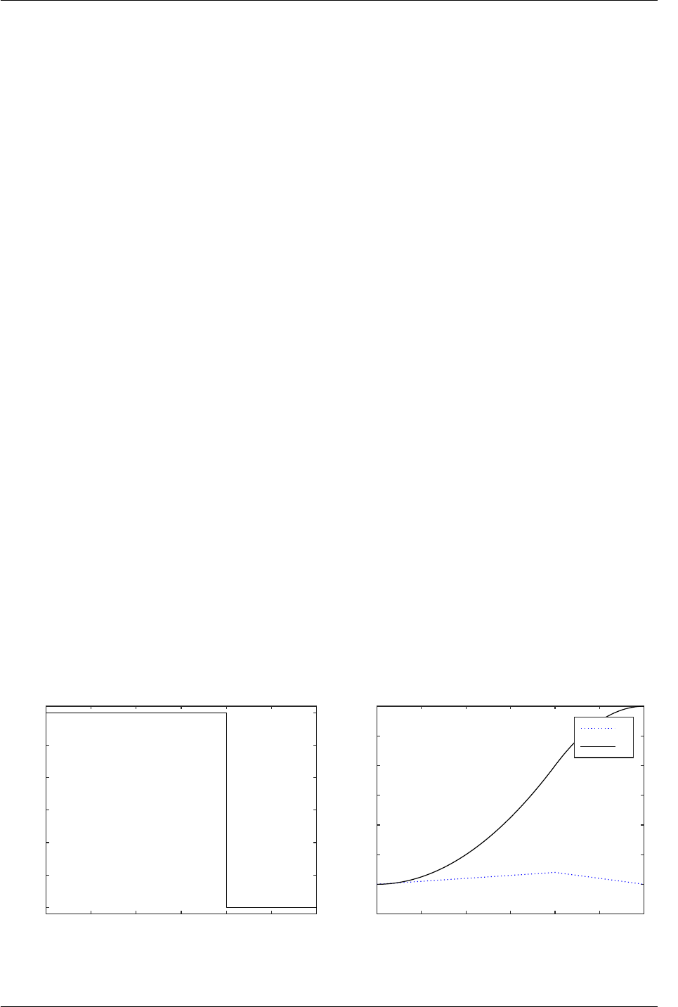
The value of the objective function evaluated for optimal control profile is of value of
30.00 after 85 iterations with exitflag equal to 1 (fmincon) or after 28 iterations (ipopt).
Graphical representation of the solution of the problem (3.24) is shown in Fig. 3.13.
time
0 5 10 15 20 25 30
u
-2
-1.5
-1
-0.5
0
0.5
1
time
0 5 10 15 20 25 30
x1, x 2
-50
0
50
100
150
200
250
300
x1
x2
Figure 3.13: Control and state profiles for minimum time car problem
29

3.2. DAE SYSTEMS
The same problem with constrained velocity during the whole trajectory x2<10 (prob-
lem car2) converged to the minimum value of 37.50 after 139/31 iterations (fmincon/ipopt).
Graphical representation of the solution is shown in Fig. 3.14.
time
0 10 20 30 40
u
-2
-1.5
-1
-0.5
0
0.5
1
time
0 10 20 30 40
x1
-2
0
2
4
6
8
10
12
time
0 10 20 30 40
x2
0
50
100
150
200
250
300
Figure 3.14: Control and state profiles for constrained minimum time car problem
3.2 DAE systems
3.2.1 Example 6: Batch Reactor Problem
Consider a batch reactor [5,18] with the consecutive reactions A→B→C:
max
u(t)J=x2(tf) (3.25)
such that
˙x1=−k1x2
1, x1(0) = 1 (3.26)
˙x2=k1x2
1−k2x2, x2(0) = 0 (3.27)
0 = k1−4000e(−
2500
T)(3.28)
0 = k2−620000e(−
5000
T)(3.29)
with x1, x2as states representing concentrations of A, and B, temperature T∈[298,398] as
control variable, such that tf= 1.
Function process,objfun,confun definitions
Step1: Write an M-file process.m
function sys = process(t,x,flag,u,p)
switch flag
case 0 % f(x,u,p,t)
sys = [-x(3)*(x(1)^2);
x(3)*(x(1)^2)-x(4)*x(2);
x(3)-4000*exp(-u);
x(4)-620000*exp(-2*u)];
case 1 % df/dx
sys = [-2*x(3)*x(1),2*x(3)*x(1),0,0;
30

3.2. DAE SYSTEMS
0,-x(4),0,0;
-(x(1)^2),x(1)^2,1,0;
0,-x(2),0,1];
case 2 % df/du
sys = [0,0,4000*exp(-u),2*620000*exp(-2*u)];
case 3 % df/dp
sys = [];
case 4 % df/dt
sys = [];
case 5 % x0
sys = [1;0;5.0736;0.9975];
case 6 % dx0/dp
sys = [];
case 7 % M
sys = [1,0,0,0;
0,1,0,0;
0,0,0,0;
0,0,0,0];
case 8 % unused flag
sys = [];
otherwise
error([’unhandled flag = ’,num2str(flag)]);
end
Step2: Write an M-file objfun
function [f,Df] = objfun(t,x,u,p)
% objective function
f = [-x(2)]; % J
% gradients of the objective function
Df.t = []; % dJ/dt
Df.x = [0;-1;0;0]; % dJ/dx
Df.u = []; % dJ/du
Df.p = []; % dJ/dp
Step3: Invoke dynopt by writing an M-file problem5dae.m as follows:
options = optimset(’LargeScale’,’off’,’Display’,’iter’);
options = optimset(options,’GradObj’,’on’,’GradConstr’,’on’);
options = optimset(options,’MaxFunEvals’,1e5);
options = optimset(options,’MaxIter’,1e5);
options = optimset(options,’TolFun’,1e-7);
options = optimset(options,’TolCon’,1e-7);
options = optimset(options,’TolX’,1e-7);
options = optimset(options,’Algorithm’,’sqp’); %2010a
%options = optimset(options,’Algorithm’,’active-set’); %2008b
optimparam.optvar = 3;
31
3.3. MAXIMISATION
optimparam.objtype = [];
optimparam.ncolx = 5;
optimparam.ncolu = 2;
optimparam.li = ones(3,1)*(1/3);
optimparam.tf = 1;
optimparam.ui = ones(1,3)*7.35;
optimparam.par = [];
optimparam.bdu = [6.2813 8.3894];
optimparam.bdx = [0 1;0 1;0.9085 7.4936;0.0320 2.1760];
optimparam.bdp =[];
optimparam.objfun = @objfun;
optimparam.confun = [];
optimparam.process = @process;
optimparam.options = options;
[optimout,optimparam]=dynopt(optimparam)
save optimresults optimout optimparam
[tplot,uplot,xplot] = profiles(optimout,optimparam,50);
save optimprofiles tplot uplot xplot
graph
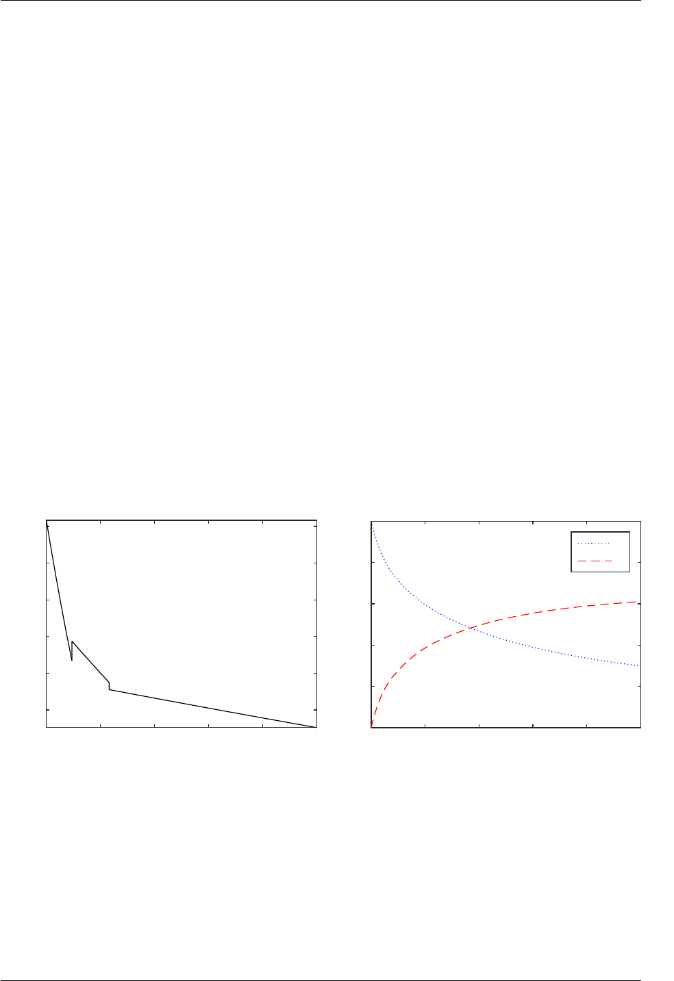
After 134 iterations, optimal value of x2(tf) = 0.6106136 was found using fmincon. The
same solution was found using ipopt but after almost 20000 iterations. Graphical represen-
tation of the problem (3.25) solution is shown in Figs. 3.15 and 3.16.
time
0 0.2 0.4 0.6 0.8 1
u
330
340
350
360
370
380
Figure 3.15: Control profile for batch reactor problem
as DAE problem
time
0 0.2 0.4 0.6 0.8 1
x1, x 2
0
0.2
0.4
0.6
0.8
1
x1
x2
Figure 3.16: State profiles for batch reactor problem
as DAE problem
3.3 Maximisation
dynopt performs minimisation of the objective function f(t, x, u). Maximisation is achieved
by supplying the routine with −f(t, x, u) .
32

3.4. GREATER THAN ZERO CONSTRAINTS
3.4 Greater than Zero Constraints
The Optimisation Toolbox assumes nonlinear inequality constraints are of the form Ci(x)≤
0. Greater than zero constraints are expressed as less than zero constraints by multiplying
them by −1. For example, a constraint of the form Ci(x)≥0 is equivalent to the constraint
−Ci(x)≤0.
33

CHAPTER 4
Reference
This chapter contains description of the function dynopt, the main function of the collection
of functions which extend the capability of MATLAB Optimisation Toolbox, specifically of
the constrained nonlinear minimisation routine fmincon. The chapter starts with section
listing general descriptions of all the input and output arguments and the parameters in the
optimisation options structure, continues with the function description, and ends with some
tutorial.
4.1 Function Arguments
All input and output arguments to the dynopt function are described in this section. Sec-
tion 4.1.1 describes all input arguments built in input structure optimparam. Then output
arguments built in output structure optimout are treated in section 4.1.2 and as last the
optimisation options parameters structure options which is given by MATLAB is described
in Tab. 4.2. It is important to mention here, that the names of input and output structures
can be changed by user, but their fields described later have to be used as described.
ni – number of intervals
nx – number of state variables
nu – number of control variables
np – number of parameters
nm – number of measurements
Table 4.1: Some predefined variables which are used for function description
Table 4.1 describes some predefined variables which are used to simplify dynopt’s de-
scription in sections 4.1.1 and 4.1.2.
34

4.1. FUNCTION ARGUMENTS
4.1.1 Input Arguments
As mentioned before, input arguments described bellow do entry dynopt in a structure
called optimparam. This contains them as fields, e.g., optimparam.optvar.optimparam has
following fields to be set:
optvar – The choice of optimisation variables: 1 - times, 2 - control, 2 - parameters. Their
combination is given by their summations, e.g., 3 - optimise times and control. All the
possibilities are listed below
1 - optimise times,
2 - optimise control,
3 - optimise times and control,
4 - optimise parameters,
5 - optimise times and parameters,
6 - optimise control and parameters,
7 - optimise all: times, control, and parameters.
objtype – Parameter which defines the type of objective function to be minimised/maximised
in optimisation. Two possible types of objective function may have been used:
Mayer type - if Mayer type objective function is used set the parameter objtype to
an empty matrix.
Sum type - if Sum type objective function is used, parameter objtype is a structure
containing two variables tm, and xm.tm is a nm-by-1 vector of times, in which
the measurements are taken. xm is a nx-by-nm matrix of taken measurements in
times tm. For more information about the types of objective functions see objfun
description in section 4.2.3.
ncolx – Parameter which represents the number of collocation points for state variables.
This has always to be a number greater than zero.
ncolu – Parameter which represents the number of collocation points for control variables. It
may have been defined as [ ] if control variable doesn’t belong to optimisation variables
and also doesn’t occur in process,objfun,confun. Otherwise it has to be a number
greater than zero.
li – Parameter representing lengths of intervals. It has always to be filled with ni–by–1
vector of initial lengths of intervals.
tf – Parameter representing the final time, if the value of tfis not specified use empty
brackets [ ].
ui – Parameter representing control variables applied on each time interval in li. As men-
tioned for ncolu parameter, if control variable is needed it has to be defined as nu–by–ni
matrix of control variables for each interval. Otherwise it has to be an empty matrix
[ ].
35

4.1. FUNCTION ARGUMENTS
par – Parameter representing time independent parameters. As in ui also here it may have
been defined either np–by–1 vector of time independent parameters or an empty matrix
[ ].
bdu – Parameter representing bounds to the control variables. If not defined it has to be an
empty matrix [ ]. If control constraints are the same in each time interval then it has
to be an nu–by–2 matrix: [lbu ubu]. If control constraints are not the same in each
time interval then it has to be an nu–by–ni*2 matrix: [lbu1ubu1,...,lbuniubuni]
where niis the number of intervals.
bdx – Parameter representing bounds to the states. If not defined it has to be an empty
matrix [ ]. If state constraints are the same in each time interval then it has to be an
nx–by–2 matrix: [lbx ubx]. If state constraints are not the same in each time interval
then it has to be an nx–by–ni*2 matrix: [lbx1ubx1,...,lbxniubxni] where niis the
number of intervals.
bdp – Parameter representing bounds to the parameters. If defined it has to be an np–by–2
matrix: [lbp ubp], otherwise an empty matrix [ ].
objfun – The function to be optimised. objfun is the name of an M-file. For more information
about this input argument, see section 4.2.3.
confun – The function that computes the nonlinear equality and inequality constraints.
confun is the name of an M-file. For more information about this input argument, see
section 4.2.3.
process – The function that describes given process. process is the name of an M-file. For
more information about this input argument, see section 4.2.3.
options – An optimisation options parameter structure that defines parameters used by the
optimisation functions. This parameter is defined by MATLAB for all optimisation
routines of MATLAB Optimization Toolbox. For information about the parameters
which are important for dynopt, see Tab. 4.2 or the individual function reference pages.
These parameters can be specified using the function optimset.
In addition to these, parameter NLPsolver determines NLP solver using the fminsdp
toolbox. The default one is fmincon but others can be specified as well if installed
separately. This parameter can be set directly as
options.NLPsolver=’ipopt’;
Table 4.2: Optimisation options parameters
Parameter Name Description
DerivativeCheck Compare user-supplied analytic derivatives (gradients) to finite dif-
ferencing derivatives (medium-scale algorithm only), default value:
’off’.
Continued on next page
36

4.1. FUNCTION ARGUMENTS
concluded from previous page
Parameter Name Description
Diagnostics Print diagnostic information about the function to be minimised or
solved, default value: ’off’.
DiffMaxChange Maximum change in variables for finite difference derivatives
(medium-scale algorithm only), default value: 0.1000.
DiffMinChange Minimum change in variables for finite difference derivatives
(medium-scale algorithm only), default value: 1.0000e-008.
Display Level of display. ’off’ displays no output, ’iter’ displays output at each
iteration, ’final’ displays just the final output, default value: ’final’.
GradConstr Gradients for the nonlinear constraints defined by user, default value:
’off’.
GradObj Gradient for the objective function defined by user, default value:
’off’.
LargeScale User large-scale algorithm if possible, default value: ’on’.
MaxFunEvals Maximum number of function evaluations allowed, default value:
’100*numberofvariables’.
MaxIter Maximum number of iterations allowed, default value: 400.
TolCon Termination Tolerance on the constraint violation, default value:
1.0000e-006.
TolFun Termination Tolerance on the function value, default value: 1.0000e-
006.
TolX Termination Tolerance on x, default value: 1.0000e-006.
TypicalX Typical x values (large-scale algorithm only), default value:
’ones(numberofvariables,1)’.
NLPsolver Choice of NLP solver, possible values: ’fmincon’, ’snopt’, ’ipopt’,
’knitro’, ’mma’, ’gcmma’, default: ’fmincon’.
4.1.2 Output Arguments
As for input arguments, the same holds for output arguments. That means that the output
arguments described bellow do leave dynopt in a structure called optimout. This contains
them as fields, e.g., optimout.nlpx.optimout has following fields:
nlpx – holds the solution found by the dynopt. If exitflag >0, then nlpx is a solution
otherwise, nlpx is the value the optimisation routine was at when it terminated pre-
maturely. Vector nlpx contains all the parameters ∆ζi,uij ,xij ,pdefined in the NLP
formulation in section 2.3.
fval – holds the value of the objective function in objfun at the solution nlpx.
exitflag – represents the exit condition of optimisation. exitflag may be:
>0 indicates that the function converged to a solution nlpx,
0 indicates that the maximum number of function evaluations or iterations was reached,
<0 indicates that the function did not converge to a solution.
37

4.2. FUNCTION DESCRIPTION
output – represents an output structure that contains information about the results of the
optimisation. output.iterations gives the information about the number of itera-
tion, output.funcCount gives the information about the number of function evalua-
tions, output.algorithm returns the used algorithm, output.stepsize returns the
taken final stepsize (medium-scale algorithm only), output.firstorderopt gives the
information about a measure of first-order optimality (large-scale algorithm only).
lambda – The Lagrange multipliers at the solution nlpx.lambda is a structure where
each field is for a different constraint type. lamdba.lower for the lower bounds lb,
lambda.upper for the upper bounds ub, lambda.ineqlin for the linear inequalities,
lambda.eqlin for the linear equalities, lambda.ineqnonlin for the nonlinear inequal-
ities, lambda.eqnonlin for the nonlinear equalities.
grad – holds the value of the gradient of objfun at the solution nlpx.
t– is a vector of times for optimal control profile returned by dynopt.
u– is a vector/matrix of optimal control profiles returned by dynopt.
p– is a vector/empty matrix of the optimal values of the parameters.
Function parameters described in section 4.1.2, and Tab. 4.2 are implicitly given by
MATLAB Optimization Toolbox for all it’s subroutines. They also present parameters useful
for dynopt through function fmincon.
4.2 Function Description
4.2.1 Purpose
The actual version of dynopt is able to solve dynamic optimisation problems which cost
functions can be expressed either in the Mayer form or in the Sum form. The problem
formulation can be described by following set of DAEs:
min
u(t),pG(x(tf), tf,p) (4.1)
or
min
u(t),p
nm
X
i=1 S(ti,x(ti),u(ti),p,xmes(ti)) (4.2)
such that
M˙x(t) = f(t, x(t),u(t),p)
x(t0) = x0(p)
h(t, x,u,p) = 0
g(t, x,u,p)≤0
xL
i≤x(t)≤xU
i, i = 1,...,ni
uL
i≤u(t)≤uU
i, i = 1,...,ni
pL≤p≤pU
with the following nomenclature:
38

4.2. FUNCTION DESCRIPTION
G(·) – objective function in Mayer form evaluated at final conditions,
Pnm
i=1 S(·) – objective function of Sum form evaluated in times of taking the measurements
ti,
M– a constant mass matrix,
h– equality design constraint vector,
g– inequality design constraint vector,
x(t) – state profile vector,
u(t) – control profile vector,
p– vector of time independent parameters,
x0– initial conditions for state vector,
xL
i,xU
i– state profile bounds on each interval i= 1,...,ni,
uL
i,uU
i– control profile bounds on each interval i= 1,...,ni,
pL,pU– bounds to the parameters.
4.2.2 Syntax and Description
[optimout,optimparam]=dynopt(optimparam)
starts with the initial lengths of intervals li, initial control values for each interval ui for
defined number of collocation points for state variables ncolx, and for control variables ncolu
to the final time tf, and minimises either a Mayer type objfun evaluated in the final time
or Sum type objfun subject to the nonlinear inequalities or equalities defined in confun for
time t0,tfor over full time interval characterised by flag in confun subject to a given system
in process with the optimisation parameters specified in the structure options, with the
defined set of lower and upper bounds on the control variables bdu, state variables bdx, and
time independent parameters bdp so that solution is always in the range of these bounds.
All before mentioned variables do entry dynopt in optimparam structure. The solution is
returned in the otpimout structure described in section 4.1.2.
4.2.3 Arguments
The arguments passed into the function are described in section 4.1.1. The arguments
returned by the function are described in section 4.1.2. Details relevant to dynopt are
included below for objfun,confun,process.
objfun The function to be minimised. objfun is a string containing the name of an M-file
function, e.g., objfun.m. Whereas dynopt optimises a given performance index
39

4.2. FUNCTION DESCRIPTION
Mayer form (4.1) objective function is evaluated at the final time tf, thus objfun
takes a scalar t- final time tf, scalar/vector x- the state variable(s), scalar/vector
u- the control variable(s), both evaluated at corresponding final time tf, scalar/vector
p- time independent parameters, and returns a scalar value fof the objective
function evaluated at these value. The M-file function has to have the following
form:
function [f] = objfun(t,x,u,p)
f = []; % J
Sum form (4.2) objective function is evaluated in the times of taking measurements
ti, thus objfun takes a scalar t- time of taking measurements ti, scalar/vector x-
state variable(s), u- the control variable(s), both evaluated at corresponding time
ti, scalar/vector p- time independent parameters, scalar/vector xm - measured
variable(s) in the above mentioned time ti, and returns a scalar value fof the
objective function evaluated at these values. The M-file function has to have the
following form:
function [f] = objfun(t,x,u,p,xm)
f = []; % J
If the gradients of the objective function can also be computed and options.GradObj
is ’on’, as set by options = optimset(’GradObj’,’on’) then the function objfun must
return, in the second output argument, the structure Df holding the gradient values
with respect to time t, states x, controls uand parameters pas follows:
function [f,Df] = objfun(t,x,u,p,xm)
% objective function
f = []; % J
% gradient of the objective function
Df.t = []; % dJ/dt
Df.x = []; % dJ/dx
Df.u = []; % dJ/du
Df.p = []; % dJ/dp
The gradients Df.t,Df.x,Df.u,Df.p are the partial derivatives of fat the points t,
x,u,p. That means, Df.t is the partial derivative of fwith respect to the t, the ith
component of Df.x is the partial derivative of fwith respect to the ith component
of x, the ith component of Df.u is the partial derivative of fwith respect to the ith
component of u, the ith component of Df.p is the partial derivative of fwith respect
to the ith component of p.
confun The function that computes the nonlinear inequality constraints g(t, x, u, p)<=0
marked as output argument cand nonlinear equality constraints h(t, x, u, p) = 0,
marked as output argument ceq. As mentioned before, dynopt optimises a given
performance index subject to the constraints defined in corresponding flag:
flag = 0 the constraints are implied at the beginning t=t0,
40

4.2. FUNCTION DESCRIPTION
flag = 1 the constraints are implied over the whole time interval t∈[t0, tf],
flag = 2 the constraints are implied at the end t=tf.
confun is a string containing the name of an M-file function, e.g., confun.m.confun
takes a scalar t- time value corresponding to the time t, scalar/vector x- state variable
value(s), and scalar/vector u- control variable value(s) both corresponding to the value
of t, scalar/vector p- time independent parameters, and returns two arguments, a
vector cof the nonlinear inequalities and a vector ceq of the nonlinear equalities, both
evaluated at t,x,u,pfor given flag. For example, if confun=@confun, then the M-file
confun.m would have the form:
function [c,ceq] = confun(t,x,flag,u,p)
switch flag
case 0 % constraints in t0
% constraints
c = [];
ceq = [];
case 1 % constraints over interval [t0,tf]
% constraints
c = [];
ceq = [];
case 2 % constraints in tf
% constraints
c = [];
ceq = [];
end
If the gradients of the constraints can also be computed and the options.GradConstr
is ’on’, as set by options = optimset(’GradConstr’,’on’) then confun is a string con-
taining the name of an M-file function, e.g., confun.m. The function confun must
return, in the third and fourth output argument, structures Dc, and Dceq holding the
gradient values t,x,u,pwith respect to themselves.
function [c,ceq,Dc,Dceq] = confun(t,x,flag,u,p)
switch flag
case 0 % constraints in t0
% constraints
c = [];
ceq = [];
% gradient the calculus
if nargout == 4
Dc.t = [];
Dc.x = [];
Dc.u = [];
Dc.p = [];
41

4.2. FUNCTION DESCRIPTION
Dceq.t = [];
Dceq.x = [];
Dceq.u = [];
Dceq.p = [];
end
case 1 % constraints over interval [t0,tf]
% constraints
c = [];
ceq = [];
% gradient calculus
if nargout == 4
Dc.t = [];
Dc.x = [];
Dc.u = [];
Dc.p = [];
Dceq.t = [];
Dceq.x = [];
Dceq.u = [];
Dceq.p = [];
end
case 2 % constraints in tf
% constraints
c = [];
ceq = [];
% gradient calculus
if nargout == 4
Dc.t = [];
Dc.x = [];
Dc.u = [];
Dc.p = [];
Dceq.t = [];
Dceq.x = [];
Dceq.u = [];
Dceq.p = [];
end
end
The gradients Dc.t,Dc.x,Dc.u,Dc.p are the partial derivatives of cat the points
t,x,u,p. That means, Dc.t is the partial derivative of cwith respect to t, the ith
component of Dc.x is the partial derivative of cwith respect to the ith component
of x, the ith component of Dc.u is the partial derivative of cwith respect to the ith
component of u, the ith component of Dc.p is the partial derivative of cwith respect
to the ith component of p, and the gradients Dceq.t,Dceq.x,Dceq.u,Dceq.p are the
partial derivatives of ceq at the points t,x,u,p.
process The function which describes process model, that means the right hand sizes of
ODE or DAE equations. If the process model is described by system of ODE’s the
mass matrix M in flag = 7 shall be left an empty matrix, because of being set by
42

4.2. FUNCTION DESCRIPTION
dynopt by default. If the system is describe by DAE’s the mass matrix M in flag =
7 should be singular. process is a string containing the name of an M-file function,
e.g., process.m.process takes a time t, scalar/vector of state variable x, scalar flag,
scalar/vector of control variable u, both corresponding to time t, and scalar/vector
of time independent parameters p, and returns sys values with respect to flag value
evaluated at time t. The M-file function has to be written in the following form:
function sys = process(t,x,flag,u,p)
switch flag
case 0 % f(x,u,p,t)
sys = [];
case 1 % df/dx
sys = [];
case 2 % df/du
sys = [];
case 3 % df/dp
sys = [];
case 4 % df/dt
sys = [];
case 5 % x0
sys = [];
case 6 % dx0/dp
sys = [];
case 7 % M
sys = [];
case 8 % unused flag
sys = [];
otherwise
error([’unhandled flag = ’,num2str(flag)]);
end
4.2.4 Algorithm
Large-scale optimisation By default dynopt will choose the large-scale algorithm of fmin-
con if the user supplies the gradient in objfun (and GradObj is ’on’ in options) and
if only upper and lower bounds exists or only linear equality constraints exist. This
algorithm is a subspace trust region method and is based on the interior-reflective
Newton method described in [3]. Each iteration involves the approximate solution of
a large linear system using the method of preconditioned conjugate gradients (PCG).
See the trust-region and preconditioned conjugate gradient method descriptions in the
Large-Scale Algorithms chapter in [2].
Medium-scale optimisation dynopt uses through the fmincon Sequential Programming
(SQP) method. In this method, a Quadratic Programming (QP) subproblem is solved
at each iteration. An estimate of the Hessian of the Lagrangian is updated at each
iteration using the BFGS formula [3].
A line search is performed using a merit function similar to that proposed by [11]. The
QP subproblem is solved using an active set strategy similar to that described in [9].
43

4.3. ADDITIONAL FUNCTIONS
A full description of this algorithm is found in the Constrained optimisation section of
the Introduction to algorithms chapter of the Optimization Toolbox manual. See also
the SQP implementation section in the Introduction to Algorithms chapter for more
details on the algorithm used.
The software layer of fminsdp toolbox adds different NLP solvers that have to be installed
separately. This version of dynopt was tested with open source solver Ipopt 3.12.4. Note
that ipopt requires user supplied gradients in the cost functions and constraints. If these are
not supplied, fmincon is used instead. For concrete options of this solver and other available
other ones see their documentations.
4.3 Additional Functions
In this section, two functions are presented: profiles, which prepares plot-able state and
control profiles and constraints, which prepares a user given equality and inequality plot-
able constraints from the optimisation results returned in optimout.
4.3.1 Function profiles
[tplot,uplot,xplot] = profiles(optimout,optimparam,ntimes)
takes an optimal output optimout and other input arguments optimparam described in
section 4.1.1, and returns vector tplot, vector/matrix uplot, vector/matrix xplot with
respect to ntimes which defines the number of points plotted per interval.
4.3.2 Function constraints
[tp,cp,ceqp] = constraints(optimout,optimparam,ntimes)
takes an optimal output optimout returned by dynopt, and other input arguments optimparam
described in section 4.1.1, and returns vector tp,nonlinear inequality constraint vector/matrix
cp, nonlinear equality constraint vector/matrix ceqp defined in confun with respect to
ntimes which defines the number of points plotted per interval.
It is simple to make a graphical representation of obtained results by using MATLAB’s
plot function.
44

CHAPTER 5
Examples
This chapter contains a few another examples from the literature dealing with chemical re-
actors. The examples were chosen to illustrate the ability of the dynopt package to treat the
problems of varying levels of difficulty. The example files can be found in the directory ex-
amples/problemX, where X means the number of the problem presented in this chapter.
5.1 Problem 4
Consider a tubular reactor with parallel reactions A→B,A→Ctaking place [5,13,18]:
max
u(t)J=x2(tf) (5.1)
such that
˙x1=−(u+ 0.5u2)x1x1(0) = 1
˙x2=ux1x2(0) = 0
u∈[0,5] tf= 1
where
x1(t) – dimensionless concentration of A,
x2(t) – dimensionless concentration of B,
u(t) – control variable.
This problem was treated by [5,13,18] and the value of performance index of value of
0.57353 was reported as global optimum by [5]. Moreover the value of 0.57284 was reported
by [18]. By using 6 collocation points for state variables, 2 collocation points for control
variables on the same number of intervals as in the literature to this problem, we obtained
a slightly closer value of performance index of 0.5734171 to the reported global maximum
(109 iterations, exitflag equal to 1). Ipopt needed more than 5400 iterations and converged
to 0.57305461. The optimal control and state profiles are given in Figs. 5.1 and 5.2.
45
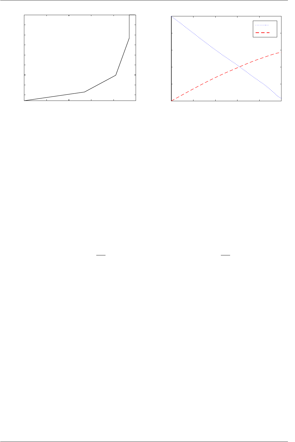
5.2. PROBLEM 5
time
0 0.2 0.4 0.6 0.8 1
u
1
1.5
2
2.5
3
3.5
4
4.5
5
Figure 5.1: Control profile for problem 4
time
0 0.2 0.4 0.6 0.8 1
x1, x 2
0
0.2
0.4
0.6
0.8
1
x1
x2
Figure 5.2: State profiles for problem 4
5.2 Problem 5
Consider a batch reactor [5,18] where a series of reactions A→B→Cis involved. This
example is similar to that in section 3.2.1. The difference is just in the reactor model
description. Here the process is described as an ODE system.
max
u(t)J=x2(tf) (5.2)
such that
˙x1=−k1x2
1x1(0) = 1
˙x2=k1x2
1−k2x2x2(0) = 0
k1= 4000e(−
2500
T)k2= 620000e(−
5000
T)
T∈[298,398] tf= 1
where
x1(t) – concentration of A,
x2(t) – concentration of B,
T– temperature (control variable).
The objective of problem (5.2) is to obtain the optimal temperature profile that maximises
the yield of the intermediate product B at the end of a specified time of operation in a batch
reactor where the reaction A→B→Ctake place. The problem was solved using a
relaxed reduced space SQP strategy by [13] and the value of 0.610775 was reported as global
maximum. Rajesh et al. reached the value of 0.61045. We obtained optimal value of 0.6107682
(1000 iterations, 11468 function evaluations, exitflag equal to 0 (maxiter exceeded), by using
5 collocation points for state variables and keeping control variable profile as piecewise linear
on 4 time intervals. This is quite closer to the global one. The same settings for ipopt resulted
in a non-optimal solution. The optimal control and state profiles are given in Figs. 5.3 and
5.4.
46
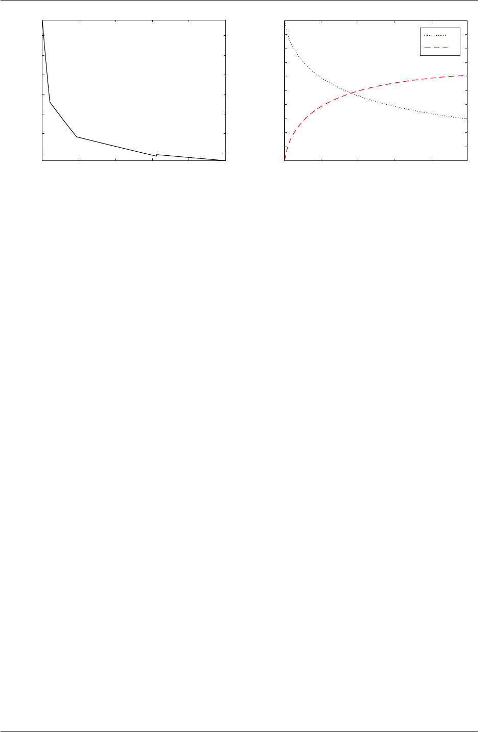
5.3. PROBLEM 6
time
0 0.2 0.4 0.6 0.8 1
u
330
340
350
360
370
380
390
Figure 5.3: Control profile for problem 5
time
0 0.2 0.4 0.6 0.8 1
x1, x 2
0.1
0.2
0.3
0.4
0.5
0.6
0.7
0.8
0.9 x1
x2
Figure 5.4: State profiles for problem 5
5.3 Problem 6
Consider a catalytic plug flow reactor [5,18] involving the following reactions:
A↔B→C
max
u(t)J= 1 −x1(tf)−x2(tf) (5.3)
such that
˙x1=u(10x2−x1)x1(0) = 1
˙x2=−u(10x2−x1)−(1 −u)x2x2(0) = 0
u∈[0,1] tf= 12
where
x1(t) – mole fraction of A,
x2(t) – mole fraction of B,
u(t) – fraction of type 1 catalyst.
Optimisation of this problem has also been analysed. This problem was solved by [13,18]
and the optima 0.476946, 0.47615 were reported. Value of the performance index obtained
for this problem using dynopt was 0.477712 (243 iterations, exitflag equal to 1, fmincon) or
0.477458 (172 iterations, ipopt). In this case 5 collocation points for state variables and 2
collocation points for control variables were chosen. The number of time-intervals have been
set to 12. The optimal control and state profiles are given in Figs. 5.5 and 5.6.
5.4 Problem 7
Consider the following problem [1,8,15]
max
u(t)J=Z0.2
05.8(qx1−u4)−3.7u1−4.1u2
+q(23x4+ 11x5+ 28x6+ 35x7)−5.0u2
3
−0.099dt(5.4)
47
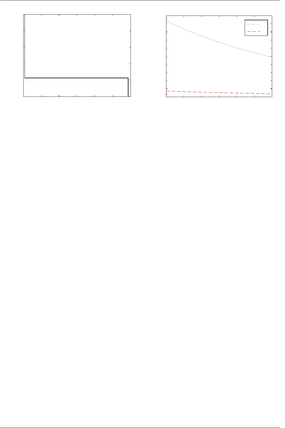
5.4. PROBLEM 7
time
0 2 4 6 8 10 12
u
0
0.2
0.4
0.6
0.8
1
Figure 5.5: Control profile for problem 6
time
0 2 4 6 8 10 12
x1, x 2
0.1
0.2
0.3
0.4
0.5
0.6
0.7
0.8
0.9 x1
x2
Figure 5.6: State profiles for problem 6
such that
˙x1=u4−qx1−17.6x1x2−23x1x6u3
˙x2=u1−qx2−17.6x1x2−146x2x3
˙x3=u2−qx3−73x2x3
˙x4=−qx4+ 35.2x1x2−51.3x4x5
˙x5=−qx5+ 219x2x3−51.3x4x5
˙x6=−qx6+ 102.6x4x5−23x1x6u3
˙x7=−qx7+ 46x1x6u3
x(0) = [0.1883 0.2507 0.0467 0.0899 0.1804 0.1394 0.1046]T
q=u1+u2+u4
0≤u1≤20
0≤u2≤6
0≤u3≤4
0≤u4≤20
tf= 0.2
where
x1(t)−x7(t) – states,
u1(t)−u4(t) – controls.
Analogous to the section 3.1.4, the cost function can be rewritten to the Mayer form by
introducing a new state defined by the integral function with its initial value equal to zero.
This problem was solved by [8,12]. Reported optimal value of 21.757 was obtained
using CVP method implemented in DYNO. For this problem, 4 collocation points for state
variables, 2 collocation points for control variables for 10 intervals were defined and an
optimum was found at value of 21.82317 (860 iterations, exitflag equal to 1, fmincon). The
solver Ipopt did not converge after 10000 iterations. The optimal control and state profiles
are given in Fig. 5.7.
48

5.5. PROBLEM 9
5.5 Problem 9
Consider the following problem [7] which describes diafiltration optimal design problem:
min
α(t)J=x2(tf) (5.5)
subject to differential equations:
˙x1=x1
x3
q(x1, x2) [R1(x1, x2)−α], x1(0) = 150 (5.6)
˙x2=x2
x3
q(x1, x2) [R2(x1, x2)−α], x2(0) = 300 (5.7)
˙x3=q(x1, x2)(α−1), x3(0) = 0.03 (5.8)
state path constraints:
x3(t)≥0.01 (5.9)
x3(t)≤0.035 (5.10)
final time constraints:
x3(tf) = 0.01 (5.11)
and simple bound constraints on optimized variable
α∈[0,1] (5.12)
where R1,R2, q are function of states determined experimentally as
q=S1(x2)eS2(x2)x1(5.13)
R1= (z1x2+z2)x1+ (z3x2+z4) (5.14)
R2=W1(x2)eW2(x2)x1(5.15)
where S1, S2, W1, W2are second order polynomials in x2
S1(x2) = s1x2
2+s2x2+s3(5.16)
S2(x2) = s4x2
2+s5x2+s6(5.17)
W1(x2) = w1x2
2+w2x2+w3(5.18)
W2(x2) = w4x2
2+w5x2+w6(5.19)
and s1−6, z1−4, w1−6are coefficients that were determined from laboratory experiments with
the process solution (see Table 5.1).
The optimal control profile α(t) is at zero for the first part of trajectory and one after
the switch. The volume (x3) shows that the first part of the trajectory basically decreases
the volume until it is on the lower constraint and keeps it approximately constant until end
of the batch. Thus, the optimal control strategy for this problem represents a traditional
diafiltration process with two parts: pre-concentration followed by approximately constant-
volume step until end of the batch. The minimum of x2(6) = 23.13 was obtained with 2
piece-wise constant profiles of α. Simulation results are shown in Fig. 5.8.
49
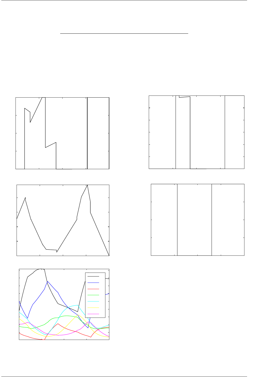
5.5. PROBLEM 9
Table 5.1: Experimentally obtained coefficient values for Rjand q.
s w z
1 68.1250 10−97.8407 10−6-0.0769 10−6
2 -56.4512 10−6-4.0507 10−3-0.0035 10−3
3 32.5553 10−31.0585 0.0349 10−3
4 -4.3529 10−91.2318 10−90.9961
5 3.3216 10−6-9.7660 10−6
6 -2.7141 10−3-1.1677 10−3
time
0 0.05 0.1 0.15 0.2
u1
0
5
10
15
20
time
0 0.05 0.1 0.15 0.2
u2
0
1
2
3
4
5
6
time
0 0.05 0.1 0.15 0.2
u3
0
0.5
1
1.5
2
time
0 0.05 0.1 0.15 0.2
u4
0
5
10
15
20
time
0 0.05 0.1 0.15 0.2
x1, x 2, x 3, x 4, x 5, x 6, x 7
0.05
0.1
0.15
0.2
0.25
0.3
0.35
0.4
0.45
x1
x2
x3
x4
x5
x6
x7
Figure 5.7: Control and state profiles for problem 7
50
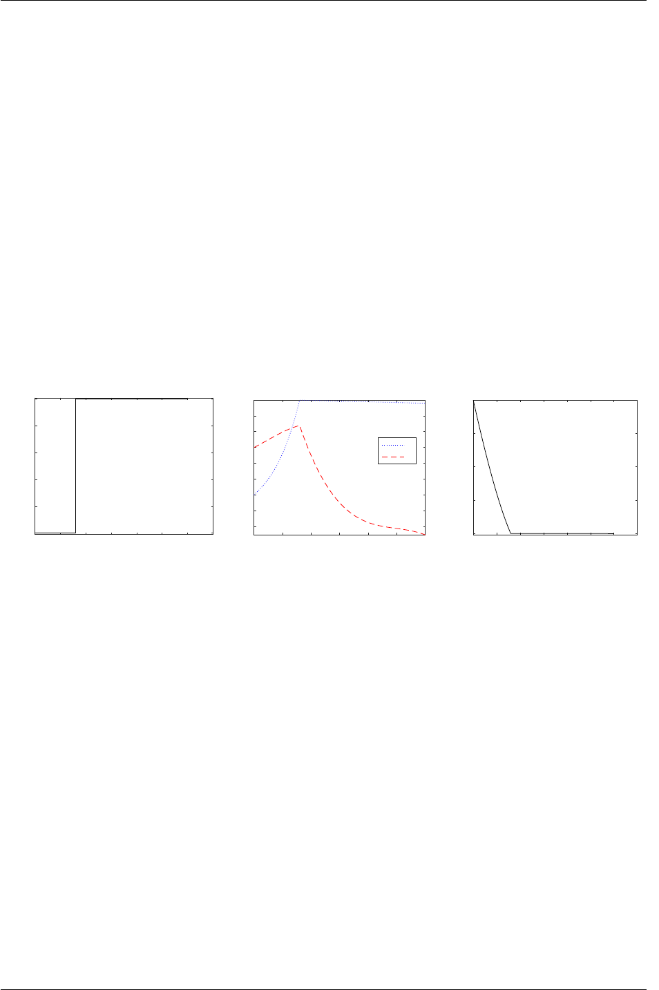
5.5. PROBLEM 9
time [h]
0 1 2 3 4 5 6 7
α [-]
0
0.2
0.4
0.6
0.8
1
time [h]
0123456
x1, x 2 [mol m -3]
50
100
150
200
250
300
350
400
x1
x2
time [h]
01234567
x3 [m 3]
0.01
0.015
0.02
0.025
0.03
Figure 5.8: Diafiltration problem: optimal α(left), concentrations (middle), and volume (right) as functions
of time
51

Bibliography
[1] M-S. G. E. Balsa-Canto, J. R. Banga, A. A. Alonso, and V. S. Vassiliadis. Dynamic
optimization of chemical and biochemical processes using restricted second-order infor-
mation. Computers and Chemical Engineering, 25(4-6):539–546, 2001. 47
[2] T. F. Coleman, M. A. Branch, and A. Grace. Optimization Toolbox User’s Guide.
MathWorks, Inc., 01 1999. 43
[3] T. F. Coleman and Y. Li. An interior, trust region approach for nonlinear minimization
subject to bounds. SIAM Journal on Optimization, 6:418–445, 1996. 43
[4] J. E. Cuthrell and L. T. Biegler. On the optimization of differential-algebraic process
systems. AIChE Journal, 33:1257–1270, 1987. 6
[5] S.A. Dadebo and K.B. McAuley. Dynamic optimization of constrained chemical engi-
neering problems using dinamic programming. Computers and Chemical Engineering,
19:513–525, 1995. 30,45,46,47
[6] W. F. Feehery. Dynamic Optimisation with Path Constraints. PhD thesis, MIT, 1998.
21
[7] M. Fikar, Z. Kov´acs, and P. Czermak. A unified modeling framework for optimal
water usage in batch diafiltration processes. Journal of Membrane Science, 2010.
doi:10.1016/j.memsci.2010.03.019. 49
[8] M. Fikar and M. A. Latifi. User’s guide for FORTRAN dynamic optimisation code
DYNO. Technical Report mf0201, LSGC CNRS, Nancy, France; STU Bratislava, Slovak
Republic, 2002. 24,27,47,48
[9] P. E. Gill, W. Murray, and M. A. Wright. Practical Optimization. Academic Press,
London, 1981. 43
[10] C. J. Goh and K. L. Teo. Control parametrization: A unified approach to optimal
control problems with general constraints. Automatica, 24:3–18, 01 1988. 5
[11] S. P. Han. A globally convergent method for nonlinear programming. Journal of Opti-
mization Theory and Applications, 22:297, 1977. 43
52

BIBLIOGRAPHY
[12] D. Jacobson and M. Lele. A transformation technique for optimal control problems
with a state variable inequality constraint. IEEE Trans. Automatic Control, 5:457–464,
1969. 21,48
[13] J. S. Logsdon and L. T. Biegler. Accurate solution of differential-algebraic optimization
problems. Chemical Engineering Science, (28):1628–1639, 1989. 6,45,46,47
[14] J. S. Logsdon and L. T. Biegler. Decomposition strategies for large-scale dynamic
optimization problems. Chemical Engineering Science, 47(4):851–864, 1992. 6
[15] R. Luus. Application of dynamic programming to high-dimensional non-linear optimal
control problems. Int. J. Control, 52(1):239–250, 1990. 47
[16] R. Luus. Optimal control by dynamic programming using systematic reduction in grid
size. Int. J. Control, 51:995–1013, 1990. 18
[17] R. Luus. Application of iterative dynamic to state constrained optimal control problems.
Hungarian Journal of Industrial Chemistry, 19:245–254, 1991. 10,13
[18] J. Rajesh, K. Gupta, H.S. Kusumakar, V.K. Jayaraman, and B.D. Kulkarni. Dynamic
optimization of chemical processes using ant colony framework. Computers and Chem-
istry, 25:583–595, 2001. 10,13,18,30,45,46,47
[19] Carl-Johan Thore. A code for solving non-linear op-
timization problems with matrix inequality constraints.
https://www.mathworks.com/matlabcentral/fileexchange/43643-fminsdp, 2014.
3
[20] A. W¨
achter and L. T. Biegler. On the implementation of a primal-dual interior point
filter line search algorithm for large-scale nonlinear programming. Mathematical Pro-
gramming, 106(1):25–57, 2006. 9
53
