Edge RUsers Guide
User Manual:
Open the PDF directly: View PDF ![]() .
.
Page Count: 106 [warning: Documents this large are best viewed by clicking the View PDF Link!]
edgeR: differential expression analysis
of digital gene expression data
User’s Guide
Yunshun Chen, Davis McCarthy,
Matthew Ritchie, Mark Robinson, Gordon K. Smyth
First edition 17 September 2008
Last revised 24 April 2018
Contents
1 Introduction 5
1.1 Scope ............................................ 5
1.2 Citation........................................... 6
1.3 Howtogethelp....................................... 7
1.4 Quickstart ......................................... 8
2 Overview of capabilities 9
2.1 Terminology......................................... 9
2.2 Aligningreadstoagenome ................................ 9
2.3 Producing a table of read counts . . . . . . . . . . . . . . . . . . . . . . . . . . . . . 9
2.4 Reading the counts from a file . . . . . . . . . . . . . . . . . . . . . . . . . . . . . . . 10
2.5 TheDGEListdataclass .................................. 10
2.6 Filtering........................................... 10
2.7 Normalization........................................ 11
2.7.1 Normalization is only necessary for sample-specific effects . . . . . . . . . . . 11
2.7.2 Sequencingdepth.................................. 12
2.7.3 RNAcomposition ................................. 12
2.7.4 GCcontent ..................................... 12
2.7.5 Genelength..................................... 13
2.7.6 Model-based normalization, not transformation . . . . . . . . . . . . . . . . . 13
2.7.7 Pseudo-counts ................................... 13
2.8 Negativebinomialmodels ................................. 14
2.8.1 Introduction .................................... 14
2.8.2 Biological coefficient of variation (BCV) . . . . . . . . . . . . . . . . . . . . . 14
2.8.3 EstimatingBCVs.................................. 15
2.8.4 Quasi negative binomial . . . . . . . . . . . . . . . . . . . . . . . . . . . . . . 16
2.9 Pairwise comparisons between two or more groups (classic) . . . . . . . . . . . . . . 16
2.9.1 Estimating dispersions . . . . . . . . . . . . . . . . . . . . . . . . . . . . . . . 16
2.9.2 TestingforDEgenes................................ 17
2.10 More complex experiments (glm functionality) . . . . . . . . . . . . . . . . . . . . . 17
2.10.1 Generalized linear models . . . . . . . . . . . . . . . . . . . . . . . . . . . . . 17
2.10.2 Estimating dispersions . . . . . . . . . . . . . . . . . . . . . . . . . . . . . . . 18
2.10.3 TestingforDEgenes................................ 19
1
2.11 What to do if you have no replicates . . . . . . . . . . . . . . . . . . . . . . . . . . . 20
2.12 Differential expression above a fold-change threshold . . . . . . . . . . . . . . . . . . 21
2.13 Gene ontology (GO) and pathway analysis . . . . . . . . . . . . . . . . . . . . . . . . 22
2.14Genesettesting....................................... 22
2.15Clustering,heatmapsetc.................................. 23
2.16Alternativesplicing..................................... 23
2.17 CRISPR-Cas9 and shRNA-seq screen analysis . . . . . . . . . . . . . . . . . . . . . . 24
2.18 Bisulfite sequencing and differential methylation analysis . . . . . . . . . . . . . . . . 24
3 Specific experimental designs 25
3.1 Introduction......................................... 25
3.2 Twoormoregroups .................................... 25
3.2.1 Introduction .................................... 25
3.2.2 Classicapproach .................................. 26
3.2.3 GLMapproach................................... 27
3.2.4 Questions and contrasts . . . . . . . . . . . . . . . . . . . . . . . . . . . . . . 28
3.2.5 A more traditional glm approach . . . . . . . . . . . . . . . . . . . . . . . . . 28
3.2.6 An ANOVA-like test for any differences . . . . . . . . . . . . . . . . . . . . . 30
3.3 Experiments with all combinations of multiple factors . . . . . . . . . . . . . . . . . 30
3.3.1 Defining each treatment combination as a group . . . . . . . . . . . . . . . . 30
3.3.2 Nested interaction formulas . . . . . . . . . . . . . . . . . . . . . . . . . . . . 32
3.3.3 Treatment effects over all times . . . . . . . . . . . . . . . . . . . . . . . . . . 33
3.3.4 Interaction at any time . . . . . . . . . . . . . . . . . . . . . . . . . . . . . . 33
3.4 Additive models and blocking . . . . . . . . . . . . . . . . . . . . . . . . . . . . . . . 34
3.4.1 Pairedsamples ................................... 34
3.4.2 Blocking....................................... 34
3.4.3 Batcheffects .................................... 36
3.5 Comparisons both between and within subjects . . . . . . . . . . . . . . . . . . . . . 36
4 Case studies 39
4.1 RNA-Seq of oral carcinomas vs matched normal tissue . . . . . . . . . . . . . . . . . 39
4.1.1 Introduction .................................... 39
4.1.2 Readinginthedata ................................ 39
4.1.3 Annotation ..................................... 40
4.1.4 Filtering and normalization . . . . . . . . . . . . . . . . . . . . . . . . . . . . 41
4.1.5 Dataexploration.................................. 41
4.1.6 Thedesignmatrix ................................. 42
4.1.7 Estimating the dispersion . . . . . . . . . . . . . . . . . . . . . . . . . . . . . 43
4.1.8 Differential expression . . . . . . . . . . . . . . . . . . . . . . . . . . . . . . . 44
4.1.9 Gene ontology analysis . . . . . . . . . . . . . . . . . . . . . . . . . . . . . . . 45
4.1.10 Setup ........................................ 46
4.2 RNA-Seq of pathogen inoculated arabidopsis with batch effects . . . . . . . . . . . . 47
4.2.1 Introduction .................................... 47
4.2.2 RNAsamples.................................... 47
2
4.2.3 Loadingthedata.................................. 47
4.2.4 Filtering and normalization . . . . . . . . . . . . . . . . . . . . . . . . . . . . 48
4.2.5 Dataexploration.................................. 48
4.2.6 Thedesignmatrix ................................. 49
4.2.7 Estimating the dispersion . . . . . . . . . . . . . . . . . . . . . . . . . . . . . 50
4.2.8 Differential expression . . . . . . . . . . . . . . . . . . . . . . . . . . . . . . . 51
4.2.9 Setup ........................................ 53
4.3 Profiles of Yoruba HapMap individuals . . . . . . . . . . . . . . . . . . . . . . . . . . 54
4.3.1 Background..................................... 54
4.3.2 Loadingthedata.................................. 54
4.3.3 Filtering and normalization . . . . . . . . . . . . . . . . . . . . . . . . . . . . 55
4.3.4 Estimating the dispersion . . . . . . . . . . . . . . . . . . . . . . . . . . . . . 56
4.3.5 Differential expression . . . . . . . . . . . . . . . . . . . . . . . . . . . . . . . 58
4.3.6 Genesettesting .................................. 58
4.3.7 Setup ........................................ 60
4.4 RNA-Seq profiles of mouse mammary gland . . . . . . . . . . . . . . . . . . . . . . . 61
4.4.1 Introduction .................................... 61
4.4.2 Read alignment and processing . . . . . . . . . . . . . . . . . . . . . . . . . . 61
4.4.3 Count loading and annotation . . . . . . . . . . . . . . . . . . . . . . . . . . . 62
4.4.4 Filtering and normalization . . . . . . . . . . . . . . . . . . . . . . . . . . . . 63
4.4.5 Dataexploration.................................. 64
4.4.6 Thedesignmatrix ................................. 65
4.4.7 Estimating the dispersion . . . . . . . . . . . . . . . . . . . . . . . . . . . . . 66
4.4.8 Differential expression . . . . . . . . . . . . . . . . . . . . . . . . . . . . . . . 67
4.4.9 ANOVA-liketesting ................................ 70
4.4.10 Gene ontology analysis . . . . . . . . . . . . . . . . . . . . . . . . . . . . . . . 71
4.4.11 Genesettesting .................................. 72
4.4.12 Setup ........................................ 74
4.5 Differential splicing after Pasilla knockdown . . . . . . . . . . . . . . . . . . . . . . . 75
4.5.1 Introduction .................................... 75
4.5.2 RNA-Seqsamples ................................. 75
4.5.3 Read alignment and processing . . . . . . . . . . . . . . . . . . . . . . . . . . 76
4.5.4 Count loading and annotation . . . . . . . . . . . . . . . . . . . . . . . . . . . 76
4.5.5 Filtering and normalization . . . . . . . . . . . . . . . . . . . . . . . . . . . . 78
4.5.6 Dataexploration.................................. 78
4.5.7 Thedesignmatrix ................................. 79
4.5.8 Estimating the dispersion . . . . . . . . . . . . . . . . . . . . . . . . . . . . . 80
4.5.9 Differential expression . . . . . . . . . . . . . . . . . . . . . . . . . . . . . . . 81
4.5.10 Alternativesplicing................................. 82
4.5.11 Setup ........................................ 84
4.5.12 Acknowledgements................................. 85
4.6 CRISPR-Cas9 knockout screen analysis . . . . . . . . . . . . . . . . . . . . . . . . . 85
4.6.1 Introduction .................................... 85
4.6.2 Sequenceprocessing ................................ 85
3
4.6.3 Filtering and data exploration . . . . . . . . . . . . . . . . . . . . . . . . . . 86
4.6.4 The design matrix and dispersion estimation . . . . . . . . . . . . . . . . . . 89
4.6.5 Differential representation analysis . . . . . . . . . . . . . . . . . . . . . . . . 90
4.6.6 Gene set tests to summarize over multiple sgRNAs targeting the same gene . 91
4.6.7 Setup ........................................ 92
4.6.8 Acknowledgements................................. 93
4.7 Bisulfite sequencing of mouse oocytes . . . . . . . . . . . . . . . . . . . . . . . . . . 93
4.7.1 Introduction .................................... 93
4.7.2 Readinginthedata ................................ 94
4.7.3 Filtering and normalization . . . . . . . . . . . . . . . . . . . . . . . . . . . . 95
4.7.4 Dataexploration.................................. 97
4.7.5 Thedesignmatrix ................................. 97
4.7.6 Estimating the dispersion . . . . . . . . . . . . . . . . . . . . . . . . . . . . . 98
4.7.7 Differentially methylated regions . . . . . . . . . . . . . . . . . . . . . . . . . 99
4.7.8 Setup ........................................100
4
Chapter 1
Introduction
1.1 Scope
This guide provides an overview of the Bioconductor package edgeR for differential expression anal-
yses of read counts arising from RNA-Seq, SAGE or similar technologies [29]. The package can be
applied to any technology that produces read counts for genomic features. Of particular interest
are summaries of short reads from massively parallel sequencing technologies such as IlluminaTM,
454 or ABI SOLiD applied to RNA-Seq, SAGE-Seq or ChIP-Seq experiments, pooled shRNA-seq
or CRISPR-Cas9 genetic screens and bisulfite sequencing for DNA methylation studies. edgeR pro-
vides statistical routines for assessing differential expression in RNA-Seq experiments or differential
marking in ChIP-Seq experiments.
The package implements exact statistical methods for multigroup experiments developed by
Robinson and Smyth [31, 32]. It also implements statistical methods based on generalized linear
models (glms), suitable for multifactor experiments of any complexity, developed by McCarthy et
al. [20], Lund et al. [18], Chen et al. [5] and Lun et al. [17]. Sometimes we refer to the former
exact methods as classic edgeR, and the latter as glm edgeR. However the two sets of methods
are complementary and can often be combined in the course of a data analysis. Most of the glm
functions can be identified by the letters “glm” as part of the function name. The glm functions can
test for differential expression using either likelihood ratio tests[20, 5] or quasi-likelihood F-tests
[18, 17].
A particular feature of edgeR functionality, both classic and glm, are empirical Bayes methods
that permit the estimation of gene-specific biological variation, even for experiments with minimal
levels of biological replication.
edgeR can be applied to differential expression at the gene, exon, transcript or tag level. In
fact, read counts can be summarized by any genomic feature. edgeR analyses at the exon level are
easily extended to detect differential splicing or isoform-specific differential expression.
This guide begins with brief overview of some of the key capabilities of package, and then gives
a number of fully worked case studies, from counts to lists of genes.
5
1.2 Citation
The edgeR package implements statistical methods from the following publications. Please try to
cite the appropriate articles when you publish results obtained using the software, as such citation
is the main means by which the authors receive credit for their work.
Robinson, MD, and Smyth, GK (2008). Small sample estimation of negative binomial dispersion,
with applications to SAGE data. Biostatistics 9, 321–332.
Proposed the idea of sharing information between genes by estimating the negative binomial
variance parameter globally across all genes. This made the use of negative binomial models
practical for RNA-Seq and SAGE experiments with small to moderate numbers of replicates.
Introduced the terminology dispersion for the variance parameter. Proposed conditional max-
imum likelihood for estimating the dispersion, assuming common dispersion across all genes.
Developed an exact test for differential expression appropriate for the negative binomially dis-
tributed counts. Despite the official publication date, this was the first of the papers to be
submitted and accepted for publication.
Robinson, MD, and Smyth, GK (2007). Moderated statistical tests for assessing differences in tag
abundance. Bioinformatics 23, 2881–2887.
Introduced empirical Bayes moderated dispersion parameter estimation. This is a crucial im-
provement on the previous idea of estimating the dispersions from a global model, because it
permits gene-specific dispersion estimation to be reliable even for small samples. Gene-specific
dispersion estimation is necessary so that genes that behave consistently across replicates should
rank more highly than genes that do not.
Robinson, MD, McCarthy, DJ, Smyth, GK (2010). edgeR: a Bioconductor package for differential
expression analysis of digital gene expression data. Bioinformatics 26, 139–140.
Announcement of the edgeR software package. Introduced the terminology coefficient of biolog-
ical variation.
Robinson, MD, and Oshlack, A (2010). A scaling normalization method for differential expression
analysis of RNA-seq data. Genome Biology 11, R25.
Introduced the idea of model-based scale normalization of RNA-Seq data. Proposed TMM
normalization.
McCarthy, DJ, Chen, Y, Smyth, GK (2012). Differential expression analysis of multifactor RNA-
Seq experiments with respect to biological variation. Nucleic Acids Research 40, 4288-4297.
Extended negative binomial differential expression methods to glms, making the methods appli-
cable to general experiments. Introduced the use of Cox-Reid approximate conditional maximum
likelihood for estimating the dispersion parameters, and used this for empirical Bayes modera-
tion. Developed fast algorithms for fitting glms to thousands of genes in parallel. Gives a more
complete explanation of the concept of biological coefficient of variation.
Lun, ATL, Chen, Y, and Smyth, GK (2016). It’s DE-licious: a recipe for differential expression
analyses of RNA-seq experiments using quasi-likelihood methods in edgeR. Methods in Molecular
Biology 1418, 391–416.
6
This book chapter explains the glmQLFit and glmQLFTest functions, which are alternatives to
glmFit and glmLRT. They replace the chisquare approximation to the likelihood ratio statistic
with a quasi-likelihood F-test, resulting in more conservative and rigorous type I error rate
control.
Chen, Y, Lun, ATL, and Smyth, GK (2014). Differential expression analysis of complex RNA-
seq experiments using edgeR. In: Statistical Analysis of Next Generation Sequence Data, Somnath
Datta and Daniel S Nettleton (eds), Springer, New York.
This book chapter explains the estimateDisp function and the weighted likelihood empirical
Bayes method.
Zhou, X, Lindsay, H, and Robinson, MD (2014). Robustly detecting differential expression in RNA
sequencing data using observation weights. Nucleic Acids Research, 42, e91.
Explains estimateGLMRobustDisp, which is designed to make the downstream tests done by
glmLRT robust to outlier observations.
Dai, Z, Sheridan, JM, Gearing, LJ, Moore, DL, Su, S, Wormald, S, Wilcox, S, O’Connor, L, Dickins,
RA, Blewitt, ME, and Ritchie, ME (2014). edgeR: a versatile tool for the analysis of shRNA-seq
and CRISPR-Cas9 genetic screens. F1000Research 3, 95.
This paper explains the processAmplicons function for obtaining counts from the fastq files
of shRNA-seq and CRISPR-Cas9 genetic screens and outlines a general workflow for analyzing
data from such screens.
Chen, Y, Lun, ATL, and Smyth, GK (2016). From reads to genes to pathways: differential ex-
pression analysis of RNA-Seq experiments using Rsubread and the edgeR quasi-likelihood pipeline.
F1000Research 5, 1438.
This paper describes a complete workflow of differential expression and pathway analysis using
the edgeR quasi-likelihood pipeline.
Chen, Y, Pal, B, Visvader, JE, and Smyth, GK (2017). Differential methylation analysis of reduced
representation bisulfite sequencing experiments using edgeR. F1000Research 6, 2055.
This paper explains a novel approach of detecting differentially methylated regions (DMRs) of
reduced representation bisulfite sequencing (RRBS) experiments using edgeR.
1.3 How to get help
Most questions about edgeR will hopefully be answered by the documentation or references. If
you’ve run into a question that isn’t addressed by the documentation, or you’ve found a conflict
between the documentation and what the software does, then there is an active support community
that can offer help.
The edgeR authors always appreciate receiving reports of bugs in the package functions or
in the documentation. The same goes for well-considered suggestions for improvements. All
other questions or problems concerning edgeR should be posted to the Bioconductor support
7
site https://support.bioconductor.org. Please send requests for general assistance and ad-
vice to the support site rather than to the individual authors. Posting questions to the Bio-
conductor support site has a number of advantages. First, the support site includes a commu-
nity of experienced edgeR users who can answer most common questions. Second, the edgeR
authors try hard to ensure that any user posting to Bioconductor receives assistance. Third,
the support site allows others with the same sort of questions to gain from the answers. Users
posting to the support site for the first time will find it helpful to read the posting guide at
http://www.bioconductor.org/help/support/posting-guide.
Note that each function in edgeR has its own online help page. For example, a detailed descrip-
tion of the arguments and output of the exactTest function can be read by typing ?exactTest or
help(exactTest) at the Rprompt. If you have a question about any particular function, reading
the function’s help page will often answer the question very quickly. In any case, it is good etiquette
to check the relevant help page first before posting a question to the support site.
The authors do occasionally answer questions posted to other forums, such as SEQAnswers or
Biostar, but it is not possible to do this on a regular basis.
1.4 Quick start
edgeR offers many variants on analyses. The glm approach is more popular than the classic approach
as it offers great flexibilities. There are two testing methods under the glm framework: likelihood
ratio test and quasi-likelihood F-test. The quasi-likelihood method is highly recommended for
differential expression analyses of bulk RNA-seq data as it gives stricter error rate control by
accounting for the uncertainty in dispersion estimation. The likelihood ratio test can be useful in
some special cases such as single cell RNA-seq and datasets with no replicates. The details of these
methods are described in Chapter 2.
A typical edgeR analysis might look like the following. Here we assume there are four RNA-Seq
libraries in two groups, and the counts are stored in a tab-delimited text file, with gene symbols in
a column called Symbol.
> x <- read.delim("TableOfCounts.txt",row.names="Symbol")
> group <- factor(c(1,1,2,2))
> y <- DGEList(counts=x,group=group)
> y <- calcNormFactors(y)
> design <- model.matrix(~group)
> y <- estimateDisp(y,design)
To perform quasi-likelihood F-tests:
> fit <- glmQLFit(y,design)
> qlf <- glmQLFTest(fit,coef=2)
> topTags(qlf)
To perform likelihood ratio tests:
> fit <- glmFit(y,design)
> lrt <- glmLRT(fit,coef=2)
> topTags(lrt)
8
Chapter 2
Overview of capabilities
2.1 Terminology
edgeR performs differential abundance analysis for pre-defined genomic features. Although not
strictly necessary, it usually desirable that these genomic features are non-overlapping. For sim-
plicity, we will hence-forth refer to the genomic features as “genes”, although they could in principle
be transcripts, exons, general genomic intervals or some other type of feature. For ChIP-seq exper-
iments, abundance might relate to transcription factor binding or to histone mark occupancy, but
we will henceforth refer to abundance as in terms of gene expression. In other words, the remainder
of this guide will use terminology as for a gene-level analysis of an RNA-seq experiment, although
the methodology is more widely applicable than that.
2.2 Aligning reads to a genome
The first step in an RNA-seq analysis is usually to align the raw sequence reads to a reference
genome, although there are many variations on this process. Alignment needs to allow for the fact
that reads may span multiple exons which may align to well separated locations on the genome.
We find the subread-featureCounts pipeline [14, 15] to be very fast and effective for this purpose,
but the Bowtie-TopHat-htseq pipeline is also very popular [1].
2.3 Producing a table of read counts
edgeR works on a table of integer read counts, with rows corresponding to genes and columns to
independent libraries. The counts represent the total number of reads aligning to each gene (or
other genomic locus).
Such counts can be produced from aligned reads by a variety of short read software tools.
We find the featureCounts function of the Rsubread package [15] to be particularly effective and
convenient, but other tools are available such as findOverlaps in the GenomicRanges package or
the Python software htseq-counts.
Reads can be counted in a number of ways. When conducting gene-level analyses, the counts
could be for reads mapping anywhere in the genomic span of the gene or the counts could be for
9
exons only. We usually count reads that overlap any exon for the given gene, including the UTR
as part of the first exon [15].
For data from pooled shRNA-seq or CRISPR-Cas9 genetic screens, the processAmplicons func-
tion [8] can be used to obtain counts directly from fastq files.
Note that edgeR is designed to work with actual read counts. We not recommend that predicted
transcript abundances are input the edgeR in place of actual counts.
2.4 Reading the counts from a file
If the table of counts has been written to a file, then the first step in any analysis will usually be
to read these counts into an R session.
If the count data is contained in a single tab-delimited or comma-separated text file with multiple
columns, one for each sample, then the simplest method is usually to read the file into R using one
of the standard R read functions such as read.delim. See the quick start above, or the case study
on LNCaP Cells, or the case study on oral carcinomas later in this guide for examples.
If the counts for different samples are stored in separate files, then the files have to be read
separately and collated together. The edgeR function readDGE is provided to do this. Files need to
contain two columns, one for the counts and one for a gene identifier.
2.5 The DGEList data class
edgeR stores data in a simple list-based data object called a DGEList. This type of object is easy
to use because it can be manipulated like any list in R. The function readDGE makes a DGEList
object directly. If the table of counts is already available as a matrix or a data.frame, xsay, then
aDGEList object can be made by
> y <- DGEList(counts=x)
A grouping factor can be added at the same time:
> group <- c(1,1,2,2)
> y <- DGEList(counts=x, group=group)
The main components of an DGEList object are a matrix counts containing the integer counts, a
data.frame samples containing information about the samples or libraries, and a optional data.frame
genes containing annotation for the genes or genomic features. The data.frame samples contains a
column lib.size for the library size or sequencing depth for each sample. If not specified by the
user, the library sizes will be computed from the column sums of the counts. For classic edgeR the
data.frame samples must also contain a column group, identifying the group membership of each
sample.
2.6 Filtering
Genes with very low counts across all libraries provide little evidence for differential expression. In
the biological point of view, a gene must be expressed at some minimal level before it is likely to be
10
translated into a protein or to be biologically important. In addition, the pronounced discreteness
of these counts interferes with some of the statistical approximations that are used later in the
pipeline. These genes should be filtered out prior to further analysis.
As a rule of thumb, genes are dropped if they can’t possibly be expressed in all the samples for
any of the conditions. Users can set their own definition of genes being expressed. Usually a gene
is required to have a count of 5-10 in a library to be considered expressed in that library. Users
should also filter with count-per-million (CPM) rather than filtering on the counts directly, as the
latter does not account for differences in library sizes between samples.
Here is a simple example. Suppose the sample information of a DGEList object yis shown as
follows:
> y$samples
group lib.size norm.factors
Sample1 1 10880519 1
Sample2 1 9314747 1
Sample3 1 11959792 1
Sample4 2 7460595 1
Sample5 2 6714958 1
We filter out lowly expressed genes using the following commands:
> keep <- rowSums(cpm(y)>1) >= 2
> y <- y[keep, , keep.lib.sizes=FALSE]
Here, a CPM of 1 corresponds to a count of 6-7 in the smallest sample. A requirement for
expression in two or more libraries is used as the minimum number of samples in each group is two.
This ensures that a gene will be retained if it is only expressed in both samples in group 2. It is
also recommended to recalculate the library sizes of the DGEList object after the filtering though
the difference is usually negligible.
2.7 Normalization
2.7.1 Normalization is only necessary for sample-specific effects
edgeR is concerned with differential expression analysis rather than with the quantification of
expression levels. It is concerned with relative changes in expression levels between conditions,
but not directly with estimating absolute expression levels. This greatly simplifies the technical
influences that need to be taken into account, because any technical factor that is unrelated to
the experimental conditions should cancel out of any differential expression analysis. For example,
read counts can generally be expected to be proportional to length as well as to expression for any
transcript, but edgeR does not generally need to adjust for gene length because gene length has the
same relative influence on the read counts for each RNA sample. For this reason, normalization
issues arise only to the extent that technical factors have sample-specific effects.
11
2.7.2 Sequencing depth
The most obvious technical factor that affects the read counts, other than gene expression levels,
is the sequencing depth of each RNA sample. edgeR adjusts any differential expression analysis
for varying sequencing depths as represented by differing library sizes. This is part of the basic
modeling procedure and flows automatically into fold-change or p-value calculations. It is always
present, and doesn’t require any user intervention.
2.7.3 RNA composition
The second most important technical influence on differential expression is one that is less obvious.
RNA-seq provides a measure of the relative abundance of each gene in each RNA sample, but does
not provide any measure of the total RNA output on a per-cell basis. This commonly becomes
important when a small number of genes are very highly expressed in one sample, but not in
another. The highly expressed genes can consume a substantial proportion of the total library size,
causing the remaining genes to be under-sampled in that sample. Unless this RNA composition
effect is adjusted for, the remaining genes may falsely appear to be down-regulated in that sample
[30].
The calcNormFactors function normalizes for RNA composition by finding a set of scaling factors
for the library sizes that minimize the log-fold changes between the samples for most genes. The
default method for computing these scale factors uses a trimmed mean of M-values (TMM) between
each pair of samples [30]. We call the product of the original library size and the scaling factor the
effective library size. The effective library size replaces the original library size in all downsteam
analyses.
TMM is the recommended for most RNA-Seq data where the majority (more than half) of
the genes are believed not differentially expressed between any pair of the samples. The following
commands perform the TMM normalization and display the normalization factors.
> y <- calcNormFactors(y)
> y$samples
group lib.size norm.factors
Sample1 1 10880519 1.17
Sample2 1 9314747 0.86
Sample3 1 11959792 1.32
Sample4 2 7460595 0.91
Sample5 2 6714958 0.83
The normalization factors of all the libraries multiply to unity. A normalization factor below
one indicates that a small number of high count genes are monopolizing the sequencing, causing
the counts for other genes to be lower than would be usual given the library size. As a result, the
library size will be scaled down, analogous to scaling the counts upwards in that library. Conversely,
a factor above one scales up the library size, analogous to downscaling the counts.
2.7.4 GC content
The GC-content of each gene does not change from sample to sample, so it can be expected to
have little effect on differential expression analyses to a first approximation. Recent publications,
12
however, have demonstrated that sample-specific effects for GC-content can be detected [28, 11].
The EDASeq [28] and cqn [11] packages estimate correction factors that adjust for sample-specific
GC-content effects in a way that is compatible with edgeR. In each case, the observation-specific
correction factors can be input into the glm functions of edgeR as an offset matrix.
2.7.5 Gene length
Like GC-content, gene length does not change from sample to sample, so it can be expected to
have little effect on differential expression analyses. Nevertheless, sample-specific effects for gene
length have been detected [11], although the evidence is not as strong as for GC-content.
2.7.6 Model-based normalization, not transformation
In edgeR, normalization takes the form of correction factors that enter into the statistical model.
Such correction factors are usually computed internally by edgeR functions, but it is also possible
for a user to supply them. The correction factors may take the form of scaling factors for the library
sizes, such as computed by calcNormFactors, which are then used to compute the effective library
sizes. Alternatively, gene-specific correction factors can be entered into the glm functions of edgeR
as offsets. In the latter case, the offset matrix will be assumed to account for all normalization
issues, including sequencing depth and RNA composition.
Note that normalization in edgeR is model-based, and the original read counts are not them-
selves transformed. This means that users should not transform the read counts in any way before
inputing them to edgeR. For example, users should not enter RPKM or FPKM values to edgeR
in place of read counts. Such quantities will prevent edgeR from correctly estimating the mean-
variance relationship in the data, which is a crucial to the statistical strategies underlying edgeR.
Similarly, users should not add artificial values to the counts before inputing them to edgeR.
edgeR is not designed to work with estimated expression levels, for example as might be output
by Cufflinks. edgeR can work with expected counts as output by RSEM, but raw counts are still
preferred.
2.7.7 Pseudo-counts
The classic edgeR functions estimateCommonDisp and exactTest produce a matrix of pseudo-counts
as part of the output object. The pseudo-counts are used internally to speed up computation of the
conditional likelihood used for dispersion estimation and exact tests in the classic edgeR pipeline.
The pseudo-counts represent the equivalent counts would have been observed had the library sizes
all been equal, assuming the fitted model. The pseudo-counts are computed for a specific purpose,
and their computation depends on the experimental design as well as the library sizes, so users
are advised not to interpret the psuedo-counts as general-purpose normalized counts. They are
intended mainly for internal use in the edgeR pipeline.
Disambiguation. Note that some other software packages use the term pseudo-count to mean
something analogous to prior counts in edgeR, i.e., a starting value that is added to a zero count to
avoid missing values when computing logarithms. In edgeR, a pseudo-count is a type of normalized
count and a prior count is a starting value used to offset small counts.
13

2.8 Negative binomial models
2.8.1 Introduction
The starting point for an RNA-Seq experiment is a set of nRNA samples, typically associated
with a variety of treatment conditions. Each sample is sequenced, short reads are mapped to
the appropriate genome, and the number of reads mapped to each genomic feature of interest is
recorded. The number of reads from sample imapped to gene gwill be denoted ygi. The set
of genewise counts for sample imakes up the expression profile or library for that sample. The
expected size of each count is the product of the library size and the relative abundance of that
gene in that sample.
2.8.2 Biological coefficient of variation (BCV)
RNA-Seq profiles are formed from nRNA samples. Let πgi be the fraction of all cDNA fragments in
the ith sample that originate from gene g. Let Gdenote the total number of genes, so PG
g=1 πgi = 1
for each sample. Let √φgdenote the coefficient of variation (CV) (standard deviation divided by
mean) of πgi between the replicates i. We denote the total number of mapped reads in library iby
Niand the number that map to the gth gene by ygi. Then
E(ygi) = µgi =Niπgi.
Assuming that the count ygi follows a Poisson distribution for repeated sequencing runs of the same
RNA sample, a well known formula for the variance of a mixture distribution implies:
var(ygi) = Eπ[var(y|π)] + varπ[E(y|π)] = µgi +φgµ2
gi.
Dividing both sides by µ2
gi gives
CV2(ygi)=1/µgi +φg.
The first term 1/µgi is the squared CV for the Poisson distribution and the second is the squared
CV of the unobserved expression values. The total CV2therefore is the technical CV2with which
πgi is measured plus the biological CV2of the true πgi. In this article, we call φgthe dispersion
and pφgthe biological CV although, strictly speaking, it captures all sources of the inter-library
variation between replicates, including perhaps contributions from technical causes such as library
preparation as well as true biological variation between samples.
Two levels of variation can be distinguished in any RNA-Seq experiment. First, the relative
abundance of each gene will vary between RNA samples, due mainly to biological causes. Second,
there is measurement error, the uncertainty with which the abundance of each gene in each sample
is estimated by the sequencing technology. If aliquots of the same RNA sample are sequenced, then
the read counts for a particular gene should vary according to a Poisson law [19]. If sequencing
variation is Poisson, then it can be shown that the squared coefficient of variation (CV) of each
count between biological replicate libraries is the sum of the squared CVs for technical and biological
variation respectively,
Total CV2= Technical CV2+ Biological CV2.
14
Biological CV (BCV) is the coefficient of variation with which the (unknown) true abundance
of the gene varies between replicate RNA samples. It represents the CV that would remain between
biological replicates if sequencing depth could be increased indefinitely. The technical CV decreases
as the size of the counts increases. BCV on the other hand does not. BCV is therefore likely to be
the dominant source of uncertainty for high-count genes, so reliable estimation of BCV is crucial
for realistic assessment of differential expression in RNA-Seq experiments. If the abundance of each
gene varies between replicate RNA samples in such a way that the genewise standard deviations are
proportional to the genewise means, a commonly occurring property of measurements on physical
quantities, then it is reasonable to suppose that BCV is approximately constant across genes.
We allow however for the possibility that BCV might vary between genes and might also show a
systematic trend with respect to gene expression or expected count.
The magnitude of BCV is more important than the exact probabilistic law followed by the true
gene abundances. For mathematical convenience, we assume that the true gene abundances follow
a gamma distributional law between replicate RNA samples. This implies that the read counts
follow a negative binomial probability law.
2.8.3 Estimating BCVs
When a negative binomial model is fitted, we need to estimate the BCV(s) before we carry out the
analysis. The BCV, as shown in the previous section, is the square root of the dispersion parameter
under the negative binomial model. Hence, it is equivalent to estimating the dispersion(s) of the
negative binomial model.
The parallel nature of sequencing data allows some possibilities for borrowing information from
the ensemble of genes which can assist in inference about each gene individually. The easiest
way to share information between genes is to assume that all genes have the same mean-variance
relationship, in other words, the dispersion is the same for all the genes [32]. An extension to this
“common dispersion” approach is to put a mean-dependent trend on a parameter in the variance
function, so that all genes with the same expected count have the same variance.
However, the truth is that the gene expression levels have non-identical and dependent distri-
bution between genes, which makes the above assumptions too naive. A more general approach
that allows genewise variance functions with empirical Bayes moderation was introduced several
years ago [31] and was extended to generalized linear models and thus more complex experimental
designs [20]. Only when using tagwise dispersion will genes that are consistent between replicates
be ranked more highly than genes that are not. It has been seen in many RNA-Seq datasets that
allowing gene-specific dispersion is necessary in order that differential expression is not driven by
outliers. Therefore, the tagwise dispersions are strongly recommended in model fitting and testing
for differential expression.
In edgeR, we apply an empirical Bayes strategy for squeezing the tagwise dispersions towards a
global dispersion trend or towards a common dispersion value. The amount of squeeze is determined
by the weight given to the global value on one hand and the precision of the tagwise estimates on
the other. The relative weights given to the two are determined the prior and residual degrees of
freedom. By default, the prior degrees of freedom, which determines the amount of empirical Bayes
moderation, is estimated by examining the heteroskedasticity of the data [5].
15
2.8.4 Quasi negative binomial
The NB model can be extended with quasi-likelihood (QL) methods to account for gene-specific
variability from both biological and technical sources [18, 17]. Under the QL framework, the
variance of the count ygi is a quadratic function of the mean,
var(ygi) = σ2
g(µgi +φµ2
gi),
where φis the NB dispersion parameter and σ2
gis the QL dispersion parameter.
Any increase in the observed variance of ygi will be modelled by an increase in the estimates
for φand/or σ2
g. In this model, the NB dispersion φis a global parameter whereas the QL is gene-
specific, so the two dispersion parameters have different roles. The NB dispersion describes the
overall biological variability across all genes. It represents the observed variation that is attributable
to inherent variability in the biological system, in contrast to the Poisson variation from sequencing.
The QL dispersion picks up any gene-specific variability above and below the overall level.
The common NB dispersion for the entire data set can be used for the global parameter. In
practice, we use the trended dispersions to account for the empirical mean-variance relationships.
Since the NB dispersion under the QL framework reflects the overall biological variability, it does
not make sense to use the tagwise dispersions.
Estimation of the gene-specific QL dispersion is difficult as most RNA-seq data sets have limited
numbers of replicates. This means that there is often little information to stably estimate the
dispersion for each gene. To overcome this, an empirical Bayes (EB) approach is used whereby
information is shared between genes [35, 18, 25]. Briefly, a mean-dependent trend is fitted to the
raw QL dispersion estimates. The raw estimates are then squeezed towards this trend to obtain
moderated EB estimates, which can be used in place of the raw values for downstream hypothesis
testing. This EB strategy reduces the uncertainty of the estimates and improves testing power.
2.9 Pairwise comparisons between two or more groups (classic)
2.9.1 Estimating dispersions
edgeR uses the quantile-adjusted conditional maximum likelihood (qCML) method for experiments
with single factor.
Compared against several other estimators (e.g. maximum likelihood estimator, Quasi-likelihood
estimator etc.) using an extensive simulation study, qCML is the most reliable in terms of bias on
a wide range of conditions and specifically performs best in the situation of many small samples
with a common dispersion, the model which is applicable to Next-Gen sequencing data. We have
deliberately focused on very small samples due to the fact that DNA sequencing costs prevent large
numbers of replicates for SAGE and RNA-seq experiments.
The qCML method calculates the likelihood by conditioning on the total counts for each tag, and
uses pseudo counts after adjusting for library sizes. Given a table of counts or a DGEList object, the
qCML common dispersion and tagwise dispersions can be estimated using the estimateDisp() func-
tion. Alternatively, one can estimate the qCML common dispersion using the estimateCommonDisp()
function, and then the qCML tagwise dispersions using the estimateTagwiseDisp() function.
However, the qCML method is only applicable on datasets with a single factor design since
it fails to take into account the effects from multiple factors in a more complicated experiment.
16
When an experiment has more than one factor involved, we need to seek a new way of estimating
dispersions.
Here is a simple example of estimating dispersions using the qCML method. Given a DGEList
object y, we estimate the dispersions using the following commands.
To estimate common dispersion and tagwise dispersions in one run (recommended):
y <- estimateDisp(y)
Alternatively, to estimate common dispersion:
y <- estimateCommonDisp(y)
Then to estimate tagwise dispersions:
y <- estimateTagwiseDisp(y)
Note that common dispersion needs to be estimated before estimating tagwise dispersions if
they are estimated separately.
2.9.2 Testing for DE genes
For all the Next-Gen squencing data analyses we consider here, people are most interested in
finding differentially expressed genes/tags between two (or more) groups. Once negative binomial
models are fitted and dispersion estimates are obtained, we can proceed with testing procedures
for determining differential expression using the exact test.
The exact test is based on the qCML methods. Knowing the conditional distribution for the
sum of counts in a group, we can compute exact p-values by summing over all sums of counts that
have a probability less than the probability under the null hypothesis of the observed sum of counts.
The exact test for the negative binomial distribution has strong parallels with Fisher’s exact test.
As we dicussed in the previous section, the exact test is only applicable to experiments with a
single factor. The testing can be done by using the function exactTest(), and the function allows
both common dispersion and tagwise dispersion approaches. For example:
> et <- exactTest(y)
> topTags(et)
2.10 More complex experiments (glm functionality)
2.10.1 Generalized linear models
Generalized linear models (GLMs) are an extension of classical linear models to nonnormally dis-
tributed response data [24, 22]. GLMs specify probability distributions according to their mean-
variance relationship, for example the quadratic mean-variance relationship specified above for read
counts. Assuming that an estimate is available for φg, so the variance can be evaluated for any
value of µgi, GLM theory can be used to fit a log-linear model
log µgi =xT
iβg+ log Ni
17
for each gene [16, 4]. Here xiis a vector of covariates that specifies the treatment conditions
applied to RNA sample i, and βgis a vector of regression coefficients by which the covariate effects
are mediated for gene g. The quadratic variance function specifies the negative binomial GLM
distributional family. The use of the negative binomial distribution is equivalent to treating the
πgi as gamma distributed.
2.10.2 Estimating dispersions
For general experiments (with multiple factors), edgeR uses the Cox-Reid profile-adjusted likelihood
(CR) method in estimating dispersions. The CR method is derived to overcome the limitations
of the qCML method as mentioned above. It takes care of multiple factors by fitting generalized
linear models (GLM) with a design matrix.
The CR method is based on the idea of approximate conditional likelihood which reduces to
residual maximum likelihood. Given a table counts or a DGEList object and the design matrix of
the experiment, generalized linear models are fitted. This allows valid estimation of the dispersion,
since all systematic sources of variation are accounted for.
The CR method can be used to calculate a common dispersion for all the tags, trended dis-
persion depending on the tag abundance, or separate dispersions for individual tags. These can
be done by calling the function estimateDisp() with a specified design. Alternatively, one can
estimate the common, trended and tagwise dispersions separately using estimateGLMCommonDisp(),
estimateGLMTrendedDisp() and estimateGLMTagwiseDisp(), respectively. The tagwise dispersion
approach is strongly recommended in multi-factor experiment cases.
Here is a simple example of estimating dispersions using the GLM method. Given a DGEList
object yand a design matrix, we estimate the dispersions using the following commands.
To estimate common dispersion, trended dispersions and tagwise dispersions in one run (rec-
ommended):
y <- estimateDisp(y, design)
Alternatively, one can use the following calling sequence to estimate them one by one. To
estimate common dispersion:
y <- estimateGLMCommonDisp(y, design)
To estimate trended dispersions:
y <- estimateGLMTrendedDisp(y, design)
To estimate tagwise dispersions:
y <- estimateGLMTagwiseDisp(y, design)
Note that we need to estimate either common dispersion or trended dispersions prior to the es-
timation of tagwise dispersions. When estimating tagwise dispersions, the empirical Bayes method
is applied to squeeze the tagwise dispersions towards a common dispersion or towards trended
dispersions, whichever exists. If both exist, the default is to use the trended dispersions.
For more detailed examples, see the case study in Section 4.1 (Tuch’s data), Section 4.2 (ara-
bidopsis data), Section 4.3 (Nigerian data) and Section 4.4 (Fu’s data).
18
2.10.3 Testing for DE genes
For general experiments, once dispersion estimates are obtained and negative binomial general-
ized linear models are fitted, we can proceed with testing procedures for determining differential
expression using either quasi-likelihood (QL) F-test or likelihood ratio test.
While the likelihood ratio test is a more obvious choice for inferences with GLMs, the QL F-test
is preferred as it reflects the uncertainty in estimating the dispersion for each gene. It provides more
robust and reliable error rate control when the number of replicates is small. The QL dispersion
estimation and hypothesis testing can be done by using the functions glmQLFit() and glmQLFTest().
Given raw counts, NB dispersion(s) and a design matrix, glmQLFit() fits the negative binomial
GLM for each tag and produces an object of class DGEGLM with some new components. This DGEGLM
object can then be passed to glmQLFTest() to carry out the QL F-test. User can select one or more
coefficients to drop from the full design matrix. This gives the null model against which the full
model is compared. Tags can then be ranked in order of evidence for differential expression, based
on the p-value computed for each tag.
As a brief example, consider a situation in which are three treatment groups, each with two
replicates, and the researcher wants to make pairwise comparisons between them. A QL model
representing the study design can be fitted to the data with commands such as:
> group <- factor(c(1,1,2,2,3,3))
> design <- model.matrix(~group)
> fit <- glmQLFit(y, design)
The fit has three parameters. The first is the baseline level of group 1. The second and third are
the 2 vs 1 and 3 vs 1 differences.
To compare 2 vs 1:
> qlf.2vs1 <- glmQLFTest(fit, coef=2)
> topTags(qlf.2vs1)
To compare 3 vs 1:
> qlf.3vs1 <- glmQLFTest(fit, coef=3)
To compare 3 vs 2:
> qlf.3vs2 <- glmQLFTest(fit, contrast=c(0,-1,1))
The contrast argument in this case requests a statistical test of the null hypothesis that coefficient3−coefficient2
is equal to zero.
To find genes different between any of the three groups:
> qlf <- glmQLFTest(fit, coef=2:3)
> topTags(qlf)
For more detailed examples, see the case study in Section 4.2 (arabidopsis data), Section 4.3
(Nigerian data) and Section 4.4 (Fu’s data).
Alternatively, one can perform likelihood ratio test to test for differential expression. The testing
can be done by using the functions glmFit() and glmLRT(). To apply the likelihood ratio test to
the above example and compare 2 vs 1:
19
> fit <- glmFit(y, design)
> lrt.2vs1 <- glmLRT(fit, coef=2)
> topTags(lrt.2vs1)
Similarly for the other comparisons.
For more detailed examples, see the case study in section 4.1 (Tuch’s data)
2.11 What to do if you have no replicates
edgeR is primarily intended for use with data including biological replication. Nevertheless, RNA-
Seq and ChIP-Seq are still expensive technologies, so it sometimes happens that only one library can
be created for each treatment condition. In these cases there are no replicate libraries from which to
estimate biological variability. In this situation, the data analyst is faced with the following choices,
none of which are ideal. We do not recommend any of these choices as a satisfactory alternative
for biological replication. Rather, they are the best that can be done at the analysis stage, and
options 2–4 may be better than assuming that biological variability is absent.
1. Be satisfied with a descriptive analysis, that might include an MDS plot and an analysis of
fold changes. Do not attempt a significance analysis. This may be the best advice.
2. Simply pick a reasonable dispersion value, based on your experience with similar data, and use
that for exactTest or glmFit. Typical values for the common BCV (square-root-dispersion)
for datasets arising from well-controlled experiments are 0.4 for human data, 0.1 for data on
genetically identical model organisms or 0.01 for technical replicates. Here is a toy example
with simulated data:
> bcv <- 0.2
> counts <- matrix( rnbinom(40,size=1/bcv^2,mu=10), 20,2)
> y <- DGEList(counts=counts, group=1:2)
> et <- exactTest(y, dispersion=bcv^2)
Note that the p-values obtained and the number of significant genes will be very sensitive to
the dispersion value chosen, and be aware that less well controlled datasets, with unaccounted-
for batch effects and so on, could have in reality much larger dispersions than are suggested
here. Nevertheless, choosing a nominal dispersion value may be more realistic than ignoring
biological variation entirely.
3. Remove one or more explanatory factors from the linear model in order to create some residual
degrees of freedom. Ideally, this means removing the factors that are least important but, if
there is only one factor and only two groups, this may mean removing the entire design matrix
or reducing it to a single column for the intercept. If your experiment has several explanatory
factors, you could remove the factor with smallest fold changes. If your experiment has several
treatment conditions, you could try treating the two most similar conditions as replicates.
Estimate the dispersion from this reduced model, then insert these dispersions into the data
object containing the full design matrix, then proceed to model fitting and testing with glmFit
and glmLRT. This approach will only be successful if the number of DE genes is relatively small.
20
In conjunction with this reduced design matrix, you could try estimateGLMCommonDisp with
method="deviance",robust=TRUE and subset=NULL. This is our current best attempt at an
automatic method to estimate dispersion without replicates, although it will only give good
results when the counts are not too small and the DE genes are a small proportion of the
whole. Please understand that this is only our best attempt to return something useable.
Reliable estimation of dispersion generally requires replicates.
4. If there exist a sizeable number of control transcripts that should not be DE, then the dis-
persion could be estimated from them. For example, suppose that housekeeping is an index
variable identifying housekeeping genes that do not respond to the treatment used in the
experiment. First create a copy of the data object with only one treatment group:
> y1 <- y
> y1$samples$group <- 1
Then estimate the common dispersion from the housekeeping genes and all the libraries as
one group:
> y0 <- estimateDisp(y1[housekeeping,], trend="none", tagwise=FALSE)
Then insert this into the full data object and proceed:
> y$common.dispersion <- y0$common.dispersion
> fit <- glmFit(y, design)
> lrt <- glmLRT(fit)
and so on. A reasonably large number of control transcripts is required, at least a few dozen
and ideally hundreds.
2.12 Differential expression above a fold-change threshold
All the above testing methods identify differential expression based on statistical significance re-
gardless of how small the difference might be. On the other hand, one might be more interested
in studying genes of which the expression levels change by a certain amount. A commonly used
approach is to conduct DE tests, apply a fold-change cut-off and then rank all the genes above
that fold-change threshold by p-value. In some other cases genes are first chosen according to a p-
value cut-off and then sorted by their fold-changes. These combinations of p-value and fold-change
threshold criteria seem to give more biological meaningful sets of genes than using either of them
alone. However, they are both ad hoc and do not give meaningful p-values for testing differential
expressions relative to a fold-change threshold. They favour lowly expressed but highly variable
genes and destroy the control of FDR in general.
edgeR offers a rigorous statistical test for thresholded hypotheses under the GLM framework.
It is analogous to TREAT [21] but much more powerful than the original TREAT method. Given
a fold-change (or log-fold-change) threshold, the thresholded testing can be done by calling the
function glmTreat() on a DGEGLM object produced by either glmFit() or glmQLFit().
In the example shown in Section 2.10.3, suppose we are detecting genes of which the log2-fold-
changes for 1 vs 2 are significantly greater than 1, i.e., fold-changes significantly greater than 2, we
use the following commands:
21
> fit <- glmQLFit(y, design)
> tr <- glmTreat(fit, coef=2, lfc=1)
> topTags(tr)
Note that the fold-change threshold in glmTreat() is not the minimum value of the fold-change
expected to see from the testing results. Genes will need to exceed this threshold by some way
before being declared statistically significant. It is better to interpret the threshold as “the fold-
change below which we are definitely not interested in the gene” rather than “the fold-change above
which we are interested in the gene”. In the presence of a huge number of DE genes, a relatively
large fold-change threshold may be appropriate to narrow down the search to genes of interest. In
the lack of DE genes, on the other hand, a small or even no fold-change threshold shall be used.
For more detailed examples, see the case study in Section 4.4 (Fu’s data).
2.13 Gene ontology (GO) and pathway analysis
The gene ontology (GO) enrichment analysis and the KEGG pathway enrichment analysis are
the common downstream procedures to interpret the differential expression results in a biological
context. Given a set of genes that are up- or down-regulated under a certain contrast of interest, a
GO (or pathway) enrichment analysis will find which GO terms (or pathways) are over- or under-
represented using annotations for the genes in that set.
The GO analysis can be performed using the goana() function in edgeR. The KEGG pathway
analysis can be performed using the kegga() function in edgeR. Both goana() and kegga() take
aDGELRT or DGEExact object. They both use the NCBI RefSeq annotation. Therefore, the Entrez
Gene identifier (ID) should be supplied for each gene as the row names of the input object. Also
users should set species according to the organism being studied. The top set of most enriched GO
terms can be viewed with the topGO() function, and the top set of most enriched KEGG pathways
can be viewed with the topKEGG() function.
Suppose we want to identify GO terms and KEGG pathways that are over-represented in group
2 compared to group 1 from the previous example in Section 2.10.3 assuming the samples are
collected from mice. We use the following commands:
> qlf <- glmQLFTest(fit, coef=2)
> go <- goana(qlf, species="Mm")
> topGO(go, sort="up")
> keg <- kegga(qlf, species="Mm")
> topKEGG(keg, sort="up")
For more detailed examples, see the case study in Section 4.1 (Tuch’s data) and Section 4.4
(Fu’s data).
2.14 Gene set testing
In addition to the GO and pathway analysis, edgeR offers different types of gene set tests for RNA-
Seq data. These gene set tests are the extensions of the original gene set tests in limma in order to
handle DGEList objects.
22
The roast() function performs ROAST gene set tests [38]. It is a self-contained gene set test.
Given a gene set, it tests whether the majority of the genes in the set are DE across the comparison
of interest.
The mroast() function does ROAST tests for multiple sets, including adjustment for multiple
testing.
The fry() function is a fast version of mroast(). It assumes all the genes in a set have equal
variances. Since edgeR uses the z-score equivalents of NB random deviates for the gene set tests,
the above assumption is always met. Hence, fry() is recommended over roast() and mroast() in
edgeR. It gives the same result as mroast() with an infinite number of rotations.
The camera() function performs a competitive gene set test accounting for inter-gene correlation.
It tests whether a set of genes is highly ranked relative to other genes in terms of differential
expression [39].
The romer() function performs a gene set enrichment analysis. It implements a GSEA approach
[36] based on rotation instead of permutation.
Unlike goana() and kegga(), the gene set tests are not limited to GO terms or KEGG pathways.
Any pre-defined gene set can be used, for example MSigDB gene sets. A common application is to
use a set of DE genes that was defined from an analysis of an independent data set.
For more detailed examples, see the case study in Section 4.3 (Nigerian’s data) and Section 4.4
(Fu’s data).
2.15 Clustering, heatmaps etc
The function plotMDS draws a multi-dimensional scaling plot of the RNA samples in which distances
correspond to leading log-fold-changes between each pair of RNA samples. The leading log-fold-
change is the average (root-mean-square) of the largest absolute log-fold-changes between each pair
of samples. This plot can be viewed as a type of unsupervised clustering. The function also provides
the option of computing distances in terms of BCV between each pair of samples instead of leading
logFC.
Inputing RNA-seq counts to clustering or heatmap routines designed for microarray data is not
straight-forward, and the best way to do this is still a matter of research. To draw a heatmap
of individual RNA-seq samples, we suggest using moderated log-counts-per-million. This can be
calculated by cpm with positive values for prior.count, for example
> logcpm <- cpm(y, prior.count=2, log=TRUE)
where yis the normalized DGEList object. This produces a matrix of log2counts-per-million
(logCPM), with undefined values avoided and the poorly defined log-fold-changes for low counts
shrunk towards zero. Larger values for prior.count produce stronger moderation of the values
for low counts and more shrinkage of the corresponding log-fold-changes. The logCPM values can
optionally be converted to RPKM or FPKM by subtracting log2of gene length, see rpkm().
2.16 Alternative splicing
edgeR can also be used to analyze RNA-Seq data at the exon level to detect differential splicing
or isoform-specific differential expression. Alternative splicing events are detected by testing for
23
differential exon usage for each gene, that is testing whether the log-fold-changes differ between
exons for the same gene.
Both exon-level and gene-level tests can be performed simultaneously using the diffSpliceDGE()
function in edgeR. The exon-level test tests for the significant difference between the exon’s logFC
and the overall logFC for the gene. Two testing methods at the gene-level are provided. The first is
to conduct a gene-level statistical test using the exon-level test statistics. Whether it is a likelihood
ratio test or a QL F-test depends on the pipeline chosen. The second is to convert the exon-level
p-values into a genewise p-value by the Simes’ method. The first method is likely to be powerful
for genes in which several exons are differentially spliced. The Simes’ method is likely to be more
powerful when only a minority of the exons for a gene are differentially spliced.
The top set of most significant spliced genes can be viewed by the topSpliceDGE() function. The
exon-level testing results for a gene of interest can be visualized by the plotSpliceDGE() function.
For more detailed examples, see the case study in Section 4.5 (Pasilla’s data).
2.17 CRISPR-Cas9 and shRNA-seq screen analysis
edgeR can also be used to analyze data from CRISPR-Cas9 and shRNA-seq genetic screens as
described in Dai et al. (2014) [8]. Screens of this kind typically involve the comparison of two or
more cell populations either in the presence or absence of a selective pressure, or as a time-course
before and after a selective pressure is applied. The goal is to identify sgRNAs (or shRNAs) whose
representation changes (either increases or decreases) suggesting that disrupting the target gene’s
function has an effect on the cell.
To begin, the processAmplicons function can be used to obtain counts for each sgRNA (or
shRNA) in the screen in each sample and organise them in a DGEList for down-stream analysis
using either the classic edgeR or GLM pipeline mentioned above. Next, gene set testing methods
such as camera and roast can be used to summarize results from multiple sgRNAs or shRNAs
targeting the same gene to obtain gene-level results.
For a detailed example, see the case study in Section 4.6 (CRISPR-Cas9 knockout screen anal-
ysis).
2.18 Bisulfite sequencing and differential methylation analysis
Cytosine methylation is a DNA modification generally associated with transcriptional silencing[33].
edgeR can be used to analyze DNA methylation data generated from bisulfite sequencing technology[6].
A DNA methylation study often involves comparing methylation levels at CpG loci between dif-
ferent experimental groups. Differential methylation analyses can be performed in edgeR for
both whole genome bisulfite sequencing (WGBS) and reduced representation bisulfite sequencing
(RRBS). This is done by considering the observed read counts of both methylated and unmethy-
lated CpG’s across all the samples. Extra coefficients are added to the design matrix to represent
the methylation levels and the differences of the methylation levels betweeen groups.
See the case study in Section 4.7 (Bisulfite sequencing of mouse oocytes) for a detailed worked
example of a differential methylation analysis. Another example workflow is given by Chen et al
[6].
24
Chapter 3
Specific experimental designs
3.1 Introduction
In this chapter, we outline the principles for setting up the design matrix and forming contrasts for
some typical experimental designs.
Throughout this chapter we will assume that the read alignment, normalization and dispersion
estimation steps described in the previous chapter have already been completed. We will assume
that a DGEList object yhas been created containing the read counts, library sizes, normalization
factors and dispersion estimates.
3.2 Two or more groups
3.2.1 Introduction
The simplest and most common type of experimental design is that in which a number of experi-
mental conditions are compared on the basis of independent biological replicates of each condition.
Suppose that there are three experimental conditions to be compared, treatments A, B and C, say.
The samples component of the DGEList data object might look like:
> y$samples
group lib.size norm.factors
sample.1 A 100001 1
sample.2 A 100002 1
sample.3 B 100003 1
sample.4 B 100004 1
sample.5 C 100005 1
Note that it is not necessary to have multiple replicates for all the conditions, although it is usually
desirable to do so. By default, the conditions will be listed in alphabetical order, regardless of the
order that the data were read:
> levels(y$samples$group)
[1] "A" "B" "C"
25
3.2.2 Classic approach
The classic edgeR approach is to make pairwise comparisons between the groups. For example,
> et <- exactTest(y, pair=c("A","B"))
> topTags(et)
will find genes differentially expressed (DE) in B vs A. Similarly
> et <- exactTest(y, pair=c("A","C"))
for C vs A, or
> et <- exactTest(y, pair=c("C","B"))
for B vs C.
Alternatively, the conditions to be compared can be specified by number, so that
> et <- exactTest(y, pair=c(3,2))
is equivalent to pair=c("C","B"), given that the second and third levels of group are Band C
respectively.
Note that the levels of group are in alphabetical order by default, but can be easily changed.
Suppose for example that C is a control or reference level to which conditions A and B are to be
compared. Then one might redefine the group levels, in a new data object, so that C is the first
level:
> y2 <- y
> y2$samples$group <- relevel(y2$samples$group, ref="C")
> levels(y2$samples$group)
[1] "C" "A" "B"
Now
> et <- exactTest(y2, pair=c("A","B"))
would still compare B to A, but
> et <- exactTest(y2, pair=c(1,2))
would now compare A to C.
When pair is not specified, the default is to compare the first two group levels, so
> et <- exactTest(y)
compares B to A, whereas
> et <- exactTest(y2)
compares A to C.
26
3.2.3 GLM approach
The glm approach to multiple groups is similar to the classic approach, but permits more general
comparisons to be made. The glm approach requires a design matrix to describe the treatment
conditions. We will usually use the model.matrix function to construct the design matrix, although
it could be constructed manually. There are always many equivalent ways to define this matrix.
Perhaps the simplest way is to define a coefficient for the expression level of each group:
> design <- model.matrix(~0+group, data=y$samples)
> colnames(design) <- levels(y$samples$group)
> design
ABC
sample.1 1 0 0
sample.2 1 0 0
sample.3 0 1 0
sample.4 0 1 0
sample.5 0 0 1
Here, the 0+ in the model formula is an instruction not to include an intercept column and instead
to include a column for each group.
One can compare any of the treatment groups using the contrast argument of the glmQLFTest
or glmLRT function. For example,
> fit <- glmQLFit(y, design)
> qlf <- glmQLFTest(fit, contrast=c(-1,1,0))
> topTags(qlf)
will compare B to A. The meaning of the contrast is to make the comparison -1*A + 1*B + 0*C,
which is of course is simply B-A.
The contrast vector can be constructed using makeContrasts if that is convenient. The above
comparison could have been made by
> BvsA <- makeContrasts(B-A, levels=design)
> qlf <- glmQLFTest(fit, contrast=BvsA)
One could make three pairwise comparisons between the groups by
> my.contrasts <- makeContrasts(BvsA=B-A, CvsB=C-B, CvsA=A-C, levels=design)
> qlf.BvsA <- glmQLFTest(fit, contrast=my.contrasts[,"BvsA"])
> topTags(qlf.BvsA)
> qlf.CvsB <- glmQLFTest(fit, contrast=my.contrasts[,"CvsB"])
> topTags(qlf.CvsB)
> qlf.CvsA <- glmQLFTest(fit, contrast=my.contrasts[,"CvsA"])
> topTags(qlf.CvsA)
which would compare B to A, C to B and C to A respectively.
Any comparison can be made. For example,
> qlf <- glmQLFTest(fit, contrast=c(-0.5,-0.5,1))
would compare C to the average of A and B. Alternatively, this same contrast could have been
specified by
> my.contrast <- makeContrasts(C-(A+B)/2, levels=design)
> qlf <- glmQLFTest(fit, contrast=my.contrast)
with the same results.
27

3.2.4 Questions and contrasts
The glm approach allows an infinite variety of contrasts to be tested between the groups. This
embarassment of riches leads to the question, which specific contrasts should we test? This answer
is that we should form and test those contrasts that correspond to the scientific questions that we
want to answer. Each statistical test is an answer to a particular question, and we should make
sure that our questions and answers match up.
To clarify this a little, we will consider a hypothetical experiment with four groups. The groups
correspond to four different types of cells: white and smooth, white and furry, red and smooth and
red furry. We will think of white and red as being the major group, and smooth and furry as being
a sub-grouping. Suppose the RNA samples look like this:
Sample Color Type Group
1 White Smooth A
2 White Smooth A
3 White Furry B
4 White Furry B
5 Red Smooth C
6 Red Smooth C
7 Red Furry D
8 Red Furry D
To decide which contrasts should be made between the four groups, we need to be clear what
are our scientific hypotheses. In other words, what are we seeking to show?
First, suppose that we wish to find genes that are always higher in red cells than in white
cells. Then we will need to form the four contrasts C-A,C-B,D-A and D-B, and select genes that are
significantly up for all four contrasts.
Or suppose we wish to establish that the difference between Red and White is large compared
to the differences between Furry and Smooth. An efficient way to establish this would be to form
the three contrasts B-A,D-C and (C+D)/2-(A+B)/2. We could confidently make this assertion for
genes for which the third contrast is far more significant than the first two. Even if B-A and D-C are
statistically significant, we could still look for genes for which the fold changes for (C+D)/2-(A+B)/2
are much larger than those for B-A or D-C.
We might want to find genes that are more highly expressed in Furry cells regardless of color.
Then we would test the contrasts B-A and D-C, and look for genes that are significantly up for both
contrasts.
Or we want to assert that the difference between Furry over Smooth is much the same regardless
of color. In that case you need to show that the contrast (B+D)/2-(A+C)/2 (the average Furry effect)
is significant for many genes but that (D-C)-(B-A) (the interaction) is not.
3.2.5 A more traditional glm approach
A more traditional way to create a design matrix in R is to include an intercept term that represents
the first level of the factor. We included 0+ in our model formula above. Had we omitted it, the
design matrix would have had the same number of columns as above, but the first column would
be the intercept term and the meanings of the second and third columns would change:
28
> design <- model.matrix(~group, data=y$samples)
> design
(Intercept) groupB groupC
sample.1 1 0 0
sample.2 1 0 0
sample.3 1 1 0
sample.4 1 1 0
sample.5 1 0 1
Now the first coefficient will measure the baseline logCPM expression level in the first treatment
condition (here group A), and the second and third columns are relative to the baseline. Here the
second and third coefficients represent B vs A and C vs A respectively. In other words, coef=2 now
means B-A and coef=3 means C-A, so
> fit <- glmQLFit(y, design)
> qlf <- glmQLFTest(fit, coef=2)
would test for differential expression in B vs A. and
> qlf <- glmQLFTest(fit, coef=3)
would test for differential expression in C vs A.
This parametrization makes good sense when the first group represents a reference or control
group, as all comparison are made with respect to this condition. If we releveled the factor to make
level C the first level (see Section 3.2.2), then the design matrix becomes:
> design2 <- model.matrix(~group, data=y2$samples)
> design2
(Intercept) groupA groupB
sample.1 1 1 0
sample.2 1 1 0
sample.3 1 0 1
sample.4 1 0 1
sample.5 1 0 0
Now
> fit2 <- glmQLFit(y2, design2)
> qlf <- glmQLFTest(fit2, coef=2)
compares A to C, and
> qlf <- glmQLFTest(fit2, coef=3)
compares B to C. With this parametrization, one could still compare B to A using
> qlf <- glmQLFTest(fit2, contrast=c(0,-1,1))
Note that
> qlf <- glmQLFTest(fit2, coef=1)
should not be used. It would test whether the first coefficient is zero, but it is not meaningful to
compare the logCPM in group A to zero.
29
3.2.6 An ANOVA-like test for any differences
It might be of interest to find genes that are DE between any of the groups, without specifying
before-hand which groups might be different. This is analogous to a one-way ANOVA test. In
edgeR, this is done by specifying multiple coefficients to glmQLFTest or glmLRT, when the design
matrix includes an intercept term. For example, with fit as defined in the previous section,
> qlf <- glmQLFTest(fit, coef=2:3)
> topTags(qlf)
will find any genes that differ between any of the treatment conditions A, B or C. Technically, this
procedure tests whether either of the contrasts B-A or C-A are non-zero. Since at least one of these
must be non-zero when differences exist, the test will detect any differences. To have this effect,
the coef argument should specify all the coefficients except the intercept.
Note that this approach does not depend on how the group factor was defined, or how the
design matrix was formed, as long as there is an intercept column. For example
> qlf <- glmQLFTest(fit2, coef=2:3)
gives exactly the same results, even though fit2 and fit were computed using different design
matrices. Here fit2 is as defined in the previous section.
3.3 Experiments with all combinations of multiple factors
3.3.1 Defining each treatment combination as a group
We now consider experiments with more than one experimental factor, but in which every combi-
nation of experiment conditions can potentially have a unique effect. For example, suppose that an
experiment has been conducted with an active drug and a placebo, at three times from 0 hours to
2 hours, with all samples obtained from independent subjects. The data frame targets describes
the treatment conditions applied to each sample:
> targets
Treat Time
Sample1 Placebo 0h
Sample2 Placebo 0h
Sample3 Placebo 1h
Sample4 Placebo 1h
Sample5 Placebo 2h
Sample6 Placebo 2h
Sample7 Drug 0h
Sample8 Drug 0h
Sample9 Drug 1h
Sample10 Drug 1h
Sample11 Drug 2h
Sample12 Drug 2h
As always, there are many ways to setup a design matrix. A simple, multi-purpose approach is to
combine all the experimental factors into one combined factor:
30
> Group <- factor(paste(targets$Treat,targets$Time,sep="."))
> cbind(targets,Group=Group)
Treat Time Group
Sample1 Placebo 0h Placebo.0h
Sample2 Placebo 0h Placebo.0h
Sample3 Placebo 1h Placebo.1h
Sample4 Placebo 1h Placebo.1h
Sample5 Placebo 2h Placebo.2h
Sample6 Placebo 2h Placebo.2h
Sample7 Drug 0h Drug.0h
Sample8 Drug 0h Drug.0h
Sample9 Drug 1h Drug.1h
Sample10 Drug 1h Drug.1h
Sample11 Drug 2h Drug.2h
Sample12 Drug 2h Drug.2h
Then we can take the same approach as in the previous section on two or more groups. Each
treatment time for each treatment drug is a group:
> design <- model.matrix(~0+Group)
> colnames(design) <- levels(Group)
> fit <- glmQLFit(y, design)
Then we can make any comparisons we wish. For example, we might wish to make the following
contrasts:
> my.contrasts <- makeContrasts(
+ Drug.1vs0 = Drug.1h-Drug.0h,
+ Drug.2vs0 = Drug.2h-Drug.0h,
+ Placebo.1vs0 = Placebo.1h-Placebo.0h,
+ Placebo.2vs0 = Placebo.2h-Placebo.0h,
+ DrugvsPlacebo.0h = Drug.0h-Placebo.0h,
+ DrugvsPlacebo.1h = (Drug.1h-Drug.0h)-(Placebo.1h-Placebo.0h),
+ DrugvsPlacebo.2h = (Drug.2h-Drug.0h)-(Placebo.2h-Placebo.0h),
+ levels=design)
To find genes responding to the drug at 1 hour:
> qlf <- glmQLFTest(fit, contrast=my.contrasts[,"Drug.1vs0"])
or at 2 hours:
> qlf <- glmQLFTest(fit, contrast=my.contrasts[,"Drug.2vs0"])
To find genes with baseline differences between the drug and the placebo at 0 hours:
> qlf <- glmQLFTest(fit, contrast=my.contrasts[,"DrugvsPlacebo.0h"])
To find genes that have responded differently to the drug and the placebo at 2 hours:
> qlf <- glmQLFTest(fit, contrast=my.contrasts[,"DrugvsPlacebo.2h"])
Of course, it is not compulsory to use makeContrasts to form the contrasts. The coefficients are
the following:
31
> colnames(fit)
[1] "Drug.0h" "Drug.1h" "Drug.2h" "Placebo.0h" "Placebo.1h" "Placebo.2h"
so
> qlf <- glmQLFTest(fit, contrast=c(-1,0,1,0,0,0))
would find the Drug.2vs0 contrast, and
> qlf <- glmQLFTest(fit, contrast=c(-1,0,1,1,0,-1))
is another way of specifying the DrugvsPlacebo.2h contrast.
3.3.2 Nested interaction formulas
We generally recommend the approach of the previous section, because it is so explicit and easy to
understand. However it may be useful to be aware of more short-hand approach to form the same
contrasts in the previous section using a model formula. First, make sure that the placebo is the
reference level:
> targets$Treat <- relevel(targets$Treat, ref="Placebo")
Then form the design matrix:
> design <- model.matrix(~Treat + Treat:Time, data=targets)
> fit <- glmQLFit(y, design)
The meaning of this formula is to consider all the levels of time for each treatment drug separately.
The second term is a nested interaction, the interaction of Time within Treat. The coefficient
names are:
> colnames(fit)
[1] "(Intercept)" "TreatDrug"
[3] "TreatPlacebo:Time1h" "TreatDrug:Time1h"
[5] "TreatPlacebo:Time2h" "TreatDrug:Time2h"
Now most of the above contrasts are directly available as coefficients:
> qlf <- glmQLFTest(fit, coef=2)
is the baseline drug vs placebo comparison,
> qlf <- glmQLFTest(fit, coef=4)
is the drug effect at 1 hour,
> qlf <- glmQLFTest(fit, coef=6)
is the drug effect at 2 hours, and finally
> qlf <- glmQLFTest(fit, contrast=c(0,0,0,0-1,1))
is the DrugvsPlacebo.2h contrast.
32
3.3.3 Treatment effects over all times
The nested interaction model makes it easy to find genes that respond to the treatment at any
time, in a single test. Continuing the above example,
> qlf <- glmQLFTest(fit, coef=c(4,6))
finds genes that respond to the treatment at either 1 hour or 2 hours versus the 0 hour baseline.
This is analogous to an ANOVA F-test for a normal linear model.
3.3.4 Interaction at any time
The full interaction formula is
> design <- model.matrix(~Treat * Time, data=targets)
which is equivalent to
> design <- model.matrix(~Treat + Time + Treat:Time, data=targets)
> fit <- glmQLFit(y, design)
This formula is primarily useful as a way to conduct an overall test for interaction. The coefficient
names are:
> colnames(design)
[1] "(Intercept)" "TreatDrug"
[3] "Time1h" "Time2h"
[5] "TreatDrug:Time1h" "TreatDrug:Time2h"
Now
> qlf <- glmQLFTest(fit, coef=2)
is again the baseline drug vs placebo comparison, but
> qlf <- glmQLFTest(fit, coef=3)
and
> qlf <- glmQLFTest(fit, coef=4)
are the effects of the reference drug, i.e., the effects of the placebo at 1 hour and 2 hours. The last
two coefficients give the DrugvsPlacebo.1h and DrugvsPlacebo.2h contrasts, so that
> qlf <- glmQLFTest(fit, coef=5:6)
is useful because it detects genes that respond differently to the drug, relative to the placebo, at
either of the times.
33

3.4 Additive models and blocking
3.4.1 Paired samples
Paired samples occur whenever we compare two treatments and each independent subject in the
experiment receives both treatments. Suppose for example that an experiment is conducted to
compare a new treatment (T) with a control (C). Suppose that both the control and the treatment
are administered to each of three patients. This produces the sample data:
FileName Subject Treatment
File1 1 C
File2 1 T
File3 2 C
File4 2 T
File5 3 C
File6 3 T
This is a paired design in which each subject receives both the control and the active treatment.
We can therefore compare the treatment to the control for each patient separately, so that baseline
differences between the patients are subtracted out.
The design matrix is formed from an additive model formula without an interaction term:
> Subject <- factor(targets$Subject)
> Treat <- factor(targets$Treatment, levels=c("C","T"))
> design <- model.matrix(~Subject+Treat)
The omission of an interaction term is characteristic of paired designs. We are not interested in the
effect of the treatment on an individual patient (which is what an interaction term would examine).
Rather we are interested in the average effect of the treatment over a population of patients.
As always, the dispersion has to be estimated:
> y <- estimateDisp(y,design)
We proceed to fit a linear model and test for the treatment effect. Note that we can omit the
coef argument to glmQLFTest because the treatment effect is the last coefficient in the model.
> fit <- glmQLFit(y, design)
> qlf <- glmQLFTest(fit)
> topTags(qlf)
This test detects genes that are differentially expressed in response to the active treatment compared
to the control, adjusting for baseline differences between the patients. This test can be viewed as
a generalization of a paired t-test.
See the oral carcinomas case study of Section 4.1 for a fully worked analysis with paired samples.
3.4.2 Blocking
Paired samples are a simple example of what is called “blocking” in experimental design. The idea
of blocking is to compare treatments using experimental subjects that are as similar as possible, so
that the treatment difference stands out as clearly as possible.
34

Suppose for example that we wish to compare three treatments A, B and C using experimental
animals. Suppose that animals from the same litter are appreciably more similar than animals from
different litters. This might lead to an experimental setup like:
FileName Litter Treatment
File1 1 A
File2 1 B
File3 1 C
File4 2 B
File5 2 A
File6 2 C
File7 3 C
File8 3 B
File9 3 A
Here it is the differences between the treatments that are of interest. The differences between the
litters are not of primary interest, nor are we interested in a treatment effect that occurs for in only
one litter, because that would not be reproducible.
We can compare the three treatments adjusting for any baseline differences between the litters
by fitting an additive model:
> Litter <- factor(targets$Litter)
> Treatment <- factor(targets$Treatment)
> design <- model.matrix(~Litter+Treatment)
This creates a design matrix with five columns: three for the litters and two more for the differences
between the treatments.
If fit is the fitted model with this design matrix, then we may proceed as follows. To detect
genes that are differentially expressed between any of the three treatments, adjusting for litter
differences:
> qlf <- glmQLFTest(fit, coef=4:5)
> topTags(qlf)
To detect genes that are differentially expressed in treatment B vs treatment A:
> qlf <- glmQLFTest(fit, coef=4)
> topTags(qlf)
To detect genes that are differentially expressed in treatment C vs treatment A:
> qlf <- glmQLFTest(fit, coef=5)
> topTags(qlf)
To detect genes that are differentially expressed in treatment C vs treatment B:
> qlf <- glmQLFTest(fit, contrast=c(0,0,0,-1,1))
> topTags(qlf)
35
The advantage of using litter as a blocking variable in the analysis is that this will make the
comparison between the treatments more precise, if litter-mates are more alike that animals from
different litters. On the other hand, if litter-mates are no more alike than animals from different
litters, which might be so for genetically identical inbred laboratory animals, then the above analysis
is somewhat inefficient because the litter effects are being estimated unnecessarily. In that case, it
would be better to omit litter from the model formula.
3.4.3 Batch effects
Another situation in which additive model formulas are used is when correcting for batch effects
in an experiment. The situation here is analogous to blocking, the only difference being that the
batch effects were probably unintended rather than a deliberate aspect of the experimental design.
The analysis is the same as for blocking. The treatments can be adjusted for differences between
the batches by using an additive model formula of the form:
> design <- model.matrix(~Batch+Treatment)
In this type of analysis, the treatments are compared only within each batch. The analysis is
corrected for baseline differences between the batches.
The Arabidopsis case study in Section 4.2 gives a fully worked example with batch effects.
3.5 Comparisons both between and within subjects
Here is a more complex scenario, posed by a poster to the Bioconductor mailing list. The experiment
has 18 RNA samples collected from 9 subjects. The samples correspond to cells from 3 healthy
patients, either treated or not with a hormone; cells from 3 patients with disease 1, either treated
or not with the hormone; and cells from 3 patients with disease 2, either treated or not with the
hormone. The targets frame looks like this:
> targets
Disease Patient Treatment
1 Healthy 1 None
2 Healthy 1 Hormone
3 Healthy 2 None
4 Healthy 2 Hormone
5 Healthy 3 None
6 Healthy 3 Hormone
7 Disease1 4 None
8 Disease1 4 Hormone
9 Disease1 5 None
10 Disease1 5 Hormone
11 Disease1 6 None
12 Disease1 6 Hormone
13 Disease2 7 None
14 Disease2 7 Hormone
15 Disease2 8 None
16 Disease2 8 Hormone
17 Disease2 9 None
18 Disease2 9 Hormone
36
If all the RNA samples were collected from independent subjects, then this would be nested factorial
experiment, from which we would want to estimate the treatment effect for each disease group. As
it is, however, we have a paired comparison experiment for each disease group. The feature that
makes this experiment complex is that some comparisons (between the diseases) are made between
patients while other comparisons (hormone treatment vs no treatment) are made within patients.
The design matrix will be easier to construct in R if we re-number the patients within each
disease group:
> Patient <- gl(3,2,length=18)
We also define Disease and Treatment to be factors, with the control state as the first level in each
case:
> Disease <- factor(targets$Disease, levels=c("Healthy","Disease1","Disease2"))
> Treatment <- factor(targets$Treatment, levels=c("None","Hormone"))
This gives us a revised targets frame:
> data.frame(Disease,Patient,Treatment)
Disease Patient Treatment
1 Healthy 1 None
2 Healthy 1 Hormone
3 Healthy 2 None
4 Healthy 2 Hormone
5 Healthy 3 None
6 Healthy 3 Hormone
7 Disease1 1 None
8 Disease1 1 Hormone
9 Disease1 2 None
10 Disease1 2 Hormone
11 Disease1 3 None
12 Disease1 3 Hormone
13 Disease2 1 None
14 Disease2 1 Hormone
15 Disease2 2 None
16 Disease2 2 Hormone
17 Disease2 3 None
18 Disease2 3 Hormone
Now we can construct the design matrix. The critical feature to appreciate is that Patient and
Treatment are of interest within each disease group, so we use the nested factorial formula discussed
in a previous section. The patients are nested with the disease groups, because we have different
patients in each group. The treatment is nested within disease groups, because we are interested
in the disease-specific treatment effects. The model formula has the main effect for disease plus
nested interactions with Patient and Treatment:
> design <- model.matrix(~Disease+Disease:Patient+Disease:Treatment)
> colnames(design)
[1] "(Intercept)" "DiseaseDisease1"
[3] "DiseaseDisease2" "DiseaseHealthy:Patient2"
[5] "DiseaseDisease1:Patient2" "DiseaseDisease2:Patient2"
[7] "DiseaseHealthy:Patient3" "DiseaseDisease1:Patient3"
[9] "DiseaseDisease2:Patient3" "DiseaseHealthy:TreatmentHormone"
[11] "DiseaseDisease1:TreatmentHormone" "DiseaseDisease2:TreatmentHormone"
37
After estimating the dispersions (code not shown), we can fit a linear model:
> fit <- glmQLFit(y, design)
To find genes responding to the hormone in healthy patients:
> qlf <- glmQLFTest(fit, coef="DiseaseHealthy:TreatmentHormone")
> topTags(qlf)
To find genes responding to the hormone in disease1 patients:
> qlf <- glmQLFTest(fit, coef="DiseaseDisease1:TreatmentHormone")
> topTags(qlf)
To find genes responding to the hormone in disease2 patients:
> qlf <- glmQLFTest(fit, coef="DiseaseDisease2:TreatmentHormone")
> topTags(qlf)
To find genes that respond to the hormone in any disease group:
> qlf <- glmQLFTest(fit, coef=10:12)
> topTags(qlf)
To find genes that respond differently to the hormone in disease1 vs healthy patients:
> qlf <- glmQLFTest(fit, contrast=c(0,0,0,0,0,0,0,0,0,-1,1,0))
> topTags(qlf)
To find genes that respond differently to the hormone in disease2 vs healthy patients:
> qlf <- glmQLFTest(fit, contrast=c(0,0,0,0,0,0,0,0,0,-1,0,1))
> topTags(qlf)
To find genes that respond differently to the hormone in disease2 vs disease1 patients:
> qlf <- glmQLFTest(fit, contrast=c(0,0,0,0,0,0,0,0,0,0,-1,1))
> topTags(qlf)
38
Chapter 4
Case studies
4.1 RNA-Seq of oral carcinomas vs matched normal tissue
4.1.1 Introduction
This section provides a detailed analysis of data from a paired design RNA-seq experiment, featuring
oral squamous cell carcinomas and matched normal tissue from three patients [37]. The aim of the
analysis is to detect genes differentially expressed between tumor and normal tissue, adjusting for
any differences between the patients. This provides an example of the GLM capabilities of edgeR.
RNA was sequenced on an Applied Biosystems SOLiD System 3.0 and reads mapped to the
UCSC hg18 reference genome [37]. Read counts, summarised at the level of refSeq transcripts, are
available in Table S1 of Tuch et al. [37].
4.1.2 Reading in the data
The read counts for the six individual libraries are stored in one tab-delimited file. To make this
file, we downloaded Table S1 from Tuch et al. [37], deleted some unnecessary columns and edited
the column headings slightly:
> rawdata <- read.delim("TableS1.txt", check.names=FALSE, stringsAsFactors=FALSE)
> head(rawdata)
RefSeqID Symbol NbrOfExons 8N 8T 33N 33T 51N 51T
1 NM_182502 TMPRSS11B 10 2592 3 7805 321 3372 9
2 NM_003280 TNNC1 6 1684 0 1787 7 4894 559
3 NM_152381 XIRP2 10 9915 15 10396 48 23309 7181
4 NM_022438 MAL 3 2496 2 3585 239 1596 7
5 NM_001100112 MYH2 40 4389 7 7944 16 9262 1818
6 NM_017534 MYH2 40 4402 7 7943 16 9244 1815
For easy manipulation, we put the data into a DGEList object:
> library(edgeR)
> y <- DGEList(counts=rawdata[,4:9], genes=rawdata[,1:3])
39
4.1.3 Annotation
The study by Tuch et al. [37] was undertaken a few years ago, so not all of the RefSeq IDs provided
by match RefSeq IDs currently in use. We retain only those transcripts with IDs in the current
NCBI annotation, which is provided by the org.HS.eg.db package:
> library(org.Hs.eg.db)
> idfound <- y$genes$RefSeqID %in% mappedRkeys(org.Hs.egREFSEQ)
> y <- y[idfound,]
> dim(y)
[1] 15550 6
We add Entrez Gene IDs to the annotation:
> egREFSEQ <- toTable(org.Hs.egREFSEQ)
> head(egREFSEQ)
gene_id accession
1 1 NM_130786
2 1 NP_570602
3 2 NM_000014
4 2 NM_001347423
5 2 NM_001347424
6 2 NM_001347425
> m <- match(y$genes$RefSeqID, egREFSEQ$accession)
> y$genes$EntrezGene <- egREFSEQ$gene_id[m]
Now use the Entrez Gene IDs to update the gene symbols:
> egSYMBOL <- toTable(org.Hs.egSYMBOL)
> head(egSYMBOL)
gene_id symbol
1 1 A1BG
2 2 A2M
3 3 A2MP1
4 9 NAT1
5 10 NAT2
6 11 NATP
> m <- match(y$genes$EntrezGene, egSYMBOL$gene_id)
> y$genes$Symbol <- egSYMBOL$symbol[m]
> head(y$genes)
RefSeqID Symbol NbrOfExons EntrezGene
1 NM_182502 TMPRSS11B 10 132724
2 NM_003280 TNNC1 6 7134
3 NM_152381 XIRP2 10 129446
4 NM_022438 MAL 3 4118
5 NM_001100112 MYH2 40 4620
6 NM_017534 MYH2 40 4620
40
4.1.4 Filtering and normalization
Different RefSeq transcripts for the same gene symbol count predominantly the same reads. So we
keep one transcript for each gene symbol. We choose the transcript with highest overall count:
> o <- order(rowSums(y$counts), decreasing=TRUE)
> y <- y[o,]
> d <- duplicated(y$genes$Symbol)
> y <- y[!d,]
> nrow(y)
[1] 10519
Normally we would also filter lowly expressed genes. For this data, all transcripts already have
at least 50 reads for all samples of at least one of the tissues types.
Recompute the library sizes:
> y$samples$lib.size <- colSums(y$counts)
Use Entrez Gene IDs as row names:
> rownames(y$counts) <- rownames(y$genes) <- y$genes$EntrezGene
> y$genes$EntrezGene <- NULL
TMM normalization is applied to this dataset to account for compositional difference between
the libraries.
> y <- calcNormFactors(y)
> y$samples
group lib.size norm.factors
8N 1 7990315 1.146
8T 1 7371269 1.085
33N 1 15755705 0.673
33T 1 14044469 0.973
51N 1 21544075 1.032
51T 1 15194044 1.190
4.1.5 Data exploration
The first step of an analysis should be to examine the samples for outliers and for other relationships.
The function plotMDS produces a plot in which distances between samples correspond to leading
biological coefficient of variation (BCV) between those samples:
> plotMDS(y)
41
−3 −2 −1 0 1 2
−1.0 0.0 0.5 1.0 1.5 2.0
Leading logFC dim 1
Leading logFC dim 2
8N
8T
33N
33T
51N
51T
In the plot, dimension 1 separates the tumor from the normal samples, while dimension 2 roughly
corresponds to patient number. This confirms the paired nature of the samples. The tumor samples
appear more heterogeneous than the normal samples.
4.1.6 The design matrix
Before we fit negative binomial GLMs, we need to define our design matrix based on the ex-
perimental design. Here we want to test for differential expression between tumour and normal
tissues within patients, i.e. adjusting for differences between patients. In statistical terms, this is
an additive linear model with patient as the blocking factor:
> Patient <- factor(c(8,8,33,33,51,51))
> Tissue <- factor(c("N","T","N","T","N","T"))
> data.frame(Sample=colnames(y),Patient,Tissue)
Sample Patient Tissue
1 8N 8 N
2 8T 8 T
3 33N 33 N
4 33T 33 T
5 51N 51 N
6 51T 51 T
> design <- model.matrix(~Patient+Tissue)
> rownames(design) <- colnames(y)
> design
(Intercept) Patient33 Patient51 TissueT
8N 1 0 0 0
8T 1 0 0 1
33N 1 1 0 0
33T 1 1 0 1
51N 1 0 1 0
42
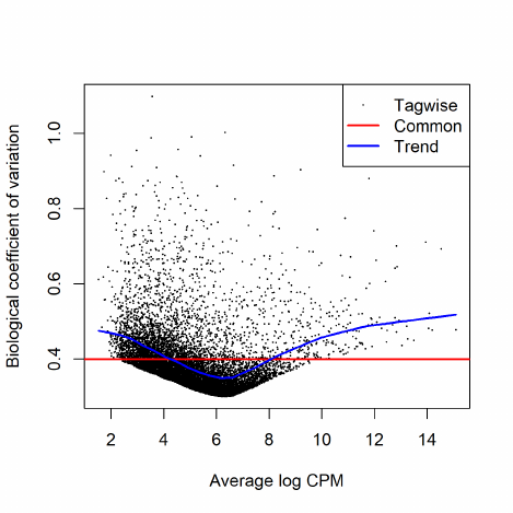
51T 1 0 1 1
attr(,"assign")
[1]0112
attr(,"contrasts")
attr(,"contrasts")$Patient
[1] "contr.treatment"
attr(,"contrasts")$Tissue
[1] "contr.treatment"
This sort of additive model is appropriate for paired designs, or experiments with batch effects.
4.1.7 Estimating the dispersion
We estimate the NB dispersion for the dataset.
> y <- estimateDisp(y, design, robust=TRUE)
> y$common.dispersion
[1] 0.159
The square root of the common dispersion gives the coefficient of variation of biological variation.
Here the common dispersion is found to be 0.159, so the coefficient of biological variation is around
0.4.
The dispersion estimates can be viewed in a BCV plot:
> plotBCV(y)
43
4.1.8 Differential expression
Now proceed to determine differentially expressed genes. Fit genewise glms:
> fit <- glmFit(y, design)
Conduct likelihood ratio tests for tumour vs normal tissue differences and show the top genes:
> lrt <- glmLRT(fit)
> topTags(lrt)
Coefficient: TissueT
RefSeqID Symbol NbrOfExons logFC logCPM LR PValue FDR
5737 NM_001039585 PTGFR 4 -5.18 4.74 98.7 3.00e-23 3.16e-19
5744 NM_002820 PTHLH 4 3.97 6.21 92.2 7.88e-22 4.15e-18
3479 NM_001111283 IGF1 5 -3.99 5.71 86.5 1.38e-20 4.82e-17
1288 NM_033641 COL4A6 45 3.66 5.72 77.6 1.29e-18 3.39e-15
10351 NM_007168 ABCA8 38 -3.98 4.94 75.9 3.01e-18 6.33e-15
5837 NM_005609 PYGM 20 -5.48 5.99 75.4 3.94e-18 6.90e-15
487 NM_004320 ATP2A1 23 -4.62 5.96 74.8 5.22e-18 7.85e-15
27179 NM_014440 IL36A 4 -6.17 5.40 72.2 1.99e-17 2.62e-14
196374 NM_173352 KRT78 9 -4.25 7.61 70.8 3.96e-17 4.63e-14
83699 NM_031469 SH3BGRL2 4 -3.93 5.53 67.8 1.85e-16 1.94e-13
Note that glmLRT has conducted a test for the last coefficient in the linear model, which we can see
is the tumor vs normal tissue effect:
> colnames(design)
[1] "(Intercept)" "Patient33" "Patient51" "TissueT"
The genewise tests are for tumor vs normal differential expression, adjusting for baseline differences
between the three patients. The tests can be viewed as analogous to paired t-tests. The top DE
tags have tiny p-values and FDR values, as well as large fold changes.
Here’s a closer look at the counts-per-million in individual samples for the top genes:
> o <- order(lrt$table$PValue)
> cpm(y)[o[1:10],]
8N 8T 33N 33T 51N 51T
5737 49.69 0.875 27.08 0.878 78.11 2.5434
5744 7.32 95.859 11.80 204.147 6.88 116.3326
3479 50.24 3.124 32.37 1.902 211.60 14.2098
1288 12.12 140.227 6.32 94.430 4.86 56.8393
10351 52.64 3.124 39.45 2.121 79.19 6.0820
5837 152.80 2.750 119.57 1.170 97.68 5.6950
487 107.91 3.124 147.03 3.804 102.81 8.9019
27179 40.08 1.250 172.13 3.292 36.08 0.0553
196374 372.22 20.747 581.13 47.764 145.05 4.5339
83699 96.22 5.124 117.11 5.413 48.19 5.4185
We see that all the top genes have consistent tumour vs normal changes for the three patients.
The total number of differentially expressed genes at 5% FDR is given by:
> summary(decideTests(lrt))
44
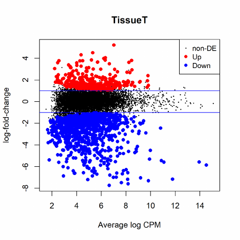
TissueT
Down 938
NotSig 9250
Up 331
Plot log-fold change against log-counts per million, with DE genes highlighted:
> plotMD(lrt)
> abline(h=c(-1, 1), col="blue")
The blue lines indicate 2-fold changes.
4.1.9 Gene ontology analysis
We perform a gene ontology analysis focusing on the ontology of biological process (BP). The genes
up-regulated in the tumors tend to be associated with cell differentiation, cell migration and tissue
morphogenesis:
> go <- goana(lrt)
> topGO(go, ont="BP", sort="Up", n=30)
Term Ont N Up Down P.Up P.Down
GO:0022610 biological adhesion BP 822 64 144 6.24e-12 2.48e-16
GO:0007155 cell adhesion BP 816 63 143 1.36e-11 3.11e-16
GO:0040011 locomotion BP 1031 71 146 1.11e-10 3.55e-09
GO:0030198 extracellular matrix organization BP 237 29 46 3.07e-10 3.06e-07
GO:0030154 cell differentiation BP 2318 122 293 3.32e-10 4.38e-12
GO:0048869 cellular developmental process BP 2465 127 302 4.75e-10 8.35e-11
GO:0009888 tissue development BP 1158 75 175 5.15e-10 2.09e-13
GO:0043062 extracellular structure organization BP 264 30 49 9.20e-10 5.16e-07
GO:0006928 movement of cell or subcellular component BP 1182 75 175 1.32e-09 1.36e-12
45
GO:0016477 cell migration BP 852 59 131 4.79e-09 1.21e-10
GO:0048870 cell motility BP 904 61 133 6.72e-09 1.73e-09
GO:0051674 localization of cell BP 904 61 133 6.72e-09 1.73e-09
GO:0022008 neurogenesis BP 910 61 104 8.64e-09 4.12e-03
GO:0048699 generation of neurons BP 846 58 97 9.58e-09 5.05e-03
GO:0009653 anatomical structure morphogenesis BP 1602 89 224 2.02e-08 1.94e-13
GO:0032502 developmental process BP 3536 159 408 2.52e-08 2.65e-11
GO:0048856 anatomical structure development BP 3281 150 394 3.06e-08 1.59e-13
GO:0030155 regulation of cell adhesion BP 422 36 64 4.45e-08 1.45e-05
GO:0007275 multicellular organism development BP 2990 139 355 5.45e-08 3.92e-11
GO:0060429 epithelium development BP 726 50 90 1.03e-07 6.79e-04
GO:0043588 skin development BP 212 23 29 2.13e-07 1.32e-02
GO:0048731 system development BP 2689 126 337 2.43e-07 1.04e-13
GO:0048729 tissue morphogenesis BP 419 34 55 3.56e-07 2.17e-03
GO:0048598 embryonic morphogenesis BP 347 30 40 4.77e-07 5.44e-02
GO:0048513 animal organ development BP 1979 99 270 4.92e-07 4.48e-15
GO:0030182 neuron differentiation BP 765 50 89 5.15e-07 4.81e-03
GO:0048468 cell development BP 1207 68 173 9.50e-07 3.14e-11
GO:0008544 epidermis development BP 236 23 36 1.44e-06 9.59e-04
GO:0009887 animal organ morphogenesis BP 595 41 87 1.64e-06 1.93e-06
GO:0007399 nervous system development BP 1328 72 141 1.78e-06 1.27e-02
4.1.10 Setup
This analysis was conducted on:
> sessionInfo()
R version 3.5.0 (2018-04-23)
Platform: x86_64-w64-mingw32/x64 (64-bit)
Running under: Windows 10 x64 (build 16299)
Matrix products: default
locale:
[1] LC_COLLATE=English_Australia.1252 LC_CTYPE=English_Australia.1252
[3] LC_MONETARY=English_Australia.1252 LC_NUMERIC=C
[5] LC_TIME=English_Australia.1252
attached base packages:
[1] parallel stats4 stats graphics grDevices utils datasets methods base
other attached packages:
[1] org.Hs.eg.db_3.6.0 AnnotationDbi_1.41.5 IRanges_2.13.28 S4Vectors_0.17.42
[5] Biobase_2.39.2 BiocGenerics_0.25.3 edgeR_3.21.9 limma_3.35.15
loaded via a namespace (and not attached):
[1] locfit_1.5-9.1 Rcpp_0.12.16 lattice_0.20-35 GO.db_3.6.0 digest_0.6.15 grid_3.5.0
[7] DBI_0.8 RSQLite_2.1.0 blob_1.1.1 splines_3.5.0 statmod_1.4.30 tools_3.5.0
[13] bit64_0.9-7 bit_1.1-12 compiler_3.5.0 pkgconfig_2.0.1 memoise_1.1.0
46
4.2 RNA-Seq of pathogen inoculated arabidopsis with batch ef-
fects
4.2.1 Introduction
This case study re-analyses Arabidopsis thaliana RNA-Seq data described by Cumbie et al. [7].
Summarized count data is available as a data object in the CRAN package NBPSeq comparing
∆hrcC challenged and mock-inoculated samples [7]. Samples were collected in three batches, and
adjustment for batch effects proves to be important. The aim of the analysis therefore is to detect
genes differentially expressed in response to ∆hrcC challenge, while correcting for any differences
between the batches.
4.2.2 RNA samples
Pseudomonas syringae is a bacterium often used to study plant reactions to pathogens. In this
experiment, six-week old Arabidopsis plants were inoculated with the ∆hrcC mutant of P. syringae,
after which total RNA was extracted from leaves. Control plants were inoculated with a mock
pathogen.
Three biological replicates of the experiment were conducted at separate times and using inde-
pendently grown plants and bacteria.
The six RNA samples were sequenced one per lane on an Illumina Genome Analyzer. Reads
were aligned and summarized per gene using GENE-counter. The reference genome was derived
from the TAIR9 genome release (www.arabidopsis.org).
4.2.3 Loading the data
Load the data from the NBPSeq package:
> library(NBPSeq)
> library(edgeR)
> data(arab)
> head(arab)
mock1 mock2 mock3 hrcc1 hrcc2 hrcc3
AT1G01010 35 77 40 46 64 60
AT1G01020 43 45 32 43 39 49
AT1G01030 16 24 26 27 35 20
AT1G01040 72 43 64 66 25 90
AT1G01050 49 78 90 67 45 60
AT1G01060 0 15 2 0 21 8
There are two experimental factors, treatment (hrcc vs mock) and the time that each replicate was
conducted:
> Treat <- factor(substring(colnames(arab),1,4))
> Treat <- relevel(Treat, ref="mock")
> Time <- factor(substring(colnames(arab),5,5))
We then create a DGEList object:
> y <- DGEList(counts=arab, group=Treat)
47
4.2.4 Filtering and normalization
There is no purpose in analysing genes that are not expressed in either experimental condition. We
consider a gene to be expressed at a reasonable level in a sample if it has at least two counts for
each million mapped reads in that sample. This cutoff is ad hoc, but serves to require at least 4–6
reads in this case. Since this experiment has three replicates for each condition, a gene should be
expressed in at least three samples if it responds to at least one condition. Hence we keep genes
with at least two counts per million (CPM) in at least three samples:
> keep <- rowSums(cpm(y)>2) >= 3
> table(keep)
keep
FALSE TRUE
9696 16526
> y <- y[keep, , keep.lib.sizes=FALSE]
Note that the filtering does not use knowledge of what treatment corresponds to each sample, so
the filtering does not bias the subsequent differential expression analysis.
The TMM normalization is applied to account for the compositional biases:
> y <- calcNormFactors(y)
> y$samples
group lib.size norm.factors
mock1 mock 1896802 0.979
mock2 mock 1898690 1.054
mock3 mock 3249396 0.903
hrcc1 hrcc 2119367 1.051
hrcc2 hrcc 1264927 1.096
hrcc3 hrcc 3516253 0.932
4.2.5 Data exploration
An MDS plot shows the relative similarities of the six samples.
> plotMDS(y, col=rep(1:2, each=3))
48
−2 −1 0 1
−1.0 −0.5 0.0 0.5 1.0 1.5
Leading logFC dim 1
Leading logFC dim 2
mock1
mock2
mock3
hrcc1
hrcc2
hrcc3
Distances on an MDS plot of a DGEList object correspond to leading log-fold-change between each
pair of samples. Leading log-fold-change is the root-mean-square average of the largest log2-fold-
changes between each pair of samples. Each pair of samples extracted at each time tend to cluster
together, suggesting a batch effect. The hrcc treated samples tend to be below the mock samples
for each time, suggesting a treatment effect within each time. The two samples at time 1 are less
consistent than at times 2 and 3.
To examine further consistency of the three replicates, we compute predictive log2-fold-changes
(logFC) for the treatment separately for the three times.
> design <- model.matrix(~Time+Time:Treat)
> logFC <- predFC(y,design,prior.count=1,dispersion=0.05)
The logFC at the three times are positively correlated with one another, as we would hope:
> cor(logFC[,4:6])
Time1:Treathrcc Time2:Treathrcc Time3:Treathrcc
Time1:Treathrcc 1.000 0.315 0.400
Time2:Treathrcc 0.315 1.000 0.437
Time3:Treathrcc 0.400 0.437 1.000
The correlation is highest between times 2 and 3.
4.2.6 The design matrix
Before we fit GLMs, we need to define our design matrix based on the experimental design. We
want to test for differential expressions between ∆hrcC challenged and mock-inoculated samples
within batches, i.e. adjusting for differences between batches. In statistical terms, this is an additive
linear model. So the design matrix is created as:
49
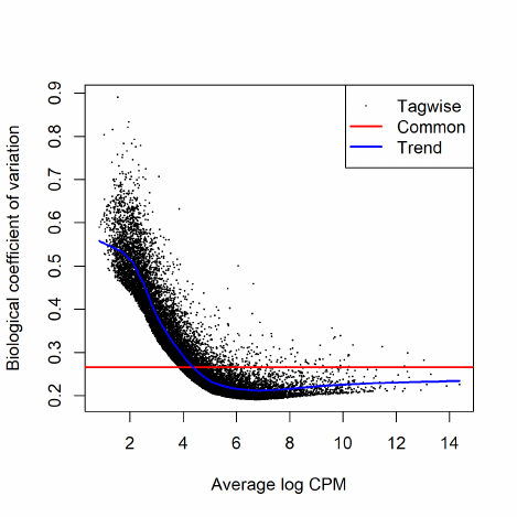
> design <- model.matrix(~Time+Treat)
> rownames(design) <- colnames(y)
> design
(Intercept) Time2 Time3 Treathrcc
mock1 1 0 0 0
mock2 1 1 0 0
mock3 1 0 1 0
hrcc1 1 0 0 1
hrcc2 1 1 0 1
hrcc3 1 0 1 1
attr(,"assign")
[1]0112
attr(,"contrasts")
attr(,"contrasts")$Time
[1] "contr.treatment"
attr(,"contrasts")$Treat
[1] "contr.treatment"
4.2.7 Estimating the dispersion
Estimate the genewise dispersion estimates over all genes, allowing for a possible abundance trend.
The estimation is also robustified against potential outlier genes.
> y <- estimateDisp(y, design, robust=TRUE)
> y$common.dispersion
[1] 0.0705
> plotBCV(y)
50
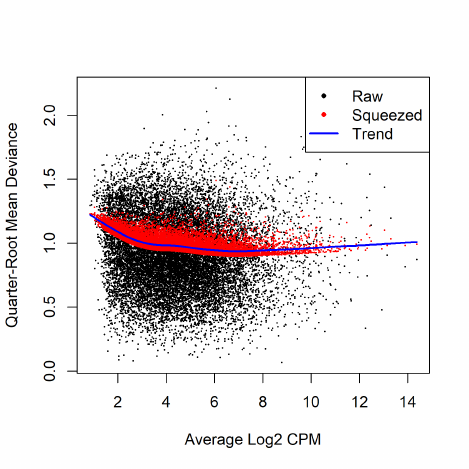
The square root of dispersion is the coefficient of biological variation (BCV). The common
BCV is on the high side, considering that this is a designed experiment using genetically identical
plants. The trended dispersion shows a decreasing trend with expression level. At low logCPM,
the dispersions are very large indeed.
Note that only the trended dispersion is used under the quasi-likelihood (QL) pipeline. The
tagwise and common estimates are shown here but will not be used further.
The QL dispersions can be estimated using the glmQLFit function, and then be visualized with
the plotQLDisp function.
> fit <- glmQLFit(y, design, robust=TRUE)
> plotQLDisp(fit)
4.2.8 Differential expression
Now we test for significant differential expression in each gene using the QL F-test.
First we check whether there was a genuine need to adjust for the experimental times. We do
this by testing for differential expression between the three times. There is considerable differential
expression, justifying our decision to adjust for the batch effect:
> qlf <- glmQLFTest(fit, coef=2:3)
> topTags(qlf)
Coefficient: Time2 Time3
logFC.Time2 logFC.Time3 logCPM F PValue FDR
AT5G66800 5.58 -1.065 5.48 150.1 8.93e-10 1.48e-05
AT5G23000 5.58 -0.292 5.71 127.5 2.48e-09 2.05e-05
AT5G31702 5.83 -2.568 5.95 113.9 5.03e-09 2.77e-05
AT2G45830 5.42 -0.589 4.71 108.4 6.84e-09 2.83e-05
AT3G33004 4.81 -1.763 5.63 102.8 9.47e-09 3.13e-05
51
AT2G11230 3.50 -1.532 5.60 98.7 1.22e-08 3.36e-05
AT2G07782 3.48 -1.616 5.28 93.5 1.70e-08 4.01e-05
AT2G18193 3.05 -2.396 5.08 84.8 3.09e-08 6.04e-05
AT2G23910 3.59 -0.384 5.13 83.9 3.29e-08 6.04e-05
AT5G54830 3.07 -0.367 6.07 79.7 4.51e-08 7.31e-05
> FDR <- p.adjust(qlf$table$PValue, method="BH")
> sum(FDR < 0.05)
[1] 1628
Now conduct QL F-tests for the pathogen effect and show the top genes. By default, the test is for
the last coefficient in the design matrix, which in this case is the treatment effect:
> qlf <- glmQLFTest(fit)
> topTags(qlf)
Coefficient: Treathrcc
logFC logCPM F PValue FDR
AT2G19190 4.50 7.37 304 1.83e-10 2.62e-06
AT2G39530 4.34 6.71 278 3.17e-10 2.62e-06
AT3G46280 4.78 8.10 247 6.70e-10 2.78e-06
AT2G39380 4.94 5.77 247 6.72e-10 2.78e-06
AT1G51800 3.97 7.71 232 9.92e-10 3.28e-06
AT1G51850 5.32 5.42 209 1.89e-09 4.30e-06
AT5G48430 6.32 6.73 203 2.30e-09 4.30e-06
AT2G44370 5.41 5.20 200 2.50e-09 4.30e-06
AT1G51820 4.34 6.37 198 2.64e-09 4.30e-06
AT3G55150 5.78 4.90 196 2.80e-09 4.30e-06
Here’s a closer look at the individual counts-per-million for the top genes. The top genes are very
consistent across the three replicates:
> top <- rownames(topTags(qlf))
> cpm(y)[top,]
mock1 mock2 mock3 hrcc1 hrcc2 hrcc3
AT2G19190 16.696 12.0 13.29 341.3 254.7 351.1
AT2G39530 7.001 9.0 13.29 158.1 191.9 243.1
AT3G46280 18.850 17.0 18.40 384.8 374.5 820.9
AT2G39380 2.154 3.0 4.77 91.6 84.4 135.1
AT1G51800 29.083 16.5 30.66 362.4 347.8 464.0
AT1G51850 1.077 1.0 3.75 78.1 56.3 108.9
AT5G48430 4.309 4.5 0.00 189.1 314.6 125.1
AT2G44370 2.154 1.0 1.70 57.0 67.1 86.0
AT1G51820 9.694 7.5 6.13 121.2 156.6 191.3
AT3G55150 0.539 1.0 1.36 43.1 64.9 64.4
The total number of genes significantly up-regulated or down-regulated at 5% FDR is summa-
rized as follows:
> summary(decideTests(qlf))
Treathrcc
Down 837
NotSig 14797
Up 892
52
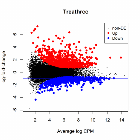
We can plot all the logFCs against average count size, highlighting the DE genes:
> plotMD(qlf)
> abline(h=c(-1,1), col="blue")
The blue lines indicate 2-fold up or down.
4.2.9 Setup
This analysis was conducted on:
> sessionInfo()
R version 3.5.0 (2018-04-23)
Platform: x86_64-w64-mingw32/x64 (64-bit)
Running under: Windows 10 x64 (build 16299)
Matrix products: default
locale:
[1] LC_COLLATE=English_Australia.1252 LC_CTYPE=English_Australia.1252
[3] LC_MONETARY=English_Australia.1252 LC_NUMERIC=C
[5] LC_TIME=English_Australia.1252
attached base packages:
[1] parallel stats4 stats graphics grDevices utils datasets methods base
other attached packages:
[1] NBPSeq_0.3.0 org.Hs.eg.db_3.6.0 AnnotationDbi_1.41.5 IRanges_2.13.28
[5] S4Vectors_0.17.42 Biobase_2.39.2 BiocGenerics_0.25.3 edgeR_3.21.9
[9] limma_3.35.15
53
loaded via a namespace (and not attached):
[1] Rcpp_0.12.16 magrittr_1.5 splines_3.5.0 munsell_0.4.3 bit_1.1-12
[6] statmod_1.4.30 colorspace_1.3-2 lattice_0.20-35 rlang_0.2.0 stringr_1.3.0
[11] plyr_1.8.4 blob_1.1.1 tools_3.5.0 grid_3.5.0 gtable_0.2.0
[16] DBI_0.8 lazyeval_0.2.1 bit64_0.9-7 digest_0.6.15 tibble_1.4.2
[21] reshape2_1.4.3 ggplot2_2.2.1 memoise_1.1.0 qvalue_2.11.0 RSQLite_2.1.0
[26] stringi_1.1.7 pillar_1.2.1 compiler_3.5.0 GO.db_3.6.0 scales_0.5.0
[31] locfit_1.5-9.1 pkgconfig_2.0.1
4.3 Profiles of Yoruba HapMap individuals
4.3.1 Background
RNA-Seq profiles were made of cell lines derived from lymphoblastoid cells from 69 different Yoruba
individuals from Ibadan, Nigeria [26] [27]. The profiles were generated as part of the International
HapMap project [12]. RNA from each individual was sequenced on at least two lanes of an Illumina
Genome Analyser 2, and mapped reads to the human genome using MAQ v0.6.8.
The study group here is essentially an opportunity sample and the individuals are likely to be
genetically diverse. In this analysis we look at genes that are differentially expressed between males
and female.
4.3.2 Loading the data
Read counts summarized by Ensembl gene identifiers are available in the tweeDEseqCountData
package:
> library(tweeDEseqCountData)
> data(pickrell1)
> Counts <- exprs(pickrell1.eset)
> dim(Counts)
[1] 38415 69
> Counts[1:5,1:5]
NA18486 NA18498 NA18499 NA18501 NA18502
ENSG00000127720 6 32 14 35 14
ENSG00000242018 20 21 24 22 16
ENSG00000224440 0 0 0 0 0
ENSG00000214453 0 0 0 0 0
ENSG00000237787 0 0 1 0 0
In this analysis we will compare female with male individuals.
> Gender <- pickrell1.eset$gender
> table(Gender)
54
Gender
female male
40 29
> rm(pickrell1.eset)
Annotation for each Ensemble gene is also available from the tweeDEseqCountData package:
> data(annotEnsembl63)
> annot <- annotEnsembl63[,c("Symbol","Chr")]
> annot[1:5,]
Symbol Chr
ENSG00000252775 U7 5
ENSG00000207459 U6 5
ENSG00000252899 U7 5
ENSG00000201298 U6 5
ENSG00000222266 U6 5
> rm(annotEnsembl63)
Form a DGEList object combining the counts and associated annotation:
> library(edgeR)
> y <- DGEList(counts=Counts, genes=annot[rownames(Counts),])
4.3.3 Filtering and normalization
Keep genes with least 1 count-per-million reads (cpm) in at least 20 samples:
> isexpr <- rowSums(cpm(y)>1) >= 20
Keep only genes with defined annotation, and recompute library sizes:
> hasannot <- rowSums(is.na(y$genes))==0
> y <- y[isexpr & hasannot, , keep.lib.sizes=FALSE]
> dim(y)
[1] 17310 69
The library sizes vary from about 5 million to over 15 million:
> barplot(y$samples$lib.size*1e-6, names=1:69, ylab="Library size (millions)")
55
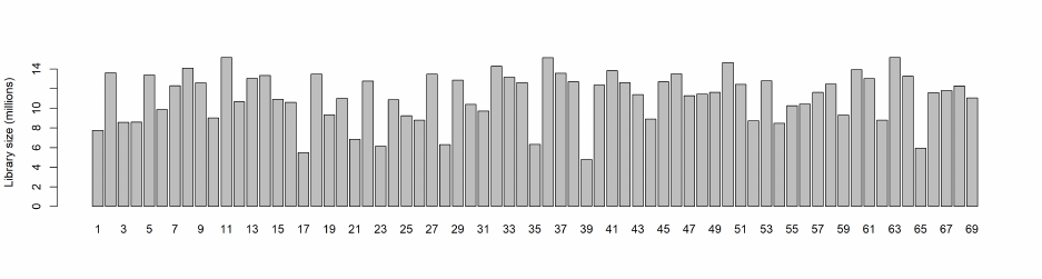
Apply TMM normalization to account for the composition biases:
> y <- calcNormFactors(y)
> head(y$samples)
group lib.size norm.factors
NA18486 1 7749527 0.939
NA18498 1 13612983 1.110
NA18499 1 8569631 0.963
NA18501 1 8595024 1.201
NA18502 1 13375275 0.938
NA18504 1 9881732 0.979
4.3.4 Estimating the dispersion
We are interested in the differences between male and female. Hence, we create a design matrix
using the gender factor. We estimate the NB dispersion using estimateDisp. The estimation is
robustified against potential outlier genes.
> design <- model.matrix(~Gender)
> y <- estimateDisp(y, design, robust=TRUE)
> plotBCV(y)
56
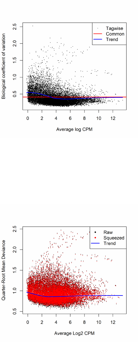
We then estimate the QL dispersions around the dispersion trend using glmQLFit. The large
number of cases and the high variability means that the QL dispersions are not squeezed very
heavily from the raw values:
> fit <- glmQLFit(y, design, robust=TRUE)
> plotQLDisp(fit)
57
4.3.5 Differential expression
Now find genes differentially expressed between male and females. Positive log-fold-changes mean
higher expression in males. The highly ranked genes are mostly on the X or Y chromosomes. Top
ranked is the famous XIST gene, which is known to be expressed only in females.
> qlf <- glmQLFTest(fit)
> topTags(qlf,n=15)
Coefficient: Gendermale
Symbol Chr logFC logCPM F PValue FDR
ENSG00000229807 XIST X -9.49 7.249 1213 1.03e-46 1.78e-42
ENSG00000099749 CYorf15A Y 4.28 1.757 857 1.19e-41 1.03e-37
ENSG00000131002 CYorf15B Y 5.63 2.055 587 2.66e-36 1.31e-32
ENSG00000157828 RPS4Y2 Y 3.18 4.207 585 3.02e-36 1.31e-32
ENSG00000233864 TTTY15 Y 4.84 1.254 538 4.42e-35 1.53e-31
ENSG00000198692 EIF1AY Y 2.36 3.247 376 3.04e-30 8.78e-27
ENSG00000165246 NLGN4Y Y 5.09 1.676 303 1.70e-27 4.21e-24
ENSG00000183878 UTY Y 1.86 3.137 253 3.24e-25 7.01e-22
ENSG00000243209 AC010889.1 Y 2.66 0.797 232 3.63e-24 6.29e-21
ENSG00000129824 RPS4Y1 Y 2.53 5.401 232 3.63e-24 6.29e-21
ENSG00000012817 KDM5D Y 1.47 4.950 222 1.16e-23 1.82e-20
ENSG00000213318 RP11-331F4.1 16 3.67 3.688 217 2.87e-23 4.13e-20
ENSG00000067048 DDX3Y Y 1.62 5.621 181 2.48e-21 3.30e-18
ENSG00000146938 NLGN4X X 3.94 1.048 139 1.81e-18 2.24e-15
ENSG00000232928 RP13-204A15.4 X 1.44 3.558 111 3.19e-16 3.68e-13
> summary(decideTests(qlf))
Gendermale
Down 46
NotSig 17243
Up 21
4.3.6 Gene set testing
The tweeDEseqCountData package includes a list of genes belonging to the male-specific region of
chromosome Y, and a list of genes located in the X chromosome that have been reported to escape
X-inactivation. We expect genes in the first list to be up-regulated in males, whereas genes in the
second list should be up-regulated in females.
> data(genderGenes)
> Ymale <- rownames(y) %in% msYgenes
> Xescape <- rownames(y) %in% XiEgenes
Roast gene set tests by fry() confirm that the male-specific genes are significantly up as a group
in our comparison of males with females, whereas the X genes are significantly down as a group
[38].
58
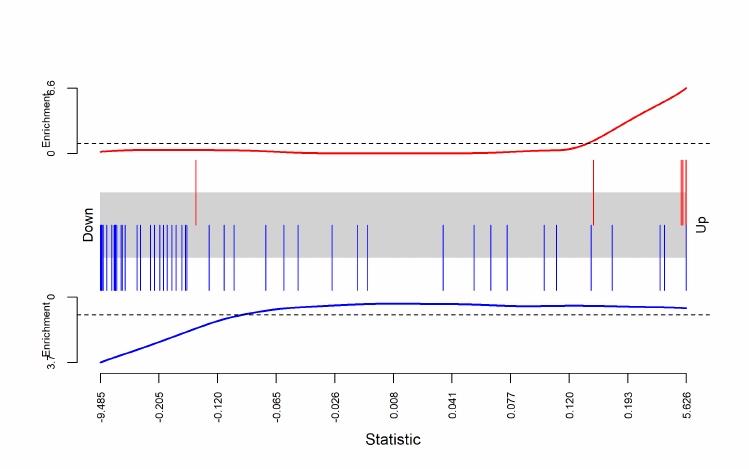
> index <- list(Y=Ymale, X=Xescape)
> fry(y, index=index, design=design)
NGenes Direction PValue FDR PValue.Mixed FDR.Mixed
Y 12 Up 7.04e-46 1.41e-45 5.86e-11 5.86e-11
X 46 Down 7.25e-17 7.25e-17 2.28e-66 4.55e-66
A barcode plot can be produced to visualize the results. Genes are ranked from left to right
by decreasing log-fold-change in the background of the barcode plot. Genes in the set of msYgenes
are represented by red bars whereas genes in the set of XiEgenes are represented by blue bars.
The line above the barcode shows the relative local enrichment of the vertical bars in each part
of the plot. This particular plot suggests that the male-specific genes tend to have large positive
log-fold-changes, whereas the X genes tend to have large negative log-fold-changes.
> barcodeplot(qlf$table$logFC, index[[1]], index[[2]])
The results from competitive camera gene sets tests are even more convincing [39]. The positive
intergene correlations here show that the genes in each set tend to be biologically correlated:
> camera(y, index, design)
NGenes Direction PValue FDR
Y 12 Up 1.27e-295 2.55e-295
X 46 Down 3.02e-25 3.02e-25
See where the X and Y genes fall on the MA plot:
59
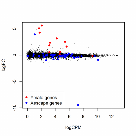
> with(qlf$table, plot(logCPM,logFC,pch=16,cex=0.2))
> with(qlf$table, points(logCPM[Xescape],logFC[Xescape],pch=16,col="blue"))
> with(qlf$table, points(logCPM[Ymale],logFC[Ymale],pch=16,col="red"))
> legend("bottomleft",legend=c("Ymale genes","Xescape genes"),pch=16,,col=c("red","blue"))
4.3.7 Setup
This analysis was conducted on:
> sessionInfo()
R version 3.5.0 (2018-04-23)
Platform: x86_64-w64-mingw32/x64 (64-bit)
Running under: Windows 10 x64 (build 16299)
Matrix products: default
locale:
[1] LC_COLLATE=English_Australia.1252 LC_CTYPE=English_Australia.1252
[3] LC_MONETARY=English_Australia.1252 LC_NUMERIC=C
[5] LC_TIME=English_Australia.1252
attached base packages:
[1] parallel stats4 stats graphics grDevices utils datasets methods base
other attached packages:
[1] tweeDEseqCountData_1.17.0 NBPSeq_0.3.0 org.Hs.eg.db_3.6.0
[4] AnnotationDbi_1.41.5 IRanges_2.13.28 S4Vectors_0.17.42
[7] Biobase_2.39.2 BiocGenerics_0.25.3 edgeR_3.21.9
[10] limma_3.35.15
60
loaded via a namespace (and not attached):
[1] Rcpp_0.12.16 compiler_3.5.0 pillar_1.2.1 plyr_1.8.4 tools_3.5.0
[6] digest_0.6.15 statmod_1.4.30 bit_1.1-12 RSQLite_2.1.0 memoise_1.1.0
[11] tibble_1.4.2 gtable_0.2.0 lattice_0.20-35 pkgconfig_2.0.1 rlang_0.2.0
[16] DBI_0.8 stringr_1.3.0 locfit_1.5-9.1 bit64_0.9-7 grid_3.5.0
[21] qvalue_2.11.0 GO.db_3.6.0 ggplot2_2.2.1 reshape2_1.4.3 blob_1.1.1
[26] magrittr_1.5 scales_0.5.0 splines_3.5.0 colorspace_1.3-2 stringi_1.1.7
[31] lazyeval_0.2.1 munsell_0.4.3
4.4 RNA-Seq profiles of mouse mammary gland
4.4.1 Introduction
The RNA-Seq data of this case study is described in Fu et al. [9]. The sequence and count data
are publicly available from the Gene Expression Omnibus (GEO) at the series accession number
GSE60450. This study examines the expression profiles of basal stem-cell enriched cells (B) and
committed luminal cells (L) in the mammary gland of virgin, pregnant and lactating mice. Six
groups are present, with one for each combination of cell type and mouse status. Each group
contains two biological replicates. This is summarized in the table below, where the basal and
luminal cell types are abbreviated with Band Lrespectively.
> targets <- read.delim("targets.txt", header=TRUE)
> targets
FileName GEOAccession CellType Status
1 SRR1552450.fastq GSM1480297 B virgin
2 SRR1552451.fastq GSM1480298 B virgin
3 SRR1552452.fastq GSM1480299 B pregnant
4 SRR1552453.fastq GSM1480300 B pregnant
5 SRR1552454.fastq GSM1480301 B lactate
6 SRR1552455.fastq GSM1480302 B lactate
7 SRR1552444.fastq GSM1480291 L virgin
8 SRR1552445.fastq GSM1480292 L virgin
9 SRR1552446.fastq GSM1480293 L pregnant
10 SRR1552447.fastq GSM1480294 L pregnant
11 SRR1552448.fastq GSM1480295 L lactate
12 SRR1552449.fastq GSM1480296 L lactate
The name of the file containing the read sequences for each library is also shown. Each file is
downloaded from the Sequence Read Archive and has an accession number starting with SRR, e.g.,
SRR1552450 for the first library in targets.
4.4.2 Read alignment and processing
Prior to read alignment, these files are converted into the FASTQ format using the fastq-dump utility
from the SRA Toolkit. See http://www.ncbi.nlm.nih.gov/books/NBK158900 for how to download
and use the SRA Toolkit.
61
Before the differential expression analysis can proceed, these reads must be aligned to the mouse
genome and counted into annotated genes. This can be achieved with functions in the Rsubread
package [14]. We assume that an index of the mouse genome is already available - if not, this can
be constructed from a FASTA file of the genome sequence with the buildindex command. In this
example, we assume that the prefix for the index files is mm10. The reads in each FASTQ file are
then aligned to the mouse genome, as shown below.
> library(Rsubread)
> output.files <- sub(".fastq", ".bam", targets$FileName)
> align("mm10", readfile1=targets$FileName, phredOffset=33,
+ input_format="FASTQ", output_file=output.files)
This produces a set of BAM files, where each file contains the read alignments for each library.
The mapped reads can be counted into mouse genes by using the featureCounts function. It uses
the exon intervals defined in the NCBI annotation of the mm10 genome.
> fc <- featureCounts(output.files, annot.inbuilt="mm10")
> colnames(fc$counts) <- 1:12
> head(fc$counts)
123456789101112
497097 438 300 65 237 354 287 0 0 0 0 0 0
100503874101104000000
100038431000000000000
19888 1 1 0 0 0 0 10 3 10 2 0 0
20671 106 182 82 105 43 82 16 25 18 8 3 10
27395 309 234 337 300 290 270 560 464 489 328 307 342
The row names of the matrix represent the Entrez gene identifiers for each gene. In the output
from featureCounts, the column names of fc$counts are the output file names from align. Here,
we simplify them for brevity.
4.4.3 Count loading and annotation
We create a DGEList object as follows
> group <- factor(paste0(targets$CellType, ".", targets$Status))
> y <- DGEList(fc$counts, group=group)
> colnames(y) <- targets$GEO
Human-readable gene symbols can also be added to complement the Entrez identifiers for each
gene, using the annotation in the org.Mm.eg.db package.
> require(org.Mm.eg.db)
> Symbol <- mapIds(org.Mm.eg.db,keys=rownames(y),keytype="ENTREZID",column="SYMBOL")
> y$genes <- data.frame(Symbol=Symbol)
62
4.4.4 Filtering and normalization
Here, a gene is only retained if it is expressed at a minimum level:
> keep <- filterByExpr(y)
> summary(keep)
Mode FALSE TRUE
logical 11210 15969
> y <- y[keep, , keep.lib.sizes=FALSE]
TMM normalization is performed to eliminate composition biases between libraries.
> y <- calcNormFactors(y)
> y$samples
group lib.size norm.factors
GSM1480297 B.virgin 23219195 1.238
GSM1480298 B.virgin 21769326 1.214
GSM1480299 B.pregnant 24092719 1.125
GSM1480300 B.pregnant 22657703 1.071
GSM1480301 B.lactate 21522881 1.036
GSM1480302 B.lactate 20009184 1.087
GSM1480291 L.virgin 20385437 1.368
GSM1480292 L.virgin 21699830 1.365
GSM1480293 L.pregnant 22236469 1.004
GSM1480294 L.pregnant 21983364 0.923
GSM1480295 L.lactate 24720123 0.529
GSM1480296 L.lactate 24653390 0.535
The performance of the TMM normalization procedure can be examined using mean-difference
(MD) plots. This visualizes the library size-adjusted log-fold change between two libraries (the
difference) against the average log-expression across those libraries (the mean). The following MD
plot is generated by comparing sample 1 against an artificial library constructed from the average
of all other samples.
> plotMD(cpm(y, log=TRUE), column=1)
> abline(h=0, col="red", lty=2, lwd=2)
63
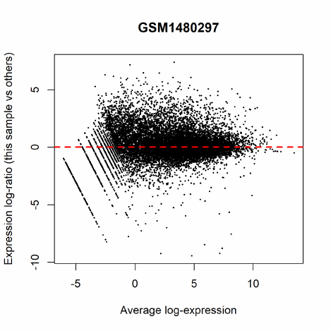
Ideally, the bulk of genes should be centred at a log-fold change of zero. This indicates that
any composition bias between libraries has been successfully removed. This quality check should
be repeated by constructing a MD plot for each sample.
4.4.5 Data exploration
The data can be explored by generating multi-dimensional scaling (MDS) plots. This visualizes
the differences between the expression profiles of different samples in two dimensions.
> points <- c(0,1,2,15,16,17)
> colors <- rep(c("blue", "darkgreen", "red"), 2)
> plotMDS(y, col=colors[group], pch=points[group])
> legend("topleft", legend=levels(group), pch=points, col=colors, ncol=2)
64
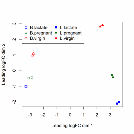
Replicate samples from the same group cluster together in the plot, while samples from different
groups form separate clusters. This indicates that the differences between groups are larger than
those within groups, i.e., differential expression is greater than the variance and can be detected.
The distance between basal samples on the left and luminal cells on the right is about 6 units,
corresponding to a leading fold change of about 64-fold (26= 64) between basal and luminal. The
expression differences between virgin, pregnant and lactating are greater for luminal cells than for
basal.
4.4.6 The design matrix
The experimental design for this study can be parametrized with a one-way layout, whereby one
coefficient is assigned to each group. The design matrix contains the predictors for each sample
and and is constructed using the code below.
> design <- model.matrix(~ 0 + group)
> colnames(design) <- levels(group)
> design
B.lactate B.pregnant B.virgin L.lactate L.pregnant L.virgin
1 0 0 1 0 0 0
2 0 0 1 0 0 0
3 0 1 0 0 0 0
4 0 1 0 0 0 0
5 1 0 0 0 0 0
6 1 0 0 0 0 0
7 0 0 0 0 0 1
8 0 0 0 0 0 1
9 0 0 0 0 1 0
10 0 0 0 0 1 0
65
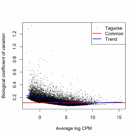
11 0 0 0 1 0 0
12 0 0 0 1 0 0
attr(,"assign")
[1]111111
attr(,"contrasts")
attr(,"contrasts")$group
[1] "contr.treatment"
4.4.7 Estimating the dispersion
The NB dispersion is estimated using the estimateDisp function. This returns the DGEList object
with additional entries for the estimated NB dispersions for all gene. These estimates can be
visualized with plotBCV, which shows the root-estimate, i.e., the biological coefficient of variation
for each gene.
> y <- estimateDisp(y, design, robust=TRUE)
> y$common.dispersion
[1] 0.0134
> plotBCV(y)
Note that only the trended dispersion is used under the quasi-likelihood (QL) pipeline. The tagwise
and common estimates are shown here but will not be used further.
For the QL dispersions, estimation can be performed using the glmQLFit function. This returns
aDGEGLM object containing the estimated values of the GLM coefficients for each gene, as well as
the fitted mean-QL dispersion trend, the squeezed QL estimates and the prior degrees of freedom
(df). These can be visualized with the plotQLDisp function.
66
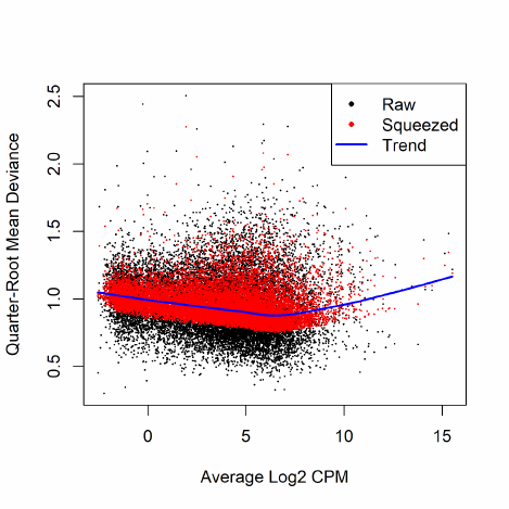
> fit <- glmQLFit(y, design, robust=TRUE)
> head(fit$coefficients)
B.lactate B.pregnant B.virgin L.lactate L.pregnant L.virgin
497097 -11.14 -12.02 -11.23 -19.0 -19.03 -19.0
20671 -12.77 -12.51 -12.15 -14.5 -14.31 -14.1
27395 -11.27 -11.30 -11.53 -10.6 -10.87 -10.9
18777 -10.15 -10.21 -10.77 -10.1 -10.39 -10.4
21399 -9.89 -9.74 -9.79 -10.2 -9.97 -10.0
58175 -16.16 -14.85 -15.99 -13.3 -12.29 -12.1
> plotQLDisp(fit)
Setting robust=TRUE in glmQLFit is strongly recommended [25]. Setting robust=TRUE in estimateDisp
has no effect on the downstream analysis, but is nevertheless very useful as it identifies genes that
are outliers from the mean-NB dispersion trend.
4.4.8 Differential expression
We test for significant differential expression in each gene, using the QL F-test. The contrast of
interest can be specified using the makeContrasts function. Here, genes are tested for DE between
the basal pregnant and lactating groups. This is done by defining the null hypothesis as B.pregnant
- B.lactate = 0.
> con <- makeContrasts(B.pregnant - B.lactate, levels=design)
> qlf <- glmQLFTest(fit, contrast=con)
The top set of most significant genes can be examined with topTags. Here, a positive log-
fold change represents genes that are up in B.pregnant over B.lactate. Multiplicity correction
67
is performed by applying the Benjamini-Hochberg method on the p-values, to control the false
discovery rate (FDR).
> topTags(qlf)
Coefficient: -1*B.lactate 1*B.pregnant
Symbol logFC logCPM F PValue FDR
12992 Csn1s2b -6.09 10.18 423 4.27e-11 6.81e-07
211577 Mrgprf -5.15 2.74 345 1.17e-10 7.15e-07
226101 Myof -2.32 6.44 324 1.74e-10 7.15e-07
381290 Atp2b4 -2.14 6.14 323 1.79e-10 7.15e-07
140474 Muc4 7.17 6.05 307 2.41e-10 7.70e-07
231830 Micall2 2.25 5.18 282 4.12e-10 1.10e-06
24117 Wif1 1.82 6.76 259 6.85e-10 1.56e-06
12740 Cldn4 5.32 9.87 299 8.47e-10 1.60e-06
21953 Tnni2 -5.75 3.86 315 9.00e-10 1.60e-06
231991 Creb5 -2.57 4.87 243 1.03e-09 1.64e-06
The top gene Csn1s2b has a large negative log2-fold-change, showing that it is far more highly
expressed in lactating than pregnant mice. This gene is known to be a major source of protein in
milk.
The total number of DE genes in each direction at a FDR of 5% can be examined with
decideTests. There are in fact nearly 4500 DE genes an FDR cut-off of 5% in this comparison:
> summary(decideTests(qlf))
-1*B.lactate 1*B.pregnant
Down 2509
NotSig 10694
Up 2766
The differential expression test results can be visualized using an MD plot. The log-fold change
for each gene is plotted against the average abundance, i.e., logCPM in the result table above.
Significantly DE genes at a FDR of 5% are highlighted.
> plotMD(qlf)
68
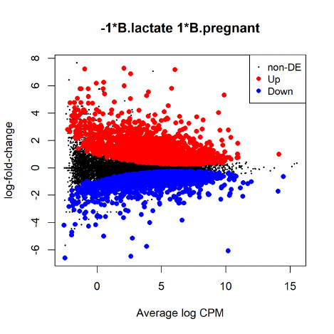
We use glmTreat to narrow down the list of DE genes and focus on genes that are more bio-
logically meaningful. We test whether the differential expression is significantly above a log2-fold-
change of log21.2, i.e., a fold-change of 1.2.
> tr <- glmTreat(fit, contrast=con, lfc=log2(1.2))
> topTags(tr)
Coefficient: -1*B.lactate 1*B.pregnant
Symbol logFC unshrunk.logFC logCPM PValue FDR
12992 Csn1s2b -6.09 -6.09 10.18 4.51e-11 7.20e-07
211577 Mrgprf -5.15 -5.15 2.74 1.27e-10 8.71e-07
226101 Myof -2.32 -2.32 6.44 2.49e-10 8.71e-07
140474 Muc4 7.17 7.34 6.05 2.67e-10 8.71e-07
381290 Atp2b4 -2.14 -2.15 6.14 2.73e-10 8.71e-07
231830 Micall2 2.25 2.25 5.18 6.06e-10 1.61e-06
12740 Cldn4 5.32 5.32 9.87 8.98e-10 1.88e-06
21953 Tnni2 -5.75 -5.76 3.86 9.44e-10 1.88e-06
24117 Wif1 1.82 1.82 6.76 1.22e-09 2.17e-06
231991 Creb5 -2.57 -2.58 4.87 1.37e-09 2.19e-06
Around 3000 genes are detected as DE with fold-change significantly above 1.2 at an FDR
cut-off of 5%.
> summary(decideTests(tr))
-1*B.lactate 1*B.pregnant
Down 1434
NotSig 12728
Up 1807
69
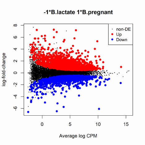
The test results are visualized in the following smear plot. Genes that are significantly DE
above a fold-change of 1.2 at an FDR of 5% are highlighted in red.
> plotMD(tr)
4.4.9 ANOVA-like testing
The differential expression analysis of two-group comparison can be easily extended to comparisons
between three or more groups. This is done by creating a matrix of contrasts, where which each
column represents a contrast between two groups of interest. In this manner, users can perform a
one-way analysis of variance (ANOVA) for each gene.
As an example, suppose we want to compare the three groups in the luminal population, i.e.,
virgin, pregnant and lactating. An appropriate contrast matrix can be created as shown below, to
make pairwise comparisons between all three groups.
> con <- makeContrasts(
+ L.PvsL = L.pregnant - L.lactate,
+ L.VvsL = L.virgin - L.lactate,
+ L.VvsP = L.virgin - L.pregnant, levels=design)
The QL F-test is then applied to identify genes that are DE among the three groups. This
combines the three pairwise comparisons into a single F-statistic and p-value. The top set of
significant genes can be displayed with topTags.
> anov <- glmQLFTest(fit, contrast=con)
> topTags(anov)
70
Coefficient: LR test on 2 degrees of freedom
Symbol logFC.L.PvsL logFC.L.VvsL logFC.L.VvsP logCPM F PValue FDR
19242 Ptn -1.54 7.26 8.800 7.97 2389 3.14e-17 5.01e-13
13645 Egf -5.36 -7.22 -1.865 3.67 1123 3.91e-15 2.80e-11
52150 Kcnk6 -2.42 -7.00 -4.579 5.91 1016 7.37e-15 2.80e-11
12992 Csn1s2b -8.55 -11.36 -2.811 10.18 1055 8.53e-15 2.80e-11
15439 Hp 1.08 5.42 4.336 4.93 987 8.88e-15 2.80e-11
14183 Fgfr2 -1.15 3.95 5.096 7.38 953 1.11e-14 2.80e-11
20856 Stc2 -1.81 3.19 5.005 6.10 914 1.45e-14 2.80e-11
11941 Atp2b2 -7.37 -10.56 -3.191 6.60 1135 1.53e-14 2.80e-11
13358 Slc25a1 -4.13 -4.91 -0.785 7.49 889 1.73e-14 2.80e-11
17068 Ly6d 3.42 9.24 5.819 4.68 887 1.75e-14 2.80e-11
Note that the three contrasts of pairwise comparisons are linearly dependent. Constructing
the contrast matrix with any two of the contrasts would be sufficient to specify an ANOVA test.
For instance, the contrast matrix shown below produces the same test results but with a different
column of log-fold changes.
> con <- makeContrasts(
+ L.PvsL = L.pregnant - L.lactate,
+ L.VvsP = L.virgin - L.pregnant, levels=design)
4.4.10 Gene ontology analysis
Further analyses are required to interpret the differential expression results in a biological context.
One common downstream procedure is a gene ontology (GO) enrichment analysis.
Suppose we want to identify GO terms that are over-represented in the basal lactating group
compared to the basal pregnancy group. This can be achieved by applying the goana function to
the differential expression results of that comparison. The top set of most enriched GO terms can
be viewed with the topGO function.
> con <- makeContrasts(B.lactate - B.pregnant, levels=design)
> qlf <- glmQLFTest(fit, contrast=con)
> go <- goana(qlf, species = "Mm")
> topGO(go, n=30)
Term Ont N Up Down P.Up P.Down
GO:0042254 ribosome biogenesis BP 269 7 153 1.00e+00 5.16e-49
GO:0022613 ribonucleoprotein complex biogenesis BP 397 24 193 1.00e+00 1.36e-47
GO:1990904 ribonucleoprotein complex CC 723 50 279 1.00e+00 8.59e-44
GO:0022626 cytosolic ribosome CC 118 1 84 1.00e+00 5.25e-38
GO:0006364 rRNA processing BP 184 3 109 1.00e+00 1.94e-37
GO:0016072 rRNA metabolic process BP 211 10 116 1.00e+00 1.99e-35
GO:0003723 RNA binding MF 975 103 315 1.00e+00 8.03e-32
GO:0005840 ribosome CC 228 4 113 1.00e+00 3.76e-29
GO:0003735 structural constituent of ribosome MF 152 1 85 1.00e+00 5.53e-27
GO:0022625 cytosolic large ribosomal subunit CC 65 0 51 1.00e+00 5.89e-27
GO:0032991 protein-containing complex CC 4437 661 1002 9.80e-01 4.38e-26
71
GO:0034470 ncRNA processing BP 323 15 136 1.00e+00 7.05e-26
GO:0044391 ribosomal subunit CC 190 1 96 1.00e+00 9.18e-26
GO:0044445 cytosolic part CC 236 22 110 9.99e-01 1.53e-25
GO:0034660 ncRNA metabolic process BP 423 29 160 1.00e+00 3.47e-24
GO:0006396 RNA processing BP 774 66 247 1.00e+00 4.25e-24
GO:0005730 nucleolus CC 775 108 247 9.40e-01 5.21e-24
GO:0030684 preribosome CC 77 0 53 1.00e+00 2.46e-23
GO:0006412 translation BP 552 53 191 1.00e+00 2.91e-23
GO:0043043 peptide biosynthetic process BP 569 54 195 1.00e+00 3.63e-23
GO:0008150 biological_process BP 14525 2412 2529 9.90e-23 4.78e-01
GO:0043604 amide biosynthetic process BP 633 61 209 1.00e+00 1.74e-22
GO:0070013 intracellular organelle lumen CC 3427 515 792 9.33e-01 1.91e-22
GO:0031974 membrane-enclosed lumen CC 3430 515 792 9.36e-01 2.52e-22
GO:0043233 organelle lumen CC 3430 515 792 9.36e-01 2.52e-22
GO:0005575 cellular_component CC 14574 2416 2535 4.29e-22 5.56e-01
GO:0050794 regulation of cellular process BP 7668 1429 1356 4.77e-21 1.88e-01
GO:0042273 ribosomal large subunit biogenesis BP 71 1 48 1.00e+00 9.72e-21
GO:0003674 molecular_function MF 14346 2386 2473 1.17e-20 9.59e-01
GO:0065007 biological regulation BP 8522 1559 1533 2.13e-20 1.85e-02
The row names of the output are the universal identifiers of the GO terms, with one term
per row. The Term column gives the names of the GO terms. These terms cover three domains -
biological process (BP), cellular component (CC) and molecular function (MF), as shown in the
Ont column. The Ncolumn represents the total number of genes that are annotated with each
GO term. The Up and Down columns represent the number of genes with the GO term that are
significantly up- and down-regulated in this differential expression comparison, respectively. The
P.Up and P.Down columns contain the p-values for over-representation of the GO term across the
set of up- and down-regulated genes, respectively. The output table is sorted by the minimum of
P.Up and P.Down by default.
The goana function uses the NCBI RefSeq annotation. Therefore, the Entrez Gene identifier
(ID) should be supplied for each gene as the row names of qlf.
4.4.11 Gene set testing
Another downstream step uses the rotation gene set test (ROAST) [38]. Given a set of genes, we
can test whether the majority of the genes in the set are DE across the contrast of interest. It is
useful when the specified set contains all genes involved in some pathway or process.
In our case study, suppose we are interested in three GO terms related to cytokinesis. Each
term will be used to define a set containing all genes that are annotated with that term. The names
of these terms can be viewed as shown below.
> library(GO.db)
> cyt.go <- c("GO:0032465", "GO:0000281", "GO:0000920")
> term <- select(GO.db, keys=cyt.go, columns="TERM")
> term
GOID TERM
1 GO:0032465 regulation of cytokinesis
72
2 GO:0000281 mitotic cytokinesis
3 GO:0000920 cell separation after cytokinesis
We construct a list of three components, each of which is a vector of Entrez Gene IDs for all
genes annotated with one of the GO terms. We then convert the Gene IDs into row indices of the
fit object using the function ids2indices.
> Rkeys(org.Mm.egGO2ALLEGS) <- cyt.go
> ind <- ids2indices(as.list(org.Mm.egGO2ALLEGS), row.names(fit))
We proceed to run ROAST on the defined gene sets for the contrast of interest. Suppose the
comparison of interest is between the virgin and lactating groups in the basal population. We use
fry to test for multiple gene sets.
> con <- makeContrasts(B.virgin-B.lactate, levels=design)
> fr <- fry(y, index=ind, design=design, contrast=con)
> fr
NGenes Direction PValue FDR PValue.Mixed FDR.Mixed
GO:0032465 65 Up 0.00121 0.00239 7.02e-06 7.02e-06
GO:0000920 16 Down 0.00159 0.00239 4.58e-06 7.02e-06
GO:0000281 63 Up 0.00603 0.00603 6.52e-06 7.02e-06
Each row corresponds to a single gene set, i.e., GO term. The NGenes column gives the number
of genes in each set. The net direction of change is determined from the significance of changes in
each direction, and is shown in the Direction column. The PValue provides evidence for whether
the majority of genes in the set are DE in the specified direction, whereas the PValue.Mixed tests
for differential expression in any direction. FDRs are computed from the corresponding p-values
across all sets.
A barcode plot can be produced with the barcodeplot function to visualize the results for any
particular set. In this case, visualization is performed for the gene set defined by GO:0032465.
Here, genes are represented by bars and are ranked from left to right by decreasing log-fold change.
This forms the barcode-like pattern. The line above the barcode shows the relative local enrichment
of the vertical bars in each part of the plot. This particular plot suggests that most genes in this
set are up-regulated in the virgin group compared to the lactating group.
> res <- glmQLFTest(fit, contrast=con)
> barcodeplot(res$table$logFC, ind[[1]], main=names(ind)[1])
73
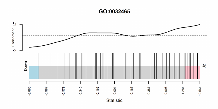
4.4.12 Setup
This analysis was conducted on:
> sessionInfo()
R version 3.5.0 (2018-04-23)
Platform: x86_64-w64-mingw32/x64 (64-bit)
Running under: Windows 10 x64 (build 16299)
Matrix products: default
locale:
[1] LC_COLLATE=English_Australia.1252 LC_CTYPE=English_Australia.1252
[3] LC_MONETARY=English_Australia.1252 LC_NUMERIC=C
[5] LC_TIME=English_Australia.1252
attached base packages:
[1] parallel stats4 stats graphics grDevices utils datasets methods base
other attached packages:
[1] GO.db_3.6.0 org.Mm.eg.db_3.6.0 tweeDEseqCountData_1.17.0
[4] NBPSeq_0.3.0 org.Hs.eg.db_3.6.0 AnnotationDbi_1.41.5
[7] IRanges_2.13.28 S4Vectors_0.17.42 Biobase_2.39.2
[10] BiocGenerics_0.25.3 edgeR_3.21.9 limma_3.35.15
loaded via a namespace (and not attached):
[1] Rcpp_0.12.16 compiler_3.5.0 pillar_1.2.1 plyr_1.8.4 tools_3.5.0
[6] digest_0.6.15 statmod_1.4.30 bit_1.1-12 RSQLite_2.1.0 memoise_1.1.0
[11] tibble_1.4.2 gtable_0.2.0 lattice_0.20-35 pkgconfig_2.0.1 rlang_0.2.0
[16] DBI_0.8 stringr_1.3.0 locfit_1.5-9.1 bit64_0.9-7 grid_3.5.0
[21] qvalue_2.11.0 ggplot2_2.2.1 reshape2_1.4.3 blob_1.1.1 magrittr_1.5
[26] scales_0.5.0 splines_3.5.0 colorspace_1.3-2 stringi_1.1.7 lazyeval_0.2.1
[31] munsell_0.4.3
74
4.5 Differential splicing after Pasilla knockdown
4.5.1 Introduction
The RNA-Seq data of this case study was produced by Brooks et al [3]. Drosophila melanogaster
was used as a model system to study the proteins NOVA1 and NOVA2 which are known to regulate
splicing in mammals. In particular, an RNA interference system (RNAi) was used to knock down
the expression of the D. melanogaster ortholog of NOVA1 and NOVA2, which is Pasilla.
The experiment compared treated and untreated cells from the S2-DRSC cell line. In this case
study we are interested in exons and genes that are differentially expressed after Pasilla knockdown,
as well as genes that are differentially spliced in the knockdown samples as compared to wildtype.
4.5.2 RNA-Seq samples
The RNA-Seq data of the six samples were deposited on GEO http://www.ncbi.nlm.nih.gov/geo.
The GEO accession numbers and titles were prepared in a csv file:
> library(edgeR)
> GEO <- readTargets("GEO-samples.csv", sep=",")
> GEO
GEO Title Pasilla
1 GSM461176 S2_DRSC_Untreated-1 Normal
2 GSM461177 S2_DRSC_Untreated-3 Normal
3 GSM461178 S2_DRSC_Untreated-4 Normal
4 GSM461179 S2_DRSC_CG8144_RNAi-1 Down
5 GSM461180 S2_DRSC_CG8144_RNAi-3 Down
6 GSM461181 S2_DRSC_CG8144_RNAi-4 Down
There are three untreated biological samples, in which Pasilla should be expressed at normal levels,
and three treated biological samples, in which Pasilla should be expressed at reduced levels.
While GEO records the sample information, the sequencing data file are actually held on the
NCBI Short Read Archive (SRA). The RNA samples were sequenced on an Illumina Genome
Analyzer II. Multiple sequencing runs were used for several of the samples, resulting in a total of
20 SRA files:
> SRA <- readTargets("SRA-Files.csv", sep=",")
> SRA
SRA GEO Title RunDate FlowCellID Type ReadLength
1 SRR031708 GSM461176 S2_DRSC_Untreated-1 7/15/08 308T2AAXX SE 45
2 SRR031709 GSM461176 S2_DRSC_Untreated-1 7/15/08 308T2AAXX SE 45
3 SRR031710 GSM461176 S2_DRSC_Untreated-1 8/15/08 30AYWAAXX SE 45
4 SRR031711 GSM461176 S2_DRSC_Untreated-1 8/15/08 30AYWAAXX SE 45
5 SRR031712 GSM461176 S2_DRSC_Untreated-1 8/15/08 30AYWAAXX SE 45
6 SRR031713 GSM461176 S2_DRSC_Untreated-1 8/15/08 30AYWAAXX SE 45
7 SRR031714 GSM461177 S2_DRSC_Untreated-3 11/14/08 30MNEAAXX PE 37
8 SRR031715 GSM461177 S2_DRSC_Untreated-3 12/23/08 30M2BAAXX PE 37
9 SRR031716 GSM461178 S2_DRSC_Untreated-4 12/23/08 30M2BAAXX PE 37
75

10 SRR031717 GSM461178 S2_DRSC_Untreated-4 12/23/08 30M2BAAXX PE 37
11 SRR031718 GSM461179 S2_DRSC_CG8144_RNAi-1 7/15/08 308T2AAXX SE 45
12 SRR031719 GSM461179 S2_DRSC_CG8144_RNAi-1 7/18/08 308UEAAXX SE 45
13 SRR031720 GSM461179 S2_DRSC_CG8144_RNAi-1 8/15/08 30AYWAAXX SE 45
14 SRR031721 GSM461179 S2_DRSC_CG8144_RNAi-1 8/15/08 30AYWAAXX SE 45
15 SRR031722 GSM461179 S2_DRSC_CG8144_RNAi-1 8/15/08 30AYWAAXX SE 45
16 SRR031723 GSM461179 S2_DRSC_CG8144_RNAi-1 8/21/08 308A0AAXX SE 45
17 SRR031724 GSM461180 S2_DRSC_CG8144_RNAi-3 12/23/08 30M2BAAXX PE 37
18 SRR031725 GSM461180 S2_DRSC_CG8144_RNAi-3 12/23/08 30M2BAAXX PE 37
19 SRR031726 GSM461181 S2_DRSC_CG8144_RNAi-4 12/23/08 30M2BAAXX PE 37
20 SRR031727 GSM461181 S2_DRSC_CG8144_RNAi-4 12/23/08 30M2BAAXX PE 37
The last two columns of the above target file indicate whether the samples are single end (SE)
sequencing with 45 base-pair reads or paired end (PE) sequencing with 37 bp reads.
4.5.3 Read alignment and processing
The SRA format files were first converted to FASTQ format using the SRA Toolkit. Then an
index file of the D. melanogaster reference genome was built in Rsubread[14] using the FASTA
files downloaded from ftp://ftp.ncbi.nlm.nih.gov/genomes/Drosophila_melanogaster/RELEASE_5_
48. Finally, reads were aligned to the reference D. melanogaster genome using Rsubread.
Next we counted the number of reads or fragments overlapping each annotated exon of each gene.
GFF files containing gene and exon annotation were downloaded from ftp://ftp.ncbi.nlm.nih.
gov/genomes/Drosophila_melanogaster/RELEASE_5_48. The five *.gff files, one for each chromosome,
were concatenated into one file, and repeated exons instances of the same exon (same start and
stop position) were removed to create a data frame of start/stop positions called unique.gff. The
single end (SE) reads were counted by:
> fc_SE <- featureCounts(SE_bam_files, annot.ext="unique.gff",
+ isGTFAnnotationFile=TRUE, GTF.featureType="exon", GTF.attrType="ID",
+ useMetaFeatures=FALSE, allowMultiOverlap=TRUE)
where SE bam files is a vector of BAM file names for the SE reads. The paired end (PE) reads
were counted by:
> fc_PE <- featureCounts(PE_bam_files, annot.ext="unique.gff",
+ isGTFAnnotationFile=TRUE, GTF.featureType="exon", GTF.attrType="ID",
+ useMetaFeatures=FALSE, allowMultiOverlap=TRUE, isPairedEnd=TRUE)
where PE bam files is a vector of BAM file names for the PE reads.
4.5.4 Count loading and annotation
We create a DGEList object as follows
> y.all <- DGEList(counts=cbind(fc_SE$counts, fc_PE$counts), genes=fc_SE$annotation)
> dim(y.all)
76
[1] 74184 20
> head(y.all$genes)
GeneID Chr Start End Strand Length
138088 30970 NC_004354.3 138094 139379 - 1286
138087 30970 NC_004354.3 139445 139611 - 167
138089 30970 NC_004354.3 139445 139889 - 445
138086 30970 NC_004354.3 139713 139889 - 177
138091 30971 NC_004354.3 140011 141629 + 1619
138092 30971 NC_004354.3 142415 144271 + 1857
The annotation includes Entrez ID and the length, chromosome and start and stop position of each
exon. We resort the samples back to original SRA order and collapse the data so that there is a
single column for each GEO sample by summing the counts over the technical replicates:
> y.all <- y.all[, SRA$SRA]
> y <- sumTechReps(y.all, ID=SRA$GEO)
> y$samples
group lib.size norm.factors
GSM461176 1 31007529 1
GSM461177 1 13040952 1
GSM461178 1 15030819 1
GSM461179 1 28143539 1
GSM461180 1 14901292 1
GSM461181 1 16264066 1
> colnames(y) <- c("N1","N3","N4","D1","D3","D4")
Annotation for D. melanogaster genes was downloaded from ftp://ftp.ncbi.nlm.nih.gov/gene/
DATA/GENE_INFO/Invertebrates. We now add selected annotation columns to the DGEList object:
> ncbi.L1 <- readLines("Drosophila_melanogaster.gene_info", n = 1)
> ncbi.colname <- unlist(strsplit(substring(ncbi.L1, 10, 234), ’ ’))
> ncbi <- read.delim("Drosophila_melanogaster.gene_info", skip=1,
+ header=FALSE, stringsAsFactors=FALSE)
> colnames(ncbi) <- ncbi.colname
> m <- match(y$genes$GeneID, ncbi$GeneID)
> y$genes$Chr <- ncbi$chromosome[m]
> y$genes$Symbol <- ncbi$Symbol[m]
> y$genes$Strand <- NULL
> head(y$genes)
GeneID Chr Start End Length Symbol
138088 30970 X 138094 139379 1286 CG3038
138087 30970 X 139445 139611 167 CG3038
138089 30970 X 139445 139889 445 CG3038
138086 30970 X 139713 139889 177 CG3038
138091 30971 X 140011 141629 1619 G9a
138092 30971 X 142415 144271 1857 G9a
77
4.5.5 Filtering and normalization
Here, an exon is only retained if it is expressed at a count-per-million (CPM) above 1 in at least 3
samples.
> keep <- rowSums(cpm(y) > 1) >=3
> summary(keep)
Mode FALSE TRUE
logical 36926 37258
> y <- y[keep, , keep.lib.sizes=FALSE]
TMM normalization is performed to eliminate composition biases between libraries.
> y <- calcNormFactors(y)
> y$samples
group lib.size norm.factors
N1 1 30872843 0.955
N3 1 12962245 1.031
N4 1 14908555 0.976
D1 1 27989806 1.005
D3 1 14760887 1.022
D4 1 16172265 1.014
4.5.6 Data exploration
The data can be explored by generating multi-dimensional scaling (MDS) plots. This visualizes
the differences between the expression profiles of different samples in two dimensions.
> plotMDS(y)
78
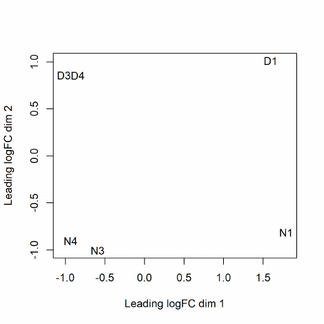
The MDS plot shows clear separation of the Pasilla down vs normal samples, but also a batch effect
associated with sequencing type and date.
4.5.7 The design matrix
To account for the batch effect observed from the MDS plot, we create a design matrix as follows:
> Batch <- factor(c(1,3,4,1,3,4))
> Pasilla <- factor(GEO$Pasilla, levels=c("Normal","Down"))
> design <- model.matrix(~ Batch + Pasilla)
> design
(Intercept) Batch3 Batch4 PasillaDown
1 1 0 0 0
2 1 1 0 0
3 1 0 1 0
4 1 0 0 1
5 1 1 0 1
6 1 0 1 1
attr(,"assign")
[1]0112
attr(,"contrasts")
attr(,"contrasts")$Batch
[1] "contr.treatment"
attr(,"contrasts")$Pasilla
[1] "contr.treatment"
79
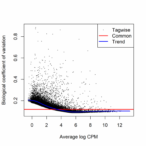
4.5.8 Estimating the dispersion
We estimate NB dispersions using the estimateDisp function. The estimated dispersions can be
visualized with plotBCV.
> y <- estimateDisp(y, design, robust=TRUE)
> y$common.dispersion
[1] 0.0141
> plotBCV(y)
Note that only the trended dispersion is used under the quasi-likelihood (QL) pipeline. The tagwise
and common estimates are shown here but will not be used further.
For the QL dispersions, estimation can be performed using the glmQLFit function. The results
can be visualized with the plotQLDisp function.
> fit <- glmQLFit(y, design, robust=TRUE)
> plotQLDisp(fit)
80

4.5.9 Differential expression
We test for differentially expressed exons between Pasilla knockdown and normal using the QL
F-test.
> qlf <- glmQLFTest(fit, coef=4)
The top set of most significant exons can be examined with topTags. Here, a positive log-fold
change represents exons that are up in Pasilla knockdown over normal. Multiplicity correction
is performed by applying the Benjamini-Hochberg method on the p-values, to control the false
discovery rate (FDR).
> topTags(qlf)
Coefficient: PasillaDown
GeneID Chr Start End Length Symbol logFC logCPM F PValue FDR
150709 32007 X 10674926 10676128 1203 sesB -3.26 7.21 949 7.41e-15 1.39e-10
150713 32007 X 10675026 10676128 1103 sesB -3.26 7.21 948 7.46e-15 1.39e-10
150697 32008 X 10672987 10673728 742 Ant2 2.85 6.14 863 1.48e-14 1.84e-10
91614 42865 3R 19970915 19971592 678 Kal1 -4.43 3.81 756 3.88e-14 3.61e-10
107856 44030 3L 2561932 2562843 912 msn -2.46 5.59 615 1.74e-13 1.30e-09
150702 32008 X 10674230 10674694 465 Ant2 2.97 4.55 575 2.83e-13 1.33e-09
150695 32008 X 10674230 10674559 330 Ant2 2.96 4.55 574 2.86e-13 1.33e-09
70750 44258 3R 5271691 5272628 938 ps -2.27 5.95 572 2.97e-13 1.33e-09
11333 44548 2R 6407125 6408782 1658 lola 2.26 6.15 565 3.21e-13 1.33e-09
96433 43230 3R 22697648 22697717 70 BM-40-SPARC -2.17 6.65 542 4.37e-13 1.63e-09
The total number of DE exons in each direction at a FDR of 5% can be examined with
decideTests.
81
> is.de <- decideTests(qlf, p.value=0.05)
> summary(is.de)
PasillaDown
Down 2059
NotSig 33385
Up 1814
4.5.10 Alternative splicing
We detect alternative splicing by testing for differential exon usage between Pasilla knockdown and
normal in each gene.
> sp <- diffSpliceDGE(fit, coef=4, geneid="GeneID", exonid="Start")
Total number of exons: 37258
Total number of genes: 8192
Number of genes with 1 exon: 1619
Mean number of exons in a gene: 5
Max number of exons in a gene: 56
Two testing methods at the gene-level are provided. The Simes’ method is likely to be more
powerful when only a minority of the exons for a gene are differentially spliced. The F-tests are
likely to be powerful for genes in which several exons are differentially spliced.
The top spliced genes under the Simes’ method are shown below:
> topSpliceDGE(sp, test="Simes", n=20)
GeneID Chr Symbol NExons P.Value FDR
141235 45320 X trol 44 1.64e-30 1.08e-26
11214 44548 2R lola 30 4.28e-30 1.41e-26
95956 44448 3R scrib 35 1.10e-20 2.40e-17
107810 44030 3L msn 24 1.15e-18 1.89e-15
19880 36773 2R Dg 15 2.17e-18 2.86e-15
16060 36542 2R shot 38 2.03e-17 2.22e-14
82117 42130 3R osa 17 2.50e-17 2.35e-14
32242 37893 2R slik 19 2.59e-15 2.13e-12
131170 40205 3L CG42674 16 3.88e-15 2.84e-12
163416 32817 X CrebB-17A 12 1.00e-14 6.58e-12
150694 32008 X Ant2 5 1.02e-13 6.07e-11
110493 38491 3L ens 16 1.88e-13 1.03e-10
41795 3771968 2L Msp-300 33 2.80e-12 1.41e-09
115767 38879 3L pbl 12 3.84e-12 1.80e-09
2032 2768716 2R mim 25 8.98e-12 3.93e-09
526 35494 2R laccase2 9 2.81e-11 1.11e-08
150710 32007 X sesB 7 2.88e-11 1.11e-08
166094 33098 X CG32521 8 4.29e-11 1.57e-08
52823 34652 2L vir-1 7 8.31e-11 2.88e-08
85970 42428 3R Stat92E 14 4.41e-10 1.45e-07
82
The top spliced genes identified by F-tests are shown below:
> topSpliceDGE(sp, test="gene", n=20)
GeneID Chr Symbol NExons gene.F P.Value FDR
141235 45320 X trol 44 52.5 2.53e-51 1.66e-47
11214 44548 2R lola 30 42.7 6.84e-34 2.25e-30
41795 3771968 2L Msp-300 33 22.7 2.34e-27 5.13e-24
95956 44448 3R scrib 35 17.2 1.08e-24 1.78e-21
16060 36542 2R shot 38 11.1 6.90e-20 9.07e-17
32242 37893 2R slik 19 25.8 1.22e-18 1.34e-15
166094 33098 X CG32521 8 64.1 1.14e-14 1.07e-11
19880 36773 2R Dg 15 21.8 2.57e-14 2.11e-11
2032 2768716 2R mim 25 10.7 8.49e-14 6.20e-11
107810 44030 3L msn 24 10.6 3.12e-13 2.05e-10
150694 32008 X Ant2 5 108.1 4.05e-13 2.36e-10
82117 42130 3R osa 17 15.6 4.30e-13 2.36e-10
163416 32817 X CrebB-17A 12 22.3 2.49e-12 1.26e-09
150710 32007 X sesB 7 51.5 5.26e-12 2.47e-09
131170 40205 3L CG42674 16 12.7 4.91e-11 2.15e-08
115767 38879 3L pbl 12 15.8 2.81e-10 1.16e-07
134207 40464 3L Ten-m 12 15.6 3.49e-10 1.35e-07
11103 36104 2R G-oalpha47A 13 14.1 3.87e-10 1.41e-07
108973 38376 3L BtbVII 10 18.7 5.84e-10 2.02e-07
110493 38491 3L ens 16 10.6 7.63e-10 2.51e-07
We plot all the exons for the top two most differentially spliced genes. Exons that are individ-
ually significant are highlighted.
> par(mfrow=c(1,2))
> plotSpliceDGE(sp, geneid="trol", genecol="Symbol")
> plotSpliceDGE(sp, geneid="lola", genecol="Symbol")
83
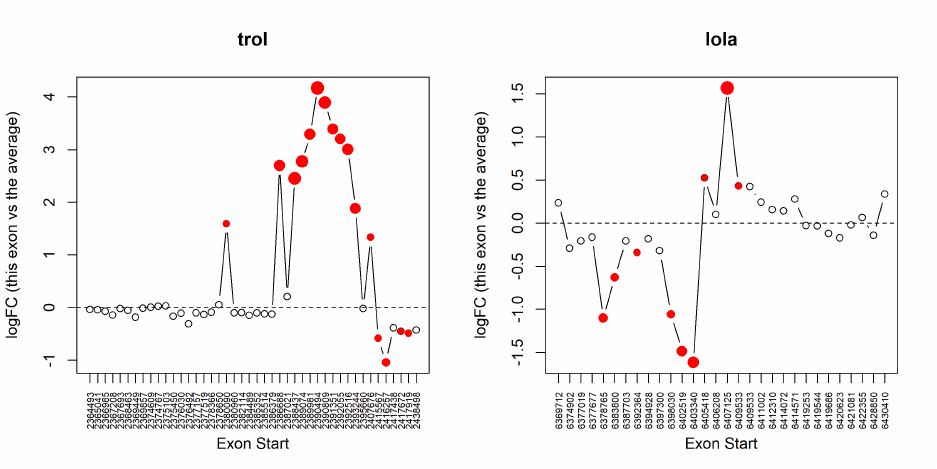
We can see that a block of five or six exons at the right end of the trol gene are relatively lost
when Pasilla is down. Most exons in the first half of the gene behave similarly to each other. This
gene is on the negative strand, so transcription is from right to left. The gene trol was identified
by Brooks et al [3] to have a novel set of coordinately regulated exons.
4.5.11 Setup
This analysis was conducted on:
> sessionInfo()
R version 3.5.0 (2018-04-23)
Platform: x86_64-w64-mingw32/x64 (64-bit)
Running under: Windows 10 x64 (build 16299)
Matrix products: default
locale:
[1] LC_COLLATE=English_Australia.1252 LC_CTYPE=English_Australia.1252
[3] LC_MONETARY=English_Australia.1252 LC_NUMERIC=C
[5] LC_TIME=English_Australia.1252
attached base packages:
[1] parallel stats4 stats graphics grDevices utils datasets methods base
other attached packages:
[1] GO.db_3.6.0 org.Mm.eg.db_3.6.0 tweeDEseqCountData_1.17.0
[4] NBPSeq_0.3.0 org.Hs.eg.db_3.6.0 AnnotationDbi_1.41.5
[7] IRanges_2.13.28 S4Vectors_0.17.42 Biobase_2.39.2
[10] BiocGenerics_0.25.3 edgeR_3.21.9 limma_3.35.15
84

loaded via a namespace (and not attached):
[1] Rcpp_0.12.16 compiler_3.5.0 pillar_1.2.1 plyr_1.8.4 tools_3.5.0
[6] digest_0.6.15 statmod_1.4.30 bit_1.1-12 RSQLite_2.1.0 memoise_1.1.0
[11] tibble_1.4.2 gtable_0.2.0 lattice_0.20-35 pkgconfig_2.0.1 rlang_0.2.0
[16] DBI_0.8 stringr_1.3.0 locfit_1.5-9.1 bit64_0.9-7 grid_3.5.0
[21] qvalue_2.11.0 ggplot2_2.2.1 reshape2_1.4.3 blob_1.1.1 magrittr_1.5
[26] scales_0.5.0 splines_3.5.0 colorspace_1.3-2 stringi_1.1.7 lazyeval_0.2.1
[31] munsell_0.4.3
4.5.12 Acknowledgements
Thanks to Yang Liao for mapping the reads and running featureCounts and Yifang Hu for the
initial analysis of the data.
4.6 CRISPR-Cas9 knockout screen analysis
4.6.1 Introduction
Dai et al. (2014) [8] describe the use of edgeR to analyze data from pooled genetic screens utilizing
either shRNAs or CRISPR-Cas9 to disrupt gene expression in a population of cells.
In this case study we analyze data from a pooled screen that uses CRISPR-Cas9 (clustered
regularly interspaced short palindromic repeats-associated nuclease Cas9) knockout technology. In
this example, a library of around 64,000 sgRNAs (as used in Shalem et al. 2014 [34]) were screened
to look for genes that may lead to resistance from a particular drug. This unpublished data set has
been anonymised.
4.6.2 Sequence processing
Multiple single guide RNAs (sgRNAs) per gene (generally between 3-6) were included in the
screen. Below we read in the raw sequences from the paired end fastq files screen4 R1.fastq and
screen4 R2.fastq using the processAmplicons function in edgeR. This screen employed a dual in-
dexing strategy where the first 8 bases from each pair of reads contained an index sequence that
uniquely identifies which sample a particular sgRNA sequence originated from. Matches between
sample indexes and sgRNAs listed in the files Samples4.txt and sgRNAs4.txt are identified by
processAmplicons to produce a DGEList of counts.
> # Read in sample & sgRNA information
> sampleanno <- read.table("Samples4.txt", header=TRUE, sep="\t")
> sampleanno[1:5,]
> sgseqs <- read.table("sgRNAs4.txt", header=TRUE, sep="\t")
> sgseqs[1:5,]
> # Process raw sequences from fastq files
> x <- processAmplicons("screen4_R1.fastq", readfile2="screen4_R2.fastq",
+ barcodefile="Samples4.txt", hairpinfile="sgRNAs4.txt",
+ barcodeStart=1, barcodeEnd=8, hairpinStart=33, hairpinEnd=52,
+ barcodeStartRev=1, barcodeEndRev=8, verbose=TRUE)
85
Note that this dual indexing strategy requires an additional column named ‘SequencesRev’ in
the file that contains the sample annotation information. Also, readFile2 must be specified, along
with position information (barcodeStartRev,barcodeEndRev) for the second index in the second
read from each pair (in this case the index can be found in the first 8 bases).
4.6.3 Filtering and data exploration
We next filter out sgRNAs and samples with low numbers of reads.
> x
An object of class "DGEList"
$counts
A1_1_1 A2_1_2 A3_1_3 A4_1_4 A5_1_5 A6_1_6 A7_2_1 A8_2_2 A9_2_3 A10_2_4 A11_2_5 A12_2_6
sgRNA1 0 14 0 0 3 36 1 55 0 23 0 62
sgRNA2 0 18 0 0 1 22 0 26 0 29 0 43
sgRNA3 0 50 0 0 4 52 1 98 0 60 0 111
sgRNA4 0 32 0 0 3 55 2 54 0 51 0 57
sgRNA5 0 7 0 0 1 3 0 3 0 5 1 5
A13_3_1 A14_3_2 A15_3_3 A16_3_4 A17_3_5 A18_3_6 A19_4_1 A20_4_2 A21_4_3 A22_4_4 A23_4_5
sgRNA1 0 21 0 30 21 36 0 37 0 39 1
sgRNA2 0 27 0 27 26 30 1 23 0 44 0
sgRNA3 0 59 0 62 24 63 0 44 0 106 0
sgRNA4 0 43 0 50 19 26 0 44 0 94 0
sgRNA503031701080
A24_4_6 B1_5_1 B2_5_2 B3_5_3 B4_5_4 B5_5_5 B6_5_6 B7_6_1 B8_6_2 B9_6_3 B10_6_4 B11_6_5
sgRNA1 63 3 5 5 26 11 4 3 4 14 3 8
sgRNA2 34 14 27 16 77 22 42 9 24 12 27 15
sgRNA3 70 16 39 27 53 41 43 31 24 14 35 43
sgRNA4 107 15 13 12 24 12 22 10 10 11 20 15
sgRNA5 3 0 5 12 15 6 25 6 9 6 3 9
B12_6_6 B13_7_1 B14_7_2 B15_7_3 B16_7_4 B17_7_5 B18_7_6 B19_8_1 B20_8_2 B21_8_3 B22_8_4
sgRNA1 6 9 10 6 8 11 31 6 13 9 25
sgRNA2 41 11 23 14 64 46 66 18 31 12 94
sgRNA3 45 38 51 14 59 38 73 31 29 31 63
sgRNA4 18 13 12 7 28 15 23 14 18 19 27
sgRNA5 16 1 5 0 3 7 11 1 7 3 18
B23_8_5 B24_8_6 A1_1_7 A2_1_8 A3_1_9 A7_2_7 A8_2_8 A9_2_9 A13_3_7 A14_3_8 A15_3_9 A19_4_7
sgRNA1 13 19 0 18 0 0 38 0 0 16 0 0
sgRNA2 36 64 0 12 0 0 18 0 0 15 0 0
sgRNA3 58 74 0 30 0 4 71 0 0 32 0 1
sgRNA4 19 36 0 27 0 1 39 0 0 34 0 1
sgRNA5 24 12 0 2 0 0 2 0 0 8 0 0
A20_4_8 A21_4_9 B1_5_7 B2_5_8 B3_5_9 B7_6_7 B8_6_8 B9_6_9 B13_7_7 B14_7_8 B15_7_9 B19_8_7
sgRNA1 32 0 5 6 5 10 5 15 2 9 3 10
sgRNA2 16 0 9 20 8 11 22 7 7 22 16 20
sgRNA3 39 0 10 19 23 19 14 30 30 35 24 27
sgRNA4 28 0 8 9 9 8 10 5 11 9 8 11
sgRNA5 0 0 0 9 4 4 10 3 2 2 0 3
B20_8_8 B21_8_9
sgRNA1 15 8
sgRNA2 20 9
86
sgRNA3 18 17
sgRNA4 12 11
sgRNA5 10 8
64746 more rows ...
$samples
ID lib.size norm.factors SequencesReverse group Infection Replicate IndexF IndexR
1 A1_1_1 188 1 TAAGGCGA Drug 1 1 1 1
2 A2_1_2 667530 1 CGTACTAG NoDrug 1 1 1 2
3 A3_1_3 1340 1 AGGCAGAA Drug 1 1 1 3
4 A4_1_4 2473 1 TCCTGAGC NoDrug 1 1 1 4
5 A5_1_5 69161 1 GGACTCCT Drug 1 1 1 5
67 more rows ...
$genes
ID Sequences Gene
1 sgRNA1 TACCCTGGGACTGTACCCCC 99
2 sgRNA2 ACCCTTGCTGCACGACCTGC 99
3 sgRNA3 TCGCTCGCCCCGCTCTTCCT 99
4 sgRNA4 TGACGCCTCGGACGTGTCTG 19
5 sgRNA5 CGTCATAGCCAATCTTCTTC 19
64746 more rows ...
> table(x$samples$group)
Drug NoDrug
40 32
> # Filter sgRNAs and samples with low counts
> # Need a CPM greater than 5 in 15 or more samples to keep sgRNAs
> selr <- rowSums(cpm(x$counts)>5)>=15
> # Need at least 100,000 reads to keep a given sample
> selc <- colSums(x$counts)>=100000
> x <- x[selr,selc]
> # Set up drug treatment colours
> cols <- as.numeric(x$samples$group)+2
> # Plot number of sgRNAs that could be matched per sample
> # and total for each sgRNA across all samples
> par(mfrow=c(2,1))
> barplot(colSums(x$counts), las=2, main="Counts per index", col=cols, cex.names=0.5, cex.axis=0.8)
> legend("topright", legend=c("Control", "Drug"), col=c(3,4), pch=15)
> barplot(rowSums(x$counts), las=2, main="Counts per sgRNA", axisnames=FALSE, cex.axis=0.8)
87
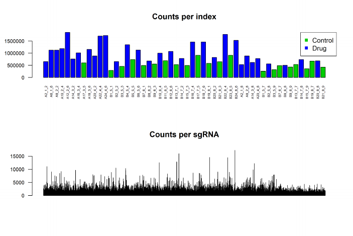
A multidimensional scaling plot was generated to assess the consistency between replicate sam-
ples. There is a clear separation between the two infections, indicating the need to incorporate an
effect for this in the GLM.
> # Make an MDS plot to visualise relationships between replicate samples
> # Set up infection colours
> cols2 <- x$samples$Infection
> par(mfrow=c(1,2))
> plotMDS(x, col=cols, main="MDS Plot: drug treatment colours")
> legend("topleft", legend=c("Control", "Drug"), col=c(3,4), pch=15)
> plotMDS(x, col=cols2, main="MDS Plot: infection colours")
> legend("topleft", legend=c("Inf#1", "Inf#2"), col=c(1,2), pch=15)
88
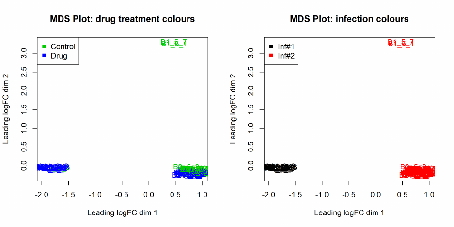
4.6.4 The design matrix and dispersion estimation
A design matrix is set up for the GLM analysis, and the sgRNA-specific variation is estimated and
plotted (while taking into account both drug treatment and infection number).
> # Set up design matrix for GLM
> treatment <- relevel(as.factor(x$samples$group), "NoDrug")
> infection <- as.factor(x$samples$Infection)
> des <- model.matrix(~treatment+infection)
> des[1:5,]
(Intercept) treatmentDrug infection2
1 1 0 0
2 1 0 0
3 1 0 0
4 1 0 0
5 1 0 0
> colnames(des)[2:3] <- c("Drug", "Infection2")
> # Estimate dispersions
> xglm <- estimateDisp(x, des)
> sqrt(xglm$common.disp)
[1] 0.258
> # Plot BCVs versus abundance
> plotBCV(xglm, main="BCV Plot")
89
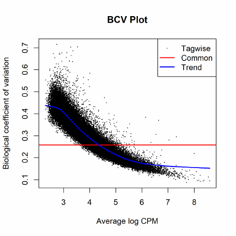
4.6.5 Differential representation analysis
We use the function glmFit to fit the sgRNA-specific models and glmLRT to do the testing between
the drug treated and control samples. The top ranked sgRNAs are listed using the topTags function
and sgRNAs with FDR <0.0001 [2] and log-fold-change ≥1 are highlighted on a plot of log-fold-
change versus log-counts-per-millions by the plotSmear function. Since this is a positive screen,
we highlight over-represented sgRNAs (i.e. those with positive log-fold-changes) since the model is
parameterized to compare drug treatment versus control (coefficient 2 in the design matrix).
> # Fit negative bionomial GLM
> fit <- glmFit(xglm, des)
> # Carry out Likelihood ratio test
> lrt <- glmLRT(fit, coef=2)
> # Show top ranked sgRNAs
> topTags(lrt)
Coefficient: Drug
ID Sequences Gene logFC logCPM LR PValue FDR
sgRNA816 sgRNA816 TCCGAACTCCCCCTTCCCGA 269 4.36 7.32 699 4.54e-154 2.56e-149
sgRNA4070 sgRNA4070 GTTGTGCTCAGTACTGACTT 1252 2.94 8.00 659 2.14e-145 6.04e-141
sgRNA6351 sgRNA6351 AAAAACGTATCTATTTTTAC 1957 3.37 6.34 422 8.56e-94 1.61e-89
sgRNA12880 sgRNA12880 CTGCACCGAAGAGAGCTGCT 3979 2.83 7.04 322 5.45e-72 7.68e-68
sgRNA23015 sgRNA23015 CAATTTGATCTCTTCTACTG 6714 3.16 4.83 233 1.35e-52 1.52e-48
sgRNA62532 sgRNA62532 AAACACGTCCAGTGCAGCCC 19612 2.79 4.91 216 6.18e-49 5.81e-45
sgRNA38819 sgRNA38819 TACGTTGTCGGGCGCCGCCA 11531 2.42 6.54 204 2.96e-46 2.38e-42
sgRNA3887 sgRNA3887 AACGCTGGACTCGAATGGCC 1194 2.28 5.33 203 4.05e-46 2.85e-42
sgRNA19299 sgRNA19299 GGGGTCTTACCCGAGGCTCC 5732 1.94 5.63 202 7.67e-46 4.80e-42
sgRNA52924 sgRNA52924 CCACCGCGTTCCACTTCTTG 16395 2.87 6.64 193 5.54e-44 3.12e-40
90
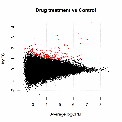
> # Select sgRNAs with FDR < 0.0001 and logFC <= -1 to highlight on plot
> thresh <- 0.0001
> lfc <- 1
> top4 <- topTags(lrt, n=Inf)
> top4ids <- top4$table[top4$table$FDR<thresh & top4$table$logFC>=lfc,1]
> # Plot logFC versus logCPM
> plotSmear(lrt, de.tags=top4ids, pch=20, cex=0.6, main="Drug treatment vs Control")
> abline(h = c(-1, 0, 1), col = c("dodgerblue", "yellow", "dodgerblue"), lty=2)
4.6.6 Gene set tests to summarize over multiple sgRNAs targeting the same
gene
We finish this analysis by summarising data across multiple sgRNAs that target the same gene in
order to get a gene-by-gene ranking, rather than a sgRNA-specific one. The camera gene-set test
[39] is used for this purpose. For this analysis, the collection of sgRNAs that target a specific gene
can be regarded as a ‘set’. In the code below, we restrict our analysis to genes with more than 3
sgRNAs. A barcode plot, highlighting the rank of sgRNAs for a given gene relative to the entire
data set is generated for the top-ranked gene (11531). Abundance of sgRNAs targeting this gene
tend to increase with drug treatment (FDR=0.0003).
> # Carry out camera gene-set analysis
> genesymbols <- x$genes[,3]
> genesymbollist <- list()
> unq <- unique(genesymbols)
> unq <- unq[!is.na(unq)]
> for(i in unq) {
+ sel <- genesymbols==i & !is.na(genesymbols)
+ if(sum(sel)>3)
91
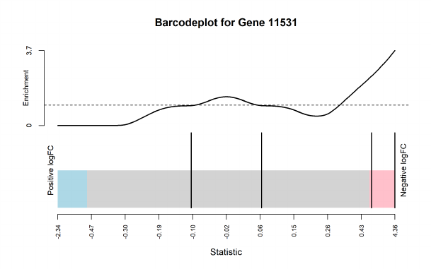
+ genesymbollist[[i]] <- which(sel)
+ }
> # Run camera for all genes
> camera.res <- camera(xglm, index=genesymbollist, des, contrast=2)
> # Display results for top ranked genes
> camera.res[1:10,]
NGenes Direction PValue FDR
19612 5 Up 1.44e-08 7.92e-05
8808 4 Up 9.36e-06 2.33e-02
3979 4 Up 1.34e-05 2.33e-02
8370 4 Up 1.69e-05 2.33e-02
11531 4 Up 2.33e-05 2.57e-02
10386 4 Up 1.40e-04 1.14e-01
2005 4 Up 1.45e-04 1.14e-01
4086 4 Up 1.95e-04 1.34e-01
10784 4 Up 2.26e-04 1.38e-01
11412 5 Up 6.93e-04 3.82e-01
> # Make a barcode plot for an example that ranks highly
> # Gene 11531
> barcodeplot(lrt$table$logFC,index=genesymbollist[[11531]],
+ main="Barcodeplot for Gene 11531",
+ labels=c("Positive logFC", "Negative logFC"),
+ quantile=c(-0.5,0.5))
The raw data from this example and several other case studies for this technology can be found
at http://bioinf.wehi.edu.au/shRNAseq/.
4.6.7 Setup
This analysis was conducted on:
> sessionInfo()
92
R version 3.5.0 (2018-04-23)
Platform: x86_64-w64-mingw32/x64 (64-bit)
Running under: Windows 10 x64 (build 16299)
Matrix products: default
locale:
[1] LC_COLLATE=English_Australia.1252 LC_CTYPE=English_Australia.1252
[3] LC_MONETARY=English_Australia.1252 LC_NUMERIC=C
[5] LC_TIME=English_Australia.1252
attached base packages:
[1] parallel stats4 stats graphics grDevices utils datasets methods base
other attached packages:
[1] GO.db_3.6.0 org.Mm.eg.db_3.6.0 tweeDEseqCountData_1.17.0
[4] NBPSeq_0.3.0 org.Hs.eg.db_3.6.0 AnnotationDbi_1.41.5
[7] IRanges_2.13.28 S4Vectors_0.17.42 Biobase_2.39.2
[10] BiocGenerics_0.25.3 edgeR_3.21.9 limma_3.35.15
loaded via a namespace (and not attached):
[1] Rcpp_0.12.16 compiler_3.5.0 pillar_1.2.1 plyr_1.8.4 tools_3.5.0
[6] digest_0.6.15 statmod_1.4.30 bit_1.1-12 RSQLite_2.1.0 memoise_1.1.0
[11] tibble_1.4.2 gtable_0.2.0 lattice_0.20-35 pkgconfig_2.0.1 rlang_0.2.0
[16] DBI_0.8 stringr_1.3.0 locfit_1.5-9.1 bit64_0.9-7 grid_3.5.0
[21] qvalue_2.11.0 ggplot2_2.2.1 reshape2_1.4.3 blob_1.1.1 magrittr_1.5
[26] scales_0.5.0 splines_3.5.0 colorspace_1.3-2 stringi_1.1.7 lazyeval_0.2.1
[31] munsell_0.4.3
4.6.8 Acknowledgements
Thanks to Dr Sam Wormald from the WEHI for providing the data set used in this case study.
4.7 Bisulfite sequencing of mouse oocytes
4.7.1 Introduction
The bisulfite sequencing (BS-seq) data of this case study is described in Gahurova et al. [10]. The
sequence and count data are publicly available from the Gene Expression Omnibus (GEO) at the
series accession number GSE86297.
This study investigates the onset and progression of de novo methylation. Growing oocytes
from pre-pubertal mouse ovaries (post-natal days 7-18) isolated and sorted into the following,
non-overlapping size categories: 40-45, 50-55 and 60-65 µm with two biological replicates in each.
Methylation maps were generated by bisulfite conversion of oocyte DNA and Illumina sequencing.
Reduced representation bisulfite sequencing (RRBS [23]) was applied for focusing coverage of CGIs
and other GC-rich sequences in all three size classes of oocytes. RRBS reads were trimmed to
remove poor quality calls and adapters using Trim Galore and mapped to the mouse genome
GRCm38 assembly by Bismark [13]. This is summarized in the table below.
93
> targets <- read.delim("targets.txt", header=TRUE)
> targets
GEO Sample Source
1 GSM2299710 RRBS_40_45A 40-45um
2 GSM2299711 RRBS_40_45B 40-45um
3 GSM2299712 RRBS_50_55A 50-55um
4 GSM2299713 RRBS_50_55B 50-55um
5 GSM2299714 RRBS_60_65A 60-65um
6 GSM2299715 RRBS_60_65B 60-65um
4.7.2 Reading in the data
The Bismark outputs of the data include one coverage file of the methylation in CpG context for
each sample. The coverage file for each of the six samples is available for download at GEO. The
first six rows of the coverage output of CpG methylation in the first sample are shown below.
> s1 <- read.delim(file="GSM2299710_RRBS_40-45oocyte_LibA.cov.txt", header=FALSE)
> head(s1)
V1 V2 V3 V4 V5 V6
1 6 3121266 3121266 0.00 0 17
2 6 3121296 3121296 0.00 0 17
3 6 3179319 3179319 1.28 1 77
4 6 3180316 3180316 4.55 1 21
5 6 3182928 3182928 4.33 22 486
6 6 3182937 3182937 5.37 61 1074
The six columns (from left to right) represent: chromosome, start position, end position, methyla-
tion proportion in percentage, number of methylated C’s and number of un-methylated C’s. Since
the start and end positions of a CpG site from Bismark are the same, we can keep only one of
them. The last two columns of counts are we will use for the analysis.
Suppose we are interested in the CpG methylation in chromosome 1. We read in the coverage
files of all six samples. Then we subset the data (chromosome 1 only) and combine the read counts
of methylated and un-methylated C’s of all the samples. A DGEList object is created using the
count table, and the chromosome number and positions are used for annotation.
> head(data)
Chr Position 40-45um-A-Me 40-45um-A-Un 40-45um-B-Me 40-45um-B-Un 50-55um-A-Me 50-55um-A-Un
1 1 3020877 11 73 17 60 14 100
2 1 3020891 6 78 4 74 4 112
3 1 3020946 4 142 8 361 5 205
4 1 3020988 9 29 20 71 13 47
5 1 3021013 4 33 11 80 5 55
6 1 3093908 3 33 1 32 5 26
50-55um-B-Me 50-55um-B-Un 60-65um-A-Me 60-65um-A-Un 60-65um-B-Me 60-65um-B-Un
1 0 21 5 81 9 48
94
2 2 19 5 81 9 48
3 8 157 17 178 19 149
4 6 88 11 39 1 24
5 16 76 9 41 12 13
6 1 0 2 29 1 14
> group <- targets$Source
> y <- DGEList(counts=data[,-(1:2)], group=rep(group,each=2), genes=data[,1:2])
> y
An object of class "DGEList"
$counts
40-45um-A-Me 40-45um-A-Un 40-45um-B-Me 40-45um-B-Un 50-55um-A-Me 50-55um-A-Un 50-55um-B-Me
1 11 73 17 60 14 100 0
2 6 78 4 74 4 112 2
3 4 142 8 361 5 205 8
4 9 29 20 71 13 47 6
5 4 33 11 80 5 55 16
50-55um-B-Un 60-65um-A-Me 60-65um-A-Un 60-65um-B-Me 60-65um-B-Un
1 21 5 81 9 48
2 19 5 81 9 48
3 157 17 178 19 149
4 88 11 39 1 24
5 76 9 41 12 13
140814 more rows ...
$samples
group lib.size norm.factors
40-45um-A-Me 40-45um 64671 1
40-45um-A-Un 40-45um 2024346 1
40-45um-B-Me 40-45um 87460 1
40-45um-B-Un 40-45um 3098364 1
50-55um-A-Me 50-55um 141225 1
7 more rows ...
$genes
Chr Position
1 1 3020877
2 1 3020891
3 1 3020946
4 1 3020988
5 1 3021013
140814 more rows ...
The count matrix of the DGEList object has a total of 12 columns with 2 columns (methylated
and unmethylated C’s) for each of the 6 samples. There are more than 140,000 CpG sites detected
on chromosome 1 across all the samples by Bismark.
4.7.3 Filtering and normalization
For each CpG site, both the numbers of methylated and unmethylated C’s should be taken into
account for assessing the methylation status. The total number of methylated and unmethylated
95
C’s at a CpG site detected in a particular sample can be considered as the “expression level” of
that CpG site in that sample. Hence, the sequencing depth of each sample should be calculated
using the total number of methylated and unmethylated C’s detected in that sample. Filtering and
normalization should also be based on the sum of methylated and unmethylated counts of each
CpG site.
Here a CpG site is retained if it has at least 10 counts (either methylated or unmethylated) in
all six samples.
> counts.total <- t(rowsum(t(y$counts), group=gl(6,2)))
> keep <- rowSums(counts.total >= 10) == 6
> table(keep)
keep
FALSE TRUE
121814 19005
> y <- y[keep, , keep.lib.sizes=FALSE]
Normalization is an essential step in RNA-seq differential expression analysis. It is however
slightly different in differential methylation analysis of BS-seq data.
For DNA methyaltion studies, the direct comparison between methylated and unmethylated
CpGs is usually not of interest. If a scaling normalization factor, for example from TMM, is
calculated for each sample, then the same normalization factor shall be applied to both methylated
and unmethylated counts within that sample. When the methylation levels between different
samples are compared, the scaling factors are cancelled out within each sample and hence has no
effect on the final differential methylation results. Therefore we do not perform normalization as
we would for RNA-seq data.
We set the library sizes for each sample to be the average of the total read counts for the
methylated and unmethylated libraries:
> TotalReadCount <- colMeans(matrix(y$samples$lib.size, nrow=2))
> y$samples$lib.size <- rep(TotalReadCount, each=2)
> y$samples
group lib.size norm.factors
40-45um-A-Me 40-45um 668196 1
40-45um-A-Un 40-45um 668196 1
40-45um-B-Me 40-45um 1249858 1
40-45um-B-Un 40-45um 1249858 1
50-55um-A-Me 50-55um 740245 1
50-55um-A-Un 50-55um 740245 1
50-55um-B-Me 50-55um 809096 1
50-55um-B-Un 50-55um 809096 1
60-65um-A-Me 60-65um 617650 1
60-65um-A-Un 60-65um 617650 1
60-65um-B-Me 60-65um 655405 1
60-65um-B-Un 60-65um 655405 1
96
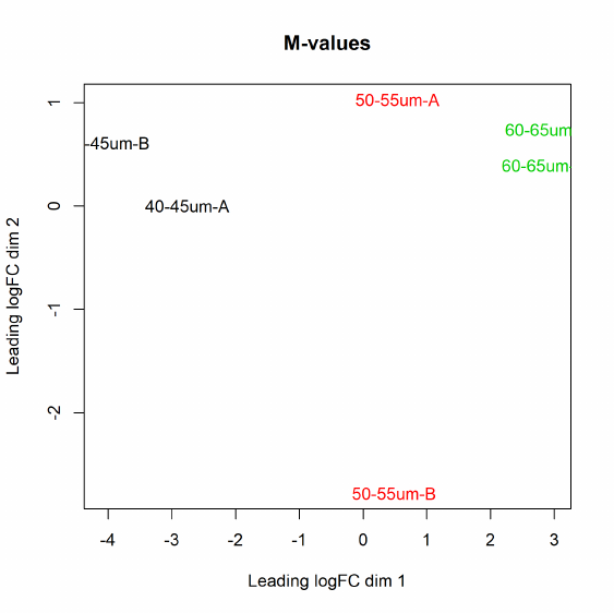
4.7.4 Data exploration
The data can be explored by generating multi-dimensional scaling (MDS) plots on the methylation
level (M-value) of the CpG sites. The M-value is calcualted by the log of the ratio of methylated
and unmethylated C’s, which is equivalent to the difference between methylated and unmethylated
C’s on the log-scale. A prior count of 2 is added to avoid logarithms of zero.
> Me <- y$counts[, meth=="Me"]
> Un <- y$counts[, meth=="Un"]
> M <- log2(Me + 2) - log2(Un + 2)
> samples <- paste0(group, "-", rep(c("A","B"), 3))
> colnames(M) <- samples
> plotMDS(M, col=rep(1:3, each=2), main="M-values")
Replicate samples cluster together within the 40-45 and 60-65 µm categories but are far apart
in the 50-55 µm group. The plot also indicates a huge difference in methylation level between the
40-45 and 60-65 µm groups.
4.7.5 The design matrix
One aim of the study is to identify differentially methylated regions (DMR) between different
groups. As a result, a design matrix is constructed as follows.
97
> sam <- rep(samples, each=2)
> meth <- factor(rep(c("Me","Un"),6), levels=c("Un","Me"))
> design <- model.matrix(~ sam + meth)
> colnames(design) <- gsub("sam","",colnames(design))
> colnames(design) <- gsub("meth","",colnames(design))
> colnames(design)[1] <- "Int"
> design <- cbind(design,
+ Me2=c(0,0,0,0,1,0,1,0,0,0,0,0),
+ Me3=c(0,0,0,0,0,0,0,0,1,0,1,0))
> design
Int 40-45um-B 50-55um-A 50-55um-B 60-65um-A 60-65um-B Me Me2 Me3
1 1 0 0 0 0 0 1 0 0
2 1 0 0 0 0 0 0 0 0
3 1 1 0 0 0 0 1 0 0
4 1 1 0 0 0 0 0 0 0
5 1 0 1 0 0 0 1 1 0
6 1 0 1 0 0 0 0 0 0
7 1 0 0 1 0 0 1 1 0
8 1 0 0 1 0 0 0 0 0
9 1 0 0 0 1 0 1 0 1
10 1 0 0 0 1 0 0 0 0
11 1 0 0 0 0 1 1 0 1
12 1 0 0 0 0 1 0 0 0
The first six columns represent the sample effect. The 7th column “Me” represents the methy-
lation level (or M-value) in the 40-45 µm group. The 8th column “Me2” represents the difference
in methylation level between the 50-55 and the 40-45 µm groups. Finally, the last column “Me3”
represents the difference in methylation level between the 60-65 and the 40-45 µm groups.
4.7.6 Estimating the dispersion
We proceed to the standard edgeR pipeline. We estimate the NB dispersion for each CpG site
using the estimateDisp function. It has been noticed in practice that dispersion estimates of BS-seq
data seem to be independent of abundances. Therefore, we would not consider a mean-dependent
dispersion trend for BS-seq methylation data.
> y <- estimateDisp(y, design=design, trend="none")
> y$common.dispersion
[1] 0.382
> summary(y$prior.df)
Min. 1st Qu. Median Mean 3rd Qu. Max.
Inf Inf Inf Inf Inf Inf
The estimated prior degrees of freedom are infinite for all the CpGs, which implies all the CpG-wise
dispersions are exactly the same as the common dispersion. A BCV plot is often useful to visualize
the dispersion estimates, but it is not informative in this case.
98
4.7.7 Differentially methylated regions
We fit NB GLMs for all the CpG loci.
> fit <- glmFit(y, design)
We identify differentially methylated regions (DMRs) (or CpG sites) between the 40-45 and
60-65 µm group using the likelihood-ratio test. As mentioned before, the difference is represented
by the last coefficient “Me3”.
> lrt <- glmLRT(fit, coef=9)
The top set of most significant DMRs can be examined with topTags. Here, positive log-fold
changes represent CpG sites that have higher methylation level in the 60-65 µm group compared
to the 40-45 µm group. Multiplicity correction is performed by applying the Benjamini-Hochberg
method on the p-values, to control the false discovery rate (FDR).
> topTags(lrt)
Coefficient: Me3
Chr Position logFC logCPM LR PValue FDR
62156 1 172206751 13.9 5.24 46.6 8.54e-12 1.62e-07
44214 1 131987595 10.8 6.66 41.7 1.04e-10 9.87e-07
60285 1 169954561 12.2 6.31 40.9 1.59e-10 1.01e-06
23994 1 74571516 13.0 4.89 40.1 2.42e-10 1.13e-06
9188 1 36499377 14.9 3.92 39.1 3.98e-10 1.13e-06
32279 1 89533694 12.0 6.30 39.0 4.14e-10 1.13e-06
62149 1 172206570 10.3 6.66 38.8 4.60e-10 1.13e-06
25965 1 75475455 12.4 5.07 38.8 4.75e-10 1.13e-06
15132 1 51978650 12.2 5.36 38.4 5.82e-10 1.23e-06
45070 1 132515608 11.8 5.18 38.1 6.86e-10 1.24e-06
The total number of DMRs in each direction at a FDR of 5% can be examined with decideTests.
> summary(decideTests(lrt))
Me3
Down 12
NotSig 17440
Up 1553
The differential methylation results can be visualized using an MD plot. The difference of the
M-value for each CpG site is plotted against the average abundance of that CpG site. Significantly
DMRs at a FDR of 5% are highlighted.
> plotMD(lrt)
99
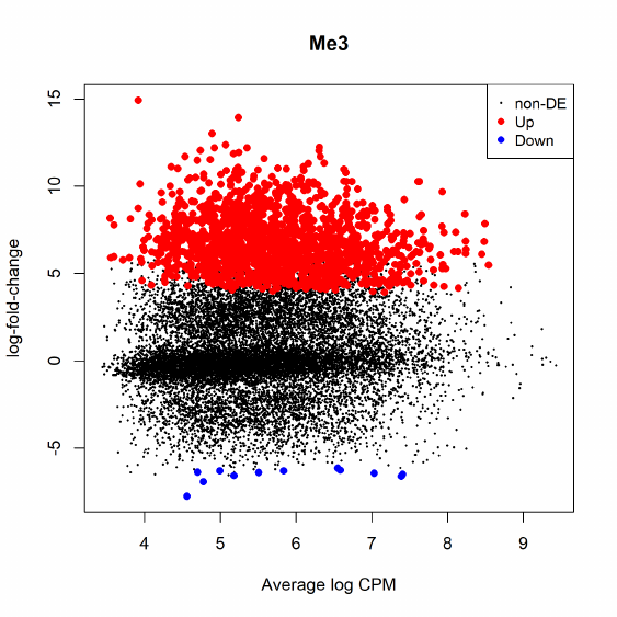
It can be seen that most of the DMRs have higher methylation levels in 60-65 µm group
compared to the 40-45 µm group. This is consistent with the findings in Gahurova et al. [10].
4.7.8 Setup
This analysis was conducted on:
> sessionInfo()
R version 3.5.0 (2018-04-23)
Platform: x86_64-w64-mingw32/x64 (64-bit)
Running under: Windows 10 x64 (build 16299)
Matrix products: default
locale:
[1] LC_COLLATE=English_Australia.1252 LC_CTYPE=English_Australia.1252
[3] LC_MONETARY=English_Australia.1252 LC_NUMERIC=C
[5] LC_TIME=English_Australia.1252
attached base packages:
[1] parallel stats4 stats graphics grDevices utils datasets methods base
other attached packages:
[1] GO.db_3.6.0 org.Mm.eg.db_3.6.0 tweeDEseqCountData_1.17.0
[4] NBPSeq_0.3.0 org.Hs.eg.db_3.6.0 AnnotationDbi_1.41.5
100
[7] IRanges_2.13.28 S4Vectors_0.17.42 Biobase_2.39.2
[10] BiocGenerics_0.25.3 edgeR_3.21.9 limma_3.35.15
loaded via a namespace (and not attached):
[1] Rcpp_0.12.16 compiler_3.5.0 pillar_1.2.1 plyr_1.8.4 tools_3.5.0
[6] digest_0.6.15 statmod_1.4.30 bit_1.1-12 RSQLite_2.1.0 memoise_1.1.0
[11] tibble_1.4.2 gtable_0.2.0 lattice_0.20-35 pkgconfig_2.0.1 rlang_0.2.0
[16] DBI_0.8 stringr_1.3.0 locfit_1.5-9.1 bit64_0.9-7 grid_3.5.0
[21] qvalue_2.11.0 ggplot2_2.2.1 reshape2_1.4.3 blob_1.1.1 magrittr_1.5
[26] scales_0.5.0 splines_3.5.0 colorspace_1.3-2 stringi_1.1.7 lazyeval_0.2.1
[31] munsell_0.4.3
101
Bibliography
1. Anders, S., McCarthy, D.J., Chen, Y., Okoniewski, M., Smyth, G.K., Huber, W., and Robinson,
M.D. (2013). Count-based differential expression analysis of RNA sequencing data using R and
Bioconductor. Nature Protocols 8, 1765–1786.
2. Benjamini, Y. and Hochberg, Y. (1995). Controlling the false discovery rate: a practical and
powerful approach to multiple testing. Journal of the Royal Statistical Society Series B 57,
289–300.
3. Brooks, A.N., Yang, L., Duff, M.O., Hansen, K.D., Park, J.W., Dudoit, S., Brenner, S.E.,
and Graveley, B.R. (2011). Conservation of an RNA regulatory map between Drosophila and
mammals. Genome Res 21, 193–202.
4. Bullard, J.H., Purdom, E., Hansen, K.D., and Dudoit, S. (2010). Evaluation of statistical
methods for normalization and differential expression in mRNA-Seq experiments. BMC Bioin-
formatics 18, 11–94.
5. Chen, Y., Lun, A.T.L., and Smyth, G.K. (2014). Differential expression analysis of complex
RNA-seq experiments using edgeR. In S. Datta and D.S. Nettleton, editors, Statistical Analysis
of Next Generation Sequence Data, pages 51–74. Springer, New York.
6. Chen, Y., Pal, B., Visvader, J.E., and Smyth, G.K. (2017). Differential methylation analysis of
reduced representation bisulfite sequencing experiments using edgeR. F1000Research 6, 2055.
7. Cumbie, J.S., Kimbrel, J.A., Di, Y., Schafer, D.W., Wilhelm, L.J., Fox, S.E., Sullivan, C.M.,
Curzon, A.D., Carrington, J.C., Mockler, T.C., and Chang, J.H. (2011). Gene-counter: A
computational pipeline for the analysis of RNA-Seq data for gene expression differences. PLoS
ONE 6, e25279.
8. Dai, Z., Sheridan, J.M., Gearing, L.J., Moore, D.L., Su, S., Wormald, S., Wilcox, S., O’Connor,
L., Dickins, R.A., Blewitt, M.E., and Ritchie, M.E. (2014). edgeR: a versatile tool for the
analysis of shRNA-seq and CRISPR-Cas9 genetic screens. F1000Res 3, 95.
9. Fu, N.Y., Rios, A., Pal, B., Soetanto, R., Lun, A.T.L., Liu, K., Beck, T., Best, S., Vaillant,
F., Bouillet, P., Strasser, A., Preiss, T., Smyth, G.K., Lindeman, G., , and Visvader, J. (2015).
EGF-mediated induction of Mcl-1 at the switch to lactation is essential for alveolar cell survival.
Nature Cell Biology 17, 365–375.
102
10. Gahurova, L., Tomizawa, S.i., Smallwood, S.A., Stewart-Morgan, K.R., Saadeh, H., Kim, J.,
Andrews, S.R., Chen, T., and Kelsey, G. (2017). Transcription and chromatin determinants of
de novo DNA methylation timing in oocytes. Epigenetics & chromatin 10, 25.
11. Hansen, K.D., Irizarry, R.A., and Zhijin, W. (2012). Removing technical variability in RNA-seq
data using conditional quantile normalization. Biostatistics 13, 204–216.
12. International HapMap Consortium, T. (2005). A haplotype map of the human genome. Nature
437, 1299–1320.
13. Krueger, F. and Andrews, S.R. (2011). Bismark: a flexible aligner and methylation caller for
Bisulfite-Seq applications. bioinformatics 27, 1571–1572.
14. Liao, Y., Smyth, G.K., and Shi, W. (2013). The Subread aligner: fast, accurate and scalable
read mapping by seed-and-vote. Nucleic Acids Research 41, e108.
15. Liao, Y., Smyth, G.K., and Shi, W. (2014). featureCounts: an efficient general-purpose read
summarization program. Bioinformatics 30, 923–930.
16. Lu, J., Tomfohr, J., and Kepler, T. (2005). Identifying differential expression in multiple SAGE
libraries: an overdispersed log-linear model approach. BMC Bioinformatics 6, 165.
17. Lun, A.T.L., Chen, Y., and Smyth, G.K. (2016). It’s DE-licious: a recipe for differential
expression analyses of RNA-seq experiments using quasi-likelihood methods in edgeR. Methods
in Molecular Biology 1418, 391–416.
18. Lund, S., Nettleton, D., McCarthy, D., and Smyth, G. (2012). Detecting differential expression
in RNA-sequence data using quasi-likelihood with shrunken dispersion estimates. Statistical
Applications in Genetics and Molecular Biology 11, Article Number 8.
19. Marioni, J.C., Mason, C.E., Mane, S.M., Stephens, M., and Gilad, Y. (2008). RNA-seq: An
assessment of technical reproducibility and comparison with gene expression arrays. Genome
Res 18, 1509–1517.
20. McCarthy, D.J., Chen, Y., and Smyth, G.K. (2012). Differential expression analysis of multi-
factor RNA-Seq experiments with respect to biological variation. Nucleic Acids Research 40,
4288–4297.
21. McCarthy, D.J. and Smyth, G.K. (2009). Testing significance relative to a fold-change threshold
is a TREAT. Bioinformatics 25, 765–771.
22. McCullagh, P. and Nelder, J.A. (1989). Generalized Linear Models. Chapman & Hall/CRC,
Boca Raton, Florida, 2nd edition.
23. Meissner, A., Gnirke, A., Bell, G.W., Ramsahoye, B., Lander, E.S., and Jaenisch, R. (2005).
Reduced representation bisulfite sequencing for comparative high-resolution DNA methylation
analysis. Nucleic acids research 33, 5868–5877.
103
24. Nelder, J.A. and Wedderburn, R.W.M. (1972). Generalized linear models. Journal of the Royal
Statistical Society Series A (General) 135, 370–384.
25. Phipson, B., Lee, S., Majewski, I.J., Alexander, W.S., and Smyth, G.K. (2016). Robust hy-
perparameter estimation protects against hypervariable genes and improves power to detect
differential expression. Annals of Applied Statistics 10, 946–963.
26. Pickrell, J.K., Marioni, J.C., Pai, A.A., Degner, J.F., Engelhardt, B.E., Nkadori, E., Veyri-
eras, J.B., Stephens, M., Gilad, Y., and Pritchard, J.K. (2010). Understanding mechanisms
underlying human gene expression variation with RNA sequencing. Nature 464, 768–772.
27. Pickrell, J.K., Pai, A.A., Gilad, Y., and Pritchard, J.K. (2010). Noisy splicing drives mRNA
isoform diversity in human cells. PLoS Genetics 6, e1001236.
28. Risso, D., Schwartz, K., Sherlock, G., and Dudoit, S. (2011). GC-content normalization for
RNA-Seq data. BMC Bioinformatics 12, 480.
29. Robinson, M., McCarthy, D., and Smyth, G. (2010). edgeR: a Bioconductor package for
differential expression analysis of digital gene expression data. Bioinformatics 26, 139–140.
30. Robinson, M.D. and Oshlack, A. (2010). A scaling normalization method for differential ex-
pression analysis of RNA-seq data. Genome Biology 11, R25.
31. Robinson, M.D. and Smyth, G.K. (2007). Moderated statistical tests for assessing differences
in tag abundance. Bioinformatics 23, 2881–2887.
32. Robinson, M.D. and Smyth, G.K. (2008). Small-sample estimation of negative binomial dis-
persion, with applications to SAGE data. Biostatistics 9, 321–332.
33. Sch¨ubeler, D. (2015). Function and information content of DNA methylation. Nature 517,
321–326.
34. Shalem, O., Sanjana, N.E., Hartenian, E., Shi, X., Scott, D.A., Mikkelsen, T.S., Heckl, D.,
Ebert, B.L., Root, D.E., Doench, J.G., and Zhang, F. (2014). Genome-scale CRISPR-Cas9
knockout screening in human cells. Science 343, 84–7.
35. Smyth, G.K. (2004). Linear models and empirical Bayes methods for assessing differential ex-
pression in microarray experiments. Statistical Applications in Genetics and Molecular Biology
3, Article 3.
36. Subramanian, A., Tamayo, P., Mootha, V.K., Mukherjee, S., Ebert, B.L., Gillette, M.A.,
Paulovich, A., Pomeroy, S.L., Golub, T.R., Lander, E.S., and Mesirov, J.P. (2005). Gene
set enrichment analysis: a knowledge-based approach for interpreting genome-wide expression
profiles. Proc Natl Acad Sci USA 102, 15545–50.
37. Tuch, B.B., Laborde, R.R., Xu, X., Gu, J., Chung, C.B., Monighetti, C.K., Stanley, S.J.,
Olsen, K.D., Kasperbauer, J.L., Moore, E.J., Broomer, A.J., Tan, R., Brzoska, P.M., Muller,
M.W., Siddiqui, A.S., Asmann, Y.W., Sun, Y., Kuersten, S., Barker, M.A., Vega, F.M.D.L.,
and Smith, D.I. (2010). Tumor transcriptome sequencing reveals allelic expression imbalances
associated with copy number alterations. PLoS ONE 5, e9317.
104
38. Wu, D., Lim, E., Vaillant, F., Asselin-Labat, M., Visvader, J., and Smyth, G. (2010). ROAST:
rotation gene set tests for complex microarray experiments. Bioinformatics 26, 2176–2182.
39. Wu, D. and Smyth, G. (2012). Camera: a competitive gene set test accounting for inter-gene
correlation. Nucleic Acids Research 40, e133.
105
