Elasticsearch: The Definitive Guide Elasticsearch
User Manual:
Open the PDF directly: View PDF ![]() .
.
Page Count: 719 [warning: Documents this large are best viewed by clicking the View PDF Link!]
- Table of Contents
- Foreword
- Preface
- Part I. Getting Started
- Chapter 1. You Know, for Search…
- Installing Elasticsearch
- Running Elasticsearch
- Talking to Elasticsearch
- Document Oriented
- Finding Your Feet
- Indexing Employee Documents
- Retrieving a Document
- Search Lite
- Search with Query DSL
- More-Complicated Searches
- Full-Text Search
- Phrase Search
- Highlighting Our Searches
- Analytics
- Tutorial Conclusion
- Distributed Nature
- Next Steps
- Chapter 2. Life Inside a Cluster
- Chapter 3. Data In, Data Out
- What Is a Document?
- Document Metadata
- Indexing a Document
- Retrieving a Document
- Checking Whether a Document Exists
- Updating a Whole Document
- Creating a New Document
- Deleting a Document
- Dealing with Conflicts
- Optimistic Concurrency Control
- Partial Updates to Documents
- Retrieving Multiple Documents
- Cheaper in Bulk
- Chapter 4. Distributed Document Store
- Chapter 5. Searching—The Basic Tools
- Chapter 6. Mapping and Analysis
- Chapter 7. Full-Body Search
- Chapter 8. Sorting and Relevance
- Chapter 9. Distributed Search Execution
- Chapter 10. Index Management
- Chapter 11. Inside a Shard
- Chapter 1. You Know, for Search…
- Part II. Search in Depth
- Chapter 12. Structured Search
- Chapter 13. Full-Text Search
- Chapter 14. Multifield Search
- Chapter 15. Proximity Matching
- Chapter 16. Partial Matching
- Chapter 17. Controlling Relevance
- Theory Behind Relevance Scoring
- Lucene’s Practical Scoring Function
- Query-Time Boosting
- Manipulating Relevance with Query Structure
- Not Quite Not
- Ignoring TF/IDF
- function_score Query
- Boosting by Popularity
- Boosting Filtered Subsets
- Random Scoring
- The Closer, The Better
- Understanding the price Clause
- Scoring with Scripts
- Pluggable Similarity Algorithms
- Changing Similarities
- Relevance Tuning Is the Last 10%
- Part III. Dealing with Human Language
- Chapter 18. Getting Started with Languages
- Chapter 19. Identifying Words
- Chapter 20. Normalizing Tokens
- Chapter 21. Reducing Words to Their Root Form
- Chapter 22. Stopwords: Performance Versus Precision
- Chapter 23. Synonyms
- Chapter 24. Typoes and Mispelings
- Part IV. Aggregations
- Chapter 25. High-Level Concepts
- Chapter 26. Aggregation Test-Drive
- Chapter 27. Building Bar Charts
- Chapter 28. Looking at Time
- Chapter 29. Scoping Aggregations
- Chapter 30. Filtering Queries and Aggregations
- Chapter 31. Sorting Multivalue Buckets
- Chapter 32. Approximate Aggregations
- Chapter 33. Significant Terms
- Chapter 34. Controlling Memory Use and Latency
- Chapter 35. Closing Thoughts
- Part V. Geolocation
- Part VI. Modeling Your Data
- Chapter 40. Handling Relationships
- Chapter 41. Nested Objects
- Chapter 42. Parent-Child Relationship
- Chapter 43. Designing for Scale
- Part VII. Administration, Monitoring, and Deployment
- Chapter 44. Monitoring
- Chapter 45. Production Deployment
- Chapter 46. Post-Deployment
- Index
- About the Authors

■
■
■
■
■
■
■
Clinton Gormley &
Zachary Tong
Elasticsearch
The Definitive Guide
A DISTRIBUTED REAL-TIME SEARCH AND ANALYTICS ENGINE

DATABA SESWEB
Elasticsearch: The Definitive Guide
ISBN: 978-1-449-35854-9
US $49.99 CAN $57.99
“
The book could easily be
retitled as 'Understanding
search engines using
Elasticsearch.' Great job.
Way beyond just simply
using Elasticsearch.
”
—Ivan Brusic
Search Consultant
Twitter: @oreillymedia
facebook.com/oreilly
Whether you need full-text search or real-time analytics of structured data—
or both—the Elasticsearch distributed search engine is an ideal way to put
your data to work. This practical guide not only shows you how to search,
analyze, and explore data with Elasticsearch, but also helps you deal with the
complexities of human language, geolocation, and relationships.
If you’re a newcomer to both search and distributed systems, you’ll
quickly learn how to integrate Elasticsearch into your application. More
experienced users will pick up lots of advanced techniques. Throughout
the book, you’ll follow a problem-based approach to learn why, when, and
how to use Elasticsearch features.
■Understand how Elasticsearch interprets data in your
documents
■Index and query your data to take advantage of search
concepts such as relevance and word proximity
■Handle human language through the eective use of analyzers
and queries
■Summarize and group data to show overall trends, with
aggregations and analytics
■Use geo-points and geo-shapes—Elasticsearch’s approaches
to geolocation
■Model your data to take advantage of Elasticsearch’s horizontal
scalability
■Learn how to congure and monitor your cluster in production
Clinton Gormley was the first user of Elasticsearch and wrote the Perl API back
in 2010. When Elasticsearch formed a company in 2012, he joined as a developer
and the maintainer of the Perl modules.
Zachary Tong has been working with Elasticsearch since 2011, and has written
several tutorials to help beginners using the server. Zach is a developer at
Elasticsearch and maintains the PHP client.

Clinton Gormley and Zachary Tong
Elasticsearch: The Denitive Guide
978-1-449-35854-9
[LSI]
Elasticsearch: The Denitive Guide
by Clinton Gormley and Zachary Tong
Copyright © 2015 Elasticsearch. All rights reserved.
Printed in the United States of America.
Published by O’Reilly Media, Inc. , 1005 Gravenstein Highway North, Sebastopol, CA 95472.
O’Reilly books may be purchased for educational, business, or sales promotional use. Online editions are
also available for most titles (http://safaribooksonline.com). For more information, contact our corporate/
institutional sales department: 800-998-9938 or corporate@oreilly.com.
Editors: Mike Loukides and Brian Anderson
Production Editor: Shiny Kalapurakkel
Proofreader: Sharon Wilkey
Indexer: Ellen Troutman-Zaig
Interior Designer: David Futato
Cover Designer: Ellie Volkhausen
Illustrator: Rebecca Demarest
January 2015: First Edition
Revision History for the First Edition
2015-01-16: First Release
See http://oreilly.com/catalog/errata.csp?isbn=9781449358549 for release details.
The O’Reilly logo is a registered trademark of O’Reilly Media, Inc. Elasticsearch: e Denitive Guide, the
cover image, and related trade dress are trademarks of O’Reilly Media, Inc.
Many of the designations used by manufacturers and sellers to distinguish their products are claimed as
trademarks. Where those designations appear in this book, and O’Reilly Media, Inc. was aware of a trade‐
mark claim, the designations have been printed in caps or initial caps.
While the publisher and the authors have used good faith efforts to ensure that the information and
instructions contained in this work are accurate, the publisher and the authors disclaim all responsibility
for errors or omissions, including without limitation responsibility for damages resulting from the use of
or reliance on this work. Use of the information and instructions contained in this work is at your own
risk. If any code samples or other technology this work contains or describes is subject to open source
licenses or the intellectual property rights of others, it is your responsibility to ensure that your use
thereof complies with such licenses and/or rights.

Table of Contents
Foreword. . . . . . . . . . . . . . . . . . . . . . . . . . . . . . . . . . . . . . . . . . . . . . . . . . . . . . . . . . . . . . . . . . . . . xxi
Preface. . . . . . . . . . . . . . . . . . . . . . . . . . . . . . . . . . . . . . . . . . . . . . . . . . . . . . . . . . . . . . . . . . . . . xxiii
Part I. Getting Started
1. You Know, for Search…. . . . . . . . . . . . . . . . . . . . . . . . . . . . . . . . . . . . . . . . . . . . . . . . . . . . . . 3
Installing Elasticsearch 4
Installing Marvel 5
Running Elasticsearch 5
Viewing Marvel and Sense 6
Talking to Elasticsearch 6
Java API 6
RESTful API with JSON over HTTP 7
Document Oriented 9
JSON 9
Finding Your Feet 10
Let’s Build an Employee Directory 10
Indexing Employee Documents 10
Retrieving a Document 12
Search Lite 13
Search with Query DSL 15
More-Complicated Searches 16
Full-Text Search 17
Phrase Search 18
Highlighting Our Searches 19
Analytics 20
Tutorial Conclusion 23
iii

Distributed Nature 23
Next Steps 24
2. Life Inside a Cluster. . . . . . . . . . . . . . . . . . . . . . . . . . . . . . . . . . . . . . . . . . . . . . . . . . . . . . . . . 25
An Empty Cluster 26
Cluster Health 26
Add an Index 27
Add Failover 29
Scale Horizontally 30
Then Scale Some More 31
Coping with Failure 32
3. Data In, Data Out. . . . . . . . . . . . . . . . . . . . . . . . . . . . . . . . . . . . . . . . . . . . . . . . . . . . . . . . . . . 35
What Is a Document? 36
Document Metadata 37
_index 37
_type 37
_id 38
Other Metadata 38
Indexing a Document 38
Using Our Own ID 38
Autogenerating IDs 39
Retrieving a Document 40
Retrieving Part of a Document 41
Checking Whether a Document Exists 42
Updating a Whole Document 42
Creating a New Document 43
Deleting a Document 44
Dealing with Conflicts 45
Optimistic Concurrency Control 47
Using Versions from an External System 49
Partial Updates to Documents 50
Using Scripts to Make Partial Updates 51
Updating a Document That May Not Yet Exist 52
Updates and Conflicts 53
Retrieving Multiple Documents 54
Cheaper in Bulk 56
Don’t Repeat Yourself 60
How Big Is Too Big? 60
4. Distributed Document Store. . . . . . . . . . . . . . . . . . . . . . . . . . . . . . . . . . . . . . . . . . . . . . . . . 61
Routing a Document to a Shard 61
iv | Table of Contents

How Primary and Replica Shards Interact 62
Creating, Indexing, and Deleting a Document 63
Retrieving a Document 65
Partial Updates to a Document 66
Multidocument Patterns 67
Why the Funny Format? 69
5. Searching—The Basic Tools. . . . . . . . . . . . . . . . . . . . . . . . . . . . . . . . . . . . . . . . . . . . . . . . . . 71
The Empty Search 72
hits 73
took 73
shards 73
timeout 74
Multi-index, Multitype 74
Pagination 75
Search Lite 76
The _all Field 77
More Complicated Queries 78
6. Mapping and Analysis. . . . . . . . . . . . . . . . . . . . . . . . . . . . . . . . . . . . . . . . . . . . . . . . . . . . . . . 79
Exact Values Versus Full Text 80
Inverted Index 81
Analysis and Analyzers 84
Built-in Analyzers 84
When Analyzers Are Used 85
Testing Analyzers 86
Specifying Analyzers 87
Mapping 87
Core Simple Field Types 88
Viewing the Mapping 89
Customizing Field Mappings 89
Updating a Mapping 91
Testing the Mapping 92
Complex Core Field Types 93
Multivalue Fields 93
Empty Fields 93
Multilevel Objects 94
Mapping for Inner Objects 94
How Inner Objects are Indexed 95
Arrays of Inner Objects 95
Table of Contents | v

7. Full-Body Search. . . . . . . . . . . . . . . . . . . . . . . . . . . . . . . . . . . . . . . . . . . . . . . . . . . . . . . . . . . 97
Empty Search 97
Query DSL 98
Structure of a Query Clause 99
Combining Multiple Clauses 99
Queries and Filters 100
Performance Differences 101
When to Use Which 101
Most Important Queries and Filters 102
term Filter 102
terms Filter 102
range Filter 102
exists and missing Filters 103
bool Filter 103
match_all Query 103
match Query 104
multi_match Query 104
bool Query 105
Combining Queries with Filters 105
Filtering a Query 106
Just a Filter 107
A Query as a Filter 107
Validating Queries 108
Understanding Errors 108
Understanding Queries 109
8. Sorting and Relevance. . . . . . . . . . . . . . . . . . . . . . . . . . . . . . . . . . . . . . . . . . . . . . . . . . . . . 111
Sorting 111
Sorting by Field Values 112
Multilevel Sorting 113
Sorting on Multivalue Fields 113
String Sorting and Multifields 114
What Is Relevance? 115
Understanding the Score 116
Understanding Why a Document Matched 119
Fielddata 119
9. Distributed Search Execution. . . . . . . . . . . . . . . . . . . . . . . . . . . . . . . . . . . . . . . . . . . . . . . . 121
Query Phase 122
Fetch Phase 123
Search Options 125
preference 125
vi | Table of Contents

timeout 126
routing 126
search_type 127
scan and scroll 127
10. Index Management. . . . . . . . . . . . . . . . . . . . . . . . . . . . . . . . . . . . . . . . . . . . . . . . . . . . . . . . 131
Creating an Index 131
Deleting an Index 132
Index Settings 132
Configuring Analyzers 133
Custom Analyzers 134
Creating a Custom Analyzer 135
Types and Mappings 137
How Lucene Sees Documents 137
How Types Are Implemented 138
Avoiding Type Gotchas 138
The Root Object 140
Properties 140
Metadata: _source Field 141
Metadata: _all Field 142
Metadata: Document Identity 144
Dynamic Mapping 145
Customizing Dynamic Mapping 147
date_detection 147
dynamic_templates 148
Default Mapping 149
Reindexing Your Data 150
Index Aliases and Zero Downtime 151
11. Inside a Shard. . . . . . . . . . . . . . . . . . . . . . . . . . . . . . . . . . . . . . . . . . . . . . . . . . . . . . . . . . . . 153
Making Text Searchable 154
Immutability 155
Dynamically Updatable Indices 155
Deletes and Updates 158
Near Real-Time Search 159
refresh API 160
Making Changes Persistent 161
flush API 165
Segment Merging 166
Table of Contents | vii

optimize API 168
Part II. Search in Depth
12. Structured Search. . . . . . . . . . . . . . . . . . . . . . . . . . . . . . . . . . . . . . . . . . . . . . . . . . . . . . . . . 173
Finding Exact Values 173
term Filter with Numbers 174
term Filter with Text 175
Internal Filter Operation 178
Combining Filters 179
Bool Filter 179
Nesting Boolean Filters 181
Finding Multiple Exact Values 182
Contains, but Does Not Equal 183
Equals Exactly 184
Ranges 185
Ranges on Dates 186
Ranges on Strings 187
Dealing with Null Values 187
exists Filter 188
missing Filter 190
exists/missing on Objects 191
All About Caching 192
Independent Filter Caching 192
Controlling Caching 193
Filter Order 194
13. Full-Text Search. . . . . . . . . . . . . . . . . . . . . . . . . . . . . . . . . . . . . . . . . . . . . . . . . . . . . . . . . . . 197
Term-Based Versus Full-Text 197
The match Query 199
Index Some Data 199
A Single-Word Query 200
Multiword Queries 201
Improving Precision 202
Controlling Precision 203
Combining Queries 204
Score Calculation 205
Controlling Precision 205
How match Uses bool 206
Boosting Query Clauses 207
Controlling Analysis 209
viii | Table of Contents

Default Analyzers 211
Configuring Analyzers in Practice 213
Relevance Is Broken! 214
14. Multield Search. . . . . . . . . . . . . . . . . . . . . . . . . . . . . . . . . . . . . . . . . . . . . . . . . . . . . . . . . . 217
Multiple Query Strings 217
Prioritizing Clauses 218
Single Query String 219
Know Your Data 220
Best Fields 221
dis_max Query 222
Tuning Best Fields Queries 223
tie_breaker 224
multi_match Query 225
Using Wildcards in Field Names 226
Boosting Individual Fields 227
Most Fields 227
Multifield Mapping 228
Cross-fields Entity Search 231
A Naive Approach 231
Problems with the most_fields Approach 232
Field-Centric Queries 232
Problem 1: Matching the Same Word in Multiple Fields 233
Problem 2: Trimming the Long Tail 233
Problem 3: Term Frequencies 234
Solution 235
Custom _all Fields 235
cross-fields Queries 236
Per-Field Boosting 238
Exact-Value Fields 239
15. Proximity Matching. . . . . . . . . . . . . . . . . . . . . . . . . . . . . . . . . . . . . . . . . . . . . . . . . . . . . . . . 241
Phrase Matching 242
Term Positions 242
What Is a Phrase 243
Mixing It Up 244
Multivalue Fields 245
Closer Is Better 246
Proximity for Relevance 247
Improving Performance 249
Rescoring Results 249
Finding Associated Words 250
Table of Contents | ix

Producing Shingles 251
Multifields 252
Searching for Shingles 253
Performance 255
16. Partial Matching. . . . . . . . . . . . . . . . . . . . . . . . . . . . . . . . . . . . . . . . . . . . . . . . . . . . . . . . . . 257
Postcodes and Structured Data 258
prefix Query 259
wildcard and regexp Queries 260
Query-Time Search-as-You-Type 262
Index-Time Optimizations 264
Ngrams for Partial Matching 264
Index-Time Search-as-You-Type 265
Preparing the Index 265
Querying the Field 267
Edge n-grams and Postcodes 270
Ngrams for Compound Words 271
17. Controlling Relevance. . . . . . . . . . . . . . . . . . . . . . . . . . . . . . . . . . . . . . . . . . . . . . . . . . . . . . 275
Theory Behind Relevance Scoring 275
Boolean Model 276
Term Frequency/Inverse Document Frequency (TF/IDF) 276
Vector Space Model 279
Lucene’s Practical Scoring Function 282
Query Normalization Factor 283
Query Coordination 284
Index-Time Field-Level Boosting 286
Query-Time Boosting 286
Boosting an Index 287
t.getBoost() 288
Manipulating Relevance with Query Structure 288
Not Quite Not 289
boosting Query 290
Ignoring TF/IDF 291
constant_score Query 291
function_score Query 293
Boosting by Popularity 294
modifier 296
factor 298
boost_mode 299
max_boost 301
Boosting Filtered Subsets 301
x | Table of Contents

filter Versus query 302
functions 303
score_mode 303
Random Scoring 303
The Closer, The Better 305
Understanding the price Clause 308
Scoring with Scripts 308
Pluggable Similarity Algorithms 310
Okapi BM25 310
Changing Similarities 313
Configuring BM25 314
Relevance Tuning Is the Last 10% 315
Part III. Dealing with Human Language
18. Getting Started with Languages. . . . . . . . . . . . . . . . . . . . . . . . . . . . . . . . . . . . . . . . . . . . . 319
Using Language Analyzers 320
Configuring Language Analyzers 321
Pitfalls of Mixing Languages 323
At Index Time 323
At Query Time 324
Identifying Language 324
One Language per Document 325
Foreign Words 326
One Language per Field 327
Mixed-Language Fields 329
Split into Separate Fields 329
Analyze Multiple Times 329
Use n-grams 330
19. Identifying Words. . . . . . . . . . . . . . . . . . . . . . . . . . . . . . . . . . . . . . . . . . . . . . . . . . . . . . . . . 333
standard Analyzer 333
standard Tokenizer 334
Installing the ICU Plug-in 335
icu_tokenizer 335
Tidying Up Input Text 337
Tokenizing HTML 337
Tidying Up Punctuation 338
20. Normalizing Tokens. . . . . . . . . . . . . . . . . . . . . . . . . . . . . . . . . . . . . . . . . . . . . . . . . . . . . . . . 341
In That Case 341
Table of Contents | xi

You Have an Accent 342
Retaining Meaning 343
Living in a Unicode World 346
Unicode Case Folding 347
Unicode Character Folding 349
Sorting and Collations 350
Case-Insensitive Sorting 351
Differences Between Languages 353
Unicode Collation Algorithm 353
Unicode Sorting 354
Specifying a Language 355
Customizing Collations 358
21. Reducing Words to Their Root Form. . . . . . . . . . . . . . . . . . . . . . . . . . . . . . . . . . . . . . . . . . 359
Algorithmic Stemmers 360
Using an Algorithmic Stemmer 361
Dictionary Stemmers 363
Hunspell Stemmer 364
Installing a Dictionary 365
Per-Language Settings 365
Creating a Hunspell Token Filter 366
Hunspell Dictionary Format 367
Choosing a Stemmer 369
Stemmer Performance 370
Stemmer Quality 370
Stemmer Degree 370
Making a Choice 371
Controlling Stemming 371
Preventing Stemming 371
Customizing Stemming 372
Stemming in situ 373
Is Stemming in situ a Good Idea 375
22. Stopwords: Performance Versus Precision. . . . . . . . . . . . . . . . . . . . . . . . . . . . . . . . . . . . . 377
Pros and Cons of Stopwords 378
Using Stopwords 379
Stopwords and the Standard Analyzer 379
Maintaining Positions 380
Specifying Stopwords 380
Using the stop Token Filter 381
Updating Stopwords 383
Stopwords and Performance 383
xii | Table of Contents

and Operator 383
minimum_should_match 384
Divide and Conquer 385
Controlling Precision 386
Only High-Frequency Terms 387
More Control with Common Terms 388
Stopwords and Phrase Queries 388
Positions Data 389
Index Options 389
Stopwords 390
common_grams Token Filter 391
At Index Time 392
Unigram Queries 393
Bigram Phrase Queries 393
Two-Word Phrases 394
Stopwords and Relevance 394
23. Synonyms. . . . . . . . . . . . . . . . . . . . . . . . . . . . . . . . . . . . . . . . . . . . . . . . . . . . . . . . . . . . . . . . 395
Using Synonyms 396
Formatting Synonyms 397
Expand or contract 398
Simple Expansion 398
Simple Contraction 399
Genre Expansion 400
Synonyms and The Analysis Chain 401
Case-Sensitive Synonyms 401
Multiword Synonyms and Phrase Queries 402
Use Simple Contraction for Phrase Queries 404
Synonyms and the query_string Query 405
Symbol Synonyms 405
24. Typoes and Mispelings. . . . . . . . . . . . . . . . . . . . . . . . . . . . . . . . . . . . . . . . . . . . . . . . . . . . . 409
Fuzziness 409
Fuzzy Query 410
Improving Performance 411
Fuzzy match Query 412
Scoring Fuzziness 413
Phonetic Matching 413
Part IV. Aggregations
Table of Contents | xiii

25. High-Level Concepts. . . . . . . . . . . . . . . . . . . . . . . . . . . . . . . . . . . . . . . . . . . . . . . . . . . . . . . 419
Buckets 420
Metrics 420
Combining the Two 420
26. Aggregation Test-Drive. . . . . . . . . . . . . . . . . . . . . . . . . . . . . . . . . . . . . . . . . . . . . . . . . . . . . 423
Adding a Metric to the Mix 426
Buckets Inside Buckets 427
One Final Modification 429
27. Building Bar Charts. . . . . . . . . . . . . . . . . . . . . . . . . . . . . . . . . . . . . . . . . . . . . . . . . . . . . . . . 433
28. Looking at Time. . . . . . . . . . . . . . . . . . . . . . . . . . . . . . . . . . . . . . . . . . . . . . . . . . . . . . . . . . . 437
Returning Empty Buckets 439
Extended Example 441
The Sky’s the Limit 443
29. Scoping Aggregations. . . . . . . . . . . . . . . . . . . . . . . . . . . . . . . . . . . . . . . . . . . . . . . . . . . . . . 445
30. Filtering Queries and Aggregations. . . . . . . . . . . . . . . . . . . . . . . . . . . . . . . . . . . . . . . . . . 449
Filtered Query 449
Filter Bucket 450
Post Filter 451
Recap 452
31. Sorting Multivalue Buckets. . . . . . . . . . . . . . . . . . . . . . . . . . . . . . . . . . . . . . . . . . . . . . . . . 453
Intrinsic Sorts 453
Sorting by a Metric 454
Sorting Based on “Deep” Metrics 455
32. Approximate Aggregations. . . . . . . . . . . . . . . . . . . . . . . . . . . . . . . . . . . . . . . . . . . . . . . . . 457
Finding Distinct Counts 458
Understanding the Trade-offs 460
Optimizing for Speed 461
Calculating Percentiles 462
Percentile Metric 464
Percentile Ranks 467
Understanding the Trade-offs 469
33. Signicant Terms. . . . . . . . . . . . . . . . . . . . . . . . . . . . . . . . . . . . . . . . . . . . . . . . . . . . . . . . . . 471
significant_terms Demo 472
Recommending Based on Popularity 474
xiv | Table of Contents

Recommending Based on Statistics 478
34. Controlling Memory Use and Latency. . . . . . . . . . . . . . . . . . . . . . . . . . . . . . . . . . . . . . . . . 481
Fielddata 481
Aggregations and Analysis 483
High-Cardinality Memory Implications 486
Limiting Memory Usage 487
Fielddata Size 488
Monitoring fielddata 489
Circuit Breaker 490
Fielddata Filtering 491
Doc Values 493
Enabling Doc Values 494
Preloading Fielddata 494
Eagerly Loading Fielddata 495
Global Ordinals 496
Index Warmers 498
Preventing Combinatorial Explosions 500
Depth-First Versus Breadth-First 502
35. Closing Thoughts. . . . . . . . . . . . . . . . . . . . . . . . . . . . . . . . . . . . . . . . . . . . . . . . . . . . . . . . . . 507
Part V. Geolocation
36. Geo-Points. . . . . . . . . . . . . . . . . . . . . . . . . . . . . . . . . . . . . . . . . . . . . . . . . . . . . . . . . . . . . . . 511
Lat/Lon Formats 511
Filtering by Geo-Point 512
geo_bounding_box Filter 513
Optimizing Bounding Boxes 514
geo_distance Filter 515
Faster Geo-Distance Calculations 516
geo_distance_range Filter 517
Caching geo-filters 517
Reducing Memory Usage 519
Sorting by Distance 520
Scoring by Distance 522
37. Geohashes. . . . . . . . . . . . . . . . . . . . . . . . . . . . . . . . . . . . . . . . . . . . . . . . . . . . . . . . . . . . . . . 523
Mapping Geohashes 524
geohash_cell Filter 525
Table of Contents | xv

38. Geo-aggregations. . . . . . . . . . . . . . . . . . . . . . . . . . . . . . . . . . . . . . . . . . . . . . . . . . . . . . . . . 527
geo_distance Aggregation 527
geohash_grid Aggregation 530
geo_bounds Aggregation 532
39. Geo-shapes. . . . . . . . . . . . . . . . . . . . . . . . . . . . . . . . . . . . . . . . . . . . . . . . . . . . . . . . . . . . . . . 535
Mapping geo-shapes 536
precision 536
distance_error_pct 537
Indexing geo-shapes 537
Querying geo-shapes 538
Querying with Indexed Shapes 540
Geo-shape Filters and Caching 541
Part VI. Modeling Your Data
40. Handling Relationships. . . . . . . . . . . . . . . . . . . . . . . . . . . . . . . . . . . . . . . . . . . . . . . . . . . . 545
Application-side Joins 546
Denormalizing Your Data 548
Field Collapsing 549
Denormalization and Concurrency 552
Renaming Files and Directories 555
Solving Concurrency Issues 555
Global Locking 556
Document Locking 557
Tree Locking 558
41. Nested Objects. . . . . . . . . . . . . . . . . . . . . . . . . . . . . . . . . . . . . . . . . . . . . . . . . . . . . . . . . . . . 561
Nested Object Mapping 563
Querying a Nested Object 564
Sorting by Nested Fields 565
Nested Aggregations 567
reverse_nested Aggregation 568
When to Use Nested Objects 570
42. Parent-Child Relationship. . . . . . . . . . . . . . . . . . . . . . . . . . . . . . . . . . . . . . . . . . . . . . . . . . 571
Parent-Child Mapping 572
Indexing Parents and Children 572
Finding Parents by Their Children 573
min_children and max_children 575
Finding Children by Their Parents 575
xvi | Table of Contents

Children Aggregation 576
Grandparents and Grandchildren 577
Practical Considerations 579
Memory Use 579
Global Ordinals and Latency 580
Multigenerations and Concluding Thoughts 580
43. Designing for Scale. . . . . . . . . . . . . . . . . . . . . . . . . . . . . . . . . . . . . . . . . . . . . . . . . . . . . . . . 583
The Unit of Scale 583
Shard Overallocation 585
Kagillion Shards 586
Capacity Planning 587
Replica Shards 588
Balancing Load with Replicas 589
Multiple Indices 590
Time-Based Data 592
Index per Time Frame 592
Index Templates 593
Retiring Data 594
Migrate Old Indices 595
Optimize Indices 595
Closing Old Indices 596
Archiving Old Indices 596
User-Based Data 597
Shared Index 597
Faking Index per User with Aliases 600
One Big User 601
Scale Is Not Infinite 602
Part VII. Administration, Monitoring, and Deployment
44. Monitoring. . . . . . . . . . . . . . . . . . . . . . . . . . . . . . . . . . . . . . . . . . . . . . . . . . . . . . . . . . . . . . . 607
Marvel for Monitoring 607
Cluster Health 608
Drilling Deeper: Finding Problematic Indices 609
Blocking for Status Changes 611
Monitoring Individual Nodes 612
indices Section 613
OS and Process Sections 616
JVM Section 617
Threadpool Section 620
Table of Contents | xvii

FS and Network Sections 622
Circuit Breaker 622
Cluster Stats 623
Index Stats 623
Pending Tasks 624
cat API 626
45. Production Deployment. . . . . . . . . . . . . . . . . . . . . . . . . . . . . . . . . . . . . . . . . . . . . . . . . . . . 631
Hardware 631
Memory 631
CPUs 632
Disks 632
Network 633
General Considerations 633
Java Virtual Machine 634
Transport Client Versus Node Client 634
Configuration Management 635
Important Configuration Changes 635
Assign Names 636
Paths 636
Minimum Master Nodes 637
Recovery Settings 638
Prefer Unicast over Multicast 639
Don’t Touch These Settings! 640
Garbage Collector 640
Threadpools 641
Heap: Sizing and Swapping 641
Give Half Your Memory to Lucene 642
Don’t Cross 32 GB! 642
Swapping Is the Death of Performance 644
File Descriptors and MMap 645
Revisit This List Before Production 646
46. Post-Deployment. . . . . . . . . . . . . . . . . . . . . . . . . . . . . . . . . . . . . . . . . . . . . . . . . . . . . . . . . . 647
Changing Settings Dynamically 647
Logging 648
Slowlog 648
Indexing Performance Tips 649
Test Performance Scientifically 650
Using and Sizing Bulk Requests 650
Storage 651
Segments and Merging 651
xviii | Table of Contents

Other 653
Rolling Restarts 654
Backing Up Your Cluster 655
Creating the Repository 655
Snapshotting All Open Indices 656
Snapshotting Particular Indices 657
Listing Information About Snapshots 657
Deleting Snapshots 658
Monitoring Snapshot Progress 658
Canceling a Snapshot 661
Restoring from a Snapshot 661
Monitoring Restore Operations 662
Canceling a Restore 663
Clusters Are Living, Breathing Creatures 664
Index. . . . . . . . . . . . . . . . . . . . . . . . . . . . . . . . . . . . . . . . . . . . . . . . . . . . . . . . . . . . . . . . . . . . . . . 665
Table of Contents | xix

Foreword
One of the most nerve-wracking periods when releasing the first version of an open
source project occurs when the IRC channel is created. You are all alone, eagerly hop‐
ing and wishing for the first user to come along. I still vividly remember those days.
One of the first users that jumped on IRC was Clint, and how excited was I. Well…
for a brief period, until I found out that Clint was actually a Perl user, no less working
on a website that dealt with obituaries. I remember asking myself why couldn’t we get
someone from a more “hyped” community, like Ruby or Python (at the time), and a
slightly nicer use case.
How wrong I was. Clint ended up being instrumental to the success of Elasticsearch.
He was the first user to roll out Elasticsearch into production (version 0.4 no less!),
and the interaction with Clint was pivotal during the early days in shaping Elastic‐
search into what it is today. Clint has a unique insight into what is simple, and he is
very rarely wrong, which has a huge impact on various usability aspects of Elastic‐
search, from management, to API design, to day-to-day usability features. It was a no
brainer for us to reach out to Clint and ask if he would join our company immedi‐
ately after we formed it.
Another one of the first things we did when we formed the company was offer public
training. It’s hard to express how nervous we were about whether or not people
would even sign up for it.
We were wrong.
The trainings were and still are a rave success with waiting lists in all major cities.
One of the people who caught our eye was a young fellow, Zach, who came to one of
our trainings. We knew about Zach from his blog posts about using Elasticsearch
(and secretly envied his ability to explain complex concepts in a very simple manner)
and from a PHP client he wrote for the software. What we found out was that Zach
had actually paid to attend the Elasticsearch training out of his own pocket! You can’t
xxi

really ask for more than that, and we reached out to Zach and asked if he would join
our company as well.
Both Clint and Zach are pivotal to the success of Elasticsearch. They are wonderful
communicators who can explain Elasticsearch from its high-level simplicity, to its
(and Apache Lucene’s) low-level internal complexities. It’s a unique skill that we
dearly cherish here at Elasticsearch. Clint is also responsible for the Elasticsearch Perl
client, while Zach is responsible for the PHP one - both wonderful pieces of code.
And last, both play an instrumental role in most of what happens daily with the Elas‐
ticsearch project itself. One of the main reasons why Elasticsearch is so popular is its
ability to communicate empathy to its users, and Clint and Zach are both part of the
group that makes this a reality.
xxii | Foreword

Preface
The world is swimming in data. For years we have been simply overwhelmed by the
quantity of data flowing through and produced by our systems. Existing technology
has focused on how to store and structure warehouses full of data. That’s all well and
good—until you actually need to make decisions in real time informed by that data.
Elasticsearch is a distributed, scalable, real-time search and analytics engine. It ena‐
bles you to search, analyze, and explore your data, often in ways that you did not
anticipate at the start of a project. It exists because raw data sitting on a hard drive is
just not useful.
Whether you need full-text search, real-time analytics of structured data, or a combi‐
nation of the two, this book introduces you to the fundamental concepts required to
start working with Elasticsearch at a basic level. With these foundations laid, it will
move on to more-advanced search techniques, which you will need to shape the
search experience to fit your requirements.
Elasticsearch is not just about full-text search. We explain structured search, analyt‐
ics, the complexities of dealing with human language, geolocation, and relationships.
We will also discuss how best to model your data to take advantage of the horizontal
scalability of Elasticsearch, and how to configure and monitor your cluster when
moving to production.
Who Should Read This Book
This book is for anybody who wants to put their data to work. It doesn’t matter
whether you are starting a new project and have the flexibility to design the system
from the ground up, or whether you need to give new life to a legacy system. Elastic‐
search will help you to solve existing problems and open the way to new features that
you haven’t yet considered.
This book is suitable for novices and experienced users alike. We expect you to have
some programming background and, although not required, it would help to have
xxiii

used SQL and a relational database. We explain concepts from first principles, help‐
ing novices to gain a sure footing in the complex world of search.
The reader with a search background will also benefit from this book. Elasticsearch is
a new technology that has some familiar concepts. The more experienced user will
gain an understanding of how those concepts have been implemented and how they
interact in the context of Elasticsearch. Even the early chapters contain nuggets of
information that will be useful to the more advanced user.
Finally, maybe you are in DevOps. While the other departments are stuffing data into
Elasticsearch as fast as they can, you’re the one charged with stopping their servers
from bursting into flames. Elasticsearch scales effortlessly, as long as your users play
within the rules. You need to know how to set up a stable cluster before going into
production, and then be able to recognize the warning signs at three in the morning
in order to prevent catastrophe. The earlier chapters may be of less interest to you,
but the last part of the book is essential reading—all you need to know to avoid melt‐
down.
Why We Wrote This Book
We wrote this book because Elasticsearch needs a narrative. The existing reference
documentation is excellent—as long as you know what you are looking for. It assumes
that you are intimately familiar with information-retrieval concepts, distributed sys‐
tems, the query DSL, and a host of other topics.
This book makes no such assumptions. It has been written so that a complete begin‐
ner—to both search and distributed systems—can pick it up and start building a pro‐
totype within a few chapters.
We have taken a problem-based approach: this is the problem, how do I solve it, and
what are the trade-offs of the alternative solutions? We start with the basics, and each
chapter builds on the preceding ones, providing practical examples and explaining
the theory where necessary.
The existing reference documentation explains how to use features. We want this
book to explain why and when to use various features.
Elasticsearch Version
The explanations and code examples in this book target the latest version of Elastic‐
search available at the time of going to print—version 1.4.0—but Elasticsearch is a
rapidly evolving project. The online version of this book will be updated as Elastic‐
search changes.
You can find the latest version of this book online.
xxiv | Preface

You can also track the changes that have been made by visiting the GitHub reposi‐
tory.
How to Read This Book
Elasticsearch tries very hard to make the complex simple, and to a large degree it suc‐
ceeds in this. That said, search and distributed systems are complex, and sooner or
later you have to get to grips with some of the complexity in order to take full advan‐
tage of Elasticsearch.
Complexity, however, is not the same as magic. We tend to view complex systems as
magical black boxes that respond to incantations, but there are usually simple pro‐
cesses at work within. Understanding these processes helps to dispel the magic—
instead of hoping that the black box will do what you want, understanding gives you
certainty and clarity.
This is a definitive guide: we help you not only to get started with Elasticsearch, but
also to tackle the deeper more, interesting topics. These include Chapter 2, Chapter 4,
Chapter 9, and Chapter 11, which are not essential reading but do give you a solid
understanding of the internals.
The first part of the book should be read in order as each chapter builds on the previ‐
ous one (although you can skim over the chapters just mentioned). Later chapters
such as Chapter 15 and Chapter 16 are more standalone and can be referred to as
needed.
Navigating This Book
This book is divided into seven parts:
•Chapters 1 through 11 provide an introduction to Elasticsearch. They explain
how to get your data in and out of Elasticsearch, how Elasticsearch interprets the
data in your documents, how basic search works, and how to manage indices. By
the end of this section, you will already be able to integrate your application with
Elasticsearch. Chapters 2, 4, 9, and 11 are supplemental chapters that provide
more insight into the distributed processes at work, but are not required reading.
•Chapters 12 through 17 offer a deep dive into search—how to index and query
your data to allow you to take advantage of more-advanced concepts such as
word proximity, and partial matching. You will understand how relevance works
and how to control it to ensure that the best results are on the first page.
•Chapters 18 through 24 tackle the thorny subject of dealing with human lan‐
guage through effective use of analyzers and queries. We start with an easy
approach to language analysis before diving into the complexities of language,
Preface | xxv

alphabets, and sorting. We cover stemming, stopwords, synonyms, and fuzzy
matching.
•Chapters 25 through 35 discuss aggregations and analytics—ways to summarize
and group your data to show overall trends.
•Chapters 36 through 39 present the two approaches to geolocation supported by
Elasticsearch: lat/lon geo-points, and complex geo-shapes.
•Chapters 40 through 43 talk about how to model your data to work most effi‐
ciently with Elasticsearch. Representing relationships between entities is not as
easy in a search engine as it is in a relational database, which has been designed
for that purpose. These chapters also explain how to suit your index design to
match the flow of data through your system.
•Finally, Chapters 44 through 46 discuss moving to production: the important
configurations, what to monitor, and how to diagnose and prevent problems.
There are three topics that we do not cover in this book, because they are evolving
rapidly and anything we write will soon be out-of-date:
• Highlighting of result snippets: see Highlighting.
•Did-you-mean and search-as-you-type suggesters: see Suggesters.
• Percolation—finding queries which match a document: see Percolators.
Online Resources
Because this book focuses on problem solving in Elasticsearch rather than syntax, we
sometimes reference the existing documentation for a complete list of parameters.
The reference documentation can be found here:
http://www.elasticsearch.org/guide/
Conventions Used in This Book
The following typographical conventions are used in this book:
Italic
Indicates emphasis, and new terms or concepts.
Constant width
Used for program listings, as well as within paragraphs to refer to program ele‐
ments such as variable or function names, databases, data types, environment
variables, statements, and keywords.
xxvi | Preface

This icon signifies a tip, suggestion.
This icon signifies a general note.
This icon indicates a warning or caution.
Using Code Examples
This book is here to help you get your job done. In general, if example code is offered
with this book, you may use it in your programs and documentation. You do not
need to contact us for permission unless you’re reproducing a significant portion of
the code. For example, writing a program that uses several chunks of code from this
book does not require permission. Selling or distributing a CD-ROM of examples
from O’Reilly books does require permission. Answering a question by citing this
book and quoting example code does not require permission. Incorporating a signifi‐
cant amount of example code from this book into your product’s documentation does
require permission.
We appreciate, but do not require, attribution. An attribution usually includes the
title, author, publisher, and ISBN. For example: Elasticsearch: e Denitive Guide by
Clinton Gormley and Zachary Tony (O’Reilly). Copyright 2015 Elasticsearch BV,
978-1-449-35854-9.
If you feel your use of code examples falls outside fair use or the permission given
above, feel free to contact us at permissions@oreilly.com.
Safari® Books Online
Safari Books Online is an on-demand digital library that deliv‐
ers expert content in both book and video form from the
world’s leading authors in technology and business.
Preface | xxvii

Technology professionals, software developers, web designers, and business and crea‐
tive professionals use Safari Books Online as their primary resource for research,
problem solving, learning, and certification training.
Safari Books Online offers a range of plans and pricing for enterprise, government,
education, and individuals.
Members have access to thousands of books, training videos, and prepublication
manuscripts in one fully searchable database from publishers like O’Reilly Media,
Prentice Hall Professional, Addison-Wesley Professional, Microsoft Press, Sams, Que,
Peachpit Press, Focal Press, Cisco Press, John Wiley & Sons, Syngress, Morgan Kauf‐
mann, IBM Redbooks, Packt, Adobe Press, FT Press, Apress, Manning, New Riders,
McGraw-Hill, Jones & Bartlett, Course Technology, and hundreds more. For more
information about Safari Books Online, please visit us online.
How to Contact Us
Please address comments and questions concerning this book to the publisher:
O’Reilly Media, Inc.
1005 Gravenstein Highway North
Sebastopol, CA 95472
800-998-9938 (in the United States or Canada)
707-829-0515 (international or local)
707-829-0104 (fax)
We have a web page for this book, where we list errata, examples, and any additional
information. You can access this page at http://oreil.ly/1ylQuK6.
To comment or ask technical questions about this book, send email to bookques
tions@oreilly.com.
For more information about our books, courses, conferences, and news, see our web‐
site at http://www.oreilly.com.
Find us on Facebook: http://facebook.com/oreilly
Follow us on Twitter: http://twitter.com/oreillymedia
Watch us on YouTube: http://www.youtube.com/oreillymedia
Acknowledgments
Why are spouses always relegated to a last but not least disclaimer? There is no doubt
in our minds that the two people most deserving of our gratitude are Xavi Sánchez
Catalán, Clinton’s long-suffering husband, and Genevieve Flanders, Zach’s fiancée.
xxviii | Preface

They have looked after us and loved us, picked up the slack, put up with our absence
and our endless moaning about how long the book was taking, and, most impor‐
tantly, they are still here.
Thank you to Shay Banon for creating Elasticsearch in the first place, and to Elastic‐
search the company for supporting our work on the book. Our colleagues at Elastic‐
search deserve a big thank you as well. They have helped us pick through the innards
of Elasticsearch to really understand how it works, and they have been responsible for
adding improvements and fixing inconsistencies that were brought to light by writing
about them.
Two colleagues in particular deserve special mention:
• Robert Muir patiently shared his deep knowledge of search in general and Lucene
in particular. Several chapters are the direct result of joining his pearls of wisdom
into paragraphs.
•Adrien Grand dived deep into the code to answer question after question, and
checked our explanations to ensure they make sense.
Thank you to O’Reilly for undertaking this project and working with us to make this
book available online for free, to our editor Brian Anderson for cajoling us along gen‐
tly, and to our kind and gentle reviewers Benjamin Devèze, Ivan Brusic, and Leo Lap‐
worth. Your reassurances kept us hopeful.
Finally, we would like to thank our readers, some of whom we know only by their
GitHub identities, who have taken the time to report problems, provide corrections,
or suggest improvements:
Adam Canady, Adam Gray, Alexander Kahn, Alexander Reelsen, Alaattin Kahraman‐
lar, Ambrose Ludd, Anna Beyer, Andrew Bramble, Baptiste Cabarrou, Bart Vande‐
woestyne, Bertrand Dechoux, Brian Wong, Brooke Babcock, Charles Mims, Chris
Earle, Chris Gilmore, Christian Burgas, Colin Goodheart-Smithe, Corey Wright,
Daniel Wiesmann, David Pilato, Duncan Angus Wilkie, Florian Hopf, Gavin Foo,
Gilbert Chang, Grégoire Seux, Gustavo Alberola, Igal Sapir, Iskren Ivov Chernev, Ita‐
mar Syn-Hershko, Jan Forrest, Jānis Peisenieks, Japheth Thomson, Jeff Myers, Jeff
Patti, Jeremy Falling, Jeremy Nguyen, J.R. Heard, Joe Fleming, Jonathan Page, Joshua
Gourneau, Josh Schneier, Jun Ohtani, Keiji Yoshida, Kieren Johnstone, Kim Laplume,
Kurt Hurtado, Laszlo Balogh, londocr, losar, Lucian Precup, Lukáš Vlček, Malibu
Carl, Margirier Laurent, Martijn Dwars, Matt Ruzicka, Mattias Pfeiffer, Mehdy Ama‐
zigh, mhemani, Michael Bonfils, Michael Bruns, Michael Salmon, Michael Scharf ,
Mitar Milutinović, Mustafa K. Isik, Nathan Peck, Patrick Peschlow, Paul Schwarz,
Pieter Coucke, Raphaël Flores, Robert Muir, Ruslan Zavacky, Sanglarsh Boudhh, San‐
tiago Gaviria, Scott Wilkerson, Sebastian Kurfürst, Sergii Golubev, Serkan Kucukbay,
Preface | xxix

Thierry Jossermoz, Thomas Cucchietti, Tom Christie, Ulf Reimers, Venkat Somula,
Wei Zhu, Will Kahn-Greene, and Yuri Bakumenko.
xxx | Preface

PART I
Getting Started
Elasticsearch is a real-time distributed search and analytics engine. It allows you to
explore your data at a speed and at a scale never before possible. It is used for full-text
search, structured search, analytics, and all three in combination:
•Wikipedia uses Elasticsearch to provide full-text search with highlighted search
snippets, and search-as-you-type and did-you-mean suggestions.
•e Guardian uses Elasticsearch to combine visitor logs with social -network data
to provide real-time feedback to its editors about the public’s response to new
articles.
•Stack Overflow combines full-text search with geolocation queries and uses
more-like-this to find related questions and answers.
• GitHub uses Elasticsearch to query 130 billion lines of code.
But Elasticsearch is not just for mega-corporations. It has enabled many startups like
Datadog and Klout to prototype ideas and to turn them into scalable solutions. Elas‐
ticsearch can run on your laptop, or scale out to hundreds of servers and petabytes of
data.
No individual part of Elasticsearch is new or revolutionary. Full-text search has been
done before, as have analytics systems and distributed databases. The revolution is
the combination of these individually useful parts into a single, coherent, real-time
application. It has a low barrier to entry for the new user, but can keep pace with you
as your skills and needs grow.
If you are picking up this book, it is because you have data, and there is no point in
having data unless you plan to do something with it.
Unfortunately, most databases are astonishingly inept at extracting actionable knowl‐
edge from your data. Sure, they can filter by timestamp or exact values, but can they
perform full-text search, handle synonyms, and score documents by relevance? Can
they generate analytics and aggregations from the same data? Most important, can
they do this in real time without big batch-processing jobs?
This is what sets Elasticsearch apart: Elasticsearch encourages you to explore and uti‐
lize your data, rather than letting it rot in a warehouse because it is too difficult to
query.
Elasticsearch is your new best friend.

CHAPTER 1
You Know, for Search…
Elasticsearch is an open-source search engine built on top of Apache Lucene™, a full-
text search-engine library. Lucene is arguably the most advanced, high-performance,
and fully featured search engine library in existence today—both open source and
proprietary.
But Lucene is just a library. To leverage its power, you need to work in Java and to
integrate Lucene directly with your application. Worse, you will likely require a
degree in information retrieval to understand how it works. Lucene is very complex.
Elasticsearch is also written in Java and uses Lucene internally for all of its indexing
and searching, but it aims to make full-text search easy by hiding the complexities of
Lucene behind a simple, coherent, RESTful API.
However, Elasticsearch is much more than just Lucene and much more than “just”
full-text search. It can also be described as follows:
•A distributed real-time document store where every eld is indexed and searcha‐
ble
• A distributed search engine with real-time analytics
•Capable of scaling to hundreds of servers and petabytes of structured and
unstructured data
And it packages up all this functionality into a standalone server that your application
can talk to via a simple RESTful API, using a web client from your favorite program‐
ming language, or even from the command line.
It is easy to get started with Elasticsearch. It ships with sensible defaults and hides
complicated search theory away from beginners. It just works, right out of the box.
With minimal understanding, you can soon become productive.
3

Elasticsearch can be downloaded, used, and modified free of charge. It is available
under the Apache 2 license, one of the most flexible open source licenses available.
As your knowledge grows, you can leverage more of Elasticsearch’s advanced features.
The entire engine is configurable and flexible. Pick and choose from the advanced
features to tailor Elasticsearch to your problem domain.
The Mists of Time
Many years ago, a newly married unemployed developer called Shay Banon followed
his wife to London, where she was studying to be a chef. While looking for gainful
employment, he started playing with an early version of Lucene, with the intent of
building his wife a recipe search engine.
Working directly with Lucene can be tricky, so Shay started work on an abstraction
layer to make it easier for Java programmers to add search to their applications. He
released this as his first open source project, called Compass.
Later Shay took a job working in a high-performance, distributed environment with
in-memory data grids. The need for a high-performance, real-time, distributed search
engine was obvious, and he decided to rewrite the Compass libraries as a standalone
server called Elasticsearch.
The first public release came out in February 2010. Since then, Elasticsearch has
become one of the most popular projects on GitHub with commits from over 300
contributors. A company has formed around Elasticsearch to provide commercial
support and to develop new features, but Elasticsearch is, and forever will be, open
source and available to all.
Shay’s wife is still waiting for the recipe search…
Installing Elasticsearch
The easiest way to understand what Elasticsearch can do for you is to play with it, so
let’s get started!
The only requirement for installing Elasticsearch is a recent version of Java. Prefera‐
bly, you should install the latest version of the official Java from www.java.com.
You can download the latest version of Elasticsearch from elasticsearch.org/download.
curl -L -O http://download.elasticsearch.org/PATH/TO/VERSION.zip
unzip elasticsearch-$VERSION.zip
cd elasticsearch-$VERSION
Fill in the URL for the latest version available on elasticsearch.org/download.
4 | Chapter 1: You Know, for Search…

When installing Elasticsearch in production, you can use the
method described previously, or the Debian or RPM packages pro‐
vided on the downloads page. You can also use the officially sup‐
ported Puppet module or Chef cookbook.
Installing Marvel
Marvel is a management and monitoring tool for Elasticsearch, which is free for
development use. It comes with an interactive console called Sense, which makes it
easy to talk to Elasticsearch directly from your browser.
Many of the code examples in the online version of this book include a View in Sense
link. When clicked, it will open up a working example of the code in the Sense con‐
sole. You do not have to install Marvel, but it will make this book much more interac‐
tive by allowing you to experiment with the code samples on your local Elasticsearch
cluster.
Marvel is available as a plug-in. To download and install it, run this command in the
Elasticsearch directory:
./bin/plugin -i elasticsearch/marvel/latest
You probably don’t want Marvel to monitor your local cluster, so you can disable data
collection with this command:
echo 'marvel.agent.enabled: false' >> ./config/elasticsearch.yml
Running Elasticsearch
Elasticsearch is now ready to run. You can start it up in the foreground with this:
./bin/elasticsearch
Add -d if you want to run it in the background as a daemon.
Test it out by opening another terminal window and running the following:
curl 'http://localhost:9200/?pretty'
You should see a response like this:
{
"status": 200,
"name": "Shrunken Bones",
"version": {
"number": "1.4.0",
"lucene_version": "4.10"
},
"tagline": "You Know, for Search"
}
Running Elasticsearch | 5

This means that your Elasticsearch cluster is up and running, and we can start experi‐
menting with it.
A node is a running instance of Elasticsearch. A cluster is a group
of nodes with the same cluster.name that are working together
to share data and to provide failover and scale, although a single
node can form a cluster all by itself.
You should change the default cluster.name to something appropriate to you, like
your own name, to stop your nodes from trying to join another cluster on the same
network with the same name!
You can do this by editing the elasticsearch.yml file in the config/ directory and
then restarting Elasticsearch. When Elasticsearch is running in the foreground, you
can stop it by pressing Ctrl-C; otherwise, you can shut it down with the shutdown
API:
curl -XPOST 'http://localhost:9200/_shutdown'
Viewing Marvel and Sense
If you installed the Marvel management and monitoring tool, you can view it in a
web browser by visiting http://localhost:9200/_plugin/marvel/.
You can reach the Sense developer console either by clicking the “Marvel dashboards”
drop-down in Marvel, or by visiting http://localhost:9200/_plugin/marvel/sense/.
Talking to Elasticsearch
How you talk to Elasticsearch depends on whether you are using Java.
Java API
If you are using Java, Elasticsearch comes with two built-in clients that you can use in
your code:
Node client
The node client joins a local cluster as a non data node. In other words, it doesn’t
hold any data itself, but it knows what data lives on which node in the cluster,
and can forward requests directly to the correct node.
Transport client
The lighter-weight transport client can be used to send requests to a remote clus‐
ter. It doesn’t join the cluster itself, but simply forwards requests to a node in the
cluster.
6 | Chapter 1: You Know, for Search…

Both Java clients talk to the cluster over port 9300, using the native Elasticsearch
transport protocol. The nodes in the cluster also communicate with each other over
port 9300. If this port is not open, your nodes will not be able to form a cluster.
The Java client must be from the same version of Elasticsearch as
the nodes; otherwise, they may not be able to understand each
other.
More information about the Java clients can be found in the Java API section of the
Guide.
RESTful API with JSON over HTTP
All other languages can communicate with Elasticsearch over port 9200 using a
RESTful API, accessible with your favorite web client. In fact, as you have seen, you
can even talk to Elasticsearch from the command line by using the curl command.
Elasticsearch provides official clients for several languages—
Groovy, JavaScript, .NET, PHP, Perl, Python, and Ruby—and
there are numerous community-provided clients and integrations,
all of which can be found in the Guide.
A request to Elasticsearch consists of the same parts as any HTTP request:
curl -X<VERB> '<PROTOCOL>://<HOST>/<PATH>?<QUERY_STRING>' -d '<BODY>'
The parts marked with < > above are:
VERB
The appropriate HTTP method or verb: GET, POST, PUT, HEAD, or DELETE.
PROTOCOL
Either http or https (if you have an https proxy in front of Elasticsearch.)
HOST
The hostname of any node in your Elasticsearch cluster, or localhost for a node
on your local machine.
PORT
The port running the Elasticsearch HTTP service, which defaults to 9200.
QUERY_STRING
Any optional query-string parameters (for example ?pretty will pretty-print the
JSON response to make it easier to read.)
Talking to Elasticsearch | 7

BODY
A JSON-encoded request body (if the request needs one.)
For instance, to count the number of documents in the cluster, we could use this:
curl -XGET 'http://localhost:9200/_count?pretty' -d '
{
"query": {
"match_all": {}
}
}
'
Elasticsearch returns an HTTP status code like 200 OK and (except for HEAD requests)
a JSON-encoded response body. The preceding curl request would respond with a
JSON body like the following:
{
"count" : 0,
"_shards" : {
"total" : 5,
"successful" : 5,
"failed" : 0
}
}
We don’t see the HTTP headers in the response because we didn’t ask curl to display
them. To see the headers, use the curl command with the -i switch:
curl -i -XGET 'localhost:9200/'
For the rest of the book, we will show these curl examples using a shorthand format
that leaves out all the bits that are the same in every request, like the hostname and
port, and the curl command itself. Instead of showing a full request like
curl -XGET 'localhost:9200/_count?pretty' -d '
{
"query": {
"match_all": {}
}
}'
we will show it in this shorthand format:
GET /_count
{
"query": {
"match_all": {}
}
}
8 | Chapter 1: You Know, for Search…

In fact, this is the same format that is used by the Sense console that we installed with
Marvel. If in the online version of this book, you can open and run this code example
in Sense by clicking the View in Sense link above.
Document Oriented
Objects in an application are seldom just a simple list of keys and values. More often
than not, they are complex data structures that may contain dates, geo locations,
other objects, or arrays of values.
Sooner or later you’re going to want to store these objects in a database. Trying to do
this with the rows and columns of a relational database is the equivalent of trying to
squeeze your rich, expressive objects into a very big spreadsheet: you have to flatten
the object to fit the table schema—usually one field per column—and then have to
reconstruct it every time you retrieve it.
Elasticsearch is document oriented, meaning that it stores entire objects or documents.
It not only stores them, but also indexes the contents of each document in order to
make them searchable. In Elasticsearch, you index, search, sort, and filter documents
—not rows of columnar data. This is a fundamentally different way of thinking about
data and is one of the reasons Elasticsearch can perform complex full-text search.
JSON
Elasticsearch uses JavaScript Object Notation, or JSON, as the serialization format for
documents. JSON serialization is supported by most programming languages, and
has become the standard format used by the NoSQL movement. It is simple, concise,
and easy to read.
Consider this JSON document, which represents a user object:
{
"email": "john@smith.com",
"first_name": "John",
"last_name": "Smith",
"info": {
"bio": "Eco-warrior and defender of the weak",
"age": 25,
"interests": [ "dolphins", "whales" ]
},
"join_date": "2014/05/01"
}
Although the original user object was complex, the structure and meaning of the
object has been retained in the JSON version. Converting an object to JSON for
indexing in Elasticsearch is much simpler than the equivalent process for a flat table
structure.
Document Oriented | 9

Almost all languages have modules that will convert arbitrary data
structures or objects into JSON for you, but the details are specific
to each language. Look for modules that handle JSON serialization
or marshalling. The official Elasticsearch clients all handle conver‐
sion to and from JSON for you automatically.
Finding Your Feet
To give you a feel for what is possible in Elasticsearch and how easy it is to use, let’s
start by walking through a simple tutorial that covers basic concepts such as indexing,
search, and aggregations.
We’ll introduce some new terminology and basic concepts along the way, but it is OK
if you don’t understand everything immediately. We’ll cover all the concepts intro‐
duced here in much greater depth throughout the rest of the book.
So, sit back and enjoy a whirlwind tour of what Elasticsearch is capable of.
Let’s Build an Employee Directory
We happen to work for Megacorp, and as part of HR’s new “We love our drones!” ini‐
tiative, we have been tasked with creating an employee directory. The directory is
supposed to foster employer empathy and real-time, synergistic, dynamic collabora‐
tion, so it has a few business requirements:
• Enable data to contain multi value tags, numbers, and full text.
• Retrieve the full details of any employee.
• Allow structured search, such as finding employees over the age of 30.
• Allow simple full-text search and more-complex phrase searches.
• Return highlighted search snippets from the text in the matching documents.
• Enable management to build analytic dashboards over the data.
Indexing Employee Documents
The first order of business is storing employee data. This will take the form of an
employee document’: a single document represents a single employee. The act of stor‐
ing data in Elasticsearch is called indexing, but before we can index a document, we
need to decide where to store it.
In Elasticsearch, a document belongs to a type, and those types live inside an index.
You can draw some (rough) parallels to a traditional relational database:
10 | Chapter 1: You Know, for Search…

Relational DB ⇒ Databases ⇒ Tables ⇒ Rows ⇒ Columns
Elasticsearch ⇒ Indices ⇒ Types ⇒ Documents ⇒ Fields
An Elasticsearch cluster can contain multiple indices (databases), which in turn con‐
tain multiple types (tables). These types hold multiple documents (rows), and each
document has multiple elds (columns).
Index Versus Index Versus Index
You may already have noticed that the word index is overloaded with several mean‐
ings in the context of Elasticsearch. A little clarification is necessary:
Index (noun)
As explained previously, an index is like a database in a traditional relational
database. It is the place to store related documents. The plural of index is indices
or indexes.
Index (verb)
To index a document is to store a document in an index (noun) so that it can be
retrieved and queried. It is much like the INSERT keyword in SQL except that, if
the document already exists, the new document would replace the old.
Inverted index
Relational databases add an index, such as a B-tree index, to specific columns in
order to improve the speed of data retrieval. Elasticsearch and Lucene use a
structure called an inverted index for exactly the same purpose.
By default, every field in a document is indexed (has an inverted index) and thus
is searchable. A field without an inverted index is not searchable. We discuss
inverted indexes in more detail in “Inverted Index” on page 81.
So for our employee directory, we are going to do the following:
•Index a document per employee, which contains all the details of a single
employee.
• Each document will be of type employee.
• That type will live in the megacorp index.
• That index will reside within our Elasticsearch cluster.
In practice, this is easy (even though it looks like a lot of steps). We can perform all of
those actions in a single command:
PUT /megacorp/employee/1
{
"first_name" : "John",
"last_name" : "Smith",
Indexing Employee Documents | 11

"age" : 25,
"about" : "I love to go rock climbing",
"interests": [ "sports", "music" ]
}
Notice that the path /megacorp/employee/1 contains three pieces of information:
megacorp
The index name
employee
The type name
1
The ID of this particular employee
The request body—the JSON document—contains all the information about this
employee. His name is John Smith, he’s 25, and enjoys rock climbing.
Simple! There was no need to perform any administrative tasks first, like creating an
index or specifying the type of data that each field contains. We could just index a
document directly. Elasticsearch ships with defaults for everything, so all the neces‐
sary administration tasks were taken care of in the background, using default values.
Before moving on, let’s add a few more employees to the directory:
PUT /megacorp/employee/2
{
"first_name" : "Jane",
"last_name" : "Smith",
"age" : 32,
"about" : "I like to collect rock albums",
"interests": [ "music" ]
}
PUT /megacorp/employee/3
{
"first_name" : "Douglas",
"last_name" : "Fir",
"age" : 35,
"about": "I like to build cabinets",
"interests": [ "forestry" ]
}
Retrieving a Document
Now that we have some data stored in Elasticsearch, we can get to work on the busi‐
ness requirements for this application. The first requirement is the ability to retrieve
individual employee data.
12 | Chapter 1: You Know, for Search…

This is easy in Elasticsearch. We simply execute an HTTP GET request and specify the
address of the document—the index, type, and ID. Using those three pieces of infor‐
mation, we can return the original JSON document:
GET /megacorp/employee/1
And the response contains some metadata about the document, and John Smith’s
original JSON document as the _source field:
{
"_index" : "megacorp",
"_type" : "employee",
"_id" : "1",
"_version" : 1,
"found" : true,
"_source" : {
"first_name" : "John",
"last_name" : "Smith",
"age" : 25,
"about" : "I love to go rock climbing",
"interests": [ "sports", "music" ]
}
}
In the same way that we changed the HTTP verb from PUT to GET
in order to retrieve the document, we could use the DELETE verb to
delete the document, and the HEAD verb to check whether the docu‐
ment exists. To replace an existing document with an updated ver‐
sion, we just PUT it again.
Search Lite
A GET is fairly simple—you get back the document that you ask for. Let’s try some‐
thing a little more advanced, like a simple search!
The first search we will try is the simplest search possible. We will search for all
employees, with this request:
GET /megacorp/employee/_search
You can see that we’re still using index megacorp and type employee, but instead of
specifying a document ID, we now use the _search endpoint. The response includes
all three of our documents in the hits array. By default, a search will return the top
10 results.
{
"took": 6,
"timed_out": false,
"_shards": { ... },
"hits": {
Search Lite | 13

"total": 3,
"max_score": 1,
"hits": [
{
"_index": "megacorp",
"_type": "employee",
"_id": "3",
"_score": 1,
"_source": {
"first_name": "Douglas",
"last_name": "Fir",
"age": 35,
"about": "I like to build cabinets",
"interests": [ "forestry" ]
}
},
{
"_index": "megacorp",
"_type": "employee",
"_id": "1",
"_score": 1,
"_source": {
"first_name": "John",
"last_name": "Smith",
"age": 25,
"about": "I love to go rock climbing",
"interests": [ "sports", "music" ]
}
},
{
"_index": "megacorp",
"_type": "employee",
"_id": "2",
"_score": 1,
"_source": {
"first_name": "Jane",
"last_name": "Smith",
"age": 32,
"about": "I like to collect rock albums",
"interests": [ "music" ]
}
}
]
}
}
The response not only tells us which documents matched, but
also includes the whole document itself: all the information that
we need in order to display the search results to the user.
14 | Chapter 1: You Know, for Search…

Next, let’s try searching for employees who have “Smith” in their last name. To do
this, we’ll use a lightweight search method that is easy to use from the command line.
This method is often referred to as a query-string search, since we pass the search as a
URL query-string parameter:
GET /megacorp/employee/_search?q=last_name:Smith
We use the same _search endpoint in the path, and we add the query itself in the q=
parameter. The results that come back show all Smiths:
{
...
"hits": {
"total": 2,
"max_score": 0.30685282,
"hits": [
{
...
"_source": {
"first_name": "John",
"last_name": "Smith",
"age": 25,
"about": "I love to go rock climbing",
"interests": [ "sports", "music" ]
}
},
{
...
"_source": {
"first_name": "Jane",
"last_name": "Smith",
"age": 32,
"about": "I like to collect rock albums",
"interests": [ "music" ]
}
}
]
}
}
Search with Query DSL
Query-string search is handy for ad hoc searches from the command line, but it has
its limitations (see “Search Lite” on page 76). Elasticsearch provides a rich, flexible,
query language called the query DSL, which allows us to build much more compli‐
cated, robust queries.
The domain-specic language (DSL) is specified using a JSON request body. We can
represent the previous search for all Smiths like so:
Search with Query DSL | 15

GET /megacorp/employee/_search
{
"query" : {
"match" : {
"last_name" : "Smith"
}
}
}
This will return the same results as the previous query. You can see that a number of
things have changed. For one, we are no longer using query-string parameters, but
instead a request body. This request body is built with JSON, and uses a match query
(one of several types of queries, which we will learn about later).
More-Complicated Searches
Let’s make the search a little more complicated. We still want to find all employees
with a last name of Smith, but we want only employees who are older than 30. Our
query will change a little to accommodate a lter, which allows us to execute struc‐
tured searches efficiently:
GET /megacorp/employee/_search
{
"query" : {
"filtered" : {
"filter" : {
"range" : {
"age" : { "gt" : 30 }
}
},
"query" : {
"match" : {
"last_name" : "smith"
}
}
}
}
}
This portion of the query is a range lter, which will find all ages older than 30—
gt stands for greater than.
This portion of the query is the same match query that we used before.
Don’t worry about the syntax too much for now; we will cover it in great detail later.
Just recognize that we’ve added a lter that performs a range search, and reused the
same match query as before. Now our results show only one employee who happens
to be 32 and is named Jane Smith:
16 | Chapter 1: You Know, for Search…

{
...
"hits": {
"total": 1,
"max_score": 0.30685282,
"hits": [
{
...
"_source": {
"first_name": "Jane",
"last_name": "Smith",
"age": 32,
"about": "I like to collect rock albums",
"interests": [ "music" ]
}
}
]
}
}
Full-Text Search
The searches so far have been simple: single names, filtered by age. Let’s try a more
advanced, full-text search—a task that traditional databases would really struggle
with.
We are going to search for all employees who enjoy rock climbing:
GET /megacorp/employee/_search
{
"query" : {
"match" : {
"about" : "rock climbing"
}
}
}
You can see that we use the same match query as before to search the about field for
“rock climbing.” We get back two matching documents:
{
...
"hits": {
"total": 2,
"max_score": 0.16273327,
"hits": [
{
...
"_score": 0.16273327,
"_source": {
"first_name": "John",
"last_name": "Smith",
Full-Text Search | 17

"age": 25,
"about": "I love to go rock climbing",
"interests": [ "sports", "music" ]
}
},
{
...
"_score": 0.016878016,
"_source": {
"first_name": "Jane",
"last_name": "Smith",
"age": 32,
"about": "I like to collect rock albums",
"interests": [ "music" ]
}
}
]
}
}
The relevance scores
By default, Elasticsearch sorts matching results by their relevance score, that is, by
how well each document matches the query. The first and highest-scoring result is
obvious: John Smith’s about field clearly says “rock climbing” in it.
But why did Jane Smith come back as a result? The reason her document was
returned is because the word “rock” was mentioned in her about field. Because only
“rock” was mentioned, and not “climbing,” her _score is lower than John’s.
This is a good example of how Elasticsearch can search within full-text fields and
return the most relevant results first. This concept of relevance is important to Elastic‐
search, and is a concept that is completely foreign to traditional relational databases,
in which a record either matches or it doesn’t.
Phrase Search
Finding individual words in a field is all well and good, but sometimes you want to
match exact sequences of words or phrases. For instance, we could perform a query
that will match only employee records that contain both “rock” and “climbing” and
that display the words are next to each other in the phrase “rock climbing.”
To do this, we use a slight variation of the match query called the match_phrase
query:
GET /megacorp/employee/_search
{
"query" : {
"match_phrase" : {
18 | Chapter 1: You Know, for Search…

"about" : "rock climbing"
}
}
}
This, to no surprise, returns only John Smith’s document:
{
...
"hits": {
"total": 1,
"max_score": 0.23013961,
"hits": [
{
...
"_score": 0.23013961,
"_source": {
"first_name": "John",
"last_name": "Smith",
"age": 25,
"about": "I love to go rock climbing",
"interests": [ "sports", "music" ]
}
}
]
}
}
Highlighting Our Searches
Many applications like to highlight snippets of text from each search result so the user
can see why the document matched the query. Retrieving highlighted fragments is
easy in Elasticsearch.
Let’s rerun our previous query, but add a new highlight parameter:
GET /megacorp/employee/_search
{
"query" : {
"match_phrase" : {
"about" : "rock climbing"
}
},
"highlight": {
"fields" : {
"about" : {}
}
}
}
Highlighting Our Searches | 19

When we run this query, the same hit is returned as before, but now we get a new
section in the response called highlight. This contains a snippet of text from the
about field with the matching words wrapped in <em></em> HTML tags:
{
...
"hits": {
"total": 1,
"max_score": 0.23013961,
"hits": [
{
...
"_score": 0.23013961,
"_source": {
"first_name": "John",
"last_name": "Smith",
"age": 25,
"about": "I love to go rock climbing",
"interests": [ "sports", "music" ]
},
"highlight": {
"about": [
"I love to go <em>rock</em> <em>climbing</em>"
]
}
}
]
}
}
The highlighted fragment from the original text
You can read more about the highlighting of search snippets in the highlighting refer‐
ence documentation.
Analytics
Finally, we come to our last business requirement: allow managers to run analytics
over the employee directory. Elasticsearch has functionality called aggregations, which
allow you to generate sophisticated analytics over your data. It is similar to GROUP BY
in SQL, but much more powerful.
For example, let’s find the most popular interests enjoyed by our employees:
GET /megacorp/employee/_search
{
"aggs": {
"all_interests": {
"terms": { "field": "interests" }
}
20 | Chapter 1: You Know, for Search…

}
}
Ignore the syntax for now and just look at the results:
{
...
"hits": { ... },
"aggregations": {
"all_interests": {
"buckets": [
{
"key": "music",
"doc_count": 2
},
{
"key": "forestry",
"doc_count": 1
},
{
"key": "sports",
"doc_count": 1
}
]
}
}
}
We can see that two employees are interested in music, one in forestry, and one in
sports. These aggregations are not precalculated; they are generated on the fly from
the documents that match the current query. If we want to know the popular interests
of people called Smith, we can just add the appropriate query into the mix:
GET /megacorp/employee/_search
{
"query": {
"match": {
"last_name": "smith"
}
},
"aggs": {
"all_interests": {
"terms": {
"field": "interests"
}
}
}
}
The all_interests aggregation has changed to include only documents matching
our query:
Analytics | 21

...
"all_interests": {
"buckets": [
{
"key": "music",
"doc_count": 2
},
{
"key": "sports",
"doc_count": 1
}
]
}
Aggregations allow hierarchical rollups too. For example, let’s find the average age of
employees who share a particular interest:
GET /megacorp/employee/_search
{
"aggs" : {
"all_interests" : {
"terms" : { "field" : "interests" },
"aggs" : {
"avg_age" : {
"avg" : { "field" : "age" }
}
}
}
}
}
The aggregations that we get back are a bit more complicated, but still fairly easy to
understand:
...
"all_interests": {
"buckets": [
{
"key": "music",
"doc_count": 2,
"avg_age": {
"value": 28.5
}
},
{
"key": "forestry",
"doc_count": 1,
"avg_age": {
"value": 35
}
},
{
"key": "sports",
22 | Chapter 1: You Know, for Search…

"doc_count": 1,
"avg_age": {
"value": 25
}
}
]
}
The output is basically an enriched version of the first aggregation we ran. We still
have a list of interests and their counts, but now each interest has an additional
avg_age, which shows the average age for all employees having that interest.
Even if you don’t understand the syntax yet, you can easily see how complex aggrega‐
tions and groupings can be accomplished using this feature. The sky is the limit as to
what kind of data you can extract!
Tutorial Conclusion
Hopefully, this little tutorial was a good demonstration about what is possible in Elas‐
ticsearch. It is really just scratching the surface, and many features—such as sugges‐
tions, geolocation, percolation, fuzzy and partial matching—were omitted to keep the
tutorial short. But it did highlight just how easy it is to start building advanced search
functionality. No configuration was needed—just add data and start searching!
It’s likely that the syntax left you confused in places, and you may have questions
about how to tweak and tune various aspects. That’s fine! The rest of the book dives
into each of these issues in detail, giving you a solid understanding of how Elastic‐
search works.
Distributed Nature
At the beginning of this chapter, we said that Elasticsearch can scale out to hundreds
(or even thousands) of servers and handle petabytes of data. While our tutorial gave
examples of how to use Elasticsearch, it didn’t touch on the mechanics at all. Elastic‐
search is distributed by nature, and it is designed to hide the complexity that comes
with being distributed.
The distributed aspect of Elasticsearch is largely transparent. Nothing in the tutorial
required you to know about distributed systems, sharding, cluster discovery, or doz‐
ens of other distributed concepts. It happily ran the tutorial on a single node living
inside your laptop, but if you were to run the tutorial on a cluster containing 100
nodes, everything would work in exactly the same way.
Elasticsearch tries hard to hide the complexity of distributed systems. Here are some
of the operations happening automatically under the hood:
Tutorial Conclusion | 23

•Partitioning your documents into different containers or shards, which can be
stored on a single node or on multiple nodes
•Balancing these shards across the nodes in your cluster to spread the indexing
and search load
•Duplicating each shard to provide redundant copies of your data, to prevent data
loss in case of hardware failure
•Routing requests from any node in the cluster to the nodes that hold the data
you’re interested in
•Seamlessly integrating new nodes as your cluster grows or redistributing shards
to recover from node loss
As you read through this book, you’ll encounter supplemental chapters about the dis‐
tributed nature of Elasticsearch. These chapters will teach you about how the cluster
scales and deals with failover (Chapter 2), handles document storage (Chapter 4),
executes distributed search (Chapter 9), and what a shard is and how it works (Chap‐
ter 11).
These chapters are not required reading—you can use Elasticsearch without under‐
standing these internals—but they will provide insight that will make your knowledge
of Elasticsearch more complete. Feel free to skim them and revisit at a later point
when you need a more complete understanding.
Next Steps
By now you should have a taste of what you can do with Elasticsearch, and how easy
it is to get started. Elasticsearch tries hard to work out of the box with minimal
knowledge and configuration. The best way to learn Elasticsearch is by jumping in:
just start indexing and searching!
However, the more you know about Elasticsearch, the more productive you can
become. The more you can tell Elasticsearch about the domain-specific elements of
your application, the more you can fine-tune the output.
The rest of this book will help you move from novice to expert. Each chapter explains
the essentials, but also includes expert-level tips. If you’re just getting started, these
tips are probably not immediately relevant to you; Elasticsearch has sensible defaults
and will generally do the right thing without any interference. You can always revisit
these chapters later, when you are looking to improve performance by shaving off any
wasted milliseconds.
24 | Chapter 1: You Know, for Search…

CHAPTER 2
Life Inside a Cluster
Supplemental Chapter
As mentioned earlier, this is the first of several supplemental chapters about how
Elasticsearch operates in a distributed environment. In this chapter, we explain com‐
monly used terminology like cluster, node, and shard, the mechanics of how Elastic‐
search scales out, and how it deals with hardware failure.
Although this chapter is not required reading—you can use Elasticsearch for a long
time without worrying about shards, replication, and failover—it will help you to
understand the processes at work inside Elasticsearch. Feel free to skim through the
chapter and to refer to it again later.
Elasticsearch is built to be always available, and to scale with your needs. Scale can
come from buying bigger servers (vertical scale, or scaling up) or from buying more
servers (horizontal scale, or scaling out).
While Elasticsearch can benefit from more-powerful hardware, vertical scale has its
limits. Real scalability comes from horizontal scale—the ability to add more nodes to
the cluster and to spread load and reliability between them.
With most databases, scaling horizontally usually requires a major overhaul of your
application to take advantage of these extra boxes. In contrast, Elasticsearch is dis
tributed by nature: it knows how to manage multiple nodes to provide scale and high
availability. This also means that your application doesn’t need to care about it.
In this chapter, we show how you can set up your cluster, nodes, and shards to scale
with your needs and to ensure that your data is safe from hardware failure.
25

An Empty Cluster
If we start a single node, with no data and no indices, our cluster looks like
Figure 2-1.
Figure 2-1. A cluster with one empty node
A node is a running instance of Elasticsearch, while a cluster consists of one or more
nodes with the same cluster.name that are working together to share their data and
workload. As nodes are added to or removed from the cluster, the cluster reorganizes
itself to spread the data evenly.
One node in the cluster is elected to be the master node, which is in charge of manag‐
ing cluster-wide changes like creating or deleting an index, or adding or removing a
node from the cluster. The master node does not need to be involved in document-
level changes or searches, which means that having just one master node will not
become a bottleneck as traffic grows. Any node can become the master. Our example
cluster has only one node, so it performs the master role.
As users, we can talk to any node in the cluster, including the master node. Every node
knows where each document lives and can forward our request directly to the nodes
that hold the data we are interested in. Whichever node we talk to manages the pro‐
cess of gathering the response from the node or nodes holding the data and returning
the final response to the client. It is all managed transparently by Elasticsearch.
Cluster Health
Many statistics can be monitored in an Elasticsearch cluster, but the single most
important one is cluster health, which reports a status of either green, yellow, or
red:
GET /_cluster/health
On an empty cluster with no indices, this will return something like the following:
{
"cluster_name": "elasticsearch",
26 | Chapter 2: Life Inside a Cluster

"status": "green",
"timed_out": false,
"number_of_nodes": 1,
"number_of_data_nodes": 1,
"active_primary_shards": 0,
"active_shards": 0,
"relocating_shards": 0,
"initializing_shards": 0,
"unassigned_shards": 0
}
The status field is the one we’re most interested in.
The status field provides an overall indication of how the cluster is functioning. The
meanings of the three colors are provided here for reference:
green
All primary and replica shards are active.
yellow
All primary shards are active, but not all replica shards are active.
red
Not all primary shards are active.
In the rest of this chapter, we explain what primary and replica shards are and explain
the practical implications of each of the preceding colors.
Add an Index
To add data to Elasticsearch, we need an index—a place to store related data. In real‐
ity, an index is just a logical namespace that points to one or more physical shards.
A shard is a low-level worker unit that holds just a slice of all the data in the index. In
Chapter 11, we explain in detail how a shard works, but for now it is enough to know
that a shard is a single instance of Lucene, and is a complete search engine in its own
right. Our documents are stored and indexed in shards, but our applications don’t
talk to them directly. Instead, they talk to an index.
Shards are how Elasticsearch distributes data around your cluster. Think of shards as
containers for data. Documents are stored in shards, and shards are allocated to
nodes in your cluster. As your cluster grows or shrinks, Elasticsearch will automati‐
cally migrate shards between nodes so that the cluster remains balanced.
A shard can be either a primary shard or a replica shard. Each document in your
index belongs to a single primary shard, so the number of primary shards that you
have determines the maximum amount of data that your index can hold.
Add an Index | 27

While there is no theoretical limit to the amount of data that a pri‐
mary shard can hold, there is a practical limit. What constitutes the
maximum shard size depends entirely on your use case: the hard‐
ware you have, the size and complexity of your documents, how
you index and query your documents, and your expected response
times.
A replica shard is just a copy of a primary shard. Replicas are used to provide redun‐
dant copies of your data to protect against hardware failure, and to serve read
requests like searching or retrieving a document.
The number of primary shards in an index is fixed at the time that an index is cre‐
ated, but the number of replica shards can be changed at any time.
Let’s create an index called blogs in our empty one-node cluster. By default, indices
are assigned five primary shards, but for the purpose of this demonstration, we’ll
assign just three primary shards and one replica (one replica of every primary shard):
PUT /blogs
{
"settings" : {
"number_of_shards" : 3,
"number_of_replicas" : 1
}
}
Our cluster now looks like Figure 2-2. All three primary shards have been allocated to
Node 1.
Figure 2-2. A single-node cluster with an index
If we were to check the cluster-health now, we would see this:
{
"cluster_name": "elasticsearch",
"status": "yellow",
"timed_out": false,
"number_of_nodes": 1,
"number_of_data_nodes": 1,
28 | Chapter 2: Life Inside a Cluster

"active_primary_shards": 3,
"active_shards": 3,
"relocating_shards": 0,
"initializing_shards": 0,
"unassigned_shards": 3
}
Cluster status is yellow.
Our three replica shards have not been allocated to a node.
A cluster health of yellow means that all primary shards are up and running (the
cluster is capable of serving any request successfully) but not all replica shards are
active. In fact, all three of our replica shards are currently unassigned—they haven’t
been allocated to a node. It doesn’t make sense to store copies of the same data on the
same node. If we were to lose that node, we would lose all copies of our data.
Currently, our cluster is fully functional but at risk of data loss in case of hardware
failure.
Add Failover
Running a single node means that you have a single point of failure—there is no
redundancy. Fortunately, all we need to do to protect ourselves from data loss is to
start another node.
Starting a Second Node
To test what happens when you add a second node, you can start a new node in
exactly the same way as you started the first one (see “Running Elasticsearch” on page
5), and from the same directory. Multiple nodes can share the same directory.
As long as the second node has the same cluster.name as the first node (see the ./
config/elasticsearch.yml file), it should automatically discover and join the cluster
run by the first node. If it doesn’t, check the logs to find out what went wrong. It may
be that multicast is disabled on your network, or that a firewall is preventing your
nodes from communicating.
If we start a second node, our cluster would look like Figure 2-3.
Add Failover | 29

Figure 2-3. A two-node cluster—all primary and replica shards are allocated
The second node has joined the cluster, and three replica shards have been allocated
to it—one for each primary shard. That means that we can lose either node, and all of
our data will be intact.
Any newly indexed document will first be stored on a primary shard, and then copied
in parallel to the associated replica shard(s). This ensures that our document can be
retrieved from a primary shard or from any of its replicas.
The cluster-health now shows a status of green, which means that all six shards
(all three primary shards and all three replica shards) are active:
{
"cluster_name": "elasticsearch",
"status": "green",
"timed_out": false,
"number_of_nodes": 2,
"number_of_data_nodes": 2,
"active_primary_shards": 3,
"active_shards": 6,
"relocating_shards": 0,
"initializing_shards": 0,
"unassigned_shards": 0
}
Cluster status is green.
Our cluster is not only fully functional, but also always available.
Scale Horizontally
What about scaling as the demand for our application grows? If we start a third node,
our cluster reorganizes itself to look like Figure 2-4.
30 | Chapter 2: Life Inside a Cluster

Figure 2-4. A three-node cluster—shards have been reallocated to spread the load
One shard each from Node 1 and Node 2 have moved to the new Node 3, and we have
two shards per node, instead of three. This means that the hardware resources (CPU,
RAM, I/O) of each node are being shared among fewer shards, allowing each shard to
perform better.
A shard is a fully fledged search engine in its own right, and is capable of using all of
the resources of a single node. With our total of six shards (three primaries and three
replicas), our index is capable of scaling out to a maximum of six nodes, with one
shard on each node and each shard having access to 100% of its node’s resources.
Then Scale Some More
But what if we want to scale our search to more than six nodes?
The number of primary shards is fixed at the moment an index is created. Effectively,
that number defines the maximum amount of data that can be stored in the index.
(The actual number depends on your data, your hardware and your use case.) How‐
ever, read requests—searches or document retrieval—can be handled by a primary or
a replica shard, so the more copies of data that you have, the more search throughput
you can handle.
The number of replica shards can be changed dynamically on a live cluster, allowing
us to scale up or down as demand requires. Let’s increase the number of replicas from
the default of 1 to 2:
PUT /blogs/_settings
{
"number_of_replicas" : 2
}
As can be seen in Figure 2-5, the blogs index now has nine shards: three primaries
and six replicas. This means that we can scale out to a total of nine nodes, again with
one shard per node. This would allow us to triple search performance compared to
our original three-node cluster.
Scale Horizontally | 31
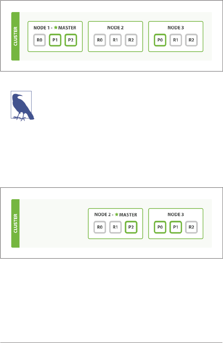
Figure 2-5. Increasing the number_of_replicas to 2
Of course, just having more replica shards on the same number of
nodes doesn’t increase our performance at all because each shard
has access to a smaller fraction of its node’s resources. You need to
add hardware to increase throughput.
But these extra replicas do mean that we have more redundancy:
with the node configuration above, we can now afford to lose two
nodes without losing any data.
Coping with Failure
We’ve said that Elasticsearch can cope when nodes fail, so let’s go ahead and try it out.
If we kill the first node, our cluster looks like Figure 2-6.
Figure 2-6. Cluster aer killing one node
The node we killed was the master node. A cluster must have a master node in order
to function correctly, so the first thing that happened was that the nodes elected a new
master: Node 2.
Primary shards 1 and 2 were lost when we killed Node 1, and our index cannot func‐
tion properly if it is missing primary shards. If we had checked the cluster health at
this point, we would have seen status red: not all primary shards are active!
32 | Chapter 2: Life Inside a Cluster

Fortunately, a complete copy of the two lost primary shards exists on other nodes, so
the first thing that the new master node did was to promote the replicas of these
shards on Node 2 and Node 3 to be primaries, putting us back into cluster health
yellow. This promotion process was instantaneous, like the flick of a switch.
So why is our cluster health yellow and not green? We have all three primary shards,
but we specified that we wanted two replicas of each primary, and currently only one
replica is assigned. This prevents us from reaching green, but we’re not too worried
here: were we to kill Node 2 as well, our application could still keep running without
data loss, because Node 3 contains a copy of every shard.
If we restart Node 1, the cluster would be able to allocate the missing replica shards,
resulting in a state similar to the one described in Figure 2-5. If Node 1 still has copies
of the old shards, it will try to reuse them, copying over from the primary shard only
the files that have changed in the meantime.
By now, you should have a reasonable idea of how shards allow Elasticsearch to scale
horizontally and to ensure that your data is safe. Later we will examine the life cycle
of a shard in more detail.
Coping with Failure | 33

CHAPTER 3
Data In, Data Out
Whatever program we write, the intention is the same: to organize data in a way that
serves our purposes. But data doesn’t consist of just random bits and bytes. We build
relationships between data elements in order to represent entities, or things that exist
in the real world. A name and an email address have more meaning if we know that
they belong to the same person.
In the real world, though, not all entities of the same type look the same. One person
might have a home telephone number, while another person has only a cell-phone
number, and another might have both. One person might have three email addresses,
while another has none. A Spanish person will probably have two last names, while
an English person will probably have only one.
One of the reasons that object-oriented programming languages are so popular is that
objects help us represent and manipulate real-world entities with potentially complex
data structures. So far, so good.
The problem comes when we need to store these entities. Traditionally, we have
stored our data in columns and rows in a relational database, the equivalent of using a
spreadsheet. All the flexibility gained from using objects is lost because of the inflexi‐
bility of our storage medium.
But what if we could store our objects as objects? Instead of modeling our application
around the limitations of spreadsheets, we can instead focus on using the data. The
flexibility of objects is returned to us.
An object is a language-specific, in-memory data structure. To send it across the net‐
work or store it, we need to be able to represent it in some standard format. JSON is a
way of representing objects in human-readable text. It has become the de facto stan‐
dard for exchanging data in the NoSQL world. When an object has been serialized
into JSON, it is known as a JSON document.
35

Elasticsearch is a distributed document store. It can store and retrieve complex data
structures—serialized as JSON documents—in real time. In other words, as soon as a
document has been stored in Elasticsearch, it can be retrieved from any node in the
cluster.
Of course, we don’t need to only store data; we must also query it, en masse and at
speed. While NoSQL solutions exist that allow us to store objects as documents, they
still require us to think about how we want to query our data, and which fields
require an index in order to make data retrieval fast.
In Elasticsearch, all data in every eld is indexed by default. That is, every field has a
dedicated inverted index for fast retrieval. And, unlike most other databases, it can
use all of those inverted indices in the same query, to return results at breathtaking
speed.
In this chapter, we present the APIs that we use to create, retrieve, update, and delete
documents. For the moment, we don’t care about the data inside our documents or
how to query them. All we care about is how to store our documents safely in Elastic‐
search and how to get them back again.
What Is a Document?
Most entities or objects in most applications can be serialized into a JSON object,
with keys and values. A key is the name of a field or property, and a value can be a
string, a number, a Boolean, another object, an array of values, or some other special‐
ized type such as a string representing a date or an object representing a geolocation:
{
"name": "John Smith",
"age": 42,
"confirmed": true,
"join_date": "2014-06-01",
"home": {
"lat": 51.5,
"lon": 0.1
},
"accounts": [
{
"type": "facebook",
"id": "johnsmith"
},
{
"type": "twitter",
"id": "johnsmith"
}
]
}
36 | Chapter 3: Data In, Data Out

Often, we use the terms object and document interchangeably. However, there is a dis‐
tinction. An object is just a JSON object—similar to what is known as a hash, hash‐
map, dictionary, or associative array. Objects may contain other objects. In
Elasticsearch, the term document has a specific meaning. It refers to the top-level, or
root object that is serialized into JSON and stored in Elasticsearch under a unique ID.
Document Metadata
A document doesn’t consist only of its data. It also has metadata—information about
the document. The three required metadata elements are as follows:
_index
Where the document lives
_type
The class of object that the document represents
_id
The unique identifier for the document
_index
An index is like a database in a relational database; it’s the place we store and index
related data.
Actually, in Elasticsearch, our data is stored and indexed in shards,
while an index is just a logical namespace that groups together one
or more shards. However, this is an internal detail; our application
shouldn’t care about shards at all. As far as our application is con‐
cerned, our documents live in an index. Elasticsearch takes care of
the details.
We cover how to create and manage indices ourselves in Chapter 10, but for now we
will let Elasticsearch create the index for us. All we have to do is choose an index
name. This name must be lowercase, cannot begin with an underscore, and cannot
contain commas. Let’s use website as our index name.
_type
In applications, we use objects to represent things such as a user, a blog post, a com‐
ment, or an email. Each object belongs to a class that defines the properties or data
associated with an object. Objects in the user class may have a name, a gender, an
age, and an email address.
Document Metadata | 37

In a relational database, we usually store objects of the same class in the same table,
because they share the same data structure. For the same reason, in Elasticsearch we
use the same type for documents that represent the same class of thing, because they
share the same data structure.
Every type has its own mapping or schema definition, which defines the data struc‐
ture for documents of that type, much like the columns in a database table. Docu‐
ments of all types can be stored in the same index, but the mapping for the type tells
Elasticsearch how the data in each document should be indexed.
We show how to specify and manage mappings in “Types and Mappings” on page
137, but for now we will rely on Elasticsearch to detect our document’s data structure
automatically.
A _type name can be lowercase or uppercase, but shouldn’t begin with an
underscore or contain commas. We will use blog for our type name.
_id
The ID is a string that, when combined with the _index and _type,
uniquely identifies a document in Elasticsearch. When creating a new document, you
can either provide your own _id or let Elasticsearch generate one for you.
Other Metadata
There are several other metadata elements, which are presented in “Types and Map‐
pings” on page 137. With the elements listed previously, we are already able to store a
document in Elasticsearch and to retrieve it by ID—in other words, to use Elastic‐
search as a document store.
Indexing a Document
Documents are indexed—stored and made searchable—by using the index API. But
first, we need to decide where the document lives. As we just discussed, a document’s
_index, _type, and _id uniquely identify the document. We can either provide our
own _id value or let the index API generate one for us.
Using Our Own ID
If your document has a natural identifier (for example, a user_account field or some
other value that identifies the document), you should provide your own _id, using
this form of the index API:
38 | Chapter 3: Data In, Data Out

PUT /{index}/{type}/{id}
{
"field": "value",
...
}
For example, if our index is called website, our type is called blog, and we choose the
ID 123, then the index request looks like this:
PUT /website/blog/123
{
"title": "My first blog entry",
"text": "Just trying this out...",
"date": "2014/01/01"
}
Elasticsearch responds as follows:
{
"_index": "website",
"_type": "blog",
"_id": "123",
"_version": 1,
"created": true
}
The response indicates that the indexing request has been successfully created and
includes the _index, _type, and _id metadata, and a new element: _version.
Every document in Elasticsearch has a version number. Every time a change is made
to a document (including deleting it), the _version number is incremented. In “Deal‐
ing with Conflicts” on page 45, we discuss how to use the _version number to ensure
that one part of your application doesn’t overwrite changes made by another part.
Autogenerating IDs
If our data doesn’t have a natural ID, we can let Elasticsearch autogenerate one for us.
The structure of the request changes: instead of using the PUT verb (“store this docu‐
ment at this URL”), we use the POST verb (“store this document under this URL”).
The URL now contains just the _index and the _type:
POST /website/blog/
{
"title": "My second blog entry",
"text": "Still trying this out...",
"date": "2014/01/01"
}
The response is similar to what we saw before, except that the _id field has been gen‐
erated for us:
Indexing a Document | 39

{
"_index": "website",
"_type": "blog",
"_id": "wM0OSFhDQXGZAWDf0-drSA",
"_version": 1,
"created": true
}
Autogenerated IDs are 22 character long, URL-safe, Base64-encoded string univer
sally unique identiers, or UUIDs.
Retrieving a Document
To get the document out of Elasticsearch, we use the same _index, _type, and _id,
but the HTTP verb changes to GET:
GET /website/blog/123?pretty
The response includes the by-now-familiar metadata elements, plus the _source field,
which contains the original JSON document that we sent to Elasticsearch when we
indexed it:
{
"_index" : "website",
"_type" : "blog",
"_id" : "123",
"_version" : 1,
"found" : true,
"_source" : {
"title": "My first blog entry",
"text": "Just trying this out...",
"date": "2014/01/01"
}
}
Adding pretty to the query-string parameters for any request, as
in the preceding example, causes Elasticsearch to pretty-print the
JSON response to make it more readable. The _source field, how‐
ever, isn’t pretty-printed. Instead we get back exactly the same
JSON string that we passed in.
The response to the GET request includes {"found": true}. This confirms that the
document was found. If we were to request a document that doesn’t exist, we would
still get a JSON response, but found would be set to false.
Also, the HTTP response code would be 404 Not Found instead of 200 OK. We can
see this by passing the -i argument to curl, which causes it to display the response
headers:
40 | Chapter 3: Data In, Data Out

curl -i -XGET http://localhost:9200/website/blog/124?pretty
The response now looks like this:
HTTP/1.1 404 Not Found
Content-Type: application/json; charset=UTF-8
Content-Length: 83
{
"_index" : "website",
"_type" : "blog",
"_id" : "124",
"found" : false
}
Retrieving Part of a Document
By default, a GET request will return the whole document, as stored in the _source
field. But perhaps all you are interested in is the title field. Individual fields can be
requested by using the _source parameter. Multiple fields can be specified in a
comma-separated list:
GET /website/blog/123?_source=title,text
The _source field now contains just the fields that we requested and has filtered out
the date field:
{
"_index" : "website",
"_type" : "blog",
"_id" : "123",
"_version" : 1,
"exists" : true,
"_source" : {
"title": "My first blog entry" ,
"text": "Just trying this out..."
}
}
Or if you want just the _source field without any metadata, you can use the _source
endpoint:
GET /website/blog/123/_source
which returns just the following:
{
"title": "My first blog entry",
"text": "Just trying this out...",
"date": "2014/01/01"
}
Retrieving a Document | 41

Checking Whether a Document Exists
If all you want to do is to check whether a document exists—you’re not interested in
the content at all—then use the HEAD method instead of the GET method. HEAD
requests don’t return a body, just HTTP headers:
curl -i -XHEAD http://localhost:9200/website/blog/123
Elasticsearch will return a 200 OK status code if the document exists:
HTTP/1.1 200 OK
Content-Type: text/plain; charset=UTF-8
Content-Length: 0
And a 404 Not Found if it doesn’t exist:
curl -i -XHEAD http://localhost:9200/website/blog/124
HTTP/1.1 404 Not Found
Content-Type: text/plain; charset=UTF-8
Content-Length: 0
Of course, just because a document didn’t exist when you checked it, doesn’t mean
that it won’t exist a millisecond later: another process might create the document in
the meantime.
Updating a Whole Document
Documents in Elasticsearch are immutable; we cannot change them. Instead, if we
need to update an existing document, we reindex or replace it, which we can do using
the same index API that we have already discussed in “Indexing a Document” on
page 38.
PUT /website/blog/123
{
"title": "My first blog entry",
"text": "I am starting to get the hang of this...",
"date": "2014/01/02"
}
In the response, we can see that Elasticsearch has incremented the _version number:
{
"_index" : "website",
"_type" : "blog",
"_id" : "123",
"_version" : 2,
"created": false
}
42 | Chapter 3: Data In, Data Out

The created flag is set to false because a document with the same index, type,
and ID already existed.
Internally, Elasticsearch has marked the old document as deleted and added an
entirely new document. The old version of the document doesn’t disappear immedi‐
ately, although you won’t be able to access it. Elasticsearch cleans up deleted docu‐
ments in the background as you continue to index more data.
Later in this chapter, we introduce the update API, which can be used to make partial
updates to a document. This API appears to change documents in place, but actually
Elasticsearch is following exactly the same process as described previously:
1. Retrieve the JSON from the old document
2. Change it
3. Delete the old document
4. Index a new document
The only difference is that the update API achieves this through a single client
request, instead of requiring separate get and index requests.
Creating a New Document
How can we be sure, when we index a document, that we are creating an entirely new
document and not overwriting an existing one?
Remember that the combination of _index, _type, and _id uniquely identifies a
document. So the easiest way to ensure that our document is new is by letting Elastic‐
search autogenerate a new unique _id, using the POST version of the index request:
POST /website/blog/
{ ... }
However, if we already have an _id that we want to use, then we have to tell Elastic‐
search that it should accept our index request only if a document with the same
_index, _type, and _id doesn’t exist already. There are two ways of doing this, both of
which amount to the same thing. Use whichever method is more convenient for you.
The first method uses the op_type query-string parameter:
PUT /website/blog/123?op_type=create
{ ... }
And the second uses the /_create endpoint in the URL:
PUT /website/blog/123/_create
{ ... }
Creating a New Document | 43

If the request succeeds in creating a new document, Elasticsearch will return the
usual metadata and an HTTP response code of 201 Created.
On the other hand, if a document with the same _index, _type, and _id already
exists, Elasticsearch will respond with a 409 Conflict response code, and an error
message like the following:
{
"error" : "DocumentAlreadyExistsException[[website][4] [blog][123]:
document already exists]",
"status" : 409
}
Deleting a Document
The syntax for deleting a document follows the same pattern that we have seen
already, but uses the DELETE method :
DELETE /website/blog/123
If the document is found, Elasticsearch will return an HTTP response code of 200 OK
and a response body like the following. Note that the _version number has been
incremented:
{
"found" : true,
"_index" : "website",
"_type" : "blog",
"_id" : "123",
"_version" : 3
}
If the document isn’t found, we get a 404 Not Found response code and a body like
this:
{
"found" : false,
"_index" : "website",
"_type" : "blog",
"_id" : "123",
"_version" : 4
}
Even though the document doesn’t exist (found is false), the _version number has
still been incremented. This is part of the internal bookkeeping, which ensures that
changes are applied in the correct order across multiple nodes.
44 | Chapter 3: Data In, Data Out

As already mentioned in “Updating a Whole Document” on page
42, deleting a document doesn’t immediately remove the docu‐
ment from disk; it just marks it as deleted. Elasticsearch will clean
up deleted documents in the background as you continue to index
more data.
Dealing with Conicts
When updating a document with the index API, we read the original document,
make our changes, and then reindex the whole document in one go. The most recent
indexing request wins: whichever document was indexed last is the one stored in
Elasticsearch. If somebody else had changed the document in the meantime, their
changes would be lost.
Many times, this is not a problem. Perhaps our main data store is a relational data‐
base, and we just copy the data into Elasticsearch to make it searchable. Perhaps there
is little chance of two people changing the same document at the same time. Or per‐
haps it doesn’t really matter to our business if we lose changes occasionally.
But sometimes losing a change is very important. Imagine that we’re using Elastic‐
search to store the number of widgets that we have in stock in our online store. Every
time that we sell a widget, we decrement the stock count in Elasticsearch.
One day, management decides to have a sale. Suddenly, we are selling several widgets
every second. Imagine two web processes, running in parallel, both processing the
sale of one widget each, as shown in Figure 3-1.
Dealing with Conicts | 45
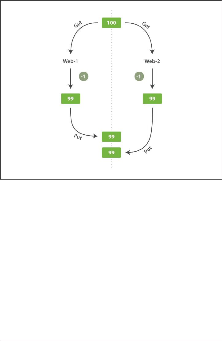
Figure 3-1. Consequence of no concurrency control
The change that web_1 made to the stock_count has been lost because web_2 is
unaware that its copy of the stock_count is out-of-date. The result is that we think
we have more widgets than we actually do, and we’re going to disappoint customers
by selling them stock that doesn’t exist.
The more frequently that changes are made, or the longer the gap between reading
data and updating it, the more likely it is that we will lose changes.
In the database world, two approaches are commonly used to ensure that changes are
not lost when making concurrent updates:
Pessimistic concurrency control
Widely used by relational databases, this approach assumes that conflicting
changes are likely to happen and so blocks access to a resource in order to pre‐
vent conflicts. A typical example is locking a row before reading its data, ensuring
that only the thread that placed the lock is able to make changes to the data in
that row.
46 | Chapter 3: Data In, Data Out

Optimistic concurrency control
Used by Elasticsearch, this approach assumes that conflicts are unlikely to hap‐
pen and doesn’t block operations from being attempted. However, if the underly‐
ing data has been modified between reading and writing, the update will fail. It is
then up to the application to decide how it should resolve the conflict. For
instance, it could reattempt the update, using the fresh data, or it could report the
situation to the user.
Optimistic Concurrency Control
Elasticsearch is distributed. When documents are created, updated, or deleted, the
new version of the document has to be replicated to other nodes in the cluster. Elas‐
ticsearch is also asynchronous and concurrent, meaning that these replication
requests are sent in parallel, and may arrive at their destination out of sequence. Elas‐
ticsearch needs a way of ensuring that an older version of a document never over‐
writes a newer version.
When we discussed index, get, and delete requests previously, we pointed out that
every document has a _version number that is incremented whenever a document is
changed. Elasticsearch uses this _version number to ensure that changes are applied
in the correct order. If an older version of a document arrives after a new version, it
can simply be ignored.
We can take advantage of the _version number to ensure that conflicting changes
made by our application do not result in data loss. We do this by specifying the ver
sion number of the document that we wish to change. If that version is no longer
current, our request fails.
Let’s create a new blog post:
PUT /website/blog/1/_create
{
"title": "My first blog entry",
"text": "Just trying this out..."
}
The response body tells us that this newly created document has _version number 1.
Now imagine that we want to edit the document: we load its data into a web form,
make our changes, and then save the new version.
First we retrieve the document:
GET /website/blog/1
The response body includes the same _version number of 1:
{
"_index" : "website",
Optimistic Concurrency Control | 47

"_type" : "blog",
"_id" : "1",
"_version" : 1,
"found" : true,
"_source" : {
"title": "My first blog entry",
"text": "Just trying this out..."
}
}
Now, when we try to save our changes by reindexing the document, we specify the
version to which our changes should be applied:
PUT /website/blog/1?version=1
{
"title": "My first blog entry",
"text": "Starting to get the hang of this..."
}
We want this update to succeed only if the current _version of this document in
our index is version 1.
This request succeeds, and the response body tells us that the _version has been
incremented to 2:
{
"_index": "website",
"_type": "blog",
"_id": "1",
"_version": 2
"created": false
}
However, if we were to rerun the same index request, still specifying version=1, Elas‐
ticsearch would respond with a 409 Conflict HTTP response code, and a body like
the following:
{
"error" : "VersionConflictEngineException[[website][2] [blog][1]:
version conflict, current [2], provided [1]]",
"status" : 409
}
This tells us that the current _version number of the document in Elasticsearch is 2,
but that we specified that we were updating version 1.
What we do now depends on our application requirements. We could tell the user
that somebody else has already made changes to the document, and to review the
changes before trying to save them again. Alternatively, as in the case of the widget
stock_count previously, we could retrieve the latest document and try to reapply the
change.
48 | Chapter 3: Data In, Data Out

All APIs that update or delete a document accept a version parameter, which allows
you to apply optimistic concurrency control to just the parts of your code where it
makes sense.
Using Versions from an External System
A common setup is to use some other database as the primary data store and Elastic‐
search to make the data searchable, which means that all changes to the primary data‐
base need to be copied across to Elasticsearch as they happen. If multiple processes
are responsible for this data synchronization, you may run into concurrency prob‐
lems similar to those described previously.
If your main database already has version numbers—or a value such as timestamp
that can be used as a version number—then you can reuse these same version num‐
bers in Elasticsearch by adding version_type=external to the query string. Version
numbers must be integers greater than zero and less than about 9.2e+18--a positive
long value in Java.
The way external version numbers are handled is a bit different from the internal ver‐
sion numbers we discussed previously. Instead of checking that the current _version
is the same as the one specified in the request, Elasticsearch checks that the current
_version is less than the specified version. If the request succeeds, the external ver‐
sion number is stored as the document’s new _version.
External version numbers can be specified not only on index and delete requests, but
also when creating new documents.
For instance, to create a new blog post with an external version number of 5, we can
do the following:
PUT /website/blog/2?version=5&version_type=external
{
"title": "My first external blog entry",
"text": "Starting to get the hang of this..."
}
In the response, we can see that the current _version number is 5:
{
"_index": "website",
"_type": "blog",
"_id": "2",
"_version": 5,
"created": true
}
Now we update this document, specifying a new version number of 10:
PUT /website/blog/2?version=10&version_type=external
{
Optimistic Concurrency Control | 49

"title": "My first external blog entry",
"text": "This is a piece of cake..."
}
The request succeeds and sets the current _version to 10:
{
"_index": "website",
"_type": "blog",
"_id": "2",
"_version": 10,
"created": false
}
If you were to rerun this request, it would fail with the same conflict error we saw
before, because the specified external version number is not higher than the current
version in Elasticsearch.
Partial Updates to Documents
In “Updating a Whole Document” on page 42, we said that the way to update a docu‐
ment is to retrieve it, change it, and then reindex the whole document. This is true.
However, using the update API, we can make partial updates like incrementing a
counter in a single request.
We also said that documents are immutable: they cannot be changed, only replaced.
The update API must obey the same rules. Externally, it appears as though we are
partially updating a document in place. Internally, however, the update API simply
manages the same retrieve-change-reindex process that we have already described.
The difference is that this process happens within a shard, thus avoiding the network
overhead of multiple requests. By reducing the time between the retrieve and reindex
steps, we also reduce the likelihood of there being conflicting changes from other
processes.
The simplest form of the update request accepts a partial document as the doc
parameter, which just gets merged with the existing document. Objects are merged
together, existing scalar fields are overwritten, and new fields are added. For instance,
we could add a tags field and a views field to our blog post as follows:
POST /website/blog/1/_update
{
"doc" : {
"tags" : [ "testing" ],
"views": 0
}
}
If the request succeeds, we see a response similar to that of the index request:
50 | Chapter 3: Data In, Data Out

{
"_index" : "website",
"_id" : "1",
"_type" : "blog",
"_version" : 3
}
Retrieving the document shows the updated _source field:
{
"_index": "website",
"_type": "blog",
"_id": "1",
"_version": 3,
"found": true,
"_source": {
"title": "My first blog entry",
"text": "Starting to get the hang of this...",
"tags": [ "testing" ],
"views": 0
}
}
Our new fields have been added to the _source.
Using Scripts to Make Partial Updates
Scripts can be used in the update API to change the contents of the _source field,
which is referred to inside an update script as ctx._source. For instance, we could
use a script to increment the number of views that our blog post has had:
POST /website/blog/1/_update
{
"script" : "ctx._source.views+=1"
}
Scripting with Groovy
For those moments when the API just isn’t enough, Elasticsearch allows you to write
your own custom logic in a script. Scripting is supported in many APIs including
search, sorting, aggregations, and document updates. Scripts can be passed in as part
of the request, retrieved from the special .scripts index, or loaded from disk.
The default scripting language is a Groovy, a fast and expressive scripting language,
similar in syntax to JavaScript. It runs in a sandbox to prevent malicious users from
breaking out of Elasticsearch and attacking the server.
You can read more about scripting in the scripting reference documentation.
Partial Updates to Documents | 51

We can also use a script to add a new tag to the tags array. In this example we specify
the new tag as a parameter rather than hardcoding it in the script itself. This allows
Elasticsearch to reuse the script in the future, without having to compile a new script
every time we want to add another tag:
POST /website/blog/1/_update
{
"script" : "ctx._source.tags+=new_tag",
"params" : {
"new_tag" : "search"
}
}
Fetching the document shows the effect of the last two requests:
{
"_index": "website",
"_type": "blog",
"_id": "1",
"_version": 5,
"found": true,
"_source": {
"title": "My first blog entry",
"text": "Starting to get the hang of this...",
"tags": ["testing", "search"],
"views": 1
}
}
The search tag has been appended to the tags array.
The views field has been incremented.
We can even choose to delete a document based on its contents, by setting ctx.op to
delete:
POST /website/blog/1/_update
{
"script" : "ctx.op = ctx._source.views == count ? 'delete' : 'none'",
"params" : {
"count": 1
}
}
Updating a Document That May Not Yet Exist
Imagine that we need to store a page view counter in Elasticsearch. Every time that a
user views a page, we increment the counter for that page. But if it is a new page, we
can’t be sure that the counter already exists. If we try to update a nonexistent docu‐
ment, the update will fail.
52 | Chapter 3: Data In, Data Out

In cases like these, we can use the upsert parameter to specify the document that
should be created if it doesn’t already exist:
POST /website/pageviews/1/_update
{
"script" : "ctx._source.views+=1",
"upsert": {
"views": 1
}
}
The first time we run this request, the upsert value is indexed as a new document,
which initializes the views field to 1. On subsequent runs, the document already
exists, so the script update is applied instead, incrementing the views counter.
Updates and Conicts
In the introduction to this section, we said that the smaller the window between the
retrieve and reindex steps, the smaller the opportunity for conflicting changes. But it
doesn’t eliminate the possibility completely. It is still possible that a request from
another process could change the document before update has managed to reindex
it.
To avoid losing data, the update API retrieves the current _version of the document
in the retrieve step, and passes that to the index request during the reindex step. If
another process has changed the document between retrieve and reindex, then the
_version number won’t match and the update request will fail.
For many uses of partial update, it doesn’t matter that a document has been changed.
For instance, if two processes are both incrementing the page-view counter, it doesn’t
matter in which order it happens; if a conflict occurs, the only thing we need to do is
reattempt the update.
This can be done automatically by setting the retry_on_conflict parameter to the
number of times that update should retry before failing; it defaults to 0.
POST /website/pageviews/1/_update?retry_on_conflict=5
{
"script" : "ctx._source.views+=1",
"upsert": {
"views": 0
}
}
Retry this update five times before failing.
This works well for operations such as incrementing a counter, where the order of
increments does not matter, but in other situations the order of changes is important.
Like the index API, the update API adopts a last-write-wins approach by default, but
Partial Updates to Documents | 53

it also accepts a version parameter that allows you to use optimistic concurrency
control to specify which version of the document you intend to update.
Retrieving Multiple Documents
As fast as Elasticsearch is, it can be faster still. Combining multiple requests into one
avoids the network overhead of processing each request individually. If you know
that you need to retrieve multiple documents from Elasticsearch, it is faster to
retrieve them all in a single request by using the multi-get, or mget, API, instead of
document by document.
The mget API expects a docs array, each element of which specifies the _index,
_type, and _id metadata of the document you wish to retrieve. You can also specify a
_source parameter if you just want to retrieve one or more specific fields:
GET /_mget
{
"docs" : [
{
"_index" : "website",
"_type" : "blog",
"_id" : 2
},
{
"_index" : "website",
"_type" : "pageviews",
"_id" : 1,
"_source": "views"
}
]
}
The response body also contains a docs array that contains a response per document,
in the same order as specified in the request. Each of these responses is the same
response body that we would expect from an individual get request:
{
"docs" : [
{
"_index" : "website",
"_id" : "2",
"_type" : "blog",
"found" : true,
"_source" : {
"text" : "This is a piece of cake...",
"title" : "My first external blog entry"
},
"_version" : 10
},
{
54 | Chapter 3: Data In, Data Out

"_index" : "website",
"_id" : "1",
"_type" : "pageviews",
"found" : true,
"_version" : 2,
"_source" : {
"views" : 2
}
}
]
}
If the documents you wish to retrieve are all in the same _index (and maybe even of
the same _type), you can specify a default /_index or a default /_index/_type in the
URL.
You can still override these values in the individual requests:
GET /website/blog/_mget
{
"docs" : [
{ "_id" : 2 },
{ "_type" : "pageviews", "_id" : 1 }
]
}
In fact, if all the documents have the same _index and _type, you can just pass an
array of ids instead of the full docs array:
GET /website/blog/_mget
{
"ids" : [ "2", "1" ]
}
Note that the second document that we requested doesn’t exist. We specified type
blog, but the document with ID 1 is of type pageviews. This nonexistence is reported
in the response body:
{
"docs" : [
{
"_index" : "website",
"_type" : "blog",
"_id" : "2",
"_version" : 10,
"found" : true,
"_source" : {
"title": "My first external blog entry",
"text": "This is a piece of cake..."
}
},
{
"_index" : "website",
Retrieving Multiple Documents | 55

"_type" : "blog",
"_id" : "1",
"found" : false
}
]
}
This document was not found.
The fact that the second document wasn’t found didn’t affect the retrieval of the first
document. Each doc is retrieved and reported on individually.
The HTTP status code for the preceding request is 200, even
though one document wasn’t found. In fact, it would still be 200 if
none of the requested documents were found—because the mget
request itself completed successfully. To determine the success or
failure of the individual documents, you need to check the found
flag.
Cheaper in Bulk
In the same way that mget allows us to retrieve multiple documents at once, the bulk
API allows us to make multiple create, index, update, or delete requests in a single
step. This is particularly useful if you need to index a data stream such as log events,
which can be queued up and indexed in batches of hundreds or thousands.
The bulk request body has the following, slightly unusual, format:
{ action: { metadata }}\n
{ request body }\n
{ action: { metadata }}\n
{ request body }\n
...
This format is like a stream of valid one-line JSON documents joined together by
newline (\n) characters. Two important points to note:
•Every line must end with a newline character (\n), including the last line. These
are used as markers to allow for efficient line separation.
•The lines cannot contain unescaped newline characters, as they would interfere
with parsing. This means that the JSON must not be pretty-printed.
56 | Chapter 3: Data In, Data Out

In “Why the Funny Format?” on page 69, we explain why the bulk
API uses this format.
The action/metadata line specifies what action to do to which document.
The action must be one of the following:
create
Create a document only if the document does not already exist. See “Creating a
New Document” on page 43.
index
Create a new document or replace an existing document. See “Indexing a Docu‐
ment” on page 38 and “Updating a Whole Document” on page 42.
update
Do a partial update on a document. See “Partial Updates to Documents” on page
50.
delete
Delete a document. See “Deleting a Document” on page 44.
The metadata should specify the _index, _type, and _id of the document to be
indexed, created, updated, or deleted.
For instance, a delete request could look like this:
{ "delete": { "_index": "website", "_type": "blog", "_id": "123" }}
The request body line consists of the document _source itself—the fields and values
that the document contains. It is required for index and create operations, which
makes sense: you must supply the document to index.
It is also required for update operations and should consist of the same request body
that you would pass to the update API: doc, upsert, script, and so forth. No
request body line is required for a delete.
{ "create": { "_index": "website", "_type": "blog", "_id": "123" }}
{ "title": "My first blog post" }
If no _id is specified, an ID will be autogenerated:
{ "index": { "_index": "website", "_type": "blog" }}
{ "title": "My second blog post" }
To put it all together, a complete bulk request has this form:
Cheaper in Bulk | 57

POST /_bulk
{ "delete": { "_index": "website", "_type": "blog", "_id": "123" }}
{ "create": { "_index": "website", "_type": "blog", "_id": "123" }}
{ "title": "My first blog post" }
{ "index": { "_index": "website", "_type": "blog" }}
{ "title": "My second blog post" }
{ "update": { "_index": "website", "_type": "blog", "_id": "123", "_retry_on_conflict" : 3} }
{ "doc" : {"title" : "My updated blog post"} }
Notice how the delete action does not have a request body; it is followed imme‐
diately by another action.
Remember the final newline character.
The Elasticsearch response contains the items array, which lists the result of each
request, in the same order as we requested them:
{
"took": 4,
"errors": false,
"items": [
{ "delete": {
"_index": "website",
"_type": "blog",
"_id": "123",
"_version": 2,
"status": 200,
"found": true
}},
{ "create": {
"_index": "website",
"_type": "blog",
"_id": "123",
"_version": 3,
"status": 201
}},
{ "create": {
"_index": "website",
"_type": "blog",
"_id": "EiwfApScQiiy7TIKFxRCTw",
"_version": 1,
"status": 201
}},
{ "update": {
"_index": "website",
"_type": "blog",
"_id": "123",
"_version": 4,
"status": 200
}}
]
}}
58 | Chapter 3: Data In, Data Out

All subrequests completed successfully.
Each subrequest is executed independently, so the failure of one subrequest won’t
affect the success of the others. If any of the requests fail, the top-level error flag is set
to true and the error details will be reported under the relevant request:
POST /_bulk
{ "create": { "_index": "website", "_type": "blog", "_id": "123" }}
{ "title": "Cannot create - it already exists" }
{ "index": { "_index": "website", "_type": "blog", "_id": "123" }}
{ "title": "But we can update it" }
In the response, we can see that it failed to create document 123 because it already
exists, but the subsequent index request, also on document 123, succeeded:
{
"took": 3,
"errors": true,
"items": [
{ "create": {
"_index": "website",
"_type": "blog",
"_id": "123",
"status": 409,
"error": "DocumentAlreadyExistsException
[[website][4] [blog][123]:
document already exists]"
}},
{ "index": {
"_index": "website",
"_type": "blog",
"_id": "123",
"_version": 5,
"status": 200
}}
]
}
One or more requests has failed.
The HTTP status code for this request reports 409 CONFLICT.
The error message explaining why the request failed.
The second request succeeded with an HTTP status code of 200 OK.
That also means that bulk requests are not atomic: they cannot be used to implement
transactions. Each request is processed separately, so the success or failure of one
request will not interfere with the others.
Cheaper in Bulk | 59

Don’t Repeat Yourself
Perhaps you are batch-indexing logging data into the same index, and with the same
type. Having to specify the same metadata for every document is a waste. Instead,
just as for the mget API, the bulk request accepts a default /_index or /_index/_type
in the URL:
POST /website/_bulk
{ "index": { "_type": "log" }}
{ "event": "User logged in" }
You can still override the _index and _type in the metadata line, but it will use the
values in the URL as defaults:
POST /website/log/_bulk
{ "index": {}}
{ "event": "User logged in" }
{ "index": { "_type": "blog" }}
{ "title": "Overriding the default type" }
How Big Is Too Big?
The entire bulk request needs to be loaded into memory by the node that receives our
request, so the bigger the request, the less memory available for other requests. There
is an optimal size of bulk request. Above that size, performance no longer improves
and may even drop off. The optimal size, however, is not a fixed number. It depends
entirely on your hardware, your document size and complexity, and your indexing
and search load.
Fortunately, it is easy to find this sweet spot: Try indexing typical documents in
batches of increasing size. When performance starts to drop off, your batch size is too
big. A good place to start is with batches of 1,000 to 5,000 documents or, if your
documents are very large, with even smaller batches.
It is often useful to keep an eye on the physical size of your bulk requests. One thou‐
sand 1KB documents is very different from one thousand 1MB documents. A good
bulk size to start playing with is around 5-15MB in size.
60 | Chapter 3: Data In, Data Out

CHAPTER 4
Distributed Document Store
In the preceding chapter, we looked at all the ways to put data into your index and
then retrieve it. But we glossed over many technical details surrounding how the data
is distributed and fetched from the cluster. This separation is done on purpose; you
don’t really need to know how data is distributed to work with Elasticsearch. It just
works.
In this chapter, we dive into those internal, technical details to help you understand
how your data is stored in a distributed system.
Content Warning
The information presented in this chapter is for your interest. You are not required to
understand and remember all the detail in order to use Elasticsearch. The options
that are discussed are for advanced users only.
Read the section to gain a taste for how things work, and to know where the informa‐
tion is in case you need to refer to it in the future, but don’t be overwhelmed by the
detail.
Routing a Document to a Shard
When you index a document, it is stored on a single primary shard. How does Elas‐
ticsearch know which shard a document belongs to? When we create a new docu‐
ment, how does it know whether it should store that document on shard 1 or shard 2?
The process can’t be random, since we may need to retrieve the document in the
future. In fact, it is determined by a simple formula:
shard = hash(routing) % number_of_primary_shards
61
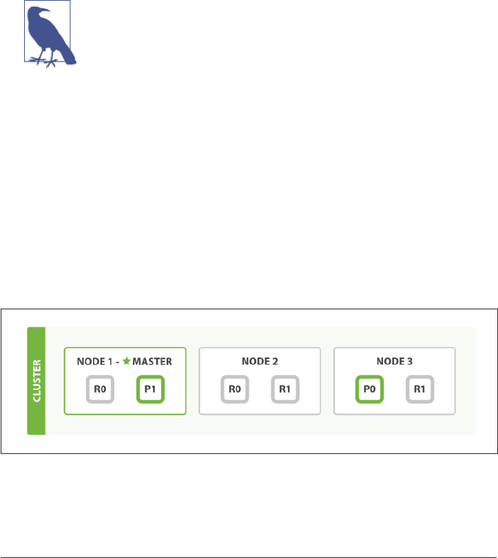
The routing value is an arbitrary string, which defaults to the document’s _id but
can also be set to a custom value. This routing string is passed through a hashing
function to generate a number, which is divided by the number of primary shards in
the index to return the remainder. The remainder will always be in the range 0 to
number_of_primary_shards - 1, and gives us the number of the shard where a par‐
ticular document lives.
This explains why the number of primary shards can be set only when an index is
created and never changed: if the number of primary shards ever changed in the
future, all previous routing values would be invalid and documents would never be
found.
Users sometimes think that having a fixed number of primary
shards makes it difficult to scale out an index later. In reality, there
are techniques that make it easy to scale out as and when you need.
We talk more about these in Chapter 43.
All document APIs (get, index, delete, bulk, update, and mget) accept a routing
parameter that can be used to customize the document-to- shard mapping. A custom
routing value could be used to ensure that all related documents—for instance, all the
documents belonging to the same user—are stored on the same shard. We discuss in
detail why you may want to do this in Chapter 43.
How Primary and Replica Shards Interact
For explanation purposes, let’s imagine that we have a cluster consisting of three
nodes. It contains one index called blogs that has two primary shards. Each primary
shard has two replicas. Copies of the same shard are never allocated to the same
node, so our cluster looks something like Figure 4-1.
Figure 4-1. A cluster with three nodes and one index
We can send our requests to any node in the cluster. Every node is fully capable of
serving any request. Every node knows the location of every document in the cluster
62 | Chapter 4: Distributed Document Store
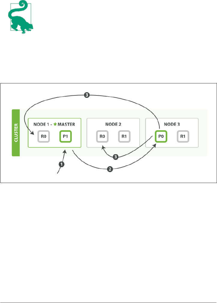
and so can forward requests directly to the required node. In the following examples,
we will send all of our requests to Node 1, which we will refer to as the requesting
node.
When sending requests, it is good practice to round-robin
through all the nodes in the cluster, in order to spread the load.
Creating, Indexing, and Deleting a Document
Create, index, and delete requests are write operations, which must be successfully
completed on the primary shard before they can be copied to any associated replica
shards, as shown in Figure 4-2.
Figure 4-2. Creating, indexing, or deleting a single document
Here is the sequence of steps necessary to successfully create, index, or delete a docu‐
ment on both the primary and any replica shards:
1. The client sends a create, index, or delete request to Node 1.
2. The node uses the document’s _id to determine that the document belongs to
shard 0. It forwards the request to Node 3, where the primary copy of shard 0 is
currently allocated.
3. Node 3 executes the request on the primary shard. If it is successful, it forwards
the request in parallel to the replica shards on Node 1 and Node 2. Once all of the
Creating, Indexing, and Deleting a Document | 63

replica shards report success, Node 3 reports success to the requesting node,
which reports success to the client.
By the time the client receives a successful response, the document change has been
executed on the primary shard and on all replica shards. Your change is safe.
There are a number of optional request parameters that allow you to influence this
process, possibly increasing performance at the cost of data security. These options
are seldom used because Elasticsearch is already fast, but they are explained here for
the sake of completeness:
replication
The default value for replication is sync. This causes the primary shard to wait
for successful responses from the replica shards before returning.
If you set replication to async, it will return success to the client as soon as the
request has been executed on the primary shard. It will still forward the request
to the replicas, but you will not know whether the replicas succeeded.
This option is mentioned specifically to advise against using it. The default sync
replication allows Elasticsearch to exert back pressure on whatever system is
feeding it with data. With async replication, it is possible to overload Elastic‐
search by sending too many requests without waiting for their completion.
consistency
By default, the primary shard requires a quorum, or majority, of shard copies
(where a shard copy can be a primary or a replica shard) to be available before
even attempting a write operation. This is to prevent writing data to the “wrong
side” of a network partition. A quorum is defined as follows:
int( (primary + number_of_replicas) / 2 ) + 1
The allowed values for consistency are one (just the primary shard), all (the
primary and all replicas), or the default quorum, or majority, of shard copies.
Note that the number_of_replicas is the number of replicas specied in the
index settings, not the number of replicas that are currently active. If you have
specified that an index should have three replicas, a quorum would be as follows:
int( (primary + 3 replicas) / 2 ) + 1 = 3
But if you start only two nodes, there will be insufficient active shard copies to
satisfy the quorum, and you will be unable to index or delete any documents.
timeout
What happens if insufficient shard copies are available? Elasticsearch waits, in the
hope that more shards will appear. By default, it will wait up to 1 minute. If you
64 | Chapter 4: Distributed Document Store
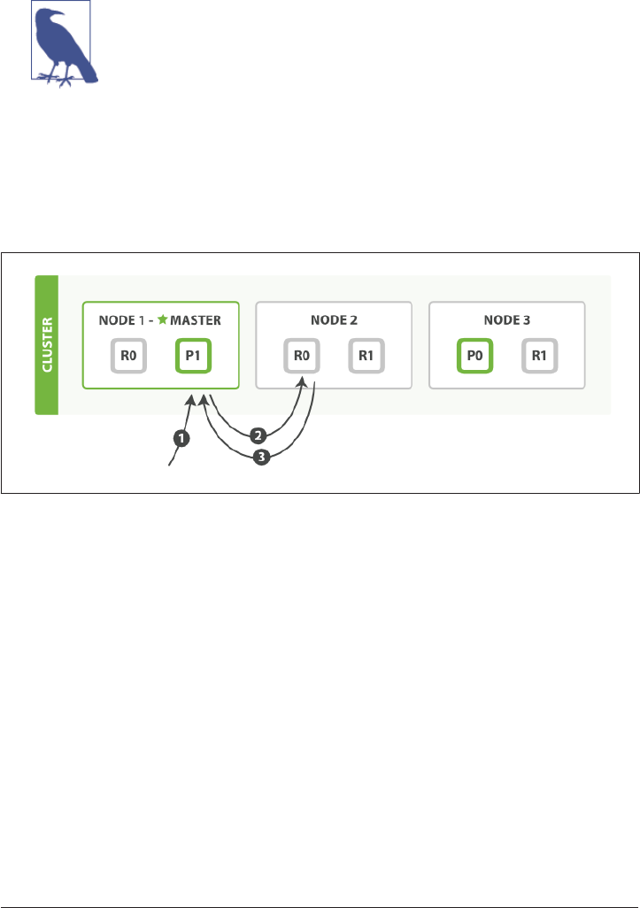
need to, you can use the timeout parameter to make it abort sooner: 100 is 100
milliseconds, and 30s is 30 seconds.
A new index has 1 replica by default, which means that two active
shard copies should be required in order to satisfy the need for a
quorum. However, these default settings would prevent us from
doing anything useful with a single-node cluster. To avoid this
problem, the requirement for a quorum is enforced only when num
ber_of_replicas is greater than 1.
Retrieving a Document
A document can be retrieved from a primary shard or from any of its replicas, as
shown in Figure 4-3.
Figure 4-3. Retrieving a single document
Here is the sequence of steps to retrieve a document from either a primary or replica
shard:
1. The client sends a get request to Node 1.
2. The node uses the document’s _id to determine that the document belongs to
shard 0. Copies of shard 0 exist on all three nodes. On this occasion, it forwards
the request to Node 2.
3. Node 2 returns the document to Node 1, which returns the document to the cli‐
ent.
For read requests, the requesting node will choose a different shard copy on every
request in order to balance the load; it round-robins through all shard copies.
It is possible that, while a document is being indexed, the document will already be
present on the primary shard but not yet copied to the replica shards. In this case, a
Retrieving a Document | 65
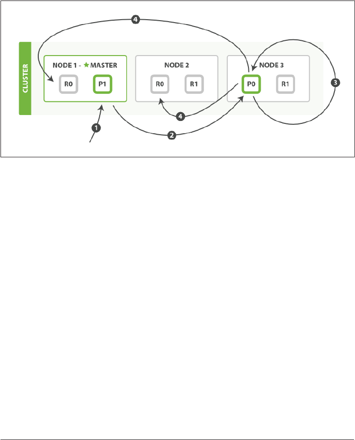
replica might report that the document doesn’t exist, while the primary would have
returned the document successfully. Once the indexing request has returned success
to the user, the document will be available on the primary and all replica shards.
Partial Updates to a Document
The update API , as shown in Figure 4-4, combines the read and write patterns
explained previously.
Figure 4-4. Partial updates to a document
Here is the sequence of steps used to perform a partial update on a document:
1. The client sends an update request to Node 1.
2. It forwards the request to Node 3, where the primary shard is allocated.
3. Node 3 retrieves the document from the primary shard, changes the JSON in the
_source field, and tries to reindex the document on the primary shard. If the
document has already been changed by another process, it retries step 3 up to
retry_on_conflict times, before giving up.
4. If Node 3 has managed to update the document successfully, it forwards the new
version of the document in parallel to the replica shards on Node 1 and Node 2 to
be reindexed. Once all replica shards report success, Node 3 reports success to
the requesting node, which reports success to the client.
66 | Chapter 4: Distributed Document Store
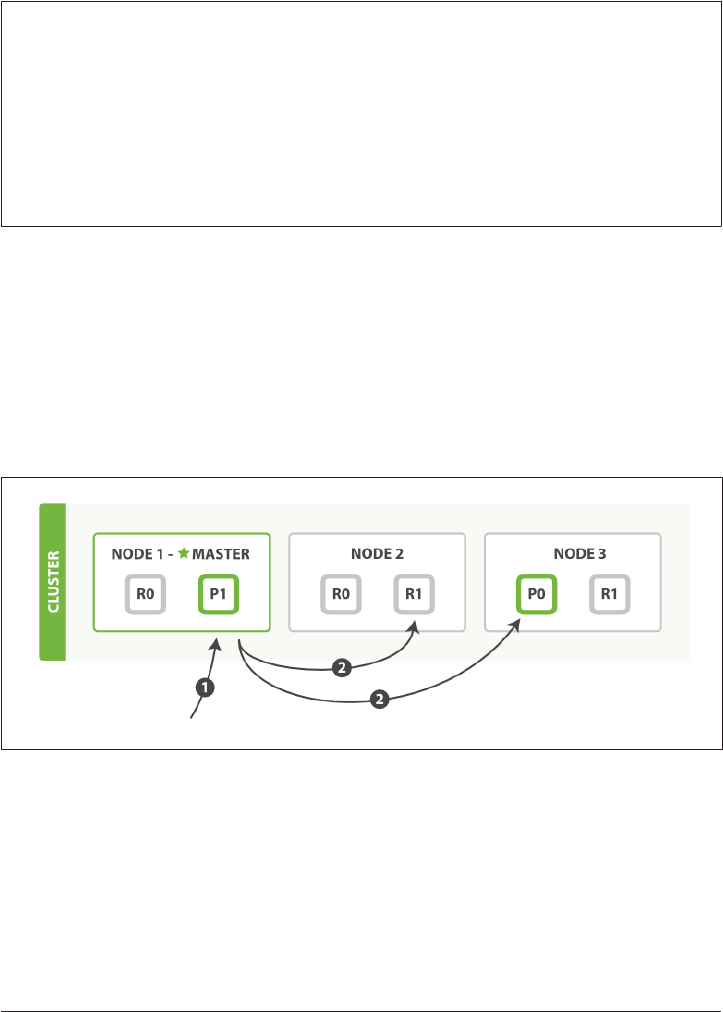
The update API also accepts the routing, replication, consistency, and timeout
parameters that are explained in “Creating, Indexing, and Deleting a Document” on
page 63.
Document-Based Replication
When a primary shard forwards changes to its replica shards, it doesn’t forward the
update request. Instead it forwards the new version of the full document. Remember
that these changes are forwarded to the replica shards asynchronously, and there is no
guarantee that they will arrive in the same order that they were sent. If Elasticsearch
forwarded just the change, it is possible that changes would be applied in the wrong
order, resulting in a corrupt document.
Multidocument Patterns
The patterns for the mget and bulk APIs are similar to those for individual docu‐
ments. The difference is that the requesting node knows in which shard each docu‐
ment lives. It breaks up the multidocument request into a multidocument request per
shard, and forwards these in parallel to each participating node.
Once it receives answers from each node, it collates their responses into a single
response, which it returns to the client, as shown in Figure 4-5.
Figure 4-5. Retrieving multiple documents with mget
Here is the sequence of steps necessary to retrieve multiple documents with a single
mget request:
1. The client sends an mget request to Node 1.
Multidocument Patterns | 67
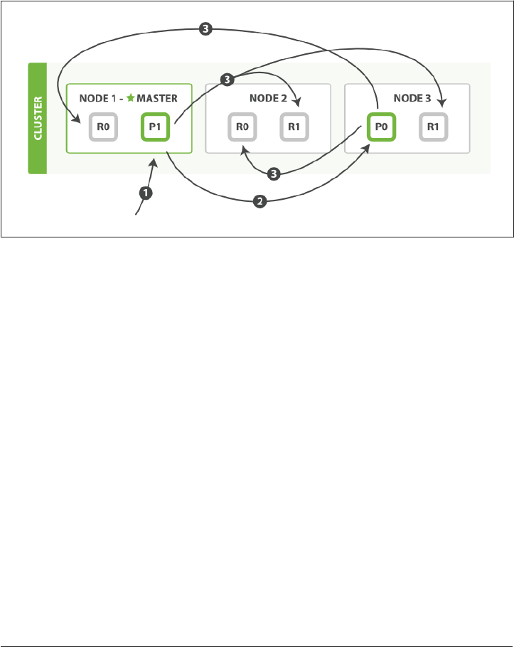
2. Node 1 builds a multi-get request per shard, and forwards these requests in paral‐
lel to the nodes hosting each required primary or replica shard. Once all replies
have been received, Node 1 builds the response and returns it to the client.
A routing parameter can be set for each document in the docs array.
The bulk API, as depicted in Figure 4-6, allows the execution of multiple create,
index, delete, and update requests within a single bulk request.
Figure 4-6. Multiple document changes with bulk
The sequence of steps followed by the bulk API are as follows:
1. The client sends a bulk request to Node 1.
2. Node 1 builds a bulk request per shard, and forwards these requests in parallel to
the nodes hosting each involved primary shard.
3. The primary shard executes each action serially, one after another. As each action
succeeds, the primary forwards the new document (or deletion) to its replica
shards in parallel, and then moves on to the next action. Once all replica shards
report success for all actions, the node reports success to the requesting node,
which collates the responses and returns them to the client.
The bulk API also accepts the replication and consistency parameters at the top
level for the whole bulk request, and the routing parameter in the metadata for each
request.
68 | Chapter 4: Distributed Document Store

Why the Funny Format?
When we learned about bulk requests earlier in “Cheaper in Bulk” on page 56, you
may have asked yourself, “Why does the bulk API require the funny format with the
newline characters, instead of just sending the requests wrapped in a JSON array, like
the mget API?”
To answer this, we need to explain a little background: Each document referenced in
a bulk request may belong to a different primary shard, each of which may be alloca‐
ted to any of the nodes in the cluster. This means that every action inside a bulk
request needs to be forwarded to the correct shard on the correct node.
If the individual requests were wrapped up in a JSON array, that would mean that we
would need to do the following:
•Parse the JSON into an array (including the document data, which can be very
large)
• Look at each request to determine which shard it should go to
• Create an array of requests for each shard
• Serialize these arrays into the internal transport format
• Send the requests to each shard
It would work, but would need a lot of RAM to hold copies of essentially the same
data, and would create many more data structures that the Java Virtual Machine
(JVM) would have to spend time garbage collecting.
Instead, Elasticsearch reaches up into the networking buffer, where the raw request
has been received, and reads the data directly. It uses the newline characters to iden‐
tify and parse just the small action/metadata lines in order to decide which shard
should handle each request.
These raw requests are forwarded directly to the correct shard. There is no redundant
copying of data, no wasted data structures. The entire request process is handled in
the smallest amount of memory possible.
Multidocument Patterns | 69

CHAPTER 5
Searching—The Basic Tools
So far, we have learned how to use Elasticsearch as a simple NoSQL-style distributed
document store. We can throw JSON documents at Elasticsearch and retrieve each
one by ID. But the real power of Elasticsearch lies in its ability to make sense out of
chaos — to turn Big Data into Big Information.
This is the reason that we use structured JSON documents, rather than amorphous
blobs of data. Elasticsearch not only stores the document, but also indexes the content
of the document in order to make it searchable.
Every eld in a document is indexed and can be queried. And it’s not just that. During
a single query, Elasticsearch can use all of these indices, to return results at breath-
taking speed. That’s something that you could never consider doing with a traditional
database.
A search can be any of the following:
•A structured query on concrete fields like gender or age, sorted by a field like
join_date, similar to the type of query that you could construct in SQL
•A full-text query, which finds all documents matching the search keywords, and
returns them sorted by relevance
• A combination of the two
While many searches will just work out of the box, to use Elasticsearch to its full
potential, you need to understand three subjects:
Mapping
How the data in each field is interpreted
Analysis
How full text is processed to make it searchable
71

Query DSL
The flexible, powerful query language used by Elasticsearch
Each of these is a big subject in its own right, and we explain them in detail in Part II.
The chapters in this section introduce the basic concepts of all three—just enough to
help you to get an overall understanding of how search works.
We will start by explaining the search API in its simplest form.
Test Data
The documents that we will use for test purposes in this chapter can be found in this
gist: https://gist.github.com/clintongormley/8579281.
You can copy the commands and paste them into your shell in order to follow along
with this chapter.
Alternatively, if you’re in the online version of this book, you can click here to open in
Sense.
The Empty Search
The most basic form of the search API is the empty search, which doesn’t specify any
query but simply returns all documents in all indices in the cluster:
GET /_search
The response (edited for brevity) looks something like this:
{
"hits" : {
"total" : 14,
"hits" : [
{
"_index": "us",
"_type": "tweet",
"_id": "7",
"_score": 1,
"_source": {
"date": "2014-09-17",
"name": "John Smith",
"tweet": "The Query DSL is really powerful and flexible",
"user_id": 2
}
},
... 9 RESULTS REMOVED ...
],
"max_score" : 1
},
72 | Chapter 5: Searching—The Basic Tools

"took" : 4,
"_shards" : {
"failed" : 0,
"successful" : 10,
"total" : 10
},
"timed_out" : false
}
hits
The most important section of the response is hits, which contains the total num‐
ber of documents that matched our query, and a hits array containing the first 10 of
those matching documents—the results.
Each result in the hits array contains the _index, _type, and _id of the document,
plus the _source field. This means that the whole document is immediately available
to us directly from the search results. This is unlike other search engines, which
return just the document ID, requiring you to fetch the document itself in a separate
step.
Each element also has a _score. This is the relevance score, which is a measure of how
well the document matches the query. By default, results are returned with the most
relevant documents first; that is, in descending order of _score. In this case, we didn’t
specify any query, so all documents are equally relevant, hence the neutral _score of 1
for all results.
The max_score value is the highest _score of any document that matches our query.
took
The took value tells us how many milliseconds the entire search request took to exe‐
cute.
shards
The _shards element tells us the total number of shards that were involved in the
query and, of them, how many were successful and how many failed. We wouldn’t
normally expect shards to fail, but it can happen. If we were to suffer a major disaster
in which we lost both the primary and the replica copy of the same shard, there
would be no copies of that shard available to respond to search requests. In this case,
Elasticsearch would report the shard as failed, but continue to return results from
the remaining shards.
The Empty Search | 73

timeout
The timed_out value tells us whether the query timed out. By default, search requests
do not time out. If low response times are more important to you than complete
results, you can specify a timeout as 10 or 10ms (10 milliseconds), or 1s (1 second):
GET /_search?timeout=10ms
Elasticsearch will return any results that it has managed to gather from each shard
before the requests timed out.
It should be noted that this timeout does not halt the execution of
the query; it merely tells the coordinating node to return the results
collected so far and to close the connection. In the background,
other shards may still be processing the query even though results
have been sent.
Use the time-out because it is important to your SLA, not because
you want to abort the execution of long-running queries.
Multi-index, Multitype
Did you notice that the results from the preceding empty search contained docu‐
ments of different types—user and tweet—from two different indices—us and gb?
By not limiting our search to a particular index or type, we have searched across all
documents in the cluster. Elasticsearch forwarded the search request in parallel to a
primary or replica of every shard in the cluster, gathered the results to select the over‐
all top 10, and returned them to us.
Usually, however, you will want to search within one or more specific indices, and
probably one or more specific types. We can do this by specifying the index and type
in the URL, as follows:
/_search
Search all types in all indices
/gb/_search
Search all types in the gb index
/gb,us/_search
Search all types in the gb and us indices
/g*,u*/_search
Search all types in any indices beginning with g or beginning with u
/gb/user/_search
Search type user in the gb index
74 | Chapter 5: Searching—The Basic Tools

/gb,us/user,tweet/_search
Search types user and tweet in the gb and us indices
/_all/user,tweet/_search
Search types user and tweet in all indices
When you search within a single index, Elasticsearch forwards the search request to a
primary or replica of every shard in that index, and then gathers the results from each
shard. Searching within multiple indices works in exactly the same way—there are
just more shards involved.
Searching one index that has five primary shards is exactly equiva
lent to searching five indices that have one primary shard each.
Later, you will see how this simple fact makes it easy to scale flexibly as your require‐
ments change.
Pagination
Our preceding empty search told us that 14 documents in the cluster match our
(empty) query. But there were only 10 documents in the hits array. How can we see
the other documents?
In the same way as SQL uses the LIMIT keyword to return a single “page” of results,
Elasticsearch accepts the from and size parameters:
size
Indicates the number of results that should be returned, defaults to 10
from
Indicates the number of initial results that should be skipped, defaults to 0
If you wanted to show five results per page, then pages 1 to 3 could be requested as
follows:
GET /_search?size=5
GET /_search?size=5&from=5
GET /_search?size=5&from=10
Beware of paging too deep or requesting too many results at once. Results are sorted
before being returned. But remember that a search request usually spans multiple
Pagination | 75

shards. Each shard generates its own sorted results, which then need to be sorted cen‐
trally to ensure that the overall order is correct.
Deep Paging in Distributed Systems
To understand why deep paging is problematic, let’s imagine that we are searching
within a single index with five primary shards. When we request the first page of
results (results 1 to 10), each shard produces its own top 10 results and returns them
to the requesting node, which then sorts all 50 results in order to select the overall top
10.
Now imagine that we ask for page 1,000—results 10,001 to 10,010. Everything works
in the same way except that each shard has to produce its top 10,010 results. The
requesting node then sorts through all 50,050 results and discards 50,040 of them!
You can see that, in a distributed system, the cost of sorting results grows exponen‐
tially the deeper we page. There is a good reason that web search engines don’t return
more than 1,000 results for any query.
In “Reindexing Your Data” on page 150 we explain how you can
retrieve large numbers of documents efficiently.
Search
Lite
There are two forms of the search API: a “lite” query-string version that expects all its
parameters to be passed in the query string, and the full request body version that
expects a JSON request body and uses a rich search language called the query DSL.
The query-string search is useful for running ad hoc queries from the command line.
For instance, this query finds all documents of type tweet that contain the word elas
ticsearch in the tweet field:
GET /_all/tweet/_search?q=tweet:elasticsearch
The next query looks for john in the name field and mary in the tweet field. The
actual query is just
+name:john +tweet:mary
but the percent encoding needed for query-string parameters makes it appear more
cryptic than it really is:
GET /_search?q=%2Bname%3Ajohn+%2Btweet%3Amary
76 | Chapter 5: Searching—The Basic Tools

The + prefix indicates conditions that must be satisfied for our query to match. Simi‐
larly a - prefix would indicate conditions that must not match. All conditions without
a + or - are optional—the more that match, the more relevant the document.
The _all Field
This simple search returns all documents that contain the word mary:
GET /_search?q=mary
In the previous examples, we searched for words in the tweet or name fields. How‐
ever, the results from this query mention mary in three fields:
• A user whose name is Mary
• Six tweets by Mary
• One tweet directed at @mary
How has Elasticsearch managed to find results in three different fields?
When you index a document, Elasticsearch takes the string values of all of its fields
and concatenates them into one big string, which it indexes as the special _all field.
For example, when we index this document:
{
"tweet": "However did I manage before Elasticsearch?",
"date": "2014-09-14",
"name": "Mary Jones",
"user_id": 1
}
it’s as if we had added an extra field called _all with this value:
"However did I manage before Elasticsearch? 2014-09-14 Mary Jones 1"
The query-string search uses the _all field unless another field name has been speci‐
fied.
The _all field is a useful feature while you are getting started with
a new application. Later, you will find that you have more control
over your search results if you query specific fields instead of the
_all field. When the _all field is no longer useful to you, you can
disable it, as explained in “Metadata: _all Field” on page 142.
Search Lite | 77

More Complicated Queries
The next query searches for tweets, using the following criteria:
• The name field contains mary or john
• The date is greater than 2014-09-10
• The _all field contains either of the words aggregations or geo
+name:(mary john) +date:>2014-09-10 +(aggregations geo)
As a properly encoded query string, this looks like the slightly less readable result:
?q=%2Bname%3A(mary+john)+%2Bdate%3A%3E2014-09-10+%2B(aggregations+geo)
As you can see from the preceding examples, this lite query-string search is surpris‐
ingly powerful. Its query syntax, which is explained in detail in the Query String Syn‐
tax reference docs, allows us to express quite complex queries succinctly. This makes
it great for throwaway queries from the command line or during development.
However, you can also see that its terseness can make it cryptic and difficult to debug.
And it’s fragile—a slight syntax error in the query string, such as a misplaced -, :, /,
or ", and it will return an error instead of results.
Finally, the query-string search allows any user to run potentially slow, heavy queries
on any field in your index, possibly exposing private information or even bringing
your cluster to its knees!
For these reasons, we don’t recommend exposing query-string
searches directly to your users, unless they are power users who
can be trusted with your data and with your cluster.
Instead, in production we usually rely on the full-featured request body search API,
which does all of this, plus a lot more. Before we get there, though, we first need to
take a look at how our data is indexed in Elasticsearch.
78 | Chapter 5: Searching—The Basic Tools

CHAPTER 6
Mapping and Analysis
While playing around with the data in our index, we notice something odd. Some‐
thing seems to be broken: we have 12 tweets in our indices, and only one of them
contains the date 2014-09-15, but have a look at the total hits for the following
queries:
GET /_search?q=2014 # 12 results
GET /_search?q=2014-09-15 # 12 results !
GET /_search?q=date:2014-09-15 # 1 result
GET /_search?q=date:2014 # 0 results !
Why does querying the _all field for the full date return all tweets, and querying the
date field for just the year return no results? Why do our results differ when search‐
ing within the _all field or the date field?
Presumably, it is because the way our data has been indexed in the _all field is differ‐
ent from how it has been indexed in the date field. So let’s take a look at how Elastic‐
search has interpreted our document structure, by requesting the mapping (or
schema definition) for the tweet type in the gb index:
GET /gb/_mapping/tweet
This gives us the following:
{
"gb": {
"mappings": {
"tweet": {
"properties": {
"date": {
"type": "date",
"format": "dateOptionalTime"
},
"name": {
79

"type": "string"
},
"tweet": {
"type": "string"
},
"user_id": {
"type": "long"
}
}
}
}
}
}
Elasticsearch has dynamically generated a mapping for us, based on what it could
guess about our field types. The response shows us that the date field has been recog‐
nized as a field of type date. The _all field isn’t mentioned because it is a default
field, but we know that the _all field is of type string.
So fields of type date and fields of type string are indexed differently, and can thus
be searched differently. That’s not entirely surprising. You might expect that each of
the core data types—strings, numbers, Booleans, and dates—might be indexed
slightly differently. And this is true: there are slight differences.
But by far the biggest difference is between fields that represent exact values (which
can include string fields) and fields that represent full text. This distinction is really
important—it’s the thing that separates a search engine from all other databases.
Exact Values Versus Full Text
Data in Elasticsearch can be broadly divided into two types: exact values and full text.
Exact values are exactly what they sound like. Examples are a date or a user ID, but
can also include exact strings such as a username or an email address. The exact value
Foo is not the same as the exact value foo. The exact value 2014 is not the same as the
exact value 2014-09-15.
Full text, on the other hand, refers to textual data—usually written in some human
language — like the text of a tweet or the body of an email.
Full text is often referred to as unstructured data, which is a misno‐
mer—natural language is highly structured. The problem is that the
rules of natural languages are complex, which makes them difficult
for computers to parse correctly. For instance, consider this sen‐
tence:
May is fun but June bores me.
Does it refer to months or to people?
80 | Chapter 6: Mapping and Analysis

Exact values are easy to query. The decision is binary; a value either matches the
query, or it doesn’t. This kind of query is easy to express with SQL:
WHERE name = "John Smith"
AND user_id = 2
AND date > "2014-09-15"
Querying full-text data is much more subtle. We are not just asking, “Does this docu‐
ment match the query” but “How well does this document match the query?” In other
words, how relevant is this document to the given query?
We seldom want to match the whole full-text field exactly. Instead, we want to search
within text fields. Not only that, but we expect search to understand our intent:
• A search for UK should also return documents mentioning the United Kingdom.
•A search for jump should also match jumped, jumps, jumping, and perhaps even
leap.
•johnny walker should match Johnnie Walker, and johnnie depp should match
Johnny Depp.
•fox news hunting should return stories about hunting on Fox News, while fox
hunting news should return news stories about fox hunting.
To facilitate these types of queries on full-text fields, Elasticsearch first analyzes the
text, and then uses the results to build an inverted index. We will discuss the inverted
index and the analysis process in the next two sections.
Inverted Index
Elasticsearch uses a structure called an inverted index, which is designed to allow very
fast full-text searches. An inverted index consists of a list of all the unique words that
appear in any document, and for each word, a list of the documents in which it
appears.
For example, let’s say we have two documents, each with a content field containing
the following:
1. The quick brown fox jumped over the lazy dog
2. Quick brown foxes leap over lazy dogs in summer
To create an inverted index, we first split the content field of each document into
separate words (which we call terms, or tokens), create a sorted list of all the unique
terms, and then list in which document each term appears. The result looks some‐
thing like this:
Inverted Index | 81

Term Doc_1 Doc_2
-------------------------
Quick | | X
The | X |
brown | X | X
dog | X |
dogs | | X
fox | X |
foxes | | X
in | | X
jumped | X |
lazy | X | X
leap | | X
over | X | X
quick | X |
summer | | X
the | X |
------------------------
Now, if we want to search for quick brown, we just need to find the documents in
which each term appears:
Term Doc_1 Doc_2
-------------------------
brown | X | X
quick | X |
------------------------
Total | 2 | 1
Both documents match, but the first document has more matches than the second. If
we apply a naive similarity algorithm that just counts the number of matching terms,
then we can say that the first document is a better match—is more relevant to our
query—than the second document.
But there are a few problems with our current inverted index:
•Quick and quick appear as separate terms, while the user probably thinks of
them as the same word.
•fox and foxes are pretty similar, as are dog and dogs; They share the same root
word.
•jumped and leap, while not from the same root word, are similar in meaning.
They are synonyms.
With the preceding index, a search for +Quick +fox wouldn’t match any documents.
(Remember, a preceding + means that the word must be present.) Both the term
Quick and the term fox have to be in the same document in order to satisfy the query,
but the first doc contains quick fox and the second doc contains Quick foxes.
82 | Chapter 6: Mapping and Analysis

Our user could reasonably expect both documents to match the query. We can do
better.
If we normalize the terms into a standard format, then we can find documents that
contain terms that are not exactly the same as the user requested, but are similar
enough to still be relevant. For instance:
•Quick can be lowercased to become quick.
•foxes can be stemmed--reduced to its root form—to become fox. Similarly, dogs
could be stemmed to dog.
•jumped and leap are synonyms and can be indexed as just the single term jump.
Now the index looks like this:
Term Doc_1 Doc_2
-------------------------
brown | X | X
dog | X | X
fox | X | X
in | | X
jump | X | X
lazy | X | X
over | X | X
quick | X | X
summer | | X
the | X | X
------------------------
But we’re not there yet. Our search for +Quick +fox would still fail, because we no
longer have the exact term Quick in our index. However, if we apply the same nor‐
malization rules that we used on the content field to our query string, it would
become a query for +quick +fox, which would match both documents!
This is very important. You can find only terms that exist in your
index, so both the indexed text and the query string must be nor
malized into the same form.
This process of tokenization and normalization is called analysis, which we discuss in
the next section.
Inverted Index | 83

Analysis and Analyzers
Analysis is a process that consists of the following:
•First, tokenizing a block of text into individual terms suitable for use in an inver‐
ted index,
•Then normalizing these terms into a standard form to improve their “searchabil‐
ity,” or recall
This job is performed by analyzers. An analyzer is really just a wrapper that combines
three functions into a single package:
Character lters
First, the string is passed through any character lters in turn. Their job is to tidy
up the string before tokenization. A character filter could be used to strip out
HTML, or to convert & characters to the word and.
Tokenizer
Next, the string is tokenized into individual terms by a tokenizer. A simple token‐
izer might split the text into terms whenever it encounters whitespace or punctu‐
ation.
Token lters
Last, each term is passed through any token lters in turn, which can change
terms (for example, lowercasing Quick), remove terms (for example, stopwords
such as a, and, the) or add terms (for example, synonyms like jump and leap).
Elasticsearch provides many character filters, tokenizers, and token filters out of the
box. These can be combined to create custom analyzers suitable for different pur‐
poses. We discuss these in detail in “Custom Analyzers” on page 134.
Built-in Analyzers
However, Elasticsearch also ships with prepackaged analyzers that you can use
directly. We list the most important ones next and, to demonstrate the difference in
behavior, we show what terms each would produce from this string:
"Set the shape to semi-transparent by calling set_trans(5)"
Standard analyzer
The standard analyzer is the default analyzer that Elasticsearch uses. It is the best
general choice for analyzing text that may be in any language. It splits the text on
word boundaries, as defined by the Unicode Consortium, and removes most
punctuation. Finally, it lowercases all terms. It would produce
set, the, shape, to, semi, transparent, by, calling, set_trans, 5
84 | Chapter 6: Mapping and Analysis

Simple analyzer
The simple analyzer splits the text on anything that isn’t a letter, and lowercases
the terms. It would produce
set, the, shape, to, semi, transparent, by, calling, set, trans
Whitespace analyzer
The whitespace analyzer splits the text on whitespace. It doesn’t lowercase. It
would produce
Set, the, shape, to, semi-transparent, by, calling, set_trans(5)
Language analyzers
Language-specific analyzers are available for many languages. They are able to
take the peculiarities of the specified language into account. For instance, the
english analyzer comes with a set of English stopwords (common words like and
or the that don’t have much impact on relevance), which it removes. This ana‐
lyzer also is able to stem English words because it understands the rules of
English grammar.
The english analyzer would produce the following:
set, shape, semi, transpar, call, set_tran, 5
Note how transparent, calling, and set_trans have been stemmed to their
root form.
When Analyzers Are Used
When we index a document, its full-text fields are analyzed into terms that are used to
create the inverted index. However, when we search on a full-text field, we need to
pass the query string through the same analysis process, to ensure that we are search‐
ing for terms in the same form as those that exist in the index.
Full-text queries, which we discuss later, understand how each field is defined, and so
they can do the right thing:
•When you query a full-text field, the query will apply the same analyzer to the
query string to produce the correct list of terms to search for.
• When you query an exact-value field, the query will not analyze the query string,
but instead search for the exact value that you have specified.
Now you can understand why the queries that we demonstrated at the start of this
chapter return what they do:
• The date field contains an exact value: the single term 2014-09-15.
Analysis and Analyzers | 85

•The _all field is a full-text field, so the analysis process has converted the date
into the three terms: 2014, 09, and 15.
When we query the _all field for 2014, it matches all 12 tweets, because all of them
contain the term 2014:
GET /_search?q=2014 # 12 results
When we query the _all field for 2014-09-15, it first analyzes the query string to
produce a query that matches any of the terms 2014, 09, or 15. This also matches all
12 tweets, because all of them contain the term 2014:
GET /_search?q=2014-09-15 # 12 results !
When we query the date field for 2014-09-15, it looks for that exact date, and finds
one tweet only:
GET /_search?q=date:2014-09-15 # 1 result
When we query the date field for 2014, it finds no documents because none contain
that exact date:
GET /_search?q=date:2014 # 0 results !
Testing Analyzers
Especially when you are new to Elasticsearch, it is sometimes difficult to understand
what is actually being tokenized and stored into your index. To better understand
what is going on, you can use the analyze API to see how text is analyzed. Specify
which analyzer to use in the query-string parameters, and the text to analyze in the
body:
GET /_analyze?analyzer=standard
Text to analyze
Each element in the result represents a single term:
{
"tokens": [
{
"token": "text",
"start_offset": 0,
"end_offset": 4,
"type": "<ALPHANUM>",
"position": 1
},
{
"token": "to",
"start_offset": 5,
"end_offset": 7,
"type": "<ALPHANUM>",
"position": 2
86 | Chapter 6: Mapping and Analysis

},
{
"token": "analyze",
"start_offset": 8,
"end_offset": 15,
"type": "<ALPHANUM>",
"position": 3
}
]
}
The token is the actual term that will be stored in the index. The position indicates
the order in which the terms appeared in the original text. The start_offset and
end_offset indicate the character positions that the original word occupied in the
original string.
The type values like <ALPHANUM> vary per analyzer and can be
ignored. The only place that they are used in Elasticsearch is in
the keep_types token filter.
The analyze API is a useful tool for understanding what is happening inside Elastic‐
search indices, and we will talk more about it as we progress.
Specifying Analyzers
When Elasticsearch detects a new string field in your documents, it automatically
configures it as a full-text string field and analyzes it with the standard analyzer.
You don’t always want this. Perhaps you want to apply a different analyzer that suits
the language your data is in. And sometimes you want a string field to be just a string
field—to index the exact value that you pass in, without any analysis, such as a string
user ID or an internal status field or tag.
To achieve this, we have to configure these fields manually by specifying the mapping.
Mapping
In order to be able to treat date fields as dates, numeric fields as numbers, and string
fields as full-text or exact-value strings, Elasticsearch needs to know what type of data
each field contains. This information is contained in the mapping.
As explained in Chapter 3, each document in an index has a type. Every type has its
own mapping, or schema denition. A mapping defines the fields within a type, the
datatype for each field, and how the field should be handled by Elasticsearch. A map‐
ping is also used to configure metadata associated with the type.
Mapping | 87

We discuss mappings in detail in “Types and Mappings” on page 137. In this section,
we’re going to look at just enough to get you started.
Core Simple Field Types
Elasticsearch supports the following simple field types:
• String: string
• Whole number: byte, short, integer, long
• Floating-point: float, double
• Boolean: boolean
• Date: date
When you index a document that contains a new field—one previously not seen—
Elasticsearch will use dynamic mapping to try to guess the field type from the basic
datatypes available in JSON, using the following rules:
JSON type
Field type
Boolean: true or false
boolean
Whole number: 123
long
Floating point: 123.45
double
String, valid date: 2014-09-15
date
String: foo bar
string
This means that if you index a number in quotes ("123"), it will
be mapped as type string, not type long. However, if the field is
already mapped as type long, then Elasticsearch will try to con‐
vert the string into a long, and throw an exception if it can’t.
88 | Chapter 6: Mapping and Analysis

Viewing the Mapping
We can view the mapping that Elasticsearch has for one or more types in one or more
indices by using the /_mapping endpoint. At the start of this chapter, we already
retrieved the mapping for type tweet in index gb:
GET /gb/_mapping/tweet
This shows us the mapping for the fields (called properties) that Elasticsearch gener‐
ated dynamically from the documents that we indexed:
{
"gb": {
"mappings": {
"tweet": {
"properties": {
"date": {
"type": "date",
"format": "dateOptionalTime"
},
"name": {
"type": "string"
},
"tweet": {
"type": "string"
},
"user_id": {
"type": "long"
}
}
}
}
}
}
Incorrect mappings, such as having an age field mapped as type
string instead of integer, can produce confusing results to your
queries.
Instead of assuming that your mapping is correct, check it!
Customizing Field Mappings
While the basic field datatypes are sufficient for many cases, you will often need to
customize the mapping for individual fields, especially string fields. Custom map‐
pings allow you to do the following:
• Distinguish between full-text string fields and exact value string fields
• Use language-specific analyzers
Mapping | 89

• Optimize a field for partial matching
• Specify custom date formats
• And much more
The most important attribute of a field is the type. For fields other than string fields,
you will seldom need to map anything other than type:
{
"number_of_clicks": {
"type": "integer"
}
}
Fields of type string are, by default, considered to contain full text. That is, their
value will be passed through an analyzer before being indexed, and a full-text query
on the field will pass the query string through an analyzer before searching.
The two most important mapping attributes for string fields are index and ana
lyzer.
index
The index attribute controls how the string will be indexed. It can contain one of
three values:
analyzed
First analyze the string and then index it. In other words, index this field as full
text.
not_analyzed
Index this field, so it is searchable, but index the value exactly as specified. Do
not analyze it.
no
Don’t index this field at all. This field will not be searchable.
The default value of index for a string field is analyzed. If we want to map the field
as an exact value, we need to set it to not_analyzed:
{
"tag": {
"type": "string",
"index": "not_analyzed"
}
}
90 | Chapter 6: Mapping and Analysis

The other simple types (such as long, double, date etc) also accept
the index parameter, but the only relevant values are no and
not_analyzed, as their values are never analyzed.
analyzer
For analyzed string fields, use the analyzer attribute to specify which analyzer to
apply both at search time and at index time. By default, Elasticsearch uses the stan
dard analyzer, but you can change this by specifying one of the built-in analyzers,
such as whitespace, simple, or english:
{
"tweet": {
"type": "string",
"analyzer": "english"
}
}
In “Custom Analyzers” on page 134, we show you how to define and use custom ana‐
lyzers as well.
Updating a Mapping
You can specify the mapping for a type when you first create an index. Alternatively,
you can add the mapping for a new type (or update the mapping for an existing type)
later, using the /_mapping endpoint.
Although you can add to an existing mapping, you can’t change it.
If a field already exists in the mapping, the data from that field
probably has already been indexed. If you were to change the field
mapping, the already indexed data would be wrong and would not
be properly searchable.
We can update a mapping to add a new field, but we can’t change an existing field
from analyzed to not_analyzed.
To demonstrate both ways of specifying mappings, let’s first delete the gb index:
DELETE /gb
Then create a new index, specifying that the tweet field should use the english ana‐
lyzer:
PUT /gb
{
"mappings": {
"tweet" : {
Mapping | 91

"properties" : {
"tweet" : {
"type" : "string",
"analyzer": "english"
},
"date" : {
"type" : "date"
},
"name" : {
"type" : "string"
},
"user_id" : {
"type" : "long"
}
}
}
}
}
This creates the index with the mappings specified in the body.
Later on, we decide to add a new not_analyzed text field called tag to the tweet
mapping, using the _mapping endpoint:
PUT /gb/_mapping/tweet
{
"properties" : {
"tag" : {
"type" : "string",
"index": "not_analyzed"
}
}
}
Note that we didn’t need to list all of the existing fields again, as we can’t change them
anyway. Our new field has been merged into the existing mapping.
Testing the Mapping
You can use the analyze API to test the mapping for string fields by name. Compare
the output of these two requests:
GET /gb/_analyze?field=tweet
Black-cats
GET /gb/_analyze?field=tag
Black-cats
The text we want to analyze is passed in the body.
92 | Chapter 6: Mapping and Analysis

The tweet field produces the two terms black and cat, while the tag field produces
the single term Black-cats. In other words, our mapping is working correctly.
Complex Core Field Types
Besides the simple scalar datatypes that we have mentioned, JSON also has null val‐
ues, arrays, and objects, all of which are supported by Elasticsearch.
Multivalue Fields
It is quite possible that we want our tag field to contain more than one tag. Instead of
a single string, we could index an array of tags:
{ "tag": [ "search", "nosql" ]}
There is no special mapping required for arrays. Any field can contain zero, one, or
more values, in the same way as a full-text field is analyzed to produce multiple
terms.
By implication, this means that all the values of an array must be of the same datatype.
You can’t mix dates with strings. If you create a new field by indexing an array, Elas‐
ticsearch will use the datatype of the first value in the array to determine the type of
the new field.
When you get a document back from Elasticsearch, any arrays will
be in the same order as when you indexed the document. The
_source field that you get back contains exactly the same JSON
document that you indexed.
However, arrays are indexed—made searchable—as multivalue
fields, which are unordered. At search time, you can’t refer to “the
first element” or “the last element.” Rather, think of an array as a
bag of values.
Empty Fields
Arrays can, of course, be empty. This is the equivalent of having zero values. In fact,
there is no way of storing a null value in Lucene, so a field with a null value is also
considered to be an empty field.
These four fields would all be considered to be empty, and would not be indexed:
"null_value": null,
"empty_array": [],
"array_with_null_value": [ null ]
Complex Core Field Types | 93

Multilevel Objects
The last native JSON datatype that we need to discuss is the object — known in other
languages as a hash, hashmap, dictionary or associative array.
Inner objects are often used to embed one entity or object inside another. For
instance, instead of having fields called user_name and user_id inside our tweet
document, we could write it as follows:
{
"tweet": "Elasticsearch is very flexible",
"user": {
"id": "@johnsmith",
"gender": "male",
"age": 26,
"name": {
"full": "John Smith",
"first": "John",
"last": "Smith"
}
}
}
Mapping for Inner Objects
Elasticsearch will detect new object fields dynamically and map them as type object,
with each inner field listed under properties:
{
"gb": {
"tweet": {
"properties": {
"tweet": { "type": "string" },
"user": {
"type": "object",
"properties": {
"id": { "type": "string" },
"gender": { "type": "string" },
"age": { "type": "long" },
"name": {
"type": "object",
"properties": {
"full": { "type": "string" },
"first": { "type": "string" },
"last": { "type": "string" }
}
}
}
}
}
}
94 | Chapter 6: Mapping and Analysis

}
}
Root object
Inner objects
The mapping for the user and name fields has a similar structure to the mapping for
the tweet type itself. In fact, the type mapping is just a special type of object map‐
ping, which we refer to as the root object. It is just the same as any other object, except
that it has some special top-level fields for document metadata, such as _source, and
the _all field.
How Inner Objects are Indexed
Lucene doesn’t understand inner objects. A Lucene document consists of a flat list of
key-value pairs. In order for Elasticsearch to index inner objects usefully, it converts
our document into something like this:
{
"tweet": [elasticsearch, flexible, very],
"user.id": [@johnsmith],
"user.gender": [male],
"user.age": [26],
"user.name.full": [john, smith],
"user.name.first": [john],
"user.name.last": [smith]
}
Inner elds can be referred to by name (for example, first). To distinguish between
two fields that have the same name, we can use the full path (for example,
user.name.first) or even the type name plus the path (tweet.user.name.first).
In the preceding simple flattened document, there is no field
called user and no field called user.name. Lucene indexes only
scalar or simple values, not complex data structures.
Arrays of Inner Objects
Finally, consider how an array containing inner objects would be indexed. Let’s say we
have a followers array that looks like this:
{
"followers": [
{ "age": 35, "name": "Mary White"},
{ "age": 26, "name": "Alex Jones"},
{ "age": 19, "name": "Lisa Smith"}
Complex Core Field Types | 95

]
}
This document will be flattened as we described previously, but the result will look
like this:
{
"followers.age": [19, 26, 35],
"followers.name": [alex, jones, lisa, smith, mary, white]
}
The correlation between {age: 35} and {name: Mary White} has been lost as each
multivalue field is just a bag of values, not an ordered array. This is sufficient for us to
ask, “Is there a follower who is 26 years old?”
But we can’t get an accurate answer to this: “Is there a follower who is 26 years old
and who is called Alex Jones?”
Correlated inner objects, which are able to answer queries like these, are called nested
objects, and we cover them later, in Chapter 41.
96 | Chapter 6: Mapping and Analysis

CHAPTER 7
Full-Body Search
Search lite—a query-string search—is useful for ad hoc queries from the command
line. To harness the full power of search, however, you should use the request body
search API, so called because most parameters are passed in the HTTP request body
instead of in the query string.
Request body search—henceforth known as search—not only handles the query itself,
but also allows you to return highlighted snippets from your results, aggregate analyt‐
ics across all results or subsets of results, and return did-you-mean suggestions, which
will help guide your users to the best results quickly.
Empty Search
Let’s start with the simplest form of the search API, the empty search, which returns
all documents in all indices:
GET /_search
{}
This is an empty request body.
Just as with a query-string search, you can search on one, many, or _all indices, and
one, many, or all types:
GET /index_2014*/type1,type2/_search
{}
And you can use the from and size parameters for pagination:
GET /_search
{
"from": 30,
97

"size": 10
}
A GET Request with a Body?
The HTTP libraries of certain languages (notably JavaScript) don’t allow GET requests
to have a request body. In fact, some users are suprised that GET requests are ever
allowed to have a body.
The truth is that RFC 7231—the RFC that deals with HTTP semantics and content—
does not define what should happen to a GET request with a body! As a result, some
HTTP servers allow it, and some—especially caching proxies—don’t.
The authors of Elasticsearch prefer using GET for a search request because they feel
that it describes the action—retrieving information—better than the POST verb. How‐
ever, because GET with a request body is not universally supported, the search API
also accepts POST requests:
POST /_search
{
"from": 30,
"size": 10
}
The same rule applies to any other GET API that requires a request body.
We present aggregations in depth in Part IV, but for now, we’re going to focus just on
the query.
Instead of the cryptic query-string approach, a request body search allows us to write
queries by using the query domain-specic language, or query DSL.
Query DSL
The query DSL is a flexible, expressive search language that Elasticsearch uses to
expose most of the power of Lucene through a simple JSON interface. It is what you
should be using to write your queries in production. It makes your queries more flex‐
ible, more precise, easier to read, and easier to debug.
To use the Query DSL, pass a query in the query parameter:
GET /_search
{
"query": YOUR_QUERY_HERE
}
The empty search—{}—is functionally equivalent to using the match_all query
clause, which, as the name suggests, matches all documents:
98 | Chapter 7: Full-Body Search

GET /_search
{
"query": {
"match_all": {}
}
}
Structure of a Query Clause
A query clause typically has this structure:
{
QUERY_NAME: {
ARGUMENT: VALUE,
ARGUMENT: VALUE,...
}
}
If it references one particular field, it has this structure:
{
QUERY_NAME: {
FIELD_NAME: {
ARGUMENT: VALUE,
ARGUMENT: VALUE,...
}
}
}
For instance, you can use a match query clause to find tweets that mention elastic
search in the tweet field:
{
"match": {
"tweet": "elasticsearch"
}
}
The full search request would look like this:
GET /_search
{
"query": {
"match": {
"tweet": "elasticsearch"
}
}
}
Combining Multiple Clauses
Query clauses are simple building blocks that can be combined with each other to cre‐
ate complex queries. Clauses can be as follows:
Query DSL | 99

•Leaf clauses (like the match clause) that are used to compare a field (or fields) to a
query string.
•Compound clauses that are used to combine other query clauses. For instance, a
bool clause allows you to combine other clauses that either must match,
must_not match, or should match if possible:
{
"bool": {
"must": { "match": { "tweet": "elasticsearch" }},
"must_not": { "match": { "name": "mary" }},
"should": { "match": { "tweet": "full text" }}
}
}
It is important to note that a compound clause can combine any other query clauses,
including other compound clauses. This means that compound clauses can be nested
within each other, allowing the expression of very complex logic.
As an example, the following query looks for emails that contain business opportu
nity and should either be starred, or be both in the Inbox and not marked as spam:
{
"bool": {
"must": { "match": { "email": "business opportunity" }},
"should": [
{ "match": { "starred": true }},
{ "bool": {
"must": { "folder": "inbox" }},
"must_not": { "spam": true }}
}}
],
"minimum_should_match": 1
}
}
Don’t worry about the details of this example yet; we will explain in full later. The
important thing to take away is that a compound query clause can combine multiple
clauses—both leaf clauses and other compound clauses—into a single query.
Queries and Filters
Although we refer to the query DSL, in reality there are two DSLs: the query DSL and
the filter DSL. Query clauses and filter clauses are similar in nature, but have slightly
different purposes.
A lter asks a yes|no question of every document and is used for fields that contain
exact values:
100 | Chapter 7: Full-Body Search

• Is the created date in the range 2013 - 2014?
• Does the status field contain the term published?
• Is the lat_lon field within 10km of a specified point?
A query is similar to a filter, but also asks the question: How well does this document
match?
A typical use for a query is to find documents
• Best matching the words full text search
•Containing the word run, but maybe also matching runs, running, jog, or
sprint
•Containing the words quick, brown, and fox—the closer together they are, the
more relevant the document
•Tagged with lucene, search, or java—the more tags, the more relevant the
document
A query calculates how relevant each document is to the query, and assigns it a rele‐
vance _score, which is later used to sort matching documents by relevance. This con‐
cept of relevance is well suited to full-text search, where there is seldom a completely
“correct” answer.
Performance Dierences
The output from most filter clauses—a simple list of the documents that match the
filter—is quick to calculate and easy to cache in memory, using only 1 bit per docu‐
ment. These cached filters can be reused efficiently for subsequent requests.
Queries have to not only find matching documents, but also calculate how relevant
each document is, which typically makes queries heavier than filters. Also, query
results are not cachable.
Thanks to the inverted index, a simple query that matches just a few documents may
perform as well or better than a cached filter that spans millions of documents. In
general, however, a cached filter will outperform a query, and will do so consistently.
The goal of filters is to reduce the number of documents that have to be examined by
the query.
When to Use Which
As a general rule, use query clauses for full-text search or for any condition that
should affect the relevance score, and use filter clauses for everything else.
Queries and Filters | 101

Most Important Queries and Filters
While Elasticsearch comes with many queries and filters, you will use just a few fre‐
quently. We discuss them in much greater detail in Part II but next we give you a
quick introduction to the most important queries and filters.
term Filter
The term filter is used to filter by exact values, be they numbers, dates, Booleans, or
not_analyzed exact-value string fields:
{ "term": { "age": 26 }}
{ "term": { "date": "2014-09-01" }}
{ "term": { "public": true }}
{ "term": { "tag": "full_text" }}
terms Filter
The terms filter is the same as the term filter, but allows you to specify multiple values
to match. If the field contains any of the specified values, the document matches:
{ "terms": { "tag": [ "search", "full_text", "nosql" ] }}
range Filter
The range filter allows you to find numbers or dates that fall into a specified range:
{
"range": {
"age": {
"gte": 20,
"lt": 30
}
}
}
The operators that it accepts are as follows:
gt
Greater than
gte
Greater than or equal to
lt
Less than
lte
Less than or equal to
102 | Chapter 7: Full-Body Search

exists and missing Filters
The exists and missing filters are used to find documents in which the specified
field either has one or more values (exists) or doesn’t have any values (missing). It is
similar in nature to IS_NULL (missing) and NOT IS_NULL (exists)in SQL:
{
"exists": {
"field": "title"
}
}
These filters are frequently used to apply a condition only if a field is present, and to
apply a different condition if it is missing.
bool Filter
The bool filter is used to combine multiple filter clauses using Boolean logic. It
accepts three parameters:
must
These clauses must match, like and.
must_not
These clauses must not match, like not.
should
At least one of these clauses must match, like or.
Each of these parameters can accept a single filter clause or an array of filter clauses:
{
"bool": {
"must": { "term": { "folder": "inbox" }},
"must_not": { "term": { "tag": "spam" }},
"should": [
{ "term": { "starred": true }},
{ "term": { "unread": true }}
]
}
}
match_all Query
The match_all query simply matches all documents. It is the default query that is
used if no query has been specified:
{ "match_all": {}}
Most Important Queries and Filters | 103

This query is frequently used in combination with a filter—for instance, to retrieve all
emails in the inbox folder. All documents are considered to be equally relevant, so
they all receive a neutral _score of 1.
match Query
The match query should be the standard query that you reach for whenever you want
to query for a full-text or exact value in almost any field.
If you run a match query against a full-text field, it will analyze the query string by
using the correct analyzer for that field before executing the search:
{ "match": { "tweet": "About Search" }}
If you use it on a field containing an exact value, such as a number, a date, a Boolean,
or a not_analyzed string field, then it will search for that exact value:
{ "match": { "age": 26 }}
{ "match": { "date": "2014-09-01" }}
{ "match": { "public": true }}
{ "match": { "tag": "full_text" }}
For exact-value searches, you probably want to use a filter instead
of a query, as a filter will be cached.
Unlike the query-string search that we showed in “Search Lite” on page 76, the match
query does not use a query syntax like +user_id:2 +tweet:search. It just looks for
the words that are specified. This means that it is safe to expose to your users via a
search field; you control what fields they can query, and it is not prone to throwing
syntax errors.
multi_match Query
The multi_match query allows to run the same match query on multiple fields:
{
"multi_match": {
"query": "full text search",
"fields": [ "title", "body" ]
}
}
104 | Chapter 7: Full-Body Search

bool Query
The bool query, like the bool filter, is used to combine multiple query clauses. How‐
ever, there are some differences. Remember that while filters give binary yes/no
answers, queries calculate a relevance score instead. The bool query combines the
_score from each must or should clause that matches. This query accepts the follow‐
ing parameters:
must
Clauses that must match for the document to be included.
must_not
Clauses that must not match for the document to be included.
should
If these clauses match, they increase the _score; otherwise, they have no effect.
They are simply used to refine the relevance score for each document.
The following query finds documents whose title field matches the query string how
to make millions and that are not marked as spam. If any documents are starred or
are from 2014 onward, they will rank higher than they would have otherwise. Docu‐
ments that match both conditions will rank even higher:
{
"bool": {
"must": { "match": { "title": "how to make millions" }},
"must_not": { "match": { "tag": "spam" }},
"should": [
{ "match": { "tag": "starred" }},
{ "range": { "date": { "gte": "2014-01-01" }}}
]
}
}
If there are no must clauses, at least one should clause has to
match. However, if there is at least one must clause, no should
clauses are required to match.
Combining Queries with Filters
Queries can be used in query context, and filters can be used in lter context.
Throughout the Elasticsearch API, you will see parameters with query or filter in
the name. These expect a single argument containing either a single query or filter
clause respectively. In other words, they establish the outer context as query context
or filter context.
Combining Queries with Filters | 105

Compound query clauses can wrap other query clauses, and compound filter clauses
can wrap other filter clauses. However, it is often useful to apply a filter to a query or,
less frequently, to use a full-text query as a filter.
To do this, there are dedicated query clauses that wrap filter clauses, and vice versa,
thus allowing us to switch from one context to another. It is important to choose the
correct combination of query and filter clauses to achieve your goal in the most effi‐
cient way.
Filtering a Query
Let’s say we have this query:
{ "match": { "email": "business opportunity" }}
We want to combine it with the following term filter, which will match only docu‐
ments that are in our inbox:
{ "term": { "folder": "inbox" }}
The search API accepts only a single query parameter, so we need to wrap the query
and the filter in another query, called the filtered query:
{
"filtered": {
"query": { "match": { "email": "business opportunity" }},
"filter": { "term": { "folder": "inbox" }}
}
}
We can now pass this query to the query parameter of the search API:
GET /_search
{
"query": {
"filtered": {
"query": { "match": { "email": "business opportunity" }},
"filter": { "term": { "folder": "inbox" }}
}
}
}
106 | Chapter 7: Full-Body Search

Just a Filter
While in query context, if you need to use a filter without a query (for instance, to
match all emails in the inbox), you can just omit the query:
GET /_search
{
"query": {
"filtered": {
"filter": { "term": { "folder": "inbox" }}
}
}
}
If a query is not specified it defaults to using the match_all query, so the preceding
query is equivalent to the following:
GET /_search
{
"query": {
"filtered": {
"query": { "match_all": {}},
"filter": { "term": { "folder": "inbox" }}
}
}
}
A Query as a Filter
Occasionally, you will want to use a query while you are in filter context. This can be
achieved with the query filter, which just wraps a query. The following example
shows one way we could exclude emails that look like spam:
GET /_search
{
"query": {
"filtered": {
"filter": {
"bool": {
"must": { "term": { "folder": "inbox" }},
"must_not": {
"query": {
"match": { "email": "urgent business proposal" }
}
}
}
}
}
}
}
Combining Queries with Filters | 107

Note the query filter, which is allowing us to use the match query inside a bool
lter.
You seldom need to use a query as a filter, but we have included it
for completeness’ sake. The only time you may need it is when
you need to use full-text matching while in filter context.
Validating Queries
Queries can become quite complex and, especially when combined with different
analyzers and field mappings, can become a bit difficult to follow. The validate-
query API can be used to check whether a query is valid.
GET /gb/tweet/_validate/query
{
"query": {
"tweet" : {
"match" : "really powerful"
}
}
}
The response to the preceding validate request tells us that the query is invalid:
{
"valid" : false,
"_shards" : {
"total" : 1,
"successful" : 1,
"failed" : 0
}
}
Understanding Errors
To find out why it is invalid, add the explain parameter to the query string:
GET /gb/tweet/_validate/query?explain
{
"query": {
"tweet" : {
"match" : "really powerful"
}
}
}
The explain flag provides more information about why a query is invalid.
108 | Chapter 7: Full-Body Search

Apparently, we’ve mixed up the type of query (match) with the name of the field
(tweet):
{
"valid" : false,
"_shards" : { ... },
"explanations" : [ {
"index" : "gb",
"valid" : false,
"error" : "org.elasticsearch.index.query.QueryParsingException:
[gb] No query registered for [tweet]"
} ]
}
Understanding Queries
Using the explain parameter has the added advantage of returning a human-
readable description of the (valid) query, which can be useful for understanding
exactly how your query has been interpreted by Elasticsearch:
GET /_validate/query?explain
{
"query": {
"match" : {
"tweet" : "really powerful"
}
}
}
An explanation is returned for each index that we query, because each index can
have different mappings and analyzers:
{
"valid" : true,
"_shards" : { ... },
"explanations" : [ {
"index" : "us",
"valid" : true,
"explanation" : "tweet:really tweet:powerful"
}, {
"index" : "gb",
"valid" : true,
"explanation" : "tweet:realli tweet:power"
} ]
}
From the explanation, you can see how the match query for the query string really
powerful has been rewritten as two single-term queries against the tweet field, one
for each term.
Validating Queries | 109

Also, for the us index, the two terms are really and powerful, while for the gb index,
the terms are realli and power. The reason for this is that we changed the tweet
field in the gb index to use the english analyzer.
110 | Chapter 7: Full-Body Search

CHAPTER 8
Sorting and Relevance
By default, results are returned sorted by relevance—with the most relevant docs first.
Later in this chapter, we explain what we mean by relevance and how it is calculated,
but let’s start by looking at the sort parameter and how to use it.
Sorting
In order to sort by relevance, we need to represent relevance as a value. In Elastic‐
search, the relevance score is represented by the floating-point number returned in the
search results as the _score, so the default sort order is _score descending.
Sometimes, though, you don’t have a meaningful relevance score. For instance, the
following query just returns all tweets whose user_id field has the value 1:
GET /_search
{
"query" : {
"filtered" : {
"filter" : {
"term" : {
"user_id" : 1
}
}
}
}
}
Filters have no bearing on _score, and the missing-but-implied match_all query just
sets the _score to a neutral value of 1 for all documents. In other words, all docu‐
ments are considered to be equally relevant.
111

Sorting by Field Values
In this case, it probably makes sense to sort tweets by recency, with the most recent
tweets first. We can do this with the sort parameter:
GET /_search
{
"query" : {
"filtered" : {
"filter" : { "term" : { "user_id" : 1 }}
}
},
"sort": { "date": { "order": "desc" }}
}
You will notice two differences in the results:
"hits" : {
"total" : 6,
"max_score" : null,
"hits" : [ {
"_index" : "us",
"_type" : "tweet",
"_id" : "14",
"_score" : null,
"_source" : {
"date": "2014-09-24",
...
},
"sort" : [ 1411516800000 ]
},
...
}
The _score is not calculated, because it is not being used for sorting.
The value of the date field, expressed as milliseconds since the epoch, is returned
in the sort values.
The first is that we have a new element in each result called sort, which contains the
value(s) that was used for sorting. In this case, we sorted on date, which internally is
indexed as milliseconds since the epoch. The long number 1411516800000 is equivalent
to the date string 2014-09-24 00:00:00 UTC.
The second is that the _score and max_score are both null. Calculating the _score
can be quite expensive, and usually its only purpose is for sorting; we’re not sorting
by relevance, so it doesn’t make sense to keep track of the _score. If you want the
_score to be calculated regardless, you can set the track_scores parameter to true.
112 | Chapter 8: Sorting and Relevance

As a shortcut, you can specify just the name of the field to sort on:
"sort": "number_of_children"
Fields will be sorted in ascending order by default, and the _score
value in descending order.
Multilevel Sorting
Perhaps we want to combine the _score from a query with the date, and show all
matching results sorted first by date, then by relevance:
GET /_search
{
"query" : {
"filtered" : {
"query": { "match": { "tweet": "manage text search" }},
"filter" : { "term" : { "user_id" : 2 }}
}
},
"sort": [
{ "date": { "order": "desc" }},
{ "_score": { "order": "desc" }}
]
}
Order is important. Results are sorted by the first criterion first. Only results whose
first sort value is identical will then be sorted by the second criterion, and so on.
Multilevel sorting doesn’t have to involve the _score. You could sort by using several
different fields, on geo-distance or on a custom value calculated in a script.
Query-string search also supports custom sorting, using the sort
parameter in the query string:
GET /_search?sort=date:desc&sort=_score&q=search
Sorting on Multivalue Fields
When sorting on fields with more than one value, remember that the values do not
have any intrinsic order; a multivalue field is just a bag of values. Which one do you
choose to sort on?
For numbers and dates, you can reduce a multivalue field to a single value by using
the min, max, avg, or sum sort modes. For instance, you could sort on the earliest date
in each dates field by using the following:
Sorting | 113

"sort": {
"dates": {
"order": "asc",
"mode": "min"
}
}
String Sorting and Multields
Analyzed string fields are also multivalue fields, but sorting on them seldom gives
you the results you want. If you analyze a string like fine old art, it results in three
terms. We probably want to sort alphabetically on the first term, then the second
term, and so forth, but Elasticsearch doesn’t have this information at its disposal at
sort time.
You could use the min and max sort modes (it uses min by default), but that will result
in sorting on either art or old, neither of which was the intent.
In order to sort on a string field, that field should contain one term only: the whole
not_analyzed string. But of course we still need the field to be analyzed in order to
be able to query it as full text.
The naive approach to indexing the same string in two ways would be to include two
separate fields in the document: one that is analyzed for searching, and one that is
not_analyzed for sorting.
But storing the same string twice in the _source field is waste of space. What we
really want to do is to pass in a single eld but to index it in two dierent ways. All of
the core field types (strings, numbers, Booleans, dates) accept a fields parameter that
allows you to transform a simple mapping like
"tweet": {
"type": "string",
"analyzer": "english"
}
into a multield mapping like this:
"tweet": {
"type": "string",
"analyzer": "english",
"fields": {
"raw": {
"type": "string",
"index": "not_analyzed"
}
}
}
114 | Chapter 8: Sorting and Relevance

The main tweet field is just the same as before: an analyzed full-text field.
The new tweet.raw subfield is not_analyzed.
Now, or at least as soon as we have reindexed our data, we can use the tweet field for
search and the tweet.raw field for sorting:
GET /_search
{
"query": {
"match": {
"tweet": "elasticsearch"
}
},
"sort": "tweet.raw"
}
Sorting on a full-text analyzed field can use a lot of memory. See
“Fielddata” on page 119 for more information.
What Is Relevance?
We’ve mentioned that, by default, results are returned in descending order of rele‐
vance. But what is relevance? How is it calculated?
The relevance score of each document is represented by a positive floating-point
number called the _score. The higher the _score, the more relevant the document.
A query clause generates a _score for each document. How that score is calculated
depends on the type of query clause. Different query clauses are used for different
purposes: a fuzzy query might determine the _score by calculating how similar the
spelling of the found word is to the original search term; a terms query would incor‐
porate the percentage of terms that were found. However, what we usually mean by
relevance is the algorithm that we use to calculate how similar the contents of a full-
text field are to a full-text query string.
The standard similarity algorithm used in Elasticsearch is known as term frequency/
inverse document frequency, or TF/IDF, which takes the following factors into
account:
Term frequency
How often does the term appear in the field? The more often, the more relevant.
A field containing five mentions of the same term is more likely to be relevant
than a field containing just one mention.
What Is Relevance? | 115

Inverse document frequency
How often does each term appear in the index? The more often, the less relevant.
Terms that appear in many documents have a lower weight than more-
uncommon terms.
Field-length norm
How long is the field? The longer it is, the less likely it is that words in the field
will be relevant. A term appearing in a short title field carries more weight than
the same term appearing in a long content field.
Individual queries may combine the TF/IDF score with other factors such as the term
proximity in phrase queries, or term similarity in fuzzy queries.
Relevance is not just about full-text search, though. It can equally be applied to yes/no
clauses, where the more clauses that match, the higher the _score.
When multiple query clauses are combined using a compound query like the bool
query, the _score from each of these query clauses is combined to calculate the over‐
all _score for the document.
We have a whole chapter dedicated to relevance calculations and
how to bend them to your will: Chapter 17.
Understanding the Score
When debugging a complex query, it can be difficult to understand exactly how a
_score has been calculated. Elasticsearch has the option of producing an explanation
with every search result, by setting the explain parameter to true.
GET /_search?explain
{
"query" : { "match" : { "tweet" : "honeymoon" }}
}
The explain parameter adds an explanation of how the _score was calculated to
every result.
Adding explain produces a lot of output for every hit, which can
look overwhelming, but it is worth taking the time to understand
what it all means. Don’t worry if it doesn’t all make sense now; you
can refer to this section when you need it. We’ll work through the
output for one hit bit by bit.
116 | Chapter 8: Sorting and Relevance

First, we have the metadata that is returned on normal search requests:
{
"_index" : "us",
"_type" : "tweet",
"_id" : "12",
"_score" : 0.076713204,
"_source" : { ... trimmed ... },
It adds information about the shard and the node that the document came from,
which is useful to know because term and document frequencies are calculated per
shard, rather than per index:
"_shard" : 1,
"_node" : "mzIVYCsqSWCG_M_ZffSs9Q",
Then it provides the _explanation. Each entry contains a description that tells you
what type of calculation is being performed, a value that gives you the result of the
calculation, and the details of any subcalculations that were required:
"_explanation": {
"description": "weight(tweet:honeymoon in 0)
[PerFieldSimilarity], result of:",
"value": 0.076713204,
"details": [
{
"description": "fieldWeight in 0, product of:",
"value": 0.076713204,
"details": [
{
"description": "tf(freq=1.0), with freq of:",
"value": 1,
"details": [
{
"description": "termFreq=1.0",
"value": 1
}
]
},
{
"description": "idf(docFreq=1, maxDocs=1)",
"value": 0.30685282
},
{
"description": "fieldNorm(doc=0)",
"value": 0.25,
}
]
}
]
}
What Is Relevance? | 117

Summary of the score calculation for honeymoon
Term frequency
Inverse document frequency
Field-length norm
Producing the explain output is expensive. It is a debugging
tool only. Don’t leave it turned on in production.
The first part is the summary of the calculation. It tells us that it has calculated the
weight—the TF/IDF—of the term honeymoon in the field tweet, for document 0. (This
is an internal document ID and, for our purposes, can be ignored.)
It then provides details of how the weight was calculated:
Term frequency
How many times did the term honeymoon appear in the tweet field in this docu‐
ment?
Inverse document frequency
How many times did the term honeymoon appear in the tweet field of all docu‐
ments in the index?
Field-length norm
How long is the tweet field in this document? The longer the field, the smaller
this number.
Explanations for more-complicated queries can appear to be very complex, but really
they just contain more of the same calculations that appear in the preceding example.
This information can be invaluable for debugging why search results appear in the
order that they do.
The output from explain can be difficult to read in JSON, but it is
easier when it is formatted as YAML. Just add format=yaml to the
query string.
118 | Chapter 8: Sorting and Relevance

Understanding Why a Document Matched
While the explain option adds an explanation for every result, you can use the
explain API to understand why one particular document matched or, more impor‐
tant, why it didn’t match.
The path for the request is /index/type/id/_explain, as in the following:
GET /us/tweet/12/_explain
{
"query" : {
"filtered" : {
"filter" : { "term" : { "user_id" : 2 }},
"query" : { "match" : { "tweet" : "honeymoon" }}
}
}
}
Along with the full explanation that we saw previously, we also now have a descrip
tion element, which tells us this:
"failure to match filter: cache(user_id:[2 TO 2])"
In other words, our user_id filter clause is preventing the document from matching.
Fielddata
Our final topic in this chapter is about an internal aspect of Elasticsearch. While we
don’t demonstrate any new techniques here, fielddata is an important topic that we
will refer to repeatedly, and is something that you should be aware of.
When you sort on a field, Elasticsearch needs access to the value of that field for every
document that matches the query. The inverted index, which performs very well
when searching, is not the ideal structure for sorting on field values:
• When searching, we need to be able to map a term to a list of documents.
•When sorting, we need to map a document to its terms. In other words, we need
to “uninvert” the inverted index.
To make sorting efficient, Elasticsearch loads all the values for the field that you want
to sort on into memory. This is referred to as elddata.
Elasticsearch doesn’t just load the values for the documents that
matched a particular query. It loads the values from every docu
ment in your index, regardless of the document type.
Fielddata | 119

The reason that Elasticsearch loads all values into memory is that uninverting the
index from disk is slow. Even though you may need the values for only a few docs for
the current request, you will probably need access to the values for other docs on the
next request, so it makes sense to load all the values into memory at once, and to keep
them there.
Fielddata is used in several places in Elasticsearch:
• Sorting on a field
• Aggregations on a field
• Certain filters (for example, geolocation filters)
• Scripts that refer to fields
Clearly, this can consume a lot of memory, especially for high-cardinality string fields
—string fields that have many unique values—like the body of an email. Fortunately,
insufficient memory is a problem that can be solved by horizontal scaling, by adding
more nodes to your cluster.
For now, all you need to know is what fielddata is, and to be aware that it can be
memory hungry. Later, we will show you how to determine the amount of memory
that fielddata is using, how to limit the amount of memory that is available to it, and
how to preload fielddata to improve the user experience.
120 | Chapter 8: Sorting and Relevance

CHAPTER 9
Distributed Search Execution
Before moving on, we are going to take a detour and talk about how search is exe‐
cuted in a distributed environment. It is a bit more complicated than the basic create-
read-update-delete (CRUD) requests that we discussed in Chapter 4.
Content Warning
The information presented in this chapter is for your interest. You are not required to
understand and remember all the detail in order to use Elasticsearch.
Read this chapter to gain a taste for how things work, and to know where the infor‐
mation is in case you need to refer to it in the future, but don’t be overwhelmed by the
detail.
A CRUD operation deals with a single document that has a unique combination of
_index, _type, and routing values (which defaults to the document’s _id). This
means that we know exactly which shard in the cluster holds that document.
Search requires a more complicated execution model because we don’t know which
documents will match the query: they could be on any shard in the cluster. A search
request has to consult a copy of every shard in the index or indices we’re interested in
to see if they have any matching documents.
But finding all matching documents is only half the story. Results from multiple
shards must be combined into a single sorted list before the search API can return a
“page” of results. For this reason, search is executed in a two-phase process called
query then fetch.
121
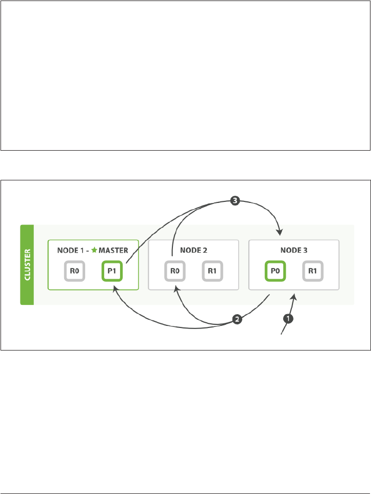
Query Phase
During the initial query phase, the query is broadcast to a shard copy (a primary or
replica shard) of every shard in the index. Each shard executes the search locally and
builds a priority queue of matching documents.
Priority Queue
A priority queue is just a sorted list that holds the top-n matching documents. The size
of the priority queue depends on the pagination parameters from and size. For
example, the following search request would require a priority queue big enough to
hold 100 documents:
GET /_search
{
"from": 90,
"size": 10
}
The query phase process is depicted in Figure 9-1.
Figure 9-1. Query phase of distributed search
The query phase consists of the following three steps:
1. The client sends a search request to Node 3, which creates an empty priority
queue of size from + size.
2. Node 3 forwards the search request to a primary or replica copy of every shard in
the index. Each shard executes the query locally and adds the results into a local
sorted priority queue of size from + size.
122 | Chapter 9: Distributed Search Execution

3. Each shard returns the doc IDs and sort values of all the docs in its priority queue
to the coordinating node, Node 3, which merges these values into its own priority
queue to produce a globally sorted list of results.
When a search request is sent to a node, that node becomes the coordinating node. It
is the job of this node to broadcast the search request to all involved shards, and to
gather their responses into a globally sorted result set that it can return to the client.
The first step is to broadcast the request to a shard copy of every node in the index.
Just like document GET requests, search requests can be handled by a primary shard
or by any of its replicas. This is how more replicas (when combined with more hard‐
ware) can increase search throughput. A coordinating node will round-robin through
all shard copies on subsequent requests in order to spread the load.
Each shard executes the query locally and builds a sorted priority queue of length
from + size—in other words, enough results to satisfy the global search request all
by itself. It returns a lightweight list of results to the coordinating node, which con‐
tains just the doc IDs and any values required for sorting, such as the _score.
The coordinating node merges these shard-level results into its own sorted priority
queue, which represents the globally sorted result set. Here the query phase ends.
An index can consist of one or more primary shards, so a search
request against a single index needs to be able to combine the
results from multiple shards. A search against multiple or all indi‐
ces works in exactly the same way—there are just more shards
involved.
Fetch Phase
The query phase identifies which documents satisfy the search request, but we still
need to retrieve the documents themselves. This is the job of the fetch phase, shown
in Figure 9-2.
Fetch Phase | 123
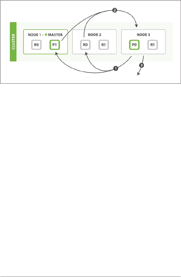
Figure 9-2. Fetch phase of distributed search
The distributed phase consists of the following steps:
1. The coordinating node identifies which documents need to be fetched and issues
a multi GET request to the relevant shards.
2. Each shard loads the documents and enriches them, if required, and then returns
the documents to the coordinating node.
3. Once all documents have been fetched, the coordinating node returns the results
to the client.
The coordinating node first decides which documents actually need to be fetched. For
instance, if our query specified { "from": 90, "size": 10 }, the first 90 results
would be discarded and only the next 10 results would need to be retrieved. These
documents may come from one, some, or all of the shards involved in the original
search request.
The coordinating node builds a multi-get request for each shard that holds a perti‐
nent document and sends the request to the same shard copy that handled the query
phase.
The shard loads the document bodies—the _source field—and, if requested, enriches
the results with metadata and search snippet highlighting. Once the coordinating
124 | Chapter 9: Distributed Search Execution

node receives all results, it assembles them into a single response that it returns to the
client.
Deep Pagination
The query-then-fetch process supports pagination with the from and size parame‐
ters, but within limits. Remember that each shard must build a priority queue of
length from + size, all of which need to be passed back to the coordinating node.
And the coordinating node needs to sort through number_of_shards * (from +
size) documents in order to find the correct size documents.
Depending on the size of your documents, the number of shards, and the hardware
you are using, paging 10,000 to 50,000 results (1,000 to 5,000 pages) deep should be
perfectly doable. But with big-enough from values, the sorting process can become
very heavy indeed, using vast amounts of CPU, memory, and bandwidth. For this rea‐
son, we strongly advise against deep paging.
In practice, “deep pagers” are seldom human anyway. A human will stop paging after
two or three pages and will change the search criteria. The culprits are usually bots or
web spiders that tirelessly keep fetching page after page until your servers crumble at
the knees.
If you do need to fetch large numbers of docs from your cluster, you can do so effi‐
ciently by disabling sorting with the scan search type, which we discuss later in this
chapter.
Search Options
A few optional query-string parameters can influence the search process.
preference
The preference parameter allows you to control which shards or nodes are used to
handle the search request. It accepts values such as _primary, _primary_first,
_local, _only_node:xyz, _prefer_node:xyz, and _shards:2,3, which are explained
in detail on the search preference documentation page.
However, the most generally useful value is some arbitrary string, to avoid the bounc
ing results problem.
Bouncing Results
Imagine that you are sorting your results by a timestamp field, and two documents
have the same timestamp. Because search requests are round-robined between all
Search Options | 125

available shard copies, these two documents may be returned in one order when the
request is served by the primary, and in another order when served by the replica.
This is known as the bouncing results problem: every time the user refreshes the page,
the results appear in a different order. The problem can be avoided by always using
the same shards for the same user, which can be done by setting the preference
parameter to an arbitrary string like the user’s session ID.
timeout
By default, the coordinating node waits to receive a response from all shards. If one
node is having trouble, it could slow down the response to all search requests.
The timeout parameter tells the coordinating node how long it should wait before
giving up and just returning the results that it already has. It can be better to return
some results than none at all.
The response to a search request will indicate whether the search timed out and how
many shards responded successfully:
...
"timed_out": true,
"_shards": {
"total": 5,
"successful": 4,
"failed": 1
},
...
The search request timed out.
One shard out of five failed to respond in time.
If all copies of a shard fail for other reasons—perhaps because of a hardware failure—
this will also be reflected in the _shards section of the response.
routing
In “Routing a Document to a Shard” on page 61, we explained how a custom routing
parameter could be provided at index time to ensure that all related documents, such
as the documents belonging to a single user, are stored on a single shard. At search
time, instead of searching on all the shards of an index, you can specify one or more
routing values to limit the search to just those shards:
GET /_search?routing=user_1,user2
This technique comes in handy when designing very large search systems, and we
discuss it in detail in Chapter 43.
126 | Chapter 9: Distributed Search Execution

search_type
While query_then_fetch is the default search type, other search types can be speci‐
fied for particular purposes, for example:
GET /_search?search_type=count
count
The count search type has only a query phase. It can be used when you don’t
need search results, just a document count or aggregations on documents match‐
ing the query.
query_and_fetch
The query_and_fetch search type combines the query and fetch phases into a
single step. This is an internal optimization that is used when a search request
targets a single shard only, such as when a routing value has been specified.
While you can choose to use this search type manually, it is almost never useful
to do so.
dfs_query_then_fetch and dfs_query_and_fetch
The dfs search types have a prequery phase that fetches the term frequencies
from all involved shards in order to calculate global term frequencies. We discuss
this further in “Relevance Is Broken!” on page 214.
scan
The scan search type is used in conjunction with the scroll API to retrieve large
numbers of results efficiently. It does this by disabling sorting. We discuss scan-
and-scroll in the next section.
scan and scroll
The scan search type and the scroll API are used together to retrieve large numbers
of documents from Elasticsearch efficiently, without paying the penalty of deep pagi‐
nation.
scroll
A scrolled search allows us to do an initial search and to keep pulling batches of
results from Elasticsearch until there are no more results left. It’s a bit like a cur
sor in a traditional database.
A scrolled search takes a snapshot in time. It doesn’t see any changes that are
made to the index after the initial search request has been made. It does this by
keeping the old data files around, so that it can preserve its “view” on what the
index looked like at the time it started.
scan and scroll | 127

scan
The costly part of deep pagination is the global sorting of results, but if we disable
sorting, then we can return all documents quite cheaply. To do this, we use the
scan search type. Scan instructs Elasticsearch to do no sorting, but to just return
the next batch of results from every shard that still has results to return.
To use scan-and-scroll, we execute a search request setting search_type to scan, and
passing a scroll parameter telling Elasticsearch how long it should keep the scroll
open:
GET /old_index/_search?search_type=scan&scroll=1m
{
"query": { "match_all": {}},
"size": 1000
}
Keep the scroll open for 1 minute.
The response to this request doesn’t include any hits, but does include a _scroll_id,
which is a long Base-64 encoded string. Now we can pass the _scroll_id to the
_search/scroll endpoint to retrieve the first batch of results:
GET /_search/scroll?scroll=1m
c2Nhbjs1OzExODpRNV9aY1VyUVM4U0NMd2pjWlJ3YWlBOzExOTpRNV9aY1VyUVM4U0
NMd2pjWlJ3YWlBOzExNjpRNV9aY1VyUVM4U0NMd2pjWlJ3YWlBOzExNzpRNV9aY1Vy
UVM4U0NMd2pjWlJ3YWlBOzEyMDpRNV9aY1VyUVM4U0NMd2pjWlJ3YWlBOzE7dG90YW
xfaGl0czoxOw==
Keep the scroll open for another minute.
The _scroll_id can be passed in the body, in the URL, or as a query parameter.
Note that we again specify ?scroll=1m. The scroll expiry time is refreshed every time
we run a scroll request, so it needs to give us only enough time to process the current
batch of results, not all of the documents that match the query.
The response to this scroll request includes the first batch of results. Although we
specified a size of 1,000, we get back many more documents. When scanning, the
size is applied to each shard, so you will get back a maximum of size * num
ber_of_primary_shards documents in each batch.
The scroll request also returns a new _scroll_id. Every time we
make the next scroll request, we must pass the _scroll_id
returned by the previous scroll request.
When no more hits are returned, we have processed all matching documents.
128 | Chapter 9: Distributed Search Execution


CHAPTER 10
Index Management
We have seen how Elasticsearch makes it easy to start developing a new application
without requiring any advance planning or setup. However, it doesn’t take long before
you start wanting to fine-tune the indexing and search process to better suit your par‐
ticular use case. Almost all of these customizations relate to the index, and the types
that it contains. In this chapter, we introduce the APIs for managing indices and type
mappings, and the most important settings.
Creating an Index
Until now, we have created a new index by simply indexing a document into it. The
index is created with the default settings, and new fields are added to the type map‐
ping by using dynamic mapping. Now we need more control over the process: we
want to ensure that the index has been created with the appropriate number of pri‐
mary shards, and that analyzers and mappings are set up before we index any data.
To do this, we have to create the index manually, passing in any settings or type map‐
pings in the request body, as follows:
PUT /my_index
{
"settings": { ... any settings ... },
"mappings": {
"type_one": { ... any mappings ... },
"type_two": { ... any mappings ... },
...
}
}
In fact, if you want to, you can prevent the automatic creation of indices by adding
the following setting to the config/elasticsearch.yml file on each node:
131

action.auto_create_index: false
Later, we discuss how you can use “Index Templates” on page 593
to preconfigure automatically created indices. This is particularly
useful when indexing log data: you log into an index whose name
includes the date and, as midnight rolls over, a new properly con‐
figured index automatically springs into existence.
Deleting an Index
To delete an index, use the following request:
DELETE /my_index
You can delete multiple indices with this:
DELETE /index_one,index_two
DELETE /index_*
You can even delete all indices with this:
DELETE /_all
Index Settings
There are many many knobs that you can twiddle to customize index behavior, which
you can read about in the Index Modules reference documentation, but…
Elasticsearch comes with good defaults. Don’t twiddle these knobs
until you understand what they do and why you should change
them.
Two of the most important settings are as follows:
number_of_shards
The number of primary shards that an index should have, which defaults to 5.
This setting cannot be changed after index creation.
number_of_replicas
The number of replica shards (copies) that each primary shard should have,
which defaults to 1. This setting can be changed at any time on a live index.
For instance, we could create a small index—just one primary shard—and no replica
shards with the following request:
PUT /my_temp_index
{
132 | Chapter 10: Index Management

"settings": {
"number_of_shards" : 1,
"number_of_replicas" : 0
}
}
Later, we can change the number of replica shards dynamically using the update-
index-settings API as follows:
PUT /my_temp_index/_settings
{
"number_of_replicas": 1
}
Conguring Analyzers
The third important index setting is the analysis section, which is used to configure
existing analyzers or to create new custom analyzers specific to your index.
In “Analysis and Analyzers” on page 84, we introduced some of the built-in analyzers,
which are used to convert full-text strings into an inverted index, suitable for search‐
ing.
The standard analyzer, which is the default analyzer used for full-text fields, is a good
choice for most Western languages. It consists of the following:
• The standard tokenizer, which splits the input text on word boundaries
• The standard token filter, which is intended to tidy up the tokens emitted by the
tokenizer (but currently does nothing)
• The lowercase token filter, which converts all tokens into lowercase
• The stop token filter, which removes stopwords—common words that have little
impact on search relevance, such as a, the, and, is.
By default, the stopwords filter is disabled. You can enable it by creating a custom
analyzer based on the standard analyzer and setting the stopwords parameter. Either
provide a list of stopwords or tell it to use a predefined stopwords list from a particu‐
lar language.
In the following example, we create a new analyzer called the es_std analyzer, which
uses the predefined list of Spanish stopwords:
PUT /spanish_docs
{
"settings": {
"analysis": {
"analyzer": {
"es_std": {
Conguring Analyzers | 133

"type": "standard",
"stopwords": "_spanish_"
}
}
}
}
}
The es_std analyzer is not global—it exists only in the spanish_docs index where we
have defined it. To test it with the analyze API, we must specify the index name:
GET /spanish_docs/_analyze?analyzer=es_std
El veloz zorro marrón
The abbreviated results show that the Spanish stopword El has been removed cor‐
rectly:
{
"tokens" : [
{ "token" : "veloz", "position" : 2 },
{ "token" : "zorro", "position" : 3 },
{ "token" : "marrón", "position" : 4 }
]
}
Custom Analyzers
While Elasticsearch comes with a number of analyzers available out of the box, the
real power comes from the ability to create your own custom analyzers by combining
character filters, tokenizers, and token filters in a configuration that suits your partic‐
ular data.
In “Analysis and Analyzers” on page 84, we said that an analyzer is a wrapper that
combines three functions into a single package, which are executed in sequence:
Character lters
Character filters are used to “tidy up” a string before it is tokenized. For instance,
if our text is in HTML format, it will contain HTML tags like <p> or <div> that
we don’t want to be indexed. We can use the html_strip character filter to
remove all HTML tags and to convert HTML entities like Á into the cor‐
responding Unicode character Á.
An analyzer may have zero or more character filters.
Tokenizers
An analyzer must have a single tokenizer. The tokenizer breaks up the string into
individual terms or tokens. The standard tokenizer, which is used in the stan
dard analyzer, breaks up a string into individual terms on word boundaries, and
134 | Chapter 10: Index Management

removes most punctuation, but other tokenizers exist that have different behav‐
ior.
For instance, the keyword tokenizer outputs exactly the same string as it received,
without any tokenization. The whitespace tokenizer splits text on whitespace
only. The pattern tokenizer can be used to split text on a matching regular
expression.
Token lters
After tokenization, the resulting token stream is passed through any specified
token filters, in the order in which they are specified.
Token filters may change, add, or remove tokens. We have already mentioned the
lowercase and stop token filters, but there are many more available in Elastic‐
search. Stemming token filters “stem” words to their root form. The ascii_fold
ing filter removes diacritics, converting a term like "très" into "tres". The
ngram and edge_ngram token filters can produce tokens suitable for partial
matching or autocomplete.
In Part II, we discuss examples of where and how to use these tokenizers and filters.
But first, we need to explain how to create a custom analyzer.
Creating a Custom Analyzer
In the same way as we configured the es_std analyzer previously, we can configure
character filters, tokenizers, and token filters in their respective sections under analy
sis:
PUT /my_index
{
"settings": {
"analysis": {
"char_filter": { ... custom character filters ... },
"tokenizer": { ... custom tokenizers ... },
"filter": { ... custom token filters ... },
"analyzer": { ... custom analyzers ... }
}
}
}
As an example, let’s set up a custom analyzer that will do the following:
1. Strip out HTML by using the html_strip character filter.
2. Replace & characters with " and ", using a custom mapping character filter:
"char_filter": {
"&_to_and": {
"type": "mapping",
Custom Analyzers | 135

"mappings": [ "&=> and "]
}
}
3. Tokenize words, using the standard tokenizer.
4. Lowercase terms, using the lowercase token filter.
5. Remove a custom list of stopwords, using a custom stop token filter:
"filter": {
"my_stopwords": {
"type": "stop",
"stopwords": [ "the", "a" ]
}
}
Our analyzer definition combines the predefined tokenizer and filters with the cus‐
tom filters that we have configured previously:
"analyzer": {
"my_analyzer": {
"type": "custom",
"char_filter": [ "html_strip", "&_to_and" ],
"tokenizer": "standard",
"filter": [ "lowercase", "my_stopwords" ]
}
}
To put it all together, the whole create-index request looks like this:
PUT /my_index
{
"settings": {
"analysis": {
"char_filter": {
"&_to_and": {
"type": "mapping",
"mappings": [ "&=> and "]
}},
"filter": {
"my_stopwords": {
"type": "stop",
"stopwords": [ "the", "a" ]
}},
"analyzer": {
"my_analyzer": {
"type": "custom",
"char_filter": [ "html_strip", "&_to_and" ],
"tokenizer": "standard",
"filter": [ "lowercase", "my_stopwords" ]
}}
}}}
136 | Chapter 10: Index Management

After creating the index, use the analyze API to test the new analyzer:
GET /my_index/_analyze?analyzer=my_analyzer
The quick & brown fox
The following abbreviated results show that our analyzer is working correctly:
{
"tokens" : [
{ "token" : "quick", "position" : 2 },
{ "token" : "and", "position" : 3 },
{ "token" : "brown", "position" : 4 },
{ "token" : "fox", "position" : 5 }
]
}
The analyzer is not much use unless we tell Elasticsearch where to use it. We can
apply it to a string field with a mapping such as the following:
PUT /my_index/_mapping/my_type
{
"properties": {
"title": {
"type": "string",
"analyzer": "my_analyzer"
}
}
}
Types and Mappings
A type in Elasticsearch represents a class of similar documents. A type consists of a
name—such as user or blogpost—and a mapping. The mapping, like a database
schema, describes the fields or properties that documents of that type may have, the
datatype of each field—such as string, integer, or date—and how those fields
should be indexed and stored by Lucene.
In “What Is a Document?” on page 36, we said that a type is like a table in a relational
database. While this is a useful way to think about types initially, it is worth explain‐
ing in more detail exactly what a type is and how they are implemented on top of
Lucene.
How Lucene Sees Documents
A document in Lucene consists of a simple list of field-value pairs. A field must have
at least one value, but any field can contain multiple values. Similarly, a single string
value may be converted into multiple values by the analysis process. Lucene doesn’t
care if the values are strings or numbers or dates—all values are just treated as opaque
bytes.
Types and Mappings | 137

When we index a document in Lucene, the values for each field are added to the
inverted index for the associated field. Optionally, the original values may also be
stored unchanged so that they can be retrieved later.
How Types Are Implemented
Elasticsearch types are implemented on top of this simple foundation. An index may
have several types, each with its own mapping, and documents of any of these types
may be stored in the same index.
Because Lucene has no concept of document types, the type name of each document
is stored with the document in a metadata field called _type. When we search for
documents of a particular type, Elasticsearch simply uses a filter on the _type field to
restrict results to documents of that type.
Lucene also has no concept of mappings. Mappings are the layer that Elasticsearch
uses to map complex JSON documents into the simple flat documents that Lucene
expects to receive.
For instance, the mapping for the name field in the user type may declare that the
field is a string field, and that its value should be analyzed by the whitespace ana‐
lyzer before being indexed into the inverted index called name:
"name": {
"type": "string",
"analyzer": "whitespace"
}
Avoiding Type Gotchas
The fact that documents of different types can be added to the same index introduces
some unexpected complications.
Imagine that we have two types in our index: blog_en for blog posts in English, and
blog_es for blog posts in Spanish. Both types have a title field, but one type uses
the english analyzer and the other type uses the spanish analyzer.
The problem is illustrated by the following query:
GET /_search
{
"query": {
"match": {
"title": "The quick brown fox"
}
}
}
138 | Chapter 10: Index Management

We are searching in the title field in both types. The query string needs to be ana‐
lyzed, but which analyzer does it use: spanish or english? It will use the analyzer for
the first title field that it finds, which will be correct for some docs and incorrect for
the others.
We can avoid this problem either by naming the fields differently—for example,
title_en and title_es—or by explicitly including the type name in the field name
and querying each field separately:
GET /_search
{
"query": {
"multi_match": {
"query": "The quick brown fox",
"fields": [ "blog_en.title", "blog_es.title" ]
}
}
}
The multi_match query runs a match query on multiple fields and combines the
results.
Our new query uses the english analyzer for the field blog_en.title and the span
ish analyzer for the field blog_es.title, and combines the results from both fields
into an overall relevance score.
This solution can help when both fields have the same datatype, but consider what
would happen if you indexed these two documents into the same index:
• Type: user
{ "login": "john_smith" }
Types and Mappings | 139

• Type: event
{ "login": "2014-06-01" }
Lucene doesn’t care that one field contains a string and the other field contains a date.
It will happily index the byte values from both fields.
However, if we now try to sort on the event.login field, Elasticsearch needs to load
the values in the login field into memory. As we said in “Fielddata” on page 119, it
loads the values for all documents in the index regardless of their type.
It will try to load these values either as a string or as a date, depending on which
login field it sees first. This will either produce unexpected results or fail outright.
To ensure that you don’t run into these conflicts, it is advisable to
ensure that fields with the same name are mapped in the same way
in every type in an index.
The Root Object
The uppermost level of a mapping is known as the root object. It may contain the fol‐
lowing:
•A properties section, which lists the mapping for each field that a document may
contain
•Various metadata fields, all of which start with an underscore, such as _type, _id,
and _source
•Settings, which control how the dynamic detection of new fields is handled, such
as analyzer, dynamic_date_formats, and dynamic_templates
•Other settings, which can be applied both to the root object and to fields of type
object, such as enabled, dynamic, and include_in_all
Properties
We have already discussed the three most important settings for document fields or
properties in “Core Simple Field Types” on page 88 and “Complex Core Field Types”
on page 93:
type
The datatype that the field contains, such as string or date
140 | Chapter 10: Index Management

index
Whether a field should be searchable as full text (analyzed), searchable as an
exact value (not_analyzed), or not searchable at all (no)
analyzer
Which analyzer to use for a full-text field, both at index time and at search time
We will discuss other field types such as ip, geo_point, and geo_shape in the appro‐
priate sections later in the book.
Metadata: _source Field
By default, Elasticsearch stores the JSON string representing the document body in
the _source field. Like all stored fields, the _source field is compressed before being
written to disk.
This is almost always desired functionality because it means the following:
•The full document is available directly from the search results—no need for a
separate round-trip to fetch the document from another data store.
• Partial update requests will not function without the _source field.
•When your mapping changes and you need to reindex your data, you can do so
directly from Elasticsearch instead of having to retrieve all of your documents
from another (usually slower) data store.
•Individual fields can be extracted from the _source field and returned in get or
search requests when you don’t need to see the whole document.
•It is easier to debug queries, because you can see exactly what each document
contains, rather than having to guess their contents from a list of IDs.
That said, storing the _source field does use disk space. If none of the preceding rea‐
sons is important to you, you can disable the _source field with the following map‐
ping:
PUT /my_index
{
"mappings": {
"my_type": {
"_source": {
"enabled": false
}
}
}
}
In a search request, you can ask for only certain fields by specifying the _source
parameter in the request body:
The Root Object | 141

GET /_search
{
"query": { "match_all": {}},
"_source": [ "title", "created" ]
}
Values for these fields will be extracted from the _source field and returned instead
of the full _source.
Stored Fields
Besides indexing the values of a field, you can also choose to store the original field
value for later retrieval. Users with a Lucene background use stored fields to choose
which fields they would like to be able to return in their search results. In fact, the
_source field is a stored field.
In Elasticsearch, setting individual document fields to be stored is usually a false opti‐
mization. The whole document is already stored as the _source field. It is almost
always better to just extract the fields that you need by using the _source parameter.
Metadata: _all Field
In “Search Lite” on page 76, we introduced the _all field: a special field that indexes
the values from all other fields as one big string. The query_string query clause (and
searches performed as ?q=john) defaults to searching in the _all field if no other
field is specified.
The _all field is useful during the exploratory phase of a new application, while you
are still unsure about the final structure that your documents will have. You can
throw any query string at it and you have a good chance of finding the document
you’re after:
GET /_search
{
"match": {
"_all": "john smith marketing"
}
}
As your application evolves and your search requirements become more exacting,
you will find yourself using the _all field less and less. The _all field is a shotgun
approach to search. By querying individual fields, you have more flexbility, power,
and fine-grained control over which results are considered to be most relevant.
142 | Chapter 10: Index Management

One of the important factors taken into account by the relevance
algorithm is the length of the field: the shorter the field, the more
important. A term that appears in a short title field is likely to be
more important than the same term that appears somewhere in a
long content field. This distinction between field lengths disap‐
pears in the _all field.
If you decide that you no longer need the _all field, you can disable it with this map‐
ping:
PUT /my_index/_mapping/my_type
{
"my_type": {
"_all": { "enabled": false }
}
}
Inclusion in the _all field can be controlled on a field-by-field basis by using the
include_in_all setting, which defaults to true. Setting include_in_all on an object
(or on the root object) changes the default for all fields within that object.
You may find that you want to keep the _all field around to use as a catchall full-text
field just for specific fields, such as title, overview, summary, and tags. Instead of
disabling the _all field completely, disable include_in_all for all fields by default,
and enable it only on the fields you choose:
PUT /my_index/my_type/_mapping
{
"my_type": {
"include_in_all": false,
"properties": {
"title": {
"type": "string",
"include_in_all": true
},
...
}
}
}
Remember that the _all field is just an analyzed string field. It uses the default ana‐
lyzer to analyze its values, regardless of which analyzer has been set on the fields
where the values originate. And like any string field, you can configure which ana‐
lyzer the _all field should use:
PUT /my_index/my_type/_mapping
{
"my_type": {
"_all": { "analyzer": "whitespace" }
The Root Object | 143

}
}
Metadata: Document Identity
There are four metadata fields associated with document identity:
_id
The string ID of the document
_type
The type name of the document
_index
The index where the document lives
_uid
The _type and _id concatenated together as type#id
By default, the _uid field is stored (can be retrieved) and indexed (searchable). The
_type field is indexed but not stored, and the _id and _index fields are neither
indexed nor stored, meaning they don’t really exist.
In spite of this, you can query the _id field as though it were a real field. Elasticsearch
uses the _uid field to derive the _id. Although you can change the index and store
settings for these fields, you almost never need to do so.
The _id field does have one setting that you may want to use: the path setting tells
Elasticsearch that it should extract the value for the _id from a field within the docu‐
ment itself.
PUT /my_index
{
"mappings": {
"my_type": {
"_id": {
"path": "doc_id"
},
"properties": {
"doc_id": {
"type": "string",
"index": "not_analyzed"
}
}
}
}
}
Extract the doc _id from the doc_id field.
144 | Chapter 10: Index Management

Then, when you index a document:
POST /my_index/my_type
{
"doc_id": "123"
}
the _id value will be extracted from the doc_id field in the document body:
{
"_index": "my_index",
"_type": "my_type",
"_id": "123",
"_version": 1,
"created": true
}
The _id has been extracted correctly.
While this is very convenient, be aware that it has a slight perfor‐
mance impact on bulk requests (see “Why the Funny Format?”
on page 69). The node handling the request can no longer use
the optimized bulk format to parse just the metadata line in
order to decide which shard should receive the request. Instead, it has to parse
the document body as well.
Dynamic Mapping
When Elasticsearch encounters a previously unknown field in a document, it uses
dynamic mapping to determine the datatype for the field and automatically adds the
new field to the type mapping.
Sometimes this is the desired behavior and sometimes it isn’t. Perhaps you don’t know
what fields will be added to your documents later, but you want them to be indexed
automatically. Perhaps you just want to ignore them. Or—especially if you are using
Elasticsearch as a primary data store—perhaps you want unknown fields to throw an
exception to alert you to the problem.
Fortunately, you can control this behavior with the dynamic setting, which accepts the
following options:
true
Add new fields dynamically—the default
false
Ignore new fields
Dynamic Mapping | 145

strict
Throw an exception if an unknown field is encountered
The dynamic setting may be applied to the root object or to any field of type object.
You could set dynamic to strict by default, but enable it just for a specific inner
object:
PUT /my_index
{
"mappings": {
"my_type": {
"dynamic": "strict",
"properties": {
"title": { "type": "string"},
"stash": {
"type": "object",
"dynamic": true
}
}
}
}
}
The my_type object will throw an exception if an unknown field is encountered.
The stash object will create new fields dynamically.
With this mapping, you can add new searchable fields into the stash object:
PUT /my_index/my_type/1
{
"title": "This doc adds a new field",
"stash": { "new_field": "Success!" }
}
But trying to do the same at the top level will fail:
PUT /my_index/my_type/1
{
"title": "This throws a StrictDynamicMappingException",
"new_field": "Fail!"
}
Setting dynamic to false doesn’t alter the contents of the _source
field at all. The _source will still contain the whole JSON docu‐
ment that you indexed. However, any unknown fields will not be
added to the mapping and will not be searchable.
146 | Chapter 10: Index Management

Customizing Dynamic Mapping
If you know that you are going to be adding new fields on the fly, you probably want
to leave dynamic mapping enabled. At times, though, the dynamic mapping “rules”
can be a bit blunt. Fortunately, there are settings that you can use to customize these
rules to better suit your data.
date_detection
When Elasticsearch encounters a new string field, it checks to see if the string con‐
tains a recognizable date, like 2014-01-01. If it looks like a date, the field is added as
type date. Otherwise, it is added as type string.
Sometimes this behavior can lead to problems. Imagine that you index a document
like this:
{ "note": "2014-01-01" }
Assuming that this is the first time that the note field has been seen, it will be added
as a date field. But what if the next document looks like this:
{ "note": "Logged out" }
This clearly isn’t a date, but it is too late. The field is already a date field and so this
“malformed date” will cause an exception to be thrown.
Date detection can be turned off by setting date_detection to false on the root
object:
PUT /my_index
{
"mappings": {
"my_type": {
"date_detection": false
}
}
}
With this mapping in place, a string will always be a string. If you need a date field,
you have to add it manually.
Elasticsearch’s idea of which strings look like dates can be altered
with the dynamic_date_formats setting.
Customizing Dynamic Mapping | 147

dynamic_templates
With dynamic_templates, you can take complete control over the mapping that is
generated for newly detected fields. You can even apply a different mapping depend‐
ing on the field name or datatype.
Each template has a name, which you can use to describe what the template does, a
mapping to specify the mapping that should be applied, and at least one parameter
(such as match) to define which fields the template should apply to.
Templates are checked in order; the first template that matches is applied. For
instance, we could specify two templates for string fields:
•es: Field names ending in _es should use the spanish analyzer.
•en: All others should use the english analyzer.
We put the es template first, because it is more specific than the catchall en template,
which matches all string fields:
PUT /my_index
{
"mappings": {
"my_type": {
"dynamic_templates": [
{ "es": {
"match": "*_es",
"match_mapping_type": "string",
"mapping": {
"type": "string",
"analyzer": "spanish"
}
}},
{ "en": {
"match": "*",
"match_mapping_type": "string",
"mapping": {
"type": "string",
"analyzer": "english"
}
}}
]
}}}
Match string fields whose name ends in _es.
Match all other string fields.
148 | Chapter 10: Index Management

The match_mapping_type allows you to apply the template only to fields of the speci‐
fied type, as detected by the standard dynamic mapping rules, (for example string or
long).
The match parameter matches just the field name, and the path_match parameter
matches the full path to a field in an object, so the pattern address.*.name would
match a field like this:
{
"address": {
"city": {
"name": "New York"
}
}
}
The unmatch and path_unmatch patterns can be used to exclude fields that would
otherwise match.
More configuration options can be found in the reference documentation for the root
object.
Default Mapping
Often, all types in an index share similar fields and settings. It can be more conve‐
nient to specify these common settings in the _default_ mapping, instead of having
to repeat yourself every time you create a new type. The _default_ mapping acts as a
template for new types. All types created aer the _default_ mapping will include all
of these default settings, unless explicitly overridden in the type mapping itself.
For instance, we can disable the _all field for all types, using the _default_ map‐
ping, but enable it just for the blog type, as follows:
PUT /my_index
{
"mappings": {
"_default_": {
"_all": { "enabled": false }
},
"blog": {
"_all": { "enabled": true }
}
}
}
The _default_ mapping can also be a good place to specify index-wide dynamic
templates.
Default Mapping | 149

Reindexing Your Data
Although you can add new types to an index, or add new fields to a type, you can’t
add new analyzers or make changes to existing fields. If you were to do so, the data
that had already been indexed would be incorrect and your searches would no longer
work as expected.
The simplest way to apply these changes to your existing data is to reindex: create a
new index with the new settings and copy all of your documents from the old index
to the new index.
One of the advantages of the _source field is that you already have the whole docu‐
ment available to you in Elasticsearch itself. You don’t have to rebuild your index
from the database, which is usually much slower.
To reindex all of the documents from the old index efficiently, use scan-and-scroll to
retrieve batches of documents from the old index, and the bulk API to push them
into the new index.
Reindexing in Batches
You can run multiple reindexing jobs at the same time, but you obviously don’t want
their results to overlap. Instead, break a big reindex down into smaller jobs by filter‐
ing on a date or timestamp field:
GET /old_index/_search?search_type=scan&scroll=1m
{
"query": {
"range": {
"date": {
"gte": "2014-01-01",
"lt": "2014-02-01"
}
}
},
"size": 1000
}
If you continue making changes to the old index, you will want to make sure that you
include the newly added documents in your new index as well. This can be done by
rerunning the reindex process, but again filtering on a date field to match only docu‐
ments that have been added since the last reindex process started.
150 | Chapter 10: Index Management

Index Aliases and Zero Downtime
The problem with the reindexing process described previously is that you need to
update your application to use the new index name. Index aliases to the rescue!
An index alias is like a shortcut or symbolic link, which can point to one or more
indices, and can be used in any API that expects an index name. Aliases give us an
enormous amount of flexibility. They allow us to do the following:
• Switch transparently between one index and another on a running cluster
• Group multiple indices (for example, last_three_months)
• Create “views” on a subset of the documents in an index
We will talk more about the other uses for aliases later in the book. For now we will
explain how to use them to switch from an old index to a new index with zero down‐
time.
There are two endpoints for managing aliases: _alias for single operations, and
_aliases to perform multiple operations atomically.
In this scenario, we will assume that your application is talking to an index called
my_index. In reality, my_index will be an alias that points to the current real index.
We will include a version number in the name of the real index: my_index_v1,
my_index_v2, and so forth.
To start off, create the index my_index_v1, and set up the alias my_index to point to it:
PUT /my_index_v1
PUT /my_index_v1/_alias/my_index
Create the index my_index_v1.
Set the my_index alias to point to my_index_v1.
You can check which index the alias points to:
GET /*/_alias/my_index
Or which aliases point to the index:
GET /my_index_v1/_alias/*
Both of these return the following:
{
"my_index_v1" : {
"aliases" : {
"my_index" : { }
}
Index Aliases and Zero Downtime | 151

}
}
Later, we decide that we want to change the mappings for a field in our index. Of
course, we can’t change the existing mapping, so we have to reindex our data. To start,
we create my_index_v2 with the new mappings:
PUT /my_index_v2
{
"mappings": {
"my_type": {
"properties": {
"tags": {
"type": "string",
"index": "not_analyzed"
}
}
}
}
}
Then we reindex our data from my_index_v1 to my_index_v2, following the process
described in “Reindexing Your Data” on page 150. Once we are satisfied that our
documents have been reindexed correctly, we switch our alias to point to the new
index.
An alias can point to multiple indices, so we need to remove the alias from the old
index at the same time as we add it to the new index. The change needs to be atomic,
which means that we must use the _aliases endpoint:
POST /_aliases
{
"actions": [
{ "remove": { "index": "my_index_v1", "alias": "my_index" }},
{ "add": { "index": "my_index_v2", "alias": "my_index" }}
]
}
Your application has switched from using the old index to the new index transpar‐
ently, with zero downtime.
Even when you think that your current index design is perfect, it is
likely that you will need to make some change later, when your
index is already being used in production.
Be prepared: use aliases instead of indices in your application.
Then you will be able to reindex whenever you need to. Aliases are
cheap and should be used liberally.
152 | Chapter 10: Index Management

CHAPTER 11
Inside a Shard
In Chapter 2, we introduced the shard, and described it as a low-level worker unit. But
what exactly is a shard and how does it work? In this chapter, we answer these ques‐
tions:
• Why is search near real-time?
• Why are document CRUD (create-read-update-delete) operations real-time?
•How does Elasticsearch ensure that the changes you make are durable, that they
won’t be lost if there is a power failure?
• Why does deleting documents not free up space immediately?
•What do the refresh, flush, and optimize APIs do, and when should you use
them?
The easiest way to understand how a shard functions today is to start with a history
lesson. We will look at the problems that needed to be solved in order to provide a
distributed durable data store with near real-time search and analytics.
Content Warning
The information presented in this chapter is for your interest. You are not required to
understand and remember all the detail in order to use Elasticsearch. Read this chap‐
ter to gain a taste for how things work, and to know where the information is in case
you need to refer to it in the future, but don’t be overwhelmed by the detail.
153

Making Text Searchable
The first challenge that had to be solved was how to make text searchable. Traditional
databases store a single value per field, but this is insufficient for full-text search.
Every word in a text field needs to be searchable, which means that the database
needs to be able to index multiple values—words, in this case—in a single field.
The data structure that best supports the multiple-values-per-eld requirement is the
inverted index, which we introduced in “Inverted Index” on page 81. The inverted
index contains a sorted list of all of the unique values, or terms, that occur in any
document and, for each term, a list of all the documents that contain it.
Term | Doc 1 | Doc 2 | Doc 3 | ...
------------------------------------
brown | X | | X | ...
fox | X | X | X | ...
quick | X | X | | ...
the | X | | X | ...
When discussing inverted indices, we talk about indexing docu
ments because, historically, an inverted index was used to index
whole unstructured text documents. A document in Elasticsearch is
a structured JSON document with fields and values. In reality,
every indexed field in a JSON document has its own inverted
index.
The inverted index may hold a lot more information than the list of documents that
contain a particular term. It may store a count of the number of documents that con‐
tain each term, the number of times a term appears in a particular document, the
order of terms in each document, the length of each document, the average length of
all documents, and more. These statistics allow Elasticsearch to determine which
terms are more important than others, and which documents are more important
than others, as described in “What Is Relevance?” on page 115.
The important thing to realize is that the inverted index needs to know about all
documents in the collection in order for it to function as intended.
In the early days of full-text search, one big inverted index was built for the entire
document collection and written to disk. As soon as the new index was ready, it
replaced the old index, and recent changes became searchable.
154 | Chapter 11: Inside a Shard

Immutability
The inverted index that is written to disk is immutable: it doesn’t change. Ever. This
immutability has important benefits:
•There is no need for locking. If you never have to update the index, you never
have to worry about multiple processes trying to make changes at the same time.
•Once the index has been read into the kernel’s filesystem cache, it stays there,
because it never changes. As long as there is enough space in the filesystem
cache, most reads will come from memory instead of having to hit disk. This
provides a big performance boost.
•Any other caches (like the filter cache) remain valid for the life of the index. They
don’t need to be rebuilt every time the data changes, because the data doesn’t
change.
•Writing a single large inverted index allows the data to be compressed, reducing
costly disk I/O and the amount of RAM needed to cache the index.
Of course, an immutable index has its downsides too, primarily the fact that it is
immutable! You can’t change it. If you want to make new documents searchable, you
have to rebuild the entire index. This places a significant limitation either on the
amount of data that an index can contain, or the frequency with which the index can
be updated.
Dynamically Updatable Indices
The next problem that needed to be solved was how to make an inverted index
updatable without losing the benefits of immutability? The answer turned out to be:
use more than one index.
Instead of rewriting the whole inverted index, add new supplementary indices to
reflect more-recent changes. Each inverted index can be queried in turn—starting
with the oldest—and the results combined.
Lucene, the Java libraries on which Elasticsearch is based, introduced the concept of
per-segment search. A segment is an inverted index in its own right, but now the word
index in Lucene came to mean a collection of segments plus a commit point—a file that
lists all known segments, as depicted in Figure 11-1. New documents are first added
to an in-memory indexing buffer, as shown in Figure 11-2, before being written to an
on-disk segment, as in Figure 11-3
Dynamically Updatable Indices | 155
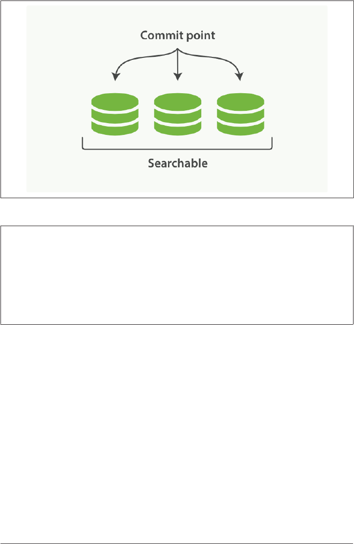
Figure 11-1. A Lucene index with a commit point and three segments
Index Versus Shard
To add to the confusion, a Lucene index is what we call a shard in Elasticsearch, while
an index in Elasticsearch is a collection of shards. When Elasticsearch searches an
index, it sends the query out to a copy of every shard (Lucene index) that belongs to
the index, and then reduces the per-shards results to a global result set, as described
in Chapter 9.
A per-segment search works as follows:
1. New documents are collected in an in-memory indexing buffer. See Figure 11-2.
2. Every so often, the buffer is commited:
• A new segment—a supplementary inverted index—is written to disk.
• A new commit point is written to disk, which includes the name of the new seg‐
ment.
•The disk is fsync’ed—all writes waiting in the filesystem cache are flushed to
disk, to ensure that they have been physically written.
3. The new segment is opened, making the documents it contains visible to search.
4. The in-memory buffer is cleared, and is ready to accept new documents.
156 | Chapter 11: Inside a Shard
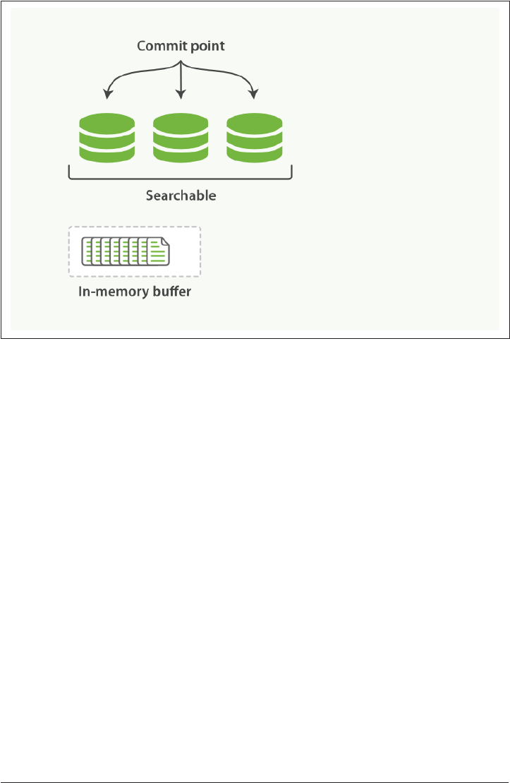
Figure 11-2. A Lucene index with new documents in the in-memory buer, ready to
commit
Dynamically Updatable Indices | 157
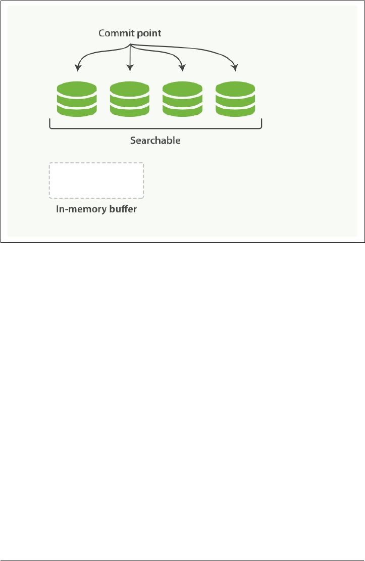
Figure 11-3. Aer a commit, a new segment is added to the commit point and the buer
is cleared
When a query is issued, all known segments are queried in turn. Term statistics are
aggregated across all segments to ensure that the relevance of each term and each
document is calculated accurately. In this way, new documents can be added to the
index relatively cheaply.
Deletes and Updates
Segments are immutable, so documents cannot be removed from older segments, nor
can older segments be updated to reflect a newer version of a document. Instead,
every commit point includes a .del file that lists which documents in which seg‐
ments have been deleted.
When a document is “deleted,” it is actually just marked as deleted in the .del file. A
document that has been marked as deleted can still match a query, but it is removed
from the results list before the final query results are returned.
Document updates work in a similar way: when a document is updated, the old ver‐
sion of the document is marked as deleted, and the new version of the document is
indexed in a new segment. Perhaps both versions of the document will match a query,
but the older deleted version is removed before the query results are returned.
158 | Chapter 11: Inside a Shard
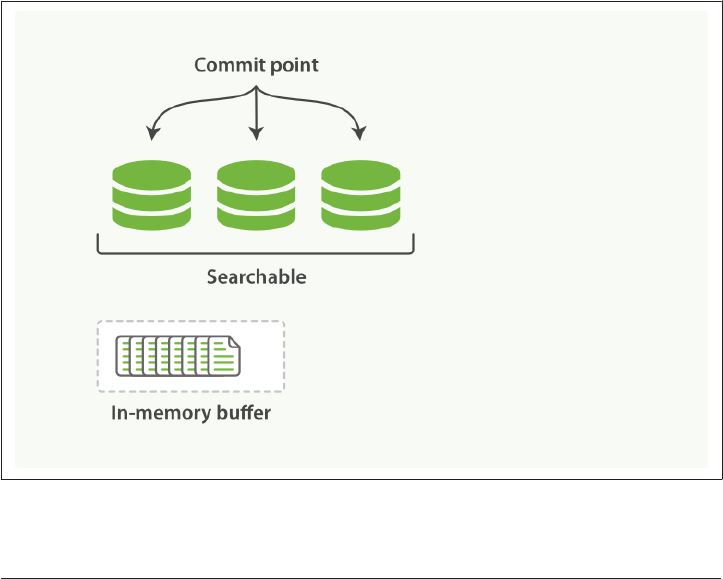
In “Segment Merging” on page 166, we show how deleted documents are purged
from the filesystem.
Near Real-Time Search
With the development of per-segment search, the delay between indexing a docu‐
ment and making it visible to search dropped dramatically. New documents could be
made searchable within minutes, but that still isn’t fast enough.
The bottleneck is the disk. Commiting a new segment to disk requires an fsync to
ensure that the segment is physically written to disk and that data will not be lost if
there is a power failure. But an fsync is costly; it cannot be performed every time a
document is indexed without a big performance hit.
What was needed was a more lightweight way to make new documents visible to
search, which meant removing fsync from the equation.
Sitting between Elasticsearch and the disk is the filesystem cache. As before, docu‐
ments in the in-memory indexing buffer (Figure 11-4) are written to a new segment
(Figure 11-5). But the new segment is written to the filesystem cache first—which is
cheap—and only later is it flushed to disk—which is expensive. But once a file is in
the cache, it can be opened and read, just like any other file.
Figure 11-4. A Lucene index with new documents in the in-memory buer
Near Real-Time Search | 159
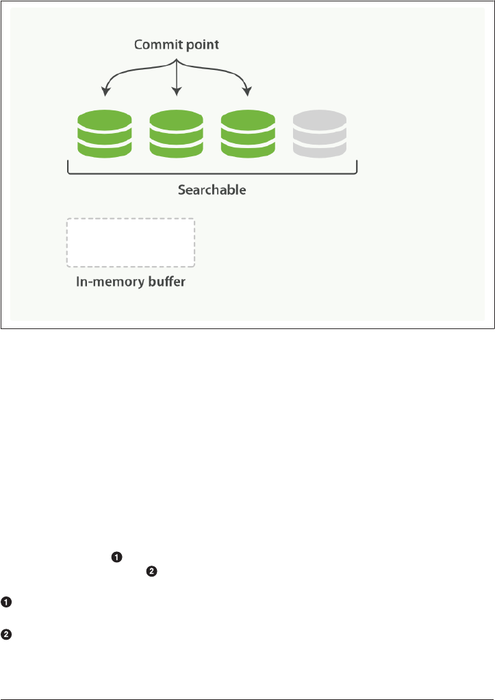
Lucene allows new segments to be written and opened—making the documents they
contain visible to search—without performing a full commit. This is a much lighter
process than a commit, and can be done frequently without ruining performance.
Figure 11-5. e buer contents have been written to a segment, which is searchable, but
is not yet commited
refresh API
In Elasticsearch, this lightweight process of writing and opening a new segment is
called a refresh. By default, every shard is refreshed automatically once every second.
This is why we say that Elasticsearch has near real-time search: document changes are
not visible to search immediately, but will become visible within 1 second.
This can be confusing for new users: they index a document and try to search for it,
and it just isn’t there. The way around this is to perform a manual refresh, with the
refresh API:
POST /_refresh
POST /blogs/_refresh
Refresh all indices.
Refresh just the blogs index.
160 | Chapter 11: Inside a Shard

While a refresh is much lighter than a commit, it still has a perfor‐
mance cost. A manual refresh can be useful when writing tests, but
don’t do a manual refresh every time you index a document in pro‐
duction; it will hurt your performance. Instead, your application
needs to be aware of the near real-time nature of Elasticsearch and
make allowances for it.
Not all use cases require a refresh every second. Perhaps you are using Elasticsearch
to index millions of log files, and you would prefer to optimize for index speed rather
than near real-time search. You can reduce the frequency of refreshes on a per-index
basis by setting the refresh_interval:
PUT /my_logs
{
"settings": {
"refresh_interval": "30s"
}
}
Refresh the my_logs index every 30 seconds.
The refresh_interval can be updated dynamically on an existing index. You can
turn off automatic refreshes while you are building a big new index, and then turn
them back on when you start using the index in production:
POST /my_logs/_settings
{ "refresh_interval": -1 }
POST /my_logs/_settings
{ "refresh_interval": "1s" }
Disable automatic refreshes.
Refresh automatically every second.
The refresh_interval expects a duration such as 1s (1 second)
or 2m (2 minutes). An absolute number like 1 means 1
millisecond--a sure way to bring your cluster to its knees.
Making Changes Persistent
Without an fsync to flush data in the filesystem cache to disk, we cannot be sure that
the data will still be there after a power failure, or even after exiting the application
normally. For Elasticsearch to be reliable, it needs to ensure that changes are persisted
to disk.
Making Changes Persistent | 161

In “Dynamically Updatable Indices” on page 155, we said that a full commit flushes
segments to disk and writes a commit point, which lists all known segments. Elastic‐
search uses this commit point during startup or when reopening an index to decide
which segments belong to the current shard.
While we refresh once every second to achieve near real-time search, we still need to
do full commits regularly to make sure that we can recover from failure. But what
about the document changes that happen between commits? We don’t want to lose
those either.
Elasticsearch added a translog, or transaction log, which records every operation in
Elasticsearch as it happens. With the translog, the process now looks like this:
1. When a document is indexed, it is added to the in-memory buffer and appended
to the translog, as shown in Figure 11-6.
Figure 11-6. New documents are added to the in-memory buer and appended to
the transaction log
2. The refresh leaves the shard in the state depicted in Figure 11-7. Once every sec‐
ond, the shard is refreshed:
•The docs in the in-memory buffer are written to a new segment, without an
fsync.
• The segment is opened to make it visible to search.
162 | Chapter 11: Inside a Shard
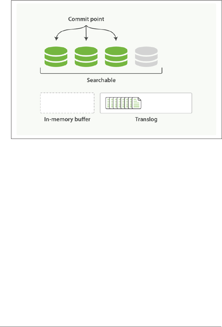
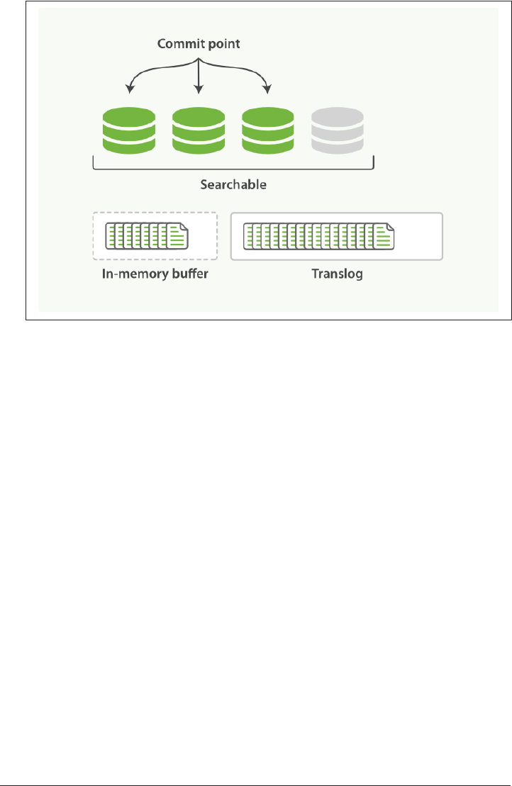
Figure 11-8. e transaction log keeps accumulating documents
4. Every so often—such as when the translog is getting too big—the index is
flushed; a new translog is created, and a full commit is performed (see
Figure 11-9):
• Any docs in the in-memory buffer are written to a new segment.
• The buffer is cleared.
• A commit point is written to disk.
• The filesystem cache is flushed with an fsync.
• The old translog is deleted.
The translog provides a persistent record of all operations that have not yet been
flushed to disk. When starting up, Elasticsearch will use the last commit point to
recover known segments from disk, and will then replay all operations in the translog
to add the changes that happened after the last commit.
The translog is also used to provide real-time CRUD. When you try to retrieve,
update, or delete a document by ID, it first checks the translog for any recent changes
before trying to retrieve the document from the relevant segment. This means that it
always has access to the latest known version of the document, in real-time.
164 | Chapter 11: Inside a Shard
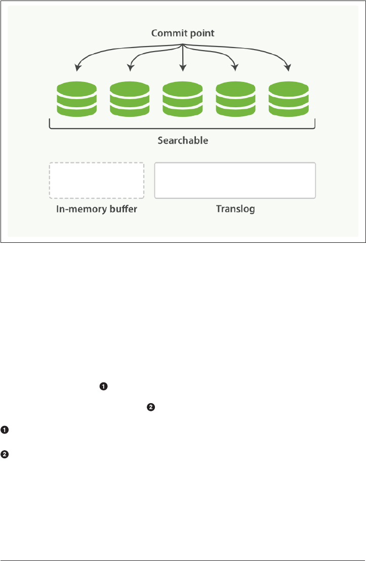
Figure 11-9. Aer a ush, the segments are fully commited and the transaction log is
cleared
ush API
The action of performing a commit and truncating the translog is known in Elastic‐
search as a ush. Shards are flushed automatically every 30 minutes, or when the
translog becomes too big. See the translog documentation for settings that can be
used to control these thresholds:
The flush API can be used to perform a manual flush:
POST /blogs/_flush
POST /_flush?wait_for_ongoing
Flush the blogs index.
Flush all indices and wait until all flushes have completed before returning.
You seldom need to issue a manual flush yourself; usually, automatic flushing is all
that is required.
Making Changes Persistent | 165

That said, it is beneficial to flush your indices before restarting a node or closing an
index. When Elasticsearch tries to recover or reopen an index, it has to replay all of
the operations in the translog, so the shorter the log, the faster the recovery.
How Safe Is the Translog?
The purpose of the translog is to ensure that operations are not lost. This begs the
question: how safe is the translog?
Writes to a file will not survive a reboot until the file has been fsync‘ed to disk. By
default, the translog is fsync‘ed every 5 seconds. Potentially, we could lose 5 seconds
worth of data—if the translog were the only mechanism that we had for dealing with
failure.
Fortunately, the translog is only part of a much bigger system. Remember that an
indexing request is considered successful only after it has completed on both the pri‐
mary shard and all replica shards. Even if the node holding the primary shard were to
suffer catastrophic failure, it would be unlikely to affect the nodes holding the replica
shards at the same time.
While we could force the translog to fsync more frequently (at the cost of indexing
performance), it is unlikely to provide more reliability.
Segment Merging
With the automatic refresh process creating a new segment every second, it doesn’t
take long for the number of segments to explode. Having too many segments is a
problem. Each segment consumes file handles, memory, and CPU cycles. More
important, every search request has to check every segment in turn; the more seg‐
ments there are, the slower the search will be.
Elasticsearch solves this problem by merging segments in the background. Small seg‐
ments are merged into bigger segments, which, in turn, are merged into even bigger
segments.
This is the moment when those old deleted documents are purged from the filesys‐
tem. Deleted documents (or old versions of updated documents) are not copied over
to the new bigger segment.
There is nothing you need to do to enable merging. It happens automatically while
you are indexing and searching. The process works like as depicted in Figure 11-10:
1. While indexing, the refresh process creates new segments and opens them for
search.
166 | Chapter 11: Inside a Shard
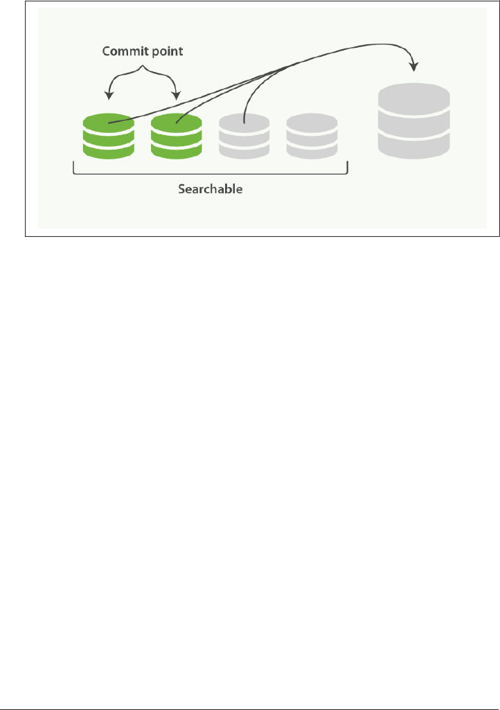
2. The merge process selects a few segments of similar size and merges them into a
new bigger segment in the background. This does not interrupt indexing and
searching.
Figure 11-10. Two commited segments and one uncommited segment in the process
of being merged into a bigger segment
3. Figure 11-11 illustrates activity as the merge completes:
• The new segment is flushed to disk.
•A new commit point is written that includes the new segment and excludes the
old, smaller segments.
• The new segment is opened for search.
• The old segments are deleted.
Segment Merging | 167
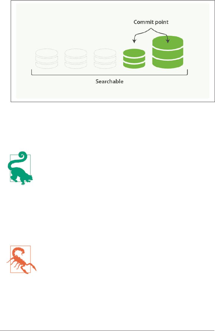
Figure 11-11. Once merging has nished, the old segments are deleted
The merging of big segments can use a lot of I/O and CPU, which can hurt search
performance if left unchecked. By default, Elasticsearch throttles the merge process so
that search still has enough resources available to perform well.
See “Segments and Merging” on page 651 for advice about tuning
merging for your use case.
optimize API
The optimize API is best described as the forced merge API. It forces a shard to be
merged down to the number of segments specified in the max_num_segments parame‐
ter. The intention is to reduce the number of segments (usually to one) in order to
speed up search performance.
The optimize API should not be used on a dynamic index—an
index that is being actively updated. The background merge pro‐
cess does a very good job, and optimizing will hinder the pro‐
cess. Don’t interfere!
In certain specific circumstances, the optimize API can be beneficial. The typical use
case is for logging, where logs are stored in an index per day, week, or month. Older
indices are essentially read-only; they are unlikely to change.
168 | Chapter 11: Inside a Shard

In this case, it can be useful to optimize the shards of an old index down to a single
segment each; it will use fewer resources and searches will be quicker:
POST /logstash-2014-10/_optimize?max_num_segments=1
Merges each shard in the index down to a single segment
Be aware that merges triggered by the optimize API are not throt‐
tled at all. They can consume all of the I/O on your nodes, leaving
nothing for search and potentially making your cluster unrespon‐
sive. If you plan on optimizing an index, you should use shard allo‐
cation (see “Migrate Old Indices” on page 595) to first move the
index to a node where it is safe to run.
Segment Merging | 169

PART II
Search in Depth
In Part I we covered the basic tools in just enough detail to allow you to start search‐
ing your data with Elasticsearch. It won’t take long, though, before you find that you
want more: more flexibility when matching user queries, more-accurate ranking of
results, more-specific searches to cover different problem domains.
To move to the next level, it is not enough to just use the match query. You need to
understand your data and how you want to be able to search it. The chapters in this
part explain how to index and query your data to allow you to take advantage of word
proximity, partial matching, fuzzy matching, and language awareness.
Understanding how each query contributes to the relevance _score will help you to
tune your queries: to ensure that the documents you consider to be the best results
appear on the first page, and to trim the “long tail” of barely relevant results.
Search is not just about full-text search: a large portion of your data will be structured
values like dates and numbers. We will start by explaining how to combine structured
search with full-text search in the most efficient way.

CHAPTER 12
Structured Search
Structured search is about interrogating data that has inherent structure. Dates, times,
and numbers are all structured: they have a precise format that you can perform logi‐
cal operations on. Common operations include comparing ranges of numbers or
dates, or determining which of two values is larger.
Text can be structured too. A box of crayons has a discrete set of colors: red, green,
blue. A blog post may be tagged with keywords distributed and search. Products
in an ecommerce store have Universal Product Codes (UPCs) or some other identi‐
fier that requires strict and structured formatting.
With structured search, the answer to your question is always a yes or no; something
either belongs in the set or it does not. Structured search does not worry about docu‐
ment relevance or scoring; it simply includes or excludes documents.
This should make sense logically. A number can’t be more in a range than any other
number that falls in the same range. It is either in the range—or it isn’t. Similarly, for
structured text, a value is either equal or it isn’t. There is no concept of more similar.
Finding Exact Values
When working with exact values, you will be working with filters. Filters are impor‐
tant because they are very, very fast. Filters do not calculate relevance (avoiding the
entire scoring phase) and are easily cached. We’ll talk about the performance benefits
of filters later in “All About Caching” on page 192, but for now, just keep in mind that
you should use filters as often as you can.
173

term Filter with Numbers
We are going to explore the term filter first because you will use it often. This filter is
capable of handling numbers, Booleans, dates, and text.
Let’s look at an example using numbers first by indexing some products. These docu‐
ments have a price and a productID:
POST /my_store/products/_bulk
{ "index": { "_id": 1 }}
{ "price" : 10, "productID" : "XHDK-A-1293-#fJ3" }
{ "index": { "_id": 2 }}
{ "price" : 20, "productID" : "KDKE-B-9947-#kL5" }
{ "index": { "_id": 3 }}
{ "price" : 30, "productID" : "JODL-X-1937-#pV7" }
{ "index": { "_id": 4 }}
{ "price" : 30, "productID" : "QQPX-R-3956-#aD8" }
Our goal is to find all products with a certain price. You may be familiar with SQL if
you are coming from a relational database background. If we expressed this query as
an SQL query, it would look like this:
SELECT document
FROM products
WHERE price = 20
In the Elasticsearch query DSL, we use a term filter to accomplish the same thing.
The term filter will look for the exact value that we specify. By itself, a term filter is
simple. It accepts a field name and the value that we wish to find:
{
"term" : {
"price" : 20
}
}
The term filter isn’t very useful on its own, though. As discussed in “Query DSL” on
page 98, the search API expects a query, not a filter. To use our term filter, we need
to wrap it with a filtered query:
GET /my_store/products/_search
{
"query" : {
"filtered" : {
"query" : {
"match_all" : {}
},
"filter" : {
"term" : {
"price" : 20
}
}
174 | Chapter 12: Structured Search

}
}
}
The filtered query accepts both a query and a filter.
A match_all is used to return all matching documents. This is the default behav‐
ior, so in future examples we will simply omit the query section.
The term filter that we saw previously. Notice how it is placed inside the filter
clause.
Once executed, the search results from this query are exactly what you would expect:
only document 2 is returned as a hit (because only 2 had a price of 20):
"hits" : [
{
"_index" : "my_store",
"_type" : "products",
"_id" : "2",
"_score" : 1.0,
"_source" : {
"price" : 20,
"productID" : "KDKE-B-9947-#kL5"
}
}
]
Filters do not perform scoring or relevance. The score comes from the match_all
query, which treats all docs as equal, so all results receive a neutral score of 1.
term Filter with Text
As mentioned at the top of this section, the term filter can match strings just as easily
as numbers. Instead of price, let’s try to find products that have a certain UPC identi‐
fication code. To do this with SQL, we might use a query like this:
SELECT product
FROM products
WHERE productID = "XHDK-A-1293-#fJ3"
Translated into the query DSL, we can try a similar query with the term filter, like so:
GET /my_store/products/_search
{
"query" : {
"filtered" : {
"filter" : {
"term" : {
"productID" : "XHDK-A-1293-#fJ3"
Finding Exact Values | 175

}
}
}
}
}
Except there is a little hiccup: we don’t get any results back! Why is that? The problem
isn’t with the the term query; it is with the way the data has been indexed. If we use
the analyze API (“Testing Analyzers” on page 86), we can see that our UPC has been
tokenized into smaller tokens:
GET /my_store/_analyze?field=productID
XHDK-A-1293-#fJ3
{
"tokens" : [ {
"token" : "xhdk",
"start_offset" : 0,
"end_offset" : 4,
"type" : "<ALPHANUM>",
"position" : 1
}, {
"token" : "a",
"start_offset" : 5,
"end_offset" : 6,
"type" : "<ALPHANUM>",
"position" : 2
}, {
"token" : "1293",
"start_offset" : 7,
"end_offset" : 11,
"type" : "<NUM>",
"position" : 3
}, {
"token" : "fj3",
"start_offset" : 13,
"end_offset" : 16,
"type" : "<ALPHANUM>",
"position" : 4
} ]
}
There are a few important points here:
• We have four distinct tokens instead of a single token representing the UPC.
• All letters have been lowercased.
• We lost the hyphen and the hash (#) sign.
176 | Chapter 12: Structured Search

So when our term filter looks for the exact value XHDK-A-1293-#fJ3, it doesn’t find
anything, because that token does not exist in our inverted index. Instead, there are
the four tokens listed previously.
Obviously, this is not what we want to happen when dealing with identification codes,
or any kind of precise enumeration.
To prevent this from happening, we need to tell Elasticsearch that this field contains
an exact value by setting it to be not_analyzed. We saw this originally in “Customiz‐
ing Field Mappings” on page 89. To do this, we need to first delete our old index
(because it has the incorrect mapping) and create a new one with the correct map‐
pings:
DELETE /my_store
PUT /my_store
{
"mappings" : {
"products" : {
"properties" : {
"productID" : {
"type" : "string",
"index" : "not_analyzed"
}
}
}
}
}
Deleting the index first is required, since we cannot change mappings that
already exist.
With the index deleted, we can re-create it with our custom mapping.
Here we explicitly say that we don’t want productID to be analyzed.
Now we can go ahead and reindex our documents:
POST /my_store/products/_bulk
{ "index": { "_id": 1 }}
{ "price" : 10, "productID" : "XHDK-A-1293-#fJ3" }
{ "index": { "_id": 2 }}
{ "price" : 20, "productID" : "KDKE-B-9947-#kL5" }
{ "index": { "_id": 3 }}
{ "price" : 30, "productID" : "JODL-X-1937-#pV7" }
{ "index": { "_id": 4 }}
{ "price" : 30, "productID" : "QQPX-R-3956-#aD8" }
Finding Exact Values | 177

Only now will our term filter work as expected. Let’s try it again on the newly indexed
data (notice, the query and filter have not changed at all, just how the data is map‐
ped):
GET /my_store/products/_search
{
"query" : {
"filtered" : {
"filter" : {
"term" : {
"productID" : "XHDK-A-1293-#fJ3"
}
}
}
}
}
Since the productID field is not analyzed, and the term filter performs no analysis,
the query finds the exact match and returns document 1 as a hit. Success!
Internal Filter Operation
Internally, Elasticsearch is performing several operations when executing a filter:
1. Find matching docs.
The term filter looks up the term XHDK-A-1293-#fJ3 in the inverted index and
retrieves the list of documents that contain that term. In this case, only document
1 has the term we are looking for.
2. Build a bitset.
The filter then builds a bitset--an array of 1s and 0s—that describes which docu‐
ments contain the term. Matching documents receive a 1 bit. In our example, the
bitset would be [1,0,0,0].
3. Cache the bitset.
Last, the bitset is stored in memory, since we can use this in the future and skip
steps 1 and 2. This adds a lot of performance and makes filters very fast.
When executing a filtered query, the filter is executed before the query. The
resulting bitset is given to the query, which uses it to simply skip over any documents
that have already been excluded by the filter. This is one of the ways that filters can
improve performance. Fewer documents evaluated by the query means faster
response times.
178 | Chapter 12: Structured Search

Combining Filters
The previous two examples showed a single filter in use. In practice, you will proba‐
bly need to filter on multiple values or fields. For example, how would you express
this SQL in Elasticsearch?
SELECT product
FROM products
WHERE (price = 20 OR productID = "XHDK-A-1293-#fJ3")
AND (price != 30)
In these situations, you will need the bool filter. This is a compound lter that accepts
other filters as arguments, combining them in various Boolean combinations.
Bool Filter
The bool filter is composed of three sections:
{
"bool" : {
"must" : [],
"should" : [],
"must_not" : [],
}
}
must
All of these clauses must match. The equivalent of AND.
must_not
All of these clauses must not match. The equivalent of NOT.
should
At least one of these clauses must match. The equivalent of OR.
And that’s it! When you need multiple filters, simply place them into the different
sections of the bool filter.
Each section of the bool filter is optional (for example, you can
have a must clause and nothing else), and each section can contain
a single filter or an array of filters.
To replicate the preceding SQL example, we will take the two term filters that we used
previously and place them inside the should clause of a bool filter, and add another
clause to deal with the NOT condition:
Combining Filters | 179

GET /my_store/products/_search
{
"query" : {
"filtered" : {
"filter" : {
"bool" : {
"should" : [
{ "term" : {"price" : 20}},
{ "term" : {"productID" : "XHDK-A-1293-#fJ3"}}
],
"must_not" : {
"term" : {"price" : 30}
}
}
}
}
}
}
Note that we still need to use a filtered query to wrap everything.
These two term filters are children of the bool filter, and since they are placed
inside the should clause, at least one of them needs to match.
If a product has a price of 30, it is automatically excluded because it matches a
must_not clause.
Our search results return two hits, each document satisfying a different clause in the
bool filter:
"hits" : [
{
"_id" : "1",
"_score" : 1.0,
"_source" : {
"price" : 10,
"productID" : "XHDK-A-1293-#fJ3"
}
},
{
"_id" : "2",
"_score" : 1.0,
"_source" : {
"price" : 20,
"productID" : "KDKE-B-9947-#kL5"
}
}
]
Matches the term filter for productID = "XHDK-A-1293-#fJ3"
180 | Chapter 12: Structured Search
Matches the term filter for price = 20
Nesting Boolean Filters
Even though bool is a compound filter and accepts children filters, it is important to
understand that bool is just a filter itself. This means you can nest bool filters inside
other bool filters, giving you the ability to make arbitrarily complex Boolean logic.
Given this SQL statement:
SELECT document
FROM products
WHERE productID = "KDKE-B-9947-#kL5"
OR ( productID = "JODL-X-1937-#pV7"
AND price = 30 )
We can translate it into a pair of nested bool filters:
GET /my_store/products/_search
{
"query" : {
"filtered" : {
"filter" : {
"bool" : {
"should" : [
{ "term" : {"productID" : "KDKE-B-9947-#kL5"}},
{ "bool" : {
"must" : [
{ "term" : {"productID" : "JODL-X-1937-#pV7"}},
{ "term" : {"price" : 30}}
]
}}
]
}
}
}
}
}
Because the term and the bool are sibling clauses inside the first Boolean should,
at least one of these filters must match for a document to be a hit.
These two term clauses are siblings in a must clause, so they both have to match
for a document to be returned as a hit.
The results show us two documents, one matching each of the should clauses:
"hits" : [
{
"_id" : "2",
"_score" : 1.0,
Combining Filters | 181

"_source" : {
"price" : 20,
"productID" : "KDKE-B-9947-#kL5"
}
},
{
"_id" : "3",
"_score" : 1.0,
"_source" : {
"price" : 30,
"productID" : "JODL-X-1937-#pV7"
}
}
]
This productID matches the term in the first bool.
These two fields match the term filters in the nested bool.
This was a simple example, but it demonstrates how Boolean filters can be used as
building blocks to construct complex logical conditions.
Finding Multiple Exact Values
The term filter is useful for finding a single value, but often you’ll want to search for
multiple values. What if you want to find documents that have a price of $20 or $30?
Rather than using multiple term filters, you can instead use a single terms filter (note
the s at the end). The terms filter is simply the plural version of the singular term
filter.
It looks nearly identical to a vanilla term too. Instead of specifying a single price, we
are now specifying an array of values:
{
"terms" : {
"price" : [20, 30]
}
}
And like the term filter, we will place it inside a filtered query to use it:
GET /my_store/products/_search
{
"query" : {
"filtered" : {
"filter" : {
"terms" : {
"price" : [20, 30]
}
}
182 | Chapter 12: Structured Search

}
}
}
The terms filter as seen previously, but placed inside the filtered query
The query will return the second, third, and fourth documents:
"hits" : [
{
"_id" : "2",
"_score" : 1.0,
"_source" : {
"price" : 20,
"productID" : "KDKE-B-9947-#kL5"
}
},
{
"_id" : "3",
"_score" : 1.0,
"_source" : {
"price" : 30,
"productID" : "JODL-X-1937-#pV7"
}
},
{
"_id": "4",
"_score": 1.0,
"_source": {
"price": 30,
"productID": "QQPX-R-3956-#aD8"
}
}
]
Contains, but Does Not Equal
It is important to understand that term and terms are contains operations, not equals.
What does that mean?
If you have a term filter for { "term" : { "tags" : "search" } }, it will match
both of the following documents:
{ "tags" : ["search"] }
{ "tags" : ["search", "open_source"] }
This document is returned, even though it has terms other than search.
Recall how the term filter works: it checks the inverted index for all documents that
contain a term, and then constructs a bitset. In our simple example, we have the fol‐
lowing inverted index:
Finding Multiple Exact Values | 183

Token DocIDs
open_source 2
search 1,2
When a term filter is executed for the token search, it goes straight to the corre‐
sponding entry in the inverted index and extracts the associated doc IDs. As you can
see, both document 1 and document 2 contain the token in the inverted index. There‐
fore, they are both returned as a result.
The nature of an inverted index also means that entire field equal‐
ity is rather difficult to calculate. How would you determine
whether a particular document contains only your request term?
You would have to find the term in the inverted index, extract the
document IDs, and then scan every row in the inverted index, look‐
ing for those IDs to see whether a doc has any other terms.
As you might imagine, that would be tremendously inefficient and
expensive. For that reason, term and terms are must contain opera‐
tions, not must equal exactly.
Equals Exactly
If you do want that behavior—entire field equality—the best way to accomplish it
involves indexing a secondary field. In this field, you index the number of values that
your field contains. Using our two previous documents, we now include a field that
maintains the number of tags:
{ "tags" : ["search"], "tag_count" : 1 }
{ "tags" : ["search", "open_source"], "tag_count" : 2 }
Once you have the count information indexed, you can construct a bool filter that
enforces the appropriate number of terms:
GET /my_index/my_type/_search
{
"query": {
"filtered" : {
"filter" : {
"bool" : {
"must" : [
{ "term" : { "tags" : "search" } },
{ "term" : { "tag_count" : 1 } }
]
}
}
}
184 | Chapter 12: Structured Search

}
}
Find all documents that have the term search.
But make sure the document has only one tag.
This query will now match only the document that has a single tag that is search,
rather than any document that contains search.
Ranges
When dealing with numbers in this chapter, we have so far searched for only exact
numbers. In practice, filtering on ranges is often more useful. For example, you might
want to find all products with a price greater than $20 and less than $40.
In SQL terms, a range can be expressed as follows:
SELECT document
FROM products
WHERE price BETWEEN 20 AND 40
Elasticsearch has a range filter, which, unsurprisingly, allows you to filter ranges:
"range" : {
"price" : {
"gt" : 20,
"lt" : 40
}
}
The range filter supports both inclusive and exclusive ranges, through combinations
of the following options:
•gt: > greater than
•lt: < less than
•gte: >= greater than or equal to
•lte: <= less than or equal to
GET /my_store/products/_search
{
"query" : {
"filtered" : {
"filter" : {
"range" : {
"price" : {
"gte" : 20,
"lt" : 40
}
Ranges | 185

}
}
}
}
}
If you need an unbounded range (for example, just >20), omit one of the boundaries:
"range" : {
"price" : {
"gt" : 20
}
}
Ranges on Dates
The range filter can be used on date fields too:
"range" : {
"timestamp" : {
"gt" : "2014-01-01 00:00:00",
"lt" : "2014-01-07 00:00:00"
}
}
When used on date fields, the range filter supports date math operations. For exam‐
ple, if we want to find all documents that have a timestamp sometime in the last hour:
"range" : {
"timestamp" : {
"gt" : "now-1h"
}
}
This filter will now constantly find all documents with a timestamp greater than the
current time minus 1 hour, making the filter a sliding window across your documents.
Date math can also be applied to actual dates, rather than a placeholder like now. Just
add a double pipe (||) after the date and follow it with a date math expression:
"range" : {
"timestamp" : {
"gt" : "2014-01-01 00:00:00",
"lt" : "2014-01-01 00:00:00||+1M"
}
}
Less than January 1, 2014 plus one month
Date math is calendar aware, so it knows the number of days in each month, days in a
year, and so forth. More details about working with dates can be found in the date
format reference documentation.
186 | Chapter 12: Structured Search

Ranges on Strings
The range filter can also operate on string fields. String ranges are calculated lexico
graphically or alphabetically. For example, these values are sorted in lexicographic
order:
• 5, 50, 6, B, C, a, ab, abb, abc, b
Terms in the inverted index are sorted in lexicographical order,
which is why string ranges use this order.
If we want a range from a up to but not including b, we can use the same range filter
syntax:
"range" : {
"title" : {
"gte" : "a",
"lt" : "b"
}
}
Be Careful of Cardinality
Numeric and date fields are indexed in such a way that ranges are efficient to calcu‐
late. This is not the case for string fields, however. To perform a range on a string
field, Elasticsearch is effectively performing a term filter for every term that falls in
the range. This is much slower than a date or numeric range.
String ranges are fine on a field with low cardinality—a small number of unique
terms. But the more unique terms you have, the slower the string range will be.
Dealing with Null Values
Think back to our earlier example, where documents have a field named tags. This is
a multivalue field. A document may have one tag, many tags, or potentially no tags at
all. If a field has no values, how is it stored in an inverted index?
That’s a trick question, because the answer is, it isn’t stored at all. Let’s look at that
inverted index from the previous section:
Token DocIDs
Dealing with Null Values | 187
open_source 2
search 1,2
How would you store a field that doesn’t exist in that data structure? You can’t! An
inverted index is simply a list of tokens and the documents that contain them. If a
field doesn’t exist, it doesn’t hold any tokens, which means it won’t be represented in
an inverted index data structure.
Ultimately, this means that a null, [] (an empty array), and [null] are all equivalent.
They simply don’t exist in the inverted index!
Obviously, the world is not simple, and data is often missing fields, or contains
explicit nulls or empty arrays. To deal with these situations, Elasticsearch has a few
tools to work with null or missing values.
exists Filter
The first tool in your arsenal is the exists filter. This filter will return documents that
have any value in the specified field. Let’s use the tagging example and index some
example documents:
POST /my_index/posts/_bulk
{ "index": { "_id": "1" }}
{ "tags" : ["search"] }
{ "index": { "_id": "2" }}
{ "tags" : ["search", "open_source"] }
{ "index": { "_id": "3" }}
{ "other_field" : "some data" }
{ "index": { "_id": "4" }}
{ "tags" : null }
{ "index": { "_id": "5" }}
{ "tags" : ["search", null] }
The tags field has one value.
The tags field has two values.
The tags field is missing altogether.
The tags field is set to null.
The tags field has one value and a null.
The resulting inverted index for our tags field will look like this:
188 | Chapter 12: Structured Search

Token DocIDs
open_source 2
search 1,2,5
Our objective is to find all documents where a tag is set. We don’t care what the tag is,
so long as it exists within the document. In SQL parlance, we would use an IS NOT
NULL query:
SELECT tags
FROM posts
WHERE tags IS NOT NULL
In Elasticsearch, we use the exists filter:
GET /my_index/posts/_search
{
"query" : {
"filtered" : {
"filter" : {
"exists" : { "field" : "tags" }
}
}
}
}
Our query returns three documents:
"hits" : [
{
"_id" : "1",
"_score" : 1.0,
"_source" : { "tags" : ["search"] }
},
{
"_id" : "5",
"_score" : 1.0,
"_source" : { "tags" : ["search", null] }
},
{
"_id" : "2",
"_score" : 1.0,
"_source" : { "tags" : ["search", "open source"] }
}
]
Document 5 is returned even though it contains a null value. The field exists
because a real-value tag was indexed, so the null had no impact on the filter.
Dealing with Null Values | 189

The results are easy to understand. Any document that has terms in the tags field
was returned as a hit. The only two documents that were excluded were documents 3
and 4.
missing Filter
The missing filter is essentially the inverse of exists: it returns documents where
there is no value for a particular field, much like this SQL:
SELECT tags
FROM posts
WHERE tags IS NULL
Let’s swap the exists filter for a missing filter from our previous example:
GET /my_index/posts/_search
{
"query" : {
"filtered" : {
"filter": {
"missing" : { "field" : "tags" }
}
}
}
}
And, as you would expect, we get back the two docs that have no real values in the
tags field—documents 3 and 4:
"hits" : [
{
"_id" : "3",
"_score" : 1.0,
"_source" : { "other_field" : "some data" }
},
{
"_id" : "4",
"_score" : 1.0,
"_source" : { "tags" : null }
}
]
When null Means null
Sometimes you need to be able to distinguish between a field that doesn’t have a
value, and a field that has been explicitly set to null. With the default behavior that
we saw previously, this is impossible; the data is lost. Luckily, there is an option that
we can set that replaces explicit null values with a placeholder value of our choosing.
190 | Chapter 12: Structured Search

When specifying the mapping for a string, numeric, Boolean, or date field, you can
also set a null_value that will be used whenever an explicit null value is encoun‐
tered. A field without a value will still be excluded from the inverted index.
When choosing a suitable null_value, ensure the following:
•It matches the field’s type. You can’t use a string null_value in a field of type
date.
•It is different from the normal values that the field may contain, to avoid confus‐
ing real values with null values.
exists/missing on Objects
The exists and missing filters also work on inner objects, not just core types. With
the following document
{
"name" : {
"first" : "John",
"last" : "Smith"
}
}
you can check for the existence of name.first and name.last but also just name.
However, in “Types and Mappings” on page 137, we said that an object like the pre‐
ceding one is flattened internally into a simple field-value structure, much like this:
{
"name.first" : "John",
"name.last" : "Smith"
}
So how can we use an exists or missing filter on the name field, which doesn’t really
exist in the inverted index?
The reason that it works is that a filter like
{
"exists" : { "field" : "name" }
}
is really executed as
{
"bool": {
"should": [
{ "exists": { "field": { "name.first" }}},
{ "exists": { "field": { "name.last" }}}
]
Dealing with Null Values | 191

}
}
That also means that if first and last were both empty, the name namespace would
not exist.
All About Caching
Earlier in this chapter (“Internal Filter Operation” on page 178), we briefly discussed
how filters are calculated. At their heart is a bitset representing which documents
match the filter. Elasticsearch aggressively caches these bitsets for later use. Once
cached, these bitsets can be reused wherever the same filter is used, without having to
reevaluate the entire filter again.
These cached bitsets are “smart”: they are updated incrementally. As you index new
documents, only those new documents need to be added to the existing bitsets, rather
than having to recompute the entire cached filter over and over. Filters are real-time
like the rest of the system; you don’t need to worry about cache expiry.
Independent Filter Caching
Each filter is calculated and cached independently, regardless of where it is used. If
two different queries use the same filter, the same filter bitset will be reused. Likewise,
if a single query uses the same filter in multiple places, only one bitset is calculated
and then reused.
Let’s look at this example query, which looks for emails that are either of the follow‐
ing:
• In the inbox and have not been read
•Not in the inbox but have been marked as important
"bool": {
"should": [
{ "bool": {
"must": [
{ "term": { "folder": "inbox" }},
{ "term": { "read": false }}
]
}},
{ "bool": {
"must_not": {
"term": { "folder": "inbox" }
},
"must": {
"term": { "important": true }
}
}}
192 | Chapter 12: Structured Search

]
}
These two filters are identical and will use the same bitset.
Even though one of the inbox clauses is a must clause and the other is a must_not
clause, the two clauses themselves are identical. This means that the bitset is calcula‐
ted once for the first clause that is executed, and then the cached bitset is used for the
other clause. By the time this query is run a second time, the inbox filter is already
cached and so both clauses will use the cached bitset.
This ties in nicely with the composability of the query DSL. It is easy to move filters
around, or reuse the same filter in multiple places within the same query. This isn’t
just convenient to the developer—it has direct performance benefits.
Controlling Caching
Most leaf lters—those dealing directly with fields like the term filter—are cached,
while compound filters, like the bool filter, are not.
Leaf filters have to consult the inverted index on disk, so it makes
sense to cache them. Compound filters, on the other hand, use fast
bit logic to combine the bitsets resulting from their inner clauses,
so it is efficient to recalculate them every time.
Certain leaf filters, however, are not cached by default, because it doesn’t make sense
to do so:
Script lters
The results from script filters cannot be cached because the meaning of the
script is opaque to Elasticsearch.
Geo-lters
The geolocation filters, which we cover in more detail in Part V, are usually used
to filter results based on the geolocation of a specific user. Since each user has a
unique geolocation, it is unlikely that geo-filters will be reused, so it makes no
sense to cache them.
Date ranges
Date ranges that use the now function (for example "now-1h"), result in values
accurate to the millisecond. Every time the filter is run, now returns a new time.
Older filters will never be reused, so caching is disabled by default. However,
when using now with rounding (for example, now/d rounds to the nearest day),
caching is enabled by default.
All About Caching | 193

Sometimes the default caching strategy is not correct. Perhaps you have a compli‐
cated bool expression that is reused several times in the same query. Or you have a
filter on a date field that will never be reused. The default caching strategy can be
overridden on almost any filter by setting the _cache flag:
{
"range" : {
"timestamp" : {
"gt" : "2014-01-02 16:15:14"
},
"_cache": false
}
}
It is unlikely that we will reuse this exact timestamp.
Disable caching of this filter.
Later chapters provide examples of when it can make sense to override the default
caching strategy.
Filter Order
The order of filters in a bool clause is important for performance. More-specific fil‐
ters should be placed before less-specific filters in order to exclude as many docu‐
ments as possible, as early as possible.
If Clause A could match 10 million documents, and Clause B could match only 100
documents, then Clause B should be placed before Clause A.
Cached filters are very fast, so they should be placed before filters that are not cachea‐
ble. Imagine that we have an index that contains one month’s worth of log events.
However, we’re mostly interested only in log events from the previous hour:
GET /logs/2014-01/_search
{
"query" : {
"filtered" : {
"filter" : {
"range" : {
"timestamp" : {
"gt" : "now-1h"
}
}
}
}
}
}
194 | Chapter 12: Structured Search

This filter is not cached because it uses the now function, the value of which changes
every millisecond. That means that we have to examine one month’s worth of log
events every time we run this query!
We could make this much more efficient by combining it with a cached filter: we can
exclude most of the month’s data by adding a filter that uses a fixed point in time,
such as midnight last night:
"bool": {
"must": [
{ "range" : {
"timestamp" : {
"gt" : "now-1h/d"
}
}},
{ "range" : {
"timestamp" : {
"gt" : "now-1h"
}
}}
]
}
This filter is cached because it uses now rounded to midnight.
This filter is not cached because it uses now without rounding.
The now-1h/d clause rounds to the previous midnight and so excludes all documents
created before today. The resulting bitset is cached because now is used with rounding,
which means that it is executed only once a day, when the value for midnight-last-
night changes. The now-1h clause isn’t cached because now produces a time accurate to
the nearest millisecond. However, thanks to the first filter, this second filter need only
check documents that have been created since midnight.
The order of these clauses is important. This approach works only because the since-
midnight clause comes before the last-hour clause. If they were the other way around,
then the last-hour clause would need to examine all documents in the index, instead
of just documents created since midnight.
Filter Order | 195

CHAPTER 13
Full-Text Search
Now that we have covered the simple case of searching for structured data, it is time
to explore full-text search: how to search within full-text fields in order to find the
most relevant documents.
The two most important aspects of full-text search are as follows:
Relevance
The ability to rank results by how relevant they are to the given query, whether
relevance is calculated using TF/IDF (see “What Is Relevance?” on page 115),
proximity to a geolocation, fuzzy similarity, or some other algorithm.
Analysis
The process of converting a block of text into distinct, normalized tokens (see
“Analysis and Analyzers” on page 84) in order to (a) create an inverted index and
(b) query the inverted index.
As soon as we talk about either relevance or analysis, we are in the territory of quer‐
ies, rather than filters.
Term-Based Versus Full-Text
While all queries perform some sort of relevance calculation, not all queries have an
analysis phase. Besides specialized queries like the bool or function_score queries,
which don’t operate on text at all, textual queries can be broken down into two fami‐
lies:
Term-based queries
Queries like the term or fuzzy queries are low-level queries that have no analysis
phase. They operate on a single term. A term query for the term Foo looks for
197

that exact term in the inverted index and calculates the TF/IDF relevance _score
for each document that contains the term.
It is important to remember that the term query looks in the inverted index for
the exact term only; it won’t match any variants like foo or FOO. It doesn’t matter
how the term came to be in the index, just that it is. If you were to index
["Foo","Bar"] into an exact value not_analyzed field, or Foo Bar into an ana‐
lyzed field with the whitespace analyzer, both would result in having the two
terms Foo and Bar in the inverted index.
Full-text queries
Queries like the match or query_string queries are high-level queries that
understand the mapping of a field:
•If you use them to query a date or integer field, they will treat the query
string as a date or integer, respectively.
•If you query an exact value (not_analyzed) string field, they will treat the
whole query string as a single term.
•But if you query a full-text (analyzed) field, they will first pass the query
string through the appropriate analyzer to produce the list of terms to be
queried.
Once the query has assembled a list of terms, it executes the appropriate low-
level query for each of these terms, and then combines their results to produce
the final relevance score for each document.
We will discuss this process in more detail in the following chapters.
You seldom need to use the term-based queries directly. Usually you want to query
full text, not individual terms, and this is easier to do with the high-level full-text
queries (which end up using term-based queries internally).
198 | Chapter 13: Full-Text Search

If you do find yourself wanting to use a query on an exact value
not_analyzed field, think about whether you really want a query or
a filter.
Single-term queries usually represent binary yes/no questions and
are almost always better expressed as a filter, so that they can bene‐
fit from filter caching:
GET /_search
{
"query": {
"filtered": {
"filter": {
"term": { "gender": "female" }
}
}
}
}
The match Query
The match query is the go-to query—the first query that you should reach for when‐
ever you need to query any field. It is a high-level full-text query, meaning that it
knows how to deal with both full-text fields and exact-value fields.
That said, the main use case for the match query is for full-text search. So let’s take a
look at how full-text search works with a simple example.
Index Some Data
First, we’ll create a new index and index some documents using the bulk API:
DELETE /my_index
PUT /my_index
{ "settings": { "number_of_shards": 1 }}
POST /my_index/my_type/_bulk
{ "index": { "_id": 1 }}
{ "title": "The quick brown fox" }
{ "index": { "_id": 2 }}
{ "title": "The quick brown fox jumps over the lazy dog" }
{ "index": { "_id": 3 }}
{ "title": "The quick brown fox jumps over the quick dog" }
{ "index": { "_id": 4 }}
{ "title": "Brown fox brown dog" }
Delete the index in case it already exists.
The match Query | 199

Later, in “Relevance Is Broken!” on page 214, we explain why we created this
index with only one primary shard.
A Single-Word Query
Our first example explains what happens when we use the match query to search
within a full-text field for a single word:
GET /my_index/my_type/_search
{
"query": {
"match": {
"title": "QUICK!"
}
}
}
Elasticsearch executes the preceding match query as follows:
1. Check the eld type.
The title field is a full-text (analyzed) string field, which means that the query
string should be analyzed too.
2. Analyze the query string.
The query string QUICK! is passed through the standard analyzer, which results in
the single term quick. Because we have a just a single term, the match query can
be executed as a single low-level term query.
3. Find matching docs.
The term query looks up quick in the inverted index and retrieves the list of
documents that contain that term—in this case, documents 1, 2, and 3.
4. Score each doc.
The term query calculates the relevance _score for each matching document, by
combining the term frequency (how often quick appears in the title field of
each document), with the inverse document frequency (how often quick appears
in the title field in all documents in the index), and the length of each field
(shorter fields are considered more relevant). See “What Is Relevance?” on page
115.
This process gives us the following (abbreviated) results:
"hits": [
{
"_id": "1",
"_score": 0.5,
"_source": {
200 | Chapter 13: Full-Text Search

"title": "The quick brown fox"
}
},
{
"_id": "3",
"_score": 0.44194174,
"_source": {
"title": "The quick brown fox jumps over the quick dog"
}
},
{
"_id": "2",
"_score": 0.3125,
"_source": {
"title": "The quick brown fox jumps over the lazy dog"
}
}
]
Document 1 is most relevant because its title field is short, which means that
quick represents a large portion of its content.
Document 3 is more relevant than document 2 because quick appears twice.
Multiword Queries
If we could search for only one word at a time, full-text search would be pretty inflex‐
ible. Fortunately, the match query makes multiword queries just as simple:
GET /my_index/my_type/_search
{
"query": {
"match": {
"title": "BROWN DOG!"
}
}
}
The preceding query returns all four documents in the results list:
{
"hits": [
{
"_id": "4",
"_score": 0.73185337,
"_source": {
"title": "Brown fox brown dog"
}
},
{
"_id": "2",
Multiword Queries | 201

"_score": 0.47486103,
"_source": {
"title": "The quick brown fox jumps over the lazy dog"
}
},
{
"_id": "3",
"_score": 0.47486103,
"_source": {
"title": "The quick brown fox jumps over the quick dog"
}
},
{
"_id": "1",
"_score": 0.11914785,
"_source": {
"title": "The quick brown fox"
}
}
]
}
Document 4 is the most relevant because it contains "brown" twice and "dog"
once.
Documents 2 and 3 both contain brown and dog once each, and the title field is
the same length in both docs, so they have the same score.
Document 1 matches even though it contains only brown, not dog.
Because the match query has to look for two terms—["brown","dog"]—internally it
has to execute two term queries and combine their individual results into the overall
result. To do this, it wraps the two term queries in a bool query, which we examine in
detail in “Combining Queries” on page 204.
The important thing to take away from this is that any document whose title field
contains at least one of the specied terms will match the query. The more terms that
match, the more relevant the document.
Improving Precision
Matching any document that contains any of the query terms may result in a long tail
of seemingly irrelevant results. It’s a shotgun approach to search. Perhaps we want to
show only documents that contain all of the query terms. In other words, instead of
brown OR dog, we want to return only documents that match brown AND dog.
The match query accepts an operator parameter that defaults to or. You can change
it to and to require that all specified terms must match:
202 | Chapter 13: Full-Text Search

GET /my_index/my_type/_search
{
"query": {
"match": {
"title": {
"query": "BROWN DOG!",
"operator": "and"
}
}
}
}
The structure of the match query has to change slightly in order to accommodate
the operator parameter.
This query would exclude document 1, which contains only one of the two terms.
Controlling Precision
The choice between all and any is a bit too black-or-white. What if the user specified
five query terms, and a document contains only four of them? Setting operator to
and would exclude this document.
Sometimes that is exactly what you want, but for most full-text search use cases, you
want to include documents that may be relevant but exclude those that are unlikely to
be relevant. In other words, we need something in-between.
The match query supports the minimum_should_match parameter, which allows you
to specify the number of terms that must match for a document to be considered rele‐
vant. While you can specify an absolute number of terms, it usually makes sense to
specify a percentage instead, as you have no control over the number of words the
user may enter:
GET /my_index/my_type/_search
{
"query": {
"match": {
"title": {
"query": "quick brown dog",
"minimum_should_match": "75%"
}
}
}
}
When specified as a percentage, minimum_should_match does the right thing: in the
preceding example with three terms, 75% would be rounded down to 66.6%, or two
out of the three terms. No matter what you set it to, at least one term must match for
a document to be considered a match.
Multiword Queries | 203

The minimum_should_match parameter is flexible, and different
rules can be applied depending on the number of terms the user
enters. For the full documentation see the minimum_should_match
reference documentation.
To fully understand how the match query handles multiword queries, we need to look
at how to combine multiple queries with the bool query.
Combining Queries
In “Combining Filters” on page 179 we discussed how to, use the bool filter to com‐
bine multiple filter clauses with and, or, and not logic. In query land, the bool query
does a similar job but with one important difference.
Filters make a binary decision: should this document be included in the results list or
not? Queries, however, are more subtle. They decide not only whether to include a
document, but also how relevant that document is.
Like the filter equivalent, the bool query accepts multiple query clauses under the
must, must_not, and should parameters. For instance:
GET /my_index/my_type/_search
{
"query": {
"bool": {
"must": { "match": { "title": "quick" }},
"must_not": { "match": { "title": "lazy" }},
"should": [
{ "match": { "title": "brown" }},
{ "match": { "title": "dog" }}
]
}
}
}
The results from the preceding query include any document whose title field con‐
tains the term quick, except for those that also contain lazy. So far, this is pretty sim‐
ilar to how the bool filter works.
The difference comes in with the two should clauses, which say that: a document is
not required to contain either brown or dog, but if it does, then it should be considered
more relevant:
{
"hits": [
{
"_id": "3",
"_score": 0.70134366,
204 | Chapter 13: Full-Text Search

"_source": {
"title": "The quick brown fox jumps over the quick dog"
}
},
{
"_id": "1",
"_score": 0.3312608,
"_source": {
"title": "The quick brown fox"
}
}
]
}
Document 3 scores higher because it contains both brown and dog.
Score Calculation
The bool query calculates the relevance _score for each document by adding
together the _score from all of the matching must and should clauses, and then
dividing by the total number of must and should clauses.
The must_not clauses do not affect the score; their only purpose is to exclude docu‐
ments that might otherwise have been included.
Controlling Precision
All the must clauses must match, and all the must_not clauses must not match, but
how many should clauses should match? By default, none of the should clauses are
required to match, with one exception: if there are no must clauses, then at least one
should clause must match.
Just as we can control the precision of the match query, we can control how many
should clauses need to match by using the minimum_should_match parameter, either
as an absolute number or as a percentage:
GET /my_index/my_type/_search
{
"query": {
"bool": {
"should": [
{ "match": { "title": "brown" }},
{ "match": { "title": "fox" }},
{ "match": { "title": "dog" }}
],
"minimum_should_match": 2
}
}
}
Combining Queries | 205

This could also be expressed as a percentage.
The results would include only documents whose title field contains "brown" AND
"fox", "brown" AND "dog", or "fox" AND "dog". If a document contains all three, it
would be considered more relevant than those that contain just two of the three.
How match Uses bool
By now, you have probably realized that multiword match queries simply wrap the
generated term queries in a bool query. With the default or operator, each term query
is added as a should clause, so at least one clause must match. These two queries are
equivalent:
{
"match": { "title": "brown fox"}
}
{
"bool": {
"should": [
{ "term": { "title": "brown" }},
{ "term": { "title": "fox" }}
]
}
}
With the and operator, all the term queries are added as must clauses, so all clauses
must match. These two queries are equivalent:
{
"match": {
"title": {
"query": "brown fox",
"operator": "and"
}
}
}
{
"bool": {
"must": [
{ "term": { "title": "brown" }},
{ "term": { "title": "fox" }}
]
}
}
And if the minimum_should_match parameter is specified, it is passed directly through
to the bool query, making these two queries equivalent:
206 | Chapter 13: Full-Text Search

{
"match": {
"title": {
"query": "quick brown fox",
"minimum_should_match": "75%"
}
}
}
{
"bool": {
"should": [
{ "term": { "title": "brown" }},
{ "term": { "title": "fox" }},
{ "term": { "title": "quick" }}
],
"minimum_should_match": 2
}
}
Because there are only three clauses, the minimum_should_match value of 75% in
the match query is rounded down to 2. At least two out of the three should clau‐
ses must match.
Of course, we would normally write these types of queries by using the match query,
but understanding how the match query works internally lets you take control of the
process when you need to. Some things can’t be done with a single match query, such
as give more weight to some query terms than to others. We will look at an example
of this in the next section.
Boosting Query Clauses
Of course, the bool query isn’t restricted to combining simple one-word match quer‐
ies. It can combine any other query, including other bool queries. It is commonly
used to fine-tune the relevance _score for each document by combining the scores
from several distinct queries.
Imagine that we want to search for documents about “full-text search,” but we want to
give more weight to documents that also mention “Elasticsearch” or “Lucene.” By
more weight, we mean that documents mentioning “Elasticsearch” or “Lucene” will
receive a higher relevance _score than those that don’t, which means that they will
appear higher in the list of results.
A simple bool query allows us to write this fairly complex logic as follows:
GET /_search
{
"query": {
"bool": {
Boosting Query Clauses | 207

"must": {
"match": {
"content": {
"query": "full text search",
"operator": "and"
}
}
},
"should": [
{ "match": { "content": "Elasticsearch" }},
{ "match": { "content": "Lucene" }}
]
}
}
}
The content field must contain all of the words full, text, and search.
If the content field also contains Elasticsearch or Lucene, the document will
receive a higher _score.
The more should clauses that match, the more relevant the document. So far, so
good.
But what if we want to give more weight to the docs that contain Lucene and even
more weight to the docs containing Elasticsearch?
We can control the relative weight of any query clause by specifying a boost value,
which defaults to 1. A boost value greater than 1 increases the relative weight of that
clause. So we could rewrite the preceding query as follows:
GET /_search
{
"query": {
"bool": {
"must": {
"match": {
"content": {
"query": "full text search",
"operator": "and"
}
}
},
"should": [
{ "match": {
"content": {
"query": "Elasticsearch",
"boost": 3
}
}},
{ "match": {
208 | Chapter 13: Full-Text Search

"content": {
"query": "Lucene",
"boost": 2
}
}}
]
}
}
}
These clauses use the default boost of 1.
This clause is the most important, as it has the highest boost.
This clause is more important than the default, but not as important as the Elas
ticsearch clause.
The boost parameter is used to increase the relative weight of a
clause (with a boost greater than 1) or decrease the relative weight
(with a boost between 0 and 1), but the increase or decrease is not
linear. In other words, a boost of 2 does not result in double the
_score.
Instead, the new _score is normalized after the boost is applied.
Each type of query has its own normalization algorithm, and the
details are beyond the scope of this book. Suffice to say that a
higher boost value results in a higher _score.
If you are implementing your own scoring model not based on
TF/IDF and you need more control over the boosting process, you
can use the function_score query to manipulate a document’s
boost without the normalization step.
We present other ways of combining queries in the next chapter, Chapter 14. But first,
let’s take a look at the other important feature of queries: text analysis.
Controlling Analysis
Queries can find only terms that actually exist in the inverted index, so it is important
to ensure that the same analysis process is applied both to the document at index
time, and to the query string at search time so that the terms in the query match the
terms in the inverted index.
Although we say document, analyzers are determined per field. Each field can have a
different analyzer, either by configuring a specific analyzer for that field or by falling
Controlling Analysis | 209

back on the type, index, or node defaults. At index time, a field’s value is analyzed by
using the configured or default analyzer for that field.
For instance, let’s add a new field to my_index:
PUT /my_index/_mapping/my_type
{
"my_type": {
"properties": {
"english_title": {
"type": "string",
"analyzer": "english"
}
}
}
}
Now we can compare how values in the english_title field and the title field are
analyzed at index time by using the analyze API to analyze the word Foxes:
GET /my_index/_analyze?field=my_type.title
Foxes
GET /my_index/_analyze?field=my_type.english_title
Foxes
Field title, which uses the default standard analyzer, will return the term
foxes.
Field english_title, which uses the english analyzer, will return the term fox.
This means that, were we to run a low-level term query for the exact term fox, the
english_title field would match but the title field would not.
High-level queries like the match query understand field mappings and can apply the
correct analyzer for each field being queried. We can see this in action with the
validate-query API:
GET /my_index/my_type/_validate/query?explain
{
"query": {
"bool": {
"should": [
{ "match": { "title": "Foxes"}},
{ "match": { "english_title": "Foxes"}}
]
}
}
}
which returns this explanation:
210 | Chapter 13: Full-Text Search

(title:foxes english_title:fox)
The match query uses the appropriate analyzer for each field to ensure that it looks
for each term in the correct format for that field.
Default Analyzers
While we can specify an analyzer at the field level, how do we determine which ana‐
lyzer is used for a field if none is specified at the field level?
Analyzers can be specified at several levels. Elasticsearch works through each level
until it finds an analyzer that it can use. At index time, the order is as follows:
• The analyzer defined in the field mapping, else
•e analyzer dened in the _analyzer eld of the document, else
• The default analyzer for the type, which defaults to
• The analyzer named default in the index settings, which defaults to
• The analyzer named default at node level, which defaults to
• The standard analyzer
At search time, the sequence is slightly different:
•e analyzer dened in the query itself, else
• The analyzer defined in the field mapping, else
• The default analyzer for the type, which defaults to
• The analyzer named default in the index settings, which defaults to
• The analyzer named default at node level, which defaults to
• The standard analyzer
The two lines in italics in the preceding lists highlight differences in
the index time sequence and the search time sequence. The _ana
lyzer field allows you to specify a default analyzer for each docu‐
ment (for example, english, french, spanish) while the analyzer
parameter in the query specifies which analyzer to use on the query
string. However, this is not the best way to handle multiple lan‐
guages in a single index because of the pitfalls highlighted in
Part III.
Occasionally, it makes sense to use a different analyzer at index and search time. For
instance, at index time we may want to index synonyms (for example, for every
Controlling Analysis | 211

occurrence of quick, we also index fast, rapid, and speedy). But at search time, we
don’t need to search for all of these synonyms. Instead we can just look up the single
word that the user has entered, be it quick, fast, rapid, or speedy.
To enable this distinction, Elasticsearch also supports the index_analyzer and
search_analyzer parameters, and analyzers named default_index and
default_search.
Taking these extra parameters into account, the full sequence at index time really
looks like this:
• The index_analyzer defined in the field mapping, else
• The analyzer defined in the field mapping, else
• The analyzer defined in the _analyzer field of the document, else
• The default index_analyzer for the type, which defaults to
• The default analyzer for the type, which defaults to
• The analyzer named default_index in the index settings, which defaults to
• The analyzer named default in the index settings, which defaults to
• The analyzer named default_index at node level, which defaults to
• The analyzer named default at node level, which defaults to
• The standard analyzer
And at search time:
• The analyzer defined in the query itself, else
• The search_analyzer defined in the field mapping, else
• The analyzer defined in the field mapping, else
• The default search_analyzer for the type, which defaults to
• The default analyzer for the type, which defaults to
• The analyzer named default_search in the index settings, which defaults to
• The analyzer named default in the index settings, which defaults to
• The analyzer named default_search at node level, which defaults to
• The analyzer named default at node level, which defaults to
• The standard analyzer
212 | Chapter 13: Full-Text Search

Conguring Analyzers in Practice
The sheer number of places where you can specify an analyzer is quite overwhelming.
In practice, though, it is pretty simple.
Use index settings, not cong les
The first thing to remember is that, even though you may start out using Elastic‐
search for a single purpose or a single application such as logging, chances are that
you will find more use cases and end up running several distinct applications on the
same cluster. Each index needs to be independent and independently configurable.
You don’t want to set defaults for one use case, only to have to override them for
another use case later.
This rules out configuring analyzers at the node level. Additionally, configuring ana‐
lyzers at the node level requires changing the config file on every node and restarting
every node, which becomes a maintenance nightmare. It’s a much better idea to keep
Elasticsearch running and to manage settings only via the API.
Keep it simple
Most of the time, you will know what fields your documents will contain ahead of
time. The simplest approach is to set the analyzer for each full-text field when you
create your index or add type mappings. While this approach is slightly more ver‐
bose, it enables you to easily see which analyzer is being applied to each field.
Typically, most of your string fields will be exact-value not_analyzed fields such as
tags or enums, plus a handful of full-text fields that will use some default analyzer like
standard or english or some other language. Then you may have one or two fields
that need custom analysis: perhaps the title field needs to be indexed in a way that
supports nd-as-you-type.
You can set the default analyzer in the index to the analyzer you want to use for
almost all full-text fields, and just configure the specialized analyzer on the one or
two fields that need it. If, in your model, you need a different default analyzer per
type, then use the type level analyzer setting instead.
A common work flow for time based data like logging is to create a
new index per day on the fly by just indexing into it. While this
work flow prevents you from creating your index up front, you can
still use index templates to specify the settings and mappings that a
new index should have.
Controlling Analysis | 213

Relevance Is Broken!
Before we move on to discussing more-complex queries in Chapter 14, let’s make a
quick detour to explain why we created our test index with just one primary shard.
Every now and again a new user opens an issue claiming that sorting by relevance is
broken and offering a short reproduction: the user indexes a few documents, runs a
simple query, and finds apparently less-relevant results appearing above more-
relevant results.
To understand why this happens, let’s imagine that we create an index with two pri‐
mary shards and we index ten documents, six of which contain the word foo. It may
happen that shard 1 contains three of the foo documents and shard 2 contains the
other three. In other words, our documents are well distributed.
In “What Is Relevance?” on page 115, we described the default similarity algorithm
used in Elasticsearch, called term frequency / inverse document frequency or TF/IDF.
Term frequency counts the number of times a term appears within the field we are
querying in the current document. The more times it appears, the more relevant is
this document. The inverse document frequency takes into account how often a term
appears as a percentage of all the documents in the index. The more frequently the
term appears, the less weight it has.
However, for performance reasons, Elasticsearch doesn’t calculate the IDF across all
documents in the index. Instead, each shard calculates a local IDF for the documents
contained in that shard.
Because our documents are well distributed, the IDF for both shards will be the same.
Now imagine instead that five of the foo documents are on shard 1, and the sixth
document is on shard 2. In this scenario, the term foo is very common on one shard
(and so of little importance), but rare on the other shard (and so much more impor‐
tant). These differences in IDF can produce incorrect results.
In practice, this is not a problem. The differences between local and global IDF
diminish the more documents that you add to the index. With real-world volumes of
data, the local IDFs soon even out. The problem is not that relevance is broken but
that there is too little data.
For testing purposes, there are two ways we can work around this issue. The first is to
create an index with one primary shard, as we did in the section introducing the
match query. If you have only one shard, then the local IDF is the global IDF.
The second workaround is to add ?search_type=dfs_query_then_fetch to your
search requests. The dfs stands for Distributed Frequency Search, and it tells Elastic‐
search to first retrieve the local IDF from each shard in order to calculate the global
IDF across the whole index.
214 | Chapter 13: Full-Text Search

Don’t use dfs_query_then_fetch in production. It really isn’t
required. Just having enough data will ensure that your term fre‐
quencies are well distributed. There is no reason to add this extra
DFS step to every query that you run.
Relevance Is Broken! | 215

CHAPTER 14
Multield Search
Queries are seldom simple one-clause match queries. We frequently need to search for
the same or different query strings in one or more fields, which means that we need
to be able to combine multiple query clauses and their relevance scores in a way that
makes sense.
Perhaps we’re looking for a book called War and Peace by an author called Leo Tol‐
stoy. Perhaps we’re searching the Elasticsearch documentation for “minimum should
match,” which might be in the title or the body of a page. Or perhaps we’re searching
for users with first name John and last name Smith.
In this chapter, we present the available tools for constructing multiclause searches
and how to figure out which solution you should apply to your particular use case.
Multiple Query Strings
The simplest multifield query to deal with is the one where we can map search terms
to specic elds. If we know that War and Peace is the title, and Leo Tolstoy is the
author, it is easy to write each of these conditions as a match clause and to combine
them with a bool query:
GET /_search
{
"query": {
"bool": {
"should": [
{ "match": { "title": "War and Peace" }},
{ "match": { "author": "Leo Tolstoy" }}
]
}
}
}
217

The bool query takes a more-matches-is-better approach, so the score from each
match clause will be added together to provide the final _score for each document.
Documents that match both clauses will score higher than documents that match just
one clause.
Of course, you’re not restricted to using just match clauses: the bool query can wrap
any other query type, including other bool queries. We could add a clause to specify
that we prefer to see versions of the book that have been translated by specific transla‐
tors:
GET /_search
{
"query": {
"bool": {
"should": [
{ "match": { "title": "War and Peace" }},
{ "match": { "author": "Leo Tolstoy" }},
{ "bool": {
"should": [
{ "match": { "translator": "Constance Garnett" }},
{ "match": { "translator": "Louise Maude" }}
]
}}
]
}
}
}
Why did we put the translator clauses inside a separate bool query? All four match
queries are should clauses, so why didn’t we just put the translator clauses at the same
level as the title and author clauses?
The answer lies in how the score is calculated. The bool query runs each match query,
adds their scores together, then multiplies by the number of matching clauses, and
divides by the total number of clauses. Each clause at the same level has the same
weight. In the preceding query, the bool query containing the translator clauses
counts for one-third of the total score. If we had put the translator clauses at the same
level as title and author, they would have reduced the contribution of the title and
author clauses to one-quarter each.
Prioritizing Clauses
It is likely that an even one-third split between clauses is not what we need for the
preceding query. Probably we’re more interested in the title and author clauses then
we are in the translator clauses. We need to tune the query to make the title and
author clauses relatively more important.
218 | Chapter 14: Multield Search

The simplest weapon in our tuning arsenal is the boost parameter. To increase the
weight of the title and author fields, give them a boost value higher than 1:
GET /_search
{
"query": {
"bool": {
"should": [
{ "match": {
"title": {
"query": "War and Peace",
"boost": 2
}}},
{ "match": {
"author": {
"query": "Leo Tolstoy",
"boost": 2
}}},
{ "bool": {
"should": [
{ "match": { "translator": "Constance Garnett" }},
{ "match": { "translator": "Louise Maude" }}
]
}}
]
}
}
}
The title and author clauses have a boost value of 2.
The nested bool clause has the default boost of 1.
The “best” value for the boost parameter is most easily determined by trial and error:
set a boost value, run test queries, repeat. A reasonable range for boost lies between 1
and 10, maybe 15. Boosts higher than that have little more impact because scores are
normalized.
Single Query String
The bool query is the mainstay of multiclause queries. It works well for many cases,
especially when you are able to map different query strings to individual fields.
The problem is that, these days, users expect to be able to type all of their search
terms into a single field, and expect that the application will figure out how to give
them the right results. It is ironic that the multifield search form is known as
Advanced Search—it may appear advanced to the user, but it is much simpler to
implement.
Single Query String | 219

There is no simple one-size-ts-all approach to multiword, multifield queries. To get
the best results, you have to know your data and know how to use the appropriate
tools.
Know Your Data
When your only user input is a single query string, you will encounter three scenarios
frequently:
Best elds
When searching for words that represent a concept, such as “brown fox,” the
words mean more together than they do individually. Fields like the title and
body, while related, can be considered to be in competition with each other.
Documents should have as many words as possible in the same eld, and the
score should come from the best-matching eld.
Most elds
A common technique for fine-tuning relevance is to index the same data into
multiple fields, each with its own analysis chain.
The main field may contain words in their stemmed form, synonyms, and words
stripped of their diacritics, or accents. It is used to match as many documents as
possible.
The same text could then be indexed in other fields to provide more-precise
matching. One field may contain the unstemmed version, another the original
word with accents, and a third might use shingles to provide information about
word proximity.
These other fields act as signals to increase the relevance score of each matching
document. The more elds that match, the better.
Cross elds
For some entities, the identifying information is spread across multiple fields,
each of which contains just a part of the whole:
• Person: first_name and last_name
• Book: title, author, and description
• Address: street, city, country, and postcode
In this case, we want to find as many words as possible in any of the listed fields.
We need to search across multiple fields as if they were one big field.
All of these are multiword, multifield queries, but each requires a different strategy.
We will examine each strategy in turn in the rest of this chapter.
220 | Chapter 14: Multield Search

Best Fields
Imagine that we have a website that allows users to search blog posts, such as these
two documents:
PUT /my_index/my_type/1
{
"title": "Quick brown rabbits",
"body": "Brown rabbits are commonly seen."
}
PUT /my_index/my_type/2
{
"title": "Keeping pets healthy",
"body": "My quick brown fox eats rabbits on a regular basis."
}
The user types in the words “Brown fox” and clicks Search. We don’t know ahead of
time if the user’s search terms will be found in the title or the body field of the post,
but it is likely that the user is searching for related words. To our eyes, document 2
appears to be the better match, as it contains both words that we are looking for.
Now we run the following bool query:
{
"query": {
"bool": {
"should": [
{ "match": { "title": "Brown fox" }},
{ "match": { "body": "Brown fox" }}
]
}
}
}
And we find that this query gives document 1 the higher score:
{
"hits": [
{
"_id": "1",
"_score": 0.14809652,
"_source": {
"title": "Quick brown rabbits",
"body": "Brown rabbits are commonly seen."
}
},
{
"_id": "2",
"_score": 0.09256032,
"_source": {
"title": "Keeping pets healthy",
Best Fields | 221

"body": "My quick brown fox eats rabbits on a regular basis."
}
}
]
}
To understand why, think about how the bool query calculates its score:
1. It runs both of the queries in the should clause.
2. It adds their scores together.
3. It multiplies the total by the number of matching clauses.
4. It divides the result by the total number of clauses (two).
Document 1 contains the word brown in both fields, so both match clauses are suc‐
cessful and have a score. Document 2 contains both brown and fox in the body field
but neither word in the title field. The high score from the body query is added to
the zero score from the title query, and multiplied by one-half, resulting in a lower
overall score than for document 1.
In this example, the title and body fields are competing with each other. We want to
find the single best-matching field.
What if, instead of combining the scores from each field, we used the score from the
best-matching field as the overall score for the query? This would give preference to a
single field that contains both of the words we are looking for, rather than the same
word repeated in different fields.
dis_max Query
Instead of the bool query, we can use the dis_max or Disjunction Max Query. Dis‐
junction means or (while conjunction means and) so the Disjunction Max Query
simply means return documents that match any of these queries, and return the score of
the best matching query:
{
"query": {
"dis_max": {
"queries": [
{ "match": { "title": "Brown fox" }},
{ "match": { "body": "Brown fox" }}
]
}
}
}
This produces the results that we want:
222 | Chapter 14: Multield Search

{
"hits": [
{
"_id": "2",
"_score": 0.21509302,
"_source": {
"title": "Keeping pets healthy",
"body": "My quick brown fox eats rabbits on a regular basis."
}
},
{
"_id": "1",
"_score": 0.12713557,
"_source": {
"title": "Quick brown rabbits",
"body": "Brown rabbits are commonly seen."
}
}
]
}
Tuning Best Fields Queries
What would happen if the user had searched instead for “quick pets”? Both docu‐
ments contain the word quick, but only document 2 contains the word pets. Neither
document contains both words in the same eld.
A simple dis_max query like the following would choose the single best matching
field, and ignore the other:
{
"query": {
"dis_max": {
"queries": [
{ "match": { "title": "Quick pets" }},
{ "match": { "body": "Quick pets" }}
]
}
}
}
{
"hits": [
{
"_id": "1",
"_score": 0.12713557,
"_source": {
"title": "Quick brown rabbits",
"body": "Brown rabbits are commonly seen."
}
},
{
Tuning Best Fields Queries | 223

"_id": "2",
"_score": 0.12713557,
"_source": {
"title": "Keeping pets healthy",
"body": "My quick brown fox eats rabbits on a regular basis."
}
}
]
}
Note that the scores are exactly the same.
We would probably expect documents that match on both the title field and the
body field to rank higher than documents that match on just one field, but this isn’t
the case. Remember: the dis_max query simply uses the _score from the single best-
matching clause.
tie_breaker
It is possible, however, to also take the _score from the other matching clauses into
account, by specifying the tie_breaker parameter:
{
"query": {
"dis_max": {
"queries": [
{ "match": { "title": "Quick pets" }},
{ "match": { "body": "Quick pets" }}
],
"tie_breaker": 0.3
}
}
}
This gives us the following results:
{
"hits": [
{
"_id": "2",
"_score": 0.14757764,
"_source": {
"title": "Keeping pets healthy",
"body": "My quick brown fox eats rabbits on a regular basis."
}
},
{
"_id": "1",
"_score": 0.124275915,
"_source": {
"title": "Quick brown rabbits",
224 | Chapter 14: Multield Search

"body": "Brown rabbits are commonly seen."
}
}
]
}
Document 2 now has a small lead over document 1.
The tie_breaker parameter makes the dis_max query behave more like a halfway
house between dis_max and bool. It changes the score calculation as follows:
1. Take the _score of the best-matching clause.
2. Multiply the score of each of the other matching clauses by the tie_breaker.
3. Add them all together and normalize.
With the tie_breaker, all matching clauses count, but the best-matching clause
counts most.
The tie_breaker can be a floating-point value between 0 and 1,
where 0 uses just the best-matching clause and 1 counts all match‐
ing clauses equally. The exact value can be tuned based on your
data and queries, but a reasonable value should be close to zero,
(for example, 0.1 - 0.4), in order not to overwhelm the best-
matching nature of dis_max.
multi_match Query
The multi_match query provides a convenient shorthand way of running the same
query against multiple fields.
There are several types of multi_match query, three of which just
happen to coincide with the three scenarios that we listed in “Know
Your Data” on page 220: best_fields, most_fields, and
cross_fields.
By default, this query runs as type best_fields, which means that it generates a
match query for each field and wraps them in a dis_max query. This dis_max query
{
"dis_max": {
"queries": [
{
"match": {
"title": {
"query": "Quick brown fox",
multi_match Query | 225

"minimum_should_match": "30%"
}
}
},
{
"match": {
"body": {
"query": "Quick brown fox",
"minimum_should_match": "30%"
}
}
},
],
"tie_breaker": 0.3
}
}
could be rewritten more concisely with multi_match as follows:
{
"multi_match": {
"query": "Quick brown fox",
"type": "best_fields",
"fields": [ "title", "body" ],
"tie_breaker": 0.3,
"minimum_should_match": "30%"
}
}
The best_fields type is the default and can be left out.
Parameters like minimum_should_match or operator are passed through to the
generated match queries.
Using Wildcards in Field Names
Field names can be specified with wildcards: any field that matches the wildcard pat‐
tern will be included in the search. You could match on the book_title, chap
ter_title, and section_title fields, with the following:
{
"multi_match": {
"query": "Quick brown fox",
"fields": "*_title"
}
}
226 | Chapter 14: Multield Search

Boosting Individual Fields
Individual fields can be boosted by using the caret (^) syntax: just add ^boost after
the field name, where boost is a floating-point number:
{
"multi_match": {
"query": "Quick brown fox",
"fields": [ "*_title", "chapter_title^2" ]
}
}
The chapter_title field has a boost of 2, while the book_title and sec
tion_title fields have a default boost of 1.
Most Fields
Full-text search is a battle between recall—returning all the documents that are rele‐
vant—and precision—not returning irrelevant documents. The goal is to present the
user with the most relevant documents on the first page of results.
To improve recall, we cast the net wide—we include not only documents that match
the user’s search terms exactly, but also documents that we believe to be pertinent to
the query. If a user searches for “quick brown fox,” a document that contains fast
foxes may well be a reasonable result to return.
If the only pertinent document that we have is the one containing fast foxes, it will
appear at the top of the results list. But of course, if we have 100 documents that con‐
tain the words quick brown fox, then the fast foxes document may be considered
less relevant, and we would want to push it further down the list. After including
many potential matches, we need to ensure that the best ones rise to the top.
A common technique for fine-tuning full-text relevance is to index the same text in
multiple ways, each of which provides a different relevance signal. The main field
would contain terms in their broadest-matching form to match as many documents
as possible. For instance, we could do the following:
•Use a stemmer to index jumps, jumping, and jumped as their root form: jump.
Then it doesn’t matter if the user searches for jumped; we could still match docu‐
ments containing jumping.
• Include synonyms like jump, leap, and hop.
•Remove diacritics, or accents: for example, ésta, está, and esta would all be
indexed without accents as esta.
Most Fields | 227
However, if we have two documents, one of which contains jumped and the other
jumping, the user would probably expect the first document to rank higher, as it con‐
tains exactly what was typed in.
We can achieve this by indexing the same text in other fields to provide more-precise
matching. One field may contain the unstemmed version, another the original word
with diacritics, and a third might use shingles to provide information about word
proximity. These other fields act as signals that increase the relevance score of each
matching document. The more fields that match, the better.
A document is included in the results list if it matches the broad-matching main field.
If it also matches the signal fields, it gets extra points and is pushed up the results list.
We discuss synonyms, word proximity, partial-matching and other potential signals
later in the book, but we will use the simple example of stemmed and unstemmed
fields to illustrate this technique.
Multield Mapping
The first thing to do is to set up our field to be indexed twice: once in a stemmed
form and once in an unstemmed form. To do this, we will use multields, which we
introduced in “String Sorting and Multifields” on page 114:
DELETE /my_index
PUT /my_index
{
"settings": { "number_of_shards": 1 },
"mappings": {
"my_type": {
"properties": {
"title": {
"type": "string",
"analyzer": "english",
"fields": {
"std": {
"type": "string",
"analyzer": "standard"
}
}
}
}
}
}
}
See “Relevance Is Broken!” on page 214.
The title field is stemmed by the english analyzer.
228 | Chapter 14: Multield Search

The title.std field uses the standard analyzer and so is not stemmed.
Next we index some documents:
PUT /my_index/my_type/1
{ "title": "My rabbit jumps" }
PUT /my_index/my_type/2
{ "title": "Jumping jack rabbits" }
Here is a simple match query on the title field for jumping rabbits:
GET /my_index/_search
{
"query": {
"match": {
"title": "jumping rabbits"
}
}
}
This becomes a query for the two stemmed terms jump and rabbit, thanks to the
english analyzer. The title field of both documents contains both of those terms, so
both documents receive the same score:
{
"hits": [
{
"_id": "1",
"_score": 0.42039964,
"_source": {
"title": "My rabbit jumps"
}
},
{
"_id": "2",
"_score": 0.42039964,
"_source": {
"title": "Jumping jack rabbits"
}
}
]
}
If we were to query just the title.std field, then only document 2 would match.
However, if we were to query both fields and to combine their scores by using the
bool query, then both documents would match (thanks to the title field) and docu‐
ment 2 would score higher (thanks to the title.std field):
GET /my_index/_search
{
"query": {
Most Fields | 229

"multi_match": {
"query": "jumping rabbits",
"type": "most_fields",
"fields": [ "title", "title.std" ]
}
}
}
We want to combine the scores from all matching fields, so we use the
most_fields type. This causes the multi_match query to wrap the two field-
clauses in a bool query instead of a dis_max query.
{
"hits": [
{
"_id": "2",
"_score": 0.8226396,
"_source": {
"title": "Jumping jack rabbits"
}
},
{
"_id": "1",
"_score": 0.10741998,
"_source": {
"title": "My rabbit jumps"
}
}
]
}
Document 2 now scores much higher than document 1.
We are using the broad-matching title field to include as many documents as possi‐
ble—to increase recall—but we use the title.std field as a signal to push the most
relevant results to the top.
The contribution of each field to the final score can be controlled by specifying cus‐
tom boost values. For instance, we could boost the title field to make it the most
important field, thus reducing the effect of any other signal fields:
GET /my_index/_search
{
"query": {
"multi_match": {
"query": "jumping rabbits",
"type": "most_fields",
"fields": [ "title^10", "title.std" ]
}
}
}
230 | Chapter 14: Multield Search

The boost value of 10 on the title field makes that field relatively much more
important than the title.std field.
Cross-elds Entity Search
Now we come to a common pattern: cross-fields entity search. With entities like per
son, product, or address, the identifying information is spread across several fields.
We may have a person indexed as follows:
{
"firstname": "Peter",
"lastname": "Smith"
}
Or an address like this:
{
"street": "5 Poland Street",
"city": "London",
"country": "United Kingdom",
"postcode": "W1V 3DG"
}
This sounds a lot like the example we described in “Multiple Query Strings” on page
217, but there is a big difference between these two scenarios. In “Multiple Query
Strings” on page 217, we used a separate query string for each field. In this scenario,
we want to search across multiple fields with a single query string.
Our user might search for the person “Peter Smith” or for the address “Poland Street
W1V.” Each of those words appears in a different field, so using a dis_max /
best_fields query to find the single best-matching field is clearly the wrong
approach.
A Naive Approach
Really, we want to query each field in turn and add up the scores of every field that
matches, which sounds like a job for the bool query:
{
"query": {
"bool": {
"should": [
{ "match": { "street": "Poland Street W1V" }},
{ "match": { "city": "Poland Street W1V" }},
{ "match": { "country": "Poland Street W1V" }},
{ "match": { "postcode": "Poland Street W1V" }}
]
}
Cross-elds Entity Search | 231

}
}
Repeating the query string for every field soon becomes tedious. We can use the
multi_match query instead, and set the type to most_fields to tell it to combine the
scores of all matching fields:
{
"query": {
"multi_match": {
"query": "Poland Street W1V",
"type": "most_fields",
"fields": [ "street", "city", "country", "postcode" ]
}
}
}
Problems with the most_elds Approach
The most_fields approach to entity search has some problems that are not immedi‐
ately obvious:
•It is designed to find the most fields matching any words, rather than to find the
most matching words across all elds.
•It can’t use the operator or minimum_should_match parameters to reduce the
long tail of less-relevant results.
•Term frequencies are different in each field and could interfere with each other to
produce badly ordered results.
Field-Centric Queries
All three of the preceding problems stem from most_fields being eld-centric rather
than term-centric: it looks for the most matching elds, when really what we’re inter‐
ested is the most matching terms.
The best_fields type is also field-centric and suffers from simi‐
lar problems.
First we’ll look at why these problems exist, and then how we can combat them.
232 | Chapter 14: Multield Search

Problem 1: Matching the Same Word in Multiple Fields
Think about how the most_fields query is executed: Elasticsearch generates a sepa‐
rate match query for each field and then wraps these match queries in an outer bool
query.
We can see this by passing our query through the validate-query API:
GET /_validate/query?explain
{
"query": {
"multi_match": {
"query": "Poland Street W1V",
"type": "most_fields",
"fields": [ "street", "city", "country", "postcode" ]
}
}
}
which yields this explanation:
(street:poland street:street street:w1v)
(city:poland city:street city:w1v)
(country:poland country:street country:w1v)
(postcode:poland postcode:street postcode:w1v)
You can see that a document matching just the word poland in two fields could score
higher than a document matching poland and street in one field.
Problem 2: Trimming the Long Tail
In “Controlling Precision” on page 203, we talked about using the and operator or the
minimum_should_match parameter to trim the long tail of almost irrelevant results.
Perhaps we could try this:
{
"query": {
"multi_match": {
"query": "Poland Street W1V",
"type": "most_fields",
"operator": "and",
"fields": [ "street", "city", "country", "postcode" ]
}
}
}
All terms must be present.
However, with best_fields or most_fields, these parameters are passed down to
the generated match queries. The explanation for this query shows the following:
Field-Centric Queries | 233

(+street:poland +street:street +street:w1v)
(+city:poland +city:street +city:w1v)
(+country:poland +country:street +country:w1v)
(+postcode:poland +postcode:street +postcode:w1v)
In other words, using the and operator means that all words must exist in the same
eld, which is clearly wrong! It is unlikely that any documents would match this
query.
Problem 3: Term Frequencies
In “What Is Relevance?” on page 115, we explained that the default similarity algo‐
rithm used to calculate the relevance score for each term is TF/IDF:
Term frequency
The more often a term appears in a field in a single document, the more relevant
the document.
Inverse document frequency
The more often a term appears in a field in all documents in the index, the less
relevant is that term.
When searching against multiple fields, TF/IDF can introduce some surprising
results.
Consider our example of searching for “Peter Smith” using the first_name and
last_name fields. Peter is a common first name and Smith is a common last name—
both will have low IDFs. But what if we have another person in the index whose name
is Smith Williams? Smith as a first name is very uncommon and so will have a high
IDF!
A simple query like the following may well return Smith Williams above Peter Smith
in spite of the fact that the second person is a better match than the first.
{
"query": {
"multi_match": {
"query": "Peter Smith",
"type": "most_fields",
"fields": [ "*_name" ]
}
}
}
The high IDF of smith in the first name field can overwhelm the two low IDFs of
peter as a first name and smith as a last name.
234 | Chapter 14: Multield Search

Solution
These problems only exist because we are dealing with multiple fields. If we were to
combine all of these fields into a single field, the problems would vanish. We could
achieve this by adding a full_name field to our person document:
{
"first_name": "Peter",
"last_name": "Smith",
"full_name": "Peter Smith"
}
When querying just the full_name field:
•Documents with more matching words would trump documents with the same
word repeated.
•The minimum_should_match and operator parameters would function as
expected.
•The inverse document frequencies for first and last names would be combined so
it wouldn’t matter whether Smith were a first or last name anymore.
While this would work, we don’t like having to store redundant data. Instead, Elastic‐
search offers us two solutions—one at index time and one at search time—which we
discuss next.
Custom _all Fields
In “Metadata: _all Field” on page 142, we explained that the special _all field indexes
the values from all other fields as one big string. Having all fields indexed into one
field is not terribly flexible, though. It would be nice to have one custom _all field for
the person’s name, and another custom _all field for the address.
Elasticsearch provides us with this functionality via the copy_to parameter in a field
mapping:
PUT /my_index
{
"mappings": {
"person": {
"properties": {
"first_name": {
"type": "string",
"copy_to": "full_name"
},
"last_name": {
"type": "string",
"copy_to": "full_name"
},
Custom _all Fields | 235

"full_name": {
"type": "string"
}
}
}
}
}
The values in the first_name and last_name fields are also copied to the
full_name field.
With this mapping in place, we can query the first_name field for first names, the
last_name field for last name, or the full_name field for first and last names.
Mappings of the first_name and last_name fields have no bear‐
ing on how the full_name field is indexed. The full_name field
copies the string values from the other two fields, then indexes
them according to the mapping of the full_name field only.
cross-elds Queries
The custom _all approach is a good solution, as long as you thought about setting it
up before you indexed your documents. However, Elasticsearch also provides a
search-time solution to the problem: the multi_match query with type cross_fields.
The cross_fields type takes a term-centric approach, quite different from the field-
centric approach taken by best_fields and most_fields. It treats all of the fields as
one big field, and looks for each term in any eld.
To illustrate the difference between field-centric and term-centric queries, look at the
explanation for this field-centric most_fields query:
GET /_validate/query?explain
{
"query": {
"multi_match": {
"query": "peter smith",
"type": "most_fields",
"operator": "and",
"fields": [ "first_name", "last_name" ]
}
}
}
All terms are required.
For a document to match, both peter and smith must appear in the same field, either
the first_name field or the last_name field:
236 | Chapter 14: Multield Search

(+first_name:peter +first_name:smith)
(+last_name:peter +last_name:smith)
A term-centric approach would use this logic instead:
+(first_name:peter last_name:peter)
+(first_name:smith last_name:smith)
In other words, the term peter must appear in either field, and the term smith must
appear in either field.
The cross_fields type first analyzes the query string to produce a list of terms, and
then it searches for each term in any field. That difference alone solves two of the
three problems that we listed in “Field-Centric Queries” on page 232, leaving us just
with the issue of differing inverse document frequencies.
Fortunately, the cross_fields type solves this too, as can be seen from this
validate-query request:
GET /_validate/query?explain
{
"query": {
"multi_match": {
"query": "peter smith",
"type": "cross_fields",
"operator": "and",
"fields": [ "first_name", "last_name" ]
}
}
}
Use cross_fields term-centric matching.
It solves the term-frequency problem by blending inverse document frequencies
across fields:
+blended("peter", fields: [first_name, last_name])
+blended("smith", fields: [first_name, last_name])
In other words, it looks up the IDF of smith in both the first_name and the
last_name fields and uses the minimum of the two as the IDF for both fields. The fact
that smith is a common last name means that it will be treated as a common first
name too.
cross-elds Queries | 237

For the cross_fields query type to work optimally, all fields
should have the same analyzer. Fields that share an analyzer are
grouped together as blended fields.
If you include fields with a different analysis chain, they will be
added to the query in the same way as for best_fields. For
instance, if we added the title field to the preceding query
(assuming it uses a different analyzer), the explanation would be as
follows:
(+title:peter +title:smith)
(
+blended("peter", fields: [first_name, last_name])
+blended("smith", fields: [first_name, last_name])
)
This is particularly important when using the mini
mum_should_match and operator parameters.
Per-Field Boosting
One of the advantages of using the cross_fields query over custom _all fields is
that you can boost individual fields at query time.
For fields of equal value like first_name and last_name, this generally isn’t required,
but if you were searching for books using the title and description fields, you
might want to give more weight to the title field. This can be done as described
before with the caret (^) syntax:
GET /books/_search
{
"query": {
"multi_match": {
"query": "peter smith",
"type": "cross_fields",
"fields": [ "title^2", "description" ]
}
}
}
The title field has a boost of 2, while the description field has the default
boost of 1.
The advantage of being able to boost individual fields should be weighed against the
cost of querying multiple fields instead of querying a single custom _all field. Use
whichever of the two solutions that delivers the most bang for your buck.
238 | Chapter 14: Multield Search

Exact-Value Fields
The final topic that we should touch on before leaving multifield queries is that of
exact-value not_analyzed fields. It is not useful to mix not_analyzed fields with ana
lyzed fields in multi_match queries.
The reason for this can be demonstrated easily by looking at a query explanation.
Imagine that we have set the title field to be not_analyzed:
GET /_validate/query?explain
{
"query": {
"multi_match": {
"query": "peter smith",
"type": "cross_fields",
"fields": [ "title", "first_name", "last_name" ]
}
}
}
Because the title field is not analyzed, it searches that field for a single term consist‐
ing of the whole query string!
title:peter smith
(
blended("peter", fields: [first_name, last_name])
blended("smith", fields: [first_name, last_name])
)
That term clearly does not exist in the inverted index of the title field, and can
never be found. Avoid using not_analyzed fields in multi_match queries.
Exact-Value Fields | 239

CHAPTER 15
Proximity Matching
Standard full-text search with TF/IDF treats documents, or at least each field within a
document, as a big bag of words. The match query can tell us whether that bag con‐
tains our search terms, but that is only part of the story. It can’t tell us anything about
the relationship between words.
Consider the difference between these sentences:
• Sue ate the alligator.
• The alligator ate Sue.
• Sue never goes anywhere without her alligator-skin purse.
A match query for sue alligator would match all three documents, but it doesn’t
tell us whether the two words form part of the same idea, or even the same para‐
graph.
Understanding how words relate to each other is a complicated problem, and we can’t
solve it by just using another type of query, but we can at least find words that appear
to be related because they appear near each other or even right next to each other.
Each document may be much longer than the examples we have presented: Sue and
alligator may be separated by paragraphs of other text. Perhaps we still want to
return these documents in which the words are widely separated, but we want to give
documents in which the words are close together a higher relevance score.
This is the province of phrase matching, or proximity matching.
241

In this chapter, we are using the same example documents that we
used for the match query.
Phrase Matching
In the same way that the match query is the go-to query for standard full-text search,
the match_phrase query is the one you should reach for when you want to find words
that are near each other:
GET /my_index/my_type/_search
{
"query": {
"match_phrase": {
"title": "quick brown fox"
}
}
}
Like the match query, the match_phrase query first analyzes the query string to pro‐
duce a list of terms. It then searches for all the terms, but keeps only documents that
contain all of the search terms, in the same positions relative to each other. A query
for the phrase quick fox would not match any of our documents, because no docu‐
ment contains the word quick immediately followed by fox.
The match_phrase query can also be written as a match query with
type phrase:
"match": {
"title": {
"query": "quick brown fox",
"type": "phrase"
}
}
Term Positions
When a string is analyzed, the analyzer returns not only a list of terms, but also the
position, or order, of each term in the original string:
GET /_analyze?analyzer=standard
Quick brown fox
This returns the following:
242 | Chapter 15: Proximity Matching

{
"tokens": [
{
"token": "quick",
"start_offset": 0,
"end_offset": 5,
"type": "<ALPHANUM>",
"position": 1
},
{
"token": "brown",
"start_offset": 6,
"end_offset": 11,
"type": "<ALPHANUM>",
"position": 2
},
{
"token": "fox",
"start_offset": 12,
"end_offset": 15,
"type": "<ALPHANUM>",
"position": 3
}
]
}
The position of each term in the original string.
Positions can be stored in the inverted index, and position-aware queries like the
match_phrase query can use them to match only documents that contain all the
words in exactly the order specified, with no words in-between.
What Is a Phrase
For a document to be considered a match for the phrase “quick brown fox,” the fol‐
lowing must be true:
•quick, brown, and fox must all appear in the field.
• The position of brown must be 1 greater than the position of quick.
• The position of fox must be 2 greater than the position of quick.
If any of these conditions is not met, the document is not considered a match.
Phrase Matching | 243

Internally, the match_phrase query uses the low-level span query
family to do position-aware matching. Span queries are term-level
queries, so they have no analysis phase; they search for the exact
term specified.
Thankfully, most people never need to use the span queries
directly, as the match_phrase query is usually good enough. How‐
ever, certain specialized fields, like patent searches, use these low-
level queries to perform very specific, carefully constructed
positional searches.
Mixing It Up
Requiring exact-phrase matches may be too strict a constraint. Perhaps we do want
documents that contain “quick brown fox” to be considered a match for the query
“quick fox,” even though the positions aren’t exactly equivalent.
We can introduce a degree of flexibility into phrase matching by using the slop
parameter:
GET /my_index/my_type/_search
{
"query": {
"match_phrase": {
"title": {
"query": "quick fox",
"slop": 1
}
}
}
}
The slop parameter tells the match_phrase query how far apart terms are allowed to
be while still considering the document a match. By how far apart we mean how many
times do you need to move a term in order to make the query and document match?
We’ll start with a simple example. To make the query quick fox match a document
containing quick brown fox we need a slop of just 1:
Pos 1 Pos 2 Pos 3
-----------------------------------------------
Doc: quick brown fox
-----------------------------------------------
Query: quick fox
Slop 1: quick ↳ fox
Although all words need to be present in phrase matching, even when using slop, the
words don’t necessarily need to be in the same sequence in order to match. With a
high enough slop value, words can be arranged in any order.
244 | Chapter 15: Proximity Matching

To make the query fox quick match our document, we need a slop of 3:
Pos 1 Pos 2 Pos 3
-----------------------------------------------
Doc: quick brown fox
-----------------------------------------------
Query: fox quick
Slop 1: fox|quick ↵
Slop 2: quick ↳ fox
Slop 3: quick ↳ fox
Note that fox and quick occupy the same position in this step. Switching word
order from fox quick to quick fox thus requires two steps, or a slop of 2.
Multivalue Fields
A curious thing can happen when you try to use phrase matching on multivalue
fields. Imagine that you index this document:
PUT /my_index/groups/1
{
"names": [ "John Abraham", "Lincoln Smith"]
}
Then run a phrase query for Abraham Lincoln:
GET /my_index/groups/_search
{
"query": {
"match_phrase": {
"names": "Abraham Lincoln"
}
}
}
Surprisingly, our document matches, even though Abraham and Lincoln belong to
two different people in the names array. The reason for this comes down to the way
arrays are indexed in Elasticsearch.
When John Abraham is analyzed, it produces this:
• Position 1: john
• Position 2: abraham
Then when Lincoln Smith is analyzed, it produces this:
• Position 3: lincoln
• Position 4: smith
Multivalue Fields | 245

In other words, Elasticsearch produces exactly the same list of tokens as it would have
for the single string John Abraham Lincoln Smith. Our example query looks for
abraham directly followed by lincoln, and these two terms do indeed exist, and they
are right next to each other, so the query matches.
Fortunately, there is a simple workaround for cases like these, called the posi
tion_offset_gap, which we need to configure in the field mapping:
DELETE /my_index/groups/
PUT /my_index/_mapping/groups
{
"properties": {
"names": {
"type": "string",
"position_offset_gap": 100
}
}
}
First delete the groups mapping and all documents of that type.
Then create a new groups mapping with the correct values.
The position_offset_gap setting tells Elasticsearch that it should increase the cur‐
rent term position by the specified value for every new array element. So now, when
we index the array of names, the terms are emitted with the following positions:
• Position 1: john
• Position 2: abraham
• Position 103: lincoln
• Position 104: smith
Our phrase query would no longer match a document like this because abraham and
lincoln are now 100 positions apart. You would have to add a slop value of 100 in
order for this document to match.
Closer Is Better
Whereas a phrase query simply excludes documents that don’t contain the exact
query phrase, a proximity query—a phrase query where slop is greater than 0—incor‐
porates the proximity of the query terms into the final relevance _score. By setting a
high slop value like 50 or 100, you can exclude documents in which the words are
really too far apart, but give a higher score to documents in which the words are
closer together.
246 | Chapter 15: Proximity Matching

The following proximity query for quick dog matches both documents that contain
the words quick and dog, but gives a higher score to the document in which the
words are nearer to each other:
POST /my_index/my_type/_search
{
"query": {
"match_phrase": {
"title": {
"query": "quick dog",
"slop": 50
}
}
}
}
Note the high slop value.
{
"hits": [
{
"_id": "3",
"_score": 0.75,
"_source": {
"title": "The quick brown fox jumps over the quick dog"
}
},
{
"_id": "2",
"_score": 0.28347334,
"_source": {
"title": "The quick brown fox jumps over the lazy dog"
}
}
]
}
Higher score because quick and dog are close together
Lower score because quick and dog are further apart
Proximity for Relevance
Although proximity queries are useful, the fact that they require all terms to be
present can make them overly strict. It’s the same issue that we discussed in “Control‐
ling Precision” on page 203 in Chapter 13: if six out of seven terms match, a docu‐
ment is probably relevant enough to be worth showing to the user, but the
match_phrase query would exclude it.
Proximity for Relevance | 247

Instead of using proximity matching as an absolute requirement, we can use it as a
signal—as one of potentially many queries, each of which contributes to the overall
score for each document (see “Most Fields” on page 227).
The fact that we want to add together the scores from multiple queries implies that
we should combine them by using the bool query.
We can use a simple match query as a must clause. This is the query that will deter‐
mine which documents are included in our result set. We can trim the long tail with
the minimum_should_match parameter. Then we can add other, more specific queries
as should clauses. Every one that matches will increase the relevance of the matching
docs.
GET /my_index/my_type/_search
{
"query": {
"bool": {
"must": {
"match": {
"title": {
"query": "quick brown fox",
"minimum_should_match": "30%"
}
}
},
"should": {
"match_phrase": {
"title": {
"query": "quick brown fox",
"slop": 50
}
}
}
}
}
}
The must clause includes or excludes documents from the result set.
The should clause increases the relevance score of those documents that match.
We could, of course, include other queries in the should clause, where each query tar‐
gets a specific aspect of relevance.
248 | Chapter 15: Proximity Matching

Improving Performance
Phrase and proximity queries are more expensive than simple match queries.
Whereas a match query just has to look up terms in the inverted index, a
match_phrase query has to calculate and compare the positions of multiple possibly
repeated terms.
The Lucene nightly benchmarks show that a simple term query is about 10 times as
fast as a phrase query, and about 20 times as fast as a proximity query (a phrase query
with slop). And of course, this cost is paid at search time instead of at index time.
Usually the extra cost of phrase queries is not as scary as these
numbers suggest. Really, the difference in performance is a testi‐
mony to just how fast a simple term query is. Phrase queries on
typical full-text data usually complete within a few milliseconds,
and are perfectly usable in practice, even on a busy cluster.
In certain pathological cases, phrase queries can be costly, but this
is unusual. An example of a pathological case is DNA sequencing,
where there are many many identical terms repeated in many posi‐
tions. Using higher slop values in this case results in a huge growth
in the number of position calculations.
So what can we do to limit the performance cost of phrase and proximity queries?
One useful approach is to reduce the total number of documents that need to be
examined by the phrase query.
Rescoring Results
In the preceding section, we discussed using proximity queries just for relevance pur‐
poses, not to include or exclude results from the result set. A query may match mil‐
lions of results, but chances are that our users are interested in only the first few pages
of results.
A simple match query will already have ranked documents that contain all search
terms near the top of the list. Really, we just want to rerank the top results to give an
extra relevance bump to those documents that also match the phrase query.
The search API supports exactly this functionality via rescoring. The rescore phase
allows you to apply a more expensive scoring algorithm—like a phrase query—to
just the top K results from each shard. These top results are then resorted according
to their new scores.
The request looks like this:
Improving Performance | 249

GET /my_index/my_type/_search
{
"query": {
"match": {
"title": {
"query": "quick brown fox",
"minimum_should_match": "30%"
}
}
},
"rescore": {
"window_size": 50,
"query": {
"rescore_query": {
"match_phrase": {
"title": {
"query": "quick brown fox",
"slop": 50
}
}
}
}
}
}
The match query decides which results will be included in the final result set and
ranks results according to TF/IDF.
The window_size is the number of top results to rescore, per shard.
The only rescoring algorithm currently supported is another query, but there are
plans to add more algorithms later.
Finding Associated Words
As useful as phrase and proximity queries can be, they still have a downside. They are
overly strict: all terms must be present for a phrase query to match, even when using
slop.
The flexibility in word ordering that you gain with slop also comes at a price, because
you lose the association between word pairs. While you can identify documents in
which sue, alligator, and ate occur close together, you can’t tell whether Sue ate or
the alligator ate.
When words are used in conjunction with each other, they express an idea that is big‐
ger or more meaningful than each word in isolation. The two clauses I’m not happy
I’m working and I’m happy I’m not working contain the sames words, in close proxim‐
ity, but have quite different meanings.
250 | Chapter 15: Proximity Matching

If, instead of indexing each word independently, we were to index pairs of words,
then we could retain more of the context in which the words were used.
For the sentence Sue ate the alligator, we would not only index each word (or
unigram) as a term
["sue", "ate", "the", "alligator"]
but also each word and its neighbor as single terms:
["sue ate", "ate the", "the alligator"]
These word pairs (or bigrams) are known as shingles.
Shingles are not restricted to being pairs of words; you could index
word triplets (trigrams) as well:
["sue ate the", "ate the alligator"]
Trigrams give you a higher degree of precision, but greatly increase
the number of unique terms in the index. Bigrams are sufficient for
most use cases.
Of course, shingles are useful only if the user enters the query in the same order as in
the original document; a query for sue alligator would match the individual words
but none of our shingles.
Fortunately, users tend to express themselves using constructs similar to those that
appear in the data they are searching. But this point is an important one: it is not
enough to index just bigrams; we still need unigrams, but we can use matching
bigrams as a signal to increase the relevance score.
Producing Shingles
Shingles need to be created at index time as part of the analysis process. We could
index both unigrams and bigrams into a single field, but it is cleaner to keep unig‐
rams and bigrams in separate fields that can be queried independently. The unigram
field would form the basis of our search, with the bigram field being used to boost
relevance.
First, we need to create an analyzer that uses the shingle token filter:
DELETE /my_index
PUT /my_index
{
"settings": {
"number_of_shards": 1,
"analysis": {
"filter": {
Finding Associated Words | 251

"my_shingle_filter": {
"type": "shingle",
"min_shingle_size": 2,
"max_shingle_size": 2,
"output_unigrams": false
}
},
"analyzer": {
"my_shingle_analyzer": {
"type": "custom",
"tokenizer": "standard",
"filter": [
"lowercase",
"my_shingle_filter"
]
}
}
}
}
}
See “Relevance Is Broken!” on page 214.
The default min/max shingle size is 2 so we don’t really need to set these.
The shingle token filter outputs unigrams by default, but we want to keep unig‐
rams and bigrams separate.
The my_shingle_analyzer uses our custom my_shingles_filter token filter.
First, let’s test that our analyzer is working as expected with the analyze API:
GET /my_index/_analyze?analyzer=my_shingle_analyzer
Sue ate the alligator
Sure enough, we get back three terms:
•sue ate
•ate the
•the alligator
Now we can proceed to setting up a field to use the new analyzer.
Multields
We said that it is cleaner to index unigrams and bigrams separately, so we will create
the title field as a multifield (see “String Sorting and Multifields” on page 114):
252 | Chapter 15: Proximity Matching

PUT /my_index/_mapping/my_type
{
"my_type": {
"properties": {
"title": {
"type": "string",
"fields": {
"shingles": {
"type": "string",
"analyzer": "my_shingle_analyzer"
}
}
}
}
}
}
With this mapping, values from our JSON document in the field title will be
indexed both as unigrams (title) and as bigrams (title.shingles), meaning that
we can query these fields independently.
And finally, we can index our example documents:
POST /my_index/my_type/_bulk
{ "index": { "_id": 1 }}
{ "title": "Sue ate the alligator" }
{ "index": { "_id": 2 }}
{ "title": "The alligator ate Sue" }
{ "index": { "_id": 3 }}
{ "title": "Sue never goes anywhere without her alligator skin purse" }
Searching for Shingles
To understand the benefit that the shingles field adds, let’s first look at the results
from a simple match query for “The hungry alligator ate Sue”:
GET /my_index/my_type/_search
{
"query": {
"match": {
"title": "the hungry alligator ate sue"
}
}
}
This query returns all three documents, but note that documents 1 and 2 have the
same relevance score because they contain the same words:
{
"hits": [
{
"_id": "1",
Finding Associated Words | 253

"_score": 0.44273707,
"_source": {
"title": "Sue ate the alligator"
}
},
{
"_id": "2",
"_score": 0.44273707,
"_source": {
"title": "The alligator ate Sue"
}
},
{
"_id": "3",
"_score": 0.046571054,
"_source": {
"title": "Sue never goes anywhere without her alligator skin purse"
}
}
]
}
Both documents contain the, alligator, and ate and so have the same score.
We could have excluded document 3 by setting the minimum_should_match
parameter. See “Controlling Precision” on page 203.
Now let’s add the shingles field into the query. Remember that we want matches on
the shingles field to act as a signal—to increase the relevance score—so we still need
to include the query on the main title field:
GET /my_index/my_type/_search
{
"query": {
"bool": {
"must": {
"match": {
"title": "the hungry alligator ate sue"
}
},
"should": {
"match": {
"title.shingles": "the hungry alligator ate sue"
}
}
}
}
}
We still match all three documents, but document 2 has now been bumped into first
place because it matched the shingled term ate sue.
254 | Chapter 15: Proximity Matching

{
"hits": [
{
"_id": "2",
"_score": 0.4883322,
"_source": {
"title": "The alligator ate Sue"
}
},
{
"_id": "1",
"_score": 0.13422975,
"_source": {
"title": "Sue ate the alligator"
}
},
{
"_id": "3",
"_score": 0.014119488,
"_source": {
"title": "Sue never goes anywhere without her alligator skin purse"
}
}
]
}
Even though our query included the word hungry, which doesn’t appear in any of our
documents, we still managed to use word proximity to return the most relevant docu‐
ment first.
Performance
Not only are shingles more flexible than phrase queries, but they perform better as
well. Instead of paying the price of a phrase query every time you search, queries for
shingles are just as efficient as a simple match query. A small price is paid at index
time, because more terms need to be indexed, which also means that fields with shin‐
gles use more disk space. However, most applications write once and read many
times, so it makes sense to optimize for fast queries.
This is a theme that you will encounter frequently in Elasticsearch: enables you to
achieve a lot at search time, without requiring any up-front setup. Once you under‐
stand your requirements more clearly, you can achieve better results with better per‐
formance by modeling your data correctly at index time.
Finding Associated Words | 255

CHAPTER 16
Partial Matching
A keen observer will notice that all the queries so far in this book have operated on
whole terms. To match something, the smallest unit had to be a single term. You can
find only terms that exist in the inverted index.
But what happens if you want to match parts of a term but not the whole thing? Par
tial matching allows users to specify a portion of the term they are looking for and
find any words that contain that fragment.
The requirement to match on part of a term is less common in the full-text search-
engine world than you might think. If you have come from an SQL background, you
likely have, at some stage of your career, implemented a poor man’s full-text search
using SQL constructs like this:
WHERE text LIKE "*quick*"
AND text LIKE "*brown*"
AND text LIKE "*fox*"
*fox* would match “fox” and “foxes.”
Of course, with Elasticsearch, we have the analysis process and the inverted index that
remove the need for such brute-force techniques. To handle the case of matching
both “fox” and “foxes,” we could simply use a stemmer to index words in their root
form. There is no need to match partial terms.
That said, on some occasions partial matching can be useful. Common use cases
include the following:
•Matching postal codes, product serial numbers, or other not_analyzed values
that start with a particular prefix or match a wildcard pattern or even a regular
expression
257

•search-as-you-type—displaying the most likely results before the user has finished
typing the search terms
•Matching in languages like German or Dutch, which contain long compound
words, like Weltgesundheitsorganisation (World Health Organization)
We will start by examining prefix matching on exact-value not_analyzed fields.
Postcodes and Structured Data
We will use United Kingdom postcodes (postal codes in the United States) to illus‐
trate how to use partial matching with structured data. UK postcodes have a well-
defined structure. For instance, the postcode W1V 3DG can be broken down as follows:
•W1V: This outer part identifies the postal area and district:
—W indicates the area (one or two letters)
—1V indicates the district (one or two numbers, possibly followed by a letter
•3DG: This inner part identifies a street or building:
—3 indicates the sector (one number)
—DG indicates the unit (two letters)
Let’s assume that we are indexing postcodes as exact-value not_analyzed fields, so we
could create our index as follows:
PUT /my_index
{
"mappings": {
"address": {
"properties": {
"postcode": {
"type": "string",
"index": "not_analyzed"
}
}
}
}
}
And index some postcodes:
PUT /my_index/address/1
{ "postcode": "W1V 3DG" }
PUT /my_index/address/2
{ "postcode": "W2F 8HW" }
PUT /my_index/address/3
258 | Chapter 16: Partial Matching

{ "postcode": "W1F 7HW" }
PUT /my_index/address/4
{ "postcode": "WC1N 1LZ" }
PUT /my_index/address/5
{ "postcode": "SW5 0BE" }
Now our data is ready to be queried.
prex Query
To find all postcodes beginning with W1, we could use a simple prefix query:
GET /my_index/address/_search
{
"query": {
"prefix": {
"postcode": "W1"
}
}
}
The prefix query is a low-level query that works at the term level. It doesn’t analyze
the query string before searching. It assumes that you have passed it the exact prefix
that you want to find.
By default, the prefix query does no relevance scoring. It just finds
matching documents and gives them all a score of 1. Really, it
behaves more like a filter than a query. The only practical differ‐
ence between the prefix query and the prefix filter is that the fil‐
ter can be cached.
Previously, we said that “you can find only terms that exist in the inverted index,” but
we haven’t done anything special to index these postcodes; each postcode is simply
indexed as the exact value specified in each document. So how does the prefix query
work?
Remember that the inverted index consists of a sorted list of unique terms (in this
case, postcodes). For each term, it lists the IDs of the documents containing that term
in the postings list. The inverted index for our example documents looks something
like this:
prex Query | 259

Term: Doc IDs:
-------------------------
"SW5 0BE" | 5
"W1F 7HW" | 3
"W1V 3DG" | 1
"W2F 8HW" | 2
"WC1N 1LZ" | 4
-------------------------
To support prefix matching on the fly, the query does the following:
1. Skips through the terms list to find the first term beginning with W1.
2. Collects the associated document IDs.
3. Moves to the next term.
4. If that term also begins with W1, the query repeats from step 2; otherwise, we’re
finished.
While this works fine for our small example, imagine that our inverted index contains
a million postcodes beginning with W1. The prefix query would need to visit all one
million terms in order to calculate the result!
And the shorter the prefix, the more terms need to be visited. If we were to look for
the prefix W instead of W1, perhaps we would match 10 million terms instead of just
one million.
The prefix query or filter are useful for ad hoc prefix matching,
but should be used with care. They can be used freely on fields
with a small number of terms, but they scale poorly and can put
your cluster under a lot of strain. Try to limit their impact on
your cluster by using a long prefix; this reduces the number of terms that need to
be visited.
Later in this chapter, we present an alternative index-time solution that makes prefix
matching much more efficient. But first, we’ll take a look at two related queries: the
wildcard and regexp queries.
wildcard and regexp Queries
The wildcard query is a low-level, term-based query similar in nature to the prefix
query, but it allows you to specify a pattern instead of just a prefix. It uses the stan‐
dard shell wildcards: ? matches any character, and * matches zero or more characters.
This query would match the documents containing W1F 7HW and W2F 8HW:
260 | Chapter 16: Partial Matching

GET /my_index/address/_search
{
"query": {
"wildcard": {
"postcode": "W?F*HW"
}
}
}
The ? matches the 1 and the 2, while the * matches the space and the 7 and 8.
Imagine now that you want to match all postcodes just in the W area. A prefix match
would also include postcodes starting with WC, and you would have a similar problem
with a wildcard match. We want to match only postcodes that begin with a W, fol‐
lowed by a number. The regexp query allows you to write these more complicated
patterns:
GET /my_index/address/_search
{
"query": {
"regexp": {
"postcode": "W[0-9].+"
}
}
}
The regular expression says that the term must begin with a W, followed by any
number from 0 to 9, followed by one or more other characters.
The wildcard and regexp queries work in exactly the same way as the prefix query.
They also have to scan the list of terms in the inverted index to find all matching
terms, and gather document IDs term by term. The only difference between them
and the prefix query is that they support more-complex patterns.
This means that the same caveats apply. Running these queries on a field with many
unique terms can be resource intensive indeed. Avoid using a pattern that starts with
a wildcard (for example, *foo or, as a regexp, .*foo).
Whereas prefix matching can be made more efficient by preparing your data at index
time, wildcard and regular expression matching can be done only at query time.
These queries have their place but should be used sparingly.
wildcard and regexp Queries | 261

The prefix, wildcard, and regexp queries operate on terms. If you
use them to query an analyzed field, they will examine each term
in the field, not the field as a whole.
For instance, let’s say that our title field contains “Quick brown
fox” which produces the terms quick, brown, and fox.
This query would match:
{ "regexp": { "title": "br.*" }}
But neither of these queries would match:
{ "regexp": { "title": "Qu.*" }}
{ "regexp": { "title": "quick br*" }}
The term in the index is quick, not Quick.
quick and brown are separate terms.
Query-Time Search-as-You-Type
Leaving postcodes behind, let’s take a look at how prefix matching can help with full-
text queries. Users have become accustomed to seeing search results before they have
finished typing their query—so-called instant search, or search-as-you-type. Not only
do users receive their search results in less time, but we can guide them toward results
that actually exist in our index.
For instance, if a user types in johnnie walker bl, we would like to show results for
Johnnie Walker Black Label and Johnnie Walker Blue Label before they can finish
typing their query.
As always, there are more ways than one to skin a cat! We will start by looking at the
way that is simplest to implement. You don’t need to prepare your data in any way;
you can implement search-as-you-type at query time on any full-text field.
In “Phrase Matching” on page 242, we introduced the match_phrase query, which
matches all the specified words in the same positions relative to each other. For-query
time search-as-you-type, we can use a specialization of this query, called the
match_phrase_prefix query:
{
"match_phrase_prefix" : {
"brand" : "johnnie walker bl"
}
}
This query behaves in the same way as the match_phrase query, except that it treats
the last word in the query string as a prefix. In other words, the preceding example
would look for the following:
262 | Chapter 16: Partial Matching

•johnnie
• Followed by walker
• Followed by words beginning with bl
If you were to run this query through the validate-query API, it would produce this
explanation:
"johnnie walker bl*"
Like the match_phrase query, it accepts a slop parameter (see “Mixing It Up” on page
244) to make the word order and relative positions somewhat less rigid:
{
"match_phrase_prefix" : {
"brand" : {
"query": "walker johnnie bl",
"slop": 10
}
}
}
Even though the words are in the wrong order, the query still matches because we
have set a high enough slop value to allow some flexibility in word positions.
However, it is always only the last word in the query string that is treated as a prefix.
Earlier, in “prefix Query” on page 259, we warned about the perils of the prefix—how
prefix queries can be resource intensive. The same is true in this case. A prefix of a
could match hundreds of thousands of terms. Not only would matching on this many
terms be resource intensive, but it would also not be useful to the user.
We can limit the impact of the prefix expansion by setting max_expansions to a rea‐
sonable number, such as 50:
{
"match_phrase_prefix" : {
"brand" : {
"query": "johnnie walker bl",
"max_expansions": 50
}
}
}
The max_expansions parameter controls how many terms the prefix is allowed to
match. It will find the first term starting with bl and keep collecting terms (in alpha‐
betical order) until it either runs out of terms with prefix bl, or it has more terms
than max_expansions.
Query-Time Search-as-You-Type | 263

Don’t forget that we have to run this query every time the user types another charac‐
ter, so it needs to be fast. If the first set of results isn’t what users are after, they’ll keep
typing until they get the results that they want.
Index-Time Optimizations
All of the solutions we’ve talked about so far are implemented at query time. They
don’t require any special mappings or indexing patterns; they simply work with the
data that you’ve already indexed.
The flexibility of query-time operations comes at a cost: search performance. Some‐
times it may make sense to move the cost away from the query. In a real- time web
application, an additional 100ms may be too much latency to tolerate.
By preparing your data at index time, you can make your searches more flexible and
improve performance. You still pay a price: increased index size and slightly slower
indexing throughput, but it is a price you pay once at index time, instead of paying it
on every query.
Your users will thank you.
Ngrams for Partial Matching
As we have said before, “You can find only terms that exist in the inverted index.”
Although the prefix, wildcard, and regexp queries demonstrated that that is not
strictly true, it is true that doing a single-term lookup is much faster than iterating
through the terms list to find matching terms on the fly. Preparing your data for par‐
tial matching ahead of time will increase your search performance.
Preparing your data at index time means choosing the right analysis chain, and the
tool that we use for partial matching is the n-gram. An n-gram can be best thought of
as a moving window on a word. The n stands for a length. If we were to n-gram the
word quick, the results would depend on the length we have chosen:
• Length 1 (unigram): [ q, u, i, c, k ]
• Length 2 (bigram): [ qu, ui, ic, ck ]
• Length 3 (trigram): [ qui, uic, ick ]
• Length 4 (four-gram): [ quic, uick ]
• Length 5 (five-gram): [ quick ]
Plain n-grams are useful for matching somewhere within a word, a technique that we
will use in “Ngrams for Compound Words” on page 271. However, for search-as-you-
type, we use a specialized form of n-grams called edge n-grams. Edge n-grams are
264 | Chapter 16: Partial Matching

anchored to the beginning of the word. Edge n-gramming the word quick would
result in this:
•q
•qu
•qui
•quic
•quick
You may notice that this conforms exactly to the letters that a user searching for
“quick” would type. In other words, these are the perfect terms to use for instant
search!
Index-Time Search-as-You-Type
The first step to setting up index-time search-as-you-type is to define our analysis
chain, which we discussed in “Configuring Analyzers” on page 133, but we will go
over the steps again here.
Preparing the Index
The first step is to configure a custom edge_ngram token filter, which we will call the
autocomplete_filter:
{
"filter": {
"autocomplete_filter": {
"type": "edge_ngram",
"min_gram": 1,
"max_gram": 20
}
}
}
This configuration says that, for any term that this token filter receives, it should pro‐
duce an n-gram anchored to the start of the word of minimum length 1 and maxi‐
mum length 20.
Then we need to use this token filter in a custom analyzer, which we will call the
autocomplete analyzer:
{
"analyzer": {
"autocomplete": {
"type": "custom",
"tokenizer": "standard",
Index-Time Search-as-You-Type | 265

"filter": [
"lowercase",
"autocomplete_filter"
]
}
}
}
Our custom edge-ngram token filter
This analyzer will tokenize a string into individual terms by using the standard
tokenizer, lowercase each term, and then produce edge n-grams of each term, thanks
to our autocomplete_filter.
The full request to create the index and instantiate the token filter and analyzer looks
like this:
PUT /my_index
{
"settings": {
"number_of_shards": 1,
"analysis": {
"filter": {
"autocomplete_filter": {
"type": "edge_ngram",
"min_gram": 1,
"max_gram": 20
}
},
"analyzer": {
"autocomplete": {
"type": "custom",
"tokenizer": "standard",
"filter": [
"lowercase",
"autocomplete_filter"
]
}
}
}
}
}
See “Relevance Is Broken!” on page 214.
First we define our custom token filter.
Then we use it in an analyzer.
You can test this new analyzer to make sure it is behaving correctly by using the ana
lyze API:
266 | Chapter 16: Partial Matching

GET /my_index/_analyze?analyzer=autocomplete
quick brown
The results show us that the analyzer is working correctly. It returns these terms:
•q
•qu
•qui
•quic
•quick
•b
•br
•bro
•brow
•brown
To use the analyzer, we need to apply it to a field, which we can do with the update-
mapping API:
PUT /my_index/_mapping/my_type
{
"my_type": {
"properties": {
"name": {
"type": "string",
"analyzer": "autocomplete"
}
}
}
}
Now, we can index some test documents:
POST /my_index/my_type/_bulk
{ "index": { "_id": 1 }}
{ "name": "Brown foxes" }
{ "index": { "_id": 2 }}
{ "name": "Yellow furballs" }
Querying the Field
If you test out a query for “brown fo” by using a simple match query
GET /my_index/my_type/_search
{
"query": {
Index-Time Search-as-You-Type | 267

"match": {
"name": "brown fo"
}
}
}
you will see that both documents match, even though the Yellow furballs doc con‐
tains neither brown nor fo:
{
"hits": [
{
"_id": "1",
"_score": 1.5753809,
"_source": {
"name": "Brown foxes"
}
},
{
"_id": "2",
"_score": 0.012520773,
"_source": {
"name": "Yellow furballs"
}
}
]
}
As always, the validate-query API shines some light:
GET /my_index/my_type/_validate/query?explain
{
"query": {
"match": {
"name": "brown fo"
}
}
}
The explanation shows us that the query is looking for edge n-grams of every word
in the query string:
name:b name:br name:bro name:brow name:brown name:f name:fo
The name:f condition is satisfied by the second document because furballs has been
indexed as f, fu, fur, and so forth. In retrospect, this is not surprising. The same
autocomplete analyzer is being applied both at index time and at search time, which
in most situations is the right thing to do. This is one of the few occasions when it
makes sense to break this rule.
268 | Chapter 16: Partial Matching
We want to ensure that our inverted index contains edge n-grams of every word, but
we want to match only the full words that the user has entered (brown and fo). We
can do this by using the autocomplete analyzer at index time and the standard ana‐
lyzer at search time. One way to change the search analyzer is just to specify it in the
query:
GET /my_index/my_type/_search
{
"query": {
"match": {
"name": {
"query": "brown fo",
"analyzer": "standard"
}
}
}
}
This overrides the analyzer setting on the name field.
Alternatively, we can specify the index_analyzer and search_analyzer in the map‐
ping for the name field itself. Because we want to change only the search_analyzer,
we can update the existing mapping without having to reindex our data:
PUT /my_index/my_type/_mapping
{
"my_type": {
"properties": {
"name": {
"type": "string",
"index_analyzer": "autocomplete",
"search_analyzer": "standard"
}
}
}
}
Use the autocomplete analyzer at index time to produce edge n-grams of every
term.
Use the standard analyzer at search time to search only on the terms that the
user has entered.
If we were to repeat the validate-query request, it would now give us this explana‐
tion:
name:brown name:fo
Repeating our query correctly returns just the Brown foxes document.
Index-Time Search-as-You-Type | 269

Because most of the work has been done at index time, all this query needs to do is to
look up the two terms brown and fo, which is much more efficient than the
match_phrase_prefix approach of having to find all terms beginning with fo.
Completion Suggester
Using edge n-grams for search-as-you-type is easy to set up, flexible, and fast. How‐
ever, sometimes it is not fast enough. Latency matters, especially when you are trying
to provide instant feedback. Sometimes the fastest way of searching is not to search at
all.
The completion suggester in Elasticsearch takes a completely different approach. You
feed it a list of all possible completions, and it builds them into a nite state trans
ducer, an optimized data structure that resembles a big graph. To search for sugges‐
tions, Elasticsearch starts at the beginning of the graph and moves character by
character along the matching path. Once it has run out of user input, it looks at all
possible endings of the current path to produce a list of suggestions.
This data structure lives in memory and makes prefix lookups extremely fast, much
faster than any term-based query could be. It is an excellent match for autocomple‐
tion of names and brands, whose words are usually organized in a common order:
“Johnny Rotten” rather than “Rotten Johnny.”
When word order is less predictable, edge n-grams can be a better solution than the
completion suggester. This particular cat may be skinned in myriad ways.
Edge n-grams and Postcodes
The edge n-gram approach can also be used for structured data, such as the postcodes
example from earlier in this chapter. Of course, the postcode field would need to be
analyzed instead of not_analyzed, but you could use the keyword tokenizer to treat
the postcodes as if they were not_analyzed.
The keyword tokenizer is the no-operation tokenizer, the tokenizer
that does nothing. Whatever string it receives as input, it emits
exactly the same string as a single token. It can therefore be used
for values that we would normally treat as not_analyzed but that
require some other analysis transformation such as lowercasing.
This example uses the keyword tokenizer to convert the postcode string into a token
stream, so that we can use the edge n-gram token filter:
{
"analysis": {
"filter": {
270 | Chapter 16: Partial Matching

"postcode_filter": {
"type": "edge_ngram",
"min_gram": 1,
"max_gram": 8
}
},
"analyzer": {
"postcode_index": {
"tokenizer": "keyword",
"filter": [ "postcode_filter" ]
},
"postcode_search": {
"tokenizer": "keyword"
}
}
}
}
The postcode_index analyzer would use the postcode_filter to turn postcodes
into edge n-grams.
The postcode_search analyzer would treat search terms as if they were
not_indexed.
Ngrams for Compound Words
Finally, let’s take a look at how n-grams can be used to search languages with com‐
pound words. German is famous for combining several small words into one massive
compound word in order to capture precise or complex meanings. For example:
Aussprachewörterbuch
Pronunciation dictionary
Militärgeschichte
Military history
Weißkopfseeadler
White-headed sea eagle, or bald eagle
Weltgesundheitsorganisation
World Health Organization
Rindeischetikettierungsüberwachungsaufgabenübertragungsgesetz
The law concerning the delegation of duties for the supervision of cattle marking
and the labeling of beef
Somebody searching for “Wörterbuch” (dictionary) would probably expect to see
“Aussprachewörtebuch” in the results list. Similarly, a search for “Adler” (eagle)
should include “Weißkopfseeadler.”
Ngrams for Compound Words | 271

One approach to indexing languages like this is to break compound words into their
constituent parts using the compound word token filter. However, the quality of the
results depends on how good your compound-word dictionary is.
Another approach is just to break all words into n-grams and to search for any
matching fragments—the more fragments that match, the more relevant the docu‐
ment.
Given that an n-gram is a moving window on a word, an n-gram of any length will
cover all of the word. We want to choose a length that is long enough to be meaning‐
ful, but not so long that we produce far too many unique terms. A trigram (length 3)
is probably a good starting point:
PUT /my_index
{
"settings": {
"analysis": {
"filter": {
"trigrams_filter": {
"type": "ngram",
"min_gram": 3,
"max_gram": 3
}
},
"analyzer": {
"trigrams": {
"type": "custom",
"tokenizer": "standard",
"filter": [
"lowercase",
"trigrams_filter"
]
}
}
}
},
"mappings": {
"my_type": {
"properties": {
"text": {
"type": "string",
"analyzer": "trigrams"
}
}
}
}
}
The text field uses the trigrams analyzer to index its contents as n-grams of
length 3.
272 | Chapter 16: Partial Matching

Testing the trigrams analyzer with the analyze API
GET /my_index/_analyze?analyzer=trigrams
Weißkopfseeadler
returns these terms:
wei, eiß, ißk, ßko, kop, opf, pfs, fse, see, eea,ead, adl, dle, ler
We can index our example compound words to test this approach:
POST /my_index/my_type/_bulk
{ "index": { "_id": 1 }}
{ "text": "Aussprachewörterbuch" }
{ "index": { "_id": 2 }}
{ "text": "Militärgeschichte" }
{ "index": { "_id": 3 }}
{ "text": "Weißkopfseeadler" }
{ "index": { "_id": 4 }}
{ "text": "Weltgesundheitsorganisation" }
{ "index": { "_id": 5 }}
{ "text": "Rindfleischetikettierungsüberwachungsaufgabenübertragungsgesetz" }
A search for “Adler” (eagle) becomes a query for the three terms adl, dle, and ler:
GET /my_index/my_type/_search
{
"query": {
"match": {
"text": "Adler"
}
}
}
which correctly matches “Weißkopfsee-adler”:
{
"hits": [
{
"_id": "3",
"_score": 3.3191128,
"_source": {
"text": "Weißkopfseeadler"
}
}
]
}
A similar query for “Gesundheit” (health) correctly matches “Welt-gesundheit-
sorganisation,” but it also matches “Militär-ges-chichte” and
“Rindfleischetikettierungsüberwachungsaufgabenübertragungs-ges-etz,” both of
which also contain the trigram ges.
Ngrams for Compound Words | 273

Judicious use of the minimum_should_match parameter can remove these spurious
results by requiring that a minimum number of trigrams must be present for a docu‐
ment to be considered a match:
GET /my_index/my_type/_search
{
"query": {
"match": {
"text": {
"query": "Gesundheit",
"minimum_should_match": "80%"
}
}
}
}
This is a bit of a shotgun approach to full-text search and can result in a large inver‐
ted index, but it is an effective generic way of indexing languages that use many com‐
pound words or that don’t use whitespace between words, such as Thai.
This technique is used to increase recall—the number of relevant documents that a
search returns. It is usually used in combination with other techniques, such as shin‐
gles (see “Finding Associated Words” on page 250) to improve precision and the rele‐
vance score of each document.
274 | Chapter 16: Partial Matching

CHAPTER 17
Controlling Relevance
Databases that deal purely in structured data (such as dates, numbers, and string
enums) have it easy: they just have to check whether a document (or a row, in a rela‐
tional database) matches the query.
While Boolean yes/no matches are an essential part of full-text search, they are not
enough by themselves. Instead, we also need to know how relevant each document is
to the query. Full-text search engines have to not only find the matching documents,
but also sort them by relevance.
Full-text relevance formulae, or similarity algorithms, combine several factors to pro‐
duce a single relevance _score for each document. In this chapter, we examine the
various moving parts and discuss how they can be controlled.
Of course, relevance is not just about full-text queries; it may need to take structured
data into account as well. Perhaps we are looking for a vacation home with particular
features (air-conditioning, sea view, free WiFi). The more features that a property has,
the more relevant it is. Or perhaps we want to factor in sliding scales like recency,
price, popularity, or distance, while still taking the relevance of a full-text query into
account.
All of this is possible thanks to the powerful scoring infrastructure available in Elas‐
ticsearch.
We will start by looking at the theoretical side of how Lucene calculates relevance,
and then move on to practical examples of how you can control the process.
Theory Behind Relevance Scoring
Lucene (and thus Elasticsearch) uses the Boolean model to find matching documents,
and a formula called the practical scoring function to calculate relevance. This formula
275

borrows concepts from term frequency/inverse document frequency and the vector
space model but adds more-modern features like a coordination factor, field length
normalization, and term or query clause boosting.
Don’t be alarmed! These concepts are not as complicated as the
names make them appear. While this section mentions algorithms,
formulae, and mathematical models, it is intended for consump‐
tion by mere humans. Understanding the algorithms themselves is
not as important as understanding the factors that influence the
outcome.
Boolean Model
The Boolean model simply applies the AND, OR, and NOT conditions expressed in the
query to find all the documents that match. A query for
full AND text AND search AND (elasticsearch OR lucene)
will include only documents that contain all of the terms full, text, and search, and
either elasticsearch or lucene.
This process is simple and fast. It is used to exclude any documents that cannot possi‐
bly match the query.
Term Frequency/Inverse Document Frequency (TF/IDF)
Once we have a list of matching documents, they need to be ranked by relevance. Not
all documents will contain all the terms, and some terms are more important than
others. The relevance score of the whole document depends (in part) on the weight of
each query term that appears in that document.
The weight of a term is determined by three factors, which we already introduced in
“What Is Relevance?” on page 115. The formulae are included for interest’s sake, but
you are not required to remember them.
Term frequency
How often does the term appear in this document? The more often, the higher the
weight. A field containing five mentions of the same term is more likely to be relevant
than a field containing just one mention. The term frequency is calculated as follows:
tf(t in d) = √frequency
The term frequency (tf) for term t in document d is the square root of the num‐
ber of times the term appears in the document.
276 | Chapter 17: Controlling Relevance

If you don’t care about how often a term appears in a field, and all you care about is
that the term is present, then you can disable term frequencies in the field mapping:
PUT /my_index
{
"mappings": {
"doc": {
"properties": {
"text": {
"type": "string",
"index_options": "docs"
}
}
}
}
}
Setting index_options to docs will disable term frequencies and term positions.
A field with this mapping will not count how many times a term appears, and
will not be usable for phrase or proximity queries. Exact-value not_analyzed
string fields use this setting by default.
Inverse document frequency
How often does the term appear in all documents in the collection? The more often,
the lower the weight. Common terms like and or the contribute little to relevance, as
they appear in most documents, while uncommon terms like elastic or hippopota
mus help us zoom in on the most interesting documents. The inverse document fre‐
quency is calculated as follows:
idf(t) = 1 + log ( numDocs / (docFreq + 1))
The inverse document frequency (idf) of term t is the logarithm of the number
of documents in the index, divided by the number of documents that contain the
term.
Field-length norm
How long is the field? The shorter the field, the higher the weight. If a term appears in
a short field, such as a title field, it is more likely that the content of that field is
about the term than if the same term appears in a much bigger body field. The field
length norm is calculated as follows:
norm(d) = 1 / √numTerms
The field-length norm (norm) is the inverse square root of the number of terms in
the field.
Theory Behind Relevance Scoring | 277

While the field-length norm is important for full-text search, many other fields don’t
need norms. Norms consume approximately 1 byte per string field per document in
the index, whether or not a document contains the field. Exact-value not_analyzed
string fields have norms disabled by default, but you can use the field mapping to dis‐
able norms on analyzed fields as well:
PUT /my_index
{
"mappings": {
"doc": {
"properties": {
"text": {
"type": "string",
"norms": { "enabled": false }
}
}
}
}
}
This field will not take the field-length norm into account. A long field and a
short field will be scored as if they were the same length.
For use cases such as logging, norms are not useful. All you care about is whether a
field contains a particular error code or a particular browser identifier. The length of
the field does not affect the outcome. Disabling norms can save a significant amount
of memory.
Putting it together
These three factors—term frequency, inverse document frequency, and field-length
norm—are calculated and stored at index time. Together, they are used to calculate
the weight of a single term in a particular document.
When we refer to documents in the preceding formulae, we are
actually talking about a field within a document. Each field has its
own inverted index and thus, for TF/IDF purposes, the value of the
field is the value of the document.
When we run a simple term query with explain set to true (see “Understanding the
Score” on page 116), you will see that the only factors involved in calculating the
score are the ones explained in the preceding sections:
278 | Chapter 17: Controlling Relevance

PUT /my_index/doc/1
{ "text" : "quick brown fox" }
GET /my_index/doc/_search?explain
{
"query": {
"term": {
"text": "fox"
}
}
}
The (abbreviated) explanation from the preceding request is as follows:
weight(text:fox in 0) [PerFieldSimilarity]: 0.15342641
result of:
fieldWeight in 0 0.15342641
product of:
tf(freq=1.0), with freq of 1: 1.0
idf(docFreq=1, maxDocs=1): 0.30685282
fieldNorm(doc=0): 0.5
The final score for term fox in field text in the document with internal Lucene
doc ID 0.
The term fox appears once in the text field in this document.
The inverse document frequency of fox in the text field in all documents in this
index.
The field-length normalization factor for this field.
Of course, queries usually consist of more than one term, so we need a way of com‐
bining the weights of multiple terms. For this, we turn to the vector space model.
Vector Space Model
The vector space model provides a way of comparing a multiterm query against a
document. The output is a single score that represents how well the document
matches the query. In order to do this, the model represents both the document and
the query as vectors.
A vector is really just a one-dimensional array containing numbers, for example:
[1,2,5,22,3,8]
In the vector space model, each number in the vector is the weight of a term, as calcu‐
lated with term frequency/inverse document frequency.
Theory Behind Relevance Scoring | 279
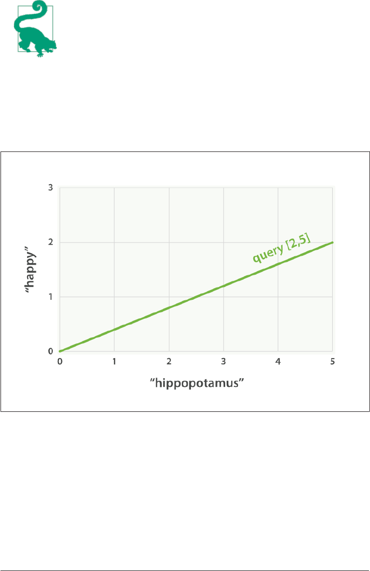
While TF/IDF is the default way of calculating term weights for the
vector space model, it is not the only way. Other models like
Okapi-BM25 exist and are available in Elasticsearch. TF/IDF is the
default because it is a simple, efficient algorithm that produces
high-quality search results and has stood the test of time.
Imagine that we have a query for “happy hippopotamus.” A common word like happy
will have a low weight, while an uncommon term like hippopotamus will have a high
weight. Let’s assume that happy has a weight of 2 and hippopotamus has a weight of 5.
We can plot this simple two-dimensional vector—[2,5]—as a line on a graph starting
at point (0,0) and ending at point (2,5), as shown in Figure 17-1.
Figure 17-1. A two-dimensional query vector for “happy hippopotamus” represented
Now, imagine we have three documents:
1. I am happy in summer.
2. After Christmas I’m a hippopotamus.
3. The happy hippopotamus helped Harry.
280 | Chapter 17: Controlling Relevance
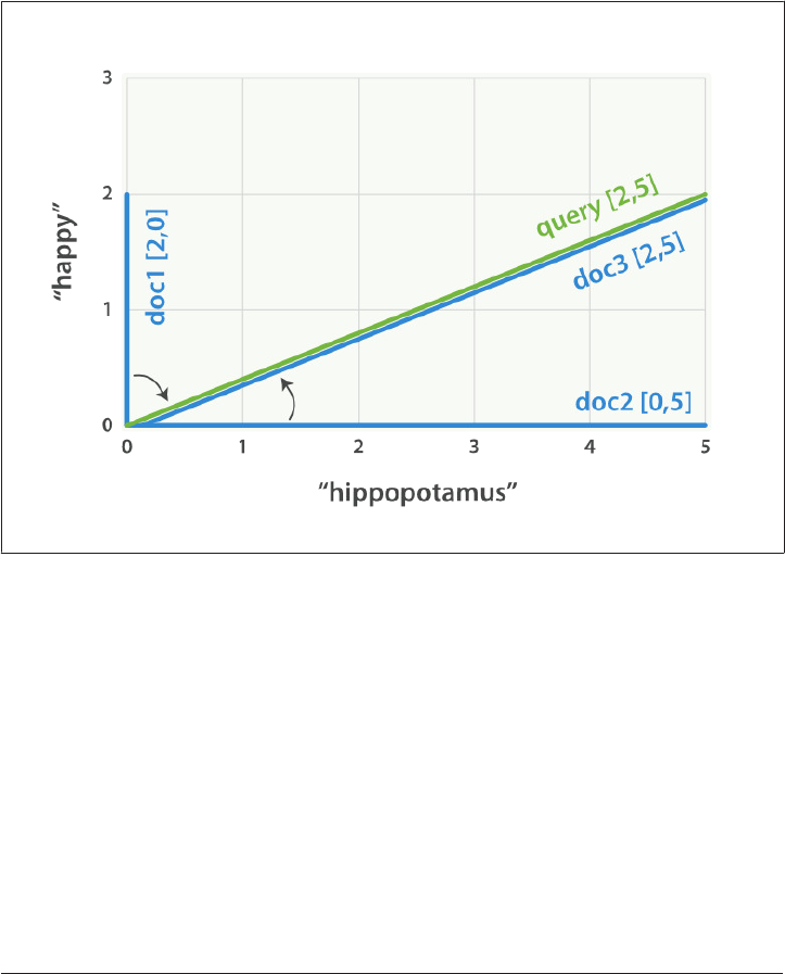
We can create a similar vector for each document, consisting of the weight of each
query term—happy and hippopotamus—that appears in the document, and plot these
vectors on the same graph, as shown in Figure 17-2:
• Document 1: (happy,____________)—[2,0]
• Document 2: ( ___ ,hippopotamus)—[0,5]
• Document 3: (happy,hippopotamus)—[2,5]
Figure 17-2. Query and document vectors for “happy hippopotamus”
The nice thing about vectors is that they can be compared. By measuring the angle
between the query vector and the document vector, it is possible to assign a relevance
score to each document. The angle between document 1 and the query is large, so it is
of low relevance. Document 2 is closer to the query, meaning that it is reasonably rel‐
evant, and document 3 is a perfect match.
Theory Behind Relevance Scoring | 281

In practice, only two-dimensional vectors (queries with two terms)
can be plotted easily on a graph. Fortunately, linear algebra—the
branch of mathematics that deals with vectors—provides tools to
compare the angle between multidimensional vectors, which
means that we can apply the same principles explained above to
queries that consist of many terms.
You can read more about how to compare two vectors by using
cosine similarity.
Now that we have talked about the theoretical basis of scoring, we can move on to see
how scoring is implemented in Lucene.
Lucene’s Practical Scoring Function
For multiterm queries, Lucene takes the Boolean model, TF/IDF, and the vector
space model and combines them in a single efficient package that collects matching
documents and scores them as it goes.
A multiterm query like
GET /my_index/doc/_search
{
"query": {
"match": {
"text": "quick fox"
}
}
}
is rewritten internally to look like this:
GET /my_index/doc/_search
{
"query": {
"bool": {
"should": [
{"term": { "text": "quick" }},
{"term": { "text": "fox" }}
]
}
}
}
The bool query implements the Boolean model and, in this example, will include
only documents that contain either the term quick or the term fox or both.
As soon as a document matches a query, Lucene calculates its score for that query,
combining the scores of each matching term. The formula used for scoring is called
282 | Chapter 17: Controlling Relevance

the practical scoring function. It looks intimidating, but don’t be put off—most of the
components you already know. It introduces a few new elements that we discuss next.
score(q,d) =
queryNorm(q)
· coord(q,d)
· ∑ (
tf(t in d)
· idf(t)²
· t.getBoost()
· norm(t,d)
) (t in q)
score(q,d) is the relevance score of document d for query q.
queryNorm(q) is the query normalization factor (new).
coord(q,d) is the coordination factor (new).
The sum of the weights for each term t in the query q for document d.
tf(t in d) is the term frequency for term t in document d.
idf(t) is the inverse document frequency for term t.
t.getBoost() is the boost that has been applied to the query (new).
norm(t,d) is the field-length norm, combined with the index-time field-level
boost, if any. (new).
You should recognize score, tf, and idf. The queryNorm, coord, t.getBoost, and
norm are new.
We will talk more about query-time boosting later in this chapter, but first let’s get
query normalization, coordination, and index-time field-level boosting out of the
way.
Query Normalization Factor
The query normalization factor (queryNorm) is an attempt to normalize a query so that
the results from one query may be compared with the results of another.
Lucene’s Practical Scoring Function | 283

Even though the intent of the query norm is to make results from
different queries comparable, it doesn’t work very well. The only
purpose of the relevance _score is to sort the results of the current
query in the correct order. You should not try to compare the rele‐
vance scores from different queries.
This factor is calculated at the beginning of the query. The actual calculation depends
on the queries involved, but a typical implementation is as follows:
queryNorm = 1 / √sumOfSquaredWeights
The sumOfSquaredWeights is calculated by adding together the IDF of each term
in the query, squared.
The same query normalization factor is applied to every docu‐
ment, and you have no way of changing it. For all intents and pur‐
poses, it can be ignored.
Query Coordination
The coordination factor (coord) is used to reward documents that contain a higher
percentage of the query terms. The more query terms that appear in the document,
the greater the chances that the document is a good match for the query.
Imagine that we have a query for quick brown fox, and that the weight for each term
is 1.5. Without the coordination factor, the score would just be the sum of the weights
of the terms in a document. For instance:
• Document with fox → score: 1.5
• Document with quick fox → score: 3.0
• Document with quick brown fox → score: 4.5
The coordination factor multiplies the score by the number of matching terms in the
document, and divides it by the total number of terms in the query. With the coordi‐
nation factor, the scores would be as follows:
• Document with fox → score: 1.5 * 1 / 3 = 0.5
• Document with quick fox → score: 3.0 * 2 / 3 = 2.0
• Document with quick brown fox → score: 4.5 * 3 / 3 = 4.5
The coordination factor results in the document that contains all three terms being
much more relevant than the document that contains just two of them.
284 | Chapter 17: Controlling Relevance

Remember that the query for quick brown fox is rewritten into a bool query like
this:
GET /_search
{
"query": {
"bool": {
"should": [
{ "term": { "text": "quick" }},
{ "term": { "text": "brown" }},
{ "term": { "text": "fox" }}
]
}
}
}
The bool query uses query coordination by default for all should clauses, but it does
allow you to disable coordination. Why might you want to do this? Well, usually the
answer is, you don’t. Query coordination is usually a good thing. When you use a
bool query to wrap several high-level queries like the match query, it also makes sense
to leave coordination enabled. The more clauses that match, the higher the degree of
overlap between your search request and the documents that are returned.
However, in some advanced use cases, it might make sense to disable coordination.
Imagine that you are looking for the synonyms jump, leap, and hop. You don’t care
how many of these synonyms are present, as they all represent the same concept. In
fact, only one of the synonyms is likely to be present. This would be a good case for
disabling the coordination factor:
GET /_search
{
"query": {
"bool": {
"disable_coord": true,
"should": [
{ "term": { "text": "jump" }},
{ "term": { "text": "hop" }},
{ "term": { "text": "leap" }}
]
}
}
}
When you use synonyms (see Chapter 23), this is exactly what happens internally: the
rewritten query disables coordination for the synonyms. Most use cases for disabling
coordination are handled automatically; you don’t need to worry about it.
Lucene’s Practical Scoring Function | 285

Index-Time Field-Level Boosting
We will talk about boosting a field—making it more important than other fields—at
query time in “Query-Time Boosting” on page 286. It is also possible to apply a boost
to a field at index time. Actually, this boost is applied to every term in the field, rather
than to the field itself.
To store this boost value in the index without using more space than necessary, this
field-level index-time boost is combined with the field-length norm (see “Field-
length norm” on page 277) and stored in the index as a single byte. This is the value
returned by norm(t,d) in the preceding formula.
We strongly recommend against using field-level index-time boosts
for a few reasons:
•Combining the boost with the field-length norm and storing it
in a single byte means that the field-length norm loses preci‐
sion. The result is that Elasticsearch is unable to distinguish
between a field containing three words and a field containing
five words.
•To change an index-time boost, you have to reindex all your
documents. A query-time boost, on the other hand, can be
changed with every query.
•If a field with an index-time boost has multiple values, the
boost is multiplied by itself for every value, dramatically
increasing the weight for that field.
Query-time boosting is a much simpler, cleaner, more flexible
option.
With query normalization, coordination, and index-time boosting out of the way, we
can now move on to the most useful tool for influencing the relevance calculation:
query-time boosting.
Query-Time Boosting
In Prioritizing Clauses, we explained how you could use the boost parameter at
search time to give one query clause more importance than another. For instance:
GET /_search
{
"query": {
"bool": {
"should": [
{
"match": {
286 | Chapter 17: Controlling Relevance

"title": {
"query": "quick brown fox",
"boost": 2
}
}
},
{
"match": {
"content": "quick brown fox"
}
}
]
}
}
}
The title query clause is twice as important as the content query clause,
because it has been boosted by a factor of 2.
A query clause without a boost value has a neutral boost of 1.
Query-time boosting is the main tool that you can use to tune relevance. Any type of
query accepts a boost parameter. Setting a boost of 2 doesn’t simply double the final
_score; the actual boost value that is applied goes through normalization and some
internal optimization. However, it does imply that a clause with a boost of 2 is twice
as important as a clause with a boost of 1.
Practically, there is no simple formula for deciding on the “correct” boost value for a
particular query clause. It’s a matter of try-it-and-see. Remember that boost is just
one of the factors involved in the relevance score; it has to compete with the other
factors. For instance, in the preceding example, the title field will probably already
have a “natural” boost over the content field thanks to the field-length norm (titles
are usually shorter than the related content), so don’t blindly boost fields just because
you think they should be boosted. Apply a boost and check the results. Change the
boost and check again.
Boosting an Index
When searching across multiple indices, you can boost an entire index over the oth‐
ers with the indices_boost parameter. This could be used, as in the next example, to
give more weight to documents from a more recent index:
GET /docs_2014_*/_search
{
"indices_boost": {
"docs_2014_10": 3,
"docs_2014_09": 2
},
Query-Time Boosting | 287

"query": {
"match": {
"text": "quick brown fox"
}
}
}
This multi-index search covers all indices beginning with docs_2014_.
Documents in the docs_2014_10 index will be boosted by 3, those in
docs_2014_09 by 2, and any other matching indices will have a neutral boost of 1.
t.getBoost()
These boost values are represented in the “Lucene’s Practical Scoring Function” on
page 282 by the t.getBoost() element. Boosts are not applied at the level that they
appear in the query DSL. Instead, any boost values are combined and passsed down
to the individual terms. The t.getBoost() method returns any boost value applied
to the term itself or to any of the queries higher up the chain.
In fact, reading the explain output is a little more complex than
that. You won’t see the boost value or t.getBoost() mentioned in
the explanation at all. Instead, the boost is rolled into the query
Norm that is applied to a particular term. Although we said that the
queryNorm is the same for every term, you will see that the query
Norm for a boosted term is higher than the queryNorm for an
unboosted term.
Manipulating Relevance with Query Structure
The Elasticsearch query DSL is immensely flexible. You can move individual query
clauses up and down the query hierarchy to make a clause more or less important.
For instance, imagine the following query:
quick OR brown OR red OR fox
We could write this as a bool query with all terms at the same level:
GET /_search
{
"query": {
"bool": {
"should": [
{ "term": { "text": "quick" }},
{ "term": { "text": "brown" }},
{ "term": { "text": "red" }},
{ "term": { "text": "fox" }}
288 | Chapter 17: Controlling Relevance

]
}
}
}
But this query might score a document that contains quick, red, and brown the same
as another document that contains quick, red, and fox. Red and brown are synonyms
and we probably only need one of them to match. Perhaps we really want to express
the query as follows:
quick OR (brown OR red) OR fox
According to standard Boolean logic, this is exactly the same as the original query,
but as we have already seen in Combining Queries, a bool query does not concern
itself only with whether a document matches, but also with how well it matches.
A better way to write this query is as follows:
GET /_search
{
"query": {
"bool": {
"should": [
{ "term": { "text": "quick" }},
{ "term": { "text": "fox" }},
{
"bool": {
"should": [
{ "term": { "text": "brown" }},
{ "term": { "text": "red" }}
]
}
}
]
}
}
}
Now, red and brown compete with each other at their own level, and quick, fox, and
red OR brown are the top-level competitive terms.
We have already discussed how the match, multi_match, term, bool, and dis_max
queries can be used to manipulate scoring. In the rest of this chapter, we present three
other scoring-related queries: the boosting query, the constant_score query, and
the function_score query.
Not Quite Not
A search on the Internet for “Apple” is likely to return results about the company, the
fruit, and various recipes. We could try to narrow it down to just the company by
Not Quite Not | 289

excluding words like pie, tart, crumble, and tree, using a must_not clause in a bool
query:
GET /_search
{
"query": {
"bool": {
"must": {
"match": {
"text": "apple"
}
},
"must_not": {
"match": {
"text": "pie tart fruit crumble tree"
}
}
}
}
}
But who is to say that we wouldn’t miss a very relevant document about Apple the
company by excluding tree or crumble? Sometimes, must_not can be too strict.
boosting Query
The boosting query solves this problem. It allows us to still include results that
appear to be about the fruit or the pastries, but to downgrade them—to rank them
lower than they would otherwise be:
GET /_search
{
"query": {
"boosting": {
"positive": {
"match": {
"text": "apple"
}
},
"negative": {
"match": {
"text": "pie tart fruit crumble tree"
}
},
"negative_boost": 0.5
}
}
}
It accepts a positive query and a negative query. Only documents that match the
positive query will be included in the results list, but documents that also match the
290 | Chapter 17: Controlling Relevance

negative query will be downgraded by multiplying the original _score of the docu‐
ment with the negative_boost.
For this to work, the negative_boost must be less than 1.0. In this example, any
documents that contain any of the negative terms will have their _score cut in half.
Ignoring TF/IDF
Sometimes we just don’t care about TF/IDF. All we want to know is that a certain
word appears in a field. Perhaps we are searching for a vacation home and we want to
find houses that have as many of these features as possible:
• WiFi
• Garden
• Pool
The vacation home documents look something like this:
{ "description": "A delightful four-bedroomed house with ... " }
We could use a simple match query:
GET /_search
{
"query": {
"match": {
"description": "wifi garden pool"
}
}
}
However, this isn’t really full-text search. In this case, TF/IDF just gets in the way. We
don’t care whether wifi is a common term, or how often it appears in the document.
All we care about is that it does appear. In fact, we just want to rank houses by the
number of features they have—the more, the better. If a feature is present, it should
score 1, and if it isn’t, 0.
constant_score Query
Enter the constant_score query. This query can wrap either a query or a filter, and
assigns a score of 1 to any documents that match, regardless of TF/IDF:
GET /_search
{
"query": {
"bool": {
"should": [
{ "constant_score": {
Ignoring TF/IDF | 291

"query": { "match": { "description": "wifi" }}
}},
{ "constant_score": {
"query": { "match": { "description": "garden" }}
}},
{ "constant_score": {
"query": { "match": { "description": "pool" }}
}}
]
}
}
}
Perhaps not all features are equally important—some have more value to the user
than others. If the most important feature is the pool, we could boost that clause to
make it count for more:
GET /_search
{
"query": {
"bool": {
"should": [
{ "constant_score": {
"query": { "match": { "description": "wifi" }}
}},
{ "constant_score": {
"query": { "match": { "description": "garden" }}
}},
{ "constant_score": {
"boost": 2
"query": { "match": { "description": "pool" }}
}}
]
}
}
}
A matching pool clause would add a score of 2, while the other clauses would
add a score of only 1 each.
The final score for each result is not simply the sum of the scores
of all matching clauses. The coordination factor and query nor‐
malization factor are still taken into account.
We could improve our vacation home documents by adding a not_analyzed fea
tures field to our vacation homes:
{ "features": [ "wifi", "pool", "garden" ] }
292 | Chapter 17: Controlling Relevance

By default, a not_analyzed field has field-length norms disabled and has
index_options set to docs, disabling term frequencies, but the problem remains: the
inverse document frequency of each term is still taken into account.
We could use the same approach that we used previously, with the constant_score
query:
GET /_search
{
"query": {
"bool": {
"should": [
{ "constant_score": {
"query": { "match": { "features": "wifi" }}
}},
{ "constant_score": {
"query": { "match": { "features": "garden" }}
}},
{ "constant_score": {
"boost": 2
"query": { "match": { "features": "pool" }}
}}
]
}
}
}
Really, though, each of these features should be treated like a filter. A vacation home
either has the feature or it doesn’t—a filter seems like it would be a natural fit. On top
of that, if we use filters, we can benefit from filter caching.
The problem is this: filters don’t score. What we need is a way of bridging the gap
between filters and queries. The function_score query does this and a whole lot
more.
function_score Query
The function_score query is the ultimate tool for taking control of the scoring pro‐
cess. It allows you to apply a function to each document that matches the main query
in order to alter or completely replace the original query _score.
In fact, you can apply different functions to subsets of the main result set by using
filters, which gives you the best of both worlds: efficient scoring with cacheable filters.
It supports several predefined functions out of the box:
weight
Apply a simple boost to each document without the boost being normalized: a
weight of 2 results in 2 * _score.
function_score Query | 293

field_value_factor
Use the value of a field in the document to alter the _score, such as factoring in a
popularity count or number of votes.
random_score
Use consistently random scoring to sort results differently for every user, while
maintaining the same sort order for a single user.
Decay functions—linear, exp, gauss
Incorporate sliding-scale values like publish_date, geo_location, or price into
the _score to prefer recently published documents, documents near a latitude/
longitude (lat/lon) point, or documents near a specified price point.
script_score
Use a custom script to take complete control of the scoring logic. If your needs
extend beyond those of the functions in this list, write a custom script to imple‐
ment the logic that you need.
Without the function_score query, we would not be able to combine the score from
a full-text query with a factor like recency. We would have to sort either by _score or
by date; the effect of one would obliterate the effect of the other. This query allows
you to blend the two together: to still sort by full-text relevance, but giving extra
weight to recently published documents, or popular documents, or products that are
near the user’s price point. As you can imagine, a query that supports all of this can
look fairly complex. We’ll start with a simple use case and work our way up the com‐
plexity ladder.
Boosting by Popularity
Imagine that we have a website that hosts blog posts and enables users to vote for the
blog posts that they like. We would like more-popular posts to appear higher in the
results list, but still have the full-text score as the main relevance driver. We can do
this easily by storing the number of votes with each blog post:
294 | Chapter 17: Controlling Relevance

PUT /blogposts/post/1
{
"title": "About popularity",
"content": "In this post we will talk about...",
"votes": 6
}
At search time, we can use the function_score query with the field_value_factor
function to combine the number of votes with the full-text relevance score:
GET /blogposts/post/_search
{
"query": {
"function_score": {
"query": {
"multi_match": {
"query": "popularity",
"fields": [ "title", "content" ]
}
},
"field_value_factor": {
"field": "votes"
}
}
}
}
The function_score query wraps the main query and the function we would like
to apply.
The main query is executed first.
The field_value_factor function is applied to every document matching the
main query.
Every document must have a number in the votes field for the function_score
to work.
In the preceding example, the final _score for each document has been altered as fol‐
lows:
new_score = old_score * number_of_votes
This will not give us great results. The full-text _score range usually falls somewhere
between 0 and 10. As can be seen in Figure 17-3, a blog post with 10 votes will com‐
pletely swamp the effect of the full-text score, and a blog post with 0 votes will reset
the score to zero.
Boosting by Popularity | 295

Figure 17-3. Linear popularity based on an original _score of 2.0
modier
A better way to incorporate popularity is to smooth out the votes value with some
modifier. In other words, we want the first few votes to count a lot, but for each sub‐
sequent vote to count less. The difference between 0 votes and 1 vote should be much
bigger than the difference between 10 votes and 11 votes.
A typical modifier for this use case is log1p, which changes the formula to the fol‐
lowing:
new_score = old_score * log(1 + number_of_votes)
The log function smooths out the effect of the votes field to provide a curve like the
one in Figure 17-4.
296 | Chapter 17: Controlling Relevance

Figure 17-4. Logarithmic popularity based on an original _score of 2.0
The request with the modifier parameter looks like the following:
GET /blogposts/post/_search
{
"query": {
"function_score": {
"query": {
"multi_match": {
"query": "popularity",
"fields": [ "title", "content" ]
}
},
"field_value_factor": {
"field": "votes",
"modifier": "log1p"
}
}
}
}
Set the modifier to log1p.
Boosting by Popularity | 297

The available modifiers are none (the default), log, log1p, log2p, ln, ln1p, ln2p,
square, sqrt, and reciprocal. You can read more about them in the
field_value_factor documentation.
factor
The strength of the popularity effect can be increased or decreased by multiplying the
value in the votes field by some number, called the factor:
GET /blogposts/post/_search
{
"query": {
"function_score": {
"query": {
"multi_match": {
"query": "popularity",
"fields": [ "title", "content" ]
}
},
"field_value_factor": {
"field": "votes",
"modifier": "log1p",
"factor": 2
}
}
}
}
Doubles the popularity effect
Adding in a factor changes the formula to this:
new_score = old_score * log(1 + factor * number_of_votes)
A factor greater than 1 increases the effect, and a factor less than 1 decreases the
effect, as shown in Figure 17-5.
298 | Chapter 17: Controlling Relevance

Figure 17-5. Logarithmic popularity with dierent factors
boost_mode
Perhaps multiplying the full-text score by the result of the field_value_factor func‐
tion still has too large an effect. We can control how the result of a function is com‐
bined with the _score from the query by using the boost_mode parameter, which
accepts the following values:
multiply
Multiply the _score with the function result (default)
sum
Add the function result to the _score
min
The lower of the _score and the function result
max
The higher of the _score and the function result
replace
Replace the _score with the function result
If, instead of multiplying, we add the function result to the _score, we can achieve a
much smaller effect, especially if we use a low factor:
Boosting by Popularity | 299
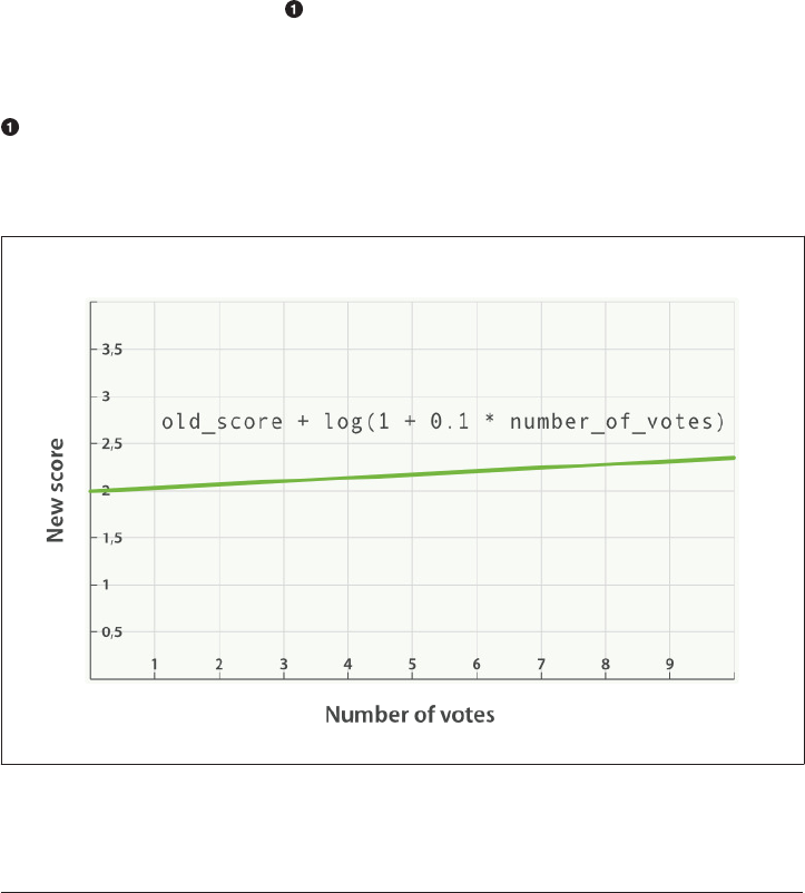
GET /blogposts/post/_search
{
"query": {
"function_score": {
"query": {
"multi_match": {
"query": "popularity",
"fields": [ "title", "content" ]
}
},
"field_value_factor": {
"field": "votes",
"modifier": "log1p",
"factor": 0.1
},
"boost_mode": "sum"
}
}
}
Add the function result to the _score.
The formula for the preceding request now looks like this (see Figure 17-6):
new_score = old_score + log(1 + 0.1 * number_of_votes)
Figure 17-6. Combining popularity with sum
300 | Chapter 17: Controlling Relevance
max_boost
Finally, we can cap the maximum effect that the function can have by using the
max_boost parameter:
GET /blogposts/post/_search
{
"query": {
"function_score": {
"query": {
"multi_match": {
"query": "popularity",
"fields": [ "title", "content" ]
}
},
"field_value_factor": {
"field": "votes",
"modifier": "log1p",
"factor": 0.1
},
"boost_mode": "sum",
"max_boost": 1.5
}
}
}
Whatever the result of the field_value_factor function, it will never be greater
than 1.5.
The max_boost applies a limit to the result of the function only,
not to the final _score.
Boosting Filtered Subsets
Let’s return to the problem that we were dealing with in “Ignoring TF/IDF” on page
291, where we wanted to score vacation homes by the number of features that each
home possesses. We ended that section by wishing for a way to use cached filters to
affect the score, and with the function_score query we can do just that.
The examples we have shown thus far have used a single function for all documents.
Now we want to divide the results into subsets by using filters (one filter per feature),
and apply a different function to each subset.
Boosting Filtered Subsets | 301
The function that we will use in this example is the weight, which is similar to the
boost parameter accepted by any query. The difference is that the weight is not nor‐
malized by Lucene into some obscure floating-point number; it is used as is.
The structure of the query has to change somewhat to incorporate multiple functions:
GET /_search
{
"query": {
"function_score": {
"filter": {
"term": { "city": "Barcelona" }
},
"functions": [
{
"filter": { "term": { "features": "wifi" }},
"weight": 1
},
{
"filter": { "term": { "features": "garden" }},
"weight": 1
},
{
"filter": { "term": { "features": "pool" }},
"weight": 2
}
],
"score_mode": "sum",
}
}
}
This function_score query has a filter instead of a query.
The functions key holds a list of functions that should be applied.
The function is applied only if the document matches the (optional) filter.
The pool feature is more important than the others so it has a higher weight.
The score_mode specifies how the values from each function should be com‐
bined.
The new features to note in this example are explained in the following sections.
lter Versus query
The first thing to note is that we have specified a filter instead of a query. In this
example, we do not need full-text search. We just want to return all documents that
302 | Chapter 17: Controlling Relevance

have Barcelona in the city field, logic that is better expressed as a filter instead of a
query. All documents returned by the filter will have a _score of 1. The func
tion_score query accepts either a query or a filter. If neither is specified, it will
default to using the match_all query.
functions
The functions key holds an array of functions to apply. Each entry in the array may
also optionally specify a filter, in which case the function will be applied only to
documents that match that filter. In this example, we apply a weight of 1 (or 2 in the
case of pool) to any document that matches the filter.
score_mode
Each function returns a result, and we need a way of reducing these multiple results
to a single value that can be combined with the original _score. This is the role of the
score_mode parameter, which accepts the following values:
multiply
Function results are multiplied together (default).
sum
Function results are added up.
avg
The average of all the function results.
max
The highest function result is used.
min
The lowest function result is used.
first
Uses only the result from the first function that either doesn’t have a filter or that
has a filter matching the document.
In this case, we want to add the weight results from each matching filter together to
produce the final score, so we have used the sum score mode.
Documents that don’t match any of the filters will keep their original _score of 1.
Random Scoring
You may have been wondering what consistently random scoring is, or why you would
ever want to use it. The previous example provides a good use case. All results from
Random Scoring | 303

the previous example would receive a final _score of 1, 2, 3, 4, or 5. Maybe there are
only a few homes that score 5, but presumably there would be a lot of homes scoring
2 or 3.
As the owner of the website, you want to give your advertisers as much exposure as
possible. With the current query, results with the same _score would be returned in
the same order every time. It would be good to introduce some randomness here, to
ensure that all documents in a single score level get a similar amount of exposure.
We want every user to see a different random order, but we want the same user to see
the same order when clicking on page 2, 3, and so forth. This is what is meant by
consistently random.
The random_score function, which outputs a number between 0 and 1, will produce
consistently random results when it is provided with the same seed value, such as a
user’s session ID:
GET /_search
{
"query": {
"function_score": {
"filter": {
"term": { "city": "Barcelona" }
},
"functions": [
{
"filter": { "term": { "features": "wifi" }},
"weight": 1
},
{
"filter": { "term": { "features": "garden" }},
"weight": 1
},
{
"filter": { "term": { "features": "pool" }},
"weight": 2
},
{
"random_score": {
"seed": "the users session id"
}
}
],
"score_mode": "sum",
}
}
}
The random_score clause doesn’t have any filter, so it will be applied to all
documents.
304 | Chapter 17: Controlling Relevance

Pass the user’s session ID as the seed, to make randomization consistent for that
user. The same seed will result in the same randomization.
Of course, if you index new documents that match the query, the order of results will
change regardless of whether you use consistent randomization or not.
The Closer, The Better
Many variables could influence the user’s choice of vacation home. Maybe she would
like to be close to the center of town, but perhaps would be willing to settle for a place
that is a bit farther from the center if the price is low enough. Perhaps the reverse is
true: she would be willing to pay more for the best location.
If we were to add a filter that excluded any vacation homes farther than 1 kilometer
from the center, or any vacation homes that cost more than £100 a night, we might
exclude results that the user would consider to be a good compromise.
The function_score query gives us the ability to trade off one sliding scale (like loca‐
tion) against another sliding scale (like price), with a group of functions known as the
decay functions.
The three decay functions—called linear, exp, and gauss—operate on numeric
fields, date fields, or lat/lon geo-points. All three take the same parameters:
origin
The central point, or the best possible value for the field. Documents that fall at
the origin will get a full _score of 1.0.
scale
The rate of decay—how quickly the _score should drop the further from the ori
gin that a document lies (for example, every £10 or every 100 meters).
decay
The _score that a document at scale distance from the origin should receive.
Defaults to 0.5.
offset
Setting a nonzero offset expands the central point to cover a range of values
instead of just the single point specified by the origin. All values in the range -
offset <= origin <= +offset will receive the full _score of 1.0.
The only difference between these three functions is the shape of the decay curve.
The difference is most easily illustrated with a graph (see Figure 17-7).
The Closer, The Better | 305

Figure 17-7. Decay function curves
The curves shown in Figure 17-7 all have their origin—the central point—set to 40.
The offset is 5, meaning that all values in the range 40 - 5 <= value <= 40 + 5
are treated as though they were at the origin—they all get the full score of 1.0.
Outside this range, the score starts to decay. The rate of decay is determined by the
scale (which in this example is set to 5), and the decay (which is set to the default of
0.5). The result is that all three curves return a score of 0.5 at origin +/- (offset
+ scale), or at points 30 and 50.
The difference between linear, exp, and gauss is the shape of the curve at other
points in the range:
•The linear funtion is just a straight line. Once the line hits zero, all values out‐
side the line will return a score of 0.0.
• The exp (exponential) function decays rapidly, then slows down.
•The gauss (Gaussian) function is bell-shaped—it decays slowly, then rapidly,
then slows down again.
Which curve you choose depends entirely on how quickly you want the _score to
decay, the further a value is from the origin.
306 | Chapter 17: Controlling Relevance

To return to our example: our user would prefer to rent a vacation home close to the
center of London ({ "lat": 51.50, "lon": 0.12}) and to pay no more than £100 a
night, but our user considers price to be more important than distance. We could
write this query as follows:
GET /_search
{
"query": {
"function_score": {
"functions": [
{
"gauss": {
"location": {
"origin": { "lat": 51.5, "lon": 0.12 },
"offset": "2km",
"scale": "3km"
}
}
},
{
"gauss": {
"price": {
"origin": "50",
"offset": "50",
"scale": "20"
}
},
"weight": 2
}
]
}
}
}
The location field is mapped as a geo_point.
The price field is numeric.
See “Understanding the price Clause” on page 308 for the reason that origin is
50 instead of 100.
The price clause has twice the weight of the location clause.
The location clause is easy to understand:
• We have specified an origin that corresponds to the center of London.
• Any location within 2km of the origin receives the full score of 1.0.
The Closer, The Better | 307

• Locations 5km (offset + scale) from the centre receive a score of 0.5.
Understanding the price Clause
The price clause is a little trickier. The user’s preferred price is anything up to £100,
but this example sets the origin to £50. Prices can’t be negative, but the lower they are,
the better. Really, any price between £0 and £100 should be considered optimal.
If we were to set the origin to £100, then prices below £100 would receive a lower
score. Instead, we set both the origin and the offset to £50. That way, the score
decays only for any prices above £100 (origin + offset).
The weight parameter can be used to increase or decrease the con‐
tribution of individual clauses. The weight, which defaults to 1.0,
is multiplied by the score from each clause before the scores are
combined with the specified score_mode.
Scoring with Scripts
Finally, if none of the function_score’s built-in functions suffice, you can implement
the logic that you need with a script, using the script_score function.
For an example, let’s say that we want to factor our profit margin into the relevance
calculation. In our business, the profit margin depends on three factors:
• The price per night of the vacation home.
•The user’s membership level—some levels get a percentage discount above a cer‐
tain price per night threshold.
•The negotiated margin as a percentage of the price-per-night, after user dis‐
counts.
The algorithm that we will use to calculate the profit for each home is as follows:
if (price < threshold) {
profit = price * margin
} else {
profit = price * (1 - discount) * margin;
}
We probably don’t want to use the absolute profit as a score; it would overwhelm the
other factors like location, popularity and features. Instead, we can express the profit
as a percentage of our target profit. A profit margin above our target will have a pos‐
308 | Chapter 17: Controlling Relevance
itive score (greater than 1.0), and a profit margin below our target will have a nega‐
tive score (less than 1.0):
if (price < threshold) {
profit = price * margin
} else {
profit = price * (1 - discount) * margin
}
return profit / target
The default scripting language in Elasticsearch is Groovy, which for the most part
looks a lot like JavaScript. The preceding algorithm as a Groovy script would look like
this:
price = doc['price'].value
margin = doc['margin'].value
if (price < threshold) {
return price * margin / target
}
return price * (1 - discount) * margin / target
The price and margin variables are extracted from the price and margin fields
in the document.
The threshold, discount, and target variables we will pass in as params.
Finally, we can add our script_score function to the list of other functions that we
are already using:
GET /_search
{
"function_score": {
"functions": [
{ ...location clause... },
{ ...price clause... },
{
"script_score": {
"params": {
"threshold": 80,
"discount": 0.1,
"target": 10
},
"script": "price = doc['price'].value; margin = doc['margin'].value;
if (price < threshold) { return price * margin / target };
return price * (1 - discount) * margin / target;"
}
}
]
}
}
Scoring with Scripts | 309

The location and price clauses refer to the example explained in “The Closer,
The Better” on page 305.
By passing in these variables as params, we can change their values every time we
run this query without having to recompile the script.
JSON cannot include embedded newline characters. Newline characters in the
script should either be escaped as \n or replaced with semicolons.
This query would return the documents that best satisfy the user’s requirements for
location and price, while still factoring in our need to make a profit.
The script_score function provides enormous flexibility. Within
a script, you have access to the fields of the document, to the cur‐
rent _score, and even to the term frequencies, inverse document
frequencies, and field length norms (see Text scoring in scripts).
That said, scripts can have a performance impact. If you do find
that your scripts are not quite fast enough, you have three options:
•Try to precalculate as much information as possible and
include it in each document.
•Groovy is fast, but not quite as fast as Java. You could reimple‐
ment your script as a native Java script. (See Native Java
Scripts).
•Use the rescore functionality described in “Rescoring Results”
on page 249 to apply your script to only the best-scoring docu‐
ments.
Pluggable Similarity Algorithms
Before we move on from relevance and scoring, we will finish this chapter with a
more advanced subject: pluggable similarity algorithms. While Elasticsearch uses the
“Lucene’s Practical Scoring Function” on page 282 as its default similarity algorithm,
it supports other algorithms out of the box, which are listed in the Similarity Modules
documentation.
Okapi BM25
The most interesting competitor to TF/IDF and the vector space model is called
Okapi BM25, which is considered to be a state-of-the-art ranking function. BM25
originates from the probabilistic relevance model, rather than the vector space model,
yet the algorithm has a lot in common with Lucene’s practical scoring function.
310 | Chapter 17: Controlling Relevance

Both use of term frequency, inverse document frequency, and field-length normaliza‐
tion, but the definition of each of these factors is a little different. Rather than
explaining the BM25 formula in detail, we will focus on the practical advantages that
BM25 offers.
Term-frequency saturation
Both TF/IDF and BM25 use inverse document frequency to distinguish between
common (low value) words and uncommon (high value) words. Both also recognize
(see “Term frequency” on page 276) that the more often a word appears in a docu‐
ment, the more likely is it that the document is relevant for that word.
However, common words occur commonly. The fact that a common word appears
many times in one document is offset by the fact that the word appears many times in
all documents.
However, TF/IDF was designed in an era when it was standard practice to remove the
most common words (or stopwords, see Chapter 22) from the index altogether. The
algorithm didn’t need to worry about an upper limit for term frequency because the
most frequent terms had already been removed.
In Elasticsearch, the standard analyzer—the default for string fields—doesn’t
remove stopwords because, even though they are words of little value, they do still
have some value. The result is that, for very long documents, the sheer number of
occurrences of words like the and and can artificially boost their weight.
BM25, on the other hand, does have an upper limit. Terms that appear 5 to 10 times
in a document have a significantly larger impact on relevance than terms that appear
just once or twice. However, as can be seen in Figure 17-8, terms that appear 20 times
in a document have almost the same impact as terms that appear a thousand times or
more.
This is known as nonlinear term-frequency saturation.
Pluggable Similarity Algorithms | 311

Figure 17-8. Term frequency saturation for TF/IDF and BM25
Field-length normalization
In “Field-length norm” on page 277, we said that Lucene considers shorter fields to
have more weight than longer fields: the frequency of a term in a field is offset by the
length of the field. However, the practical scoring function treats all fields in the same
way. It will treat all title fields (because they are short) as more important than all
body fields (because they are long).
BM25 also considers shorter fields to have more weight than longer fields, but it con‐
siders each field separately by taking the average length of the field into account. It
can distinguish between a short title field and a long title field.
In “Query-Time Boosting” on page 286, we said that the title
field has a natural boost over the body field because of its length.
This natural boost disappears with BM25 as differences in field
length apply only within a single field.
Tuning BM25
One of the nice features of BM25 is that, unlike TF/IDF, it has two parameters that
allow it to be tuned:
312 | Chapter 17: Controlling Relevance

k1
This parameter controls how quickly an increase in term frequency results in
term-frequency saturation. The default value is 1.2. Lower values result in
quicker saturation, and higher values in slower saturation.
b
This parameter controls how much effect field-length normalization should have.
A value of 0.0 disables normalization completely, and a value of 1.0 normalizes
fully. The default is 0.75.
The practicalities of tuning BM25 are another matter. The default values for k1 and b
should be suitable for most document collections, but the optimal values really
depend on the collection. Finding good values for your collection is a matter of
adjusting, checking, and adjusting again.
Changing Similarities
The similarity algorithm can be set on a per-field basis. It’s just a matter of specifying
the chosen algorithm in the field’s mapping:
PUT /my_index
{
"mappings": {
"doc": {
"properties": {
"title": {
"type": "string",
"similarity": "BM25"
},
"body": {
"type": "string",
"similarity": "default"
}
}
}
}
The title field uses BM25 similarity.
The body field uses the default similarity (see “Lucene’s Practical Scoring Func‐
tion” on page 282).
Currently, it is not possible to change the similarity mapping for an existing field.
You would need to reindex your data in order to do that.
Changing Similarities | 313

Conguring BM25
Configuring a similarity is much like configuring an analyzer. Custom similarities can
be specified when creating an index. For instance:
PUT /my_index
{
"settings": {
"similarity": {
"my_bm25": {
"type": "BM25",
"b": 0
}
}
},
"mappings": {
"doc": {
"properties": {
"title": {
"type": "string",
"similarity": "my_bm25"
},
"body": {
"type": "string",
"similarity": "BM25"
}
}
}
}
}
Create a custom similarity called my_bm25, based on the built-in BM25 similarity.
Disable field-length normalization. See “Tuning BM25” on page 312.
Field title uses the custom similarity my_bm25.
Field body uses the built-in similarity BM25.
A custom similarity can be updated by closing the index, updating
the index settings, and reopening the index. This allows you to
experiment with different configurations without having to rein‐
dex your documents.
314 | Chapter 17: Controlling Relevance

Relevance Tuning Is the Last 10%
In this chapter, we looked at a how Lucene generates scores based on TF/IDF. Under‐
standing the score-generation process is critical so you can tune, modulate, attenuate,
and manipulate the score for your particular business domain.
In practice, simple combinations of queries will get you good search results. But to
get great search results, you’ll often have to start tinkering with the previously men‐
tioned tuning methods.
Often, applying a boost on a strategic field or rearranging a query to emphasize a par‐
ticular clause will be sufficient to make your results great. Sometimes you’ll need
more-invasive changes. This is usually the case if your scoring requirements diverge
heavily from Lucene’s word-based TF/IDF model (for example, you want to score
based on time or distance).
With that said, relevancy tuning is a rabbit hole that you can easily fall into and never
emerge. The concept of most relevant is a nebulous target to hit, and different people
often have different ideas about document ranking. It is easy to get into a cycle of
constant fiddling without any apparent progress.
We encourage you to avoid this (very tempting) behavior and instead properly
instrument your search results. Monitor how often your users click the top result, the
top 10, and the first page; how often they execute a secondary query without selecting
a result first; how often they click a result and immediately go back to the search
results, and so forth.
These are all indicators of how relevant your search results are to the user. If your
query is returning highly relevant results, users will select one of the top-five results,
find what they want, and leave. Irrelevant results cause users to click around and try
new search queries.
Once you have instrumentation in place, tuning your query is simple. Make a change,
monitor its effect on your users, and repeat as necessary. The tools outlined in this
chapter are just that: tools. You have to use them appropriately to propel your search
results into the great category, and the only way to do that is with strong measure‐
ment of user behavior.
Relevance Tuning Is the Last 10% | 315

PART III
Dealing with Human Language
I know all those words, but that sentence makes no sense to me.
—Matt Groening
Full-text search is a battle between precision—returning as few irrelevant documents
as possible—and recall—returning as many relevant documents as possible. While
matching only the exact words that the user has queried would be precise, it is not
enough. We would miss out on many documents that the user would consider to be
relevant. Instead, we need to spread the net wider, to also search for words that are
not exactly the same as the original but are related.
Wouldn’t you expect a search for “quick brown fox” to match a document containing
“fast brown foxes,” “Johnny Walker” to match “Johnnie Walker,” or “Arnolt Schwar‐
zenneger” to match “Arnold Schwarzenegger”?
If documents exist that do contain exactly what the user has queried, those docu‐
ments should appear at the top of the result set, but weaker matches can be included
further down the list. If no documents match exactly, at least we can show the user
potential matches; they may even be what the user originally intended!
There are several lines of attack:
•Remove diacritics like ´, ^, and ¨ so that a search for rôle will also match role,
and vice versa. See Chapter 20.
•Remove the distinction between singular and plural—fox versus foxes—or
between tenses—jumping versus jumped versus jumps—by stemming each word
to its root form. See Chapter 21.
•Remove commonly used words or stopwords like the, and, and or to improve
search performance. See Chapter 22.
•Including synonyms so that a query for quick could also match fast, or UK could
match United Kingdom. See Chapter 23.
•Check for misspellings or alternate spellings, or match on homophones—words
that sound the same, like their versus there, meat versus meet versus mete. See
Chapter 24.
Before we can manipulate individual words, we need to divide text into words, which
means that we need to know what constitutes a word. We will tackle this in Chap‐
ter 19.
But first, let’s take a look at how to get started quickly and easily.

CHAPTER 18
Getting Started with Languages
Elasticsearch ships with a collection of language analyzers that provide good, basic,
out-of-the-box support for many of the world’s most common languages:
Arabic, Armenian, Basque, Brazilian, Bulgarian, Catalan, Chinese, Czech, Danish,
Dutch, English, Finnish, French, Galician, German, Greek, Hindi, Hungarian, Indo‐
nesian, Irish, Italian, Japanese, Korean, Kurdish, Norwegian, Persian, Portuguese,
Romanian, Russian, Spanish, Swedish, Turkish, and Thai.
These analyzers typically perform four roles:
• Tokenize text into individual words:
The quick brown foxes → [The, quick, brown, foxes]
• Lowercase tokens:
The → the
• Remove common stopwords:
[The, quick, brown, foxes] → [quick, brown, foxes]
• Stem tokens to their root form:
foxes → fox
Each analyzer may also apply other transformations specific to its language in order
to make words from that language more searchable:
• The english analyzer removes the possessive 's:
John's → john
• The french analyzer removes elisions like l' and qu' and diacritics like ¨ or ^:
319

l'église → eglis
•The german analyzer normalizes terms, replacing ä and ae with a, or ß with ss,
among others:
äußerst → ausserst
Using Language Analyzers
The built-in language analyzers are available globally and don’t need to be configured
before being used. They can be specified directly in the field mapping:
PUT /my_index
{
"mappings": {
"blog": {
"properties": {
"title": {
"type": "string",
"analyzer": "english"
}
}
}
}
}
The title field will use the english analyzer instead of the default standard
analyzer.
Of course, by passing text through the english analyzer, we lose information:
GET /my_index/_analyze?field=title
I'm not happy about the foxes
Emits token: i'm, happi, about, fox
We can’t tell if the document mentions one fox or many foxes; the word not is a
stopword and is removed, so we can’t tell whether the document is happy about foxes
or not. By using the english analyzer, we have increased recall as we can match more
loosely, but we have reduced our ability to rank documents accurately.
To get the best of both worlds, we can use multifields to index the title field twice:
once with the english analyzer and once with the standard analyzer:
PUT /my_index
{
"mappings": {
"blog": {
"properties": {
"title": {
320 | Chapter 18: Getting Started with Languages

"type": "string",
"fields": {
"english": {
"type": "string",
"analyzer": "english"
}
}
}
}
}
}
}
The main title field uses the standard analyzer.
The title.english subfield uses the english analyzer.
With this mapping in place, we can index some test documents to demonstrate how
to use both fields at query time:
PUT /my_index/blog/1
{ "title": "I'm happy for this fox" }
PUT /my_index/blog/2
{ "title": "I'm not happy about my fox problem" }
GET /_search
{
"query": {
"multi_match": {
"type": "most_fields",
"query": "not happy foxes",
"fields": [ "title", "title.english" ]
}
}
}
Use the most_fields query type to match the same text in as many fields as pos‐
sible.
Even though neither of our documents contain the word foxes, both documents are
returned as results thanks to the word stemming on the title.english field. The
second document is ranked as more relevant, because the word not matches on the
title field.
Conguring Language Analyzers
While the language analyzers can be used out of the box without any configuration,
most of them do allow you to control aspects of their behavior, specifically:
Conguring Language Analyzers | 321

Stem-word exclusion
Imagine, for instance, that users searching for the “World Health Organization”
are instead getting results for “organ health.” The reason for this confusion is that
both “organ” and “organization” are stemmed to the same root word: organ.
Often this isn’t a problem, but in this particular collection of documents, this
leads to confusing results. We would like to prevent the words organization and
organizations from being stemmed.
Custom stopwords
The default list of stopwords used in English are as follows:
a, an, and, are, as, at, be, but, by, for, if, in, into, is, it,
no, not, of, on, or, such, that, the, their, then, there, these,
they, this, to, was, will, with
The unusual thing about no and not is that they invert the meaning of the words
that follow them. Perhaps we decide that these two words are important and that
we shouldn’t treat them as stopwords.
To customize the behavior of the english analyzer, we need to create a custom ana‐
lyzer that uses the english analyzer as its base but adds some configuration:
PUT /my_index
{
"settings": {
"analysis": {
"analyzer": {
"my_english": {
"type": "english",
"stem_exclusion": [ "organization", "organizations" ],
"stopwords": [
"a", "an", "and", "are", "as", "at", "be", "but", "by", "for",
"if", "in", "into", "is", "it", "of", "on", "or", "such", "that",
"the", "their", "then", "there", "these", "they", "this", "to",
"was", "will", "with"
]
}
}
}
}
}
GET /my_index/_analyze?analyzer=my_english
The World Health Organization does not sell organs.
Prevents organization and organizations from being stemmed
Specifies a custom list of stopwords
Emits tokens world, health, organization, does, not, sell, organ
322 | Chapter 18: Getting Started with Languages

We discuss stemming and stopwords in much more detail in Chapter 21 and Chap‐
ter 22, respectively.
Pitfalls of Mixing Languages
If you have to deal with only a single language, count yourself lucky. Finding the right
strategy for handling documents written in several languages can be challenging.
At Index Time
Multilingual documents come in three main varieties:
•One predominant language per document, which may contain snippets from
other languages (See “One Language per Document” on page 325.)
• One predominant language per eld, which may contain snippets from other lan‐
guages (See “One Language per Field” on page 327.)
• A mixture of languages per field (See “Mixed-Language Fields” on page 329.)
The goal, although not always achievable, should be to keep languages separate. Mix‐
ing languages in the same inverted index can be problematic.
Incorrect stemming
The stemming rules for German are different from those for English, French, Swed‐
ish, and so on. Applying the same stemming rules to different languages will result in
some words being stemmed correctly, some incorrectly, and some not being stemmed
at all. It may even result in words from different languages with different meanings
being stemmed to the same root word, conflating their meanings and producing con‐
fusing search results for the user.
Applying multiple stemmers in turn to the same text is likely to result in rubbish, as
the next stemmer may try to stem an already stemmed word, compounding the prob‐
lem.
Stemmer per Script
The one exception to the only-one-stemmer rule occurs when each language is written
in a different script. For instance, in Israel it is quite possible that a single document
may contain Hebrew, Arabic, Russian (Cyrillic), and English:
הרהזא - Предупреждение - ريذحت - Warning
Each language uses a different script, so the stemmer for one language will not inter‐
fere with another, allowing multiple stemmers to be applied to the same text.
Pitfalls of Mixing Languages | 323

Incorrect inverse document frequencies
In “What Is Relevance?” on page 115, we explained that the more frequently a term
appears in a collection of documents, the less weight that term has. For accurate rele‐
vance calculations, you need accurate term-frequency statistics.
A short snippet of German appearing in predominantly English text would give more
weight to the German words, given that they are relatively uncommon. But mix those
with documents that are predominantly German, and the short German snippets
now have much less weight.
At Query Time
It is not sufficient just to think about your documents, though. You also need to think
about how your users will query those documents. Often you will be able to identify
the main language of the user either from the language of that user’s chosen interface
(for example, mysite.de versus mysite.fr) or from the accept-language HTTP
header from the user’s browser.
User searches also come in three main varieties:
• Users search for words in their main language.
•Users search for words in a different language, but expect results in their main
language.
•Users search for words in a different language, and expect results in that language
(for example, a bilingual person, or a foreign visitor in a web cafe).
Depending on the type of data that you are searching, it may be appropriate to return
results in a single language (for example, a user searching for products on the Spanish
version of the website) or to combine results in the identified main language of the
user with results from other languages.
Usually, it makes sense to give preference to the user’s language. An English-speaking
user searching the Web for “deja vu” would probably prefer to see the English Wiki‐
pedia page rather than the French Wikipedia page.
Identifying Language
You may already know the language of your documents. Perhaps your documents are
created within your organization and translated into a list of predefined languages.
Human pre-identification is probably the most reliable method of classifying lan‐
guage correctly.
Perhaps, though, your documents come from an external source without any lan‐
guage classification, or possibly with incorrect classification. In these cases, you need
324 | Chapter 18: Getting Started with Languages

to use a heuristic to identify the predominant language. Fortunately, libraries are
available in several languages to help with this problem.
Of particular note is the chromium-compact-language-detector library from Mike
McCandless, which uses the open source (Apache License 2.0) Compact Language
Detector (CLD) from Google. It is small, fast, and accurate, and can detect 160+ lan‐
guages from as little as two sentences. It can even detect multiple languages within a
single block of text. Bindings exist for several languages including Python, Perl, Java‐
Script, PHP, C#/.NET, and R.
Identifying the language of the user’s search request is not quite as simple. The CLD is
designed for text that is at least 200 characters in length. Shorter amounts of text,
such as search keywords, produce much less accurate results. In these cases, it may be
preferable to take simple heuristics into account such as the country of origin, the
user’s selected language, and the HTTP accept-language headers.
One Language per Document
A single predominant language per document requires a relatively simple setup.
Documents from different languages can be stored in separate indices—blogs-en,
blogs-fr, and so forth—that use the same type and the same fields for each index,
just with different analyzers:
PUT /blogs-en
{
"mappings": {
"post": {
"properties": {
"title": {
"type": "string",
"fields": {
"stemmed": {
"type": "string",
"analyzer": "english"
}
}}}}}}
PUT /blogs-fr
{
"mappings": {
"post": {
"properties": {
"title": {
"type": "string",
"fields": {
"stemmed": {
"type": "string",
"analyzer": "french"
One Language per Document | 325

}
}}}}}}
Both blogs-en and blogs-fr have a type called post that contains the field
title.
The title.stemmed subfield uses a language-specific analyzer.
This approach is clean and flexible. New languages are easy to add—just create a new
index—and because each language is completely separate, we don’t suffer from the
term-frequency and stemming problems described in “Pitfalls of Mixing Languages”
on page 323.
The documents of a single language can be queried independently, or queries can tar‐
get multiple languages by querying multiple indices. We can even specify a preference
for particular languages with the indices_boost parameter:
GET /blogs-*/post/_search
{
"query": {
"multi_match": {
"query": "deja vu",
"fields": [ "title", "title.stemmed" ]
"type": "most_fields"
}
},
"indices_boost": {
"blogs-en": 3,
"blogs-fr": 2
}
}
This search is performed on any index beginning with blogs-.
The title.stemmed fields are queried using the analyzer specified in each index.
Perhaps the user’s accept-language headers showed a preference for English,
and then French, so we boost results from each index accordingly. Any other lan‐
guages will have a neutral boost of 1.
Foreign Words
Of course, these documents may contain words or sentences in other languages, and
these words are unlikely to be stemmed correctly. With predominant-language docu‐
ments, this is not usually a major problem. The user will often search for the exact
words—for instance, of a quotation from another language—rather than for inflec‐
tions of a word. Recall can be improved by using techniques explained in Chapter 20.
326 | Chapter 18: Getting Started with Languages

Perhaps some words like place names should be queryable in the predominant lan‐
guage and in the original language, such as Munich and München. These words are
effectively synonyms, which we discuss in Chapter 23.
Don’t Use Types for Languages
You may be tempted to use a separate type for each language, instead of a separate
index. For best results, you should avoid using types for this purpose. As explained in
“Types and Mappings” on page 137, fields from different types but with the same field
name are indexed into the same inverted index. This means that the term frequencies
from each type (and thus each language) are mixed together.
To ensure that the term frequencies of one language don’t pollute those of another,
either use a separate index for each language, or a separate field, as explained in the
next section.
One Language per Field
For documents that represent entities like products, movies, or legal notices, it is
common for the same text to be translated into several languages. Although each
translation could be represented in a single document in an index per language,
another reasonable approach is to keep all translations in the same document:
{
"title": "Fight club",
"title_br": "Clube de Luta",
"title_cz": "Klub rvácu",
"title_en": "Fight club",
"title_es": "El club de la lucha",
...
}
Each translation is stored in a separate field, which is analyzed according to the lan‐
guage it contains:
PUT /movies
{
"mappings": {
"movie": {
"properties": {
"title": {
"type": "string"
},
"title_br": {
"type": "string",
"analyzer": "brazilian"
},
"title_cz": {
One Language per Field | 327

"type": "string",
"analyzer": "czech"
},
"title_en": {
"type": "string",
"analyzer": "english"
},
"title_es": {
"type": "string",
"analyzer": "spanish"
}
}
}
}
}
The title field contains the original title and uses the standard analyzer.
Each of the other fields uses the appropriate analyzer for that language.
Like the index-per-language approach, the eld-per-language approach maintains
clean term frequencies. It is not quite as flexible as having separate indices. Although
it is easy to add a new field by using the update-mapping API, those new fields may
require new custom analyzers, which can only be set up at index creation time. As a
workaround, you can close the index, add the new analyzers with the update-
settings API, then reopen the index, but closing the index means that it will require
some downtime.
The documents of a single language can be queried independently, or queries can tar‐
get multiple languages by querying multiple fields. We can even specify a preference
for particular languages by boosting that field:
GET /movies/movie/_search
{
"query": {
"multi_match": {
"query": "club de la lucha",
"fields": [ "title*", "title_es^2" ],
"type": "most_fields"
}
}
}
This search queries any field beginning with title but boosts the title_es field
by 2. All other fields have a neutral boost of 1.
328 | Chapter 18: Getting Started with Languages

Mixed-Language Fields
Usually, documents that mix multiple languages in a single field come from sources
beyond your control, such as pages scraped from the Web:
{ "body": "Page not found / Seite nicht gefunden / Page non trouvée" }
They are the most difficult type of multilingual document to handle correctly.
Although you can simply use the standard analyzer on all fields, your documents will
be less searchable than if you had used an appropriate stemmer. But of course, you
can’t choose just one stemmer—stemmers are language specific. Or rather, stemmers
are language and script specific. As discussed in “Stemmer per Script” on page 323, if
every language uses a different script, then stemmers can be combined.
Assuming that your mix of languages uses the same script such as Latin, you have
three choices available to you:
• Split into separate fields
• Analyze multiple times
• Use n-grams
Split into Separate Fields
The Compact Language Detector mentioned in “Identifying Language” on page 324
can tell you which parts of the document are in which language. You can split up the
text based on language and use the same approach as was used in “One Language per
Field” on page 327.
Analyze Multiple Times
If you primarily deal with a limited number of languages, you could use multi-fields
to analyze the text once per language:
PUT /movies
{
"mappings": {
"title": {
"properties": {
"title": {
"type": "string",
"fields": {
"de": {
"type": "string",
"analyzer": "german"
},
"en": {
"type": "string",
Mixed-Language Fields | 329

"analyzer": "english"
},
"fr": {
"type": "string",
"analyzer": "french"
},
"es": {
"type": "string",
"analyzer": "spanish"
}
}
}
}
}
}
}
The main title field uses the standard analyzer.
Each subfield applies a different language analyzer to the text in the title field.
Use n-grams
You could index all words as n-grams, using the same approach as described in
“Ngrams for Compound Words” on page 271. Most inflections involve adding a suf‐
fix (or in some languages, a prefix) to a word, so by breaking each word into n-grams,
you have a good chance of matching words that are similar but not exactly the same.
This can be combined with the analyze-multiple times approach to provide a catchall
field for unsupported languages:
PUT /movies
{
"settings": {
"analysis": {...}
},
"mappings": {
"title": {
"properties": {
"title": {
"type": "string",
"fields": {
"de": {
"type": "string",
"analyzer": "german"
},
"en": {
"type": "string",
"analyzer": "english"
},
"fr": {
330 | Chapter 18: Getting Started with Languages

"type": "string",
"analyzer": "french"
},
"es": {
"type": "string",
"analyzer": "spanish"
},
"general": {
"type": "string",
"analyzer": "trigrams"
}
}
}
}
}
}
}
In the analysis section, we define the same trigrams analyzer as described in
“Ngrams for Compound Words” on page 271.
The title.general field uses the trigrams analyzer to index any language.
When querying the catchall general field, you can use minimum_should_match to
reduce the number of low-quality matches. It may also be necessary to boost the
other fields slightly more than the general field, so that matches on the the main lan‐
guage fields are given more weight than those on the general field:
GET /movies/movie/_search
{
"query": {
"multi_match": {
"query": "club de la lucha",
"fields": [ "title*^1.5", "title.general" ],
"type": "most_fields",
"minimum_should_match": "75%"
}
}
}
All title or title.* fields are given a slight boost over the title.general field.
The minimum_should_match parameter reduces the number of low-quality
matches returned, especially important for the title.general field.
Mixed-Language Fields | 331

CHAPTER 19
Identifying Words
A word in English is relatively simple to spot: words are separated by whitespace or
(some) punctuation. Even in English, though, there can be controversy: is you’re one
word or two? What about o’clock, cooperate, half-baked, or eyewitness?
Languages like German or Dutch combine individual words to create longer com‐
pound words like Weißkopfseeadler (white-headed sea eagle), but in order to be able
to return Weißkopfseeadler as a result for the query Adler (eagle), we need to
understand how to break up compound words into their constituent parts.
Asian languages are even more complex: some have no whitespace between words,
sentences, or even paragraphs. Some words can be represented by a single character,
but the same single character, when placed next to other characters, can form just one
part of a longer word with a quite different meaning.
It should be obvious that there is no silver-bullet analyzer that will miraculously deal
with all human languages. Elasticsearch ships with dedicated analyzers for many lan‐
guages, and more language-specific analyzers are available as plug-ins.
However, not all languages have dedicated analyzers, and sometimes you won’t even
be sure which language(s) you are dealing with. For these situations, we need good
standard tools that do a reasonable job regardless of language.
standard Analyzer
The standard analyzer is used by default for any full-text analyzed string field. If we
were to reimplement the standard analyzer as a custom analyzer, it would be defined
as follows:
333

{
"type": "custom",
"tokenizer": "standard",
"filter": [ "lowercase", "stop" ]
}
In Chapter 20 and Chapter 22, we talk about the lowercase, and stop token lters,
but for the moment, let’s focus on the standard tokenizer.
standard Tokenizer
A tokenizer accepts a string as input, processes the string to break it into individual
words, or tokens (perhaps discarding some characters like punctuation), and emits a
token stream as output.
What is interesting is the algorithm that is used to identify words. The whitespace
tokenizer simply breaks on whitespace—spaces, tabs, line feeds, and so forth—and
assumes that contiguous nonwhitespace characters form a single token. For instance:
GET /_analyze?tokenizer=whitespace
You're the 1st runner home!
This request would return the following terms: You're, the, 1st, runner, home!
The letter tokenizer, on the other hand, breaks on any character that is not a letter,
and so would return the following terms: You, re, the, st, runner, home.
The standard tokenizer uses the Unicode Text Segmentation algorithm (as defined in
Unicode Standard Annex #29) to find the boundaries between words, and emits
everything in-between. Its knowledge of Unicode allows it to successfully tokenize
text containing a mixture of languages.
Punctuation may or may not be considered part of a word, depending on where it
appears:
GET /_analyze?tokenizer=standard
You're my 'favorite'.
In this example, the apostrophe in You're is treated as part of the word, while the
single quotes in 'favorite' are not, resulting in the following terms: You're, my,
favorite.
The uax_url_email tokenizer works in exactly the same way as the
standard tokenizer, except that it recognizes email addresses and
URLs and emits them as single tokens. The standard tokenizer, on
the other hand, would try to break them into individual words. For
instance, the email address joe-bloggs@foo-bar.com would result
in the tokens joe, bloggs, foo, bar.com.
334 | Chapter 19: Identifying Words

The standard tokenizer is a reasonable starting point for tokenizing most languages,
especially Western languages. In fact, it forms the basis of most of the language-
specific analyzers like the english, french, and spanish analyzers. Its support for
Asian languages, however, is limited, and you should consider using the icu_token
izer instead, which is available in the ICU plug-in.
Installing the ICU Plug-in
The ICU analysis plug-in for Elasticsearch uses the International Components for Uni
code (ICU) libraries (see site.project.org) to provide a rich set of tools for dealing with
Unicode. These include the icu_tokenizer, which is particularly useful for Asian
languages, and a number of token filters that are essential for correct matching and
sorting in all languages other than English.
The ICU plug-in is an essential tool for dealing with languages
other than English, and it is highly recommended that you install
and use it. Unfortunately, because it is based on the external ICU
libraries, different versions of the ICU plug-in may not be compati‐
ble with previous versions. When upgrading, you may need to
reindex your data.
To install the plug-in, first shut down your Elasticsearch node and then run the fol‐
lowing command from the Elasticsearch home directory:
./bin/plugin -install elasticsearch/elasticsearch-analysis-icu/$VERSION
The current $VERSION can be found at https://github.com/elasticsearch/
elasticsearch-analysis-icu.
Once installed, restart Elasticsearch, and you should see a line similar to the following
in the startup logs:
[INFO][plugins] [Mysterio] loaded [marvel, analysis-icu], sites [marvel]
If you are running a cluster with multiple nodes, you will need to install the plug-in
on every node in the cluster.
icu_tokenizer
The icu_tokenizer uses the same Unicode Text Segmentation algorithm as the stan
dard tokenizer, but adds better support for some Asian languages by using a
dictionary-based approach to identify words in Thai, Lao, Chinese, Japanese, and
Korean, and using custom rules to break Myanmar and Khmer text into syllables.
Installing the ICU Plug-in | 335

For instance, compare the tokens produced by the standard and icu_tokenizers,
respectively, when tokenizing “Hello. I am from Bangkok.” in Thai:
GET /_analyze?tokenizer=standard
สวสดี ผมมกกรุเทพฯ
The standard tokenizer produces two tokens, one for each sentence: สวสดี, ผมมก
กรุเทพฯ. That is useful only if you want to search for the whole sentence “I am from
Bangkok.”, but not if you want to search for just “Bangkok.”
GET /_analyze?tokenizer=icu_tokenizer
สวสดี ผมมกกรุเทพฯ
The icu_tokenizer, on the other hand, is able to break up the text into the individual
words (สวสดี, ผม, ม, ก, กรุเทพฯ), making them easier to search.
In contrast, the standard tokenizer “over-tokenizes” Chinese and Japanese text, often
breaking up whole words into single characters. Because there are no spaces between
words, it can be difficult to tell whether consecutive characters are separate words or
form a single word. For instance:
•向 means facing, 日 means sun, and 葵 means hollyhock. When written together,
向日葵 means sunower.
•五 means ve or h, 月 means month, and 雨 means rain. The first two charac‐
ters written together as 五月 mean the month of May, and adding the third char‐
acter, 五月雨 means continuous rain. When combined with a fourth character,
式, meaning style, the word 五月雨式 becomes an adjective for anything consec‐
utive or unrelenting.
Although each character may be a word in its own right, tokens are more meaningful
when they retain the bigger original concept instead of just the component parts:
GET /_analyze?tokenizer=standard
向日葵
GET /_analyze?tokenizer=icu_tokenizer
向日葵
The standard tokenizer in the preceding example would emit each character as a sep‐
arate token: 向, 日, 葵. The icu_tokenizer would emit the single token 向日葵 (sun‐
flower).
Another difference between the standard tokenizer and the icu_tokenizer is that
the latter will break a word containing characters written in different scripts (for
example, βeta) into separate tokens—β, eta—while the former will emit the word as
a single token: βeta.
336 | Chapter 19: Identifying Words

Tidying Up Input Text
Tokenizers produce the best results when the input text is clean, valid text, where
valid means that it follows the punctuation rules that the Unicode algorithm expects.
Quite often, though, the text we need to process is anything but clean. Cleaning it up
before tokenization improves the quality of the output.
Tokenizing HTML
Passing HTML through the standard tokenizer or the icu_tokenizer produces poor
results. These tokenizers just don’t know what to do with the HTML tags. For exam‐
ple:
GET /_analyzer?tokenizer=standard
<p>Some déjà vu <a href="http://somedomain.com>">website</a>
The standard tokenizer confuses HTML tags and entities, and emits the following
tokens: p, Some, d, eacute, j, agrave, vu, a, href, http, somedomain.com, website, a.
Clearly not what was intended!
Character lters can be added to an analyzer to preprocess the text before it is passed
to the tokenizer. In this case, we can use the html_strip character filter to remove
HTML tags and to decode HTML entities such as é into the corresponding
Unicode characters.
Character filters can be tested out via the analyze API by specifying them in the
query string:
GET /_analyzer?tokenizer=standard&char_filters=html_strip
<p>Some déjà vu <a href="http://somedomain.com>">website</a>
To use them as part of the analyzer, they should be added to a custom analyzer defini‐
tion:
PUT /my_index
{
"settings": {
"analysis": {
"analyzer": {
"my_html_analyzer": {
"tokenizer": "standard",
"char_filter": [ "html_strip" ]
}
}
}
}
}
Once created, our new my_html_analyzer can be tested with the analyze API:
Tidying Up Input Text | 337

GET /my_index/_analyzer?analyzer=my_html_analyzer
<p>Some déjà vu <a href="http://somedomain.com>">website</a>
This emits the tokens that we expect: Some, déjà, vu, website.
Tidying Up Punctuation
The standard tokenizer and icu_tokenizer both understand that an apostrophe
within a word should be treated as part of the word, while single quotes that surround
a word should not. Tokenizing the text You're my 'favorite'. would correctly emit
the tokens You're, my, favorite.
Unfortunately, Unicode lists a few characters that are sometimes used as apostrophes:
U+0027
Apostrophe (')—the original ASCII character
U+2018
Left single-quotation mark (‘)—opening quote when single-quoting
U+2019
Right single-quotation mark (’)—closing quote when single-quoting, but also the
preferred character to use as an apostrophe
Both tokenizers treat these three characters as an apostrophe (and thus as part of the
word) when they appear within a word. Then there are another three apostrophe-like
characters:
U+201B
Single high-reversed-9 quotation mark (‛)—same as U+2018 but differs in appear‐
ance
U+0091
Left single-quotation mark in ISO-8859-1—should not be used in Unicode
U+0092
Right single-quotation mark in ISO-8859-1—should not be used in Unicode
Both tokenizers treat these three characters as word boundaries—a place to break text
into tokens. Unfortunately, some publishers use U+201B as a stylized way to write
names like M‛coy, and the second two characters may well be produced by your word
processor, depending on its age.
Even when using the “acceptable” quotation marks, a word written with a single right
quotation mark—You’re—is not the same as the word written with an apostrophe—
You're—which means that a query for one variant will not find the other.
338 | Chapter 19: Identifying Words

Fortunately, it is possible to sort out this mess with the mapping character filter, which
allows us to replace all instances of one character with another. In this case, we will
replace all apostrophe variants with the simple U+0027 apostrophe:
PUT /my_index
{
"settings": {
"analysis": {
"char_filter": {
"quotes": {
"type": "mapping",
"mappings": [
"\\u0091=>\\u0027",
"\\u0092=>\\u0027",
"\\u2018=>\\u0027",
"\\u2019=>\\u0027",
"\\u201B=>\\u0027"
]
}
},
"analyzer": {
"quotes_analyzer": {
"tokenizer": "standard",
"char_filter": [ "quotes" ]
}
}
}
}
}
We define a custom char_filter called quotes that maps all apostrophe variants
to a simple apostrophe.
For clarity, we have used the JSON Unicode escape syntax for each character, but
we could just have used the characters themselves: "‘=>'".
We use our custom quotes character filter to create a new analyzer called
quotes_analyzer.
As always, we test the analyzer after creating it:
GET /my_index/_analyze?analyzer=quotes_analyzer
You’re my ‘favorite’ M‛Coy
This example returns the following tokens, with all of the in-word quotation marks
replaced by apostrophes: You're, my, favorite, M'Coy.
The more effort that you put into ensuring that the tokenizer receives good-quality
input, the better your search results will be.
Tidying Up Input Text | 339

CHAPTER 20
Normalizing Tokens
Breaking text into tokens is only half the job. To make those tokens more easily
searchable, they need to go through a normalization process to remove insignificant
differences between otherwise identical words, such as uppercase versus lowercase.
Perhaps we also need to remove significant differences, to make esta, ésta, and está
all searchable as the same word. Would you search for déjà vu, or just for deja vu?
This is the job of the token filters, which receive a stream of tokens from the token‐
izer. You can have multiple token filters, each doing its particular job. Each receives
the new token stream as output by the token filter before it.
In That Case
The most frequently used token filter is the lowercase filter, which does exactly what
you would expect; it transforms each token into its lowercase form:
GET /_analyze?tokenizer=standard&filters=lowercase
The QUICK Brown FOX!
Emits tokens the, quick, brown, fox
It doesn’t matter whether users search for fox or FOX, as long as the same analysis
process is applied at query time and at search time. The lowercase filter will trans‐
form a query for FOX into a query for fox, which is the same token that we have
stored in our inverted index.
To use token filters as part of the analysis process, we can create a custom analyzer:
PUT /my_index
{
"settings": {
"analysis": {
341

"analyzer": {
"my_lowercaser": {
"tokenizer": "standard",
"filter": [ "lowercase" ]
}
}
}
}
}
And we can test it out with the analyze API:
GET /my_index/_analyze?analyzer=my_lowercaser
The QUICK Brown FOX!
Emits tokens the, quick, brown, fox
You Have an Accent
English uses diacritics (like ´, ^, and ¨) only for imported words—like rôle, déjà,
and däis—but usually they are optional. Other languages require diacritics in order
to be correct. Of course, just because words are spelled correctly in your index doesn’t
mean that the user will search for the correct spelling.
It is often useful to strip diacritics from words, allowing rôle to match role, and vice
versa. With Western languages, this can be done with the asciifolding character fil‐
ter. Actually, it does more than just strip diacritics. It tries to convert many Unicode
characters into a simpler ASCII representation:
•ß ⇒ ss
•æ ⇒ ae
•ł ⇒ l
•ɰ ⇒ m
•⁇ ⇒ ??
•❷ ⇒ 2
•⁶ ⇒ 6
Like the lowercase filter, the asciifolding filter doesn’t require any configuration
but can be included directly in a custom analyzer:
PUT /my_index
{
"settings": {
"analysis": {
"analyzer": {
"folding": {
342 | Chapter 20: Normalizing Tokens

"tokenizer": "standard",
"filter": [ "lowercase", "asciifolding" ]
}
}
}
}
}
GET /my_index?analyzer=folding
My œsophagus caused a débâcle
Emits my, oesophagus, caused, a, debacle
Retaining Meaning
Of course, when you strip diacritical marks from a word, you lose meaning. For
instance, consider these three Spanish words:
esta
Feminine form of the adjective this, as in esta silla (this chair) or esta (this one).
ésta
An archaic form of esta.
está
The third-person form of the verb estar (to be), as in está feliz (he is happy).
While we would like to conflate the first two forms, they differ in meaning from the
third form, which we would like to keep separate. Similarly:
sé
The first person form of the verb saber (to know) as in Yo sé (I know).
se
The third-person reflexive pronoun used with many verbs, such as se sabe (it is
known).
Unfortunately, there is no easy way to separate words that should have their diacritics
removed from words that shouldn’t. And it is quite likely that your users won’t know
either.
Instead, we index the text twice: once in the original form and once with diacritics
removed:
PUT /my_index/_mapping/my_type
{
"properties": {
"title": {
"type": "string",
"analyzer": "standard",
You Have an Accent | 343

"fields": {
"folded": {
"type": "string",
"analyzer": "folding"
}
}
}
}
}
The title field uses the standard analyzer and will contain the original word
with diacritics in place.
The title.folded field uses the folding analyzer, which strips the diacritical
marks.
You can test the field mappings by using the analyze API on the sentence Esta está
loca (This woman is crazy):
GET /my_index/_analyze?field=title
Esta está loca
GET /my_index/_analyze?field=title.folded
Esta está loca
Emits esta, está, loca
Emits esta, esta, loca
Let’s index some documents to test it out:
PUT /my_index/my_type/1
{ "title": "Esta loca!" }
PUT /my_index/my_type/2
{ "title": "Está loca!" }
Now we can search across both fields, using the multi_match query in most_fields
mode to combine the scores from each field:
GET /my_index/_search
{
"query": {
"multi_match": {
"type": "most_fields",
"query": "esta loca",
"fields": [ "title", "title.folded" ]
}
}
}
344 | Chapter 20: Normalizing Tokens

Running this query through the validate-query API helps to explain how the query
is executed:
GET /my_index/_validate/query?explain
{
"query": {
"multi_match": {
"type": "most_fields",
"query": "está loca",
"fields": [ "title", "title.folded" ]
}
}
}
The multi-match query searches for the original form of the word (está) in the
title field, and the form without diacritics esta in the title.folded field:
(title:está title:loca )
(title.folded:esta title.folded:loca)
It doesn’t matter whether the user searches for esta or está; both documents will
match because the form without diacritics exists in the the title.folded field. How‐
ever, only the original form exists in the title field. This extra match will push the
document containing the original form of the word to the top of the results list.
We use the title.folded field to widen the net in order to match more documents,
and use the original title field to push the most relevant document to the top. This
same technique can be used wherever an analyzer is used, to increase matches at the
expense of meaning.
The asciifolding filter does have an option called preserve_orig
inal that allows you to index the original token and the folded
token in the same position in the same field. With this option
enabled, you would end up with something like this:
Position 1 Position 2
--------------------------
(ésta,esta) loca
--------------------------
While this appears to be a nice way to save space, it does mean that
you have no way of saying, “Give me an exact match on the original
word.” Mixing tokens with and without diacritics can also end up
interfering with term-frequency counts, resulting in less-reliable
relevance calcuations.
As a rule, it is cleaner to index each field variant into a separate
field, as we have done in this section.
You Have an Accent | 345

Living in a Unicode World
When Elasticsearch compares one token with another, it does so at the byte level. In
other words, for two tokens to be considered the same, they need to consist of exactly
the same bytes. Unicode, however, allows you to write the same letter in different
ways.
For instance, what’s the difference between é and é? It depends on who you ask.
According to Elasticsearch, the first one consists of the two bytes 0xC3 0xA9, and the
second one consists of three bytes, 0x65 0xCC 0x81.
According to Unicode, the differences in how they are represented as bytes is irrele‐
vant, and they are the same letter. The first one is the single letter é, while the second
is a plain e combined with an acute accent ´.
If you get your data from more than one source, it may happen that you have the
same letters encoded in different ways, which may result in one form of déjà not
matching another!
Fortunately, a solution is at hand. There are four Unicode normalization forms, all of
which convert Unicode characters into a standard format, making all characters com‐
parable at a byte level: nfc, nfd, nfkc, nfkd.
Unicode Normalization Forms
The composed forms—nfc and nfkc—represent characters in the fewest bytes possi‐
ble. So é is represented as the single letter é. The decomposed forms—nfd and nfkd—
represent characters by their constituent parts, that is e + ´.
The canonical forms—nfc and nfd—represent ligatures like ffi or œ as a single charac‐
ter, while the compatibility forms—nfkc and nfkd—break down these composed
characters into a simpler multiletter equivalent: f + f + i or o + e.
It doesn’t really matter which normalization form you choose, as long as all your text
is in the same form. That way, the same tokens consist of the same bytes. That said,
the compatibility forms allow you to compare ligatures like ffi with their simpler rep‐
resentation, ffi.
You can use the icu_normalizer token filter to ensure that all of your tokens are in
the same form:
PUT /my_index
{
"settings": {
"analysis": {
"filter": {
346 | Chapter 20: Normalizing Tokens

"nfkc_normalizer": {
"type": "icu_normalizer",
"name": "nfkc"
}
},
"analyzer": {
"my_normalizer": {
"tokenizer": "icu_tokenizer",
"filter": [ "nfkc_normalizer" ]
}
}
}
}
}
Normalize all tokens into the nfkc normalization form.
Besides the icu_normalizer token filter mentioned previously,
there is also an icu_normalizer character filter, which does the
same job as the token filter, but does so before the text reaches the
tokenizer. When using the standard tokenizer or icu_tokenizer,
this doesn’t really matter. These tokenizers know how to deal with
all forms of Unicode correctly.
However, if you plan on using a different tokenizer, such as the
ngram, edge_ngram, or pattern tokenizers, it would make sense to
use the icu_normalizer character filter in preference to the token
filter.
Usually, though, you will want to not only normalize the byte order of tokens, but
also lowercase them. This can be done with icu_normalizer, using the custom nor‐
malization form nfkc_cf, which we discuss in the next section.
Unicode Case Folding
Humans are nothing if not inventive, and human language reflects that. Changing the
case of a word seems like such a simple task, until you have to deal with multiple lan‐
guages.
Take, for example, the lowercase German letter ß. Converting that to upper case gives
you SS, which converted back to lowercase gives you ss. Or consider the Greek letter
ς (sigma, when used at the end of a word). Converting it to uppercase results in Σ,
which converted back to lowercase, gives you σ.
The whole point of lowercasing terms is to make them more likely to match, not less!
In Unicode, this job is done by case folding rather than by lowercasing. Case folding is
Unicode Case Folding | 347

the act of converting words into a (usually lowercase) form that does not necessarily
result in the correct spelling, but does allow case-insensitive comparisons.
For instance, the letter ß, which is already lowercase, is folded to ss. Similarly, the
lowercase ς is folded to σ, to make σ, ς, and Σ comparable, no matter where the letter
appears in a word.
The default normalization form that the icu_normalizer token filter uses is nfkc_cf.
Like the nfkc form, this does the following:
•Composes characters into the shortest byte representation
• Uses compatibility mode to convert characters like ffi into the simpler ffi
But it also does this:
•Case-folds characters into a form suitable for case comparison
In other words, nfkc_cf is the equivalent of the lowercase token filter, but suitable
for use with all languages. The on-steroids equivalent of the standard analyzer would
be the following:
PUT /my_index
{
"settings": {
"analysis": {
"analyzer": {
"my_lowercaser": {
"tokenizer": "icu_tokenizer",
"filter": [ "icu_normalizer" ]
}
}
}
}
}
The icu_normalizer defaults to the nfkc_cf form.
We can compare the results of running Weißkopfseeadler and WEISSKOPFSEEADLER
(the uppercase equivalent) through the standard analyzer and through our Unicode-
aware analyzer:
GET /_analyze?analyzer=standard
Weißkopfseeadler WEISSKOPFSEEADLER
GET /my_index/_analyze?analyzer=my_lowercaser
Weißkopfseeadler WEISSKOPFSEEADLER
Emits tokens weißkopfseeadler, weisskopfseeadler
348 | Chapter 20: Normalizing Tokens

Emits tokens weisskopfseeadler, weisskopfseeadler
The standard analyzer emits two different, incomparable tokens, while our custom
analyzer produces tokens that are comparable, regardless of the original case.
Unicode Character Folding
In the same way as the lowercase token filter is a good starting point for many lan‐
guages but falls short when exposed to the entire tower of Babel, so the asciifolding
token filter requires a more effective Unicode character-folding counterpart for deal‐
ing with the many languages of the world.
The icu_folding token filter (provided by the icu plug-in) does the same job as the
asciifolding filter, but extends the transformation to scripts that are not ASCII-
based, such as Greek, Hebrew, Han, conversion of numbers in other scripts into their
Latin equivalents, plus various other numeric, symbolic, and punctuation transfor‐
mations.
The icu_folding token filter applies Unicode normalization and case folding from
nfkc_cf automatically, so the icu_normalizer is not required:
PUT /my_index
{
"settings": {
"analysis": {
"analyzer": {
"my_folder": {
"tokenizer": "icu_tokenizer",
"filter": [ "icu_folding" ]
}
}
}
}
}
GET /my_index/_analyze?analyzer=my_folder
The Arabic numerals are folded to their Latin equivalent: 12345.
If there are particular characters that you would like to protect from folding, you can
use a UnicodeSet (much like a character class in regular expressions) to specify which
Unicode characters may be folded. For instance, to exclude the Swedish letters å, ä, ö,
Å, Ä, and Ö from folding, you would specify a character class representing all Unicode
characters, except for those letters: [^åäöÅÄÖ] (^ means everything except).
PUT /my_index
{
Unicode Character Folding | 349

"settings": {
"analysis": {
"filter": {
"swedish_folding": {
"type": "icu_folding",
"unicodeSetFilter": "[^åäöÅÄÖ]"
}
},
"analyzer": {
"swedish_analyzer": {
"tokenizer": "icu_tokenizer",
"filter": [ "swedish_folding", "lowercase" ]
}
}
}
}
}
The swedish_folding token filter customizes the icu_folding token filter to
exclude Swedish letters, both uppercase and lowercase.
The swedish analyzer first tokenizes words, then folds each token by using the
swedish_folding filter, and then lowercases each token in case it includes some
of the uppercase excluded letters: Å, Ä, or Ö.
Sorting and Collations
So far in this chapter, we have looked at how to normalize tokens for the purposes of
search. The final use case to consider in this chapter is that of string sorting.
In “String Sorting and Multifields” on page 114, we explained that Elasticsearch can‐
not sort on an analyzed string field, and demonstrated how to use multields to
index the same field once as an analyzed field for search, and once as a not_ana
lyzed field for sorting.
The problem with sorting on an analyzed field is not that it uses an analyzer, but that
the analyzer tokenizes the string value into multiple tokens, like a bag of words, and
Elasticsearch doesn’t know which token to use for sorting.
Relying on a not_analyzed field for sorting is inflexible: it allows us to sort on only
the exact value of the original string. However, we can use analyzers to achieve other
sort orders, as long as our chosen analyzer always emits only a single token for each
string value.
350 | Chapter 20: Normalizing Tokens

Case-Insensitive Sorting
Imagine that we have three user documents whose name fields contain Boffey, BROWN,
and bailey, respectively. First we will apply the technique described in “String Sort‐
ing and Multifields” on page 114 of using a not_analyzed field for sorting:
PUT /my_index
{
"mappings": {
"user": {
"properties": {
"name": {
"type": "string",
"fields": {
"raw": {
"type": "string",
"index": "not_analyzed"
}
}
}
}
}
}
}
The analyzed name field is used for search.
The not_analyzed name.raw field is used for sorting.
We can index some documents and try sorting:
PUT /my_index/user/1
{ "name": "Boffey" }
PUT /my_index/user/2
{ "name": "BROWN" }
PUT /my_index/user/3
{ "name": "bailey" }
GET /my_index/user/_search?sort=name.raw
The preceding search request would return the documents in this order: BROWN, Bof
fey, bailey. This is known as lexicographical order as opposed to alphabetical order.
Essentially, the bytes used to represent capital letters have a lower value than the bytes
used to represent lowercase letters, and so the names are sorted with the lowest bytes
first.
That may make sense to a computer, but doesn’t make much sense to human beings
who would reasonably expect these names to be sorted alphabetically, regardless of
Sorting and Collations | 351

case. To achieve this, we need to index each name in a way that the byte ordering cor‐
responds to the sort order that we want.
In other words, we need an analyzer that will emit a single lowercase token:
PUT /my_index
{
"settings": {
"analysis": {
"analyzer": {
"case_insensitive_sort": {
"tokenizer": "keyword",
"filter": [ "lowercase" ]
}
}
}
}
}
The keyword tokenizer emits the original input string as a single unchanged
token.
The lowercase token filter lowercases the token.
With the case_insentive_sort analyzer in place, we can now use it in our multifield:
PUT /my_index/_mapping/user
{
"properties": {
"name": {
"type": "string",
"fields": {
"lower_case_sort": {
"type": "string",
"analyzer": "case_insensitive_sort"
}
}
}
}
}
PUT /my_index/user/1
{ "name": "Boffey" }
PUT /my_index/user/2
{ "name": "BROWN" }
PUT /my_index/user/3
{ "name": "bailey" }
GET /my_index/user/_search?sort=name.lower_case_sort
352 | Chapter 20: Normalizing Tokens

The name.lower_case_sort field will provide us with case-insentive sorting.
The preceding search request returns our documents in the order that we expect: bai
ley, Boffey, BROWN.
But is this order correct? It appears to be correct as it matches our expectations, but
our expectations have probably been influenced by the fact that this book is in
English and all of the letters used in our example belong to the English alphabet.
What if we were to add the German name Böhm?
Now our names would be returned in this order: bailey, Boffey, BROWN, Böhm. The
reason that böhm comes after BROWN is that these words are still being sorted by the
values of the bytes used to represent them, and an r is stored as the byte 0x72, while ö
is stored as 0xF6 and so is sorted last. The byte value of each character is an accident
of history.
Clearly, the default sort order is meaningless for anything other than plain English. In
fact, there is no “right” sort order. It all depends on the language you speak.
Dierences Between Languages
Every language has its own sort order, and sometimes even multiple sort orders. Here
are a few examples of how our four names from the previous section would be sorted
in different contexts:
• English: bailey, boffey, böhm, brown
• German: bailey, boffey, böhm, brown
• German phonebook: bailey, böhm, boffey, brown
• Swedish: bailey, boffey, brown, böhm
The reason that the German phonebook sort order places böhm
before boffey is that ö and oe are considered synonyms when deal‐
ing with names and places, so böhm is sorted as if it had been writ‐
ten as boehm.
Unicode Collation Algorithm
Collation is the process of sorting text into a predefined order. The Unicode Collation
Algorithm, or UCA (see www.unicode.org/reports/tr10) defines a method of sorting
strings into the order defined in a Collation Element Table (usually referred to just as a
collation).
Sorting and Collations | 353

The UCA also defines the Default Unicode Collation Element Table, or DUCET, which
defines the default sort order for all Unicode characters, regardless of language. As
you have already seen, there is no single correct sort order, so DUCET is designed to
annoy as few people as possible as seldom as possible, but it is far from being a pana‐
cea for all sorting woes.
Instead, language-specific collations exist for pretty much every language under the
sun. Most use DUCET as their starting point and add a few custom rules to deal with
the peculiarities of each language.
The UCA takes a string and a collation as inputs and outputs a binary sort key. Sort‐
ing a collection of strings according to the specified collation then becomes a simple
comparison of their binary sort keys.
Unicode Sorting
The approach described in this section will probably change in a
future version of Elasticsearch. Check the icu plugin documenta‐
tion for the latest information.
The icu_collation token filter defaults to using the DUCET collation for sorting.
This is already an improvement over the default sort. To use it, all we need to do is to
create an analyzer that uses the default icu_collation filter:
PUT /my_index
{
"settings": {
"analysis": {
"analyzer": {
"ducet_sort": {
"tokenizer": "keyword",
"filter": [ "icu_collation" ]
}
}
}
}
}
Use the default DUCET collation.
Typically, the field that we want to sort on is also a field that we want to search on, so
we use the same multifield approach as we used in “Case-Insensitive Sorting” on page
351:
PUT /my_index/_mapping/user
{
354 | Chapter 20: Normalizing Tokens

"properties": {
"name": {
"type": "string",
"fields": {
"sort": {
"type": "string",
"analyzer": "ducet_sort"
}
}
}
}
}
With this mapping, the name.sort field will contain a sort key that will be used only
for sorting. We haven’t specified a language, so it defaults to using the DUCET colla‐
tion.
Now, we can reindex our example docs and test the sorting:
PUT /my_index/user/_bulk
{ "index": { "_id": 1 }}
{ "name": "Boffey" }
{ "index": { "_id": 2 }}
{ "name": "BROWN" }
{ "index": { "_id": 3 }}
{ "name": "bailey" }
{ "index": { "_id": 4 }}
{ "name": "Böhm" }
GET /my_index/user/_search?sort=name.sort
Note that the sort key returned with each document, which in ear‐
lier examples looked like brown and böhm, now looks like gobbledy‐
gook: ᖔ乏昫တ倈⠀\u0001. The reason is that the icu_collation
filter emits keys intended only for efficient sorting, not for any
other purposes.
The preceding search returns our docs in this order: bailey, Boffey, Böhm, BROWN.
This is already an improvement, as the sort order is now correct for English and Ger‐
man, but it is still incorrect for German phonebooks and Swedish. The next step is to
customize our mapping for different languages.
Specifying a Language
The icu_collation filter can be configured to use the collation table for a specific
language, a country-specific version of a language, or some other subset such as Ger‐
man phonebooks. This can be done by creating a custom version of the token filter by
using the language, country, and variant parameters as follows:
Sorting and Collations | 355

English
{ "language": "en" }
German
{ "language": "de" }
Austrian German
{ "language": "de", "country": "AT" }
German phonebooks
{ "language": "en", "variant": "@collation=phonebook" }
You can read more about the locales supported by ICU at: http://
bit.ly/1u9LEdp.
This example shows how to set up the German phonebook sort order:
PUT /my_index
{
"settings": {
"number_of_shards": 1,
"analysis": {
"filter": {
"german_phonebook": {
"type": "icu_collation",
"language": "de",
"country": "DE",
"variant": "@collation=phonebook"
}
},
"analyzer": {
"german_phonebook": {
"tokenizer": "keyword",
"filter": [ "german_phonebook" ]
}
}
}
},
"mappings": {
"user": {
"properties": {
"name": {
"type": "string",
"fields": {
"sort": {
"type": "string",
"analyzer": "german_phonebook"
}
}
356 | Chapter 20: Normalizing Tokens

}
}
}
}
}
First we create a version of the icu_collation customized for the German
phonebook collation.
Then we wrap that up in a custom analyzer.
And we apply it to our name.sort field.
Reindex the data and repeat the same search as we used previously:
PUT /my_index/user/_bulk
{ "index": { "_id": 1 }}
{ "name": "Boffey" }
{ "index": { "_id": 2 }}
{ "name": "BROWN" }
{ "index": { "_id": 3 }}
{ "name": "bailey" }
{ "index": { "_id": 4 }}
{ "name": "Böhm" }
GET /my_index/user/_search?sort=name.sort
This now returns our docs in this order: bailey, Böhm, Boffey, BROWN. In the German
phonebook collation, Böhm is the equivalent of Boehm, which comes before Boffey.
Multiple sort orders
The same field can support multiple sort orders by using a multifield for each lan‐
guage:
PUT /my_index/_mapping/_user
{
"properties": {
"name": {
"type": "string",
"fields": {
"default": {
"type": "string",
"analyzer": "ducet"
},
"french": {
"type": "string",
"analyzer": "french"
},
"german": {
"type": "string",
Sorting and Collations | 357

"analyzer": "german_phonebook"
},
"swedish": {
"type": "string",
"analyzer": "swedish"
}
}
}
}
}
We would need to create the corresponding analyzers for each of these collations.
With this mapping in place, results can be ordered correctly for French, German, and
Swedish users, just by sorting on the name.french, name.german, or name.swedish
fields. Unsupported languages can fall back to using the name.default field, which
uses the DUCET sort order.
Customizing Collations
The icu_collation token filter takes many more options than just language, coun
try, and variant, which can be used to tailor the sorting algorithm. Options are
available that will do the following:
• Ignore diacritics
• Order uppercase first or last, or ignore case
• Take punctuation and whitespace into account or ignore it
• Sort numbers as strings or by their numeric value
• Customize existing collations or define your own custom collations
Details of these options are beyond the scope of this book, but more information can
be found in the ICU plug-in documentation and in the ICU project collation docu‐
mentation.
358 | Chapter 20: Normalizing Tokens

CHAPTER 21
Reducing Words to Their Root Form
Most languages of the world are inected, meaning that words can change their form
to express differences in the following:
•Number: fox, foxes
•Tense: pay, paid, paying
•Gender: waiter, waitress
•Person: hear, hears
•Case: I, me, my
•Aspect: ate, eaten
•Mood: so be it, were it so
While inflection aids expressivity, it interferes with retrievability, as a single root word
sense (or meaning) may be represented by many different sequences of letters.
English is a weakly inflected language (you could ignore inflections and still get rea‐
sonable search results), but some other languages are highly inflected and need extra
work in order to achieve high-quality search results.
Stemming attempts to remove the differences between inflected forms of a word, in
order to reduce each word to its root form. For instance foxes may be reduced to the
root fox, to remove the difference between singular and plural in the same way that
we removed the difference between lowercase and uppercase.
The root form of a word may not even be a real word. The words jumping and jumpi
ness may both be stemmed to jumpi. It doesn’t matter—as long as the same terms are
produced at index time and at search time, search will just work.
359

If stemming were easy, there would be only one implementation. Unfortunately,
stemming is an inexact science that suffers from two issues: understemming and
overstemming.
Understemming is the failure to reduce words with the same meaning to the same
root. For example, jumped and jumps may be reduced to jump, while jumping may be
reduced to jumpi. Understemming reduces retrieval relevant documents are not
returned.
Overstemming is the failure to keep two words with distinct meanings separate. For
instance, general and generate may both be stemmed to gener. Overstemming
reduces precision: irrelevant documents are returned when they shouldn’t be.
Lemmatization
A lemma is the canonical, or dictionary, form of a set of related words—the lemma of
paying, paid, and pays is pay. Usually the lemma resembles the words it is related to
but sometimes it doesn’t — the lemma of is, was, am, and being is be.
Lemmatization, like stemming, tries to group related words, but it goes one step fur‐
ther than stemming in that it tries to group words by their word sense, or meaning.
The same word may represent two meanings—for example,wake can mean to wake
up or a funeral. While lemmatization would try to distinguish these two word senses,
stemming would incorrectly conflate them.
Lemmatization is a much more complicated and expensive process that needs to
understand the context in which words appear in order to make decisions about what
they mean. In practice, stemming appears to be just as effective as lemmatization, but
with a much lower cost.
First we will discuss the two classes of stemmers available in Elasticsearch—“Algo‐
rithmic Stemmers” on page 360 and “Dictionary Stemmers” on page 363—and then
look at how to choose the right stemmer for your needs in “Choosing a Stemmer” on
page 369. Finally, we will discuss options for tailoring stemming in “Controlling
Stemming” on page 371 and “Stemming in situ” on page 373.
Algorithmic Stemmers
Most of the stemmers available in Elasticsearch are algorithmic in that they apply a
series of rules to a word in order to reduce it to its root form, such as stripping the
final s or es from plurals. They don’t have to know anything about individual words
in order to stem them.
360 | Chapter 21: Reducing Words to Their Root Form

These algorithmic stemmers have the advantage that they are available out of the box,
are fast, use little memory, and work well for regular words. The downside is that they
don’t cope well with irregular words like be, are, and am, or mice and mouse.
One of the earliest stemming algorithms is the Porter stemmer for English, which is
still the recommended English stemmer today. Martin Porter subsequently went on to
create the Snowball language for creating stemming algorithms, and a number of the
stemmers available in Elasticsearch are written in Snowball.
The kstem token filter is a stemmer for English which combines
the algorithmic approach with a built-in dictionary. The dictionary
contains a list of root words and exceptions in order to avoid con‐
flating words incorrectly. kstem tends to stem less aggressively than
the Porter stemmer.
Using an Algorithmic Stemmer
While you can use the porter_stem or kstem token filter directly, or create a
language-specific Snowball stemmer with the snowball token filter, all of the algo‐
rithmic stemmers are exposed via a single unified interface: the stemmer token filter,
which accepts the language parameter.
For instance, perhaps you find the default stemmer used by the english analyzer to
be too aggressive and you want to make it less aggressive. The first step is to look up
the configuration for the english analyzer in the language analyzers documentation,
which shows the following:
{
"settings": {
"analysis": {
"filter": {
"english_stop": {
"type": "stop",
"stopwords": "_english_"
},
"english_keywords": {
"type": "keyword_marker",
"keywords": []
},
"english_stemmer": {
"type": "stemmer",
"language": "english"
},
"english_possessive_stemmer": {
"type": "stemmer",
"language": "possessive_english"
}
},
Algorithmic Stemmers | 361

"analyzer": {
"english": {
"tokenizer": "standard",
"filter": [
"english_possessive_stemmer",
"lowercase",
"english_stop",
"english_keywords",
"english_stemmer"
]
}
}
}
}
}
The keyword_marker token filter lists words that should not be stemmed. This
defaults to the empty list.
The english analyzer uses two stemmers: the possessive_english and the
english stemmer. The possessive stemmer removes 's from any words before
passing them on to the english_stop, english_keywords, and english_stem
mer.
Having reviewed the current configuration, we can use it as the basis for a new ana‐
lyzer, with the following changes:
•Change the english_stemmer from english (which maps to the porter_stem
token filter) to light_english (which maps to the less aggressive kstem token fil‐
ter).
• Add the asciifolding token filter to remove any diacritics from foreign words.
•Remove the keyword_marker token filter, as we don’t need it. (We discuss this in
more detail in “Controlling Stemming” on page 371.)
Our new custom analyzer would look like this:
PUT /my_index
{
"settings": {
"analysis": {
"filter": {
"english_stop": {
"type": "stop",
"stopwords": "_english_"
},
"light_english_stemmer": {
"type": "stemmer",
"language": "light_english"
362 | Chapter 21: Reducing Words to Their Root Form

},
"english_possessive_stemmer": {
"type": "stemmer",
"language": "possessive_english"
}
},
"analyzer": {
"english": {
"tokenizer": "standard",
"filter": [
"english_possessive_stemmer",
"lowercase",
"english_stop",
"light_english_stemmer",
"asciifolding"
]
}
}
}
}
}
Replaced the english stemmer with the less aggressive light_english stemmer
Added the asciifolding token filter
Dictionary Stemmers
Dictionary stemmers work quite differently from algorithmic stemmers. Instead of
applying a standard set of rules to each word, they simply look up the word in the
dictionary. Theoretically, they could produce much better results than an algorithmic
stemmer. A dictionary stemmer should be able to do the following:
• Return the correct root word for irregular forms such as feet and mice
•Recognize the distinction between words that are similar but have different word
senses—for example, organ and organization
In practice, a good algorithmic stemmer usually outperforms a dictionary stemmer.
There are a couple of reasons this should be so:
Dictionary quality
A dictionary stemmer is only as good as its dictionary. The Oxford English Dic‐
tionary website estimates that the English language contains approximately
750,000 words (when inflections are included). Most English dictionaries avail‐
able for computers contain about 10% of those.
Dictionary Stemmers | 363

The meaning of words changes with time. While stemming mobility to mobil
may have made sense previously, it now conflates the idea of mobility with a
mobile phone. Dictionaries need to be kept current, which is a time-consuming
task. Often, by the time a dictionary has been made available, some of its entries
are already out-of-date.
If a dictionary stemmer encounters a word not in its dictionary, it doesn’t know
how to deal with it. An algorithmic stemmer, on the other hand, will apply the
same rules as before, correctly or incorrectly.
Size and performance
A dictionary stemmer needs to load all words, all prefixes, and all suffixes into
memory. This can use a significant amount of RAM. Finding the right stem for a
word is often considerably more complex than the equivalent process with an
algorithmic stemmer.
Depending on the quality of the dictionary, the process of removing prefixes and
suffixes may be more or less efficient. Less-efficient forms can slow the stemming
process significantly.
Algorithmic stemmers, on the other hand, are usually simple, small, and fast.
If a good algorithmic stemmer exists for your language, it is usu‐
ally a better choice than a dictionary-based stemmer. Languages
with poor (or nonexistent) algorithmic stemmers can use the
Hunspell dictionary stemmer, which we discuss in the next sec‐
tion.
Hunspell Stemmer
Elasticsearch provides dictionary-based stemming via the hunspell token filter.
Hunspell hunspell.sourceforge.net is the spell checker used by Open Office, LibreOf‐
fice, Chrome, Firefox, Thunderbird, and many other open and closed source projects.
Hunspell dictionaries can be obtained from the following:
•extensions.openoce.org: Download and unzip the .oxt extension file.
•addons.mozilla.org: Download and unzip the .xpi addon file.
•OpenOffice archive: Download and unzip the .zip file.
A Hunspell dictionary consists of two files with the same base name—such as en_US
—but with one of two extensions:
364 | Chapter 21: Reducing Words to Their Root Form

.dic
Contains all the root words, in alphabetical order, plus a code representing all
possible suffixes and prefixes (which collectively are known as axes)
.aff
Contains the actual prefix or suffix transformation for each code listed in
the .dic file
Installing a Dictionary
The Hunspell token filter looks for dictionaries within a dedicated Hunspell direc‐
tory, which defaults to ./config/hunspell/. The .dic and .aff files should be
placed in a subdirectory whose name represents the language or locale of the diction‐
aries. For instance, we could create a Hunspell stemmer for American English with
the following layout:
config/
└ hunspell/
└ en_US/
├ en_US.dic
├ en_US.aff
└ settings.yml
The location of the Hunspell directory can be changed by setting indices.analy
sis.hunspell.dictionary.location in the config/elasticsearch.yml file.
en_US will be the name of the locale or language that we pass to the hunspell
token filter.
Per-language settings file, described in the following section.
Per-Language Settings
The settings.yml file contains settings that apply to all of the dictionaries within the
language directory, such as these:
---
ignore_case: true
strict_affix_parsing: true
The meaning of these settings is as follows:
ignore_case
Hunspell dictionaries are case sensitive by default: the surname Booker is a dif‐
ferent word from the noun booker, and so should be stemmed differently. It may
seem like a good idea to use the hunspell stemmer in case-sensitive mode, but
that can complicate things:
Hunspell Stemmer | 365
•A word at the beginning of a sentence will be capitalized, and thus appear to
be a proper noun.
•The input text may be all uppercase, in which case almost no words will be
found.
•The user may search for names in all lowercase, in which case no capitalized
words will be found.
As a general rule, it is a good idea to set ignore_case to true.
strict_affix_parsing
The quality of dictionaries varies greatly. Some dictionaries that are available
online have malformed rules in the .aff file. By default, Lucene will throw an
exception if it can’t parse an affix rule. If you need to deal with a broken affix file,
you can set strict_affix_parsing to false to tell Lucene to ignore the broken
rules.
Custom Dictionaries
If multiple dictionaries (.dic files) are placed in the same directory, they will be
merged together at load time. This allows you to tailor the downloaded dictionaries
with your own custom word lists:
config/
└ hunspell/
└ en_US/
├ en_US.dic
├ en_US.aff
├ custom.dic
└ settings.yml
The custom and en_US dictionaries will be merged.
Multiple .aff files are not allowed, as they could use conflicting rules.
The format of the .dic and .aff files is discussed in “Hunspell Dictionary Format”
on page 367.
Creating a Hunspell Token Filter
Once your dictionaries are installed on all nodes, you can define a hunspell token
filter that uses them:
PUT /my_index
{
"settings": {
366 | Chapter 21: Reducing Words to Their Root Form

"analysis": {
"filter": {
"en_US": {
"type": "hunspell",
"language": "en_US"
}
},
"analyzer": {
"en_US": {
"tokenizer": "standard",
"filter": [ "lowercase", "en_US" ]
}
}
}
}
}
The language has the same name as the directory where the dictionary lives.
You can test the new analyzer with the analyze API, and compare its output to that
of the english analyzer:
GET /my_index/_analyze?analyzer=en_US
reorganizes
GET /_analyze?analyzer=english
reorganizes
Returns organize
Returns reorgan
An interesting property of the hunspell stemmer, as can be seen in the preceding
example, is that it can remove prefixes as well as as suffixes. Most algorithmic stem‐
mers remove suffixes only.
Hunspell dictionaries can consume a few megabytes of RAM. For‐
tunately, Elasticsearch creates only a single instance of a dictionary
per node. All shards that use the same Hunspell analyzer share the
same instance.
Hunspell Dictionary Format
While it is not necessary to understand the format of a Hunspell dictionary in order
to use the hunspell tokenizer, understanding the format will help you write your
own custom dictionaries. It is quite simple.
Hunspell Stemmer | 367
For instance, in the US English dictionary, the en_US.dic file contains an entry for
the word analyze, which looks like this:
analyze/ADSG
The en_US.aff file contains the prefix or suffix rules for the A, G, D, and S flags. Each
flag consists of a number of rules, only one of which should match. Each rule has the
following format:
[type] [flag] [letters to remove] [letters to add] [condition]
For instance, the following is suffix (SFX) rule D. It says that, when a word ends in a
consonant (anything but a, e, i, o, or u) followed by a y, it can have the y removed
and ied added (for example, ready → readied).
SFX D y ied [^aeiou]y
The rules for the A, G, D, and S flags mentioned previously are as follows:
SFX D Y 4
SFX D 0 d e
SFX D y ied [^aeiou]y
SFX D 0 ed [^ey]
SFX D 0 ed [aeiou]y
SFX S Y 4
SFX S y ies [^aeiou]y
SFX S 0 s [aeiou]y
SFX S 0 es [sxzh]
SFX S 0 s [^sxzhy]
SFX G Y 2
SFX G e ing e
SFX G 0 ing [^e]
PFX A Y 1
PFX A 0 re .
analyze ends in an e, so it can become analyzed by adding a d.
analyze does not end in s, x, z, h, or y, so it can become analyzes by adding an
s.
analyze ends in an e, so it can become analyzing by removing the e and adding
ing.
The prefix re can be added to form reanalyze. This rule can be combined with
the suffix rules to form reanalyzes, reanalyzed, reanalyzing.
368 | Chapter 21: Reducing Words to Their Root Form

More information about the Hunspell syntax can be found on the Hunspell docu‐
mentation site.
Choosing a Stemmer
The documentation for the stemmer token filter lists multiple stemmers for some lan‐
guages. For English we have the following:
english
The porter_stem token filter.
light_english
The kstem token filter.
minimal_english
The EnglishMinimalStemmer in Lucene, which removes plurals
lovins
The Snowball based Lovins stemmer, the first stemmer ever produced.
porter
The Snowball based Porter stemmer
porter2
The Snowball based Porter2 stemmer
possessive_english
The EnglishPossessiveFilter in Lucene which removes 's
Add to that list the Hunspell stemmer with the various English dictionaries that are
available.
One thing is for sure: whenever more than one solution exists for a problem, it means
that none of the solutions solves the problem adequately. This certainly applies to
stemming — each stemmer uses a different approach that overstems and understems
words to a different degree.
The stemmer documentation page highlights the recommended stemmer for each
language in bold, usually because it offers a reasonable compromise between perfor‐
mance and quality. That said, the recommended stemmer may not be appropriate for
all use cases. There is no single right answer to the question of which is the best stem‐
mer — it depends very much on your requirements. There are three factors to take
into account when making a choice: performance, quality, and degree.
Choosing a Stemmer | 369

Stemmer Performance
Algorithmic stemmers are typically four or five times faster than Hunspell stemmers.
“Handcrafted” algorithmic stemmers are usually, but not always, faster than their
Snowball equivalents. For instance, the porter_stem token filter is significantly faster
than the Snowball implementation of the Porter stemmer.
Hunspell stemmers have to load all words, prefixes, and suffixes into memory, which
can consume a few megabytes of RAM. Algorithmic stemmers, on the other hand,
consist of a small amount of code and consume very little memory.
Stemmer Quality
All languages, except Esperanto, are irregular. While more-formal words tend to fol‐
low a regular pattern, the most commonly used words often have irregular rules.
Some stemming algorithms have been developed over years of research and produce
reasonably high-quality results. Others have been assembled more quickly with less
research and deal only with the most common cases.
While Hunspell offers the promise of dealing precisely with irregular words, it often
falls short in practice. A dictionary stemmer is only as good as its dictionary. If Hun‐
spell comes across a word that isn’t in its dictionary, it can do nothing with it. Hun‐
spell requires an extensive, high-quality, up-to-date dictionary in order to produce
good results; dictionaries of this caliber are few and far between. An algorithmic
stemmer, on the other hand, will happily deal with new words that didn’t exist when
the designer created the algorithm.
If a good algorithmic stemmer is available for your language, it makes sense to use it
rather than Hunspell. It will be faster, will consume less memory, and will generally be
as good or better than the Hunspell equivalent.
If accuracy and customizability is important to you, and you need (and have the
resources) to maintain a custom dictionary, then Hunspell gives you greater flexibility
than the algorithmic stemmers. (See “Controlling Stemming” on page 371 for cus‐
tomization techniques that can be used with any stemmer.)
Stemmer Degree
Different stemmers overstem and understem to a different degree. The light_ stem‐
mers stem less aggressively than the standard stemmers, and the minimal_ stemmers
less aggressively still. Hunspell stems aggressively.
Whether you want aggressive or light stemming depends on your use case. If your
search results are being consumed by a clustering algorithm, you may prefer to match
more widely (and, thus, stem more aggressively). If your search results are intended
for human consumption, lighter stemming usually produces better results. Stemming
370 | Chapter 21: Reducing Words to Their Root Form

nouns and adjectives is more important for search than stemming verbs, but this also
depends on the language.
The other factor to take into account is the size of your document collection. With a
small collection such as a catalog of 10,000 products, you probably want to stem more
aggressively to ensure that you match at least some documents. If your collection is
large, you likely will get good matches with lighter stemming.
Making a Choice
Start out with a recommended stemmer. If it works well enough, there is no need to
change it. If it doesn’t, you will need to spend some time investigating and comparing
the stemmers available for language in order to find the one that best suits your pur‐
poses.
Controlling Stemming
Out-of-the-box stemming solutions are never perfect. Algorithmic stemmers, espe‐
cially, will blithely apply their rules to any words they encounter, perhaps conflating
words that you would prefer to keep separate. Maybe, for your use case, it is impor‐
tant to keep skies and skiing as distinct words rather than stemming them both
down to ski (as would happen with the english analyzer).
The keyword_marker and stemmer_override token filters allow us to customize the
stemming process.
Preventing Stemming
The stem_exclusion parameter for language analyzers (see “Configuring Language
Analyzers” on page 321) allowed us to specify a list of words that should not be stem‐
med. Internally, these language analyzers use the keyword_marker token filter to
mark the listed words as keywords, which prevents subsequent stemming token filters
from touching those words.
For instance, we can create a simple custom analyzer that uses the porter_stem token
filter, but prevents the word skies from being stemmed:
PUT /my_index
{
"settings": {
"analysis": {
"filter": {
"no_stem": {
"type": "keyword_marker",
"keywords": [ "skies" ]
}
},
Controlling Stemming | 371

"analyzer": {
"my_english": {
"tokenizer": "standard",
"filter": [
"lowercase",
"no_stem",
"porter_stem"
]
}
}
}
}
}
They keywords parameter could accept multiple words.
Testing it with the analyze API shows that just the word skies has been excluded
from stemming:
GET /my_index/_analyze?analyzer=my_english
sky skies skiing skis
Returns: sky, skies, ski, ski
While the language analyzers allow us only to specify an array of
words in the stem_exclusion parameter, the keyword_marker
token filter also accepts a keywords_path parameter that allows us
to store all of our keywords in a file. The file should contain one
word per line, and must be present on every node in the cluster. See
“Updating Stopwords” on page 383 for tips on how to update this
file.
Customizing Stemming
In the preceding example, we prevented skies from being stemmed, but perhaps we
would prefer it to be stemmed to sky instead. The stemmer_override token filter
allows us to specify our own custom stemming rules. At the same time, we can handle
some irregular forms like stemming mice to mouse and feet to foot:
PUT /my_index
{
"settings": {
"analysis": {
"filter": {
"custom_stem": {
"type": "stemmer_override",
"rules": [
"skies=>sky",
"mice=>mouse",
372 | Chapter 21: Reducing Words to Their Root Form

"feet=>foot"
]
}
},
"analyzer": {
"my_english": {
"tokenizer": "standard",
"filter": [
"lowercase",
"custom_stem",
"porter_stem"
]
}
}
}
}
}
GET /my_index/_analyze?analyzer=my_english
The mice came down from the skies and ran over my feet
Rules take the form original=>stem.
The stemmer_override filter must be placed before the stemmer.
Returns the, mouse, came, down, from, the, sky, and, ran, over, my, foot.
Just as for the keyword_marker token filter, rules can be stored in
a file whose location should be specified with the rules_path
parameter.
Stemming in situ
For the sake of completeness, we will finish this chapter by explaining how to index
stemmed words into the same field as unstemmed words. As an example, analyzing
the sentence e quick foxes jumped would produce the following terms:
Pos 1: (the)
Pos 2: (quick)
Pos 3: (foxes,fox)
Pos 4: (jumped,jump)
The stemmed and unstemmed forms occupy the same position.
Stemming in situ | 373

Read “Is Stemming in situ a Good Idea” on page 375 before
using this approach.
To achieve stemming in situ, we will use the keyword_repeat token filter, which, like
the keyword_marker token filter (see “Preventing Stemming” on page 371), marks
each term as a keyword to prevent the subsequent stemmer from touching it. How‐
ever, it also repeats the term in the same position, and this repeated term is stemmed.
Using the keyword_repeat token filter alone would result in the following:
Pos 1: (the,the)
Pos 2: (quick,quick)
Pos 3: (foxes,fox)
Pos 4: (jumped,jump)
The stemmed and unstemmed forms are the same, and so are repeated need‐
lessly.
To prevent the useless repetition of terms that are the same in their stemmed and
unstemmed forms, we add the unique token filter into the mix:
PUT /my_index
{
"settings": {
"analysis": {
"filter": {
"unique_stem": {
"type": "unique",
"only_on_same_position": true
}
},
"analyzer": {
"in_situ": {
"tokenizer": "standard",
"filter": [
"lowercase",
"keyword_repeat",
"porter_stem",
"unique_stem"
]
}
}
}
}
}
374 | Chapter 21: Reducing Words to Their Root Form

The unique token filter is set to remove duplicate tokens only when they occur in
the same position.
The keyword_repeat token filter must appear before the stemmer.
The unique_stem filter removes duplicate terms after the stemmer has done its
work.
Is Stemming in situ a Good Idea
People like the idea of stemming in situ: “Why use an unstemmed field and a stem‐
med field if I can just use one combined field?” But is it a good idea? The answer is
almost always no. There are two problems.
The first is the inability to separate exact matches from inexact matches. In this chap‐
ter, we have seen that words with different meanings are often conflated to the same
stem word: organs and organization both stem to organ.
In “Using Language Analyzers” on page 320, we demonstrated how to combine a
query on a stemmed field (to increase recall) with a query on an unstemmed field (to
improve relevance). When the stemmed and unstemmed fields are separate, the con‐
tribution of each field can be tuned by boosting one field over another (see “Prioritiz‐
ing Clauses” on page 218). If, instead, the stemmed and unstemmed forms appear in
the same field, there is no way to tune your search results.
The second issue has to do with how the relevance score is calculated. In “What Is
Relevance?” on page 115, we explained that part of the calculation depends on the
inverse document frequency — how often a word appears in all the documents in our
index. Using in situ stemming for a document that contains the text jump jumped
jumps would result in these terms:
Pos 1: (jump)
Pos 2: (jumped,jump)
Pos 3: (jumps,jump)
While jumped and jumps appear once each and so would have the correct IDF, jump
appears three times, greatly reducing its value as a search term in comparison with
the unstemmed forms.
For these reasons, we recommend against using stemming in situ.
Stemming in situ | 375

CHAPTER 22
Stopwords: Performance Versus Precision
Back in the early days of information retrieval, disk space and memory were limited
to a tiny fraction of what we are accustomed to today. It was essential to make your
index as small as possible. Every kilobyte saved meant a significant improvement in
performance. Stemming (see Chapter 21) was important, not just for making searches
broader and increasing retrieval in the same way that we use it today, but also as a
tool for compressing index size.
Another way to reduce index size is simply to index fewer words. For search purposes,
some words are more important than others. A significant reduction in index size can
be achieved by indexing only the more important terms.
So which terms can be left out? We can divide terms roughly into two groups:
Low-frequency terms
Words that appear in relatively few documents in the collection. Because of their
rarity, they have a high value, or weight.
High-frequency terms
Common words that appear in many documents in the index, such as the, and,
and is. These words have a low weight and contribute little to the relevance
score.
Of course, frequency is really a scale rather than just two points
labeled low and high. We just draw a line at some arbitrary point
and say that any terms below that line are low frequency and above
the line are high frequency.
Which terms are low or high frequency depend on the documents themselves. The
word and may be a low-frequency term if all the documents are in Chinese. In a col‐
377

lection of documents about databases, the word database may be a high-frequency
term with little value as a search term for that particular collection.
That said, for any language there are words that occur very commonly and that sel‐
dom add value to a search. The default English stopwords used in Elasticsearch are as
follows:
a, an, and, are, as, at, be, but, by, for, if, in, into, is, it,
no, not, of, on, or, such, that, the, their, then, there, these,
they, this, to, was, will, with
These stopwords can usually be filtered out before indexing with little negative impact
on retrieval. But is it a good idea to do so?
Pros and Cons of Stopwords
We have more disk space, more RAM, and better compression algorithms than exis‐
ted back in the day. Excluding the preceding 33 common words from the index will
save only about 4MB per million documents. Using stopwords for the sake of reduc‐
ing index size is no longer a valid reason. (However, there is one caveat to this state‐
ment, which we discuss in “Stopwords and Phrase Queries” on page 388.)
On top of that, by removing words from the index, we are reducing our ability to per‐
form certain types of searches. Filtering out the words listed previously prevents us
from doing the following:
• Distinguishing happy from not happy.
• Searching for the band The The.
• Finding Shakespeare’s quotation “To be, or not to be”
• Using the country code for Norway: no
The primary advantage of removing stopwords is performance. Imagine that we
search an index with one million documents for the word fox. Perhaps fox appears in
only 20 of them, which means that Elastisearch has to calculate the relevance _score
for 20 documents in order to return the top 10. Now, we change that to a search for
the OR fox. The word the probably occurs in almost all the documents, which
means that Elasticsearch has to calculate the _score for all one million documents.
This second query simply cannot perform as well as the first.
Fortunately, there are techniques that we can use to keep common words searchable,
while still maintaining good performance. First, we’ll start with how to use stop‐
words.
378 | Chapter 22: Stopwords: Performance Versus Precision

Using Stopwords
The removal of stopwords is handled by the stop token filter which can be used when
creating a custom analyzer (see “Using the stop Token Filter” on page 381). However,
some out-of-the-box analyzers come with the stop filter pre-integrated:
Language analyzers
Each language analyzer defaults to using the appropriate stopwords list for that
language. For instance, the english analyzer uses the _english_ stopwords list.
standard analyzer
Defaults to the empty stopwords list: _none_, essentially disabling stopwords.
pattern analyzer
Defaults to _none_, like the standard analyzer.
Stopwords and the Standard Analyzer
To use custom stopwords in conjunction with the standard analyzer, all we need to
do is to create a configured version of the analyzer and pass in the list of stopwords
that we require:
PUT /my_index
{
"settings": {
"analysis": {
"analyzer": {
"my_analyzer": {
"type": "standard",
"stopwords": [ "and", "the" ]
}
}
}
}
}
This is a custom analyzer called my_analyzer.
This analyzer is the standard analyzer with some custom configuration.
The stopwords to filter out are and and the.
This same technique can be used to configure custom stopword
lists for any of the language analyzers.
Using Stopwords | 379

Maintaining Positions
The output from the analyze API is quite interesting:
GET /my_index/_analyze?analyzer=my_analyzer
The quick and the dead
{
"tokens": [
{
"token": "quick",
"start_offset": 4,
"end_offset": 9,
"type": "<ALPHANUM>",
"position": 2
},
{
"token": "dead",
"start_offset": 18,
"end_offset": 22,
"type": "<ALPHANUM>",
"position": 5
}
]
}
Note the position of each token.
The stopwords have been filtered out, as expected, but the interesting part is that the
position of the two remaining terms is unchanged: quick is the second word in the
original sentence, and dead is the fifth. This is important for phrase queries—if the
positions of each term had been adjusted, a phrase query for quick dead would have
matched the preceding example incorrectly.
Specifying Stopwords
Stopwords can be passed inline, as we did in the previous example, by specifying an
array:
"stopwords": [ "and", "the" ]
The default stopword list for a particular language can be specified using the _lang_
notation:
"stopwords": "_english_"
The predefined language-specific stopword lists available in Elas‐
ticsearch can be found in the stop token filter documentation.
380 | Chapter 22: Stopwords: Performance Versus Precision

Stopwords can be disabled by specifying the special list: _none_. For instance, to use
the english analyzer without stopwords, you can do the following:
PUT /my_index
{
"settings": {
"analysis": {
"analyzer": {
"my_english": {
"type": "english",
"stopwords": "_none_"
}
}
}
}
}
The my_english analyzer is based on the english analyzer.
But stopwords are disabled.
Finally, stopwords can also be listed in a file with one word per line. The file must be
present on all nodes in the cluster, and the path can be specified with the stop
words_path parameter:
PUT /my_index
{
"settings": {
"analysis": {
"analyzer": {
"my_english": {
"type": "english",
"stopwords_path": "stopwords/english.txt"
}
}
}
}
}
The path to the stopwords file, relative to the Elasticsearch config directory
Using the stop Token Filter
The stop token filter can be combined with a tokenizer and other token filters when
you need to create a custom analyzer. For instance, let’s say that we wanted to create a
Spanish analyzer with the following:
• A custom stopwords list
• The light_spanish stemmer
Using Stopwords | 381

• The asciifolding filter to remove diacritics
We could set that up as follows:
PUT /my_index
{
"settings": {
"analysis": {
"filter": {
"spanish_stop": {
"type": "stop",
"stopwords": [ "si", "esta", "el", "la" ]
},
"light_spanish": {
"type": "stemmer",
"language": "light_spanish"
}
},
"analyzer": {
"my_spanish": {
"tokenizer": "spanish",
"filter": [
"lowercase",
"asciifolding",
"spanish_stop",
"light_spanish"
]
}
}
}
}
}
The stop token filter takes the same stopwords and stopwords_path parameters
as the standard analyzer.
See “Algorithmic Stemmers” on page 360.
The order of token filters is important, as explained next.
We have placed the spanish_stop filter after the asciifolding filter. This means that
esta, ésta, and está will first have their diacritics removed to become just esta,
which will then be removed as a stopword. If, instead, we wanted to remove esta and
ésta, but not está, we would have to put the spanish_stop filter before the ascii
folding filter, and specify both words in the stopwords list.
382 | Chapter 22: Stopwords: Performance Versus Precision

Updating Stopwords
A few techniques can be used to update the list of stopwords used by an analyzer.
Analyzers are instantiated at index creation time, when a node is restarted, or when a
closed index is reopened.
If you specify stopwords inline with the stopwords parameter, your only option is to
close the index and update the analyzer configuration with the update index settings
API, then reopen the index.
Updating stopwords is easier if you specify them in a file with the stopwords_path
parameter. You can just update the file (on every node in the cluster) and then force
the analyzers to be re-created by either of these actions:
• Closing and reopening the index (see open/close index), or
• Restarting each node in the cluster, one by one
Of course, updating the stopwords list will not change any documents that have
already been indexed. It will apply only to searches and to new or updated docu‐
ments. To apply the changes to existing documents, you will need to reindex your
data. See “Reindexing Your Data” on page 150.
Stopwords and Performance
The biggest disadvantage of keeping stopwords is that of performance. When Elastic‐
search performs a full-text search, it has to calculate the relevance _score on all
matching documents in order to return the top 10 matches.
While most words typically occur in much fewer than 0.1% of all documents, a few
words such as the may occur in almost all of them. Imagine you have an index of one
million documents. A query for quick brown fox may match fewer than 1,000 docu‐
ments. But a query for the quick brown fox has to score and sort almost all of the
one million documents in your index, just in order to return the top 10!
The problem is that the quick brown fox is really a query for the OR quick OR
brown OR fox—any document that contains nothing more than the almost meaning‐
less term the is included in the result set. What we need is a way of reducing the
number of documents that need to be scored.
and Operator
The easiest way to reduce the number of documents is simply to use the and operator
with the match query, in order to make all words required.
A match query like this:
Stopwords and Performance | 383

{
"match": {
"text": {
"query": "the quick brown fox",
"operator": "and"
}
}
}
is rewritten as a bool query like this:
{
"bool": {
"must": [
{ "term": { "text": "the" }},
{ "term": { "text": "quick" }},
{ "term": { "text": "brown" }},
{ "term": { "text": "fox" }}
]
}
}
The bool query is intelligent enough to execute each term query in the optimal order
—it starts with the least frequent term. Because all terms are required, only docu‐
ments that contain the least frequent term can possibly match. Using the and operator
greatly speeds up multiterm queries.
minimum_should_match
In “Controlling Precision” on page 203, we discussed using the mini
mum_should_match operator to trim the long tail of less-relevant results. It is useful
for this purpose alone but, as a nice side effect, it offers a similar performance benefit
to the and operator:
{
"match": {
"text": {
"query": "the quick brown fox",
"minimum_should_match": "75%"
}
}
}
In this example, at least three out of the four terms must match. This means that the
only docs that need to be considered are those that contain either the least or second
least frequent terms.
This offers a huge performance gain over a simple query with the default or operator!
But we can do better yet…
384 | Chapter 22: Stopwords: Performance Versus Precision

Divide and Conquer
The terms in a query string can be divided into more-important (low-frequency) and
less-important (high-frequency) terms. Documents that match only the less impor‐
tant terms are probably of very little interest. Really, we want documents that match
as many of the more important terms as possible.
The match query accepts a cutoff_frequency parameter, which allows it to divide
the terms in the query string into a low-frequency and high-frequency group. The
low-frequency group (more-important terms) form the bulk of the query, while the
high-frequency group (less-important terms) is used only for scoring, not for match‐
ing. By treating these two groups differently, we can gain a real boost of speed on pre‐
viously slow queries.
Domain-Specic Stopwords
One of the benefits of cutoff_frequency is that you get domain-specic stopwords
for free. For instance, a website about movies may use the words movie, color, black,
and white so often that they could be considered almost meaningless. With the stop
token filter, these domain-specific terms would have to be added to the stopwords list
manually. However, because the cutoff_frequency looks at the actual frequency of
terms in the index, these words would be classified as high frequency automatically.
Take this query as an example:
{
"match": {
"text": {
"query": "Quick and the dead",
"cutoff_frequency": 0.01
}
}
Any term that occurs in more than 1% of documents is considered to be high fre‐
quency. The cutoff_frequency can be specified as a fraction (0.01) or as an
absolute number (5).
This query uses the cutoff_frequency to first divide the query terms into a low-
frequency group (quick, dead) and a high-frequency group (and, the). Then, the
query is rewritten to produce the following bool query:
{
"bool": {
"must": {
"bool": {
"should": [
Divide and Conquer | 385

{ "term": { "text": "quick" }},
{ "term": { "text": "dead" }}
]
}
},
"should": {
"bool": {
"should": [
{ "term": { "text": "and" }},
{ "term": { "text": "the" }}
]
}
}
}
}
At least one low-frequency/high-importance term must match.
High-frequency/low-importance terms are entirely optional.
The must clause means that at least one of the low-frequency terms—quick or dead—
_must_ be present for a document to be considered a match. All other documents are
excluded. The should clause then looks for the high-frequency terms and and the,
but only in the documents collected by the must clause. The sole job of the should
clause is to score a document like “Quick and the dead” higher than “_The_ quick but
dead”. This approach greatly reduces the number of documents that need to be exam‐
ined and scored.
Setting the operator parameter to and would make all low-
frequency terms required, and score documents that contain all
high-frequency terms higher. However, matching documents
would not be required to contain all high-frequency terms. If you
would prefer all low- and high-frequency terms to be required, you
should use a bool query instead. As we saw in “and Operator” on
page 383, this is already an efficient query.
Controlling Precision
The minimum_should_match parameter can be combined with cutoff_frequency but
it applies to only the low-frequency terms. This query:
{
"match": {
"text": {
"query": "Quick and the dead",
"cutoff_frequency": 0.01,
"minimum_should_match": "75%"
386 | Chapter 22: Stopwords: Performance Versus Precision

}
}
would be rewritten as follows:
{
"bool": {
"must": {
"bool": {
"should": [
{ "term": { "text": "quick" }},
{ "term": { "text": "dead" }}
],
"minimum_should_match": 1
}
},
"should": {
"bool": {
"should": [
{ "term": { "text": "and" }},
{ "term": { "text": "the" }}
]
}
}
}
}
Because there are only two terms, the original 75% is rounded down to 1, that is:
one out of two low-terms must match.
The high-frequency terms are still optional and used only for scoring.
Only High-Frequency Terms
An or query for high-frequency terms only—`‘To be, or not to be’'—is the worst case
for performance. It is pointless to score all the documents that contain only one of
these terms in order to return just the top 10 matches. We are really interested only in
documents in which the terms all occur together, so in the case where there are no
low-frequency terms, the query is rewritten to make all high-frequency terms
required:
{
"bool": {
"must": [
{ "term": { "text": "to" }},
{ "term": { "text": "be" }},
{ "term": { "text": "or" }},
{ "term": { "text": "not" }},
{ "term": { "text": "to" }},
{ "term": { "text": "be" }}
]
Divide and Conquer | 387

}
}
More Control with Common Terms
While the high/low frequency functionality in the match query is useful, sometimes
you want more control over how the high- and low-frequency groups should be han‐
dled. The match query exposes a subset of the functionality available in the common
terms query.
For instance, we could make all low-frequency terms required, and score only docu‐
ments that have 75% of all high-frequency terms with a query like this:
{
"common": {
"text": {
"query": "Quick and the dead",
"cutoff_frequency": 0.01,
"low_freq_operator": "and",
"minimum_should_match": {
"high_freq": "75%"
}
}
}
}
See the common terms query reference page for more options.
Stopwords and Phrase Queries
About 5% of all queries are phrase queries (see “Phrase Matching” on page 242), but
they often account for the majority of slow queries. Phrase queries can perform
poorly, especially if the phrase includes very common words; a phrase like “To be, or
not to be” could be considered pathological. The reason for this has to do with the
amount of data that is necessary to support proximity matching.
In “Pros and Cons of Stopwords” on page 378, we said that removing stopwords saves
only a small amount of space in the inverted index. That was only partially true. A
typical index may contain, among other data, some or all of the following:
Terms dictionary
A sorted list of all terms that appear in the documents in the index, and a count
of the number of documents that contain each term.
Postings list
A list of which documents contain each term.
Term frequency
How often each term appears in each document.
388 | Chapter 22: Stopwords: Performance Versus Precision

Positions
The position of each term within each document, for phrase and proximity quer‐
ies.
Osets
The start and end character offsets of each term in each document, for snippet
highlighting. Disabled by default.
Norms
A factor used to normalize fields of different lengths, to give shorter fields more
weight.
Removing stopwords from the index may save a small amount of space in the terms
dictionary and the postings list, but positions and osets are another matter. Positions
and offsets data can easily double, triple, or quadruple index size.
Positions Data
Positions are enabled on analyzed string fields by default, so that phrase queries will
work out of the box. The more often that a term appears, the more space is needed to
store its position data. Very common words, by definition, appear very commonly,
and their positions data can run to megabytes or gigabytes on large collections.
Running a phrase query on a high-frequency word like the might result in gigabytes
of data being read from disk. That data will be stored in the kernel filesystem cache to
speed up later access, which seems like a good thing, but it might cause other data to
be evicted from the cache, which will slow subsequent queries.
This is clearly a problem that needs solving.
Index Options
The first question you should ask yourself is: Do you need phrase or proximity queries?
Often, the answer is no. For many use cases, such as logging, you need to know
whether a term appears in a document — information that is provided by the postings
list—but not where it appears. Or perhaps you need to use phrase queries on one or
two fields, but you can disable positions data on all of the other analyzed string
fields.
The index_options parameter allows you to control what information is stored in
the index for each field. Valid values are as follows:
docs
Only store which documents contain which terms. This is the default for not_ana
lyzed string fields.
Stopwords and Phrase Queries | 389

freqs
Store docs information, plus how often each term appears in each document.
Term frequencies are needed for complete TF/IDF relevance calculations, but
they are not required if you just need to know whether a document contains a
particular term.
positions
Store docs and freqs, plus the position of each term in each document. This is
the default for analyzed string fields, but can be disabled if phrase/proximity
matching is not needed.
offsets
Store docs, freqs, positions, and the start and end character offsets of each
term in the original string. This information is used by the postings highlighter
but is disabled by default.
You can set index_options on fields added at index creation time, or when adding
new fields by using the put-mapping API. This setting can’t be changed on existing
fields:
PUT /my_index
{
"mappings": {
"my_type": {
"properties": {
"title": {
"type": "string"
},
"content": {
"type": "string",
"index_options": "freqs"
}
}
}
}
The title field uses the default setting of positions, so it is suitable for phrase/
proximity queries.
The content field has positions disabled and so cannot be used for phrase/prox‐
imity queries.
Stopwords
Removing stopwords is one way of reducing the size of the positions data quite dra‐
matically. An index with stopwords removed can still be used for phrase queries
because the original positions of the remaining terms are maintained, as we saw in
390 | Chapter 22: Stopwords: Performance Versus Precision

“Maintaining Positions” on page 380. But of course, excluding terms from the index
reduces searchability. We wouldn’t be able to differentiate between the two phrases
Man in the moon and Man on the moon.
Fortunately, there is a way to have our cake and eat it: the common_grams token filter.
common_grams Token Filter
The common_grams token filter is designed to make phrase queries with stopwords
more efficient. It is similar to the shingles token filter (see “Finding Associated
Words” on page 250), which creates bigrams out of every pair of adjacent words. It is
most easily explained by example.
The common_grams token filter produces different output depending on whether
query_mode is set to false (for indexing) or to true (for searching), so we have to
create two separate analyzers:
PUT /my_index
{
"settings": {
"analysis": {
"filter": {
"index_filter": {
"type": "common_grams",
"common_words": "_english_"
},
"search_filter": {
"type": "common_grams",
"common_words": "_english_",
"query_mode": true
}
},
"analyzer": {
"index_grams": {
"tokenizer": "standard",
"filter": [ "lowercase", "index_filter" ]
},
"search_grams": {
"tokenizer": "standard",
"filter": [ "lowercase", "search_filter" ]
}
}
}
}
}
First we create two token filters based on the common_grams token filter:
index_filter for index time (with query_mode set to the default false), and
search_filter for query time (with query_mode set to true).
common_grams Token Filter | 391

The common_words parameter accepts the same options as the stopwords param‐
eter (see “Specifying Stopwords” on page 380). The filter also accepts a com
mon_words_path parameter, which allows you to maintain the common words
list in a file.
Then we use each filter to create an analyzer for index time and another for
query time.
With our custom analyzers in place, we can create a field that will use the
index_grams analyzer at index time:
PUT /my_index/_mapping/my_type
{
"properties": {
"text": {
"type": "string",
"index_analyzer": "index_grams",
"search_analyzer": "standard"
}
}
}
The text field uses the index_grams analyzer at index time, but defaults to using
the standard analyzer at search time, for reasons we will explain next.
At Index Time
If we were to analyze the phrase e quick and brown fox with shingles, it would pro‐
duce these terms:
Pos 1: the_quick
Pos 2: quick_and
Pos 3: and_brown
Pos 4: brown_fox
Our new index_grams analyzer produces the following terms instead:
Pos 1: the, the_quick
Pos 2: quick, quick_and
Pos 3: and, and_brown
Pos 4: brown
Pos 5: fox
All terms are output as unigrams—the, quick, and so forth—but if a word is a com‐
mon word or is followed by a common word, then it also outputs a bigram in the
same position as the unigram—the_quick, quick_and, and_brown.
392 | Chapter 22: Stopwords: Performance Versus Precision

Unigram Queries
Because the index contains unigrams, the field can be queried using the same techni‐
ques that we have used for any other field, for example:
GET /my_index/_search
{
"query": {
"match": {
"text": {
"query": "the quick and brown fox",
"cutoff_frequency": 0.01
}
}
}
}
The preceding query string is analyzed by the search_analyzer configured for the
text field—the standard analyzer in this example—to produce the terms the, quick,
and, brown, fox.
Because the index for the text field contains the same unigrams as produced by the
standard analyzer, search functions as it would for any normal field.
Bigram Phrase Queries
However, when we come to do phrase queries, we can use the specialized
search_grams analyzer to make the process much more efficient:
GET /my_index/_search
{
"query": {
"match_phrase": {
"text": {
"query": "The quick and brown fox",
"analyzer": "search_grams"
}
}
}
}
For phrase queries, we override the default search_analyzer and use the
search_grams analyzer instead.
The search_grams analyzer would produce the following terms:
Pos 1: the_quick
Pos 2: quick_and
Pos 3: and_brown
Pos 4: brown
Pos 5: fox
common_grams Token Filter | 393

The analyzer has stripped out all of the common word unigrams, leaving the com‐
mon word bigrams and the low-frequency unigrams. Bigrams like the_quick are
much less common than the single term the. This has two advantages:
•The positions data for the_quick is much smaller than for the, so it is faster to
read from disk and has less of an impact on the filesystem cache.
•The term the_quick is much less common than the, so it drastically decreases
the number of documents that have to be examined.
Two-Word Phrases
There is one further optimization. By far the majority of phrase queries consist of
only two words. If one of those words happens to be a common word, such as
GET /my_index/_search
{
"query": {
"match_phrase": {
"text": {
"query": "The quick",
"analyzer": "search_grams"
}
}
}
}
then the search_grams analyzer outputs a single token: the_quick. This transforms
what originally could have been an expensive phrase query for the and quick into a
very efficient single-term lookup.
Stopwords and Relevance
The last topic to cover before moving on from stopwords is that of relevance. Leaving
stopwords in your index could make the relevance calculation less accurate, especially
if your documents are very long.
As we have already discussed in “Term-frequency saturation” on page 311, the reason
for this is that term-frequency/inverse document frequency doesn’t impose an upper
limit on the impact of term frequency. Very common words may have a low weight
because of inverse document frequency but, in long documents, the sheer number of
occurrences of stopwords in a single document may lead to their weight being artifi‐
cially boosted.
You may want to consider using the Okapi BM25 similarity on long fields that
include stopwords instead of the default Lucene similarity.
394 | Chapter 22: Stopwords: Performance Versus Precision

CHAPTER 23
Synonyms
While stemming helps to broaden the scope of search by simplifying inflected words
to their root form, synonyms broaden the scope by relating concepts and ideas. Per‐
haps no documents match a query for “English queen,” but documents that contain
“British monarch” would probably be considered a good match.
A user might search for “the US” and expect to find documents that contain United
States, USA, U.S.A., America, or the States. However, they wouldn’t expect to see
results about the states of matter or state machines.
This example provides a valuable lesson. It demonstrates how simple it is for a human
to distinguish between separate concepts, and how tricky it can be for mere
machines. The natural tendency is to try to provide synonyms for every word in the
language, to ensure that any document is findable with even the most remotely
related terms.
This is a mistake. In the same way that we prefer light or minimal stemming to
aggressive stemming, synonyms should be used only where necessary. Users under‐
stand why their results are limited to the words in their search query. They are less
understanding when their results seems almost random.
Synonyms can be used to conflate words that have pretty much the same meaning,
such as jump, leap, and hop, or pamphlet, leaflet, and brochure. Alternatively, they
can be used to make a word more generic. For instance, bird could be used as a more
general synonym for owl or pigeon, and adult could be used for man or woman.
Synonyms appear to be a simple concept but they are quite tricky to get right. In this
chapter, we explain the mechanics of using synonyms and discuss the limitations and
gotchas.
395

Synonyms are used to broaden the scope of what is considered a
matching document. Just as with stemming or partial matching,
synonym fields should not be used alone but should be combined
with a query on a main field that contains the original text in unad‐
ulterated form. See “Most Fields” on page 227 for an explanation of
how to maintain relevance when using synonyms.
Using Synonyms
Synonyms can replace existing tokens or be added to the token stream by using the
synonym token filter:
PUT /my_index
{
"settings": {
"analysis": {
"filter": {
"my_synonym_filter": {
"type": "synonym",
"synonyms": [
"british,english",
"queen,monarch"
]
}
},
"analyzer": {
"my_synonyms": {
"tokenizer": "standard",
"filter": [
"lowercase",
"my_synonym_filter"
]
}
}
}
}
}
First, we define a token filter of type synonym.
We discuss synonym formats in “Formatting Synonyms” on page 397.
Then we create a custom analyzer that uses the my_synonym_filter.
396 | Chapter 23: Synonyms

Synonyms can be specified inline with the synonyms parameter, or
in a synonyms file that must be present on every node in the clus‐
ter. The path to the synonyms file should be specified with the syno
nyms_path parameter, and should be either absolute or relative to
the Elasticsearch config directory. See “Updating Stopwords” on
page 383 for techniques that can be used to refresh the synonyms
list.
Testing our analyzer with the analyze API shows the following:
GET /my_index/_analyze?analyzer=my_synonyms
Elizabeth is the English queen
Pos 1: (elizabeth)
Pos 2: (is)
Pos 3: (the)
Pos 4: (british,english)
Pos 5: (queen,monarch)
All synonyms occupy the same position as the original term.
A document like this will match queries for any of the following: English queen,
British queen, English monarch, or British monarch. Even a phrase query will
work, because the position of each term has been preserved.
Using the same synonym token filter at both index time and search
time is redundant. If, at index time, we replace English with the
two terms english and british, then at search time we need to
search for only one of those terms. Alternatively, if we don’t use
synonyms at index time, then at search time, we would need to
convert a query for English into a query for english OR british.
Whether to do synonym expansion at search or index time can be a
difficult choice. We will explore the options more in “Expand or
contract” on page 398.
Formatting Synonyms
In their simplest form, synonyms are listed as comma-separated values:
"jump,leap,hop"
If any of these terms is encountered, it is replaced by all of the listed synonyms. For
instance:
Formatting Synonyms | 397

Original terms: Replaced by:
────────────────────────────────
jump → (jump,leap,hop)
leap → (jump,leap,hop)
hop → (jump,leap,hop)
Alternatively, with the => syntax, it is possible to specify a list of terms to match (on
the left side), and a list of one or more replacements (on the right side):
"u s a,united states,united states of america => usa"
"g b,gb,great britain => britain,england,scotland,wales"
Original terms: Replaced by:
────────────────────────────────
u s a → (usa)
united states → (usa)
great britain → (britain,england,scotland,wales)
If multiple rules for the same synonyms are specified, they are merged together. The
order of rules is not respected. Instead, the longest matching rule wins. Take the fol‐
lowing rules as an example:
"united states => usa",
"united states of america => usa"
If these rules conflicted, Elasticsearch would turn United States of America into
the terms (usa),(of),(america). Instead, the longest sequence wins, and we end up
with just the term (usa).
Expand or contract
In “Formatting Synonyms” on page 397, we have seen that it is possible to replace
synonyms by simple expansion, simple contraction, or generic expansion. We will look
at the trade-offs of each of these techniques in this section.
This section deals with single-word synonyms only. Multiword
synonyms add another layer of complexity and are discussed later
in “Multiword Synonyms and Phrase Queries” on page 402.
Simple Expansion
With simple expansion, any of the listed synonyms is expanded into all of the listed
synonyms:
"jump,hop,leap"
398 | Chapter 23: Synonyms

Expansion can be applied either at index time or at query time. Each has advantages
() and disadvantages (). When to use which comes down to performance versus
flexibility.
Index time Query time
Index size Bigger index because all
synonyms must be indexed.
Normal.
Relevance All synonyms will have the same
IDF (see “What Is Relevance?” on
page 115), meaning that more
commonly used words will have
the same weight as less commonly
used words.
The IDF for each
synonym will be correct.
Performance A query needs to find only the
single term specified in the query
string.
A query for a single
term is rewritten to look
up all synonyms, which
decreases performance.
Flexibility The synonym rules can’t be
changed for existing documents.
For the new rules to have effect,
existing documents have to be
reindexed.
Synonym rules can be
updated without
reindexing documents.
Simple Contraction
Simple contraction maps a group of synonyms on the left side to a single value on the
right side:
"leap,hop => jump"
It must be applied both at index time and at query time, to ensure that query terms
are mapped to the same single value that exists in the index.
This approach has some advantages and some disadvantages compared to the simple
expansion approach:
Index size
The index size is normal, as only a single term is indexed.
Relevance
The IDF for all terms is the same, so you can’t distinguish between more com‐
monly used words and less commonly used words.
Expand or contract | 399

Performance
A query needs to find only the single term that appears in the index.
Flexibility
New synonyms can be added to the left side of the rule and applied at query
time. For instance, imagine that we wanted to add the word bound to the rule
specified previously. The following rule would work for queries that contain
bound or for newly added documents that contain bound:
"leap,hop,bound => jump"
But we could expand the effect to also take into account existing documents that
contain bound by writing the rule as follows:
"leap,hop,bound => jump,bound"
When you reindex your documents, you could revert to the previous rule to gain
the performance benefit of querying only a single term.
Genre Expansion
Genre expansion is quite different from simple contraction or expansion. Instead of
treating all synonyms as equal, genre expansion widens the meaning of a term to be
more generic. Take these rules, for example:
"cat => cat,pet",
"kitten => kitten,cat,pet",
"dog => dog,pet"
"puppy => puppy,dog,pet"
By applying genre expansion at index time:
• A query for kitten would find just documents about kittens.
• A query for cat would find documents abouts kittens and cats.
• A query for pet would find documents about kittens, cats, puppies, dogs, or pets.
Alternatively, by applying genre expansion at query time, a query for kitten would
be expanded to return documents that mention kittens, cats, or pets specifically.
You could also have the best of both worlds by applying expansion at index time to
ensure that the genres are present in the index. Then, at query time, you can choose
to not apply synonyms (so that a query for kitten returns only documents about kit‐
tens) or to apply synonyms in order to match kittens, cats and pets (including the
canine variety).
With the preceding example rules above, the IDF for kitten will be correct, while the
IDF for cat and pet will be artificially deflated. However, this works in your favor—a
genre-expanded query for kitten OR cat OR pet will rank documents with kitten
400 | Chapter 23: Synonyms

highest, followed by documents with cat, and documents with pet would be right at
the bottom.
Synonyms and The Analysis Chain
The example we showed in “Formatting Synonyms” on page 397, used u s a as a
synonym. Why did we use that instead of U.S.A.? The reason is that the synonym
token filter sees only the terms that the previous token filter or tokenizer has emitted.
Imagine that we have an analyzer that consists of the standard tokenizer, with the
lowercase token filter followed by a synonym token filter. The analysis process for the
text U.S.A. would look like this:
original string → "U.S.A."
standard tokenizer → (U),(S),(A)
lowercase token filter → (u),(s),(a)
synonym token filter → (usa)
If we had specified the synonym as U.S.A., it would never match anything because,
by the time my_synonym_filter sees the terms, the periods have been removed and
the letters have been lowercased.
This is an important point to consider. What if we want to combine synonyms with
stemming, so that jumps, jumped, jump, leaps, leaped, and leap are all indexed as the
single term jump? We could place the synonyms filter before the stemmer and list all
inflections:
"jumps,jumped,leap,leaps,leaped => jump"
But the more concise way would be to place the synonyms filter after the stemmer,
and to list just the root words that would be emitted by the stemmer:
"leap => jump"
Case-Sensitive Synonyms
Normally, synonym filters are placed after the lowercase token filter and so all syno‐
nyms are written in lowercase, but sometimes that can lead to odd conflations. For
instance, a CAT scan and a cat are quite different, as are PET (positron emmision
tomography) and a pet. For that matter, the surname Little is distinct from the
adjective little (although if a sentence starts with the adjective, it will be uppercased
anyway).
If you need use case to distinguish between word senses, you will need to place your
synonym filter before the lowercase filter. Of course, that means that your synonym
rules would need to list all of the case variations that you want to match (for example,
Little,LITTLE,little).
Synonyms and The Analysis Chain | 401

Instead of that, you could have two synonym filters: one to catch the case-sensitive
synonyms and one for all the case-insentive synonyms. For instance, the case-
sensitive rules could look like this:
"CAT,CAT scan => cat_scan"
"PET,PET scan => pet_scan"
"Johnny Little,J Little => johnny_little"
"Johnny Small,J Small => johnny_small"
And the case-insentive rules could look like this:
"cat => cat,pet"
"dog => dog,pet"
"cat scan,cat_scan scan => cat_scan"
"pet scan,pet_scan scan => pet_scan"
"little,small"
The case-sensitive rules would CAT scan but would match only the CAT in CAT scan.
For this reason, we have the odd-looking rule cat_scan scan in the case-insensitive
list to catch bad replacements.
You can see how quickly it can get complicated. As always, the
analyze API is your friend—use it to check that your analyzers
are configured correctly. See “Testing Analyzers” on page 86.
Multiword Synonyms and Phrase Queries
So far, synonyms appear to be quite straightforward. Unfortunately, this is where
things start to go wrong. For phrase queries to function correctly, Elasticsearch needs
to know the position that each term occupies in the original text. Multiword syno‐
nyms can play havoc with term positions, especially when the injected synonyms are
of differing lengths.
To demonstrate, we’ll create a synonym token filter that uses this rule:
"usa,united states,u s a,united states of america"
PUT /my_index
{
"settings": {
"analysis": {
"filter": {
"my_synonym_filter": {
"type": "synonym",
"synonyms": [
"usa,united states,u s a,united states of america"
]
}
},
402 | Chapter 23: Synonyms

"analyzer": {
"my_synonyms": {
"tokenizer": "standard",
"filter": [
"lowercase",
"my_synonym_filter"
]
}
}
}
}
}
GET /my_index/_analyze?analyzer=my_synonyms&text=
The United States is wealthy
The tokens emitted by the analyze request look like this:
Pos 1: (the)
Pos 2: (usa,united,u,united)
Pos 3: (states,s,states)
Pos 4: (is,a,of)
Pos 5: (wealthy,america)
If we were to index a document analyzed with synonyms as above, and then run a
phrase query without synonyms, we’d have some surprising results. These phrases
would not match:
• The usa is wealthy
• The united states of america is wealthy
• The U.S.A. is wealthy
However, these phrases would:
• United states is wealthy
• Usa states of wealthy
• The U.S. of wealthy
• U.S. is america
If we were to use synonyms at query time instead, we would see even more-bizarre
matches. Look at the output of this validate-query request:
GET /my_index/_validate/query?explain
{
"query": {
"match_phrase": {
"text": {
"query": "usa is wealthy",
"analyzer": "my_synonyms"
Multiword Synonyms and Phrase Queries | 403

}
}
}
}
The explanation is as follows:
"(usa united u united) (is states s states) (wealthy a of) america"
This would match documents containg u is of america but wouldn’t match any
document that didn’t contain the term america.
Multiword synonyms affect highlighting in a similar way. A query
for USA could end up returning a highlighted snippet such as: “The
United States is wealthy”.
Use Simple Contraction for Phrase Queries
The way to avoid this mess is to use simple contraction to inject a single term that
represents all synonyms, and to use the same synonym token filter at query time:
PUT /my_index
{
"settings": {
"analysis": {
"filter": {
"my_synonym_filter": {
"type": "synonym",
"synonyms": [
"united states,u s a,united states of america=>usa"
]
}
},
"analyzer": {
"my_synonyms": {
"tokenizer": "standard",
"filter": [
"lowercase",
"my_synonym_filter"
]
}
}
}
}
}
GET /my_index/_analyze?analyzer=my_synonyms
The United States is wealthy
The result of the preceding analyze request looks much more sane:
404 | Chapter 23: Synonyms

Pos 1: (the)
Pos 2: (usa)
Pos 3: (is)
Pos 5: (wealthy)
And repeating the validate-query request that we made previously yields a simple,
sane explanation:
"usa is wealthy"
The downside of this approach is that, by reducing united states of america
down to the single term usa, you can’t use the same field to find just the word united
or states. You would need to use a separate field with a different analysis chain for
that purpose.
Synonyms and the query_string Query
We have tried to avoid discussing the query_string query because we don’t recom‐
mend using it. In More-Complicated Queries, we said that, because the query_string
query supports a terse mini search-syntax, it could frequently lead to surprising
results or even syntax errors.
One of the gotchas of this query involves multiword synonyms. To support its search-
syntax, it has to parse the query string to recognize special operators like AND, OR, +, -,
field:, and so forth. (See the full query_string syntax here.)
As part of this parsing process, it breaks up the query string on whitespace, and
passes each word that it finds to the relevant analyzer separately. This means that
your synonym analyzer will never receive a multiword synonym. Instead of seeing
United States as a single string, the analyzer will receive United and States sepa‐
rately.
Fortunately, the trustworthy match query supports no such syntax, and multiword
synonyms will be passed to the analyzer in their entirety.
Symbol Synonyms
The final part of this chapter is devoted to symbol synonyms, which are unlike the
synonyms we have discussed until now. Symbol synonyms are string aliases used to
represent symbols that would otherwise be removed during tokenization.
While most punctuation is seldom important for full-text search, character combina‐
tions like emoticons may be very signficant, even changing the meaning of the the
text. Compare these:
Symbol Synonyms | 405

• I am thrilled to be at work on Sunday.
• I am thrilled to be at work on Sunday :(
The standard tokenizer would simply strip out the emoticon in the second sentence,
conflating two sentences that have quite different intent.
We can use the mapping character filter to replace emoticons with symbol synonyms
like emoticon_happy and emoticon_sad before the text is passed to the tokenizer:
PUT /my_index
{
"settings": {
"analysis": {
"char_filter": {
"emoticons": {
"type": "mapping",
"mappings": [
":)=>emoticon_happy",
":(=>emoticon_sad"
]
}
},
"analyzer": {
"my_emoticons": {
"char_filter": "emoticons",
"tokenizer": "standard",
"filter": [ "lowercase" ]
]
}
}
}
}
}
GET /my_index/_analyze?analyzer=my_emoticons
I am :) not :(
The mappings filter replaces the characters to the left of => with those to the right.
Emits tokens i, am, emoticon_happy, not, emoticon_sad.
It is unlikely that anybody would ever search for emoticon_happy, but ensuring that
important symbols like emoticons are included in the index can be helpful when
doing sentiment analysis. Of course, we could equally have used real words, like
happy and sad.
406 | Chapter 23: Synonyms


CHAPTER 24
Typoes and Mispelings
We expect a query on structured data like dates and prices to return only documents
that match exactly. However, good full-text search shouldn’t have the same restriction.
Instead, we can widen the net to include words that may match, but use the relevance
score to push the better matches to the top of the result set.
In fact, full-text search that only matches exactly will probably frustrate your users.
Wouldn’t you expect a search for “quick brown fox” to match a document containing
“fast brown foxes,” “Johnny Walker” to match “Johnnie Walker,” or “Arnold Shcwar‐
zenneger” to match “Arnold Schwarzenegger”?
If documents exist that do contain exactly what the user has queried, they should
appear at the top of the result set, but weaker matches can be included further down
the list. If no documents match exactly, at least we can show the user potential
matches; they may even be what the user originally intended!
We have already looked at diacritic-free matching in Chapter 20, word stemming in
Chapter 21, and synonyms in Chapter 23, but all of those approaches presuppose that
words are spelled correctly, or that there is only one way to spell each word.
Fuzzy matching allows for query-time matching of misspelled words, while phonetic
token filters at index time can be used for sounds-like matching.
Fuzziness
Fuzzy matching treats two words that are “fuzzily” similar as if they were the same
word. First, we need to define what we mean by fuzziness.
In 1965, Vladimir Levenshtein developed the Levenshtein distance, which measures
the number of single-character edits required to transform one word into the other.
He proposed three types of one-character edits:
409

•Substitution of one character for another: _f_ox → _b_ox
•Insertion of a new character: sic → sic_k_
•Deletion of a character:: b_l_ack → back
Frederick Damerau later expanded these operations to include one more:
•Transposition of two adjacent characters: _st_ar → _ts_ar
For example, to convert the word bieber into beaver requires the following steps:
1. Substitute v for b: bie_b_er → bie_v_er
2. Substitute a for i: b_i_ever → b_a_ever
3. Transpose a and e: b_ae_ver → b_ea_ver
These three steps represent a Damerau-Levenshtein edit distance of 3.
Clearly, bieber is a long way from beaver—they are too far apart to be considered a
simple misspelling. Damerau observed that 80% of human misspellings have an edit
distance of 1. In other words, 80% of misspellings could be corrected with a single edit
to the original string.
Elasticsearch supports a maximum edit distance, specified with the fuzziness
parameter, of 2.
Of course, the impact that a single edit has on a string depends on the length of the
string. Two edits to the word hat can produce mad, so allowing two edits on a string
of length 3 is overkill. The fuzziness parameter can be set to AUTO, which results in
the following maximum edit distances:
•0 for strings of one or two characters
•1 for strings of three, four, or five characters
•2 for strings of more than five characters
Of course, you may find that an edit distance of 2 is still overkill, and returns results
that don’t appear to be related. You may get better results, and better performance,
with a maximum fuzziness of 1.
Fuzzy Query
The fuzzy query is the fuzzy equivalent of the term query. You will seldom use it
directly yourself, but understanding how it works will help you to use fuzziness in the
higher-level match query.
410 | Chapter 24: Typoes and Mispelings

To understand how it works, we will first index some documents:
POST /my_index/my_type/_bulk
{ "index": { "_id": 1 }}
{ "text": "Surprise me!"}
{ "index": { "_id": 2 }}
{ "text": "That was surprising."}
{ "index": { "_id": 3 }}
{ "text": "I wasn't surprised."}
Now we can run a fuzzy query for the term surprize:
GET /my_index/my_type/_search
{
"query": {
"fuzzy": {
"text": "surprize"
}
}
}
The fuzzy query is a term-level query, so it doesn’t do any analysis. It takes a single
term and finds all terms in the term dictionary that are within the specified fuzzi
ness. The default fuzziness is AUTO.
In our example, surprize is within an edit distance of 2 from both surprise and
surprised, so documents 1 and 3 match. We could reduce the matches to just sur
prise with the following query:
GET /my_index/my_type/_search
{
"query": {
"fuzzy": {
"text": {
"value": "surprize",
"fuzziness": 1
}
}
}
}
Improving Performance
The fuzzy query works by taking the original term and building a Levenshtein autom
aton—like a big graph representing all the strings that are within the specified edit
distance of the original string.
The fuzzy query then uses the automation to step efficiently through all of the terms
in the term dictionary to see if they match. Once it has collected all of the matching
terms that exist in the term dictionary, it can compute the list of matching docu‐
ments.
Fuzzy Query | 411

Of course, depending on the type of data stored in the index, a fuzzy query with an
edit distance of 2 can match a very large number of terms and perform very badly.
Two parameters can be used to limit the performance impact:
prefix_length
The number of initial characters that will not be “fuzzified.” Most spelling errors
occur toward the end of the word, not toward the beginning. By using a pre
fix_length of 3, for example, you can signficantly reduce the number of match‐
ing terms.
max_expansions
If a fuzzy query expands to three or four fuzzy options, the new options may be
meaningful. If it produces 1,000 options, they are essentially meaningless. Use
max_expansions to limit the total number of options that will be produced. The
fuzzy query will collect matching terms until it runs out of terms or reaches the
max_expansions limit.
Fuzzy match Query
The match query supports fuzzy matching out of the box:
GET /my_index/my_type/_search
{
"query": {
"match": {
"text": {
"query": "SURPRIZE ME!",
"fuzziness": "AUTO",
"operator": "and"
}
}
}
}
The query string is first analyzed, to produce the terms [surprize, me], and then
each term is fuzzified using the specified fuzziness.
Similarly, the multi_match query also supports fuzziness, but only when executing
with type best_fields or most_fields:
GET /my_index/my_type/_search
{
"query": {
"multi_match": {
"fields": [ "text", "title" ],
"query": "SURPRIZE ME!",
"fuzziness": "AUTO"
}
412 | Chapter 24: Typoes and Mispelings

}
}
Both the match and multi_match queries also support the prefix_length and
max_expansions parameters.
Fuzziness works only with the basic match and multi_match quer‐
ies. It doesn’t work with phrase matching, common terms, or
cross_fields matches.
Scoring Fuzziness
Users love fuzzy queries. They assume that these queries will somehow magically find
the right combination of proper spellings. Unfortunately, the truth is somewhat more
prosaic.
Imagine that we have 1,000 documents containing “Schwarzenegger,” and just one
document with the misspelling “Schwarzeneger.” According to the theory of term fre‐
quency/inverse document frequency, the misspelling is much more relevant than the
correct spelling, because it appears in far fewer documents!
In other words, if we were to treat fuzzy matches like any other match, we would
favor misspellings over correct spellings, which would make for grumpy users.
Fuzzy matching should not be used for scoring purposes—only to
widen the net of matching terms in case there are misspellings.
By default, the match query gives all fuzzy matches the constant score of 1. This is
sufficient to add potential matches onto the end of the result list, without interfering
with the relevance scoring of nonfuzzy queries.
Fuzzy queries alone are much less useful than they initially appear.
They are better used as part of a “bigger” feature, such as the
search-as-you-type completion suggester or the did-you-mean
phrase suggester.
Phonetic Matching
In a last, desperate, attempt to match something, anything, we could resort to search‐
ing for words that sound similar, even if their spelling differs.
Scoring Fuzziness | 413

Several algorithms exist for converting words into a phonetic representation. The
Soundex algorithm is the granddaddy of them all, and most other phonetic algo‐
rithms are improvements or specializations of Soundex, such as Metaphone and Dou‐
ble Metaphone (which expands phonetic matching to languages other than English),
Caverphone for matching names in New Zealand, the Beider-Morse algorithm, which
adopts the Soundex algorithm for better matching of German and Yiddish names,
and the Kölner Phonetik for better handling of German words.
The thing to take away from this list is that phonetic algorithms are fairly crude, and
very specific to the languages they were designed for, usually either English or Ger‐
man. This limits their usefulness. Still, for certain purposes, and in combination with
other techniques, phonetic matching can be a useful tool.
First, you will need to install the Phonetic Analysis plug-in from http://bit.ly/1CreKJQ
on every node in the cluster, and restart each node.
Then, you can create a custom analyzer that uses one of the phonetic token filters and
try it out:
PUT /my_index
{
"settings": {
"analysis": {
"filter": {
"dbl_metaphone": {
"type": "phonetic",
"encoder": "double_metaphone"
}
},
"analyzer": {
"dbl_metaphone": {
"tokenizer": "standard",
"filter": "dbl_metaphone"
}
}
}
}
}
First, configure a custom phonetic token filter that uses the double_metaphone
encoder.
Then use the custom token filter in a custom analyzer.
Now we can test it with the analyze API:
GET /my_index/_analyze?analyzer=dbl_metaphone
Smith Smythe
414 | Chapter 24: Typoes and Mispelings

Each of Smith and Smythe produce two tokens in the same position: SM0 and XMT.
Running John, Jon, and Johnnie through the analyzer will all produce the two tokens
JN and AN, while Jonathon results in the tokens JN0N and ANTN.
The phonetic analyzer can be used just like any other analyzer. First map a field to use
it, and then index some data:
PUT /my_index/_mapping/my_type
{
"properties": {
"name": {
"type": "string",
"fields": {
"phonetic": {
"type": "string",
"analyzer": "dbl_metaphone"
}
}
}
}
}
PUT /my_index/my_type/1
{
"name": "John Smith"
}
PUT /my_index/my_type/2
{
"name": "Jonnie Smythe"
}
The name.phonetic field uses the custom dbl_metaphone analyzer.
The match query can be used for searching:
GET /my_index/my_type/_search
{
"query": {
"match": {
"name.phonetic": {
"query": "Jahnnie Smeeth",
"operator": "and"
}
}
}
}
This query returns both documents, demonstrating just how coarse phonetic match‐
ing is. Scoring with a phonetic algorithm is pretty much worthless. The purpose of
Phonetic Matching | 415

phonetic matching is not to increase precision, but to increase recall—to spread the
net wide enough to catch any documents that might possibly match.
It usually makes more sense to use phonetic algorithms when retrieving results which
will be consumed and post-processed by another computer, rather than by human
users.
416 | Chapter 24: Typoes and Mispelings

PART IV
Aggregations
Until this point, this book has been dedicated to search. With search, we have a query
and we want to find a subset of documents that match the query. We are looking for
the proverbial needle(s) in the haystack.
With aggregations, we zoom out to get an overview of our data. Instead of looking for
individual documents, we want to analyze and summarize our complete set of data:
• How many needles are in the haystack?
• What is the average length of the needles?
• What is the median length of the needles, broken down by manufacturer?
• How many needles were added to the haystack each month?
Aggregations can answer more subtle questions too:
• What are your most popular needle manufacturers?
• Are there any unusual or anomalous clumps of needles?
Aggregations allow us to ask sophisticated questions of our data. And yet, while the
functionality is completely different from search, it leverages the same data-
structures. This means aggregations execute quickly and are near real-time, just like
search.
This is extremely powerful for reporting and dashboards. Instead of performing roll
ups of your data (that crusty Hadoop job that takes a week to run), you can visualize
your data in real time, allowing you to respond immediately. Your report changes as
your data changes, rather than being pre-calculated, out of date and irrelevant.
Finally, aggregations operate alongside search requests. This means you can both
search/filter documents and perform analytics at the same time, on the same data, in
a single request. And because aggregations are calculated in the context of a user’s
search, you’re not just displaying a count of four-star hotels—you’re displaying a
count of four-star hotels that match their search criteria.
Aggregations are so powerful that many companies have built large Elasticsearch
clusters solely for analytics.

CHAPTER 25
High-Level Concepts
Like the query DSL, aggregations have a composable syntax: independent units of
functionality can be mixed and matched to provide the custom behavior that you
need. This means that there are only a few basic concepts to learn, but nearly limitless
combinations of those basic components.
To master aggregations, you need to understand only two main concepts:
Buckets
Collections of documents that meet a criterion
Metrics
Statistics calculated on the documents in a bucket
That’s it! Every aggregation is simply a combination of one or more buckets and zero
or more metrics. To translate into rough SQL terms:
SELECT COUNT(color)
FROM table
GROUP BY color
COUNT(color) is equivalent to a metric.
GROUP BY color is equivalent to a bucket.
Buckets are conceptually similar to grouping in SQL, while metrics are similar to
COUNT(), SUM(), MAX(), and so forth.
Let’s dig into both of these concepts and see what they entail.
419

Buckets
A bucket is simply a collection of documents that meet a certain criteria:
• An employee would land in either the male or female bucket.
• The city of Albany would land in the New York state bucket.
• The date 2014-10-28 would land within the October bucket.
As aggregations are executed, the values inside each document are evaluated to deter‐
mine whether they match a bucket’s criteria. If they match, the document is placed
inside the bucket and the aggregation continues.
Buckets can also be nested inside other buckets, giving you a hierarchy or conditional
partitioning scheme. For example, Cincinnati would be placed inside the Ohio state
bucket, and the entire Ohio bucket would be placed inside the USA country bucket.
Elasticsearch has a variety of buckets, which allow you to partition documents in
many ways (by hour, by most-popular terms, by age ranges, by geographical location,
and more). But fundamentally they all operate on the same principle: partitioning
documents based on a criteria.
Metrics
Buckets allow us to partition documents into useful subsets, but ultimately what we
want is some kind of metric calculated on those documents in each bucket. Bucketing
is the means to an end: it provides a way to group documents in a way that you can
calculate interesting metrics.
Most metrics are simple mathematical operations (for example, min, mean, max, and
sum) that are calculated using the document values. In practical terms, metrics allow
you to calculate quantities such as the average salary, or the maximum sale price, or
the 95th percentile for query latency.
Combining the Two
An aggregation is a combination of buckets and metrics. An aggregation may have a
single bucket, or a single metric, or one of each. It may even have multiple buckets
nested inside other buckets. For example, we can partition documents by which
country they belong to (a bucket), and then calculate the average salary per country
(a metric).
Because buckets can be nested, we can derive a much more complex aggregation:
420 | Chapter 25: High-Level Concepts

1. Partition documents by country (bucket).
2. Then partition each country bucket by gender (bucket).
3. Then partition each gender bucket by age ranges (bucket).
4. Finally, calculate the average salary for each age range (metric)
This will give you the average salary per <country, gender, age> combination. All
in one request and with one pass over the data!
Combining the Two | 421

CHAPTER 26
Aggregation Test-Drive
We could spend the next few pages defining the various aggregations and their syn‐
tax, but aggregations are truly best learned by example. Once you learn how to think
about aggregations, and how to nest them appropriately, the syntax is fairly trivial.
A complete list of aggregation buckets and metrics can be found at
the online reference documentation. We’ll cover many of them in
this chapter, but glance over it after finishing so you are familiar
with the full range of capabilities.
So let’s just dive in and start with an example. We are going to build some aggrega‐
tions that might be useful to a car dealer. Our data will be about car transactions: the
car model, manufacturer, sale price, when it sold, and more.
First we will bulk-index some data to work with:
POST /cars/transactions/_bulk
{ "index": {}}
{ "price" : 10000, "color" : "red", "make" : "honda", "sold" : "2014-10-28" }
{ "index": {}}
{ "price" : 20000, "color" : "red", "make" : "honda", "sold" : "2014-11-05" }
{ "index": {}}
{ "price" : 30000, "color" : "green", "make" : "ford", "sold" : "2014-05-18" }
{ "index": {}}
{ "price" : 15000, "color" : "blue", "make" : "toyota", "sold" : "2014-07-02" }
{ "index": {}}
{ "price" : 12000, "color" : "green", "make" : "toyota", "sold" : "2014-08-19" }
{ "index": {}}
{ "price" : 20000, "color" : "red", "make" : "honda", "sold" : "2014-11-05" }
{ "index": {}}
{ "price" : 80000, "color" : "red", "make" : "bmw", "sold" : "2014-01-01" }
423

{ "index": {}}
{ "price" : 25000, "color" : "blue", "make" : "ford", "sold" : "2014-02-12" }
Now that we have some data, let’s construct our first aggregation. A car dealer may
want to know which color car sells the best. This is easily accomplished using a sim‐
ple aggregation. We will do this using a terms bucket:
GET /cars/transactions/_search?search_type=count
{
"aggs" : {
"colors" : {
"terms" : {
"field" : "color"
}
}
}
}
Aggregations are placed under the top-level aggs parameter (the longer aggrega
tions will also work if you prefer that).
We then name the aggregation whatever we want: colors, in this example
Finally, we define a single bucket of type terms.
Aggregations are executed in the context of search results, which means it is just
another top-level parameter in a search request (for example, using the /_search
endpoint). Aggregations can be paired with queries, but we’ll tackle that later in
Chapter 29.
You’ll notice that we used the count search_type. Because we don’t
care about search results—the aggregation totals—the count
search_type will be faster because it omits the fetch phase.
Next we define a name for our aggregation. Naming is up to you; the response will be
labeled with the name you provide so that your application can parse the results later.
Next we define the aggregation itself. For this example, we are defining a single terms
bucket. The terms bucket will dynamically create a new bucket for every unique term
it encounters. Since we are telling it to use the color field, the terms bucket will
dynamically create a new bucket for each color.
Let’s execute that aggregation and take a look at the results:
{
...
"hits": {
424 | Chapter 26: Aggregation Test-Drive

"hits": []
},
"aggregations": {
"colors": {
"buckets": [
{
"key": "red",
"doc_count": 4
},
{
"key": "blue",
"doc_count": 2
},
{
"key": "green",
"doc_count": 2
}
]
}
}
}
No search hits are returned because we used the search_type=count parameter
Our colors aggregation is returned as part of the aggregations field.
The key to each bucket corresponds to a unique term found in the color field. It
also always includes doc_count, which tells us the number of docs containing the
term.
The count of each bucket represents the number of documents with this color.
The response contains a list of buckets, each corresponding to a unique color (for
example, red or green). Each bucket also includes a count of the number of docu‐
ments that “fell into” that particular bucket. For example, there are four red cars.
The preceding example is operating entirely in real time: if the documents are search‐
able, they can be aggregated. This means you can take the aggregation results and
pipe them straight into a graphing library to generate real-time dashboards. As soon
as you sell a silver car, your graphs would dynamically update to include statistics
about silver cars.
Voila! Your first aggregation!
Aggregation Test-Drive | 425

Adding a Metric to the Mix
The previous example told us the number of documents in each bucket, which is use‐
ful. But often, our applications require more-sophisticated metrics about the docu‐
ments. For example, what is the average price of cars in each bucket?
To get this information, we need to tell Elasticsearch which metrics to calculate, and
on which fields. This requires nesting metrics inside the buckets. Metrics will calculate
mathematical statistics based on the values of documents within a bucket.
Let’s go ahead and add an average metric to our car example:
GET /cars/transactions/_search?search_type=count
{
"aggs": {
"colors": {
"terms": {
"field": "color"
},
"aggs": {
"avg_price": {
"avg": {
"field": "price"
}
}
}
}
}
}
We add a new aggs level to hold the metric.
We then give the metric a name: avg_price.
And finally, we define it as an avg metric over the price field.
As you can see, we took the previous example and tacked on a new aggs level. This
new aggregation level allows us to nest the avg metric inside the terms bucket. Effec‐
tively, this means we will generate an average for each color.
Just like the colors example, we need to name our metric (avg_price) so we can
retrieve the values later. Finally, we specify the metric itself (avg) and what field we
want the average to be calculated on (price):
{
...
"aggregations": {
"colors": {
"buckets": [
{
426 | Chapter 26: Aggregation Test-Drive

"key": "red",
"doc_count": 4,
"avg_price": {
"value": 32500
}
},
{
"key": "blue",
"doc_count": 2,
"avg_price": {
"value": 20000
}
},
{
"key": "green",
"doc_count": 2,
"avg_price": {
"value": 21000
}
}
]
}
}
...
}
New avg_price element in response
Although the response has changed minimally, the data we get out of it has grown
substantially. Before, we knew there were four red cars. Now we know that the aver‐
age price of red cars is $32,500. This is something that you can plug directly into
reports or graphs.
Buckets Inside Buckets
The true power of aggregations becomes apparent once you start playing with differ‐
ent nesting schemes. In the previous examples, we saw how you could nest a metric
inside a bucket, which is already quite powerful.
But the real exciting analytics come from nesting buckets inside other buckets. This
time, we want to find out the distribution of car manufacturers for each color:
GET /cars/transactions/_search?search_type=count
{
"aggs": {
"colors": {
"terms": {
"field": "color"
},
"aggs": {
Buckets Inside Buckets | 427

"avg_price": {
"avg": {
"field": "price"
}
},
"make": {
"terms": {
"field": "make"
}
}
}
}
}
}
Notice that we can leave the previous avg_price metric in place.
Another aggregation named make is added to the color bucket.
This aggregation is a terms bucket and will generate unique buckets for each car
make.
A few interesting things happened here. First, you’ll notice that the previous
avg_price metric is left entirely intact. Each level of an aggregation can have many
metrics or buckets. The avg_price metric tells us the average price for each car color.
This is independent of other buckets and metrics that are also being built.
This is important for your application, since there are often many related, but entirely
distinct, metrics that you need to collect. Aggregations allow you to collect all of them
in a single pass over the data.
The other important thing to note is that the aggregation we added, make, is a terms
bucket (nested inside the colors terms bucket). This means we will generate a
(color, make) tuple for every unique combination in your dataset.
Let’s take a look at the response (truncated for brevity, since it is now growing quite
long):
{
...
"aggregations": {
"colors": {
"buckets": [
{
"key": "red",
"doc_count": 4,
"make": {
"buckets": [
{
"key": "honda",
428 | Chapter 26: Aggregation Test-Drive

"doc_count": 3
},
{
"key": "bmw",
"doc_count": 1
}
]
},
"avg_price": {
"value": 32500
}
},
...
}
Our new aggregation is nested under each color bucket, as expected.
We now see a breakdown of car makes for each color.
Finally, you can see that our previous avg_price metric is still intact.
The response tells us the following:
• There are four red cars.
• The average price of a red car is $32,500.
• Three of the red cars are made by Honda, and one is a BMW.
One Final Modication
Just to drive the point home, let’s make one final modification to our example before
moving on to new topics. Let’s add two metrics to calculate the min and max price for
each make:
GET /cars/transactions/_search?search_type=count
{
"aggs": {
"colors": {
"terms": {
"field": "color"
},
"aggs": {
"avg_price": { "avg": { "field": "price" }
},
"make" : {
"terms" : {
"field" : "make"
},
One Final Modication | 429

"aggs" : {
"min_price" : { "min": { "field": "price"} },
"max_price" : { "max": { "field": "price"} }
}
}
}
}
}
}
We need to add another aggs level for nesting.
Then we include a min metric.
And a max metric.
Which gives us the following output (again, truncated):
{
...
"aggregations": {
"colors": {
"buckets": [
{
"key": "red",
"doc_count": 4,
"make": {
"buckets": [
{
"key": "honda",
"doc_count": 3,
"min_price": {
"value": 10000
},
"max_price": {
"value": 20000
}
},
{
"key": "bmw",
"doc_count": 1,
"min_price": {
"value": 80000
},
"max_price": {
"value": 80000
}
}
]
},
"avg_price": {
"value": 32500
430 | Chapter 26: Aggregation Test-Drive

}
},
...
The min and max metrics that we added now appear under each make
With those two buckets, we’ve expanded the information derived from this query to
include the following:
• There are four red cars.
• The average price of a red car is $32,500.
• Three of the red cars are made by Honda, and one is a BMW.
• The cheapest red Honda is $10,000.
• The most expensive red Honda is $20,000.
One Final Modication | 431

CHAPTER 27
Building Bar Charts
One of the exciting aspects of aggregations are how easily they are converted into
charts and graphs. In this chapter, we are focusing on various analytics that we can
wring out of our example dataset. We will also demonstrate the types of charts aggre‐
gations can power.
The histogram bucket is particularly useful. Histograms are essentially bar charts,
and if you’ve ever built a report or analytics dashboard, you undoubtedly had a few
bar charts in it. The histogram works by specifying an interval. If we were histogram‐
ming sale prices, you might specify an interval of 20,000. This would create a new
bucket every $20,000. Documents are then sorted into buckets.
For our dashboard, we want to know how many cars sold in each price range. We
would also like to know the total revenue generated by that price bracket. This is cal‐
culated by summing the price of each car sold in that interval.
To do this, we use a histogram and a nested sum metric:
GET /cars/transactions/_search?search_type=count
{
"aggs":{
"price":{
"histogram":{
"field": "price",
"interval": 20000
},
"aggs":{
"revenue": {
"sum": {
"field" : "price"
}
}
}
433

}
}
}
The histogram bucket requires two parameters: a numeric field, and an interval
that defines the bucket size.
A sum metric is nested inside each price range, which will show us the total reve‐
nue for that bracket
As you can see, our query is built around the price aggregation, which contains a
histogram bucket. This bucket requires a numeric field to calculate buckets on, and
an interval size. The interval defines how “wide” each bucket is. An interval of 20000
means we will have the ranges [0-19999, 20000-39999, ...].
Next, we define a nested metric inside the histogram. This is a sum metric, which will
sum up the price field from each document landing in that price range. This gives us
the revenue for each price range, so we can see if our business makes more money
from commodity or luxury cars.
And here is the response:
{
...
"aggregations": {
"price": {
"buckets": [
{
"key": 0,
"doc_count": 3,
"revenue": {
"value": 37000
}
},
{
"key": 20000,
"doc_count": 4,
"revenue": {
"value": 95000
}
},
{
"key": 80000,
"doc_count": 1,
"revenue": {
"value": 80000
}
}
]
}
434 | Chapter 27: Building Bar Charts
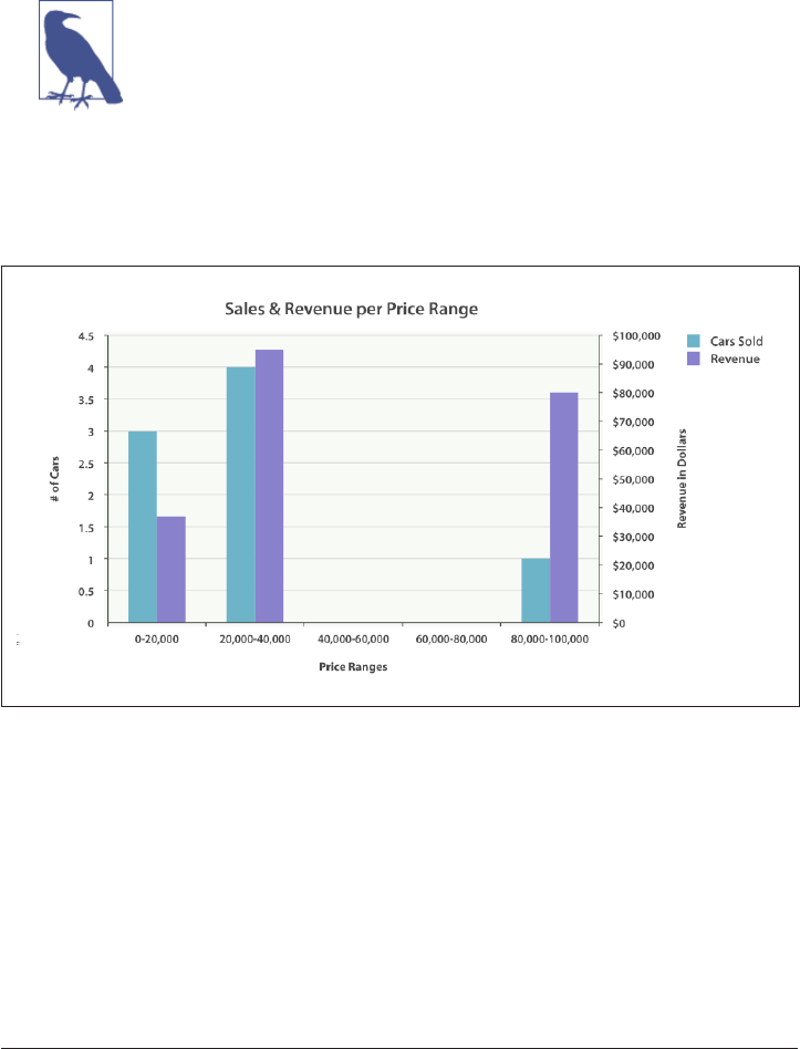
}
}
The response is fairly self-explanatory, but it should be noted that the histogram keys
correspond to the lower boundary of the interval. The key 0 means 0-19,999, the key
20000 means 20,000-39,999, and so forth.
You’ll notice that empty intervals, such as $40,000-60,000, is miss‐
ing in the response. The histogram bucket omits these by default,
since it could lead to the unintended generation of potentially
enormous output.
We’ll discuss how to include empty buckets in the next section,
“Returning Empty Buckets” on page 439.
Graphically, you could represent the preceding data in the histogram shown in
Figure 27-1.
Figure 27-1. Sales and Revenue per price bracket
Of course, you can build bar charts with any aggregation that emits categories and
statistics, not just the histogram bucket. Let’s build a bar chart of popular makes, and
their average price, and then calculate the standard error to add error bars on our
chart. This will use the terms bucket and an extended_stats metric:
GET /cars/transactions/_search?search_type=count
{
"aggs": {
"makes": {
"terms": {
Building Bar Charts | 435

"field": "make",
"size": 10
},
"aggs": {
"stats": {
"extended_stats": {
"field": "price"
}
}
}
}
}
}
This will return a list of makes (sorted by popularity) and a variety of statistics about
each. In particular, we are interested in stats.avg, stats.count, and
stats.std_deviation. Using this information, we can calculate the standard error:
std_err = std_deviation / count
This will allow us to build a chart like Figure 27-2.
Figure 27-2. Average price of all makes, with error bars
436 | Chapter 27: Building Bar Charts

CHAPTER 28
Looking at Time
If search is the most popular activity in Elasticsearch, building date histograms must
be the second most popular. Why would you want to use a date histogram?
Imagine your data has a timestamp. It doesn’t matter what the data is—Apache log
events, stock buy/sell transaction dates, baseball game times—anything with a time‐
stamp can benefit from the date histogram. When you have a timestamp, you often
want to build metrics that are expressed over time:
• How many cars sold each month this year?
• What was the price of this stock for the last 12 hours?
• What was the average latency of our website every hour in the last week?
While regular histograms are often represented as bar charts, date histograms tend to
be converted into line graphs representing time series. Many companies use Elastic‐
search solely for analytics over time series data. The date_histogram bucket is their
bread and butter.
The date_histogram bucket works similarly to the regular histogram. Rather than
building buckets based on a numeric field representing numeric ranges, it builds
buckets based on time ranges. Each bucket is therefore defined as a certain calendar
size (for example, 1 month or 2.5 days).
437

Can a Regular Histogram Work with Dates?
Technically, yes. A regular histogram bucket will work with dates. However, it is not
calendar-aware. With the date_histogram, you can specify intervals such as 1 month,
which knows that February is shorter than December. The date_histogram also has
the advantage of being able to work with time zones, which allows you to customize
graphs to the time zone of the user, not the server.
The regular histogram will interpret dates as numbers, which means you must specify
intervals in terms of milliseconds. And the aggregation doesn’t know about calendar
intervals, which makes it largely useless for dates.
Our first example will build a simple line chart to answer this question: how many
cars were sold each month?
GET /cars/transactions/_search?search_type=count
{
"aggs": {
"sales": {
"date_histogram": {
"field": "sold",
"interval": "month",
"format": "yyyy-MM-dd"
}
}
}
}
The interval is requested in calendar terminology (for example, one month per
bucket).
We provide a date format so that bucket keys are pretty.
Our query has a single aggregation, which builds a bucket per month. This will give
us the number of cars sold in each month. An additional format parameter is pro‐
vided so the buckets have “pretty” keys. Internally, dates are simply represented as a
numeric value. This tends to make UI designers grumpy, however, so a prettier for‐
mat can be specified using common date formatting.
The response is both expected and a little surprising (see if you can spot the surprise):
{
...
"aggregations": {
"sales": {
"buckets": [
{
438 | Chapter 28: Looking at Time

"key_as_string": "2014-01-01",
"key": 1388534400000,
"doc_count": 1
},
{
"key_as_string": "2014-02-01",
"key": 1391212800000,
"doc_count": 1
},
{
"key_as_string": "2014-05-01",
"key": 1398902400000,
"doc_count": 1
},
{
"key_as_string": "2014-07-01",
"key": 1404172800000,
"doc_count": 1
},
{
"key_as_string": "2014-08-01",
"key": 1406851200000,
"doc_count": 1
},
{
"key_as_string": "2014-10-01",
"key": 1412121600000,
"doc_count": 1
},
{
"key_as_string": "2014-11-01",
"key": 1414800000000,
"doc_count": 2
}
]
...
}
The aggregation is represented in full. As you can see, we have buckets that represent
months, a count of docs in each month, and our pretty key_as_string.
Returning Empty Buckets
Notice something odd about that last response?
Yep, that’s right. We are missing a few months! By default, the date_histogram (and
histogram too) returns only buckets that have a nonzero document count.
This means your histogram will be a minimal response. Often, this is not the behav‐
ior you want. For many applications, you would like to dump the response directly
into a graphing library without doing any post-processing.
Returning Empty Buckets | 439

Essentially, we want buckets even if they have a count of zero. We can set two addi‐
tional parameters that will provide this behavior:
GET /cars/transactions/_search?search_type=count
{
"aggs": {
"sales": {
"date_histogram": {
"field": "sold",
"interval": "month",
"format": "yyyy-MM-dd",
"min_doc_count" : 0,
"extended_bounds" : {
"min" : "2014-01-01",
"max" : "2014-12-31"
}
}
}
}
}
This parameter forces empty buckets to be returned.
This parameter forces the entire year to be returned.
The two additional parameters will force the response to return all months in the
year, regardless of their doc count. The min_doc_count is very understandable: it
forces buckets to be returned even if they are empty.
The extended_bounds parameter requires a little explanation. The min_doc_count
parameter forces empty buckets to be returned, but by default Elasticsearch will
return only buckets that are between the minimum and maximum value in your data.
So if your data falls between April and July, you’ll have buckets representing only
those months (empty or otherwise). To get the full year, we need to tell Elasticsearch
that we want buckets even if they fall before the minimum value or aer the maxi‐
mum value.
The extended_bounds parameter does just that. Once you add those two settings,
you’ll get a response that is easy to plug straight into your graphing libraries and give
you a graph like Figure 28-1.
440 | Chapter 28: Looking at Time

Figure 28-1. Cars sold over time
Extended Example
Just as we’ve seen a dozen times already, buckets can be nested in buckets for more-
sophisticated behavior. For illustration, we’ll build an aggregation that shows the total
sum of prices for all makes, listed by quarter. Let’s also calculate the sum of prices per
individual make per quarter, so we can see which car type is bringing in the most
money to our business:
GET /cars/transactions/_search?search_type=count
{
"aggs": {
"sales": {
"date_histogram": {
"field": "sold",
"interval": "quarter",
"format": "yyyy-MM-dd",
"min_doc_count" : 0,
"extended_bounds" : {
"min" : "2014-01-01",
"max" : "2014-12-31"
}
},
"aggs": {
"per_make_sum": {
"terms": {
"field": "make"
},
Extended Example | 441

"aggs": {
"sum_price": {
"sum": { "field": "price" }
}
}
},
"total_sum": {
"sum": { "field": "price" }
}
}
}
}
}
Note that we changed the interval from month to quarter.
Calculate the sum per make.
And the total sum of all makes combined together.
This returns a (heavily truncated) response:
{
....
"aggregations": {
"sales": {
"buckets": [
{
"key_as_string": "2014-01-01",
"key": 1388534400000,
"doc_count": 2,
"total_sum": {
"value": 105000
},
"per_make_sum": {
"buckets": [
{
"key": "bmw",
"doc_count": 1,
"sum_price": {
"value": 80000
}
},
{
"key": "ford",
"doc_count": 1,
"sum_price": {
"value": 25000
}
}
]
}
442 | Chapter 28: Looking at Time
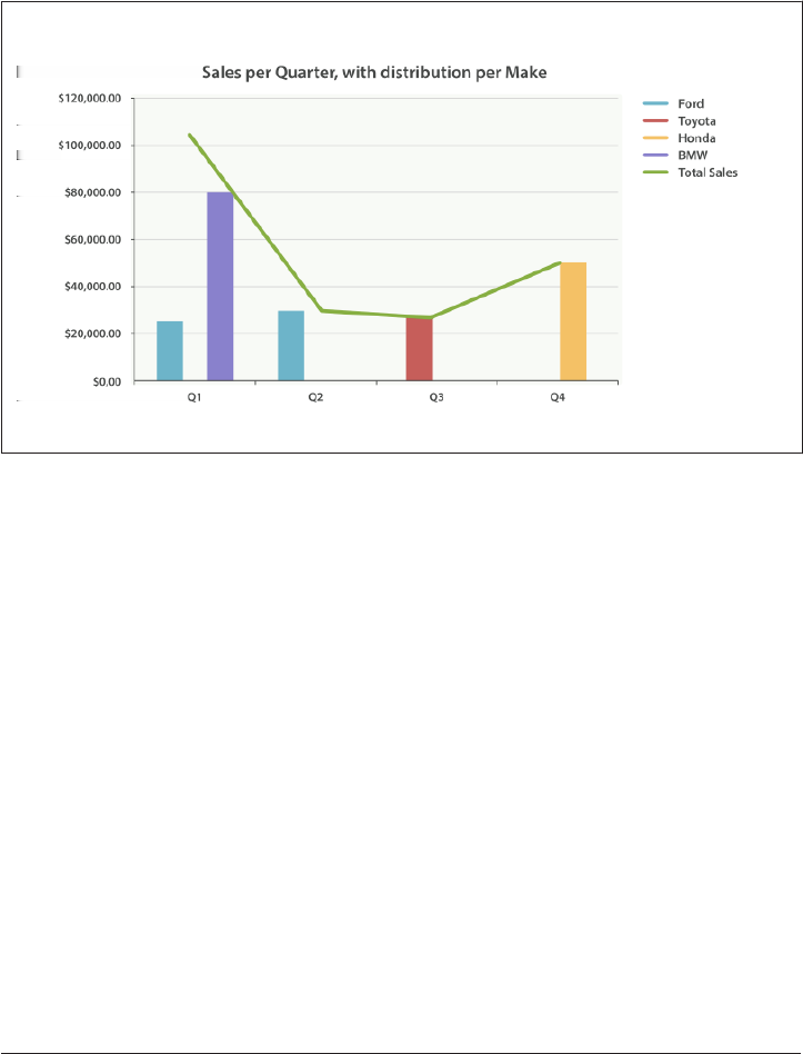
},
...
}
We can take this response and put it into a graph, showing a line chart for total sale
price, and a bar chart for each individual make (per quarter), as shown in
Figure 28-2.
Figure 28-2. Sales per quarter, with distribution per make
The Sky’s the Limit
These were obviously simple examples, but the sky really is the limit when it comes to
charting aggregations. For example, Figure 28-3 shows a dashboard in Kibana built
with a variety of aggregations.
The Sky’s the Limit | 443

Figure 28-3. Kibana—a real time analytics dashboard built with aggregations
Because of the real-time nature of aggregations, dashboards like this are easy to
query, manipulate, and interact with. This makes them ideal for nontechnical
employees and analysts who need to analyze the data but cannot build a Hadoop job.
To build powerful dashboards like Kibana, however, you’ll likely need some of the
more advanced concepts such as scoping, filtering, and sorting aggregations.
444 | Chapter 28: Looking at Time

CHAPTER 29
Scoping Aggregations
With all of the aggregation examples given so far, you may have noticed that we omit‐
ted a query from the search request. The entire request was simply an aggregation.
Aggregations can be run at the same time as search requests, but you need to under‐
stand a new concept: scope. By default, aggregations operate in the same scope as the
query. Put another way, aggregations are calculated on the set of documents that
match your query.
Let’s look at one of our first aggregation examples:
GET /cars/transactions/_search?search_type=count
{
"aggs" : {
"colors" : {
"terms" : {
"field" : "color"
}
}
}
}
You can see that the aggregation is in isolation. In reality, Elasticsearch assumes “no
query specified” is equivalent to “query all documents.” The preceding query is inter‐
nally translated as follows:
GET /cars/transactions/_search?search_type=count
{
"query" : {
"match_all" : {}
},
"aggs" : {
"colors" : {
"terms" : {
445

"field" : "color"
}
}
}
}
The aggregation always operates in the scope of the query, so an isolated aggregation
really operates in the scope of a match_all query—that is to say, all documents.
Once armed with the knowledge of scoping, we can start to customize aggregations
even further. All of our previous examples calculated statistics about all of the data:
top-selling cars, average price of all cars, most sales per month, and so forth.
With scope, we can ask questions such as “How many colors are Ford cars are avail‐
able in?” We do this by simply adding a query to the request (in this case a match
query):
GET /cars/transactions/_search
{
"query" : {
"match" : {
"make" : "ford"
}
},
"aggs" : {
"colors" : {
"terms" : {
"field" : "color"
}
}
}
}
We are omitting search_type=count so that search hits are returned too.
By omitting the search_type=count this time, we can see both the search results and
the aggregation results:
{
...
"hits": {
"total": 2,
"max_score": 1.6931472,
"hits": [
{
"_source": {
"price": 25000,
"color": "blue",
"make": "ford",
"sold": "2014-02-12"
}
},
446 | Chapter 29: Scoping Aggregations

{
"_source": {
"price": 30000,
"color": "green",
"make": "ford",
"sold": "2014-05-18"
}
}
]
},
"aggregations": {
"colors": {
"buckets": [
{
"key": "blue",
"doc_count": 1
},
{
"key": "green",
"doc_count": 1
}
]
}
}
}
This may seem trivial, but it is the key to advanced and powerful dashboards. You can
transform any static dashboard into a real-time data exploration device by adding a
search bar. This allows the user to search for terms and see all of the graphs (which
are powered by aggregations, and thus scoped to the query) update in real time. Try
that with Hadoop!
Global Bucket
You’ll often want your aggregation to be scoped to your query. But sometimes you’ll
want to search for a subset of data, but aggregate across all of your data.
For example, say you want to know the average price of Ford cars compared to the
average price of all cars. We can use a regular aggregation (scoped to the query) to get
the first piece of information. The second piece of information can be obtained by
using a global bucket.
The global bucket will contain all of your documents, regardless of the query scope;
it bypasses the scope completely. Because it is a bucket, you can nest aggregations
inside it as usual:
GET /cars/transactions/_search?search_type=count
{
"query" : {
"match" : {
"make" : "ford"
Scoping Aggregations | 447

}
},
"aggs" : {
"single_avg_price": {
"avg" : { "field" : "price" }
},
"all": {
"global" : {},
"aggs" : {
"avg_price": {
"avg" : { "field" : "price" }
}
}
}
}
}
This aggregation operates in the query scope (for example, all docs matching
ford)
The global bucket has no parameters.
This aggregation operates on the all documents, regardless of the make.
The single_avg_price metric calculation is based on all documents that fall under
the query scope—all ford cars. The avg_price metric is nested under a global
bucket, which means it ignores scoping entirely and calculates on all the documents.
The average returned for that aggregation represents the average price of all cars.
If you’ve made it this far in the book, you’ll recognize the mantra: use a filter wher‐
ever you can. The same applies to aggregations, and in the next chapter we show you
how to filter an aggregation instead of just limiting the query scope.
448 | Chapter 29: Scoping Aggregations

CHAPTER 30
Filtering Queries and Aggregations
A natural extension to aggregation scoping is filtering. Because the aggregation oper‐
ates in the context of the query scope, any filter applied to the query will also apply to
the aggregation.
Filtered Query
If we want to find all cars over $10,000 and also calculate the average price for those
cars, we can simply use a filtered query:
GET /cars/transactions/_search?search_type=count
{
"query" : {
"filtered": {
"filter": {
"range": {
"price": {
"gte": 10000
}
}
}
}
},
"aggs" : {
"single_avg_price": {
"avg" : { "field" : "price" }
}
}
}
Fundamentally, using a filtered query is no different from using a match query, as
we discussed in the previous chapter. The query (which happens to include a filter)
449

returns a certain subset of documents, and the aggregation operates on those docu‐
ments.
Filter Bucket
But what if you would like to filter just the aggregation results? Imagine we are build‐
ing the search page for our car dealership. We want to display search results accord‐
ing to what the user searches for. But we also want to enrich the page by including the
average price of cars (matching the search) that were sold in the last month.
We can’t use simple scoping here, since there are two different criteria. The search
results must match ford, but the aggregation results must match ford AND sold >
now - 1M.
To solve this problem, we can use a special bucket called filter. You specify a filter,
and when documents match the filter’s criteria, they are added to the bucket.
Here is the resulting query:
GET /cars/transactions/_search?search_type=count
{
"query":{
"match": {
"make": "ford"
}
},
"aggs":{
"recent_sales": {
"filter": {
"range": {
"sold": {
"from": "now-1M"
}
}
},
"aggs": {
"average_price":{
"avg": {
"field": "price"
}
}
}
}
}
}
Using the filter bucket to apply a filter in addition to the query scope.
450 | Chapter 30: Filtering Queries and Aggregations

This avg metric will therefore average only docs that are both ford and sold in
the last month.
Since the filter bucket operates like any other bucket, you are free to nest other
buckets and metrics inside. All nested components will “inherit” the filter. This allows
you to filter selective portions of the aggregation as required.
Post Filter
So far, we have a way to filter both the search results and aggregations (a filtered
query), as well as filtering individual portions of the aggregation (filter bucket).
You may be thinking to yourself, “hmm…is there a way to filter just the search results
but not the aggregation?” The answer is to use a post_filter.
This is a top-level search-request element that accepts a filter. The filter is applied
aer the query has executed (hence the post moniker: it runs post query execution).
Because it operates after the query has executed, it does not affect the query scope—
and thus does not affect the aggregations either.
We can use this behavior to apply additional filters to our search criteria that don’t
affect things like categorical facets in your UI. Let’s design another search page for
our car dealer. This page will allow the user to search for a car and filter by color.
Color choices are populated via an aggregation:
GET /cars/transactions/_search?search_type=count
{
"query": {
"match": {
"make": "ford"
}
},
"post_filter": {
"term" : {
"color" : "green"
}
},
"aggs" : {
"all_colors": {
"terms" : { "field" : "color" }
}
}
}
The post_filter element is a top-level element and filters just the search hits.
Post Filter | 451

The query portion is finding all ford cars. We are then building a list of colors with a
terms aggregation. Because aggregations operate in the query scope, the list of colors
will correspond with the colors that Ford cars are painted.
Finally, the post_filter will filter the search results to show only green ford cars.
This happens aer the query is executed, so the aggregations are unaffected.
This is often important for coherent UIs. Imagine that a user clicks a category in your
UI (for example, green). The expectation is that the search results are filtered, but not
the UI options. If you applied a filtered query, the UI would instantly transform to
show only green as an option—not what the user wants!
Performance consideration
Use a post_filter only if you need to differentially filter search
results and aggregations. Sometimes people will use post_filter
for regular searches.
Don’t do this! The nature of the post_filter means it runs aer
the query, so any performance benefit of filtering (such as caches)
is lost completely.
The post_filter should be used only in combination with aggre‐
gations, and only when you need differential filtering.
Recap
Choosing the appropriate type of filtering—search hits, aggregations, or both—often
boils down to how you want your user interface to behave. Choose the appropriate
filter (or combinations) depending on how you want to display results to your user.
• A filtered query affects both search results and aggregations.
• A filter bucket affects just aggregations.
• A post_filter affects just search results.
452 | Chapter 30: Filtering Queries and Aggregations

CHAPTER 31
Sorting Multivalue Buckets
Multivalue buckets—the terms, histogram, and date_histogram—dynamically pro‐
duce many buckets. How does Elasticsearch decide the order that these buckets are
presented to the user?
By default, buckets are ordered by doc_count in descending order. This is a good
default because often we want to find the documents that maximize some criteria:
price, population, frequency. But sometimes you’ll want to modify this sort order, and
there are a few ways to do it, depending on the bucket.
Intrinsic Sorts
These sort modes are intrinsic to the bucket: they operate on data that bucket gener‐
ates, such as doc_count. They share the same syntax but differ slightly depending on
the bucket being used.
Let’s perform a terms aggregation but sort by doc_count, in ascending order:
GET /cars/transactions/_search?search_type=count
{
"aggs" : {
"colors" : {
"terms" : {
"field" : "color",
"order": {
"_count" : "asc"
}
}
}
}
}
453

Using the _count keyword, we can sort by doc_count, in ascending order.
We introduce an order object into the aggregation, which allows us to sort on one of
several values:
_count
Sort by document count. Works with terms, histogram, date_histogram.
_term
Sort by the string value of a term alphabetically. Works only with terms.
_key
Sort by the numeric value of each bucket’s key (conceptually similar to _term).
Works only with histogram and date_histogram.
Sorting by a Metric
Often, you’ll find yourself wanting to sort based on a metric’s calculated value. For
our car sales analytics dashboard, we may want to build a bar chart of sales by car
color, but order the bars by the average price, ascending.
We can do this by adding a metric to our bucket, and then referencing that metric
from the order parameter:
GET /cars/transactions/_search?search_type=count
{
"aggs" : {
"colors" : {
"terms" : {
"field" : "color",
"order": {
"avg_price" : "asc"
}
},
"aggs": {
"avg_price": {
"avg": {"field": "price"}
}
}
}
}
}
The average price is calculated for each bucket.
Then the buckets are ordered by the calculated average in ascending order.
454 | Chapter 31: Sorting Multivalue Buckets

This lets you override the sort order with any metric, simply by referencing the name
of the metric. Some metrics, however, emit multiple values. The extended_stats
metric is a good example: it provides half a dozen individual metrics.
If you want to sort on a multivalue metric, you just need to use the dot-path to the
metric of interest:
GET /cars/transactions/_search?search_type=count
{
"aggs" : {
"colors" : {
"terms" : {
"field" : "color",
"order": {
"stats.variance" : "asc"
}
},
"aggs": {
"stats": {
"extended_stats": {"field": "price"}
}
}
}
}
}
Using dot notation, we can sort on the metric we are interested in.
In this example we are sorting on the variance of each bucket, so that colors with the
least variance in price will appear before those that have more variance.
Sorting Based on “Deep” Metrics
In the prior examples, the metric was a direct child of the bucket. An average price
was calculated for each term. It is possible to sort on deeper metrics, which are grand‐
children or great-grandchildren of the bucket—with some limitations.
You can define a path to a deeper, nested metric by using angle brackets (>), like so:
my_bucket>another_bucket>metric.
The caveat is that each nested bucket in the path must be a single-value bucket. A
filter bucket produces a single bucket: all documents that match the filtering crite‐
ria. Multivalue buckets (such as terms) generate many dynamic buckets, which
makes it impossible to specify a deterministic path.
Currently, there are only three single-value buckets: filter, global, and
reverse_nested. As a quick example, let’s build a histogram of car prices, but order
the buckets by the variance in price of red and green (but not blue) cars in each price
range:
Sorting Based on “Deep” Metrics | 455

GET /cars/transactions/_search?search_type=count
{
"aggs" : {
"colors" : {
"histogram" : {
"field" : "price",
"interval": 20000,
"order": {
"red_green_cars>stats.variance" : "asc"
}
},
"aggs": {
"red_green_cars": {
"filter": { "terms": {"color": ["red", "green"]}},
"aggs": {
"stats": {"extended_stats": {"field" : "price"}}
}
}
}
}
}
}
Sort the buckets generated by the histogram according to the variance of a nested
metric.
Because we are using a single-value filter, we can use nested sorting.
Sort on the stats generated by this metric.
In this example, you can see that we are accessing a nested metric. The stats metric
is a child of red_green_cars, which is in turn a child of colors. To sort on that met‐
ric, we define the path as red_green_cars>stats.variance. This is allowed because
the filter bucket is a single-value bucket.
456 | Chapter 31: Sorting Multivalue Buckets

CHAPTER 32
Approximate Aggregations
Life is easy if all your data fits on a single machine. Classic algorithms taught in
CS201 will be sufficient for all your needs. But if all your data fits on a single
machine, there would be no need for distributed software like Elasticsearch at all. But
once you start distributing data, algorithm selection needs to be made carefully.
Some algorithms are amenable to distributed execution. All of the aggregations dis‐
cussed thus far execute in a single pass and give exact results. These types of algo‐
rithms are often referred to as embarrassingly parallel, because they parallelize to
multiple machines with little effort. When performing a max metric, for example, the
underlying algorithm is very simple:
1. Broadcast the request to all shards.
2. Look at the price field for each document. If price > current_max, replace cur
rent_max with price.
3. Return the maximum price from all shards to the coordinating node.
4. Find the maximum price returned from all shards. This is the true maximum.
The algorithm scales linearly with machines because the algorithm requires no coor‐
dination (the machines don’t need to discuss intermediate results), and the memory
footprint is very small (a single integer representing the maximum).
Not all algorithms are as simple as taking the maximum value, unfortunately. More
complex operations require algorithms that make conscious trade-offs in perfor‐
mance and memory utilization. There is a triangle of factors at play: big data, exact‐
ness, and real-time latency.
You get to choose two from this triangle:
457

Exact + real time
Your data fits in the RAM of a single machine. The world is your oyster; use any
algorithm you want. Results will be 100% accurate and relatively fast.
Big data + exact
A classic Hadoop installation. Can handle petabytes of data and give you exact
answers—but it may take a week to give you that answer.
Big data + real time
Approximate algorithms that give you accurate, but not exact, results.
Elasticsearch currently supports two approximate algorithms (cardinality and per
centiles). These will give you accurate results, but not 100% exact. In exchange for a
little bit of estimation error, these algorithms give you fast execution and a small
memory footprint.
For most domains, highly accurate results that return in real time across all your data
is more important than 100% exactness. At first blush, this may be an alien concept to
you. “We need exact answers!” you may yell. But consider the implications of a 0.5%
error:
• The true 99th percentile of latency for your website is 132ms.
• An approximation with 0.5% error will be within +/- 0.66ms of 132ms.
• The approximation returns in milliseconds, while the “true” answer may take sec‐
onds, or be impossible.
For simply checking on your website’s latency, do you care if the approximate answer
is 132.66ms instead of 132ms? Certainly, not all domains can tolerate approximations
—but the vast majority will have no problem. Accepting an approximate answer is
more often a cultural hurdle rather than a business or technical imperative.
Finding Distinct Counts
The first approximate aggregation provided by Elasticsearch is the cardinality met‐
ric. This provides the cardinality of a field, also called a distinct or unique count. You
may be familiar with the SQL version:
SELECT DISTINCT(color)
FROM cars
Distinct counts are a common operation, and answer many fundamental business
questions:
• How many unique visitors have come to my website?
• How many unique cars have we sold?
458 | Chapter 32: Approximate Aggregations

• How many distinct users purchased a product each month?
We can use the cardinality metric to determine the number of car colors being sold
at our dealership:
GET /cars/transactions/_search?search_type=count
{
"aggs" : {
"distinct_colors" : {
"cardinality" : {
"field" : "color"
}
}
}
}
This returns a minimal response showing that we have sold three different-colored
cars:
...
"aggregations": {
"distinct_colors": {
"value": 3
}
}
...
We can make our example more useful: how many colors were sold each month? For
that metric, we just nest the cardinality metric under a date_histogram:
GET /cars/transactions/_search?search_type=count
{
"aggs" : {
"months" : {
"date_histogram": {
"field": "sold",
"interval": "month"
},
"aggs": {
"distinct_colors" : {
"cardinality" : {
"field" : "color"
}
}
}
}
}
}
Finding Distinct Counts | 459

Understanding the Trade-os
As mentioned at the top of this chapter, the cardinality metric is an approximate
algorithm. It is based on the HyperLogLog++ (HLL) algorithm. HLL works by hash‐
ing your input and using the bits from the hash to make probabilistic estimations on
the cardinality.
You don’t need to understand the technical details (although if you’re interested, the
paper is a great read!), but you should be aware of the properties of the algorithm:
•Configurable precision, which controls memory usage (more precise == more
memory).
• Excellent accuracy on low-cardinality sets.
•Fixed memory usage. Whether there are thousands or billions of unique values,
memory usage depends on only the configured precision.
To configure the precision, you must specify the precision_threshold parameter.
This threshold defines the point under which cardinalities are expected to be very
close to accurate. Consider this example:
GET /cars/transactions/_search?search_type=count
{
"aggs" : {
"distinct_colors" : {
"cardinality" : {
"field" : "color",
"precision_threshold" : 100
}
}
}
}
precision_threshold accepts a number from 0–40,000. Larger values are treated
as equivalent to 40,000.
This example will ensure that fields with 100 or fewer distinct values will be extremely
accurate. Although not guaranteed by the algorithm, if a cardinality is under the
threshold, it is almost always 100% accurate. Cardinalities above this will begin to
trade accuracy for memory savings, and a little error will creep into the metric.
For a given threshold, the HLL data-structure will use about precision_threshold *
8 bytes of memory. So you must balance how much memory you are willing to sacri‐
fice for additional accuracy.
Practically speaking, a threshold of 100 maintains an error under 5% even when
counting millions of unique values.
460 | Chapter 32: Approximate Aggregations

Optimizing for Speed
If you want a distinct count, you usually want to query your entire dataset (or nearly
all of it). Any operation on all your data needs to execute quickly, for obvious reasons.
HyperLogLog is very fast already—it simply hashes your data and does some bit-
twiddling.
But if speed is important to you, we can optimize it a little bit further. Since HLL sim‐
ply needs the hash of the field, we can precompute that hash at index time. When the
query executes, we can skip the hash computation and load the value directly out of
fielddata.
Precomputing hashes is useful only on very large and/or high-
cardinality fields. Calculating the hash on these fields is non-
negligible at query time.
However, numeric fields hash very quickly, and storing the original
numeric often requires the same (or less) memory. This is also true
on low-cardinality string fields; there are internal optimizations
that guarantee that hashes are calculated only once per unique
value.
Basically, precomputing hashes is not guaranteed to make all fields
faster — only those that have high cardinality and/or large strings.
And remember, precomputing simply shifts the cost to index time.
You still pay the price; you just choose when to pay it.
To do this, we need to add a new multifield to our data. We’ll delete our index, add a
new mapping that includes the hashed field, and then reindex:
DELETE /cars/
PUT /cars/
{
"mappings": {
"color": {
"type": "string",
"fields": {
"hash": {
"type": "murmur3"
}
}
}
}
}
POST /cars/transactions/_bulk
{ "index": {}}
{ "price" : 10000, "color" : "red", "make" : "honda", "sold" : "2014-10-28" }
Finding Distinct Counts | 461

{ "index": {}}
{ "price" : 20000, "color" : "red", "make" : "honda", "sold" : "2014-11-05" }
{ "index": {}}
{ "price" : 30000, "color" : "green", "make" : "ford", "sold" : "2014-05-18" }
{ "index": {}}
{ "price" : 15000, "color" : "blue", "make" : "toyota", "sold" : "2014-07-02" }
{ "index": {}}
{ "price" : 12000, "color" : "green", "make" : "toyota", "sold" : "2014-08-19" }
{ "index": {}}
{ "price" : 20000, "color" : "red", "make" : "honda", "sold" : "2014-11-05" }
{ "index": {}}
{ "price" : 80000, "color" : "red", "make" : "bmw", "sold" : "2014-01-01" }
{ "index": {}}
{ "price" : 25000, "color" : "blue", "make" : "ford", "sold" : "2014-02-12" }
This multifield is of type murmur3, which is a hashing function.
Now when we run an aggregation, we use the color.hash field instead of the color
field:
GET /cars/transactions/_search?search_type=count
{
"aggs" : {
"distinct_colors" : {
"cardinality" : {
"field" : "color.hash"
}
}
}
}
Notice that we specify the hashed multifield, rather than the original.
Now the cardinality metric will load the values (the precomputed hashes) from
"color.hash" and use those in place of dynamically hashing the original value.
The savings per document is small, but if hashing each field adds 10 nanoseconds and
your aggregation touches 100 million documents, that adds 1 second per query. If you
find yourself using cardinality across many documents, perform some profiling to
see if precomputing hashes makes sense for your deployment.
Calculating Percentiles
The other approximate metric offered by Elasticsearch is the percentiles metric.
Percentiles show the point at which a certain percentage of observed values occur. For
example, the 95th percentile is the value that is greater than 95% of the data.
Percentiles are often used to find outliers. In (statistically) normal distributions, the
0.13th and 99.87th percentiles represent three standard deviations from the mean.
462 | Chapter 32: Approximate Aggregations

Any data that falls outside three standard deviations is often considered an anomaly
because it is so different from the average value.
To be more concrete, imagine that you are running a large website and it is your job
to guarantee fast response times to visitors. You must therefore monitor your website
latency to determine whether you are meeting your goal.
A common metric to use in this scenario is the average latency. But this is a poor
choice (despite being common), because averages can easily hide outliers. A median
metric also suffers the same problem. You could try a maximum, but this metric is
easily skewed by just a single outlier.
This graph in Figure 32-1 visualizes the problem. If you rely on simple metrics like
mean or median, you might see a graph that looks like Figure 32-1.
Figure 32-1. Average request latency over time
Everything looks fine. There is a slight bump, but nothing to be concerned about. But
if we load up the 99th percentile (the value that accounts for the slowest 1% of laten‐
cies), we see an entirely different story, as shown in Figure 32-2.
Calculating Percentiles | 463

Figure 32-2. Average request latency with 99th percentile over time
Whoa! At 9:30 a.m., the mean is only 75ms. As a system administrator, you wouldn’t
look at this value twice. Everything normal! But the 99th percentile is telling you that
1% of your customers are seeing latency in excess of 850ms—a very different story.
There is also a smaller spike at 4:48 a.m. that wasn’t even noticeable in the mean/
median.
This is just one use-case for a percentile. Percentiles can also be used to quickly eye‐
ball the distribution of data, check for skew or bimodalities, and more.
Percentile Metric
Let’s load a new dataset (the car data isn’t going to work well for percentiles). We are
going to index a bunch of website latencies and run a few percentiles over it:
POST /website/logs/_bulk
{ "index": {}}
{ "latency" : 100, "zone" : "US", "timestamp" : "2014-10-28" }
{ "index": {}}
{ "latency" : 80, "zone" : "US", "timestamp" : "2014-10-29" }
{ "index": {}}
{ "latency" : 99, "zone" : "US", "timestamp" : "2014-10-29" }
{ "index": {}}
{ "latency" : 102, "zone" : "US", "timestamp" : "2014-10-28" }
{ "index": {}}
{ "latency" : 75, "zone" : "US", "timestamp" : "2014-10-28" }
{ "index": {}}
{ "latency" : 82, "zone" : "US", "timestamp" : "2014-10-29" }
{ "index": {}}
464 | Chapter 32: Approximate Aggregations

{ "latency" : 100, "zone" : "EU", "timestamp" : "2014-10-28" }
{ "index": {}}
{ "latency" : 280, "zone" : "EU", "timestamp" : "2014-10-29" }
{ "index": {}}
{ "latency" : 155, "zone" : "EU", "timestamp" : "2014-10-29" }
{ "index": {}}
{ "latency" : 623, "zone" : "EU", "timestamp" : "2014-10-28" }
{ "index": {}}
{ "latency" : 380, "zone" : "EU", "timestamp" : "2014-10-28" }
{ "index": {}}
{ "latency" : 319, "zone" : "EU", "timestamp" : "2014-10-29" }
This data contains three values: a latency, a data center zone, and a date timestamp.
Let’s run percentiles over the whole dataset to get a feel for the distribution:
GET /website/logs/_search?search_type=count
{
"aggs" : {
"load_times" : {
"percentiles" : {
"field" : "latency"
}
},
"avg_load_time" : {
"avg" : {
"field" : "latency"
}
}
}
}
The percentiles metric is applied to the latency field.
For comparison, we also execute an avg metric on the same field.
By default, the percentiles metric will return an array of predefined percentiles: [1,
5, 25, 50, 75, 95, 99]. These represent common percentiles that people are inter‐
ested in—the extreme percentiles at either end of the spectrum, and a few in the mid‐
dle. In the response, we see that the fastest latency is around 75ms, while the slowest
is almost 600ms. In contrast, the average is sitting near 200ms, which is much less
informative:
...
"aggregations": {
"load_times": {
"values": {
"1.0": 75.55,
"5.0": 77.75,
"25.0": 94.75,
"50.0": 101,
"75.0": 289.75,
Calculating Percentiles | 465

"95.0": 489.34999999999985,
"99.0": 596.2700000000002
}
},
"avg_load_time": {
"value": 199.58333333333334
}
}
So there is clearly a wide distribution in latencies. Let’s see whether it is correlated to
the geographic zone of the data center:
GET /website/logs/_search?search_type=count
{
"aggs" : {
"zones" : {
"terms" : {
"field" : "zone"
},
"aggs" : {
"load_times" : {
"percentiles" : {
"field" : "latency",
"percents" : [50, 95.0, 99.0]
}
},
"load_avg" : {
"avg" : {
"field" : "latency"
}
}
}
}
}
}
First we separate our latencies into buckets, depending on their zone.
Then we calculate the percentiles per zone.
The percents parameter accepts an array of percentiles that we want returned,
since we are interested in only slow latencies.
From the response, we can see the EU zone is much slower than the US zone. On the
US side, the 50th percentile is very close to the 99th percentile—and both are close to
the average.
In contrast, the EU zone has a large difference between the 50th and 99th percentile.
It is now obvious that the EU zone is dragging down the latency statistics, and we
know that 50% of the EU zone is seeing 300ms+ latencies.
466 | Chapter 32: Approximate Aggregations

...
"aggregations": {
"zones": {
"buckets": [
{
"key": "eu",
"doc_count": 6,
"load_times": {
"values": {
"50.0": 299.5,
"95.0": 562.25,
"99.0": 610.85
}
},
"load_avg": {
"value": 309.5
}
},
{
"key": "us",
"doc_count": 6,
"load_times": {
"values": {
"50.0": 90.5,
"95.0": 101.5,
"99.0": 101.9
}
},
"load_avg": {
"value": 89.66666666666667
}
}
]
}
}
...
Percentile Ranks
There is another, closely related metric called percentile_ranks. The percentiles
metric tells you the lowest value below which a given percentage of documents fall.
For instance, if the 50th percentile is 119ms, then 50% of documents have values of
no more than 119ms. The percentile_ranks tells you which percentile a specific
value belongs to. The percentile_ranks of 119ms is the 50th percentile. It is basi‐
cally a two-way relationship. For example:
• The 50th percentile is 119ms.
• The 119ms percentile rank is the 50th percentile.
Calculating Percentiles | 467

So imagine that our website must maintain an SLA of 210ms response times or less.
And, just for fun, your boss has threatened to fire you if response times creep over
800ms. Understandably, you would like to know what percentage of requests are
actually meeting that SLA (and hopefully at least under 800ms!).
For this, you can apply the percentile_ranks metric instead of percentiles:
GET /website/logs/_search?search_type=count
{
"aggs" : {
"zones" : {
"terms" : {
"field" : "zone"
},
"aggs" : {
"load_times" : {
"percentile_ranks" : {
"field" : "latency",
"values" : [210, 800]
}
}
}
}
}
}
The percentile_ranks metric accepts an array of values that you want ranks for.
After running this aggregation, we get two values back:
"aggregations": {
"zones": {
"buckets": [
{
"key": "eu",
"doc_count": 6,
"load_times": {
"values": {
"210.0": 31.944444444444443,
"800.0": 100
}
}
},
{
"key": "us",
"doc_count": 6,
"load_times": {
"values": {
"210.0": 100,
"800.0": 100
}
}
468 | Chapter 32: Approximate Aggregations

}
]
}
}
This tells us three important things:
• In the EU zone, the percentile rank for 210ms is 31.94%.
• In the US zone, the percentile rank for 210ms is 100%.
• In both EU and US, the percentile rank for 800ms is 100%.
In plain english, this means that the EU zone is meeting the SLA only 32% of the
time, while the US zone is always meeting the SLA. But luckily for you, both zones
are under 800ms, so you won’t be fired (yet!).
The percentile_ranks metric provides the same information as percentiles, but
presented in a different format that may be more convenient if you are interested in
specific value(s).
Understanding the Trade-os
Like cardinality, calculating percentiles requires an approximate algorithm. The naive
implementation would maintain a sorted list of all values—but this clearly is not pos‐
sible when you have billions of values distributed across dozens of nodes.
Instead, percentiles uses an algorithm called TDigest (introduced by Ted Dunning
in Computing Extremely Accurate Quantiles Using T-Digests). As with HyperLo‐
gLog, it isn’t necessary to understand the full technical details, but it is good to know
the properties of the algorithm:
•Percentile accuracy is proportional to how extreme the percentile is. This means
that percentiles such as the 1st or 99th are more accurate than the 50th. This is
just a property of how the data structure works, but it happens to be a nice prop‐
erty, because most people care about extreme percentiles.
•For small sets of values, percentiles are highly accurate. If the dataset is small
enough, the percentiles may be 100% exact.
•As the quantity of values in a bucket grows, the algorithm begins to approximate
the percentiles. It is effectively trading accuracy for memory savings. The exact
level of inaccuracy is difficult to generalize, since it depends on your data distri‐
bution and volume of data being aggregated.
Similar to cardinality, you can control the memory-to-accuracy ratio by changing a
parameter: compression.
Calculating Percentiles | 469

The TDigest algorithm uses nodes to approximate percentiles: the more nodes avail‐
able, the higher the accuracy (and the larger the memory footprint) proportional to
the volume of data. The compression parameter limits the maximum number of
nodes to 20 * compression.
Therefore, by increasing the compression value, you can increase the accuracy of
your percentiles at the cost of more memory. Larger compression values also make
the algorithm slower since the underlying tree data structure grows in size, resulting
in more expensive operations. The default compression value is 100.
A node uses roughly 32 bytes of memory, so in a worst-case scenario (for example, a
large amount of data that arrives sorted and in order), the default settings will pro‐
duce a TDigest roughly 64KB in size. In practice, data tends to be more random, and
the TDigest will use less memory.
470 | Chapter 32: Approximate Aggregations

CHAPTER 33
Signicant Terms
The significant_terms (SigTerms) aggregation is rather different from the rest of
the aggregations. All the aggregations we have seen so far are essentially simple math
operations. By combining the various building blocks, you can build sophisticated
aggregations and reports about your data.
significant_terms has a different agenda. To some, it may even look a bit like
machine learning. The significant_terms aggregation finds uncommonly common
terms in your data-set.
What do we mean by uncommonly common? These are terms that are statistically
unusual — data that appears more frequently than the background rate would sug‐
gest. These statistical anomalies are usually indicative of something interesting in
your data.
For example, imagine you are in charge of detecting and tracking down credit card
fraud. Customers call and complain about unusual transactions appearing on their
credit card — their account has been compromised. These transactions are just symp‐
toms of a larger problem. Somewhere in the recent past, a merchant has either know‐
ingly stolen the customers’ credit card information, or has unknowingly been
compromised themselves.
Your job is to find the common point of compromise. If you have 100 customers com‐
plaining of unusual transactions, those customers likely share a single merchant—and
it is this merchant that is likely the source of blame.
Of course, it is a little more nuanced than just finding a merchant that all customers
share. For example, many of the customers will have large merchants like Amazon in
their recent transaction history. We can rule out Amazon, however, since many
uncompromised credit cards also have Amazon as a recent merchant.
471

This is an example of a commonly common merchant. Everyone, whether compro‐
mised or not, shares the merchant. This makes it of little interest to us.
On the opposite end of the spectrum, you have tiny merchants such as the corner
drug store. These are commonly uncommon—only one or two customers have trans‐
actions from the merchant. We can rule these out as well. Since all of the compro‐
mised cards did not interact with the merchant, we can be sure it was not to blame for
the security breach.
What we want are uncommonly common merchants. These are merchants that every
compromised card shares, but that are not well represented in the background noise
of uncompromised cards. These merchants are statistical anomalies; they appear
more frequently than they should. It is highly likely that these uncommonly common
merchants are to blame.
significant_terms aggregation does just this. It analyzes your data and finds terms
that appear with a frequency that is statistically anomalous compared to the back‐
ground data.
What you do with this statistical anomaly depends on the data. With the credit card
data, you might be looking for fraud. With ecommerce, you might be looking for an
unidentified demographic so you can market to them more efficiently. If you are ana‐
lyzing logs, you might find one server that throws a certain type of error more often
than it should. The applications of significant_terms is nearly endless.
signicant_terms Demo
Because the significant_terms aggregation works by analyzing statistics, you need
to have a certain threshold of data for it to become effective. That means we won’t be
able to index a small amount of example data for the demo.
Instead, we have a pre-prepared dataset of around 80,000 documents. This is saved as
a snapshot (for more information about snapshots and restore, see “Backing Up Your
Cluster” on page 655) in our public demo repository. You can “restore” this dataset
into your cluster by using these commands:
PUT /_snapshot/sigterms
{
"type": "url",
"settings": {
"url": "http://download.elasticsearch.org/definitiveguide/sigterms_demo/"
}
}
GET /_snapshot/sigterms/_all
POST /_snapshot/sigterms/snapshot/_restore
472 | Chapter 33: Signicant Terms

GET /mlmovies,mlratings/_recovery
Register a new read-only URL repository pointing at the demo snapshot
(Optional) Inspect the repository to learn details about available snapshots
Begin the Restore process. This will download two indices into your cluster: mlmo
vies and mlratings
(Optional) Monitor the Restore process using the Recovery API
The dataset is around 50 MB and may take some time to down‐
load.
In this demo, we are going to look at movie ratings by users of MovieLens. At Movie‐
Lens, users make movie recommendations so other users can find new movies to
watch. For this demo, we are going to recommend movies by using signifi
cant_terms based on an input movie.
Let’s take a look at some sample data, to get a feel for what we are working with.
There are two indices in this dataset, mlmovies and mlratings. Let’s look at mlmovies
first:
GET mlmovies/_search
{
"took": 4,
"timed_out": false,
"_shards": {...},
"hits": {
"total": 10681,
"max_score": 1,
"hits": [
{
"_index": "mlmovies",
"_type": "mlmovie",
"_id": "2",
"_score": 1,
"_source": {
"offset": 2,
"bytes": 34,
"title": "Jumanji (1995)"
}
},
....
signicant_terms Demo | 473

Execute a search without a query, so that we can see a random sampling of docs.
Each document in mlmovies represents a single movie. The two important pieces of
data are the _id of the movie and the title of the movie. You can ignore offset and
bytes; they are artifacts of the process used to extract this data from the original CSV
files. There are 10,681 movies in this dataset.
Now let’s look at mlratings:
GET mlratings/_search
{
"took": 3,
"timed_out": false,
"_shards": {...},
"hits": {
"total": 69796,
"max_score": 1,
"hits": [
{
"_index": "mlratings",
"_type": "mlrating",
"_id": "00IC-2jDQFiQkpD6vhbFYA",
"_score": 1,
"_source": {
"offset": 1,
"bytes": 108,
"movie": [122,185,231,292,
316,329,355,356,362,364,370,377,420,
466,480,520,539,586,588,589,594,616
],
"user": 1
}
},
...
Here we can see the recommendations of individual users. Each document represents
a single user, denoted by the user ID field. The movie field holds a list of movies that
this user watched and recommended.
Recommending Based on Popularity
The first strategy we could take is trying to recommend movies based on popularity.
Given a particular movie, we find all users who recommended that movie. Then we
aggregate all their recommendations and take the top five most popular.
We can express that easily with a terms aggregation and some filtering. Let’s look at
Talladega Nights, a comedy about NASCAR racing starring Will Ferrell. Ideally, our
recommender should find other comedies in a similar style (and more than likely also
starring Will Ferrell).
474 | Chapter 33: Signicant Terms

First we need to find the Talladega Nights ID:
GET mlmovies/_search
{
"query": {
"match": {
"title": "Talladega Nights"
}
}
}
...
"hits": [
{
"_index": "mlmovies",
"_type": "mlmovie",
"_id": "46970",
"_score": 3.658795,
"_source": {
"offset": 9575,
"bytes": 74,
"title": "Talladega Nights: The Ballad of Ricky Bobby (2006)"
}
},
...
Talladega Nights is ID 46970.
Armed with the ID, we can now filter the ratings and apply our terms aggregation to
find the most popular movies from people who also like Talladega Nights:
GET mlratings/_search?search_type=count
{
"query": {
"filtered": {
"filter": {
"term": {
"movie": 46970
}
}
}
},
"aggs": {
"most_popular": {
"terms": {
"field": "movie",
"size": 6
}
}
}
}
signicant_terms Demo | 475

We execute our query on mlratings this time, and specify search_type=count
since we are interested only in the aggregation results.
Apply a filter on the ID corresponding to Talladega Nights.
Finally, find the most popular movies by using a terms bucket.
We perform the search on the mlratings index, and apply a filter for the ID of Talla
dega Nights. Since aggregations operate on query scope, this will effectively filter the
aggregation results to only the users who recommended Talladega Nights. Finally, we
execute a terms aggregation to bucket the most popular movies. We are requesting
the top six results, since it is likely that Talladega Nights itself will be returned as a hit
(and we don’t want to recommend the same movie).
The results come back like so:
{
...
"aggregations": {
"most_popular": {
"buckets": [
{
"key": 46970,
"key_as_string": "46970",
"doc_count": 271
},
{
"key": 2571,
"key_as_string": "2571",
"doc_count": 197
},
{
"key": 318,
"key_as_string": "318",
"doc_count": 196
},
{
"key": 296,
"key_as_string": "296",
"doc_count": 183
},
{
"key": 2959,
"key_as_string": "2959",
"doc_count": 183
},
{
"key": 260,
"key_as_string": "260",
"doc_count": 90
476 | Chapter 33: Signicant Terms

}
]
}
}
...
We need to correlate these back to their original titles, which can be done with a sim‐
ple filtered query:
GET mlmovies/_search
{
"query": {
"filtered": {
"filter": {
"ids": {
"values": [2571,318,296,2959,260]
}
}
}
}
}
And finally, we end up with the following list:
1. Matrix, The
2. Shawshank Redemption
3. Pulp Fiction
4. Fight Club
5. Star Wars Episode IV: A New Hope
OK—well that is certainly a good list! I like all of those movies. But that’s the prob‐
lem: most everyone likes that list. Those movies are universally well-liked, which
means they are popular on everyone’s recommendations. The list is basically a recom‐
mendation of popular movies, not recommendations related to Talladega Nights.
This is easily verified by running the aggregation again, but without the filter on Tal
ladega Nights. This will give a top-five most popular movie list:
GET mlratings/_search?search_type=count
{
"aggs": {
"most_popular": {
"terms": {
"field": "movie",
"size": 5
}
}
}
}
signicant_terms Demo | 477

This returns a list that is very similar:
1. Shawshank Redemption
2. Silence of the Lambs, The
3. Pulp Fiction
4. Forrest Gump
5. Star Wars Episode IV: A New Hope
Clearly, just checking the most popular movies is not sufficient to build a good, dis‐
criminating recommender.
Recommending Based on Statistics
Now that the scene is set, let’s try using significant_terms. significant_terms will
analyze the group of people who enjoy Talladega Nights (the foreground group) and
determine what movies are most popular. It will then construct a list of popular films
for everyone (the background group) and compare the two.
The statistical anomalies will be the movies that are over-represented in the fore‐
ground compared to the background. Theoretically, this should be a list of comedies,
since people who enjoy Will Ferrell comedies will recommend them at a higher rate
than the background population of people.
Let’s give it a shot:
GET mlratings/_search?search_type=count
{
"query": {
"filtered": {
"filter": {
"term": {
"movie": 46970
}
}
}
},
"aggs": {
"most_sig": {
"significant_terms": {
"field": "movie",
"size": 6
}
}
}
}
The setup is nearly identical — we just use significant_terms instead of terms.
478 | Chapter 33: Signicant Terms

As you can see, the query is nearly the same. We filter for users who liked Talladega
Nights; this forms the foreground group. By default, significant_terms will use the
entire index as the background, so we don’t need to do anything special.
The results come back as a list of buckets similar to terms, but with some extra meta‐
data:
...
"aggregations": {
"most_sig": {
"doc_count": 271,
"buckets": [
{
"key": 46970,
"key_as_string": "46970",
"doc_count": 271,
"score": 256.549815498155,
"bg_count": 271
},
{
"key": 52245,
"key_as_string": "52245",
"doc_count": 59,
"score": 17.66462367106966,
"bg_count": 185
},
{
"key": 8641,
"key_as_string": "8641",
"doc_count": 107,
"score": 13.884387742677438,
"bg_count": 762
},
{
"key": 58156,
"key_as_string": "58156",
"doc_count": 17,
"score": 9.746428133759462,
"bg_count": 28
},
{
"key": 52973,
"key_as_string": "52973",
"doc_count": 95,
"score": 9.65770100311672,
"bg_count": 857
},
{
"key": 35836,
"key_as_string": "35836",
"doc_count": 128,
"score": 9.199001116457955,
signicant_terms Demo | 479

"bg_count": 1610
}
]
...
The top-level doc_count shows the number of docs in the foreground group.
Each bucket lists the key (for example, movie ID) being aggregated.
A doc_count for that bucket.
And a background count, which shows the rate at which this value appears in the
entire background.
You can see that the first bucket we get back is Talladega Nights. It is found in all 271
documents, which is not surprising. Let’s look at the next bucket: key 52245.
This ID corresponds to Blades of Glory, a comedy about male figure skating that also
stars Will Ferrell. We can see that it was recommended 59 times by the people who
also liked Talladega Nights. This means that 21% of the foreground group recom‐
mended Blades of Glory (59 / 271 = 0.2177).
In contrast, Blades of Glory was recommended only 185 times in the entire dataset,
which equates to a mere 0.26% (185 / 69796 = 0.00265). Blades of Glory is there‐
fore a statistical anomaly: it is uncommonly common in the group of people who like
Talladega Nights. We just found a good recommendation!
If we look at the entire list, they are all comedies that would fit as good recommenda‐
tions (many of which also star Will Ferrell):
1. Blades of Glory
2. Anchorman: The Legend of Ron Burgundy
3. Semi-Pro
4. Knocked Up
5. 40-Year-Old Virgin, The
This is just one example of the power of significant_terms. Once you start using
significant_terms, you find many situations where you don’t want the most popu‐
lar—you want the most uncommonly common. This simple aggregation can uncover
some surprisingly sophisticated trends in your data.
480 | Chapter 33: Signicant Terms

CHAPTER 34
Controlling Memory Use and Latency
Fielddata
Aggregations work via a data structure known as elddata (briefly introduced in
“Fielddata” on page 119). Fielddata is often the largest consumer of memory in an
Elasticsearch cluster, so it is important to understand how it works.
Fielddata can be loaded on the fly into memory, or built at index
time and stored on disk. Later, we will talk about on-disk fielddata
in “Doc Values” on page 493. For now we will focus on in-memory
fielddata, as it is currently the default mode of operation in Elastic‐
search. This may well change in a future version.
Fielddata exists because inverted indices are efficient only for certain operations. The
inverted index excels at finding documents that contain a term. It does not perform
well in the opposite direction: determining which terms exist in a single document.
Aggregations need this secondary access pattern.
Consider the following inverted index:
Term Doc_1 Doc_2 Doc_3
------------------------------------
brown | X | X |
dog | X | | X
dogs | | X | X
fox | X | | X
foxes | | X |
in | | X |
jumped | X | | X
lazy | X | X |
leap | | X |
over | X | X | X
481

quick | X | X | X
summer | | X |
the | X | | X
------------------------------------
If we want to compile a complete list of terms in any document that mentions brown,
we might build a query like so:
GET /my_index/_search
{
"query" : {
"match" : {
"body" : "brown"
}
},
"aggs" : {
"popular_terms": {
"terms" : {
"field" : "body"
}
}
}
}
The query portion is easy and efficient. The inverted index is sorted by terms, so first
we find brown in the terms list, and then scan across all the columns to see which
documents contain brown. We can very quickly see that Doc_1 and Doc_2 contain the
token brown.
Then, for the aggregation portion, we need to find all the unique terms in Doc_1 and
Doc_2. Trying to do this with the inverted index would be a very expensive process:
we would have to iterate over every term in the index and collect tokens from Doc_1
and Doc_2 columns. This would be slow and scale poorly: as the number of terms and
documents grows, so would the execution time.
Fielddata addresses this problem by inverting the relationship. While the inverted
index maps terms to the documents containing the term, fielddata maps documents
to the terms contained by the document:
Doc Terms
-----------------------------------------------------------------
Doc_1 | brown, dog, fox, jumped, lazy, over, quick, the
Doc_2 | brown, dogs, foxes, in, lazy, leap, over, quick, summer
Doc_3 | dog, dogs, fox, jumped, over, quick, the
-----------------------------------------------------------------
Once the data has been uninverted, it is trivial to collect the unique tokens from
Doc_1 and Doc_2. Go to the rows for each document, collect all the terms, and take
the union of the two sets.
482 | Chapter 34: Controlling Memory Use and Latency

The fielddata cache is per segment. In other words, when a new
segment becomes visible to search, the fielddata cached from old
segments remains valid. Only the data for the new segment needs
to be loaded into memory.
Thus, search and aggregations are closely intertwined. Search finds documents by
using the inverted index. Aggregations collect and aggregate values from fielddata,
which is itself generated from the inverted index.
The rest of this chapter covers various functionality that either decreases fielddata’s
memory footprint or increases execution speed.
Fielddata is not just used for aggregations. It is required for any
operation that needs to look up the value contained in a specific
document. Besides aggregations, this includes sorting, scripts that
access field values, parent-child relationships (see Chapter 42), and
certain types of queries or filters, such as the geo_distance filter.
Aggregations and Analysis
Some aggregations, such as the terms bucket, operate on string fields. And string
fields may be either analyzed or not_analyzed, which begs the question: how does
analysis affect aggregations?
The answer is “a lot,” but it is best shown through an example. First, index some
documents representing various states in the US:
POST /agg_analysis/data/_bulk
{ "index": {}}
{ "state" : "New York" }
{ "index": {}}
{ "state" : "New Jersey" }
{ "index": {}}
{ "state" : "New Mexico" }
{ "index": {}}
{ "state" : "New York" }
{ "index": {}}
{ "state" : "New York" }
We want to build a list of unique states in our dataset, complete with counts. Simple—
let’s use a terms bucket:
GET /agg_analysis/data/_search?search_type=count
{
"aggs" : {
"states" : {
"terms" : {
"field" : "state"
Aggregations and Analysis | 483

}
}
}
}
This gives us these results:
{
...
"aggregations": {
"states": {
"buckets": [
{
"key": "new",
"doc_count": 5
},
{
"key": "york",
"doc_count": 3
},
{
"key": "jersey",
"doc_count": 1
},
{
"key": "mexico",
"doc_count": 1
}
]
}
}
}
Oh dear, that’s not at all what we want! Instead of counting states, the aggregation is
counting individual words. The underlying reason is simple: aggregations are built
from the inverted index, and the inverted index is post-analysis.
When we added those documents to Elasticsearch, the string "New York" was ana‐
lyzed/tokenized into ["new", "york"]. These individual tokens were then used to
populate fielddata, and ultimately we see counts for new instead of New York.
This is obviously not the behavior that we wanted, but luckily it is easily corrected.
We need to define a multifield for state and set it to not_analyzed. This will prevent
New York from being analyzed, which means it will stay a single token in the aggrega‐
tion. Let’s try the whole process over, but this time specify a raw multifield:
DELETE /agg_analysis/
PUT /agg_analysis
{
"mappings": {
"data": {
484 | Chapter 34: Controlling Memory Use and Latency

"properties": {
"state" : {
"type": "string",
"fields": {
"raw" : {
"type": "string",
"index": "not_analyzed"
}
}
}
}
}
}
}
POST /agg_analysis/data/_bulk
{ "index": {}}
{ "state" : "New York" }
{ "index": {}}
{ "state" : "New Jersey" }
{ "index": {}}
{ "state" : "New Mexico" }
{ "index": {}}
{ "state" : "New York" }
{ "index": {}}
{ "state" : "New York" }
GET /agg_analysis/data/_search?search_type=count
{
"aggs" : {
"states" : {
"terms" : {
"field" : "state.raw"
}
}
}
}
This time we explicitly map the state field and include a not_analyzed sub-
field.
The aggregation is run on state.raw instead of state.
Now when we run our aggregation, we get results that make sense:
{
...
"aggregations": {
"states": {
"buckets": [
{
"key": "New York",
Aggregations and Analysis | 485

"doc_count": 3
},
{
"key": "New Jersey",
"doc_count": 1
},
{
"key": "New Mexico",
"doc_count": 1
}
]
}
}
}
In practice, this kind of problem is easy to spot. Your aggregations will simply return
strange buckets, and you’ll remember the analysis issue. It is a generalization, but
there are not many instances where you want to use an analyzed field in an aggrega‐
tion. When in doubt, add a multifield so you have the option for both.
High-Cardinality Memory Implications
There is another reason to avoid aggregating analyzed fields: high-cardinality fields
consume a large amount of memory when loaded into fielddata. The analysis process
often (although not always) generates a large number of tokens, many of which are
unique. This increases the overall cardinality of the field and contributes to more
memory pressure.
Some types of analysis are extremely unfriendly with regards to memory. Consider an
n-gram analysis process. The term New York might be n-grammed into the following
tokens:
•ne
•ew
•w
• y
•yo
•or
•rk
You can imagine how the n-gramming process creates a huge number of unique
tokens, especially when analyzing paragraphs of text. When these are loaded into
memory, you can easily exhaust your heap space.
486 | Chapter 34: Controlling Memory Use and Latency

So, before aggregating across fields, take a second to verify that the fields are not_ana
lyzed. And if you want to aggregate analyzed fields, ensure that the analysis process
is not creating an obscene number of tokens.
At the end of the day, it doesn’t matter whether a field is analyzed
or not_analyzed. The more unique values in a field—the higher
the cardinality of the field—the more memory that is required.
This is especially true for string fields, where every unique string
must be held in memory—longer strings use more memory.
Limiting Memory Usage
In order for aggregations (or any operation that requires access to field values) to be
fast, access to fielddata must be fast, which is why it is loaded into memory. But load‐
ing too much data into memory will cause slow garbage collections as the JVM tries
to find extra space in the heap, or possibly even an OutOfMemory exception.
It may surprise you to find that Elasticsearch does not load into fielddata just the val‐
ues for the documents that match your query. It loads the values for all documents in
your index, even documents with a different _type!
The logic is: if you need access to documents X, Y, and Z for this query, you will prob‐
ably need access to other documents in the next query. It is cheaper to load all values
once, and to keep them in memory, than to have to scan the inverted index on every
request.
The JVM heap is a limited resource that should be used wisely. A number of mecha‐
nisms exist to limit the impact of fielddata on heap usage. These limits are important
because abuse of the heap will cause node instability (thanks to slow garbage collec‐
tions) or even node death (with an OutOfMemory exception).
Choosing a Heap Size
There are two rules to apply when setting the Elasticsearch heap size, with the
$ES_HEAP_SIZE environment variable:
No more than 50% of available RAM
Lucene makes good use of the filesystem caches, which are managed by the ker‐
nel. Without enough filesystem cache space, performance will suffer.
No more than 32 GB: If the heap is less than 32 GB, the JVM can use compressed
pointers, which saves a lot of memory: 4 bytes per pointer instead of 8 bytes.
Limiting Memory Usage | 487

+ Increasing the heap from 32 GB to 34 GB would mean that you have much less
memory available, because all pointers are taking double the space. Also, with bigger
heaps, garbage collection becomes more costly and can result in node instability.
This limit has a direct impact on the amount of memory that can be devoted to field‐
data.
Fielddata Size
The indices.fielddata.cache.size controls how much heap space is allocated to
fielddata. When you run a query that requires access to new field values, it will load
the values into memory and then try to add them to fielddata. If the resulting field‐
data size would exceed the specified size, other values would be evicted in order to
make space.
By default, this setting is unbounded—Elasticsearch will never evict data from field‐
data.
This default was chosen deliberately: fielddata is not a transient cache. It is an in-
memory data structure that must be accessible for fast execution, and it is expensive
to build. If you have to reload data for every request, performance is going to be
awful.
A bounded size forces the data structure to evict data. We will look at when to set this
value, but first a warning:
This setting is a safeguard, not a solution for insufficient memory.
If you don’t have enough memory to keep your fielddata resident in
memory, Elasticsearch will constantly have to reload data from
disk, and evict other data to make space. Evictions cause heavy disk
I/O and generate a large amount of garbage in memory, which
must be garbage collected later on.
Imagine that you are indexing logs, using a new index every day. Normally you are
interested in data from only the last day or two. Although you keep older indices
around, you seldom need to query them. However, with the default settings, the field‐
data from the old indices is never evicted! fielddata will just keep on growing until
you trip the fielddata circuit breaker (see “Circuit Breaker” on page 490), which will
prevent you from loading any more fielddata.
At that point, you’re stuck. While you can still run queries that access fielddata from
the old indices, you can’t load any new values. Instead, we should evict old values to
make space for the new values.
488 | Chapter 34: Controlling Memory Use and Latency

To prevent this scenario, place an upper limit on the fielddata by adding this setting
to the config/elasticsearch.yml file:
indices.fielddata.cache.size: 40%
Can be set to a percentage of the heap size, or a concrete value like 5gb
With this setting in place, the least recently used fielddata will be evicted to make
space for newly loaded data.
There is another setting that you may see online: indices.field
data.cache.expire.
We beg that you never use this setting! It will likely be deprecated in
the future.
This setting tells Elasticsearch to evict values from fielddata if they
are older than expire, whether the values are being used or not.
This is terrible for performance. Evictions are costly, and this effec‐
tively schedules evictions on purpose, for no real gain.
There isn’t a good reason to use this setting; we literally cannot
theory-craft a hypothetically useful situation. It exists only for
backward compatibility at the moment. We mention the setting in
this book only since, sadly, it has been recommended in various
articles on the Internet as a good performance tip.
It is not. Never use it!
Monitoring elddata
It is important to keep a close watch on how much memory is being used by fielddata,
and whether any data is being evicted. High eviction counts can indicate a serious
resource issue and a reason for poor performance.
Fielddata usage can be monitored:
• per-index using the indices-stats API:
GET /_stats/fielddata?fields=*
• per-node using the nodes-stats API:
GET /_nodes/stats/indices/fielddata?fields=*
• Or even per-index per-node:
GET /_nodes/stats/indices/fielddata?level=indices&fields=*
By setting ?fields=*, the memory usage is broken down for each field.
Limiting Memory Usage | 489

Circuit Breaker
An astute reader might have noticed a problem with the fielddata size settings. field‐
data size is checked aer the data is loaded. What happens if a query arrives that tries
to load more into fielddata than available memory? The answer is ugly: you would get
an OutOfMemoryException.
Elasticsearch includes a elddata circuit breaker that is designed to deal with this sit‐
uation. The circuit breaker estimates the memory requirements of a query by intro‐
specting the fields involved (their type, cardinality, size, and so forth). It then checks
to see whether loading the required fielddata would push the total fielddata size over
the configured percentage of the heap.
If the estimated query size is larger than the limit, the circuit breaker is tripped and
the query will be aborted and return an exception. This happens before data is loaded,
which means that you won’t hit an OutOfMemoryException.
Available Circuit Breakers
Elasticsearch has a family of circuit breakers, all of which work to ensure that mem‐
ory limits are not exceeded:
indices.breaker.fielddata.limit
The fielddata circuit breaker limits the size of fielddata to 60% of the heap, by
default.
indices.breaker.request.limit
The request circuit breaker estimates the size of structures required to complete
other parts of a request, such as creating aggregation buckets, and limits them to
40% of the heap, by default.
indices.breaker.total.limit
The total circuit breaker wraps the request and fielddata circuit breakers to
ensure that the combination of the two doesn’t use more than 70% of the heap by
default.
The circuit breaker limits can be specified in the config/elasticsearch.yml file, or
can be updated dynamically on a live cluster:
PUT /_cluster/settings
{
"persistent" : {
"indices.breaker.fielddata.limit" : "40%"
}
}
490 | Chapter 34: Controlling Memory Use and Latency

The limit is a percentage of the heap.
It is best to configure the circuit breaker with a relatively conservative value. Remem‐
ber that fielddata needs to share the heap with the request circuit breaker, the index‐
ing memory buffer, the filter cache, Lucene data structures for open indices, and
various other transient data structures. For this reason, it defaults to a fairly conserva‐
tive 60%. Overly optimistic settings can cause potential OOM exceptions, which will
take down an entire node.
On the other hand, an overly conservative value will simply return a query exception
that can be handled by your application. An exception is better than a crash. These
exceptions should also encourage you to reassess your query: why does a single query
need more than 60% of the heap?
In “Fielddata Size” on page 488, we spoke about adding a limit to
the size of fielddata, to ensure that old unused fielddata can be evic‐
ted. The relationship between indices.fielddata.cache.size
and indices.breaker.fielddata.limit is an important one. If
the circuit-breaker limit is lower than the cache size, no data will
ever be evicted. In order for it to work properly, the circuit breaker
limit must be higher than the cache size.
It is important to note that the circuit breaker compares estimated query size against
the total heap size, not against the actual amount of heap memory used. This is done
for a variety of technical reasons (for example, the heap may look full but is actually
just garbage waiting to be collected, which is hard to estimate properly). But as the
end user, this means the setting needs to be conservative, since it is comparing against
total heap, not free heap.
Fielddata Filtering
Imagine that you are running a website that allows users to listen to their favorite
songs. To make it easier for them to manage their music library, users can tag songs
with whatever tags make sense to them. You will end up with a lot of tracks tagged
with rock, hiphop, and electronica, but also with some tracks tagged with
my_16th_birthday_favorite_anthem.
Now imagine that you want to show users the most popular three tags for each song.
It is highly likely that tags like rock will show up in the top three, but my_16th_birth
day_favorite_anthem is very unlikely to make the grade. However, in order to calcu‐
late the most popular tags, you have been forced to load all of these one-off terms into
memory.
Fielddata Filtering | 491

Thanks to fielddata filtering, we can take control of this situation. We know that we’re
interested in only the most popular terms, so we can simply avoid loading any terms
that fall into the less interesting long tail:
PUT /music/_mapping/song
{
"properties": {
"tag": {
"type": "string",
"fielddata": {
"filter": {
"frequency": {
"min": 0.01,
"min_segment_size": 500
}
}
}
}
}
}
The fielddata key allows us to configure how fielddata is handled for this field.
The frequency filter allows us to filter fielddata loading based on term frequen‐
cies.
Load only terms that occur in at least 1% of documents in this segment.
Ignore any segments that have fewer than 500 documents.
With this mapping in place, only terms that appear in at least 1% of the documents in
that segment will be loaded into memory. You can also specify a max term frequency,
which could be used to exclude terms that are too common, such as stopwords.
Term frequencies, in this case, are calculated per segment. This is a limitation of the
implementation: fielddata is loaded per segment, and at that point the only term fre‐
quencies that are visible are the frequencies for that segment. However, this limitation
has interesting properties: it allows newly popular terms to rise to the top quickly.
Let’s say that a new genre of song becomes popular one day. You would like to include
the tag for this new genre in the most popular list, but if you were relying on term
frequencies calculated across the whole index, you would have to wait for the new tag
to become as popular as rock and electronica. Because of the way frequency filter‐
ing is implemented, the newly added tag will quickly show up as a high-frequency tag
within new segments, so will quickly float to the top.
The min_segment_size parameter tells Elasticsearch to ignore segments below a cer‐
tain size. If a segment holds only a few documents, the term frequencies are too
492 | Chapter 34: Controlling Memory Use and Latency

coarse to have any meaning. Small segments will soon be merged into bigger seg‐
ments, which will then be big enough to take into account.
Filtering terms by frequency is not the only option. You can also
decide to load only those terms that match a regular expression.
For instance, you could use a regex filter on tweets to load only
hashtags into memory — terms the start with a #. This assumes
that you are using an analyzer that preserves punctuation, like the
whitespace analyzer.
Fielddata filtering can have a massive impact on memory usage. The trade-off is fairly
obvious: you are essentially ignoring data. But for many applications, the trade-off is
reasonable since the data is not being used anyway. The memory savings is often
more important than including a large and relatively useless long tail of terms.
Doc Values
In-memory fielddata is limited by the size of your heap. While this is a problem that
can be solved by scaling horizontally—you can always add more nodes—you will find
that heavy use of aggregations and sorting can exhaust your heap space while other
resources on the node are underutilized.
While fielddata defaults to loading values into memory on the fly, this is not the only
option. It can also be written to disk at index time in a way that provides all the func‐
tionality of in-memory fielddata, but without the heap memory usage. This alterna‐
tive format is called doc values.
Doc values were added to Elasticsearch in version 1.0.0 but, until recently, they were
much slower than in-memory fielddata. By benchmarking and profiling perfor‐
mance, various bottlenecks have been identified—in both Elasticsearch and Lucene—
and removed.
Doc values are now only about 10–25% slower than in-memory fielddata, and come
with two major advantages:
•They live on disk instead of in heap memory. This allows you to work with quan‐
tities of fielddata that would normally be too large to fit into memory. In fact,
your heap space ($ES_HEAP_SIZE) can now be set to a smaller size, which
improves the speed of garbage collection and, consequently, node stability.
•Doc values are built at index time, not at search time. While in-memory fielddata
has to be built on the fly at search time by uninverting the inverted index, doc
values are prebuilt and much faster to initialize.
Doc Values | 493

The trade-off is a larger index size and slightly slower fielddata access. Doc values are
remarkably efficient, so for many queries you might not even notice the slightly
slower speed. Combine that with faster garbage collections and improved initializa‐
tion times and you may notice a net gain.
The more filesystem cache space that you have available, the better doc values will
perform. If the files holding the doc values are resident in the filesystem cache, then
accessing the files is almost equivalent to reading from RAM. And the filesystem
cache is managed by the kernel instead of the JVM.
Enabling Doc Values
Doc values can be enabled for numeric, date, Boolean, binary, and geo-point fields,
and for not_analyzed string fields. They do not currently work with analyzed string
fields. Doc values are enabled per field in the field mapping, which means that you
can combine in-memory fielddata with doc values:
PUT /music/_mapping/song
{
"properties" : {
"tag": {
"type": "string",
"index" : "not_analyzed",
"doc_values": true
}
}
}
Setting doc_values to true at field creation time is all that is required to use
disk-based fielddata instead of in-memory fielddata.
That’s it! Queries, aggregations, sorting, and scripts will function as normal; they’ll
just be using doc values now. There is no other configuration necessary.
Use doc values freely. The more you use them, the less stress you
place on the heap. It is possible that doc values will become the
default format in the near future.
Preloading Fielddata
The default behavior of Elasticsearch is to load in-memory fielddata lazily. The first
time Elasticsearch encounters a query that needs fielddata for a particular field, it will
load that entire field into memory for each segment in the index.
494 | Chapter 34: Controlling Memory Use and Latency

For small segments, this requires a negligible amount of time. But if you have a few 5
GB segments and need to load 10 GB of fielddata into memory, this process could
take tens of seconds. Users accustomed to subsecond response times would all of a
sudden be hit by an apparently unresponsive website.
There are three methods to combat this latency spike:
• Eagerly load fielddata
• Eagerly load global ordinals
• Prepopulate caches with warmers
All are variations on the same concept: preload the fielddata so that there is no
latency spike when the user needs to execute a search.
Eagerly Loading Fielddata
The first tool is called eager loading (as opposed to the default lazy loading). As new
segments are created (by refreshing, flushing, or merging), fields with eager loading
enabled will have their per-segment fielddata preloaded before the segment becomes
visible to search.
This means that the first query to hit the segment will not need to trigger fielddata
loading, as the in-memory cache has already been populated. This prevents your
users from experiencing the cold cache latency spike.
Eager loading is enabled on a per-field basis, so you can control which fields are pre-
loaded:
PUT /music/_mapping/_song
{
"price_usd": {
"type": "integer",
"fielddata": {
"loading" : "eager"
}
}
}
By setting fielddata.loading: eager, we tell Elasticsearch to preload this field’s
contents into memory.
Fielddata loading can be set to lazy or eager on existing fields, using the update-
mapping API.
Preloading Fielddata | 495

Eager loading simply shifts the cost of loading fielddata. Instead of
paying at query time, you pay at refresh time.
Large segments will take longer to refresh than small segments.
Usually, large segments are created by merging smaller segments
that are already visible to search, so the slower refresh time is not
important.
Global Ordinals
One of the techniques used to reduce the memory usage of string fielddata is called
ordinals.
Imagine that we have a billion documents, each of which has a status field. There are
only three statuses: status_pending, status_published, status_deleted. If we were
to hold the full string status in memory for every document, we would use 14 to 16
bytes per document, or about 15 GB.
Instead, we can identify the three unique strings, sort them, and number them: 0, 1, 2.
Ordinal | Term
-------------------
0 | status_deleted
1 | status_pending
2 | status_published
The original strings are stored only once in the ordinals list, and each document just
uses the numbered ordinal to point to the value that it contains.
Doc | Ordinal
-------------------------
0 | 1 # pending
1 | 1 # pending
2 | 2 # published
3 | 0 # deleted
This reduces memory usage from 15 GB to less than 1 GB!
But there is a problem. Remember that fielddata caches are per segment. If one seg‐
ment contains only two statuses—status_deleted and status_published—then the
resulting ordinals (0 and 1) will not be the same as the ordinals for a segment that
contains all three statuses.
If we try to run a terms aggregation on the status field, we need to aggregate on the
actual string values, which means that we need to identify the same values across all
segments. A naive way of doing this would be to run the aggregation on each seg‐
ment, return the string values from each segment, and then reduce them into an
overall result. While this would work, it would be slow and CPU intensive.
496 | Chapter 34: Controlling Memory Use and Latency

Instead, we use a structure called global ordinals. Global ordinals are a small in-
memory data structure built on top of fielddata. Unique values are identified across
all segments and stored in an ordinals list like the one we have already described.
Now, our terms aggregation can just aggregate on the global ordinals, and the conver‐
sion from ordinal to actual string value happens only once at the end of the aggrega‐
tion. This increases performance of aggregations (and sorting) by a factor of three or
four.
Building global ordinals
Of course, nothing in life is free. Global ordinals cross all segments in an index, so if a
new segment is added or an old segment is deleted, the global ordinals need to be
rebuilt. Rebuilding requires reading every unique term in every segment. The higher
the cardinality—the more unique terms that exist—the longer this process takes.
Global ordinals are built on top of in-memory fielddata and doc values. In fact, they
are one of the major reasons that doc values perform as well as they do.
Like fielddata loading, global ordinals are built lazily, by default. The first request that
requires fielddata to hit an index will trigger the building of global ordinals. Depend‐
ing on the cardinality of the field, this can result in a significant latency spike for your
users. Once global ordinals have been rebuilt, they will be reused until the segments
in the index change: after a refresh, a flush, or a merge.
Eager global ordinals
Individual string fields can be configured to prebuild global ordinals eagerly:
PUT /music/_mapping/_song
{
"song_title": {
"type": "string",
"fielddata": {
"loading" : "eager_global_ordinals"
}
}
}
Setting eager_global_ordinals also implies loading fielddata eagerly.
Just like the eager preloading of fielddata, eager global ordinals are built before a new
segment becomes visible to search.
Preloading Fielddata | 497

Ordinals are only built and used for strings. Numerical data (inte‐
gers, geopoints, dates, etc) doesn’t need an ordinal mapping, since
the value itself acts as an intrinsic ordinal mapping.
Therefore, you can only enable eager global ordinals for string
fields.
Doc values can also have their global ordinals built eagerly:
PUT /music/_mapping/_song
{
"song_title": {
"type": "string",
"doc_values": true,
"fielddata": {
"loading" : "eager_global_ordinals"
}
}
}
In this case, fielddata is not loaded into memory, but doc values are loaded into
the filesystem cache.
Unlike fielddata preloading, eager building of global ordinals can have an impact on
the real-time aspect of your data. For very high cardinality fields, building global ordi‐
nals can delay a refresh by several seconds. The choice is between paying the cost on
each refresh, or on the first query after a refresh. If you index often and query sel‐
dom, it is probably better to pay the price at query time instead of on every refresh.
Make your global ordinals pay for themselves. If you have very
high cardinality fields that take seconds to rebuild, increase the
refresh_interval so that global ordinals remain valid for longer.
This will also reduce CPU usage, as you will need to rebuild global
ordinals less often.
Index Warmers
Finally, we come to index warmers. Warmers predate eager fielddata loading and
eager global ordinals, but they still serve a purpose. An index warmer allows you to
specify a query and aggregations that should be run before a new segment is made
visible to search. The idea is to prepopulate, or warm, caches so your users never see a
spike in latency.
Originally, the most important use for warmers was to make sure that fielddata was
pre-loaded, as this is usually the most costly step. This is now better controlled with
the techniques we discussed previously. However, warmers can be used to prebuild
filter caches, and can still be used to preload fielddata should you so choose.
498 | Chapter 34: Controlling Memory Use and Latency
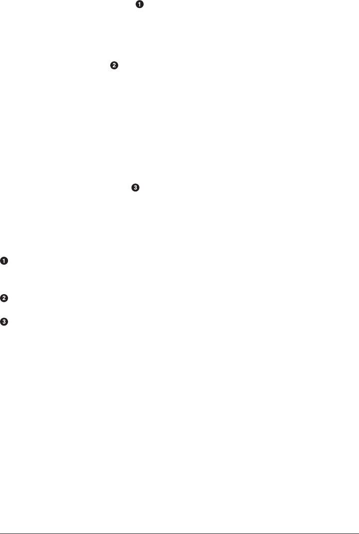
Let’s register a warmer and then talk about what’s happening:
PUT /music/_warmer/warmer_1
{
"query" : {
"filtered" : {
"filter" : {
"bool": {
"should": [
{ "term": { "tag": "rock" }},
{ "term": { "tag": "hiphop" }},
{ "term": { "tag": "electronics" }}
]
}
}
}
},
"aggs" : {
"price" : {
"histogram" : {
"field" : "price",
"interval" : 10
}
}
}
}
Warmers are associated with an index (music) and are registered using the
_warmer endpoint and a unique ID (warmer_1).
The three most popular music genres have their filter caches prebuilt.
The fielddata and global ordinals for the price field will be preloaded.
Warmers are registered against a specific index. Each warmer is given a unique ID,
because you can have multiple warmers per index.
Then you just specify a query, any query. It can include queries, filters, aggregations,
sort values, scripts—literally any valid query DSL. The point is to register queries that
are representative of the traffic that your users will generate, so that appropriate
caches can be prepopulated.
When a new segment is created, Elasticsearch will literally execute the queries regis‐
tered in your warmers. The act of executing these queries will force caches to be
loaded. Only after all warmers have been executed will the segment be made visible to
search.
Preloading Fielddata | 499

Similar to eager loading, warmers shift the cost of cold caches to
refresh time. When registering warmers, it is important to be judi‐
cious. You could add thousands of warmers to make sure every
cache is populated—but that will drastically increase the time it
takes for new segments to be made searchable.
In practice, select a handful of queries that represent the majority
of your user’s queries and register those.
Some administrative details (such as getting existing warmers and deleting warmers)
that have been omitted from this explanation. Refer to the warmers documentation
for the rest of the details.
Preventing Combinatorial Explosions
The terms bucket dynamically builds buckets based on your data; it doesn’t know up
front how many buckets will be generated. While this is fine with a single aggrega‐
tion, think about what can happen when one aggregation contains another aggrega‐
tion, which contains another aggregation, and so forth. The combination of unique
values in each of these aggregations can lead to an explosion in the number of buck‐
ets generated.
Imagine we have a modest dataset that represents movies. Each document lists the
actors in that movie:
{
"actors" : [
"Fred Jones",
"Mary Jane",
"Elizabeth Worthing"
]
}
If we want to determine the top 10 actors and their top costars, that’s trivial with an
aggregation:
{
"aggs" : {
"actors" : {
"terms" : {
"field" : "actors",
"size" : 10
},
"aggs" : {
"costars" : {
"terms" : {
"field" : "actors",
"size" : 5
}
500 | Chapter 34: Controlling Memory Use and Latency

}
}
}
}
}
This will return a list of the top 10 actors, and for each actor, a list of their top five
costars. This seems like a very modest aggregation; only 50 values will be returned!
However, this seemingly innocuous query can easily consume a vast amount of mem‐
ory. You can visualize a terms aggregation as building a tree in memory. The actors
aggregation will build the first level of the tree, with a bucket for every actor. Then,
nested under each node in the first level, the costars aggregation will build a second
level, with a bucket for every costar, as seen in Figure 34-1. That means that a single
movie will generate n2 buckets!
Figure 34-1. Build full depth tree
To use some real numbers, imagine each movie has 10 actors on average. Each movie
will then generate 102 == 100 buckets. If you have 20,000 movies, that’s roughly
2,000,000 generated buckets.
Now, remember, our aggregation is simply asking for the top 10 actors and their co-
stars, totaling 50 values. To get the final results, we have to generate that tree of
2,000,000 buckets, sort it, and finally prune it such that only the top 10 actors are left.
This is illustrated in Figure 34-2 and Figure 34-3.
Preventing Combinatorial Explosions | 501
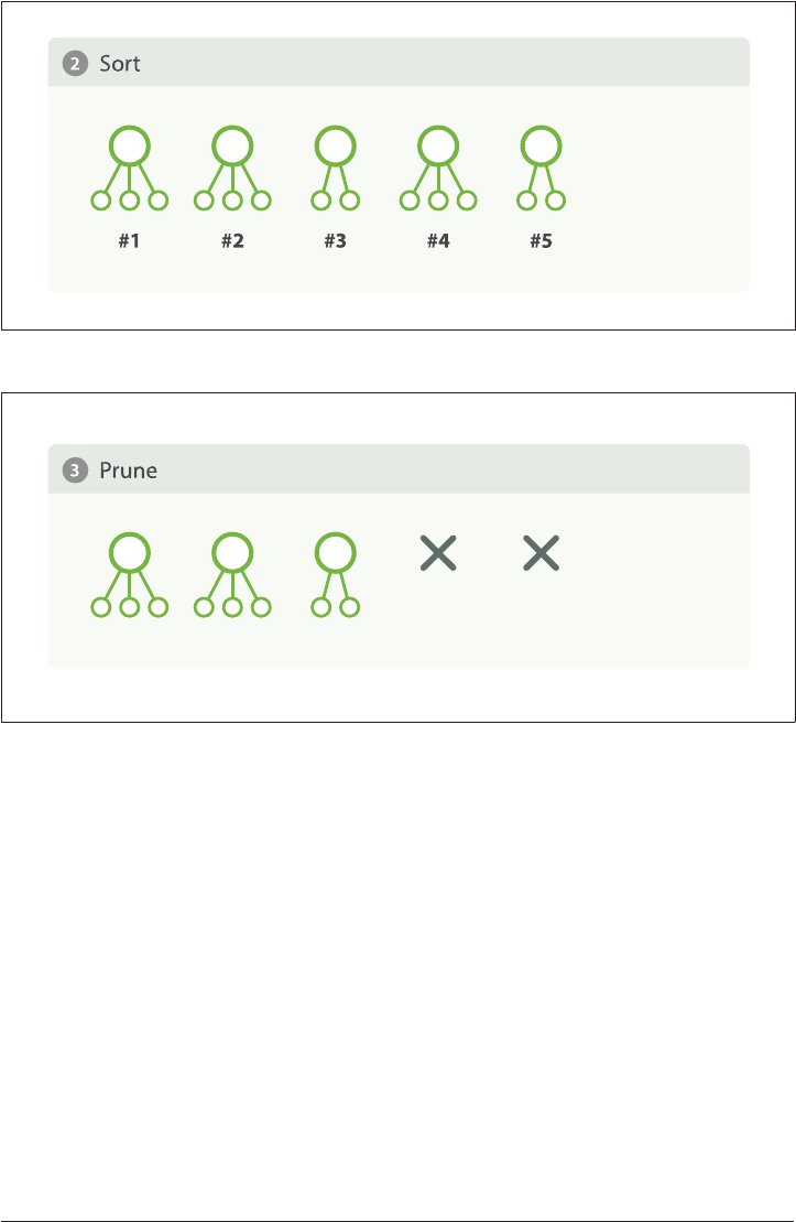
Figure 34-2. Sort tree
Figure 34-3. Prune tree
At this point you should be quite distraught. Twenty thousand documents is paltry,
and the aggregation is pretty tame. What if you had 200 million documents, wanted
the top 100 actors and their top 20 costars, as well as the costars’ costars?
You can appreciate how quickly combinatorial expansion can grow, making this strat‐
egy untenable. There is not enough memory in the world to support uncontrolled
combinatorial explosions.
Depth-First Versus Breadth-First
Elasticsearch allows you to change the collection mode of an aggregation, for exactly
this situation. The strategy we outlined previously—building the tree fully and then
pruning—is called depth-rst and it is the default. Depth-first works well for the
majority of aggregations, but can fall apart in situations like our actors and costars
example.
502 | Chapter 34: Controlling Memory Use and Latency

For these special cases, you should use an alternative collection strategy called
breadth-rst. This strategy works a little differently. It executes the first layer of aggre‐
gations, and then performs a pruning phase before continuing, as illustrated in
Figure 34-4 through Figure 34-6.
In our example, the actors aggregation would be executed first. At this point, we
have a single layer in the tree, but we already know who the top 10 actors are! There
is no need to keep the other actors since they won’t be in the top 10 anyway.
Figure 34-4. Build rst level
Figure 34-5. Sort rst level
Preventing Combinatorial Explosions | 503
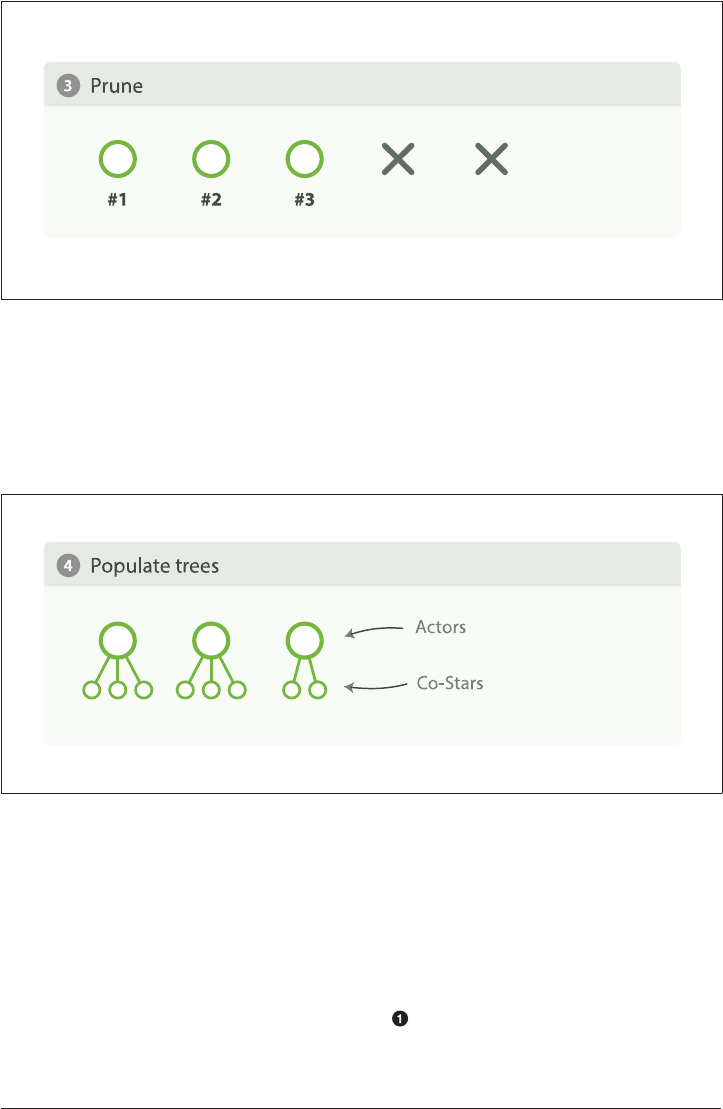
Figure 34-6. Prune rst level
Since we already know the top ten actors, we can safely prune away the rest of the
long tail. After pruning, the next layer is populated based on its execution mode, and
the process repeats until the aggregation is done, as illustrated in Figure 34-7. This
prevents the combinatorial explosion of buckets and drastically reduces memory
requirements for classes of queries that are amenable to breadth-first.
Figure 34-7. Populate full depth for remaining nodes
To use breadth-first, simply enable it via the collect parameter:
{
"aggs" : {
"actors" : {
"terms" : {
"field" : "actors",
"size" : 10,
"collect_mode" : "breadth_first"
},
"aggs" : {
504 | Chapter 34: Controlling Memory Use and Latency

"costars" : {
"terms" : {
"field" : "actors",
"size" : 5
}
}
}
}
}
}
Enable breadth_first on a per-aggregation basis.
Breadth-first should be used only when you expect more buckets to be generated
than documents landing in the buckets. Breadth-first works by caching document
data at the bucket level, and then replaying those documents to child aggregations
after the pruning phase.
The memory requirement of a breadth-first aggregation is linear to the number of
documents in each bucket prior to pruning. For many aggregations, the number of
documents in each bucket is very large. Think of a histogram with monthly intervals:
you might have thousands or hundreds of thousands of documents per bucket. This
makes breadth-first a bad choice, and is why depth-first is the default.
But for the actor example—which generates a large number of buckets, but each
bucket has relatively few documents—breadth-first is much more memory efficient,
and allows you to build aggregations that would otherwise fail.
Preventing Combinatorial Explosions | 505

CHAPTER 35
Closing Thoughts
This section covered a lot of ground, and a lot of deeply technical issues. Aggrega‐
tions bring a power and flexibility to Elasticsearch that is hard to overstate. The abil‐
ity to nest buckets and metrics, to quickly approximate cardinality and percentiles, to
find statistical anomalies in your data, all while operating on near-real-time data and
in parallel to full-text search—these are game-changers to many organizations.
It is a feature that, once you start using it, you’ll find dozens of other candidate uses.
Real-time reporting and analytics is central to many organizations (be it over busi‐
ness intelligence or server logs).
But with great power comes great responsibility, and for Elasticsearch that often
means proper memory stewardship. Memory is often the limiting factor in Elastic‐
search deployments, particularly those that heavily utilize aggregations. Because
aggregation data is loaded to fielddata—and this is an in-memory data structure—
managing efficient memory usage is important.
The management of this memory can take several forms, depending on your particu‐
lar use-case:
•At a data level, by making sure you analyze (or not_analyze) your data appropri‐
ately so that it is memory-friendly
•During indexing, by configuring heavy fields to use disk-based doc values instead
of in-memory fielddata
• At search time, by utilizing approximate aggregations and data filtering
• At a node level, by setting hard memory and dynamic circuit-breaker limits
•At an operations level, by monitoring memory usage and controlling slow
garbage-collection cycles, potentially by adding more nodes to the cluster
507

Most deployments will use one or more of the preceding methods. The exact combi‐
nation is highly dependent on your particular environment. Some organizations need
blisteringly fast responses and opt to simply add more nodes. Other organizations are
limited by budget and choose doc values and approximate aggregations.
Whatever the path you take, it is important to assess the available options and create
both a short- and long-term plan. Decide how your memory situation exists today
and what (if anything) needs to be done. Then decide what will happen in six months
or one year as your data grows. What methods will you use to continue scaling?
It is better to plan out these life cycles of your cluster ahead of time, rather than pan‐
icking at 3 a.m. because your cluster is at 90% heap utilization.
508 | Chapter 35: Closing Thoughts

PART V
Geolocation
Gone are the days when we wander around a city with paper maps. Thanks to smart‐
phones, we now know exactly where we are all the time, and we expect websites to
use that information. I’m not interested in restaurants in Greater London—I want to
know about restaurants within a 5-minute walk of my current location.
But geolocation is only one part of the puzzle. The beauty of Elasticsearch is that it
allows you to combine geolocation with full-text search, structured search, and ana‐
lytics.
For instance: show me restaurants that mention vitello tonnato, are within a 5-minute
walk, and are open at 11 p.m., and then rank them by a combination of user rating,
distance, and price. Another example: show me a map of vacation rental properties
available in August throughout the city, and calculate the average price per zone.
Elasticsearch offers two ways of representing geolocations: latitude-longitude points
using the geo_point field type, and complex shapes defined in GeoJSON, using the
geo_shape field type.
Geo-points allow you to find points within a certain distance of another point, to cal‐
culate distances between two points for sorting or relevance scoring, or to aggregate
into a grid to display on a map. Geo-shapes, on the other hand, are used purely for
filtering. They can be used to decide whether two shapes overlap, or whether one
shape completely contains other shapes.

CHAPTER 36
Geo-Points
A geo-point is a single latitude/longitude point on the Earth’s surface. Geo-points can
be used to calculate distance from a point, to determine whether a point falls within a
bounding box, or in aggregations.
Geo-points cannot be automatically detected with dynamic mapping. Instead,
geo_point fields should be mapped explicitly:
PUT /attractions
{
"mappings": {
"restaurant": {
"properties": {
"name": {
"type": "string"
},
"location": {
"type": "geo_point"
}
}
}
}
}
Lat/Lon Formats
With the location field defined as a geo_point, we can proceed to index documents
containing latitude/longitude pairs, which can be formatted as strings, arrays, or
objects:
511

PUT /attractions/restaurant/1
{
"name": "Chipotle Mexican Grill",
"location": "40.715, -74.011"
}
PUT /attractions/restaurant/2
{
"name": "Pala Pizza",
"location": {
"lat": 40.722,
"lon": -73.989
}
}
PUT /attractions/restaurant/3
{
"name": "Mini Munchies Pizza",
"location": [ -73.983, 40.719 ]
}
A string representation, with "lat,lon".
An object representation with lat and lon explicitly named.
An array representation with [lon,lat].
Everybody gets caught at least once: string geo-points are "lati
tude,longitude", while array geo-points are [longitude,lati
tude]—the opposite order!
Originally, both strings and arrays in Elasticsearch used latitude
followed by longitude. However, it was decided early on to switch
the order for arrays in order to conform with GeoJSON.
The result is a bear trap that captures all unsuspecting users on
their journey to full geolocation nirvana.
Filtering by Geo-Point
Four geo-point filters can be used to include or exclude documents by geolocation:
geo_bounding_box
Find geo-points that fall within the specified rectangle.
geo_distance
Find geo-points within the specified distance of a central point.
512 | Chapter 36: Geo-Points

geo_distance_range
Find geo-points within a specified minimum and maximum distance from a cen‐
tral point.
geo_polygon
Find geo-points that fall within the specified polygon. is lter is very expensive.
If you find yourself wanting to use it, you should be looking at geo-shapes
instead.
All of these filters work in a similar way: the lat/lon values are loaded into memory
for all documents in the index, not just the documents that match the query (see
“Fielddata” on page 119). Each filter performs a slightly different calculation to check
whether a point falls into the containing area.
Geo-filters are expensive — they should be used on as few docu‐
ments as possible. First remove as many documents as you can
with cheaper filters, like term or range filters, and apply the geo-
filters last.
The bool filter will do this for you automatically. First it applies any
bitset-based filters (see “All About Caching” on page 192) to
exclude as many documents as it can as cheaply as possible. Then it
applies the more expensive geo or script filters to each remaining
document in turn.
geo_bounding_box Filter
This is by far the most efficient geo-filter because its calculation is very simple. You
provide it with the top, bottom, left, and right coordinates of a rectangle, and all it
does is compare the latitude with the left and right coordinates, and the longitude
with the top and bottom coordinates:
GET /attractions/restaurant/_search
{
"query": {
"filtered": {
"filter": {
"geo_bounding_box": {
"location": {
"top_left": {
"lat": 40.8,
"lon": -74.0
},
"bottom_right": {
"lat": 40.7,
"lon": -73.0
}
}
geo_bounding_box Filter | 513

}
}
}
}
}
These coordinates can also be specified as bottom_left and top_right.
Optimizing Bounding Boxes
The geo_bounding_box is the one geo-filter that doesn’t require all geo-points to be
loaded into memory. Because all it has to do is check whether the lat and lon values
fall within the specified ranges, it can use the inverted index to do a glorified range
filter.
To use this optimization, the geo_point field must be mapped to index the lat and
lon values separately:
PUT /attractions
{
"mappings": {
"restaurant": {
"properties": {
"name": {
"type": "string"
},
"location": {
"type": "geo_point",
"lat_lon": true
}
}
}
}
}
The location.lat and location.lon fields will be indexed separately. These
fields can be used for searching, but their values cannot be retrieved.
Now, when we run our query, we have to tell Elasticsearch to use the indexed lat and
lon values:
GET /attractions/restaurant/_search
{
"query": {
"filtered": {
"filter": {
"geo_bounding_box": {
"type": "indexed",
"location": {
"top_left": {
514 | Chapter 36: Geo-Points

"lat": 40.8,
"lon": -74.0
},
"bottom_right": {
"lat": 40.7,
"lon": -73.0
}
}
}
}
}
}
}
Setting the type parameter to indexed (instead of the default memory) tells Elas‐
ticsearch to use the inverted index for this filter.
While a geo_point field can contain multiple geo-points, the
lat_lon optimization can be used only on fields that contain a
single geo-point.
geo_distance Filter
The geo_distance filter draws a circle around the specified location and finds all
documents that have a geo-point within that circle:
GET /attractions/restaurant/_search
{
"query": {
"filtered": {
"filter": {
"geo_distance": {
"distance": "1km",
"location": {
"lat": 40.715,
"lon": -73.988
}
}
}
}
}
}
Find all location fields within 1km of the specified point. See Distance Units for a
list of the accepted units.
geo_distance Filter | 515

The central point can be specified as a string, an array, or (as in this example) an
object. See “Lat/Lon Formats” on page 511.
A geo-distance calculation is expensive. To optimize performance, Elasticsearch
draws a box around the circle and first uses the less expensive bounding-box calcula‐
tion to exclude as many documents as it can. It runs the geo-distance calculation on
only those points that fall within the bounding box.
Do your users really require an accurate circular filter to be
applied to their results? Using a rectangular bounding box is
much more efficient than geo-distance and will usually serve their
purposes just as well.
Faster Geo-Distance Calculations
The distance between two points can be calculated using algorithms, which trade per‐
formance for accuracy:
arc
The slowest but most accurate is the arc calculation, which treats the world as a
sphere. Accuracy is still limited because the world isn’t really a sphere.
plane
The plane calculation, which treats the world as if it were flat, is faster but less
accurate. It is most accurate at the equator and becomes less accurate toward the
poles.
sloppy_arc
So called because it uses the SloppyMath Lucene class to trade accuracy for speed,
the sloppy_arc calculation uses the Haversine formula to calculate distance. It is
four to five times as fast as arc, and distances are 99.9% accurate. This is the
default calculation.
You can specify a different calculation as follows:
GET /attractions/restaurant/_search
{
"query": {
"filtered": {
"filter": {
"geo_distance": {
"distance": "1km",
"distance_type": "plane",
"location": {
"lat": 40.715,
"lon": -73.988
}
516 | Chapter 36: Geo-Points

}
}
}
}
}
Use the faster but less accurate plane calculation.
Will your users really care if a restaurant is a few meters outside
their specified radius? While some geo applications require great
accuracy, less-accurate but faster calculations will suit the majority
of use cases just fine.
geo_distance_range Filter
The only difference between the geo_distance and geo_distance_range filters is
that the latter has a doughnut shape and excludes documents within the central hole.
Instead of specifying a single distance from the center, you specify a minimum dis‐
tance (with gt or gte) and maximum distance (with lt or lte), just like a range fil‐
ter:
GET /attractions/restaurant/_search
{
"query": {
"filtered": {
"filter": {
"geo_distance_range": {
"gte": "1km",
"lt": "2km",
"location": {
"lat": 40.715,
"lon": -73.988
}
}
}
}
}
}
Matches locations that are at least 1km from the center, and less than 2km from the
center.
Caching geo-lters
The results of geo-filters are not cached by default, for two reasons:
Caching geo-lters | 517

•Geo-filters are usually used to find entities that are near to a user’s current loca‐
tion. The problem is that users move, and no two users are in exactly the same
location. A cached filter would have little chance of being reused.
•Filters are cached as bitsets that represent all documents in a segment. Imagine
that our query excludes all documents but one in a particular segment. An unc‐
ached geo-filter just needs to check the one remaining document, but a cached
geo-filter would need to check all of the documents in the segment.
That said, caching can be used to good effect with geo-filters. Imagine that your index
contains restaurants from all over the United States. A user in New York is not inter‐
ested in restaurants in San Francisco. We can treat New York as a hot spot and draw a
big bounding box around the city and neighboring areas.
This geo_bounding_box filter can be cached and reused whenever we have a user
within the city limits of New York. It will exclude all restaurants from the rest of the
country. We can then use an uncached, more specific geo_bounding_box or geo_dis
tance filter to narrow the remaining results to those that are close to the user:
GET /attractions/restaurant/_search
{
"query": {
"filtered": {
"filter": {
"bool": {
"must": [
{
"geo_bounding_box": {
"type": "indexed",
"_cache": true,
"location": {
"top_left": {
"lat": 40,8,
"lon": -74.1
},
"bottom_right": {
"lat": 40.4,
"lon": -73.7
}
}
}
},
{
"geo_distance": {
"distance": "1km",
"location": {
"lat": 40.715,
"lon": -73.988
}
}
518 | Chapter 36: Geo-Points

}
]
}
}
}
}
}
The cached bounding box filter reduces all results down to those in the greater
New York area.
The more costly geo_distance filter narrows the results to those within 1km of
the user.
Reducing Memory Usage
Each lat/lon pair requires 16 bytes of memory, memory that is in short supply. It
needs this much memory in order to provide very accurate results. But as we have
commented before, such exacting precision is seldom required.
You can reduce the amount of memory that is used by switching to a compressed
fielddata format and by specifying how precise you need your geo-points to be. Even
reducing precision to 1mm reduces memory usage by a third. A more realistic setting
of 3m reduces usage by 62%, and 1km saves a massive 75%!
This setting can be changed on a live index with the update-mapping API:
POST /attractions/_mapping/restaurant
{
"location": {
"type": "geo_point",
"fielddata": {
"format": "compressed",
"precision": "1km"
}
}
}
Each lat/lon pair will require only 4 bytes, instead of 16.
Alternatively, you can avoid using memory for geo-points altogether, either by using
the technique described in “Optimizing Bounding Boxes” on page 514, or by storing
geo-points as doc values:
PUT /attractions
{
"mappings": {
"restaurant": {
"properties": {
Reducing Memory Usage | 519

"name": {
"type": "string"
},
"location": {
"type": "geo_point",
"doc_values": true
}
}
}
}
}
Geo-points will not be loaded into memory, but instead stored on disk.
Mapping a geo-point to use doc values can be done only when the field is first cre‐
ated. There is a small performance cost in using doc values instead of fielddata, but
with memory in such short supply, it is often worth doing.
Sorting by Distance
Search results can be sorted by distance from a point:
While you can sort by distance, “Scoring by Distance” on page 522
is usually a better solution.
GET /attractions/restaurant/_search
{
"query": {
"filtered": {
"filter": {
"geo_bounding_box": {
"type": "indexed",
"location": {
"top_left": {
"lat": 40,8,
"lon": -74.0
},
"bottom_right": {
"lat": 40.4,
"lon": -73.0
}
}
}
}
}
},
"sort": [
520 | Chapter 36: Geo-Points

{
"_geo_distance": {
"location": {
"lat": 40.715,
"lon": -73.998
},
"order": "asc",
"unit": "km",
"distance_type": "plane"
}
}
]
}
Calculate the distance between the specified lat/lon point and the geo-point in
the location field of each document.
Return the distance in km in the sort keys for each result.
Use the faster but less accurate plane calculation.
You may ask yourself: why do we specify the distance unit? For sorting, it doesn’t
matter whether we compare distances in miles, kilometers, or light years. The reason
is that the actual value used for sorting is returned with each result, in the sort ele‐
ment:
...
"hits": [
{
"_index": "attractions",
"_type": "restaurant",
"_id": "2",
"_score": null,
"_source": {
"name": "New Malaysia",
"location": {
"lat": 40.715,
"lon": -73.997
}
},
"sort": [
0.08425653647614346
]
},
...
This restaurant is 0.084km from the location we specified.
You can set the unit to return these values in whatever form makes sense for your
application.
Sorting by Distance | 521

Geo-distance sorting can also handle multiple geo-points, both in
the document and in the sort parameters. Use the sort_mode to
specify whether it should use the min, max, or avg distance between
each combination of locations. This can be used to return “friends
nearest to my work and home locations.”
Scoring by Distance
It may be that distance is the only important factor in deciding the order in which
results are returned, but more frequently we need to combine distance with other fac‐
tors, such as full-text relevance, popularity, and price.
In these situations, we should reach for the function_score query that allows us to
blend all of these factors into an overall score. See “The Closer, The Better” on page
305 for an example that uses geo-distance to influence scoring.
The other drawback of sorting by distance is performance: the distance has to be cal‐
culated for all matching documents. The function_score query, on the other hand,
can be executed during the rescore phase, limiting the number of calculations to just
the top n results.
522 | Chapter 36: Geo-Points

CHAPTER 37
Geohashes
Geohashes are a way of encoding lat/lon points as strings. The original intention
was to have a URL-friendly way of specifying geolocations, but geohashes have
turned out to be a useful way of indexing geo-points and geo-shapes in databases.
Geohashes divide the world into a grid of 32 cells—4 rows and 8 columns—each rep‐
resented by a letter or number. The g cell covers half of Greenland, all of Iceland, and
most of Great Britian. Each cell can be further divided into another 32 cells, which
can be divided into another 32 cells, and so on. The gc cell covers Ireland and Eng‐
land, gcp covers most of London and part of Southern England, and gcpuuz94k is the
entrance to Buckingham Palace, accurate to about 5 meters.
In other words, the longer the geohash string, the more accurate it is. If two geo‐
hashes share a prefix— and gcpuuz—then it implies that they are near each other. The
longer the shared prefix, the closer they are.
That said, two locations that are right next to each other may have completely differ‐
ent geohashes. For instance, the Millenium Dome in London has geohash u10hbp,
because it falls into the u cell, the next top-level cell to the east of the g cell.
Geo-points can index their associated geohashes automatically, but more important,
they can also index all geohash prexes. Indexing the location of the entrance to
Buckingham Palace—latitude 51.501568 and longitude -0.141257—would index all
of the geohashes listed in the following table, along with the approximate dimensions
of each geohash cell:
Geohash Level Dimensions
g 1 ~ 5,004km x 5,004km
523

Geohash Level Dimensions
gc 2 ~ 1,251km x 625km
gcp 3 ~ 156km x 156km
gcpu 4 ~ 39km x 19.5km
gcpuu 5 ~ 4.9km x 4.9km
gcpuuz 6 ~ 1.2km x 0.61km
gcpuuz9 7 ~ 152.8m x 152.8m
gcpuuz94 8 ~ 38.2m x 19.1m
gcpuuz94k 9 ~ 4.78m x 4.78m
gcpuuz94kk 10 ~ 1.19m x 0.60m
gcpuuz94kkp 11 ~ 14.9cm x 14.9cm
gcpuuz94kkp5 12 ~ 3.7cm x 1.8cm
The geohash_cell filter can use these geohash prefixes to find locations near a speci‐
fied lat/lon point.
Mapping Geohashes
The first step is to decide just how much precision you need. Although you could
index all geo-points with the default full 12 levels of precision, do you really need to
be accurate to within a few centimeters? You can save yourself a lot of space in the
index by reducing your precision requirements to something more realistic, such as
1km:
PUT /attractions
{
"mappings": {
"restaurant": {
"properties": {
"name": {
"type": "string"
},
"location": {
"type": "geo_point",
"geohash_prefix": true,
"geohash_precision": "1km"
524 | Chapter 37: Geohashes

}
}
}
}
}
Setting geohash_prefix to true tells Elasticsearch to index all geohash prefixes,
up to the specified precision.
The precision can be specified as an absolute number, representing the length of
the geohash, or as a distance. A precision of 1km corresponds to a geohash of
length 7.
With this mapping in place, geohash prefixes of lengths 1 to 7 will be indexed, pro‐
viding geohashes accurate to about 150 meters.
geohash_cell Filter
The geohash_cell filter simply translates a lat/lon location into a geohash with the
specified precision and finds all locations that contain that geohash—a very efficient
filter indeed.
GET /attractions/restaurant/_search
{
"query": {
"filtered": {
"filter": {
"geohash_cell": {
"location": {
"lat": 40.718,
"lon": -73.983
},
"precision": "2km"
}
}
}
}
}
The precision cannot be more precise than that specified in the geohash_preci
sion mapping.
This filter translates the lat/lon point into a geohash of the appropriate length—in
this example dr5rsk—and looks for all locations that contain that exact term.
However, the filter as written in the preceding example may not return all restaurants
within 5km of the specified point. Remember that a geohash is just a rectangle, and
geohash_cell Filter | 525

the point may fall anywhere within that rectangle. If the point happens to fall near the
edge of a geohash cell, the filter may well exclude any restaurants in the adjacent cell.
To fix that, we can tell the filter to include the neigboring cells, by setting neighbors
to true:
GET /attractions/restaurant/_search
{
"query": {
"filtered": {
"filter": {
"geohash_cell": {
"location": {
"lat": 40.718,
"lon": -73.983
},
"neighbors": true,
"precision": "2km"
}
}
}
}
}
This filter will look for the resolved geohash and all surrounding geohashes.
Clearly, looking for a geohash with precision 2km plus all the neighboring cells results
in quite a large search area. This filter is not built for accuracy, but it is very efficient
and can be used as a prefiltering step before applying a more accurate geo-filter.
Specifying the precision as a distance can be misleading. A pre
cision of 2km is converted to a geohash of length 6, which
actually has dimensions of about 1.2km x 0.6km. You may find it
more understandable to specify an actual length such as 5 or 6.
The other advantage that this filter has over a geo_bounding_box filter is that it sup‐
ports multiple locations per field. The lat_lon option that we discussed in “Optimiz‐
ing Bounding Boxes” on page 514 is efficient, but only when there is a single lat/lon
point per field.
526 | Chapter 37: Geohashes

CHAPTER 38
Geo-aggregations
Although filtering or scoring results by geolocation is useful, it is often more useful to
be able to present information to the user on a map. A search may return way too
many results to be able to display each geo-point individually, but geo-aggregations
can be used to cluster geo-points into more manageable buckets.
Three aggregations work with fields of type geo_point:
geo_distance
Groups documents into concentric circles around a central point.
geohash_grid
Groups documents by geohash cell, for display on a map.
geo_bounds
Returns the lat/lon coordinates of a bounding box that would encompass all of
the geo-points. This is useful for choosing the correct zoom level when displaying
a map.
geo_distance Aggregation
The geo_distance agg is useful for searches such as to “find all pizza restaurants
within 1km of me.” The search results should, indeed, be limited to the 1km radius
specified by the user, but we can add “another result found within 2km”:
GET /attractions/restaurant/_search
{
"query": {
"filtered": {
"query": {
"match": {
"name": "pizza"
527

}
},
"filter": {
"geo_bounding_box": {
"location": {
"top_left": {
"lat": 40,8,
"lon": -74.1
},
"bottom_right": {
"lat": 40.4,
"lon": -73.7
}
}
}
}
}
},
"aggs": {
"per_ring": {
"geo_distance": {
"field": "location",
"unit": "km",
"origin": {
"lat": 40.712,
"lon": -73.988
},
"ranges": [
{ "from": 0, "to": 1 },
{ "from": 1, "to": 2 }
]
}
}
},
"post_filter": {
"geo_distance": {
"distance": "1km",
"location": {
"lat": 40.712,
"lon": -73.988
}
}
}
}
The main query looks for restaurants with pizza in the name.
The bounding box filters these results down to just those in the greater New York
area.
528 | Chapter 38: Geo-aggregations

The geo_distance agg counts the number of results within 1km of the user, and
between 1km and 2km from the user.
Finally, the post_filter reduces the search results to just those restaurants
within 1km of the user.
The response from the preceding request is as follows:
"hits": {
"total": 1,
"max_score": 0.15342641,
"hits": [
{
"_index": "attractions",
"_type": "restaurant",
"_id": "3",
"_score": 0.15342641,
"_source": {
"name": "Mini Munchies Pizza",
"location": [
-73.983,
40.719
]
}
}
]
},
"aggregations": {
"per_ring": {
"buckets": [
{
"key": "*-1.0",
"from": 0,
"to": 1,
"doc_count": 1
},
{
"key": "1.0-2.0",
"from": 1,
"to": 2,
"doc_count": 1
}
]
}
}
The post_filter has reduced the search hits to just the single pizza restaurant
within 1km of the user.
geo_distance Aggregation | 529

The aggregation includes the search result plus the other pizza restaurant within
2km of the user.
In this example, we have counted the number of restaurants that fall into each con‐
centric ring. Of course, we could nest subaggregations under the per_rings aggrega‐
tion to calculate the average price per ring, the maximium popularity, and more.
geohash_grid Aggregation
The number of results returned by a query may be far too many to display each geo-
point individually on a map. The geohash_grid aggregation buckets nearby geo-
points together by calculating the geohash for each point, at the level of precision that
you define.
The result is a grid of cells—one cell per geohash—that can be displayed on a map. By
changing the precision of the geohash, you can summarize information across the
whole world, by country, or by city block.
The aggregation is sparse—it returns only cells that contain documents. If your geo‐
hashes are too precise and too many buckets are generated, it will return, by default,
the 10,000 most populous cells—those containing the most documents. However, it
still needs to generate all the buckets in order to figure out which are the most popu‐
lous 10,000. You need to control the number of buckets generated by doing the fol‐
lowing:
1. Limit the result with a geo_bounding_box filter.
2. Choose an appropriate precision for the size of your bounding box.
GET /attractions/restaurant/_search?search_type=count
{
"query": {
"filtered": {
"filter": {
"geo_bounding_box": {
"location": {
"top_left": {
"lat": 40,8,
"lon": -74.1
},
"bottom_right": {
"lat": 40.4,
"lon": -73.7
}
}
}
}
}
530 | Chapter 38: Geo-aggregations

},
"aggs": {
"new_york": {
"geohash_grid": {
"field": "location",
"precision": 5
}
}
}
}
The bounding box limits the scope of the search to the greater New York area.
Geohashes of precision 5 are approximately 5km x 5km.
Geohashes with precision 5 measure about 25km2 each, so 10,000 cells at this preci‐
sion would cover 250,000km2. The bounding box that we specified measures approxi‐
mately 44km x 33km, or about 1,452km2, so we are well within safe limits; we
definitely won’t create too many buckets in memory.
The response from the preceding request looks like this:
...
"aggregations": {
"new_york": {
"buckets": [
{
"key": "dr5rs",
"doc_count": 2
},
{
"key": "dr5re",
"doc_count": 1
}
]
}
}
...
Each bucket contains the geohash as the key.
Again, we didn’t specify any subaggregations, so all we got back was the document
count. We could have asked for popular restaurant types, average price, or other
details.
geohash_grid Aggregation | 531

To plot these buckets on a map, you need a library that understands
how to convert a geohash into the equivalent bounding box or cen‐
tral point. Libraries exist in JavaScript and other languages that will
perform this conversion for you, but you can also use information
from “geo_bounds Aggregation” on page 532 to perform a similar
job.
geo_bounds Aggregation
In our previous example, we filtered our results by using a bounding box that covered
the greater New York area. However, our results were all located in downtown Man‐
hattan. When displaying a map for our user, it makes sense to zoom into the area of
the map that contains the data; there is no point in showing lots of empty space.
The geo_bounds aggregation does exactly this: it calculates the smallest bounding box
that is needed to encapsulate all of the geo-points:
GET /attractions/restaurant/_search?search_type=count
{
"query": {
"filtered": {
"filter": {
"geo_bounding_box": {
"location": {
"top_left": {
"lat": 40,8,
"lon": -74.1
},
"bottom_right": {
"lat": 40.4,
"lon": -73.9
}
}
}
}
}
},
"aggs": {
"new_york": {
"geohash_grid": {
"field": "location",
"precision": 5
}
},
"map_zoom": {
"geo_bounds": {
"field": "location"
}
}
532 | Chapter 38: Geo-aggregations

}
}
The geo_bounds aggregation will calculate the smallest bounding box required to
encapsulate all of the documents matching our query.
The response now includes a bounding box that we can use to zoom our map:
...
"aggregations": {
"map_zoom": {
"bounds": {
"top_left": {
"lat": 40.722,
"lon": -74.011
},
"bottom_right": {
"lat": 40.715,
"lon": -73.983
}
}
},
...
In fact, we could even use the geo_bounds aggregation inside each geohash cell, in
case the geo-points inside a cell are clustered in just a part of the cell:
GET /attractions/restaurant/_search?search_type=count
{
"query": {
"filtered": {
"filter": {
"geo_bounding_box": {
"location": {
"top_left": {
"lat": 40,8,
"lon": -74.1
},
"bottom_right": {
"lat": 40.4,
"lon": -73.9
}
}
}
}
}
},
"aggs": {
"new_york": {
"geohash_grid": {
"field": "location",
"precision": 5
},
geo_bounds Aggregation | 533

"aggs": {
"cell": {
"geo_bounds": {
"field": "location"
}
}
}
}
}
}
The cell_bounds subaggregation is calculated for every geohash cell.
Now the points in each cell have a bounding box:
...
"aggregations": {
"new_york": {
"buckets": [
{
"key": "dr5rs",
"doc_count": 2,
"cell": {
"bounds": {
"top_left": {
"lat": 40.722,
"lon": -73.989
},
"bottom_right": {
"lat": 40.719,
"lon": -73.983
}
}
}
},
...
534 | Chapter 38: Geo-aggregations

CHAPTER 39
Geo-shapes
Geo-shapes use a completely different approach than geo-points. A circle on a com‐
puter screen does not consist of a perfect continuous line. Instead it is drawn by col‐
oring adjacent pixels as an approximation of a circle. Geo-shapes work in much the
same way.
Complex shapes—such as points, lines, polygons, multipolygons, and polygons with
holes,--are “painted” onto a grid of geohash cells, and the shape is converted into a list
of the geohashes of all the cells that it touches.
Actually, two types of grids can be used with geo-shapes: geo‐
hashes, which we have already discussed and which are the default
encoding, and quad trees. Quad trees are similar to geohashes
except that there are only four cells at each level, instead of 32. The
difference comes down to a choice of encoding.
All of the geohashes that compose a shape are indexed as if they were terms. With this
information in the index, it is easy to determine whether one shape intersects with
another, as they will share the same geohash terms.
That is the extent of what you can do with geo-shapes: determine the relationship
between a query shape and a shape in the index. The relation can be one of the fol‐
lowing:
intersects
The query shape overlaps with the indexed shape (default).
disjoint
The query shape does not overlap at all with the indexed shape.
535

within
The indexed shape is entirely within the query shape.
Geo-shapes cannot be used to caculate distance, cannot be used for sorting or scor‐
ing, and cannot be used in aggregations.
Mapping geo-shapes
Like fields of type geo_point, geo-shapes have to be mapped explicitly before they
can be used:
PUT /attractions
{
"mappings": {
"landmark": {
"properties": {
"name": {
"type": "string"
},
"location": {
"type": "geo_shape"
}
}
}
}
}
There are two important settings that you should consider changing precision and
distance_error_pct.
precision
The precision parameter controls the maximum length of the geohashes that are
generated. It defaults to a precision of 9, which equates to a geohash with dimensions
of about 5m x 5m. That is probably far more precise than you need.
The lower the precision, the fewer terms that will be indexed and the faster the search
will be. But of course, the lower the precision, the less accurate are your geo-shapes.
Consider just how accurate you need your shapes to be—even one or two levels of
precision can represent a significant savings.
You can specify precisions by using distances—for example, 50m or 2km—but ulti‐
mately these distances are converted to the same levels as described in Chapter 37.
536 | Chapter 39: Geo-shapes

distance_error_pct
When indexing a polygon, the big central continuous part can be represented cheaply
by a short geohash. It is the edges that matter. Edges require much smaller geohashes
to represent them with any accuracy.
If you’re indexing a small landmark, you want the edges to be quite accurate. It
wouldn’t be good to have one monument overlapping with the next. When indexing
an entire country, you don’t need quite as much precision. Fifty meters here or there
isn’t likely to start any wars.
The distance_error_pct specifies the maximum allowable error based on the size of
the shape. It defaults to 0.025, or 2.5%. In other words, big shapes (like countries) are
allowed to have fuzzier edges than small shapes (like monuments).
The default of 0.025 is a good starting point, but the more error that is allowed, the
fewer terms that are required to index a shape.
Indexing geo-shapes
Shapes are represented using GeoJSON, a simple open standard for encoding two-
dimensional shapes in JSON. Each shape definition contains the type of shape—
point, line, polygon, envelope,—and one or more arrays of longitude/latitude
points.
In GeoJSON, coordinates are always written as longitude fol‐
lowed by latitude.
For instance, we can index a polygon representing Dam Square in Amsterdam as fol‐
lows:
PUT /attractions/landmark/dam_square
{
"name" : "Dam Square, Amsterdam",
"location" : {
"type" : "polygon",
"coordinates" : [[
[ 4.89218, 52.37356 ],
[ 4.89205, 52.37276 ],
[ 4.89301, 52.37274 ],
[ 4.89392, 52.37250 ],
[ 4.89431, 52.37287 ],
[ 4.89331, 52.37346 ],
[ 4.89305, 52.37326 ],
[ 4.89218, 52.37356 ]
Indexing geo-shapes | 537

]]
}
}
The type parameter indicates the type of shape that the coordinates represent.
The list of lon/lat points that describe the polygon.
The excess of square brackets in the example may look confusing, but the GeoJSON
syntax is quite simple:
1. Each lon/lat point is represented as an array:
[lon,lat]
2. A list of points is wrapped in an array to represent a polygon:
[[lon,lat],[lon,lat], ... ]
3. A shape of type polygon can optionally contain several polygons; the first repre‐
sents the polygon proper, while any subsequent polygons represent holes in the
first:
[
[[lon,lat],[lon,lat], ... ], # main polygon
[[lon,lat],[lon,lat], ... ], # hole in main polygon
...
]
See the Geo-shape mapping documentation for more details about the supported
shapes.
Querying geo-shapes
The unusual thing about the geo_shape query and geo_shape filter is that they allow
us to query using shapes, rather than just points.
For instance, if our user steps out of the central train station in Amsterdam, we could
find all landmarks within a 1km radius with a query like this:
GET /attractions/landmark/_search
{
"query": {
"geo_shape": {
"location": {
"shape": {
"type": "circle",
"radius": "1km"
"coordinates": [
4.89994,
52.37815
538 | Chapter 39: Geo-shapes

]
}
}
}
}
}
The query looks at geo-shapes in the location field.
The shape key indicates that the shape is specified inline in the query.
The shape is a circle, with a radius of 1km.
This point is situated at the entrance of the central train station in Amsterdam.
By default, the query (or filter—do the same job) looks for indexed shapes that inter‐
sect with the query shape. The relation parameter can be set to disjoint to find
indexed shapes that don’t intersect with the query shape, or within to find indexed
shapes that are completely contained by the query shape.
For instance, we could find all landmarks in the center of Amsterdam with this
query:
GET /attractions/landmark/_search
{
"query": {
"geo_shape": {
"location": {
"relation": "within",
"shape": {
"type": "polygon",
"coordinates": [[
[4.88330,52.38617],
[4.87463,52.37254],
[4.87875,52.36369],
[4.88939,52.35850],
[4.89840,52.35755],
[4.91909,52.36217],
[4.92656,52.36594],
[4.93368,52.36615],
[4.93342,52.37275],
[4.92690,52.37632],
[4.88330,52.38617]
]]
}
}
}
}
}
Querying geo-shapes | 539

Match only indexed shapes that are completely within the query shape.
This polygon represents the center of Amsterdam.
Querying with Indexed Shapes
With shapes that are often used in queries, it can be more convenient to store them in
the index and to refer to them by name in the query. Take our example of central
Amsterdam in the previous example. We could store it as a document of type neigh
borhood.
First, we set up the mapping in the same way as we did for landmark:
PUT /attractions/_mapping/neighborhood
{
"properties": {
"name": {
"type": "string"
},
"location": {
"type": "geo_shape"
}
}
}
Then we can index a shape for central Amsterdam:
PUT /attractions/neighborhood/central_amsterdam
{
"name" : "Central Amsterdam",
"location" : {
"type" : "polygon",
"coordinates" : [[
[4.88330,52.38617],
[4.87463,52.37254],
[4.87875,52.36369],
[4.88939,52.35850],
[4.89840,52.35755],
[4.91909,52.36217],
[4.92656,52.36594],
[4.93368,52.36615],
[4.93342,52.37275],
[4.92690,52.37632],
[4.88330,52.38617]
]]
}
}
After the shape is indexed, we can refer to it by index, type, and id in the query itself:
540 | Chapter 39: Geo-shapes

GET /attractions/landmark/_search
{
"query": {
"geo_shape": {
"location": {
"relation": "within",
"indexed_shape": {
"index": "attractions",
"type": "neighborhood",
"id": "central_amsterdam",
"path": "location"
}
}
}
}
}
By specifying indexed_shape instead of shape, Elasticsearch knows that it needs
to retrieve the query shape from the specified document and path.
There is nothing special about the shape for central Amsterdam. We could equally
use our existing shape for Dam Square in queries. This query finds neighborhoods
that intersect with Dam Square:
GET /attractions/neighborhood/_search
{
"query": {
"geo_shape": {
"location": {
"indexed_shape": {
"index": "attractions",
"type": "landmark",
"id": "dam_square",
"path": "location"
}
}
}
}
}
Geo-shape Filters and Caching
The geo_shape query and filter perform the same function. The query simply acts as
a filter: any matching documents receive a relevance _score of 1. Query results can‐
not be cached, but filter results can be.
The results are not cached by default. Just as with geo-points, any change in the coor‐
dinates in a shape are likely to produce a different set of geohashes, so there is little
point in caching filter results. That said, if you filter using the same shapes repeatedly,
it can be worth caching the results, by setting _cache to true:
Geo-shape Filters and Caching | 541

GET /attractions/neighborhood/_search
{
"query": {
"filtered": {
"filter": {
"geo_shape": {
"_cache": true,
"location": {
"indexed_shape": {
"index": "attractions",
"type": "landmark",
"id": "dam_square",
"path": "location"
}
}
}
}
}
}
}
The results of this geo_shape filter will be cached.
542 | Chapter 39: Geo-shapes

PART VI
Modeling Your Data
Elasticsearch is a different kind of beast, especially if you come from the world of
SQL. It comes with many benefits: performance, scale, near real-time search, and
analytics across massive amounts of data. And it is easy to get going! Just download
and start using it.
But it is not magic. To get the most out of Elasticsearch, you need to understand how
it works and how to make it work for your needs.
Handling relationships between entities is not as obvious as it is with a dedicated rela‐
tional store. The golden rule of a relational database—normalize your data—does not
apply to Elasticsearch. In Chapter 40, Chapter 41, and Chapter 42 we discuss the pros
and cons of the available approaches.
Then in Chapter 43 we talk about the features that Elasticsearch offers that enable
you to scale out quickly and flexibly. Scale is not one-size-fits-all. You need to think
about how data flows through your system, and design your model accordingly.
Time-based data like log events or social network streams require a very different
approach than more static collections of documents.
And finally, we talk about the one thing in Elasticsearch that doesn’t scale.

CHAPTER 40
Handling Relationships
In the real world, relationships matter: blog posts have comments, bank accounts
have transactions, customers have bank accounts, orders have order lines, and direc‐
tories have files and subdirectories.
Relational databases are specifically designed—and this will not come as a surprise to
you—to manage relationships:
•Each entity (or row, in the relational world) can be uniquely identified by a pri
mary key.
•Entities are normalized. The data for a unique entity is stored only once, and
related entities store just its primary key. Changing the data of an entity has to
happen in only one place.
• Entities can be joined at query time, allowing for cross-entity search.
•Changes to a single entity are atomic, consistent, isolated, and durable. (See ACID
Transactions for more on this subject.)
• Most relational databases support ACID transactions across multiple entities.
But relational databases do have their limitations, besides their poor support for full-
text search. Joining entities at query time is expensive—more joins that are required,
the more expensive the query. Performing joins between entities that live on different
hardware is so expensive that it is just not practical. This places a limit on the amount
of data that can be stored on a single server.
Elasticsearch, like most NoSQL databases, treats the world as though it were flat. An
index is a flat collection of independent documents. A single document should con‐
tain all of the information that is required to decide whether it matches a search
request.
545

While changing the data of a single document in Elasticsearch is ACIDic, transac‐
tions involving multiple documents are not. There is no way to roll back the index to
its previous state if part of a transaction fails.
This FlatWorld has its advantages:
• Indexing is fast and lock-free.
• Searching is fast and lock-free.
•Massive amounts of data can be spread across multiple nodes, because each
document is independent of the others.
But relationships matter. Somehow, we need to bridge the gap between FlatWorld and
the real world. Four common techniques are used to manage relational data in Elas‐
ticsearch:
•Application-side joins
•Data denormalization
•Nested objects
•Parent/child relationships
Often the final solution will require a mixture of a few of these techniques.
Application-side Joins
We can (partly) emulate a relational database by implementing joins in our applica‐
tion. For instance, let’s say we are indexing users and their blog posts. In the relational
world, we would do something like this:
PUT /my_index/user/1
{
"name": "John Smith",
"email": "john@smith.com",
"dob": "1970/10/24"
}
PUT /my_index/blogpost/2
{
"title": "Relationships",
"body": "It's complicated...",
"user": 1
}
The index, type, and id of each document together function as a primary key.
546 | Chapter 40: Handling Relationships

The blogpost links to the user by storing the user’s id. The index and type aren’t
required as they are hardcoded in our application.
Finding blog posts by user with ID 1 is easy:
GET /my_index/blogpost/_search
{
"query": {
"filtered": {
"filter": {
"term": { "user": 1 }
}
}
}
}
To find blogposts by a user called John, we would need to run two queries: the first
would look up all users called John in order to find their IDs, and the second would
pass those IDs in a query similar to the preceding one:
GET /my_index/user/_search
{
"query": {
"match": {
"name": "John"
}
}
}
GET /my_index/blogpost/_search
{
"query": {
"filtered": {
"filter": {
"terms": { "user": [1] }
}
}
}
}
The values in the terms filter would be populated with the results from the first
query.
The main advantage of application-side joins is that the data is normalized. Changing
the user’s name has to happen in only one place: the user document. The disadvan‐
tage is that you have to run extra queries in order to join documents at search time.
In this example, there was only one user who matched our first query, but in the real
world we could easily have millions of users named John. Including all of their IDs in
the second query would make for a very large query, and one that has to do millions
of term lookups.
Application-side Joins | 547

This approach is suitable when the first entity (the user in this example) has a small
number of documents and, preferably, they seldom change. This would allow the
application to cache the results and avoid running the first query often.
Denormalizing Your Data
The way to get the best search performance out of Elasticsearch is to use it as it is
intended, by denormalizing your data at index time. Having redundant copies of data
in each document that requires access to it removes the need for joins.
If we want to be able to find a blog post by the name of the user who wrote it, include
the user’s name in the blog-post document itself:
PUT /my_index/user/1
{
"name": "John Smith",
"email": "john@smith.com",
"dob": "1970/10/24"
}
PUT /my_index/blogpost/2
{
"title": "Relationships",
"body": "It's complicated...",
"user": {
"id": 1,
"name": "John Smith"
}
}
Part of the user’s data has been denormalized into the blogpost document.
Now, we can find blog posts about relationships by users called John with a single
query:
GET /my_index/blogpost/_search
{
"query": {
"bool": {
"must": [
{ "match": { "title": "relationships" }},
{ "match": { "user.name": "John" }}
]
}
}
}
The advantage of data denormalization is speed. Because each document contains all
of the information that is required to determine whether it matches the query, there is
no need for expensive joins.
548 | Chapter 40: Handling Relationships

Field Collapsing
A common requirement is the need to present search results grouped by a particular
field. We might want to return the most relevant blog posts grouped by the user’s
name. Grouping by name implies the need for a terms aggregation. To be able to
group on the user’s whole name, the name field should be available in its original
not_analyzed form, as explained in “Aggregations and Analysis” on page 483:
PUT /my_index/_mapping/blogpost
{
"properties": {
"user": {
"properties": {
"name": {
"type": "string",
"fields": {
"raw": {
"type": "string",
"index": "not_analyzed"
}
}
}
}
}
}
}
The user.name field will be used for full-text search.
The user.name.raw field will be used for grouping with the terms aggregation.
Then add some data:
PUT /my_index/user/1
{
"name": "John Smith",
"email": "john@smith.com",
"dob": "1970/10/24"
}
PUT /my_index/blogpost/2
{
"title": "Relationships",
"body": "It's complicated...",
"user": {
"id": 1,
"name": "John Smith"
}
}
PUT /my_index/user/3
Field Collapsing | 549

{
"name": "Alice John",
"email": "alice@john.com",
"dob": "1979/01/04"
}
PUT /my_index/blogpost/4
{
"title": "Relationships are cool",
"body": "It's not complicated at all...",
"user": {
"id": 3,
"name": "Alice John"
}
}
Now we can run a query looking for blog posts about relationships, by users called
John, and group the results by user, thanks to the top_hits aggregation:
GET /my_index/blogpost/_search?search_type=count
{
"query": {
"bool": {
"must": [
{ "match": { "title": "relationships" }},
{ "match": { "user.name": "John" }}
]
}
},
"aggs": {
"users": {
"terms": {
"field": "user.name.raw",
"order": { "top_score": "desc" }
},
"aggs": {
"top_score": { "max": { "script": "_score" }},
"blogposts": { "top_hits": { "_source": "title", "size": 5 }}
}
}
}
}
The blog posts that we are interested in are returned under the blogposts aggre‐
gation, so we can disable the usual search hits by setting the
search_type=count.
The query returns blog posts about relationships by users named John.
The terms aggregation creates a bucket for each user.name.raw value.
550 | Chapter 40: Handling Relationships

The top_score aggregation orders the terms in the users aggregation by the top-
scoring document in each bucket.
The top_hits aggregation returns just the title field of the five most relevant
blog posts for each user.
The abbreviated response is shown here:
...
"hits": {
"total": 2,
"max_score": 0,
"hits": []
},
"aggregations": {
"users": {
"buckets": [
{
"key": "John Smith",
"doc_count": 1,
"blogposts": {
"hits": {
"total": 1,
"max_score": 0.35258877,
"hits": [
{
"_index": "my_index",
"_type": "blogpost",
"_id": "2",
"_score": 0.35258877,
"_source": {
"title": "Relationships"
}
}
]
}
},
"top_score": {
"value": 0.3525887727737427
}
},
...
The hits array is empty because we set search_type=count.
There is a bucket for each user who appeared in the top results.
Under each user bucket there is a blogposts.hits array containing the top
results for that user.
Field Collapsing | 551

The user buckets are sorted by the user’s most relevant blog post.
Using the top_hits aggregation is the equivalent of running a query to return the
names of the users with the most relevant blog posts, and then running the same
query for each user, to get their best blog posts. But it is much more efficient.
The top hits returned in each bucket are the result of running a light mini-query
based on the original main query. The mini-query supports the usual features that
you would expect from search such as highlighting and pagination.
Denormalization and Concurrency
Of course, data denormalization has downsides too. The first disadvantage is that the
index will be bigger because the _source document for every blog post is bigger, and
there are more indexed fields. This usually isn’t a huge problem. The data written to
disk is highly compressed, and disk space is cheap. Elasticsearch can happily cope
with the extra data.
The more important issue is that, if the user were to change his name, all of his blog
posts would need to be updated too. Fortunately, users don’t often change names.
Even if they did, it is unlikely that a user would have written more than a few thou‐
sand blog posts, so updating blog posts with the scroll and bulk APIs would take
less than a second.
However, let’s consider a more complex scenario in which changes are common, far
reaching, and, most important, concurrent.
In this example, we are going to emulate a filesystem with directory trees in Elastic‐
search, much like a filesystem on Linux: the root of the directory is /, and each direc‐
tory can contain files and subdirectories.
We want to be able to search for files that live in a particular directory, the equivalent
of this:
grep "some text" /clinton/projects/elasticsearch/*
This requires us to index the path of the directory where the file lives:
PUT /fs/file/1
{
"name": "README.txt",
"path": "/clinton/projects/elasticsearch",
"contents": "Starting a new Elasticsearch project is easy..."
}
The filename
The full path to the directory holding the file
552 | Chapter 40: Handling Relationships

Really, we should also index directory documents so we can list all
files and subdirectories within a directory, but for brevity’s sake, we
will ignore that requirement.
We also want to be able to search for files that live anywhere in the directory tree
below a particular directory, the equivalent of this:
grep -r "some text" /clinton
To support this, we need to index the path hierarchy:
•/clinton
•/clinton/projects
•/clinton/projects/elasticsearch
This hierarchy can be generated automatically from the path field using the
path_hierarchy tokenizer:
PUT /fs
{
"settings": {
"analysis": {
"analyzer": {
"paths": {
"tokenizer": "path_hierarchy"
}
}
}
}
}
The custom paths analyzer uses the path_hierarchy tokenizer with its default
settings. See path_hierarchy tokenizer.
The mapping for the file type would look like this:
PUT /fs/_mapping/file
{
"properties": {
"name": {
"type": "string",
"index": "not_analyzed"
},
"path": {
"type": "string",
"index": "not_analyzed",
"fields": {
"tree": {
Denormalization and Concurrency | 553

"type": "string",
"analyzer": "paths"
}
}
}
}
}
The name field will contain the exact name.
The path field will contain the exact directory name, while the path.tree field
will contain the path hierarchy.
Once the index is set up and the files have been indexed, we can perform a search for
files containing elasticsearch in just the /clinton/projects/elasticsearch
directory like this:
GET /fs/file/_search
{
"query": {
"filtered": {
"query": {
"match": {
"contents": "elasticsearch"
}
},
"filter": {
"term": {
"path": "/clinton/projects/elasticsearch"
}
}
}
}
}
Find files in this directory only.
Every file that lives in any subdirectory under /clinton will include the term /clin
ton in the path.tree field. So we can search for all files in any subdirectory of /clin
ton as follows:
GET /fs/file/_search
{
"query": {
"filtered": {
"query": {
"match": {
"contents": "elasticsearch"
}
},
"filter": {
554 | Chapter 40: Handling Relationships

"term": {
"path.tree": "/clinton"
}
}
}
}
}
Find files in this directory or in any of its subdirectories.
Renaming Files and Directories
So far, so good. Renaming a file is easy—a simple update or index request is all that is
required. You can even use optimistic concurrency control to ensure that your change
doesn’t conflict with the changes from another user:
PUT /fs/file/1?version=2
{
"name": "README.asciidoc",
"path": "/clinton/projects/elasticsearch",
"contents": "Starting a new Elasticsearch project is easy..."
}
The version number ensures that the change is applied only if the document in
the index has this same version number.
We can even rename a directory, but this means updating all of the files that exist
anywhere in the path hierarchy beneath that directory. This may be quick or slow,
depending on how many files need to be updated. All we would need to do is to use
scan-and-scroll to retrieve all the files, and the bulk API to update them. The process
isn’t atomic, but all files will quickly move to their new home.
Solving Concurrency Issues
The problem comes when we want to allow more than one person to rename files or
directories at the same time. Imagine that you rename the /clinton directory, which
contains hundreds of thousands of files. Meanwhile, another user renames the single
file /clinton/projects/elasticsearch/README.txt. That user’s change, although it
started after yours, will probably finish more quickly.
One of two things will happen:
•You have decided to use version numbers, in which case your mass rename will
fail with a version conflict when it hits the renamed README.asciidoc file.
•You didn’t use versioning, and your changes will overwrite the changes from the
other user.
Solving Concurrency Issues | 555

The problem is that Elasticsearch does not support ACID transactions. Changes to
individual documents are ACIDic, but not changes involving multiple documents.
If your main data store is a relational database, and Elasticsearch is simply being used
as a search engine or as a way to improve performance, make your changes in the
database first and replicate those changes to Elasticsearch after they have succeeded.
This way, you benefit from the ACID transactions available in the database, and all
changes to Elasticsearch happen in the right order. Concurrency is dealt with in the
relational database.
If you are not using a relational store, these concurrency issues need to be dealt with
at the Elasticsearch level. The following are three practical solutions using Elastic‐
search, all of which involve some form of locking:
• Global Locking
• Document Locking
• Tree Locking
The solutions described in this section could also be implemented
by applying the same principles while using an external system
instead of Elasticsearch.
Global Locking
We can avoid concurrency issues completely by allowing only one process to make
changes at any time. Most changes will involve only a few files and will complete very
quickly. A rename of a top-level directory may block all other changes for longer, but
these are likely to be much less frequent.
Because document-level changes in Elasticsearch are ACIDic, we can use the exis‐
tence or absence of a document as a global lock. To request a lock, we try to create
the global-lock document:
PUT /fs/lock/global/_create
{}
If this create request fails with a conflict exception, another process has already been
granted the global lock and we will have to try again later. If it succeeds, we are now
the proud owners of the global lock and we can continue with our changes. Once we
are finished, we must release the lock by deleting the global lock document:
DELETE /fs/lock/global
556 | Chapter 40: Handling Relationships
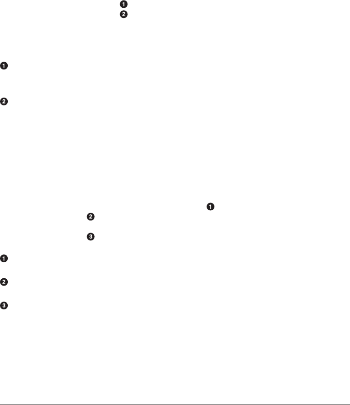
Depending on how frequent changes are, and how long they take, a global lock could
restrict the performance of a system significantly. We can increase parallelism by
making our locking more fine-grained.
Document Locking
Instead of locking the whole filesystem, we could lock individual documents by using
the same technique as previously described. A process could use a scan-and-scroll
request to retrieve the IDs of all documents that would be affected by the change, and
would need to create a lock file for each of them:
PUT /fs/lock/_bulk
{ "create": { "_id": 1}}
{ "process_id": 123 }
{ "create": { "_id": 2}}
{ "process_id": 123 }
...
The ID of the lock document would be the same as the ID of the file that should
be locked.
The process_id is a unique ID that represents the process that wants to perform
the changes.
If some files are already locked, parts of the bulk request will fail and we will have to
try again.
Of course, if we try to lock all of the files again, the create statements that we used
previously will fail for any file that is already locked by us! Instead of a simple create
statement, we need an update request with an upsert parameter and this script:
if ( ctx._source.process_id != process_id ) {
assert false;
}
ctx.op = 'noop';
process_id is a parameter that we pass into the script.
assert false will throw an exception, causing the update to fail.
Changing the op from update to noop prevents the update request from making
any changes, but still returns success.
The full update request looks like this:
POST /fs/lock/1/_update
{
"upsert": { "process_id": 123 },
"script": "if ( ctx._source.process_id != process_id )
Solving Concurrency Issues | 557

{ assert false }; ctx.op = 'noop';"
"params": {
"process_id": 123
}
}
If the document doesn’t already exist, the upsert document will be inserted—much
the same as the create request we used previously. However, if the document does
exist, the script will look at the process_id stored in the document. If it is the same as
ours, it aborts the update (noop) and returns success. If it is different, the assert
false throws an exception and we know that the lock has failed.
Once all locks have been successfully created, the rename operation can begin. After‐
ward, we must release all of the locks, which we can do with a delete-by-query
request:
POST /fs/_refresh
DELETE /fs/lock/_query
{
"query": {
"term": {
"process_id": 123
}
}
}
The refresh call ensures that all lock documents are visible to the delete-by-
query request.
Document-level locking enables fine-grained access control, but creating lock files for
millions of documents can be expensive. In certain scenarios, such as this example
with directory trees, it is possible to achieve fine-grained locking with much less
work.
Tree Locking
Rather than locking every involved document, as in the previous option, we could
lock just part of the directory tree. We will need exclusive access to the file or direc‐
tory that we want to rename, which can be achieved with an exclusive lock document:
{ "lock_type": "exclusive" }
And we need shared locks on any parent directories, with a shared lock document:
{
"lock_type": "shared",
"lock_count": 1
}
558 | Chapter 40: Handling Relationships

The lock_count records the number of processes that hold a shared lock.
A process that wants to rename /clinton/projects/elasticsearch/README.txt
needs an exclusive lock on that file, and a shared lock on /clinton, /clinton/
projects, and /clinton/projects/elasticsearch.
A simple create request will suffice for the exclusive lock, but the shared lock needs a
scripted update to implement some extra logic:
if (ctx._source.lock_type == 'exclusive') {
assert false;
}
ctx._source.lock_count++
If the lock_type is exclusive, the assert statement will throw an exception,
causing the update request to fail.
Otherwise, we increment the lock_count.
This script handles the case where the lock document already exists, but we will also
need an upsert document to handle the case where it doesn’t exist yet. The full
update request is as follows:
POST /fs/lock/%2Fclinton/_update
{
"upsert": {
"lock_type": "shared",
"lock_count": 1
},
"script": "if (ctx._source.lock_type == 'exclusive')
{ assert false }; ctx._source.lock_count++"
}
The ID of the document is /clinton, which is URL-encoded to %2fclinton.
The upsert document will be inserted if the document does not already exist.
Once we succeed in gaining a shared lock on all of the parent directories, we try to
create an exclusive lock on the file itself:
PUT /fs/lock/%2Fclinton%2fprojects%2felasticsearch%2fREADME.txt/_create
{ "lock_type": "exclusive" }
Now, if somebody else wants to rename the /clinton directory, they would have to
gain an exclusive lock on that path:
PUT /fs/lock/%2Fclinton/_create
{ "lock_type": "exclusive" }
Solving Concurrency Issues | 559

This request would fail because a lock document with the same ID already exists. The
other user would have to wait until our operation is done and we have released our
locks. The exclusive lock can just be deleted:
DELETE /fs/lock/%2Fclinton%2fprojects%2felasticsearch%2fREADME.txt
The shared locks need another script that decrements the lock_count and, if the
count drops to zero, deletes the lock document:
if (--ctx._source.lock_count == 0) {
ctx.op = 'delete'
}
Once the lock_count reaches 0, the ctx.op is changed from update to delete.
This update request would need to be run for each parent directory in reverse order,
from longest to shortest:
POST /fs/lock/%2Fclinton%2fprojects%2felasticsearch/_update
{
"script": "if (--ctx._source.lock_count == 0) { ctx.op = 'delete' } "
}
Tree locking gives us fine-grained concurrency control with the minimum of effort.
Of course, it is not applicable to every situation—the data model must have some sort
of access path like the directory tree for it to work.
None of the three options—global, document, or tree locking—
deals with the thorniest problem associated with locking: what hap‐
pens if the process holding the lock dies?
The unexpected death of a process leaves us with two problems:
•How do we know that we can release the locks held by the
dead process?
•How do we clean up the change that the dead process did not
manage to complete?
These topics are beyond the scope of this book, but you will need
to give them some thought if you decide to use locking.
While denormalization is a good choice for many projects, the need for locking
schemes can make for complicated implementations. Instead, Elasticsearch provides
two models that help us deal with related entities: nested objects and parent-child rela
tionships.
560 | Chapter 40: Handling Relationships

CHAPTER 41
Nested Objects
Given the fact that creating, deleting, and updating a single document in Elasticsearch
is atomic, it makes sense to store closely related entities within the same document.
For instance, we could store an order and all of its order lines in one document, or we
could store a blog post and all of its comments together, by passing an array of com
ments:
PUT /my_index/blogpost/1
{
"title": "Nest eggs",
"body": "Making your money work...",
"tags": [ "cash", "shares" ],
"comments": [
{
"name": "John Smith",
"comment": "Great article",
"age": 28,
"stars": 4,
"date": "2014-09-01"
},
{
"name": "Alice White",
"comment": "More like this please",
"age": 31,
"stars": 5,
"date": "2014-10-22"
}
]
}
If we rely on dynamic mapping, the comments field will be autocreated as an
object field.
561

Because all of the content is in the same document, there is no need to join blog posts
and comments at query time, so searches perform well.
The problem is that the preceding document would match a query like this:
GET /_search
{
"query": {
"bool": {
"must": [
{ "match": { "name": "Alice" }},
{ "match": { "age": 28 }}
]
}
}
}
Alice is 31, not 28!
The reason for this cross-object matching, as discussed in “Arrays of Inner Objects”
on page 95, is that our beautifully structured JSON document is flattened into a sim‐
ple key-value format in the index that looks like this:
{
"title": [ eggs, nest ],
"body": [ making, money, work, your ],
"tags": [ cash, shares ],
"comments.name": [ alice, john, smith, white ],
"comments.comment": [ article, great, like, more, please, this ],
"comments.age": [ 28, 31 ],
"comments.stars": [ 4, 5 ],
"comments.date": [ 2014-09-01, 2014-10-22 ]
}
The correlation between Alice and 31, or between John and 2014-09-01, has been
irretrievably lost. While fields of type object (see “Multilevel Objects” on page 94)
are useful for storing a single object, they are useless, from a search point of view, for
storing an array of objects.
This is the problem that nested objects are designed to solve. By mapping the comm
ments field as type nested instead of type object, each nested object is indexed as a
hidden separate document, something like this:
{
"comments.name": [ john, smith ],
"comments.comment": [ article, great ],
"comments.age": [ 28 ],
"comments.stars": [ 4 ],
"comments.date": [ 2014-09-01 ]
}
{
"comments.name": [ alice, white ],
562 | Chapter 41: Nested Objects

"comments.comment": [ like, more, please, this ],
"comments.age": [ 31 ],
"comments.stars": [ 5 ],
"comments.date": [ 2014-10-22 ]
}
{
"title": [ eggs, nest ],
"body": [ making, money, work, your ],
"tags": [ cash, shares ]
}
First nested object
Second nested object
The root or parent document
By indexing each nested object separately, the fields within the object maintain their
relationships. We can run queries that will match only if the match occurs within the
same nested object.
Not only that, because of the way that nested objects are indexed, joining the nested
documents to the root document at query time is fast—almost as fast as if they were a
single document.
These extra nested documents are hidden; we can’t access them directly. To update,
add, or remove a nested object, we have to reindex the whole document. It’s impor‐
tant to note that, the result returned by a search request is not the nested object alone;
it is the whole document.
Nested Object Mapping
Setting up a nested field is simple—where you would normally specify type object,
make it type nested instead:
PUT /my_index
{
"mappings": {
"blogpost": {
"properties": {
"comments": {
"type": "nested",
"properties": {
"name": { "type": "string" },
"comment": { "type": "string" },
"age": { "type": "short" },
"stars": { "type": "short" },
"date": { "type": "date" }
}
Nested Object Mapping | 563

}
}
}
}
}
A nested field accepts the same parameters as a field of type object.
That’s all that is required. Any comments objects would now be indexed as separate
nested documents. See the nested type reference docs for more.
Querying a Nested Object
Because nested objects are indexed as separate hidden documents, we can’t query
them directly. Instead, we have to use the nested query or nested filter to access
them:
GET /my_index/blogpost/_search
{
"query": {
"bool": {
"must": [
{ "match": { "title": "eggs" }},
{
"nested": {
"path": "comments",
"query": {
"bool": {
"must": [
{ "match": { "comments.name": "john" }},
{ "match": { "comments.age": 28 }}
]
}}}}
]
}}}
The title clause operates on the root document.
The nested clause “steps down” into the nested comments field. It no longer has
access to fields in the root document, nor fields in any other nested document.
The comments.name and comments.age clauses operate on the same nested docu‐
ment.
A nested field can contain other nested fields. Similarly, a nested
query can contain other nested queries. The nesting hierarchy is
applied as you would expect.
564 | Chapter 41: Nested Objects

Of course, a nested query could match several nested documents. Each matching
nested document would have its own relevance score, but these multiple scores need
to be reduced to a single score that can be applied to the root document.
By default, it averages the scores of the matching nested documents. This can be con‐
trolled by setting the score_mode parameter to avg, max, sum, or even none (in which
case the root document gets a constant score of 1.0).
GET /my_index/blogpost/_search
{
"query": {
"bool": {
"must": [
{ "match": { "title": "eggs" }},
{
"nested": {
"path": "comments",
"score_mode": "max",
"query": {
"bool": {
"must": [
{ "match": { "comments.name": "john" }},
{ "match": { "comments.age": 28 }}
]
}}}}
]
}}}
Give the root document the _score from the best-matching nested document.
A nested filter behaves much like a nested query, except that it
doesn’t accept the score_mode parameter. It can be used only in l
ter context—such as inside a filtered query—and it behaves like
any other filter: it includes or excludes, but it doesn’t score.
While the results of the nested filter itself are not cached, the usual
caching rules apply to the filter inside the nested filter.
Sorting by Nested Fields
It is possible to sort by the value of a nested field, even though the value exists in a
separate nested document. To make the result more interesting, we will add another
record:
PUT /my_index/blogpost/2
{
"title": "Investment secrets",
"body": "What they don't tell you ...",
"tags": [ "shares", "equities" ],
Sorting by Nested Fields | 565

"comments": [
{
"name": "Mary Brown",
"comment": "Lies, lies, lies",
"age": 42,
"stars": 1,
"date": "2014-10-18"
},
{
"name": "John Smith",
"comment": "You're making it up!",
"age": 28,
"stars": 2,
"date": "2014-10-16"
}
]
}
Imagine that we want to retrieve blog posts that received comments in October,
ordered by the lowest number of stars that each blog post received. The search
request would look like this:
GET /_search
{
"query": {
"nested": {
"path": "comments",
"filter": {
"range": {
"comments.date": {
"gte": "2014-10-01",
"lt": "2014-11-01"
}
}
}
}
},
"sort": {
"comments.stars": {
"order": "asc",
"mode": "min",
"nested_filter": {
"range": {
"comments.date": {
"gte": "2014-10-01",
"lt": "2014-11-01"
}
}
}
}
}
}
566 | Chapter 41: Nested Objects

The nested query limits the results to blog posts that received a comment in
October.
Results are sorted in ascending (asc) order by the lowest value (min) in the com
ment.stars field in any matching comments.
The nested_filter in the sort clause is the same as the nested query in the main
query clause. The reason is explained next.
Why do we need to repeat the query conditions in the nested_filter? The reason is
that sorting happens after the query has been executed. The query matches blog posts
that received comments in October, but it returns blog post documents as the result.
If we didn’t include the nested_filter clause, we would end up sorting based on any
comments that the blog post has ever received, not just those received in October.
Nested Aggregations
In the same way as we need to use the special nested query to gain access to nested
objects at search time, the dedicated nested aggregation allows us to aggregate fields
in nested objects:
GET /my_index/blogpost/_search?search_type=count
{
"aggs": {
"comments": {
"nested": {
"path": "comments"
},
"aggs": {
"by_month": {
"date_histogram": {
"field": "comments.date",
"interval": "month",
"format": "yyyy-MM"
},
"aggs": {
"avg_stars": {
"avg": {
"field": "comments.stars"
}
}
}
}
}
}
}
}
Nested Aggregations | 567

The nested aggregation “steps down” into the nested comments object.
Comments are bucketed into months based on the comments.date field.
The average number of stars is calculated for each bucket.
The results show that aggregation has happened at the nested document level:
...
"aggregations": {
"comments": {
"doc_count": 4,
"by_month": {
"buckets": [
{
"key_as_string": "2014-09",
"key": 1409529600000,
"doc_count": 1,
"avg_stars": {
"value": 4
}
},
{
"key_as_string": "2014-10",
"key": 1412121600000,
"doc_count": 3,
"avg_stars": {
"value": 2.6666666666666665
}
}
]
}
}
}
...
There are a total of four comments: one in September and three in October.
reverse_nested Aggregation
A nested aggregation can access only the fields within the nested document. It can’t
see fields in the root document or in a different nested document. However, we can
step out of the nested scope back into the parent with a reverse_nested aggregation.
For instance, we can find out which tags our commenters are interested in, based on
the age of the commenter. The comment.age is a nested field, while the tags are in the
root document:
GET /my_index/blogpost/_search?search_type=count
{
568 | Chapter 41: Nested Objects

"aggs": {
"comments": {
"nested": {
"path": "comments"
},
"aggs": {
"age_group": {
"histogram": {
"field": "comments.age",
"interval": 10
},
"aggs": {
"blogposts": {
"reverse_nested": {},
"aggs": {
"tags": {
"terms": {
"field": "tags"
}
}
}
}
}
}
}
}
}
}
The nested agg steps down into the comments object.
The histogram agg groups on the comments.age field, in buckets of 10 years.
The reverse_nested agg steps back up to the root document.
The terms agg counts popular terms per age group of the commenter.
The abbreviated results show us the following:
..
"aggregations": {
"comments": {
"doc_count": 4,
"age_group": {
"buckets": [
{
"key": 20,
"doc_count": 2,
"blogposts": {
"doc_count": 2,
"tags": {
Nested Aggregations | 569

"doc_count_error_upper_bound": 0,
"buckets": [
{ "key": "shares", "doc_count": 2 },
{ "key": "cash", "doc_count": 1 },
{ "key": "equities", "doc_count": 1 }
]
}
}
},
...
There are four comments.
There are two comments by commenters between the ages of 20 and 30.
Two blog posts are associated with those comments.
The popular tags in those blog posts are shares, cash, and equities.
When to Use Nested Objects
Nested objects are useful when there is one main entity, like our blogpost, with a
limited number of closely related but less important entities, such as comments. It is
useful to be able to find blog posts based on the content of the comments, and the
nested query and filter provide for fast query-time joins.
The disadvantages of the nested model are as follows:
•To add, change, or delete a nested document, the whole document must be rein‐
dexed. This becomes more costly the more nested documents there are.
•Search requests return the whole document, not just the matching nested docu‐
ments. Although there are plans afoot to support returning the best -matching
nested documents with the root document, this is not yet supported.
Sometimes you need a complete separation between the main document and its asso‐
ciated entities. This separation is provided by the parent-child relationship.
570 | Chapter 41: Nested Objects

CHAPTER 42
Parent-Child Relationship
The parent-child relationship is similar in nature to the nested model: both allow you
to associate one entity with another. The difference is that, with nested objects, all
entities live within the same document while, with parent-child, the parent and chil‐
dren are completely separate documents.
The parent-child functionality allows you to associate one document type with
another, in a one-to-many relationship—one parent to many children. The advantages
that parent-child has over nested objects are as follows:
• The parent document can be updated without reindexing the children.
•Child documents can be added, changed, or deleted without affecting either the
parent or other children. This is especially useful when child documents are large
in number and need to be added or changed frequently.
• Child documents can be returned as the results of a search request.
Elasticsearch maintains a map of which parents are associated with which children. It
is thanks to this map that query-time joins are fast, but it does place a limitation on
the parent-child relationship: the parent document and all of its children must live on
the same shard.
At the time of going to press, the parent-child ID map is held in
memory as part of fielddata. There are plans afoot to change the
default setting to use doc values by default instead.
571

Parent-Child Mapping
All that is needed in order to establish the parent-child relationship is to specify
which document type should be the parent of a child type. This must be done at index
creation time, or with the update-mapping API before the child type has been cre‐
ated.
As an example, let’s say that we have a company that has branches in many cities. We
would like to associate employees with the branch where they work. We need to be
able to search for branches, individual employees, and employees who work for par‐
ticular branches, so the nested model will not help. We could, of course, use
application-side-joins or data denormalization here instead, but for demonstration
purposes we will use parent-child.
All that we have to do is to tell Elasticsearch that the employee type has the branch
document type as its _parent, which we can do when we create the index:
PUT /company
{
"mappings": {
"branch": {},
"employee": {
"_parent": {
"type": "branch"
}
}
}
}
Documents of type employee are children of type branch.
Indexing Parents and Children
Indexing parent documents is no different from any other document. Parents don’t
need to know anything about their children:
POST /company/branch/_bulk
{ "index": { "_id": "london" }}
{ "name": "London Westminster", "city": "London", "country": "UK" }
{ "index": { "_id": "liverpool" }}
{ "name": "Liverpool Central", "city": "Liverpool", "country": "UK" }
{ "index": { "_id": "paris" }}
{ "name": "Champs Élysées", "city": "Paris", "country": "France" }
When indexing child documents, you must specify the ID of the associated parent
document:
PUT /company/employee/1?parent=london
{
572 | Chapter 42: Parent-Child Relationship

"name": "Alice Smith",
"dob": "1970-10-24",
"hobby": "hiking"
}
This employee document is a child of the london branch.
This parent ID serves two purposes: it creates the link between the parent and the
child, and it ensures that the child document is stored on the same shard as the par‐
ent.
In “Routing a Document to a Shard” on page 61, we explained how Elasticsearch uses
a routing value, which defaults to the _id of the document, to decide which shard a
document should belong to. The routing value is plugged into this simple formula:
shard = hash(routing) % number_of_primary_shards
However, if a parent ID is specified, it is used as the routing value instead of the _id.
In other words, both the parent and the child use the same routing value—the _id of
the parent—and so they are both stored on the same shard.
The parent ID needs to be specified on all single-document requests: when retrieving
a child document with a GET request, or when indexing, updating, or deleting a child
document. Unlike a search request, which is forwarded to all shards in an index, these
single-document requests are forwarded only to the shard that holds the document—
if the parent ID is not specified, the request will probably be forwarded to the wrong
shard.
The parent ID should also be specified when using the bulk API:
POST /company/employee/_bulk
{ "index": { "_id": 2, "parent": "london" }}
{ "name": "Mark Thomas", "dob": "1982-05-16", "hobby": "diving" }
{ "index": { "_id": 3, "parent": "liverpool" }}
{ "name": "Barry Smith", "dob": "1979-04-01", "hobby": "hiking" }
{ "index": { "_id": 4, "parent": "paris" }}
{ "name": "Adrien Grand", "dob": "1987-05-11", "hobby": "horses" }
If you want to change the parent value of a child document, it is
not sufficient to just reindex or update the child document—the
new parent document may be on a different shard. Instead, you
must first delete the old child, and then index the new child.
Finding Parents by Their Children
The has_child query and filter can be used to find parent documents based on the
contents of their children. For instance, we could find all branches that have employ‐
ees born after 1980 with a query like this:
Finding Parents by Their Children | 573

GET /company/branch/_search
{
"query": {
"has_child": {
"type": "employee",
"query": {
"range": {
"dob": {
"gte": "1980-01-01"
}
}
}
}
}
}
Like the nested query, the has_child query could match several child documents,
each with a different relevance score. How these scores are reduced to a single score
for the parent document depends on the score_mode parameter. The default setting is
none, which ignores the child scores and assigns a score of 1.0 to the parents, but it
also accepts avg, min, max, and sum.
The following query will return both london and liverpool, but london will get a
better score because Alice Smith is a better match than Barry Smith:
GET /company/branch/_search
{
"query": {
"has_child": {
"type": "employee",
"score_mode": "max"
"query": {
"match": {
"name": "Alice Smith"
}
}
}
}
}
The default score_mode of none is significantly faster than the
other modes because Elasticsearch doesn’t need to calculate the
score for each child document. Set it to avg, min, max, or sum only
if you care about the score.
574 | Chapter 42: Parent-Child Relationship

min_children and max_children
The has_child query and filter both accept the min_children and max_children
parameters, which will return the parent document only if the number of matching
children is within the specified range.
This query will match only branches that have at least two employees:
GET /company/branch/_search
{
"query": {
"has_child": {
"type": "employee",
"min_children": 2,
"query": {
"match_all": {}
}
}
}
}
A branch must have at least two employees in order to match.
The performance of a has_child query or filter with the min_children or max_chil
dren parameters is much the same as a has_child query with scoring enabled.
has_child Filter
The has_child filter works in the same way as the has_child query, except that it
doesn’t support the score_mode parameter. It can be used only in lter context—such
as inside a filtered query—and behaves like any other filter: it includes or excludes,
but doesn’t score.
While the results of a has_child filter are not cached, the usual caching rules apply to
the filter inside the has_child filter.
Finding Children by Their Parents
While a nested query can always return only the root document as a result, parent
and child documents are independent and each can be queried independently. The
has_child query allows us to return parents based on data in their children, and the
has_parent query returns children based on data in their parents.
It looks very similar to the has_child query. This example returns employees who
work in the UK:
Finding Children by Their Parents | 575

GET /company/employee/_search
{
"query": {
"has_parent": {
"type": "branch",
"query": {
"match": {
"country": "UK"
}
}
}
}
}
Returns children who have parents of type branch
The has_parent query also supports the score_mode, but it accepts only two settings:
none (the default) and score. Each child can have only one parent, so there is no need
to reduce multiple scores into a single score for the child. The choice is simply
between using the score (score) or not (none).
has_parent Filter
The has_parent filter works in the same way as the has_parent query, except that it
doesn’t support the score_mode parameter. It can be used only in lter context—such
as inside a filtered query—and behaves like any other filter: it includes or excludes,
but doesn’t score.
While the results of a has_parent filter are not cached, the usual caching rules apply
to the filter inside the has_parent filter.
Children Aggregation
Parent-child supports a children aggregation as a direct analog to the nested aggre‐
gation discussed in “Nested Aggregations” on page 567. A parent aggregation (the
equivalent of reverse_nested) is not supported.
This example demonstrates how we could determine the favorite hobbies of our
employees by country:
GET /company/branch/_search?search_type=count
{
"aggs": {
"country": {
"terms": {
"field": "country"
},
576 | Chapter 42: Parent-Child Relationship

"aggs": {
"employees": {
"children": {
"type": "employee"
},
"aggs": {
"hobby": {
"terms": {
"field": "employee.hobby"
}
}
}
}
}
}
}
}
The country field in the branch documents.
The children aggregation joins the parent documents with their associated chil‐
dren of type employee.
The hobby field from the employee child documents.
Grandparents and Grandchildren
The parent-child relationship can extend across more than one generation—grand‐
children can have grandparents—but it requires an extra step to ensure that docu‐
ments from all generations are indexed on the same shard.
Let’s change our previous example to make the country type a parent of the branch
type:
PUT /company
{
"mappings": {
"country": {},
"branch": {
"_parent": {
"type": "country"
}
},
"employee": {
"_parent": {
"type": "branch"
}
}
}
}
Grandparents and Grandchildren | 577

branch is a child of country.
employee is a child of branch.
Countries and branches have a simple parent-child relationship, so we use the same
process as we used in “Indexing Parents and Children” on page 572:
POST /company/country/_bulk
{ "index": { "_id": "uk" }}
{ "name": "UK" }
{ "index": { "_id": "france" }}
{ "name": "France" }
POST /company/branch/_bulk
{ "index": { "_id": "london", "parent": "uk" }}
{ "name": "London Westmintster" }
{ "index": { "_id": "liverpool", "parent": "uk" }}
{ "name": "Liverpool Central" }
{ "index": { "_id": "paris", "parent": "france" }}
{ "name": "Champs Élysées" }
The parent ID has ensured that each branch document is routed to the same shard as
its parent country document. However, look what would happen if we were to use
the same technique with the employee grandchildren:
PUT /company/employee/1?parent=london
{
"name": "Alice Smith",
"dob": "1970-10-24",
"hobby": "hiking"
}
The shard routing of the employee document would be decided by the parent ID—
london—but the london document was routed to a shard by its own parent ID—uk. It
is very likely that the grandchild would end up on a different shard from its parent
and grandparent, which would prevent the same-shard parent-child mapping from
functioning.
Instead, we need to add an extra routing parameter, set to the ID of the grandparent,
to ensure that all three generations are indexed on the same shard. The indexing
request should look like this:
PUT /company/employee/1?parent=london&routing=uk
{
"name": "Alice Smith",
"dob": "1970-10-24",
"hobby": "hiking"
}
The routing value overrides the parent value.
578 | Chapter 42: Parent-Child Relationship

The parent parameter is still used to link the employee document with its parent, but
the routing parameter ensures that it is stored on the same shard as its parent and
grandparent. The routing value needs to be provided for all single-document
requests.
Querying and aggregating across generations works, as long as you step through each
generation. For instance, to find countries where employees enjoy hiking, we need to
join countries with branches, and branches with employees:
GET /company/country/_search
{
"query": {
"has_child": {
"type": "branch",
"query": {
"has_child": {
"type": "employee",
"query": {
"match": {
"hobby": "hiking"
}
}
}
}
}
}
}
Practical Considerations
Parent-child joins can be a useful technique for managing relationships when index-
time performance is more important than search-time performance, but it comes at a
significant cost. Parent-child queries can be 5 to 10 times slower than the equivalent
nested query!
Memory Use
At the time of going to press, the parent-child ID map is still held in memory. There
are plans to change the map to use doc values instead, which will be a big memory
saving. Until that happens, you need to be aware of the following: the string _id field
of every parent document has to be held in memory, and every child document
requires 8 bytes (a long value) of memory. Actually, it’s a bit less thanks to compres‐
sion, but this gives you a rough idea.
You can check how much memory is being used by the parent-child cache by consult‐
ing the indices-stats API (for a summary at the index level) or the node-stats API
(for a summary at the node level):
Practical Considerations | 579

GET /_nodes/stats/indices/id_cache?human
Returns memory use of the ID cache summarized by node in a human-friendly
format.
Global Ordinals and Latency
Parent-child uses global ordinals to speed up joins. Regardless of whether the parent-
child map uses an in-memory cache or on-disk doc values, global ordinals still need
to be rebuilt after any change to the index.
The more parents in a shard, the longer global ordinals will take to build. Parent-
child is best suited to situations where there are many children for each parent, rather
than many parents and few children.
Global ordinals, by default, are built lazily: the first parent-child query or aggregation
after a refresh will trigger building of global ordinals. This can introduce a significant
latency spike for your users. You can use eager_global_ordinals to shift the cost of
building global ordinals from query time to refresh time, by mapping the _parent
field as follows:
PUT /company
{
"mappings": {
"branch": {},
"employee": {
"_parent": {
"type": "branch",
"fielddata": {
"loading": "eager_global_ordinals"
}
}
}
}
}
Global ordinals for the _parent field will be built before a new segment becomes
visible to search.
With many parents, global ordinals can take several seconds to build. In this case, it
makes sense to increase the refresh_interval so that refreshes happen less often
and global ordinals remain valid for longer. This will greatly reduce the CPU cost of
rebuilding global ordinals every second.
Multigenerations and Concluding Thoughts
The ability to join multiple generations (see “Grandparents and Grandchildren” on
page 577) sounds attractive until you think of the costs involved:
580 | Chapter 42: Parent-Child Relationship

• The more joins you have, the worse performance will be.
•Each generation of parents needs to have their string _id fields stored in mem‐
ory, which can consume a lot of RAM.
As you consider your relationship schemes and whether parent-child is right for you,
consider this advice about parent-child relationships:
•Use parent-child relationships sparingly, and only when there are many more
children than parents.
• Avoid using multiple parent-child joins in a single query.
•Avoid scoring by using the has_child filter, or the has_child query with
score_mode set to none.
• Keep the parent IDs short, so that they require less memory.
Above all: think about the other relationship techniques that we have discussed before
reaching for parent-child.
Practical Considerations | 581

CHAPTER 43
Designing for Scale
Elasticsearch is used by some companies to index and search petabytes of data every
day, but most of us start out with something a little more humble in size. Even if we
aspire to be the next Facebook, it is unlikely that our bank balance matches our aspi‐
rations. We need to build for what we have today, but in a way that will allow us to
scale out flexibly and rapidly.
Elasticsearch is built to scale. It will run very happily on your laptop or in a cluster
containing hundreds of nodes, and the experience is almost identical. Growing from
a small cluster to a large cluster is almost entirely automatic and painless. Growing
from a large cluster to a very large cluster requires a bit more planning and design,
but it is still relatively painless.
Of course, it is not magic. Elasticsearch has its limitations too. If you are aware of
those limitations and work with them, the growing process will be pleasant. If you
treat Elasticsearch badly, you could be in for a world of pain.
The default settings in Elasticsearch will take you a long way, but to get the most bang
for your buck, you need to think about how data flows through your system. We will
talk about two common data flows: time-based data (such as log events or social net‐
work streams, where relevance is driven by recency), and user-based data (where a
large document collection can be subdivided by user or customer).
This chapter will help you make the right decisions up front, to avoid nasty surprises
later.
The Unit of Scale
In “Dynamically Updatable Indices” on page 155, we explained that a shard is a
Lucene index and that an Elasticsearch index is a collection of shards. Your applica‐
583
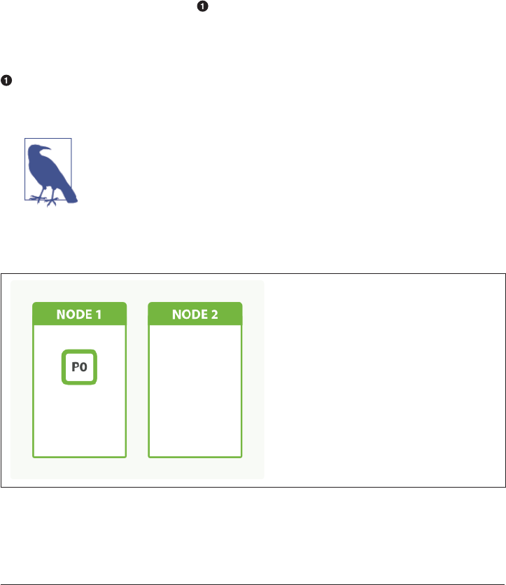
tion talks to an index, and Elasticsearch routes your requests to the appropriate
shards.
A shard is the unit of scale. The smallest index you can have is one with a single shard.
This may be more than sufficient for your needs—a single shard can hold a lot of data
—but it limits your ability to scale.
Imagine that our cluster consists of one node, and in our cluster we have one index,
which has only one shard:
PUT /my_index
{
"settings": {
"number_of_shards": 1,
"number_of_replicas": 0
}
}
Create an index with one primary shard and zero replica shards.
This setup may be small, but it serves our current needs and is cheap to run.
At the moment we are talking about only primary shards. We dis‐
cuss replica shards in “Replica Shards” on page 588.
One glorious day, the Internet discovers us, and a single node just can’t keep up with
the traffic. We decide to add a second node, as per Figure 43-1. What happens?
Figure 43-1. An index with one shard has no scale factor
The answer is: nothing. Because we have only one shard, there is nothing to put on
the second node. We can’t increase the number of shards in the index, because the
584 | Chapter 43: Designing for Scale
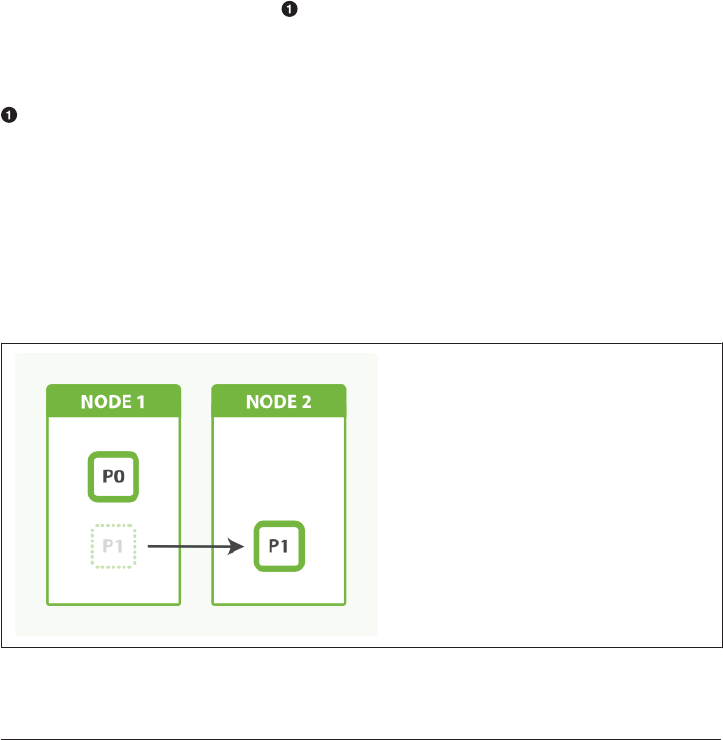
number of shards is an important element in the algorithm used to route documents
to shards:
shard = hash(routing) % number_of_primary_shards
Our only option now is to reindex our data into a new, bigger index that has more
shards, but that will take time that we can ill afford. By planning ahead, we could have
avoided this problem completely by overallocating.
Shard Overallocation
A shard lives on a single node, but a node can hold multiple shards. Imagine that we
created our index with two primary shards instead of one:
PUT /my_index
{
"settings": {
"number_of_shards": 2,
"number_of_replicas": 0
}
}
Create an index with two primary shards and zero replica shards.
With a single node, both shards would be assigned to the same node. From the point
of view of our application, everything functions as it did before. The application com‐
municates with the index, not the shards, and there is still only one index.
This time, when we add a second node, Elasticsearch will automatically move one
shard from the first node to the second node, as depicted in Figure 43-2. Once the
relocation has finished, each shard will have access to twice the computing power that
it had before.
Figure 43-2. An index with two shards can take advantage of a second node
Shard Overallocation | 585

We have been able to double our capacity by simply copying a shard across the net‐
work to the new node. The best part is, we achieved this with zero downtime. All
indexing and search requests continued to function normally while the shard was
being moved.
A new index in Elasticsearch is allotted five primary shards by default. That means
that we can spread that index out over a maximum of five nodes, with one shard on
each node. That’s a lot of capacity, and it happens without you having to think about
it at all!
Shard Splitting
Users often ask why Elasticsearch doesn’t support shard-splitting—the ability to split
each shard into two or more pieces. The reason is that shard-splitting is a bad idea:
•Splitting a shard is almost equivalent to reindexing your data. It’s a much heavier
process than just copying a shard from one node to another.
•Splitting is exponential. You start with one shard, then split into two, and then
four, eight, sixteen, and so on. Splitting doesn’t allow you to increase capacity by
just 50%.
•Shard splitting requires you to have enough capacity to hold a second copy of
your index. Usually, by the time you realize that you need to scale out, you don’t
have enough free space left to perform the split.
In a way, Elasticsearch does support shard splitting. You can always reindex your data
to a new index with the appropriate number of shards (see “Reindexing Your Data”
on page 150). It is still a more intensive process than moving shards around, and still
requires enough free space to complete, but at least you can control the number of
shards in the new index.
Kagillion Shards
The first thing that new users do when they learn about shard overallocation is to say
to themselves:
I don’t know how big this is going to be, and I can’t change the index size later on, so to
be on the safe side, I’ll just give this index 1,000 shards…
—A new user
One thousand shards—really? And you don’t think that, perhaps, between now and
the time you need to buy one thousand nodes, that you may need to rethink your data
model once or twice and have to reindex?
A shard is not free. Remember:
586 | Chapter 43: Designing for Scale

• A shard is a Lucene index under the covers, which uses file handles, memory, and
CPU cycles.
•Every search request needs to hit a copy of every shard in the index. That’s fine if
every shard is sitting on a different node, but not if many shards have to compete
for the same resources.
•Term statistics, used to calculate relevance, are per shard. Having a small amount
of data in many shards leads to poor relevance.
A little overallocation is good. A kagillion shards is bad. It is diffi‐
cult to define what constitutes too many shards, as it depends on
their size and how they are being used. A hundred shards that are
seldom used may be fine, while two shards experiencing very heavy
usage could be too many. Monitor your nodes to ensure that they
have enough spare capacity to deal with exceptional conditions.
Scaling out should be done in phases. Build in enough capacity to get to the next
phase. Once you get to the next phase, you have time to think about the changes you
need to make to reach the phase after that.
Capacity Planning
If 1 shard is too few and 1,000 shards are too many, how do I know how many shards
I need? This is a question that is impossible to answer in the general case. There are
just too many variables: the hardware that you use, the size and complexity of your
documents, how you index and analyze those documents, the types of queries that
you run, the aggregations that you perform, how you model your data, and more.
Fortunately, it is an easy question to answer in the specific case—yours:
1. Create a cluster consisting of a single server, with the hardware that you are con‐
sidering using in production.
2. Create an index with the same settings and analyzers that you plan to use in pro‐
duction, but with only one primary shard and no replicas.
3. Fill it with real documents (or as close to real as you can get).
4. Run real queries and aggregations (or as close to real as you can get).
Essentially, you want to replicate real-world usage and to push this single shard until
it “breaks.” Even the definition of breaks depends on you: some users require that all
responses return within 50ms; others are quite happy to wait for 5 seconds.
Capacity Planning | 587

Once you define the capacity of a single shard, it is easy to extrapolate that number to
your whole index. Take the total amount of data that you need to index, plus some
extra for future growth, and divide by the capacity of a single shard. The result is the
number of primary shards that you will need.
Capacity planning should not be your first step.
First look for ways to optimize how you are using Elasticsearch.
Perhaps you have inefficient queries, not enough RAM, or you have
left swap enabled?
We have seen new users who, frustrated by initial performance,
immediately start trying to tune the garbage collector or adjust the
number of threads, instead of tackling the simple problems like
removing wildcard queries.
Replica Shards
Up until now we have spoken only about primary shards, but we have another tool in
our belt: replica shards. The main purpose of replicas is for failover, as discussed in
Chapter 2: if the node holding a primary shard dies, a replica is promoted to the role
of primary.
At index time, a replica shard does the same amount of work as the primary shard.
New documents are first indexed on the primary and then on any replicas. Increasing
the number of replicas does not change the capacity of the index.
However, replica shards can serve read requests. If, as is often the case, your index is
search heavy, you can increase search performance by increasing the number of repli‐
cas, but only if you also add extra hardware.
Let’s return to our example of an index with two primary shards. We increased
capacity of the index by adding a second node. Adding more nodes would not help us
to add indexing capacity, but we could take advantage of the extra hardware at search
time by increasing the number of replicas:
POST /my_index/_settings
{
"number_of_replicas": 1
}
Having two primary shards, plus a replica of each primary, would give us a total of
four shards: one for each node, as shown in Figure 43-3.
588 | Chapter 43: Designing for Scale
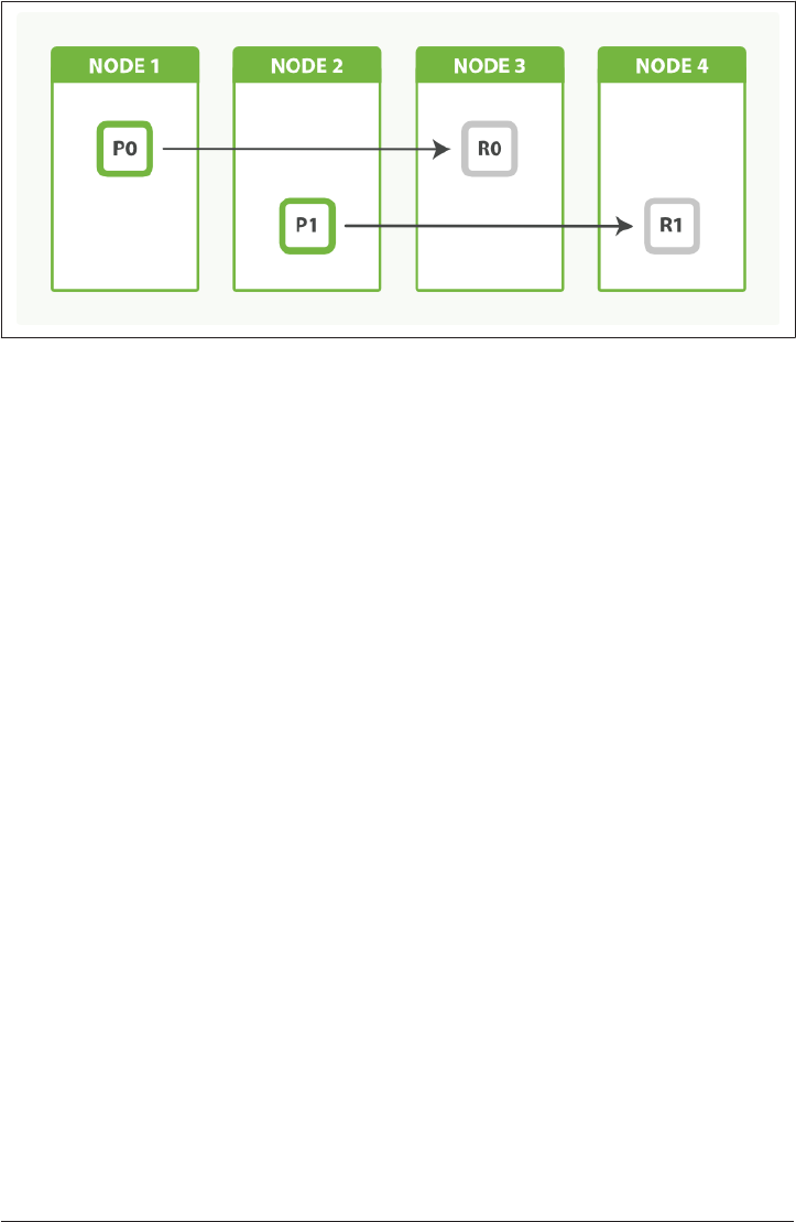
Figure 43-3. An index with two primary shards and one replica can scale out across four
nodes
Balancing Load with Replicas
Search performance depends on the response times of the slowest node, so it is a
good idea to try to balance out the load across all nodes. If we added just one extra
node instead of two, we would end up with two nodes having one shard each, and
one node doing double the work with two shards.
We can even things out by adjusting the number of replicas. By allocating two repli‐
cas instead of one, we end up with a total of six shards, which can be evenly divided
between three nodes, as shown in Figure 43-4:
POST /my_index/_settings
{
"number_of_replicas": 2
}
As a bonus, we have also increased our availability. We can now afford to lose two
nodes and still have a copy of all our data.
Replica Shards | 589
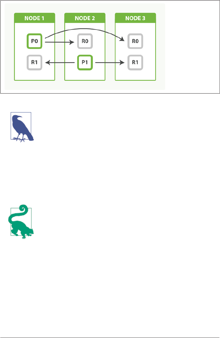
Figure 43-4. Adjust the number of replicas to balance the load between nodes
The fact that node 3 holds two replicas and no primaries is not
important. Replicas and primaries do the same amount of work;
they just play slightly different roles. There is no need to ensure
that primaries are distributed evenly across all nodes.
Multiple Indices
Finally, remember that there is no rule that limits your application to using only a
single index. When we issue a search request, it is forwarded to a copy (a primary or
a replica) of all the shards in an index. If we issue the same search request on multiple
indices, the exact same thing happens—there are just more shards involved.
Searching 1 index of 50 shards is exactly equivalent to searching
50 indices with 1 shard each: both search requests hit 50 shards.
This can be a useful fact to remember when you need to add capacity on the fly.
Instead of having to reindex your data into a bigger index, you can just do the follow‐
ing:
• Create a new index to hold new data.
• Search across both indices to retrieve new and old data.
In fact, with a little forethought, adding a new index can be done in a completely
transparent way, without your application ever knowing that anything has changed.
590 | Chapter 43: Designing for Scale

In “Index Aliases and Zero Downtime” on page 151, we spoke about using an index
alias to point to the current version of your index. For instance, instead of naming
your index tweets, name it tweets_v1. Your application would still talk to tweets,
but in reality that would be an alias that points to tweets_v1. This allows you to
switch the alias to point to a newer version of the index on the fly.
A similar technique can be used to expand capacity by adding a new index. It requires
a bit of planning because you will need two aliases: one for searching and one for
indexing:
PUT /tweets_1/_alias/tweets_search
PUT /tweets_1/_alias/tweets_index
Both the tweets_search and the tweets_index alias point to index tweets_1.
New documents should be indexed into tweets_index, and searches should be per‐
formed against tweets_search. For the moment, these two aliases point to the same
index.
When we need extra capacity, we can create a new index called tweets_2 and update
the aliases as follows:
POST /_aliases
{
"actions": [
{ "add": { "index": "tweets_2", "alias": "tweets_search" }},
{ "remove": { "index": "tweets_1", "alias": "tweets_index" }},
{ "add": { "index": "tweets_2", "alias": "tweets_index" }}
]
}
Add index tweets_2 to the tweets_search alias.
Switch tweets_index from tweets_1 to tweets_2.
A search request can target multiple indices, so having the search alias point to
tweets_1 and tweets_2 is perfectly valid. However, indexing requests can target only
a single index. For this reason, we have to switch the index alias to point to only the
new index.
A document GET request, like an indexing request, can target only
one index. This makes retrieving a document by ID a bit more
complicated in this scenario. Instead, run a search request with the
ids query, or do a multi-get request on tweets_1 and tweets_2.
Multiple Indices | 591

Using multiple indices to expand index capacity on the fly is of particular benefit
when dealing with time-based data such as logs or social-event streams, which we
discuss in the next section.
Time-Based Data
One of the most common use cases for Elasticsearch is for logging, so common in
fact that Elasticsearch provides an integrated logging platform called the ELK stack—
Elasticsearch, Logstash, and Kibana—to make the process easy.
Logstash collects, parses, and enriches logs before indexing them into Elasticsearch.
Elasticsearch acts as a centralized logging server, and Kibana is a graphic frontend
that makes it easy to query and visualize what is happening across your network in
near real-time.
Most traditional use cases for search engines involve a relatively static collection of
documents that grows slowly. Searches look for the most relevant documents, regard‐
less of when they were created.
Logging—and other time-based data streams such as social-network activity—are
very different in nature. The number of documents in the index grows rapidly, often
accelerating with time. Documents are almost never updated, and searches mostly
target the most recent documents. As documents age, they lose value.
We need to adapt our index design to function with the flow of time-based data.
Index per Time Frame
If we were to have one big index for documents of this type, we would soon run out
of space. Logging events just keep on coming, without pause or interruption. We
could delete the old events, with a delete-by-query:
DELETE /logs/event/_query
{
"query": {
"range": {
"@timestamp": {
"lt": "now-90d"
}
}
}
}
Deletes all documents where Logstash’s @timestamp field is older than 90 days.
But this approach is very inecient. Remember that when you delete a document, it is
only marked as deleted (see “Deletes and Updates” on page 158). It won’t be physically
deleted until the segment containing it is merged away.
592 | Chapter 43: Designing for Scale

Instead, use an index per time frame. You could start out with an index per year
(logs_2014) or per month (logs_2014-10). Perhaps, when your website gets really
busy, you need to switch to an index per day (logs_2014-10-24). Purging old data is
easy: just delete old indices.
This approach has the advantage of allowing you to scale as and when you need to.
You don’t have to make any difficult decisions up front. Every day is a new opportu‐
nity to change your indexing time frames to suit the current demand. Apply the same
logic to how big you make each index. Perhaps all you need is one primary shard per
week initially. Later, maybe you need five primary shards per day. It doesn’t matter—
you can adjust to new circumstances at any time.
Aliases can help make switching indices more transparent. For indexing, you can
point logs_current to the index currently accepting new log events, and for search‐
ing, update last_3_months to point to all indices for the previous three months:
POST /_aliases
{
"actions": [
{ "add": { "alias": "logs_current", "index": "logs_2014-10" }},
{ "remove": { "alias": "logs_current", "index": "logs_2014-09" }},
{ "add": { "alias": "last_3_months", "index": "logs_2014-10" }},
{ "remove": { "alias": "last_3_months", "index": "logs_2014-07" }}
]
}
Switch logs_current from September to October.
Add October to last_3_months and remove July.
Index Templates
Elasticsearch doesn’t require you to create an index before using it. With logging, it is
often more convenient to rely on index autocreation than to have to create indices
manually.
Logstash uses the timestamp from an event to derive the index name. By default, it
indexes into a different index every day, so an event with a @timestamp of 2014-10-01
00:00:01 will be sent to the index logstash-2014.10.01. If that index doesn’t already
exist, it will be created for us.
Usually we want some control over the settings and mappings of the new index. Per‐
haps we want to limit the number of shards to 1, and we want to disable the _all
field. Index templates can be used to control which settings should be applied to
newly created indices:
Index Templates | 593

PUT /_template/my_logs
{
"template": "logstash-*",
"order": 1,
"settings": {
"number_of_shards": 1
},
"mappings": {
"_default_": {
"_all": {
"enabled": false
}
}
},
"aliases": {
"last_3_months": {}
}
}
Create a template called my_logs.
Apply this template to all indices beginning with logstash-.
This template should override the default logstash template that has a lower
order.
Limit the number of primary shards to 1.
Disable the _all field for all types.
Add this index to the last_3_months alias.
This template specifies the default settings that will be applied to any index whose
name begins with logstash-, whether it is created manually or automatically. If we
think the index for tomorrow will need more capacity than today, we can update the
index to use a higher number of shards.
The template even adds the newly created index into the last_3_months alias,
although removing the old indices from that alias will have to be done manually.
Retiring Data
As time-based data ages, it becomes less relevant. It’s possible that we will want to see
what happened last week, last month, or even last year, but for the most part, we’re
interested in only the here and now.
The nice thing about an index per time frame is that it enables us to easily delete old
data: just delete the indices that are no longer relevant:
594 | Chapter 43: Designing for Scale

DELETE /logs_2013*
Deleting a whole index is much more efficient than deleting individual documents:
Elasticsearch just removes whole directories.
But deleting an index is very nal. There are a number of things we can do to help
data age gracefully, before we decide to delete it completely.
Migrate Old Indices
With logging data, there is likely to be one hot index—the index for today. All new
documents will be added to that index, and almost all queries will target that index. It
should use your best hardware.
How does Elasticsearch know which servers are your best servers? You tell it, by
assigning arbitrary tags to each server. For instance, you could start a node as follows:
./bin/elasticsearch --node.box_type strong
The box_type parameter is completely arbitrary—you could have named it whatever
you like—but you can use these arbitrary values to tell Elasticsearch where to allocate
an index.
We can ensure that today’s index is on our strongest boxes by creating it with the fol‐
lowing settings:
PUT /logs_2014-10-01
{
"settings": {
"index.routing.allocation.include.box_type" : "strong"
}
}
Yesterday’s index no longer needs to be on our strongest boxes, so we can move it to
the nodes tagged as medium by updating its index settings:
POST /logs_2014-09-30/_settings
{
"index.routing.allocation.include.box_type" : "medium"
}
Optimize Indices
Yesterday’s index is unlikely to change. Log events are static: what happened in the
past stays in the past. If we merge each shard down to just a single segment, it’ll use
fewer resources and will be quicker to query. We can do this with the “optimize API”
on page 168.
It would be a bad idea to optimize the index while it was still allocated to the strong
boxes, as the optimization process could swamp the I/O on those nodes and impact
Retiring Data | 595

the indexing of today’s logs. But the medium boxes aren’t doing very much at all, so we
are safe to optimize.
Yesterday’s index may have replica shards. If we issue an optimize request, it will opti‐
mize the primary shard and the replica shards, which is a waste. Instead, we can
remove the replicas temporarily, optimize, and then restore the replicas:
POST /logs_2014-09-30/_settings
{ "number_of_replicas": 0 }
POST /logs_2014-09-30/_optimize?max_num_segments=1
POST /logs_2014-09-30/_settings
{ "number_of_replicas": 1 }
Of course, without replicas, we run the risk of losing data if a disk suffers catastrophic
failure. You may want to back up the data first, with the snapshot-restore API.
Closing Old Indices
As indices get even older, they reach a point where they are almost never accessed.
We could delete them at this stage, but perhaps you want to keep them around just in
case somebody asks for them in six months.
These indices can be closed. They will still exist in the cluster, but they won’t consume
resources other than disk space. Reopening an index is much quicker than restoring
it from backup.
Before closing, it is worth flushing the index to make sure that there are no transac‐
tions left in the transaction log. An empty transaction log will make index recovery
faster when it is reopened:
POST /logs_2014-01-*/_flush
POST /logs_2014-01-*/_close
POST /logs_2014-01-*/_open
Flush all indices from January to empty the transaction logs.
Close all indices from January.
When you need access to them again, reopen them with the open API.
Archiving Old Indices
Finally, very old indices can be archived off to some long-term storage like a shared
disk or Amazon’s S3 using the snapshot-restore API, just in case you may need to
access them in the future. Once a backup exists, the index can be deleted from the
cluster.
596 | Chapter 43: Designing for Scale

User-Based Data
Often, users start using Elasticsearch because they need to add full-text search or ana‐
lytics to an existing application. They create a single index that holds all of their docu‐
ments. Gradually, others in the company realize how much benefit Elasticsearch
brings, and they want to add their data to Elasticsearch as well.
Fortunately, Elasticsearch supports multitenancy so each new user can have her own
index in the same cluster. Occasionally, somebody will want to search across the
documents for all users, which they can do by searching across all indices, but most
of the time, users are interested in only their own documents.
Some users have more documents than others, and some users will have heavier
search loads than others, so the ability to specify the number of primary shards and
replica shards that each index should have fits well with the index-per-user model.
Similarly, busier indices can be allocated to stronger boxes with shard allocation fil‐
tering. (See “Migrate Old Indices” on page 595.)
Don’t just use the default number of primary shards for every
index. Think about how much data that index needs to hold. It
may be that all you need is one shard—any more is a waste of
resources.
Most users of Elasticsearch can stop here. A simple index-per-user approach is suffi‐
cient for the majority of cases.
In exceptional cases, you may find that you need to support a large number of users,
all with similar needs. An example might be hosting a search engine for thousands of
email forums. Some forums may have a huge amount of traffic, but the majority of
forums are quite small. Dedicating an index with a single shard to a small forum is
overkill—a single shard could hold the data for many forums.
What we need is a way to share resources across users, to give the impression that
each user has his own index without wasting resources on small users.
Shared Index
We can use a large shared index for the many smaller forums by indexing the forum
identifier in a field and using it as a filter:
PUT /forums
{
"settings": {
"number_of_shards": 10
},
"mappings": {
User-Based Data | 597

"post": {
"properties": {
"forum_id": {
"type": "string",
"index": "not_analyzed"
}
}
}
}
}
PUT /forums/post/1
{
"forum_id": "baking",
"title": "Easy recipe for ginger nuts",
...
}
Create an index large enough to hold thousands of smaller forums.
Each post must include a forum_id to identify which forum it belongs to.
We can use the forum_id as a filter to search within a single forum. The filter will
exclude most of the documents in the index (those from other forums), and filter
caching will ensure that responses are fast:
GET /forums/post/_search
{
"query": {
"filtered": {
"query": {
"match": {
"title": "ginger nuts"
}
},
"filter": {
"term": {
"forum_id": {
"baking"
}
}
}
}
}
}
The term filter is cached by default.
This approach works, but we can do better. The posts from a single forum would fit
easily onto one shard, but currently they are scattered across all ten shards in the
index. This means that every search request has to be forwarded to a primary or rep‐
598 | Chapter 43: Designing for Scale

lica of all ten shards. What would be ideal is to ensure that all the posts from a single
forum are stored on the same shard.
In “Routing a Document to a Shard” on page 61, we explained that a document is
allocated to a particular shard by using this formula:
shard = hash(routing) % number_of_primary_shards
The routing value defaults to the document’s _id, but we can override that and pro‐
vide our own custom routing value, such as forum_id. All documents with the same
routing value will be stored on the same shard:
PUT /forums/post/1?routing=baking
{
"forum_id": "baking",
"title": "Easy recipe for ginger nuts",
...
}
Using forum_id as the routing value ensures that all posts from the same forum
are stored on the same shard.
When we search for posts in a particular forum, we can pass the same routing value
to ensure that the search request is run on only the single shard that holds our docu‐
ments:
GET /forums/post/_search?routing=baking
{
"query": {
"filtered": {
"query": {
"match": {
"title": "ginger nuts"
}
},
"filter": {
"term": {
"forum_id": {
"baking"
}
}
}
}
}
}
The query is run on only the shard that corresponds to this routing value.
We still need the filter, as a single shard can hold posts from many forums.
Shared Index | 599

Multiple forums can be queried by passing a comma-separated list of routing values,
and including each forum_id in a terms filter:
GET /forums/post/_search?routing=baking,cooking,recipes
{
"query": {
"filtered": {
"query": {
"match": {
"title": "ginger nuts"
}
},
"filter": {
"terms": {
"forum_id": {
[ "baking", "cooking", "recipes" ]
}
}
}
}
}
}
While this approach is technically efficient, it looks a bit clumsy because of the need
to specify routing values and terms filters on every query or indexing request. Index
aliases to the rescue!
Faking Index per User with Aliases
To keep our design simple and clean, we would like our application to believe that we
have a dedicated index per user—or per forum in our example—even if the reality is
that we are using one big shared index. To do that, we need some way to hide the
routing value and the filter on forum_id.
Index aliases allow us to do just that. When you associate an alias with an index, you
can also specify a filter and routing values:
PUT /forums/_alias/baking
{
"routing": "baking",
"filter": {
"term": {
"forum_id": "baking"
}
}
}
Now, we can treat the baking alias as if it were its own index. Documents indexed
into the baking alias automatically get the custom routing value applied:
600 | Chapter 43: Designing for Scale

PUT /baking/post/1
{
"forum_id": "baking",
"title": "Easy recipe for ginger nuts",
...
}
We still need the forum_id field for the filter to work, but the custom routing
value is now implicit.
Queries run against the baking alias are run just on the shard associated with the cus‐
tom routing value, and the results are automatically filtered by the filter we specified:
GET /baking/post/_search
{
"query": {
"match": {
"title": "ginger nuts"
}
}
}
Multiple aliases can be specified when searching across multiple forums:
GET /baking,recipes/post/_search
{
"query": {
"match": {
"title": "ginger nuts"
}
}
}
Both routing values are applied, and results can match either filter.
One Big User
Big, popular forums start out as small forums. One day we will find that one shard in
our shared index is doing a lot more work than the other shards, because it holds the
documents for a forum that has become very popular. That forum now needs its own
index.
The index aliases that we’re using to fake an index per user give us a clean migration
path for the big forum.
The first step is to create a new index dedicated to the forum, and with the appropri‐
ate number of shards to allow for expected growth:
PUT /baking_v1
{
"settings": {
One Big User | 601

"number_of_shards": 3
}
}
The next step is to migrate the data from the shared index into the dedicated index,
which can be done using scan-and-scroll and the bulk API. As soon as the migration
is finished, the index alias can be updated to point to the new index:
POST /_aliases
{
"actions": [
{ "remove": { "alias": "baking", "index": "forums" }},
{ "add": { "alias": "baking", "index": "baking_v1" }}
]
}
Updating the alias is atomic; it’s like throwing a switch. Your application continues
talking to the baking API and is completely unaware that it now points to a new dedi‐
cated index.
The dedicated index no longer needs the filter or the routing values. We can just rely
on the default sharding that Elasticsearch does using each document’s _id field.
The last step is to remove the old documents from the shared index, which can be
done with a delete-by-query request, using the original routing value and forum ID:
DELETE /forums/post/_query?routing=baking
{
"query": {
"term": {
"forum_id": "baking"
}
}
}
The beauty of this index-per-user model is that it allows you to reduce resources,
keeping costs low, while still giving you the flexibility to scale out when necessary,
and with zero downtime.
Scale Is Not Innite
Throughout this chapter we have spoken about many of the ways that Elasticsearch
can scale. Most scaling problems can be solved by adding more nodes. But one
resource is finite and should be treated with respect: the cluster state.
The cluster state is a data structure that holds the following cluster-level information:
• Cluster-level settings
• Nodes that are part of the cluster
602 | Chapter 43: Designing for Scale

• Indices, plus their settings, mappings, analyzers, warmers, and aliases
• The shards associated with each index, plus the node on which they are allocated
You can view the current cluster state with this request:
GET /_cluster/state
The cluster state exists on every node in the cluster, including client nodes. This is
how any node can forward a request directly to the node that holds the requested
data—every node knows where every document lives.
Only the master node is allowed to update the cluster state. Imagine that an indexing
request introduces a previously unknown field. The node holding the primary shard
for the document must forward the new mapping to the master node. The master
node incorporates the changes in the cluster state, and publishes a new version to all
of the nodes in the cluster.
Search requests use the cluster state, but they don’t change it. The same applies to
document-level CRUD requests unless, of course, they introduce a new field that
requires a mapping update. By and large, the cluster state is static and is not a bottle‐
neck.
However, remember that this same data structure has to exist in memory on every
node, and must be published to every node whenever it is updated. The bigger it is,
the longer that process will take.
The most common problem that we see with the cluster state is the introduction of
too many fields. A user might decide to use a separate field for every IP address, or
every referer URL. The following example keeps track of the number of times a page
has been visited by using a different field name for every unique referer:
Scale Is Not Innite | 603

POST /counters/pageview/home_page/_update
{
"script": "ctx._source[referer]++",
"params": {
"referer": "http://www.foo.com/links?bar=baz"
}
}
This approach is catastrophically bad! It will result in millions of fields, all of which
have to be stored in the cluster state. Every time a new referer is seen, a new field is
added to the already bloated cluster state, which then has to be published to every
node in the cluster.
A much better approach is to use nested objects, with one field for the parameter
name—referer𠅊nd another field for its associated value—count:
"counters": [
{ "referer": "http://www.foo.com/links?bar=baz", "count": 2 },
{ "referer": "http://www.linkbait.com/article_3", "count": 10 },
...
]
The nested approach may increase the number of documents, but Elasticsearch is
built to handle that. The important thing is that it keeps the cluster state small and
agile.
Eventually, despite your best intentions, you may find that the number of nodes and
indices and mappings that you have is just too much for one cluster. At this stage, it is
probably worth dividing the problem into multiple clusters. Thanks to tribe nodes,
you can even run searches across multiple clusters, as if they were one big cluster.
604 | Chapter 43: Designing for Scale

PART VII
Administration, Monitoring, and
Deployment
The majority of this book is aimed at building applications by using Elasticsearch as
the backend. This section is a little different. Here, you will learn how to manage
Elasticsearch itself. Elasticsearch is a complex piece of software, with many moving
parts. Many APIs are designed to help you manage your Elasticsearch deployment.
In this chapter, we cover three main topics:
•Monitoring your cluster’s vital statistics, understanding which behaviors are nor‐
mal and which should be cause for alarm, and interpreting various stats provided
by Elasticsearch
•Deploying your cluster to production, including best practices and important
configuration that should (or should not!) be changed
•Performing post-deployment logistics, such as a rolling restart or backup of your
cluster

CHAPTER 44
Monitoring
Elasticsearch is often deployed as a cluster of nodes. A variety of APIs let you manage
and monitor the cluster itself, rather than interact with the data stored within the
cluster.
As with most functionality in Elasticsearch, there is an overarching design goal that
tasks should be performed through an API rather than by modifying static configura‐
tion files. This becomes especially important as your cluster scales. Even with a provi‐
sioning system (such as Puppet, Chef, and Ansible), a single HTTP API call is often
simpler than pushing new configurations to hundreds of physical machines.
To that end, this chapter presents the various APIs that allow you to dynamically
tweak, tune, and configure your cluster. It also covers a host of APIs that provide sta‐
tistics about the cluster itself so you can monitor for health and performance.
Marvel for Monitoring
At the very beginning of the book (“Installing Marvel” on page 5), we encouraged
you to install Marvel, a management monitoring tool for Elasticsearch, because it
would enable interactive code samples throughout the book.
If you didn’t install Marvel then, we encourage you to install it now. This chapter
introduces a large number of APIs that emit an even larger number of statistics.
These stats track everything from heap memory usage and garbage collection counts
to open file descriptors. These statistics are invaluable for debugging a misbehaving
cluster.
The problem is that these APIs provide a single data point: the statistic right now.
Often you’ll want to see historical data too, so you can plot a trend. Knowing memory
607

usage at this instant is helpful, but knowing memory usage over time is much more
useful.
Furthermore, the output of these APIs can get truly hairy as your cluster grows. Once
you have a dozen nodes, let alone a hundred, reading through stacks of JSON
becomes very tedious.
Marvel periodically polls these APIs and stores the data back in Elasticsearch. This
allows Marvel to query and aggregate the metrics, and then provide interactive
graphs in your browser. There are no proprietary statistics that Marvel exposes; it
uses the same stats APIs that are accessible to you. But it does greatly simplify the col‐
lection and graphing of those statistics.
Marvel is free to use in development, so you should definitely try it out!
Cluster Health
An Elasticsearch cluster may consist of a single node with a single index. Or it may
have a hundred data nodes, three dedicated masters, a few dozen client nodes—all
operating on a thousand indices (and tens of thousands of shards).
No matter the scale of the cluster, you’ll want a quick way to assess the status of your
cluster. The Cluster Health API fills that role. You can think of it as a 10,000-foot
view of your cluster. It can reassure you that everything is all right, or alert you to a
problem somewhere in your cluster.
Let’s execute a cluster-health API and see what the response looks like:
GET _cluster/health
Like other APIs in Elasticsearch, cluster-health will return a JSON response. This
makes it convenient to parse for automation and alerting. The response contains
some critical information about your cluster:
{
"cluster_name": "elasticsearch_zach",
"status": "green",
"timed_out": false,
"number_of_nodes": 1,
"number_of_data_nodes": 1,
"active_primary_shards": 10,
"active_shards": 10,
"relocating_shards": 0,
"initializing_shards": 0,
"unassigned_shards": 0
}
The most important piece of information in the response is the status field. The sta‐
tus may be one of three values:
608 | Chapter 44: Monitoring

green
All primary and replica shards are allocated. Your cluster is 100% operational.
yellow
All primary shards are allocated, but at least one replica is missing. No data is
missing, so search results will still be complete. However, your high availability is
compromised to some degree. If more shards disappear, you might lose data.
Think of yellow as a warning that should prompt investigation.
red
At least one primary shard (and all of its replicas) are missing. This means that
you are missing data: searches will return partial results, and indexing into that
shard will return an exception.
The green/yellow/red status is a great way to glance at your cluster and understand
what’s going on. The rest of the metrics give you a general summary of your cluster:
•number_of_nodes and number_of_data_nodes are fairly self-descriptive.
•active_primary_shards indicates the number of primary shards in your cluster.
This is an aggregate total across all indices.
•active_shards is an aggregate total of all shards across all indices, which
includes replica shards.
•relocating_shards shows the number of shards that are currently moving from
one node to another node. This number is often zero, but can increase when
Elasticsearch decides a cluster is not properly balanced, a new node is added, or a
node is taken down, for example.
•initializing_shards is a count of shards that are being freshly created. For
example, when you first create an index, the shards will all briefly reside in ini
tializing state. This is typically a transient event, and shards shouldn’t linger in
initializing too long. You may also see initializing shards when a node is first
restarted: as shards are loaded from disk, they start as initializing.
•unassigned_shards are shards that exist in the cluster state, but cannot be found
in the cluster itself. A common source of unassigned shards are unassigned repli‐
cas. For example, an index with five shards and one replica will have five unas‐
signed replicas in a single-node cluster. Unassigned shards will also be present if
your cluster is red (since primaries are missing).
Drilling Deeper: Finding Problematic Indices
Imagine something goes wrong one day, and you notice that your cluster health looks
like this:
Cluster Health | 609

{
"cluster_name": "elasticsearch_zach",
"status": "red",
"timed_out": false,
"number_of_nodes": 8,
"number_of_data_nodes": 8,
"active_primary_shards": 90,
"active_shards": 180,
"relocating_shards": 0,
"initializing_shards": 0,
"unassigned_shards": 20
}
OK, so what can we deduce from this health status? Well, our cluster is red, which
means we are missing data (primary + replicas). We know our cluster has 10 nodes,
but see only 8 data nodes listed in the health. Two of our nodes have gone missing.
We see that there are 20 unassigned shards.
That’s about all the information we can glean. The nature of those missing shards are
still a mystery. Are we missing 20 indices with 1 primary shard each? Or 1 index with
20 primary shards? Or 10 indices with 1 primary + 1 replica? Which index?
To answer these questions, we need to ask cluster-health for a little more informa‐
tion by using the level parameter:
GET _cluster/health?level=indices
This parameter will make the cluster-health API add a list of indices in our cluster
and details about each of those indices (status, number of shards, unassigned shards,
and so forth):
{
"cluster_name": "elasticsearch_zach",
"status": "red",
"timed_out": false,
"number_of_nodes": 8,
"number_of_data_nodes": 8,
"active_primary_shards": 90,
"active_shards": 180,
"relocating_shards": 0,
"initializing_shards": 0,
"unassigned_shards": 20
"indices": {
"v1": {
"status": "green",
"number_of_shards": 10,
"number_of_replicas": 1,
"active_primary_shards": 10,
"active_shards": 20,
"relocating_shards": 0,
"initializing_shards": 0,
"unassigned_shards": 0
610 | Chapter 44: Monitoring

},
"v2": {
"status": "red",
"number_of_shards": 10,
"number_of_replicas": 1,
"active_primary_shards": 0,
"active_shards": 0,
"relocating_shards": 0,
"initializing_shards": 0,
"unassigned_shards": 20
},
"v3": {
"status": "green",
"number_of_shards": 10,
"number_of_replicas": 1,
"active_primary_shards": 10,
"active_shards": 20,
"relocating_shards": 0,
"initializing_shards": 0,
"unassigned_shards": 0
},
....
}
}
We can now see that the v2 index is the index that has made the cluster red.
And it becomes clear that all 20 missing shards are from this index.
Once we ask for the indices output, it becomes immediately clear which index is hav‐
ing problems: the v2 index. We also see that the index has 10 primary shards and one
replica, and that all 20 shards are missing. Presumably these 20 shards were on the
two nodes that are missing from our cluster.
The level parameter accepts one more option:
GET _cluster/health?level=shards
The shards option will provide a very verbose output, which lists the status and loca‐
tion of every shard inside every index. This output is sometimes useful, but because
of the verbosity can be difficult to work with. Once you know the index that is having
problems, other APIs that we discuss in this chapter will tend to be more helpful.
Blocking for Status Changes
The cluster-health API has another neat trick that is useful when building unit and
integration tests, or automated scripts that work with Elasticsearch. You can specify a
wait_for_status parameter, which will only return after the status is satisfied. For
example:
Cluster Health | 611

GET _cluster/health?wait_for_status=green
This call will block (not return control to your program) until the cluster-health
has turned green, meaning all primary and replica shards have been allocated. This is
important for automated scripts and tests.
If you create an index, Elasticsearch must broadcast the change in cluster state to all
nodes. Those nodes must initialize those new shards, and then respond to the master
that the shards are Started. This process is fast, but because network latency may
take 10–20ms.
If you have an automated script that (a) creates an index and then (b) immediately
attempts to index a document, this operation may fail, because the index has not been
fully initialized yet. The time between (a) and (b) will likely be less than 1ms—not
nearly enough time to account for network latency.
Rather than sleeping, just have your script/test call cluster-health with a
wait_for_status parameter. As soon as the index is fully created, the cluster-
health will change to green, the call will return control to your script, and you may
begin indexing.
Valid options are green, yellow, and red. The call will return when the requested sta‐
tus (or one “higher”) is reached. For example, if you request yellow, a status change
to yellow or green will unblock the call.
Monitoring Individual Nodes
Cluster-health is at one end of the spectrum—a very high-level overview of every‐
thing in your cluster. The node-stats API is at the other end. It provides a bewilder‐
ing array of statistics about each node in your cluster.
Node-stats provides so many stats that, until you are accustomed to the output, you
may be unsure which metrics are most important to keep an eye on. We’ll highlight
the most important metrics to monitor (but we encourage you to log all the metrics
provided—or use Marvel—because you’ll never know when you need one stat or
another).
The node-stats API can be executed with the following:
GET _nodes/stats
Starting at the top of the output, we see the cluster name and our first node:
{
"cluster_name": "elasticsearch_zach",
"nodes": {
"UNr6ZMf5Qk-YCPA_L18BOQ": {
"timestamp": 1408474151742,
612 | Chapter 44: Monitoring

"name": "Zach",
"transport_address": "inet[zacharys-air/192.168.1.131:9300]",
"host": "zacharys-air",
"ip": [
"inet[zacharys-air/192.168.1.131:9300]",
"NONE"
],
...
The nodes are listed in a hash, with the key being the UUID of the node. Some infor‐
mation about the node’s network properties are displayed (such as transport address,
and host). These values are useful for debugging discovery problems, where nodes
won’t join the cluster. Often you’ll see that the port being used is wrong, or the node
is binding to the wrong IP address/interface.
indices Section
The indices section lists aggregate statistics for all the indices that reside on this par‐
ticular node:
"indices": {
"docs": {
"count": 6163666,
"deleted": 0
},
"store": {
"size_in_bytes": 2301398179,
"throttle_time_in_millis": 122850
},
The returned statistics are grouped into the following sections:
•docs shows how many documents reside on this node, as well as the number of
deleted docs that haven’t been purged from segments yet.
•The store portion indicates how much physical storage is consumed by the
node. This metric includes both primary and replica shards. If the throttle time is
large, it may be an indicator that your disk throttling is set too low (discussed in
“Segments and Merging” on page 651).
"indexing": {
"index_total": 803441,
"index_time_in_millis": 367654,
"index_current": 99,
"delete_total": 0,
"delete_time_in_millis": 0,
"delete_current": 0
},
"get": {
"total": 6,
"time_in_millis": 2,
Monitoring Individual Nodes | 613

"exists_total": 5,
"exists_time_in_millis": 2,
"missing_total": 1,
"missing_time_in_millis": 0,
"current": 0
},
"search": {
"open_contexts": 0,
"query_total": 123,
"query_time_in_millis": 531,
"query_current": 0,
"fetch_total": 3,
"fetch_time_in_millis": 55,
"fetch_current": 0
},
"merges": {
"current": 0,
"current_docs": 0,
"current_size_in_bytes": 0,
"total": 1128,
"total_time_in_millis": 21338523,
"total_docs": 7241313,
"total_size_in_bytes": 5724869463
},
•indexing shows the number of docs that have been indexed. This value is a
monotonically increasing counter; it doesn’t decrease when docs are deleted. Also
note that it is incremented anytime an index operation happens internally, which
includes things like updates.
Also listed are times for indexing, the number of docs currently being indexed,
and similar statistics for deletes.
•get shows statistics about get-by-ID statistics. This includes GET and HEAD
requests for a single document.
•search describes the number of active searches (open_contexts), number of
queries total, and the amount of time spent on queries since the node was started.
The ratio between query_time_in_millis / query_total can be used as a
rough indicator for how efficient your queries are. The larger the ratio, the more
time each query is taking, and you should consider tuning or optimization.
The fetch statistics detail the second half of the query process (the fetch in query-
then-fetch). If more time is spent in fetch than query, this can be an indicator of
slow disks or very large documents being fetched, or potentially search requests
with paginations that are too large (for example, size: 10000).
•merges contains information about Lucene segment merges. It will tell you the
number of merges that are currently active, the number of docs involved, the
614 | Chapter 44: Monitoring

cumulative size of segments being merged, and the amount of time spent on
merges in total.
Merge statistics can be important if your cluster is write heavy. Merging con‐
sumes a large amount of disk I/O and CPU resources. If your index is write heavy
and you see large merge numbers, be sure to read “Indexing Performance Tips”
on page 649.
Note: updates and deletes will contribute to large merge numbers too, since they
cause segment fragmentation that needs to be merged out eventually.
"filter_cache": {
"memory_size_in_bytes": 48,
"evictions": 0
},
"id_cache": {
"memory_size_in_bytes": 0
},
"fielddata": {
"memory_size_in_bytes": 0,
"evictions": 0
},
"segments": {
"count": 319,
"memory_in_bytes": 65812120
},
...
•filter_cache indicates the amount of memory used by the cached filter bitsets,
and the number of times a filter has been evicted. A large number of evictions
could indicate that you need to increase the filter cache size, or that your filters
are not caching well (for example, they are churning heavily because of high car‐
dinality, such as caching now date expressions).
However, evictions are a difficult metric to evaluate. Filters are cached on a per-
segment basis, and evicting a filter from a small segment is much less expensive
than evicting a filter from a large segment. It’s possible that you have many evic‐
tions, but they all occur on small segments, which means they have little impact
on query performance.
Use the eviction metric as a rough guideline. If you see a large number, investi‐
gate your filters to make sure they are caching well. Filters that constantly evict,
even on small segments, will be much less effective than properly cached filters.
•id_cache shows the memory usage by parent/child mappings. When you use
parent/children, the id_cache maintains an in-memory join table that maintains
the relationship. This statistic will show you how much memory is being used.
There is little you can do to affect this memory usage, since it has a fairly linear
Monitoring Individual Nodes | 615

relationship with the number of parent/child docs. It is heap-resident, however,
so it’s a good idea to keep an eye on it.
•field_data displays the memory used by fielddata, which is used for aggrega‐
tions, sorting, and more. There is also an eviction count. Unlike filter_cache,
the eviction count here is useful: it should be zero or very close. Since field data is
not a cache, any eviction is costly and should be avoided. If you see evictions
here, you need to reevaluate your memory situation, fielddata limits, queries, or
all three.
•segments will tell you the number of Lucene segments this node currently serves.
This can be an important number. Most indices should have around 50–150 seg‐
ments, even if they are terabytes in size with billions of documents. Large num‐
bers of segments can indicate a problem with merging (for example, merging is
not keeping up with segment creation). Note that this statistic is the aggregate
total of all indices on the node, so keep that in mind.
The memory statistic gives you an idea of the amount of memory being used by
the Lucene segments themselves. This includes low-level data structures such as
posting lists, dictionaries, and bloom filters. A very large number of segments
will increase the amount of overhead lost to these data structures, and the mem‐
ory usage can be a handy metric to gauge that overhead.
OS and Process Sections
The OS and Process sections are fairly self-explanatory and won’t be covered in great
detail. They list basic resource statistics such as CPU and load. The OS section
describes it for the entire OS, while the Process section shows just what the Elastic‐
search JVM process is using.
These are obviously useful metrics, but are often being measured elsewhere in your
monitoring stack. Some stats include the following:
• CPU
• Load
• Memory usage
• Swap usage
• Open file descriptors
616 | Chapter 44: Monitoring

JVM Section
The jvm section contains some critical information about the JVM process that is
running Elasticsearch. Most important, it contains garbage collection details, which
have a large impact on the stability of your Elasticsearch cluster.
Garbage Collection Primer
Before we describe the stats, it is useful to give a crash course in garbage collection
and its impact on Elasticsearch. If you are familar with garbage collection in the JVM,
feel free to skip down.
Java is a garbage-collected language, which means that the programmer does not man‐
ually manage memory allocation and deallocation. The programmer simply writes
code, and the Java Virtual Machine (JVM) manages the process of allocating memory
as needed, and then later cleaning up that memory when no longer needed.
When memory is allocated to a JVM process, it is allocated in a big chunk called the
heap. The JVM then breaks the heap into two groups, referred to as generations:
Young (or Eden)
The space where newly instantiated objects are allocated. The young generation
space is often quite small, usually 100 MB–500 MB. The young-gen also contains
two survivor spaces.
Old
The space where older objects are stored. These objects are expected to be long-
lived and persist for a long time. The old-gen is often much larger than then
young-gen, and Elasticsearch nodes can see old-gens as large as 30 GB.
When an object is instantiated, it is placed into young-gen. When the young genera‐
tion space is full, a young-gen garbage collection (GC) is started. Objects that are still
“alive” are moved into one of the survivor spaces, and “dead” objects are removed. If
an object has survived several young-gen GCs, it will be “tenured” into the old gener‐
ation.
A similar process happens in the old generation: when the space becomes full, a
garbage collection is started and dead objects are removed.
Nothing comes for free, however. Both the young- and old-generation garbage collec‐
tors have phases that “stop the world.” During this time, the JVM literally halts execu‐
tion of the program so it can trace the object graph and collect dead objects. During
this stop-the-world phase, nothing happens. Requests are not serviced, pings are not
responded to, shards are not relocated. The world quite literally stops.
This isn’t a big deal for the young generation; its small size means GCs execute
quickly. But the old-gen is quite a bit larger, and a slow GC here could mean 1s or
even 15s of pausing—which is unacceptable for server software.
Monitoring Individual Nodes | 617

The garbage collectors in the JVM are very sophisticated algorithms and do a great
job minimizing pauses. And Elasticsearch tries very hard to be garbage-collection
friendly, by intelligently reusing objects internally, reusing network buffers, and offer‐
ing features like “Doc Values” on page 493. But ultimately, GC frequency and dura‐
tion is a metric that needs to be watched by you, since it is the number one culprit for
cluster instability.
A cluster that is frequently experiencing long GC will be a cluster that is under heavy
load with not enough memory. These long GCs will make nodes drop off the cluster
for brief periods. This instability causes shards to relocate frequently as Elasticsearch
tries to keep the cluster balanced and enough replicas available. This in turn increases
network traffic and disk I/O, all while your cluster is attempting to service the normal
indexing and query load.
In short, long GCs are bad and need to be minimized as much as possible.
Because garbage collection is so critical to Elasticsearch, you should become inti‐
mately familiar with this section of the node-stats API:
"jvm": {
"timestamp": 1408556438203,
"uptime_in_millis": 14457,
"mem": {
"heap_used_in_bytes": 457252160,
"heap_used_percent": 44,
"heap_committed_in_bytes": 1038876672,
"heap_max_in_bytes": 1038876672,
"non_heap_used_in_bytes": 38680680,
"non_heap_committed_in_bytes": 38993920,
•The jvm section first lists some general stats about heap memory usage. You can
see how much of the heap is being used, how much is committed (actually alloca‐
ted to the process), and the max size the heap is allowed to grow to. Ideally,
heap_committed_in_bytes should be identical to heap_max_in_bytes. If the
committed size is smaller, the JVM will have to resize the heap eventually—and
this is a very expensive process. If your numbers are not identical, see “Heap: Siz‐
ing and Swapping” on page 641 for how to configure it correctly.
The heap_used_percent metric is a useful number to keep an eye on. Elastic‐
search is configured to initiate GCs when the heap reaches 75% full. If your node
is consistently >= 75%, your node is experiencing memory pressure. This is a
warning sign that slow GCs may be in your near future.
If the heap usage is consistently >=85%, you are in trouble. Heaps over 90–95%
are in risk of horrible performance with long 10–30s GCs at best, and out-of-
memory (OOM) exceptions at worst.
618 | Chapter 44: Monitoring

"pools": {
"young": {
"used_in_bytes": 138467752,
"max_in_bytes": 279183360,
"peak_used_in_bytes": 279183360,
"peak_max_in_bytes": 279183360
},
"survivor": {
"used_in_bytes": 34865152,
"max_in_bytes": 34865152,
"peak_used_in_bytes": 34865152,
"peak_max_in_bytes": 34865152
},
"old": {
"used_in_bytes": 283919256,
"max_in_bytes": 724828160,
"peak_used_in_bytes": 283919256,
"peak_max_in_bytes": 724828160
}
}
},
•The young, survivor, and old sections will give you a breakdown of memory
usage of each generation in the GC. These stats are handy for keeping an eye on
relative sizes, but are often not overly important when debugging problems.
"gc": {
"collectors": {
"young": {
"collection_count": 13,
"collection_time_in_millis": 923
},
"old": {
"collection_count": 0,
"collection_time_in_millis": 0
}
}
}
•gc section shows the garbage collection counts and cumulative time for both
young and old generations. You can safely ignore the young generation counts
for the most part: this number will usually be large. That is perfectly normal.
In contrast, the old generation collection count should remain small, and have a
small collection_time_in_millis. These are cumulative counts, so it is hard to
give an exact number when you should start worrying (for example, a node with
a one-year uptime will have a large count even if it is healthy). This is one of the
reasons that tools such as Marvel are so helpful. GC counts over time are the
important consideration.
Monitoring Individual Nodes | 619

Time spent GC’ing is also important. For example, a certain amount of garbage is
generated while indexing documents. This is normal and causes a GC every now
and then. These GCs are almost always fast and have little effect on the node:
young generation takes a millisecond or two, and old generation takes a few hun‐
dred milliseconds. This is much different from 10-second GCs.
Our best advice is to collect collection counts and duration periodically (or use
Marvel) and keep an eye out for frequent GCs. You can also enable slow-GC log‐
ging, discussed in “Logging” on page 648.
Threadpool Section
Elasticsearch maintains threadpools internally. These threadpools cooperate to get
work done, passing work between each other as necessary. In general, you don’t need
to configure or tune the threadpools, but it is sometimes useful to see their stats so
you can gain insight into how your cluster is behaving.
There are about a dozen threadpools, but they all share the same format:
"index": {
"threads": 1,
"queue": 0,
"active": 0,
"rejected": 0,
"largest": 1,
"completed": 1
}
Each threadpool lists the number of threads that are configured (threads), how many
of those threads are actively processing some work (active), and how many work
units are sitting in a queue (queue).
If the queue fills up to its limit, new work units will begin to be rejected, and you will
see that reflected in the rejected statistic. This is often a sign that your cluster is
starting to bottleneck on some resources, since a full queue means your node/cluster
is processing at maximum speed but unable to keep up with the influx of work.
Bulk Rejections
If you are going to encounter queue rejections, it will most likely be caused by bulk
indexing requests. It is easy to send many bulk requests to Elasticsearch by using con‐
current import processes. More is better, right?
In reality, each cluster has a certain limit at which it can not keep up with ingestion.
Once this threshold is crossed, the queue will quickly fill up, and new bulks will be
rejected.
620 | Chapter 44: Monitoring

This is a good thing. Queue rejections are a useful form of back pressure. They let you
know that your cluster is at maximum capacity, which is much better than sticking
data into an in-memory queue. Increasing the queue size doesn’t increase perfor‐
mance; it just hides the problem. If your cluster can process only 10,000 docs per sec‐
ond, it doesn’t matter whether the queue is 100 or 10,000,000—your cluster can still
process only 10,000 docs per second.
The queue simply hides the performance problem and carries a real risk of data-loss.
Anything sitting in a queue is by definition not processed yet. If the node goes down,
all those requests are lost forever. Furthermore, the queue eats up a lot of memory,
which is not ideal.
It is much better to handle queuing in your application by gracefully handling the
back pressure from a full queue. When you receive bulk rejections, you should take
these steps:
1. Pause the import thread for 3–5 seconds.
2. Extract the rejected actions from the bulk response, since it is probable that many
of the actions were successful. The bulk response will tell you which succeeded
and which were rejected.
3. Send a new bulk request with just the rejected actions.
4. Repeat from step 1 if rejections are encountered again.
Using this procedure, your code naturally adapts to the load of your cluster and natu‐
rally backs off.
Rejections are not errors: they just mean you should try again later.
There are a dozen threadpools. Most you can safely ignore, but a few are good to keep
an eye on:
indexing
Threadpool for normal indexing requests
bulk
Bulk requests, which are distinct from the nonbulk indexing requests
get
Get-by-ID operations
search
All search and query requests
merging
Threadpool dedicated to managing Lucene merges
Monitoring Individual Nodes | 621

FS and Network Sections
Continuing down the node-stats API, you’ll see a bunch of statistics about your file‐
system: free space, data directory paths, disk I/O stats, and more. If you are not moni‐
toring free disk space, you can get those stats here. The disk I/O stats are also handy,
but often more specialized command-line tools (iostat, for example) are more use‐
ful.
Obviously, Elasticsearch has a difficult time functioning if you run out of disk space
—so make sure you don’t.
There are also two sections on network statistics:
"transport": {
"server_open": 13,
"rx_count": 11696,
"rx_size_in_bytes": 1525774,
"tx_count": 10282,
"tx_size_in_bytes": 1440101928
},
"http": {
"current_open": 4,
"total_opened": 23
},
•transport shows some basic stats about the transport address. This relates to
inter-node communication (often on port 9300) and any transport client or node
client connections. Don’t worry if you see many connections here; Elasticsearch
maintains a large number of connections between nodes.
•http represents stats about the HTTP port (often 9200). If you see a very large
total_opened number that is constantly increasing, that is a sure sign that one of
your HTTP clients is not using keep-alive connections. Persistent, keep-alive
connections are important for performance, since building up and tearing down
sockets is expensive (and wastes file descriptors). Make sure your clients are con‐
figured appropriately.
Circuit Breaker
Finally, we come to the last section: stats about the fielddata circuit breaker (intro‐
duced in “Circuit Breaker” on page 490):
622 | Chapter 44: Monitoring

"fielddata_breaker": {
"maximum_size_in_bytes": 623326003,
"maximum_size": "594.4mb",
"estimated_size_in_bytes": 0,
"estimated_size": "0b",
"overhead": 1.03,
"tripped": 0
}
Here, you can determine the maximum circuit-breaker size (for example, at what size
the circuit breaker will trip if a query attempts to use more memory). This section
will also let you know the number of times the circuit breaker has been tripped, and
the currently configured overhead. The overhead is used to pad estimates, because
some queries are more difficult to estimate than others.
The main thing to watch is the tripped metric. If this number is large or consistently
increasing, it’s a sign that your queries may need to be optimized or that you may
need to obtain more memory (either per box or by adding more nodes).
Cluster Stats
The cluster-stats API provides similar output to the node-stats. There is one cru‐
cial difference: Node Stats shows you statistics per node, while cluster-stats shows
you the sum total of all nodes in a single metric.
This provides some useful stats to glance at. You can see for example, that your entire
cluster is using 50% of the available heap or that filter cache is not evicting heavily. Its
main use is to provide a quick summary that is more extensive than the cluster-
health, but less detailed than node-stats. It is also useful for clusters that are very
large, which makes node-stats output difficult to read.
The API may be invoked as follows:
GET _cluster/stats
Index Stats
So far, we have been looking at node-centric statistics: How much memory does this
node have? How much CPU is being used? How many searches is this node servic‐
ing?
Sometimes it is useful to look at statistics from an index-centric perspective: How
many search requests is this index receiving? How much time is spent fetching docs in
that index?
To do this, select the index (or indices) that you are interested in and execute an
Index stats API:
Cluster Stats | 623

GET my_index/_stats
GET my_index,another_index/_stats
GET _all/_stats
Stats for my_index.
Stats for multiple indices can be requested by separating their names with a
comma.
Stats indices can be requested using the special _all index name.
The stats returned will be familar to the node-stats output: search fetch get index
bulk segment counts and so forth
Index-centric stats can be useful for identifying or verifying hot indices inside your
cluster, or trying to determine why some indices are faster/slower than others.
In practice, however, node-centric statistics tend to be more useful. Entire nodes tend
to bottleneck, not individual indices. And because indices are usually spread across
multiple nodes, index-centric statistics are usually not very helpful because they
aggregate data from different physical machines operating in different environments.
Index-centric stats are a useful tool to keep in your repertoire, but are not usually the
first tool to reach for.
Pending Tasks
There are certain tasks that only the master can perform, such as creating a new index
or moving shards around the cluster. Since a cluster can have only one master, only
one node can ever process cluster-level metadata changes. For 99.9999% of the time,
this is never a problem. The queue of metadata changes remains essentially zero.
In some rare clusters, the number of metadata changes occurs faster than the master
can process them. This leads to a buildup of pending actions that are queued.
The pending-tasks API will show you what (if any) cluster-level metadata changes
are pending in the queue:
GET _cluster/pending_tasks
Usually, the response will look like this:
{
"tasks": []
}
624 | Chapter 44: Monitoring

This means there are no pending tasks. If you have one of the rare clusters that bottle‐
necks on the master node, your pending task list may look like this:
{
"tasks": [
{
"insert_order": 101,
"priority": "URGENT",
"source": "create-index [foo_9], cause [api]",
"time_in_queue_millis": 86,
"time_in_queue": "86ms"
},
{
"insert_order": 46,
"priority": "HIGH",
"source": "shard-started ([foo_2][1], node[tMTocMvQQgGCkj7QDHl3OA], [P],
s[INITIALIZING]), reason [after recovery from gateway]",
"time_in_queue_millis": 842,
"time_in_queue": "842ms"
},
{
"insert_order": 45,
"priority": "HIGH",
"source": "shard-started ([foo_2][0], node[tMTocMvQQgGCkj7QDHl3OA], [P],
s[INITIALIZING]), reason [after recovery from gateway]",
"time_in_queue_millis": 858,
"time_in_queue": "858ms"
}
]
}
You can see that tasks are assigned a priority (URGENT is processed before HIGH, for
example), the order it was inserted, how long the action has been queued and what
the action is trying to perform. In the preceding list, there is a create-index action
and two shard-started actions pending.
When Should I Worry About Pending Tasks?
As mentioned, the master node is rarely the bottleneck for clusters. The only time it
could bottleneck is if the cluster state is both very large and updated frequently.
For example, if you allow customers to create as many dynamic fields as they wish,
and have a unique index for each customer every day, your cluster state will grow very
large. The cluster state includes (among other things) a list of all indices, their types,
and the fields for each index.
So if you have 100,000 customers, and each customer averages 1,000 fields and 90
days of retention—that’s nine billion fields to keep in the cluster state. Whenever this
changes, the nodes must be notified.
Pending Tasks | 625

The master must process these changes, which requires nontrivial CPU overhead,
plus the network overhead of pushing the updated cluster state to all nodes.
It is these clusters that may begin to see cluster-state actions queuing up. There is no
easy solution to this problem, however. You have three options:
•Obtain a beefier master node. Vertical scaling just delays the inevitable, unfortu‐
nately.
•Restrict the dynamic nature of the documents in some way, so as to limit the
cluster-state size.
• Spin up another cluster after a certain threshold has been crossed.
cat API
If you work from the command line often, the cat APIs will be helpful to you.
Named after the linux cat command, these APIs are designed to work like *nix
command-line tools.
They provide statistics that are identical to all the previously discussed APIs (Health,
node-stats, and so forth), but present the output in tabular form instead of JSON.
This is very convenient for a system administrator, and you just want to glance over
your cluster or find nodes with high memory usage.
Executing a plain GET against the cat endpoint will show you all available APIs:
GET /_cat
=^.^=
/_cat/allocation
/_cat/shards
/_cat/shards/{index}
/_cat/master
/_cat/nodes
/_cat/indices
/_cat/indices/{index}
/_cat/segments
/_cat/segments/{index}
/_cat/count
/_cat/count/{index}
/_cat/recovery
/_cat/recovery/{index}
/_cat/health
/_cat/pending_tasks
/_cat/aliases
/_cat/aliases/{alias}
/_cat/thread_pool
/_cat/plugins
626 | Chapter 44: Monitoring

/_cat/fielddata
/_cat/fielddata/{fields}
Many of these APIs should look familiar to you (and yes, that’s a cat at the top :) ).
Let’s take a look at the Cat Health API:
GET /_cat/health
1408723713 12:08:33 elasticsearch_zach yellow 1 1 114 114 0 0 114
The first thing you’ll notice is that the response is plain text in tabular form, not
JSON. The second thing you’ll notice is that there are no column headers enabled by
default. This is designed to emulate *nix tools, since it is assumed that once you
become familiar with the output, you no longer want to see the headers.
To enable headers, add the ?v parameter:
GET /_cat/health?v
epoch time cluster status node.total node.data shards pri relo init
1408[..] 12[..] el[..] 1 1 114 114 0 0 114
unassign
Ah, much better. We now see the timestamp, cluster name, status, the number of
nodes in the cluster, and more—all the same information as the cluster-health API.
Let’s look at node-stats in the cat API:
GET /_cat/nodes?v
host ip heap.percent ram.percent load node.role master name
zacharys-air 192.168.1.131 45 72 1.85 d * Zach
We see some stats about the nodes in our cluster, but the output is basic compared to
the full node-stats output. You can include many additional metrics, but rather than
consulting the documentation, let’s just ask the cat API what is available.
You can do this by adding ?help to any API:
GET /_cat/nodes?help
id | id,nodeId | unique node id
pid | p | process id
host | h | host name
ip | i | ip address
port | po | bound transport port
version | v | es version
build | b | es build hash
jdk | j | jdk version
disk.avail | d,disk,diskAvail | available disk space
heap.percent | hp,heapPercent | used heap ratio
heap.max | hm,heapMax | max configured heap
ram.percent | rp,ramPercent | used machine memory ratio
cat API | 627

ram.max | rm,ramMax | total machine memory
load | l | most recent load avg
uptime | u | node uptime
node.role | r,role,dc,nodeRole | d:data node, c:client node
master | m | m:master-eligible, *:current master
...
...
(Note that the output has been truncated for brevity).
The first column shows the full name, the second column shows the short name, and
the third column offers a brief description about the parameter. Now that we know
some column names, we can ask for those explicitly by using the ?h parameter:
GET /_cat/nodes?v&h=ip,port,heapPercent,heapMax
ip port heapPercent heapMax
192.168.1.131 9300 53 990.7mb
Because the cat API tries to behave like *nix utilities, you can pipe the output to
other tools such as sort grep or awk. For example, we can find the largest index in
our cluster by using the following:
% curl 'localhost:9200/_cat/indices?bytes=b' | sort -rnk8
yellow test_names 5 1 3476004 0 376324705 376324705
yellow .marvel-2014.08.19 1 1 263878 0 160777194 160777194
yellow .marvel-2014.08.15 1 1 234482 0 143020770 143020770
yellow .marvel-2014.08.09 1 1 222532 0 138177271 138177271
yellow .marvel-2014.08.18 1 1 225921 0 138116185 138116185
yellow .marvel-2014.07.26 1 1 173423 0 132031505 132031505
yellow .marvel-2014.08.21 1 1 219857 0 128414798 128414798
yellow .marvel-2014.07.27 1 1 75202 0 56320862 56320862
yellow wavelet 5 1 5979 0 54815185 54815185
yellow .marvel-2014.07.28 1 1 57483 0 43006141 43006141
yellow .marvel-2014.07.21 1 1 31134 0 27558507 27558507
yellow .marvel-2014.08.01 1 1 41100 0 27000476 27000476
yellow kibana-int 5 1 2 0 17791 17791
yellow t 5 1 7 0 15280 15280
yellow website 5 1 12 0 12631 12631
yellow agg_analysis 5 1 5 0 5804 5804
yellow v2 5 1 2 0 5410 5410
yellow v1 5 1 2 0 5367 5367
yellow bank 1 1 16 0 4303 4303
yellow v 5 1 1 0 2954 2954
yellow p 5 1 2 0 2939 2939
yellow b0001_072320141238 5 1 1 0 2923 2923
yellow ipaddr 5 1 1 0 2917 2917
yellow v2a 5 1 1 0 2895 2895
yellow movies 5 1 1 0 2738 2738
yellow cars 5 1 0 0 1249 1249
yellow wavelet2 5 1 0 0 615 615
628 | Chapter 44: Monitoring

By adding ?bytes=b, we disable the human-readable formatting on numbers and
force them to be listed as bytes. This output is then piped into sort so that our indi‐
ces are ranked according to size (the eighth column).
Unfortunately, you’ll notice that the Marvel indices are clogging up the results, and
we don’t really care about those indices right now. Let’s pipe the output through grep
and remove anything mentioning Marvel:
% curl 'localhost:9200/_cat/indices?bytes=b' | sort -rnk8 | grep -v marvel
yellow test_names 5 1 3476004 0 376324705 376324705
yellow wavelet 5 1 5979 0 54815185 54815185
yellow kibana-int 5 1 2 0 17791 17791
yellow t 5 1 7 0 15280 15280
yellow website 5 1 12 0 12631 12631
yellow agg_analysis 5 1 5 0 5804 5804
yellow v2 5 1 2 0 5410 5410
yellow v1 5 1 2 0 5367 5367
yellow bank 1 1 16 0 4303 4303
yellow v 5 1 1 0 2954 2954
yellow p 5 1 2 0 2939 2939
yellow b0001_072320141238 5 1 1 0 2923 2923
yellow ipaddr 5 1 1 0 2917 2917
yellow v2a 5 1 1 0 2895 2895
yellow movies 5 1 1 0 2738 2738
yellow cars 5 1 0 0 1249 1249
yellow wavelet2 5 1 0 0 615 615
Voila! After piping through grep (with -v to invert the matches), we get a sorted list
of indices without Marvel cluttering it up.
This is just a simple example of the flexibility of cat at the command line. Once you
get used to using cat, you’ll see it like any other *nix tool and start going crazy with
piping, sorting, and grepping. If you are a system admin and spend any time SSH’d
into boxes, definitely spend some time getting familiar with the cat API.
cat API | 629

CHAPTER 45
Production Deployment
If you have made it this far in the book, hopefully you’ve learned a thing or two about
Elasticsearch and are ready to deploy your cluster to production. This chapter is not
meant to be an exhaustive guide to running your cluster in production, but it covers
the key things to consider before putting your cluster live.
Three main areas are covered:
•Logistical considerations, such as hardware recommendations and deployment
strategies
• Configuration changes that are more suited to a production environment
•Post-deployment considerations, such as security, maximizing indexing perfor‐
mance, and backups
Hardware
If you’ve been following the normal development path, you’ve probably been playing
with Elasticsearch on your laptop or on a small cluster of machines laying around.
But when it comes time to deploy Elasticsearch to production, there are a few recom‐
mendations that you should consider. Nothing is a hard-and-fast rule; Elasticsearch is
used for a wide range of tasks and on a bewildering array of machines. But these rec‐
ommendations provide good starting points based on our experience with produc‐
tion clusters.
Memory
If there is one resource that you will run out of first, it will likely be memory. Sorting
and aggregations can both be memory hungry, so enough heap space to accommo‐
631

date these is important. Even when the heap is comparatively small, extra memory
can be given to the OS filesystem cache. Because many data structures used by Lucene
are disk-based formats, Elasticsearch leverages the OS cache to great effect.
A machine with 64 GB of RAM is the ideal sweet spot, but 32 GB and 16 GB
machines are also common. Less than 8 GB tends to be counterproductive (you end
up needing many, many small machines), and greater than 64 GB has problems that
we will discuss in “Heap: Sizing and Swapping” on page 641.
CPUs
Most Elasticsearch deployments tend to be rather light on CPU requirements. As
such, the exact processor setup matters less than the other resources. You should
choose a modern processor with multiple cores. Common clusters utilize two to eight
core machines.
If you need to choose between faster CPUs or more cores, choose more cores. The
extra concurrency that multiple cores offers will far outweigh a slightly faster clock
speed.
Disks
Disks are important for all clusters, and doubly so for indexing-heavy clusters (such
as those that ingest log data). Disks are the slowest subsystem in a server, which
means that write-heavy clusters can easily saturate their disks, which in turn become
the bottleneck of the cluster.
If you can afford SSDs, they are by far superior to any spinning media. SSD-backed
nodes see boosts in both query and indexing performance. If you can afford it, SSDs
are the way to go.
Check Your I/O Scheduler
If you are using SSDs, make sure your OS I/O scheduler is configured correctly.
When you write data to disk, the I/O scheduler decides when that data is actually sent
to the disk. The default under most *nix distributions is a scheduler called cfq (Com‐
pletely Fair Queuing).
This scheduler allocates time slices to each process, and then optimizes the delivery of
these various queues to the disk. It is optimized for spinning media: the nature of
rotating platters means it is more efficient to write data to disk based on physical lay‐
out.
This is inefficient for SSD, however, since there are no spinning platters involved.
Instead, deadline or noop should be used instead. The deadline scheduler optimizes
based on how long writes have been pending, while noop is just a simple FIFO queue.
632 | Chapter 45: Production Deployment

This simple change can have dramatic impacts. We’ve seen a 500-fold improvement to
write throughput just by using the correct scheduler.
If you use spinning media, try to obtain the fastest disks possible (high-performance
server disks, 15k RPM drives).
Using RAID 0 is an effective way to increase disk speed, for both spinning disks and
SSD. There is no need to use mirroring or parity variants of RAID, since high availa‐
bility is built into Elasticsearch via replicas.
Finally, avoid network-attached storage (NAS). People routinely claim their NAS sol‐
ution is faster and more reliable than local drives. Despite these claims, we have never
seen NAS live up to its hype. NAS is often slower, displays larger latencies with a
wider deviation in average latency, and is a single point of failure.
Network
A fast and reliable network is obviously important to performance in a distributed
system. Low latency helps ensure that nodes can communicate easily, while high
bandwidth helps shard movement and recovery. Modern data-center networking (1
GbE, 10 GbE) is sufficient for the vast majority of clusters.
Avoid clusters that span multiple data centers, even if the data centers are colocated in
close proximity. Definitely avoid clusters that span large geographic distances.
Elasticsearch clusters assume that all nodes are equal—not that half the nodes are
actually 150ms distant in another data center. Larger latencies tend to exacerbate
problems in distributed systems and make debugging and resolution more difficult.
Similar to the NAS argument, everyone claims that their pipe between data centers is
robust and low latency. This is true—until it isn’t (a network failure will happen even‐
tually; you can count on it). From our experience, the hassle of managing cross–data
center clusters is simply not worth the cost.
General Considerations
It is possible nowadays to obtain truly enormous machines: hundreds of gigabytes of
RAM with dozens of CPU cores. Conversely, it is also possible to spin up thousands
of small virtual machines in cloud platforms such as EC2. Which approach is best?
In general, it is better to prefer medium-to-large boxes. Avoid small machines,
because you don’t want to manage a cluster with a thousand nodes, and the overhead
of simply running Elasticsearch is more apparent on such small boxes.
Hardware | 633

At the same time, avoid the truly enormous machines. They often lead to imbalanced
resource usage (for example, all the memory is being used, but none of the CPU) and
can add logistical complexity if you have to run multiple nodes per machine.
Java Virtual Machine
You should always run the most recent version of the Java Virtual Machine (JVM),
unless otherwise stated on the Elasticsearch website. Elasticsearch, and in particular
Lucene, is a demanding piece of software. The unit and integration tests from Lucene
often expose bugs in the JVM itself. These bugs range from mild annoyances to seri‐
ous segfaults, so it is best to use the latest version of the JVM where possible.
Java 7 is strongly preferred over Java 6. Either Oracle or OpenJDK are acceptable.
They are comparable in performance and stability.
If your application is written in Java and you are using the transport client or node
client, make sure the JVM running your application is identical to the server JVM. In
few locations in Elasticsearch, Java’s native serialization is used (IP addresses, excep‐
tions, and so forth). Unfortunately, Oracle has been known to change the serialization
format between minor releases, leading to strange errors. This happens rarely, but it is
best practice to keep the JVM versions identical between client and server.
Please Do Not Tweak JVM Settings
The JVM exposes dozens (hundreds even!) of settings, parameters, and configura‐
tions. They allow you to tweak and tune almost every aspect of the JVM.
When a knob is encountered, it is human nature to want to turn it. We implore you to
squash this desire and not use custom JVM settings. Elasticsearch is a complex piece
of software, and the current JVM settings have been tuned over years of real-world
usage.
It is easy to start turning knobs, producing opaque effects that are hard to measure,
and eventually detune your cluster into a slow, unstable mess. When debugging clus‐
ters, the first step is often to remove all custom configurations. About half the time,
this alone restores stability and performance.
Transport Client Versus Node Client
If you are using Java, you may wonder when to use the transport client versus the
node client. As discussed at the beginning of the book, the transport client acts as a
communication layer between the cluster and your application. It knows the API and
can automatically round-robin between nodes, sniff the cluster for you, and more.
But it is external to the cluster, similar to the REST clients.
634 | Chapter 45: Production Deployment

The node client, on the other hand, is actually a node within the cluster (but does not
hold data, and cannot become master). Because it is a node, it knows the entire clus‐
ter state (where all the nodes reside, which shards live in which nodes, and so forth).
This means it can execute APIs with one less network hop.
There are uses-cases for both clients:
•The transport client is ideal if you want to decouple your application from the
cluster. For example, if your application quickly creates and destroys connections
to the cluster, a transport client is much “lighter” than a node client, since it is not
part of a cluster.
Similarly, if you need to create thousands of connections, you don’t want to have
thousands of node clients join the cluster. The TC will be a better choice.
• On the flipside, if you need only a few long-lived, persistent connection objects to
the cluster, a node client can be a bit more efficient since it knows the cluster lay‐
out. But it ties your application into the cluster, so it may pose problems from a
firewall perspective.
Conguration Management
If you use configuration management already (Puppet, Chef, Ansible), you can skip
this tip.
If you don’t use configuration management tools yet, you should! Managing a hand‐
ful of servers by parallel-ssh may work now, but it will become a nightmare as you
grow your cluster. It is almost impossible to edit 30 configuration files by hand
without making a mistake.
Configuration management tools help make your cluster consistent by automating
the process of config changes. It may take a little time to set up and learn, but it will
pay itself off handsomely over time.
Important Conguration Changes
Elasticsearch ships with very good defaults, especially when it comes to performance-
related settings and options. When in doubt, just leave the settings alone. We have
witnessed countless dozens of clusters ruined by errant settings because the adminis‐
trator thought he could turn a knob and gain 100-fold improvement.
Conguration Management | 635

Please read this entire section! All configurations presented are
equally important, and are not listed in any particular order. Please
read through all configuration options and apply them to your
cluster.
Other databases may require tuning, but by and large, Elasticsearch does not. If you
are hitting performance problems, the solution is usually better data layout or more
nodes. There are very few “magic knobs” in Elasticsearch. If there were, we’d have
turned them already!
With that said, there are some logistical configurations that should be changed for
production. These changes are necessary either to make your life easier, or because
there is no way to set a good default (because it depends on your cluster layout).
Assign Names
Elasticseach by default starts a cluster named elasticsearch. It is wise to rename
your production cluster to something else, simply to prevent accidents whereby
someone’s laptop joins the cluster. A simple change to elasticsearch_production
can save a lot of heartache.
This can be changed in your elasticsearch.yml file:
cluster.name: elasticsearch_production
Similarly, it is wise to change the names of your nodes. As you’ve probably noticed by
now, Elasticsearch assigns a random Marvel superhero name to your nodes at startup.
This is cute in development—but less cute when it is 3a.m. and you are trying to
remember which physical machine was Tagak the Leopard Lord.
More important, since these names are generated on startup, each time you restart
your node, it will get a new name. This can make logs confusing, since the names of
all the nodes are constantly changing.
Boring as it might be, we recommend you give each node a name that makes sense to
you—a plain, descriptive name. This is also configured in your elasticsearch.yml:
node.name: elasticsearch_005_data
Paths
By default, Elasticsearch will place the plug-ins, logs, and—most important—your
data in the installation directory. This can lead to unfortunate accidents, whereby the
installation directory is accidentally overwritten by a new installation of Elasticsearch.
If you aren’t careful, you can erase all your data.
Don’t laugh—we’ve seen it happen more than a few times.
636 | Chapter 45: Production Deployment

The best thing to do is relocate your data directory outside the installation location.
You can optionally move your plug-in and log directories as well.
This can be changed as follows:
path.data: /path/to/data1,/path/to/data2
# Path to log files:
path.logs: /path/to/logs
# Path to where plugins are installed:
path.plugins: /path/to/plugins
Notice that you can specify more than one directory for data by using comma-
separated lists.
Data can be saved to multiple directories, and if each directory is mounted on a dif‐
ferent hard drive, this is a simple and effective way to set up a software RAID 0. Elas‐
ticsearch will automatically stripe data between the different directories, boosting
performance
Minimum Master Nodes
The minimum_master_nodes setting is extremely important to the stability of your
cluster. This setting helps prevent split brains, the existence of two masters in a single
cluster.
When you have a split brain, your cluster is at danger of losing data. Because the mas‐
ter is considered the supreme ruler of the cluster, it decides when new indices can be
created, how shards are moved, and so forth. If you have two masters, data integrity
becomes perilous, since you have two nodes that think they are in charge.
This setting tells Elasticsearch to not elect a master unless there are enough master-
eligible nodes available. Only then will an election take place.
This setting should always be configured to a quorum (majority) of your master-
eligible nodes. A quorum is (number of master-eligible nodes / 2) + 1. Here
are some examples:
• If you have ten regular nodes (can hold data, can become master), a quorum is 6.
•If you have three dedicated master nodes and a hundred data nodes, the quorum
is 2, since you need to count only nodes that are master eligible.
•If you have two regular nodes, you are in a conundrum. A quorum would be 2,
but this means a loss of one node will make your cluster inoperable. A setting of
1 will allow your cluster to function, but doesn’t protect against split brain. It is
best to have a minimum of three nodes in situations like this.
Important Conguration Changes | 637

This setting can be configured in your elasticsearch.yml file:
discovery.zen.minimum_master_nodes: 2
But because Elasticsearch clusters are dynamic, you could easily add or remove nodes
that will change the quorum. It would be extremely irritating if you had to push new
configurations to each node and restart your whole cluster just to change the setting.
For this reason, minimum_master_nodes (and other settings) can be configured via a
dynamic API call. You can change the setting while your cluster is online:
PUT /_cluster/settings
{
"persistent" : {
"discovery.zen.minimum_master_nodes" : 2
}
}
This will become a persistent setting that takes precedence over whatever is in the
static configuration. You should modify this setting whenever you add or remove
master-eligible nodes.
Recovery Settings
Several settings affect the behavior of shard recovery when your cluster restarts. First,
we need to understand what happens if nothing is configured.
Imagine you have ten nodes, and each node holds a single shard—either a primary or
a replica—in a 5 primary / 1 replica index. You take your entire cluster offline for
maintenance (installing new drives, for example). When you restart your cluster, it
just so happens that five nodes come online before the other five.
Maybe the switch to the other five is being flaky, and they didn’t receive the restart
command right away. Whatever the reason, you have five nodes online. These five
nodes will gossip with each other, elect a master, and form a cluster. They notice that
data is no longer evenly distributed, since five nodes are missing from the cluster, and
immediately start replicating new shards between each other.
Finally, your other five nodes turn on and join the cluster. These nodes see that their
data is being replicated to other nodes, so they delete their local data (since it is now
redundant, and may be outdated). Then the cluster starts to rebalance even more,
since the cluster size just went from five to ten.
During this whole process, your nodes are thrashing the disk and network, moving
data around—for no good reason. For large clusters with terabytes of data, this use‐
less shuffling of data can take a really long time. If all the nodes had simply waited for
the cluster to come online, all the data would have been local and nothing would need
to move.
638 | Chapter 45: Production Deployment

Now that we know the problem, we can configure a few settings to alleviate it. First,
we need to give Elasticsearch a hard limit:
gateway.recover_after_nodes: 8
This will prevent Elasticsearch from starting a recovery until at least eight nodes are
present. The value for this setting is a matter of personal preference: how many nodes
do you want present before you consider your cluster functional? In this case, we are
setting it to 8, which means the cluster is inoperable unless there are eight nodes.
Then we tell Elasticsearch how many nodes should be in the cluster, and how long we
want to wait for all those nodes:
gateway.expected_nodes: 10
gateway.recover_after_time: 5m
What this means is that Elasticsearch will do the following:
• Wait for eight nodes to be present
•Begin recovering after 5 minutes or after ten nodes have joined the cluster,
whichever comes first.
These three settings allow you to avoid the excessive shard swapping that can occur
on cluster restarts. It can literally make recovery take seconds instead of hours.
Prefer Unicast over Multicast
Elasticsearch is configured to use multicast discovery out of the box. Multicast works
by sending UDP pings across your local network to discover nodes. Other Elastic‐
search nodes will receive these pings and respond. A cluster is formed shortly after.
Multicast is excellent for development, since you don’t need to do anything. Turn a
few nodes on, and they automatically find each other and form a cluster.
This ease of use is the exact reason you should disable it in production. The last thing
you want is for nodes to accidentally join your production network, simply because
they received an errant multicast ping. There is nothing wrong with multicast per se.
Multicast simply leads to silly problems, and can be a bit more fragile (for example, a
network engineer fiddles with the network without telling you—and all of a sudden
nodes can’t find each other anymore).
In production, it is recommended to use unicast instead of multicast. This works by
providing Elasticsearch a list of nodes that it should try to contact. Once the node
contacts a member of the unicast list, it will receive a full cluster state that lists all
nodes in the cluster. It will then proceed to contact the master and join.
This means your unicast list does not need to hold all the nodes in your cluster. It just
needs enough nodes that a new node can find someone to talk to. If you use dedicated
Important Conguration Changes | 639

masters, just list your three dedicated masters and call it a day. This setting is config‐
ured in your elasticsearch.yml:
discovery.zen.ping.multicast.enabled: false
discovery.zen.ping.unicast.hosts: ["host1", "host2:port"]
Make sure you disable multicast, since it can operate in parallel with unicast.
Don’t Touch These Settings!
There are a few hotspots in Elasticsearch that people just can’t seem to avoid tweak‐
ing. We understand: knobs just beg to be turned. But of all the knobs to turn, these
you should really leave alone. They are often abused and will contribute to terrible
stability or terrible performance. Or both.
Garbage Collector
As briefly introduced in “Garbage Collection Primer” on page 617, the JVM uses a
garbage collector to free unused memory. This tip is really an extension of the last tip,
but deserves its own section for emphasis:
Do not change the default garbage collector!
The default GC for Elasticsearch is Concurrent-Mark and Sweep (CMS). This GC
runs concurrently with the execution of the application so that it can minimize pau‐
ses. It does, however, have two stop-the-world phases. It also has trouble collecting
large heaps.
Despite these downsides, it is currently the best GC for low-latency server software
like Elasticsearch. The official recommendation is to use CMS.
There is a newer GC called the Garbage First GC (G1GC). This newer GC is designed
to minimize pausing even more than CMS, and operate on large heaps. It works by
dividing the heap into regions and predicting which regions contain the most
reclaimable space. By collecting those regions first (garbage rst), it can minimize
pauses and operate on very large heaps.
Sounds great! Unfortunately, G1GC is still new, and fresh bugs are found routinely.
These bugs are usually of the segfault variety, and will cause hard crashes. The Lucene
test suite is brutal on GC algorithms, and it seems that G1GC hasn’t had the kinks
worked out yet.
We would like to recommend G1GC someday, but for now, it is simply not stable
enough to meet the demands of Elasticsearch and Lucene.
640 | Chapter 45: Production Deployment

Threadpools
Everyone loves to tweak threadpools. For whatever reason, it seems people cannot
resist increasing thread counts. Indexing a lot? More threads! Searching a lot? More
threads! Node idling 95% of the time? More threads!
The default threadpool settings in Elasticsearch are very sensible. For all threadpools
(except search) the threadcount is set to the number of CPU cores. If you have eight
cores, you can be running only eight threads simultaneously. It makes sense to assign
only eight threads to any particular threadpool.
Search gets a larger threadpool, and is configured to # cores * 3.
You might argue that some threads can block (such as on a disk I/O operation),
which is why you need more threads. This is not a problem in Elasticsearch: much of
the disk I/O is handled by threads managed by Lucene, not Elasticsearch.
Furthermore, threadpools cooperate by passing work between each other. You don’t
need to worry about a networking thread blocking because it is waiting on a disk
write. The networking thread will have long since handed off that work unit to
another threadpool and gotten back to networking.
Finally, the compute capacity of your process is finite. Having more threads just
forces the processor to switch thread contexts. A processor can run only one thread at
a time, so when it needs to switch to a different thread, it stores the current state (reg‐
isters, and so forth) and loads another thread. If you are lucky, the switch will happen
on the same core. If you are unlucky, the switch may migrate to a different core and
require transport on an inter-core communication bus.
This context switching eats up cycles simply by doing administrative housekeeping;
estimates can peg it as high as 30μs on modern CPUs. So unless the thread will be
blocked for longer than 30μs, it is highly likely that that time would have been better
spent just processing and finishing early.
People routinely set threadpools to silly values. On eight core machines, we have run
across configs with 60, 100, or even 1000 threads. These settings will simply thrash
the CPU more than getting real work done.
So. Next time you want to tweak a threadpool, please don’t. And if you absolutely can
not resist, please keep your core count in mind and perhaps set the count to double.
More than that is just a waste.
Heap: Sizing and Swapping
The default installation of Elasticsearch is configured with a 1 GB heap. For just about
every deployment, this number is far too small. If you are using the default heap val‐
ues, your cluster is probably configured incorrectly.
Heap: Sizing and Swapping | 641

There are two ways to change the heap size in Elasticsearch. The easiest is to set an
environment variable called ES_HEAP_SIZE. When the server process starts, it will
read this environment variable and set the heap accordingly. As an example, you can
set it via the command line as follows:
export ES_HEAP_SIZE=10g
Alternatively, you can pass in the heap size via a command-line argument when start‐
ing the process, if that is easier for your setup:
./bin/elasticsearch -Xmx=10g -Xms=10g
Ensure that the min (Xms) and max (Xmx) sizes are the same to prevent the heap
from resizing at runtime, a very costly process.
Generally, setting the ES_HEAP_SIZE environment variable is preferred over setting
explicit -Xmx and -Xms values.
Give Half Your Memory to Lucene
A common problem is configuring a heap that is too large. You have a 64 GB machine
—and by golly, you want to give Elasticsearch all 64 GB of memory. More is better!
Heap is definitely important to Elasticsearch. It is used by many in-memory data
structures to provide fast operation. But with that said, there is another major user of
memory that is o heap: Lucene.
Lucene is designed to leverage the underlying OS for caching in-memory data struc‐
tures. Lucene segments are stored in individual files. Because segments are immuta‐
ble, these files never change. This makes them very cache friendly, and the underlying
OS will happily keep hot segments resident in memory for faster access.
Lucene’s performance relies on this interaction with the OS. But if you give all avail‐
able memory to Elasticsearch’s heap, there won’t be any left over for Lucene. This can
seriously impact the performance of full-text search.
The standard recommendation is to give 50% of the available memory to Elastic‐
search heap, while leaving the other 50% free. It won’t go unused; Lucene will happily
gobble up whatever is left over.
Don’t Cross 32 GB!
There is another reason to not allocate enormous heaps to Elasticsearch. As it turns
out, the JVM uses a trick to compress object pointers when heaps are less than ~32
GB.
In Java, all objects are allocated on the heap and referenced by a pointer. Ordinary
object pointers (OOP) point at these objects, and are traditionally the size of the
642 | Chapter 45: Production Deployment

CPU’s native word: either 32 bits or 64 bits, depending on the processor. The pointer
references the exact byte location of the value.
For 32-bit systems, this means the maximum heap size is 4 GB. For 64-bit systems,
the heap size can get much larger, but the overhead of 64-bit pointers means there is
more wasted space simply because the pointer is larger. And worse than wasted space,
the larger pointers eat up more bandwidth when moving values between main mem‐
ory and various caches (LLC, L1, and so forth).
Java uses a trick called compressed oops to get around this problem. Instead of point‐
ing at exact byte locations in memory, the pointers reference object osets. This means
a 32-bit pointer can reference four billion objects, rather than four billion bytes. Ulti‐
mately, this means the heap can grow to around 32 GB of physical size while still
using a 32-bit pointer.
Once you cross that magical ~30–32 GB boundary, the pointers switch back to ordi‐
nary object pointers. The size of each pointer grows, more CPU-memory bandwidth
is used, and you effectively lose memory. In fact, it takes until around 40–50 GB of
allocated heap before you have the same eective memory of a 32 GB heap using
compressed oops.
The moral of the story is this: even when you have memory to spare, try to avoid
crossing the 32 GB heap boundary. It wastes memory, reduces CPU performance, and
makes the GC struggle with large heaps.
Heap: Sizing and Swapping | 643

I Have a Machine with 1 TB RAM!
The 32 GB line is fairly important. So what do you do when your machine has a lot of
memory? It is becoming increasingly common to see super-servers with 300–500 GB
of RAM.
First, we would recommend avoiding such large machines (see “Hardware” on page
631).
But if you already have the machines, you have two practical options:
•Are you doing mostly full-text search? Consider giving 32 GB to Elasticsearch
and letting Lucene use the rest of memory via the OS filesystem cache. All that
memory will cache segments and lead to blisteringly fast full-text search.
•Are you doing a lot of sorting/aggregations? You’ll likely want that memory in
the heap then. Instead of one node with 32 GB+ of RAM, consider running two
or more nodes on a single machine. Still adhere to the 50% rule, though. So if
your machine has 128 GB of RAM, run two nodes, each with 32 GB. This means
64 GB will be used for heaps, and 64 will be left over for Lucene.
If you choose this option, set cluster.routing.allocation.same_shard.host:
true in your config. This will prevent a primary and a replica shard from colo‐
cating to the same physical machine (since this would remove the benefits of rep‐
lica high availability).
Swapping Is the Death of Performance
It should be obvious, but it bears spelling out clearly: swapping main memory to disk
will crush server performance. Think about it: an in-memory operation is one that
needs to execute quickly.
If memory swaps to disk, a 100-microsecond operation becomes one that take 10 mil‐
liseconds. Now repeat that increase in latency for all other 10us operations. It isn’t dif‐
ficult to see why swapping is terrible for performance.
The best thing to do is disable swap completely on your system. This can be done
temporarily:
sudo swapoff -a
To disable it permanently, you’ll likely need to edit your /etc/fstab. Consult the
documentation for your OS.
If disabling swap completely is not an option, you can try to lower swappiness. This
value controls how aggressively the OS tries to swap memory. This prevents swapping
644 | Chapter 45: Production Deployment

under normal circumstances, but still allows the OS to swap under emergency mem‐
ory situations.
For most Linux systems, this is configured using the sysctl value:
vm.swappiness = 1
A swappiness of 1 is better than 0, since on some kernel versions a swappiness
of 0 can invoke the OOM-killer.
Finally, if neither approach is possible, you should enable mlockall. file. This allows
the JVM to lock its memory and prevent it from being swapped by the OS. In your
elasticsearch.yml, set this:
bootstrap.mlockall: true
File Descriptors and MMap
Lucene uses a very large number of files. At the same time, Elasticsearch uses a large
number of sockets to communicate between nodes and HTTP clients. All of this
requires available file descriptors.
Sadly, many modern Linux distributions ship with a paltry 1,024 file descriptors
allowed per process. This is far too low for even a small Elasticsearch node, let alone
one that is handling hundreds of indices.
You should increase your file descriptor count to something very large, such as
64,000. This process is irritatingly difficult and highly dependent on your particular
OS and distribution. Consult the documentation for your OS to determine how best
to change the allowed file descriptor count.
Once you think you’ve changed it, check Elasticsearch to make sure it really does
have enough file descriptors:
GET /_nodes/process
{
"cluster_name": "elasticsearch__zach",
"nodes": {
"TGn9iO2_QQKb0kavcLbnDw": {
"name": "Zach",
"transport_address": "inet[/192.168.1.131:9300]",
"host": "zacharys-air",
"ip": "192.168.1.131",
"version": "2.0.0-SNAPSHOT",
"build": "612f461",
"http_address": "inet[/192.168.1.131:9200]",
"process": {
"refresh_interval_in_millis": 1000,
"id": 19808,
File Descriptors and MMap | 645

"max_file_descriptors": 64000,
"mlockall": true
}
}
}
}
The max_file_descriptors field shows the number of available descriptors that
the Elasticsearch process can access.
Elasticsearch also uses a mix of NioFS and MMapFS for the various files. Ensure that
you configure the maximum map count so that there is ample virtual memory avail‐
able for mmapped files. This can be set temporarily:
sysctl -w vm.max_map_count=262144
Or you can set it permanently by modifying vm.max_map_count setting in your /etc/
sysctl.conf.
Revisit This List Before Production
You are likely reading this section before you go into production. The details covered
in this chapter are good to be generally aware of, but it is critical to revisit this entire
list right before deploying to production.
Some of the topics will simply stop you cold (such as too few available file descrip‐
tors). These are easy enough to debug because they are quickly apparent. Other
issues, such as split brains and memory settings, are visible only after something bad
happens. At that point, the resolution is often messy and tedious.
It is much better to proactively prevent these situations from occurring by configur‐
ing your cluster appropriately before disaster strikes. So if you are going to dog-ear
(or bookmark) one section from the entire book, this chapter would be a good candi‐
date. The week before deploying to production, simply flip through the list presented
here and check off all the recommendations.
646 | Chapter 45: Production Deployment

CHAPTER 46
Post-Deployment
Once you have deployed your cluster in production, there are some tools and best
practices to keep your cluster running in top shape. In this short chapter, we talk
about configuring settings dynamically, tweaking logging levels, improving indexing
performance, and backing up your cluster.
Changing Settings Dynamically
Many settings in Elasticsearch are dynamic and can be modified through the API.
Configuration changes that force a node (or cluster) restart are strenuously avoided.
And while it’s possible to make the changes through the static configs, we recom‐
mend that you use the API instead.
The cluster-update API operates in two modes:
Transient
These changes are in effect until the cluster restarts. Once a full cluster restart
takes place, these settings are erased.
Persistent
These changes are permanently in place unless explicitly changed. They will sur‐
vive full cluster restarts and override the static configuration files.
Transient versus persistent settings are supplied in the JSON body:
PUT /_cluster/settings
{
"persistent" : {
"discovery.zen.minimum_master_nodes" : 2
},
"transient" : {
"indices.store.throttle.max_bytes_per_sec" : "50mb"
647

}
}
This persistent setting will survive full cluster restarts.
This transient setting will be removed after the first full cluster restart.
A complete list of settings that can be updated dynamically can be found in the online
reference docs.
Logging
Elasticsearch emits a number of logs, which are placed in ES_HOME/logs. The default
logging level is INFO. It provides a moderate amount of information, but is designed
to be rather light so that your logs are not enormous.
When debugging problems, particularly problems with node discovery (since this
often depends on finicky network configurations), it can be helpful to bump up the
logging level to DEBUG.
You could modify the logging.yml file and restart your nodes—but that is both tedi‐
ous and leads to unnecessary downtime. Instead, you can update logging levels
through the cluster-settings API that we just learned about.
To do so, take the logger you are interested in and prepend logger. to it. Let’s turn up
the discovery logging:
PUT /_cluster/settings
{
"transient" : {
"logger.discovery" : "DEBUG"
}
}
While this setting is in effect, Elasticsearch will begin to emit DEBUG-level logs for the
discovery module.
Avoid TRACE. It is extremely verbose, to the point where the logs
are no longer useful.
Slowlog
There is another log called the slowlog. The purpose of this log is to catch queries and
indexing requests that take over a certain threshold of time. It is useful for hunting
down user-generated queries that are particularly slow.
648 | Chapter 46: Post-Deployment
By default, the slowlog is not enabled. It can be enabled by defining the action (query,
fetch, or index), the level that you want the event logged at (WARN, DEBUG, and so forth)
and a time threshold.
This is an index-level setting, which means it is applied to individual indices:
PUT /my_index/_settings
{
"index.search.slowlog.threshold.query.warn" : "10s",
"index.search.slowlog.threshold.fetch.debug": "500ms",
"index.indexing.slowlog.threshold.index.info": "5s"
}
Emit a WARN log when queries are slower than 10s.
Emit a DEBUG log when fetches are slower than 500ms.
Emit an INFO log when indexing takes longer than 5s.
You can also define these thresholds in your elasticsearch.yml file. Indices that do
not have a threshold set will inherit whatever is configured in the static config.
Once the thresholds are set, you can toggle the logging level like any other logger:
PUT /_cluster/settings
{
"transient" : {
"logger.index.search.slowlog" : "DEBUG",
"logger.index.indexing.slowlog" : "WARN"
}
}
Set the search slowlog to DEBUG level.
Set the indexing slowlog to WARN level.
Indexing Performance Tips
If you are in an indexing-heavy environment, such as indexing infrastructure logs,
you may be willing to sacrifice some search performance for faster indexing rates. In
these scenarios, searches tend to be relatively rare and performed by people internal
to your organization. They are willing to wait several seconds for a search, as opposed
to a consumer facing a search that must return in milliseconds.
Indexing Performance Tips | 649

Because of this unique position, certain trade-offs can be made that will increase your
indexing performance.
These Tips Apply Only to Elasticsearch 1.3+
This book is written for the most recent versions of Elasticsearch, although much of
the content works on older versions.
The tips presented in this section, however, are explicitly for version 1.3+. There have
been multiple performance improvements and bugs fixed that directly impact index‐
ing. In fact, some of these recommendations will reduce performance on older ver‐
sions because of the presence of bugs or performance defects.
Test Performance Scientically
Performance testing is always difficult, so try to be as scientific as possible in your
approach. Randomly fiddling with knobs and turning on ingestion is not a good way
to tune performance. If there are too many causes, it is impossible to determine which
one had the best eect. A reasonable approach to testing is as follows:
1. Test performance on a single node, with a single shard and no replicas.
2. Record performance under 100% default settings so that you have a baseline to
measure against.
3. Make sure performance tests run for a long time (30+ minutes) so you can evalu‐
ate long-term performance, not short-term spikes or latencies. Some events (such
as segment merging, and GCs) won’t happen right away, so the performance pro‐
file can change over time.
4. Begin making single changes to the baseline defaults. Test these rigorously, and if
performance improvement is acceptable, keep the setting and move on to the
next one.
Using and Sizing Bulk Requests
This should be fairly obvious, but use bulk indexing requests for optimal perfor‐
mance. Bulk sizing is dependent on your data, analysis, and cluster configuration, but
a good starting point is 5–15 MB per bulk. Note that this is physical size. Document
count is not a good metric for bulk size. For example, if you are indexing 1,000 docu‐
ments per bulk, keep the following in mind:
• 1,000 documents at 1 KB each is 1 MB.
650 | Chapter 46: Post-Deployment

• 1,000 documents at 100 KB each is 100 MB.
Those are drastically different bulk sizes. Bulks need to be loaded into memory at the
coordinating node, so it is the physical size of the bulk that is more important than
the document count.
Start with a bulk size around 5–15 MB and slowly increase it until you do not see per‐
formance gains anymore. Then start increasing the concurrency of your bulk inges‐
tion (multiple threads, and so forth).
Monitor your nodes with Marvel and/or tools such as iostat, top, and ps to see
when resources start to bottleneck. If you start to receive EsRejectedExecutionExcep
tion, your cluster can no longer keep up: at least one resource has reached capacity.
Either reduce concurrency, provide more of the limited resource (such as switching
from spinning disks to SSDs), or add more nodes.
When ingesting data, make sure bulk requests are round-robined
across all your data nodes. Do not send all requests to a single
node, since that single node will need to store all the bulks in mem‐
ory while processing.
Storage
Disks are usually the bottleneck of any modern server. Elasticsearch heavily uses
disks, and the more throughput your disks can handle, the more stable your nodes
will be. Here are some tips for optimizing disk I/O:
• Use SSDs. As mentioned elsewhere, they are superior to spinning media.
•Use RAID 0. Striped RAID will increase disk I/O, at the obvious expense of
potential failure if a drive dies. Don’t use mirrored or parity RAIDS since replicas
provide that functionality.
•Alternatively, use multiple drives and allow Elasticsearch to stripe data across
them via multiple path.data directories.
•Do not use remote-mounted storage, such as NFS or SMB/CIFS. The latency
introduced here is antithetical to performance.
•If you are on EC2, beware of EBS. Even the SSD-backed EBS options are often
slower than local instance storage.
Segments and Merging
Segment merging is computationally expensive, and can eat up a lot of disk I/O.
Merges are scheduled to operate in the background because they can take a long time
Indexing Performance Tips | 651

to finish, especially large segments. This is normally fine, because the rate of large
segment merges is relatively rare.
But sometimes merging falls behind the ingestion rate. If this happens, Elasticsearch
will automatically throttle indexing requests to a single thread. This prevents a seg
ment explosion problem, in which hundreds of segments are generated before they
can be merged. Elasticsearch will log INFO-level messages stating now throttling
indexing when it detects merging falling behind indexing.
Elasticsearch defaults here are conservative: you don’t want search performance to be
impacted by background merging. But sometimes (especially on SSD, or logging sce‐
narios), the throttle limit is too low.
The default is 20 MB/s, which is a good setting for spinning disks. If you have SSDs,
you might consider increasing this to 100–200 MB/s. Test to see what works for your
system:
PUT /_cluster/settings
{
"persistent" : {
"indices.store.throttle.max_bytes_per_sec" : "100mb"
}
}
If you are doing a bulk import and don’t care about search at all, you can disable
merge throttling entirely. This will allow indexing to run as fast as your disks will
allow:
PUT /_cluster/settings
{
"transient" : {
"indices.store.throttle.type" : "none"
}
}
Setting the throttle type to none disables merge throttling entirely. When you are
done importing, set it back to merge to reenable throttling.
If you are using spinning media instead of SSD, you need to add this to your elastic
search.yml:
index.merge.scheduler.max_thread_count: 1
Spinning media has a harder time with concurrent I/O, so we need to decrease the
number of threads that can concurrently access the disk per index. This setting will
allow max_thread_count + 2 threads to operate on the disk at one time, so a setting
of 1 will allow three threads.
For SSDs, you can ignore this setting. The default is Math.min(3, Runtime.getRun
time().availableProcessors() / 2), which works well for SSD.
652 | Chapter 46: Post-Deployment

Finally, you can increase index.translog.flush_threshold_size from the default
200 MB to something larger, such as 1 GB. This allows larger segments to accumulate
in the translog before a flush occurs. By letting larger segments build, you flush less
often, and the larger segments merge less often. All of this adds up to less disk I/O
overhead and better indexing rates.
Other
Finally, there are some other considerations to keep in mind:
•If you don’t need near real-time accuracy on your search results, consider drop‐
ping the index.refresh_interval of each index to 30s. If you are doing a large
import, you can disable refreshes by setting this value to -1 for the duration of
the import. Don’t forget to reenable it when you are finished!
•If you are doing a large bulk import, consider disabling replicas by setting
index.number_of_replicas: 0. When documents are replicated, the entire
document is sent to the replica node and the indexing process is repeated verba‐
tim. This means each replica will perform the analysis, indexing, and potentially
merging process.
In contrast, if you index with zero replicas and then enable replicas when inges‐
tion is finished, the recovery process is essentially a byte-for-byte network trans‐
fer. This is much more efficient than duplicating the indexing process.
•If you don’t have a natural ID for each document, use Elasticsearch’s auto-ID
functionality. It is optimized to avoid version lookups, since the autogenerated ID
is unique.
•If you are using your own ID, try to pick an ID that is friendly to Lucene. Exam‐
ples include zero-padded sequential IDs, UUID-1, and nanotime; these IDs have
consistent, sequential patterns that compress well. In contrast, IDs such as
UUID-4 are essentially random, which offer poor compression and slow down
Lucene.
Indexing Performance Tips | 653

Rolling Restarts
There will come a time when you need to perform a rolling restart of your cluster—
keeping the cluster online and operational, but taking nodes offline one at a time.
The common reason is either an Elasticsearch version upgrade, or some kind of
maintenance on the server itself (such as an OS update, or hardware). Whatever the
case, there is a particular method to perform a rolling restart.
By nature, Elasticsearch wants your data to be fully replicated and evenly balanced. If
you shut down a single node for maintenance, the cluster will immediately recognize
the loss of a node and begin rebalancing. This can be irritating if you know the node
maintenance is short term, since the rebalancing of very large shards can take some
time (think of trying to replicate 1TB—even on fast networks this is nontrivial).
What we want to do is tell Elasticsearch to hold off on rebalancing, because we have
more knowledge about the state of the cluster due to external factors. The procedure
is as follows:
1. If possible, stop indexing new data. This is not always possible, but will help
speed up recovery time.
2. Disable shard allocation. This prevents Elasticsearch from rebalancing missing
shards until you tell it otherwise. If you know the maintenance window will be
short, this is a good idea. You can disable allocation as follows:
PUT /_cluster/settings
{
"transient" : {
"cluster.routing.allocation.enable" : "none"
}
}
3. Shut down a single node, preferably using the shutdown API on that particular
machine:
POST /_cluster/nodes/_local/_shutdown
4. Perform a maintenance/upgrade.
5. Restart the node, and confirm that it joins the cluster.
6. Reenable shard allocation as follows:
PUT /_cluster/settings
{
"transient" : {
"cluster.routing.allocation.enable" : "all"
}
}
654 | Chapter 46: Post-Deployment

Shard rebalancing may take some time. Wait until the cluster has returned to sta‐
tus green before continuing.
7. Repeat steps 2 through 6 for the rest of your nodes.
8. At this point you are safe to resume indexing (if you had previously stopped), but
waiting until the cluster is fully balanced before resuming indexing will help to
speed up the process.
Backing Up Your Cluster
As with any software that stores data, it is important to routinely back up your data.
Elasticsearch replicas provide high availability during runtime; they allow you to tol‐
erate sporadic node loss without an interruption of service.
Replicas do not provide protection from catastrophic failure, however. For that, you
need a real backup of your cluster—a complete copy in case something goes wrong.
To back up your cluster, you can use the snapshot API. This will take the current
state and data in your cluster and save it to a shared repository. This backup process
is “smart.” Your first snapshot will be a complete copy of data, but all subsequent
snapshots will save the delta between the existing snapshots and the new data. Data is
incrementally added and deleted as you snapshot data over time. This means subse‐
quent backups will be substantially faster since they are transmitting far less data.
To use this functionality, you must first create a repository to save data. There are sev‐
eral repository types that you may choose from:
• Shared filesystem, such as a NAS
• Amazon S3
• HDFS (Hadoop Distributed File System)
• Azure Cloud
Creating the Repository
Let’s set up a shared filesystem repository:
PUT _snapshot/my_backup
{
"type": "fs",
"settings": {
"location": "/mount/backups/my_backup"
}
}
Backing Up Your Cluster | 655
We provide a name for our repository, in this case it is called my_backup.
We specify that the type of the repository should be a shared filesystem.
And finally, we provide a mounted drive as the destination.
The shared filesystem path must be accessible from all nodes in
your cluster!
This will create the repository and required metadata at the mount point. There are
also some other options that you may want to configure, depending on the perfor‐
mance profile of your nodes, network, and repository location:
max_snapshot_bytes_per_sec
When snapshotting data into the repo, this controls the throttling of that process.
The default is 20mb per second.
max_restore_bytes_per_sec
When restoring data from the repo, this controls how much the restore is throt‐
tled so that your network is not saturated. The default is 20mb per second.
Let’s assume we have a very fast network and are OK with extra traffic, so we can
increase the defaults:
POST _snapshot/my_backup/
{
"type": "fs",
"settings": {
"location": "/mount/backups/my_backup",
"max_snapshot_bytes_per_sec" : "50mb",
"max_restore_bytes_per_sec" : "50mb"
}
}
Note that we are using a POST instead of PUT. This will update the settings of the
existing repository.
Then add our new settings.
Snapshotting All Open Indices
A repository can contain multiple snapshots. Each snapshot is associated with a cer‐
tain set of indices (for example, all indices, some subset, or a single index). When cre‐
656 | Chapter 46: Post-Deployment

ating a snapshot, you specify which indices you are interested in and give the
snapshot a unique name.
Let’s start with the most basic snapshot command:
PUT _snapshot/my_backup/snapshot_1
This will back up all open indices into a snapshot named snapshot_1, under the
my_backup repository. This call will return immediately, and the snapshot will pro‐
ceed in the background.
Usually you’ll want your snapshots to proceed as a background
process, but occasionally you may want to wait for completion in
your script. This can be accomplished by adding a wait_for_com
pletion flag:
PUT _snapshot/my_backup/snapshot_1?wait_for_completion=true
This will block the call until the snapshot has completed. Note that
large snapshots may take a long time to return!
Snapshotting Particular Indices
The default behavior is to back up all open indices. But say you are using Marvel, and
don’t really want to back up all the diagnostic .marvel indices. You just don’t have
enough space to back up everything.
In that case, you can specify which indices to back up when snapshotting your clus‐
ter:
PUT _snapshot/my_backup/snapshot_2
{
"indices": "index_1,index_2"
}
This snapshot command will now back up only index1 and index2.
Listing Information About Snapshots
Once you start accumulating snapshots in your repository, you may forget the details
relating to each—particularly when the snapshots are named based on time demarca‐
tions (for example, backup_2014_10_28).
To obtain information about a single snapshot, simply issue a GET reguest against the
repo and snapshot name:
GET _snapshot/my_backup/snapshot_2
This will return a small response with various pieces of information regarding the
snapshot:
Backing Up Your Cluster | 657

{
"snapshots": [
{
"snapshot": "snapshot_1",
"indices": [
".marvel_2014_28_10",
"index1",
"index2"
],
"state": "SUCCESS",
"start_time": "2014-09-02T13:01:43.115Z",
"start_time_in_millis": 1409662903115,
"end_time": "2014-09-02T13:01:43.439Z",
"end_time_in_millis": 1409662903439,
"duration_in_millis": 324,
"failures": [],
"shards": {
"total": 10,
"failed": 0,
"successful": 10
}
}
]
}
For a complete listing of all snapshots in a repository, use the _all placeholder
instead of a snapshot name:
GET _snapshot/my_backup/_all
Deleting Snapshots
Finally, we need a command to delete old snapshots that are no longer useful. This is
simply a DELETE HTTP call to the repo/snapshot name:
DELETE _snapshot/my_backup/snapshot_2
It is important to use the API to delete snapshots, and not some other mechanism
(such as deleting by hand, or using automated cleanup tools on S3). Because snap‐
shots are incremental, it is possible that many snapshots are relying on old segments.
The delete API understands what data is still in use by more recent snapshots, and
will delete only unused segments.
If you do a manual file delete, however, you are at risk of seriously corrupting your
backups because you are deleting data that is still in use.
Monitoring Snapshot Progress
The wait_for_completion flag provides a rudimentary form of monitoring, but
really isn’t sufficient when snapshotting or restoring even moderately sized clusters.
658 | Chapter 46: Post-Deployment

Two other APIs will give you more-detailed status about the state of the snapshotting.
First you can execute a GET to the snapshot ID, just as we did earlier get information
about a particular snapshot:
GET _snapshot/my_backup/snapshot_3
If the snapshot is still in progress when you call this, you’ll see information about
when it was started, how long it has been running, and so forth. Note, however, that
this API uses the same threadpool as the snapshot mechanism. If you are snapshot‐
ting very large shards, the time between status updates can be quite large, since the
API is competing for the same threadpool resources.
A better option is to poll the _status API:
GET _snapshot/my_backup/snapshot_3/_status
The _status API returns immediately and gives a much more verbose output of sta‐
tistics:
{
"snapshots": [
{
"snapshot": "snapshot_3",
"repository": "my_backup",
"state": "IN_PROGRESS",
"shards_stats": {
"initializing": 0,
"started": 1,
"finalizing": 0,
"done": 4,
"failed": 0,
"total": 5
},
"stats": {
"number_of_files": 5,
"processed_files": 5,
"total_size_in_bytes": 1792,
"processed_size_in_bytes": 1792,
"start_time_in_millis": 1409663054859,
"time_in_millis": 64
},
"indices": {
"index_3": {
"shards_stats": {
"initializing": 0,
"started": 0,
"finalizing": 0,
"done": 5,
"failed": 0,
"total": 5
},
"stats": {
Backing Up Your Cluster | 659

"number_of_files": 5,
"processed_files": 5,
"total_size_in_bytes": 1792,
"processed_size_in_bytes": 1792,
"start_time_in_millis": 1409663054859,
"time_in_millis": 64
},
"shards": {
"0": {
"stage": "DONE",
"stats": {
"number_of_files": 1,
"processed_files": 1,
"total_size_in_bytes": 514,
"processed_size_in_bytes": 514,
"start_time_in_millis": 1409663054862,
"time_in_millis": 22
}
},
...
A snapshot that is currently running will show IN_PROGRESS as its status.
This particular snapshot has one shard still transferring (the other four have
already completed).
The response includes the overall status of the snapshot, but also drills down into per-
index and per-shard statistics. This gives you an incredibly detailed view of how the
snapshot is progressing. Shards can be in various states of completion:
INITIALIZING
The shard is checking with the cluster state to see whether it can be snapshotted.
This is usually very fast.
STARTED
Data is being transferred to the repository.
FINALIZING
Data transfer is complete; the shard is now sending snapshot metadata.
DONE
Snapshot complete!
FAILED
An error was encountered during the snapshot process, and this shard/index/
snapshot could not be completed. Check your logs for more information.
660 | Chapter 46: Post-Deployment

Canceling a Snapshot
Finally, you may want to cancel a snapshot or restore. Since these are long-running
processes, a typo or mistake when executing the operation could take a long time to
resolve—and use up valuable resources at the same time.
To cancel a snapshot, simply delete the snapshot while it is in progress:
DELETE _snapshot/my_backup/snapshot_3
This will halt the snapshot process. Then proceed to delete the half-completed snap‐
shot from the repository.
Restoring from a Snapshot
Once you’ve backed up some data, restoring it is easy: simply add _restore to the ID
of the snapshot you wish to restore into your cluster:
POST _snapshot/my_backup/snapshot_1/_restore
The default behavior is to restore all indices that exist in that snapshot. If snapshot_1
contains five indices, all five will be restored into our cluster. As with the snapshot
API, it is possible to select which indices we want to restore.
There are also additional options for renaming indices. This allows you to match
index names with a pattern, and then provide a new name during the restore process.
This is useful if you want to restore old data to verify its contents, or perform some
other processing, without replacing existing data. Let’s restore a single index from the
snapshot and provide a replacement name:
POST /_snapshot/my_backup/snapshot_1/_restore
{
"indices": "index_1",
"rename_pattern": "index_(.+)",
"rename_replacement": "restored_index_$1"
}
Restore only the index_1 index, ignoring the rest that are present in the snap‐
shot.
Find any indices being restored that match the provided pattern.
Then rename them with the replacement pattern.
This will restore index_1 into your cluster, but rename it to restored_index_1.
Restoring from a Snapshot | 661

Similar to snapshotting, the restore command will return imme‐
diately, and the restoration process will happen in the background.
If you would prefer your HTTP call to block until the restore is fin‐
ished, simply add the wait_for_completion flag:
POST _snapshot/my_backup/snapshot_1/_restore?wait_for_completion=true
Monitoring Restore Operations
The restoration of data from a repository piggybacks on the existing recovery mecha‐
nisms already in place in Elasticsearch. Internally, recovering shards from a reposi‐
tory is identical to recovering from another node.
If you wish to monitor the progress of a restore, you can use the recovery API. This
is a general-purpose API that shows the status of shards moving around your cluster.
The API can be invoked for the specific indices that you are recovering:
GET /_recovery/restored_index_3
Or for all indices in your cluster, which may include other shards moving around,
unrelated to your restore process:
GET /_recovery/
The output will look similar to this (and note, it can become very verbose depending
on the activity of your clsuter!):
{
"restored_index_3" : {
"shards" : [ {
"id" : 0,
"type" : "snapshot",
"stage" : "index",
"primary" : true,
"start_time" : "2014-02-24T12:15:59.716",
"stop_time" : 0,
"total_time_in_millis" : 175576,
"source" : {
"repository" : "my_backup",
"snapshot" : "snapshot_3",
"index" : "restored_index_3"
},
"target" : {
"id" : "ryqJ5lO5S4-lSFbGntkEkg",
"hostname" : "my.fqdn",
"ip" : "10.0.1.7",
"name" : "my_es_node"
},
"index" : {
"files" : {
"total" : 73,
662 | Chapter 46: Post-Deployment

"reused" : 0,
"recovered" : 69,
"percent" : "94.5%"
},
"bytes" : {
"total" : 79063092,
"reused" : 0,
"recovered" : 68891939,
"percent" : "87.1%"
},
"total_time_in_millis" : 0
},
"translog" : {
"recovered" : 0,
"total_time_in_millis" : 0
},
"start" : {
"check_index_time" : 0,
"total_time_in_millis" : 0
}
} ]
}
}
The type field tells you the nature of the recovery; this shard is being recovered
from a snapshot.
The source hash describes the particular snapshot and repository that is being
recovered from.
The percent field gives you an idea about the status of the recovery. This particu‐
lar shard has recovered 94% of the files so far; it is almost complete.
The output will list all indices currently undergoing a recovery, and then list all
shards in each of those indices. Each shard will have stats about start/stop time, dura‐
tion, recover percentage, bytes transferred, and more.
Canceling a Restore
To cancel a restore, you need to delete the indices being restored. Because a restore
process is really just shard recovery, issuing a delete-index API alters the cluster
state, which will in turn halt recovery. For example:
DELETE /restored_index_3
If restored_index_3 was actively being restored, this delete command would halt the
restoration as well as deleting any data that had already been restored into the cluster.
Restoring from a Snapshot | 663

Clusters Are Living, Breathing Creatures
Once you get a cluster into production, you’ll find that it takes on a life of its own.
Elasticsearch works hard to make clusters self-sufficient and just work. But a cluster
still requires routine care and feeding, such as routine backups and upgrades.
Elasticsearch releases new versions with bug fixes and performance enhancements at
a very fast pace, and it is always a good idea to keep your cluster current. Similarly,
Lucene continues to find new and exciting bugs in the JVM itself, which means you
should always try to keep your JVM up-to-date.
This means it is a good idea to have a standardized, routine way to perform rolling
restarts and upgrades in your cluster. Upgrading should be a routine process, rather
than a once-yearly fiasco that requires countless hours of precise planning.
Similarly, it is important to have disaster recovery plans in place. Take frequent snap‐
shots of your cluster—and periodically test those snapshots by performing a real
recovery! It is all too common for organizations to make routine backups but never
test their recovery strategy. Often you’ll find a glaring deficiency the first time you
perform a real recovery (such as users being unaware of which drive to mount). It’s
better to work these bugs out of your process with routine testing, rather than at 3
a.m. when there is a crisis.
664 | Chapter 46: Post-Deployment

Index
Symbols
32gb Heap boundary, 642
A
ACID transactions, 545, 556
action, in bulk requests, 57, 69
ad hoc searches, 15
aggregations, 20, 417
aggs parameter, 424
and analysis, 483
approximate, 457
cardinality, 458
percentiles, 462
basic example
adding a metric, 426
adding extra metrics, 429
buckets nested in other buckets, 427
building bar charts from, 433
building date histograms from, 437
children aggregation, 576
doc values, 493
extended example, 441
field collapsing, 549
fielddata
datastructure overview, 501
filtering, 491, 513
using instead of inverted index, 482
filtering just aggregations, 450
geo, 527
geohash_grid, 530
geo_bounds, 532
geo_distance, 527
hierarchical rollups in, 22
high-level concepts, 419
buckets, 419
combining buckets and metrics, 420
metrics, 420
limiting memory usage, 487
fielddata circuit breaker, 490
fielddata size, 488
moitoring fielddata, 489
managing efficient memory usage, 507
nested, 567
reverse_nested aggregation, 568
operating alongside search requests, 418
preventing combinatorial explosions, 500
depth-first versus breadth-first, 502
returning empty buckets, 439
scoping, 445
global bucket, 447
Significant Terms, 471
significant_terms
demonstration of, 472
sorting multivalue buckets, 453
aliases, index, 151, 591, 593, 600
_all field, 77, 80, 142, 149, 235
alphabetical order, 351
analysis, 197
aggregations and, 483
controlling, 209
defined, 84
high-cardinality fields, memory use issues,
486
in single term match query, 200
synonyms and the analysis chain, 401
analytics, 20
over time, 437
analytics systems, 1
665

analyze API, using to understand tokenization,
176
analyzed fields, 483
aggregations and, 486
avoiding mixing with not analyzed fields in
multi_match queries, 239
for searh, 350
match or query-string queries on, 198
prefix, wildcard, and regexp queries on, 262
string fields, 114
analyzer attribute, string fields, 91
analyzers, 84
adding character filters to, 337
autocomplete custom analyzer, 265
built-in, 84, 133
changing search analyzer from index ana‐
lyzer, 269
character filters, tokenizers, and token fil‐
ters in, 134
configuring for all field, 143
configuring in practice, 213
custom
creating, 135
telling Elasticsearch where to use, 137
default, 211
determined per-field, 209
for mixed language fields, 329
in cross-fields queries, 238
specifying, 87
stop filter pre-integrated, 379
stopwords list, updating, 383
string values passed through, 90
testing, 86
testing using analyze API, 137
using different analyzers at index and search
time, 211
using token filters, 341
and operator, 276
in match queries, 202
most fields and best fields queries and, 233
using with match query, 383
Apache 2 license, 4
Apache Lucene, 3
apostrophes, 338
application-side joins, 546
approximate algorithms, 458
cardinality, 458
percentiles, 462
percentile ranks, 467
understanding the tradeoffs, 469
arc distance calculation, 516
arrays, 93
empty, 93, 188
geo-point, lon/lat format, 511
indexed as multi-value fields, 93
of inner objects, 95
asciifolding character filter, 342
preserve_original option, 345
asciifolding token filter, 349, 362
in custom Spanish analyzer, 382
ascii_folding filter, 135
Asian languages
icu_tokenizer for, 335
identifying words, 333
async value, replication parameter, 64
average metric, 426, 463
for website latency, 465
avg sort mode, 113
B
backing up your cluster, 655
canceling a snapshot, 661
creating the repository, 655
deleting old snapshots, 658
listing information about snapshots, 657
snapshots on all open indexes, 656
snapshotting particular indices, 657
bar charts, building from aggregations,
433-436, 443
beadth-first collection strategy, 503
best fields queries, 221
multi-match queries, 225
problems with field-centric queries, 232
tuning, 223
bigrams, 251, 391
bigram phrase queries, 393
bitsets, caching of, 192
BM25, 310
configuring, 314
term frequency saturation, 311, 394
bool clause, 100
bool filter, 103, 179
applying cheaper filters before geo-filters,
513
must, must_not, and should clauses, 103
nesting in another bool filter, 181
with two term filters in should clause and
must_not clause, 179
666 | Index

bool query, 105, 204
boosting weight of query clauses, 207
controlling precision, 205
manipulating relevance with query struc‐
ture, 288
mapping search terms to specific fields in
match clause, 217
must, must_not, and should clauses, 105
must_not clause, 289
nested bool query in, 218
prioritizing clauses, 218
proximity query for relevance in, 248
relevance score calculation, 222
score calculation, 205
use by match query in multi-word searches,
206
Boolean Model, 275, 282
boolean type, 88
boost parameter, 208
boosting individual fields in multi_match
queries, 227
score normalied after boost applied, 209
setting value, 287
using to prioritize query clauses, 219
boosting
by popularity, 294
filtered subsets, 301
index time field-level boosting, 286
per-field boosting in cross-fields queries,
238
query-time, 286
boosting a field, 328
boosting an index, 287
t.getBoost(), 288
boosting query, 290
boost_mode parameter, 299
bouncing results problem, 125
buckets, 419
combining with metrics, 420
date_histogram, 437
empty, returning, 439
filter, 450
generated by geohash_grid aggregation,
controlling, 530
global, 447
histogram, 433
multivalue, sorting, 453
by a metric, 454
intrinsic sorts, 453
on deeper, nested metrics, 455
nested in other buckets, 427
extended example, 441
nesting metrics in, 426
returned by significant_terms aggregation,
479
terms bucket (example), 424
bulk API, 56
bulk requests, not transactions, 59
common bulk request, example, 57
default /_index or _index/_type, 60
Elasticsearch response, 58
format of requests, 69
multiple document changes with, 68
optimal size of requests, 60
rejections of bulk requests, 620
using and sizing bulk requests, 650
C
_cache flag, 194
caching
bitsets representing documents matching
filters, 192
cached filters, order of, 194
geo-shape filters and, 541
of geo-filters, 517
of leaf filters, controlling, 193
canonical forms (Unicode normalization), 346
capacity planning, 587
cardinality, 458
finding distinct counts, 458
high-cardinality fields, memory use issues,
486
optimizing for speed, 461
string ranges and, 187
understanding the tradeoffs, 460
case folding, 347
case insensitive sorting, 351
case-sensitive synonyms, 401
Cat API, 626
cell_bounds aggregation, 534
changes, persisting, 161
character filters, 84, 134, 337
mapping character filter, 339
character folding, 349
children aggregation, 576
circuit breakers, 490
clients, 634
other than Java, 7
Index | 667

providing scan-and-scroll helpers, 129
cluster health, 26, 608
checking after adding an index, 28
checking after adding second node, 30
Cluster Settings API, updating logging levels,
648
cluster state, 602
Cluster Update API, 647
clusters, 25
adding an index, 27
administration, 607
Cat API, 626
Cluster Health API, 608
Cluster Stats API, 623
index stats, 623
Marvel for monitoring, 607
monitoring individual nodes, 612
Pending Tasks API, 624
backing up, 655
changing default name, 6
coping with failure of nodes, 32
defined, 6
deployment (see deployment)
empty, 26
indices (databases) in, 11
maintaining, 664
rolling restarts, 654
three-node cluster, 30
two-node cluster, 30
collation, 353
customizing collations, 358
collect parameter, enabling breadth-first, 504
collection mode, 502
columns, 11
combinatorial explosions, preventing, 500
commit point, 155, 162
committing segments to disk, 159
common terms query, 388
common_grams token filter, 391
at index time, 392
bigram phrase queries, 393
two word phrases, 394
unigram queries, 393
Compact Language Detector (CLD), 325, 329
compatibility forms (Unicode normalization),
346
completion suggester, 270
composed forms (Unicode normalization), 346
compound query clauses, 100
relevance score for results, 116
compressed object pointers, 643
compression parameter (percentiles), 469
concurrency
denormalization and, 552
solving concurrency issues, 555
concurrency control, 46
optimistic, 47
Concurrent-Mark and Sweep (CMS) garbage
collector, 640
configuration changes, important, 635
assigning names, 636
minimum_master_nodes setting, 637
paths, 636
preferring unicast over multicast, 639
recovery settings, 638
configuration management, 635
conflicts
dealing with, 45
updates and, 53
consistency request parameter, 64
in bulk requests, 68
consistently random scoring, 303
constant_score query, 291
coordination factor (coord), 284
copy_to parameter, 235
count search type, 127, 424
CPUs (central processing units), 632
create-index request, 136
created flag, 43
cross-fields entity search, 231
cross-fields queries, 236
analyzers in, 238
blending inverse document frequencies
across fields, 237
per-field boosting, 238
CRUD (create-read-update-delete) operations,
121
curl command
-i argument, 40
talking to Elasticsearch with, 7
cursors, 127
cutoff_frequency parameter, 385
D
Damerau, Frederick J., 410
dashboards
adding a search bar, 447
building from aggregations, 443
668 | Index

data types
complex core field types, 93
core, different indexing of, 80
databases
in clusters, 11
ineptness at extracting actionable data, 2
date field, sorting search results by, 112
date histograms, building, 437, 459
date math operations, 186
date ranges, 186
using now function, no caching of, 193
date type, 88
dates field, sorting on earliest value, 113
date_detection setting, 147
decay functions, 305
decomposed forms (Unicode normalization),
346
deep paging, problems with, 76, 125
default mapping, 149
Default Unicode Collation Element Table
(DUCET), 354, 355
default_index analyzer, 212
default_search parameter, 212
DELETE method
deleting documents, 44
deleting indices, 132
delete-by-query request, 558
deleted documents, 43, 158
purging of, 166
denormalization
and concurrency, 552
denormalizing data at index time, 548
deployment, 631
configuration changes, important, 635
configuration management, 635
file descriptors and MMap, 645
hardware, 631
heap, sizing and swapping, 641
Java Virtual Machine (JVM), 634
settings to leave unaltered, 640
depth-first collection strategy, 502
description
of relevance score calculations, 117
of why a document didn't match, 119
DFS (Distributed Frequency Search), 214
dfs search types, 127
dfs_query_then_fetch search type, 214
diacritics, 342
stripping, meaning loss from, 343
dictionary stemmers, 363
dictionary quality and, 363
Hunspell stemmer, 364
size and performance, 364
disks, 632
distance
calculating, 516
sorting search results by, 520
distance_error_pct (geo-shapes), 537
distinct counts, 458
optimizing for speed, 461
distributed databases, 1
distributed nature of Elasticsearch, 23
distributed search execution, 121
fetch phase, 123
query phase, 122
dis_max (disjunction max) query, 222, 223
multi_match query wrapped in, 225
using tie_breaker parameter, 224
doc values, 493
enabling, 494
storing geo-points as, 519
docs array
in request, 54
in response body, 54
Document Already Exists Exception, 44
document locking, 557
document oriented, 9
document store, Elasticsearch as, 36
documents, 562
checking whether a document exists, 42
creating, 43
creating, indexing, and deleting, 63
deleting, 44
in Lucene, 137
indexing, 10, 38
JSON serialization format, 9
metadata, 37
multiple changes with bulk, 68
objects versus, 37
partial updates, 50, 66
using scripts, 51
partitioning into shards, 24
requesting non-existent document, 40
retrieving, 12, 40, 65
retrieving multiple, 54
retrieving multiple with mget, 67
retrieving part of, 41
routing a document to a shard, 61
Index | 669

updating whole document, 42
doc_count, 425
buckets ordered by, 453
doc_id field, 145
domain specific stopwords, 385
double type, 88
DSL (Domain Specific Language), 15
Query and Filter DSL, 100
dynamic mapping, 88, 145
custom, 147
date_detection setting, 147
dynamic_templates setting, 148
geo-points and, 511
dynamic setting, 145
dynamic_templates setting, 148
E
eager global ordinals, 580
eager loading
of fielddata, 495
of global ordinals, 497
edge n-grams, 264
and postcodes, 270
edge_engram token filter, 135
edge_ngram token filter, 265
Elasticsearch
capabilities, 3
defined, 1
installing, 3, 4
representing geolocations, 509
running, 5
talking to, 6
ELK stack, 592
email addresses and URLs, tokenizer for, 334
emoticons, 405
replacing with symbol synonyms, 406
employee directory, building (example), 10
empty cluster, 26
empty search, 72, 97
equivalent to match_all query clause, 98
English
inflection in, 359
sort order, 353
stemmers for, 361, 369
stopwords, 378
english analyzer, 91, 319
configuring, 321
customizing the stemmer, 362
default stemmer, examining, 361
information lost with, 320
using without stopwords, 381
english stemmer, 362
ES_HEAP_SIZE environment variable, 642
exact values, 80
exact value not_analyzed fields in multifield
search, 239
fields representing, 80
filters with yes|no questions for fields con‐
taining, 100
finding, 173
finding multiple, 182
not_analyzed fields, querying, 199
querying fields representing, 85
searching for, match queries and, 104
exists filter, 103, 188
using on objects, 191
exp (exponential) function, 305
explain API, understanding why a document
matched, 119
explain parameter, 108, 116
for relevance score calculation, 116
formatting output in YAML, 118
overhead of using, 118
explanation of relevance score calculation, 117
extended_bounds parameter, 440
extended_stats metric, 435
external version numbers, 49
F
factor (function_score), 298
failed shards (in a search), 73
failover, adding, 29
failure of nodes, coping with, 32
fetch phase of distributed search, 123
field collapsing, 549
field-centric queries, 232
differences between term-centric queries
and, 236
field-length norm, 116, 118, 277, 286, 287
fielddata, 119, 481, 487
compressed, using for geo-points, 519
doc values, 493
expiry, 489
filtering, 491
loaded into memory vs. on disk, 481
monitoring, 489
pre-loading, 494
size, 488
670 | Index

statistics on, 616
uses other than aggregations, 483
fielddata cache, 483
fielddata circuit breaker, 490, 622
fields, 11
core simple types, 88
customizing field mappings, 89
datatypes, 137
empty, 93
index options, 389
mixed language, 329
multi-value, 93
multivalue
sorting on, 113
one language per field, 327
returning individual document fields, 41
searching on, 71
sorting by multiple fields, 113
sorting search results by field values, 112
stored, 142
wildcards in field names, 226
fields parameter, 114
field_value_factor function, 295
factor parameter, 298
modifier parameter, 296
file descriptors, 645
files
renaming files and directories, 555
searching for files in a particular directory,
552
filesystem cache, 159
filesystem repository, 655
filesystem, statistics on, 622
filter bucket, 450, 455
Filter DSL, 100
filtered query, 174, 449
terms filter in, 182
filtering
aggregation results, not the query, 450
by geo-points, 512
geo_bounding_box filter, 513
geo_distance filter, 515
geo_distance_range filter, 517
in aggregations, 475
search results, not the aggregation, 451
serch query results, 449
filters, 16
bitsets representing documents matching,
caching of, 192
caching geo-filters, 517
combining, 179
in bool filter, 179
nesting bool filters, 181
combining with queries, 105
filtering a query, 106
query as a filter, 107
using just a filter in query context, 107
controlling caching of, 193
geohash_cell, 524, 525
geo_shape, 541
important, 102
in function_score query, 302
independent caching of, 192
internal filter operation, 178
order of, 194
overriding default caching strategy on, 194
performance, queries versus, 101
queries versus, 100
score and, 111
single-term queries better expressed as, 199
when to use, 101
Finite State Transducer, 270
flush API, 165
flushes, 165
folding analyzer, 344
forums, resource allocation for, 597
one big user, 601
found flag, 56
french analyzer, 319
from parameter, 75, 97, 125
fsync, 159
full text, 80
fields representing, 80
querying fields representing, 85
full text search, 1, 17, 71, 197
battle between precision and recall, 317
boosting query clauses, 207
combining queries, 204
controlling precision, 205
combining with structured search, 171
controlling analysis, 209
configuring analyzers in practice, 213
default analyzers, 211
finding inexact matches, 317
fuzzy matching, 409
how match query uses bool query, 206
match query, 199
indexing data, 199
Index | 671

single word query, 200
multi-word queries, 201
controlling precision, 203
improving precision, 202
term-based versus, 197
function_score query, 209, 293
boosting filtered subsets, 301
boost_mode parameter, 299
decay functions, 305
field_value_factor function, 295
functions key, 303
max_boost parameter, 301
random_score function, 304
score_mode parameter, 303
using script_score function, 308
fuzziness, 409
fuzzy matching, 409
match query, 412
fuzzy queries, 197, 410
calculation of relevence score, 115
improving performance, 411
scoring fuzziness, 413
G
garbage collection, 617
garbage collector, 640
Garbage First GC (G1GC), 640
gauss (Gaussian) function, 305
in function_score query, 307
genre expansion (synonyms), 400
geo-aggregations, 527
geo-filters, caching, 517
geo-points, 511
distance between, sorting search results by,
520
filtering by, 512
location fields defined as, lat/lon formats,
511
reducing memory usage, 519
geo-shapes, 535
distance_error_pct parameter, 537
geo_shape filters, caching and, 541
indexing, 537
mapping, 536
precision, 536
querying, 538
querying with indexed shapes, 540
geohash cells, geo_bounds aggregation in, 533
geohashes, 523
in geo-shapes, 535
mapping, 524
geohash_cell filter, 524, 525
geohash_grid aggregation, 530
geohash_precision parameter, 524
geohash_prefix parameter, 524
GeoJSON, 537
geolocation, 509
geolocation filters, no caching of results, 193
geo_bounding_box filter, 513
caching and reusing, 518
optimization, 514
using instead of geo_distance, 516
geo_bounds aggregation, 532
geo_distance aggregation, 527
geo_distance filter, 515, 518
faster geo_distance calculations, 516
geo_distance_range filter, 517
geo_point field type, 509
geo_shape field type, 509
German
collation table for, icu_collation filter using,
355
compound words in, 271
sort order, 353
german analyzer, 320
GET method, 13, 591
no body for GET requests, 98
global bucket, 447, 455
global lock, 556
global ordinals, 497, 580
building, 497
eager, 497
grandparents and grandchildren, 577, 580
Groovy, 51
script factoring profit margins into rele‐
vance calculations, 309
H
hardware, 631
CPUs, 632
disks, 632
general considerations, 633
memory, 631
network, 633
hashes, pre-computing for cardinality metric,
461
has_child query and filter, 573
filter, 575
672 | Index

min_children or max_children parameters,
575
query, 574
has_parent query and filter
filter, 576
query, 575
Haversine formula (for distance), 516
HEAD method, 42
heap, 632
rules for setting size of, 487
sizing and setting, 641
32gb heap boundary, 642
giving half your memory to Lucene, 642
swapping, death of performance, 644
highlighting searches, 19
multiword synonyms and, 404
histogram bucket, 433
dates and, 438
histograms, 433
buckets generated by, sorting on a deep
metric, 455
building date histograms, 437
hits, 73
HLL (HyperLogLog) algorithm, 460, 461
horizontal scaling, Elasticsearch and, 25
HTML, tokenizing, 337
html_strip character filter, 337
HTTP methods, 13
DELETE, 44, 132
GET, 40, 591
GET and POST, use for search requests, 98
HEAD, 42
POST, 39, 43
PUT, 43
HTTP requests, 7
retrieving a document with GET, 13
Hunspell stemmer
creating a hunspell token filter, 366
custom dictionaries, 366
Hunspell dictionary format, 367
installing a dictionary, 365
obtaining a Hunspell dictionary, 364
per-language settings, 365
performance, 370
strict_affix_parsing, 366
using in case insensitive mode, 365
HyperLogLog (HLL) algorithm, 460, 461
I
I/O scheduler, 632
ICU plugin, installing, 335
icu_collation token filter, 354
customizing collations, 358
specifying a language, 355
icu_folding token filter, 349
icu_normalizer character filter, 347
icu_normalizer token filter, 346
nfkc_cf normalization form, 348
icu_tokenizer, 335, 335
handling of punctuation, 338
id
auto-ID functionality of Elasticsearch, 653
autogenerating, 39
providing for a document, 38
specifying in a request, 13
_id, in document metadata, 38
id field, 144
path setting, 144
IDF (see inverse document frequency)
include_in_all setting, 143
index aliases, 151, 591, 600
index attribute, strings, 90
index field, 144
index settings, 132
analysis, 133
creating custom analyzers, 135
number_of_replicas, 132
number_of_shards, 132
index time optimizations, 264
index warmers, 498
index, meanings in Elasticsearch, 11
indexed shapes, querying with, 540
indexing, 10, 42, 71
(see also reindexing)
a document, 38
analyzers, use on full text fields, 85
applying analyzers, 211
differences in, for different core types, 80
field-level index time boosts, 286
in Elasticsearch, 36
mixed languages, pitfalls of, 323
of arrays, 93
of inner objects, 95
performance tips, 649
bulk requests, using and sizing, 650
other considerations, 653
performance testing, 650
Index | 673

segments and merging, 651
storage, 651
postcodes, 258
reindexing your data, 150
text with diacritics removed, 343
index_analyzer parameter, 212, 269
index_options parameter, 389
indices, 10, 27, 545
archiving old indices, 596
boosting an index, 287
closing old indices, 596
creating, 28, 131
deleting, 132, 594
documents in different languages, 325
dynamically updatable, 155
explanation for each index queried, 109
fixed number of primary shards, 31
flushing, 165
in Elasticsearch, 156
in Lucene, 155
index per-timeframe, 593
deleting old data and, 594
index statistics, 623
index-per-user model, 597
indices section in Node Stats API, 613
migrating old indices, 595
multi-index search, 123
multiple, 590
open, snapshots on, 656
optimizing, 595
preventing automatic creation of, 131
problematic, finding, 609
refresh_interval, 161
restoring from a snapshot, 661
shared, 597
migrating data to dedicated index, 601
snapshotting particular, 657
specifying in search requests, 74
specifying index in a request, 13
templates, 593
typical, data contained in, 388
_index, in document metadata, 37
indices-stats API, 579
indices_boost parameter, 287
specifying preference for a specific lan‐
guage, 326
inflection, 359
inner fields, 95
inner objects, 94
arrays of, 95
indexing of, 95
mapping for, 94
instant search, 262
International Components for Unicode libra‐
ries (see ICU plugin, installing)
inverse document frequency, 115, 118, 214, 277
blending across fields in cross-fields queries,
237
field-centric queries and, 234
incorrect, in multilingual documents, 324
stemming in situ and, 375
use by TF/IDF and BM25, 311
inverted index, 11, 81-83, 154
fielddata versus, 481
for postcodes, 259
immutability, 155
sorting and, 119
items array, listing results of bulk requests, 58
J
Java, 3
clients for Elasticsearch, 6, 634
installing, 4
scripting in, 310
Java Virtual Machine (see JVM)
JavaScript Object Notation (see JSON)
joins
application-side, 546
in relational databases, 545
JSON, 9
converting your data to, 10
datatypes
complex, 93
simple core types, 88
objects, 36
representing objects in human-readable
text, 35
shapes in (GeoJSON), 537
JSON documents, 35, 562
JVM (Java Virtual Machine), 634
avoiding custom configuration, 634
heap usage, fielddata and, 487
statistics on, 617
K
keys and values, 36
keyword tokenizer, 135, 352
674 | Index

using for values treated as not_analyzed,
270
keyword_marker token filter, 362, 371
keywords_path parameter, 372
preventing stemming of certain words, 371
keyword_repeat token filter, 374
Kibana, 592
dashboard in, 443
kstem token filter, 361
L
language analyzers, 85, 319
combining query on stemmed and unstem‐
med field, 375
configuring, 321
stem word exclusion, 322
other transformations specific to the lan‐
guage, 319
roles performed by, 319
stem_exclusion parameter, 372
stop filter pre-integrated, 379
using, 320
languages
collation table for a specific language,
icu_collation filter using, 355
collations, 354
getting started with, 319
identifyig words, 333
inflection in, 359
mixed language fields, 329
analyzing multiple times, 329
n-grams, indexing words as, 330
splitting into separate fields, 329
mixing, pitfalls of, 323
not using types for, 327
one language per document, 325
one language per field, 327
phonetic algorithms, 414
predefined stopword lists for, 380
sort order, differences in, 353
stemmers for, 369
using many compound words, indexing of,
271
latitude/longitude pairs
encoding lat/lon points as strings with geo‐
hashes, 523
geo-point fields mapped to index lat/lon
values separately, 514
lat/lon formats for geo-points, 511
multiple lat/lon points per field, geo‐
hash_cell, 526
reducing memory usage by lat/lon pairs,
519
leaf clauses, 100
leaf filters, caching of, 193
lemma, 360
lemmatisation, 360
letter tokenizer, 334
Levenshtein automation, 411
Levenshtein distance, 409
lexicographical order, 351
lexicographical order, string ranges, 187
light_spanish stemmer, 381
line charts, building from aggregations, 438,
443
linear function, 305
load balancing with replica shards, 589
location clause, Gaussian function example, 307
location field, defined as geo-point, 511
locking
document locking, 557
global lock, 556
tree locking, 558
logging
Elasticsearch logging, 648
using Elasticsearch for, 592
Logstash, 592, 593
long type, 88
longitude/latitude coordinates in GeoJSON,
537
lowercase token filter, 133, 341, 352
nfkc_cf normalization form and, 348
Lucene, 3
memory for, 642
M
mapping (types), 38, 79, 87, 137, 138
applying custom analyzer to a string field,
137
copy_to parameter, 235
customizing field mappings, 89
default, 149
dynamic, 145
custom, 147
geo-points, 511
geo-shapes, 536
geohashes, 524
incorrect mapping, 89
Index | 675

inner objects, 94
multifield mapping, 228
nested object, 563
parent-child, 572
position_offset_gap, 246
root object, 140
specifying similarity algorithm, 313
testing, 92
transforming simple mapping to multifield
mapping, 114
updating, 91
viewing, 89
mapping character filter, 339
replacements of exact character sequences,
407
replacing emoticons with symbol synonyms,
406
Marvel
defined, 5
downloading and installing, 5
monitoring with, 607
Sense console, 9
viewing, 6
master node, 26
killing and replacing, 32
match clause, mapping search terms to specific
fields, 217
match queries, 16
match query, 99, 104, 199
applying appropriate analyzer to each field,
210
cutoff_frequency parameter, 385
fuzzy match query, 413
fuzzy matching, 412
minimum_should_match parameter, 203
multi-word query, 201
multi_match queries, 225
operator parameter, 202
single word query, 200
use of bool query in multi-word searches,
206
match_all query, 103
isolated aggregations in scope of, 446
score as neutral 1, 111
match_all query clause, 98, 175
match_mapping_type setting, 149
match_phrase query, 242
documents matching a phrase, 243
on multivalue fields, 245
position of terms, 242
slop parameter, 244
use of span queries for position-aware
matching, 244
match_phrase_prefix query, 262
caution with, 263
max_expansions, 263
slop parameter, 263
max sort mode, 113
max_boost parameter, 301
max_children parameter, 575
max_expansions parameter, 263, 412
max_score value, 73
mean/median metric, 463
memory, 631
statistics on, 616
swapping as the death of performance, 644
memory usage
cardinality metric, 460
fielddata, 481
high-cardinality fields, 486
parent-child ID map, 579
percentiles, controlling memory/accuracy
ratio, 469
reducing for geo-points, 519
merging segments, 166, 651
optimize API and, 168
metadata, document, 37
identity, 144
in bulk requests, 57
not repeating in bullk requests, 60
_all field, 142
_source field, 141
metrics, 420
adding more to aggregation (example), 429
adding to basic aggregation (example), 426
combining with buckets, 420
for website latency monitoring, 463
independent, on levels of an aggregation,
428
sorting multivalue buckets by, 454
deeper, nested metrics, 455
multivalue metric, 455
mget (multi-get) API, 54, 591
retrieving multiple documents, process of,
67
milliseconds-since-the-epoch (date), 112
min and max metrics (aggregation example),
430
676 | Index

min sort mode, 113
minimum_master_nodes setting, 637
minimum_should_match parameter, 203, 384
controlling precision, 386
in bool queries, 205
match query using bool query, 206
most fields and best fields queries, 233
min_children parameter, 575
min_doc_count parameter, 440
min_segment_size parameter, 492
missing filter, 103, 190
using on objects, 191
MMapFS, 646
modeling your data, 543
modifier parameter, 296
most fields queries, 227, 321
explanation for field-centric approach, 236
multifield mapping, 228
problems for entity search, 232
problems with field-centric queries, 232
mulltitenancy, 597
multicast versus unicast, 639
multifield mapping, 114
multifield search, 217
best fields queries, 221
tuning, 223
cross-fields entity search, 231
cross-fields queries, 236
custom _all fields, 235
exact value fields, 239
field-centric queries, problems with, 232
most fields queries, 227
multiple query strings, 217
prioritizing query clauses, 218
multi_match query, 225
single query string, 219
multifields, 252
analying mixed language fields, 329
using to index a field with two different ana‐
lyzers, 320
multilevel sorting, 113
multi_match queries, 104, 225
boosting individual fields, 227
cross_fields type, 236
fuzziness support, 412
most_fields type, 232
wildcards in field names, 226
must clause
in bool filters, 103, 179
in bool queries, 105
must_not clause
in bool filters, 103, 179
in bool queries, 105, 205
N
\n (newline) characters in bulk requests, 56
n-grams, 264
for mixed language fields, 330
memory use issues associated with, 486
using with compound words, 271
negative_boost, 291
neighbors setting (geohash_cell), 526
nested aggregation, 567
nested fields, sorting by, 565
nested object mapping, 563
nested objects, 561, 604
parent-child relationships versus, 571
querying, 564
when to use, 570
network, 633
statistics on, 622
nfc normalization form, 346
nfd normalization form, 346
nfkc normalization form, 346
nfkc_cf normalization form, 348, 349
nfkd normalization form, 346
ngram and edge_ngram token filters, 135
node client, 6
versus transport client, 634
Node Stats API, 612-623
nodes
cluster state, 603
coordinating node for search requests, 123
defined, 6
failure of, 32
in clusters, 26
monitoring individual nodes, 612
sending requests to, 62
starting a second node, 29
normalization, 83
of tokens, 341
query normalization factor, 283
score normalied after boost applied, 209
NoSQL databases, 545
not operator, 276
not_analyzed fields, 483
exact value, in multi-field queries, 239
field length norms and index_options, 293
Index | 677

for string sorting, 350
using keyword tokenizer with, 270
not_analyzed string fields, 177
match or query-string queries on, 198
sorting on, 114
now function
date ranges using, 193
filters using, caching and, 195
null values, 187
empty fields as, 93
working with, using exists filter, 188
working with, using missing filter, 190
null_value setting, 191
number_of_shards setting, 132
O
object offsets, 643
objects, 36, 94
defined, 35
documents versus, 37
geo-point, lat/lon format, 511
inner objects, 94
nested, 561, 604
represented by JSON, 35
storing as objects, 35
using exists/missing filters on, 191
Okapi BM25 (see BM25)
one-to-many relationships, 571
operating system (OS), statistics on, 616
optimistic concurrency control, 47, 555
optimize API, 168
op_type query string parameter, 43
or operator, 276
in match queries, 202
order parameter (aggregations), 454
ordinals, 496
OutOfMemoryException, 490
P
pagination, 75, 97
supported by query-then-fetch process, 125
parent-child relationship, 571
children aggregation, 576
finding children by their parents, 575
finding parents by their children, 573
min_children and max_children, 574
global ordinals and latency, 580
grandparents and grandchildren, 577
guidelines for using, 581
memory usage, 579
multi-generations, 580
parent-child mapping, 572
performance and, 579
partial matching, 257
common use cases, 257
index time optimizations, 264
n-grams, 264
index time search-as-you-type, 265
preparing the index, 265
querying the field, 267
postcodes and structured data, 258
query time search-as-you-type, 262
using n-grams for compound words, 271
wildcard and regexp queries, 260
path setting, id field, 144
paths, 636
path_hierarchy tokenizer, 553
path_map parameter, 149
path_unmap pattern, 149
pattern analyzer
stopwords and, 379
pattern tokenizer, 135
Pending Tasks API, 624
per-segment search, 155
percentiles, 458, 462
assessing website latency with, 463
percentile ranks, 467
understanding the tradeoffs, 469
performance testing, 650
persistent changes, making, 161
pessimistic concurrency control, 46
phonetic algorithms, 414
Phonetic Analysis plugin, 414
phonetic matching, 413
creating a phonetic analyzer, 414
purpose of, 415
phrase matching, 18, 242
criteria for matching documents, 243
improving performance, 249
multiword synonyms and, 402
using simple contraction, 404
stopwords and, 388
common_grams token filter, 391
index options, 389
positions data, 380, 389
term positions, 242
plane distance calculation, 516
popularity
678 | Index

boosting by, 294
movie recommendations based on, 474
port 9200 for non-Java clients, 7
port 9300 for Java clients, 7
Porter stemmer for English, 361
porter_stem token filter, 371
position-aware matching, 242
position_offset_gap, 246
positive query and negative query (in boosting
query), 290
possessive_english stemmer, 362
post filter, 451
geo_distance aggregation, 529
performance and, 452
POST method, 39, 43
use for search requests, 98
post-deployment
backing up your cluster, 655
changing settings dynamically, 647
clusters, rolling restarts and upgrades, 664
indexing performance tips, 649
logging, 648
restoring from a snapshot, 661
rolling restarts, 654
postcodes (UK), partial matching with, 258
prefix query, 259
regexp query, 261
using edge n-grams, 270
wildcard queries, 260
practical scoring function, 283
coordination factor, 284
index time field-level boosting, 286
query normalization factor, 283
t.getBoost() method, 288
precision
controlling for bool query, 205
improving for full text search multi-word
queries, 202
in full text search, 317
precision parameter, geo-shapes, 536
precision_threshold parameter (cardinality
metric), 460
preference parameter, 125
prefix query, 259
caution with, 260
match_phrase_prefix query, 262
on analyzed fields, 262
prefix_length parameter, 412
pretty-printing JSON response, 40
price clause (Gaussian function example), 308
primary key, 545
primary shards, 27, 584
assigned to indices, 28
creating, indexing, and deleting a docu‐
ment, 63
fixed number in an index, 31
fixed number of, routing and, 62
forwarding changes to replica shards, 67
in three-node cluster, 30
interaction with replica shards, 62
node failure and, 32
number per-index, 597
priority queue, 122
probabalistic relevance model, 310
process (Elasticsearch JVM), statistics on, 616
properties, 89
important settings, 140
proximity matching, 241
finding associated words, 250-255
improving performance, 249
on multivalue fields, 245
phrase matching, 242
proximity queries, 246
slop parameter, 244
using for relevance, 247
punctuation
in words, 334
tokenizers' handling of, 338
PUT method, 43
put-mapping API, 390
Q
quad trees, 535
queries
combining with filters, 105
filtering a query, 106
query filter, 107
using just a filter in query context, 107
filtered, 449
filters versus, 101
important, 103
in aggregations, 445
manipulating relevance with query struc‐
ture, 288
mixed languages and, 324
nested, 564
performance, filters versus, 101
validating, 108
Index | 679

when to use, 101
query coordination, 284
Query DSL, 15, 98
combining multiple clauses, 99
structure of a query clause, 99
query normalization factor, 283
query parameter, 98
query phase of distributed search, 122
query strings, 15
adding pretty, 40
op_type parameter, 43
retry_on_conflict parameter, 53
searching with, 76
sorting search results for, 113
synonyms and, 405
syntax, reference for, 78
version_type=external, 49
query_and_fetch serch type, 127
query_then_fetch search type, 127
quorum, 64, 637
quotation marks, 338
R
random_score function, 304
range filters, 16, 102, 514
geo_distance_range filter, 517
using on dates, 186
using on numbers, 185
using on strings, 187
recall
improving in full text searches, 227
in full text search, 317
increasing with phonetic matching, 416
recovery settings, 638
refresh API, 160
refresh_interval setting, 161, 580, 653
regex filtering, 493
regexp query, 261
on analyzed fields, 262
reindexing, 42, 150
using index aliases, 152
relation parameter (geo-shapes), 535
disjoint or within, 539
relational databases
Elasticsearch used with, 556
indices, 11
managing relationships, 545
relationships, 545
application-side joins, 546
denormalization and concurrency, 552
denormalizing your data, 548
field collapsing, 549
parent-child, 571
solving concurrency issues, 555
techniques for managing relational data in
Elasticsearch, 546
relevance, 197
calculation by queries, 101
controlling, 275
boosting by popularity, 294
boosting filtered subsets, 301
boosting query, 290
changing similarities, 313
function_score query, 293
ignoring TF/IDF, 291
Lucene's practical scoring function, 282
manipulating relevance with query
structure, 288
must_not clause in bool query, 289
query time boosting, 286
random scoring, 303
scoring with scripts, 308
tuning relevance, 315
using decay functions, 305
using pluggable similarity algorithms,
310
defined, 115
differences in IDF producing incorrect
results, 214
fine-tuning full text relevance, 227
importance to Elasticsearch, 18
proximity queries for, 247
sorting results by, 111
stopwords and, 394
understanding why a document matched,
119
relevance scores, 18, 73
calculating for single term match query
results, 200
calculation in bool queries, 205, 218, 222
calculation in dis_max queries, 223
using tie_breaker parameter, 224
controlling weight of query clauses, 207
for proximity queries, 247
fuzziness and, 413
rescoring results for top-N documents with
proximity query, 249
returned in search results score, 111
680 | Index

stemming in situ and, 375
theory behind, 275-282
understanding, 116
replica shards, 27, 588
allocated to second node, 30
assigned to indices, 28
balancing load with, 589
creating, indexing, and deleting a docu‐
ment, 63
index optimization and, 596
interaction with primary shards, 62
number_of_replicas index setting, 132
replicas, disabling during large bulk imports,
653
replication request parameter
in bulk requests, 68
sync and async values, 64
request body line, bulk requests, 57
request body search, 97
empty search, 97
requests to Elasticsearch, 7
rescoring, 249, 310
RESTful API, communicating with Elastic‐
seach, 7
restoring from a snapshot, 661
canceling a restore, 663
monitoring restore operations, 662
retry_on_conflict parameter, 53
reverse_nested aggregation, 568
rolling restart of your cluster, 654
root object, 37, 95, 140
date_detection setting, 147
properties, 140
routing a document to a shard, 61, 599
routing parameter, 62, 68, 126
rows, 11
S
scalability, Elasticsearch and, 25
scaling
capacity planning, 587
designing for scale, 583
faking index-per-user with aliases, 600
horizontally, 30
increasing number of replica shards, 31
index templates and, 593
replica shards, 588
retiring data, 594
scale is not infinite, 602
shard as unit of scale, 583
shard overallocation, 585
limiting, 586
shared index, 597
time-based data and, 592
user-based data, 597
using multiple indices, 590
scan search type, 127, 128
scan-and-scroll, 128
using in reindexing documents, 150
schema definition, types, 38, 87
scoping aggregations, 445-448
using a global bucket, 447
score, 111
(see also relevance; relevance scores)
calculation of, 115, 116
for empty search, 73
not calculating, 112
relevance score of search results, 111
score_mode parameter, 303, 576
script filters, no caching of results, 193
scripts
performance and, 310
using to make partial updates, 51
script_score function, 308
scroll API, 127
scan and scroll, 127
scrolled search, 127
scroll_id, 128
search options, 125
preference, 125
routing, 126
search_type, 127
timeout, 126
search-as-you-type, 262
index time, 265
searches
highlighting search results, 19
more complicated, 16
simple search, 13
searching, 71
aggregations executed in context of search
results, 424
applying analyzers, 211
empty search, 72
hits, 73
multi-index, multi-type search, 74
near real-time search, 159
query string searches, 76
Index | 681

search versus aggregations, 417
types of searches, 71
using Elasticsearch, 171
using GET and POST HTTP methods for
search requests, 98
search_analyzer parameter, 212, 269
search_type, 127
count, 446
dfs_query_then_fetch, 214
scan and scroll, 128
segments, 155
committing to disk, 159
fielddata cache, 483
merging, 166, 651
optimize API, 168
number served by a node, 616
Sense console (Marvel plugin), 5
curl requests in, 9
viewing, 6
shapes (see geo-shapes)
shard splitting, 586
shards, 24, 153
as unit of scale, 584
defined, 27
determining number you need, 587
grouped in indices, 37
handling search requests, 123
horizontal scaling and safety of data, 32
indices versus, 156
interaction of primary and replica shards,
62
local inverse document frequency (IDF),
214
number involved in an empty search, 73
number_of_shards index setting, 132
overallocation of, 585
limiting, 586
primary, 27
refreshes, 160
replica, 28, 588
routing a document to, 61, 598
shingles, 251
better performance than phrase queries, 255
producing at index time, 251
searching for, 253
shingles token filter, 391
should clause
in bool filters, 103, 179
in bool queries, 105, 204
significant_terms aggregation, 471
demonstration of, 472
similarity algorithms, 82, 275
changing on a per-field basis, 313
configuring custom similarities, 314
pluggable, 310
Term Frequency/Inverse Document Fre‐
quency (TF/IDF), 115
simple analyzer, 85
simple contraction (synonyms), 399
using for phrase queries, 404
simple expansion (synonyms), 398
size parameter, 75, 97, 125
in scanning, 128
slop parameter, 244
match_prhase_prefix query, 263
proximity queries and, 246
sloppy_arc distance calculation, 516
Slowlog, 648
snapshot-restore API, 596, 655
Snowball langauge (stemmers), 361
social-network activity, 592
sort modes, 113
sort parameter, 112
using in query strings, 113
sorting, 350
by distance, 520
by field values, 112
by nested fields, 565
by relevance, 111
case insensitive, 351
default ordering, 113
differences between languages, 353
in query string searches, 113
multilevel, 113
multiple sort orders supported by same
field, 357
of multivalue buckets, 453
intrinsic sorts, 453
sorting by a metric, 454
on multivalue fields, 113
specifying just the field name to sort on, 113
string sorting and multifields, 114
Unicode, 354
_source field, 13, 40, 41, 51, 141
span queries, 244
Spanish
analyzer using Spanish stopwords, 133
custom analyzer for, 381
682 | Index

stripping diacritics, meaning loss from, 343
sparse aggregations, 530
standard analyzer, 84, 87, 333
components of, 133
specifying another analyzer for strings, 91
stop filter, 379
stopwords and, 379
standard error, calculating, 436
standard token filter, 133
standard tokenizer, 133, 134, 334
handling of punctuation, 338
icu_tokenizer versus, 336
tokenizing HTML, 337
statistics, movie recommendations based on
(example), 478
status field, 27
stemmer_override token filter, 371, 372
stemming token filters, 135
stemming words, 85, 359
algorithmic stemmers, 360
using, 361
choosing a stemmer, 369
stemmer degree, 370
stemmer performance, 370
stemmer quality, 370
combining synonyms with, 401
controlling stemming, 371
customizing stemming, 372
preventing stemming, 371
dictionary stemmers, 363
Hunspell stemmer, 364
incorrect stemming in multilingual docu‐
ments, 323
stem word exclusion, configuring, 322
stemming in situ, 373
good idea, or not, 375
understemming and overstemming, 360
stop token filter, 133, 379
using in custom analyzer, 381
stopwords, 85
configuring for language analyzers, 322
disabling, 381
domain specific, 385
low and high frequency terms, 385
controlling precision, 386
more control over common terms, 388
only high frequency terms, 387
maintaining position of terms and, 380
performance and, 383
using and operator, 383
using minimum_should_match opera‐
tor, 384
performance versus precision, 377
phrase queries and, 388
common_grams token filter, 391
index options, 389
positions data, 389
removing stopwords, 390
pros and cons of, 378
relevance and, 394
removal from index, 311
removal of, 379
specifying, 380
updating list used by analyzers, 383
using stop token filter, 381
using with standard analyzer, 379
stopwords parameter, 133
stopwords_path parameter, 381, 383
storage, 651
stored fields, 142
strict_affix_parsing, 366
string fields, 80
customized mappings, 89
field-length norm, 278
mapping attributes, index and analyzer, 90
strings
analyzed or not_analyzed string fields, 483
empty, 188
geo-point, lat/lon format, 511
geohash, 523
sorting on string fields, 114
sring type, 88
using range filter on, 187
structured search, 173
caching of filter results, 192
combining filters, 179
combining with full text search, 171
contains, but does not equal, 183
dealing with null values, 187
equals exactly, 184
filter order, 194
finding exact values, 173
intrnal filter operations, 178
using term filter with numbers, 174
using term filter with text, 175
finding multiple exact values, 182
ranges, 185
successful shards (in a search), 73
Index | 683

sum sort mode, 113
swapping, the death of performance, 644
swedish analyzer, 349
Swedish, sort order, 353
swedish_folding filter, 349
symbol synonyms, 405
sync value, replication parameter, 64
synonym token filter, 396
using at index time versus search time, 397
synonyms, 395
and the analysis chain, 401
case-sensitive synonyms, 401
expanding or contracting, 398
genre expansion, 400
simple contraction, 399
simple expansion, 398
formatting, 397
multiword, and phrase queries, 402
using simple contraction, 404
multiword, and query string queries, 405
query coordination and, 285
specifying inline or in a separate file, 397
symbol, 405
using, 396
T
t.getBoost() method, 288
tables, 11
TDigest algorithm, 469
templates
dynamic_templates setting, 148
index, 593
term filter, 102
contains, but does not equal, 183
placing inside bool filter, 179
with numbers, 174
with text, 175
term frequency
cutoff_frequency parameter in match query,
385
fielddata filtering based on, 492
high and low, 377
problems with field-centric queries, 234
Term Frequency/Inverse Document Frequency
(TF/IDF) similarity algorithm, 115, 214,
276, 282
field-length norm, 277
ignoring, 291
in Vector Space Model, 279
inverse document frequency, 277
stopwords and, 394
surprising results when searching against
multiple fields, 234
term frequency, 276
weight calculation for a term, 118
term-based queries, 197
terms, 81
uncommonly common, finding with Sig‐
Terms aggregation, 471
terms aggregation, 549
movie recommendations (example), 474,
476
terms bucket
defining in example aggregation, 424
nested in another terms bucket, 428
terms filter, 102, 182
contains, but does not equal, 183
text
making it searchable, 154
tidying up text input for tokenizers, 337
threadpools, 641
statistics on, 620
tie_breaker parameter, 224
value of, 225
time, analytics over, 437-444
time-based data, 592
timed_out value in search results, 74
timeout parameter, 65, 126
not halting query execution, 74
specifying in a request, 74
timestamps, use by Logstash to create index
names, 593
token filters, 84, 135, 341
using with analyzers, 341
tokenization, 81
in standard analyzer, 133
tokenizers, 84, 334
in analyzers, 134
tokens, 81
normalizing, 341
diacritics, 342
for sorting and collation, 350
lowercase filter, 341
Unicode and, 346
Unicode case folding, 347
Unicode character folding, 349
took value (empty search), 73
top_hits aggregation, 552
684 | Index

track_scores parameter, 112
translog (transaction log), 162
flushes and, 165
safety of, 166
transport client, 6
versus node client, 634
trigrams, 251, 272
type field, 138, 144
types, 10
core simple field types, 88
accepting fields parameter, 114
defined, 137
gotchas, avoiding, 138
implementation in Elasticsearch, 138
in employee directory (example), 11
mapping for, 87
dynamic mapping of new types, 88
updating, 91
names of, 38
not using for languages, 327
specifying in search requests, 74
specifying type in a request, 13
type values returned by analyzers, 87
_type, in document metadata, 38
typoes and misspellings
fuzziness, defining, 409
fuzzy match query, 412
fuzzy matching, 409
fuzzy query, 410
phonetic matching, 413
scoring fuzziness, 413
U
uax_url_email tokenizer, 334
uid field, 144
unbounded ranges, 186
unicast, preferring over multicast, 639
Unicode
case folding, 347
character folding, 349
normalization forms, 346
sorting, 354
token normalization and, 346
Unicode Collation Algorithm (UCA), 353, 355
Unicode Text Segmentation algorithm, 334, 335
unigrams, 251
unigram phrase queries, 393
unique counts, 458
unique token filter, 374
unmatch pattern, 149
update-index-settings API, 133
update-mapping API, applying custom auto‐
complete analyzer to a field, 267
updating documents
conflicts and, 53
partial updates, 50, 66
using scripts, 51
that don't already exist, 52
whole document, 42
upsert parameter, 53
user-based data, 597
UUIDs (universally unique identifiers), 40, 653
V
validate query API, 108, 210
understqnding errors, 108
values, 36
Vector Space Model, 279, 282
version number (documents), 39
incremented for document not found, 44
incremented when document replaced, 42
using an external version number, 49
using to avoid conflicts, 47
vertical scaling, Elasticsearch and, 25
W
warmers (see index warmers)
weight
calculation of, 118, 278
in Vector Space Model, 279
controlling for query clauses, 207
low frequency terms, 377
using boost parameter to prioritize query
clauses, 219
weight function, 302
weight parameter (in function_score query),
308
whitespace analyzer, 85
whitespace tokenizer, 135, 334
wildcard query, 260
on analyzed fields, 262
wildcards in field names, 226
window_size parameter, 250
word boundaries, 84, 334
words
dividing text into, 318
identifying, 333
installing ICU plugin, 335
Index | 685


About the Authors
Clinton Gormley was the first user of Elasticsearch and wrote the Perl API back in
2010. When Elasticsearch formed a company in 2012, he joined as a developer and
the maintainer of the Perl modules. Now Clinton spends a lot of his time designing
the user interfaces and speaking and writing about Elasticsearch. He studied medi‐
cine at the University of Cape Town and lives in Barcelona.
Zachary Tong has been working with Elasticsearch since 2011. During that time, he
has written a number of tutorials to help beginners start using Elasticsearch. Zach is
now a developer at Elasticsearch and maintains the PHP client, gives trainings, and
helps customers manage clusters in production. He studied biology at Rensselaer Pol‐
ytechnic Institute and now lives in South Carolina.
Colophon
The animal on the cover of Elasticsearch: e Denitive Guide is an Elegant Snail-
eater (Dipsas Elegans). This snake is native to Ecuador, in the Pacific slopes of the
Andes. As the name suggests, the diet of the elegant snail-eater consists primarily of
snails and slugs, which they find by slowly navigating the forest floor or low-lying
shrubs.
The male of this snake species range between 636 and 919 mm in length, while
females range between 560 and 782 mm. The whole body includes various brown
hues, with alternating dark and light vertical bars throughout.
The elegant snail-eater is non-venomous and very docile. They prefer moist sur‐
roundings during the daytime, such as under leaves or in rotting logs and come out
to forage at night. They lay an average of seven eggs per clutch. The current, moist
habitat in which these snakes thrive is becoming smaller due to human encroachment
and destruction, which may lead to their extinction.
Many of the animals on O’Reilly covers are endangered; all of them are important to
the world. To learn more about how you can help, go to animals.oreilly.com.
The cover image is from Johnson’s Natural History. The cover fonts are URW Type‐
writer and Guardian Sans. The text font is Adobe Minion Pro; the heading font is
Adobe Myriad Condensed; and the code font is Dalton Maag’s Ubuntu Mono.
