Elastix, The Manual Elastix V4.8
User Manual:
Open the PDF directly: View PDF ![]() .
.
Page Count: 65
- 1 Introduction
- 2 Image registration
- 3 elastix
- 4 transformix
- 5 Tutorial
- 6 Advanced topics
- 6.1 Metrics
- 6.1.1 Image registration with multiple metrics and/or images
- 6.1.2 -mutual information
- 6.1.3 Penalty terms
- 6.1.4 Bending energy penalty
- 6.1.5 Rigidity penalty
- 6.1.6 DisplacementMagnitudePenalty: inverting transformations
- 6.1.7 Corresponding points: help the registration
- 6.1.8 VarianceOverLastDimensionMetric: aligning time series
- 6.2 Image samplers
- 6.3 Interpolators
- 6.4 Transforms
- 6.5 Optimisation methods
- 6.1 Metrics
- 7 Developers guide
- A Example parameter file
- B Example transform parameter file
- C Practical exercise: using VV with elastix
- D Software License
- Bibliography

the manual
Stefan Klein and Marius Staring
September 4, 2015
Contents
1 Introduction 1
1.1 Outline of this manual ........................................ 1
1.2 Quick start . . . . . . . . . . . . . . . . . . . . . . . . . . . . . . . . . . . . . . . . . . . . . . 1
1.3 Acknowledgements .......................................... 2
2 Image registration 3
2.1 Registration framework ....................................... 3
2.2 Images . . . . . . . . . . . . . . . . . . . . . . . . . . . . . . . . . . . . . . . . . . . . . . . . . 5
2.3 Metrics . . . . . . . . . . . . . . . . . . . . . . . . . . . . . . . . . . . . . . . . . . . . . . . . 6
2.4 Image samplers ............................................ 7
2.5 Interpolators . . . . . . . . . . . . . . . . . . . . . . . . . . . . . . . . . . . . . . . . . . . . . 8
2.6 Transforms . . . . . . . . . . . . . . . . . . . . . . . . . . . . . . . . . . . . . . . . . . . . . . 8
2.7 Optimisers . . . . . . . . . . . . . . . . . . . . . . . . . . . . . . . . . . . . . . . . . . . . . . . 11
2.8 Multi-resolution . . . . . . . . . . . . . . . . . . . . . . . . . . . . . . . . . . . . . . . . . . . . 13
2.8.1 Data complexity ....................................... 13
2.8.2 Transformation complexity ................................. 13
2.9 Evaluating registration ........................................ 14
2.10 Visualizing registration ........................................ 15
3elastix 17
3.1 Introduction . . . . . . . . . . . . . . . . . . . . . . . . . . . . . . . . . . . . . . . . . . . . . . 17
3.1.1 Key features ......................................... 17
3.2 Getting started . . . . . . . . . . . . . . . . . . . . . . . . . . . . . . . . . . . . . . . . . . . . 18
3.2.1 Getting started the really easy way ............................. 18
3.2.2 Getting started the easy way . . . . . . . . . . . . . . . . . . . . . . . . . . . . . . . . 18
3.3 How to call elastix ......................................... 19
3.4 The parameter file .......................................... 20
4transformix 22
4.1 Introduction . . . . . . . . . . . . . . . . . . . . . . . . . . . . . . . . . . . . . . . . . . . . . . 22
4.2 How to call transformix ...................................... 22
4.3 The transform parameter file .................................... 23
4.4 Some details . . . . . . . . . . . . . . . . . . . . . . . . . . . . . . . . . . . . . . . . . . . . . . 24
4.4.1 Run-time ........................................... 24
4.4.2 Memory consumption .................................... 24
i
5 Tutorial 25
5.1 Selecting the registration components ............................... 25
5.2 Overview of all parameters ..................................... 25
5.3 Important parameters ........................................ 26
5.3.1 Registration .......................................... 26
5.3.2 Metric . . . . . . . . . . . . . . . . . . . . . . . . . . . . . . . . . . . . . . . . . . . . . 26
5.3.3 Sampler . . . . . . . . . . . . . . . . . . . . . . . . . . . . . . . . . . . . . . . . . . . . 26
5.3.4 Interpolator .......................................... 27
5.3.5 Transform ........................................... 27
5.3.6 Optimiser ........................................... 28
5.3.7 Image pyramids ........................................ 30
5.4 Masks . . . . . . . . . . . . . . . . . . . . . . . . . . . . . . . . . . . . . . . . . . . . . . . . . 31
5.5 Trouble shooting ........................................... 32
5.5.1 Common errors ........................................ 32
5.5.2 Bad initial alignment ..................................... 32
5.5.3 Memory consumption .................................... 33
6 Advanced topics 34
6.1 Metrics . . . . . . . . . . . . . . . . . . . . . . . . . . . . . . . . . . . . . . . . . . . . . . . . 34
6.1.1 Image registration with multiple metrics and/or images . . . . . . . . . . . . . . . . . 34
6.1.2 α-mutual information .................................... 35
6.1.3 Penalty terms ......................................... 35
6.1.4 Bending energy penalty ................................... 36
6.1.5 Rigidity penalty ....................................... 37
6.1.6 DisplacementMagnitudePenalty: inverting transformations . . . . . . . . . . . . . . . . 37
6.1.7 Corresponding points: help the registration . . . . . . . . . . . . . . . . . . . . . . . . 37
6.1.8 VarianceOverLastDimensionMetric: aligning time series . . . . . . . . . . . . . . . . . 38
6.2 Image samplers . . . . . . . . . . . . . . . . . . . . . . . . . . . . . . . . . . . . . . . . . . . . 38
6.3 Interpolators . . . . . . . . . . . . . . . . . . . . . . . . . . . . . . . . . . . . . . . . . . . . . 38
6.4 Transforms . . . . . . . . . . . . . . . . . . . . . . . . . . . . . . . . . . . . . . . . . . . . . . 38
6.5 Optimisation methods ........................................ 39
7 Developers guide 40
7.1 Relation to ITK ........................................... 40
7.2 Overview of the elastix code .................................... 41
7.2.1 Directory structure ...................................... 41
7.3 Using elastix in your own software . . . . . . . . . . . . . . . . . . . . . . . . . . . . . . . . 41
7.3.1 Including elastix code in your own software . . . . . . . . . . . . . . . . . . . . . . . 41
7.3.2 Using elastix as a library ................................. 42
7.4 Creating new components ...................................... 45
7.5 Coding style . . . . . . . . . . . . . . . . . . . . . . . . . . . . . . . . . . . . . . . . . . . . . . 46
A Example parameter file 49
B Example transform parameter file 51
C Practical exercise: using VV with elastix 52
C.1 Manual rigid registration ....................................... 52
C.2 Automated rigid registration .................................... 53
C.3 Non-rigid registration ........................................ 53
ii
Chapter 1
Introduction
This manual describes a software package for image registration: elastix. The software consists of a
collection of algorithms that are commonly used to solve medical image registration problems. A large part
of the code is based on the Insight Toolkit (ITK). The modular design of elastix allows the user to quickly
test and compare different registration methods for his/her specific application. The command-line interface
simplifies the processing of large amounts of data sets, using scripting.
1.1 Outline of this manual
In Chapter 2quite an extensive introduction to some general theory of image registration is given. Also, the
different components of which a registration method consists, are treated. In Chapter 3,elastix is described
and its usage is explained. Chapter 4is dedicated to transformix, a program accompanying elastix. A
tutorial is given in Chapter 5, including many recommendations based on the authors’ experiences. More
advanced registration topics are covered in Chapter 6. The final chapter provides more details for those
interested in the setup of the source code, gives information on how to implement your own additions
to elastix, and describes the use of elastix as a library instead of a command line program. In the
Appendices Aand Bexample (transform) parameter files are given. Appendix Dcontains the software
license and disclaimer under which elastix is currently distributed.
1.2 Quick start
•Download elastix from http://elastix.isi.uu.nl/download.php. See Section 3.2 for details about
the installation. Do not forget to subscribe to the elastix mailing list, which is the main forum for
questions and announcements.
•Read some basics about the program at http://elastix.isi.uu.nl/about.php and in this manual.
•Try the example of usage. It can be found in the About section of the website. If you don’t get the
example running at your computer take a look at the FAQ in the general section:
http://elastix.isi.uu.nl/FAQ.php
•Read the complete manual if you are the type of person that first wants to know.
•Get started with your own application. If you need more information at this point you can now start
reading the manual. You can find more information on tuning the parameters in Chapter 5. A list of all
available parameters can be found at http://elastix.isi.uu.nl/doxygen/pages.html. Also take
1
a look at the parameter file database at http://elastix.isi.uu.nl/wiki.php, for many example
parameter files.
•When you are stuck, don’t miss the tutorial in Chapter 5of this manual. Also, take a look at the FAQ
again for some common problems.
•When you are still stuck, do not hesitate to send an e-mail to the elastix mailing list. In general, you
will soon get an answer. To subscribe visit http://lists.bigr.nl/mailman/listinfo/elastix.
1.3 Acknowledgements
The first version of this manual has been written while the authors worked at the Image Sciences Institute
(ISI, http://www.isi.uu.nl), Utrecht, The Netherlands. We thank the users of elastix, whose questions
and remarks helped improving the usability and documentation of elastix. Specifically, we want to thank
the following people for proofreading (parts of) this manual when we constructed a first version: Josien
Pluim, Keelin Murphy, Martijn van der Bom, Sascha M¨unzing, Jeroen de Bresser, Bram van Ginneken,
Kajo van der Marel, Adri¨enne Mendrik (in no specific order). Over the years several users have contributed
their work as new components in elastix, see the website for a list.
2
Chapter 2
Image registration
This chapter introduces primary registration concepts that are at the base of elastix. More advanced
registration topics are covered in Chapter 6.
Image registration is an important tool in the field of medical imaging. In many clinical situations several
images of a patient are made in order to analyse the patient’s situation. These images are acquired with,
for example, X-ray scanners, Magnetic Resonance Imaging (MRI) scanners, Computed Tomography (CT)
scanners, and Ultrasound scanners, which provide knowledge about the anatomy of the subject. Combination
of patient data, mono- or multi-modal, often yields additional clinical information not apparent in the
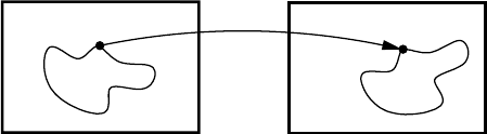
separate images. For this purpose, the spatial relation between the images has to be found. Image registration
is the task of finding a spatial one-to-one mapping from voxels in one image to voxels in the other image,
see Figure 2.1. Good reviews on the subject are given in Maintz and Viergever [1998], Lester and Arridge
[1999], Hill et al. [2001], Hajnal et al. [2001], Zitov´a and Flusser [2003], Modersitzki [2004].
The following section introduces the mathematical formulation of the registration process and gives an
overview of the components of which a general registration method consists. After that, in Sections 2.3-2.8,
each component is discussed in more detail. For each component, the name used by elastix is given, in
typewriter style. In Section 2.9, methods to evaluate the registration results are discussed.
2.1 Registration framework
Two images are involved in the registration process. One image, the moving image IM(x), is deformed to fit
the other image, the fixed image IF(x). The fixed and moving image are of dimension dand are each defined
on their own spatial domain: ΩF⊂Rdand ΩM⊂Rd, respectively. Registration is the problem of finding a
displacement u(x) that makes IM(x+u(x)) spatially aligned to IF(x). An equivalent formulation is to say
that registration is the problem of finding a transformation T(x) = x+u(x) that makes IM(T(x)) spatially
aligned to IF(x). The transformation is defined as a mapping from the fixed image to the moving image,
i.e. T: ΩF⊂Rd→ΩM⊂Rd. The quality of alignment is defined by a distance or similarity measure S,
pq
T
Figure 2.1: Image registration is the task of finding a spatial transformation mapping one image to another.
Left is the fixed image and right the moving image. Adopted from Ib´a˜nez et al. [2005].
3
pyramid
optimiser
fixed image
transform
sampler
metric
multi−resolution
interpolatorpyramidmoving image
resolution level
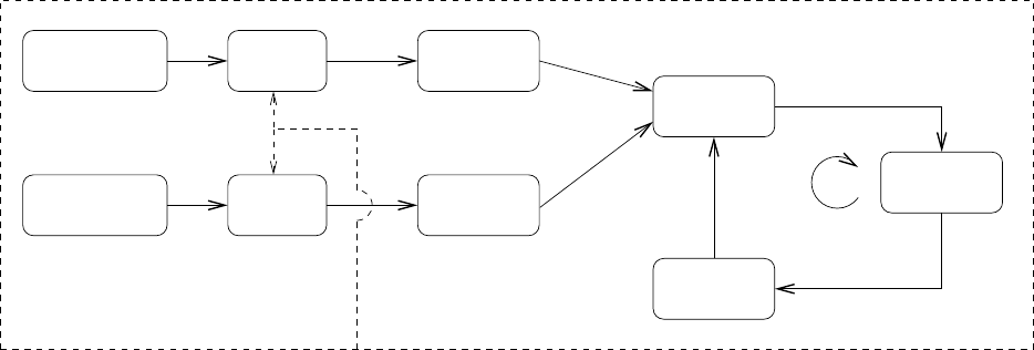
Figure 2.2: The basic registration components.
such as the sum of squared differences (SSD), the correlation ratio, or the mutual information (MI) measure.
Because this problem is ill-posed for nonrigid transformations T, a regularisation or penalty term Pis often
introduced that constrains T.
Commonly, the registration problem is formulated as an optimisation problem in which the cost function
Cis minimised w.r.t. T:
ˆ
T= arg min
TC(T;IF, IM),with (2.1)
C(T;IF, IM) = −S(T;IF, IM) + γP(T),(2.2)
where γweighs similarity against regularity. To solve the above minimisation problem, there are basically
two approaches: parametric and nonparametric. The reader is referred to Fischer and Modersitzki [2004]
for an overview on nonparametric methods, which are not discussed in this manual. The elastix software
is based on the parametric approach. In parametric methods, the number of possible transformations is
limited by introducing a parametrisation (model) of the transformation. The original optimisation problem
thus becomes:
ˆ
Tµ= arg min
Tµ
C(Tµ;IF, IM),(2.3)
where the subscript µindicates that the transform has been parameterised. The vector µcontains the
values of the “transformation parameters”. For example, when the transformation is modelled as a 2D rigid
transformation, the parameter vector µcontains one rotation angle and the translations in xand ydirection.
We may write Equation (2.3) also as:
ˆ
µ= arg min
µC(µ;IF, IM).(2.4)
From this equation it becomes clear that the original problem (2.1) has been simplified. Instead of optimising
over a “space of functions T”, we now optimise over the elements of µ. Examples of other transformation
models are given in Section 2.6.
Figure 2.2 shows the general components of a parametric registration algorithm in a block scheme. The
scheme is a slightly extended version of the scheme introduced in Ib´a˜nez et al. [2005]. Several components
can be recognised from Equations (2.1)-(2.4); some will be introduced later. First of all, we have the images.
The concept of an image needs to be defined. This is done in Section 2.2. Then we have the cost function
C, or “metric”, which defines the quality of alignment. As mentioned earlier, the cost function consists of
a similarity measure Sand a regularisation term P. The regularisation term Pis not discussed in this
4

0 10050 150 200
0
50
100
150
200
250
300
30.0
20.0
Size=7x6
Spacing=( 20.0, 30.0 )
Physical extent=( 140.0, 180.0 )
Origin=(60.0,70.0)
Image Origin
Voronoi Region
Pixel Coverage
Delaunay Region
Linear Interpolation Region
Pixel Coordinates
Spacing[0]
Spacing[1]
Figure 2.3: Geometrical concepts associated with the ITK image. Adopted from Ib´a˜nez et al. [2005].
chapter, but in Chapter 6. The similarity measure Sis discussed in Section 2.3. The definition of the
similarity measure introduces the sampler component, which is treated in Section 2.4. Some examples of
transformation models Tµare given in Section 2.6. The optimisation procedure to actually solve the problem
(2.4) is explained in Section 2.7. During the optimisation, the value IM(Tµ(x)) is evaluated at non-voxel
positions, for which intensity interpolation is needed. Choices for the interpolator are described in Section
2.5. Another thing, not immediately clear from Equations (2.1)-(2.4), is the use of multi-resolution strategies
to speed-up registration, and to make it more robust, see Section 2.8.
2.2 Images
Since image registration is all about images, we have to be careful with what is meant by an image. We
adopt the notion of an image from the Insight Toolkit [Ib´a˜nez et al.,2005, p. 40]:
Additional information about the images is considered mandatory. In particular the information
associated with the physical spacing between pixels and the position of the image in space with
respect to some world coordinate system are extremely important. Image origin and spacing are
fundamental to many applications. Registration, for example, is performed in physical coordi-
nates. Improperly defined spacing and origins will result in inconsistent results in such processes.
Medical images with no spatial information should not be used for medical diagnosis, image
analysis, feature extraction, assisted radiation therapy or image guided surgery. In other words,
medical images lacking spatial information are not only useless but also hazardous.
Figure 2.3 illustrates the main geometrical concepts associated with the itk::Image. In this figure,
circles are used to represent the centre of pixels. The value of the pixel is assumed to exist as
a Dirac Delta Function located at the pixel centre. Pixel spacing is measured between the pixel
centres and can be different along each dimension. The image origin is associated with the
coordinates of the first pixel in the image. A pixel is considered to be the rectangular region
surrounding the pixel centre holding the data value. This can be viewed as the Voronoi region of
the image grid, as illustrated in the right side of the figure. Linear interpolation of image values
is performed inside the Delaunay region whose corners are pixel centres.
Therefore, you should take care that you use an image format that is able to store the relevant information
(e.g. mhd, DICOM). Some image formats, like bmp, do not store the origin and spacing. This may cause
serious problems!
5

Up to elastix version 4.2, the image orientation (direction cosines) was not yet fully supported in
elastix. From elastix 4.3, image orientation is fully supported, but can be disabled for backward com-
patibility reasons.
2.3 Metrics
Several choices for the similarity measure can be found in the literature. Some common choices are described
below. Between brackets the name of the metric in elastix is given:
Mean Squared Difference (MSD): (AdvancedMeanSquares) The MSD is defined as:
MSD(µ;IF, IM) = 1
|ΩF|X
xi∈ΩF
(IF(xi)−IM(Tµ(xi)))2,(2.5)
with ΩFthe domain of the fixed image IF, and |ΩF|the number of voxels. Given a transformation T,
this measure can easily be implemented by looping over the voxels in the fixed image, taking IF(xi),
calculating IM(Tµ(xi)) by interpolation, and adding the squared difference to the sum.
Normalised Correlation Coefficient (NCC): (AdvancedNormalizedCorrelation) The NCC is defined
as:
NCC(µ;IF, IM) = P
xi∈ΩFIF(xi)−IFIM(Tµ(xi)) −IM
rP
xi∈ΩFIF(xi)−IF2P
xi∈ΩFIM(Tµ(xi)) −IM2,(2.6)
with the average grey-values IF=1
|ΩF|P
xi∈ΩF
IF(xi) and IM=1
|ΩF|P
xi∈ΩF
IM(Tµ(xi)).
Mutual Information (MI): (AdvancedMattesMutualInformation) For MI [Maes et al.,1997,Viola and
Wells III,1997,Mattes et al.,2003] we use a definition given by Th´evenaz and Unser [2000]:
MI(µ;IF, IM) = X
m∈LMX
f∈LF
p(f, m;µ) log2p(f, m;µ)
pF(f)pM(m;µ),(2.7)
where LFand LMare sets of regularly spaced intensity bin centres, pis the discrete joint probability,
and pFand pMare the marginal discrete probabilities of the fixed and moving image, obtained by
summing pover mand f, respectively. The joint probabilities are estimated using B-spline Parzen
windows:
p(f, m;µ) = 1
|ΩF|X
xi∈ΩF
wF(f/σF−IF(xi)/σF)
×wM(m/σM−IM(Tµ(xi))/σM),
(2.8)
where wFand wMrepresent the fixed and moving B-spline Parzen windows. The scaling constants σF
and σMmust equal the intensity bin widths defined by LFand LM. These follow directly from the
grey-value ranges of IFand IMand the user-specified number of histogram bins |LF|and |LM|.
Normalized Mutual Information (NMI): (NormalizedMutualInformation)
NMI is defined by NMI = (H(IF) + H(IM))/H(IF, IM), with Hdenoting entropy. This expression
can be compared to the definition of MI in terms of H: MI = H(IF) + H(IM)−H(IF, IM). Again,
6
with the joint probabilities defined by 2.8 (using B-spline Parzen windows), NMI can be written as:
NMI(µ;IF, IM) = P
f∈LF
pF(f) log2pF(f) + P
m∈LM
pM(m;µ) log2pM(m;µ)
P
m∈LMP
f∈LF
p(f, m;µ) log2p(f, m;µ)
=P
m∈LMP
f∈LF
p(f, m;µ) log2(pF(f)pM(m;µ))
P
m∈LMP
f∈LF
p(f, m;µ) log2p(f, m;µ).(2.9)
Kappa Statistic (KS): (AdvancedKappaStatistic) KS is defined as:
KS(µ;IF, IM) =
2P
xi∈ΩF
1IF(xi)=f,IM(Tµ(xi))=f
P
xi∈ΩF
1IF(xi)=f+1IM(Tµ(xi))=f
,(2.10)
where 1is the indicator function, and fa user-defined foreground value that defaults to 1.
The MSD measure is a measure that is only suited for two images with an equal intensity distribution,
i.e. for images from the same modality. NCC is less strict, it assumes a linear relation between the intensity
values of the fixed and moving image, and can therefore be used more often. The MI measure is even more
general: only a relation between the probability distributions of the intensities of the fixed and moving image
is assumed. For MI it is well-known that it is suited not only for mono-modal, but also for multi-modal image
pairs. This measure is often a good choice for image registration. The NMI measure is, just like MI, suitable
for mono- and multi-modality registration. Studholme et al. [1999] seems to indicate better performance
than MI in some cases. The KS measure is specifically meant to register binary images (segmentations). It
measures the “overlap” of the segmentations.
2.4 Image samplers
In Equations (2.5)-(2.8) we observe a loop over the fixed image: Pxi∈ΩF. Until now, we assumed that the
loop goes over all voxels of the fixed image. In general, this is not necessary. A subset may suffice [Th´evenaz
and Unser,2000,Klein et al.,2007]. The subset may be selected in different ways: random, on a grid, etc.
The sampler component represents this process.
The following samplers are often used:
Full: (Full) A full sampler simply selects all voxel coordinates xiof the fixed image.
Grid: (Grid) The grid sampler defines a regular grid on the fixed image and selects the coordinates xion
the grid. Effectively, the grid sampler thus downsamples the fixed image (not preceded by smoothing).
The size of the grid (or equivalently, the downsampling factor, which is the original fixed image size
divided by the grid size) is a user input.
Random: (Random) A random sampler randomly selects a user-specified number of voxels from the fixed
image, whose coordinates form xi. Every voxel has equal chance to be selected. A sample is not
necessarily selected only once.
Random Coordinate: (RandomCoordinate) A random coordinate sampler is similar to a random sampler.
It also randomly selects a user-specified number of coordinates xi. However, the random coordinate
sampler is not limited to voxel positions. Coordinates between voxels can also be selected. The grey-
value IF(xi) at those locations must of course be obtained by interpolation.
7

(a) (b) (c) (d) (e)
Figure 2.4: Interpolation. (a) nearest neighbour, (b) linear, (c) B-spline N= 2, (d) B-spline N= 3, (e)
B-spline N= 5.
While at first sight the full sampler seems the most obvious choice, in practice it is not always used,
because of its computational costs in large images. The random samplers are especially useful in combination
with a stochastic optimisation method [Klein et al.,2007]. See also Section 2.7. The use of the random
coordinate sampler makes the cost function Ca more smooth function of µ, which makes the optimisation
problem (2.4) easier to solve. This has been shown in Th´evenaz and Unser [2008].
2.5 Interpolators
As stated previously, during the optimisation the value IM(Tµ(x)) is evaluated at non-voxel positions, for
which intensity interpolation is needed. Several methods for interpolation exist, varying in quality and speed.
Some examples are given in Figure 2.4.
Nearest neighbour: (NearestNeighborInterpolator) This is the most simple technique, low in quality,
requiring little resources. The intensity of the voxel nearest in distance is returned.
Linear: (LinearInterpolator) The returned value is a weighted average of the surrounding voxels, with
the distance to each voxel taken as weight.
N-th order B-spline: (BSplineInterpolator or BSplineInterpolatorFloat for a memory efficient ver-
sion) The higher the order, the better the quality, but also requiring more computation time. In fact,
nearest neighbour (N= 0) and linear interpolation (N= 1) also fall in this category. See Unser [1999]
for more details.
During registration a first-order B-spline interpolation, i.e. linear interpolation, often gives satisfactory
results. It is a good trade-off between quality and speed. To generate the final result, i.e. the deformed
result of the registration, a higher-order interpolation is usually required, for which we recommend N= 3.
The final result is generated in elastix by a so-called ResampleInterpolator. Any one of the above can
be used, but you need to prepend the name with Final, for example: FinalLinearInterpolator.
2.6 Transforms
A frequent confusion about the transformation is its direction. In elastix the transformation is defined as a
coordinate mapping from the fixed image domain to the moving image domain:T: ΩF⊂Rd→
ΩM⊂Rd. The confusion usually stems from the phrase: “the moving image is deformed to fit the fixed
image”. Although one can speak about image registration like this, such a phrase is not meant to reflect
mathematical underlyings: one deforms the moving image, but the transformation is still defined from fixed
to moving image. The reason for this becomes clear when trying to compute the deformed moving image (the
registration result) IM(Tµ(x)) (this process is frequently called resampling). If the transformation would be
defined from moving to fixed image, not all voxels in the fixed image domain would be mapped to (e.g. in
8
case of a scaling), and holes would occur in the deformed moving image. With the transformation defined as
it is, resampling is quite simple: loop over all voxels xin the fixed image domain ΩF, compute its mapped
position y=Tµ(x), interpolate the moving image at y, and fill in this value at xin the output image.
The transformation model used for Tµdetermines what type of deformations between the fixed and
moving image you can handle. In order of increasing flexibility, these are the translation, the rigid, the
similarity, the affine, the nonrigid B-spline and the nonrigid thin-plate spline like transformations.
Translation: (TranslationTransform) The translation is defined as:
Tµ(x) = x+t,(2.11)
with tthe translation vector. The parameter vector is simply defined by µ=t.
Rigid: (EulerTransform) A rigid transformation is defined as:
Tµ(x) = R(x−c) + t+c,(2.12)
with the matrix Ra rotation matrix (i.e. orthonormal and proper), cthe centre of rotation, and t
translation again. The image is treated as a rigid body, which can translate and rotate, but cannot be
scaled/stretched. The rotation matrix is parameterised by the Euler angles (one in 2D, three in 3D).
The parameter vector µconsists of the Euler angles (in rad) and the translation vector. In 2D, this
gives a vector of length 3: µ= (θz, tx, ty)T, where θzdenotes the rotation around the axis normal to
the image. In 3D, this gives a vector of length 6: µ= (θx, θy, θz, tx, ty, tz)T. The centre of rotation is
not part of µ; it is a fixed setting, usually the centre of the image.
Similarity: (SimilarityTransform) A similarity transformation is defined as
Tµ(x) = sR(x−c) + t+c,(2.13)
with sa scalar and Ra rotation matrix. This means that the image is treated as an object, which can
translate, rotate, and scale isotropically. The rotation matrix is parameterised by an angle in 2D, and by
a so-called “versor” in 3D (Euler angles could have been used as well). The parameter vector µconsists
of the angle/versor, the translation vector, and the isotropic scaling factor. In 2D, this gives a vector
of length 4: µ= (s, θz, tx, ty)T. In 3D, this gives a vector of length 7: µ= (q1, q2, q3, tx, ty, tz, s)T,
where q1,q2, and q3are the elements of the versor. There are few cases when you need this transform.
Affine: (AffineTransform) An affine transformation is defined as:
Tµ(x) = A(x−c) + t+c,(2.14)
where the matrix Ahas no restrictions. This means that the image can be translated, rotated, scaled,
and sheared. The parameter vector µis formed by the matrix elements aij and the translation vector.
In 2D, this gives a vector of length 6: µ= (a11, a12, a21, a22, tx, ty)T. In 3D, this gives a vector of
length 12.
We also have implemented another flavor of the affine transformation, with identical meaning, but
using another parametrization. Instead of having µformed by the matrix elements + translation, it is
formed by drotations, dshear factors, dscales, and dtranslations. The definition reads:
Tµ(x) = RGS(x−c) + t+c,(2.15)
with R,Gand Sthe rotation, shear and scaling matrix, respectively. It can be selected using
AffineDTITransform, as it was first made with DTI imaging in mind, although it can be used anywhere
else as well. It is currently only implemented in 3D, and also has 12 parameters.
9

B-splines: (BSplineTransform) For the category of non-rigid transformations, B-splines [Rueckert et al.,
1999] are often used as a parameterisation:
Tµ(x) = x+X
xk∈Nx
pkβ3x−xk
σ,(2.16)
with xkthe control points, β3(x) the cubic multidimensional B-spline polynomial [Unser,1999], pkthe
B-spline coefficient vectors (loosely speaking, the control point displacements), σthe B-spline control
point spacing, and Nxthe set of all control points within the compact support of the B-spline at x.
The control points xkare defined on a regular grid, overlayed on the fixed image. In this context we
talk about ‘the control point grid that is put on the fixed image’, and about ‘control points that are
moved around’. Note that Tµ(xk)6=xk+pk, a common misunderstanding. Calling pkthe control
point displacements is, therefore, actually somewhat misleading. Also note that the control point grid
is entirely unrelated to the grid used by the Grid image sampler, see Section 2.4.
The control point grid is defined by the amount of space between the control points σ= (σ1,...,σd)
(with dthe image dimension), which can be different for each direction. B-splines have local support
(|Nx|is small), which means that the transformation of a point can be computed from only a couple
of surrounding control points. This is beneficial both for modelling local transformations, and for fast
computation. The parameters µare formed by the B-spline coefficients pk. The number of control
points P= (P1,...,Pd) determines the number of parameters M, by M= (P1×...×Pd)×d.Piin
turn is determined by the image size sand the B-spline grid spacing, i.e. Pi≈si/σi(where we use
≈since some additional control points are placed just outside the image). For 3D images, M≈10000
parameters is not an unusual case, and Mcan easily grow to 105−106. The parameter vector (for 2D
images) is composed as follows: µ= (p1x, p2x,...,pP1, p1y, p2y,...,pP2)T.
Thin-plate splines: (SplineKernelTransform) Thin-plate splines are another well-known representation
for nonrigid transformations. The thin-plate spline is an instance of the more general class of kernel-
based transforms Davis et al. [1997], Brooks and Arbel [2007]. The transformation is based on a set of
Kcorresponding landmarks in the fixed and moving image: xfix
kand xmov
k, k = 1,...,K, respectively.
The transformation is expressed as a sum of an affine component and a nonrigid component:
Tµ(x) = x+Ax+t+X
xfix
k
ckG(x−xfix
k),(2.17)
where G(r) is a basis function and ckare the coefficients corresponding to each landmark. The
coefficients ckand the elements of Aand tare computed from the landmark displacements dk=
xmov
k−xfix
k. The specific choice of basis function G(r) determines the “physical behaviour”. The most
often used choice of G(r) leads to the thin-plate spline, but another useful alternative is the elastic-body
spline Davis et al. [1997]. The spline kernel transforms are often less efficient than the B-splines (because
they lack the compact support property of the B-splines), but they allow for more flexibility in placing
the control points xfix
k. The moving landmarks form the parameter vector µ. Both landmark sets are
needed to define a transformation. Note that in order to perform a registration, only the fixed landmark
positions are given by the user; the moving landmarks are initialized to equal the fixed landmarks,
corresponding to the identity transformation, and are subsequently optimized. The parameter vector
is (for 2D images) composed as follows: µ= (xmov
1x, xmov
1y, xmov
2x, xmov
2y,...,xmov
Kx , xmov
Ky )T. Note the
difference in ordering of µcompared to the B-splines transform.
See Figure 2.5 for an illustration of different transforms. Choose the transformation that fits your needs:
only choose a nonrigid transformation if you expect that the underlying problem contains local deformations,
choose a rigid transformation if you only need to compensate for differences in pose. To initialise a nonrigid
10
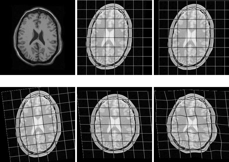
(a) fixed (b) moving (c) translation
(d) rigid (e) affine (f) B-spline
Figure 2.5: Different transformations. (a) the fixed image, (b) the moving image with a grid overlayed, (c)
the deformed moving image IM(Tµ(x)) with a translation transformation, (d) a rigid transformation, (e) an
affine transformation, and (f) a B-spline transformation. The deformed moving image nicely resembles the
fixed image IF(x) using the B-spline transformation. The overlay grids give an indication of the deformations
imposed on the moving image. NB: the overlayed grid in (f) is NOT the B-spline control point grid, since
that one is defined on the fixed image!
registration problem, perform a rigid or affine one first. The result of the initial rigid or affine registration
Tˆ
µ0is combined with a nonrigid transformation TNR
µin one of the following two ways:
addition: Tµ(x) = TNR
µ(x) + Tˆ
µ0(x)−x(2.18)
composition: Tµ(x) = TNR
µ(Tˆ
µ0(x)) = (TNR
µ◦Tˆ
µ0)(x) (2.19)
The latter method is in general to be preferred, because it makes several postregistration analysis tasks
somewhat more straightforward.
2.7 Optimisers
To solve the optimisation problem (2.4), i.e. to obtain the optimal transformation parameter vector ˆ
µ,
commonly an iterative optimisation strategy is employed:
µk+1 =µk+akdk, k = 0,1,2,··· ,(2.20)
with dkthe ‘search direction’ at iteration k,aka scalar gain factor controlling the step size along the search
direction. The optimisation process is illustrated in Figure 2.6.Klein et al. [2007] give an overview of
various optimisation routines the literature offers. Examples are quasi-Newton (QN), nonlinear conjugate
11
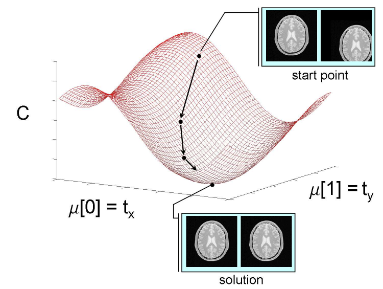
Figure 2.6: Iterative optimisation. Example for registration with a translation transformation model. The
arrows indicate the steps akdktaken in the direction of the optimum, which is the minimum of the cost
function.
gradient (NCG), gradient descent (GD), and Robbins-Monro (RM). Gradient descent and Robbins-Monro
are discussed below. For details on other optimisation methods we refer to [Klein et al.,2007,Nocedal and
Wright,1999].
Gradient descent (GD): (StandardGradientDescent or RegularStepGradientDescent) Gradient de-
scent optimisation methods take the search direction as the negative gradient of the cost function:
µk+1 =µk−akg(µk),(2.21)
with g(µk) = ∂C/∂µevaluated at the current position µk. Several choices exist for the gain factor ak.
It can for example be determined by a line search or by using a predefined function of k.
Robbins-Monro (RM): (StandardGradientDescent or FiniteDifferenceGradientDescent) The RM
optimisation method replaces the calculation of the derivative of the cost function g(µk) by an ap-
proximation e
gk.
µk+1 =µk−ake
gk,(2.22)
The approximation is potentially faster to compute, but might deteriorate convergence properties of
the GD scheme, since every iteration an approximation error g(µk)−e
gkis made. Klein et al. [2007]
showed that using only a small random subset of voxels (≈2000) from the fixed image accelerates regis-
tration significantly, without compromising registration accuracy. The Random or RandomCoordinate
samplers, described in Section 2.4, are examples of samplers that pick voxels randomly. It is important
that a new subset of fixed image voxels is selected every iteration k, so that the approximation error
12

has zero mean. The RM method is usually combined with akas a predefined decaying function of k:
ak=a
(k+A)α,(2.23)
where a > 0, A≥1, and 0 ≤α≤1 are user-defined constants. In our experience, a reasonable choice
is α≈0.6 and Aapproximately 10% of the user-defined maximum number of iterations, or less. The
choice of the overall gain, a, depends on the expected ranges of µand gand is thus problem-specific. In
our experience, the registration result is not very sensitive to small perturbations of these parameters.
Section 5.3.6 gives some more advice.
Note that GD and RM are in fact very similar. Running RM with a Full sampler (see Section 2.4),
instead of a Random sampler, is equivalent to performing GD. We recommend the use of RM over GD, since
it is so much faster, without compromising on accuracy. In that case, the parameter ais the parameter
that is to be tuned for your application. A more advanced version of the StandardGradientDescent is
the AdaptiveStochasticGradientDescent, which requires less parameters to be set and tends to be more
robust Klein et al. [2009].
Other optimisers available in elastix are: FullSearch,ConjugateGradient,ConjugateGradientFRPR,
QuasiNewtonLBFGS,RSGDEachParameterApart,SimultaneousPerturbation,CMAEvolutionStrategy.
2.8 Multi-resolution
For a good overview of multi-resolution strategies see Lester and Arridge [1999]. Two hierarchical methods
are distinguished: reduction of data complexity, and reduction of transformation complexity.
2.8.1 Data complexity
It is common to start the registration process using images that have lower complexity, e.g., images that are
smoothed and possibly downsampled. This increases the chance of successful registration. A series of images
with increasing amount of smoothing is called a scale space. If the images are not only smoothed, but also
downsampled, the data is not only less complex, but the amount of data is actually reduced. In that case,
we talk about a “pyramid”. However, confusingly, the word pyramid is used by us also to refer to a scale
space. Several scale spaces or pyramids are found in the literature, amongst others Gaussian and Laplacian
pyramids, morphological scale space, and spline and wavelet pyramids. The Gaussian pyramid is the most
common one. In elastix we have:
Gaussian pyramid: (FixedRecursiveImagePyramid and MovingRecursiveImagePyramid) Applies smooth-
ing and down-sampling.
Gaussian scale space: (FixedSmoothingImagePyramid and MovingSmoothingImagePyramid) Applies smooth-
ing and no down-sampling.
Shrinking pyramid: (FixedShrinkingImagePyramid and MovingShrinkingImagePyramid) Applies no smooth-
ing, but only down-sampling.
Figure 2.7 shows the Gaussian pyramid with and without downsampling. In combination with a Full
sampler (see Section 2.4), using a pyramid with downsampling will save a lot of time in the first resolution
levels, because the image contains much fewer voxels. In combination with a Random sampler, or Random-
Coordinate, the downsampling step is not necessary, since the random samplers select a user-defined number
of samples anyway, independent of the image size.
13

(a) resolution 0 (b) resolution 1 (c) resolution 2 (d) original
(e) resolution 0 (f) resolution 1 (g) resolution 2 (h) original
Figure 2.7: Two multi-resolution strategies using a Gaussian pyramid (σ= 8.0,4.0,2.0 voxels). The first
row shows multi-resolution with down-sampling (FixedRecursiveImagePyramid), the second row without
(FixedSmoothingImagePyramid). Note that in the first row, for each dimension, the image size is halved
every resolution, but that the voxel size increases with a factor 2, so physically the images are of the same
size every resolution.
2.8.2 Transformation complexity
The second multiresolution strategy is to start the registration with fewer degrees of freedom for the trans-
formation model. The degrees of freedom of the transformation equals the length (number of elements) of
the parameter vector µ.
An example of this was already mentioned in Section 2.6: the use of a rigid transformation prior to
nonrigid (B-spline) registration. We may even use a three-level strategy: first rigid, then affine, then nonrigid
B-spline.
Another example is to increase the number of degrees of freedom within the transformation model. With
a B-spline transformation, it is often good practice to start registration with a coarse control point grid, only
capable of modelling coarse deformations. In subsequent resolutions the B-spline grid is gradually refined,
thereby introducing the capability to match smaller structures. See Section 5.3.5.
2.9 Evaluating registration
How do you verify that your registration was successful? This is a difficult problem. In general, you don’t
know for each voxel where it should map to. Here are some hints:
•The deformed moving image IM(Tµ(x)) should look similar to the fixed image IF(x). So, compare
images side by side in a viewer. You can also display the two images on top of each other with a
checkerboard view or a dragable cross. Besides looking similar, also check that the deformed moving
image has the same texture as the moving image. Sudden blurred areas in the deformed image may
indicate that the deformation at that region is too large.
•For mono-modal image data you can inspect the difference image. Perfect registration would result in
a difference image without any edges, just noise.
14

•Compute the overlap of segmented anatomical structures after registration. The better the overlap,
the better the registration. Note that this requires you to (manually) segment structures in your data.
To measure overlap, commonly the Dice similarity coefficient (DSC) is used:
DSC(X, Y ) = 2|X∩Y|
|X|+|Y|,(2.24)
where Xand Yrepresent the binary label images, and |·|denotes the number of voxels that equal 1.
A higher DSC indicates a better correspondence. A value of 1 indicates perfect overlap, a value of 0
means no overlap at all. Also the Tannimoto coefficient (TC) is used often. It is related to the DSC by
DSC = 2TC/(TC + 1). See also Crum et al. [2006]. It is important to realise that the surface-volume
ratio of the segmented structures influences the overlap values you typically get [Rohlfing et al.,2004].
A value of DSC = 0.8 would be very good for the overlap of complex vessel structures. For large
spherical objects though, an overlap <0.9 is in general not very good. What is good enough depends
of course on your application.
•Compute the distance after registration between points that you know correspond. You can obtain
corresponding points by manually clicking them in the fixed and the moving image. A less time-
consuming option is the semi-automated approach of Murphy et al. Murphy et al. [2008], which is
designed for finding corresponding points in the lung. Ideally, the registration has found the same
correspondence as the ground truth.
•Inspect the deformation field by looking at the determinant of the Jacobian of Tµ(x). Values smaller
than 1 indicate local compression, values larger than 1 indicate local expansion, and 1 means volume
preservation. The measure is quantitative: a value of 1.1 means a 10% increase in volume. If this
value deviates substantially from 1, you may be worried (but maybe not if this is what you expect for
your application). In case it is negative you have “foldings” in your transformation, and you definitely
should be worried.
•Inspect the convergence, by computing for each iteration the exact metric value (and not an approx-
imated value, when you do random sampling), and plot it. For example for the MSD measure, the
lower the metric value, the better the registration.
•Do not use image similarity as a way to evaluate your registration. Torsten Rohlfing can explain why
Rohlfing [2012].
2.10 Visualizing registration
elastix is a command line program and does not do visualization. It takes the input fixed and moving
image and at the end of the registration generates an output (result) image. Usually, however, you will need
to inspect the end result visually. For this you can use an external viewer. Such a viewer does not come
with the elastix package, but is a stand-alone application, with dedicated functionality for visualization.
We have listed a number of visualization tools in Table 2.1. All of them are freely available, sometimes even
as open source. The list is not exhaustive.
15

Tool
Open source?
Platforms url and comments
MeVisLab ✕XXX http://www.mevislab.de/ MeVisLab has modular framework for the de-
velopment of image processing algorithms and visualization and interac-
tion methods, with a special focus on medical imaging. Quite easy in
use.
ITK-SNAP X XXX http://www.itksnap.org Visualization, mostly targeted to segmenta-
tion.
ParaView X XXX http://www.paraview.org/ Data analysis, exploration and visualization
application. Renderings are nice. Sometimes difficult in use.
3DSlicer X XXX http://www.slicer.org/ Application and framework for medical image
analysis, visualization, and surgical navigation.
VV X XXX http://www.creatis.insa-lyon.fr/rio/vv The 4D Slicer, a fast and
simple viewer. VV is more specifically designed for qualitative evaluation
of image registration and deformation field visualization. A tutorial on
the use of VV in combination with elastix can be found in Appendix C
of this manual.
Table 2.1: A number of visualization tools. The three marks for the platforms column denote Windows,
Linux and Mac OSX support, respectively.
16

Chapter 3
elastix
3.1 Introduction
The development of elastix started half to late 2003, and was intended to facilitate our registration research.
After some initial versions we decided to put the separate components of elastix in separate libraries. This
resulted in major version 3.0 in November 2004. elastix 3.0 was also the first version that was made
publicly available on the elastix website, around the same time. The continued development brings us
today (September 4, 2015) to version 4.8.
what where
Website http://elastix.isi.uu.nl
SVN repository https://svn.bigr.nl/elastix/trunkpublic
Dashboard http://my.cdash.org/index.php?project=elastix
WIKI http://elastix.isi.uu.nl/wiki.php
FAQ http://elastix.isi.uu.nl/FAQ.php
Mailing list subscription http://lists.bigr.nl/mailman/listinfo/elastix
Mailing list elastix@bigr.nl
The website also contains a doxygen1generated part that provides documentation of the source code.
An overview of all available classes can be found at
http://elastix.isi.uu.nl/doxygen/classes.html.
For each class a description of this class is given, together with information on how to use it in elastix. See
http://elastix.isi.uu.nl/doxygen/modules.html
for an overview of all available components.
3.1.1 Key features
elastix is
•open source, freely available from http://elastix.isi.uu.nl;
•based on the ITK, so the code base is thoroughly tested. Quite some modifications/additions are made
to the original ITK code though, such as the use of samplers, a transformation class that combines
multiple transformation using composition or addition, and more.
1http://www.doxygen.org
17

•suitable for many image formats. The use of ITK implies that all image formats supported by ITK are
supported by elastix. Some often used (medical) image formats are: .mhd (MetaIO), .hdr (Analyze),
.nii (NIfTI), .gipl, .dcm (DICOM slices). DICOM directories are not directly supported by elastix;
•multi-platform (at least Windows, Linux and Mac OS), multi-compiler (at least Visual C++ 2008,
2010, gcc 4.x, clang 3.3+), and supports 32 and 64 bit systems. The underlying ITK code builds on
many more platforms, see www.itk.org/Wiki/ITK_Prerequisites. So, it is highly portable to the
platform of the user’s choice;
•highly configurable: there is a lot of choice for all the registration components. Choosing the configu-
ration that suits your needs is easy thanks to human readable and editable parameter file;
•easy to use for large amounts of data, since elastix can be called easily in a script;
•fast, thanks to stochastic subsampling Klein et al. [2007], and thanks to multi-threading and code
optimizations Shamonin et al. [2014];
•relatively easy to extend, i.e. to add new components, so it is very suited for research also.
3.2 Getting started
This section describes how you can install elastix, either directly from the binaries, or by compiling elastix
yourself.
3.2.1 Getting started the really easy way
The easiest way to get started with elastix is to use the pre-compiled binaries.
1. Download the compressed archive from the website:
http://elastix.isi.uu.nl/download.php
2. Extract the archive to a folder of your choice.
3. Make sure your operating system can find the program:
(a) Windows 7: Go to the control panel, go to “System”, go to “Advanced system settings”, click
“Environmental variables”, add folder to the variable “path”.
(b) Linux: Add the following lines to your .bashrc file:
export PATH=folder/bin:$PATH
export LD LIBRARY PATH=folder/lib:$LD LIBRARY PATH
or call elastix with the full path: fullPathToFolder\elastix. Note that in Linux, you will have to
set the LD LIBRARY PATH anyway.
3.2.2 Getting started the easy way
It is also possible to compile elastix yourself, since the source code is freely available. In this section, we
assume you use the Microsoft Visual C++ 2008 (or higher) compiler under Windows, and the GCC compiler
under Linux/MacOS.
1. Download and install CMake: www.cmake.org.
18

2. Download and compile the ITK version 4.8: www.itk.org. Make sure to set the following (advanced)
CMake variable to ON:Module ITKReview, and optionally ITK USE 64BITS IDS and ITK LEGACY REMOVE.
For faster building of ITK you can switch off BUILD EXAMPLES and BUILD TESTING.
3. Obtain the sources. There are three possibilities:
(a) Download the compressed sources from the website. Extract the archive to <your-elastix-folder>
of your choice.
(b) Use subversion (https://subversion.tigris.org) to check out the release from the subversion
repository:
svn co --username elastixguest --password elastixguest
https://svn.bigr.nl/elastix/tagspublic/elastix_XX_X <your-elastix-folder>
where XX X is the major version number (first 2 digits) and the minor version number (1 digit).
So, for example, for version 4.8 this would be 04 8.
(c) Use subversion to check out the latest development version. NB: this version might be unstable!
svn co --username elastixguest --password elastixguest
https://svn.bigr.nl/elastix/trunkpublic <your-elastix-folder>
4. Run CMake for elastix:
(a) Windows: start CMake. Find the src folder with the source code. Set the folder where you
want the binaries to be created. Click “Configure” and select the compiler that you use. Set the
CMAKE INSTALL PREFIX to the directory where you want elastix installed. Click “Configure”
until all cache values are no longer red, and click “Generate”.
(b) Linux: run CMake from the folder where you want the binaries to be created, with as command
line argument the folder in which the sources were extracted: ccmake <src-folder>. Set the
CMAKE BUILD TYPE to “Release” and the CMAKE INSTALL PREFIX to the directory where you want
elastix installed.
CMake will create a project or solution or make file for your compiler.
5. Compile elastix by opening the project and selecting “compile” in release mode, or on Linux by
running make install. Your compiler will now create the elastix binaries. On Windows you can
perform the installation step (which copies the binaries to the CMAKE INSTALL PREFIX directory) by
also ‘compiling’ the INSTALL project.
6. Make sure your operating system can find the program, see above.
For developers: When running CMake, you may toggle the display of the “advanced” options. In this
list you will find several options like USE BSplineTransform ON/OFF. By default only the most commonly
used components are ON. To reduce compilation time, you may turn some components OFF, which you do
not plan to use anyway. Be careful though to not turn off essential components. The released binaries are
compiled with all components ON.
3.3 How to call elastix
elastix is a command line program, although since version 4.7 (February 2014) initial support for a library
interface is available, see Section 7.3.2. This means that you have to open a command line interface (a
DOS-box, a shell) and type in an appropriate elastix command. This also means that there is no graphical
user interface. Help on using the program can be acquired as follows:
19

elastix --help
which will give a list of mandatory and optional arguments. The most basic command to run a registration
is as follows:
elastix -f fixedImage.ext -m movingImage.ext -out outputDirectory -p parameterFile.txt
where ‘ext’ is the extension of the image files. The above arguments are mandatory. These are minimally
needed to run elastix. The parameter file is an important file: it contains, in normal text, what kind of
registration is performed (i.e. what metric, optimiser, etc.) and what the parameters are that define the
registration. It gives a high amount of flexibility and control over the process. More information about the
parameter file is given in Section 3.4. All output of elastix is written to the output directory, which needs
to be created before running elastix. The output consists of a log file (elastix.log), the parameters of
the transformation Tµthat relates the fixed and the moving image (TransformParameters.?.txt), and,
optionally, the resulting registered image IM(Tµ(x)) (result.?.mhd). The log file contains all messages
that were print to screen during registration. Also the parameterFile.txt is copied into the log file, and
the contents of the TransformParameters.?.txt files are included. The log file is thus especially useful for
trouble shooting.
Besides the mandatory arguments, there are some optional arguments. Mask images can be provided by
adding -fMask fixedMask.ext and/or -mMask movingMask.ext to the command line. An initial transfor-
mation can be provided with a valid transform parameter file by adding -t0 TransformParameters.txt
to the command line. With the command line option -threads unsigned int the user can specify the
maximum number of threads that elastix will use.
Running multiple registrations in succession, each possibly of a different type, and with the output of a
previous registration as input to the next, can be done with elastix in several ways. The first one is to run
elastix once with the first registration, and use its output (the TransformParameter.0.txt that can be
found in the output directory) as input for a new run of elastix with the command line argument -t0. So:
elastix -f ... -m ... -out out1 -p param1.txt
elastix -f ... -m ... -out out2 -p param2.txt -t0 out1/TransformParameters.0.txt
elastix -f ... -m ... -out out3 -p param3.txt -t0 out2/TransformParameters.0.txt
and so on. Another possibility is combine the registrations with one run of elastix:
elastix ... -p param1.txt -p param2.txt -p param3.txt
The transformations from each of the registrations are automatically combined, using one of the equations
(2.18) and (2.19).
On the elastix-website, in the ‘About’ section, you can find an example on how to use the program.
Maybe now is the time to try the example and see a registration in action.
3.4 The parameter file
The parameter file is a text file that defines the components of the registration and their parameter values.
Supplying a parameter works as follows:
(ParameterName value(s))
So parameters are provided between brackets, first the name, followed by one or more values. If the value is
of type string then the values need to be quoted:
(ParameterName "value1" ... "valueN")
20
Comments can be provided by starting the line with ‘//’. The order in which the parameters are given
does not matter, but parameters can only be specified once. A minimal example of a valid parameter file is
given in Appendix A. A list of available parameters for each class is given at http://elastix.isi.uu.nl/
doxygen/parameter.html. Examples of parameter files can be found at the wiki: http://elastix.bigr.
nl/wiki/index.php/Parameter_file_database.
Since the choice of the several components and the parameter values define the registration, it is very
important to set them wisely. These choices are what make the registration a success or a disaster. Therefore,
a separate chapter is dedicated to the fine art of tuning a registration, see Chapter 5.
21

Chapter 4
transformix
4.1 Introduction
By now you are able to at least run a registration, by calling elastix correctly. It is often also useful
to apply the transformation as found by the registration to another image. Maybe you want to apply the
transformation to an original (larger) image to gain resolution. Or maybe you need the transformation to
apply it to a label image (segmentation). For those purposes a program called transformix is available. It
was developed simultaneously with elastix.
4.2 How to call transformix
Like elastix,transformix is a command line driven program. You can get basic help on how to call it, by:
transformix --help
which will give a list of mandatory and optional arguments.
The most basic command is as follows:
transformix -in inputImage.ext -out outputDirectory -tp TransformParameters.txt
This call will transform the input image and write it, together with a log file transformix.log, to the output
directory. The transformation you want to apply is defined in the transform parameter file. The transform
parameter file could be the result of a previous run of elastix (see Section 3.3), but may also be written
by yourself. Section 4.3 explains the structure and contents that a transform parameter file should have.
Besides using transformix for deforming images, you can also use transformix to evaluate the trans-
formation Tµ(x) at some points x∈ΩF. This means that the input points are specified in the fixed image
domain (!), since the transformation direction is from fixed to moving image, as explained in Section 2.6. If
you want to deform a set of user-specified points, the appropriate call is:
transformix -def inputPoints.txt -out outputDirectory -tp TransformParameters.txt
This will create a file outputpoints.txt containing the input points xand the transformed points Tµ(x)
(given as voxel indices of the fixed image and additionally as physical coordinates), the displacement vector
Tµ(x)−x(in physical coordinates), and, if -in inputImage.ext is also specified, the transformed output
points as indices of the input image1. The inputPoints.txt file should have the following structure:
1The downside of this is that the input image is also deformed, which consumes time and may not be needed by the user.
If this is a problem, just run transformix without -in and compute the voxel indices yourself, based on the Tµ(x) physical
coordinate data.
22

<index, point>
<number of points>
point1 x point1 y [point1 z]
point2 x point2 y [point2 z]
...
The first line indicates whether the points are given as “indices” (of the fixed image), or as “points” (in
physical coordinates). The second line stores the number of points that will be specified. After that the
point data is given.
Instead of the custom .txt format for the input points, transformix also supports .vtk files:
transformix -def inputPoints.vtk -out outputDirectory -tp TransformParameters.txt
The output is then saved as outputpoints.vtk. The support for .vtk files is still a bit limited. Currently,
only ASCII files are supported, with triangle meshes. Any meta point data is lost in the output file.
If you want to know the deformation at all voxels of the fixed image, simply use -def all:
transformix -def all -out outputDirectory -tp TransformParameters.txt
The deformation field is stored as a vector image deformationField.mhd. Each voxel contains the displace-
ment vector Tµ(x)−xin physical coordinates. The elements of the vectors are stored as float values.
In addition to computing the deformation field, transformix has the capability to compute the spatial
Jacobian of the transformation. The determinant of the spatial Jacobian identifies the amount of local
compression or expansion and can be quite useful, for example in lung ventilation studies. The determinant
of the spatial Jacobian can be computed on the entire image only using:
transformix -jac all -out outputDirectory -tp TransformParameters.txt
The complete spatial Jacobian matrix can also be computed:
transformix -jacmat all -out outputDirectory -tp TransformParameters.txt
where each voxel is filled with a d×dmatrix, with dthe image dimension, instead of a simply a scalar value.
With the command-line option -threads unsigned int the user can specify the maximum number of
threads that transformix will use.
4.3 The transform parameter file
The result of a registration is the transformation Tµrelating the fixed and moving image. The parameters
of this transformation are stored in a TransformParameters.?.txt-file. An example of its structure for a
2D rigid transformation is given in Appendix B. The text file contains all information necessary to resample
an input image (the moving image) to the region specified in the file (by default the fixed image region).
The transform parameter file can be manually edited or created as is convenient for the user. Mul-
tiple transformations are composed by iteratively supplying another transform parameter file with the
InitialTransformParametersFileName tag. The last transformation will be the one where the initial
transform parameter file name is set to "NoInitialTransform".
An important parameter in the transform parameter files is the FinalBSplineInterpolationOrder.
Usually it is set to 3, because that produces the best quality result image after registration, see Sec 5.3.4.
However, if you use transformix to deform a segmentation of the moving image (so, a binary image), you
need to manually change the FinalBSplineInterpolationOrder to 0. This will make sure that the deformed
segmentation is still a binary label image. If third order interpolation is used, the deformed segmentation
image will contain garbage. This is related to the “overshoot-property” of higher-order B-spline interpolation.
23
4.4 Some details
4.4.1 Run-time
The run-time of transformix is built up of the following parts:
1. Computing the B-spline decomposition of the input image (in case you selected the FinalBSpline-
Interpolator);
2. Computing the transformation for each voxel;
3. Interpolating the input image for each voxel.
We have never performed tests to measure the computational complexity of each step, but we think that
step 1 is the least time-consuming task. This step can obviously be avoided by using a nearest neighbour or
linear interpolator. Step 2 is dependent on the choice of the transformation, where linear transformations,
such as the rigid and affine transform, are substantially faster than nonlinear transforms, such as the B-spline
transform. Step 3 depends on the specific interpolator. In order of increasing complexity: nearest neighbour,
linear, 1st-order B-spline, 2nd-order B-spline, etc.
4.4.2 Memory consumption
For more information about memory consumption, see Section 5.5.3 and also:
http://elastix.bigr.nl/wiki/index.php/Memory_consumption_transformix
24

Chapter 5
Tutorial
5.1 Selecting the registration components
When performing registration one carefully has to choose the several components, as specified in Chapter 2.
The components must be specified in the parameter file. For example:
(Transform "BSplineTransform")
(Metric "AdvancedMattesMutualInformation")
...
In Table 5.1 a list of the components that need to be specified is given, with some recommendations. The
“Registration” component was not mentioned in Chapter 2. The registration component serves to connect all
other components and implements the multiresolution aspect of registration. So, one may say that it actually
implements the block scheme of Figure 2.2. Also the “Resampler” component was not explicitly mentioned
in Chapter 2. It simply serves to generate the deformed moving image after registration. Currently there is
only one Resampler available in elastix: the DefaultResampler. The component is therefore not further
discussed.
Component Recommendation
Registration MultiResolutionRegistration
Metric AdvancedMattesMutualInformation
Sampler RandomCoordinate
Interpolator LinearInterpolator
ResampleInterpolator FinalBSplineInterpolator
Resampler DefaultResampler
Transform Depends on the application
Optimizer AdaptiveStochasticGradientDescent
FixedImagePyramid FixedSmoothingImagePyramid
MovingImagePyramid MovingSmoothingImagePyramid
Table 5.1: Some recommendations for the several components.
5.2 Overview of all parameters
A list of all available components of elastix can be found at:
http://elastix.isi.uu.nl/doxygen/modules.html
25
A list of all parameters that can be specified for each registration component can be found at the elastix
website:
http://elastix.isi.uu.nl/doxygen/parameter.html
At that site you can find how to specify a parameter and what the default value is. We have tried to come
up with sensible defaults, although the defaults will certainly not work in all cases. A collection of successful
parameter files can be found at the wiki:
http://elastix.bigr.nl/wiki/index.php/Parameter_file_database
This may get you started with your particular application.
5.3 Important parameters
In the same order as in Section 2.3 we discuss the important parameters for each component and explain
the recommendations made in Table 5.1.
5.3.1 Registration
Just use the MultiResolutionRegistration method, since multi-resolution is a good idea. And if you still
think you don’t need all this multi-resolution, you can always set the NumberOfResolutions to 1. You don’t
have to set anything else. Section 5.3.7 discusses the number of resolutions in more detail.
5.3.2 Metric
The AdvancedMattesMutualInformation usually works well, both for mono- and multi-modal images. It
supports fast computation of the metric value and derivative in case the transform is a B-spline by exploiting
its compact support. You need to set the number of histogram bins, which is needed to compute the joint
histogram. A good value for this depends on the dynamic range of your input images, but in our experience
32 is usually ok:
(NumberOfHistogramBins 32)
5.3.3 Sampler
The RandomCoordinate sampler works well in conjunction with the StandardGradientDescent and
AdaptiveStochasticGradientDescent optimisers, which are the recommended optimisation routines. These
optimisation methods can be used with a small amount of samples, randomly selected in every iteration,
see Section 2.7, which significantly decreases registration time. Set the NumberOfSpatialSamples to 3000.
Don’t go lower than 2000. Compared to samplers that draw samples on the voxel-grid (such as the Random
sampler), the RandomCoordinate sampler avoids what is known as the grid-effect [Th´evenaz and Unser,
2008].
An important option for the random samplers, discussed in Section 5.3.6 is:
(NewSamplesEveryIteration "true")
which enforces the selection of new samples in every iteration.
An interesting option for the RandomCoordinate sampler is the UseRandomSampleRegion parameter,
used in combination with the SampleRegionSize parameter. If UseRandomSampleRegion is set to "false"
(the default), the sampler draws samples from the entire image domain. When set to "true", the sampler
randomly selects one voxel, and then selects the remaining samples in a square neighbourhood around that
voxel. The size of the neighbourhood is determined by the SampleRegionSize (in physical coordinates). An
example for 3D images:
26

(ImageSampler "RandomCoordinate")
(NewSamplesEveryIteration "true")
(UseRandomSampleRegion "true")
(SampleRegionSize 50.0 50.0 50.0)
(NumberOfSpatialSamples 2000)
In every iteration, a square region of 503mm is randomly selected. In that region, 2000 samples are selected
according to a uniform distribution. Effectively, a kind of localised similarity measure is obtained, which
sometimes gives better registration results. See Klein et al. [2008] for more information on this approach.
For the sample region size a reasonable value to try is ≈1/3 of the image size.
5.3.4 Interpolator
During the registration, use the LinearInterpolator. In our current implementation it is much faster than
the first order B-spline interpolator, even though they are theoretically the same thing.
We recommend a higher quality third order B-spline interpolator for generating the resulting deformed
moving image:
(ResampleInterpolator "FinalBSplineInterpolator")
(FinalBSplineInterpolationOrder 3)
5.3.5 Transform
This choice depends on the application at hand. For images of the same patient where you expect no
nonrigid deformation, you can consider a rigid transformation, i.e. choose the EulerTransform. If you want
to compensate for differences in scale, consider the affine transformation: AffineTransform. These two
transformations require a centre of rotation, which can be set by the user. By default the geometric centre
of the fixed image is taken, which is recommended. Another parameter that needs to be set is the Scales.
The scales define for each element of the transformation parameters µa scaling value, which is used during
optimisation. The scaling serves to bring the elements of µin the same range (parameters corresponding to
rotation have in general a much smaller range than parameters corresponding to translation). We recommend
to let elastix compute it automatically: (AutomaticScalesEstimation "true")1. Always start with a
rigid or affine transformation before doing a nonrigid one, to get a good initial alignment.
For nonrigid registration problems elastix has the BSplineTransform. The B-spline nonrigid trans-
formation is defined by a uniform grid of control points. This grid is defined by the spacing between the
grid nodes. The spacing defines how dense the grid is, or what the locality is of the transformation you can
model. For each resolution level you can define a different grid spacing. This is what we call multi-grid. In
general, we recommend to start with a coarse B-spline grid, i.e. a more global transformation. This way
the larger structures are matched first, for the same reason as why you should start with a rigid or affine
transformation. In later resolutions you can refine the transformation in a stepwise fashion; the idea is that
you subsequently match smaller structures, up to the final precision. The final grid spacing is specified with:
(FinalGridSpacingInPhysicalUnits 10.0 10.0 10.0)
with as much numbers as there are dimensions in your image. The spacing is in most medical images specified
in millimetres. It is also possible to specify the grid in voxel units:
(FinalGridSpacingInVoxels 16.0 16.0 16.0)
1The implementation is given in elastix\src\Core\ComponentBaseClasses\elxTransformBase.hxx
27
If the final B-spline grid spacing is chosen high, then you cannot match small structures. On the other
hand, if the grid spacing is chosen very low, then small structures can be matched, but you possibly allow
the transformation to have too much freedom. This can result in irregular transformations, especially on
homogenous parts of your image, since there are no edges (or other information) at such areas that can guide
the registration. A penalty or regularisation term, see Equation (2.2), can help to avoid these problems. It
is hard to recommend a value for the final grid spacing, since it depends on the desired accuracy. But we can
try: if you are interested in somewhat larger structures, you could set it to 32 voxels, for matching smaller
structures you could go down to 16 or 8 voxels, or even up to 4. The last choice will maybe require some
regularisation term, unless maybe if you have carefully and gradually refined the grid spacing.
To specify a multi-grid schedule use the GridSpacingSchedule command:
(NumberOfResolutions 4)
(FinalGridSpacingInVoxels 8.0 8.0)
(GridSpacingSchedule 6.0 6.0 4.0 4.0 2.5 2.5 1.0 1.0)
The GridSpacingSchedule defines the multiplication factors for all resolution levels. In combination with
the final grid spacing, the grid spacing for all resolution levels is determined. In case of 2D images, the above
schedule specifies a grid spacing of 6 ×8 = 48 voxels in resolution level 0, via 32 and 20 voxels, to 8 voxels
in the final resolution level. The default value for the GridSpacingSchedule uses a powers-of-2 scheme:
(GridSpacingSchedule 8.0 8.0 4.0 4.0 2.0 2.0 1.0 1.0) (for 2D images).
As a side-note: the number of parameters that are minimised in (2.1) is determined by the size of µ, i.e.
in case of the B-spline deformable transform by the control point grid spacing. If you double the spacing, the
number of parameters are increased by a factor 8 for a 3D image. For a 2563image and a grid spacing of 16
voxels this will result in approximately (256/16)3×3≈12.000 parameters; for a grid spacing of 8 voxels this
is almost 100.000 parameters. The amount of parameters can be directly related to memory consumption
and registration time, depending on the specific implementation.
In most literature, cubic (3rd-order) B-splines are used for image registration. Other spline orders are also
possible of course. You may experiment with the BSplineTransformSplineOrder option. Orders 1, 2, and
3 are supported. A lower order will reduce the computation time, but may cause less smooth deformations.
With order 1, the deformation field is not even differentiable anymore, strictly speaking.
As an alternative to the B-spline transform, elastix includes the SplineKernelTransform, which imple-
ments a thin-plate spline type of transform. See Sections 2.6 and 6.4 for more information on this transform.
Lastly, it is wise to include the following line in every parameter file:
(HowToCombineTransforms "Compose")
Up to elastix version 4.2, by default, if this line was omitted, "Add" was used for backwards compatibility.
From elastix version 4.3, the default has been changed to "Compose", which is better in most applications.
See Section 2.6, Equations (2.18) and (2.19) for explanation.
5.3.6 Optimiser
The StandardGradientDescent method, see Equations (2.21) and (2.23) offers the possibility to perform
fast registration, see Klein et al. [2007]. The key idea is that you use a random subset of voxels (samples),
newly selected in each iteration, to compute the cost function derivatives. The number of samples to use is
specified using the parameter NumberOfSpatialSamples, see Section 5.3.3. Typically, 2000-5000 is enough.
It is important to tell the optimiser to select new samples in every iteration:
(NewSamplesEveryIteration "true")
A downside of the StandardGradientDescent method is that you need to tune the parameters of the
gain factor ak, see Section 5.3. Equation (2.22) needs a choice for the step size ak, which is in elastix
defined as in Equation (2.23). Figure 5.2 gives some examples.
28
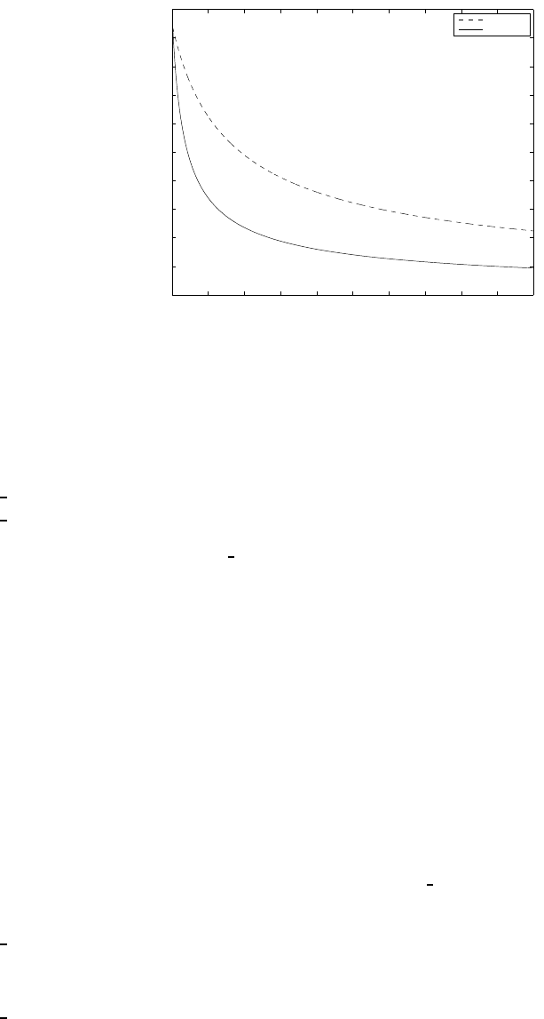
0 50 100 150 200 250 300 350 400 450 500
0
10
20
30
40
50
60
70
80
90
100
sequence 1
sequence 2
k
ak
Figure 5.1: Sequence 1: a= 1000, A= 50, α= 0.602. Sequence 2: a= 400, A= 10, α= 0.602. Both
sequences start with the same step size, but sequence 2 decays much faster.
The parameters αand Adefine the decay slope of the function. For the parameter αwe recommend the
value 0.6. For A, use something in the order of 50:
(SP alpha 0.6)
(SP A 50.0)
This leaves the parameter a, called SP ain elastix, as the most important parameter to tune. And it is
an important parameter, it can mean success for a good choice and failure if not! If ais set too high, the
iterative solving algorithm (2.22) becomes unstable, and you may deform your image beyond recognition.
If ais set too low, you will never make it to the optimum, or may get stuck in a very small nearby local
optimum. Figure 5.2 illustrates this.
A good choice for ais dependent on the cost function that is used for registration: the athat will give
you a good result for MSD is not the same as the one that gives a good result for MI. Finally, aalso
depends on the amount of deformation that you expect between the fixed and the moving image. So again,
recommendations are hard to give. In general we advise you to think in orders of magnitude, if a= 10
is too small, try a= 100 and not a= 11. For mutual information, normalised correlation coefficient, and
normalised mutual information, you could start around a= 1000. For the mean squared difference metric
you could try something smaller than 1. If ais chosen way too big, you may encounter the error message
“Too many samples map outside moving image buffer”. This error may have other causes as well though.
The FAQ at the elastix website gives more information on this error message.
For every resolution you could specify a different value of SP a, but it might be easier to start with the
same value for every resolution.
(SP a 1000.0 1000.0 1000.0)
or, equivalently:
(SP a 1000.0)
The last important option related to the optimiser is the maximum number of iterations:
(MaximumNumberOfIterations 500)
which is, in the case of StandardGradientDescent, not only the maximum, but also the minimum, since
there is no other stopping condition implemented for this optimiser. In general, the more iterations, the
29
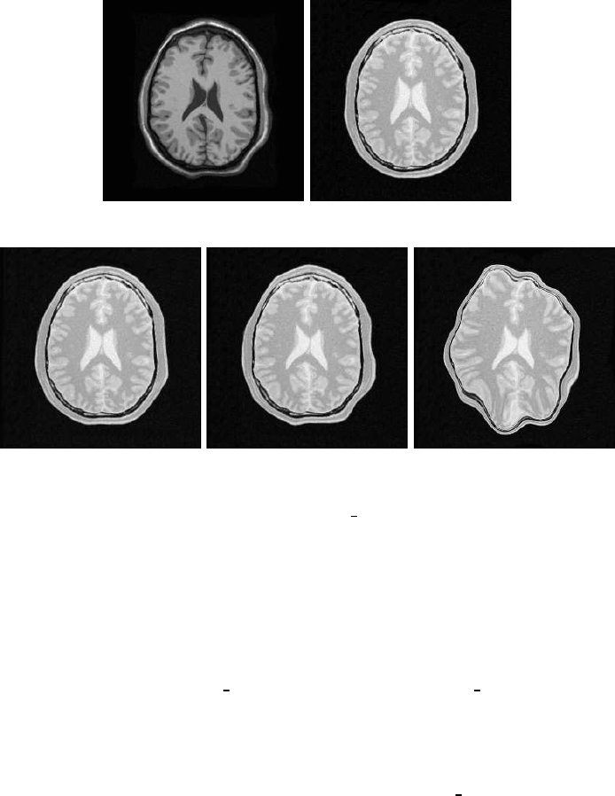
(a) (b)
(c) (d) (e)
Figure 5.2: The effect of the choice of the step size a(SP A). This example can be downloaded from the
elastix website. (a) the fixed image, (b) the moving image. (c)-(e) show the registered images, with (c)
a= 320 is too small, (d) a= 3200 as in the downloadable example is good, (e) a= 32000 is too large.
better the registration result. But, of course, more iterations take more time. A value of 500 is a good start.
Use 2000 if computation time is not such an issue. You may try to go down to 200 iterations if you are in a
hurry. For small 2D images, and rigid registration, even less iterations may suffice. A side benefit of using
more iterations is that a wider range of SP agives good results. Tuning SP a then becomes easier.
Are you getting tired of the difficulty of tuning a?
Start using the AdaptiveStochasticGradientDescent optimizer. This optimizer is very similar to the
StandardGradientDescent, but estimates a proper initial value for SP aautomatically. See Klein et al.
[2009] for more details. In practice this optimizer works in many applications with its default settings. Only
the number of iterations must be specified by the user:
(Optimizer "AdaptiveStochasticGradientDescent")
(MaximumNumberOfIterations 500)
There are some optional extra parameters, such as SigmoidInitialTime and MaximumStepLength, which are
explained in the paper [Klein et al.,2009]. In addition to automatically computing the step size, this optimizer
also implements an adaptive step size mechanism, which generally makes the optimization somewhat more
robust. The only downside of this optimizer is that it is relatively time-consuming to estimate ain case of
a large degree of freedom (large size of µ), but we are addressing this issue [Qiao et al.,2014].
5.3.7 Image pyramids
The FixedImagePyramid and the MovingImagePyramid have identical options. What is said below about
the FixedImagePyramid works similarly for the MovingImagePyramid.
30
Use the FixedSmoothingImagePyramid, since it will not throw away valuable information, and since
you are not using the FullSampler anyway, down-sampling will not save you any time. It may consume
quite some memory though for large images and many resolution levels. Two parameters have to be set
to define the multi-resolution strategy: the number of resolutions (NumberOfResolutions) and the specific
down-sampling schedule that is used in each resolution (FixedImagePyramidSchedule). If you only set the
NumberOfResolutions, a default schedule will be used that smoothes the fixed image by a factor of 2 in
each dimension, starting from σ= 0.5 in the last resolution. That schedule is usually fine. In case you have
highly anisotropic data, you might want to blur less in the direction of the largest spacing.
In general 3 resolutions is a good starting point. If the fixed and moving image are initially far away, you
can increase the number of resolution levels to, say, 5 or 6. This way the images are more blurred and more
attention is paid to register large, dominant structures.
The pyramid schedule defines the amount of blurring (and down-sampling in case a FixedRecursiveImagePyramid
is used), in each direction x, y, z and for each resolution level. It can be specified as follows:
(NumberOfResolutions 4)
(FixedImagePyramidSchedule 8 8 4 4 2 2 1 1)
In this example 4 resolutions for a 2D image are used. At resolution level 0 the image is blurred with σ= 8/2
voxels in each direction (σis half the pyramid schedule value). At level 1 σ= 4/2 is used, and finally at
the last level, level 4, the original images are used for registration. Specifying the fixed and moving image
pyramids with an identical schedule can be done with one command:
(ImagePyramidSchedule 4 4 2 2 2 1 1 1 1)
for a 3D image with 3 resolution levels, where less smoothing is performed in the z-direction.
5.4 Masks
Sometimes you are specifically interested in aligning only a part of the image. A possibility to focus on this
part is to crop the image. Cropping, however, restricts the region of interest (ROI) to be a square (2D) or
cube (3D) only. If you need an irregular shaped ROI, you can use masks. A mask is a binary image, filled
with 0’s and 1’s. If you use a mask, you only perform registration on the part of the image that is within
the masks, i.e. where the mask has 1’s.
You can/should use a mask
•when your image contains an artificial edge that has no real meaning. The registration might be
tempted to align these artificial edges, thereby neglecting the meaningful edges. The conic beam edge
in ultrasound images is an example of such an artificial edge.
•when the image contains structures in the neighbourhood of your ROI that may influence the reg-
istration within your ROI. This is for example the case when matching lung data. Usually, you are
interested in the lungs, and not if the rib cage is well aligned. However, the ribs are structures that
for example in CT can have a strong influence on the similarity metric, especially if you use the MSD
metric. In that case, the rib cage may be well aligned at the cost of vessels structures near the border
of the lung with the rib cage. In this case it will help you if you use a dilated lung segmentation as a
mask.
Masks can be used both for the fixed and the moving image. A fixed image mask is sufficient to focus
the registration on a ROI, since samples are drawn from the fixed image. You only want to use a mask for
the moving image when your moving image contains nonsense grey values near the ROI.
In case you are using a mask to prevent bad karma from an artificial edge, you also need to set the
parameter:
31
(ErodeMask "true")
If not, then when performing multi-resolution, information from the artificial edge will flow into you ROI
due to the smoothing step. In case the edge around your ROI is meaningful, e.g. in the lung example, you
should set it to false, because this edge will help to guide the registration.
A common exception that elastix throws when drawing samples is: “Could not find enough image
samples within reasonable time. Probably the mask is too small.” The probable cause for this is that your
fixed image mask is too small. See the FAQ for more information.
5.5 Trouble shooting
5.5.1 Common errors
Some common sources of confusion and questions have been gathered in a FAQ, which can be found at
http://elastix.isi.uu.nl/FAQ.php
5.5.2 Bad initial alignment
When the initial alignment between two images is very off, you cannot start a nonrigid registration. And
sometimes it can be a hassle to get it right. What factors can help to get it right?
•Start with a transformation with a low degree of freedom, i.e. the translation, rigid, similarity or affine
transform. Sometimes the images are really far off, and have no overlap to begin with (NB: the position
of images in physical space is determined by the origin and voxel spacing; see Section 2.2). A solution
is then to add the following line to your parameter file:
(AutomaticTransformInitialization "true")
This parameter facilitates the automatic estimation of an initial alignment for the aforementioned
transformations. Three methods to do so are supported: the default method which aligns the centres
of the fixed and moving image, a method that aligns the centres of gravity, and a method that simply
aligns the image origins. A method can be selected by adding one of the following lines to the parameter
file:
(AutomaticTransformInitializationMethod "GeometricalCenter")
(AutomaticTransformInitializationMethod "CenterOfGravity")
(AutomaticTransformInitializationMethod "Origins")
Note that “Origins” is currently only available for the affine transformation.
•You need a good multi-resolution strategy, i.e. quite a bit of resolution levels. This way a lot of
smoothing is going on, blurring away all the details and thereby focussing the registration on the
major structures.
•Use more iterations.
•Take larger steps. Set the parameter aso high that the translation component of the transformation
takes a step of several voxels in each iteration, up to 10. Maybe it will work, and in that case you
will get alignment pretty quick, but the step size ais still large, so you immediately jump away from
alignment again. If that happens, you should let the sequence ak=a/(A+k)αdecay relatively fast.
This can be achieved by setting both aand Aa bit lower, see Figure 5.1.
32
•In case you need to find a large rotation, you might want to take larger steps for the rotation, but not
for the translation. This can be achieved by modifying the scales parameter, see Section 5.3.5:
(Scales 10000.0)
You can set it lower to take larger rotation steps. If it is set to 1.0 you take as large steps for
the rotation as for the translation (but the rotation is defined in radials). If you set it really high
(>106) you won’t rotate at all. You probably don’t need to go lower than 1000.0. Note that the
AutomaticScalesEstimation option usually works fine, so specifying Scales is not necessary.
5.5.3 Memory consumption
The typical size of clinical images increases as a function of time. Therefore, memory efficiency will become
more of an issue. elastix consumes ≈100 MB of memory for small images, for larger image pairs (2563)
and some common components, consumption can be about 1 - 1.5 GB. With very large images (4003and
above) memory consumption can rise above 2 GB limit of older 32-bit Windows systems. Or perhaps you
are using a laptop. Or perhaps you are using elastix within another memory-consuming master program.
What to do with large images?
•Buy yourself a brand new computer with a lot of memory. Nowadays both the computer and the
operating system will be 64 bit, so that you can actually address this much memory.
•Images in elastix are internally by default represented as a bunch of voxels of floating type. You can
modify this to short images:
(FixedInternalImagePixelType "short")
(MovingInternalImagePixelType "short")
This way you save half the amount of memory that is used to store the fixed and moving images, and
their multi-resolution pyramids. This will come at the cost of a loss of precision, but may not be that
harmful. This option is useful both for elastix and transformix.
•Change the interpolator that is used during registration. In case a B-spline interpolator is used, note
that it stores a coefficient image internally in double type. You can also specify a float version:
(Interpolator "BSplineInterpolatorFloat")
which saves you another bit of memory the size of a short image. This option is useful for elastix
only. To save even more memory, use the LinearInterpolator.
•Change the interpolator that is used when resampling an image:
(ResampleInterpolator "FinalBSplineInterpolatorFloat")
This option is useful both for elastix and transformix. However, for elastix it will only save you
some memory at the very end of the registration.
•Use downsampled images during the registration. This probably will not effect the registration accuracy
too much. After registration you can apply the resulting transformation to the original full size moving
image, using transformix. See the FAQ for more information.
33

Chapter 6
Advanced topics
6.1 Metrics
6.1.1 Image registration with multiple metrics and/or images
Up till now we viewed image registration as the problem of finding the spatial relation between one fixed
image and one moving image, using one similarity metric to define the fit. Sometimes, it is desirable to
combine multiple metrics, or multiple fixed and moving images, or both. All these three generalisations are
available in elastix:
multi-metric In this case the registration cost function is defined as:
C(Tµ;IF, IM) = 1
PN
i=1 ωi
N
X
i=1
ωiCi(Tµ;IF, IM),(6.1)
with ωithe weights. This way the same fixed and moving image is used for every sub-metric Ci. This
way one can for example simultaneously optimise the MSD and MI during a registration.
elastix should be called like:
elastix -f fixed.ext -m moving.ext -out outDir -p parameterFile.txt
multi-image In this case the registration cost function is defined as:
C(Tµ;IF, IM) = 1
PN
i=1 ωi
N
X
i=1
ωiC(Tµ;Ii
F, Ii
M).(6.2)
This way one can simultaneously register all channels of multi-spectral input data, using a single type
of cost function for all channels.
elastix should be called like:
elastix -f0 fixed0.ext -f1 fixed1.ext -f<>... -m0 moving0.ext -m1 moving1.ext
-m<>... -out outDir -p parameterFile.txt
both In this case the registration cost function is defined as:
C(Tµ;IF, IM) = 1
PN
i=1 ωi
N
X
i=1
ωiCi(Tµ;Ii
F, Ii
M).(6.3)
34
This is the most general way of registration supported by elastix. This will make it possible for
example to register two lung CT data sets with MI, while simultaneously registering the fissure seg-
mentations with the kappa statistic. The two may help each other in getting a better registration
compared to only using a single channel.
All three scenarios use the multi-metric registration method, which is selected in the parameter file with:
(Registration "MultiMetricMultiResolutionRegistration")
Other parts of the parameter file should look like:
(FixedImagePyramid "FixedSmoothingImagePyramid" "FixedSmoothingImagePyramid" ...)
(MovingImagePyramid "MovingSmoothingImagePyramid" "MovingSmoothingImagePyramid" ... )
(Interpolator "BSplineInterpolator" "BSplineInterpolator" ...)
(Metric "AdvancedMattesMutualInformation" "AdvancedMeanSquareDifference" ...)
(ImageSampler "RandomCoordinate" "RandomCoordinate" ...)
(Metric0Weight 0.125)
(Metric1Weight 0.125)
(Metric2Weight 0.125)
etc
Another way of registering multi-spectral data is to use the α-mutual information measure, described
below.
6.1.2 α-mutual information
The α-mutual information metric computes true multi-channel α-mutual information. It does not use high-
dimensional joint histograms, but instead relies on k-nearest neighbour graphs to estimate α-MI. Details can
be found in Staring et al. [2009]. It is specified in the parameter file with:
(Registration "MultiResolutionRegistrationWithFeatures")
(FixedImagePyramid "FixedSmoothingImagePyramid" "FixedSmoothingImagePyramid")
(MovingImagePyramid "MovingSmoothingImagePyramid" "MovingSmoothingImagePyramid")
(Interpolator "BSplineInterpolator" "BSplineInterpolator")
(Metric "KNNGraphAlphaMutualInformation")
(ImageSampler "MultiInputRandomCoordinate")
// KNN specific
(Alpha 0.99)
(AvoidDivisionBy 0.0000000001)
(TreeType "KDTree")
(BucketSize 50)
(SplittingRule "ANN_KD_STD")
(ShrinkingRule "ANN_BD_SIMPLE")
(TreeSearchType "Standard")
(KNearestNeighbours 20)
(ErrorBound 10.0)
A complete list of the available parameters can be found in the doxygen documentation →
elx::KNNGraphAlphaMutualInformationMetric.
6.1.3 Penalty terms
This paragraph requires extension and modification.
35

In order to regularise the transformation Tµoften a penalty term P(µ) is added to the cost function, so
it becomes:
C=γ1S+γ2P,(6.4)
where γ1, γ2user-defined constants that weigh similarity against regularity.
Penalty term are often based on the first or second order spatial derivatives of the transformation. An
example is the bending energy of the transformation, which is arguably the most common penalty term, see
Section 6.1.4.
The derivative of the similarity measure usually involves computation of the spatial derivative of the
moving image: ∂IM
∂x, and the derivative of the transformation to its parameters: ∂T
∂µ. In the ITK the
last derivative is implemented using transform->GetJacobian(), i.e. the derivative to the transformation
parameters µis referred to as ‘Jacobian’.
Penalty terms usually consist of the first and second order spatial derivatives of the transformation,
i.e. ∂T
∂xand ∂2T
∂x∂xT. We will refer to these derivatives as the ‘SpatialJacobian’ and the ‘SpatialHessian’
to clearly distinguish between these derivatives and the ‘Jacobian’. In order to apply the gradient descent
optimisation routine (2.21), (2.22), we additionally need the derivatives ∂
∂µ
∂T
∂xand ∂
∂µ
∂2T
∂x∂xT. These we call
the ‘JacobianOfSpatialJacobian’ and ‘JacobianOfSpatialHessian’, respectively.
The transform class as defined in the ITK does not support the computation of spatial derivatives ∂T/∂x
and ∂2T/∂x2, and their derivatives to µ. Initially, we created non-generic classes that combine mutual infor-
mation and the mentioned penalty terms specifically (the MattesMutualInformationWithRigidityPenalty
component in elastix version 4.3 and earlier). In 2010, however, we created a more advanced version of
the ITK transform that does implement these spatial derivatives. Additionally, we created a bending energy
regularisation class that takes advantage of these functions, see Section 6.1.4. We also reimplemented the
rigidity penalty term, see Section 6.1.5; it currently however does not yet use these spatial derivatives. More
detailed information can be found in Staring and Klein [2010a].
This all means that it is possible in elastix to combine any similarity metric with any of the available
penalty terms (currently the bending energy and the rigidity penalty term).
6.1.4 Bending energy penalty
The bending energy penalty term is defined in 2D as:
PBE(µ) = 1
PX
e
xi
∂2T
∂x∂xT(e
xi)
2
F
(6.5)
=1
PX
e
xi
2
X
j=1 ∂2Tj
∂x2
1
(e
xi)2
+ 2 ∂2Tj
∂x1∂x2
(e
xi)2
+∂2Tj
∂x2
2
(e
xi)2
,(6.6)
where Pis the number of points e
xi, and the tilde denotes the difference between a variable and a given
point over which a term is evaluated. As you can see it penalises sharp deviations of the transformation
(e.g. no high compression followed by a nearby high expansion). You can use it to regularise your nonrigid
transformation if you experience problems such as foldings. In our current implementation the computation
time of this term is relatively large, though.
It can be selected in elastix using
(Metric "AnySimilarityMetric" "TransformBendingEnergyPenalty")
(Metric0Weight 1.0)
(Metric1Weight <weight>)
and has no further parameters.
36

6.1.5 Rigidity penalty
Some more advanced metrics, not found in the ITK, are available in elastix: The rigidity penalty term
Prigid(Tµ;IM) described in Staring et al. [2007a]. It is specified in the parameter file with:
(Metric "AnySimilarityMetric" "TransformRigidityPenalty")
// normal similarity metric parameters
...
// Weights
(Metric0Weight 1.0)
(Metric1Weight 0.1)
// Rigidity penalty parameters:
(OrthonormalityConditionWeight 1.0)
(PropernessConditionWeight 100.0)
(MovingRigidityImageName "movingRigidityImage.mhd")
A complete list of the available parameters can be found in the doxygen documentation →
elx::TransformRigidityPenalty. See also Section 6.1.3.
6.1.6 DisplacementMagnitudePenalty: inverting transformations
The DisplacementMagnitudePenalty is a cost function that penalises ||Tµ(x)−x||2. You can use this
to invert transforms, by setting the transform to be inverted as an initial transform (using -t0), setting
(HowToCombineTransforms "Compose"), and running elastix with this metric, using the original fixed
image set both as fixed (-f) and moving (-m) image. After that you can manually set the initial transform
in the last parameter file to "NoInitialTransform", and voila, you have the inverse transform! Strictly
speaking, you should then also change the Size/Spacing/Origin/Index/Direction settings to match that of
the moving image. Select it with:
(Metric "DisplacementMagnitudePenalty")
Note that inverting a transformation becomes conceptually very similar to performing an image registration
in this way. Consequently, the same choices are relevant: optimisation algorithm, multiresolution etc...
Note that this procedure was described and evaluated in Metz et al. [2011].
6.1.7 Corresponding points: help the registration
Most of the similarity measures in elastix are based on corresponding characteristics of the fixed and
moving image. It is possible, however, to register based on point correspondence. Therefore, in elastix
4.4 we introduced a metric that minimises the distance of two point sets with known correspondence. It is
defined as:
SCP =1
PX
xF i
kxMi −Tµ(xF i)k(6.7)
where Pis the number of points xi, and xF i,xMi corresponding points from the fixed and moving image
point sets, respectively. The metric can be used to help in a difficult image registration task that fails if
performed fully automatically. A user can manually click corresponding points (or maybe automatically
extract), and setup elastix to not only minimise based on intensity, but also taking into account that some
positions are known to correspond. The derivative of SCP reads:
∂
∂µSCP =−1
PX
xF i
1
kxMi −Tµ(xF i)k(xMi −Tµ(xF i)) ∂T
∂µ(xF i).(6.8)
In elastix this metric can be selected using:
37
(Metric "AnySimilarityMetric" "CorrespondingPointsEuclideanDistanceMetric")
(Metric0Weight 1.0)
(Metric1Weight <weight>)
Note that this metric must be specified as the last metric, due to some technical constraints. The fixed and
moving point set can be specified on the command line:
elastix ... -fp fixedPointSet.txt -mp movingPointSet.txt
The point set files have to be defined in a specific format, identical to supplying points to transformix, see
Section 4.2.
6.1.8 VarianceOverLastDimensionMetric: aligning time series
This metric is explained in Metz et al. [2011]. Example parameter files can be found on the wiki parameter
file database, entry par0012.
This metric should be used to estimate the motion in dynamic imaging data (time series). The variance
of intensities over time is measured. Two- to four-dimensional imaging data is supported.
6.2 Image samplers
RandomSparseMask This variant of the random sampler is useful if the fixed image mask is sparse (i.e.
consists of many zeros).
6.3 Interpolators
ReducedDimensionBSplineInterpolator This is a variant of the normal B-spline interpolator, which
uses a 0th order spline in the last dimension. This saves time when aligning time-series, when you do
not have to interpolate in the last (time) dimension anyway. Its usage is illustrated in entry par0012
of the parameter file database.
6.4 Transforms
DeformationFieldTransform This transform serves as a wrapper around existing deformation field vector
images. It computes the transformation by interpolating the deformation field image. The relevant
tags in the transform parameter file are as follows:
(Transform "DeformationFieldTransform")
(DeformationFieldFileName "deformationField.mhd")
(DeformationFieldInterpolationOrder 1)
(NumberOfParameters 0)
The deformation field image’s pixel type should be a vector of float elements. It could be a deformation
field that is the result of transformix -def all for example! Since this transform does not have any
parameters (the µhas zero length), it makes no sense to use it for registration. It can just be used as
an initial transformation (supplied by the option -t0) or as input for transformix.
SplineKernelTransform As an alternative to the B-spline transform, elastix includes a SplineKernelTransform,
which implements a thin-plate spline type of transform; see also Section 2.6. This transformation re-
quires a list of fixed image landmarks (control points) to be specified with the command line option
38
“-ipp ipp.txt”, by means of an input points file which has the same format as the -def file used
by transformix (see Section 4.2). See the doxygen documentation on the website for a list of its
parameters.
The moving image landmarks are optimized during the registration, and can be found in the resulting
TransformParameters.txt file, in the parameter “TransformParameters”. See Section 2.6 for the
ordering of the parameters.
WeightedCombinationTransform This is a transformation that is modelled as a weighted combination
of user-specified transformations: Tµ(x) = PiwiTi(x). The weights wiform the parameter vector
µ. The sub-transforms Ti(x) may for example follow from a statistical deformation model, obtained
by principal component analysis. See the doxygen documentation on the website for a list of its
parameters.
BSplineTransformWithDiffusion This transform implements the work described in Staring et al. [2007b].
BSplineStackTransform This transformation model defines a stack of independent B-spline transforma-
tions. Its usage is illustrated in Metz et al. [2011]. Example parameter files can be found on the wiki
parameter file database, entry par0012.
6.5 Optimisation methods
Conjugate gradient —ConjugateGradientFRPR
CMAEvolutionStrategy
FiniteDifferenceGradientDescent
Full search
Quasi Newton
RegularStepGradientDescent —RSGDEachParameterApart
SimultaneousPerturbation
39
Chapter 7
Developers guide
7.1 Relation to ITK
A large part of the elastix code is based on the ITK Ib´a˜nez et al. [2005]. The use of the ITK implies that
the low-level functionality (image classes, memory allocation etc.) is thoroughly tested. Naturally, all image
formats supported by the ITK are supported by elastix as well. The C++ source code can be compiled on
multiple operating systems (Windows XP, Linux, Mac OS X), using various compilers (MS Visual Studio,
GCC), and supports both 32 and 64 bit systems.
In addition to the existing ITK image registration classes, elastix implements new functionality. The
most important enhancements are listed in Table 7.1. Note that from version 4 ITK also has transform
concatenation and supports spatial derivatives (but not their derivatives to µagain).
7.2 Overview of the elastix code
The elastix source code consists roughly of two layers, both written in C++: A) ITK-style classes that
implement image registration functionality, and B) elastix wrappers that take care of reading and setting
parameters, instantiating and connecting components, saving (intermediate) results, and similar ‘adminis-
trative’ tasks. The modular design enables adding new components, without changing the elastix core.
Adding a new component starts by creating the layer A class, which can be compiled and tested independent
of layer B. Subsequently, a small layer B wrapper needs to be written, which connects the layer A class to
the other parts of elastix.
The image samplers, for example, are implemented as ITK classes that all inherit from a base class
itk::ImageSamplerBase. These can be found in src/Common/ImageSamplers. This is “layer A” in elastix.
For each sampler (random, grid, full... ) a wrapper is written, located in src/Components/ImageSamplers,
which takes care of configuring the sampler before each new resolution of the registration process. This is
“layer B” of elastix.
7.2.1 Directory structure
The basic directory structure is as follows:
•dox
•src/Common: ITK classes, Layer A stuff. This directory also contains some external libraries, unrelated
to ITK, like xout (which is written by us) and the ANNlib.
•src/Core: this is the main elastix kernel, responsible for the execution flow, connecting the classes,
reading parameters etc.
40

•A modular framework for sampling strategies. See for more details Staring and
Klein [2010b].
•Several new optimisers: Kiefer-Wolfowitz, Robbins-Monro, adaptive stochastic
gradient descent, evolutionary strategy. Complete rework of existing ITK op-
timisers, adding more user control and better error handling: quasi-Newton,
nonlinear conjugate gradient.
•Several new or more flexible cost functions: (normalised) mutual information,
implemented with Parzen windowing similar to Th´evenaz and Unser [2000], mul-
tifeature α-mutual information, bending energy penalty term, rigidity penalty
term.
•The ability to concatenate any number of geometric transformations.
•The transformations support computation of not only ∂T/∂µ, but also of spatial
derivatives ∂T/∂xand ∂2T/∂x2, and their derivatives to µ, frequently required
for the computation of regularisation terms. Additionally, the compact support of
certain transformations is integrated more generally. See for more details Staring
and Klein [2010a].
•Linear combinations of cost functions, instead of just a single cost function.
Table 7.1: The most important enhancements and additions in elastix, compared to the ITK.
•src/Components: this directory contains the components and their elastix wrappers (layer B). Very
component-specific layer A code can also be found here.
In elastix 4.4 and later versions, it is also possible to add your own Component directories. These can
be located anywhere outside the elastix source tree. See Section 7.4 for more details about this.
7.3 Using elastix in your own software
There are (at least) three ways to use elastix in your own software:
1. Compile the elastix executable and directly call it with the appropriate arguments. This is the most
easy way, and Matlab and MeVisLab code exists for that.
2. Include the elastix source code in your own project, see Section 7.3.1.
3. Compile elastix as a library and link to it, see Section 7.3.2. This functionality is available as of
version 4.7 (February 2014).
7.3.1 Including elastix code in your own software
You may find some elastix classes useful to integrate in your own project. For example, if you are developing
a new elastix component and first would like to test it outside elastix (see Section 7.4. In such a case, you
could of course copy the required elastix files to your own project, or set the include-paths manually, but
this would not be very convenient.
41

To make it easier, a UseElastix.cmake file is generated in the elastix binary directory. You can
include this in the CMakeLists.txt file of your own project, and CMake will make sure that all necessary
include directories are set. Also, you can link to the elastix libraries, such as elxCommon, to avoid
recompiling code.
An example of this can be found in the directory dox/externalproject of the elastix source distribution.
7.3.2 Using elastix as a library
Introduction
elastix also offers the possibility to be used as dynamic or static linked library. This offers the possibility
to integrate its functionality in your own software, without having to call the external elastix executable.
The latter namely has the downside that your software, which presumably already has the fixed and moving
images in memory, has to store these images to disk. elastix will then load them again (so they will be
in memory twice), perform the registration, and write the result to disk. Your software then needs to load
the result from the disk to memory. This approach obviously leads to an increase in memory use, decrease
in performance due to the reading/writing overhead, and is just not very elegant. When using elastix
as a library your software only has to pass memory pointers to the library interface, so there is no need
for reading/writing or in-memory image duplication. After registration elastix will pass a pointer to the
resulting image back to your program.
Library functionality is still quite heavily under development, but the following basic functionality is
already available:
•Registration of any pair of images using any combination of elastix components.
•Usage of registration masks.
•Usage of multiple parameter files consecutively (similar to using the -p option of the elastix executable
multiple times).
•Using transformix to transform an image.
Building elastix as a static or dynamic library
To build elastix as a library you have to disable the ELASTIX BUILD EXECUTABLE option in CMake. With
this option disabled a build project for a static library will be created. If you want to create a dynamic
library (not very well tested), you have to enable the ELASTIX BUILD SHARED LIBS option.
Linking with the elastix library
When building your own software project, you need to link elastix and provide the elastix source directory
as an include directory to your compiler. You can do this, for example, by adding the following code to your
CMakeLists.txt file:
set( ELASTIX_BUILD_DIR "" CACHE PATH "Path to elastix build folder" )
set( ELASTIX_USE_FILE ${ELASTIX_BUILD_DIR}/UseElastix.cmake )
if( EXISTS ${ELASTIX_USE_FILE} )
include( ${ELASTIX_USE_FILE} )
link_libraries( param )
link_libraries( elastix )
link_libraries( transformix )
endif()
42

This will add a parameter to CMake, ELASTIX BUILD DIR, which needs to be provided by the user upon
running CMake. You should provide the directory in which you have build the elastix sources (the directory
having the UseElastix.cmake file). If you want to control better to which binaries you link elastix, use
the CMake target link libraries directive instead.
Preparing registration parameter settings
To be able to run elastix, you need to prepare the parameter settings first. You can do this for example
by reading them from file:
#include "elastixlib.h"
#include "itkParameterFileParser.h"
using namespace elastix;
typedef ELASTIX::ParameterMapType RegistrationParametersType;
typedef itk::ParameterFileParser ParserType;
// Create parser for transform parameters text file.
ParserType::Pointer file_parser = ParserType::New();
// Try parsing transform parameters text file.
file_parser->SetParameterFileName( "par_registration.txt" );
try
{
file_parser->ReadParameterFile();
}
catch( itk::ExceptionObject & e )
{
std::cout << e.what() << std::endl;
// Do some error handling!
}
// Retrieve parameter settings as map.
RegistrationParametersType parameters = file_parser->GetParameterMap();
If you want to use multiple parameter files consecutively, load them one by one and add them to a vector:
typedef std::vector<RegistrationParametersType> RegistrationParametersContainerType;
Then use this vector in the code below instead of the single parameter map. You can also set up the parameter
map in your C++ code. Check the typedef of ELASTIX::ParameterMapType for the exact format.
Running elastix
Once the parameter settings are loaded, run elastix using, for example, the following code:
ELASTIX* elastix = new ELASTIX();
int error = 0;
try
{
error = elastix->RegisterImages(
static_cast<typename itk::DataObject::Pointer>( fixed_image.GetPointer() ),
43
static_cast<typename itk::DataObject::Pointer>( moving_image.GetPointer() ),
parameters, // Parameter map read in previous code
output_directory, // Directory where output is written, if enabled
write_log_file, // Enable/disable writing of elastix.log
output_to_console, // Enable/disable output to console
0, // Provide fixed image mask (optional, 0 = no mask)
0 // Provide moving image mask (optional, 0 = no mask)
);
}
catch( itk::ExceptionObject &err )
{
// Do some error handling.
}
if( error == 0 )
{
if( elastix->GetResultImage().IsNotNull() )
{
// Typedef the ITKImageType first...
ITKImageType * output_image = static_cast<ITKImageType *>(
elastix->GetResultImage().GetPointer() );
}
else
{
// Registration failure. Do some error handling.
}
// Get transform parameters of all registration steps.
RegistrationParametersContainerType transform_parameters
= elastix->GetTransformParameterMapList();
// Clean up memory.
delete elastix;
Running transformix
Given the transformation parameters provided by the ELASTIX class, you can run transformix:
TRANSFORMIX* transformix = new TRANSFORMIX();
int error = 0;
try
{
error = transformix->TransformImage(
static_cast<typename itk::DataObject::Pointer>( input_image_adapter.GetPointer() ),
transform_parameters, // Parameters resulting from elastix run
write_log_file, // Enable/disable writing of transformix.log
output_to_console); // Enable/disable output to console
}
catch( itk::ExceptionObject &err )
{
44

// Do some error handling.
}
if( error == 0 )
{
// Typedef the ITKImageType first...
ITKImageType * output_image = static_cast<ITKImageType *>(
transformix->GetResultImage().GetPointer() );
}
else
{
// Do some error handling.
}
// Clean up memory.
delete transformix;
Alternatively, you can read the transformation parameters from file (for example, from TransformParameters.0.txt)
using the parameter file parser in the same way as was shown for the registration parameters above.
7.4 Creating new components
If you want to create your own component, it is natural to start writing the layer A class, without bothering
about elastix. The layer A filter should implement all basic functionality and you can test in a separate
ITK program if it does what it is supposed to do. Once you got this ITK class to work, it is trivial to write
the layer B wrapper in elastix (start by copy-pasting from existing components).
With CMake, you can tell elastix in which directories the source code of your new components is
located, using the ELASTIX USER COMPONENT DIRS option. elastix will search all subdirectories of these
directories for CMakeLists.txt files that contain the command ADD ELXCOMPONENT( <name> ... ). The
CMakeLists.txt file that accompanies an elastix component looks typically like this:
ADD_ELXCOMPONENT( AdvancedMeanSquaresMetric
elxAdvancedMeanSquaresMetric.h
elxAdvancedMeanSquaresMetric.hxx
elxAdvancedMeanSquaresMetric.cxx
itkAdvancedMeanSquaresImageToImageMetric.h
itkAdvancedMeanSquaresImageToImageMetric.hxx )
The ADD ELXCOMPONENT command is a macro defined in src/Components/CMakeLists.txt. The first argu-
ment is the name of the layer B wrapper class, which is declared in “elxAdvancedMeanSquaresMetric.h”.
After that, you can specify the source files on which the component relies. In the example above, the files
that start with “itk” form the layer A code. Files that start with “elx” are the layer B code. The file
“elxAdvancedMeanSquaresMetric.cxx” is particularly simple. It just consists of two lines:
#include "elxAdvancedMeanSquaresMetric.h"
elxInstallMacro( AdvancedMeanSquaresMetric );
The elxInstallMacro is defined in src/Core/Install/elxMacro.h.
The files elxAdvancedMeanSquaresMetric.h/hxx together define the layer B wrapper class. That class
inherits from the corresponding layer A class, but also from an elx::BaseComponent. This gives us the
45
opportunity to add a common interface to all elastix components, regardless of the ITK classes from which
they inherit. Examples of this interface are the following methods:
void BeforeAll(void)
void BeforeRegistration(void)
void BeforeEachResolution(void)
void AfterEachResolution(void)
void AfterEachIteration(void)
void AfterRegistration(void)
These methods are automatically invoked at the moments indicated by the name of the function. This gives
you a chance to read/set some parameters, print some output, save some results etc.
7.5 Coding style
In order to improve code readability and consistency, which has a positive influence on maintainability we
have adopted a coding style. A rough uncrustify configuration file is provided in elastix since version
4.7.
White spacing Good spacing improves code readability. Therefore,
•Don’t use tabs. Tabs depend on tab size, which will make the code appearance dependent on the
viewer. We use 2 spaces per tab. In Visual Studio this can be set as a preference: go to tools
→options →text editor →All languages →Tabs, then tab size = indent size = 2 and mark
“insert spaces”. In vim you can adapt your .vimrc to include the lines set ts=2; set sw=2;
set expandtab.
•No spaces at the end of a line, like in ITK. It’s just ugly. To make them (very) noticeable add
the following in your .vimrc:
:highlight ExtraWhitespace ctermbg=red guibg=red
:match ExtraWhitespace /\s\+$/
•Use spaces in functions, for loops, indices, etc. So,
FunctionName(.void.);
for(.i.=.0;.i.<.10;.++i.)
vector[.i.].=.3;
Indentation l
•Not too much, not too long lines
namespace itk
{
^
^
/**
.* ********************* Function ******************************
.*/
^
template <class TTemplate1, class TTemplate2>
void
ClassName<TTemplate1, TTemplate2>
46

::Function(.void.)
{
..//Function body
..this->OtherMemberFunction(.arguments.);
..for(.i.=.0;.i.<.10;.++i.)
..{
....x.+=.i.*.i;
..}
^
} // end Function()
^
}.//.end.namespace.itk
•A class looks like
namespace itk
{
^
/**.\class.ClassName
.*.\brief.Brief.description
.*
.*.Detailed.description
.*
.*.\ingroup.Group
.*/
^
template < templateArguments >
class.ClassName:
public.SuperclassName
{
public:
^
../**.Standard.class.typedefs..*/
..typedef.ClassName..................Self;
..typedef.SuperclassName.............Superclass;
Variable and function naming It’s nice if from the name of a variable you know that it’s local or a class
member. Therefore,
•Member variables are prepended with m, followed by a capital. In the implementation refer to
them using this->. So, this->m_MemberVariable is correct.
•Local variables should start with a lower case character.
•Functions should start with a capital.
•Member functions should also be called using this->
Better code Some simple things to look at:
•Use const wherever you can
•For floats don’t use 0, but 0.0 to avoid possible bugs.
47
•Use the virtual keyword when overriding a virtual function in a derived class. This is not strictly
needed in C++, but when you use it, it is immediately clear that a function overridden or meant
to be overridden.
•Always use opening and closing brackets. Although it is not always needed for C++, do
if(.condition.)
{
..valid = true;
}
instead of
if(.condition.)
..valid = true;
Also for for-loops.
Commenting Code is meant to be read by others, or by you in years time. So,
•Comment a lot
•End functions with } // end FunctionName()
48
Appendix A
Example parameter file
//ImageTypes
(FixedInternalImagePixelType "float")
(MovingInternalImagePixelType "float")
(UseDirectionCosines "true")
//Components
(Registration "MultiResolutionRegistration")
(FixedImagePyramid "FixedRecursiveImagePyramid")
(MovingImagePyramid "MovingRecursiveImagePyramid")
(Interpolator "BSplineInterpolator")
(Metric "AdvancedMattesMutualInformation")
(Optimizer "AdaptiveStochasticGradientDescent")
(ResampleInterpolator "FinalBSplineInterpolator")
(Resampler "DefaultResampler")
(Transform "EulerTransform")
// ********** Pyramid
// Total number of resolutions
(NumberOfResolutions 3)
// ********** Transform
//(CenterOfRotation 128 128) center by default
(AutomaticTransformInitialization "true")
(AutomaticScalesEstimation "true")
(HowToCombineTransforms "Compose")
// ********** Optimizer
// Maximum number of iterations in each resolution level:
(MaximumNumberOfIterations 300 300 600)
(AutomaticParameterEstimation "true")
(UseAdaptiveStepSizes "true")
49
// ********** Metric
//Number of grey level bins in each resolution level:
(NumberOfHistogramBins 32)
(FixedKernelBSplineOrder 1)
(MovingKernelBSplineOrder 3)
// ********** Several
(WriteTransformParametersEachIteration "false")
(WriteTransformParametersEachResolution "false")
(ShowExactMetricValue "false")
(ErodeMask "true")
// ********** ImageSampler
// Number of spatial samples used to compute the
// mutual information in each resolution level:
(ImageSampler "RandomCoordinate")
(NumberOfSpatialSamples 2048)
(NewSamplesEveryIteration "true")
// ********** Interpolator and Resampler
//Order of B-Spline interpolation used in each resolution level:
(BSplineInterpolationOrder 1)
//Order of B-Spline interpolation used for applying the final deformation:
(FinalBSplineInterpolationOrder 3)
//Default pixel value for pixels that come from outside the picture:
(DefaultPixelValue 0)
50
Appendix B
Example transform parameter file
(Transform "EulerTransform")
(NumberOfParameters 3)
(TransformParameters -0.000000 -4.564513 -2.091174)
(InitialTransformParametersFileName "NoInitialTransform")
(HowToCombineTransforms "Compose")
// Image specific
(FixedImageDimension 2)
(MovingImageDimension 2)
(FixedInternalImagePixelType "float")
(MovingInternalImagePixelType "float")
(Size 256 256)
(Index 0 0)
(Spacing 1.0000000000 1.0000000000)
(Origin 0.0000000000 0.0000000000)
// EulerTransform specific
(CenterOfRotationPoint 128.0000000000 128.0000000000)
// ResampleInterpolator specific
(ResampleInterpolator "FinalBSplineInterpolator")
(FinalBSplineInterpolationOrder 3)
// Resampler specific
(Resampler "DefaultResampler")
(DefaultPixelValue 0.000000)
(ResultImageFormat "mhd")
(ResultImagePixelType "short")
51
Appendix C
Practical exercise: using VV with
elastix
This exercise has been kindly provided by Simon Rit (Creatis).
The goal of these practical exercises is to introduce you to the problem of image registration. Because
software development is time consuming, you will not develop your own software but use existing open-source
programs:
•elastix (http://elastix.isi.uu.nl/, [1]) is an open-source platform for automated image regis-
tration based on the Insight Segmentation and Registration Toolkit (www.itk.org). The development
was initiated by the Image Sciences Institute of the University Medical Center of Utrecht (The Nether-
lands). It is command line driven with configuration settings defined in a parameter file. The user
manual is available here: http://elastix.isi.uu.nl/download/elastix_manual_v4.5.pdf.
•vv (http://vv.creatis.insa-lyon.fr/), [2]) is an open-source and cross platform image viewer,
designed for fast and simple visualization, based on ITK and the Visualization Toolkit (www.vtk.org).
The development was initiated by the CREATIS laboratory of Lyon (France). It can also be command
line driven. Command line options are accessible with vv --help, key shortcuts with F1.
To run a command window in Windows, click on Executer in the Windows menu and type cmd. In this
window, you can:
•Change drive by typing, e.g., D: to go to drive D.
•Change folder by typing, e.g., cd tmp to go to subfolder tmp.
•Create a directory by typing, e.g., mkdir toto to create a toto subfolder.
At the end of the exercises, you should be able to do rigid (manual and automated) as well as non-rigid
registrations and to visualize the results. You will write a report to answer the instructions with a bold font
which will contain concise comments supported with screenshots whenever possible.
C.1 Manual rigid registration
•Download the images ct.mha and cbct.mha:http://www.creatis.insa-lyon.fr/~srit/tete.
•Open them in vv with the command line vv ct.mha cbct.mha. Observe them, change image on each
slicer and analyze the effect of each shortcut and mouse option in the help menu (F1).
52
•Open them in vv with the command line vv --linkall ct.mha cbct.mha and observe the difference.
•Open them in vv with the command line vv ct.mha --overlay cbct.mha and observe the difference.
•In the menu Tools, open the manual registration tool and play with the sliders. Check that the
behavior of vv manual registration is consistent with that described in the elastix manual, section
2.6.
•Manually register the two images.
•Knowing that the convention is Euler angles with YXZ, explain how the resulting matrix
is computed from the parameters.
•The software is not robust to the gimbal lock. Explain for which parameter(s) the gimbal lock
is reached and observe the consequence in vv.
C.2 Automated rigid registration
•Download the elastix parameter file Par0005.MI.rigid.txt which has been taken from the elastix
database on their website.
•Create a rigid directory with mkdir rigid and run elastix with the command line
elastix -f cbct.mha -m ct.mha -p Par0005.MI.rigid.txt -out rigid
Observe the result with vv by typing the result parameters in the manual registration
window (in the file rigid/TransformParameters.0.txt).
•Detect a not so well aligned region and elaborate on the cause.
•Compare 3 similarity measures and plot their evolution during optimization.
C.3 Non-rigid registration
•Download the pre-registered image ct.mhd and check that only deformations are left with
vv ct.mhd --overlay cbct.mha.
•Download the elastix parameter file Par0005.MI.1.txt. The latter has been modified to account for
the embedded rigid registration with the parameter
(UseDirectionCosines "true").
•Create a dir directory with mkdir dir and run
elastix -f cbct.mha -m ct.mhd -p Par0005.MI.1.txt -out dir
•Create a dirres directory with mkdir dirres and run
transformix -in ct.mhd -out dirres -tp dir/TransformParameters.0.R1.txt -def all
•Discuss the results using the two commands:
vv cbct.mha --vf dirres/deformationField.mhd
vv --linkall cbct.mha --overlay ct.mhd cbct.mha --overlay dirres/result.mhd
[1] S. Klein, M. Staring, K. Murphy, M.A. Viergever, and J.P.W. Pluim. elastix: a toolbox for intensity-
based medical image registration. IEEE Trans Med Imaging, 29(1):196–205, Jan 2010.
[2] S. Rit, R. Pinho, V. Delmon, M. Pech, G. Bouilhol, J. Schaerer, B. Navalpakkam, J. Vandemeulebroucke,
P. Seroul, and D. Sarrut. VV, a 4D slicer. In Proceedings of the Fourth International Workshop on Pulmonary
Image Analysis, pages 171–175, Toronto, Canada, September 2011.
53
Appendix D
Software License
D.1 Copyright Notice
elastix Copyright Notice:
Copyright 2014 University Medical Center Utrecht and contributors
Licensed under the Apache License, Version 2.0 (the "License"); you
may not use this file except in compliance with the License. You may
obtain a copy of the License at
http://www.apache.org/licenses/LICENSE-2.0.txt
Unless required by applicable law or agreed to in writing, software
distributed under the License is distributed on an "AS IS" BASIS,
WITHOUT WARRANTIES OR CONDITIONS OF ANY KIND, either express or
implied. See the License for the specific language governing
permissions and limitations under the License.
-------------------------------------------------------------------------------
See LICENSE file for details.
-------------------------------------------------------------------------------
Historical note
elastix was initially developed under contract of the University
Medical Center Utrecht, The Netherlands, by Stefan Klein and Marius
Staring under supervision of Josien P.W. Pluim. It is currently
maintained at the Leiden University Medical Center, The Netherlands,
and at Erasmus Medical Center, Rotterdam, The Netherlands.
Versions of elastix prior to elastix v4.8 are distributed under the
new and simplified BSD license approved by the Open Source
Initiative (OSI)
[http://www.opensource.org/licenses/bsd-license.php].
Starting with its version elastix v4.8, elastix is distributed under
54
the Apache 2.0 License.
The software is partially derived from the Insight Segmentation and
Registration Toolkit (ITK). Prior to ITK 4, ITK is distributed under
the new and simplified BSD licence. Starting with its version ITK 4
the ITK is distributed under the Apache 2.0 License. The ITK is
required by elastix for compilation of the source code.
-------------------------------------------------------------------------------
elastix contains code from third parties that have different
copyrights.
They are:
1) Insight Toolkit: Copyright by the Insight Software Consortium
Distributed under the Apache 2.0 license.
Several files throughout elastix are derived from the
Insight Toolkit.
2) ANN library: Copyright by the University of Maryland.
Distributed under the GNU Lesser Public Licence.
The files can be found in the subdirectory
Common/KNN/ann_1.1. Please read the content of the
subdirectory for details.
D.2 Software Licence
Apache License
Version 2.0, January 2004
http://www.apache.org/licenses/
TERMS AND CONDITIONS FOR USE, REPRODUCTION, AND DISTRIBUTION
1. Definitions.
"License" shall mean the terms and conditions for use, reproduction,
and distribution as defined by Sections 1 through 9 of this document.
"Licensor" shall mean the copyright owner or entity authorized by
the copyright owner that is granting the License.
"Legal Entity" shall mean the union of the acting entity and all
other entities that control, are controlled by, or are under common
control with that entity. For the purposes of this definition,
"control" means (i) the power, direct or indirect, to cause the
direction or management of such entity, whether by contract or
otherwise, or (ii) ownership of fifty percent (50%) or more of the
outstanding shares, or (iii) beneficial ownership of such entity.
"You" (or "Your") shall mean an individual or Legal Entity
exercising permissions granted by this License.
55
"Source" form shall mean the preferred form for making modifications,
including but not limited to software source code, documentation
source, and configuration files.
"Object" form shall mean any form resulting from mechanical
transformation or translation of a Source form, including but
not limited to compiled object code, generated documentation,
and conversions to other media types.
"Work" shall mean the work of authorship, whether in Source or
Object form, made available under the License, as indicated by a
copyright notice that is included in or attached to the work
(an example is provided in the Appendix below).
"Derivative Works" shall mean any work, whether in Source or Object
form, that is based on (or derived from) the Work and for which the
editorial revisions, annotations, elaborations, or other modifications
represent, as a whole, an original work of authorship. For the purposes
of this License, Derivative Works shall not include works that remain
separable from, or merely link (or bind by name) to the interfaces of,
the Work and Derivative Works thereof.
"Contribution" shall mean any work of authorship, including
the original version of the Work and any modifications or additions
to that Work or Derivative Works thereof, that is intentionally
submitted to Licensor for inclusion in the Work by the copyright owner
or by an individual or Legal Entity authorized to submit on behalf of
the copyright owner. For the purposes of this definition, "submitted"
means any form of electronic, verbal, or written communication sent
to the Licensor or its representatives, including but not limited to
communication on electronic mailing lists, source code control systems,
and issue tracking systems that are managed by, or on behalf of, the
Licensor for the purpose of discussing and improving the Work, but
excluding communication that is conspicuously marked or otherwise
designated in writing by the copyright owner as "Not a Contribution."
"Contributor" shall mean Licensor and any individual or Legal Entity
on behalf of whom a Contribution has been received by Licensor and
subsequently incorporated within the Work.
2. Grant of Copyright License. Subject to the terms and conditions of
this License, each Contributor hereby grants to You a perpetual,
worldwide, non-exclusive, no-charge, royalty-free, irrevocable
copyright license to reproduce, prepare Derivative Works of,
publicly display, publicly perform, sublicense, and distribute the
Work and such Derivative Works in Source or Object form.
3. Grant of Patent License. Subject to the terms and conditions of
this License, each Contributor hereby grants to You a perpetual,
worldwide, non-exclusive, no-charge, royalty-free, irrevocable
(except as stated in this section) patent license to make, have made,
use, offer to sell, sell, import, and otherwise transfer the Work,
where such license applies only to those patent claims licensable
56
by such Contributor that are necessarily infringed by their
Contribution(s) alone or by combination of their Contribution(s)
with the Work to which such Contribution(s) was submitted. If You
institute patent litigation against any entity (including a
cross-claim or counterclaim in a lawsuit) alleging that the Work
or a Contribution incorporated within the Work constitutes direct
or contributory patent infringement, then any patent licenses
granted to You under this License for that Work shall terminate
as of the date such litigation is filed.
4. Redistribution. You may reproduce and distribute copies of the
Work or Derivative Works thereof in any medium, with or without
modifications, and in Source or Object form, provided that You
meet the following conditions:
(a) You must give any other recipients of the Work or
Derivative Works a copy of this License; and
(b) You must cause any modified files to carry prominent notices
stating that You changed the files; and
(c) You must retain, in the Source form of any Derivative Works
that You distribute, all copyright, patent, trademark, and
attribution notices from the Source form of the Work,
excluding those notices that do not pertain to any part of
the Derivative Works; and
(d) If the Work includes a "NOTICE" text file as part of its
distribution, then any Derivative Works that You distribute must
include a readable copy of the attribution notices contained
within such NOTICE file, excluding those notices that do not
pertain to any part of the Derivative Works, in at least one
of the following places: within a NOTICE text file distributed
as part of the Derivative Works; within the Source form or
documentation, if provided along with the Derivative Works; or,
within a display generated by the Derivative Works, if and
wherever such third-party notices normally appear. The contents
of the NOTICE file are for informational purposes only and
do not modify the License. You may add Your own attribution
notices within Derivative Works that You distribute, alongside
or as an addendum to the NOTICE text from the Work, provided
that such additional attribution notices cannot be construed
as modifying the License.
You may add Your own copyright statement to Your modifications and
may provide additional or different license terms and conditions
for use, reproduction, or distribution of Your modifications, or
for any such Derivative Works as a whole, provided Your use,
reproduction, and distribution of the Work otherwise complies with
the conditions stated in this License.
5. Submission of Contributions. Unless You explicitly state otherwise,
any Contribution intentionally submitted for inclusion in the Work
57
by You to the Licensor shall be under the terms and conditions of
this License, without any additional terms or conditions.
Notwithstanding the above, nothing herein shall supersede or modify
the terms of any separate license agreement you may have executed
with Licensor regarding such Contributions.
6. Trademarks. This License does not grant permission to use the trade
names, trademarks, service marks, or product names of the Licensor,
except as required for reasonable and customary use in describing the
origin of the Work and reproducing the content of the NOTICE file.
7. Disclaimer of Warranty. Unless required by applicable law or
agreed to in writing, Licensor provides the Work (and each
Contributor provides its Contributions) on an "AS IS" BASIS,
WITHOUT WARRANTIES OR CONDITIONS OF ANY KIND, either express or
implied, including, without limitation, any warranties or conditions
of TITLE, NON-INFRINGEMENT, MERCHANTABILITY, or FITNESS FOR A
PARTICULAR PURPOSE. You are solely responsible for determining the
appropriateness of using or redistributing the Work and assume any
risks associated with Your exercise of permissions under this License.
8. Limitation of Liability. In no event and under no legal theory,
whether in tort (including negligence), contract, or otherwise,
unless required by applicable law (such as deliberate and grossly
negligent acts) or agreed to in writing, shall any Contributor be
liable to You for damages, including any direct, indirect, special,
incidental, or consequential damages of any character arising as a
result of this License or out of the use or inability to use the
Work (including but not limited to damages for loss of goodwill,
work stoppage, computer failure or malfunction, or any and all
other commercial damages or losses), even if such Contributor
has been advised of the possibility of such damages.
9. Accepting Warranty or Additional Liability. While redistributing
the Work or Derivative Works thereof, You may choose to offer,
and charge a fee for, acceptance of support, warranty, indemnity,
or other liability obligations and/or rights consistent with this
License. However, in accepting such obligations, You may act only
on Your own behalf and on Your sole responsibility, not on behalf
of any other Contributor, and only if You agree to indemnify,
defend, and hold each Contributor harmless for any liability
incurred by, or claims asserted against, such Contributor by reason
of your accepting any such warranty or additional liability.
END OF TERMS AND CONDITIONS
58
Bibliography
R. Brooks and T. Arbel. Improvements to the itk::KernelTransform and subclasses. The Insight Journal,
January - June, 2007. URL http://hdl.handle.net/1926/494.
W. R. Crum, O. Camara, and D. L. G. Hill. Generalized overlap measures for evaluation and validation in
medical image analysis. IEEE Trans. Med. Imag., 25(11):1451–1461, 2006.
M. H. Davis, A. Khotanzad, D. P. Flamig, and S. E. Harms. A physics-based coordinate transformation for
3-D image matching. IEEE Trans. Med. Imag., 26(3):317–328, 1997.
B. Fischer and J. Modersitzki. A unified approach to fast image registration and a new curvature based
registration technique. Linear Algebra Appl., 380:107 – 124, 2004.
Joseph V Hajnal, Derek L G Hill, and David J Hawkes, editors. Medical Image Registration. CRC Press,
2001. ISBN 0849300649.
D. L. G. Hill, P. G. Batchelor, M. Holden, and D. J. Hawkes. Medical image registration. Phys. Med. Biol.,
46(3):R1 – R45, 2001.
L. Ib´a˜nez, W. Schroeder, L. Ng, and J. Cates. The ITK Software Guide. Kitware, Inc. ISBN 1-930934-15-7,
second edition, 2005.
S. Klein, M. Staring, and J. P. W. Pluim. Evaluation of optimisation methods for nonrigid medical image
registration using mutual information and B-splines. IEEE Trans. Image Process., 16(12):2879 – 2890,
December 2007.
S. Klein, U. A. van der Heide, I. M. Lips, M. van Vulpen, M. Staring, and J. P. W. Pluim. Automatic
segmentation of the prostate in 3D MR images by atlas matching using localized mutual information.
Med. Phys., 35(4):1407 – 1417, April 2008.
S. Klein, J. P. W. Pluim, M. Staring, and M.A. Viergever. Adaptive stochastic gradient descent optimisation
for image registration. International Journal of Computer Vision, 81(3):227 – 239, March 2009.
H. Lester and S. R. Arridge. A survey of hierarchical non-linear medical image registration. Pattern Recognit.,
32(1):129 – 149, 1999.
F. Maes, A. Collignon, D. Vandermeulen, G. Marchal, and P. Suetens. Multimodality image registration by
maximization of mutual information. IEEE Trans. Med. Imag., 16(2):187 – 198, 1997.
J. B. A. Maintz and M. A. Viergever. A survey of medical image registration. Med. Image Anal., 2(1):1 –
36, 1998.
D. Mattes, D. R. Haynor, H. Vesselle, T. K. Lewellen, and W. Eubank. PET-CT image registration in the
chest using free-form deformations. IEEE Trans. Med. Imag., 22(1):120 – 128, 2003.
59
C.T. Metz, S. Klein, M. Schaap, T. van Walsum, and W.J. Niessen. Nonrigid registration of dynamic medical
imaging data using nD+t B-splines and a groupwise optimization approach. Medical Image Analysis, 15
(2):238–249, 2011.
J. Modersitzki. Numerical Methods for Image Registration. Oxford University Press, 2004. ISBN 978-
0198528418.
K. Murphy, B. van Ginneken, J.P.W. Pluim, S. Klein, and M. Staring. Semi-automatic reference stan-
dard construction for quantitative evaluation of lung CT registration. In Medical Image Computing and
Computer-Assisted Intervention (MICCAI), volume 5242 of Lecture Notes in Computer Science, pages
1006 – 1013, 2008.
J. Nocedal and S. J. Wright. Numerical optimization. Springer-Verlag, New York, 1999. ISBN 0-387-98793-2.
Y. Qiao, B.P.F. Lelieveldt, and M. Staring. Fast automatic estimation of the optimization step size for
nonrigid image registration. In SPIE Medical Imaging: Image Processing, Proceedings of SPIE, 2014.
T. Rohlfing, R. Brandt, R. Menzel, and C. R. Maurer Jr. Evaluation of atlas selection strategies for atlas-
based image segmentation with application to confocal microscopy images of bee brains. NeuroImage, 21
(4):1428–1442, 2004.
Torsten Rohlfing. Image similarity and tissue overlaps as surrogates for image registration accuracy: Widely
used but unreliable. IEEE Transactions on Medical Imaging, 31(2):153–163, Feb. 2012.
D. Rueckert, L. I. Sonoda, C. Hayes, D. L. G. Hill, M. O. Leach, and D. J. Hawkes. Nonrigid registration
using free-form deformations: Application to breast MR images. IEEE Trans. Med. Imag., 18(8):712 –
721, 1999.
Denis P. Shamonin, Esther E. Bron, Boudewijn P.F. Lelieveldt, Marion Smits, Stefan Klein, and Marius
Staring. Fast parallel image registration on CPU and GPU for diagnostic classification of Alzheimer’s
disease. Frontiers in Neuroinformatics, 7(50):1–15, 2014.
M. Staring and S. Klein. itk::transforms supporting spatial derivatives. The Insight Journal, 2010a. URL
http://hdl.handle.net/10380/3215.
M. Staring and S. Klein. An image sampling framework for the itk. The Insight Journal, 2010b. URL
http://hdl.handle.net/10380/3190.
M. Staring, S. Klein, and J. P. W. Pluim. A rigidity penalty term for nonrigid registration. Medical Physics,
34(11):4098 – 4108, 2007a.
M. Staring, S. Klein, and J. P. W. Pluim. Nonrigid registration with tissue-dependent filtering of the
deformation field. Physics in Medicine and Biology, 52(23):6879 – 6892, 2007b.
M. Staring, U. A. van der Heide, S. Klein, M. A. Viergever, and J. P. W. Pluim. Registration of cervical
MRI using multifeature mutual information. IEEE Transactions on Medical Imaging, 28(9):1412–1421,
2009.
C. Studholme, D. L. G. Hill, and D. J. Hawkes. An overlap invariant entropy measure of 3D medical image
alignment. Pattern Recognit., 32:71–86, 1999.
P. Th´evenaz and M. Unser. Optimization of mutual information for multiresolution image registration. IEEE
Trans. Image Process., 9(12):2083 – 2099, 2000.
P. Th´evenaz and M. Unser. Halton sampling for image registration based on mutual information. Sampling
Theory in Signal and Image Processing, 7(2):141–171, 2008.
60
M. Unser. Splines: A perfect fit for signal and image processing. IEEE Signal Process. Mag., 16(6):22 – 38,
1999.
Paul Viola and William M. Wells III. Alignment by maximization of mutual information. Int. J. Comput.
Vis., 24(2):137 – 154, 1997.
B. Zitov´a and J. Flusser. Image registration methods: a survey. Image Vis. Comput., 21(11):977–1000, 2003.
61
