Event Study Guide
User Manual:
Open the PDF directly: View PDF ![]() .
.
Page Count: 13

Practical Guide to Event Studies
David Novgorodsky Bradley Setzler
Department of Economics, University of Chicago
January 5, 2019
1 Identification with Perfect Control Groups
In this section, we define our parameter of interest in event study designs as well as a set of key assumptions that play
a role in its identification. We borrow heavily from the presentation in Abraham and Sun (2018). Throughout, we
motivate our approach using an example taken from Fadlon and Nielsen (2017) (FN hereafter) where the outcome
is wife’s labor supply and the research design leverages variation in the timing of spousal death.
1.1 Notation and Parameter of Interest
Notation: For individual i, denote the outcome in year tby Yit (this is observed), the year at which treatment
occurs by Ei(this is observed), and the potential outcomes by Yit (e)(this is not observed unless Ei=e). 1
•Example 1 (FN): Yit = wife’s labor supply, Ei= year that husband dies of fatal heart attack.
Parameter of interest: We are interested in the average treatment on the treated, which is ATTt(e)≡
EYit (e)−Yit (∞)
Eit =e, where Yit (∞)is the outcome an iwould have at tif counterfactually assigned treat-
ment at time ∞(i.e., never treated). This is the average difference in Yit that is due to being treated at einstead
of ∞, among those who are treated at e.
•Example 1 (FN): EYit (1995) −Yit (∞)
Eit = 1995is the difference in labor supply at, say, time t= 1997
for a wife whose husband died in 1995 versus if her husband had never died.
1.2 Parallel Trends vs No Anticipation
Definition: Parallel Trends is defined as EYis (∞)−Yit (∞)
Ei=e=EYis (∞)−Yit (∞)
Ei=e0, for all
e6=e0and all t6=s. This says that, for any two observed cohorts eand e0, the change over time they would have
had in the absence of treatment is the same.
•Example 1 (FN): Parallel trends requires that, for wives whose husbands died in 1995 and wives whose
husbands died in 2000, if none of their husbands had died, they would have experienced the same change in
mean labor supply between 1995 and 1996.
1Athey and Imbens (2018) also begin with a setting where onset dates define potential outcomes, but with a focus on design-based
estimators where the source of uncertainty is in the assignment mechanism for onset dates across sample units.
1

Definition: No Anticipation is defined as Yit (e) = Yit (∞), for all t<eand for all e. This says that, prior to
the onset of treatment, outcomes do not depend on the time at which treatment will occur.
•Example 1 (FN): No anticipation requires that, in 1994, wives of husbands who died in 1995 did not have
different labor supply than they would have had if their husbands had never died.
1.3 Differences-in-differences under Parallel Trends and No Anticipation
Let s < e ≤t<e0and consider this estimator:
DiDt,s(e, e0)≡EYit
Ei=e−EYis
Ei=e−EYit
Ei=e0−EYis
Ei=e0
which depends only on observable quantities.
Theorem 1: If Parallel Trends and No Anticipation hold, then DiDt,s(e, e0) = ATTt(e)if s < e ≤t<e0.
Proof of Theorem 1: We start with ATTt(e)and show that it equals DiDt,s(e, e0).2
1. We add and subtract Y∞
s:
ATTt(e)≡E[Ye
t−Y∞
t|E=e] = E[Ye
t−Y∞
s|E=e]−E[Y∞
t−Y∞
s|E=e]
2. We apply Parallel Trends:
ATTt(e) = E[Ye
t−Y∞
s|E=e]−E[Y∞
t−Y∞
s|E=e0]
3. No Anticipation lets us replace some of these Y∞terms with Yeor Ye0terms:
ATTt(e) = E[Ye
t−Ye
s|E=e]−EhYe0
t−Ye0
s|E=e0i≡DiDt,s(e, e0)
Definition: Perfect Control Group: We see from the above result that a Perfect Control Group for treated
cohort eduring the years t<e0is any cohort e0that satisfies both Parallel Trends and No Anticipation. Note: A
perfect control group may be a future winner e0<∞or a never-winner e0=∞, it just depends on the empirical
context.
2 Identification with Imperfect Control Groups
An imperfect control group for winners at eis a cohort of winners e0(or never-winners e0=∞) that either fails
to satisfy Parallel Trends or fails to satisfy No Anticipation. We now consider various types of imperfect control
groups and show conditions under which we can still identify some of the ATTt(e)terms.
2This proof is essentially an abbreviated version of the proof of Proposition 4 in Abraham and Sun (2018) in the case of a single
control cohort e0.
2
●●●●●
●●●●●●●●●●●
●●●●●●●●●●
●●●●●●
Treatment
Treatment
E=2000 is valid control group
for E=1995 in shaded area
0.4
0.5
0.6
0.7
0.8
1990 1995 2000 2005
Year
Wife's Mean Labor Supply
Husband Died
●●
●●
E=1995
E=2000
(a) No Anticipation
●●●
●●
●●●●●●●●●●●
●●●●●●●●
●●
●●●●●●
Anticipation
Anticipation
Treatment
Treatment
E=2000 is valid control group
for E=1995 in shaded area
0.4
0.5
0.6
0.7
0.8
1990 1995 2000 2005
Year
Wife's Mean Labor Supply
Husband Died
●●
●●
E=1995
E=2000
(b) k= 2 Years of Anticipation
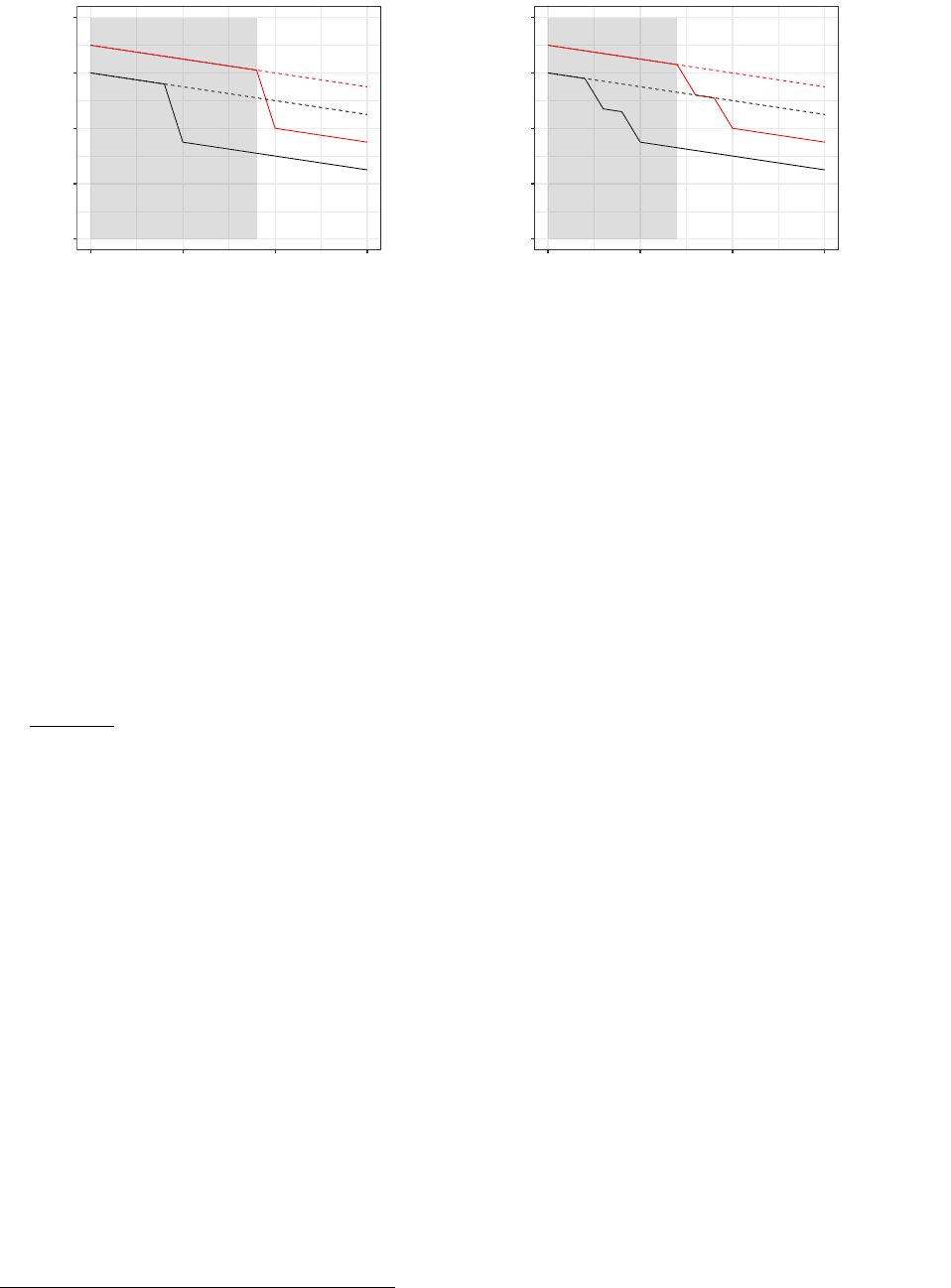
Figure 1: Anticipation in Example 1
Notes: Here, we consider the model with Y∞
t= 0.75−0.005 (t−1990) ,∀tfor the Ei= 2000 cohort, and Y∞
t= 0.70−0.005 (t−1990) ,∀t
for the Ei= 1995 cohort. Clearly, this satisfies the Parallel Trends assumption, since EYis (∞)−Yit (∞)
Ei= 1995=
EYis (∞)−Yit (∞)
Ei= 2000= 0.005 (t−s). In Figure (a), we also impose No Anticipation, so cohort E= 2000 is clearly a
Perfect Control Group for the E= 1995 cohort during the years prior to t= 2000. In Figure (b), we relax No Anticipation for k= 2
years prior to the event. As discussed in the text, this means that cohort E= 2000 is still a valid control group for the E= 1995 cohort
during the years prior to when anticipation begins in year t= 1998 = 2000 −k. The true treatment effect is −0.1. In Figure (b), the
anticipation effect is −0.05.
2.1 Parallel Trends Holds, but Anticipation Occurs for the kYears before the Event
2.1.1 What Can Be Identified with No Restrictions on Anticipation?
Suppose that winning is anticipated k > 0years before it happens. The anticipation at tmeans that Ye0
t6=Y∞
t
for t≥e0−k, so the substitution E[Y∞
t|E=e0] = EhYe0
t|E=e0iis no longer true, so Theorem 1 fails.
Figure 1 shows the following:
•In Figure 1(a), there is no anticipation, so e0= 2000 is a valid control group for e= 1995 as long as t < e0;
in particular, EY∞
t
E= 2000=EYt
E= 2000= 0.75 −0.005t, where −0.005tis the assumed common
time trend for all cohorts.
•In Figure 1(b), there is k= 2 years of anticipation, so e0= 2000 is a valid control group for e= 1995 only on
t<e0−k. We can see that E[Y∞
1999|E= 2000] = 0.75, but E[Y1999|E= 2000] = 0.65 due to anticipation, so
clearly E[Y1999|E= 2000] 6=E[Y∞
1999|E= 2000], so E= 2000 fails as a control group when t= 1999.
As illustrated with the shaded area in Figure 1(b), the E= 2000 cohort is still a valid control group for the
E= 1995 cohort during any t < 1998, that is, any year prior to when E= 2000 begins to anticipate treatment.
This makes clear the cost of having an imperfect control group: we can only identify ATTtfor t < 1998 in Figure
1(b), whereas we can identify ATTt(e)for t= 1998,1999 as well in Figure 1(a).3
2.1.2 What Can Be Identified under Parallel Anticipation?
Finally, we show that, since the anticipation effect is identified for cohort e, we can correct for the anticipation in
cohort e0if they both anticipate in the same way.
3If anticipation occurs for k=∞years prior to the event, then E= 2000 is never a valid control group for E= 1995, as emphasized
by Borusyak and Jaravel (2017).
3
●
●
●
●
●
●
●
●
●
●
●
●
●
●
●
●
●
●
●
●
●
●
●
●
●
●
●
●
●
●
●
●
Treatment
Treatment
0.3
0.4
0.5
0.6
0.7
0.8
1990 1995 2000 2005
Year
Wife's Mean Labor Supply
Husband Died
●●
●●
E=1995
E=2000
(a) Raw Data
●
●
●
●
●
●
●
●
●
●
●
●
●
●
●
●
●
●
●
●
●
●
●
●
●
●
●
●
●
●
●
●
Treatment Treatment
E=2000 is valid control group
for E=1995 in shaded area
0.3
0.4
0.5
0.6
0.7
0.8
1990 1995 2000 2005
Year
Wife's Mean Labor Supply
Husband Died
●●
●●
E=1995
E=2000
(b) Removing the Linear Trends
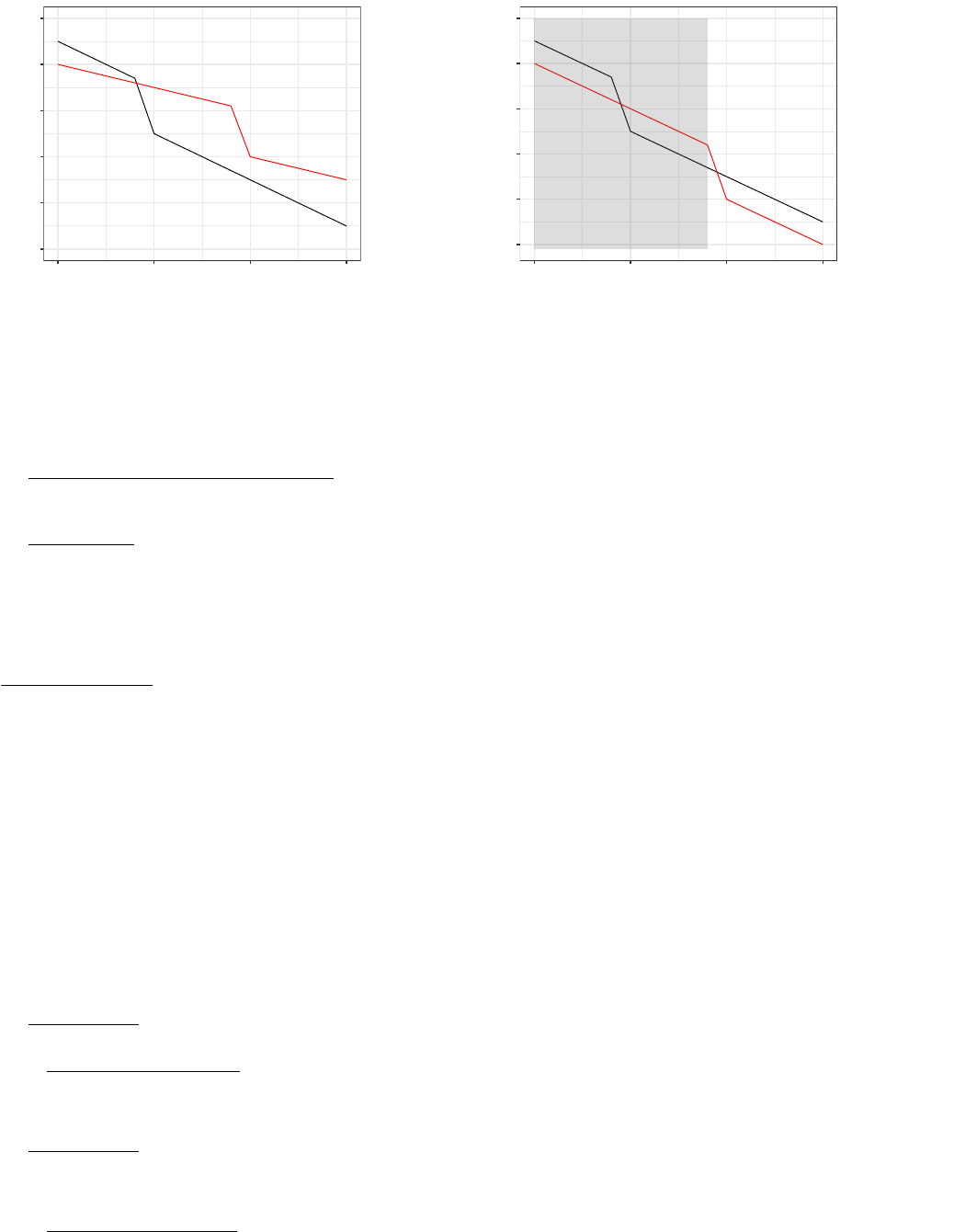
Figure 2: Non-Parallel but Linear Trends in Example 1
Notes: Here, we consider the model with Y∞
t= 0.70 −0.01 (t−1990) for the Ei= 2000 cohort, and Y∞
t= 0.75 −0.02 (t−1990) for
the Ei= 1995 cohort. The true treatment effect is −0.1. In Figure (b), we replace the E= 2000 time-trend −0.01 (t−1990) with the
E= 1995 time-trend −0.02 (t−1990) so that it satisfies Parallel Trends.
Definition: Parallel Anticipation: Denoting t0≡t+ (e0−e), we say that two cohorts have parallel antici-
pation effects if EYe
t−Y∞
t
E=e=EhYe0
t0−Y∞
t0
E=e0i.
Theorem 2: If Parallel Trends holds, No Anticipation holds on e−k < t, and Parallel Anticipation holds, then
•(a) DiDt,s(e, e0) = ATTt(e)on e−k < t for s<e≤t<e0, and,
•(b) DiDt,s(e, e0) + DiDs,s0(e, e0) = ATTt(e)for e−k≤s<e<t<e0, where s0=e−(e0−t).
Sketch of Proof: Theorem 2(a) is the same as Theorem 1, just for a smaller range of years. Theorem 2(b) is
proven by showing that DiDt,s(e, e0) = ATTt(e)−ATTt−k0(e)for some k≥k0>0, then we choose s0=t−k0and
see that ATTt−k0(e) = DiDs,s0(e, e0)under Parallel Anticipation, so we just add DiDs,s0(e, e0)to DiDt,s(e, e0)as a
bias correction.
2.2 No Anticipation Holds, but Parallel Trends Fails in a Parametric Way
Suppose that the cohort treated at eand the cohort treated at e0would have different trends if never treated.
Because there is No Anticipation, any differences in the trends for cohorts eand e0at time t < e must be exactly
equal to the deviation from Parallel Trends and implies that we can correct for the differential trends by estimating
them in the pre-period. We now show this formally and illustrate it in Figure 2.
Corollary 1: If No Anticipation holds, EYis (∞)−Yit (∞)
Ei=e=EYis −Yit
Ei=eif s<t<e<e0.
•Proof of Corollary 1: This is simply substituting that Yit (∞) = Yit (e)if t < e by No Anticipation.
Denote the deviation from Parallel Trends by ψt,s (e, e0)≡EYis (∞)−Yit (∞)
Ei=e−EYis (∞)−Yit (∞)
Ei=e0.
Corollary 2: If No Anticipation holds, then ψt,s (e, e0) = EYis −Yit
Ei=e−EYis −Yit
Ei=e0if s < t <
e<e0, where the right-hand side is observable.
•Proof of Corollary 2: This is just plugging in Corollary 1 for both eand e0into the definition of ψt,s (e, e0).
4
●
●
●
●
●
●
●
●
●
●
●
●
●
●
●
●
●
●●●●
●
Treatment
Treatment
0.3
0.4
0.5
0.6
0.7
1990 1992 1994 1996 1998 2000
Year
Wife's Mean Labor Supply
Husband Died
●●
●●
E=1995
E=2000
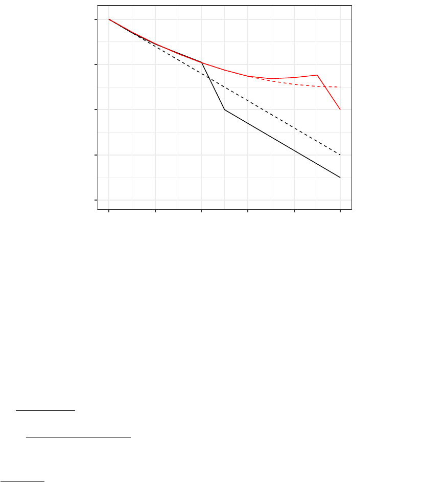
Figure 3: Neither No Anticipation nor Parallel Trends in Example 1
Notes: Suppose the economist only observes the solid lines for years 1990-2000. Here, we consider the model with Y∞
t= 0.70 −
0.03 (t−1990) for the Ei= 1995 cohort, and Y∞
t= 0.70 −0.03 (t−1990) + 0.001 (t−1990)2for the Ei= 2000 cohort, which are
shown with the dashed lines. The anticipation effects are 0.005,0.015, and 0.025 during the 3 years prior to the event. The true
treatment effect is −0.05 (the difference between the black solid and dashed lines), but the DiD estimate (the difference between the
solid red and black lines) is about −0.20 in t= 1999 (4 times the true effect in magnitude), despite the solid lines coinciding almost
perfectly in t < 1995.
We have shown the the deviation from Parallel Trends is observable if No Anticipation holds. We can then use this
to see if it follows a parametric trend, such as linearity. Finally, if we assume that the parametric trend is the same
at t≥eas it is at t<e, we can correct for the non-parallel trends on t≥e.
Theorem 3: If No Anticipation holds, then DiDt,s(e, e0) = ATTt(e) + ψt,s (e, e0).
•Proof of Theorem 3: This follows from the proof of Theorem 1, but including the term ψt,s (e, e0)in step
2 when subsituting in for the pre-trend.
Figure 2 illustrates how to use the observed pre-trend at time t<eto correct for the non-parallel trend for all
t. The same approach can be used to correct for any parametric function ψt,s (e, e0). This is an extrapolation
approach: we observe the deviation from parallel in the pre-period, extrapolate what the deviation will be in the
post-period, then correct the e0cohort so that it becomes parallel.
2.3 Can We Learn Anything if Neither Assumption Holds?
The results in the previous section suggest the following:
•Given No Anticipation, we can test for Parallel Trends and use the data to choose the design;
•Given Parallel Trends, we can test for No Anticipation and use the data to choose the design.
So that is the beginning of the analysis – either we start by believing in Parallel Trends, or we start by believing
in No Anticipation, and then we can test/correct for the other. This is where choosing the empirical context is
5

important: just as we look for instruments that are ex ante as-good-as-random in IV applications, we look for
events that are ex ante as-good-as-parallel or as-good-as-unanticipated in event studies.
To illustrate why we need either No Anticipation or Parallel Trends to get anywhere in an event study, Figure
3provides an example where the observed pre-trends “look nice,” but both No Anticipation and Parallel Trends fail,
amd this causes the DiD estimator to be severely biased. Clearly, we can’t use the approaches above to correct for
deviations in the pre-trends because there are no deviations in the pre-trends, and we can’t correct for anticipation
because they match perfectly in the years where anticipation would be expected.
3 Regression Estimators and Stacking Cohorts
3.1 Regressions with Perfect Control Groups
3.1.1 1 Treatment Cohort and 1 Control Cohort
Suppose that any cohort e0> e is a Perfect Control Group for e(that is, it satisfies both Parallel Trends and No
Anticipation). Since,
DiDt,s(e, e0)≡EYit
Ei=e−EYis
Ei=e−EYit
Ei=e0−EYis
Ei=e0
It is easy to show that, if we estimate the following regression,
Yit =α(e, e0) + δ(e, e0)1t+τ(e, e0)1e+γt,s(e, e0)1t1e+it,for Ei∈ {e, e0}and s<e≤t<e0
then OLS returns γt,s(e, e0) = DiDt,s(e, e0). If e0is a Perfect Control Group for e, it follows that γt,s(e, e0) =
ATT t(e).
3.1.2 1 Treatment Cohort and MControl Cohorts
Suppose we have cohorts e<e0< e00 . Then, we can write,
Yit =α(e, e0) + δ(e, e0)1t+τ(e, e0)1e+γt,s(e, e0)1t1e+it,for Ei∈ {e, e0}and s<e≤t<e0
Yit =α(e, e00 ) + δ(e, e00 )1t+τ(e, e00 )1e+γt,s(e, e00 )1t1e+it,for Ei∈ {e, e00 }and s < e ≤t<e00
If both eand e0are Perfect Control Groups at the same t, then γt,s(e, e0) = γt,s(e, e00 ). For the years satisfying
s < e ≤t<e0< e00 (so that e0and e00 are both valid control groups for e), we can recover γt,s in a single regression
with both control cohorts by “stacking” them into a single equation as follows:
Yit =α(e, {e0, e00 }) + δ(e, {e0, e00 })1t+τ(e, {e0, e00 })1e+γt,s(e, {e0, e00 })1t1e+it,for Ei∈ {e, e0, e00 }and s < e ≤t < e0< e00
The stacked regression says that, during the years tin which both e0and e00 are control groups, we can use both
6

e0and e00 when estimating the parameters. The δtwill use all 3 cohorts to estimate the year effect; the δecohort
will be the average difference at sbetween cohort eand the other two cohorts (weighted by number of observations
for each of the other two cohorts); and γt,s will pick up the DiD estimator of the form,
DiDt,s(e, {e0, e00 })≡EYit
Ei=e−EYis
Ei=e−EYit
Ei=e0or Ei=e00 −EYis
Ei=e0or Ei=e00
where all that has changed is that the conditioning set for the second difference includes both cohorts e0and e00 .
Note that, under the assumptions, having more control cohorts improves precision of the estimator by increasing
sample size, but does not affect identification. Note also that the control groups available for different ttimes will
vary. For example, if the data is from 2001-2006 and e= 2003, then cohorts e0∈ {2004,2005,2006}will be available
for t= 2003,e0∈ {2005,2006}will be available for t= 2004, and e0= 2006 will be available for t= 2005. If the
pre-period is s= 2001, then all of these control cohorts e0∈ {2004,2005,2006}are available for the pre-period.
This means it is important to be careful to use the same cohorts that are available at twhen estimating the
mean at s; otherwise, the difference EYit
Ei=e0or Ei=e00 −EYis
Ei=e0or Ei=e00 will be affected by
composition changes between sand trather than only by the time effects this term is meant to capture. This is
done mechanically by including intercepts for each cohort.
3.1.3 LTreatment Cohorts and MControl Cohorts
Notice that, when there are two control cohorts, there are also two treatment cohorts, since the middle cohort can
be used both as a treated and control cohort. Let’s consider the simplest case where e=e0−1 = e00 −2so that
e, e0, e00 are each in adjacent years. Then, e00 can be used twice as a control group – it can be the control group for
eboth at t=eand t=e0, and as the control group for e0at t=e0. Let’s focus on t=eand s < e:
Yit =α(e, {e0, e00 }) + δ(e, {e0, e00 })1t=e+τ(e, {e0, e00 })1e+γt=e,s(e, {e0, e00 })1t=e1e+it,for Ei∈ {e, e0, e00 }and t∈ {s, e}
Yit =α(e0, e00 ) + δ(e0, e00 )1t=e+1 +τ(e0, e00 )1e+1 +γt=e+1,s(e0, e00 )1t=e+1 1e0+it,for Ei∈ {e0, e00 }and t∈ {s, e + 1}
The first equation identifies ATT t=e(e)when pooling the e0, e00 cohorts as control groups. The last equation
identifies γt=e+1,s(e0, e00 ) = ATT t=e+1(e0)using the e00 cohort as the control group. Importantly, the control group
in the first equation e0is the treatment group in the second equation.
How can we run a single regression that correctly uses e0as the control group for ebut also uses e0as a treatment
group where e00 is its control group? We can do this by stacking the data with duplicates and introducing the
reference cohort variable, r.4In the first equation, r=eis the reference cohort for both e0and e00 . In the second
equation, r=e0is the reference cohort for e00 . So there are two copies of the e0observation, but one is coded with
r=eand the other is coded with r=e0. Then, to estimate γt=e,s(e, {e0, e00 }), we fully interact the regression that
uses eas the treatment group and e0, e00 as the control groups with an indicator 1r=e, and to estimate γt=e+1,s(e0, e00 ),
4Several recent studies use such a stacking approach with various choices of control group, including Fadlon and Nielsen (2017),
Deshpande and Li (forthcoming), and Jensen (2018). Borusyak and Jaravel (2017) also suggest a subsample regression approach
similar to the stacking approach as a potential solution to negative weighting issues of more typical dynamic event study regression
specifications when cohorts have heterogeneous ATT effects. As an alternative, Abraham and Sun (2018) propose a regression approach
that does not require stacking, but instead relies on using a single control cohort (the cohort with the latest treatment onset time) to
identify all cohort-specific ATT effects.
7

we fully interact the regression that uses e0as the treatment group and e00 as the control group with an indicator
1r=e0. Then, we can estimate both regressions simultaneously, since they are fully interacted with the 1rindicators
so that it is equivalent to estimating the two regressions separately. Given the stacked representation with reference
cohort interactions, we can consider the following assumption:
Definition: Homogeneous ATT in Event Time: We say the ATT is homogeneous in event time if ATTt(e) =
ATTt0(e0) = ATTpost , for all e, e0, t, t0, where post ≡e0−eand t0≡t+post.
To impose homogeneity in our regression representation, we want γt=e,s(e, {e0, e00 }) = γt=e+1,s(e0, e00 ), but we
still want to allow for δ(e, {e0, e00 })6=δ(e0, e00 )and τ(e, {e0, e00 })6=τ(e0, e00 ). This is easy in our reference-cohort
representation: we simply drop the interaction with 1rwith each of the γterms so that the regression will force
γt=e,s(e, {e0, e00 }) = γt=e+1,s(e0, e00 ). This is equivalent to a GMM estimator where we estimate the first regression
separately from the second regression, but impose a penalty on deviations from γt=e,s(e, {e0, e00 }) = γt=e+1,s(e0, e00 ).
This extends to the general case: we can always account for Ltreatment cohorts and Mcontrol cohorts by
reframing it as each 1 treatment cohort matched to as many control cohorts as possible for each outcome time t,
then fully interacting each of these regressions with the treatment reference cohort indicator 1r. We present the
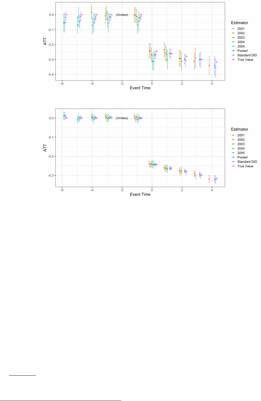
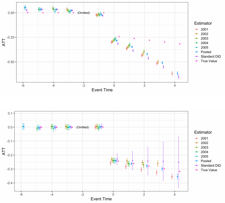
general case in Figure 4. Here, we simulate data from a model with dynamic ATTs (across event time) that are
homogeneous (across cohorts). The Perfect Control Group assumption is satisfied. We compare estimates when
allowing for heterogeneity across cohorts, the Pooled estimate when imposing homogeneity in the estimator, and
also compare these to the standard DiD estimator that does not use stacking.
We see that the true values are well recovered by the Pooled and Standard DiD estimators, with some evidence
that the Pooled standard errors are tighter due to using more control observations in the central event times. By
contrast, the cohort-specific estimates are substantially more noisy with larger standard errors, illustrating the
benefit of imposing homogeneity when the true model is homogeneous.
3.2 Regressions with Imperfect Control Groups
3.2.1 LTreatment Cohorts and MControl Cohorts: No Anticipation Holds, but Trends are not
Parallel
Suppose that we are in the case where for all cohorts, No Anticipation holds, however Parallel Trends does not
hold. As demonstrated in Figure 2, if the precise form of the deviation from parallel trends, ψt,s (e, e0), is known,
we could directly remove the bias due to differing parallel trends from each observation of unit iat time tand
proceed as in Section 3.1.3. However, in practice, ψt,s (e, e0)is unknown. Nonetheless, for a given parametric form,
we may use the pre-treatment observations t<efor each cohort to identify the cohort-specific components of
the trend (under the assumption that the pre-treatment trend continues unchanged post-treatment). Then, by
residualizing the outcome Yit with respect to the recovered trend component, we again regain Parallel Trends and
are back in the case in Section 3.1.3. For example, suppose that the underlying deviation from parallel trends is
cohort-specific linear trends. For exposition, let tmin denote each unit i’s earliest calendar time observation. To
adjust for cohort-specific linear trends, we first restrict the sample to observations t<eand consider the following
regression:
8
(a) Small N
(b) Large N
Figure 4: Stacked Regression in Example 1
Notes: This figure presents estimates using the stacked regression described above for small and large data simulations. Each point
estimate uses the maximum possible treatment and control observations. Results are presented without imposing homogeneity (each
treatment cohort has its own estimate) and imposing homogeneity (“Pooled”). Finally, the standard DiD regression is presented which
does not stack data. The true value is provided for comparison. Note that the true model has homogeneous ATT effects across cohorts.
Yit =α+ψe1e(t−tmin) + it,for t<e
Next, we use the recovered slope parameters ψefrom the above regression to construct the trend contribution
to each Yit,˜
Yit =ψe(t−tmin). Finally, we produce residualized outcome data ˆ
Yit ≡Yit −˜
Yit. Under the joint
assumptions that the deviation from parallel trends takes a cohort-specific linear form and that this trend persists
post-treatment, ˆ
Yit would now satisfy both No Anticipation and Parallel Trends and we can proceed with the
approach in Section 3.1.3.5
Figure 5 demonstrates the correction for non-parallel trends with stacked data. In Figure 5(a), we show
how biased the estimators are when Parallel Trends fails in a linear way. In Figure 5(b), we correct the stacked
estimators using the two-step approach where we fit time-trends on pre-treatment data and then extrapolate those
5We ignore discussion of inference, however, given that this strategy would rely on pre-estimated pre-trend parameters, one would
want standard errors on estimated ATT parameters to reflect this pre-estimation.
9
(a) Linear Trends, No Correction
(b) Linear Trends, Corrected
Figure 5: Stacked Regression with Linear (Non-parallel) Trends in Example 1
Notes: The true model has linear non-parallel trends. This figure presents estimates using the stacked regression described above
(a) not corrected for non-parallel trends, and (b) correcting linearly for non-parallel trends. Each point estimate uses the maximum
possible treatment and control observations. Results are presented without imposing homogeneity (each treatment cohort has its own
estimate) and imposing homogeneity (“Pooled”). Finally, the standard DiD regression is presented which does not stack data. The
true value is provided for comparison. Note that the true model has homogeneous ATT effects across cohorts. We use the two-step
residualization method in each estimator except for Standard DiD, where we follow standard practice by controlling for linear cohort
trends in the regression.
trends on post-treatment time periods in order to residualize out the time trends. In the Standard DiD estimator,
we include linear cohort-specific time-trends in the regression. We see that the corrections generally perform well,
though standard DiD is affected by large standard errors.
3.2.2 LTreatment Cohorts and MControl Cohorts: Parallel Trends Holds, but there is Anticipation
Suppose that we are in the case where for all cohorts, Parallel Trends holds, but No Anticipation does not hold; that
is, for each treated cohort with onset time e, individuals begin adjusting their outcome in anticipation of treatment
as of period e−k,k > 0. As discussed in Section 2.1.1, for a given cohort e, anticipation is analogous to moving
the treatment onset time for all later cohorts kperiods into the future. This mapping suggests how we adjust the
approach in Section 3.1.3 for a given anticipation period - when stacking control observations for a given reference
cohort r=e, only use Ei∈ {e0|e0> e +k}. For example, consider the case with with five adjacent cohorts, i.e.,
e=e0−1 = e00 −2 = e000 −3 = e0000 −4and suppose k= 2, meaning that all cohorts begin adjusting their outomc in
anticipation of being treated two periods prior to treatment onset. Unlike in Section 3.1.3, for t=e, we could no
10
(a) Anticipation, No Correction
(b) Anticipation, Corrected
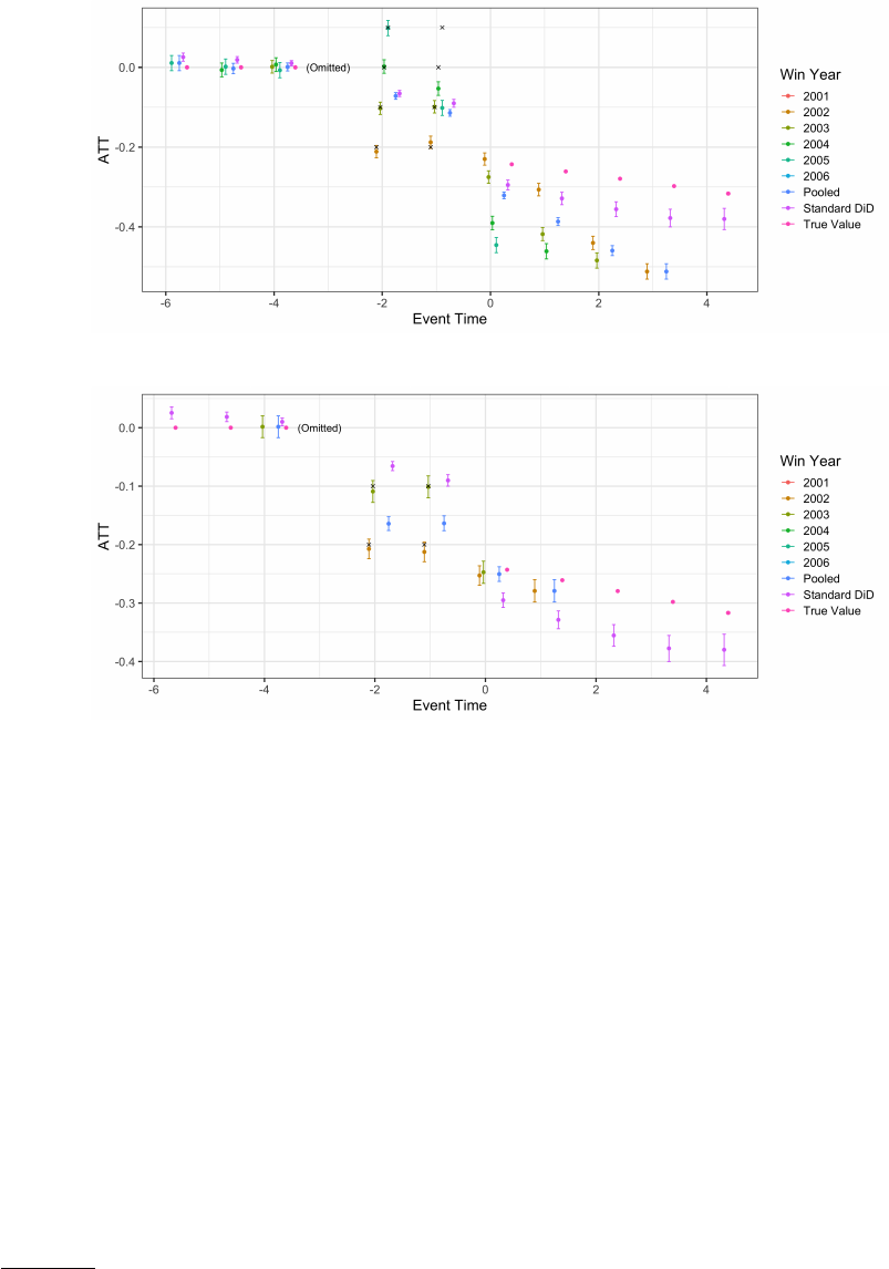
Figure 6: Stacked Regression with 2 Years of Anticipation in Example 1
Notes: The true model has 2 years of anticipation, and anticipation is heterogeneous across cohorts. This figure presents estimates using
the stacked regression described above (a) not corrected for 2 years of anticipation, and (b) correcting for 2 years of anticipation by
restricting control groups. Each point estimate uses the maximum possible treatment and control observations. Results are presented
without imposing homogeneity (each treatment cohort has its own estimate) and imposing homogeneity (“Pooled”). Finally, the
standard DiD regression is presented which does not stack data. The true value is provided for comparison. Note that the true model
has homogeneous ATT effects across cohorts.
longer include {e0, e00 }in the set of control groups. Thus, for the reference cohort r=e, the underlying regression
for the r=esubsample would now be
Yit =α(e, {e000 , e0000 }) + δ(e, {e000 , e0000 })1t=e+τ(e, {e000 , e0000 })1e+γt=e,s(e, {e000 , e0000 })1t=e1e+it,
for Ei∈ {e, e000 , e0000 }and t∈ {s, e}
Otherwise, the approach to recover the identified ATT effects proceeds as in Section 3.1.3.
In Figure 6, we introduce k= 2 periods of anticipation. Figure 6(a) demonstrates the bias in the estimators
when not accounting for this anticipation. Note that, as long as the reference event time is prior to anticipation
(event time -3 in the figure), the standard DiD performs well with anticipation. In Figure 6(b), we correct for
anticipation in the stacked estimators by limiting which control cohorts are used to be at least two cohorts ahead.
As a result, we cannot estimate as many effects across event times. Note: Standard DiD would be able to correct
for anticipation if anticipation were homogeneous across cohorts, as Standard DiD implicitly includes a correction
11
for homogeneous anticipation.
4 Code
We wrote a software package in R, called eventStudy, which makes everything here extremely easy. To install the
software in R, just type install.packages(“eventStudy”).
Stacking/Correcting the Data
It takes one line of code to construct the stacked data and correct for anticipation if needed:
stacked_data = ES_clean_data(data, min_control_gap = 1, max_control_gap = Inf, omitted_event_time = -2)
•You can change the omitted event time by setting, for example, omitted_event_time = -2.
•You can set a minimum gap before using a control cohort (to correct for anticipation) by setting, for example,
min_control_gap = 3.
•You can also set a maximum control cohort, e.g., FN use 5 cohorts ahead only, which you can do in our
command by setting min_control_gap = 5 and max_control_gap = 5.
Finally, to correct for linear deviations from Parallel Trends, simply do this before running ES_clean_data:
data = ES_parallelize_trends(data)
ATT Estimation
It takes one line of code to run the estimator on the stacked data and find the dynamic ATTs:
results = ES_estimate_ATT(stacked_data, homogeneous_ATT = FALSE, omitted_event_time = -2)
where homogeneous_ATT=TRUE would instead impose homogeneity and the omitted event time should be set to
match the one used when stacking the data.
For convenience, we also provide an implementation of the Standard DiD estimator,
standard_results = ES_estimate_std_did(data, cohort_specific_trends = FALSE, omitted_event_time = -2)
where cohort_specific_trends=TRUE would include the linear time trends by cohort.
References
Abraham, S. and L. Sun (2018): “Estimating Dynamic Treatment Effects in Event Studies with Heterogeneous
Treatment Effects,” Working paper.
Athey, S. and G. W. Imbens (2018): “Design-based Analysis in Difference-In-Differences Settings with Staggered
Adoption,” Working paper.
12
Borusyak, K. and X. Jaravel (2017): “Revisiting Event Study Designs with an Application to the Estimation
of the Marginal Propensity to Consume,” Working paper.
Deshpande, M. and Y. Li (forthcoming): “Who Is Screened Out? Application Costs and the Targeting of
Disability Programs,” American Economic Journal: Economic Policy.
Fadlon, I. and T. H. Nielsen (2017): “Family Labor Supply Responses to Severe Health Shocks,” Working
paper.
Jensen, A. (2018): “Loaded but Lonely: Housing and Saving Responses to Spousal Death in Old Age,” Working
paper.
13
