Aaa Fundamentals Of Probability Solutions Manual
User Manual:
Open the PDF directly: View PDF ![]() .
.
Page Count: 343 [warning: Documents this large are best viewed by clicking the View PDF Link!]

Instructor's Solutions Manual
Third Edition
Fundamentals of
ProbabilitY
With Stochastic Processes
SAEED GHAHRAMANI
Western New England College
Upper Saddle River, New Jersey 07458

Contents
1 Axioms of Probability 1
1.2 Sample Space and Events 1
1.4 Basic Theorems 2
1.7 Random Selection of Points from Intervals 7
Review Problems 9
2 Combinatorial Methods 13
2.2 Counting Principle 13
2.3 Permutations 16
2.4 Combinations 18
2.5 Stirling’ Formula 31
Review Problems 31
3 Conditional Probability and Independence 35
3.1 Conditional Probability 35
3.2 Law of Multiplication 39
3.3 Law of Total Probability 41
3.4 Bayes’ Formula 46
3.5 Independence 48
3.6 Applications of Probability to Genetics 56
Review Problems 59
4Distribution Functions and
Discrete Random Variables 63
4.2 Distribution Functions 63
4.3 Discrete Random Variables 66
4.4 Expectations of Discrete Random Variables 71
4.5 Variances and Moments of Discrete Random Variables 77
4.6 Standardized Random Variables 83
Review Problems 83

iv Contents
5 Special Discrete Distributions 87
5.1 Bernoulli and Binomial Random Variables 87
5.2 Poisson Random Variable 94
5.3 Other Discrete Random Variables 99
Review Problems 106
6 Continuous Random Variables 111
6.1 Probability Density Functions 111
6.2 Density Function of a Function of a Random Variable 113
6.3 Expectations and Variances 116
Review Problems 123
7 Special Continuous Distributions 126
7.1 Uniform Random Variable 126
7.2 Normal Random Variable 131
7.3 Exponential Random Variables 139
7.4 Gamma Distribution 144
7.5 Beta Distribution 147
7.6 Survival Analysis and Hazard Function 152
Review Problems 153
8 Bivariate Distributions 157
8.1 Joint Distribution of Two Random Variables 157
8.2 Independent Random Variables 166
8.3 Conditional Distributions 174
8.4 Transformations of Two Random Variables 183
Review Problems 191
9 Multivariate Distributions 200
9.1 Joint Distribution of n>2 Random Variables 200
9.2 Order Statistics 210
9.3 Multinomial Distributions 215
Review Problems 218

Contents v
10 More Expectations and Variances 222
10.1 Expected Values of Sums of Random Variables 222
10.2 Covariance 227
10.3 Correlation 237
10.4 Conditioning on Random Variables 239
10.5 Bivariate Normal Distribution 251
Review Problems 254
11 Sums of Independent Random
Variables and Limit Theorems 261
11.1 Moment-Generating Functions 261
11.2 Sums of Independent Random Variables 269
11.3 Markov and Chebyshev Inequalities 274
11.4 Laws of Large Numbers 278
11.5 Central Limit Theorem 282
Review Problems 287
12 Stochastic Processes 291
12.2 More on Poisson Processes 291
12.3 Markov Chains 296
12.4 Continuous-Time Markov Chains 315
12.5 Brownian Motion 326
Review Problems 331

Chapter 1
Axioms of Probability
1.2 SAMPLE SPACE AND EVENTS
1. For 1 ≤i, j ≤3, by (i, j ) we mean that Vann’s card number is i, and Paul’s card number is
j. Clearly, A=(1,2), (1,3), (2,3)and B=(2,1), (3,1), (3,2).
(a) Since A∩B=∅, the events Aand Bare mutually exclusive.
(b) None of (1,1),(2,2),(3,3)belongs to A∪B. Hence A∪Bnot being the sample space
shows that Aand Bare not complements of one another.
2. S={RRR,RRB,RBR,RBB,BRR,BRB,BBR,BBB}.
3. {x:0<x<20};{1,2,3,... ,19}.
4. Denote the dictionaries by d1,d2; the third book by a. The answers are
{d1d2a, d1ad2,d
2d1a, d2ad1,ad
1d2,ad
2d1}and {d1d2a, ad1d2}.
5. EF: One 1 and one even.
EcF: One 1 and one odd.
EcFc: Both even or both belong to {3,5}.
6. S={QQ,QN,QP,QD,DN,DP,NP,NN,PP}.(a) {QP };(b) {DN, DP, NN};(c) ∅.
7. S=x:7≤x≤91
6;x:7≤x≤71
4∪x:73
4≤x≤81
4∪x:83
4≤x≤91
6.
8. E∪F∪G=G:IfEor Foccurs, then Goccurs.
EFG =G:IfGoccurs, then Eand Foccur.
9. For 1 ≤i≤3, 1 ≤j≤3, by aibjwe mean passenger agets off at hotel iand passenger b
gets off at hotel j. The answers are {aibj:1≤i≤3,1≤j≤3}and {a1b1,a
2b2,a
3b3},
respectively.
10. (a) (E ∪F )(F ∪G) =(F ∪E)(F ∪G) =F∪EG.
2Chapter 1 Axioms of Probability
(b) Using part (a), we have
(E ∪F )(Ec∪F )(E ∪Fc)=(F ∪EEc)(E ∪Fc)=F(E ∪Fc)=FE ∪FFc=FE.
11. (a) ABcCc;(b) A∪B∪C;(c) AcBcCc;(d) ABCc∪ABcC∪AcBC;
(e) ABcCc∪AcBcC∪AcBCc;(f) (A −B) ∪(B −A) =(A ∪B) −AB.
12. If B=∅, the relation is obvious. If the relation is true for every event A, then it is true for S,
the sample space, as well. Thus
S=(B ∩Sc)∪(Bc∩S) =∅∪Bc=Bc,
showing that B=∅.
13. Parts (a) and (d) are obviously true; part (c) is true by DeMorgan’s law; part (b) is false: throw
a four-sided die; let F={1,2,3},G={2,3,4},E={1,4}.
14. (a) ∞
n=1An;(b) 37
n=1An.
15. Straightforward.
16. Straightforward.
17. Straightforward.
18. Let a1,a2, and a3be the first, the second, and the third volumes of the dictionary. Let a4,a5,
a6, and a7be the remaining books. Let A={a1,a
2,... ,a
7}; the answers are
S=x1x2x3x4x5x6x7:xi∈A, 1≤i≤7,and xi= xjif i= j
and x1x2x3x4x5x6x7∈S:xixi+1xi+2=a1a2a3for some i,1≤i≤5,
respectively.
19. ∞
m=1∞
n=mAn.
20. Let B1=A1,B2=A2−A1,B3=A3−(A1∪A2),...,Bn=An−n−1
i=1Ai,....
1.4 BASIC THEOREMS
1. No; P(sum 11)=2/36 while P(sum 12)=1/36.
2. 0.33 +0.07 =0.40.

Section 1.4 Basic Theorems 3
3. Let Ebe the event that an earthquake will damage the structure next year. Let Hbe the
event that a hurricane will damage the structure next year. We are given that P(E) =0.015,
P(H) =0.025, and P(EH) =0.0073. Since
P(E ∪H) =P(E)+P(H)−P(EH) =0.015 +0.025 −0.0073 =0.0327,
the probability that next year the structure will be damaged by an earthquake and/or a hurricane
is 0.0327. The probability that it is not damaged by any of the two natural disasters is 0.9673.
4. Let Abe the event of a randomly selected driver having an accident during the next 12 months.
Let Bbe the event that the person is male. By Theorem 1.7, the desired probability is
P (A) =P (AB) +P (ABc)=0.12 +0.06 =0.18.
5. Let Abe the event that a randomly selected investor invests in traditional annuities. Let Bbe
the event that he or she invests in the stock market. Then P (A) =0.75, P(B) =0.45, and
P(A∪B) =0.85. Since,
P (AB) =P (A) +P(B)−P(A∪B) =0.75 +0.45 −0.85 =0.35,
35% invest in both stock market and traditional annuities.
6. The probability that the first horse wins is 2/7. The probability that the second horse wins
is 3/10. Since the events that the first horse wins and the second horse wins are mutually
exclusive, the probability that either the first horse or the second horse will win is
2
7+3
10 =41
70.
7. In point of fact Rockford was right the first time. The reporter is assuming that both autopsies
are performed by a given doctor. The probability that both autopsies are performed by the same
doctor–whichever doctor it may be–is 1/2. Let AB represent the case in which Dr. A performs
the first autopsy and Dr. B performs the second autopsy, with similar representations for other
cases. Then the sample space is S={AA,AB,BA,BB}. The event that both autopsies are
performed by the same doctor is {AA, BB}. Clearly, the probability of this event is 2/4=1/2.
8. Let mbe the probability that Marty will be hired. Then m+(m +0.2)+m=1 which gives
m=8/30; so the answer is 8/30 +2/10 =7/15.
9. Let sbe the probability that the patient selected at random suffers from schizophrenia. Then
s+s/3+s/2+s/10 =1 which gives s=15/29.
10. P(A∪B) ≤1 implies that P (A) +P(B)−P (AB) ≤1.
11. (a) 2/52 +2/52 =1/13; (b) 12/52 +26/52 −6/53 =8/13; (c) 1−(16/52)=9/13.

4Chapter 1 Axioms of Probability
12. (a) False; toss a die and let A={1,2},B={2,3}, and C={1,3}.
(b) False; toss a die and let A={1,2,3,4},B={1,2,3,4,5},C={1,2,3,4,5,6}.
13. A simple Venn diagram shows that the answers are 65% and 10%, respectively.
14. Applying Theorem 1.6 twice, we have
P(A∪B∪C) =P(A∪B) +P(C)−P(A ∪B)C
=P (A) +P(B)−P (AB) +P(C)−P (AC ∪BC)
=P (A) +P(B)−P (AB) +P(C)−P (AC) −P(BC)+P (ABC)
=P (A) +P(B)+P(C)−P (AB) −P (AC) −P(BC)+P (ABC).
15. Using Theorem 1.5, we have that the desired probability is
P (AB −ABC) +P (AC −ABC) +P(BC −ABC)
=P (AB) −P (ABC) +P (AC) −P (ABC) +P(BC)−P (ABC)
=P (AB) +P (AC) +P(BC)−3P (ABC).
16. 7/11.
17. n
i=1pij .
18. Let Mand Fdenote the events that the randomly selected student earned an A on the midterm
exam and an A on the final exam, respectively. Then
P(MF) =P(M)+P(F)−P(M ∪F),
where P(M) =17/33, P(F) =14/33,and by DeMorgan’s law,
P(M ∪F) =1−P(McFc)=1−11
33 =22
33.
Therefore,
P(MF) =17
33 +14
33 −22
33 =3
11.
19. A Venn diagram shows that the answers are 1/8, 5/24, and 5/24, respectively.
20. The equation has real roots if and only if b2≥4c. From the 36 possible outcomes for (b, c),
in the following 19 cases we have that b2≥4c:(2,1),(3,1),(3,2),(4,1),...,(4,4),(5,1),
...,(5,6),(6,1),...,(6,6). Therefore, the answer is 19/36.
21. The only prime divisors of 63 are 3 and 7. Thus the number selected is relatively prime to 63
if and only if it is neither divisible by 3 nor by 7. Let Aand Bbe the events that the outcome

Section 1.4 Basic Theorems 5
is divisible by 3 and 7, respectively. The desired quantity is
P(A
cBc)=1−P(A∪B) =1−P (A) −P(B)+P (AB)
=1−21
63 −9
63 +3
63 =4
7.
22. Let Tand Fbe the events that the number selected is divisible by 3 and 5, respectively.
(a) The desired quantity is the probability of the event TFc:
P(TFc)=P(T)−P(TF) =333
1000 −66
1000 =267
1000.
(b) The desired quantity is the probability of the event TcFc:
P(TcFc)=1−P(T ∪F) =1−P(T)−P(F)+P(TF)
=1−333
1000 −200
1000 +66
1000 =533
1000.
23. (Draw a Venn diagram.) From the data we have that 55% passed all three, 5% passed calculus
and physics but not chemistry, and 20% passed calculus and chemistry but not physics. So at
least (55 +5+20)%=80% must have passed calculus. This number is greater than the given
78% for all of the students who passed calculus. Therefore, the data is incorrect.
24. By symmetry the answer is 1/4.
25. Let A,B, and Cbe the events that the number selected is divisible by 4, 5, and 7, respectively.
We are interested in P (ABcCc).NowABcCc=A−A(B ∪C) and A(B ∪C) ⊆A.Soby
Theorem 1.5,
P (ABcCc)=P (A) −PA(B ∪C)=P (A) −P (AB ∪AC)
=P (A) −P (AB) −P (AC) +P (ABC)
=250
1000 −50
1000 −35
1000 +7
1000 =172
1000.
26. A Venn diagram shows that the answer is 0.36.
27. Let Abe the event that the first number selected is greater than the second; let Bbe the
event that the second number selected is greater than the first; and let Cbe the event that
the two numbers selected are equal. Then P (A) +P(B)+P(C) =1, P (A) =P(B), and
P(C) =1/100. These give P (A) =99/200.
28. Let B1=A1, and for n≥2, Bn=An−n−1
i=1Ai. Then {B1,B
2,...}is a sequence of
mutually exclusive events and ∞
i=1Ai=∞
i=1Bi.Hence

6Chapter 1 Axioms of Probability
P∞
n=1
An=P∞
n=1
Bn=∞
n=1
P(B
n)≤∞
n=1
P(A
n),
since Bn⊆An,n≥1.
29. By Boole’s inequality (Exercise 28),
P∞
n=1
An=1−P∞
n=1
Ac
n≥1−∞
n=1
P(A
c
n).
30. She is wrong! Consider the next 50 flights. For 1 ≤i≤50, let Aibe the event that the ith
mission will be completed without mishap. Then 50
i=1Aiis the event that all of the next 50
missions will be completed successfully. We will show that P50
i=1Ai>0.This proves
that Mia is wrong. Note that the probability of the simultaneous occurrence of any number of
Ac
i’s is nonzero. Furthermore, consider any set Econsisting of n(n≤50) of the Ac
i’s. It is
reasonable to assume that the probability of the simultaneous occurrence of the events of Eis
strictly less than the probability of the simultaneous occurrence of the events of any subset of
E. Using these facts, it is straightforward to conclude from the inclusion–exclusion principle
that,
P50
i=1
Ac
i<
50
i=1
P(A
c
i)=
50
i=1
1
50 =1.
Thus, by DeMorgan’s law,
P50
i=1
Ai=1−P50
i=1
Ac
i>1−1=0.
31. Qsatisfies Axioms 1 and 2, but not necessarily Axiom 3. So it is not, in general, a probability
on S. Let S={1,2,3,}. Let P{1}=P{2}=P{3}=1/3. Then Q{1}=Q{2}=
1/9, whereas Q{1,2}=P{1,2}2=4/9.Therefore,
Q{1,2,}= Q{1}+Q{2}.
Ris not a probability on Sbecause it does not satisfy Axiom 2; that is, R(S) = 1.
32. Let BRB mean that a blue hat is placed on the first player’s head, a red hat on the second
player’s head, and a blue hat on the third player’s head, with similar representations for other
cases. The sample space is
S={BBB,BRB,BBR,BRR,RRR,RRB,RBR,RBB}.
This shows that the probability that two of the players will have hats of the same color and
the third player’s hat will be of the opposite color is 6/8=3/4. The following improvement,

Section 1.7 Random Selection of Points from Intervals 7
based on this observation, explained by Sara Robinson in Tuesday, April 10, 2001 issue of
the New York Times, is due to Professor Elwyn Berlekamp of the University of California at
Berkeley.
Three-fourths of the time, two of the players will have hats of the same color and
the third player’s hat will be the opposite color. The group can win every time this
happens by using the following strategy: Once the game starts, each player looks
at the other two players’ hats. If the two hats are different colors, he [or she] passes.
If they are the same color, the player guesses his [or her] own hat is the opposite
color. This way, every time the hat colors are distributed two and one, one player
will guess correctly and the others will pass, and the group will win the game. When
all the hats are the same color, however, all three players will guess incorrectly and
the group will lose.
1.7 RANDOM SELECTION OF POINTS FROM INTERVALS
1. 30 −10
30 −0=2
3.
2. 0.0635 −0.04
0.12 −0.04 =0.294.
3. (a) False; in the experiment of choosing a point at random from the interval (0,1), let
A=(0,1)−{1/2}.Ais not the sample space but P (A) =1.
(b) False; in the same experiment P{1/2}=0 while {1
2} =∅.
4. P(A∪B) ≥P (A) =1, so P(A∪B) =1.This gives
P (AB) =P (A) +P(B)−P(A∪B) =1+1−1=1.
5. The answer is
P{1,2,... ,1999}=
1999
i=1
P{i}=
1999
i=1
0=0.
6. For i=0, 1, 2, ..., 9, the probability that iappears as the first digit of the decimal represen-
tation of the selected point is the probability that the point falls into the interval i
10,i+1
10 .
Therefore, it equals
i+1
10 −i
10
1−0=1
10.
This shows that all numerals are equally likely to appear as the first digit of the decimal
representation of the selected point.

8Chapter 1 Axioms of Probability
7. No, it is not. Let S={w1,w
2,...}. Suppose that for some p>0, P{wi}=p, i =1, 2,
.... Then, by Axioms 2 and 3, ∞
i=1p=1.This is impossible.
8. Use induction. For n=1, the theorem is trivial. Exercise 4 proves the theorem for n=2.
Suppose that the theorem is true for n. We show it for n+1,
P(A
1A2···AnAn+1)=P(A
1A2···An)+P(A
n+1)−P(A
1A2···An∪An+1)
=1+1−1=1,
where P(A
1A2···An)=1 is true by the induction hypothesis, and
P(A
1A2···An∪An+1)≥P(A
n+1)=1,
implies that P(A
1A2···An∪An+1)=1.
9. (a) Clearly, 1
2∈∞
n=11
2−1
2n,1
2+1
2n.Ifx∈∞
n=11
2−1
2n,1
2+1
2n, then, for all n≥1,
1
2−1
2n<x< 1
2+1
2n.
Letting n→∞, we obtain 1/2≤x≤1/2; thus x=1/2.
(b) Let Anbe the event that the point selected at random is in 1
2−1
2n,1
2+1
2n;then
A1⊇A2⊇A3⊇···⊇An⊇An+1⊇···.
Since P(A
n)=1
n, by the continuity property of the probability function,
P{1/2}=lim
n→∞ P(A
n)=0.
10. The set of rational numbers is countable. Let Q={r1,r
2,r
3,...}be the set of rational
numbers in (0,1). Then
P(Q)=P{r1,r
2,r
3,...}=∞
i=1
P{ri}=0.
Let Ibe the set of irrational numbers in (0,1); then
P(I)=P(Qc)=1−P(Q)=1.
11. For i=0,1,2,... ,9, the probability that iappears as the nth digit of the decimal represen-
tation of the selected point is the probability that the point falls into the following subset of
(0,1):
10n−1−1
m=010m+i
10n,10m+i+1
10n.

Chapter 1 Review Problems 9
Since the intervals in this union are mutually exclusive, the probability that the point falls into
this subset is
10n−1−1
m=0
10m+i+1
10n−10m+i
10n
1−0=10n−1·1
10n=1
10.
This shows that all numerals are equally likely to appear as the nth digit of the decimal
representation of the selected point.
12. P(B
m)≤∞
n=mP(A
n). Since ∞
n=1P(A
n)converges,
lim
m→∞ P(B
m)≤lim
m→∞
∞
n=m
P(A
n)=0.
This gives limm→∞ P(B
m)=0.Therefore,
B1⊇B2⊇B3⊇···⊇Bm⊇Bm+1⊇···
implies that
P∞
m=1
∞
n=m
An=P∞
m=1
Bm=lim
m→∞ P(B
m)=0.
13. In the experiment of choosing a random point from (0,1), let Et=(0,1)−{t}, for 0 <t <1.
Then P(E
t)=1 for all t, while
P
t∈(0,1)
Et=P(∅)=0.
14. Clearly rn∈(αn,β
n). By the geometric series theorem,
∞
n=1
(βn−αn)=∞
n=1
ε
2n+1=ε
1
4
1−1
2
=ε
2<ε.
REVIEW PROBLEMS FOR CHAPTER 1
1. 3.25 −2
4.3−2=0.54.
2. We have that
S=∅,{1},∅,{2},∅,{1,2},{1},{2},{1},{1,2},{2},{1,2}.
10 Chapter 1 Axioms of Probability
The desired events are
(a) ∅,{1},∅,{2},∅,{1,2},{1},{2};(b) ∅,{1,2},{1},{2};
(c) ∅,{1},∅,{2},∅,{1,2},{1},{1,2},{2},{1,2}.
3. Since A⊆B, we have that Bc⊆Ac.This implies that (a) is false but (b) is true.
4. In the experiment of tossing a die let A={1,3,5}and B={5}; then both (a) and (b) are
false.
5. We may define a sample space Sas follows.
S=x1x2···xn:n≥1,x
i∈{H,T}; xi= xi+1,1≤i≤n−2;xn−1=xn.
6. A venn diagram shows that 18 are neither male nor for surgery.
7. We have that ABC ⊆BC,soP (ABC) ≤P(BC) and hence P(BC)−P (ABC) ≥0. This
and the following give the result.
P(A∪B∪C) =P (A) +P(B)+P(C)−P (AB) +P (AC) +P(BC)−P (ABC)
≤P (A) +P(B)+P(C).
8. If P (AB) =P (AC) =P(BC) =0,then P (ABC) =0 since ABC ⊆AB. These imply that
P(A∪B∪C) =P (A) +P(B)+P(C)−P (AB) −P (AC) −P(BC)+P (ABC)
=P (A) +P(B)+P(C).
Now suppose that
P(A∪B∪C) =P (A) +P(B)+P(C).
This relation implies that
P (AB) +P(BC)+P (AC) −P (ABC)=0.(1)
Since P (AC) −P (ABC) ≥0 we have that the sum of three nonnegative quantities is 0; so
each of them is 0. That is,
P (AB) =0,P(BC)=0, P (AC) =P (ABC). (2)
Now rewriting (1) as
P (AB) +P (AC) +P(BC)−P (ABC)=0,
the same argument implies that
P (AB) =0, P (AC) =0,P(BC)=P (ABC). (3)
Comparing (2) and (3) we have
P (AB) =P (AC) =P(BC) =0.

Chapter 1 Review Problems 11
9. Let Wbe the event that a randomly selected person from this community drinks or serves
white wine. Let Rbe the event that she or he drinks or serves red wine. We are given that
P(W) =0.40, P(R) =0.50, and P(W ∪R) =0.70. Since
P(WR) =P(W)+P(R)−P(W ∪R) =0.40 +0.50 −0.70 =0.20,
20% percent drink or serve both red and white wine.
10. No, it is not right. The probability that the second student chooses the tire the first student
chose is 1/4.
11. By De Morgan’s second law,
P(A
cBc)=1−P(AcBc)c=1−P(A∪B) =1−P (A) −P(B)+P (AB).
12. By Theorem 1.5 and the fact that A−Band B−Aare mutually exclusive,
P(A −B) ∪(B −A)=P(A−B) +P(B −A) =P(A−AB) +P(B −AB)
=P (A) −P (AB) +P(B)−P (AB) =P (A) +P(B)−2P (AB).
13. Denote a box of books by ai, if it is received from publisher i,i=1,2,3.The sample space
is
S=x1x2x3x4x5x6:two of the xi’s are a1,two of them are a2,and the remaining two are a3.
The desired event is E=x1x2x3x4x5x6∈S:x5=x6.
14. Let E,F,G, and Hbe the events that the next baby born in this town has blood type O, A, B,
and AB, respectively. Then
P(E) =P (F ), P (G) =1
10P (F ), P (G) =2P(H).
These imply
P(E) =P(F) =20P(H).
Therefore, from
P(E)+P(F)+P (G) +P(H) =1,
we get
20P(H)+20P(H)+2P(H)+P(H) =1,
which gives P(H) =1/43.
15. Let F,S, and Nbe the events that the number selected is divisible by 4, 7, and 9, respectively.
We are interested in P(FcScNc)which is equal to 1 −P(F ∪S∪N) by DeMorgan’s law.

12 Chapter 1 Axioms of Probability
Now
P(F ∪S∪N) =P(F)+P(S)+P(N)−P(FS)−P(FN)−P(SN)+P(FSN)
=250
1000 +142
1000 +111
1000 −35
1000 −27
1000 −15
1000 +3
1000 =0.429.
So the desired probability is 0.571.
16. The number is relatively prime to 150 if is not divisible by 2, 3, or 5. Let A,B, and Cbe the
events that the number selected is divisible by 2, 3, and 5, respectively. We are interested in
P(A
cBcCc)=1−P(A∪B∪C).Now
P(A∪B∪C) =P (A) +P(B)+P(C)−P (AB) −P (AC) −P(BC)+P (ABC)
=75
150 +50
150 +30
150 −25
150 −15
150 −10
150 +5
150 =11
15.
Therefore, the answer is 1 −11
15 =4
15.
17. (a) Uc
iDc
i;(b) U1U2···Un;(c) (Uc
1Dc
1)∪(Uc
2Dc
2)∪···∪(Uc
nDc
n);
(d) (U1D2Uc
3Dc
3)∪(U1Uc
2Dc
2D3)∪(D1U2Uc
3Dc
3)∪(D1Uc
2Dc
2U3)
∪(Dc
1Uc
1D2U3)∪(Dc
1Uc
1U2D2)∪(Dc
1Uc
1Dc
2Uc
2Dc
3Uc
3);
(e) Dc
1Dc
2···Dc
n.
18. 199 −96
199 −0=103
199.
19. We must have b2<4ac. There are 6 ×6×6=216 possible outcomes for a,b, and c.For
cases in which a<c,a>c, and a=c, it can be checked that there are 73, 73, and 27 cases
in which b2<4ac, respectively. Therefore, the desired probability is
73 +73 +27
216 =173
216.

Chapter 2
Combinatorial Methods
2.2 COUNTING PRINCIPLES
1. The total number of six-digit numbers is 9×10×10×10×10×10 =9×10⁵since the first digit
cannot be 0. The number of six-digit numbers without the digit five is 8 ×9×9×9×9×9=
8×95.Hence there are 9 ×10⁵−8×95=427,608 six-digit numbers that contain the digit
five.
2. (a) 55=3125.(b) 53=125.
3. There are 26 ×26 ×26 =17,576 distinct sets of initials. Hence in any town with more than
17,576 inhabitants, there are at least two persons with the same initials. The answer to the
question is therefore yes.
4. 415 =1,073,741,824.
5. 2
223 =1
222 ≈0.00000024.
6. (a) 525=380,204,032.(b) 52 ×51 ×50 ×49 ×48 =311,875,200.
7. 6/36 =1/6.
8. (a) 4×3×2×2
12 ×8×8×4=1
64.(b) 1−8×5×6×2
12 ×8×8×4=27
32.
9. 1
415 ≈0.00000000093.
10. 26 ×25 ×24 ×10 ×9×8=11,232,000.
11. There are 263×102=1,757,600 such codes; so the answer is positive.
12. 2nm.
13. (2+1)(3+1)(2+1)=36.(See the solution to Exercise 24.)

14 Chapter 2 Combinatorial Methods
14. There are (26−1)23=504 possible sandwiches. So the claim is true.
15. (a) 54=625.(b) 54−5×4×3×2=505.
16. 212 =4096.
17. 1−48 ×48 ×48 ×48
52 ×52 ×52 ×52 =0.274.
18. 10 ×9×8×7=5040. (a) 9×9×8×7=4536; (b) 5040 −1×1×8×7=4984.
19. 1−(N −1)n
Nn.
20. By Example 2.6, the probability is 0.507 that among Jenny and the next 22 people she meets
randomly there are two with the same birthday. However, it is quite possible that one of these
two persons is not Jenny. Let nbe the minimum number of people Jenny must meet so that
the chances are better than even that someone shares her birthday. To find n, let Adenote the
event that among the next npeople Jenny meets randomly someone’s birthday is the same as
Jenny’s. We have
P (A) =1−P(A
c)=1−364n
365n.
To have P (A) > 1/2, we must find the smallest nfor which
1−364n
365n>1
2,
or 364n
365n<1
2.
This gives
n>
log 1
2
log 364
365
=252.652.
Therefore, for the desired probability to be greater than 0.5, nmust be 253. To some this might
seem counterintuitive.
21. Draw a tree diagram for the situation in which the salesperson goes from Ito Bfirst. In
this situation, you will find that in 7 out of 23 cases, she will end up staying at island I.By
symmetry, if she goes from Ito H,D,orFfirst, in each of these situations in 7 out of 23
cases she will end up staying at island I. So there are 4 ×23 =92 cases altogether and in
4×7=28 of them the salesperson will end up staying at island I. Since 28/92 =0.3043, the
answer is 30.43%. Note that the probability that the salesperson will end up staying at island
Iis not 0.3043 because not all of the cases are equiprobable.

Section 2.2 Counting Principle 15
22. He is at 0 first, next he goes to 1 or −1. If at 1, then he goes to 0 or 2. If at −1, then he goes
to0or−2, and so on. Draw a tree diagram. You will find that after walking 4 blocks, he is at
one of the points 4, 2, 0, −2, or −4. There are 16 possible cases altogether. Of these 6 end up
at 0, none at 1, and none at −1. Therefore, the answer to (a) is 6/16 and the answer to (b) is 0.
23. We can think of a number less than 1,000,000 as a six-digit number by allowing it to start with
0 or 0’s. With this convention, it should be clear that there are 96such numbers without the
digit five. Hence the desired probability is 1 −(96/106)=0.469.
24. Divisors of Nare of the form pe1
1pe2
2···pek
k,where ei=0,1,2,... ,n
i,1≤i≤k. Therefore,
the answer is (n1+1)(n2+1)···(nk+1).
25. There are 64possibilities altogether. In 54of these possibilities there is no 3. In 53of these
possibilities only the first die lands 3. In 53of these possibilities only the second die lands 3,
and so on. Therefore, the answer is
54+4×53
64=0.868.
26. Any subset of the set {salami, turkey, bologna, corned beef, ham, Swiss cheese, American
cheese} except the empty set can form a reasonable sandwich. There are 27−1 possibilities.
To every sandwich a subset of the set {lettuce, tomato, mayonnaise} can also be added. Since
there are 3 possibilities for bread, the final answer is (27−1)×23×3=3048 and the
advertisement is true.
27. 11 ×10 ×9×8×7×6×5×4
118=0.031.
28. For i=1,2,3, let Aibe the event that no one departs at stop i. The desired quantity is
P(A
c
1Ac
2Ac
3)=1−P(A
1∪A2∪A3). Now
P(A
1∪A2∪A3)=P(A
1)+P(A
2)+P(A
3)
−P(A
1A2)−P(A
1A3)−P(A
2A3)+P(A
1A2A3)
=26
36+26
36+26
36−1
36−1
36−1
36+0=7
27.
Therefore, the desired probability is 1 −(7/27)=20/27.
29. For 0 ≤i≤9, the sum of the first two digits is iin (i +1)ways. Therefore, there are (i +1)2
numbers in the given set with the sum of the first two digits equal to the sum of the last two
digits and equal to i.Fori=10, there are 92numbers in the given set with the sum of the first
two digits equal to the sum of the last two digits and equal to 10. For i=11, the corresponding
numbers are 82and so on. Therefore, there are altogether
12+22+···+102+92+82+···+12=670

16 Chapter 2 Combinatorial Methods
numbers with the desired probability and hence the answer is 670/104=0.067.
30. Let Abe the event that the number selected contains at least one 0. Let Bbe the event that it
contains at least one 1 and Cbe the event that it contains at least one 2. The desired quantity
is P (ABC) =1−P(A
c∪Bc∪Cc), where
P(A
c∪Bc∪Cc)=P(A
c)+P(Bc)+P(Cc)
−P(A
cBc)−P(A
cCc)−P(BcCc)+P(A
cBcCc)
=9r
9×10r−1+8×9r−1
9×10r−1+8×9r−1
9×10r−1−8r
9×10r−1−8r
9×10r−1
−7×8r−1
9×10r−1+7r
9×10r−1.
2.3 PERMUTATIONS
1. The answer is 1
4!=1
24 ≈0.0417.
2. 3!=6.
3. 8!
3!5!=56.
4. The probability that John will arrive right after Jim is 7!/8!(consider Jim and John as one
arrival). Therefore, the answer is 1 −(7!/8!)=0.875.
Another Solution: If Jim is the last person, John will not arrive after Jim. Therefore, the
remaining seven can arrive in 7!ways. If Jim is not the last person, the total number of
possibilities in which John will not arrive right after Jim is 7 ×6×6!. So the answer is
7!+7×6×6!
8!=0.875.
5. (a) 312 =531,441. (b) 12!
6!6!=924.(c) 12!
3!4!5!=27,720.
6. 6P2=30.
7. 20!
4!3!5!8!=3,491,888,400.
8. (5×4×7)×(4×3×6)×(3×2×5)
3!=50,400.

Section 2.3 Permutations 17
9. There are 8!schedule possibilities. By symmetry, in 8!/2 of them Dr. Richman’s lecture
precedes Dr. Chollet’s and in 8!/2 ways Dr. Richman’s lecture precedes Dr. Chollet’s. So the
answer is 8!/2=20,160.
10. 11!
3!2!3!3!=92,400.
11. 1−(6!/66)=0.985.
12. (a) 11!
4!4!2!=34,650.
(b) Treating all P’s as one entity, the answer is 10!
4!4!=6300.
(c) Treating all I’s as one entity, the answer is 8!
4!2!=840.
(d) Treating all P’s as one entity, and all I’s as another entity, the answer is 7!
4!=210.
(e) By (a) and (c), The answer is 840/34650 =0.024.
13. 8!
2!3!3!68=0.000333.
14. 9!
3!3!3!529=6.043 ×10⁻¹³.
15. m!
(n +m)!.
16. Each girl and each boy has the same chance of occupying the 13th chair. So the answer is
12/20 =0.6.This can also be seen from 12 ×19!
20!=12
20 =0.6.
17. 12!
1212 =0.000054.
18. Look at the five math books as one entity. The answer is 5!×18!
22!=0.00068.
19. 1−9P7
97=0.962.
20. 2×5!×5!
10!=0.0079.
21. n!/nn.

18 Chapter 2 Combinatorial Methods
22. 1−(6!/66)=0.985.
23. Suppose that Aand Bare not on speaking terms. 134P4committees can be formed in which
neither Aserves nor B;4×134 P3committees can be formed in which Aserves and Bdoes not.
The same numbers of committees can be formed in which Bserves and Adoes not. Therefore,
the answer is 134P4+2(4×134 P3)=326,998,056.
24. (a) mn.(b) mPn.(c) n!.
25. 3·8!
2!3!2!1!68=0.003.
26. (a) 20!
39 ×37 ×35 ×···×5×3×1=7.61 ×10⁻⁶.
(b) 1
39 ×37 ×35 ×···×5×3×1=3.13 ×10⁻²⁴.
27. Thirty people can sit in 30!ways at a round table. But for each way, if they rotate 30 times
(everybody move one chair to the left at a time) no new situations will be created. Thus in
30!/30 =29!ways 15 married couples can sit at a round table. Think of each married couple
as one entity and note that in 15!/15 =14!ways 15 such entities can sit at a round table. We
have that the 15 couples can sit at a round table in (2!)15 ·14!different ways because if the
couples of each entity change positions between themselves, a new situation will be created.
So the desired probability is
14!(2!)15
29!=3.23 ×10⁻¹⁶.
The answer to the second part is
24!(2!)5
29!=2.25 ×10⁻⁶.
28. In 13!ways the balls can be drawn one after another. The number of those in which the first
white appears in the second or in the fourth or in the sixth or in the eighth draw is calculated
as follows. (These are Jack’s turns.)
8×5×11!+8×7×6×5×9!+8×7×6×5×4×5×7!
+8×7×6×5×4×3×2×5×5!=2,399,846,400.
Therefore, the answer is 2,399,846,400/13!=0.385.

Section 2.4 Combinations 19
2.4 COMBINATIONS
1. 20
6=38,760.
2.
100
i=51 100
i=583,379,627,841,332,604,080,945,354,060 ≈5.8×1029.
3. 20
625
6=6,864,396,000.
4. 12
340
2
52
5=0.066.
5. N−1
n−1N
n=n
N.
6. 5
32
2=10.
7. 8
35
23
3=560.
8. 18
6+18
4=21,624.
9. 10
512
7=0.318.
10. The coefficient of 23x9in the expansion of (2+x)12 is 12
9. Therefore, the coefficient of x9
is 2312
9=1760.
11. The coefficient of (2x)3(−4y)4in the expansion of (2x−4y)7is 7
4. Thus the coefficient
of x3y2in this expansion is 23(−4)47
4=71,680.
12. 9
36
4+26
3=4620.

20 Chapter 2 Combinatorial Methods
13. (a) 10
5210 =0.246; (b)
10
i=510
i210 =0.623.
14. If their minimum is larger than 5, they are all from the set {6,7,8,... ,20}. Hence the answer
is 15
520
5=0.194.
15. (a) 6
228
4
34
6=0.228; (b) 6
6+6
6+10
6+12
6
34
6=0.00084.
16. 50
5150
45
200
50 =0.00206.
17.
n
i=0
2in
i=
n
i=0n
i2i1n−i=(2+1)n=3n.
n
i=0
xin
i=
n
i=0n
ixi1n−i=(x +1)n.
18. 6
25466=0.201.
19. 21224
12=0.00151.
20. Royal Flush: 4
52
5=0.0000015.
Straight flush: 36
52
5=0.000014.
Four of a kind:
13 ×124
1
52
5=0.00024.

Section 2.4 Combinations 21
Full house:
134
3·124
2
52
5=0.0014.
Flush:
413
5−40
52
5=0.002.
Straight: 10(4)5−40
52
5=0.0039.
Three of a kind:
134
3·12
242
52
5=0.021.
Two pairs: 13
24
24
2·114
1
52
5=0.048.
One pair:
134
2·12
343
52
5=0.42.
None of the above: 1−the sum of all of the above cases =0.5034445.
21. The desired probability is
12
612
6
24
12=0.3157.
22. The answer is the solution of the equation x
3=20. This equation is equivalent to
x(x −1)(x −2)=120 and its solution is x=6.

22 Chapter 2 Combinatorial Methods
23. There are 9×103=9000 four-digit numbers. From every 4-combination of the set {0,1,... ,9},
exactly one four-digit number can be constructed in which its ones place is less than its tens
place, its tens place is less than its hundreds place, and its hundreds place is less than its
thousands place. Therefore, the number of such four-digit numbers is 10
4=210.Hence
the desired probability is 0.023333.
24.
(x +y+z)2=
n1+n2+n3=2
n!
n1!n2!n3!xn1yn2zn3
=2!
2!0!0!x2y0z0+2!
0!2!0!x0y2z0+2!
0!0!2!x0y0z2
+2!
1!1!0!x1y1z0+2!
1!0!1!x1y0z1+2!
0!1!1!x0y1z1
=x2+y2+z2+2xy +2xz +2yz.
25. The coefficient of (2x)2(−y)3(3z)2in the expansion of (2x−y+3z)7is 7!
2!3!2!.Thus the
coefficient of x2y3z2in this expansion is 22(−1)3(3)27!
2!3!2!=−7560.
26. The coefficient of (2x)3(−y)7(3)3in the expansion of (2x−y+3)13 is 13!
3!7!3!.Therefore,
the coefficient of x3y7in this expansion is 23(−1)7(3)313!
3!7!3!=−7,413,120.
27. In 52!
13!13!13!13!=52!
(13!)4ways 52 cards can be dealt among four people. Hence the sample
space contains 52!/(13!)4points. Now in 4!ways the four different suits can be distributed
among the players; thus the desired probability is 4!/[52!/(13!)4]≈4.47 ×10−28.
28. The theorem is valid for k=2; it is the binomial expansion. Suppose that it is true for all
integers ≤k−1. We show it for k. By the binomial expansion,
(x1+x2+···+xk)n=
n
n1=0n
n1xn1
1(x2+···+xk)n−n1
=
n
n1=0n
n1xn1
1
n2+n3+···+nk=n−n1
(n −n1)!
n2!n3!···nk!xn2
2xn3
3···xnk
k
=
n1+n2+···+nk=nn
n1(n −n1)!
n2!n3!···nk!xn1
1xn2
2···xnk
k

Section 2.4 Combinations 23
=
n1+n2+···+nk=n
n!
n1!n2!···nk!xn1
1xn2
2···xnk
k.
29. We must have 8 steps. Since the distance from M to L is ten 5-centimeter intervals and the
first step is made at M, there are 9 spots left at which the remaining 7 steps can be made. So
the answer is 9
7=36.
30. (a) 2
198
49+98
48
100
50 =0.753; (b) 250100
50 =1.16 ×10⁻¹⁴.
31. (a) It must be clear that
n1=n
2
n2=n1
2+nn1
n3=n2
2+n2(n +n1)
n4=n3
2+n3(n +n1+n2)
.
.
.
nk=nk−1
2+nk−1(n +n1+···+nk−1).
(b) For n=25,000, successive calculations of nk’s yield,
n1=312,487,500,
n2=48,832,030,859,381,250,
n3=1,192,283,634,186,401,370,231,933,886,715,625,
n4=710,770,132,174,366,339,321,713,883,042,336,781,236,
550,151,462,446,793,456,831,056,250.
For n=25,000, the total number of all possible hybrids in the first four generations,
n1+n2+n3+n4, is 710,770,132,174,366,339,321,713,883,042,337,973,520,184,337,
863,865,857,421,889,665,625. This number is approximately 710 ×1063.
32. For n=1, we have the trivial identity
x+y=1
0x0y1−0+1
1x1y1−1.

24 Chapter 2 Combinatorial Methods
Assume that
(x +y)n−1=
n−1
i=0n−1
ixiyn−1−i.
This gives
(x +y)n=(x +y)
n−1
i=0n−1
ixiyn−1−i
=
n−1
i=0n−1
ixi+1yn−1−i+
n−1
i=0n−1
ixiyn−i
=
n
i=1n−1
i−1xiyn−i+
n−1
i=0n−1
ixiyn−i
=xn+
n−1
i=1n−1
i−1+n−1
ixiyn−i+yn
=xn+
n−1
i=1n
ixiyn−i+yn=
n
i=0n
ixiyn−i.
33. The desired probability is computed as follows.
12
630
228
226
224
222
220
218
315
312
39
36
33
31230 ≈0.000346.
34. (a) 10
626
20
6=0.347; (b) 10
19
424
20
6=0.520;
(c) 10
28
222
20
6=0.130; (d) 10
3
20
6=0.0031.
35. 26
1326
13
52
26=0.218.

Section 2.4 Combinations 25
36. Let a 6-element combination of a set of integers be denoted by {a1,a
2,... ,a
6}, where a1<
a2<···<a
6. It can be easily verified that the function h:B→Adefined by
h{a1,a
2,... ,a
6}={a1,a
2+1,... ,a
6+5}
is one-to-one and onto. Therefore, there is a one-to-one correspondence between Band
A. This shows that the number of elements in Ais 44
6. Thus the probability that no
consecutive integers are selected among the winning numbers is 44
649
6≈0.505.This
implies that the probability of at least two consecutive integers among the winning numbers
is approximately 1 −0.505 =0.495. Given that there are 47 integers between 1 and 49, this
high probability might be counter-intuitive. Even without knowledge of expected value, a
keen student might observe that, on the average, there should be (49 −1)/7=6.86 numbers
between each aiand ai+1,1≤i≤5. Thus he or she might erroneously think that it is unlikely
to obtain consecutive integers frequently.
37. (a) Let Eibe the event that car i remains unoccupied. The desired probability is
P(Ec
1Ec
2···Ec
n)=1−P(E
1∪E2∪···∪En).
Clearly,
P(E
i)=(n −1)m
nm,1≤i≤n;
P(E
iEj)=(n −2)m
nm,1≤i, j ≤n, i = j;
P(E
iEjEk)=(n −3)m
nm,1≤i, j, k ≤n, i = j= k;
and so on. Therefore, by the inclusion-exclusion principle,
P(E
1∪E2∪···∪En)=
n
i=1
(−1)i−1n
i(n −i)m
nm.
So
P(Ec
1Ec
2···Ec
n)=1−
n
i=1
(−1)i−1n
i(n −i)m
nm=
n
i=0
(−1)in
i(n −i)m
nm
=1
nm
n
i=0
(−1)in
i(n −i)m.
(b) Let Fbe the event that cars 1, 2, ...,n−rare all occupied and the remaining cars are
unoccupied. The desired probability is n
rP(F). Now by part (a), the number of ways m

26 Chapter 2 Combinatorial Methods
passengers can be distributed among n−rcars, no car remaining unoccupied is
n−r
i=0
(−1)in−r
i(n −r−i)m.
So
P(F) =1
nm
n−r
i=0
(−1)in−r
i(n −r−i)m
and hence the desired probability is
1
nmn
rn−r
i=0
(−1)in−r
i(n −r−i)m.
38. Let the nindistinguishable balls be represented by nidentical oranges and the ndistinguishable
cells be represented by npersons. We should count the number of different ways that the n
oranges can be divided among the npersons, and the number of different ways in which exactly
one person does not get an orange. The answer to the latter part is n(n −1)since in this case
one person does not get an orange, one person gets exactly two oranges, and the remaining
persons each get exactly one orange. There are nchoices for the person who does not get
an orange and n−1 choices for the person who gets exactly two oranges; n(n −1)choices
altogether. To count the number of different ways that the noranges can be divided among the
npersons, add n−1 identical apples to the oranges and note that by Theorem 2.4, the total
number of permutations of these n−1 apples and noranges is (2n−1)!
n!(n −1)!. (We can arrange
n−1 identical apples and nidentical oranges in a row in (2n−1)!/n!(n −1)!ways.) Now
each one of these (2n−1)!
n!(n −1)!=2n−1
npermutations corresponds to a way of dividing the
noranges among the npersons and vice versa. Give all of the oranges preceding the first apple
to the first person, the oranges between the first and the second apples to the second person,
the oranges between the second and the third apples to the third person and so on. Therefore,
if, for example, an apple appears in the beginning of the permutation, the first person does not
get an orange, and if two apples are at the end of the permutations, the (n −1)st and the nth
persons get no oranges. Thus the answer is n(n −1)2n−1
n.
39. The left side of the identity is the binomial expansion of (1−1)n=0.

Section 2.4 Combinations 27
40. Using the hint, we have
n
0+n+1
1+n+2
2+···+n+r
r
=n
0+n+2
1−n+1
0+n+3
2−n+2
1
+n+4
3−n+3
2+···+n+r+1
r−n+r
r−1
=n
0−n+1
0+n+r+1
r=n+r+1
r.
41. The identity expresses that to choose rballs from nred and mblue balls, we must choose
either rred balls, 0 blue balls or r−1 red balls, one blue ball or r−2 red balls, two blue balls
or ··· 0 red balls, rblue balls.
42. Note that 1
i+1n
i=1
n+1n+1
i+1.Hence
The given sum =1
n+1n+1
1+n+1
2+···+n+1
n+1=1
n+1(2n+1−1).
43. 5
23345=0.264.
44. (a) PN=t
mN−t
n−m
N
n.
(b) From part (a), we have
PN
PN−1=(N −t)(N −n)
N(N −t−n+m) .
This implies PN>P
N−1if and only if (N −t)(N −n)>N(N−t−n+m) or, equivalently,
if and only if N≤nt/m.SoPNis increasing if and only if N≤nt/m. This shows that the
maximum of PNis at [nt/m], where by [nt/m]we mean the greatest integer ≤nt/m.
45. The sample space consists of (n +1)4elements. Let the elements of the sample be denoted by
x1,x2,x3, and x4. To count the number of samples (x1,x
2,x
3,x
4)for which x1+x2=x3+x4,
let y3=n−x3and y4=n−x4. Then y3and y4are also random elements from the set
{0,1,2,... ,n}. The number of cases in which x1+x2=x3+x4is identical to the number of
cases in which x1+x2+y3+y4=2n. By Example 2.23, the number of nonnegative integer

28 Chapter 2 Combinatorial Methods
solutions to this equation is 2n+3
3. However, this also counts the solutions in which one
of x1,x2,y3, and y4is greater than n. Because of the restrictions 0 ≤x1,x
2,y
3,y
4≤n,
we must subtract, from this number, the total number of the solutions in which one of x1,x2,
y3, and y4is greater than n. Such solutions are obtained by finding all nonnegative integer
solutions of the equation x1+x2+y3+y4=n−1, and then adding n+1 to exactly one
of x1,x2,y3, and y4. Their count is 4 times the number of nonnegative integer solutions of
x1+x2+y3+y4=n−1; that is, 4n+2
3.Therefore, the desired probability is
2n+3
3−4n+2
3
(n +1)4=2n2+4n+3
3(n +1)3.
46. (a) The n−munqualified applicants are “ringers.” The experiment is not affected by their
inclusion, so that the probability of any one of the qualified applicants being selected is the
same as it would be if there were only qualified applicants. That is, 1/m. This is because in
a random arrangement of mqualified applicants, the probability that a given applicant is the
first one is 1/m.
(b) Let Abe the event that a given qualified applicant is hired. We will show that P (A) =
1/m. Let Eibe the event that the given qualified applicant is the ith applicant interviewed,
and he or she is the first qualified applicant to be interviewed. Clearly,
P (A) =
n−m+1
i=1
P(E
i),
where
P(E
i)=n−mPi−1·1·(n −i)!
n!.
Therefore,
P (A) =
n−m+1
i=1
n−mPi−1·(n −i)!
n!
=
n−m+1
i=1
(n −m)!
(n −m−i+1)!(n −i)!
n!
=
n−m+1
i=1
1
m!·1
n!
m!(n −m)!
·(n −i)!
(n −m−i+1)!(m −1)!(m −1)!
=
n−m+1
i=1
1
m·1
n
mn−i
m−1

Section 2.4 Combinations 29
=1
m·1
n
m
n−m+1
i=1n−i
m−1.(4)
To calculate
n−m+1
i=1n−i
m−1, note that n−i
m−1is the coefficient of xm−1in the expansion
of (1+x)n−i. Therefore,
n−m+1
i=1n−i
m−1is the coefficient of xm−1in the expansion of
n−m+1
i=1
(1+x)n−i=(1+x)n−(1+x)m−1
x.
This shows that
n−m+1
i=1n−i
m−1is the coefficient of xmin the expansion of
(1+x)n−(1+x)m−1, which is n
m.So (4) implies that
P (A) =1
m·1
n
m·n
m=1
m.
47. Clearly, N=610,N(Ai)=510,N(AiAj)=410,i= j, and so on. So S1has 6
1equal
terms, S2has 6
2equal terms, and so on. Therefore, the solution is
610 −6
1510 +6
2410 −6
3310 +6
4210 −6
5110 +6
6010 =16,435,440.
48. |A0|=1
2n
3n−3
3,|A1|=1
2n
33
1n−3
2,|A2|=1
2n
33
2n−3
1.
The answer is |A0|
|A0|+|A1|+|A2|=(n −4)(n −5)
n2+2.
49. The coefficient of xnin (1+x)2nis 2n
n. Its coefficient in (1+x)n(1+x)nis
n
0n
n+n
1 n
n−1+n
2 n
n−2+···+n
nn
0
=n
02
+n
12
+n
22
+···+n
n2
,

30 Chapter 2 Combinatorial Methods
since n
i=n
n−1,0≤i≤n.
50. Consider a particular set of kletters. Let Mbe the number of possibilities in which only
these kletters are addressed correctly. The desired probability is the quantity n
kMn!.All
we got to do is to find M. To do so, note that the remaining n−kletters are all addressed
incorrectly. For these n−kletters, there are n−kaddresses. But the addresses are written
on the envelopes at random. The probability that none is addressed correctly on one hand is
M/(n −k)!, and on the other hand, by Example 2.24, is
1−
n−k
i=1
(−1)i−1
i!=
n
i=2
(−1)i−1
i!.
So Msatisfies
M
(n −k)!=
n
i=2
(−1)i−1
i!,
and hence
M=(n −k)!
n
i=2
(−1)i−1
i!.
The final answer is
n
kM
n!=n
k(n −k)!
n
i=2
(−1)i−1
i!
n!=1
k!
n
i=2
(−1)i−1
i!.
51. The set of all sequences of H’s and T’s of length iwith no successive H’s are obtained either
by adding a T to the tails of all such sequences of length i−1, or a TH to the tails of all such
sequences of length i−2. Therefore,
xi=xi−1+xi−2,i≥2.
Clearly, x1=2 and x3=3. For consistency, we define x0=1. From the theory of recurrence
relations we know that the solution of xi=xi−1+xi−2is of the form xi=Ari
1+Bri
2, where
r1and r2are the solutions of r2=r+1. Therefore, r1=1+√5
2and r2=1−√5
2and so
xi=A1+√5
2i
+B1−√5
2i
.
Using the initial conditions x0=1 and x2=2, we obtain A=5+3√5
10 and B=5−3√5
10 .

Section 2.5 Stirling’s Formula 31
Hence the answer is
xn
2n=1
2n5+3√5
10 1+√5
2n
+5−3√5
10 1−√5
2n
=1
10 ×22n5+3√51+√5n+5−3√51−√5n.
52. For this exercise, a solution is given by Abramson and Moser in the October 1970 issue of the
American Mathematical Monthly.
2.5 STIRLING’s FORMULA
1. (a) 2n
n1
22n=(2n)!
n!n!
1
22n∼√4πn(2n)2ne−2n
(2πn)n2ne−2n22n∼1
√πn.
(b) (2n)!3
(4n)!(n!)2∼√4πn(2n)2ne−2n3
√8πn(4n)4ne−4n(2πn)n2ne−2n=√2
4n.
REVIEW PROBLEMS FOR CHAPTER 2
1. The desired quantity is equal to the number of subsets of all seven varieties of fruit minus 1
(the empty set); so it is 27−1=127.
2. The number of choices Virginia has is equal to the number of subsets of {1,2,5,10,20}minus
1 (for empty set). So the answer is 25−1=31.
3. (6×5×4×3)/64=0.278.
4. 1010
2=0.222.
5. 9!
3!2!2!2!=7560.
6. 5!/5=4!=24.
7. 3!·4!·4!·4!=82,944.
8. 1−23
6
30
6=0.83.

32 Chapter 2 Combinatorial Methods
9. Since the refrigerators are identical, the answer is 1.
10. 6!=720.
11. (Draw a tree diagram.) In 18 out of 52 possible cases the tournament ends because John wins
4 games without winning 3 in a row. So the answer is 34.62%.
12. Yes, it is because the probability of what happened is 1/72=0.02.
13. 98=43,046,721.
14. (a) 26 ×25 ×24 ×23 ×22 ×21 =165,765,600;
(b) 26 ×25 ×24 ×23 ×22 ×5=39,468,000;
(c) 5
2263
1252
1241
123 =21,528,000.
15. 6
3+6
1+6
1+6
12
12
1
10
3=0.467.
Another Solution: 6
3+6
14
2
10
3=0.467.
16. 8×4×6P4
8P6=0.571.
17. 1−278
288=0.252.
18. (3!/3)(5!)3
15!/15 =0.000396.
19. 312 =531,441.
20. 4
148
123
136
122
124
121
112
12
52!
13!13!13!13!
=0.1055.

Chapter 2 Review Problems 33
21. Let A1,A2,A3, and A4be the events that there is no professor, no associate professor, no
assistant professor, and no instructor in the committee, respectively. The desired probability
is
P(A
c
1Ac
2Ac
3Ac
4)=1−P(A
1∪A2∪A3∪A4),
where P(A
1∪A2∪A3∪A4)is calculated using the inclusion-exclusion principle:
P(A
1∪A2∪A3∪A4)=P(A
1)+P(A
2)+P(A
3)+P(A
4)
−P(A
1A2)−P(A
1A3)−P(A
1A4)−P(A
2A3)−P(A
2A4)−P(A
3A4)
+P(A
1A2A3)+P(A
1A3A4)+P(A
1A2A4)+P(A
2A3A4)−P(A
1A2A3A4)
=134
628
6+28
6+24
6+22
6−22
6−18
6−16
6−18
6
−16
6−12
6+12
6+6
6+10
6+6
6−0=0.621.
Therefore, the desired probability equals 1 −0.621 =0.379.
22. (15!)2
30!/(2!)15 =0.0002112.
23. (N −n+1)N
n.
24. (a) 4
248
24
52
26=0.390; (b) 40
1
52
13=6.299 ×10⁻¹¹;
(c) 13
539
88
831
5
52
1339
13=0.00000261.
25. 12!/(3!)4=369,600.
26. There is a one-to-one correspondence between all cases in which the eighth outcome obtained
is not a repetition and all cases in which the first outcome obtained will not be repeated. The
answer is 6×5×5×5×5×5×5×5
6×6×6×6×6×6×6×6=5
67
=0.279.
27. There are 9 ×103=9,000 four-digit numbers. To count the number of desired four-digit
numbers, note that if 0 is to be one of the digits, then the thousands place of the number must be
34 Chapter 2 Combinatorial Methods
0, but this cannot be the case since the first digit of an n-digit number is nonzero. Keeping this
in mind, it must be clear that from every 4-combination of the set {1,2,... ,9}, exactly one
four-digit number can be constructed in which its ones place is greater than its tens place, its
tens place is greater than it hundreds place, and its hundreds place is greater than its thousands
place. Therefore, the number of such four-digit numbers is 9
4=126.Hence the desired
probability is =0.014.
28. Since the sum of the digits of 100,000 is 1, we ignore 100,000 and assume that all of the numbers
have five digits by placing 0’s in front of those with less than five digits. The following process
establishes a one-to-one correspondence between such numbers, d1d2d3d4d5,5
i=1di=8,
and placement of 8 identical objects into 5 distinguishable cells: Put d1of the objects into
the first cell, d2of the objects into the second cell, d3into the third cell, and so on. Since
this can be done in 8+5−1
5−1=12
8=495 ways, the number of integers from the set
{1,2,3,... ,100000}in which the sum of the digits is 8 is 495. Hence the desired probability
is 495/100,000 =0.00495.

Chapter 3
Conditional Probability
and Independence
3.1 CONDITIONAL PROBABILITY
1. P(W |U) =P(UW)
P(U) =0.15
0.25 =0.60.
2. Let Ebe the event that in the blood of the randomly selected soldier A antigen is found. Let
Fbe the event that the blood type of the soldier is A. We have
P(F |E) =P(FE)
P(E) =0.41
0.41 +0.04 =0.911.
3. 0.20
0.32 =0.625.
4. The reduced sample space is (1,4), (2,3), (3,2), (4,1), (4,6), (5,5), (6,4); therefore, the
desired probability is 1/7.
5. 30 −20
30 −15 =2
3.
6. Both of the inequalities are equivalent to P (AB) > P (A)P (B).
7. 1/3
(1/3)+(1/2)=2
5.
8. 4/30 =0.133.

36 Chapter 3 Conditional Probability and Independence
9.
40
265
6
105
8
1−
2
i=0
40
8−i65
i
105
8
=0.239.
10. P(α =i|β=0)=⎧
⎪
⎪
⎨
⎪
⎪
⎩
1/19 if i=0
2/19 if i=1,2,3,... ,9
0ifi=10,11,12,... ,18.
11. Let b∗gb mean that the oldest child of the family is a boy, the second oldest is a girl, the youngest
is a boy, and the boy found in the family is the oldest child, with similar representations for
other cases. The reduced sample space is
S=ggb∗,gb
∗g, b∗gg, b∗bg, bb∗g, gb∗b, gbb∗,bgb
∗,b
∗gb, b∗bb, bb∗b, bbb∗.
Note that the outcomes of the sample space are not equiprobable. We have that
P{ggb∗}=P{gb∗g}=P{b∗gg}=1/7
P{b∗bg}=P{bb∗g}=1/14
P{gb∗b}=P{gbb∗}=1/14
P{bgb∗}=P{b∗gb}=1/14
P{b∗bb}=P{bb∗b}=P{bbb∗}=1/21.
The solutions to (a), (b), (c) are as follows.
(a) P{bb∗g}=1/14;
(b) P{bb∗g, gbb∗,bgb
∗,bb
∗b, bbb∗}=13/42;
(c) P{b∗bg, bb∗g, gb∗b, gbb∗,bgb
∗,b
∗gb}=3/7.
12. P (A) =1 implies that P(A∪B) =1. Hence, by
P(A∪B) =P (A) +P(B)−P (AB),
we have that P(B) =P (AB). Therefore,
P(B |A) =P (AB)
P (A) =P(B)
1=P(B).

Section 3.1 Conditional Probability 37
13. P(A |B) =P (AB)
b,where
P (AB) =P (A) +P(B)−P(A∪B) ≥P (A) +P(B)−1=a+b−1.
14. (a) P (AB) ≥0,P(B)>0. Therefore, P(A |B) =P (AB)
P(B) ≥0.
(b) P(S |B) =P(SB)
P(B) =P(B)
P(B) =1.
(c) P∞
i=1
AiB=
P∞
i=1AiB
P(B) =
P∞
i=1AiB
P(B)
=
∞
i=1
P(A
iB)
P(B) =∞
i=1
P(A
iB)
P(B) =∞
i=1
P(A
i|B).
Note that P(∪∞
i=1AiB) =∞
i=1P(A
iB), since mutual exclusiveness of Ai’s imply that of
AiB’s; i.e., AiAj=∅,i= j, implies that (AiB)(AjB) =∅,i= j.
15. The given inequalities imply that P(EF) ≥P (GF ) and P(EFc)≥P (GF c). Thus
P(E) =P(EF)+P(EFc)≥P (GF ) +P (GF c)=P (G).
16. Reduce the sample space: Marlon chooses from six dramas and seven comedies two at random.
What is the probability that they are both comedies? The answer is 7
213
2=0.269.
17. Reduce the sample space: There are 21 crayons of which three are red. Seven of these crayons
are selected at random and given to Marty. What is the probability that three of them are red?
The answer is 18
421
7=0.0263.
18. (a) The reduced sample space is S={1,3,5,7,9,... ,9999}. There are 5000 elements in
S. Since the set {5,7,9,11,13,15,... ,9999}includes exactly 4998/3=1666 odd numbers
that are divisible by three, the reduced sample space has 1667 odd numbers that are divisible
by 3. So the answer is 1667/5000 =0.3334.
(b) Let Obe the event that the number selected at random is odd. Let Fbe the event that it is
divisible by 5 and Tbe the event that it is divisible by 3. The desired probability is calculated
as follows.
P(FcTc|O) =1−P(F ∪T|O) =1−P(F |O) −P(T |O) +P(FT |O)
=1−1000
5000 −1667
5000 +333
5000 =0.5332.

38 Chapter 3 Conditional Probability and Independence
19. Let Abe the event that during this period he has hiked in Oregon Ridge Park at least once. Let
Bbe the event that during this period he has hiked in this park at least twice. We have
P(B |A) =P(B)
P (A) ,
where
P (A) =1−510
610 =0.838
and
P(B) =1−510
610 −10 ×59
610 =0.515.
So the answer is 0.515/0.838 =0.615.
20. The numbers of 333 red and 583 blue chips are divisible by 3. Thus the reduced sample space
has 333 +583 =916 points. Of these numbers, [1000/15]=66 belong to red balls and
are divisible by 5 and [1750/15]=116 belong to blue balls and are divisible by 5. Thus the
desired probability is 182/916 =0.199.
21. Reduce the sample space: There are two types of animals in a laboratory, 15 type I and 13
type II. Six animals are selected at random; what is the probability that at least two of them
are Type II? The answer is
1−15
6+13
115
5
28
6=0.883.
22. Reduce the sample space: 30 students of which 12 are French and nine are Korean are divided
randomly into two classes of 15 each. What is the probability that one of them has exactly
four French and exactly three Korean students? The solution to this problem is
12
49
39
8
30
1515
15=0.00241.
23. This sounds puzzling because apparently the only deduction from the name “Mary” is that one
of the children is a girl. But the crucial difference between this and Example 3.2 is reflected
in the implicit assumption that both girls cannot be Mary. That is, the same name cannot be
used for two children in the same family. In fact, any other identifying feature that cannot be
shared by both girls would do the trick.

Section 3.2 Law of Multiplication 39
3.2 LAW OF MULTIPLICATION
1. Let Gbe the event that Susan is guilty. Let Lbe the event that Robert will lie. The probability
that Robert will commit perjury is
P (GL) =P (G)P (L |G) =(0.65)(0.25)=0.1625.
2. The answer is 11
14 ×10
13 ×9
12 ×8
11 ×7
10 ×6
9=0.15.
3. By the law of multiplication, the answer is
52
52 ×50
51 ×48
50 ×46
49 ×44
48 ×42
47 =0.72.
4. (a) 8
20 ×7
19 ×6
18 ×5
17 =0.0144;
(b) 8
20 ×7
19 ×12
18 +8
20 ×12
19 ×7
18 +12
20 ×8
19 ×7
18 +8
20 ×7
19 ×6
18 =0.344.
5. (a) 6
11 ×5
10 ×5
9×4
8×4
7×3
6×3
5×2
4×2
3×1
2×1
1=0.00216.
(b) 5
11 ×4
10 ×3
9×2
8×1
7=0.00216.
6. 3
8×5
10 ×5
13 ×8
15 +5
8×3
11 ×8
13 ×5
16 =0.0712.
7. Let Aibe the event that the ith person draws the “you lose” paper. Clearly,
P(A
1)=1
200,
P(A
2)=P(A
c
1A2)=P(A
c
1)P (A2|Ac
1)=199
200 ·1
199 =1
200,
P(A
3)=P(A
c
1Ac
2A3)=P(A
c
1)P (Ac
2|Ac
1)P (A3|Ac
1Ac
2)=199
200 ·198
199 ·1
198 =1
200,
and so on. Therefore, P(A
i)=1/200 for 1 ≤i≤200.This means that it makes no difference
if you draw first, last or anywhere in the middle. Here is Marilyn Vos Savant’s intuitive solution
to this problem:

40 Chapter 3 Conditional Probability and Independence
It makes no difference if you draw first, last, or anywhere in the middle. Look at it
this way: Say the robbers make everyone draw at once. You’d agree that everyone
has the same change of losing (one in 200), right? Taking turns just makes that
same event happen in a slow and orderly fashion. Envision a raffle at a church with
200 people in attendance, each person buys a ticket. Some buy a ticket when they
arrive, some during the event, and some just before the winner is drawn. It doesn’t
matter. At the party the end result is this: all 200 guests draw a slip of paper, and,
regardless of when they look at the slips, the result will be identical: one will lose.
You can’t alter your chances by looking at your slip before anyone else does, or
waiting until everyone else has looked at theirs.
8. Let Bbe the event that a randomly selected person from the population at large has poor credit
report. Let Ibe the event that the person selected at random will improve his or her credit
rating within the next three years. We have
P(B |I) =P(BI)
P(I) =P(I |B)P(B)
P(I) =(0.30)(0.18)
0.75 =0.072.
The desired probability is 1−0.072 =0.928.Therefore, 92.8% of the people who will improve
their credit records within the next three years are the ones with good credit ratings.
9. For 1 ≤n≤39, let Enbe the event that none of the first n−1 cards is a heart or the ace
of spades. Let Fnbe the event that the nth card drawn is the ace of spades. Then the event
of “no heart before the ace of spades” is 39
n=1EnFn. Clearly, {EnFn,1≤n≤39}forms a
sequence of mutually exclusive events. Hence
P39
n=1
EnFn=
39
n=1
P(E
nFn)=
39
n=1
P(E
n)P (Fn|En)
=
39
n=1
38
n−1
52
n−1×1
53 −n=1
14,
a result which is not unexpected.
10. P(F)P(E |F) =13
339
6
52
9×10
43 =0.059.
11. By the law of multiplication,
P(A
n)=2
3×3
4×4
5×···×n+1
n+2=2
n+2.

Section 3.3 Law of Total Probability 41
Now since A1⊇A2⊇A3⊇···⊇An⊇An+1⊇···,by Theorem 1.8,
P∞
i=1
Ai=lim
n→∞ P(A
n)=0.
3.3 LAW OF TOTAL PROBABILITY
1. 1
2×0.05 +1
2×0.0025 =0.02625.
2. (0.16)(0.60)+(0.20)(0.40)=0.176.
3. 1
3(0.75)+1
3(0.68)+1
3(0.47)=0.633.
4. 12
51 ×13
52 +13
51 ×39
52 =1
4.
5. 11
50 ×13
2
52
2+12
50 ×13
139
1
52
2+13
50 ×39
2
52
2=1
4.
6. (0.20)(0.40)+(0.35)(0.60)=0.290.
7. (0.37)(0.80)+(0.63)(0.65)=0.7055.
8. 1
6(0.6)+1
6(0.5)+1
6(0.7)+1
6(0.9)+1
6(0.7)+1
6(0.8)=0.7.
9. (0.50)(0.04)+(0.30)(0.02)+(0.20)(0.04)=0.034.
10. Let Bbe the event that the randomly selected child from the countryside is a boy. Let Ebe
the event that the randomly selected child is the first child of the family and Fbe the event
that he or she is the second child of the family. Clearly, P(E) =2/3 and P(F) =1/3. By
the law of total probability,
P(B) =P(B |E)P(E) +P(B |F)P(F) =1
2×2
3+1
2×1
3=1
2.
Therefore, assuming that sex distributions are equally probable, in the Chinese countryside,
the distribution of sexes will remain equal. Here is Marilyn Vos Savant’s intuitive solution to
this problem:

42 Chapter 3 Conditional Probability and Independence
The distribution of sexes will remain roughly equal. That’s because–no matter how
many or how few children are born anywhere, anytime, with or without restriction–
half will be boys and half will be girls: Only the act of conception (not the govern-
ment!) determines their sex.
One can demonstrate this mathematically. (In this example, we’ll assume that
women with firstborn girls will always have a second child.) Let’s say 100 women
give birth, half to boys and half to girls. The half with boys must end their families.
There are now 50 boys and 50 girls. The half with girls (50) give birth again, half
to boys and half to girls. This adds 25 boys and 25 girls, so there are now 75 boys
and 75 girls. Now all must end their families. So the result of the policy is that there
will be fewer children in number, but the boy/girl ratio will not be affected.
11. The probability that the first person gets a gold coin is 3/5. The probability that the second
person gets a gold coin is
2
4×3
5+3
4×2
5=3
5.
The probability that the third person gets a gold coin is
3
5×2
4×1
3+3
5×2
4×2
3+2
5×3
4×2
5+2
5×1
4×3
3=3
5,
and so on. Therefore, they are all equal.
12. A Probabilistic Solution: Let nbe the number of adults in the town. Let xbe the number
of men in the town. Then n−xis the number of women in the town. Since the number of
married men and married women are equal, we have
x·7
9=(n −x) ·3
5.
This relation implies that x=(27/62)n. Therefore, the probability that a randomly selected
adult is male is (27/62)nn=27/62. The probability that a randomly selected adult is female
is 1 −(27/62)=35/62. Let Abe the event that a randomly selected adult is married. Let M
be the event that the randomly selected adult is a man, and let Wbe the event that the randomly
selected adult is a woman. By the law of total probability,
P (A) =P(A |M)P(M) +P(A |W)P(W)
=7
9·27
62 +3
5·35
62 =42
62 =21
31 ≈0.677.
Therefore, 21/31st of the adults are married.
An Arithmetical Solution: The common numerator of the two fractions is 21. Hence
21/27th of the men and 21/35th of the women are married. We find the common numerator
because the number of married men and the number of married women are equal. This shows
that of every 27 +35 =62 adults, 21 +21 =42 are married. Hence 42/62th = 21/31st of the
adults in the town are married.

Section 3.3 Law of Total Probability 43
13. The answer is clearly 0.40. This can also be computed from
(0.40)(0.75)+(0.40)(0.25)=0.40.
14. Let Abe the event that a randomly selected child is the kth born of his or her family. Let Bj
be the event that he or she is from a family with jchildren. Then
P (A) =
c
j=k
P(A |Bj)P (Bj),
where, clearly, P(A |Bj)=1/j . To find P(B
j), note that there are αiNfamilies with j
children. Therefore, the total number of children in the world is c
i=0i(αiN)of which j(Nα
j)
are from families with jchildren. Hence
P(B
j)=j(Nα
j)
c
i=0i(αiN) =jαj
c
i=0iαi
.
This shows that the desired fraction is given by
P (A) =
c
j=k
P(A |Bj)P (Bj)=
c
j=k
1
j·jαj
c
i=0iαi
=
c
j=k
αj
c
i=0iαi=c
j=kαj
c
i=0iαi
.
15. Q(E |F) =Q(EF )
Q(F ) =P(EF |B)
P(F |B) =
P(EFB)
P(B)
P(FB)
P(B)
=P(EFB)
P(FB) =P(E |FB).
16. Let M,C, and Fdenote the events that the random student is married, is married to a student
at the same campus, and is female, respectively. We have that
P(F |M) =P(F |MC)P (C |M)+P(F |MCc)P (Cc|M) =(0.40)1
3+(0.30)2
3=0.333.
17. Let p(k, n) be the probability that exactly kof the first nseeds planted in the farm germinated.
Using induction on n, we will show that p(k, n) =1/(n −1)for all k<n.Forn=2,
p(1,2)=1=1/(2−1)is true. If p(k, n −1)=1/(n −2)for all k<n−1, then, by the
law of total probability,
p(k, n) =k−1
n−1p(k −1,n−1)+n−k−1
n−1p(k, n −1)
=k−1
n−1·1
n−2+n−k−1
n−1·1
n−2=1
n−1.
This proves the induction hypothesis.

44 Chapter 3 Conditional Probability and Independence
18. Reducing the sample space, we have that the answer is 7/10.
19. 8
3
18
3×10
3
18
3+7
3
18
3×10
28
1
18
3+6
3
18
3×10
18
2
18
3+5
3
18
3×8
3
18
3=0.0383.
20. We have that
P(A |G) =P(A |GO)P (O |G) +P(A |GM)P (M |G) +P(A |GY )P (Y |G)
=0×1
3+1
2×1
3+3
4×1
3=5
12.
21. Let Ebe the event that the third number falls between the first two. Let Abe the event that
the first number is smaller than the second number. We have that
P(E |A) =P(EA)
P (A) =1/6
1/2=1
3.
Intuitively, the fact that P (A) =1/2 and P(EA) =1/6 should be clear (say, by symmetry).
However, we can prove these rigorously. We show that P (A) =1/2; P(EA) =1/6 can be
proved similarly. Let Bbe the event that the second number selected is smaller than the first
number. Clearly A=Bcand we only need to show that P(B) =1/2. To do this, let Bibe
the event that the first number drawn is i,1≤i≤n. Since {B1,B
2,... ,B
n}is a partition of
the sample space,
P(B) =
n
i=1
P(B |Bi)P (Bi).
Now P(B |B1)=0 because if the first number selected is 1, the second number selected
cannot be smaller. P(B |Bi)=i−1
n−1,1≤i≤nsince if the first number is i, the second
number must be one of 1, 2, 3, ...,i−1 if it is to be smaller. Thus
P(B) =
n
i=1
P(B |Bi)P (Bi)=
n
i=2
i−1
n−1·1
n=1
(n −1)n
n
i=2
(i −1)
=1
(n −1)n1+2+3+···+(n −1)=1
(n −1)n ·(n −1)n
2=1
2.
22. Let Embe the event that Avril selects the best suitor given her strategy. Let Bibe the event
that the best suitor is the ith of Avril’s dates. By the law of total probability,
P(E
m)=
n
i=1
P(E
m|Bi)P (Bi)=1
n
n
i=1
P(E
m|Bi).

Section 3.3 Law of Total Probability 45
Clearly, P(E
m|Bi)=0 for 1 ≤i≤m.Fori>m, if the ith suitor is the best, then Avril
chooses him if and only if among the first i−1 suitors Avril dates, the best is one of the first
m.So
P(E
m|Bi)=m
i−1.
Therefore,
P(E
m)=1
n
n
i=m+1
m
i−1=m
n
n
i=m+1
1
i−1.
Now n
i=m+1
1
i−1≈n
m
1
xdx =ln n
m.
Thus
P(E
m)≈m
nln n
m.
To find the maximum of P(E
m), consider the differentiable function
h(x) =x
nln n
x.
Since
h(x) =1
nln n
x−1
n=0
implies that x=n/e, the maximum of P(E
m)is at m=[n/e], where [n/e]is the greatest
integer less than or equal to n/e. Hence Avril should dump the first [n/e]suitors she dates
and marry the first suitor she dates afterward who is better than all those preceding him. The
probability that with such a strategy she selects the best suitor of all nis approximately
hn
e=1
eln e=1
e≈0.368.
23. Let Nbe the set of nonnegative integers. The domain of fis
(g, r) ∈N×N:0≤g≤N, 0≤r≤N, 0<g+r<2N.
Extending the domain of fto all points (g, r) ∈R×R, we find that ∂f
∂g =∂f
∂r =0gives
g=r=N/2 and f(N/2,N/2)=1/2.However, this is not the maximum value because on
the boundary of the domain of falong r=0, we find that
f(g,0)=1
21+N−g
2N−g
is maximum at g=1 and
f(1,0)=1
23N−2
2N−1≥1
2.

46 Chapter 3 Conditional Probability and Independence
We also find that on the boundary along r=N,
f(g,N) =1
2g
g+N+1
is maximum at g=N−1 and
f(N −1,N) =1
23N−2
2N−1≥1
2.
The maximums of falong other sides of the boundary are all less than 1
23N−2
2N−1. Therefore,
there are exactly two maximums and they occur at (1,0)and (N −1,N). That is, the maximum
of foccurs if one urn contains one green and 0 red balls and the other one contains N−1 green
and Nred balls. For large N, the probability that the prisoner is freed is 1
23N−2
2N−1≈3
4.
3.4 BAYES’ FORMULA
1. (3/4)(0.40)
(3/4)(0.40)+(1/3)(0.60)=3
5.
2. 1(2/3)
1(2/3)+(1/4)(1/3)=8
9.
3. Let Gand Ibe the events that the suspect is guilty and innocent, respectively. Let Abe the
event that the suspect is left-handed. Since {G, I }is a partition of the sample space, we can
use Bayes’ formula to calculate P(G |A), the probability that the suspect has committed the
crime in view of the new evidence.
P(G |A) =P(A |G)P (G)
P(A |G)P (G) +P(A |I)P(I) =(0.85)(0.65)
(0.85)(0.65)+(0.23)(0.35)≈0.87.
4. Let Gbe the event that Susan is guilty. Let Cbe the event that Robert and Julie give conflicting
testimony. By Bayes’ formula,
P(G |C) =P(C |G)P (G)
P(C |G)P (G) +P(C |Gc)P (Gc)=(0.25)(0.65)
(0.25)(0.65)+(0.30)(0.35)=0.607.
5. (0.02)(0.30)
(0.02)(0.30)+(0.05)(0.70)=0.1463.
6. 6
311
31
2
6
311
31
2+11
2=4
37.

Section 3.4 Bayes’ Formula 47
7. (0.92)(1/5000)
(0.92)(1/5000)+(1/500)(4999/5000)=0.084.
8. Let Abe the event that two of the three coins are dimes. Let Bbe the event that the coin
selected from urn I is a dime. Then
P(B |A) =P(A |B)P(B)
P(A |B)P(B) +P(A |Bc)P (Bc)=5
7·3
4+2
7·1
44
7
5
7·3
4+2
7·1
44
7+5
7·1
43
7
=68
83.
9. (0.15)(0.25)
(0.15)(0.25)+(0.85)(0.75)=0.056.
10. Let Rbe the event that the upper side of the card selected is red. Let BB be the event that the
card with both sides black is selected. Define RR and RB similarly. By Bayes’ Formula,
P(RB |R) =P(R |RB)P (RB)
P(R |RB)P (RB) +P(R |RR)P(RR) +P(R |BB)P(BB)
=(1/2)(1/3)
(1/2)(1/3)+1(1/3)+0(1/3)=1
3.
11.
11
6
5
i=01000 −i
100 1000
100 1
6=0.21.
12. Let Abe the event that the wallet originally contained a $2 bill. Let Bbe the event that the
bill removed is a $2 bill. The desired probability is given by
P(A |B) =PB|AP (A)
PB|AP (A) +PB|AcP(A
c)
=
1×1
2
1×1
2+1
2×1
2
=2
3.
13. By Bayes’ formula, the probability that the horse that comes out is from stable I equals
(20/33)(1/2)
(20/33)(1/2)+(25/33)(1/2)=4
9.
The probability that it is from stable II is 5/9; hence the desired probability is
20
33 ·4
9+25
33 ·5
9=205
297 =0.69.

48 Chapter 3 Conditional Probability and Independence
14.
2
4·5
23
2
8
4
0·5
4
8
4+1
4·5
33
1
8
4+2
4·5
23
2
8
4+3
4·5
13
3
8
4
=0.571.
15. Let Ibe the event that the person is ill with the disease, Nbe the event that the result of the
test on the person is negative, and Rdenote the event that the person has the rash. We are
interested in P(I |R):
P(I |R) =P(IN |R) +P(INc|R) =0+P(INc|R).
Since {IN,INc,IcN,IcNc}is a partition of the sample space, by Bayes’ Formula,
P(I |R) =P(INc|R)
=P(R |INc)P (I N c)
P(R |I N )P (I N ) +P(R |INc)P (I N c)+P(R |IcN)P(IcN) +P(R |IcNc)P (I cNc)
=(0.2)(0.30 ×0.90)
0(0.30 ×0.10)+(0.2)(0.30 ×0.90)+0(0.70 ×0.75)+(0.2)(0.70 ×0.25)=0.61.
3.5 INDEPENDENCE
1. No, because by independence, regardless of the number of heads that have previously occurred,
the probability of tails remains to be 1/2 on each flip.
2. Aand Bare mutually exclusive; therefore, they are dependent. If Aoccurs, then the probability
that Boccurs is 0 and vice versa.
3. Neither. Since the probability that a fighter plane returns from a mission without mishap is
49/50 independent of other missions, the probability that a pilot who flew 49 consecutive
missions without mishap making another successful flight is still 49/50=0.98; neither higher
nor lower than the probability of success in any other mission.
4. P (AB) =1/12 =(1/2)(1/6);so Aand Bare independent.
5. (3/8)3(5/8)5=0.00503.
6. (3/4)2=0.5625.

Section 3.5 Independence 49
7. (a) (0.725)2=0.526; (b) (1−0.725)2=0.076.
8. Suppose that for an event A,P (A) =3/4. Then the probability that Aoccurs in two con-
secutive independent experiments is 9/16. So the correct odds are 9 to 7, not 9 to 1. In later
computations, Cardano, himself, had realized that the correct answer is 9 to 7 and not 9 to 1.
9. We have that
P(A beats B) =P(A rolls 4)=4
6,
P(B beats A) =1−P(Abeats B) =1−4
6=2
6,
P(B beats C) =P(C rolls 2)=4
6,
P(C beats B) =1−P(B beats C) =1−4
6=2
6,
P(C beats D) =P(C rolls 6)+P(C rolls 2 and Drolls 1)=2
6+4
6×3
6=4
6,
P(D beats C) =1−P(C beats D) =1−4
6=2
6,
P(D beats A) =P(D rolls 5)+P(D rolls 1 and Arolls 0)=3
6+3
6×2
6=4
6.
10. For 1 ≤i≤4, let Aibe the event of obtaining 6 on the ith toss. Chevalier de Méré had
implicitly thought that Ai’s are mutually exclusive and so
PA1∪A2∪A3∪A4=1
6+1
6+1
6+1
6=4×1
6.
Clearly Ai’s are not mutually exclusive. The correct answers are 1 −(5/6)4=0.5177 and
1−(35/36)24 =0.4914.
11. (1−0.0001)64 =0.9936.
12. In the experiment of tossing a coin, let Abe the event of obtaining heads and Bbe the event
of obtaining tails.
13. (a) P(A∪B) ≥P (A) =1, so P(A∪B) =1. Now
1=P(A∪B) =P (A) +P(B)−P (AB) =1+P(B)−P (AB)
gives P(B) =P (AB).
(b) If P (A) =0, then P (AB) =0; so P (AB) =P (A)P (B) is valid. If P (A) =1, by
part (a), P (AB) =P(B) =P (A)P (B).
14. P (AA) =P (A)P (A) implies that P (A) =P (A)2.This gives P (A) =0orP (A) =1.

50 Chapter 3 Conditional Probability and Independence
15. P (AB) =P (A)P (B) implies that P (A) =P (A)P (B). This gives P (A)1−P(B)
=0;
so P (A) =0orP(B) =1.
16. 1−(0.45)6=0.9917.
17. 1−(0.3)(0.2)(0.1)=0.994.
18. There are
(100 ×10 9)×(300 ×10 9)−1=30 ×10 21 −1
other stars in the universe. Provided that Aczel’s estimate is correct, the probability of no life
in orbit around any one given star in the known universe is
0.99999999999995
independently of other stars. Therefore, the probability of no life in orbit around any other
star is
(0.99999999999995)30,000,000,000,000,000,000,000 −1.
Using Aczel’s words, “this number is indistinguishable from 0 at any level of decimal accuracy
reported by the computer.” Hence the probability that there is life in orbit around at least one
other star is 1 for all practical purposes. If there were only a billion galaxies each having 10
billion stars, still the probability of life would have been indistinguishable from 1.0 at any level
of accuracy reported by the computer. In fact, if we divide the stars into mutually exclusive
groups with each group containing billions of stars, then the argument above and Exercise 8
of Section 1.7 imply that the probability of life in orbit around many other stars is a number
practically indistinguishable from 1.
19. 1−(0.94)15 −15(0.94)14(0.06)=0.226.
20. Aand Bare independent if and only if P (AB) =P (A)P (B), or, equivalently, if and only if
m
M+W=M
M+W·m+w
M+W.
This implies that m/M =w/W. Therefore, Aand Bare independent if and only if the fraction
of the men who smoke is equal to the fraction of the women who smoke.
21. (a) By Theorem 1.6,
PA(B ∪C)=P (AB ∪AC) =P (AB) +P (AC) −P (ABC)
=P (A)P (B) +P (A)P (C) −P (A)P (B)P (C)
=P (A)P(B)+P(C)−P(B)P(C)
=P (A)P (B ∪C).
(b) P(A −B)C=P (ABcC) =P (A)P (Bc)P (C) =P (ABc)P (C) =P(A−B)P(C).
22. 1−(5/6)6=0.6651.

Section 3.5 Independence 51
23. (a) 1−(n −1)/nn.(b) As n→∞, this approaches 1 −(1/e) =0.6321.
24. 1−(0.85)10 −10(0.85)9(0.15)
1−(0.85)10 =0.567.
25. No. In the experiment of choosing a random number from (0,1), let A,B, and Cdenote the
events that the point lies in (0,1/2),(1/4,3/4), and (1/2,1), respectively.
26. Denote a family with two girls and one boy by ggb, with similar representations for other
cases. The sample space is S={ggg, bbb, ggb, gbb}.wehave
P{ggg}=P{bbb}=1/8,P
{ggb}=P{gbb}=3/8.
Clearly, P (A) =6/8=3/4, P(B) =4/8=1/2, and P (AB) =3/8.Since P (AB) =
P (A)P (B), the events Aand Bare independent. Using the same method, we can show that
for families with two children and for families with four children, Aand Bare not independent.
27. If pis the probability of its occurrence in one trial, 1 −(1−p)4=0.59.This implies that
p=0.2.
28. (a) 1−(1−p1)(1−p2)···(1−pn). (b) (1−p1)(1−p2)···(1−pn).
29. Let Eibe the event that the switch located at iis closed. The desired probability is
P(E
1E2E4E6∪E1E3E5E6)=P(E
1E2E4E6)+P(E
1E3E5E6)−P(E
1E2E3E4E5E6)=2p4−p6.
30. 5
32
331
32
=0.329.
31. For n=3, the probabilities of the given events, respectively, are
3
21
221
2+1
23
=1
2,
and 3
11
21
22
+3
21
221
2=3
4.
The probability of their joint occurrence is
3
21
221
2=3
8=1
2·3
4.
So the given events are independent. For n=4, similar calculations show that the given
events are not independent.

52 Chapter 3 Conditional Probability and Independence
32. (a) 1−(1/2)n.(b) n
k1
2n
.
(c) Let Anbe the event of getting nheads in the first nflips. We have
A1⊇A2⊇A3⊇···⊇An⊇An+1⊇···.
The event of getting heads in all of the flips indefinitely is ∞
n=1An.By the continuity property
of probability function (Theorem 1.8), its probability is
P∞
n=1
An=lim
n→∞ P(A
n)=lim
n→∞ 1
2n
=0.
33. Let Aibe the event that the sixth sum obtained is i,i=2,3,... ,12. Let Bbe the event that
the sixth sum obtained is not a repetition. By the law of total probability,
P(B) =
12
i=2
P(B |Ai)P (Ai).
Note that in this sum, the terms for i=2 and i=12 are equal. This is true also for the terms
for i=3 and 11, for the terms for i=4 and 10, for the terms for i=5 and 9, and for the
terms for i=6 and 8. So
P(B) =26
i=2
P(B |Ai)P (Ai)+P(B |A7)P (A7)
=235
3651
36+34
3652
36+33
3653
36+32
3654
36
+31
3655
36+30
3656
36=0.5614.
34. (a) Let Ebe the event that Dr. May’s suitcase does not reach his destination with him. We
have
P(E) =(0.04)+(0.96)(0.05)+(0.96)(0.95)(0.05)+(0.96)(0.95)(0.95)(0.04)=0.168,
or simply, P(E) =1−(0.96)(0.95)(0.96)=0.168.
(b) Let Dbe the event that the suitcase is lost in Da Vinci airport in Rome. Then, by Bayes’
formula,
P(D |E) =P(D)
P(E) =(0.96)(0.05)
0.168 =0.286.
35. Let Ebe the event of obtaining heads on the coin before an ace from the cards. Let H,T,A,
and Ndenote the events of heads, tails, ace, and not ace in the first experiment, respectively.
We use two different techniques to solve this problem.

Section 3.5 Independence 53
Technique 1: By the law of total probability,
P(E) =P(E |H)P(H)+P(E |T)P(T)=1·1
2+P(E |T)·1
2,
where
P(E |T)=P(E |T A)P (A |T)+P(E |T N )P (N |T)=0·1
13 +P(E)·12
13.
Thus
P(E) =1
2+P(E)12
131
2,
which gives P(E) =13/14.
Technique 2: We have that
P(E) =P(E |H A)P (H A)+P(E |T A)P (T A)+P(E |H N )P (H N )+P(E |T N)P (T N).
Thus
P(E) =1×1
2×1
13 +0×1
2×1
13 +1×1
2×12
13 +P(E)×1
2×12
13.
This gives P(E) =13/14.
36. Let P (A) =pand P(B) =q. Let Anbe the event that none of Aand Boccurs in the first
n−1 trials and the outcome of the nth experiment is A. The desired probability is
P∞
n=1
An=∞
n=1
P(A
n)=∞
n=1
(1−p−q)n−1p=p
1−(1−p−q) =p
p+q.
37. The probability of sum 5 is 1/9 and the probability of sum 7 is 1/6. Therefore, by the result of
Exercise 36, the desired probability is 1/9
1/6+1/9=2/5.
38. Let Abe the event that one of them is red and the other one is blue. Let RB represent the
event that the ball drawn from urn I is red and the ball drawn form urn II is blue, with similar
representations for RR,BB, and BR. We have that
P (A) =P(A |RB)P (RB) +P(A |RR)P(RR) +P(A |BB)P(BB) +P(A |BR)P (BR)
=9
15
1
14
29
10 ·5
6+8
16
1
14
29
10 ·1
6+10
14
1
14
21
10 ·5
6+9
15
1
14
21
10 ·1
6
=0.495.

54 Chapter 3 Conditional Probability and Independence
39. For convenience, let p0=0; the desired probability is
1−
n
i=1
(1−pi)−
n
i=1
(1−p1)(1−p2)···(1−pi−1)pi(1−pi+1)···(1−pn).
40. Let pbe the probability that a randomly selected person was born on one of the first 365 days;
then 365p+(p/4)=1 implies that p=4/1461.Let Ebe the event that exactly four people
of this group have the same birthday and that all the others have different birthdays. Eis the
union of the following three mutually exclusive events:
F: Exactly four people of this group have the same birthday, all the others have different
birthdays, and none of the birthdays is on the 366th day.
G: Exactly four people of this group have the same birthday, all the others have different
birthdays, and exactly one has his/her birthday on the 366th day.
H: Exactly four people of this group have their birthday on the 366th day and all the others
have different birthdays.
We have that
P(E) =P(F)+P (G) +P(H)
=365
130
44
14614
·364
26 26!4
146126
+30
11
1461·365
129
44
14614
·364
25 25!4
146125
+30
41
14614
·365
26 26!4
146126
=0.00020997237.
If we were allowed to ignore the effect of the leap year, the solution would have been as
follows. 365
130
11
3654
·364
26 26!1
36526
=0.00021029.
41. Let Eibe the event that the switch located at iis closed. We want to calculate the probability of
E2E4∪E1E5∪E2E3E5∪E1E3E4. Using the rule to calculate the probability of the union of
several events (the inclusion-exclusion principle) we get that the answer is 2p2+2p3−5p4+p5.
42. Let Ebe the event that Awill answer correctly to his or her first question. Let Fand Gbe
the corresponding events for Band C, respectively. Clearly,
P (ABC) =P (ABC |EF G)P (EF G) +P (ABC |EcF G)P (EcFG)
+P (ABC |EcFc)P (EcFc). (5)
Now
P (ABC |EFG) =P (ABC), (6)

Section 3.5 Independence 55
and
P (ABC |EcFc)=1.(7)
To calculate P (ABC |EcFG), note that since Ahas already lost, the game continues between
Band C. Let BC be the event that Bloses and Cwins. Then
P (ABC |EcFG) =P(BC). (8)
Let F2be the event that Banswers the second question correctly; then
P(BC) =P(BC |F2)P (F2)+P(BC |FC
2)P (F C
2). (9)
To find P(BC |F2), note that this quantity is the probability that Bloses to Cgiven that B
did not lose the first play. So, by independence, this is the probability that Bloses to Cgiven
that Cplays first. Now by symmetry, this quantity is the same as Closing to Bif Bplays first.
Thus it is equal to P(CB), and hence (9) gives
P(BC) =P(CB)·p+1·(1−p);
noting that P(CB) =1−P(BC), this gives
P(BC) =1
1+p.
Therefore, by (8),
P (ABC |EcFG) =1
1+p.
substituting this, (8), and (7) in (5), yields
P (ABC) =P (ABC) ·p3+1
1+p(1−p)p2+(1−p)2.
Solving this for P (ABC), we obtain
P (ABC) =1
(1+p)(1+p+p2).
Now we find P(BCA)and P(CAB).
P(BCA) =P(BCA |E)P(E) +P(BCA |Ec)P (Ec)
=P (ABC) ·p+0·(1−p) =p
(1+p)(1+p+p2),
P(CAB) =P(CAB |E)P (E) +P(CAB |Ec)P (Ec)
=P(BCA)·p+0·(1−p) =p2
(1+p)(1+p+p2).

56 Chapter 3 Conditional Probability and Independence
43. We have that
P(H
1)=P(H
1|H)P(H)+P(H
1|Hc)P (H c)=1
2·1
4+0·3
4=1
8.
Similarly, P(H
2)=1/8.To calculate P(Hc
1Hc
2), the probability that none of her sons is
hemophiliac, we condition on Hagain.
P(Hc
1Hc
2)=P(Hc
1Hc
2|H)P(H)+P(Hc
1Hc
2|Hc)P (H c).
Clearly, P(Hc
1Hc
2|Hc)=1.To find P(Hc
1Hc
2|H), we use the fact that H1and H2are
conditionally independent given H.
P(Hc
1Hc
2|H) =P(Hc
1|H)P(Hc
2|H) =1
2·1
2=1
4.
Thus
P(Hc
1Hc
2)=1
4·1
4+1·3
4=13
16.
44. The only quantity not calculated in the hint is P(U
i|Rm). By Bayes’ Formula,
P(U
i|Rm)=P(R
m|Ui)P (Ui)
n
k=0
P(R
m|Uk)P (Uk)=i
nm1
n+1
n
k=0k
nm1
n+1=i
nm
n
k=0k
nm
.
3.6 APPLICATIONS OF PROBABILITY TO GENETICS
1. Clearly, Kim and Dan both have genotype OO. With a genotype other than AO for John, it is
impossible for Dan to have blood type O. Therefore, the probability is 1 that John’s genotype
is AO.
2. The answer is k
2+k=k(k +1)
2.
3. The genotype of the parent with wrinkled shape is necessarily rr. The genotype of the other
parent is either Rr or RR. But, RR will never produce wrinkled offspring. So it must be Rr.
Therefore, the parents are rr and Rr.
4. Let Arepresent the dominant allele for free earlobes and arepresent the recessive allele for
attached earlobes. Let Brepresent the dominant allele for freckles and brepresent the recessive
allele for no freckles. Since Dan has attached earlobes and no freckles, Kim and John both
must be AaBb. This implies that Kim and John’s next child is AA with probability 1/4, Aa

Section 3.6 Applications of Probability to Genetics 57
with probability 1/2, and aa with probability 1/4. Therefore, the next child has free earlobes
with probability 3/4. Similarly, the next child is BB with probability 1/4, Bb with probability
1/2, and bb with probability 1/4. Hence he or she will have no freckles with probability 1/4.
By independence, the desired probability is (3/4)(1/4)=3/16.
5. If the genes are not linked, 25% of the offspring are expected to be BbV v, 25% are expected
to be bbvv, 25% are expected to be Bbvv, and 25% are expected to be bbV v. The observed
data shows that the genes are linked.
6. Clearly, John’s genotype is either Dd or dd. Let Ebe the event that it is dd. Then Ecis the
event that John’s genotype is Dd. Let Fbe the event that Dan is deaf. That is, his genotype
is dd. We use Bayes’ theorem to calculate the desired probability.
P(E |F) =P(F |E)P(E)
P(F |E)P (E) +P(F |Ec)P (Ec)
=1·(0.01)
1·(0.01)+(1/2)(0.99)=0.0198.
Therefore, the probability is 0.0198 that John is also deaf.
7. A person who has cystic fibrosis carries two mutant alleles. Applying the Hardy-Weinberg
law, we have that q2=0.0529, or q=0.23. Therefore, p=0.77. Since q2+2pq =
1−p2=0.4071, the percentage of the people who carry at least one mutant allele of the
disease is 40.71%.
8. Dan inherits all of his sex-linked genes from his mother. Therefore, John being normal has no
effect on whether or not Dan has hemophilia or not. Let Ebe the event that Kim is Hh. Then
Ecis the event that Kim is HH. Let Fbe the event that Dan has hemophilia. By the law of
total probability,
P(F) =P(F |E)P(E) +P(F |Ec)P (Ec)
=(1/2)2(0.98)(0.02)+0·(0.98)(0.98)=0.0196.
9. Dan has inherited all of his sex-linked genes from his mother. Let E1be the event that Kim is
CC,E2be the event that she is Cc, and E3be the event that she is cc. Let Fbe the event that
Dan is color-blind. By Bayes’ formula, the desired probability is
P(E
3|F) =P(F |E3)P (E3)
P(F |E1)P (E1)+P(F |E2)P (E2)+P(F |E3)P (E3)
=1·(0.17)(0.17)
0·(0.83)(0.83)+(1/2)2(0.83)(0.17)+1·(0.17)(0.17)=0.17.
10. Since Ann is hh and John is hemophiliac, Kim is either Hh or hh. Let Ebe the event that she
is Hh. Then Ecis the event that she is hh. Let Fbe the event that Ann has hemophilia. By

58 Chapter 3 Conditional Probability and Independence
Bayes’ formula, the desired probability is
P(E |F) =P(F |E)P(E)
P(F |E)P (E) +P(F |Ec)P (Ec)
=(1/2)2(0.98)(0.02)
(1/2)2(0.98)(0.02)+1·(0.02)(0.02)=0.98.
11. Clearly, both parents of Mr. J must be Cc. Since Mr. J has survived to adulthood, he is not cc.
Therefore, he is either CC or Cc.Wehave
P(he is CC |he is CC or Cc) =P(he is CC)
P(he is CC or Cc) =1/4
3/4=1
3.
P(he is Cc |he is CC or Cc) =2
3.
Mr. J’s wife is either CC with probability 1 −por Cc with probability p. Let Ebe the event
that Mr. J is Cc,Fbe the event that his wife is Cc, and Hbe the event that their next child is
cc. The desired probability is
P(H) =P(HEF) =P(H |EF )P (EF )
=P(H |EF )P (E)P (F ) =1
4·2
3·p=p
6.
12. Let E1be the event that both parents are of genotype AA, let E2be the event that one parent
is of genotype Aa and the other of genotype AA, and let E3be the event that both parents are
of genotype Aa. Let Fbe the event that the man is of genotype AA. By Bayes’ formula,
P(E
1|F) =P(F |E1)P (E1)
P(F |E1)P (E1)+P(F |E2)P (E2)+P(F |E3)P (E3)
=1·p4
1·p4+(1/2)·4p3q+(1/4)·4p2q2=p2
(p +q)2=p2.
Similarly, P(E
2|F) =2pq and P(E
3|F) =q2. Let Bbe the event that the brother is AA.
We have
P(B |F) =P(B |FE
1)P (E1|F)+P(B |FE
2)P (E2|F)+P(B |FE
3)P (E3|F)
=P(B |E1)P (E1|F)+P(B |E2)P (E2|F)+P(B |E3)P (E3|F)
=1·p2+1
2·2pq +1
4·q2=(2p+q)2
4=(1+p)2
4.

Chapter 3 Review Problems 59
REVIEW PROBLEMS FOR CHAPTER 3
1. 12
30 ·13
30 +13
30 ·12
30 =26
75 =0.347.
2. 1−(0.97)6=0.167.
3. (0.48)(0.30)+(0.67)(0.53)+(0.89)(0.17)=0.65.
4. (0.5)(0.05)+(0.7)(0.02)+(0.8)(0.035)=0.067.
5. (a) (0.95)(0.97)(0.85)=0.783; (b) 1−(0.05)(0.03)(0.05)=0.999775;
(c) 1−(0.95)(0.97)(0.85)=0.217; (d) (0.05)(0.03)(0.15)=0.000225.
6. 103/132 =0.780.
7. (0.08)(0.20)
(0.2)(0.3)+(0.25)(0.5)+(0.08)(0.20)=0.0796.
8. 1−26
639
6=0.929.
9. 1/6.
10.
1−5
610
−105
691
6
1−5
610 =0.615.
11.
2
7·4
7
2
7·4
7+5
7·3
7
=8
23 =0.35.
12. Let Abe the event of “head on the coin.” Let Bbe the event of “tail on the coin and 1 or 2 on
the die.” Then Aand Bare mutually exclusive, and by the result of Exercise 36 of Section 3.5,
the answer is 1/2
(1/2)+(1/6)=3
4.
13. The probability that the number of 1’s minus the number of 2’s will be 3 is
P(four 1’s and one 2)+P(three 1’s and no 2’s)
=6
41
642
11
64
6+6
31
634
63
=0.03.

60 Chapter 3 Conditional Probability and Independence
14. The probability that the first urn was selected in the first place is
20
45 ·1
2
20
45 ·1
2+10
25 ·1
2
=10
19.
The desired probability is
20
45 ·10
19 +10
25 ·9
19 ≈0.42.
15. Let Bbe the event that the ball removed from the third urn is blue. Let BR be the event that
the ball drawn from the first urn is blue and the ball drawn from the second urn is red. Define
BB,RB, and RR similarly. We have that
P(B) =P(B |BB)P(BB) +P(B |RB)P (RB) +P(B |RR)P (RR) +P(B |BR)P (BR)
=4
14 ·1
10
5
6+5
14 ·9
10
5
6+6
14 ·9
10
1
6+5
14 ·1
10
1
6=38
105 =0.36.
16. Let Ebe the event that Lorna guesses correctly. Let Rbe the event that a red hat is placed
on Lorna’s head, and Bbe the event that a blue hat is placed on her head. By the law of total
probability,
P(E) =P(E |R)P(R) +P(E |B)P(B)
=α·1
2+(1−α) ·1
2=1
2
This shows that Lorna’s chances are 50% to guess correctly no matter what the value of αis.
This should be intuitively clear.
17. Let Fbe the event that the child is found; Ebe the event that he is lost in the east wing, and
Wbe the event that he is lost in the west wing. We have
P(F) =P(F |E)P(E) +P(F |W)P(W)
=1−(0.6)3(0.75)+1−(0.6)2(0.25)=0.748.
18. The answer is that it is the same either way. Let Wbe the event that they win one of the nights
to themselves. Let Fbe the event that they win Friday night to themselves. Then
P(W) =P(W |F)P(F)+P(W |Fc)P (F c)=1·1
3+1
2·2
3=2
3.
19. Let Abe the event that Kevin is prepared. We have that
P(R |BcSc)=P(RBcSc)
P(BcSc)=P(RBcSc|A)P (A) +P(RBcSc|Ac)P (Ac)
P(BcSc|A)P (A) +P(BcSc|Ac)P (Ac)
=(0.85)(0.15)2(0.85)+(0.20)(0.80)2(0.15)
(0.15)2(0.85)+(0.80)2(0.15)=0.308.

Chapter 3 Review Problems 61
Note that
P(R) =P(R |A)P (A) +P(R |Ac)P (Ac)=(0.85)(0.85)+(0.20)(0.15)=0.7525.
Since P(R |BcSc)= P(R), the events R,B, and Sare not independent. However, it must be
clear that R,B, and Sare conditionally independent given that Kevin is prepared and they are
conditionally independent given that Kevin is unprepared. To explain this, suppose that we are
given that, for example, Smith and Brown both failed a student. This information will increase
the probability that the student was unprepared. Therefore, it increases the probability that
Rose will also fails the student. However, if we know that the student was unprepared, the
knowledge that Smith and Brown failed the student does not affect the probability that Rose
will also fail the student.
20. (a) Let Abe the event that Adam has at least one king; Bbe the event that he has at least
two kings. We have
P(B |A) =P (AB)
P (A) =P(Adam has at least two kings)
P(Adam has at least one king)
=
1−48
13
52
13−48
124
1
52
13
1−48
13
52
13
=0.3696.
(b) Let Abe the event that Adam has the king of diamonds. Let Bbe the event that he has
the king of diamonds and at least one other king. Then
P(B |A) =P(BA)
P (A) =
48
113
1+48
103
2+48
93
3
52
13
51
12
52
13
=0.5612.
Knowing that Adam has the king of diamonds reduces the sample space to a size considerably
smaller than the case in which we are given that he has a king. This is why the answer to
62 Chapter 3 Conditional Probability and Independence
part (b) is larger than the answer to part (a). If one is not convinced of this, he or she should
solve the problem in a simpler case. For example, a case in which there are four cards, say,
king of diamonds, king of hearts, jack of clubs, and eight of spade. If two cards are drawn,
the reduced sample space in the case Adam announces that he has a king is
{KdKh,K
dJc,K
d8s,K
hJc,K
h8s},
while the reduced sample space in the case Adam announces that he has the king of diamonds
is
{KdKh,K
dJc,K
d8s}.
In the first case, the probability of more kings is 1/5; in the second case the probability of
more kings is 1/3.
Chapter 4
Distribution Functions and
Discrete Random Variables
4.2 DISTRIBUTION FUNCTIONS
1. The set of possible values of Xis {0,1,2,3,4,5}. The probabilities associated with these
values are
x0 1 2345
P(X =x) 6/36 10/36 8/36 6/36 4/36 2/36
2. The set of possible values of Xis {−6,−2,−1,2,3,4}.The probabilities associated with
these values are
P(X =−6)=P(X =2)=P(X =4)=5
2
15
2=0.095,
P(X =−2)=P(X =−1)=P(X =3)=5
15
1
15
2=0.238.
3. The set of possible values of X is {0,1,2... ,N}. Assuming that people have the disease
independent of each other,
P(X =i) = (1−p)i−1p1≤i≤N
(1−p)Ni=0.
4. Let Xbe the length of the side of a randomly chosen plastic die manufactured by the factory,
then
P(X
3>1.424)=P(X > 1.125)=1.25 −1.125
1.25 −1=1
2.
64 Chapter 4 Distribution Functions and Discrete Random Variables
5. P(X < 1)=F(1−)=1/2.
P(X =1)=F(1)−F(1−)=1/6.
P(1≤X<2)=F(2−)−F(1−)=1/4.
P(X > 1/2)=1−F(1/2)=1−1/2=1/2.
P(X =3/2)=0.
P(1<X≤6)=F(6)−F(1)=1−2/3=1/3.
6. Let Fbe the distribution function of X. Then
F(t) =
⎧
⎪
⎪
⎪
⎪
⎪
⎪
⎪
⎪
⎨
⎪
⎪
⎪
⎪
⎪
⎪
⎪
⎪
⎩
0t<0
1/80≤t<1
1/21≤t<2
7/82≤t<3
1t≥3.
7. Note that Xis neither continuous nor discrete. The answers are
(a) F(6−)=1 implies that k(−36 +72 −3)=1; so k=1/33.
(b) F(4)−F(2)=29/33 −4/33 =25/33.
(c) 1−F(3)=1−(24/33)=9/33.
(d) P(X ≤4|X≥3)=F(4)−F(3−)
1−F(3−)=
29
33 −9
33
1−9
33
=5
6.
8. F(Q
0.5)=1/2 implies that 1 +e−x=2. The only solution of this question is x=0. So
x=0 is the median of F. Similarly, F(Q
0.25)=1/4 implies that 1 +e−x=4, the solution
of which is x=−ln 3.F(Q
0.75)=3/4 implies that 1 +e−x=4/3, the solution of which is
x=ln 3. So −ln 3 and ln 3 are the first and the third quartiles of F, respectively. Therefore,
50% of the years the rate at which the price of oil per gallon changes is negative or zero, 25%
of the years the rate is −ln 3 ≈−1.0986 or less, and 75% of the years the rate is ln 3 ≈1.0986
or less.
9. (a)
P(|X|≤t) =P(−t≤X≤t) =P(X ≤t) −P(X < −t)
=F(t)−1−P(X ≥−t)=F(t)−1−P(x ≤t)=2F(t)−1.
(b) Using part (a), we have
P(|X|>t)=1−P(|X|≤t) =1−2F(t)−1=21−F(t)
.

Section 4.2 Distribution Functions 65
(c)
P(X =t) =1+P(X =t) −1=P(X ≤t) +P(X > t)+P(X =t) −1
=P(X ≤t) +P(X ≥t) −1=P(X ≤t) +P(X ≤−t) −1
=F(t)+F(−t) −1.
10. Fis a distribution function because F(−∞)=0, F(∞)=1, Fis right continuous, and
F(t) =1
πe−t>0 implies that Fis nondecreasing.
11. Fis a distribution function because F(−∞)=0, F(∞)=1, Fis right continuous, and
F(t) =1
(1+t)2>0 implies that it is nondecreasing.
12. Clearly, Fis right continuous. On t<0 and on t≥0, it is increasing, limt→∞ F(t) =1,
and limt→−∞ F(t) =0. It looks like Fsatisfies all of the conditions necessary to make
it a distribution function. However, F(0−)=1/2>F(0+)=1/4 shows that F is not
nondecreasing. Therefore, Fis not a probability distribution function.
13. Let the departure time of the last flight before the passenger arrives be 0. Then Y, the arrival
time of the passenger is a random number from (0,45). The waiting time is X=45 −Y.We
have that for 0 ≤t≤45,
P(X ≤t) =P(45 −Y≤t) =P(Y ≥45 −t) =45 −(45 −t)
45 =t
45.
So F, the distribution function of Xis
F(t) =⎧
⎪
⎪
⎨
⎪
⎪
⎩
0t<0
t/45 0 ≤t<45
1t≥45.
14. Let Xbe the first two-digit number selected from the set {00,01,02,... ,99}which is between
4 and 18. Since for i=4,5,... ,18,
P(X =i|4≤X≤18)=P(X =i)
P(4≤X≤18)=1/100
15/100 =1
15,
we have that Xis chosen randomly from the set {4,5,... ,18}.
15. Let Xbe the minimum of the three numbers,
P(X < 5)=1−P(X ≥5)=1−36
3
40
3=0.277.

66 Chapter 4 Distribution Functions and Discrete Random Variables
16.
P(X
2−5X+6>0)=P(X−2)(X−3)>0=P(X < 2)+P(X > 3)=2−0
3−0+0=2
3.
17.
F(t) =⎧
⎪
⎪
⎪
⎪
⎨
⎪
⎪
⎪
⎪
⎩
0t<0
t
1−t0≤t<1/2
1t≥1/2.
18. The distribution function of Xis F(t) =0ift<1; F(t) =1−(89/90)nif n≤t<n+1,
n≥1.Since
F(26−)=1−89
9025
=0.244 <0.25 <1−89
9026
=0.252 =F(26),
26 is the first quartile. Since
F(63−)=1−89
9062
=0.4998 <0.5<1−89
9063
=0.505 =F(63),
63 is the median of X. Similarly,
F(125−)=1−89
90124
=0.7498 <0.75 <1−89
90125
=0.753 =F(125),
implies that 125 is the third quartile of X.
19.
G(t) =⎧
⎨
⎩
F(t) t < 5
1t≥5.
4.3 DISCRETE RANDOM VARIABLES
1. F, the distribution functions of Xis given by
F(x) =
⎧
⎪
⎪
⎪
⎪
⎪
⎪
⎪
⎪
⎪
⎪
⎪
⎨
⎪
⎪
⎪
⎪
⎪
⎪
⎪
⎪
⎪
⎪
⎪
⎩
0ifx<1
1/15 if 1 ≤x<2
3/15 if 2 ≤x<3
6/15 if 3 ≤x<4
10/15 if 4 ≤x<5
1ifx≥5.
Section 4.3 Discrete Random Variables 67
2. p, the probability mass function of X,isgivenby
x1 23456
p(x) 11/36 9/36 7/36 5/36 3/36 1/36
F, the probability distribution function of X,isgivenby
F(x) =
⎧
⎪
⎪
⎪
⎪
⎪
⎪
⎪
⎪
⎪
⎪
⎪
⎪
⎪
⎪
⎨
⎪
⎪
⎪
⎪
⎪
⎪
⎪
⎪
⎪
⎪
⎪
⎪
⎪
⎪
⎩
0ifx<1
11/36 if 1 ≤x<2
20/36 if 2 ≤x<3
27/36 if 3 ≤x<4
32/36 if 4 ≤x<5
35/36 if 5 ≤x<6
1ifx≥6.
3. The possible values of Xare 2, 3, ..., 12. The sample space of this experiment consists of 36
equally likely outcomes. Hence the probability of any of them is 1/36. Thus
p(2)=P(X =2)=P(1,1)=1/36,
p(3)=P(X =3)=P(1,2), (2,1)=2/36,
p(4)=P(X =4)=P(1,3), (2,2), (3,1)=3/36.
Similarly,
i56789101112
p(i) 4/36 5/36 6/36 5/36 4/36 3/36 2/36 1/36
4. Let pbe the probability mass function of X.Wehave
x−22 4 6
p(x) 1/2 1/10 13/45 1/9
5. Let pbe the probability mass function of Xand qbe the probability mass function of Y.We
have
p(i) =9
10i−11
10,i=1,2,... .
q(j) =P(Y =j) =PX=j−1
2=9
10(j −3)/21
10,j=3,5,7,... .
6. Mode of p=1; mode of q=1.

68 Chapter 4 Distribution Functions and Discrete Random Variables
7. (a) 5
k=1kx =1⇒k=1/15.
(b) k(−1)2+k+4k+9k=1⇒k=1/15.
(c) ∞
x=1
k1
9x
=1⇒k=1
∞
x=1(1/9)x=1 1/9
1−(1/9)=8.
(d) k(1+2+···+n) =1⇒k=1
n(n +1)/2=2
n(n +1).
(e) k(12+22+···+n2)=1⇒k=6
n(n +1)(2n+1).
8. Let pbe the probability mass function of X; then
p(i) =P(X =i) =18
i 28
12 −i
46
12i=0,1,2,... ,12.
9. For x<0, F(x) =0. If x≥0, for some nonnegative integer n,n≤x<n+1, and we have
that
F(x) =
n
i=0
3
41
4i
=3
41+1
4+1
42
+···+1
4n
=3
4·1−(1/4)n+1
1−(1/4)=1−1
4n+1
.
Thus
F(x) = 0ifx<0
1−(1/4)n+1if n≤x<n+1,n=0,1,2,... .
10. Let pbe the probability mass function of Xand Fbe its distribution function. We have
p(i) =5
6i−11
6,i=1,2,3,... .
F(x) =0 for x<1. If x≥1, for some positive integer n,n≤x<n+1, and we have that
F(x) =
n
i=15
6i−11
6=1
61+5
6+5
62
+···+5
6n−1
=1
6·1−(5/6)n
1−(5/6)=1−5
6n
.

Section 4.3 Discrete Random Variables 69
Hence
F(x) =⎧
⎪
⎨
⎪
⎩
0ifx<1
1−5
6n
if n≤x<n+1,n=1,2,3,... .
11. The set of possible values of Xis {2,3,4,...}.Forn≥2, X=nif and only if either all of
the first n−1 bits generated are 0 and the nth bit generated is 1, or all of the first n−1 bits
generated are 1 and the nth bit generated is 0. Therefore, by independence,
P(X =n) =1
2n−1
·1
2+1
2n−1
·1
2=1
2n−1
,n≥2.
12. The event Z>ioccurs if and only if Liz has not played with Bob since iSundays ago, and
the earliest she will play with him is next Sunday. Now the probability is i/k that Liz will
play with Bob if last time they played was iSundays ago; hence
P(Z > i) =1−i
k,i=1,2,... ,k−1.
Let pbe the probability mass function of Z. Then, using this fact for 1 ≤i≤k, we obtain
p(i) =P(Z =i) =P(Z > i −1)−P(Z > i) =1−i−1
k−1−i
k=1
k.
13. The possible values of Xare 0, 1, 2, 3, 4, and 5. For i,0≤i≤5,
P(X =i) =5
i6Pi·9P5−i·10!
15!.
The numerical values of these probabilities are as follows.
i012345
P(X =i) 42/1001 252/1001 420/1001 240/1001 45/1001 2/1001
14. For i=0,1, 2, and 3, we have
P(X =i) =10
i10 −i
6−2i26−2i
20
6.
The numerical values of these probabilities are as follows.
i0123
p(i) 112/323 168/323 42/323 1/323

70 Chapter 4 Distribution Functions and Discrete Random Variables
15. Clearly,
P(X > n) =P6
i=1
Ei·
To calculate PE1∪E2∪···∪E6, we use the inclusion-exclusion principle. To do so, we
must calculate the probabilities of all possible intersections of the events from E1,...,E6,
add the probabilities that are obtained by intersecting an odd number of events, and subtract
all the probabilities that are obtained by intersecting an even number of events. Clearly, there
are 6
1terms of the form P(E
i),6
2terms of the form P(E
iEj),6
3terms of the form
P(E
iEjEk), and so on. Now for all i,P(E
i)=(5/6)n; for all iand j,P(E
iEj)=(4/6)n;
for all i,j, and k,P(E
iEjEk)=(3/6)n; and so on. Thus
P(X > n) =P(E
1∪E2∪···∪E6)
=6
15
6n
−6
24
6n
+6
33
6n
−6
42
6n
+6
51
6n
=65
6n
−154
6n
+203
6n
−152
6n
+61
6n
.
Let pbe the probability mass function of X. The set of all possible values of Xis {6,7,8,...},
and
p(n) =P(X =n) =P(X > n−1)−P(X > n)
=5
6n−1
−54
6n−1
+103
6n−1
−102
6n−1
+51
6n−1
,n≥6.
16. Put the students in some random order. Suppose that the first two students form the first team,
the third and fourth students form the second team, the fifth and sixth students form the third
team, and so on. Let Fstand for “female” and Mstand for “male.” Since our only concern
is gender of the students, the total number of ways we can form 13 teams, each consisting of
two students, is equal to the number of distinguishable permutations of a sequence of 23 M’s
and three F’s. By Theorem 2.4, this number is 26!
23!3!=26
3.The set of possible values of
the random variable Xis {2,4,... ,26}. To calculate the probabilities associated with these
values, note that for k=1,2,... ,13, X=2kif and only if one of the following events
occurs:
A: One of the first k−1 teams is a female-female team, the kth team is either a male-female
or a female-male team, and the remaining teams are all male-male teams.
B: The first k−1 teams are all male-male teams, and the kth team is either a male-female
team or a female-male team.
Section 4.4 Expectations of Discrete Random Variables 71
To find P (A), note that for Ato occur, there are k−1 possibilities for one of the first k−1 teams
to be a female-female team, two possibilities for the kth team (male-female and female-male),
and one possibility for the remaining teams to be all male-male teams. Therefore,
P (A) =2(k −1)
26
3.
To find P(B), note that for B to occur, there is one possibility for the first k−1 teams to
be all male-male, and two possibilities for the kth team: male-female and female-male. The
number of possibilities for the remaining 13−kteams is equal to the number of distinguishable
permutations of two F’s and (26−2k)−2M’s, which, by Theorem 2.4, is 26 −2k)!
2!(26 −2k−2)!=
26 −2k
2.Therefore,
P(B) =
226 −2k
2
26
3.
Hence, for 1 ≤k≤13,
P(X =2k) =P (A) +P(B) =
2(k −1)+226 −2k
2
26
3=1
650k2−1
26k+1
4.
4.4 EXPECTATIONS OF DISCRETE RANDOM VARIABLES
1. Yes, of course there is a fallacy in Dickens’ argument. If, in England, at that time there were
exactly two train accidents each month, then Dickens would have been right. Usually, for all
n>0 and for any two given days, the probability of ntrain accidents in day 1 is equal to the
probability of naccidents in day 2. Therefore, in all likelihood the risk of train accidents on
the final day in March and the risk of such accidents on the first day in April would have been
about the same. The fact that train accidents occurred at random days, two per month on the
average, imply that in some months more than two and in other months two or less accidents
were occurring.
2. Let Xbe the fine that the citizen pays on a random day. Then
E(X) =25(0.60)+0(0.40)=15.
Therefore, it is much better to park legally.

72 Chapter 4 Distribution Functions and Discrete Random Variables
3. The expected value of the winning amount is
304000
2,000,000 +800500
2,000,000 +1,200,0001
2,000,000 =0.86.
Considering the cost of the ticket, the expected value of the player’s gain in one game is
−1+0.86 =−0.14.
4. Let Xbe the amount that the player gains in one game, then
P(X =4)=4
36
1
10
4=0.114,P(X=9)=1
10
4=0.005,
and P(X =−1)=1−0.114 −0.005 =0.881.Thus
E(X) =−1(0.881)+4(0.114)+9(0.005)=−0.38.
Therefore, on the average, the player loses 38 cents per game.
5. Let Xbe the net gain in one play of the game. The set of possible values of Xis {−8,−4,0,6,10}.
The probabilities associated with these values are
p(−8)=p(0)=1
5
2=1
10,p(−4)=2
12
1
5
2=4
10,
and p(6)=p(10)=2
1
5
2=2
10.Hence
E(X) =−8·1
10 −4·4
10 +0·1
10 +6·2
10 +10 ·2
10 =4
5.
Since E(X) > 0, the game is not fair.
6. The expected number of defective items is
3
i=0
i·5
i 15
5−i
20
3=0.75.

Section 4.4 Expectations of Discrete Random Variables 73
7. For i=4,5,6,7, let Xibe the profit if imagazines are ordered. Then
E(X4)=4a
3,
E(X5)=2a
3·6
18 +5a
3·12
18 =4a
3,
E(X6)=0·6
18 +a·5
18 +6a
3·7
18 =19a
18 ,
E(X7)=−2a
3·6
18 +a
3·5
18 +4a
3·4
18 +7a
3·3
18 =10a
18 .
Since 4a/3>19a/18 and 4a/3>10a/18, either 4, or 5 magazines should be ordered to
maximize the profit in the long run.
8. (a) ∞
x=1
6
π2x2=6
π2
∞
x=1
1
x2=6
π2·π2
6=1.
(b) E(X) =∞
x=1
x6
π2x2=6
π2
∞
x=1
1
x=∞.
9. (a)
2
i=−2
p(x) =9
27 +4
27 +1
27 +4
27 +9
27 =1.
(b) E(X) =2
x=−2xp(x) =0,E(|X|)=2
x=−2|x|p(x) =44/27,
E(X2)=2
x=−2x2p(x) =80/27.Hence
E(2X2−5X+7)=2(80/27)−5(0)+7=349/27.
10. Let Rbe the radius of the randomly selected disk; then E(2πR) =2π
10
i=1
i1
10 =11π.
11. p(x) the probability mass function of Xis given by
x−3034
p(x) 3/8 1/8 1/4 1/4
Hence
E(X) =−3·3
8+0·1
8+3·1
4+4·1
4=5
8,
E(X2)=9·3
8+0·1
8+9·1
4+16 ·1
4=77
8,

74 Chapter 4 Distribution Functions and Discrete Random Variables
E(|X|)=3·3
8+0·1
8+3·1
4+4·1
4=23
8,
E(X2−2|X|)=77
8−223
8=31
8,
E(X|X|)=−9·3
8+0·1
8+9·1
4+16 ·1
4=23
8.
12. E(X) =
10
i=1
i·1
10 =11
2and E(X2)=
10
i=1
i2·1
10 =77
2.So
EX(11 −X)=E(11X−X2)=11 ·11
2−77
2=22.
13. Let Xbe the number of different birthdays; we have
P(X =4)=365 ×364 ×363 ×362
3654=0.9836,
P(X =3)=4
2365 ×364 ×363
3654=0.0163,
P(X =2)=4
2365 ×364 +4
3365 ×364
3654=0.00007,
P(X =1)=365
3654=0.000000021.
Thus
E(X) =4(0.9836)+3(0.0163)+2(0.00007)+1(0.000,000,021)=3.98.
14. Let Xbe the number of children they should continue to have until they have one of each sex.
For i≥2, clearly, X=iif and only if either all of their first i−1 children are boys and the ith
child is a girl, or all of their first i−1 children are girls and the ith child is a boy. Therefore,
by independence,
P(X =i) =1
2i−1
·1
2+1
2i−1
·1
2=1
2i−1
,i≥2.
So
E(X) =∞
i=2
i1
2i−1
=−1+∞
i=1
i1
2i−1
=−1+1
(1−1/2)2=3.
Note that for |r|<1,∞
i=1iri−1=1/[(1−r)2].

Section 4.4 Expectations of Discrete Random Variables 75
15. Let Ajbe the event that the person belongs to a family with jchildren. Then
P(K =k) =
c
j=0
P(K =k|Aj)P (Aj)=
c
j=k
1
jαj.
Therefore,
E(K) =
c
k=1
kP(K =k) =
c
k=1
k
c
j=k
αj
j=
c
k=1
c
j=k
kαj
j.
16. Let Xbe the number of cards to be turned face up until an ace appears. Let Abe the event
that no ace appears among the first i−1 cards that are turned face up. Let Bbe the event that
the ith card turned face up is an ace. We have
P(X =i) =P (AB) =P(B|A)P (A) =4
52 −(i −1)·48
i−1
52
i−1.
Therefore,
E(X) =
49
i=1
i48
i−14
52
i−1(53 −i) =10.6.
To some, this answer might be counterintuitive.
17. Let Xbe the largest number selected. Clearly,
P(X =i) =P(X ≤i) −P(X ≤i−1)=i
Nn
−i−1
Nn
,i=1,2,... ,N.
Hence
E(X) =
N
i=1in+1
Nn−i(i −1)n
Nn=1
Nn
N
i=1in+1−i(i −1)n
=1
Nn
N
i=1in+1−(i −1)n+1−(i −1)n=
Nn+1−
N
i=1
(i −1)n
Nn.
For large N,
N
i=1
(i −1)n≈N
0
xndx =Nn+1
n+1.

76 Chapter 4 Distribution Functions and Discrete Random Variables
Therefore,
E(X) ≈
Nn+1−Nn+1
n+1
Nn=nN
n+1.
18. (a) Note that 1
n(n +1)=1
n−1
n+1.
So k
n=1
1
n(n +1)=
k
n=11
n−1
n+1=1−1
k+1.
This implies that
∞
n=1
p(n) =lim
k→∞
k
n=1
1
n(n +1)=1−lim
k→∞
1
k+1=1.
Therefore, pis a probability mass function.
(b) E(X) =∞
n=1
np(n) =∞
n=1
1
n+1=∞,
where the last equality follows since we know from calculus that the harmonic series,
1+1/2+1/3+···,is divergent. Hence E(X) does not exist.
19. By the solution to Exercise 16, Section 4.3, it should be clear that for 1 ≤k≤n,
P(X =2k) =
2(k −1)+22n−2k
2
2n
3.
Hence
E(X) =
n
k=1
2kP(X =2k) =
n
k=1=
4k(k −1)+4k2n−2k
2
2n
3
=4
2n
32
n
k=1
k3−(4n−2)
n
k=1
k2+(2n2−n−1)
n
n=1
k
=4
2n
32·n2(n +1)2
4−(4n−2)·n(n +1)(2n+1)
6+(2n2−n−1)n(n +1)
2
=(n +1)2
2n−1.

Section 4.5 Variances and Moments of Discrete Random Variables 77
4.5 VARIANCES AND MOMENTS OF DISCRETE RANDOM VARIABLES
1. On average, in the long run, the two businesses have the same profit. The one that has a profit
with lower standard deviation should be chosen by Mr. Jones because he’s interested in steady
income. Therefore, he should choose the first business.
2. The one with lower standard deviation, namely, the second device.
3. E(X) =3
x=−3xp(x) =−1,E(X
2)=3
x=−3x2p(x) =4.Therefore, Var(X) =4−1=3.
4. p, the probability mass function of Xis given by
x−30 6
p(x) 3/8 3/8 2/8
Thus
E(X) =−9
8+12
8=3
8,E(X
2)=27
8+72
8=99
8,
Var(X) =99
8−9
64 =783
64 =12.234,σ
X=√12.234 =3.498.
5. By straightforward calculations,
E(X) =
N
i=1
i·1
N=1
N·N(N +1)
2=N+1
2,
E(X2)=
N
i=1
i2·1
N=1
N·N(N +1)(2N+1)
6=(N +1)(2N+1)
6,
Var(X) =(N +1)(2N+1)
6−(N +1)2
4=N2−1
12 ,
σX=!N2−1
12 .
6. Clearly,
E(X) =
5
i=0
i·13
i 39
5−i
52
5=1.25,
E(X2)=
5
i=0
i2·13
i 39
5−i
52
5=2.426.

78 Chapter 4 Distribution Functions and Discrete Random Variables
Therefore, Var(X) =2.426 −(1.25)2=0.864, and hence σX=√0.864 =0.9295.
7. By the Corollary of Theorem 4.2, E(X2−2X) =3 implies that E(X2)−2E(X) =3.
Substituting E(X) =1 in this relation gives E(X2)=5.Hence, by Theorem 4.3,
Var(X) =E(X2)−E(X)2=5−1=4.
By Theorem 4.5,
Var(−3X+5)=9Var(X) =9×4=36.
8. Let Xbe Harry’s net gain. Then
X=⎧
⎪
⎪
⎪
⎪
⎨
⎪
⎪
⎪
⎪
⎩
−2 with probability 1/8
0.25 with probability 3/8
0.50 with probability 3/8
0.75 with probability 1/8.
Thus
E(X) =−2·1
8+0.25 ·3
8+0.50 ·3
8+0.75 ·1
8=0.125
E(X2)=(−2)2·1
8+0.252·3
8+0.502·3
8+0.752·1
8=0.6875.
These show that the expected value of Harry’s net gain is 12.5 cents. Its variance is
Var(X) =0.6875 −0.1252=0.671875.
9. Note that E(X) =E(Y) =0.Clearly,
P|X−0|≤t= 0ift<1
1ift≥1,
P|Y−0|≤t= 0ift<10
1ift≥10.
These relations, clearly, show that for all t>0,
P|Y−0|≤t≤P|X−0|≤t.
Therefore, Xis more concentrated about 0 than Yis.
10. (a) Let Xbe the number of trials required to open the door. Clearly,
P(X =x) =1−1
nx−11
n,x=1,2,3,... .

Section 4.5 Variances and Moments of Discrete Random Variables 79
Thus
E(X) =∞
x=1
x1−1
nx−11
n=1
n
∞
x=1
x1−1
nx−1
.(10)
We know from calculus that ∀r,|r|<1,
∞
x=1
xrx−1=1
(1−r)2.(11)
Thus
∞
x=1
x1−1
nx−1
=1
1−1−1
n2=n2.(12)
Substituting (12) in (10), we obtain E(X) =n. To calculate Var(X), first we find E(X2).We
have
E(X2)=∞
x=1
x21−1
nx−11
n=1
n
∞
x=1
x21−1
nx−1
.(13)
Now to calculate this sum, we multiply both sides of (11) by rand then differentiate it with
respect to r;weget
∞
x=1
x2rx−1=1+r
(1−r)3.
Using this relation in (13), we obtain
E(X2)=1
n·
1+1−1
n
1−1−1
n3=2n2−n.
Therefore,
Var(X) =(2n2−n) −n2=n(n −1).
(b) Let Aibe the event that on the ith trial the door opens. Let Xbe the number of trials
required to open the door. Then
P(X =1)=1
n,

80 Chapter 4 Distribution Functions and Discrete Random Variables
P(X =2)=P(A
c
1A2)=P(A
2|Ac
1)P (Ac
1)
=1
n−1·n−1
n=1
n,
P(X =3)=P(A
c
1Ac
2A3)=P(A
3|Ac
2Ac
1)P (Ac
2Ac
1)
=P(A
3|Ac
2Ac
1)P (Ac
2|Ac
1)P (Ac
1)
=1
n−2·n−2
n−1·n−1
n=1
n.
Similarly, P(X =i) =1/n for 1 ≤i≤n. Therefore, Xis a random number selected from
{1,2,3,... ,n}. By Exercise 5, E(X) =(n +1)/2 and Var(X) =(n2−1)/12.
11. For E(X3)to exist, we must have E|X3|<∞.Now
∞
n=1
x3
np(xn)=6
π2
∞
n=1
(−1)nn√n
n2=6
π2
∞
n=1
(−1)n
√n<∞,
whereas
E|X3|=∞
n=1|x3
n|p(xn)=6
π2
∞
n=1
n√n
n2=6
π2
∞
n=1
1
√n=∞.
12. For 0 <s<r, clearly,
|x|s≤max 1,|x|r≤1+|x|r,∀x∈R.
Let Abe the set of possible values of Xand pbe its probability mass function. Since the rth
absolute moment of Xexists, x∈A|x|rp(x) < ∞.Now
x∈A|x|sp(x) ≤
x∈A1+|x|rp(x)
=
x∈A
p(x) +
x∈A|x|rp(x) =1+
x∈A|x|rp(x) < ∞,
implies that the absolute moment of order sof Xalso exists.
13. Var(X)=Var(Y ) implies that
E(X2)−E(X)2=E(Y2)−E(Y)2.
Since E(X) =E(Y), this implies that E(X2)=EY2.Let
P(X =a) =p1,P(X=b) =p2,P(X=c) =p3;
P(Y =a) =q1,P(Y=b) =q2,P(Y=c) =q3.
Section 4.5 Variances and Moments of Discrete Random Variables 81
Clearly,
p1+p2+p3=q1+q2+q3=1.
This implies
(p1−q1)+(p2−q2)+(p3−q3)=0.(14)
The relations E(X) =E(Y) and E(X2)=E(Y2)imply that
ap1+bp2+cp3=aq1+bq2+cq3
a2p1+b2p2+c2p3=a2q1+b2q2+c2q3.
These and equation (14) give us the following system of 3 equations in the 3 unknowns p1−q1,
p2−q2, and p3−q3.
⎧
⎪
⎨
⎪
⎩
(p1−q1)+(p2−q2)+(p3−q3)=0
a(p1−q1)+b(p2−q2)+c(p3−q3)=0
a2(p1−q1)+b2(p2−q2)+c2(p3−q3)=0.
In matrix form, this is equivalent to
⎛
⎝
111
abc
a2b2c2⎞
⎠⎛
⎝
p1−q1
p2−q2
p3−q3⎞
⎠=⎛
⎝
0
0
0⎞
⎠.(15)
Now
det ⎛
⎝
111
abc
a2b2c2⎞
⎠=bc2+ca2+ab2−ba2−cb2−ac2
=(c −a)(c −b)(b −a) = 0,
since a,b, and care three different real numbers. This implies that the matrix
⎛
⎝
111
abc
a2b2c2⎞
⎠
is invertible. Hence the solution to (15) is
p1−q1=p2−q2=p3−q3=0.
Therefore, p1=q1,p2=q2,p3=q3implying that Xand Yare identically distributed.
82 Chapter 4 Distribution Functions and Discrete Random Variables
14. Let
P(X =a1)=p1,P(X=a2)=p2, ... , P(X =an)=pn;
P(Y =a1)=q1,P(Y=a2)=q2, ... , P(Y =an)=qn.
Clearly,
p1+p2+···+pn=q1+q2+···+qn=1.
This implies that
(p1−q1)+(p2−q2)+···+(pn−qn)=0.
The relations E(Xr)=E(Yr), for r=1,2,... ,n−1 imply that
a1p1+a2p2+···+anpn=a1q1+a2q2+···+anqn,
a2
1p1+a2
2p2+···+a2
npn=a2
1q1+a2
2q2+···+a2
nqn,
.
.
.
an−1
1p1+an−1
2p2+···+an−1
npn=an−1
1q1+an−1
2q2+···+an−1
nqn.
These and the previous relation give us the following nequations in the nunknowns p1−q1,
p2−q2,...,pn−qn.
⎧
⎪
⎪
⎪
⎪
⎪
⎪
⎨
⎪
⎪
⎪
⎪
⎪
⎪
⎩
(p1−q1)+(p2−q2)+··· + (pn−qn)=0
a1(p1−q1)+a2(p2−q2)+··· + an(pn−qn)=0
a2
1(p1−q1)+a2
2(p2−q2)+··· + a2
n(pn−qn)=0
......................................................
an−1
1(p1−q1)+an−1
2(p2−q2)+··· +an−1
n(pn−qn)=0
In matrix form, this is equivalent to
⎛
⎜
⎜
⎜
⎜
⎜
⎝
11··· 1
a1a2··· an
a2
1a2
2··· a2
n
.
.
..
.
..
.
.
an−1
1an−1
2··· an−1
n
⎞
⎟
⎟
⎟
⎟
⎟
⎠
⎛
⎜
⎜
⎜
⎜
⎜
⎝
p1−q1
p2−q2
p3−q3
.
.
.
pn−qn
⎞
⎟
⎟
⎟
⎟
⎟
⎠=⎛
⎜
⎜
⎜
⎜
⎜
⎝
0
0
0
.
.
.
0
⎞
⎟
⎟
⎟
⎟
⎟
⎠
.(16)
Now
det ⎛
⎜
⎜
⎜
⎜
⎜
⎝
11··· 1
a1a2··· an
a2
1a2
2··· a2
n
.
.
..
.
..
.
.
an−1
1an−1
2··· an−1
n
⎞
⎟
⎟
⎟
⎟
⎟
⎠=
j=n,n−1,... ,2
i<j
(aj−ai)= 0,

Section 4.6 Standardized Random Variables 83
since ai’s are all different real numbers. The formula for the determinant of this type of
matrices is well known. These are referred to as Vandermonde determinants, after the famous
French mathematicianA. T.Vandermonde (1735–1796). The above determinant being nonzero
implies that the matrix ⎛
⎜
⎜
⎜
⎜
⎜
⎝
11··· 1
a1a2··· an
a2
1a2
2··· a2
n
.
.
..
.
..
.
.
an−1
1an−1
2··· an−1
n
⎞
⎟
⎟
⎟
⎟
⎟
⎠
is invertible. Hence the solution to (16) is
p1−q1=p2−q2=···=pn−qn=0.
Therefore, p1=q1,p2=q2,...,pn=qn, implying that Xand Yare identically distributed.
4.6 STANDARDIZED RANDOM VARIABLES
1. Let X1be the number of TV sets the salesperson in store 1 sells and X2be the number of
TV sets the salesperson in store 2 sells. We have that X∗
1=(10 −13)/5=−0.6 and
X∗
2=(6−7)/4=−0.25.Therefore, the number of TV sets the salesperson in store 2 sells
is 0.6 standard deviations below the mean, whereas the number of TV sets the salesperson
in store 2 sells is 0.25 standard deviations below the mean. So Mr. Norton should hire the
salesperson who worked in store 2.
2. Let Xbe the final grade comparable to Velma’s 82 in the midterm. We must have
82 −72
12 =X−68
15 .
This gives X=80.5.
REVIEW PROBLEMS FOR CHAPTER 4
1. Note that 10
2=45.We have
i1, 2, 16, 17 3, 4, 14, 15 5, 6, 12, 13 7, 8, 10, 11 9
p(i) 1/45 2/45 3/45 4/45 5/45

84 Chapter 4 Distribution Functions and Discrete Random Variables
2. The answer is
1·2
34 +2·5
34 +3·9
34 +4·9
34 +5·4
34 +6·5
34 =3.676.
3. Let Nbe the number of secretaries to be interviewed to find one who knows T
E
X. We must
find the least nfor which P(N ≤n) ≥0.50 or 1 −P(N > n) ≥0.50 or 1 −(0.98)n≥0.50.
This gives (0.98)n≤0.50 or n≥ln 0.50/ln 0.98 =34.31.Therefore, n=35.
4. Let Fbe the distribution function of X, then
F(t) =1−1+t
200e−t/200,t≥0.
Using this, we obtain
P(200 ≤X≤300)=P(X ≤300)−P(X < 200)=F(300)−F(200−)
=F(300)−F(200)=0.442 −0.264 =0.178.
5. Let Xbe the number of sections that will get a hard test. We want to calculate E(X). The
random variable Xcan only assume the values 0, 1, 2, 3, and 4; its probability mass function
is given by
p(i) =P(X =i) =8
i 22
4−i
30
4,i=0,1,2,3,4,
where the numerical values of p(i)’s are as follows.
i01234
p(i) 0.2669 0.4496 0.2360 0.0450 0.0026
Thus
E(X) =0(0.2669)+1(0.4496)+2(0.2360)+3(0.0450)+4(0.00026)=1.067.
6. (a) 1−F(6)=5/36.(b) F(9)=76/81.(c) F(7)−F(2)=44/49.
7. We have that
E(X) =(15.85)(0.15)+(15.9)(0.21)+(16)(0.35)+(16.1)(0.15)+(16.2)(0.14)=16,
Var(X) =(15.85 −16)2(0.15)+(15.9−16)2(0.21)+(16 −16)2(0.35)
+(16.1−16)2(0.15)+(16.2−16)2(0.14)=0.013.
E(Y) =(15.85)(0.14)+(15.9)(0.05)+(16)(0.64)+(16.1)(0.08)+(16.2)(0.09)=16,
Var(Y ) =(15.85 −16)2(0.14)+(15.9−16)2(0.05)+(16 −16)2(0.64)
+(16.1−16)2(0.08)+(16.2−16)2(0.09)=0.008.

Chapter 4 Review Problems 85
These show that, on the average, companies Aand Bfill their bottles with 16 fluid ounces of
soft drink. However, the amount of soda in bottles from company Avary more than in bottles
from company B.
8. Let Fbe the distribution function of X, Then
F(t) =
⎧
⎪
⎪
⎪
⎪
⎪
⎪
⎪
⎪
⎪
⎪
⎪
⎨
⎪
⎪
⎪
⎪
⎪
⎪
⎪
⎪
⎪
⎪
⎪
⎩
0t<58
7/30 58 ≤t<62
13/30 62 ≤t<64
18/30 64 ≤t<76
23/30 76 ≤t<80
1t≥80.
9. (a) To determine the value of k, note that ∞
i=0
k(2t)i
i!=1.Therefore, k∞
i=0
(2t)i
i!=1.This
implies that ke2t=1ork=e−2t.Thus p(i) =e−2t(2t)i
i!.
(b)
P(X < 4)=
3
i=0
P(X =i) =e−2t1+2t+2t2+(4t3/3),
P(X > 1)=1−P(X =0)−P(X =1)=1−e−2t−2te−2t.
10. Let pbe the probability mass function, and Fbe the distribution function of X.Wehave
p(0)=p(3)=1
8,p(1)=p(2)=3
8,and
F(t) =
⎧
⎪
⎪
⎪
⎪
⎪
⎪
⎪
⎪
⎪
⎨
⎪
⎪
⎪
⎪
⎪
⎪
⎪
⎪
⎪
⎩
0t<0
1/80≤t<1
4/81≤t<2
7/82≤t<3
1t≥3.
11. (a) The sample space has 52!elements because when the cards are dealt face down, any
ordering of the cards is a possibility. To find p(j), the probability that the 4th king
will appear on the jth card, we claim that in 4
1·(j −1)P3·48!ways the 4th king
will appear on the jth card, and the remaining 3 kings earlier. To see this, note that

86 Chapter 4 Distribution Functions and Discrete Random Variables
we have 4
1combinations for the king that appears on the jth card, and (j −1)P3
different permutations for the remaining 3 kings that appear earlier. The last term 48!,
is for the remaining 48 cards that can appear in any order in the remaining 48 positions.
Therefore,
p(j) =4
1·(j −1)P3·48!
52!=j−1
3
52!
4!48!
=j−1
3
52
4.
(b) The probability that the player wins is p(52)=51
352
4=1/13.
(c) To find
E=
52
j=4
jp(j) =1
52
4
52
j=4
jj−1
3,
the expected length of the game, we use a technique introduced by Jenkyns and Muller
in Mathematics Magazine, 54, (1981), page 203. We have the following relation which
can be readily checked.
jj−1
3=4
5(j +1)j
4−jj−1
4,j≥5.
This gives
52
j=5
jj−1
3=4
552
j=5
(j +1)j
4−
52
j=5
jj−1
4
=4
55352
4−54
4=11,478,736,
where the next-to-the-last equality follows because terms cancel out in pairs. Thus
E=1
52
4
52
j=4
jj−1
3=1
52
44+
52
j=5
jj−1
3
=1
52
4(4+11,478,736)=42.4.
As Jenkyns and Muller have noted, “This relatively high expectation value is what makes the
game interesting. However, the low probability of winning makes it frustrating!”

Chapter 5
Special Discrete
Distributions
5.1 BERNOULLI AND BINOMIAL RANDOM VARIABLES
1. 8
41
443
44
=0.087.
2. (a) 64 ×1
2=32.
(b) 6×1
2+1=4 (note that we should count the mother of the family as well).
3. 6
31
635
63
=0.054.
4. 6
21
1029
104
=0.098.
5. 5
210
30220
303
=0.33.
6. Let Xbe the number of defective nails. If the manufacturer’s claim is true, we have
P(X ≥2)=1−P(X =0)−P(X =1)
=1−24
0(0.03)0(0.97)24 −24
1(0.03)(0.97)23 =0.162.
This shows that there is 16.2% chance that two or more defective nails is found. Therefore, it
is not fair to reject company’s claim.
7. Let pand qbe the probability mass functions of Xand Y, respectively. Then
p(x) =4
x(0.60)x(0.40)4−x,x=0,1,2,3,4;

88 Chapter 5 Special Discrete Distributions
q(y) =P(Y =y) =PX=y−1
2
=4
y−1
2(0.60)(y−1)/2(0.40)4−[(y−1)/2],y=1,3,5,7,9.
8.
8
i=015
i(0.8)i(0.2)15−i=0.142.
9. 10
511
36525
365
=0.108.
10. (a) 1−5
01
302
35
−5
11
312
34
=0.539.(b) 5
21
1029
103
=0.073.
11. We know that p(x) is maximum at [(n +1)p].If (n +1)p is an integer, p(x) is maximum at
[(n +1)p]=np +p. But in such a case, some straightforward algebra shows that
n
np +ppnp +p(1−p)n−np −p=n
np +p−1pnp +p−1(1−p)n−np −p+1,
implying that p(x) is also maximum at np +p−1.
12. The probability of royal or straight flush is 4052
5.If Ernie plays ngames, he will get, on
the average, n4052
5royal or straight flushes. We want to have 40n52
5=1;this
gives n=52
540 =64,974.
13. 6
31
332
33
=0.219.
14. 1−(999/1000)100 =0.095.
15. The maximum occurs at k=[11(0.45)]=4.The maximum probability is
10
4(0.45)4(0.55)6=0.238.
16. Call the event of obtaining a full house success. X, the number of full houses is nindependent
poker hands is a binomial random variable with parameters (n, p), where pis the probability
that a random poker hand is a full house. To calculate p, note that there are 52
5possible
poker hands and 4
34
213!
11!=3744 full houses. Thus p=374452
5≈0.0014.Hence

Section 5.1 Bernoulli and Binomial Random Variables 89
E(X) =np ≈0.0014nand Var(X) =np ( 1−p) ≈0.00144n. Note that if nis approximately
715, then E(X) =1. Thus we should expect to find, on the average, one full house in every
715 random poker hands.
17. 1−6
61
463
40
−6
51
453
4≈0.995.
18. 1−3000
0(0.0005)0(0.9995)3000 −3000
1(0.0005)(0.9995)2999 ≈0.442.
19. The expected value of the expenses if sent in one parcel is
45.20 ×0.07 +5.20 ×0.93 =8.
The expected value of the expenses if sent in two parcels is
(23.30 ×2)(0.07)2+(23.30 +3.30)2
1(0.07)(0.93)+(6.60)(0.93)2=9.4.
Therefore, it is preferable to send in a single parcel.
20. Let nbe the minimum number of children they should plan to have. Since the probability of all
girls is (1/2)nand the probability of all boys is (1/2)n, we must have 1−(1/2)n−(1/2)n≥0.95.
This gives (1/2)n−1≤0.05 or n−1≥ln 0.05
ln(0.5)=4.32 or n≥5.32. Therefore, n=6.
21. (a) For this to happen, exactly one of the Nstations has to attempt transmitting a message.
The probability of this is N
1p(1−p)N−1=Np(1−p)N−1.
(b) Let f(p) =Np(1−p)N−1. The value of pwhich maximizes the probability of a message
going through with no collision is the root of the equation f(p) =0. Now
f(p) =N(1−p)N−1−Np(N −1)(1−p)N−2=0.
Noting that p= 1, this equation gives p=1/N. This answer makes a lot of sense because at
every “suitable instance,” on average, Np =1 station will transmit a message.
(c) By part (b), the maximum probability is
f1
N=N1
N1−1
NN−1
=1−1
NN−1
.
As N→∞, this probability approaches 1/e, showing that for large numbers of stations
(in reality 20 or more), the probability of a successful transmission is approximately 1/e
independently of the number of stations if p=1/N.

90 Chapter 5 Special Discrete Distributions
22. The kstudents whose names have been called are not standing. Let A1,A2,...,An−kbe the
students whose names have not been called. For i,1≤i≤n−k, call Aia “success,” if he or
she is standing; failure, otherwise. Therefore, whether Aiis standing or sitting is a Bernoulli
trial, and hence the random variable Xis the number of successes in n−kBernoulli trials.
For Xto be binomial, for i= j, the event that Aiis a success must be independent of the
event that Ajis a success. Furthermore, the probability that Aiis a success must be the same
for all i,1≤i≤n−k. The latter condition is satisfied since Aiis standing if and only if his
original seat was among the first k. This happens with probability p=k/n regardless of i.
However, the former condition is not valid. The relation
PAjis standing |Aiis standing=k−1
n,
shows that given Aiis a success changes the probability that Ajis success. That is, Aibeing a
success is not independent of Ajbeing a success. This shows that Xis not a binomial random
variable.
23. Let Xbe the number of undecided voters who will vote for abortion. The desired probability
is
Pb+(n −X)>a+X=PX<n+(b −a)
2=[n+(b−a)
2]
i=0n
i1
2i1
2n−i
=1
2n[n+(b−a)
2]
i=0n
i.
24. Let Xbe the net gain of the player per unit of stake. Xis a discrete random variable with
possible values −1, 1, 2, and 3. We have
P(X =−1)=3
01
605
63
=125
216,
P(X =1)=3
11
65
62
=75
216,
P(X =2)=3
21
625
6=15
216,
P(X =3)=3
31
635
60
=1
216.
Hence
E(X) =−1·125
216 +1·75
216 +2·15
216 +3·1
216 ≈−0.08.
Therefore, the player loses 0.08 per unit stake.

Section 5.1 Bernoulli and Binomial Random Variables 91
25.
E(X2)=
n
x=1
x2n
xpx(1−p)n−x=
n
x=1
(x2−x+x)n
xpx(1−p)n−x
=
n
x=1
x(x −1)n
xpx(1−p)n−x+
n
x=1
xn
xpx(1−p)n−x
=
n
x=2
n!
(x −2)!(n −x)!px(1−p)n−x+E(X)
=n(n −1)p2
n
x=2n−2
x−2px−2(1−p)n−x+np
=n(n −1)p2p+(1−p)n−2+np =n2p2−np 2+np .
26. (a) A four-engine plane is preferable to a two-engine plane if and only if
1−4
0p0(1−p)4−4
1p(1−p)3>1−2
0p0(1−p)2.
This inequality gives p>2/3.Hence a four-engine plane is preferable if and only if p>2/3.
If p=2/3, it makes no difference.
(b) A five-engine plane is preferable to a three-engine plane if and only if
5
5p5(1−p)0+5
4p4(1−p) +5
3p3(1−p)2>3
2p2(1−p) +p3.
Simplifying this inequality, we get 3(p −1)2(2p−1)≥0 which implies that a five-engine
plane is preferable if and only if 2p−1≥0. That is, for p>1/2, a five-engine plane is
preferable; for p<1/2, a three-engine plane is preferable; for p=1/2 it makes no difference.
27. Clearly, 8 bits are transmitted. A parity check will not detect an error in the 7–bit character
received erroneously if and only if the number of bits received incorrectly is even. Therefore,
the desired probability is
4
n=18
2n(1−0.999)2n(0.999)8−2n=0.000028.
28. The message is erroneously received but the errors are not detected by the parity-check if for
1≤j≤6, jof the characters are erroneously received but not detected by the parity–check,
and the remaining 6−jcharacters are all transmitted correctly. By the solution of the previous
exercise, the probability of this event is
6
j=1
(0.000028)j(0.999)8(6−j) =0.000161.

92 Chapter 5 Special Discrete Distributions
29. The probability of a straight flush is 4052
5≈0.000015391.Hence we must have
1−n
0(0.000015391)0(1−0.000015391)n≥3
4.
This gives
(1−0.000015391)n≤1
4.
So
n≥log(1/4)
log(1−0.000015391)≈90071.06.
Therefore, n≈90,072.
30. Let p,q, and rbe the probabilities that a randomly selected offspring is AA,Aa, and aa,
respectively. Note that both parents of the offspring are AA with probability (α/n)2, they are
both Aa with probability 1−(α/n)2, and the probability is 2(α/n)1−(α/n)that one
parent is AA and the other is Aa. Therefore, by the law of total probability,
p=1·α
n2
+1
4·1−α
n2
+1
2·2α
n1−α
n=1
4α
n2
+1
2α
n+1
4,
q=0·α
n2
+1
21−α
n2
+1
2·2α
n1−α
n=1
2−1
2α
n2
,
r=0·α
n2
+1
41−α
n2
+0·2α
n1−α
n=1
41−α
n2
.
The probability that at most two of the offspring are aa is
2
i=0m
iri(1−r)m−i.
The probability that exactly iof the offspring are AA and the remaining are all Aa is
m
ipiqm−i.
31. The desired probability is the sum of three probabilities: probability of no customer served and
two new arrivals, probability of one customer served and three new arrivals, and probability
of two customers served and four new arrivals. These quantities, respectively, are (0.4)4·
4
2(0.45)2(0.55)2,4
1(0.6)(0.4)3·4
3(0.45)3(0.55), and 4
2(0.6)2(0.4)2·(0.45)4. The
sum of these quantities, which is the answer, is 0.054.

Section 5.1 Bernoulli and Binomial Random Variables 93
32. (a) Let Sbe the event that the first trial is a success and Ebe the event that in ntrials, the
number of successes is even. Then
P(E) =P(E|S)P(S) +P(E|Sc)P (Sc).
Thus
rn=(1−rn−1)p +rn−1(1−p).
Using this relation, induction, and r0=1,we find that
rn=1
21+(1−2p)n.
(b) The left sum is the probability of 0, 2, 4, ...,or[n/2]successes. Thus it is the probability
of an even number of successes in nBernoulli trials and hence it is equal to rn.
33. For 0 ≤i≤n, let Bibe the event that iof the balls are red. Let Abe the event that in drawing
kballs from the urn, successively, and with replacement, no red balls appear. Then
P(B
0|A) =P(A|B0)P (B0)
n
i=0
P(A|Bi)P (Bi)=
1×1
2n
n
i=0n−i
nkn
i1
2n=1
n
i=0n
in−i
nk
.
34. Let Ebe the event that Albert’s statement is the truth and Fbe the event that Donna tells the
truth. Since Rose agrees with Donna and Rose always tells the truth, Donna is telling the truth
as well. Therefore, the desired probability is P(E |F) =P (EF )/P (F ). To calculate P(F),
observe that for Rose to agree with Donna, none, two, or all four of Albert, Brenda, Charles,
and Donna should have lied. Since these four people lie independently, this will happen with
probability 1
34
+4
22
321
32
+2
34
=41
81.
To calculate P(EF), note that EF is the event that Albert tells the truth and Rose agrees with
Donna. This happens if all of them tell the truth, or Albert tells the truth but exactly two of
Brenda, Charles and Donna lie. Hence
P(EF) =1
34
+1
3·3
22
321
3=13
81.
Therefore,
P(E |F) =P(EF)
P(F) =13/81
41/81 =13
41 =0.317.

94 Chapter 5 Special Discrete Distributions
5.2 POISSON RANDOM VARIABLES
1. λ=(0.05)(60)=3;the answer is 1 −e−330
0!=1−e−3=0.9502.
2. λ=1.8; the answer is 3
i=0
e−1.8(1.8)i
i!≈0.89.
3. λ=0.025 ×80 =2; the answer is 1 −e−220
0!−e−221
1!=1−3e−2=0.594.
4. λ=(500)(0.0014)=0.7.The answer is 1 −e−0.7(0.7)0
0!−e−0.7(0.7)1
1!≈0.156.
5. We call a room “success” if it is vacant next Saturday; we call it “failure” if it is occupied.
Assuming that next Saturday is a random day, X, the number of vacant rooms on that day is
approximately Poisson with rate λ=35.Thus the desired probability is
1−
29
i=0
e−35(35)i
i!=0.823.
6. λ=(3/10)35 =10.5.The probability of 10 misprints in a given chapter is e−10.5(10.5)10
10!=
0.124.Therefore, the desired probability is (0.124)2=0.0154.
7. P(X =1)=P(X =3)implies that e−λλ=e−λλ3
3!from which we get λ=√6.The answer
is e−√6√65
5!=0.063.
8. The probability that a bun contains no raisins is e−n/k (n/k)0
0!=e−n/k.So the answer is
4
2e−2n/k(1−e−n/ k )2.
9. Let Xbe the number of times the randomly selected kid has hit the target. We are given that
P(X =0)=0.04; this implies that e−λ20
0!=0.04 or e−λ=0.04.So λ=−ln 0.04 =3.22.
Now
P(X ≥2)=1−P(X =0)−P(X =1)=1−0.04 −e−λλ
1!
=1−0.04 −(0.04)(3.22)=0.83.
Therefore, 83% of the kids have hit the target at least twice.

Section 5.2 Poisson Random Variables 95
10. First we calculate pi’s from binomial probability mass function with n=26 and p=1/365.
Then we calculate them from Poisson probability mass function with parameter λ=np =
26/365.For different values of i, the results are as follows.
iBinomial Poisson
0 0.93115 0.93125
10.06651 0.06634
20.00228 0.00236
3 0.00005 0.00006.
Remark: In this example, since success is very rare, even for small n’s Poisson gives good
approximation for binomial. The following table demonstrates this fact for n=5.
iBinomial Poisson
0 0.9874 0.9864
10.0136 0.0136
20.00007 0.00009.
11. Let N(t) be the number of shooting stars observed up to time t. Let one minute be the unit of
time. Then N(t):t≥0is a Poisson process with λ=1/12.We have that
PN(30)=3=e−30/12(30/12)3
3!=0.21.
12. PN(2)=0=e−3(2)=e−6=0.00248.
13. Let N(t)be the number of wrong calls up to t. If one day is taken as the time unit, it is reasonable
to assume that N(t):t≥0is a Poisson process with λ=1/7.By the independent increment
property and stationarity, the desired probability is
PN(1)=0=e−(1/7)·1=0.87.
14. Choose one month as the unit of time. Then λ=5 and the probability of no crimes during
any given month of a year is PN(1)=0=e−5=0.0067.Hence the desired probability is
12
2(0.0067)2(1−0.0067)10 =0.0028.
15. Choose one day as the unit of time. Then λ=3 and the probability of no accidents in one day
is
PN(1)=0=e−3=0.0498.
The number of days without any accidents in January is approximately another Poisson random
variable with approximate rate 31(0.05)=1.55.Hence the desired probability is
e−1.55(1.55)3
3!≈0.13.

96 Chapter 5 Special Discrete Distributions
16. Choosing one hours as time unit, we have that λ=6.Therefore, the desired probability is
PN(0.5)=1 and N(2.5)=10=PN(0.5)=1 and N(2.5)−N(0.5)=9
=PN(0.5)=1PN(2.5)−N(0.5)=9
=PN(0.5)=1PN(2)=9
=31e−3
1!·129e−12
9!≈0.013.
17. The expected number of fractures per meter is λ=1/60.Let N(t) be the number of fractures
in tmeters of wire. Then
PN(t) =n=e−t/60(t/60)n
n!,n=0,1,2,... .
In a ten minute period, the machine turns out 70 meters of wire. The desired probability,
PN(70)>1is calculated as follows:
PN(70)>1=1−PN(70)=0−PN(70)=1
=1−e−70/60 −70
60e−70/60 ≈0.325.
18. Let the epoch at which the traffic light for the left–turn lane turns red be labeled t=0. Let
N(t) be the number of cars that arrive at the junction at or prior to ttrying to turn left. Since
cars arrive at the junction according to a Poisson process, clearly, N(t):t≥0is a stationary
and orderly process which possesses independent increments. Therefore, N(t):t≥0is
also a Poisson process. Its parameter is given by λ=EN(1)=4(0.22)=0.88.(For a
rigorous proof, see the solution to Exercise 9, Section 12.2.) Thus
PN(t) =n=e−(0.88)t (0.88)tn
n!,
and the desired probability is
PN(3)≥4=1−
3
n=0
e−(0.88)3(0.88)3n
n!≈0.273.
19. Let Xbe the number of earthquakes of magnitude 5.5 or higher on the Richter scale during the
next 60 years. Clearly, Xis a Poisson random variable with parameter λ=6(1.5)=9.Let A
be the event that the earthquakes will not damage the bridge during the next 60 years. Since
the events {X=i},i=0,1,2,..., are mutually exclusive and ∞
i=1{X=i}is the sample
space, by the Law of Total Probability (Theorem 3.4),
P (A) =∞
i=0
P(A |X=i)P(X =i) =∞
i=0
(1−0.015)ie−99i
i!
=∞
i=0
(0.985)ie−99i
i!=e−9∞
i=0(0.985)(9)i
i!=e−9e(0.985)(9)=0.873716.

Section 5.2 Poisson Random Variables 97
20. Let Nbe the total number of letter carriers in America. Let nbe the total number of dog bites
letter carriers sustain. Let Xbe the number of bites a randomly selected letter carrier, say Karl,
sustains on a given year. Call a bite “success,” if it is Karl that is bitten and failure if anyone
but Karl is bitten. Since the letter carriers are bitten randomly, it is reasonable to assume that
Xis approximately a binomial random variable with parameters nand p=1/N. Given that
nis large (it was more than 7000 in 1983 and at least 2,795 in 1997), 1/N is small, and n/N is
moderate, Xcan be approximated by a Poisson random variable with parameter λ=n/N. We
know that P(X =0)=0.94. This implies that (e−λ·λ0)/0!=0.94. Thus e−λ=0.94, and
hence λ=−ln 0.94 =0.061875.Therefore, Xis a Poisson random variable with parameter
0.061875. Now
PX>1|X≥1=P(X > 1)
P(X ≥1)=1−P(X =0)−P(X =1)
1−P(X =0)
=1−0.94 −0.0581625
1−0.94 =0.030625,
where
P(X =1)=e−λ·λ1
1!=λe−λ=(0.061875)(0.94)=0.0581625.
Therefore, approximately 3.06% of the letter carriers who sustained one bite, will be bitten
again.
21. We should find nso that 1 −e−nM/N (nM/N)0
0!≥α. This gives n≥−Nln(1−α)/M. The
answer is the least integer greater than or equal to −Nln(1−α)/M.
22. (a) For each k-combination n1,n2,...,nkof 1, 2, ...,n, there are (n −1)n−kdistributions
with exactly kmatches, where the matches occur at n1,n2,...,nk. This is because each of
the remaining n−kballs can be placed into any of the cells except the cell that has the same
number as the ball. Since there are n
kk-combinations n1,n2,...,nkof 1, 2, ...,n, the total
number of ways we can place the nballs into the ncells so that there are exactly kmatches is
n
k(n −1)n−k. Hence the desired probability is n
k(n −1)n−k
nn.
(b) Let Xbe the number of matches. We will show that limn→∞ P(X =k) =e−1/k!; that is,
Xis Poisson with parameter 1. We have
lim
n→∞ P(X =k) =lim
n→∞ n
k(n −1)n−k
nn=lim
n→∞ n
kn−1
nn
(n −1)−k
=lim
n→∞
1
k!·n!
(n −k)!·1−1
nn
·1
(n −1)k=1
k!e−1·

98 Chapter 5 Special Discrete Distributions
Note that limn→∞ 1−1
nn
=e−1, and lim
n→∞
n!
(n −k)!(n −1)k=1, since by Stirling’s
formula,
lim
n→∞
n!
(n −k)!(n −1)k=lim
n→∞
√2πn ·nn·e−n
√2π(n −k) ·(n −k)n−k·e−(n−k) ·(n −1)k
=lim
n→∞ (n
n−k·nn
(n −k)n·(n −k)k
(n −1)k·1
ek
=1· ·ek·1·1
ek=1,
where nn
(n −k)n→ekbecause (n −k)n
nn=1−k
nn
→e−k.
23. (a) The probability of an even number of events in (t, t +α) is
∞
n=0
e−λα(λα)2n
(2n)!=e−λα ∞
n=0
(λα)2n
(2n)!=e−αλ1
2
∞
n=0
(λα)n
n!+1
2
∞
n=0
(−λα)n
n!
=e−αλ1
2eλα +1
2e−λα=1
2(1+e−2λα).
(b) The probability of an odd number of events in (t, t +α) is
∞
n=1
e−λα(λα)2n−1
(2n−1)!=e−λα ∞
n=1
(λα)2n−1
(2n−1)!=e−λα1
2
∞
n=0
(λα)n
n!−1
2
∞
n=0
(−λα)n
n!
=e−λα1
2eλα −1
2e−λα=1
21−e−2λα.
24. We have that
PN1(t) =n, N2(t) =m
=∞
i=0
PN1(t) =n, N2(t) =m|N(t) =iPN(t) =i
=PN1(t) =n, N2(t) =m|N(t) =n+mPN(t) =n+m
=n+m
npn(1−p)m·e−λt (λt)n+m
(n +m)!.
Therefore,
PN1(t) =n=∞
m=0
PN1(t) =n, N2(t) =m

Section 5.3 Other Discrete Random Variables 99
=∞
m=0n+m
npn(1−p)m·e−λt (λt)n+m
(n +m)!
=∞
m=0
(n +m)!
n!m!pn(1−p)me−λtpe−λt (1−p)(λt)n(λt)m
(n +m)!
=∞
m=0
e−λtpe−λt (1−p)(λtp)nλt (1−p)m
n!m!
=e−λtp(λtp)n
n!
∞
m=0
e−λt (1−p)λt (1−p)m
m!
=e−λtp(λtp)n
n!.
It can easily be argued that the other properties of Poisson process are also satisfied for the
process N1(t) :t≥0.So
N1(t) :t≥0is a Poisson process with rate λp . By symmetry,
N2(t) :t≥0is a Poisson process with rate λ(1−p).
25. Let N(t) be the number of females entering the store between 0 and t. By Exercise 24,
N(t):t≥0is a Poisson process with rate 1 ·(2/3)=2/3.Hence the desired probability is
PN(15)=15=e−15(2/3)15(2/3)15
15!=0.035.
26. (a) Let Abe the region whose points have a (positive) distance dor less from the given tree.
The desired probability is the probability of no trees in this region and is equal to
e−λπd2(λπd 2)0
0!=e−λπd2.
(b) We want to find the probability that the region Ahas at most n−1 trees. The desired
quantity is
n−1
i=0
e−λπd2(λπd 2)i
i!.
27. p(i) =(λ/ i)p(i −1)implies that for i<λ, the function pis increasing and for i>λit is
decreasing. Hence i=[λ]is the maximum.
5.3 OTHER DISCRETE RANDOM VARIABLES
1. Let Ddenote a defective item drawn, and Ndenote a nondefective item drawn. The answer
is S=NNN, DNN, NDN, NND, NDD, DND, DDN.

100 Chapter 5 Special Discrete Distributions
2. S=ss,fss,sfs,sffs,ffss,fsfs,sfffs,fsffs,fffss,ffsfs,....
3. (a) 1/(1/12)=12.(b) 11
1221
12≈0.07.
4. (a) (1−pq)r−1pq. (b) 1/pq.
5. 7
2(0.2)3(0.8)5≈0.055.
6. (a) (0.55)5(0.45)≈0.023.(b) (0.55)3(0.45)(0.55)3(0.45)≈0.0056.
7. 5
145
750
8=0.42.
8. The probability that at least nlight bulbs are required is equal to the probability that the first
n−1 light bulbs are all defective. So the answer is pn−1.
9. We have
P(N =n)
P(X =x) =n−1
x−1px(1−p)n−x
n
xpx(1−p)n−x=x
n.
10. Let Xbe the number of the words the student had to spell until spelling a word correctly. The
random variable Xis geometric with parameter 0.70. The desired probability is given by
P(X ≤4)=
4
i=1
(0.30)i−1(0.70)=0.9919.
11. The average number of digits until the fifth 3 is 5/(1/10)=50.So the average number of
digits before the fifth 3 is 49.
12. The probability that a random bridge hand has three aces is
p=4
348
10
52
13=0.0412.
Therefore, the average number of bridge hands until one has three aces is 1/p =1/0.0412 =
24.27.
13. Either the (N +1)st success must occur on the (N +M−m+1)st trial, or the (M +1)st

Section 5.3 Other Discrete Random Variables 101
failure must occur on the (N +M−m+1)st trial. The answer is
N+M−m
N1
2N+M−m+1
+N+M−m
M1
2N+M−m+1
.
14. We have that X+10 is negative binomial with parameters (10,0.15). Therefore, ∀i≥0,
P(X =i) =P(X+10 =i+10)=i+9
9(0.15)10(0.85)i.
15. Let Xbe the number of good diskettes in the sample. The desired probability is
P(X ≥9)=P(X =9)+P(X =10)=10
190
9
100
10 +90
1010
0
100
10 ≈0.74.
16. We have that 560(0.35)=196 persons make contributions. So the answer is
1−364
15
560
15 −364
14 196
1
560
15 =0.987.
17. The transmission of a message takes more than tminutes, if the first [t/2]+1 times it is sent
it will be garbled, where [t/2]is the greatest integer less than or equal to t/2. The probability
of this is p[t/2]+1.
18. The probability that the sixth coin is accepted on the nth try is
n−1
5(0.10)6(0.90)n−6.
Therefore, the desired probability is
∞
n=50 n−1
5(0.10)6(0.90)n−6=1−
49
n=6n−1
5(0.10)6(0.90)n−6=0.6346.
19. The probability that the station will successfully transmit or retransmit a message is (1−p)N−1.
This is because for the station to successfully transmit or retransmit its message, none of the
other stations should transmit messages at the same instance. The number of transmissions
and retransmissions of a message until the success is geometric with parameter (1−p)N−1.
Therefore, on average, the number of transmissions and retransmissions is 1/(1−p)N−1.

102 Chapter 5 Special Discrete Distributions
20. If the fifth tail occurs after the 14th trial, ten or more heads have occurred. Therefore, the fifth
tail occurs before the tenth head if and only if the fifth tail occurs before or on the 14th flip.
Calling tails success, X, the number of flips required to get the fifth tail is negative binomial
with parameters 5 and 1/2. The desired probability is given by
14
n=5
P(X =n) =
14
n=5n−1
41
251
2n−5
≈0.91.
21. The probability of a straight is
1045−40
52
5=0.003924647.
Therefore, the expected number of poker hands required until the first straight is
1/0.003924647 =254.80.
22. (a) Since
P(X =n−1)
P(X =n) =1
1−p>1,
P(X =n) is a decreasing function of n; hence its maximum is at n=1.
(b) The probability that Xis even is given by
∞
k=1
P(X =2k) =∞
k=1
p(1−p)2k−1=p(1−p)
1−(1−p)2=1−p
2−p.
(c) We want to show the following:
Let Xbe a discrete random variable with the set of possible values 1,2,3....
If for all positive integers nand m,
P(X > n+m|X>m)=P (X > n), (17)
then Xis a geometric random variable. That is, there exists a number p,
0<p<1, such that
P(X =n) =p(1−p)n−1.(18)
To prove this, note that (17) implies that for all positive integers nand m,
P(X > n+m)
P(X > m) =P (X > n).
Therefore,
P(X > n+m) =P (X > n)P (X > m). (19)

Section 5.3 Other Discrete Random Variables 103
Let p=P(X =1); using induction, we prove that (18) is valid for all positive integers n.To
show (18) for n=2, note that (19) implies that
P(X > 2)=P(X > 1)P (X > 1).
Since P(X > 1)=1−P(X =1)=1−p, this relation gives
1−P(X =1)−P(X =2)=(1−p)2,
or
1−p−P(X =2)=(1−p)2,
which yields
P(X =2)=p(1−p),
so (18) is also true for n=2. Now assume that (18) is valid for all positive integers i,i≤n;
that is, assume that
P(X =i) =p(1−p)i−1,i≤n. (20)
We will show that (18) is true for n+1. The induction hypothesis [relation (20)] implies that
P(X ≤n) =
n
i=1
P(X =i) =
n
i=1
p(1−p)i−1=p1−(1−p)n
1−(1−p) =1−(1−p)n.
So P(X > n) =(1−p)nand, similarly, P(X > n−1)=(1−p)n−1.Now (19) yields
P(X > n+1)=P (X > n)P (X > 1),
which implies that
1−P(X ≤n) −P(X =n+1)=(1−p)n(1−p).
Substituting P(X ≤n) =1−(1−p)nin this relation, we obtain
P(X =n+1)=p(1−p)n,
which establishes (18) for n+1. Therefore, we have what we wanted to show.
23. Consider a coin for which the probability of tails is 1 −pand the probability of heads is p.
In successive and independent flips of the coin, let X1be the number of flips until the first
head, X2be the total number of flips until the second head, X3be the total number of flips
until the third head, and so on. Then the length of the first character of the message and X1
are identically distributed. The total number of the bits forming the first two characters of
the message and X2are identically distributed. The total number of the bits forming the first
three characters of the message and X3are identically distributed, and so on. Therefore, the
total number of the bits forming the message has the same distribution as Xk. This is negative
binomial with parameters kand p.

104 Chapter 5 Special Discrete Distributions
24. Let Xbe the number of cartons to be opened before finding one without rotten eggs. Xis not a
geometric random variable because the number of cartons is limited, and one carton not having
rotten eggs is not independent of another carton not having rotten eggs. However, it should be
obvious that a geometric random variable with parameter p=1000
12 1200
12 =0.1109 is
a good approximation for X. Therefore, we should expect approximately 1/p =1/0.1109 =
9.015 cartons to be opened before finding one without rotten eggs.
25. Either the Nth success should occur on the (2N−M)th trial or the Nth failure should occur
on the (2N−M)th trial. By symmetry, the answer is
2·2N−M−1
N−11
2N1
2N−M
=2N−M−1
N−11
22N−M−1
.
26. The desired quantity is 2 times the probability of exactly Nsuccesses in (2N−1)trials and
failures on the (2N)th and (2N+1)st trials:
22N−1
N1
2N1−1
2(2N−1)−N
·1−1
22
=2N−1
N1
22N
.
27. Let Xbe the number of rolls until Adam gets a six. Let Ybe the number of rolls of the die
until Andrew rolls an odd number. Since the events (X =i),1≤i<∞, form a partition of
the sample space, by Theorem 3.4,
PY>X
=∞
i=1
PY>X|X=iPX=i=∞
i=1
PY>i
PX=i
=∞
i=11
2i
·5
6i−11
6=6
5·1
6
∞
i=15
12i
=1
5·
5
12
1−5
12
=1
7,
where P(Y > i) =(1/2)isince for Yto be greater than i, Andrew must obtain an even number
on each of the the first irolls.
28. The probability of 4 tagged trout among the second 50 trout caught is
pn=50
4n−50
46
n
50.
It is logical to find the value of nfor which pnis maximum. (In statistics this value is called
the maximum likelihood estimate for the number of trout in the lake.) To do this, note that
pn
pn−1=(n −50)2
n(n −96).

Section 5.3 Other Discrete Random Variables 105
Now pn≥pn−1if and only if (n −50)2≥n(n −96),orn≤625. Therefore, n=625 makes
pnmaximum, and hence there are approximately 625 trout in the lake.
29. (a) Intuitively, it should be clear that the answer is D/N. To prove this, let Ejbe the event of
obtaining exactly jdefective items among the first (k −1)draws. Let Akbe the event that the
kth item drawn is defective. We have
P(A
k)=
k−1
j=0
P(A
k|Ej)P (Ej)=
k−1
j=0
D−j
N−k+1·D
j N−D
k−1−j
N
k−1.
Now
(D −j)D
j=DD−1
j
and
(N −k+1)N
k−1=NN−1
k−1.
Therefore,
P(A
k)=
k−1
j=0
DD−1
j N−D
k−1−j
NN−1
k−1=D
N
k−1
j=0
D−1
j N−D
k−1−j
N−1
k−1=D
N,
where
k−1
j=0
D−1
j N−D
k−1−j
N−1
k−1=1
since D−1
j N−D
k−1−j
N−1
k−1is the probability mass function of a hypergeometric random
variable with parameters N−1, D−1, and k−1.
(b) Intuitively, it should be clear that the answer is (D −1)/(N −1). To prove this, let Akbe
as before and let Fjbe the event of exactly jdefective items among the first (k −2)draws.
Let Bbe the event that the (k −1)st and the kth items drawn are defective. We have
P(B) =
k−2
j=0
P(B |Fj)P (Fj)

106 Chapter 5 Special Discrete Distributions
=
k−2
j=0
(D −j)(D −j−1)
(N −k+2)(N −k+1)·D
j N−D
k−2−j
N
k−2
=
k−2
j=0
D(D −1)D−2
j N−D
k−2−j
N(N −1)N−2
k−2
=D(D −1)
N(N −1)
k−2
j=0
D−2
j N−D
k−2−j
N−2
k−2
=D(D −1)
N(N −1).
Using this, we have that the desired probability is
P(A
k|Ak−1)=P(A
kAk−1)
P(A
k−1)=P(B)
P(A
k−1)=
D(D −1)
N(N −1)
D
N
=D−1
N−1.
REVIEW PROBLEMS FOR CHAPTER 5
1.
20
i=12 20
i(0.25)i(0.75)20−i=0.0009.
2. N(t), the number of customers arriving at the post office at or prior to tis a Poisson process
with λ=1/3. Thus
PN(30)≤6=
6
i=0
PN(30)=i=
6
i=0
e−(1/3)30(1/3)30i
i!=0.130141.
3. 4·8
30 =1.067.
4.
2
i=012
i(0.30)i(0.70)12−i=0.253.

Chapter 5 Review Problems 107
5. 5
2(0.18)2(0.82)3=0.179.
6.
1999
i=2i−1
2−11
10002999
1000i−2
=0.59386.
7.
12
i=7
160
i 200
12 −i
360
12 =0.244.
8. Call a train that arrives between 10:15 A.M. and 10:28 A.M. a success. Then p, the probability
of success is
p=28 −15
60 =13
60.
Therefore, the expected value and the variance of the number of trains that arrive in the given
period are 10(13/60)=2.167 and 10(13/60)(47/60)=1.697,respectively.
9. The number of checks returned during the next two days is Poisson with λ=6. The desired
probability is
P(X ≤4)=
4
i=0
e−66i
i!=0.285.
10. Suppose that 5% of the items are defective. Under this hypothesis, there are 500(0.05)=25
defective items. The probability of two defective items among 30 items selected at random is
25
2475
28
500
30 =0.268.
Therefore, under the above hypothesis, having two defective items among 30 items selected
at random is quite probable. The shipment should not be rejected.
11. Nis a geometric random variable with p=1/2. So E(N) =1/p =2, and Var(N ) =
(1−p)/p2=1−(1/2)/(1/4)=2.
12. 5
651
6=0.067.
13. The number of times a message is transmitted or retransmitted is geometric with parameter
1−p. Therefore, the expected value of the number of transmissions and retransmissions of a

108 Chapter 5 Special Discrete Distributions
message is 1/(1−p). Hence the expected number of retransmissions of a message is
1
1−p−1=p
1−p.
14. Call a customer a “success,” if he or she will make a purchase using a credit card. Let E
be the event that a customer entering the store will make a purchase. Let F be the event that
the customer will use a credit card. To find p, the probability of success, we use the law of
multiplication:
p=P(EF) =P(E)PF|E=(0.30)(0.85)=0.255.
The random variable Xis binomial with parameters 6 and 0.255. Hence
PX=i=6
i0.255i1−0.2556−i,i=0,1,... ,6.
Clearly, E(X) =np =6(0.255)=1.53 and
Var(X) =np (1−p) =6(0.255)(1−0.255)=1.13985.
15.
5
i=3
18
i 10
5−i
28
5=0.772.
16. By the formula for the expected value of a hypergeometric random variable, the desired quantity
is (5×6)/16 =1.875.
17. We want to find the probability that at most 4 of the seeds do not germinate:
4
i=040
i(0.06)i(0.94)40−i=0.91.
18. 1−
2
i=020
i(0.06)i(0.94)20−i=0.115.
Let Xbe the number of requests for reservations at the end of the second day. It is reasonable
to assume that Xis Poisson with parameter 3 ×3×2=18.Hence the desired probability is
P(X ≥24)=1−
23
i=0
P(X =i) =1−
23
i=0
e−18 (18)i
i!=1−0.89889 =0.10111.

Chapter 5 Review Problems 109
19. Suppose that the company’s claim is correct. Then the probability of 12 or less drivers using
seat belts regularly is
12
i=020
i(0.70)i(0.30)20−i≈0.228.
Therefore, under the assumption that the company’s claim is true, it is quite likely that out of
20 randomly selected drivers, 12 use seat belts. This is not a reasonable evidence to conclude
that the insurance company’s claim is false.
20. (a) (0.999)999(0.001)1=0.000368.(b) 2999
2(0.001)3(0.999)2997 =0.000224.
21. Let Xbe the number of children having the disease. We have that the desired probability is
P(X =3|X≥1)=P(X =3)
P(X ≥1)=5
3(0.23)3(0.77)2
1−(0.77)5=0.0989.
22. (a) w
w+bn−1b
w+b.(b) w
w+bn−1
.
23. Let nbe the desired number of seeds to be planted. Let Xbe the number of seeds which
will germinate. We have that Xis binomial with parameters nand 0.75. We want to find the
smallest nfor which
P(X ≥5)≥0.90.
or, equivalently,
P(X < 5)≤0.10.
That is, we want to find the smallest nfor which
4
i=0n
i(0.75)i(.25)n−i≤0.10.
By trial and error, as the following table shows, we find that the smallest nsatisfying
P(X < 5)≤0.10 is 9. So at least nine seeds is to be planted.
n4
i=0n
i(0.75)i(.25)n−i
5 0.7627
60.4661
7 0.2436
80.1139
90.0489

110 Chapter 5 Special Discrete Distributions
24. Intuitively, it must be clear that the answer is k/n. To prove this, let Bbe the event that the ith
baby born is blonde. Let Abe the event that kof the nbabies are blondes. We have
P(B |A) =P (AB)
P (A) =
p·n−1
k−1pk−1(1−p)n−k
n
kpk(1−p)n−k=n−1
k−1
n
k=k
n.
25. The size of a seed is a tiny fraction of the size of the area. Let us divide the area up into many
small cells each about the size of a seed. Assume that, when the seeds are distributed, each
of them will land in a single cell. Accordingly, the number of seeds distributed will equal
the number of nonempty cells. Suppose that each cell has an equal chance of having a seed
independent of other cells (this is only approximately true). Since λis the average number of
seeds per unit area, the expected number of seeds in the area, A,isλA. Let us call a cell in
Aa “success” if it is occupied by a seed. Let nbe the total number of cells in Aand pbe
the probability that a cell will contain a seed. Then X, the number of cells in Awith seeds
is a binomial random variable with parameters nand p. Using the formula for the expected
number of successes in a binomial distribution (=np ), we see that np =λA and p=λA/n.
As ngoes to infinity, papproaches zero while np remains finite. Hence the number of seeds
that fall on the area Ais a Poisson random variable with parameter λA and
P(X =i) =e−λA(λA)i
i!.
26. Let D/N →p, then by the Remark 5.2, for all n,
D
xN−D
n−x
N
n≈n
xpx(1−p)n−x.
Now since n→∞and nD/N →λ,nis large and np is appreciable, thus
n
xpx(1−p)n−x≈e−λλx
x!.

Chapter 6
Continuous Random
Variables
6.1 PROBABILITY DENSITY FUNCTIONS
1. (a) ∞
0
ce−3xdx =1⇒ c=3.
(b) P(0<X≤1/2)=1/2
0
3e−3xdx =1−e−3/2≈0.78.
2. (a) f(x)=⎧
⎨
⎩
32
x3x≥4
0x<4.
(b) P(X ≤5)=1−(16/25)=9/25,
P(X ≥6)=16/36 =4/9,
P(5≤X≤7)=1−(16/49)−1−(16/25)=0.313,
P(1≤X<3.5)=0−0=0.
3. (a) 2
1
c(x −1)(2−x)dx =1⇒ c−x3
3+3x2
2−2x2
1=1⇒ c=6.
(b) F(x) =x
1
6(x −1)(2−x)dx, 1≤x<2.Thus
F(x) =⎧
⎪
⎨
⎪
⎩
0x<1
−2x3+9x2−12x+51≤x<2
1x≥2.
(c) P(X < 5/4)=F(5/4)=5/32,
P(3/2≤X≤2)=F(2)−F(3/2)=1−(1/2)=1/2.
4. (a) P(X < 1.5)=1.5
1
2
x2dx =2
3.

112 Chapter 6 Continuous Random Variables
(b) P(1<X<1.25 |X<1.5)=1.25
1
2
x2dx
1.5
1
2
x2dx =2/5
2/3=3
5.
5. (a) 1
−1
c
√1−x2dx =1⇒ c·arcsin x1
−1=1⇒ c=1/π.
(b) For −1<x<1,
F(x) =x
−1
1
π)1−x2dx =1
πarcsin x+1
2.
Thus
F(x) =⎧
⎪
⎪
⎪
⎪
⎨
⎪
⎪
⎪
⎪
⎩
0x<−1
1
πarcsin x+1
2−1≤x<1
1x≥1.
6. Since h(x) ≥0 and
∞
α
f(x)
1−F(α) dx =1
1−F(α) ∞
α
f(x)dx =1
1−F(α)1−F(α)
=1,
his a probability density function.
7. (a) Let Fbe the distribution function of X. Then Xis symmetric about αif and only if for all
x,1−F(α +x) =F(α −x), or upon differentiation f(α+x) =f(α−x).
(b) f(α+x) =f(α−x) if and only if (α −x−3)2=(α +x−3)2.This is true for all x, if
and only if α−x−3=−(α +x−3)which gives α=3.A similar argument shows that g
is symmetric about α=1.
8. (a) Since fis a probability density function, ∞
−∞
f(x)dx =1.But
∞
−∞
f(x)dx =0
−1
k(2x−3x2)dx =k0
−1
(2x−3x2)dx =kx2−x30
−1=−2k.
So −2k=1ork=−1/2.
(b) The loss is at most $500 if and only if X≥−1/2. Therefore, the desired probability is
PX≥−1
2=0
−1/2−1
2(2x−3x2)dx =−1
2x2−x30
−1/2=3
16.

Section 6.2 Density Function of a Function of a Random Variable 113
9. P(X > 15)=∞
15
1
15e−x/15 dx =1
e.Thus the answer is
8
i=48
i1
ei1−1
e8−i
=0.3327.
10. Since αf +βg ≥0 and
∞
−∞ αf (x) +βg(x)dx =α∞
−∞
f(x)dx +β∞
−∞
g(x) dx =α+β=1,
αf +βg is also a probability density function.
11. Since F(−∞)=0 and F(∞)=1, We have that
α+β(−π/2)=0
α+β(π/2)=1.
Solving this system of two equations in two unknown, we obtain α=1/2 and β=1/π. Thus
f(x)=F(x) =2
π(4+x2),−∞ <x<∞.
6.2 DENSITY FUNCTION OF A FUNCTION OF A RANDOM VARIABLE
1. Let Gbe the distribution function of Y; for −8<y<8,
G(y) =P(Y ≤y) =P(X
3≤y) =P(X ≤3
√y)=3
√y
−2
1
4dx =1
4
3
√y+1
2.
Therefore,
G(y) =⎧
⎪
⎪
⎪
⎪
⎨
⎪
⎪
⎪
⎪
⎩
0y<−8
1
4
3
√y+1
2−8≤y<8
1y≥8.
This gives
g(y) =G(y) =⎧
⎪
⎨
⎪
⎩
1
12y−2/3−8<y<8
0 otherwise.

114 Chapter 6 Continuous Random Variables
Let Hbe the distribution function of Z; for 0 ≤z<16,
H(z) =P(X
4≤z) =P(−4
√z≤x≤4
√z)=4
√z
−4
√z
1
4dx =1
2
4
√z.
Thus
H(z) =⎧
⎪
⎪
⎪
⎪
⎨
⎪
⎪
⎪
⎪
⎩
0z<0
1
2
4
√z0≤z<16
1z≥16.
This gives
h(z) =H(z) =⎧
⎪
⎨
⎪
⎩
1
8z−3/40<z<16
0 otherwise.
2. Let Gbe the probability distribution function of Yand gbe its probability density function.
For t>0,
G(t) =PeX≤t=P(X ≤ln t) =F(ln t).
For t≤0, G(t) =0. Therefore,
g(t) =G(t) =⎧
⎪
⎨
⎪
⎩
1
tf(ln t) t > 0
0t≤0.
3. The set of possible values of Xis A=(0,∞). Let h:(0,∞)→Rbe defined by h(x) =x√x.
The set of possible values of his B=(0,∞). The inverse of his g, where g(y) =y2/3.Thus
g(y) =2/(33
√y)and hence
fY(y) =2
33
√ye−y2/3,y∈(0,∞).
To find the probability density function of e−X, let h:(0,∞)→Rbe defined by h(x) =e−x;
his an invertible function with the set of possible values B=(0,1). The inverse of his
g(z) =−ln z.Sog(z) =−1/z. Therefore,
fZ(z) =e−(−ln z)−1
z=z·1
z=1,z∈(0,1);
0, otherwise.

Section 6.2 Density Function of a Function of a Random Variable 115
4. The set of possible values of Xis A=(0,∞). Let h:(0,∞)→Rbe defined by h(x) =
log2x. The set of possible values of his B=(−∞,∞). h is invertible and its inverse is
g(y) =2y, where g(y) =(ln 2)2y. Thus
fY(y) =3e−32y(ln 2)2y=(3ln2)2ye−3(2y),y∈(−∞,∞).
5. Let Gand gbe the probability distribution and the probability density functions of Y, respec-
tively. Then
G(y) =P(Y ≤y) =P3
√X2≤y=P(X ≤y√y)
=y√y
0
λe−λx dx =1−e−λy √y,y∈[0,∞).
So
g(y) =G(y) =3λ
2√ye−λy √y,y≥0;
0, otherwise.
6. Let Gand gbe the probability distribution and density functions of X2, respectively. For
t≥0,
G(t) =P(X
2≤t) =P(−√t<X<√t)=F(
√t)−F(−√t).
Thus
g(t) =G(t) =1
2√tf(
√t)+1
2√tf(−√t)=1
2√tf(
√t)+f(−√t)
,t≥0.
For t<0, g(t) =0.
7. Let Gand gbe the distribution and density functions of Z, respectively. For −π/2<z<π/2,
G(z) =P(arctan X≤z) =P(X ≤tan z) =tan z
−∞
1
π(1+x2)dx
=1
πarctan xtan z
−∞ =1
πz+1
2.
Thus
g(z) =⎧
⎪
⎨
⎪
⎩
1
π−π
2<z< π
2
0 elsewhere.
8. Let Gand gbe distribution and density functions of Y, respectively. Then
G(t) =P(Y ≤t) =P(Y ≤t|X≤1)P (X ≤1)+P(Y ≤t|X>1)P (X > 1)
=P(X ≤t|X≤1)P (X ≤1)+PX≥1
tX>1P(X > 1).

116 Chapter 6 Continuous Random Variables
For t≥1, this gives
G(t) =1·1
0
e−xdx +1·∞
1
e−xdx =1.
For 0 <t<1, this gives
G(t) =P(X ≤t) +PX≥1
t=t
0
e−xdx +∞
1/t
e−xdx =1−e−t+e−1/t.
Hence
G(t) =⎧
⎪
⎨
⎪
⎩
0t≤0
1−e−t+e−1/t 0<t<1
1t≥1.
Therefore,
g(t) =G(t) =⎧
⎪
⎨
⎪
⎩
e−t+1
t2e−1/t 0<t<1
0 elsewhere.
6.3 EXPECTATIONS AND VARIANCES
1. The probability density function of Xis f(x)=⎧
⎨
⎩
32/x3x≥4
0x<4.
Thus
(a) E(X) =∞
4
32
x2dx =8.
(b) E(X2)=∞
4
32
xdx =∞;so Var(X) =E(X2)−E(X)2does not exist.
2. (a) E(X) =62
1
(−x3+3x2−2x)dx =3
2.
(b) E(X2)=62
1
(−x4+3x3−2x2)dx =23
10;soVar(X) =23
10 −9
4=1
20,and σX=1
√20.
3. The standardized value of the lifetime of a car muffler manufactured by company A is
(4.25−5)/2=−0.375. The corresponding value for company B is (3.75−4)/1.5=−0.167.
Therefore, the muffler of company B has performed relatively better.
4. EeX=∞
0
ex(3e−3x)dx =∞
0
3e−2xdx =3/2.

Section 6.3 Expectations and Variances 117
5. E(X) =1
−1
x
π√1−x2dx =0,because the integrand is an odd function.
6. Let fbe the probability density function of Y. Clearly,
f(y)=F(y) =⎧
⎪
⎪
⎨
⎪
⎪
⎩
k
Ae−k(α−y)/A −∞ <y≤α
0y>α.
Therefore,
E(Y) =α
−∞
k
Aye−k(α−y)/A dy =k
Ae−kα/AA
kyeky/A −A2
k2eky/Aα
−∞ =α−A
k.
7. Let Hbe the distribution function of C; then
P(F ≤t) =PC≤t−32
1.8=Ht−32
1.8.
Hence the probability density function of Fis
d
dt P(F ≤t) =1
1.8ht−32
1.8=5
9ht−32
1.8.
The expected value of Fis given by
E(F) =1.8E(C) +32 =1.8∞
−∞
xh(x) dx +32.
8. E(ln X) =2
1
2lnx
x2dx. To calculate this integral, let U=ln x,dV =1/x2, and use
integration by parts:
2
1
2lnx
x2dx =−2lnx
x
2
1−2
1−2
x2dx =1−ln 2 =0.3069.
9. The expected value of the length of the other side is given by
E)81 −X2=4
2)81 −x2·x
6dx.
Letting u=81 −x2,wegetdu =−2xdxand
E)81 −X2=1
12 77
65
√udu ≈8.4.

118 Chapter 6 Continuous Random Variables
10. E(X) =∞
−∞
1
2xe−|x|dx =0,because the integrand is an odd function. Now
E(X2)=∞
−∞
1
2x2e−|x|dx =∞
0
x2e−xdx
since the integrand is an even function; applying integration by parts to the last integral twice,
we obtain E(X2)=2.Hence Var(X) =2−02=2.
11. Note that
E|X|α=∞
−∞
|x|α
π(1+x2)dx =2
π∞
0
xα
(1+x2)dx
since the integrand is an even function. Now for 0 <α<1,
∞
0
xα
1+x2dx =1
0
xα
1+x2dx +∞
1
xα
1+x2dx.
Clearly, the first integral in the right side is convergent. To show that the second one is also
convergent, note that.
xα
1+x2≤xα
x2=1
x2−α.
Therefore,
∞
1
xα
1+x2dx ≤∞
1
1
x2−αdx =1
(α −1)x1−α∞
1=1
1−α<∞.
For α≥1,
∞
0
xα
1+x2≥∞
1
xα
1+x2dx ≥∞
1
x
1+x2dx =1
2ln(1+x2)∞
1=∞.
So ∞
0
xα
1+x2dx diverges.
12. By Remark 6.4,
E(X) =∞
0
P(X > t)dt =∞
0
(αe−λt +βe−µt )dt =α
λ+β
µ.
13. (a) c1is an arbitrary positive number because ∀c1,∞
c1
c1
x2dx =1.For n>1, ∞
cn
cn
xn+1dx =
1 implies that cn=n−1/(n−1).
(b) E(Xn)=∞
cn
cn
xndx =⎧
⎨
⎩∞if n=1
n(n−2)/(n−1)/(n −1)if n>1.
(c) P(Z
n≤t) =P(ln Xn≤t) =P(X
n≤et)=et
cn
cn
xn+1dx =cn
n1
cn
n−1
ent ,where
Section 6.3 Expectations and Variances 119
cn=n−1/(n−1).Let gnbe the probability density function of Zn. Then gn(t) =cne−nt ,
t≥ln cn.
(d) E(Xm+1
n)=∞
cn
cnxm+1
xn+1dx. This integral exists if and only if m−n<−1.
14. Using integration by parts twice, we obtain
E(Xn+1)=1
ππ
0
xn+2sin xdx =πn+1+(n +2)1
ππ
0
xn+1cos xdx
=πn+1+(n +2)−(n +1)1
ππ
0
xnsin xdx
=πn+1+(n +2)−(n +1)E(Xn−1).
Hence
E(Xn+1)+(n +1)(n +2)E(Xn−1)=πn+1.
15. Since Xis symmetric about α, for all x∈(−∞,∞),f(α+x) =f(α−x). Letting y=x+α,
we have
E(X) =∞
−∞
yf (y) dy =∞
−∞
(x +α)f (x +α) dx
=∞
−∞
xf (x +α) dx +α∞
−∞
f(x +α) dx.
Now since fis symmetric about α,xf (x +α) is an odd function,
−xf (−x+α) =−
xf (x +α).
Therefore, ∞
−∞
xf (x +α) =0. Since ∞
−∞
f(x +α) dx =∞
−∞
f(y)dy =1, we have
E(X) =0+α·1=α.
To show that the median of Xis α, we will show that P(X ≤α) =P(X ≥α). This also
shows that the value of these two probabilities is 1/2. Letting u=α−x,wehave
P(X ≤α) =α
−∞
f(x)dx =∞
0
f(α−u) du.
Letting u=x−α, we have that
P(X ≥α) =∞
α
f(x)dx =∞
0
f(u+α) du.

120 Chapter 6 Continuous Random Variables
Since for all u,
f(α−u) =f(α+u),
we have that
P(X ≤α) =P(X ≥α) =1/2.
16. By Theorem 6.3,
E|X−y|=∞
−∞ |x−y|f(x)dx =y
−∞
(y −x)f (x) dx +∞
y
(x −y)f (x) dx
=yy
−∞
f(x)dx −y
−∞
xf (x) dx +∞
y
xf (x) dx −y∞
y
f(x)dx.
Hence
dE|X−y|
dy =y
−∞
f(x)dx +yf (y) −yf (y) −yf (y) −∞
y
f(x)dx +yf (y)
=y
−∞
f(x)dx −∞
y
f(x)dx.
Setting dE|X−y|
dy =0, we obtain that yis the solution of the following equation:
y
−∞
f(x)dx =∞
y
f(x)dx.
By the definition of the median of a continuous random variable, the solution to this equation
is y=median(X). Hence E|X−y|is minimum for y=median(X).
17. (a) ∞
0
I(t)dt =X
0
I(t)dt +∞
X
I(t)dt =X
0
dt +∞
X
0dt =X.
(Note that ∞
0
I(t)dt is a random variable.)
(b) E(X) =E∞
0
I(t)dt=∞
0
EI(t)
dt =∞
0
P(X > t)dt =∞
01−F(t)
dt.
(c) By part (b),
E(Xr)=∞
0
P(X
r>t)dt=∞
0
PX> r
√tdt
=∞
01−Fr
√tdt =r∞
0
yr−11−F(y)
dy,
where the last equality follows by the substitution y=r
√t.

Section 6.3 Expectations and Variances 121
18. On the interval [n, n +1),
P|X|≥n+1≤P|X|>t
≤P|X|≥n.
Therefore,
n+1
n
P|X|≥n+1dt ≤n+1
n
P|X|>t
dt ≤n+1
n
P|X|≥ndt,
or
P|X|≥n+1≤n+1
n
P|X|>t
dt ≤P|X|≥n.
So ∞
n=0
P|X|≥n+1≤∞
n=0n+1
n
P|X|>t
dt ≤∞
n=0
P|X|>n
,
and hence ∞
n=1
P|X|≥n≤E|X|≤1+∞
n=1
P|X|≥n.
19. By Exercise 12,
E(X) =α
λ+β
µ.
Using Exercise 16, we obtain
E(X2)=2∞
0
x(αe−λx +βe−µx )dx =2α
λ2+2β
µ2.
Hence
Var(X) =2α
λ2+2β
µ2−α
λ+β
µ2
=2α−α2
λ2+2β−β2
µ2−2αβ
λµ .
20. X≥st Yimplies that for all t,
P(X > t) ≥P(Y > t). (21)
Taking integrals of both sides of (21) yields,
∞
0
P(X > t)dt ≥∞
0
P(Y > t)dt. (22)
Relation (21) also implies that
1−P(X ≤t) ≥1−P(Y ≤t),
or, equivalently,
P(X ≤t) ≤P(Y ≤t)·
122 Chapter 6 Continuous Random Variables
Since this is true for all t,wehave
P(X ≤−t) ≤P(Y ≤−t)·
Taking integrals of both sides of this inequality, we have
∞
0
P(X ≤−t) ≤∞
0
P(Y ≤−t)dt,
or, equivalently,
−∞
0
P(X ≤−t) ≥−
∞
0
P(Y ≤−t)dt. (23)
Adding (22) and (23) yields
∞
0
P(X > t)dt −∞
0
P(X ≤−t)dt ≥∞
0
P(Y > t)dt −∞
0
P(Y ≤−t)dt·
By Theorem 6.2, this gives E(X) ≥E(Y). To show that the converse of this theorem is false,
let Xand Ybe discrete random variables both with set of possible values {1,2,3}. Let the
probability mass functions of Xand Ybe defined by
pX(1)=0.3pX(2)=0.4pX(3)=0.3
pY(1)=0.5pY(2)=0.1pY(3)=0.4
We have that E(X) =2> E(Y ) =1.9.However, since
P(X > 2)=0.3< P (Y > 2)=0.4,
we see that Xis not stochastically larger than Y.
21. First, we show that limx→−∞ xPX≤x=0.To do so, since x→−∞, we concentrate on
negative values of x. Letting u=−t,wehave
xPX≤x=xx
−∞
f(t)dt =x∞
−x
f(−u) du =−∞
−x−xf (−u) du.
So it suffices to show that as x→−∞,*∞
−x−xf (−u) du →0.Now
∞
−x−xf (−u) du ≤∞
−x
uf (−u) du.
Therefore, it remains to prove that *∞
−xuf (−u) du →0asx→−∞. But this is true because
∞
−∞ |u|f(−u) du =∞
−∞ |x|f(x)dx < ∞.

Chapter 6 Review Problems 123
Next, we will show that limx→∞ xPX>x
=0.To do so, note that
lim
x→∞ xPX>x
=lim
x→∞ x∞
x
f(t)dt ≤lim
x→∞ ∞
x
tf (t) dt =0
since *∞
−∞ |tf (t)|dt < ∞.
REVIEW PROBLEMS FOR CHAPTER 6
1. Let Fbe the distribution function of Y. Clearly, F(y) =0ify≤1. For y>1,
F(y) =P1
X≤y=PX≥1
y=
1−1
y
1−0=1−1
y.
So
f(y)=F(y) =⎧
⎨
⎩
1/y2y>1
0 elsewhere.
2. E(X) =∞
1
x·2
x3dx =∞
1
2
x2dx =−2
x
∞
1=2,
E(X2)=∞
1
x2·2
x3dx =2lnx∞
1=∞.So Var(X) does not exist.
3. E(X) =1
0
(6x2−6x3)dx =2x3−6
4x41
0=1
2,
E(X2)=1
0
(6x3−6x4)dx =6
4x4−6
5x51
0=3
10,
Var(X) =3
10 −1
22
=1
20,σ
X=1
2√5.
Therefore,
P1
2−2
2√5<X< 1
2+2
2√5=1
2+1
√5
1
2−1
√5
(6x−6x2)dx
=3x2−2x31
2+1
√5
1
2−1
√5
=11
5√5.

124 Chapter 6 Continuous Random Variables
4. We have that
P(−2<X<1)=1
−2
e−|x|
2dx =1
20
−2
exdx +1
0
e−xdx
=1−1
2e−1
2e2=0.748.
5. For all c>0, ∞
0
c
1+xdx =cln(1+x)∞
0=∞.
So, for no value of c,f(x)is a probability density function.
6. The set of possible values of Xis A=[1,2]. Let h:[1,2]→Rbe defined by h(x) =ex. The
set of possible values of eXis B=[e, e2]; the inverse of his g(y) =ln y, where g(y) =1/y.
Therefore,
fY(y) =4(ln y)3
15 |g(y)|=4(ln y)3
15y,y∈[e, e2].
Applying the same procedure to Zand W, we obtain
fZ(z) =4(√z)
3
15 1
2√z=2z
15,z∈[1,4].
fW(w) =2(1+√w)
3
15√ww∈[0,1].
7. The set of possible values of Xis A=(0,1). Let h:(0,1)→Rbe defined by h(x) =x4.
The set of possible values of X4is B=(0,1). The inverse of h(x) =x4is g(y) =4
√y.So
g(y) =1
4y−3/4=1
4√y4
√y.We have that
fY(y) =30(4
√y)
2(1−4
√y)
21
44
)y3=30√y(1−4
√y)
21
4√y4
√y
=15(1−4
√y)
2
24
√y,y∈(0,1).
8. We have that
f(x)=F(x) =⎧
⎪
⎨
⎪
⎩
1
π√1−x2−1<x<1
0 otherwise.
Therefore,
E(X) =1
−1
x
π√1−x2dx =0
since the integrand is an odd function.

Chapter 6 Review Problems 125
9. Clearly n
i=1αifi≥0.Since
∞
−∞ n
i=1
αifi(x) dx =
n
i=1
αi∞
−∞
fi(x) dx =
n
i=1
αi=1,
n
i=1αifiis a probability density function.
10. Let U=xand dV =f(x)dx. Then dU =dx and V=F(x). Since F(α) =1,
E(X) =α
0
xf (x) dx =xF (x)α
0−α
0
F(x)dx
=αF (α) −α
0
F(x)dx =α−α
0
F(x)dx
=α
0
dx −α
0
F(x)dx =α
01−F(x)
dx.
11. Let Xbe the lifetime of a random light bulb. The probability that it lasts over 1000 hours is
P(X > 1000)=∞
1000
5×105
x3dx =5×10⁵−1
2x2∞
1000 =1
4.
Thus the probability that out of six such light bulbs two last over 1000 hours is
6
21
423
44
≈0.3
12. Since Y≥0, P(Y ≤t) =0 for t<0. For t≥0,
P(Y ≤t) =P|X|≤t=P(−t≤X≤t) =P(X ≤t) −P(X < −t)
=P(X ≤t) −P(X ≤−t) =F(t)−F(−t).
Hence G, the probability distribution function of |X|is given by
G(t) = F(t)−F(−t) if t≥0
0ift<0;
g, the probability density function of |X|is obtained by differentiating G:
g(t) =G(t) = f(t)+f(−t) if t≥0
0ift<0.

Chapter 7
Special Continuous
Distributions
7.1 UNIFORM RANDOM VARIABLES
1. (23 −20)/(27 −20)=3/7.
2. 15(1/4)=3.75.
3. Let 2:00 P.M. be the origin, then aand bsatisfy the following system of two equations in two
unknown. ⎧
⎪
⎪
⎨
⎪
⎪
⎩
a+b
2=0
(b −a)2
12 =12.
Solving this system, we obtain a=−6 and b=6. So the bus arrives at a random time
between 1:54 P.M. and 2:06 P.M.
4. P(b
2−4≥0)=P(b > 2orb<−2)=2/6=1/3.
5. The probability density function of R, the radius of the sphere is
f(r) =⎧
⎪
⎨
⎪
⎩
1
4−2=1
22<r<4
0 elsewhere.
Thus
E(V ) =4
24
3πr31
2dr =40π.
P4
3πR3<36π=P(R3<27)=P(R < 3)=1
2.
6. The problem is equivalent to choosing a random number Xfrom (0,). The desired probability
is
PX≤
3+PX≥2
3=/3
+−(2/3)
=2
3.

Section 7.1 Uniform Random Variables 127
7. Let Xbe a random number from (0, ). The probability of the desired event is
Pmin(X, −X) ≥
3=PX≥
3,−X≥
3=P
3≤X≤2
3=
2
3−
3
=1
3.
8. 180 −90
180 −60 =3
4.
9. Let Xbe a random point from (0,b). A triangular pen is possible to construct if and only if
the segments a,X, and b−Xare sides of a triangle. The probability of this is
Pa<X+(b −X), X < a +(b −X), b −X<a+X=Pb−a
2<X< a+b
2
=
a+b
2−b−a
2
b=a
b.
10. Let Fbe the probability distribution function and fbe the probability density function of X.
By definition,
F(x) =P(X ≤x) =P(tan θ≤x) =P(θ ≤arctan x)
=
arctan x−−π
2
π
2−−π
2=1
πarctan x+1
2,−∞ <x<∞.
Thus
f(x)=F(x) =1
π(1+x2),−∞ <x<∞.
11. For i=0,1,2,... ,n−1,
P[nX]=i=P(i ≤nX < i +1)=Pi
n≤X<i+1
n=
i+1
n−i
n
1−0=1
n.
P[nX]=i=0,otherwise. Therefore, [nX]is a random number from the set
0,1,2,... ,n−1.
12. (a) Let Gand gbe the distribution and density functions of Y, respectively. Since Y≥0,
G(x) =0ifx≤0.If x≥0,
G(x) =P(Y ≤x) =P−ln(1−X) ≤x=PX≤1−e−x
=(1−e−x)−0
1−0=1−e−x.

128 Chapter 7 Special Continuous Distributions
Thus
g(x) =G(x) = e−xx≥0
0 otherwise.
(b) Let Hand hbe the probability distribution and probability density functions of Z, respec-
tively. For n>0, H(x) =P(Z ≤x) =0,x<0;
H(x) =P(Z ≤x) =P(X ≤n
√x)=n
√x, 0<x<1;
H(x) =1, if x≥1.Therefore,
h(x) =H(x) =⎧
⎪
⎨
⎪
⎩
1
nx1
n−10<x<1
0 elsewhere.
For n<0, H(x) =P(X
n≤x) =0,x<1;
H(x) =P(X
n≤x) =PX−n≥1
x=PX≥1
x−1
n
=P(X ≥x1/n)=1−x1/n,x≥1.
Therefore,
h(x) =⎧
⎪
⎨
⎪
⎩
−1
nx1
n−1if x≥1
0ifx<1.
13. Cleary, E(X) =(1+θ)/2. This implies that θ=2E(X) −1. Now
Var(X) =EX2−E(X)2=(1+θ−0)2
12 .
Therefore,
EX2−1+θ
22
=1+2θ+θ2
12 .
This yields,
EX2=θ2+2θ+1
3.
So
3E(X2)−2θ−1=θ2.
But θ=2E(X) −1; so
3E(X2)−22E(X) −1−1=θ2.
This implies that
E(3X2−4X+1)=θ2.
Therefore, one choice for g(X) is g(X) =3X2−4X+1.

Section 7.1 Uniform Random Variables 129
14. Let Sbe the sample space over which Xis defined. The functions X:S→Rand F:R→
[0,1]can be composed to obtain the random variable F(X):S→[0,1]. Clearly,
PF(X) ≤t= 1ift≥1
0ift≤0.
Let t∈(0,1); it remains to prove that PF(X) ≤t=t. To show this, note that since F
is continuous, F(−∞)=0, and F(∞)=1, the inverse image of t,F−1{t}, is nonempty.
We know that Fis nondecreasing; since Fis not necessarily strictly increasing, F−1{t}
might have more than one element. For example, if Fis the constant ton some internal
(a, b) ⊆(0,1), then F(x) =tfor all x∈(a, b), implying that (a, b) is contained in F−1{t}.
Let
x0=inf x:F(x)>t
.
Then F(x
0)=tand
F(x) ≤tif and only if x≤x0.
Therefore,
PF(X) ≤t=PX≤x0=F(x
0)=t.
We have shown that
PF(X) ≤t=⎧
⎪
⎨
⎪
⎩
0ift≤0
tif 0 ≤t≤1
1ift≥1,
meaning that F(X)is uniform over (0,1).
15. We are given that Yis a uniform random variable. First we show that Yis uniform over the
interval (0,1). To do this, it suffices to show that P(Y ≤1)=1 and P(Y < 0)=0. These
are obvious implications of the fact that gis nonnegative and ∞
−∞
g(x) dx =1:
P(Y ≤1)=PX
−∞
g(t) dt ≤1=1.
P(Y < 0)=PX
−∞
g(t) dt < 0=0,
The following relation shows that the probability density function of Xis g.
d
duP(X ≤u) =d
duPY≤u
−∞
g(t) dt=d
du ⎛
⎜
⎜
⎝u
−∞
g(t) dt −0
1−0⎞
⎟
⎟
⎠=g(u),
where the last equality follows from the fundamental theorem of calculus.

130 Chapter 7 Special Continuous Distributions
16. Let Fbe the distribution function of X, then F(t) =P(X ≤t) is 0 for t<−1 and is 1 for
t≥4. Let −1≤t<4; we have that
F(t) =P(X ≤t) =P(5ω−1≤t) =Pω≤t+1
5
=Pω∈0,t+1
5=(t+1)/5
0
dx =t+1
5.
Therefore,
F(t) =⎧
⎪
⎪
⎪
⎪
⎨
⎪
⎪
⎪
⎪
⎩
0t<−1
t+1
5−1≤t<4
1t≥4.
This is the distribution function of a uniform random variable over (−1,4).
17. We have that X=nif and only if √Y=0.y1ny3y4y5···,or, equivalently, if and only if,
10√Y=y1.ny3y4y5···.Therefore, X=nif and only if for some k∈0,1,2,... ,9,
k+n
10 ≤10√Y<k+n+1
10 .
This is equivalent to
1
100k+n
102
≤Y< 1
100k+n+1
10 2
.
Therefore, the desired probability is
9
k=0
P1
100k+n
102
≤Y< 1
100k+n+1
10 2
=
9
k=01
100k+n+1
10 2
−1
100k+n
102
=
9
k=0
20k+2n+1
10,000 =0.091 +0.002n.
We see that this quantity increases as ndoes.

Section 7.2 Normal Random Variables 131
7.2 NORMAL RANDOM VARIABLES
1. Since np =(0.90)(50)=45 and )np ( 1−p) =2.12,
P(X ≥44.5)=PZ≥44.5−45
2.12 =P(Z ≥−0.24)
=1−(−0.24)=(0.24)=0.5948.
2. np =1095/365 =3 and )np (1−p) =(3364
365=1.73.Therefore,
P(X ≥5.5)=PZ≥5.5−3
1.73 =1−(1.45)=0.0735.
3. We have that
P(|Z|)≤x) =P(−x≤Z≤x) =(x) −(−x)
=(x) −1−(x)=2(x) −1=(x).
4. Let
g(x) =P(x < Z < x +α) =1
√2πx+α
x
e−y2/2dy.
The number xthat maximizes P(x < Z < x +α) is the root of g(x) =0; that is, it is the
solution of
g(x) =1
√2πe−(x+α)2/2−e−x2/2=0,
which is x=−α/2.
5. E(X cos X),E(sin X), and EX
1+X2are, respectively, 1
√2π∞
−∞
(x cos x)e−x2/2dx,
1
√2π∞
−∞
(sin x)e−x2/2dx, and 1
√2π∞
−∞
x
1+x2e−x2/2dx. Since these are integrals of
odd functions from −∞ to ∞, all three of them are 0.
6. (a) P(X > 35.5)=PX−35.5
4.8>35.5−35.5
4.8=1−(0)=0.5.
(b) The desired probability is given by
P(30 <X<40)=P30 −35.5
4.8<X< 40 −35.5
4.8=(0.94)−(−1.15)
=(0.94)+(1.15)−1=0.8264 +0.8749 −1=0.701.

132 Chapter 7 Special Continuous Distributions
7. Let Xbe the grade of a randomly selected student;
P(X ≥90)=PZ≥90 −67
8=1−(2.88)=1−0.9980 =0.002,
P(80 ≤X<90)=P80 −67
8≤Z<90 −67
8=(2.88)−(1.63)
=0.9980 −0.9484 =0.0496.
Similarly, P(70 ≤X<80)=0.3004, P(60 ≤X<70)=0.4586, and P(X < 60)=
0.1894.Therefore, approximately 0.2%, 4.96%, 30.04%, 45.86%, and 18.94% get A, B, C, D,
and F, respectively.
8. Let Xbe the blood pressure of a randomly selected person;
P(89 <X<96)=P89 −80
7<Z< 96 −80
7=P(1.29 <Z<2.29)=0.0875,
P(X > 95)=PZ>95 −80
7=0.016.
Therefore, 8.75% have mild hypertension while 1.6% are hypertensive.
9. P(74.5<X<75.8)=P(−0.5<Z<0.8)=(0.8)−1−(0.5)=0.4796.
10. We must find xso that P(110 −x<X<110 +x) =0.50,or, equivalently,
P−x
20 <X−110
20 <x
20=0.50.
Therefore, we must find the value of xwhich satisfies P−x/20 <Z<x/20=0.50 or
(x/20)−(−x/20)=0.50. Since (−x/20)=1−(x/20),xsatisfies 2(x/20)=1.50
or (x/20)=0.75. Using Table 1 of the appendix, we get x/20 =0.67 or x=13.4 So the
desired interval is (110 −13.4,110 +13.4)=(96.6,123.4).
11. Let Xbe the amount of cereal in a box. We want to have P(X ≥16)≥0.90.This gives
PZ≥16 −16.5
σ≥0.90,
or (0.5/σ ) ≥0.90. The smallest value for 0.5/σ satisfying this inequality is 1.29; so the
largest value for σis obtained from 0.5/σ =1.29. This gives σ=0.388.
12. Let Xbe the score of a randomly selected individual;
P(X ≥14)=PZ≥14 −12
3=P(Z ≥0.67)=0.2514.
Therefore, the probability that none of the eight individuals make a score less than 14 is
(0.2514)8=0.000016.

Section 7.2 Normal Random Variables 133
13. We want to find tso that P(X ≤t) =1/2.This implies that
PX−µ
σ≤t−µ
σ=1
2,
or t−µ
σ=1
2;sot−µ
σ=0 which gives t=µ.
14. We have that
P(|X−µ|>kσ)=P(X−µ>kσ)+P(X −µ<−kσ) =P(Z > k)+P(Z < −k)
=1−(k)+1−(k)=21−(k).
This shows that P(|X−µ|>kσ)does not depend on µor σ.
15. Let Xbe the lifetime of a randomly selected light bulb.
P(X ≥900)=PZ≥900 −1000
100 =1−(−1)=(1)=0.8413.
Hence the company’s claim is false.
16. Let Xbe the lifetime of the light bulb manufactured by the first company. Let Ybe the
lifetime of the light bulb manufactured by the second company. Assuming that Xand Yare
independent, the desired probability, Pmax(X, Y ) ≥980, is calculated as follows.
Pmax(X, Y ) ≥980=1−Pmax(X, Y ) < 980=1−P(X < 980,Y < 980)
=1−P(X < 980) P (Y < 980)
=1−PZ<980 −1000
100 PZ<980 −900
150
=1−P(Z < −0.2)P (Z < 0.53)=1−1−(0.2)(0.53)
=1−(1−0.5793)(0.7019)=0.7047.
17. Let rbe the rate of return of this stock; ris a normal random variable with mean µ=0.12
and standard deviation σ=0.06.Let nbe the number of shares Mrs. Lovotti should purchase.
We want to find the smallest nfor which the probability of profit in one year is at least $1000.
Let Xbe the current price of the total shares of the stock that Mrs. Lovotti buys this year,
and Ybe the total price of the shares next year. We want to find the smallest nfor which
P(Y −X≥1000).Wehave
P(Y −X≥1000)=PY−X
X≥1000
X=Pr≥1000
X
=Pr≥1000
35n=P⎛
⎜
⎜
⎝Z≥
1000
35n−0.12
0.06 ⎞
⎟
⎟
⎠≥0.90.

134 Chapter 7 Special Continuous Distributions
Therefore, we want to find the smallest nfor which
P⎛
⎜
⎜
⎝Z≤
1000
35n−0.12
0.06 ⎞
⎟
⎟
⎠≤0.10.
By Table 1 of the Appendix, this is satisfied if
1000
35n−0.12
0.06 ≤−1.29.
This gives n≥670.69.Therefore, Mrs. Lovotti should buy 671 shares of the stock.
18. We have that
f(x)=1
√1/2√πexp −(x −1)2
1/2=1
(1/2)√2πexp −(x −1)2
2(1/4).
This shows that fis the probability density function of a normal random variable with mean
1 and standard deviation 1/2 (variance 1/4).
19. Let Fbe the distribution function of |X−µ|.F(t) =0ift<0; for t≥0,
F(t) =P|X−µ|≤t=P(−t≤X−µ≤t)
=P(µ−t≤X≤µ+t) =P−t
σ≤X−µ
σ≤t
σ
=t
σ−−t
σ=t
σ−1−t
σ=2t
σ−1.
Therefore,
F(t) =⎧
⎨
⎩
2t
σ−1t≥0
0 otherwise.
This gives
F(t) =2
σt
σt≥0.
Hence
E|X−µ|=∞
0
t2
σt
σdt.
substituting u=t/σ, we obtain
E(|X−µ|)=2σ∞
0
u(u) du =2σ
√2π∞
0
ue−u2/2du
=2σ
√2π−e−u2/2∞
0=2σ
√2π=σ(2
π.

Section 7.2 Normal Random Variables 135
20. The general form of the probability density function of a normal random variable is
f(x)=1
σ√2πexp −(x −µ)2
2σ2=1
σ√2πexp −1
2σ2x2+µ
σ2x−µ2
2σ2.
Comparing this with the given probability density function, we see that
⎧
⎪
⎪
⎪
⎪
⎪
⎪
⎪
⎪
⎪
⎪
⎪
⎨
⎪
⎪
⎪
⎪
⎪
⎪
⎪
⎪
⎪
⎪
⎪
⎩
√k=1
σ√2π
k2=1
2σ2
2k=−µ
σ2
µ2
2σ2=1.
Solving the first two equations for kand σ, we obtain k=πand σ=1/(π√2). These and
the third equation give µ=−1/π which satisfy the fourth equation. So k=πand fis the
probability density function of N−1
π,1
2π2.
21. Let Xbe the viscosity of the given brand. We must find the smallest xfor which P(X ≤x) ≥
0.90 or PZ≤x−37
10 ≥0.90.This gives x−37
10 ≥0.90 or (x −37)/10 =1.29; so
x=49.9.
22. Let Xbe the length of the residence of a family selected at random from this town. Since
P(X ≥96)=PZ≥96 −80
30 =0.298,
using binomial distribution, the desired probability is
1−
2
i=012
i(0.298)i(1−0.298)12−i=0.742.
23. We have
E(eαZ)=∞
−∞
eαx ·1
√2πe−x2/2dx
=eα2/2∞
−∞
1
√2πe−1
2α2+αx−1
2x2dx
=eα2/2∞
−∞
1
√2πe−1
2(x−α)2dx =eα2/2,

136 Chapter 7 Special Continuous Distributions
where ∞
−∞
1
√2πe−1
2(x−α)2dx =1, since 1
√2πe−1
2(x−α)2is the probability density function
of a normal random variable with mean αand variance 1.
24. For t≥0,
P(Y ≤t) =P−√t≤X≤√t=P−√t
σ≤Z≤√t
σ=2√t
σ−1.
Let fbe the probability density function of Y. Then
f(t)=d
dt P(Y ≤t) =21
2σ√t√t
σ,t≥0.
So
f(t)=⎧
⎪
⎨
⎪
⎩
1
σ√2πt exp −t
2σ2t≥0
0t≤0.
25. For t≥0,
P(Y ≤t) =PeX≤t=P(X ≤ln t) =PZ≤ln t−µ
σ=ln t−µ
σ.
Let fbe the probability density function of Y.Wehave
f(t)=d
dt P(Y ≤t) =1
σtln t−µ
σ,t≥0.
So
f(t)=⎧
⎪
⎨
⎪
⎩
1
σt√2πexp −(ln t−µ)2
2σ2t≥0
0 otherwise.
26. Let fbe the probability density function of Y. Since for t≥0,
P(Y ≤t) =P)|X|≤t=P|X|≤t2=P−t2≤X≤t2=2(t2)−1,
we have that
f(t)=d
dt P(Y ≤t) =⎧
⎪
⎨
⎪
⎩
4t1
√2πe−t4/2t≥0
0 otherwise.
27. Suppose that Xis the number of books sold in a month. The random variable Xis binomial
with parameters n=(800)(30)=24,000 and p=1/5001.Moreover, E(X) =np =4.8
and σX=√np (1−p) =2.19. Let kbe the number of copies of the bestseller to be ordered

Section 7.2 Normal Random Variables 137
every month. We want to have P(X < k) > 0.98 or P(X ≤k−1)>0.98. Using
De Moivre-Laplace theorem and making correction for continuity, this inequality is valid if
PX−4.8
2.19 <k−1+0.5−4.8
2.19 >0.98.
From Table 1 of the appendix, we have (k −1+0.5−4.8)/2.19 =2.06, or k=9.81.
Therefore, the store should order 10 copies a month.
28. Let Xbe the number of light bulbs of type I. We want to calculate P(18 ≤X≤22).
Since the number of light bulbs is large and half of the light bulbs are type I, we can assume
that Xis approximately binomial with parameters 40 and 1/2. Note that np =20 and
√np (1−p) =√10. Using De Moivre-Laplace theorem and making correction for continuity,
we have
P(17.5≤X≤22.5)=P17.5−20
√10 ≤X−20
√10 ≤22.5−20
√10
=(0.79)−(−0.79)=2(0.79)−1=0.5704.
Remark: Using binomial distribution, the solution to this problem is
22
i=18 40
i1
2i1
240−i
=0.5704.
As we see, up to at least 4 decimal places, this solution gives the same answer as obtained
above. This indicates the importance of correction for continuity; if it is ignored, we obtain
0.4714, an answer which is almost 10% lower than the actual answer.
29. Let Xbe the number of 1’s selected; Xis binomial with parameters 100,000 and 1/40. Thus
np =2500 and √np (1−p) =49.37. So
P(X ≥3500)≈PZ≥3499.50 −2500
49.37 =1−(20.25)=0.
Hence it is fair to say that the algorithm is not accurate.
30. Note that
ka−x2=kexp −x2ln a=kexp −x2
1/ln a.
Comparing this with the probability density function of a normal random variable with pa-
rameters µand σ, we see that µ=0 and 2σ2=1/ln a. Thus σ=√1/(2lna), and hence
k=1
σ√2π=(ln a
π.
So, for this value of k, the function fis the probability density function a normal random
variable with mean 0 and standard deviation √1/(2lna).

138 Chapter 7 Special Continuous Distributions
31. (a) The derivation of these inequalities from the hint is straightforward.
(b) By part (a),
1−1
x2<1−(x)
1/(x√2π)e−x2/2<1.
Thus
1≤lim
x→∞
1−(x)
1/(x√2π)e−x2/2≤1,
from which (b) follows.
32. By part (b) of Exercise 31,
lim
t→∞ PZ>t+x
tZ≥t=lim
t→∞
PZ>t+x
t
P(Z ≥t)
=lim
t→∞
1
t+x
t√2π
exp −t+x
t22
1
t√2πe−t2/2
=lim
t→∞
t2
t2+xexp −x−x2
2t2=e−x.
33. Let Xbe the amount of soft drink in a random bottle. We are given that P(X < 15.5)=0.07
and P(X > 16.3)=0.10.These imply that 15.5−µ
σ=0.07 and and 16.3−µ
σ=
0.90. Using Tables 1 and 2 of the appendix, we obtain
⎧
⎪
⎪
⎨
⎪
⎪
⎩
15.5−µ
σ=−1.48
16.3−µ
σ=1.28.
Solving these two equations in two unknowns, we obtain µ=15.93 and σ=0.29.
34. Let Xbe the height of a randomly selected skeleton from group 1. Then
P(X > 185)=PZ>185 −172
9=P(Z > 1.44)=0.0749.

Section 7.3 Exponential Random Variables 139
Now suppose that the skeleton’s of the second group belong to the family of the first group.
The probability of finding three or more skeleton’s with heights above 185 centimeters is
5
i=35
i(0.0749)i(0.9251)5−i=0.0037.
Since the chance of this event is very low, it is reasonable to assume that the second group is
not part of the first one. However, we must be careful that in reality, this observation is not
sufficient to make a judgment. In the lack of other information, if a decision is to be made
solely based on this observation, then we must reject the hypothesis that the second group is
part of the first one.
35. For t∈(0,∞), let Abe the region whose points have a (positive) distance tor less from the
given tree. The area of Ais πt2. Let Xbe the distance from the given tree to its nearest tree.
We have that
P(X > t) =P(no trees in A) =e−λπt 2(λπ t2)0
0!=e−λπt2.
Now by Remark 6.4,
E(X) =∞
0
P(X > t)dt =∞
0
e−λπt2dt.
Letting u=√2λπ t, we obtain
E(X) =1
√λ
1
√2π∞
0
e−u2/2du =1
√λ
1
2=1
2√λ.
36. Note that dy =xds;so
I2=∞
0∞
0
e−(x2+x2s2)/2xds
dx =∞
0∞
0
e−x2(1+s2)/2xdx
ds (let u=x2)
=∞
0∞
0
e−u(1+s2)/21
2duds =1
2∞
0−2
1+s2e−u(1+s2)/2∞
0ds
=∞
0
1
1+s2ds =arctan s∞
0=π
2.
7.3 EXPONENTIAL RANDOM VARIABLES
1. Let Xbe the time until the next customer arrives; Xis exponential with parameter λ=3.
Hence P(X > x) =e−λx ,and P(X > 3)=e−9=0.0001234.

140 Chapter 7 Special Continuous Distributions
2. Let mbe the median of an exponential random variable with rate λ. Then P(X > m) =1/2;
thus e−λm =1/2orm=ln 2
λ.
3. For −∞ <y<∞,
P(Y ≤y) =P(−ln X≤y) =PX≥e−y=e−e−y.
Thus g(y), the probability density function of Yis given by
g(y) =d
dy P(Y ≤y) =e−y·e−e−y=e−y−e−y.
4. Let Xbe the time between the first and second heart attacks. We are given that P(X ≤5)=
1/2.Since exponential is memoryless, the probability that a person who had one heart attack
five years ago will not have another one during the next five years is still P(X > 5)which is
1−P(X ≤5)=1/2.
5. (a) Suppose that the next customer arrives in Xminutes. By the memoryless property, the
desired probability is
PX< 1
30=1−e−5(1/30)=0.1535.
(b) Let Ybe the time between the arrival times of the 10th and 11th customers; Yis exponential
with λ=5. So the answer is
PY≤1
30=1−e−5(1/30)=0.1535.
6.
P|X−E(X)|≥2σX=PX−1
λ≥2
λ
=PX−1
λ≥2
λ+PX−1
λ≤−2
λ
=PX≥3
λ+PX≤−1
λ
=e−λ(3/λ) +0=e−3=0.049787.
7. (a) P(X > t) =e−λt .
(b) P(t ≤X≤s) =1−e−λs −1−e−λt =e−λt −e−λs .
8. The number of documents typed by the secretary on a given eight-hour working day is Poisson
with parameter λ=8.So the answer is
∞
i=12
e−88i
i!=1−
11
i=0
e−88i
i!=1−0.888 =0.112.

Section 7.3 Exponential Random Variables 141
9. The answer is
E350 −40N(12)=350 −401
18 ·12=323.33.
10. Mr. Jones makes his phone calls when either A or B is finished his call. At that time the
remaining phone call of A or B, whichever is not finished, and the duration of the call of
Mr. Jones both have the same distribution due to the memoryless property of the exponential
distribution. Hence, by symmetry, the probability that Mr. Jones finishes his call sooner than
the other one is 1/2.
11. Let N(t) be the number of change-of-states occurring in [0,t]. Let X1be the time until the
machine breaks down for the first time. Let X2be the time it will take to repair the machine,
X3be the time since the machine was fixed until it breaks down again, and so on. Clearly, X1,
X2,... are the times between consecutive change of states. Since {X1,X
2,...}is a sequence
of independent and identically distributed exponential random variables with mean 1/λ,by
Remark 7.2, N(t):t≥0is a Poisson process with rate λ. Therefore, N(t) is a Poisson
random variable with parameter λt.
12. The probability mass function of Lis given by
P(L =n) =(1−p)n−1p, n =1,2,3,... .
Hence
P(L>n)=(1−p)n,n=0,1,2,... .
Therefore,
P(T ≤x) =P(L ≤1000x) =1−P(L > 1000x) =1−(1−p)1000x
=1−e1000xln(1−p) =1−e−x[−1000 ln(1−p)],x>0.
This shows that Tis exponential with parameter λ=−1000 ln(1−p).
13. (a) We must have ∞
−∞
ce−|x|dx =1; thus
c=1
∞
−∞
e−|x|dx =1
2∞
0
e−xdx =1
2.
(b) E(X2n+1)=∞
−∞
1
2x2n+1e−|x|dx =0,because the integrand is an odd function.
E(X2n)=∞
−∞
1
2x2ne−|x|dx =∞
0
x2ne−xdx,
because the integrand is an even function. We now use induction to prove that ∞
0
xne−xdx =
n!.Forn=1, the integral is the expected value of an exponential random variable with

142 Chapter 7 Special Continuous Distributions
parameter 1; so it equals to 1 =1!. Assume that the identity is valid for n−1. Using
integration by parts, we show it for n.
∞
0
xne−xdx =−
−xne−x∞
0+∞
0
nxn−1e−xdx =0+n(n −1)!=n!.
Hence E(X2n)=(2n)!.
14. P[X]=n=P(n ≤X<n+1)=n+1
n
λe−λx dx =−e−λx
n+1
n=e−λn1−e−λ.This
is the probability mass function of a geometric random variable with parameter p=1−e−λ.
15. Let that G(t) =P(X > t) =1−F(t). By the memoryless property of X,
P(X > s +t|X>t)=P(X > s),
for all s≥0 and t≥0.This implies that
P(X > s +t) =P(X > s)P(X > t),
or
G(s +t) =G(s)G(t), t ≥0,s≥0.(24)
Now for arbitrary positive integers nand m, (24) gives that
G2
n=G1
n+1
n=G1
nG1
n=G1
n2
,
G3
n=G2
n+1
n=G2
nG1
n=G1
n2
G1
n=G1
n3
,
.
.
.
Gm
n=G1
nm
.
Also
G(1)=G1
n+1
n+···+1
n
+,- .
nterms =G1
nn
yields
G1
n=G(1)1/n.(25)
Hence
G(m/n) =G(1)m/n.(26)

Section 7.3 Exponential Random Variables 143
Now we show that G(1)>0. If not, G(1)=0 and by (25), G(1/n) =0 for all positive
integer n. This and right continuity of Gimply that
P(X ≤0)=F(0)=1−G(0)=1−Glim
n→∞
1
n
=1−lim
n→∞ G1
n=1−0=1,
which is a contradiction to the given fact that Xis a positive random variable. Thus G(1)>0
and we can define λ=−ln G(1). This gives
G(1)=e−λ,
and by (26),
G(m/n) =e−λ(m/n).
Thus far, we have proved that for any positive rational t,
G(t) =e−λt .(27)
To prove the same relation for a positive irrational number t, recall from calculus that for each
positive integer n, there exists a rational number tnin t, t +1
n. Since t<t
n<t+1
n,
limn→∞ tnexists and is t. On the other hand because Fis right continuous, G=1−Fis also
right continuous and so
G(t) =lim
n→∞ G(tn).
But since tnis rational, (27) implies that, G(tn)=e−λtn.Hence
G(t) =lim
n→∞ e−λtn=e−λt .
Thus F(t) =1−e−λt for all t, and Xis exponential.
Remark: If Xis memoryless, then P(X ≤0)=0.To see this, note that P(X > s +t|X>
t) =P(X > s) implies P(X ≤s+t|X>t)=P(X ≤s). Letting s=t=0, we get
P(X ≤0|X>0)=P(X ≤0). But P(X ≤0|X>0)=0;therefore P(X ≤0)=0.
This shows that the memoryless property cannot be defined for random variables possessing
nonpositive values with positive probability.

144 Chapter 7 Special Continuous Distributions
7.4 GAMMA DISTRIBUTIONS
1. Let fbe the probability density function of a gamma random variable with parameters rand
λ. Then
f(x)=λrxr−1e−λx
(r) .
Therefore,
f(x) =λr
(r)−λe−λx xr−1+e−λx (r −1)xr−2=−λr+1
(r) xr−2e−λx x−r−1
λ.
This relation implies that the function fis increasing if x<(r−1)/λ, it is decreasing if
x>(r−1)/λ, and f(x) =0ifx=(r −1)/λ. Therefore, x=(r −1)/λ is a maximum
of the function f. Moreover, since fhas only one root, the point x=(r −1)/λ is the only
maximum of f.
2. We have that
P(cX ≤t) =P(X ≤t/c) =t/c
0
(λe−λx )(λx)r−1
(r) dx (let u=cx)
=t
0
λe−λu/c (λu/c)r−1
(r) (1/c) du
=t
0
(λ/c)e−λu/c(λu/c)r−1
(r) du.
This shows that cX is gamma with parameters rand λ/c.
3. Let N(t) be the number of babies born at or prior to t.N(t):t≥0is a Poisson process
with λ=12.Let Xbe the time it takes before the next three babies are born. The random
variable Xis gamma with parameters 3 and 12. The desired probability is
P(X ≥7/24)=∞
7/24
12e−12x(12x)2
(3)dx =864 ∞
7/24
x2e−12xdx.
Applying integration by parts twice, we get
x2e−12xdx =−1
12x2e−12x−1
72xe−12x−1
864e−12x+c.
Thus
PX≥7
24=864−1
12x2e−12x−1
72xe−12x−1
864e−12x∞
7/24 =0.3208.
Remark: A simpler way to do this problem is to avoid gamma random variables and use the
properties of Poisson processes:
PN7
24≤2=
2
i=0
PN7
24=i=
2
i=0
e−(7/24)12(7/24)12i
i!=0.3208.

Section 7.4 Gamma Distributions 145
4.
∞
−∞
f(x)dx =∞
0
λe−λx (λx)r−1
(r) dx =λr
(r) ∞
0
e−λx xr−1dx.
Let t=λx; then dt =λdx,so
∞
−∞
f(x)dx =λr
(r) ∞
0
e−t·tr−1
λr−1·1
λdx
=1
(r) ∞
0
e−ttr−1dt =1
(r) (r) =1.
5. Let Xbe the time until the restaurant starts to make profit; Xis a gamma random variable with
parameters 31 and 12. Thus E(X) =31/12; that is, two hours and 35 minutes.
6. By the method of Example 5.17, the number of defective light bulbs produced is a Poisson
process at the rate of (200)(0.015)=3 per hour. Therefore, X, the time until 25 defective
light bulbs are produced is gamma with parameters λ=3 and r=25. Hence
E(X) =r
λ=25
3=8.33.
That is, it will take, on average, 8 hours and 20 minutes to fill up the can.
7.
1
2=∞
0
t−1/2e−tdt.
Making the substitution t=y2/2, we get
1
2=√2∞
0
e−y2/2dy =√2
2∞
−∞
e−y2/2dy
=√π·1
√2π∞
−∞
e−y2/2dy =√π.

146 Chapter 7 Special Continuous Distributions
Hence
3
2=1
21
2=1
2·√π,
5
2=3
23
2=3
2·1
2·√π,
7
2=5
25
2=5
2·3
2·1
2·√π,
.
.
.
n+1
2=2n+1
2=2n−1
2·2n−3
2···7
2·5
2·3
2·1
2·√π
=(2n)!
22n(2n) ···6·4·2√π
=(2n)!√π
2n·2n·n!=(2n)!√π
4n·n!.
8. (a) Let Fbe the probability distribution function of Y.Fort≤0, F(t) =P(Z2≤t) =0.
For t>0,
F(t) =P(Y ≤t) =PZ2≤t=P−√t≤Z≤√t
=√t−−√t=√t−1−√t=2√t−1.
Let fbe the probability density function of Y.Fort≤0, f(t) =0.For t>0,
f(t)=F(t) =2·1
2√t√t=1
√t·1
√2πe−t/2=1
√2πte−t/2=
1
2e−t/21
2t−1/2
(1/2),
where by the previous exercise, √π=(1/2). This shows that Yis gamma with parameters
λ=1/2 and r=1/2.
(b) Since (X −µ)/σ is standard normal, by part (a), Wis gamma with parameters λ=1/2
and r=1/2.
9. The following solution is an intuitive one. A rigorous mathematical solution would have to
consider the sum of two random variables, each being the minimum of nexponential random

Section 7.5 Beta Distributions 147
variables; so it would require material from joint distributions. However, the intuitive solution
has its own merits and it is important for students to understand it.
Let the time Howard enters the bank be the origin and let N(t) be the number of customers
served by time t. As long as all of the servers are busy, due to the memoryless property of
the exponential distribution, N(t):t≥0is a Poisson process with rate nλ. This follows
because if one server serves at the rate λ,nservers will serve at the rate nλ. For the Poisson
process N(t):t≥0, every time a customer is served and leaves, an “event” has occurred.
Therefore, again because of the memoryless property, the service time of the person ahead
of Howard begins when the first “event” occurs and Howard’s service time begins when the
second “event” occurs. Therefore, Howard’s waiting time in the queue is the time of the
second event of the Poisson process N(t),t ≥0. This period, as we know, has a gamma
distribution with parameters 2 and nλ.
10. Since the lengths of the characters are independent of each other and identically distributed,
for any two intervals 1and 2with the same length, the probability that ncharacters are
emitted during 1is equal to the probability that ncharacters are emitted in 2.Moreover, for
s>0, the number of characters being emitted during (t, t +s]is independent of the number of
characters that have been emitted in [0,t]. Clearly, characters are not emitted simultaneously.
Therefore, N(t):t≥0is stationary, possesses independent increments, and is orderly. So
it is a Poisson process. By Exercise 11, Section 7.3, the time until the first character is emitted
is exponential with parameter λ=−1000 ln(1−p). Thus N(t):t≥0is a Poisson process
with parameter λ=−1000 ln(1−p). Knowing this, we have that the time until the message
is emitted, that is, the time until the kth character is emitted is gamma with parameters kand
λ=−1000 ln(1−p).
7.5 BETA DISTRIBUTIONS
1. Yes, it is a probability density function of a beta random variable with parameters α=2 and
β=3. Note that 1
B(2,3)=4!
1!2!=12.We have
E(X) =2
5,VarX=6
6(52)=1
25.
2. No, it is not because, for α=3 and β=5, we have
1
B(3,5)=7!
2!4!=105 = 120.
3. Let α=5 and β=6. Then fis the probability density function of a beta random variable
with parameters 5 and 6 for
c=1
B(5,6)=10!
4!5!=1260.

148 Chapter 7 Special Continuous Distributions
For this value of c,
E(X) =5
11,Va r X=30
12(112)=5
242.
4. The answer is
P(p ≥0.60)=1
0.60
1
B(20,13)x19 (1−x)12 dx
=32!
19!12!1
0.60
x19 (1−x)12 dx =0.538.
5. Let Xbe the proportion of resistors the procurement office purchases from this vendor. We
know that Xis beta. Let αand βbe the parameters of the density function of X. Then
⎧
⎪
⎪
⎪
⎨
⎪
⎪
⎪
⎩
α
α+β=1
3
αβ
(α +β+1)(α +β)2=1
18.
Solving this system of 2 equations in 2 unknowns, we obtain α=1 and β=2. The desired
probability is
P(X ≥7/12)=1
7/12
1
B(1,2)x1−1(1−x)2−1dx =21
7/12
(1−x)dx =50
288 ≈0.17.
6. Let Xbe the median of the fractions for the 13 sections of the course; Xis a beta random
variable with parameters 7 and 7. Let Ybe a binomial random variable with parameters 13
and 0.40. By Theorem 7.2,
P(X ≤0.40)=P(Y ≥7).
Therefore,
P(X ≥0.40)=P(Y ≤6)=
6
i=013
i(0.40)i(0.60)13−i=0.771156.
7. Let Ybe a binomial random variable with parameters 25 and 0.25; by Theorem 7.2,
P(X ≤0.25)=P(Y ≥5).
Therefore,
P(X ≥0.25)=P(Y < 5)=
4
i=025
i(0.25)i(0.75)25−i=0.214.

Section 7.5 Beta Distributions 149
8. (a) Clearly,
E(Y) =a+(b −a)E(X) =a+(b −a) α
α+β,
Var(X) =(b −a)2Var(X) =(b −a)2αβ
(α +β+1)(α +β)2.
(b) Note that 0 <X<1 implies that a<Y <b. Let a<t<b; then
P(Y ≤t) =Pa+(b −a)X ≤t=PX≤t−a
b−a
=(t−a)/(b−a)
0
1
B(α, β) xα−1(1−x)β−1dx.
Let y=(b −a)x +a;wehave
P(Y ≤t) =t
a
1
B(α, β)y−a
b−aα−11−y−a
b−aβ−1
·1
b−ady
=t
a
1
b−a·1
B(α, β)y−a
b−aα−1b−y
b−aβ−1
dy.
This shows that the probability density function of Yis
f(y)=1
b−a·1
B(α, β)y−a
b−aα−1b−y
b−aβ−1
, a<y<b.
(c) Note that a=2, b=6. Hence
P(Y < 3)=3
2
1
4·4!
1!2!y−2
46−y
42
dy
=3
64 3
2
(y −2)(6−y)2dy =3
64 ·67
12 =67
256 ≈0.26.
9. Suppose that
f(x)=1
B(α, β) xα−1(1−x)β−1,0<x<1,
is symmetric about a point a. Then f(a−x) =f(a+x). That is, for 0 <x<min(a, 1−a),
(a −x)α−1(1−a+x)β−1=(a +x)α−1(1−a−x)β−1.(28)
Since αand βare not necessarily integers, for (a −x)α−1and (1−a−x)β−1to be well-defined,
we need to restrict ourselves to the range 0 <x<min(a, 1−a).Now,ifa<1−a, then,
by continuity, (28) is valid for x=a. Substituting afor xin (28), we obtain
(2a)α−1(1−2a)β−1=0.

150 Chapter 7 Special Continuous Distributions
Since a= 0, this implies that a=1/2.If 1 −a<a, then, by continuity, (28) is valid for
x=1−a. Substituting 1 −afor xin (28), we obtain
(2a−1)α−1(2−2a)β−1=0.
Since a= 1, this implies that a=1/2. Therefore, in either case a=1/2.In (28), substituting
a=1/2, and taking x=1/4, say, we get
(1/4)α−1(3/4)β−1=(3/4)α−1(1/4)β−1.
This gives 3β−α=0, which can only hold for α=β. Therefore, only beta density functions
with α=βare symmetric, and they are symmetric about a=1/2.
10. t=0givesx=0; t=∞gives x=1. Since dx =2t
(1+t2)2dt,wehave
B(α, β) =∞
0t2
1+t2α−11
1+t2β−1
·2t
(1+t2)2dt =2∞
0
t2α−1(1+t2)−(α+β) dt.
11. We have that
B(α, β) =1
0
xα−1(1−x)β−1dx.
Let x=cos2θto obtain
B(α, β) =2π/2
0
(cos θ)2α−1(sin θ)2β−1dθ.
Now
(α) =∞
0
tα−1e−tdt.
Use the substitution t=y2to obtain
(α) =2∞
0
y2α−1e−y2dy.
This implies that
(α)(β) =4∞
0∞
0
x2α−1y2β−1e−(x2+y2)dxdy.
Now we evaluate this double integral by means of a change of variables to polar coordinates:
y=rsin θ,x=rcos θ;we obtain
(α)(β) =4∞
0π/2
0
r2(α+β)−1(cos θ)2α−1(sin θ)2β−1e−r2dθdr
=2B(α, β) ∞
0
r2(α+β)−1e−r2dr =B(α, β) ∞
0
uα+β−1e−udu (let u=r2)
=B(α, β)(α +β).

Section 7.5 Beta Distributions 151
Thus
B(α, β) =(α)(β)
(α +β) .
12. We will show that E(X2)=n/(n −2). Since E(X2)<∞, by Remark 6.6, E(X) < ∞.
Since E(X) exists and xf (x) is an odd function, we have
E(X) =∞
−∞
xf (x) dx =0.
Consequently,
Var(X) =E(X2)−E(X)2=n
n−2.
Therefore, all we need to find is E(X2). By Theorem 6.3,
E(X2)=
n+1
2
√nπ n
2∞
−∞
x21+x2
n−(n+1)/2
dx.
Substituting x=(√n)t in this integral yields
E(X2)=
n+1
2
√nπ n
2∞
−∞
(nt2)(1+t2)−(n+1)/2√ndt
=
n+1
2
√π
n
2·2n∞
0
t2(1+t2)−(n+1)/2dt.
By the previous two exercises,
2∞
0
t2(1+t2)−(n+1)/2dt =B3
2,n−2
2=
3
2n−2
2
n+1
2.
Therefore,
E(X2)=
n+1
2
√π·n
2·n·
3
2n−2
2
n+1
2=
n3
2n−2
2
√π
n
2.
By the solution to Exercise 7, Section 7.4, (1/2)=√π.Using the identity (r+1)=r(r),
we have
3
2=1
21
2=√π
2;
n
2=n−2
2+1=n−2
2n−2
2.

152 Chapter 7 Special Continuous Distributions
Consequently,
E(X2)=
n√π
2n−2
2
√π·n−2
2n−2
2=n
n−2.
7.6 SURVIVAL ANALYSIS AND HAZARD FUNCTIONS
1. Let Xbe the lifetime of the electrical component, Fbe its probability distribution function,
and λ(t) be its failure rate. For some constants αand β, we are given that
λ(t) =αt +β.
Since λ(48)=0.10 and λ(72)=0.15,
48α+β=0.10
72α+β=0.15.
Solving this system of two equations in two unknowns gives α=1/480 and β=0. Hence
λ(t) =t/480.By (7.6), for t>0,
P(X > t) =¯
F(t) =exp −t
0
u
480 du=e−t2/960.
Let fbe the probability density function of X. This also gives
f(t)=−d
dt ¯
F(t) =t
480e−t2/960.
The answer to part (a) is
P(X > 30)=e−900/960 =e−0.9375 =0.392.
The exact value for part (b) is
P(X < 31 |X>30)=P(30 <X<31)
P(X > 30)
=1
0.392 31
30
(t/480)e−t2/960 dt =0.02411
0.392 =0.0615.
Note that for small t,λ(t)tis approximately the probability that the component fails
within thours after t, given that it has not yet failed by time t. Letting t=1, for t=30,
λ(t)t≈0.0625 which is relatively close to the exact value of 0.0615. This is interesting
because t=1 is not that small, and one may not expect close approximations anyway.

Chapter 7 Review Problems 153
2. Let ¯
Fbe the survival function of a Weibull random variable. We have
¯
F(t) =∞
t
αxα−1e−xαdx.
Letting u=xα,wehavedu =αxα−1dx. Thus
¯
F(t) =∞
tα
e−udu =−e−u∞
tα=e−tα.
Therefore,
λ(t) =αtα−1e−tα
e−tα=αtα−1·
λ(t) =1, for α=1; so the Weibull in this case is exponential with parameter 1. Clearly, for
α<1, λ(t) < 0; so λ(t) is decreasing. For α>1, λ(t) > 0; so λ(t) is increasing. Note that
for α=2, the failure rate is the straight line λ(t) =2t.
REVIEW PROBLEMS FOR CHAPTER 7
1. 30 −25
37 −25 =5
12.
2. Let Xbe the weight of a randomly selected women from this community. The desired quantity
is
P(X > 170 |X>140)=P(X > 170)
P(X > 140)=
PZ>170 −130
20
PZ>140 −130
20
=P(Z > 2)
P(Z > 0.5)=1−(2)
1−(0.5)=1−0.9772
1−0.6915 =0.074.
3. Let Xbe the number of times the digit 5 is generated; Xis binomial with parameters n=1000
and p=1/10.Thus np =100 and √np ( 1−p) =√90 =9.49. Using normal approximation
and making correction for continuity,
P(X ≤93.5)=PZ≤93.5−100
9.49 =P(Z ≤−0.68)=1−(0.68)=0.248.
4. The given relation implies that
1−e−2λ=2(1−e−3λ)−(1−e−2λ).

154 Chapter 7 Special Continuous Distributions
This is equivalent to
3e−2λ−2e−3λ−1=0,
or, equivalently, e−λ−122e−λ+1=0.
The only root of this equation is λ=0 which is not acceptable. Therefore, it is not possible
that Xsatisfy the given relation.
5. Let Xbe the lifetime of a random light bulb. Then
P(X < 1700)=1−e−(1/1700)·1700 =1−e−1.
The desired probability is
1−P(none fails)−P(one fails)
=1−20
0(1−e−1)0(e−1)20 −20
11−e−1e−119 =0.999999927.
6. Note that limx→0xln x=0;so
E(−ln X) =1
0
(−ln x)dx =x−xln x1
0=1.
7. Let Xbe the diameter of the randomly chosen disk in inches. We are given that X∼N(4,1).
We want to find the distribution function of 2.5X;wehave
P(2.5X≤x) =P(X ≤x/2.5)=1
√2πx/2.5
−∞
e−(t−4)2/2dt.
8. If α<0, then α+β<β; therefore,
P(α ≤X≤α+β) =P(0≤X≤α+β) ≤P(0≤X≤β).
If α>0, then e−λα <1. Thus
P(α ≤X≤α+β) =1−e−λ(α+β)−1−e−λα
=e−λα1−e−λβ <1−e−λβ =P(0≤X≤β).
9. We are given that 1/λ =1.25; so λ=0.8. Let Xbe the time it takes for a random student to
complete the test. Since P(X > 1)=e−(0.8)1=e−0.8,the desired probability is
1−e−0.810 =1−e−8=0.99966.
Chapter 7 Review Problems 155
10. Note that
f(x)=ke−[x−(3/2)]2+17/4=ke17/4·e−[x−(3/2)]2.
Comparing this with the probability density function of a normal random variable with mean
3/2, we see that σ2=1/2 and ke17/4=1/(σ √2π). Therefore,
k=1
σ√2πe−17/4=1
πe−17/4.
11. Let Xbe the grade of a randomly selected student.
P(X ≥90)=PZ≥90 −72
7=1−(2.57)=0.0051.
Similarly,
P(80 ≤X<90)=P(1.14 ≤Z<2.57)=0.122,
P(70 ≤X<80)=P(−0.29 ≤Z<1.14)=0.487,
P(60 ≤X<70)=P(−1.71 ≤Z<−0.29)=0.3423,
P(X < 60)=P(Z < −1.71)=0.0436.
Therefore, approximately 0.51% will get A, 12.2% will get B, 48.7% will get C, 34.23% D,
and 4.36% F.
12. Since E(X) =1/λ,
PX>E(X)
=e−λ(1/λ) =e−1=0.36788.
13. Round off error to the nearest integer is uniform over (−0.5,0.5); round off error to the nearest
1st decimal place is uniform over (−0.05,0.05); round off error to the nearest 2nd decimal
place is uniform over (−0.005,0.005), and so on. In general, round off error to the nearest k
decimal places is uniform over (−5/10k+1,5/10k+1).
14. We want to find the smallest afor which P(X ≤a) ≥0.90. This implies
PZ≤a−175
22 ≥0.90.
Using Table 1 of the appendix, we see that (a −175)/22 =1.29 or a=203.38.
15. Let Xbe the breaking strength of the yarn under consideration. Clearly,
P(X ≥100)=PZ≥100 −95
11 =1−(0.45)=0.33.
So the desired probability is
1−10
0(0.33)0(0.67)10 −10
1(0.33)1(0.67)9=0.89.

156 Chapter 7 Special Continuous Distributions
16. Let Xbe the time until the 91st call is received. Xis a gamma random variable with parameters
r=91 and λ=23. The desired probability is
P(X ≥4)=∞
4
23e−23x(23x)91−1
(91)dx
=1−4
0
23e−23x(23x)91−1
90!dx
=1−2391
90!4
0
x90e−23xdx =1−0.55542 =0.44458.
17. Clearly,
E(X) =(1−θ) +(1+θ)
2=1,
Var(X) =(1+θ−1+θ)2
12 =θ2
3.
Now
EX2−E(X)2=θ2
3
implies that
EX2=θ2
3+1,
which yeilds 3E(X2)−1=θ2,or, equivalently, E(3X2−1)=θ2.Therefore, one choice for
g(X) is g(X) =3X2−1.
18. Let αand βbe the parameters of the density function of X/. Solving the following two
equations in two unknowns,
E(X/) =α
α+β=3
7,
Var(X/) =αβ
(α +β+1)(α +β)2=3
98,
we obtain α=3 and β=4. Therefore, X/ is beta with parameters 3 and 4. The desired
probability is
P (/7<X</3)=P(1/7< X/ < 1/3)=1/3
1/7
1
B(3,4)x2(1−x)3dx
=60 1/3
1/7
x2(1−x)3dx =0.278.

Chapter 8
Bivariate Distributions
8.1 JOINT DISTRIBUTIONS OF TWO RANDOM VARIABLES
1. (a) 2
x=12
y=1k(x/y) =1 implies that k=2/9.
(b) pX(x) =2
y=1(2x)/(9y)=x/3,x=1,2.
pY(y) =2
x=1(2x)/(9y)=2/(3y), y =1,2.
(c) P(X > 1|Y=1)=p(2,1)
pY(1)=4/9
2/3=2
3.
(d) E(X) =
2
y=1
2
x=1
x·2
9x
y=5
3;E(Y) =
2
y=1
2
x=1
y·2
9x
y=4
3.
2. (a) 3
x=12
y=1c(x +y) =1 implies that c=1/21.
(b) pX(x) =2
y=1(1/21)(x +y) =(2x+3)/21.x=1,2,3.
pY(y) =3
x=1(1/21)(x +y) =(6+3y)/21.y=1,2.
(c) P(X ≥2|Y=1)=p(2,1)+p(3,1)
pY(1)=7/21
9/21 =7
9.
(d) E(X) =
3
x=1
2
y=1
1
21x(x +y) =46
21;E(Y) =
3
x=1
2
y=1
1
21y(x +y) =11
7.
3. (a) k(1+1+1+9+4+9)=1 implies that k=1/25.
(b) pX(1)=p(1,1)+p(1,3)=12/25,p
X(2)=p(2,3)=13/25;
pY(1)=p(1,1)=2/25,p
Y(3)=p(1,3)+p(2,3)=23/25.

158 Chapter 8 Bivariate Distributions
Therefore,
pX(x) =⎧
⎨
⎩
12/25 if x=1
13/25 if x=2,
pY(y) =⎧
⎨
⎩
2/25 if y=1
23/25 if y=3.
(c) E(X) =1·12
25 +2·13
25 =38
25;E(Y) =1·2
25 +3·23
25 =71
25.
4. P(X > Y) =p(1,0)+p(2,0)+p(2,1)=2/5,
P(X +Y≤2)=p(1,0)+p(1,1)+p(2,0)=7/25,
P(X +Y=2)=p(1,1)+p(2,0)=6/25.
5. Let Xbe the number of sheep stolen; let Ybe the number of goats stolen. Let p(x, y) be the
joint probability mass function of Xand Y. Then, for 0 ≤x≤4, 0 ≤y≤4, 0 ≤x+y≤4,
p(x, y) =7
x8
y 5
4−x−y
20
4;
p(x, y) =0, for other values of xand y.
6. The following table gives p(x, y), the joint probability mass function of Xand Y;pX(x), the
marginal probability mass function of X; and pY(y), the marginal probability mass function
of Y.
y
x0 1 2345pX(x)
2 1/36 0 00001/36
30 2/36 0000
2/36
41/36 0 2/36 0 0 0 3/36
5 0 2/36 0 2/36 0 0 4/36
61/36 0 2/36 0 2/36 0 5/36
70 2/36 0 2/36 0 2/36 6/36
81/36 0 2/36 0 2/36 0 5/36
9 0 2/36 0 2/36 0 0 4/36
10 1/36 0 2/36 0 0 0 3/36
11 0 2/36 00002/36
12 1/36 0 00001/36
pY(y) 6/36 10/36 8/36 6/36 4/36 2/36
7. p(1,1)=0, p(1,0)=0.30, p(0,1)=0.50, p(0,0)=0.20.

Section 8.1 Joint Distributions of Two Random Variables 159
8. (a) For 0 ≤x≤7, 0 ≤y≤7, 0 ≤x+y≤7,
p(x, y) =13
x13
y 26
7−x−y
52
7.
For all other values of xand y,p(x, y) =0.
(b) P(X ≥Y) =3
y=07−y
x=yp(x, y) =0.61107.
9. (a) fX(x) =x
0
2dy =2x, 0≤x≤1; fY(y) =1
y
2dx =2(1−y), 0≤y≤1.
(b) E(X) =1
0
xfX(x) dx =1
0
x(2x) dx =2/3;
E(Y) =1
0
yfY(y) dy =1
0
2y(1−y) dy =1/3.
(c) PX<1
2=1/2
0
fX(x) dx =1/2
0
2xdx =1
4,
P(X < 2Y) =1
0x
x/2
2dy dx =1
2,
P(X =Y) =0.
10. (a) fX(x) =x
0
8xy dy =4x3,0≤x≤1,
fY(y) =1
y
8xy dx =4y(1−y2), 0≤y≤1.
(b) E(X) =1
0
xfX(x) dx =1
0
x·4x3dx =4/5;
E(Y) =1
0
yfY(y) dy =1
0
y·4y(1−y2)dy =8/15.
11. fX(x) =2
0
1
2ye−xdy =e−x,x>0;fY(y) =∞
0
1
2ye−xdx =1
2y, 0<y<2.
12. Let R=(x, y):0≤x≤1,0≤y≤1. Since area(R) =1, P(X+Y≤1/2)is the area
of the region (x, y) ∈R:x+y≤1/2which is 1/8. Similarly, P(X −Y≤1/2)is the

160 Chapter 8 Bivariate Distributions
area of the region (x, y) ∈R:x−y≤1/2which is 7/8. P(X
2+Y2≤1)is the area of
the region (x, y) ∈R:x2+y2≤1which is π/4. P(XY ≤1/4)is the sum of the area
of the region (x, y) :0≤x≤1/4,0≤y≤1which is 1/4 and the area of the region under
the curve y=1/(4x) from 1/4 to 1. (Draw a figure.) Therefore,
P(XY ≤1/4)=1
4+1
1/4
1
4xdx ≈0.597.
13. (a) The area of Ris 1
0
(x −x2)dx =1
6;so
f(x, y) = 6if(x, y) ∈R
0 elsewhere.
(b) fX(x) =x
x2
f(x, y) dy =x
x2
6dy =6x(1−x), 0<x<1;
fY(y) =√y
y
f(x, y) dx =√y
y
6dx =6(√y−y), 0<y<1.
(c) E(X) =1
0
xfX(x) dx =1
0
6x2(1−x)dx =1/2;
E(Y) =1
0
yfY(y) dy =1
0
6y(√y−y) dy =2/5.
14. Let Xand Ybe the minutes past 11:30 A.M. that the man and his fiancée arrive at the
lobby, respectively. We have that Xand Yare uniformly distributed over (0,30). Let
S=(x, y):0≤x≤30,0≤y≤30, and R=(x, y) ∈S:y≤x−12 or y≥x+12.
The desired probability is the area of Rdivided by the area of S: 324/900 =0.36. (Draw a
figure.)
15. Let Xand Ybe two randomly selected points from the interval (0,). We are interested in
E|X−Y|. Since the joint probability density function of Xand Yis
f(x, y) =⎧
⎪
⎨
⎪
⎩
1
20<x<, 0<y<
0 elsewhere,

Section 8.1 Joint Distributions of Two Random Variables 161
E|X−Y|=
0
0|x−y|1
2dx dy
=1
2
0y
0
(y −x)dxdy +1
2
0
y
(x −y)dxdy
=
6+
6=
3.
16. The problem is equivalent to the following: Two random numbers Xand Yare selected at
random and independently from (0,). What is the probability that |X−Y|<X? Let
S=(x, y):0<x<, 0<y<
and
R=(x, y) ∈S:|x−y|<x
=(x, y) ∈S:y<2x.
The desired probability is the area of Rwhich is 32/4 divided by 2. So the answer is 3/4.
(Draw a figure.)
17. Let S=(x, y):0<x<1,0<y<1and R=(x, y) ∈S:y≤xand x2+y2≤1.
The desired probability is the area of Rwhich is π/8 divided by the area of Swhich is 1. So
the answer is π/8.
18. We prove this for the case in which Xand Yare continuous random variables with joint
probability density function f. For discrete random variables the proof is similar. The relation
P(X ≤Y) =1, implies that f (x, y) =0ifx>y. Hence by Theorem 8.2,
E(X) =∞
−∞ ∞
−∞
xf(x,y)dxdy
=∞
−∞ y
−∞
xf(x,y)dxdy
≤∞
−∞ y
−∞
yf(x,y)dxdy
=∞
−∞ ∞
−∞
yf(x,y)dxdy =E(Y).
19. Let Hbe the distribution function of a random variable with probability density function h.
That is, let H(x) =x
−∞
h(y) dy. Then
P(X ≥Y) =∞
−∞ x
−∞
h(x)h(y) dy dx =∞
−∞
h(x)x
−∞
h(y) dydx
=∞
−∞
h(x)H (x) dx =1
2H(x)
2
∞
−∞ =1
2(12−02)=1
2.
20. Since 0 ≤2G(x) −1≤1, 0 ≤2H(y)−1≤1, and −1≤α≤1, we have that
−1≤α2G(x) −12H(y) −1≤1.

162 Chapter 8 Bivariate Distributions
So
0≤1+α2G(x) −12H(y) −1≤2.
This and g(x) ≥0, h(y) ≥0 imply that f (x, y) ≥0. To prove that fis a joint probability
density function, it remains to show that ∞
−∞ ∞
−∞
f(x, y) dx dy =1.
∞
−∞ ∞
−∞
f(x, y) dx dy
=∞
−∞ ∞
−∞
g(x)h(y) dx dy +α∞
−∞ ∞
−∞
g(x)h(y)2G(x) −12H(y)−1dx dy
=1+α∞
−∞
h(y)2H(y) −1dy∞
−∞
g(x)2G(x) −1dx
=1+α1
42H(y) −12∞
−∞
1
42G(x) −12∞
−∞ =1+α·0·0=1.
Now we calculate the marginals.
fX(x) =∞
−∞
g(x)h(y)1+α2G(x) −12H(y)−1dy
=∞
−∞
g(x)h(y) dy +α∞
−∞
g(x)h(y)2G(x) −12H(y)−1dy
=g(x) ∞
−∞
h(y) dy +αg(x)2G(x) −1∞
−∞
h(y)2H(y) −1dy
=g(x) +αg(x)2G(x) −11
42H(y) −12∞
−∞
=g(x) +αg(x)2G(x) −1·0=g(x) +0=g(x).
Similarly, fY(y) =h(y).
21. Orient the circle counterclockwise and let Xbe the length of the arc NM and Ybe length of
the arc NL. Let Rbe the radius of the circle; clearly, 0 ≤X≤2πR and 0 ≤Y≤2πR.
The angle MNL is acute if and only if |Y−X|<πR.Therefore, the sample space of this
experiment is
S=(x, y):0≤x≤2πR, 0≤y≤2πR
and the desired event is
E=(x, y) ∈S:|y−x|<πR
.
The probability that MNL is acute is the area of Ewhich is 3π2R2divided by the area of S
which is 4π2R2;that is, 3/4.
22. Let
S=(x, y) ∈R2:0≤x≤1,0≤y≤1,A=(x, y) ∈S:0<x+y<0.5,
B=(x, y) ∈S:0.5<x+y<1.5,C=(x, y) ∈S:x+y>1.5.

Section 8.1 Joint Distributions of Two Random Variables 163
The probability that the integer nearest to x+yis0is area(A)
area (S) =1
8,The probability that the
integer nearest to x+yis1is area(B)
area(S) =3
4,and the probability that the nearest integer to
x+yis2isarea (C)
area(S) =1
8.
23. Let Xbe a random number from (0,a) and Ybe a random number from (0,b).In
4
3=4
ways we can select three of X,a−X,Y, and b−Y.IfX,a−X, and Yare selected, a
triangular pen is possible to make if and only if X<(a−X) +Y,a−X<X+Y, and
Y<X+(a −X). The probability of this event is the area of
(x, y) ∈R2:0<x<a, 0<y<b, 2x−y<a, 2x+y>a, y<a
which is a2/2 divided by the area of
S=(x, y) ∈R2:0<x<a, 0<y<b
which is ab:(a2/2)/ab =a/(2b). Similarly, for each of the other three 3-combinations of
X,a−x,Y, and b−Yalso the probability that the three segments can be used to form a
triangular pen is a/(2b). Thus the desired probability is
1
4·a
2b+1
4·a
2b+1
4·a
2b+1
4·a
2b=a
2b.
24. Let Xand Ybe the two points that are placed on the segment. Let Ebe the event that the length
of none of the three parts exceeds the given value α. Clearly, P(E |X<Y)=P(E |Y<X)
and P(X < Y) =P(Y < X) =1/2.Therefore,
P(E) =P(E |X<Y)P(X<Y)+P(E |Y<X)P(Y<X)
=P(E |X<Y)
1
2+P(E |X<Y)
1
2=P(E |X<Y).
This shows that for calculation of P(E), we may reduce the sample space to the case where
X<Y. The reduced sample space is
S=(x, y):x<y, 0<x<, 0<y<
.
The desired probability is the area of
R=(x, y) ∈S:x < α, y −x<α, y>−α
divided by area(S) =2/2.But
area(R) =⎧
⎪
⎪
⎪
⎨
⎪
⎪
⎪
⎩
(3α−)2
2if
3≤α≤
2
2
2−32
21−α
2
if
2≤α≤.

164 Chapter 8 Bivariate Distributions
Hence the desired probability is
P(E) =⎧
⎪
⎪
⎨
⎪
⎪
⎩
3α
−12
if
3≤α≤
2
1−31−α
2
if
2≤α≤.
25. Ris the square bounded by the lines x+y=1, −x+y=1, −x−y=1, and x−y=1; its
area is 2. To find the probability density function of X, the x-coordinate of the point selected
at random from R, first we calculate P(X ≤t), ∀t.For−1≤t<0, P(X ≤t) is the area of
the triangle bound by the lines −x+y=1, −x−y=1, and x=twhich is (1+t)2divided
by area(R) =2.(Draw a figure.) For 0 ≤t<1, P(X ≤t) is the area inside Rto the left of
the line x=twhich is 2 −(1−t)2divided by area(R) =2. Therefore,
P(X ≤t) =
⎧
⎪
⎪
⎪
⎪
⎪
⎪
⎪
⎪
⎪
⎨
⎪
⎪
⎪
⎪
⎪
⎪
⎪
⎪
⎪
⎩
0t<−1
(1+t)2
2−1≤t<0
2−(1−t)2
20≤t<1
1t≥1,
and hence
d
dt P(X ≤t) =⎧
⎪
⎨
⎪
⎩
1+t−1≤t<0
1−t0≤t<1
0 otherwise.
This shows that fX(t), the probability density function of Xis given by fX(t) =1−|t|,
−1≤t≤1; 0, elsewhere.
26. Clearly,
P(Z ≤z) =
{(x,y):y/x≤z}
f(x, y) dx dy.
Now for x>0, y/x ≤zif and only if y≤xz; for x<0, y/x ≤zif and only if y≥xz.
Therefore, integration region is
(x, y):x<0,y≥xz∪(x, y) :x>0,y≤xz.
Thus
P(Z ≤z) =0
−∞ ∞
xz
f(x, y) dydx +∞
0xz
−∞
f(x, y) dydx.

Section 8.1 Joint Distributions of Two Random Variables 165
Using the substitution y=tx,weget
P(Z ≤z) =0
−∞ −∞
z
xf (x , t x ) d t dx +∞
0z
−∞
xf (x , t x ) d t dx
=0
−∞ z
−∞ −xf (x , t x ) d t dx +∞
0z
−∞
xf (x , t x ) d t dx
=0
−∞ z
−∞ |x|f(x,tx)dtdx +∞
0z
−∞ |x|f(x,tx)du
dx
=∞
−∞ z
−∞ |x|f(x,tx)dtdx =z
−∞ ∞
−∞ |x|f(x,tx)dxdt.
Differentiating with respect to z, Fundamental Theorem of Calculus implies that,
fZ(z) =d
dzP(Z ≤z) =∞
−∞ |x|f(x, xz) dx.
27. Note that there are exactly nsuch closed semicircular disks because the probability that the
diameter through Picontains any other point Pjis 0. (Draw a figure.) Let Ebe the event that
all the points are contained in a closed semicircular disk. Let Eibe the event that the points
are all in Di. Clearly, E=∪
n
i=1Ei. Since there is at most one Di,1≤i≤n, that contains all
the Pi’s, the events E1,E2,...,Enare mutually exclusive. Hence
P(E) =Pn
i=1
Ei=
n
i=1
P(E
i)=
n
i=11
2n−1
=n1
2n−1
,
where the next-to-the-last equality follows because P(E
i)is the probability that P1,P2,
...,Pi−1,Pi+1,...,Pnfall inside Di. The probability that any of these falls inside Diis
(area of Di)/(area of the disk) =1/2 independently of the others. Hence the probability that
all of them fall inside Diis (1/2)n−1.
28. We have that
fX(x) =(α +β+γ)
(α)(β)(γ ) 1−x
0
xα−1yβ−1(1−x−y)γ−1dy
=1
B(α, β +γ)B(β,γ)xα−11−x
0
yβ−1(1−x−y)γ−1dy.
Let z=y/(1−x); then dy =(1−x) dz, and
1−x
0
yβ−1(1−x−y)γ−1dy =(1−x)β+γ−11
0
zβ−1(1−z)γ−1dz =(1−x)β+γ−1B(β, γ ).
So
fX(x) =1
B(α, β +γ)B(β,γ)xα−1(1−x)β+γ−1B(β, γ )
=1
B(α, β +γ)xα−1(1−x)β+γ−1.

166 Chapter 8 Bivariate Distributions
This shows that Xis beta with parameters (α, β +γ). A similar argument shows that Yis
beta with parameters (β, γ +α).
29. It is straightforward to check that f(x, y) ≥0, fis continuous and
∞
−∞ ∞
−∞
f(x, y) dx dy =1.
Therefore, fis a continuous probability density function. We will show that ∂F
∂x does not
exist at (0,0). Similarly, one can show that ∂F
∂x does not exist at any point on the y-axis. Note
that for small x > 0,
F (x, 0)−F(0,0)=P(X ≤x , Y ≤0)−P(X ≤0,Y≤0)
=P(0≤X≤x , Y ≤0)=0
−∞ x
0
f(x, y) dx dy.
Now, from the definition of f(x, y), we must have x < (1/2)eyor, equivalently,
y>ln(2x). Thus, for small x > 0,
F (x, 0)−F(0,0)=0
ln(2x) x
0
(1−2xe−y)dxdy =(x)2−(x) ln(2x) +x
2.
This implies that
lim
x→0+
F (x, 0)−F(0,0)
x =lim
x→0+x −ln(2x) −1
2=∞,
showing that ∂F
∂x does not exist at (0,0).
8.2 INDEPENDENT RANDOM VARIABLES
1. Note that pX(x) =(1/25)(3x2+5), pY(y) =(1/25)(2y2+5). Now pX(1)=8/25,
pY(0)=5/25, and p(1,0)=1/25. Since p(1,0)= pX(1)pY(0),Xand Yare dependent.
2. Note that
p(1,1)=1
7,
pX(1)=p(1,1)+p(1,2)=1
7+2
7=3
7,
pY(1)=p(1,1)+p(2,1)=1
7+5
7=6
7.
Since p(1,1)= pX(1)pY(1),Xand Yare dependent.

Section 8.2 Independent Random Variables 167
3. By the independence of Xand Y,
P(X =1,Y=3)=P(X =1)P (Y =3)=1
22
3·1
22
33
=4
81.
P(X +Y=3)=P(X =1,Y=2)+P(X =2,Y=1)
=1
22
3·1
22
32
+1
22
32
·1
22
3=4
27.
4. No, they are not independent because, for example, P(X =0|Y=8)=1but
P(X =0)=39
8
52
8=0.08175 = 1,
showing that P(X =0|Y=8)= P(X =0).
5. The answer is 7
21
221
25
·8
21
221
26
=0.0179.
6. We have that
Pmax(X, Y ) ≤t=P(X ≤t, Y ≤t) =P(X ≤t)P(Y ≤t) =F (t)G(t).
Pmin(X, Y ) ≤t=1−Pmin(X,Y)>t
=1−P(X > t, Y > t) =1−P(X > t)P(Y > t)
=1−1−F(t)
1−G(t)=F(t)+G(t) −F (t)G(t).
7. Let Xand Ybe the number of heads obtained by Adam and Andrew, respectively. The desired
probability is
n
i=0
P(X =i, Y =i) =
n
i=0
P(X =i)P(Y =i)
=
n
i=0n
i1
2i1
2n−i
·n
i1
2i1
2n−i
=1
22nn
i=0n
i2
=1
22n2n
n,
where the last equality follows by Example 2.28.

168 Chapter 8 Bivariate Distributions
An Intuitive Solution: Let Zbe the number of tails obtained by Andrew. The desired proba-
bility is
n
i=0
P(X =i, Y =i) =
n
i=0
P(X =i, Z =i) =
n
i=0
P(X =i, Y =n−i)
=P(Adam and Andrew get a total of nheads)
=P(nheads in 2nflips of a fair coin)=1
22n2n
n.
8. For i, j ∈0,1,2,3, the sum of the numbers in the ith row is pX(i) and the sum of the
numbers in the jth row is pY(j ). We have that
pX(0)=0.41,p
X(1)=0.44,p
X(2)=0.14,p
X(3)=0.01;
pY(0)=0.41,p
Y(1)=0.44,p
Y(2)=0.14,p
Y(3)=0.01.
Since for all x,y ∈0,1,2,3,p(x, y) =pX(x)pY(y),Xand Yare independent.
9. They are not independent because
fX(x) =x
0
2dy =2x, 0≤x≤1;
fY(y) =1
y
2dx =2(1−y), 0≤y≤1;
and so f(x, y) = fX(x)fY(y).
10. Let Xand Ybe the amount of cholesterol in the first and in the second sandwiches, respectively.
Since Xand Yare continuous random variables, P(X =Y) =0 regardless of what the
probability density functions of Xand Yare.
11. We have that
fX(x) =∞
0
x2e−x(y+1)dy =xe−x,x≥0;
fY(y) =∞
0
x2e−x(y+1)dx =2
(y +1)3,y≥0,
where the second integral is calculated by applying integration by parts twice. Now since
f(x, y) = fX(x)fY(y),Xand Yare not independent.

Section 8.2 Independent Random Variables 169
12. Clearly,
E(XY) =1
01
x
(xy)(8xy) dy dx =1
01
x
8y2dyx2dx =4
9,
E(X) =1
01
x
x(8xy) dy dx =8
15,
E(Y) =1
01
x
y(8xy) dy dx =4
5.
So E(XY) = E(X)E(Y).
13. Since
f(x, y) =e−x·2e−2y=fX(x)fY(y),
Xand Yare independent exponential random variables with parameters 1 and 2, respectively.
Therefore,
E(X2Y) =E(X2)E(Y ) =2·1
2=1.
14. The joint probability density function of Xand Yis given by
f(x, y) = e−(x+y) x>0,y>0
0 elsewhere.
Let Gbe the probability distribution function, and gbe the probability density function of
X/Y .Fort>0,
G(t) =PX
Y≤t=P(X ≤tY)
=∞
0ty
0
e−(x+y) dxdy =t
1+t.
Therefore, for t>0,
g(t) =G(t) =1
(1+t)2.
Note that G(t) =0 for t<0; G(0)does not exist.
15. Let Fand fbe the probability distribution and probability density functions of max(X, Y ),
respectively. Clearly,
F(t) =Pmax(X, Y ) ≤t=P(X ≤t, Y ≤t) =(1−e−t)2,t≥0.
Thus
f(t)=F(t) =2e−t(1−e−t)=2e−t−2e−2t.

170 Chapter 8 Bivariate Distributions
Hence
Emax(X, Y )=2∞
0
te−tdt −∞
0
2te−2tdt =2−1
2=3
2.
Note that ∞
0
te−tdt is the expected value of an exponential random variable with parameter
1, thus it is 1. Also, ∞
0
2te−2tdt is the expected value of an exponential random variable
with parameter 2, thus it is 1/2.
16. Let Fand fbe the probability distribution and probability density functions of max(X, Y ).
For −1<t<1,
F(t) =Pmax(X, Y ) ≤t=P(X ≤t, Y ≤t) =P(X ≤t)P(Y ≤t) =t+1
22
.
Thus
f(t)=F(t) =t+1
2,−1<t<1.
Therefore,
E(X) =1
−1
tt+1
2dt =1
3.
17. Let Fand fbe the probability distribution and probability density functions of XY, respec-
tively. Clearly, for t≤0, F(t) =0 and for t≥1, F(t) =1. For 0 <t<1,
F(t) =P(XY ≤t) =1−P(XY > t) =1−1
t1
t/x
dy dx =t−tln t.
Hence
f(t)=F(t) = −ln t0<t<1
0 elsewhere.
18. The joint probability density function of Xand Yis given by
f(x, y) =⎧
⎪
⎨
⎪
⎩
1
area (R) =1
πif (x, y) ∈R
0 otherwise.
Now
fX(x) =√1−x2
−√1−x2
1
πdy =2
π)1−x2,
fY(y) =√1−y2
−√1−y2
1
πdx =2
π)1−y2.
Since f(x, y) = fX(x)fY(y), the random variables Xand Yare not independent.

Section 8.2 Independent Random Variables 171
19. Let Xbe the number of adults and Ybe the number of children who get sick. The desired
probability is
5
i=0
6
j=i+1
P(Y =i, X =j) =
5
i=0
6
j=i+1
P(Y =i)P(X =j)
=
5
i=0
6
j=i+16
i(0.30)i(0.70)6−i·6
j(0.2)j(0.8)6−j=0.22638565.
20. Let Xbe the lifetime of the muffler Elizabeth buys from company A and Ybe the lifetime of
the muffler she buys from company B. The joint probability density function of Xand Yis
h(x, y) =f(x)g(y),x>0,y>0.So the desired probability is
P(Y > X) =∞
0∞
x
2
11e−(2y)/11 dy1
6e−x/6dx =11
23.
21. If IAand IBare independent, then
P(I
A=1,I
B=1)=P(I
A=1)P (IB=1).
This is equivalent to P (AB) =P (A)P (B) which shows that Aand Bare independent. On
the other hand, if {A, B}is an independent set, so are the following: A, Bc,Ac,B, and
Ac,Bc. Therefore,
P (AB) =P (A)P (B), P (ABc)=P (A)P (Bc),
P(A
cB) =P(A
c)P (B), P (AcBc)=P(A
c)P (Bc).
These relations, respectively, imply that
P(I
A=1,I
B=1)=P(I
A=1)P (IB=1),
P(I
A=1,I
B=0)=P(I
A=1)P (IB=0),
P(I
A=0,I
B=1)=P(I
A=0)P (IB=1),
P(I
A=0,I
B=0)=P(I
A=0)P (IB=0).
These four relations show that IAand IBare independent random variables.
22. The joint probability density function of Band Cis
f (b, c) =⎧
⎪
⎨
⎪
⎩
9b2c2
676 1<b<3,1<c<3
0 otherwise.
For X2+BX+Cto have two real roots we must have B2−4C>0, or, equivalently, B2>4C.
Let
E=(b, c) :1<b<3,1<c<3,b
2>4c;

172 Chapter 8 Bivariate Distributions
the desired probability is
E
9b2c2
676 db dc =3
2b2/4
1
9b2c2
676 dcdb ≈0.12.
(Draw a figure to verify the region of integration.)
23. Note that
fX(x) =∞
−∞
g(x)h(y) dy =g(x) ∞
−∞
h(y) dy,
fY(y) =∞
−∞
g(x)h(y) dx =h(y) ∞
−∞
g(x) dx.
Now
fX(x)fY(y) =g(x)h(y) ∞
−∞
h(y) dy ∞
−∞
g(x) dx
=f(x, y) ∞
−∞ ∞
−∞
h(y)g(x) dy dx
=f(x, y) ∞
−∞ ∞
−∞
f(x, y) dy dx =f (x, y).
This relation shows that Xand Yare independent.
24. Let Gand gbe the probability distribution and probability density functions of
max(X, Y )min(X, Y ). Then G(t) =0ift<1. For t≥1,
G(t) =Pmax(X, Y )
min(X, Y ) ≤t=Pmax(X, Y ) ≤tmin(X, Y )
=PX≤tmin(X, Y ), Y ≤tmin(X, Y )
=Pmin(X, Y ) ≥X
t,min(X, Y ) ≥Y
t
=PX≥X
t,Y≥X
t,X≥Y
t,Y≥Y
t
=PY≥X
t,X≥Y
t=PX
t≤Y≤tX.
This quantity is the area of the region
(x, y):0<x<1,0<y<1,x
t≤y≤tx
Section 8.2 Independent Random Variables 173
which is equal to (t −1)/t. Hence
G(t) =⎧
⎪
⎨
⎪
⎩
0t<1
t−1
tt≥1,
and therefore,
g(t) =G(t) =⎧
⎪
⎨
⎪
⎩
1
t2t≥1
0 elsewhere.
25. Let Fbe the distribution function of X/(X +Y). Since X/(X +Y) ∈(0,1), we have that
F(t) = 0t<0
1t≥1.
For 0 ≤t<1,
PX
X+Y≤t=PY≥1−t
tX=λ2∞
0∞
[(1−t)x]/t
e−λx e−λy dy dx
=λ∞
0
e−λx e−[λ(1−t)x]/t dx =λ∞
0
e−λx/t dt =t.
Therefore,
F(t) =⎧
⎪
⎨
⎪
⎩
0t<0
t0≤t<1
1t≥1.
This shows that X/(X +Y) is uniform over (0,1).
26. The fact that if Xand Yare both normal with mean 0 and equal variance implies that f (x, y) is
circularly symmetrical is straightforward. We prove the converse; suppose that fis circularly
symmetrical, then there exists a function ϕso that
fX(x)fY(y) =ϕ)x2+y2.
Differentiating this relation with respect to xand using
fY(y) =fX(x)fY(y)
fX(x) =ϕ)x2+y2/fX(x)
yields
ϕ)x2+y2
ϕ)x2+y2)x2+y2=f
X(x)
xfX(x).

174 Chapter 8 Bivariate Distributions
Now the right side of this equation is a function of xwhile its left side is a function of )x2+y2.
This implies that f
X(x)/xfX(x)is constant. To prove this, we show that for any given x1
and x2,
f
X(x1)
x1fX(x1)=f
X(x2)
x2fX(x2).
Let y1=x2and y2=x1; then x2
1+y2
1=x2
2+y2
2and we have
f
X(x1)
x1fX(x1)=
ϕ/x2
1+y2
1
ϕ/x2
1+y2
1/x2
1+y2
1
=
ϕ/x2
2+y2
2
ϕ/x2
2+y2
2/x2
2+y2
2
=f
X(x2)
x2fX(x2).
We have shown that for some constant k,
f
X(x)
xfX(x) =k.
Therefore, f
X(x)
fX(x) =kx and hence ln fX(x) =1
2kx2+c, or
fX(x) =e(1/2)kx2+c=αe(1/2)kx2,
where α=ec.Now since ∞
−∞
αe(1/2)kx2dx =1, we have that k<0. Let σ=)−1/k;
then fX(x) =αe−x2/(2σ2)and ∞
−∞
αe−x2/(2σ2)dx =1 implies that α=1/(σ √2π). So
fX(x) =1
σ√2πe−x2/(2σ2), showing that X∼N(0,σ2). The fact that Y∼N(0,σ2)is
proved similarly.
8.3 CONDITIONAL DISTRIBUTIONS
1. pY(y) =
2
x=1
p(x, y) =1
25(2y2+5). Thus
pX|Y(x|y) =p(x, y)
pY(y) =(1/25)(x2+y2)
(1/25)(2y2+5)=x2+y2
2y2+5x=1,2,y=0,1,2,
P(X =2|Y=1)=pX|Y(2|1)=5/7,
E(X|Y=1)=
2
x=1
xpX|Y(x|1)=
2
x=1
xx2+1
7=12
7.

Section 8.3 Conditional Distributions 175
2. Since
fY(y) =y
0
2dx =2y, 0<y<1,
we have that
fX|Y(x|y) =f(x, y)
fY(y) =2
2y=1
y,0<x<y, 0<y<1.
3. Let Xbe the number of flips of the coin until the sixth head is obtained. Let Ybe the number
of flips of the coin until the third head is obtained. Let Zbe the number of additional flips
of the coin after the third head occurs until the sixth head occurs; Zis a negative binomial
random variable with parameters 3 and 1/2. By the independence of the trials,
pX|Y(x|5)=P(Z =x−5)=x−6
21
231
2x−8
=x−6
21
2x−5
,x=8,9,10,... .
4. Note that
fX|Yx3
4=3x2+(9/16)
(27/16)+1=1
43(48x2+27).
Therefore,
P1
4<X< 1
2Y=3
4=1/2
1/4
1
43(48x2+27)dx =17
86.
5. In the discrete case, let p(x,y) be the joint probability mass function of Xand Y, and let A
be the set of possible values of X. Then
E(X |Y=y) =
x∈A
xp(x, y)
pY(y) =
x∈A
xpX(x)pY(y)
pY(y) =
x∈A
xpX(x) =E(X).
In the continuous case, letting f (x,y) be the joint probability density function of Xand Y,
we get
E(X |Y=y) =∞
−∞
xf(x, y)
fY(y) dx =∞
−∞
xfX(x)fY(y)
fY(y) dx
=∞
−∞
xfX(x) dx =E(X).
6. Since
fY(y) =∞
−∞
f(x, y) dx =1
0
(x +y)dx =1
2+y,

176 Chapter 8 Bivariate Distributions
the desired quantity is given by
fX|Y(x|y) =⎧
⎪
⎨
⎪
⎩
x+y
(1/2)+y0≤x≤1,0≤y≤1
0 elsewhere.
7. Clearly,
fY(y) =∞
0
e−x(y+1)dx =1
y+1,0≤y≤e−1.
Therefore,
E(X |Y=y) =∞
−∞
xfX|Y(x|y)dx =∞
0
xf (x, y)
fY(y) dx
=∞
0
xe−x(y+1)
1/(y +1)dx =1
y+1.
Note that, the last integral, *∞
0x(y +1)e−x(y+1)dx is 1/(y +1)because it is the expected
value of an exponential random variable with parameter y+1.
8. Let f(x, y) be the joint probability density function of Xand Y. Clearly,
f(x, y) =fX|Y(x|y)fY(y).
Thus
fX(x) =∞
−∞
fX|Y(x|y)fY(y) dy.
Now
fY(y) = 10<y<1
0 elsewhere,
and
fX|Y(x|y) =⎧
⎪
⎨
⎪
⎩
1
1−y0<y<1,y<x<1
0 elsewhere.
Therefore, for 0 <x<1,
fX(x) =x
0
1
1−ydy =−ln(1−x),
and hence
fX(x) = −ln(1−x) 0<x<1
0 elsewhere.

Section 8.3 Conditional Distributions 177
9. f(x, y), the joint probability density function of Xand Yis given by
f(x, y) =⎧
⎪
⎨
⎪
⎩
1
πif x2+y2≤1
0 otherwise.
Thus
fY4
5=√1−(16/25)
−√1−(16/25)
1
πdx =6
5π.
Now
fX|Yx4
5=
fx, 4
5
fY4
5=5
6,−3
5≤x≤3
5.
Therefore,
P0≤X≤4
11 y=4
5=4/11
0
5
6dx =10
33.
10. (a) ∞
0x
−x
ce−xdy dx =1 implies that c=1/2.
(b) fX|Y(x|y) =f(x, y)
fY(y) =(1/2)e−x
∞
|y|
(1/2)e−xdx =e−x+|y|,x>|y|,
fY|X(y|x) =(1/2)e−x
x
−x
(1/2)e−xdy =1
2x,−x<y<x.
(c) By part (b), given X=x,Yis a uniform random variable over (−x, x). Therefore,
E(Y|X=x) =0 and
Var(Y |X=x) =x−(−x)2
12 =x2
3.
11. Let f(x, y) be the joint probability density function of Xand Y. Since
fX|Y(x|y) =⎧
⎪
⎨
⎪
⎩
1
20 +(2y)/3−20 =3
2y20 <x<20 +2y
3
0 otherwise,
and
fY(y) =⎧
⎨
⎩
1/30 0 <y<30
0 elsewhere,

178 Chapter 8 Bivariate Distributions
we have that
f(x, y) =fX|Y(x|y)fY(y) =⎧
⎪
⎨
⎪
⎩
1
20y20 <x<20 +2y
3,0<y<30
0 elsewhere.
12. Let Xbe the first arrival time. Clearly,
PX≤x|N(t) =1= 0ifx<0
1ifx≥t.
For 0 ≤x<t,
PX≤x|N(t) =1=PX≤x, N(t) =1
PN(t) =1=PN(x) =1,N(t−x) =0
PN(t) =1
=PN(x) =1PN(t −x) =0
PN(t) =1=
e−λx (λx)1
1!·e−λ(t−x)λ(t −x)0
0!
e−λt (λt)1
1!
=x
t,
where the third equality follows from the independence of the random variables N(x) and
N(t −x) (recall that Poisson processes possess independent increments). We have shown that
PX≤x|N(t) =1=⎧
⎪
⎪
⎪
⎨
⎪
⎪
⎪
⎩
0ifx<0
x/t if 0 ≤x<t
1ifx≥t.
This shows that the conditional distribution of Xgiven N(t) =1 is uniform on (0,1).
13. For x≤y, the fact that the conditional distribution of Xgiven Y=yis hypergeometric
follows from the following:
P(X =x|Y=y) =P(X =x, Y =y)
P(Y =y) =P(X =x)P(Y −X=y−x)
P(Y =y)
=m
xpx(1−p)m−x·n−m
y−xpy−x(1−p)(n−m)−(y−x)
n
ypy(1−p)n−y=m
xn−m
y−x
n
y.

Section 8.3 Conditional Distributions 179
It must be clear that the conditional distribution of Ygiven that X=xis binomial with
parameters n−mand p. That is,
P(Y =y|X=x) =n−m
y−xpy−x(1−p)n−m−y+x,y=x, x +1,... ,n−m+x.
14. Let f(x, y) be the joint probability density function of Xand Y. By the solution to Exercise 25,
Section 8.1,
f(x, y) =⎧
⎨
⎩
1/2|x|+|y|≤1
0 elsewhere,
and
fY(y) =1−|y|,−1≤y≤1.
Hence
fX|Y(x|y) =1/2
1−|y|=1
21−|y|,−1+|y|≤x≤1−|y|,−1≤y≤1.
15. Let λbe the parameter of N(t):t≥0. The fact that for s<t, the conditional distribution of
N(s) given N(t) =nis binomial with parameters nand p=s/t, follows from the following
relations for i≤n.
PN(s) =i|N(t) =n=PN(s) =i, N(t) =n
PN(t) =n
=PN(s) =i, N(t) −N(s) =n−i
PN(t) =n=PN(s) =iPN(t) −N(s) =n−i
PN(t) =n
=PN(s) =iPN(t −s) =n−i
PN(t) =n=
e−λs (λs)i
i!·e−λ(t−s)λ(t −s)n−i
(n −i)!
e−λt (λt)n
n!
=n
is
ti1−s
tn−i
,
where the third equality follows since Poisson processes possess independent increments and
the fourth equality follows since Poisson processes are stationary.

180 Chapter 8 Bivariate Distributions
For i≥k,
PN(t) =i|N(s) =k=PN(t) −N(s) =i−k|N(s) =k
=PN(t) −N(s) =i−k=PN(t −s) =i−k
=e−λ(t−s)λ(t −s)i−k
(i −k)!
shows that the conditional distribution of N(t) given N(s) =kis Poisson with parameter
λ(t −s).
16. Let p(x, y) be the joint probability mass function of Xand Y. Clearly,
pY(5)=12
1341
13,
and
p(x, 5)=⎧
⎪
⎪
⎪
⎪
⎪
⎨
⎪
⎪
⎪
⎪
⎪
⎩
11
13x−11
1312
134−x1
13x<5
0x=5
11
1341
1312
13x−61
13x>5.
Using these, we have that
E(X |Y=5)=∞
x=1
xpX|Y(x|5)=∞
x=1
xp(x, 5)
pY(5)
=
4
x=1
1
11x11
12x
+∞
x=6
x11
1241
1312
13x−6
=0.72932 +11
1241
13∞
y=0
(y +6)12
13y
=0.72932 +11
1241
13 ∞
y=0
y12
13y
+6∞
y=012
13y
=0.702932 +11
1241
1312/13
(1/13)2+61
1−(12/13)=13.412.
Remark: In successive draws of cards from an ordinary deck of 52 cards, one at a time,
randomly, and with replacement, the expected value of the number of draws until the first ace
is 1/(1/13)=13.This exercise shows that knowing the first king occurred on the fifth trial
will increase, on the average, the number of trials until the first ace 0.412 draws.

Section 8.3 Conditional Distributions 181
17. Let Xbe the number of blue chips in the first 9 draws and Ybe the number of blue chips drawn
altogether. We have that
E(X |Y=10)=
9
x=0
xp(x, 10)
pY(10)
=
9
x=1
x9
x12
22x10
229−x
·9
10 −x12
2210−x10
22x−1
18
1012
221010
228
=
9
x=1
x9
x 9
10 −x
18
10=9×10
18 =5,
where the last sum is (9×10)/18 because it is the expected value of a hypergeometric random
variable with N=18, D=9, and n=10.
18. Clearly,
fX(x) =1
x
n(n −1)(y −x)n−2dy =n(1−x)n−1.
Thus
fY|X(y|x) =f(x, y)
fX(x) =n(n −1)(y −x)n−2
n(1−x)n−1=(n −1)(y −x)n−2
(1−x)n−1.
Therefore,
E(Y |X=x) =1
x
y(n −1)(y −x)n−2
(1−x)n−1dy =n−1
(1−x)n−11
x
y(y −x)n−2dy.
But
1
x
y(y −x)n−2dy =1
x
(y −x+x)(y −x)n−2dy
=1
x
(y −x)n−1dy +1
x
x(y −x)n−2dy
=(1−x)n
n+x(1−x)n−1
n−1.
Thus
E(Y |X=x) =n−1
n(1−x) +x=n−1
n+1
nx.

182 Chapter 8 Bivariate Distributions
19. (a) The area of the triangle is 1/2. So
f(x, y) = 2ifx≥0, y≥0, x+y≤1
0 elsewhere.
(b) fY(y) =1−y
0
2dx =2(1−y), 0<y<1.Therefore,
fX|Y(x|y) =2
2(1−y) =1
1−y,0≤x≤1−y, 0≤y<1.
(c) By part (b), given that Y=y,Xis a uniform random variable over (0,1−y). Thus
E(X |Y=y) =(1−y)/2, 0 <y<1.
20. Clearly,
pX(x) =
x
y=0
1
e2y!(x −y)!=1
e2x!
x
y=0
x!
y!(x −y)!=e−2
x!
x
y=0x
y=e−2·2x
x!,
where the last equality follows since x
y=0x
yis the number of subsets of a set with x
elements and hence is equal to 2x.Therefore, pX(x) is Poisson with parameter 2 and so
pY|X(y|x) =p(x, y)
pX(x) =x
y2−x.
This yields
E(Y |X=x) =
x
y=0
yx
y2−x=
x
y=0
yx
y1
2y1
2x−y
=x
2,
where the last equality follows because the last sum is the expected value of a binomial random
variable with parameters xand 1/2.
21. Let Xbe the lifetime of the dead battery. We want to calculate E(X |X<s). Since Xis a
continuous random variable, this is the same as E(X |X≤s). To find this quantity, let
FX|X≤s(t) =P(X ≤t|X≤s),
and fX|X≤s(t) =F
X|X≤s(t). Then
E(X |X≤s) =∞
0
tfX|X≤s(t) dt.

Section 8.4 Transformations of Two Random Variables 183
Now
FX|X≤s(t) =P(X ≤t|X≤s) =P(X ≤t,X ≤s)
P(X ≤s)
=⎧
⎨
⎩
P(X ≤t)
P(X ≤s) if t<s
1ift≥s.
Differentiating FX|X≤s(t) with respect to t, we obtain
fX|X≤s(t) =⎧
⎨
⎩
f(t)
F(s) if t<s
0 otherwise.
This yields
E(X |X≤s) =1
F(s) s
0
tf (t ) d t.
8.4 TRANSFORMATIONS OF TWO RANDOM VARIABLES
1. Let fbe the joint probability density function of Xand Y. Clearly,
f(x, y) = 10<x<1,0<y<1
0 elswhere.
The system of two equations in two unknowns
−2lnx=u
−2lny=v
defines a one-to-one transformation of
R=(x, y):0<x<1,0<y<1
onto the region
Q=(u, v) :u>0,v>0.
It has the unique solution x=e−u/2,y=e−v/2. Hence
J=
−1
2e−u/20
0−1
2e−v/2
=1
4e−(u+v)/2= 0.
By Theorem 8.8, g(u, v), the joint probability density function of Uand Vis
g(u, v) =fe−u/2,e
−v/21
4e−(u+v)/2=1
4e−(u+v)/2, u>0,v>0.

184 Chapter 8 Bivariate Distributions
2. Let f(x, y) be the joint probability density function of Xand Y. Clearly,
f(x, y) =f1(x)f2(y), x > 0,y>0.
Let V=Xand g(u, v) be the joint probability density functions of Uand V. The probability
density function of Uis gU(u), its marginal density function. The system of two equations in
two unknowns x/y =u
x=v
defines a one-to-one transformation of
R=(x, y):x>0,y>0
onto the region
Q=(u, v) :u>0,v>0.
It has the unique solution x=v,y=v/u. Hence
J=
01
−v
u2
1
u
=v
u2= 0.
By Theorem 8.8,
g(u, v) =fv, v
uv
u2=v
u2fv, v
u=v
u2f1(v)f2v
uu>0,v>0.
Therefore,
gU(u) =∞
0
v
u2f1(v)f2v
udv, u > 0.
3. Let g(r, θ) be the joint probability density function of Rand . We will show that g(r, θ) =
gR(r)g(θ ). This proves the surprising result that Rand are independent. Let f (x, y) be
the joint probability density function of Xand Y. Clearly,
f(x, y) =1
2πe−(x2+y2)/2,−∞ <x<∞,−∞ <y<∞.
Let Rbe the entire xy-plane excluded the set of points on the x-axis with x≥0. This causes
no problems since
P(Y =0,X≥0)=P(Y =0)P (X ≥0)=0.
The system of two equations in two unknowns
⎧
⎨
⎩)x2+y2=r
arctan y
x=θ
Section 8.4 Transformations of Two Random Variables 185
defines a one-to-one transformation of Ronto the region
Q=(r, θ) :r>0,0<θ <2π.
It has the unique solution x=rcos θ
y=rsin θ.
Hence
J=
cos θ−rsin θ
sin θrcos θ=r= 0.
By Therorem 8.8, g(r, θ) is given by
g(r, θ) =f(rcos θ,r sin θ)|r|= 1
2πre−r2/20<θ <2π, r > 0.
Now
gR(r) =2π
0
1
2πre−r2/2dθ =re−r2/2,r>0,
and
g(θ) =∞
0
1
2πre−r2/2dr =1
2π,0<θ<2π.
Therefore, g(r, θ) =gR(r)g(θ), showing that Rand are independent random variables.
The formula for g(θ) indicates that is a uniform random variable over the interval (0,2π).
The probability density function obtained for Ris called Rayleigh.
4. Method 1: By the convolution theorem (Theorem 8.9), g, the probability density function of
the sum of Xand Y, the two random points selected from (0,1)is given by
g(t) =∞
−∞
f1(x)f2(t −x)dx,
where f1and f2are, respectively, the probability density functions of Xand Y. Since
f1(x) =f2(x) = 1x∈(0,1)
0 elsewhere,
the integrand, f1(x)f2(t −x) is nonzero if 0 <x<1 and t−1<x<t.This shows that for
t<0 and t≥2, g(t) =0. For 0 ≤t<1, t−1<0; thus
g(t) =t
0
dx =t.
For 1 ≤t<2, 0 <t−1<1; therefore,
g(t) =1
t−1
dx =1−(t −1)=2−t.

186 Chapter 8 Bivariate Distributions
So
g(t) =⎧
⎪
⎨
⎪
⎩
tif 0 ≤t<1
2−tif 1 ≤t<2
0 otherwise.
Method 2: Note that the sample space of the experiment of choosing two random numbers
from (0,1)is
S=(x, y) ∈R2:0<x<1,0<y<1.
So, for 0 ≤t<1, P(X +Y≤t) is the area of the region
(x, y) ∈S:0<x≤t, 0<y≤t, x +y≤t
divided by the area of S:t2/2. For 1 ≤t<2, P(X +Y≤t) is the area of
S−(x, y) ∈S:t−1≤x<1,t−1≤y<1,x+y>t
divided by the area of S:1−(2−t)2
2. (Draw figures to verify these regions.) Let Gbe the
probability distribution function of X+Y. We have shown that
G(t) =
⎧
⎪
⎪
⎪
⎪
⎪
⎪
⎪
⎪
⎪
⎨
⎪
⎪
⎪
⎪
⎪
⎪
⎪
⎪
⎪
⎩
0t<0
t2
20≤t<1
1−(2−t)2
21≤t<2
1t≥2.
Therefore,
g(t) =G(t) =⎧
⎪
⎨
⎪
⎩
t0≤t<1
2−t1≤t<2
0 otherwise.
5. (a) Clearly, pX(x) =1/3 for x=−1,0,1 and pY(y) =1/3 for y=−1,0,1. Since
P(X +Y=z) =⎧
⎪
⎪
⎪
⎨
⎪
⎪
⎪
⎩
1/9z=−2,+2
2/9z=−1,+1
3/9z=0,
the relation
P(X +Y=z) =
x
pX(x)pY(z −x)
is easily seen to be true.

Section 8.4 Transformations of Two Random Variables 187
(b) p(x, y) =pX(x)pY(y) for all possible values xand yof Xand Yif and only if (1/9)+c=
1/9 and (1/9)−c=1/9; that is, if and only if c=0.
6. Let h(x, y) be the joint probability density function of Xand Y. Then
h(x, y) =⎧
⎪
⎪
⎨
⎪
⎪
⎩
1
x2y2x≥1,y≥1
0 elsewhere.
Consider the system of two equations in two unknowns
x/y =u
xy =v. (29)
This system has the unique solution
x=√uv
y=√v/u. (30)
We have that
x≥1⇐⇒ √uv ≥1⇐⇒ u≥1
v,
y≥1⇐⇒ √v/u ≥1⇐⇒ v≥u.
Clearly, x≥1, y≥1 imply that v=xy ≥1, so 1
v>0. Therefore, the system of equations
(29) defines a one-to-one transformation of
R=(x, y):x≥1,y≥1
onto the region
Q=(u, v) :0<1
v≤u≤v.
By (30),
J=
1
2(v
u
1
2(u
v
−√v
2u√u
1
2√uv
=1
2u= 0.
Hence, by Theorem 8.8, g(u, v), the joint probability density function of Uand Vis given by
g(u, v) =h√uv, (v
u|J|= 1
2uv2,0<1
v≤u≤v.

188 Chapter 8 Bivariate Distributions
7. Let hbe the joint probability density function of Xand Y. Clearly,
h(x, y) = e−(x+y) x>0,y>0
0 elsewhere.
Consider the system of two equations in two unknowns
x+y=u
ex=v. (31)
This system has the unique solution
x=ln v
y=u−ln v. (32)
We have that
x>0⇐⇒ ln v>0⇐⇒ v>1,
y>0⇐⇒ u−ln v>0⇐⇒ eu>v.
Therefore, the system of equations (31) defines a one-to-one transformation of
R=(x, y):x>0,y>0
onto the region
Q=(u, v) :u>0,1<v<e
u.
By (32),
J=
01
v
1−1
v
=−1
v= 0.
Hence, by Theorem 8.8, g(u, v), the joint probability density function of Uand Vis given by
g(u, v) =h(ln v, u −ln v)|J|=1
ve−u,u>0,1<v<e
u.
8. Let U=X+Yand V=X−Y. Let g(u, v) be the joint probability density function of U
and V. We will show that g(u, v) =gU(u)gV(v). To do so, let f (x, y) be the joint probability
density function of Xand Y. Then
f(x, y) =1
2πe−(x2+y2)/2,−∞ <x<∞,−∞ <y<∞.
The system of two equations in two unkowns
x+y=u
x−y=v

Section 8.4 Transformations of Two Random Variables 189
defines a one-to-one correspondence from the entire xy-plane onto the entire uv-plane. It has
the unique solution ⎧
⎪
⎨
⎪
⎩
x=u+v
2
y=u−v
2.
Hence
J=
1/21/2
1/2−1/2=−1
2= 0.
By Theorem 8.8,
g(u, v) =fu+v
2,u−v
2|J|
=1
4πexp ⎡
⎢
⎢
⎣−u+v
22
+u−v
22
2⎤
⎥
⎥
⎦=1
4πe−(u2+v2)/4,−∞ <u,v<∞.
This gives
gU(u) =1
4π∞
−∞
e−(u2+v2)/4dv =1
4πe−u2/4∞
−∞
e−v2/4dv
=1
2√πe−u2/4∞
−∞
1
2√πe−v2/4dv =1
2√πe−u2/4,−∞ <u<∞,
where the last equality follows because 1
2√πe−v2/4is the probability density function of
a normal random variable with mean 0 and variance 2. Thus its integral over the interval
(−∞,∞)is 1. Similarly,
gV(v) =1
2√πe−v2/2,−∞ <v<∞.
Since g(u, v) =gU(u)gV(v),Uand Vare independent normal random variables each with
mean 0 and variance 2.
9. Let fbe the joint probability density function of Xand Y. Clearly,
f(x, y) =λr1+r2xr1−1yr2−1e−λ(x+y)
(r1)(r2),x>0,y>0.
Consider the system of two equations in two unknowns
⎧
⎨
⎩
x+y=u
x
x+y=v. (33)

190 Chapter 8 Bivariate Distributions
Clearly, (33) implies that u>0 and v>0. This system has the unique solution
x=uv
y=u−uv. (34)
We have that
x>0⇐⇒ uv > 0⇐⇒ u>0 and v>0,
y>0⇐⇒ u−uv > 0⇐⇒ v<1.
Therefore, the system of equations (33) defines a one-to-one transformation of
R=(x, y):x>0,y>0
onto the region
Q=(u, v) :u>0,0<v<1.
By (34),
J=
vu
1−v−u=−u= 0.
Hence by Thereom 8.8, the joint probability density function of Uand Vis given by
g(u, v) =f (uv, u −uv)|J|=λr1+r2ur1+r2−1e−λuvr1−1(1−v)r2−1
(r1)(r2)u>0,0<v<1.
Note that
g(u, v) =λe−λu(λu)r1+r2−1
(r1+r2)·(r1+r2)
(r1)(r2)vr1−1(1−v)r2−1
=λe−λu(λu)r1+r2−1
(r1+r2)·1
B(r1,r
2)vr1−1(1−v)r2−1,u>0,0<v<1.
This shows that
g(u, v) =gU(u)gV(v).
That is, Uand Vare independent. Furthermore, it shows that gU(u) is the probability density
function of a gamma random variable with parameter r1+r2and λ;gV(v) is the probability
density function of a beta random variable with parameters r1and r2.
10. Let fbe the joint probability density function of Xand Y. Clearly,
f(x, y) =λ2e−λ(x+y),x>0,y>0.
The system of two equations in two unknowns
x+y=u
x/y =v

Chapter 8 Review Problems 191
defines a one-to-one transformation of
R=(x, y):x>0,y>0
onto the region
Q=(u, v) :u>0,v > 0.
It has he unique solution x=uv/(1+v),y=u/(1+v). Hence
J=
v
1+v
u
(1+v)2
1
1+v−u
(1+v)2
=− u
(1+v)2= 0.
By Theorem 8.8, g(u, v), the joint probability density function of Uand Vis
g(u, v) =fuv
1+v,u
1+v|J|= λ2u
(1+v)2e−λu,u>0,v>0.
This shows that g(u, v) =gU(u)gV(v), where
gU(u) =λ2ue−λu,u>0,
and
gV(v) =1
(1+v)2,v>0.
Therefore, U=X+Yand V=X/Y are independent random variables.
REVIEW PROBLEMS FOR CHAPTER 8
1. (a) We have that
P(XY ≤6)=p(1,2)+p(1,4)+p(1,6)+p(2,2)+p(3,2)
=0.05 +0.14 +0.10 +0.25 +0.15 =0.69.
(b) First we calculate pX(x) and pY(y), the marginal probability mass functions of Xand Y.
They are given by the following table.
x
y123pY(y)
2 0.05 0.25 0.15 0.45
4 0.14 0.10 0.17 0.41
60.10 0.02 0.02 0.14
pX(x) 0.29 0.37 0.34

192 Chapter 8 Bivariate Distributions
Therefore,
E(X) =1(0.29)+2(0.37)+3(0.34)=2.05;
E(Y) =2(0.45)+4(0.41)+6(0.14)=3.38.
2. (a) and (b) p(x, y), the joint probability mass function of Xand Y, and pX(x) and pY(y), the
marginal probability mass functions of Xand Yare given by the following table.
y
x12345 6
pX(x)
2 1/36 0000 01/36
30 2/36 0 0 0 0 2/36
40 1/36 2/36 0 0 0 3/36
50 0 2/36 2/36 0 0 4/36
60 0 1/36 2/36 2/36 0 5/36
7 0 0 0 2/36 2/36 2/36 6/36
80 0 0 1/36 2/36 2/36 5/36
900002/36 2/36 4/36
10 00001/36 2/36 3/36
11 000002/36 2/36
12 000001/36 1/36
pY(y) 1/36 3/36 5/36 7/36 9/36 11/36
(c) E(X) =15
x=2xpX(x) =7;E(Y) =6
y=1ypY(y) =161/36 ≈4.47.
3. Let Xbe the number of spades and Ybe the number of hearts in the random bridge hand. The
desired probability mass function is
pX|Y(x|4)=p(x, 4)
pY(4)=
13
x13
4 26
9−x
52
13
13
439
9
52
13
=13
x 26
9−x
39
9,0≤x≤9.
4. The set of possible values of Xand Y, both, is 0,1,2,3. Let p(x, y)be their joint probability
mass function; then
p(x, y) =13
x13
y 26
3−x−y
52
3,0≤x, y, x +y≤3.

Chapter 8 Review Problems 193
5. Reducing the sample space, the answer is 13
x 13
6−x
26
6,0≤x≤6.
6. (a) 2
0x
0
c
xdydx =1⇒ c=1/2.
(b) fX(x) =x
0
1
2xdy =1
2,0<x< 1
2,
fY(y) =2
y
1
2xdx =1
2ln x2
y=1
2ln 2
y,0<y<2.
7. Note that f(x, y) =1
2y3
2x2+1
2,where 1
2y,0<y<2 and 3
2x2+1
2,0<x<1 are
probability density functions. Therefore,
fY(y) =1
2y, 0<y<2,
fX(x) =3
2x2+1
2,0<x<1.
We observe that f(x,y) =fX(x)fY(y). This shows that Xand Yare independent random
variables and hence E(XY) =E(X)E(Y). This relation can also be verified directly:
E(XY) =1
02
03
4x3y2+1
4xy2dydx =5
6,
E(X) =1
02
03
4x3y+1
4xydydx =5
8,
E(Y) =1
02
03
4x2y2+1
4y2dydx =4
3.
Hence
E(XY) =5
6=5
8·4
3=E(X)E(Y).
8. A distribution function is 0 at −∞ and1at∞, so it cannot be constant everywhere. F(x, y)
is not a joint probability distribution function because assuming it is, we get that FX(x) is
constant everywhere:
FX(x) =F(x,∞)=1,∀x.

194 Chapter 8 Bivariate Distributions
9. The answer is πr2
2−πr2
3
πr2
1=r2
2−r2
3
r2
1
.
10. Let Ybe the total number of heads obtained. Let Xbe the total number of heads in the first
10 flips. For 2 ≤x≤10,
pX|Y(x |12)=p(x, 12)
pY(12)=10
x1
210
·10
12 −x1
210
20
121
220 =10
x 10
12 −x
20
12.
This is the probability mass function of a hypergeometric random variable with parameters
N=20, D=10, and n=12. Its expected value is nD
N=12 ×10
20 =6,as expected.
11. f(x, y), the joint probability density function of Xand Yis given by
f(x, y) =∂2
∂x ∂yF(x, y) =4xye−x2e−y2,x>0,y>0.
Therefore, by symmetry,
P(X > 2Y)+P(Y > 2X) =2P(X > 2Y) =2∞
0∞
2y
4xye−x2e−y2dxdy =2
5.
12. We have that
fX(x) =1−x
0
3(x +y)dy =−3
2x2+3
2,0<x<1,
By symmetry,
fY(y) =−3
2y2+3
2,0<y<1.
Therefore,
P(X +Y>1/2)=1/2
01−x
(1/2)−x
3(x +y)dydx +1
1/21−x
0
3(x +y)dydx
=9
64 +5
16 =29
64.
13. Since
fX|Y(x|y) =f(x, y)
fY(y) =e−y
*1
0e−ydx =1,0<x<1,y>0,
we have that
E(Xn|Y=y) =1
0
xn·1dx =1
n+1,n≥1.

Chapter 8 Review Problems 195
14. Let p(x, y) be the joint probability mass function of Xand Y. We have that
p(x, y) =10
x1
4x3
410−x
·15
y1
4y3
415−y
=10
x15
y1
4x+y3
425−x−y
,0≤x≤10,0≤y≤15.
15. 1
01
x
cx(1−x)dydx =1⇒ c=12. Clearly,
fX(x) =1
x
12x(1−x)dy =12x(1−x)2,0<x<1,
fY(y) =y
0
12x(1−x)dx =6y2−4y3,0<y<1.
Since f(x, y) = fX(x)fY(y),Xand Yare not independent.
16. The area of the region bounded by y=x2−1 and y=1−x2is
1
−11−x2
x2−1
dydx =8
3.
Therefore f(x, y), the joint probability density function of Xand Yis given by
f(x, y) = 3/8x2−1<y<1−x2,−1<x<1
0 elsewhere.
Clearly,
fX(x) =1−x2
x2−1
3
8dy =3
4(1−x2), −1<x<1.
To find fY(y), note that for −1<y<0,
fY(y) =√1+y
−√1+y
3
8dx =3
4)1+y
and, for 0 ≤y<1,
fY(y) =√1−y
−√1−y
3
8dx =3
4)1−y.

196 Chapter 8 Bivariate Distributions
So
fY(y) =
⎧
⎪
⎪
⎪
⎪
⎪
⎪
⎨
⎪
⎪
⎪
⎪
⎪
⎪
⎩
3
4)1+y−1<y<0
3
4)1−y0≤y<1
0 otherwise.
Since f(x, y) = fX(x)fY(y),Xand Yare not independent.
17. Let f(x, y) be the joint probability density function of Xand Y,Gbe the probability distri-
bution function of X/Y , and gbe the probability density function of X/Y . We have that
f(x, y) = 1/20<x<1,0<y<2
0 otherwise.
Clearly, P (X/Y ≤t) =0ift<0. For 0 ≤t<1/2,
PX
Y≤t=2
0ty
0
1
2dxdy =t.
For t≥1/2,
PX
Y≥t=1
02
x/t
1
2dydx =1−1
4t.
(Draw appropriate figures to verify the limits of these integrals.) Therefore,
G(t) =⎧
⎪
⎪
⎪
⎪
⎪
⎨
⎪
⎪
⎪
⎪
⎪
⎩
0t<0
t0≤t<1
2
1−1
4tt≥1
2.
This gives
g(t) =G(t) =⎧
⎪
⎪
⎪
⎪
⎪
⎨
⎪
⎪
⎪
⎪
⎪
⎩
0t<0
10≤t<1
2
1
4t2t≥1
2.
18. No, because G(∞,∞)=F(∞)+F(∞)=2= 1.
19. The problem is equivalent to the following: Two points Xand Yare selected independently
and at random from the interval (0,). What is the probability that the length of at least one

Chapter 8 Review Problems 197
interval is less than /20? The solution to this problem is as follows:
Pmin(X, Y −X, −Y) <
20 X<Y
P(X < Y)
+Pmin(Y, X −Y, −X) <
20 X>Y
P(X > Y)
=2Pmin(X, Y −X, −Y) <
20 X<Y
P(X < Y)
=2Pmin(X, Y −X, −Y) <
20 X<Y
·1
2
=1−Pmin(X, Y −X, −Y) ≥
20 X<Y
=1−PX≥
20,Y−X≥
20,−Y≥
20 X<Y
=1−PX≥
20,Y−X≥
20,Y≤19
20 X<Y
.
Now PX≥
20,Y−X≥
20,Y≤19
20 X<Y
is the area of the region
6(x, y) ∈R2:0<x<, 0<y<, x≥
20,y−x≥
20,y≤19
20 7
divided by the area of the triangle
(x, y) ∈R2:0<x<, 0<y<, y>x
;
that is, 17
20 ×17
20
2÷2
2=0.7225.
Therefore, the desired probability is 1 −0.7225 =0.2775.
20. Let p(x, y) be the joint probability mass function of Xand Y.
p(x, y) =P(X =x, Y =y) =(0.90)x−1(0.10)(0.90)y−1(0.10)=(0.90)x+y−2(0.10)2.
21. We have that
fX(x) =x
−x
dy =2x, 0<x<1,
fY(y) =⎧
⎪
⎪
⎪
⎪
⎨
⎪
⎪
⎪
⎪
⎩
1
−y
dx =1+y−1<y<0
1
y
dx =1−y0<y<1,

198 Chapter 8 Bivariate Distributions
fX|Y(x|y) =⎧
⎪
⎪
⎪
⎨
⎪
⎪
⎪
⎩
1
1+y−y<x<1,−1<y<0
1
1−yy<x<1,0<y<1,
and
fY|X(y|x) =1
2x,−x<y<x.
Thus
E(Y |X=x) =x
−x
y
2xdy =0=0·x+0,
and
E(X |Y=y) =⎧
⎪
⎪
⎪
⎪
⎨
⎪
⎪
⎪
⎪
⎩
1
−y
x
1+ydx =1−y
2,−1<y<0
1
y
x
1−ydx =1+y
2,0<y<1.
22. We present the solution given by Merryfield, Viet, and Watson, in the August–September 1997
issue of the American Mathematical Monthly. Let fbe the joint probability density function
of Xand Y.
E(WA)=b
ab
a
WA(x, y)f (x, y) dxdy,
E(WB)=b
ab
a
WB(x, y)f (x, y) dxdy.
Let U=Y,V=X,h1(x, y) =yand h2(x, y) =x. Then the system of equations
y=u
x=v
has the unique solution x=v,y=u, and
J=01
10
=−1= 0.
Applying the change of variables formula for multiple intergrals, we obtain
E(WA)=b
ab
a
WA(x, y)f (x, y) dxdy =b
ab
a
WA(v, u)f (v, u)|J|dudv
=b
ab
a
WA(v, u)f (v, u) dudv.
Chapter 8 Review Problems 199
Since the distribution of the money in each player’s wallet is the same, the joint distributions
of (X, Y ) and (Y, X) have the same probability density function fsatisfying f(x,y) =
f(y, x). Observing that WA(Y, X) =WB(X, Y ), we have that WA(v, u) =WB(u, v). This
and f(v,u)=f (u, v) imply that
E(WA)=b
ab
a
WB(u, v)f (u, v) dudv =E(WB).
On the other hand, WA(X, Y ) =−WB(X, Y ) implies that E(WA)=−E(WB). Thus
E(WA)=−E(WA), implying that E(WA)=E(WB)=0.

Chapter 9
Multivariate Distributions
9.1 JOINT DISTRIBUTIONS OF n>2 RANDOM VARIABLES
1. Let p(h, d, c, s) be the joint probability mass function of the number of hearts, diamonds,
clubs, and spades selected. We have
p(h, d, c, s) =13
h13
d13
c13
s
52
13,h+d+c+s=13,0≤h, d, c, s ≤13.
2. Let p(a, h, n, w) be the joint probability mass function of A,H,N, and W. Clearly,
p(a, h, n, w) =8
a7
h3
n20
w
38
12,
a+h+n+w=12,0≤a≤8,0≤h≤7,0≤n≤3,0≤w≤12.
The marginal probability mass function of Ais given by
pA(a) =8
a 30
12 −a
38
12,0≤a≤8.
3. (a) The desired joint marginal probability mass functions are given by
pX,Y (x, y) =
2
z=1
xyz
162 =xy
54 ,x=4,5,y=1,2,3.
pY,Z(y, z) =
5
x=4
xyz
162 =yz
18,y=1,2,3,z=1,2.
pX,Z(x, z) =
3
y=1
xyz
162 =xz
27,x=4,5,z=1,2.

Section 9.1 Joint Distributions of n> 2 Random Variables 201
(b) E(YZ) =
3
y=1
2
z=1
yzpY,Z(y, z) =
3
y=1
2
z=1
(yz)2
18 =35
9.
4. (a) The desired marginal joint probability mass functions are given by
fX,Y (x, y) =∞
y
6e−x−y−zdz =6e−x−2y,0<x<y<∞.
fX,Z(x, z) =z
x
6e−x−y−zdy =6e−x−z(e−x−e−z), 0<x<z<∞.
fY,Z(y, z) =y
0
6e−x−y−zdx =6e−y−z(1−e−y), 0<y<z<∞.
(b) E(X) =∞
0∞
x
xfX,Y (x,y)dydx =∞
0∞
x
6xe−x−2ydy dx =∞
0
3xe−3xdx =
1/3.
5. They are not independent because P(X
1=1,X
2=1,X
3=0)=1/4, whereas
P(X
1=1)P (X2=1)P (X3=0)=1/8.
6. Note that
fX(x) =∞
0∞
0
x2e−x(1+y+z) dy dz
=x2e−x∞
0
e−xz∞
0
e−xy dydz =e−x,x>0,
fY(y) =∞
0∞
0
x2e−x(1+y+z) dzdx =1
(1+y)2,y>0,
and similarly,
fZ(z) =1
(1+z)2,z>0.
Also
fX,Y (x, y) =∞
0
x2e−x(1+y+z) dz =xe−x(1+y),y>0.
Since
f(x, y, z) = fX(x)fY(y)fZ(z),
X,Y, and Zare not independent. Since fX,Y (x, y) = fX(x)fY(y), X,Y, and Zare not
pairwise independent either.

202 Chapter 9 Multivariate Distributions
7. (a) The marginal probability distribution functions of X,Y, and Zare, respectively, given by
FX(x) =F(x,∞,∞)=1−e−λ1x,x>0,
FY(y) =F(∞,y,∞)=1−e−λ2y,y>0,
FZ(z) =F(∞,∞,z) =1−e−λ3z,z>0.
Since F(x, y, z) =FX(x)FY(y)FZ(z), the random variables X,Y, and Zare independent.
(b) From part (a) it is clear that X,Y, and Zare independent exponential random variables
with parameters λ1,λ2, and λ3, respectively. Hence their joint probability density functions is
given by
f(x, y, z) =λ1λ2λ3e−λ1x−λ2y−λ3z.
(c) The desired probability is calculated as follows:
P(X < Y < Z) =∞
0∞
x∞
y
f (x, y, z) dz dy dx
=λ1λ2λ3∞
0
e−λ1x∞
x
e−λ2y∞
y
e−λ3zdzdydx
=λ1λ2
(λ2+λ3)(λ1+λ2+λ3).
8. (a) Clearly f(x, y, z) ≥0 for the given domain. Since
1
0x
0y
0−ln x
xy dzdydx =1,
fis a joint probability density function.
(b) fX,Y (x, y) =y
0−ln x
xy dz =−ln x
x,0≤y≤x≤1.
fY(y) =1
yy
0−ln x
xy dzdx =1
2(ln y)2,0≤y≤1.
9. For 1 ≤i≤n, let Xibe the distance of the ith point selected at random from the origin. For
r<R, the desired probability is
P(X
1≥r, X2≥r,... ,X
n≥r) =P(X
1≥r)P(X2≥r)···P(X
n≥r)
=πR2−πr2
πR2n
=1−r2
R2n
.
For r≥R, the desired probability is 0.
10. The sphere inscribed in the cube has radius aand is centered at the origin. Hence the desired
probability is (4/3)πa3/(8a3)=π/6.
Section 9.1 Joint Distributions of n> 2 Random Variables 203
11. Yes, it is because f≥0 and
∞
0∞
x1∞
x2···∞
xn−1
e−xndxndxn−1···dx1
=∞
0∞
x1∞
x2···∞
xn−2
e−xn−1dxn−1···dx1
=···=∞
0∞
x1
e−x2dx2dx1=∞
0
e−x1dx1=1.
12. Let f(x
1,x
2,x
3)be the joint probability density function of X1,X2, and X3, the lifetimes of
the original, the second, and the third transistors, respectively. We have that
f(x
1,x
2,x
3)=1
5e−x1/5·1
5e−x2/5·1
5e−x3/5=1
125e−(x1+x2+x3)/5.
Now
P(X
1+X2+X3<15)=15
015−x1
015−x1−x2
0
1
125e−(x1+x2+x3)/5dx3dx2dx1
=15
015−x1
01
25e−(x1+x2)/5−1
25e−3dx2dx1
=15
01
5e−x1/5−4
5e−3+1
25e−3x1dx1
=1−17
2e−3=0.5768.
Therefore, the desired probability is P(X
1+X2+X3≥15)=1−0.5768 =0.4232.
13. Let Fbe the distribution function of X. We have that
F(t) =P(X ≤t) =1−P(X > t) =1−P(X
1>t,X
2>t,... ,X
n>t)
=1−P(X
1> t)P (X2>t)···P(X
n>t)=1−e−λ1te−λ2t···e−λnt
=1−e−(λ1+λ2+···+λn)t ,t>0.
Thus Xis exponential with parameter λ1+λ2+···+λn.
14. Let Ybe the number of functioning components of the system. The random variable Yis
binomial with parameters nand p. The reliability of this system is given by
r=P(X =1)=P(Y ≥k) =
n
i=kn
ipi(1−p)n−i.

204 Chapter 9 Multivariate Distributions
15. Let Xibe the lifetime of the ith part. The time until the item fails is the random variable
min(X1,X
2,... ,X
n)which by the solution to Exercise 13 is exponentially distributed with
parameter nλ. Thus the average life of the item is 1/(nλ).
16. Let X1,X2,... be the lifetimes of the transistors selected at random. Clearly,
N=min n:Xn>s
.
Note that
PXN≤t|N=n=PXn≤t|X1≤s, X2≤s,...,X
n−1≤s, Xn>s).
This shows that for s≥t,PXN≤t|N=n=0.For s<t,
PXN≤t|N=n=P(s < X
n≤t, X1≤s, X2≤s,...,X
n−1≤s)
P(X
1≤s, X2≤s,...,X
n−1≤s, Xn>s)
=P(s < X
n≤t)P(X1≤s)P(X2≤s) ···P(X
n−1≤s)
P(X
1≤s)P(X2≤s) ···P(X
n−1≤s)P(Xn>s)
=P(s < X
n≤t)
P(X
n>s) =F(t)−F(s)
1−F(s) .
This relation shows that the probability distribution function of XNgiven N=ndoes not
depend on n. Therefore, XNand Nare independent.
17. Clearly,
X=X11−(1−X2)(1−X3)1−(1−X4)(1−X5X6)X7
=X1X7X2X4+X3X4−X2X3X4+X2X5X6+X3X5X6
−X2X3X5X6−X2X4X5X6−X3X4X5X6+X2X3X4X5X6.
The reliability of this system is
r=p1p7p2p4+p3p4−p2p3p4+p2p5p6+p3p5p6
−p2p3p5p6−p2p4p5p6−p3p4p5p6+p2p3p4p5p6.
18. Let Gand Fbe the distribution functions of max1≤i≤nXiand min1≤i≤nXi, respectively. Let
gand fbe their probability density functions, respectively. For 0 ≤t<1,
G(t) =P(X
1≤t,X2≤t,... ,X
n≤t)
=P(X
1≤t)P(X2≤t)···P(X
n≤t) =tn.

Section 9.1 Joint Distributions of n> 2 Random Variables 205
So
G(t) =⎧
⎪
⎨
⎪
⎩
0t<0
tn0≤t<1
1t≥1.
Therefore,
g(t) =G(t) = ntn−10<t<1
0 elsewhere.
This gives
Emax
1≤i≤nXi=1
0
ntndt =n
n+1.
Similarly, for 0 ≤t<1,
F(t) =Pmin
1≤i≤nXi≤t=1−Pmin
1≤i≤nXi>t
=1−P(X
1> t)P (X2>t)···P(X
n>t)
=1−(1−t)n,0≤t<1.
Hence
F(t) =⎧
⎪
⎨
⎪
⎩
0t<0
1−(1−t)n0≤t<1
1t≥1,
and
f(t)= n(1−t)n−10<t<1
0 otherwise.
So
Emin
1≤i≤nXi=1
0
nt (1−t)n−1dt =1
n+1.
19. We have that
Pmax(X1,X
2,... ,X
n)≤t=P(X
1≤t,X2≤t,... ,X
n≤t)
=P(X
1≤t)P(X2≤t)···P(X
n≤t)
=F(t)
n,
and
Pmin(X1,X
2,... ,X
n)≤t=1−Pmin(X1,X
2,... ,X
n)>t
=1−P(X
1>t,X
2>t,... ,X
n>t)
=1−P(X
1> t)P (X2>t)···P(X
n>t)
=1−1−F(t)
n.

206 Chapter 9 Multivariate Distributions
20. We have that
P(Y
n>x)=Pmin(X1,X
2,... ,X
n)>x
n
=PX1>x
n,X
2>x
n,...,X
n>x
n
=PX1>x
nPX2>x
n···PXn>x
n
=1−x
nn
.
Thus
lim
n→∞ P(Y
n>x)=lim
n→∞ 1−x
nn
=e−x,x>0.
21. We have that
P(X < Y < Z) =∞
−∞ ∞
x∞
y
h(x)h(y)h(z) dz dy dx
=∞
−∞ ∞
x
h(x)h(y)1−H(y)
dy dx
=∞
−∞
h(x) −1
21−H(y)
2∞
x
dx
=1
2∞
−∞
h(x)1−H(x)
2dx
=1
2−1
31−H(x)
3∞
−∞ =1
6.
22. Noting that X2
i=Xi,1≤i≤5, we have
X=max{X2X5,X
2X3X4,X
1X4,X
1X3X5}
=1−(1−X2X5)(1−X2X3X4)(1−X1X4)(1−X1X3X5)
=X2X5+X1X4+X1X3X5+X2X3X4−X1X2X3X4−X1X2X3X5
−X1X2X4X5−X1X3X4X5−X2X3X4X5+2X1X2X3X4X5.
Therefore, whenever the system is turned on for water to flow from A to B, water reaches B
with probability rgiven by,
r=P(X =1)=E(X) =p2p5+p1p4+p1p3p5+p2p3p4−p1p2p3p4
−p1p2p3p5−p1p2p4p5−p1p3p4p5−p2p3p4p5+2p1p2p3p4p5.
23. Clearly, B=(1×1)/2 and h=1. So the volume of the pyramid is (1/3)Bh =1/6.
Therefore, the joint probability density function of X,Y, and Zis
f(x, y, z) = 6(x,y,z) ∈V
0 otherwise.
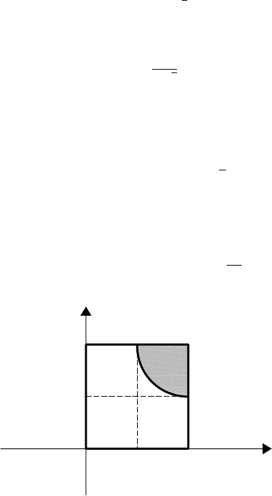
Section 9.1 Joint Distributions of n> 2 Random Variables 207
Thus
fX(x) =1−x
01−x−y
0
6dzdy =3(1−x)2,0<x<1.
Similarly, fY(y) =3(1−y)2,0<y<1,and fZ(z) =3(1−z)2,0<z<1.Since
f(x, y, z) = fX(x)fY(y)fZ(z),
X,Y, and Zare not independent.
24. The probability that Ax2+Bx+C=0 has real roots is equal to the probability that B2−4AC ≥
0. To calculate this quantity, we will first evaluate the distribution functions of B2and −4AC
and then use the convolution theorem to find the distribution function of B2−4AC.
FB2(t) =P(B2≤t) =⎧
⎪
⎪
⎨
⎪
⎪
⎩
0ift<0
√tif 0 ≤t<1
1ift≥1,
fB2(t) =F
B2(t) =⎧
⎨
⎩
1
2√tif 0 <t<1
0 otherwise,
and
F−4AC (t) =P(−4AC ≤t) =⎧
⎪
⎪
⎪
⎨
⎪
⎪
⎪
⎩
0ift<−4
PAC ≥−t
4if −4≤t<0
1ift≥0.
Now Aand Care random numbers from (0,1); hence (A, C) is a random point from the
square (0,1)×(0,1)in the ac-plane. Therefore, P (AC ≥−t/4)=PC≥−t/(4A)is the
area of the shaded region bounded by a=1, c=1, c=−t
4aof Figure 1.
c
a
-t/4
-t/4
1
1
0
Figure 1 The shaded region of Exercise 24.

208 Chapter 9 Multivariate Distributions
Thus, for −4≤t<0,
F−4AC (t) =1
−t/41
−t/(4a)
dcda =1+t
4−t
4ln −t
4.
Therefore,
F−4AC (t) =P(−4AC ≤t) =⎧
⎪
⎪
⎪
⎨
⎪
⎪
⎪
⎩
0ift<−4
1+t
4−t
4ln −t
4if −4≤t<0
1ift>0.
Applying convolution theorem, we obtain
PB2−4AC ≥0=1−PB2−4AC < 0
=1−∞
−∞
F−4AC (0−x)fB2(x)dx
=1−1
01−x
4+x
4ln x
41
2√xdx.
Letting y=√x/2,we get dy =1
4√xdx.So
PB2−4AC ≥0=1−1/2
0
(1−y2+y2ln y2)2dy
=1−1/2
0
2dy +21/2
0
(y2−y2ln y2)dy
=21/2
0
(y2−y2ln y2)dy.
Now by integration by parts (u=ln y2,dv =y2dy),
y2ln y2dy =1
3y3ln y2−2
9y3.
Thus
PB2−4AC ≥0=10
9y3−2
3y3ln y21/2
0=5
36 +1
6ln 2 ≈0.25.
25. The following solution by Scott Harrington, Duke University, Durham, NC, was given in The
College Mathematics Journal, September 1993.
Let Vbe the set of points (A,B,C) ∈[0,1]3such that f(x) =x3+Ax2+Bx+C=0
has all real roots. The probability that all of the roots are real is the volume of V.

Section 9.1 Joint Distributions of n> 2 Random Variables 209
The function is cubic, so it either has one real root and two complex roots or
three real roots. Since the coefficient of x3is positive, limx→−∞ f(x) =−∞and
limx→+∞ f(x) =+∞. The number of real roots of the graph of f(x) depends on
the nature of the critical points of the function f.
f(x) =3x2+2Ax +B=0,
with roots
x=−1
3A±1
3)A2−3B.
Let D=√A2−3B,x1=−
1
3(A +D), and x2=−
1
3(A −D). If A2<3Bthen the
critical points are imaginary, so the graph of f(x) is strictly increasing and there
must be exactly one real root. Thus we may assume A2≥3B.
In order for there to be three real roots, counting multiplicities, the local maximum
x1,f(x
1)and local minimum x2,f(x
2)must satisfy f(x
1)≥0and f(x
2)≤0;
that is,
f(x
1)=−1
27 (A3+3A2D+3AD2+D3)
+1
9A(A2+2AD +D2)−1
3B(A +D) +C≥0,
f(x
2)=−1
27 (A3−3A2D+3AD2−D3)
+1
9A(A2−2AD +D2)−1
3B(A −D) +C≤0.
Simplifying produces two half-spaces:
C≥1
27 −2A3+9AB −2(A2−3B)3/2,(constraint surface 1);
C≤1
27 −2A3+9AB +2(A2−3B)3/2,(constraint surface 2).
These two surfaces intersect at the curve given parametrically by A=t,B=1
3t2
and C=1
27 t3.Note that all points in the intersection of these two half-spaces
satisfy B≤1
3A2.Surface 2 intersects the plane C=0at the A-axis, but surface 1
intersects the plane C=0at the curve B=1
4A2, which is a quadratic curve in the
plane C=0located between the A-axis and the upper limit B=1
3A2.Therefore, V
is the region above the plane C=0and constraint surface 1, and below constraint
surface 2. The volume of Vis the volume V2under surface 2 minus the volume V1
under surface 1. Now
V1=1
a=0(1/3)a2
b=(1/4)a2
1
27 −2a3+9ab −2(a2−3b)3/2db da

210 Chapter 9 Multivariate Distributions
=1
0
1
27 −2a3b+9
2ab2+4
15 (a2−3b)5/2(1/3)a2
b=(1/4)a2
da
=1
0
1
27 ·7
160 a5da =7
25,920 ,and
V2=1
a=0(1/3)a2
b=0
1
27 −2a3+9ab +2(a2−3b)3/2db da
=1
0
1
27 −2a3b+9
2ab2−4
15 (a2−3b)5/2(1/3)a2
b=0
da =1
0
1
270 a5da =1
1620 .
Thus
V=V2−V1=1
1,620 −7
25,920 =1
2,880 .
9.2 ORDER STATISTICS
1. By Theorem 9.5, we have that
f3(x) =4!
2!1!f(x)
F(x)
21−F(x)
,
where
f(x)=⎧
⎨
⎩
10<x<1
0 otherwise,
and
F(x) =⎧
⎪
⎪
⎪
⎨
⎪
⎪
⎪
⎩
0x<0
x0≤x<1
1x≥1.
Therefore,
f3(x) =12x2(1−x), 0<x<1.
Hence the desired probability is
1/2
1/4
12x2(1−x) dx =67
256 =0.26172.
2. Let X1and X2be the points selected at random. By Theorem 9.6, the joint probability density
function of X(1)and X(2)is given by
f12(x, y) =2!
(1−1)!(2−1−1)!(2−2)!x1−1(y −x)2−1−1,0<x<y<1.

Section 9.2 Order Statistics 211
So
f12(x, y) =2,0<x<y<1.
We have that, the desired probability is given by
PX(2)≥3X(1)=1
0y/3
0
2dx dy =1
3.
3. By Theorem 9.5, f4(x), the probability density function of X(4)is given by
f4(x) =4!
3!0!λe−λx 1−e−λx 3e−λx 4−4=4λe−λx 1−e−λx 3.
The desired probability is
∞
3λ
4λe−λx 1−e−λx 3dx =1−1−e−3λ24.
4. By Remark 6.4,
EX(n)=∞
0
PX(n) >x)dx.
Now
PX(n) >x
=1−PX(n) ≤x
=1−P(X
1≤x,X2≤x,... ,X
n≤x) =1−F(x)
n.
So
EX(n)=∞
01−F(x)
ndx.
5. To find PX(i) =k,0≤k≤n, note that
PX(i) =k=1−PX(i) <k
−PX(i) >k
.
Let Nbe the number of Xj’s that are less than k. Then Nis a binomial random variable with
parameters mand
p1=
k−1
l=0n
lpl(1−p)n−l.(35)
Let Lbe the number of Xj’s that are greater than k. Then Lis a binomial random variable
with parameters mand
p2=
n
l=k+1n
lpl(1−p)n−l.(36)

212 Chapter 9 Multivariate Distributions
Clearly,
PX(i) <k
=P(N ≥i) =
m
j=im
jpj
1(1−p1)m−j,
and
PX(i) >k
=P(L ≥m−i+1)=
m
j=m−i+1m
jpj
2(1−p2)m−j.
Thus, for 0 ≤k≤n,
PX(i) =k=1−
m
j=im
jpj
1(1−p1)m−j−
m
j=m−i+1m
jpj
2(1−p2)m−j,
where p1and p2are given by (35) and (36).
6. By Theorem 9.6, the joint probability density function of X(1)and X(n) is given by
f1n(x, y) =n(n −1)f (x)f (y)F(y)−F(x)
n−2,x<y.
Therefore,
G(t) =PX(1)+X(n)
2≤t=PX(1)+X(n) ≤2t
=t
−∞ 2t−x
x
n(n −1)f (x)f (y)F(y)−F(x)
n−2dy dx
=nt
−∞ F(2t−x) −F(x)
n−1f(x)dx.
7. By Theorem 9.5, f1(x), the probability density function of X(1)is given by
f1(x) =2!
(1−1)!(2−1)!λe−λx 1−e−λx 1−1e−λx 2−1=2λe−2λx ,x≥0.
By Theorem 9.6, f12(x, y), the joint probability density function of X(1)and X(2)is given by
f12(x, y) =2!
(1−1)!(2−1−1)!(2−2)!λe−λx λe−λy
=1−e−λx 1−1e−λx −e−λy 2−1−1=2λ2e−λ(x+y),0≤x<y<∞.
Let U=X(1)and V=X(2)−X(1).We will show that g(u, v), the joint probability density
function of Uand Vsatisfy g(u, v) =gU(u)gV(v). This proves that Uand Vare independent.
To find g(u, v), note that the system of two equations in two unknowns
x=u
y−x=v

Section 9.2 Order Statistics 213
defines a one-to-one transformation of
R=(x, y):0≤x<y<∞
onto the region
Q=(u, v) :u≥0,v>0.
It has the unique solution x=u,y=u+v. Hence
J=
10
11
=1= 0.
By Thereom 8.8,
g(u, v) =f12(u, u +v)|J|=2λ2e−λ(u+2v),u≥0,v>0.
Since
g(u, v) =gU(u)gV(v),
where
gU(u) =2λe−2λu,u≥0,
and
gV(v) =λe−λv ,v>0,
we have that Uand Vare independent. Furthermore, Uis exponential with parameter 2λand
Vis exponential with parameter λ.
8. Let f12(x, y) be the joint probability density function of X(1)and X(2). By Theorem 9.6,
f12(x, y) =2!f(x)f(y)=2·1
σ√2πe−x2/2σ2·1
σ√2πe−y2/2σ2
=1
σ2πe−x2/2σ2·e−y2/2σ2,−∞ <x<y<∞.
Therefore,
EX(1)=∞
−∞ y
−∞
x·1
σ2πe−x2/2σ2·e−y2/2σ2dx dy
=1
σ2π∞
−∞
e−y2/2σ2y
−∞
xe−x2/2σ2dxdy
=1
σ2π∞
−∞
e−y2/2σ2·(−σ2)e−y2/2σ2dy
=−1
π∞
−∞
e−y2/σ 2dy
214 Chapter 9 Multivariate Distributions
=−1
π·σ√π·1
σ
√2·√2π∞
−∞
e−y2
2(σ/√2)2dy
=−1
π·σ√π·1=− σ
√π.
9. (a) By Theorem 9.6, the joint probability density function of X(1)and X(n) is given by
f1n(x, y) = n(n −1)f (x)f (y)F(y)−F(x)
n−2x<y
0 elsewhere.
We will use this to find g(r, v), the joint probability density function of R=X(n) −X(1)
and V=X(n). The probability density function of the sample range, R, is then the marginal
probability density function of R. That is,
gR(r) =∞
−∞
g(r, v)dv.
To find g(r, v), we will use Theorem 8.8. The system of two equations in two unknowns
y−x=r
y=v
defines a one-to-one transformation of
(x, y):−∞<x<y<∞
onto the region (r, v) :−∞<v<∞,r>0.
It has the unique solution x=v−r,y=v. Hence
J=
−11
01
=−1= 0.
By Theorem 8.8, g(u, v) is given by
g(r, v) =f1n(v −r, v)|J|
=n(n −1)f (v −r)f(v)F(v)−F(v −r)n−2,−∞ <v<∞,r>0.
This implies
gR(r) =∞
−∞
n(n −1)f (v −r)f(v)F(v)−F(v −r)n−2dv, r > 0.(37)

Section 9.3 Multinomial Distributions 215
(b) The probability density function of nrandom numbers from (0,1)is obtained by letting
f(v) =⎧
⎨
⎩
10<v<1
0 otherwise,
and F(v) −F(v −r) =v−(v −r) =rin (37). Note that the integrand of the integral in
(37) is nonzero if 0 <v<1 and if 0 <v−r<1; that is, if 0 <r<v<1.Therefore,
gR(r) =1
r
n(n −1)rn−2dv =n(n −1)rn−2(1−r), 0<r<1.
10. Let fand Fbe the probability density and distribution functions of Xi,1≤i≤n, respectively.
We have that
f(x)=⎧
⎨
⎩
1/θ 0<x<θ
0 elsewhere
and
F(x) =⎧
⎪
⎪
⎪
⎨
⎪
⎪
⎪
⎩
0x<0
x/θ 0≤x<θ
1x≥θ.
Let g(r) be the probability density function of R=X(n) −X(1). By part (a) of Exercise 9,
g(r) =θ
r
n(n −1)v
θ−v−r
θn−2
dv =n(n −1)rn−2
θn(θ −r) 0<r<θ.
(Note that 0 <v<θand 0 <v−r<θimply that r<v<θ.) Therefore,
E(R) =∞
0
rn(n −1)rn−2
θn(θ −r)dr =n−1
n+1θ.
9.3 MULTINOMIAL DISTRIBUTIONS
1. The desired probability is
8!
3!2!3!150
8003400
8002250
8003
=0.028.
2. We have that
P(B =i, R =j, G =20 −i−j)
=20!
i!j!(20 −i−j)!(0.2)i(0.3)j(0.5)20−i,0≤i, j ≤20,i+j≤20.

216 Chapter 9 Multivariate Distributions
3. Let U,D, and Sbe the number of days among the next six days that the stock market moves
up, moves down, and remains the same, respectively. The desired probability is
P(U =0,D=0,S=6)+P(U =1,D=1,S=4)
+P(U =2,D=2,S=2)+P(U =3,D=3,S=0)
=6!
0!0!6!1
405
1201
36
+6!
1!1!4!1
415
1211
34
+6!
2!2!2!1
425
1221
32
+6!
3!3!0!1
435
1231
30
=0.171.
4. Let A,B,C,D, and Fbe the number of students who get A, B, C, D, and F, respectively. The
desired probability is given by
P(A =2,B=5,C=5,D=2,F=1)+P(A =3,B=5,C=5,D=2,F=0)
=15!
2!5!5!2!1!(0.16)2(0.34)5(0.34)5(0.14)2(0.02)1
+15!
3!5!5!2!0!(0.16)3(0.34)5(0.34)5(0.14)2(0.02)0
=0.0172.
5. Let L,M, and Sbe the number of large, medium, and small watermelons among the five
watermelons Joanna buys, respectively.
(a) We have that
P(L ≥2)=1−P(L =0)−P(L =1)
=1−5
0(0.50)0(0.50)5−5
1(0.50)1(0.50)4=0.8125.
(b) P(L =2,M=2,S=1)=5!
2!2!1!(0.5)2(0.3)2(0.2)1=0.135.
(c) Using parts (a) and (b) and
P(L =3,M=2,S=0)=5!
3!2!0!(0.5)3(0.3)2(0.2)0=0.1125,
we have that
P(M =2|L≥2)=P(M =2,L≥2)
P(L ≥2)
=P(L =2,M=2,S=1)+P(L =3,M=2,S=0)
P(L ≥2)
=0.135 +0.1125
0.8125 =0.3046.

Section 9.3 Multinomial Distributions 217
6. Let Xbe the number of faculty members who are below 40 and Ybe the number of those who
are above 50 in the committee. The desired probability mass function is
pX|Y(x|2)=
10!
x!2!(8−x)!(0.5)x(0.3)2(0.2)8−x
10
2(0.3)2(0.7)8=8
x5
7x2
78−x
,0≤x≤8.
7. The probability is 1/4 that the blood type of a child of this man and woman is AB. The
probability is 1/4 that it is A, and the probability is 1/2 that it is B. The desired probability is
equal to
6!
3!2!1!1
231
421
41
=15
128 =0.117.
8. The probability of two AA’s, two Aa’s, and two aa’s is
g(p) =6!
2!2!2!(p2)22p(1−p)2(1−p)22=360p6(1−p)6.
To find the maximum of this function, set g(p) =0 to obtain p=1/2.
9. Let N(t) be the number of customers who arrive at the store by time t. We are given that
N(t):t≥0is a Poisson process with λ=3. Let X,Y, and Zbe the number of cus-
tomers who use charge cards, write personal checks, and pay cash in five operating minutes,
respectively. Then
P(X =5,Y=2,Z=3)
=∞
n=10
PX=5,Y=2,Z=3|N(5)=nPN(5)=n
=∞
n=10
n!
5!2!3!(n −10)!(0.40)5(0.10)2(0.20)3(0.30)n−10 ·e−1515n
n!
=(0.40)5(0.10)2(0.20)3e−151510
3!5!2!
∞
n=10
(0.30)n−10(15)n−10
(n −10)!
=(0.00010035)∞
n=10
(4.5)n−10
(n −10)!=(0.00010035)e4.5=0.009033.

218 Chapter 9 Multivariate Distributions
REVIEW PROBLEMS FOR CHAPTER 9
1. Let p(b, r, g) be the joint probability mass function of B,R, and G. Then
p(b, r, g) =20
b30
r50
g
100
20 ,b+r+g=20,0≤b, r, g ≤20.
2. Let Fbe the distribution function of X. Let X1,X2,...,Xnbe the outcomes of the first,
second, ..., and the nth rolls, respectively. Then X=min(X1,X
2,... ,X
n). Therefore,
F(t) =P(X ≤t) =1−P(X > t) =1−P(X
1>t,X
2>t,...,X
n>t)
=1−P(X
1>t)
n=
⎧
⎪
⎪
⎪
⎪
⎪
⎪
⎪
⎪
⎪
⎪
⎪
⎪
⎪
⎪
⎪
⎪
⎨
⎪
⎪
⎪
⎪
⎪
⎪
⎪
⎪
⎪
⎪
⎪
⎪
⎪
⎪
⎪
⎪
⎩
0t<1
1−5
6n1≤t<2
1−4
6n2≤t<3
1−3
6n3≤t<4
1−2
6n4≤t<5
1−1
6n5≤t<6
1t≥6.
The probability mass function of Xis
p(x) =P(X =x) =7−x
6n
−6−x
6n
,x=1,2,3,4,5,6.
3. Let D1,D2,...,Dnbe the distances of the points selected from the origin. Let D=
min(D1,D
2,... ,D
n). The desired probability is
P(D ≥r) =P(D
1≥r, D2≥r,...,D
n≥r) =P(D
1≥r)n=1−P(D
1<r)
n
=1−(4/3)πr3
8a3n
=1−π
6r
a3n
.
4. (a) c1
01
01
0
(x +y+2z)dz dy dx =1⇒ c=1/2.

Chapter 9 Review Problems 219
(b) We have that
PX<1
3Y<1
2,Z<1
4=
PX<1
3,Y<1
2,Z<1
4
PY<1
2,Z<1
4
=1/3
01/2
01/4
0
1
2(x +y+2z)dz dy dx
1
01/2
01/4
0
1
2(x +y+2z)dz dy dx =1/36
1/8=2
9.
5. The joint probability mass function of the number of times each face appears is multinomial.
Hence the desired probability is 18!
(3!)61
618
=0.00135.
6. Using the multinomial distribution, the answer is
7!
3!2!2!(0.4)3(0.35)2(0.25)2=0.1029.
7. For 1 ≤i≤n, let Xibe the lifetime of the ith component. Then
min(X1,X
2,... ,X
n)is the lifetime of the system. Let ¯
F(t) be the survival function of
the system. By the independence of the lifetimes of the components, for all t>0,
¯
F(t) =Pmin(X1,X
2,... ,X
n)>t
=P(X
1>t,X
2>t,... ,X
n>t)
=P(X
1> t)P (X2>t)···P(X
n>t)=¯
F1(t) ¯
F2(t) ··· ¯
Fn(t).
8. For 1 ≤i≤n, let Xibe the lifetime of the ith component. Then
max(X1,X
2,... ,X
n)is the lifetime of the system. Let ¯
F(t) be the survival function of
the system. By the independence of the lifetimes of the components, for all t>0,
¯
F(t) =Pmax(X1,X
2,... ,X
n)>t
=1−Pmax(X1,X
2,... ,X
n)≤t
=1−P(X
1≤t,X2≤t,... ,X
n≤t)
=1−P(X
1≤t)P(X2≤t)···P(X
n≤t)
=1−F1(t)F2(t) ···Fn(t).
9. The problem is equivalent to the following: Two points Xand Yare selected independently
and at random from the interval (0,). What is the probability that the length of at least one

220 Chapter 9 Multivariate Distributions
interval is less than /20? The solution to this problem is as follows:
Pmin(X, Y −X, −Y) <
20 X<Y
P(X < Y)
+Pmin(Y, X −Y, −X) <
20 X>Y
P(X > Y)
=2Pmin(X, Y −X, −Y) <
20 X<Y
P(X < Y)
=2Pmin(X, Y −X, −Y) <
20 X<Y
·1
2
=1−Pmin(X, Y −X, −Y) ≥
20 X<Y
=1−PX≥
20,Y−X≥
20,−Y≥
20 X<Y
=1−PX≥
20,Y−X≥
20,Y≤19
20 X<Y
.
Now PX≥
20,Y−X≥
20,Y≤19
20 X<Y
is the area of the region
6(x, y) ∈R2:0<x<, 0<y<, x≥
20,y−x≥
20,y≤19
20 7
divided by the area of the triangle
(x, y) ∈R2:0<x<, 0<y<, y>x
;
that is, 17
20 ×17
20
2÷2
2=0.7225.
Therefore, the desired probability is 1 −0.7225 =0.2775.
10. Let f13(x, y) be the joint probability density function of X(1)and X(3). By Theorem 9.6,
f13(x, y) =6(y −x), 0<x<y<1.
Let U=X(1)+X(3)
2and V=X(1). Using Theorem 8.8, we will find g(u, v), the joint
probability density function of Uand V. The probability density function of the midrange of
these three random variables is gU(u). The system of two equations in two unknowns
⎧
⎨
⎩
x+y
2=u
x=v

Chapter 9 Review Problems 221
defines a one-to-one transformation of
R=(x, y):0<x<y<1
onto the region
Q=(u, v) :0<v<u<v+1
2<1
that has the unique solution x=v
y=2u−v.
Hence
J=
01
2−1=−2= 0;
therefore,
g(u, v) =f13(v, 2u−v)|J|=24(u −v), 0<v<u< v+1
2<1.
To find gU(u), draw the region Qto see that
gU(u) =⎧
⎪
⎪
⎪
⎪
⎨
⎪
⎪
⎪
⎪
⎩
u
0
24(u −v) dv 0<u<1/2
u
2u−1
24(u −v) dv 1/2≤u<1.
Therefore,
gU(u) =⎧
⎪
⎨
⎪
⎩
12u20<u<1/2
12(u −1)21/2≤u<1.
The expected value of Uis given by
E(U) =1/2
0
12u3du +1
1/2
12u(u −1)2du =3
16 +5
16 =1
2.

Chapter 10
More Expectations
and Variances
10.1 EXPECTED VALUES OF SUMS OF RANDOM VARIABLES
1. Since
E(X) =1
0
x(1−x) dx +2
1
x(x −1)dx =2
3,
and
E(X2)=1
0
x2(1−x)dx +2
1
x2(x −1)dx =3
2,
we have that
E(X2+X) =3
2+2
3=13
6.
2. By Example 10.7, the answer is 5
2/5=12.5.
3. We have that E(X2)=Var(X) +E(X)2=1. Similarly, E(Y2)=E(Z2)=1.Thus
EX2(Y +5Z)2=E(X2)E(Y +5Z)2=E(Y2+25Z2+10YZ)
=E(Y2)+25E(Z2)+10E(Y)E(Z) =26.
4. Since f(x, y) =e−x·2e−2y,Xand Yare independent exponential random variables with
parameters 1 and 2, respectively. Thus E(X) =1, E(Y) =1/2,
E(X2)=Var (X) +E(X)2=1+1=2,
and
E(Y2)=Va r(Y ) +E(Y)2=1
4+1
4=1
2.
Therefore, E(X2+Y2)=2+1
2=5
2.

Section 10.1 Expected Values of Sums of Random Variables 223
5. let X1,X2,X3,X4, and X5be geometric random variables with parameters 1, 4/5, 3/5, 2/5,
and 1/5, respectively. The desired quantity is
E(X1+X2+X3+X4+X5)=E(X1)+E(X2)+E(X3)+E(X4)+E(X5)
=1+5
4+5
3+5
2+5=11.42.
6. Clearly,
E(Xi)=1·1
n+0·1−1
n=1
n.
Thus E(X1+X2+···+Xn)=n·1
n=1 is the desired quantity.
7. Let X1,X2,X3, and X4be the cost of a band to play music, the amount the caterer will charge,
the rent of a hall to give the party, and other expenses, respectively. Let Nbe the number
of people who participate. We have that E(X1)=1550, E(X2)=1900,E(X
3)=1000,
E(X4)=550,and
E(N) =
200
i=151
i·1
50 =1
50200
i=1
i−
150
i=1
i=1
50200 ×201
2−150 ×151
2=175.50.
To have no loss on average, let xbe the amount (in dollars) that the society should charge each
participant. We must have
E(X1+X2+X3+X4)≤E(xN) =xE(N ).
This gives
x≥E(X1)+E(X2)+E(X3)+E(X4)
175.50 =1550 +1900 +1000 +550
175.50 =28.49.
So to have no loss on the average, the society should charge each participant $28.49.
8. (a) E(→007)=E(007 →007)=1,000.
(b)
E(→156156)=E(→156)+E(156 →156156)
=E(156 →156)+E(156156 →156156)
=1,000 +1,000,000 =1,001,000.
(c)
E(→575757)=E(→57)+E(57 →5757)+E(5757 →575757)
=E(57 →57)+E(5757 →5757)+E(575757 →575757)
=100 +10,000 +1,000,000 =1,010,100.

224 Chapter 10 More Expectations and Variances
9. Let Xbe the number of students standing at the front of the room after k,1≤k<nnames
have been called. The kstudents whose names have been called are not standing. Let A1,A2,
...,An−kbe the students whose names have not been called. Let
Xi= 1ifAiis standing
0 otherwise.
Clearly,
X=X1+X2+···+Xn−k.
For i,1≤i≤n−k,
E(Xi)=PAiis standing=k
n.
This is because Aiis standing if and only if his or her original seat was among the first k.
Hence
E(X) =E(X1)+E(X2)+···+E(Xn−k)=(n −k) ·k
n=(n −k)k
n.
10. By Theorem 10.2,
Emin(X1,X
2,... ,X
n)=∞
k=1
Pmin(X1,X
2,... ,X
n)≥k
=∞
k=1
P(X
1≥k, X2≥k,...X
n≥k)
=∞
k=1
P(X
1≥k)P (X2≥k) ···P(X
n≥k)
=∞
k=1P(X
1≥k)n=∞
k=1∞
i=k
pin=∞
k=1
hn
k.
11. Let E1be the event that the first three outcomes are heads and the fourth outcome is tails.
For 2 ≤i≤n−3, let Eibe as defined in the hint. Let En−2be the event that the outcome
(n −3)is tails and the last three outcomes are heads. The expected number of exactly three
consecutive heads is
EX1+
n−3
i=2
Xi+Xn−2=E(X1)+
n−3
i=2
E(Xi)+E(Xn−2)
=P(E
1)+
n−3
i=2
P(E
i)+P(E
n−2)
=1
24
+
n−3
i=21
25
+1
24
=1
23
+(n −4)1
25
=n
32.

Section 10.1 Expected Values of Sums of Random Variables 225
12. Let
Xi= 1 if the ith box is empty
0 otherwise;
The expected number of the empty boxes is
E(X1+X2+···+X40)=40E(Xi)=40P(X
i=1)=4039
4080
≈5.28.
13. The expected number of birthdays that belong to one student is
E(X1+X2+···+X25)=25E(Xi)=25P(X
i=1)=25364
36524
=23.41.
14. Let Xi=1, if the birthdays of at least two students are on the ith day of the year, and Xi=0,
otherwise. The desired quantity is
E365
i=1
Xi=365E(Xi)=365P(X
i=1)
=365 1−364
36525
−25
11
365364
36524=0.788.
15. Let u1,u
2,... ,u
39 be an enumeration of the nonheart cards. Let
Xi= 1 if no heart is drawn before uiis drawn
0 otherwise.
Let Nbe the number of cards drawn until a heart is drawn. Clearly, N=1+39
i=1Xi.By
the result of Exercise 9, Section 3.2,
E(N) =1+
39
i=1
E(Xi)=1+
39
i=1
P(X
i=1)
=1+
39
i=1
1
14 =1+39 ·1
14 =3.786.
Note that if the experiment was performed with replacement, then E(N) =4.
16. We have that
E(→THTHTTHTHT)=E(→T)+E(T→THT)+E(THT →THTHT)
+E(THTHT →THTHTTHTHT)
=E(→T)+E(THT →THT)+E(THTHT →THTHT)
+E(THTHTTHTHT →THTHTTHTHT)
=2+8+32 +1,024 =1,066.

226 Chapter 10 More Expectations and Variances
17. (a) ∞
0∞
0
I(x, y) dx dy is the area of the rectangle
(x, y) ∈R2:0≤x<X,0≤y<Y
;
therefore it is equal to XY.
(b) Part (a) implies that
E(XY) =∞
0∞
0
EI(x, y)dx dy =∞
0∞
0
P(X > x,Y > y)dx dy.
18. Clearly N>iif and only if
X1≥X2≥X3≥···≥Xi.
Hence for i≥2,
P(N > i) =PX1≥X2≥X3≥···≥Xi−1≥Xi=1
i!
because Xi’s are independent and identically distributed. So, by Theorem 10.2,
E(N) =∞
i=1
P(N ≥i) =∞
i=0
P(N > i) =P(N > 0)+P(N > 1)+∞
i=2
1
i!
=1+1+∞
i=2
1
i!=∞
i=0
1
i!=e.
19. If the first red chip is drawn on or before the 10th draw, let Nbe the number of chips before
the first red chip. Otherwise, let N=10. Clearly,
P(N =i) =1
2i1
2=1
2i+1
,0≤i≤9;P(N =10)=1
210
.
The desired quantity is
E(10 −N) =
9
i=0
(10 −i)1
2i+1
+(10 −10)·1
210
≈9.001.
20. Clearly, if for some λ∈R,X =λY , Cauchy-Schwarz’s inequality becomes equality. We
show that the converse of this is also true. Suppose that for random variables Xand Y,
E(XY) =)E(X2)E(Y 2).
Then
4E(XY)2−4E(X2)E(Y 2)=0.

Section 10.2 Covariance 227
Now the left side of this equation is the discriminant of the quadratic equation
E(Y2)λ2−2E(XY)λ+E(X2)=0.
Hence this quadratic equation has exactly one root. On the other hand,
E(Y2)λ2−2E(XY)λ+E(X2)=E(X −λY )2.
So the equation
E(X −λY )2=0
has a unique solution. That is, there exists a unique number λ1∈Rsuch that
E(X −λ1Y)
2=0.
Since the expected value of a positive random variable is positive, this implies that with
probability 1, X−λ1Y=0orX=λ1Y.
10.2 COVARIANCE
1. Since Xand Yare independent random variables, Cov(X, Y ) =0.
2. E(X) =
3
x=1
4
y=3
1
70 x2(x +y) =17
7;
E(Y) =3
x=14
y=3
1
70 xy(x +y) =124
35 ;
E(XY) =
3
x=1
4
y=3
1
70 x2y(x +y) =43
5.
Therefore,
Cov(X, Y ) =E(XY) −E(X)E(Y ) =43
5−17
7·124
35 =− 1
245.
3. Intuitively, E(X) is the average of 1, 2, ..., 6 which is 7/2; E(Y) is (7/2)(1/2)=7/4.To
show these, note that
E(X) =
6
x=1
xpX(x) =
6
x=1
x(1/6)=7/2.

228 Chapter 10 More Expectations and Variances
By the table constructed for p(x, y) in Example 8.2,
E(Y) =0·63
384 +1·120
384 +2·99
384 +3·64
384 +4·29
384 +5·8
384 +6·1
384 =7
4.
By the same table,
E(XY) =
6
x=1
6
y=0
xyp(x,y) =91/12.
Therefore,
Cov(X, Y ) =E(XY) −E(X)E(Y ) =91
12 −7
2·7
4=35
24 >0.
This shows that Xand Yare positively correlated. The higher the outcome from rolling the
die, the higher the number of tails obtained—a fact consistent with our intuition.
4. Let Xbe the number of sheep stolen; let Ybe the number of goats stolen. Let p(x, y) be the
joint probability mass function of Xand Y. Then, for 0 ≤x≤4, 0 ≤y≤4, 0 ≤x+y≤4,
p(x, y) =7
x8
y 5
4−x−y
20
4;
p(x, y) =0, for other values of xand y. Clearly, Xis a hypergeometric random variable with
parameters n=4, D=7, and N=20. Therefore,
E(X) =nD
N=28
20 =7
5.
Yis a hypergeometric random variable with parameters n=4, D=8, and N=20. Therefore,
E(Y) =nD
N=32
20 =8
5.
Since
E(XY) =
4
x=0
4−x
y=0
xyp(x,y) =168
95 ,
we have
Cov(X, Y ) =E(XY) −E(X)E(Y ) =168
95 −7
5·8
5=−224
475 <0.
Therefore, Xand Yare negatively correlated as expected.
Section 10.2 Covariance 229
5. Since Y=n−X,
E(XY) =E(nX −X2)=nE(X) −E(X2)=nE(X) −Va r (X) +E(X)2
=n·np −np (1−p) +n2p2=n(n −1)p(1−p),
and
Cov(X, Y ) =E(XY) −E(X)E(Y ) =n(n −1)p(1−p) −np ·n(1−p) =−np (1−p).
This confirms the (obvious) fact that Xand Yare negatively correlated.
6. Both (a) and (b) are straightforward results of relation (10.6).
7. Since Cov(X, Y ) =0, we have
Cov(X, Y +Z) =Cov(X, Y ) +Cov(X, Z) =Cov(X, Z).
8. By relation (10.6),
Cov(X +Y, X −Y) =E(X2−Y2)−E(X +Y)E(X −Y)
=E(X2)−E(Y2)−E(X)2+E(Y)2=Va r (X) −Var (Y ).
9. In Theorem 10.4, let a=1 and b=−1.
10. (a) This is an immediate result of Exercise 8 above.
(b) By relation (10.6),
Cov(X, XY ) =E(X2Y)−E(X)E(XY)
=E(X2)E(Y ) −E(X)2E(Y) =E(Y)Var(X).
11. The probability density function of is given by
f(θ) =⎧
⎪
⎨
⎪
⎩
1
2πif θ∈[0,2π]
0 otherwise.
Therefore,
E(XY) =2π
0
sin θcos θ1
2πdθ =0, E(X) =2π
0
sin θ1
2πdθ =0,
E(Y) =2π
0
cos θ1
2πdθ =0.
Thus Cov(X, Y ) =E(XY) −E(X)E(Y ) =0.

230 Chapter 10 More Expectations and Variances
12. The joint probability density function of Xand Yis given by
f(x, y) =⎧
⎪
⎨
⎪
⎩
1
πx2+y2≤1
0 elsewhere.
Xand Yare dependent because, for example,
P0<X< 1
2Y=0=1
4
while,
P0<X< 1
2=21/2
0√1−x2
0
1
πdy dx =2
π1/2
0)1−x2dx
=1
6+√3
4π= P0<X< 1
2Y=0.
Xand Yare uncorrelated because
E(X) =
x2+y2≤1
x1
πdx dy =1
π1
02π
0
r2cos θdθdr=0,
E(Y) =
x2+y2≤1
y1
πdx dy =1
π1
02π
0
r2sin θdθdr=0,
and
E(XY) =
x2+y2≤1
xy 1
πdx dy =1
π1
02π
0
r3cos θsin θdθdr=0,
implying that Cov(X, Y ) =E(XY) −E(X)E(Y ) =0.
13. We have that
E(X) =2
1/2
8
15x2dx =1.4,E
X2=2
1/2
8
15x3dx =2.125,
E(Y) =9/4
1/4
6
13y3/2dy =1.396,E
Y2=9/4
1/4
6
13y5/2dy =2.252.
These give Var(X) =2.125 −1.42=0.165, and Var(Y ) =2.252 −1.3962=0.303.Hence
E(X +Y) =1.4+1.396 =2.796, and by independence of Xand Y,
Var(X +Y) =Va r (X) +Va r (Y ) =0.165 +0.303 =0.468.
Therefore, the expected value and variance of the total raise Mr. Jones will get next year are
$2796 and $468, respectively.

Section 10.2 Covariance 231
14. We have that
Var(XY ) =E(X2Y2)−E(X)E(Y)2=E(X2)E(Y 2)−µ2
1µ2
2
=(µ2
1+σ2
1)(µ2
2+σ2
2)−µ2
1µ2
2=σ2
1σ2
2+µ2
1σ2
2+µ2
2σ2
1.
15. (a) Let U1and U2be the measurements obtained using the voltmeter for V1and V2, respec-
tively. Then V1=U1+X1and V2=U2+X2, where X1and X2, the measurement
errors, are independent random variables with mean 0 and variance σ2.So the error
variance in the estimation of V1and V2using the first method is σ2.
(b) Let U3and U4be the measurements obtained,using the voltmeter, for Vand W, respec-
tively. Then V=U3+X3and W=U4+X4, where X3and X4, the measurement errors,
are independent random variables with mean 0 and variance σ2.Since (U3+U4)/2is
used to estimate V1, and (U3−U4)/2 is used to estimate V2,
V1=V+W
2=U3+U4
2+X3+X4
2,
and
V2=V−W
2=U3−U4
2+X3−X4
2,
we have that, for part (b), (X3+X4)/2 and (X3−X4)/2 are the measurement errors in
measuring V1and V2, respectively. The independence of X3and X4yields
VarX3+X4
2=1
4Var(X3)+Var(X4)=1
4(σ 2+σ2)=σ2
2,
and
VarX3−X4
2=1
4Var(X3)+Var(X4)=1
4(σ 2+σ2)=σ2
2.
Therefore, the error variances in the estimation of V1and V2, using the second method,
is σ2/2, showing that the second method is preferable.
16. Let rbe the annual rate of return for Mr. Ingham’s total investment. We have
Var(r) =Var(0.18r1+0.40r2+0.42r3)
=(0.18)2Var(r1)+(0.40)2Var(r2)+(0.42)2Var(r3)
+2(0.18)(0.40)Cov(r1,r
2)+2(0.18)(0.42)Cov(r1,r
3)
+2(0.40)(0.42)Cov(r2,r
3)
=(0.18)2(0.064)+(0.40)2(0.0144)+(0.42)2(0.01)
+2(0.18)(0.40)(0.03)+2(0.18)(0.42)(0.015)+2(0.40)(0.42)(0.021)
=0.01979.

232 Chapter 10 More Expectations and Variances
Hence the standard deviation of the annual rate of return for Mr. Ingham’s total investment is
√0.01979 =0.14.
17. Let r1,r2, and r3be the annual rates of return for Mr. Kowalski’s investments in financial
assets 1, 2, and 3, respectively. Let rbe the annual rate of return for his total investment.
Then, by Example 4.25,
r=0.25r1+0.40r2+0.35r3.
Since the assets are uncorrelated, we have
E(r) =(0.25)(0.12)+(0.40)(0.15)+(0.35)(0.18)=0.153,
Var(r) =(0.25)2(0.08)2+(0.40)2(0.12)2+(0.35)2(0.15)2=0.00546,
σr=)Var(r) =0.074.
Hence r∼N(0.153,0.00546). Let Xbe the total investment of Mr. Kowalski. We are given
that X=50,000.Let Ybe the total return of Mr. Kowalski’s investment next year. The
desired probability is
P(Y −X≥10,000)=PY−X
X≥10,000
50,000
=P(r ≥0.2)=PZ≥0.2−0.153
0.074
=P(Z ≥0.64)=1−(0.64)=1−0.7389 =0.2611.
18. (a) We have that
E(X) =1
01
x
8x2ydydx =8
15, E(Y ) =1
01
x
8xy2dy dx =4
5,
E(X2)=1
01
x
8x3ydydx =1
3,E(Y
2)=1
01
x
8xy3dy dx =2
3,
E(XY) =1
01
x
8x2y2dy dx =4
9,
Cov(X, Y ) =E(XY) −E(X)E(Y ) =4
9−8
15 ·4
5=4
225,
Var(X) =1
3−8
152
=11
225,Va r (Y ) =2
3−4
52
=2
75.
Therefore,
Var(X +Y) =11
225 +2
75 +2·4
225 =1
9.

Section 10.2 Covariance 233
(b) Since Cov(X, Y ) = 0,Xand Yare not independent. This does not contradict Exercise 23
of Section 8.2 because although f(x, y) is the product of a function of xand a function of y,
its domain is not of the form
(x, y):a≤x≤b, c ≤y≤d.
In the domain of f,xand yare related by x≤y.
19. For 1 ≤i≤n, let Xibe the ith random number selected; we have
Varn
i=1
Xi=
n
i=1
Var(Xi)=
n
i=1
(1−0)2
12 =n
12.
20. By the hint,
E(X) =∞
0∞
0
1
2x4e−(y+1)x dx dy =∞
0
1
24!
(y +1)5dy =3,
E(Y) =∞
0∞
0
1
2x3ye−x(y+1)dx dy =∞
0
1
2y3!
(y +1)4dy =1
2,
and
E(XY) =∞
0∞
0
1
2x4ye−(y+1)x dx dy =∞
0
1
3y4!
(y +1)5dy =1.
Since Cov(X, Y ) =1−3
2=−1
2<0,,Xand Yare negatively correlated.
21. Note that
E(X −t)2=E(X −µ+µ−t)2
=E(X −µ)2+2(µ −t)E(X −µ) +(µ −t)2
=E(X −µ)2+(µ −t)2.
This relation shows that E(X −t)2is minimum if (µ −t)2=0; that is, if t=µ. For this
value, E(X −t)2=Var (X).
22. Clearly,
Cov(IA,I
B)=E(IAIB)−E(IA)E(IB)=P (AB) −P (A)P (B).
This shows that Cov(IA,I
B)>0⇐⇒ P (AB) > P (A)P (B) ⇐⇒ P (AB)
P(B) > P (A),⇐⇒
P(A |B)>P(A). The proof that IAand IBare positively correlated if and only if P(B|A) >
P(B) follows by symmetry.

234 Chapter 10 More Expectations and Variances
23. By Exercise 6,
Cov(aX +bY, cZ +dW) =aCov(X, cZ +dW) +bCov(Y, cZ +dW)
=ac Cov(X, Z) +ad Cov(X, W ) +bc Cov(Y, Z) +bd Cov(Y, W ).
24. By Exercise 6 and an induction on n,
Covn
i=1
aiXi,
m
j=1
bjYj=
n
i=1
aiCovXi,
m
j=1
bjYj.
By Exercise 6 and an induction on m,
CovXi,
m
j=1
bjYj=
m
j=1
bjCov(Xi,Y
j).
The desired identity follows from these two identities.
25. For 1 ≤i≤n, let Xi=1 if the outcome of the ith throw is 1; let Xi=0, otherwise. For
1≤j≤n, let Yj=1 if the outcome of the jth throw is 6; let Yj=0, otherwise. Clearly,
Cov(Xi,Y
j)=0ifi= j. By Exercise 24,
Covn
i
Xi,
n
j=1
Yj=
n
j=1
n
i=1
Cov(Xi,Y
j)=
n
i=1
Cov(Xi,Y
i)
=
n
i=1E(XiYi)−E(Xi)E(Yi)=
n
i=10−1
6·1
6=−n
36.
As expected, in nthrows of a fair die, the number of ones and the number of sixes are negatively
correlated.
26. Let Sn=n
i=1aiXi,µi=E(Xi); then
E(Sn)=
n
i=1
aiµi,S
n−E(Sn)=
n
i=1
ai(Xi−µi).
Thus
Var(Sn)=E n
i=1
ai(Xi−µi)2
=
n
i=1
a2
iE(Xi−µi)2+2
i<j
aiajE(Xi−µi)(Xj−µj)
=
n
i=1
a2
iVar(Xi)+2
i<j
aiajCov(Xi,X
j).

Section 10.2 Covariance 235
27. To find Var(X), we use the following identity:
Varn
i=1
Xi=
n
i=1
Var(Xi)+2
i<j
Cov(Xi,X
j). (38)
Now for 1 ≤i≤n,
E(Xi)=P(A
i)=D
N,E(X
2
i)=P(A
i)=D
N.
Thus
Var(Xi)=E(X2
i)−E(Xi)2=D
N−D
N2
=D(N −D)
N2.
Also for i<j,
XiXj= 1ifAiAjoccurs
0 otherwise.
Therefore,
E(XiXj)=P(A
iAj)=P(A
j|Ai)P (Ai)=D−1
N−1·D
N=(D −1)D
(N −1)N ,
and
Cov(Xi,X
j)=E(XiXj)−E(Xi)E(Xj)
=(D −1)D
(N −1)N −D
N·D
N=−D(N −D)
(N −1)N2.
Substituting the values of Var(Xi)’s and Cov(Xi,X
j)back into (38), we get
Var(X) =nD(N −D)
N2+2n
2−D(N −D)
(N −1)N2
=nD(N −D)
N21−n−1
N−1.
This follows since in (38), and
i<j
have nand n
2=n(n −1)
2equal terms, respectively.
28. Let Xi=1, if the ith couple is left intact; 0, otherwise. We are interested in Var(n
i=1Xi),
where
Varn
i=1
Xi=
n
i=1
Var(Xi)+2
i<j
Cov(Xi,X
j).
To find Var(Xi), note that since X2
i=Xi,
Var(Xi)=EX2
i−E(Xi)2=E(Xi)−E(Xi)2.

236 Chapter 10 More Expectations and Variances
By Example 10.3,
E(Xi)=(2n−m)(2n−m−1)
2n(2n−1).
So
Var(Xi)=(2n−m)(2n−m−1)
2n(2n−1)1−(2n−m)(2n−m−1)
2n(2n−1).
To find Cov(Xi,X
j), note that XiXj=1iftheith and jth couples are left intact; 0, otherwise.
Now
Cov(Xi,X
j)=E(XiXj)−E(Xi)E(Xj)=P(X
iXj=1)−E(Xi)E(Xj)
=2n−4
m
2n
m−(2n−m)(2n−m−1)
2n(2n−1)2
.
Therefore,
Cov(Xi,X
j)=(2n−m)(2n−m−1)(2n−m−2)(2n−m−3)
2n(2n−1)(2n−2)(2n−3)
−(2n−m)(2n−m−1)
2n(2n−1)2
.
So
Varn
i=1
Xi=n(2n−m)(2n−m−1)
2n(2n−1)1−(2n−m)(2n−m−1)
2n(2n−1)
+2n(n −1)
2(2n−m)(2n−m−1)(2n−m−2)(2n−m−3)
2n(2n−1)(2n−2)(2n−3)
−(2n−m)2(2n−m−1)2
4n2(2n−1)2
=(2n−m)(2n−m−1)
2(2n−1)1−(2n−m)(2n−m−1)
2n(2n−1)
+(n −1)(2n−m)(2n−m−1)(2n−m−2)(2n−m−3)
2(2n−1)(2n−2)(2n−3)
−(2n−m)2(2n−m−1)2
4n(2n−1)2

Section 10.3 Correlation 237
=(2n−m)(2n−m−1)
2(2n−1)1−(2n−m)(2n−m−1)
2n(2n−1)
+(n −1)(2n−m−2)(2n−m−3)
(2n−2)(2n−3)
−(n −1)(2n−m)(2n−m−1)
2n(2n−1)
=(2n−m)(2n−m−1)
2(2n−1)1+(n −1)(2n−m−2)(2n−m−3)
(2n−2)(2n−3)
−(2n−m)(2n−m−1)
2(2n−1).
10.3 CORRELATION
1. We have that Cov(X, Y ) =ρ(X,Y)σXσY=3;thus
Var(2X−4Y+3)=Va r (2X−4Y) =4Var(X) +16Var(Y ) −16Cov(X, Y )
=4(4)+16(9)−16(3)=112.
2. By Exercise 23 of Section 8.2, Xand Yare independent random variables. This can also be
shown directly by verifying the relation f(x, y) =fX(x)fY(y).Hence Cov(X, Y ) =0, and
therefore ρ(X,Y) =0.
3. Let Xand Ybe the lengths of the pieces obtained. Since Y=1−X, by Theorem 10.5,
ρ(X,Y) =−1.Since Xand Yare uniform over (0,1),σX=1/√12 and σY=1/√12.
Therefore,
Cov(X, Y ) =ρ(X,Y)σXσY=(−1)1
√12 1
√12=−1
12.
4. If α1β1=0, both sides of the relation are 0 and the equality holds. If α1β1= 0, then
ρ(α1X+α2,β
1Y+β2)=Cov(α1X+α2,β
1Y+β2)
σα1X+α2·σβ1Y+β2
=Cov(α1X, β1Y)
|α1|σX·|β1|σY=α1β1Cov(X, Y )
|α1||β1|σXσY=sgn(α1β1)ρ(X, Y ).
5. No, because for all random variables Xand Y,−1≤ρ(X,Y) ≤1.

238 Chapter 10 More Expectations and Variances
6. By Exercise 6 of Section 10.2,
Cov(X +Y, X −Y) =Var (X) −Va r (Y ).
Since Cov(X, Y ) =0,
σX+Y·σX−Y=)Var(X +Y)·Va r (X −Y)
=/Var(X) +Var(Y )Var(X) +Var(Y )
=Var(X) +Var (Y ).
Therefore,
ρ(X +Y, X −Y) =Cov(X +Y, X −Y)
σX+Y·σX−Y=Var(X) −Var (Y )
Var(X) +Var (Y ) .
7. Using integration by parts, we obtain
E(X) =1
2π/2
0π/2
0
xsin(x +y) dx dy =π
4,
E(X2)=1
2π/2
0π/2
0
x2sin(x +y) dx dy =π2
8+π
2−2.
Hence
Var(X) =π2
8+π
2−2−π2
16 =π
2−2+π2
16 .
By symmetry, E(Y) =π
4and Var(Y ) =π
2−2+π2
16 . Since
E(XY) =1
2π/2
0π/2
0
xy sin(x +y) dx dy =π
2−1,
Cov(X, Y ) =π
2−1−π2
16 . Therefore,
ρ(X,Y) =Cov(X, Y )
√Var(X) ·√Va r (Y ) =(π/2)−1−(π2/16)
(π/2)−2+(π2/16)=−0.245.
Since ρ(X,Y) =±1,there is no linear relation between Xand Y.

Section 10.4 Conditioning on Random Variables 239
10.4 CONDITIONING ON RANDOM VARIABLES
1. Let Nbe the number of tosses required; then
E(N) =EE(N|X)=E(N |X=0)P (X =0)+E(N |X=1)P (X =1)
=1+E(N)1
2+1
2·1+1
22+E(N)1
2.
Solving this equation for E(N), we obtain E(N) =5.
2. We have that
EY(t)
=EEY(t)|X=EY(t) |X<t
P(X < t)+EY(t) |X≥tP(X ≥t)
=EaX −a
3(t −X)P(X < t)+E(at)P (X ≥t)
=E4a
3X−at
3P(X < t)+atP (X ≥t)
=4a
311
2−at
3t−4
7−4+at7−t
3
=1
9a(22 −t)(t −4)+1
3at(7−t).
To find the value of tthat maximizes EY(t)
, we solve d
dt EY(t)
=1
9a(−8t+47)=0 for
t. We get t=47/8=5.875.
3. (a) Clearly,
E(Xn|Xn−1=x) =x·x
b+(x +1)·b−x
b=1+1−1
bx.
This implies that
E(Xn|Xn−1)=1+1−1
bXn−1.
Therefore,
E(Xn)=EE(Xn|Xn−1)=1+1−1
bE(Xn−1). (39)
Now we use induction to prove that
E(Xn)=b−d1−1
bn
.(40)
For n=1, (40) holds since
E(X1)=(b −d)b−d
b+(b −d+1)d
b=b−d1−1
b.

240 Chapter 10 More Expectations and Variances
Suppose that (40) is valid for n, we show that it is valid for n+1 as well. By (39),
E(Xn+1)=1+1−1
bE(Xn)=1+1−1
bb−d1−1
bn
=1+b1−1
b−d1−1
bn+1
=b−d1−1
bn+1
.
This shows that (40) holds for n+1, and hence for all n.
(b) We have that
P(E
n)=
b
x=b−d
P(E
n|Xn−1=x)P(Xn−1=x) =
b
x=b−d
x
bP(X
n−1=x)
=1
b
b
x=b−d
xP(Xn−1=x) =1
bE(Xn−1)=1−d
b1−1
bn−1
.
4. Let Vbe a random variable defined by
V= 1 with probability p
0 with probability 1 −p.
Then
X= Yif V=1
Zif V=0.
Therefore,
E(X) =EE(X |V)
=E(X |V=1)P (V =1)+E(X |V=0)P (V =0)
=E(Y)p +E(Z)(1−p).
5. The probability that a page should be retyped is
p=1−e−3/2(3/2)0
0!−e−3/2(3/2)1
1!−e−3/2(3/2)2
2!=0.1912.
Thus E(X1)=200(0.1912)and
E(X2)=EE(X2|X1)=
200
x=0
E(X2|X1=x)P(X1=x)
=
200
x=0
(0.1912)xP (X1=x) =(0.1912)E(X1)=(0.1912)2(200).
Similarly,
E(X3)=EE(X3|X2)=(0.1912)3(200)

Section 10.4 Conditioning on Random Variables 241
and, in general,
E(Xn)=(0.1912)n(200).
Therefore, by (10.2),
E∞
i=1
Xi=∞
i=1
E(Xi)=∞
i=1
(0.1912)i(200)=2000.1912
1−0.1912=47.28.
6. For i≥1, let Xibe the length of the ith character of the message. Since the total number of
the bits of the message is K
i=1Xi, and since it will take (1/1000)th of a second to emit a bit,
we have that T=(1/1000)K
i=1Xi. By Wald’s equation and Theorem 10.8,
E(T ) =1
1000E(K)E(X1)=1
1000µ·1
p=µ
1000p
Var(T ) =1
10002E(K)Va r (X1)+E(X1)2Var(K)
=1
10002µ·1−p
p2+1
p2σ2=µ(1−p) +σ2
1,000,000p2.
7. We have that
E(Xn)=EE(Xn|Y)
=E(Xn|Y=1)P (Y =1)+E(Xn|Y=0)P (Y =0)
=0·P(Y =1)+1+E(Xn+1)39 −n
52 −n.
This recursive relation and E(X39)=0 imply that E(X38)=1/14, E(X37)=2/14,
E(X36)=3/14, and, in general, E(Xi)=(39 −i)/14.The answer is
1+E(X0)=1+39
14 =53
14 =3.786.
8. Let Fbe the distribution function of X.Wehave
P(X < Y) =∞
−∞
P(X < Y |Y=y)g(y) dy
=∞
−∞
P(X < y)g(y) dy =∞
−∞
F(y) g(y) dy.

242 Chapter 10 More Expectations and Variances
9. Let fbe the probability density function of λ; then
P(N =i) =∞
0
P(N =i|λ=x)f (x)dx
=∞
0
e−xxi
i!e−xdx =∞
0
e−2xxi
i!dx
=1
i!1
2i∞
0
e−2x(2x)idx
=1
i!1
2i+1∞
0
e−uuidu =1
2i+1
.
In these calculations, we have used the substitution u=2xand the relation
∞
0
e−uuidu =i!.
10. Suppose that player A carries xdollars in his wallet. Then player A wins if and only if player
B carries ydollars, y∈(x, 1]in his wallet. Thus player A wins ydollars with probability
1−x. In such a case, the expected amount player A wins is (1+x)/2. Player A loses xdollars
with probability x. Therefore,
E(WA|X=x) =1+x
2·(1−x) +(−x) ·x=1
2−3
2x2.
Let fXbe the probability density function of X, then
fX(x) = 1if0≤x≤1
0 otherwise.
Therefore,
E(WA)=EE(WA|X)=1
0
E(WA|X=x)fX(x) dx
=1
01
2−3
2x2dx =1
2x−1
2x31
0=0.
The solution above was presented by Kent G. Merryfield, Ngo Viet, and Saleem Watson in
their joint paper "The Wallet Paradox" published in the August-September 1977 issue of the
American Mathematical Monthly. Note the following observations by the authors.
It is interesting to consider special cases of this formula for the conditional expec-
tation. Since E(WA|X=1)=−1and E(WA|X=0)=1/2, we see that a player
carrying one dollar in his wallet should expect to lose it, whereas a player carrying
nothing in his wallet should expect to gain half a dollar (the mean). Interestingly, if a
player is carrying half a dollar (the mean) in his wallet, then E(WA|X=1/2)=1/8;
that is, his expectation of winning is positive.

Section 10.4 Conditioning on Random Variables 243
11. (a) To derive the relation
E(Kn|Kn−1=i) =(i +1)1
2+i+1+E(Kn)1
2
=(i +1)+1
2E(Kn),
we noted the following. It took itosses of the coin to obtain n−1 consecutive heads. If the
result of the next toss is heads, we have the desired nconsecutive heads. This occurs with
probability 1/2. However, if the result of the next toss is tails, then, on the average, we need
an additional E(Kn)tosses [a total of i+1+E(Kn)tosses] to obtain nconsecutive heads.
This also happens with probability 1/2.
(b) From (a) it should be clear that
E(Kn|Kn−1)=(Kn−1+1)+1
2E(Kn).
(c) Finding the expected values of both sides of (b) yields
E(Kn)=E(Kn−1)+1+1
2E(Kn).
Solving this for E(Kn), we obtain
E(Kn)=2+2E(Kn−1).
(d) Note that K1is a geometric random variable with parameter 1/2. Thus E(K1)=2.Solving
E(Kn)=2+2E(Kn−1)recursively, we get
E(Kn)=2+22+23+···+2n=2(1+2+···+2n−1)
=2·2n−1
2−1=2(2n−1).
12. Suppose that the last tour left at time 0. Let Xbe the time from 0 until the next guided tour
begins. Let S10 be the time from 0 until 10 new tourists arrive. The random variable S10 is
gamma with parameters λ=1/5 and n=10. Let Fand fbe the probability distribution and
density functions of S10. Then, for t≥0,
f(t)=1
5e−t/5(t/5)9
9!.
To find E(X), note that
E(X) =E(X |S10 <60)P (S10 <60)+E(X |S10 ≥60)P (S10 ≥60)
=E(S10 |S10 <60)P (S10 <60)+60P(S
10 ≥60).

244 Chapter 10 More Expectations and Variances
Now
P(S
10 <60)=60
0
1
5e−t/5(t/5)9
9!dt =0.7576,
and, by Remark 8.1,
E(S10 |S10 <60)=1
F(60)60
0
tf (t) dt
=1
0.7576 60
0
1
5te−t/5(t/5)9
9!dt =43.0815.
Therefore,
E(X) =(43.0815)(0.7576)+60(1−0.7576)=47.18.
This shows that the expected length of time between two consecutive tours is approximately
47 minutes and 10 seconds.
13. Let X1be the time until the first application arrives. Let X2be the time between the first and
second applications, and so forth. Then Xi’s are independent exponential random variables
with mean 1/λ =1/5 of a day. Let Nbe the first integer for which
X1≤2,X
2≤2, ... , X
N≤2,X
N+1>2.
The time that the admissions office has to wait before doubling its student recruitment efforts
is SN+1=X1+X2+···+XN+1. Therefore,
E(SN+1)=EE(SN+1|N)=∞
i=0
E(SN+1|N=i)P(N =i).
Now, for i≥0,
E(SN+1|N=i) =E(X1+X2+···+Xi+1|N=i) =
i+1
j=1
E(Xj|N=i)
=i
j=1
E(Xj|Xj≤2)+E(Xi+1|Xi+1>2),
where by Remark 8.1,
E(Xj|Xj≤2)=1
F(2)2
0
tf (t ) d t,
E(Xi+1|Xi+1>2)=1
1−F(2)∞
2
tf (t ) d t,

Section 10.4 Conditioning on Random Variables 245
Fand fbeing the probability distribution and density functions of Xi’s, respectively. That is,
for t≥0, F(t) =1−e−5t,f(t)=5e−5t. Thus, for 1 ≤j≤i,
E(Xj|Xj≤2)=1
1−e−10 2
0
5te
−5tdt =(1.0000454)−t−1
5e−5t2
0
=(1.0000454)(0.19999)=0.1999092
and, for j=i+1,
E(Xi+1|Xi+1>2)=1
e−10 ∞
2
5te
−5tdt =e10−t−1
5e−5t∞
2=2.2.
Thus, for i≥0,
E(SN+1|N=i) =(0.1999092)i +2.2.
To find P(N =i), note that for i≥0,
P(N =i) =P(X
1≤2,X
2≤2, ... , X
i≤2,X
i+1>2)
=F(2)i1−F(2)=(0.9999546)i(0.0000454).
Putting all these together, we obtain
E(SN+1)=∞
i=0
E(SN+1|N=i)P(N =i)
=∞
i=0(0.1999092)i +2.2(0.9999546)i(0.0000454)
=(0.00000908)∞
i=0
i(0.9999546)i+(0.00009988)∞
i=0
(0.9999546)i
=(0.00000908)·0.9999546
(1−0.9999546)2+(0.00009988)·1
1−0.9999546
=4407.286,
where the next to last equality follows from ∞
i=1iri=r/(1−r)2, and ∞
i=0ri=
1/(1−r), |r|<1.Since an academic year is 9 months long, and contains approximately
180 business days, the admission officers should not be concerned about this rule at all. It
will take 4,407.286 business days, on average, until there is a lapse of two days between two
consecutive applications.
14. Let Xibe the number of calls until Steven has not missed Adam in exactly iconsecutive calls.
We have that
EXi|Xi−1= Xi−1+1 with probability p
Xi−1+1+E(Xi)with probability 1 −p.

246 Chapter 10 More Expectations and Variances
Therefore,
E(Xi)=EE(Xi|Xi−1)=E(Xi−1)+1p+E(Xi−1)+1+E(Xi)(1−p).
Solving this equation for E(Xi), we obtain
E(Xi)=1
p1+E(Xi−1).
Now X1is a geometric random variable with parameter p.SoE(X1)=1/p. Thus
E(X2)=1
p1+E(X1)=1
p1+1
p,
E(X3)=1
p1+E(X2)=1
p1+1
p+1
p2,
.
.
.
E(Xk)=1
p1+1
p+1
p2+···+ 1
pk−1=1
p·(1/p k)−1
(1/p) −1=1−pk
pk(1−p).
15. Let Nbe the number of games to be played until Emily wins two of the most recent three
games. Let Xbe the number of games to be played until Emily wins a game for the first time.
The random variable Xis geometric with parameter 0.35. Hence E(X) =1/0.35. First, we
find the random variable E(N |X) in terms of X. Then we obtain E(N) by calculating the
expected value of E(N |X). Let Wbe the event that Emily wins the (X +1)st game as well.
Let LW be the event that Emily loses the (X +1)st game but wins the (X +2)nd game. Let
LL be the event that Emily loses both the (X +1)st and the (X +2)nd games. Given X=x,
we have
E(N |X=x) =(x +1)P (W ) +(x +2)P (LW ) +(x +2)+E(N)P (LL).
So
E(N |X=x) =(x +1)(0.35)+(x +2)(0.65)(0.35)+(x +2)+E(N)(0.65)2.
This gives
E(N |X=x) =x+(0.4225)E(N) +1.65.
Therefore,
E(N |X) =X+(0.4225)E(N) +1.65.
Hence
E(N) =EE(N |X)=E(X) +(0.4225)E(N) +1.65 =1
0.35 +(0.4225)E(N) +1.65.
Solving this for E(N) gives E(N) =7.805.
Section 10.4 Conditioning on Random Variables 247
16. Since hemophilia is a sex-linked disease, and John is phenotypically normal, John is H.
Therefore, no matter what Kim’s genotype is, none of the daughters has hemophilia. Whether
a boy has hemophilia or not depends solely on the genotype of Kim. Let Xbe the number
of the boys who have hemophilia. To find, E(X), the expected number of the boys who have
hemophilia, let
Z=⎧
⎪
⎪
⎨
⎪
⎪
⎩
0 if Kim is hh
1 if Kim is Hh
2 if Kim is HH.
Then
E(X) =EE(X |Z)
=E(X |Z=0)P (Z =0)+E(X |Z=1)P (Z =1)+E(X |Z=2)P (Z =2)
=4(0.02)(0.02)+4(1/2)2(0.98)(0.02)+00.98)(0.98)=0.08.
Therefore, on average, 0.08 of the boys and hence 0.08 of the children are expected to have
hemophilia.
17. Let Xbe the number of bags inspected until an unacceptable bag is found. Let Knbe the number
of consequent bags inspected until nconsecutive acceptable bags are found. The number of
bags inspected in one inspection cycle is X+Km. We are interested in E(X +Km)=
E(X) +E(Km). Clearly, Xis a geometric random variable with parameter α(1−p).So
E(X) =1/α(1−p).To find E(Km), note that ∀n,
E(Kn)=EE(Kn|Kn−1).
Now
E(Kn|Kn−1=i) =(i +1)p +i+1+E(Kn)(1−p)
=(i +1)+(1−p)E(Kn). (41)
To derive this relation, we noted the following. It took iinspections to find n−1 consecutive
acceptable bags. If the next bag inspected is also acceptable, we have the nconsecutive
acceptable bags required in i+1 inspections. This occurs with probability p. However, if
the next bag inspected is unacceptable, then, on the average, we need an additional E(Kn)
inspections a total of i+1+E(Kn)inspectionsuntil we get nconsecutive acceptable bags
of cinnamon. This happens with probability 1 −p.
From (41), we have
E(Kn|Kn−1)=(Kn−1+1)+(1−p)E(Kn).
Finding the expected values of both sides of this relation gives
E(Kn)=E(Kn−1)+1+(1−p)E(Kn).

248 Chapter 10 More Expectations and Variances
Solving for E(Kn), we obtain
E(Kn)=1
p+E(Kn−1)
p.
Noting that E(K1)=1/p and solving recursively, we find that
E(Kn)=1
p+1
p2+···+ 1
pn.
Therefore, the desired quantity is
E(X +Km)=E(X) +E(Km)
=1
α(1−p) +1
p1+1
p+···+ 1
pm−1
=1
α(1−p) +1
p·1
pm
−1
1
p−1=(1−α)pm+α
αpm(1−p) .
18. For 0 <t≤1, let N(t) be the number of batteries changed by time t. Let Xbe the lifetime
of the initial battery used; Xis a uniform random variable over the interval (0,1). Therefore,
fX, the probability density function of X,isgivenby
fX(x) = 1if0<x<1
0 otherwise.
We are interested in K(t) =EN(t). Clearly,
EN(t)=EEN(t) |X=∞
0
EN(t) |X=xfX(x) dx
=t
01+EN(t −x)dx =t+t
0
EN(t −x)dx
=t+t
0
K(u) du,
where the last equality follows from the substitution u=t−x. Differentiating both sides of
K(t) =t+*t
0K(u) du with respect to t, we obtain K(t) =1+K(t) which is equivalent to
K(t)
1+K(t) =1.
Thus, for some constant c,
ln 1+K(t)=t+c,
Section 10.4 Conditioning on Random Variables 249
or,
1+K(t) =et+c.
The initial condition K(0)=EN(0)=0 yields ec=1; so
K(t) =et−1.
On average, after 950 hours of operation, K(0.95)=1.586 batteries are used.
19. Since E(X|Y)is a function of Y, by Example 10.23,
E(XZ) =EE(XZ|Y)
=EEXE(X|Y)|Y
=EE(X|Y)E(X|Y)
=E(Z2).
Therefore,
EX−E(X|Y)
2=E(X −Z)2
=E(X2−2ZX +Z2)=E(X2)−2E(Z2)+E(Z2)
=E(X2)−E(Z2)=E(X2)−EE(X|Y)
2.
20. Let Z=E(X|Y); then
Var(X|Y) =E(X −Z)2|Y
=E(X2−2XZ +Z2|Y)
=E(X2|Y)−2E(XZ|Y)+E(Z2|Y).
Since E(X|Y)is a function of Y, by Example 10.23,
E(XZ|Y) =EXE(X|Y)|Y=E(X|Y)E(X|Y) =Z2.
Also
E(Z2|Y) =EE(X|Y)
2|Y=E(X|Y)
2=Z2
since, in general, Ef(Y)|Y=f(Y):ifY=y, then Ef(Y)|Yis defined to be
Ef(Y)|Y=y=Ef(y)|Y=y=f(y).
Therefore,
Var(X|Y) =E(X2|Y)−2Z2+Z2=E(X2|Y)−E(X|Y)
2.
21. By the definition of variance,
VarN
i=1
Xi=E N
i=1
Xi2−EN
i=1
Xi2
,(42)
250 Chapter 10 More Expectations and Variances
where by Wald’s equation,
EN
i=1
Xi2
=E(X)E(N)2=E(N)2·E(X)2.(43)
Now since Nis independent of {X1,X
2,...},
E N
i=1
Xi2=EEN
i=1
Xi2N
=∞
n=1
E N
i=1
Xi2N=nP(N =n)
=∞
n=1
E n
i=1
Xi2N=nP(N =n)
=∞
n=1
En
i=1
Xi2
P(N =n).
Thus
E N
i=1
Xi2=∞
n=1
En
i=1
X2
i+2
i<j
XiXjP(N =n)
=∞
n=1nE(X2)+2
i<j
E(Xi)E(Xj)P(N =n)
=E(X2)∞
n=1
nP (N =n) +∞
n=1
2n
2E(X)E(X)P(N =n) =
=E(X2)E(N) +E(X)2∞
n=1
n(n −1)P (N =n)
=E(X2)E(N) +E(X)2EN(N −1)
=E(X2)E(N) +E(X)2E(N2)−E(X)2E(N).
Putting this and (43) in (42), we obtain
VarN
i=1
Xi=E(X2)E(N) +E(X)2E(N2)−E(X)2E(N) −E(N)2E(X)2
=E(N)E(X2)−E(X)2+E(X)2E(N2)−E(N)2.

Section 10.5 Bivariate Normal Distribution 251
Therefore,
VarN
i=1
Xi=E(N)Var(X) +[E(X)]2Va r (N ).
10.5 BIVARIATE NORMAL DISTRIBUTION
1. The conditional probability density function of Y, given that X=70 is normal with mean
E(Y |X=x) =µY+ρσY
σX
(x −µX)=60 +(0.45)2.7
3(70 −71)=59.595,
and standard deviation
σ2
Y|X=x=/(1−ρ2)σ 2
Y=2.7)1−(0.45)2=2.411.
Therefore, the desired probability is
P(Y ≥59 |X=70)=PY−59.595
2.411 ≥59 −59.595
2.411 X=70
=1−(−0.25)=(0.25)=0.5987.
2. By (10.24),
f(x, y) =1
162πexp 1
162x2+y2.
(a) Since ρ=0, Xand Yare independent normal random variables with mean 0 and standard
deviation 9. Therefore,
PX≤6,Y≤12=P(X ≤6)P (Y ≤12)=PX−0
9≤6
9PY−0
12 ≤12
9
=(0.67)(1.23)=(0.7486)(0.9082)=0.68.
(b) To find PX2+Y2≤36, we use polar coordinates.
PX2+Y2≤36=1
162π
x2+y2≤36
exp −1
162x2+y2dy dx
=1
2π2π
06
0
exp −1
162r2·2r
162 dr dθ.
Now let u=r2/162;du =(2r/162)dr and we get
PX2+Y2≤36=1
2π2π
02/9
0
e−ududθ =1−e−2/9=0.8.

252 Chapter 10 More Expectations and Variances
3. Note that
Var(αX +Y) =α2σ2
X+σ2
Y+2αρ(X, Y )σXσY.
Setting d
dαVar(αX +Y) =0, we get α=−ρ(X,Y)σY
σX
.
4. By (10.24), f (x,y) is maximum if and only if Q(x, y) is minimum. Let z1=x−µX
σX
and
z2=y−µY
σY
.Then |ρ|≤1 implies that
Q(x, y) =z2
1−2ρz1z2+z2
2≥z2
1−2|ρz1z2|+z2
2
≥z2
1−2|z1z2|+z2
2=|z1|−|z2|2≥0.
This inequality shows that Qis minimum if Q(x, y) =0. This happens at x=µXand
y=µY.Therefore, (µX,µ
Y)is the point at which the maximum of fis obtained.
5. We have that
fX(x) =x
0
2dy =2x, 0<x<1,
fY(y) =1
y
2dx =2(1−y), 0<y<1,
fX|Y(x|y) =2
2(1−y) =1
1−y,y<x<1.
fY|X(y|x) =2
2x=1
x,0<y<x.
Therefore,
E(X |Y=y) =1
y
xfX|Y(x|y)dx =1
y
x1
1−ydx =1+y
2,0<y<1,
E(Y |X=x) =x
0
yfY|X(y|x)dy =x
0
y1
xdy =x
2,0<x<1.
Now since E(Y |X=x) is a linear function of xand E(X |Y=y) is a linear function of y,
by Lemma 10.3,
µY+ρσY
σX
(x −µX)=x
2

Section 10.5 Bivariate Normal Distribution 253
and
µX+ρσX
σY
(y −µY)=1+y
2.
These relations imply that
ρσY
σX=1
2and ρσX
σY=1
2.
Hence ρ>0 and ρ2=ρσY
σX·ρσX
σY=1
4.Therefore ρ=1/2.
6. We use Theorem 8.8 to find the joint probability density function of Xand Y. The joint
probability density function of Zand Wis given by
f(z,w) =1
2πexp −1
2z2+w2.
Let h1(z, w) =σ1z+µ1and h2(z, w) =σ2ρz+)1−ρ2w+µ2.The system of equations
⎧
⎨
⎩
σ1z+µ1=x
σ2ρz +)1−ρ2w+µ2=y
defines a one-to-one transformation of R2in the zw-plane onto R2in the xy-plane. It has a
unique solution
z=x−µ1
σ1
,
w=1
)1−ρ2y−µ2
σ2−ρ(x −µ1)
σ1
for zand win terms of xand y. Moreover,
J=
1
σ1
0
−ρ
σ1)1−ρ2
1
σ2)1−ρ2
=1
σ1σ2)1−ρ2= 0.
Hence, by Theorem 8.8, the joint probability density function of Xand Yis given by
1
σ1σ2)1−ρ2fx−µ1
σ1
,1
)1−ρ2y−µ2
σ2−ρx−µ1
σ1.
Noting that f(z,w) =1
2πexp −1
2z2+w2. Straightforward calculations will result in
(10.24), showing that the joint probability density function of Xand Yis bivariate normal.

254 Chapter 10 More Expectations and Variances
7. Using Theorem 8.8, it is straightforward to show that the joint probability density function of
X+Yand X−Yis bivariate normal. Since
ρ(X +Y, X −Y) =Cov(X +Y, X −Y)
σX+Y·σX−Y=Var(X) −Var (Y )
σX+Y·σX−Y=0,
X+Yand X−Yare uncorrelated. But for bivariate normal, uncorrelated and independence
are equivalent. So X+Yand X−Yare independent.
REVIEW PROBLEMS FOR CHAPTER 10
1. Number the last 10 graduates who will walk on the stage 1 through 10. Let Xi=1iftheith
graduate receives his or her own diploma; 0, otherwise. The number of graduates who will
receive their own diploma is X=X1+X2+···+Xn.Since
E(Xi)=1·1
n+0·1−1
n=1
n,
we have
E(X) =E(X1)+E(X2)+···+E(Xn)=n·1
n=1.
2. Since
E(X) =2
1
(2x2−2x)dx =5
3,
and
E(X3)=2
1
(2x4−2x3)dx =49
10,
we have that
E(X3+2X−7)=49
10 +10
3−7=37
30.
3. Since
E(X2)=1
31
02
0
(3x5+x3y)dy dx =1
2,
and
E(XY) =1
31
02
0
(3x4y+x2y2)dydx =94
135,
we have that E(X2+2XY) =1
2+188
135 =511
270.

Chapter 10 Review Problems 255
4. Let X1,X2,...,Xnbe geometric random variables with parameters 1, (n −1)/n,(n −2)/n,
... ,1/n, respectively. The desired quantity is
E(X1+X2+···+Xn)=1+n
n−1+n
n−2+···+n
=1+n1
n−1+1
n−2+···+1
2+1=1+nan−1.
5. Let Xbe the number of tosses until 4 consecutive sixes. Let Ybe the number of tosses until
the first non-six outcome is obtained. We have
E(X) =EE(X|Y)
=∞
i=1
E(X |Y=i)P(Y =i)
=
4
i=1
E(X |Y=i)P(Y =i) +∞
i=5
E(X |Y=i)P(Y =i)
=
4
i=1i+E(X)1
6i−15
6+∞
i=5
41
6i−15
6.
This equation reduces to
E(X) =1+E(X)5
6+2+E(X)1
6·5
6+3+E(X)1
625
6
+4+E(X)1
635
6+45
6(1/6)4
1−(1/6).
Solving this equation for E(X), we obtain E(X) =1554.
6. f(x, y, z) =(2x)(2y)(2z),0<x<1, 0 <y<1, 0 <z<1. Since 2x,0<x<1
is a probability density function, 2y,0<y<1 is a probability density function, and 2z,
0<z<1 is also a probability density function, these three functions are fX(x),fY(y), and
fZ(z), respectively. Therefore, f(x, y, z) =fX(x)fY(y)fZ(z) showing that X,Y, and Zare
independent. Thus
ρ(X,Y) =ρ(Y,Z) =ρ(X,Z) =0.
7. Since Cov(X, Y ) =σXσYρ(X,Y) =2,
Var(3X−5Y+7)=Va r (3X−5Y) =9Var(X) +25Var(Y ) −15Cov(X, Y )
=9+225 −30 =204.
8. Clearly,
pX(1)=p(1,1)+p(1,3)=12/25,p
X(2)=p(2,3)=13/25;
pY(1)=p(1,1)=2/25,p
Y(3)=p(1,3)+p(2,3)=23/25.

256 Chapter 10 More Expectations and Variances
Therefore,
pX(x) =⎧
⎨
⎩
12/25 if x=1
13/25 if x=2,
pY(y) =⎧
⎨
⎩
2/25 if y=1
23/25 if y=3.
These yield
E(X) =1·12
25 +2·13
25 =38
25;
E(Y) =1·2
25 +3·23
25 =71
25;
E(XY) =(1)(1)1
25(12+12)+(1)(3)1
25(12+32)+(2)(3)1
25(22+32)=22
5.
Thus
Cov(X, Y ) =E(XY) −E(X)E(Y ) =22
5−38
25 ·71
25 =52
625.
9. In Exercise 6, Section 8.1, we calculated p(x, y),pX(x), and pY(y). The results of that
exercise yield
E(X) =
12
x=2
xpX(x) =7;
E(Y) =
5
y=0
ypY(y) =35/18;
E(XY) =
12
x=2
5
y=0
xyp(x,y) =245/18.
Therefore,
Cov(X, Y ) =E(XY) −E(X)E(Y ) =(245/18)−7(35/18)=0.
This shows that Xand Yare uncorrelated. Note that Xand Yare not independent as the
following shows.
1/36 =p(2,0)= pX(2)pY(0)=(1/36)(6/36)=1/216.
10. Let pbe the probability mass function of |X−Y|,qbe the probability mass function of X+Y,
and rbe the probability mass function of |X2−Y2|.Wehave
x012
p(x) 726/1296 520/1296 50/1296,

Chapter 10 Review Problems 257
x01234
q(x) 625/1296 500/1296 150/1296 20/1296 1/1296,
x0134
r(x) 726/1296 500/1296 20/1296 50/1296.
Using these we obtain
E|X2−Y2|=760
1296,E
|X−Y|=620
1296,E(X+Y) =864
1296,
E|X−Y|2=720
1296,E
(X +Y)
2=1,σ
|X−Y|=0.572,
σX+Y=0.831.
Therefore,
ρ|X−Y|,|X+Y|=Cov|X−Y|,X+Y
σ|X−Y|·σX+Y
=E|X2−Y2|−E|X−Y|E(X +Y)
σ|X−Y|·σX+Y
=(760/1296)−(620/1296)(864/1296)
(0.831)(0.572)=0.563.
11. One way to solve this problem is to note that the desired probability is the area of the region
under the curve y=sin xfrom x=0tox=π/2 divided by the area of the rectangle
[0,π/2]×[0,1].Hence it is π/2
0
sin xdx
π/2=2
π.
A second way to find this probability is to note that (X, Y ) lies below the curve y=sin xif
and only if Y<sin X. Noting that f, the probability density function of Xis given by
f(x)=⎧
⎪
⎨
⎪
⎩
2
πif 0 <x< π
2
0 otherwise,
and conditioning on X, we obtain
P(Y < sin X) =π/2
0
P(Y < sin X|X=x)f(x)dx =π/2
0
sin x−0
1−0·2
πdx
=−2
πcos x
π/2
0=2
π.

258 Chapter 10 More Expectations and Variances
12. (a) Clearly,
fX(x) =x
0
e−xdy =xe−x,0<x<∞,
fY(y) =∞
y
e−xdx =e−y,0<y<∞.
(b) we have that
E(X) =∞
0
x2e−x=2, E(Y ) =∞
0
ye−y=1,
EX2=∞
0
x3e−xdx =6,E
Y2=∞
0
y2e−y=2.
Therefore, Var(X) =2 and Var(Y ) =1.Also
E(XY) =∞
0∞
y
e−xdx dy =3.
Thus
ρ(X,Y) =E(XY) −E(X)E(Y)
σXσY=3−2
√2·1=1
√2.
13. Let h(α, β) =E(Y −α−βX)2.Then
h(α, β) =EY2+α2+β2EX2−2αE(Y ) −2βE(XY) +2αβE(X).
Setting ∂h
∂α =0 and ∂h
∂β =0, we obtain
α+E(X)β =E(Y)
E(X)α +EX2β=E(XY).
Solving this system of two equations in two unknowns, we obtain
β=Cov(X, Y )
σ2
X=ρσXσY
σ2
X=ρσY
σX
,
α=µY−ρσY
σX
µX.
Therefore, Y=µY+ρσY
σX
(X −µX).
14. We have that
E(X) =∞
0∞
0
xye−y(1+x) dy dx =∞
0
x
1+x∞
0
(1+x)ye−y(1+x) dydx.

Chapter 10 Review Problems 259
Now *∞
0(1+x)ye−y(1+x) dy is the expected value of an exponential random variable with
parameter 1 +x,soitis1/(1+x). Letting u=1+x,wehave
E(X) =∞
0
x
(1+x)2dx =∞
1
u−1
u2du
=∞
1
1
udu −∞
1
1
u2du =ln u
∞
1−1=∞.
(b) To find E(X|Y), note that
E(X |Y=y) =∞
0
xfX|Y(x|y)dx =∞
0
xf(x, y)
fY(y) dx,
where
fY(y) =∞
0
ye−y(1+x) dx =e−y∞
0
ye−yx dx =e−y.
Note that *∞
0ye−yx dx =1 because ye−yx is the probability density function of an exponential
random variable with parameter 1. So
E(X |Y=y) =∞
0
xye−ye−yx
e−ydx =∞
0
xye−xy dx =1
y,
where the last equality holds because the last integral is the expected value of an exponential
random variable with parameter y. Since ∀y>0,E(X|Y=y) =1/y,E(X|Y) =1/Y.
15. Let Xand Ydenote the number of minutes past 10:00 A.M. that bus A and bus B arrive at
the station, respectively. Xis uniformly distributed over (0,30). Given that X=x,Yis
uniformly distributed over (0,x). Let f(x,y) be the joint probability density function of X
and Y. We calculate E(Y) by conditioning on X:
E(Y) =EE(Y|X)=∞
−∞
E(Y |X=x)fX(x) dx =30
0
x
2·1
30 dx =30
4.
Thus the expected arrival time of bus B is 7.5 minutes past 10:00 A.M.
16. To find the distribution function of N
i=1Xi, note that
PN
i=1
Xi≤t=∞
n=1
PN
i=1
Xi≤tN=nP(N =n)
=∞
n=1
Pn
i=1
Xi≤tN=nP(N =n)
=∞
n=1
Pn
i=1
Xi≤tP(N =n),

260 Chapter 10 More Expectations and Variances
where the last inequality follows since Nis independent of X1,X
2,X
3,....Now
n
i=1Xi
is a gamma random variable with parameters nand λ. Thus
PN
i=1
Xi≤t=∞
n=1t
0
λe−λx (λx)n−1
(n −1)!dx(1−p)n−1p
=∞
n=1t
0
λp e −λx λ(1−p)xn−1
(n −1)!dx
=t
0
λp e −λx ∞
n=1λ(1−p)xn−1
(n −1)!dx
=t
0
λp e −λx eλ(1−p)x dx
=t
0
λp e −λp x dx =1−e−λp t .
This shows that N
i=1Xiis exponential with parameter λp .
17. Let X1,X2,...,Xi,...,X20 be geometric random variables with parameters 1, 19/20, ...,
20 −(i −1)/20, ..., 1/20. The desired quantity is
E20
i=1
Xi=
20
i=1
E(Xi)=
20
i=1
20
20 −(i −1)=71.9548.

Chapter 11
Sums of Independent
Random Variables
and Limit Theorems
11.1 MOMENT-GENERATING FUNCTIONS
1. MX(t) =EetX=
5
x=1
etxp(x) =1
5et+e2t+e3t+e4t+e5t.
2. (a) For t= 0,
MX(t) =EetX=3
−1
1
4etx dx =1
4e3t−e−t
t,
whereas for t=0, MX(0)=1.Thus
MX(t) =⎧
⎪
⎨
⎪
⎩
1
4e3t−e−t
tif t= 0
1ift=0.
Since Xis uniform over (−1,3),E(X) =−1+3
2=1 and Var(X) =3−(−1)2
12 =4
3.
(b) By the definition of derivative,
E(X) =M
X(0)=lim
h→0
MX(h) −MX(0)
h=lim
h→0
1
he3h−e−h
4h−1
=lim
h→0
e3h−e−h−4h
4h2=lim
h→0
3e3h+e−h−4
8h=lim
h→0
9e3h−e−h
8=1,
where the fifth and sixth equalities follow from L’Hôpital’s rule.

262 Chapter 11 Sums of Independent Random Variables and Limit Theorems
3. Note that
MX(t) =EetX=∞
x=1
etx ·21
3x
=2∞
x=1
etx ·e−xln 3 =2∞
x=1
ex(t−ln 3).
Restricting the domain of MX(t) to the set t:t<ln 3and using the geometric series
theorem, we get
MX(t) =2et−ln 3
1−et−ln 3 =2et
3−et.
(Note that e−ln 3 =1/3.) Differentiating MX(t), we obtain
M
X(t) =6et
3−et2,
which gives E(X) =M
X(0)=3/2.
4. For t=0, MX(0)=1.For t= 0, using integration by parts, we obtain
MX(t) =1
0
2xetx dx =2et
t−2et
t2+2
t2.
5. (a) For t=0, MX(0)=1.For t= 0,
MX(t) =1
0
etx ·6x(1−x) dx =61
0
xetx dx −61
0
x2etx dx
=6et
t−et
t2+1
t2−6et
t−2et
t2+2et
t3−2
t3=12(1−et)
t3+6(1+et)
t2.
(b) By the definition of derivative,
E(X) =M
X(0)=lim
t→0
MX(t) −MX(0)
t=lim
t→0
12(1−et)
t3+6(1+et)
t2−1
t
=lim
t→0
12(1−et)+6t(1+et)−t3
t4=1
2,
where the last equality is calculated by applying L’Hôpital’s rule four times.
6. Let Abe the set of possible values of X. Clearly, MX(t) =x∈Aetxp(x), where p(x) is the

Section 11.1 Moment-Generating Functions 263
probability mass function of X. Therefore,
M
X(t) =
x∈A
xetxp(x),
M
X(t) =
x∈A
x2etxp(x),
.
.
.
M(n)
X(t) =
x∈A
xnetxp(x).
Therefore,
M(n)
X(0)=
x∈A
xnp(x) =E(Xn).
7. (a) By definition,
MX(t) =EetX=∞
x=0
etx e−λλx
x!=e−λ∞
x=0
(λet)x
x!=e−λexp(λet)=exp λ(et−1).
(b) From
M
X(t) =λetexp λ(et−1)
and
M
X(t) =λet2exp λ(et−1)+λetexp λ(et−1),
we obtain E(X) =M
X(0)=λand E(X2)=M
X(0)=λ2+λ. Therefore,
Var(X) =(λ2+λ) −λ2=λ.
8. The probability density function of Xis given by
f(x)=⎧
⎪
⎨
⎪
⎩
1
b−aif a<x<b
0 otherwise.
Therefore, for t= 0,
MX(t) =EetX=b
a
1
b−aetx dx =1
b−aetb −eta
t,
whereas for t=0, MX(0)=1.Thus
MX(t) =⎧
⎨
⎩
1
b−aetb −eta
tif t= 0
1ift=0.
264 Chapter 11 Sums of Independent Random Variables and Limit Theorems
9. The probability mass function of a geometric random variable X,p(x) with parameter pis
given by
p(x) =pq x−1,q=1−p, x =1,2,3,... .
Thus
MX(t) =∞
x=1
pq x−1etx =p
q
∞
x=1qetx.
Now by the geometric series theorem, ∞
x=1qetxconverges to qet/1−qetif qet<1
or, equivalently, if t<−ln q. Restricting the domain of MX(t) to the set {t:t<−ln q},we
obtain
MX(t) =p
q
∞
x=1qetx=p
q·qet
1−qet=pet
1−qet.
Now
M
X(t) =pet
(1−qet)2and M
X(t) =pet+pqe2t
(1−qet)3.
Therefore,
E(X) =M
X(0)=p
(1−q)2=1
p.
and
E(X2)=M
X(0)=p(1+q)
(1−q)3=1+q
p2.
Thus
Var(X) =E(X2)−E(X)2=1+q
p2−1
p2=q
p2.
10. Let Xbe a discrete random variable with the probability mass function p(x) =x/21, x=
1,2,3,4,5,6. The moment-generating function of Xis the given function.
11. Xis a discrete random variable with the set of possible values {1,3,4,5}and probability mass
function
x134 5
p(x) 5/15 4/15 2/15 4/15.
12. We have that
M2X+1(t) =Ee(2X+1)t =etEe2tX=etMX(2t) =et
1−2t,t<
1
2.
13. Note that
M
X(t) =24
(2−t)4,M
X(t) =96
(2−t)5.
Therefore,
E(X) =M
X(0)=24
16 =3
2,E(X
2)=M
X(0)=96
32 =3,
and hence Var(X) =3−(9/4)=3/4.

Section 11.1 Moment-Generating Functions 265
14. Since for odd r’s, M(r)
X(t) =(et−e−t)/6 and for even r’s, M(r)
X(t) =(et+e−t)/6,we have
that E(Xr)=0ifris odd and E(Xr)=1/3ifris even.
15. For a random variable X, we must have MX(0)=1. Since t/(1−t) is 0 at 0, it cannot be a
moment-generating function.
16. (a) The distribution of Xis binomial with parameters 7 and 1/4.
(b) The distribution of Xis geometric with parameter 1/2.
(c) The distribution of Xis gamma with parameters rand 2.
(d) The distribution of Xis Poisson with parameter λ=3.
17. Since
MX(t) =1
3et+2
34
,
Xis a binomial random variable with parameters 4 and 1/3; therefore,
P(X ≤2)=
2
i=04
i1
3i2
34−i
=8
9.
18. By relation (11.2),
MX(t) =∞
n=0
2n
n!tn=∞
n=0
(2t)n
n!=e2t.
This shows that X=2 with probability 1.
19. We know that for t= 0,
MX(t) =et−1
t(1−0)=et−1
t.
Therefore, for t= 0,
MaX+b(t) =Eet(aX+b)=ebt EeatX=ebt MX(at )
=ebt ·eat −1
at =e(a+b)t −ebt
(a +b) −bt,
which is the moment-generating function of a uniform random variable over (b, a +b).
20. Let µn=E(Zn); then
MX(t) =∞
n=0
Mn
X(0)
n!tn=∞
n=0
µn
n!tn.(44)
Now et=∞
n=0(tn/n!). Therefore,
et2/2=∞
n=0
(t2/2)n
n!=∞
n=0
t2n
2nn!=∞
n=0
(2n)!
2nn!
t2n
(2n)!.

266 Chapter 11 Sums of Independent Random Variables and Limit Theorems
comparing this relation with (44), we obtain E(Z2n+1)=0, ∀n≥0 and E(Z2n)=(2n)!
2nn!,
∀n≥1.
21. By definition,
MX(t) =λr
(r) ∞
0
etxxr−1e−λx dx =λr
(r) ∞
0
e(t−λ)x xr−1dx.
This integral converges if t<λ. Therefore, if we restrict the range of MX(t) to t<λ, by the
substitution u=(λ −t)x, we obtain
MX(t) =λr
(r) ∞
0
e−uur−1
(λ −t)rdu =λr
(r) ·(r)
(λ −t)r=λ
λ−tr
.
Now M
X(t) =rλr(λ −t)−r−1; thus E(X) =M
X(0)=r/λ. Also
M
X(t) =r(r +1)λr(λ −t)−r−2;
therefore, E(X2)=M
X(0)=r(r +1)/λ2, and hence
Var(X) =r(r +1)
λ2−r
λ2
=r
λ2.
22. (a) Let Fbe the distribution function of X. We have that
P(−X≤t) =P(X ≥−t) =∞
−t
f(x)dx.
Letting u=−xand noting that f(−u) =f (u), we obtain
P(−X≤t) =−∞
t
f(−u) (−du) =t
−∞
f (u) du =F(t).
This shows that the distribution function of −Xis also F.
(b) Clearly,
MX(−t) =∞
−∞
e−txf(x)dx.
Letting u=−x,weget
MX(−t) =∞
−∞
etuf(−u) du =∞
−∞
etuf (u) du =MX(t).
A second way to explain this is to note that MX(−t) is the moment-generating function of
−X. Since Xand −Xare identically distributed, we must have that MX(t) =MX(−t).

Section 11.1 Moment-Generating Functions 267
23. Note that
MX(t) =EetX=∞
x=1
6
π2x2etx =6
π2
∞
x=1
etx
x2.
Now by the ratio test,
lim
x→∞
et(x+1)/(x +1)2
etx/x2=lim
x→∞
x2
x2+2x+1et=et
which is >1 for t∈(0,∞). Therefore, ∞
x=1
etx
x2diverges on (0,∞)and thus on no interval
of the form (−δ, δ), δ > 0, MX(t) exists.
24. For t<1/2, (11.2) implies that
MX(t) =∞
n=0
E(Xn)
n!tn=∞
n=0
(n +1)(2t)n=1
2
∞
n=0
d
dt (2t)n+1
=1
2
d
dt ∞
n=0
(2t)n+1=1
2·d
dt ∞
n=0
(2t)n−1=1
2·d
dt 1
1−2t−1
=1
(1−2t)2=1/2
(1/2)−t2
.
We see that for t<1/2, MX(t) exists; furthermore, it is the moment-generating function of a
gamma random variable with parameters r=2 and λ=1/2.
25. (a) At the end of the first period, with probability 1, the investment will grow to
A+AX
k=A1+X
k;
at the end of the second period, with probability 1, it will grow to
A1+X
k+A1+X
k·X
k=A1+X
k2
;
and, in general, at the end of the nth period, with probability 1, it will grow to A1+X
kn
.
(b) Dividing a year into kequal periods allows the banks to compound interest quarterly,
monthly, or daily. If we increase k, we can compound interest every minute, second,
or even fraction of a second. For an infinitesimal ε>0, suppose that the interest
is compounded at the end of each period of length ε.Ifε→0, then the interest is
compounded continuously. Since a year is 1/ε periods, each of length ε, the interest
rate per period of length εis the random variable X/(1/ε) =εX. Suppose that at time
t, the investment has grown to A(t). Then at t+ε, with probability 1, the investment
will be
A(t +ε) =A(t) +A(t) ·εX.

268 Chapter 11 Sums of Independent Random Variables and Limit Theorems
This implies that
PA(t +ε) −A(t)
ε=XA(t)=1.
Letting ε→0, yields
Plim
ε→0
A(t +ε) −A(t)
ε=XA(t)=1
or, equivalently, with probability 1,
A(t) =XA(t).
(c) Part (b) implies that, with probability 1,
A(t)
A(t) =X.
Integrating both sides of this equation, we obtain that, with probability 1,
ln[A(t)]=tX +C,
or
A(t) =etX+c.
Considering the fact that A(0)=A, this equation yields A=ec. Therefore, with
probability 1,
A(t) =etX ·ec=AetX.
This shows that if the interest rate is compounded continuously, then an initial investment
of Adollars will grow, in tyears, with probability 1, to the random variable AetX, whose
expected value is
E(AetX)=AE(etX)=AMX(t).
We have shown the following:
If money is invested in a bank at an annual rate X, where Xis a random
variable, and if the bank compounds interest continuously, then, on av-
erage, the money will grow by a factor of MX(t), the moment-generating
function of the interest rate.
26. Since Xiand Xjare binomial with parameters (n, pi)and (n, pj),
E(Xi)=npi,E(X
j)=npj,
σXi=)npi(1−pi), σXj=)npj(1−pj).

Section 11.2 Sums of Independent Random Variables 269
To find E(XiXj), note that
M(t1,t
2)=Eet1Xi+t2Xj
=
n
xi=0
n−xi
xj=0
et1xi+t2xjP(X
i=xi,X
j=xj)
=
n
xi=0
n−xi
xj=0
et1xi+t2xj·n!
xi!xj!(n −xi−xj)!pxi
ipxj
j(1−pi−pj)n−xi−xj
=
n
xi=0
n−xi
xj=0
n!
xi!xj!(n −xi−xj)!et1pixiet2pjxj(1−pi−pj)n−xi−xj
=piet1+pjet2+1−pi−pjn,
where the last equality follows from multinomial expansion (Theorem 2.6). Therefore,
∂2M
∂t1∂t2
(t1,t
2)=n(n −1)pipjet1et2piet1+pjet2+1−pi−pjn−2,
and so
E(XiXj)=∂2M
∂t1∂t2
(0,0)=n(n −1)pipj.
Thus
ρ(Xi,X
j)=n(n −1)pipj−(npi)(npj)
√npi(1−pi)·)npj(1−pj)=−
(pipj
(1−pi)(1−pj).
11.2 SUMS OF INDEPENDENT RANDOM VARIABLES
1. MαX(t) =EetαX=MX(tα) =exp αµt +(1/2)α2σ2t2.
2. Since
MX1+X2+···+Xn(t) =MX1(t)MX2(t) ···MXn(t) =pet
1−(1−p)etn
,
X1+X2+···+Xnis negative binomial with parameters (n, p).
3. Since
MX1+X2+···+Xn(t) =MX1(t)MX2(t) ···MXn(t) =λ
λ−tn
,
X1+X2+···+Xnis gamma with parameters nand λ.

270 Chapter 11 Sums of Independent Random Variables and Limit Theorems
4. For 1 ≤i≤n, let Xibe negative binomial with parameters riand p. We have that
MX1+X2+···+Xn(t) =MX1(t)MX2(t) ···MXn(t)
=pet
1−(1−p)etr1pet
1−(1−p)etr2···pet
1−(1−p)etrn
=pet
1−(1−p)etr1+r2+···+rn.
Thus X1+X2+···+Xris negative binomial with parameters r1+r2+···+rnand p.
5. Since
MX1+X2+···+Xn(t) =MX1(t)MX2(t) ···MXn(t)
=λ
λ−tr1λ
λ−tr2···λ
λ−trn
=λ
λ−tr1+r2+···+rn,
X1+X2+···+Xnis gamma with parameters r1+r2+···+rnand λ.
6. By Theorem 11.4, the total number of underfilled bottles is binomial with parameters 180 and
0.15. Therefore, the desired probability is
180
27 (0.15)27(0.85)153 =0.083.
7. For j<i,P(X =i|X+Y=j) =0. For j≥i,
P(X =i|X+Y=j) =P(X =i, Y =j−i)
P(X +Y=j) =P(X =i)P(Y =j−i)
P(X +Y=j)
=n
ipi(1−p)n−i·m
j−ipj−i(1−p)m−(j−i)
n+m
jpj(1−p)n+m−j=n
i m
j−i
n+m
j.
Interpretation: Given that in n+mtrials exactly jsuccesses have occurred, the probability
mass function of the number of successes in the first ntrials is hypergeometric. This should
be intuitively clear.

Section 11.2 Sums of Independent Random Variables 271
8. Since X+Y+Zis Poisson with parameter λ1+λ2+λ3and X+Zis Poisson with parameter
λ1+λ3, we have that
P(Y =y|X+Y+Z=t) =P(Y =y, X +Z=t−y)
P(X +Y+Z=t)
=
e−λ2λy
2
y!·e−(λ1+λ3)(λ1+λ3)t−y
(t −y)!
e−(λ1+λ2+λ3)(λ1+λ2+λ3)t
t!
=t
yλ2
λ1+λ2+λ3yλ1+λ3
λ1+λ2+λ3t−y
.
9. Let Xbe the remaining calling time of the person in the booth. Let Ybe the calling time of the
person ahead of Mr. Watkins. By the memoryless property of exponential, Xis exponential
with parameter 1/8. Since Yis also exponential with parameter 1/8, assuming that Xand Y
are independent, the waiting time of Mr. Watkins, X+Y, is gamma with parameters 2 and
1/8. Therefore,
P(X +Y≥12)=∞
12
1
64xe−x/8dx =5
2e−3/2=0.558.
10. By Theorem 11.7, X+Y∼N(5,9),X−Y∼N(−3,9), and 3X+4Y∼N(19,130). Thus
P(X +Y>0)=PX+Y−5
3>0−5
3=1−(−1.67)=(1.67)=0.9525,
P(X −Y<2)=PX−Y+3
3<2+3
3=(1.67)=0.9525,
and
P(3X+4Y>20)=P3X+4Y−19
√130 >20 −19
√130 =1−(0.9)=0.4641.
11. Theorem 11.7 implies that ¯
X∼N(110,1.6), where ¯
Xis the average of the IQ’s of the
randomly selected students. Therefore,
P( ¯
X≥112)=P¯
X−110
√1.6≥112 −110
√1.6=1−(1.58)=0.0571.
12. Let ¯
X1be the average of the accounts selected at store 1 and ¯
X2be the average of the accounts
selected at store 2. We have that
¯
X1∼N90,900
10 =N(90,90)and ¯
X2∼N100,2500
15 =N100,500
3.

272 Chapter 11 Sums of Independent Random Variables and Limit Theorems
Therefore, ¯
X1−¯
X2∼N−10,770
3and so
P( ¯
X1>¯
X2)=P( ¯
X1−¯
X2>0)=P¯
X1−¯
X2+10
√770/3>0+10
√770/3
=1−(0.62)=0.2676.
13. By Exercise 6, Section 10.5, Xand Yare sums of independent standard normal random
variables. Hence αX +βY is a linear combination of independent standard normal random
variables. Thus, by Theorem 11.7, αX +βY is normal.
14. By Exercise 13, X−Yis normal; its mean is 71 −60 =11, its variance is
Var(X −Y) =Va r (X) +Va r (Y ) −2Cov(X, Y )
=Var(X) +Var (Y ) −2ρ(X,Y)σXσY
=9+(2.7)2−2(0.45)(3)(2.7)=9.
Therefore,
P(X −Y≥8)=PX−Y−11
3≥8−11
3=1−(−1)=(1)=0.8413.
15. Let ¯
Xbe the average of the weights of the 12 randomly selected athletes. Let X1,X2,...,
X12 be the weights of these athletes. Since
¯
X∼N225,252
12 =N225,625
12 ,
we have that
P(X
1+X2+···+X12 ≤2700)=P¯
X≤2700
12 =P( ¯
X≤225)
=P¯
X−225
√625/12 ≤225 −225
√625/12 =(0)=1
2.
16. Let ¯
X1and ¯
X2be the averages of the final grades of the probability and calculus courses
Dr. Olwell teaches, respectively. We have that
¯
X1∼N65,418
22 =N(65,19)and ¯
X2∼N72,448
28 =N(72,16).
Therefore, ¯
X1−¯
X2∼N(−7,35)and hence the desired probability is
P|¯
X1−¯
X2|≥2=P( ¯
X1−¯
X2≥2)+P( ¯
X1−¯
X2≤−2)
=P¯
X1−¯
X2+7
√35 ≥2+7
√35 +P¯
X1−¯
X2+7
√35 ≤−2+7
√35
=1−(1.52)+(0.85)=1−0.9352 +0.8023 =0.8671.

Section 11.2 Sums of Independent Random Variables 273
17. Let Xand Ybe the lifetimes of the mufflers of the first and second cars, respectively.
(a) To calculate the desired probability, P(|X−Y|≥1.5), note that by symmetry,
P|X−Y|≥1.5=2P(X −Y≥1.5).
Now X−Y∼N(0,2), hence
P|X−Y|≥1.5=2PX−Y−0
√2≥1.5−0
√2=21−(1.06)=0.289.
(b) Let Zbe the lifetime of the first muffler the family buys. By symmetry, the desired
probability is
2P(Y > X +Z) =2P(Y −X−Z>0).
Now Y−X−Z∼N(−3,3). Hence
2P(Y −X−Z>0)=2PY−X−Z+3
√3>0+3
√3=21−(1.73)=0.0836.
18. Let nbe the maximum number of passengers who can use the elevator and X1,X2,...,Xn
be the weights of nrandom passengers. We must have
P(X
1+X2+···Xn>3000)<0.0003
or, equivalently,
P(X
1+X2+···+Xn≤3000)>0.9997.
Let ¯
Xbe the mean of the weights of the nrandom passengers. We must have
P¯
X≤3000
n>0.9997.
Since ¯
X∼N155,625
n, we must have
P¯
X−155
25/√n≤(3000/n) −155
25/√n>0.9997,
or
3000
25√n−155√n
25 >0.9997.
Using Table 2 of the Appendix, this gives
3000
25√n−155√n
25 ≥3.49
or, equivalently,
155n+87.25√n−3000 ≤0.

274 Chapter 11 Sums of Independent Random Variables and Limit Theorems
Since the roots of the quadratic equation 155n+87.25√n−3000 =0 are (approximately)
√n=4.127 and √n=−4.69, the inequality is valid if and only if
√n+4.69√n−4.127≤0.
But √n+4.69 >0, so the inequality is valid if and only if √n−4.127 ≤0orn≤17.032.
Therefore the answer is n=17.
19. By Remark 9.3, the marginal joint probability mass function of X1,X2,...,Xkis multinomial
with parameters nand (p1,p2,... ,p
k,1−p1−p2−···−pk). Thus, letting p=p1+p2+
···+pkand x=x1+x2+···+xk, we have that
p(x1,x
2,... ,x
k)=n!
x1!x2!···xk!(n −x)!px1
1px2
2···pxk
k(1−p)n−x.
This gives
P(X
1+X2+···+Xk=i)
=
x1+x2+···+xk=i
n!
x1!x2!···xk!(n −i)!px1
1px2
2···pxk
k(1−p)n−i
=n!
i!(n −i)!(1−p)n−i
x1+x2+···+xk=i
i!
x1!x2!···xk!px1
1px2
2···pxk
k
=n
i(1−p)n−i(p1+p2+···+pk)i
=n
ipi(1−p)n−i.
This shows that X1+X2+···+Xkis binomial with parameters nand p=p1+p2+···+pk.
20. First note that if Y1and Y2are two exponential random variables each with rate λ, min(Y1,Y
2)
is exponential with rate 2λ. Now let A1,A2,...,A11 be the customers in the line ahead of
Kim. Due to the memoryless property of exponential random variables, X1, the time until
A1’s turn to make a call is exponential with rate 2(1/3)=2/3. The time until A2’s turn to
call is X1+X2, where X2is exponential with rate 2(1/3)=2/3. Continuing this argument
and considering the fact that Kim is the 12th person waiting in the line, we have that the time
until Kim’s turn to make a phone call is X1+X2+···+X12, where {X1,X
2,... ,X
12}
is an independent and identically distributed sequence of exponential random variables each
with rate 2/3. Hence the distribution of the waiting time of Kim is gamma with parameters
(12,2/3). Her expected waiting time is 12(2/3)=18.
11.3 MARKOV AND CHEBYSHEV INEQUALITIES
1. Let Xbe the lifetime (in months) of a randomly selected dollar bill. We are given that
E(X) =22. By Markov inequality,

Section 11.3 Markov and Chebyshev Inequalities 275
P(X ≥60)≤22
60 =0.37.
This shows that at most 37% of the one-dollar bills last 60 or more months; that is, at least
five years.
2. We have that P(X ≥2)=2/5. Hence, by Markov’s inequality,
2
5=P(X ≥2)≤E(X)
2.
This gives E(X) ≥4/5.
3. (a) P(X ≥11)≤E(X)
11 =5
11 =0.4545.
(b) P(X ≥11)=P(X−5≥6)≤P|X−5|≥6≤σ2
36 =42 −25
36 =0.472.
4. Let Xbe the lifetime of the randomly selected light bulb; we have
P(X ≤700)≤P|X−800|≥100≤2500
10,000 =0.25.
5. Let Xbe the number of accidents that will occur tomorrow. Then
(a) P(X ≥5)≤2
5=0.4.
(b) P(X ≥5)=1−
4
i=0
e−22i
i!=0.053.
(c) P(X ≥5)=P(X−2≥3)≤P|X−2|≥3≤2
9=0.222
6. Let Xbe the IQ of a randomly selected student from this campus; we have
P(X > 140)≤P|X−110|>30≤15
900 =0.017.
Therefore, less than 1.7% of these students have an IQ above 140.
7. Let Xbe the waiting period from the time Helen orders the book until she receives it. We want
to find aso that P(X < a) ≥0.95 or, equivalently, P(X ≥a) ≤0.05.But
P(X ≥a) =P(X−7≥a−7)≤P|X−7|≥a−7≤4
(a −7)2.
So we should determine the value of afor which 4/(a −7)2≤0.05; it is easily seen that
a≥15.9ora=16. Therefore, Helen should order the book 16 days earlier.

276 Chapter 11 Sums of Independent Random Variables and Limit Theorems
8. By Markov’s inequality, P(X ≥2µ) ≤µ
2µ=1
2.
9. P(X > 2µ) =P(X −µ>µ)≤P|X−µ|≥µ≤µ
µ2=1
µ.
10. We have that
P(38 <¯
X<46)=P(−4<¯
X−42 <4)=P|¯
X−42|<4
=1−P|¯
X−42|≥4.
By (11.3),
P|¯
X−42|≥4≤60
16(25)=3
20.
Hence
P(38 <¯
X<46)≥1−3
20 =17
20 =0.85.
11. For i=1,2,... ,n, let Xibe the IQ of the ith student selected at random. We want to find n,
so that
P−3<X1+X2+···+Xn
n−µ<3≥0.92
or, equivalently,
P(|¯
X−µ|≥3)≤0.08.
Since E(Xi)=µand Var(Xi)=150, by (11.3),
P(|¯
X−µ|≥3)≤150
32·n.
Therefore, all we need to do is to find nfor which 150/(9n) ≤0.08.This gives n≥
150/[9(0.08)]=208.33. Thus the psychologist should choose a sample of size 209.
12. Let X1,X2,...,Xnbe the random sample, µbe the expected value of the distribution, and σ2
be the variance of the distribution. We want to find nso that
P(|¯
X−µ|<2σ) ≥0.98
or, equivalently,
P(|¯
X−µ|≥2σ) < 0.02.
By (11.3),
P(|¯
X−µ|≥2σ) ≤σ2
(2σ)
2·n=1
4n.
Therefore, all we need to do is to make sure that 1/(4n) ≤0.02. This gives n≥12.5. So a
sample of size 13 gives a mean which is within 2 standard deviations from the expected value
with a probability of at least 0.98.

Section 11.3 Markov and Chebyshev Inequalities 277
13. Call a random observation success, if the operator is busy. Call it failure, if he is free. In
(11.5), let ε=0.05 and α=0.04;wehave
n≥1
4(0.05)2(0.04)=2500.
Therefore, at least 2500 independent observations should be made to ensure that (1/n) n
i=1
estimates p, the proportion of time that the airline operator is busy, with a maximum error of
0.05 with probability 0.96 or higher.
14. By (11.5),
n≥1
4(0.05)2(0.06)=1666.67.
Therefore, it suffices to flip the coin n=1667 times independently.
15. P|X−µ|≥α=P|X−µ|2n≥α2n≤E(X −µ)2n
α2n.
16. By Markov’s inequality, P(X > t) =PekX >e
kt ≤EekX
ekt .
17. By the Corollary of Cauchy-Schwarz Inequality (Theorem 10.3),
E(X −Y)
2≤E(X −Y)
2=0.
This gives that E(X −Y) =0.Therefore,
Var(X −Y) =E(X −Y)
2−E(X −Y)
2=0.
We have shown that X−Yis a random variable with mean 0 and variance 0; by Example 11.16,
P(X −Y=0)=1.So with probability 1, X=Y.
18. If Y=Xwith probability 1, Theorem 10.5 implies that ρ(X,Y) =1.Suppose that ρ(X,Y) =
1; we show that X=Y with probability 1. Note that E(X) =E(Y) =(n +1)/2, Var(X) =
Var(Y ) =(n2−1)/12, and σX=σY=)(n2−1)/12.These and
1=ρ(X,Y) =E(XY) −E(X)E(Y)
σXσY
imply that E(XY) =(2n2+3n+1)/6.Therefore,
E(X −Y)
2=E(X2−2XY +Y2)=E(X2)+E(Y2)−2E(XY)
=Var(X) +E(X)2+Va r(Y ) +E(Y)2−2E(XY)
=n2−1
12 +n+1
22
+n2−1
12 +n+1
22
−2n2+3n+1
3=0.
E(X −Y)
2=0 implies that with probability 1, X=Y (see Exercise 17 above).

278 Chapter 11 Sums of Independent Random Variables and Limit Theorems
19. By Markov’s inequality,
PX≥1
tln α=P(tX ≥ln α) =PetX ≥α≤EetX
α=1
αMX(t).
20. Using gamma function introduced in Section 7.4,
E(X) =1
n!∞
0
xn+1e−xdx =(n +2)
n!=(n +1)!
n!=n+1,
E(X2)=1
n!∞
0
xn+2e−xdx =(n +3)
n!=(n +2)!
n!=(n +1)(n +2).
Hence σ2
X=(n +1)(n +2)−(n +1)2=n+1. Now
P(0<X<2n+2)=1−P(X ≥2n+2),
and by Chebyshev’s inequality,
P(X ≥2n+2)=PX−(n +1)≥n+1≤PX−(n +1)≥n+1
≤n+1
(n +1)2=1
n+1.
Therefore,
P(0<X<2n+1)≥1−1
n+1=n
n+1.
11.4 LAWS OF LARGE NUMBERS
1. Since
E(Xi)=1
0
x·4x(1−x) dx =1
3,
by the strong law of large numbers,
Plim
n→∞
X1+X2+···+Xn
n=1
3=1.
2. If X1>Mwith probability 1, then X2>Mwith probability 1 since X1and X2are identically
distributed. Therefore, X1+X2>2M>Mwith probability 1. This argument shows that
{X1>M}⊆{X1+X2>M}⊆{X1+X2+X3>M}⊆···.
Therefore, by the continuity of probability function (Theorem 1.8),
lim
n→∞ P(X
1+X2+···+Xn>M)=Plim
n→∞ X1+X2+···+Xn>M
.

Section 11.4 Laws of Large Numbers 279
By this relation, it suffices to show that ∀M>0,
lim
n→∞ X1+X2+···+Xn>M (45)
with probability 1. Let Sbe the sample space over which Xi’s are defined. Let µ=E(Xi);
we are given that µ>0. By the central limit theorem,
Plim
n→∞
X1+X2+···Xn
n=µ=1.
Therefore, letting
V=ω∈S:lim
n→∞
X1(ω) +X2(ω) +···Xn(ω)
n=µ,
we have that P(V) =1.To establish (45), it is sufficient to show that ∀ω∈V,
lim
n→∞ X1(ω) +X2(ω) +···Xn(ω) =∞.(46)
To do so, applying the definition of limit to
lim
n→∞
X1(ω) +X2(ω) +···Xn(ω)
n=µ,
we have that for ε=µ/2, there exists a positive integer N(depending on ω) such that ∀n>N,
X1(ω) +X2(ω) +···Xn(ω)
n−µ<ε=µ
2
or, equivalently,
−µ
2<X1(ω) +X2(ω) +···Xn(ω)
n−µ<µ
2.
This yields
X1(ω) +X2(ω) +···Xn(ω)
n>µ
2.
Thus, for all n>N,
X1(ω) +X2(ω) +···Xn(ω) > nµ
2,
which establishes (46).
3. For 0 <ε<1,
P|Yn−0|>ε
=1−P|Yn−0|≤ε=1−P(X ≤n) =1−n
0
f(x)dx.
Therefore,
lim
n→∞ P|Yn−0|>ε
=1−∞
0
f(x)dx =1−1=0,
showing that Ynconverges to 0 in probability.

280 Chapter 11 Sums of Independent Random Variables and Limit Theorems
4. By the strong law of large numbers, Sn/n converges to µalmost surely. Therefore, Sn/n
converges to µin probability and hence
lim
n→∞ Pn(µ −ε) ≤Sn≤n(µ +ε)=lim
n→∞ Pµ−ε≤Sn
n≤µ+ε
=lim
n→∞ PSn
n−µ≤ε
=1−lim
n→∞ PSn
n−µ>ε
=1−0=1.
5. Suppose that the bank will never be empty of customers again. We will show a contradiction.
Let Un=T1+T2+···+Tn. Then Unis the time the nth new customer arrives. Let Wibe the
service time of the ith new customer served. Clearly, W1,W2,W3,... are independent and
identically distributed random variables with E(Wi)=1/µ. Let Zn=T1+W1+W2+···+Wn.
Since the bank will never be empty of customers, Znis the departure time of the nth new
customer served. By the strong law of large numbers,
lim
n→∞
Un
n=1
λ
and
lim
n→∞
Zn
n=lim
n→∞ T1
n+W1+W2+···+Wn
n
=lim
n→∞
T1
n+lim
n→∞
W1+W2+···+Wn
n=0+1
µ=1
µ.
Clearly, the bank will never remain empty of customers again if and only if ∀n,
Un+1<Z
n.
This implies that
Un+1
n<Zn
n
or, equivalently,
n+1
n·Un+1
n+1<Zn
n.
Thus
lim
n→∞
n+1
n·Un+1
n+1≤lim
n→∞
Zn
n(47)
Since lim
n→∞
n+1
n=1, and with probability 1, lim
n→∞
Un+1
n+1=1
λand lim
n→∞
Zn
n=1
µ,(47)
implies that 1
λ≤1
µor λ≥µ. This is a contradiction to the fact that λ<µ. Hence, with
probability 1, eventually, for some period, the bank will be empty of customers again.

Section 11.4 Laws of Large Numbers 281
6. Suppose that the bank will never be empty of customers again. We will show a contradiction.
Let Un=T1+T2+···+Tn. Then Unis the time the nth new customer arrives. Let Rbe the
sum of the remaining service time of the customer being served and the sums of the service
times of the mcustomers present in the queue at t=0. Let Zn=R+S1+S2+···+Sn.
Since the bank will never be empty of customers, and customers are served on a first-come,
first-served basis, we have that U1<Rand hence Znis the departure time of the nth new
customer. By the strong law of large numbers,
lim
n→∞
Un
n=1
λ
and
lim
n→∞
Zn
n=lim
n→∞ R
n+S1+S2+···+Sn
n
=lim
n→∞
R
n+lim
n→∞
S1+S2+···+Sn
n=0+1
µ=1
µ.
Clearly, the bank will never remain empty of customers if and only if ∀n,
Un+1<Z
n.
This implies that
Un+1
n<Zn
n
or, equivalently,
n+1
n·Un+1
n+1<Zn
n.
Thus
lim
n→∞
n+1
n·Un+1
n+1≤lim
n→∞
Zn
n(48)
Since lim
n→∞
n+1
n=1, and with probability 1, lim
n→∞
Un+1
n+1=1
λand lim
n→∞
Zn
n=1
µ,(48)
implies that 1
λ≤1
µor λ≥µ. This is a contradiction to the fact that λ<µ. Hence, with
probability 1, eventually, for some period, the bank will be empty of customers.
7. Xnconverges to 0 in probability because for every ε>0, P|Xn−0|≥εis the probability
that the random point selected from [0,1]is in i
2k,i+1
2k.Now n→∞implies that 2k→∞
and the length of the interval i
2k,i+1
2k→0, Therefore, limn→∞ P|Xn−0|≥ε=0.
However, Xndoes not converge at any point because for all positive natural number N, there
are always m>Nand n>N, such that Xm=0 and Xn=1 making it impossible for
|Xn−Xm|to be less than a given 0 <ε<1.

282 Chapter 11 Sums of Independent Random Variables and Limit Theorems
11.5 CENTRAL LIMIT THEOREM
1. Let X1,X2,...,X150 be the random points selected from the interval (0,1). For 1 ≤i≤150,
Xiis uniform over (0,1). Therefore, E(Xi)=µ=0.5 and σXi=1/√12.We have
P0.48 <X1+X2+···+X150
150 <0.52=P(72 <X
1+X2+···+X150 <78)
=P72 −(150)(0.5)
√1501/√12 <X1+X2+···+X150 −(150)(0.5)
√1501/√12 <78 −(150)(0.5)
√1501/√12
≈(0.85)−(−0.85)=2(0.85)−1=2(0.8023)−1=0.6046.
2. For 1 ≤i≤35, let Xibe the score of the ith student selected at random. By the central limit
theorem
P(460 <¯
X<540)=P460 <X1+X2+···+X35
35 <540
=P(16100 <X
1+X2+···+X35 <18900)
=P16100 −35(500)
100√35 <X1+X2+···+X35 −35(500)
100√35 <18900 −35(500)
100√35
=P−2.37 <X1+X2+···+X35 −35(500)
100√35 <2.37
=(2.37)−(−2.37)=0.9911 −0.0089 =0.9822.
3. We have that
µ=3
1
1
9xx+5
2dx =56
27 =2.07,
E(X2)=3
1
1
9x2x+5
2dx =125
27 ,
σX=)(125/27)−(56/27)2=0.57.
The desired probability is
P(2<¯
X<2.15)=P2<X1+X2+···+X24
24 <2.15
=P(48 <X
1+X2+···+X24 <51.6)

Section 11.5 Central Limit Theorem 283
=P48 −24(2.07)
0.57√24 <X1+X2+···+X24 −24(2.07)
0.57√24 <51.6−24(2.07)
0.57√24
≈(0.69)−(−0.60)=0.7549 −0.2743 =0.4806.
4. Let X1,X2,...,Xnbe the sample. Since fis an even function, for 1 ≤i≤n,
E(Xi)=∞
−∞
1
2xe−|x|dx =0
E(X2
i)=∞
−∞
1
2x2e−|x|dx =∞
0
x2e−xdx =2
σXi=√2−0=√2.
By the central limit theorem,
P( ¯
X>0)=PX1+X2+···+Xn
n>0
=PX1+X2+···+Xn−n(0)
√2√n>0=1−(0)=0.5.
5. Let µ=E(Xi)and σ=σXi.Clearly, E(Sn)=nµ and σSn=σ√n; thus, by the central limit
theorem,
PE(Sn)−σSn ≤Sn≤E(Sn)+σSn=Pnµ −σ√n≤Sn≤nµ +σ√n
=P−1≤Sn−nµ
σ√n≤1≈(1)−(−1)=2(1)−1=0.6826.
6. For 1 ≤i≤300, let Xibe the amount of the ith expenditure minus Jim’s ith record; Xiis ap-
proximately uniform over (−1/2,1/2). Hence E(Xi)=0 and σXi=/(1/2)−(−1/2)2/12 =
1/(2√3). The desired probability is
P(−10 <X
1+X2+···+X300 <10)
=P−10 −300(0)
√3001/(2√3)<X1+X2+···+X300 −300(0)
√3001/(2√3)<10 −300(0)
√3001/(2√3)
≈(2)−(−2)=0.9772 −0.0228 =0.9544.
7. Note that actual value is a nebulous concept. In this exercise, like everywhere else, we are
using it to mean the average of a very large number of measurements. Let Xibe the error in

284 Chapter 11 Sums of Independent Random Variables and Limit Theorems
the ith measurement; µ=E(Xi)=0, σ=σXi=1/√3.Hence
P−0.25 <X1+X2+···+X50
50 <0.25
=P(−12.5<X
1+X2+···+X50 <12.5)
=P−12.5
1/√3√50 <X1+X2+···+X50
1/√3√50 <12.5
1/√3√50
≈(3.06)−(−3.06)=2(3.06)−1=0.9778.
8. For 1 ≤i≤300, let Xi=2, if the ith employee attends with his or her spouse; let Xi=1,
if the ith employee attends alone; let Xi=0, if the ith employee does not attend. To find the
desired quantity, the probability of the event 300
i=1Xi≥320, note that
µ=E(Xi)=2·1
3+1·1
3+0·1
3=1,
E(X2
i)=4·1
3+1·1
3+0·1
3=5
3,
σ2
Xi=5
3−1=2
3,σ
Xi=(2
3.
Thus
P300
i=1
Xi≥320=P300
i=1Xi−300
√2/3√300 ≥320 −300
√2/3√300≈1−(1.41)=0.0793.
9. Direct calculations show that
µ=6
4
xf (x) dx =2/ln(3/2)=4.93,
E(X2)=6
4
x2f(x)dx =10/ln(3/2)
σX=!10
ln(3/2)−4
[ln(3/2)]2=0.577.
We want to find nso that
P|¯
X−µ|≤0.07≥0.98
or, equivalently,
P(−0.07 ≤¯
X−µ≤0.07)≥0.98.

Section 11.5 Central Limit Theorem 285
Since
P−0.07 ≤X1+X2+···+Xn
n−µ<0.07
=P(−0.07n≤X1+X2+···+Xn−nµ ≤0.07n)
=P−0.07n
0.577√n≤X1+X2+···+Xn−nµ
0.577√n≤0.07n
0.577√n
≈0.12√n−−0.12√n=20.12√n−1,
all we need to do is to find nso that
20.12√n−1≥0.98,
or 0.12√n≥0.99. By Table 2 of the appendix, this is satisfied if 0.12√n≥2.33, or
n≥377.007. Therefore, for all sample sizes of 378 or larger, the sample mean is within
±0.07 of the µ.
10. Let
Xi= 0.125 with probability 1/2
−0.125 with probability 1/2.
The change in the stock price, per share, after 60 days is X1+X2+···+X60.Clearly,
E(Xi)=0 and σXi=0.125. To find the distribution of X1+X2+···+X60, note that for
all t,
P60
i=1
Xi≤t=P60
i=1Xi−60(0)
0.125√60 ≤t
0.125√60≈t
0.968.
This relation implies that
PX1+X2+···+X60
0.968 ≤t≈(t).
So (X1+X2+···+X60)/0.968 is approximately standard normal and hence
X1+X2+···+X60 ∼N(0,0.9682).
Since the most likely value of a normal random variable with mean 0 is 0, the change in the
stock price after 60 days is most likely 0 and hence the most likely value of the holdings of
this investor after 60 days is 50,000.
11. Let X1be the number of tosses until the first tails. Let X2be the number of additional tosses
until the second tails; X3be the number of tosses after the second tails until the third tails,
and so on. Clearly, Xi’s are independent geometric random variables, each with parameter

286 Chapter 11 Sums of Independent Random Variables and Limit Theorems
1/2. To find the desired probability, P(X
1+X2+···+X50 ≥75), note that E(Xi)=2 and
σXi=√1−(1/2)
1/2=2)1/2.Therefore,
P(X
1+X2+···+X50 ≥75)
=PX1+X2+···+X50 −50(2)
√50 ·2√1/2≥75 −50(2)
√50 ·2√1/2
≈1−(−2.5)=(2.5)=0.9938.
12. By Exercise 8, Section 7.4, for each i,i≥1, the random variable X2
iis gamma with parameters
λ=1/2 and r=1/2. Therefore,
µ=E(X2
i)=r
λ=1
and
σ2=Var(X2
i)=r
λ2=2.
Therefore, by central limit theorem,
lim
n→∞ PSn≤n+√2n=lim
n→∞ PSn−n
√2n≤1
=lim
n→∞ PSn−nµ
σ√n≤1=(1)=0.8413.
13. Let Yn=n
i=1Xi;Ynis Poisson with rate n. On the one hand,
P(Y
n≤n) =
n
k=0
e−nnk
k!=1
en
n
k=0
nk
k!,
and on the other hand,
lim
n→∞ P(Y
n≤n) =lim
n→∞ Pn
i=1
Xi≤n
=lim
n→∞ Pn
i=1Xi−n
√n≤n−n
√n=(0)=1
2.
So
lim
n→∞
1
en
∞
k=0
nk
k!=1
2.

Chapter 11 Review Problems 287
REVIEW PROBLEMS FOR CHAPTER 11
1. ¯
X, the average wage of a sample of 10 employees is normal with mean $27000 and standard
deviation $4900/√10 =$1549.52. Therefore, the desired probability is
P( ¯
X≥30,000)=P¯
X−27000
1549.52 ≥30,000 −27000
1549.52 =1−(1.94)=0.0262.
2. MX(t) is the moment-generating function of a binomial random variable with parameters 10
and 2/3. Therefore, Var(X) =10 ×2
3×1
3=20
9and
P(X ≥8)=
10
i=810
i2
3i1
310−i
=0.299.
3. MX(t) is the moment-generating function of a discrete random variable Xwith P(X =1)=
1/6, P(X =2)=1/3, and P(X =3)=1/2. Therefore, F, the distribution function of Xis
given by
F(x) =
⎧
⎪
⎪
⎪
⎪
⎪
⎪
⎨
⎪
⎪
⎪
⎪
⎪
⎪
⎩
0t<1
1/61≤t<2
1/22≤t<3
1t≥3.
4. MX(t) is the moment-generating function of a normal random variable with mean 1 and
variance 4.
5. Xis a uniform random variable over the interval (−1/2,1/2).
6. Xis a Poisson random variable with parameter λ=1/2. Therefore,
P(X > 0)=1−P(X =0)=1−e−1/2=0.393.
7. Note that
M(n)
X(t) =(−1)n+1(n +1)!
(1−t)n+2.
Therefore, E(Xn)=M(n)
X(0)=(−1)n+1(n +1)!.
8. Let ¯
Xbe the average of the heights of 10 randomly selected men and ¯
Ybe the average
heights of 6 randomly selected women. Theorem 10.7 implies that ¯
X∼N173,40
10and
¯
Y∼N160,20
6; thus ¯
X−¯
Y∼N13,22
3. Therefore,
P( ¯
X−¯
Y≥5)=P¯
X−¯
Y−13
√22/3≥5−13
√22/3=(2.95)=0.9984.

288 Chapter 11 Sums of Independent Random Variables and Limit Theorems
9. By definition,
EetX=∞
−∞
1
2e−|x|etx dx =0
−∞
1
2ex·etx dx +∞
0
1
2e−x·etx dx
=1
20
−∞
e(1+t)x dx +1
2∞
0
ex(t−1)dx.
Now for these integrals to exist, we must restrict the domain of the moment-generating function
of Xto {t∈R:−1<t<1}. In this domain,
MX(t) =EetX=1
2(1+t)e(1+t)x
0
−∞ +1
2(t −1)ex(t−1)∞
0
=1
2(1+t) +1
2(1−t) =1
1−t2.
10. (a) By the law of total probability (Theorem 3.4),
P(X +Y=n) =
n
i=0
P(X +Y=n|X=i)P(X =i)
=
n
i=0
P(X +Y=n, X =i) =
n
i=0
P(Y =n−i, X =i)
=
n
i=0
P(X =i)P(Y =n−i).
(b) By part (a),
P(X +Y=n) =
n
i=0
e−λλi
i!·e−µµn−i
(n −i)!=e−(λ+µ) ·1
n!·
n
i=0n
iλiµn−i
=e−(λ+µ)(λ +µ)n
n!,
where the last equality follows from the binomial expansion (Theorem 2.5).
11. We have
P0.95 <X1+X2+···+X28
28 <1.05=P(26.6<X
1+X2+···+X28 <29.4)
=P26.6−28
2√28 <X1+X2+···+X28 −28(1)
2√28 <29.4−28
2√28
≈(0.13)−(−0.13)=0.5517 −0.4483 =0.1034.

Chapter 11 Review Problems 289
12. In (11.5), let ε=0.01 and α=0.06; we have
n≥1
4(0.01)2(0.06)=41,666.67.
Therefore, at least 41667 patients should participate in the trial.
13. By (11.4),
P|8
p−p|<0.05≥1−p(1−p)
(0.05)25000 ≥1−1
4(0.05)25000 =0.98,
since p(1−p) ≤1/4 implies that −p(1−p) ≥−1/4.
14. For i=1,2,3,... ,n, let Xibe the IQ of the ith student of the sample. We want to determine
nso that
P−0.2<X1+X2+···+Xn
n−µ<.2≥0.98.
Since E(Xi)=µand Var(Xi)=170, by the central limit theorem,
P−0.2<n
i=1Xi
n−µ<0.2=P−(0.2)n <
n
i=1
Xi−nµ<(0.2)n
=P−(0.2)n
√170n<n
i=1Xi−nµ
√170n<(0.2)n
√170n
≈(0.2)n
√170n−−(0.2)n
√170n=20.2√n
√170 −1≥0.98.
Therefore, we should determine nso that (0.2√n/√170)≥0.98.From Table 2 of the
Appendix, we find (0.2)√n/√170 =2.33,which implies that n=23072.8250; therefore,
the psychologist should choose a sample of size 23073.
15. Let Xibe the amount chopped off on the ith charge in dollars. Let Xbe the actual amount
Ed has charged to his credit card this month minus the amount his record shows. Clearly,
X=X1+X2+···+X20,and for 1 ≤i≤20, Xiis uniform over (0,1). Thus E(Xi)=1/2
and Var(Xi)=1/12 and hence E(X) =20/2=10 and Var(X) =20/12 =5/3.Therefore,
by Chebyshev’s inequality,
P(X > 15)=P(X −10 >5)≤P|X−10|>5
=P|X−E(X)|>5≤5/3
25 =0.0667.
16. P(X ≥45)≤P|X−0|≥45≤152/452=1/9.

290 Chapter 11 Sums of Independent Random Variables and Limit Theorems
17. Suppose that the ith randomly selected book is Xicentimeters thick. The desired probability
is
P(X
1+X2+···+X31 ≤87)=PX1+X2+···+X31 −3(31)
1√31 ≤87 −3(31)
1√31
≈87 −93
√31 =(−1.08)=1−0.8599 =0.1401.
18. For 1 ≤i≤20, let Xidenote the outcome of the ith roll. We have
E(Xi)=
6
i=1
i·1
6=7
2,E(X
2
i)=
6
i=1
i2·1
6=91
6.
Thus Var(Xi)=91
6−49
4=35
12,and hence
P65 ≤
20
i=1
Xi≤75=P65 −70
√35/12 ·√20 ≤20
i=1Xi−70
√35/12 ·√20 ≤75 −70
√35/12 ·√20
≈(0.65)−(−0.65)=2(0.65)−1=0.4844.
19. By Markov’s inequality, P(X ≥nµ) ≤µ
nµ =1
n.So nP (X ≥nµ) ≤1.
20. Let X=26
i=1Xi. We have that
E(Xi)=26/51 =0.5098,E(X
2
i)=E(Xi)=0.5098,
Var(Xi)=0.5098 −(0.5098)2=0.2499,
E(XiXj)=P(X
i=1,X
j=1)=P(X
i=1)P (Xj=1|Xi=1)=26
51 ·25
49 =0.2601,
and
Cov(Xi,X
j)=E(XiXj)−E(Xi)E(Xj)=0.2601 −(0.5098)2=0.0002.
Thus E(X) =26(0.5098)=13.2548 and
Var(X) =
26
i=1
Var(Xi)+2
i<j
Cov(Xi,X
j)
=26(0.2499)+226
2(0.0002)=6.6274.
Therefore, by Chebyshev’s inequality,
P(X ≤10)≤P|X−13.2548|≥3.2548≤6.6274
(3.2548)2=0.6256.

Chapter 12
Stochastic Processes
12.2 MORE ON POISSON PROCESSES
1. We know that EN(t)=Va r N(t)=λt. Hence EN(t)/t=λand VarN(t)/t=λ/t.
Applying Chebyshev’s inequality to N(t)/t,wehave
PN(t)
t−λ≥ε≤λ
tε2.
As t→∞, the result follows from this relation.
2. By Wald’s equation,
EY(52)=EN(52)E(Xi)=52(2.3)(1.2)=143.52.
By Theorem 10.8,
VarY(52)=EN(52)Va r (Xi)+E(Xi)2VarN(52)
=52(2.3)(0.7)2+(1.2)252(2.3)=230.828,
σY(52)=√230.828 =15.193.
3. Let X1be the time between Linda’s arrival at the point and the first car passing by her. Let
X2be the time between the first and second cars passing Linda, and so forth. The Xi’s are
independent exponential random variables with mean 1/λ =7.Let Nbe the first integer for
which
X1≤15,X
2≤15, ... , X
N≤15,X
N+1>15.
The time Linda has to wait before being able to cross the street is 0 if N=0 (i.e., X1>15),
and is SN=X1+X2+···+XN, otherwise. Therefore,
E(SN)=EE(SN|N)=∞
i=0
E(SN|N=i)P(N =i)
=∞
i=1
E(SN|N=i)P(N =i),

292 Chapter 12 Stochastic Processes
where the last equality follows since for N=0, we have that SN=0. Now
E(SN|N=i) =E(X1+X2+···+Xi|N=i) =
i
j=1
E(Xj|N=i)
=
i
j=1
E(Xj|Xj≤15),
where by Remark 8.1,
E(Xj|Xj≤15)=1
F(15)15
0
tf (t) dt ;
Fand fbeing the probability distribution and density functions of Xi’s, respectively. That is,
for t≥0, F(t) =1−e−t/7,f(t) =(1/7)e−t/7. Thus
E(Xj|Xj≤15)=1
1−e−15/715
0
t
7e−t/7dt =(1.1329)−(t +7)e−t/715
0
=(1.1329)(4.41898)=5.00631.
This gives E(SN|N=i) =5.00631i. To find P(N =i), note that for i≥1,
P(N =i) =P(X
1≤15,X
2≤15, ... , X
i≤15,X
i+1>15)
=F(15)i1−F(15)=(0.8827)i(0.1173).
Putting all these together, we obtain
E(SN)=∞
i=1
E(SN|N=i)P(N =i) =∞
i=1
(5.00631i)(0.8827)i(0.1173)
=(0.5872)∞
i=1
i(0.8827)i=(0.5872)·0.8827
(1−0.8827)2=37.6707,
where the next to last equality follows from ∞
i=1iri=r/(1−r)2,|r|<1.Therefore, on
average, Linda has to wait approximately 38 seconds before she can cross the street.
4. Label the time point 9:00 A.M. as t=0. Then t=4 corresponds to 1:00 P.M. Let N(t) be
the number of fish caught at or prior to t;N(t):t≥0is a Poisson process with rate 2.
Let X1,X2,...,X6be six uniformly distributed independent random variables over [0,4].
By theorem 12.4, given that N(4)=6, the time that the fisherman caught the first fish is
Y=min(X1,X
2,... ,X
6). Therefore, the desired probability is
P(Y < 1)=1−P(Y ≥1)=1−Pmin(X1,X
2,... ,X
6)≥1
=1−P(X
1≥1,X
2≥1,... ,X
6≥1)
=1−P(X
1≥1)P (X2≥1)···P(X
6≥1)=1−3
46
=0.822.

Section 12.2 More on Poisson Processes 293
5. Let S1,S2, and S3be the number of meters of wire manufactured, after the inspector left,
until the first, second, and third fractures appeared, respectively. By Theorem 12.4, given that
N(200)=3, the joint probability density function of S1,S2, and S3is
fS1,S2,S3|N(200)(t1,t
2,t
3|3)=3!
8,000,000 ,0<t
1<t
2<t
3<200.
Using this, the probability we are interested in, is given by the following triple integral:
P(S
1+60 <S
2,S
2+60 <S
3)=80
0140
t1+60 200
t2+60
3!
8,000,000 dt3dt2dt1
=3!
8,000,000 80
0140
t1+60
(140 −t2)dt
2dt1
=6
8,000,000 80
03200 −80t1+1
2t2
1dt1
=6
8,000,000 1
6t3
1−40t2
1+3200t180
0
=8
125 =0.064.
6. By (12.8), the conditional probability density function of Sk, given that N(t) =n,is
fSk|N(t)(x|n) =n!
(n −k)!(k −1)!·1
tx
tk−11−x
tn−k
,0≤x≤t.
Therefore,
ESk|N(t) =n=t
0
n!
(n −k)!(k −1)!x·1
tx
tk−11−x
tn−k
dx.
Letting x/t =u,wehave(1/t) dx =du. Thus
ESk|N(t) =n=n!
(n −k)!(k −1)!t1
0
uk(1−u)n−kdu.
What we want to show follows from the following relations discussed in Section 7.5:
1
0
uk(1−u)n−kdu =B(k +1,n−k+1)=(k +1)(n −k+1)
(n +2)=k!(n −k)!
(n +1)!.
7. Let Tbe the time until the next arrival, and let Sbe the time until the next departure. By
the memoryless property of exponential random variables, Tand Sare exponential random
variables with parameters λand µ, respectively. They are independent by the definition of an
M/M/1 queue. Thus
P (A) =P(T > t and S>T)=P(T > t)P(S > t) =e−λt ·e−µt =e−(λ+µ)t ,

294 Chapter 12 Stochastic Processes
P(B) =P(S > T) =∞
0
P(S > T |T=u)λe−λu du
=∞
0
P(S > u |T=u)λe−λu du =∞
0
P (S > u)λe−λu du
=λ∞
0
e−µu ·eλu du =λ
λ+µ.
A similar calculation shows that
P (AB) =P(S > T > t) =∞
t
P(S > T |T=u)λe−λu du
=∞
t
e−µu ·λe−λu du =λ
λ+µe−(λ+µ)t =P (A)P (B).
8.(a) Let Xbe the number of customers arriving to the queue during a service period S. Then
P(X =n) =∞
0
P(X =n|S=t)µe−µt dt =∞
0
e−λt (λt)n
n!µe−µt dt
=λnµ
n!∞
0
tne−(λ+µ)t dt =λnµ
n!(λ +µ) ∞
0
tn(λ +µ)e−(λ+µ)t dt.
Note that (λ +µ)e−(λ+µ)t is the probability density function of an exponential random
variable Zwith parameter λ+µ. Hence
P(X =n) =λnµ
n!(λ +µ)E(Zn).
By Example 11.4,
E(Zn)=n!
(λ +µ)n.
Therefore,
P(X =n) =λnµ
(λ +µ)n+1=1−λ
λ+µnµ
λ+µ,n≥0.
This is the probability mass function of a geometric random variable with parameter
µ/(λ +µ).
(b) Due to the memoryless property of exponential random variables, the remaining service
time of the customer being served is also exponential with parameter µ. Hence we want
to find the number of new customers arriving during a period, which is the sum of n+1
independent exponential random variables. Since during each of these service times the
number of new arrivals is geometric with parameter µ/(λ +µ), during the entire period
under consideration, the distribution of the total number of new customers arriving is the
sum of n+1 independent geometric random variables each with parameter µ/(λ +µ),
which is negative binomial with parameters n+1 and µ/(λ +µ).

Section 12.2 More on Poisson Processes 295
9. It is straightforward to check that M(t) is stationary, orderly, and possesses independent
increments. Clearly, M(0)=0. Thus M(t):t≥0is a Poisson process. To find its rate,
note that, for 0 ≤k<∞,
PM(t) =k=∞
n=k
PM(t) =k|N(t) =nPN(t) =n
=∞
n=kn
kpk(1−p)n−k·e−λt (λt)n
n!
=e−λt pk
k!(1−p)k
∞
n=kλt (1−p)n
(n −k)!
=e−λt pk
k!(1−p)k·λt (1−p)k∞
n=kλt (1−p)n−k
(n −k)!
=e−λt pk
k!(λt)keλt (1−p) =(λpt)k
k!e−λp t .
This shows that the parameter of M(t):t≥0is λp .
10. Note that PVi=min(V1,V
2,... ,V
k)is the probability that the first shock occurring to
the system is of type i. Suppose that the first shock occurs to the system at time u.Ifwe
label the time point uas t=0, then from that point on, by stationarity and the independent-
increments property, probabilistically, the behavior of these Poisson processes is identical to
the system considered prior to u. So the probability that the second shock is of type iis
identical to the probability that the first shock is of type i, and so on. Hence they are all equal
to PVi=min(V1,V
2,... ,V
k). To find this probability, note that, for 1 ≤j≤k,Vj’s,
are independent exponential random variables, and the probability density function of Vjis
λje−λjt. Thus P(V
j>u)=e−λju. By conditioning on Vi,wehave
PVi=min(V1,... ,V
k)
=∞
0
Pmin(V1,... ,V
k)=Vi|Vi=uλie−λiudu
=λi∞
0
Pmin(V1,... ,V
k)=u|Vi=ue−λiudu
=λi∞
0
P(V
1≥u,... ,V
i−1≥u, Vi+1≥u,... ,V
k≥u|Vi=u)e−λiudu
=λi∞
0
P(V
1≥u,... ,V
i−1≥u, Vi+1≥u,... ,V
k≥u)e−λiudu
=λi∞
0
P(V
1≥u) ···P(V
i−1≥u)P (Vi+1≥u) ···P(V
k≥u)e−λiudu

296 Chapter 12 Stochastic Processes
=λi∞
0
e−λ1u···e−λi−1u·e−λi+1u···e−λku·e−λiudu
=λi∞
0
e−(λ1+···+λk)u du =λi∞
0
e−λu du =λi
λ.
12.3 MARKOV CHAINS
1. {Xn:n=1,2,...}is not a Markov chain. For example, P(X
4=1)depends on all the values
of X1,X2, and X3, and not just X3. That is, whether or not the fourth person selected is female
depends on the genders of all three persons selected prior to the fourth and not only on the
gender of the third person selected.
2. For j≥0,
P(X
n=j) =∞
i=0
P(X
n=j|X0=i)P(X0=i) =∞
i=0
pn
ij p(i),
where pn
ij is the ij th entry of the matrix Pn.
3. The transition probability matrix of this Markov chain is
P=
⎛
⎜
⎜
⎜
⎜
⎜
⎜
⎝
01/20001/2
1/201/2000
01/201/20 0
001/201/20
0001/201/2
1/20001/20
⎞
⎟
⎟
⎟
⎟
⎟
⎟
⎠
.
By calculating P4and P5, we will find that, (a) the probability that in 4 transitions the Markov
chain returns to 1 is P4
11 =3/8;(b) the probability that, in 5 transitions, the Markov chain
enters 2 or 6 is
p5
12 +p5
16 =11
32 +11
32 =11
16.
4. Solution 1: Starting at 0, the process eventually enters 1 or 2 with equal probabilities. Since
2 is absorbing, “never entering 1” is equivalent to eventually entering 2 directly from 0. The
probability of that is 1/2.
Solution 2: Let Zbe the number of transitions until the first visit to 1. Note that state 2 is
absorbing. If the process enters 2, it will always remain there. Hence Z=nif and only if the

Section 12.3 Markov Chains 297
first n−1 transitions are from 0 to 0, and the nth transition is from 0 to 1, implying that
P(Z =n) =1
2n−11
4,n=1,2,... .
The probability that the process ever enters 1 is
P(Z < ∞)=∞
n=11
2n−11
4=1/4
1−(1/2)=1
2.
Therefore, the probability that the process never enters 1 is 1 −(1/2)=1/2.
5. (a) By the Markovian property, given the present, the future is independent of the past.
Thus the probability that tomorrow Emmett will not take the train to work is, simply,
p21 +p23 =1/2+1/6=2/3.
(b) The desired probability is
p21p11 +p21p13 +p23p31 +p23p33 =1/4.
6. Let Xndenote the number of balls in urn I after ntransfers. The stochastic process {Xn:n=
0,1,...}is a Markov chain with state space {0,1,... ,5}and transition probability matrix
P=
⎛
⎜
⎜
⎜
⎜
⎜
⎜
⎝
010000
1/504/50 0 0
02/503/50 0
003/502/50
0004/501/5
000010
⎞
⎟
⎟
⎟
⎟
⎟
⎟
⎠
.
Direct calculations show that
P(6)=P6=
⎛
⎜
⎜
⎜
⎜
⎜
⎜
⎜
⎜
⎜
⎜
⎜
⎜
⎜
⎜
⎜
⎜
⎜
⎜
⎜
⎜
⎜
⎜
⎜
⎜
⎜
⎝
241
3125 02044
3125 0168
625 0
05293
15625 09492
15625 0168
3125
1022
15625 09857
15625 04746
15625 0
04746
15625 09857
15625 01022
15625
168
3125 09492
15625 05293
15625 0
0168
625 02044
3125 0241
3125
⎞
⎟
⎟
⎟
⎟
⎟
⎟
⎟
⎟
⎟
⎟
⎟
⎟
⎟
⎟
⎟
⎟
⎟
⎟
⎟
⎟
⎟
⎟
⎟
⎟
⎟
⎠
.

298 Chapter 12 Stochastic Processes
Hence, by Theorem 12.5,
P(X
6=4)=0·168
625 +1
15 ·0+2
15 ·4746
15625 +3
15 ·0+4
15 ·5293
15625 +5
15 ·0=0.1308.
7. By drawing a transition graph, it is readily seen that this Markov chain consists of the recurrent
classes {0,3}and {2,4}and the transient class {1}.
8.Let Znbe the outcome of the nth toss. Then
Xn+1=max(Xn,Z
n+1)
shows that {Xn:n=1,2,...}is a Markov chain. Its state space is {1,2,... ,6}, and its
transition probability matrix is given by
P=
⎛
⎜
⎜
⎜
⎜
⎜
⎜
⎝
1/61/61/61/61/61/6
02/61/61/61/61/6
003/61/61/61/6
0004/61/61/6
00005/61/6
000001
⎞
⎟
⎟
⎟
⎟
⎟
⎟
⎠
.
It is readily seen that no two states communicate with each other. Therefore, we have six
classes of which {1},{2},{3},{4},{5}, are transient, and {6}is recurrent (in fact, absorbing).
9. This can be achieved more easily by drawing a transition graph. An example of a desired
matrix is as follows:
⎛
⎜
⎜
⎜
⎜
⎜
⎜
⎜
⎜
⎜
⎜
⎝
001/201/2000
10000000
01000000
001/32/30000
000002/503/5
00 0 0 1/201/20
000003/502/5
00 0 0 1/302/30
⎞
⎟
⎟
⎟
⎟
⎟
⎟
⎟
⎟
⎟
⎟
⎠
.
10. For 1 ≤i≤7, starting from state i, let xibe the probability that the Markov chain will
eventually be absorbed into state 4. We are interested in x6. Applying the law of total
Section 12.3 Markov Chains 299
probability repeatedly, we obtain the following system of linear equations:
⎧
⎪
⎪
⎪
⎪
⎪
⎪
⎪
⎪
⎪
⎪
⎪
⎪
⎪
⎪
⎨
⎪
⎪
⎪
⎪
⎪
⎪
⎪
⎪
⎪
⎪
⎪
⎪
⎪
⎪
⎩
x1=(0.3)x1+(0.7)x2
x2=(0.3)x1+(0.2)x2+(0.5)x3
x3=(0.6)x4+(0.4)x5
x4=1
x5=x3
x6=(0.1)x1+(0.3)x2+(0.1)x3+(0.2)x5+(0.2)x6+(0.1)x7
x7=0.
Solving this system of equations, we obtain
⎧
⎪
⎪
⎨
⎪
⎪
⎩
x1=x2=x3=x4=x5=1
x6=0.875
x7=0.
Therefore, the probability is 0.875 that, starting from state 6, the Markov chain will eventually
be absorbed into state 4.
11. Let π1,π2, and π3be the long-run probabilities that the sportsman devotes to horseback riding,
sailing, and scuba diving, respectively. Then, by Theorem 12.7, π1,π2, and π3are obtained
from solving the system of equations.
⎛
⎝
π1
π2
π3⎞
⎠=⎛
⎝
0.20 0.32 0.60
0.30 0.15 0.13
0.50 0.53 0.27⎞
⎠⎛
⎝
π1
π2
π3⎞
⎠
along with π1+π2+π3=1. The matrix equation above gives us the following system of
equations ⎧
⎪
⎨
⎪
⎩
π1=0.20π1+0.32π2+0.60π3
π2=0.30π1+0.15π2+0.13π3
π3=0.50π1+0.53π2+0.27π3.
By choosing any two of these equations along with π1+π2+π3=1, we obtain a system of
three equations in three unknowns. Solving that system yields π1=0.38856, π2=0.200056,
and π3=0.411383.Hence the long-run probability that on a randomly selected vacation day
the sportsman sails is approximately 0.20.
12. For n≥1, let
Xn= 1 if the nth fish caught is trout
0 if the nth fish caught is not trout.
300 Chapter 12 Stochastic Processes
Then {Xn:n=1,2,...}is a Markov chain with state space {0,1}and transition probability
matrix 10/11 1/11
8/91/9
Let π0be the fraction of fish in the lake that are not trout, and π1be the fraction of fish in the
lake that are trout. Then, by Theorem 12.7, π0and π1satisfy
π0
π1=10/11 8/9
1/11 1/9π0
π1,
which gives us the following system of equations
⎧
⎨
⎩
π0=(10/11)π0+(8/9)π1
π1=(1/11)π0+(1/9)π1.
By choosing any one of these equations along with the relation π0+π1=1, we obtain a
system of two equations in two unknown. Solving that system yields π0=88/97 ≈0.907
and π1=9/97 ≈0.093.Therefore, approximately 9.3% of the fish in the lake are trout.
13. Let
Xn=⎧
⎪
⎨
⎪
⎩
1 if the nth card is drawn by player I
2 if the nth card is drawn by player II
3 if the nth card is drawn by player III.
{Xn:n=1,2,...}is a Markov chain with probability transition matrix
P=⎛
⎝
48/52 4/52 0
039/52 13/52
12/52 0 40/52⎞
⎠.
Let π1,π2, and π3be the proportion of cards drawn by players I, II, and III, respectively. π1,
π2, and π3are obtained from
⎛
⎝
π1
π2
π3⎞
⎠=⎛
⎝
12/13 0 3/13
1/13 3/40
01/410/13⎞
⎠⎛
⎝
π1
π2
π3⎞
⎠
and π1+π2+π3=1, which gives π1=39/64 ≈0.61, π2=12/64 ≈0.19, and π3=
13/64 ≈0.20.
14. For 1 ≤i≤9, let πibe the probability that the mouse is in cell i,1≤i≤9, at a random time
Section 12.3 Markov Chains 301
in the future. Then πi’s satisfy
⎛
⎜
⎜
⎜
⎜
⎜
⎜
⎜
⎜
⎜
⎜
⎜
⎜
⎝
π1
π2
π3
π4
π5
π6
π7
π8
π9
⎞
⎟
⎟
⎟
⎟
⎟
⎟
⎟
⎟
⎟
⎟
⎟
⎟
⎠
=
⎛
⎜
⎜
⎜
⎜
⎜
⎜
⎜
⎜
⎜
⎜
⎜
⎜
⎝
01/301/300000
1/201/201/40000
01/30 0 01/3000
1/20001/401/20 0
01/301/301/301/30
001/201/40001/2
0001/30 0 01/30
00001/401/201/2
000001/301/30
⎞
⎟
⎟
⎟
⎟
⎟
⎟
⎟
⎟
⎟
⎟
⎟
⎟
⎠
⎛
⎜
⎜
⎜
⎜
⎜
⎜
⎜
⎜
⎜
⎜
⎜
⎜
⎝
π1
π2
π3
π4
π5
π6
π7
π8
π9
⎞
⎟
⎟
⎟
⎟
⎟
⎟
⎟
⎟
⎟
⎟
⎟
⎟
⎠
.
Solving this system of equations along with 9
i=1π1, we obtain
π1=π3=π7=π9=1/12,
π2=π4=π6=π8=1/8,
π5=1/6.
15. Let Xndenote the number of balls in urn I after ntransfers. The stochastic process {Xn:n=
0,1,...}is a Markov chain with state space {0,1,... ,5}and transition probability matrix
P=
⎛
⎜
⎜
⎜
⎜
⎜
⎜
⎝
010000
1/504/50 0 0
02/503/50 0
003/502/50
0004/501/5
000010
⎞
⎟
⎟
⎟
⎟
⎟
⎟
⎠
.
Clearly, {Xn:n=0,1,...}is an irreducible recurrent Markov chain; since it is finite-state,
it is positive recurrent. However, {Xn:n=0,1,...}is not aperiodic, and the period of each
state is 2. Hence the limiting probabilities do not exist. For 0 ≤i≤5, let πibe the fraction of
time urn I contains iballs. Then with this interpretation, πi’s satisfy the following equations
⎛
⎜
⎜
⎜
⎜
⎜
⎜
⎝
π0
π1
π2
π3
π4
π5
⎞
⎟
⎟
⎟
⎟
⎟
⎟
⎠=
⎛
⎜
⎜
⎜
⎜
⎜
⎜
⎝
01/50 0 00
102/50 00
04/503/500
003/504/50
00 02/501
00 0 01/50
⎞
⎟
⎟
⎟
⎟
⎟
⎟
⎠
⎛
⎜
⎜
⎜
⎜
⎜
⎜
⎝
π0
π1
π2
π3
π4
π5
⎞
⎟
⎟
⎟
⎟
⎟
⎟
⎠
,
5
i=0πi=1.Solving these equations, we obtain
π0=π5=1/31,
π1=π4=5/31,
π2=π3=10/31.
302 Chapter 12 Stochastic Processes
Therefore, the fraction of time an urn is empty is π0+π5=2/31.Hence the expected number
of balls transferred between two consecutive times that an urn becomes empty is 31/2=15.5.
16. Solution 1: Let Xnbe the number of balls in urn I immediately before the nth game begins.
Then {Xn:n=1,2,...}is a Markov chain with state space {0,1,... ,7}and transition
probability matrix
P=
⎛
⎜
⎜
⎜
⎜
⎜
⎜
⎜
⎜
⎜
⎜
⎝
3/41/4000000
1/41/21/400000
01/41/21/40000
001/41/21/40 0 0
0001/41/21/40 0
00001/41/21/40
000001/41/21/4
0000001/43/4
⎞
⎟
⎟
⎟
⎟
⎟
⎟
⎟
⎟
⎟
⎟
⎠
.
Since the transition probability matrix is doubly stochastic; that is, the sum of each column
is also 1, for i=0,1,... ,7, πi, the long-run probability that the number of balls in urn I
immediately before a game begins is 1/8 (see Example 12.35). This implies that the long-run
probability mass function of the number of balls in urn I or II is 1/8 for i=0,1,... ,7.
Solution 2: Let Xnbe the number of balls in the urn selected at step 1 of the nth game. Then
{Xn:n=1,2,...}is a Markov chain with state space {0,1,... ,7}and transition probability
matrix
P=
⎛
⎜
⎜
⎜
⎜
⎜
⎜
⎜
⎜
⎜
⎜
⎝
1/20000001/2
1/41/40 0 0 01/41/4
01/41/40 01/41/40
001/41/41/41/40 0
0001/21/20 0 0
001/41/41/41/40 0
01/41/40 01/41/40
1/41/40 0 0 01/41/4
⎞
⎟
⎟
⎟
⎟
⎟
⎟
⎟
⎟
⎟
⎟
⎠
.
Since the transition probability matrix is doubly stochastic; that is, the sum of each column
is also 1, for i=0,1,... ,7, πi, the long-run probability that the number of balls in the
urn selected at step 1 of a game is 1/8 (see Example 12.35). This implies that the long-run
probability mass function of the number of balls in urn I or II is 1/8 for i=0,1,... ,7.
17. For i≥0, state iis directly accessible from 0. On the other hand, iis accessible from i+1.
These two facts make it possible for all states to communicate with each other. Therefore, the
Markov chain has only one class. Since 0 is recurrent and aperiodic (note that p00 >0 makes
0 aperiodic), all states are recurrent and aperiodic. Let πkbe the long-run probability that a

Section 12.3 Markov Chains 303
computer selected at the end of a semester will last at least kadditional semesters. Solving
⎛
⎜
⎜
⎜
⎝
π0
π1
π2
.
.
.
⎞
⎟
⎟
⎟
⎠=⎛
⎜
⎜
⎜
⎝
p1100...
p2010...
p3001...
.
.
.
⎞
⎟
⎟
⎟
⎠⎛
⎜
⎜
⎜
⎝
π0
π1
π2
.
.
.
⎞
⎟
⎟
⎟
⎠
along with ∞
i=0πi=1, we obtain
π0=1
1+∞
i=1(1−p1−p2−···−pi),
πk=1−p1−p2−···−pk
1+∞
i=1(1−p1−p2−···−pi),k≥1.
18.Let DN denote the state at which the last movie Mr. Gorfin watched was not a drama, but
the one before that was a drama. Define DD,ND, and NN similarly, and label the states
DD,DN,ND, and NN by 0, 1, 2, and 3, respectively. Let Xn=0 if the nth and (n −1)st
movies Mr. Gorfin watched were both dramas. Define Xn=1, 2, and 3 similarly. Then
{Xn:n=1,2,...}is a Markov chain with state space {0,1,2,3}and transition probability
matrix
P=⎛
⎜
⎜
⎝
7/81/80 0
001/21/2
1/21/20 0
001/87/8
⎞
⎟
⎟
⎠.
(a) If the first two movies Mr. Gorfin watched last weekend were dramas, the probability
that the fourth one is a drama is p2
00 +p2
02. Since
P2=⎛
⎜
⎜
⎝
49/64 7/64 1/16 1/16
1/41/41/16 7/16
7/16 1/16 1/41/4
1/16 1/16 7/64 49/64
⎞
⎟
⎟
⎠,
the desired probability is (49/64)+(1/16)=53/64.
(b) Let π0denote the long-run probability that Mr. Gorfin watches two dramas in a row.
Define π1,π2, and π3similarly. We have that,
⎛
⎜
⎜
⎝
π0
π1
π2
π3
⎞
⎟
⎟
⎠=⎛
⎜
⎜
⎝
7/801/20
1/801/20
01/201/8
01/207/8
⎞
⎟
⎟
⎠⎛
⎜
⎜
⎝
π0
π1
π2
π3
⎞
⎟
⎟
⎠.
Solving this system along with π0+π1+π2+π3=1, we obtain π0=2/5, π1=1/10,
π2=1/10, and π3=2/5. Hence the probability that Mr. Gorfin watches two dramas
in a row is 2/5.

304 Chapter 12 Stochastic Processes
19. Clearly,
Xn+1= 0 if the (n +1)st outcome is 6
1+Xnotherwise.
This relation shows that {Xn:n=1,2,...}is a Markov chain. Its transition probability
matrix is given by
P=⎛
⎜
⎜
⎜
⎜
⎜
⎝
1/65/6000...
1/605/60 0...
1/60 05/60...
1/60005/6...
.
.
.
⎞
⎟
⎟
⎟
⎟
⎟
⎠
.
It is readily seen that all states communicate with 0. Therefore, by transitivity of the com-
munication property, all states communicate with each other. Therefore, the Markov chain is
irreducible. Clearly, 0 is recurrent. Since p00 >0, it is aperiodic as well. Hence all states
are recurrent and aperiodic. On the other hand, starting at 0, the expected number of transi-
tions until the process returns to 0 is 6. This is because the number of tosses until the next
6 obtained is a geometric random variable with probability of success p=1/6, and hence
expected value 1/p =6. Therefore, 0, and hence all other states are positive recurrent. Next,
a simple probabilistic argument shows that,
πi=5
6i1
6,i=0,1,2,... .
This can also be shown by solving the following system of equations:
⎧
⎪
⎪
⎪
⎪
⎪
⎪
⎪
⎪
⎪
⎨
⎪
⎪
⎪
⎪
⎪
⎪
⎪
⎪
⎪
⎩
⎛
⎜
⎜
⎜
⎜
⎜
⎜
⎜
⎝
π0
π1
π2
π3
.
.
.
⎞
⎟
⎟
⎟
⎟
⎟
⎟
⎟
⎠
=
⎛
⎜
⎜
⎜
⎜
⎜
⎜
⎜
⎝
1/61/61/61/6...
5/6000...
05/60 0...
005/60...
.
.
.
⎞
⎟
⎟
⎟
⎟
⎟
⎟
⎟
⎠
⎛
⎜
⎜
⎜
⎜
⎜
⎜
⎜
⎝
π0
π1
π2
π3
.
.
.
⎞
⎟
⎟
⎟
⎟
⎟
⎟
⎟
⎠
π0+π1+π2+···=1.
20. (a) Let
Xn= 1 if Alberto wins the nth game
0 if Alberto loses the nth game.
Then {Xn:n=1,2,...}is a Markov chain with state space {0,1}. Its transition
probability matrix is P=1−pp
p1−p.Using induction, we will now show that
P(n) =Pn=⎛
⎜
⎜
⎝
1
2+1
2(1−2p)n1
2−1
2(1−2p)n
1
2−1
2(1−2p)n1
2+1
2(1−2p)n
⎞
⎟
⎟
⎠.

Section 12.3 Markov Chains 305
Clearly, for n=1, P(1)=P. Suppose that
P(n) =⎛
⎜
⎜
⎜
⎝
1
2+1
2(1−2p)n1
2−1
2(1−2p)n
1
2−1
2(1−2p)n1
2+1
2(1−2p)n
⎞
⎟
⎟
⎟
⎠.
We will show that
Pn+1=⎛
⎜
⎜
⎜
⎝
1
2+1
2(1−2p)n+11
2−1
2(1−2p)n+1
1
2−1
2(1−2p)n+11
2+1
2(1−2p)n+1
⎞
⎟
⎟
⎟
⎠.
To do so, note that
P(n+1)=p00 p01
p10 p11pn
00 pn
01
pn
10 pn
11=p00pn
00 +p01pn
10 p00pn
01 +p01pn
11
p10pn
00 +p11pn
10 p10pn
01 +p11pn
11.
Thus
pn+1
11 =p10pn
01 +p11pn
11 =p1
2−1
2(1−2p)n+(1−p)1
2+1
2(1−2p)n
=1
2p+(1−p)+1
2(1−2p)n−p+(1−p)=1
2+1
2(1−2p)n+1.
This establishes what we wanted to show. The proof that pn+1
00 =1
2+1
2(1−2p)n+1is
identical to what we just showed. We have
Pn+1
01 =1−Pn+1
00 =1−1
2+1
2(1−2p)n=1
2−1
2(1−2p)n.
Similarly,
pn+1
10 =1−pn+1
11 =1
2−1
2(1−2p)n.
(b) Let π0and π1be the long-run probabilities that Alberto loses and wins a game, respec-
tively. Then π0
π1=1−pp
p1−pπ0
π1,
and π0+π1=1 imply that π0=π1=1/2.Therefore, the expected number of games
Alberto will play between two consecutive wins is 1/π1=2.

306 Chapter 12 Stochastic Processes
21. For each j≥0, limn→∞ pn
ij exists and is independent of iif the following system of equations,
in π0,π1,..., have a unique solution.
⎧
⎪
⎪
⎪
⎪
⎪
⎪
⎪
⎪
⎪
⎨
⎪
⎪
⎪
⎪
⎪
⎪
⎪
⎪
⎪
⎩
⎛
⎜
⎜
⎜
⎜
⎜
⎜
⎜
⎝
π0
π1
π2
π3
.
.
.
⎞
⎟
⎟
⎟
⎟
⎟
⎟
⎟
⎠
=
⎛
⎜
⎜
⎜
⎜
⎜
⎜
⎜
⎝
1−p1−p0000...
p01−p000...
0p01−p00...
00p01−p0...
.
.
.
⎞
⎟
⎟
⎟
⎟
⎟
⎟
⎟
⎠
⎛
⎜
⎜
⎜
⎜
⎜
⎜
⎜
⎝
π0
π1
π2
π3
.
.
.
⎞
⎟
⎟
⎟
⎟
⎟
⎟
⎟
⎠
π0+π1+π2+···=1.
From the matrix equation, we obtain
πi=p
1−pi
π0,i=0,1,... .
For these quantities to satisfy ∞
i=0πi=1, we need the geometric series ∞
i=0p
1−pi
to
converge. Hence we must have p<1−p,orp<1/2.Therefore, for p<1/2, this
irreducible, aperiodic Markov chain which is positively recurrent has limiting probabilities.
Note that, for p<1/2,
π0
∞
i=0p
1−pi
=1
yields π0=1−p
1−p. Thus the limiting probabilities are
πi=p
1−pi1−p
1−p,i=0,1,2,... .
22. Let Ynbe Carl’s fortune after the nth game. Let Xnbe Stan’s fortune after the nth game. Let
Zn=Yn−Xn. The {Zn:n=0,1,...}is a random walk with state space {0,±2,±4,...}.
We have that Z0=0, and at each step either the process moves two units to the right with
probability 0.46 or two units to the left with probability 0.54. Let Abe the event that, starting
at 0, the random walk will eventually enter 2; P (A) is the desired quantity. By the law of total
probability,
P (A) =P(A |Z1=2)P (Z1=2)+P(A |Z1=−2)P (Z1=−2)
=1·(0.46)+P (A)2·(0.54).
To show that P(A |Z1=−2)=P (A)2, let Ebe the event of, starting from −2, eventually
entering 0. It should be clear that P(E) =P (A). By independence of Eand A,wehave
P(A |Z=−2)=P(EA) =P(E)P(A) =P (A)2.
Section 12.3 Markov Chains 307
We have shown that P (A), the quantity we are interested in, satisfies
(0.54)P (A)2−P (A) +0.46 =0.
This is a quadratic equation in P (A). Solving it gives P (A) =23/27 ≈0.85.
23. We will use induction on m.Form=1, the relation is, simply, the Markovian property, which
is true. Suppose that the relation is valid for m−1. We will show that it is also valid for m.
We have
P(X
n+m=j|X0=i0,X
1=i1,... ,X
n=in)
=
i∈S
P(X
n+m=j|X0=i0,... ,X
n=in,X
n+m−1=i)
P(X
n+m−1=i|X0=i0,... ,X
n=in)
=
i∈S
P(X
n+m=j|Xn+m−1=i)P(Xn+m−1=i|Xn=in)
=
i∈S
P(X
n+m=j|Xn+m−1=i, Xn=in)P (Xn+m−1=i|Xn=in)
=P(X
n+m=j|Xn=in),
where the following relations are valid from the definition of Markov chain: given the present
state, the process is independent of the past.
P(X
n+m=j|X0=i0,... ,X
n=in,X
n+m−1=i) =P(X
n+m=j|Xn+m−1=i),
P(X
n+m=j|Xn+m−1=i) =P(X
n+m=j|Xn+m−1=i, Xn=in).
24. Let (0,0), the origin, be denoted by O. It should be clear that, for all n≥0, P2n+1
OO =0.Now,
for n≥1, let Z1,Z2,Z3, and Z4be the number of transitions to the right, left, up, and down,
respectively. The joint probability mass function of Z1,Z2,Z3, and Z4is multinomial. We
have
P2n
OO =
n
i=0
P(Z
1=i, Z2=i, Z3=n−i, Z4=n−i)
=
n
i=0
(2n)!
i!i!(n −i)!(n −i)!1
4i1
4i1
4n−i1
4n−i
=
n
i=0
(2n)!
n!n!·n!
i!(n −i)!·n!
i!(n −i)!1
42n
=1
42n2n
nn
i=0n
i2
.

308 Chapter 12 Stochastic Processes
By Example 2.28,
n
i=0n
i2
=2n
n.Thus Pn
OO =1
42n2n
n2
.Now, by Theorem 2.7
(Stirling’s formula),
1
42n2n
n2
=1
42n
·(2n)!
n!n!2
∼1
42n·√4πn(2n)2ne−2n
(√2πn ·nn·e−n)22
=1
πn.
Therefore, ∞
n=1
Pn
OO =∞
n=11
42n2n
n2
is convergent if and only if ∞
n=1
1
πn is convergent.
Since 1
π
∞
n=1
1
nis divergent, ∞
n=1Pn
OO is divergent, showing that the state (0,0)is recurrent.
25. Clearly, P(X
n+1=1|Xn=0)=1.For i≥1, given Xn=i, either Xn+1=i+1 in which
case we say that a transition to the right has occurred, or Xn+1=i−1 in which case we say
that a transition to the left has occurred. For i≥1, given Xn=i, when the nth transition
occurs, let Sbe the remaining service time of the customer being served or the service time
of a new customer, whichever applies. Let Tbe the time from the nth transition until the next
arrival. By the memoryless property of exponential random variables, Sand Tare exponential
random variables with parameters µand λ, respectively. For i≥1,
P(X
n+1=i+1|Xn=i) =P(T < S) =∞
0
P(S > T |T=t)λe−λt dt
=∞
0
P (S > t)λe−λt dt =∞
0
e−µt ·λe−λt dt =λ
λ+µ.
Therefore,
P(X
n+1=i−1|Xn=i) =P(T > S) =1−λ
λ+µ=µ
λ+µ.
These calculations show that knowing Xn, the next transition does not depend on the values of
Xjfor j<n. Therefore, {Xn:n=1,2,...}is a Markov chain, and its transition probability
matrix is given by
P=
⎛
⎜
⎜
⎜
⎜
⎜
⎜
⎜
⎜
⎜
⎜
⎝
01000...
µ
λ+µ0λ
λ+µ00...
0µ
λ+µ0λ
λ+µ0...
00µ
λ+µ0λ
λ+µ...
.
.
.
⎞
⎟
⎟
⎟
⎟
⎟
⎟
⎟
⎟
⎟
⎟
⎠
.
Since all states are accessible from each other, this Markov chain is irreducible. Starting from
0, for the Markov chain to return to 0, it needs to make as many transitions to the left as it
Section 12.3 Markov Chains 309
makes to the right. Therefore, Pn
00 >0 only for positive even integers. Since the greatest
common divisor of such integers is 2, the period of 0, and hence the period of all other states
is 2.
26. The ij th element of PQ is the product of the ith row of Pwith the jth column of Q. Thus
it is
piqj .To show that the sum of each row of PQis 1, we will now calculate the sum
of the elements of the ith row of PQ, which is
j
piqj =
j
piqj =
pi
j
qj =
pi =1.
Note that
j
qj =1 and
pi =1 since the sum of the elements of the th row of Qand
the sum of the elements of the ith row of Pare 1.
27. If state jis accessible from state i, there is a path
i=i1,i
2,i
3, ... , i
n=j
from ito j.Ifn≤K, we are done. If n>K, by the pigeonhole principle, there must exist k
and (k<) so that ik=i. Now the path
i=i1,i
2, ... , i
k,i
k+1, ... , i
,i
+1, ... , i
n=j
can be reduced to
i=i1,i
2, ... , i
k,i
+1, ... , i
n=j
which is still a path from ito jbut in fewer steps. Repeating this procedure, we can eliminate
all of the states that appear more than once from the path and yet reach from ito jwith a
positive probability. After all such eliminations are made, we obtain a path
i=i1,i
m1,i
m2, ... , i
n=j
in which the states i1,im1,im2,...,inare distinct states. Since there are Kstates altogether,
this path has at most Kstates.
28.Let I={n≥1:pn
ii >0}and J={n≥1:pn
jj >0}. Then d(i), the period of i, is the
greatest common divisor of the elements of I, and d(j), the period of j, is the greatest common
divisor of the elements of J.Ifd(i) = d(j), then one of d(i) and d(j) is smaller than the
other one. We will prove the theorem for the case in which d(j)<d(i). The proof for the
case in which d(i)<d(j)follows by symmetry. Suppose that for positive integers nand m,
pn
ij >0 and pm
ji >0. Let k∈J; then pk
jj >0. We have
pn+m
ii ≥pn
ij pm
ji >0,

310 Chapter 12 Stochastic Processes
and
pn+k+m
ii ≥pn
ij pk
jj pm
ji >0.
By these inequalities, we have that d(i) divides n+mand n+k+m. Hence it divides
(n +k+m) −(n +m) =k. We have shown that, if k∈J, then d(i) divides k. This means
that d(i) divides all members of J. It contradicts the facts that d(j) is the greatest common
divisor of Jand d(j)<d(i). Therefore, we must have d(i) =d(j).
29. The stochastic process {Xn:n=1,2,...}is a Markov chain with state space {0,1,... ,k−1}.
For 0 ≤i≤k−2, a transition is only possible from state ito0ori+1. The only transition
from k−1isto0. LetZbe the number of weeks it takes Liz to play again with Bob from the
time they last played. The event Z>ioccurs if and only if Liz has not played with Bob since
iSundays ago, and the earliest she will play with him is next Sunday. Now the probability is
i/k that Liz will play with Bob if last time they played was iSundays ago; hence
P(Z > i) =1−i
k,i=1,2,... ,k−1.
Using this fact, for 0 ≤i≤k−2, we obtain
pi(i+1)=P(X
n+1=i+1|Xn=i) =P(X
n=i, Xn+1=i+1)
P(X
n=i)
=P(Z > i +1)
P(Z > i) =
1−i+1
k
1−i
k
=k−i−1
k−i,
pi0=P(X
n+1=0|Xn=i) =1−k−i−1
k−i=1
k−i,
p(k−1)0=P(X
n+1=0|Xn=k−1)=1.
Hence the transition probability matrix of {Xn:n=1,2,...}is given by

Section 12.3 Markov Chains 311
P=
⎛
⎜
⎜
⎜
⎜
⎜
⎜
⎜
⎜
⎜
⎜
⎜
⎜
⎜
⎜
⎜
⎜
⎜
⎜
⎜
⎜
⎜
⎜
⎜
⎜
⎜
⎜
⎜
⎜
⎝
1
k1−1
k000... 00
1
k−101−1
k−100... 00
1
k−2001−1
k−20... 00
1
k−300 01−1
k−3... 00
.
.
.
1
20000... 01
2
10000... 00
⎞
⎟
⎟
⎟
⎟
⎟
⎟
⎟
⎟
⎟
⎟
⎟
⎟
⎟
⎟
⎟
⎟
⎟
⎟
⎟
⎟
⎟
⎟
⎟
⎟
⎟
⎟
⎟
⎟
⎠
.
It should be clear that the Markov chain under consideration is irreducible, aperiodic, and
positively recurrent. For 0 ≤i≤k−1, let πibe the long-run probability that Liz says no to
Bob for iconsecutive weeks. π0,π1,...,πk−1are obtained from solving the following matrix
equation along with k−1
i=0πi=1.
⎛
⎜
⎜
⎜
⎜
⎜
⎜
⎜
⎜
⎜
⎜
⎜
⎜
⎜
⎜
⎜
⎜
⎜
⎜
⎜
⎜
⎜
⎝
π0
π1
π2
π3
.
.
.
πk−2
πk−1
⎞
⎟
⎟
⎟
⎟
⎟
⎟
⎟
⎟
⎟
⎟
⎟
⎟
⎟
⎟
⎟
⎟
⎟
⎟
⎟
⎟
⎟
⎠
=
⎛
⎜
⎜
⎜
⎜
⎜
⎜
⎜
⎜
⎜
⎜
⎜
⎜
⎜
⎜
⎜
⎜
⎜
⎜
⎜
⎜
⎜
⎜
⎜
⎜
⎜
⎜
⎜
⎜
⎜
⎜
⎝
1
k
1
k−1
1
k−2
1
k−3... 1
21
1−1
k000... 00
01−1
k−100... 00
001−1
k−20... 00
00 01−1
k−3... 00
.
.
.
0000... 1
20
⎞
⎟
⎟
⎟
⎟
⎟
⎟
⎟
⎟
⎟
⎟
⎟
⎟
⎟
⎟
⎟
⎟
⎟
⎟
⎟
⎟
⎟
⎟
⎟
⎟
⎟
⎟
⎟
⎟
⎟
⎟
⎠
⎛
⎜
⎜
⎜
⎜
⎜
⎜
⎜
⎜
⎜
⎜
⎜
⎜
⎜
⎜
⎜
⎜
⎜
⎜
⎜
⎜
⎜
⎝
π0
π1
π2
π3
.
.
.
πk−2
πk−1
⎞
⎟
⎟
⎟
⎟
⎟
⎟
⎟
⎟
⎟
⎟
⎟
⎟
⎟
⎟
⎟
⎟
⎟
⎟
⎟
⎟
⎟
⎠
.
The matrix equation gives
πi=k−i
kπ0,i=1,2,... ,k −1.

312 Chapter 12 Stochastic Processes
Using k−1
i=0πi=1, we obtain
π0
k−1
i=0
k−i
k=1
or, equivalently,
π0
kk−1
i=0
k−
k−1
i=0
i=1.
This implies that
π0
kk2−(k −1)k
2=1,
which gives π0=2/(k +1). Hence
πi=2(k −i)
k(k +1),i=0,1,2,... ,k−1.
30. Let Xibe the amount of money player Ahas after igames. Clearly, X0=aand {Xn:n=
0,1,...}is a Markov chain with state space {0,1,... ,a,a +1,... ,a +b}. For 0 ≤i≤
a+b, let mi=E(T |X0=i). Let Fbe the event that Awins the first game. Then, for
1≤i≤a+b−1,
E(T |X0=i) =E(T |X0=i, F )P (F |X0=i) +E(T |X0=i, F c)P (F c|X0=i).
This gives
mi=(1+mi+1)1
2+(1+mi−1)1
2,1≤i≤a+b−1,
or, equivalently,
2mi=2+mi+1+mi−1,1≤i≤a+b−1.
Now rewrite this relation as
mi+1−mi=−2+mi−mi−1,1≤i≤a+b−1,
and, for 1 ≤i≤a+b, let
yi=mi−mi−1.
Then
yi+1=−2+yi,1≤i≤a+b−1,
and, for 1 ≤i≤a+b,
mi=y1+y2+···+yi.
Clearly, m0=0, ma+b=0,y
1=m1, and
y2=−2+y1=−2+m1,
y3=−2+y2=−2+(−2+m1)=−4+m1
.
.
.
yi=−2(i −1)+m1,1≤i≤a+b.
Section 12.3 Markov Chains 313
Hence, for 1 ≤i≤a+b,
mi=y1+y2+···+yi
=im1−21+2+···+(i −1)
=im1−i(i −1)=i(m1−i+1).
This and ma+b=0 imply that
(a +b)(m1−a−b+1)=0,
or m1=a+b−1. Therefore,
mi=i(a +b−i),
and hence the desired quantity is
E(T |X0=a) =ma=ab.
31. Let qbe a positive solution of the equation x=∞
i=0αixi. Then q=∞
i=0αiqi. We will
show that ∀n≥0, P(X
n=0)≤q. This implies that
p=lim
n→∞ P(X
n=0)≤q.
To establish that P(X
n=0)≤q, we use induction. For n=0, P(X
0=0)=0≤qis
trivially true. Suppose that P(X
n=0)≤q. We have
P(X
n+1=0)=∞
i=0
P(X
n+1=0|X1=i)P(X1=i).
It should be clear that
P(X
n+1=0|X1=i) =P(X
n=0|X0=1)i.
However, since P(X
0=1)=1,
P(X
n=0|X0=1)=P(X
n=0).
Therefore,
P(X
n+1=0|X1=i) =P(X
n=0)i.
Thus
P(X
n+1=0)=∞
i=0P(X
n=0)iP(X
1=i) ≤∞
i=0
qiαi=q.
This establishes the theorem.

314 Chapter 12 Stochastic Processes
32. Multiplying Psuccessively, we obtain
p12 =1
13
p2
12 =9
131
13+1
13,
p3
12 =9
1321
13+9
131
13+1
13,
and in general,
pn
12 =1
139
13n−1
+9
13n−2
+···+1
=1
13 ·
1−9
13n
1−9
13
=1
41−9
13n.
Hence the desired probability is limn→∞ pn
12 =1/4.
33. We will use induction. Let n=1; then, for 1 +j−ito be nonnegative, we must have
i−1≤j. For the inequality 1+j−i
2≤1 to be valid, we must have j≤i+1. Therefore,
i−1≤j≤i+1. But, for j=i,1+j−iis not even. Therefore, if 1 +j−iis an even
nonnegative integer satisfying 1+j−i
2≤1, we must have j=i−1orj=i+1. For
j=i−1,
n+j−i
2=1+i−1−i
2=0 and n−j+i
2=1−i+1+i
2=1.
Hence
P(X
1=i−1|X0=i) =1−p=1
0p0(1−p)1,
showing that the relation is valid. For j=i+1,
n+j−i
2=1+i+1−i
2=1 and n−j+i
2=1−i−1+i
2=0.
Hence
P(X
1=i+1|X0=i) =p=1
1p1(1−p)0,
showing that the relation is valid in this case as well. Since, for a simple random walk, the
only possible transitions from iare to states i+1 and i−1, in all other cases
P(X
1=j|X0=i) =0.

Section 12.4 Continuous-Time Markov Chains 315
We have established the theorem for n=1. Now suppose that it is true for n. We will show
it for n+1 by conditioning on Xn:
P(X
n+1=j|X0=i) =P(X
n+1=j|X0=i, Xn=j−1)P (Xn=j−1|X0=i)
+P(X
n+1=j|X0=i, Xn=j+1)P (Xn=j+1|X0=i)
=P(X
n+1=j|Xn=j−1)P (Xn=j−1|X0=i)
+P(X
n+1=j|Xn=j+1)P (Xn=j+1|X0=i)
=p·n
n+j−1−i
2p(n+j−1−i)/2(1−p)(n−j+1+i)/2
+(1−p)n
n+j+1−i
2p(n+j+1−i)/2(1−p)(n−j−1+i)/2
= n
n−1+j−i
2+n
n+1+j−i
2p(n+1+j−i)/2(1−p)(n+1−j+i)/2
=n+1
n+1+j−i
2p(n+1+j−i)/2(1−p)(n+1−j+i)/2.
12.4 CONTINUOUS-TIME MARKOV CHAINS
1. By Chapman-Kolmogorov equations,
pij (t +h) −pij (t) =∞
k=0
pik(h)pkj (t) −pij (t)
=
k=i
pik(h)pkj (t) +pii(h)pij (t) −pij (t)
=
k=i
pik(h)pkj (t) +pij (t)pii(h) −1.
Thus pij (t +h) −pij (t)
h=
k=i
pik(h)
hpkj (t) −pij (t) 1−pii(h)
h.
Letting h→0, by (12.13) and (12.14), we have
p
ij (t) =
k=i
qikpkj (t) −νipij (t).
316 Chapter 12 Stochastic Processes
2. Clearly, X(t):t≥is a continuous-time Markov chain. Its balance equations are as follows:
State Input rate to =Output rate from
f µπ0=λπf
0λπf+µπ1+µπ2+µπ3=µπ0+λπ0
1λπ0=λπ1+µπ1
2λπ1=λπ2+µπ2
3λπ2=µπ3.
Solving these equations along with
πf+π0+π1+π2+π3=1
we obtain
πf=µ2
λ(λ +µ),π
0=µ
λ+µ,
π1=λµ
(λ +µ)2,π
2=λ2µ
(λ +µ)3,
π3=λ
λ+µ3
.
3. The fact that X(t):t≥0is a continuous-time Markov chain should be clear. The balance
equations are
State Input rate to =Output rate from
(0,0) µπ(1,0)+λπ(0,1)=λπ(0,0)+µπ(0,0)
(n, 0) µπ(n+1,0)+λπ(n−1,0)=λπ(n,0)+µπ(n,0),n≥1
(0,m) λπ(0,m+1)+µπ(0,m−1)=λπ(0,m) +µπ(0,m) m≥1.
4. Let X(t) be the number of customers in the system at time t. Then the process X(t):t≥0
is a birth and death process with λn=λ, n ≥0, and µn=nµ,n≥1. To find π0, the
probability that the system is empty, we will first calculate the sum in (12.18). We have
∞
n=1
λ0λ1···λn−1
µ1µ2···µn=∞
n=1
λn
n!µn=∞
n=1
1
n!λ
µn
=−1+∞
n=0
1
n!λ
µn
=−1+eλ/µ.
Hence, by (12.18),
π0=1
1−1+eλ/µ =e−λ/µ.

Section 12.4 Continuous-Time Markov Chains 317
By (12.17),
πn=λnπ0
n!µn=(λ/µ)ne−λ/µ
n!,n=0,1,2,... .
This shows that the long-run number of customers in such an M/M/∞queueing system is
Poisson with parameter λ/µ. The average number of customers in the system is, therefore,
λ/µ.
5. Let X(t) be the number of operators busy serving customers at time t. Clearly, X(t):t≥0
is a finite-state birth and death process with state space {0,1,... ,c}, birth rates λn=λ,
n=0,1,... ,c, and death rates µn=nµ,n=0,1,... ,c. Let π0be the proportion of
time that all operators are free. Let πcbe the proportion of time all of them are busy serving
customers.
(a) πcis the desired quantity. By (12.22),
π0=1
1+
c
n=1
λn
n!µn
=1
c
n=0
1
n!λ
µn
.
By (12.21),
πc=
1
c!(λ/µ)c
c
n=0
1
n!(λ/µ)n
.
This formula is called Erlang’s loss formula.
(b) We want to find the smallest cfor which
1/c!
c
n=0(1/n!)≤0.004.
For c=5, the left side is 0.00306748. For c=4, it is 0.01538462. Therefore, the
airline must hire at least five operators to reduce the probability of losing a call to a
number less than 0.004.
6. No, it is not because it is possible for the process to enter state 0 directly from state 2. In a
birth and death process, from a state i, transitions are only possible to the states i−1 and i+1.
7. For n≥0, let Hnbe the time, starting from n, until the process enters state n+1 for the first
time. Clearly, E(H0)=1/λ and, by Lemma 12.2,
E(Hn)=1
λ+E(Hn−1), n ≥1.

318 Chapter 12 Stochastic Processes
Hence
E(H0)=1
λ,
E(H1)=1
λ+1
λ=2
λ,
E(H2)=1
λ+2
λ=3
λ.
Continuing this process, we obtain,
E(Hn)=n+1
λ,n≥0.
The desired quantity is
j−1
n=i
E(Hn)=
j−1
n=i
n+1
λ=1
λ(i +1)+(i +2)+···+j
=1
λ(1+2+···+j) −(1+2+···+i)
=1
λj(j +1)
2−i(i +1)
2=j(j +1)−i(i +1)
2λ.
8.Suppose that a birth occurs each time that an out-of-order machine is repaired and begins to
operate, and a death occurs each time that a machine breaks down. The fact that X(t):t≥0
is a birth and death process with state space {0,1,... ,m}should be clear. The birth and death
rates are
λn= kλ n =0,1,... ,m−k
(m −n)λ n =m−k+1,m−k+2,... ,m,
µn=nµ n =0,1,... ,m.
9. The Birth rates are λ0=λ
λn=αnλ, n ≥1.
The death rates are µ0=0
µn=µ+(n −1)γ, n ≥1.
10. Let X(t) be the population size at time t. Then X(t):t≥0is a birth and death process
with birth rates λn=nλ +γ,n≥0, and death rates µn=nµ,n≥1. For i≥0, let Hi

Section 12.4 Continuous-Time Markov Chains 319
be the time, starting from i, until the population size reaches i+1 for the first time. We are
interested in E(H0)+E(H1)+E(H2). Note that, by Lemma 12.2,
E(Hi)=1
λi+µi
λi
E(Hi−1), i ≥1.
Since E(H0)=1/γ ,
E(H1)=1
λ+γ+µ
λ+γ·1
γ=µ+γ
γ(λ+γ),
and
E(H2)=1
2λ+γ+2µ
2λ+γ·µ+γ
γ(λ+γ) =γ(λ+γ)+2µ(µ +γ)
γ(λ+γ)(2λ+γ) .
Thus the desired quantity is
E(H0)+E(H1)+E(H2)=(λ +γ)(2λ+γ)+(µ +γ)(2λ+2µ+γ)+γ(λ+γ)
γ(λ+γ)(2λ+γ) .
11. Let X(t) be the number of deaths in the time interval [0,t]. Since there are no births, by
Remark 7.2, it should be clear that X(t):t≥0is a Poisson process with rate µas long as
the population is not extinct. Therefore, for 0 <j ≤i,
pij (t) =e−µt (µt)i−j
(i −j)!.
Clearly, p00(t) =1. For i>0, j=0, we have
pi0(t) =1−
i
j=1
pij (t) =1−
i
j=1
e−µt (µt)i−j
(i −j)!=1−
1
j=i
e−µt (µt)i−j
(i −j)!.
Letting k=i−jyields
pi0(t) =1−
i−1
k=0
e−µt (µt)k
k!=∞
k=i
e−µt (µt)k
k!.
12. Suppose that a birth occurs whenever a physician takes a break, and a death occurs whenever
he or she becomes available to answer patients’ calls. Let X(t) be the number of physicians
on break at time t. Then X(t):t≥0is a birth and death process with state space {0,1,2}.
Clearly, X(t) =0ifattboth of the physicians are available to answer patients’ calls, X(t) =1
if at tonly one of the physicians is available to answer patients’ calls, and X(t) =2ifatt
none of the physicians is available to answer patients’ calls. We have that
λ0=2λ, λ1=λ, λ2=0,

320 Chapter 12 Stochastic Processes
µ0=0,µ
1=µ, µ2=2µ.
Therefore,
ν0=2λ, ν1=λ+µ, ν2=2µ.
Also,
p01 =p21 =1,p
02 =p20 =0,p
10 =µ
λ+µ,p
12 =λ
λ+µ.
Therefore,
q01 =ν0p01 =2λ, q10 =ν1p10 =µ,
q12 =ν1p12 =λ, q21 =ν2p21 =2µ,
q02 =q20 =0.
Substituting these quantities in the Kolmogorov backward equations
p
ij (t) =
k=i
qikpkj (t) −νipij (t),
we obtain
p
00(t) =2λp10(t) −2λp00(t)
p
01(t) =2λp11(t) −2λp01(t )
p
02(t) =2λp12(t) −2λp02(t)
p
10(t) =λp20(t) +µp00(t) −(λ +µ)p10(t)
p
11(t) =λp21(t) +µp01(t ) −(λ +µ)p11(t)
p
12(t) =λp22(t) +µp02(t) −(λ +µ)p12(t)
p
20(t) =2µp10(t) −2µp20(t)
p
21(t) =2µp11(t) −2µp21(t )
p
22(t) =2µp12(t) −2µp22(t).
13. Let X(t) be the number of customers in the system at time t. Then X(t):n≥0is a birth
and death process with λn=λ, for n≥0, and
µn= nµ n =0,1,... ,c
cµ n>c.
By (12.21), for n=1,2,...c,
πn=λn
n!µnπ0=1
n!λ
µn
π0;
for n>c,
πn=λn
c!µc(cµ)n−cπ0=λn
c!cn−cµnπ0=cc
c!λ
cµn
π0=cc
c!ρnπ0.

Section 12.4 Continuous-Time Markov Chains 321
Noting that c
n=0πn+∞
n=c+1πn=1, we have
π0
c
n=0
1
n!λ
µn
+π0
cc
c!
∞
n=c+1
ρn=1.
Since ρ<1, we have ∞
n=c+1ρn=ρc+1
1−ρ.Therefore,
π0=1
c
n=0
1
n!λ
µn
+cc
c!
∞
n=c+1
ρn=c!(1−ρ)
c!(1−ρ)
c
n=0
1
n!λ
µn
+ccρc+1
.
14. Let s, t > 0. If j<i, then pij (s +t) =0, and
∞
k=0
pik(s)pkj (t) =
i−1
k=0
pik(s)pkj (t) +∞
k=i
pik(s)pkj (t) =0,
since pik(s) =0ifk<i, and pkj (t) =0ifk≥i>j.Therefore, for j<i, the Chapman-
Kolmogorov equations are valid. Now suppose that j>i. Then
∞
k=0
pik(s)pkj (t) =
j
k=i
pik(s)pkj (t)
=
j
k=i
e−λs (λs)k−i
(k −i)!·e−λt (λt)j−k
(j −k)!
=e−λ(t+s)
(j −i)!
j
k=i
(j −i)!
k−i)!(j −k)!(λs)k−i(λt)j−k
=e−λ(t+s)
(j −i)!
j−i
=0
(j −i)!
!(j −i−)!(λs)(λt)(j −i)−
=e−λ(t+s)
(j −i)!
j−i
=0j−i
(λs)(λt)(j −i)−
=e−λ(t+s)
(j −i)!(λs +λt)j−i
where the last equality follows by Theorem 2.5, the binomial expansion. Since
e−λ(t+s)
(j −i)!λ(t +s)j−i=pij (s +t),
we have shown that the Chapman-Kolmogorov equations are satisfied.
322 Chapter 12 Stochastic Processes
15. Let X(t) be the number of particles in the shower tunits of time after the cosmic particle enters
the earth’s atmosphere. Clearly, X(t):t≥0is a continuous-time Markov chain with state
space {1,2,...}and νi=iλ,i≥1.In fact, X(t):t≥0is a pure birth process, but that
fact will not help us solve this exercise.Clearly, for i≥1, j≥1,
pij = 1ifj=i+1
0ifj= i+1.
Hence
qij = νiif j=i+1
0ifj= i+1.
We are interested in finding p1n(t). This is the desired probability. For n=1, p11(t ) is the
probability that the cosmic particle does not collide with any air particles during the first t
units of time in the earth’s atmosphere. Since the time it takes the particle to collide with
another particle is exponential with parameter λ,wehavep11(t) =e−λt .Forn≥2, by the
Kolmogorov’s forward equation,
p
1n(t) =
k=n
qknp1k(t) −νnp1n(t )
=q(n−1)np1(n−1)(t) −νnp1n(t)
=νn−1p1(n−1)(t) −νnp1n(t).
Therefore,
p
1n(t) =(n −1)λp1(n−1)(t) −nλp1n(t). (49)
For n=2, this gives
p
12(t) =λp11(t) −2λp12(t)
or, equivalently,
p
12(t) =λe−λt −2λp12(t).
Solving this first order linear differential equation with boundary condition p12(0)=0, we
obtain
p12(t) =e−λt (1−e−λt ).
For n=3, by (49),
p
13(t) =2λp12(t) −3λp13(t)
or, equivalently,
p
13(t) =2λe−λt (1−e−λt )−3λp13(t).
Solving this first order linear differential equation with boundary condition p13(0)=0 yields
p13(t) =e−λt (1−e−λt )2.
Continuing this process, and using induction, we obtain that
p1n(t) =e−λt (1−e−λt )n−1n≥1.

Section 12.4 Continuous-Time Markov Chains 323
16. It is straightforward to see that
π(i,j) =λ
µ1i1−λ
µ1λ
µ2j1−λ
µ2,i,j≥0,
satisfy the following balance equations for the tandem queueing system under consideration.
Hence, by Example 12.43, π(i,j ) is the product of an M/M/1 system having icustomers in
the system, and another M/M/1 queueing system having jcustomers in the system. This
establishes what we wanted to show.
State Input rate to =Output rate from
(0,0) µ2π(0,1)=λπ(0,0)
(i, 0),i≥1µ2π(i,1)+λπ(i−1,0)=λπ(i,0)+µ1π(i,0)
(0,j),j≥1µ2π(0,j +1)+µ1π(1,j −1)=λπ(0,j ) +µ2π(0,j )
(i, j),i, j ≥1µ2π(i,j +1)+µ1π(i+1,j −1)+λπ(i−1,j) =λπ(i,j ) +µ1π(i,j ) +µ2π(i,j ).
17. Clearly, X(t):t≥0is a birth and death process with birth rates λi=iλ,i≥0, and death
rates µi=iµ +γ,i>0; µ0=0. For some m≥1, suppose that X(t) =m. Then, for
infinitesimal values of h, by (12.5), the population at t+his m+1 with probability mλh+o(h),
it is m−1 with probability (mµ +γ)h+o(h), and it is still mwith probability
1−mλh −o(h) −(mµ +γ)h−o(h) =1−(mλ +mµ +γ)h+o(h).
Therefore,
EX(t +h) |X(t) =m=(m +1)mλh +o(h)+(m −1)(mµ +γ)h+o(h)
+m1−(mλ +mµ +γ)h+o(h)
=m+m(λ −µ) −γh+o(h).
This relation implies that
EX(t +h) |X(t)=X(t) +(λ −µ)X(t) −γh+o(h).
Equating the expected values of both sides, and noting that
EEX(t +h) |X(t)=EX(t +h),
we obtain
EX(t +h)=EX(t)+h(λ −µ)EX(t)−γh+o(h).
For simplicity, let g(t) =EX(t).We have shown that
g(t +h) =g(t) +h(λ −µ)g(t) −γh+o(h)

324 Chapter 12 Stochastic Processes
or, equivalently,
g(t +h) −g(t)
h=(λ −µ)g(t) −γ+o(h)
h.
As h→0, this gives
g(t) =(λ −µ)g(t) −γ.
If λ=µ, then g(t) =−γ.Sog(t) =−γt +c. Since g(0)=n, we must have c=n,or
g(t) =−γt +n.Ifλ= µ, to solve the first order linear differential equation,
g(t) =(λ −µ)g(t) −γ,
let f(t)=(λ −µ)g(t) −γ. Then
1
λ−µf(t) =f(t),
or f(t)
f(t) =λ−µ.
This yields
ln |f(t)|=(λ −µ)t +c,
or
f(t)=e(λ−µ)t +c=Ke(λ−µ)t ,
where K=ec. Thus
g(t) =K
λ−µe(λ−µ)t +γ
λ−µ.
Now g(0)=nimplies that K=n(γ −µ) −γ. Thus
g(t) =EX(t)=ne(λ−µ)t +γ
λ−µ1−e(λ−µ)t .
18.For n≥0, let Enbe the event that, starting from state n, eventually extinction will occur. Let
αn=P(E
n). Clearly, α0=1. We will show that αn=1, for all n.Forn≥1, starting from
n, let Znbe the state to which the process will move. Then Znis a discrete random variable
with set of possible values {n−1,n+1}. Conditioning on Znyields
P(E
n)=P(E
n|Zn=n−1)P (Zn=n−1)+P(E
n|Zn=n+1)P (Zn=n+1).
Hence
αn=αn−1·µn
λn+µn+αn+1·λn
λn+µn
,n≥1,
or, equivalently,
λn(αn+1−αn)=µn(αn−αn−1), n ≥1.

Section 12.4 Continuous-Time Markov Chains 325
For n≥0, let yn=αn+1−αn.Wehave
λnyn=µnyn−1,n≥1,
or
yn=µn
λn
yn−1,n≥1.
Therefore,
y1=µ1
λ1
y0
y2=µ2
λ2
y1=µ1µ2
λ1λ2
y0
.
.
.
yn=µ1µ2···µn
λ1λ2···λn
y0.n≥1.
On the other hand, by yn=αn+1−αn,n≥0,
α1=α0+y0=1+y0
α2=α1+y1=1+y0+y1
.
.
.
αn+1=1+y0+y1+···+yn.
Hence
αn+1=1+y0+
n
k=1
yk
=1+y0+y0
n
k=1
µ1µ2···µk
λ1λ2···λk
=1+y01+
n
k=1
µ1µ2···µk
λ1λ2···λk
=1+(α1−1)1+
n
k=1
µ1µ2···µk
λ1λ2···λk.
Since ∞
k=1
µ1µ2···µk
λ1λ2···λk=∞, the sequence
n
k=1
µ1µ2···µk
λ1λ2···λk
increases without bound. For
αn’s to exist, this requires that α1=1, which in turn implies that αn+1=1, for n≥1.

326 Chapter 12 Stochastic Processes
12.5 BROWNIAN MOTION
1. (a) By the independent-increments property of Brownian motions, the desired probability
is
P−1/2<Z(10)<1/2|Z(5)=0
=P−1/2<Z(10)−Z(5)<1/2|Z(5)=0
=P−1/2<Z(10)−Z(5)<1/2.
Since Z(10)−Z(5)is normal with mean 0 and variance (10 −5)σ 2=45, letting
Z∼N(0,1),wehave
P−1/2<Z(10)−Z(5)<1/2
=P−0.5−0
√45 <Z< 0.5−0
√45
≈P(−0.07 <Z<0.07)=(0.07)−(−0.07)=0.056.
(b) In Theorem 12.9, let t1=5, t2=7, z1=0, z2=−1. We have
EZ(6)|Z(5)=0 and Z(7)=−1=0+−1−0
7−5(6−5)=−0.5,
VarZ(6)|Z(5)=0 and Z(7)=−1=9·(7−6)(6−5)
7−5=4.5.
2. In the subsection of 12.5, The Maximum of a Brownian Motion, we have shown that
Pmax
0≤s≤tX(s) ≤u=⎧
⎨
⎩
2u
σ√t−1u≥0
0u<0.
We will show that |X(t)|has the same probability distribution function. To do so, note that
X(t) ∼N(0,σ2t) and X(t )/(σ √t) is standard normal. Thus, for u≥0,
P|X(t)|≤u=P−u≤X(t) ≤u=PX(t) ≤u−PX(t) < −u
=PZ≤u
σ√t−PZ<−u
σ√t
=u
σ√t−1−u
σ√t=2u
σ√t−1.
For u<0, P|X(t)|≤u=0. Hence max
0≤s≤tX(s) and |X(t)|are identically distributed.

Section 12.5 Brownian Motion 327
3. Let Z∼N(0,1). Since X(t) ∼N(0,σ2t),wehave
P|X(t)|
t>ε
=P|X(t)|>εt
=PX(t)>εt
+PX(t) < −εt
=PZ> εt
σ√t+PZ<−εt
σ√t
=PZ>ε√t
σ+PZ<−ε√t
σ
=1−ε√t/σ+−ε√t/σ
=1−ε√t/σ+1−ε√t/σ=2−2ε√t/σ.
This implies that
lim
t→0P|X(t)|
t>ε
=2−1=1.
whereas
lim
t→∞ P|X(t)|
t>ε
=2−2=0,
4. Let Fbe the probability distribution function of 1/Y2. Let Z∼N(0,1).Wehave
F(t) =P1/Y2≤t=PY2≥1/t=PY≥1/√t+PY≤−1/√t
=PZ≥α
σ√t+PZ≤− α
σ√t
=1−α
σ√t+−α
σ√t=21−α
σ√t,
which, by (12.35), is also the distribution function of Tα.
5. Clearly, P(T < x) =0ifx≤t.Forx>t, by Theorem 12.10,
P(T < x) =Pat least one zero in (t, x)=2
πarccos (t
x.
Let Fbe the distribution function of T. We have shown that
F(x) =⎧
⎪
⎨
⎪
⎩
0x≤t
2
πarccos (t
xx≥t.
6. Rewrite X(t1)+X(t2)as X(t1)+X(t2)=2X(t1)+X(t2)−X(t1). Now 2X(t1)and X(t2)−
X(t1)are independent random variables. By Theorem 11.7, 2X(t1)∼N(0,4σ2t1). Since
X(t2)−X(t1)∼N0,σ2(t2−t1), applying Theorem 11.7 once more implies that
2X(t1)+X(t2)−X(t1)∼N0,4σ2t1+σ2(t2−t1).

328 Chapter 12 Stochastic Processes
Hence X(t1)+X(t2)∼N(0,3σ2t1+σ2t2).
7. Let f(x, y) be the joint probability density function of X(t) and X(t+u). Let fX(t+u)|X(t)(y|a)
be the conditional probability density function of X(t +u) given that X(t) =a. Let fX(t)(x)
be the probability density function of X(t). We know that X(t) is normal with mean 0 and
variance σ2t. The formula for f(x, y) is given by (12.28). Using these, we obtain
fX(t+u)|X(t)(y|a) =f(a,y)
fX(t)(a) =
1
2σ2π√tu exp −1
2σ2a2
t+(y −a)2
u
1
σ√2πt exp −a2
2σ2t
=1
σ√2πu exp −1
2σ2u(y −a)2.
This shows that the conditional probability density function of X(t +u) given that X(t) =a
is normal with mean aand variance σ2u. Hence
EX(t +u) |X(t) =a=a.
This implies that
EX(t +u) |X(t)=X(t).
8.By Example 10.23,
EX(t)X(t +u) |X(t)=X(t)EX(t +u) |X(t).
By Exercise 7 above,
EX(t +u) |X(t)=X(t).
Hence
EX(t)X(t +u)=EEX(t)X(t +u) |X(t)
=EX(t)EX(t +u) |X(t)
=EX(t) ·X(t)=EX(t)2
=VarX(t)+EX(t)2=σ2t+0=σ2t.
9. For t>0, the probability density function of Z(t) is
φt(x) =1
σ√2πt exp −x2
2σ2t.

Section 12.5 Brownian Motion 329
Therefore,
EV(t)
=E|Z(t)|=∞
−∞ |x|φt(x) dx
=2∞
0
xφt(x) dx =2∞
0
x
σ√2πte−x2/(2σ2t) dx.
Making the change of variable u=x
σ√tyields
EV(t)
=σ(2t
π∞
0
ue−u2/2du =σ(2t
π−e−u2/2∞
0=σ(2t
π.
VarV(t)
=EV(t)
2−EV(t)
2=EZ(t)2−2σ2t
π
=σ2t−2σ2t
π=σ2t1−2
π,
since
EZ(t)2=Va r Z(t)+EZ(t)2=σ2t+0=σ2t.
To find PV(t)≤z|V(0)=z0, note that, by (12.27),
PV(t)≤z|V(0)=z0=P|Z(t)|≤z|V(0)=z0
=P−z≤Z(t) ≤z|V(0)=z0
=z
−z
1
σ√2πte−(u−z0)2/(2σ2t) du.
Letting U∼N(z0,σ2t) and Z∼N(0,1), this implies that
PV(t)≤z|V(0)=z0=P(−z≤U≤z)
=P−z−z0
σ√t≤z≤z−z0
σ√t
=z−z0
σ√t−−z−z0
σ√t
=z+z0
σ√t+z−z0
σ√t−1.
10. Clearly, D(t) =)X(t)2+Y(t)
2+Z(t)2.Since X(t),Y(t), and Z(t) are independent and

330 Chapter 12 Stochastic Processes
identically distributed normal random variables with mean 0 and variance σ2t,wehave
ED(t)=∞
−∞ ∞
−∞ ∞
−∞ )x2+y2+z2·1
σ√2πte−x2/(2σ2t) ·1
σ√2πte−y2/(2σ2t)
·1
σ√2πte−z2/(2σ2t) dx dy dz
=1
2πσ3t√2πt ∞
−∞ ∞
−∞ ∞
−∞ )x2+y2+z2·e−(x2+y2+z2)/(2σ2t) dx dy dz.
We now make a change of variables to spherical coordinates: x=ρsin φcos θ,y=
ρsin φsin θ,z=ρcos φ,ρ2=x2+y2+z2,dx dy dz =ρ2sin φdρdφdθ,0≤ρ<∞,
0≤φ≤π, and 0 ≤θ≤2π. We obtain
ED(t)=1
2πσ3t√2πt 2π
0π
0∞
0
ρe−ρ2/(2σ2t) ·ρ2sin φdρdφ,dθ
=1
2πσ3t√2πt 2π
0π
0∞
0
ρ3e−ρ2/(2σ2t) dρsin φdφ
dθ
=1
2πσ3t√2πt 2π
0π
0−σ2t(ρ2+2σ2t)e−ρ2/(2σ2t)∞
0sin φdφ
dθ
=1
2πσ3t√2πt ·2σ4t22π
0π
0
sin φdφ
dθ =2σ(2t
π.
11. Noting that √5.29 =2.3, we have
V(t)=95e−2t+2.3W(t),
where W(t):t≥0is a standard Brownian motion. Hence W(t) ∼N(0,t). The desired
probability is
PV(0.75)<80=P95e−2(0.75)+2.3W(0.75)<80
=Pe2.3W(0.75)<3.774=PW(0.75)<0.577
=PW(0.75)−0
√0.75 <0.577
√0.75=P(Z < 0.67)=(0.67)=0.7486.

Chapter 12 Review Problems 331
REVIEW PROBLEMS FOR CHAPTER 12
1. Label the time point 10:00 as t=0. We are given that N(180)=10 and are interested in
PS10 ≥160 |N(180)=10.Let X1,X2,...,X10 be 10 independent random variables uni-
formly distributed over the interval [0,180]. Let Y=max(X1,... ,X
10). By Theorem 12.4,
PS10 >160 |N(180)=10=P(Y > 160)=1−P(Y ≤160)
=1−Pmax(X1,... ,X
10)≤160
=1−P(X
1≤160)P (X2≤160)···P(X
10 ≤160)
=1−160
18010
=0.692.
2. For all positive integer n, we have that
P2n=10
01
and P2n+1=01
10
.
Therefore, {Xn:n=0,1,...}is not regular.
3. By drawing a transition graph, it can be readily seen that, if states 0, 1, 2, 3, and 4 are renamed
0, 4, 2, 1, and 3, respectively, then the transition probability matrix P1will change to P2.
4. Let Zbe the number of transitions until the first visit to 1. Clearly, Zis a geometric random
variable with parameter p=3/5. Hence its expected value is 1/p =5/3.
5. By drawing a transition graph, it is readily seen that this Markov chain consists of two recurrent
classes {3,5}and {4}, and two transient classes {1}and {2}.
6. We have that
Xn+1= Xnif the (n +1)st outcome is not 6
1+Xnif the (n +1)st outcome is 6.
This shows that {Xn:n=1,2,...}is a Markov chain with state space {0,1,2,...}. Its
transition probability matrix is given by
P=⎛
⎜
⎜
⎜
⎜
⎜
⎝
5/61/6000...
05/61/60 0...
005/61/60...
0005/61/6...
.
.
.
⎞
⎟
⎟
⎟
⎟
⎟
⎠
.
All states are transient; no two states communicate with each other. Therefore, we have
infinitely many classes; namely, {0},{1},{2},..., and each one of them is transient.

332 Chapter 12 Stochastic Processes
7. The desired probability is
p11p11 +p11p12 +p12p22 +p12p21 +p21p11 +p21p12 +p22p21 +p22p22
=(0.20)2+(0.20)(0.30)+(0.30)(0.15)+(0.30)(0.32)
+(0.32)(0.20)+(0.32)(0.30)+(0.15)(0.32)+(0.15)2=0.4715.
8.The following is an example of such a transition probability matrix:
P=
⎛
⎜
⎜
⎜
⎜
⎜
⎜
⎜
⎜
⎜
⎜
⎝
00100 000
1 0 00 0 0 00
00010 000
01/2001/2000
00001/32/300
00000 010
00000 001
00000 100
⎞
⎟
⎟
⎟
⎟
⎟
⎟
⎟
⎟
⎟
⎟
⎠
.
9. For n≥1, let
Xn= 1 if the nth golfball produced is defective
0 if the nth golfball produced is good.
Then {Xn:n=1,2,...}is a Markov chain with state space {0,1}and transition probability
matrix 15/18 3/18
11/12 1/12 .Let π0be the fraction of golfballs produced that are good, and π1be
the fraction of the balls produced that are defective. Then, by Theorem 12.7, π0and π1satisfy
π0
π1=15/18 11/12
3/18 1/12 π0
π1,
which gives us the following system of equations
⎧
⎨
⎩
π0=(15/18)π0+(11/12)π1
π1=(3/18)π0+(1/12)π1.
By choosing any one of these equations along with the relation π0+π1=1, we obtain a
system of two equations in two unknowns. Solving that system yields
π0=11
13 ≈0.85 and π1=2
13 ≈0.15.
Therefore, approximately 15% of the golfballs produced have no logos.
10. Let
Xn=⎧
⎪
⎨
⎪
⎩
1 if the nth ball is drawn by Carmela
2 if the nth ball is drawn by Daniela
3 if the nth ball is drawn by Lucrezia.
Chapter 12 Review Problems 333
The process {Xn:n=1,2,...}is an irreducible, aperiodic, positive recurrent Markov chain
with transition probability matrix
P=⎛
⎝
7/31 11/31 13/31
7/31 11/31 13/31
7/31 11/31 13/31⎞
⎠.
Let π1,π2, and π3be the long-run proportion of balls drawn by Carmela, Daniela, and Lucrezia,
respectively. Intuitively, it should be clear that these quantities are 7/31, 11/31, and 13/31,
respectively. However, that can be seen also by solving the following matrix equation along
with π0+π1+π3=1.
⎛
⎝
π1
π2
π3⎞
⎠=⎛
⎝
7/31 7/31 7/31
11/31 11/31 11/31
13/31 13/31 13/31⎞
⎠⎛
⎝
π1
π2
π3⎞
⎠.
11. Let π1and π2be the long-run probabilities that Francesco devotes to playing golf and playing
tennis, respectively. Then, by Theorem 12.7, π1and π2are obtained from solving the system
of equations π1
π2=0.30 0.58
0.70 0.42π1
π2
along with π1+π2=1. The matrix equation above gives the following system of equations:
π1=0.30π1+0.58π2
π2=0.70π1+0.42π2.
By choosing any one of these equations along with the relation π1+π2=1, we obtain
a system of two equations in two unknowns. Solving that system yields π1=0.453125
and π2=0.546875.Therefore, the long-run probability that, on a randomly selected day,
Francesco plays tennis is approximately 0.55.
12. Suppose that a train leaves the station at t=0. Let X1be the time until the first passenger
arrives at the station after t=0. Let X2be the additional time it will take until a train arrives
at the station, X3be the time after that until a passenger arrives, and so on. Clearly, X1,
X2,... are the times between consecutive change of states. By the memoryless property
of exponential random variables, {X1,X
2,...}is a sequence of independent and identically
distributed exponential random variables with mean 1/λ. Hence, by Remark 7.2, N(t):t≥
0is a Poisson process with rate λ. Therefore, N(t) is a Poisson random variable with
parameter λt.
13. Let X(t) be the number of components working at time t. Clearly, X(t):t≥0is a
continuous-time Markov chain with state space {0,1,2}. Let π0,π1, and π2be the long-run
proportion of time the process is in states 0, 1, and 2, respectively. The balance equations for
X(t):t≥0are as follows:

334 Chapter 12 Stochastic Processes
State Input rate to =Output rate from
0λπ1=µπ0
1 2λπ2+µπ0=µπ1+λπ1
2µπ1=2λπ2
From these equations, we obtain π1=µ
λπ0and π2=µ2
2λ2π0.Using π0+π1+π2=1 yields
π0=2λ2
2λ2+2λµ +µ2.
Hence the desired probability is
1−π0=µ(2λ+µ)
2λ2+2λµ +µ2.
14. Suppose that every time an out-of-order machine is repaired and is ready to operate a birth
occurs. Suppose that a death occurs every time that a machine breaks down. The fact that
X(t):t≥0is a birth and death process should be clear. The birth and death rates are
λn=⎧
⎪
⎪
⎨
⎪
⎪
⎩
kλ n =0,1,... ,m+s−k
(m +s−n)λ n =m+s−k+1,m+s−k+2,... ,m+s
0n≥m+s;
µn=⎧
⎪
⎪
⎨
⎪
⎪
⎩
nµ n =0,1,... ,m
mµ n =m+1,m+2,... ,m+s
0n>m+s.
15. Let X(t) be the number of machines operating at time t. For 0 ≤i≤m, let πibe the long-run
proportion of time that there are exactly imachines operating. Suppose that a birth occurs
each time that an out-of-order machine is repaired and begins to operate, and a death occurs
each time that a machine breaks down. Then X(t):t≥0is a birth and death process with
state space {0,1,... ,m}, and birth and death rates, respectively, given by λi=(m −i)λ and
µi=iµ for i=0,1,... ,m. To find π0, first we will calculate the following sum:
m
i=1
λ0λ1···λi−1
µ1µ2···µi=
m
i=1
(mλ)(m −1)λ(m −2)λ···(m −i+1)λ
µ(2µ)(3µ) ···(iµ)
=
m
i=1
mPiλi
i!µi=
m
i=1m
iλ
µi
=−1+
m
i=0m
iλ
µi
1m−i=−1+1+λ
µm
,

Chapter 12 Review Problems 335
where mPiis the number of i-element permutations of a set containing mobjects. Hence, by
(12.22),
π0=1+λ
µ−m
=λ+µ
µ−m
=µ
λ+µm
.
By (12.21),
πi=λ0λ1···λi−1
µ1µ2···µi
π0=mPiλi
i!µiπ0
=m
iλ
µiµ
λ+µm
=m
iλ
µiµ
λ+µiµ
λ+µm−i
=m
iλ
λ+µi1−λ
λ+µm−i
,0≤i≤m.
Therefore, in steady-state, the number of machines that are operating is binomial with param-
eters mand λ/(λ +µ).
16. Let X(t) be the number of cars at the center, either being inspected or waiting to be inspected,
at time t. Clearly, X(t):t≥0is a birth and death process with rates λn=λ/(n +1),
n≥0, and µn=µ,n≥1. Since
∞
n=1
λ0λ1···λn−1
µ1µ2···µn=∞
n=1
λ·λ
2·λ
3···λ
n
µn=−1+∞
n=0
1
n!λ
µn
=eλ/µ −1.
By (12.18), π0=e−λ/µ.Hence, by (12.17),
πn=
λ·λ
2·λ
3···λ
n
µne−λ/µ =(λ/µ)ne−λ/µ
n!,n≥0.
Therefore, the long-run probability that there are ncars at the center for inspection is Poisson
with rate λ/µ.
17. Let X(t) be the population size at time t. Then X(t):t≥0is a birth and death process with
birth rates λn=nλ,n≥1, and death rates µn=nµ,n≥0. For i≥0, let Hibe the time,
starting from i, until the population size reaches i+1 for the first time. We are interested in
4
i=1E(Hi). Note that, by Lemma 12.2,
E(Hi)=1
λi+µi
λi
E(Hi−1), i ≥1.
Since E(H0)=1/λ,
E(H1)=1
λ+µ
λ·1
λ=1
λ+µ
λ2,

336 Chapter 12 Stochastic Processes
E(H2)=1
2λ+2µ
2λ·1
λ+µ
λ2=1
2λ+µ
λ2+µ2
λ3,
E(H3)=1
3λ+3µ
3λ1
2λ+µ
λ2+µ2
λ3=1
3λ+µ
2λ2+µ2
λ3+µ3
λ4,
E(H4)=1
4λ+4µ
4λ1
3λ+µ
2λ2+µ2
λ3+µ3
λ4=1
4λ+µ
3λ2+µ2
2λ3+µ3
λ4+µ4
λ5.
Therefore, the answer is
4
i=1
E(Hi)=25λ4+34λ3µ+30λ2µ2+24λµ3+12µ4
12λ5.
18.Let X(t) be the population size at time t. Then X(t):t≥0is a birth and death process
with rates λn=γ, n ≥0, and µn=nµ,n≥1. To find πi’s, we will first calculate the sum
in the relation (12.18):
∞
n=1
λ0λ1···λn−1
µ1µ2···µn=∞
n=1
γn
n!µn=−1+∞
n=0
1
n!γ
µn
=−1+eγ/µ.
Thus, by (12.18), π0=e−γ/µ and, by (12.17), for i≥1,
πi=γn
n!µne−γ/µ =(γ /µ)ne−γ/µ
n!.
Hence the steady-state probability mass function of the population size is Poisson with pa-
rameter γ/µ.
19. By applying Theorem 12.9 to Y(t):t≥0with t1=0, t2=t,y1=0, y2=y, and t=s,
we have
EY(s) |Y(t) =y=0+y−0
t−0(s −0)=s
ty,
and
VarY(s) |Y(t) =y=σ2·(t −s)(s −0)
t−0=σ2(t −s)s
t.
20. First, suppose that s<t. By Example 10.23,
EX(s)X(t) |X(s)=X(s)EX(t) |X(s).
Now, by Exercise 7, Section 12.5,
EX(t) |X(s)=X(s).
Chapter 12 Review Problems 337
Hence
EX(s)X(t)=EEX(s)X(t) |X(s)
=EX(s)EX(t) |X(s)
=EX(s)X(s)=EX(s)2
=VarX(s)+EX(s)2
=σ2s+0=σ2s.
For t<s,by symmetry,
EX(s)X(t)=σ2t.
Therefore,
EX(s)X(t)=σ2min(s, t).
21. By Theorem 12.10,
P(U < x and T>y)=Pno zeros in (x, y)=1−2
πarccos (x
y.
22. Let the current price of the stock, per share, be v0. Noting that √27.04 =5.2, we have
V(t)=v0e3t+5.2W(t),
where W(t):t≥0is a standard Brownian motion. Hence W(t) ∼N(0,t). The desired
probability is calculated as follows:
PV(2)≥2v0=Pv0e6+5.2W(2)≥2v0
=P6+5.2W(2)≥ln 2=PW(2)≥−1.02
=PW(2)−0
√2≥−0.72
=P(Z ≥−0.72)=1−P(Z < −0.72)
=1−(−0.72)=0.7642.
