G PROMS Developer Guide
User Manual:
Open the PDF directly: View PDF ![]() .
.
Page Count: 272 [warning: Documents this large are best viewed by clicking the View PDF Link!]
- Model Developer Guide
- Table of Contents
- Chapter 1. gPROMS Fundamentals
- Chapter 2. Declaring Variable and Connection types
- Chapter 3. Defining Models and Processes
- Chapter 4. Arrays
- Chapter 5. Intrinsic gPROMS functions
- Chapter 6. Conditional Equations
- Chapter 7. Distributed Models
- Chapter 8. Composite Models
- Chapter 9. Ordered Sets
- Chapter 10. Defining a Public Model Interface
- Chapter 11. Defining Schedules
- Building a Schedule
- Elementary tasks
- Specifying the relative timing of multiple tasks
- Result control elementary tasks
- The Save and Restore elementary tasks
- Chapter 12. Defining Tasks
- Chapter 13. Stochastic Simulation in gPROMS
- Chapter 14. Controlling the Execution of Model-based Activities
- The PRESET section
- The SOLUTIONPARAMETERS section
- Controlling result generation and destination
- Controlling the behaviour of Foreign Objects
- Choosing mathematical solvers for model-based activities
- Configuring model validation and diagnosis
- Configuring the mathematical solvers
- Specifying solver-type algorithmic parameters
- Specifying default linear and nonlinear equation solvers
- Standard solvers for linear algebraic equations
- Standard solvers for nonlinear algebraic equations
- Standard solvers for differential-algebraic equations
- Chapter 15. Model Analysis and Diagnosis
- Well-posed models and degrees-of-freedom
- High-index DAE systems
- Origin of index and the initialisation of DAEs
- Automatic index reduction in gPROMS
- High-index DAEs, initialisation and integration
- Inconsistent initial conditions
- Chapter 16. Initialisation Procedures
- Initialisation Procedures for Non-Composite Models
- Specifying Initialisation Procedures in the Model
- Changing the Value of a Parameter
- Changing the Value of a Degree of Freedom
- Changing the Choice of a Degree of Freedom
- Simplifying Equations
- Specifying the sequence of Actions in Initilisations Procedures
- The START section may contain any number of actions:
- Explicitly reverting changes:
- The implicit final step when no NEXT section is specified:
- Making more than one change to a Variable/Parameter before reverting it:
- Reverting some simplifications in parallel and some in sequence:
- They can all be combined:
- Specifying how the reversions are performed
- Specifying which Initialisation Procedures to use in the Process
- Performing a simulation activity using Initialisation Procedures
- Specifying Initialisation Procedures in the Model
- Initialisation Procedures for Composite Models
- Reference
- Initialisation Procedures for Non-Composite Models

Model Developer Guide
Release v3.5
June 2012

Model Developer Guide
Release v3.5
June 2012
Copyright © 1997-2012 Process Systems Enterprise Limited
Process Systems Enterprise Limited
6th Floor East
26-28 Hammersmith Grove
London W6 7HA
United Kingdom
Tel: +44 20 85630888
Fax: +44 20 85630999
WWW: http://www.psenterprise.com
Trademarks
gPROMS is a registered trademark of Process Systems Enterprise Limited ("PSE"). All other
registered and pending trademarks mentioned in this material are considered the sole property
of their respective owners. All rights reserved.
Legal notice
No part of this material may be copied, distributed, published, retransmitted or modified in any
way without the prior written consent of PSE. This document is the property of PSE, and must
not be reproduced in any manner without prior written permission.
Disclaimer
gPROMS provides an environment for modelling the behaviour of complex systems. While
gPROMS provides valuable insights into the behaviour of the system being modelled, this is
not a substitute for understanding the real system and any dangers that it may present. Except as
otherwise provided, all warranties, representations, terms and conditions express and implied
(including implied warranties of satisfactory quality and fitness for a particular purpose) are
expressly excluded to the fullest extent permitted by law. gPROMS provides a framework
for applications which may be used for supervising a process control system and initiating
operations automatically. gPROMS is not intended for environments which require fail-safe
characteristics from the supervisor system. PSE specifically disclaims any express or implied
warranty of fitness for environments requiring a fail-safe supervisor. Nothing in this disclaimer
shall limit PSE's liability for death or personal injury caused by its negligence.
Acknowledgements
ModelBuilder uses the following third party free-software packages. The distribution and use
of these libraries is governed by their respective licenses which can be found in full in the
distribution. Where required, the source code will made available upon request. Please contact
support.gPROMS@psenterprise.com in such a case.
Many thanks to the developers of these great products!

Table 1. Third party free-software packages
Software/Copyright Website License
ANTLR http://www.antlr2.org/ Public Domain
Batik http://xmlgraphics.apache.org/batik/ Apache v2.0
Copyright © 1999-2007 The Apache Software Foundation.
BLAS http://www.netlib.org/blas BSD Style
Copyright © 1992-2009 The University of Tennessee.
Boost http://www.boost.org/ Boost
Copyright © 1999-2007 The Apache Software Foundation.
Castor http://www.castor.org/ Apache v2.0
Copyright © 2004-2005 Werner Guttmann
Commons CLI http://commons.apache.org/cli/ Apache v2.0
Copyright © 2002-2004 The Apache Software Foundation.
Commons Collections http://commons.apache.org/collections/ Apache v2.0
Copyright © 2002-2004 The Apache Software Foundation.
Commons Lang http://commons.apache.org/lang/ Apache v2.0
Copyright © 1999-2008 The Apache Software Foundation.
Commons Logging http://commons.apache.org/logging/ Apache v1.1
Copyright © 1999-2001 The Apache Software Foundation.
Crypto++ (AES/Rijndael
and SHA-256) http://www.cryptopp.com/ Public Domain
Copyright © 1995-2009 Wei Dai and contributors.
Fast MD5 http://www.twmacinta.com/myjava/
fast_md5.php LGPL v2.1
Copyright © 2002-2005 Timothy W Macinta.
HQP http://hqp.sourceforge.net/ LGPL v2
Copyright © 1994-2002 Ruediger Franke.
Jakarta Regexp http://jakarta.apache.org/regexp/ Apache v1.1
Copyright © 1999-2002 The Apache Software Foundation.
JavaHelp http://javahelp.java.net/ GPL v2 with
classpath exception
Copyright © 2011, Oracle and/or its affiliates.
JXButtonPanel http://swinghelper.dev.java.net/ LGPL v2.1 (or
later)
Copyright © 2011, Oracle and/or its affiliates.
LAPACK http://www.netlib.org/lapack/ BSD Style
libodbc++ http://libodbcxx.sourceforge.net/ LGPL v2

Software/Copyright Website License
Copyright © 1999-2000 Manush Dodunekov <manush@stendahls.net>
Copyright © 1994-2008 Free Software Foundation, Inc.
lp_solve http://lpsolve.sourceforge.net/ LGPL v2.1
Copyright © 1998-2001 by the University of Florida.
Copyright © 1991, 2009 Free Software Foundation, Inc.
MiGLayout http://www.miglayout.com/ BSD
Copyright © 2007 MiG InfoCom AB.
Netbeans http://www.netbeans.org/ SPL
Copyright © 1997-2007 Sun Microsystems, Inc.
omniORB http://omniorb.sourceforge.net/ LGPL v2
Copyright © 1996-2001 AT&T Laboratories Cambridge.
Copyright © 1997-2006 Free Software Foundation, Inc.
TimingFramework http://timingframework.dev.java.net/ BSD
Copyright © 1997-2008 Sun Microsystems, Inc.
VecMath http://vecmath.dev.java.net/ GPL v2 with
classpath exception
Copyright © 1997-2008 Sun Microsystems, Inc.
Wizard Framework http://wizard-framework.dev.java.net/ LGPL
Copyright © 2004-2005 Andrew Pietsch.
Xalan http://xml.apache.org/xalan-j/ Apache v2.0
Copyright © 1999-2006 The Apache Software Foundation.
Xerces-C http://xerces.apache.org/xerces-c/ Apache v2.0
Copyright © 1994-2008 The Apache Software Foundation.
Xerces-J http://xerces.apache.org/xerces2-j/ Apache v2.0
Copyright © 1999-2005 The Apache Software Foundation.
This product includes software developed by the Apache Software Foundation, http://
www.apache.org/.
gPROMS also uses the following third party commercial packages:
•FLEXnet Publisher software licensing management from Acresso Software Inc., http://
www.acresso.com/.
•JClass DesktopViews by Quest Software, Inc., http://www.quest.com/jclass-desktopviews/.
•JGraph by JGraph Ltd., http://www.jgraph.com/.

v
Table of Contents
1. gPROMS Fundamentals .............................................................................................................. 1
Variables and Variable Types .................................................................................................. 1
Connection Types .................................................................................................................. 2
Models ................................................................................................................................. 3
gPROMS Language declaration for Models ........................................................................ 4
Tasks ................................................................................................................................... 5
gPROMS language declaration for Tasks ........................................................................... 5
Processes .............................................................................................................................. 6
gPROMS Language declaration for Processes ..................................................................... 7
Saved Variable Sets ............................................................................................................... 8
2. Declaring Variable and Connection types ..................................................................................... 10
Declaring Variable Types ...................................................................................................... 10
Declaring Connection Types .................................................................................................. 10
The Parameters and Variables tab ................................................................................... 11
The Graphical representation tab .................................................................................... 12
The Port categories tab and Connectivity rules .................................................................. 13
The Display templates tab ............................................................................................. 14
3. Defining Models and Processes .................................................................................................. 15
An illustrative buffer tank example ......................................................................................... 16
Defining a gPROMS Model ................................................................................................... 17
The PARAMETER section ............................................................................................ 17
The VARIABLE section ............................................................................................... 18
The EQUATION section ............................................................................................... 18
Defining a gPROMS Process ................................................................................................. 19
The UNIT section ........................................................................................................ 20
The SET section .......................................................................................................... 20
The ASSIGN section .................................................................................................... 21
The INITIAL section .................................................................................................... 21
The SOLUTIONPARAMETER section ........................................................................... 22
The SCHEDULE section ............................................................................................... 22
4. Arrays .................................................................................................................................... 24
Declaring arrays in Models .................................................................................................... 24
Declaring arrays of Parameters in Models ........................................................................ 25
Declaring arrays of Variables in Models .......................................................................... 25
Declaring arrays of Selectors in Models ........................................................................... 26
Declaring arrays of Units in Composite Models ................................................................ 26
Referring to array elements ................................................................................................... 27
General rules for array expressions ......................................................................................... 28
Using arrays in equations ...................................................................................................... 29
Writing implicit array equations ..................................................................................... 29
Writing explicit array equations using the FOR construct .................................................... 30
Zero-Length Arrays .............................................................................................................. 30
5. Intrinsic gPROMS functions ....................................................................................................... 32
Vector intrinsic functions ...................................................................................................... 32
Scalar intrinsic functions ....................................................................................................... 33
6. Conditional Equations ............................................................................................................... 36
Using State-Transition Networks to model discontinuities ........................................................... 36
The Case conditional construct ............................................................................................... 40
Some general considerations when using the Case construct ................................................ 42
Initial values of Selector variables .................................................................................. 42
The If conditional construct ................................................................................................... 43
7. Distributed Models ................................................................................................................... 45
Declaring Distribution Domains ............................................................................................. 46
Declaring Distributed Variables .............................................................................................. 47
Defining Distributed Equations .............................................................................................. 49

Model Developer Guide
vi
Introducing Partial Differential Equations ................................................................................. 50
First order partial derivatives ......................................................................................... 50
Higher-order partial derivatives ...................................................................................... 51
Conservative discretisation formulae for partial derivatives .................................................. 51
Introducing Integral Expressions ............................................................................................. 52
Single integrals ............................................................................................................ 52
Multiple integrals ......................................................................................................... 52
Relationship between the Integral and Sigma Operators ...................................................... 53
Explicit and Implicit Distributed Equations .............................................................................. 53
Providing Boundary Conditions .............................................................................................. 54
Specifying Discretisation Methods .......................................................................................... 55
Non-uniform grids ....................................................................................................... 57
8. Composite Models .................................................................................................................... 60
Motivation for Model Decomposition ...................................................................................... 60
Instances of lower-level Models: Units .................................................................................... 60
Topology connectivity using the gPROMS Language ................................................................. 62
Arrays of Units ................................................................................................................... 62
Variable pathnames and WITHIN ........................................................................................... 63
Expressions involving arrays of Units ...................................................................................... 64
Model specifications ............................................................................................................. 67
Setting Parameter values in Composite Models ......................................................................... 68
Setting Connection Type Parameters ............................................................................... 68
Implicit Parameter Propagation ....................................................................................... 70
9. Ordered Sets ............................................................................................................................ 72
Declaring Ordered Sets ......................................................................................................... 72
Declaring Arrays of Parameters, Variables and Units ................................................................. 73
Ordered Set Operations and Referencing Rules ......................................................................... 74
Set Operations ............................................................................................................. 74
Ordered Set Referencing Rules ....................................................................................... 75
Built-in Functions ........................................................................................................ 75
Ordered Set Intrinsic Functions ...................................................................................... 76
Examples of the Use of Ordered Sets ...................................................................................... 76
Ordered Sets in Model Specification Dialogs ............................................................................ 79
10. Defining a Public Model Interface ............................................................................................. 82
Defining a Model icon .......................................................................................................... 82
Defining Model Ports ........................................................................................................... 84
Create a new Port ........................................................................................................ 85
Ports and the gPROMS Language ................................................................................... 86
Defining a Specification dialog and Model Reports .................................................................... 87
Defining Public Model Attributes ................................................................................... 88
Specifications dialog tabs .............................................................................................. 89
Configure specification dialog ........................................................................................ 90
Defining Model help .................................................................................................... 92
Defining custom reports ................................................................................................ 94
Defining custom graphics ............................................................................................ 113
11. Defining Schedules ............................................................................................................... 116
Building a Schedule ............................................................................................................ 117
The Schedule Tab Toolbar ........................................................................................... 129
Elementary tasks ................................................................................................................ 130
The Reassign (Reset) elementary task ............................................................................ 131
The Switch elementary task ......................................................................................... 133
The Replace elementary task ........................................................................................ 136
The Reinitial elementary task ....................................................................................... 137
The Continue elementary task ...................................................................................... 138
The Stop elementary task ............................................................................................ 140
Specifying the relative timing of multiple tasks ....................................................................... 140
Sequential execution — Sequence ................................................................................. 141
Concurrent execution — Parallel .................................................................................. 143

Model Developer Guide
vii
Conditional execution — If .......................................................................................... 145
Iterative execution — While ........................................................................................ 146
Result control elementary tasks ............................................................................................ 148
The message elementary task ....................................................................................... 148
The Monitor elementary task ........................................................................................ 149
The Resetresults elementary task .................................................................................. 152
The Save and Restore elementary tasks .................................................................................. 152
12. Defining Tasks ..................................................................................................................... 155
The Variable and Schedule sections of a Task ......................................................................... 155
The Parameter section of a Task ........................................................................................... 156
Hierarchical Task Construction ............................................................................................. 159
Building Tasks using the graphical interface ........................................................................... 160
Using the Interface tab ................................................................................................ 160
Using the Variables tab ............................................................................................... 162
Using the Schedule tab ............................................................................................... 163
Intrinsic Tasks ................................................................................................................... 166
Viewing the Schedule Generated by Intrinsic Tasks ......................................................... 168
Controlling the Use of Intrinsic Tasks ............................................................................ 169
13. Stochastic Simulation in gPROMS ........................................................................................... 172
Assigning random numbers to Parameters and Variables ........................................................... 174
Plotting results of multiple stochastic simulations .................................................................... 175
Combining multiple simulations .................................................................................... 175
Plotting probability density functions ............................................................................. 176
Stochastic Simulation Example ............................................................................................. 179
Stochastic gPROMS process model ............................................................................... 179
Stochastic simulation results ......................................................................................... 184
14. Controlling the Execution of Model-based Activities ................................................................... 186
The PRESET section .......................................................................................................... 186
The SOLUTIONPARAMETERS section ................................................................................ 188
Controlling result generation and destination ................................................................... 189
Controlling the behaviour of Foreign Objects .................................................................. 190
Choosing mathematical solvers for model-based activities ................................................. 191
Configuring model validation and diagnosis .................................................................... 192
Configuring the mathematical solvers ............................................................................ 192
Specifying solver-type algorithmic parameters ................................................................. 193
Specifying default linear and nonlinear equation solvers .................................................... 194
Standard solvers for linear algebraic equations ........................................................................ 195
The MA28 solver ....................................................................................................... 195
The MA48 solver ....................................................................................................... 196
Standard solvers for nonlinear algebraic equations ................................................................... 197
The BDNLSOL solver ................................................................................................ 198
The SPARSE solver ................................................................................................... 199
Standard solvers for differential-algebraic equations ................................................................. 201
The DASOLV solver .................................................................................................. 202
sradau. The SRADAU solver ....................................................................................... 209
15. Model Analysis and Diagnosis ................................................................................................ 212
Well-posed models and degrees-of-freedom ............................................................................ 212
Case I: over-specified systems ...................................................................................... 212
Case II: under-specified systems ................................................................................... 214
High-index DAE systems .................................................................................................... 216
Origin of index and the initialisation of DAEs ................................................................. 216
Automatic index reduction in gPROMS ......................................................................... 218
High-index DAEs, initialisation and integration ............................................................... 223
Inconsistent initial conditions ............................................................................................... 233
16. Initialisation Procedures ......................................................................................................... 236
Initialisation Procedures for Non-Composite Models ................................................................ 236
Specifying Initialisation Procedures in the Model ............................................................. 236
Specifying which Initialisation Procedures to use in the Process ......................................... 245

Model Developer Guide
viii
Performing a simulation activity using Initialisation Procedures .......................................... 246
Initialisation Procedures for Composite Models ....................................................................... 246
The USE Section for Composite Models ........................................................................ 247
Synchronising the Initialisation Procedures of sub Models ................................................. 248
Reference .......................................................................................................................... 252
Specifying Initialisation Procedures in Models ................................................................ 253
Specifying Initialisation Procedures in Processes ............................................................. 253
The USE section ........................................................................................................ 253
The START section .................................................................................................... 254
The NEXT section ..................................................................................................... 255

ix
List of Figures
1.1. Variable Types declared in the gPROMS Process Model Library ..................................................... 2
1.2. The PMLMaterial Connection Type from the gPROMS Process Model Library - Parameters and
Variable declaration tab .................................................................................................................. 3
1.3. An example Task used to define change in heat input to the Flash drum Model from the gPROMS
Process Model Library ................................................................................................................... 6
1.4. An example of a Saved Variable Set .......................................................................................... 9
2.1. An example Variable Types table ............................................................................................. 10
2.2. The PMLMaterial Connection type - the Parameters and Variables Tab. .......................................... 11
2.3. Connection Type - Graphical Representation tab ......................................................................... 12
2.4. Choosing predefined colours for Ports (or Connections). ............................................................... 13
2.5. Defining custom colour for ports or connections. ......................................................................... 13
2.6. The PMLMaterial Connection type in the gPROMS PML - Port categories ...................................... 14
2.7. Connection Type - Display templates tab ................................................................................... 14
3.1. The Buffer Tank Model entity ................................................................................................. 15
3.2. The Buffer Tank Process entity. ............................................................................................... 16
3.3. Buffer tank with gravity-driven outflow. .................................................................................... 16
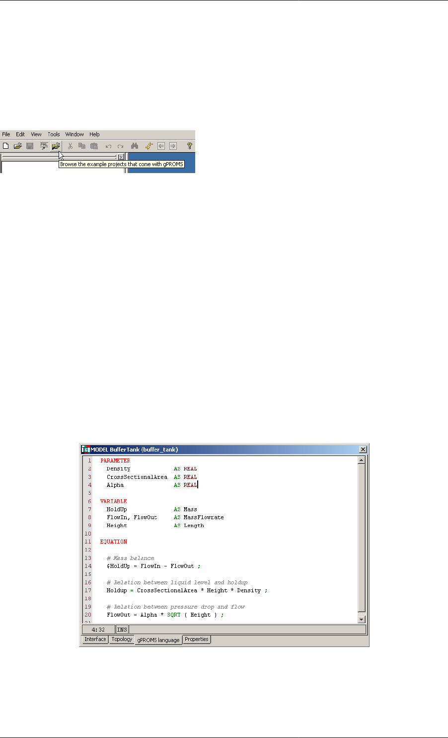
3.4. gPROMS Language definition for a Buffer Tank Model. .............................................................. 17
3.5. Buffer tank Model ................................................................................................................. 19
3.6. An example Process for the buffer tank. .................................................................................... 20
4.1. Model for a series of linked trays. ............................................................................................ 27
6.1. Vessel with overflow weir ....................................................................................................... 37
6.2. STN representation of vessel with overflow weir ......................................................................... 38
6.3. Vessel with bursting disc ........................................................................................................ 38
6.4. Vessel with safety relief valve ................................................................................................. 39
6.5. Hypothetical system model. ..................................................................................................... 40
7.1. Tubular flow reactor ............................................................................................................... 46
7.2. Example of a problem requiring non-uniform grids ...................................................................... 58
7.3. A logarithmic transformation ................................................................................................... 59
8.1. Distillation Column Model ...................................................................................................... 61
8.2. Reactor Flowsheet .................................................................................................................. 69
8.3. Reactor Port Sets ................................................................................................................... 69
8.4. Inconsistent Parameters propagated through Port Sets: inconsistent components specified .................... 70
8.5. Inconsistent Parameters propagated through Port Sets: extra component specified .............................. 70
9.1. Reaction Data Tables Labelled with Elements from Ordered Sets ................................................... 80
9.2. Entering a New Reaction: the Data Tables are Automatically Updated ............................................. 81
9.3. Ordered Set being defined by a Physical Property Foreign Object ................................................... 81
10.1. Defining an icon - (a) the Select icon button on the interface tab .................................................. 83
10.2. Defining an icon - (b) selecting the desired image file ................................................................ 83
10.3. Defining an icon - (c) choosing the default icon size .................................................................. 83
10.4. The Port table ...................................................................................................................... 84
10.5. Creating a new Port .............................................................................................................. 85
10.6. Public Model Attributes page ................................................................................................. 89
10.7. Defining the tabs for the Specification dialog ............................................................................ 90
10.8. Configuring the specification dialog ........................................................................................ 91
10.9. Model Specification Dialog including Initialisation Procedure ...................................................... 92
10.10. Example Model Report configuration ..................................................................................... 95
10.11. Default Orientation of 3D Plots (left) and Definition of Coordinates with no Rotation (right) ........... 101
10.12. Example of a contour plot .................................................................................................. 102
10.13. Example custom graphic specification .................................................................................. 114
10.14. Test specification dialog .................................................................................................... 115
11.1. Graphical Schedule Editor .................................................................................................... 116
11.2. Schedule Language Editor .................................................................................................... 117
11.3. gPROMS language tab with no Schedule ................................................................................ 118
11.4. Schedule tab with no Schedule ............................................................................................. 118
11.5. Task Palette ....................................................................................................................... 119

Model Developer Guide
x
11.6. Continue Task configuration dialog ....................................................................................... 120
11.7. Continue Task in a Schedule ................................................................................................ 121
11.8. Continue Task in a Schedule (gPROMS language tab) .............................................................. 121
11.9. Width Controls .................................................................................................................. 122
11.10. Schedule after a Reassign task was inserted ........................................................................... 123
11.11. Schedule with example multiple selections ............................................................................ 125
11.12. Initial configuration dialog ................................................................................................. 126
11.13. Configuration dialog with illegal Variable path ...................................................................... 126
11.14. Configuration dialog with legal but undefined Variable path ..................................................... 127
11.15. Warnings are shown on the graphical Schedule ...................................................................... 127
11.16. Configuration dialog with illegal expression .......................................................................... 127
11.17. Configuration dialog showing advanced view ........................................................................ 128
11.18. Schedule Tab Toolbar ........................................................................................................ 129
11.19. Overview pane ................................................................................................................. 130
11.20. Width Controls ................................................................................................................. 130
11.21. Reassign Task configuration dialog ...................................................................................... 133
11.22. Switch Task configuration dialog ......................................................................................... 135
11.23. Switch Task configuration dialog: selecting a value ................................................................ 135
11.24. Replace Task configuration dialog ....................................................................................... 136
11.25. Reinitial Task configuration dialog ...................................................................................... 138
11.26. Continue Task configuration dialog ...................................................................................... 140
11.27. Mixing tank Process — graphical representation of tasks in Sequence ........................................ 143
11.28. Mixing tank Process — graphical representation of Tasks in Parallel .......................................... 145
11.29. If Task configuration dialog ............................................................................................... 146
11.30. A new If Task .................................................................................................................. 146
11.31. Graphical representation of the If Task ................................................................................. 146
11.32. While Task configuration dialog .......................................................................................... 147
11.33. A new If Task .................................................................................................................. 148
11.34. Graphical representation of the While Task ........................................................................... 148
11.35. Message Task configuration dialog ...................................................................................... 149
11.36. Output from the example Schedule illustrating MONITOR FREQUENCY .................................. 151
11.37. Monitor Task configuration dialog ....................................................................................... 152
11.38. Message Task configuration dialog ...................................................................................... 152
11.39. Auto Update Source Project Option ..................................................................................... 153
11.40. Save Task configuration dialog ........................................................................................... 154
11.41. Restore Task configuration dialog ........................................................................................ 154
12.1. New Task Interface tab ....................................................................................................... 161
12.2. Adding a new Parameter ...................................................................................................... 161
12.3. Adding a MODEL Parameter ............................................................................................... 162
12.4. Adding a new local Variable ................................................................................................ 163
12.5. Simulate user-defined Task .................................................................................................. 164
12.6. Local variable assignment Task configuration dialog ................................................................ 164
12.7. Task Palette for user-defined Tasks ....................................................................................... 165
12.8. Completing the Task configuration dialog for a predefined Task ................................................. 165
12.9. Execution Output Indicating the Inclusion of Intrinsic Tasks ...................................................... 168
12.10. Execution Output Showing the Detailed Schedule for Intrinsic Tasks ......................................... 169
12.11. Illustration of Intrinsic Task control ..................................................................................... 171
12.12. Example of a Unit with enabled Intrinsic Tasks ..................................................................... 171
13.1. Values assigned to the temperature for each scenario. ............................................................... 172
13.2. Probability density function for the product mole fraction. ......................................................... 173
13.3. Standard deviation of the product mole fraction ....................................................................... 173
13.4. Values assigned to the temperature for each scenario. ............................................................... 184
13.5. Probability density function for the product mole fraction X(4). .................................................. 185
13.6. Standard deviation of the product mole fraction X(4). ............................................................... 185
15.1. gPROMS diagnostics for a high-index problem ....................................................................... 220
15.2. The initial condition that needs to be removed ......................................................................... 220
15.3. gPROMS diagnostics for a high-index problem ....................................................................... 221
15.4. gPROMS output after automatic index reduction ...................................................................... 222


xii
List of Tables
1. Third party free-software packages ............................................................................................... 3
2.1. Enforced connectivity rules ..................................................................................................... 14
5.1. Vector intrinsic functions ........................................................................................................ 32
5.2. Scalar intrinsic functions ......................................................................................................... 33
7.1. Closed and open domain notation ............................................................................................. 49
7.2. Numerical methods for distributed systems in gPROMS ............................................................... 55
7.3. Numerical methods for integrals in gPROMS ............................................................................. 56
7.4. Domain transformations available in gPROMS ........................................................................... 59
10.1. Attributes of the <PMA_TABLE> tag .................................................................................... 103
10.2. Attributes of the <HeaderFont> and <BodyFont> tags ............................................................... 104
10.3. Attributes of the <Plot2D> tag .............................................................................................. 105
10.4. Attributes of the <Font> tag ................................................................................................. 105
10.5. Attributes of the <Legend> tag ............................................................................................. 106
10.6. Attributes of the <Axis> tag ................................................................................................. 106
10.7. Attributes of the <Grid> tag ................................................................................................. 107
10.8. Attributes of the <Line> tag ................................................................................................. 108
10.9. Attributes of the <Plot3D> tag .............................................................................................. 109
10.10. Attributes of the <Font> tag ............................................................................................... 110
10.11. Attributes of the <Legend> tag ........................................................................................... 111
10.12. Attributes of the <Axis> tag ............................................................................................... 111
10.13. Attributes of the <Surface> tag ........................................................................................... 112
10.14. Attributes of the <Rotation> tag .......................................................................................... 112
10.15. Alginment options ............................................................................................................. 114
13.1. Probability distribution functions available in gPROMS. ............................................................ 174
14.1. Effects of Output level on execution diagnostics ...................................................................... 190

xiii
List of Examples
4.1. Parameter section of a liquid-phase CSTR Model ........................................................................ 25
4.2. Variable section of a liquid-phase CSTR Model .......................................................................... 26
4.3. Arrays of Selectors ................................................................................................................ 26
5.1. Multi-component mixing tank Model entity ................................................................................ 34
5.2. Matrix multiplication Model entity ........................................................................................... 35
6.1. Model entity for a vessel equipped with a bursting disc ................................................................ 41
6.2. Model entity for a vessel equipped with an overflow weir ............................................................. 43
7.1. Parameter and DISTRIBUTION_DOMAIN sections for a Model of a tubular reactor ......................... 47
7.2. Variable section for a Model of a tubular reactor ......................................................................... 48
7.3. Setting the discretisation methods, orders and granularities ............................................................ 57
11.1. Applications of the Reassign task .......................................................................................... 131
11.2. Manipulating selector variables using the Switch task ............................................................... 134
11.3. Automatic calculation of controller bias using a Replace task ..................................................... 136
11.4. Applications of the Reinitial task .......................................................................................... 137
11.5. Mixing tank Process ........................................................................................................... 141
11.6. Mixing tank Process — tasks in Sequence .............................................................................. 142
11.7. Mixing tank Schedule — tasks in Parallel ............................................................................... 144
11.8. Application of the If conditional structure ............................................................................... 145
11.9. Application of the While iterative structure ............................................................................. 147
11.10. Example of the MONITOR task .......................................................................................... 150
11.11. Application of the Save and Restore Tasks. ........................................................................... 154
12.1. Task for a digital PI control law ........................................................................................... 156
12.2. Task to switch on a pump .................................................................................................... 157
12.3. Parameterised Task for a digital PI control law ........................................................................ 158
12.4. Low-level Task to operate a reactor ....................................................................................... 159
12.5. High-level Task to operate a reactor train ............................................................................... 160
14.1. Process used to solve the initialisation problem only ................................................................. 187
14.2. Full Process restoring data from the successful initialisation ....................................................... 187
15.1. Illustrative example: over-specified system ............................................................................. 213
15.2. Illustrative example: under-specified system ............................................................................ 215
15.3. Illustrative example: system with inconsistent initial conditions .................................................. 234

xiv
List of Equations
3.1. Mass balance ........................................................................................................................ 16
3.2. Relation between liquid level and holdup ................................................................................... 16
3.3. Characterisation of the output flowrate ...................................................................................... 17

1
Chapter 1. gPROMS Fundamentals
gPROMS process models are built from a number of fundamental building blocks or Entities (see also: Entities).
A gPROMS process model (for a Simulation activity) consists of the following entities:
•Variable Types
• Connection Types
•Models
• Tasks
•Processes
• Saved Variable Sets
Note that the entities required as a minimum are highlighted in bold.
In addition
• To execute Optimisation activities, Optimisation entites are required. For details on solving Optimisation
problems in gPROMS refer to the gPROMS Advanced Users Guide - included in the gPROMS installation.
• To execute Model Validation activities (Parameter Estimation and Experiment Design), Parameter
Estimation, Experiment Design and Experiment Entites are required. For details on solving Parameter
Estimation and Experiment Design problems in gPROMS refer to the Model Validation Guide
Variables and Variable Types
See also: Declaring Variable Types
In gPROMS, all quantities calculated by Model Equations are Variables; Variables are always Real (continuous)
numbers and must always be given a Variable Type.
Variable Types have the following information,
• A name, to which the type may be referred globally.
• A default value for Variables of this type. This value will be used as an initial guess for any iterative calculation
involving Variables of this type, unless it is overridden for individual Variables or a better guess is available
from a previous calculation.
•Upper and lower bounds on the values of Variables of this type. Any calculation involving Variables of this type
must give results that lie within these bounds. These bounds can be used to ensure that the results of a calculation
are physically meaningful. Again, these bounds may be overridden1for individual Variables of this type.
• An optional unit of measurement. Users are encouraged to provide this in order to aid Model readability.
1It is possible to override the bounds on certain Variables. This is done using in PRESET section of the Process entity.
gPROMS Fundamentals
2
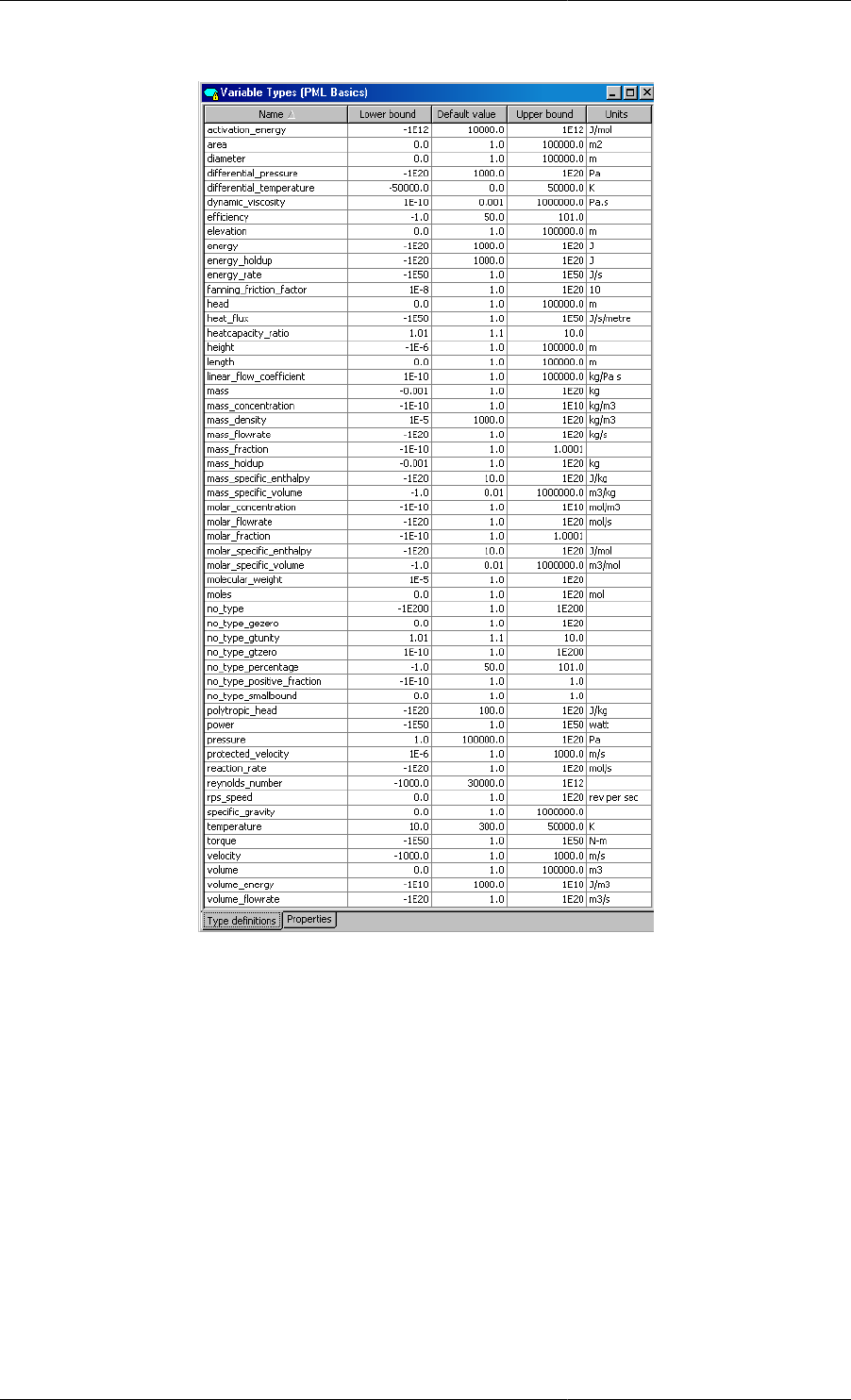
Figure 1.1. Variable Types declared in the gPROMS Process Model Library
When developing gPROMS Models you can either use the existing Variable Types that are found in the gPROMS
Process Model Library (PML) (refer to the gPROMS Process Model Library Guide) or define your own Variable
Types.
Connection Types
See also: Declaring Connection Types
Connections between different Units in a flowsheet Model are associated with a Connection Type which defines
the type of information conveyed by the connection.
A Connection Type definition includes
• A declaration of a set of Parameters, Distribution domains and Variables; these are identical to those that are
declared in Models.
• A Graphical representation.
• Connectivity rules to allow and forbid connections between Ports of different categories.
gPROMS Fundamentals
3
• A Display template which specifies how any connection based on this Connection Type appears in results stream
tables.
A connections to or from a Unit is made from its Model Port. Model Ports are associated with a Connection Type
and all the quantities declared by the Connection Type are automatically included in the Model that declares the
Port.
When a connection between two Ports is made in a flowsheet Model; all the Variables, Parameters and Distribution
domain are equated.
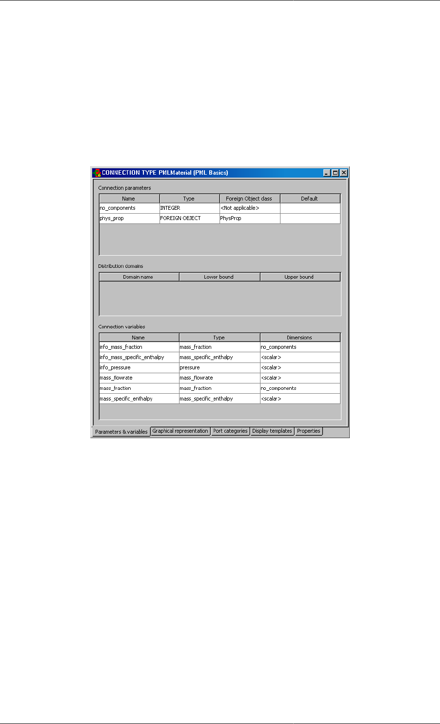
Figure 1.2. The PMLMaterial Connection Type from the gPROMS
Process Model Library - Parameters and Variable declaration tab
When developing gPROMS Models you can either use existing Connection Types such as those that are found in
the gPROMS Process Model Library (PML) or you can define your own Connection Types.
Models
See also: Defining a gPROMS Model
A Model provides a description of the physical behavior of a given system in the form of mathematical equations: a
gPROMS process model will contain at least one Model. Each Model contains the following information (defined
in each of its associated tabs):
• A gPROMS Language declaration: a Model's gPROMS Language tab is where the mathematical equations are
provided along with the declaration of the quantities (such as Parameters and Variables) that appear in these
equations.
• A Public Interface: a Model interface consists of an icon, Model port declarations and a Specification dialog.
The interface captures information explaining how to use the Model within composite or flowsheet Models and
to aid in making Model specifications.
• A topology: the topology tab is used for the graphical construction of flowsheet Models. On the topology tab you
can drag and drop existing component Models and equate their Model Ports by making graphical connections.
Note that these connections are of course represented in the gPROMS language tab as mathematical equations.

gPROMS Fundamentals
4
gPROMS Language declaration for Models
The gPROMS Language Tab in the Model entity comprises a number of sections, each containing a different type
of information regarding the system being Modelled. The minimal information that needs to be specified in any
Model is the following:
• A set of constant Parameters that characterise the system. These correspond to quantities that will never be
calculated by any simulation or other type of calculation making use of this Model. Therefore, their values must
always be specified before the simulation begins and remain unchanged thereafter. They are declared in the
PARAMETER section.
• A set of Variables that describe the time-dependent behaviour of the system. These may be specified in later
sections or left to be calculated by the simulation. They are declared in the VARIABLE section.
• A set of Equations involving the declared Variables and Parameters. These are used to determine the time-
dependent behaviour of the system. They are declared in the EQUATION section.
The structure of a simple Model declaration in the gPROMS language is the following:
PARAMETER
... Parameter declarations ....
VARIABLE
... Variable declarations ...
EQUATION
... Equation declarations ...
The general structure that a Model entity may have is shown below.
Please note that the SET, ASSIGN, INITIAL and INITIALSELECTOR sections are also part of a Process and that
there are both advantages and disadvantages in using these sections in a Model. This is discussed at the example
of Parameter settings for composite Models.
PARAMETER
... Parameter declarations ...
DISTRIBUTION_DOMAIN # For distributed Models
... Distribution domain declarations ...
UNIT
... Sub-Model declarations ...
PORT
... PORT declarations ...
PORTSET
... PORTSET declarations ...
Variable
... Variable declarations ...

gPROMS Fundamentals
5
SET
... PARAMETER value settings ...
BOUNDARY # For distributed Models
... Boundary conditions for partial differential equations ...
TOPOLOGY
... Equations defining the connection of sub-Models ...
EQUATION
... Equation declarations ...
ASSIGN
... Degrees of freedom assignment ...
PRESET
... PRESET specifications ...
INITIALSELECTOR
... Initial SELECTOR specifications ...
INITIAL
... Initial conditions specifications ...
Tasks
See also: Defining a Task
A Task is a Model of an operating procedure. An operating procedure can be considered as a recipe that defines
periods of undisturbed operation along with specified or conditional external disturbances to the system.
A Process Entity defines an operating procedure for a process model; this is done either with explicit statements in
the Process entity or by invoking one or more generic Tasks (or indeed some combination of the two). So typically,
a Task defines part of the operating procedure for a whole Process.
A Task
• can be re-used multiple times during a dynamic simulation
• is associated with one or more Models and thus can be used on different Model instances (Units) based on the
same Model
• can invoke other Tasks and thus complex operating procedures can be defined in a hierarchical manner.
gPROMS language declaration for Tasks
A Task is defined by three sections: Task Parameter declarations, (optional) Task Variable declarations and a
Schedule where the Task's operating procedure is expressed in terms of the Task Parameters and Variables.
Overall, the structure of a Task definition is the following:
gPROMS Fundamentals
6
PARAMETER
... Parameter declarations ...
VARIABLE
... Local Variable declarations ...
SCHEDULE
... Schedule declaration ...
Task Parameters may be of any of the following types:
• INTEGER, REAL or LOGICAL constants. These are used to Parameterise a Task with respect to, for instance,
controller tuning Parameters, event durations etc.
• INTEGER_EXPRESSION, REAL_EXPRESSION or LOGICAL_EXPRESSION. These are used to
parameterise a Task with respect to, for instance, logical conditions for the conditional and iterative structures
etc.
• Model. These are used to parameterise a Task with respect to the actual Models on which it acts.
The purpose of Parameters in a Task is to defines the number and type of arguments that a Task accepts as
arguments and enables one to write generic reusable tasks. All Task Parameters must be given a value whenever
the Task is invoked.
Task Variables are the equivalent of local subroutine Variables and as such are calculated by the Task. They should
not be confused with Model Variables and are NOT associated with Variable Types instead they are declared to
be of type INTEGER or REAL.
The Schedule section defines the part of the operating procedure implemented by the Task. It is similar to the
Schedule section in Processes, the only difference being that it has access to the local Variables declared in the
Variable section. The values of the latter can be manipulated by using assignment statements.
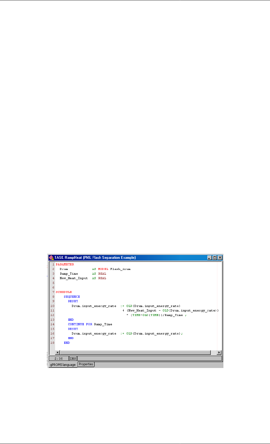
Figure 1.3. An example Task used to define change in heat input to
the Flash drum Model from the gPROMS Process Model Library
Processes
See also: Defining a gPROMS Process
A Model can usually be used to study the behaviour of the system under many different circumstances. Each
such specific situation is called a simulation activity. The coupling of Models with the particulars of a dynamic
simulation activity is done in a Process Entity. A Process performs two key roles

gPROMS Fundamentals
7
• to instantiate a generic Model: this is done by providing specifications for all the Model's Parameters, Input
Variables (degrees of freedom), Selectors and Initial Conditions that have not been given values directly in the
Model. Any specifications given in Specification dialogs from the topology of a flowsheet Model will appear
as un-editable text in the Process Entity
• to define an operating procedure [5] for a process model in the form of a Schedule; a Schedule may
simply specify the execution of an undisturbed simulation for a period of time to a more complex scenario such
as Modelling the start-up of a complex Process with multiple external disturbances to the system. Complex
operating policies will usually make use of Tasks. Steady-State simulations require no Schedule.
Solver configuration information for all Model based activities is also specified in Process entities.
gPROMS language for Processes
gPROMS Language declaration for Processes
A gPROMS Project may contain multiple Processes, each corresponding to a different simulation activity (e.g.
simulation of system startup, simulation of system shutdown, steady state operation, etc.). A Process is partitioned
into sections, each containing information required to define the corresponding dynamic simulation activity:
UNIT
... Declaration of Model instances ....
MONITOR
... Variable path patterns ....
SET
... Parameter value settings ...
ASSIGN
... Degrees of freedom assignment ...
PRESET
... PRESET specifications ...
INITIALSELECTOR
... Initial SELECTOR specifications ...
INITIAL
... Initial conditions specifications ...
SOLUTIONPARMETERS
... Model based activity solver specifications ...
SCHEDULE
... Operating procedure specifications ...
gPROMS Fundamentals
8
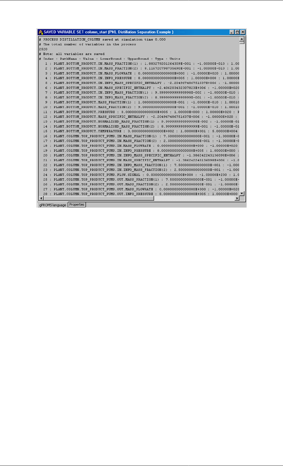
Saved Variable Sets
The values of all Model Variable and Selectors at a particular simulation time can be saved for later re-use; these
values are stored in Saved Variable Sets.
Saved Variable Sets are used
• to provide good initial guesses for initialisation calculations (over-riding the default values for the Variables
taken from their Variable Type). This is done in the PRESET section.
• during a simulation to change the values of the Variables and Selectors to those stored in the Saved Variable Set.
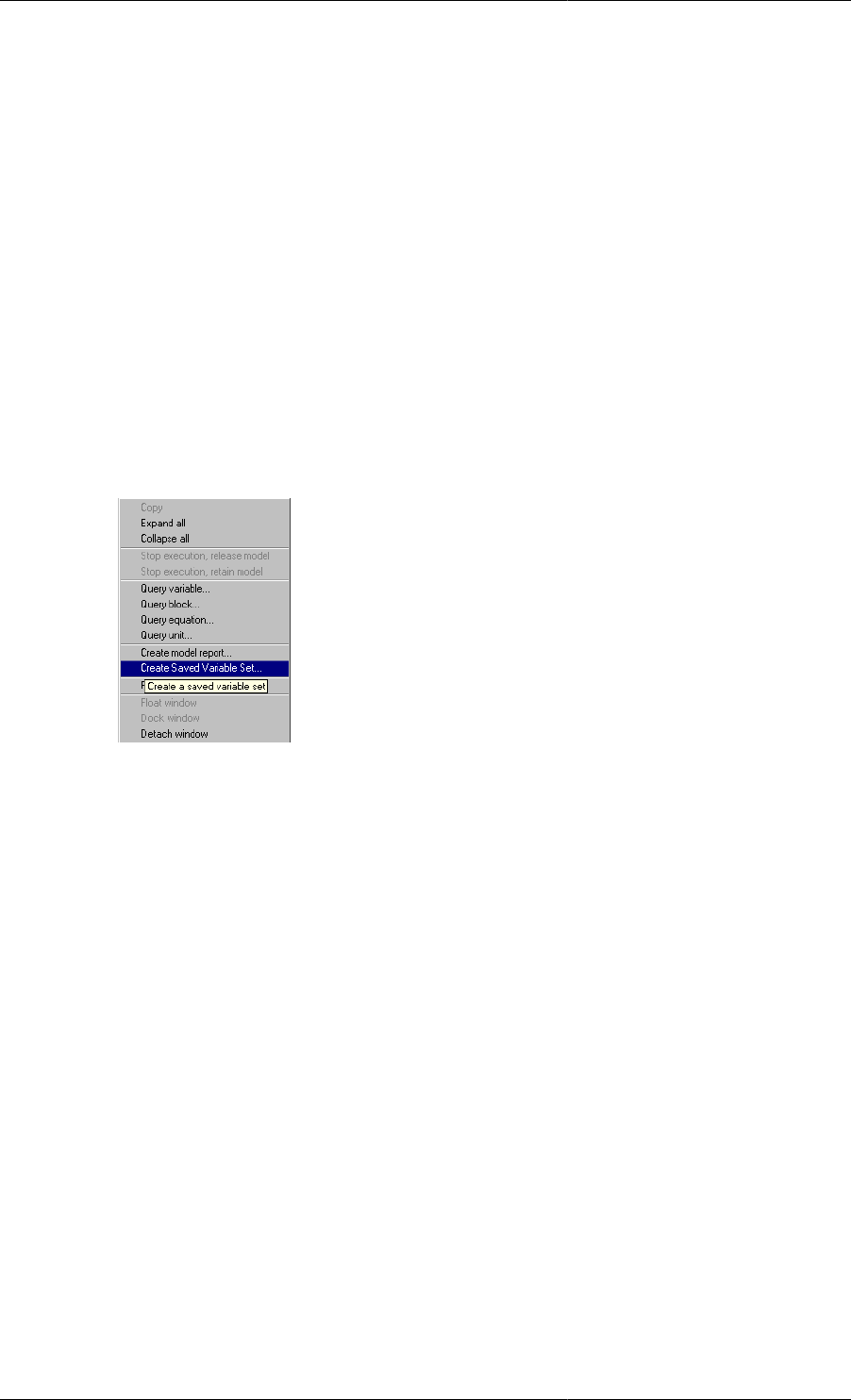
Saved Variable Sets are created from a simulation activity either
• using the SAVE elementary task in a Schedule
• right clicking on the Execution Window and selecting Create Saved Variable Set ..... from the short-cut menu.
Note that this is only possible if a license was retained following the execution of the simulation activity:
Any new Saved Variable Set created during a simulation activity will be stored in the Results folder of the
Execution Case. In order to use it in any subsequent activity the Saved Variable Set must be copied into the working
project where it will appear in the Saved Variable Sets entity group.
gPROMS Fundamentals
9
Figure 1.4. An example of a Saved Variable Set
10
Chapter 2. Declaring Variable and
Connection types
Variable Types are an essential requirement for all gPROMS process models as all Variables in a gPROMS Model
must be associated with a Variable Type.
In a similar way all Model Ports must be associated with a Connection Type.
When developing gPROMS Models you can either use existing Variable or Connection Types, such as those that
are found in the gPROMS Process Model Library (PML), or you can define your own:
• Declaring new Variable Types
• Declaring new Connection Types
Declaring Variable Types
Variable Types appear under the first entry in the Project tree. In order to create your own Variable Types; you can
either select New entity.... from the Entity menu - choosing Variable Type as the Entity type (see also: Entities)
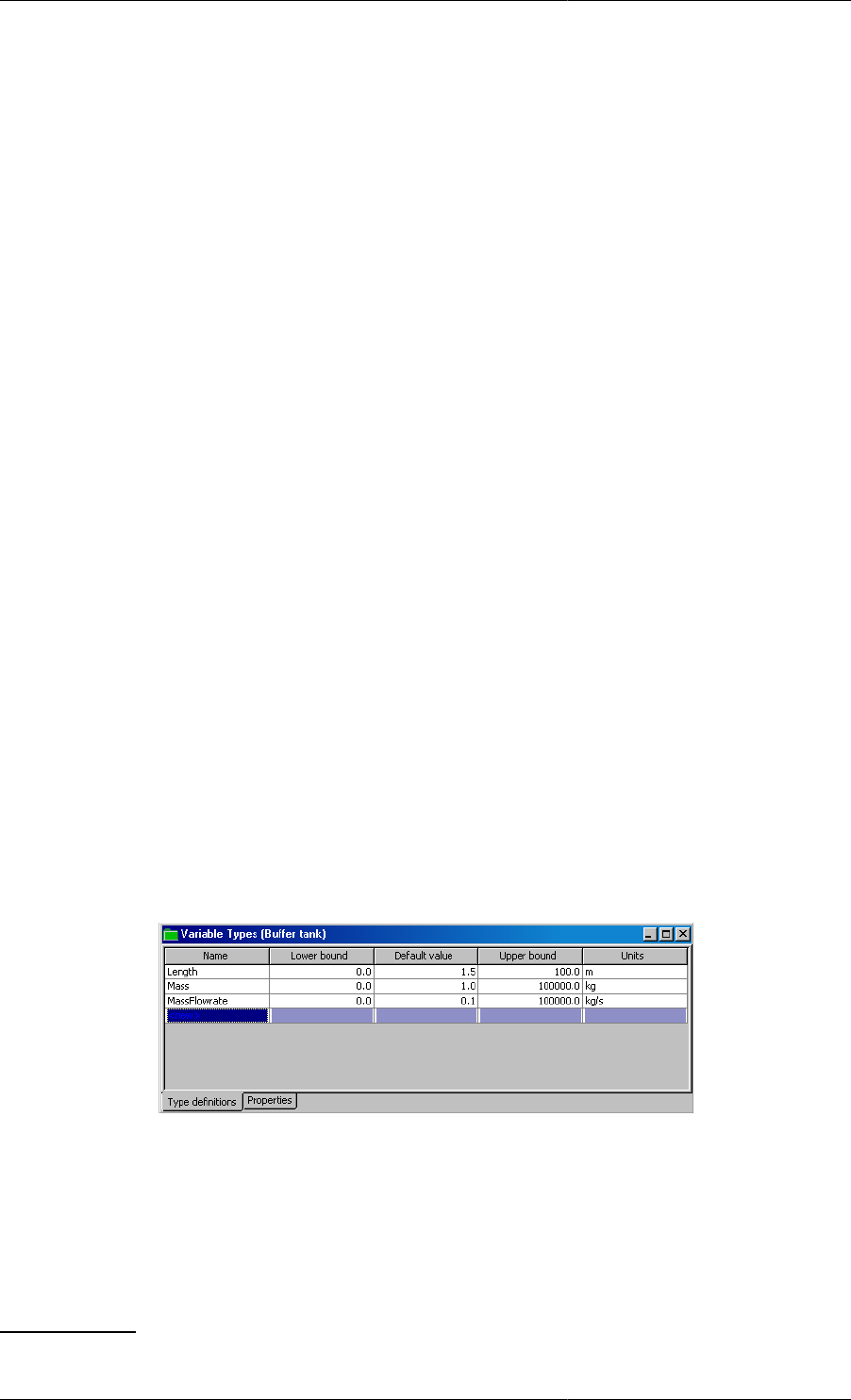
or if you open an existing Variable Type it is possible to edit the Variable Types table, shown below, by typing
the name in the <new> row and pressing enter.
Once the Variable Type has been introduced to the table the following information should be provided
• A default value for Variables of this type. This value will be used as an initial guess for any iterative calculation
involving Variables of this type, unless it is overridden for individual Variables or a better guess is available
from a previous calculation.
•Upper and lower bounds on the values of Variables of this type. Any calculation involving Variables of this type
must give results that lie within these bounds. These bounds can be used to ensure that the results of a calculation
are physically meaningful. Again, these bounds may be overridden1for individual Variables of this type.
• An optional unit of measurement. Users are encouraged to provide this in order to aid Model readability.
Figure 2.1. An example Variable Types table
The values of the lower bounds, initial values and upper bounds are checked for consistency (i.e. you cannot enter
an initial value outside the bounds or enter a lower bounds greater than the upper bound).
Declaring Connection Types
Connection Types are declared using a multi-tab forms-based editor. Each of the four principal tabs allows you
to declare different aspects of the Connection Type:
1It is possible to override the bounds on certain Variables. This is done using in PRESET section of the Process entity.
Declaring Variable
and Connection types
11
• Parameters & Variables tab
• Graphical representation tab
• Port categories tab
• Display templates tab
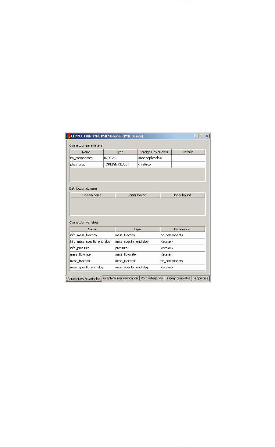
The Parameters and Variables tab
To declare quantities for a Connection Type simply double click on the cells labeled <new> and enter the name
of the quantity. You can then enter information pertaining to Parameters, Distribution Domains and Variables -
these are identical to those that are declared in Models.
Figure 2.2. The PMLMaterial Connection type - the Parameters and Variables Tab.
• For Parameter declarations, a Type - Integer, Real or ForeignObject - must be provided.
• If ForeignObject is selected then a class can also be provided.
• For Integer and Real Parameters it is also possible to provide a default value.
• For Distribution Domain declarations, lower and upper bounds must be provided.
• For Variable declarations, a Variable Type must be provided; this should be selected from a drop-down list
of all Variable Types declared in this Project (or cross-referenced Projects). The Connection Type can include
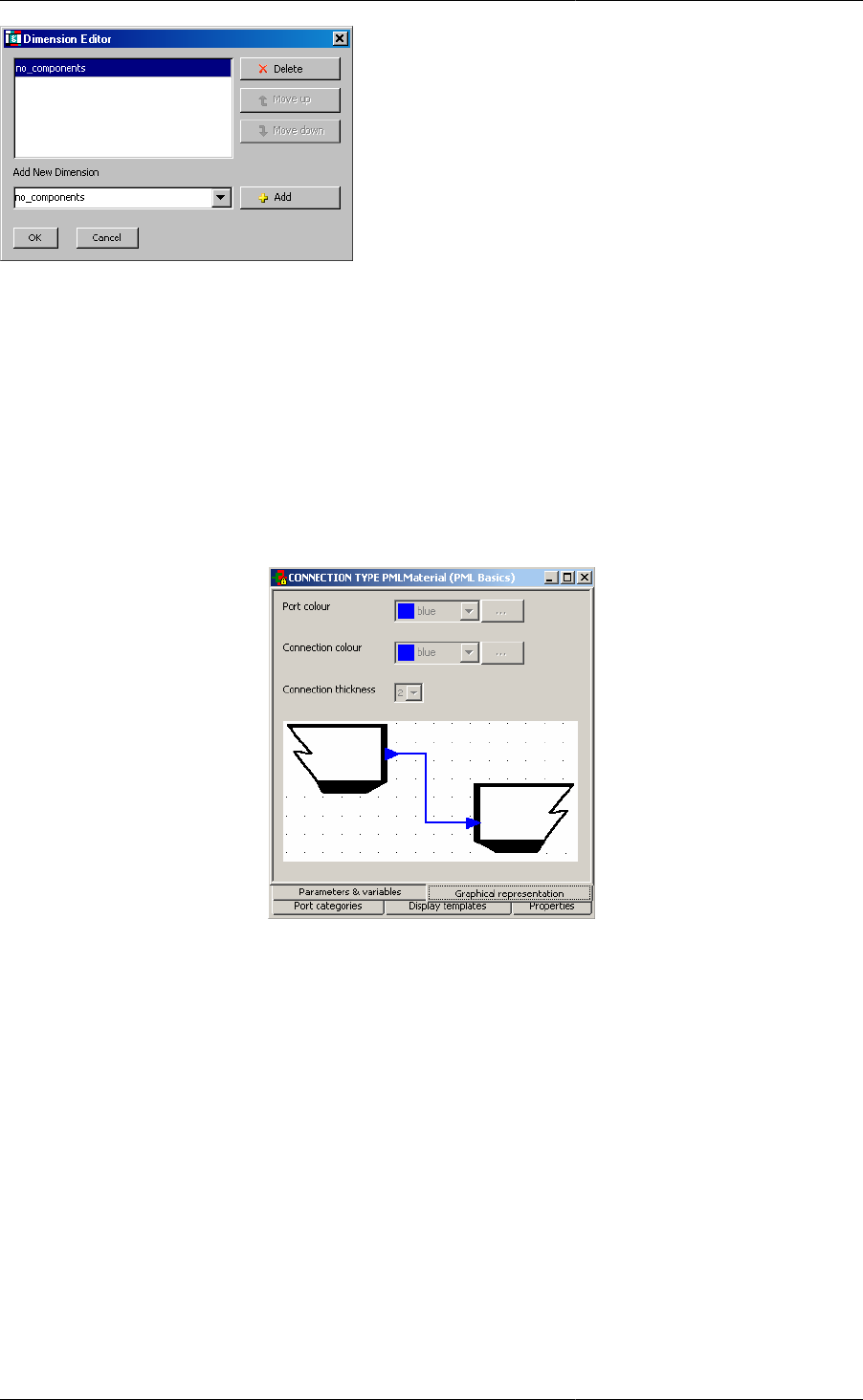
scalar and Array Variables:
• To define the dimensionality of the Array click on the <scalar> cell to access the Dimension Editor.
• In the Add New Dimension box either select an Integer Parameter that has been declared in this Connection
Type or type in a literal value (e.g. 7).
• It is possible to declare multiple dimensioned Variables by Adding more than one Dimension - multiple
dimensions can be ordered using the Move Up and Move Down buttons
Declaring Variable
and Connection types
12
The Graphical representation tab
Connections between different Units in a flowsheet Model are associated with a Connection Type. Such
connections are displayed graphically on the flowsheet Model's topology tab - the graphical representation of such
connections is determined by its Connection Type.
The information provided on the graphical representation tab determines the colour of the Ports and of the
connectivity line, as well as the line thickness.
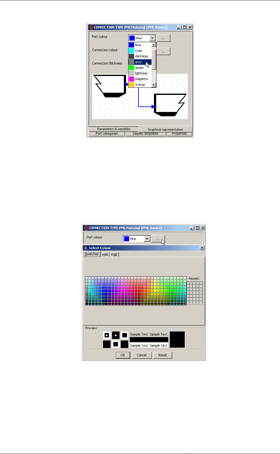
Figure 2.3. Connection Type - Graphical Representation tab
To change colours of Ports or Connectivity lines, the user has the option of selecting a predefined colour from a
drop-down list (as shown below).
Declaring Variable
and Connection types
13
Figure 2.4. Choosing predefined colours for Ports (or Connections).
Alternatively, the user is able to define custom colours by doing the following:
1. Click on the ... button
2. Use either Swatches, HGB or RGB to define the exact colour you want
3. When finished, click OK to select the chosen colour.
Figure 2.5. Defining custom colour for ports or connections.
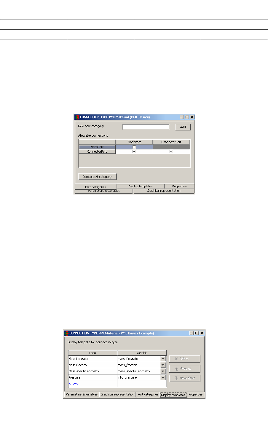
The Port categories tab and Connectivity rules
gPROMS enforces a number of rules to ensure that only valid connections can be made when building flowsheet
Models, and as such all Ports must be defined as an Inlet, an Outlet or a Bi-directional Port. When defining a
Model Port the developer must specify which of these categories the Port belongs to and gPROMS enforces the
rules shown in the following table (e.g. it is possible to connect an Outlet Port to an Inlet Port but not an outlet
to an outlet):
Declaring Variable
and Connection types
14
Table 2.1. Enforced connectivity rules
Inlet Outlet Bi-directional
Inlet Disallowed Allowed Allowed
Outlet Allowed Disallowed Allowed
Bi-directional Allowed Allowed Allowed
In addition, for a particular Connection Type, it is possible to define an additional set of rules by defining new
user-specified categories. The gPROMS Process Model Library (PML) makes use of this capability: in the PML
a Port must be either a Node or a Connector with Node-to-Node connections forbidden (see also: Understanding
the PML):
Figure 2.6. The PMLMaterial Connection type in the gPROMS PML - Port categories
To define new connectivity rules; simply enter each of the categories by providing each with a name and clicking
Add. Then specify whether a particular connection is valid by checking the appropiate box in the Allowable
connectionstable: leaving the box unchecked means that the connection is not valid.
If you wish to delete a particular Port category, then simply click on its name in the Allowable connections table
and then click on the Delete port category button at the bottom of the window.
The Display templates tab
The Display templates tab enables you to define which of the Variables carried by the Connection Type should
appear in results stream tables.
On this tab you provide a label for each of the Variables that should be displayed in the stream table and the
order in which the quantities should appear in the table. Note that only those quantities that appear on the Display
templates tab will appear in stream tables.
Figure 2.7. Connection Type - Display templates tab
To enter information, simply click on the relevant cells that contain <new> and then select a Variable from the
drop-down list. Re-order the table as desired using the Move up and Move down buttons.
15
Chapter 3. Defining Models and
Processes
The development of a basic gPROMS process model is explained by reference to the gPROMS Project Buffer
Tank.gPJ that can be found in the installation.You can access this by clicking on the Browse Examples button on
the gPROMS Toolbar and then navigating to "General capabilities\Other examples\Buffer Tank.gPJ".
An illustrative buffer tank example is used to demonstrate the following:
• Defining Models
• the gPROMS language to enter Model Equations
• how to declare the Parameters and Variables that appear in these Equations
• Defining Processes
• how to set values for Model Parameters
• how to specify the values of Model Variables to satisfy the degrees of freedom
• how to provide initial values for the state (differential) Variables
Note: to create your own Model and Process Entites; select New entity....from the Entity menu - choosing Model
or Process as the Entity type (see also: Entities).
Figure 3.1. The Buffer Tank Model entity
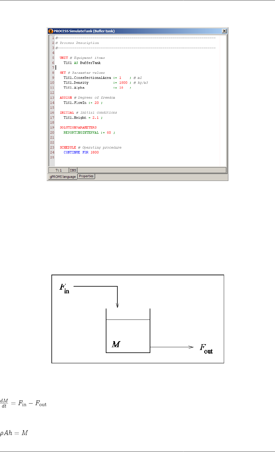
Defining Models and Processes
16
Figure 3.2. The Buffer Tank Process entity.
An illustrative buffer tank example
Buffer Tank.gPJ describes a simple buffer tank with gravity-driven outflow (see the figure below). It is a good
choice for illustrating the main features of the gPROMS language because it comprises only one simple unit
operation, for which a primitive model can be constructed. Primitive models are mathematical models that are
completely specified in terms of explicitly declared variables and equations. They usually correspond to simple
unit operations or parts thereof. Primitive models form the building blocks for the construction of higher-level,
composite model of complex unit operations or entire process flowsheets.
Figure 3.3. Buffer tank with gravity-driven outflow.
The dynamic mathematical model of the buffer tank process takes the following form:
Equation 3.1. Mass balance
Equation 3.2. Relation between liquid level and holdup
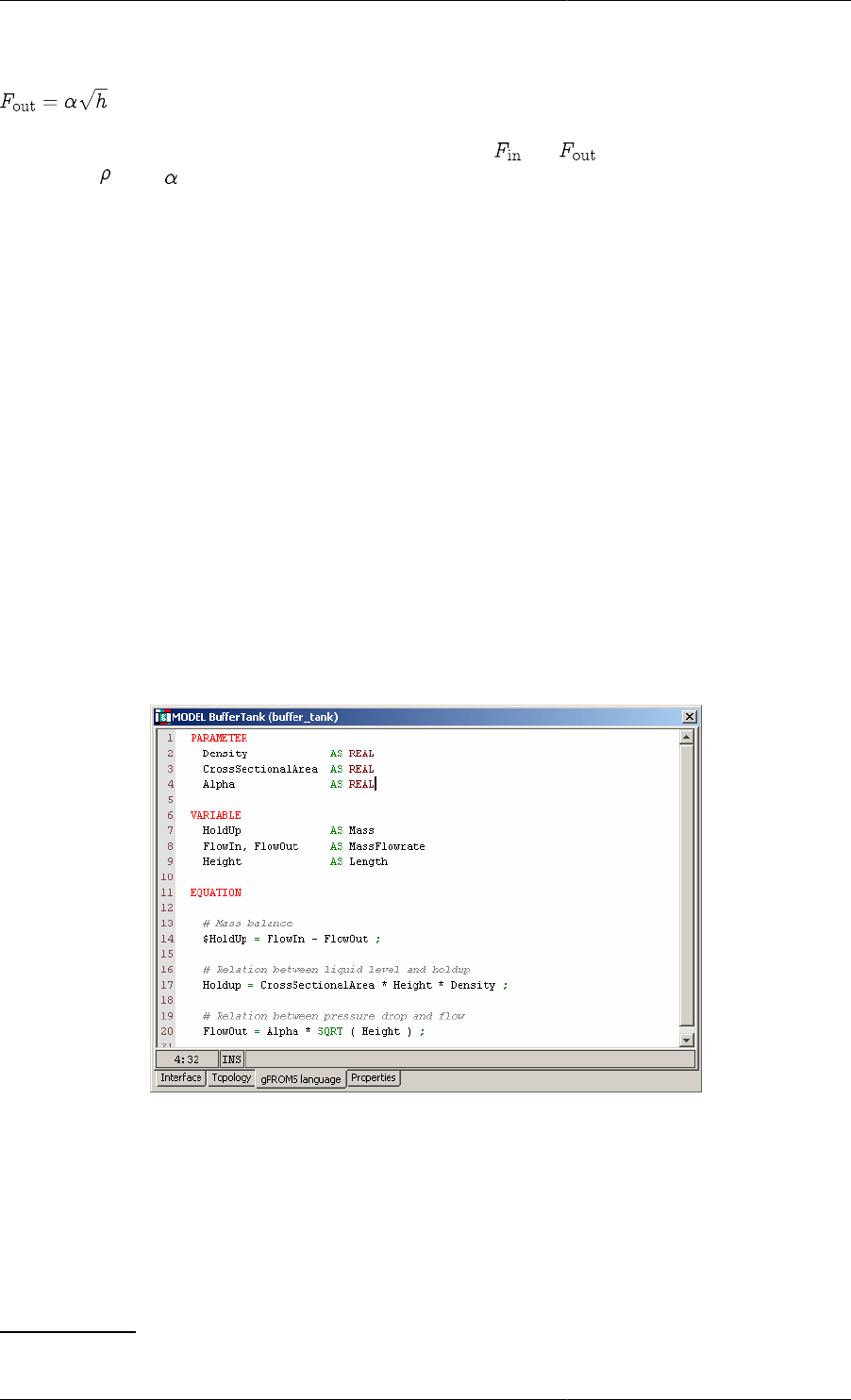
Defining Models and Processes
17
Equation 3.3. Characterisation of the output flowrate
Here, M and h are the mass and level of liquid in the tank, and and are the inlet and outlet flowrates
respectively. , A and denote the density of the liquid material, the cross-sectional area of the tank and the outlet
valve constant, respectively. For the purposes of this example, these last three quantities are assumed to be known
constants.
Defining a gPROMS Model
In gPROMS, Model Entities are the central part any process model. A working gPROMS Project will contain (or
reference) at least one Model:
A Model is defined as a set of quantities and mathematical equations that, when coupled with a
set of specifications, describe the behaviour of a given system.
The gPROMS language declaration for a basic Model will typically consist of three parts1:
• PARAMETER declarations
• VARIABLE declarations
• EQUATION declarations
Figure 3.4. gPROMS Language definition for a Buffer Tank Model.
The PARAMETER section
The Parameter section is used to declare the parameters of a Model. Parameters are time-invariant quantities that
will not, under any circumstances, be the result of a calculation. Quantities such as physical constants (pi, R, etc.),
Arrhenius coefficients and stoichiometric coefficients usually fall into this category. In the buffer tank process,
rho, A and alpha were assumed constant and are thus declared as parameters of the Buffer Tank Model:
PARAMETER
1A Model may contain more parts. A comprehensive overview can be found in gPROMS Language declaration for Models..

Defining Models and Processes
18
Rho AS REAL
CrossSectionalArea AS REAL
Alpha AS REAL
Each parameter has a unique name (identifier) by which it can be referenced (for example, in expressions).
Identifiers in the gPROMS language start with a letter (a-z and A-Z) and may comprise letters, numbers (1-9)
and underscores (_). The gPROMS language is not case sensitive, i.e. Temp and TEMP are considered to be
identical.
Each parameter is also declared to be of a certain type (e.g. INTEGER, LOGICAL or REAL). All three parameters
of the Buffer Tank Model are of type REAL.
Parameter declarations may optionally include the assignment of default values. For instance:
PARAMETER
NoComp AS INTEGER
NoReactions AS INTEGER DEFAULT 1
Finally, note that the categorisation of certain quantities as Parameters is sometimes tenuous. Designating a
quantity as a Parameter has the advantage of reducing the total number of Variables in a model. However, this
quantity can no longer be treated as an unknown in any future use of the model. Consider, for instance, the
quantities that characterise the size and geometry of a vessel. From the point of view of dynamic simulation, these
can be viewed as Parameters. However, from the point of view of steady-state design calculations performed with
the same model, these quantities may be considered unknowns under certain circumstances. It may, therefore, be
better to classify them as Variables.
The VARIABLE section
The VARIABLE section is used to declare the Variables of a Model. All quantities that are calculated in Model
Equations must be declared as Model Variables. For instance, in the example process, M, h, and are
variables of the Buffer Tank Model:
VARIABLE
HoldUp AS Mass
FlowIn, FlowOut AS MassFlowrate
Height AS Length
Like Parameters, Variables are always Real continuous numbers. All Variables must be given a type, however,
Variable Types are user-defined (see also: Declaring Variable Types).
The EQUATION section
The EQUATION section is used to declare the equations that determine the time trajectories of the variables already
declared in the VARIABLE section.
The gPROMS language is purely declarative. That is, the order in which the equations are declared is of no
importance. Simple equations are equalities between two real expressions (see the figure below). These expressions
may comprise:
• Integer or real constants (e.g. 2, 3.14159, etc.).
• Parameters that have been declared in the PARAMETER section (e.g. Rho, Alpha, PI, etc.).
• Variables that have been declared in the VARIABLE section (e.g. HoldUp, Height, FlowOut, etc.). The
special symbol $ preceding a variable name denotes the derivative with respect to time of that variable (e.g.
$HoldUp etc.).
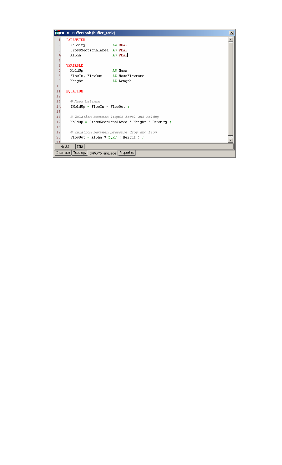
Defining Models and Processes
19
Figure 3.5. Buffer tank Model
Similarly to most programming languages, expressions are formed by combining the above operands with the
arithmetic operators + (addition), - (subtraction), * (multiplication), / (division) and ^ (exponentiation), as well
as built-in intrinsic functions (e.g. square root: SQRT() ). The latter are described in greater detail in Intrinsic
Functions in gPROMS.
Intrinsic functions have the highest precedence priority, followed by the ^ operator and then the division
and multiplication operators. The addition and subtraction operators have the lowest precedence. Naturally,
parentheses may be used to alter these precedence rules as required.
Finally, note that comments can be added to clarify the contents of the Model where needed. As shown in the
figure above, gPROMS accepts two types of comments. One type begins with # and extends to the end of the
current line. The other type starts with { and ends with } and may span multiple lines. Moreover, comments of
this type may be nested within one another.
Defining a gPROMS Process
In the gPROMS language a Model is used to define the physical behaviour of a system and it usually contains
PARAMETER, VARIABLE and EQUATION declarations. A model can usually be used to study the behaviour of
the system under many different circumstances. Each such specific situation is called a simulation activity. The
coupling of Models with the particulars of a dynamic simulation activity is done in a Process.
A gPROMS Project may contain multiple PROCESSes, each corresponding to a different simulation activity (e.g.
simulation of plant startup, simulation of plant shutdown, etc.). Each such PROCESS must be given a different
name and these will be automatically placed in alphabetical order in the gPROMS Project tree. A PROCESS is
partitioned into the following key sections:
• The UNIT section
• The SET section
• The ASSIGN section
• The INITIAL section
• The SOLUTIONPARAMETERS section
• The SCHEDULE section
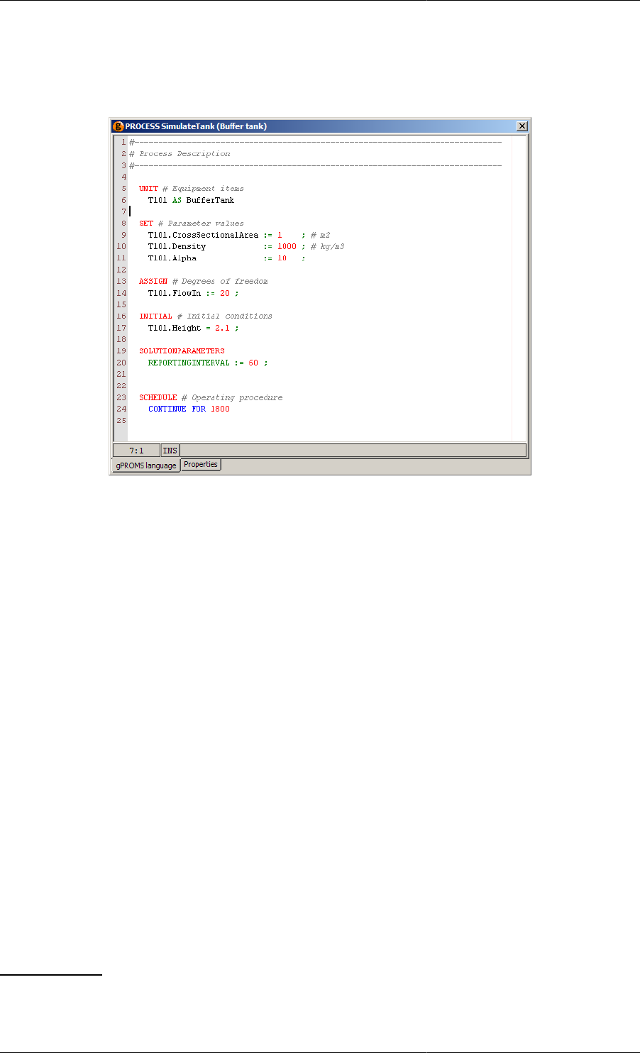
Defining Models and Processes
20
The gPROMS Language definition for the entire PROCESS (named SimulateTank) for a dynamic simulation
activity involving the buffer tank process is shown in the figure below.
Figure 3.6. An example Process for the buffer tank.
The UNIT section
The first item of information required to set up a dynamic simulation activity is the process equipment under
investigation. This is declared in the UNIT section of a PROCESS.
Equipment items are declared as instances of Models. For example
UNIT
T101 AS BufferTank
creates an instance of MODEL BufferTank, named T101. T101 is described by the variables declared within the
BufferTank Model and its time-dependent behaviour is partially determined by the corresponding equations.
The SET section
Before an instance of a Model can actually be used in a simulation, all its parameters must be specified (unless
they have been given default values). This is done in the SET section of a PROCESS.2For example,
SET
T101.Rho := 1000 ; # kg/m3
T101.CrossSectionalArea := 1 ; # m2
T101.Alpha := 10 ;
sets the parameters of T101 to appropriate values. Note that:
• in order to refer to parameter Rho of instance T101 of Model BufferTank, we use the pathname notation
T101.Rho
2The specification of parameter values can also be performed within Models, using a SET section that is completely equivalent to the one
described here. However, it is generally advisable that parameters be set at the PROCESS level. This practice maximises the reusability of the
underlying Models and minimises the probability of error.

Defining Models and Processes
21
•It is recommended that you use pathname completion to help construct full and valid pathnames
correctly; this is available within all entities in gPROMS. Semantic errors, such as referencing a quantity
in a lower-level Model that doesn't exist, are only detected when a Model based activity is executed.
• It is also common, particularly for composite Models, to use the WITHIN construct to complete pathnames
• Parameter values are set using the assignment operator (:=). In other words, the arithmetic expression appearing
on the right hand side is first evaluated; its value is then given to the parameter appearing on the left hand side.
This is another general rule of the gPROMS language:
A General Rule of the gPROMS Language
gPROMS always uses the symbol := to assign a value or expression appearing on the right hand side to the single
identifier appearing on the left hand side. gPROMS always uses the symbol = to declare the equality of the two
general expressions appearing on either side of this symbol.
The ASSIGN section
The set of equations resulting from the instantiation of Models declared in the UNIT section is typically under-
determined. This simply means that there are more variables than equations. The number of degrees of freedom
in the simulation activity is given by:
Number of degrees of freedom (NDOF) = Number of variables - Number of equations.
For the simulation activity to be fully defined, NDOF variables must be specified as either constant values or given
functions of time. Variables specified in this way are the input variables (or "inputs") of this simulation activity.
The remainder of the variables are the unknown variables, the time variation of which will be determined by the
solution of the system equations. Clearly, the number of unknowns is equal to the number of available equations
- we therefore have a "square" system of equations.
The specification of input variables is provided in the ASSIGN section of the PROCESS3. For instance,
ASSIGN
T101.Fin := 20 ;
designates the inlet flowrate as an input and assigns it a constant value of 20. Again, in order to emphasise the
assignment form of these specifications, input specifications use the assignment operator (:=).
The inlet flowrate may not be constant but may vary with the simulation time, for instance by linearly increasing
ASSIGN
T101.Fin := 20 + 1.2*TIME ;
In this example, the built-in function TIME is used to reference the value of the simulation time. Please note that
the value of the simulation time depends on the chosen units of measurement.
TIME can be used with any of gPROMS' built-in functions, for instance in order to create a sinosoidal oscillation:
ASSIGN
T101.Fin := 20 + SIN(TIME) ;
The INITIAL section
Before dynamic simulation can commence, consistent values for the system variables at t = 0 must be determined.
To this end, a number of additional specifications are needed. These augment the system of equations that describe
3The specification of degrees of freedom can also be performed within Models, using an ASSIGN section that is completely equivalent to the
one described here. However, it is generally advisable that variables be assigned at the PROCESS level. This practice maximises the reusability
of the underlying Models and minimises the probability of error.

Defining Models and Processes
22
the behaviour of the system and result in a square system of equations at t = 0. The solution of the latter provides
the condition of the system at t = 0.
Traditionally, the term "initial condition" refers to a set of values for the differential variables at t = 0. However,
gPROMS follows a more general approach where the initial conditions are regarded as additional equations that
hold at t = 0 and can take any form. This, of course, allows for the traditional specification of "initial values"
for the differential variables or, indeed, for any appropriate subset of system variables; however, it also makes
possible the specification of much more general initial conditions as equations of arbitrary complexity.
The INITIAL section is used to declare the initial condition information pertaining to a dynamic simulation
activity. For instance,
INITIAL
T101.Height = 2.1 ;
specifies an initial condition for the buffer tank system by stating that the height of liquid in the tank at t = 0 is
2.1m. Note that, in contrast to the SET and ASSIGN sections, the equality operator (=) is used here to emphasise
the fact that initial conditions are general equations.4
An initial condition that is frequently employed for the dynamic simulation of process systems is the assumption
of steady-state, constraining the time derivatives of the differential variables to zero. In gPROMS, this can be
achieved by manually specifying all derivatives to be zero:
INITIAL
T101.$Holdup = 0 ;
However, this would be tedious for models with large numbers of differential variables, so the keyword
STEADY_STATE may be utilised to specify this initial condition, as shown below:
INITIAL STEADY_STATE
In this latter case, no further specifications are required.
The SOLUTIONPARAMETER section
The user also has the option to control various aspects of model-based activities carried out in gPROMS such as
solver settings and output specifications. The SOLUTIONPARAMETERS section is used for this purpose. Detailed
information regarding this topic will be covered in more detail in Numerical Solver Parameters.
For example,
SOLUTIONPARAMETERS
REPORTINGINTERVAL := 60;
The REPORTINGINTERVAL is the interval at which result values will be collected during the dynamic simulation
(note that it does not effect the accuracy of the subsequent integration in any way). For this example, an interval of
60 is a reasonable choice. The REPORTINGINTERVAL may be over-ridden from the simulation execution dialog.
The user does not need give any settings in this section. In such a case the user will be prompted to enter a
REPORTINGINTERVAL in a dialog box.
The SCHEDULE section
Information on the external manipulations (e.g. known disturbances) that are to be simulated is provided in the
SCHEDULE section of the PROCESS. We restrict our attention to the simplest possible case, allowing the system
to operate without any external disturbance over a specified period of time. This is achieved via the:
4The specification of initial conditions can also be performed within Models, using an INITIAL section that is completely equivalent to the
one described here. However, it is generally advisable that initial conditions be specified at the PROCESS level. This practice maximises the
reusability of the underlying Models and minimises the probability of error.


24
Chapter 4. Arrays
The gPROMS language provides some advanced mechanisms for the declaration of complex equation structures
in Models.
In many cases, a number of Parameters, Variables or Equations that appear in a Model are closely related. Examples
include:
•the stoichiometric coefficients, , of a set of components i=1,..,NoComp participating in a set of reactions
j=1,..,NoReact;
• the concentrations, Ci, of components i=1,..,NoComp in a multi-component system;
• the equations expressing the conservation of components i=1,..,NoComp in a multi-component system.
In such cases, we need effective mechanisms for declaring and handling these entities as a group rather than
individually. In a manner similar to most high-level programming languages, gPROMS achieves this aim via the
use of arrays.
We must consider
• Declaring arrays of Parameters, Variables, Selectors and Units
• Rules for referring to array elements and array expressions
• Using arrays in equations
.
Declaring arrays in Models
Arrays are used in many places during Model construction
• Declaring arrays of Parameters
• Declaring arrays of Variables
• Declaring arrays of Selectors
• Declaring arrays of Units in Composite Models
In all these cases
• Arrays can have any number of dimensions.
• The size of each dimension can be a general integer expression involving a combination of:
• integer constants;
• scalar integer Model Parameters;
• individual elements of arrays of integer Model Parameters;
• integer arithmetic operators - these include the usual arithmetic operators +, -, * and ^, as well as the integer
division operator DIV and the division remainder operator MOD.
• The index of each dimension ranges from 1 to the size of dimension, with the exception of zero-length Arrays.

Arrays
25
Declaring arrays of Parameters in Models
Model Parameters are declared in the Parameter section of gPROMS Models to belong to the basic types INTEGER
or REAL. Such Parameters may be scalars or arrays of one, two or more dimensions. Consider, for instance,
the Parameter section in a model of a liquid-phase continuous stirred tank reactor (CSTR). This is shown in the
gPROMS code below.
Example 4.1. Parameter section of a liquid-phase CSTR Model
# MODEL LiquidPhaseCSTR
PARAMETER
# Number of components
NoComp AS INTEGER
# Number of reactions
NoReact AS INTEGER
# Component molar densities
Rho AS ARRAY(NoComp) OF REAL
# Stoichiometric coefficient of component i in reaction j
Nu AS ARRAY(NoComp,NoReact) OF REAL DEFAULT 0
# Order of component i in reaction j
Order AS ARRAY(NoComp,NoReact) OF REAL DEFAULT 0
Here, NoComp and NoReact denote the numbers of chemical components and chemical reactions occurring in
this system. Each of these is a simple (scalar) INTEGER Parameter. On the other hand, the densities of the pure
components form a vector of real quantities declared as an array of length NoComp:
Rho AS ARRAY(NoComp) OF REAL
For the purposes of this example, the pure component densities are assumed to be constant but different to each
other.
Similarly, Nu and Order are two-dimensional arrays of REAL Parameters. The number of elements in the first
dimension is NoComp; the number of elements in the second dimension is NoReact. We note that, if a DEFAULT
value is specified for an array Parameter, this is taken to refer to all elements of that array.
Declaring arrays of Variables in Models
Arrays of Model Variables are declared in a manner very similar to that used for Parameters. For example, the
Variable section of the liquid-phase CSTR Model entity is shown in the gPROMS code below.

Arrays
26
Example 4.2. Variable section of a liquid-phase CSTR Model
# MODEL LiquidPhaseCSTR
PARAMETER
...
VARIABLE
# Input and output molar flowrates
Flow_In, Flow_Out AS MolarFlowrate
# Liquid phase volume
V AS Volume
# Component molar holdups
HoldUp AS ARRAY(NoComp) OF Moles
# Input and output component mole fractions
X_In, X_Out AS ARRAY(NoComp) OF MoleFraction
# Component concentrations
C AS ARRAY(NoComp) OF Concentration
# Reaction rates
Rate AS ARRAY(NoReact) OF ReactionRate
Arrays of Parameters and Variables may have any number of dimensions. The number of elements in each
dimension is specified in terms of an integer expression (e.g. HoldUp AS ARRAY(NoComp+1) OF REAL is
acceptable). The total number of elements in an array is the product of the number of elements in each dimension.
Declaring arrays of Selectors in Models
As with Variables and Parameters, arrays of Selectors may also be defined (see The Case conditional construct
for an introduction to Selectors), as shown in the example below.
Example 4.3. Arrays of Selectors
# MODEL LiquidPhaseCSTR
PARAMETER
NoDiscs AS INTEGER
...
VARIABLE
...
SELECTOR
DiscFlag AS ARRAY(NoDiscs) OF (Intact, Burst) DEFAULT Intact
Declaring arrays of Units in Composite Models
As with Variables and Parameters, arrays of Units may also be defined (see Composite Models). The figure below
illustrates a potential use of this feature in the definition of a Model for a series of distillation column trays.
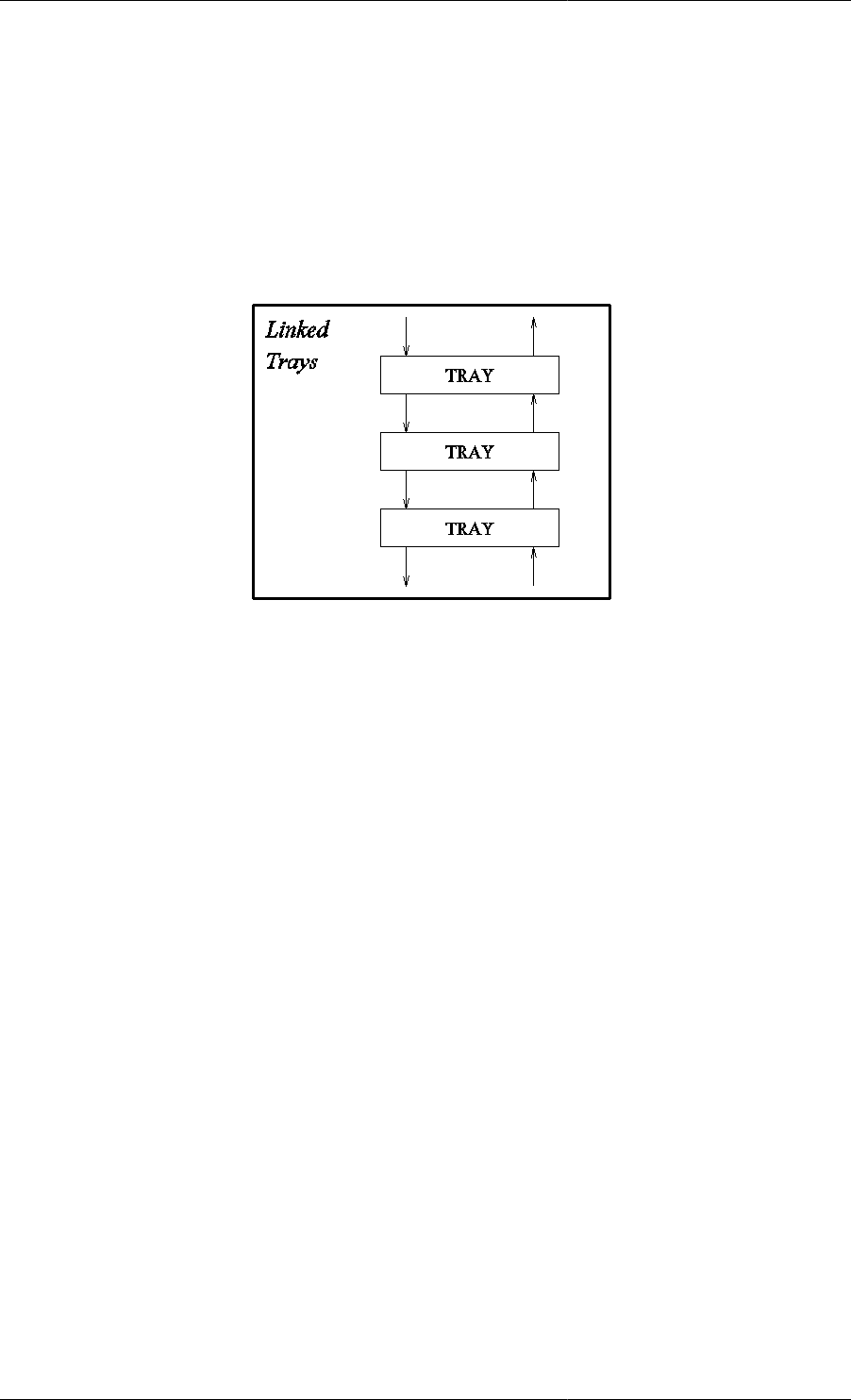
Arrays
27
Figure 4.1. Model for a series of linked trays.
# MODEL LinkedTrays
PARAMETER
NoTrays AS INTEGER
...
UNIT
Stage AS ARRAY(NoTrays) OF Tray
Here, the higher-level Model LinkedTrays contains an array, called Stage, of instances of Model Tray.
The Parameters and Variables within these instances can be referenced by combining the pathname and array
notations. For instance, an equation within the LinkedTrays model may refer to the Variable:
Stage(1).LiquidHoldup
Also, an equation may employ the Variable:
Stage(TopSection.NoTrays DIV 2).T
referring to the temperature at the middle tray of the top section of the column.
Referring to array elements
The contents of an array may be referenced in several different ways (consider the declarations given below:)
• Entire arrays can be referenced by using their names alone. For instance, Rho denotes the entire array of
component molar densities.
• Individual elements can be referenced by using the name of the array and an index to the element in
question enclosed in brackets. For one-dimensional arrays, this index should be an integer expression. For
instance, the second element of array Rho is Rho(2) while the element of array HoldUp before the last is
HoldUp(NoComp-1). For multi-dimensional arrays, the index is a list of such expressions, one for each
dimension. Thus, Nu(2,4) refers to the element on the second row and fourth column of array Nu.
• A subset of the elements in one or more dimensions can be referenced through the use of 'slice' notation. For
instance, Holdup(2:4) refers to the 2nd, 3rd and 4th elements of array Holdup. Nu(2:4,3:5) refers to
the slice of array HoldUp included between rows 2 to 4 and columns 3 to 5 (a 3 × 3 array in itself). Naturally,
Nu(1:NoComp,1:NoReac) is equivalent to Nu. Similarly, Nu(1:1,3:3) is equivalent to Nu(1,3).
• An entire dimension of an array can be referenced by leaving a blank. For instance, Nu(2,) refers to the entire
second row of array Nu, while Nu(,1:3) refers to columns 1 to 3. Naturally, Nu(,) is equivalent to Nu.
Arrays
28
PARAMETER
# Number of components
NoComp AS INTEGER
# Number of reactions
NoReact AS INTEGER
# Component molar densities
Rho AS ARRAY(NoComp) OF REAL
# Stoichiometric coefficient of component i in reaction j
Nu AS ARRAY(NoComp,NoReact) OF REAL DEFAULT 0
VARIABLE
# Component molar holdups
HoldUp AS ARRAY(NoComp) OF Moles
General rules for array expressions
A powerful concept in gPROMS is that of array expressions. Consider, for example, the algebraic expression:
x * y + w * z
If x, y, w and z are scalar Variables, then the above also corresponds to a scalar. However, in gPROMS, the
expression x * y + w * z is valid even if x, y and z are arrays provided they have the same dimensionality
and size. For example, if we have the declarations:
PARAMETER
n, m AS INTEGER
VARIABLE
x, y, z AS ARRAY (n,m) OF SomeQuantity
w AS SomeQuantity
then the expression x * y + w * z also represents a two-dimensional array of size n × m, the (i,j)th element
of which is equal to for i=1,..,n and j=1,..,m.
Although in the above examples, the gPROMS interpretation of the array expression coincided with the standard
mathematical one, this is not always the case. For example, the expressions x * y / z and w / x + z ^
y are also valid in gPROMS, representing two-dimensional arrays of size n × m, the (i,j)th elements of which are
equal to and respectively.
In general, consider an expression x ⊕ y where x and y are scalar or array expressions, and ⊕ is a binary arithmetic
operator (+, -, *, /, ^). This is a valid gPROMS expression if and only if it conforms to one of the four cases
listed below:
Case x y Dimensionality
of x ⊕ yInterpretation
of x ⊕ y
1 Scalar Scalar Scalar x ⊕ y
2 Array Scalar Same as x xijk... ⊕ y
3 Scalar Array Same as y x ⊕ yijk...
4 Array Array Same as x and y xijk... ⊕ yijk...
Clearly, case 4 is valid only if both x and y have exactly the same dimensionality and size.
Arrays
29
The above rules can be applied recursively to check the validity and to interpret expressions of arbitrary
complexity. At the lowest level, x and y will be (scalar) constants, scalar Parameters or Variables, or arrays of
Parameters or Variables, or slices of arrays of Parameters or Variables. For example, it can be verified that the
following is a valid two-dimensional expression of size 3 × 2:
3.23 / x(1:3, 4:5) * z(5:7, 1:2) + w(10:12, 2:3) + 4.13
Using arrays in equations
Elements of arrays (both Parameters and Variables) can be used in Equations as if they were individual Parameters
or Variables. For example, the equation that defines the concentration of component 2 in the liquid-phase CSTR
can be written as follows:
HoldUp(2) = C(2) * V ;
However, arrays can be used more effectively to declare several equations simultaneously (i.e. for all components).
This can be done in two different ways:
• implicitly :gPROMS automatically expands the equation
• explicitly :using the FOR construct
Writing implicit array equations
We have seen how array expressions can be formed by combining arrays of Parameters or Variables, or elements
or slices of these. By analogy, gPROMS allows the definition of array equations of the form:
Expression E = Expression F;
that are valid provided they conform to one of the following four cases:
Case E F Dimensionality
of E = F Interpretation
of E = F
1 Scalar Scalar Scalar E = F
2 Array Scalar Same as E Eijk... = F
3 Scalar Array Same as F E = Fijk...
4 Array Array Same as E and F Eijk... = Fijk...
Thus, in view of the following Variable definitions:
PARAMETER
...
VARIABLE
# Liquid phase volume
V AS Volume
# Component molar holdups
HoldUp AS ARRAY(NoComp) OF Moles
# Component concentrations
C AS ARRAY(NoComp) OF Concentration
...
the following is a valid equation:
HoldUp = C * V ;

Arrays
30
gPROMS automatically expands such equations into an set of equations. For example, if NoComp = 5, the
above will expand to:
HoldUp(1) = C(1) * V ;
HoldUp(2) = C(2) * V ;
...
HoldUp(5) = C(5) * V ;
Writing explicit array equations using the FOR
construct
We have seen how array equations can be written in an implicit manner by exploiting the array expression
capability of gPROMS. An alternative is to write array equations explicitly using a FOR construct that is similar to
that provided by most high-level programming languages. Thus, consider the equation describing the conservation
of component i in a multi-component buffer tank. This can be written mathematically as:
In gPROMS, this can be written in two completely equivalent ways, namely implicitly, in the form:
$M = Fin*Xin - Fout*X ;
or explicitly, in the form:
FOR i := 1 TO NoComp DO
$M(i) = Fin*Xin(i) - Fout*X(i) ;
END
The above are completely equivalent: which one you use depends entirely on your preference. However, situations
do exist in which the required equations cannot be described via implicit declaration, and the use of explicit FOR
constructs is essential.
The counter of a FOR construct (e.g. i in the above example) is an integer quantity that may be referenced only
by equations enclosed within the construct. The range of this counter must be specified in terms of any arithmetic
expressions involving integer constants, integer Parameters and/or integer arithmetic operators. Moreover, a step
increment may be specified. For instance,
FOR i := NoComp+1 TO 2*NoComp STEP 2 DO
...
END
will start by assign i a values of NoComp+1 and then will increment it by 2 until it exceeds 2*NoComp. If no
increment is specified, its value defaults to 1. A FOR construct may enclose an arbitrary number of equations of
any type -- including other For constructs. This allows nesting of For constructs to arbitrary depth; in such cases:
• each FOR construct must use a different name for its counter variable;
• any expression that appears within each For construct (including those defining its range and increment) may
involve the counters of any enclosing For constructs.
Zero-Length Arrays
For dynamic Arrays (i.e. Arrays whose bounds are set by an expression involving other Parameters), it is possible
to set the length of the Array to zero1. This is useful for two reasons:
• Greater modelling power and flexibility
1In principle, one could also set the length to zero explicity, but this would be pointless!

Arrays
31
Suppose we wish to create a simulation of a flowsheet containing a reactor and a mixer. The ability to set Arrays
to zero length means that we may use the same model for both the reactor and mixer. The NoReact Parameter
can be set to zero for the mixer instance, causing the model to revert to a mixer. This is because any equations
indexed over an Array of zero length are completely omitted from the Model instance, as are any terms indexed
over the Array. This means that the equations defining the rates of reaction, reaction constants and the rate terms
in the material and energy balance equations are all omitted, resulting in a smaller, more efficient formulation.
• More flexibility when defining flowsheet Topologies
Zero lengh Arrays mean that Models with dynamic Ports can be used without having to have at least one
connection.
32
Chapter 5. Intrinsic gPROMS
functions
Intrinsic gPROMS functions are used in equations to perform mathematical operations that would be difficult or
even impossible to declare using normal language operators. The gPROMS language contains two categories of
intrinsic functions, namely:
• Vector intrinsic functions - that take a single argument (scalar or array) and return a result of same dimensionality
as the input.
• Scalar intrinsic functions - that take multiple arguments (scalar or array) and return a scalar result.
Vector intrinsic functions
All vector intrinsic functions have the following characteristics:
• they take a single argument representing a scalar or array expression;
• they return a result of dimensionality and size identical to those of their argument.
The table below lists all vector functions that are recognised by gPROMS.
Table 5.1. Vector intrinsic functions
Identifier Function
ACOS The arccosine (in radians) of the argument
ASIN The arcsine (in radians) of the argument
ATAN The arctangent (in radians) of the argument
ABS The absolute value of the argument
COS The cosine of the argument (in radians)
COSH The hyperbolic cosine of the argument
EXP The exponential of the argument
INT The largest integer that does not exceed the argument
LOG The natural logarithm of the argument
LOG10 The logarithm to base 10 of the argument
SGN The sign of the argument
SIN The sine of the argument (in radians)
SINH The hyperbolic sine of the argument
SQRT The square root of the argument
TAN The tangent of the argument (in radians)
TANH The hyperbolic tangent of the argument
The result of each of the above functions is obtained by applying the corresponding operation to each element of
the argument. For example, consider the declarations:
PARAMETER
n, m AS INTEGER
Intrinsic gPROMS functions
33
VARIABLE
x, y, z AS ARRAY (n,m) OF SomeQuantity
w AS SomeQuantity
Then, x * SQRT(y+w) / SIN(z) is a valid expression representing an n × m array, the (i,j)th element of which is
equal to:
for i=1,..,n and j=1,..,m.
Scalar intrinsic functions
All scalar intrinsic functions have the following characteristics:
• they take an arbitrary number of arguments, each representing a scalar or array expression;
• they return a scalar result.
The table below lists all scalar functions that are recognised by gPROMS.
Table 5.2. Scalar intrinsic functions
Identifier Function
SIGMA The sum of all elements of all arguments
PRODUCT The product of all elements of all arguments
MIN The smallest of all elements of all arguments
MAX The largest of all elements of all arguments
The use of scalar intrinsic functions provides a powerful mechanism for writing complex mathematical expressions
in gPROMS. However, some care is necessary in their use with array equations written using automatic expansion.
Consider, for instance, a mixing tank receiving a number of multi-component input streams. The conservation
equation for component i can be written mathematically as:
In gPROMS, this can be written as:
FOR i := 1 TO NoComp DO
$M(i) = SIGMA(Fin*Xin(1:NoInput,i)) - Fout*X(i) ;
END
Note that the 'alternative' formulation using automatic expansions:
$M = SIGMA(Fin*Xin) - Fout*X ;
is actually incorrect since:
• the expression Fin*Xin violates the conformance rules for array expressions;
• the expression SIGMA(Fin*Xin) is a scalar, not a vector of length NoComp.
A complete model for the mixing tank, illustrating many of the important points highlighted above, is given in
the gPROMS code below.

Intrinsic gPROMS functions
34
Example 5.1. Multi-component mixing tank Model entity
# MODEL MixingTank
PARAMETER
NoComp, NoInput AS INTEGER
CrossSectionalArea AS REAL
Rho AS ARRAY(NoComp) OF REAL
ValvePosition AS REAL
VARIABLE
Fin AS ARRAY(NoInput) OF Flowrate
Xin AS ARRAY(NoInput,NoComp) OF MassFraction
Fout AS Flowrate
X AS ARRAY(NoComp) OF MassFraction
M AS ARRAY(NoComp) OF Mass
TotalHoldup AS Mass
TotalVolume AS Volume
Height AS Length
EQUATION
# Mass balance
FOR i := 1 TO NoComp DO
$M(i) = SIGMA(Fin*Xin(,i)) - Fout*X(i) ;
END
# Mass fractions
TotalHoldup = SIGMA(M) ;
M = X * TotalHoldup ;
# Calculation of liquid level from holdup
TotalVolume = SIGMA(M/Density) ;
TotalVolume = CrossSectionalArea * Height ;
Fout = ValvePosition * SQRT ( Height ) ;
As an additional example, the gPROMS code below illustrates the use of nested FOR constructs to implement the
matrix-matrix multiplication operation between matrices A (n × m) and B (m × q), resulting in a matrix C (n × q).

Intrinsic gPROMS functions
35
Example 5.2. Matrix multiplication Model entity
# MODEL MatrixMultiplication
PARAMETER
n, m, q AS INTEGER
VARIABLE
A AS ARRAY (n, m) OF SomeQuantity
B AS ARRAY (m, q) OF SomeQuantity
C AS ARRAY (n, q) OF SomeQuantity
EQUATION
FOR i := 1 TO n DO
FOR j := 1 TO q DO
C(i,j) = SIGMA(A(i,)*B(,j))
END
END

36
Chapter 6. Conditional Equations
The physical behaviour of many process operations is described in terms of discontinuous equations, the form of
which depends on the current variable values and, in certain cases (e.g. involving hysteresis effects), also some
aspects of the past history of the system.
gPROMS provides two powerful facilities for describing discontinuous equations in Model Entities. As
background it helps to understand State-Transition Networks (STNs which form a general basis for modelling
discontinuities:
• The CASE construct: this provides a direct description of general STNs in the gPROMS language. For example:
# An example of the CASE conditional construct - for flow over a weir.
SELECTOR
WeirFlag AS (Above, Below)
...
EQUATION
...
CASE WeirFlag OF
WHEN Above : FlowOut = 1.84 * (Rho/MolecularWeight)
* WeirLength * ABS(Height-WeirHeight)^1.5 ;
SWITCH TO Below IF Height < WeirHeight ;
WHEN Below : FlowOut = 0 ;
SWITCH TO Above IF Height > WeirHeight ;
END # Case
...
• The IF construct may be used to described a special form of reversible symmetric STNs that occur very
frequently in practical applications. For example:
# An example of the IF conditional construct - for flow over a weir.
IF Height > WeirHeight THEN
FlowOut = 1.84 * (Rho/MolecularWeight)
* WeirLength * ABS(Height-WeirHeight)^1.5 ;
ELSE
FlowOut = 0 ;
END # If
It should be noted that, in Model entites, we are interested in discontinuities that arise because of the intrinsic
behaviour of the system and not as a result of external discrete actions imposed on the system by its environment
or its operators (e.g. the opening and closing of manual valves).See: Defining Schedules .
Using State-Transition Networks to model
discontinuities
Discontinuities in the description of the physical behaviour of process systems may arise in different ways such as:
• transitions from laminar to turbulent flow;
• reversal of the direction of flow;
• appearance and disappearance of thermodynamic phases;
• equipment failure;
and many others.
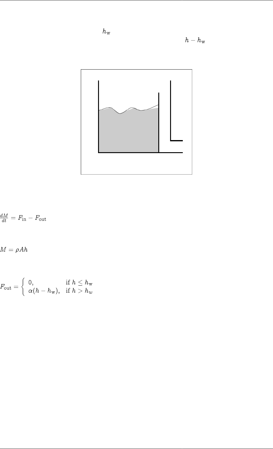
Conditional Equations
37
State-Transition Networks (STNs) provide a general way of describing discontinuous systems. This concept is
best introduced via an example. Consider the vessel depicted in the figure below. When the level of liquid in the
vessel, h, is below the height of the weir, , no outflow is observed. When, on the other hand, the liquid level
exceeds the weir height, the rate of outflow is assumed to be proportional to .
Figure 6.1. Vessel with overflow weir
The mathematical model of the transient behaviour of this system can be written as follows:
Mass balance
Calculation of liquid level in the tank
Characterisation of the output flowrate
We note that two different sets of equations are needed to describe the behaviour of this system depending on
whether the level of the liquid is above or below the weir. Thus, the system may exist in two distinct states, Flow
and NoFlow, that correspond respectively to whether or not liquid flows over the weir. At any particular time, the
system is in exactly one of these states. However, transitions from one state to the other will occur instantaneously
if certain conditions are met. For example, if, while the system in state NoFlow, the height of the liquid exceeds
that of the weir, the system will instantaneously jump to state Flow. Conversely, if, while the system in state Flow,
the height of the liquid drops below that of the weir, the system will instantaneously jump to state NoFlow.
The above situation can be represented graphically in terms of an STN as shown in the figure below. The two
circles (or ellipses) denote the two possible system states; for convenience, the form of the discontinuous equation
(involving the characterisation of the output flowrate) in each of these states is also shown within these circles.
On the other hand, the mass balance and liquid level equations do not appear in this figure as their form is
independent of the state the system is in. The transitions between the two states are also shown in figure as arrows
connecting the corresponding circles. Again for convenience, each arrow is labelled with the logical condition that
triggers the corresponding transition.
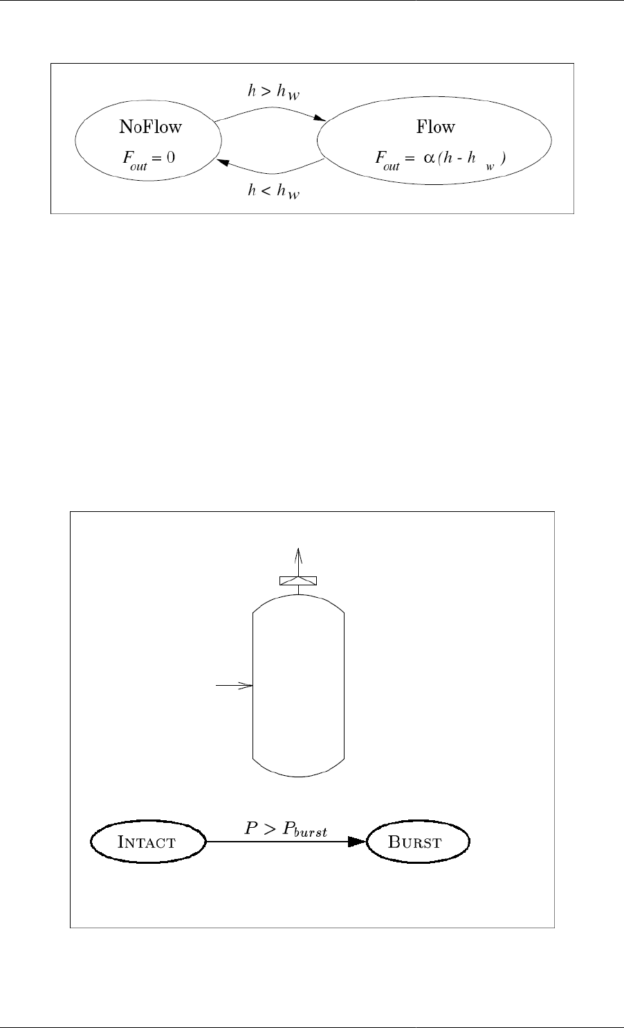
Conditional Equations
38
Figure 6.2. STN representation of vessel with overflow weir
The STN represents a reversible, symmetric discontinuity because:
• the system may jump from either of the two states to the other and,
• the logical condition for one the two transitions is the exact negation of that for the other.
An example of a different type of discontinuity is shown in the figure below. Here, a vessel is fitted with a bursting
disc. The disc can either be intact (with no gas flow from the vessel) or burst (with gas venting from the disc to
the flare stack). This gives rise to two distinct system states (Intact and Burst). As in the previous example, some
of the equations that describe the system take a different form in each of these states while some others remain
unchanged. A transition from Intact to Burst occurs when the pressure in the vessel rises above the set pressure and
the disc shatters. The resulting outflow of gas will then cause an reduction of the pressure which, eventually, may
drop below its set value. However, the system cannot return to its Intact state once the disc has shattered - unless
it is repaired as a result of an external action. Consequently, this is an example of an irreversible discontinuity.
Figure 6.3. Vessel with bursting disc
A final example is that of a vessel fitted with a safety relief valve (see figure below). The valve can be either open
or closed, which again gives rise to two system states (Open and Closed). A transition from the Closed to the
Open state occurs when the pressure in the vessel rises above the set pressure, while a transition from the Open
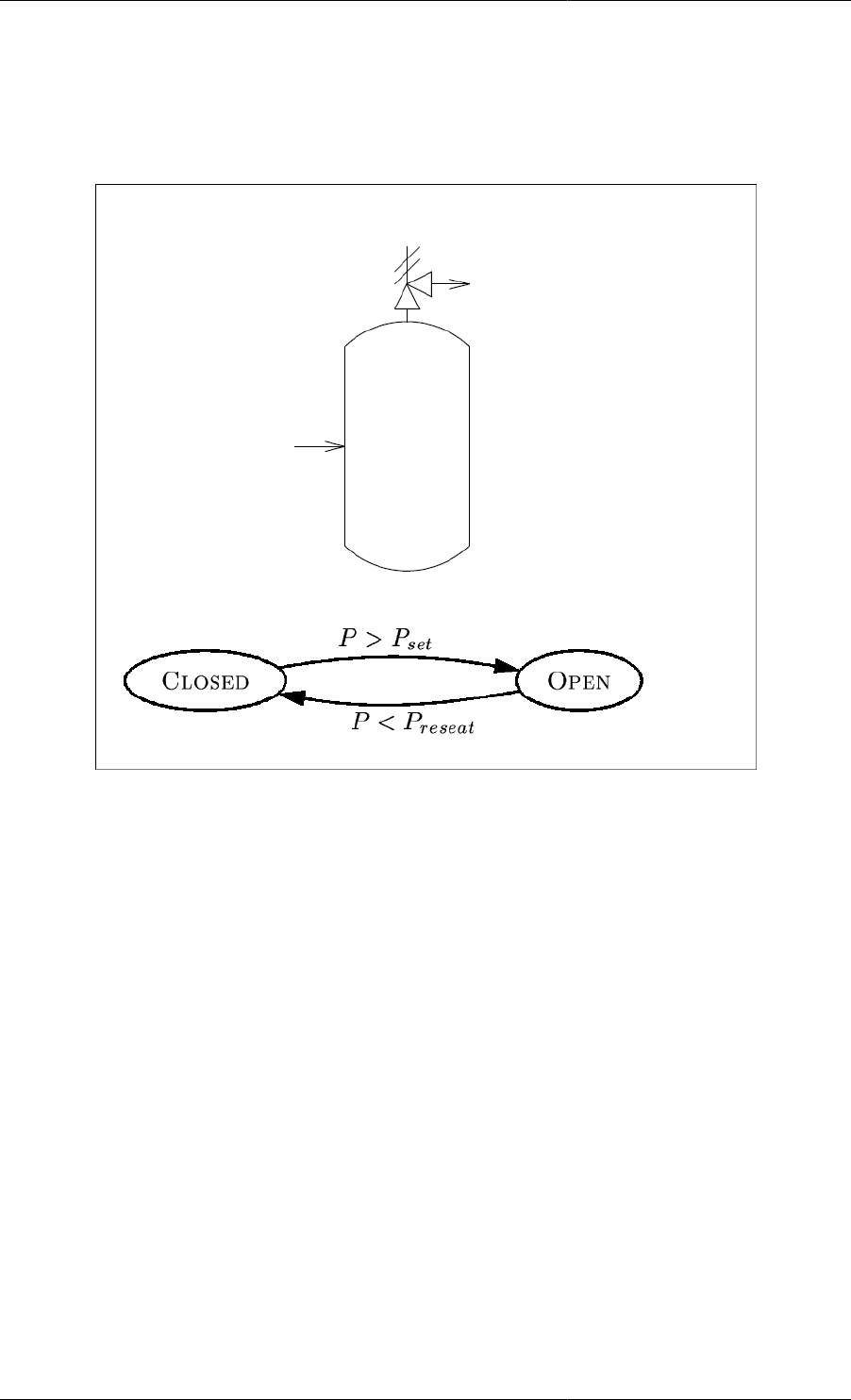
Conditional Equations
39
to the Closed state occurs when the pressure falls below a (lower) reset pressure. This is a reversible, asymmetric
discontinuity because, although there are possible transitions in both directions, the two transition conditions are
not the exact negation of each other.
Figure 6.4. Vessel with safety relief valve
We note that, in all three examples, only a subset of the model equations are directly related to the discontinuity
and change from one state to another. The rest of the equations remain unchanged regardless of the state the system
is in. Summarising, a discontinuity in the physical behaviour of a system gives rise to a number of possible system
states. Naturally, at any given time, the system can be in exactly one of these states. Some of the equations that
determine the behaviour of the system hold irrespective of the system state. However, some others take a different
form in each state. Transitions between the different states take place when certain logical conditions are satisfied.
A system may exhibit more than one physical discontinuity described by multiple STNs and/or more than two
states within the same STN. For instance, a more detailed model of the weir vessel would seek to characterise the
nature of the fluid flow in the outlet pipe. This would give rise to three system states, i.e. Laminar, Turbulent
and Choked. A complex STN for a hypothetical system is depicted in the figure below. Here, the system exhibits
two separate physical discontinuities involving three and two possible states respectively.
• Equations 1, 2 and 3 remain unaffected by the discontinuities and are valid throughout.
• Equation 4 is affected by the first discontinuity and is written as 4a, 4b or 4c, depending on the state of the
system.
• Equations 5 and 6 are affected by the second discontinuity and are written as 5a, 5b and 6a, 6b in each of the
two states respectively.
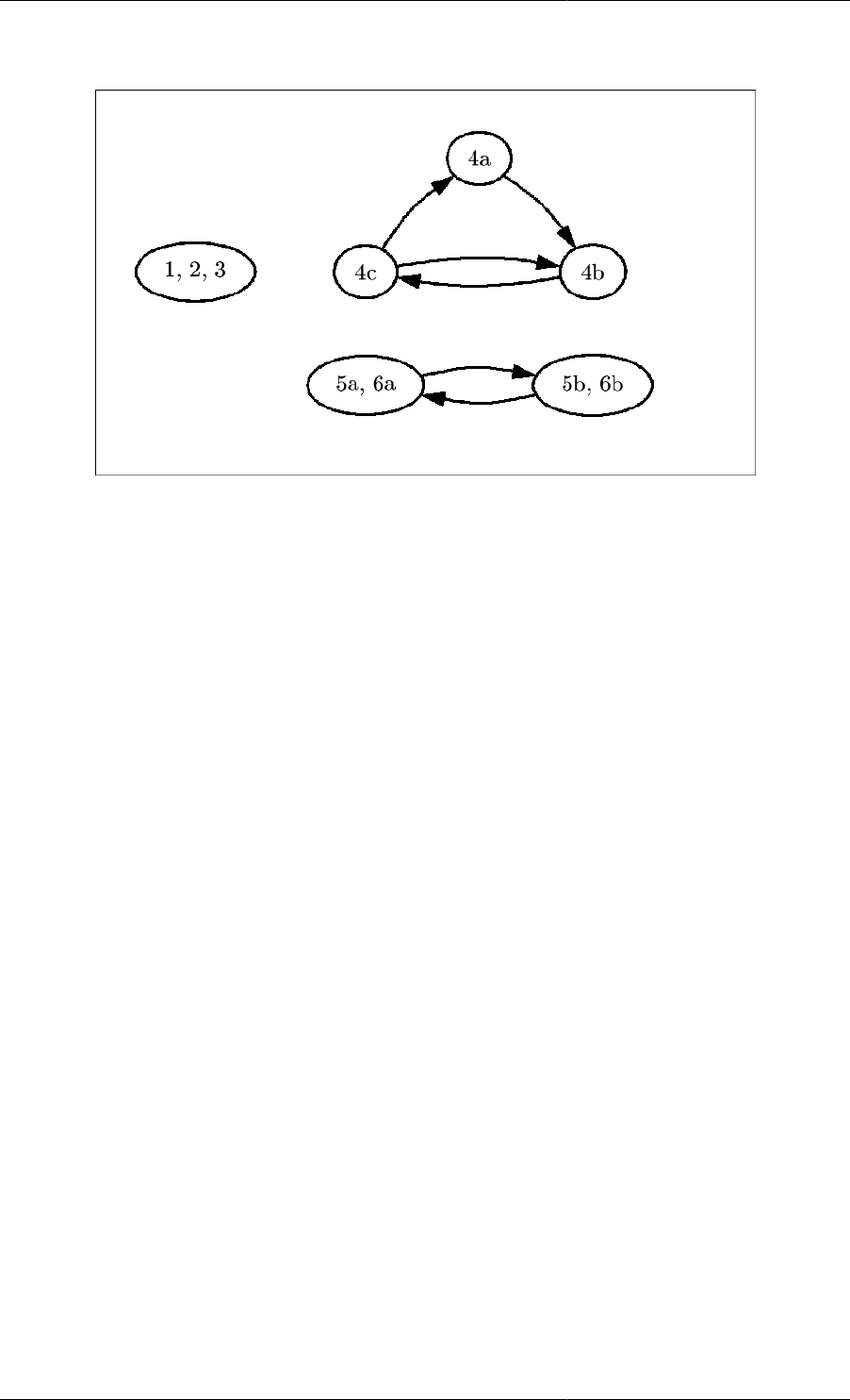
Conditional Equations
40
Figure 6.5. Hypothetical system model.
The Case conditional construct
The gPROMS example below illustrates the use of the CASE construct in a Model of a vessel with a bursting disc.

Conditional Equations
41
Example 6.1. Model entity for a vessel equipped with a bursting disc
# MODEL VesselWithDisc
PARAMETER
R AS REAL DEFAULT 8.314 # J/K.mol
VesselVolume AS REAL
BurstPressure AS REAL
AtmPressure AS REAL
DiscConstant AS REAL
VARIABLE
FlowIn, FlowOut AS MolarFlowrate
ReliefFlow AS MolarFlowrate
HoldUp AS Moles
T AS Temperature
Pressure AS Pressure
SELECTOR
DiscFlag AS (Intact, Burst) DEFAULT Intact
EQUATION
# Mass balance
$HoldUp = FlowIn - FlowOut - ReliefFlow ;
# Ideal gas law
Pressure * VesselVolume = Holdup * R * T ;
CASE DiscFlag OF
WHEN Intact : ReliefFlow = 0 ;
SWITCH TO Burst IF Pressure > BurstPressure ;
WHEN Burst : ReliefFlow = DiscConstant * SQRT(R*T) ;
END # Case
# Energy balance
. . . . . . . . . . . . . . . . . . . . . .
We note that this Model presents two features of interest:
1. A SELECTOR section is used for the declaration of the system states that arise from the discontinuity:
SELECTOR
DiscFlag AS (Intact, Burst) DEFAULT Intact
declares an enumerated ("selector'') variable, DiscFlag that can take only two values, namely Intact
or Burst, with the former being the default value at the start of the simulation (see below). The default
specification is optional and may be omitted.
2. The Model equations include the CASE equation:
CASE DiscFlag OF
WHEN Intact : ReliefFlow = 0 ;
SWITCH TO Burst IF Pressure > BurstPressure ;
WHEN Burst : ReliefFlow = DiscConstant * SQRT(R*T) ;
END # Case
that defines
• the equation(s) that hold in each state, and

Conditional Equations
42
• the logical condition(s) that trigger transitions between states.
More precisely, the above CASE construct states that:
• When the system is in the Intact state, the relief flow is zero. The system remains in this state as long as
the pressure in the vessel is lower than the bursting pressure of the disc. When it exceeds that limit, a transition
to the Burst state is initiated.
• When the system is in the Burst state, the relief flow is calculated from a sonic flow relationship. The form of
the equation presented here is only for illustration purposes. A more detailed form would take account of various
other effects, including the transition from sonic to sub-sonic flow as the pressure in the vessel decreases. As
this is an irreversible discontinuity, there is no transition going back to the Intact state.
Some general considerations when using the Case
construct
In general, a Case equation comprises two or more clauses, one for each possible value of the corresponding
Selector variable. Each of the clauses comprises a list of equations, followed by an optional list of Switch
statements that define transitions from the current clause to other clauses of the Case equation. The list of equations
may include any combination of simple, array and even conditional equations - including not only Case constructs
but also If constructs. The latter feature allows nesting of conditional equations to arbitrary depth. It is important,
however, to observe the following restrictions:
• The number of equations in each clause of a Case construct must be the same.
• Each Selector variable may be used in only one Case construct.
The reason for the first restriction is obvious if one considers that the number of variables in the Model remains
unaffected by the occurrence of transitions. Consequently, any change in the number of equations would lead to
an over- or under-specified problem. The second restriction is imposed to avoid inconsistencies that might arise
from different Case attempting to force the same Selector variable to switch to different values at the same time.
Initial values of Selector variables
Another important consideration concerning the use of Case equations is that, in order for a simulation experiment
to commence, the initial (i.e. at time t=0) value of the corresponding Selector variable has to be specified. Thus,
in our example the user must specify whether or not the disc is initially intact or not. This information cannot be
inferred automatically by gPROMS: the mere fact that the initial system pressure is below the bursting value does
not necessarily mean that the disc is intact - it may well have burst as a result of earlier operation! If a default
value has been specified for the Selector variable in the Model, then this will be used as its initial value for the
simulation. More generally, this value can be set or overridden for individual simulation experiments. This is done
in the INITIALSELECTOR section of the Process (or Model). For instance:
UNIT T101 AS VesselWithDisc
...
INITIALSELECTOR
T101.DiscFlag := T101.Burst ; # Disc is initially burst
INITIAL
T101.Pressure - T101.BurstPressure = -1E5 ;
...
Thus, in this example, we specify the disc as being burst despite the fact that the initial pressure of the system is
specified to be 1 bar below the bursting pressure. From the syntactical point of view, it is important to note the use
of the full pathname T101.Burst to denote the value of the SELECTOR variable. A specification of the form:
UNIT T101 AS VesselWithDisc
...
SELECTOR

Conditional Equations
43
T101.DiscFlag := Burst ; # Disc is initially burst
would be meaningless as the identifier Burst is not known directly to the Process section - it is defined only
within the context of MODEL VesselWithDisc of which T101 is an instance.
The If conditional construct
Case constructs provide a general way in which STNs of arbitrary complexity can be described in the gPROMS
language. However, reversible and symmetric discontinuities are by the far the most commonly encountered
discontinuities in industrial processing systems. Although such discontinuities can be declared using Case
constructs, gPROMS provides the alternative IF conditional construct specifically as a convenient shorthand for
the declaration of this common type of discontinuity.
Example 6.2. Model entity for a vessel equipped with an overflow weir
# MODEL VesselWithWeir
PARAMETER
Rho AS REAL
MolecularWeight AS REAL
CrossSectionalArea AS REAL
WeirHeight AS REAL
WeirLength AS REAL
VARIABLE
HoldUp AS Mass
FlowIn, FlowOut AS MassFlowrate
Height AS Length
EQUATION
# Mass balance
$HoldUp = FlowIn - FlowOut ;
# Calculation of liquid level from holdup
Holdup = CrossSectionalArea * Height * Rho ;
IF Height > WeirHeight THEN
# Francis formula for flow over a weir
FlowOut = 1.84 * (Rho/MolecularWeight)
* WeirLength * ABS(Height-WeirHeight)^1.5 ;
ELSE
FlowOut = 0 ;
END # If
The gPROMS example above demonstrates the use of an IF equation in the declaration of a Model for a vessel
fitted with an overflow weir.
IF Height > WeirHeight THEN
# Francis formula for flow over a weir
FlowOut = 1.84 * (Rho/MolecularWeight)
* WeirLength * ABS(Height-WeirHeight)^1.5 ;
ELSE
FlowOut = 0 ;
END # If
A logical condition (in this case, Liquid_Level > Weir_Height) is used to choose between two clauses,
each comprising a list of equations. If the logical condition is satisfied, the equations declared in the first clause are

Conditional Equations
44
included in the system model, otherwise the equations of the second clause are included. As with Case equations,
the number of equations in each clause must be the same. As If equations are a special case of Case equations,
there is always a Case equation that achieves the same result. For instance, the IF equation for the overflow weir
is equivalent to the following CASE equation:
SELECTOR
WeirFlag AS (Above, Below)
...
EQUATION
...
CASE WeirFlag OF
WHEN Above : FlowOut = 1.84 * (Rho/MolecularWeight)
* WeirLength * ABS(Height-WeirHeight)^1.5 ;
SWITCH TO Below IF Height < WeirHeight ;
WHEN Below : FlowOut = 0 ;
SWITCH TO Above IF Height > WeirHeight ;
END # Case
...
A subtle difference between If and Case equations is that, in If equations, the initially active state of the system
cannot be specified explicitly by the user. Instead, it is determined automatically by the initialisation calculation,
which ensures that the consistent initial values obtained satisfy both the logical condition and the equations in
this state. However, the solution of non-linear systems involving such conditional equations is far from trivial.
Moreover, it is possible that a valid solutions exists in either clause of an If equation; in such cases, the solution
found will depend on the initial guesses and the numerical method employed during the initialisation procedure.
In view of these factors, it may sometimes be preferable to use a Case equation instead, especially if the initial
state of the system is known a priori.

45
Chapter 7. Distributed Models
A significant number of unit operations in chemical or biochemical processes take place in distributed systems in
which properties vary with respect to one or more spatial dimensions as well as time. For instance, a tubular reactor
is described in terms of parameters and variables that, in addition to time, depend on the axial and radial position
within the reactor (e.g. T(z,r,t) etc). Other common examples of distributed unit operations include packed bed
absorption, adsorption and distillation columns and chromatographic columns. In other unit operations, material
properties are characterised by probability density functions instead of single scalar values. Examples include
crystallisation units and polymerisation reactors, in which the size of the crystals and the length of the polymer
chains respectively are described in terms of distribution functions. The form of the latter may also vary with both
time and spatial position. In fact, most complex processes involve a combination of distributed and lumped unit
operations. The equations that determine the behaviour of such unit operations are typically systems of integral,
partial differential, ordinary differential and algebraic equations (IPDAEs).
To develop a process model that considers distributed quantities we need to consider
• The definition of distributed Model entites
• Declaring Distribution domains
• Declaring Distributed Variables
• Defining Distributed Equations
• Introducing Partial Differential Equations
• Introducing Integral Expressions
• Explicit and implicit Distributed Equations
• Providing Boundary conditions
• Requirements for specifying discretisation methods and non-uniform grids in Process entites.
Distributed modelling is explained by reference to the gPROMS Project tubular.gPJ that can be found in the
installation. You can access this by clicking on the Browse Examples button on the gPROMS Toolbar and then
navigating to "General capabilities\Other examples\tubular.gPJ".
The tubular model is illustrated in the figure below; which shows a tubular reactor used to carry out a liquid-
phase exothermic chemical reaction. The intensive properties of the fluid in the tube vary with both axial and
radial position as well as with time. The reactor is surrounded by a well-mixed cooling jacket. Thus, the intensive
properties of the cooling medium are assumed to be uniform throughout the jacket but may still vary with time.
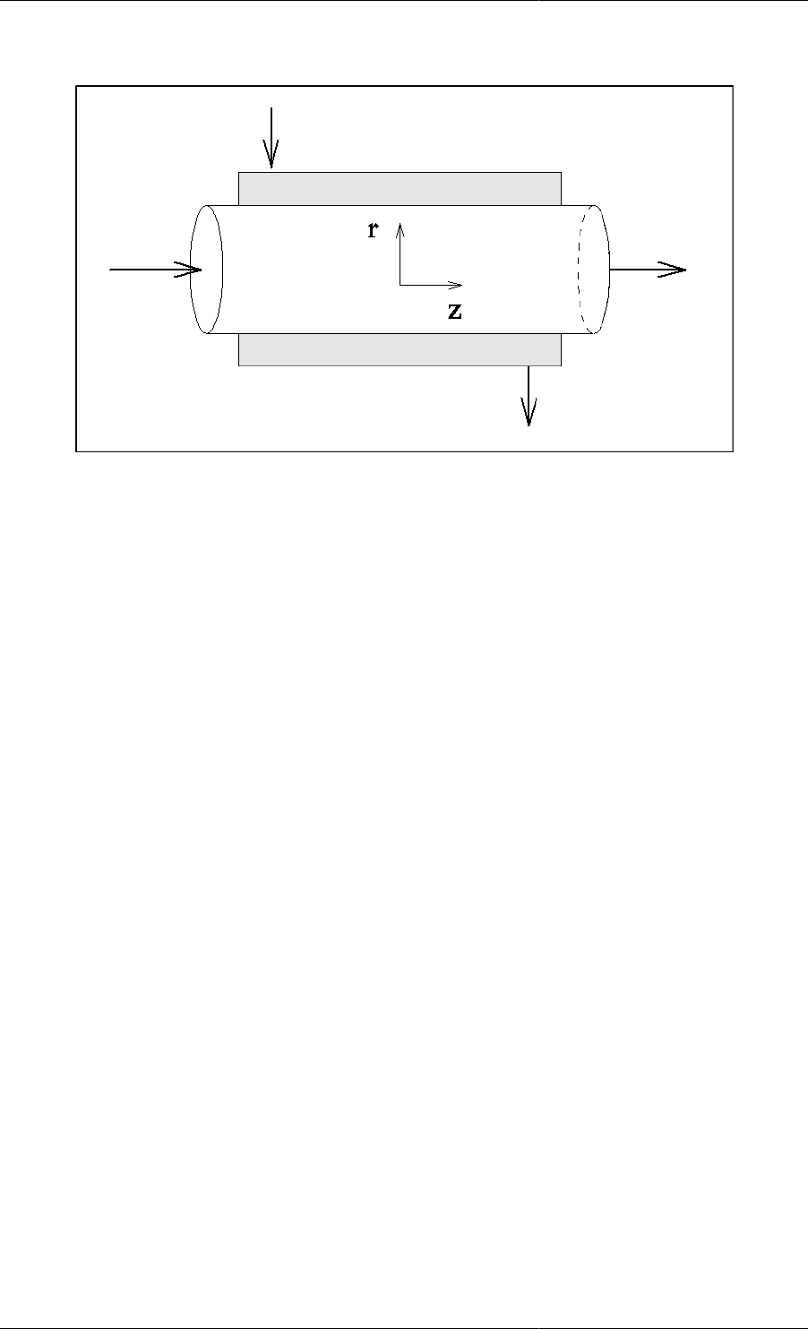
Distributed Models
46
Figure 7.1. Tubular flow reactor
Declaring Distribution Domains
The temperature in the reactor varies with time, axial and radial position (T(z,r,t)). Although all Variables that
are declared within a Model are automatically assumed to be functions of time, variations over other distribution
domains (in this case the axial and radial domains, z and r respectively) have to be specified explicitly. Distribution
domains are declared in the DISTRIBUTION_DOMAIN section of a Model. The gPROMS code below shows how
two such domains called Axial and Radial are declared in a Model of a tubular reactor. The extents of both
domains are specified in terms of two Model Parameters, namely ReactorLength and ReactorRadius,
respectively.

Distributed Models
47
Example 7.1. Parameter and DISTRIBUTION_DOMAIN
sections for a Model of a tubular reactor
# MODEL TubularReactor
PARAMETER
# Number of components
NoComp AS INTEGER
# Geometrical parameters
ReactorRadius,
ReactorLength AS REAL
# Transport properties
# Axial and radial mass diffusivities
Dz, Dr AS REAL
# Axial and radial thermal conductivities
Kz, Kr AS REAL
# Reaction
# Stoichiometric coefficients
Nu AS ARRAY(NoComp) OF INTEGER
...
DISTRIBUTION_DOMAIN
Axial AS [ 0 : ReactorLength ]
Radial AS [ 0 : ReactorRadius ]
...
In general, the lower and upper bounds of the range of each Distribution Domain can be specified in terms of
real expressions involving real constants and/or real parameters. Thus, the following are also valid Distribution
Domain declarations:
# Normalised axial and radial domains
DISTRIBUTION_DOMAIN
z AS [ 0 : 1 ]
r AS [ 0 : 1 ]
# Axial domain encompassing the second half of the reactor
DISTRIBUTION_DOMAIN
HalfAxial AS [ ReactorLength/2 : ReactorLength ]
Declaring Distributed Variables
A Model may involve Variables with different degrees of distribution. For instance, in the tubular reactor example,
the temperature of the fluid and the concentrations of the various chemical components within the tube are indeed
functions of both the radial and axial positions. However, the wall temperature is a function only of axial position,
while the temperature in the cooling jacket does not vary with spatial position at all. Note that all of these variables
are also functions of time, as is always the case with Variables in gPROMS.

Distributed Models
48
Example 7.2. Variable section for a Model of a tubular reactor
# MODEL TubularReactor
PARAMETER
...
DISTRIBUTION_DOMAIN
...
VARIABLE
# Reactor temperature
T AS DISTRIBUTION(Axial,Radial) OF Temperature
# Concentrations
C AS DISTRIBUTION(NoComp,Axial,Radial) OF Concentration
# Feed composition
Cin AS ARRAY(NoComp) OF Concentration
# Cooling jacket temperature
Tc AS Temperature
...
• Variable T, which represents the temperature in the reactor, is declared as a DISTRIBUTION over the two
continuous domains, Axial and Radial.
• Variable C, representing the concentrations of the various components in the reactor, is clearly an array of
variables distributed over both the radial and axial domains. In gPROMS, an array of distributions is represented
by adding one or more extra domains to a Distribution. These domains are discrete in nature and they do not
need to be declared explicitly in the DISTRIBUTION_DOMAIN section - a simple integer expression in the
VARIABLE declaration suffices.
• For example, the concentration variable C ranges from 1 to NoComp, the number of components in the system),
as well as over the two continuous domains, Axial and Radial.
• Variable Cin, representing the concentrations of the various components in the feed, is distributed over the
discrete domain of components only. Although this could be written as:
Cin AS DISTRIBUTION(NoComp) OF Concentration
here we prefer to use the Array concept as it is more natural.
• Variable Tc, representing the temperature in the cooling jacket, is solely a function of time.
In essence, then, Distribution is a generalisation of the Array concept that allows a Variable to vary over both
continuous and discrete domains. Conversely, an Array is a special case of a Distribution that is used to declare
Variables that are distributed over discrete domains only. Although Distributions can also be used for that purpose,
the Array construct is retained for compatibility with other programming languages. Note that it is not permitted
to declare a Variable that is distributed over two domains of the same type. For instance, a temperature field over
a square domain cannot be declared as:
T AS DISTRIBUTION(XDomain,XDomain) OF Temperature
The reason for this restriction is that a more complex syntax would then be required in order to distinguish between
partial derivatives of the Variable T with respect to the first and the second independent Variables. This does not
actually lead to any real restriction in functionality: Variable T could easily be declared as:
T AS DISTRIBUTION(XDomain,YDomain) OF Temperature

Distributed Models
49
where XDomain and YDomain are declared to be identical:
DISTRIBUTION_DOMAIN
XDomain, YDomain AS [ 0.0 : Length ]
This also has the advantage of allowing different discretisation methods to be applied to each of the two domains.
Defining Distributed Equations
As with lumped models, Distributed Variables in Models are related through sets of equations that are declared in
the Equation section. For example, consider the following declarations within a Model of a tubular reactor:
# MODEL TubularReactor
PARAMETER
# Geometrical parameters
ReactorRadius,
ReactorLength AS REAL
# Heat transfer parameters
U, S AS REAL
...
DISTRIBUTION_DOMAIN
Axial AS [ 0 : ReactorLength ]
Radial AS [ 0 : ReactorRadius ]
VARIABLES
Vz, Vr AS DISTRIBUTION (Axial, Radial) OF Velocity
T AS DISTRIBUTION (Axial, Radial) OF Temperature
Twall AS DISTRIBUTION (Axial) OF Temperature
Tc AS Temperature
In this case, Vz * T is a valid expression that is distributed over the entire Axial and Radial domains.
Similarly,
U * S * ( T(,ReactorRadius) - Tc )
is also a valid expression distributed over the entire Axial domain. In some cases, it may be desired to define
an expression over part of a particular domain. This can be achieved by using slices of distributions, very similar
to the slice concept for arrays. For example, the expression:
Vz(0:ReactorLength/2, ) * T(0:ReactorLength/2, )
is distributed over the first half of the Axial domain and the entire Radial domain. The mathematical modelling
of distributed systems often requires a rather subtle distinction between the entire domain including its boundaries,
and the domain excluding all or part of its boundaries. In standard mathematical terminology, these two kinds of
domain are referred to as 'closed' and 'open' respectively. One major reason for introducing this distinction is that
some of the equations (e.g. conservation laws) may hold only in the interior of a domain while being replaced by
appropriate boundary conditions on the domain boundaries. To allow the modellers to make the above distinction,
gPROMS employs the notation shown in the table below.
Table 7.1. Closed and open domain notation
Mathematical notation Interpretation gPROMS notation
[a,b] a : b

Distributed Models
50
Mathematical notation Interpretation gPROMS notation
(a,b] a|+ : b
[a,b) a : b|-
(a,b) a|+ : b|-
Thus, the Variable slice Vz(0|+:ReactorLength, 0|+:ReactorRadius|-) denotes the values Vz(z,r)
for the values of z and r satisfying 0 < z <= ReactorLength and 0 < r < ReactorRadius. We conclude by
formally defining the validity of expressions involving distributed Variables. Consider an expression x ? y where
x and y are scalar or distributed expressions, and ? is a binary arithmetic operator (+, -, *, /, ^). Then this is a
valid gPROMS expression if and only if it conforms to one of the four cases listed below:
Case x y Dimensionality
of x ? y Interpretation
of x ? y
1. Scalar Scalar Scalar x ? y
2. Array Scalar Same as xx_{...} ? y
3. Scalar Distribution Same as yx ? y_{...}
4. Distribution Distribution Same as x and yx_{...} ? y_{...}
Clearly, case 4 is valid only if both x and y are distributed over exactly the same domains, also taking account of
whether each of these is open or closed. For example, the following is a valid expression:
Vz(0|+:ReactorLength,ReactorRadius|-) * Twall(0|+:ReactorLength)
that is distributed over the Axial domain which is open on (i.e does not include) the left boundary (z=0) but
closed on (i.e includes) the right boundary (z=ReactorLength). On the other hand, the expression:
Vz(0|+:ReactorLength,ReactorRadius) * T(0:ReactorLength,ReactorRadius)
is invalid because the first operand Vz is distributed over a domain that is open on the left and closed on the right,
while the second operand T is distributed over a domain that is closed on both ends.
Introducing Partial Differential Equations
Partial differentiation of a distributed Variable or expression with respect to a domain over which it is distributed
is achieved with the PARTIAL operator. Its syntax is of the form:
PARTIAL ( Expression, DistributionDomain )
where Expression is a general expression and DistributionDomain is one of the distribution domains in the system.
Normally, at least one of the Variables involved in the differentiated expression will be distributed over the
specified domain, otherwise the result of the differentiation will be zero. Partial operators may also be nested. The
result of a Partial operator is generally a distributed expression that has exactly the same degree of distribution
as the Expression being differentiated.
In the gPROMS language it is possible to write expressions involving both
• First order partial derivatives
• Higher order partial derivatives
First order partial derivatives
Considering the example presented in Distributed Equations, the following are examples of valid first order partial
derivative expressions:
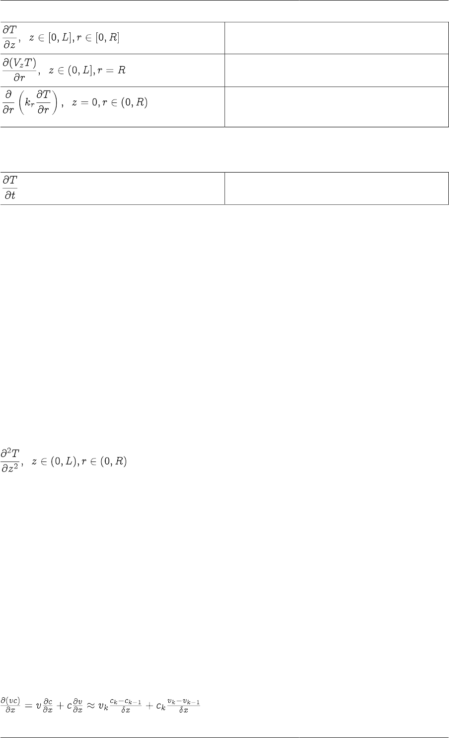
Distributed Models
51
PARTIAL(T,Axial)
PARTIAL(Vz(0|+:L, ReactorRadius) *
T(0|+:L,ReactorRadius),Radial)
PARTIAL(Kr(0,0|+:ReactorRadius|-) *
PARTIAL(T(0,0|
+:ReactorRadius|-),Radial),Radial)
Note that the partial differentiation operator with respect to time is denoted by symbol $ rather than the operator
PARTIAL. Thus:
$T
There are two reasons for this:
• The use of $ is consistent with the time derivative operator in lumped systems.
• The numerical solution methods in gPROMS treat the time domain quite differently to the explicitly declared
distribution domains.
Higher-order partial derivatives
PARTIAL operators may be nested to express higher order derivatives as follows:
PARTIAL( Expression, PARTIAL( Expression, DistributionDomain ), DistributionDomain )
Alternatively, the following abbreviated form may be used:
PARTIAL ( Expression, DistributionDomain, DistributionDomain )
Here differentiation first takes place with respect to the first domain, then with respect to the second etc. For
example:
PARTIAL(T(0|+:ReactorLength|-,0|+:ReactorRadius|-,Axial,Axial)
Conservative discretisation formulae for partial
derivatives
There are two main approaches to discretise a partial derivative of an expression (for a given numerical method):
1. Apply the chain rule to reduce the term to a series of derivatives of a single variable and apply the discretisation
scheme to each simple derivative
2. Apply the discretisation scheme directly to the complex derivative
A very common example of this is the convection term in conservation equations. The product of some conserved
quantity, c, is multiplied by a bulk velocity v and the partial derivative with respect to position, x, is required. If
the first approach above is applied, as illustrated below, then the numerical solution may contain errors resulting
in the quantity c not being conserved.
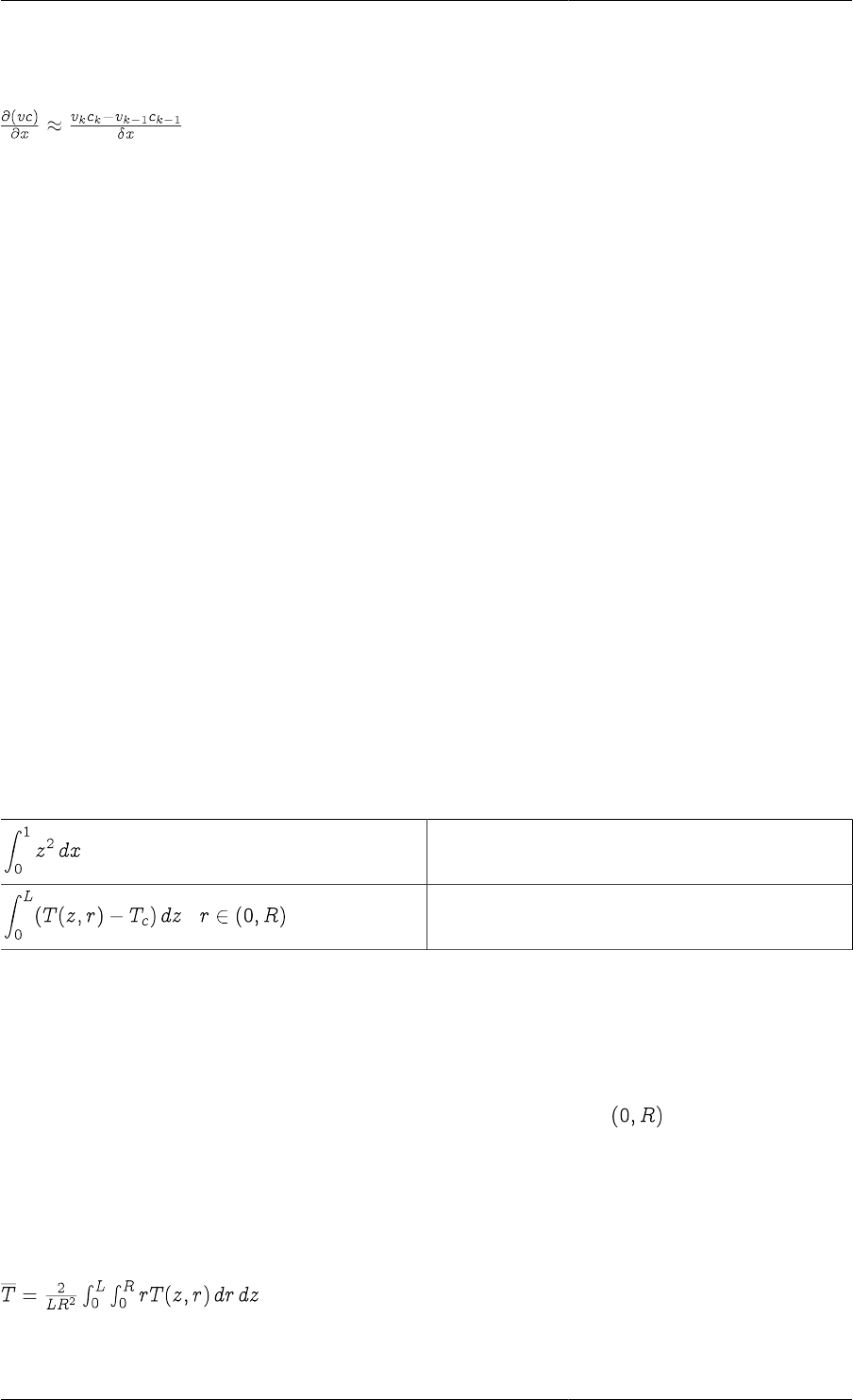
Distributed Models
52
For this reason, gPROMS always applies the second "conservative" formulation to complex derivatives, as shown
below for the simple convection term.
For this reason, therefore, conserved quantities are always conserved in the numerical solutions that gPROMS
provides.
Introducing Integral Expressions
Integrals occur frequently in equations arising in a number of branches of physics and engineering. In process
engineering applications, they often occur in population balance models describing, for instance, crystal
size distributions, activity distributions of recycled catalyst particles, and the age and size distribution of
microbiological cultures. They also appear when average values of distributed Variables need be calculated.
Integration of a distributed Variable with respect to a domain is achieved with the INTEGRAL operator. Its syntax
is of the form:
INTEGRAL ( IntegralRange ; Expression )
where Expression is a general expression involving Variables that are distributed over one or more distribution
domains and IntegralRange represents the range of integration. The result of a Integral operator is generally an
expression that is distributed over one less domain than the Expression being integrated.
In the gPROMS language it is possible to evaluate
• Single integrals
• Multiple integrals
Single integrals
The following are examples of single integrals:
INTEGRAL(z := 0:1 ; z^2)
INTEGRAL(z := 0:ReactorLength ; T(z,0|
+:ReactorRadius|-)-Tc)
Note that an integration variable (e.g. z in the above examples) is introduced to define the range of integration.
The integrand is generally an expression that may involve the Model Variables and/or the integration variable. The
numerical method used to evaluate the integral depends on whether or not a distributed Model Variable appears
in the integrand and the numerical methods specified (see Specifying Discretisation Methods).
Also note that, in the first example above, the result of the Integral is just a scalar quantity. On the other hand, the
second example results in an expression that is distributed over the open domain .
Multiple integrals
Multiple integrals can be defined via a shorthand notation. For example, the mean temperature in the entire tubular
reactor is given by:
which, in gPROMS, can be written as:
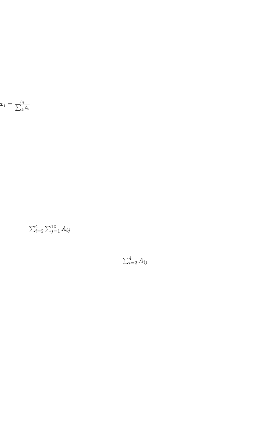
Distributed Models
53
2 / (ReactorLength*ReactorRadius^2) *
INTEGRAL(z := 0:ReactorLength , r := 0:ReactorRadius ; r*Temp(z,r))
Relationship between the Integral and Sigma
Operators
The Distribution concept can be considered as a generalisation of an Array, so the Integral operator can also be
used for the integration of a given expression over discrete domains that define Array sizes. Thus, Integral can
itself be viewed as a generalisation of the Sigma intrinsic function for carrying out discrete domain summations.
For instance, the molar fractions of the reactants at the tubular reactor entrance are defined as:
This equation can be represented in terms of either the SIGMA function or the INTEGRAL function, as shown
below:
# Using SIGMA function
X(,0) = C(,0) / SIGMA(C(,0)) ;
# Using INTEGRAL operator
X(,0) = C(,0) / INTEGRAL(i := 1:NoComp ; C(i,0)) ;
However, the Integral operator is more general than the Sigma function; whereas Sigma always results in a scalar
by summing all dimensions of its argument, Integral can have a more narrowly specified summation domain. For
instance, consider a two-dimensional array Variable A(5,10). Then
SIGMA ( A(2:4, ) )
is the scalar , whereas
INTEGRAL (i := 2:4 ; A(i, ) )
is a vector of length 10, the jth element of which is .
Explicit and Implicit Distributed Equations
As in the case of array equations, there are two different ways of writing distributed equations in gPROMS: in
an implicit manner or an explicit manner.
Implicit specification
The first exploits the concept of distributed expressions to define equations in an implicit manner. For example,
the following equation sets the temperature throughout the interior of the reactor to a uniform value of 298K:
T(0|+:ReactorLength|-,0|+:ReactorRadius|-) = 298 ;
This compact form of the equation will be automatically expanded by gPROMS.
Explicit specification
An alternative way of writing the same equation is in an explicit form by making use of For constructs:
FOR z := 0|+ TO ReactorLength|- DO
FOR r := 0|+ TO ReactorRadius|- DO
T(z,r) := 298 ;
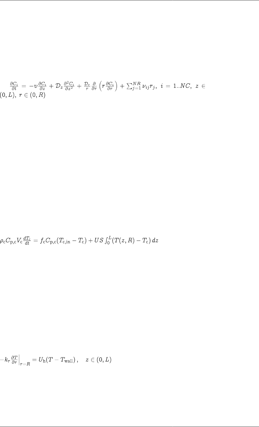
Distributed Models
54
END
END
The two forms are completely equivalent, from the points of view of both the definition of the equation and its
numerical solution. Thus, which one you use depends on preference. However, the definition of some distributed
equations require the extra flexibility afforded by the use of the FOR construct. One such case involves equations
which involve the independent Variables directly. Another case arises with equations involving SIGMA and/or
INTEGRAL operators that need to be applied only to some of the domains of their arguments. For example,
consider the chemical species conservation equations within the tubular reactor. These are of the form:
These can be written in gPROMS as follows:
FOR i := 1 TO NoComp DO
FOR z := 0|+ TO ReactorLength|- DO
FOR r := 0|+ TO ReactorRadius|- DO
$Concentration(i,z,r) =
- Velocity * PARTIAL(C(i,z,r),Axial)
+ Dz * PARTIAL(C(i,z,r),Axial,Axial)
+ (Dr/r) * PARTIAL(r*PARTIAL(C(i,z,r),Radial),Radial)
+ SIGMA(Nu(i,)*r(,z,r)) ;
END
END
END
Note how the range of application of each FOR construct is defined so as to ensure that the equation is enforced
only at the interior of the domain of interest. As a second example consider the energy conservation equation for
the cooling jacket. This leads to a lumped equation that is related to the reactor energy balance through an integral
term describing the heat flux over the entire length of the reactor:
This can be written in gPROMS as follows:
Rhoc * Cpc * Vc * $Tc = Fc * Cpc * ( TcIn - Tc )
+ U * S * INTEGRAL( z := 0:ReactorLength ; T(z,ReactorRadius)-Tc) ;
Providing Boundary Conditions
In contrast to initial conditions, which may differ from one simulation experiment to the next, boundary conditions
are part of the description of the physical system behaviour itself. In gPROMS, they are therefore specified
within Models. Boundary conditions can be viewed simply as additional equations relating the Model Variables;
consequently, they may be included in the Equation section, together with all other model equations. However,
for the sake of clarity, the user is encouraged to include the boundary conditions in a separate section, under the
keyword Boundary. For instance, the boundary condition for heat transfer at the tubular reactor wall,
can be written as follows:
BOUNDARY
...

Distributed Models
55
# Heat transfer relation at tube wall
FOR z := 0|+ TO ReactorLength|- DO
- Kr * PARTIAL(T(z,ReactorRadius),Radial) =
Uh * ( T(z,ReactorRadius) - Twall(z) ) ;
END
...
EQUATION
In any case, gPROMS currently treats the BOUNDARY and EQUATION sections in exactly the same way for the
purposes of numerical solution.
Specifying Discretisation Methods
The solution of systems of IPDAEs is generally a difficult problem. Changing the value of a parameter or one of
the boundary conditions may lead to completely different behaviour from that originally anticipated. Furthermore,
although some numerical methods can accurately solve a given system, other numerical methods may be totally
unable to do so.
The systems of IPDAEs defined within gPROMS Models are solved using the method-of-lines family of numerical
methods. This involves discretisation of the distributed equations with respect to all spatial domains, which reduces
the problem to the solution of a set of DAEs.
A number of different techniques fall within the method-of-lines family of methods, depending on the
discretisation scheme used for discretising the spatial domains. Ideally, this discretisation scheme should be
selected automatically — or, indeed, a single discretisation method that can deal efficiently with all forms of
equations and boundary conditions would be desirable. However, this is not technically feasible at the moment
and therefore gPROMS relies on the user to specify the preferred discretisation method. Three specifications are
necessary to completely determine most discretisation methods:
•Type of spatial discretisation method. The proper choice of the discretisation method is often the critical decision
for solving a system of IPDAEs. As we mentioned earlier, because no method is reliable for all problems, the
incorrect choice of method may lead to physically unrealistic solutions, or even fail to obtain any results.
•Order of approximation. The order of approximation for partial derivatives and integrals in finite difference
methods, and the degree of polynomials used in finite element methods has a great influence on the accuracy
of the solution. This is especially true if coarse grids or only a small number of elements are used.
•Number of discretisation intervals/elements. The number of discretisation intervals in finite difference methods
and the number of elements in finite element methods are also of great significance in determining the
solution trajectory. A coarse grid or a small number of elements for a steep gradient problem may result in
an unacceptably inaccurate solution. On the other hand, too fine a grid or too many elements will increase the
required computational efforts drastically, leading to an inefficient solution procedure.
The gPROMS language allows users to specify all three characteristics. DISTRIBUTION_DOMAINs are treated
as Parameters and can be Set to the desired discretisation method, order and granularity of approximation. The
table below lists the currently available numerical methods, their corresponding keywords in the language and the
currently supported orders of approximation for each.
Table 7.2. Numerical methods for distributed systems in gPROMS
Numerical method Keyword Order(s)
Centered finite difference method CFDM 2, 4, 6
Backward finite difference method BFDM 1, 2
Forward finite difference method FFDM 1, 2
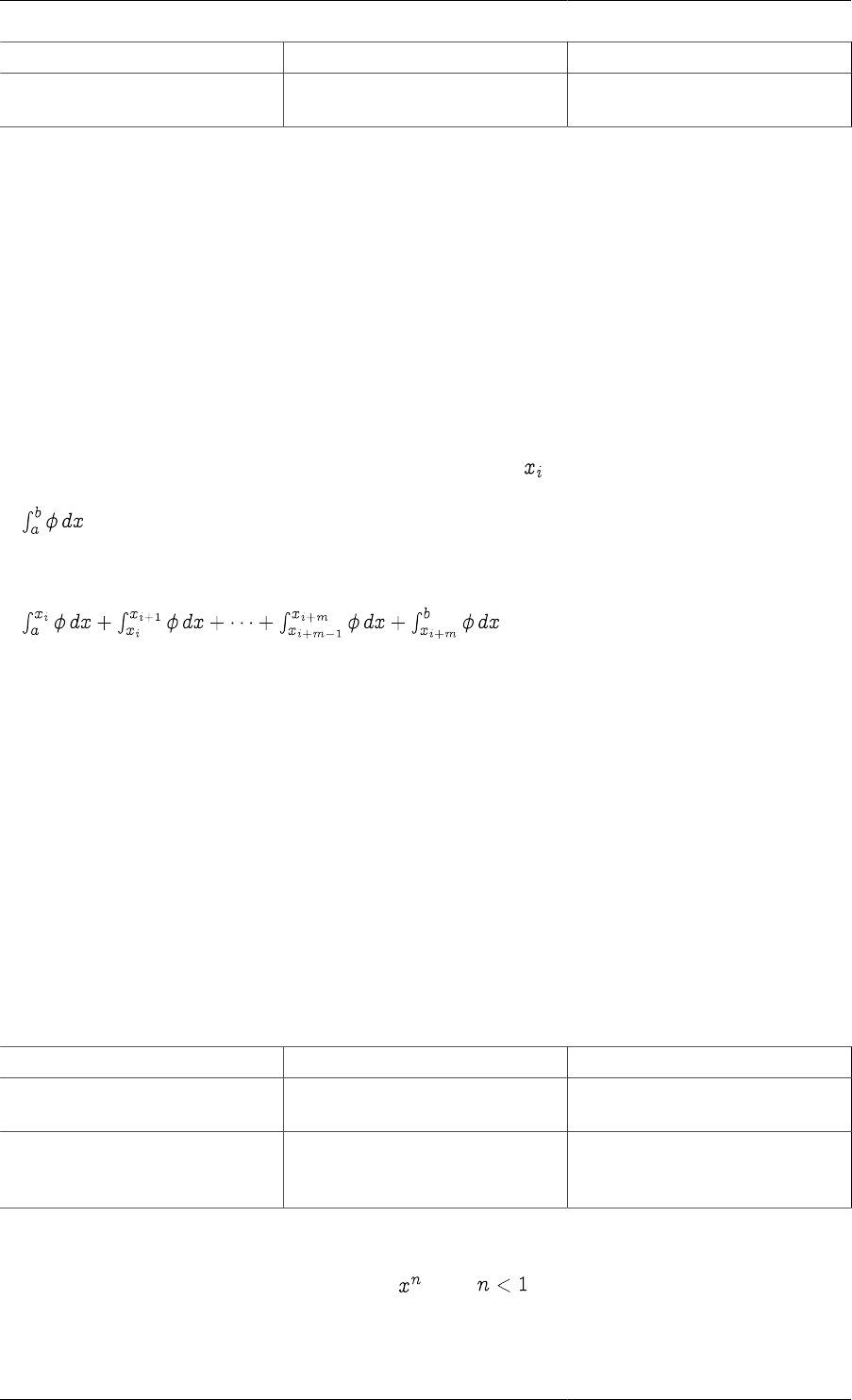
Distributed Models
56
Numerical method Keyword Order(s)
Orthogonal collocation
on finite elements method OCFEM 2, 3, 4
As was mentioned earlier, the numerical methods applied to integrals depend on the nature of the integrand. If the
integrand is an expression involving only the integration variable, then the integration method is fixed (since there
is no way to specify the method). These implicit integrals are all evaluated using 5th order Gaussian Quadrature.
If the integrand involves one or more distributed Model Variables, then the method of the integration is explicitly
specified (because all distributed Variables must be defined over a Distribution Domain, which must be set a value
as described in the table above). The following procedure below is applied to any integrals of this nature.
1. First, if the integral is defined over more than one domain, it is decomposed into a nested set of 1-D integrations.
The innermost integrals are evaluated first, which provide terms in the integrands at the next level, which now
become ordinary 1-D integrals themselves. This procedure is repeated until the outermost integral (i.e. the one
with the highest dimension) has been evaluated.
2. Each of the 1-D integrals that must be evaluated in step 1 are first decomposed into a sum of integrals over a
set of subintervals. This is based on the range of the Distribution Domain and number of intervals specified in
its numerical method. This gives a number of interval boundaries, . An integral of the form
then becomes
.
So, if the integral is specified over the interval [a,b] within a Distribution Domain defined to be over the interval
[0,L] with a numerical method using N intervals, the number of subintervals used for the integration will be
roughly (b-a)N/L.
3. Each of the subintegrals in step 2 is integrated using a polynomial approximation consistent with the numerical
method specified for the Distribution Domain.
Overall, the numerical methods for evaluating integrals do not in general correspond to any well-known methods.
In some cases, the methods may reduce to trapezoidal or Simpson's rules; but not always. However, and most
importantly, the method that is applied is always consistent with the numerical method used to approximate the
partial derivatives over the same Distribution Domain.
The numerical methods applied to the various integrals that may be encountered in gPROMS Models are
summarised in the table below.
Table 7.3. Numerical methods for integrals in gPROMS
Type of integral Numerical method used Number of intervals
Implicit 5th order, six point
Gaussian Quadrature —
Explicit approximation is consistent
with numerical method used to
approximate partial derivatives
depends on the Distribution
Domain and the integration interval
Clearly, the numerical methods used in evaluating integrals have a direct effect on the accuracy of the solution.
There are some situations where the Gaussian Quadradure used in evalulating implicit integrals results in
significant errors. One example is the power function . When , the results of the numerical integration can
be quite poor. Of course, when the integral can be solved analytically, it is always better to include the analytical
expression rather than the integral, as in this case. However, should numerical integration be required, greater
accuracy can sometimes be achieved by defining a distributed Variable (over a newly specified domain), equating

Distributed Models
57
it to the integrand and then integrating the Variable. Then, the number of elements can be specified such that the
accuracy of the integral is as required. An example of this is shown below.
DISTRIBUTION_DOMAIN
MyIntegrationDomain AS [1:100]
VARIABLE
Integrand AS DISTRIBUTION(MyIntegrationDomain) OF NoType
Implicit AS NoType
Explicit AS NoType
SET
MyIntegrationDomain := [ BFDM, 1, 200 ] ;
EQUATION
FOR x := 1 TO 100 DO
Integrand(x) = 1/x ;
END
Implicit = INTEGRAL( x := 1:100; 1/x ) ;
Explicit = INTEGRAL( x := 1:100; Integrand(x) ) ;
Here, the same integration is performed using the two methods. The implicit method will be quite inaccurate,
whereas the explicit one will be much better (depending on the order and number of elements specified for
MyIntegrationDomain).
Example 7.3. Setting the discretisation methods, orders and granularities
# PROCESS StartUpSimulation
UNIT
R101 IS TubularReactor
...
SET
R101.Axial := [ CFDM, 2, 150] ;
R101.Radial := [ OCFEM, 3, 4] ;
...
An excerpt from a Process entity involving an instance R101 of a 2D tubular reactor Model.
The Axial domain within this instance is to be discretised using centered finite differences
of second order over a uniform grid of 150 intervals. On the other hand, the Radial domain
is to be handled using third order orthogonal collocation over four finite elements. Note that
the specification of discretisation methods is done separately for each distribution domain in
each instance of the corresponding Model, thus allowing maximal flexibility in this respect.
Similarly to other Parameters, although it is possible to specify numerical solution method
information within the Models themselves, in the interests of model reusability and generality, is
often better to associate these with the specific instances of Models that are included in Processes.
Non-uniform grids
The discretisation methods described so far have all been based on a uniform grid. For finite-difference methods,
all elements are the same size: the length of the Distribution_Domain divided by the number of elements. The
same is true of Orthogonal Collocation on Finite Elements (although within each element, the collocation points
are placed according to the order of the method and may be non-uniform, though always symmetrically placed).
For many problems, uniform grids are unsuitable because there may be regions where there are large gradients
and other regions where the gradients are small. Applying a uniform grid to the whole domain would therefore
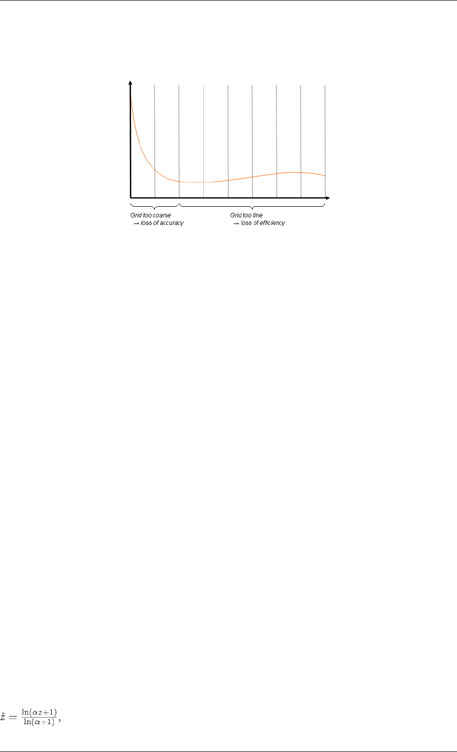
Distributed Models
58
result in a loss of accuracy where the gradients are too high, because the grid would be too coarse, and would be
inefficient in the low-gradient regions, where the grid would be too fine. This is illustrated in the figure below.
Figure 7.2. Example of a problem requiring non-uniform grids
There are two main approaches to this problem. If the behaviour of the system is roughly known a priori, then
a non-uniform grid may be specified to account for the spacial variation of the gradients. If the behaviour it not
know sufficiently well, then adaptive non-uniform grids must be employed. Here, the solution procedure places
the grid points in order to minimise the error.
gPROMS supports the use of a number of user-specified non-uniform grids. A non-uniform grid can be specified
through two mechanisms:
1. Manually specifying the grid points
2. Specifying a grid transformation
Examples demonstrating the use of the concepts can be found in the gPROMS Project nonuniformgrids.gPJ
in the examples sub-directory. It allows to compare the results of differently sized equidistant grids against each
other and also against non-uniform grids. In particular it can be seen that the same precision can be achieved with
a lower number of discretisation points using a non-uniform grid when compared against an equidistant grid.
Manually specifying grid points
The first approach to specifying a non-uniform grid is for the user to specify the location of all the grid nodes. This
is done in the SET section when Setting the Distribution Domain Parameter. Rather than specifying the number of
elements, simply enter the normalised positions of each of the internal grid nodes. The outer two nodes are fixed at
0 and 1 automatically, representing the lower and upper bounds of the domain, respectively. Below is an example
specification for a second-order centred finite-difference scheme with 10 non-uniform elements.
DISTRIBUTION_DOMAIN
Axial AS [0 : ReactorLength]
SET
Axial := [CFDM, 2, (0.356, 0.524, 0.635,
0.719, 0.785, 0.841,
0.888, 0.930, 0.967)] ;
Specifying a grid transformation
An easier (but less general) way to specify the grid nodes is by use of a tranformation. If the problem is expected
to exhibit large gradients at the start of the domain, which reduce towards the end of the domain, a logarithmic
transformation can be used to place more nodes near the lower bound of the domain. This can be represented by
the following equation, the effect of which is illustrated in the figure below.

Distributed Models
59
where is the transformed coordinate and the original coordinate. Below it can be seen that a uniform grid in
the transformed domain leads to the desired non-uniform grid in the original domain.
Figure 7.3. A logarithmic transformation
Conversely, should one desire more grid points at the end of the domain, an exponential transformation may be
used. The form of the transformation is:
To specify a transformed domain, enter the type of transformation with its parameter ( ) in parentheses to the
specification of the Distribution Domain. For the logarithmic transformation, with = 4, this would be specified
as follows.
DISTRIBUTION_DOMAIN
Axial AS [0 : ReactorLength]
SET
Axial := [CFDM, 2, 10, TRANSFORM(LOG, 4.0)] ;
Other numerical methods are specified in exactly the same way. A list of the available transformations, their
keywords and arguments is given below.
Table 7.4. Domain transformations available in gPROMS
Domain transformation Keyword Parameter(s)
Logarithmic TRANSFORM( LOG, ) larger than or equal to zero
Exponential TRANSFORM( EXP, ) can take any real value
Please note that for the exponential transormation a negative value will be the inverse transformation of the
corresponding positive value.

60
Chapter 8. Composite Models
A composite Model is one that contains one or more other Model entities as a sub-Model. Composite Models can
either be constructed graphically on the topology tab of a flowsheet model or using the gPROMS language; or
even some combination of these two approaches.
In the case of graphical model construction, Connections between sub-Models can only be made to Model Ports
(see: Constructing flowsheet Models). Whereas in the gPROMS language, Connections can be made via Model
Ports and also by writing equations that directly access the Model Variables and Parameters. It should be note
that graphical connections between Model Ports are automatically represented in the gPROMS language tab and
vice-versa.
• Motivation for Model decomposition: the benefits of building reusable Model components.
• How to build composite Models in gPROMS
• Declaring instances of lower-level Models in the UNIT Section
• Topology connections in the gPROMS Language
• The use WITHIN construct for simplifying notation when referring to quantities within sub-Models,
• Making specifications for composite Models
• Model specifications
• Setting Parameter values in composite Models
Motivation for Model Decomposition
Certain complex unit operations may involve many tens of thousands of Variables and equations. Although in
principle all of these could be written in a single Model entity, in practice such an undertaking would be extremely
tedious and error-prone. The gPROMS language provides tools for managing such complexity.
The key principle involved is called hierarchical sub-Model decomposition, whereby the Model for a complex
unit operation is constructed progressively in a number of hierarchical levels. This is much easier than constructing
a very large primitive Model (see also: Defining Models and Processes ) for the unit operation because at each
level in the hierarchy you can concentrate on only a small fraction of the modelling task. As a result, the Models
are easier to construct and less likely to contain errors.
Moreover, this strategy promotes Model reusability and efficient Model development practices, since suitably
Parameterised sub-Models can be used several times, but only be constructed and tested once. The gPROMS
language encourages hierarchical sub-Model decomposition by offering mechanisms that support:
• the declaration of high-level Models that contain instances of lower-level Models
• the connection of the above instances using Equations and topology connections.
Instances of lower-level Models: Units
In gPROMS, an instance of a Model is called a Unit. Consequently, if we wish to insert one or more instances of
one or more Models within another (higher-level) Model, we have to introduce a Unit section within the latter.
Consider, for instance, the declaration of a distillation column Model that is outlined in the figure below.

Composite Models
61
Figure 8.1. Distillation Column Model
# MODEL DistillationColumn
PARAMETER
# Number of trays
NoTrays AS INTEGER
# Feed tray position
FeedPosition AS INTEGER
UNIT
Condenser AS TotalCondenser
Reboiler AS PartialReboiler
TopSection AS LinkedTrays
BottomSection AS LinkedTrays
Feed AS FeedTray
VARIABLE
ColumnEnergyRequirement AS Energy_Flowrate
EQUATION
#Definition of column energy requirement
Reboiler.HeatingLoad - Condenser.CoolingLoad = ColumnEnergyRequirement
The PARAMETER and VARIABLE sections of this composite Model are very similar to those of simple
(primitive) Models – see Defining Models. However, the UNIT section, above specifies that the Model also
comprises a number of instances of other Models, namely:
• Condenser. This is an instance of Model TotalCondenser.
• Reboiler. This is an instance of Model PartialReboiler.
• TopSection, BottomSection. These are both instances of Model LinkedTrays.
• Feed. This is an instance of Model FeedTray.
Each of the lower-level Models may either be primitive or include a UNIT section themselves. For instance,
TotalCondenser, PartialReboiler and FeedTray are likely to be primitive Models. In contrast, LinkedTrays is
most probably a composite Model. In any case, there is no limitation with respect to the number of levels in this
hierarchical decomposition.
Finally, the EQUATION section introduces an Equation that determines the net energy requirement for the entire
column:
Reboiler.HeatingLoad - Condenser.CoolingLoad = ColumnEnergyRequirement ;
The equation involves three Variables. One of these (ColumnEnergyRequirement) belongs directly to the
DistillationColumn Model having been declared explicitly in its Variable section. The other two Variables
(Reboiler.HeatingLoad and Condenser.CoolingLoad) belong to the Units Reboiler and Condenser , respectively.
Of course, for this to be correct, Models PartialReboiler and TotalCondenser must contain Variables
Reboiler.HeatingLoad and Condenser.CoolingLoad respectively.
The above equation illustrates a general property of higher-level Models. This is their ability to refer to entities
(e.g. Parameters and Variables) that are declared within the Units that they contain - as well, of course, as their
own entities. Furthermore, as we have seen, this reference is done using a pathname construct. The latter can be
arbitrarily long. For example, suppose that the TotalCondenser Model is not primitive but comprises instances of
several lower-level Models; then the following may be a valid pathname:

Composite Models
62
Condenser.RefluxDrum.LevelController.Gain
referring to the gain of the controller used to control the liquid level in the reflux drum of the condenser.
Finally note that the DistillationColumn Model does not yet express how the flows of material and energy between
the sub-units are equated; this could be done directly with Equations. For example:
...
EQUATION
#Definition of column energy requirement
Reboiler.HeatingLoad - Condenser.CoolingLoad = ColumnEnergyRequirement
# Connectivity for rebolier/Bottom Section
Reboiler.Vapour_out = BottomSection.Vapour_in;
Reboiler.y_vapour_out = BottomSection.y_vapour_in;
Reboiler.T_vapour_out = BottomSection.T_vapour_in;
...
Of course, Equations need to be provided for all the connections between all of the Units.
However, in practice it is usually more convenient to connect Units using topology connections to Model Ports
(assuming that they have been defined of course) – see Topology connectivity using the gPROMS Language.
Topology connectivity using the gPROMS
Language
Connections made between a Model's Ports (see: Defining Ports), whether created graphically (see: Constructing
flowsheet Models) on the composite Model's topology tab or directly in the gPROMS language, should be placed
in the TOPOLOGY section; the general syntax for this is shown below
TOPOLOGY
UnitName.PortName = UnitName.PortName # for scalar PORTs
UnitName.PortName(PortNumber) = UnitName.PortName # for array PORTs
UnitName.PortName(PortNumber) = UnitName.PortName(PortNumber) # for array PORTs
UnitName.PortName = UnitName.PortName(PortNumber) # for array PORTs
EQUATION
... Model equations ...
The following should be noted:
• Graphical connections are automatically represented in the gPROMS language tab and likewise any connections
added directly in the gPROMS language will be shown on the composite Model's topology tab (following a
syntax check). Similarly connections deleted from either location will be synchronised.
• The TOPOLOGY section comes just before the EQUATION section in a gPROMS Model entity.
• When connecting Units via Ports the user must ensure that the Connection Types are the same and that all
Connectivity rules are satisfied.
• When a Connection is made all Parameters, Distributions and Variables in the Ports are equated.
Arrays of Units
Recalling the DistillationColumn Model used to introduce lower-level Model instances, one of its sub-
Models is a Model of a column section, called LinkedTrays:

Composite Models
63
# MODEL DistillationColumn
PARAMETER
...
UNIT
Condenser AS TotalCondenser
Reboiler AS PartialReboiler
TopSection AS LinkedTrays
BottomSection AS LinkedTrays
Feed AS FeedTray
...
As its name implies, LinkedTrays could contain a number of instances of a Tray Model. Clearly it would be
convenient to define an Array of Tray Model instances, and this can be done as follows.
# Model LinkedTrays
PARAMETER
NoTrays AS INTEGER
...
UNIT
Trays AS ARRAY(NoTrays) OF Tray
...
See also Declaring arrays of Units in Models.
Referring to arrays of Units is done in a similar manner to Parameters and Variables (see Referring to array
elements). For example, one would refer to the liquid mole fraction of component 2 in the 5th tray of the top
section of the column using the following path name:
Column.TopSection.Trays(5).x(2)
Variable pathnames and WITHIN
As the number of intermediate hierarchical levels increases, so does the length of the pathnames required to
reference Parameters and Variables at or close to the bottom of the hierarchy. Pathnames of the form:
SeparationSection.Column(2).TopSection.Stage(1).T
are quite common when dealing with complex processes.
It is recommended that you use pathname completion to help construct full and valid pathnames correctly;
this is available within all entities in gPROMS. Semantic errors, such as referencing a quantity in a lower-level
Model that doesn't exist, are only detected when a Model based activity is executed.
Nevertheless, writing equations with long pathnames can become tedious and make code difficult to read,
especially if a large part of the pathname is common to many of the Parameters or Variables referenced by an
equation. The WITHIN construct helps relieve some of this burden.
A WITHIN construct encloses a list of equations and defines a prefix to be used for all Parameters and Variables
referenced by the enclosed equations. Suppose, for instance, that Model Tray has a Variable Q that determines
the heat loss from the tray to the environment. However, it contains no equation that actually determines this heat
loss. Consider now using this tray Model within the top and bottom sections of a column. We wish to specify a
simple heat transfer equation for determining the heat loss in the top section; however, the bottom section is well
insulated. One way we can achieve this is as follows:

Composite Models
64
MODEL DistillationColumn
PARAMETER
TAmbient AS REAL
UA AS REAL
NoTrays AS INTEGER
UNIT
TopSection, BottomSection AS LinkedTrays
EQUATION
WITHIN TopSection DO
FOR k := 1 TO NoTrays DO
WITHIN Stage(k) DO
Q = UA * (T - TAmbient) ;
END # Within Stage(k)
END # For k
END # Within TopSection
WITHIN BottomSection DO
FOR k := 1 TO NoTrays DO
WITHIN Stage(k) DO
Q = 0 ;
END # Within Stage (k)
END # For k
END # Within BottomSection
In trying to interpret the equation:
Q = UA * (T - TAmbient) ;
gPROMS will need to identify (resolve) the symbols Q, UA, T and TAmbient. It starts doing this by searching the
Model corresponding to the UNIT mentioned in the innermost WITHIN statement. In this case, this is Model Tray
which does, indeed, contain Variables Q and T. However, symbols UA and TAmbient still remain unresolved.
Therefore, gPROMS considers the next enclosing WITHIN statement; this indicates that it should search Model
LinkedTrays (of which TopSection is an instance). However, this Model does not contain the missing identifiers.
So gPROMS now has to consider Model DistillationColumn itself – which does indeed allow it to resolve UA
and TAmbient.
It is interesting to note that both the DistillationColumn and the LinkedTrays Models contain the
Parameter NoTrays. However, this does not result in any ambiguity in resolving this Parameter when it appears
in each of the two FOR constructs: gPROMS always tries to resolve symbols by searching the innermost WITHIN
first. Thus, NoTrays in:
WITHIN TopSection DO
FOR k := 1 TO NoTrays DO
...
END
END # within TopSection
clearly refers to TopSection.NoTrays and not to Parameter NoTrays in DistillationColumn.
Expressions involving arrays of Units
Occasionally, it will be necessary to write expressions involving of arrays of units and/or slices of arrays of units
(i.e. a subset of the elements of an array – see Referring to array elements). The rules governing expressions
involving arrays of units are similar to those governing array expressions involving only Variables. However,
there are some additional complications with arrays of units, so one should be familiar with the General rules for
array expressions and Using arrays in equations before continuing.

Composite Models
65
There are two situations to consider when writing expressions of arrays of units. The simplest case is when slices
are specified for all dimensions of all arrays; the other is when at least one dimension of an array is unspecified
(e.g. A(2:3,)).
In the examples to come, the following conventions are used.
• Variable names always begin with the letter V; all other entities are Units.
• Whole arrays are always indicated using parentheses and their dimensionality is indicated using commas to
delimit the indices. For example, a two-dimensional array will be written as V(,) rather than V() or V, which
are equally valid in gPROMS but could be confused with a one-dimensional array and a scalar respectively.
The first, and simplest, case to consider is when all dimensions of all arrays are specified (either by giving a
specific element or a slice of elements). The expression below is an example of such an expression.
UA(1:2).UB.P(1:3).V1 + UC.UD(1:2).P(1:3).V2 = 3 ;
This case is quite simple. It is clear that this expression should be expanded to give:
UA(1).UB.P(1).V1 + UC.UD(1).P(1).V2 = 3 ;
UA(1).UB.P(2).V1 + UC.UD(1).P(2).V2 = 3 ;
UA(1).UB.P(3).V1 + UC.UD(1).P(3).V2 = 3 ;
UA(1).UB.P(1).V1 + UC.UD(1).P(1).V2 = 3 ;
UA(2).UB.P(2).V1 + UC.UD(2).P(2).V2 = 3 ;
UA(2).UB.P(3).V1 + UC.UD(2).P(3).V2 = 3 ;
The rules governing expressions like these are the same as those for ordinary arrays. Each of the terms on the left-
hand side of the expression can be thought of as 2x3 arrays. The presence and location of any scalar elements
do not affect this behaviour: UB and UC are in different places in the paths but neither their location nor their
existence changes the dimensionality of the two terms. So the whole expression can be considered dimensionally
equivalent to:
VA(1:2,1:3) + VB(1:2,1:3) = 3 ;
and this is a legal array expression, because VA and VB have exactly the same dimensions.
Even the dimensionality of the variables is unimportant to the validity of expressions of this type. The next example
demonstrates this.
UA(3:3,1:2).UB.P(1:4).V1 + UC.P(1,5:6).V2(1:4) = 3
Now the dimensions of UA and UC.P are identical (1x2) and the dimensions of UB.P are identical to UC.P.V2,
so each term is equivalent to a 1x2x4 array and the expression is equivalent to:
VA(3:3,1:2,1:4) + VB(1,5:6,1:4) = 3
So when all indices of all arrays are specified completely, the rules are identical to ordinary arrays: each term must
be a scalar or of the same dimensionality.
When it is necessary to refer to whole arrays, the situation becomes a little more complicated. Consider the first
example again, but now writing the expression for the whole range of array elements:
UA().UB.P().V1 + UC.UD().P().V2 = 3 ;
At first glance, this might look the same. Certainly, the number of elements in UA() must be the same as the
number of elements in UC.UD(). However, the dimensionality of P() is harder to define in a simple way: the
problem is that P() may have different number of elements for each element of UA().UB or UC.UD(). A more
relevant example of this is given below.
COLUMN_A(,).TRAY().V = COLUMN_B(,).TRAY().V ;

Composite Models
66
Here, we have two 2-dimensional arrays of distillation-column units, perhaps forming a separation network. There
is no guarantee that each column will have the same number of trays: in fact it is extremely unlikely. So it is not
possible to consider this expression, or the one before, as a simple array expression. What must be done instead
is to consider the dimensions in each term of the expression more carefully.
First, it is clear that COLUMN_A(,) and COLUMN_B(,) must have the same dimensionality. Next, for each
element of COLUMN_A(,) and COLUMN_B(,), the number of trays must also be equal, so that the following
condition is met:
The dimensionality of COLUMN_A(i,j).TRAY() must be equal to the dimensionality of
COLUMN_B(i,j).TRAY() for all i and j.
This must be true for the whole path of each term in the expression (unless the term is scalar). We can now define
a dimension tree for each term, which describes completely the dimensionality of the term.
The dimension trees for both terms in the example:
UA(3:3,1:2).UB.P(1:4).V1 + UC.P(1,5:6).V2(1:4) = 3
are:
• (1,2)
• 4
• 4
If we were to write the expression as:
UA(,).UB.P().V1 + UC.P(,).V2() = 3
with UA(,) and UC.P(,) both being 1x2 arrays; UA(1,1).UB.P having 3 elements; UA(1,2).UB.P having
4 elements; UC.P(1,1).V2 having 4 elements and UC.P(1,2).V2 having 3 elements, then the dimension
trees would be:
• (1,2) [UA(,)]
• 3
• 4
and:
• (1,2) [UC.P(,)]
• 4
• 3
As these two trees are not identical, the two terms will not be compatible and the expression will be illegal.
The general rule for expressions involving arrays of units is therefore an extension of the rule for array Variables.
If we have an expression of the form:
Expression E = Expression F;
it will be valid provided is conforms to one of the following four cases:
Case E F Dimension tree of E = F
1 Scalar Scalar Scalar

Composite Models
67
Case E F Dimension tree of E = F
2 Dimension tree Scalar Same as E
3 Scalar Dimension tree Same as F
4 Dimension tree Dimension tree Same as E and F
In case 4, the dimension trees of E and F must be identical. Either expression may comprise binary operations of
the form x ⊕ y, for which the following rules must also apply:
Case x y Dimension tree of x ⊕ y
1 Scalar Scalar Scalar
2 Dimension tree Scalar Same as x
3 Scalar Dimension tree Same as y
4 Dimension tree Dimension tree Same as x and y
Again, in case 4, the dimension trees of x and y must be identical.
Model specifications
It is usually recommended that the values of all unknown Model quantities are provided in Process entities (See
also: Defining Process Entities), where:
• Parameter values are fixed in the SET section
• Variables are specified in the ASSIGN section
• Initial conditions are provided in the INITIAL section
• The initial values of Selectors are provided in the INITIALSELECTOR section
However, the same sections exist in Model entities. So it is equally possibly to provide a specification directly in
the Model that declares the quantity to be specified or any composite Model that includes the Model. See also:
gPROMS language for Models.
Care should be taken to remember that making a specification in a Model can greatly reduce the generality of such
a Model. In general a quantity may be given a value at most once and it is not possible to overwrite a specification
given at a lower level. However, giving a Parameter the exactly same value more than once does not cause an error.
Consider, for instance, the following situation:
• Model X declares a Parameter S to be of type REAL.
• Model Y contains a unit XX which is an instance of X.
• Model Z contains a unit YY which is an instance of Y.
• Process P contains a unit ZZ which is an instance of Z.
Then, the value of Parameter S can be explicitly set in of the following ways:
1. In X:
SET
S := 1.5 ;
2. In Y:
SET

Composite Models
68
XX.S := 1.5 ;
3. In Z:
SET
YY.XX.S := 1.5 ;
4. In P:
SET
ZZ.YY.XX.S := 1.5 ;
If a Parameter is explicitly SET in a Model, it will have that value in all instances of that Model. For example,
if we use option 2 above, XX.S will have a value of 1.5 in all subsequent instances of Model Y anywhere in the
problem. It is usually advisable that Parameters be explicitly set at the Process level. This practice maximises the
reusability of the underlying Models and minimises the probability of error.
Setting Parameter values in Composite
Models
Before any Model based activity is executed in gPROMS the values of all Parameters (even if not used) must be
resolved. A Parameter's value must have been determined in one of the following ways:
• Explicit Parameter specification: to Set a Parameter to either to a literal value or to another Parameter value (or
even some expression involving the two)
• From topology connections : for Connection Type Parameters only
• From implicit Parameter Propagation in Composite Models: top down propagation from higher level Models
to lower level models
• From a Default specification: only if the Parameter is not given a value directly by any of the three previous
approaches
Any Parameter that does not have a value following the above four steps will result in an error that causes the
Model based activity to fail. Giving a Parameter the exactly same value more than once does not cause an error;
however, clearly, giving a Parameter different values is an error.
Setting Connection Type Parameters
The Parameters included in Connection Types can be set explicitly like regular Model Parameters. However, their
values are usually obtained from topology connections and Port Sets:
•Topology connections: when a connection between two Ports is made the equivalent Parameters in these Ports
are equated.
•Port sets: These are configured when the Ports for any component Model entity are configured (also see:
Defining Model Ports). For all Ports belonging to the same set (i.e. those in the same Port set): the equivalent
Connection Type Parameters are equated. This mechanism is often used by component Model developers to
equate the Parameters in an Outlet Port to those in an Inlet Port.
These two mechanisms (if Port sets are implemented) mean that information corresponding to the properties carried
by the Connection are automatically propagated along the stream path. In the gPROMS Process Model Library
this is used so that the Parameter corresponding to physical properties only needs to be set in the Source Model.
It is of course possible within the component Model to access the Port Parameters and use them directly in Model
Equations declarations, or indeed, to Set Model Parameters equal to the Parameters declared by the Port definition.
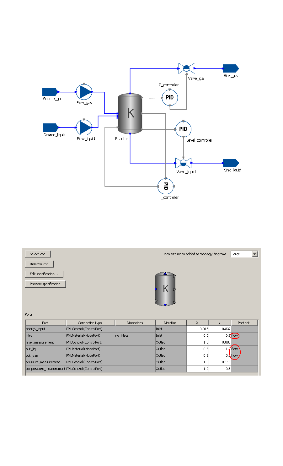
Composite Models
69
Example of Parameter Propagation with Port Sets
As an example of the use of Port Sets, consider the PML Flowsheet shown below.
Figure 8.2. Reactor Flowsheet
Each of the connector Models in this Flowsheet (pumps, reactor and valves) have common Port Sets linking their
inputs to their outputs. This is shown for the reactor Model below.
Figure 8.3. Reactor Port Sets
This means that once the properties of the Source_gas Model instance are specified, they automatically propagate
along the direction of flow: i.e. to Flow_gas, Reactor, Valve_gas, Simk_gas, Valve_liquid and
Sink_liquid. More specifically, because the properties of Source_gas define the inlet properties of
Flow_gas and the inlet of Flow_gas shares the same Port Set as its outlet ("flow"), the properties are
propagated along. Similarly, the inlet of the Reactor is linked to both of its outlets by the same Port Set.
Note, however, that the Parameters are not propagated backwards, so Source_liquid must be specified as well. Of
course, some of its properties cannot be specified independently and care must be taken to make sure that there are
no conflicts. If, for example, one were to specify a different set of components for Source_liquid, gPROMS would
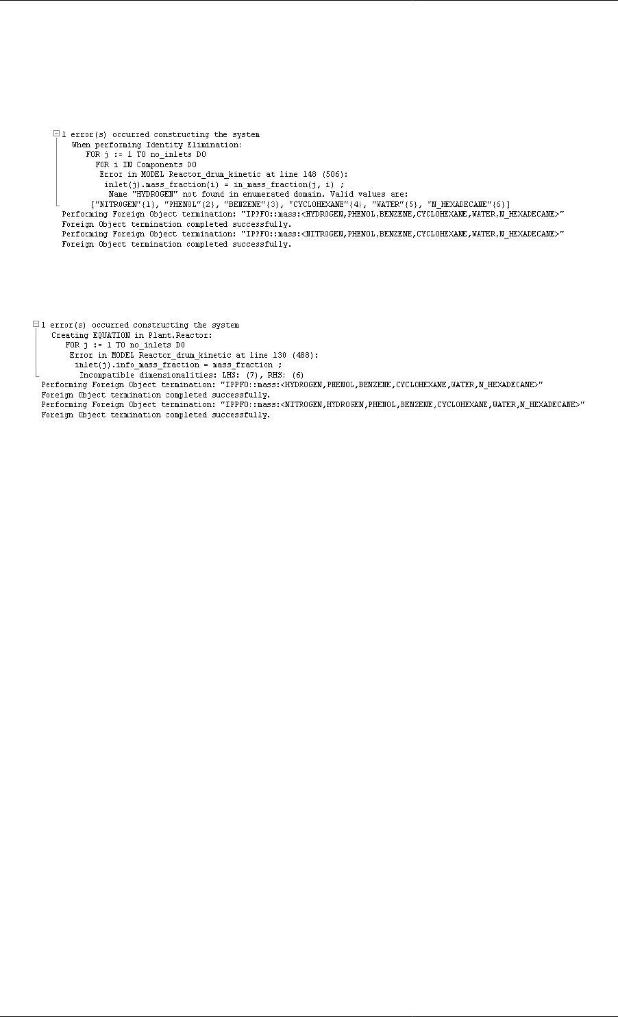
Composite Models
70
report a conflict between the two sets of specifications propagated to the inlet of Reactor. Below are shown two
examples of inconsistent component specifications.
Figure 8.4. Inconsistent Parameters propagated
through Port Sets: inconsistent components specified
Figure 8.5. Inconsistent Parameters propagated
through Port Sets: extra component specified
Implicit Parameter Propagation
As well as the propagation of Connection Type Parameters along stream paths the values of Model Parameters
can propagate from higher- to lower-level Models.
For example, a Parameter that corresponds to the number of components (e.g. NoComp) may well be present in the
higher-level Model of a distillation column and in all of its constituent Model instances. Ideally, we would like to
be able to set the value of this Parameter at the highest level only and rely on an automatic mechanism to propagate
it through the hierarchy towards the lower levels. This not only saves effort in specifying the Model but also
reduces the possibility of errors arising due to inconsistent specifications, especially during Model development
(e.g. specifying NoComp=5 in some parts of the column and NoComp=4 in others).
If a Parameter appearing in an instance of a Model is not SET explicitly, gPROMS will automatically search
hierarchically the higher-level Models containing it for a Parameter of the same name and type which has been
given an explicit value. If this is found, the Parameter in the lower-level Model will adopt the value assigned to
the Parameter with the same name in the higher-level Model.
Another way of looking at this is that an explicit SET specification for a Parameter in a higher-level Model X
propagates downwards and covers all Parameters of the same name and type in any lower-level Models, instances
of which are contained in X. This establishes an automatic Parameter propagation mechanism.
For instance, consider the hierarchy of Models X, Y and Z (which all contain a declaration of a Parameter
NoComp) : such that
• Model X .
• Model Y contains a unit XX which is an instance of X.
• Model Z contains a unit YY which is an instance of Y.
• Process P contains a unit ZZ which is an instance of Z.
We then have various possibilities:
1. Set Parameter in P:

Composite Models
71
SET
ZZ.NoComp := 5 ;
Although nothing is said explicitly about Parameters ZZ.YY.NoComp and ZZ.YY.XX.NoComp, the automatic
Parameter propagation will ensure that these also take the value of 5.
2. Set Parameter in P:
SET
ZZ.NoComp := 5 ;
but also in Y:
SET
NoComp := 3 ;
This is equivalent to:
ZZ.NoComp := 5 ;
ZZ.YY.NoComp := 3 ;
ZZ.YY.XX.NoComp := 3 ;
Note that the value of the Parameter in YY is set explicitly and automatically propagates downwards, setting
the value of the Parameter in XX. Therefore, when gPROMS automatically propagates the assignment in P,
it cannot override the existing value.
We also recall that the specification of discretisation methods for distribution domains is treated exactly as that
for Parameters - hence, it also undergoes automatic propagation. For instance, if:
SET
ZZ.Axial := [OCFEM, 3, 10] ;
appears in a Process, all Model instances within ZZ which declare an Axial domain will use the same discretisation
method - unless, of course, their Axial specification is explicitly SET to a different value.

72
Chapter 9. Ordered Sets
You should be familiar with the use of Arrays before proceeding further.
gPROMS allows the use of Ordered Sets as array indices, in addition to simple integer indices. These substantially
increase the descriptive power of the modeling language because they allow the user to use strings to reference
array elements rather than integers. For example: instead of mole fractions being defined as x(1), x(2) and
x(3); x('H2'), x('CH4') and even x('Ethane') can be used instead. The importance for ease and
correctness of model building should be evident. Ordered Sets can be used for
• Parameters
• Variables
• Units
Each of these entities can be defined as Arrays or Distributions over Ordered Sets.
Developing models involving Ordered Sets requires the following:
• Declaring Ordered Sets
• Declaring Arrays of Parameters, Variables and Units using Ordered Sets
• Ordered Set operations and referencing rules
A set of examples and the gPROMS Project orderedsets.gPJ illustrate more complex use of Ordered_Sets.
Declaring Ordered Sets
The Ordered Set is a type of Parameter and is therefore declared in the PARAMETER section of your gPROMS
Model.
They are declared as follows:
PARAMETER
Gases, Liquids, Species AS ORDERED_SET
As with other Parameters, the values are defined in the set section. In the case of Ordered Sets, it is the set elements
that must be defined.
SET
Gases := ['H2', 'CH4', 'Ethane'] ;
Liquids := ['Octane', 'Decane'] ;
Species := Gases + Liquids ;
Note that the + operator is the set union operator in this case. More information on operators may be found here.
Each element of the Ordered Set is a user-defined string. Strings are delimeted by single quotes (as shown above)
or by double quotes (") and can contain any character apart from the same character used to delimit the string.
Also, each element of the Ordered Set must be unique: if any duplicate elements are defined, these are ignored
by gPROMS. The following example specification produces an Ordered Set containing just three elements: "1",
"2" and "3", in that order.
SET
Numbers := [ '1', '2', '3', '2' ] ;

Ordered Sets
73
Some examples of legal and illegal element specifications are shown below:
SET
Legal := [ "1", '2"', "3'" ] ; # all legal
Illegal := [ '1'', "2"" ] ; # all illegal
# \ \_____ this element is delimeted by " so the string
# \ may include any character apart from "
# \_________ this one is delimited by ' so it cannot contain '
Ordered Sets are also compatible with physical-property interfaces. In this next example, the elements of the
Ordered Set are specified by a physical-property Foreign Object.
PARAMETER
Species AS ORDERED_SET
PhysProp AS FOREIGN_OBJECT "PhysProp"
NoComp AS INTEGER
SET
NoComp := PhysProp.NumberOfComponents ;
Species := PhysProp.Components ;
Declaring Arrays of Parameters, Variables
and Units
Each of these types of entity are declared in a very similar way to Arrays over integer domains. So for Parameters
the declaration is:
PARAMETER
FormulaWeight AS ARRAY(Species) OF REAL
As with Arrays generally, multiple dimensions are possible. For example, if an Ordered Set Reactions had also
been defined, then the parameter Nu, representing stoichiometric coefficients could be declared by:
PARAMETER
Nu AS ARRAY(Species, Reactions) OF INTEGER
For Variables, the declaration is:
VARIABLE
X AS ARRAY(Species) OF MassFraction
Referencing of Parameters and Variables defined in this way (i.e. to specify them in a SET or ASSIGN statement
or to refer to them in in Equations) is discussed here.
Similarly, Arrays of Units (Model instances) are declared by:
UNIT
Reactors AS ARRAY(ReactorNames) OF LiquidPhaseCSTR
And the properties of each element of the Unit may be specified by:

Ordered Sets
74
SET
WITHIN Reactors('LowTempReactor') DO
...
END
# Etc.
Finally, it is also possible to declare Selector variables as Arrays of Ordered Sets. The syntax follows the above
rules and those for declaring Arrays of Selector variables over integer domains: enter the name of the Ordered Set
rather than an integer bound for the Array size.
Ordered Set Operations and Referencing
Rules
The following features may be used when developing a Model containing Ordered Sets:
• Set Operations
• Referencing Rules
• Built-in Functions
• Intrinsic Functions
Set Operations
The allowed set operations are:
• Union, defined by +
example:
Species := Gases + Liquids ;
• Intersection, defined by *
example:
Intermediates := Gases * Liquids ;
• Set difference, defined by -
example:
NonCondensibles := Gases – Liquids ;
For Union and Intersection, there are variants that takean arbitrary number of arguments:
•UNION()
examples:
AllComponents := UNION(InputConnections().Components);
(InputConnections() is an array of nInputs Connections, each carrying an Ordered Set parameter
Components.)
Slices can be used as well:
Components := UNION(InputConnections(2:nInputs-1).Components);
•INTERSECTION()

Ordered Sets
75
example:
CommonComponents := INTERSECTION(InputConnections().Components);
Note that because the sets are ordered, the operations are non-commutative, i.e. Gases + Liquids <>
Liquids + Gases (the order of the species will be different in the two cases).
Also, standard arithmetic operator precedence applies to Ordered Set operations: that is, intersections are
performed before unions and differences. The order in which these operations are performed may, however, be
modified using parentheses.
Ordered Set Referencing Rules
In Parameter specifications, Equations and Assign statements, one may refer to individual elements, slices or the
whole Array, as in the case of integer domains. Of course, rather than using integers to refer to individual elements
or define slices, the names of the elements in the Ordered Sets are used. The two examples below illustrate the
specification of a single element of a Parameter and an Assignment of a slice of a Variable.
SET
FormulaWeight('H2') := 2 ;
ASSIGN
Flowrate('CH4':'C4H10') := 0.0 ;
In the second example above, the flowrates of all the Array elements in the Ordered Set from 'CH4' to 'C4H10'
will be set to 0.
In this next example, a material balance Equation is written (implicitly) for all Species:
$M = Fin*Xin – Fout*X ;
where M, Xin and X are Arrays over the domain 'Species'.
As with Integer domains, FOR loops can be used instead of implicit declarations of Array Equations:
FOR i IN Species DO
$M(i) = Fin*Xin(i) - Fout*X(i) ;
END
Multiple domains are handled quite easily. The example below is a material balance for all Species with generation
terms summed over the Reactions domain:
$M = Fin*Xin – Fout*Xout + SIGMA( (Nu(,Reactions)*Rate(Reactions) ) ;
(For clarity, this may also have been declared explicitly.)
More sophisticated expressions involving set operations and slices are also possible; some examples are given here.
Built-in Functions
The summation operator, SIGMA, is defined over the Ordered Set, e.g.
SIGMA(x(Species)) = 1 ;
The integral operator, INTEGRAL, is also defined over an Ordered Set, e.g.:
INTEGRAL(s OVER QuadPoints ; x(s)*y(s)) = 100.0 ;
where QuadPoints is the Ordered Set.

Ordered Sets
76
Slices and set operations within built-in functions are also allowed, e.g.:
SIGMA(x('H2O':'Ethane'))
INTEGRAL(s OVER S1*S2 ; x(s)*y(s))
where S1 and S2 are Ordered Sets.
Ordered Set Intrinsic Functions
A number of intrinsic functions are defined for Ordered Set Parameters.
The first element of an Ordered Set is returned as a string by:
OrderedSetParam.First
The last element of an Ordered Set is returned as a string by:
OrderedSetParam.Last
The Cardinality (i.e. the size) of an Ordered Set is returned as an integer by:
OrderedSetParam.Card
The ith Element of an Ordered Set is returned as a string by:
OrderedSetParam.Element(i)
(where i = 1 is the first element) .
One area where this might be useful is in defining material balance equations for all but one of the species in the
model. One possibility is as follows.
EQUATION
FOR i IN Species - Species.Last
$M(i) = Fin*Xin(i) - Fout*X(i) ;
END
SIGMA(X(Species)) = 1 ;
The index of a specific element is returned as an integer by:
OrderedSetParam.Index(ElementName)
A boolean value indicating whether or not an Ordered Set contains a specific element is returned by:
OrderedSetParam.Contains(ElementName)
A subset over a certain range is returned by:
OrderedSetParam.Subset(m,n) - a subset from index m to n inclusive
OrderedSetParam.Subset(m) - a subset from index m to the last element inclusive
The index can be given as a string argument as well as integers.
Examples of the Use of Ordered Sets
Here, we have a database of molecular weights from which we will copy some into a smaller list of components:
PARAMETER
ReagentSpecies, ProcessSpecies, AllSpecies AS ORDERED_SET
VARIABLE

Ordered Sets
77
MW AS ARRAY(AllSpecies) OF MolWt
MWsub AS ARRAY(ReagentSpecies) OF MolWt
SET
ReagentSpecies := ['HNO3', 'H2O', 'NaOH', 'tbp/ok'] ;
ProcessSpecies := ['HNO3', 'H2O', 'Uranium'] ;
AllSpecies := ReagentSpecies + ProcessSpecies ;
EQUATION
MW('HNO3') = 1 + 14 + 3*16 ;
MW('H2O') = 2*1 + 16 ;
MW('NaOH') = 23 + 16 + 1 ;
MW('tbp/ok') = 10*12 + 22 ; # approx
MW('Uranium') = 238 ;
FOR i IN ReagentSpecies DO
MWsub(i) = MW(i) ;
END
(Note that it would not be legal to shorten the names of the Ordered Sets to Reagent, Process and All because
Process is a reserved word in gPROMS.)
Equations can be written that use streams with identical species lists:
VARIABLE
MassIn AS ARRAY(ProcessSpecies) OF MassFlow
MassOut AS ARRAY(ProcessSpecies) OF MassFlow
Losses AS ARRAY(ProcessSpecies) OF MassFlow
SET
ProcessSpecies := ['HNO3', 'H2O', 'Uranium'] ;
EQUATION
FOR i IN ProcessSpecies DO
MassOut(i) = MassIn(i) - Losses(i) ;
END
The equation can also be written as
MassOut = MassIn - Losses;
Care needs to be taken when combining streams with different species lists:
VARIABLE
MassInR AS ARRAY(ReagentSpecies) OF MassFlow
MassInP AS ARRAY(ProcessSpecies) OF MassFlow
MassOut AS ARRAY(AllSpecies) OF MassFlow
SET
ReagentSpecies := ['HNO3', 'H2O', 'NaOH', 'tbp/ok'] ;
ProcessSpecies := ['HNO3', 'H2O', 'Uranium'] ;
AllSpecies := ReagentSpecies + ProcessSpecies ;
EQUATION
#...for the species common to all streams
FOR i IN ReagentSpecies*ProcessSpecies DO

Ordered Sets
78
MassOut(i) = MassInR(i) + MassInP(i);
END
#...for the species only in the Reagent stream
FOR i IN ReagentSpecies - ProcessSpecies DO
MassOut(i) = MassInR(i);
END
#...for the species only in the Process stream
FOR i IN ProcessSpecies - ReagentSpecies DO
MassOut(i) = MassInP(i);
END
A mixer might mix streams with different species into a single output. This therefore combines three species lists
that may be disjoint sets. Care needs to be taken in writing the material-balance equations:
VARIABLE
MassInR AS ARRAY(Reagents) OF MassFlow
MassInI AS ARRAY(Inerts) OF MassFlow
MassInS AS ARRAY(Solids) OF MassFlow
MassOut AS ARRAY(AllSpecies) OF MassFlow
SET
ReagentSpecies := ['HNO3', 'H2O'] ;
Inerts := ['tbp/ok'] ;
Solids := ['Uranium'] ;
AllSpecies := Reagents + Inerts + Solids ;
EQUATION
FOR i IN Reagents DO
MassOut(i) = MassInR(i) ;
END
FOR i IN Inerts DO
MassOut(i) = MassInI(i) ;
END
FOR i IN Solids DO
MassOut(i) = MassInS(i) ;
END
Combining three species lists with common entries
VARIABLE
MassInR AS ARRAY(ProcessSpecies) OF MassFlow
MassInI AS ARRAY(Inerts) OF MassFlow
MassInS AS ARRAY(Solids) OF MassFlow
MassOut AS ARRAY(AllSpecies) OF MassFlow
SET
ProcessSpecies := ['HNO3','H2O','Uranium','tbp/ok'] ;
Inerts := ['tbp/ok', 'Unknown'] ;
Solids := ['Uranium', 'Unknown'] ;
AllSpecies := ProcessSpecies + Inerts + Solids ;
EQUATION
#..for the components common to all streams
FOR i IN ProcessSpecies*Inerts*Solids DO
MassOut(i) = MassInP(i) + MassInI(i) + MassInS(i) ;

Ordered Sets
79
END
#..for the componets in Process and Inert streams only
FOR i IN ProcessSpecies*Inerts - ProcessSpecies*Inerts*Solids DO
MassOut(i) = MassInP(i) + MassInI(i) ;
END
#..for the components in Process and Solids streams only
FOR i IN ProcessSpecies*Solids - ProcessSpecies*Inerts*Solids DO
MassOut(i) = MassInP(i) + MassInS(i) ;
END
#..for the components in the Solids and Inert streams only
FOR i IN Solids*Inerts - ProcessSpecies*Inerts*Solids DO
MassOut(i) = MassInS(i) + MassInI(i) ;
END
#... and so on
Summation over a subset of an Ordered_Set
VARIABLE
MassIn AS ARRAY(ReagentSpecies) OF MassFlow
TotalProcessFlow AS MassFlow
SET
ReagentSpecies := ['HNO3','NaOH','tbp/ok','H2O'] ;
ProcessSpecies := ['HNO3','H2O'] ;
EQUATION
TotalProcessFlow = SIGMA(MassIn(ProcessSpecies)) ;
As with other Arrays, we can have multiple dimensions. For example, a solid liquid separation process described
by a recovery factor (RF) might be modelled as:
VARIABLE
InFlow AS ARRAY(Species, Phase) OF MassFlow
OutFlow AS ARRAY(Species, Phase) OF MassFlow
RF AS ARRAY(Species, Phase) OF MassFlow
SET
Species := ['Cs134', 'Cs137', 'Sr90'] ;
Phase := ['Liquid', 'Solid'] ;
EQUATION
FOR i IN Species DO
OutFlow(i,'Liquid') = InFlow(i,'Liquid')*(1 - RF(i,'Liquid'))
+ InFlow(i,'Solid')*RF(i,'Solid') ;
OutFlow(i,'Solid') = InFlow(i,'Solid')*(1 - RF(i,'Solid'))
+ InFlow(i,'Liquid')*RF(i,'Liquid') ;
END
Ordered Sets in Model Specification Dialogs
Ordered Sets can be specified in Model specification dialogs just as any other Parameter. The elements of the
Ordered Set can be entered by the user and these will then affect the input tables of any Parameters or Variables
that depend on the Ordered Set. In the example below, we have model of a reactor with an Ordered Set of reactions
and stoichiometric parameters that are indexed over the set of reactions and components.
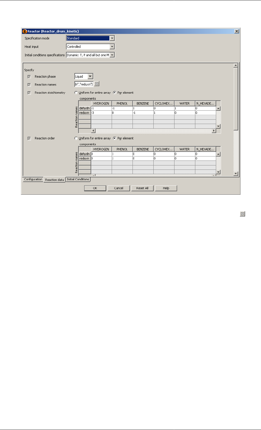
Ordered Sets
80
Figure 9.1. Reaction Data Tables Labelled with Elements from Ordered Sets
The elements of the Ordered Set of reactions (labelled Reaction names) can be specified using gPROMS language,
as shown above, or by editing each element individually in a matrix. In order to do this, left click on the button
next to the text box. In the image below, another reaction has been entered in this fashion. Notice that the tables
for the stoichiometric parameters are automatically updated once the new reaction has been entered (or an existing
one deleted — simply by editing the entry and deleting it).
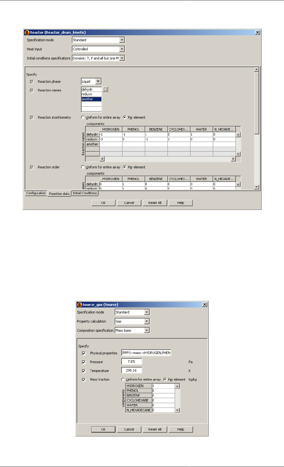
Ordered Sets
81
Figure 9.2. Entering a New Reaction: the Data Tables are Automatically Updated
It is also apparent from the above figures, that the components are also represented by an Ordered Set. This can
be specified in exactly the same way, but in this example, it is given by a physical property Foreign Object. Just
as when changing, adding or removing an element of the reactions Ordered Set, the data-entry tables for any
Parameters or Variables that are indexed over the set of components will automatically change. The figure below
shows the format for entering component data using the Ideal Physical Property Foreign Object (see the Physical
Properies Guide): the Ordered Set of components is automatically updated by the physical-propery Foreign Object
whenever the specification is changed, and this then updates the table of mass fractions below and the reaction-
data tables in the figure above.
Figure 9.3. Ordered Set being defined by a Physical Property Foreign Object
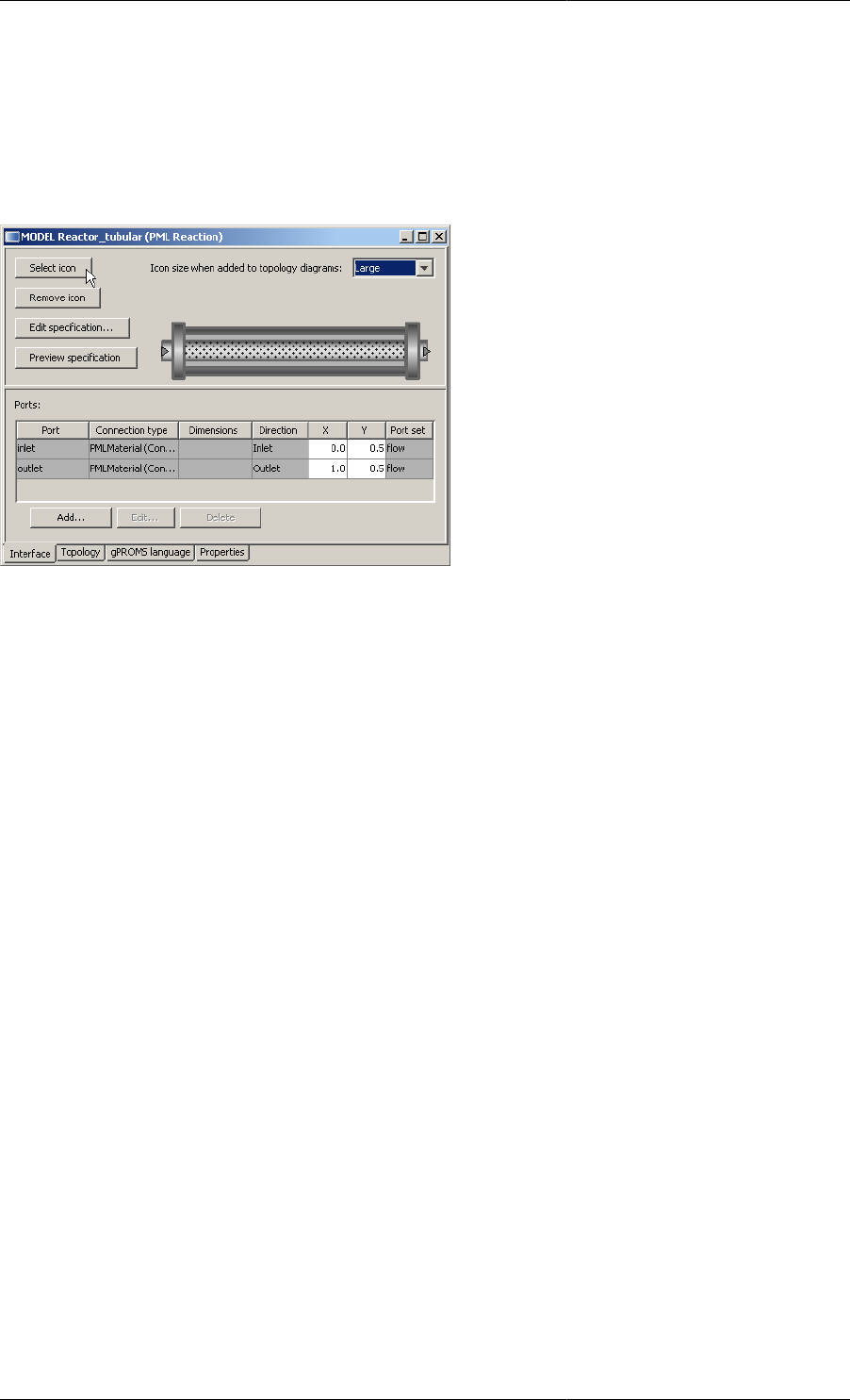
82
Chapter 10. Defining a Public Model
Interface
Providing a Model with a Public Interface allows it to be used quickly and easily on the topology tab of flowsheet
Models.
The Model Interface has four key facets:
• A Model icon which determines how the Model is displayed on the topology tab of flowsheet Models.
• Model Ports to allow connections to other component Models.
• A Specifications dialog to enable easy specification of Model inputs and initial conditions.
• A Model report to present key results in a clear format following a Simulation activity.
Defining a Model icon
The Model icon determines how an instance of the Model is displayed on the topology tab of a flowsheet Model.
It is possible to associate any icon of your choice with a particular Model. To do so, you need to do the following:
• On the interface tab the Model entity click on the Select icon button (see figure (a) below). This will open a
dialog box that allows you to browse and select your desired image.
• Use the browser to select your image file and press the OK button (see figure (b) below).
• ModelBuilder supports the following image formats: .svg, .gif, .jpg (or .jpeg) and .png.
• You have the option of selecting a default size for the icon size (see figure (c) below).
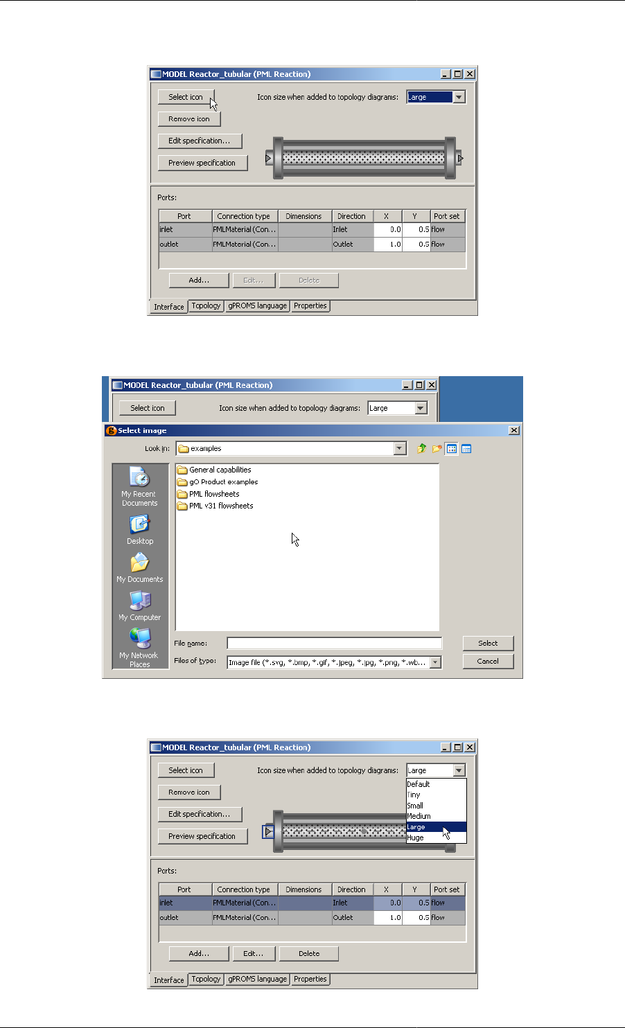
Defining a Public Model Interface
83
Figure 10.1. Defining an icon - (a) the Select icon button on the interface tab
Figure 10.2. Defining an icon - (b) selecting the desired image file
Figure 10.3. Defining an icon - (c) choosing the default icon size
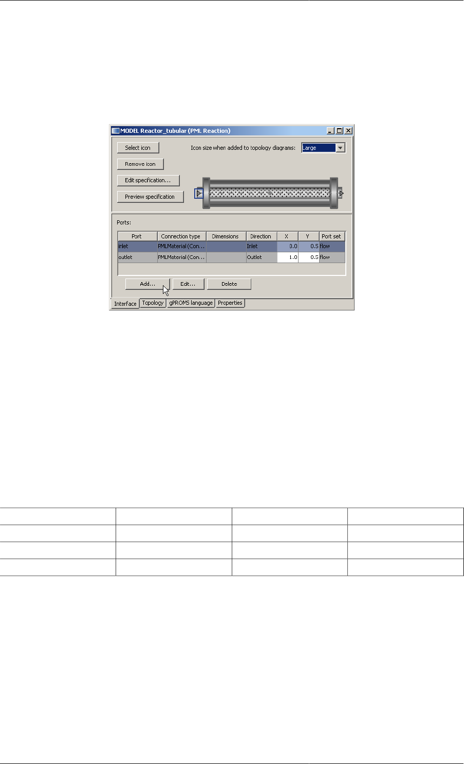
Defining a Public Model Interface
84
Defining Model Ports
Topology connections to and from a Unit are made from its Ports. These are configured from the Port table in
the lower pane of the Interface tab:
Figure 10.4. The Port table
The Port table shows the following information:
• Port name: the name by which the Port will be referenced in the gPROMS language.
• Connection Type: the Connection Type which the Port is associated with (see also: Declaring new Connection
Types). Only topology connections of this type can be connected to this Port.
• Dimensions: the dimensionality of the Port — both scalar and Array Ports are supported.
• Array Ports of Fixed size(s) and of Dynamic size are supported. For dynamically-sized Ports, the size of the
Array is specified by the number of connections made to that Port. If no connections are made, the size of
the Array will be set to zero, the benefits of which are discussed here.
• Direction: The Port direction — Inlet, Outlet or Bi-directional. gPROMS enforces the following rules
Inlet Outlet Bi-directional
Inlet Disallowed Allowed Allowed
Outlet Allowed Disallowed Allowed
Bi-directional Allowed Allowed Allowed
• X & Y co-ordinates: the location of the Port on the Model's icon.
• Port set: The set to which the Port belongs.
• For all Ports belonging to the same set (i.e. those in the same Port set): the equivalent Connection Type
Parameters will be equated. For example; in a device with two flow paths such as a heat exchanger, with a
hot stream and a cold stream, the hot inlet and outlet Ports would be in a hot set and the cold inlet and outlet
Ports would be in a cold set. (see also: Setting Connection Type Parameters).
• Ports in the same set are indicated graphically on the Model's icon by a dotted connectivity line; indicating
(material or information) flow paths.
From the interface tab, click on the Add button to Create a new Port.
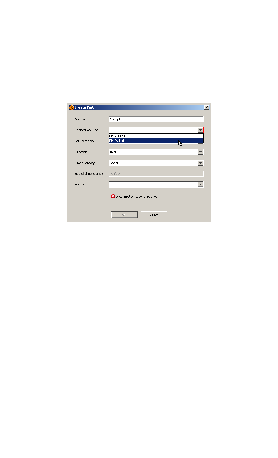
Defining a Public Model Interface
85
When you declare a Port in a Model, it is associated with a Connection Type. All the quantities declared by the
Connection Type (Variables, Parameters and Distribution Domains) are automatically included in the Model that
declares the Port. So an equivalent number of Equations should be provided in the Model entity to make use of
the additional Variables. This is done in the gPROMS language declaration for the Model.
Create a new Port
Click on the Add button to define a new Port, or click the Edit button to modify an existing Port. This will activate
a Create Port (or Edit Port) dialog box:
Figure 10.5. Creating a new Port
• Port name: enter the name of the Port
• Connection type: choose the Connection Type from a drop down menu or manually enter the name.
• Port category: if the Connection Type enforces connectivity rules a Port category must be provided; select this
from the drop-down menu.
• The category of a Port determines which other Ports a connection may be made to (see also: The Port
categories tab and Connectivity rules).
• Direction: choose an Inlet, Outlet or a Bi-directional Port.
• Dimensionality: you can select a Scalar Port, an Array Port of Fixed size(s) or an Array Port of Dynamic size.
• If you select Scalar, then no further specification is required.
• If an Array Port of Fixed size(s) is selected, then under Size of dimension(s) enter the size(s) as either a literal
value (e.g. 7) or using an Integer Parameter whose value is provided elsewhere.
• If an Array Port of Dynamic size is selected, then select an Integer Parameter from the Model declarations.
This Parameter will be set automatically to a value equal to the number of connections made to the Port.
• If there are no connections made to the port, the Parameter will be set to zero. This will result in an Array
of zero length, the benefits of which are discussed here.
• Port set: you can add a name for a new set or select a name of an existing set (see also: Port set and Setting
Connection Type Parameters).
The locations of Ports on the Model icon are specified directly on the Interface tab. The location of a Port is stored
in terms of an X co-ordinate and a Y co-ordinate [0 to 1], with (0,0) being in the top left corner of the icon. To
determine the location of the Port:

Defining a Public Model Interface
86
• Either (i) move the Port to the appropriate place on the icon by dragging it using the mouse;
• or (ii) enter a co-ordinate: to do this simply click on the relevant cell and type in the number.
Ports and the gPROMS Language
All Ports defined using the Interface tab, are reflected on the Model's gPROMS Language tab with the following
syntax:
PORT
PortName AS ConnectionType
PortName AS ARRAY (Size <,>) OF ConnectionType.
Port sets are also reflected on the Model's gPROMS Language tab with the following syntax (though in read-
only text):
PORTSET
[PortName, ..., PortName] {PortsetName} ;
An example of Ports and Port sets for the Reactor_tubular Model from the gPROMS Process Model Library is
shown below
PORT
in AS PMLMaterial
out AS PMLMaterial
PORTSET
# Start Port Sets
[in, out] {flow} ;
# End Port Sets
All the quantities declared for this Connection Type (Variables, Parameters and Distribution Domains) are
automatically included in the Model. As with the development of composite Models, these are referenced using
a pathname construct:
Therefore, to equate the Connection Type Parameters carried by the inlet Port to equivalent Model Parameters;
one could write:
SET
no_components := in.no_components,
phys_prop := in.phys_prop;
........
Similarly, the Connection Type Variables are used directly in Model Equations (you may note from this that the
Reactor_tubular Model is a distributed Model):
EQUATION
# Using Port Variables in a Model as Boundary conditions for a distributed model
mass_flowrate(0) = in.mass_flowrate/number_of_tubes ;
mass_fraction(,0) = in.mass_fraction = in.info_mass_fraction ;
mass_specific_enthalpy(0) = in.mass_specific_enthalpy = in.info_mass_specific_enthalpy ;
pressure(0) = in.info_pressure ;
mass_flowrate(1) = out.mass_flowrate/number_of_tubes ;
mass_fraction(,1) = out.mass_fraction ;
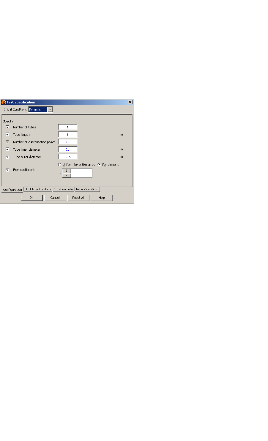
Defining a Public Model Interface
87
mass_specific_enthalpy(1) = out.mass_specific_enthalpy ;
...............
Defining a Specification dialog and Model
Reports
A Model is defined both by its Equations and the specifications that must be provided to satisfy its degrees of
freedom. In gPROMS, the required set of specifications and the initial conditions for a Model can be stored with
that Model. These are then accessed via its Specification dialog, as shown below.
The Specification dialog makes it easy to share the Model with other users and makes it faster and easier to re-
use the Model:
• Specification dialogs are accessed from a flowsheet Model's topology tab. (see also: Constructing flowsheet
Models).
• Specification dialogs allow:
• Parameters to be Set values,
• Variables to be Assigned values,
• Selectors to be given initial values,
• and Initial conditions to be defined.
• The specifications made using Specification dialogs in a flowsheet Model are displayed as read-only text in the
Process entity that includes the flowsheet Model.
• In the associated Process entity the user has the option to include unit dialog specifications or not. This option
is accessed
•either from the Entity menu when the Process entity is selected
•or from the short-cut menu accessed by right-clicking on the appropriate Process entity.
When removing dialog specifications; the existing specifications can be left for manual modification or
removed completely.
Specification dialogs are configured from a Model's interface tab by clicking the Edit specification ... button. This
will also give you the opportunity to define a Model report. Model reports are used to present key results in a clear
format following a Simulation activity (see also: Viewing Model reports).

Defining a Public Model Interface
88
After clicking the Edit specification ... button you are guided through the following five steps:
• Public Model Attributes
• Define tabs in Dialog
• Configure Specification Dialog
• Define Model Help
• Configure report
To move between the steps use the Next and Previous buttons; when the Specification is complete click the Finish
button. At any point it is possible to Preview the specification dialog and the Model reports using the Preview
specification and Preview report buttons:
Defining Public Model Attributes
Step 1
The first step is to specify from the full set of Parameters, Variables and Selectors declared by the Model (the
Model symbols) a sub-set which shall be exported as Public Model Attributes (PMA). These are essentially those
that will either appear on a Specification dialog or appear on a Model report.
When compared against other Model symbols, Public Model Attributes have the following additional information
• Name: A display name for the PMA not necessarily the same as its ID (i.e. how it is referred to in the gPROMS
language)
• Default : The default value for the PMA when it appears on the Specification dialog
• Lower and Upper bounds: These are used to guide the Model user to provide sensible values for the specification
• It is still possible for a user to provide a value outside these bounds but the value enter will be highlighted
with a warning message
• For Variables it is anticipated that these bounds would be much tighter than those provided by its Variable
Type which are usually relatively loose.
• Units: The engineering units are displayed wherever the PMA appears on the Model's Specification dialog and
report
• Field width and Field alignment: The size and alignment of the space provided to give the PMAs value.
• Description: In the description, additional information about the PMA can be given; this is displayed to the
Model user as a tool-tip when the mouse hovers over the PMA on the Specifications dialog.

Defining a Public Model Interface
89
Figure 10.6. Public Model Attributes page
To define the Public Model Attributes:
• Select the Public Model Attributes from the Model symbols pane. Do this by clicking on the check box to select
the desired Model attribute; all the checked symbols will appear in the Public Model Attributes table.
• The default value, the lower bound, the upper bound and the units for the PMA are entered directly in the PMA
table.
• Note that the bounds and units are only meaningful if the attribute is a Parameter or a Variable. The bounds
for PMA Variables are initially taken from their Variable Types but it is highly recommended that these are
refined to bounds that prevent the Model being used in operating regions for which it is not valid.
• The PMA's name, description and the width of its value field and the alignment for this field are specified in a
separate pane and are accessed by selecting the PMA in the PMA table.
As can be seen in the image above, Initialisation Procedures can be included in a Public Model Interface. A name
and description can be given for the Initialisation Procedure and the default value must be set to DEFAULT. At
present, the Model user will only have the option of selecting whether or not Initialisation Procedures are used; if
they are to be used, they must be the default Initialisation Procedure. Non-default Initialisation Procedures must
be specified using the gPROMS language tab of the Process.
Specifications dialog tabs
Step 2
The Specification dialog can have any number of tabs (including zero); these can be given appropriate names.
Tabs are typically used to group similar PMAs together and, equally, to separate dissimilar quantities. For example,
it is common to put Variable Assignments on one tab, Configuration, and Initial condition specifications on
another, Initial conditions.
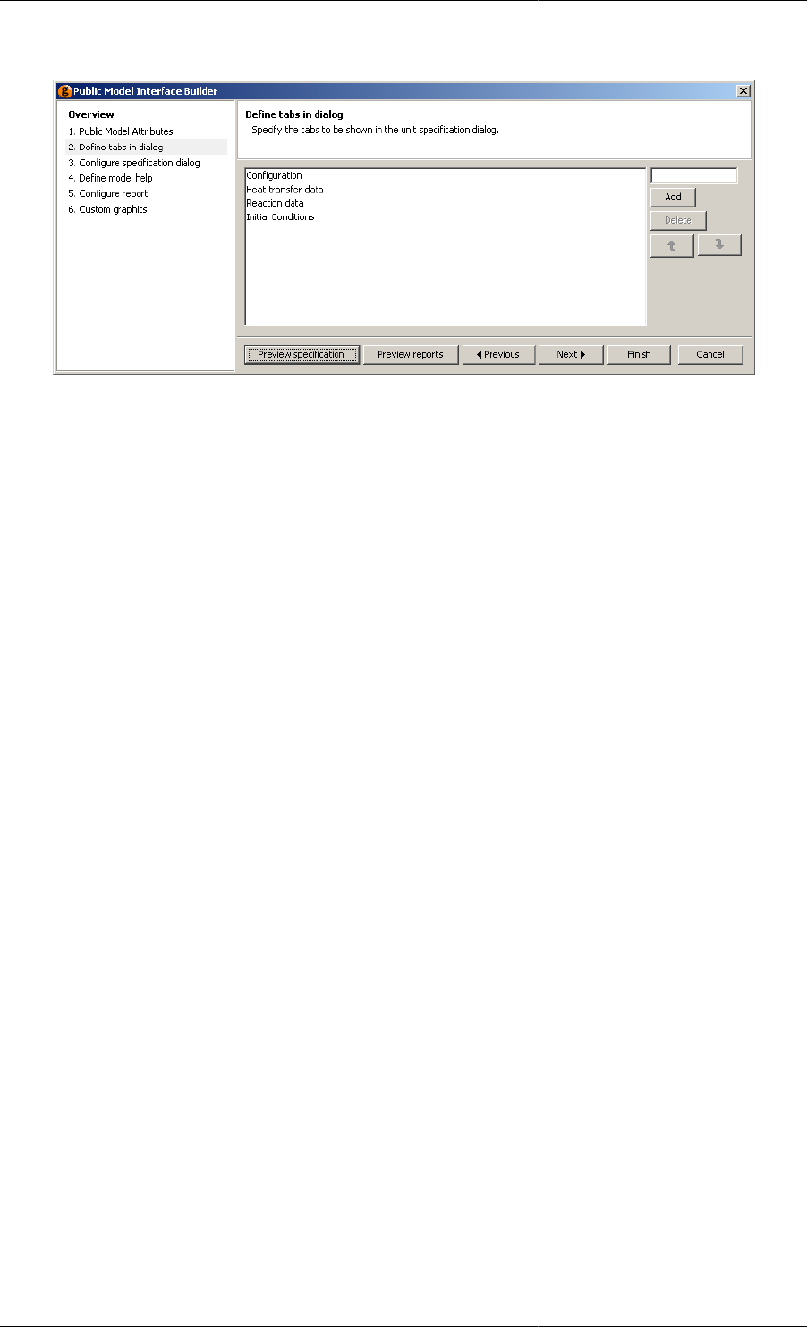
Defining a Public Model Interface
90
Figure 10.7. Defining the tabs for the Specification dialog
To define a tab:
• Type the tab name in the field on the righ-hand-side and click Add
• If multiple tabs are present these can be ordered using the up and down arrow buttons
Configure specification dialog
Step 3
Model specifications are given in terms of the Public Model Attributes (PMAs); these are accessed by the Model
user from the Specification dialog. Following the identification of the PMAs in Step 1, the following additional
information must be provided to configure the behaviour of the dialog:
• which of the PMAs should appear on the dialog
• on which dialog tab the PMAs should appear
• the type of specification required for the PMA
• Obligatory - the Model user must provide this specification
• Optional (on) - the Model user can provide this specification; the default is that the specification should be
given
• Optional (off) - the Model user can provide this specification; the default is that the specification is not given
Furthermore, whilst Parameter PMA specifications will automatically appear in the SET section and Selector PMA
specifications will automatically appear in the INITIALSELECTOR section, we must specify whether a Variable
PMA corresponds to an Initial condition equation (INITIAL section), a Model input (ASSIGN section) or even
a Preset value (PRESET section).
Initial conditions
Two types of initial condition specification are possible using a Specification dialog:
• Dynamic: these are of the form:
PMA_Variable = value;
• Steady-state: the equations for steady-state Initial conditions must be provided by the Model developer
Both specifications types can be enabled for a Specifications dialog and, if so, these should be separated into
different specification groups. If the steady-state group is selected then the Model user need not give any further
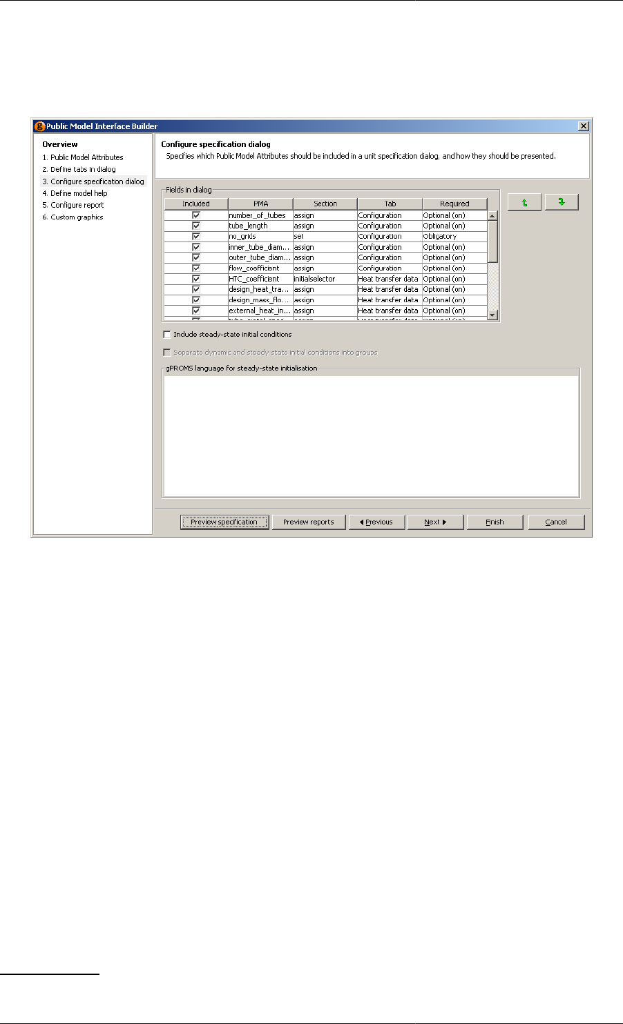
Defining a Public Model Interface
91
specification regarding the Initial conditions. On the other hand, if the dynamic group is selected then the Initial
values of the PMA Variables must be provided in the Specification dialog
Figure 10.8. Configuring the specification dialog
To specify which of the Public Model Attributes (PMAs) should be included in the Specification dialog and the
appearance of the Specification dialog:
• Select the PMAs that you wish to include in the Specifications dialog by checking the box next to the PMA1.
• If you have selected a PMA Variable: choose the section of the Process entity that the PMA will appear in when
given a value: ASSIGN, INITIAL or PRESET.
• If multiple tabs have been selected:- specify which tab of the Specification dialog the PMA should appear on
• Choose the type of specification required for the PMA - Obligatory; Optional (on) or Optional (off).
• If steady-state initial conditions are required -
•check the Include steady-state initial conditions box
• if dynamic initial conditions have also been provided (i.e. PMA Variables with INITIAL as the section) then
also check the Separate dynamic and steady-state initial conditions into groups box
• If the Include steady-state initial conditions box is checked: the gPROMS language for the steady-state initial
conditions for this Model must be entered in the space provided. For example, the steady-state initial conditions
for a distributed tubular reactor (where volume_specific_internal_energy and mass_conc are the state Variables)
can be written:
FOR z := 0|+ TO 1 DO
1You may have chosen some PMAs because they are useful output variables.
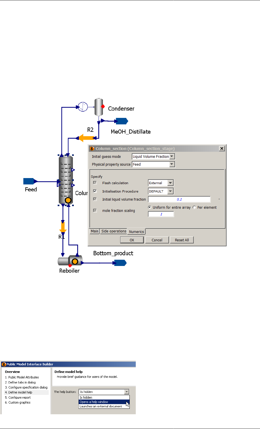
Defining a Public Model Interface
92
$volume_specific_internal_energy(z) = 0;
FOR i := 1 TO no_components DO
$mass_conc(i,z) = 0;
END # For
END # For
For Initialisation Procedures, the type of specification must be set to Optional (on). An example of Initialisation
Procedure specification in a Model specification dialog is shown below. (To activate the Model specification
dialog, double click on the Unit.)
Figure 10.9. Model Specification Dialog including Initialisation Procedure
The Model user is able to check or uncheck the Initialisation Procedure in order to enable or disable it. However,
the combobox to the right contains only DEFAULT and cannot be changed, since the choice of Initialisation
Procedure cannot be made in a Model specification dialog at present.
Defining Model help
Step 4
A Help button can be added to the public Model interface. Help can be provided in two different ways or disabled
according to the selection made using the listbox in step 4 of the Public Model Interface Builder dialog:
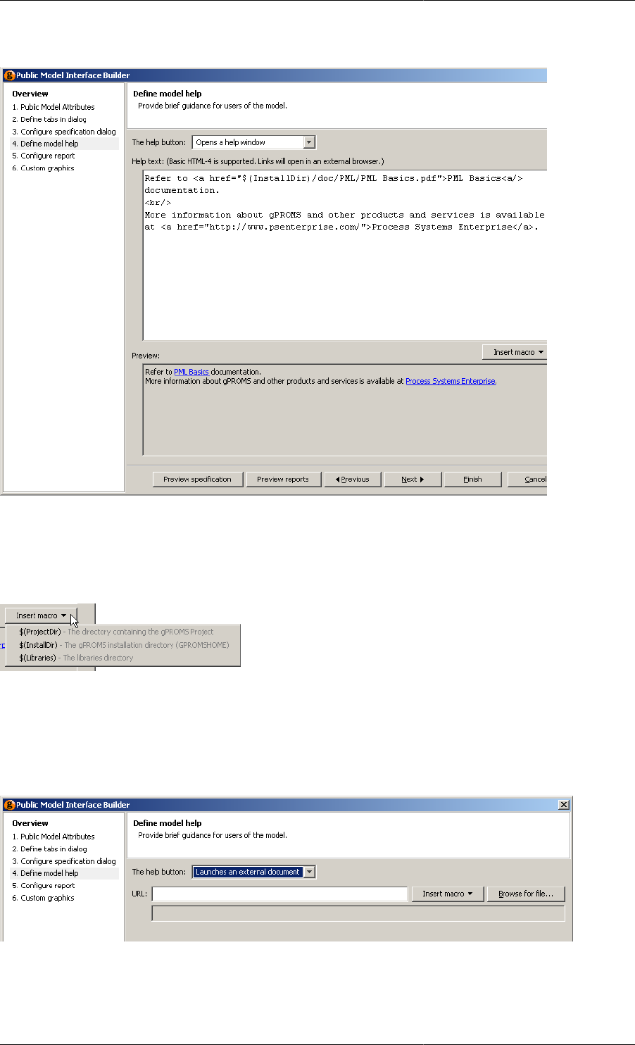
Defining a Public Model Interface
93
When Opens a help window is selected, the dialog changes to include a text box and a preview pane. The help
page must be defined using XHTML and can include links to external web pages and documents, as shown below.
The preview pane is updated in real time, as the XHTML is edited above. Any links in the help page are active
in the preview pane and can be followed by left clicking on them. Links to external web sites will open a new
browser window or tab (depending on your browser settings); links to files will launch the appropriate reader.
When providing links to documents, the Insert macro button provides a quick way to refer to common directories:
When typing in the path to an external document, selecting one of the options from the list box above will result
in the macro being inserted into the text. See the previous screen shot for an example.
The simplest way to provide Model help is to link directly to an external document. This is done by selecting
Launches an external document from the Help button: list box. The Public Model Interface Builder dialog will
then change to:
There are two ways to specify the location of the external document:
• Type the location into the URL: text box
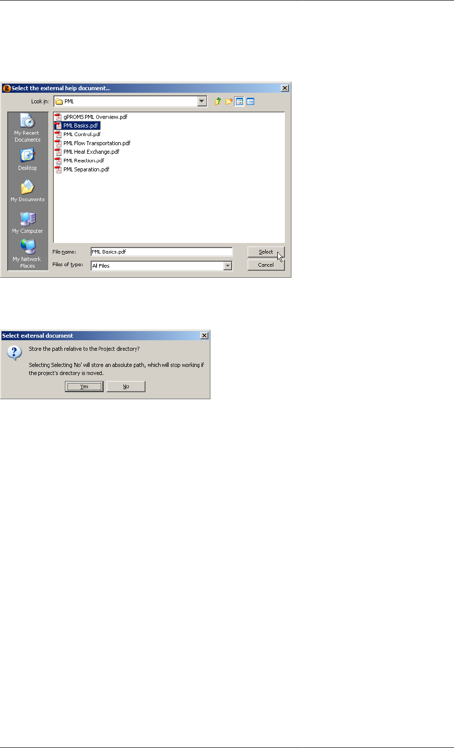
Defining a Public Model Interface
94
• The Insert macro button can be used as before
• Locate the document using the Browse for file... button
When using the file browser, navigate to the desired document and press Select:
If the document is contained in the same directory as the project file (or is contained in one of its sub directories),
then another dialog will appear. This allows you to choose whether to specify the location of the document as an
absolute path or a relative one.
If documentation is always kept in the same location, then select an absolute path: this way, the project file can be
moved to a different location without breaking the link. This would be useful if, for example, a Model developer
released a project file to a number of different users but wanted to keep one copy of the documentation in a single
public directory. If the documentation is to be kept in the same folder as the project file (or one of its subfolders),
then select a relative path so that the project folder can be moved to a different location without breaking the link.
Defining custom reports
Stage 5
Model reports are used to present key results in a clear format following a Simulation activity (see also: Viewing
Model reports).
There are three ways to configure the reports for a Model. These are:
• None — no report for the Model will be generated.
• Basic — a basic tabular report for the Model will be generated automatically using a simple configuration tool.
• Advanced — the user can fully specify the format of the report, including tables and plots, using xml. This
method gives the most control over the reports but is the most complicated to use.
To select the method for specifying reports, left click on the drop-down menu and select the desired option.
Selecting Basic enables a GUI in the bottom pane of the window, where you can select the Variables that should
be included in the report. Selecting Advanced enables a text editor in the bottom pane, where you may enter xml

Defining a Public Model Interface
95
to define the report. There may already be some xml present if you have already defined a report using the Basic
method.
Once you have finished, press the Finish button at the bottom of the window.
Basic Report Configuration
The basic tool for configuring model reports enables you to select variables for inclusion in the report in tabular
form only. Check the boxes of all the variables you wish to appear in the report and then click Finish to complete
the configuration.
If you want to include any plots in the report, then you must select Advanced from the drop-down menu.
Figure 10.10. Example Model Report configuration
Advanced Report Configuration
Advanced report configuration is achieved using xml. In addition to standard HTML tags, so that headings, images2
and hyperlinks to external documents and URLs may be included to enhance the report, there are three custom
tags that define five types of Model report. These are:
• Simple Tags — to present basic model attributes.
• Tables — to present tabulated data.
• 2D Plots — to present Variable data graphically as a function of one of the independent domains.
• x-y Plots — to plot values of one Variable as a function of another Variable. (This is a special case of the 2D
Plot, so read about 2D Plots first.)
• 3D Plots — to display a surface plot of one Variable as a function of 2 independent domains.
• Contour Plots — to display a contour plot of one Variable as a function of 2 independent domains.
2The following image formats are supported in Model reports: .gif, .jpg (and .jpeg) and .png. They can be inserted into model reports using
the standard <img src=""/> tag, e.g.:
<img src="file:///c:/temp/test.gif"/> <img src="http://www.psenterprise.com/css/psebutton.png"/>.

Defining a Public Model Interface
96
As with the Basic configuration utility, once you have finished editing the xml, simply press the Finish button
at the bottom of the window.
Note that a <br/> tag is required between any of the entities above in order to ensure they are correctly displayed
vertically on the page. To place entities side-by-side, use a table:
<table>
<tr>
<td><Plot3D ...></td>
<td><Plot3D ...></td>
</tr>
</table>
Simple Tags
The following simple tags may be used when developing Model Reports.
•<PMA_UNIT> displays the unit name.
•<PMA_NAME id="..."> displays the PMA name of the PMA specified by the id attribute.
•<PMA_UOM id="..."> displays the units of measurement for the PMA specified by the id attribute.
•<PMA_VALUE id="..."> displays the value(s) of the PMA specified by the id attribute.
Tables
Tables can be included in a Model report using two xml tags. The first, <PMA_TABLE>, creates the table; the
second, <Attribute/>, specifies a variable for inclusion in the table. There may be multiple <Attribute/
> tags within a <PMA_TABLE> tag to form a table containing as many variables as desired. An example is given
below.
<PMA_TABLE>
<Attribute id="a_Variable"/>
</PMA_TABLE>
The xml above creates a table within the report that displays the values associated with the Variable called
a_Variable. If the Variable specified in the id attribute is distributed over any number of domains, then all
of the values will be tabulated automatically.
To include more than one variable, simply add further <Attribute/> tags within the <PMA_TABLE> construct.
The number format for each variable can be set by specifying the numberFormat attribute of the
<Attribute/> tag:
<PMA_TABLE>
<Attribute id="a_Variable" numberFormat="%.pS"/>
</PMA_TABLE>
where p (the precision) is an integer from 0 to 9 and S (the specifier) is one of "G", "f" and "E", respectively
representing the General, Fixed and Scientific number formats. If the general format is chosen, then p is restricted
to integers from 1 to 6 and represents the number of significant figures; the fixed number format allows integers
from 0 to 9, which represent the number of decimal places; the scientific format allows beteen 0 and 5 decimal
places. Some examples are given below.
<PMA_TABLE>
<Attribute id="Variable1" numberFormat="%.4G"/> <!--General with 4 s.f.-->
<Attribute id="Variable2" numberFormat="%.6f"/> <!--Fixed with 6 d.p.-->
<Attribute id="Variable3" numberFormat="%.3G"/> <!--Scientific with 3 d.p.-->
Defining a Public Model Interface
97
</PMA_TABLE>
The <PMA_TABLE> tag may also contain a numberFormat Attribute. This specifies the number format
for any <Attribute> tags that do not contain a numberFormat Attribute. This is a more compact and
convenient method for setting the same number format for several Variables. If there is no numberFormat
Attribute specified for the <PMA_TABLE> tag and there are <Attribute> tags that do not contain a
numberFormat Attribute, then the number format for these <Attribute> tags is taken from the specification
in the ModelBuilder preferences, in the Results section of the Activity execution preferences.
Note that all of the tags and attributes described above are case senstitive: if they are not typed exactly as shown
above, then the report will not be generated and an error message will be displayed instead.
The full list of available number formats is given in the table below.
Format name Format string
General, 1 s.f. "%.1G"
General, 2 s.f. "%.2G"
General, 3 s.f. "%.3G"
General, 4 s.f. "%.4G"
General, 5 s.f. "%.5G"
General, 6 s.f. "%.6G"
Fixed, 0 d.p. "%.0f"
Fixed, 1 d.p. "%.1f"
Fixed, 2 d.p. "%.2f"
Fixed, 3 d.p. "%.3f"
Fixed, 4 d.p. "%.4f"
Fixed, 5 d.p. "%.5f"
Fixed, 6 d.p. "%.6f"
Fixed, 7 d.p. "%.7f"
Fixed, 8 d.p. "%.8f"
Fixed, 9 d.p. "%.9f"
Scientific, 0 d.p. "%.0E"
Scientific, 1 d.p. "%.1E"
Scientific, 2 d.p. "%.2E"
Scientific, 3 d.p. "%.3E"
Scientific, 4 d.p. "%.4E"
Scientific, 5 d.p. "%.5E"
2D Plots
2D Plots are created using the <Plot2D> tag and lines specified with the <Line/> tag. The basic format is:
<Plot2D version="1">
<Line idY=""/>
</Plot2D>
The version attribute of the <Plot2D> tag is mandatory and must be equal to 1.
Each <Line/> tag specifies which Variable is to be plotted against which independent domain, using the idY
attribute. The format of the attribute is a string comprising the name of the Variable to be plotted and a specification

Defining a Public Model Interface
98
indicating which domain should be free and plotted on the abscissa and the values of any domains that need to
be fixed3. This is best illustrated with an example.
<Plot2D version="1">
<Line idY="A(TIME=#)"/>
</Plot2D>
Here we have just one line specified for this 2D Plot (which will be 600 pixels wide and 400 pixels high).
The idY attribute of the <Line/> tag specifyies that the Variable A should be plotted with time as the independent
variable on the abscissa. Here, we see two features of the specification format: the first domain is always time and
is indicated by the string "TIME=", followed by either a number or the # symbol. The # symbol indicates that the
domain should be free and will be plotted on the abscissa. Since there are no other domain specifications, A must
be defined either as a scalar or as a vector. If A is defined as a scalar, then the <Line/> tag simply produces one
line in the 2D Plot. However, if A is defined as a vector (i.e. distributed over just one domain, either discrete or
continuous), then the <Line/> tag produces one line for every element of the domain.
To clarify the above, if the Variable A is defined in the Model by:
VARIABLE
A AS NoType
Then only one line will be plotted in the graph. However, A may also be defined by:
VARIABLE
A AS ARRAY(NoComp) OF NoType
or
VARIABLE
A AS ARRAY(Components) OF NoType
or
VARIABLE
A AS DISTRIBUTION(X_Domain) OF NoType
where NoComp is an integer, Components is an Ordered Set and X_Domain is a DistributionDomain. In any
of these cases, a series of lines will be plotted in the graph, one for each element of A.
If, in this second case, you want to plot only a single line, corresponding to a fixed value of the domain over which
A is defined, then this can be achieved by (for example):
<Plot2D version="1">
<Line idY="A(TIME=#,1)"/>
</Plot2D>
Another alternative is to plot the variable against the domain for some fixed value of time. This is done with the
following commands.
<Plot2D version="1">
<Line idY="A(TIME=0,#)"/>
</Plot2D>
The same rules apply to Variables defined over more than one domain, as shown in this next example.
<Plot2D version="1">
<Line idY="A(TIME=#)"/>
3Of course, there can only be one free domain in a 2D Plot and all other domains need to be fixed.

Defining a Public Model Interface
99
<Line idY="B(TIME=#,1)"/>
<Line idY="C(TIME=5,2,#)"/>
<Line idY="C(TIME=#,1,0)"/>
</Plot2D>
Here, we have 4 <Line/> tags, which will produce 4 lines in the graph, assuming the following variable
definitions.
VARIABLE
A AS NoType
B AS ARRAY(NoComp) OF NoType
C AS DISTRIBUTION(NoComp, X_Domain) OF NoType
So, the first <Line/> tag produces a plot of A against time; the second gives B(1) versus time; the third gives
the second component of C plotted against the x domain at time t = 5; and finally the last <Line/> specifies the
first component of C to be plotted agains time with the x domain fixed at 0.
Notice that the abscissa of the graph may be used to represent more than one independent domain. Although this
practice is allowed, it may result in confusing graphs, so it would be best to produce two separate graphs: one with
time on the abscissa and the other with the x domain.
Note that all of the tags and attributes described above are case senstitive: if they are not typed exactly as shown
above, then the report will not be generated and an error message will be displayed instead.
x-y Plots
x-y plots are essentially a special case of the 2D Plot. The difference is simply that a 2D Plot displays the values
of one or more Variables against one of the independent domains; whereas an x-y plot displays the values of one
Variable against another Variable. (As with 2D plots, you could display more than one relationship per graph, but
this might be rather confusing.)
An x-y plot is easily defined by using an appropriate <Line/> tag in a normal <Plot2D> construct. This is best
illustrated with an example. Consider the following Variable definitions.
VARIABLE
VapourMoleFraction AS DISTRIBUTION(NoComp, X_Domain) OF MoleFraction
LiquidMoleFraction AS DISTRIBUTION(NoComp, X_Domain) OF MoleFraction
In a normal 2D plot, we could plot either (or both) of these variables as functions of time, the x domain or indeed
the number of components; but it may be useful to be able to plot the vapour mole fraction as a function of the
liquid mole fraction, to produce an equilibrium diagram. This is achieved with the following xml commands.
<Plot2D version="1">
<Line idY="VapourMoleFraction(TIME=#,1,0)" idX="LiquidMoleFraction(TIME=#,1,0)"/>
</Plot2D>
This essentially produces a plot of vapour mole fraction against liquid mole fraction of component 1 at x = 0,
parameterised by time. One could equally parameterise using the x domain:
<Plot2D version="1">
<Line idY="VapourMoleFraction(TIME=0,1,#)" idX="LiquidMoleFraction(TIME=0,1,#)"/>
</Plot2D>
One may parameterise using any of the independent domains, with the only restriction being that the same domain
must be free in both of the id attributes in each <Line/> tag. Of course, having to fix all of the other independent
domains can be a bit restrictive, but one can include more points in the x-y plot by including more <Line/>
tags, for example:
<Plot2D version="1">

Defining a Public Model Interface
100
<Line idY="VapourMoleFraction(TIME=#,1,0)" idX="LiquidMoleFraction(TIME=#,1,0)"/>
<Line idY="VapourMoleFraction(TIME=#,1,1)" idX="LiquidMoleFraction(TIME=#,1,1)"/>
<Line idY="VapourMoleFraction(TIME=0,1,#)" idX="LiquidMoleFraction(TIME=0,1,#)"/>
<Line idY="VapourMoleFraction(TIME=10,1,#)" idX="LiquidMoleFraction(TIME=10,1,#)"/>
</Plot2D>
Similarly, we may want to generate a phase diagram by plotting, say, Temperature as a function of both the
liquid and vapour mole fractions. Assuming the appropriate definition of Temperature, this can be done by:
<Plot2D version="1">
<Line idY="Temperature(TIME=#,0)" idX="LiquidMoleFraction(TIME=#,1,0)"/>
<Line idY="Temperature(TIME=#,0)" idX="VapourMoleFraction(TIME=#,1,0)"/>
</Plot2D>
Note that it is not necessary that the variables have the same number of dimensions; only that they are defined
over the same domain that is specified to be free in the <Line/> tag. That is, the # symbol should specify the
same domain in each <Line/> tag.
Note also that gPROMS does not check that the values of the fixed domains are identical in each <Line/> tag. If
they are specified different values, it is almost certain that the graph produced will be physically meaningless.
Note that all of the tags and attributes described above are case senstitive: if they are not typed exactly as shown
above, then the report will not be generated and an error message will be displayed instead.
3D Plots
For Variables that are defined over two or more independent domains (including time), 3D plots may be generated
using the <Plot3D> construct and its associated <Surface/> tag. The basic format is:
<Plot3D version="1">
<Surface id=""/>
</Plot3D>
where the string specified in the id attribute defines the variable to be plotted (in this case, only one variable is
allowed per plot), against which domains it should be plotted on which axes, and the values to which all other
domains should be fixed. Like 2D plots, the width and height attributes are mandatory and specify the width
and height of the plot in pixels. As an example, consider the following Variable definition.
VARIABLE
Temperature AS DISTRIBUTION(Axial, Radial) OF AbsoluteTemperature
This Variable therefore has 3 independent domains: time (even in a steady-state simulation), axial and radial. To
define a 3D plot, we must select two of the domains to be free and fix the third. For the two free domains, we
may also choose which of the cartesian-coordinate axes will be used: x or y. The surface will then be plotted using
a standard right-handed cartesian-coordinate system with the x axis horizontally in the plane of the screen/page
and the z axis vertically in the plane of the screen/page. The y axis therefore points into the screen/page and is
perpendicular to it. Variable values will be plotted on the z axis, with the two free domains on the x and y axes,
as specified in the <Surface/> tag.
For the above Variable definition, one possible plot is generated with the following xml.
<Plot3D version="1">
<Surface id="Temperature(TIME=#x,#y,0)"/>
</Plot3D>
Here, the time domain has been specifed to be represented by the x axis and the axial domain by the y axis. The
values of Temperature plotted are to correspond r = 0 in the radial domain. The #x string specifies which free
domain is represented by the x axis, and the #y string behaves similarly.

Defining a Public Model Interface
101
If the Variable defined above were used in a steady-state simulation, the surface can only be defined in one of
two ways:
<Plot3D version="1">
<Surface id="Temperature(TIME=0,#x,#y)"/>
</Plot3D>
the only other possibility being to swap which axes represent the axial and radial domains.
Note that all of the tags and attributes described above are case senstitive: if they are not typed exactly as shown
above, then the report will not be generated and an error message will be displayed instead.
3D Plot Orientation
It is often necessary to adjust the orientation of a 3D plot to show the shape of the surface more clearly. This can
be achieved using the <Rotation/> tag within the <Plot3D> construct. This allows the user to specify the
orientation of the plot by using standard rotations about each of the cartesian-coordinate axes. The basic syntax
is as follows (using the example presented before).
<Plot3D version="1">
<Surface id="Temperature(TIME=0,#x,#y)"/>
<Rotation x="0" y="0" z="0"/>
</Plot3D>
Each attribute defines the rotation in degrees about its corresponding axis. The values may be positive or negative.
The values above (i.e. no rotation) produce a coordinate system with the x and z axes in the plane of the screen/page,
with the x axis horizonal. By defintion, the y axis therefore points into the screen/page. This is not a particularly
useful view, so the default view is to rotate the coordinates 45 degrees about both the x and z axes. In other words,
omitting the <Rotation/> tag altogether is the same as specifying:
<Plot3D version="1">
<Surface id="Temperature(TIME=0,#x,#y)"/>
<Rotation x="45" y="0" z="45"/>
</Plot3D>
Of course, any other values may be specified to suit the Variable being plotted. The figure below shows the default
rotation on the left and no rotation on the right (along with an indication of the positive direction of rotation for
each axis). The plot on the left has time assigned to the x axis and NoComp to the y axis.
Figure 10.11. Default Orientation of 3D Plots (left)
and Definition of Coordinates with no Rotation (right)
Note that all of the tags and attributes described above are case senstitive: if they are not typed exactly as shown
above, then the report will not be generated and an error message will be displayed instead.
Contour plots
Contour plots are a special case of 3D plots in which no 3-dimensional surface is plotted but where the contour
lines are projected onto the x-y-area. The example below shows the temperature at the exit of a tubular reactor.
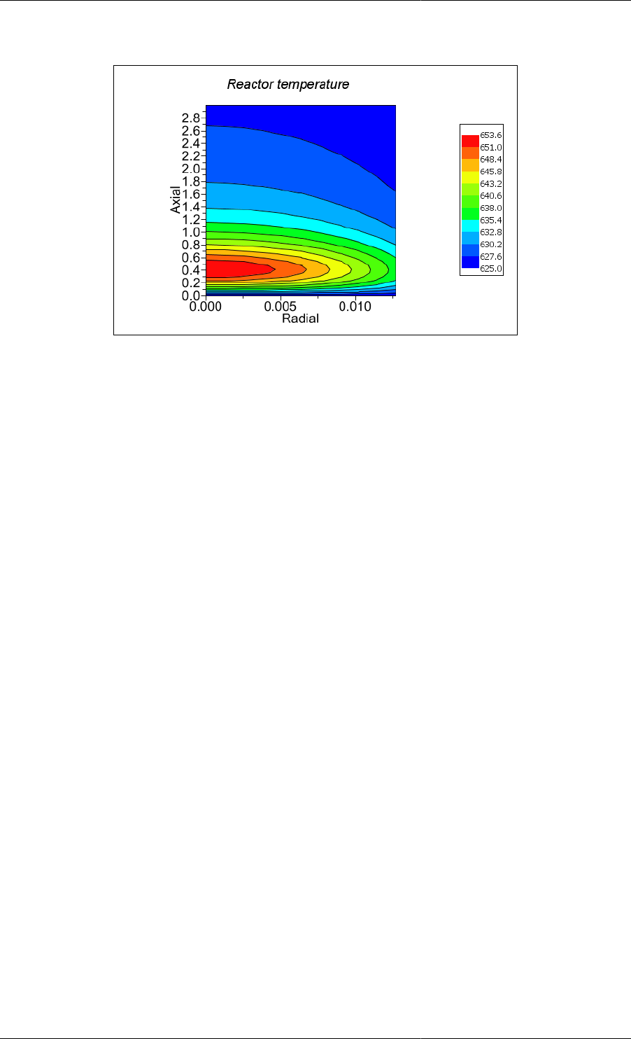
Defining a Public Model Interface
102
Figure 10.12. Example of a contour plot
The xml code for defining this plot looks as follows. The important Surface attributes to set are mesh and shade,
both require the value false.
<Plot3D width="600" height="400" version="1" border="true">
<Header label="Reactor temperature">
<Font name="Times" size="20" style="italic"/>
</Header>
<Legend show="true" border="true" anchor="right" orientation="vertical" style="continuous">
<Font name="Arial" size="12"/>
</Legend>
<Axes>
<LabelFont name="Arial" size="50"/>
<NumberFont name="Arial" size="50"/>
<Axis orientation="x" show="true"/>
<Axis orientation="y" show="true"/>
<Axis orientation="z" show="true"/>
</Axes>
<Surface id="Reactor.T(TIME=5,#y, #x)" mesh="false" shade="false"
contours="true" zones="true"/>
<Rotation x="90" y="0" z="0"/>
</Plot3D>
Note that all of the tags and attributes described above are case senstitive: if they are not typed exactly as shown
above, then the report will not be generated and an error message will be displayed instead.
Formatting Options
Each of the environments for creating different types of Model Report have a number of tags for specifying how
they should be formatted.
• Formatting options for <PMA_TABLE>
• Formatting options for <Plot2D>
• Formatting options for <Plot3D>
Tags can be used in two ways, depending on whether they may contain other tags. If a tag may not contain any
other tags, then it can only be used in the "simple tag" form:
<TagName attribute1="" attribute2="" ... attributeN=""/>
Defining a Public Model Interface
103
However, when other tags need to be included, then the full tag form must be used:
<TagName attribute1="" attribute2="" ... attributeN="">
<!-- contained tags go here -->
</TagName>
Unless otherwise stated, attributes and tags are optionally specified and there can be at most one of each tag.
Formatting options for <PMA_TABLE>
The <PMA_TABLE> tag has a number of attributes that specify how the table will look in the report. These are
described in the table below. Where there are only a certain number of allowable values for the attribute, these
are listed inside brackets, separated by pipes. E.g. [true|false] means that an attribute may only take the values
true or false (of course, when specifying the values of attributes, they must always be enclosed in quotes,
e.g. attr="true").
Note that all of the tags and attributes described here are case senstitive: if they are not typed exactly as shown
above, then the report will not be generated and an error message will be displayed instead.
Table 10.1. Attributes of the <PMA_TABLE> tag
Attribute Name Description Default Value Notes
pmas Determines which
Public Model
Attributes are shown.
specified [all|variables|
parameters, specified]
specified means...
border The border
width in pixels. 1 Only non-negative
integers allowed.
lineThickness The thickness of the lines
between the cells in pixels. 0 Only non-negative
integers allowed.
cellspacing The cell spacing in pixels. 1 Only non-negative
integers allowed.
units Specifies whether or
not to display the units. true [true|false]
tableAlign Alignment of table
relative to the page. left [left|center|right]
headerAlign Alignment of
table headings. center [left|center|right]
pmaNamesAlign Alignment of
PMA names. left [left|center|right]
pmaValuesAlign Alignment of
PMA values. left [left|center|right]
unitsAlign Alignment of units. left [left|center|right]
altBGColorMode Alternate the
background colour
for each PMA name?
true [true|false]
altBGColor Alternating
background colour. #DEEFEE Takes a string defining the
colour either as a name
or in hexadecimal RGB
format preceded by a #
character. The allowable
names (case insensitve)
are: Black (#000000),
Green (#008000),
Silver (#C0C0C0),

Defining a Public Model Interface
104
Attribute Name Description Default Value Notes
Lime (#00FF00),
Gray (#808080),
Olive (#808000),
White (#FFFFFF),
Yellow (#FFFF00),
Maroon (#800000),
Navy (#000080),
Red (#FF0000),
Blue (#0000FF),
Purple (#800080),
Teal (#008080),
Fuchsia (#FF00FF),
Aqua (#00FFFF).
pmaColTitle Title for PMA column. Name
valueTitle Title for value column. Value at time $t $t is replaced by the
time selected using
the slider at the top of
the reports window.
unitsTitle Title for units column. Units
numberFormat Specifies the formatting
of numbers in the table. N/A See Tables.
The <Attribute> tag is a simple tag that specifies which Public Model Attribute to include in the PMA Table.
One tag is used for each Variable to be included, which is specified using the mandatory id attribute. For example,
a single Variable would be tabulated thus:
<PMA_TABLE>
<Attribute id="..."/>
</PMA_TABLE>
The format for the id attribute is similar for each type of Model Report.
In addition to the <Attribute/> tag, two tags provide formatting options for the header and body font. These are
<HeaderFont> and <BodyFont>, both of which take the following attributes.
Table 10.2. Attributes of the <HeaderFont> and <BodyFont> tags
Attribute Name Description Default Value Notes
name The name of the font. Automatically chosen
size The size of the
font in points. Automatically chosen Only positive
integers allowed.
style The font style. Automatically chosen Can be a combination
of bold, italic, underline
and strikeout, separated
by commas. E.g.
style=bold, italic.
Formatting options for <Plot2D>
The <Plot2D> tag has a number of attributes that specify how the graph will look in the report. These are described
in the table below. Where there are only a certain number of allowable values for the attribute, these are listed inside
brackets, separated by pipes. E.g. [true|false] means that an attribute may only take the values true or false.
Note that all of the tags and attributes described here are case senstitive: if they are not typed exactly as shown
above, then the report will not be generated and an error message will be displayed instead.
Defining a Public Model Interface
105
Table 10.3. Attributes of the <Plot2D> tag
Attribute Name Description Default Value Notes
width The width of the
graph in pixels. 500 Only positive
integers allowed.
height The height of the
graph in pixels. 300 Only positive
integers allowed.
border Defines in a border
should be drawn
around the graph.
false [true|false]
version The version of the
XML plot format. — This attribute is mandatory
and must be set to 1.
The remainder of the formatting for 2D plots is done using embedded tags within the <Plot2D> tag. These are:
•<Header>
•<Footer>
•<Legend>
•<Axes>
•<Grid>
•<Line>
The <Header> and <Footer> tags define the text at the head and foot of the graph. They both contain one
attribute and one <Font> tag. The Label attribute is a mandatory attribute and is the string defining the text
used for the header/footer. The <Font> tag defines the font used for the text. It has the following attributes.
Table 10.4. Attributes of the <Font> tag
Attribute Name Description Default Value Notes
name The name of the font. Automatically chosen
size The size of the
font in points. Automatically chosen Only positive
integers allowed.
style The font style. Automatically chosen Can be a combination
of bold, italic, underline
and strikeout, separated
by commas. E.g.
style="bold, italic".
For example, the header might be specified like this:
<Plot2D version="1">
<Header label="Some text to use at the head of the graph.">
<Font name="Arial" size="12" style="bold"/>
</Header>
</Plot2D>
Or if the font were to be determined automatically, one could specify the header more simply like this:
<Plot2D version="1">
<Header label="Some text to use at the head of the graph."/>
</Plot2D>

Defining a Public Model Interface
106
The <Legend> tag defines the properties of the graph legend, including whether or not it is displayed. It may
contain a <Font> tag, which defines the font used for the text, and it has the following attributes.
Table 10.5. Attributes of the <Legend> tag
Attribute Name Description Default Value Notes
show Defines whether or not
the legend is visible. true [true|false]
border Specifies if a border
should be drawn
around the legend.
false [true|false]
anchor The position
relative to the graph. right [top|topRight|right|
bottomRight|bottom|
bottomLeft|left|topLeft]
orientation Whether the labels
are listed horizontally
or vertically.
vertical [horizontal|vertical]
fixSymbolSize Whether the symbols
have a fixed size. false [true|false]
The <Axes> tag is a full-form tag that contains just 3 sub-tags. These are:
•<LabelFont> specifies the font attributes for the axis label. This tag has the same attributes as the <Font>
tag.
•<NumberFont> specifies the font attributes for the numbers on the axis. This tag has the same attributes as
the <Font> tag.
•<Axis> defines each of the axes on the graph. There may be up to 3 <Axis> tags used: one for each of the
possible axes x, y and y2. If none are used, all of the axes will take default properties.
The <Axis> tag is a simple tag that contains the following attributes.
Table 10.6. Attributes of the <Axis> tag
Attribute Name Description Default Value Notes
orientation The axis to which the
attributes will apply. — Mandatory. [x|y|y2]
label The text used to
label the axis. Either "Time" or the
id of the first line
associated with this axis.
show Boolean specifying
that the axis is visible. true [true|false]
min The minimum
extent of the axis. — Any real number.
max The maximum
extent of the axis. — Any real number.
transform Applies a transform to
the numbers on the axis. — Any simple expression
containing numbers and
the +, -, * and / operators.
Operations are performed
in sequence; there is no
operator precidence and
bracketed expressions are
not allowed. A typical
use of this functionality

Defining a Public Model Interface
107
Attribute Name Description Default Value Notes
would be to change the
units of measurement
on a plot. e.g. If you
had Temperature (K)
vs. Time (sec) data but
you wanted to plot it
as Temperature (F) vs.
Time (hr) then you would
enter /3600 (or /60/60) as
the transformation for the
x-axis -273.15*1.8+32
as the transformation
for the y-axis
log Defines a logarithmic axis. false [true|false]
origin The value at the origin. Automatically chosen Any real number.
numbering The frequency of
numbers on the axis. Automatically chosen Any real number.
ticks The frequency of
ticks on the axis. numbering/2 Any real number.
precision The number of
decimal places of the
numbers on the axis.
0 Only non-negative
integers allowed.
labelRotation The rotation of
the axis label. 0 [0|90|180|270] Rotation
is anticlockwise
and in degrees.
The <Grid> tag defines the properties of any gridlines shown on the graph. There may be up to 2 <Grid> tags
within the <Plot2D> tag, each one defining the horizontal and vertical grid lines. The horizontal grid lines may
be associated with either the primary (left) or secondary (right) y axis. It is a simple tag that contains only the
following attributes.
Table 10.7. Attributes of the <Grid> tag
Attribute Name Description Default Value Notes
orientation The axis to which the grid
lines will be associated. — Mandatory. [x|y|y2]
increment The interval
between grid lines. Automatically chosen Only positive real
numbers allowed.
pattern The style of
the line drawn. solid [none|solid|longDash|
dotted|shortDash|
lslDash|dashDot]
color The colour of
the line drawn. black Takes a string defining the
colour either as a name
or in hexadecimal RGB
format preceded by a #
character. The allowable
names (case insensitve)
are: Black (#000000),
Green (#008000),
Silver (#C0C0C0),
Lime (#00FF00),
Gray (#808080),
Olive (#808000),

Defining a Public Model Interface
108
Attribute Name Description Default Value Notes
White (#FFFFFF),
Yellow (#FFFF00),
Maroon (#800000),
Navy (#000080),
Red (#FF0000),
Blue (#0000FF),
Purple (#800080),
Teal (#008080),
Fuchsia (#FF00FF),
Aqua (#00FFFF).
width The width of
the line drawn. 1 Only positive
integers allowed.
The <Line> tag is responsible for specifying which Variables are plotted in the graph. One <Line> tag is used
for each Variable plotted and there can be as many tags as needed. It is a simple tag that contains only the following
attributes.
Table 10.8. Attributes of the <Line> tag
Attribute Name Description Default Value Notes
idY Variable id for y axis. — Mandatory. A string
defining the Variable to
be plotted on the y axis.
idX Variable id for x
axis (only required
for x-y plots).
— A string defining the
Variable to be plotted
on the x axis. Only
used for x-y plots.
label A name for this line to
appear in the legend. The name of the Variable The default value uses
only the Variable name
and not the full path:
e.g. if the full path is
Flowsheet.Column.m_Waste,
then the default value
will be "m_Waste".
axis Which of the y axes
are used primary (y)
or secondary (y2).
y [y|y2]
pattern The style of
the line drawn. solid [none|solid|longDash|
dotted|shortDash|
lslDash|dashDot]
color The colour of
the line drawn. Automatically chosen Takes a string defining the
colour either as a name
or in hexadecimal RGB
format preceded by a #
character. The allowable
names (case insensitve)
are: Black (#000000),
Green (#008000),
Silver (#C0C0C0),
Lime (#00FF00),
Gray (#808080),
Olive (#808000),
White (#FFFFFF),
Yellow (#FFFF00),

Defining a Public Model Interface
109
Attribute Name Description Default Value Notes
Maroon (#800000),
Navy (#000080),
Red (#FF0000),
Blue (#0000FF),
Purple (#800080),
Teal (#008080),
Fuchsia (#FF00FF),
Aqua (#00FFFF).
width The width of
the line drawn. 1 Only positive
integers allowed.
symbolShape The shape of the symbols
drawn for each data
point on the line.
Automatically chosen [none|dot|box|triangle|
diamond|star|verticalLine|
horizontalLine|
cross|circle|square]
symbolColor The colour of the
symbols drawn for each
data point on the line.
Automatically chosen Takes a string defining the
colour either as a name
or in hexadecimal RGB
format preceded by a #
character. The allowable
names (case insensitve)
are: Black (#000000),
Green (#008000),
Silver (#C0C0C0),
Lime (#00FF00),
Gray (#808080),
Olive (#808000),
White (#FFFFFF),
Yellow (#FFFF00),
Maroon (#800000),
Navy (#000080),
Red (#FF0000),
Blue (#0000FF),
Purple (#800080),
Teal (#008080),
Fuchsia (#FF00FF),
Aqua (#00FFFF).
symbolSize The size of the
symbol at each point
plotted for this line.
6 Only positive
integers allowed.
Formatting options for <Plot3D>
The <Plot3D> tag has a number of attributes that specify how the graph will look in the report. These are
described in the table below. Where there are only a certain number of allowable values for the attribute, these
are listed inside brackets, separated by pipes. E.g. [true|false] means that an attribute may only take the values
true or false.
Note that all of the tags and attributes described above are case senstitive: if they are not typed exactly as shown
above, then the report will not be generated and an error message will be displayed instead.
Table 10.9. Attributes of the <Plot3D> tag
Attribute Name Description Default Value Notes
width The width of the
graph in pixels. 600 Only positive
integers allowed.

Defining a Public Model Interface
110
Attribute Name Description Default Value Notes
height The height of the
graph in pixels. 400 Only positive
integers allowed.
border Defines in a border
should be drawn
around the graph.
false [true|false]
version The version of the
XML plot format. — This attribute is mandatory
and must be set to 1.
The remainder of the formatting for 3D plots is done using embedded tags withing the <Plot3D> tag. These are:
•<Header>
•<Footer>
•<Legend>
•<Axes>
•<Surface>
•<Rotation>
The <Header> and <Footer> tags define the text at the head and foot of the graph. They both contain one
attribute and one tag. The label attribute is a mandatory attribute and is the string defining the text used for the
header/footer. The <Font> tag defines the font used for the text. It has the following attributes.
Table 10.10. Attributes of the <Font> tag
Attribute Name Description Default Value Notes
name The name of the font. Automatically chosen
size The size of the
font in points. Automatically chosen Only positive
integers allowed.
style The font style. Automatically chosen Can be a combination
of bold, italic, underline
and strikeout, separated
by commas. E.g.
style="bold, italic".
For example, the header might be specified like this:
<Plot3D version="1">
<Header label="Some text to use at the head of the graph.">
<Font name="Arial" size="12" style="bold"/>
</Header>
</Plot3D>
Or if the font were to be determined automatically, one could specify the header more simply like this:
<Plot3D version="1">
<Header label="Some text to use at the head of the graph."/>
</Plot3D>
The <Legend> tag defines the properties of the graph legend, including whether or not it is displayed. It may
contain a <Font> tag, which defines the font used for the text, and it has the following attributes.

Defining a Public Model Interface
111
Table 10.11. Attributes of the <Legend> tag
Attribute Name Description Default Value Notes
show Defines whether or not
the legend is visible. true [true|false]
border Specifies if a border
should be drawn
around the legend.
false [true|false]
anchor The position
relative to the graph. right [top|topRight|right|
bottomRight|bottom|
bottomLeft|left|topLeft]
orientation Whether the labels
are listed horizontally
or vertically.
vertical [horizontal|vertical]
style Determines the
type of legend. continuous [continuous|stepped]
The <Axes> tag is a full-form tag that contains just 3 sub-tags. These are:
•<LabelFont> specifies the font attributes for the axis label. This tag has the same attributes as the <Font>
tag.
•<NumberFont> specifies the font attributes for the numbers on the axis. This tag has the same attributes as
the <Font> tag.
•<Axis> defines each of the axes on the graph. There may be up to 3 <Axis> tags used: one for each of the
possible axes x, y and z. If none are used, all of the axes will take default properties.
The <Axis> tag is a simple tag that contains the following attributes.
Table 10.12. Attributes of the <Axis> tag
Attribute Name Description Default Value Notes
orientation The axis to which the
attributes will apply. — Mandatory. [x|y|z]
label The text used to
label the axis. Either "Time" or the
id of the first line
associated with this axis.
show Boolean specifying
that the axis is visible. true [true|false]
min The minimum
extent of the axis. — Any real number.
max The maximum
extent of the axis. — Any real number.
transform Applies a transform to
the numbers on the axis. — Any simple expression
containing numbers and
the +, -, * and / operators.
Operations are performed
in sequence; there is no
operator precidence and
bracketed expressions are
not allowed. A typical
use of this functionality
would be to change the
units of measurement

Defining a Public Model Interface
112
Attribute Name Description Default Value Notes
on a plot. e.g. If you
had Temperature (K)
vs. Time (sec) data but
you wanted to plot it
as Temperature (F) vs.
Time (hr) then you would
enter /3600 (or /60/60) as
the transformation for the
x-axis -273.15*1.8+32
as the transformation
for the y-axis
scale Scales the axis by
a certain amount. 1.0 Only positive real
numbers are allowed.
The <Surface> tag is responsible for specifying which Variable will be plotted in the graph. There must be
exactly one <Surface> tag in each 3D plot. It is a simple tag that contains only the following attributes.
Table 10.13. Attributes of the <Surface> tag
Attribute Name Description Default Value Notes
id Variable id. — Mandatory. A string
defining the Variable to
be plotted (on the z axis)
and the free domains to be
used on the x and y axes.
mesh Display a wire mess
effect on the surface. true [true|false]
shade Include colours
on the surface. true [true|false]
contours Inlcude contour
lines on the surface. true [true|false]
zones Divide the surface up into
different zones (colours). true [true|false]
The final tag specifies the orientation of the 3D graph. This is done by giving rotations about each of the axes,
relative to a starting orientation, where the x axis is horizontal and in the plane of the screen/paper, the z axis is
vertical and in the plane of the screen/paper, and the y axis is perpendicular to and pointing into the screen/paper.
The simple tag <Rotation> is used to specify these rotations, and if omitted the default rotations will be used.
The <Rotation> tag has just 3 optional attributes:
Table 10.14. Attributes of the <Rotation> tag
Attribute Name Description Default Value Notes
x Rotation about the
x axis, in degrees. 45 Any real number.
y Rotation about the
y axis, in degrees. 0 Any real number.
z Rotation about the
z axis, in degrees. 45 Any real number.
Format of the id, idX and idY attributes
The id, idX and idY attributes effectively define a set of data. A valid id consists of a valid variable name
followed by parameters (comma delimited within parenthases) with the first parameter beginning "TIME=". For a

Defining a Public Model Interface
113
2D or x-y plot, "#" denotes the independent domain. For a 3D plot, "#x" and "#y" denote the independent x and
independent y domains respectively. For PMA tables, "#" denotes the time specified by the user (using the slider
bar at the top of the report window). If the TIME parameter is omitted, it will be assumed to be "TIME=#", e.g.
"q(a,b)" = "q(TIME=#,a,b)". Wildcards (*) are permitted in PMA tables, 2D plots and x-y plots to avoid
using multiple tags to define a range of variables to plot. Some examples are given below.
• Example Variable definitions
•VARIABLE
q AS DISTRIBUTION(NoComp, Axial) OF NoType
r AS DISTRIBUTION(NoComp, Axial) OF NoType
• PMA tables
•<Attribute id="q(TIME=#,a,b)"/>
The value of q at the specified time with NoComp=a, Axial=b.
•<Attribute id="q(TIME=#,*,b)"/>
the value of q at the specified time with Axial=b, for each element NoComp.
• 2D plots
•<Line idY="q(TIME=#,a,b)"/>
A single line of q vs TIME with NoComp=a, Axial=b.
•<Line idY="q(TIME=a,#,b)"/>
A single line of q vs NoComp with TIME=a, Axial=b.
•<Line idY="q(TIME=a,*,#)"/>
A number of lines of q vs Axial with TIME=a: one for each element of NoComp.
• x-y plots
•<Line idX="q(TIME=#,a,b)" idY="r(TIME=#,c,d)"/>
A single line of how q (with NoComp=a and Axial=b) varies against r (with NoComp=c and Axial=d)
over the whole TIME domain.
• 3D plots
•<Surface id="q(TIME=#x,a,#y)"/>
A surface of q vs TIME (x axis) and Axial (y axis) with NoComp=a.
Defining custom graphics
Custom graphics allow placing images at the top and the bottom of a dialog, for instance in order to provide them
with a company's branding. The following image formats are supported: .gif, .jpg (and .jpeg), .png and .svg.
The controls in this part of the interface builder allow adding or removing images, choosing the alignment and
also to set a background colour in RGB format.
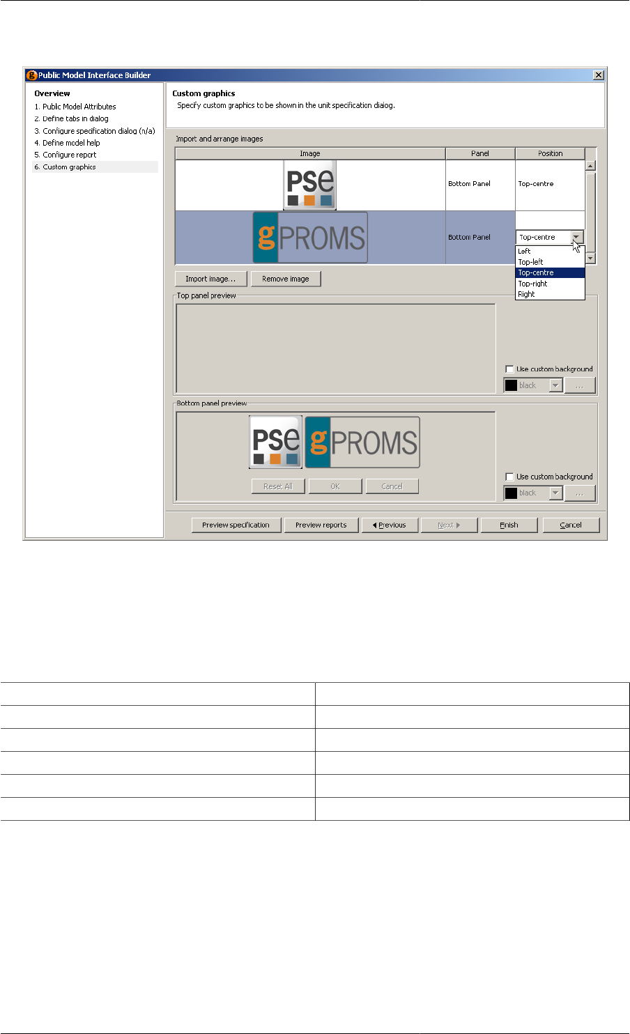
Defining a Public Model Interface
114
Figure 10.13. Example custom graphic specification
In the example above, two images have been imported and assigned to the bottom panel. The top and bottom panel
preview panes show how the images will be aligned on the dialog. Here, both images are set to Top-centre and
their position is shown relative to the buttons that will appear at the bottom of the configuration dialog. Of course,
any image can be assigned to either the top or bottom panel and aligned using the following options.
Table 10.15. Alginment options
Alignment Position in panel
Left Flush left, level with the controls
Top-left Flush left, above the controls
Top-centre Centred, above the controls
Top-right Flush right, above the controls
Right Flush right, level with the controls
Clicking on the Preview specification button activates a preview dialog. The dialog for the example above is
shown below.
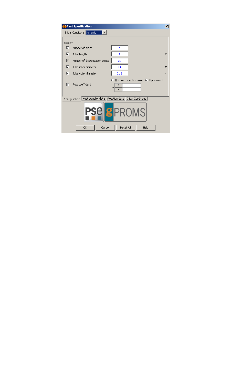
Defining a Public Model Interface
115
Figure 10.14. Test specification dialog

116
Chapter 11. Defining Schedules
Schedules are used in gPROMS to define operating procedures. An operating procedure can be considered as a
recipe that defines periods of undisturbed operation along with specified or conditional external disturbances to
the system. The Schedule section is the last part of the Process entity (for defining a simulation activity).
Schedules can be generated (and modified) by entering gPROMS language, by using a graphical interface or by
using a combination of the two. Both methods are entirely equivalent and interchangeable: when a schedule is
modified using the graphical interface, the equivalent change is automatically made to the language and, similarly,
changes made to the gPROMS language are automatically applied to the graphical representation of the Schedule.
The Schedule is stored in either a Process or a Task entity and can be viewed by selecting either the Schedule tab
or the gPROMS language tab from the Process window. The Schedule tab displays the graphical representation
of the Schedule and the gPROMS language tab displays all of the language associated with the Process (i.e. Unit,
Set, Assign etc.); the Schedule is located at the end, so one may need to scroll the window to see the Schedule.
These two views are shown below for a Process.
Figure 11.1. Graphical Schedule Editor
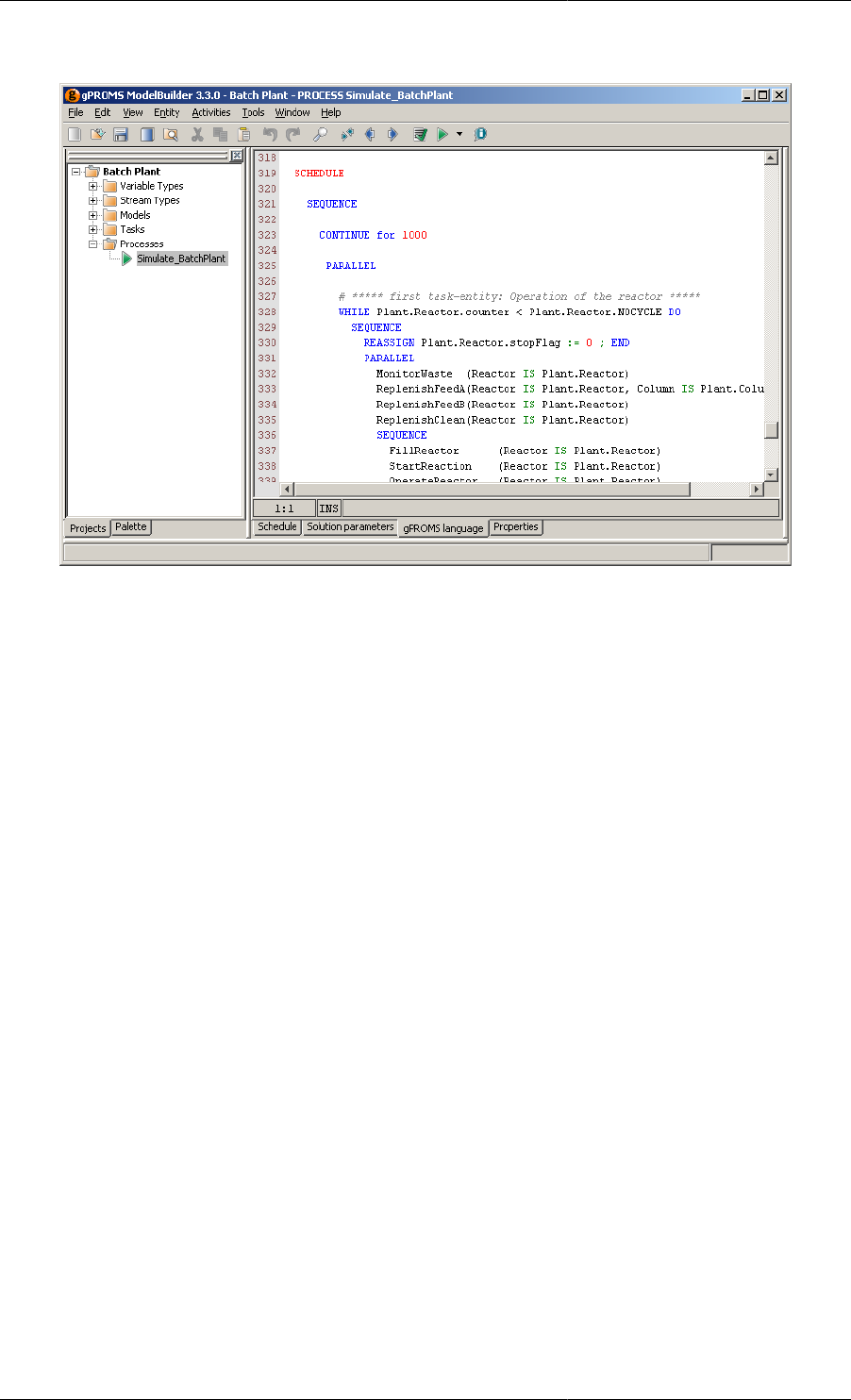
Defining Schedules
117
Figure 11.2. Schedule Language Editor
Schedules are specified using:
• Elementary tasks, which are used to specify external disturbances to the systems (e.g. changing the values of
simulation input variables, specifying periods of undisturbed operation etc);
• Timing structures, which combine elementary tasks and specify the manner in which they are executed
(sequentially, concurrently, conditionally or iteratively);
• Results-control elementary tasks, which control the way the results are displayed (but do not affect the results
themselves); and
• Tasks for creating and using Saved Variable Sets.
The Schedule may also include user-specified Tasks, which are re-usable parts of the operating procedure. Tasks
are associated with one or more Models and can be used multiple times within a Schedule and by other Tasks.
See: Defining Tasks.
Before considering the above elements in detail, one must first be familiar with the procedure of Building a
Schedule.
Building a Schedule
There are two main ways to build a Schedule: using the graphical interface or by entering gPROMS language.
The former is by far the most convenient and is described here. The gPROMS language for Schedules is covered
in the following sections, describing the Tasks in detail.
To begin building a Schedule, one must first create a Process. Let's assume one already exists, which contains all
of the specifications for the simulation apart from the Schedule; that is:
• Units are defined,
• Parameters have all been Set,
• Variables have been Assigned to take up any degrees of freedom and
• Initial conditions have been specified
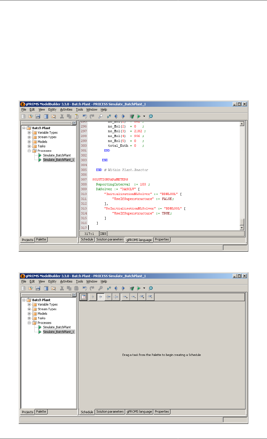
Defining Schedules
118
so that the simulation can be initialised. All that remains is to define what should happen during the simulation
and when. For example, one can fill a reactor, heat it up, keep the temperature constant while the reactions take
place, cool it down and finally empty it. These actions are defined by specifying changes in Assigned Variables
and periods of uninterrupted simulation, all by using elementary Tasks.
Before these Tasks can be placed into the Schedule, we must first create a Schedule. To do so, double-click on the
Process to open it in the gPROMS editor window. There are four tabs in the Process window: Schedule, Solution
parameters, gPROMS language and properties. The gPROMS language tab contains all of the code that defines
the elements of the Process listed above. The code for the Schedule will be placed at the end, in a SCHEDULE
section. The graphical interface is shown in the Schedule tab. These two views are shown below.
Figure 11.3. gPROMS language tab with no Schedule
Figure 11.4. Schedule tab with no Schedule
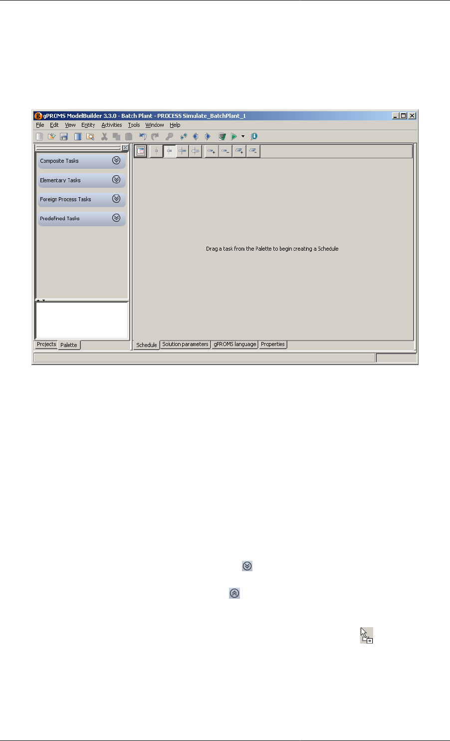
Defining Schedules
119
To create the Schedule using the graphical interface, a Task needs to be dragged from the Task Palette onto the
Schedule window. Therefore, one must first click on the Palette tab in the Project tree. If the Palette tab is not
visible, then it can be enabled by selecting Palette from the View menu or by pressing CTRL+F11. The Task
Palette is shown below.
Figure 11.5. Task Palette
The Task Palette is divided into two panes: the top pane contains all of the available Tasks (arranged in four
categories) and the bottom pane contains an explanation of the currently-selected Task. The four cetegories of
Task are:
• Composite Tasks, which combine elementary tasks and specify the manner in which they are executed
(sequentially, concurrently, conditionally or iteratively);
• Elementary Tasks, which are used to specify external disturbances to the systems (e.g. changing the values of
simulation input variables, specifying periods of undisturbed operation etc);
• Foreign Process Tasks, which control the way the results are displayed (but do not affect the results themselves);
and
• Predefined Tasks, which are user-defined reusable Tasks that contain a segment of an operating procedure.
To expand a category, simply left click on its title or on the symbol next to it. All of the available Tasks will
then be shown. Left clicking on a task will display further information about it in the window at the bottom of the
palette. Left clicking on the category title again or on the symbol will collapse the category.
To create the Schedule, left click on a Task and, while holding the left mouse button down, drag the Task onto the
Schedule window. Before the mouse button is released, the mouse pointer will change to to indicate that the
task will be copied into the Schedule. When the mouse button is released, the Schedule is created and the Task is
placed into the Schedule. Most Tasks, however, need to be configured before they can be added to the Schedule;
in these cases, a configuration dialog will appear and it must be completed before the Task is added.
This is demonstrated in the following example. Suppose we only want to simulate the Process for a given amount
of time, without changing any of the input specifications. This is done with the Continue Task. Since the Continue
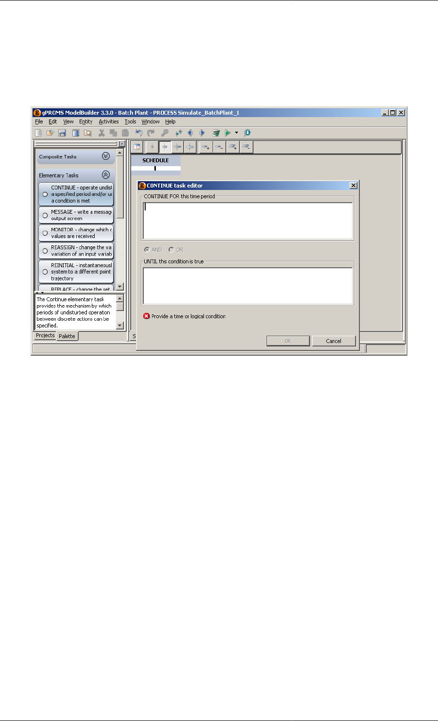
Defining Schedules
120
Task instructs gPROMS to simulate the Process for a given amount of time (or until a certain condition is satisfied),
this time (or condition) must be specified before the Task can be added to the Schedule. The figure below shows
the Schedule and Task configuration dialog just after the Task had been dragged onto the Schedule window and
the left mouse button released.
Figure 11.6. Continue Task configuration dialog
Configuration dialogs automatically check syntax, so this one initially states that the configuration will only be
complete when a time value is entered in the first text box or a logical condition is entered in the second one. It is
also possible to enter values in both boxes and the two conditions will be combined with an AND or OR logical
operator, which can be selected using the radio button. In this case, it is disabled because both text boxes are
empty. Once the configuration is complete, the OK button will be enabled and left clicking on this will complete
the addition of the Task to the Schedule. This is shown in the figure below. (Left clicking on the Cancel button
will cancel the addition of the Task, but will leave a blank Schedule in the Schedule window (visible just above
the configuration dialog).)
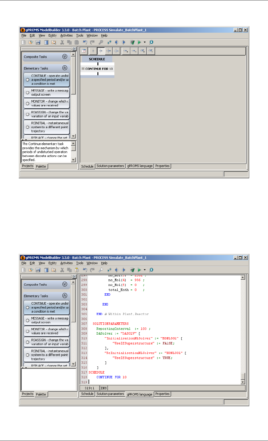
Defining Schedules
121
Figure 11.7. Continue Task in a Schedule
Notice also that by left clicking on the Continue Task, the bottom pane of the Task Palette has been populated
with an overview of the Continue Task. The scroll bar on the right can be used to scroll through the text and the
size of the pane can be adjusted by dragging the divider up or down.
When a Task is added to the Schedule using the graphical interface, the gPROMS language is automatically added
to the Process, as can be seen in the language tab below. The Schedule could have been created by typing this
code into the Process and the same graphical Schedule would have been generated automatically.
Figure 11.8. Continue Task in a Schedule (gPROMS language tab)
Returning to the Schedule tab, it can be seen that the Schedule itself is represented in the graphical interface. It
contains a black vertical line above and below the Continue Task. These lines are "hot spots" where additional
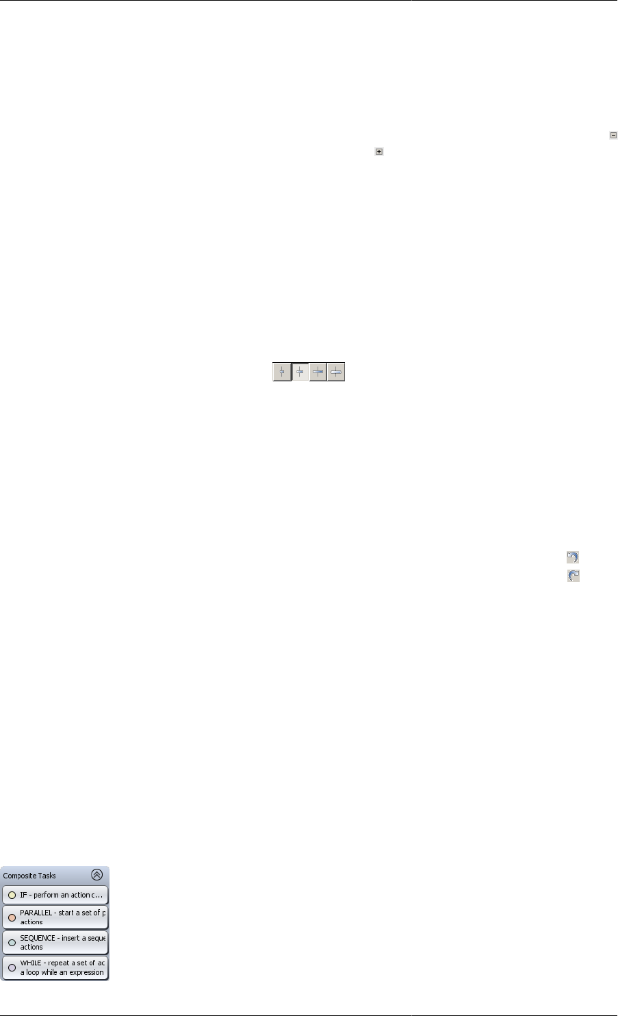
Defining Schedules
122
Tasks can be added. In a blank Schedule (as seen in the screen shot showing the Task configuration dialog), there
is just one black line and therefore only one place where a new task can be added. Once a Task has been added, a
new one can be added before or after the first one, by dragging a new Task onto one of the lines.
The Continue Task displays the gPROMS language resulting from the specification made in the configuration
dialog. In this case, the number 10 was entered in the first text box, specifying that gPROMS should simulate the
Process for 10 units of time and then stop. It is possible to hide the details of any Task by left clicking on the
symbol on the left (the details can be shown again by pressing on the symbol). This allows the user to customise
how much detail is shown in the graphical view: as can be seen in the screen shot above, Tasks can be nested
within other Tasks such that a complex hierarchy can be built up and it may not be desirable to see all of this detail
all of the time. For this screen shot, the details of the Parallel Tasks were hidden so that the whole of the Schedule
was visible in the editor. To save space, gPROMS will also only show the first 4 lines of code associated with a
Task. An ellipsis (…) is used to indicate that some information is not being shown. There are three ways to see
the details: 1. double click on the Task to bring up the configuration dialog; 2. view the Task language by right
clicking on the Task and selecting Go to language from the context menu; or 3. move the mouse pointer over the
Task and hold it there until a tool tip appears showing the details. You can also adjust the width of the Task boxes
by pressing one of the four buttons shown below (see also the Schedule Tab Toolbar).
Figure 11.9. Width Controls
The first three limit the width of the Task boxes to small, medium and large. The last one removes the limit so that
the Task boxes will be as wide as the longest visible line of language. The currently-selected option is indicated
by the depressed button (the second one in the case above). In the screen shot above, it can be seen that the boxes
are too narrow to show all of the lines for some of the tasks and this is indicated by the ellipsis at the end of the
line (in the While and Parallel tasks).
Any Task can be selected by left clicking on it. Once selected, a Task can be deleted by pressing the DEL key or
by right clicking and selecting Delete from the context menu. The Task can also be copied or cut using the context
menu. It may be pasted into the Schedule by right clicking on one of the black lines and selecting Paste. Note that
if you delete a Composite Task, then all of the Tasks that it contains will also be deleted. Pressing the button
or CTRL+z will undo any changes made to the Schedule, including the deleting of Tasks. (Pressing the button
or CTRL+y will redo any changes that have been undone.)
Tasks can also be reconfigured by double-clicking on them. This will open the Task Configuration dialog, allowing
the details of the Task to be modified.
The context menu also provides another way of adding a new Task to an existing Schedule. Right clicking on
a black line activates the context menu, which contains sub menus for each of the built-in Tasks: Composite,
Elementary and Foreign Process. So to add a new Task using this method, right click on a black line, open the
appropriate menu and left click on the Task you want to insert. The result is identical to dragging from the Task
Palette: if necessary, a configuration dialog will appear and then the Task will be inserted in the chosen place.
So far, the Schedule we have created is very simple. Most Schedules will be more complex than this, and they
may include many Tasks, some occurring after others have finished, some occurring concurrently with others and
some Tasks may need to be performed iteratively or only if some condition is met. These structures can be created
by using the Composite Tasks that have been mentioned briefly before. The Composite Tasks section of the Task
Palette contains the four Tasks that allow Schedules of arbitrary complexity to be built. These are:

Defining Schedules
123
Each of these Tasks can be dragged onto a hot spot in the Schedule and they then provide locations for more Tasks
to be added. These Tasks will be described in more detail later (see: Composite tasks). For now, we shall focus
on the Sequence Task as the principles covered here apply to all of the above.
Let us proceed with the example given so far. We currently have just one Task in the Schedule: a Continue Task.
Suppose that after the 10 units of time, we want to change the value of one of the input Variables. This can be
done with the Reassign Task, and so all that need be done is to drag a Reassign Task onto the hot spot below the
Continue Task. (Alternatively, we could right-click on the hot spot and choose Reassign from the Add elementary
task context menu.
The result of the insertion is shown below (after the Reassign task has been configured — how to do this will be
described in the Reassign section).
Figure 11.10. Schedule after a Reassign task was inserted
The first thing to notice is that a Sequence Task has automatically been inserted into the Schedule. This is because
if two or more Tasks are to be performed in series, they must be enclosed in a Sequence Task. To save always
having to insert the Sequence Task before adding elementary Tasks (such as the Continue and Reassign Tasks
here) gPROMS will always insert a Sequence Task if one is needed. This means that you can drag any Task onto
any hot spot and the resulting Schedule will always be valid.
Next, we have changed to width of the Task boxes to show all of the details of the Reassign Task. Here, the
Reassign Task changes the value of the Plant.Reactor.STR.flow_Lin Variable to 50.
The automatically-generated gPROMS language now looks like this:
SCHEDULE
SEQUENCE
CONTINUE FOR 10
REASSIGN
Plant.Reactor.STR.flow_Lin := 50;
END
END
It would have been easy to type this into the gPROMS language tab, but larger more complex Schedules (with all
four types of Composite Task being nested in complex arrangements) become harder to follow in this view and this
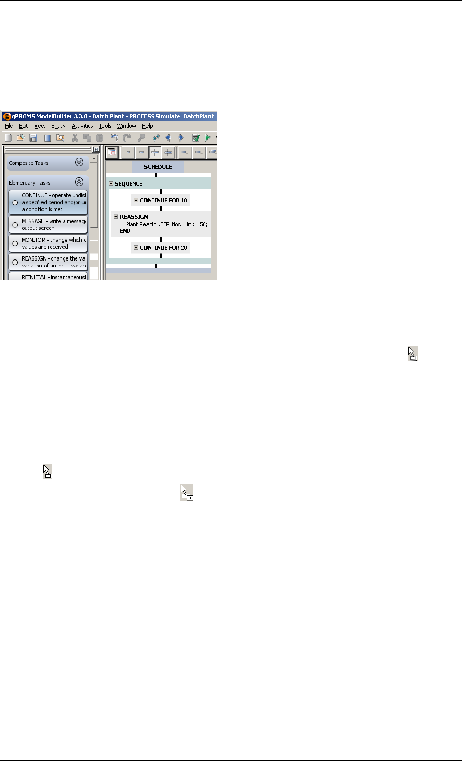
Defining Schedules
124
method is therefore more prone to error. The graphical view is much easier to follow and to modify, particularly
if one wants to move or copy Tasks from one place to another, as we shall demonstrate now.
The Schedule currently does nothing new: although the Flow_Lin variable changes value, gPROMS stops the
simulation immediately afterwards. To see the effect of the change in flowrate, we must add another Continue
Task. If we add one after the Reassign Task and set it to simulate for 20 time units, we will have the following.
Now suppose that we want to see what would happen if we started the simulation by Continuing for 20 units,
Reassigning the Flow_Lin Variable and then Continuing for 10 units of time. We could just double click on the
first Task and change its value to 20 and then do the same for the third task, but a quicker and easier way to swap
these Tasks over is to move them. To move a Task, left click on it and, while holding the left mouse button down,
drag it to another hot spot. Before the left mouse button is released, the mouse pointer will change to to indicate
that the Task is being moved. Note, this is similar to the pointer when a Task is being added, but without the "+"
sign. When the left mouse button is released, the Task will be moved to the new location (note that Tasks cannot
be moved if the new location requires the addition of a new Sequence Task — in this case, one must either insert
a new Sequence and then move the Task or copy the Task and then delete the original one). Using this method,
it is very quick and easy to move Tasks around.
It is also possible to copy Tasks. This is done in a similar way to moving Tasks but by also holding down the
CTRL key. To copy a Task, drag it to a new hot spot exactly as if it were being moved. The mouse pointer will
change to to show that it is being moved. Now, before releasing the left mouse button, hold down the CTRL
key. The mouse pointer will now change to to indicate that the Task is being copied. Keeping the CTRL key
down, release the left mouse button and the duplicate Task will be added to the Schedule. gPROMS will insert a
new Sequence Task if necessary. You can change a copy to a move or vice versa at any time during a drag: all
that matters is the state of the CTRL key when the left mouse button is release.
If you prefer not to drag Tasks around, it is also possible to move or copy Tasks using the Cut, Copy and
Paste commands in the Edit and context menus or their keyboard shortcuts (CTRL+x, CTRL+c and CTRL+v
respectively). Simply right click on the Task, select Cut or Copy from the context menu, then right click on the
desired hot spot and select Paste. To use the keyboard shortcuts, left click on the Task, press CTRL+x or CTRL+c,
left click on the desired hot spot and press CTRL+v. (The currently-selected hot spot is shown as a blue line
instead of a black one.)
It is possible to move, copy or delete multiple Tasks simultaneously. This is done by making multiple selections.
To make a multiple selection, select the first Task as usual (by left clicking on it), then hold down the CTRL
key and select another Task. As long as the CTRL key is held down, more Tasks can be added to the selection
by left clicking on them. (Note that Tasks cannot be removed from the selection by left clicking on them again.)
There is one restriction when making multiple selections: once the first Task is selected, you can only add more
Tasks to the selection if those Tasks belong to the same Composite Task as the first one and at the same level in
the Task hierarchy. The Schedule below (which is a modified version of the Batch Plant example) will be used
to illustrate this.
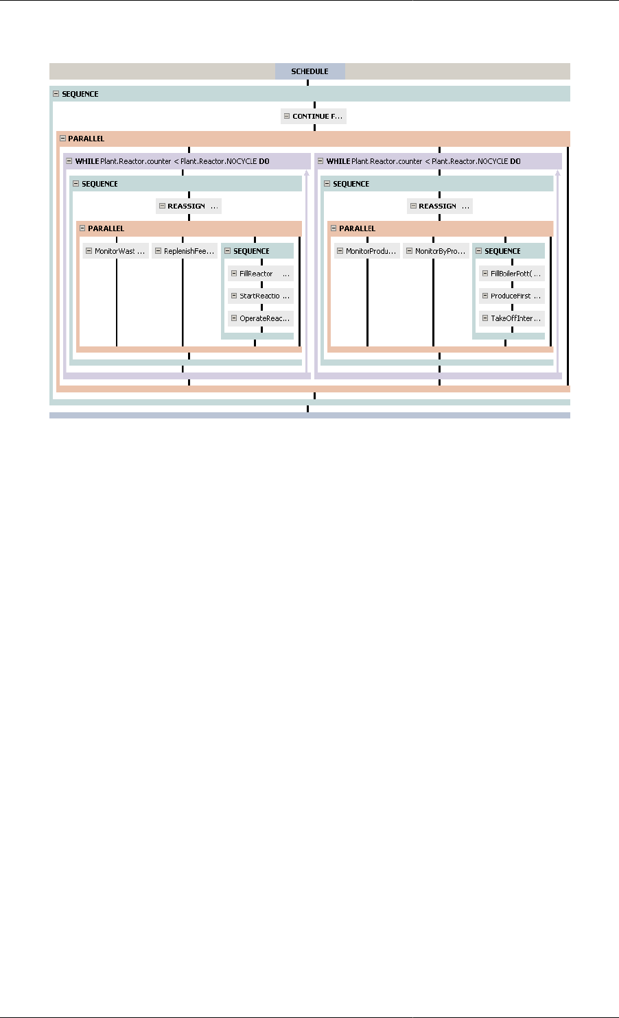
Defining Schedules
125
Figure 11.11. Schedule with example multiple selections
The Continue Task at the top and the large Parallel Task can both be part of the same multiple selection because
they are both part of the first Sequence Task. All of the other Tasks are also within the main Sequence Task, but
because they are deeper in the hierarchy, they cannot be selected along with the first Continue Task.
The two While Tasks can form a multiple selection because they both belong to the large Parallel Task.
The two small Parallel Tasks cannot form a multiple selection because, even though they are at the same level in
the hierarchy, they belong to different Sequence Tasks.
Finally, if we select the MonitorWast … Task, we can also select the ReplenishFee… Task and the Sequence
next to it, but neither the FillReactor … Task (wrong level) nor the MonitorProdu… Task (not in the same
Parallel).
Once a multiple selection has been made, it can be moved, copied or deleted just like a single Task. To delete all
of the Tasks in a multiple selection (including any Tasks contained within them), simply press the DEL key or
right click and select Delete from the context menu. To move or copy, make sure the CTRL key is held down and
then left click and drag one of the Tasks to its new location. Releasing the left mouse button while CTRL is still
held down will result in a copy; releasing the CTRL key first will result in a move. Releasing CTRL and pressing
ESC while the Tasks are being dragged cancels the move/copy and retains the multiple selection.
When the Tasks in the multiple selection have been moved or copied, they will be pasted into the new location in
a specific order. First, if they are not copied or moved to a Sequence Task, then one will be inserted automatically
and they will be inserted into that. Next, they will be inserted into the Sequence Task in the order that they had
in their original Composite Task. That is: if they were originally in a Sequence Task, then their time order will
remain the same; if they were in a Parallel Task then the order from left to right in the Parallel Task will become
the order from first to last in the Sequence; finally, if they were in an If Task then the Task in the TRUE branch
will be inserted before the Task in the ELSE branch.
Just as with any other edit made to the Schedule, a completed move or copy of a multiple selection can be undone
by pressing CTRL+z or the undo button.
We have seen that when most Tasks are added to the Schedule, a configuration dialog appears. This is because
most Tasks need some information to function. In the case of the Continue Task, we needed to specify an amount
of time and/or a condition. We also saw that the Reassign Task needs to know which Variables to Reassign and
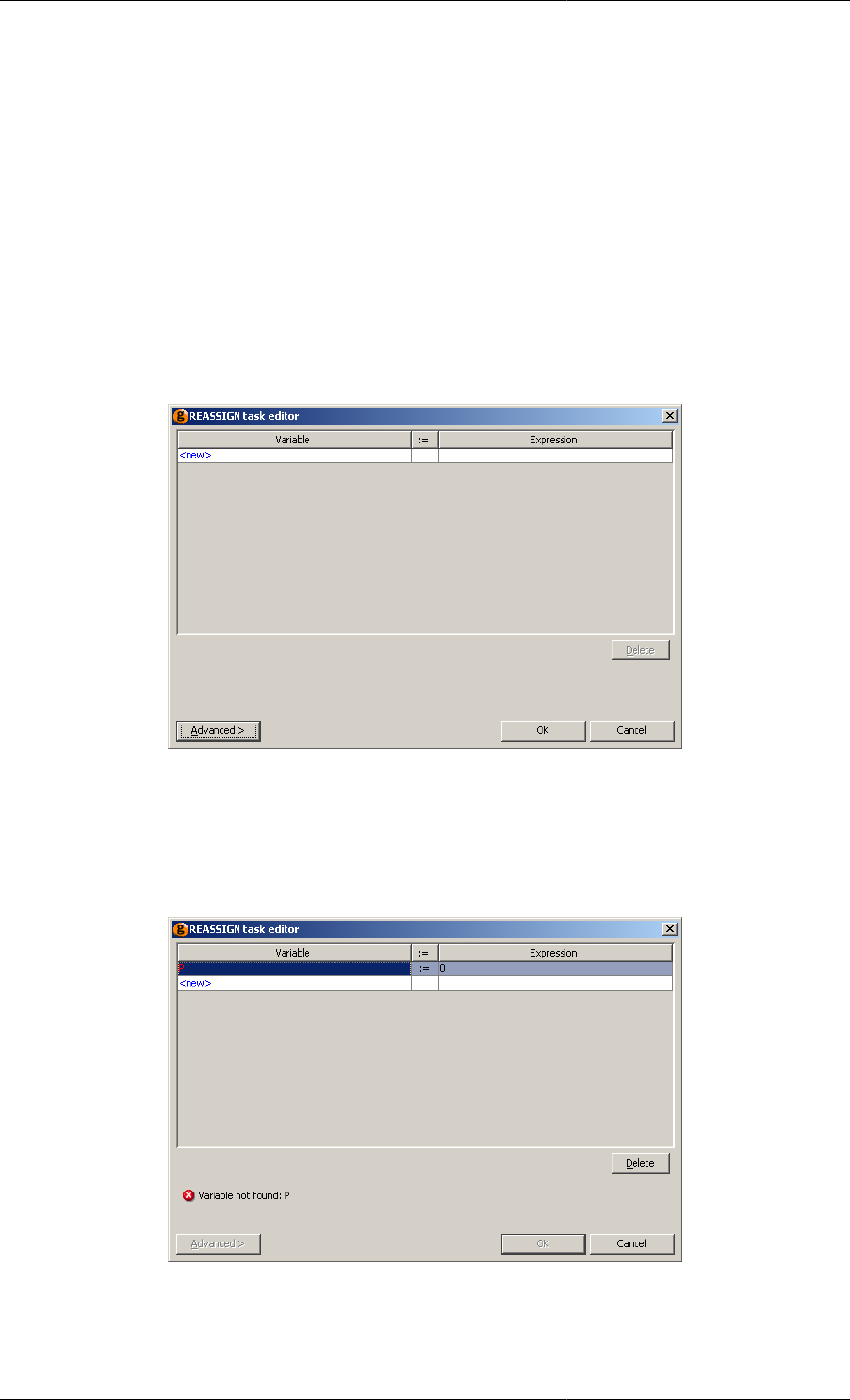
Defining Schedules
126
the new values that they should take. Since different Tasks require different data, each configuration dialog will be
different. These are discussed in detail in the sections that describe the Tasks. There are, however, some common
features that can be described first.
The two features that are common to a lot of Task configuration dialogs are real-time syntax checking and the
Advanced view.
All Task configuration dialogs constantly check for errors in the input data. Whenever the data would prevent
the Task from working correctly, the OK button is disabled forcing the user to correct the error (or provide the
minimum amount of data) before the Task can be inserted or amended.
The Reassign Task requires a list of Variables and values to assign to them. When first inserted into the Schedule,
the list is empty as is shown in the screen shot below.
Figure 11.12. Initial configuration dialog
The Reassign Task is allowed to contain an empty list of Variables, so there is no error shown and the OK button
is enabled. To add a new Variable, click on the <new> text, enter the path of a Variable and press RETURN. The
path will be checked to make sure it is valid, as shown below.
Figure 11.13. Configuration dialog with illegal Variable path
As the path is incorrect, the dialog reports an error and disables the OK button. If a syntactically valid path is
entered, but the Variable does not exist, gPROMS gives a warning instead and enables the OK button. This is
because one might want to define this Variable after adding the Task.
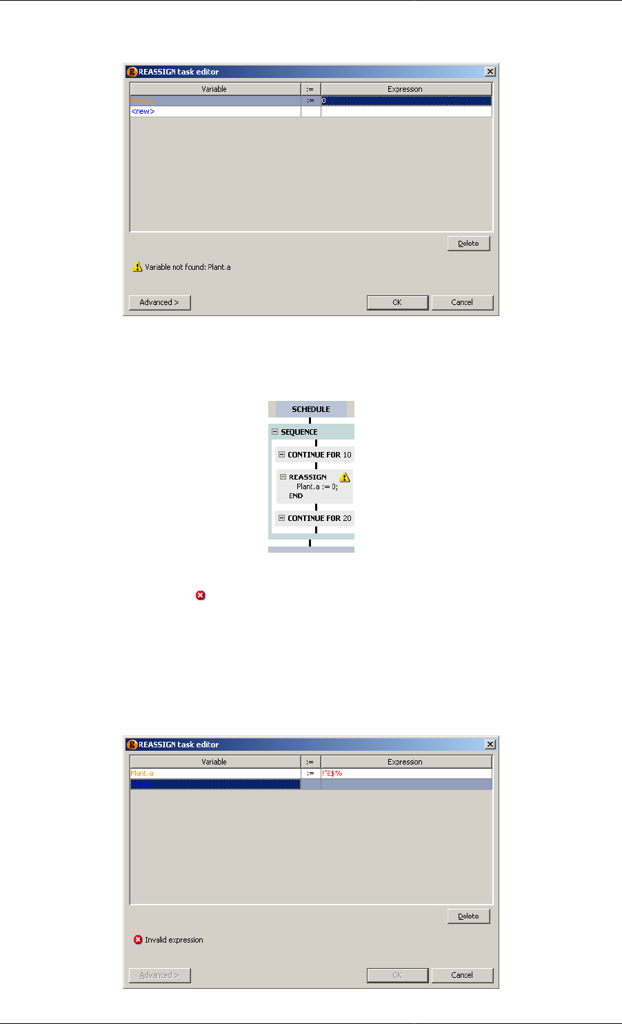
Defining Schedules
127
Figure 11.14. Configuration dialog with legal but undefined Variable path
This warning is also shown in the graphical Schedule:
Figure 11.15. Warnings are shown on the graphical Schedule
If the Schedule is entered using gPROMS language tab, then syntax errors can occur and they will also be shown
in the graphical Schedule (using a symbol). Double click on the Task (or go back to the gPROMS language
tab) to see the error message(s).
Once a legal Variable path has been entered, an expression for the new value must be entered. By default, this
is zero but when a new expression is entered, gPROMS checks its syntax and displays the message below if it is
illegal. Note also that warnings are highlighted in orange and errors in red.
Figure 11.16. Configuration dialog with illegal expression
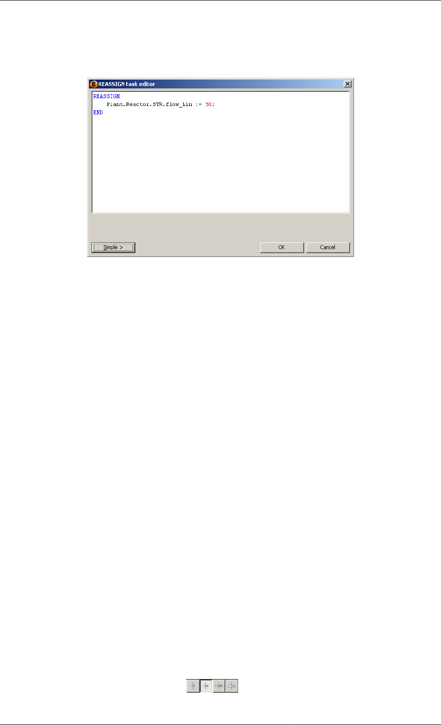
Defining Schedules
128
When all of the input data are correctly entered, the Advanced button is enabled. This allows you to see the
gPROMS language of the Task, as shown below.
Figure 11.17. Configuration dialog showing advanced view
Pressing the Simple button returns to the tabular view.
In summary:
• Schedules can be created using gPROMS language or the graphical interface
• Both methods are equivalent and can be used interchangeably on the same Schedule
• To create a Schedule
1. Click on the Schedule tab of a Process
2. Open the Task Palette
• if not visible, select Palette from the View menu or press CTRL+F11
3. Drag a Task from the Task Palette onto the Schedule
• Additional Tasks can be dragged from the Task Palette into the Schedule using the hot spots (vertical black
lines in the Schedule) or by right clicking on a hot spot and using the context menu to insert a new Task
• For most Tasks, a configuration dialog will appear and need to be completed before the Task is inserted
• The simple view allows the Task to be configured using text boxes and buttons
• The advanced view allows the Task to be configured using gPROMS language
• Both views have real-time syntax checking
• Double click on existing Tasks in the Schedule to bring up their configuration dialogs
• Composite Tasks allow complex structures to be built up
• Sequence, Parallel, While and If allow sequential, concurrent, iterative and conditional execution of Tasks
• A Sequence Task is automatically inserted if needed
• Task information is shown on the Schedule and the level of detail shown is controlled by:
•Setting the width of Task boxes, using the buttons

Defining Schedules
129
• Hiding or showing the details using the or buttons (or by using the Schedule Tab Toolbar)
• Tasks never show more than four lines of language in the graphical Schedule; to see the full details:
• Move the mouse pointer over the Task to bring up a tool tip that shows all of the language;
• Double click on the Task and select the Advanced view; or
• Right click on the Task and select Go to language from the context menu
• Tasks can be selected by left clicking on them
• multiple selections can be made by holding the CTRL key and left clicking on Tasks
• multiple selections may only comprise Tasks belonging directly to the same Composite Task
• Tasks can be moved by dragging them to a new hot spot and copied by dragging with the CTRL key held down
• Works with multiple selections as long as the CTRL key is held down
• The original order is retained and a Sequence is added if necessary
• The Cut, Copy, Paste and Delete context menu items can be used for moving, copying or deleting selected Tasks
• All of the gPROMS language for Schedules is contained in the gPROMS language tab of the Process, within
a SCHEDULE section at the end
The next subsection briefly describes the Schedule Tab Toolbar.
The subsequent sections describe in more detail (including how to write gPROMS language):
• Elementary tasks (what to do),
• Timing structures (when to do it),
• Results-control elementary tasks, and
• Tasks for creating and using Saved Variable Sets.
Predefined Tasks are described afterwards. See: Defining Tasks.
The Schedule Tab Toolbar
When the Schedule tab is selected, the toolbar below will be visible.
Figure 11.18. Schedule Tab Toolbar
This contains 3 sets of controls.
The first is the overview control. When this button is pressed, an additional pane will be inserted between the
Project tree (or Task palette, if this is selected instead) and the Schedule. This pane shows an overview of the
Schedule and is useful when the Schedule is so complicated that it takes up more more space than can be shown
in the Schedule tab. An example of this is shown below (where the Project tree and Palette have been hidden in
order to show more detail).
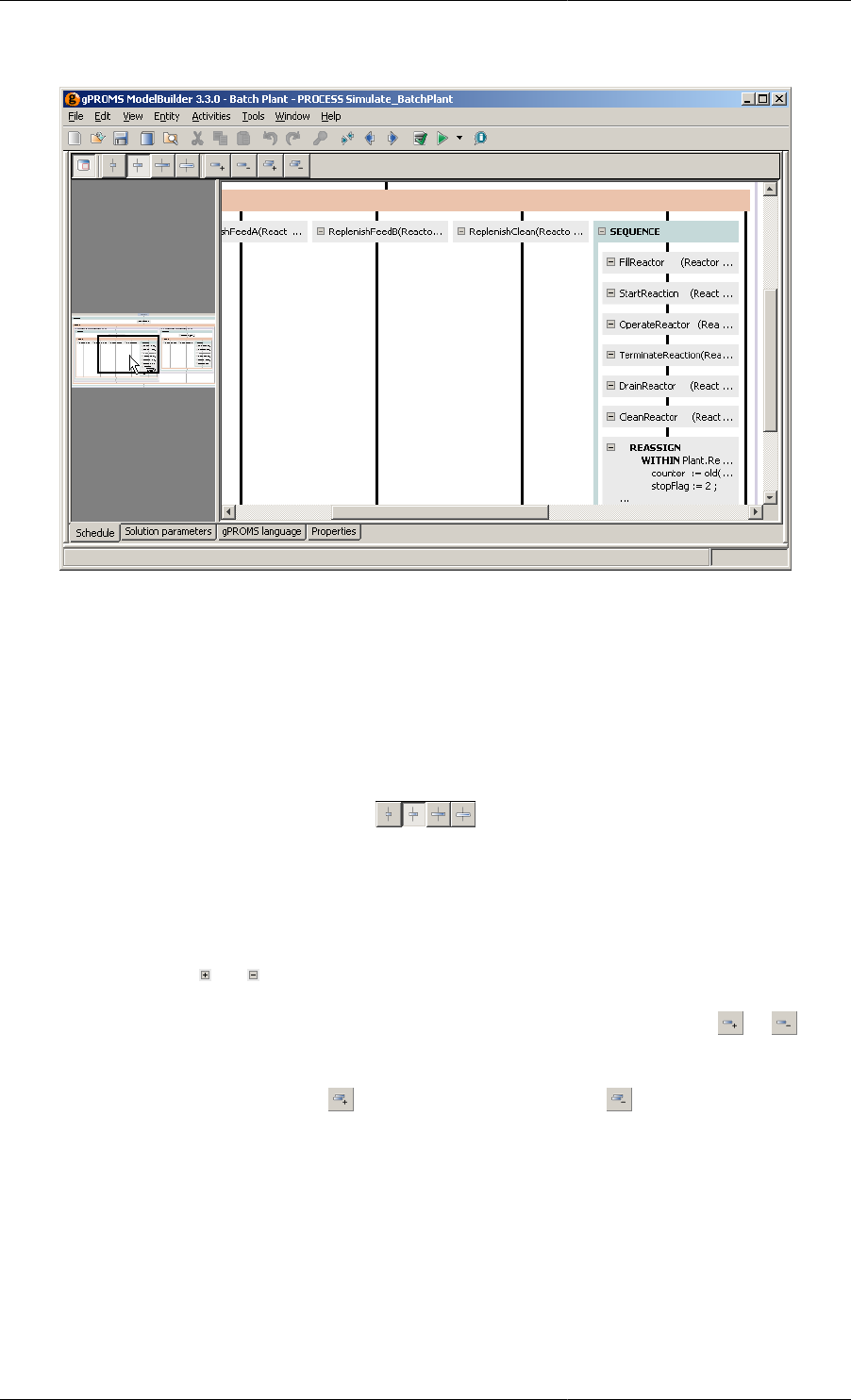
Defining Schedules
130
Figure 11.19. Overview pane
The black box on the overview indicates the view shown in the main, right-hand pane. This box automatically
moves as you adjust the view in the right-hand pane by dragging the scroll bars. You can also move the black box
directly by left clicking on it and dragging it to a new position in the overview (as is being done in the screenshot
above). This then automatically changes the view in the large right-hand pane.
The next four buttons, shown below, allow one to adjust the width of the Task boxes shown in the Schedule tab.
Figure 11.20. Width Controls
The first three limit the width of the Task boxes to small, medium and large. The last one removes the limit so that
the Task boxes will be as wide as the longest visible line of language. The currently-selected option is indicated
by the depressed button (the second one in the screenshot above).
The final set of four controls allow one to expand or collapse the information shown in the task boxes (the
equivalent of pressing the and buttons of a particular task).
To expand or collapse an individual Task, left click on it (to select it) and then press either or on the
toolbar respectively.
To expand all Tasks in the Schedule, press . And to collapse all Tasks, press .
Elementary tasks
The following elementary tasks that can be used to define "what to do" during a gPROMS simulation:
• Reassign
• Switch
• Replace

Defining Schedules
131
• Reinital
• Continue
The Reassign (Reset) elementary task
Model Variables can be Assigned values which can be either fixed or dependent on the simulation time using
expressions containing the Time statement. Up to now, Assignments could be changed using the Reset elementary
Task. With gPROMS v3.3, the Reassign elementary Task has been introduced and it serves exactly the same
purpose as Reset but has a better link to Assign.
Users are encouraged to adapt the Reassign statement in their models to use the more clearly related pair of Assign
and Reassign.
Full backward compatibility is maintained and all existing and new models using the Reset elementary Task will
continue working as before; they are also properly displayed in the new editor for Graphical Schedules and Tasks.
The syntax for the Reassign task is:
REASSIGN
VariablePath := Expression ;
END
where VariablePath is the full path to any Variable in the Process and Expression is any expression
involving constant numerical quantities and the keyword TIME (which represents the simulation time). This means
that the expression may involve numbers and Parameters (or functions thereof) but not Variables because they are
not inherrently constant. When gPROMS refers to a Variable, it refers to the whole trajectory of it, so in order
to include Variables in a Reassign statement, the OLD() function must be used. This function can only be used
in a Schedule and it returns the value of a Variable (or a function involving Variables) at the time immediately
before it is used; it has no meaning within Models, because no well-defined values for the variables exist before
the simulation commences.
Within statements can be used inside a Reassign task in order to avoid repeating long pathnames.
The examples below demonstrate some applications of the Reassign task.
Example 11.1. Applications of the Reassign task
REASSIGN
V101.Position := 1.0 ;
END
REASSIGN
WITHIN C101 DO
Signal := OLD( Bias + Gain * ( Error + IntegralError/ResetTime ) ) ;
END
END
REASSIGN
T101.FlowIn := OLD(T101.FlowIn) + 0.1 ;
END
In the first example, a Reassign task is used to model the instantaneous opening of a manual valve by a process
operator. The Model that corresponds to unit V101 contains a variable called Position, which represents the
position of the valve stem, and an equation that relates the flowrate through the valve to the pressure drop across it
according to the position of the stem and the inherent characteristics of the valve. The initial position of the valve
stem is specified in the Assign section of the corresponding Process. During the simulation, the Reassign task
'reaches' into the model and changes the value of this input variable, just as an operator would walk into the plant

Defining Schedules
132
and manipulate the valve. The action is considered to occur in such a small time interval relative to the length of
the entire simulation, that it can be modelled as an instantaneous change.
The second example demonstrates how the action of a digital controller at the end of its sampling interval might
be modelled. Here, the expression on the right hand side of the assignment is evaluated at the time of execution
of the Reassign task. The value of the expression is used to update the value of the control signal instantaneously
and according to a proportional-integral control law. This example illustrates the use of the OLD built-in function
to refer to the value of the Variables immediately before the execution of the Reassign task.
Finally, in the third example the Reassign task is used to impose a step change of magnitude 0.1 on variable
T101.FlowIn, representing the input flowrate to a vessel. The OLD function must be used here because the time
at which the Reassign Task occurs may not be known a priori, so the Value of T101.FlowIn may not be known
and cannot be replaced with a literal value.
Using the TIME function in a Reassign
In the Assign section of a Process a Variable value can be made dependent on the simulation time by using the
TIME function
ASSIGN
T101.Fin := 20 + 1.2*TIME ;
The Reassign elementary task can be used to change this Assignment in a Schedule in the same way as for all
other Assignments. In particular, the built-in function OLD can also be used with TIME which is useful in order to
avoid discontinuities in input variables. In the following example, a Variable has been Assigned a constant value
which is subsequently changed in the Schedule to form a ramp
ASSIGN
T101.Fin := 20;
...
SCHEDULE
...
REASSIGN
T101.Fin := OLD(T101.Fin) + 1.2*(TIME - OLD(TIME));
END
It is important to note the difference between using TIME and OLD(TIME). In the example below, the value
of Variable A will vary with the simulation time after the Reassign whereas the value of B will remain constant at
the value of the simulation time immediately before the Reassign task.
REASSIGN
A := TIME;
B := OLD(TIME);
END
CONTINUE FOR 100
The Reassign Task configuration dialog
When inserting or modifying a Reassign Task using the graphical Schedule interface, the following Task
configuration dialog is used.
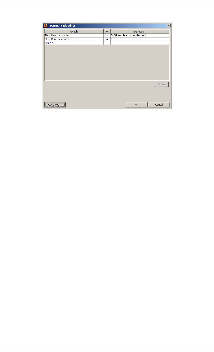
Defining Schedules
133
Figure 11.21. Reassign Task configuration dialog
This dialog contains a list of all of the Variables that are to be Reassign by the Task. To add a new Variable to
the list, left click on the cell containing <new> and enter the full path of a Variable. Pathname completion can
be used at this stage, just as when typing gPROMS language into a Model or a Process. Once the Variable path
has been entered press RETURN and the associated Expression cell will be set by default to zero. To modify this
value, left click on the cell and enter any valid gPROMS expression: as in the examples shown before, this may
contain other Variable paths, built-in functions (including OLD()) and the TIME keyword. As many Variables
are required can be added in this way.
To delete a Variable from the Reassign Task, simply select it by left clicking on its row and then press the Delete
button.
Once complete, press the OK button.
The Cancel button will close the dialog and discard any changes made to the Task. If the dialog was activated due
to the addition of a new Task, then no Task will be added.
The Advanced button can be used to enter gPROMS language. For a new Task, the dialog will contain an empty
REASSIGN statement:
REASSIGN
END
The WITHIN statement may be used in the Advanced view (just as it can be in the gPROMS language tab) if
many Variables within the same Unit are to be Reset. The Advanced view also supports pathname completion
and copy/paste functionality.
The Switch elementary task
Similar to the Reassign task, the Switch task may be used to alter the value of Selector Variables. Manipulation
of a Selector state by a Switch task forces the underlying model to change state as a result of an external action
as opposed to a physico-chemical mechanism. Applications include the switching of a pump on or off as shown
below, the replacement of a shattered bursting disc by an operator etc.

Defining Schedules
134
Example 11.2. Manipulating selector variables using the Switch task
# MODEL Pump
VARIABLE
FlowIn, FlowOut AS Flowrate
PressIn, PressOut AS Pressure
PressRise AS Pressure
SELECTOR
PumpStatus AS (PumpOn,PumpOff)
EQUATION
FlowOut = FlowIn ;
PressOut = PressIn + PressRise ;
CASE PumpStatus OF
WHEN PumpOn : FlowOut = f(PressRise) ;
WHEN PumpOff : PressRise = 0 ;
END # Case
# in the SCHEDULE of a Process
SWITCH
P101.PumpStatus := P101.PumpOn ;
END # Switch
In this example Model Pump has two states, PumpOn and PumpOff, designated by the selector variable Status
and representing whether the pump is on or off. When the pump is switched on, the pump characteristic relates the
pressure rise across the pump to the flowrate through the pump (note that f(PressRise) is not valid gPROMS
language: in this case it is short-hand for some function of the Variable PressRise). When the pump is switched
off, the pressure rise is set to zero. Note that no SWITCH statements are present in the CASE statement because no
physico-chemical transitions link these two states. Whether the pump is initially switched on or off forms part of
the initial condition of each simulation experiment. This information is specified in the SELECTOR section of the
corresponding Process. On the other hand, external actions during the simulation are modelled by Switch tasks
and cause dynamic changes to this status.
The Switch Task configuration dialog
When inserting or modifying a Switch Task using the graphical Schedule interface, the following Task
configuration dialog is used.
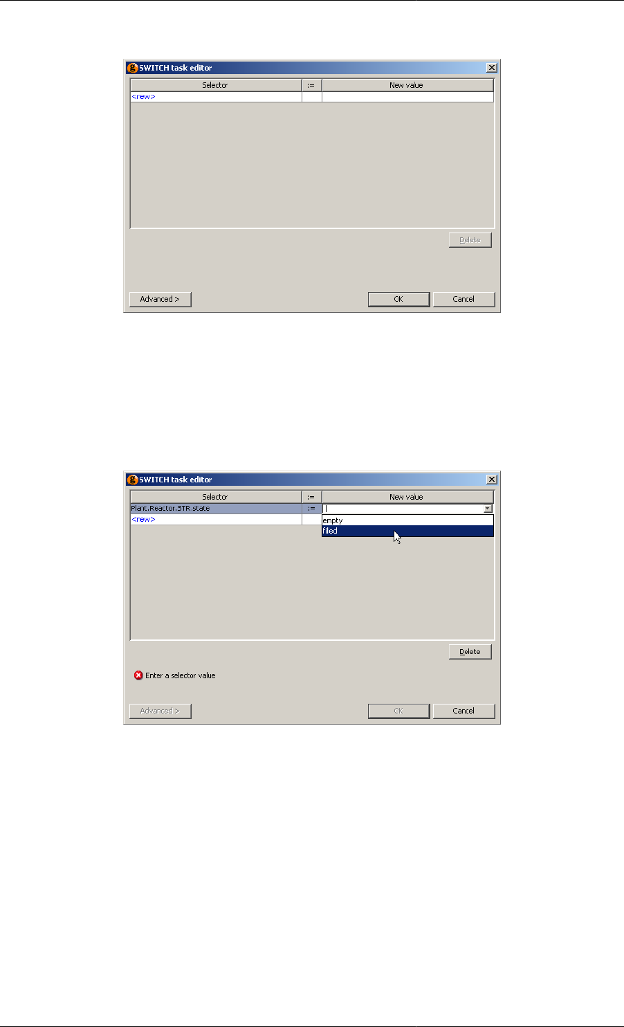
Defining Schedules
135
Figure 11.22. Switch Task configuration dialog
This dialog contains a list of all of the Selector Variables that are to be Switched by the Task. To add a new Selector
Variable to the list, left click on the cell containing <new> and enter the full path of a Selector Variable. Pathname
completion can be used at this stage, just as when typing gPROMS language into a Model or a Process. Once the
Selector Variable path has been entered press RETURN. If a valid Selector Variable path has been entered, the
New value cell will now contain a list of possible values one of which must be selected from the list box (otherwise
a syntax error will be reported — see below). As many Selector Variables are required can be added in this way.
Figure 11.23. Switch Task configuration dialog: selecting a value
To delete a Selector Variable from the Switch Task, simply select it by left clicking on its row and then press
the Delete button.
Once complete, press the OK button.
The Cancel button will close the dialog and discard any changes made to the Task. If the dialog was activated due
to the addition of a new Task, then no Task will be added.
The Advanced button can be used to enter gPROMS language. For a new Task, the dialog will contain an empty
SWITCH statement:
SWITCH
END
The WITHIN statement may be used in the Advanced view (just as it can be in the gPROMS language tab) if
many Variables within the same Unit are to be Switched. The Advanced view also supports pathname completion
and copy/paste functionality.
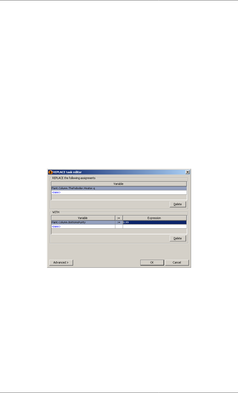
Defining Schedules
136
The Replace elementary task
The Replace elementary task 'unAssigns' an input variable (leaving it free to vary) and Assigns a different one in
its place. An interesting application of the Replace task is the automatic calculation of the steady-state bias of a
controller. In order to determine the bias, a steady-state calculation is performed in which the controller error is set
to zero by an input equation, while the bias is free to vary. The bias value obtained by this calculation corresponds
to the correct steady-state bias for the controller. Therefore, before dynamic simulation begins, the Replace task
shown below can be used to "unAssign'' the error variable and Assign the bias variable to its steady-state value. The
controller error is then free to fluctuate as disturbances are introduced and the controller attempts corrective action.
Example 11.3. Automatic calculation of controller bias using a Replace task
REPLACE
PI101.Error
WITH
PI101.Bias := OLD(PI101.Bias) ;
END
The Replace Task configuration dialog
When inserting or modifying a Replace Task using the graphical Schedule interface, the following Task
configuration dialog is used.
Figure 11.24. Replace Task configuration dialog
This dialog contains a list of all of the Assigned Variables that are to be Replaced by the Task and a list of
replacement Assignments. To add a new Assigned Variable to the list, left click on the cell in the top half of the
dialog containing <new> and enter the full path of an already-Assigned Variable. Pathname completion can be
used at this stage, just as when typing gPROMS language into a Model or a Process. Press RETURN when done.
Add more Variables by repeating this process until all of the Variables that need to be Replaced have been entered.
The bottom half of the dialog contains a list of Variables that are to be Assigned in replacement of the Variables
listed above. This part of the dialog behaves exactly the same as the Reassign dialog. The only restriction is that
this part of the dialog must contain exactly the same number of Variable Assignments as Variables listed in the
top half (otherwise the problem will be under or over specified, and gPROMS will report an error.).
To delete a Variable from the either of the lists, simply select it by left clicking on its row and then press the
appropriate Delete button.
Once complete, press the OK button.
The Cancel button will close the dialog and discard any changes made to the Task. If the dialog was activated due
to the addition of a new Task, then no Task will be added.

Defining Schedules
137
The Advanced button can be used to enter gPROMS language. For a new Task, the dialog will contain an empty
REPLACE statement:
REPLACE
WITH
END
The WITHIN statement may be used in the Advanced view (just as it can be in the gPROMS language tab) if
many Variables within the same Unit are to be Switched. The Advanced view also supports pathname completion
and copy/paste functionality.
The Reinitial elementary task
Both the Reassign and Replace elementary tasks introduce discontinuities in the simulation. Although these
discontinuities may affect the values of input and/or algebraic variables, they do not normally affect the values of
differential variables. The latter usually represent quantities that are conserved according to the laws of physics
(e.g. mass, energy, momentum etc.) and are therefore continuous across such discontinuities; gPROMS follows
this assumption and normally expects the values of the differential variables before the discontinuity to be the same
as those just after the discontinuity. The Reinitial elementary task makes it possible to introduce discontinuities
in the differential variables themselves. Of course, once we drop the continuity assumption, we need to provide
some other information to replace it.
Example 11.4. Applications of the Reinitial task
REINITIAL
PI101.IntegralError
WITH
PI101.IntegralError = 0 ;
END
REINITIAL
R101.HoldUp(1),
R101.HoldUp(2)
WITH
R101.HoldUp(1) = 2 * OLD(R101.Holdup(1)) ;
R101.X(2) = 0.3 ;
END
Two examples of the application of the REINITIAL task are shown in the gPROMS code above. In the
first example, the integral error of a PI controller is reset to zero. The execution of this task will result in
a reinitialisation calculation in which the usual assumption concerning the continuity of differential variable
PI101.IntegralError will be replaced by the equation in the second clause of the REINITIAL task. The
latter simply states that the value of PI101.IntegralError after the discontinuity is zero. Note that this is a
general equation and not just an assignment, which is why we do not write:
PI101.IntegralError := 0 ;
This is consistent with the treatment of general initial conditions in gPROMS. In the second example, the holdups
of components A and B in a chemical reactor change by instantaneous additions of material. The amounts added
are such that, in the final mixture, the holdup of A is doubled while the mass fraction of B is 0.3. Note again that
the condition specified is a general equation involving any variables in the problem and not just the ones that are
reinitialised. Naturally, the number of differential variables in the first clause of a REINITIAL task must match
the number of equations in the second clause.
The Reinitial Task configuration dialog
When inserting or modifying a Reinitial Task using the graphical Schedule interface, the following Task
configuration dialog is used.
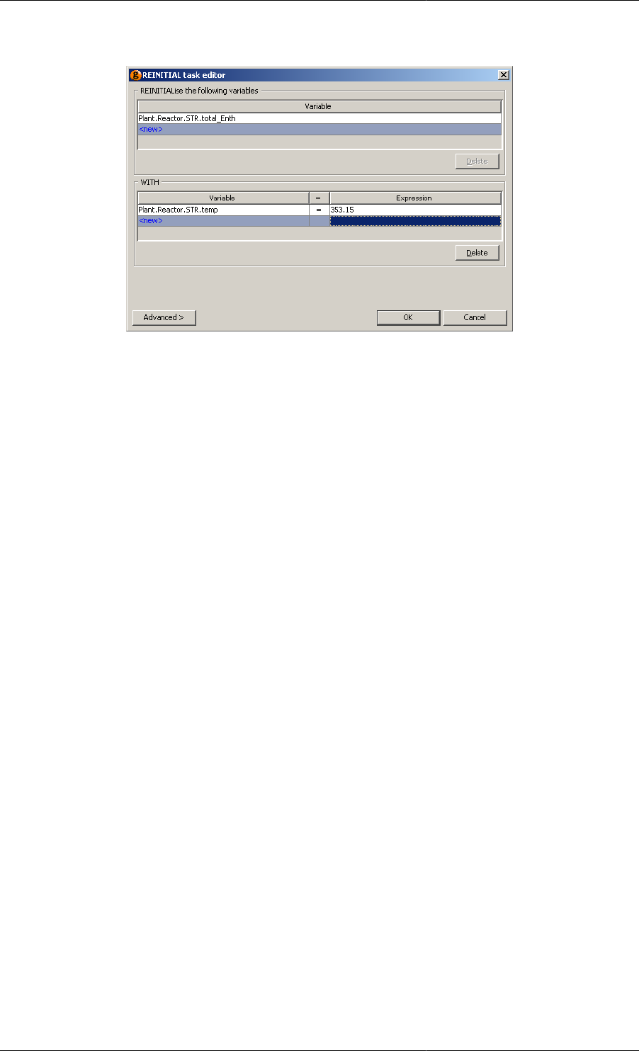
Defining Schedules
138
Figure 11.25. Reinitial Task configuration dialog
This dialog contains a list of all of the differential Variables that are to be Reinitialised by the Task and a list of
new initial conditions. To add a new differential Variable to the list, left click on the cell in the top half of the
dialog containing <new> and enter the full path of a Variable. Pathname completion can be used at this stage, just
as when typing gPROMS language into a Model or a Process. Press RETURN when done. Add more Variables
by repeating this process until all of the Variables that need to be Reinitialised have been entered.
The bottom half of the dialog contains a list of initial conditions that are to be used to reinitialise the system.
This part of the dialog behaves exactly the same as the Reassign dialog, although its function is fundamentally
different: these are additional equations to be used for reinitialisation; not assignments of degrees of freedom. This
part of the dialog must contain exactly the same number of equations as Variables listed in the top half (otherwise
the initialisation problem will be under or over specified, and gPROMS will report an error.). When using the
Simple view of the dialog, these initial conditions must be of the form <Variable> = <Expression>. Use the
Advanced view or the gPROMS language tab of the Process to enter more general initial conditions (of the form
<Expression> = <Expression>).
To delete a Variable from the either of the lists, simply select it by left clicking on its row and then press the
appropriate Delete button.
Once complete, press the OK button.
The Cancel button will close the dialog and discard any changes made to the Task. If the dialog was activated due
to the addition of a new Task, then no Task will be added.
The Advanced button can be used to enter gPROMS language. For a new Task, the dialog will contain an empty
REINITIAL statement:
REINITIAL
WITH
END
The WITHIN statement may be used in the Advanced view (just as it can be in the gPROMS language tab) if
many Variables within the same Unit are to be Switched. The Advanced view also supports pathname completion
and copy/paste functionality.
The Continue elementary task
The execution of all elementary tasks described so far takes place instantaneously with respect to the simulation
clock. The Continue elementary task provides the mechanism by which periods of undisturbed operation between
discrete actions can be specified. We have already used the CONTINUE task in its simplest form:

Defining Schedules
139
CONTINUE FOR TimePeriod
This specifies a period of undisturbed process operation, starting from when the Continue task is encountered and
extending until the simulation clock has advanced TimePeriod time units. In fact, as well as being a real number,
TimePeriod may alternatively be a real expression involving any quantities that the schedule has access to. For
example:
# Continue for 100 time units
CONTINUE FOR 100
# Continue for period equal to the sampling interval
CONTINUE FOR C101.SamplingInterval
Alternatively, the period of undisturbed process operation can be specified implicitly, in terms of a logical
condition:
CONTINUE UNTIL LogicalCondition
In this case, simulation continues until LogicalCondition becomes true. Again, LogicalCondition can be of
arbitrary complexity and can involve any quantities that the schedule has access to. For example:
# Continue until required conversion has been achieved
CONTINUE UNTIL R101.Conversion > 0.95
# Continue until reactant holdups have been exhausted
CONTINUE UNTIL R101.HoldUp(1) < Epsilon AND R101.HoldUp(2) < Epsilon
The two forms described above may also be combined in a single CONTINUE task through the use of AND and
OR operators:
CONTINUE FOR TimePeriod AND UNTIL LogicalCondition
CONTINUE FOR TimePeriod OR UNTIL LogicalCondition
Here, the period of undisturbed operation extends until the simulation clock has advanced TimePeriod time units
and/or until LogicalCondition becomes true, respectively. For instance,
CONTINUE FOR 100 OR UNTIL R101.Conversion > 0.95
advances the simulation for at most 100 time units even if the reactor conversion never reaches the required value,
while
CONTINUE FOR 100 AND UNTIL R101.Conversion > 0.95
advances the simulation for a minimum of 100 time units and then waits for the reactor conversion to reach the
required value.
The Continue Task configuration dialog
When inserting or modifying a Continue Task using the graphical Schedule interface, the following Task
configuration dialog is used.
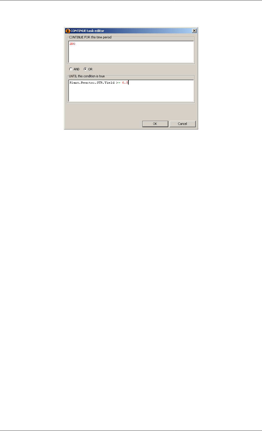
Defining Schedules
140
Figure 11.26. Continue Task configuration dialog
This dialog contains two text boxes, at least one of which must contain a valid entry.
The first box may contain a number or an expression that results in a number . This is used to provide the amount
of simulation time the Continue Task will use to advance the simulation. The gPROMS language produced is:
CONTINUE FOR contents of first box
The second box may contain any logical expression and is the equivalent of:
CONTINUE UNTIL contents of second box
which causes the simulation to advance until the value of the expression becomes FALSE.
If both boxes contain valid expressions, then they will be combined into one statement using the value determined
by the radio button in the middle (which is only enabled when both boxes are complete). If the AND button is
selected, the following language is generated.
CONTINUE FOR contents of first box AND UNTIL contents of second box
There is no Advanced view for the Continue Task. To enter gPROMS language directly, use the gPROMS language
tab for the Process or right click on the Continue Task and select Go to language from the context menu.
The Stop elementary task
Stop is a simple elementary tasks that may be used to halt a simulation (perhaps in conjunction with a conditional
statement) The syntax for STOP is:
STOP
There is no configuration dialog for the Stop Task as no further information is required.
Specifying the relative timing of multiple
tasks
Having discussed the elementary tasks that define "what to do", we now introduce the following timing statements
that describe "how/when" to do something:
• Sequence

Defining Schedules
141
• Parallel
• If
• While
These are combined with the elementary tasks to create complex operating procedures.
Sequential execution — Sequence
Sequential execution begins with the first task and only proceeds to the next task when execution of the preceding
task has terminated. Sequential execution of a series of tasks is specified by enclosing them within a Sequence
structure. The execution of a Sequence structure is complete when the execution of the last task in the structure has
terminated. The gPROMS code below shows a Process for a simulation experiment involving a multi-component
mixing tank. Unit T101 is a tank with two input streams, containing a mixture of components A, B and C. The
values of the flowrates and component mole fractions of the inlet streams are specified in the Assign section. The
outlet valve is closed. Initially, the tank contains 1000kg of component A, with additional components B and C
to make up a volume of 1.5m3. The initial amount of component C is twice that of component B. The schedule
of operation in the gPROMS code below contains only a Continue task, thus defining a period of continuous
operation with a duration of 120 time units.
Example 11.5. Mixing tank Process
# PROCESS SimpleSim
UNIT
T101 AS MixingTank
SET # Parameter values
WITHIN T101 DO
NoComp := 3 ;
NoInput := 2 ;
ValveConstant := 10 ;
CrossSectionalArea := 1 ; # m2
Density := [ 950, 1000, 900 ] ; # kg/m3
END # Within
ASSIGN # Degrees of freedom
WITHIN T101 DO
# First inlet stream
Fin(1) := 5 ;
Xin(1,) := [ 0.12, 0.21, 0.67 ] ;
# Second inlet stream
Fin(2) := 15 ;
Xin(2,) := [ 0.98, 0.01, 0.01 ] ;
# Outlet stream valve fully closed
ValvePosition := 0.0 ;
END # Within
INITIAL # Initial conditions
WITHIN T101 DO
HoldUp(1) = 1000 ;
2 * Holdup(2) = HoldUp(3) ;
TotalVolume = 1.5 ;
END # Within
SCHEDULE
CONTINUE FOR 120

Defining Schedules
142
The gPROMS code below illustrates how a more complicated operating procedure may be defined by using a
SEQUENCE structure in the SCHEDULE section. The execution of this simulation experiment will result in the
following:
1. Simulation begins. Based on the input equations specified in the ASSIGN section and the initial conditions
specified in the INITIAL section, consistent initial values are determined for all variables in the system.
2. The first CONTINUE UNTIL task is executed. Simulation proceeds until the volume of liquid in the tank
exceeds 3.5m3.
3. The first REASSIGN task is executed. The flowrate of the first inlet stream is set to zero, while that of the
second inlet stream is increased by 50%.
4. The second CONTINUE UNTIL task is executed. Simulation proceeds until the volume of liquid in the tank
exceeds 5m3.
5. The second REASSIGN task is executed. The flowrates of both inlet streams are set to zero. The outlet valve
is opened completely.
6. The third CONTINUE UNTIL task is executed. Simulation proceeds until the tank drains.
Example 11.6. Mixing tank Process — tasks in Sequence
# PROCESS SeqSim
...
SCHEDULE
SEQUENCE
# Fill up tank to 3.5 m3
CONTINUE UNTIL T101.TotalVolume > 3.5
# Turn off first inlet stream and
# increase the flowrate of the second by 50%
REASSIGN
WITHIN T101 DO
Fin(1) := 0 ;
Fin(2) := 1.5 * OLD(Fin(2)) ;
END # Within
END # Reassign
# Fill up tank to 5 m3
CONTINUE UNTIL T101.TotalVolume > 5.0
# Turn off second inlet stream and
# open the outlet valve completely
REASSIGN
WITHIN T101 DO
Fin(2) := 0 ;
ValvePosition := 1 ;
END # Within
END # Reassign
# Drain tank
CONTINUE UNTIL T101.TotalVolume < 0.01
END # Sequence
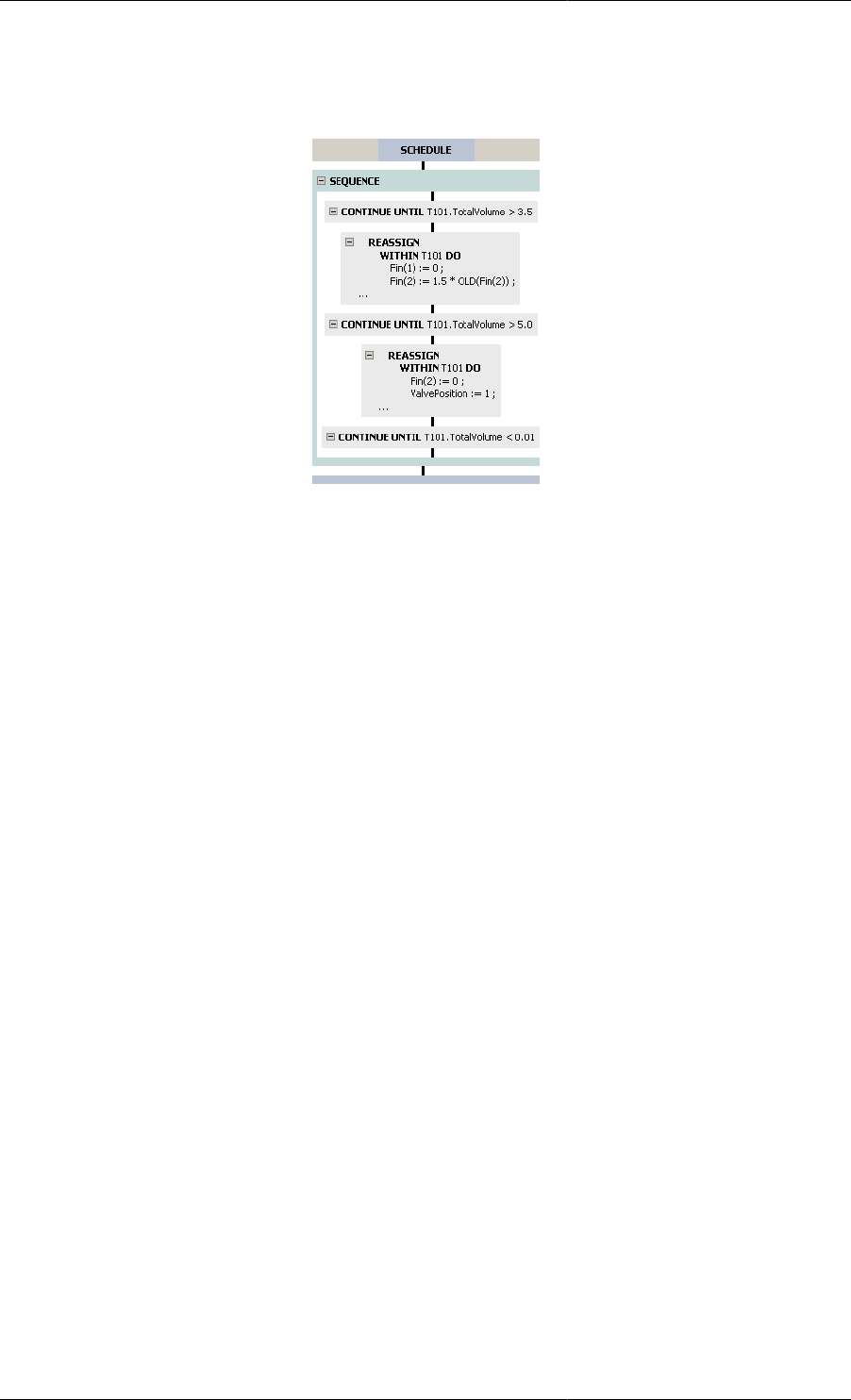
Defining Schedules
143
The equivalent graphical representation is shown below.
Figure 11.27. Mixing tank Process — graphical representation of tasks in Sequence
There is no configuration dialog for the Sequence Task as all of the information about the order of its constituent
Tasks is contained in the graphical representation.
Concurrent execution — Parallel
Tasks to be executed in parallel are enclosed within a Parallel structure. Execution of all tasks begins
simultaneously and proceeds concurrently. The execution of a Parallel structure is completed when all tasks have
terminated. The gPROMS code below demonstrates the use of concurrent tasks in specifying an operating policy
for the mixing tank example. The operating policy is in fact the same as in the gPROMS code above. However,
here, the operating policies for the two inlet and the outlet streams are specified separately with three SEQUENCE
structures. These are then enclosed in a PARALLEL structure, so that the three policies are executed concurrently.

Defining Schedules
144
Example 11.7. Mixing tank Schedule — tasks in Parallel
SCHEDULE
PARALLEL
# Operating policy for first inlet stream
SEQUENCE
# Fill up tank to 3.5 m3
CONTINUE UNTIL T101.TotalVolume > 3.5
# Turn off first inlet stream
REASSIGN
T101.Fin(1) := 0 ;
END # Reassign
END # Sequence
# Operating policy for second inlet stream
SEQUENCE
# Fill up tank to 3.5 m3
CONTINUE UNTIL T101.TotalVolume > 3.5
# Increase the flowrate of the second inlet stream by 50%
REASSIGN
T101.Fin(2) := 1.5 * OLD(T101.Fin(2)) ;
END # Reassign
# Fill up tank to 5 m3
CONTINUE UNTIL T101.TotalVolume > 5.0
# Turn off second inlet stream and
REASSIGN
T101.Fin(2) := 0 ;
END # Reassign
END # Sequence
# Operating policy for outlet stream
SEQUENCE
# Wait until both inlet streams have been turned off
CONTINUE UNTIL ( T101.Fin(1) < 0.01 ) AND ( T101.Fin(2) < 0.01 )
# Open the outlet valve completely
REASSIGN
T101.ValvePosition := 1 ;
END # Reassign
# Drain tank
CONTINUE UNTIL T101.TotalVolume < 0.01
END # Sequence
END # Parallel
The equivalent graphical representation is shown below.
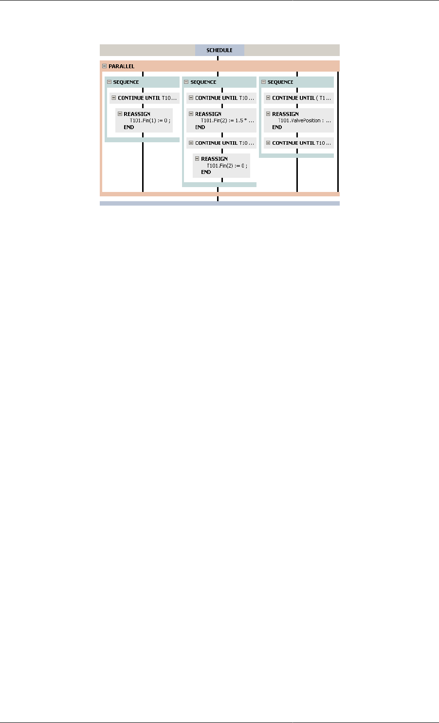
Defining Schedules
145
Figure 11.28. Mixing tank Process — graphical representation of Tasks in Parallel
There is no configuration dialog for the Parallel Task as all of the information about its constituent Tasks is
contained in the graphical representation.
The black vertical line on the far right is the hot spot for inserting a new Task to be performed in Parallel with
the existing 3 Sequences.
Conditional execution — If
In many circumstances, the correct external actions to apply to a system cannot be fully determined a priori and
must be established from decisions that can only be made while the simulation is in progress. For instance, consider
a batch operation involving a series of elementary processing steps applied to a batch of material. Once all steps
are completed a decision is made as to whether the batch is acceptable, should receive further processing or should
be discarded. This decision depends only on the quality of the batch, so the result can only be established after
the preceding steps have been completed.
The If conditional structure enables selection between alternative actions based on the current status of a system.
In common with most programming languages, it comprises an If clause, an optional Else clause and a logical
condition. If the logical condition is true when the If structure is encountered, the contents of the If clause are
executed; otherwise, the contents of the Else clause are executed. As with all other timing structures, conditional
structures can be nested in arbitrary manner. The gPROMS code below shows the application of the If structure
to 'clipping' a digital control signal before sending it off to a control valve. If, at the time of execution, the signal
proves to be greater than 1.0 or less that 0.0, the stem position is set to 1.0 and 0.0 respectively. Otherwise, the
stem position is set to the value indicated by the control signal.
Example 11.8. Application of the If conditional structure
SCHEDULE
...
IF C101.ControlSignal > 1.0 THEN
REASSIGN V101.Position := 1.0 ; END
ELSE
IF C101.ControlSignal < 0.0 THEN
REASSIGN V101.Position := 0.0 ; END
ELSE
REASSIGN V101.Position := OLD(C101.ControlSignal) ; END
END # If
END # If
...
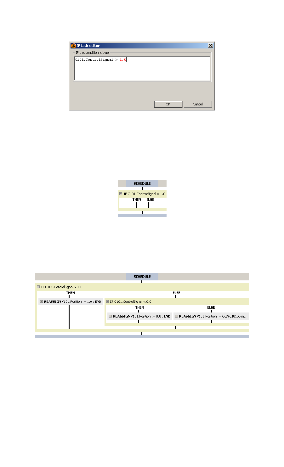
Defining Schedules
146
When using the graphical interface, inserting an If Task will activate the following Task configuration dialog.
Figure 11.29. If Task configuration dialog
Enter a valid logical expression in the text box (e.g. C101.ControlSignal > 1.0) and press the OK button.
gPROMS checks the syntax of the expression and only enables the OK button when it is valid.
There is no Advanced view of the configuration dialog for the If Task.
Once a valid expression has been provided, the If Task will be inserted and will look like this:
Figure 11.30. A new If Task
Drag new Tasks onto the THEN hot spot to provide the operating policy to be performed if the condition is TRUE.
The ELSE branch contains the optional operating policy when then if condition is FALSE.
The graphical representation of the example above is shown below.
Figure 11.31. Graphical representation of the If Task
Iterative execution — While
Many processing systems are characterised by the repetitive nature of external actions required to achieve the
desired operation. For example, periodic processes, such as pressure swing or temperature swing adsorption,
are usually brought to and maintained at a 'cyclic steady-state' by a sequence of external actions that is applied
repeatedly. Also, the action of a digital control system on a process can be considered to consist of a regular cycle
between continuous operation, sampling and implementation of discrete actions.
The While iterative structure permits the repeated execution of the tasks it encloses for as long as a logical condition
is satisfied. When the While structure is first encountered, the logical condition is examined. If it is satisfied, the
enclosed tasks are executed. The condition is then examined again and, if still satisfied, the enclosed tasks are
executed once more. This process continues until the condition is no longer satisfied, at which point the execution
of the While structure is completed. Note that, if the condition is not satisfied initially, the execution of the While
structure terminates immediately. The gPROMS code below illustrates the use of a WHILE structure in specifying
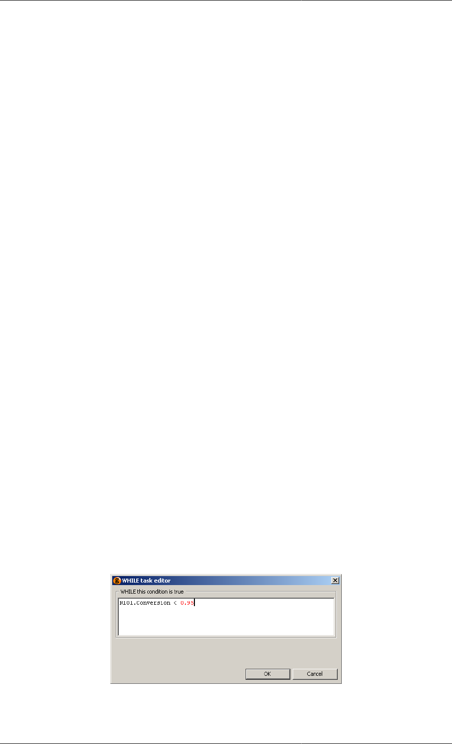
Defining Schedules
147
the operation of a digital PI controller. While the conversion in the reactor is below 0.95, the controller repeatedly
goes through an inactive step of 5 time units (CONTINUE task), followed by a sampling and calculation step
(REASSIGN task), followed by a clipping and implementation step (IF structure).
Example 11.9. Application of the While iterative structure
SCHEDULE
...
WHILE R101.Conversion < 0.95 DO
SEQUENCE
# Continuous operation
CONTINUE FOR 5
# Sampling and calculation
REASSIGN
C101.Error := 150.0 - Sensor101.Measurement ;
C101.IntegralError := C101.IntegralError + 5.0*C101.Error ;
C101.ControlSignal := 0.5 + 1.2*(C101.Error +
C101.IntegralError/20.0) ;
END # Reassign
# Clipping and implementation
IF C101.ControlSignal > 1.0 THEN
REASSIGN
V101.Position := 1.0 ;
END
ELSE
IF C101.ControlSignal < 0.0 THEN
REASSIGN
V101.Position := 0.0 ;
END
ELSE
REASSIGN
V101.Position := OLD(C101.ControlSignal) ;
END
END # If
END # If
END # Sequence
END # While
...
When using the graphical interface, inserting a While Task will activate the following Task configuration dialog.
Figure 11.32. While Task configuration dialog
Enter a valid logical expression in the text box (e.g. R101.Conversion < 0.95) and press the OK button.
gPROMS checks the syntax of the expression and only enables the OK button when it is valid.
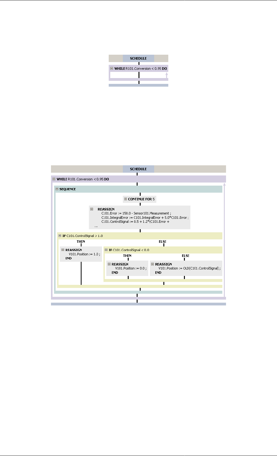
Defining Schedules
148
There is no Advanced view of the configuration dialog for the While Task.
Once a valid expression has been provided, the While Task will be inserted and will look like this:
Figure 11.33. A new If Task
The While Task may only contain a single Task. Any Task can be dragged onto the hot spot for the While Task.
To include more Tasks, they must be contained in one of the other Composite Tasks, so drag a Sequence, Parallel
or If Task into the While Task and then drag new Tasks into the Composite Task. (A quicker way to include a
Sequence Task is to drag the first Elementary Task into the While Task and then to drag the second Elementary
Task into it after the first: gPROMS will then automatically insert the required Sequence Task.
The graphical representation of the example above is shown below.
Figure 11.34. Graphical representation of the While Task
Result control elementary tasks
The "what to do" elementary tasks influence the numerical results of a simulation (e.g. Reassign changes the
value of a degree of freedom, thereby changing the results of the simulation). We now consider the following
useful "result control" elementary tasks that influence the generation of results of a simulation, and not the results
themselves:
• Message
• Monitor
• Resetresults
The message elementary task
Message is a simple elementary tasks that may be used to write a message to the screen. The syntax for MESSAGE
is:
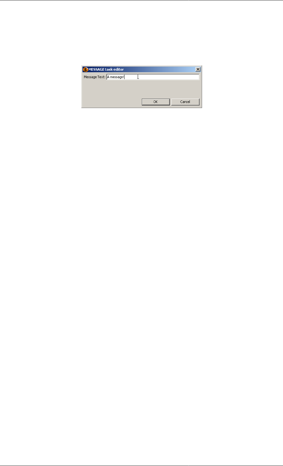
Defining Schedules
149
MESSAGE "text"
When using the graphical interface, the Task configuration dialog for the Message Task is used to specify the
message text:
Figure 11.35. Message Task configuration dialog
Simply enter the desired text (without the quotes) in the text box and press the OK button.
The Monitor elementary task
Normally, during a gPROMS simulation the values of all variables at each reporting interval are sent to the Output
Channel in order to be plotted. The Monitor task may be used to restrict the amount of data that is sent, and may
be useful for a number of reasons:
• For large distributed models, which may consist of tens of thousands of variables, only a small proportion may
be of particular importance and it may sometimes useful to prevent gPROMS from sending all of these variables.
One such example is chromatographic processes, where only the effluent profiles may be of importance. In this
case, many of the variables are of secondary importance and could be suppressed from the gPROMS output.
• Restricting the output from gPROMS may be useful in other circumstances: for example, periodic adsorption
processes require many cycles of operation before a periodic steady state is achieved. If the modeller is only
interested in the steady-state conditions, then the output from gPROMS may be disabled until the final cycle.
• Finally, restricting the data that are sent results in much smaller files (large distributed models may require
several Megabytes of storage).
The above situations can be dealt with in two ways, depending on whether variables should be suppressed
permanently or only at certain times. The Monitor section of the Process is used to specify which variables are
to be monitored during the simulation; those that are not specified are permanently suppressed. If the Monitor
section is omitted, then all variables are monitored. The syntax for the MONITOR section is as follows:
UNIT
...
MONITOR
VariablePathPattern ;
...
SET
...
where VariablePathPattern is the full pathname of the variable to be monitored. Asterisks (*) and percent signs
(%) can be used as a wild cards to specify ranges of Variables that are to be monitored. Asterisks match any
sequence of characters and percent signs match any single character. Any Variable paths that match the string
expressions in the MONITOR section are included in the results. Some examples of VariablePathPattern are:
MONITOR
* ; # monitor everything! (same as not including a MONITOR section
aaa.* ; # monitor all Variables and Units in aaa

Defining Schedules
150
aa% ; # monitor all Variables and Units begining with aa and ending
# in any other character, e.g. aaa, aab, aac, aa0, aa_ etc.
aaa.v* ; # monitor all Variables and Units in aaa that begin with a v
aaa.*.y(*,2) ; # monitor all Variables y that belong to any Unit of aaa
# (or any subunits thereof), provided that they are arrays of
# dimension > 1; monitor only the elements with the last index = 2
*.x* ; # all variables starting with x would be monitored in all units
# also, any units starting with x would also be monitored entirely
Note that for distributed variables (i.e. those that depend on a DISTRIBUTION_DOMAIN), the indices must be
integers and depend on the numerical method applied to the domain. For each distributed variable, gPROMS will
generate an indexed variable with the same number of dimensions as the number of DISTRIBUTION_DOMAINs
that the variable depends on. The length of each dimension is equal to NE × O + 1 for OCFEM and NE+1 for
finite difference methods, where NE is the number of elements and O is the order of the method. For example,
if the variable DV1 is defined by:
DV1 AS DISTRIBUTION(x,y) OF NoType
where the DISTRIBUTION_DOMAINs x and y are Set to the following methods:
x := [ OCFEM, 3, 5 ] ;
y := [ BFDM, 2, 20 ] ;
then the maximum values for the indices of DV1 are 16 (5 × 3 + 1) and 21 (20+1) respectively.
During the simulation, the output of all variables that are specified in the Monitor section can be toggled using
the Monitor task. The syntax for this is:
MONITOR ON
to enable monitoring, and:
MONITOR OFF
to disable monitoring. Note that this is a Task that can only appear in the Schedule of a Process and is distinct
from the MONITOR section of the Process.
One final use of the MONITOR Task is to change the frequency at which results are sent to the Output Channel(s).
This is done by:
MONITOR FREQUENCY NumericalValue
where NumericalValue is a number or an expression that results in a number.
An example of the MONITOR task is shown in the gPROMS code below, where the task DoSomeCycles operates
the process until cyclic steady stage is achieved, then DoOneCycle operates the process for a single cycle after
monitoring has been enabled.
Example 11.10. Example of the MONITOR task
SCHEDULE
SEQUENCE
MONITOR OFF
DoSomeCycles ;
MONITOR ON
DoOneCycle ;
END
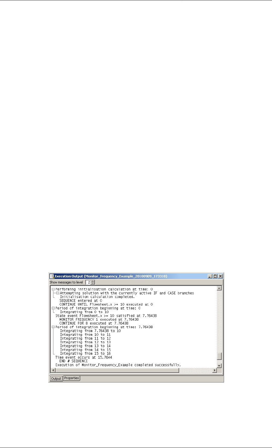
Defining Schedules
151
Another example of the MONITOR task, illustrating the FREQUENCY keyword, is shown next. In this example,
the first Task manipulates the inputs of the system slowly so that a reporting interval of 10 is more than enough
to observe the dynamics. Then, the FastOperation Task creates much faster dynamics, which are too fast
to be seen clearly with a reporting interval of 10. The MONITOR task changes the reporting interval to a more
suitable value. The benefit of this approach, compared with simply setting the ReportingInterval to 1 in
the SOLUTIONPARAMETERS section, is that the resulting Case is much smaller.
SOLUTIONPARAMETERS
ReportingInterval := 10 ;
SCHEDULE
SEQUENCE
SlowOperation ;
MONITOR FREQUENCY 1
FastOperation ;
END
where SlowOperation and FastOperation are Tasks that respectively produce slow and fast dynamics in the
simulation.
Exactly when the reporting interval is updated depends on when the MONITOR Task is encountered. gPROMS
will always continue to the end of the current reporting interval before updating. The example below illustrates
precisely what happens.
SOLUTIONPARAMETERS
ReportingInterval := 10;
SCHEDULE
SEQUENCE
CONTINUE FOR 7
MONITOR FREQUENCY 1
CONTINUE FOR 8
END
Figure 11.36. Output from the example Schedule illustrating MONITOR FREQUENCY
As can be seen, gPROMS starts at time, t = 0 and begins integration with the reporting interval equal to 10, so
gPROMS outputs data at t = 0 and the next set of data are due at t = 10. At t = 7.76, the Continue Task ends, so
a set of data is sent to the output channel at this time (because data are always sent when a discontinuity occurs).
The reporting interval is updated to every 1 unit of time but this will not change until the next scheduled reporting
time, t = 10, so gPROMS then integrates from 7.76 to 10. At t = 10 another set of data is sent to the output channel
and the new reporting interval takes effect: gPROMS now integrates from 10 to 11, and so on.
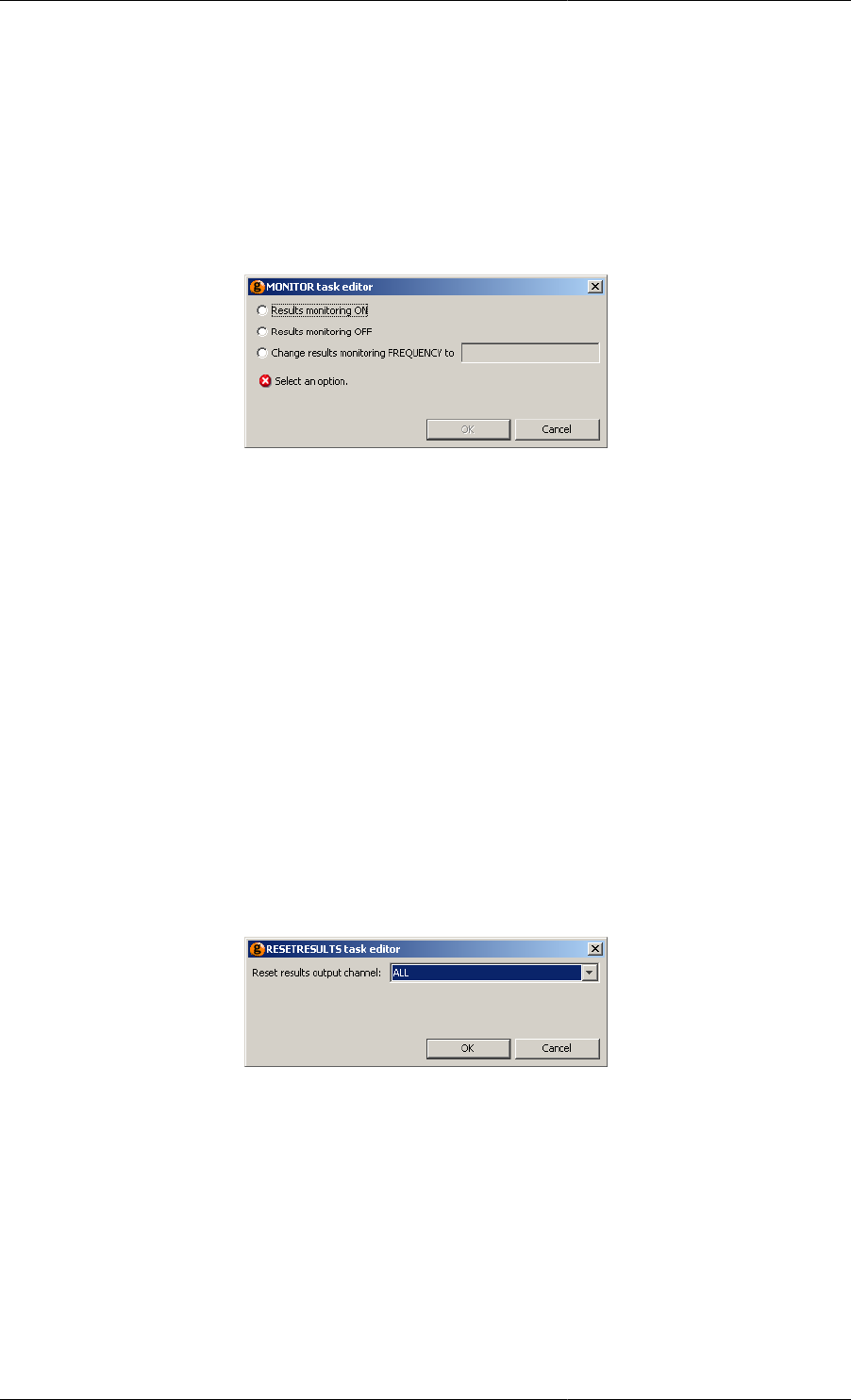
Defining Schedules
152
The reason for this behaviour is clear: if gPROMS were to update the reporting interval immediately, then data
would be sent to the output channel at times 0, 7.76, 8.76, 9.76 etc., which is not very elegant.
The Monitor Task configuration dialog
When inserting or modifying a Monitor Task using the graphical Schedule interface, the following Task
configuration dialog is used.
Figure 11.37. Monitor Task configuration dialog
The Monitor Task configuration dialog allows one to turn monitoring off or on, or to specify a monitoring
frequency. Only one option can be selected. To turn on monitoring and set a new value for the monitoring
frequency, simply insert two Monitor Tasks.
The Resetresults elementary task
The RESETRESULTS may be used in the Schedule section of Processes or Tasks to discard all previous data that
was transmitted to a particular output channel. It may be called using one of the following commands:
RESETRESULTS gRMS
RESETRESULTS gPLOT
RESETRESULTS gExcelOutput
RESETRESULTS gUserOutput
RESETRESULTS ALL
When using the graphical interface, the Task configuration dialog for the Resetresults Task is used to specify one
of the above options:
Figure 11.38. Message Task configuration dialog
Simply select the desired option using the list box and press the OK button.
The Save and Restore elementary tasks
Occasionally, it may be necessary to use the solution of one simulation in another. gPROMS provides a facility to
Save the current values of all or some of the variables in a simulation and to Restore them in (the same) or another
simulation through the use of Saved Variable Sets. The syntax of the SAVE and RESTORE tasks are:
SAVE <VarType> "V_Set_Name"
and
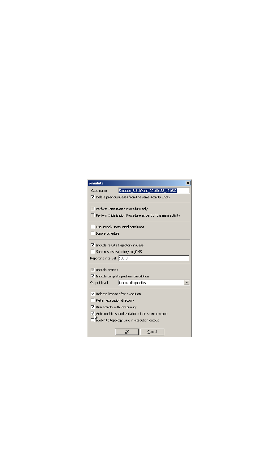
Defining Schedules
153
RESTORE <VarType> "V_Set_Name"
where the optional argument VarType can be one of STATE, ALGEBRAIC and INPUT (or any combination of
these, separated by commas), and V_Set_Name is the name of the Saved Variable Set that the variables will be
saved in (or restored from). If the VarType argument is omitted, then gPROMS will save the values of all variables;
whereas arguments STATE, ALGEBRAIC and INPUT instruct gPROMS to save only the values of the state,
algebraic or input variables respectively. The VarType optional argument works similarly with the Restore task.
Any new Variable Set created during a simulation activity using the Save elementary task will be stored in the
Results Entity group within the Execution Case. So that the Variable Set can be used in conjunction with the
Restore elementary task, the Variable Set must then be copied into the working project where it will appear in
the Saved Variable Sets Entity group.
It is also possible to over-write (or modify) an existing Variable Set by using the Save elementary task on a Variable
Set already present in the source project. In this instance, two Saved Variable Sets with the same name will appear
in the Execution Case: the original (from the working project) will appear in the Original Entities and the new
entity created by the Save elementary task will be stored under Results.
ModelBuilder can be configured so that the Saved Variable Set in the Project is automatically updated. This is done
by checking the auto update source project option in the execution dialog that can also be seen in the figure below.
Figure 11.39. Auto Update Source Project Option
Variables may also be Restored from multiple sets, separated by commas:
RESTORE "v_set1", "v_set2"
Note that, unlike in the PRESET section, when using the Restore Task to restore state Variables, the values of all
Selector Variables will be restored as well.
The gPROMS code below illustrates how the SAVE and RESTORE tasks could have been used in the example
problem presented in the Monitor section. Rather than solving the problem in one Process, with Monitor used to
show only the last cycle of operation, here we can use two Processes: one to establish the cyclic steady state and to
save the variables, and the second to simulate a single cycle using as initial conditions the values of the variables
at the end of the simulation of the first Process. One advantage of this approach is that the variables can be plotted
against the local time for the cycle (i.e. the cycle starts at time = 0) as opposed to the global time of the whole
simulation (where the start of the cycle will be at some arbitrary time).
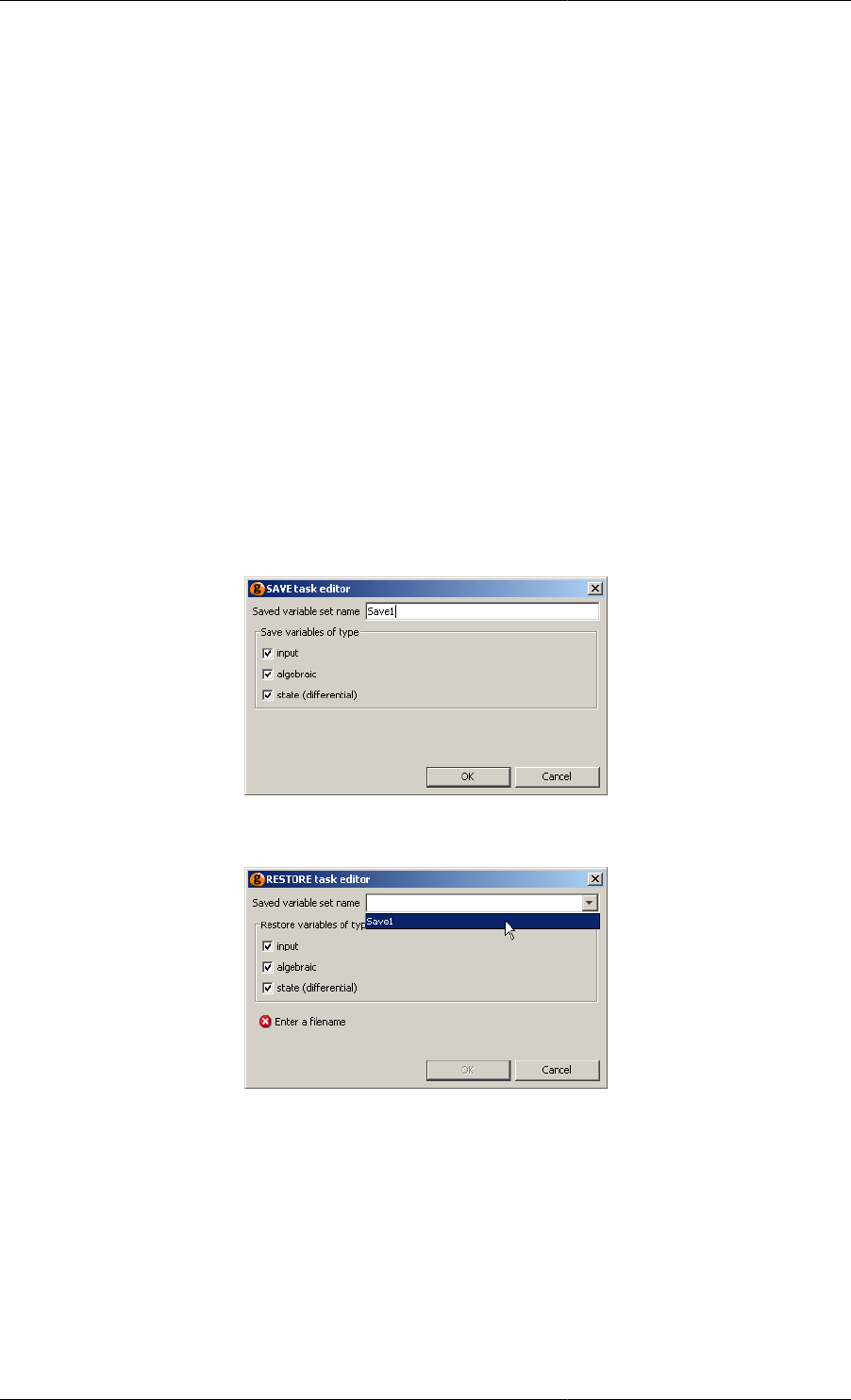
Defining Schedules
154
Example 11.11. Application of the Save and Restore Tasks.
# the Schedule of one Process or Task
SCHEDULE
SEQUENCE
MONITOR OFF
DoSomeCycles ;
SAVE STATE "CyclicSteadyState"
END
# the Schedule of another Process or Task
SCHEDULE
SEQUENCE
MONITOR OFF
RESTORE STATE "CyclicSteadyState"
MONITOR ON
DoOneCycle ;
END
When Save or Restore Tasks are inserted into the Schedule using the graphical editor, the following configuration
dialogs are used.
Figure 11.40. Save Task configuration dialog
Figure 11.41. Restore Task configuration dialog
When configuring a Save Task, the name of the Saved Variable Set must be entered in the text box. The types of
Variables stored in the Saved Variable Set are specified by checking or unchecking the boxes next to the Variable
types: input, algebraic and state (differential). These can be set in any combination.
The Restore Task is configured similarly to the Save Task. The only exception is that the name of the Saved
Variable Set must be specified by choosing an option from the list box. The list box will only contain the names
of the Saved Variable Sets present in the Project.

155
Chapter 12. Defining Tasks
A Task forms a re-usable part of the operating procedure; it is associated with one or more Models and can be
used multiple times within a Schedule and by other Tasks.
A Task entity is defined by three sections: Task Parameter declarations, (optional) Task Variable declarations and
a Schedule where the Task's operating procedure is expressed in terms of the Task Parameters and Variables.
Overall, the structure of a Task definition is the following:
PARAMETER
... Parameter declarations ...
VARIABLE
... Local variable declarations ...
SCHEDULE
... Schedule declaration ...
The Variable and Schedule sections of a Task
The Variable section is used to declare local variables. They can only be used within the Task in which they are
declared. Task Variables are the equivalent of local subroutine Variables and as such are calculated by the Task.
They should not be confused with Model Variables and are NOT associated with Variable Types instead they are
declared to be of type INTEGER or REAL.
The Schedule section defines the operating policy implemented by the Task. It is based on the same language used
to define the Schedule section in Process Entities, the only difference being that a Task Schedule has access to the
local variables declared in the Variable section. The values of the latter can be manipulated by using assignment
statements.1
1Changing the value of a Task Variable does not require a RESET statement; this only applies to Model Variables.

Defining Tasks
156
Example 12.1. Task for a digital PI control law
# TASK DigitalPI
VARIABLE
Error, IntegralError, ControlSignal AS REAL
SCHEDULE
SEQUENCE
IntegralError := 0 ;
WHILE TIME < 1000 DO
SEQUENCE
CONTINUE FOR 5.0
Error := 150.0 - Sensor101.Measurement ;
IntegralError := IntegralError + 5.0*Error ;
ControlSignal := 0.5 + 1.2 * ( Error + IntegralError/20.0 ) ;
IF ControlSignal > 1.0 THEN
RESET Valve201.Position := 1.0 ; END
ELSE
IF ControlSignal < 0.0 THEN
RESET Valve201.Position := 0.0 ; END
ELSE
RESET Valve201.Position := OLD(ControlSignal) ; END
END # If
END # If
END # Sequence
END # While
END # Sequence
This example shows a TASK that models the action of a digital PI controller. Three local variables are declared in
the VARIABLE section, namely Error, IntegralError and ControlSignal. In the SCHEDULE section,
an assignment statement initialises IntegralError to zero. Then, the repeated action of the controller is
specified within a WHILE structure. This is executed until a termination condition is satisfied (in this case,
when 1000 time units have passed on the simulation clock). The action of the controller is itself a sequence of
elementary Tasks. First, a CONTINUE task is used to enforce a period of undisturbed operation (5 time units).
After this, sampling takes place. The signal of a temperature sensor is used to update the controller Error and
IntegralError and a ControlSignal is calculated. An IF structure is used to clip the signal which is then
implemented it through a RESET task.
In essence, Tasks are user-defined tasks. Once declared, they are equivalent to elementary tasks and can be used
in Process Schedules or even within the Schedules of other Tasks. For instance,
SCHEDULE
PARALLEL
DigitalPI
CONTINUE FOR 1000
END # Parallel
executes the digital control law in parallel with the operation of the rest of the process.
The Parameter section of a Task
The Digital PI control example, although useful for grouping a series of elementary tasks together, has a big
disadvantage: it is extremely specific. First of all, it refers to a unique sensor/valve pair, Sensor101 and
Valve201 respectively. Moreover, the sampling interval (5 time units) and controller tuning parameters (150.0,
0.5, 1.2, 20.0) are expressed as constant values. Finally, the task always terminates after 1000 time units have
elapsed and is thus appropriate for a simulation of that length only. If it were necessary to apply the same operating
procedure to a different sensor/valve pair possibly using different tuning parameters for the controller, a new Task

Defining Tasks
157
would have to be declared. This is clearly unsatisfactory. In most instances, we want to be able to declare Tasks
that are independent of the details of an individual simulation.
For instance, we want to be able to define a Task that switches 'a' pump on and another that switches 'a' pump off.
'A' is used to indicate that the actual pump on which the Tasks act remains unspecified until the moment they are
used in a particular simulation experiment. Similarly, we want to be able to define a Task for 'a' digital controller
and only specify the sensor/valve pair it uses and the values for its tuning parameters when the Task is actually
used in a simulation experiment.
This is achieved by using Task parameters. Upon declaration, a Task can be parameterised with respect to an
arbitrary number of parameters. The actual values of these parameters have to be specified only when the Task
is actually used in a specific simulation experiment.
Task parameters are declared in the Parameter section. Declared parameters may be of any of the following types:
•INTEGER, REAL or LOGICAL constants. These are used to parameterise a TASK with respect to, for instance,
controller tuning parameters, event durations etc.
•INTEGER_EXPRESSION, REAL_EXPRESSION or LOGICAL_EXPRESSION. These are used to
parameterise a TASK with respect to, for instance, logical conditions for the conditional and iterative structures
etc.
•MODEL. These are used to parameterise a TASK with respect to the actual Models on which it acts.
Example 12.2. Task to switch on a pump
# TASK SwitchPumpOn
PARAMETER
Pump AS MODEL GenericPump
SCHEDULE
RESET
Pump.Status := Pump.Open ;
END # Reset
This example shows a task that switches a pump on. Once this Task has been defined, it can be used in a Schedule
section. For instance,
SCHEDULE
...
SwitchPumpOn(Pump IS Plant.P201)
...
will switch on pump Plant.P201, while
SCHEDULE
...
SEQUENCE
SwitchPumpOn(Pump IS Plant.P205)
SwitchPumpOn(Pump IS Plant.P206)
SwitchPumpOn(Pump IS Plant.P207)
END # Sequence
...
will, in sequence, switch on pumps Plant.P205, Plant.P206 and Plant.P207.
Note that, when executing a Task that contains parameters, the proper list of arguments must be given along
with the name of the Task. Tasks that contain parameters can be thought of as the equivalent of subroutines or

Defining Tasks
158
functions in high-level programming languages. Variables declared in the Variable section are the equivalent of
local subroutine variables. On the other hand, the Parameter section is the equivalent of a function prototype. It
defines the number and type of arguments that a Task accepts as arguments. A 'call' to the Task then includes a
list of all the Parameters declared in the Task and values for each of them.
Example 12.3. Parameterised Task for a digital PI control law
# TASK DigitalPI
PARAMETER
SetPoint, Bias, Gain, IntegralTime AS REAL
SamplingInterval AS REAL
TerminationCondition AS LOGICAL_EXPRESSION
Sensor AS MODEL GenericSensor
Valve AS MODEL GenericValve
VARIABLE
Error, IntegralError, ControlSignal AS REAL
SCHEDULE
SEQUENCE
IntegralError := 0 ;
WHILE NOT TerminationCondition DO
SEQUENCE
CONTINUE FOR SamplingInterval
Error := SetPoint - Sensor.Measurement ;
IntegralError := IntegralError + SamplingInterval*Error ;
ControlSignal := Bias + Gain*( Error +
IntegralError/IntegralTime ) ;
IF ControlSignal > 1.0 THEN
RESET Valve.Position := 1.0 ; END
ELSE
IF ControlSignal < 0.0 THEN
RESET Valve.Position := 0.0 ; END
ELSE
RESET Valve.Position := OLD(ControlSignal) ; END
END # If
END # If
END # Sequence
END # While
END # Sequence
This example presents the correct version of the digital controller Task. The Parameters include real constants
that determine the various tuning parameters and the sampling interval, a logical expression that determines the
termination of control, and model parameters that determine the sensor/valve pair on which the controller is used.
This Task is much more reusable. It can be used for any sensor/valve pair in a simulation experiment and different
tuning parameters for the controller can be specified without rewriting the Task. For instance,
SCHEDULE
...
PARALLEL
DigitalPI
( SetPoint IS 150.0,
Bias IS 0.5,
Gain IS 1.2,
IntegralTime IS 20.0,
SamplingInterval IS 5.0,

Defining Tasks
159
TerminationCondition IS Plant.T101.TotalVolume > 5.0,
Sensor IS Plant.Sensor101,
Valve IS Plant.Valve205 )
DigitalPI
( SetPoint IS 10.0,
Bias IS 0.8,
Gain IS 2.6,
IntegralTime IS 50.0,
SamplingInterval IS 1.0,
TerminationCondition IS Plant.R101.Temperature > 80.0,
Sensor IS Plant.Sensor103,
Valve IS Plant.Valve207 )
END # Parallel
...
will initiate two digital control procedures in parallel, acting on two different sensor/valve pairs. The two
procedures also have different controller tuning characteristics and a different logical expression determining their
termination.
Hierarchical Task Construction
A complex operation on one or more items of process equipment can usually be decomposed into lower-
level, simpler operations. Each of the lower-level operations may in turn be decomposed in other, more
primitive operations, the decomposition continuing until all operations can be described in terms of elementary
manipulations of the underlying models made possible by elementary tasks. Similarly to hierarchical sub-model
decomposition, this hierarchical sub-task decomposition defeats complexity by restricting the scope of the
problem considered at any point to a manageable level.
Hierarchical sub-task decomposition in gPROMS is possible because previously declared Tasks may be used
within other, higher-level Tasks and is greatly facilitated by the fact that suitably parameterised Tasks may be
reused several times in different parts of an operation.
Example 12.4. Low-level Task to operate a reactor
# TASK OperateReactor
PARAMETER
Reactor AS MODEL StirredReactor
SR AS REAL
StartTemperature AS REAL
Terminationcondition AS LOGICAL_EXPRESSION
SCHEDULE
SEQUENCE
RESET
Reactor.SteamRate := SR ;
END
CONTINUE UNTIL Reactor.Temperature > StartTemperature
RESET
Reactor.SteamRate := 0 ;
END
CONTINUE UNTIL TerminationCondition
END # Sequence
Consider, for instance, the gPROMS code above containing the OperateReactor TASK. It specifies an
operating procedure for performing a reaction in a reactor of type StirredReactor (a parameter of the
TASK). The operating procedure is simple, involving the execution of four elementary tasks in sequence. First,

Defining Tasks
160
the steam supply rate to the reactor is set to a value SR. Operation then continues until the temperature in the
reactor has exceeded a predefined limit StartTemperature. Finally, the steam supply is cut off and operation
continues until a TerminationCondition is satisfied. In addition to the reactor unit, SR, StartTemperature
and TerminationCondition are also parameters of the TASK, of type REAL, REAL_EXPRESSION and
LOGICAL_EXPRESSION respectively.
Example 12.5. High-level Task to operate a reactor train
# TASK OperateReactorTrain
PARAMETER
Plant AS MODEL ReactorTrain
SCHEDULE
PARALLEL
PerformReaction
( Reactor IS Plant.R1,
SR IS 35.3,
StartTemperature IS 70.0,
TerminationCondition IS Plant.R1.Conversion(1) > 0.95 )
PerformReaction
( Reactor IS Plant.R2,
SR IS 10.0,
StartTemperature IS 40.0,
TerminationCondition IS Plant.R2.Temperature > 120.0 )
END # Parallel
The gPROMS code above illustrates how the OperateReactor TASK is used to define a higher-level Task,
namely OperateReactionTrain. Two OperateReactor tasks are invoked in parallel to model the
operation of two reactors. Parameterisation also permits the specification of different values for the operating
parameters of the two reactors.
Building Tasks using the graphical interface
Just as it is possible to construct a Schedule of a Process using a graphical interface, it is also possible to build
new user-defined Tasks graphically. The following tabs provide a graphical interface for building (or modifying)
user-defined Tasks and are entirely equivalent to typing in gPROMS language.
• Interface, which is equivalent to the PARAMETER section
• Variables, which is equivalent to the VARIABLE section
• Schedule, which is equivalent to the Schedule section
Either or both methods can be used interchangeably: modifications made using one of the three tabs above will
automatically result in the same changes to the appropriate section of the gPROMS language tab and vice versa.
These three tabs are described next. You should be familiar with Defining Schedules (in particular, using the
graphical interface) before reading the documentation on the Schedule tab.
Using the Interface tab
After inserting a new Task in the Project (right click on Tasks in the Project tree, select New entity..., provide a
name and click OK), left click on the Interface tab and the following will be shown.
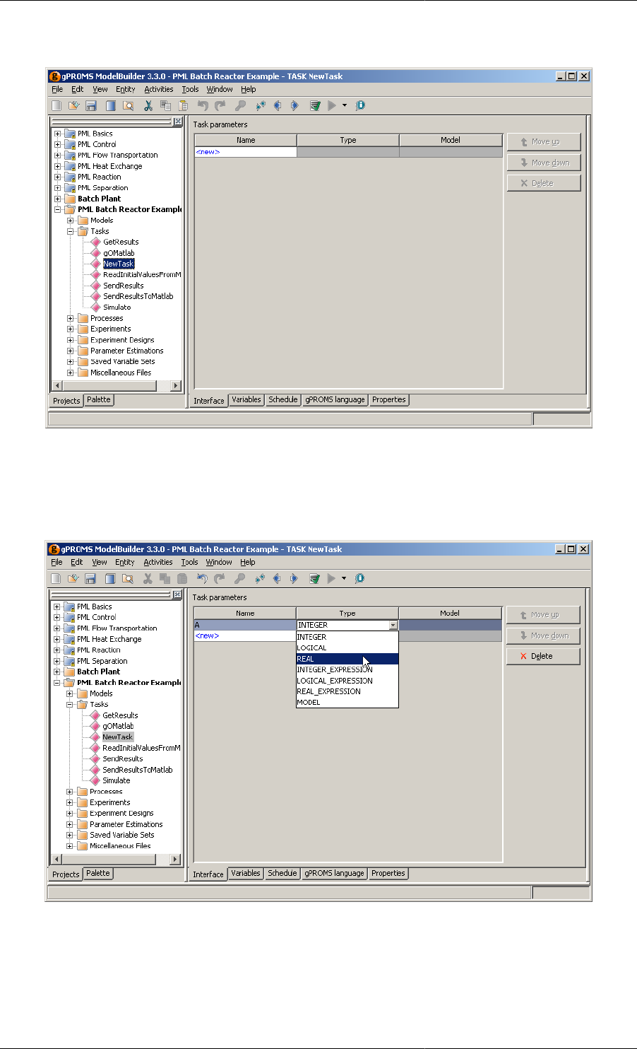
Defining Tasks
161
Figure 12.1. New Task Interface tab
The Interface tab contains a list of all of the Parameters in the Task. To add a new Parameter, left click on the
<new> cell and enter a name for the new Parameter. Then the type can be chosen from the list box, as shown below.
Figure 12.2. Adding a new Parameter
MODEL Parameters require a further specification: left click in the model cell and type the name of a Model. A
list box containing all existing Models in the Project can be activated by pressing CTRL+SPACE. This is shown
below.
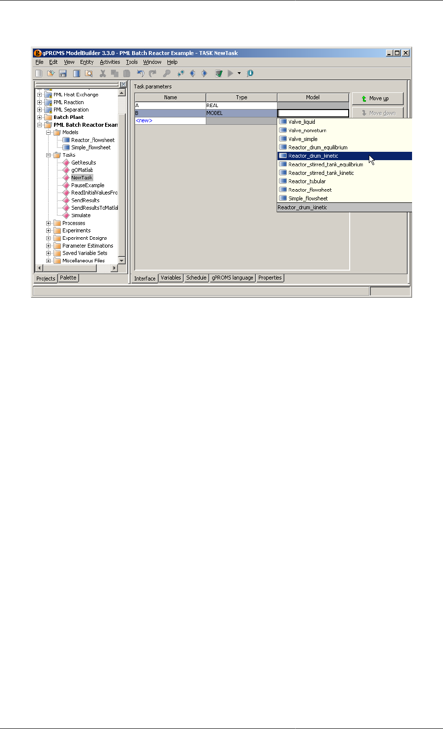
Defining Tasks
162
Figure 12.3. Adding a MODEL Parameter
The order of the Parameters can be changed by selecting the Parameter and pressing the Move up or Move down
buttons. Parameters can be removed from the Task by selecting a Parameter and pressing the Delete button.
For this example, the gPROMS language tab now contains:
PARAMETER
A AS REAL
B AS MODEL Reactor_drum_kinetic
Once all of the Parameters have been specified, the Variables tab can be selected in order to define any
local Variables for the Task.
Using the Variables tab
The Variables tab contains a list of all of the local Variables in the Task. To add a new local Variable, click on the
<new> cell and enter a name for the new Variable. Then the type can be chosen from the list box, as shown below.
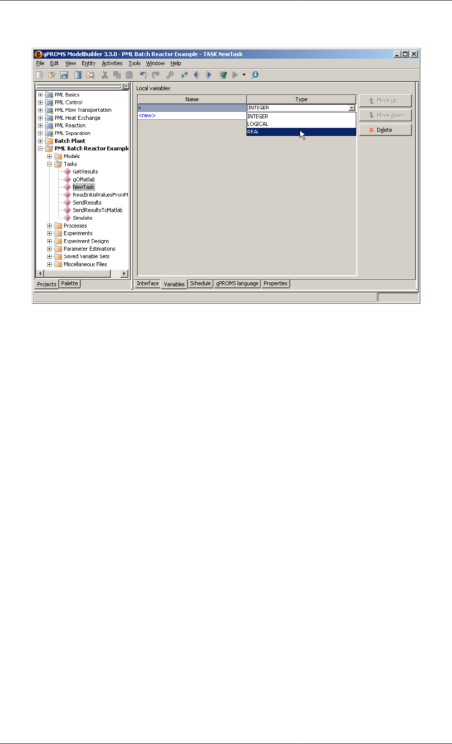
Defining Tasks
163
Figure 12.4. Adding a new local Variable
The order of the local Variables can be changed by selecting the Variable and pressing the Move up or Move down
buttons. Local Variables can be removed from the Task by selecting a Variable and pressing the Delete button.
For this example (including the Parameters defined before), the gPROMS language tab now contains:
PARAMETER
A AS REAL
B AS MODEL Reactor_drum_kinetic
VARIABLE
x AS REAL
Once all of the local Variables have been specified, the Schedule tab can be selected in order to define the operating
policy for the Task.
Using the Schedule tab
Task Schedules are constructed in exactly the same way as Process Schedules (see Defining Schedules), with one
additional feature: when the Schedule tab of a Task is open, the Task palette will contain one extra elementary
Task for assigning the value of a local Variable (and this will also be added to the context menu).
The use of user-defined Tasks in Schedules is also described here. This was deferred from the section on Defining
Schedules because user-defined Tasks had not been described at that point.
The screen shot below shows the Simulate user-defined Task from the PLM Batch Reactor example, along with
the Task palette.
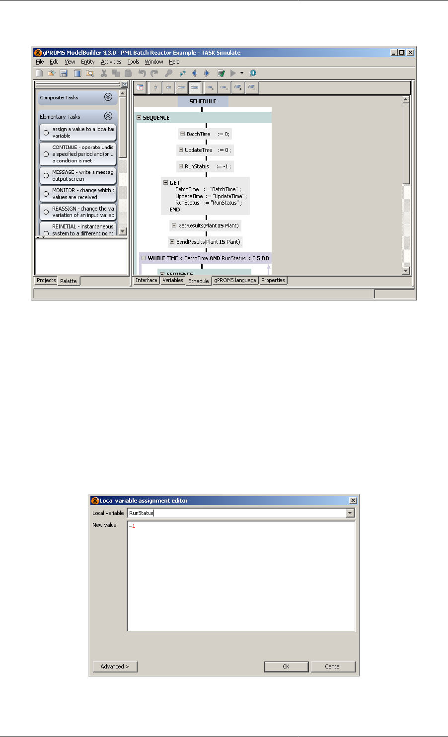
Defining Tasks
164
Figure 12.5. Simulate user-defined Task
The first three Tasks in the outer Sequence are local Variable assignment Tasks.
To insert a new Assign local variable Task, left click on the Task in the Task palette and drag it onto a hot spot in
the Schedule. Alternatively, right click on a hot spot and select Local variable assignment from the Add elementary
task context menu. When this is done, a Task configuration dialog will appear.
To configure the Task, select a local Variable from the list box and then enter an expression for its new value in
the text box below. Pressing the OK button completes the addition of the Task.
The Advanced view shows the equivalent gPROMS language.
The screenshot below shows the configuration dialog for the third Task in the Schedule above.
Figure 12.6. Local variable assignment Task configuration dialog
The next Task in the Schedule (the GET Task) is a Foreign Process Task. These are described in Using Foreign
Processes.
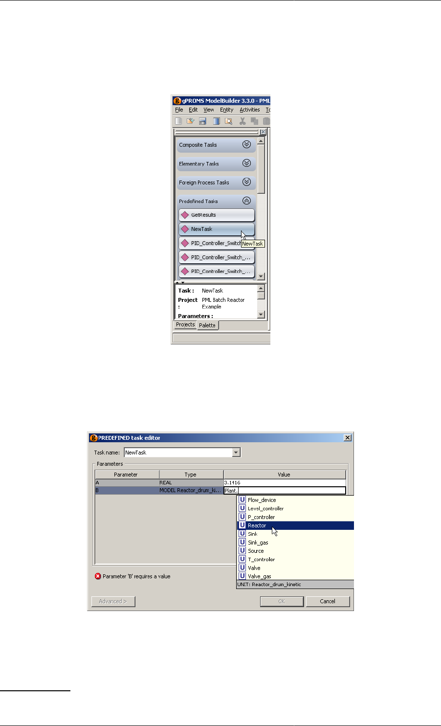
Defining Tasks
165
The two Tasks following the GET Task are user-defined Tasks that have been inserted into the Schedule. User-
defined Tasks can be inserted into a Schedule using the Task palette or the context menu. The Predefined Tasks
section of the Task palette contains a list of all predefined Tasks, as shown below.
Figure 12.7. Task Palette for user-defined Tasks
Predefined Tasks are inserted into the Schedule by dragging them from the palette to the Schedule.2 When this
is done, a configuration dialog will appear allowing the Parameters of the Task to be specified. The dialog for
our new Task is shown below.
Figure 12.8. Completing the Task configuration dialog for a predefined Task
Once all of the Parameters have been specified correctly, you can press the OK button and the Task will be inserted.
The Advanced view shows the gPROMS language:
NewTask(A IS 3.1416, B IS Plant.Reactor)
2Unlike built-in Tasks, predefined Tasks cannot be inserted into the Schedule using the context menu.

Defining Tasks
166
Intrinsic Tasks
When discussing the Parameter section within a Task, we considered an example where there were two digital PI
controllers. The Task for each controller must be called in the Process section in order to activate the controller
and specify its tuning parameters. This small example of just two controllers requires a reasonable amount of code
to be written in the Schedule section of the Process. More complex Models, where there might be tens or even
hundreds of controllers, may lead to a large schedule section with much repeated code. Specifying all of these
tasks is not only time consuming but also prone to error. Since these Tasks must be enabled for each and every
controller, it is possible to automate the specification of these Tasks in the Schedule of a Process. More generally,
one can associate a number of Tasks with any Model, so that each instantiation of the Model automatically (and
invisibly) adds the Tasks to the Schedule section. These are called Intrinsic Tasks and are nothing more than a
declaration in the Model of which (already defined) Tasks should be automatically included in the Schedule, thus
automating the laborious manual procedure.
As an example of the use of Intrinsic Tasks, let us assume that we want to model a plant with three reactors that are
structurally identical but are used for different duties. This means that the plant Model will contain three instances
of the same reactor Model but with different properties. Now if the reactor Model contains three control loops,
e.g. for pressure, temperature and level, the following Schedule would be required to model the controllers using
ordinary Tasks. (For brevity, some parameters have been omitted.)
SCHEDULE
...
PARALLEL
# Controllers for Reactor1
DigitalPI
( SetPoint IS 373.0,
Bias IS 0.5,
Gain IS 1.2,
Sensor IS Plant.Reactor1.TemperatureSensor,
Valve IS Plant.Reactor1.CoolingWaterValve )
DigitalPI
( SetPoint IS 10.0,
Bias IS 0.8,
Gain IS 2.6,
Sensor IS Plant.Reactor1.PressureSensor,
Valve IS Plant.Reactor1.PressureReliefValve )
DigitalPI
( SetPoint IS 1.0,
Bias IS 0,
Gain IS 2,
Sensor IS Plant.Reactor1.LevelSensor,
Valve IS Plant.Reactor1.LiquidOutletValve )
# Controllers for Reactor2
DigitalPI
( SetPoint IS 425.0,
Bias IS 1,
Gain IS 3,
Sensor IS Plant.Reactor2.TemperatureSensor,
Valve IS Plant.Reactor2.CoolingWaterValve )
DigitalPI
( ...
Sensor IS Plant.Reactor2.PressureSensor,
Valve IS Plant.Reactor2.PressureReliefValve )
DigitalPI
( ...
Sensor IS Plant.Reactor2.LevelSensor,
Valve IS Plant.Reactor2.LiquidOutletValve )

Defining Tasks
167
# Controllers for Reactor3
...
END # Parallel
...
Clearly, there is a lot of repeated code that is mostly unnecessary apart from the need to specify different tuning
parameters. The use of Intrinsic Tasks is ideal in this type of situation. To implement Intrinsic Task, one first has
to define them in the Model itself, which is illustrated below for the reactor example.
# MODEL Reactor
PARAMETER
...
TemperatureSetpoint AS REAL
TemperatureGain AS REAL
...
...
EQUATION
...
INTRINSIC_TASK
DigitalPI
( SetPoint IS TemperatureSetPoint,
Bias IS TemperatureBias,
Gain IS TemperatureGain,
Sensor IS TemperatureSensor,
Valve IS CoolingWaterValve )
DigitalPI
( SetPoint IS PressureSetPoint,
Bias IS PressureBias,
Gain IS PressureGain,
Sensor IS PressureSensor,
Valve IS PressureReliefValve )
DigitalPI
( SetPoint IS LevelSetPoint,
Bias IS LevelBias,
Gain IS LevelGain,
Sensor IS LevelSensor,
Valve IS LiquidOutletValve )
# END of Model Reactor
Now, each instance of the Model Reactor will automatically have DigitalPI Tasks enabled in the Schedule section
of the Process without the user needing to provide them. Of course, the set points and tuning parameters will need
to be specified (unless defaults are provided and are suitable) but these would have to be specified in any case.
So the Schedule section could be a simple as:
SCHEDULE
CONTINUE FOR 100
and the controller Tasks will be added, in parallel with the user-defined Schedule, by gPROMS when the Process
is executed.
Note that since ordinary Tasks are only active in dynamic Simulation activities, Intrinsic Tasks are also limited to
dynamic Simulation activities. In other words, if a Process contains dynamic Models with Intrinsic Tasks, they will
be ignored if there is no Schedule section defined in the Process or if the Ignore schedule option of the Execution
Dialog is checked.
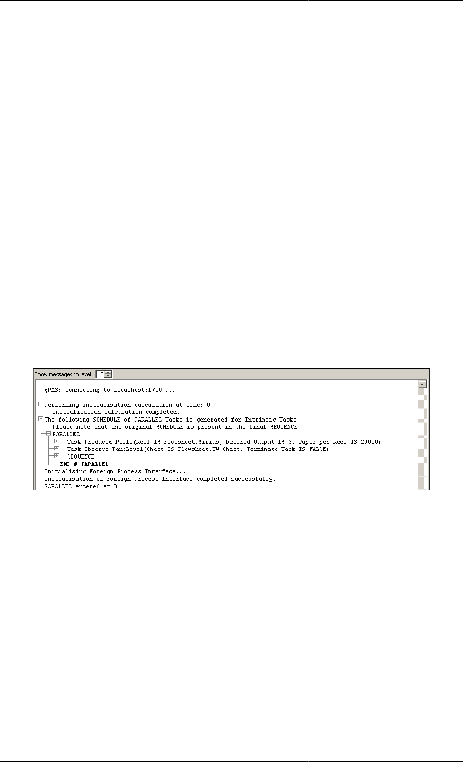
Defining Tasks
168
In the above examples, the names of a number of Units within the Model were passed to the Model Parameters of
the Task. It may also be necessary to pass the Model itself as an argument to the Task. The This_Unit keyword
is used for this purpose, as illustrated below.
# MODEL A_model
...
INTRINSIC_TASK
Task1(
theModel IS This_Unit,
aParameter IS 10 )
In this example, any instances of A_model will automatically have their names passed as arguments to the Task1
Tasks (which are automatically generated in parallel with the user-defined Schedule).
Viewing the Schedule Generated by Intrinsic Tasks
The final Schedule is reported by gPROMS in the execution output, so that you can check that the Intrinsic Tasks
are behaving as intended. After the simulation has completed, scroll the Execution Output window up until you
find the line "The following SCHEDULE of PARALLEL Tasks is generated for Intrinsic Tasks". This will be just
after the initiation has been completed. Below this line, the Intrinsic Tasks that were added to the Schedule will
be displayed. To see the detailed Schedule, simply click on the "+" symbols to expand the various elements of the
Tasks. These two views are shown in the figures below (for a different example).
Figure 12.9. Execution Output Indicating the Inclusion of Intrinsic Tasks
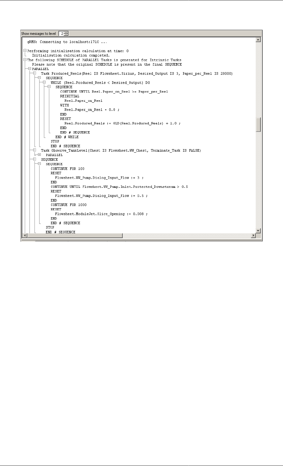
Defining Tasks
169
Figure 12.10. Execution Output Showing the Detailed Schedule for Intrinsic Tasks
The first Sequence shown was defined in the Produced_Reels Task that was specified as an Intrinsic Task: hence,
it was automatically placed in the final Schedule. The Sequence nested inside the second Sequence is the whole
Schedule from the Process, so everything else was generated automatically. Note that, since much of the Schedule
is automatically created, there is no guarantee that these Schedules will terminate, so gPROMS adds a Stop Task
to the end of the user-defined Schedule.
Controlling the Use of Intrinsic Tasks
So far, the examples on Intrinsic Tasks have assumed that these Tasks should always be enabled for every instance
of a Model containing Intrinsic Tasks. Although this is the default behaviour, one can easily select which Model
instances should have their Intrinsic Tasks enabled. There are a number of ways to achieve this.
First, all Intrinsic Tasks can be switched off by editing the process properties. In this case, no matter what
specifications are made in the Models and Process, no Intrinsic Tasks will be used and the user will have to specify
the use of Tasks manually. To do this, open the Process entity and left click on the Solution Parameters tab. Double
click on (or click on the "+" symbol next to) the Intrinsic Tasks folder. Now you can change the setting from ON
to OFF by clicking on ON and selecting OFF from the list.
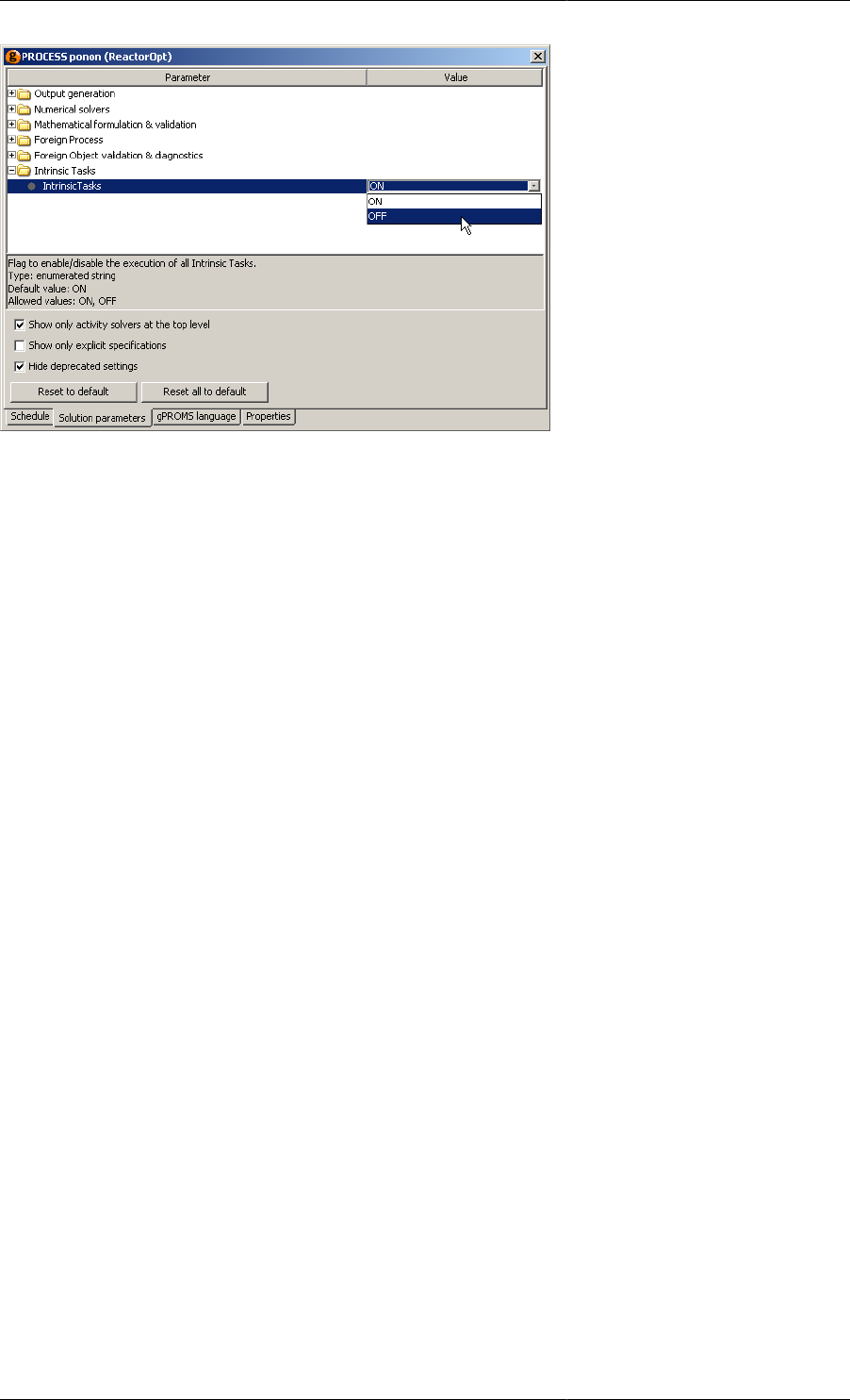
Defining Tasks
170
Finer control over the use of Intrinsic Tasks can be achieved by defining their use whenever a Model is instantiated.
To do this, the Intrinsic Tasks solution parameter of the Process must be ON. Then, there are three options for
instantiating a Model (A is the name of a Model defined in the gPROMS project):
UNIT
A AS A
A_off AS A INTRINSIC_TASKS OFF
A_on AS A INTRINSIC_TASKS ON
These three specifications work as follows.
Instantiating a model with the INTRINSIC_TASKS OFF option forces gPROMS not to use any of the Intrinsic
Tasks defined for that Model instance.
In contrast, instantiating a Model with the INTRINSIC_TASKS ON option turns on all Intrinsic Tasks for the
Model instance.
Finally, if no specification is made (the first example above), then the behaviour of the Model instance will be
the same as the Model instance within which it is contained. If it is a top-level model instance, then the default
behaviour is for the Intrinsic Tasks to be enabled. So, the behaviour of a particular Model instance will be passed
down the Model hierarchy until an explicit instantiation takes place, which will then override the behaviour of
the parent Model.
To illustrate the behaviour of Models (and sub Models) instantiated in this way, let us assume that the three Model
instances of Model A are made in a Process. Model A then contains three instances of a Model B:
UNIT
B AS B
B_off AS B INTRINSIC_TASKS OFF
B_on AS B INTRINSIC_TASKS ON
Finally, Model B also contains three different instances of Model C:
UNIT
C AS C
C_off AS C INTRINSIC_TASKS OFF
C_on AS C INTRINSIC_TASKS ON
This then produces the following Model-instance hierarchy.
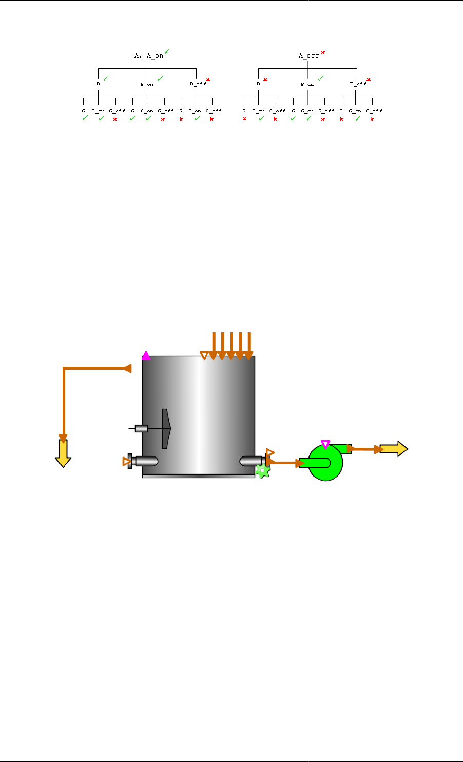
Defining Tasks
171
Figure 12.11. Illustration of Intrinsic Task control
The ticks and crosses next to each Model instance indicate whether or not intrinsic tasks are enabled for that Model
instance. Since the default behaviour for top-level Models is for Intrinsic Tasks to be enabled, A and A_on both
have their tasks enabled. Therefore, each of the Model instances within A will have the same properties as those
within A_on. The main feature is that the *_on instances always have Intrinsic Tasks enabled, *_off instances
are always disabled and the instances with the default specification always behave as the Model instance above.
ModelBuilder also allows the these specifications to be made via the graphical interface. Click on the Topology tab
and then right click on the Unit you want to specify. The context menu contains an item called Intrinsic Tasks….
Moving the mouse over this item, enables a list containing the three possible settings for the Unit. Left clicking
on one of these options sets the value for this Unit. Units with disabled Intrinsic Tasks are indicated by a red cog
image on the Unit; those with enabled Intrinsic Tasks by a green cog; and if the default specification is made, no
cog is shown. If you then switch back to the gPROMS language view, you will see that the code has changed to
reflect the choice made. An example of a Unit with enabled Intrinsic Tasks is shown below.
Figure 12.12. Example of a Unit with enabled Intrinsic Tasks
To reiterate, control over which Model instances use Intrinsic Tasks can occur only when the Process solution
parameter Intrinsic Tasks is ON; if it is OFF, then none of the Intrinsic Tasks are enabled and they must be included
explicitly in the Schedule.
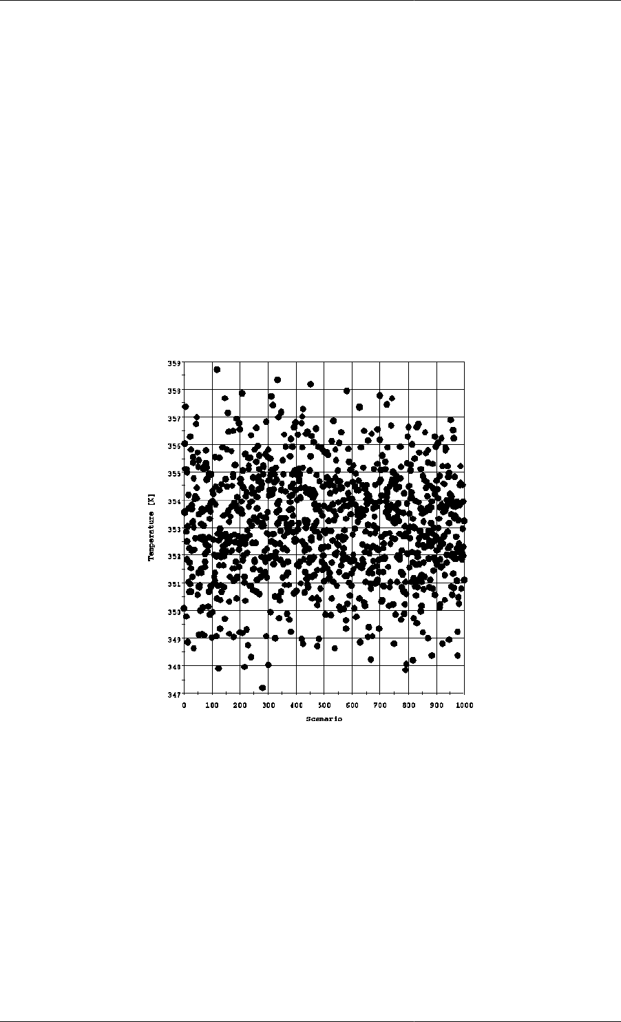
172
Chapter 13. Stochastic Simulation in
gPROMS
gPROMS can be used to perform stochastic simulations. The prime reason for considering stochastic simulation
is to determine how the distributions of key output Variables are influenced by the distributions of the input
Variables. In order to do so, you will learn how to do the following:
• Assign random numbers to Parameters and Variables
• Perform multiple simulations and plot their results in the form of probability density functions
An example of the output that can be achieved from a stochastic simulation in gPROMS is shown below
Figure 13.1. Values assigned to the temperature for each scenario.
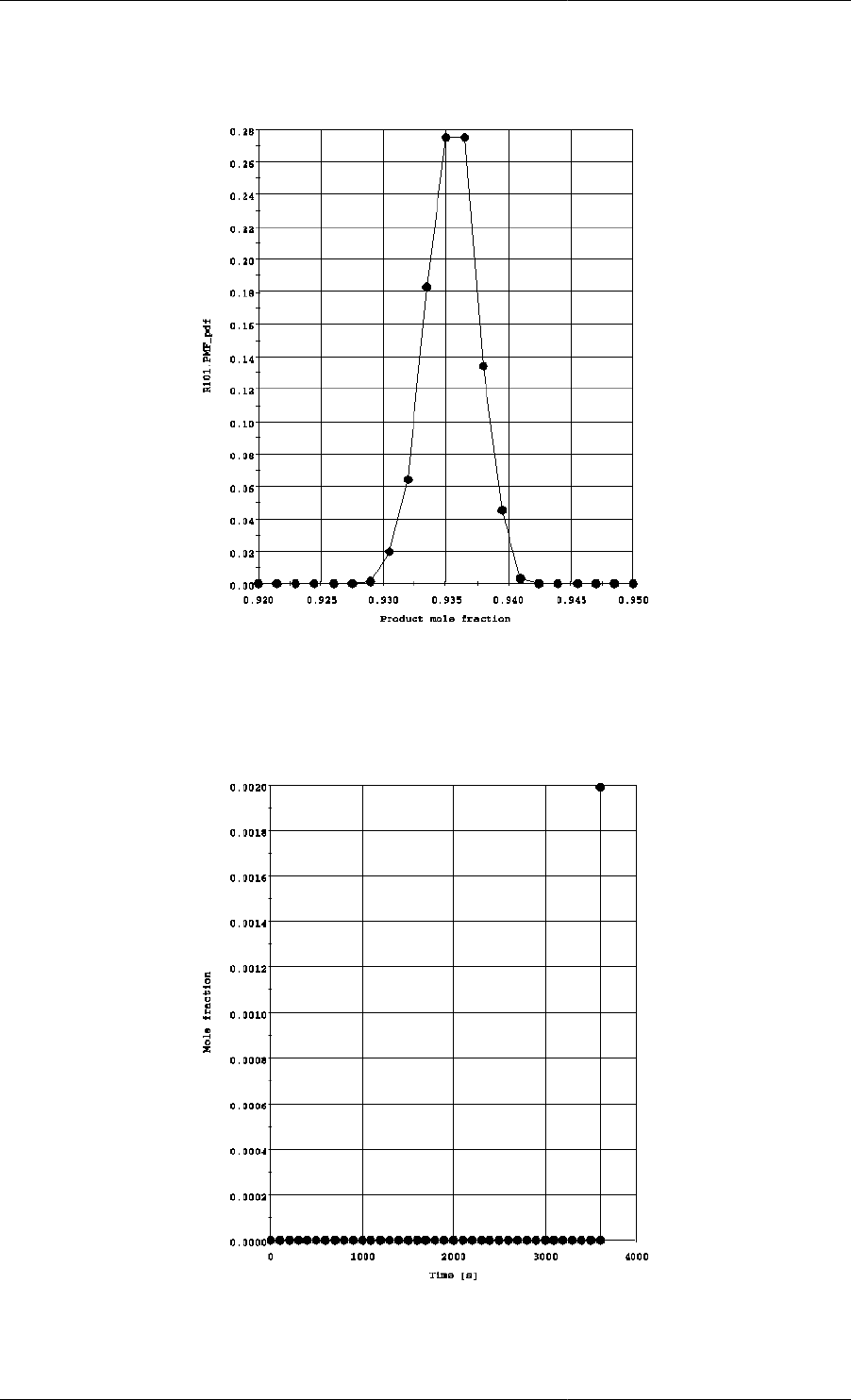
Stochastic Simulation in gPROMS
173
Figure 13.2. Probability density function for the product mole fraction.
Figure 13.3. Standard deviation of the product mole fraction

Stochastic Simulation in gPROMS
174
Assigning random numbers to Parameters
and Variables
Parameters and Variables can be given random values in the Set and Assign sections, respectively, of a Process
Entity in the same way that they are given deterministic values. Instead of assigning a literal value or expression to
the parameter or variable, special functions are used that return values sampled from the distribution. The syntax
is shown below.
...
SET
Identifier := DistributionFunction( ArgList ) ;
...
ASSIGN
Identifier := DistributionFunction( ArgList ) ;
...
The functions DistributionFunction each require a different set of arguments ArgList. The available functions are
described in table below.
Table 13.1. Probability distribution functions available in gPROMS.
Function Arguments Example
Uniform lower, upper UNIFORM(0,1) returns a
uniformly distributed number in
the range [0,1]. lower < upper.
Triangular lower, mode, upper TRIANGULAR(1,2,4) returns
a number sampled from a
triangular distribution with
mode 2, lower limit 1 and upper
limit 4. lower < mode < upper.
Normal mean, stddev NORMAL(3,0.25) returns a
value sampled from a normal
distribution with mean 3 and
standard deviation 0.25. stddev > 0.
Gamma alpha, beta GAMMA(3,1) returns a
value from the Gamma
distribution. alpha, beta > 0.
Beta alpha, beta, lower, upper BETA(1.5,5,0,1) returns a value
from the Beta distribution.
alpha, beta > 0; lower < upper.
Weibull alpha, beta WEIBULL(4,1) returns
a value from the Weibull
distribution. alpha, beta > 0.
Once Parameters and Variables have been given stochastic values, they behave exactly as though they had been
assigned deterministic values: i.e. Parameters remain constant and are not calculated by a simulation and the
Variables remain at their Assigned values unless re-assigned in a Reset statement. Any Variable may be Reset, as
usual, using a literal or an expression (using the Old operator if this involves other Variables or by assigning a new
random number. Note that Variables and Parameters can only ever be assigned 'point' values; they are not assigned
distributions. Furthermore, each time a variable is Reset to a value from a distribution, it is given a different value,
even if the distribution function's arguments are the same. For example, in the following segment of a Schedule

Stochastic Simulation in gPROMS
175
section, the variable Random is assigned two different values from the Normal distribution: one time it may be
assigned 0.23 then 0.07; another time it may be assigned 0.01 then 0.36.
...
SCHEDULE
SEQUENCE
...
RESET
Random := NORMAL(0,1) ;
END
...
RESET
Random := NORMAL(0,1) ;
END
...
END
One further issue that should be noted is that gPROMS will always seed the random number generator with
the same number each time a simulation is started. This means that the results of a stochastic simulation are
reproducible.
Plotting results of multiple stochastic
simulations
In order to examine how the distributions of key output Variables are influenced by the distributions of the input
Variables, we will describe how you can combine multiple simulations in a single process and then use the results
to evaluate metrics (such as the mean, variance, etc.) of the output Variables. Thereafter, we will outline a method
that allows you to plot the probability density functions of the output Variables.
Combining multiple simulations
Given a model with some uncertain inputs, a series of simulations can be combined into a single process by
introducing a new higher-level Model. The original model is included in the new one as an array of Units, as
shown below.
# MODEL ModelUncertain
...
VARIABLE
Input AS InputVarType # uncertain input variable
Output AS OutputVarType # important output variable
...
# MODEL Combined
PARAMETER
NoScenarios AS INTEGER
InputMean AS REAL
InputStdDev AS REAL
UNIT
Scenarios AS ARRAY(NoScenarios) OF ModelUncertain

Stochastic Simulation in gPROMS
176
The input Variables for each scenario of ModelUncertain then need to be specified as follows.
# PROCESS StochSim
UNIT
StSim AS Combined
...
ASSIGN
WITHIN StSim DO
FOR i := 1 TO NoScenarios DO
Scenarios(i).Input := NORMAL(InputMean,InputStdDev) ;
END
END
...
Note that each input Variable is Assigned a different value from the same distribution. This could also have been
done with Parameters, but parameter propagation cannot be used in this way: this would result in all Parameters
being set the same value, because the parameter in the higher-level model will be assigned randomly and then that
particular value will be propagated to the scenarios. Of course, any inputs that are common to the system (such as
design constants or precisely known operating Parameters) can be included in the higher-level model along with
equations linking them to the scenarios. This reduces the complexity of the Schedule section.
Plotting probability density functions
Now all of the scenarios are together in one Process, but it is not easy to plot them together in one graph. Rather
than having to select each Variable from each scenario instance, it would be much easier to be able to select the
whole distribution. This can easily be done as follows.
# MODEL Combined
PARAMETER
NoScenarios AS INTEGER
InputMean AS REAL
InputStdDev AS REAL
UNIT
Scenarios AS ARRAY(NoScenarios) OF ModelUncertain
VARIABLE
Input AS ARRAY(NoScenarios) OF InputVarType
Output AS ARRAY(NoScenarios) OF OutputVarType
OPmean AS NoType # mean of Output
OPvariance AS NoType # variance of Output
EQUATION
FOR i := 1 TO NoScenarios DO
Input(i) = Scenarios(i).Input ;
Output(i) = Scenarios(i).Output ;
END
OPmean = SIGMA(Output)/NoScenarios ;
OPvariance = SIGMA( (Output - OPmean)^2 )/NoScenarios ;
Now, all of the scenarios can be plotted on a single graph by selecting a single Variable in gRMS. Notice also that
the mean and variance of the output can easily be calculated.

Stochastic Simulation in gPROMS
177
Finally, it is often useful to be able to plot the probability density function (pdf) of the output. In general, for each
Variable this requires two new Variables a distribution domain and three Parameters. However, if two Variables
are in the same interval they can share the same distribution domain and Parameters. This is shown below.
# MODEL Combined
PARAMETER
NoScenarios AS INTEGER
InputMean AS REAL
InputStdDev AS REAL
NoInt_OP AS INTEGER DEFAULT 20 # number of intervals for distribution
Upper_OP AS REAL DEFAULT 3 # upper bound on distribution
Lower_OP AS REAL DEFAULT 1 # lower bound on distribution
DISTRIBUTION_DOMAIN
Dist_OP AS (Lower_OP:Upper_OP) # distribution over which
# Output will be plotted
UNIT
Scenarios AS ARRAY(NoScenarios) OF ModelUncertain
VARIABLE
Input AS ARRAY(NoScenarios) OF InputVarType
Output AS ARRAY(NoScenarios) OF OutputVarType
OPmean AS NoType # mean of Output
OPvariance AS NoType # variance of Output
# temp variable to count occurrences of Output in a particular interval:
OPacc AS DISTRIBUTION(Dist_OP,NoScenarios) OF NoType
# pdf function for Output:
OP_pdf AS DISTRIBUTION(Dist_OP) OF NoType
EQUATION
FOR i := 1 TO NoScenarios DO
Input(i) = Scenarios(i).Input ;
Output(i) = Scenarios(i).Output ;
END
OPmean = SIGMA(Output)/NoScenarios ;
OPvariance = SIGMA( (Output - OPmean)^2 )/NoScenarios ;
FOR i := Lower_OP TO Upper_OP DO
FOR j := 1 TO NoScenarios DO
IF i - (Upper_OP-Lower_OP)/NoInt_OP/2 <= Output(j) AND
Output(j) < i + (Upper_OP-Lower_OP)/NoInt_OP/2 THEN
OPacc(i,j) = 1 ;
ELSE
OPacc(i,j) = 0 ;
END
END
OP_pdf(i) = SIGMA(OPacc(i,))/NoScenarios ;
END
The three new Parameters introduced are NoInt_OP, Lower_OP and Upper_OP. These Parameters define the
distribution over which the output Variable will be plotted. NoInt_OP is the number of intervals used for the
distribution Dist_OP. This will obviously be used to set Dist_OP:

Stochastic Simulation in gPROMS
178
# PROCESS StSim
...
SET
...
Dist_OP := [BFDM, 1, NoInt_OP] ;
The first order, backward finite difference method is all that is required because the distribution domain is
essentially behaving as an array. The Parameters Lower_OP and Upper_OP are simply the lower and upper bounds
on the domain Dist_OP. The Variable being plotted, Output in this case, must lie in the interval [lower, upper] for
each scenario; otherwise, the pdf will become distorted. If the lower and upper bounds are set so that a number of
Variables lie in this interval, then all of these Variables can be plotted using the same distribution. The number of
intervals should be set appropriately so that the distribution is not too coarse. Finally, the two Variables introduced
are OPacc and OP_pdf. Each Variable being plotted will need its own pair of Variables. OPacc(i,j) is set to 1 if
the value of Output(j) (the value in scenario j) lies in interval i of the distribution domain. OP_pdf(i) therefore
represents the number of scenarios in which Output has a value in interval i. This is divided by the number of
scenarios to normalise the pdf. Plotting the pdf of a state Variable can slow down the simulation significantly
(due to the many discontinuities, and therefore re-initialisations, encountered as the values of the Variables switch
between intervals). This can be remedied by introducing one further Variable, as illustrated below for the example
already considered:
# MODEL Combined
...
VARIABLE
...
# temporary Output variable = 0 until end of simulation, then = Output
OutputEnd AS ARRAY(NoScenarios) OF OutputVarType
...
EQUATION
FOR i := 1 TO NoScenarios DO
Input(i) = Scenarios(i).Input ;
Output(i) = Scenarios(i).Output ;
END
...
FOR i := Lower_OP TO Upper_OP DO
FOR j := 1 TO NoScenarios DO
IF i - (Upper_OP-Lower_OP)/NoInt_OP/2 <= OutputEnd(j) AND
OutputEnd(j) < i + (Upper_OP-Lower_OP)/NoInt_OP/2 THEN
OPacc(i,j) = 1 ;
ELSE
OPacc(i,j) = 0 ;
END
END
OP_pdf(i) = SIGMA(OPacc(i,))/NoScenarios ;
END
# PROCESS StochSim
...

Stochastic Simulation in gPROMS
179
MONITOR
StSim.Output(*) ;
StSim.Input(*) ;
StSim.OPmean ;
StSim.OPvariance ;
StSim.OP_pdf ;
...
ASSIGN
WITHIN StSim DO
OutputEnd := 0 ;
...
END
...
SCHEDULE
SEQUENCE
...
RESET
StSim.OutputEnd := OLD(StSim.Output) ;
END
END
So, OutputEnd is 0 throughout the simulation and the If conditions are only evaluated at initialisation. Only at the
end of the simulation is OutputEnd changed, at which point all of the If statements are re-evaluated and OP_pdf
recalculated. Finally, note that the output has been restricted to only those Variables of importance by using the
Monitor section. This reduces the amount of data sent to the output channel (e.g. gRMS). Although this is not
necessary, it recommended for moderate to large problems (even small problems output large quantities of data
when the number of scenarios is large).
Stochastic Simulation Example
In this section we illustrate the important techniques of stochastic simulation in gPROMS using a simple model
of an isothermal batch reaction. The following reactions occur in the reactor, D being the desired product.
The reactor initially contains 10m3 of an equimolar mixture of A and B. The temperature is held constant at 353K
and the reaction is allowed to progress for 1 hour. The reaction rates are assumed to follow Arrhenius's law.
Stochastic gPROMS process model
A simple, generic model for an isothermal liquid-phase CSTR is used to model the process
# MODEL LiquidPhaseCSTR
PARAMETER
# Number of components
NoComp AS INTEGER
# Number of reactions
NoReac AS INTEGER
Density AS ARRAY(NoComp) OF REAL

Stochastic Simulation in gPROMS
180
# Reaction data (Arrhenius law)
ArrhConstant AS ARRAY(NoReac) OF REAL
ActivationEnergy AS ARRAY(NoReac) OF REAL
# Reaction orders
Order AS ARRAY(NoComp,NoReac) OF INTEGER
# Component stoichiometric coefficients
Nu AS ARRAY(NoComp,NoReac) OF INTEGER
# Gas constant
R AS REAL
VARIABLE
Fin AS MolarFlowrate
Xin AS ARRAY(NoComp) OF MolarFraction
Fout AS MolarFlowrate
X AS ARRAY(NoComp) OF MolarFraction
HoldUp AS ARRAY(NoComp) OF Moles
C AS ARRAY(NoComp) OF MolarConcentration
T AS Temperature
TotalHoldup AS Moles
TotalVolume AS Volume
ReactionConstant AS ARRAY(NoReac) OF NoType
Rate AS ARRAY(NoReac) OF NoType
EQUATION
# Material balance
FOR i := 1 TO NoComp DO
$HoldUp(i) = Fin*Xin(i) - Fout*X(i) + TotalVolume*SIGMA(Nu(i,)*Rate) ;
END
# Reaction rates
FOR j := 1 TO NoReac DO
ReactionConstant(j) = ArrhConstant(j) * EXP(-ActivationEnergy(j)/R/T) ;
Rate(j) = ReactionConstant(j) * PRODUCT(C^Order(,j)) ;
END
# Total volume and total holdup
TotalVolume = SIGMA(Holdup/Density) ;
TotalHoldup = SIGMA(HoldUp) ;
# Molar fractions and concentrations
Holdup = X * TotalHoldup ;
Holdup = C * TotalVolume ;
Now we assume the that temperature of the reaction may change from batch to batch. This can be modelled using
a normal distribution with a mean of 353K and a standard deviation of 2K. To see the effect of this, we need to
introduce a new composite Model to include a number of scenarios:
# MODEL Stochastic_LiquidPhaseCSTR
PARAMETER
# define common PARAMETERs here so their values can be propagated

Stochastic Simulation in gPROMS
181
# to each scenario
# -----------------------------------------------------------------
NoComp AS INTEGER
NoReac AS INTEGER
Density AS ARRAY(NoComp) OF REAL
ArrhConstant AS ARRAY(NoReac) OF REAL
ActivationEnergy AS ARRAY(NoReac) OF REAL
Order AS ARRAY(NoComp,NoReac) OF INTEGER
Nu AS ARRAY(NoComp,NoReac) OF INTEGER
R AS REAL
# -----------------------------------------------------------------
NoScenarios AS INTEGER
NoInt_PMF AS INTEGER DEFAULT 20
Upper_PMF AS REAL DEFAULT 1
Lower_PMF AS REAL DEFAULT 0.8
DISTRIBUTION_DOMAIN
Dist_PMF AS (Lower_PMF:Upper_PMF)
UNIT
Scenarios AS ARRAY(NoScenarios) OF LiquidPhaseCSTR
VARIABLE
T AS ARRAY(NoScenarios) OF Temperature
ProdMolFrac AS ARRAY(NoScenarios) OF MolarFraction
PMFmean AS NoType
PMFvariance AS NoType
PMFstddev AS NoType
# temp variable to count occurrences of Output in a particular interval:
PMFacc AS DISTRIBUTION(Dist_PMF,NoScenarios) OF NoType
# pdf function for Output:
PMF_pdf AS DISTRIBUTION(Dist_PMF) OF NoType
EQUATION
FOR i := 1 TO NoScenarios DO
T(i) = Scenarios(i).T ;
END
PMFmean = SIGMA(ProdMolFrac)/NoScenarios ;
PMFvariance = SIGMA( (ProdMolFrac - PMFmean)^2 )/NoScenarios ;
FOR i := Lower_PMF TO Upper_PMF DO
FOR j := 1 TO NoScenarios DO
IF i - (Upper_PMF-Lower_PMF)/NoInt_PMF/2 <= ProdMolFrac(j) AND
ProdMolFrac(j) < i + (Upper_PMF-Lower_PMF)/NoInt_PMF/2 THEN
PMFacc(i,j) = 1 ;
ELSE
PMFacc(i,j) = 0 ;
END
END
PMF_pdf(i) = SIGMA(PMFacc(i,))/NoScenarios ;
END

Stochastic Simulation in gPROMS
182
We have defined new distributed Variables to contain the values of the Variables of interest in each scenario. These
are T for the temperature and ProdMolFrac for the mole fraction of the product D (i.e. x_4). Again, Parameters are
defined that describe the upper and lower limits of the distribution and its coarseness. Finally, Variables are defined
for the mean, variance and standard deviation of the product mole fraction. The equations are the same as were
described before, except that there is no equation for the standard deviation or to relate the variable ProdMolFrac
to the X(4) Variables in each scenario. While we could include the equation for the standard deviation in this
model, by using the equation:
PMFstddev^2 = PMFvariance ;
this tends to slow the simulation down. The alternative used here is to Assign PMFstddev to a temporary value in
the Process section and to Reset it at the end of the simulation using:
SCHEDULE
SEQUENCE
...
RESET
xxx.PMFstddev := SQRT(OLD(xxx.PMFvariance)) ;
END
END
The final difference is the missing equation relating ProdMolFrac to Scenarios().X(4). This is because we are
plotting a pdf of a dynamic variable and want to avoid slowing the simulation but are demonstrating a different
approach to the one described before (where the additional 'End' variable was used). Here, we can avoid this
additional variable simply by Assigning ProdMolFrac itself and then Resetting at the end of the simulation. The
disadvantage with this approach is that you cannot plot the mean of the distribution over time; it only contains the
correct value at the end of the simulation, when ProdMolFrac gets assigned the correct values. In this example,
we were not concerned with plotting the mean, etc., over time and so this approach is an appropriate alternative.
The final extract of the gPROMS project, the Process entity, is shown below.
# PROCESS Stochastic
UNIT
R101 AS Stochastic_LiquidPhaseCSTR
SET
WITHIN R101 DO
NoScenarios := 1000 ;
Upper_PMF := 0.95 ;
Lower_PMF := 0.92 ;
NoInt_PMF := 20 ;
Dist_PMF := [ BFDM, 1, NoInt_PMF ] ;
NoComp := 4 ;
NoReac := 2 ;
Nu := [ -1, 0,
-1, 0,
1, -1,
0, 1 ] ;
Order := [ 1, 0,
1, 0,
0, 1,
0, 0 ] ;
R := 8.31441 ; # kJ/kmol/K
ArrhConstant := [ 8E-3, 1E-2 ] ; # m3/kmol s

Stochastic Simulation in gPROMS
183
ActivationEnergy := [ 8000, 6000 ] ; # kJ/kmol
Density := [ 17.48, 17.15, 10.24, 55.56 ] ; # kmol/m3
END
ASSIGN
WITHIN R101 DO
PMFstddev := 0 ;
FOR i := 1 TO NoScenarios DO
ProdMolFrac(i) := 0 ;
WITHIN Scenarios(i) DO
Fin := 0 ;
Fout := 0 ;
Xin := [ 0.5, 0.5, 0, 0 ] ;
T := NORMAL(353, 2) ;
END
END
END
INITIAL
WITHIN R101 DO
FOR i := 1 TO NoScenarios DO
WITHIN Scenarios(i) DO
X(2) = X(1) ;
X(3) = 0 ;
X(4) = 0 ;
TotalVolume = 10 ;
END
END
END
SCHEDULE
SEQUENCE
CONTINUE FOR 3600
RESET
FOR i := 1 TO R101.NoScenarios DO
R101.ProdMolFrac(i) := OLD(R101.Scenarios(i).X(4)) ;
END
END
RESET
R101.PMFstddev := SQRT(OLD(R101.PMFvariance)) ;
END
CONTINUE FOR .01
END
Below are some comments on the PROCESS.
• SET: This section illustrates a couple of useful features in gPROMS. The first is that some of the Parameters
are having their default values overridden. The second is that all of the Parameters in the lower-level model
(LiquidPhaseCSTR) are being propagated.
• ASSIGN: In this section we assign the dummy values to ProdMolFrac and PMFstddev. Also, some of the
degrees of freedom of the LiquidPhaseCSTR model are set, e.g. the inlet and outlet flowrates, which are set to
zero. Finally, the temperature for each scenario is set a random value from the normal distribution, N(353,2).
• INITIAL: A typical set of initial conditions are used here.
• SCHEDULE: This sections illustrates the Resetting of the Variables ProdMolFrac and PMFstddev. Note that
because PMFstddev depends on ProdMolFrac, the latter must be RESET before the former in a separate RESET
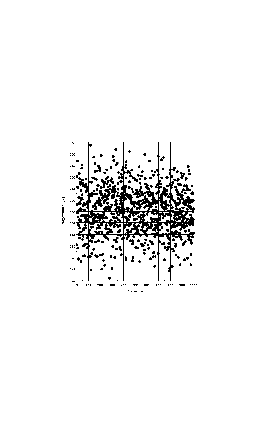
Stochastic Simulation in gPROMS
184
task. If they are RESET in the same task, then PMFstddev will be RESET based on the values in ProdMolFrac
from before the RESET task.
Finally, on some systems gRMS may not be able to plot the pdf Variables correctly (sometimes the value after
the Reset is ignored by gRMS). A simple solution is to include a short Continue at the end of the Schedule.
This is not an issue with the Excel output channel, although sending the values of a large number of Variables
to Excel takes a considerable length of time. It is therefore recommended that you Monitor only the Variables
that are necessary.
Stochastic simulation results
The results of the stochastic simulation are shown in the figures below. The last one also illustrates that in this
model, the value of the standard deviation is only correct at the end of the simulation.
Figure 13.4. Values assigned to the temperature for each scenario.

Stochastic Simulation in gPROMS
185
Figure 13.5. Probability density function for the product mole fraction X(4).
Figure 13.6. Standard deviation of the product mole fraction X(4).

186
Chapter 14. Controlling the Execution
of Model-based Activities
The Process entity is used to describe a simulation activity that is to be carried out by gPROMS using instances
of one or more Model entities. The execution of model-based activities involves the solution of different types
of mathematical problems. Typically, these are complex problems due to both their size and their nonlinearity.
gPROMS provides a number of state-of-the-art mathematical solvers that employ a combination of symbolic,
structural and numerical manipulations for the solution of these problems.
There are a number of important features of the Process entity that are related with the solution of the underlying
mathematical problems and the handling of the results produced by it:
• The PRESET section describes how you can provide initial guesses for the variables that occur in your model;
• The SOLUTIONPARAMETERS section describes how you can:
• choose appropriate solvers for different kinds of problems,
• specify the destination of any results that the solution may produce.
In addition, a detailed description of the mathematical solvers provided as standard within gPROMS. These fall
into the following categories:
• solvers for sets of linear algebraic equations;
• solvers for sets of nonlinear algebraic equations;
• solvers for mixed sets of nonlinear algebraic and differential equations;
The description of each solver includes a list of all the parameters that you can use to configure its precise behaviour
when applying it to a particular problem.
The PRESET section
At the start of each simulation, gPROMS has to solve a problem known as initialisation. For both steady-state and
dynamic simulations, gPROMS must first solve a system of algebraic equations (usually nonlinear). This naturally
requires initial guesses for all of the variables in order to provide the solution algorithm with a starting point.
These initial guesses (and appropriate bounds on the variables) are specified in the Variable Type entities. Usually,
specifying the initial guesses in this manner i.e. the same initial guess and bounds for variables of the same type) is
sufficient for gPROMS to solve the initialisation problem. Larger, more complex problems, however, may not be
suited to this approach and therefore a more flexible method is needed specifying the initial guesses. This is catered
for through the Preset section, which allows the default initial guess and bounds of a variable to be overridden.
The syntax for the Preset section is:
PRESET VariablePath := InitialValue ;
or
PRESET VariablePath := InitialValue : LowerBound : UpperBound ;
Within and For statements may also be used in the PRESET section. The PRESET section is usually found within
the Process entity, but it may also be included inside a model entity.
Even once a set of suitable initial guesses are found, some problems may take a considerable length of time to
solve. This can often be greatly reduced if the solution of the initialisation problem is used to provide the initial

Controlling the Execution
of Model-based Activities
187
guesses. This can be done in gPROMS using Saved Variable Sets by SAVEing the values of all variables after the
initialisation and restoring them in the Preset section as shown in the gPROMS code below. In the first Process, a
set of initial guesses is used that is sufficient for the initialisation to be solved. The second Process then uses the
data in the save file to solve the initialisation more quickly. Note that the second Process may also save the result of
the initialisation problem, so that changes can be made to the problem without having to run the first Process again.
Example 14.1. Process used to solve the initialisation problem only
# PROCESS InitSim1
...
PRESET
WITHIN aaa DO
x(1) := 1 ;
x(2) := 1 ;
x(3:10) := 0 ;
y() := 5 ;
z := 10 : 5 : 100 ;
...
END
...
SCHEDULE
SAVE "InitialisationData"
Example 14.2. Full Process restoring data from the successful initialisation
# PROCESS FullSim
...
PRESET
RESTORE "InitialisationData"
...
SCHEDULE
SEQUENCE
SAVE "InitialisationData"
...
END # sequence
Note that Saved Variable Sets restored in a RESTORE section do not overwrite the values of any Selector
Variables. This is because their values, specified in the INITIALSELECTOR section, are part of the problem
definition and therefore must not be modified by a RESTORE.
Multiple Saved Variable Sets can be Restored in the PRESET section, along with manually specified initial
guesses, as shown in the example below. In all cases, any initial guess provided for a particular variable, either
via an explicit specification or via a Restore, will override all earlier initial guesses for the same variable. Please
note that bounds defined by a variable type will not be overwritten by the bounds in a Saved Variable Set. This
means that any Variables that are not included in the Saved Variable Sets will have initial guesses and bounds
specified by their Variable Types.
PRESET
RESTORE "v_set1", "v_set2" ;
RESTORE "v_set3" ;
VariablePath := InitialValue ;

Controlling the Execution
of Model-based Activities
188
VariablePath := InitialValue : LowerBound : UpperBound ;
RESTORE "v_set4", "v_set5" ;
RESTORE "v_set6" ;
The SOLUTIONPARAMETERS section
The SOLUTIONPARAMETERS section allows the specification of parameters that affect:
• the results generated by the execution of a model-based activity;
• the mathematical solvers to be used for the execution of a model-based activity;
• the validation and diagnosis of the mathematical models;
• the use of Foreign Processes in a simulation activity1;
• the behaviour of Foreign Objects associated with a model-based activity;
• the behaviour of Intrinsic Tasks2.
The basic syntax for the SOLUTIONPARAMETERS section, along with the default values of the parameters,
is shown below:
SOLUTIONPARAMETERS
# parameters concerned with output generation
gExcelOutput := OFF ;
gPLOT := OFF ;
gRMS := OFF ;
gUserOutput := OFF ;
Monitor := ON ;
OutputLevel := 1 ;
ReportingInterval := 0.0 ;
ScheduleAnnotations := OFF ;
# parameters concerned with numerical solvers
DASolver := "DASOLV" ;
DOSolver := "CVP_SS" ;
EDSolver := "EXPDES" ;
PESolver := "MAXLKHD" ;
# parameters concerned with mathematical formulation and validation
IdentityElimination := ON ;
IgnoreDAEIndexAnalysis := OFF ;
IndexReduction := OFF ;
PerformStrictDAEStructuralChecks := OFF ;
# parameters concerned with Foreign Object behaviour
FOStatisticsLevel := 0 ;
IgnoreAllFODerivatives := OFF ;
LogAllFODerivatives := OFF ;
LogAllFOMethods := OFF ;
TestAllFODerivatives := OFF ;
1There is only one FPI Solution Parameter, which specifies the location of the FPI implementation. See Using Foreign Processes for details
on how to create an FPI and specify its use in the Solution Parameters.
2The IntrisicTasks Solution Parameter controls whether or not Intrinsic Tasks are enabled during a simulation activity. See Intrinsic Tasks for
details on how to create and use Intrinsic Tasks.

Controlling the Execution
of Model-based Activities
189
# parameters concerned with intrinsic tasks
IntrinsicTasks := ON ;
Normally, the above default values are sufficient to solve most problems. However, they may be overridden in the
SOLUTIONPARAMETERS section (of the gPROMS language tab) if and when necessary.
Controlling result generation and destination
The following Solution Parameters allow the user to control the generation of results by the execution of a model-
based activity, as well as the destination of these results.
• gExcelOutput: Enables or disables the Microsoft Excel output channel.
By default, this parameter is switched off. When set to on, output is sent to a file whose stem is the Process
entity name plus an index in square brackets to represent the number of times the process has been executed. For
example, if the process name was MyProcess the first output file generated would be called MYPROCESS.xls;
the second would be MYPROCESS[2].xls; and so on. A different file name can be specified directly in the
SOLUTIONPARAMETERS section using the syntax:
gExcelOutput := "FileName" ;
Note that this specification automatically switches on the output channel: i.e. gExcelOutput := ON ;. See
Microsoft Excel Output Channel for more details and for some additional options.
• gPLOT: Enables or disables the generation of text results files.
By default, this parameter is switched off. When set to on, output is sent to a file whose name is the Process entity
name followed by gPLOT. A different file name can be specified directly in the SOLUTION PARAMETERS
section using the syntax:
gPLOT := "FileName" ;
Note that this automatically implies that the gPLOT parameter is switched on.
• gRMS: Enables or disables the gRMS output channel.
By default this parameter is switched on. When set to on, output is sent to gRMS, the gPROMS Results
Management Service.
Note: This setting is overridden by the settings in the execution control dialog and only applies when an activity
is executed outside ModelBuilder, for instance in gO:RUN.
• gUserOutput: Enables or disables a user-defined output channel.
The construction of such output channels is described in detail in the gPROMS System Programmer Guide. By
default, this parameter is switched off.
• Monitor: Sets the initial state for monitoring of variables.
By default, this parameter is switched on. If set to off, no results will be collected during the execution of the
model-based activity. However, for dynamic simulation activities, monitoring can be enabled at a later stage by
inserting the Monitor elementary task in the simulation Schedule.
• OutputLevel: An integer [-1,9] that specifies the diagnostics level reported in the output.
If specified, the OutputLevel defines the initial setting in the Execution Control dialog; otherwise the dialog
will be initialised with the default value of Normal diagnostics. Currently used values are -1 (Silent), 0 (Solver
diagnostics only) and 1 (Normal diagnostics), with higher values reserved for future use (values greater than
1 behave identically to 1). The effects of this parameter on execution diagnostics are summarised in the table
below.

Controlling the Execution
of Model-based Activities
190
• ReportingInterval: Specifies the reporting interval for results.
This is the frequency at which variable values are transmitted to the output channel(s) during a dynamic
simulation activity. This parameter does not have a default value. When a simulation activity is initiated, the
ReportingInterval can be entered in a dialog box that appears before the simulation activity is performed. The
text box will already contain a value for the ReportingInterval, which will be equal to the value specified by
the ReportingInterval Parameter in the Process. If this specification is omitted, then the value will be equal to
the default value specified in the Model Builder preferences. In either case, the value in the dialog box can be
modified by the user before the simulation activity is started.
• ScheduleAnnotations: Displays unique identifying annotations on each Task in the Schedule.
Allowed values are ON and OFF (default).
Table 14.1. Effects of Output level on execution diagnostics
Output Level -1 (Silent) 0 (Solver
diagnostics only) ≥1 (Normal diagnostics,
Extra – level n)
Diagnostics for system
construction, index
reduction and structural
info, schedule execution,
STN switching etc.
Off Off On
Diagnostics of
individual solvers Off On — according to the
individual solver settings On — according to the
individual solver settings
Controlling the behaviour of Foreign Objects
The following Solution Parameters allow the user to control the behaviour of Foreign Objects associated with the
execution of a model-based activity:
• FOStatisticsLevel: An integer in the range [0, 2]
0 No statistics
1 Cumulative statistics on the CPU usage of all Foreign
Object methods and derivatives executed during any
activity
2 Detailed statistics on the CPU usage of all Foreign
Objects methods and derivatives executed during any
activity
• IgnoreAllFODerivatives: ON or OFF
If ON, ignores the analytical derivatives calculated by all Foreign Objects associated with a model-based
activity. gPROMS uses numerical perturbations instead.
• LogAllFODerivatives: ON or OFF
If ON, details of both input and output arguments to all Foreign Object derivative calls will be written to the
Execution Output.
• LogAllFOMethods: ON or OFF
If ON, details of both input and output arguments to all Foreign Object method calls will be written to the
Execution Output.
• TestAllFODerivatives: ON or OFF

Controlling the Execution
of Model-based Activities
191
If ON, compares the analytical derivatives calculated by all Foreign Objects associated with a model-based
activity against those calculated from numerical perturbations. Details of which comparisons fail this test are
written to the file DerivativeFailure.txt which will be present in the Results folder of the Execution Case after
execution.
Choosing mathematical solvers for model-based
activities
gPROMS supports four main types of model-based activity, namely:
• Simulation
• Optimisation - refer to the gPROMS Optimisation Guide.
• Parameter Estimation - refer to the gPROMS Model Validation Guide
• Experiment Design - refer to the gPROMS Model Validation Guide
Each one of these activities can be based on either steady-state or dynamic models.
gPROMS provides a range of state-of-the-art proprietary solvers for the execution of different types of activity.
Albeit sufficiently general to handle the dynamic case, these solvers are designed to automatically detect whether a
particular problem is, in fact, a steady-state one and to take this into account in its solution. gPROMS also supports
an open software architecture regarding mathematical solvers. This basically means that third-party solvers can
be used within gPROMS without any modifications either to the gPROMS software or to the models written in it.
Detailed information on this topic can be found in the gPROMS System Programmer Guide. The configuration of
the solver for all activity types is entered in the SOLUTION PARAMETERS section of the Process entity:
• DASolver specifies the solver to be used for Simulation activities3;
• DOSolver specifies the solver to be used for Optimisation activities - refer to the gPROMS Advanced Users
Guide.4;
• PESolver specifies the solver to be used for Parameter Estimation activities
• EDSolver specifies the solver to be used for Experiment Design activities
Note that a Process entity may contain specifications for all four types of solver irrespective of the kind of activity
for which it is actually used.
The value of each of the above four parameters is actually a string identifying the solver to be used, enclosed in
double quotes. For example, the syntax:
DASolver := "SRADAU";
DOSolver := "DYNOPT";
would be used to indicate that:
• dynamic simulation is to be performed with the SRADAU solver, one of the standard gPROMS dynamic
simulation solvers;
• dynamic optimisation should use a (hypothetical) third-party dynamic optimisation solver called DYNOPT.
Note that the name of the solver is always enclosed in double quotes.
3The 'DA' in DASolver stands for 'differential-algebraic'; this reflects the fact that the main mathematical operation involved in performing
dynamic simulation activities is the solution of mixed sets of differential and algebraic equations.
4The 'DO' in DOSolver stands for 'dynamic optimisation'; this reflects the fact that all standard optimisation solvers in gPROMS are designed
for the general case of optimisation of systems under transient conditions.

Controlling the Execution
of Model-based Activities
192
Configuring model validation and diagnosis
Before executing a model-based activity, gPROMS can perform various checks on and modifications to the
mathematical formulation of the problem. These are summarised below.
• IdentityElimination: ON (default) or OFF
If set to ON, the solver will attempt to reduce the size of the problem internally by removing equations of
the form , and substituting all occurrences of one of these variables with the other. Such equations are
often introduced in gPROMS models by stream connectivity equations. This may result in faster solution time
although at the current stage of development the costs of creating and using the reduced system sometimes
outweigh the benefits, particularly when many IF and CASE conditions are present.
• IgnoreDAEIndexAnalysis: ON or OFF (default)
Determines whether or not gPROMS attempts to (re)initialise a system if the index is determined to be greater
than 1.
• IndexReduction: ON or OFF (default)
Specifies whether or not gPROMS will perform automatic index reduction for high-index models. This Solution
Parameter applies to all four activities. See High-Index DAE systems for more details.
• PerformStrictDAEStructuralChecks: ON or OFF (default)
If ON, gPROMS to perform a check of the structure of the DAE system following the first initialisation and
following each reinitialisation.
This option is useful because unchecked structural errors can lead to different symptoms (such as an error
reported by the Linear Algebra solver) which can be hard to diagnose. It can be switched on during Model
development in order to detect Modelling errors before they result in (harder to diagnose) numerical errors. It
is particularly useful for Models containing IF or CASE statements.
Once the Model has been well tested, this option can be turned off, as it may have some computational overhead
for complex models, particularly those that contain IF or CASE statements that change branch frequently
during simulation. When a (re)initialisation fails a strict DAE structural check will be performed even if
PerformStrictDAEStructuralChecks := OFF.
Configuring the mathematical solvers
A mathematical solver for a model-based activity, such as dynamic simulation or optimisation, is usually a complex
piece of software. Its precise behaviour and performance in solving any particular problem is controlled by a
number of algorithmic parameters. For example, the quality of the results produced by a dynamic simulation
solver (and also the computational effort required) can be controlled by adjusting one or more error tolerances.
Each algorithmic parameter will normally have a default value which is chosen to lead to good (if not optimal)
performance for a wide range of problems; this default will be used unless the user specifies a different value.
The set of algorithmic parameters recognised by two different solvers -- even of the same type -- will generally
be different. gPROMS provides a general mechanism for specifying algorithmic parameter values of five distinct
types:
• integer algorithmic parameters (e.g. the maximum permitted number of iterations);
• real algorithmic parameters (e.g. the error tolerances);
• logical algorithmic parameters (e.g. whether a certain feature of the solver is to be used or not);
• string algorithmic parameters (e.g. the name of a file to receive special output generated by the solver);
• enumerated algorithmic parameters; these are strings (enclosed in double quotes) that can take only certain
values (e.g. "OFF", "MEDIUM", "HIGH") which are recognised by the solver;

Controlling the Execution
of Model-based Activities
193
• solver algorithmic parameters; these are strings (enclosed in double quotes) that specify sub-solvers to be used
by the solver, as explained in detail below.
For example,the following syntax would be used to specify that a dynamic simulation should be performed using
the SRADAU solver with an output level of 2, an absolute error tolerance of 10-8, and with the generation of a
special diagnostics output file switched on:
DASolver := "SRADAU" ["OutputLevel" := 2;
"AbsoluteTolerance" := 1E-8;
"Diag" := TRUE] ;
A complete list of all the parameters associated with the SRADAU solver is given. The important things to note
here are:
• the name of the algorithmic parameter is always enclosed in double quotes, as is the name of the solver itself;
• the values of algorithmic parameters of type string, enumerated and solver (not shown in the above example)
must be enclosed in double quotes;
• any algorithmic parameters not specified here will retain their default values.
Specifying solver-type algorithmic parameters
Some of the algorithmic parameters used to configure solvers may be solvers themselves. For example, solving a
set of differential and algebraic equations typically requires the solution of a number of mathematical sub-problems
involving sets of either nonlinear or linear algebraic equations. Thus, a differential-algebraic equation solver will
normally need to make use of both a nonlinear equation solver and a linear equation solver. We will refer to these as
the 'sub-solvers' associated with this solver. Some mathematical solvers have built in sub-solvers that they always
use for their operation. On the other hand, more advanced solvers may allow their users to specify the sub-solver
to be used. This can be done via an algorithmic parameter. For instance, consider the following extended form of
the example specification of the dynamic simulation solver:
DASolver := "SRADAU" ["OutputLevel" := 2;
"AbsoluteTolerance" := 1E-8;
"Diag" := TRUE;
"LASolver" := "MA28";
"InitialisationNLSolver" := "SPARSE";
"ReinitialisationNLSolver" := "SPARSE"] ;
This specifies that the SRADAU solver should use the MA28 solver for the solution of any sets of linear algebraic
equations that it needs to perform.
In addition to a sub-solver for linear equations, the SRADAU solver also needs two sub-solvers for nonlinear
algebraic equations. One of these is used for the initialisation of the dynamic simulation and the other one for re-
initialisation following discontinuities. In the above example, we are specifying that the SPARSE solver should
be used for both of these tasks. SPARSE is one of the nonlinear algebraic equation solvers provided as standard
within gPROMS.
In all cases, note that the value of a solver-type algorithmic parameter (i.e. the name of the sub-solver to be used)
needs to be enclosed in double quotes. Of course, a sub-solver is itself a solver and may have its own algorithmic
parameters that the user may specify. In the above example, we may wish to specify a tight convergence tolerance
for the initialisation solver and a slightly less tight one for re-initialisation. This can be done using the syntax:
DASolver := "SRADAU" ["OutputLevel" := 2;
"AbsoluteTolerance" := 1E-8;
"Diag" := TRUE;
"LASolver" := "MA28";
"InitialisationNLSolver" := "SPARSE"

Controlling the Execution
of Model-based Activities
194
["ConvergenceTolerance" := 1E-8];
"ReinitialisationNLSolver" := "SPARSE"
["ConvergenceTolerance" := 1E-7]] ;
In fact, some of the sub-solvers may themselves have solver-type parameters. For example, nonlinear equation
solvers, such as SPARSE, often need to solve sub-problems that involve sets of linear algebraic equations. Again,
this can be accommodated within the general syntax presented above. For example:
DASolver := "SRADAU" ["OutputLevel" := 2;
"AbsoluteTolerance" := 1E-8;
"Diag" := TRUE;
"LASolver" := "MA28";
"InitialisationNLSolver" := "SPARSE"
["ConvergenceTolerance" := 1E-8;
"LASolver" := "MA48"];
"ReinitialisationNLSolver" := "SPARSE"
["ConvergenceTolerance" := 1E-7;
"LASolver" := "MA28"]] ;
specifies that the SPARSE solver used for initialisation should make use of the MA48 linear algebra solver, while
that used for re-initialisation should employ the MA28 solver. Moreover, MA28 will be used by SRADAU to
solve any linear equations systems arising outside the initialisation and re-initialisation stages of its operation.
The above syntax for specifying and configuring sub-solvers within solvers is recursive and can be used to define
solver hierarchies with any number of levels. For example, a dynamic optimisation solver can use a differential-
algebraic equation solver, which in turn can make use of a nonlinear equation solver, which can employ a linear
equation solver.
Specifying default linear and nonlinear equation
solvers
Most mathematical solvers for simulation, optimisation and parameter estimation need to make use of sub-solvers
for the solution of sets of linear and nonlinear algebraic equations. In order to avoid having to specify and configure
these low level solvers repeatedly within the same SOLUTION PARAMETERS section, gPROMS provides two
solution parameters that can be used to specify and configure default linear and nonlinear algebraic equation
solvers. Thus, in addition to the four main solver parameters DASolver, DOSolver , EDSolver and PESolver
described in section on DAE solvers, gPROMS recognises the following two parameters:
• LASolver specifies the default sub-solver for sets of linear algebraic equations;
• NLSolver specifies the default sub-solver for sets of nonlinear algebraic equations.
Consider, for example, the specification:
# default linear algebraic equation solver configuration
LASolver := "MA28" ["PivotStabilityFactor" := 0.2;
"ExpansionFactor" := 3;
"MaxStructures" := 4] ;
# default nonlinear algebraic equation solver configuration
NLSolver := "SPARSE" [ "OutputLevel" := 3;
"MaxFuncs" := 1000;
"MaxIterNoImprove" := 5;
"NStepReductions" := 10;
"MaxIterations" := 1000;
"ConvergenceTolerance" := 1E-8] ;
DASolver := "DASOLV" ["OutputLevel" := 1;

Controlling the Execution
of Model-based Activities
195
"AbsoluteTolerance" := 1E-8] ;
DOSolver := "CVP_MS";
This specifies that, whenever the DASOLV solver needs to solve sets of linear or nonlinear algebraic equations,
it should use, respectively, the MA28 and SPARSE solvers configured as shown above. Also, whenever SPARSE
itself requires the solution of a set of linear equations, it should also use MA28 in the same configuration. The
above also specifies that the CVP_MS solver should be used for the execution of dynamic optimisation activities.
This solver will also make use of the specified sub-solver choices and configurations for linear and nonlinear
algebraic equations. Interestingly, CVP_MS also requires a differential-algebraic equation solver for its operation.
This could be achieved by specifying the value of a solver-type algorithmic parameter called DASolver, e.g.
DOSolver := "CVP_MS" ["DASolver" := "SuperDAE"]; where SuperDAE is a (hypothetical)
third-party solver for differential-algebraic equations. However, since no such explicit specification is made above,
CVP_MS will actually use the DASolver choice and configuration shown above for this purpose. In conclusion,
specifying the DASolver parameter in Solutionparameters fulfils a dual function as it defines:
• the mathematical solver to be used for simulation activities;
• the default sub-solver to be used by the optimisation and parameter estimation activity solvers whenever they
need to solve sets of differential and algebraic equations.
Standard solvers for linear algebraic
equations
There are two standard mathematical solvers for the solution of sets of linear algebraic equations in gPROMS,
namely MA28 and MA48. Both of these employ direct LU-factorisation algorithms, designed for large, sparse,
asymmetric systems of linear equations. MA48 is the newer of the two codes. The LASolver solution parameter
may be used to change and/or configure the default linear algebra sub-solver used by all higher-level solvers. If
this parameter is not specified, then the MA48 solver is used, with the default configuration shown at the start
of section below.
The MA28 solver
The algorithmic parameters used by MA28 along with their default values are shown below. This is followed by
a detailed description of each parameter.
"MA28" [ "OutputLevel" := 0;
"PivotStabilityFactor" := 0.1;
"ExpansionFactor" := 4;
"MaxStructures" := 6;
"MaxStructuresMemory" := 100000 ] ;
• OutputLevel: An integer in the range [-1, 3].
The amount of information generated by the solver. The following table indicates the lowest level at which
different types of information are produced:
-1 (None)
0 Errors and important warnings. Workspace increases.
1 Structure analysis messages
2 Location of singularities
3 Informative messages. Creation and deletion of
systems. Usage statistics on deletion.
• PivotStabilityFactor: A real number in the range [0.0, 1.0].

Controlling the Execution
of Model-based Activities
196
Controls the balance between minimising the creation of new non-zero elements during the matrix
factorisation5(PivotStabilityFactor = 0) and numerical stability (PivotStabilityFactor = 1).
• ExpansionFactor: An integer of value 1 or higher.
The amount of space that gPROMS allocates for the matrix factorisation at the start of a computation is given by:
ExpansionFactor × (Number of Nonzero Elements in Matrix)
gPROMS will automatically expand this storage at a later stage during the computation if the original allocation
is found to be insufficient. However, if the amount of storage needed by a particular computation is known
a priori6, it will usually be more efficient to allocate it from the start by specifying an appropriate value for
ExpansionFactor.
• MaxStructures: An integer of value 0 or higher.
The execution of a model-based activity in gPROMS typically involves the factorisation of a number of matrices
of several different structures. The gPROMS implementation of MA28 allows the option of storing information
on one or more structures encountered for possible re-use at a later stage of the execution if it is required again
to factorise a matrix with one of those structures. This may significantly improve the efficiency of handling
discontinuities at the expense of higher memory requirements. The parameter MaxStructures is an upper limit
on the number of distinct structures that may be stored during any one simulation.
• MaxStructureMemory: An integer of value 0 or higher.
This is an upper bound on the number of integer variable locations that may be used as part of the structure
storage scheme described above.
The MA48 solver
The algorithmic parameters used by MA48 along with their default values are shown below. This is followed by
a detailed description of each parameter.
"MA48" [ "OutputLevel" := 0;
"PivotStabilityFactor" := 0.1;
"ExpansionFactor" := 5;
"FullSwitchFactor" := 0.5;
"PivotSearchDepth" := 3;
"BLASLevel" := 32;
"MinBlock" := 1 ] ;
• OutputLevel: An integer in the range [-1, 4].
The amount of information generated by the solver. The following table indicates the lowest level at which
different types of information are produced:
0 (None)
1 Creation and deletion of systems, usage statistics
including CPU, workspace increases, numerical
singularity
2 Warning messages, e.g. for duplicate entries, which
can be ignored
3 Information from the internal Fortran calls: a few
entries of the matrix to be factorised and the result
5And consequently, the amount of storage required by the factorisation.
6For example, from experience from earlier similar computations.

Controlling the Execution
of Model-based Activities
197
4 More information, including all entries in the
factorised matrices, and the right-hand-side and
solutions vectors.
• PivotStabilityFactor: A real number in the range [0.0, 1.0].
Controls the balance between minimising the creation of new non-zero elements during the matrix
factorisation7(PivotStabilityFactor = 0) and numerical stability (PivotStabilityFactor = 1).
• ExpansionFactor: An integer of value 1 or higher.
The amount of space that gPROMS allocates for the matrix factorisation at the start of a computation is given by:
ExpansionFactor × (Number of Nonzero Elements in Matrix)
gPROMS will automatically expand this storage at a later stage during the computation if the original allocation
is found to be insufficient. However, if the amount of storage needed by a particular computation is known
a priori8, it will usually be more efficient to allocate it from the start by specifying an appropriate value for
ExpansionFactor.
• FullSwitchFactor: A real number in the range [0.0, 1.0].
The MA48 linear solver has an option of switching to full-matrix linear algebra computations at any stage during
the matrix factorisation process if the proportion of non-zero elements in the matrix remaining to be factorised
exceeds a specified threshold. The latter can be adjusted by the parameter FullSwitchFactor.
• PivotSearchDepth: An integer of value 0 or higher.
The number of columns within which the search for an appropriate pivot element during a factorisation is
limited. Generally, a higher number will result in a more numerically stable pivot selection, at the expense of
higher computation time. If PivotSearchDepth is set to zero, MA48 will use a special technique for finding the
best pivot. Although this may result in reduced fill-in, pivot search in this case is usually slower and occasionally
very slow.
• BLASLevel: An integer of value 0 or more.
MA48 makes use of the Basic Linear Algebra System (BLAS) for vector and matrix operations. BLAS is
organised in three different levels, in ascending order of sophistication of the services offered. The BLASLevel
parameter specifies that BLAS level BLASlevel+1 should be used by MA48. Additionally, if the value is 2
or more, it is used to set the block column size, a parameter only applicable to level 3. For this reason, the
default is 32.
• MinBlock: An integer of value 1 or higher.
MA48 makes use of block triangularisation as a means of accelerating the factorisation and solution of linear
systems. This parameter specifies the minimum block size to be considered in this context.
Standard solvers for nonlinear algebraic
equations
There are two standard mathematical solvers for the solution of sets of nonlinear algebraic equations in gPROMS,
namely BDNLSOL and SPARSE:
• BDNLSOL stands for 'Block Decomposition NonLinear SOLver'. It is a new implementation of a general solver
for solving sets of nonlinear equations rearranged to block triangular form, and employs a novel algorithm for the
handling of equations with reversible symmetric discontinuities (IF equations). As a modular solver component,
BDNLSOL can in principle make use of any other nonlinear solver component to solve its individual blocks.
7And consequently, minimising the amount of storage required by the factorisation.
8For example, from experience from earlier similar computations.

Controlling the Execution
of Model-based Activities
198
• SPARSE is a true solver component for solution of nonlinear algebraic systems without block decomposition.
It provides a sophisticated implementation of a Newton-type method.
The above solvers are designed to deal with large, sparse systems of equations in which the variable values are
restricted to lie within specified lower and upper bounds. Moreover, they can handle situations in which some of
the partial derivatives of the equations with respect to the variables are available analytically while the rest have
to approximated. In gPROMS models, almost all partial derivatives are computed analytically from expressions
derived using symbolic manipulations. The main exception is partial derivatives of equations involving any
Foreign Object methods that are not capable of returning partial derivatives.
An efficient combination of finite difference approximations and least-change secant updates is used for the latter
purpose.
The NLSolver solution parameter may be used to change and/or configure the default nonlinear algebra sub-solver
used by all higher-level solvers. If this parameter is not specified, then all activities make use of the BDNLSOL
solver with the default configuration shown in the corresponding section
• simulation;
• optimisation and parameter estimation activities make use of the BDNLSOL solver with the default
configuration shown in the corresponding section.
Note that NLSOL is no longer available as its functionality has been entirely been replaced by BDNLSOL.
The BDNLSOL solver
The algorithmic parameters used by BDNLSOL along with their default values are shown below. This is followed
by a detailed description of each parameter.
"BDNLSOL" ["BlockSolver" := "SPARSE";
"LASolver" := "MA48";
"OutputLevel" := 0;
"MaxStructureSwitches" := 100;
"UseIFSuperstructure" := FALSE];
• BlockSolver: A quoted string specifying a nonlinear algebraic equation solver.
The solver to be used for the solution of the nonlinear systems representing each block. This can be either
SPARSE or a third-party nonlinear algebraic equation solver (see the gPROMS System Programmer Guide).
This parameter can be followed by further specifications aimed at configuring the particular solver by setting
values to its own algorithmic parameters.
• LASolver: A quoted string specifying a linear algebraic equation solver.
The solver to be used for the solution of linear algebraic equations. This can be either one of the standard
gPROMS linear algebraic equation solvers or a third-party linear algebraic equation solver (see the gPROMS
System Programmer Guide). The default is MA48. This parameter can be followed by further specifications
aimed at configuring the particular solver by setting values to its own algorithmic parameters.
• OutputLevel: An integer in the range [-1, 5].
The amount of information generated by the solver. The following table indicates the lowest level at which
different types of information are produced:
0 (None)
1 Numbers of equations in each block in the main block
decomposition Failures to solve linear blocks
2 Result of the block decomposition: equation and
variable numbers in each block 'Solving block n'
message

Controlling the Execution
of Model-based Activities
199
3 Changed/unchanged variables due to solving single
linear equations Final variable values after solving
nontrivial blocks
5 Table of equation names necessary to interpret
information from main block decomposition step
• MaxStructureSwitches: An integer in the range [0, 1000000]
The maximum number of successive switches of conditional equations before the solution iterations will stop.
• UseIFSuperstructure. A boolean value.
If set to TRUE, the solver will attempt to take account of the occurrence of variables in both branches of IF
conditions when performing block decomposition, which will allow it to proceed through the blocks even when
the need to change IF branches is detected after solution of a given block. For problems with a large number
of IF conditions this can improve solution time considerably.
The SPARSE solver
The algorithmic parameters used by SPARSE along with their default values are shown below. This is followed
by a detailed description of each parameter.
"SPARSE" ["LASolver" := "MA48";
"BoundsTightening" := 0;
"ConvergenceTolerance" := 1E-5;
"EffectiveZero" := 1E-5;
"FDPerturbation" := 1E-5;
"IterationsWithoutNewJacobian" := 0;
"MaxFuncs" := 1000000;
"MaxIterations" := 1000;
"MaxIterNoImprove" := 10;
"MaxStructureSwitches" := 100;
"NStepReductions" := 10;
"OutputLevel" := 0;
"SingPertFactor" := 1E-2;
"SLRFactor" := 50;] ;
• LASolver: A quoted string specifying a linear algebraic equation solver.
The solver to be used for the solution of linear algebraic equations at every iteration. This can be either one of
the standard gPROMS linear algebraic equation solvers or a third-party linear algebraic equation solver (see
the gPROMS System Programmer Guide). The default is MA48. This parameter can be followed by further
specifications aimed at configuring the particular solver by setting values to its own algorithmic parameters.
• BoundsTightening: A real number in the range [0.0, 1.0].
If this parameter is set to a non-zero value, then at each iteration, after applying its usual logic to impose the true
variable bounds on the step taken, SPARSE will impose "tightened bounds". The exact value of the bounds used
is dependent on the previous guess for each variable: if the ith variable has true lower bound xil, and previous
guess xi(k), the tightened lower bound will be xil+ p (xi(k) - xil), where p is the value of this parameter. Similar
logic is applied to the tightened upper bound.
• ConvergenceTolerance: A real number in the range [10-20, 1010].
The tolerance used in testing for convergence of the nonlinear system f(x)=0 being solved. A system of n
equations f(x) in n unknowns x is assumed to have converged when the norm of the equations:

Controlling the Execution
of Model-based Activities
200
falls below the ConvergenceTolerance. This is equivalent to the absolute value of the difference between the
left and right hand sides of each and every equation in the system being below this tolerance. Note that no
automatic scaling is applied by the solver.
• EffectiveZero: A real number in the range [10-20, 1010].
The magnitude of a variable below which absolute rather than relative perturbations are used -- see parameters
FDPerturbation, SingPertFactor and SLRFactor below.
• FDPerturbation: A real number in the range [10-20, 1010].
Finite difference perturbation factor. If finite difference calculation of partial derivatives with respect to a
variable x is required, x is perturbed by:
FDPerturbation × |x|
unless FDPerturbation × |x| is less than EffectiveZero (see above), in which case it is perturbed by
FDPerturbation.
• IterationsWithoutNewJacobian: An integer in the range [0, 1000000].
If set to 0 SPARSE computes the Jacobian at every iteration. Otherwise, SPARSE will use a simple form of
Modified Newton keeping the Jacobian for a set number of iterations. In some cases this can be used to speed
up the solution.
• MaxIterations: An integer in the range [1, 1000000].
The maximum number of iterations that the solver is allowed to take. Note that, unlike MaxFuncs (see above),
this does not include any evaluations of the equations for the purpose of estimating elements of the Jacobian
matrix using finite difference perturbations.
• MaxFuncs: An integer in the range [1, 1000000].
The maximum number of evaluations of the vector of equations f(x) that is permitted during solution. This
includes the equation evaluations required for approximating any elements of the Jacobian matrix ∂f/∂x that are
not available analytically, using finite difference perturbations.
• MaxIterNoImprove: An integer in the range [1, 1000000].
The maximum number of iterations without a reduction in the norm of the equation vector (see above) before
the solver takes corrective action. For convergence to be achieved, this norm must eventually decrease to below
the ConvergenceTolerance. However, it may actually increase between two consecutive iterations.
The solver monitors the norm at each iteration. It also keeps a record of the best (i.e. lowest) norm obtained so
far in the solution, the values of the unknowns xbest at this point, and the step ∆xbest taken from this point xbest.
If no improvement over this best norm is observed within MaxIterNoImprove consecutive iterations, then the
solver attempts to take corrective action, as follows:
• the unknowns are reset to xbest + ∆xbest/2;
• the Jacobian matrix is recomputed, using finite differences for any elements not available analytically.
• MaxStructureSwitches: An integer in the range [0, 1000000]
The maximum number of successive switches of conditional equations before the solution iterations will stop.
• NStepReductions: An integer in the range [1, 1000000].
The maximum number of consecutive corrective actions that the solver is allowed to attempt. As explained
in the context of parameter MaxIterNoImprove above, the solver attempts to take certain corrective actions if
no improvement in the equation norm is achieved within a certain number of consecutive iterations. If such

Controlling the Execution
of Model-based Activities
201
corrective action is attempted more than NStepReductions times in a row (i.e. having to return to the same xbest
in all cases), then the solver terminates its operation unsuccessfully.
• OutputLevel: An integer in the range [-1, 10].
The amount of information generated by the solver. The following table indicates the lowest level at which
different types of information are produced:
-1 (None)
0 Halving of step due to unsatisfactory progress, initial
point out of bounds
1 Solution parameters on first use, variables hitting
bounds
2 Method and scaling information, residual and call
number on convergence, failure to improve in
MaxIterNoImprove iterations, residual and worst
equation number at each call to driver, variables stuck
on bounds, number of variables reset to bounds
3 Variable and equation names of each nonlinear system,
call number and condition on each call to driver, step
reduction factors, various measures of the largest steps
taken at each iteration
4 Residuals at every evaluation, variables at each
iteration, lists of variables being perturbed
5 Variable values before solution, workspace
information, solutions of linear systems (i.e. steps)
6 Complete Jacobian at each factorisation
10 Solution parameters on every use
• SingPertFactor: A real number in the range [10-20, 1010].
The perturbation factor used for escaping from local singularities. If, at a certain iteration, the Jacobian matrix
is found to be singular (with a rank r that is less than the size of the system n), the solver attempts to escape
from such a point by applying a perturbation to n-r of the system variables. For a variable x, the size of this
perturbation is:
SingPertFactor × |x|
unless |x| is less than EffectiveZero (see above), in which case it is perturbed by SingPertFactor.
• SLRFactor: A real number in the range [10-20, 1010].
The step length restriction factor, #. In the interests of improving convergence from poor initial guesses, the
solver automatically limits the step taken in any iteration by a fraction # # (0,1] so that the magnitude of the
change in any variable x does not exceed:
•#|x| if x is equal to, or exceeds the EffectiveZero (see above);
•# otherwise.
Standard solvers for differential-algebraic
equations
There are two standard mathematical solvers for the solution of mixed sets of differential and algebraic equations
in gPROMS, namely DASOLV and SRADAU:
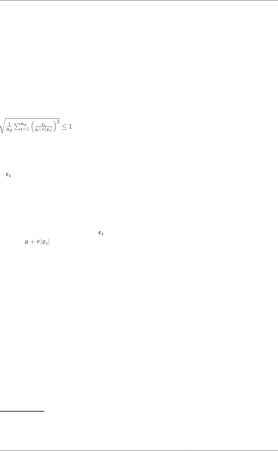
Controlling the Execution
of Model-based Activities
202
• DASOLV is based on variable time step/variable order Backward Differentiation Formulae (BDF). This has
been proved to be efficient for a wide range of problems. However, BDF solvers suffer from loss of stability
for certain types of problems (e.g. highly oscillatory ones) and they are not very efficient for problems with
frequent discontinuities.
• SRADAU implements a variable time step, fully-implicit Runge-Kutta method. It has been proved to be efficient
for the solution of problems arising from the discretisation of PDAEs with strongly advective terms (in general,
highly oscillatory ODEs), and models with frequent discontinuities.
Both of the above solvers are designed to deal with large, sparse systems of equations in which the variable values
are restricted to lie within specified lower and upper bounds. Moreover, they can handle situations in which some
of the partial derivatives of the equations with respect to the variables are available analytically while the rest
have to approximated9. Efficient finite difference approximations are used for the latter purpose. Both solvers
automatically adjust each time step taken so that the following criterion is satisfied:
where:
•nd is the number of differential variables in the problem (i.e. those that appear as $x in the gPROMS model);
• is the solver's estimate for the local error in the ith differential variable;
•xi is the current value the ith differential variable;
•a is an absolute error tolerance;
•r is a relative error tolerance.
In rough terms, this means that the error incurred in a particular variable xi over a single time step is not allowed
to exceed . The default values for a and r (10-5 in both cases) are usually adequate since:
• they control the error in variables xi of size 0.01 or higher to within acceptable ranges;
• smaller variable values are often not important from an engineering point of view10.
However, for problems in which small variable values may have an important effect on system behaviour, it is
advisable to specify a smaller absolute tolerance11.
At the end of each simulation, if an estimate of the error committed in any variable at any time step exceeds a
threshold, this is reported. See the Large residual warnings section for details.
The DASolver solution parameter may be used to change and/or configure the solver used for simulation activities,
as well as the default DAE sub-solver used by all higher-level solvers. If this parameter is not specified, then the
DASOLV solver is used, with the default configuration shown at the start of the section below.
The DASOLV solver
The algorithmic parameters used by DASOLV along with their default values are shown below. This is followed
by a detailed description of each parameter.
"DASOLV" ["InitialisationNLSolver" := "BDNLSOL";
9In gPROMS models, almost all partial derivatives are computed analytically from expressions derived using symbolic manipulations. The
main exception is partial derivatives of equations involving any Foreign Object methods that are not capable of returning partial derivatives.
10For example, a liquid level in a processing vessel of 10-4m is practically indistinguishable from one of 10-5m.
11For example, in a problem involving free radicals or ions, it may be important to distinguish between mole fraction of 10-6 and 10-7.

Controlling the Execution
of Model-based Activities
203
"LASolver" := "MA48";
"ReinitialisationNLSolver" := "BDNLSOL"
"Absolute1stTimeDerivativeThreshold" := 0.0;
"AbsolutePerturbationFactor" := 1.0E-7;
"AbsoluteTolerance" := 1E-5;
"Diag" := FALSE;
"EffectiveZero" := 1E-5;
"EventTolerance" := 1E-5;
"FDPerturbation" := 1E-6;
"FiniteDifferences" := FALSE;
"HigherOrderBiasFactor" := 1;
"MaxCorrectorIterations" := 5;
"MaxSuccessiveCorrectorFailures" := 12;
"MinimumRatioForOrderDecrease" := 1000;
"OutputLevel" := 0;
"Relative1stTimeDerivativeThreshold" := 0.0;
"Relative2ndTimeDerivativeThreshold" := 0.0;
"RelativePerturbationFactor" := 1E-4;
"RelativeTolerance" := 1E-5;
"SenErr" := FALSE;
"VariablesWithLargestCorrectorSteps" := 0]
However, BDNLSOL is used as the default InitialisationNLSolver and ReinitialisationNLSolver when DASOLV
is used for simulation activities.
• InitialisationNLSolver: A quoted string specifying a nonlinear algebraic equation solver.
The solver to be used for the solution of nonlinear algebraic equations occurring at the initialisation stage of the
integration. This can be either one of the standard gPROMS nonlinear algebraic equation solvers or a third-party
nonlinear algebraic equation solver (see the gPROMS System Programmer Guide). The default is BDNLSOL.
This parameter can be followed by further specifications aimed at configuring the particular solver by setting
values to its own algorithmic parameters.
• LASolver: A quoted string specifying a linear algebraic equation solver.
The solver to be used for the solution of linear algebraic equations at each step of the integration. This can be
either one of the standard gPROMS linear algebraic equation solvers or a third-party linear algebraic equation
solver (see the gPROMS System Programmer Guide). The default is MA48. This parameter can be followed
by further specifications aimed at configuring the particular solver by setting values to its own algorithmic
parameters.
• ReinitialisationNLSolver: A quoted string specifying a nonlinear algebraic equation solver.
The solver to be used for the solution of nonlinear algebraic equations that is necessary for re-initialisation
following discontinuities. This can be either one of the standard gPROMS nonlinear algebraic equation solvers
or a third-party nonlinear algebraic equation solver (see the gPROMS System Programmer Guide). The default
is BDNLSOL. This parameter can be followed by further specifications aimed at configuring the particular
solver by setting values to its own algorithmic parameters.
• Absolute1stTimeDerivativeThreshold: A real number in the range [0, 1010].
Unless this parameter has the value zero, it represents the value in the condition used to determine reporting
of potential 'runaway' derivatives.
If it is zero (the default), no runaway derivatives will be reported.
• AbsolutePerturbationFactor: A real number in the range [10-20, 1010]; default = 10-7.
Absolute perturbation factor for varied trajectories and second-order sensitivities.
Controlling the Execution
of Model-based Activities
204
• AbsoluteTolerance: A real number in the range [10-20, 1010].
The absolute integration tolerance. Together with the parameter RelativeTolerance (see below), they determine
whether or not a time step taken by the solver is sufficiently accurate.
• Diag: A boolean value.
Specifies whether very detailed diagnostic information is to be generated during integration.
• EffectiveZero: A real number in the range [10-20, 1010].
The magnitude of a variable below which absolute rather than relative finite difference perturbation is used --
see parameter FDPerturbation below.
• EventTolerance: A real number in the range [10-20, 1010].
The event tolerance, i.e. the maximum time interval within which discontinuities during integration are located.
• FDPerturbation: A real number in the range [10-20, 1010].
Finite difference perturbation factor. If finite difference calculation of partial derivatives with respect to a
variable X is required, X is perturbed by:
unless is less than EffectiveZero, in which case it is perturbed by FDPerturbation.
• FiniteDifferences: A boolean value; default = FALSE.
Controls whether second-order sensitivities are calculated via finite differences (TRUE) or within the BDF code
(FALSE).
• HigherOrderBiasFactor: A real number in the range [0.001, 1000].
The factor B used in the tests which the integrator makes periodically to determine whether to change the
order of integration within DASOLV. Giving this factor a value greater than 1 will "bias" the integrator
towards using higher order steps. This has been found to result in quicker solution for many problems (see also
MinimumRatioForOrderDecrease).
This test is of the form
IF r_up*B > r_sm AND r_up*B > r_dn THEN
Raise integration order
END
Where:
•r_up is the ratio which DASOLV will apply to the step if it increases the order by 1,
•r_sm is the ratio which DASOLV will apply to the step if it keeps the order the same,
•r_dn is the ratio which DASOLV will apply to the step if it decreases the order by 1.
• MaxCorrectorIterations: An integer number in the range [1,50].
The maximum number of corrector iterations to allow on a single attempt to solve the system (i.e. before cutting
the step).
• MaxSuccessiveCorrectorFailures: An integer number in the range [1,100].

Controlling the Execution
of Model-based Activities
205
The maximum number of successive corrector failures to allow before declaring an integration failure.
• MinimumRatioForOrderDecrease: A real number in the range [0.0, 109].
The factor F used in the tests which the integrator makes periodically to determine whether to reduce the
order of integration within DASOLV. Giving this factor a value greater than zero will "bias" the integrator
against reducing the step. This has been found to result in quicker solution for many problems (see also
HigherOrderBiasFactor) - in particular, setting the value to 1.0 will ensure that the order is not reduced unless
the step itself is being reduced, which often proves beneficial.
This test is of the form
IF r_dn > r_sm AND r_dn > r_up AND r_sm > F THEN
Reduce integration order
END
Where:
•r_up is the ratio which DASOLV will apply to the step if it increases the order by 1,
•r_sm is the ratio which DASOLV will apply to the step if it keeps the order the same,
•r_dn is the ratio which DASOLV will apply to the step if it decreases the order by 1.
• OutputLevel: An integer in the range [-1, 7].
The amount of information generated by the solver. The following table indicates the lowest level at which
different types of information are produced:
0 (None)
1 (Re-)initialisation times, projection of predictor onto
bounds, variables hitting bounds
2 Successful initialisation, change of branch in IF
conditional equations, location of discontinuities,
step failures, repeated convergence failures, predictor
outside bounds, predictor step reduction, variables
stuck on bounds
3 Detail of convergence failures, values of derivatives
on commencing integration, number of perturbation
groups, step length reduction due to bounds violation
4 Variable causing discontinuity, detail of perturbation
groups
5 Entry to main integrator routines, all error test values,
nonfatal singularities during integration, greatest
changes in variables at each corrector iteration
6 Convergence values at every corrector iteration, step
change factors
7 Time, step, variables, derivatives and residuals at every
corrector iteration
When OutputLevel is 3 or more, gPROMS reports the norms for differential and algebraic Variables, as shown
in the example below.
Norm values
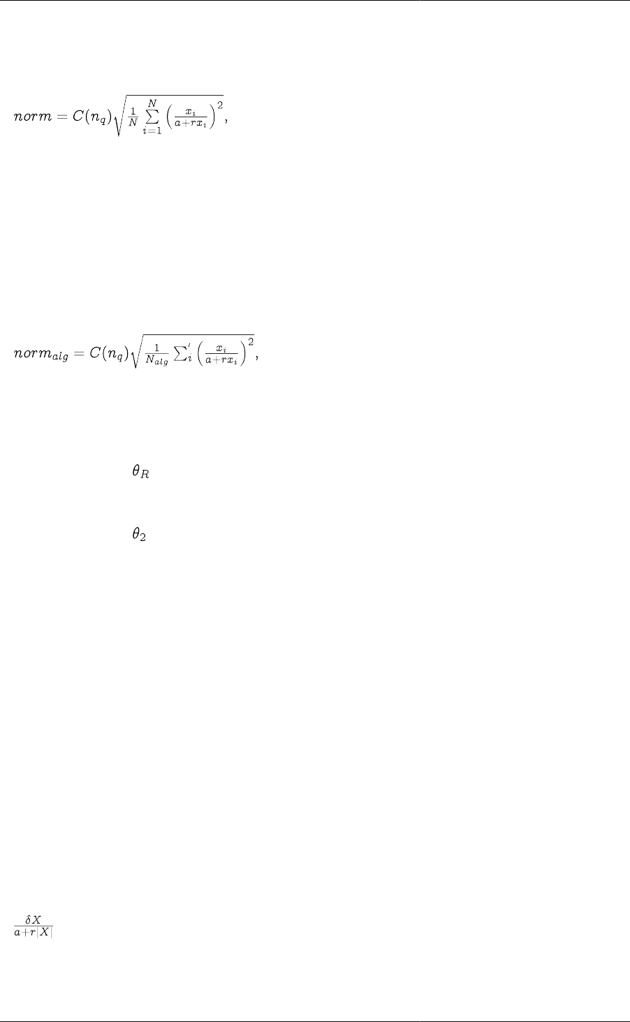
Controlling the Execution
of Model-based Activities
206
... differential and algebraic variables: 2.19219E-005
... algebraic variables only: 2.19607E-005
These norms are calculated using the following equations.
where:
•C(nq) are constants depending on the on the order of the step
•N is the number of equations
•xi are the current values of the variables
•a and r are the absolute and relative tolerances
For algebraic Variables only, the norm is calculated by:
where Nalg is the number of algebraic variables and the summation is performed over only the Nalg algebraic
variables.
• Relative1stTimeDerivativeThreshold: A real number in the range [0, 1010].
Represents the value in the condition used to determine reporting of potential ``runaway'' derivatives.
• Relative2ndTimeDerivativeThreshold: A real number in the range [0, 1010].
Represents the value in the conditions used to determine reporting of potential ``runaway'' derivatives.
• RelativePerturbationFactor: A real number in the range [10-20, 1010]; default = 10-4.
Relative perturbation factor for varied trajectories and second-order sensitivities.
• RelativeTolerance: A real number in the range [10-20, 1010]; default = 10-5.
The relative integration tolerance. Together with the parameter AbsoluteTolerance (see above), they determine
whether or not a time step taken by the solver is sufficiently accurate.
• SenErr: A boolean value.
For optimisation type activities: specifies whether the sensitivity error test is to be applied at each step of the
integration.
• VariablesWithLargestCorrectorSteps: An integer between 0 and 1000; default = 0.
On rare occasions, DASOLV fails with a "corrector step failure" message. This indicates that the code is unable
to establish a set of variable values that satisfy the system equations at a particular point. It is often caused by
errors or bad scaling in some modelling equations which results in the corrector iterations taking excessively
large steps in some of the variables. To help with the diagnosis of such problems, DASOLV can report the
variables with the largest relative change at each corrector iteration. The relative change for a variable X is
defined as:
where:
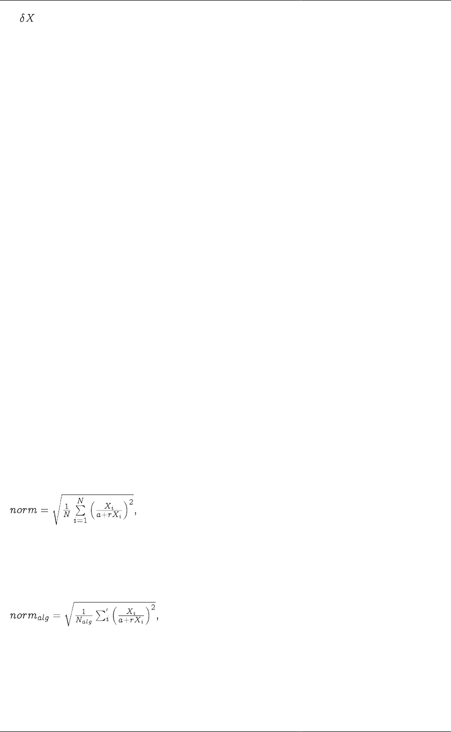
Controlling the Execution
of Model-based Activities
207
• is the step in the variable at this corrector iteration;
•a is the absolute tolerance;
•r is the relative tolerance.
The parameter VariablesWithLargestCorrectorSteps specifies the number of variables to be reported in this
manner. Note that such reporting takes place only if the parameter OutputLevel is set to a value of 0 or higher.
An example of the output is shown below:
Variables with largest (weighted) corrector steps follow...
Differential and algebraic variables (norm = 227.542):
----------------------------------------------------------------------------------------------------------------------------------
| Variable | Name | Current Value | Corrector Step | Weighted Corrector Step | Contribution to Norm |
----------------------------------------------------------------------------------------------------------------------------------
| 1 | Plant.Reactor.STR.rho_L | 12126 | 548.071 | 4519.44 | 50.00% |
| 2 | Plant.Reactor.STR.c(5) | 12126 | 548.071 | 4519.44 | 50.00% |
| 3 | Plant.Reactor.STR.vol_L | 0.000824675 | -3.72737E-05 | -3.7243 | 0.00% |
| 4 | Plant.Reactor.STR.q_Loss | 0.00692394 | -6.05969E-06 | -0.601802 | 0.00% |
| 5 | Plant.Reactor.STR.ThermoHL.hli(2) | -5.12137E-10 | -1.41695E-06 | -0.141695 | 0.00% |
----------------------------------------------------------------------------------------------------------------------------------
Algebraic variables only (norm = 250.308):
----------------------------------------------------------------------------------------------------------------------------------
| Variable | Name | Current Value | Corrector Step | Weighted Corrector Step | Contribution to Norm |
----------------------------------------------------------------------------------------------------------------------------------
| 1 | Plant.Reactor.STR.rho_L | 12126 | 548.071 | 4519.44 | 50.00% |
| 2 | Plant.Reactor.STR.c(5) | 12126 | 548.071 | 4519.44 | 50.00% |
| 3 | Plant.Reactor.STR.vol_L | 0.000824675 | -3.72737E-05 | -3.7243 | 0.00% |
| 4 | Plant.Reactor.STR.q_Loss | 0.00692394 | -6.05969E-06 | -0.601802 | 0.00% |
| 5 | Plant.Reactor.STR.ThermoHL.hli(2) | -5.12137E-10 | -1.41695E-06 | -0.141695 | 0.00% |
----------------------------------------------------------------------------------------------------------------------------------
The output is grouped in terms of differential and algebraic Variables and only algebraic Variables. In each
case, a norm value is also reported. For differential and algebraic variables, this is defined by:
where N is the number of equations. Subsequent lines list the largest
VariablesWithLargestCorrectorSteps Variables and their relative changes.
For algebraic Variables only, then norm is similarly defined:
where Nalg is the number of algebraic Variables and the summation is over only the algebraic Variables. Again,
a list of the algebraic variables with the largest corrector steps then follows.
If a subset of the system being solved by DASOLV becomes unstable, then DASOLV may fail, issuing a "repeated
error test failure" message. This indicates that the code is no longer able to control the error of integration. The
variables associated with such instabilities often exhibit excessively large values of their first and second time
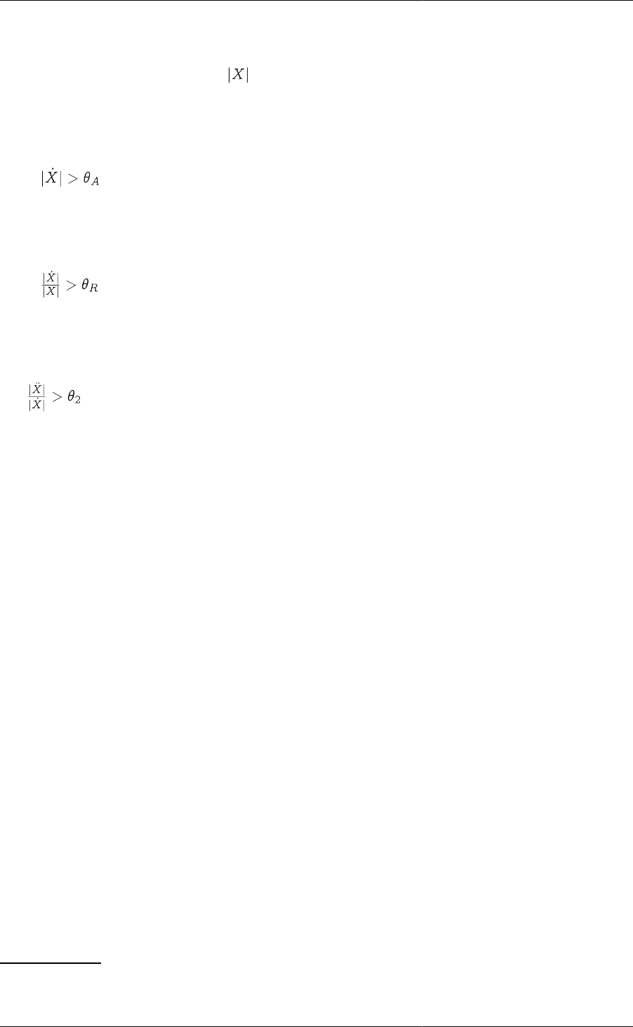
Controlling the Execution
of Model-based Activities
208
derivatives immediately preceding the instability. DASOLV exploits this fact to help in the diagnosis of such
problems. More specifically, DASOLV will report any variable X which satisfies all three of the following tests:
1. Minimum magnitude: The value of must be greater than 10-5
2. First derivative:
• EITHER
(specified with the AbsoluteDerivativeThreshold parameter)
• OR
(specified with the RelativeDerivativeThreshold parameter)
3. Second derivative:
(specified with the RelativeSecondDerivativeThreshold parameter)
Large residual warnings
At the end of every time step, DASOLV examines the equation which has the largest residual in magnitude, and
records an estimate of the error committed in each variable xi in this equation. To do this it uses the value of the
Jacobian element with respect to that variable (i.e. the partial derivative of the equation w.r.t. xi), to estimate the
change delta_i that would be needed in that variable in isolation to bring the residual to zero. The specific measure
used is |delta_i|/max(|x_i|, |x_i+delta_i|), i.e. the size of the change relative to either the actual value or the value
which would remove the residual, whichever is greater. This is referred to as the error measure for that variable.
The most important consideration for a given equation is then the smallest error measure. The reason for this is
that if the residual can be brought to zero by a very small change in any variable, a larger error measure for another
variable is relatively meaningless.
At the end of the integration, when the smallest error measure in the equation with the largest residual on any
single time step exceeds the threshold convtol*10, this single equation is reported12. All such residuals are reported
as follows:
• First the residual and time are indicated.
• The smallest error measure and the variable concerned are displayed in parentheses.
• The equation itself is then displayed.
• This is followed by a table containing a row for each variable in the equation, indicating its name, value at the
time, Jacobian element value at the time, the value of delta_i as described above, and the error measure in the
form of a percentage.
Note that if one or more singular Jacobians were observed during the solution, all equations where the smallest
error measure exceeds convtol/10 (i.e. 100 times more sensitive than the normal case) are reported, since this
situation has been found to lead to problems with variable values.
12Note that the tolerance used in the test, convtol, is taken from DASOLV's ReinitialisationNLSolver. This is done in order to relate the error
acceptable at an integration step to the error that might be committed when reinitialising the system at a discontinuity.

Controlling the Execution
of Model-based Activities
209
Also, if the DASOLV solution parameter Diag is set to true, the threshold used for this test is 10-8
In these cases where more than one residual is reported, the list is displayed in descending order of error measure,
so that the first entries are likely to be the most significant.
The SRADAU solver
The algorithmic parameters used by SRADAU along with their default values are shown below. This is followed
by a detailed description of each parameter.
"SRADAU" ["InitialisationNLSolver" := "BDNLSOL";
"LASolver" := "MA48";
"ReinitialisationNLSolver" := "BDNLSOL";
"AbsoluteTolerance" := 1E-5;
"Diag" := FALSE;
"MaxStepSize" := 1.0E10;
"EventTolerance" := 1E-5;
"OutputLevel" := 0;
"RelativeTolerance" := 1E-5;
"VariablesWithLargestCorrectorSteps" := 0]
• InitialisationNLSolver: A quoted string specifying a nonlinear algebraic equation solver.
The solver to be used for the solution of nonlinear algebraic equations occurring at the initialisation stage of the
integration. This can be either one of the standard gPROMS nonlinear algebraic equation solver or a third-party
nonlinear algebraic equation solver (see the gPROMS System Programmer Guide). The default is BDNLSOL.
This parameter can be followed by further specifications aimed at configuring the particular solver by setting
values to its own algorithmic parameters.
• LASolver: A quoted string specifying a linear algebraic equation solver.
The solver to be used for the solution of linear algebraic equations at each step of the integration. This can be
either one of the standard gPROMS linear algebraic equation solvers or a third-party linear algebraic equation
solver (see the gPROMS System Programmer Guide). The default is MA48. This parameter can be followed
by further specifications aimed at configuring the particular solver by setting values to its own algorithmic
parameters.
• ReinitialisationNLSolver: A quoted string specifying a nonlinear algebraic equation solver.
The solver to be used for the solution of nonlinear algebraic equations that is necessary for re-initialisation
following discontinuities. This can be either one of the standard gPROMS nonlinear algebraic equation solvers
or a third-party nonlinear algebraic equation solver (see the gPROMS System Programmer Guide). The default
is SPARSE. This parameter can be followed by further specifications aimed at configuring the particular solver
by setting values to its own algorithmic parameters.
• AbsoluteTolerance: A real number in the range [10-20, 1010].
The absolute integration tolerance. Together with the parameter RelativeTolerance (see below), they determine
whether or not a time step taken by the solver is sufficiently accurate.
• Diag: A boolean value.
Specifies whether very detailed diagnostic information is to be generated during integration.
• EventTolerance: A real number in the range [10-20, 1010].
The event tolerance, i.e. the maximum time interval within which discontinuities during integration are located.
• MaxStepSize: A real number in the range [10-20, 10100]; default = 1010.

Controlling the Execution
of Model-based Activities
210
This Solution Parameter sets the maximum step size used by the integrator when advancing in time.
• OutputLevel: An integer in the range [0, 4].
The amount of information generated by the solver. The following table indicates the lowest level at which
different types of information are produced:
0 (None)
1 (Re-)initialisation times, projection of predictor onto
bounds, variables hitting bounds
2 Successful initialisation, change of branch in IF
conditional equations, location of discontinuities,
step failures, repeated convergence failures, predictor
outside bounds, predictor step reduction, variables
stuck on bounds
3 Detail of convergence failures,values of derivatives
on commencing integration, number of perturbation
groups, step length reduction due to bounds violation
4 Variable causing discontinuity, detail of perturbation
groups
• RelativeTolerance: A real number in the range [10-20, 1010].
The relative integration tolerance. Together with the parameter AbsoluteTolerance (see above), they determine
whether or not a time step taken by the solver is sufficiently accurate.
• VariablesWithLargestCorrectorSteps: An integer between 0 and 1000; default = 0.
On rare occasions, SRADAU fails with a "corrector step failure" message. This indicates that the code is unable
to establish a set of variable values that satisfy the system equations at a particular point. It is often caused by
errors or bad scaling in some modelling equations which results in the corrector iterations taking excessively
large steps in some of the variables. To help with the diagnosis of such problems, SRADAU can report the
variables with the largest relative change at each corrector iteration. The relative change for a variable X is
defined as:
where:
• is the step in the variable at this corrector iteration;
•a is the absolute tolerance;
•r is the relative tolerance.
The parameter VariablesWithLargestCorrectorSteps specifies the number of variables to be reported in this
manner. Note that such reporting takes place only if the parameter OutputLevel is set to a value of 0 or higher.
An example of the output is shown below:
Variables with largest (weighted) corrector steps follow...
Differential and algebraic variables (norm = 227.542):
----------------------------------------------------------------------------------------------------------------------------------
| Variable | Name | Current Value | Corrector Step | Weighted Corrector Step | Contribution to Norm |
----------------------------------------------------------------------------------------------------------------------------------
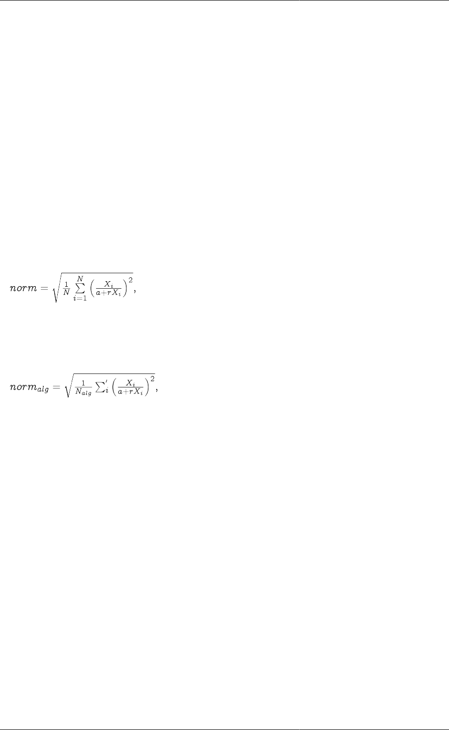
Controlling the Execution
of Model-based Activities
211
| 1 | Plant.Reactor.STR.rho_L | 12126 | 548.071 | 4519.44 | 50.00% |
| 2 | Plant.Reactor.STR.c(5) | 12126 | 548.071 | 4519.44 | 50.00% |
| 3 | Plant.Reactor.STR.vol_L | 0.000824675 | -3.72737E-05 | -3.7243 | 0.00% |
| 4 | Plant.Reactor.STR.q_Loss | 0.00692394 | -6.05969E-06 | -0.601802 | 0.00% |
| 5 | Plant.Reactor.STR.ThermoHL.hli(2) | -5.12137E-10 | -1.41695E-06 | -0.141695 | 0.00% |
----------------------------------------------------------------------------------------------------------------------------------
Algebraic variables only (norm = 250.308):
----------------------------------------------------------------------------------------------------------------------------------
| Variable | Name | Current Value | Corrector Step | Weighted Corrector Step | Contribution to Norm |
----------------------------------------------------------------------------------------------------------------------------------
| 1 | Plant.Reactor.STR.rho_L | 12126 | 548.071 | 4519.44 | 50.00% |
| 2 | Plant.Reactor.STR.c(5) | 12126 | 548.071 | 4519.44 | 50.00% |
| 3 | Plant.Reactor.STR.vol_L | 0.000824675 | -3.72737E-05 | -3.7243 | 0.00% |
| 4 | Plant.Reactor.STR.q_Loss | 0.00692394 | -6.05969E-06 | -0.601802 | 0.00% |
| 5 | Plant.Reactor.STR.ThermoHL.hli(2) | -5.12137E-10 | -1.41695E-06 | -0.141695 | 0.00% |
----------------------------------------------------------------------------------------------------------------------------------
The output is grouped in terms of differential and algebraic Variables and only algebraic Variables. In each
case, a norm value is also reported. For differential and algebraic variables, this is defined by:
where N is the number of equations. Subsequent lines list the largest
VariablesWithLargestCorrectorSteps Variables and their relative changes.
For algebraic Variables only, then norm is similarly defined:
where Nalg is the number of algebraic Variables and the summation is over only the algebraic Variables. Again,
a list of the algebraic variables with the largest corrector steps then follows.

212
Chapter 15. Model Analysis and
Diagnosis
At the start of each simulation, gPROMS analyses the mathematical model so as to assist the user in identifying
structural problems and errors in the modelling and/or the problem specification. In particular, gPROMS attempts
to determine:
• if the model is well-posed and whether alternative specifications are required for the degrees-of-freedom;
• if the underlying set of differential and algebraic equations is of index exceeding 1; and
• if the initial conditions are inconsistent.
These structural problems are considered in more detail in this section.
Well-posed models and degrees-of-freedom
In order for gPROMS to solve the underlying equation system associated with a given simulation, the model must
be well-posed and all degrees-of-freedom must be specified correctly. If there are too many or too few assignments
for the degrees-of-freedom then gPROMS will issue an error upon instantiation and state that the equations system
is over-specified or under-specified respectively. As a user you should then analyse the suggestions regarding
specifications and take the necessary action to ensure the equation system is correctly specified.
Case I: over-specified systems
An over-specified system is one which either itself consists of more equations than unknown variables, or involves
an over-specified sub-set of equations and unknowns. Mathematically, it can be shown that any over-specified
system will contain at least one sub-system involving k equations in only (k-1) distinct unknowns. gPROMS
identifies this sub-system and, where appropriate, offers informed suggestions on which Assignments may be
responsible for the over-specification. As a simple example of this, consider the gPROMS input shown in the
gPROMS code below:

Model Analysis and Diagnosis
213
Example 15.1. Illustrative example: over-specified system
#===============================================================
#MODEL mod1
VARIABLE
x1, x2, y1, y2 AS NoType
EQUATION
$x1 = x1*y1 ;
$x2 = x1 + x2*y1 + y2 ;
x1^2 = y2 ;
0 = y1 - y2 ;
#===============================================================
#PROCESS proc
UNIT
mymod AS mod1
ASSIGN
WITHIN mymod DO
y2 := 3 ;
END #within
INITIAL
WITHIN mymod DO
x1 = 0 ;
x2 = 0 ;
END #within
SOLUTIONPARAMETERS
ReportingInterval := 1 ;
SCHEDULE
CONTINUE FOR 10
It is easy to see that MODEL mod1 consists of 4 equations in 4 variables, one of which, y2, is Assigned in the
PROCESS proc. Execution of the PROCESS proc leads to the following diagnostic message:
Executing process PROC...
All 4 variables will be monitored during this simulation!
Building mathematical problem description took 0.014 seconds.
Loaded MA48 library
Execution begins....
Variables
Known : 1
Unknown : 3
Differential : 2
Algebraic : 1

Model Analysis and Diagnosis
214
Model equations : 4
Initial conditions : 2
Checking consistency of model equations and ASSIGN specifications...
ERROR: Part of your problem is over-specified.
The following 3 equation(s) involve only 2 unknown variable(s).
Model Equation 1: MYMOD.$X1 = MYMOD.X1 * MYMOD.Y1 ;
Model Equation 3: MYMOD.X1^2 = MYMOD.Y2 ;
Model Equation 4: 0 = MYMOD.Y1 - MYMOD.Y2 ;
The 2 unknown(s) occuring in these 3 equations are:
MYMOD.Y1 (ALGEBRAIC)
MYMOD.X1 (STATE)
The problem may have been caused because you ASSIGNed the
following variable(s):
MYMOD.Y2 (INPUT)
Initialisation calculation failed.
Execution of PROC fails prematurely.
gPROMS identifies the over-specified sub-system of 3 equations in 2 unknown variables and suggests that the
Assignment of the variable y2 is causing the problem. UnAssigning this variable leads to a working simulation.
Case II: under-specified systems
An under-specified system has more unknown variables than equations. In this case, gPROMS diagnoses the
problem and provides a list of candidate variables for Assignment (while advising against Assigning differential
variables). This is illustrated by the gPROMS code below:

Model Analysis and Diagnosis
215
Example 15.2. Illustrative example: under-specified system
#===============================================================
#MODEL mod1
VARIABLE
x1, x2, y1, y2, y3 AS NoType
EQUATION
$x1 = x1*y1 ;
$x2 = x1 + x2*y1 + y2 + 3*y3 ;
x1^2 = y2 ;
0 = y1 - y2 ;
#===============================================================
#PROCESS proc
UNIT
mymod AS mod1
INITIAL
WITHIN mymod DO
x1 = 0 ;
x2 = 0 ;
END #within
SOLUTIONPARAMETERS
OutputLevel := 2 ;
gRMS := OFF ;
ReportingInterval := 1 ;
SCHEDULE
CONTINUE FOR 10
gPROMS issues the following message upon execution of the PROCESS proc:
Executing process PROC...
All 5 variables will be monitored during this simulation!
Building mathematical problem description took 0.001 seconds.
Loaded MA48 library
Execution begins....
Variables
Known : 0
Unknown : 5
Differential : 2
Algebraic : 3
Model equations : 4
Initial conditions : 2

Model Analysis and Diagnosis
216
Checking consistency of model equations and ASSIGN specifications...
ERROR: Your problem is underspecified.
You need to ASSIGN 1 of the following unknown variables:
MYMOD.X2 *** Not recommended ***
MYMOD.Y3
Initialisation calculation failed.
Execution of PROC fails prematurely.
Assigning the algebraic variable y3 leads to a well-posed system.
High-index DAE systems
Consistent initialisation of DAE systems is often related to their index. The index of a DAE system is defined as the
minimum number of differentiations with respect to time that are necessary in order to obtain the time derivatives
of all variables, i.e. to reduce the system to a set of ordinary differential equations (ODEs). Index-1 systems are
generally very similar to ODEs in that the number of initial conditions that can be specified arbitrarily is equal to
the number of differential variables in the system, all the differential variables may be given arbitrary initial values,
and similar numerical methods can be used for the solution of the system. On the other hand, in "high-index"
DAEs (index > 1), the number of initial conditions that can be specified arbitrarily may be less than the number
of differential variables, the differential variables are not independent and ODE-type numerical methods may fail.
This section comprises:
• an overview of the cause of indices higher than 1 and their potential complications;
• the diagnostics, structural analysis and model manipulation performed by gPROMS to identify, report and
rectify problems with high index; and
• a more detailed explanation of high index, with examples.
Origin of index and the initialisation of DAEs
Most DAE systems follow the rule that the number of initial conditions specified must be equal to the number of
differential variables in the system. This is true for ODEs as well. Although the initial conditions do not need to be
specified directly in terms of the differential variables (e.g. the internal energy may be a differential variable in an
energy balance but the initial condition may be a temperature specification), they must be specified consistently
(more details on specifying initial conditions can be found in the Initial section and how to ensure they are specified
consistently).
However, for certain "high index" DAE systems, this is not the case. For example, if one or more algebraic
equations only include differential variables, this will reduce the number of degrees of freedom in the initial
conditions, since all of the initial values of the differential variables cannot be specified independently. Not only
does this make initialisation difficult, but it also causes problems for the DAE solver.
These high-index DAE systems can arrise in a number of process-engineering applications. Some typical examples
are:
• Constant-volume mixer
• Heater
• Chemical equilibrium
A more thorough description of these is given here.

Model Analysis and Diagnosis
217
To date, the only way around these problems has been to identify the algebraic equations that cause the
complications, differentiate them with respect to time to generate additional constraints on the initial conditions
and then specify a reduced number of initial conditions consistent with these constraints. The DAE system is
augmented with these additional differential equations and solved.
gPROMS performs the following analysis automatically:
• determine the index of the set of equations
• identify the causes (if any) of high index
• identify remedial modifications to the equations
• identify constraints on the initial conditions
These automatic index-reduction procedures are described next.
For the interested reader, more details on the causes of high index, its implications on the solution of the DAE
system and how it can be avoided or rectified are given here. However, it is not essential to read this section.
Constant-volume mixer example
This is an example where a simplification to an index-1 system results in a high-index system. The following is
the EQUATION section of a gPROMS Model of a constant-volume mixing tank.
EQUATION
FOR i := 1 TO NoComp DO
$M(i) = SIGMA( F_in*x_in(i,) ) - F_out*x(i) ;
END
M_total = SIGMA(M) ;
rho*V = M_total ;
rho = PhysProp.Density(T, P, x) ;
x = M/M_total ;
F_out = alpha*(P - P_out) ;
where M(i) is the molar holdup of component i; M_total the total molar holdup; F_in(j) is the
flowrate of inlet j; F_out the outlet flowrate; x(i) and x_in(i,j) are the mole fractions in the mixer
and inlet j, respectively; rho is the density of fluid in the tank; V the volume of the tank (specified);
PhysProp.Density(T, P, x) is a physical-property foreign-object method returning the density of a
mixture given its temperature, T, pressure, P, and mole fractions x; P_out is the exit pressure (specified); and
finally alpha is a constant.
The above model is a fairly straightforward index-1 system that can easily be solved. If, however, we
were to simplify the model by considering only liquid feeds and using a different physical property:
LiquidDensity(T,x), we would find that the model could no longer be solved using standard codes.
Heater example
This example illustrates how a very simple model can still become high index, given the wrong input specification.
This is a model of a well-stirred tank used to heat a single-component stream.
EQUATION
rho*V*$u = F*(h_in - h) + Q ;
u = PhysProp.InternalEnergy(T) ;
h = PhysProp.Enthalpy(T) ;
here, F is the flowrate of material through the heater; rho is the density of the fluid; V the volume of the tank; u
and h are the internal energy and enthalpy, respectively, of the material in the tank; h_in is the inlet enthalpy;
PhysProp.InternalEnergy(T) and PhysProp.Enthalpy(T) are physical-property foreign-object

Model Analysis and Diagnosis
218
methods returning the internal energy and enthalpy of a single component given its temperature, T; and finally Q
is rate of heating. rho, V, F and h_in are all given.
To complete the model, the variable Q must be specified. If the heating was being provided by a steam jacket, then
Q can be determined using a suitable heat-transfer law. Alternatively, electric heating can be modelled simply by
specifying the value of Q over time, e.g. Q = Q(t). In either of these cases, the model can be solved easily. Since
there is one differential variable, u, we can provide an initial condition for it, u(0). We can now calculate T(0)
from the second equation and h(0) from the third. Now the first equation can be used, along with the initial value
of Q, to calculate u(0), completing the initialisation problem.
However, what if we wanted to know what heating profile would provide a given temperature profile? We may,
then, choose to release the specification on Q and provide one for T. Given the same initial specification, u(0),
we can still calculate T(0) from the second equation and h(0) from the third. Immediately, we can see that there
is a problem, because our calculated T(0) may not be the same as the T(0) specified. Another problem is that
there is only one equation left, in the two unknowns, $u(0) and Q. There is no way to solve the problem!
Chemical-equilibrium example
In this example, we have a batch-reactor model with reversible reactions at equilibrium. The general material
balance for this problem is:
FOR i := 1 TO NoComp DO
$M(i) = V*SIGMA( r*nu(i,) ) ;
END
where, M(i) is the molar holdup of component i, V is the volume of the reaction mixture, r(j) is the rate of
reaction j and nu(i,j) is the stoichiometric coefficient of component i in reaction j.
There is no difficulty in solving this problem (with appropriate definitions of the new variables introduced) if the
rates of reaction are specified using an equation similar to the following:
FOR j := 1 TO NoReac DO
r(j) = k(j)*PRODUCT( C^ReactionPartialOrder(,j) ) ;
END
where k(j) is the rate constant for reaction j, C(i) is the molar concentration of component j and
ReactionPartialOrder(i,j) is the partial order of component i in reaction j.
This model can be used for irreversible and reversible reactions where the rate expressions are known. E.g., for
reversible reactions, simply treat the forward and reverse reactions as entirely separate reactions, with their own
rate constants.
However, it is often not possible (nor useful) to measure the rates of fast reversible reactions; usually only an
equilibrium constant is known, and so we may have instead of a rate expression a relationship similar to the
following:
EqmConst(1) = C(2)/C(1)^2 ;
where the equilibrium constant, EqmConst, is given. It is clear now that we have a problem, because some of the
r(j) variables only appear in the differential equation for the material balance. There is no way to calculate the
r(j) associated with the reactions at equilibrium and so the problem cannot be solved. This is a typical cause of
high index: algebraic variables only occuring in differential equations.
Also of note is that the equation above introduces a relationship between the concentrations of some of the species
in the problem, and therefore also the molar holdups. So it is clear that we cannot specify arbitrary initial conditions
for all of the components, as they are not all independent.
Automatic index reduction in gPROMS
gPROMS is able to reduce the index of problems automatically. However, it initially reports problems of high
index and informs the user how to turn on index reduction. Index reduction is off by default because it is usually

Model Analysis and Diagnosis
219
better to develop index-1 models rather than rely on gPROMS to reduce the index automatically, since the index
reduction techniques can be quite computationally intensive.
To illustrate automatic index reduction, consider the following model of a heater.
EQUATION
$HoldUp = Fin - Fout ;
$U = Fin*hin - Fout*h + Q ;
U = Holdup*h - P*TotalVolume ;
P * TotalVolume = Holdup * R * T ;
Fout = alpha * Holdup ;
h = hr + Cp*(T - Tr) ;
hin = hr + Cp*(Tin - Tr) ;
When the following process is executed, gPROMS can solve the problem with no difficulty.
UNIT
T101 AS Heater
SET
WITHIN T101 DO
Cp := 1.121 * 28.013 ;
hr := 0.0 ;
Tr := 298.15 ;
R := 0.082 ;
alpha := 1 ;
END
ASSIGN
WITHIN T101 DO
Fin := 10 ;
Tin := 600 ;
P := 5 ;
Q := 10 ;
END
INITIAL
WITHIN T101 DO
HoldUp = 0.5 ;
TotalVolume = 4 ;
END
However, if we replace the Assignment of Q with one on T:
ASSIGN
WITHIN T101 DO
Fin := 10 ;
Tin := 600 ;
P := 5 ;
T := 487.8049 ;
END
INITIAL
WITHIN T101 DO
HoldUp = 0.5 ;
TotalVolume = 4 ;
END
we will get a high-index problem (see the Heater Example) and gPROMS will give the following output.
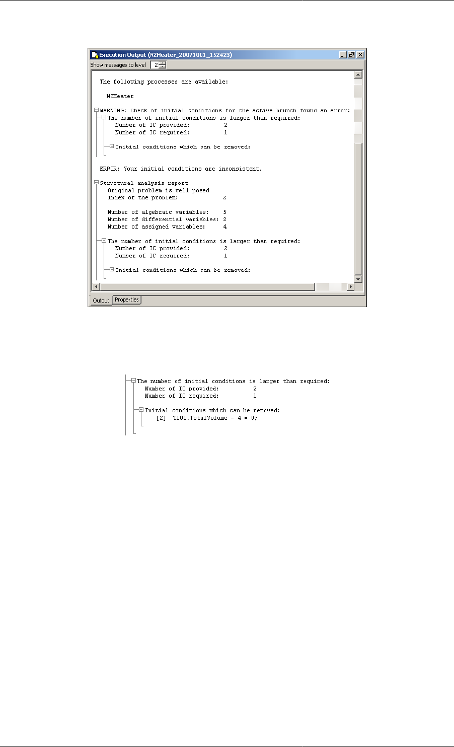
Model Analysis and Diagnosis
220
Figure 15.1. gPROMS diagnostics for a high-index problem
Click on the "+" symbol to see which initial condition should be removed:
Figure 15.2. The initial condition that needs to be removed
Now, by removing this initial condition, gPROMS reports that the correct number of conditions are specified but
that the index of the system is 2 and cannot be solved directly.

Model Analysis and Diagnosis
221
Figure 15.3. gPROMS diagnostics for a high-index problem
To enable the automatic index reduction, copy the suggested Solution Parameter into the Process as below.
ASSIGN
WITHIN T101 DO
Fin := 10 ;
Tin := 600 ;
P := 5 ;
T := 487.8049 ;
END
INITIAL
WITHIN T101 DO
HoldUp = 0.5 ;
END
SOLUTIONPARAMETERS
IndexReduction := ON ;
Now, with index reduction enabled, gPROMS is able to reduce the problem to index 1 and solve it. The
replacements made during the reduction are shown in the output:
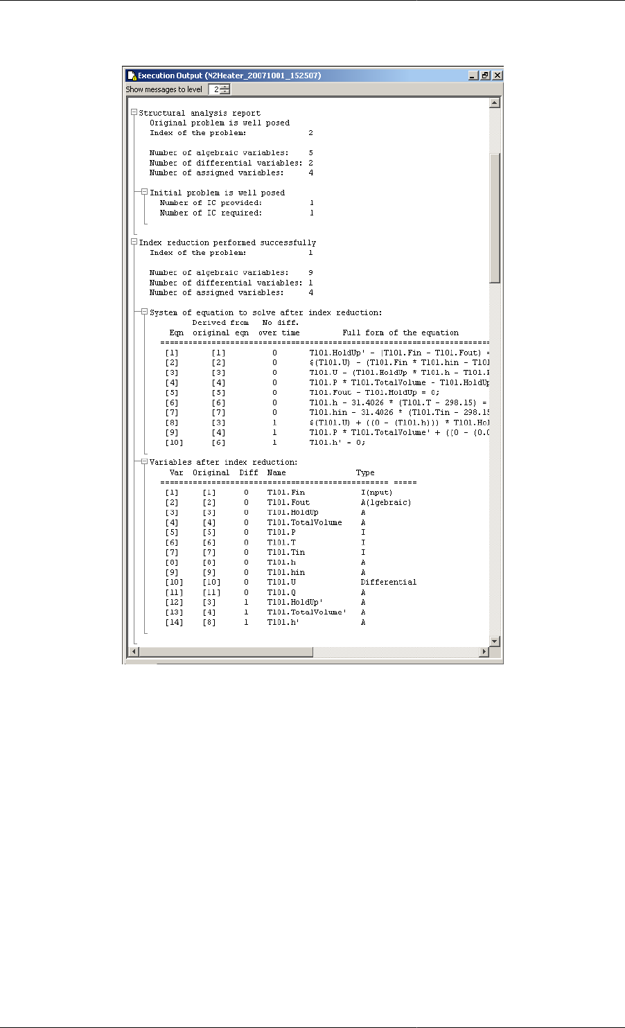
Model Analysis and Diagnosis
222
Figure 15.4. gPROMS output after automatic index reduction
After giving the above output, gPROMS continues to integrate the model as normal, since the index has now been
reduced to 1.
The above example can be found in the gPROMS Project highindex_N2_heater.gPJ in the examples
subdirectory. Please note that in the Project two Processes are present: one which specifies the temperature T as in
the explanation above. In the other Process, Specify_Q, the heat load is specified rather than the temperature.
This specification has been chose to demonstrate that the index does not only depend on the equations but also on
the chosen degrees of freedom. A more detailed explanation is given in the mathematical analysis of the heater
model.
Limitations
Currently, the following limitations exist for Models and Processes to which automatic index reduction can be
applied
• When the Index-Reduction code detects that an equation inside an IF or CASE block needs to be differentiated
to reduce the index, gPROMS will issue an error message and stop executing the simulation shortly after system
construction. Supporting such models in index reduction may be added in future releases.
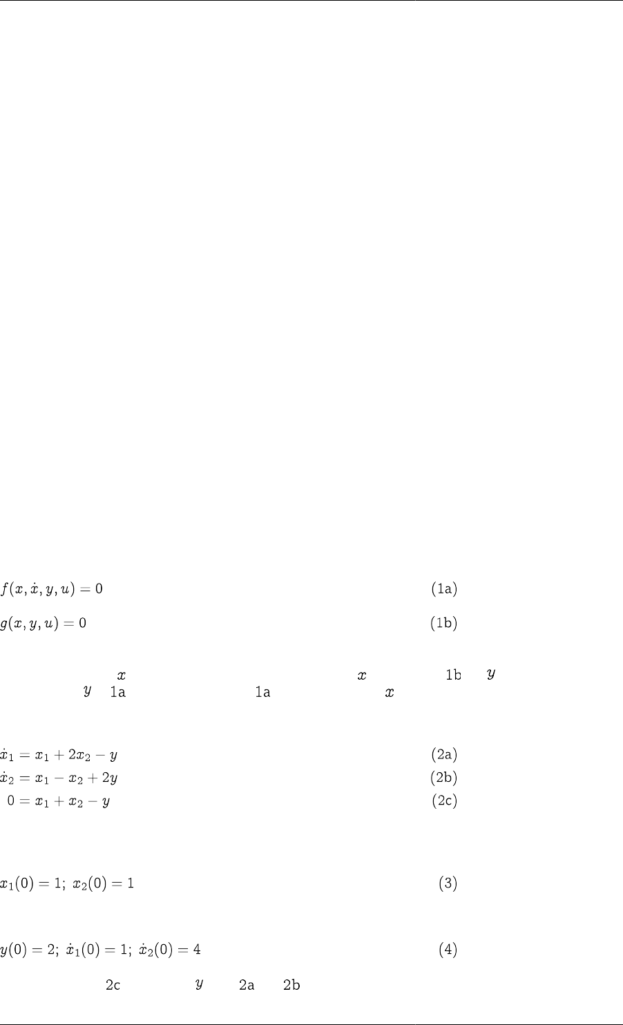
Model Analysis and Diagnosis
223
• The index may change during the execution of an activity when an IF or CASE branch switches. This is currently
not supported. When running a problem with IndexReduction := ON, this change (following any type
of switch) will be detected and will terminate the activity with an error message indicating the reason for the
termination.
Please note that it is possible to use solver settings for which the index analysis is ignored. In this case the
gPROMS solver may proceed with simulating a high-index problem without error messages but the results may
be incorrect.
High-index DAEs, initialisation and integration
This section is aimed at the interested reader who would like a more detailed mathematical analysis of the causes
of high index and how it may be avoided or remedied. None of the content here is required for an understanding of
how gPROMS reports and rectifies high-index problems, so it is safe to ignore this section. However, a thorough
understanding of index is likely to be benefitial for any modeller of chemical (or of many other) processes.
Furthermore, although gPROMS can reformulate most high-index problems automatically, this can be quite
computationally intensive, so it is preferrable to reduce any high-index models to index 1 by hand.
The following are considered:
• A simple example of an index-1 DAE system
• Simple examples of high-index DAE systems
• Index classification of DAE systems
• Integration of high-index DAE systems
• High-index DAEs in process-engineering applications
A simple example of an index-1 DAE system
It can be shown that most DAE systems of the form:
are similar to ODEs in several ways. In particular, one can specify as many arbitrary initial conditions as there are
differential variables in the system. Moreover, give values for , we can solve for (usually numerically),
then substitute in , essentially converting to a set of ODEs in .
These points can be illustrated with a simple example:
Here we have two differential variables and one algebraic variable. We can clearly specify two arbitrary initial
conditions, e.g.:
from which we can calculate:
In fact, we can use to eliminate from and , yielding:
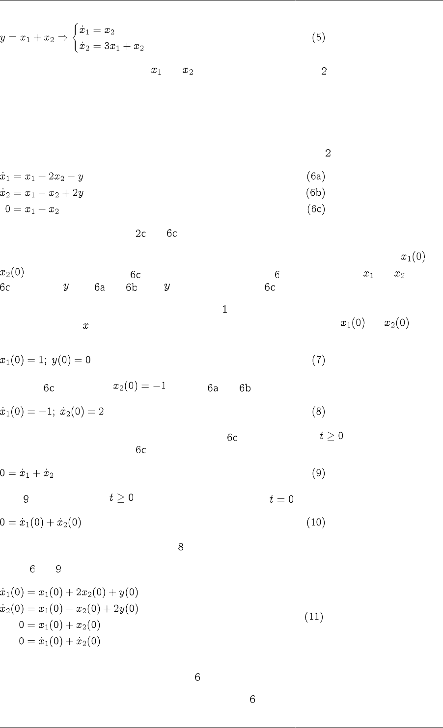
Model Analysis and Diagnosis
224
which is simply a set of two ODEs in and . Overall, then, the DAE system behaves very similarly to an
ODE one.
Simple examples of high-index DAE systems
In this section, two examples of high-index systems are described.
Consider, for this first example, a slightly modified version of the index-1 system ( ) described previously:
the only difference being between and .
We immediately note that we can no longer specify arbitrary initial values for the differential variables and
since they have to satisfy . Furthermore, we cannot convert to a set of ODEs in and by using
to eliminate from and since does not even occur in !
It can be shown that initial conditions for DAE systems ( ) do not necessarily have to be specified in terms of the
differential variables . This might seem to imply that, although we cannot specify both and , perhaps
we could specify some other combination of two variables, for instance:
Then from , we would get and from and :
This, however, is not correct. We note, in particular, that is valid at all times . We can therefore derive
a valid equation by differentiating with respect to time:
Now, is valid at all times , so, in particular, it should hold at :
which is not satisfied by our initial condition . Thus the latter is, in fact, inconsistent.
In fact, and form a set of 4 independent consistency relations that the initial variable values must satisfy:
Since these involve 5 variables, we can specify only 1 (=5-4) arbitrary initial condition, which is less than the
number of differential variables (2) in the system .
Now, for the second example, consider a slight modification of :
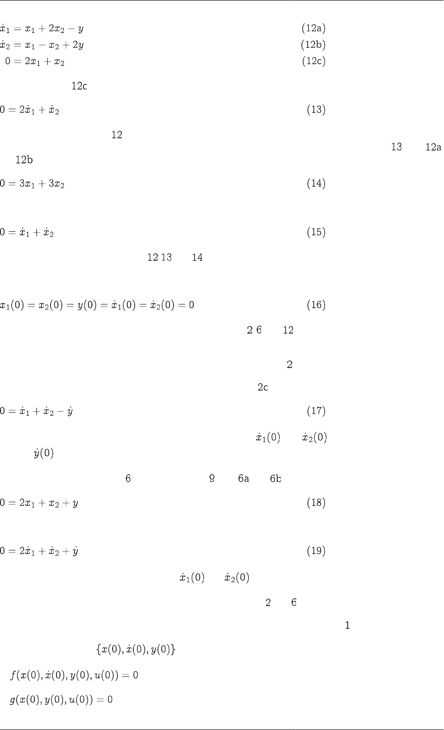
Model Analysis and Diagnosis
225
By differentiating with respect to time, we get:
which, together with system yields 4 consistency relations that the intial variable values must satisfy. So, once
again, it appears that we can specify 1 (= 5 - 4) arbitrary initial condition. However, if we combine with
and , we obtain:
which is also valid at all times. We can therefore differentiate this with respect to time to obtain:
We now have 5 consistency relations , and that the 5 initial variable values must satisfy — in fact, there
is no freedom left with respect to the specification of initial conditions. The only possible initial condition for
the system is:
Overall, what we have seen is that the three example systems , and , albeit ostensibly very similar, are, in
fact, quite different. Perhaps a natural question to ask at this point is:
Are there some further consistency relations also hidden within ?
Of course, we can easily obtain a valid relation by differentiating with respect to time:
However, this does not impose any further restrictions on both and since it also involves a new
variable .
Similarly, in the case of system , we could combine with and to yield:
and then differentiate this with respect to time to obtain:
but, once again, this does not actually restrict and .
Overall, our original conclusions regarding the initial conditions of and were correct.
We can summarise what we have seen so far with reference to the general DAE system , as follows:
•A set of initial values must always satisfy:
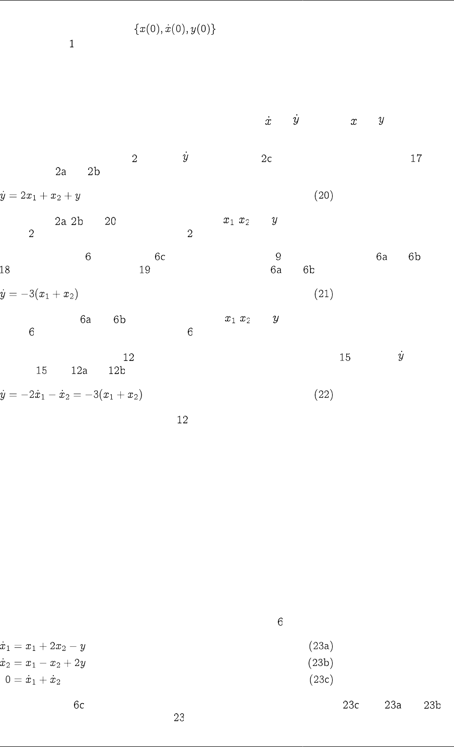
Model Analysis and Diagnosis
226
•For some systems, the values may also have to satisfy additional relations obtained by
differentiating one or more times with respect to time.
Index classification of DAE systems
The issue of consistent initialisation of DAE systems is closely related to their classification according to their
index. The index of 1 can be defined as the minimum number of differentiations with respect to time that are
necessary to obtain the time derivatieve of all variables (i.e. both and ) in terms of and — i.e. to reduce
the system to a set of ODEs.
We can apply this definition to : to obtain , we differentiate with respect to time; this yields which,
together with and , leads to:
We note that , and form a set of 3 ODEs in , and . Since one differentiation was sufficient to
reduce to an ODE system, we conclude that is an index-1 system.
In the case of system , differentiating with respect to time led to which, combined with and , yielded
. A second differentiation led to which, when combined with and yields:
This, together with and , form a set of ODEs in , and . Since two differentiations were needed to
reduce to an ODE system, we conclude that is an index-2 system.
Finally, in the case of system , two differentiations with respect to time yielded . To obtain , we need to
combine with and and differentiate the result with respect to time to get:
Since three differentiations were necessary, is an index-3 system.
By the definition of index, ODE systems are classified as "index-0". Usually, index-1 systems are very similar
to ODEs with respect to the number of initial conditions that can be specified arbitrarily and the behaviour of
numberical solution methods.
On the other hand, DAE systems of index 2 or higher are different. We have already seen the fact that their
consistent initialisation requires taking into account additional "hidden" relations that can be obtained from the
original equations via differentiation — and hence the number of arbitrary initial conditions is reduced accordingly.
Integration of high-index DAE systems
A further complication with DAE systems of high index is that the usual numerical algorithms are generally
incapable of controlling the error of integration, and this very often leads to failure, or, even worse, spurious
solutions!
For these reasons, DAE systems of index higher than 1 are usually solved by reducing their index to 1 via
differentiation with respect to time. For instance, the index-2 system can be reduced to the index-1 system:
by differentiating with respect to time. Note that it is not necessary to combine with and to
obtain a purely algebraic equation. System can then be solved using standard algorithms and codes.
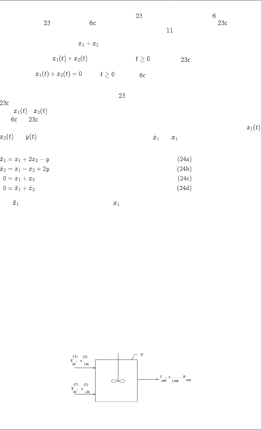
Model Analysis and Diagnosis
227
Of course, one immediate question is: "Will the solution of be the same as the solution of ? More specifically,
will the solution of satisfy equation , which has now been replaced by its time differential ?". The answer
is: "Yes, provided the initial conditions satisfy the consistency relations ."; in this case,
•the initial value of the quantity is zero
•the time gradient of is zero for all times (cf. equation )
and, therefore, for all — hence is satisfied — at least in the exact mathematical
sense.
A complication arises from the fact that, if system is solved numerically (rather than exactly), then equation
will be satisfied only within a certain specified accuracy and not exactly. Over long time horizons, this may
allow + to deviate significantly from its correct value of 0. A way of avoiding this "drift" is to include
both and in the set of equations being integrated, thereby making sure that both of them are satisfied to the
required accuracy. However, this leads to redundancy since now we have 4 equations in the 3 unknowns ,
and . One way of resolving this redundancy is to treat and as completely distinct variables —
effectively introducing an extra variable in the system:
Here is a new variable bearing no relation to as far as the numerical solution is concerned. This is now an
index-1 system that can be solved to arbitrary accuracy using standard codes.
High-index DAEs in process-engineering applications
This section is concerned with a detailed mathematical analysis of the following three examples of high-index
DAEs in process-engineering applications.
• Fixed Volume Mixing Tank
• Heater Tank
• Chemical Equilibrium
Some conclusions of the analysis are given here.
Fixed-volume mixing tank
We consider the well-stirred tank, shown in the figure below, used to mix two streams under isothermal conditions.
Figure 15.5. Constant-volume mixer tank
The mathematical model of the system is:
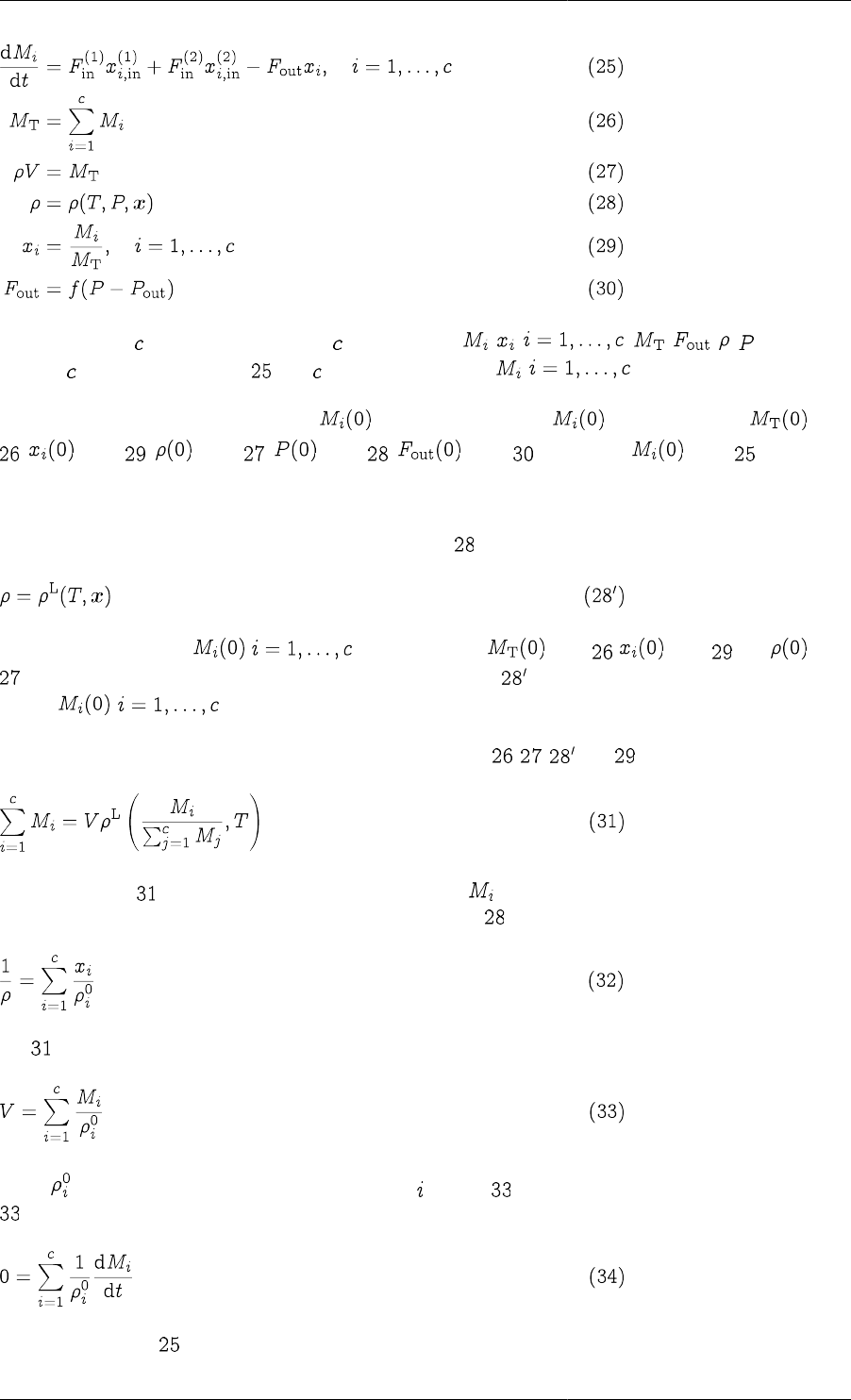
Model Analysis and Diagnosis
228
This is a set of (2 + 4) equations in the (2 + 4) variables , , ; , , , . The system
contains differential equations ( ) and differential variables, , .
We note that with this model, we can give arbitrary values: given , we can calculate from
; from ; from ; from ; from ; and finally from . Hence, this
is an index-1 system.
The above equations are valid for both gas and liquid systems. Of course, a reasonable simplifcation for liquids is
to assume that they are incompressible. Therefore, equation is simplified to:
Once again, if we specify , , we can calculate from , from and from
. At this point, however, we hit a problem: both sides of equation are already known! Effectively, we cannot
specify , independently. Therefore we have a high-index problem.
To see more clearly how the problem arises, consider combining , , and into a single equation:
It is obvious that only invovles the differential variables , and, therefore, not all of them can be given
arbitrary initial values. For instance, for an ideal liquid mixture, is of the form:
and becomes:
where is the (constant) density of pure component . Thus, is a total volume constraint. Differentiating
with respect to time, we obtain:
which, together with , lead to:
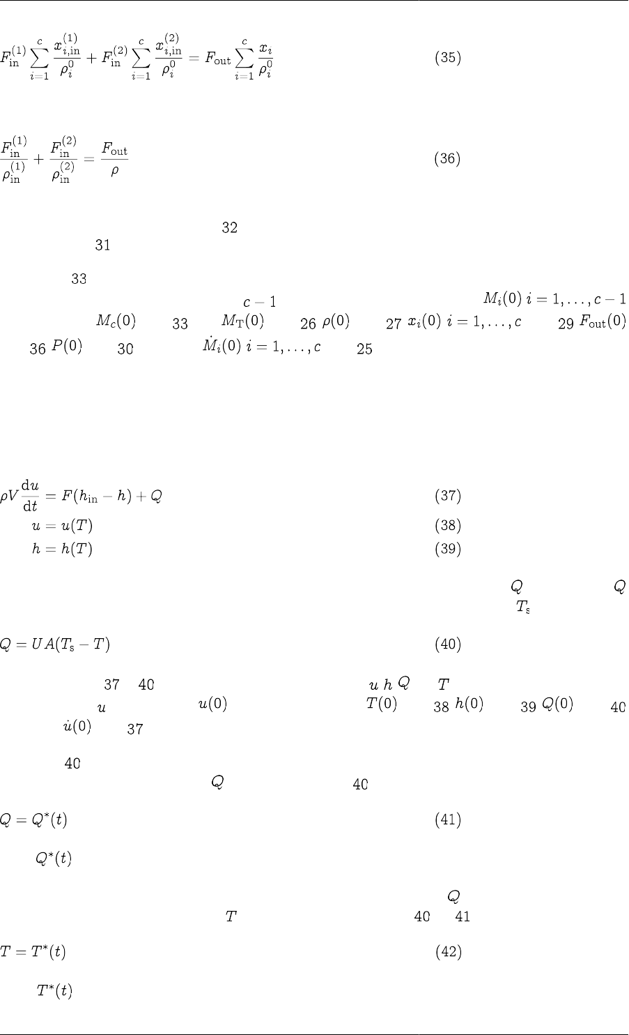
Model Analysis and Diagnosis
229
which is equivalent to:
i.e. a relationship between the volumetric flowrates of the input and output streams. Note that this is true for ideal
liquid mixtures only (i.e. those obeying ), but in any case a similar restriction could be obtained from the more
general equation with respect to time.
In any case, is an additional constraint that must be satisfied by the initial condition of the system. We can
therefore give arbitrary initial values to only variables. For instance, if we specify , ,
we can calculate from , then from , from , , from ,
from , from and finally , from .
No further equation differentiations are necessary, and therefore this is an index-2 system.
Heater tank
Consider a well-stirred tank used to heat up a single-component stream:
To define this system fully, we need an additional relation characterising the heating rate . For instance,
could be described by a heat-transfer mechanism from a steam jacket at a given temperature :
Overall, equations to form a DAE system in the 4 variables , , and . The system has one differential
variable, namely . If we specify , then we can calculate from , from , from
and finally from . This is clearly an index-1 DAE system.
Of course, corresponds to only one permissible heat-transfer mechanism. If, for instance, we were using
electrical heating, then we could vary directly, so instead of we could have:
where is a given function of time. Again, this does not change the nature (i.e. the index) of the DAE system.
On the other hand, we could well be interested in determining the variation of that would produce a certain
desired variation in the exit temperature . In this case, we would replace (or ) with:
where is a given function of time.
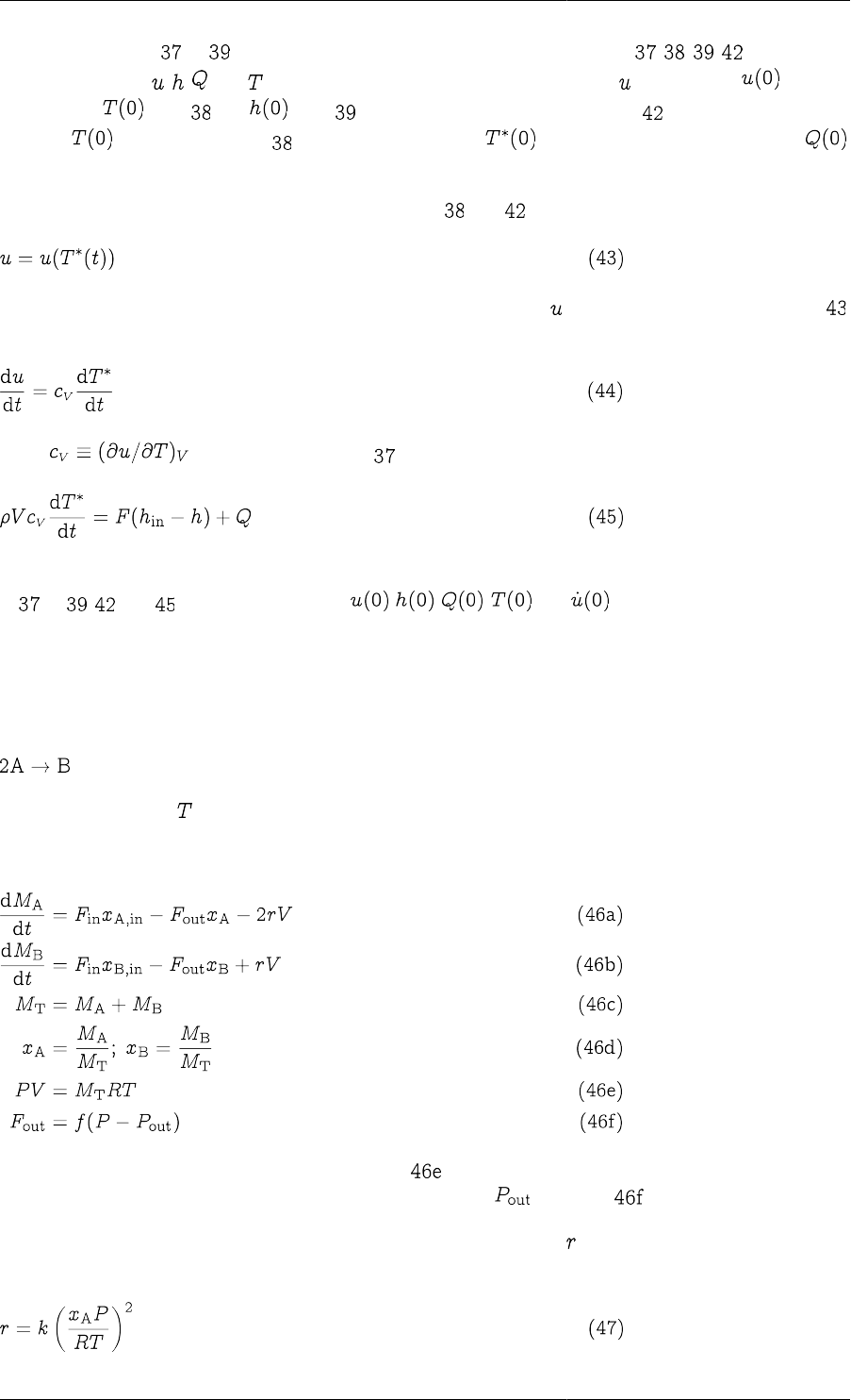
Model Analysis and Diagnosis
230
Of course, equations to are always true, so our DAE system now comprises , , , and the same
set of variables (i.e. , , and ) as before. It also still has differential variable . If we specify , we can
still calculate from and from . However, when we come to consider , we encounter a problem
since the we calculated from may not be the same as . In any case, we cannot calculate
from any one of the existing equations!
Again, this is a high index problem. In fact, if we combine and , we see that:
and, therefore, it is not possible to specify an arbitrary initial value for . Furthermore, by differentiating
with respect to time, we get:
where , and this together with yields:
which is an additional restriction that the initial values of the variables must satisfy. Overall, we have 5 equations
in to , and in 5 initial values, i.e. , , , and — therefore no arbitrary initial
condition may be imposed on this system.
Systems of high-index DAEs in chemical equilibrium
Consider a constant-volume well-stirred reactor carrying out the gas-phase dimerisation reaction:
at a given temperature, .
The mathematical model of this system comprises the equations:
Here we have assumed perfect-gas behaviour (equation ) and that the exit flowrate is a function of the difference
between the pressure in the reactor and the downstream pressure, (equation ).
To complete the above model, we need to characterise the reaction rate, . Assume first, that the reaction is
irreversible with the rate given by:
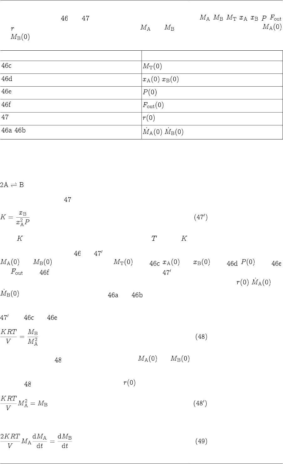
Model Analysis and Diagnosis
231
We note that equations and form a set of 8 DAEs in the 8 unknowns , , , , , ,
and . The system involves two differential variables ( and ). If we specify arbitrary values of
and , then:
From Calculate
,
, ,
Hence, this is an index-1 system, which can be solved without much difficulty.
Consider, however, what happens if the dimerisation reaction takes place under conditions of chemical
equilibrium, i.e.:
For an ideal gas mixture, will be replaced by an equilibrium relation of the form:
where is the equilibrium constant. Since the temperature is fixed, also has a constant value.
Once again, the DAE system and comprises 8 equations in the same 8 unknowns as before. If we specify
and , we can again compute from ; and from ; from
and from . However, we now note that all variables in have already been computed, and therefore
this equation is either redundant or inconsistent. Moreover, we cannot get unique values for , and
from the remaining two equations and .
As we have seen previously, the above are clear sympotoms of a high-index DAE system. In fact, by combining
with and , we obtain:
The left hand side of is just a constant. Therefore, and are related to each other and cannot
be specified arbitrarily. This is the underlying cause of the high index.
Equation also provides a way of determining . We can write is as:
which, upon differentiation with respect to time, yields:
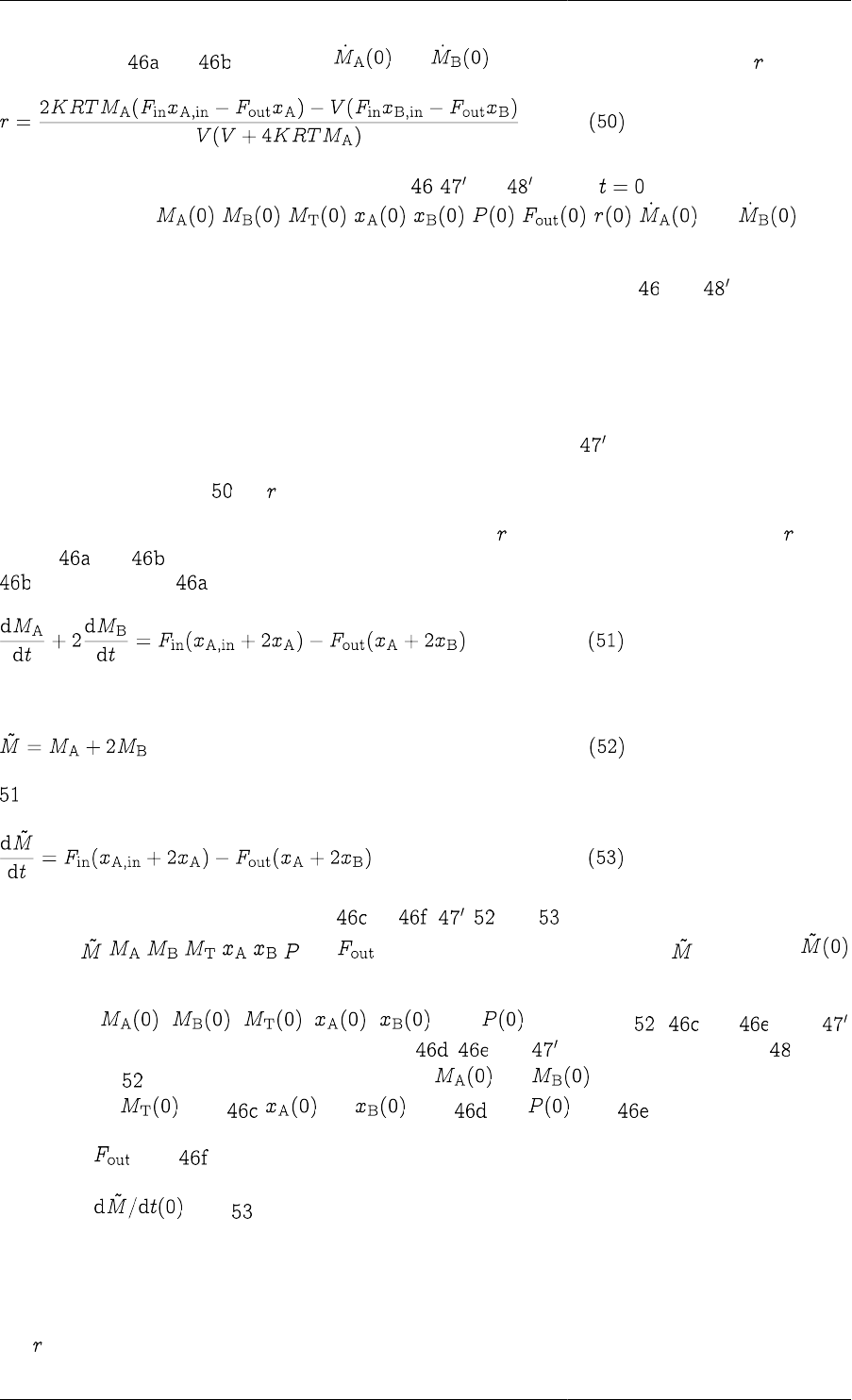
Model Analysis and Diagnosis
232
We can then use and to eliminate and . Solving the resulting equation for , we obtain:
A consistent set of initial variable values must satisfy , and at time . Thus we have 9 equations
in the 10 unknowns , , , , , , , , and , which
leaves only one degree of freedom in the specification of the initial conditions.
Once we have a consistent set of initial values, we can solve the index-1 system and using standard
algorithms.
Example of index reduction in chemical equilibrium
The handling of the high-index complications in the previous example was relatively straightforward. However,
in general, things may be much more conplicated, for instance, if we had non-ideal behaviour (with chemical
equilibrium expressed in terms of fugacities rather than partial pressures, as in ); or if we had multiple reversible
reactions at equilibrium. We also note that much of the effort in reformulating the prior system was expended in
deriving a complex relation for — a quantity we need not know in the first place!
One approach to overcoming these difficulties is to try to elimiate from the model. In particular, since occurs
only in and , we can eliminate is by combining these two equations. In this case, we have to multiply
by 2 and add it to , which yields:
If we now define a new variable:
can be written as:
Now consider the DAE system formed by to , , and . This comprises 8 equations in the 8
unknowns , , , , , , and . There is only one differential variable: . If we specify ,
we can:
•Calculate , , , , and by solving , to and
simultaneously. To understand this, remember that , and can be combined to yield which,
together with form a set of two simple equations in and . Once we get these two values, we
can calculate from ; and from ; and from .
•Calculate from .
•Calculate from .
This, then, is an index-1 system which again can be solved with standard algorithms. It is interesting to note
that this has been obtained from the original index-2 problem without any differentiations. This would appear to
contradict the definition of index (cf. index classification of DAEs). However, the reduction has been possible
only because we did not insist on determining all the variables in the original system; in particular, we decided
that was of no interest and we eliminated it using purely algebraic manipulations (i.e. no differentiations).
Model Analysis and Diagnosis
233
In doing so, we have introduced the new variable defined by equation . has an interesting physical
interpretation: it is a quantity that remains unchanged by the reaction , a so called "reaction invariant".
Equation can be interpreted as a balance on this quantity; as might be expected this balance does not involve
a reaction term.
The procedure described here can be generalised to systems that include multiple reversible reactions at
equilibrium, inlcuding additional reversible reactions where the rates of the forward and reverse reactions are
known, and additional irreversible reactions. However, this general treatment is beyond the scope of this document.
Some general conclusions
The three examples presented in this section allow us to draw certain more general conclusions:
1. High-index DAEs often arise in process-engineering applications due to "simplifications" that impose
additional constraints on the differential variables (or quantities directly related to them — cf. mixing-tank
example). For instance,
• Incompressibility → Volume constraint.
• Phase equilibrium → Vapour/liquid composition relation.
• Reaction equilibrium → Relations between component concentrations.
2. High-index DAEs also arise from "perfect control" specifications on process outputs, i.e. specifying them as
given explicit functions of time (cf. heater-tank example).
3. In all cases, a high-index DAE implies that the differential variables in the model are not independent and
cannot all be assigned arbitrary initial values.
4. Another frequent symptom that can be useful in detecting high-index DAEs is that one or more algebraic
variables occur in differential equations only (cf. in the heater-tank example).
5. If we have a high-index DAE model, in general we can either:
a. change our assumptions ("simplifications") or specifications to develop a different, index-1 model or,
b. reduce the index by differentiating some of the equations a sufficient number of times.
Inconsistent initial conditions
Once gPROMS has checked that the system is well-posed, square and of index 1, it checks the consistency of the
initial conditions and identifies sub-systems that are over- or under-specified at t = 0. For example, consider the
system shown in the gPROMS code below:
Model Analysis and Diagnosis
234
Example 15.3. Illustrative example: system with inconsistent initial conditions
#===============================================================
#MODEL mod1
VARIABLE
x1, x2, y1, y2, y3 AS NoType
EQUATION
$x1 = x1*y1 ;
$x2 = x1 + x2*y1 + y2 + 3*y3 ;
x1^2 = y2 ;
x2 = x1 + y1 + y2*y3 ;
#===============================================================
#PROCESS proc
UNIT
mymod AS mod1
ASSIGN
WITHIN mymod DO
y3 := 1 ;
END #within
INITIAL
WITHIN mymod DO
x1 = 0 ;
y2 = 1 ;
END #within
SOLUTIONPARAMETERS
ReportingInterval := 1 ;
SCHEDULE
CONTINUE FOR 10
In this case, it is clear from inspection that the initial conditions, and , are inconsistent due
to the relationship . This is confirmed by the gPROMS output:
Executing process PROC...
All 5 variables will be monitored during this simulation!
Building mathematical problem description took 0.001 seconds.
Loaded MA48 library
Execution begins....
Variables
Known : 1
Unknown : 4
Differential : 2
Algebraic : 2

Model Analysis and Diagnosis
235
Model equations : 4
Initial conditions : 2
Checking consistency of model equations and ASSIGN specifications... OK!
Checking index of differential-algebraic equations (DAEs)... OK!
Checking consistency of initial conditions...
ERROR: Your initial conditions are inconsistent.
At time t=0, the following 3 equation(s) involve only 2 unknown
variable(s).
Model Equation 3: MYMOD.X1^2 = MYMOD.Y2 ;
Initial Condition 1: MYMOD.X1 = 0 ;
Initial Condition 2: MYMOD.Y2 = 1 ;
The 2 unknown(s) occuring in these 3 equations are:
MYMOD.Y2 (ALGEBRAIC)
MYMOD.X1 (STATE)
Initialisation calculation failed.
Execution of PROC fails prematurely.
Note that using the initial conditions:
INITIAL
WITHIN mymod DO
$x1 = 0 ;
y2 = 1 ;
END #within
for example, rectifies the problem.

236
Chapter 16. Initialisation Procedures
Initialisation procedures are a way to control more precisely how gPROMS initialises models. For complex models,
this can substantially reduce the time taken to initialise them and also increase the robustness of the models
(i.e. initialisation can be performed successfully for a wider set of initial conditions, variable specifications and
parameter values). As this is done transparently, the model user can concentrate on the physical problem being
solved and need not be concerned with the mathematical and numerical issues of getting a complex model to
initialise.
Initialisation procedures comprise a set of simplifications and changes to the model, which guarantee that the
model will initialise. These changes can then be reverted in a specified order so that the original problem is solved.
By moving from an easy problem to the complex, original problem in this sequence, the ease of initialisation of
complex models can be increased significantly, which means faster and more reliable initialisation over a wider
range of input specifications compared with trying to initialise the problem in one step.
This is a procedure that good modellers tend to use: they begin modelling a process by using simplified equations
so that they have a working simple model. They then gradually add complexity until the model has the desired
fidelity. This sometimes requires using the solution of a simpler model as an initial guess for a more detailed
model. gPROMS Initialisation Procedures essentially mimic this process without the need to use Saved Variable
Sets and by permitting more than one intermediate stage; hence complex models built in this way are more flexible
and reusable.
Initialisation Procedures for Non-Composite
Models
To specify and use Initialisation Procedures for non-composite Models (i.e. Models that contain no Model
instances (UNITs)), you need to:
• Specify at least one Initialisation Procedure in the Model
• Specify which Initialisation Procedure to use in the Process
Specifying Initialisation Procedures in the Model
There are four basic techniques associated with Initialisation procedures. These are:
• Initialisation Procedures that change the value of a Parameter
• Initialisation Procedures that change the value of a Degree of Freedom (Specification)
• Initialisation Procedures that change the choice of a Degree of Freedom
• Initialisation Procedures that use simplified equations
All of the above can be combined into a single Initialisation Procedure. When more than one simplification is
applied, the order in which the simplifications are reverted can be important. The way in which these reversions
take place may also be important. These are described in:
• Specifying the order of reversions
• Specifying how the reversions are performed
Initialisation Procedures are defined using one or more INITIALISATION_PROCEDURE sections following
the PRESET section of the Model (if one exists — see gPROMS Language declaration for Models for more
information). The syntax (for non-composite Models) is:
INITIALISATION_PROCEDURE ipname DEFAULT

Initialisation Procedures
237
START
# list of modifications to the Model or its specifications
END
NEXT # NEXT sections are optional, there may be more than one
# list of Initialisation Procedure actions
END
An alternative spelling is INITIALIZATION_PROCEDURE.
The DEFAULT keyword defines the default Initialisation Procedure and makes specifying Initialisation
Procedures in Processes more convenient (this will become clearer later).
If only one Initialisation Procedure is specified, then the DEFAULT keyword compulsory. If there are more than
one Initialisation Procedures in a Model then exactly one must contain the DEFAULT keyword. If none or more
than one contain the DEFAULT keyword, then an error will be reported when executing the Process.
The START section of an Initialisation Procedure specifies which modifications should be made to the Model in
order to initialise it. Exactly how this is done is described in the sections on changing the value of a Parameter,
changing the value of a Degree of Freedom, changing the choice of a Degree of Freedom and simplifying equations.
The (optional) NEXT sections then define a sequence of changes (that of course move the initialisation problem
closer to the one specified in the Process) to the Parameters or Variables listed in the START section. Changes
specified in the same NEXT section are performed simultaneously and each NEXT section is executed in sequence.
For more details, see specifying the order of reversions.
The changes specified in each NEXT section must be contained within either a MOVE_TO or JUMP_TO section.
There can be only one of each in any NEXT section. Any changes specified within a MOVE_TO section are
performed gradually, using a continuation method; those within a JUMP_TO section are performed in a single
step. These sections are described in more detail in: specifying how reversions are performed.
After the final NEXT section has been executed, any modifications that are still in place are automatically reverted
to the original problem in a final step. This is also described in: specifying the order of reversions. Parameters and
Variables can be reverted to their original values explicitly using the REVERT keyword. This is illustrated in the
following sections on changing the value of a Parameter, changing the value of a Degree of Freedom, changing
the choice of a Degree of Freedom and simplifying equations.
Changing the Value of a Parameter
gPROMS initialisation procedures allow the model developer to specify a set of Parameter values that will
guarantee successful initialisation. From this solution of the simplified problem the Parameter values are replaced
with the desired ones in such a way that the model will always initialise. As an example, consider a lumped model
of a CSTR in which the following energy balance occurs.
The heats of reaction, , are Parameters to be specified by the Model user. Users may want to model highly
energetic reactions, so that some of these Parameters will take very large values and in some cases these can cause
difficulty or even failure during initialisation.
gPROMS Initialisation Procedures allow the Model developer to specify a set of Parameter values that will be used
to initialise the Model first and then to change these values back to the user-specified ones in a controlled manner
so that the initialisation converges even for extreme values of the Parameters. In the above example, the first step
of the Initialisation Procedure might be to set all values of to zero and solve the initialisation problem.
Upon successful initialisation, the Parameters are gradually1 returned to the user-specified values.
1By default, gPROMS applies a continuation method when reverting Parameters (and any other changes in the Initialisation Procedure) to
the values specified in the Process: that is, their values are changed continuously and smoothly rather than in one discrete jump. See section
xxx for more details.
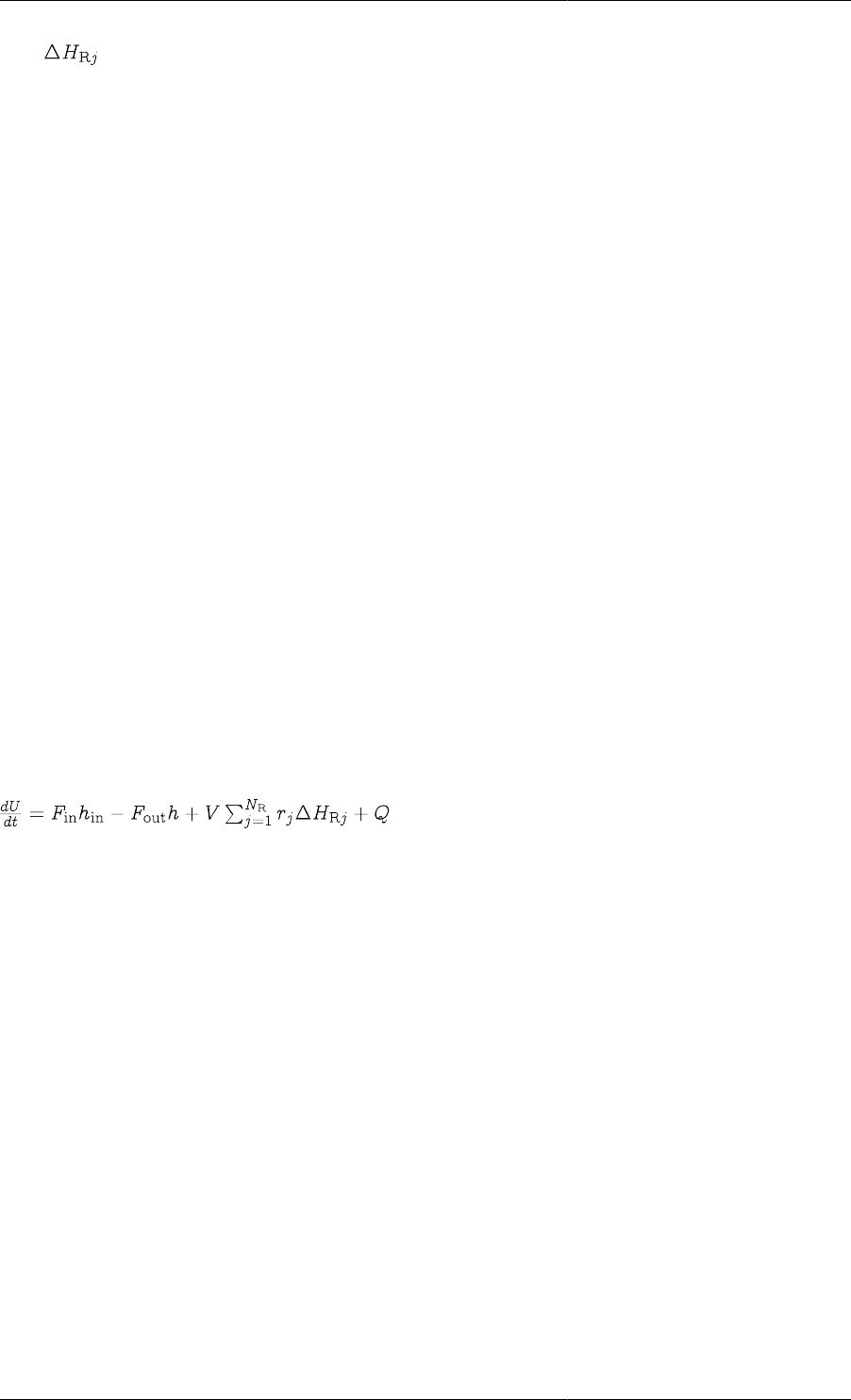
Initialisation Procedures
238
If the Parameter is defined in the gPROMS Model by:
PARAMETER
...
EnthalpyOfReaction AS ARRAY(NoReac) OF REAL
...
Then the Initialisation Procedure would be defined by:
# end of EQUATION section
INITIALISATION_PROCEDURE IP_NoHeatOfReaction
START
EnthalplyOfReaction := 0 ;
END
NEXT
MOVE_TO
REVERT EnthalpyOfReaction ;
END
END
In other words, first solve the initialisation with EnthalpyOfReaction set to zero; then, once successful, gradually
change all of their values back to those specified in the Process.
Changing the Value of a Degree of Freedom
The previous section described how models can be made more robust during initialisation. The approach was to
use a gPROMS Initialisation Procedure to specify a set of Parameter values that guarantees initialisation and how
these can be replaced by the desired values in a way that ensures successful initialisation. A similar situation arises
with the specification of degrees of freedom: that is, any degrees of freedom need to be taken up by specifying
the values of some Variables in the ASSIGN section.
Consider, once again, the energy balance equation for a lumped CSTR model:
Here for example, the rate of heat input to the system, Q, may depend on a Variable representing the steam flowrate,
Fsteam, through the vessel jacket or a coil. For an open-loop simulation, this variable would be specified in the
ASSIGN section of the gPROMS Process.
One possible initialisation procedure would then be to start the initialisation with Fsteam set to zero (which
would guarantee initialisation) and then move the value of Fsteam to the desired value.
This would be defined in gPROMS using the following code.
# end of EQUATION section
INITIALISATION_PROCEDURE IP_NoSteamFlow
START
F_steam := 0 ;
END
NEXT
MOVE_TO
REVERT F_steam ;
END
END
Note that REASSIGN or RESET tasks cannot be used to redefine the value of any ASSIGNed variables in the
context of an Initialisation Procedure.
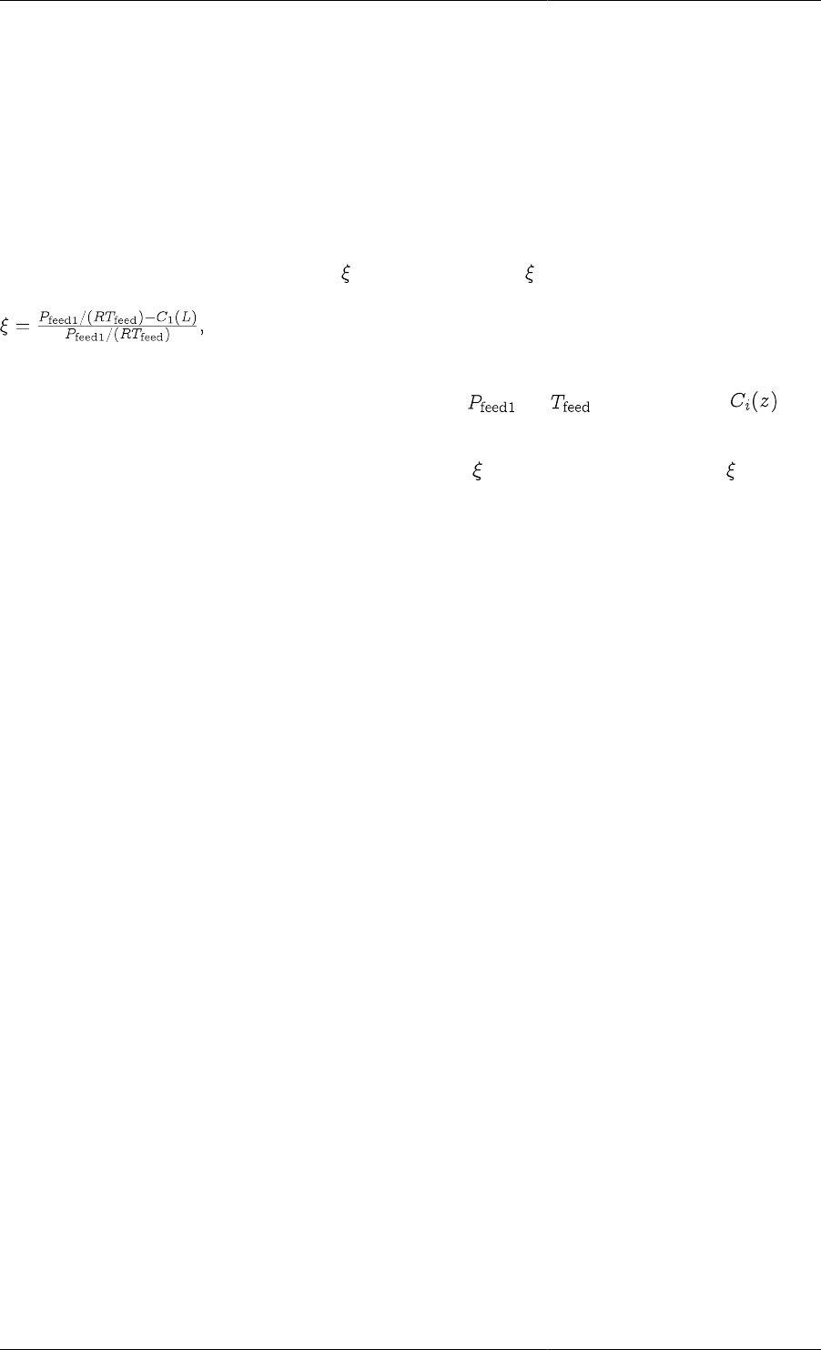
Initialisation Procedures
239
Changing the Choice of a Degree of Freedom
In some cases, simply changing the values of ASSIGNed variables may not be sufficient to guarantee successful
initialisation. The Model user may have chosen a particular set of Variables to ASSIGN that could cause difficulty
or failure during initialisation. To avoid such possibilities, initialisation procedures can define which degrees of
freedom should be specified to guarantee initialisation. The initialisation procedure then also specifies how the
choice of degrees of freedom can be reverted to the one specified in the Process by the user.
One possible use of this feature can be seen in the following example. Consider a model of a tubular reactor in
which the length of the reaction is a variable, L, to be specified (a degree of freedom) and in which there is an
equation that defines the fractional conversion of one of the reactants. might then be defined as follows.
where the perfect gas law has been used to calculate the inlet concentration of component 1, using the partial
pressure of component 1 in the feed and the feed temperature ( and , respectively) and is the
concentration of component i at axial position z in the reactor.
It is usual to specify the value of L and calculate the conversion , but it is also possible to specify as a degree
of freedom, which would then determine the value of L. The latter specification may present problems during
initialisation, however, so a suitable initialisation procedure for this model would be to replace any choice of
degree of freedom with a specification on the length of the reactor, L. This (maybe combined with a suitable value
for L) would then result in a more robust model.
This can be achieved in gPROMS using the following.
DISTRIBUTION_DOMAIN
Axial AS [0:1]
# normalised as ReactorLength is a Variable ( PARTIAL(,Axial)
# becomes 1/ReactorLength * PARTIAL(,Axial) etc. )
VARIABLE
...
ReactorLength AS Length
C AS DISTRIBUTION(NoComp,Axial) OF MolarConcentration
Conversion AS NoType
EQUATION
...
Conversion = (Pfeed(1) / (Rg * Tfeed) - C(1,1)) /
# ----------------------------------
(Pfeed(1) / (Rg * Tfeed)) ;
INITIALISATION_PROCEDURE IP_ReplaceConversion
START
REPLACE
Conversion
WITH
ReactorLength := 5 ;
# this value of L guarantees successful initialisation
END
END
NEXT
MOVE_TO
REVERT Conversion ;
END
END
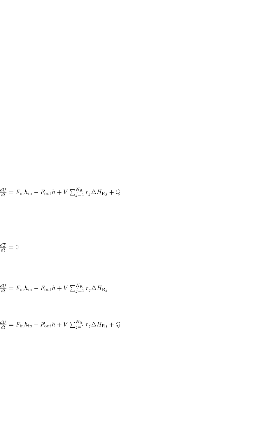
Initialisation Procedures
240
In this example, the conversion must be specified in the Process as follows.
ASSIGN
R101.Conversion := 0.95 ;
Simplifying Equations
When developing very detailed models, it is often better to start with a simple model and gradually add more
complexity. This is because initialising the fully-detailed model may be too difficult without good initial guesses.
With a much simpler model, one can obtain a solution from a poor initial guess and then use that as the initial
guess for a more detailed model. This process is repeated until the final model, with the desired level of detail,
can be solved.
gPROMS Initialisation Procedures enable the modeller to automate this process and are much more flexible and
reusable than manually initialising a complex model. This is because using the manual approach requires that
published models contain the saved variable set that is necessary to initialise the simulation. Apart from making the
published model large in size (due to the size of the saved variable set), the saved variable set will be suitable for
only a narrow range of problems: for example, if the model user wanted to change the number of chemical species
in the simulation, then the existing saved variable set may be useless and it would be impossible to initialise the
simulation. This might also happen even if only a few species were changed (the number of components remaining
the same). Initialisation Procedures allow complex models to be initialised successfully without the use of saved
variable sets and for a very much wider range of problems.
To see how the initialisation procedures are defined, consider again the energy balance equation for a lumped
CSTR model:
One way to build up to the full energy balance from simplified ones would be to start with an isothermal model,
then switch to an adiabatic model and finally to arrive at the full non-isothermal, non-adiabatic model (the equation
above).
The problem would then first be initialised using
for the energy balance.
The solution of this would then be used as the initial guess to solve the next initialisation, using
for the energy balance. Finally, the solution of the last problem would be used to initialise the model with the
desired energy balance:
(Of course, this example is quite simple and it is probably not necessary to go to these lengths in this case. However,
much more complicated models would require this treatment.)
This initialisation procedure can be defined in gPROMS first by specifying all of the equations within a CASE
statement and then using the Initialisation Procedure to SWITCH from the simplified equation(s) to the final
one(s). All of the following must be specified in the Model.
First the Selector Variable must be defined:
SELECTOR
EnergyMode AS (Isothermal, Adiabatic, NINA) DEFAULT NINA
Then the equations can be defined using a CASE statement:

Initialisation Procedures
241
EQUATION
...
CASE EnergyMode OF
WHEN Isothermal:
$T = 0 ;
WHEN Adiabatic:
$U = F_in*h_in – F_out*h + V*SIGMA(rate()*DeltaH_R()) ;
WHEN NINA:
$U = F_in*h_in – F_out*h + V*SIGMA(rate()*DeltaH_R()) + Q ;
END
...
Finally, the initialisation procedure is defined by:
INITIALISATION_PROCEDURE IP_SimpleEnergyBalance
START
EnergyMode := Isothermal ;
END
NEXT
MOVE_TO
EnergyMode := Adiabatic ;
END
END
NEXT
MOVE_TO
EnergyMode := NINA ;
END
END
Behaviour of CASE branches during initialisation
When gPROMS peforms a standard intialisation (i.e. without using any user-defined Initialisation Procedures) of a
Model containing CASE statements, the active branches of all CASE statments are determined by the values of the
Selector Variables specified in the INITIAL_SELECTOR section of the Process. These Selector Variables must
remain fixed at these values throughout and at the end of the initialisation procedure (so that the CASE branches
are locked) because their values are considered part of the initial state for the simulation.
In the case of Initialisation Procedures, all CASEs that contain SWITCH TO statements are free to switch during
the Initialisation Procedure. The exception, of course, is when the Initialisation Procedure specifically changes the
values of one or more Selector Variables. However, at the end of the Initialisation Procedure, all manipulated and
implicitly-set Selector Variables are reverted back to their specified values, consistent with a standard initialisation.
In other words, Initialisation Procedures must always result in the same initial state as a standard initialisation.
Specifying the sequence of Actions in Initilisations Procedures
Initialisation Procedures for non-composite Models must contain at least one START section and then optionally
any number of NEXT sections.
The START section specifies which Parameters, Variables or Selector Variables are to be changed during
initialisation. The START section may contain any number of simplifications (as described in the sections on
changing the value of a Parameter, changing the value of a Degree of Freedom, changing the choice of a Degree
of Freedom and simplifying equations) in any order: they are all performed in parallel and together form the first
initialisation problem.
After the first initialisation is successful, gPROMS then needs to know in what order to relax the simplifications.
This is specified by an optional sequence of NEXT sections, each of which contains a list of changes (either partial
or complete relaxations of some of the simplifications in the START section) that are to be made in parallel. If
no NEXT section is present, then gPROMS will relax all simplifications simultaneously and try to reinitialise the
problem. If any NEXT sections are present, then each NEXT section is processed in sequence, reinitialising after

Initialisation Procedures
242
each one. Any simplifications that have not been completely relaxed after the final NEXT section are then relaxed
simultaneously in an implicit final step.
Each NEXT section must contain a list of one or more changes to a Parameter or Variable listed in the START
section: they may be assigned a new value or reverted to the value specified in the Process by use of the REVERT
task. The syntax of the REVERT task is:
REVERT ParameterName ;
REVERT VariableName ;
REVERT SelectorName ;
All changes (including revertions) to a Parameter or a Variable must occur within either a MOVE_TO or
JUMP_TO section.
The examples below illustrate these ideas more clearly.
The START section may contain any number of actions:
START
aParameter := 0 ;
aVariable := 0 ;
REPLACE
anotherVariable
WITH
aThirdVariable := 0 ;
END
aSelector := Simple ;
END
In this example, all four actions are included: changing a Parameter value, changing a Variable value (degree of
freedom), changing the choice of a degree of freedom and changing the value of a Selector variable (to change
the equations being used).
Explicitly reverting changes:
INITIALISATION_PROCEDURE IP_Example1
START
aParameter := 0 ;
aVariable := 0 ;
REPLACE
anotherVariable
WITH
aThirdVariable := 0 ;
END
aSelector := Simple ;
END
NEXT
MOVE_TO
REVERT aParameter ;
REVERT aVariable ;
REVERT anotherVariable ;
REVERT aSelector ;
END
END
Here, the NEXT section reverts all actions simultaneously and smoothly.
The implicit final step when no NEXT section is specified:
INITIALISATION_PROCEDURE IP_Example1

Initialisation Procedures
243
START
aParameter := 0 ;
aVariable := 0 ;
REPLACE
anotherVariable
WITH
aThirdVariable := 0 ;
END
aSelector := Simple ;
END
Here, no NEXT sections are present, so all actions are reverted simultaneously after the first initialisation is
successful. This example is identical to the previous one, where all actions were reverted explicitly in a NEXT
section.
Making more than one change to a Variable/Parameter before reverting it:
INITIALISATION_PROCEDURE IP_Example2
START
aParameter := 0 ;
aVariable := 0 ;
REPLACE
anotherVariable
WITH
aThirdVariable := 0 ;
END
aSelector := Simple ;
END
NEXT
MOVE_TO
aParameter := 1 ;
END
END
In this example, the value of aParameter is changed continuously from 0 to 1 (with aVariable and
aThirdVariable still equal to 0, and aSelector still equal to Simple). The implicit final step then will
revert aParameter, the Variables and Selector Variable to their values specified in the Process. Implicit final
steps always revert the changes smoothly (in an implicit MOVE_TO section).
Reverting some simplifications in parallel and some in sequence:
INITIALISATION_PROCEDURE IP_Example3
START
aParameter := 0 ;
aVariable := 0 ;
REPLACE
anotherVariable
WITH
aThirdVariable := 0 ;
END
aSelector := Simple ;
END
NEXT
MOVE_TO
REVERT aParameter ;
REVERT aVariable ;
END
END
NEXT

Initialisation Procedures
244
MOVE_TO
REVERT anotherVariable ;
REVERT aSelector ;
END
END
Here, the Parameter and aVariable are reverted simultaneously and the system is reinitialised. Then the other
two Variables are reverted. (This second NEXT section could have been omitted, as the reversions would have
taken place implicitly anyway.)
They can all be combined:
INITIALISATION_PROCEDURE IP_Example4
START
aParameter := 0 ;
aVariable := 0 ;
REPLACE
anotherVariable
WITH
aThirdVariable := 0 ;
END
aSelector := Simple ;
END
NEXT
MOVE_TO
REVERT aParameter ;
aVariable := 1 ;
MOVE_TO
END
NEXT
MOVE_TO
REVERT aVariable ;
aSelector := NotSoSimple ;
END
END
NEXT
MOVE_TO
REVERT anotherVariable ;
aSelector := QuiteComplex ;
END
END
In this final example, the Parameter is reverted to its specified value at the same time as aVariable is
changed to 1. After reinitialisation, aVariable is reverted simultaneously with the change of equations to the
NotSoSimple CASE. In the final NEXT section, the specification on aThirdVariable is reverted to the
original specification on anotherVariable (note that anotherVariable is specified in the REVERT task)
while the equations are changed once more. Finally, the implicit final step reverts the equations to their full form
(i.e. the value originally specified for the aSelector Variable)
Specifying how the reversions are performed
Earlier sections have described how to make changes to Parameters, Variables and Equations during initialisation
and in which order these changes should be reverted back to the original specifications. How these reversions are
performed has not yet been discussed fully.
There are two ways that changes specified in a NEXT section can take place: either by making discrete jumps or
by changing the value smoothly from one state to the next. Discrete changes are trivial to perform: simply change
the value and reinitialise. To make a smooth change, gPROMS employs a continuation algorithm. Clearly, if the
difference between the values is large, then it will be harder to make a discrete jump and the continuation method

Initialisation Procedures
245
will be more robust; however, when it is safe to make discrete jumps, this method will usually result in faster
initialisation. In some cases, it is a matter of experimentation to determine which method is more robust and faster.
The JUMP_TO and MOVE_TO sections are used to specify which transitions are to be discrete and smooth
respectively. One MOVE_TO section and one JUMP_TO section can be placed in each NEXT section. The
example below illustrates the use of both discrete and continuous transitions.
INITIALISATION_PROCEDURE IP_Example3a
START
aParameter := 0 ;
aVariable := 0 ;
REPLACE
anotherVariable
WITH
aThirdVariable := 0 ;
END
aSelector := Simple ;
END
NEXT
MOVE_TO
REVERT aVariable ;
REVERT anotherVariable ;
END
END
NEXT
JUMP_TO
REVERT aParameter ;
END
MOVE_TO
REVERT aSelector ;
END
END
In this example, the problem is first initialised with aParameter and aVariable equal to 0, aThirdVariable is also
equal to 0 (replacing the specification of anotherVariable) and aSelector is set to Simple (specifying the use of
simplified equations).
In the first NEXT section, the two variables simultaneously make smooth transitions to their final values.
Finally, aParameter is reverted in a discrete jump at the same time as the Selector Variable is reverted to its original
value in a smooth transition.
In this case, there are no implicit reversions to be made. Should there be an implicit final step, then all reversions
are performed in a smooth transition.
This example illustrates that even though changing a degree of freedom (REPLACE) or the equations that are
being solved (SWITCHing from one CASE to another) is a discrete change, gPROMS can still perform this change
smoothly.
Specifying which Initialisation Procedures to use in
the Process
Once one or more Initialisation Procedures have been specified for a Model, one can be selected for use in a
simulation by specifying it in the Process.
The syntax is very simple:
INITIALISATION_PROCEDURE

Initialisation Procedures
246
USE
unitname : ipname ;
END
where unitname is the name of the Model instance specified in the UNIT section and ipname is the name of the
Initialisation Procedure to use. Alternatively, the keyword NONE can be used in place of ipname to specify that
no Initialisation Procedure should be used, or DEFAULT can be used to specify that the default Initialisation
Procedure must be used. An alternative spelling, INITIALIZATION_PROCEDURE, is also allowed.
Performing a simulation activity using Initialisation
Procedures
One one or more Initialisation Procedures have been defined in the Models and a Process, as described previously,
gPROMS can then use them when performing a simulation activity. In order to do this, simply execute the Process
as usual and then when the Execution control dialog appears select one of:
•Perform Initialisation Procedure only: This method only performs the Initialisation Procedure to generate the
initial guesses but does not continue to initialise the problem or execute the Schedule. This is useful if you
only want to generate the initial guesses and save them in a Saved Variable Set . (The generation of the Saved
Variable Set is specified as part of the Initialisation Procedure.)
•Perform Initialisation Procedure as part of the main activity: This method generates the initial guesses using
the Initialisation Procedure, then immediately performs an initialisation using them. If a Schedule is present,
and the Ignore schedule option is unchecked, then gPROMS will complete the simulation according to what is
specified in the Schedule. If the Initialisation Procedure specifies that a Saved Variable Set should be generated,
then this is done too.
See Executing Simulations for a full description of the Execution control dialog.
Initialisation Procedures for Composite
Models
Specifying initialisation procedures for composite Models is very similar to that of non-composite Models but
with two additional complications:
• the sub Models within the composite model may also contain Initialisation Procedures, and there needs to be
some mechanism for choosing which of these to use in a particular Initialisation Procedure; and
• any Initialisation Procedures in the sub Models may contain a number of NEXT sections and some control needs
to be applied to ensure that these NEXT sections are processed at the right time relative to the NEXT sections
in the composite Model and the ones in the other sub Models.
In order to specify which sub Model Initialisation Procedures must be used, a USE section has to be included in
the composite Model’s Initialisation Procedure. The syntax for the Initialisation Procedure in a composite Model
is as follows.
INITIALISATION_PROCEDURE ipname [DEFAULT]
USE
# list of Unit and Model specifications
END
START
# list of modifications to the Model or its specifications
END
NEXT # NEXT sections are optional, there may be more than one
# list of Initialisation Procedure actions
END

Initialisation Procedures
247
See The USE Section for Composite Models for more details on the USE section.
The START section is treated identically to non-composite Models (see Specifying Initialisation Procedures in
the Model).
The NEXT section is similar to that for non-composite Models, but with additional Initialisation Procedure Actions
for Synchronising the Initialisation Procedures of sub Models.
The USE Section for Composite Models
The syntax of the USE section in composite Models is similar to that for Processes (see Specifying which
Initialisation Procedures to use in the Process). There are some additional features needed for composite Models
that contain more than one sub Model. In this case, the USE section may contain a list of specifications: one for
each instance. That is:
USE
unitname1 : ipname1 ;
unitname2 : ipname2 ;
unitname3 : ipname3 ;
# etc.
END
If there are lots of Model instances (e.g. if there is an array), then there are some short cuts to save typing many
lines of specifications.
First, if all Model instances are to use the default Initialisation Procedure, then the following specification can
be made:
USE
: DEFAULT ;
END
If all Model instances apart from a few are to use the default Initialisation Procedure, then it is usually more
efficient to specify the above and then to override it with specific Unit specifications:
USE
# Use default ip for all units
: DEFAULT ;
# Override ip for Unit U1: use no ip
U1 : NONE ;
# Override ip for Unit U2: use specified ip
U2 : ipname ;
END
Second, arrays and slices of arrays can be used in place of single Unit names:
USE
# Specification for the whole array of Units
# (both lines are acceptable syntax)
ArrayUnit1 : ipname1 ;
ArrayUnit2() : ipname2 ;
# Specification for a slice of an array of Units
ArrayUnit3(2:3) : ipname3 ;
END
Another useful option is to specify the Initialisation Procedure to be used by all Model instances (Units) of the
same Model. This is done by:
USE
[modelname] : ipname ;

Initialisation Procedures
248
END
where modelname is the name of a Model and ipname is the name of one of its Initialisation Procedures (the
brackets are part of the syntax and must be typed — this distinguishes between a Model specification and a Unit
specification, since gPROMS allows the name of a Unit to be the same as a Model name). Just as with Unit
specifications, the NONE and DEFAULT keywords can be used.
Finally, one might want to specify a particular Initialisation Procedure for all Units of the same Model type
apart from a certain number of specific Units. This can be done by combining Model specifications with Unit
specifications as follows.
USE
unitname : ipname ;
[modelname] : ipname ;
END
In this case, all Unit specifications override the Model specifications, regardless of the order in which they are
made. As an example, consider a Model with 3 instances of Model Tank, called T101, T102 and T103. If T101
and T102 are to use the default Initialisation Procedure, and T103 is to use none, then this can be done as follows.
USE
[Tank] : DEFAULT ;
T103 : NONE ;
END
Even if the T103 specification appears before the [Tank] one, it will override the [Tank] specification for
T103.
Lastly, gPROMS will issue a warning if there are duplicate Unit specifications but will continue with the
simulations using the last specification in the list to override all previous ones.
Synchronising the Initialisation Procedures of sub
Models
Synchronisation of the various Initialisations Procedures for non-composite Models is specified using NEXT
sections, as has been described before (Specifying the sequence of Actions in Initilisations Procedures). For
composite Models, the same procedures apply in addition to being able to control when a NEXT section of a sub
Model is processed. This is done using the ADVANCE and COMPLETE actions. The syntax of the ADVANCE
action is:
ADVANCE unitname ;
or
ADVANCE [modelname] ;
The first command causes the next unprocessed NEXT section within the Initialisation Procedure of the Unit
unitname to be processed in parallel with the actions specified in the NEXT section within which it resides.
unitname may also be an array of Units or a slice of an array of Units. The second command does the same, but
for all Units of Model type modelname (note that the brackets are part of the syntax).
Since the ADVANCE keyword specifies that a subsequent NEXT section of a sub Model should be exectuted,
and all changes specified in NEXT sections must be within a MOVE_TO or JUMP_TO section, there must be no
ADVANCE commands placed inside a MOVE_TO or JUMP_TO section: doing so will result in an error.
The COMPLETE action is similar to ADVANCE but causes all of the Unit's NEXT sections to be executed in
sequence (beginning with the first unexecuted NEXT section of the Unit). The syntax is:
COMPLETE unitname ;

Initialisation Procedures
249
or
COMPLETE [modelname] ;
When more than one COMPLETE action resides in the same NEXT section, then the first unprocessed NEXT
section of each Unit is executed in parallel, followed by the second set of NEXT sections and so on until all explicit
and implicit steps are complete.
To illustrate the ADVANCE action, suppose a composite Model contains instances of two sub-models, A and B:
UNIT
A1 AS A
B1 AS B
...
Now, the Models A and B may have a number of Initialisation Procedures, such as:
# in Model A
INITIALISATION_PROCEDURE IP_A1
...
INITIALISATION_PROCEDURE IP_A2 DEFAULT
...
# in Model B
INITIALISATION_PROCEDURE IP_B1
...
INITIALISATION_PROCEDURE IP_B2 DEFAULT
...
The choice of Initialisation Procedure for the sub Models is made within the USE section of the Initialisation
Procedure of the composite Model:
INITIALISATION_PROCEDURE IP_composite1
USE
A1 : IP_A1 ;
B1 : IP_B1 ;
END
Now the Initialisation Procedures of the two sub models are defined as:
# in Model A
INITIALISATIONPROCEDURE IP_A1
START
P1 := P1_0 ;
END
NEXT
MOVE_TO
P1 := P1_1 ;
END
END
NEXT
JUMP_TO
P1 := P1_2 ;
END
END
# in Model B
INITIALISATIONPROCEDURE IP_B1
START
P2 := P2_0 ;
END
NEXT
MOVE_TO
P2 := P2_1 ;
END
END
Notice that Model B’s Initialisation Procedure has one less NEXT section, each is defined in terms of changes to
a Parameter (P1 for Model A and P2 for Model B) and each has an implicit final step that reverts the Parameter
back to its original value.
The Initialisation Procedure for the composite model is:
INITIALISATIONPROCEDURE composite_init_1
USE
A1 : IP_A1 ;

Initialisation Procedures
250
B1 : IP_B1 ;
END
START
PP := PP_0 ;
END
# Step1
NEXT
MOVE_TO
PP := PP_1 ;
END
END
# Step2
NEXT
ADVANCE A1 ;
END
# Step3
NEXT
ADVANCE A1 ;
MOVE_TO
PP := PP_2 ;
END
END
# Step 4
NEXT
ADVANCE B1 ;
END
# Step 5
NEXT
ADVANCE A1 ;
ADVANCE B1 ;
MOVE_TO
REVERT PP ;
END
END
Now, during each step in the initialisation strategy of the composite Model, the following steps occur to each of
the Models:
Step PP A1.P1 B1.P2 Comments
START PP_0 P1_0 P2_0 The first, simplest
initialisation.
1 PP_1 P1_0 P2_0 The first NEXT
section only changes
the value of PP.
2 PP_1 P1_1 P2_0 The second NEXT
section advances
the Initialisation
Procedure for A1,
which changes its
value of P1 to P1_1.
3 PP_2 P1_2 P2_0 The third NEXT
section changes the
value of PP to
PP_2 and at the
same time advances
the Initialisation
Procedure for A1,
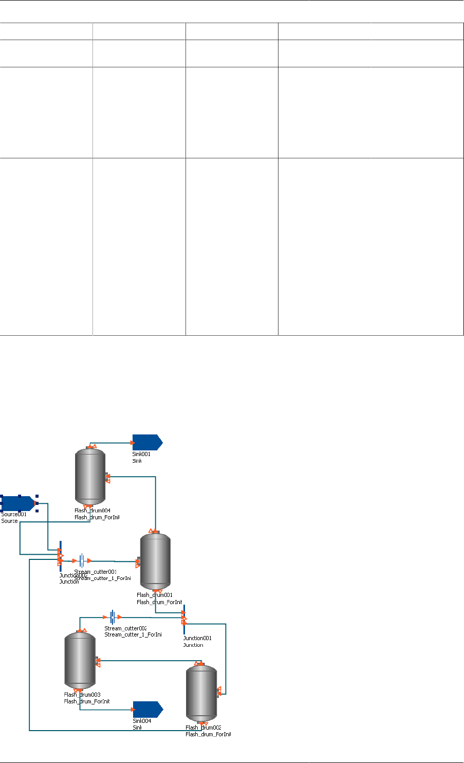
Initialisation Procedures
251
Step PP A1.P1 B1.P2 Comments
which changes the
value of P1 to P1_2.
4 PP_2 P1_2 P2_1 The fourth NEXT
section only
advances the
Initialisation
Procedure for B1,
which changes its
value of P2 to P2_1.
5 PP P1 P2 The final NEXT
section reverts PP to
the value specified
in the Process
and simultaneously
advances A1 and
B1's Initialisation
Procedures. This
causes the implicit
final steps to be
called, which revert
P1 and P2 to their
values specified in
the Process.
The example above is somewhat contrived, just to illustrate the processes occurring during initialisation. A more
useful application of sequence control in composite-Model initialisation is the convergence of flowsheets with
recycles. The figure below illustrates a composite Model containing 4 instances of a flash-drum Model, and various
other connections and splitters. Of note are the two instances of a Stream-Cutter Model. These are models that
perform stream tears but using equation simplifications: the full equations link the inlet of the Model to the outlet,
effectively connecting the stream; the simplified equations set the outlet to some given condition, tearing the
stream.

Initialisation Procedures
252
Now the Initialisation Procedures for the Stream_Cutter and Flash_drum Models are as follows.
# in Model Stream_cutter
INITIALISATION_PROCEDURE Init
START
ConnectionEqns := Simple ;
END
NEXT
MOVE_TO
REVERT ConnectionEqns ;
END
END
# in Model Flash_drum
INITIALISATION_PROCEDURE Init
START
REPLACE
Pressure
WITH
VapourFraction := VapFracStart ;
END
END
NEXT
MOVE_TO
REVERT Pressure ;
END
END
The Selector Variable ConnectionEqns represents the connection of the stream into and out of the unit; when
Simple, the stream is torn. For the Flash_drum Model, one needs to specify the pressure, but it is difficult to
initialise the Model with this specification, so the degree of freedom specified during initialisation is the vapour
fraction: it is a much easier to determine the pressure from the vapour fraction than the reverse.
Finally, the flowsheet initialisation strategy is:
INITIALISATION_PROCEDURE Init
USE
Flash_drum003 : Init;
Flash_drum004 : Init;
Stream_cutter001 : Init;
Stream_cutter002 : Init;
END
NEXT
ADVANCE Flash_drum003;
ADVANCE Flash_drum004;
END
NEXT
ADVANCE Stream_cutter001;
ADVANCE Stream_cutter002;
END
The overall Initialisation Procedure is as follows. The problem is first initialised with the simpler specification on
the vapour fraction of two of the flash drums and both recycle streams torn. Switching back to the full Model in one
step may still cause problems with convergence, so the next step is to revert the degree-of-freedom specifications
back to the flash-drum pressures; the vapour fractions now being determined from these. Finally, both stream tears
can be removed in parallel and the final solution is as desired: a fully converged flowsheet with both recycles in
place and the vapour fraction of each flash drum determined by the specified pressures.
Reference
The following conventions are used in describing the syntax of Initialisation Procedures.
• gPROMS language keywords are shown coloured in CAPITALS, even though the language is case-insensitive
• Identifiers are shown in the italic font: identifier
• An optional language construct is enclosed in brackets, e.g.: [DEFAULT]
• A compulsory language construct is enclosed in angle brackets, e.g.: <USE section>

Initialisation Procedures
253
• Choices are indicated by pipes separating each option, e.g.: identifier|DEFAULT|NONE indicates the choice
between an identifier or one of the keywords DEFAULT and NONE.
• When multiple language constructs are allowed, they are indicated by a following asterisk, e.g. [NEXT section]*
Specifying Initialisation Procedures in Models
The syntax for specifying an initialisation procedure in a Model is:
INITIALISATION_PROCEDURE ipname [DEFAULT]
[USE section]
[START section]
[NEXT section]*
A Model can have more than one initialisation procedure, each of which must have a uniquely defined name in
the same Model. The following rules are imposed on the specification of an initialisation procedure in a Model:
• The alternative keyword INITIALIZATION_PROCEDURE may be used.
• The Initialisation Procedure must not be completely empty; a syntax error will be reported if it is.
• The optional DEFAULT keyword following the name of the Initialisation Procedure is used to specify that an
Initialisation Procedure is the default in a Model. Only one IP may be assigned as default. If a Model has only
one IP specification, it is automatically assigned as the default (no keyword is required).
• The optional USE section defines which Initialisation Procedures are applied for any Units present in the Model.
Only one USE section is allowed in an Initialisation Procedure and it must not be empty.
• The optional START section contains a list of IP actions to perform prior to initialisation. Only one START
section is allowed in an Initialisation Procedure and it must not be empty.
• If there is a USE or START section in the IP, then one or more optional NEXT sections may be included. Each
NEXT section must contain at least one Initialisation Procedure action; all IP actions in a NEXT section are
performed simultaneously.
• All modifications must be declared explicitly in the START section of an Initialisation Procedure. Elementary
IP tasks are only allowed for those Model elements which were modified in the START section. An error will
be reported otherwise.
• A Unit can only be ADVANCEd in a NEXT section if it is specified in the USE section; otherwise an error
will be reported.
Specifying Initialisation Procedures in Processes
The syntax for specifying an initialisation procedure in a Process is:
INITIALISATION_PROCEDURE ipname [DEFAULT]
<USE section>
[SAVE filename;]
Only one IP specification is allowed in a Process. The SAVE task is optional and the USE section is compulsory.
The USE section
The USE section defines which Initialisation Procedures are applied for any Units present in the Model or Process.
The USE section is compulsory for an IP in a Process but optional for IPs in a Model. The syntax of the USE
section is:
USE

Initialisation Procedures
254
[: DEFAULT ;]
[unitname : ipname|DEFAULT|NONE ;]*
[[modelname] : ipname|DEFAULT|NONE ;]*
END
The USE section must contain at least one specification. Specifications can be made for any Unit present in the
Model or Process, as indicated by the second line; for all Units in the Process, first line; or for all Units of the
same Model type, third line.
Unit IP Specifications are made by entering the name of a Unit (or an array or slice of an array of Units) followed by
a colon and then either a valid IP name for the Unit (i.e., the name of an IP in the Model of which the Unit is a type)
or one of the keywords DEFAULT or NONE. The DEFAULT keyword indicates that the default IP for the Unit
should be implemented; NONE indicates that no IP should be implemented (this is useful for overriding a previous
specification for a Model or an array of Units). Lastly, if all Units in the Process are to use the default IP, then this
can be done by omitting the unitname identifier and using the DEFAULT keyword, as in the first line above.
Model IP Specifications are made by entering the name of a Model enclosed in brackets (this is part of the syntax)
followed by a colon and then either a valid IP name for the Model or one of the keywords DEFAULT or NONE.
The DEFAULT keyword indicates that the default IP for all Units declared as modelname should be implemented;
NONE indicates that no IP should be implemented.
Order and Precedence Rules
• A Unit specification can appear an arbitrary number of times, with each new specification overriding any
previous one. Duplicated specifications of the same unit are reported as a warning
• An Initialisation Procedure specified explicitly for a Unit will override a setting arising from a Model
specification.
• The order of Model specifications and Unit specifications is insignificant: even if a Model specification is
placed after a Unit specification, the Unit specification will always override the Model specification.
The START section
The START section may only appear in Models. There may only be one START section and it must contain at
least one modification of the standard Initialisation Procedure. The syntax is:
START
<modification of the standard IP>*
END
The modifications can be one of the following:
1. changes to the value of a Parameter
2. changes to the choice of a Degrees of Freedom (DoF) (i.e., changing the ASSIGNment of one Variable to an
ASSIGNment of another)
3. changes to the value of a DoF (i.e., changing the value of an ASSIGNed Variable)
4. changes to the value of a Selector Variable
For modifications of a gIP that involve Variables (cf. items 2 and 3 above), the Variables must be already
ASSIGNed, otherwise they will be reported as specification errors.
The syntax for modifications of a gIP involving Parameters, Variable values and Selectors respectively is:
ParameterPath := expression ;
VariablePath := expression ;

Initialisation Procedures
255
SelectorPath := value ;
The syntax for changing the choice of a DoF is:
REPLACE
VariablePath1
WITH
VariablePath2 := expression ;
END
where VariablePath1 must be different to VariablePath2. VariablePath and VariablePath1 must be ASSIGNed
in the Process; VariablePath2 must not have been ASSIGNed.
The modifications to the gIP are applied simultaneously before any initialisation takes place. The first initialisation
problem that gPROMS solves is the one specified in the START section.
Behaviour of CASE statements duringin Initialisation Procedures
During an Initialisation Procedure, CASE statements are free to change branches based on the values of the
Variables at each step of the Initialisation Procedure. However, the branches of any CASE specified in the
START section can, of course, be changed explicitly in a NEXT section. The final implicit step of an Initialisation
Procedure always reverts the values of Selector Variables to those specified in the INITIALSELECTOR section
so that the correct initialisation is solved.
The NEXT section
After the first initialisation problem is solved (that specified by the modifications in the START section to the gIP),
a sequence of actions may be performed in order to restore these modifications back to the initialisation problem
specified in the SET, ASSIGN and INITIALSELECTOR sections of the Process. Each step in this sequence is
specified in a NEXT section. There may be as many NEXT sections in the IP as required, including none (in which
case, all modifications to the gIP are reverted in parallel). The syntax of the NEXT section is:
NEXT
[MOVE_TO section]*
[JUMP_TO section]*
[ADVANCE statement]*
[COMPLETE statement]*
END
Each NEXT section may comprise any combination of MOVE_TO, JUMP_TO, ADVANCE and COMPLETE
statements (including multiple entries of each type). However, a NEXT section cannot be empty.
The syntax for the MOVE_TO and JUMP_TO sections are:
MOVE_TO
<Unit Initialisation Procedure action>*
END
JUMP_TO
<Unit Initialisation Procedure action>*
END
At least one Elementary UIP action must be specified in each MOVE_TO or JUMP_TO section; they must not
contain any ADVANCE or COMPLETE actions.
All of the UIP actions specified in a NEXT section are executed in parallel. If COMPLETE actions are present
along side MOVE_TO, JUMP_TO and/or ADVANCE actions, then the first NEXT sections of the Units being
COMPLETEd that need to be processed are executed in parallel with all of the other actions; the second NEXT
sections in the Units that are being COMPLETEd will then be executed in parallel, and so on until no more NEXT
sections are left to be processed.

Initialisation Procedures
256
Elementary UIP actions
Elementary UIP tasks in a NEXT section declare the change of the UIP to be applied in the next step; they may
be one of the following:
1. changes to the value of a Parameter
2. changes to the choice of a Degrees of Freedom (DoF) (i.e., changing the ASSIGNment of one Variable to an
ASSIGNment of another)
3. changes to the value of a DoF (i.e., changing the value of an ASSIGNed Variable)
4. changes to the value of a Selector Variable
5. reversion of original value of a Parameter, DoF or Selector Variable.
Elementary UIP tasks are only allowed for those Model elements that were modified in the START section;
otherwise a syntax error will occur. For changes to the choice of DoF, the Variables involved must be ASSIGNed
ones, i.e. they were not REPLACEd in an earlier step. Otherwise they will be reported as specification errors.
The syntax for items 1 to 4 above is identical to the START section. The syntax for reverting the original value
of a Parameter, Variable or Selector Variable is, respectively:
REVERT ParameterPath ;
REVERT VariablePath ;
REVERT SelectorPath ;
Implicit Final Step
If, after the final NEXT section has been processed, one or more modifications of the gIP have not been
REVERTed, a final implicit step will be performed where all remaining modifications are REVERTed to their
original values in parallel.
Advancing Initialisation Procedures of Units
If a Model contains Units, then the Initialisation Procedure may control the advancing of steps for any of the Units’
Initialisation Procedures. The ADVANCE task is used to do this within any of the NEXT sections:
NEXT
ADVANCE unitname ;
ADVANCE [modelname] ;
END
The first line advances the IP of the Unit unitname by one step, where unitname may be the path of a single Unit,
an array of Units or a slice of an array of Units. The IP of unitname can only be advanced if unitname was specified
in the USE section.
The second line advances the IPs of all Units declared as modelname (the brackets [ ] are compulsory and are part
of the syntax — modelname is not an optional argument in this case).
When more than one Unit is ADVANCEd in a NEXT section, the appropriate NEXT sections within the Units’
IPs are all processed in parallel. After the final NEXT section has been ADVANCEd , the next ADVANCE task
causes the implicit final step to be performed (if necessary). Any further ADVANCEs have no effect on any Units
that have completed their final step.
The COMPLETE task is used to advance all steps (in sequence) of a Unit or group of units and complete their
initialisation procedures; its syntax is:
NEXT
COMPLETE unitname ;

Initialisation Procedures
257
COMPLETE [modelname] ;
END
Using COMPLETE is equivalent to calling ADVANCE on a Unit (or group of Units of the same Model type)
as many times as is necessary to complete the initialisation procedure. When more than one COMPLETE task is
used in the same NEXT section, the first NEXT section of each Unit that has not yet been executed is processed
in parallel, then the second and so on until all NEXT sections and explicit final steps have been completed. To
illustrate this, the following two Initialisation Procedures are equivalent (Unit_1 has one step, Unit_2 has two
and so on).
INITIALISATION_PROCEDURE Initialise_flowsheet_using_complete DEFAULT
USE
Stream_Cutter : DEFAULT
Unit_1 : DEFAULT;
Unit_2 : DEFAULT;
Unit_3 : DEFAULT;
Unit_4 : DEFAULT;
END
NEXT # just do the first steps in parallel
ADVANCE Unit_1;
ADVANCE Unit_2;
ADVANCE Unit_3;
ADVANCE Unit_4;
END
NEXT # finish them off (2nd steps in parallel, 3rd and so on)
COMPLETE Unit_1;
COMPLETE Unit_2;
COMPLETE Unit_3;
COMPLETE Unit_4;
END
NEXT
COMPLETE Stream_Cutter;
END
INITIALISATION_PROCEDURE Initialise_flowsheet_with_advances DEFAULT
USE
Stream_Cutter : DEFAULT
Unit_1 : DEFAULT;
Unit_2 : DEFAULT;
Unit_3 : DEFAULT;
Unit_4 : DEFAULT;
END
NEXT
ADVANCE Unit_1; # Step 1 of Unit_1
ADVANCE Unit_2; # Step 1 of Unit_2
ADVANCE Unit_3; # Step 1 of Unit_3
ADVANCE Unit_4; # Step 1 of Unit_4
END
NEXT
ADVANCE Unit_2; # Step 2 of Unit_2
ADVANCE Unit_3; # Step 2 of Unit_3
ADVANCE Unit_4; # Step 2 of Unit_4
END

Initialisation Procedures
258
NEXT
ADVANCE Unit_3; # Step 3 of Unit_3
ADVANCE Unit_4; # Step 3 of Unit_4
END
NEXT
ADVANCE Unit_4; # Step 4 of Unit_4
END
NEXT
ADVANCE Stream_Cutter; # Step 1 of Stream_Cutter
END
UIP Algorithms
UIPs support discrete or continuous changes as advanced initialisation mechanisms. Algorithmically, discrete
changes will be solved by conventional algorithms for the solution of non-linear algebraic systems. Continuous
changes will be solved by a continuation method using DAE solvers.
In case of discrete changes, modifications are grouped via the following language construct:
JUMP_TO
<elementary UIP task>*
END
In case of a continuous change, modifications are grouped via the following language construct:
MOVE_TO
<elementary UIP task>*
END
The constructs above must contain at least one UIP task and cannot be nested. All UIP tasks must reside in either
a MOVE_TO or a JUMP_TO section. The only exception is the ADVANCE task, which must not appear in a
JUMP_TO or MOVE_TO section.
