G PROMS Optimisation Guide

User Manual:

Open the PDF directly: View PDF .
Page Count: 50

Optimisation Guide
Table of Contents
Chapter 1. Overview
Chapter 2. Dynamic Optimisation in gPROMS

Optimisation Guide

Release v3.5

June 2012

Optimisation Guide

Release v3.5

June 2012

Process Systems Enterprise Limited

6th Floor East

26-28 Hammersmith Grove

London W6 7HA

United Kingdom

Tel: +44 20 85630888

Fax: +44 20 85630999

WWW: http://www.psenterprise.com

Trademarks

gPROMS is a registered trademark of Process Systems Enterprise Limited ("PSE"). All other

registered and pending trademarks mentioned in this material are considered the sole property

Legal notice

No part of this material may be copied, distributed, published, retransmitted or modified in any

way without the prior written consent of PSE. This document is the property of PSE, and must

not be reproduced in any manner without prior written permission.

Disclaimer

gPROMS provides an environment for modelling the behaviour of complex systems. While

gPROMS provides valuable insights into the behaviour of the system being modelled, this is

not a substitute for understanding the real system and any dangers that it may present. Except as

otherwise provided, all warranties, representations, terms and conditions express and implied

(including implied warranties of satisfactory quality and fitness for a particular purpose) are

expressly excluded to the fullest extent permitted by law. gPROMS provides a framework

for applications which may be used for supervising a process control system and initiating

operations automatically. gPROMS is not intended for environments which require fail-safe

characteristics from the supervisor system. PSE specifically disclaims any express or implied

warranty of fitness for environments requiring a fail-safe supervisor. Nothing in this disclaimer

shall limit PSE's liability for death or personal injury caused by its negligence.

Acknowledgements

ModelBuilder uses the following third party free-software packages. The distribution and use

of these libraries is governed by their respective licenses which can be found in full in the

distribution. Where required, the source code will made available upon request. Please contact

support.gPROMS@psenterprise.com in such a case.

Many thanks to the developers of these great products!

Table 1. Third party free-software packages

Software/Copyright Website License

ANTLR http://www.antlr2.org/ Public Domain

Batik http://xmlgraphics.apache.org/batik/ Apache v2.0

BLAS http://www.netlib.org/blas BSD Style

Boost http://www.boost.org/ Boost

Castor http://www.castor.org/ Apache v2.0

Commons CLI http://commons.apache.org/cli/ Apache v2.0

Commons Collections http://commons.apache.org/collections/ Apache v2.0

Commons Lang http://commons.apache.org/lang/ Apache v2.0

Commons Logging http://commons.apache.org/logging/ Apache v1.1

Crypto++ (AES/Rijndael

and SHA-256) http://www.cryptopp.com/ Public Domain

Fast MD5 http://www.twmacinta.com/myjava/

fast_md5.php LGPL v2.1

HQP http://hqp.sourceforge.net/ LGPL v2

Jakarta Regexp http://jakarta.apache.org/regexp/ Apache v1.1

JavaHelp http://javahelp.java.net/ GPL v2 with

classpath exception

JXButtonPanel http://swinghelper.dev.java.net/ LGPL v2.1 (or

later)

LAPACK http://www.netlib.org/lapack/ BSD Style

libodbc++ http://libodbcxx.sourceforge.net/ LGPL v2

Software/Copyright Website License

lp_solve http://lpsolve.sourceforge.net/ LGPL v2.1

MiGLayout http://www.miglayout.com/ BSD

Netbeans http://www.netbeans.org/ SPL

omniORB http://omniorb.sourceforge.net/ LGPL v2

TimingFramework http://timingframework.dev.java.net/ BSD

VecMath http://vecmath.dev.java.net/ GPL v2 with

classpath exception

Wizard Framework http://wizard-framework.dev.java.net/ LGPL

Xalan http://xml.apache.org/xalan-j/ Apache v2.0

Xerces-C http://xerces.apache.org/xerces-c/ Apache v2.0

Xerces-J http://xerces.apache.org/xerces2-j/ Apache v2.0

This product includes software developed by the Apache Software Foundation, http://

www.apache.org/.

gPROMS also uses the following third party commercial packages:

•FLEXnet Publisher software licensing management from Acresso Software Inc., http://

www.acresso.com/.

•JClass DesktopViews by Quest Software, Inc., http://www.quest.com/jclass-desktopviews/.

•JGraph by JGraph Ltd., http://www.jgraph.com/.

Table of Contents

1. Overview .................................................................................................................................. 1

2. Dynamic Optimisation in gPROMS .............................................................................................. 2

Introduction .......................................................................................................................... 2

What is dynamic optimisation? ................................................................................................ 2

What is the mathematical problem? .......................................................................................... 3

The process model ......................................................................................................... 3

The initial conditions ..................................................................................................... 3

The objective function .................................................................................................... 4

Bounds on the optimisation decision variables .................................................................... 4

Other constraint types .................................................................................................... 5

What is a "solution'' of a dynamic optimisation problem? ............................................................. 6

Classes of control variable profile .................................................................................... 6

Control variable profiles in gPROMS ................................................................................ 8

Specifying dynamic optimisation problems in gPROMS ............................................................... 9

Process entities for optimisation ....................................................................................... 9

The Optimisation entity ................................................................................................ 10

Point Optimisation ............................................................................................................... 13

Specification of point Optimisation Entities ...................................................................... 13

Specification of steady-state optimisation problems ............................................................ 14

Running optimisation problems in gPROMS ............................................................................. 17

Results of the optimisation run ............................................................................................... 18

The comprehensive optimisation report file ...................................................................... 18

The optimisation report file ........................................................................................... 19

The SCHEDULE file and the Saved Variable Set .............................................................. 19

The point file .............................................................................................................. 20

Other features ...................................................................................................................... 20

Standard solvers for optimisation ............................................................................................ 21

The CVP_SS solver ..................................................................................................... 23

The OAERAP solver .................................................................................................... 23

The SRQPD solver ....................................................................................................... 26

The CVP_MS solver .................................................................................................... 29

Dynamic Optimisation Example ............................................................................................. 32

Project tree ReactorOpt.gPJ ........................................................................................... 33

Variable Type entities in ReactorOpt.gPJ ......................................................................... 33

Text contained within the Reactor Model entity ................................................................ 33

BatchReaction Model entity ........................................................................................... 35

Text contained within the OPTIMISE_REACTOR Process entity ......................................... 35

Optimisation entity (OPTIMISE_REACTOR) ................................................................... 36

Sample optimisation report file (OPTIMISE_REACTOR.out) .............................................. 36

Sample gPROMS schedule file (OPTIMISE_REACTOR.SCHEDULE) ................................. 38

Sample point file (OPTIMISE_REACTOR.point) .............................................................. 39

Simulating the optimal solution within a Process ............................................................... 39

Interpretation of screen output ........................................................................................ 41

List of Figures

2.1. Batch Reactor ......................................................................................................................... 2

2.2. Different types of control variable profile .................................................................................... 7

2.3. Different types of control variable profile .................................................................................... 8

2.4. Selecting a Saved Variable Set for use in a steady-state optimisation ............................................... 16

2.5. Executing an optimisation run via the Activities menu. ................................................................. 17

2.6. Executing an optimisation run via the Optimisation button. ........................................................... 18

2.7. Comprehensive optimisation report. .......................................................................................... 19

2.8. Single-shooting algorithm ........................................................................................................ 21

2.9. Multiple-shooting algorithm ..................................................................................................... 22

2.10. Project tree for the dynamic optimisation example. .................................................................... 33

2.11. Variable Type entities in the ReactorOpt project. ....................................................................... 33

2.12. BatchReaction Model entity for the dynamic optimisation example. .............................................. 35

2.13. Optimisation entity for the dynamic optimisation example. .......................................................... 36

vii

List of Tables

1. Third party free-software packages ............................................................................................... 3

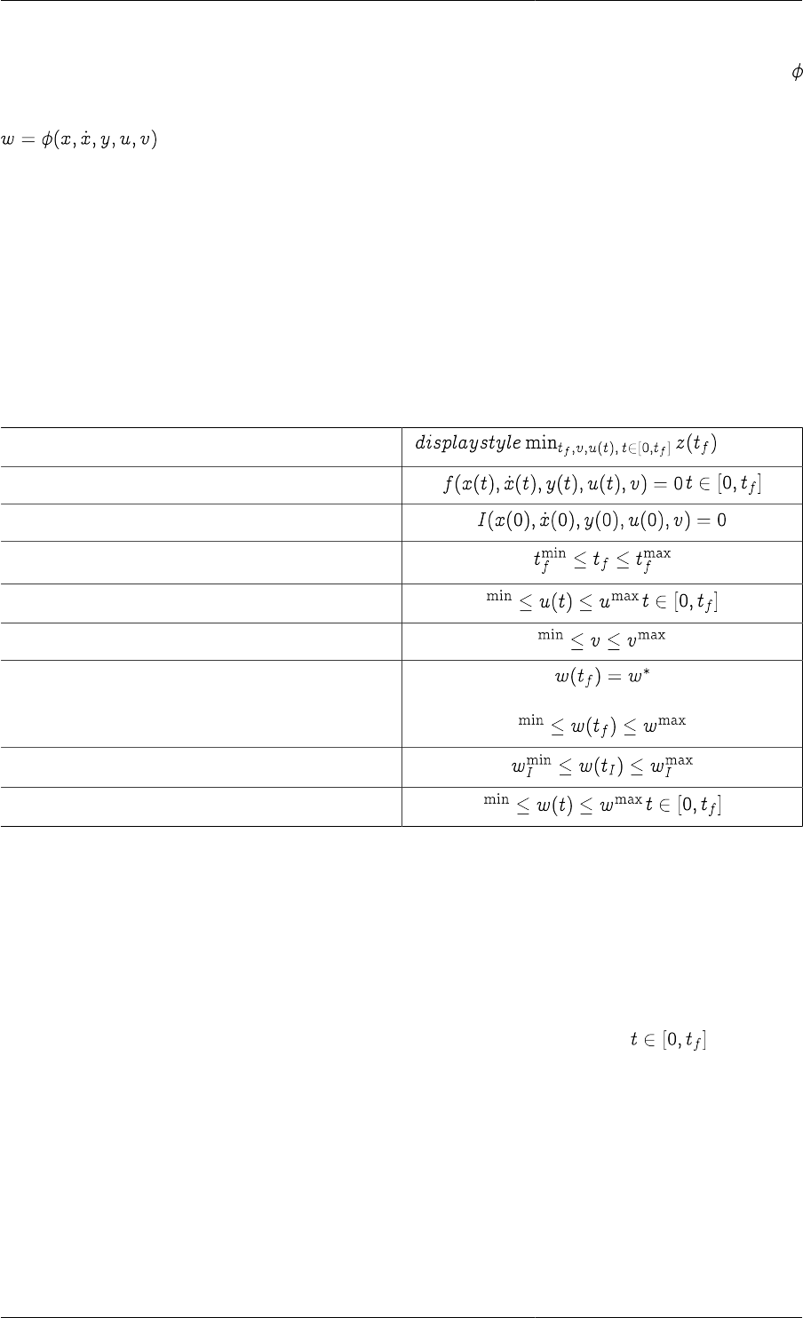
2.1. Mathematical statement of the dynamic optimisation problem ......................................................... 6

2.2. Syntax of a gPROMS Optimisation entity .................................................................................. 10

2.3. Alternative syntax for Interiorpoint constraints ............................................................................ 12

Chapter 1. Overview

gPROMS can be used to optimise the steady-state and/or the dynamic behaviour of a continuous or batch process.

Both plant design and operational optimisation can be carried out. The form of the objective function and the

constraints can be quite general. Moreover, the optimisation decision variables can be either functions of time

("controls") or time-invariant quantities.

Chapter 2. Dynamic Optimisation in

gPROMS

Introduction

This chapter describes how gPROMS can be used to perform (dynamic) optimisation calculations.

• A dynamic optimisation problem is described using a small example. We use this example throughout this guide

to illustrate the dynamic optimisation facilities provided by gPROMS.

• A dynamic optimisation problem is described mathematically.

• A definition of what constitutes a solution to the dynamic optimisation problem is given.

• A description of how to specify dynamic optimisation problems in gPROMS is given.

• A description of how to specify point (including steady-state) optimisation problems in gPROMS is given.

• A description of how optimisation problems are executed in gPROMS is given.

• An explanation of the contents of the various output files that are generated is given.

• A discussion of various other features of the optimisation capabilities of gPROMS is made.

The optimisation capabilities in gPROMS have evolved significantly in recent versions of the software.

Some basic familiarity with the gPROMS language and concepts is assumed.

What is dynamic optimisation?

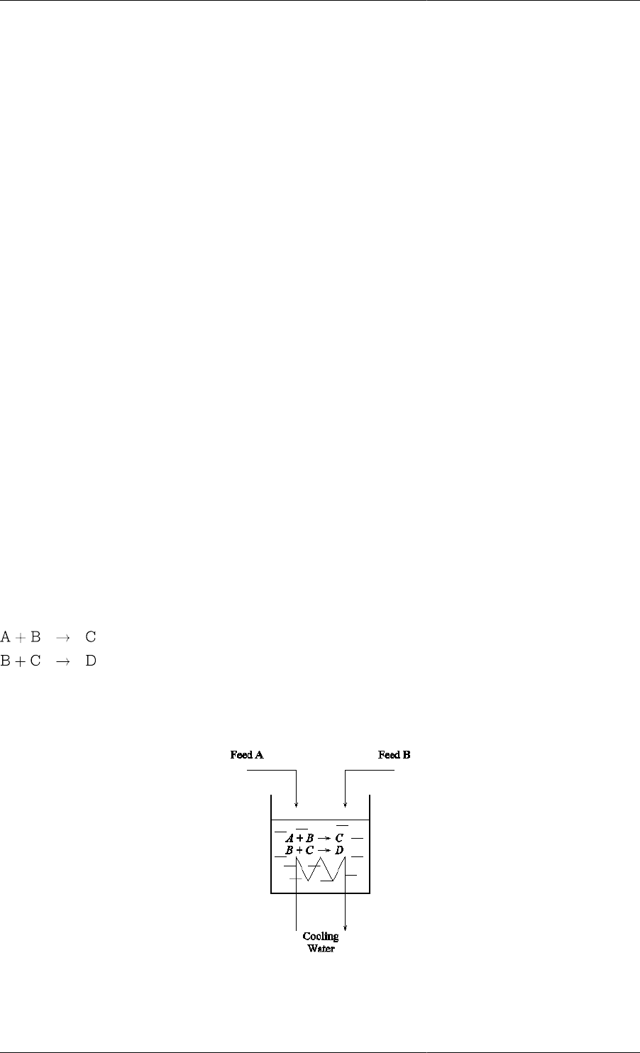
In order to introduce the various elements of the definition of the problem of dynamic optimisation, we consider

the semi-batch reactor shown in the figure below. Two exothermic reactions are taking place:

where A and B are the raw materials, C the desirable product, and D the unwanted by-product.

Figure 2.1. Batch Reactor

The reactor receives two independent inputs of pure A and B, and is cooled with cooling water circulating through

a coil. Starting with an empty reactor, we are free to vary the in-flows of A and B, as well as the cooling water

flowrate.

Dynamic Optimisation in gPROMS

For a given reactor design, our operational objective may be to determine the duration of the operation, and the time

variation of the various material and energy flowrates over this duration, so as to maximise the final concentration

of C. Of course, equipment design and resource availability usually impose certain limits within which our control

manipulations must be maintained---for instance, there is an upper limit on the available flowrate of cooling water.

In general, the design of processes operating in the transient domain also leads to problems that are similar to

operational optimisation problems, but may have additional degrees of freedom. For instance, we may wish to

determine the optimal geometry of the reactor in addition to the optimal way of operating it over time.

Because of the transient nature of the underlying process, both the operational and design problems considered

above are applications of dynamic optimisation1

and serve to introduce some of the important features of this problem in its most basic form. Some other

complications that often arise in practical applications will be introduced later.

What is the mathematical problem?

In this section we provide a mathematical statement of the class of dynamic optimisation problems solved by

gPROMS.

The process model

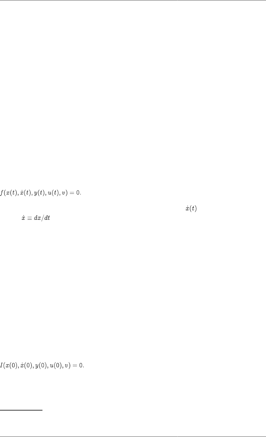
We consider processes described by mixed differential and algebraic equations of the form:

Here x(t) and y(t) are the differential and algebraic variables in the model while are the time derivatives of the

x(t) (i.e., ). u(t) are the control variables and v the time invariant parameters to be determined by the

optimisation. In the context of the batch reactor example considered earlier, the differential variables will typically

correspond to fundamental conserved quantities (such as molar component holdups and internal energy), while y

will include various quantities related to them (e.g. component molar concentrations and temperature). The input

flowrates of A, B and cooling water are the control variables u while, in the design case, the volume of the reactor

acts as a time invariant parameter v.

Note

For simplicity, the mathematical description in this document assumes that the system behaviour is

defined in terms of ordinary(with respect to time) differential and algebraic equations. However, the

optimisation capabilities of gPROMS are equally applicable to mixed lumped and distributed systems

described by general integral, partial differential and algebraic equations in time and one or more space

dimensions.

The initial conditions

In general, gPROMS assumes that the initial t=0 condition of the system is described in terms of a set of general

non-linear relations of the form:

It is important to note that, once we fix the time variation of the controls, u(t) and the values of any time

invariant parameters, v, the modelling equations together with the initial conditions completely determine the

transient response of the system. In practice, we could determine this response by performing a gPROMS dynamic

simulation.

1Often, the term "optimal control'' is also used, especially for problems that involve control variables but no time-invariant parameters (see

also: What is the mathematical model?).

Dynamic Optimisation in gPROMS

The objective function

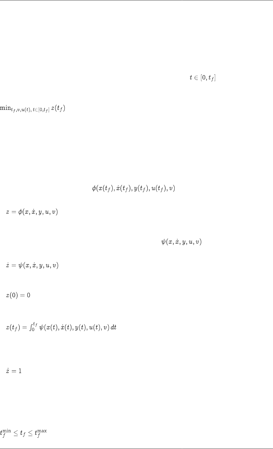
Dynamic optimisation in gPROMS seeks to determine

• the time horizon, tf,

• the values of the time invariant parameters, v, and

•the time variation of the control variables, u(t), over the entire time horizon ,

so as to minimise (or maximise) the final value of a single variable z. This can be written mathematically as:

Here the objective function variable, z is one of either the differential variables x or the algebraic variables y.

In the context of the batch reactor example, tf would be the duration of the batch reaction while z would be the

concentration of component C (either a differential or an algebraic variable, depending on the model used).

The above form of the objective function is not as restrictive as might appear at first. In particular, it is worth

noting that:

• Maximisation can be carried out as well as minimisation.

•If we wish to optimise a function of several variables instead of a single

variable, we can simply add an extra algebraic equation to the model:

The additional computational cost incurred because of this model extension is usually negligible.

•If we wish to minimise or maximise the integral of a function over the entire time horizon,

we can simply add the differential equation:

together with the initial condition:

We can easily verify that this is equivalent to:

Again, very little additional computational cost is incurred in doing this.

• Minimising the time horizon itself can be achieved by adding the equation:

together with the initial condition above.

Bounds on the optimisation decision variables

In practice, the time horizon tf will often be subject to certain lower and upper bounds:

Dynamic Optimisation in gPROMS

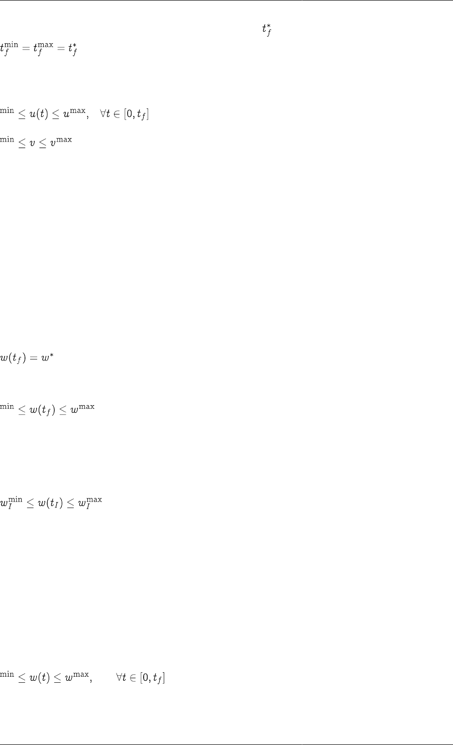
In some cases, tf will, in fact, be fixed at a given value, . This can be achieved simply by setting

As we have already seen in the batch reactor example, it is likely that the control variables and time invariant

parameters will also be subject to lower and upper bounds:

Other constraint types

End-point constraints

In some applications, it is necessary to impose certain conditions that the system must satisfy at the end of the

operation. These are called end-point constraints. For instance, in the batch reactor example, we may require:

• the final amount of material in the reactor to be at certain prescribed value;

and also

• the final temperature to lie within given limits.

In the first case, we have an equality end-point constraint of the type:

where w is one of the system variables (x or y). In the second case, we have an inequality end-point constraint:

Interior-point constraints

We can also have constraints that hold at one or more distinct times tI during the time horizon (e.g. at the middle

of the horizon). These are called interior-point constraints. These may be represented mathematically as:

where w is a system variable, and tl is a given time.

We note that both interior and end-point constraints are special cases of point constraints. However, for

convenience, gPROMS treats them separately. It also treats any constraints that have to be satisfied at the initial

time t=0 as interior-point constraints

Path constraints

We may also have certain constraints that must be satisfied at all times during the system operation. If these path

constraints are equalities, then often they can simply be added to the system model effectively converting one of

the control variables u(t) into an algebraic variable y. More often, they are inequalities of the form:

For instance, in our batch reactor example, we may require that the temperature never exceed a certain value so

as to avoid some unwanted side-reactions that are not explicitly considered by our model.

Dynamic Optimisation in gPROMS

Although we have assumed in equations representing end-point, interior-point and path constraints that the various

constraints are imposed on a single variable w, this is not really restrictive. If we wanted to constrain a function

of several variables, we could simply define a new variable w through an additional equation:

and then impose the required constraints on w.

What is a "solution'' of a dynamic

optimisation problem?

Let us start by summarising the mathematical statement of the dynamic optimisation problem as defined in: What

is the mathematical model?:

Table 2.1. Mathematical statement of the dynamic optimisation problem

Objective function subject to

Process model

Initial conditions

Time horizon bounds

Control variable bounds

Time invariant parameter bounds

End-point constraints

Interior-point constraints

Path constraints

Clearly, a "solution'' to this problem comprises three key elements:

• The value of the time horizon, tf.

• The values of the time invariant parameters, v.

• The variation of the control variables u(t) over the time horizon from t = 0 to t = tf.

As has already been mentioned, if these are specified, we can solve the model equations to determine how the

system behaves over the time horizon of interest, obtaining values of x(t) and y(t) for all . We can then

evaluate the objective function, and also check whether the various end-point and path constraints are satisfied.

Normally, there will be more than one combination of tf, v and u(t) that satisfies the bounds and the constraints---

and this, of course, is what gives rise to the optimisation problem. The latter aims to find the combination that

produces the best value of the objective function while satisfying all the constraints.

Classes of control variable profile

For the above dynamic optimisation problem to be well defined, we need to be rather more specific regarding the

type of the variation of the control variables over time that we are willing to consider. For instance, we could have:

Dynamic Optimisation in gPROMS

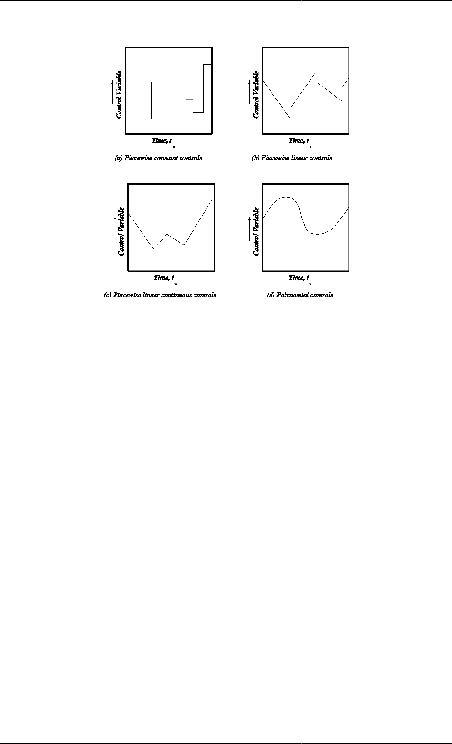
Figure 2.2. Different types of control variable profile

• Piecewise-constant controls---these remain constant at a certain value over a certain part of the time horizon

before jumping discretely to a different value over the next interval: see subfigure (a) above.

• Piecewise-linear controls---these take a certain linear time variation over a certain part of the time horizon before

jumping discretely to a different linear variation over the next interval: see subfigure (b) above.

• Piecewise-linear continuous controls---these are similar to the piecewise-linear controls described above, with

the additional requirement that their values be continuous at the interval boundaries: see subfigure (c) above.

• Controls that vary smoothly over time---perhaps as polynomials of a given degree: see subfigure (d) above.

It is important to appreciate that, in most cases, the choice of the form of the control variables is an engineering

rather than a mathematical issue: it very much depends on the capabilities of the actual control system (automatic

or manual!) that we will eventually use to implement these controls on the real plant. For instance, piecewise-

constant controls may often be preferable to other types as they are much easier to implement.

Dynamic Optimisation in gPROMS

Control variable profiles in gPROMS

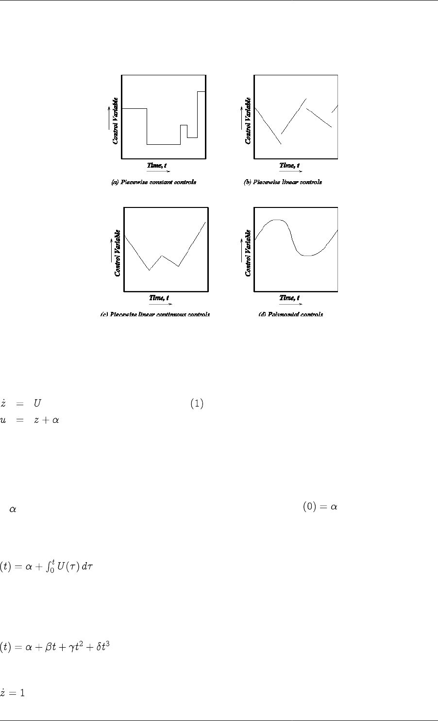
Figure 2.3. Different types of control variable profile

The dynamic optimisation facilities in gPROMS support piecewise-constant and piecewise-linear controls of the

types shown in subfigures (a) and (b) respectively. These are by far the most commonly encountered in practical

applications. However, if necessary, it is relatively straightforward to introduce several other types of control. For

instance, a piecewise-linear continuous control of the type shown in subfigure (c) can be defined by adding the

equations:

where:

•z is a new differential variable with initial condition z(0)=0;

•U is a new piecewise-constant control variable (cf. subfigure (a)) to be determined by the optimisation;

• is a new time invariant parameter representing the initial value of u (i.e. ), to be determined by the

optimisation.

We note that this is equivalent to:

which expresses the fact that the time gradient of a piecewise-linear continuous control is a piecewise-constant

function of time.

Also a cubic polynomial control variation of the form:

can be introduced by adding the following to the model equations:

Dynamic Optimisation in gPROMS

Together with the initial condition z(0)=0, this equation effectively defines z as time.

By virtue of this equation, the variable u becomes one of the algebraic variables y to be determined by solving

the model equations.

The actual control variation is determined by the values of , , and which should now be treated as time

invariant parameters v.

Specifying dynamic optimisation problems in

gPROMS

Most of the information needed for specifying dynamic optimisation problems in gPROMS will be present in the

various entities used for dynamic simulation of the process. Some additional information will have to be specified

in separate entities.

We consider each of these sources of information in turn.

Process entities for optimisation

Just like a dynamic simulation experiment, a dynamic optimisation problem in gPROMS is defined in a Process

entity. In fact, there is no difference in syntax between a simulation and an optimisation Process. Thus, the latter

specifies most of the information required for defining mathematically the optimisation problem to be solved:

• The Unit specification, together with parameter Setting, effectively determine the set of model equations f(.)=0.

• The Assign specifications mark certain system variables as fixed for the purposes of dynamic simulation. As

far as optimisation is concerned, some of these variables will be either controls or time invariant parameters

(see also: Optimisation Entity).

• The Initial specifications provide the initial conditions I(.)=0.

• An optional Preset specification may be used to override the default initial guesses and bounds for any system

variable. In particular, the bounds on the controls and time invariant parameters to be used for the purposes of the

dynamic optimisation are either those specified here or the default values specified in the Variable Type entities.

• There are two standard mathematical solvers available in gPROMS for solving dynamic optimisation problems.

The first (default) implements a control vector parameterisation algorithm based via single-shooting. This can

be specified in the Solutionparameters section of a Process entity through the syntax:

SOLUTIONPARAMETERS

DOSolver := "CVP_SS" ;

The second solver is an implementation of control vector parameterisation via multiple-shooting. This is

specified in the Solutionparameters using:

SOLUTIONPARAMETERS

DOSolver := "CVP_MS" ;

In general, CVP_MS is more suited than CVP_SS for solving dynamic optimisation problems with relatively

few differential variables but a large number of control variables and/or control intervals. A detailed description

of the two solvers and the various parameters that can be used for configuring their precise behaviour is given

in: standard solvers for optimisation.

• Any Schedule specification in the Process is ignored for the purposes of dynamic optimisation. This also means

that any Intrinsic Tasks2 used by your Models will not be executed.

2See the section "Defining Tasks" in the Model Developer Guide

Dynamic Optimisation in gPROMS

Experience indicates that most of the effort in defining a dynamic optimisation problem is, in fact, incurred in

the construction of a robust model of your process. This will probably be exactly the same model as that used

for dynamic simulations within gPROMS. However, it is worth investing some effort in ensuring that it behaves

properly for the entire range of possible values of the control variables and time invariant parameters. In particular,

you should check that the differential and algebraic variables x and y remain within any specified bounds even

for extreme values of u and v.

The various Variable Type, Model and Process entities for the batch reactor example in this chapter are shown

within a project called "ReactorOpt.gPJ'' (see the dynamic optimisation example).

The Optimisation entity

The complete specification of a dynamic optimisation problem requires some additional information which is not

provided in the gPROMS Process entity. This includes information on the time horizon and the objective function,

the form of the control variable profiles, and any end-point and path constraints that have to be imposed on the

process.

All of the above information has to be specified in a separate entity which appears under the Optimisations entry

in the gPROMS project tree. In order to create such an entity:

1. Pull-down the Entity menu from the top pane in gPROMS ModelBuilder.

2. Click on New Entity. A dialog box will appear.

3. Choose Optimisation for the Entity type and fill in the Name field. The name of the Optimisation entity must

be the name of the relevant Process entity in the gPROMS project.

The structure of the Optimisation entity is shown in the table below, with keywords having their first letter

capitalised. Most of the information presented is adequately explained by the comments in the second column.

However, it is worth clarifying some points regarding the selection of control variables and time invariant

parameters, and also the specification of interior-point constraints and path constraints.

An example of such an entity is shown in the dynamic optimisation example for the batch reactor.

Note

• To omit any lower bound from the optimisation, specify it as -1E30.

• To omit any upper bound from the optimisation, specify it as 1E30.

Table 2.2. Syntax of a gPROMS Optimisation entity

Specification Comments

#Lines starting with hash (#)

symbols are treated as comments

PROCESS {name of Process} name of Process must correspond to the name

of one of the Processes in the Project. This

specification allows one to have more several

Optimisation entities in a gPROMS Project all

referring to the same Process: e.g. to perform different

optimisation experiments on the same system.

OPTIMISATION_TYPE

{optimisation type}

The optimisation type can be one of the following

values: POINT, STEADY_STATE and DYNAMIC

Optional—If omitted, dynamic or point

optimisation will be used, depending on

whether or not a horizon is specified.

HORIZON

{IV} : {LB} : {UB}

Time horizon specification

Dynamic Optimisation in gPROMS

Specification Comments

Initial guess for tf followed by

and (cf. constraint in: Bounds on

the optimisation decision variables).

INTERVALS

{number of intervals}

{IV} : {LB} : {UB}

...

{IV} : {LB} : {UB}

Intervals in control variable profiles.

There follows one line per interval.

Initial guess, lower bound and upper

bound for the length of each interval.

PIECEWISE_CONSTANT

{variable name}

{initial profile specification}

Specification of a piecewise-constant control variable.

Its full gPROMS path name.

Optional—see also: control variables

and time invariant parameters.

PIECEWISE_LINEAR

{variable name}

{initial profile specification}

Specification of a piecewise-linear control variable.

Its full gPROMS path name.

Optional—see also: control variables

and time invariant parameters.

TIME_INVARIANT

{variable name}

{initial value specification}

Specification of a time-invariant parameter.

Its full gPROMS path name.

Optional—see also: control variables

and time invariant parameters.

ENDPOINT_EQUALITY

{variable name}

{value}

Specification of a variable on which an

equality end-point constraint is to be imposed.

Its full gPROMS path name.

The value in the constraint in: end-point constraints.

ENDPOINT_INEQUALITY

{variable name}

{LB} : {UB}

Specification of a variable on which an

inequality end-point constraint is to be imposed.

Its full gPROMS path name.

The values and in the

constraint in: end-point constraints.

INTERIORPOINT

{variable name}

{LB} : {UB}

Specification of a variable on which an

interior-point constraint is to be imposed.

Its full gPROMS path name.

The values and in the

constraint in: interior-point constraints.

Note: an alternate syntax for specifying varying

interior-point constraints will be presented later.

MAXIMISE or MINIMISE

Dynamic Optimisation in gPROMS

Specification Comments

{variable name) The objective function variable z

(see objective function equation)

Specifications of control variables and time-invariant parameters

All of the variables specified as PIECEWISE_CONSTANT, PIECEWISE_LINEAR and TIME_INVARIANT

must be Assigned in the gPROMS Process entity. Any variables that are Assigned in the Process entity but are not

included here will retain the value(s) which are assigned to them: these may be constants or functions of TIME.

Effectively, these variables are removed from the optimisation problem.

By default, the initial control-variable profiles are taken to be constant (at the Assigned value) throughout the

time horizon. Similarly, the initial guesses for time-invariant parameters are also taken to be the corresponding

Assigned values. In both cases, if the Assigned value is a function of TIME, then the initial value of this will be

used. Also the upper and lower bounds are taken, by default, to be the values specified in Variable Type entities

or in the Preset section of the Process entity (see also: Process entities for optimisation).

The defaults for initial control-variable profiles may be overridden by an INITIAL_PROFILE specification of the

following type:

INITIAL_PROFILE

{InitialValue} : {LowerBound} : {UpperBound}

...

{InitialValue} : {LowerBound} : {UpperBound}

where InitialValue, LowerBound and UpperBound are real constants. For piecewise-constant controls, one such

line must be included for each of the time intervals specified in Intervals earlier in the file, with each specification

referring to the value of the control over the corresponding interval. For piecewise-linear controls, there must be

two such lines for each interval, corresponding to the value of the control at the beginning and at the end of the

interval respectively.

The default initial guesses for time-invariant parameters may be overridden by an INITIAL_VALUE specification

of the type:

INITIAL_VALUE

{InitialValue} : {LowerBound} : {UpperBound}

where InitialValue, LowerBound and UpperBound are real constants.

Interior-point constraints

The INTERIORPOINT specifications force the named variable to lie within the specified lower and upper bounds

at a set of discrete times, namely the time-interval boundaries3The most frequent use of such specifications is as

an approximate way of enforcing path constraints—the latter are not handled directly by gPROMS.

In some applications, it can be useful to specify different bounds at each of the time-interval boundaries—for

example, a batch reaction procedure might require the temperature to lie in a narrower range in the final stages of

reaction than in the earlier stages. This can be achieved in gPROMS through the use of an alternative syntax for

the INTERIORPOINT segment of the input file as shown in the table below.

Table 2.3. Alternative syntax for Interiorpoint constraints

Specification Comments

INTERIORPOINT Specification of a variable on which an

interior-point constraint is to be imposed.

3This includes the initial point but not the final one. An ENDPOINT_INEQUALITY specification should be used to enforce a final-time

constraint, if necessary.

Dynamic Optimisation in gPROMS

Specification Comments

{variable name} Its full gPROMS path name.

VARYING

{lower bound} : {upper bound}

...

{lower bound} : {upper bound}

Keyword to indicate distinct

bounds at each interval boundary

Bounds at start of first interval.

Bounds at start of last interval.

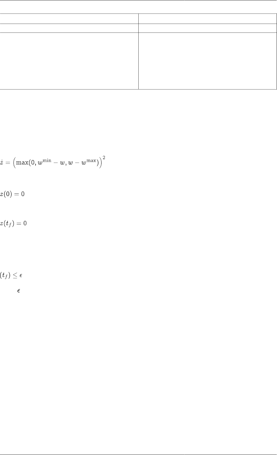
Inequality path constraints

It is worth noting that enforcing a path constraint at the interval boundaries does not automatically guarantee that

the constraints are not violated within the intervals. For many applications, this is not a major problem as path

constraints tend to be "soft'' and minor violations can be tolerated. However, if this is not the case, a more stringent

way of enforcing the constraint is to define a violation variable z within the relevant Model entity in the gPROMS

project through the equation:

with initial condition,

and then impose the additional end-point equality constraint:

It can be verified that this end-point equality constraint can be satisfied if and only if the original path constraint

is satisfied. In many cases, it is still worthwhile retaining the Interiorpoint constraints on w as this often leads to

improved numerical performance. It may also be better to relax the end-point equality constraint to an inequality

constraint:

where is a small positive tolerance. An implementation of path constraints is shown for the batch reactor

example in the Reactor Model entity, the Initial section of the OPTIMISE_REACTOR Process entity, and the

OPTIMISE_REACTOR Optimisation entity.

Point Optimisation

By default, gPROMS treats optimisation problems as dynamic ones, optimising the behaviour of a system over

a finite non-negative time horizon. However, in some cases, it is desired to optimise a system at a single time

point—performing a so-called "point" optimisation. From the mathematical point of view, this is equivalent to

solving a purely algebraic problem in which a generally nonlinear objective function is maximised or minimised

subject to generally nonlinear constraints by manipulating a set of optimisation decision variables that may be

either continuous or discrete.

Specification of point Optimisation Entities

The specification of a point optimisation problem in gPROMS is achieved simply by omitting the HORIZON part

of the corresponding Optimisation Entity. One can also use the following language to specify a point optimisation:

OPTIMISATION_TYPE

POINT

Dynamic Optimisation in gPROMS

It is worth noting that point Optimisation Entities:

• may contain TIME_INVARIANT controls as well as ENDPOINT_INEQUALITY and

ENDPOINT_EQUALITY constraints; such constraints are interpreted as simple algebraic constraints to be

satisfied by the optimal solution;

• must not contain time-varying controls PIECEWISE_CONSTANT or PIECEWISE_LINEAR ones or

constraints, or specifications of control Intervals, all of which are meaningless in this context.

Moreover,

• the value of the global TIME variable used in any Assignments in the corresponding Process Entity is taken

to be zero;

• any Initial conditions specified in corresponding Process Entity are taken as additional equality constraints to

be satisfied by the optimisation.

Note that, for the purposes of point optimisation, any time derivative terms of the form $x, that may occur in

gPROMS Model Entities, are treated as distinct to the variables x.

Specification of steady-state optimisation problems

A steady-state optimisation problem is a special case of a point optimisation one. As such, its specification must

obey all the rules outlined in: point optimisation entities.

If the underlying model is a dynamic one (i.e. its Model Entities contain one or more time derivative terms of

the form $x) , then the initial-condition of the system must be specified as STEADY_STATE in the Initial section

of the Process Entity.

It may be considerably easier to initialise complex models from a given set of initial conditions and to integrate

until steady state is obtained (rather than initialising using the STEADY_STATE initial condition). In these cases,

a special type of optimisation can be performed by using the SSOptTR solver and specifying:

OPTIMISATION_TYPE

STEADY_STATE

in the Optimisation entity (and omitting the HORIZON and INTERVALS sections).

The SSOptTR solver is selected in one of two ways, depending on the type of problem being solved:

• Continuous variables only

• use the Solution Parameters tab to specify the value of the MINLPSolver Parameter to be SSOptTR; or

• specify the following in the SOLUTIONPARAMETERS section of the Process

DOSolver := "CVP_SS" [

"MINLPSolver" := "SSOptTR"

]

• Mixed integer optimisation

• use the Solution Parameters tab to specify the value of the MINLPSolver Parameter to be OAERAP and the

value of its NLPSolver Parameter to be SSOptTR; or

• specify the following in the SOLUTIONPARAMETERS section of the Process

DOSolver := "CVP_SS" [

"MINLPSolver" := "OAERAP" [

"NLPSolver" := "SSOptTR"

]

Dynamic Optimisation in gPROMS

Finally, the time horizon needs to be specified. A simulation experiment can be performed to identify how long is

required for steady state to be established. This value is then specified using the TimeRelaxationHorizon Solution

Parameter for SSOptTR. This can be done using the Solution Parameters tab or by specifying the following in

gPROMS language (for a continuous problem):

SOLUTIONPARAMETERS

DOSolver := "CVP_SS" [

"MINLPSolver" := "SSOptTR" [

"TimeRelaxationHorizon" := 20000.0

]

The default value is 20000, but can be anything from 10-20 to 1020 depending on the problem.

The SSOptTR solver takes advantage of nature of the steady-state optimisation problem to increase the

performance of the optimisation relative to a full dynamic optimisation. One of the largest computation overheads

associated with dynamic optimisation is the integration of the sensitivity equations, which provide the optimiser

with the gradients of the constraints and objective function with respect to the decision variables. For steady-state

optimisations, SSOptTR need not perform these expensive sensitivity integrations until the steady-state solution

has been found, thus significantly reducing the computational effort.

Another feature of the steady-state optimisation problem that can be exploited relates to reinitialisation. In a

dynamic optimisation problem, the system needs to be reinitialised for every minor optimisation iteration (where

the decision variables are optimised along a fixed search direction) and this means reinitialising using the initial

conditions and performing a full sensitivity integration each time. The SSOptTR solver can simply use the steady-

state solution from the last minor iteration to reinitialise the problem and then perform the sensitivity evaluation,

thus avoiding the more complex initialisation and sensitivity integration. This behaviour can be controlled using

the following Solution Parameter:

"MINLPSolver" := "SSOptTR" [

"TimeRelaxationInitialConditions" := "MAJOR"

]

The three possible values are

•INITIAL: all reinitialisations are performed using the initial conditions and initial values (PRESET) specified

in the Process;

•MAJOR (default): reinitialisations are performed using the solution of the last successful major iteration as the

initial guess (each major iteration determines a new search direction for the decision variables);

•MINOR: reinitialisations are performed using the solution of the last successful minor iteration as the initial

guess.

Although the reinitialisation strategies outlined above can significantly reduce the solution time of steady-state

optimisation problems, there may be cases where the integration to obtain steady-state during the initial iteration

is difficult and time consuming. This behaviour can occur if there are Selector Variables in the Model and these

switch many times during the integration from the initial condition to the steady state. In such cases, the expensive

initial integration can be bypassed by using Saved Variable Sets to specify the steady-state solution, thus further

reducing the solution time. A Saved Variables Set can be specified for use in the optimisation by including the

following command:

RESTORE "Filename"

where Filename is the name of a Saved Variable Set. It is also possible to specify more than one Saved Variable

Set: this can be done by including several RESTORE commands and/or by providing a list of Saved Variable Sets

to a single RESTORE command. For example:

RESTORE "Filename1", "Filename2", "Filename3"

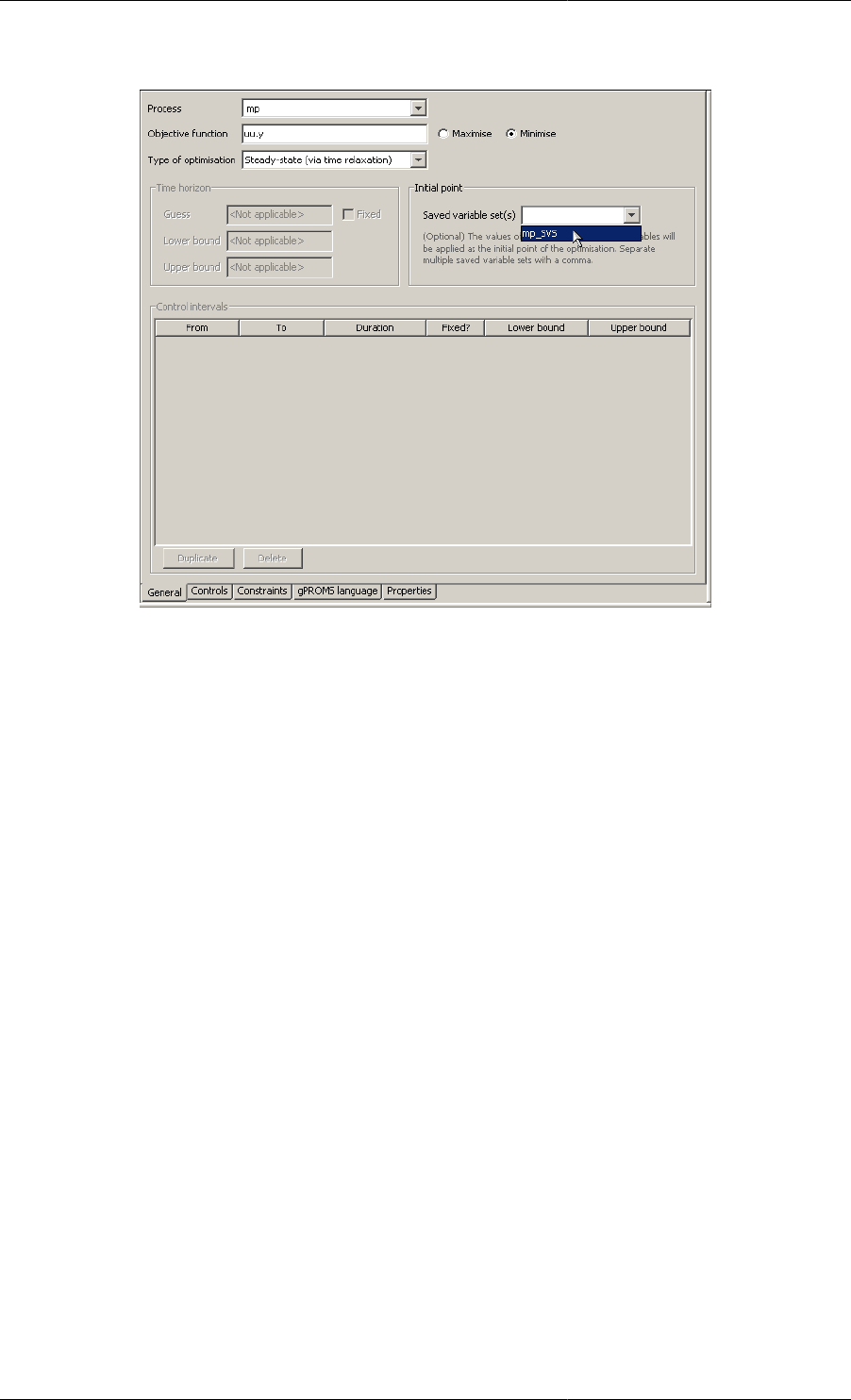
The Saved Variable Sets may also be specified using a ComboBox in the Optimisation entity. This will contain all

of the Saved Variable Sets in the Project and one can select one of them for use in the steady-state optimisation.

Dynamic Optimisation in gPROMS

Figure 2.4. Selecting a Saved Variable Set for use in a steady-state optimisation

The Saved Variable Set can be selected by using the mouse or by typing in the name in the ComboBox (where

CTRL+space may be used to autocomplete the selection).

During initial iteration, the SSOptTR solver will first initialise the system using the initial conditions specified in

the Process. Once complete, the RESTORE will be performed: all differential and Selector Variables in the system

that are present in the SavedVariableSet will be restored and the system reinitialised. This will be used as the initial

point of the time trajectory used for the steady-state optimisation. When performing mixed integer optimisation,

this procedure is applied only to the initial relaxed NLP problem.

To summarise, there are two ways to perform a steady-state optimisation:

• If the model solves quickly and is robust using the STEADY_STATE initial condition, then

• perform a Point optimisation by specifying

OPTIMISATION_TYPE

POINT

in the Optimisation entity, omitting the HORIZON and INTERVALS sections and do not use the SSOptTR

solver;

• otherwise,

• perform a Steady-State optimisation by specifying

OPTIMISATION_TYPE

STEADY_STATE

in the Optimisation entity, omitting the HORIZON and INTERVALS sections and using the SSOptTR solver.

Specify the horizon required for steady state to be reached using the TimeRelaxationHorizon Solution

Parameter of the SSOptTR solver.

Dynamic Optimisation in gPROMS

Running optimisation problems in gPROMS

As explained in: specifying dynamic optimisation problems, before an optimisation problem can be executed, it

must be specified completely in a gPROMS project that contains:

• one or more Model entities;

• a Process entity named, for example, ppp; and

• an Optimisation entity named ppp.

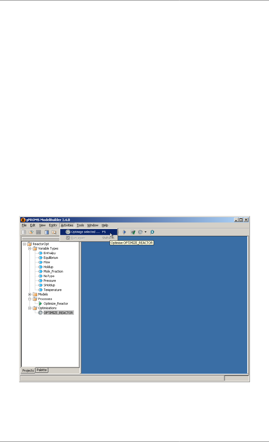
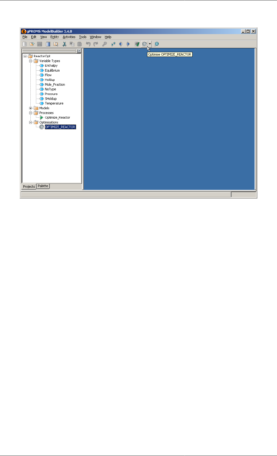
In order to run the optimisation problem:

1. Select the Optimisation entity in the gPROMS project tree.

2. Either:

a. pull down the Activities menu from the top toolbar and select Optimise;

b. left click on the optimise button on the toolbar below.

3. If there are any syntactical, cross-referencing mistakes etc. these will be detected. Otherwise, the gRMS and

execution windows are opened by gPROMS, the optimisation run starts and output is directed to the screen

of the execution window.

Figure 2.5. Executing an optimisation run via the Activities menu.

Dynamic Optimisation in gPROMS

Figure 2.6. Executing an optimisation run via the Optimisation button.

Results of the optimisation run

The execution of an optimisation run will generate five files in the Results folder of the Case:

•PPP

•PPP.out

•PPP.SCHEDULE

•PPP_SVS

•PPP.point

where PPP is the name (in capitals) of the optimisation entity that has been executed to produce these results (cf.

running optimisation problems).

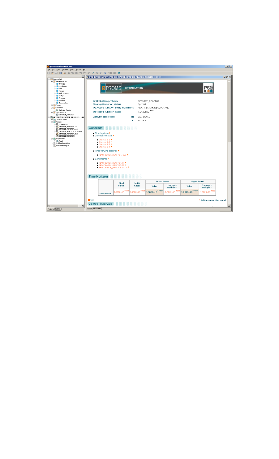
The comprehensive optimisation report file

Double-clicking on the report entry, PPP, in the Case tree causes a report window to appear in the main window,

see the figure below. The report, presented in HTML format, includes:

• a table of contents that allows quick access to the information listed below via "hyperlinks";

• general information such as the date and time of the execution of the activity, its final status and the value of

the objective function;

• information on the various optimisation decision variables (time horizon, control interval durations, and time-

invariant and time-varying controls), including the values of:

• the initial guess used,

• the final value obtained,

Dynamic Optimisation in gPROMS

• the lower and upper bounds,

• the Lagrange multipliers corresponding to the above bounds.

All active bounds are automatically highlighted.

Figure 2.7. Comprehensive optimisation report.

The optimisation report file

The PPP.out file contains a summary report on the optimisation run in a simple text format, including:

• the outcome of the optimisation run;

• the final value of the objective function;

• the final value of the time horizon and the lengths of the time intervals;

• the final values of the time-invariant parameters, and the control-variable profiles; the latter are specified in

terms of a single value per interval for piecewise-constant controls, and a pair of values for piecewise-linear

controls (as usual, corresponding to the value of the control at the start and end of each interval); and

• the values of variables on which end-point and/or interior-point constraints where specified, at the corresponding

final and/or interior-points.

The file also contains computational statistics on the performance of the numerical method.

A sample PPP.out file is listed in the dynamic optimisation example at the end of this guide.

The SCHEDULE file and the Saved Variable Set

The PPP.Schedule presents the most recent optimisation solution point in the form of a gPROMS Schedule. A

sample PPP.SCHEDULE file is listed in the dynamic optimisation example at the end of this guide.

The Schedule file can be used to reproduce the detailed results of the optimisation by carrying out a simulation

activity within gPROMS. This provides you access to the full facilities of the gPROMS Results Management.

Once the final solution of an optimisation problem is obtained, gPROMS creates a Saved Variable Set from the

initialisation of this point. The Saved Variable Set is called PPP_SVS and is used in the SCHEDULE to restore

the exact conditions at the final point.

Dynamic Optimisation in gPROMS

In order to do this:

1. Paste the contents of the Schedule file into the relevant Process entity of your gPROMS project.

2. Copy the generated Saved Variable Set from the result Case into the gPROMS project.

A optimal Process entity that contains these changes is shown for the batch reactor example. It is useful for you

to compare it with the original Process entity and the Schedule results file.

Note

The contents of the Schedule file does not always represent an optimal or even a feasible solution to the

problem: if the optimisation run is interrupted by the user, or ends without finding a satisfactory solution,

the file will simply show the point last considered by gPROMS. Only if a comment at the top of the file

states the following:

# Final Optimisation Status : Optimal Solution Found

should the results be relied upon as a (locally) optimal solution.

The point file

The PPP.point file is generated at every iteration of the optimisation calculation. It contains the same information

as the Schedule file, but in the format of an Optimisation entity (except that constraints are not reproduced). This

is useful if there is a need to restart an optimisation after a system crash or other catastrophic event, or, following

a successful solution, to provide a good 'initial guess' for a slightly altered optimisation problem.

A sample PPP.point file is listed in the dynamic optimisation example at the end of this guide.

Other features

The following apply to the current version of gPROMS:

• The initial conditions specified in the Process entity must be:

• equations of the form:

VariableName = Value ;

where VariableName is the full gPROMS pathname of a differential or algebraic variable, and Value is a

numerical value;

• or equations of the form:

$VariableName = Value ;

• or the steady-state specification:

INITIAL

STEADY_STATE

• Many applications involve the optimisation of the initial values of some of the system variables. For instance,

it may be that you want to determine the optimal initial amount of catalyst to be charged to a batch reactor. This

kind of requirement can easily be accommodated as follows:

• In the Model entity containing the variable, z, whose initial value is to be optimised, introduce:

• an additional variable,z0, of the same type as z;

•an additional variable, , of type NoType;

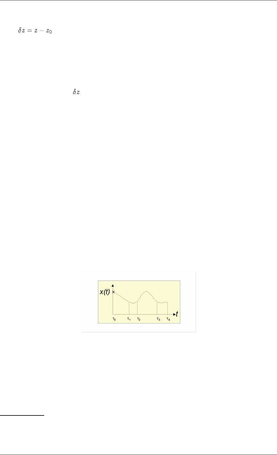
Dynamic Optimisation in gPROMS

• the additional equation:

• In the Process entity,

• assign z0 to a default value:

ASSIGN

Z0 := 1.0 ;

•set the initial value of to zero:

INITIAL

\DeltaZ = 0.0 ;

• In the Optimisation entity, declare z0 as a time-invariant parameter, specifying an initial guess and lower and

upper bounds for it.

Standard solvers for optimisation

There are two standard mathematical solvers for optimisation in gPROMS, namely CVP_SS and CVP_MS.

CVP_SS can solve optimisation problems with both discrete and continuous decision variables ("mixed integer

optimisation"). Both steady-state and dynamic problems are supported. CVP_MS can solve dynamic optimisation

problems with continuous decision variables.

For dynamic optimisation problems, both CVP_SS and CVP_MS are based on a control vector parameterisation

(CVP) approach which assumes that the time-varying control variables are piecewise-constant (or piecewise-

linear) functions of time over a specified number of control intervals. The precise values of the controls over

each interval, as well as the duration of the latter, are generally determined by the optimisation algorithm4. As

the number of control variables is usually a small fraction of the total number of variables in the problem, the

optimisation algorithm has to deal only with a relatively small number of decisions, which makes the CVP

approach applicable to large problems.

Figure 2.8. Single-shooting algorithm

The CVP_SS solver implements a "single-shooting'' dynamic optimisation algorithm. This involves the following

steps (see the figure above):

1. the optimiser chooses the duration of each control interval, and the values of the control variables over it;

2. starting from the initial point at time t=0 (shown as a cross on the vertical axis in the figure, the dynamic system

model is solved over the entire time horizon to determine the time-variation of all variables x(t) in the system;

3. the above information is used to determine the values of5:

4In addition, as explained earlier in this guide, many dynamic optimisation problems involve time-invariant parameters that also have to be

chosen by the optimiser.

5In practice, the solution of the model also needs to determine the values of the partial derivatives (sensitivities) of the objective function and

constraints with respect to all the quantities specified by the optimiser.

Dynamic Optimisation in gPROMS

• the objective function to be optimised;

• any constraints that have to be satisfied by the optimisation;

4. based on the above, the optimiser revises the choices it made at the first step, and the procedure is repeated

until convergence to the optimum is achieved.

The term "single-shooting'' arises from the second step in the above algorithm which involves a single integration

of the dynamic model over the entire horizon.

Figure 2.9. Multiple-shooting algorithm

The CVP_MS solver implements a "multiple-shooting'' dynamic optimisation algorithm with the following steps

(see the figure above):

1. the optimiser chooses the duration of each control interval, the values of the control variables over it, and,

additionally, the values of the differential variables x(t) at the start of each control interval other than the first

one (shown as solid circles in the figure);

2. for each control interval, starting from the initial point that is either known (for the first interval) or is chosen

by the optimiser (for all subsequent intervals), the dynamic system model is solved over this control interval

to determine the time-variation of all variables x(t) in the system;

3. the above information is used to determine the values of:

• the objective function to be optimised;

• any constraints that have to be satisfied by the optimisation;

• the discrepancies between the computed values of the variables x(t) at the end of each interval and the

corresponding values chosen by the optimiser at the start of the next interval;

4. based on the above, the optimiser revises the choices it made at the first step, and repeats the above procedure

until it obtains a point that:

• optimises the objective function;

• satisfies all constraints;

• ensures that all differential variables x(t) are continuous at the control interval boundaries.

The "multiple-shooting'' term reflects the fact that each control interval is treated independently at the second step

above.

Both solvers, by default, employ the DASOLV code (details in the Model Developer Guide) for the solution of

the underlying DAE problem and the computation of its sensitivities. In principle, this can be replaced by a third-

party solver with similar capabilities.

The choice between the CVP_SS and CVP_MS solvers for any dynamic optimisation problem depends primarily

on the number of optimisation decision parameters that the algorithm has to deal with in computing the sensitivities

of the model variables. In principle:

Dynamic Optimisation in gPROMS

• CVP_MS should normally be preferred for problems with many time-varying control variables and/or many

control intervals, but with relatively few differential ("state'') variables;

• CVP_SS should normally be preferred for large problems (potentially involving several hundreds or thousands

of differential ("state'') variables) but with relatively few time-varying control variables and control intervals.

In practice, some experimentation may be required to determine the better algorithm for any particular application.

The DOsolver solution parameter may be used to change and/or configure the solver used for optimisation

activities. If this parameter is not specified, then the CVP_SS solver is used, with the default configuration. See

also: CVP_SS solver.

The CVP_SS solver

CVP_SS can solve steady-state and dynamic optimisation problems with both continuous and discrete optimisation

decision variables. The algorithmic parameters used by CVP_SS along with their default values are shown below.

This is followed by a detailed description of each parameter.

"CVP_SS" [ "DASolver" := "DASOLV";

"MINLPSolver" := "OAERAP"];

DASolver - A quoted string specifying a differential-algebraic equation solver.

• The solver to be used for integrations of the model equations and their sensitivity equations at each iteration of

the optimisation. This can be either the standard DASOLV solver or a third-party differential-algebraic equation

solver (see the gPROMS System Programmer Guide). The default is DASOLV.

This parameter can be followed by further specifications aimed at configuring the particular solver by setting

values to its own algorithmic parameters (see also: specifying solver-type algorithmic parameters in the Model

Developer Guide).

MINLPSolver - A quoted string specifying a mixed integer optimisation solver.

• The solver to be used for mixed integer optimisation problems. This can be either the standard OAERAP

solver or a third-party mixed integer optimisation solver (see the gPROMS System Programmer Guide).

For optimisation problems that do not involve any discrete decision variables, this can be any CAPE-OPEN

compliant solver that is capable of solving NLPs but not MINLPs, e.g. the standard NLP solver SRQPD. The

default is OAERAP.

This parameter can be followed by further specifications aimed at configuring the particular solver by setting

values to its own algorithmic parameters (see also: specifying solver-type algorithmic parameters in the Model

Developer Guide).

The OAERAP solver

The OAERAP solver employs an outer approximation (OA) algorithm for the solution of the MINLP. As outlined

in the algorithm below, this involves solving a sequence of simpler optimisation problems, including nonlinear

programs (NLPs) at steps 1 and 3 and mixed integer linear programs (MILPs) at step 2. The OAERAP code has

been designed so that it can make direct use of any CAPE-OPEN compliant NLP and MILP solvers (see the

gPROMS System Programmer Guide) without the need for any additional interfacing or modification.

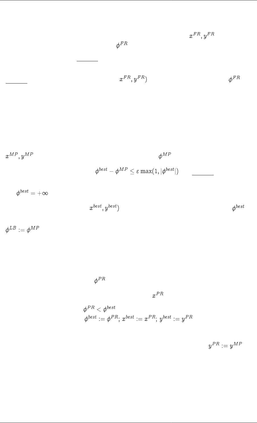
Outline of the OAERAP algorithm for the solution of a MINLP problem (minimisation case)

Given initial guesses for all optimisation decision variables, both discrete (y) and continuous (x):

Step 0: Initialisation

•Set the objective function of the best solution that is currently available, .

•Set the objective function of the best solution that may be obtained, .

Dynamic Optimisation in gPROMS

Step 1: Solve fully relaxed problem

• Solve a continuous optimisation problem (NLP) treating all discrete variables as continuous (i.e. allow them to

take any value between their lower and upper bounds) to determine optimal values of the optimisation

decision variables and of the objective function, .

• If above problem is infeasible, terminate: original problem is infeasible as posed.

• If all discrete optimisation decision variables have discrete values at the solution of the above problem, then

terminate: optimal solution of original problem is with an objective function value of .

Step 2: Solve master problem

• Construct a mixed integer linear programming (MILP) problem which:

• involves appropriate linearisations of the objective function and the constraints carried out at the solutions

of all continuous optimisation problems solved so far,

• excludes all combinations of discrete variable values that have been considered at step 2 so far.

• Solve the above MILP problem to determine optimal values of both the continuous and discrete variables

, and the corresponding value of the objective function .

•If the above problem is infeasible or if , then terminate: there are no more

combinations of discrete variables that can be usefully considered.

•If , then original problem was infeasible.

•Otherwise, the optimal solution is with a corresponding objective function value of .

• The MILP provides an improved bound on the best solution that may be obtained; therefore, update

Step 3: Solve primal optimisation problem

• Fix all discrete optimisation decision variables to their current values.

• Solve continuous optimisation problem (NLP) to determine:

•optimal value of objective function, ;

•optimal values of continuous optimisation decision variables, .

•If the above NLP is feasible and , then an improved solution to the original problem has been

found; record its details by setting .

Step 4: Iterate

•Set the next set of values of the discrete optimisation decision variables to be considered .

• Repeat from step 2.

The OAERAP solver also includes an equality relaxation (ER) scheme for handling equality constraints. It should

be emphasised that, in the case of optimisation problems defined in gPROMS, this relaxation is applied only to

any ENDPOINT_EQUALITY constraints that may appear in the Optimisation Entity.

The algorithm described above is guaranteed to obtain the globally optimal solution to the optimisation problem

posed only if the latter is convex. This is unlikely to be the case in many problems of engineering interest.

Dynamic Optimisation in gPROMS

An augmented penalty (AP) strategy is employed in order to increase the probability of a global solution being

obtained.

The algorithmic parameters used by OAERAP along with their default values are shown below. This is followed

by a detailed description of each parameter.

"OAERAP" ["MILPSolver" := "LPSOLVE",

"NLPSolver" := "SRQPD",

"MaxIterations" := 10000,

"NLPSubProblemInitialGuesses" := "MILPMasterProblem",

"OptimisationTolerance" := 1.0E-4,

"OutputLevel" := 0]

MILPSolver - A quoted string specifying a mixed integer linear programming solver.

• Specifies a CAPE-OPEN compliant solver to be used for the solution of the mixed integer linear programming

(MILP) problems at step 2 of the algorithm described above.

NLPSolver - A quoted string specifying a nonlinear programming solver.

• Specifies a CAPE-OPEN compliant solver to be used for the solution of the nonlinear programming (NLP)

problems at steps 1 and 3 of the algorithm described above.

MaxIterations - An integer in the range [1, 100000].

• The maximum number of iterations involving step 2-4 of the algorithm described above. This is essentially the

maximum number of distinct alternatives to be considered by the algorithm

NLPSubProblemInitialGuesses - either "MILPMasterProblem" or "FullyRelaxedNLP"

• Determines the source of initial guesses for the NLP Primal Optimisation.

The OAERAP algorithm employs two methods of obtaining initial guesses for the NLP Primal Problems (step

3 above).

The first is to use the solution of the fully-relaxed problem (step 1) as initial guesses for the solution of the

primal problem (step 3) at each iteration. To use this method, specify "NLPSubProblemInitialGuesses" :=

"FullyRelaxedNLP".

An alternative approach is to use the solution of the MILP master problem, at the current iteration, to

provide the initial guesses for the NLP primal problem. This is the default method, specified by setting

"NLPSubProblemInitialGuesses" := "MILPMasterProblem".

The method that will be most effective will depend on the problem being solved. One advantage of obtaining

initial guesses from the MILP master problem is that because the discrete variables in the NLP problem will

be set to the values in the solution of the MILP, the values of the continuous variables will be consistent with

the discrete ones and so should provide a good initial guess for the NLP problem. A common example of this

behaviour is process synthesis problems, where binary variables can be used to represent the existance of a

process in a flowsheet. If the solution of an MILP implies that a unit does not exist, then the MILP of step 2 will

force some related continuous variables (e.g. the flows through these units) to be zero and these are, of course,

excellent initial guesses for the NLP problem (by contrast, these might not be zero in the solution of the fully-

relaxed NLP). However, if the problem is highly non-linear, then the solution of the linearised equations in the

MILP may not be such a good initial guess for the NLP. In these cases, it may be better to use the solution of

the relaxed NLP as the initial guess for each NLP primal problem.

OptimisationTolerance - A real number in the range [0.0, 1.0].

• The optimisation tolerance used in the termination criterion at step 2 of the algorithm described above.

OutputLevel - An integer in the range [-1, 0].

• The amount of information generated by the solver. The following table indicates the lowest level at which

different types of information are produced:

Dynamic Optimisation in gPROMS

-1 (None)

0 Solution of fully relaxed point,

solution of master problem,

solution of primal optimisation problem,

final solution

The SRQPD solver

The SRQPD solver employs a sequential quadratic programming (SQP) method for the solution of the nonlinear

programming (NLP) problem. The algorithmic parameters used by SRQPD along with their default values are

shown below. This is followed by a detailed description of each parameter.

"SRQPD" [

"ConvergenceCriterion" := "ImprovedEstimateBased",

"HandleDiscreteVariables" := FALSE,

"InitialHessian" := 0,

"InitialLineSearchStepLength" := 1.0,

"MaxFun" := 10000,

"MaximumLineSearchSteps" := 20,

"MaxLineSearchStepLength" := 1.0,

"MinimumLineSearchStepLength" := 1.0E-5,

"NoImprovementTolerance" := 1.0E-12,

"OptimisationTolerance" := 0.0010,

"OutputLevel" := 0,

"Scaling" := 0

]

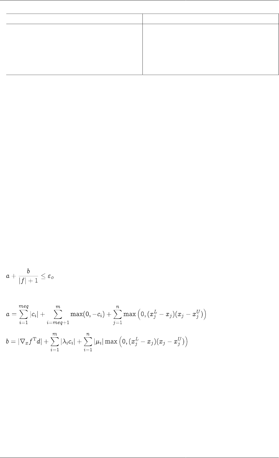
ConvergenceCriterion - Either "ImprovedEstimateBased" or "OptimalityBased"; default

"ImprovedEstimateBased".

• The "ImprovedEstimateBased" convergence criterion is:

where:

;

#o is the optimisation tolerance given by the Solution Parameter OptimisationTolerance;

f is the objective function;

c is the constraint vector (right-hand side);

meq is the number of equality constraints;

m is the total number of constraints;

n is the size of the variable vector x (i.e. the number of variables);

Dynamic Optimisation in gPROMS

and are the lower and upper bounds of variable xj;

d is the vector of corrections to x (i.e. the change in x during the current step);

is the Lagrange multiplier that corresponds to the equality constraint imposed on variable xj;

is the Lagrange multiplier that corresponds to the bound constraints imposed on variable xj.

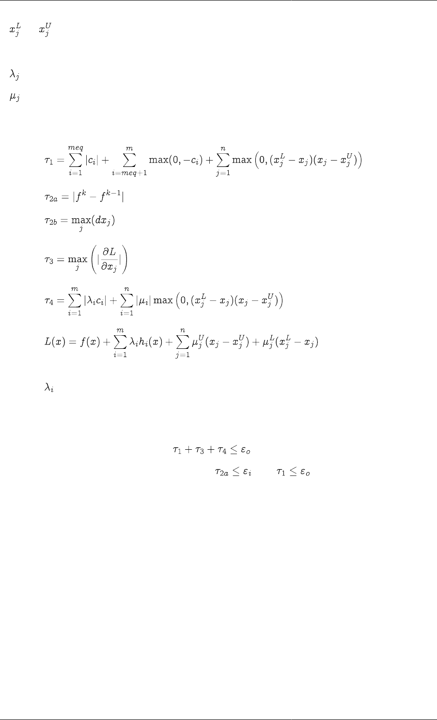
• The "OptimalityBased" convergence criterion uses two tolerances: #o, specified by the OptimisationTolerance

Solution Parameter and #i, specified by NoImprovement Tolerance. Given the following definitions:

;

, where k is the current iteration number;

, where dxj is the step calculated for xj in the latest line-search step;

;

is the Lagrange

function,

the Lagrange multipliers for the equality and inequality constraints

hi(x) and and the Lagrange multipliers for the upper and lower bound constraints;

the following tests are applied:

At the end of each major iteration: If , then terminate due to optimality;

Else if and , then terminate due to no-

improvement in the objective function.

At the end of each line-search step: If #2b ≤ #i and #1 ≤ #o, then terminate due to no-improvement in the

optimisation variables;

Else if #2b ≤ #i, then terminate due to failure to find a feasible point

within the non-improvement tolerance.

HandleDiscreteVariables - TRUE or FALSE; default FALSE.

• This parameter determines whether the solver handles mixed-integer non-linear optimisation problems by

transforming discrete controls into continuous ones.

InitialHessian - An integer in the range [0, 2]; default 0.

• By default, the initial hessian matrix is assumed to be the identity matrix (InitialHessian := 0).

• At present no other options are available but may be introduced in the future.

Dynamic Optimisation in gPROMS

InitialLineSearchStepLength - A real number in the range [10-10, 1.0]; default 1.0.

• The length of the line search step for the first optimisation iteration. An initial line search step length less than

1 is recommended when the initial approximation of the Hessian (i.e. identity matrix) is very different to the

actual values in the Hessian. This could result in a very large initial step and therefore several line search trials

before the optimiser finds a better point.

MaxFun - An integer in the range [0, 100000]; default 10000.

• The maximum number of optimiser function evaluations (i.e. solutions of the underlying steady-state or dynamic

model) to perform before halting the solution process (if no optimum has been found by that point).

MaximumLineSearchSteps - An integer in the range [1, 100]; default 20.

• The maximum number of line search steps in one optimisation iteration.

MaxLineSearchStepLength - A real number in the range [10-10, 1.0]; default 1.

• The maximum length of a line search step.

MinimumLineSearchStepLength - A real number in the range [10-10, 1.0]; default 10-5.

• The minimum length of a line search step.

NoImprovementTolerance - A real number in the range [10-20, 1.0]; default 10-12.

• The solution tolerance for non-improving objective function or optimisation variables. Only used when

ConvergenceCriterion := "OptimalityBased" (see above).

OptimisationTolerance - A real number in the range [10-20, 1.0]; default 0.001.

• The solution tolerance for the optimisation. Convergence is deemed to occur when a linear combination of the

gradients of the Lagrangian function on one hand, and the violation of the constraints on the other, drops below

this tolerance. The convergence criterion used is specified by the ConvergenceCriterion parameter described

above.

OutputLevel - An integer in the range [-1, 4]; default 0.

• The amount of information generated by the solver. The following table indicates the lowest level at which

different types of information are produced:

-1 (None)

0 Failed integrations and initialisations, optimisation

failure,

summary information from the SRQPD nonlinear

programming code,

final solution point and constraint values,

best available point after failure

1 Values of optimisation decision variables, objective

function and constraints in each major optimisation

iteration

2 Start and end times of each interval of integration,

optimisation decision variables and objective function

at each line search trial

3 Derivatives of objective function and constraints

Scaling - An integer in the range [0, 3]; default 0.

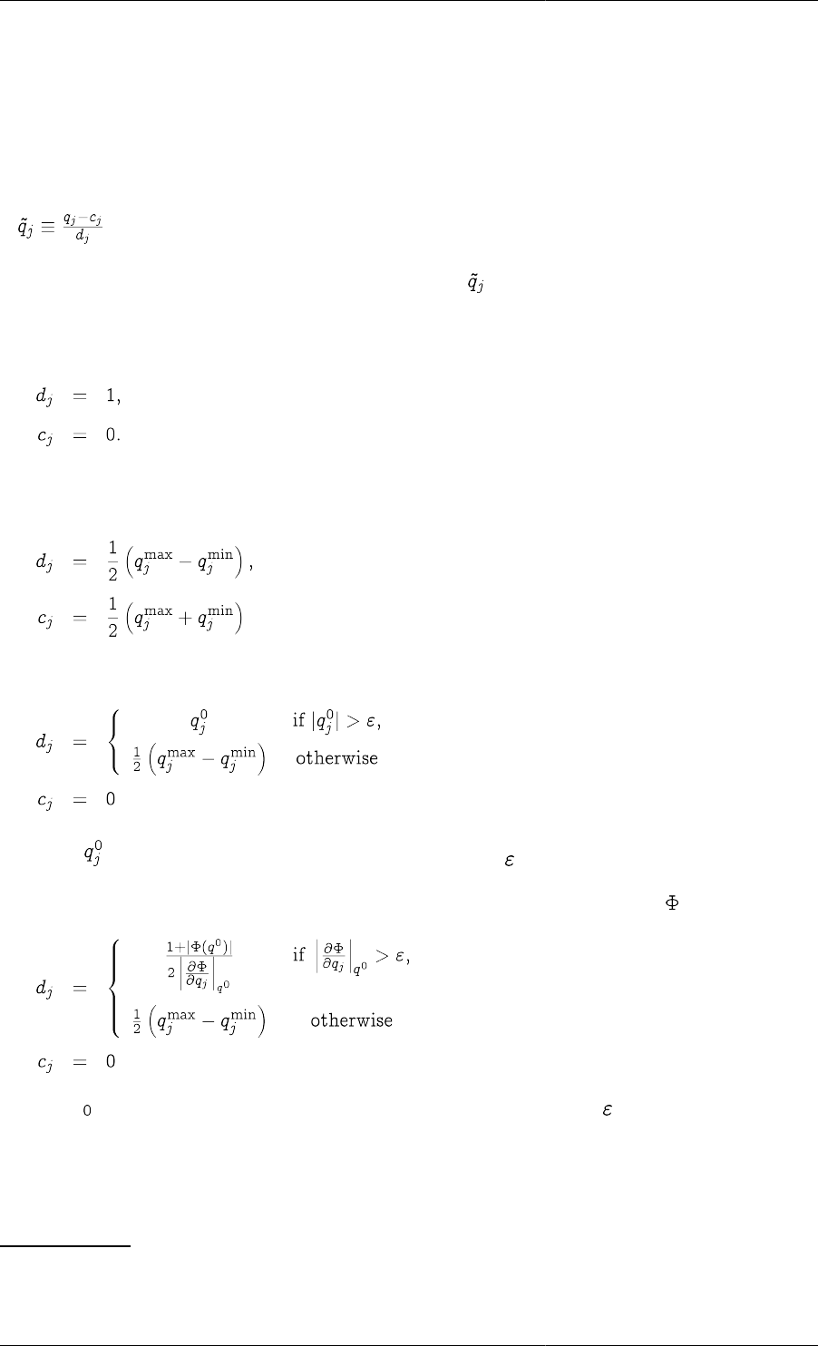
Dynamic Optimisation in gPROMS

• The form of scaling to be applied to the optimisation decision variables, including control variables, time-

invariant parameters, the length of the time horizon and the lengths of individual control intervals. These

decision variables may vary significantly in magnitude, which may adversely affect the performance of the

optimisation algorithms. Consequently, appropriate scaling of the optimisation decision variables is strongly

recommended6

The scaling performed is of the general mathematical form:

where qj is the jth original optimisation decision variable and is the corresponding scaled decision variable.

The constants cj and dj are determined automatically depending on the value of Scaling, as described below:

•Scaling = 0: No scaling (default).

•Scaling = 1: Scaling according to the ranges of the optimisation decision variables so that the scaled variables

vary between -1 and 1.

•Scaling = 2: Scaling according to the initial guesses of the optimisation variables.

where is the initial guess for the jth optimisation variable and is a small constant (currently set at 10-8).

•Scaling = 3: Scaling according to the value and the gradients of the objective function at the initial guess.

where is the vector of initial guesses of the optimisation decision variables and is a small constant (currently

set at 10-8).

The CVP_MS solver

The algorithmic parameters used by CVP_MS along with their default values are shown below. This is followed

by a detailed description of each parameter7

6A useful indication as to whether scaling is necessary is the condition number estimate that is printed out at each iteration of the optimisation

calculation. It is recommended that scaling be undertaken for problems with condition numbers exceeding 1010.

7For full details, please consult the information at http://www.systemtechnik.tu-ilmenau.de/fg_opt/omuses/omuses.html

Dynamic Optimisation in gPROMS

"CVP_MS" [ "OutputLevel" := 0;

"MaxFun" := 10000;

"SQPMinAlpha" := 1E-10;

"SQPHeLa" := "BFGS";

"SQPHeLaEps" := 1E-10;

"SQPHeLaScale" := TRUE;

"SQPHeLaEigenCtrl" := TRUE;

"SQPMaxIters" := 500;

"SQPMaxInfIters" := 10;

"SQPWatchdogStart" := 10;

"SQPWatchdogCredit" := 0;

"SQPWatchdogLogging" := FALSE;

"SQPSolver" := "Powell";

"SQPQPSolver" := "Franke";

"QPEps" := 1E-10;

"QPMatSolver" := "RedSpBKP";

"QPMaxIters" := 250;

"OptTol" := 1E-3;

"InfDefault" := 1E10;

"NumSen" := FALSE;

"SetBounds" := FALSE;

"NeedLagrangeMultipliers" := FALSE;

"DASolver" := "DASOLV"];

OutputLevel - An integer in the range [0, 4].

• The amount of information generated by the solver. The following table indicates the lowest level at which

different types of information are produced:

0 Failed integrations and initialisations, optimisation

failure,

summary information from the HQP nonlinear

programming code,

final solution point and constraint values,

best available point after failure

1 Values of optimisation decision variables, objective

function and constraints in each major optimisation

iteration

2 For each multiple-shooting interval in each major

optimisation iteration:

the values of the optimisation decision variables,

the values and derivatives of the matching conditions,

the constraints and the objective function.

MaxFun - An integer in the range [0, 100000].

• The maximum number of optimiser function evaluations (i.e. solutions of the underlying dynamic model) to

perform before halting the solution process (if no optimum has been found by that point).

SQPMinAlpha - A real number in the range [0, 105].

• Lower limit for the step length in the line search of the sequential quadratic programming (SQP) sub-solver.

SQPHeLa - A quoted string.

Dynamic Optimisation in gPROMS

• The method to be used for constructing the approximation of the Hessian matrix of the Lagrangian. Permitted

values are:

• "BFGS": partitioned BFGS update with Powell's damping

• "DScale": numerical approximation with a diagonal matrix

SQPHeLaEps - A real number in the range [0, 105].

• parameter used in SQP algorithm, see the Omuses document.

SQPHeLaScale - A boolean value.

• Use "DScale'' approach to initialise Hessian rather than setting it to the identity matrix.

SQPHeLaEigenCtrl - A boolean value.

• Control of positive definite Hessian blocks based on eigenvalues (only used with the BFGS method).

SQPMaxIters - An integer in the range [0, 100000].

• Total number of SQP iterations allowed.

SQPMaxInfIters - An integer in the range [0, 100000].

• Number of infeasible SQP iterations (i.e. points where the integration fails) allowed before failure.

SQPWatchdogStart - An integer in the range [0, 100000].

• Iteration at which to start watchdog algorithm if using "Powell" algorithm (see SQPSolver parameter below).

SQPWatchdogCredit - An integer in the range [0, 100000].

• Number of "bad'' iterations until backtracking and regular step are performed (0 means disable watchdog).

SQPWatchdogLogging - A boolean value.

• Specifies whether watchdog log output should be produced.

SQPSolver - A quoted string.

• The type of sequential quadratic programming (SQP) algorithm to be used for the optimisation. Permitted

values:

• "Powell"

• "Schittkowski"

SQPQPSolver - A quoted string.

• The type of quadratic programming (QP) solver to be used at each iteration of the optimisation. Permitted values

are:

• "Franke"

• "Mehrotra"

QPEps - A real number in the range [0, 105].

• The tolerance to which the quadratic programming sub-problems are to be solved.

Dynamic Optimisation in gPROMS

QPMatSolver - A quoted string.

• The matrix solver to use for the solution of the quadratic programming sub-problems in the optimisation.

Permitted values are (refer to Omuses document for details):

• "SpBKP"

• "RedSpBKP"

• "SpSC"

• "LQDOCP"

QPMaxIters - An integer in the range [0, 100000].

• Maximum number of QP iterations to attempt.

OptTol - A real number in the range [0.0, 1.0].

• The solution tolerance for the optimisation.

InfDefault - A real number in the range [0, 1035].

•Upper and lower bounds greater than this value in magnitude are treated as (as appropriate).

NumSen - A boolean value.

• Specifies whether sensitivities should be calculated numerically -- i.e. by repeated "normal'' integrations with

perturbed values -- rather than 'analytically', i.e. with a special sensitivity integration. Not recommended except

perhaps for large problems with very few parameters per interval.

DASolver - A quoted string specifying a differential-algebraic equation solver.

• The solver to be used for integrations of the model equations and their sensitivity equations at each stage and

each iteration of the optimisation. This can be either the standard DASOLV solver or a third-party differential-

algebraic equation solver (see the gPROMS System Programmer Guide). The default is DASOLV.

This parameter can be followed by further specifications aimed at configuring the particular solver by setting

values to its own algorithmic parameters (see also: specifying solver-type algorithmic parameters in the Model

Developer Guide).

Dynamic Optimisation Example

Here, an example of a dynamic optimisation is given using a batch-reactor Model.

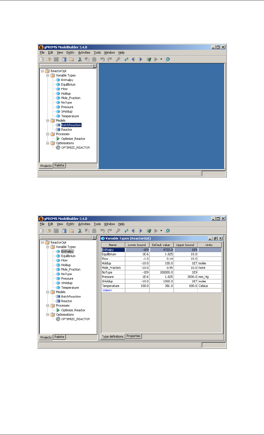
Dynamic Optimisation in gPROMS

Project tree ReactorOpt.gPJ

Figure 2.10. Project tree for the dynamic optimisation example.

Variable Type entities in ReactorOpt.gPJ

Figure 2.11. Variable Type entities in the ReactorOpt project.

Text contained within the Reactor Model entity

#---------------------------------------------------------------

# Model of an externally cooled batch reactor: A + B -> C + D

# The reactor model takes into account mass and energy balances.

#---------------------------------------------------------------

PARAMETER

NoComp AS INTEGER

Dynamic Optimisation in gPROMS

a,b,rho AS ARRAY (NoComp) OF REAL

nu AS ARRAY (NoComp) OF REAL

Ai,E,R,DH AS REAL

Tref AS REAL

VARIABLE

N,C,h AS ARRAY (NoComp) OF NoType

HR,Rate,V AS NoType

QcR,TR,K,Fcw AS NoType

Uacc,Tviol AS NoType

Obj AS NoType

EQUATION

# Component material balance

$N = V * Rate * nu ;

# Definition of reaction rate

Rate = K * C(1)* C(2) ;

# Rate constant

K = Ai * exp( - E / (R *TR) ) ;

# Energy balance

$HR = ( V * Rate * ( -DH ) ) - QcR ;

# Cooling load as a function of cooling water flowrate

QcR = 4200* 40 *Fcw ;

# Cumulative cooling water consumption

$Uacc= Fcw ;

# Definition of total enthalpy content of reactor

HR = sigma(N * h ) ;

# Pure component specific enthalpies

h = ( a * (TR - Tref ) + ( b * ( TR^2 - Tref^2 ) / 2 ) ) ;

# Relate molar concentrations C to component holdups N

V * C = N ;

# Volumetric holdup in reactor

V = sigma( N / rho ) ;

# Path constraint

$Tviol = MAX(TR - 450,0)^2 ;

# Objective to be maximised: value of product (3) - cooling water

Obj = 2*N(3) - Uacc ;

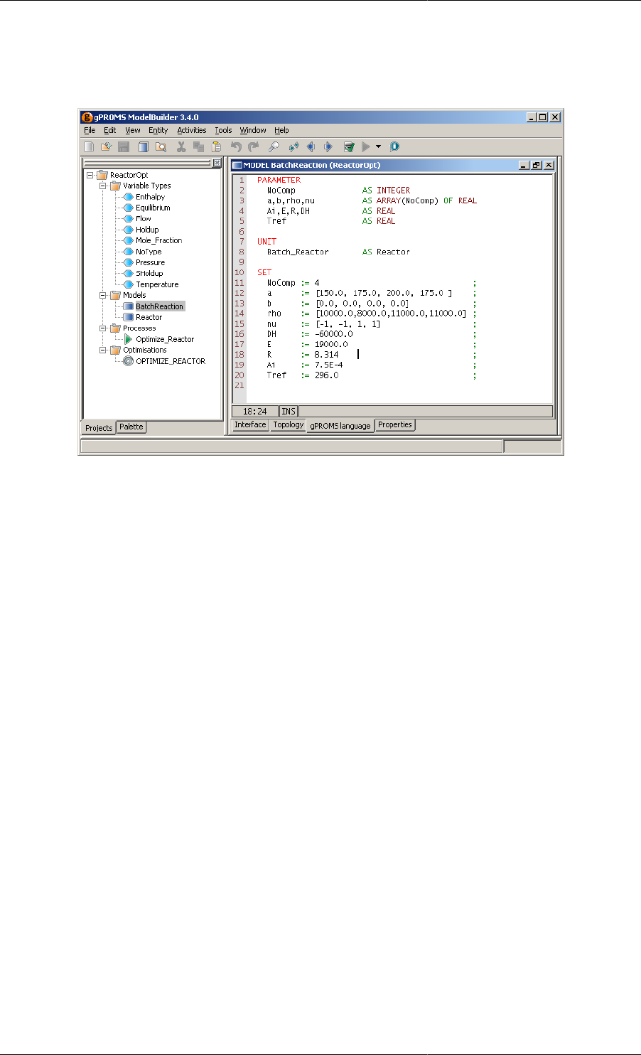
Dynamic Optimisation in gPROMS

BatchReaction Model entity

Figure 2.12. BatchReaction Model entity for the dynamic optimisation example.

Text contained within the OPTIMISE_REACTOR

Process entity

UNIT

React AS BatchReaction

ASSIGN

# This will be overridden in the Optimisation entity

WITHIN React.Batch_Reactor DO

FcW := 0.0 ;

END

PRESET

REACT.BATCH_REACTOR.RATE := 7.28422E+00 ;

REACT.BATCH_REACTOR.HR := 6.50000E+06 ;

REACT.BATCH_REACTOR.C(1) := 4.44444E+03 ;

REACT.BATCH_REACTOR.C(2) := 4.44444E+03 ;

REACT.BATCH_REACTOR.C(3) := 0.00000E+00 ;

REACT.BATCH_REACTOR.C(4) := 0.00000E+00 ;

REACT.BATCH_REACTOR.OBJ := 0.00000E+00 ;

REACT.BATCH_REACTOR.H(1) := 6.00000E+02 ;

REACT.BATCH_REACTOR.H(2) := 7.00000E+02 ;

REACT.BATCH_REACTOR.H(3) := 8.00000E+02 ;

REACT.BATCH_REACTOR.H(4) := 7.00000E+02 ;

REACT.BATCH_REACTOR.FCW := 0.00000E+00 ;

REACT.BATCH_REACTOR.K := 3.68763E-07 ;

REACT.BATCH_REACTOR.QCR := 0.00000E+00 ;

REACT.BATCH_REACTOR.V := 1.12500E+00 ;

INITIAL

WITHIN React.Batch_Reactor DO

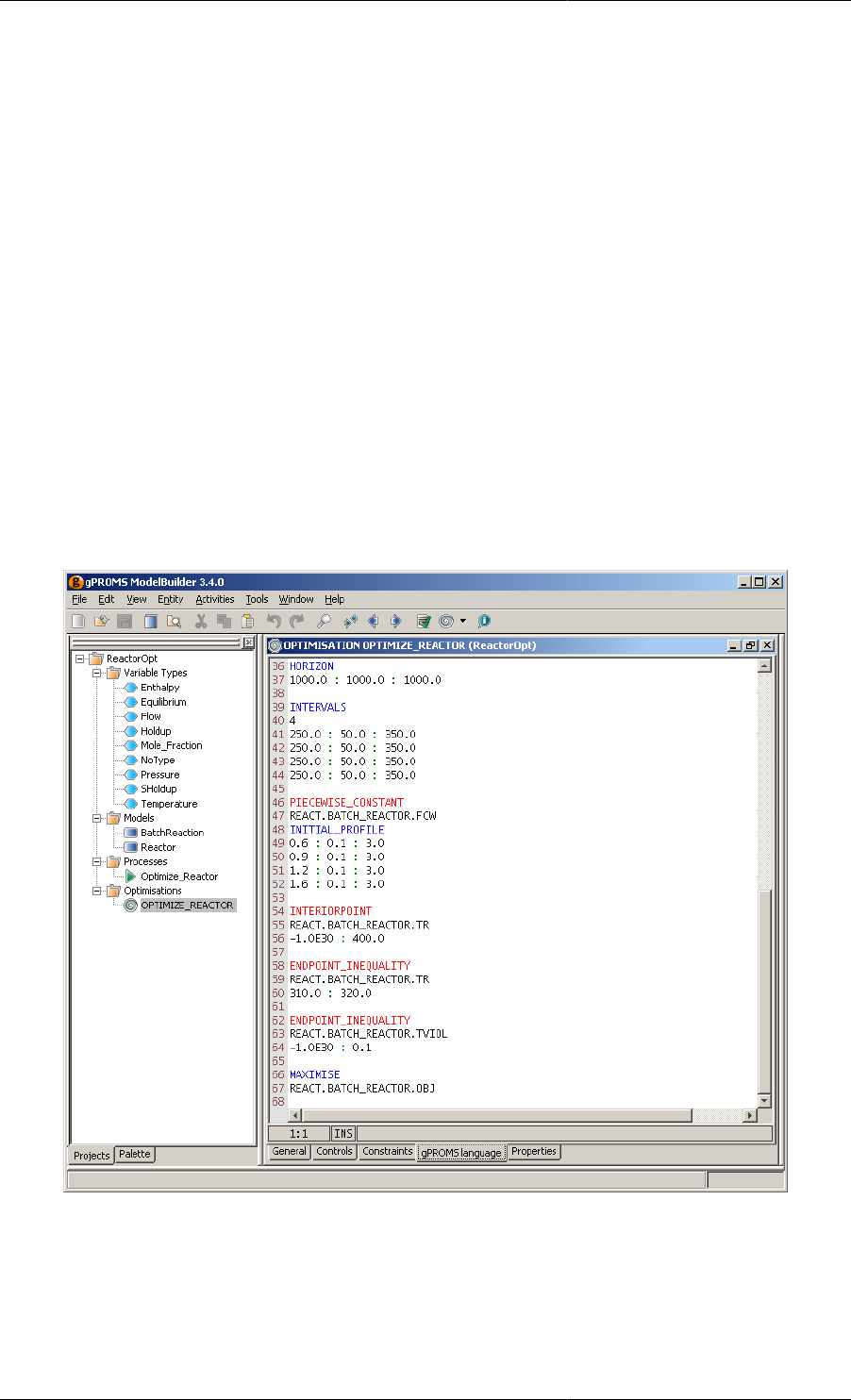
Dynamic Optimisation in gPROMS

N(1) = 5000.0 ;

N(2) = 5000.0 ;

N(3) = 0.0 ;

N(4) = 0.0 ;

TR = 300.0 ;

Uacc = 0.0 ;

Tviol = 0.0 ;

END

SOLUTIONPARAMETERS

ABSOLUTEACCURACY := 1.0E-6 ;

REPORTINGINTERVAL := 100 ;

SCHEDULE

# This will be ignored by the dynamic optimisation

SEQUENCE

CONTINUE FOR 2000

END

Optimisation entity (OPTIMISE_REACTOR)

Figure 2.13. Optimisation entity for the dynamic optimisation example.

Sample optimisation report file

(OPTIMISE_REACTOR.out)

Dynamic Optimisation in gPROMS

gPROMS Dynamic Optimisation

gPROMS Process : OPTIMIZE_REACTOR

Final Optimisation Status : Optimal Solution Found

Objective Function Being Maximised: 7642.78

Current Values of Optimisation Decision Variables

([*] denotes an active bound)

Decision Variable Type Value Lower Bound Upper Bound

Time horizon 1000 1000[*] 1000[*]

Control Interval # 1 249.718 50 350

Control Interval # 2 159.781 50 350

Control Interval # 3 288.055 50 350

Control Interval # 4 302.446 50 350

1. REACT.BATCH_REACTOR.FCW (piecewise constant)

Control

Interval Type Value Lower Bound Upper Bound

# 1 Continuous 0.1 0.1[*] 3

# 2 Continuous 1.84372 0.1 3

# 3 Continuous 0.554775 0.1 3

# 4 Continuous 3 0.1 3[*]

Current Values of Constrained Variables

([*] denotes violation of constraint)

Constrained Variable Type Time Value Lower Bound Upper Bound

REACT.BATCH_REACTOR.TR Interior 0 300 -1E+030 400

REACT.BATCH_REACTOR.TR Interior 249.718 394.578 -1E+030 400

REACT.BATCH_REACTOR.TR Interior 409.499 397.018 -1E+030 400

REACT.BATCH_REACTOR.TR Interior 697.554 398.378 -1E+030 400

REACT.BATCH_REACTOR.TR Endpoint 1000 320 310 320[*]

REACT.BATCH_REACTOR.TVIOL Endpoint 1000 0.100812 -1E+030 0.1[*]

Computational Statistics

Total CPU Time : 6.84375 seconds

CVP_SS Optimiser Statistics

CPU Time : 0.015625 seconds (0.228311 % of total time)

Number of MINLP Iterations : 0

Number of NLP Iterations : 61

Number of NLP Line Search Steps : 72

DASOLV Integrator Statistics

CPU Time : 5.23438 seconds (76.484018 % of total time)

CPU Time Spent on State Integration Only : 1.9375 seconds (37.014925 % of DASOLV time)

16292 steps, 30038 residuals : 0.546875 seconds

4140 Jacobians : 0.109375 seconds

Dynamic Optimisation in gPROMS

CPU Time Spent on Sensitivity Integration Only : 3.29688 seconds (62.985075 % of DASOLV time)

13674 steps, 37422 residuals : 0.328125 seconds

17198 Jacobians : 0.5 seconds

Mean (Sensitivity+State)/(State) CPU Ratio : 2.70161

Sample gPROMS schedule file

(OPTIMISE_REACTOR.SCHEDULE)

# Schedule generated by gOPT for process OPTIMIZE_REACTOR

# Final Optimisation Status : Optimal Solution Found

# Objective Function Being Maximised: 7642.78

SCHEDULE

SEQUENCE

PARALLEL

RESTORE "OPTIMIZE_REACTOR_SVS" ;

RESET

REACT.BATCH_REACTOR.FCW := 0.1;

END

CONTINUE FOR 249.718

RESET

REACT.BATCH_REACTOR.FCW := 1.84372;

END

CONTINUE FOR 159.781

RESET

REACT.BATCH_REACTOR.FCW := 0.554775;

END

CONTINUE FOR 288.055

RESET

REACT.BATCH_REACTOR.FCW := 3;

END

CONTINUE FOR 302.446

Dynamic Optimisation in gPROMS

END

Sample point file (OPTIMISE_REACTOR.point)

# .gOPT segment generated by gOPT for process OPTIMIZE_REACTOR

# at final solution.

HORIZON

1000 : 1000 : 1000

INTERVALS

249.718 : 50 : 350

159.781 : 50 : 350

288.055 : 50 : 350

302.446 : 50 : 350

PIECEWISE_CONSTANT

REACT.BATCH_REACTOR.FCW

INITIAL_PROFILE

0.1 : 0.1 : 3

1.84372 : 0.1 : 3

0.554775 : 0.1 : 3

3 : 0.1 : 3

Simulating the optimal solution within a Process

UNIT

React AS BatchReaction

ASSIGN

{ This was the previous ASSIGN section

# This will be overridden in the Optimisation entity

WITHIN React.Batch_Reactor DO

FcW := 0.0 ;

END

}

# This is the new one using the first RESET statement

# from the SCHEDULE file

REACT.BATCH_REACTOR.FCW:= 1.00000E-01;

PRESET

REACT.BATCH_REACTOR.RATE := 7.28422E+00 ;

REACT.BATCH_REACTOR.HR := 6.50000E+06 ;

REACT.BATCH_REACTOR.C(1) := 4.44444E+03 ;

REACT.BATCH_REACTOR.C(2) := 4.44444E+03 ;

REACT.BATCH_REACTOR.C(3) := 0.00000E+00 ;

REACT.BATCH_REACTOR.C(4) := 0.00000E+00 ;

REACT.BATCH_REACTOR.OBJ := 0.00000E+00 ;

REACT.BATCH_REACTOR.H(1) := 6.00000E+02 ;

REACT.BATCH_REACTOR.H(2) := 7.00000E+02 ;

REACT.BATCH_REACTOR.H(3) := 8.00000E+02 ;

REACT.BATCH_REACTOR.H(4) := 7.00000E+02 ;

Dynamic Optimisation in gPROMS

REACT.BATCH_REACTOR.FCW := 0.00000E+00 ;

REACT.BATCH_REACTOR.K := 3.68763E-07 ;

REACT.BATCH_REACTOR.QCR := 0.00000E+00 ;

REACT.BATCH_REACTOR.V := 1.12500E+00 ;

INITIAL

WITHIN React.Batch_Reactor DO

N(1) = 5000.0 ;

N(2) = 5000.0 ;

N(3) = 0.0 ;

N(4) = 0.0 ;

TR = 300.0 ;

Uacc = 0.0 ;

Tviol = 0.0 ;

END

SOLUTIONPARAMETERS

ABSOLUTEACCURACY := 1.0E-6 ;

REPORTINGINTERVAL := 100 ;

{ This is the previous SCHEDULE

SCHEDULE

# This will be ignored by the dynamic optimisation

SEQUENCE

CONTINUE FOR 2000

END

}

# This is the new one taken from the SCHEDULE results file

# Final Optimisation Status : Optimal Solution Found

# Objective Function Being Maximised: 7642.78

SCHEDULE

SEQUENCE

PARALLEL

RESTORE "OPTIMIZE_REACTOR_SVS" ;

RESET

REACT.BATCH_REACTOR.FCW := 0.1;

END

CONTINUE FOR 249.718

RESET

REACT.BATCH_REACTOR.FCW := 1.84372;

END

CONTINUE FOR 159.781

Dynamic Optimisation in gPROMS

RESET

REACT.BATCH_REACTOR.FCW := 0.554775;

END

CONTINUE FOR 288.055

RESET

REACT.BATCH_REACTOR.FCW := 3;

END

CONTINUE FOR 302.446

END

Interpretation of screen output

The purpose here is to explain the detailed meaning of the screen output produced by gPROMS during

optimisation, which can be of value in determining whether the problem is unsatisfactorily posed, for example.

This output is essentially of four kinds. We will review these together with a brief explanation of each. The

examples below refer to when the single-shooting algorithm CVP_SS is chosen. This output is very similar to that

when the multiple-shooting algorithm CVP_MS is invoked.

1. Display of the solution point

This is indicated by a line of the type:

After 73 cycles, the solution point is:

A report is then given of values of:

• the time invariant parameters,

• the time interval lengths and control values,

for the current solution point.

Note that the SCHEDULE and point files are updated at the same time that these values are written to the screen.

2. Output from the integration

During optimisation, gPROMS repeatedly carries out integrations for a different choices of time invariant

parameters and controls. This computation, similar to the execution of a conventional gPROMS simulation,

will produce some output if the method parameter IPRINT is not set to zero. This may be of use if there are

problems with these integrations.

3. Report on constraint residuals

Following a successful simulation, gPROMS outputs both the objective function value and a report on the status

of the constraints. The latter are marked with [*] if they are violated (for equality constraints, a violation is

indicated if the actual value differs from the desired one by more than one millionth of its magnitude).

4. Optimiser reports

Following a gradient evaluation, the optimiser will produce a report of this type:

Dynamic Optimisation in gPROMS

No. of No. of Step Objective Current Constraint

Iterations Functions Length Function Accuracy Violations

18 63 1.587E-03 -7.473E+03 8.493E-02 5.684E-14

These values have the following meanings:

• No. of Iterations: this refers to the number of full optimiser iterations, i.e. the number of gradient evaluations

used to determine new search directions.

• No. of Functions: the total number of simulations carried out so far. Since the optimiser works by selecting a

search direction and then carrying out a line search along that direction, it generally evaluates the objective

function considerably more often than it evaluates its gradient.

• Step Length: this provides a measure of how much the optimiser is altering the optimisation decision variables

between simulations.

• Objective Function: the present objective function value, negated if a maximisation is in progress.

• Current Accuracy: this shows how close the optimiser considers the current point is to optimality. When

this value falls below 10-4 (or the value supplied with the ACC keyword in the PARAMETERS entity), the

optimisation will report that the solution has been found, and terminate (after its output integration).

• Constraint Violations a measure of the total constraint violation of the current point --- zero (or very small)

if the point is feasible.

Finally, here is an example of one iteration's output for the problem OPTIMISE_REACTOR. Again, a wide screen

format is needed.

Optimisation Iteration 10

---------------------------

Values and gradients of objective function and constraints to be evaluated

at the following point:

Time Horizon: 1.00000E+03

Current Control Profiles

Duration Control 1

Interval 1 3.50000E+02 3.83448E-01

Interval 2 3.26555E+02 1.48681E+00

Interval 3 1.23949E+02 1.99611E+00

Interval 4 1.99496E+02 3.00000E+00

Control 1 = REACT.BATCH_REACTOR.FCW

Objective function and constraint residuals:

Objective Function to be Maximised: 7.48409E+03

Constraint Residuals: ([*] denotes violation)

Variable Type Lower Bound Upper Bound Current Value Time

-------- -------- ----------- ----------- ----------- -----------

REACT.BATCH_REACTOR.TR Endpoint 3.10000E+02 3.20000E+02 3.11559E+02 1.00000E+03

REACT.BATCH_REACTOR.TVIOL Endpoint N/A 1.00000E-01 0.00000E+00 1.00000E+03

No. of No. of Step Objective Current Constraint

Dynamic Optimisation in gPROMS

Iterations Functions Length Function Accuracy Violations

9 27 3.490E-03 -7.484E+03 8.236E-02 5.684E-14

Searching Along Optimisation Step..... ( 28)

After 37 cycles, the solution point is:

Time Horizon: 1.00000E+03

Current Control Profiles

Duration Control 1

Interval 1 3.50000E+02 1.00000E-01

Interval 2 5.00000E+01 1.35623E+00

Interval 3 2.50000E+02 3.00000E+00

Interval 4 3.50000E+02 3.00000E+00

Control 1 = REACT.BATCH_REACTOR.FCW

About to perform a function evaluation.

G PROMS Optimisation Guide

Navigation menu

Versions of this User Manual:

Views

Navigation