Gamlss Manual
User Manual:
Open the PDF directly: View PDF ![]() .
.
Page Count: 206 [warning: Documents this large are best viewed by clicking the View PDF Link!]
- Contents
- Introduction
- The gamlss package
- The gamlss() function
- Distributions
- Additive terms
- Diagnostics
- Model selection
- Centiles
- Examples
- Distributions in the gamlss packages
- Continuous two parameter distributions on
- Continuous three parameter distributions on
- Continuous four parameter distributions on
- Exponential Generalized Beta type 2 distribution (EGB2)
- Generalized t distribution (GT)
- Johnson SU distribution (JSUo, JSU)
- Normal-Exponential-t distribution (NET)
- Sinh-Arcsinh (SHASH)
- Skew Exponential Power type 1 distribution (SEP1)
- Skew Exponential Power type 2 distribution (SEP2)
- Skew Exponential Power type 3 distribution (SEP3)
- Skew Exponential Power type 4 distribution (SEP4)
- Skew t type 1 distribution (ST1)
- Skew t type 2 distribution (ST2)
- Skew t type 3 distribution (ST3)
- Skew t type 4 distribution (ST4)
- Skew t type 5 distribution (ST5)
- Continuous one parameter distribution in +
- Continuous two parameter distribution in +
- Continuous three parameter distribution in +
- Continuous four parameter distribution in +
- Continuous two parameter distribution in [0,1]
- Binomial type data
- Count data
- Index
Instructions on how to use the gamlss package in
R
Second Edition
Mikis Stasinopoulos, Bob Rigby and Calliope Akantziliotou
January 11, 2008

2
Preface
This document contains a brief introduction to Generalized Additive Models for Location, Scale
and Shape (GAMLSS)1and information on how to install and use the gamlss package in R. The
gamlss package is free software and comes with ABSOLUTELY NO WARRANTY.
In this edition major changes have been made in Chapter 2,3,4and in the Appendix.
For any inquiry or problem please contact Mikis Stasinopoulos at
hd.stasinopoulos@londonmet.ac.uki.
The authors would appreciate any comments for the improvement of the package or this
manual.
Warning: The models described here are very flexible and therefore should be
used with care. As simple advice
start with a simple model and built it up
do not attempt to fit overcomplex models that are not supported by your
data
compare results from several models
1The material contained here is the property of the authors and in no circumstances should be reproduced
without the authors’ permission
Contents
1 Introduction 13
1.1 What is GAMLSS . . . . . . . . . . . . . . . . . . . . . . . . . . . . . . . . . . . 13
1.2 GAMLSS: the statistical model . . . . . . . . . . . . . . . . . . . . . . . . . . . . 13
2 The gamlss package 17
2.1 How to input the GAMLSS framework packages . . . . . . . . . . . . . . . . . . 17
2.2 The different functions of the gamlss package . . . . . . . . . . . . . . . . . . . . 18
2.3 An introduction to the gamlss packages . . . . . . . . . . . . . . . . . . . . . . . 21
3 The gamlss() function 29
3.1 The arguments of the function . . . . . . . . . . . . . . . . . . . . . . . . . . . . 29
3.1.1 The algorithms . . . . . . . . . . . . . . . . . . . . . . . . . . . . . . . . . 31
3.1.2 The algorithmic control functions . . . . . . . . . . . . . . . . . . . . . . . 32
3.1.3 Weighting out observations, the weight and data=subset() arguments . . 35
3.2 The gamlss object . . . . . . . . . . . . . . . . . . . . . . . . . . . . . . . . . . . 41
3.3 The refit and update functions . . . . . . . . . . . . . . . . . . . . . . . . . . . . 45
3.3.1 refit() . . . . . . . . . . . . . . . . . . . . . . . . . . . . . . . . . . . . . . 45
3.3.2 update() . . . . . . . . . . . . . . . . . . . . . . . . . . . . . . . . . . . . . 46
3.4 The predict and lpred functions . . . . . . . . . . . . . . . . . . . . . . . . . . . . 48
3.5 The prof.dev and prof.term functions . . . . . . . . . . . . . . . . . . . . . . . . . 55
3.6 Other gamlss functions . . . . . . . . . . . . . . . . . . . . . . . . . . . . . . . . . 63
4 Distributions 67
4.1 Different distributions in gamlss() . . . . . . . . . . . . . . . . . . . . . . . . . . 67
4.2 Amending and constructing a new distribution . . . . . . . . . . . . . . . . . . . 73
4.3 Fitting distributions (with constant parameters) to a data sample . . . . . . . . . 77
4.3.1 Data with sample kurtosis less than 3 . . . . . . . . . . . . . . . . . . . . 78
4.3.2 Data with sample kurtosis more than 3 . . . . . . . . . . . . . . . . . . . 83
4.4 Plotting pdf’s using pdf.plot() . . . . . . . . . . . . . . . . . . . . . . . . . . . 91
5 Additive terms 95
5.1 Cubic splines, the cs() function . . . . . . . . . . . . . . . . . . . . . . . . . . . 96
5.2 Varying coefficient, the vc() function . . . . . . . . . . . . . . . . . . . . . . . . 97
5.3 Penalized splines, the ps() function . . . . . . . . . . . . . . . . . . . . . . . . . 102
5.4 The loess function lo() . . . . . . . . . . . . . . . . . . . . . . . . . . . . . . . 106
5.5 Fractional polynomials, the fp() function . . . . . . . . . . . . . . . . . . . . . . 109
5.6 The random effects functions . . . . . . . . . . . . . . . . . . . . . . . . . . . . . 112
3
4CONTENTS
5.6.1 The random function . . . . . . . . . . . . . . . . . . . . . . . . . . . . . . 112
5.6.2 The ra function . . . . . . . . . . . . . . . . . . . . . . . . . . . . . . . . 115
5.6.3 The random coefficient, rc, function . . . . . . . . . . . . . . . . . . . . . 120
6 Diagnostics 121
6.1 The plot function . . . . . . . . . . . . . . . . . . . . . . . . . . . . . . . . . . . 121
6.2 The wp() function . . . . . . . . . . . . . . . . . . . . . . . . . . . . . . . . . . . 127
6.3 the Q.stats function . . . . . . . . . . . . . . . . . . . . . . . . . . . . . . . . . . 131
6.4 the rqres.plot function . . . . . . . . . . . . . . . . . . . . . . . . . . . . . . . 132
7 Model selection 135
7.1 Model selection in gamlss . . . . . . . . . . . . . . . . . . . . . . . . . . . . . . . 135
7.2 Selecting explanatory variables using addterm,dropterm, and stepGAIC . . . . . 136
7.3 Selecting hyperparameters using find.hyper . . . . . . . . . . . . . . . . . . . . 148
8 Centiles 157
8.1 Plotting fitted values against one x variable using
fitted.plot() . . . . . . . . . . . . . . . . . . . . . . . . . . . . . . . . . . . . 157
8.2 Plotting centiles curves using centiles() . . . . . . . . . . . . . . . . . . . . . . 158
8.2.1 The function centiles() . . . . . . . . . . . . . . . . . . . . . . . . . . . 158
8.2.2 The function centiles.split() . . . . . . . . . . . . . . . . . . . . . . . 162
8.2.3 The function centiles.com() . . . . . . . . . . . . . . . . . . . . . . . . 167
8.2.4 The function centiles.pred() . . . . . . . . . . . . . . . . . . . . . . . . 169
9 Examples 177
9.1 The abdominal circumference data . . . . . . . . . . . . . . . . . . . . . . . . . . 177
A Distributions in the gamlss packages 181
A.1 Continuous two parameter distributions on ℜ. . . . . . . . . . . . . . . . . . . . 181
A.1.1 Normal (or Gausian) distribution (NO, NO2, NOF) . . . . . . . . . . . . 181
A.1.2 Logistic distribution (LO) . . . . . . . . . . . . . . . . . . . . . . . . . . . 182
A.1.3 Gumbel distribution (GU) . . . . . . . . . . . . . . . . . . . . . . . . . . . 182
A.1.4 Reverse Gumbel distribution (RG) . . . . . . . . . . . . . . . . . . . . . . 183
A.2 Continuous three parameter distributions on ℜ. . . . . . . . . . . . . . . . . . . 183
A.2.1 Exponential Gaussian distribution (exGAUS) . . . . . . . . . . . . . . . . 183
A.2.2 Power Exponential distribution (PE, PE2) . . . . . . . . . . . . . . . . . . 183
A.2.3 tfamily distribution (TF) . . . . . . . . . . . . . . . . . . . . . . . . . . . 184
A.3 Continuous four parameter distributions on ℜ. . . . . . . . . . . . . . . . . . . 184
A.3.1 Exponential Generalized Beta type 2 distribution (EGB2) . . . . . . . . . 184
A.3.2 Generalized tdistribution (GT) . . . . . . . . . . . . . . . . . . . . . . . . 184
A.3.3 Johnson SU distribution (JSUo, JSU) . . . . . . . . . . . . . . . . . . . . 184
A.3.4 Normal-Exponential-tdistribution (NET) . . . . . . . . . . . . . . . . . . 185
A.3.5 Sinh-Arcsinh (SHASH) . . . . . . . . . . . . . . . . . . . . . . . . . . . . 186
A.3.6 Skew Exponential Power type 1 distribution (SEP1) . . . . . . . . . . . . 186
A.3.7 Skew Exponential Power type 2 distribution (SEP2) . . . . . . . . . . . . 187
A.3.8 Skew Exponential Power type 3 distribution (SEP3) . . . . . . . . . . . . 187
A.3.9 Skew Exponential Power type 4 distribution (SEP4) . . . . . . . . . . . . 188
A.3.10 Skew ttype 1 distribution (ST1) . . . . . . . . . . . . . . . . . . . . . . . 188
A.3.11 Skew ttype 2 distribution (ST2) . . . . . . . . . . . . . . . . . . . . . . . 188
CONTENTS 5
A.3.12 Skew ttype 3 distribution (ST3) . . . . . . . . . . . . . . . . . . . . . . . 188
A.3.13 Skew ttype 4 distribution (ST4) . . . . . . . . . . . . . . . . . . . . . . . 189
A.3.14 Skew ttype 5 distribution (ST5) . . . . . . . . . . . . . . . . . . . . . . . 189
A.4 Continuous one parameter distribution in ℜ+. . . . . . . . . . . . . . . . . . . . 189
A.4.1 Exponential distribution (EXP) . . . . . . . . . . . . . . . . . . . . . . . . 189
A.5 Continuous two parameter distribution in ℜ+. . . . . . . . . . . . . . . . . . . . 190
A.5.1 Gamma distribution (GA) . . . . . . . . . . . . . . . . . . . . . . . . . . . 190
A.5.2 Log Normal distribution (LOGNO, LNO) . . . . . . . . . . . . . . . . . . 190
A.5.3 Inverse Gaussian distribution (IG) . . . . . . . . . . . . . . . . . . . . . . 190
A.5.4 Weibull distribution (WEI, WEI2, WEI3) . . . . . . . . . . . . . . . . . . 191
A.6 Continuous three parameter distribution in ℜ+. . . . . . . . . . . . . . . . . . . 191
A.6.1 Box-Cox Cole and Green distribution (BCCG) . . . . . . . . . . . . . . . 191
A.6.2 Generalized gamma distribution (GG, GG2) . . . . . . . . . . . . . . . . . 192
A.6.3 Generalized inverse Gaussian distribution (GIG) . . . . . . . . . . . . . . 193
A.6.4 Zero adjusted Inverse Gaussian distribution (ZAIG) . . . . . . . . . . . . 193
A.7 Continuous four parameter distribution in ℜ+. . . . . . . . . . . . . . . . . . . 193
A.7.1 Box-Cox tdistribution (BCT) . . . . . . . . . . . . . . . . . . . . . . . . . 193
A.7.2 Box-Cox power exponential distribution (BCPE) . . . . . . . . . . . . . . 193
A.7.3 Generalized Beta type 2 distribution (GB2) . . . . . . . . . . . . . . . . . 194
A.8 Continuous two parameter distribution in ℜ[0,1] . . . . . . . . . . . . . . . . . . 194
A.8.1 Beta distribution (BE, BEo) . . . . . . . . . . . . . . . . . . . . . . . . . 194
A.8.2 Beta inflated distribution (BEINF) . . . . . . . . . . . . . . . . . . . . . . 195
A.8.3 Generalized Beta type 1 distribution (GB1) . . . . . . . . . . . . . . . . . 195
A.9 Binomial type data . . . . . . . . . . . . . . . . . . . . . . . . . . . . . . . . . . . 195
A.9.1 The Binomial distribution (BI) . . . . . . . . . . . . . . . . . . . . . . . . 195
A.9.2 Beta Binomial distribution (BB) . . . . . . . . . . . . . . . . . . . . . . . 195
A.10 Count data . . . . . . . . . . . . . . . . . . . . . . . . . . . . . . . . . . . . . . . 196
A.10.1 Poisson distribution (PO) . . . . . . . . . . . . . . . . . . . . . . . . . . . 196
A.10.2 Negative Binomial distribution (NBI, NBII) . . . . . . . . . . . . . . . . . 196
A.10.3 Poisson-inverse Gaussian distribution (PIG) . . . . . . . . . . . . . . . . . 197
A.10.4 Delaporte distribution (DEL) . . . . . . . . . . . . . . . . . . . . . . . . . 197
A.10.5 Sichel distribution (SI, SICHEL) . . . . . . . . . . . . . . . . . . . . . . . 197
A.10.6 Zero inflated poisson (ZIP, ZIP2) . . . . . . . . . . . . . . . . . . . . . . . 198
Index 203
6CONTENTS
List of Figures
2.1 A plot of the abdominal circumference data . . . . . . . . . . . . . . . . . . . . . 21
2.2 Residual plot from the normal fitted model abd2 with µ=cs(x, 3) and log(σ) = cs(x, 3) 25
2.3 Worm plot from the normal fitted model abd2 with µ=cs(x, 3) and log(σ) = cs(x, 3)
26
3.1 Rent (R) against floor space (Fl) from the rent data . . . . . . . . . . . . . . . . 48
3.2 Profile global deviance for the degrees of freedom parameter of the tdistribution
fitted to the abdom data with µ=cs(x, 3) and σ=cs(x, 3) . . . . . . . . . . . 58
3.3 Profile global deviance for the linear trend parameter in the model gamlss(y x+qrt,
data=aids, family=NBI) . . . . . . . . . . . . . . . . . . . . . . . . . . . . . . . 60
3.4 Profile global deviance for the break point in the model gamlss(y x+(x>break)*(x-
break)+qrt,data=aids,family=NBI) . . . . . . . . . . . . . . . . . . . . . . . . 62
3.5 Profile GAIC with penalty 2.5 for the degrees of freedom in the model gamlss(y
cs(x,df=this) + qrt, data = aids, family = NBI) . . . . . . . . . . . . . . 63
4.1 Rent (R) against floor space (Fl) from the rent data . . . . . . . . . . . . . . . . 69
4.2 Plots created by (a) dGA (b) pGA (c) qGA, and (d) rGA functions respectively, i.e.
(a) the pdf (b) the cdf (c) the inverse cdf (or quantiles) and (d) a histogram of a
random sample, from the gamma distribution. . . . . . . . . . . . . . . . . . . . . 71
4.3 Plot created by (a) dNBI (b) pNBI (c) qNBI and (d) rNBI functions respectively,
(a) the pdf (b) the cdf (c) the inverse cdf and (d) a histogram of a random sample,
from the negative binomial distribution type I. . . . . . . . . . . . . . . . . . . . 72
4.4 An histogram of the y variable in the abdom data . . . . . . . . . . . . . . . . . 78
4.5 Residual plot from fitting a Normal distribution with µ= 1 and σ= 1 to the
abdom data . . . . . . . . . . . . . . . . . . . . . . . . . . . . . . . . . . . . . . . 79
4.6 The fitted BCPE distribution to the y variable of the abdom data . . . . . . . . 82
4.7 The histogram and the fitted PE distribution to the y variable of the abdom data 83
4.8 Histogram of the subset of the head circumference Dutch boys data . . . . . . . . 84
4.9 Residual plot from the Normal (NO) fitted model on the subset of the Dutch
boys data . . . . . . . . . . . . . . . . . . . . . . . . . . . . . . . . . . . . . . . . 85
4.10 Residual plot of the BCT model fitted in to the Dutch boys data . . . . . . . . . 87
4.11 The fitted BCT distribution to the Dutch boys data . . . . . . . . . . . . . . . . 88
4.12 The histigram and the fitted BCT distribution to the Dutch boys data . . . . . . 88
4.13 Residual plot of the BCPE model fitted to the subset of the Dutch data . . . . . 90
4.14 The fitted p.d.f for the BCPE model fitted to the subset of the Dutch boys data 91
4.15 Histogram and fitted BCPE distribution to the Dutch boys data . . . . . . . . . 92
7
8LIST OF FIGURES
4.16 The p.d.f. plot for the fitted BCT distribution for the abdom data at observations
2,45,139 . . . . . . . . . . . . . . . . . . . . . . . . . . . . . . . . . . . . . . . . . 93
4.17 The p.d.f from a Box-Cox t(BCT) distribution for specific parameter values . . . 93
5.1 Rent data: Additive plots for the cubic splines model . . . . . . . . . . . . . . . 98
5.2 Rent data: contour and surface plot for the fitted additive cubic splines model
model . . . . . . . . . . . . . . . . . . . . . . . . . . . . . . . . . . . . . . . . . . 99
5.3 Rent data: contour and surface plot for the fitted additive cubic splines model . 100
5.4 B-basis functions for the crash helmet data for times with 10 inner knots . . . . . 104
5.5 The helmet data fit with different degrees 0,1,2,3 corresponding to red, green,
blue and purple respectively . . . . . . . . . . . . . . . . . . . . . . . . . . . . . 105
5.6 The helmet data fit with different degrees 1,2,3 corresponding to red, green and
blue respectively . . . . . . . . . . . . . . . . . . . . . . . . . . . . . . . . . . . . 107
5.7 Rent data: contour and surface plot for the fitted loess surface model . . . . . . . 109
5.8 schools : plots of the fitted means for different degrees of freedom (on the left)
and different standard deviations of the random effect (on the right) . . . . . . . 116
6.1 Residual plots from the BCT model abd10 . . . . . . . . . . . . . . . . . . . . . . 123
6.2 Residual plots from the BCT model abd10, where the xvar and par options have
been modified . . . . . . . . . . . . . . . . . . . . . . . . . . . . . . . . . . . . . . 125
6.3 Residual plots from the NBI model fitted to the aids data . . . . . . . . . . . . . 126
6.4 Worm plot from the BCT model abd10 at default values . . . . . . . . . . . . . . 128
6.5 Worm plot from the BCT model abd10 at default values . . . . . . . . . . . . . . 130
6.6 Residual plots from the NBI model fitted to the aids data . . . . . . . . . . . . . 133
6.7 Residual plots from the NBI model fitted to the aids data . . . . . . . . . . . . . 134
7.1 Profile global deviance and GAIC for different smoothing degrees of freedom
fitted in the NBI model to the AIDS data. (a) global deviance (b) GAIC with
penalty ♯= 2, (c) ♯= 2.5 (d) ♯= 3.8, plotted against the mean smoothing degrees
of freedom . . . . . . . . . . . . . . . . . . . . . . . . . . . . . . . . . . . . . . . 151
7.2 Fitted NBI models with df=10 (red line) and df=30 (blue line) using the AIDS
data . . . . . . . . . . . . . . . . . . . . . . . . . . . . . . . . . . . . . . . . . . . 153
7.3 Abdominal data and fitted µ. . . . . . . . . . . . . . . . . . . . . . . . . . . . . 155
7.4 Fitted µ,σ,νand τfor the abdominal data . . . . . . . . . . . . . . . . . . . . 155
8.1 The fitted values for all four parameters against age, from a Box-Cox t(BCT)
distribution fitted using the abdom data, i.e. fitted values of (a) µ(b) σ(c) ν(d) τ158
8.2 Comparing the fitted values for all four parameters against age, for models abd9
and abd10, (a) µ(b) σ(c) ν(d) τ. . . . . . . . . . . . . . . . . . . . . . . . . . 159
8.3 Centiles curves using Box-Cox t(BCT) distribution for the abdom data . . . . . 160
8.4 Centiles curves using Box-Cox t(BCT) distribution for the abdom data . . . . . 161
8.5 Centiles curves using Box-Cox-tdistribution to the subset of Dutch boys data . . 163
8.6 Two centiles curves using Box-Cox t(BCT) distribution to the abdom data . . . 164
8.7 Four centiles curves using Box-Cox t(BCT) distribution to the abdom data . . . 166
8.8 Comparison of centiles curves created using cubic splines and loess . . . . . . . . 168
8.9 A plot of prediction centiles curves: on the left using selected % centiles, on the
right using selected standard normalized deviates (i.e. Z values). . . . . . . . . . 171
8.10 A plot of z-scores . . . . . . . . . . . . . . . . . . . . . . . . . . . . . . . . . . . . 172
LIST OF FIGURES 9
8.11 Plotting centiles when x-variable is transformed: in the left panel the x is trans-
formed in the fitting while in the right before the fitting . . . . . . . . . . . . . . 174
9.1 The abdominal circumference data with the fitted location (µ) curve and 2.5%
and 97.5% reference centile curves from the chosen LO model . . . . . . . . . . . 179
10 LIST OF FIGURES
List of Tables
4.1 Continuous distributions implemented within the gamlss packages (with default
link functions) . . . . . . . . . . . . . . . . . . . . . . . . . . . . . . . . . . . . . 68
4.2 Discrete distributions implemented within the gamlss packages (with default link
functions) . . . . . . . . . . . . . . . . . . . . . . . . . . . . . . . . . . . . . . . . 69
5.1 Implemented gamlss additive functions . . . . . . . . . . . . . . . . . . . . . . . . 96
5.2 The educational testing experiments data . . . . . . . . . . . . . . . . . . . . . . 113
9.1 Models for the abdominal circumference data . . . . . . . . . . . . . . . . . . . . 178
9.2 Abdominal circumference data: SBC for the logistic distribution . . . . . . . . . 178
11
12 LIST OF TABLES
Chapter 1
Introduction
This chapter is an introduction to GAMLSS statistical models. Sections 1.1 and 1.2 introduce
briefly a GAMLSS statistical model. There are several Rpackages related to GAMLSS models.
Chapter 2shows how to download these gamlss packages and also provides a basic introduction
to the gamlss packages. Chapter 3discuses the gamlss() function. Chapter 4provides infor-
mation about the different distributions which can be used in the GAMLSS model. The details
of all the distributions currently available in the gamlss packages are given in Appendix A.
Chapter 4also describes how the user can set up their own distribution in the gamlss package.
Chapter 5shows how different additive smoothers can be used within the gamlss() function.
Chapter 6shows the different diagnostic functions for a gamlss object created by the function
gamlss(). Chapter 7describes the different functions and strategies for selecting appropriate
models. Chapter 8explains how functions within the gamlss package can be used to create
centile curves.
1.1 What is GAMLSS
Generalized Additive Models for Location, Scale and Shape (GAMLSS) were introduced by
Rigby and Stasinopoulos (2001, 2005) and Akantziliotou et al. (2002) as a way of overcom-
ing some of the limitations associated with Generalized Linear Models (GLM) and Generalized
Additive Models (GAM) (Nelder and Wedderburn, 1972 and Hastie and Tibshirani, 1990, re-
spectively).
In GAMLSS the exponential family distribution assumption for the response variable (y)
is relaxed and replaced by a general distribution family, including highly skew and/or kurtotic
distributions. The systematic part of the model is expanded to allow modelling not only the
mean (or location) but other parameters of the distribution of yas linear parametric and/or
additive non-parametric functions of explanatory variables and/or random effects. Maximum
(penalised) likelihood estimation is used to fit the models.
There are two algorithms to fit the models, the CG and RS algorithms, which are discussed
in detail in Rigby and Stasinopoulos (2005).
1.2 GAMLSS: the statistical model
A GAMLSS model assumes independent observations yifor i= 1,2,...,n with probability
(density) function f(yi|θi) conditional on θiwhere θi= (θi1, θi2,...,θip) is a vector of ppa-
13
14 CHAPTER 1. INTRODUCTION
rameters, each of which is related to the explanatory variables. In many practical situations at
most p= 4 distribution parameters are required. The R implementation denotes these param-
eters as (µi, σi, νi, τi). The first two population parameters µiand σiare usually characterized
as location and scale parameters, while the remaining parameter(s), if any, are characterized
as shape parameters, although the model may be applied more generally to the parameters of
any population distribution. Let y⊤= (y1, y2,...,yn) be the nlength vector of the response
variable. Also for k= 1,2,3,4, let gk(.) be known monotonic link functions relating the kth
parameter θkto explanatory variables by semi-parametric additive models given by
g1(µ) = η1=X1β1+
J1
X
j=1
hj1(xj1)
g2(σ) = η2=X2β2+
J2
X
j=1
hj2(xj2) (1.1)
g3(ν) = η3=X3β3+
J3
X
j=1
hj3(xj3)
g4(τ) = η4=X4β4+
J4
X
j=1
hj4(xj4).
where µ,σ,ν,τand ηkand xjk , for j= 1,2,...,Jkand k= 1,2,3,4, are vectors of length n.
The function hjk is a non-parametric additive function of the explanatory variable Xjk evaluated
at xjk. The explanatory vectors xjk are assumed fixed and known. Also Xk, for k= 1,2,3,4,
are fixed design matrices while βkare the parameters vectors. Note that in typical applications
a constant or other simple model is often adequate for each of the two shape parameters (νand
τ).
The above model (1.2) is called the semi-parametric GAMLSS model. Model (1.2) has been
extended to allow random effects terms to be included in the model for µ,σ,νand τ, see Rigby
and Stasinopoulos (2005).
g1(µ) = η1=X1β1+
J1
X
j=1
Zj1γj1
g2(σ) = η2=X2β2+
J2
X
j=1
Zj2γj2(1.2)
g3(ν) = η3=X3β3+
J3
X
j=1
Zj3γj3
g4(τ) = η4=X4β4+
J4
X
j=1
Zj4γj4.
where γjk have independent (prior) normal distributions with γjk ∼Nqjk (0,G−1
jk ) and G−1
jk is
the (generalized) inverse of a a qjk ×qjk symmetric matrix Gjk =Gjk (λjk) which may depend
on a vector of hyperparameters λjk.
The parametric vectors βkand the random effects parameters γjk , for j= 1,2,...,Jkand
k= 1,2,3,4 are estimated within the GAMLSS framework (for fixed values of the smoothing
hyper-parameters λjk ) by maximising a penalized likelihood function ℓpgiven by

1.2. GAMLSS: THE STATISTICAL MODEL 15
ℓp=ℓ−1
2
p
X
k=1
Jk
X
j=1
λjkγ′
jkGjk γjk (1.3)
where ℓ=Pn
i=1 log f(yi|θi) is the log likelihood function, where, for j= 1,2,...,Jkand
k= 1,2,3,4.
There are two basic algorithms used for fitting the GAMLSS. The first, the CG algorithm,
is a generalization of the Cole and Green (1992) algorithm and it uses the first derivatives and
the expected values of the second and cross derivatives of the likelihood function with respect
to θ= (µ, σ, ν, τ). However for many population probability (density) functions f(y|θ) the
parameters θare information orthogonal (since the expected values of the cross derivatives of
the likelihood function are zero), e.g. location and scale models and dispersion family models,
or approximately so. In this case the second, the RS algorithm, which is a generalization of
the algorithm used by Rigby and Stasinopoulos (1996a, 1996b) for fitting Mean and Dispersion
Additive Models, (MADAM), is more suited. (The RS algorithm does not use the expected
values of the cross derivatives.)
16 CHAPTER 1. INTRODUCTION
Chapter 2
The gamlss package
Section 2.1 provides some information to download the main gamlss packages. Section 2.2 shows
the different functions available in the different packages available for modelling GAMLSS.
Section 2.3 provides a basic introduction to the gamlss package.
2.1 How to input the GAMLSS framework packages
The GAMLSS framework comprise of seven different packages written in the free software R,
i.e. the original gamlss package and six add-on packages
1. the original gamlss package for fitting a GAMLSS model
2. the gamlss.boot package for bootstrapping centiles.
3. the gamlss.cens package for fitting censored (left, right or interval) response variables.
4. the gamlss.dist package for additional distributions
5. the gamlss.mx package for fitting finite mixture distributions.
6. the gamlss.nl package for fitting non linear models
7. the gamlss.tr package for fitting truncated distributions.
The GAMLSS framework packages can be downloaded and installed from CRAN, the R
library at
http://www.r-project.org/
Test versions may be found at the GAMLSS web site at
http://www.gamlss.com/
The following paragraph only applies to PC’s with Microsoft Windows software. If your
PC is connected to the internet you can install the package by going in the R-menu Pack-
ages/install package(s) and get the package from CRAN. If you are not connected but you
have download the zip file earlier use Packages/install package(s) from local drive to in-
stall the package. The package gamlss will now be in the Rlibrary and you can load it using
the menu Packages/load package.../gamlss or using the command library(gamlss).
Help files are provided for all functions in the gamlss package in the usual way. For example
using
17

18 CHAPTER 2. THE GAMLSS PACKAGE
?gamlss
will bring you to the HTML help menu for the gamlss() function and similarly for other
functions within the package. The gamlss manual, Instructions on how to use the gamlss package
in R, Stasinopoulos et al. (2006), and the help files of the package can be found in a pdf form
at the ”browse directory” folder of the Help/Html help/Packages/gamlss.
2.2 The different functions of the gamlss package
The main function of the gamlss package is gamlss(). This function is used to fit a GAMLSS
model and consequently to create a gamlss object in R. Section 2.3 shows the basic use of the
function while Chapter 3provides a more detailed examination of the function. Note that all
commands in Rare case sensitive.
The following functions are use for fitting or updating a model:
gamlss() : for fitting and creating a gamlss object
refit() : to refit a gamlssobject (i.e. continue iterations) if it has not converged
update() : to update a given gamlss model object
histDist() : to fit a parametric distribution to a single (response) variable and plot
simultaneously a histogram and the fitted distribution of this variable
Note that the histDist() is designed for fitting a parametric distribution to data where no
explanatory variables exist. The functions which extract information from the fitted model
(object) are:
AIC() or GAIC() : to extract the generalized Akaike information criterion (GAIC) from a
fitted gamlss model object
coef() : to extract the linear coefficients from a fitted gamlss model object
deviance() : to extract the global deviance of the gamlss model object
extractAIC() : to extract the generalized Akaike information criterion from a fitted
gamlss model object
fitted() : to extract the fitted values from a fitted gamlss model object
formula() : to extract a model formula
fv() : to extract the fitted values for a distribution parameter (see also fitted() and
lpred())
logLik() : to extract the log likelihood
lp() : to extract the linear predictor for a distribution parameter (see also lpred)
lpred() : to extract the fitted values, linear predictor or specified terms (with standard
errors) for a distribution parameter.
model.frame() : to extract the model frame of a specified distribution parameter

2.2. THE DIFFERENT FUNCTIONS OF THE GAMLSS PACKAGE 19
model.matrix() : to extract the design matrix of a specified distribution parameter
predict() : to predict from new data values (see also lpred below)
print() : to print a gamlss object
residuals() : to extract the normalized (randomized) quantile residuals from a fitted
gamlss model object. See [16] for a definition of the normalized (randomized) quantile
residuals.
summary() : to summarize the fit in a gamlss object
terms() : to extract terms from a gamlss object
vcov() : to extract the variance-covariance matrix of the beta estimates (for all distri-
bution parameter models).
Note that some of the functions above are distribution parameter dependent. That is, these
functions have an extra argument what, which can be used to specify which of the distribution
parameters values are required i.e. "mu","sigma","nu" or tau. For example fitted(m1,
what="sigma") would give the fitted values for the σparameter from model m1.
Functions which can be used for selecting a model are:
addterm() : to add a single term, from those supplied, to a fitted gamlss model object
(used by stepGAIC() below).
dropterm() : to fit all models that differ from the current fitted gamlss model object by
dropping a single term (used by stepGAIC() below).
find.hyper() : to find the hyperparameters (e.g. degrees of freedom for smoothing terms
and/or non-linear parameters) by minimizing the profile Generalized Akaike Information
Criterion (GAIC) based on the global deviance, see Appendix A2.1 of [51].
gamlss.scope() : to define the scope for stepGAIC()
stepGAIC() : to select explanatory terms using GAIC
stepGAIC.CH() : to select (additive) using the [8] method.
stepGAIC.VR() : to select (parametric) terms using the [65] method.
VGD() : to select a model using the validation set data set, (where part of the data is used
for fitting (training) and the rest for validating the model).
Functions that they are for plotting or diagnostics are:
plot() : a plot of four graphs for the normalized (randomized) quantile residuals of a
gamlss object. The residual plots are: (i) against an x-variable (ii) against the fitted
values, (iii) a density plot and (iv) a QQ-plot. Note that residuals are randomized only
for discrete response variables, see [16].
par.plot() : for plotting parallel profile plots for individual participants in repeated
measurement analysis
pdf.plot() : for plotting the pdf functions for a given fitted gamlss object or a given
gamlss.family distribution

20 CHAPTER 2. THE GAMLSS PACKAGE
prof.dev() : for plotting the profile global deviance of one of the distribution parameters
µ,σ,νor τ.
prof.term() : for plotting the profile global deviance of one of the model (beta) param-
eters. It can be also used to study the GAIC(♯)) information profile of a hyperparameter
for a given penalty ♯for the GAIC.
Q.stats() : for printing the Q statistics of [55]
rqres.plot() : for plotting QQ-plots of different realizations of normalized randomized
quantile residuals for a model with a discrete gamlss.family distribution.
show.link() : for showing available link functions for distribution parameters in any
gamlss.family distribution
term.plot() : for plotting additive (smoothing) terms in any distribution parameter
model
wp() : worm plot of the residuals from a fitted gamlss object. See [64] for the definition
of a worm plot.
Functions created specially for centile estimation which can be applied if only one explana-
tory variable is involved are:
centiles() : to plot centile curves against an x-variable.
centiles.com(): to compare centiles curves for more than one object.
centiles.split(): as for centiles() but splits the plot at specified values of x.
centiles.pred(): to predict and plot centile curves for new x-values.
fitted.plot() : to plot fitted values for all the parameters against an x-variable
The following two functions are used in the definition of a new gamlss.family distribution
so the casual user does not need them:
make.link.gamlss() : defines the available link functions in gamlss package
checklink(): used to define the link function for each of the distribution parameters.
Some functions like gamlss(),print.gamlss(),summary.gamlss(),fitted.gamlss(),
predict.gamlss(),plot.gamlss(),term.plot(),wp(),AIC and GAIC are introduced in the
next sections.
The function gamlss() is considered in more detail in Chapter 3, where also the functions
prof.dev(),prof.term(),refit(),update(),predict(),lpred(),fv(),lp(),coef(),
formula(),model.frame(),model.matrix() and terms() are discussed.
The functions pdf.plot() and histDist() are discussed in Chapter 4, where all the dif-
ferent distributions available within the GAMLSS framework are introduced. The functions
checklink() and make.link.gamlss() are briefly discussed there. Functions related to differ-
ent smoothers are discussed in Chapter 5.
The functions plot(),wp(),rqres.plot() and Q.stats() are discussed in Chapter 6.
The functions addterm,dropterm,stepGAIC,stepGAIC.CH,stepGAIC.VR,find.hyper()
and IC() are discussed in Chapter 7.
The functions centiles(),centiles.split(),centiles.com(),centiles.pred() and
fitted.plot() are discussed in Chapter 8.
Appendix Acontains a summary of the distributions available in gamlss packages.
2.3. AN INTRODUCTION TO THE GAMLSS PACKAGES 21
15 20 25 30 35 40
50 100 150 200 250 300 350 400
age
circumference
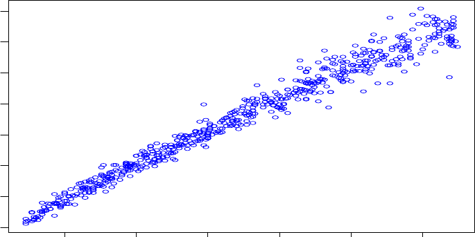
Figure 2.1: A plot of the abdominal circumference data
2.3 An introduction to the gamlss packages
The function gamlss() of the package gamlss is similar to the gam() function in the Rpackage
gam, Hastie (2005), but can fit more distributions (not only the ones belonging to the exponen-
tial family) and can model all the parameters of the distribution as functions of the explanatory
variables.
This implementation of gamlss() allows modelling of up to four parameters in a distribution
family, which are conventionally called mu,sigma,nu and tau. Here we will try to give a simple
demonstration of the gamlss package.
The following data abdom, kindly provided by Dr. Eileen M. Wright, are used here for
demonstration purposes. Data abdom comprises 610 observations of y= abdominal circumfer-
ence in mm and x= gestational age in weeks. Given that you have loaded gamlss from the R
library by
library("gamlss")
data("abdom")
plot(y~x, data=abdom, col="blue", xlab="age", ylab="circumference")
The data are plotted in Figure 2.1. To fit a normal distribution to the data with the mean
(mu) of y modelled as a cubic polynomial in age, i.e. poly(x,3), use
abd0 <- gamlss(y~poly(x,3), data=abdom, family=NO)
GAMLSS-RS iteration 1: Global Deviance = 4939.735
GAMLSS-RS iteration 2: Global Deviance = 4939.735
Since the normal distribution NO is also the default value we could omit the family argument.
To get a summary of the results use
22 CHAPTER 2. THE GAMLSS PACKAGE
summary(abd0)
*******************************************************************
Family: c("NO", "Normal")
Call: gamlss(formula = y ~ poly(x, 3), family = NO, data = abdom)
Fitting method: RS()
-------------------------------------------------------------------
Mu link function: identity
Mu Coefficients:
Estimate Std. Error t value Pr(>|t|)
(Intercept) 226.7 0.5617 403.586 0.000e+00
poly(x, 3)1 2157.7 13.8741 155.521 0.000e+00
poly(x, 3)2 -109.6 13.8741 -7.896 1.353e-14
poly(x, 3)3 -26.7 13.8741 -1.924 5.479e-02
-------------------------------------------------------------------
Sigma link function: log
Sigma Coefficients:
Estimate Std. Error t value Pr(>|t|)
(Intercept) 2.63 0.02863 91.86 0
-------------------------------------------------------------------
No. of observations in the fit: 610
Degrees of Freedom for the fit: 5
Residual Deg. of Freedom: 605
at cycle: 2
Global Deviance: 4939.735
AIC: 4949.735
SBC: 4971.802
*******************************************************************
We used the Rfunction poly() to fit orthogonal polynomials, but we could have fit the same
model using the I() function i.e.
abd00 <- gamlss(y~x+I(x^2)+I(x^3), data=abdom, family=NO)
GAMLSS-RS iteration 1: Global Deviance = 4939.735
GAMLSS-RS iteration 2: Global Deviance = 4939.735
summary(abd00)
*******************************************************************
Family: c("NO", "Normal")
Call: gamlss(formula = y ~ x + I(x^2) + I(x^3), family = NO, data = abdom)
Fitting method: RS()
-------------------------------------------------------------------
Mu link function: identity
Mu Coefficients:
Estimate Std. Error t value Pr(>|t|)
(Intercept) -65.340953 19.528047 -3.346 8.705e-04
2.3. AN INTRODUCTION TO THE GAMLSS PACKAGES 23
x 9.577417 2.354505 4.068 5.375e-05
I(x^2) 0.104515 0.089438 1.169 2.430e-01
I(x^3) -0.002075 0.001078 -1.924 5.479e-02
-------------------------------------------------------------------
Sigma link function: log
Sigma Coefficients:
Estimate Std. Error t value Pr(>|t|)
(Intercept) 2.63 0.02863 91.86 0
-------------------------------------------------------------------
No. of observations in the fit: 610
Degrees of Freedom for the fit: 5
Residual Deg. of Freedom: 605
at cycle: 2
Global Deviance: 4939.735
AIC: 4949.735
SBC: 4971.802
*******************************************************************
Warning message:
summary: vcov has failed, option qr is used instead
in: summary.gamlss(abd00)
Note that for large data sets it is more efficient (and may be essential) to calculate the
polynomials terms in advance, i.e.
x2<-x^2; x3<-x^3
and then use them within the gamlss() function since the evaluation is done then only once.
The fitted model is given by Y∼N O(ˆµ, ˆσ) where ˆµ=ˆ
β0+ˆ
β1x+ˆ
β2x2+ˆ
β3x3i.e. ˆµ=
−65.34 + 9.577x+ 0.1045x2−0.002075x3and log(ˆσ) = 2.63 so ˆσ= exp(2.63) = 13.87 (since σ
has a default log link function).
Note the warning message given above. The summary function has two ways of producing
standard errors. The default value is type="vcov". This uses the vcov method for gamlss
objects which in turn uses a non linear fitting, see Chapter ??, with only one iteration at the
maximum to obtain the Hessian matrix. Standard errors are obtained from the observed infor-
mation matrix (the inverse of the Hessian). The standard errors obtained this way are reliable
since they take into the account the interrelationship between the distribution parameters i.e.
µand σin the above case. On occasions, when the above procedure fails, the standard er-
rors are obtained from type="qr" which uses the individual fits of the parameters (used in
the gamlss() algorithms) and therefore should be used with caution. This is what happened
above and that is why we get the warning. The standard errors produced this way do not take
into the account the correlation between the estimates of the distribution parameters µ,σ,ν
and τ, [although in the example above the estimates of the distribution parameters µand σ
of the normal distribution are asymptotically uncorrelated]. Note also that when smoothing
additive terms are involved in the fitting, both methods, that is, "vcov" and "qr", produce
incorrect standard errors. Is like assuming that the estimated smoothing terms were fixed at
24 CHAPTER 2. THE GAMLSS PACKAGE
their estimated values. The functions prof.dev() and prof.term() can be used for obtaining
more reliable individual parameter confidence intervals.
Model abd0 is a linear parametric model as defined in (??). In order to fit a semi-parametric
model in age using a non-parametric smoothing cubic spline with 3 effective degrees of freedom
on top of the constant and linear terms use
> abd1<-gamlss(y~cs(x,df=3), data=abdom, family=NO)
GAMLSS-RS iteration 1: Global Deviance = 4937.16
GAMLSS-RS iteration 2: Global Deviance = 4937.16
The effective degrees of freedom used in the fitting of the mu parameters in the above model
are 5 (one for the constant, one for the linear and 3 for smoothing). Note that the gamlss()
notation is different to the gam() notation in S-PLUS where the equivalent model is fitted using
s(x,4). [Note also that when you use gam() in S-PLUS (or Rpackage gam) that the default
convergence criterion may need to be reduced for proper convergence in S-PLUS and comparison
with gamlss() results.]
The total degrees of freedom used for the above model abd1 are six, i.e. 5 for mu the mean,
and 1 for the constant scale parameter sigma the standard deviation.
Fitted values of the parameters of the object can be obtained using the fitted() function.
For example plot(x, fitted(abd1,"mu")) will plot the fitted values of mu against x. The
constant estimated scale parameter (the standard deviation of the normal in this case) can be
obtained using:
fitted(abd1,"sigma")[1]
1
13.84486
The same values can be obtained using the more general function predict():
predict(abd1,what="sigma", type="response")[1]
1
13.84486
The function predict() can be used to predict the response variable parameters for both
the old and new data values of the explanatory variables.
To model both the mean, mu, and the scale parameter, sigma, as non-parametric smoothing
cubic spline functions of x(with a normal distribution for the response) use
> abd2 <- gamlss(y~cs(x,3),sigma.formula=~cs(x,3),data=abdom, family=NO)
GAMLSS-RS iteration 1: Global Deviance = 4785.698
GAMLSS-RS iteration 2: Global Deviance = 4784.711
GAMLSS-RS iteration 3: Global Deviance = 4784.718
GAMLSS-RS iteration 4: Global Deviance = 4784.718
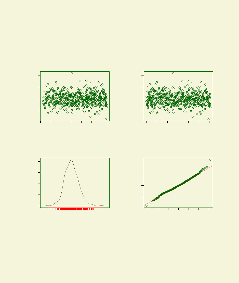
The function resid(abd2) (an abbreviation of residuals()) can be used to obtain the
(normalized randomized quantile) residuals of the model, subsequently just called residuals
throughout this manual. [The residuals only need to be randomized for discrete distributions,
see Dunn and Smyth (1996).] Residuals plots can be obtained using plot().
2.3. AN INTRODUCTION TO THE GAMLSS PACKAGES 25
50 100 150 200 250 300 350
−2 0 2 4
Against Fitted Values
Fitted Values
Quantile Residuals
0 100 200 300 400 500 600
−2 0 2 4
Against x−variable
index
Quantile Residuals
−4 −2 0 2 4
0.0 0.1 0.2 0.3 0.4
Density Estimate
Quantile. Residuals
Density
−3 −2 −1 0 1 2 3
−2 0 2 4
Normal Q−Q Plot
Theoretical Quantiles
Sample Quantiles
Figure 2.2: Residual plot from the normal fitted model abd2 with µ=cs(x, 3) and
log(σ) = cs(x, 3)
26 CHAPTER 2. THE GAMLSS PACKAGE
> plot(abd2)
*******************************************************************
Summary of the Randomised Quantile Residuals
mean = 0.0005115742
variance = 1.001641
coef. of skewness = 0.2397172
coef. of kurtosis = 3.718456
Filliben correlation coefficient = 0.9962348
*******************************************************************
<See Figure 2.2, for the plot.>
Note that the plot function does not produce additive term plots (as for example in the
gam() function of the package mgcv) in R. The function which does this in the gamlss package
is term.plot [see Chapter ?? for an example of its use].
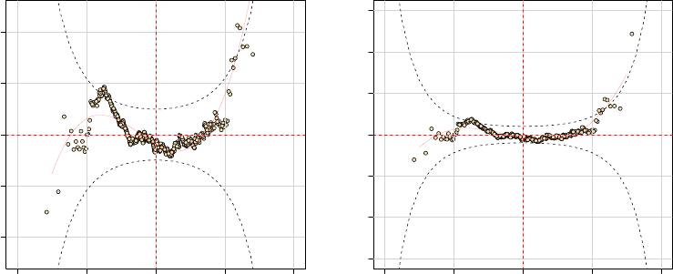
A worm plot of the residuals, see van Buuren and Fredriks (2001), can be obtained by using
the wp() function
> wp(abd2)
Warning message:
Some points are missed out
increase the y limits using ylim.all in: wp(abd2)
<See figure on the left side of Figure 2.3 for the plot.>
−4 −2 0 2 4
−0.4 −0.2 0.0 0.2 0.4
Unit normal quantile
Deviation
−4 −2 0 2 4
−1.5 −1.0 −0.5 0.0 0.5 1.0 1.5
Unit normal quantile
Deviation
Figure 2.3: Worm plot from the normal fitted model abd2 with µ=cs(x, 3) and
log(σ) = cs(x, 3)
To include all points in the worm plot change the Deviation axis range by increasing the
value of ylim.all.
wp(abd2,ylim.all=1.5)
Since there is no warning message all points have been included in the worm plot.
2.3. AN INTRODUCTION TO THE GAMLSS PACKAGES 27
<See figure on the right side of Figure 2.3 for the plot.>
[Clearly one point was omitted from the left side plot in Figure 2.3.] The default worm
plot above is a detrended normal Q-Q plot of the (normalized quantile) residuals, and indicates
a possible inadequacy in modelling the distribution, since some points plotted lie outside the
(dotted) confidence bands.
If you wish to use loess curves instead of cubic splines use:
abd3 <- gamlss(y~lo(x,span=.4),sigma.formula=~lo(x,span=.4),data=abdom, family=NO)
GAMLSS-RS iteration 1: Global Deviance = 4785.934
GAMLSS-RS iteration 2: Global Deviance = 4785.498
GAMLSS-RS iteration 3: Global Deviance = 4785.491
GAMLSS-RS iteration 4: Global Deviance = 4785.491
You can find more about the implemented smoothers of the gamlss() function in Chapter
5. Chapter 7gives you advice on how to select the appropriate smoothing parameter.
If you wish to use a different distribution instead of the normal, use the option family of
the function gamlss. For example to fit a t-distribution to the data use
> abd3 <- gamlss(y~cs(x,3),sigma.formula=~cs(x,3), data=abdom, family=TF)
GAMLSS-RS iteration 1: Global Deviance = 4777.367
GAMLSS-RS iteration 2: Global Deviance = 4776.539
GAMLSS-RS iteration 3: Global Deviance = 4776.544
GAMLSS-RS iteration 4: Global Deviance = 4776.544
A list of the different distributions implemented in gamlss() is given in Table 4of Section
1.2. The details of all the distributions currently available in gamlss() are given in Appendix
A. Chapter 4 of this manual also describes how the user can set up their own distribution in
gamlss().
Different models can be compared using their global deviances, GD =−2ˆ
ℓ, (if they are
nested) or using a generalized Akaike information criterion, GAIC =−2ˆ
ℓ+(♯.df), where ℓ(ˆ
θ) =
Pn
i=1 log f(yi|ˆµi,ˆσi,ˆνi),ˆτi) is the log-likelihood function and ♯is a required penalty e.g. ♯= 2 is
the usual Akaike information criterion. The function deviance() provides the global deviance
of the model. Notes that the GAMLSS global deviance is different from the deviance that
it is provided by the functions glm() and gam() in R. The global deviance is exactly minus
twice the fitted log likelihood function, including all constant terms in the log-likelihood. The
glm() deviance is calculated as a deviation from the saturated model and it does not include
’constant’ terms (which do not depend on the mean of distribution) in the fitted log likelihood.
To obtain the generalized Akaike information criterion use the functions AIC() or GAIC(). The
functions are identical. For example to compare the models abd1,abd2 and abd3 use
> AIC(abd1,abd2,abd3)
df AIC
abd3 11.001504 4798.547
abd2 9.999872 4804.718
abd1 6.000680 4949.162
The AIC function uses default penalty ♯= 2, i.e. the usual Akaike information criterion
(AIC). Hence the usual AIC [equivalent to GAIC(♯= 2)] selects model abd3 as the best model
(since it has the smallest value of AIC). If you wish to change the penalty ♯use the argument
k.
28 CHAPTER 2. THE GAMLSS PACKAGE
> AIC(abd1,abd2,abd3, k=3 )
df AIC
abd3 11.001504 4809.548
abd2 9.999872 4814.718
abd1 6.000680 4955.162
Hence, GAIC(♯= 3) also selects model abd3 as the best model.
Chapter 3
The gamlss() function
The function gamlss() is the main function of the package gamlss. It fits a Generalized Addi-
tive Model for Location, Scale and Shape (GAMLSS). The following sections explain how the
function can be used. Section 3.1 explains the arguments of the function, Section 3.2 describes
the components of a gamlss object (i.e. a fitted GAMLSS model) and Section 3.3.1 shows
how the functions refit and update can be used. The profiling functions prof.dev and and
prof.term are described in Section 3.5.
3.1 The arguments of the function
The usage of the function is
gamlss(formula = formula(data), sigma.formula = ~1,
nu.formula = ~1, tau.formula = ~1, family = NO(),
data = sys.parent(), weights = NULL,
contrasts = NULL, method = RS(), start.from = NULL,
mu.start = NULL, sigma.start = NULL,
nu.start = NULL, tau.start = NULL,
mu.fix = FALSE, sigma.fix = FALSE, nu.fix = FALSE,
tau.fix = FALSE, control = gamlss.control(...),
i.control = glim.control(...), ...)
where the arguments of the function are defined as follows
formula a model formula (including the response variable y) for the mu parameter
(compulsory), e.g. y∼x.
sigma.formula a model formula object for the sigma parameter, e.g. ∼x.
nu.formula a model formula for the nu parameter, e.g. ∼x.
tau.formula a model formula formula for the tau parameter, e.g. ∼x.
family agamlss.family object which defines the (conditional) distribution of the
response variable, see Chapter 4.
29
30 CHAPTER 3. THE GAMLSS() FUNCTION
data a data frame containing the variables occurring in the formula (see also Section
3.1.3)
weights a vector of weights. Note that this argument is not equivalent to the same
argument of the glm() or gam() functions. Here weights can be used i)
to weight out observations (with weights equal to 1 or 0) ii) for a weighted
likelihood analysis where the contribution of the observations to the likelihood
is weighted by the weights. Typically this is appropriate if some rows of the
data are identical and the weights represent the frequencies of these rows,
(see also Section 3.1.3). Any other use of the weights is not recommended
since this could have side effects. In particular () weights do not in general
translate to gamlss() weights and such models should instead be fitted using
offset(s) fot the parameters mu and/or sigma appropriately.
contrasts list of contrasts to be used for some or all of the factors appearing as variables
in the parameter(s) model formula.
method the algorithms for GAMLSS, i.e. RS(), CG() or mixed().
start.from a fitted GAMLSS model from which to take the starting values for the current
model
mu.start vector or scalar for initial values for the location parameter mu.
sigma.start vector or scalar for initial values for the scale parameter sigma.
nu.start vector or scalar of initial values for the shape parameter nu.
tau.start vector or scalar of initial values for the shape parameter tau.
mu.fix whether the mu parameter should be kept fixed at the mu.start value during
the fitting.
sigma.fix whether the sigma parameter should be kept fixed at the sigma.start value
during the fitting.
nu.fix whether the nu parameter should be kept fixed at the nu.start value during
the fitting.
tau.fix whether the tau parameter should be kept fixed at the tau.start value during
the fitting.
control Control parameters of the outer iterations algorithm. The default setting is
the gamlss.control function (see below).
i.control this sets the control parameters of the inner iterations of the RS algorithm.
The default setting is the glim.control function (see below).
As formulas the gamlss() accepts all glm() type formulas plus several smoothing function
formulas (see Chapter 5). Note the absence from the above list of the usual modelling options
na.action and subset. The reason these options have been removed is that, while there is
only one data set (data.frame) for the model usually there are up to four different model frames
created for each of the parameters therefore it is easier to apply the subset() or the na.omit()
functions to the original data set, i.e. data = na.omit(mydata). The gamlss() function

3.1. THE ARGUMENTS OF THE FUNCTION 31
will stop if there are NA’s in the data.
Warning: Note that the na.action, and the subset argument common to other
statistical modelling functions such as lm and glm have been removed as arguments
in the gamlss() function.
This is because while there is only one data set in the model there are usually up to
four different model frames created (one for each distribution parameter) and therefore
for consistency it is easier to apply sub-setting and na.action to the whole data set
and not to the individual frames.
For subsets use data=subset(mydata, subset_of_mydata),
for na.action use
data=na.omit(mydata)
3.1.1 The algorithms
There are three different algorithm method options
RS(): The default method is the RS algorithm, which does not requires accurate starting
values for µ,σ,νand τto ensure convergence (the default starting values, often constants,
are usually adequate). This method is faster for larger data sets.
CG(): The CG algorithm, which can be better for distributions with potentially highly
correlated parameter estimates.
mixed(): This is a mixture of the above two algorithms which starts with the RS algorithm
and finishes with the CG.
The RS() and CG() algorithms are explained in detail in Rigby and Stasinopoulos (2005).
For example
>library(gamlss)
>data(abdom)
> h<-gamlss(y~cs(x, df=3), sigma.fo=~cs(x,df=3), family=NO, data=abdom)
Loading required package: splines
GAMLSS-RS iteration 1: Global Deviance = 4785.698
GAMLSS-RS iteration 2: Global Deviance = 4784.711
GAMLSS-RS iteration 3: Global Deviance = 4784.718
GAMLSS-RS iteration 4: Global Deviance = 4784.718
fits the model using the RS algorithm. Note that the Global Deviance increases slightly
during the iterations. This can happen if smoothing additive terms are involved since the
degrees of freedom in the different fits could change very slightly. The CG algorithm is used by:
> h<-gamlss(y~cs(x, df=3), sigma.fo=~cs(x,df=3), family=NO, data=abdom,
method=CG())
GAMLSS-CG iteration 1: Global Deviance = 6022.863
GAMLSS-CG iteration 2: Global Deviance = 5512.658
32 CHAPTER 3. THE GAMLSS() FUNCTION
GAMLSS-CG iteration 3: Global Deviance = 5119.169
GAMLSS-CG iteration 4: Global Deviance = 4888.186
GAMLSS-CG iteration 5: Global Deviance = 4801.068
GAMLSS-CG iteration 6: Global Deviance = 4785.983
GAMLSS-CG iteration 7: Global Deviance = 4784.892
GAMLSS-CG iteration 8: Global Deviance = 4784.749
GAMLSS-CG iteration 9: Global Deviance = 4784.724
GAMLSS-CG iteration 10: Global Deviance = 4784.72
GAMLSS-CG iteration 11: Global Deviance = 4784.719
and the mixed algorithm is used by:
> h<-gamlss(y~cs(x, df=3), sigma.fo=~cs(x,df=3), family=NO, data=abdom,
method=mixed(2,20))
GAMLSS-RS iteration 1: Global Deviance = 4785.698
GAMLSS-RS iteration 2: Global Deviance = 4784.711
GAMLSS-CG iteration 1: Global Deviance = 4784.718
GAMLSS-CG iteration 2: Global Deviance = 4784.718
In the above example the mixed method uses 2 cycles of the RS algorithm, followed by up
to 20 cycles of the CG algorithm. All methods end up essentially with the same fitted model,
a useful check.
3.1.2 The algorithmic control functions
The gamlss.control function is defined as
gamlss.control(c.crit = 0.001, n.cyc = 20, mu.step = 1, sigma.step = 1, nu.step = 1,
tau.step = 1, gd.tol = 5, iter = 0, trace = TRUE, ...)
where
c.crit is the convergence criterion for the algorithm
n.cyc is maximum number of cycles of the algorithm
mu.step is the step length for the parameter mu
sigma.step is the step length for the parameter sigma
nu.step is the step length for the parameter nu
tau.step is the step length for the parameter tau
gd.tol global deviance tolerance level, this allows the global deviance to temporarily
increase.
iter this should not normally be used by the user. It is used when the (refit)
function is used to count the right number of iteration
trace whether to print the global deviance at each outer iteration of the RS() and
CG() algorithms. The users are advised to keep the default values TRUE so
they can check if the algorithm is converging.
3.1. THE ARGUMENTS OF THE FUNCTION 33
The function which controls the inner iteration is glim.control
glim.control(cc = 0.001, cyc = 50, trace = FALSE, bf.cyc = 30, bf.tol = 0.001,
bf.trace = FALSE,...)
where
cc is the convergence criterion for the GLIM type part of algorithm
cyc the number of cycles of the GLIM part of the algorithm
trace whether to print at each iteration of the GLIM part of the algorithm with
default FALSE.
bf.cyc the number of cycles of the backfitting algorithm
bf.tol the convergence criterion (tolerance level) for the backfitting algorithm
bf.trace whether to print at each iteration of the backfitting (TRUE) or not (FALSE,
the default)
Here is an example of how to change the convergence criterion c.crit. First fit the model
with the default convergence criterion value of 0.001.
>library(gamlss)
>data(abdom)
>h<-gamlss(y~cs(x, df=3), sigma.fo=~cs(x,df=3), family=NO, data=abdom)
GAMLSS-RS iteration 1: Global Deviance = 4785.698
GAMLSS-RS iteration 2: Global Deviance = 4784.711
GAMLSS-RS iteration 3: Global Deviance = 4784.718
GAMLSS-RS iteration 4: Global Deviance = 4784.718
Now change the convergence criterion to 0.000001 using control argument in gamlss()
with the criterion defined within gamlss.control().
> con1 <- gamlss.control(c.crit=0.000001)
> h<-gamlss(y~cs(x, df=3), sigma.fo=~cs(x,df=3), family=NO, data=abdom, control=con1)
GAMLSS-RS iteration 1: Global Deviance = 4785.698
GAMLSS-RS iteration 2: Global Deviance = 4784.711
GAMLSS-RS iteration 3: Global Deviance = 4784.718
GAMLSS-RS iteration 4: Global Deviance = 4784.718
GAMLSS-RS iteration 5: Global Deviance = 4784.718
GAMLSS-RS iteration 6: Global Deviance = 4784.718
GAMLSS-RS iteration 7: Global Deviance = 4784.718
Now let us change the default values of the trace option using the i.control argument in
gamlss90 with the trace option defined within glim.control().
> con2<- glim.control(trace=TRUE)
> h<-gamlss(y~cs(x, df=3), sigma.fo=~cs(x,df=3), family=NO, data=abdom, i.control=con2)
GLIM iteration 1: Global Deviance = 6607.297
GLIM iteration 2: Global Deviance = 6607.297
GLIM iteration 1: Global Deviance = 6036.316
GLIM iteration 2: Global Deviance = 5523.068

34 CHAPTER 3. THE GAMLSS() FUNCTION
GLIM iteration 3: Global Deviance = 5124.911
GLIM iteration 4: Global Deviance = 4890.074
GLIM iteration 5: Global Deviance = 4801.557
GLIM iteration 6: Global Deviance = 4786.591
GLIM iteration 7: Global Deviance = 4785.766
GLIM iteration 8: Global Deviance = 4785.703
GLIM iteration 9: Global Deviance = 4785.698
GLIM iteration 10: Global Deviance = 4785.698
GAMLSS-RS iteration 1: Global Deviance = 4785.698
GLIM iteration 1: Global Deviance = 4784.803
GLIM iteration 2: Global Deviance = 4784.803
GLIM iteration 1: Global Deviance = 4784.726
GLIM iteration 2: Global Deviance = 4784.712
GLIM iteration 3: Global Deviance = 4784.711
GLIM iteration 4: Global Deviance = 4784.711
GAMLSS-RS iteration 2: Global Deviance = 4784.711
GLIM iteration 1: Global Deviance = 4784.718
GLIM iteration 2: Global Deviance = 4784.718
GLIM iteration 1: Global Deviance = 4784.718
GAMLSS-RS iteration 3: Global Deviance = 4784.718
GLIM iteration 1: Global Deviance = 4784.719
GLIM iteration 1: Global Deviance = 4784.718
GAMLSS-RS iteration 4: Global Deviance = 4784.718
>
Better leave it at the default value!
Warning: If a large data set is used (say more than 10000 observations), and the
user is at an explorative stage of the analysis, where many models have to be fitted
relatively fast, it is advisable to change the c.crit in gamlss.control() to something
like 0.01 or even 0.1.
Let us now fit the tdistribution to the above data. The family option for the tdistribution
family is TF and the tdistribution degrees of freedom parameter is nu and is fitted as constant
by default.
> h<-gamlss(y~cs(x, df=3), sigma.fo=~cs(x,df=3), family=TF, data=abdom)
GAMLSS-RS iteration 1: Global Deviance = 4777.367
GAMLSS-RS iteration 2: Global Deviance = 4776.539
GAMLSS-RS iteration 3: Global Deviance = 4776.544
GAMLSS-RS iteration 4: Global Deviance = 4776.544
The fitted value for the constant degrees of freedom parameter nu is 12.00165 and can
be obtained using fitted(h,"nu")[1]. There are occasions where the user wants to fix the
parameter(s) of a distribution at specific value(s). For example, one might want to fix the
degrees of freedoms of the tdistribution say at 10. This can be done as follows
> h1<-gamlss(y~cs(x, df=3), sigma.fo=~cs(x,df=3), family=TF,
data=abdom, nu.start=10, nu.fix=TRUE)

3.1. THE ARGUMENTS OF THE FUNCTION 35
GAMLSS-RS iteration 1: Global Deviance = 4777.552
GAMLSS-RS iteration 2: Global Deviance = 4776.722
GAMLSS-RS iteration 3: Global Deviance = 4776.741
GAMLSS-RS iteration 4: Global Deviance = 4776.741
Note The tdistribution may be unstable if nu is fixed close to one (usually indicating that
this is an inappropriate value of nu for the particular data set).
3.1.3 Weighting out observations, the weight and data=subset() ar-
guments
There are two way in which the user can weight out observations from the analysis. The first
relies on the subset() function of Rand can be used in the data argument of gamlss(), i.e.
data=subset(mydata, condition), where condition is a relevant Rcode restricting the case
numbers of the data.
Warning: It was mentioned earlier that the subset argument is taken out from
gamlss(). Always use data=subset(mydata, condition)
The second way is through the weights option. Note that the weights are not performing
in the same way as in the glm() or lm() functions. There, they are prior weights used to fit
only the mean of the model, while here the same weights are applied for fitting all (possibly
four) parameters. The weights here can be used for a weighted likelihood analysis where
the contribution of the observations to the log likelihood is weighted according to weights.
Typically this is appropriate in the following cases:
frequencies: if some rows of the data are identical and the weights represent the frequencies
of these rows
zero weights: A more common application of the weights is to set them equal to zero or one
(i.e. FALSE or TRUE), so observations can be weighted out from the analysis
weighted log-likelihood: This is the case where different weights in the log-likelihood for
different observations is required. One example is the use of gamlss objects in the fitting
of finite mixtures, see package gamlss.mx.
Note than in general a model fitted to the original uncollapsed data.frame or to the collapsed
data.frame using frequencies as weights should produce identical results in terms of fitted model
parameters. The fitted values and the residuals of the two different models do not have to have
the same length as we will demonstrate in this Section.
Note that using data=subset() only fits the data cases in the subset, so fitted values for
the parameters are only calculated for the subset data cases. However using the weights option
fits all the data cases (although cases with weights 0 do not contribute to the fit) and so fitted
values for the parameters are calculated for all data cases. These fitted values will be correct if
no additive (smoothing) terms are involved in the fit.
Warning: For excluding observations use preferably subset .
36 CHAPTER 3. THE GAMLSS() FUNCTION
Let us assume that in our abdominal circumference example we want to weight out all
observations in which the x variable is less than or equal to 20. We can do this using the
function subset().
> h2<-gamlss(y~cs(x, df=3), sigma.fo=~cs(x,df=3), family=TF,
data=subset(abdom,x>20))
GAMLSS-RS iteration 1: Global Deviance = 3700.626
GAMLSS-RS iteration 2: Global Deviance = 3701.064
GAMLSS-RS iteration 3: Global Deviance = 3701.077
GAMLSS-RS iteration 4: Global Deviance = 3701.078
GAMLSS-RS iteration 5: Global Deviance = 3701.078
> length(fitted(h2)); length(resid(h2)); h2$noObs ; h2$N
[1] 456
[1] 456
[1] 456
[1] 456
Note that h2$N gives the length of the response variable while h2$noOBS is the sum of the
weights. Now we use weights:
> h3<-gamlss(y~cs(x, df=3), sigma.fo=~cs(x,df=3), family=TF,
data=abdom, weights=x>20)
GAMLSS-RS iteration 1: Global Deviance = 3700.623
GAMLSS-RS iteration 2: Global Deviance = 3701.063
GAMLSS-RS iteration 3: Global Deviance = 3701.077
GAMLSS-RS iteration 4: Global Deviance = 3701.078
GAMLSS-RS iteration 5: Global Deviance = 3701.078
> length(fitted(h3)); length(resid(h3)); h3$noObs ; h3$N
[1] 610
[1] 456
[1] 456
[1] 610
Let us assume now that we want to weight out only a few observations, say the 200th and
400th.
> index<-1:length(abdom$x)
> h4<-gamlss(y~cs(x, df=3), sigma.fo=~cs(x,df=3), family=TF,
data=subset(abdom,index!=200&index!=400))
GAMLSS-RS iteration 1: Global Deviance = 4763.397
GAMLSS-RS iteration 2: Global Deviance = 4762.488
GAMLSS-RS iteration 3: Global Deviance = 4762.468
GAMLSS-RS iteration 4: Global Deviance = 4762.467
GAMLSS-RS iteration 5: Global Deviance = 4762.466
GAMLSS-RS iteration 6: Global Deviance = 4762.467
>length(fitted(h4))
[1] 608

3.1. THE ARGUMENTS OF THE FUNCTION 37
> h5<-gamlss(y~cs(x, df=3), sigma.fo=~cs(x,df=3), family=TF,
data=abdom,weights=index!=200&index!=400)
GAMLSS-RS iteration 1: Global Deviance = 4763.268
GAMLSS-RS iteration 2: Global Deviance = 4762.459
GAMLSS-RS iteration 3: Global Deviance = 4762.464
GAMLSS-RS iteration 4: Global Deviance = 4762.465
> length(fitted(h5)); length(resid(h5)); h5$noObs ; h5$N
[1] 610
[1] 608
[1] 608
[1] 610
If the variables in the reduced data.frame are to be used extensively later on, it would make
more sense to use the subset function in advance of the fitting to create a reduced data set
(e.g. newabdom)
index<-1:length(abdom$x)
newabdon<-subset(abdom,(index!=200&index!=400) )
and use the data=newabdom argument in gamlss. Also note the difference in length in the
two fitted models.
Warning: If the weights option is used, the fitted values for the weighted out
observations contain the correct fitted values for the linear part of the model but
not for the additive smoothers. Fitted values for the additive terms can be obtained
using the predict function provided that the specific additive term has its prediction
function (for new data) implemented.
The following simple artificial example demonstrates the use of the weights argument when
frequencies are involved in the data. [The approach is particularly suited to fitting discrete
distributions to frequency count data.]
> y <- c(3,3,7,8,8,9,10,10,12,12,14,14,16,17,17,19,19,18,22,22 )
> x <- c(1,1,2,3,3,4, 5, 5, 6, 6, 7, 7, 8, 9, 9,10,10,11,12,12 )
> ex1 <- data.frame(y=y,x=x)
> ex1
y x
1 3 1
2 3 1
3 7 2
4 8 3
5 8 3
6 9 4
7 10 5
8 10 5
9 12 6
10 12 6
11 14 7
12 14 7
38 CHAPTER 3. THE GAMLSS() FUNCTION
13 16 8
14 17 9
15 17 9
16 19 10
17 19 10
18 18 11
19 22 12
20 22 12
The 20 ×2 data frame ex1 contains some identical rows, i.e. row 1 and 2 or 7 and 8. A new
data frame, containing the same information as in ex1, but with an extra variable called freq
indicating the number of identical rows in ex1 in can be create as.
> yy <- c(3, 7, 8,9, 10, 12, 14,16, 17, 19,18, 22 )
> xx <- c(1, 2, 3,4, 5, 6, 7, 8, 9, 10,11, 12 )
> ww <- c(2, 1, 2,1, 2, 2, 2, 1, 2, 2, 1, 2 )
> ex2 <- data.frame(y=yy, x=xx, freq=ww)
> ex2
y x freq
1 3 1 2
2 7 2 1
3 8 3 2
4 9 4 1
5 10 5 2
6 12 6 2
7 14 7 2
8 16 8 1
9 17 9 2
10 19 10 2
11 18 11 1
12 22 12 2
Fitting a statistical model using each of the two data frames should produce identical results.
This is demonstrated below where prior weights are used to fit the data in ex2.
> m1<- gamlss(y~x, sigma.fo=~x, data=ex1, family=NBI)
GAMLSS-RS iteration 1: Global Deviance = 91.0186
GAMLSS-RS iteration 2: Global Deviance = 90.8238
GAMLSS-RS iteration 3: Global Deviance = 90.8238
> m2<- gamlss(y~x, sigma.fo=~x, weights=freq, data=ex2, family=NBI)
GAMLSS-RS iteration 1: Global Deviance = 91.0163
GAMLSS-RS iteration 2: Global Deviance = 90.8238
GAMLSS-RS iteration 3: Global Deviance = 90.8238
> all.equal(deviance(m1),deviance(m2))
[1] TRUE
> summary(m1)
*******************************************************************
Family: c("NBI", "Negative Binomial type I")
Call: gamlss(formula = y ~ x, sigma.formula = ~x, family = NBI, data = ex1)
3.1. THE ARGUMENTS OF THE FUNCTION 39
Fitting method: RS()
-------------------------------------------------------------------
Mu link function: log
Mu Coefficients:
Estimate Std. Error t value Pr(>|t|)
(Intercept) 1.6233 0.16549 9.809 1.200e-08
x 0.1290 0.01914 6.741 2.561e-06
-------------------------------------------------------------------
Sigma link function: log
Sigma Coefficients:
Estimate Std. Error t value Pr(>|t|)
(Intercept) -36.063740 0.029107 -1239.009 7.769e-46
x -0.005447 0.004619 -1.179 2.537e-01
-------------------------------------------------------------------
No. of observations in the fit: 20
Degrees of Freedom for the fit: 4
Residual Deg. of Freedom: 16
at cycle: 3
Global Deviance: 90.82379
AIC: 98.82379
SBC: 102.8067
*******************************************************************
Warning message:
summary: vcov has failed, option qr is used instead
in: summary.gamlss(m1)
> summary(m2)
*******************************************************************
Family: c("NBI", "Negative Binomial type I")
Call: gamlss(formula = y ~ x, sigma.formula = ~x, family = NBI,
data = ex2, weights = freq)
Fitting method: RS()
-------------------------------------------------------------------
Mu link function: log
Mu Coefficients:
Estimate Std. Error t value Pr(>|t|)
(Intercept) 1.6233 0.16549 9.809 1.200e-08
x 0.1290 0.01914 6.741 2.561e-06
-------------------------------------------------------------------
Sigma link function: log
40 CHAPTER 3. THE GAMLSS() FUNCTION
Sigma Coefficients:
Estimate Std. Error t value Pr(>|t|)
(Intercept) -36.063740 0.029107 -1239.009 7.769e-46
x -0.005447 0.004619 -1.179 2.537e-01
-------------------------------------------------------------------
No. of observations in the fit: 20
Degrees of Freedom for the fit: 4
Residual Deg. of Freedom: 16
at cycle: 3
Global Deviance: 90.82379
AIC: 98.82379
SBC: 102.8067
*******************************************************************
Warning message:
summary: vcov has failed, option qr is used instead
in: summary.gamlss(m2)
> length(fitted(m1)); length(resid(m1)); m1$noObs ; m1$N
[1] 20
[1] 20
[1] 20
[1] 20
> length(fitted(m2)); length(resid(m2)); m2$noObs ; m2$N
[1] 12
[1] 20
[1] 20
[1] 12
Note the lengths of the fitted values and the residuals of the two models. In the case of model
m2 the residuals are expanded to represent all 20 original observations. Note that resid(m1)
and resid(m2) are not going to be identical in this case since both are randomized residuals
due to the fact we used a discrete distribution.
The user may be tempted to scale the weights but this may have undesirable consequences
as we demonstrate below.
> m3<- gamlss(y~x, sigma.fo=~x, weights=freq/2, data=ex2, family=NBI)
GAMLSS-RS iteration 1: Global Deviance = 45.5065
GAMLSS-RS iteration 2: Global Deviance = 45.4119
GAMLSS-RS iteration 3: Global Deviance = 45.4119
> summary(m3)
*******************************************************************
Family: c("NBI", "Negative Binomial type I")
Call: gamlss(formula = y ~ x, sigma.formula = ~x, family = NBI,
data = ex2, weights = freq/2)
Fitting method: RS()
3.2. THE GAMLSS OBJECT 41
-------------------------------------------------------------------
Mu link function: log
Mu Coefficients:
Estimate Std. Error t value Pr(>|t|)
(Intercept) 1.6233 0.23403 6.936 4.014e-05
x 0.1290 0.02707 4.767 7.607e-04
-------------------------------------------------------------------
Sigma link function: log
Sigma Coefficients:
Estimate Std. Error t value Pr(>|t|)
(Intercept) -36.063740 0.041163 -876.1118 9.236e-26
x -0.005447 0.006532 -0.8338 4.238e-01
-------------------------------------------------------------------
No. of observations in the fit: 12
Degrees of Freedom for the fit: 4
Residual Deg. of Freedom: 8
at cycle: 3
Global Deviance: 45.41189
AIC: 53.4119
SBC: 55.35152
*******************************************************************
Warning message:
summary: vcov has failed, option qr is used instead
in: summary.gamlss(m3)
> length(fitted(m3)); length(resid(m3)); m3$noObs ; m3$N
[1] 12
[1] 12
Warning message:
weights not frequencies are used so residuals remain unweighted in: residuals.gamlss(m3)
[1] 12
[1] 12
We can see that, while in this specific example the fitted coefficients are the same, the de-
viances and more importantly the standard errors have been affected by the change in weights.
Also because the weights are not frequencies the length of the residuals remains 12. In general
using weights that are not frequencies is not recommended unless the user knows what he/she
doing and is aware of the problem.
3.2 The gamlss object
The function gamlss() returns a gamlss object, that is, a GAMLSS fitted model which may
have converged or not depending whether the maximum number of iterations given by c.cyc
has been reached or not.
The generic functions print and summary can be used to print and summarize the object
as was indicated in Chapter 2.
42 CHAPTER 3. THE GAMLSS() FUNCTION
The model
> h<-gamlss(y~cs(x, df=3), sigma.fo=~cs(x,df=3), family=TF, data=abdom)
fitted earlier is used here to demonstrate the composition of a gamlss object. By calling the
names function we are able to check on the components of the object h
> names(h)
[1] "family" "parameters" "call"
[4] "y" "control" "weights"
[7] "G.deviance" "N" "rqres"
[10] "iter" "type" "method"
[13] "contrasts" "converged" "residuals"
[16] "noObs" "mu.fv" "mu.lp"
[19] "mu.wv" "mu.wt" "mu.link"
[22] "mu.terms" "mu.x" "mu.qr"
[25] "mu.coefficients" "mu.xlevels" "mu.formula"
[28] "mu.df" "mu.nl.df" "mu.s"
[31] "mu.var" "mu.coefSmo" "mu.lambda"
[34] "mu.pen" "df.fit" "pen"
[37] "df.residual" "sigma.fv" "sigma.lp"
[40] "sigma.wv" "sigma.wt" "sigma.link"
[43] "sigma.terms" "sigma.x" "sigma.qr"
[46] "sigma.coefficients" "sigma.xlevels" "sigma.formula"
[49] "sigma.df" "sigma.nl.df" "sigma.s"
[52] "sigma.var" "sigma.coefSmo" "sigma.lambda"
[55] "sigma.pen" "nu.fv" "nu.lp"
[58] "nu.wv" "nu.wt" "nu.link"
[61] "nu.terms" "nu.x" "nu.qr"
[64] "nu.coefficients" "nu.formula" "nu.df"
[67] "nu.nl.df" "nu.pen" "P.deviance"
[70] "aic" "sbc"
More generally any gamlss object has the following components
family The distribution family of the gamlss object (see Chapter 4) e.g. for the
object hwe have
> h$family
[1] "TF" "t.Family"
parameters The name of the fitted parameters as a character list.
> h$parameters
[1] "mu" "sigma" "nu"
call The call of the gamlss() function e.g.
> h$call
gamlss(formula = y ~ cs(x, df = 3), sigma.formula = ~cs(x, df = 3),
family = TF, data = abdom)
3.2. THE GAMLSS OBJECT 43
yThe response variable as a vector (or matrix), accessed by h$y
control The gamlss() fit control settings, accessed by h$control
weights The vector of weights, accessed by h$weights
G.deviance The value of global deviance which can be extracted by h$G.deviance or by
using the generic function deviance() or deviance(gamlss.object, "G")
e.g.
> deviance(h)
[1] 4776.544
> deviance(h,"G")
[1] 4776.544
NThe length of the response variable (or the number of observations in the fit
unless weights are used) e.g.
> h$N
[1] 610
noObs The actual number of observations if weights are used in the fit equal to the
sum of the weights. If no weights are used is equal to h$N.
> h$noObs
[1] 610
rqres A function to calculate the (normalized randomized quantile) residuals of
the object, accessed by h$rqres. [The residuals are randomized for discrete
distributions only see Dunn and Smyth (1996) ]
iter The number of external iterations in the fitting process i.e.
> h$iter
[1] 4
type The type of the distribution of the response variable (continuous or discrete)
i.e.
> h$type
[1] "Continuous"
method Which algorithm is used for the fit, RS(), CG() or mixed() i.e.
> h$method
RS()
contrasts Which contrasts were used in the fit, NULL if they have not been set in
gamlss() function
converged Whether the model have converged i.e.
44 CHAPTER 3. THE GAMLSS() FUNCTION
> h$converged
[1] TRUE
residuals The (normalized randomized quantile) residuals of the model which can be
extracted by h$residuals or by using the generic function residuals, (also
abbreviated as resid). [These residuals are randomized for discrete distribu-
tions only. See Dunn and Smyth (1996). .]
df.fit The total degrees of freedom use by the model, e.g. in the model h there
are 2 (for the constant and linear terms) plus 3 (for the smoothing term in
cs(x,3), i.e. a total of 5) in the mu model, another 5 degrees of freedom for
sigma, plus 1 for nu, giving a total of 11 degrees of freedom.
> h$df.fit
[1] 11.00150
df.residual The residual degrees of freedom left after the model is fitted
> h$df.residual
[1] 598.9985
pen The sum of the quadratic penalties for all the parameters (if appropriate
additive terms are fitted)
> h$pen
[1] 6.6752
P.deviance The penalized deviance, Global deviance + penalties, which can be extracted
by h$P.deviance or by using the generic function deviance(gamlss.object,"P")
e.g.
> h$pen
[1] 6.6752
> h$P.deviance
[1] 4783.22
> deviance(h,"P")
[1] 4783.22
aic The Akaike information criterion
> h$aic
[1] 4798.547
sbc The Bayesian information criterion (i.e. the Schwartz Bayesian criterion)
> h$sbc
[1] 4847.102
The rest of the components refer to the parameters of the model (if they exist). The name
parameter below should be replaced with the appropriate parameter which can be any of the
mu,sigma,nu or tau).
3.3. THE REFIT AND UPDATE FUNCTIONS 45
parameter.fv The fitted values of the appropriate parameter accessed by e.g. h$mu.fv.
The fitted values can also be extracted using the generic function fitted e.g.
fitted(h,"mu") extracts the mu fitted values
parameter.lp The linear predictor of the appropriate parameter, accessed by e.g. h$mu.lp.
parameter.wv The working variable of the appropriate parameter.
parameter.wt The working weights of the appropriate parameter.
parameter.link
The link function for appropriate parameter.
parameter.terms
The terms for the appropriate parameter model.
parameter.x The design matrix for the appropriate parameter.
parameter.qr The QR decomposition of the appropriate parameter model.
parameter.coefficients
The linear coefficients of the the appropriate parameter model which can be
also extracted using the generic function coef
parameter.formula
The formula for the appropriate parameter model.
parameter.df The appropriate parameter degrees of freedom.
parameter.nl.df
The non linear (e.g. smoothing) degrees of freedom for the appropriate pa-
rameter.
parameter.pen The sum of the quadratic penalties for the specific parameter (if appropriate
additive terms are fitted).
parameter.xlevels
(only where relevant) a record of the levels of the factors used in fitting of this
parameter.
3.3 The refit and update functions
3.3.1 refit()
The function refit() can be used if the converged component of the gamlss fitted object
is FALSE, that is, when the maximum number of iteration c.cyc has been reached without
convergence. The default value for c.cyc is 20 and it is usually sufficient for most problems.
Here it is an artificial example in which we force the algorithm to stop in the second iteration
so we can continue with refit()
> con1 <- gamlss.control(c.crit=0.000001, n.cyc=2)
> h<-gamlss(y~cs(x, df=3), sigma.fo=~cs(x,df=3), family=TF, data=abdom, control=con1)
GAMLSS-RS iteration 1: Global Deviance = 4777.367
GAMLSS-RS iteration 2: Global Deviance = 4776.539
46 CHAPTER 3. THE GAMLSS() FUNCTION
Warning message:
Algorithm RS has not yet converged in: RS()
> h<-refit(h)
GAMLSS-RS iteration 3: Global Deviance = 4776.544
GAMLSS-RS iteration 4: Global Deviance = 4776.544
3.3.2 update()
The function update() can be used to update formulae or other arguments of a gamlss fitted
object. To update formulae update uses the the Rupdate.formula() function to update the
specified distribution parameter.
The gamlss update() function is defined as
update.gamlss(object, formula., ..., what = c("mu", "sigma", "nu", "tau"),
evaluate = TRUE)
where
object agamlss fitted object
formula. the formula to update
... for updating argument in gamlss()
what what parameter of the distribution is required for updating in the formula,
mu,sigma,nu or tau, the default is what="mu"
evaluate whether to evaluate the call or not (the default is TRUE)
Here we use the AIDS data which consist of the quarterly reported AIDS cases in the
U.K. from January 1983 to March 1994 obtained from the Public Health Laboratory Service,
Communicable Disease Surveillance Centre, London. We start by using the poisson family
to model the number of reported cases (the response variable), against time (a continuous
explanatory variable) which we smooth with a cubic spline smoother using 5 effective degrees
of freedom and against qrt a factor representing quarterly seasonal effect. We then (i) change
the family to negative binomial (type I) (ii) update the smoothing parameter with df=8 (iii)
remove the quarterly seasonal effect (iv) and finally fit a normal family model with response
the log(y).
> data(aids)
> # fit a poisson model
> h.po <-gamlss(y~cs(x,2)+qrt, family=PO, data=aids)
GAMLSS-RS iteration 1: Global Deviance = 448.1315
GAMLSS-RS iteration 2: Global Deviance = 448.1315
> # update with a negative binomial
> h.nb <-update(h.po, family=NBI)
GAMLSS-RS iteration 1: Global Deviance = 388.8086
GAMLSS-RS iteration 2: Global Deviance = 390.7803
GAMLSS-RS iteration 3: Global Deviance = 391.396
GAMLSS-RS iteration 4: Global Deviance = 391.3996
GAMLSS-RS iteration 5: Global Deviance = 391.3965
3.3. THE REFIT AND UPDATE FUNCTIONS 47
GAMLSS-RS iteration 6: Global Deviance = 391.3962
> # update the smoothing
> h.nb1 <-update(h.nb,~cs(x,8)+qrt)
GAMLSS-RS iteration 1: Global Deviance = 362.943
GAMLSS-RS iteration 2: Global Deviance = 359.1257
GAMLSS-RS iteration 3: Global Deviance = 359.229
GAMLSS-RS iteration 4: Global Deviance = 359.2342
GAMLSS-RS iteration 5: Global Deviance = 359.2348
> # remove qrt
> h.nb2 <-update(h.nb1,~.-qrt)
GAMLSS-RS iteration 1: Global Deviance = 379.5511
GAMLSS-RS iteration 2: Global Deviance = 379.5303
GAMLSS-RS iteration 3: Global Deviance = 379.5628
GAMLSS-RS iteration 4: Global Deviance = 379.5626
> # put back qrt take log of y and fit a normal distribution
> h.nb3 <-update(h.nb1,log(.)~.+qrt, family=NO)
GAMLSS-RS iteration 1: Global Deviance = -42.3446
GAMLSS-RS iteration 2: Global Deviance = -42.3446
> # verify that it is the same
> h.no<-gamlss(log(y)~cs(x,8)+qrt,data=aids )
GAMLSS-RS iteration 1: Global Deviance = -42.3446
GAMLSS-RS iteration 2: Global Deviance = -42.3446
Finally we give an example taken from see Venables and Ripley (2002) Section 6.1, to
demonstrate how update can be used to fit two different lines in a analysis of covariance situation.
Each model fits a separate regression of gas consumption on temperature for the two different
levels of the factor Insul.
> library(MASS)
> data(whiteside)
> attach(whiteside)
> gasB <- gamlss(Gas~Temp, data=subset(whiteside, Insul=="Before"))
GAMLSS-RS iteration 1: Global Deviance = 5.7566
GAMLSS-RS iteration 2: Global Deviance = 5.7566
> gasA <- update(gasB,data=subset(whiteside, Insul=="After"))
GAMLSS-RS iteration 1: Global Deviance = 20.9026
GAMLSS-RS iteration 2: Global Deviance = 20.9026
> plot(Temp,Gas,pch=21,bg=c("red","green3")[unclass(Insul)])
> lines(Temp[Insul=="Before"],fitted(gasB))
> lines(Temp[Insul=="After"],fitted(gasA), col="blue")
> detach(whiteside)
> plot(Temp,Gas,pch=21,bg=c("red","green3")[unclass(Insul)])
> lines(Temp[Insul=="Before"],fitted(gasB))
> lines(Temp[Insul=="After"],fitted(gasA), col="blue")
<See figure 3.1 for the plot>
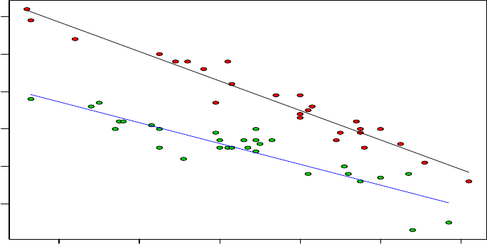
48 CHAPTER 3. THE GAMLSS() FUNCTION
0 2 4 6 8 10
2 3 4 5 6 7
Temp
Gas
Figure 3.1: Rent (R) against floor space (Fl) from the rent data
3.4 The predict and lpred functions
The function predict.gamlss() is the GAMLSS specific method which produces predictors for
the current or a new data set for a specified parameter of a gamlss object. The predict.gamlss()
can be used to extract (linear) predictors, (type="link"), fitted values, (type="response")
and contributions of terms in the (linear) predictor, (type="terms"), for a specific parame-
ter in the model at the current or new values of the x-variables in a similar way that the
predict.lm() and predict.glm() functions can be used for lm and glm objects. Problems as-
sociated with the above functions, see Venables and Ripley (2002) Section 6.4, are avoided here
since the predict() function for gamlss is based on the safe predict.gam() S-PLUS function
of Trevor Hastie, see Chambers and Hastie (1992). Note that the main difference between the
gamlss predict() and the usual predictive functions in R is the fact that the gamlss predict()
function is distribution parameter specific, that is, predictions are for one of the distribution
parameters mu,sigma,nu and tau.
Linear predictors, fitted values and specific terms for a specific distribution parameter in the
model at the current data values of the explanatory variables can be also extracted using the
function lpred() (which in fact is called from predict() if the newdata argument is NULL,
see below).
The gamlss predict() function is defined as
predict.gamlss(object, what = c("mu", "sigma", "nu", "tau"),
newdata = NULL, type = c("link", "response", "terms"),
terms = NULL, se.fit = FALSE, data = NULL, ...)
where
obj agamlss fitted object
3.4. THE PREDICT AND LPRED FUNCTIONS 49
what what parameter of the distribution is required, mu,sigma,nu or tau, the
default is what="mu"
newdata a data frame containing new values for the explanatory variables used in the
model
type The default value is type="link" gets the (linear) predictor for the specified
distribution parameter. type="response" gets the fitted values for the pa-
rameter and finally type="terms" gets the contribution of fitted terms for the
specific parameter.
terms if type="terms" is defined then this option selects a specific term for the
parameter at hand. By default all terms are selected.
se.fit if TRUE the approximate standard errors of the appropriate type are ex-
tracted. Note that standard errors are not given for new data sets, i.e. when
newdata is defined.
... for extra arguments
The lpred function of gamlss has identical arguments to the predict.gamlss() function
apart from the newdata argument which does not exist in lpred. The functions fitted() and
fv() are equivalent to using lpred() or predict() with the argument type="response".
The function lp() is equivalent of using using lpred() or predict() with the argument
type="link". The following code demonstrates some of the points.
> data(aids)
> # fitting a negative binomial type I distribution
> aids.1<-gamlss(y~poly(x,3)+qrt, family=NBI, data=aids) #
GAMLSS-RS iteration 1: Global Deviance = 383.4573
GAMLSS-RS iteration 2: Global Deviance = 381.7155
GAMLSS-RS iteration 3: Global Deviance = 381.7145
GAMLSS-RS iteration 4: Global Deviance = 381.7145
> # different ways to obtain the (linear) predictor for mu
> predict(aids.1)
1 2 3 4 5 6 7 8
1.322524 1.490931 1.996051 2.140244 2.540856 2.643345 3.084552 3.166838
9 10 11 12 13 14 15 16
3.507549 3.552144 3.937462 3.965866 4.254701 4.249425 4.586879 4.569425
17 18 19 20 21 22 23 24
4.814407 4.767284 5.064898 5.009610 5.218763 5.137819 5.403616 5.318518
25 26 27 28 29 30 31 32
5.499867 5.393124 5.635130 5.528245 5.689814 5.565298 5.791535 5.670888
33 34 35 36 37 38 39 40
5.820702 5.686435 5.904928 5.778544 5.924625 5.788633 6.007406 5.883308
41 42 43 44 45
6.033682 5.903987 6.131065 6.017277 6.179967
> identical(predict(aids.1),predict(aids.1, what="mu"))
[1] TRUE
> identical(predict(aids.1),predict(aids.1, what="mu", type="link"))
[1] TRUE
50 CHAPTER 3. THE GAMLSS() FUNCTION
> identical(predict(aids.1),lpred(aids.1))
[1] TRUE
> identical(predict(aids.1),lpred(aids.1, what="mu"))
[1] TRUE
> identical(predict(aids.1),lpred(aids.1, what="mu", type="link"))
[1] TRUE
> identical(predict(aids.1),lp(aids.1))
[1] TRUE
> identical(predict(aids.1),lp(aids.1,what="mu"))
[1] TRUE
> identical(predict(aids.1),lp(aids.1,what=mu))
[1] TRUE
> predict(aids.1, type="response")
[1] 3.752880 4.441230 7.359933 8.501513 12.690525 14.060153
[7] 21.857665 23.732334 33.366396 34.888031 51.288277 52.765969
[13] 70.435743 70.065108 98.187495 96.488586 123.273656 117.599460
[19] 158.364296 149.846225 184.705623 170.343807 222.208509 204.081110
[25] 244.659407 219.889330 280.095223 251.701754 295.838692 261.202927
[31] 327.515320 290.292221 337.208549 294.840605 366.840883 323.287991
[37] 374.138170 326.566183 406.427725 358.994714 417.248315 366.495867
[43] 459.925725 410.459336 482.976045
> identical(predict(aids.1, what="mu", type="response"),
lpred(aids.1, what="mu", type="response"))
[1] TRUE
> identical(predict(aids.1, type="response"),fitted(aids.1, what="mu") )
[1] TRUE
> identical(predict(aids.1, type="response"),fv(aids.1, what="mu") )
[1] TRUE
> identical(predict(aids.1, type="response"),fv(aids.1, what=mu) )
[1] TRUE
Note that while fv and lp allow the what argument to be set both as a character or a name,
e.g. "mu" or mu, the equivalent argument in predict,lpred and fitted allow only characters,
e.g. "mu".
se.fit=TRUE can be used to obtain approximate standard errors for both predict() or
lpred. The result would be a list containing two objects, fit and se.fit.
> paids.1 <- predict(aids.1, what="mu", se.fit=TRUE ,type="response")
> names(paids.1)
[1] "fit" "se.fit"
> paids.1$se.fit
1 2 3 4 5 6 7
0.6739890 0.6939025 1.0019629 1.0183976 1.3176894 1.2834913 1.7429449
8 9 10 11 12 13 14
1.7127567 2.1427115 2.1544452 2.9143105 2.9114575 3.6733450 3.8148465
15 16 17 18 19 20 21
5.0853267 4.9618717 6.0957367 6.0692381 7.7446967 7.2466055 8.6062972
22 23 24 25 26 27 28

3.4. THE PREDICT AND LPRED FUNCTIONS 51
8.1251614 10.0603188 9.2492801 10.8913743 9.9202147 12.2761289 11.3375706
29 30 31 32 33 34 35
13.4118442 11.9623956 14.8348532 13.5865259 15.8386666 13.9548821 16.9870776
36 37 38 39 40 41 42
15.1415277 17.1035025 15.4483994 18.5918097 16.5360814 18.9783873 19.7091914
43 44 45
25.9319310 25.4682431 33.2581498
Warning: Standard errors should be used with caution. If the (linear) predictor
contains only linear (no smoothing) terms then the standard errors of the (linear)
predictor (using the option type="link") are correctly calculated. Standard errors
for fitted distribution parameters if the link function is not the identity function are
calculated using the delta-method which could be unreliable, see Chambers and Hastie
(1992) p 240. If additive (smoothing) terms are included in the model of a specific
distribution parameter then the unreliability increases since the the standard errors of
the additive (smoothing) terms are crudely approximated using the method described
in Chambers and Hastie (1992) Section 7.4.4.
The option type="terms" creates a matrix containing the contribution to the (linear) pre-
dictor from each of the terms in the model formula. If in addition the argument se.fit=TRUE
is set then a list of two objects is created, each containing a matrix. The first matrix contains
the contribution of the terms to the (linear) predictor and the second their approximate stan-
dard errors. The number of columns in the matrices are the number of terms in the model
formula. The argument terms can be used in combination with type="terms" to select the
contribution to the (linear) predictor of a specific term in the model. A typical use of the
option type="terms" is for plotting the additive contribution of a specific term in modelling a
distribution parameter as in the function term.plot().
> paids.2 <- predict(aids.1, what="mu", type="terms")
> colnames(paids.2)
[1] "poly(x, 3)" "qrt"
> # now with se
> paids.2 <- predict(aids.1, what="mu", type="terms", se.fit=TRUE)
> names(paids.2)
[1] "fit" "se.fit"
> colnames(paids.2$fit)
[1] "poly(x, 3)" "qrt"
> colnames(paids.2$se.fit)
[1] "poly(x, 3)" "qrt"
> # select only "qrt" to save
> paids.2 <- predict(aids.1, what="mu", type="terms", se.fit=TRUE, terms="qrt")
> colnames(paids.2$fit)
[1] "qrt"
The most common use of the function predict() is to obtain fitted values for a specific
parameter at new values of the explanatory variables (predictors) for predictive purposes or for
validation. In order to do that the argument newdata should be set. The predict() function

52 CHAPTER 3. THE GAMLSS() FUNCTION
expects that the object given in newdata is a data frame containing the right x-variables used
in the model. This could cause problems if a transformed variables is used in the fitting of the
original model (see below).
The predict() function for gamlss is based on the predict.gam() S-PLUS function of
Trevor Hastie which insures that the prediction is reliable even if expressions defining the terms
in the model formula depend on the entire data vector for evaluation, are used, see Chambers
and Hastie (1992) Section 7.3.3.
We reiterate here the steps used in the execution of predict() taken from Chambers and
Hastie (1992) Section 7.3.3. Let Dold the original data frame, with original design matrix Xold,
and Dnew the new data frame (the new x-values where the fitted model has to be evaluated)
and assume that both data frames contain the right columns in the sense that the x-variables
used in the model formula (for the specific distribution parameter) are present in both.
1. Construct a new data frame using the combined (old and new) data, with columns the
matching variables included in both data frames, i.e. Dn=Dold
Dnew .
2. Construct the model frame and the corresponding new design matrix, Xn=Xold2
Xnew ,
using the combined data frame, Dn=Dold
Dnew . Note that for certain models (when the
function use to construct the design matrix is data dependent) the submatrix Xold2of
the new design matrix Xn, corresponding to the original observations in Dold, may be
different from the original design matrix Xold. This for example can happen if the the
cubic spline base, bs() is used in the model.
3. The parametric part of the model for the specified parameter is refitted using only Xold2.
If the difference of the old and the new fit is large, a warning is given.
4. The coefficients from the fit obtain using only Xold2are used to obtain the new predictions.
5. If the gamlss object contains additive (smoothing) components an additional step is taken
to evaluate the appropriate function at the the new data values. (This requires that the
additive function has a predict option)
Warning: The random(),ra() and rc() additive functions do not have a predict
option implemented.
Here we use the aids data to fit a negative binomial model using a polynomial, poly(),
a cubic spline base, bs(), and a smoothing cubic spline, cs(), function to model time (x).
The sigma parameter is a constant is the model. predict() is used first, to find values for mu
(type="response") at new data values and finally for sigma. Note that the predict() function
gives a warning when bs is used in the mu model.
> data(aids)
> # create a new data frame
> newaids<-data.frame(x=c(45,46,47), qrt=c(2,3,4))
> # use with poly

3.4. THE PREDICT AND LPRED FUNCTIONS 53
> mod1<-gamlss(y~poly(x,3)+qrt, family=NBI, data=aids) #
Loading required package: splines
GAMLSS-RS iteration 1: Global Deviance = 383.4573
GAMLSS-RS iteration 2: Global Deviance = 381.7155
GAMLSS-RS iteration 3: Global Deviance = 381.7145
GAMLSS-RS iteration 4: Global Deviance = 381.7145
> # predict "mu" at new values
> (ap1 <- predict(mod1, what="mu", newdata=newaids, type = "response"))
[1] 410.9393 521.6606 471.6455
> # use with bs
> mod2<-gamlss(y~bs(x,5)+qrt, family=NBI, data=aids) #
GAMLSS-RS iteration 1: Global Deviance = 382.634
GAMLSS-RS iteration 2: Global Deviance = 380.0695
GAMLSS-RS iteration 3: Global Deviance = 380.0674
GAMLSS-RS iteration 4: Global Deviance = 380.0674
> # predict "mu" at new values
> (ap2 <- predict(mod2, what="mu", newdata=newaids, type = "response"))
[1] 389.8785 475.1377 408.4420
Warning message:
There is a discrepancy between the original and the re-fit
used to achieve safe predictions
in: predict.gamlss(mod2, what = "mu", newdata = newaids, type = "response")
> # use with cs
>mod3<-gamlss(y~cs(x,3)+qrt, family=NBI, data=aids) #
GAMLSS-RS iteration 1: Global Deviance = 381.1313
GAMLSS-RS iteration 2: Global Deviance = 379.6472
GAMLSS-RS iteration 3: Global Deviance = 379.8807
GAMLSS-RS iteration 4: Global Deviance = 379.878
GAMLSS-RS iteration 5: Global Deviance = 379.8779
> (ap3 <- predict(mod3, what="mu", newdata=newaids, type = "response"))
[1] 398.9763 496.9106 439.8638
> # get the term contributions
> (ap4 <- predict(mod3, what="mu", newdata=newaids, type = "terms"))
cs(x, 3) qrt
1 1.308070 -0.10147125
2 1.335266 0.09084048
3 1.362463 -0.05830069
attr(,"constant")
[1] 4.782303
> # note that se.fit is not implemented with newdata
> (ap4 <- predict(mod3, what="mu", newdata=newaids, type = "terms", se.fit=TRUE))
cs(x, 3) qrt
1 1.308070 -0.10147125
2 1.335266 0.09084048
3 1.362463 -0.05830069
attr(,"constant")
[1] 4.782303
Warning message:
54 CHAPTER 3. THE GAMLSS() FUNCTION
se.fit = TRUE is not supported for new data values at the moment
in: predict.gamlss(mod3, what = "mu", newdata = newaids, type = "terms",
> # predict "sigma"
> (ap5 <- predict(mod3, what="sigma", newdata=newaids, type="response"))
[1] 0.00818511 0.00818511 0.00818511
Note that the se.fit argument is not working with new data.
The following example is taken from Venables and Ripley (2002) (who use it to demonstrate
that the predict.lm function is not working properly for lm models). Here we use gamlss()
and the safe predict.gamlss() function giving consistent correct results.
> library(MASS)
> data(wtloss)
> # squaring Days
> quad1 <-gamlss(Weight~Days+I(Days^2),data=wtloss)
GAMLSS-RS iteration 1: Global Deviance = 137.8867
GAMLSS-RS iteration 2: Global Deviance = 137.8867
> # using poly
> quad2 <-gamlss(Weight~Days+poly(Days,2),data=wtloss)
GAMLSS-RS iteration 1: Global Deviance = 137.8867
GAMLSS-RS iteration 2: Global Deviance = 137.8867
> # new data
> new.x <-data.frame(Days=seq(250,300,10), row.names=seq(250,300,10))
> # using predict
> predict(quad1, newdata=new.x)
[1] 112.5061 111.4747 110.5819 109.8277 109.2121 108.7351
> predict(quad2, newdata=new.x)
[1] 112.5061 111.4747 110.5819 109.8277 109.2121 108.7351
If a transformed variable is used in the fitting of the current data some care has to taken
to insure that the right variables exist in the new data as well. For example, let us assume
that a transformation of age is needed in the model i.e. nage<-age^.5. This could be fit-
ted as mod<-gamlss(y ~ cs(age^.5),data=mydata) or by transforming the age first, nage<-
age^.5, and then fitting mod<-gamlss(y~cs(nage), data=mydata). The later fit is more ef-
ficient particularly for a data set with large mumber of data cases. In the first case, the code
predict(mod,newdata=data.frame(age=c(34,56))) would produce the expected results. In
the second case a new data frame has to be created containing the old data plus any new
transform variable. This data frame has to be declared in the data argument of the predict()
function. The option newdata should contain a data.frame with the transformed variable
names and the transformed variable values for which prediction is required as the following
example demonstrates.
> data(abdom)
> # assume that a transformation x^5 is required
> aa<-gamlss(y~cs(x^.5),data=abdom)
GAMLSS-RS iteration 1: Global Deviance = 4936.53 GAMLSS-RS
3.5. THE PROF.DEV AND PROF.TERM FUNCTIONS 55
iteration 2: Global Deviance = 4936.53
> # predict at old values
> predict(aa, what="mu")[610]
[1] 371.3929
> # predict at new data
> predict(aa,newdata=data.frame(x=abdom$x[610]))
[1] 371.3929
> # now transform x first
> nx<-abdom$x^.5
> aaa<-gamlss(y~cs(nx),data=abdom)
GAMLSS-RS iteration 1: Global Deviance = 4936.53 GAMLSS-RS
iteration 2: Global Deviance = 4936.53
> # create a new data frame
> newd<-data.frame( abdom, nx=abdom$x^0.5)
> # predict at old values
> predict(aaa)[610]
[1] 371.3929
> # predict at new values
> predict(aaa,newdata=data.frame(nx=abdom$x[610]^.5), data=newd)
[1] 371.3929
3.5 The prof.dev and prof.term functions
The function prof.dev obtains a profile deviance plot for any of the distribution parameters
mu,sigma,nu or tau of the fitted family and is useful for checking the reliability of models in
which one (or more) of the parameters in the distributions are constant, (and therefore have not
been modelled as functions of explanatory variables). The prof.dev also provides a 100(1-α)%
profile likelihood confidence interval for the parameter for a specified value of α. For example
in the abdominal circumference data above we have fitted a tdistribution to the data. The nu
parameter is the degrees of freedom parameter of the tdistribution and it would be of some
interest to find a confidence interval for nu. Note that nu=1 corresponds to a Cauchy distribution
while a large value of nu corresponds closely to a normal distribution. Usually it takes several
attempts to select a suitable range for the parameter in order to produce a decent graph. Our
advice is to start with a sparse grid for the parameter (i.e. few points) and improve that when
you see the resulting plot (aiming to include the full 95% interval for the parameter within the
horizontal axis scale and the horizontal deviance bar representing the global deviance at the
endpoints of the parameter interval to be roughly half way up the vertical axis scale). Note
that the procedure requires fitting the model repeatedly for a sequence of fixed values of the
parameter of interest (nu in this example) so it can be slow.
Here we reproduce our first attempt (shown at the left side of figure 3.2) and our final
attempt (shown at the right side of figure 3.2).
h<-gamlss(y~cs(x, df=3), sigma.fo=~cs(x,df=3), family=TF, data=abdom)
> pdfirst<-prof.dev(h,"nu",min=2,max=20,step=1)
*******************************************************************
nu.start=( 2 )
GAMLSS-RS iteration 1: Global Deviance = 4842.181
56 CHAPTER 3. THE GAMLSS() FUNCTION
GAMLSS-RS iteration 2: Global Deviance = 4842.696
GAMLSS-RS iteration 3: Global Deviance = 4842.723
GAMLSS-RS iteration 4: Global Deviance = 4842.728
GAMLSS-RS iteration 5: Global Deviance = 4842.728
*******************************************************************
nu.start=( 3 )
GAMLSS-RS iteration 1: Global Deviance = 4807.084
GAMLSS-RS iteration 2: Global Deviance = 4806.768
GAMLSS-RS iteration 3: Global Deviance = 4806.769
GAMLSS-RS iteration 4: Global Deviance = 4806.769
*******************************************************************
...
...
...
*******************************************************************
nu.start=( 20 )
GAMLSS-RS iteration 1: Global Deviance = 4777.644
*******************************************************************
*******************************************************************
Best estimate of the fixed parameter is 12
with a Global Deviance equal to 4776.546 at position 11
*******************************************************************
<See the left side of figure 3.2 for the plot>
The default value for 100(1 −α)% is 95% but the interval is not printed in this case because
the specified range of the parameter values do not include the entire 95% CI.
pdlast<-prof.dev(h,"nu",min=5,max=45,step=1)
> pdlast<-prof.dev(h,"nu",min=5,max=45,step=1)
*******************************************************************
nu.start=( 5 )
GAMLSS-RS iteration 1: Global Deviance = 4785.339
GAMLSS-RS iteration 2: Global Deviance = 4784.86
GAMLSS-RS iteration 3: Global Deviance = 4784.879
GAMLSS-RS iteration 4: Global Deviance = 4784.88
GAMLSS-RS iteration 5: Global Deviance = 4784.88
*******************************************************************
...
...
...
*******************************************************************
nu.start=( 45 )
GAMLSS-RS iteration 1: Global Deviance = 4780.55
GAMLSS-RS iteration 2: Global Deviance = 4780.551
GAMLSS-RS iteration 3: Global Deviance = 4780.551
*******************************************************************
*******************************************************************
Best estimate of the fixed parameter is 12
3.5. THE PROF.DEV AND PROF.TERM FUNCTIONS 57
with a Global Deviance equal to 4776.546 at position 8
A 95 % Confidence interval is: ( 6.332258 , 42.81560 )
*******************************************************************
Note that a useful option in the prof.dev function is type="l" if you wish to plot only the
line and not the points in the graph.
This time the 95% confidence intervals is printed because was properly defined. For different
confident intervals change the perc option, e.g. for a 99% use perc=99. The matrix pdlast
saved by the above command contains the values of the profiling parameter and its equivalent
global deviance.
> pdlast
interval G.deviances
[1,] 5 4784.880
[2,] 6 4781.090
[3,] 7 4778.976
[4,] 8 4777.774
[5,] 9 4777.098
[6,] 10 4776.741
[7,] 11 4776.580
[8,] 12 4776.546
[9,] 13 4776.592
[10,] 14 4776.689
[11,] 15 4776.819
[12,] 16 4776.969
[13,] 17 4777.131
[14,] 18 4777.300
[15,] 19 4777.477
[16,] 20 4777.644
[17,] 21 4777.815
[18,] 22 4777.980
[19,] 23 4778.141
[20,] 24 4778.297
[21,] 25 4778.448
[22,] 26 4778.594
[23,] 27 4778.735
[24,] 28 4778.870
[25,] 29 4779.001
[26,] 30 4779.127
[27,] 31 4779.249
[28,] 32 4779.365
[29,] 33 4779.478
[30,] 34 4779.586
[31,] 35 4779.691
[32,] 36 4779.791
[33,] 37 4779.888
[34,] 38 4779.981
[35,] 39 4780.072

58 CHAPTER 3. THE GAMLSS() FUNCTION
[36,] 40 4780.159
[37,] 41 4780.242
[38,] 42 4780.324
[39,] 43 4780.402
[40,] 44 4780.478
[41,] 45 4780.551
<See the right side of figure 3.2 for the plot>
5 10 15 20
4780 4790 4800 4810 4820 4830 4840
Profile Global Deviance
Grid of the nu parameter
Global Deviances
95%
10 20 30 40
4778 4780 4782 4784
Profile Global Deviance
Grid of the nu parameter
Global Deviances
95%
Figure 3.2: Profile global deviance for the degrees of freedom parameter of the tdistribution
fitted to the abdom data with µ=cs(x, 3) and σ=cs(x, 3)
The function prof.term() is similar to the function prof.dev() but it can provide a profile
deviance for any parameter in the model not just for the distribution parameters. That is, while
prof.dev() can be applied to profile a (constant) parameter of the distribution of the response
variable y(i.e. µ,σ,νor τ), the prof.term() can be applied to any parameter in the predictor
model for µ,σ,νor τ. In order to show how the prof.term() is working consider the AIDS
data first used in Section 3.3.1. Let us assume first that we are interested to fit a linear in time
term (x) plus a factor for the the quarterly seasonal effect, qrt, using the negative binomial
model (type I) family. This model is fitted as
> aids1<-gamlss(y~x+qrt,data=aids,family=NBI)
GAMLSS-RS iteration 1: Global Deviance = 492.7247
GAMLSS-RS iteration 2: Global Deviance = 492.6375
GAMLSS-RS iteration 3: Global Deviance = 492.6373
> summary(aids1)
*******************************************************************
Family: c("NBI", "Negative Binomial type I")
Call: gamlss(formula = y ~ x + qrt, family = NBI, data = aids)
Fitting method: RS()
3.5. THE PROF.DEV AND PROF.TERM FUNCTIONS 59
-------------------------------------------------------------------
Mu link function: log
Mu Coefficients:
Estimate Std. Error t value Pr(>|t|)
(Intercept) 2.88540 0.185279 15.5732 1.412e-18
x 0.08744 0.005382 16.2446 3.268e-19
qrt2 -0.12038 0.193843 -0.6210 5.381e-01
qrt3 0.11176 0.192855 0.5795 5.655e-01
qrt4 -0.07554 0.193160 -0.3911 6.978e-01
-------------------------------------------------------------------
Sigma link function: log
Sigma Coefficients:
Estimate Std. Error t value Pr(>|t|)
(Intercept) -1.603 0.2533 -6.328 1.110e-07
-------------------------------------------------------------------
No. of observations in the fit: 45
Degrees of Freedom for the fit: 6
Residual Deg. of Freedom: 39
at cycle: 3
Global Deviance: 492.6373
AIC: 504.6373
SBC: 515.4773
*******************************************************************
>
The coefficient for the linear term in time (x) has a value of 0.08744 and its tvalue indi-
cates that it is highly significant. An approximate 95% confidence interval for this parameter
can be obtained using 0.08744 ±1.96 ×0.005382, which results to the approximate interval
(0.0769,0.0980). We shall use now the function prof.term to find a more accurate profile (de-
viance) 95% confidence interval for the linear term parameter. Note that this in the model
formula indicates which parameter to profile.
mod<-quote(gamlss(y ~ offset(this * x) + qrt, data = aids, family = NBI))
prof.term(mod, min=0.06, max=0.11, step=0.001)
GAMLSS-RS iteration 1: Global Deviance = 508.1867
GAMLSS-RS iteration 2: Global Deviance = 508.1845
...
...
...
GAMLSS-RS iteration 1: Global Deviance = 502.4454
GAMLSS-RS iteration 2: Global Deviance = 502.4449
*******************************************************************
Best estimate of the fixed parameter is 0.087
with a Global Deviance equal to 492.6412 at position 28

60 CHAPTER 3. THE GAMLSS() FUNCTION
A 95 % Confidence interval is: ( 0.07458119 , 0.1008640 )
*******************************************************************
0.06 0.07 0.08 0.09 0.10 0.11
495 500 505
Profile Global Deviance
parameter
Global Deviances
95 %
0.06 0.07 0.08 0.09 0.10 0.11
495 500 505
Profile Global Deviance
parameter
Global Deviances
99 %
Figure 3.3: Profile global deviance for the linear trend parameter in the model gamlss(y x+qrt,
data=aids, family=NBI)
<See the left side of figure 3.3 for the plot>
As we see the 95% profile deviance confident interval is (0.0746,0.1009), not far from the
approximate one of (0.0769,0.0980). In general this would not be the case if the likelihood is
not nearly quadratic at the maximum. To obtain a 99% interval use
prof.term(mod, min=0.06, max=0.11, step=0.001, perc=99)
GAMLSS-RS iteration 1: Global Deviance = 508.1867
GAMLSS-RS iteration 2: Global Deviance = 508.1845
...
...
...
GAMLSS-RS iteration 1: Global Deviance = 502.4454
GAMLSS-RS iteration 2: Global Deviance = 502.4449
*******************************************************************
Best estimate of the fixed parameter is 0.087
with a Global Deviance equal to 492.6412 at position 28
A 99 % Confidence interval is: ( 0.07034371 , 0.1055237 )
*******************************************************************
>
<See the right side of figure 3.3 for the plot>
Now we shall used plot.term to find a break point in the relationship between the response
and one of the explanatory variables. Stasinopoulos and Rigby (1992) have shown that the
AIDS data provide a clear break point between the AIDS cases and time. Here we consider a
3.5. THE PROF.DEV AND PROF.TERM FUNCTIONS 61
linear+linear model for time (x), i.e. x+(x>break)*(x-break) and we are interested to estimate
the break point.
aids.1 <- quote(gamlss(y ~ x+I((x>this)*(x-this))+qrt,family=NBI,data=aids))
prof.term(aids.1, min=1, max=45, step=1, criterion="GD")
GAMLSS-RS iteration 1: Global Deviance = 492.7247
GAMLSS-RS iteration 2: Global Deviance = 492.6375
...
...
...
GAMLSS-RS iteration 2: Global Deviance = 490.866
GAMLSS-RS iteration 1: Global Deviance = 492.6376
GAMLSS-RS iteration 2: Global Deviance = 492.6373
*******************************************************************
Best estimate of the fixed parameter is 18
with a Global Deviance equal to 377.8706 at position 18
A 95 % Confidence interval is: ( 17.22821 , 19.39456 )
*******************************************************************
The profile plot (shown in the left of figure 3.4) indicates strong support for a break point
at x= 18 but the interval is accurate enough so we repeat with a tighter interval.
> prof.term(aids.1, min=16, max=21, step=.1, criterion="GD")
GAMLSS-RS iteration 1: Global Deviance = 394.1469
GAMLSS-RS iteration 2: Global Deviance = 392.7581
GAMLSS-RS iteration 3: Global Deviance = 392.7562
GAMLSS-RS iteration 4: Global Deviance = 392.7557
...
...
GAMLSS-RS iteration 1: Global Deviance = 393.6158
GAMLSS-RS iteration 2: Global Deviance = 393.6152
GAMLSS-RS iteration 1: Global Deviance = 394.6022
GAMLSS-RS iteration 2: Global Deviance = 394.6018
*******************************************************************
Best estimate of the fixed parameter is 18.3
with a Global Deviance equal to 377.4618 at position 24
A 95 % Confidence interval is: ( 17.19859 , 19.42017 )
*******************************************************************
The resulting plot is shown in the right of figure 3.4).
Finally the function prof.term can also be used as a way of determining a smoothing (hyper)
parameter in a model by plotting the Generalized Akaike Information Criterion, GAIC(♯) [where
penalty ♯is specified by the penalty= argument of prof.term]. Consider the model gamlss(y
~ cs(x,df=??) + qrt, data = aids, family = NBI) in which we would like to determine
a reasonable value for the missing degrees of freedom. Models with different degrees of freedom
can be fitted and their generalized Akaike Information criterion (GAIC) plotted against the
degrees of freedom, see Section 7for more details. This process can be automated using the
function prof.term.
mod1<-quote(gamlss(y ~ cs(x,df=this) + qrt, data = aids, family = NBI))
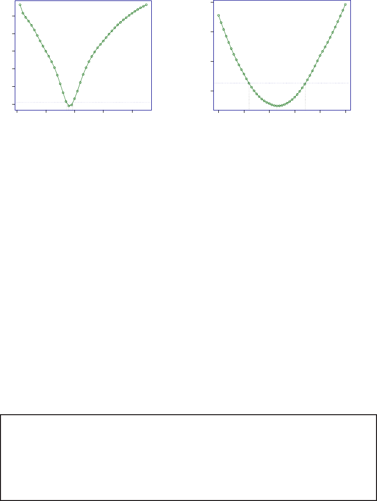
62 CHAPTER 3. THE GAMLSS() FUNCTION
0 10 20 30 40
380 400 420 440 460 480
Profile Global Deviance
parameter
Global Deviances
95 %
16 17 18 19 20 21
380 385 390 395
Profile Global Deviance
parameter
Global Deviances
95 %
Figure 3.4: Profile global deviance for the break point in the model
gamlss(y x+(x>break)*(x-break)+qrt,data=aids,family=NBI)
prof.term(mod1, min=1, max=15, step=1, criterion="IC", penalty=2.5)
GAMLSS-RS iteration 1: Global Deviance = 419.4861
GAMLSS-RS iteration 2: Global Deviance = 423.8037
...
...
...
GAMLSS-RS iteration 3: Global Deviance = 347.9344
GAMLSS-RS iteration 4: Global Deviance = 347.934
>
The profile plot (shown in figure 3.5) indicates that the degrees of freedom for smoothing
should be around 8 using criterion GAIC(2.5) (see also the discussion in chapter 7).
Warning: Profile deviance intervals should be used with care if random effects are
included in the model for any of the distribution parameters. They correspond to
a naive plug-in profile estimation which in general produces narrower intervals than
the marginal likelihood approach, see Rigby and Stasinopoulos (2005) Section 6.2 and
Appendix A.2. The more accurate profile deviance intervals are obtained from the
approximate marginal likelihoods which are model dependent. At present we do not
provide a general function for calculating these intervals.
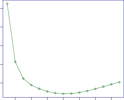
3.6. OTHER GAMLSS FUNCTIONS 63
2 4 6 8 10 12 14
400 410 420 430 440
Profile GAIC
parameter
GAIC pen= 2.5
Figure 3.5: Profile GAIC with penalty 2.5 for the degrees of freedom in the model gamlss(y
cs(x,df=this) + qrt, data = aids, family = NBI)
3.6 Other gamlss functions
They are a few other generic functions as coef(),formula(),model.frame(),model.matrix
and terms() which can apply to gamlss objects. Their main difference with other statistical
modelling objects is the extra argument what which determines what distribution parameter
the function has to extract the appropriate component. The default value is the component of
the mu distribution parameter. For example
> data(abdom)
> h<-gamlss(y~cs(x, df=3), sigma.fo=~cs(x,df=3), family=BCT, data=abdom)
GAMLSS-RS iteration 1: Global Deviance = 4772.531
GAMLSS-RS iteration 2: Global Deviance = 4772.445
GAMLSS-RS iteration 3: Global Deviance = 4772.429
GAMLSS-RS iteration 4: Global Deviance = 4772.423
GAMLSS-RS iteration 5: Global Deviance = 4772.422
GAMLSS-RS iteration 6: Global Deviance = 4772.422
> # get the coefficint for "nu"
> coef(h,"nu")
(Intercept)
-0.1228056
> # get the formula for the sigma model
64 CHAPTER 3. THE GAMLSS() FUNCTION
> formula(h, "sigma")
~cs(x, df = 3)
> # get the terms component in the nu model
> terms(h,"nu")
y~1
attr(,"variables")
list(y)
attr(,"factors")
numeric(0)
attr(,"term.labels")
character(0)
attr(,"specials")
attr(,"specials")$cs
NULL
attr(,"specials")$lo
NULL
attr(,"specials")$random
NULL
attr(,"specials")$ra
NULL
attr(,"specials")$rc
NULL
attr(,"specials")$fp
NULL
attr(,"specials")$ps
NULL
attr(,"specials")$vc
NULL
attr(,"specials")$pp
NULL
attr(,"order")
numeric(0)
attr(,"intercept")
[1] 1
attr(,"response")
[1] 1
attr(,".Environment")
<environment: 01892CB4>
attr(,"predvars")
3.6. OTHER GAMLSS FUNCTIONS 65
list(y)
attr(,"dataClasses")
y
"numeric"
66 CHAPTER 3. THE GAMLSS() FUNCTION
Chapter 4
Distributions
4.1 Different distributions in gamlss()
Tables 4.1 and 4.2 show the different continuous and discrete gamlss.family distributions
respectively available in the current version of the gamlss packages. The majority of the dis-
tributions are in the original gamlss package. The ones implemented more recently are in the
package gamlss.dist which has to be downloaded for the distributions to be used. New dis-
tributions can be added relatively easy as shown in Section 4.2. Johnson et al. (1993, 1994,
1995) are the classic reference books on distributions and cover most of the distributions in the
Tables 4.1 and 4.2. The BCPE and BCT distributions are new, see Appendix Aand Rigby and
Stasinopoulos (2004, 2006). Full specifications of all the distributions in Tables 4.1 and 4.2 are
given in Appendix A.
In order to fit a different distribution to the data change the family argument in the
gamlss() function. Column “R-name” in Tables 4.1 and 4.2 gives the definition function for
each family of distributions. The brackets in the family argument after the specific family
name, eg. GA(), are non compulsory but are needed to specify a different link function from the
default for one (or more) of the distribution parameters. Consider, for example, the rent data
(included in the gamlss package) shown in Figure 4.1. The response variable R is the monthly
net rent (rent minus calculated or estimated utility cost) and the x-variable is the floor space
in square meters (Fl). To fit a gamma distribution with the default log links for both the mu
and sigma,family=GA can be used. family=GA(mu.link="identity") can be used to change
the link function for the mean to an "identity" link.
> attach(rent)
> rent.1 <-gamlss(R~lo(Fl,span=.4),sigma.formula=~lo(Fl,span=.4),
family=GA)
GAMLSS-RS iteration 1: Global Deviance = 28044.90
GAMLSS-RS iteration 2: Global Deviance = 28044.31
GAMLSS-RS iteration 3: Global Deviance = 28044.32
GAMLSS-RS iteration 4: Global Deviance = 28044.32
> rent.2 <-gamlss(R~lo(Fl,span=.4),sigma.formula=~lo(Fl,span=.4),
family=GA(mu.link="identity"))
GAMLSS-RS iteration 1: Global Deviance = 28045.19
GAMLSS-RS iteration 2: Global Deviance = 28044.43
GAMLSS-RS iteration 3: Global Deviance = 28044.44
67

68 CHAPTER 4. DISTRIBUTIONS
Distributions R Name Section µ σ ν τ
beta BE() A.8.1 logit logit - -
beta inflated (at 0) BEOI() logit log logit -
beta inflated (at 1) BEZI() logit log logit -
beta inflated (at 0 and 1 ) BEINF() A.8.2 logit logit log log
Box-Cox Cole and Green BCCG() A.6.1 identity log identity -
Box-Cox power exponential BCPE() A.7.2 identity log identity log
Box-Cox-tBCT() A.7.1 identity log identity log
exponential EXP() A.4.1 log - - -
exponential Gaussian exGAUS() A.2.1 identity log log -
exponential gen. beta type 2 EGB2() A.3.1 identity identity log log
gamma GA() A.5.1 log log - -
generalized beta type 1 GB1() A.8.3 logit logit log log
generalized beta type 2 GB2() A.7.3 log identity log log
generalized gamma GG() A.6.2 log log identity -
generalized inverse Gaussian GIG() A.6.3 log log identity -
generalized tGT() A.3.2 identity log log log
Gumbel GU() A.1.3 identity log - -
inverse Gaussian IG() A.5.3 log log - -
Johnson’s SU (µthe mean) JSU() A.3.3 identity log identity log
Johnson’s original SU JSUo() A.3.3 identity log identity log
logistic LO() A.1.2 identity log - -
log normal LOGNO() A.5.2 log log - -
log normal (Box-Cox) LNO() A.5.2 log log fixed -
NET NET() A.3.4 identity log fixed fixed
normal NO() A.1.1 identity log - -
normal family NOF() A.1.1 identity log identity -
power exponential PE() A.2.2 identity log log -
power exponential PE2() A.2.2 identity log log -
reverse Gumbel RG() A.1.3 identity log - -
skew exponential power type 1 SEP1() A.3.6 identity log identity log
skew exponential power type 2 SEP2() A.3.7 identity log identity log
skew exponential power type 3 SEP3() A.3.8 identity log log log
skew exponential power type 4 SEP4() A.3.9 identity log log log
sinh-arcsinh SHASH() A.3.5 identity log log log
skew ttype 1 ST1() A.3.10 identity log identity log
skew ttype 2 ST2() A.3.11 identity log identity log
skew ttype 3 ST3() A.3.12 identity log log log
skew ttype 4 ST4() A.3.13 identity log log log
skew ttype 5 ST5() A.3.14 identity log identity log
tFamily TF() A.2.3 identity log log -
Weibull WEI() A.5.4 log log - -
Weibull (PH) WEI2() A.5.4 log log - -
Weibull (µthe mean) WEI3() A.5.4 log log - -
zero adjusted IG ZAIG() A.6.4 log log logit -
Table 4.1: Continuous distributions implemented within the gamlss packages (with default link
functions)
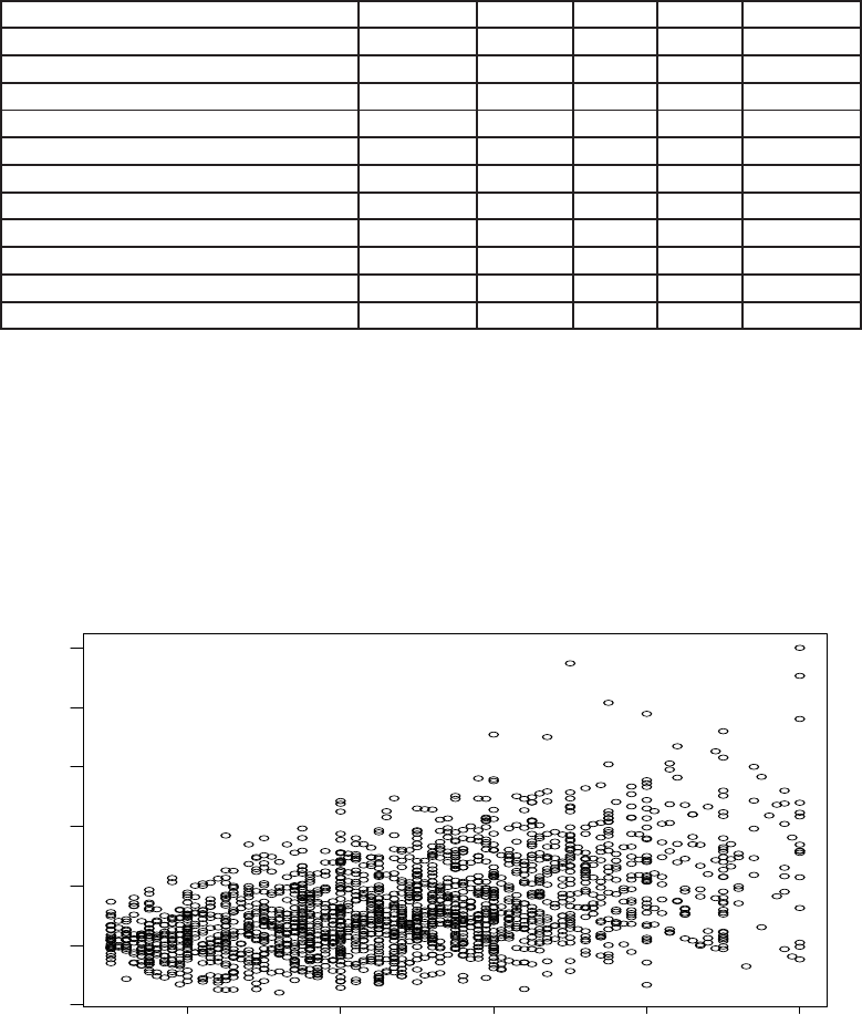
4.1. DIFFERENT DISTRIBUTIONS IN GAMLSS() 69
Distributions R Name Section µ σ ν
beta binomial BB() A.9.2 logit log -
binomial BI() A.9.1 logit - -
Delaporte DEL() A.10.4 log log logit
Negative Binomial type I NBI() A.10.2 log log -
Negative Binomial type II NBII() A.10.2 log log -
Poisson PO() A.10.1 log - -
Poisson inverse Gaussian PIG() A.10.3 log log -
Sichel SI() A.10.5 log log identity
Sichel (µthe mean) SICHEL() A.10.5 log log identity
zero inflated poisson ZIP() A.10.6 log logit -
zero inflated poisson (µthe mean) ZIP2() A.10.6 log logit -
Table 4.2: Discrete distributions implemented within the gamlss packages (with default link
functions)
40 60 80 100 120
0 500 1000 1500 2000 2500 3000
Fl
R
Figure 4.1: Rent (R) against floor space (Fl) from the rent data
70 CHAPTER 4. DISTRIBUTIONS
GAMLSS-RS iteration 4: Global Deviance = 28044.44
> detach(rent)
The second gamlss() command changes the link function for mu to "identity", while the
sigma link function remains at the default value which is the log. The default link functions for
all available distributions are shown in the last four columns of Tables 4.1 and 4.2. By printing
the relevant gamlss.family you can check the default link functions, e.g.
> BCT()
GAMLSS Family: BCT Box-Cox t
Link function for mu : identity
Link function for sigma: log
Link function for nu : identity
Link function for tau : log
In order to get all the available links for the parameters of a specific distribution use the
function show.link.
> show.link(BCT)
$mu
c("inverse", "log", "identity", "own")
$sigma
c("inverse", "log", "identity", "own")
$nu
c("inverse", "log", "identity", "own")
$tau
c("inverse", "log", "identity", "own")
An easy way to add link functions that are not available in gamlss is to use the option own
link. See for example the help file for make.link.gamlss to see how this can be achieved. All of
the distributions in Tables 4.1 and 4.2 have d,p,qand rfunctions corresponding respectively
to the probability density function (pdf) the cumulative density function (cdf) the quantiles
(i.e. inverse cdf) and random value generating functions. For example, the gamma distribution
has the functions dGA,pGA,qGA and rGA. Here we use them to provide distribution plots for the
gamma distribution shown in Figure 4.2:
PPP <- par(mfrow=c(2,2))
plot(function(y) dGA(y, mu=10 ,sigma=0.3), 0.1, 25) # pdf
plot(function(y) pGA(y, mu=10 ,sigma=0.3), 0.1, 25) # cdf
plot(function(y) qGA(y, mu=10 ,sigma=0.3), 0, 1) # inverse cdf
y<-rGA(100,mu=10,sigma=.3) # randomly generated values
hist(y)
par(PPP)
For discrete distributions use commands similar to the ones used to plot the negative bino-
mial of type I below. The resulting plots are shown in Figure 4.3
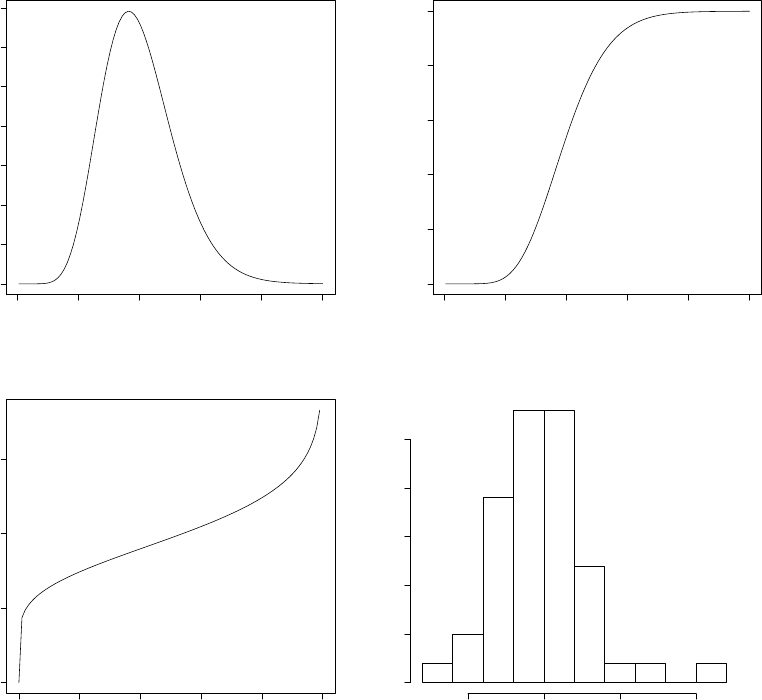
4.1. DIFFERENT DISTRIBUTIONS IN GAMLSS() 71
0 5 10 15 20 25
0.00 0.02 0.04 0.06 0.08 0.10 0.12 0.14
x
function(y) dGA(y, mu = 10, sigma = 0.3) (x)
0 5 10 15 20 25
0.0 0.2 0.4 0.6 0.8 1.0
x
function(y) pGA(y, mu = 10, sigma = 0.3) (x)
0.0 0.2 0.4 0.6 0.8 1.0
0 5 10 15
x
function(y) qGA(y, mu = 10, sigma = 0.3) (x)
Histogram of rGA(100, mu = 10, sigma = 0.3)
rGA(100, mu = 10, sigma = 0.3)
Frequency
5 10 15 20
0 5 10 15 20 25
Figure 4.2: Plots created by (a) dGA (b) pGA (c) qGA, and (d) rGA functions respectively, i.e. (a)
the pdf (b) the cdf (c) the inverse cdf (or quantiles) and (d) a histogram of a random sample,
from the gamma distribution.
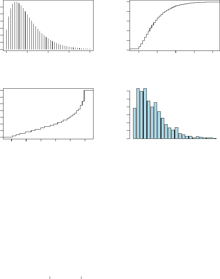
72 CHAPTER 4. DISTRIBUTIONS
0 10 20 30 40
0.00 0.02 0.04 0.06
pdf
x
pdf(x)
0 10 20 30 40
0.0 0.2 0.4 0.6 0.8 1.0
cdf
x
cdf(x)
0.0 0.2 0.4 0.6 0.8 1.0
0 5 10 20 30
inverse cdf
x
inv−cdf(x)
0 2 4 6 8 11 14 17 20 27
0 20 40 60 80 100
Figure 4.3: Plot created by (a) dNBI (b) pNBI (c) qNBI and (d) rNBI functions respectively,
(a) the pdf (b) the cdf (c) the inverse cdf and (d) a histogram of a random sample, from the
negative binomial distribution type I.
PPP <- par(mfrow=c(2,2))
plot(function(y) dNBI(y, mu = 10, sigma = 0.5 ), from=0, to=40, n=40+1, type="h",
main="pdf", ylab="pdf(x)")
cdf <- stepfun(0:39, pNBI(0:40, mu=10, sigma=0.5 ), f = 0)
plot(cdf, main="cdf", ylab="cdf(x)", do.points=FALSE )
invcdf <- stepfun(seq(0.01,.99,length=39), qNBI(seq(0.01,.99,length=40),
mu=10, sigma=0.5 ), f = 0)
plot(invcdf, main="inverse cdf", ylab="inv-cdf(x)", do.points=FALSE )
tN <- table(Ni <- rNBI(1000, mu=5, sigma=0.5))
r <- barplot(tN, col= lightblue )
par(PPP)
The “Section” column of Tables 4.1 and 4.2 shows the Section in Appendix Awhere the user
can find the appropriate parameterization of any of the distributions. Different parameteriza-
tions for any distribution in Tables 4.1 and 4.2 or brand new distributions can be added easily
in the list by amending one of the current distribution files. More advice on this subject is given
in Section 4.2. Section 4.3 describes how the distributions in Tables 4.1 and 4.2 can be fitted
to data. Section 4.4 describes the gamlss function pdf.plot().

4.2. AMENDING AND CONSTRUCTING A NEW DISTRIBUTION 73
4.2 Amending and constructing a new distribution
This Section can be omitted if the user does not plan to add a new distribution
or amend an existing distribution.
The Rfunctions implementing the normal distribution NO() are shown below.
Normal <- NO <-function (mu.link ="identity", sigma.link="log") {
# definition of the link function options
mstats <- checklink( "mu.link", "Normal", substitute(mu.link),
c("inverse", "log", "identity", "own"))
dstats <- checklink("sigma.link", "Normal", substitute(sigma.link),
c("inverse", "log", "identity", "own"))
# fitting information
structure(
list(family = c("NO", "Normal"),
parameters = list(mu=TRUE,sigma=TRUE),
nopar = 2,
type = "Continuous",
mu.link = as.character(substitute(mu.link)),
sigma.link = as.character(substitute(sigma.link)),
mu.linkfun = mstats$linkfun,
sigma.linkfun = dstats$linkfun,
mu.linkinv = mstats$linkinv,
sigma.linkinv = dstats$linkinv,
mu.dr = mstats$mu.eta,
sigma.dr = dstats$mu.eta,
dldm = function() (1/sigma^2)*(y-mu),
d2ldm2 = function() -(1/sigma^2),
dldd = function() ((y-mu)^2-sigma^2)/(sigma^3),
d2ldd2 = function() -(2/(sigma^2)),
d2ldmdd = function() rep(0,length(y)),
G.dev.incr = function(y,mu,sigma,...)
GD <- -2*dNO(y,mu,sigma,log=TRUE),
rqres = expression(rqres(pfun="pNO", type="Continuous",
y=y, mu=mu, sigma=sigma)),
mu.initial = expression({ mu <- (y+mean(y))/2 }),
sigma.initial = expression({sigma <- rep(sd(y),length(y))}),
mu.valid = function(mu) TRUE ,
sigma.valid = function(sigma) all(sigma > 0),
y.valid = function(y) TRUE
),
# the class definition
class = c("gamlss.family","family"))
}
74 CHAPTER 4. DISTRIBUTIONS
# the definition of the d, p, q, and r functions
dNO<-function(y, mu=0, sigma=1, log=FALSE)
{
fy <- dnorm(y, mean=mu, sd=sigma, log=log)
fy
}
pNO <- function(q, mu=0, sigma=1, lower.tail = TRUE, log.p = FALSE)
{
if (any(sigma <= 0)) stop(paste("sigma must be positive", "\n", ""))
cdf <- pnorm(q, mean=mu, sd=sigma, lower.tail = lower.tail, log.p = log.p)
cdf
}
qNO <- function(p, mu=0, sigma=1, lower.tail = TRUE, log.p = FALSE)
{ if (any(sigma <= 0)) stop(paste("sigma must be positive", "\n", ""))
if (log.p==TRUE) p <- exp(p) else p <- p
if (any(p < 0)|any(p > 1)) stop(paste("p must be between 0 and 1", "\n", ""))
q <- qnorm(p, mean=mu, sd=sigma, lower.tail = lower.tail )
q
}
rNO <- function(n, mu=0, sigma=1)
{
if (any(sigma <= 0)) stop(paste("sigma must be positive", "\n", ""))
r <- rnorm(n, mean=mu, sd=sigma)
r
}
#-------------------------------------------
The first function, NO, is the one providing the information for fitting the normal distribution
in gamlss. The fitting NO function has three fields i) the definition of the link functions ii)
the information needed for fitting the distribution and iii) the class definition. The last four
functions define the pdf, (dNO), the cdf (pNO), the inverse cdf i.e. quantile (qNO) and random
generated (rNO) functions associated with NO.
i) the definition of the link functions To define the link function of any of the parameters
the checklink() function is used. This function takes four arguments.
a) which.link: which parameter the link is for, e.g. "mu.link"
b) which.dist: the current distribution, e.g. "Normal" (the name is only used to report
an error in the specification of the link function)
c) link: which link is currently used, (the default value is the one given as arguments in
the function definition, e.g. substitute(mu.link)will do the job)
d) link.List: the list of the possible links for the specific parameter, e.g. c("inverse",
"log", "identity") and
e) par.link: a list containing the value of the parameter(s) (if the link has parameter(s)
as for example in the "logshifted" and "logitshifted" links).

4.2. AMENDING AND CONSTRUCTING A NEW DISTRIBUTION 75
The available links to choose from are currently the ones used by the make.link.gamlss()
function. This list includes "logit","probit","cloglog","identity","log","sqrt",
"1/mu^2","inverse","logshifted","logitshifted" and "own". This may change in
future gamlss releases to incorporate more link functions. For the use of the own see the
help files under the make.lin.gamlss where an example is given. [The object returned by
checklink() contains the link function as a function of the current parameter, the inverse
link function as a function of the current linear predictor and finally the first derivative
of the inverse link function as a function of the linear predictor i.e. dmu/deta. These
functions are used in the fitting of the distribution.]
ii) fitting information The fitting algorithm uses the following information.
family: the name of the distribution
parameters: a list indicating whether the parameter will be fitted i.e. mu=TRUE, or
fixed at initial values i.e. nu=FALSE.
nopar: the number of parameters
type: the type of distribution i.e. ”Continuous” or ”Discrete”
mu.link, sigma.link: the current link functions as character strings
mu.linkfun, sigma.linkfun: the actual link functions returned from checklink()
mu.linkinv, sigma.linkinv: the actual inverse link functions returned from checklink()
mu.dr, sigma.dr: the actual first derivative of the inverse link functions returned
from checklink()
dldm: the first derivative of the likelihood with respect to the location parameter mu
d2ldm2: the expected second derivative of the likelihood with respect to the location
parameter mu
dldd: the first derivative of the likelihood with respect to the scale parameter sigma
d2ldd2: the expected second derivative of the likelihood with respect to the scale
parameter sigma
d2ldmddd: the expected cross derivative of the likelihood with respect to both the
location mu and scale parameter sigma
G.dev.incr: the global deviance (equal to minus twice the log likelihood)
rqres: the definition of the (normalized quantile) residuals [Note these are random-
ized for discrete distributions]
mu.initial, sigma.initial: the default initial values for the starting of mu and
sigma (both vectors of length n) for the algorithm
mu.valid, sigma.valid, y.valid: valid range of values for the parameters (mu
and sigma ) and the response variable
Note that all the items above are compulsory.
[The expected second derivatives can be replaced in some cases by the negative squared
first derivatives by using the expression eval.parent(expression(-dldp^2)). This will
only work with the RS() fitting method of gamlss()].
iii) class Each family is defined as a gamlss.family object.
76 CHAPTER 4. DISTRIBUTIONS
iv) the dNO,pNO,qNO and rNO functions These four functions defined in general, the pdf,
cdf, inverse cdf and random generating functions for the distribution at hand. In the
specific case of the normal distribution these function are not necessarily needed since
Rprovides the equivalent functions dnorm,pnorm,qnorm and rnorm. We have included
them here for convenience and consistency (with our parameterization of the distribution
according to mu and sigma). From these four functions only the dfunction is usually used
within the fitting function of a distribution while the pfunction is needed for calculating
(and plotting) the residuals. The dfunction is used in the definition of global deviance
and the pfunction in the definition of the quantile normalized residuals. The residuals are
defined with the element rqres of the structure above which is using the function rqres()
of the package (gamlss). The function rqres() needs to know what type gamlss.family
distribution we are using. For example for the NO distribution above we use the code
rqres(pfun="pNO", type="Continuous", y=y, mu=mu, sigma=sigma). This in effect
will define the residuals as qnorm(pBCCG(y,mu,sigma,nu)). For discrete distributions the
function rqres() will randomized the residuals. For example the code for the Poisson
distribution is rqres(pfun="pPO", type="Discrete", ymin=0, y=y, mu=mu).
As an example in which a different parameterization a distribution is required consider the
reparameterized normal distribution in which mu is still the mean but sigma is now the variance
of the distribution rather the standard error. Only the changes from the previous definition of
the function are printed here.
Normal.var <- NO2 <-function (mu.link ="identity", sigma.link="log")
...
list(family = c("NO2","Normal with variance"),
...
dldm = function() (1/sigma)*(y-mu),
d2ldm2 = function() -(1/sigma),
dldd = function() 0.5*((y-mu)^2-sigma)/(sigma^2),
d2ldd2 = function() -(1/(2*sigma^2)),
d2ldmdd = function() rep(0,length(y)),
G.dev.incr = function(y,mu,sigma,...) -2*dNO2(y,mu,sigma,log=TRUE),
rqres = expression(rqres(pfun="pNO2", type="Continuous", y=y, mu=mu,
sigma=sigma)),
...
}
The d,p,qand rfunctions have to be amended accordingly. Since Rprovides d,p,qand
rfunctions for the normal distributions [given by dnorm,pnorm,qnorm and rnorm respectively]
the amendment here can be easily done as follows
dNO2<-function(y, mu=0, sigma=1, log=FALSE)
{
if (any(sigma <= 0)) stop(paste("sigma must be positive", "\n", ""))
fy <- dnorm(y, mean=mu, sd=sqrt(sigma), log=log)
fy
}
pNO2 <- function(q, mu=0, sigma=1, lower.tail = TRUE, log.p = FALSE)
{
4.3. FITTING DISTRIBUTIONS (WITH CONSTANT PARAMETERS) TO A DATA SAMPLE77
if (any(sigma <= 0)) stop(paste("sigma must be positive", "\n", ""))
cdf <- pnorm(q, mean=mu, sd=sqrt(sigma), lower.tail = lower.tail,
log.p = log.p)
cdf
}
qNO2 <- function(p, mu=0, sigma=1, lower.tail = TRUE, log.p = FALSE)
{ if (any(sigma <= 0)) stop(paste("sigma must be positive", "\n", ""))
if (log.p==TRUE) p <- exp(p) else p <- p
if (any(p < 0)|any(p > 1))
stop(paste("p must be between 0 and 1", "\n", ""))
q <- qnorm(p, mean=mu, sd=sqrt(sigma), lower.tail = lower.tail )
q
}
rNO2 <- function(n, mu=0, sigma=1)
{
if (any(sigma <= 0)) stop(paste("sigma must be positive", "\n", ""))
r <- rnorm(n, mean=mu, sd=sqrt(sigma))
r
}
More generally if an equivalent function does not exist it has to be written explicitly. For
example this is another version of dNO2
dNO2<-function(y, mu=0, sigma=1, log=FALSE)
{
if (any(sigma <= 0)) stop(paste("sigma must be positive", "\n", ""))
loglik <- -0.5*log(2*pi*sigma)-0.5*((y-mu)^2)/sigma
fy <- if(log==FALSE) exp(loglik) else loglik
fy
}
For users who would like to implement a different (or their own) distribution from the ones
in Tables 4.1 and 4.2 the advice is to take one of the current distribution definition files (with
similar number of parameters) and amend it. The GU(),TF(), and BCT() distributions are good
examples of 2, 3, and 4 parameter continuous distributions respectively. IG() provides a good
example where the pand qfunctions are calculated using numerical methods. The PO(),NBI()
and SI are good examples of 1,2 and 3 parameter discrete distributions respectively. The BB()
provides a example where the pand qfunctions are calculated using numerical methods.
4.3 Fitting distributions (with constant parameters) to a
data sample
In order to fit constant parameters to data, use the gamlss() function with 1 as arguments
for all the parameter formulae. Below we consider two examples, one with sample kurtosis less
than 3 (platykurtic) and one with sample kurtosis more than 3 (leptokurtic).
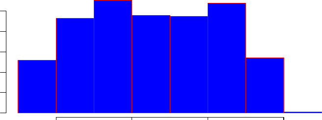
78 CHAPTER 4. DISTRIBUTIONS
4.3.1 Data with sample kurtosis less than 3
Here, for demonstration purpose, we use the abdominal data as a single sample and fit different
distributions (with constant parameters) to it.
data(abdom)
attach(abdom)
hist(y)
<See figure 4.4 for the plot.>
Histogram of y
y
Frequency
100 200 300 400
0 20 40 60 80 100
Figure 4.4: An histogram of the y variable in the abdom data
Note that the sample distribution of y is platykurtic. We fit the normal distribution (NO),
the power exponential (PE), and the Box-Cox power exponential (BCPE). [The tdistribution
(TF) and the Box-Cox t(BCT) are both unsuitable since the sample kurtosis is less than 3 (i.e.
less than the kurtosis of normal distribution)].
> abd5<- gamlss(y~1,sigma.formula=~1,family=NO)
GAMLSS-RS iteration 1: Global Deviance = 7201.417
GAMLSS-RS iteration 2: Global Deviance = 7201.417
> plot(abd5)
*******************************************************************
Summary of the Quantile Residuals
mean = 6.635566e-17
variance = 1.001642
coef. of skewness = -0.02560028
coef. of kurtosis = 1.905348
Filliben correlation coefficient = 0.9845929
*******************************************************************
<See figure 4.5 for the plot.>
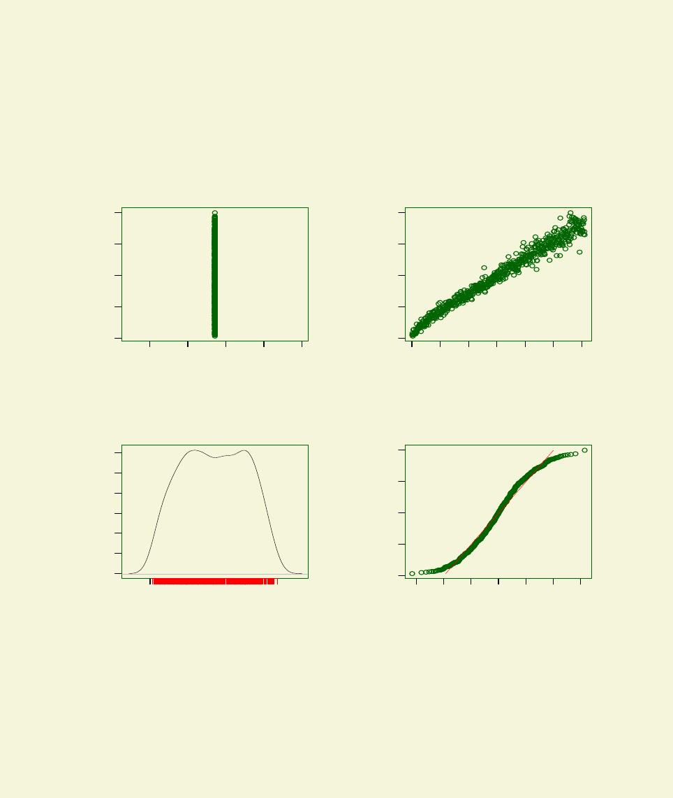
4.3. FITTING DISTRIBUTIONS (WITH CONSTANT PARAMETERS) TO A DATA SAMPLE79
225 226 227 228 229
−2 −1 0 1 2
Against Fitted Values
Fitted Values
Quantile Residuals
0 100 200 300 400 500 600
−2 −1 0 1 2
Against x−variable
index
Quantile Residuals
−2 −1 0 1 2
0.00 0.10 0.20 0.30
Density Estimate
Quantile. Residuals
Density
−3 −2 −1 0 1 2 3
−2 −1 0 1 2
Normal Q−Q Plot
Theoretical Quantiles
Sample Quantiles
Figure 4.5: Residual plot from fitting a Normal distribution with µ= 1 and σ= 1 to the
abdom data
80 CHAPTER 4. DISTRIBUTIONS
Note that the sample skewness and kurtosis are 0.0256 and 1.905 respectively (since they
are the same as for the residuals from fitting a normal distribution).
Now fit the power-exponential (PE) distribution to the abdominal data set.
> abd6 <- gamlss(y~1,sigma.formula=~1,nu.formula=~1,family=PE)
GAMLSS-RS iteration 1: Global Deviance = 7093.59
GAMLSS-RS iteration 2: Global Deviance = 7093.034
GAMLSS-RS iteration 3: Global Deviance = 7093.013
GAMLSS-RS iteration 4: Global Deviance = 7093.007
GAMLSS-RS iteration 5: Global Deviance = 7093.005
GAMLSS-RS iteration 6: Global Deviance = 7093.004
Note that the power exponential distribution, PE() provides a substantially superior fit to
the data than the normal distribution since the global deviance has reduced by 108.412.
> abd6
Family: c("PE", "Power Exponential")
Fitting method: RS()
Call: gamlss(formula = y ~ 1, sigma.formula = ~1, nu.formula = ~1,
family = PE)
Mu Coefficients:
(Intercept)
225.4
Sigma Coefficients:
(Intercept)
4.494
Nu Coefficients:
(Intercept)
2.328
Degrees of Freedom for the fit: 3 Residual Deg. of Freedom 607
Global Deviance: 7093
AIC: 7099
SBC: 7112.24
By default gamlss() allows a maximum of 20 outer iterations. If more iterations are needed
to reach convergence you can either use the refit() function as in Section 3.3.1 or increase
the number of iterations by using the function gamlss.control() as in Section 3.1.2. Let us
fit constants for the four parameter of the Box-Cox power exponential distribution, BCPE(), to
the abdominal data set:
> abd7 <- gamlss(y~1, sigma.formula=~1, nu.formula=~1,
+ tau.formula=~1, family=BCPE, data=abdom, n.cyc=50)
GAMLSS-RS iteration 1: Global Deviance = 7208.284
GAMLSS-RS iteration 2: Global Deviance = 7103.532
4.3. FITTING DISTRIBUTIONS (WITH CONSTANT PARAMETERS) TO A DATA SAMPLE81
GAMLSS-RS iteration 3: Global Deviance = 7100.521
...
GAMLSS-RS iteration 38: Global Deviance = 7092.99
GAMLSS-RS iteration 39: Global Deviance = 7092.99
Note that the Box-Cox power exponential, BCPE(), distribution does not provide a significant
improvement over the power exponential, PE(), distribution, since the global deviance has
reduced only by 0.015.
> abd7
Family: c("BCPE", "Box-Cox Power Exponential")
Fitting method: RS()
Call: gamlss(formula = y ~ 1, sigma.formula = ~1, nu.formula = ~1,
tau.formula = ~1, family = BCPE, data = abdom, n.cyc = 50)
Mu Coefficients:
(Intercept)
226.2
Sigma Coefficients:
(Intercept)
-0.9291
Nu Coefficients:
(Intercept)
1.014
Tau Coefficients:
(Intercept)
2.327
Degrees of Freedom for the fit: 4 Residual Deg. of Freedom 606
Global Deviance: 7092.99
AIC: 7100.99
SBC: 7118.64
Let us now plot the fitted distribution using the pdf.plot() function which is described in
more detail in Section 4.4.
pdf.plot(abd7,1,min=1,max=500,step=1)}
<see figure 4.6>
Note the second argument 1 indicates that we want a single plot using the fitted values from
observation 1.
The function histDist() can be used for fitting and plotting the distribution of a response
variance simultaneously. This function fits constants for each parameters of a gamlss.family
distribution using the gamlss() function and them plots the fitted distribution together with
the histogram of the yvector. The function histDist() has arguments
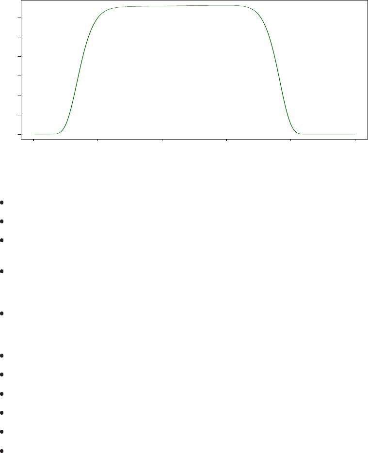
82 CHAPTER 4. DISTRIBUTIONS
0 100 200 300 400 500
0.0000 0.0005 0.0010 0.0015 0.0020 0.0025 0.0030
Box.Cox.Power.Exponential, BCPE
BCPE( mu = 226.2, sigma = 0.3949, nu = 1.014, tau = 10.26)
y
pdf, f(y)
Figure 4.6: The fitted BCPE distribution to the y variable of the abdom data
ya vector for the response variable
familya gamlss.family distribution
freqthe frequencies of the data in yif exist. freq is used as weights in the gamlss()
function fit
densitydefault value is FALSE. Change to TRUE if you would like a non-parametric
density plot together with the parametric fitted distribution plot (for continuous variable
only)
nbinsThe suggested number of bins (argument passed to truehist() of package MASS).
Either a positive integer, or a character string naming a rule: ”Scott” or ”Freedman-
Diaconis” or ”FD”. (Case is ignored.)
xlimthe minimum and the maximum x-axis value (if the default values are out of range)
ylimthe minimum and the maximum y-axis value (if the default values are out of range)
mainthe main title for the plot
xlabthe label in the x-axis
ylabthe label in the y-axis
. . . for extra arguments to be passed to the gamlss() function
The fitted PE distribution and the histogram of the abdominal data given in figure 4.7 is
produced using the commands
histDist(abdom$y,"PE")
GAMLSS-RS iteration 1: Global Deviance = 7093.59
GAMLSS-RS iteration 2: Global Deviance = 7093.032
GAMLSS-RS iteration 3: Global Deviance = 7093.014
GAMLSS-RS iteration 4: Global Deviance = 7093.008
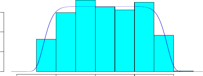
4.3. FITTING DISTRIBUTIONS (WITH CONSTANT PARAMETERS) TO A DATA SAMPLE83
GAMLSS-RS iteration 5: Global Deviance = 7093.006
GAMLSS-RS iteration 6: Global Deviance = 7093.005
0 100 200 300 400
0.000 0.001 0.002 0.003
y
Figure 4.7: The histogram and the fitted PE distribution to the y variable of the abdom data
4.3.2 Data with sample kurtosis more than 3
Here we use a subset of the head circumference data from the Fourth Dutch Growth Study,
kindly given to us by Prof. van Buuren. We have selected the data with ages between 1 and 2
years.
data(db)
subdata<-subset(db, (age > 1 & age <2))
hist(subdata$head,col="blue",border="red")
<See figure 4.8 for the histogram>
Note that the sample distribution is leptokurtic (i.e. kurtosis >3). Here we fit the nor-
mal, NO(), the tfamily, TF(), Box-Cox t,BCT(), and Box-Cox power exponential, BCPE(),
distributions.
> h1<-gamlss(subdata$head~1,family=NO)
GAMLSS-RS iteration 1: Global Deviance = 2970.53
GAMLSS-RS iteration 2: Global Deviance = 2970.53
Note that we have not bothered to declare the option sigma.formula= 1 here. By default
the gamlss() function automatically assumes that the rest of the parameters of the distribution
of the option family a constant fitted to them.
plot(h1)
*******************************************************************
Summary of the Randomised Quantile Residuals
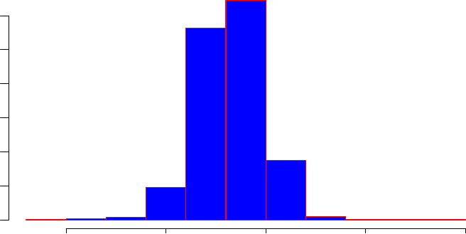
84 CHAPTER 4. DISTRIBUTIONS
Histogram of sub$head
sub$head
Frequency
40 45 50 55 60
0 50 100 150 200 250 300
Figure 4.8: Histogram of the subset of the head circumference Dutch boys data
mean = -3.382136e-17
variance = 1.001326
coef. of skewness = 0.2058114
coef. of kurtosis = 7.728382
Filliben correlation coefficient = 0.9758402
*******************************************************************
<See figure 4.9 for the residual plot. Note in the plot on the top left of figure 4.9 the
plotting procedure incorrectly plots one observation differently in the x axis from the rest.>
Note that the skewness and kurtosis of the sample subset are 0.2058 and 7.728 respectively.
The fitted values of µand σfor the normal distribution are 48.34 and 1.73 as shown below.
> fitted(h1)[1]
1
48.34265
> fitted(h1,"sigma")[1]
[1] 1.730309
If it is required to fix a parameter to a given specific value (e.g. sigma = 2) we can use
the option sigma.fix and sigma.start as follows. This fixes the value of σat its starting
value 2.
> h2<-gamlss(subdata$head~1,family=NO,sigma.fix = TRUE, sigma.start=2)
GAMLSS-RS iteration 1: Global Deviance = 2999.361
GAMLSS-RS iteration 2: Global Deviance = 2999.361
>fitted(h2)[1]
1
48.34265
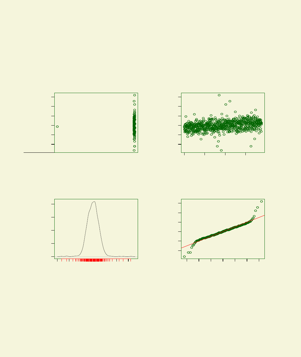
4.3. FITTING DISTRIBUTIONS (WITH CONSTANT PARAMETERS) TO A DATA SAMPLE85
−4 −2 0 2 4 6
Against Fitted Values
Fitted Values
Quantile Residuals
0 200 400 600
−4 −2 0 2 4 6
Against x−variable
index
Quantile Residuals
−6 −4 −2 0 2 4 6
0.0 0.1 0.2 0.3 0.4
Density Estimate
Quantile. Residuals
Density
−3 −2 −1 0 1 2 3
−4 −2 0 2 4 6
Normal Q−Q Plot
Theoretical Quantiles
Sample Quantiles
Figure 4.9: Residual plot from the Normal (NO) fitted model on the subset of the Dutch boys
data
86 CHAPTER 4. DISTRIBUTIONS
>fitted(h2,"sigma")[1]
[1] 2
Now let us fit a tdistribution.
> h3<-gamlss(subdata$head~1,family=TF)
GAMLSS-RS iteration 1: Global Deviance = 2899.54
GAMLSS-RS iteration 2: Global Deviance = 2898.199
GAMLSS-RS iteration 3: Global Deviance = 2898.049
GAMLSS-RS iteration 4: Global Deviance = 2898.033
GAMLSS-RS iteration 5: Global Deviance = 2898.031
GAMLSS-RS iteration 6: Global Deviance = 2898.030
The fitted values of µ,σand νare given by:
> fitted(h3,"mu")[1]
1
48.33736
> fitted(h3,"sigma")[1]
[1] 1.406914
> fitted(h3,"nu")[1]
[1] 6.505162
Now let us fit a Box-Cox tdistribution.
> h4<-gamlss(subdata$head~1,family=BCT)
GAMLSS-RS iteration 1: Global Deviance = 2911.564
GAMLSS-RS iteration 2: Global Deviance = 2898.229
GAMLSS-RS iteration 3: Global Deviance = 2898.010
GAMLSS-RS iteration 4: Global Deviance = 2897.988
GAMLSS-RS iteration 5: Global Deviance = 2897.986
GAMLSS-RS iteration 6: Global Deviance = 2897.985
The fitted values of µ,σ,νand τare given by:
> fitted(h4,"mu")[1]
1
48.33492
> fitted(h4,"sigma")[1]
[1] 0.02911198
> fitted(h4,"nu")[1]
1
0.7695857
> fitted(h4,"tau")[1]
[1] 6.50734
Plot the residuals (see figure 4.10)
> plot(h4)
*******************************************************************
Summary of the Randomised Quantile Residuals
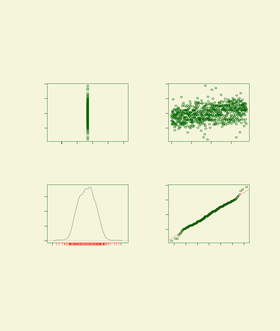
4.3. FITTING DISTRIBUTIONS (WITH CONSTANT PARAMETERS) TO A DATA SAMPLE87
mean = -0.0003782754
variance = 1.001298
coef. of skewness = 0.005689533
coef. of kurtosis = 3.156953
Filliben correlation coefficient = 0.99688
*******************************************************************
48.0 48.2 48.4 48.6 48.8
−2 0 2 4
Against Fitted Values
Fitted Values
Quantile Residuals
0 200 400 600
−2 0 2 4
Against x−variable
index
Quantile Residuals
−4 −2 0 2 4
0.0 0.1 0.2 0.3
Density Estimate
Quantile. Residuals
Density
−3 −2 −1 0 1 2 3
−2 0 2 4
Normal Q−Q Plot
Theoretical Quantiles
Sample Quantiles
Figure 4.10: Residual plot of the BCT model fitted in to the Dutch boys data
Plot the fitted BCT distribution (see figure 4.11)
pdf.plot(h4,1,min=40,max=60,step=0.1)
The function histDist can be use for plotting both the histogram and the fitted distribution
for the above data.
histDist(subdata$head,"BCT",ymax=0.30)
GAMLSS-RS iteration 1: Global Deviance = 2911.564
GAMLSS-RS iteration 2: Global Deviance = 2898.229
GAMLSS-RS iteration 3: Global Deviance = 2898.010
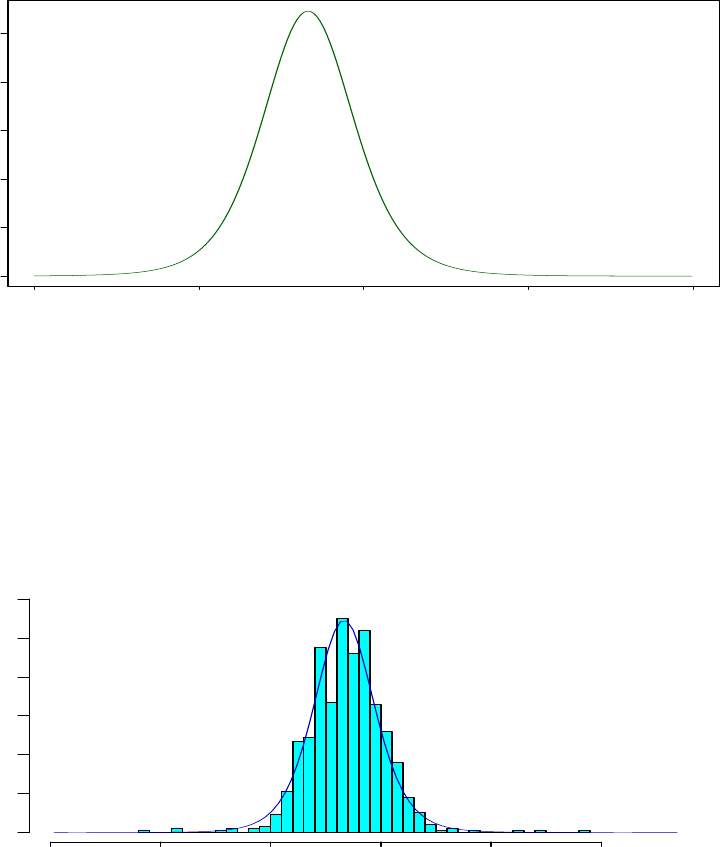
88 CHAPTER 4. DISTRIBUTIONS
40 45 50 55 60
0.00 0.05 0.10 0.15 0.20 0.25
Box.Cox.t, BCT
BCT( mu = 48.33, sigma = 0.02911, nu = 0.7696, tau = 6.507)
y
pdf, f(y)
Figure 4.11: The fitted BCT distribution to the Dutch boys data
GAMLSS-RS iteration 4: Global Deviance = 2897.988
GAMLSS-RS iteration 5: Global Deviance = 2897.986
GAMLSS-RS iteration 6: Global Deviance = 2897.985
<See figure 4.12 for the plot>
35 40 45 50 55 60
0.00 0.05 0.10 0.15 0.20 0.25 0.30
y
Figure 4.12: The histigram and the fitted BCT distribution to the Dutch boys data
Try now the BCPE distribution.
> h5<-gamlss(subdata$head~1,family=BCPE)
GAMLSS-RS iteration 1: Global Deviance = 2969.88
GAMLSS-RS iteration 2: Global Deviance = 2924.995
GAMLSS-RS iteration 3: Global Deviance = 2924.977
GAMLSS-RS iteration 4: Global Deviance = 2924.977
4.3. FITTING DISTRIBUTIONS (WITH CONSTANT PARAMETERS) TO A DATA SAMPLE89
Let us start from different starting values to make sure we converge to the same value.
> h5<-gamlss(subdata$head~1,family=BCPE,nu.start=1,tau.start=1.7)
GAMLSS-RS iteration 1: Global Deviance = 2945.519
GAMLSS-RS iteration 2: Global Deviance = 2924.990
GAMLSS-RS iteration 3: Global Deviance = 2924.977
GAMLSS-RS iteration 4: Global Deviance = 2924.977
Note that Box-Cox power exponential, BCPE() fit to the data is significantly worst that of
either the t-family distribution, TF() or the Box-Cox t distribution, BCT(), though better than
the normal distribution, NO(). The fitted values of µ,σ,νand τare given by:
> fitted(h5)[1]
1
48.33382
> fitted(h5,"sigma")[1]
1
0.03532261
> fitted(h5,"nu")[1]
1
0.5777963
> fitted(h5,"tau")[1]
1
1.389393
> plot(h5)
*******************************************************************
Summary of the Quantile Residuals
mean = -0.001821392
variance = 0.995158
coef. of skewness = 0.005233181
coef. of kurtosis = 3.953595
Filliben correlation coefficient = 0.9924379
*******************************************************************
>pdf.plot(h5,1,min=40,max=60,step=0.2)
<See figure 4.13 for the residual plot>
<See figure 4.14 for the distribution plot>
Obviously the BCT distribution fits better to this set of data than the BCPE. Now we use
the histDist() function to fit the BCPE distribution.
histDist(subdata$head,"BCPE")
GAMLSS-RS iteration 1: Global Deviance = 2969.88
GAMLSS-RS iteration 2: Global Deviance = 2924.995
GAMLSS-RS iteration 3: Global Deviance = 2924.977
GAMLSS-RS iteration 4: Global Deviance = 2924.977
The plot is shown in 4.15.
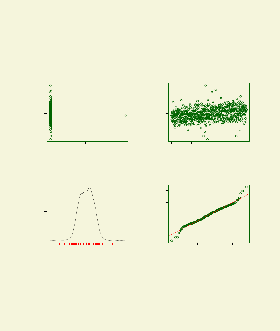
90 CHAPTER 4. DISTRIBUTIONS
48.33386 48.33386 48.33386
−4 −2 0 2 4
Against Fitted Values
Fitted Values
Quantile Residuals
0 200 400 600
−4 −2 0 2 4
Against x−variable
index
Quantile Residuals
−4 −2 0 2 4
0.0 0.1 0.2 0.3
Density Estimate
Quantile. Residuals
Density
−3 −2 −1 0 1 2 3
−4 −2 0 2 4
Normal Q−Q Plot
Theoretical Quantiles
Sample Quantiles
Figure 4.13: Residual plot of the BCPE model fitted to the subset of the Dutch data
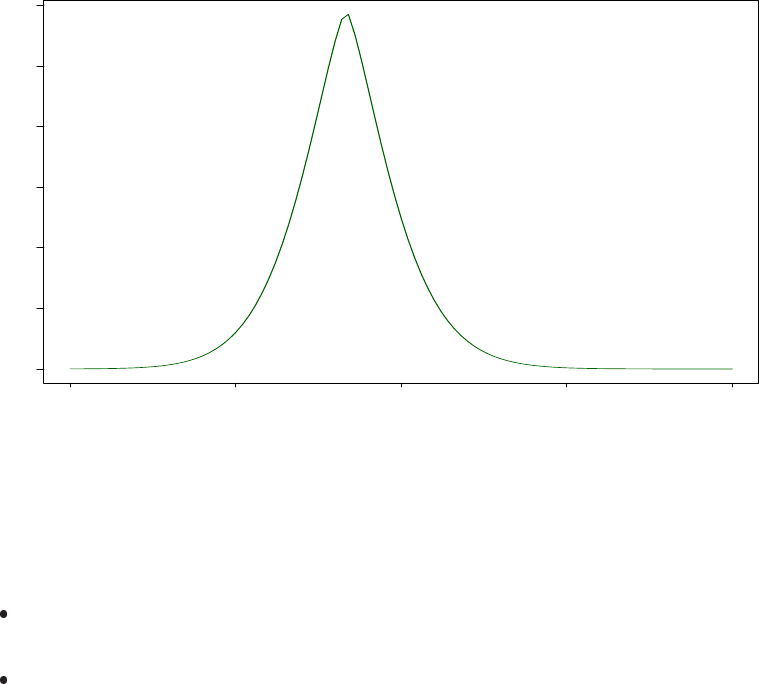
4.4. PLOTTING PDF’S USING PDF.PLOT() 91
40 45 50 55 60
0.00 0.05 0.10 0.15 0.20 0.25 0.30
Box.Cox.Power.Exponential, BCPE
BCPE( mu = 48.33, sigma = 0.03532, nu = 0.5732, tau = 1.391)
y
pdf, f(y)
Figure 4.14: The fitted p.d.f for the BCPE model fitted to the subset of the Dutch boys data
4.4 Plotting pdf’s using pdf.plot()
There are two ways of using the function pdf.plot().
given that you have already fitted a GAMLSS model and you want to see how the fitted
distribution looks at specific observation values.
when you just want to plot the distribution for specified values of the parameters of the
distribution.
As an example of the first case let us fit a BCT distribution to the data and then look at the
fitted distributions at observation cases 2, 45, and 139.
> abd8 <- gamlss(y~cs(x,df=3), sigma.formula=~x, nu.formula=~1,
+ tau.fo=~1, family=BCT, data=abdom)
Loading required package: splines
GAMLSS-RS iteration 1: Global Deviance = 4789.103
GAMLSS-RS iteration 2: Global Deviance = 4788.655
GAMLSS-RS iteration 3: Global Deviance = 4788.64
GAMLSS-RS iteration 4: Global Deviance = 4788.639
GAMLSS-RS iteration 5: Global Deviance = 4788.639
> pdf.plot(abd8,c(2,45,139), min=1,max=200,step=1)
<See figure 4.16 for the plot>
In the second case we plot the distribution BCT for specified values of the parameters.
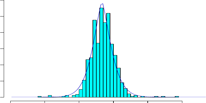
92 CHAPTER 4. DISTRIBUTIONS
35 40 45 50 55 60
0.00 0.05 0.10 0.15 0.20 0.25 0.30
y
Figure 4.15: Histogram and fitted BCPE distribution to the Dutch boys data
pdf.plot(family=BCT, min=1, max=20, step=.05, mu=10, sigma=0.15,
nu=-1, tau=c(1,10,20,40) )
Note that in general you have to play with the range of the y (min, max, step) for the plot
to look right. Also note that for the CG ,BCT and BCPE distributions, the value of sigma must be
small (eg sigma<0.2) in order for the truncation probability to be negligible so that the density
integrates to 1 and is a proper distribution. You can plot up to 8 distributions in the same plot
using the c( ) function with up to 8 numbers.
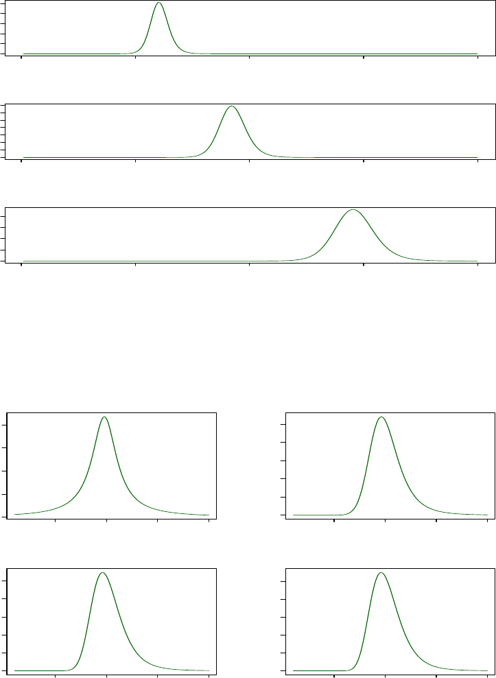
4.4. PLOTTING PDF’S USING PDF.PLOT() 93
0 50 100 150 200
0.00 0.04 0.08
Box.Cox.t, BCT
BCT( mu = 60.6, sigma = 0.06278, nu = −0.1785, tau = 9.858)
y
pdf, f(y)
0 50 100 150 200
0.00 0.02 0.04 0.06
Box.Cox.t, BCT
BCT( mu = 92.62, sigma = 0.06107, nu = −0.1785, tau = 9.858)
y
pdf, f(y)
0 50 100 150 200
0.00 0.02 0.04
Box.Cox.t, BCT
BCT( mu = 146, sigma = 0.05814, nu = −0.1785, tau = 9.858)
y
pdf, f(y)
Figure 4.16: The p.d.f. plot for the fitted BCT distribution for the abdom data at observations
2,45,139
5 10 15 20
0.00 0.05 0.10 0.15 0.20
Box.Cox.t, BCT
BCT( mu = 10, sigma = 0.15, nu = −1, tau = 1)
y
pdf, f(y)
5 10 15 20
0.00 0.05 0.10 0.15 0.20 0.25
Box.Cox.t, BCT
BCT( mu = 10, sigma = 0.15, nu = −1, tau = 10)
y
pdf, f(y)
5 10 15 20
0.00 0.05 0.10 0.15 0.20 0.25
Box.Cox.t, BCT
BCT( mu = 10, sigma = 0.15, nu = −1, tau = 20)
y
pdf, f(y)
5 10 15 20
0.00 0.05 0.10 0.15 0.20 0.25
Box.Cox.t, BCT
BCT( mu = 10, sigma = 0.15, nu = −1, tau = 40)
y
pdf, f(y)
Figure 4.17: The p.d.f from a Box-Cox t(BCT) distribution for specific parameter values
94 CHAPTER 4. DISTRIBUTIONS
Chapter 5
Additive terms
The GAMLSS model allows the user to model the distribution parameters mu,sigma,nu and
tau as linear, non-linear parametric, non-parametric (smooth) function of the explanatory vari-
ables and/or random effects terms. For modelling linear functions the user can use the standard
R notation for model formulae which is used in the fit of lm and glm models, see for exam-
ple Venables and Ripley (2002) Section 6.2. For fitting non-linear, non-parametric (smooth)
functions or random effects terms an additive term function has to be fitted.
Table 5.1 shows the additive term functions implemented in the gamlss package. The gamlss
package uses the same type of additive algorithm implemented in the R package gam, rather than
the function gam() R implementation in package mgcv. For each additive term this algorithm
requires two functions. The first one, (the one that is seen by the user), is shown in the second
column of the Table. This function defines the additive term(s) and sets the additional required
design matrices for the linear part of the additive model. For example cs(x) defines a cubic
smoothing spline function for the continuous explanatory variable x. Its is used during the
definition of the design matrix for the appropriate distribution parameter and it adds a linear
term for xin the design matrix. The second function is the one that actually performs the
additive backfitting algorithm. This function is called gamlss.name() where the name is one
of the names in column two of the Table. For example the function gamlss.cs() performs the
backfitting for cubic splines. New additive terms can be implemented by defining those two
functions.
The general policy when the backfitting is used in gamlss is to include the linear part of an
additive term in the appropriate linear term design matrix. For example, in the cubic spline
function cs() the explanatory variable say xis put in the linear design matrix of the appropriate
distribution parameter and the smoothing function is fitted as a deviation from this linear part.
This is equivalent of fitting a modified backfitting algorithm, see Hastie and Tibshirani (1990).
In other additive functions where the linear part is not needed (or defined) a column on zeros is
put in the design matrix. For example this is the case when the fractional polynomials additive
term fp() is used.
If the user wishes to create a new additive term, care should be taken on how the degrees of
freedom of the model are defined. The degrees of freedom for the (smoothing) additive terms
are usually taken to be the extra degrees of freedom on top of the linear fit. For example to
fit a smoothing cubic spline terms with 5 total degrees of freedom, df=3 should be used since
already 2 degrees of freedom have been used for the fitting of the constant and the linear part
of the explanatory variable.
After a gamlss object containing additive (smoothing) terms is used to fit a specific distri-
95

96 CHAPTER 5. ADDITIVE TERMS
Table 5.1: Implemented gamlss additive functions
Additive terms R Name Section
Cubic splines cs() 5.1
Varying coefficient vc() 5.2
Penalized splines ps() 5.3
loess lo() 5.4
Fractional polynomials fp() 5.5
Random effects random() 5.6.1
Random effects ra() 5.6.2
Random coefficient rc() 5.6.3
bution parameter the following components are (usually) saved for further use. In the output
below replace mu with sigma,nu or tau if a distribution parameter other that mu is involved.
mu.s: a matrix, each column containing the fitted values of the smoothers used to fit the
specific parameter. For example given a fitted model say mod1, mod1$mu.s would access
the additive terms fitted for mu.
mu.var: a matrix containing the estimated variance of the smoothers.
mu.df: a vector containing the extra degrees of freedom used to fit the smoothers.
mu.lambda: a vector containing the smoothing parameters (or random effects hyperparame-
ters).
mu.coefSmo: a list containing coefficients or other components from the additive smooth
fitting.
5.1 Cubic splines, the cs() function
The cubic splines function is based on the smooth.spline function of Rand can be used for
univariate smoothing. It fit a cubic smoothing spline function, see Hastie and Tibshirani (1990)
or Green and Silverman (1994).
The cs() function has the following arguments
xthe univariate vector of an explanatory variable.
df the desired equivalent number of degrees of freedom [trace of the smoother
matrix minus two (for the constant and linear fit)]. The real smoothing pa-
rameter (spar below) is found such that df=tr(S)-2, where S is the smoother
matrix which depends on spar. Values for df should be greater than 0, with
0 implying a linear fit. The default is df = 3, ie. 3 degrees of freedom for
smoothing xon top of a linear and constant term in xgiving a total of 5
degrees of freedom.
spar smoothing parameter, typically (but not necessarily) in the default range for
spar (-1.5,2]. The coefficient lambda of the integral of the squared second
derivative in the fitted (penalized log likelihood) criterion is a monotone func-
tion of ‘spar’, see the details in ’smooth.spline’ in R.
5.2. VARYING COEFFICIENT, THE VC() FUNCTION 97
c.spar This specifies minimum and maximum limits for the smoothing parameter,
the default limits being −1.5 to 2. This is an option to be used when the
degrees of freedom of the output fitted gamlss object are different from the
ones given as input in the option df, which is caused by the default limits for
the smoothing parameter being too narrow to obtain the required degrees of
freedom. The default values used are the ones given the option control.spar
in the R function ’smooth.spine()’ and they are ’c.spar=c(-1.5, 2)’. For very
large data sets e.g. 10000 observations, the upper limit may have to increase
for example to ’c.spar=c(-1.5, 2.5)’. Use this option if you have received the
warning ’The output df are different from the input, change the control.spar’.
’c.spar’ can take both vectors or lists of length 2, for example ’c.spar=c(-1.5,
2.5)’ or ’c.spar=list(-1.5, 2.5)’ would have the same effect.
As an example of using the smoothing cubic spline function cs() we use the rent data first
used in chapter 4. We remind the reader that the response variable R, is the monthly net rent
(rent minus calculated or estimated utility cost). Here we fit a additive model for floor space
(Fl) and for age (A) the year of construction.
> data(rent)
> r1<-gamlss(R~cs(Fl)+cs(A),data=rent, family=GA)
GAMLSS-RS iteration 1: Global Deviance = 27920.75
GAMLSS-RS iteration 2: Global Deviance = 27920.74
GAMLSS-RS iteration 3: Global Deviance = 27920.74
> # plotting the additive terms
> op <- par(mfrow=c(2,1))
> term.plot(r1 , se=TRUE, partial=TRUE)
The additive curves created by the function term.plot are shown in figure 5.1. We can also
plot the additive fitted surface using the R functions contour() and wireframe (the latest can
be found in the package lattice).
> # plotting the fitted surface in 3-d
> newrent<-data.frame(expand.grid(Fl=seq(30,120,5),A=seq(1890,1990,5)))
> newrent$pred<-predict(r1,newdata=newrent, type="response")
> Fln<-seq(30,120,5)
> An<-seq(1890,1990,5)
> op <- par(mfrow=c(1,1))
> contour(Fln,An,matrix(newrent$pred,nrow=length(Fln)),nlevels=30,
+ ylab="year of construction", xlab="floor space")
> library(lattice)
> wireframe(pred~Fl*A, newrent, aspect=c(1,0.5), drape=TRUE,
colorkey=list(space="right", height=0.6))
See figure 5.2 for the two plots.
5.2 Varying coefficient, the vc() function
The varying coefficient terms were introduced by Hastie and Tibshirani (1993) to accommodate
a special type of interaction between explanatory variables. This interaction takes the form
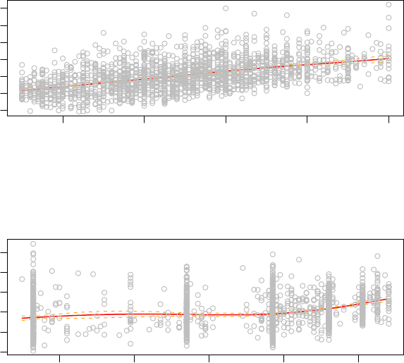
98 CHAPTER 5. ADDITIVE TERMS
40 60 80 100 120
−1.0 0.0 1.0 2.0
Fl
Partial for cs(Fl)
1900 1920 1940 1960 1980
−1.0 0.0 1.0
A
Partial for cs(A)
Figure 5.1: Rent data: Additive plots for the cubic splines model
of β(R)X, that is the linear coefficient of the explanatory variable Xis changing smoothing
according to another explanatory variable R. In many application Rwill be time. In general R
should be a continuous variable while Xcan be either continuous or categorical. In the current
gamlss implementation Xhas to be continuous or a two level factor with levels 0 and 1.
The vc() function has the following arguments
rrepresents the vector of the explanatory variable which effects the coefficients
of the explanatory variable, xi.e. β(r)∗x.
xan explanatory variable. [Note that xis center automatically by vc() due
to the invariance of varying coefficient models to location shifts in x, see
comments of Green in the discussion of Hastie and Tibshirani (1993)]
df as in function cs.
spar as in function cs.
c.spar as in function cs.
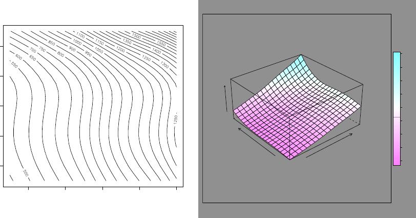
5.2. VARYING COEFFICIENT, THE VC() FUNCTION 99
floor space
year of construction
40 60 80 100 120
1900 1920 1940 1960 1980
Fl
A
pred
400
600
800
1000
1200
1400
1600
1800
2000
Figure 5.2: Rent data: contour and surface plot for the fitted additive cubic splines model model
As an example of using the function vc() consider the following models for mu in the rent
data example, using the default 3 additional degrees of freedom for each smoothing term on top
of the linear term.
data(rent)
attach(rent)
m1<-gamlss(R~cs(Fl)+cs(A), family=GA)
GAMLSS-RS iteration 1: Global Deviance = 27920.7
GAMLSS-RS iteration 2: Global Deviance = 27920.74
GAMLSS-RS iteration 3: Global Deviance = 27920.74
m2<-gamlss(R~cs(Fl)+cs(A)+vc(r=A,x=Fl), family=GA)
GAMLSS-RS iteration 1: Global Deviance = 27901.34
GAMLSS-RS iteration 2: Global Deviance = 27901.50
GAMLSS-RS iteration 3: Global Deviance = 27901.50
AIC(m1,m2)
df AIC
m2 14.00192 27929.51
m1 10.00128 27940.74
Obviously the varying coefficient model is an improvement over the simple additive model.
Note that the function term.plot() for plotting additive terms is not producing the right plot
for the varying coefficient terms, (for the additive terms it works fine). Also note that while the
variables Fl and A are not centered before the fit Fl will be automatically centered, so to plot
the fitted varying coefficient function β(A) use the following, (see figure 5.3 for the plots):
plot(m2$mu.s[,3]/(Fl-mean(Fl))~A)
Note that we divide the third column of the mu smoothing matrix, mu.s, which contains the
term β(A)(F l −¯
F l) by (Fl-mean(Fl)) in order to obtain the right function β(A). Also note
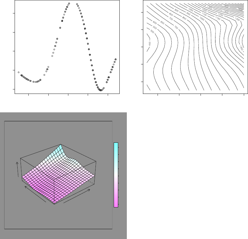
100 CHAPTER 5. ADDITIVE TERMS
1900 1920 1940 1960 1980
−0.002 −0.001 0.000 0.001 0.002
A
m2$mu.s[, 3]/(Fl − mean(Fl))
floor space
year of construction
40 60 80 100 120
1900 1920 1940 1960 1980
Fl
A
pred
400
600
800
1000
1200
1400
1600
1800
2000
Figure 5.3: Rent data: contour and surface plot for the fitted additive cubic splines model
5.2. VARYING COEFFICIENT, THE VC() FUNCTION 101
that the plotted function is the extra contribution after the main effects and interaction have
been fitted for the two variables involved, i.e. Fl*A, which is automatically put by vc() in the
linear part of the model. To plot the fitted surface use
# plotting the fitted surface in 3-d
newrent<-data.frame(expand.grid(Fl=seq(30,120,5),A=seq(1890,1990,5)))
newrent$pred<-predict(m2,newdata=newrent, type="response", data=rent)
Fln<-seq(30,120,5)
An<-seq(1890,1990,5)
op <- par(mfrow=c(1,1))
contour(Fln,An,matrix(newrent$pred,nrow=length(Fln)),nlevels=30,
ylab="year of construction", xlab="floor space")
library(lattice)
wireframe(pred~Fl*A, newrent, aspect=c(1,0.5), drape=TRUE,
colorkey=list(space="right", height=0.6))
The contour and surface plots are shown in figure 5.3.
As an example of using a factor rather than continuous variable for Xin the additive
function vc(), consider the model used in Stasinopoulos et al. (2000). The authors have fitted
the following models for mu and sigma respectively as their final model
µ=f1(F l) + f2(A) + F l ∗f3(A) + H∗f4(F l)
+F l ∗(Sp +B) + Sm +L(5.1)
log(σ) = h1(F l) + h2(A) + F l ∗(Sp +Sm) (5.2)
where, the f’s and h’s are smooth functions, the F l and Aare the floor space (in square meters)
and year of construction respectively, the H,Band Lare factors indicating whether there is
central heating, a bathroom and above average kitchen equipment respectively and the Sp and
Sm are dummy variables indicating whether the location is above average or below average
respectively. Here we first fit the above model using an (identity) link function for mu, then we
refit it using the default log link and finally we fit a model suggested by Prof. John Nelder
(2001) in a subsequent published correspondence. All models fitted use the default 3 extra
degrees of freedom for smoothing and are compared using a GAIC with penalties 2 (AIC) and
log(n) (SBC).
m3<-gamlss(R~cs(Fl)+cs(A)+vc(r=A, x=Fl)+vc(r=Fl, x=H)+Fl*(Sp+B)+Sm+L,
+ sigma.fo=~cs(Fl)+cs(A)+Fl*(Sp+Sm), family=GA(mu.link="identity"))
GAMLSS-RS iteration 1: Global Deviance = 27486.48
GAMLSS-RS iteration 2: Global Deviance = 27481.32
GAMLSS-RS iteration 3: Global Deviance = 27481.28
GAMLSS-RS iteration 4: Global Deviance = 27481.3
GAMLSS-RS iteration 5: Global Deviance = 27481.3
m4<-gamlss(R~cs(Fl)+cs(A)+vc(r=A, x=Fl)+vc(r=Fl, x=H)+Fl*(Sp+B)+Sm+L,
+ sigma.fo=~cs(Fl)+cs(A)+Fl*(Sp+Sm), family=GA)
GAMLSS-RS iteration 1: Global Deviance = 27481.26
GAMLSS-RS iteration 2: Global Deviance = 27477.89
GAMLSS-RS iteration 3: Global Deviance = 27477.87
GAMLSS-RS iteration 4: Global Deviance = 27477.87
102 CHAPTER 5. ADDITIVE TERMS
GAMLSS-RS iteration 5: Global Deviance = 27477.87
m5<-gamlss(R~cs(Fl)+cs(A)+Sp+B+Sm+L+H+Fl*Sp,
+ sigma.fo=~cs(A), family=GA)
GAMLSS-RS iteration 1: Global Deviance = 27555.38
GAMLSS-RS iteration 2: Global Deviance = 27553.49
GAMLSS-RS iteration 3: Global Deviance = 27553.48
GAMLSS-RS iteration 4: Global Deviance = 27553.48
GAIC(m1,m2,m3,m4,m5)
df AIC
m4 37.00108 27551.87
m3 37.00103 27555.30
m5 20.00054 27593.48
m2 14.00192 27929.51
m1 10.00128 27940.74
GAIC(m1,m2,m3,m4,m5, k=log(length(R)))
df AIC
m5 20.00054 27705.19
m4 37.00108 27758.53
m3 37.00103 27761.96
m1 10.00128 27996.60
m2 14.00192 28007.71
Model 4 seems superior with the original AIC but with SBC Prof. Nelder’s suggestion comes
best. [Note that the global deviance reported to in Stasinopoulos et al (2000) is different from
the one produce by GAMLSS. This is due to the fact that degrees of freedom in Stasinopoulos
et al (2000) were calculated differently.]
5.3 Penalized splines, the ps() function
Penalized Splines (or P-splines) are piecewise polynomials defined by B-spline basis functions in
the explanatory variable where the coefficients of the basis functions are penalized to guarantee
sufficient smoothness, see Eilers and Marx (1996). More precisely consider the model θ=Z(x)γ
where θcan be any distribution parameter in a GAMLSS model, Z(x) is n×qbasis design
matrix for the explanatory variable xdefined at q-different knots mostly within the range of x
and γis a q×1 vector of coefficients which have some stochastic restrictions imposed by the fact
that Dγ∼N(0, λ−1I) or equivalently by γ∼N(0, λ−1K−) where K=DTD. The matrix Dis
a (q−r)×qmatrix giving rth differences of the q-dimensional vector γ. So to define a penalized
spline we need: i) qthe number of knots in the x-axis defined by argument ps.intervals (and
of course where to put them, ps uses equal spaces in the x-axis), ii) the degree of the piecewise
polynomial used in the B-spline basis so we can define X, defined by argument degree iii)
rthe order of differences in the Dmatrix indicating the type of the penalty imposed in the
the coefficients of the B-spline basis functions, defined by argument order and iv) the amount
of smoothing required defined either by the desired equivalent degrees of freedom defined by
argument df [or alternative by the smoothing parameter defined by argument lambda].
The ps() function in gamlss package is based on an Sfunction of Brian Marx obtained from
http://www.stat.lsu.edu/faculty/marx/
The function ps() has the following arguments
5.3. PENALIZED SPLINES, THE PS() FUNCTION 103
x the univariate explanatory predictor variable (this version of ps only allows
one variable in each ps() term).
df the desired equivalent number of degrees of freedom on top of the constant
and linear terms [i.e. trace of the smoother matrix minus two for the constant
and linear terms fits, since these terms are included automatically in the linear
part of the model], (the default df is 3)
lambda the smoothing parameter (usually unknown and difficult to guess). If not
specified df is used
ps.intervals the number of knots (or break points) in the x-axis (default=20)
degree the degree of the piecewise polynomial used in the B-spline basis functions
(see also below) with default=3, i.e. cubic
order the order of the difference in the matrix Dwhich determines the penalty
on the B-spline coefficients. order=0 is for white noise (which may not be
suitable for certain data sets due to fitting instability), order=1 is for simple
random effects, order=2 is for random walks of order one and order=3 is for
random walks of order two.
As an example consider the crash helmet data from Silverman (1985). The data comprise 133
observations of accelerometer readings (accel) taken through time (times) in an experiment
on the efficacy of crash helmets. The data need modelling of both the mean and the variance
of accel as in Rigby and Stasinopoulos (1996a), but to start off here we use a model only for
the mean.
Figure 5.4 show the basis function of degree= 0,1,2,3 for times having 10 inner knots, i.e.
ps.intervals=10. The figure is generated using
plotBbasis <- function(x, nknots, degree)
{
dx <- (max(x) - min(x))/nknots
sorder <- degree + 1
Aknots <- seq(from = min(x) - degree * dx, to = max(x) + degree * dx, by = dx)
basis <- splineDesign(Aknots, x, sorder, 0 * x, outer=T)#
mmm<- paste("degree =", degree, sep=" ")
plot(c(min(x) , max(x) ), c(0,1), type="n", xlab="x", ylab="", main=mmm)
matlines(x, basis, lty=1)
}
par(mfrow = c(4, 1))
plotBbasis(x=mcycle$times, nknots=10, degree=0 )
plotBbasis(x=mcycle$times, nknots=10, degree=1 )
plotBbasis(x=mcycle$times, nknots=10, degree=2 )
plotBbasis(x=mcycle$times, nknots=10, degree=3 )
Now we fix the number of knots to the default value 20, the order to 3 and the degrees of
freedom to 15. We vary the degree to 1, 2, and 3 corresponding to using linear, quadratic and
cubic polynomial in the basis functions respectively. The resulting fits are shown in figure (5.5).
It obvious in this example that the different degrees of the piecewise polynomials used in the
B-spline basis functions do not make a difference to the fit, but the degree 2 and 3 produce
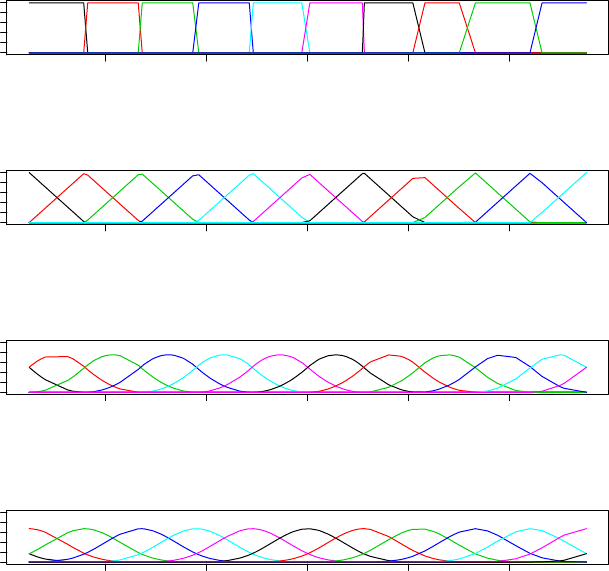
104 CHAPTER 5. ADDITIVE TERMS
10 20 30 40 50
0.0 0.6
degree = 0
x
10 20 30 40 50
0.0 0.6
degree = 1
x
10 20 30 40 50
0.0 0.6
degree = 2
x
10 20 30 40 50
0.0 0.6
degree = 3
x
Figure 5.4: B-basis functions for the crash helmet data for times with 10 inner knots
smoother curves than the one when degree=1. Do not use degree=0 as in this example the
backfitting did not converge.
> par(mfrow = c(3, 1))
> plot(accel~times, data=mcycle , main= "degree=1" )
> # degree =0 is not working
> #m0 <- gamlss(accel~ps(times,df=15,degree=0), data = mcycle)
> m1 <- gamlss(accel~ps(times,df=15,degree=1), data = mcycle)
GAMLSS-RS iteration 1: Global Deviance = 1195.225
GAMLSS-RS iteration 2: Global Deviance = 1195.225
> m2 <- gamlss(accel~ps(times,df=15,degree=2), data = mcycle)
GAMLSS-RS iteration 1: Global Deviance = 1189.215
GAMLSS-RS iteration 2: Global Deviance = 1189.215
> m3 <- gamlss(accel~ps(times,df=15,degree=3), data = mcycle)
GAMLSS-RS iteration 1: Global Deviance = 1191.953
GAMLSS-RS iteration 2: Global Deviance = 1191.953
>
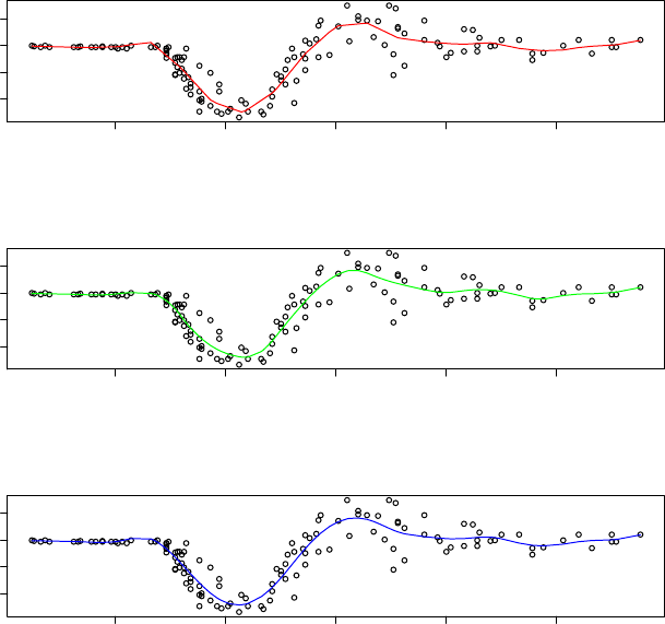
5.3. PENALIZED SPLINES, THE PS() FUNCTION 105
> lines(fitted(m1)~mcycle$times, col="red")
> plot(accel~times, data=mcycle , main= "degree=2")
> lines(fitted(m2)~mcycle$times, col="green")
> plot(accel~times, data=mcycle, main= "degree=3")
> lines(fitted(m3)~mcycle$times, col="blue")
10 20 30 40 50
−100 0 50
degree=1
times
accel
10 20 30 40 50
−100 0 50
degree=2
times
accel
10 20 30 40 50
−100 0 50
degree=3
times
accel
Figure 5.5: The helmet data fit with different degrees 0,1,2,3 corresponding to red, green, blue
and purple respectively
As an example on how the order effects the smoothness of the coefficients γconsider the
following models where we fix the degree=2 and we varied the order to 0,1,2,3.
> m20 <- gamlss(accel~ps(times,df=15,degree=2, order=0), data = mcycle)
GAMLSS-RS iteration 1: Global Deviance = 1189.380
GAMLSS-RS iteration 2: Global Deviance = 1189.379
Warning messages:
1: additive.fit convergence not obtained in 30 iterations in:
additive.fit(x = X, y = wv, w = wt * w, s = s, who = who, smooth.frame,
2: additive.fit convergence not obtained in 30 iterations in:
106 CHAPTER 5. ADDITIVE TERMS
additive.fit(x = X, y = wv, w = wt * w, s = s, who = who, smooth.frame,
> m21 <- gamlss(accel~ps(times,df=15,degree=2, order=1), data = mcycle)
GAMLSS-RS iteration 1: Global Deviance = 1188.364
GAMLSS-RS iteration 2: Global Deviance = 1188.364
Warning messages:
1: additive.fit convergence not obtained in 30 iterations in:
additive.fit(x = X, y = wv, w = wt * w, s = s, who = who, smooth.frame,
2: additive.fit convergence not obtained in 30 iterations in:
additive.fit(x = X, y = wv, w = wt * w, s = s, who = who, smooth.frame,
> m22 <- gamlss(accel~ps(times,df=15,degree=2, order=2), data = mcycle)
GAMLSS-RS iteration 1: Global Deviance = 1188.705
GAMLSS-RS iteration 2: Global Deviance = 1188.705
> m23 <- gamlss(accel~ps(times,df=15,degree=2),order=3, data = mcycle)
GAMLSS-RS iteration 1: Global Deviance = 1189.215
GAMLSS-RS iteration 2: Global Deviance = 1189.215
>
> plot(m20$mu.coefSmo[[1]]$coef, type="l", col="red")
> lines(m21$mu.coefSmo[[1]]$coef, col="green")
> lines(m22$mu.coefSmo[[1]]$coef, col="blue")
> lines(m23$mu.coefSmo[[1]]$coef, col="purple")
Ignoring that the backfitting has some problem in converging we can see from figure 5.6 that
the order has not change very much the magnitude of the coefficients. Only order=0 seems to
differ from the rest.
5.4 The loess function lo()
The function lo() allows the user to use a loess fit in a gamlss() formula. A loess fit is
a polynomial (surface) curve determined by one or more explanatory (continuous) variables,
which are fitted locally (see Cleveland et al. (1993)). The implementation of the lo() function
is very similar to the function with the same name in the S-PLUS implementation of gam.
However gamlss lo() function uses the (R) loess() function as its engine and this creates
some minor differences between the two lo() even when the same model is fitted (see below).
lo() is the only function currently available in gamlss which allows smoothing in more than
one explanatory (continuous) variables.
The complementary gamlss.lo() function uses the same C interface as loess in R. Resulting
fits between loess and lo however are different (even for a normal distribution for the response
variable) due to the different way that they are implemented. gamlss.lo() calls the C interface
after the linear part of the model has been subtracted. This in general would lead to a slightly
different smooth fit when the linear part and the smoothing part are added together at the end
of the algorithm. The gamlss.lo() is closer in principle to the gam.lo() of S-PLUS rather than
lo() of S-PLUS.
The lo() function has the following arguments
... the unspecified ... can be a comma-separated list of numeric vectors i.e.
(x1,x2,x3), numeric matrix, or expressions that evaluate to either of these. If
it is a list of vectors, they must all have the same length.
span the parameter which controls the degree of smoothing (it is function of the
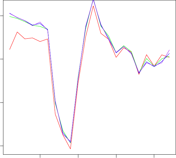
5.4. THE LOESS FUNCTION LO() 107
5 10 15 20
−100 −50 0 50
Index
gamma coefficients
Figure 5.6: The helmet data fit with different degrees 1,2,3 corresponding to red, green and
blue respectively
number of observations in a neighborhood). This is the main smoothing pa-
rameter for a loess fit. The default is span=0.5
df the effective degrees of freedom can be specified instead of span, e.g. df=5.
This is not a clear cut specification as in cubic splines. Given this parameter
an estimated span is calculated and passed to the C interface. The default is
df=NULL.
degree the degree of local polynomial to be fit; (the default is linear 1).
As an example of using the lo() function within the GAMLSS framework we consider again
the rent data. Here we fit four different models. The first two are additive models for floor
space (Fl) and for age (A) the year of construction. The third and fourth models fit surfaces
for floor space (Fl) and age (A). The first and third use a linear local fit while the second and
fourth use a quadratic fit. We choose between models using a GAIC with penalty 2.5.
> data(rent)
108 CHAPTER 5. ADDITIVE TERMS
> # fit additive loess fits first
> # degree = 1
> r11<-gamlss(R~lo(Fl)+lo(A),data=rent, family=GA)
GAMLSS-RS iteration 1: Global Deviance = 27921.69
GAMLSS-RS iteration 2: Global Deviance = 27921.69
> # degree = 2
> r12<-gamlss(R~lo(Fl,degree=2)+lo(A, degree=2),data=rent, family=GA)
GAMLSS-RS iteration 1: Global Deviance = 27917.63
GAMLSS-RS iteration 2: Global Deviance = 27917.63
> # fit loess surfaces
> # degree = 1
> r21<-gamlss(R~lo(Fl,A, degree=1),data=rent, family=GA)
GAMLSS-RS iteration 1: Global Deviance = 27908.98
GAMLSS-RS iteration 2: Global Deviance = 27908.98
> # degree = 2
> r22<-gamlss(R~lo(Fl,A, degree=2),data=rent, family=GA)
GAMLSS-RS iteration 1: Global Deviance = 27889.07
GAMLSS-RS iteration 2: Global Deviance = 27889.07
> # selecting the best model
> AIC(r11,r12,r21,r22, k=2.5)
df AIC
r22 19.08488 27936.78
r21 11.33833 27937.33
r11 10.00128 27946.69
r12 14.12759 27952.95
According to the generalized Akaike information criterion with penalty 2.5, GAIC(k= 2.5)
the best model is r22, fitting a surface with a local polynomial of degree 2. The span in all the
above models was the default one 0.5. Below we see whether a different span improves the fit.
> r223<-gamlss(R~lo(Fl,A, degree=2, span=0.3), data=rent, family=GA)
GAMLSS-RS iteration 1: Global Deviance = 27874.59
GAMLSS-RS iteration 2: Global Deviance = 27874.59
> r224<-gamlss(R~lo(Fl,A, degree=2, span=0.4), data=rent, family=GA)
GAMLSS-RS iteration 1: Global Deviance = 27882.98
GAMLSS-RS iteration 2: Global Deviance = 27882.98
> r226<-gamlss(R~lo(Fl,A, degree=2, span=0.6), data=rent, family=GA)
GAMLSS-RS iteration 1: Global Deviance = 27897.41
GAMLSS-RS iteration 2: Global Deviance = 27897.41
> AIC(r22,r223,r224,r226, k=2.5)
df AIC
r22 19.08488 27936.78
r226 16.29977 27938.16
r224 22.46753 27939.15
r223 28.89809 27946.83
It looks that the default span is fine. Now we plot the fitted surface in figure 5.7.
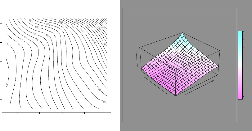
5.5. FRACTIONAL POLYNOMIALS, THE FP() FUNCTION 109
newrent<-data.frame(expand.grid(Fl=seq(30,120,5),A=seq(1890,1985,5)))
> newrent$pred<-predict(r22,newdata=newrent, type="response")
> Fln<-seq(30,120,5)
> An<-seq(1890,1985,5)
> op <- par(mfrow=c(1,1))
> contour(Fln,An,matrix(newrent$pred,nrow=length(Fln)),nlevels=30,
+ ylab="year of construction", xlab="floor space")
> library(lattice)
> wireframe(pred~Fl*A, newrent, aspect=c(1,0.5), drape=TRUE,
> colorkey=list(space="right", height=0.6))
>
Note that while the lo gamlss implementation is similar to the S-PLUS implementation of
lo in gam, the results are not always exactly the same even for similar types of models. In fact
we have found that for normal error fits the results are identical if more than one variable is
used, for example lo(x1,x2) but are not if only one variable is used. In this case the smooth
fits different slightly and also have slightly different effective degrees of freedom.
floor space
year of construction
40 60 80 100 120
1900 1920 1940 1960 1980
Fl
A
pred
400
600
800
1000
1200
1400
1600
1800
2000
Figure 5.7: Rent data: contour and surface plot for the fitted loess surface model
5.5 Fractional polynomials, the fp() function
The fp() function is an implementation of the fractional polynomials introduced by Royston
and Altman (1994). The functions involved in fp() and bfp() are loosely based on the fractional
polynomials implementation in S-PLUS written by Gareth Amber found in
http://lib.stat.cmu.edu/S/fracpoly.
The function bfp generates the right design matrix for fitting a power polynomial of the
type a+b1xp
1+b2xp2+...+bkxpk. For given powers p1, p2, ..., pk, given as the argument ’powers’
in bfp(), the function can be used to fit power polynomials in the same way as the functions
110 CHAPTER 5. ADDITIVE TERMS
poly() or bs() of the package splines are used to fit orthogonal or piecewise polynomials
respectively. The function fp(), [which uses bfp()] works as an additive smoother term in
gamlss(). It is used to fit the best fractional polynomials among a specific set of power values.
Its argument npoly determines whether one, two or three fractional polynomials should used
in the fitting. For a fixed number npoly the algorithm looks for the best fitting fractional
polynomials in the list c(-2, -1, -0.5, 0, 0.5, 1, 2, 3). Note that npoly=3 is rather
slow since it fits all possible 3-way combinations at each backfitting iteration. The function
gamlss.fp() is an internal function of gamlss allowing the fractional polynomials to be fitted
in the backfitting cycle of gamlss() and should be not used on its own.
The bfp() function has the following arguments
x the explanatory variable to be used in functions bfp() or fp().
powers a vector containing as elements the possible powers to which the x has to be
raised
shift a number for shifting the x-variable. The default values is zero, if x is positive,
or a value that insures that x will always be positive
scale a positive number for scaling the x-variable.
The fp() function has the following arguments
x as above
npoly a positive integer indicating how many fractional polynomials should be con-
sidered in the fit. Can take the values 1, 2 or 3 with 2 as default
shift as above
scale as above
As an example consider fitting fractional polynomials for the mu in the abdom data. We try
to find the how many fractional polynomials we need.
data(abdom)
# fit the best of one fractional polynomial
m1<-gamlss(y~fp(x,1),data=abdom)
GAMLSS-RS iteration 1: Global Deviance = 4967.042
GAMLSS-RS iteration 2: Global Deviance = 4967.042
# fit the best of two fractional polynomials
m2<-gamlss(y~fp(x,2),data=abdom)
GAMLSS-RS iteration 1: Global Deviance = 4941.099
GAMLSS-RS iteration 2: Global Deviance = 4941.099
# fit the best of three fractional polynomials
m3<-gamlss(y~fp(x,3),data=abdom)
GAMLSS-RS iteration 1: Global Deviance = 4933.937
GAMLSS-RS iteration 2: Global Deviance = 4933.937
> AIC(m1,m2,m3)
df AIC
m3 8 4949.937
m2 6 4953.099
5.5. FRACTIONAL POLYNOMIALS, THE FP() FUNCTION 111
m1 4 4975.042
m3$mu.coefSmo
[[1]]
[[1]]$coef
one
-121.644921 -107.251934 14.506882 -7.600717
[[1]]$power
[1] -2 3 3
[[1]]$varcoeff
[1] 44.5489430 143.4304454 0.4907324 0.1977479
m3
Family: c("NO", "Normal")
Fitting method: RS()
Call: gamlss(formula = y ~ fp(x, 3), data = abdom)
Mu Coefficients:
(Intercept) fp(x, 3)
226.7 NA
Sigma Coefficients:
(Intercept)
2.625
Degrees of Freedom for the fit: 8 Residual Deg. of Freedom 602
Global Deviance: 4933.94
AIC: 4949.94
SBC: 4985.25
Note that a normal error mode was fitted (the default), i.e. NO(µ, σ) where µis the mean
and σis the standard deviation. The best fractional polynomials model seems to be the one with
three polynomials, m3 from the AIC results. The actual powers or the polynomials can be found
by printing the mu.coefSmo list as we have done above for the chosen model. For model m3 the
best fractional polynomial powers are -2,3,3. Because of the identical powers in x, the fitted
polynomial for µis defined as µ=−107.25x−2+14.51x3−7.60x3log(x) since the default identity
link for µwas used. The correct Intercept of model m3 can be found by adding the Intercept
coefficient of mu to the first coefficient of mu.coefSmo$coef i.e. 226.7−121.64 = 105.06. The
fitted values of σis given by ˆσ= exp(2.625) = 13.80, since the default log link for σwas used.
If the fractional polynomial power is known then the model can be fitted using the function
bfp. For example an identical model to m3 above can be fitted using
> m4<-gamlss(y~bfp(x,c(-2,3,3)),data=abdom)
GAMLSS-RS iteration 1: Global Deviance = 4933.937
GAMLSS-RS iteration 2: Global Deviance = 4933.937
112 CHAPTER 5. ADDITIVE TERMS
> summary(m4)
*******************************************************************
Family: c("NO", "Normal")
Call: gamlss(formula = y ~ bfp(x, c(-2, 3, 3)), data = abdom)
Fitting method: RS()
-------------------------------------------------------------------
Mu link function: identity
Mu Coefficients:
Estimate Std. Error t value Pr(>|t|)
(Intercept) 105.07 6.6745 15.742 4.628e-47
bfp(x, c(-2, 3, 3))1 -107.25 11.9762 -8.955 4.133e-18
bfp(x, c(-2, 3, 3))2 14.51 0.7005 20.709 1.916e-72
bfp(x, c(-2, 3, 3))3 -7.60 0.4447 -17.092 9.512e-54
-------------------------------------------------------------------
Sigma link function: log
Sigma Coefficients:
Estimate Std. Error t value Pr(>|t|)
(Intercept) 2.625 0.02863 91.7 0
-------------------------------------------------------------------
No. of observations in the fit: 610
Degrees of Freedom for the fit: 5
Residual Deg. of Freedom: 605
at cycle: 2
Global Deviance: 4933.937
AIC: 4943.937
SBC: 4966.005
*******************************************************************
Note that model m4 produces the correct Intercept.
5.6 The random effects functions
5.6.1 The random function
The function random() allows the fitted values for a factor predictor to be shrunk towards the
overall mean, where the amount of shrinking depends either on lambda, or on the equivalent
degrees of freedom (df). This function is similar to the random() function in gam, documented
in Chambers and Hastie (1992).
The random() function has the following arguments
xvar a factor to be shrunk
df the target effective degrees of freedom

5.6. THE RANDOM EFFECTS FUNCTIONS 113
Table 5.2: The educational testing experiments data
school estimated standard error
treatment of effect
effect estimate of σ
A 28 15
B 8 10
C -3 16
D 7 11
E -1 9
F 1 11
G 18 10
H 12 18
lambda the smoothing parameter lambda which can be viewed as a shrinkage param-
eter. It is the reciprocal of σ2
tthe variance of the factor random effect
As an example consider the data in Table 5.2 obtained from an educational testing ex-
periment in eight schools, given by Gelman et al. (2004), Section 5.5. More details on the
experiment can be found there. The authors used this example to demonstrate an hierarchical
Bayesian analysis. What is important here is that the estimated treatment effects in column
two of the Table 5.2 are obtained by independent experiments and are assumed to come from
a normal distribution with a standard deviation obtained from column 3 of the Table 5.2.
We start by fitting a null model with a constant mean for the response variable, estimate, i.e.
yi∼N(µ, σi2), and a saturated model with different means for each school, i.e. yi∼N(µi, σi2),
where yiis the estimate at school iand σiis given by sd. As in Gelman et al. (2004) both
models are fitted using a fixed standard deviation parameter vector, sigma, given in the third
column of Table 5.2. [Strictly the third column gives estimates of sigmas based on large sample
sizes rather than fixed known sigmas. ] There are two ways to achieve this in gamlss, the first
is to use the gamlss() argument sigma.fix. [Note that sigma is fixed at its starting value, i.e.
sigma.start=sd.] The second way is using an offset in the formula for sigma. [Note that due
the default log link for sigma for the (default) normal distribution, the offset is log(sd). Note
also -1 in the sigma.fo removes the constant from the log(sigma) model.] We demonstrate
both methods below
> school <- c("A", "B", "C", "D", "E", "F", "G", "H")
> estimate <- c(28, 8, -3, 7, -1, 1, 18, 12)
> sd <- c(15, 10, 16, 11, 9, 11,10,18)
> schools <- data.frame(school=school, estimate=estimate, sd=sd)
> mnull <- gamlss(estimate~1, sigma.fo=~offset(log(sd))-1, data=schools)
GAMLSS-RS iteration 1: Global Deviance = 59.4168
GAMLSS-RS iteration 2: Global Deviance = 59.3485
GAMLSS-RS iteration 3: Global Deviance = 59.3485
> mnull1 <- gamlss(estimate~1, sigma.fix=TRUE, sigma.start=sd, data=schools)
GAMLSS-RS iteration 1: Global Deviance = 59.3485
GAMLSS-RS iteration 2: Global Deviance = 59.3485
> msat <- gamlss(estimate~school, sigma.fo=~offset(log(sd))-1, data=schools)
GAMLSS-RS iteration 1: Global Deviance = 54.6414
GAMLSS-RS iteration 2: Global Deviance = 54.6414
114 CHAPTER 5. ADDITIVE TERMS
> msat1 <- gamlss(estimate~school, sigma.fix=TRUE, sigma.start=sd,
data=schools)
GAMLSS-RS iteration 1: Global Deviance = 54.6414
> fitted(mnull)
1 2 3 4 5 6 7 8
7.685617 7.685617 7.685617 7.685617 7.685617 7.685617 7.685617 7.685617
> fitted(msat)
1 2 3 4 5 6 7 8
28 8 -3 7 -1 1 18 12
The global deviance for the null model, mnull, is 59.3485 while the fitted values are the
mean of the variable estimate. The global deviance for the saturated model, msat, is 54.6414
while the fitted values are the actual data i.e. variable estimate. We can not perform an F test
between the model since the degrees of freedom of the saturated model is zero. Nevertheless a
chi-square test between the two models result to a value of χ2= 4.7071 not significant for the
7 degrees of freedom used. That is, there is no statistical evidence to support the saturated
model. A classical statistician would probably stop here and would use the null model for any
inference on the data. Gelman et al. (2004) argue, quite convincingly, that this maybe is not a
good idea and they use an hierarchical Bayesian model to continue their analysis. The GAMLSS
framework allows us to go someway along this path. For example, the function random allows
the user to fit models with fitted values somewhere between those two extreme values of the null
and the saturated model. The model fitted by random corresponds to the model yi∼N(µi, σi2)
with µi∼N(0, σ2
ρ), where σ2
ρ= 1/λ and λis the argument lambda in the function random. By
varying lambda we can reproduce the saturate model (for λ→0) or the null model (for λ→ ∞).
Equivalently we can vary the effective degrees of freedom from zero to 8 (the argument df in
the function random) which is a one-to-one function of the parameter λ.
As an example of the use of the function random we are reproducing the null and saturate
models and also fit a model with 4 degrees of freedom.
> m0 <- gamlss(estimate~random(school,df=0.00001),
sigma.fo=~offset(log(sd))-1, data=schools)
GAMLSS-RS iteration 1: Global Deviance = 59.4168
GAMLSS-RS iteration 2: Global Deviance = 59.3485
GAMLSS-RS iteration 3: Global Deviance = 59.3485
> m1 <- gamlss(estimate~random(school,df=4),
sigma.fo=~offset(log(sd))-1, data=schools)
GAMLSS-RS iteration 1: Global Deviance = 55.8353
GAMLSS-RS iteration 2: Global Deviance = 55.8787
GAMLSS-RS iteration 3: Global Deviance = 55.8787
> ms <- gamlss(estimate~random(school,df=8),
sigma.fo=~offset(log(sd))-1, data=schools)
GAMLSS-RS iteration 1: Global Deviance = 54.6414
GAMLSS-RS iteration 2: Global Deviance = 54.6414
In fact we can go a step further and see how the fitted values of mu vary when we change the
degrees of freedom from 0 to 8. The plot on the left of figure 5.8 shows just that. It shows how
the fitted values change from a global mean of 7.68 when the degrees of freedom are at zero to
the actual data values where the degrees of freedom are at 8. The plot on the right of figure 5.8
5.6. THE RANDOM EFFECTS FUNCTIONS 115
(similar to the one given by Gelman et al. (2004) on page 142) shows how the fitted values for
mu vary for different σρ, the random effects standard deviations. Both plots in figure 5.8 were
produced using the following Rcommands.
iii <- seq(0.01,8, length=20)
matfitmu <- matrix(NA, nrow = 20 ,ncol=8)
for (i in 1:20)
{
mm<-gamlss(estimate~random(school,df=iii[i]), sigma.fo=~offset(log(sd))-1,
data=schools)
matfitmu[i,]<- fitted(mm)
}
plot(matfitmu[,1]~iii, ylim=c(-4,29), type="l", col=1, xlab="df",
ylab="fitted mu")
for (j in 2:8)
{
lines(iii,matfitmu[,j], col=j)
}
text(rep(iii[14],8),matfitmu[14,],schools$school)
tt <- seq(0.01, 50, length=20)
ttt <- 1/tt^2
matfitmu <- matrix(NA, nrow = 20 ,ncol=8)
for (i in 1:20)
{
mm<-gamlss(estimate~random(school,lambda=ttt[i]),
sigma.fo=~offset(log(sd))-1, data=schools)
matfitmu[i,]<- fitted(mm)
}
plot(matfitmu[,1]~tt, ylim=range(matfitmu), type="l", col=1,
xlab="sqrt(1/lambda)", ylab="fitted mu")
for (j in 2:8)
{
lines(tt,matfitmu[,j], col=j)
}
text(rep(tt[14],8),matfitmu[14,],schools$school)
A second example using a random effect model is considered in the next Section.
5.6.2 The ra function
This is an experimental smoother for fitting random effects in gamlss(). The function ra()
is similar to the function random discussed in the previous Section but its fitting procedure is
based on augmented least squares, a fact that makes ra() more general, but also slower to fit,
than random(). The function ra() allows the fitted values for a factor predictor to be shrunk
towards the overall mean, where the amount of shrinking depends either on lambda, or on the
equivalent degrees of freedom df.
The arguments of the function ra() are
116 CHAPTER 5. ADDITIVE TERMS
0 2 4 6 8
−5 0 5 10 15 20 25 30
df
fitted mu
A
B
C
D
E
F
G
H
0 10 20 30 40 50
0 5 10 15 20 25
sqrt(1/lambda)
fitted mu
A
B
C
D
E
F
G
H
Figure 5.8: schools : plots of the fitted means for different degrees of freedom (on the left) and
different standard deviations of the random effect (on the right)
xfactor a factor defining the subjects grouping in a one factor random effect model
term e.g. ’xfactor=Subjects’
xvector a variable if interaction with the ’xfactor’ is required ’xvector’ (experimental)
df required equivalent degrees of freedom e.g. ’df=10’
lambda lambda: the smoothing parameter which is the reciprocal (i.e. inverse) of σρ
the variance of the random effect
order the order of the difference in the matrix D, ’order=1’ is for simple random
effects, ’order=2’ is for random walk order 1 and ’order=3’ is for random walk
order 2
estimate whether to estimate the lambda parameter within the backfitting iterations
(an ad hoc method and very unreliable). Set by default to ’estimate=FALSE’.
[The lambda parameter can be more accurately estimated by selecting the
corresponding smoothing degrees of freedom using ’find.hyper’]
expl this allows an explanatory variable at the subject level to be fitted e.g. expl=~x1+x2]
data1 the data frame for the subject level variables
As a example consider the data used by Hodges (1998) and also reanalyzed by Rigby and
Stasinopoulos (2005). The data describe 341 state-based health maintenance organizations
(HMO’s) serving US Government employees. Each HMOs operate in 42 states and the district
of Columbia, Guam and Puerto Rico. The data were analyzed as part of estimating the cost
of moving military retirees and dependents from a Defense Department health plan to plans
serving US Government employees. The response variable is print the total premium of a
5.6. THE RANDOM EFFECTS FUNCTIONS 117
health insurance for an individual, while the independent variable is the factor state with 45
levels indicating different US states.
We start by comparing the speed of ra and random functions. random() is a lot faster than
ra() especially if argument df is used for fitting rather than lambda.
> data(hodges)
>
> system.time(hno <- gamlss(prind~ra(state,df=30),
data=hodges, family=NO))
GAMLSS-RS iteration 1: Global Deviance = 3051.064
GAMLSS-RS iteration 2: Global Deviance = 3051.064
[1] 4.70 0.03 4.78 NA NA
> system.time(hno1 <- gamlss(prind~random(state,df=30),
data=hodges, family=NO))
GAMLSS-RS iteration 1: Global Deviance = 3051.065
GAMLSS-RS iteration 2: Global Deviance = 3051.065
[1] 0.23 0.00 0.23 NA NA
>
> system.time(hno <- gamlss(prind~ra(state,lambda= 0.005016909),
data=hodges, family=NO))
GAMLSS-RS iteration 1: Global Deviance = 3059.331
GAMLSS-RS iteration 2: Global Deviance = 3051.597
GAMLSS-RS iteration 3: Global Deviance = 3051.098
GAMLSS-RS iteration 4: Global Deviance = 3051.066
GAMLSS-RS iteration 5: Global Deviance = 3051.064
GAMLSS-RS iteration 6: Global Deviance = 3051.064
[1] 1.71 0.01 1.72 NA NA
> system.time(hno1 <- gamlss(prind~random(state,lambda= 0.005016909),
data=hodges, family=NO))
GAMLSS-RS iteration 1: Global Deviance = 3059.331
GAMLSS-RS iteration 2: Global Deviance = 3051.597
GAMLSS-RS iteration 3: Global Deviance = 3051.098
GAMLSS-RS iteration 4: Global Deviance = 3051.066
GAMLSS-RS iteration 5: Global Deviance = 3051.064
GAMLSS-RS iteration 6: Global Deviance = 3051.064
[1] 0.40 0.00 0.41 NA NA
It is obvious that, unless a special feature of ra() is to be used, the function random() is
preferable.
It is not very difficult to establish that the normal distribution is not adequate for the data
in hand. For example consider the following two models, one with a normal distribution and
one with the BCT distribution. Both models are using a random effect model for mu with 30
effective degrees of freedom.
> hno <- gamlss(prind~ra(state,df=30), data=hodges, family=NO)
GAMLSS-RS iteration 1: Global Deviance = 3051.064
GAMLSS-RS iteration 2: Global Deviance = 3051.064
> hbct <- gamlss(prind~ra(state,df=30), data=hodges, family=BCT)
GAMLSS-RS iteration 1: Global Deviance = 3029.984
118 CHAPTER 5. ADDITIVE TERMS
GAMLSS-RS iteration 2: Global Deviance = 3028.338
GAMLSS-RS iteration 3: Global Deviance = 3028.415
GAMLSS-RS iteration 4: Global Deviance = 3028.46
GAMLSS-RS iteration 5: Global Deviance = 3028.493
GAMLSS-RS iteration 6: Global Deviance = 3028.514
GAMLSS-RS iteration 7: Global Deviance = 3028.527
GAMLSS-RS iteration 8: Global Deviance = 3028.534
GAMLSS-RS iteration 9: Global Deviance = 3028.538
GAMLSS-RS iteration 10: Global Deviance = 3028.542
GAMLSS-RS iteration 11: Global Deviance = 3028.543
GAMLSS-RS iteration 12: Global Deviance = 3028.544
GAMLSS-RS iteration 13: Global Deviance = 3028.545
There is slight instability along the way to convergence of the fitting algorithm for the BCT
model, but this should not worry us. The difference in global deviance between the two models
is 22.519 with 2 extra parameter, indicating support for the BCT model.
Random effect models can be used for modelling all the parameters of the distribution. Rigby
and Stasinopoulos (2005), for example, consider a Box-Cox tmodel allowing random effects for
all four parameters of the BCT distribution. In practice, the problem is how to decide whether
to include or not a random term in the model. In what follows, we take a heuristic approach
and use a Generalized Akaike criterion in order to decide whether a random effect should be
included or not. The function find.hyper(), discussed in more details in Section 7.3, allows
the selection of degrees of freedom for a smoothing term given a specified GAIC(♯). Below we
use a penalty ♯= 2 (that is an AIC) to check whether random effects should be included in
the parameters mu,sigma,nu or tau. In order to do that, we first have to declare the model
we wish to minimize using the quote function. Then we use the find.hyper function for the
actual minimization of GAIC. Note the use of random rather than ra(), (for better speed), and
the use of control = gamlss.control(trace=FALSE) (to suppress some of the output), in the
gamlss() function. We also set lower and upper limits for the effective degrees of freedom to
0.001, (i.e. effectively no random effect for this term) and 45 respectively.
data(hodges)
mod1<-quote(gamlss(prind~random(state, df=p[1]),
sigma.fo=~random(state,df=p[2]),
nu.fo=~random(state,df=p[3]),
tau.fo=~random(state,df=p[4]),
data=hodges, family=BCT,
control = gamlss.control(trace=FALSE)))
find.hyper(mod1,par=c(40,10, 5, 5), lower=c(0.001,0.001, 0.001, 0.001),
upper=c(45,45,45,45), pen=2)
par 40 10 5 5 crit= 3096.681 with pen= 2
par 40.1 10 5 5 crit= 3096.748 with pen= 2
par 39.9 10 5 5 crit= 3096.617 with pen= 2
par 40 10.1 5 5 crit= 3096.709 with pen= 2
par 40 9.9 5 5 crit= 3096.654 with pen= 2
par 40 10 5.1 5 crit= 3096.762 with pen= 2
par 40 10 4.9 5 crit= 3096.600 with pen= 2

5.6. THE RANDOM EFFECTS FUNCTIONS 119
par 40 10 5 5.1 crit= 3096.834 with pen= 2
par 40 10 5 4.9 crit= 3096.527 with pen= 2
par 39.34709 9.725657 4.190996 3.464871 crit= 3093.247 with pen= 2
...
...
par 36.11275 4.082199 0.001 0.001 crit= 3085.357 with pen= 2
par 36.21275 4.182199 0.001 0.001 crit= 3085.355 with pen= 2
par 36.21275 3.982199 0.001 0.001 crit= 3085.356 with pen= 2
par 36.21275 4.082199 0.101 0.001 crit= 3085.39 with pen= 2
par 36.21275 4.082199 0.001 0.001 crit= 3085.355 with pen= 2
par 36.21275 4.082199 0.001 0.101 crit= 3085.431 with pen= 2
par 36.21275 4.082199 0.001 0.001 crit= 3085.352 with pen= 2
$par
[1] 36.212755 4.082199 0.001000 0.001000
$value
[1] 3085.360
$counts
function gradient
15 15
$convergence
[1] 0
$message
[1] "CONVERGENCE: REL_REDUCTION_OF_F <= FACTR*EPSMCH"
There were 20 warnings (use warnings() to see them)
The algorithm has converged to the values 36.212755 for mu, 4.082199, for sigma, 0.001000
for nu and 0.001000 for tau. This indicates a strong need for a random effect term in mu, a
possible need for a random effect term in sigma, but no need for random effects terms in nu
and tau. [Ideally we should first repeat find.hyper just for finding dfµand dfσ(with νand
τconstants), and then fix the chosen dfµand dfσ, but here we omit this step.] We now fit the
model including random effects in mu and sigma only. Note that here we are fixing the degrees
of freedom. In random effects models we are often interested in the lambda parameter since the
standard deviations of the random effects relates to λby σρ= 1/√λ. The function ra saves
the lambda parameter in the coefSmo component of the fitted model.
> hbct <- gamlss(prind~ra(state, df=36.21),
sigma.fo=~ra(state,df=4.08),
data=hodges, family=BCT)
GAMLSS-RS iteration 1: Global Deviance = 3005.706
GAMLSS-RS iteration 2: Global Deviance = 3004.890
GAMLSS-RS iteration 3: Global Deviance = 3004.823
GAMLSS-RS iteration 4: Global Deviance = 3004.793
GAMLSS-RS iteration 5: Global Deviance = 3004.781
GAMLSS-RS iteration 6: Global Deviance = 3004.775
120 CHAPTER 5. ADDITIVE TERMS
GAMLSS-RS iteration 7: Global Deviance = 3004.772
GAMLSS-RS iteration 8: Global Deviance = 3004.77
GAMLSS-RS iteration 9: Global Deviance = 3004.769
> hbct$mu.coefSmo[[1]]$lambda
[1] 0.002687768
> 1/sqrt(hbct$mu.coefSmo[[1]]$lambda)
[1] 19.28875
> hbct$sigma.coefSmo[[1]]$lambda
[1] 102.3325
> 1/sqrt(hbct$sigma.coefSmo[[1]]$lambda)
[1] 0.09885376
So by fixing the degrees of freedom for the random effects for mu and sigma to 36.21 and
4.08 respectively we have σ1and σ2, the standard deviations of the random effects terms in µ
and σrespectively, to 19.28 and 0.0988 respectively. A general method for estimating the hyper
parameters σρbased on REML estimation is given in the Appendix A.2.3. of Stasinopoulos
and Rigby (2005). The method has been used successfully for specific random effets models
[including those in Rigby and Stasinopoulos (2005)]. Unfortunately the method is difficult
to program in a general form. The authors are working currently on an alternative MCMC
approach.
5.6.3 The random coefficient, rc, function
This is an experimental smoother for fitting random coefficient model terms and will be docu-
mented in the future.

Chapter 6
Diagnostics
There are four functions at the moment that can be used as model diagnostic tools. All of them
use the residuals of the fitted gamlss object and they are: the plot, the wp(),Q.stats() and
the rqres.plot() functions. The residuals are normalized (randomized for discrete response
variable distribution only) quantile residuals.
The (normalized randomized quantile) residuals are given by ˆri= Φ−1(ui) where Φ−1is
the inverse cumulative distribution function of a standard normal variate and ui=F(yi|ˆ
θi) if
yiis an observation from a continuous response, while uiis a random value from the uniform
distribution on the interval hF(yi−1|ˆ
θi), F (yi|ˆ
θi)iif yiis an observation from a discrete integer
response, where F(y|θ) is the cumulative distribution function with θ= (µ, σ, ν, τ). For a right
censored continuous response uiis defined as a random value from a uniform distribution on
the interval hF(yi|ˆ
θi),1i. Note that, when randomization is used, several randomized sets of
residuals (or a median set from them) should be studied before a decision about the adequacy
of the model is taken. The true residuals rihave a standard normal distribution if the model is
correct (even when the model distribution is not normal). See Dunn and Smyth (1996).
6.1 The plot function
The full name of this function is plot.gamlss() but it can be called using plot given that its
first argument is a fitted gamlss object. The function plot produces four plots for checking the
(normalized randomized quantile) residuals (called residuals subsequently) of a fitted gamlss
object, see Dunn and Smyth (1996). Randomization is only performed for discrete response
variables. The four plots are
residuals against the fitted values
residuals against an index or specified x-variable
kernel density estimate of the residuals
QQ-normal plot of the residuals
When randomization is performed in the discrete distribution families it is advisable to also
use the function rqres.plot described in Section 6.4.
The arguments of the plot.gamlss() function are
121
122 CHAPTER 6. DIAGNOSTICS
xagamlss fitted object
xvar an explanatory variable to plot the residuals against. By default the index
1:N is plotted, where N is the total number of observations.
parameters this option can be used to change the default parameters in the plotting.
The current default parameters are par(mfrow=c(2,2), mar=par("mar")+
c(0,1,0,0), col.axis = "blue4", col.main = "blue4", col.lab =
"blue4", col = "darkgreen", bg = "beige" ). These parameters are not
appropriate, when someone wishes to include the plot into a document. We
have found that the option parameters= par(mfrow = c(2,2), mar = par("mar")+
c(0,1,0,0), col.axis = "blue4", col = "blue4", col.main = "blue4",
col.lab = "blue4", pch = "+", cex = .45, cex.lab = 1.2, cex.axis =
1, cex.main = 1.2) gives reasonable plots for printed documents.
ts set this to TRUE if ACF and PACF plots of the residuals are required. This
option is appropriate if the response variable is a time series. The ACF and
PACF then replace the first two of the four plots listed above.
summaries set this to FALSE if no summary statistics of the residuals are required. By
default the function plot.gamlss() produces some summary statistics for the
(normalized randomized quantile) residuals.
Here is an example of how to used the plot function using the abdominal circumference data:
> data(abdom)
> abd10<-gamlss(y~cs(x,df=3),sigma.fo=~cs(x,df=1),data=abdom,family=BCT)
GAMLSS-RS iteration 1: Global Deviance = 4776.163
GAMLSS-RS iteration 2: Global Deviance = 4775.91
GAMLSS-RS iteration 3: Global Deviance = 4775.884
GAMLSS-RS iteration 4: Global Deviance = 4775.88
GAMLSS-RS iteration 5: Global Deviance = 4775.88
> plot(abd10)
*******************************************************************
Summary of the Quantile Residuals
mean = 0.001118164
variance = 1.002291
coef. of skewness = 0.00861578
coef. of kurtosis = 2.991170
Filliben correlation coefficient = 0.9992756
*******************************************************************
<The plot is shown in figure 6.1>
We note that the the (normalized quantile) residuals of this model behave well, e.g. their
mean is nearly zero, their variance nearly one, their coefficient of skewness near zero and their
coefficient of kurtosis is near 3. Hence the residuals are approximately normally distributed as
they should be for an adequate model.
Let us now use some of the options. Here we use the option xvar to change the the top right
hand plot so the plot shows the residuals against age (abdom$x) instead of the index. Note
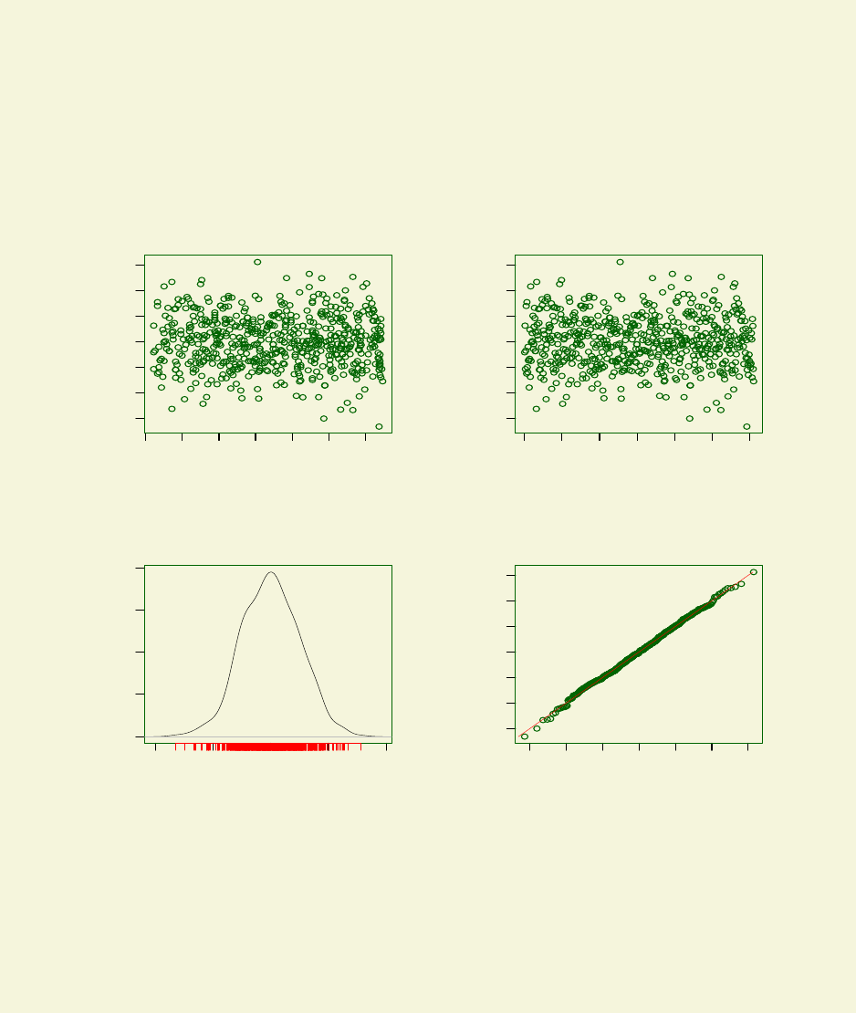
6.1. THE PLOT FUNCTION 123
50 100 150 200 250 300 350
−3 −2 −1 0 1 2 3
Against Fitted Values
Fitted Values
Quantile Residuals
0 100 200 300 400 500 600
−3 −2 −1 0 1 2 3
Against index
index
Quantile Residuals
−4 −2 0 2 4
0.0 0.1 0.2 0.3 0.4
Density Estimate
Quantile. Residuals
Density
−3 −2 −1 0 1 2 3
−3 −2 −1 0 1 2 3
Normal Q−Q Plot
Theoretical Quantiles
Sample Quantiles
Figure 6.1: Residual plots from the BCT model abd10
124 CHAPTER 6. DIAGNOSTICS
though that this makes very little different in the plot since age is already ordered. Also we
change the plotting parameters values.
> newpar<-par(mfrow=c(2,2), mar=par("mar")+c(0,1,0,0), col.axis="blue4",
+ col="blue4",
+ col.main="blue4",col.lab="blue4",pch="+",cex=.45,
+ cex.lab=1.2, cex.axis=1, cex.main=1.2 )
> plot(abd10,xvar=abdom$x,par=newpar)
*******************************************************************
Summary of the Quantile Residuals
mean = 0.001118164
variance = 1.002291
coef. of skewness = 0.00861578
coef. of kurtosis = 2.991170
Filliben correlation coefficient = 0.9992756
*******************************************************************
<The plot is shown in figure 6.2>
In order to see an application of the option (ts=TRUE) consider the aids data consisting of
45 observations on the following 3 variables:
ythe number of quarterly aids cases in England and Wales: a numeric vector
xtime in months from January 1983, 1:45 : a numeric vector
qrt the quarterly seasonal effect a factor with 4 levels, [1=Q1 (Jan-March), 2=Q2 (Apr-June),
3=Q3 (July-Sept), 4=Q4 (Oct-Dec)]
Here we model the counts y using a negative binomial distribution with a (smooth) regression
model in time x with a quarterly effect i.e. cs(x,df=7)+qrt, for the mean of y.
> data(aids)
> aids.1<-gamlss(y~cs(x,df=7)+qrt,family=NBI, data=aids )
GAMLSS-RS iteration 1: Global Deviance = 365.8121
GAMLSS-RS iteration 2: Global Deviance = 362.0205
GAMLSS-RS iteration 3: Global Deviance = 362.1087
GAMLSS-RS iteration 4: Global Deviance = 362.1116
GAMLSS-RS iteration 5: Global Deviance = 362.1123
> plot(aids.1,ts=TRUE)
*******************************************************************
Summary of the Randomised Quantile Residuals
mean = -0.01340323
variance = 0.9542376
coef. of skewness = 0.561715
coef. of kurtosis = 3.227582
Filliben correlation coefficient = 0.986852
*******************************************************************
6.1. THE PLOT FUNCTION 125
+
+
+
+
+
+
+
+
+
+
++
+
+
+
+
+
+
++
+
+
+
+
+
+
+
+
++
+
+
+
+
+
+
+
+
+
+
+
+
+
+
+
+
+
+
+
+
+
+
+
+
+
+
+
+
+
+
+
+
+
+
+
+
+
+
+
+
+
+
+
+
+
+
+
+
+
+
+
+
+
+
+
+
+
+
+
+
+
+
+
+
+
+
+
+
+
+
+
+
+
+
+
+
+
+
+
+
+
+
+
++
+
+
+
+
+
+
+
+
+
+
+
+
+
+
+
+
+
+
+
+
+
+
+
+
+
+
+
++
+
+
+
+
+
+
+
+
+
+
+
+
+
+
+
+
+
+
+
+
+
+
+
+
+
+
+
+
+
+
+
+
+
+
+
+
+
+
+
+
+
+
+
+
+
+
+
+
+
+
+
+
+
++
+
+
+
+
+
+
+
+
+
+
+
+
+
+
+
++
+
+
+
+
+
+
+
+
+
+
++
+
+
+
+
+
+
+
+
+
+
+
+
+
+
+
+
+
+
+
+
+
+
+
+
+
+
+
+
+
+
+
+
+
+
+
+
+
+
+
+
+
+
+
+
+
+
+
+
+
+
+
+
+
+
++
+
+
+
+
+
+
+
+
+
+
+
+
+
+
++
+
+
+
+
+
+
+
+
+
+
+
+
+
+
+
+
+
+
+
+
+
+
+
+
+
+
+
+
+
+
+
+
+
+
+
+
+
+
+
+
+
+
+
+
+
+
+
+
+
+
+
+
+
+
+
+
+
+
+
+
+
+
+
+
+
+
+
+
+
+
+
+
+
+
+
+
+
+
+
+
+
+
++
+
+
+
+
+
+
+
+
+
+
+
+
+
+
+
+
+
+
+
+
+
+
+
+
+
+
+
+
+
+
+
+
+
+
+
+
+
+
+
+
+
+
+
+
+
+
+
+
+
+
+
+
+
+
+
+
++
+
+
+
+
+
+
+
+
+
+
+
+
+
+
+
+
+
+
+
+
+
+
+
+
+
+
+
+
+
+
+
+
+
+
+
+
+
+
+
+
+
+
+
+
+
+
+
+
+
+
+
+
++
+
+
+
+
+
+
+
+
+
+
+
+
+
+
+
+
+
+
+
+
+
+
+
+
+
+
+
+
+
+
+
+
+
+
+
+
+
+
+
+
+
+
+
+
+
+
+
+
+
+
+
+
+
+
+
+
+
+
+
+
+
+
+
+
+
+
+
+
+
+
+
+
+
+
+
+
+
+
+
+
+
+
+
+
+
+
+
+
+
+
+
+
+
+
+
+
+
+
+
+
+
+
+
+
+
+
+
+
+
+
+
+
+
+
50 100 150 200 250 300 350
−3 −2 −1 0 1 2 3
Against Fitted Values
Fitted Values
Quantile Residuals
+
+
+
+
+
+
+
+
+
+
++
+
+
+
+
+
+
++
+
+
+
+
+
+
+
+
++
+
+
+
+
+
+
+
+
+
+
+
+
+
+
+
+
+
+
+
+
+
+
+
+
+
+
+
+
+
+
+
+
+
+
+
+
+
+
+
+
+
+
+
+
+
+
+
+
+
+
+
+
+
+
+
+
+
+
+
+
+
+
+
+
+
+
+
+
+
+
+
+
+
+
+
+
+
+
+
+
+
+
+
++
+
+
+
+
+
+
+
+
+
+
+
+
+
+
+
+
+
+
+
+
+
+
+
+
+
+
+
++
+
+
+
+
+
+
+
+
+
+
+
+
+
+
+
+
+
+
+
+
+
+
+
+
+
+
+
+
+
+
+
+
+
+
+
+
+
+
+
+
+
+
+
+
+
+
+
+
+
+
+
+
+
++
+
+
+
+
+
+
+
+
+
+
+
+
+
+
+
++
+
+
+
+
+
+
+
+
+
+
++
+
+
+
+
+
+
+
+
+
+
+
+
+
+
+
+
+
+
+
+
+
+
+
+
+
+
+
+
+
+
+
+
+
+
+
+
+
+
+
+
+
+
+
+
+
+
+
+
+
+
+
+
+
+
++
+
+
+
+
+
+
+
+
+
+
+
+
+
+
++
+
+
+
+
+
+
+
+
+
+
+
+
+
+
+
+
+
+
+
+
+
+
+
+
+
+
+
+
+
+
+
+
+
+
+
+
+
+
+
+
+
+
+
+
+
+
+
+
+
+
+
+
+
+
+
+
+
+
+
+
+
+
+
+
+
+
+
+
+
+
+
+
+
+
+
+
+
+
+
+
+
+
++
+
+
+
+
+
+
+
+
+
+
+
+
+
+
+
+
+
+
+
+
+
+
+
+
+
+
+
+
+
+
+
+
+
+
+
+
+
+
+
+
+
+
+
+
+
+
+
+
+
+
+
+
+
+
+
+
++
+
+
+
+
+
+
+
+
+
+
+
+
+
+
+
+
+
+
+
+
+
+
+
+
+
+
+
+
+
+
+
+
+
+
+
+
+
+
+
+
+
+
+
+
+
+
+
+
+
+
+
+
++
+
+
+
+
+
+
+
+
+
+
+
+
+
+
+
+
+
+
+
+
+
+
+
+
+
+
+
+
+
+
+
+
+
+
+
+
+
+
+
+
+
+
+
+
+
+
+
+
+
+
+
+
+
+
+
+
+
+
+
+
+
+
+
+
+
+
+
+
+
+
+
+
+
+
+
+
+
+
+
+
+
+
+
+
+
+
+
+
+
+
+
+
+
+
+
+
+
+
+
+
+
+
+
+
+
+
+
+
+
+
+
+
+
+
15 20 25 30 35 40
−3 −2 −1 0 1 2 3
Against abdom$x
abdom$x
Quantile Residuals
−4 −2 0 2 4
0.0 0.1 0.2 0.3 0.4
Density Estimate
Quantile. Residuals
Density
+
+
+
+
+
+
+
+
+
+
++
+
+
+
+
+
+
++
+
+
+
++
+
+
+
++
+
+
+
+
++
+
+
+
+
+
+
+
+
+
+
+
+
+
+
+
+
+
+
+
+
+
+
+
+
+
+
+
+
+
+
+
+
+
+
+
+
+
+
+
+
+
+
+
+
+
+
+
+
+
+
+
+
+
+
+
+
+
+
+
+
+
+
+
+
+
+
+
+
+
+
++
+
+
+
+
+
++
+
+
+
+
+
+
+
+
+
+
+
+
+
+
+
+
+
+
+
+
+
+
+
+
+
+
+
++
+
+
+
+
+
+
+
+
+
+
++
+
+
+
+
+
+
+
+
+
+
+
++
+
+
++
+
+
+
+
+
+
+
+
+
+
+
+
+
+
+
+
+
+
+
+
+
+
+
+
++
+
+
+
+
+
+
+
+
+
+
+
+
+
+
+
++
+
+
+
+
+
+
+
++
+
++
+
+
+
+
+
+
+
+
+
+
+
+
+
+
+
+
+
++
+
+
+
+
+
+
+
+
+
+
+
+
+
+
+
+
++
++
+
+
+
+
+
+
+
+
+
+
+
+
+
+
+++
+
+
+
+
+
+
+
+
+
+
+
+
+
+
++
+
+
+
+
+
+
+
+
+
+
+
+
+
+
+
+
+
+
+
+
+
+
+
+
+
+
+
+
+
+
+
+
+
+
+
+
+
+
+
+
+
+
+
+
+
+
+
+
+
+
+
+
+
+
+
+
++
+
+
+
+
+
+
+
+
+
+
+
+
+
+
+
+
+
+
+
+
+
+
+
++++
+
+
+
+
+
+
+
+
+
++
+
+
+
+
+
+
+
+
+
+
++
+
+
+
++
+
+
+
+
+
+
+
+
+
+
+
+
++
+
+
+
+
+
+
++
+
+
+
+
+
++
+
+
+
+
+
+
+
+
+
+
++
+
+
+
+
+
+
+
+
+
+
+
+
+
+
+
+
+
+
+
+
+
+
+
+
+
+
+
+
+
+
+
+
+
++
+
+
+
+
+
++
+
+
+
+
+
+
+
+
+
+
+
+
+
+
+
+
+
+
+
+
+
+
++
+
+
+
+
+
+
+
+
+
+
+
+
+
+
+
+
+
+
+
+
+
+
+
+
+
+
+
+
++
+
+
+
+
+
+
+
+
+
+
+
+
+
+
+
+
+
+
+
+
+
+
+
+
+
+
+
+
+
+
+
+
+
+
++
+
+
+
+
+
+
+
+
+
+
+
+
+
+
+
++
+
+
+
+
+
+
+
−3 −2 −1 0 1 2 3
−3 −2 −1 0 1 2 3
Normal Q−Q Plot
Theoretical Quantiles
Sample Quantiles
Figure 6.2: Residual plots from the BCT model abd10, where the xvar and par options have
been modified
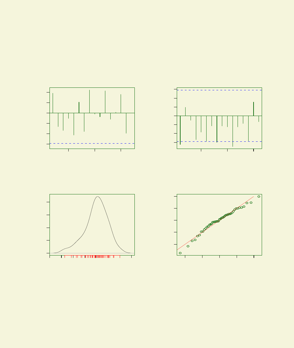
126 CHAPTER 6. DIAGNOSTICS
5 10 15
−0.3 −0.1 0.1 0.2
Lag
ACF
Series x$residuals
5 10 15
−0.3 −0.1 0.1 0.3
Lag
Partial ACF
Series x$residuals
−4 −3 −2 −1 0 1 2 3
0.0 0.1 0.2 0.3 0.4
Density Estimate
Quantile. Residuals
Density
−2 −1 0 1 2
−2 −1 0 1 2
Normal Q−Q Plot
Theoretical Quantiles
Sample Quantiles
Figure 6.3: Residual plots from the NBI model fitted to the aids data
6.2. THE WP() FUNCTION 127
<The plot is shown in figure 6.3>
Note that since here we are using a discrete distribution family to model the data the
residuals are randomized and the function rqres.plot should be used in addition to the function
plot.
6.2 The wp() function
Worm plots of the residuals were introduced by van Buuren et al. (2001) in order to identify
regions (intervals) of the explanatory variable within which the model does not fit adequately
the data (called ”model violation”). The Rfunction wp (which is based on the original S-PLUS
function of van Buuren et al. (2001)) provides single or multiple worm plots for gamlss fitted
objects. This is a diagnostic tool for checking the residuals for different ranges (by default not
overlapping) of the explanatory variable.
The arguments of the wp function are as follows:
object agamlss fitted object
xvar the explanatory variable against which the worm plots will be plotted.
n.inter the number of intervals in which the explanatory variable xvar will be cut
xcut.points the x-axis cut off points e.g. c(20,30). If xcut.points=NULL then the
n.inter argument is activated
overlap how much overlapping in the xvar intervals. Default value is overlap=0 for
non overlapping intervals
xlim.all for a single plot this value is the x-variable limit, default is xlim.all=4
xlim.worm for multiple plots this value is the x-variable limit, default is xlim.worm=3.5
show.given whether to show the x-variable intervals in the top of the graph, default is
show.given=TRUE
line whether to plot the cubic polynomial line in each worm plot, default value is
line=TRUE
ylim.all for a single plot this value is the y-variable limit, default value is
ylim.all=12*sqrt(1/length(fitted(object)))
ylim.worm for multiple plots this value is the y-variable limit, default value is
ylim.worm=12*sqrt(n.inter/length(fitted(object)))
cex the cex plotting parameter with default cex=1
pch the pch plotting parameter with default pch=21
If the xvar argument is not specified then a single worm plot is used. In this case a worm
plot is a detrended normal QQ-plot so departure from normality is highlighted. If the xvar is
specified then we have as many worm plots as n.iter. In this case the x-variable is cut into
n.iter intervals with an equal numbers observations and detrended normal QQ (i.e. worm)
plots for each interval are plotted. This is a way of highlighting failures of the model within
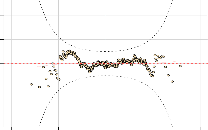
128 CHAPTER 6. DIAGNOSTICS
different ranges of the explanatory variable. The parameters of the fitted cubic polynomials to
the residuals can be obtained by e.g. coRes<-wp(model1,xvar=x,n.iner=9) and can be used
as a way of checking the region in which the model does not fit adequately.
Here is an example on how to use the wp function:
> data(abdom)
> abd10<-gamlss(y~cs(x,df=3),sigma.fo=~cs(x,df=1),data=abdom,family=BCT)
GAMLSS-RS iteration 1: Global Deviance = 4776.163
GAMLSS-RS iteration 2: Global Deviance = 4775.91
GAMLSS-RS iteration 3: Global Deviance = 4775.884
GAMLSS-RS iteration 4: Global Deviance = 4775.88
GAMLSS-RS iteration 5: Global Deviance = 4775.88
wp(abd10)
<The plot is shown in figure 6.4>
−4 −2 0 2 4
−0.4 −0.2 0.0 0.2 0.4
Unit normal quantile
Deviation
Figure 6.4: Worm plot from the BCT model abd10 at default values
Here the xvar argument is not specified so a single worm plot of the entire residuals is
plotted. In this case the plot is a detrended version of the normal QQ plot shown in the bottom
right hand side plot of the figure 6.1 or 6.2. Since all the observations fall in the ”acceptance”
region inside the two elliptic curves the overall the model appears to fit well. The red curve in
the plot is a fitted cubic polynomial to the points on the plot. More often and especially when
6.2. THE WP() FUNCTION 129
one of the explanatory variables is dominant in the analysis (as for example in centile estimation
or where we are dealing with time series data) we would like to check in which range of the
explanatory variable the model do not fit well. In the abdominal circumference example we are
interested whether the model fits well at the different regions of age. Here we are using the
option xvar to specify age and n.inter to specify 9 intervals with equal number of observations
for the worm plot. We are also saving the coefficient parameters of the fitted cubic polynomials
for further diagnostics.
> coef.1<-wp(abd10,xvar=abdom$x,n.inter=9)
number of missing points from plot= 0
number of missing points from plot= 0
number of missing points from plot= 0
number of missing points from plot= 0
number of missing points from plot= 0
number of missing points from plot= 0
number of missing points from plot= 0
number of missing points from plot= 0
number of missing points from plot= 0
> coef.1
$classes
[,1] [,2]
[1,] 12.22 16.36
[2,] 16.36 19.36
[3,] 19.36 22.50
[4,] 22.50 25.21
[5,] 25.21 28.36
[6,] 28.36 31.93
[7,] 31.93 35.21
[8,] 35.21 38.64
[9,] 38.64 42.36
$coef
[,1] [,2] [,3] [,4]
[1,] 0.038366200 0.1096908863 -0.00465157 -0.016570559
[2,] 0.064304458 0.1011059458 -0.01818442 -0.018532805
[3,] -0.061047688 0.0834373248 0.02395203 -0.056799686
[4,] -0.075182844 -0.1025361677 0.02922259 0.029898784
[5,] -0.031533969 -0.0546987874 0.01258042 -0.038303676
[6,] -0.026696480 0.0072953536 0.05373850 0.008777147
[7,] 0.084968780 -0.0655378549 -0.03199232 0.030213186
[8,] 0.043471545 -0.0005954548 -0.03230765 0.019718502
[9,] -0.002507405 -0.0408841858 -0.03271212 0.024146016
<The plot is shown in figure 6.5>
The Table of intervals ($classes) above gives the 9 non-overlapping x(i.e. age) ranges.
The Table of coefficients ($coef) gives in each column the fitted constant, linear, quadratic
and cubic coefficients ˆ
β0,ˆ
β1,ˆ
β2and ˆ
β3respectively, for each of the nine cubic polynomials fitted
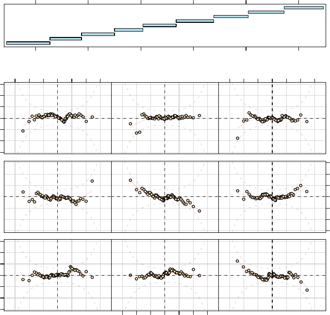
130 CHAPTER 6. DIAGNOSTICS
−1.5 −0.5 0.5 1.5
−3 −2 −1 0 1 2 3
−1.5 −0.5 0.5 1.5
−3 −2 −1 0 1 2 3
−1.5 −0.5 0.5 1.5
−3 −2 −1 0 1 2 3
Unit normal quantile
Deviation
15 20 25 30 35 40
Given : xvar
Figure 6.5: Worm plot from the BCT model abd10 at default values
6.3. THE Q.STATS FUNCTION 131
to the nine detrended QQ-plots (for the nine non-overlapping rages of age given by $classes).
van Buuren and Fredriks (2001) categorize absolute values of ˆ
β0,ˆ
β1,ˆ
β2and ˆ
β3in excess of
threshold values 0.10, 0.10, 0.05 and 0.03 respectively, as misfits or model violations, indicating
differences between the theoretical model residuals and empirical mean, variance, skewness and
kurtosis of residuals respectively, within the particular age range (of the corresponding QQ-
plot). Following these criteria in the above Table of coefficients, there are three (marginal)
misfits 0.10969, 0.10110 and -0.10254 in ˆ
β1, in the first, second and fourth range of age, one
misfit 0.0537 in ˆ
β2in the sixth range of age and two misfits −0.0568 and −0.0383 in ˆ
β3in the
third and fifth range of age.
6.3 the Q.stats function
This function calculates and prints the Q-statistics which are useful to test normality of the
residuals within a range of an independent x-variable, for example age in centile estimation, see
Royston and Wright (2000).
In order to explain what is a Q-statistic let us consider the situation where age is our
main explanatory variable. Let Gbe the number of age groups and let {rgi, i = 1,2, .., ni}be
the residuals in age group g, with mean ¯rgand standard deviation sg, for g= 1,2, .., G. The
following statistics Zg1,Zg2,Zg3,Zg4are calculated from the residuals in group gto test whether
the residuals in group ghave population mean 0, variance 1, skewness 0 and kurtosis 3, where
Zg1=n1/2
g¯rg,Zg2=ns2/3
g−[1 −2/(9ng−9)]o/{2/(9ng−9)}1/2and Zg3and Zg4are test
statistics for skewness and kurtosis given by D’Agostino et al. (1990), in their equations (13)
and (19) respectively.
The Qstatistics of Royston and Wright (2000) are then calculated by Qj=PG
g=1 Z2
gj for
j= 1,2,3,4. Royston and Wright discuss approximate distributions for the Qstatistics under
the null hypothesis that the true residuals are normally distributed (although their simulation
study was mainly for normal error models) and suggest Chi-squared distributions with adjusted
degrees of freedom G−dfµ,G−[dfσ+ 1]/2 and G−dfνfor Q1, Q2and Q3respectively. By
analogy we suggest degrees of freedom G−dfτfor Q4. The resulting significance levels should
be regarded as providing a guide to model inadequacy, rather than exact formal test results.
Significant Q1, Q2, Q3or Q4statistics indicate possible inadequacies in the models for pa-
rameters µ, σ, ν and τrespectively, which may be overcome by increasing the degrees of freedom
in the model for the particular parameter.
The Zgj statistic when squared provides the contribution from age group gto the statistic
Qj, and hence helps identify which age groups are causing the Qjstatistic to be significant and
therefore in which age groups the model is unacceptable.
Provided the number of groups Gis sufficiently large relative to the degrees of freedom in the
model for the parameter, then the Zgj values should have approximately standard normal dis-
tributions under the null hypothesis that the true residuals are standard normally distributed.
We suggest as a rough guide values of |Zgj |greater than 2 be considered as indicative of sig-
nificant inadequacies in the model. Note that significant positive (or negative) values Zgj >2
(or Zgj <2) for g= 1,2,3 or 4 indicate respectively that the residuals have a higher (or lower)
mean, variance, skewness or kurtosis than the null standard normal distribution. The model for
parameter µ, σ, ν or τmay need more degrees of freedom to overcome this. For example if the
residual mean in an age group is too high, the model for µmay need more degrees of freedom
in order for the fitted µfrom the model to increase within the age group.
The Q.stats function has the following arguments
132 CHAPTER 6. DIAGNOSTICS
obj agamlss object or any other residual vector
xvar the explanatory variable against which the Q statistics will be calulated
xcut.points the x-axis cut off points e.g. c(20,30). If xcut.points=NULL then the
n.inter argument is activated
n.inter the number of intervals in which the explanatory variable xvar will be cut
zvals if TRUE the output matrix contains the individual Z statistics rather than the
Q statistics
save whether to save the Q (or Z) statistics or not with default equal to TRUE. In
this case the functions produce a matrix giving individual Q (or Z) statistics
and the final aggregate Q’s
The following output is produced using the function Q.stats in the abd10 model fitted in
the previous Section.
> qstats<-Q.stats(abd10,xvar=abdom$x,n.inter=9)
> qstats
Z1 Z2 Z3 Z4 AgostinoK2
12.22 to 16.36 0.27872946 0.7322874 -0.03447791 -0.4622126 0.2148292
16.36 to 19.36 0.38031026 0.5724440 -0.29053682 -0.6429854 0.4978419
19.36 to 22.5 -0.31616165 -0.7875095 0.45660299 -2.1126317 4.6716990
22.5 to 25.21 -0.38070293 -0.1862518 0.80613323 1.3173178 2.3851771
25.21 to 28.36 -0.15593161 -1.8287701 0.24358698 -1.6283405 2.7108274
28.36 to 31.93 0.21306956 0.3746617 1.01613341 0.4080130 1.1990017
31.93 to 35.21 0.44491471 0.2265848 -0.72114255 0.9679677 1.4570081
35.21 to 38.64 0.09570948 0.6183272 -0.78781055 0.7541157 1.1893359
38.64 to 42.36 -0.28542399 0.3314165 -0.86848627 1.1208110 2.0104857
TOTAL Q stats 0.82550847 5.5470754 3.93075962 12.4054463 16.3362059
df for Q stats 3.99917588 6.9999620 8.00000000 8.0000000 16.0000000
p-val for Q stats 0.93494624 0.5935077 0.86331588 0.1340099 0.4297525
>
6.4 the rqres.plot function
The function rqres.plot is used to create different realizations of the normalized randomized
quantile residuals [defined in Section 6] when the distribution of the response variable is discrete.
It takes the following arguments.
obj an gamss fitted model object from a discrete family
howmany the number of QQ-plots required up to ten, with default howmany=6
all if TRUE howmany QQ-plots from the howmany realizations are plotted. If
FALSE then a single QQ-plot of the median of the howmany realizations is
plotted
save If TRUE the median residuals can be saved
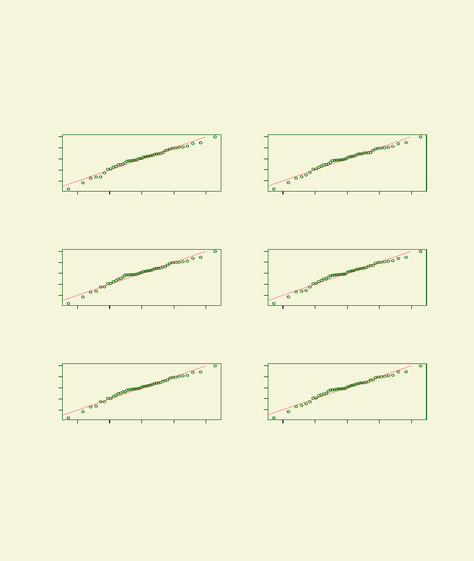
6.4. THE RQRES.PLOT FUNCTION 133
For example here we used the function rqres.plot to the AIDS data model aids.1 fitted in
Section 6.1:
rqres.plot(aids.1)
<The plot is shown in figure 6.6>
−2 −1 0 1 2
−2 −1 0 1 2
Normal Q−Q Plot
Theoretical Quantiles
Sample Quantiles
−2 −1 0 1 2
−2 −1 0 1 2
Normal Q−Q Plot
Theoretical Quantiles
Sample Quantiles
−2 −1 0 1 2
−2 −1 0 1 2
Normal Q−Q Plot
Theoretical Quantiles
Sample Quantiles
−2 −1 0 1 2
−2 −1 0 1 2
Normal Q−Q Plot
Theoretical Quantiles
Sample Quantiles
−2 −1 0 1 2
−2 −1 0 1 2
Normal Q−Q Plot
Theoretical Quantiles
Sample Quantiles
−2 −1 0 1 2
−2 −1 0 1 2
Normal Q−Q Plot
Theoretical Quantiles
Sample Quantiles
Figure 6.6: Residual plots from the NBI model fitted to the aids data
Plot 6.6 shows six realization of the normalized randomized quantile residuals from the fitted
model in all six occasions the distribution of the residuals appears to be negatively skew.
We now try 40 realization of the residuals and plot a QQ-plot of the median of these real-
izations. Again the residuals apears to be negatively skew. Hence the models is not adequate.
rqres.plot(aids.1, 40, all=FALSE)
<The plot is shown in figure 6.7>
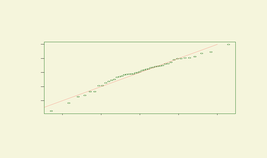
134 CHAPTER 6. DIAGNOSTICS
−2 −1 0 1 2
−2 −1 0 1 2
Normal Q−Q Plot
Theoretical Quantiles
Sample Quantiles
Figure 6.7: Residual plots from the NBI model fitted to the aids data
Chapter 7
Model selection
7.1 Model selection in gamlss
Let M={D,G,T,λ}represent the GAMLSS model, where the components: (i) Dspecifies the
distribution of the response variable (ii) Gthe set of link functions (g1,g2,g3,g4) for parameters
(µ, σ, ν, τ) (iii) Tthe set of predictor terms (tµ, tσ, tν, tτ,) for predictors (ηµ, ησ, ην, ητ) and (iv)
λthe set of (smoothing) hyperparameters.
For a specific data set, the GAMLSS model building process consists of comparing many
different competing models for which different combinations of components M={D,G,T,λ}
are tried.
Inference about quantities of interest can be made either conditionally on a single selected
’final’ model or by averaging between selected models. If the purpose of the study is to describe
the data parsimoniously, then a single ’final’ model is usually sufficient.
For parametric GAMLSS models each fitted GAMLSS model Mcan be assessed by its fitted
global deviance, GD, given by GD =−2ℓ(ˆ
θ) where ℓ(ˆ
θ) = Pn
i=1 ℓ(ˆ
θi) is the log-likelihood
function. Two nested parametric GAMLSS models, M0and M1, with fitted global deviances
GD0and GD1and error degrees of freedom dfe0and dfe1respectively may be compared using
the (generalized likelihood ratio) test statistic Λ = GD0−GD1which has an asymptotic Chi-
squared distribution under M0, with degrees of freedom d=dfe0−dfe1, (given that the usual
regularity conditions are satisfied). For each model Mthe error degrees of freedom dfeis defined
by dfe=n−Pp
k=1 dfθk, where dfθkis the degrees of freedom used in the predictor model for
parameter θkfor k= 1,...,p.
When the GAMLSS models M0and M1contain nonparametric additive terms, the same
test can be used as a guide to fitted model selection in the same way that Hastie and Tibshirani
(1990, Ch 3.9) compare ’nested’ Generalized Additive Models (GAM) fits. The degrees of
freedom used here is the trace of the smoothing matrix Sjk in the fitting algorithm, called the
’effective’ degrees of freedom, Hastie and Tibshirani (1990).
For non-nested GAMLSS models, to penalize over-fitting a generalized Akaike information
criterion (GAIC), −2ℓ(ˆ
θ) + (♯.df), can be used for model selection, where ♯is a penalty for each
degree of freedom used in the model e.g. ♯= 2 is the original Akaike information criterion,
Akaike (1974) , ♯= log nis the Schwarz Bayesian information Criterion (SBC), Schwarz (1978).
Both the original AIC and SBC criteria are asymptotically justified as predicting the degree of
fit in a new test data set, i.e. approximations to the average predictive error. Justification for
the use of SBC comes also as a crude approximation to Bayes factors, Raftery (1996, 1999). In
135
136 CHAPTER 7. MODEL SELECTION
practice it is usually found that while original AIC is very generous in model selection the SBC
is too restrictive. Our experience is that a value of the penalty ♯in the range 2.5≤♯≤3 works
well for most data. A selection of different values of ♯e.g. ♯= 2,2.5,3,3.5,4 could be used in
turn to investigate the sensitivity or robustness of the model selection to the choice of the value
of the penalty ♯.
For small data sets, the full data sample is usually used for both model fitting (minimizing
GD) and for model selection (minimizing a penalized criterion, e.g. AIC or SBC). For very large
data sets, the data could be split into (i) training, (ii) validation and (iii) test data sets. This
split is now routinely available in some statistical packages such as SAS Enterprise Miner, SAS
Institute Inc. (2000). This procedure has not been implemented yet in the gamlss package.
Within the GAMLSS framework (i) the training data could be used for model fitting (mini-
mizing its GD) (ii) the validation data could be used for model selection, in particular selection
of the distribution, link functions, predictor terms and smoothing parameters (by minimizing its
GD, denoted by VGD) and (iii) the test data could be used for the assessment of the predictive
power of the model chosen by (ii) and fitted by (i) and applied to the test data (again using its
GD, denoted by TGD).
Different model selection strategies can be used to build a GAMLSS model but more im-
portant the determination of the model adequacy should be always carried out with
respect to the substantive questions of interest and not in isolation. This means that
different problems could possibly require different model strategies.
Section 7.2 show how the functions addterm,dropterm,stepGAIC(),stepGAIC.VR() and
stepGAIC.CH()can be used to select (or eliminate) terms from a model formula. 7.3 discuss a
simple way of selecting the hyper-parameters of a GAMLSS model.
7.2 Selecting explanatory variables using addterm,dropterm,
and stepGAIC
There are five functions within gamlss to assist with selecting explanatory variable terms.
The first two are the functions addterm and dropterm which allow the addition or removal
of a term in a model respectively. Those two functions are building blocks for the functions
stepGAIC.VR() and stepGAIC.CH() suitable for stepwise selection of models. Both functions
perform the stepwise model selection using a Generalized Akaike Information Criterion. The
function stepGAIC.VR() is based on the function stepAIC given in the package MASS of Ven-
ables and Ripley (2002), (where more details and examples of the function can be found), with
the additional property that it allows selection of terms for any selected distribution parameter.
The function stepGAIC.CH is based on the S function step.gam() (see Chambers and Hastie
(1992), for more information) and it is more suited for models with smoothing additive terms in
them. Again the function stepGAIC.CH is generalized here so it can be used for any distribution
parameter within gamlss. The main difference between stepGAIC.VR() and stepGAIC.CH() lies
on the use of the scope argument. The function stepGAIC() combines the two functions by hav-
ing a extra argument additive which when is set to TRUE the stepGAIC.CH() is used otherwise
the stepGAIC.VR().stepGAIC.VR() will be pick up by default.
The functions addterm and dropterm are generic functions with their original definitions
defined at the package MASS of of Vendable and Ripley (2002). This package has to be attached,
(i.e. library(MASS)), before their method for classes gamlss can be used. The functions
stepGAIC(),stepGAIC.VR() and stepGAIC.CH() can be used without attaching MASS.
The dropterm and addterm functions in gamlss have the following arguments

7.2. SELECTING EXPLANATORY VARIABLES USING ADDTERM,DROPTERM, AND STEPGAIC137
object agamlss object.
scope a formula giving terms which might be dropped or added. For the function
dropterm the default is the model formula. For the function addterm the
scope is a formula specifying a maximal model which should include the cur-
rent one. Only terms that can be dropped or added while maintain marginality
are actually tried.
scale scale is not used in gamlss
test it takes values "none" for no test and "Chisq" for a χ2test statistic relative
to the original model.
kthe multiple of the degrees of freedom used for the penalty in the GAIC. k =
2gives the original AIC, k = log(n) is sometimes referred to as BIC or SBC.
sorted If TRUE the results are sorted in the order of the GAIC from the lowest (the
best model) to the highest (the worst model).
trace if ’TRUE’ additional information may be given on the fits as they are tried.
... : arguments passed to or from other methods.
In order to demonstrate how dropterm and addterm is working consider the US pollution
data set taken from Hand et al. (1994) data set 26, USAIR.DAT. The data are referred to 41
cities in the USA and have following 7 continuous variables.
y: sulpher dioxide concentration in air mgs. per cubic metre
x1: average annual temperature in degrees F
x2: number of manufacturers employing >20 workers
x3 : population size in thousands
x4: average annual wind speed in miles per hour
x5 : average annual rainfall in inches
x6: average number of days rainfall per year
Preliminary analysis has shown that it is better to model the distribution of the response
variable yusing the gamma rather the normal distribution. We start by fitting the full linear
additive model for mu.
> data(usair)
> # fitting all variables linearly
> mod1<-gamlss(y~., data=usair, family=GA)
GAMLSS-RS iteration 1: Global Deviance = 303.1604
GAMLSS-RS iteration 2: Global Deviance = 303.1602
Now we use the dropterm function to check whether any linear terms can be dropped.

138 CHAPTER 7. MODEL SELECTION
library(MASS)
dropterm(mod1, test="Chisq")
Single term deletions
for mu
Model:
y ~ x1 + x2 + x3 + x4 + x5 + x6
Df AIC LRT Pr(Chi)
<none> 319.16
x1 1 327.58 10.42 0.001244 **
x2 1 326.92 9.76 0.001788 **
x3 1 321.39 4.23 0.039718 *
x4 1 324.08 6.92 0.008502 **
x5 1 320.57 3.41 0.064642 .
x6 1 317.16 0.001712 0.966994
---
Signif. codes: 0 *** 0.001 ** 0.01 * 0.05 . 0.1 1
The above output gives the test for removing each of the six variables from the full model.
Given all other linear terms in the model, the variable x6 is the first to be dropped since it
has the highest p-values, 0.967, given by column Pr(Chi), and so is the least significant. To
demonstrate the function addterm considering of adding a two way interaction term into the
model mod1. Note that the scope argument has to be defined explicitly here.
addterm(mod1, scope=~(x1+x2+x3+x4+x5+x6)^2, test="Chisq")
Single term additions for mu
Model:
y ~ x1 + x2 + x3 + x4 + x5 + x6
Df AIC LRT Pr(Chi)
<none> 319.16
x1:x2 1 320.09 1.07 0.3012025
x1:x3 1 319.40 1.76 0.1843022
x1:x4 1 320.60 0.56 0.4533080
x1:x5 1 316.94 4.22 0.0398900 *
x1:x6 1 320.93 0.24 0.6277889
x2:x3 1 320.48 0.68 0.4100835
x2:x4 1 319.75 1.41 0.2344253
x2:x5 1 318.17 2.99 0.0839194 .
x2:x6 1 321.13 0.03 0.8603234
x3:x4 1 317.38 3.78 0.0519199 .
x3:x5 1 320.19 0.97 0.3253673
x3:x6 1 320.85 0.31 0.5800638
x4:x5 1 307.07 14.09 0.0001745 ***
x4:x6 1 320.33 0.83 0.3609260
x5:x6 1 318.74 2.42 0.1198891
---
Signif. codes: 0 *** 0.001 ** 0.01 * 0.05 . 0.1 1
7.2. SELECTING EXPLANATORY VARIABLES USING ADDTERM,DROPTERM, AND STEPGAIC139
detach(package:MASS)
Among the two way interactions x4:x5 is highly significant with a p-value of less that 0.001.
In order to build a model we need the functions stepGAIC(),stepGAIC.VR() and stepGAIC.CH.
The last two functions have the following arguments
object an gamlss object. This is used as the initial model in the stepwise search
scope defines the range of models examined in the stepwise search. For the function
stepGAIC.VR() this should be either a single formula, or a list containing
components upper and lower, both formulae.
For the function stepGAIC.CH the scope defines the range of models examined
in the step-wise search. It is a list of formulas, with each formula corresponding
to a term in the model. A 1 in the formula allows the additional option of
leaving the term out of the model entirely.
direction the mode of stepwise search, can be one of both,backward, or forward, with
a default of both which performs forward stepwise model selection. If the
scope argument is missing the default for direction is backward
trace if positive, information is printed during the running of stepGAIC. Larger
values may give more information on the fitting process
keep a filter function whose input is a fitted model object and the associated AIC
statistic, and whose output is arbitrary. Typically keep will select a subset
of the components of the object and return them. The default is not to keep
anything.
steps the maximum number of steps to be considered. The default is 1000 (essen-
tially as many as required). It is typically used to stop the process early.
scale scale is not used in gamlss package
what which distribution parameter is being modelled, default what="mu"
kthe multiple of the degrees of freedom used for the penalty in the GAIC
criterion. k=2gives the genuine Akaike information criterion (AIC), while
k = log(n) is sometimes referred to as Bayesian information criterion (BIC)
or Schwartz Bayesian criterion (SBC).
... any additional arguments to extractAIC. (None are currently used).
The stepGAIC() function has the same argument as the functions above but with an extra
argument additive=FALSE.
The set of models searched by stepGAIC.VR() is determined by the scope argument and its
lower and upper components. The lower and upper are model formulae. The terms defined
by the formula in lower component are always included in the model. The formula in upper
is the most complicated model that the procedure would look for inclusion. The fitted model
given the object option should lie between those two models. If the scope is missing then
a backward elimination starts from the model define by the gamlss object. In the following
example a backward elimination is performed on the model given by mod1. Note that mod2 has
a new component called anova showing the steps taken in the search of the model.
140 CHAPTER 7. MODEL SELECTION
> mod2<-stepGAIC.VR(mod1) # or just mod2<-stepGAIC(mod1)
Distribution parameter: mu Start: AIC= 319.16
y ~ x1 + x2 + x3 + x4 + x5 + x6
Df AIC
- x6 1 317.16
<none> 319.16
- x5 1 320.57
- x3 1 321.39
- x4 1 324.08
- x2 1 326.92
- x1 1 327.58
Step: AIC= 317.16
y ~ x1 + x2 + x3 + x4 + x5
Df AIC
<none> 317.16
- x3 1 319.39
- x4 1 322.48
- x5 1 324.14
- x2 1 324.92
- x1 1 336.11
> mod2$anova
Stepwise Model Path
Analysis of Deviance Table
Initial
mu
Model:
y ~ x1 + x2 + x3 + x4 + x5 + x6
Final
mu
Model:
y ~ x1 + x2 + x3 + x4 + x5
Step Df Deviance Resid. Df Resid. Dev AIC
1 33 303.1602 319.1602
2 - x6 1 0.001712207 34 303.1619 317.1619
Note that the same result is produced using mod2<-stepGAIC(mod1, additive=FALSE).
The above backward search confirms the fact that, if we want to include only linear additive
terms in the model, the variable x6 is not needed. The default penalty for the step procedure is
♯= 2) i.e. a genuine original AIC selection procedure. Increasing the penalty ♯should not make
a lot of difference since we have found above that x6 is highly non significant. For example
7.2. SELECTING EXPLANATORY VARIABLES USING ADDTERM,DROPTERM, AND STEPGAIC141
using the SBC we have
> mod2<-stepGAIC(mod1, k=log(41))
Distribution parameter: mu
Start: AIC= 332.87
y ~ x1 + x2 + x3 + x4 + x5 + x6
Df AIC
- x6 1 329.16
- x5 1 332.57
<none> 332.87
- x3 1 333.39
- x4 1 336.08
- x2 1 338.91
- x1 1 339.58
Step: AIC= 329.16
y ~ x1 + x2 + x3 + x4 + x5
Df AIC
<none> 329.16
- x3 1 329.67
- x4 1 332.76
- x5 1 334.43
- x2 1 335.20
- x1 1 346.39
As an example of using the scope argument explicitly we consider whether two way inter-
actions between the explanatory variables are needed in the model. The simplest model we are
considered here is with only a constant, i.e. lower= 1 and the most complicated is the one with
all two way interactions. The final model will be something between those two.
> mod3<-stepGAIC(mod1, scope=list(lower=~1,upper=~(x1+x2+x3+x4+x5+x6)^2))
Distribution parameter: mu
Start: AIC= 319.16
y ~ x1 + x2 + x3 + x4 + x5 + x6
Df AIC
+ x4:x5 1 307.07
+ x1:x5 1 316.94
- x6 1 317.16
+ x3:x4 1 317.38
+ x2:x5 1 318.17
+ x5:x6 1 318.74
<none> 319.16
+ x1:x3 1 319.40
+ x2:x4 1 319.75
+ x1:x2 1 320.09
142 CHAPTER 7. MODEL SELECTION
+ x3:x5 1 320.19
+ x4:x6 1 320.33
+ x2:x3 1 320.48
- x5 1 320.57
+ x1:x4 1 320.60
+ x3:x6 1 320.85
+ x1:x6 1 320.93
+ x2:x6 1 321.13
- x3 1 321.39
- x4 1 324.08
- x2 1 326.92
- x1 1 327.58
Step: AIC= 307.07
y ~ x1 + x2 + x3 + x4 + x5 + x6 + x4:x5
Df AIC
+ x1:x6 1 300.94
+ x4:x6 1 301.65
+ x1:x4 1 302.09
- x6 1 305.12
+ x3:x5 1 306.94
<none> 307.07
+ x2:x5 1 307.78
+ x2:x4 1 307.94
+ x3:x4 1 308.13
+ x3:x6 1 308.56
+ x1:x2 1 308.65
+ x2:x3 1 308.76
+ x1:x5 1 308.89
+ x2:x6 1 309.02
+ x1:x3 1 309.06
+ x5:x6 1 309.06
- x3 1 310.66
- x2 1 317.09
- x4:x5 1 319.16
- x1 1 325.97
...
...
...
Step: AIC= 292.72
y ~ x1 + x2 + x3 + x4 + x5 + x6 + x4:x5 + x1:x6 + x4:x6 + x3:x4 +
x2:x4 + x2:x3 + x3:x6 + x2:x6
Df AIC
<none> 292.72
+ x1:x4 1 293.55
+ x1:x5 1 293.95
7.2. SELECTING EXPLANATORY VARIABLES USING ADDTERM,DROPTERM, AND STEPGAIC143
+ x2:x5 1 294.08
- x2:x6 1 294.19
+ x5:x6 1 294.54
+ x3:x5 1 294.55
+ x1:x2 1 294.71
+ x1:x3 1 294.72
- x1:x6 1 295.18
- x3:x6 1 296.41
- x2:x3 1 297.34
- x3:x4 1 300.27
- x2:x4 1 300.41
- x4:x6 1 307.60
- x4:x5 1 328.13
> mod3$anova
Stepwise Model Path
Analysis of Deviance Table
Initial
mu
Model:
y ~ x1 + x2 + x3 + x4 + x5 + x6
Final
mu
Model:
y ~ x1 + x2 + x3 + x4 + x5 + x6 + x4:x5 + x1:x6 + x4:x6 + x3:x4 +
x2:x4 + x2:x3 + x3:x6 + x2:x6
Step Df Deviance Resid. Df Resid. Dev AIC
1 33 303.1602 319.1602
2 + x4:x5 1 14.087005 32 289.0732 307.0732
3 + x1:x6 1 8.133292 31 280.9399 300.9399
4 + x4:x6 1 4.786492 30 276.1534 298.1534
5 + x3:x4 1 2.082756 29 274.0706 298.0706
6 + x2:x4 1 4.460526 28 269.6101 295.6101
7 + x2:x3 1 2.886925 27 266.7232 294.7232
8 + x3:x6 1 2.532078 26 264.1911 294.1911
9 + x2:x6 1 3.468607 25 260.7225 292.7225
Model mod3 is a rather complicated interaction model. Note that the variable x6 is included
in the model mod3 since higher interactions involving x6 are selected in the model. More than
two way interactions are not permitted for continuous variables which is the case in our example.
A plot of the residuals of model mod3 indicates possible heterogeneity in the variation of y. We
shall deal with this problem later.
Now we consider the stepGAIC.CH function. For the function stepGAIC.CH() each of the
formulas in scope specifies a ”regimen”of candidate forms in which the particular term may enter
the model. For example, a term formula might be x1 + log(x1) + cs(x1, df=3). This
144 CHAPTER 7. MODEL SELECTION
means that x1 could either appear linearly, linearly in its logarithm, or as a cubic smoothing
spline function (cs()) estimated non-parametrically. Every term in the model is described by
such a term formula, and the final model is built up by selecting a component from each formula.
The function gamlss.scope() is similar to the S ’gam.scope()’ in Chambers and Hastie (1991)
and can be used to create term formulae automatically from specified data or model frames.
The supplied model object is used as the starting model, and hence there is the requirement
that one term from each of the term formulas be present in the formula of the distribution
parameter. This also implies that any terms in the formula of the distribution parameter not
contained in any of the term formulas will be forced to be present in every model considered.
Below we use the gamlss.scope() function to create a scope for the function stepGAIC.CH.
> gs<-gamlss.scope(model.frame(y~x1+x2+x3+x4+x5+x6, data=usair))
> gs
$x1 ~1 + x1 + cs(x1)
$x2 ~1 + x2 + cs(x2)
$x3 ~1 + x3 + cs(x3)
$x4 ~1 + x4 + cs(x4)
$x5 ~1 + x5 + cs(x5)
$x6 ~1 + x6 + cs(x6)
The function gamlss.scope has the following arguments:
frame a data or model frame
response which variable is the response in the data or model frame, the default is the
first
smoother what type smoother to use with default cubic smoothing spine, cs
arg any additional arguments required by the smoother, (for example df for cs)
form should a formula be returned (default), or else a character version of the
formula
Lets us experiment with the function and use a different smoother lo with a span=.7
> gs1<-gamlss.scope(model.frame(y~x1+x2+x3+x4+x5+x6, data=usair),
smoother="lo", arg="span=.7", form=TRUE)
> gs1
$x1
~1 + x1 + lo(x1, span = 0.7)
$x2
~1 + x2 + lo(x2, span = 0.7)
$x3
7.2. SELECTING EXPLANATORY VARIABLES USING ADDTERM,DROPTERM, AND STEPGAIC145
~1 + x3 + lo(x3, span = 0.7)
$x4
~1 + x4 + lo(x4, span = 0.7)
$x5
~1 + x5 + lo(x5, span = 0.7)
$x6
~1 + x6 + lo(x6, span = 0.7)
Next we are using the stepGAIC.CH to find a suitable additive model using a cubic smoothing
spline as a smoother.
> mod5<-gamlss(y~1, data=usair, family=GA)
GAMLSS-RS iteration 1: Global Deviance = 349.7146
GAMLSS-RS iteration 2: Global Deviance = 349.7146
> mod6<-stepGAIC(mod5,gs, additive=TRUE)
Distribution parameter: mu
Start: y ~ 1; AIC= 353.7146
Trial: y ~ x1 + 1 + 1 + 1 + 1 + 1; AIC= 338.0354
Trial: y ~ 1 + x2 + 1 + 1 + 1 + 1; AIC= 343.0487
Trial: y ~ 1 + 1 + x3 + 1 + 1 + 1; AIC= 349.2046
Trial: y ~ 1 + 1 + 1 + x4 + 1 + 1; AIC= 355.0206
Trial: y ~ 1 + 1 + 1 + 1 + x5 + 1; AIC= 355.4256
Trial: y ~ 1 + 1 + 1 + 1 + 1 + x6; AIC= 343.9733
Step : y ~ x1 ; AIC= 338.0354
Trial: y ~ cs(x1) + 1 + 1 + 1 + 1 + 1; AIC= 337.3823
Trial: y ~ x1 + x2 + 1 + 1 + 1 + 1; AIC= 328.781
Trial: y ~ x1 + 1 + x3 + 1 + 1 + 1; AIC= 332.942
Trial: y ~ x1 + 1 + 1 + x4 + 1 + 1; AIC= 339.6497
Trial: y ~ x1 + 1 + 1 + 1 + x5 + 1; AIC= 335.1107
Trial: y ~ x1 + 1 + 1 + 1 + 1 + x6; AIC= 335.9902
Step : y ~ x1 + x2 ; AIC= 328.781
Trial: y ~ cs(x1) + x2 + 1 + 1 + 1 + 1; AIC= 328.8904
Trial: y ~ x1 + cs(x2) + 1 + 1 + 1 + 1; AIC= 333.3071
Trial: y ~ x1 + x2 + x3 + 1 + 1 + 1; AIC= 325.665
Trial: y ~ x1 + x2 + 1 + x4 + 1 + 1; AIC= 327.6493
Trial: y ~ x1 + x2 + 1 + 1 + x5 + 1; AIC= 324.4414
Trial: y ~ x1 + x2 + 1 + 1 + 1 + x6; AIC= 325.5355
Step : y ~ x1 + x2 + x5 ; AIC= 324.4414
...
...
...
Trial: y ~ 1 + x2 + x3 + cs(x4) + cs(x5) + 1; AIC= 311.8573
Trial: y ~ cs(x1) + x2 + x3 + cs(x4) + cs(x5) + 1; AIC= 305.8555
Trial: y ~ x1 + 1 + x3 + cs(x4) + cs(x5) + 1; AIC= 315.1206
146 CHAPTER 7. MODEL SELECTION
Trial: y ~ x1 + cs(x2) + x3 + cs(x4) + cs(x5) + 1; AIC= 305.2431
Trial: y ~ x1 + x2 + 1 + cs(x4) + cs(x5) + 1; AIC= 309.6543
Trial: y ~ x1 + x2 + cs(x3) + cs(x4) + cs(x5) + 1; AIC= 307.9505
Trial: y ~ x1 + x2 + x3 + cs(x4) + x5 + 1; AIC= 305.1264
Trial: y ~ x1 + x2 + x3 + cs(x4) + cs(x5) + x6; AIC= 305.3408
> mod6$anova
From To Df Deviance Resid. Df Resid. Dev AIC
1 NA NA 39.00000 349.7146 353.7146
2 x1 -1.000000 -17.679187 38.00000 332.0354 338.0354
3 x2 -1.000000 -11.254434 37.00000 320.7810 328.7810
4 x5 -1.000000 -6.339651 36.00000 314.4414 324.4414
5 x5 cs(x5) -2.999638 -13.806449 33.00036 300.6349 316.6342
6 x3 -1.000000 -3.179355 32.00036 297.4555 315.4548
7 x4 -1.000000 -2.833942 31.00036 294.6216 314.6209
8 x4 cs(x4) -2.999290 -16.786090 28.00107 277.8355 303.8334
> mod6
Family: c("GA", "Gamma")
Fitting method: RS()
Call: gamlss(formula = y ~ x1 + x2 + x3 + cs(x4) + cs(x5), family = GA,
data = usair, trace = F)
Mu Coefficients:
(Intercept) x1 x2 x3 cs(x4) cs(x5)
6.5269155 -0.0507162 0.0013525 -0.0009617 -0.1196299 0.0160211
Sigma Coefficients:
(Intercept)
-1.199
Degrees of Freedom for the fit: 12.99893 Residual Deg. of Freedom 28.00107
Global Deviance: 277.836
AIC: 303.833
SBC: 326.108
The algorithm took eight different steps (we only included the first, second, third and eighth).
In the first step, all the linear terms are tried and the variable x1 is selected for inclusion. In the
second step, since x1 is already in the model, cs(x1) is tried together with all the linear terms
from the rest of the variable. In this second step the variable x2 is selected. The important
thing to notice here is that there is an hierarchy in the inclusion of the terms in the model
according to its scope, i.e. the component of the gamlss.scope for x1 is 1 + x1 + cs(x1)
requiring 1, (i.e. no x1 variable), x1, (linear in x1) and cs(x1), (smooth term in x1), to be
tested in a sequence. The terms for x1 in the gamlss.scope can only move one step up or down
from the current term in x1. Hence, for example, the model in x1 can only change from 1 only
to x1 but fromx1 to either 1 or cs(x1), and from cs(x1) only to x1.
We shall now try to include linear terms in the sigma model. Note that with only 41
observations and with a reasonably complicated model the mu it not advisable to try smoothing
7.2. SELECTING EXPLANATORY VARIABLES USING ADDTERM,DROPTERM, AND STEPGAIC147
terms for sigma. Here we check whether including linear terms in the model for sigma will
improve the model, i.e. reduce AIC using the spepAIC function.
mod7<-stepGAIC(mod6, what="sigma", scope=~x1+x2+x3+x4+x5+x6)
Distribution parameter: sigma Start: AIC= 303.83
~1
Df AIC
+ x3 1.00198 299.93
+ x2 1.00098 302.09
<none> 303.83
+ x4 0.99944 304.37
+ x5 1.00240 305.59
+ x1 0.99962 305.63
+ x6 1.00108 305.83
Step: AIC= 299.93
~x3
Df AIC
+ x4 0.99774 299.50
<none> 299.93
+ x6 1.00029 300.85
+ x5 0.99906 301.22
+ x1 0.99731 302.09
+ x2 0.99900 302.79
- x3 1.00198 303.83
Step: AIC= 299.5
~x3 + x4
Df AIC
<none> 299.50
- x4 0.99774 299.93
+ x5 1.00124 300.13
+ x6 1.00211 301.17
+ x1 1.00112 301.25
+ x2 1.00243 302.38
- x3 1.00027 304.37
There were 13 warnings (use warnings() to see them)
mod7$anova
Stepwise Model Path Analysis of Deviance Table
Initial sigma
Model:
~1
Final sigma

148 CHAPTER 7. MODEL SELECTION
Model:
~x3 + x4
Step Df Deviance Resid. Df Resid. Dev AIC
1 28.00107 277.8355 303.8334 2 + x3
1.0019760 5.908179 26.99910 271.9273 299.9291 3 + x4 0.9977373
2.427305 26.00136 269.5000 299.4973
It looks that the model needs x3+x3 in the formula for sigma. The warnings given during
the execution of the stepGAIC function are referring to the fact that the algorithm has not
converged occasionally in 20 iteration. In order to increase the number of iterations you have
to go back to the fitting of model mod5. This is not needed in this occasion since the results
remain the same even if we do just that.
7.3 Selecting hyperparameters using find.hyper
This function appears to work well in searching for the optimum degrees of freedom and/or
non-linear parameters (e.g. a power parameter ξused to transform x to xξ).
The function find.hyper selects the values of hyperparameters (and/or non-linear parame-
ters) in a GAMLSS model. It uses the Rfunction optim which then minimizes the generalized
Akaike information criterion (GAIC) with a user defined penalty.
Warning : For a large data set with 5 or more parameters to optimize the
function is very slow. [ For example a BCPE model with cubic smoothing
spline model for µ,σ,νand τ, with 7000 cases and 5 parameters to optimize
(4 hyperparameter smoothing degrees of freedom parameters for µ,σ,νand τ
respectively and 1 non-linear parameter) may take about 1 hour.
The arguments of the function find.hyper are
model this is a GAMLSS model in which the required hyperparameters are denoted
by p[number]. e.g.
model=gamlss(y~cs(x,df=p[1]),sigma.fo=~cs(x,df=p[2]),data=abdom)
parameters the starting parameter values in the search for the optimum hyperparameters
and/or non-linear parameters e.g. parameters=c(3,3)
other this is used to optimize non-linear parameter(s), for example a transformation
of the explanatory variable of the kind xp[3], e.g. others=quote(nx<-x^p[3])
where nx is now in the model formula
penalty specifies the penalty in the GAIC, (the default is 2.5) e.g. penalty=3
steps the steps in the parameter(s) taken during the optimization procedure (see
for example the ndeps option in optim()), by default set to 0.1 for all hyper
parameters and non-linear parameters
lower the lower bounds on the permissible values of the parameters e.g. for two
parameters lower=c(1,1). This does not apply if a method other than the
default method ”L-BFGS-B” is used
7.3. SELECTING HYPERPARAMETERS USING FIND.HYPER 149
upper the upper bounds on the permissible values of the parameters e.g for two
parameters upper=c(30,10). This does not apply if a method other than the
default method ”L-BFGS-B” is used
method the method used in optim() to numerically minimize the GAIC over the
hyperparameters and/or non-linear parameters. By default this is ”L-BFGS-
B” to allow box-restriction on the parameters
... this can be used for extra arguments in the control argument of the Rfunction
optim()
The function find.hyper returns the same output as the Rfunction optim.
As an example (but also of some difficulties arising) from using the function find.hyper
consider the AIDS data model aids.1 which was fitted in Chapter 6using cs(x,df=7). That
is, the hyperparameter (degrees of freedom for smoothing) was fixed at 7. Here we would like
to see if we could automate the process of finding the degrees of freedom. First we have to
declare the model and we do so using the quote Rfunction. For each hyperparameter to be
estimate we put p[.] with the appropriate number in the square plackets. It is advisable to use
control=gamlss.control(trace=FALSE) to switch off the printing of the global deviance in
each gamlss() iteration.
The function find.hyper is set to minimize GAIC with the default penalty=2.5. By default
the initial degrees of freedom parameter, p[1], for the search is set to 3 (i.e. par=c(3)), the
minimum value for p[1] for the search is set to 1 (i.e. lower=c(1)) and the steps in p[1] used
within the search to 0.1 (i.e. steps=c(0.1)). [The default ”L-BFGS-B” procedure starts with
the initial parameter value(s), changes each parameter in turn by ±step for that parameter,
and then jumps to new value(s) for the set of parameter(s). This is repeated until convergence.
See the help on the Rfunction (optim) for details.]
data(aids)
mod1<-quote(gamlss(y~cs(x,df=p[1])+qrt,family=NBI,data=aids,
control=gamlss.control(trace=FALSE)))
> op<-find.hyper(model=mod1, par=c(3), lower=c(1), steps=c(0.1))
par 3 crit= 402.3764 with pen= 2.5
par 3.1 crit= 401.8994 with pen= 2.5
par 2.9 crit= 402.8936 with pen= 2.5
par 4 crit= 398.9333 with pen= 2.5
par 4.1 crit= 398.6973 with pen= 2.5
par 3.9 crit= 399.1887 with pen= 2.5
par 4.977302 crit= 396.9575 with pen= 2.5
par 5.077302 crit= 396.7911 with pen= 2.5
par 4.877302 crit= 397.1292 with pen= 2.5
par 7.131224 crit= 394.5296 with pen= 2.5
par 7.231224 crit= 394.4753 with pen= 2.5
par 7.031224 crit= 394.59 with pen= 2.5
par 8.238112 crit= 394.2161 with pen= 2.5
par 8.338112 crit= 394.2183 with pen= 2.5
par 8.138112 crit= 394.2192 with pen= 2.5
par 8.246231 crit= 394.216 with pen= 2.5
par 8.346231 crit= 394.2187 with pen= 2.5
par 8.146231 crit= 394.2188 with pen= 2.5
150 CHAPTER 7. MODEL SELECTION
par 8.246778 crit= 394.2161 with pen= 2.5
par 8.346778 crit= 394.2187 with pen= 2.5
par 8.146778 crit= 394.2187 with pen= 2.5
par 8.246231 crit= 394.2161 with pen= 2.5
par 8.346231 crit= 394.2187 with pen= 2.5
par 8.146231 crit= 394.2188 with pen= 2.5
par 8.246231 crit= 394.2161 with pen= 2.5
par 8.346231 crit= 394.2187 with pen= 2.5
par 8.146231 crit= 394.2188 with pen= 2.5
par 8.246231 crit= 394.2161 with pen= 2.5
par 8.346231 crit= 394.2187 with pen= 2.5
par 8.146231 crit= 394.2188 with pen= 2.5
par 8.246231 crit= 394.2161 with pen= 2.5
par 8.346231 crit= 394.2187 with pen= 2.5
par 8.146231 crit= 394.2188 with pen= 2.5
> op
$par
[1] 8.246231
$value
[1] 394.2161
$counts
function gradient
11 11
$convergence
[1] 0
$message
[1] "CONVERGENCE: REL_REDUCTION_OF_F <= FACTR*EPSMCH"
So according to the GAIC with penalty 2.5 the optimal value for the degrees of freedom is
8.24 which looks reasonable. Unfortunately this is not the end of the story. Figure 7.1 shows
four plots, (generated using the function prof.term), where different criteria have been plotted
against the degrees of freedom for smoothing in the AIDS data: i) the left top figure shows the
global deviance (which we expect always to decrease for increasing degrees of freedom) ii) the
right top shows the AIC (GAIC with penalty 2) iii) the bottom left the GAIC with penalty 2.5
(the one we have just minimized) and iv) the SBC (GAIC with penalty log(45) = 3.8).
For the GAIC penalty=2.5 the function find.hyper found a local minimum, which in this
case is a reasonable solution (since the alternative around 30 degrees of freedom is too excessive
for only 45 observations). Using the SBC in this case would have resulted to a much clearer
minimum as shown below.
mod1<-quote(gamlss(y ~ cs(x,df=p[1]) + qrt, data = aids, family = NBI,
control=gamlss.control(trace=F)))
op<-find.hyper(mod1, par=c(10), lower=c(1), steps=c(0.1), penalty=log(45))
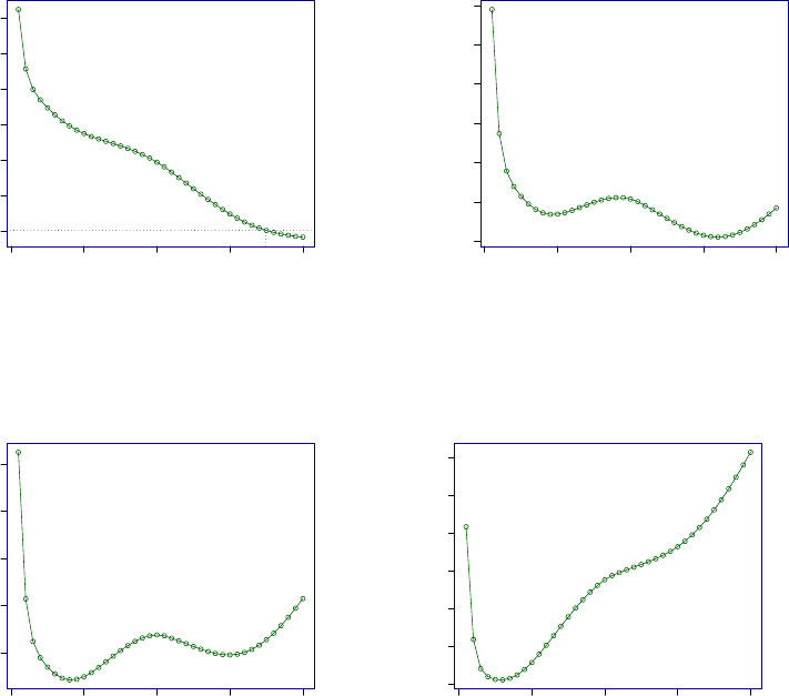
7.3. SELECTING HYPERPARAMETERS USING FIND.HYPER 151
0 10 20 30 40
300 320 340 360 380 400 420
Profile Global Deviance
parameter
Global Deviances
95 %
0 10 20 30 40
380 390 400 410 420 430 440
Profile GAIC
parameter
GAIC pen= 2
0 10 20 30 40
400 410 420 430 440
Profile GAIC
parameter
GAIC pen= 2.5
0 10 20 30 40
410 420 430 440 450 460 470
Profile GAIC
parameter
GAIC pen= 3.8
Figure 7.1: Profile global deviance and GAIC for different smoothing degrees of freedom fitted
in the NBI model to the AIDS data. (a) global deviance (b) GAIC with penalty ♯= 2, (c)
♯= 2.5 (d) ♯= 3.8, plotted against the mean smoothing degrees of freedom
152 CHAPTER 7. MODEL SELECTION
par 10 crit= 415.8063 with pen= 3.806662
par 10.1 crit= 416.0196 with pen= 3.806662
par 9.9 crit= 415.6053 with pen= 3.806662
par 9 crit= 413.9507 with pen= 3.806662
par 9.1 crit= 414.1229 with pen= 3.806662
par 8.9 crit= 413.7872 with pen= 3.806662
par 4.73133 crit= 411.4134 with pen= 3.806662
par 4.83133 crit= 411.3645 with pen= 3.806662
par 4.63133 crit= 411.4705 with pen= 3.806662
par 5.755199 crit= 411.1665 with pen= 3.806662
par 5.855199 crit= 411.1717 with pen= 3.806662
par 5.655199 crit= 411.1667 with pen= 3.806662
par 5.709297 crit= 411.1659 with pen= 3.806662
par 5.809297 crit= 411.1687 with pen= 3.806662
par 5.609297 crit= 411.1684 with pen= 3.806662
par 5.706121 crit= 411.1659 with pen= 3.806662
par 5.806121 crit= 411.1685 with pen= 3.806662
par 5.606121 crit= 411.1685 with pen= 3.806662
par 5.70922 crit= 411.1659 with pen= 3.806662
par 5.80922 crit= 411.1687 with pen= 3.806662
par 5.60922 crit= 411.1684 with pen= 3.806662
par 5.709297 crit= 411.1659 with pen= 3.806662
par 5.809297 crit= 411.1687 with pen= 3.806662
par 5.609297 crit= 411.1684 with pen= 3.806662
par 5.709297 crit= 411.1659 with pen= 3.806662
par 5.809297 crit= 411.1687 with pen= 3.806662
par 5.609297 crit= 411.1684 with pen= 3.806662
par 5.709297 crit= 411.1659 with pen= 3.806662
par 5.809297 crit= 411.1687 with pen= 3.806662
par 5.609297 crit= 411.1684 with pen= 3.806662
par 5.709297 crit= 411.1659 with pen= 3.806662
par 5.809297 crit= 411.1687 with pen= 3.806662
par 5.609297 crit= 411.1684 with pen= 3.806662
> op
$par
[1] 5.709297
$value
[1] 411.1659
$counts
function gradient
11 11
$convergence
[1] 0
$message
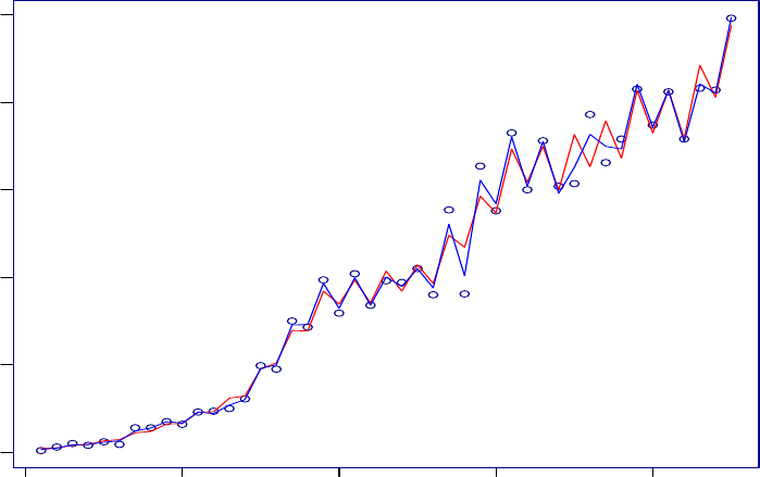
7.3. SELECTING HYPERPARAMETERS USING FIND.HYPER 153
[1] "CONVERGENCE: REL_REDUCTION_OF_F <= FACTR*EPSMCH"
>
So in this case the smoothing degrees of freedom for mu (with minimum value of criterion
SBC ≡GAIC(3.8)) is 5.7.
As an explanation of why the problem arises in this specific data we compare the fitted
values from the two different models, one with the degrees of freedom 10 and the other with 30.
Figure 7.2 shows that many of the extra degrees of freedom used in the df = 30 fit are there to
counteract the apparent misfit of observations 28, 29, 35, 36 and 37.
mod1<-gamlss(y~cs(x,df=10)+qrt,family=NBI,data=aids)
mod2<-gamlss(y~cs(x,df=30)+qrt,family=NBI,data=aids)
plot(aids$x,aids$y)
lines(aids$x,fitted(mod1),col="red")
lines(aids$x,fitted(mod2),col="blue")
0 10 20 30 40
0 100 200 300 400 500
aids$x
27
28
29 35
36
37
Figure 7.2: Fitted NBI models with df=10 (red line) and df=30 (blue line) using the AIDS data
Let us move to a different example using the abdominal circumference data. Let as as-
sume that we interested in estimating the hyper parameters p=p[1,2,3] = (dfµ, dfσ, λx). in
the model with the parameter mu modelled as cs(nx,df=p[1]) and the parameter sigma as
cs(nx,df=p[2]) where nx =xp[3] and where the family=BCT.
154 CHAPTER 7. MODEL SELECTION
mod1<-quote(gamlss(y~cs(nx,df=p[1]),sigma.fo=~cs(nx,df=p[2]),family=BCT,
+ data=abdom, control=gamlss.control(trace=FALSE)))
op<-find.hyper(model=mod1, other=quote(nx<-x^p[3]), par=c(3,1,0.5),
+ lower=c(1,1,0.001), steps=c(0.05,0.05,0.001))
par 3 1 0.5 crit= 4798.759 with pen= 2.5 par 3.05 1 0.5 crit=
4798.79 with pen= 2.5 par 2.95 1 0.5 crit= 4798.732 with pen= 2.5
par 3 1.05 0.5 crit= 4798.671 with pen= 2.5 par 3 1 0.5 crit=
4798.76 with pen= 2.5 par 3 1 0.501 crit= 4798.762 with pen= 2.5
par 3 1 0.499 crit= 4798.758 with pen= 2.5 par 2.696050 1.916867
0.2412169 crit= 4798.391 with pen= 2.5 par 2.746050 1.916867
0.2412169 crit= 4798.411 with pen= 2.5 par 2.646050 1.916867
...
...
0.2278033 crit= 4797.952 with pen= 2.5 par 2.606609 1.314610
0.2288033 crit= 4797.947 with pen= 2.5 par 2.606609 1.314610
0.2268033 crit= 4797.947 with pen= 2.5 par 2.606609 1.314610
0.2278033 crit= 4797.947 with pen= 2.5 par 2.656609 1.314610
0.2278033 crit= 4797.952 with pen= 2.5 par 2.556609 1.314610
0.2278033 crit= 4797.949 with pen= 2.5 par 2.606609 1.364610
0.2278033 crit= 4797.951 with pen= 2.5 par 2.606609 1.264610
0.2278033 crit= 4797.952 with pen= 2.5 par 2.606609 1.314610
0.2288033 crit= 4797.947 with pen= 2.5 par 2.606609 1.314610
0.2268033 crit= 4797.947 with pen= 2.5
> op
$par [1] 2.6066090 1.3146103 0.2278033
$value [1] 4797.947
$counts function gradient
22 22
$convergence [1] 0
$message [1] "CONVERGENCE: REL_REDUCTION_OF_F <= FACTR*EPSMCH"
The selected hyperparameters are 2.6 degrees of freedom for smoothing mu, 1.31 degrees of
freedom for smoothing the sigma and x0.227 for the power parameter. We refit the model and
plot its fitted parameters.
nx <- abdom$x^0.227
m1 <- gamlss(y~cs(nx,df=2.6),sigma.fo=~cs(nx,df=1.31),family=BCT,
+ data=abdom)
GAMLSS-RS iteration 1: Global Deviance = 4774.373
GAMLSS-RS iteration 2: Global Deviance = 4773.217
GAMLSS-RS iteration 3: Global Deviance = 4773.180
GAMLSS-RS iteration 4: Global Deviance = 4773.174
GAMLSS-RS iteration 5: Global Deviance = 4773.173
GAMLSS-RS iteration 6: Global Deviance = 4773.173
plot(y~x,data=abdom)
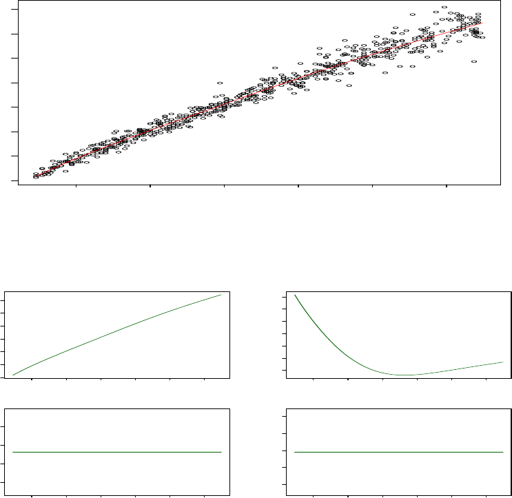
7.3. SELECTING HYPERPARAMETERS USING FIND.HYPER 155
lines(fitted(m1)~abdom$x,col="red")
fitted.plot(m1,x=abdom$x)
Figure 7.3 shows the data and the fitted mu. Figure 7.4 shows all the fitted parameter
estimates.
15 20 25 30 35 40
50 100 150 200 250 300 350 400
x
y
Figure 7.3: Abdominal data and fitted µ
15 20 25 30 35 40
50 100 150 200 250 300 350
(a)
abdom$x
mu
15 20 25 30 35 40
0.050 0.055 0.060 0.065 0.070 0.075 0.080
(b)
abdom$x
sigma
15 20 25 30 35 40
−0.14 −0.12 −0.10 −0.08
(c)
abdom$x
nu
15 20 25 30 35 40
8 10 12 14 16
(d)
abdom$x
tau
Figure 7.4: Fitted µ,σ,νand τfor the abdominal data
156 CHAPTER 7. MODEL SELECTION
Chapter 8
Centiles
Functions described in this Chapter are to be used in the special case of a GAMLSS model in
which only one explanatory variables is used. Section 8.1 describes the fitted.plot function
while Section 8discusses centile plotting.
8.1 Plotting fitted values against one x variable using
fitted.plot()
If your fitted model involves only one explanatory variable say x you can use fitted.plot()
to plot the fitted values against x.
> data(abdom)
> abd9 <- gamlss( y~cs(x,df=3), sigma.formula=~cs(x,df=3),
+ nu.formula=~1, tau.fomula=~1, family=BCT, data=abdom)
GAMLSS-RS iteration 1: Global Deviance = 4772.531
GAMLSS-RS iteration 2: Global Deviance = 4772.445
GAMLSS-RS iteration 3: Global Deviance = 4772.429
GAMLSS-RS iteration 4: Global Deviance = 4772.423
GAMLSS-RS iteration 5: Global Deviance = 4772.422
GAMLSS-RS iteration 6: Global Deviance = 4772.422
> fitted.plot(abd9,x=abdom$x)
<the plot is given in figure 8.1>
The fitted.plot function has the following arguments
object a fitted gamlss model object(with only one explanatory variable)
... optionally more fitted gamlss model objects
xthe unique explanatory variable
color whether the fitted lines plots are shown in colour, ’color=TRUE’ (the default)
or not ’color=FALSE’
line.type the x-variable label
157
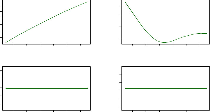
158 CHAPTER 8. CENTILES
15 20 25 30 35 40
50 100 150 200 250 300 350
(a)
abdom$x
mu
15 20 25 30 35 40
0.05 0.06 0.07 0.08
(b)
abdom$x
sigma
15 20 25 30 35 40
−0.16 −0.14 −0.12 −0.10 −0.08
(c)
abdom$x
nu
15 20 25 30 35 40
8 10 12 14 16
(d)
abdom$x
tau
Figure 8.1: The fitted values for all four parameters against age, from a Box-Cox t(BCT)
distribution fitted using the abdom data, i.e. fitted values of (a) µ(b) σ(c) ν(d) τ
The fitted values of more that one model can be also plotted together using fitted.plot.
For example here we compare model abd9 with model abd10 which has less degrees of freedom
for both mu and sigma.
> abd10 <- gamlss( y~cs(x,df=1), sigma.formula=~cs(x,df=1),
+ nu.formula=~1, tau.fomula=~1, family=BCT, data=abdom)
GAMLSS-RS iteration 1: Global Deviance = 4790.764
GAMLSS-RS iteration 2: Global Deviance = 4791.745
GAMLSS-RS iteration 3: Global Deviance = 4792.064
GAMLSS-RS iteration 4: Global Deviance = 4792.087
GAMLSS-RS iteration 5: Global Deviance = 4792.088
> fitted.plot(abd9,abd10,x=abdom$x)
<the plot is given in figure 8.2>
8.2 Plotting centiles curves using centiles()
Centile plots are currently provided for all the continuous distributions in Table ??.
There are two function for plotting centiles i) the centiles and ii) the centiles.split
which are described in sub-Section 8.2.1 and 8.2.2 respectively
8.2.1 The function centiles()
For a simple use try
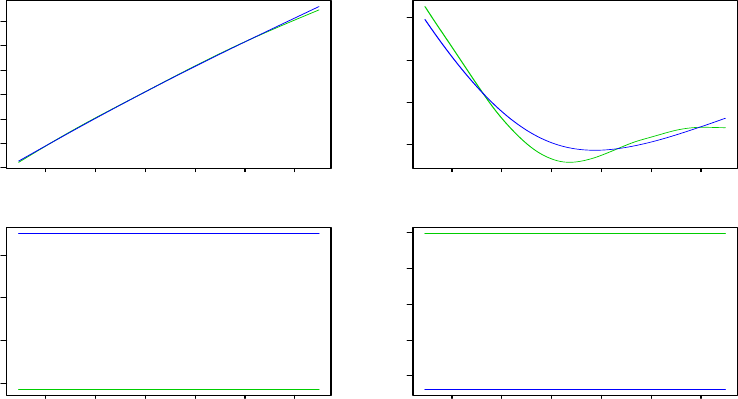
8.2. PLOTTING CENTILES CURVES USING CENTILES() 159
15 20 25 30 35 40
50 100 150 200 250 300 350
(a)
abdom$x
mu
15 20 25 30 35 40
0.05 0.06 0.07 0.08
(b)
abdom$x
sigma
15 20 25 30 35 40
−0.12 −0.10 −0.08 −0.06
(c)
abdom$x
nu
15 20 25 30 35 40
12.545 12.550 12.555 12.560 12.565
(d)
abdom$x
tau
Figure 8.2: Comparing the fitted values for all four parameters against age, for models abd9
and abd10, (a) µ(b) σ(c) ν(d) τ
abd9 <- gamlss( y~cs(x,df=3), sigma.formula=~cs(x,df=3),
nu.formula=~1, tau.fomula=~1, family=BCT, data=abdom)
GAMLSS-RS iteration 1: Global Deviance = 4772.521
GAMLSS-RS iteration 2: Global Deviance = 4772.453
GAMLSS-RS iteration 3: Global Deviance = 4772.433
GAMLSS-RS iteration 4: Global Deviance = 4772.425
GAMLSS-RS iteration 5: Global Deviance = 4772.423
GAMLSS-RS iteration 6: Global Deviance = 4772.422
centiles(abd9,abdom$x)
% of cases below 0.4 centile is 0.3278689
% of cases below 2 centile is 2.459016
% of cases below 10 centile is 8.688525
% of cases below 25 centile is 26.72131
% of cases below 50 centile is 50.32787
% of cases below 75 centile is 74.09836
% of cases below 90 centile is 90
% of cases below 98 centile is 98.19672
% of cases below 99.6 centile is 99.67213
<See figure 8.3 for the plot>
Note that Rautomatically prints the sample of cases below each of the fitted centiles from
the fitted model, so comparisons with nominal model %’s can be made. In the above example
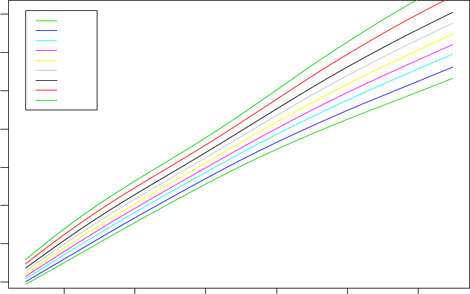
160 CHAPTER 8. CENTILES
+
+
+
+
+
+
+
+
+
+
++
+
+
+
+
+
+
++
++
+
+
+
+
+
+
++
+
+
+
+
+
+
+
+
+
+
+
+
+
+
+
+
+
+
+
+
+
+
+
+
+
+
+
+
+
+
+
+
+
+
+
+
+
+
+
+
+
+
+
+
+
+
+
+
+
+
+
+
+
+
+
+
+
+
+
++
+
+
+
+
+
++
+
+
+
+
+
+
+
+
+
+
+
+
+
+
+
++
+
+
+
+
+
+
+
+
+
+
+
+
+
+
+
+
+
+
+
+
+
+
+
+
+
+
+
++
+
+
+
+
+
+
+
+
+
+
+
+
+
+
+
+
+
+
+
+
+
+
+
+
+
+
+
+
+
+
+
+
+
+
+
+
+
+
+
+
+
+
+
+
+
+
+
+
+
+
+
+
+
++
+
+
+
+
+
+
+
+
+
+
+
+
+
+
+
++
+
+
+
+
+
+
+
+
+
+
++
+
+
+
+
+
+
+
+
+
+
+
+
+
+
+
+
+
+
+
+
+
+
+
+
+
+
+
+
+
+
+
+
+
+
+
+
+
+
+
+
+
+
+
+
+
+
+
+
+
+
+
+
+
+
++
+
+
+
+
+
+
+
+
+
+
+
+
+
+
++
+
+
+
+
+
+
+
+
+
+
+
+
+
+
+
+
+
+
+
+
+
+
+
+
+
+
+
+
+
+
+
+
+
+
+
+
+
+
+
+
+
++
+
+
+
+
+
+
+
+
+
+
+
+
+
+
+
+
+
+
+
+
+
+
+
+
+
+
+
+
+
+
+
+
+
+
+
+
+
+
+
++
+
+
+
+
+
+
+
+
+
+
+
+
+
+
+
+
+
+
+
+
+
+
+
+
+
+
+
+
+
+
+
+
+
+
+
++
+
+
+
+
+
+
+
+
+
+
+
+
+
+
+
+
+
+
+
++
+
+
+
+
+
+
+
+
+
+
+
+
+
+
+
+
+
+
+
+
+
+
+
+
+
+
+
+
+
+
+
+
+
+
+
+
+
+
+
+
+
+
+
+
+
+
+
+
+
+
+
+
++
+
+
+
+
+
+
+
+
+
+
+
+
+
+
+
+
+
+
+
+
+
+
+
+
++
+
+
+
+
+
+
+
+
+
+
+
+
+
+
+
+
+
+
+
+
+
+
+
+
+
+
+
+
+
+
+
+
+
+
+
+
+
+
+
+
+
+
+
+
+
+
+
+
+
+
+
+
+
+
+
+
+
+
+
+
+
+
+
+
+
+
+
+
+
+
+
+
+
+
+
+
+
+
+
+
+
+
+
+
+
+
+
+
15 20 25 30 35 40
50 100 150 200 250 300 350 400
x
y
Centile curves using BCT
0.4
2
10
25
50
75
90
98
99.6
0.4
2
10
25
50
75
90
98
99.6
0.4
2
10
25
50
75
90
98
99.6
0.4
2
10
25
50
75
90
98
99.6
0.4
2
10
25
50
75
90
98
99.6
0.4
2
10
25
50
75
90
98
99.6
0.4
2
10
25
50
75
90
98
99.6
0.4
2
10
25
50
75
90
98
99.6
0.4
2
10
25
50
75
90
98
99.6
Figure 8.3: Centiles curves using Box-Cox t(BCT) distribution for the abdom data
the sample % are close to the nominal model %’s.
The following are the arguments of the function centiles
obj a fitted gamlss object
xvar the unique explanatory variable for which we would like the fitted model
centiles to be calculated
cent a vector with elements the % centile values for which the fitted model centile
curves have to be evaluated. e.g. if you wish % centiles at points 5% and 95%
only use cent= c(5, 95)
legend whether a legend is required withn the plot or not, the default is legent=TRUE.
This legend identifies the different centile curves and it is boxed.
ylab the y-variable label
xlab the x-variable label
xleg position of the legend in the x-axis
yleg position of the legend in the y-axis
xlim the limits of the x-axis
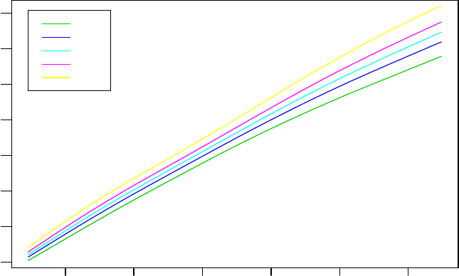
8.2. PLOTTING CENTILES CURVES USING CENTILES() 161
ylim the limits of the y-axis
save whether to save the sample percentages or not with default equal to ’FALSE’.
In this case the sample percentages are printed but are not saved
plot whether to plot the centiles. This option is useful for ’centile.split’
... for extra arguments
As an example a modified version of the centiles in figure 8.3 is given below:
> centiles(abd9,abdom$x,cent=c(5,25,50,75,95), ylab="abdominal circumference", xlab="age")
% of cases below 5 centile is 4.590164
% of cases below 25 centile is 26.72131
% of cases below 50 centile is 50.32787
% of cases below 75 centile is 74.09836
% of cases below 95 centile is 95.08197
>
<See figure 8.4 for the plot>
+
+
+
+
+
+
+
+
+
+
++
+
+
+
+
+
+
++
++
+
+
+
+
+
+
++
+
+
+
+
+
+
+
+
+
+
+
+
+
+
+
+
+
+
+
+
+
+
+
+
+
+
+
+
+
+
+
+
+
+
+
+
+
+
+
+
+
+
+
+
+
+
+
+
+
+
+
+
+
+
+
+
+
+
+
++
+
+
+
+
+
++
+
+
+
+
+
+
+
+
+
+
+
+
+
+
+
++
+
+
+
+
+
+
+
+
+
+
+
+
+
+
+
+
+
+
+
+
+
+
+
+
+
+
+
++
+
+
+
+
+
+
+
+
+
+
+
+
+
+
+
+
+
+
+
+
+
+
+
+
+
+
+
+
+
+
+
+
+
+
+
+
+
+
+
+
+
+
+
+
+
+
+
+
+
+
+
+
+
++
+
+
+
+
+
+
+
+
+
+
+
+
+
+
+
++
+
+
+
+
+
+
+
+
+
+
++
+
+
+
+
+
+
+
+
+
+
+
+
+
+
+
+
+
+
+
+
+
+
+
+
+
+
+
+
+
+
+
+
+
+
+
+
+
+
+
+
+
+
+
+
+
+
+
+
+
+
+
+
+
+
++
+
+
+
+
+
+
+
+
+
+
+
+
+
+
++
+
+
+
+
+
+
+
+
+
+
+
+
+
+
+
+
+
+
+
+
+
+
+
+
+
+
+
+
+
+
+
+
+
+
+
+
+
+
+
+
+
+
+
+
+
+
+
+
+
+
+
+
+
+
+
+
+
+
+
+
+
+
+
+
+
+
+
+
+
+
+
+
+
+
+
+
+
+
+
+
+
+
++
+
+
+
+
+
+
+
+
+
+
+
+
+
+
+
+
+
+
+
+
+
+
+
+
+
+
+
+
+
+
+
+
+
+
+
++
+
+
+
+
+
+
+
+
+
+
+
+
+
+
+
+
+
+
+
++
+
+
+
+
+
+
+
+
+
+
+
+
+
+
+
+
+
+
+
+
+
+
+
+
+
+
+
+
+
+
+
+
+
+
+
+
+
+
+
+
+
+
+
+
+
+
+
+
+
+
+
+
++
+
+
+
+
+
+
+
+
+
+
+
+
+
+
+
+
+
+
+
+
+
+
+
+
++
+
+
+
+
+
+
+
+
+
+
+
+
+
+
+
+
+
+
+
+
+
+
+
+
+
+
+
+
+
+
+
+
+
+
+
+
+
+
+
+
+
+
+
+
+
+
+
+
+
+
+
+
+
+
+
+
+
+
+
+
+
+
+
+
+
+
+
+
+
+
+
+
+
+
+
+
+
+
+
+
+
+
+
+
+
+
+
+
15 20 25 30 35 40
50 100 150 200 250 300 350 400
age
abdominal circumference
Centile curves using Box−Cox t
5
25
50
75
95
5
25
50
75
95
5
25
50
75
95
5
25
50
75
95
5
25
50
75
95
Figure 8.4: Centiles curves using Box-Cox t(BCT) distribution for the abdom data
Note that the centiles() function can be used to obtain information on how well the
distribution fits a single sample (as used in Section 4.3). A dummy x-variable has to be used
162 CHAPTER 8. CENTILES
as the second argument of the centiles() function. Here we use the age in year (age) of the
subset of the Dutch Growth Study.
data(db)
sub1<-subset(db, (age > 1 & age <2))
h4<-gamlss(sub1$head~1,family=BCT,data=sub1)
GAMLSS-RS iteration 1: Global Deviance = 2911.564
GAMLSS-RS iteration 2: Global Deviance = 2898.229
GAMLSS-RS iteration 3: Global Deviance = 2898.010
GAMLSS-RS iteration 4: Global Deviance = 2897.988
GAMLSS-RS iteration 5: Global Deviance = 2897.986
GAMLSS-RS iteration 6: Global Deviance = 2897.985
> centiles(h4,sub1$age, legend=FALSE)
% of cases below 0.4 centile is 0.5298013
% of cases below 3 centile is 2.251656
% of cases below 10 centile is 10.19868
% of cases below 25 centile is 28.07947
% of cases below 50 centile is 50.33113
% of cases below 75 centile is 74.43709
% of cases below 90 centile is 90.06623
% of cases below 97 centile is 97.8808
% of cases below 99.6 centile is 99.4702
>
<See figure 8.5 for the plot>
If no variable is available the user can create an index variable by index<-1:n , where nis
the number of observations and use this in the centiles command, i.e. centiles(h4,index).
8.2.2 The function centiles.split()
In order to split the centile plot at specific x values (eg x=c(30)) use the function centiles.split()
> centiles.split(abd9,xvar=abdom$x,xcut.points=c(30))
12.29 to 30 30 to 42.43
0.4 0.000000 0.8130081
2 1.923077 3.2520325
10 8.516484 8.9430894
25 27.472527 25.6097561
50 50.274725 50.4065041
75 73.076923 75.6097561
90 89.835165 90.2439024
98 98.626374 97.5609756
99.6 99.725275 99.5934959
<see figure 8.6 for the plot>
The Table above gives the sample % of cases below the 0.4,2,10,...,99.6 centile curves for
each of the two age ranges in the split, i.e. age range (12.29 to 30) and age range (30 to 42.43),
[where 12.29 and 42.43 are the minimum and maximum ages in the data set].
The arguments for the function centiles.split are

8.2. PLOTTING CENTILES CURVES USING CENTILES() 163
+
+
+
+
+
+
+
+
+
+
+
+
+
++
+
+
+
+
+
+
+
+
+
+
+
+
+
+
+
+
+
+
+
+
+
+
+
+
+
+
+
+
+
+
+
+
+
+
+
+
+
+
+
+
+
+
+
+
+
+
+
+
+
+
+
+
+
+
+
+
+
+
+
+
+
+
+
+
+
+
+
+
+
+
++
+
+
+
+
+
+
+
+
+
+
+
+
+
+
+
+
+
+
+
+
+
+
+
+
+
+
+
+
+
+
+
+
+
+
+
+
+
+
+
+
+
+
+
+
+
+
+
+
+
+
+
+
+
+
+
+
+
+
+
+
+
+
+
+
+
+
+
+
+
+
+
+
+
+
+
+
+
+
+
+
+
+
+
+
+
+
+
++
+
+
+
+
+
+
+
+
+
+
+
+
+
+
+
+
+
+
+
+
+
+
+
+
+
+
+
+
+
+
+
+
+
+
+
+
+
+
+
+
+
+
+
++
+
+
+
+
+
+
+
+
+
+
+
+
+
+
+
+
+
+
+
+
+
+
+
+
+
+
+
+
+
+
+
+
+
+
+
+
+
+
+
+
+
++
+
+
+
+
+
+
+
+
+
+
+
+
+
+
+
+
+
+
+
+
+
+
+
+
+
+
+
+
+
+
+
+
+
+
+
+
+
+
+
+
+
+
+
+
+
+
+
+
+
+
+
+
+
+
+
+
+
+
+
++
+
+
+
+
+
+
+
+
+
+
+
+
+
+
+
+
+
+
+
+
+
+
+
+
+
+
+
+
+
+
+
+
+
+
+
+
+
+
+
+
+
+
+
+
+
+
+
+
+
+
+
+
+
+
+
+
+
+
+
+
+
+
+
+
+
+
+
+
+
+
+
+
+
+
+
+
+
+
+
+
+
+
+
+
+
+
+
+
+
+
+
+
+
+
+
+
+
+
+
+
+
+
+
+
+
+
+
+
+
+
+
+
+
+
+
+
+
+
+
+
+
+
+
+
+
+
+
+
+
+
+
+
+
+
+
+
+
+
+
+
+
+
+
+
+
+
+
+
+
+
+
+
+
+
+
+
+
+
+
+
+
+
+
+
+
+
+
++
+
+
+
+
+
+
+
+
+
++
+
+
+
+
+
+
+
+
+
+
+
+
+
+
+
+
+
+
+
+
+
+
+
+
+
+
+
+
+
+
+
+
+
+
+
+
+
+
+
+
+
+
+
+
+
+
+
+
+
+
+
+
+
+
+
+
+
++
+
+
+
+
+
+
+
+
+
+
+
+
+
++
+
+
+
+
+
+
+
+
+
+
+
+
+
+
+
+
+
+
+
+
+
+
+
+
+
++
+
+
+
+
+
+
+
+
+
+
+
+
+
+
+
+
+
+
+
+
+
+
+
+
+
+
+
+
+
+
+
+
+
+
+
+
+
+
+
+
+
+
+
+
+
+
+
+
+
+
+
+
+
+
+
+
+
+
+
+
+
+
+
+
+
+
+
+
+
+
+
+
+
+
+
+
+
+
+
+
+
+
+
+
+
+
+
+
+
+
+
+
+
+
+
+
+
+
+
+
+
+
+
+
+
+
+
+
+
+
+
+
+
+
+
+
+
+
++
+
+
+
+
+
+
+
+
+
+
+
+
+
+
+
+
+
+
+
+
+
+
++
+
+
+
+
+
1.0 1.2 1.4 1.6 1.8 2.0
40 45 50 55 60
x
y
Centile curves using Box−Cox t
Figure 8.5: Centiles curves using Box-Cox-tdistribution to the subset of Dutch boys data
obj a fitted gamlss object
xvar the unique explanatory variable
xcut.points the x-axis cut off point(s) e.g. c(20,30). If xcut.points=NULL then the
n.inter argument is activated
n.inter if xcut.points=NULL this argument gives the number of intervals in which
the x-variable will be split, with default value 4
cent a vector with elements the % centile values for which the centile curves have
to be evaluated
legend whether a legend is required in the plots or not, the default is legent=FALSE
ylab the y-variable label
xlab the x-variable label
overlap how much overlapping in the xvar intervals. Default value is ’overlap=0’ for
non overlapping intervals
save whether to save the sample percentages or not with default equal to ’TRUE’.
In this case the functions produce a matrix giving the sample percentages for
each interval
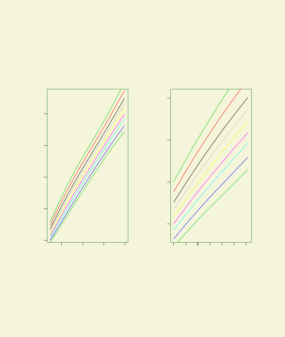
164 CHAPTER 8. CENTILES
+
+
+
+
+
+
+
+
+
+
++
+
+
+
+
+
+
++
++
+
+
+
+
+
+
++
+
+
+
+
+
+
+
+
+
+
+
+
+
+
+
+
+
+
+
+
+
+
+
+
+
+
+
+
+
+
+
+
+
+
+
+
+
+
+
+
+
+
+
+
+
+
+
+
+
+
+
+
+
+
+
+
+
+
+
++
+
+
+
+
+
++
+
+
+
+
+
+
+
+
+
+
+
+
+
+
+
++
+
+
+
+
+
+
+
+
+
+
+
+
+
+
+
+
+
+
+
+
+
+
+
+
+
+
+
++
+
+
+
+
+
+
+
+
+
+
+
+
+
+
+
+
+
+
+
+
+
+
+
+
+
+
+
+
+
+
+
+
+
+
+
+
+
+
+
+
+
+
+
+
+
+
+
+
+
+
+
+
+
++
+
+
+
+
+
+
+
+
+
+
+
+
+
+
+
++
+
+
+
+
+
+
+
+
+
+
++
+
+
+
+
+
+
+
+
+
+
+
+
+
+
+
+
+
+
+
+
+
+
+
+
+
+
+
+
+
+
+
+
+
+
+
+
+
+
+
+
+
+
+
+
+
+
+
+
+
+
+
+
+
+
++
+
+
+
+
+
+
+
+
+
+
+
+
+
+
++
+
+
+
+
+
+
+
+
+
+
+
+
+
+
+
+
+
+
+
+
+
+
+
+
+
+
+
+
+
+
+
+
+
+
+
+
+
+
+
+
+
+
+
+
+
+
+
+
+
+
+
+
+
+
+
+
+
+
+
+
+
+
+
+
15 20 25 30
50 100 150 200 250
x
y
Centile curves using BCT
+
+
+
+
+
+
+
+
+
+
+
+
+
+
+
+
+
+
++
+
+
+
+
+
+
+
+
+
+
+
+
+
+
+
+
+
+
+
+
+
+
+
+
+
+
+
+
+
+
+
+
+
+
+
++
+
+
+
+
+
+
+
+
+
+
+
+
+
+
+
+
+
+
+
++
+
+
+
+
+
+
+
+
+
+
+
+
+
+
+
+
+
+
+
+
+
+
+
+
+
+
+
+
+
+
+
+
+
+
+
+
+
+
+
+
+
+
+
+
+
+
+
+
+
+
+
+
++
+
+
+
+
+
+
+
+
+
+
+
+
+
+
+
+
+
+
+
+
+
+
+
+
++
+
+
+
+
+
+
+
+
+
+
+
+
+
+
+
+
+
+
+
+
+
+
+
+
+
+
+
+
+
+
+
+
+
+
+
+
+
+
+
+
+
+
+
+
+
+
+
+
+
+
+
+
+
+
+
+
+
+
+
+
+
+
+
+
+
+
+
+
+
+
+
+
+
+
+
+
+
+
+
+
+
+
+
+
+
+
+
30 32 34 36 38 40 42
250 300 350 400
x
y
Centile curves using BCT
Figure 8.6: Two centiles curves using Box-Cox t(BCT) distribution to the abdom data
8.2. PLOTTING CENTILES CURVES USING CENTILES() 165
plot whether to plot the centiles. This option is useful if the sample statistics only
are to be used
... for extra arguments in the par() plotting function
For example a four equal number of observation split (with no background color for the plot)
can be achieved using
centiles.split(abd9,abdom$x,bg="white")
12.22 to 20.07 20.07 to 27.07 27.07 to 34.5 34.5 to 42.5
0.4 0.000000 0.000000 0.6410256 0.6802721
2 2.597403 1.307190 2.5641026 3.4013605
10 9.090909 7.189542 10.8974359 7.4829932
25 24.675325 32.679739 23.7179487 25.8503401
50 48.051948 53.594771 49.3589744 50.3401361
75 74.025974 73.202614 73.7179487 75.5102041
90 88.311688 92.156863 87.8205128 91.8367347
98 98.051948 99.346405 97.4358974 97.9591837
99.6 100.000000 99.346405 99.3589744 100.0000000
<see figure 8.7 for the plot>
Note that for n.inter say more than 6 the centile curves are too small for any practical
use. Nevertheless sample centile statistics can be still obtained by suppressing the plot using
the argument plot=FALSE. For example in order to get sample statistics in 8 equal number of
observation splits use
> centiles.split(abd9,abdom$x,n.inter=8,plot=FALSE)
12.22 to 16.78 16.78 to 20.07 20.07 to 23.5 23.5 to 27.07 27.07 to 30.64
0.4 0.000000 0.000000 0.000000 0.000000 0.000000
2 2.531646 2.666667 1.315789 1.298701 2.702703
10 8.860759 9.333333 10.526316 3.896104 13.513514
25 29.113924 20.000000 34.210526 31.168831 27.027027
50 49.367089 46.666667 52.631579 54.545455 52.702703
75 75.949367 72.000000 68.421053 77.922078 75.675676
90 86.075949 90.666667 88.157895 96.103896 89.189189
98 98.734177 97.333333 100.000000 98.701299 98.648649
99.6 100.000000 100.000000 100.000000 98.701299 100.000000
30.64 to 34.5 34.5 to 38.36 38.36 to 42.5
0.4 1.219512 0.000000 1.315789
2 2.439024 4.225352 2.631579
10 8.536585 7.042254 7.894737
25 20.731707 22.535211 28.947368
50 46.341463 52.112676 48.684211
75 71.951220 76.056338 75.000000
90 86.585366 90.140845 93.421053
98 96.341463 98.591549 97.368421
99.6 98.780488 100.000000 100.000000
>
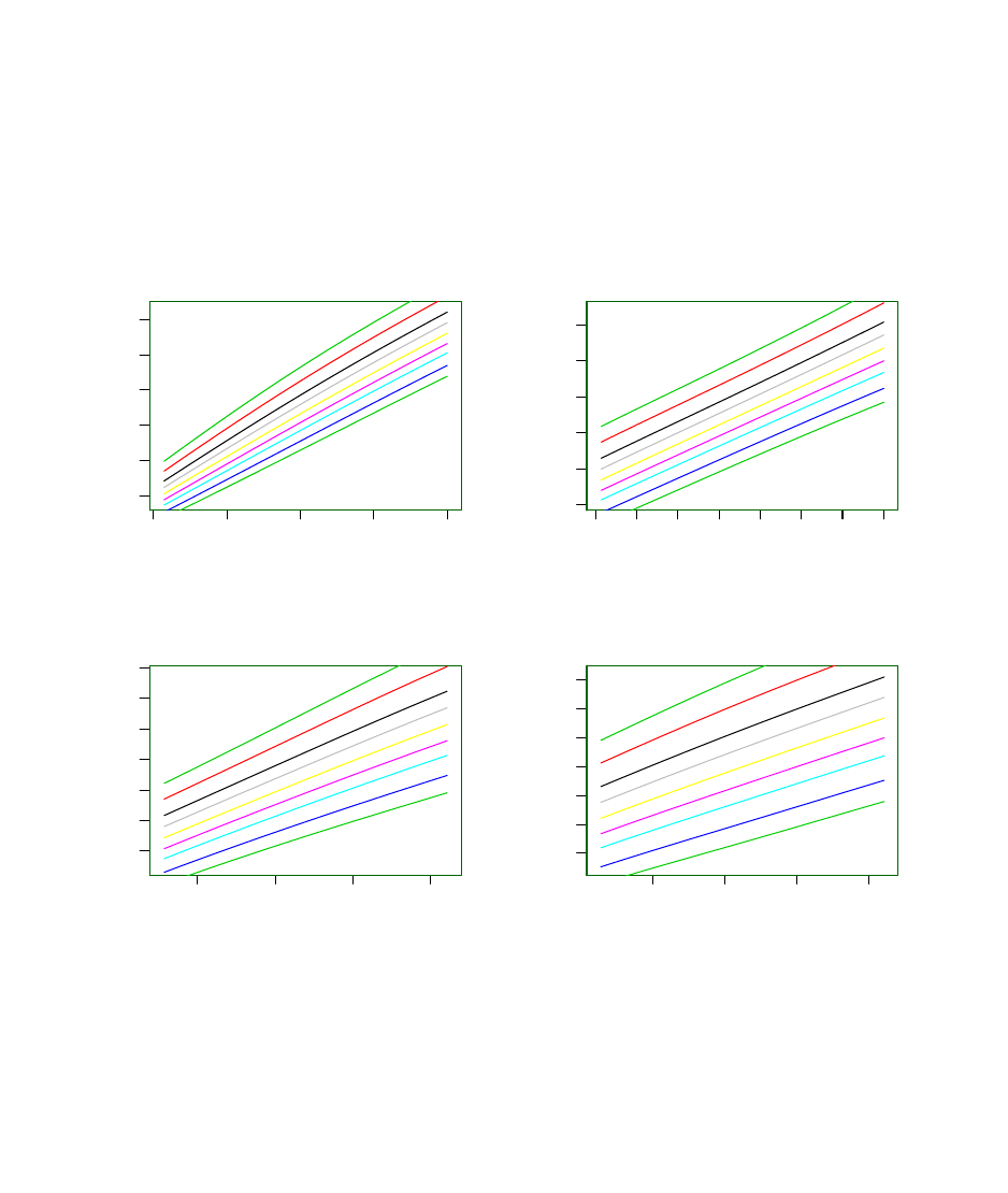
166 CHAPTER 8. CENTILES
+
+
+
+
+
+
+
+
+
+
++
+
+
+
+
+
+
++
++
+
+
+
+
+
+
+++
+
+
+
+
+
+
+
+
+
+
+
+
+
+
+
+
+
+
+
+
+
+
+
+
+
+
+
+
+
+
+
+
+
+
+
+
+
+
+
+
+
+
+
+
+
+
+
+
+
+
+
+
+
+
+
+
+
+
++
+
+
+
+
+
++
+
+
+
+
+
+
+
+
+
+
+
+
+
+
+
++
+
+
+
+
+
+
+
+
+
+
+
+
+
+
+
+
+
+
+
+
+
+
+
+
+
+
+
++
+
+
+
+
+
+
+
+
+
+
12 14 16 18 20
60 80 100 140
x
y
Centile curves using BCT
+
+
+
+
+
+
+
+
+
+
+
+
+
+
+
+
+
+
+
+
+
+
+
+
+
+
+
+
+
+
+
+
+
+
+
+
+
+
+
+
+
+
+
++
+
+
+
+
+
+
+
+
+
+
+
+
+
+
+
++
+
+
+
+
+
+
+
+
+
+
++
+
+
+
+
+
+
+
+
+
+
+
+
+
+
+
+
+
+
+
+
+
+
+
+
+
+
+
+
+
+
+
+
+
+
+
+
+
+
+
+
+
+
+
+
+
+
+
+
+
+
+
+
+
+
++
+
+
+
+
+
+
++
+
+
+
+
+
+
++
+
+
+
+
+
+
+
20 21 22 23 24 25 26 27
140 160 180 200 220 240
x
y
Centile curves using BCT
+
+
+
+
+
+
+
+
+
+
+
+
+
+
+
+
+
+
+
+
+
+
+
+
+
+
+
+
+
+
+
+
+
+
++
+
+
+
+
+
+
+
+
+
+
+
+
+
+
+
+
+
+
+
+
+
+
+
+
+
+
+
+
+
+
+
+
+
+
+
+
+
+
+++
+
+
+
+
+
+
+
+
+
+
+
+
+
+
+
+
+
+
+
+
+
+
+
+
+
+
+
+
+
+
+
+
+
+
+
++
+
+
+
+
+
+
+
+
+
+
+
+
+
+
+
+
+
+
+
++
+
+
+
+
+
+
++
+
+
+
+
+
+
+
+
+
+
+
+
+
28 30 32 34
220 260 300 340
x
y
Centile curves using BCT
+
+
+
+
++
+
+
+
+
+
+
+
+
+
+
+
+
+
+
+
+
+
+
+
+
+
+
+
+
+
++
+
+
+
+
+
+
+
+
+
+
+
+
+
+
+
+
+
+
+
+
+
+
+
+
++
+
+
+
+
+
+
+
+
+
+
+
+
+
+
+
+
+
+
+
+
+
+
+
+
+
+
+
+
+
+
+
+
+
+
+
+
+
+
+
+
+
+
+
+
+
+
+
+
+
+
+
+
+
+
+
+
+
+
+
+
+
+
+
+
+
+
+
+
+
+
+
+
+
+
+
+
+
+
+
+
+
+
+
+
+
+
+
+
36 38 40 42
280 320 360 400
x
y
Centile curves using BCT
Figure 8.7: Four centiles curves using Box-Cox t(BCT) distribution to the abdom data
8.2. PLOTTING CENTILES CURVES USING CENTILES() 167
8.2.3 The function centiles.com()
In order to compare the centile plot of more than one model use the function centiles.com().
The following example shows how centiles created by two different smoothing techniques, cubic
splines, cs() and loess, lo(), can be plotted in the same plot.
> data(abdom)
> h1<-gamlss(y~cs(x,df=3), sigma.formula=~cs(x,1), family=BCT, data=abdom)
GAMLSS-RS iteration 1: Global Deviance = 4776.174
GAMLSS-RS iteration 2: Global Deviance = 4775.895
GAMLSS-RS iteration 3: Global Deviance = 4775.876
GAMLSS-RS iteration 4: Global Deviance = 4775.876
> h2<-gamlss(y~lo(x,span=0.4), sigma.formula=~lo(x,span=0.4),
+ family=BCT, data=abdom )
GAMLSS-RS iteration 1: Global Deviance = 4773.475
GAMLSS-RS iteration 2: Global Deviance = 4773.18
GAMLSS-RS iteration 3: Global Deviance = 4773.149
GAMLSS-RS iteration 4: Global Deviance = 4773.146
GAMLSS-RS iteration 5: Global Deviance = 4773.146
> centiles.com(h1,h2,xvar=abdom$x)
******** Model 1 ********
% of cases below 0.4 centile is 0.6557377
% of cases below 10 centile is 8.688525
% of cases below 50 centile is 50.32787
% of cases below 90 centile is 88.68852
% of cases below 99.6 centile is 99.67213
******** Model 2 ********
% of cases below 0.4 centile is 0.3278689
% of cases below 10 centile is 8.688525
% of cases below 50 centile is 50.81967
% of cases below 90 centile is 89.34426
% of cases below 99.6 centile is 99.83607
>
<see the left side in figure 8.8 for the plot>
The arguments for the function centiles.com are
obj a fitted gamlss object
... optionally more fitted gamlss model objects
xvar the unique explanatory variable
cent a vector with elements the % centile values for which the centile curves are to
be evaluated
legend whether a legend is required in the plots or not, the default is legent=FALSE
ylab the y-variable label
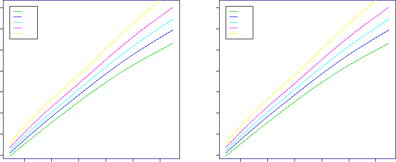
168 CHAPTER 8. CENTILES
+
+
+
+
+
+
+
+
+
+
++
+
+
+
+
+
+
++
++
+
+
+
+
+
+
++
+
+
+
+
+
+
+
+
+
+
+
+
+
+
+
+
+
+
+
+
+
+
+
+
+
+
+
+
+
+
+
+
+
+
+
+
+
+
+
+
+
+
+
+
+
+
+
+
+
+
+
+
+
+
+
+
+
+
+
++
+
+
+
+
+
++
+
+
+
+
+
+
+
+
+
+
+
+
+
+
+
++
+
+
+
+
+
+
+
+
+
+
+
+
+
+
+
+
+
+
+
+
+
+
+
+
+
+
+
++
+
+
+
+
+
+
+
+
+
+
+
+
+
+
+
+
+
+
+
+
+
+
+
+
+
+
+
+
+
+
+
+
+
+
+
+
+
+
+
+
+
+
+
+
+
+
+
+
+
+
+
+
+
++
+
+
+
+
+
+
+
+
+
+
+
+
+
+
+
++
+
+
+
+
+
+
+
+
+
+
++
+
+
+
+
+
+
+
+
+
+
+
+
+
+
+
+
+
+
+
+
+
+
+
+
+
+
+
+
+
+
+
+
+
+
+
+
+
+
+
+
+
+
+
+
+
+
+
+
+
+
+
+
+
+
++
+
+
+
+
+
+
+
+
+
+
+
+
+
+
++
+
+
+
+
+
+
+
+
+
+
+
+
+
+
+
+
+
+
+
+
+
+
+
+
+
+
+
+
+
+
+
+
+
+
+
+
+
+
+
+
+
++
+
+
+
+
+
+
+
+
+
+
+
+
+
+
+
+
+
+
+
+
+
+
+
+
+
+
+
+
+
+
+
+
+
+
+
+
+
+
+
++
+
+
+
+
+
+
+
+
+
+
+
+
+
+
+
+
+
+
+
+
+
+
+
+
+
+
+
+
+
+
+
+
+
+
+
++
+
+
+
+
+
+
+
+
+
+
+
+
+
+
+
+
+
+
+
++
+
+
+
+
+
+
+
+
+
+
+
+
+
+
+
+
+
+
+
+
+
+
+
+
+
+
+
+
+
+
+
+
+
+
+
+
+
+
+
+
+
+
+
+
+
+
+
+
+
+
+
+
++
+
+
+
+
+
+
+
+
+
+
+
+
+
+
+
+
+
+
+
+
+
+
+
+
++
+
+
+
+
+
+
+
+
+
+
+
+
+
+
+
+
+
+
+
+
+
+
+
+
+
+
+
+
+
+
+
+
+
+
+
+
+
+
+
+
+
+
+
+
+
+
+
+
+
+
+
+
+
+
+
+
+
+
+
+
+
+
+
+
+
+
+
+
+
+
+
+
+
+
+
+
+
+
+
+
+
+
+
+
+
+
+
+
15 20 25 30 35 40
50 100 150 200 250 300 350 400
x
y
Centile curves
0.4
10
50
90
99.6
0.4
10
50
90
99.6
0.4
10
50
90
99.6
0.4
10
50
90
99.6
0.4
10
50
90
99.6
0.4
10
50
90
99.6
0.4
10
50
90
99.6
0.4
10
50
90
99.6
0.4
10
50
90
99.6
0.4
10
50
90
99.6
15 20 25 30 35 40
50 100 150 200 250 300 350 400
x
y
Centile curves
0.4
10
50
90
99.6
0.4
10
50
90
99.6
0.4
10
50
90
99.6
0.4
10
50
90
99.6
0.4
10
50
90
99.6
0.4
10
50
90
99.6
0.4
10
50
90
99.6
0.4
10
50
90
99.6
0.4
10
50
90
99.6
0.4
10
50
90
99.6
Figure 8.8: Comparison of centiles curves created using cubic splines and loess
xlab the x-variable label
xleg position of the legend in the x-axis
yleg position of the legend in the y-axis
xlim the limits of the x-axis
ylim the limits of the y-axis
no.data whether the data should br plotted, default no.data=FALSE plots the data
while no.data=TRUE does not plot the data
color whether the fitted centiles are shown in colour, ’color=TRUE’ (the default)
or not ’color=FALSE’
plot whether to plot the centile curves, default plot=TRUE, or not plot=FALSE.
The argument no.data is useful for excluding the data from the plot.
> centiles.com(h1,h2,xvar=abdom$x, no.data=TRUE)
******** Model 1 ********
% of cases below 0.4 centile is 0.6557377
% of cases below 10 centile is 8.688525
% of cases below 50 centile is 50.32787
% of cases below 90 centile is 88.68852
% of cases below 99.6 centile is 99.67213
******** Model 2 ********
% of cases below 0.4 centile is 0.3278689
% of cases below 10 centile is 8.688525
% of cases below 50 centile is 50.81967
8.2. PLOTTING CENTILES CURVES USING CENTILES() 169
% of cases below 90 centile is 89.34426
% of cases below 99.6 centile is 99.83607
<see the right side in figure 8.8 for the plot>
8.2.4 The function centiles.pred()
The centiles.pred() is designed to create predictive centiles curves for new x-values, given a
gamlss fitted model. The function has three options:
i) for given new x-values and given percentage centiles calculates a matrix con-
taining the centiles values for y,
ii) for given new x-values and standard normalized centile values calculates a
matrix containing the centiles values for y,
iii) for given new x-values and new y-values calculates the z-scores.
Let take us the three cases in turn. To demonstrate the first case we start by fitting a
model to the (abdom) data and plotting its fitted centiles. Then, we create new values for x,
newx<-seq(12,40,2) and use them to find prediction centiles which are stored in a matrix mat.
The centiles are created at the default values of c(0.4, 2, 10, 25, 50, 75, 90, 98, 99.6).
These prediction centiles then can be plotted using the centiles.pred argument plot=TRUE.
> data(abdom)
> a<-gamlss(y~cs(x),sigma.fo=~cs(x), data=abdom, family=BCT)
GAMLSS-RS iteration 1: Global Deviance = 4772.531
GAMLSS-RS iteration 2: Global Deviance = 4772.445
GAMLSS-RS iteration 3: Global Deviance = 4772.429
GAMLSS-RS iteration 4: Global Deviance = 4772.423
GAMLSS-RS iteration 5: Global Deviance = 4772.422
GAMLSS-RS iteration 6: Global Deviance = 4772.422
> #plot the centiles
> centiles(a,xvar=abdom$x)
% of cases below 0.4 centile is 0.3278689
% of cases below 2 centile is 2.459016
% of cases below 10 centile is 8.688525
% of cases below 25 centile is 26.72131
% of cases below 50 centile is 50.32787
% of cases below 75 centile is 74.09836
% of cases below 90 centile is 90
% of cases below 98 centile is 98.19672
% of cases below 99.6 centile is 99.67213
> # calculate the centiles at new x values
> newx<-seq(12,40,2)
> mat <- centiles.pred(a, xname="x", xvalues=newx )
> mat
x C0.4 C2 C10 C25 C50 C75 C90
1 12 44.32712 47.53252 51.34103 54.21895 57.45386 60.90707 64.39590
170 CHAPTER 8. CENTILES
2 14 64.82615 69.10822 74.16073 77.95493 82.19681 86.69959 91.22369
3 16 85.80227 90.94380 96.96902 101.46596 106.46692 111.74631 117.02199
4 18 106.90560 112.65921 119.35570 124.32305 129.81801 135.58715 141.32117
5 20 127.75527 133.93173 141.07618 146.34660 152.14918 158.21134 164.20746
6 22 148.08126 154.60111 162.10601 167.61818 173.66415 179.95607 186.15572
7 24 168.12073 175.00558 182.90302 188.68540 195.01077 201.57521 208.02580
8 26 187.58931 194.98697 203.45802 209.65083 216.41621 223.42770 230.30833
9 28 206.01103 214.15915 223.49079 230.31354 237.76788 245.49419 253.07708
10 30 223.17621 232.26930 242.69729 250.33089 258.67980 267.34264 275.85365
11 32 239.35480 249.50728 261.17230 269.72595 279.09479 288.83057 298.40989
12 34 254.84078 266.03010 278.90819 288.36566 298.73791 309.53091 320.16449
13 36 269.69902 281.85532 295.86485 306.16542 317.47378 329.25326 340.87072
14 38 283.90699 296.99350 312.09247 323.20555 335.41677 348.14842 360.71631
15 40 298.22002 312.08705 328.09392 339.88005 352.83540 366.34781 379.69122
C98 C99.6
1 69.76056 75.10617
2 98.13402 104.96782
3 125.02793 132.88680
4 149.96646 158.39075
5 173.19566 181.89668
6 195.40663 204.31574
7 217.61987 226.82550
8 240.52564 250.31152
9 264.33860 275.12609
10 288.50947 300.64986
11 312.67947 326.39532
12 336.02950 351.30612
13 358.22508 374.95917
14 379.51072 397.65558
15 399.65391 418.93603
> # plot the centiles
> mat <- centiles.pred(a, xname="x",xvalues=newx, plot=TRUE )
<see the left side in figure 8.9 for the plot>
In the second case the objective is to create centiles based not on percentages but on standard
normalized values or Z value. These are using the centiles.pred argument dev with default
Z values dev=c(-4, -3, -2, -1, 0, 1, 2, 3, 4). [Note that the corresponding centile per-
centages for the standard normalized values can be obtained by applying Φ−1() = qNO(), the
inverse cumulative distribution function of a standard normal distribution, i.e % = Φ−1(z)].
We use the same new xvalues as above by this time we use the argument type="standard-
centiles".
> mat <- centiles.pred(a, xname="x",xvalues=newx, type="standard-centiles" )
> mat
x -4 -3 -2 -1 0 1 2
1 12 35.65419 42.31050 47.80738 52.68015 57.45386 62.71870 69.34049
2 14 53.08735 62.11735 69.47411 75.92867 82.19681 89.05186 97.59486
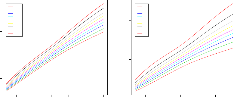
8.2. PLOTTING CENTILES CURVES USING CENTILES() 171
15 20 25 30 35 40
100 200 300 400
X
mat[, 2]
0.4
2
10
25
50
75
90
98
99.6
15 20 25 30 35 40
100 200 300 400 500
X
mat[, 2]
−4
−3
−2
−1
0
1
2
3
4
Figure 8.9: A plot of prediction centiles curves: on the left using selected % centiles, on the
right using selected standard normalized deviates (i.e. Z values).
3 16 71.52359 82.53218 91.38161 99.06728 106.46692 114.49285 124.40548
4 18 90.71768 103.22636 113.14743 121.67662 129.81801 138.57609 149.29664
5 20 110.17159 123.78631 134.45419 143.54172 152.14918 161.34045 172.50145
6 22 129.34527 143.87541 155.15124 164.68714 173.66415 183.19428 194.69389
7 24 148.20244 163.66711 175.58548 185.61255 195.01077 204.94663 216.88199
8 26 166.11621 182.79744 195.60951 206.36085 216.41621 227.02501 239.74051
9 28 182.36560 200.73358 214.84489 226.68882 237.76788 249.45856 263.47317
10 30 196.85739 217.29304 233.03510 246.27443 258.67980 271.79114 287.53623
11 32 210.07697 232.79610 250.36312 265.17908 279.09479 293.83572 311.58108
12 34 222.67767 247.62194 266.97416 283.33686 298.73791 315.08520 334.80726
13 36 234.84493 261.86452 282.88167 300.68706 317.47378 335.32000 356.88721
14 38 246.46897 275.48070 298.09903 317.29387 335.41677 354.71009 378.06099
15 40 258.58391 289.29439 313.25880 333.60983 352.83540 373.31380 398.11371
3 4
1 78.95471 95.37367
2 109.85771 130.46482
3 138.47662 161.75422
4 164.34732 188.86203
5 188.01639 212.94037
6 210.55575 235.76220
7 233.25412 259.07197
8 257.13538 284.46243
9 282.64924 312.78327
10 309.12623 343.15469
11 335.98709 374.61496
12 362.00473 405.21168
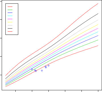
172 CHAPTER 8. CENTILES
13 386.69168 434.17889
14 410.38974 462.03101
15 432.47361 487.41529
> #to plot the centiles
> mat <- centiles.pred(a, xname="x",xvalues=newx, type="s", plot = TRUE )
<see the right side in figure 8.9 for the plot>
In the third case the objective is, for given xand yvalues, to find the corresponding z-
scores for the y values given the x values. In the example below we create new values for x
and y, we find the z-scores and then we plot them into the original centile plot.
> nx <- c(20,21.2,23,20.9,24.2,24.1,25)
> ny <- c(130,121,123,125,140,145,150)
> nz <- centiles.pred(a, xname="x",xvalues=nx,yval=ny, type="z-scores" )
> nz
[1] -2.442657 -4.042038 -4.802512 -3.594058 -4.511235 -4.221110 -4.369420
> mat <- centiles.pred(a, xname="x",xvalues=newx, type="s", plot = TRUE )
> for(i in 1:7) points(nx[i],ny[i],col="blue")
15 20 25 30 35 40
100 200 300 400 500
X
mat[, 2]
−4
−3
−2
−1
0
1
2
3
4
Figure 8.10: A plot of z-scores
<see figure 8.10 for the plot>
The arguments for the function centiles.pred are
obj a fitted gamlss object
type the default, centiles, gets the centiles values given in the option cent.
type="standard-centiles" gets the standard centiles given in the dev.
type="z-scores" gets the z-scores for given y and x new values
8.2. PLOTTING CENTILES CURVES USING CENTILES() 173
xname the name of the unique explanatory variable (it has to be the same as in the
original fitted model)
xvalues the new values for the explanatory variable where the prediction will take
place
power if power transformation is needed
yval the response values for a given x values required for the calculation of z-
scores
cent a vector with elements the % centile values for which the centile curves have
to be evaluated
dev a vector with elements the standard normalized deviate values (or Z values) for
which the centile curves have to be evaluated in the option type="standard-
centiles"
plot whether to plot the ”centiles”or the ”standard-centiles”, the default is plot=FALSE
legend whether a legend is required in the plot or not, the default is legend=TRUE
... for extra arguments
centiles.pred() can be used even when the x-variable is transformed. The transformation
could be done before or in the actual model fitting. In the first case (which is recommended for
large data sets) the argument power of the function can be used. No correction is needed in the
second case as we now demonstrate. We first fit a model by using the square root of x, x^0.5,
then get the centiles at x=30 and plot them on the original centile plot.
> aa<-gamlss(y~cs(x^0.5),sigma.fo=~cs(x^0.5), data=abdom, family=BCT)
GAMLSS-RS iteration 1: Global Deviance = 4771.563
GAMLSS-RS iteration 2: Global Deviance = 4770.55
GAMLSS-RS iteration 3: Global Deviance = 4770.524
GAMLSS-RS iteration 4: Global Deviance = 4770.519
GAMLSS-RS iteration 5: Global Deviance = 4770.519
> centiles(aa,xvar=abdom$x)
% of cases below 0.4 centile is 0.3278689
% of cases below 2 centile is 2.459016
% of cases below 10 centile is 8.52459
% of cases below 25 centile is 26.22951
% of cases below 50 centile is 50.16393
% of cases below 75 centile is 74.09836
% of cases below 90 centile is 90.32787
% of cases below 98 centile is 98.03279
% of cases below 99.6 centile is 99.67213
> mat <- centiles.pred(aa, xname="x",xvalues=c(30) )
> xx<-rep(mat[,1],9)
> yy<-mat[,2:10]
> points(xx,yy,col="red")
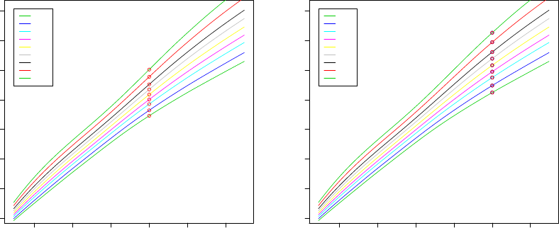
174 CHAPTER 8. CENTILES
+
+
+
+
+
+
+
+
+
+
++
+
+
+
+
+
+
++
++
+
+
+
+
+
+
++
+
+
+
+
+
+
+
+
+
+
+
+
+
+
+
+
+
+
+
+
+
+
+
+
+
+
+
+
+
+
+
+
+
+
+
+
+
+
+
+
+
+
+
+
+
+
+
+
+
+
+
+
+
+
+
+
+
+
+
++
+
+
+
+
+
++
+
+
+
+
+
+
+
+
+
+
+
+
+
+
+
++
+
+
+
+
+
+
+
+
+
+
+
+
+
+
+
+
+
+
+
+
+
+
+
+
+
+
+
++
+
+
+
+
+
+
+
+
+
+
+
+
+
+
+
+
+
+
+
+
+
+
+
+
+
+
+
+
+
+
+
+
+
+
+
+
+
+
+
+
+
+
+
+
+
+
+
+
+
+
+
+
+
++
+
+
+
+
+
+
+
+
+
+
+
+
+
+
+
++
+
+
+
+
+
+
+
+
+
+
++
+
+
+
+
+
+
+
+
+
+
+
+
+
+
+
+
+
+
+
+
+
+
+
+
+
+
+
+
+
+
+
+
+
+
+
+
+
+
+
+
+
+
+
+
+
+
+
+
+
+
+
+
+
+
++
+
+
+
+
+
+
+
+
+
+
+
+
+
+
++
+
+
+
+
+
+
+
+
+
+
+
+
+
+
+
+
+
+
+
+
+
+
+
+
+
+
+
+
+
+
+
+
+
+
+
+
+
+
+
+
+
++
+
+
+
+
+
+
+
+
+
+
+
+
+
+
+
+
+
+
+
+
+
+
+
+
+
+
+
+
+
+
+
+
+
+
+
+
+
+
+
++
+
+
+
+
+
+
+
+
+
+
+
+
+
+
+
+
+
+
+
+
+
+
+
+
+
+
+
+
+
+
+
+
+
+
+
++
+
+
+
+
+
+
+
+
+
+
+
+
+
+
+
+
+
+
+
++
+
+
+
+
+
+
+
+
+
+
+
+
+
+
+
+
+
+
+
+
+
+
+
+
+
+
+
+
+
+
+
+
+
+
+
+
+
+
+
+
+
+
+
+
+
+
+
+
+
+
+
+
++
+
+
+
+
+
+
+
+
+
+
+
+
+
+
+
+
+
+
+
+
+
+
+
+
++
+
+
+
+
+
+
+
+
+
+
+
+
+
+
+
+
+
+
+
+
+
+
+
+
+
+
+
+
+
+
+
+
+
+
+
+
+
+
+
+
+
+
+
+
+
+
+
+
+
+
+
+
+
+
+
+
+
+
+
+
+
+
+
+
+
+
+
+
+
+
+
+
+
+
+
+
+
+
+
+
+
+
+
+
+
+
+
+
15 20 25 30 35 40
50 100 150 200 250 300 350 400
x
y
Centile curves using BCT
0.4
2
10
25
50
75
90
98
99.6
0.4
2
10
25
50
75
90
98
99.6
0.4
2
10
25
50
75
90
98
99.6
0.4
2
10
25
50
75
90
98
99.6
0.4
2
10
25
50
75
90
98
99.6
0.4
2
10
25
50
75
90
98
99.6
0.4
2
10
25
50
75
90
98
99.6
0.4
2
10
25
50
75
90
98
99.6
0.4
2
10
25
50
75
90
98
99.6
+
+
+
+
+
+
+
+
+
+
++
+
+
+
+
+
+
++
++
+
+
+
+
+
+
++
+
+
+
+
+
+
+
+
+
+
+
+
+
+
+
+
+
+
+
+
+
+
+
+
+
+
+
+
+
+
+
+
+
+
+
+
+
+
+
+
+
+
+
+
+
+
+
+
+
+
+
+
+
+
+
+
+
+
+
++
+
+
+
+
+
++
+
+
+
+
+
+
+
+
+
+
+
+
+
+
+
++
+
+
+
+
+
+
+
+
+
+
+
+
+
+
+
+
+
+
+
+
+
+
+
+
+
+
+
++
+
+
+
+
+
+
+
+
+
+
+
+
+
+
+
+
+
+
+
+
+
+
+
+
+
+
+
+
+
+
+
+
+
+
+
+
+
+
+
+
+
+
+
+
+
+
+
+
+
+
+
+
+
++
+
+
+
+
+
+
+
+
+
+
+
+
+
+
+
++
+
+
+
+
+
+
+
+
+
+
++
+
+
+
+
+
+
+
+
+
+
+
+
+
+
+
+
+
+
+
+
+
+
+
+
+
+
+
+
+
+
+
+
+
+
+
+
+
+
+
+
+
+
+
+
+
+
+
+
+
+
+
+
+
+
++
+
+
+
+
+
+
+
+
+
+
+
+
+
+
++
+
+
+
+
+
+
+
+
+
+
+
+
+
+
+
+
+
+
+
+
+
+
+
+
+
+
+
+
+
+
+
+
+
+
+
+
+
+
+
+
+
++
+
+
+
+
+
+
+
+
+
+
+
+
+
+
+
+
+
+
+
+
+
+
+
+
+
+
+
+
+
+
+
+
+
+
+
+
+
+
+
++
+
+
+
+
+
+
+
+
+
+
+
+
+
+
+
+
+
+
+
+
+
+
+
+
+
+
+
+
+
+
+
+
+
+
+
++
+
+
+
+
+
+
+
+
+
+
+
+
+
+
+
+
+
+
+
++
+
+
+
+
+
+
+
+
+
+
+
+
+
+
+
+
+
+
+
+
+
+
+
+
+
+
+
+
+
+
+
+
+
+
+
+
+
+
+
+
+
+
+
+
+
+
+
+
+
+
+
+
++
+
+
+
+
+
+
+
+
+
+
+
+
+
+
+
+
+
+
+
+
+
+
+
+
++
+
+
+
+
+
+
+
+
+
+
+
+
+
+
+
+
+
+
+
+
+
+
+
+
+
+
+
+
+
+
+
+
+
+
+
+
+
+
+
+
+
+
+
+
+
+
+
+
+
+
+
+
+
+
+
+
+
+
+
+
+
+
+
+
+
+
+
+
+
+
+
+
+
+
+
+
+
+
+
+
+
+
+
+
+
+
+
+
15 20 25 30 35 40
50 100 150 200 250 300 350 400
x
y
Centile curves using BCT
0.4
2
10
25
50
75
90
98
99.6
0.4
2
10
25
50
75
90
98
99.6
0.4
2
10
25
50
75
90
98
99.6
0.4
2
10
25
50
75
90
98
99.6
0.4
2
10
25
50
75
90
98
99.6
0.4
2
10
25
50
75
90
98
99.6
0.4
2
10
25
50
75
90
98
99.6
0.4
2
10
25
50
75
90
98
99.6
0.4
2
10
25
50
75
90
98
99.6
Figure 8.11: Plotting centiles when x-variable is transformed: in the left panel the x is trans-
formed in the fitting while in the right before the fitting
As we can see from the plot in the left side of figure 8.11,centiles.pred() produce the
correct centiles lying on the proper centile curves. We now demonstrate the use of the power
argument. Here we first transform the x variable and then fit the model. Then we create a new
data frame containing the new transformed variable. This is a trick to be able to identify the
correct transformed variable name. Then we use centiles.pred() with argument power and
data.
> nx<-abdom$x^0.5
> aa<-gamlss(y~cs(nx),sigma.fo=~cs(nx), data=abdom, family=BCT)
GAMLSS-RS iteration 1: Global Deviance = 4771.563
GAMLSS-RS iteration 2: Global Deviance = 4770.55
GAMLSS-RS iteration 3: Global Deviance = 4770.524
GAMLSS-RS iteration 4: Global Deviance = 4770.519
GAMLSS-RS iteration 5: Global Deviance = 4770.519
> centiles(aa, xvar=abdom$x)
% of cases below 0.4 centile is 0.3278689
% of cases below 2 centile is 2.459016
% of cases below 10 centile is 8.52459
% of cases below 25 centile is 26.22951
% of cases below 50 centile is 50.16393
% of cases below 75 centile is 74.09836
% of cases below 90 centile is 90.32787
% of cases below 98 centile is 98.03279
% of cases below 99.6 centile is 99.67213
> newd<-data.frame( abdom, nx=abdom$x^0.5)
> mat <- centiles.pred(aa, xname="nx", xvalues=c(35), power=0.5, data=newd)
> xxx<-rep(mat[,1],9)
8.2. PLOTTING CENTILES CURVES USING CENTILES() 175
> yyy<-mat[,2:10]
> points(xxx,yyy,col="red")
176 CHAPTER 8. CENTILES
Chapter 9
Examples
9.1 The abdominal circumference data
The data are measurements of abdominal circumference (y), taken from 663 fetuses during
ultrasound scans at Kings College Hospital, London, at gestational ages (x) ranging between
12 and 42 weeks. The data were used to derive reference centile intervals for yby Chitty et al.
(1994) and also for comparing different reference centile methods by Wright and Royston (1997),
who were unable to find a satisfactory distribution for yand commented that the distribution
of residual Z-scores obtained from the different fitted models ’has somewhat longer tails than
the normal distribution’.
Initial model fitting using a normal distribution indicated that a cubic smoothing spline in x,
cs(x, 4), with 4 extra effective degrees of freedom on top of the constant term (denoted by 1), was
adequate for each of the location and log scale parameters. Hence, to determine an appropriate
distribution for these data, different distributions were fitted to the data with the location and
log scale parameters modelled using model {µ=1+cs(x,4),log(σ) = 1+cs(x,4)}, and any
shape parameters modelled as constants.
Table 9.1 shows the GD, AIC and SBC for the resulting fitted models using different distri-
butions. The logistic (LO) distribution is selected if the SBC is used as a selection criterion, and
the Box-Cox tdistribution (BCT) if the AIC is used. Having identified the need for a kurtotic
distribution we can now try to fine tune, i.e. simplify, the mean and the dispersion models.
Table 9.2 shows the SBC Table for the logistic model (LO) classified according to different
total effective degrees of freedom (on top of the constant term) for the location, (2,3,4,5,6),
and for the scale, (0,1,2,3,4), models. Corresponding Tables were obtained for each of the
other distributions in Table 9.1. The overall ’best’ model using the SBC criterion is LO{µ=
1+cs(x,3),log(σ) = 1+x}with SBC=4825.2. This was the chosen model. The AIC criterion
lead to the same model except for µ=1+cs(x,5).] Note that for the LO distribution, the
location parameter µis the mean of the distribution.
Fig. 9.1 displays the data and the fitted location parameter µfor the chosen model, together
with 2.5% and 97.5% reference centile estimates for y. For a given age x, the 100αreference
centile estimate for yis ˆ
Cα= ˆµ+zαˆσwhere zα=F−1(α) = log [α/(1 −α)], where F(z) is
the cumulative distribution function of a standard logistic distribution and ˆµand ˆσare the
fitted values of the location and scale parameters for yat x. Approximate confidence interval
bands for the centiles can also be obtained, using the empirical Bayes argument in Rigby and
Stasinopoulos (2000).
177

178 CHAPTER 9. EXAMPLES
Table 9.1: Models for the abdominal circumference data
Distributions GD AIC SBC
Normal 4784.7 4804.7 4848.9
Gamma 4780.1 4800.1 4844.2
Inv. Gaussian 4779.4 4799.4 4843.5
Gumbel 4948.2 4968.2 5012.3
Reverse Gumbel 4856.7 4876.7 4920.9
Logistic 4778.8 4798.8 4842.9
Cole and Green 4779.5 4801.5 4850.1
Power Exp. 4779.1 4801.1 4849.6
tfamily 4776.545 4798.5 4847.1
Box-Cox t4772.42 4796.43 4849.39
Box-Cox Power Exp. 4774.75 4798.76 4851.73
Table 9.2: Abdominal circumference data: SBC for the logistic distribution
dispersion
Mean
df 2 3 4 5 6
0 4925.2 4921.3 4923.6 4927.6 4932.3
1 4829.8 4825.2 4826.5 4830.2 4835.2
2 4835.5 4831.1 4832.4 4836.1 4841.0
3 4841.4 4836.6 4837.7 4841.4 4846.2
4 4847.1 4842.0 4842.9 4846.5 4851.3
A plot of the (normalized quantile) residuals (see Chapter 6) for the chosen model is shown
in Fig. 9.1. Panels (a) and (b) plot them against the fitted values and against the case number
respectively, while panels (c) and (d) provide a kernel density estimate and QQ plot for them
respectively. The quantile residuals appear random but the QQ plot indicates that the lower
tail of the distribution of the response variable is slightly shorter than the logistic. Nevertheless
it provides a reasonable fit to the data.
To validate the model, the data were randomly spit into training (60%) and validation
(40%) data sets. Minimizing the GD for the training data was used for model fitting, while
minimizing the GD for the validation data (i.e. VGD) was used for selecting the distribution
and the combination of degrees of freedom for the location and scale models. The best choice
of model using the VGD criterion was LO{µ=1+cs(x,2),log(σ) = 1+x}, which is close to
the chosen model from the SBC using all the data.
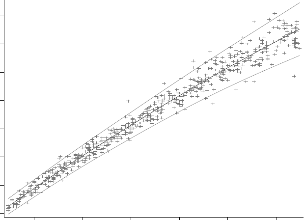
9.1. THE ABDOMINAL CIRCUMFERENCE DATA 179
15 20 25 30 35 40
50
100
150
200
250
300
350
400
Abdominal Circumference data
length of gestation (weeks)
Abdominal Circumference (mm)
Figure 9.1: The abdominal circumference data with the fitted location (µ) curve and 2.5% and
97.5% reference centile curves from the chosen LO model
180 CHAPTER 9. EXAMPLES

Appendix A
Distributions in the gamlss
packages
The distributions in Tables 4.1 and 4.2 can be divided into three categories depending on the
type of response variable:
continuous type
binomial type (with binary as special case)
counts or discrete type
Sections A.1, A.2 and A.3 cover the distributions available in gamlss packages of each of the
three types above respectively. In each case the specific parameterization(s) used by gamlss
for each of the distributions is given. For each parameterization of each distribution listed
below, functions for the probability density function (pdf), cumulative distribution function
(cdf), inverse cdf (i.e. quantile) function and random number generation are given by putting
each of the letters d,p,qand rrespectively before the gamlss.family name for the particular
distribution parameterization. For example, for the parameterization of the normal distribution
given by (A.1) below, denoted by NO(µ,σ), the corresponding gamlss.family functions dNO,
pNO, qNO and rNO define its pdf, cdf, inverse cdf and random number generation respectively.
A.1 Continuous two parameter distributions on ℜ
A.1.1 Normal (or Gausian) distribution (NO, NO2, NOF)
First parameterization (NO)
The normal distribution is the default of the argument family of the function gamlss(). The
parameterization used for the normal (or Gaussian) probability density function (pdf), denoted
by NO(µ,σ), is
fY(y|µ, σ) = 1
√2πσ exp "−(y−µ)2
2σ2#(A.1)
for −∞ < y < ∞, where −∞ < µ < ∞and σ > 0. The mean of Yis given by E(Y) = µand
the variance of Yby V ar(Y) = σ2, so µis the mean and σis the standard deviation of Y.
181

182 APPENDIX A. DISTRIBUTIONS IN THE GAMLSS PACKAGES
Second parameterization (NO2)
NO2(µ,σ) is a parameterization of the normal distribution where µrepresents the mean and σ
represents the variance of Y, i.e. fY(y|µ, σ) = (1/√2πσ) exp[−(y−µ)2/(2σ)].
Normal family (of variance-mean relationships) (NOF)
The function NOF(µ,σ,ν) defines a normal distribution family with three parameters. The
third parameter νallows the variance of the distribution to be proportional to a power of the
mean. The mean of NOF(µ,σ,ν) is equal to µwhile the variance is equal to V ar(Y) = σ2|µ|ν,
so the standard deviation is σ|µ|ν/2. The parametrization of the normal distribution given in
the function NOF(µ,σ,ν) is
f(y|µ, σ, ν) = 1
√2πσ|µ|ν/2exp −(y−µ)2
2σ2|µ|ν(A.2)
for −∞ < y < ∞, where −∞ < µ < ∞,σ > 0 and −∞ < ν < ∞.
The function NOF(µ,σ,ν) is appropriate for normally distributed regression type models
where the variance of the response variable is proportional to a power of the mean. Models of
this type are related to the ”pseudo likelihood” models of Carroll and Rubert (1987) but here a
proper likelihood is maximized. The νparameter here is not designed to be modelled against
explanatory variables but is a constant used as a device allowing us to model the variance
mean relationship. Note that, due to the high correlation between the σand νparameters, the
mixed() method argument is essential in the gamlss() fitting function. Alternatively νcan be
estimated from its profile function, obtained using gamlss package function prof.dev().
A.1.2 Logistic distribution (LO)
The logistic distribution is appropriate for moderately kurtotic data. The parameterization of
the logistic distribution, denoted here as LO(µ,σ), is given by
fY(y|µ, σ) = 1
σexp −y−µ
σ 1 + exp −y−µ
σ−2
(A.3)
for −∞ < y < ∞, where −∞ < µ < ∞and σ > 0, with E(Y) = µand V ar(Y) = π2σ2/3,
Johnson et al. (1995) p 116.
A.1.3 Gumbel distribution (GU)
The Gumbel distribution is appropriate for moderately negative skew data. The pdf of the
Gumbel distribution (or extreme value or Gompertz), denoted by GU(µ,σ), is defined by
fY(y|µ, σ) = 1
σexp y−µ
σ−exp y−µ
σ (A.4)
for −∞ < y < ∞, where −∞ < µ < ∞and σ > 0, with E(Y) = µ−γσ ≃µ−0.57722σand
V ar(Y) = π2σ2/6≃1.64493σ2. See Crowder et al. (1991) p 17.

A.2. CONTINUOUS THREE PARAMETER DISTRIBUTIONS ON ℜ183
A.1.4 Reverse Gumbel distribution (RG)
The reverse Gumbel distribution, which is also called is the type I extreme value distri-
bution is a special case of the generalized extreme value distribution, [see Johnson et al. (1995)
p 2 and p 75]. The reverse Gumbel distribution is appropriate for moderately positive skew
data. The pdf of the reverse Gumbel distribution, denoted by RG(µ,σ) is defined by
fY(y|µ, σ) = 1
σexp −y−µ
σ−exp −(y−µ)
σ (A.5)
for −∞ < y < ∞, where −∞ < µ < ∞and σ > 0, with E(Y) = µ+γσ ≃µ+ 0.57722σ
and V ar(Y) = π2σ2/6≃1.64493σ2. [Note that if Y∼RG(µ, σ) and W=−Y, then W∼
GU(−µ, σ).]
A.2 Continuous three parameter distributions on ℜ
A.2.1 Exponential Gaussian distribution (exGAUS)
The pdf of the ex-Gaussian distribution, denoted by exGAUS(µ,σ), is defined as
fY(y|µ, σ, ν) = 1
νexp µ−y
ν+σ2
2ν2Φy−µ
σ−σ
ν(A.6)
for −∞ < y < ∞, where −∞ < µ < ∞,σ > 0 and ν > 0, and where Φ is the cdf of the standard
normal distribution. Since Y=Y1+Y2where Y1∼N(µ, σ2) and Y2∼EX(ν) are independent,
the mean of Yis given by E(Y) = µ+νand the variance is given by V ar(Y) = σ2+ν2. This
distribution has also been called the lagged normal distribution, Johnson et al., (1994), p172.
A.2.2 Power Exponential distribution (PE, PE2)
First parameterization (PE)
The power exponential distribution is suitable for leptokurtic as well as platykurtic data. The
pdf of the power exponential family distribution, denoted by PE(µ,σ,ν), is defined by
fY(y|µ, σ, ν) = νexp[−z
c
ν]
2cσΓ1
ν(A.7)
for −∞ < y < ∞, where −∞ < µ < ∞,σ > 0 and ν > 0 and where z= (y−µ)/σ and
c2= Γ(1/ν)[Γ(3/ν)]−1.
In this parameterization, used by Nelson (1991), E(Y) = µand V ar(Y) = σ2. Note that
ν= 1 and ν= 2 correspond to the Laplace (i.e. two sided exponential) and normal distributions
respectively, while the uniform distribution is the limiting distribution as ν→ ∞.
The cdf of Yis given by FY(y) = 1
2[1 + FS(s)sign(z)] where S=|z/c|νhas a gamma
distribution with pdf fS(s) = s1/ν exp(−s)/Γ1
ν.
Second parameterization (PE2)
An alternative parameterization, the power exponential type 2 distribution, denoted by PE2(µ,σ,ν),
is defined by
fY(y|µ, σ, ν) = νexp[−|z|ν]
2σΓ1
ν(A.8)

184 APPENDIX A. DISTRIBUTIONS IN THE GAMLSS PACKAGES
for −∞ < y < ∞, where −∞ < µ < ∞,σ > 0 and ν > 0 and where z= (y−µ)/σ. Here
E(Y) = µand V ar(Y) = σ2/c2, where c2= Γ(1/ν)[Γ(3/ν)]−1.
See also Johnson et al., 1995, volume 2, p195, equation (24.83) for a re-parameterized version
by Subbotin (1923).
A.2.3 tfamily distribution (TF)
The tfamily distribution is suitable for modelling leptokurtic data, that is, data with higher
kurtosis than the normal distribution. The pdf of the tfamily distribution, denoted here as
TF(µ,σ,ν), is defined by
fY(y|µ, σ, ν) = 1
σB 1
2,ν
2ν1
21 + (y−µ)2
σ2ν−ν+1
2
(A.9)
for −∞ < y < ∞, where −∞ < µ < ∞,σ > 0 and ν > 0, where B(a, b) = Γ(a)Γ(b)/Γ(a+b)
is the beta function. The mean and variance of Yare given by E(Y) = µand V ar(Y) =
σ2ν/(ν−2) when ν > 2. Note that T= (Y−µ)/σ has a standard tdistribution with νdegrees
of freedom, given by Johnson et al. (1995), p 363, equation (28.2).
A.3 Continuous four parameter distributions on ℜ
A.3.1 Exponential Generalized Beta type 2 distribution (EGB2)
The pdf of the exponential generalized beta type 2 distribution, denoted by EGB2(µ, σ, ν, τ),
is defined by
fY(y|µ, σ, ν, τ) = eνz{|σ|B(ν, τ ) [1 + ez]ν+τ}−1(A.10)
for −∞ < y < ∞, where −∞ < µ < ∞,−∞ < σ < ∞,ν > 0 and τ > 0, and where
z= (y−µ)/σ, McDonald and Xu (1995), equation (3.3). Here E(Y) = µ+σ[Ψ(ν)−Ψ(τ)] and
V ar(Y) = σ2Ψ(1)(ν) + Ψ(1)(τ), from McDonald (1996), p437.
A.3.2 Generalized tdistribution (GT)
This pdf of the generalized tdistribution, denoted by GT(µ,σ,ν,τ), is defined by
fY(y|µ, σ ν, τ) = τn2σν1/τ B(1/τ, ν) [1 + |z|τ/ν]ν+(1/τ )o−1(A.11)
for −∞ < y < ∞, where −∞ < µ < ∞,σ > 0, ν > 0 and τ > 0, and where z= (y−
µ)/σ, McDonald (1991) and McDonald and Newey (1988) Here E(Y) = µand V ar(Y) =
σ2ν2/τ B3
τ, ν −2
τ/B 1
τ, ν, from McDonald (1991) p274.
A.3.3 Johnson SU distribution (JSUo, JSU)
First parameterization (JSUo)
This is the original parameterization of the Johnson Sudistribution, Johnson (1949). The
parameter νdetermines the skewness of the distribution with ν > 0 indicating negative skewness
and ν < 0 positive skewness. The parameter τdetermines the kurtosis of the distribution. τ

A.3. CONTINUOUS FOUR PARAMETER DISTRIBUTIONS ON ℜ185
should be positive and most likely in the region above 1. As τ→ ∞ the distribution approaches
the normal density function. The distribution is appropriate for leptokurtotic data.
The pdf of the original Johnson’s Su, denoted here as JSUo(µ,σ,ν,τ), is defined by
fY(y|µ, σ ν, τ) = τ
σ
1
(r2+ 1)1
2
1
√2πexp −1
2z2(A.12)
for −∞ < y < ∞, where −∞ < µ < ∞,σ > 0, −∞ < ν < ∞and τ > 0, and where
z=ν+τsinh−1(r) = ν+τlog hr+ (r2+ 1)1
2i,(A.13)
where r= (y−µ)/σ. Note that Z∼NO(0,1). Here E(Y) = µ−σω1/2sinh (ν/τ ) and
V ar(Y) = σ21
2(ω−1) [ωcosh(2ν/τ) + 1], where ω= exp(1/τ 2).
Second parameterization (JSU)
This is a reparameterization of the original Johnson Sudistribution, Johnson (1949), so that
parameters µand σare the mean and the standard deviation of the distribution. The parameter
νdetermines the skewness of the distribution with ν > 0 indicating positive skewness and ν < 0
negative. The parameter τdetermines the kurtosis of the distribution. τshould be positive and
most likely in the region above 1. As τ→ ∞ the distribution approaches the normal density
function. The distribution is appropriate for leptokurtic data.
The pdf of the Johnson’s Su, denoted here as JSU(µ,σ,ν,τ), is defined by
fY(y|µ, σ ν, τ) == τ
cσ
1
(r2+ 1)1
2
1
√2πexp −1
2z2(A.14)
for −∞ < y < ∞, where −∞ < µ < ∞,σ > 0, −∞ < ν < ∞,τ > 0, and where
z=−ν+τsinh−1(r) = −ν+τlog hr+ (r2+ 1)1
2)i,(A.15)
r=y−(µ+cσw 1
2sinh Ω)
cσ ,
c=1
2(w−1) [wcosh (2Ω) + 1]−1
2
,
w= exp(1/τ2) and Ω = −ν/τ. Note that Z∼NO(0,1). Here E(Y) = µand V ar(Y) = σ2.
A.3.4 Normal-Exponential-tdistribution (NET)
The NET distribution is a four parameter continuous distribution, although in gamlss it is
used as a two parameter distribution with the other two of its parameters fixed. It was intro-
duced by Rigby and Stasinopoulos (1994) as a robust method of fitting the mean and the scale
parameters of a symmetric distribution as functions of explanatory variables. The NET distri-
bution is the abbreviation of the Normal-Exponential-Student-tdistribution and is denoted by
NET(µ,σ,ν,τ), for given values for νand τ. It is normal up to ν, exponential from νto τand

186 APPENDIX A. DISTRIBUTIONS IN THE GAMLSS PACKAGES
Student-twith (ντ −1) degrees of freedom after τ. Fitted parameters are the first two parame-
ters, µand σ. Parameters νand τmay be chosen and fixed by the user. Alternatively estimates
of the third and forth parameters can be obtained, using the gamlss function prof.dev().
The pdf of the normal exponential tdistribution, denoted here as NET(µ,σ,ν,τ), is given
by Rigby and Stasinopoulos (1994) and defined by
fY(y|µ, σ, ν, τ) = c
σ
exp n−z2
2o,when |z| ≤ ν
exp n−ν|z|+ν2
2o,when ν < |z| ≤ τ
exp n−ντ log |z|
τ−ντ +ν2
2o,when |z|> τ
(A.16)
for −∞ < y < ∞, where −∞ < µ < ∞,σ > 0, ν > 1, τ > ν 1, and where z= (y−µ)/σ
and c= (c1+c2+c3)−1, where c1=√2π[1 −2Φ(−ν)], c2=2
νexp n−ν2
2oand c3=
2
(ντ −1)νexp n−ντ +ν2
2o, where Φ(·) is the cumulative distribution function of the standard
normal distribution. Here µis the mean of Y.
A.3.5 Sinh-Arcsinh (SHASH)
The pdf of the Sinh-Arcsinh distribution, denoted by SHASH(µ,σ,ν,τ), Jones(2005), is defined
by
fY(y|µ, σ ν, τ) = c
√2πσ(1 + r2)1/2e−z2/2(A.17)
where
z=1
2exp τsinh−1(r)−exp −νsinh−1(r)
and
c=1
2τexp τsinh−1(r)+νexp −νsinh−1(r)
and r= (y−µ)/σ for −∞ < y < ∞, where −∞ < µ < +∞,σ > 0, ν > 0 and τ > 0.
Note sinh−1(r) = log(u) where u=r+r2+ 11/2. Hence z=1
2(uτ−u−ν). Note that
Z∼NO(0,1). Hence µis the median of Y.
A.3.6 Skew Exponential Power type 1 distribution (SEP1)
The pdf of the skew exponential power type 1 distribution, denoted by SEP1(µ,σ,ν,τ), is defined
by
fY(y|µ, σ, ν, τ) = 2
σfZ1(z)FZ1(νz) (A.18)
for −∞ < y < ∞, where −∞ < µ < ∞,σ > 0, −∞ < ν < ∞and τ > 0, and where z=
(y−µ)/σ and fZ1and FZ1are the pdf and cdf of Z1∼P E2(0, τ1/τ , τ), a power exponential type
1since NET involves the Student-tdistribution with (ν τ -1) degrees of freedom

A.3. CONTINUOUS FOUR PARAMETER DISTRIBUTIONS ON ℜ187
2 distribution with fZ1(z) = α−1exp [−|z|τ/τ], where α= 2τ(1/τ )−1Γ(1/τ ). This distribution
was introduced by Azzalini (1986) as his type I distribution.
Here E(Y) = µ+σE(Z) and V ar(Y) = σ2V(Z) = σ2E(Z2)−[E(Z)]2where Z= (Y−
µ)/σ and E(Z) = sign(ν)τ1/τ Γ2
τ/Γ1
τpBEo ντ
1+ντ,1
τ,2
τ, and E(Z2) = τ2/τ Γ3
τ/Γ1
τ,
where pBEo(q, a, b) is the cdf of an original beta distribution BEo(a, b) evaluated at q, Azzalini
(1986), p202-203.
The skew normal type 1 distribution, denoted by SN1(µ,σ,ν), a special case of SEP1(µ,σ,ν,τ)
given by τ= 2, has mean and variance given by E(Y) = µ+σsign(ν)2ν2/π(1 + ν2)1/2
and V ar(Y) = σ21−2ν2/π(1 + ν2), Azzalini (1985), p174. Note that SN1 is not currently
implemented as a specific distribution, but can be obtained by fixing τ= 2 in SEP1 using the
arguments tau.start=2, tau.fix=TRUE in gamlss().
A.3.7 Skew Exponential Power type 2 distribution (SEP2)
The pdf of the skew exponential power type 2 distribution, denoted by SEP2(µ,σ,ν,τ), is defined
by
fY(y|µ, σ ν, τ) = 2
σfZ1(z) Φ(ω) (A.19)
for −∞ < y < ∞, where −∞ < µ < ∞,σ > 0, −∞ < ν < ∞, and τ > 0, and where
z= (y−µ)/σ and ω= sign(z)|z|τ /2νp2/τ and fZ1is the pdf of Z1∼P E2(0, τ1/τ , τ) and Φ(ω)
is the cdf of a standard normal variable evaluated at ω.
This distribution was introduced by Azzalini (1986) as his type II distribution and was
further developed by DiCiccio and Monti (2004). The parameter νdetermines the skewness of
the distribution with ν > 0 indicating positive skewness and ν < 0 negative. The parameter
τdetermines the kurtosis of the distribution, with τ > 2 for platykurtic data and τ < 2 for
leptokurtic.
Here E(Y) = µ+σE(Z) and V ar(Y) = σ2V(Z) where
E(Z) = 2τ1/τ ν
√πΓ1
τ(1 + ν2)(2/τ )+(1/2)
∞
X
n=0
Γ2
τ+n+1
2
(2n+ 1)!! 2ν2
1 + ν2n
(A.20)
and E(Z2) = τ1/τ Γ3
τ/Γ1
τ, where (2n+ 1)!! = 1.3.5...(2n−1), DiCiccio and Monti (2004),
p439.
For τ= 2 the SEP2(µ,σ,ν,τ) distribution is the skew normal type 1 distribution, Azzalini
(1985), denoted by SN1(µ,σ,ν), while for ν= 1 and τ= 2 the SEP2(µ,σ,ν,τ) distribution is
the normal density function, NO(µ,σ).
A.3.8 Skew Exponential Power type 3 distribution (SEP3)
This is a ”spliced-scale” distribution with pdf, denoted by SEP3(µ,σ,ν,τ), defined by
fY(y|µ, σ ν, τ) = c
σexp −1
2|νz|τI(y < µ) + exp −1
2
z
ν
τI(y≥µ)(A.21)
for −∞ < y < ∞, where −∞ < µ < ∞,σ > 0, ν > 0, and τ > 0, and where z= (y−µ)/σ
and c=ντ/(1 + ν2)21/τ Γ1
τ, Fernandez, Osiewalski and Steel (1995). Note that I() is an
indicator function, where I(u) = 1 if uis true and I(u) = 0 if uis false.

188 APPENDIX A. DISTRIBUTIONS IN THE GAMLSS PACKAGES
Note that µis the mode of Y. Here E(Y) = µ+σE(Z) and V ar(Y) = σ2V(Z) where
E(Z) = 21/τ Γ2
τν−1
ν/Γ1
τand E(Z2) = 22/τ Γ3
τν3+1
ν3/Γ1
τν+1
ν, Fernan-
dez, Osiewalski and Steel (1995), p1333, eqns. (12) and (13).
The skew normal type 2 distribution, Johnson et al. (1994) p173, denoted by SN2(µ,σ,ν),
(or two-piece normal) is a special case of SEP3(µ,σ,ν,τ) given by τ= 2.
A.3.9 Skew Exponential Power type 4 distribution (SEP4)
This is a ”spliced-shape” distribution with pdf, denoted by SEP4(µ,σ,ν,τ), defined by
fY(y|µ, σ, ν, τ) = c
σ{exp[−|z|ν]I(y < µ) + exp[−|z|τ]I(y≥µ)}(A.22)
for −∞ < y < ∞, where −∞ < µ < ∞,σ > 0, ν > 0, and τ > 0, and where z= (y−µ)/σ and
c=Γ1 + 1
ν+ Γ 1 + 1
τ−1, Jones (2005). Note that µis the mode of Y.
Here E(Y) = µ+σE(Z) and V ar(Y) = σ2V(Z) where E(Z) = c1
τΓ2
τ−1
νΓ2
ν and
E(Z2) = c1
νΓ3
ν+1
τΓ3
τ.
A.3.10 Skew ttype 1 distribution (ST1)
The pdf of the skew ttype 1 distribution, denoted by ST1(µ,σ,ν,τ), is defined by
fY(y|µ, σ, ν, τ) = 2
σfZ1(z)FZ1(νz) (A.23)
for −∞ < y < ∞, where −∞ < µ < ∞,σ > 0, −∞ < ν < ∞and τ > 0, and where
z= (y−µ)/σ and fZ1and FZ1are the pdf and cdf of Z∼T F (0,1, τ), a tdistribution with
τ > 0 degrees of freedom, with τtreated as a continuous parameter. This distribution is in the
form of a type I distribution of Azzalini (1986).
A.3.11 Skew ttype 2 distribution (ST2)
The pdf of the skew ttype 2 distribution, denoted by ST2(µ,σ,ν,τ), is defined by
fY(y|µ, σ, ν, τ) = 2
σfZ1(z)FZ2(w) (A.24)
for −∞ < y < ∞, where −∞ < µ < ∞,σ > 0, −∞ < ν < ∞, and τ > 0, and where
z= (y−µ)/σ,w=νλ1/2zand λ= (τ+ 1)/(τ+z2) and fZ1is the pdf of Z1∼T F (0,1, τ ) and
FZ1is the cdf of Z2∼T F (0,1, τ +1). This distribution is the univariate case of the multivariate
skew tdistribution introduced by Azzalini and Capitanio (2003).
Here the mean and variance of Yare given by E(Y) = µ+σE(Z) and V ar(Y) = σ2V(Z)
where E(Z) = ντ1/2Γτ−1
2/π1/2(1 + ν2)1/2Γτ
2 for τ > 1 and E(Z2) = τ/(τ−2) for
τ > 2, Azzalini and Capitanio (2003), p382.
A.3.12 Skew ttype 3 distribution (ST3)
This is a ”spliced-scale” distribution with pdf, denoted by ST 3(µ, σ, ν, τ), defined by
fY(y|µ, σ, ν, τ) = c
σ1 + z2
τν2I(y < µ) + 1
ν2I(y≥µ) (A.25)

A.4. CONTINUOUS ONE PARAMETER DISTRIBUTION IN ℜ+189
for −∞ < y < ∞, where −∞ < µ < ∞,σ > 0, ν > 0, and τ > 0, and where z= (y−µ)/σ and
c= 2ν/ σ(1 + ν2)B1
2,τ
2τ1/2, Fernandez and Steel (1998).
Note that µis the mode of Y. The mean and variance of Yare given by E(Y) = µ+
σE(Z) and V ar(Y) = σ2V(Z) where E(Z) = 2τ1/2(ν2−1)/(τ−1)B1
2,τ
2νand E(Z2) =
τν3+1
ν3/(τ−2) ν+1
ν, Fernandez and Steel (1998), p360, eqn. (5).
A.3.13 Skew ttype 4 distribution (ST4)
This is a ”spliced-shape” distribution with pdf, denoted by ST 4(µ, σ, ν, τ), defined by
fY(y|µ, σ, ν, τ) = c
σ(1 + z2
ν−(ν+1)/2
I(y < µ) + 1 + z2
τ−(τ+1)/2
I(y≥µ))(A.26)
for −∞ < y < ∞, where −∞ < µ < ∞,σ > 0, ν > 0 and τ > 0, and where z= (y−µ)/σ and
c= 2 ν1/2B1
2,ν
2+τ1/2B1
2,τ
2−1.
Here E(Y) = µ+σE(Z) and V ar(Y) = σ2V(Z) where E(Z) = ch1
τ−1−1
ν−1i, provided
ν > 1 and τ > 1, and E(Z2) = c
2τ3/2B1
2,τ
2/(τ−2)+ν3/2B1
2,ν
2/(ν−2), provided
ν > 2 and τ > 2.
A.3.14 Skew ttype 5 distribution (ST5)
The pdf of the skew t distribution type 5, denoted by ST5(µ,σ,ν,τ), Jones and Faddy (2003),
is defined by
fY(y|µ, σ, ν, τ) = c
σ1 + z
(a+b+z2)1/2a+1/21−z
(a+b+z2)1/2b+1/2
for −∞ < y < ∞, where −∞ < µ < ∞,σ > 0, −∞ < ν < ∞and τ > 0 , and where z=
(y−µ)/σ and c=2a+b−1(a+b)1/2B(a, b)−1and ν= (a−b)/[ab(a+b)]1/2and τ= 2/(a+b).
Here E(Y) = µ+σE(Z) where E(Z) = (a−b)(a+b)1/2Γa−1
2Γa−1
2/[2Γ(a)Γ(b)]
and V ar(Y) = σ2V(Z) where E(Z2) = (a+b)(a−b)2+a+b−2/[4(a−1)(b−1)], Jones
and Faddy (2003), p162.
A.4 Continuous one parameter distribution in ℜ+
A.4.1 Exponential distribution (EXP)
This is the only one parameter continuous distribution in gamlss packages. The exponential
distribution is appropriate for moderately positive skew data. The parameterization of the
exponential distribution, denoted here as EXP(µ), is defined by
fY(y|µ) = 1
µexp −y
µ(A.27)
for y > 0, where µ > 0 and where E(Y) = µand V ar(Y) = µ2.

190 APPENDIX A. DISTRIBUTIONS IN THE GAMLSS PACKAGES
A.5 Continuous two parameter distribution in ℜ+
A.5.1 Gamma distribution (GA)
The gamma distribution is appropriate for positively skew data. The pdf of the gamma distri-
bution, denoted by GA(µ,σ), is defined by
fY(y|µ, σ) = 1
(σ2µ)1/σ2
y1
σ2−1e−y/(σ2µ)
Γ(1/σ2)(A.28)
for y > 0, where µ > 0 and σ > 0. Here E(Y) = µand V ar(Y) = σ2µ2. This a reparame-
terization of Johnson et al. (1994) p 343 equation (17.23) obtained by setting σ2= 1/α and
µ=αβ.
A.5.2 Log Normal distribution (LOGNO, LNO)
Log Normal distribution (LOGNO)
The log-normal distribution is appropriate for positively skew data. The pdf of the log-normal
distribution, denoted by LOGNO(µ,σ), is defined by
fY(y|µ, σ) = 1
√2πσ2
1
yexp (−[log(y)−µ]2
2σ2)(A.29)
for y > 0, where µ > 0 and σ > 0. Here E(Y) = ω1/2eµand V ar(Y) = ω(ω−1)e2µ, where
ω= exp(σ2).
Log normal family (i.e. original Box-Cox) (LNO)
The gamlss function LNO(µ,σ,ν) allows the use of the Box-Cox power transformation approach,
Box and Cox (1964), where the transformation Y(ν) is applied to Yin order to remove skewness,
where Z= (Yν−1)/ν(if ν6= 0) + log(Y)(if ν= 0). The transformed variable Zis then
assumed to have a normal NO(µ, σ) distribution. The resulting distribution for Yis denoted
by LNO(µ,σ,ν). When ν= 0, this results in the distribution in equation (A.29). For values of
νdifferent from zero we have the resulting three parameter distribution
fY(y|µ, σ, ν) = yν−1
√2πσ2exp −(z−µ)2
2σ2(A.30)
for y > 0, where µ > 0, σ > 0 and −∞ < ν < ∞, and where z= (yν−1)/ν(if ν6=
0) + log(y)(if ν= 0). The distribution in (A.30) can be fitted for fixed νonly, e.g. ν= 0.5,
using the following arguments of gamlss():family=LNO, nu.fix=TRUE, nu.start=0.5. If ν
is unknown, it can be estimated from its profile likelihood. Alternatively instead of (A.30), the
more orthogonal parameterization of (A.30) given by the BCCG distribution in Section A.6.1 can
be used.
A.5.3 Inverse Gaussian distribution (IG)
The inverse Gaussian distribution is appropriate for highly positive skew data. The pdf of the
inverse Gaussian distribution, denoted by IG(µ,σ) is defined by
fY(y|µ, σ) = 1
p2πσ2y3exp −1
2µ2σ2y(y−µ)2(A.31)

A.6. CONTINUOUS THREE PARAMETER DISTRIBUTION IN ℜ+191
for y > 0, where µ > 0 and σ > 0 with E(Y) = µand V ar(Y) = σ2µ3. This is a reparameteri-
zation of Johnson et al. (1994) p 261 equation (15.4a), obtained by setting σ2= 1/λ.
A.5.4 Weibull distribution (WEI, WEI2, WEI3)
First parameterization (WEI)
There are three version of the two parameter Weibull distribution implemented into the gamlss
package. The first, denoted by WEI(µ,σ), has the following parameterization
fY(y|µ, σ) = σyσ−1
µσexp −y
µσ(A.32)
for y > 0, where µ > 0 and σ > 0, [see Johnson et al. (1994) p629]. The mean and the variance of
Yin this parameterization (A.32) of the two parameter Weibull are given by E(Y) = µΓ1
σ+ 1
and V ar(Y) = µ2nΓ2
σ+ 1−Γ1
σ+ 12o, from Johnson et al. (1994) p632. Although
the parameter µis a scale parameter, it also affects the mean of Y. The median of Yis
mY=µ(log 2)1/σ, see Johnson et al. (1994), p630.
Second parameterization (WEI2)
The second parameterization of the Weibull distribution, denoted by WEI2(µ,σ), is defined as
fY(y|µ, σ) = σµyσ−1e−µyσ(A.33)
for y > 0, where µ > 0 and σ > 0, Johnson et al. (1994), p686. The mean of Yin
this parameterization (A.33) is E(Y) = µ−1/σ Γ1
σ+ 1and the variance of Yis V ar(Y) =
µ−2/σ nΓ2
σ+ 1−Γ1
σ+ 12o.
In the second parameterization of the Weibull distribution the two parameters µand σare
highly correlated, so the RS method of fitting is very slow and therefore the CG() method of
fitting should be used.
Third parameterization (WEI3)
This is a parameterization of the Weibull distribution where µis the mean of the distribution.
This parameterization of the Weibull distribution, denoted by WEI3(µ,σ), is defined as
fY(y|µ, σ) = σ
βy
βσ−1
exp −y
βσ(A.34)
for y > 0, where µ > 0 and σ > 0 and where β=µ/Γ( 1
σ+ 1). The mean of Yis given by
E(Y) = µand the variance V ar(Y) = µ2nΓ( 2
σ+ 1) Γ( 1
σ+ 1)−2−1o.
A.6 Continuous three parameter distribution in ℜ+
A.6.1 Box-Cox Cole and Green distribution (BCCG)
The Box-Cox Cole and Green distribution is suitable for positively or negatively skew data. Let
Y > 0 be a positive random variable having a Box-Cox Cole and Green distribution, denoted

192 APPENDIX A. DISTRIBUTIONS IN THE GAMLSS PACKAGES
here as BCCG(µ,σ,ν), defined through the transformed random variable Zgiven by
Z=
1
σν hY
µν−1i,if ν6= 0
1
σlog( Y
µ),if ν= 0
(A.35)
for 0 < Y < ∞, where µ > 0, σ > 0 and −∞ < ν < ∞, and where the random variable
Zis assumed to follow a truncated standard normal distribution. The condition 0 < Y < ∞
(required for Yνto be real for all ν) leads to the condition −1/(σν)< Z < ∞if ν > 0 and
−∞ < Z < −1/(σν) if ν < 0, which necessitates the truncated standard normal distribution
for Z.
Hence the pdf of Yis given by
fY(y) = yν−1exp(−1
2z2)
µνσ√2πΦ( 1
σ|ν|)(A.36)
where zis given by (A.35) and Φ() is the cumulative distribution function (cdf) of a standard
normal distribution.
If the truncation probability Φ(−1
σ|ν|is negligible, the variable Yhas median µ. The pa-
rameterization (A.35) was used by Cole and Green (1992) who assumed a standard normal
distribution for Zand assumed that the truncation probability was negligible.
A.6.2 Generalized gamma distribution (GG, GG2)
First parameterization (GG)
The specific parameterization of the generalized gamma distribution used here and denoted by
GG(µ,σ,ν) was used by Lopatatzidis and Green (2000), and is defined as
fY(y|µ, σ, ν) = |ν|θθzθexp {−θz}
Γ(θ)y(A.37)
for y > 0, where µ > 0, σ > 0 and −∞ < ν < ∞and where z= (y/µ)νand θ= 1/(σ2ν2).
The mean and variance of Yare given by E(Y) = µΓθ+1
ν/θ1/ν Γ(θ)and V ar(Y) =
µ2nΓ(θ)Γ θ+2
ν−Γθ+1
ν2o/nθ2/ν [Γ(θ)]2o. Note that GG2 is not currently implemented
in gamlss.
Second parameterization (GG2)
A second parameterization, given by Johnson et al., (1995), p401, denoted by GG2(µ,σ,ν), is
defined as
fY(y|µ, σ, ν) = |µ|yµν−1
Γ(ν)σµν exp n−y
σµo(A.38)
for y > 0, where −∞ < µ < ∞,σ > 0 and ν > 0.
The mean and variance of Y∼GG2(µ,σ,ν) can be obtained from those of GG(µ,σ,ν) since
GG(µ,σ,ν)≡GG2(ν,µθ−1/ν ,θ) and GG2(µ,σ,ν)≡GG(σν1/µ,µ2ν−1/2,µ).

A.7. CONTINUOUS FOUR PARAMETER DISTRIBUTION IN ℜ+193
A.6.3 Generalized inverse Gaussian distribution (GIG)
The parameterization of the generalized inverse Gaussian distribution, denoted by GIG(µ,σ,ν),
is defined as
fY(y|µ, σ, ν) = c
µν"yν−1
2Kν1
σ2#exp −1
2σ2cy
µ+µ
cy (A.39)
for y > 0, where µ > 0, σ > 0 and −∞ < ν < ∞, where c=Kν+1 1/σ2Kν1/σ2−1and
Kλ(t) = 1
2R∞
0xλ−1exp{−1
2t(x+x−1)}dx.
Here E(Y) = µand V ar(Y) = µ22σ2(ν+ 1)/c + 1/c2−1.GIG(µ,σ,ν) is a reparame-
terization of the generalized inverse Gaussian distribution of Jorgensen (1982) . Note also that
GIG(µ,σ,-0.5) ≡IG(µ,σµ−1/2) a reparameterization of the inverse Gaussian distribution.
A.6.4 Zero adjusted Inverse Gaussian distribution (ZAIG)
The zero adjusted inverse Gaussian distribution is appropriate when the response variable Y
takes values from zero to infinity including zero, i.e. [0,∞). Hence Y= 0 has non zero probability
ν. The pdf of the zero adjusted inverse Gaussian distribution, denoted by ZAIG(µ,σ,ν), is
defined by
fY(y|µ, σ, ν) = (νif y= 0
(1 −ν)1
√2πσ2y3exp h−1
2µ2σ2y(y−µ)2iif y > 0(A.40)
for 0 ≤y < ∞, where 0 < ν < 1, µ > 0 and σ > 0 with E(Y) = (1 −ν)µand V ar(Y) =
(1 −ν)µ2(ν+µσ2).
A.7 Continuous four parameter distribution in ℜ+
A.7.1 Box-Cox tdistribution (BCT)
Let Ybe a positive random variable having a Box-Cox tdistribution, Rigby and Stasinopoulos
(2006), denoted by BCT(µ,σ,ν,τ), defined through the transformed random variable Zgiven
by (A.35), where the random variable Zis assumed to follow a truncated tdistribution with
degrees of freedom, τ > 0, treated as a continuous parameter.
The pdf of Y, a BCT(µ,σ,ν,τ) random variable, is given by
fY(y|µ, σ, ν, τ) = yν−1fT(z)
µνσFT(1
σ|ν|)(A.41)
for y > 0, where µ > 0, σ > 0 and −∞ < ν < ∞, and where zis given by (A.35) and fT(t)
and FT(t) are respectively the pdf and cumulative distribution function of a random variable
Thaving a standard tdistribution with degrees of freedom parameter τ > 0, ie T∼tτ≡
TF(0,1,τ). If the truncation probability FT(−1
σ|ν|) is negligible, the variable Yhas median µ.
A.7.2 Box-Cox power exponential distribution (BCPE)
Let Ybe a positive random variable having a Box-Cox power exponential distribution, Rigby
and Stasinopoulos (2004) , denoted by BCPE(µ,σ,ν,τ), defined through the transformed ran-
dom variable Zgiven by (A.35), where the random variable Zis assumed to follow a truncated

194 APPENDIX A. DISTRIBUTIONS IN THE GAMLSS PACKAGES
standard power exponential distribution with power parameter, τ > 0, treated as a continuous
parameter.
The pdf of Y, a BCPE(µ,σ,ν,τ) random variable, is given by (A.41), where fT(t) and FT(t)
are respectively the pdf and cumulative distribution function of a variable Thaving a standard
power exponential distribution, T∼PE(0,1,τ). If the truncation probability FT(−1
σ|ν|) is
negligible, the variable Yhas median µ.
A.7.3 Generalized Beta type 2 distribution (GB2)
This pdf of the generalized beta type 2 distribution, denoted by GB2(µ, σ, ν, τ ), is defined by
fY(y|µ, σ, ν, τ) = |σ|yσν−1nµσν B(ν, τ) [1 + (y/µ)σ]ν+τo−1(A.42)
for y > 0, where µ > 0, −∞ < σ < ∞,ν > 0 and τ > 0, McDonald and Xu (1995),
equation (2.7). The mean and variance of Yare given by E(Y) = µB ν+1
σ, τ −1
σ/B (ν, τ)
for −ν < 1
σ< τ and E(Y2) = µ2Bν+2
σ, τ −2
σ/B (ν, τ) for −ν < 2
σ< τ, McDonald (1996),
p434.
A.8 Continuous two parameter distribution in ℜ[0,1]
A.8.1 Beta distribution (BE, BEo)
The beta distribution is appropriate when the response variable takes values in a known re-
stricted range, excluding the endpoints of the range. Appropriate standardization can be ap-
plied to make the range of the response variable (0,1), i.e. from zero to one excluding the
endpoints. Note that 0 < Y < 1 so values Y= 0 and Y= 1 have zero density under the model.
First parameterization (BEo)
The original parameterization of the beta distribution, denoted by BEo(µ, σ), has pdf given by
fY(y|µ, σ) = 1
B(µ,σ)yµ−1(1 −y)σ−1for 0 < y < 1, with parameters µ > 0 and σ > 0. Here
E(Y) = µ/(µ+σ) and V ar(Y) = µσ(µ+σ)−2(µ+σ+ 1)−1.
Second parameterization (BE)
In the second parameterization of the beta distribution below the parameters µand σare
location and scale parameters that relate to the mean and standard deviation of Y. The pdf of
the beta distribution, denoted by BE(µ,σ), is defined by
fY(y|µ, σ) = 1
B(α, β)yα−1(1 −y)β−1(A.43)
for 0 < y < 1, where α=µ(1 −σ2)/σ2and β= (1 −µ)(1 −σ2)/σ2,α > 0, and β > 0 and
hence 0 < µ < 1 and 0 < σ < 1. [Note the relationship between parameters (µ,σ) and (α,β) is
given by µ=α/(α+β) and σ= (α+β+ 1)−1/2.] In this parameterization, the mean of Yis
E(Y) = µand the variance is V ar(Y) = σ2µ(1 −µ).
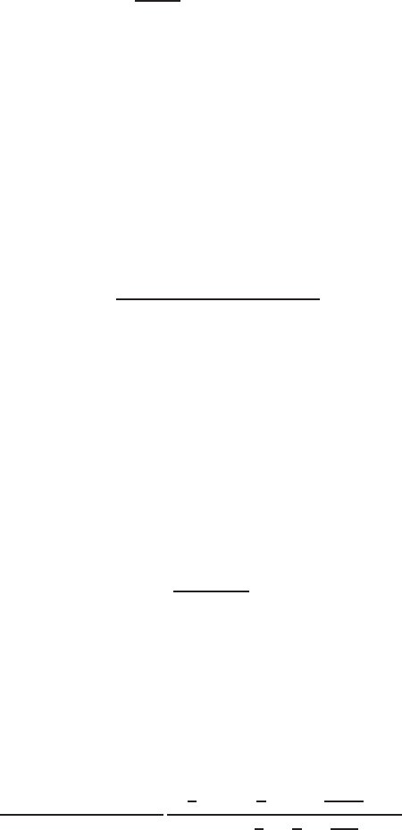
A.9. BINOMIAL TYPE DATA 195
A.8.2 Beta inflated distribution (BEINF)
The beta inflated distribution is appropriate when the response variable takes values in a known
restricted range including the endpoints of the range. Appropriate standardization can be
applied to make the range of the response variable [0,1], i.e. from zero to one including the
endpoints. Values zero and one for Yhave non zero probabilities p0and p1respectively. The
probability (density) function of the inflated beta distribution, denoted by BEINF(µ,σ,ν,τ) is
defined by
fY(y|µ, σ, ν, τ) =
p0if y= 0
(1 −p0−p1)1
B(α,β)yα−1(1 −y)β−1if 0 < y < 1
p1if y= 1
(A.44)
for 0 ≤y≤1, where α=µ(1 −σ2)/σ2,β= (1 −µ)(1 −σ2)/σ2,p0=ν(1 + ν+τ)−1,
p1=τ(1 + ν+τ)−1so α > 0, β > 0, 0 < p0<1, 0 < p1<1−p0. Hence BEINF(µ,σ,ν,τ) has
parameters µ=α/(α+β) and σ= (α+β+1)−1/2,ν=p0/p2,τ=p1/p2where p2= 1−p0−p1.
Hence 0 < µ < 1, 0 < σ < 1, ν > 0 and τ > 0.
A.8.3 Generalized Beta type 1 distribution (GB1)
The generalized beta type 1 distribution is defined by assuming Z=Yτ/[ν+ (1 −ν)Yτ]∼
BE(µ, σ). Hence, the pdf of generalized beta type 1 distribution, denoted by GB1(µ, σ, ν, τ), is
given by
fY(y|µ, σ, ν, τ) = τνβyτ α−1(1 −yτ)β−1
B(α, β)[ν+ (1 −ν)yτ]α+β(A.45)
for 0 < y < 1, where α=µ(1 −σ2)/σ2and β= (1 −µ)(1 −σ2)/σ2,α > 0 and β > 0. Hence,
GB1(µ, σ, ν, τ) has adopted parameters µ=α/(α+β), σ= (α+β+ 1)−1/2,νand τ, where
0< µ < 1, 0 < σ < 1, ν > 0 and τ > 0. The beta BE(µ, σ) distribution is a special case of
GB1(µ, σ, ν, τ) where ν= 1 and τ= 1.
A.9 Binomial type data
A.9.1 The Binomial distribution (BI)
The probability function of the binomial distribution, denoted here as BI(n,µ) , is given by
pY(y|n, µ) = P(Y=y|n, µ) = n!
y!(n−y)! µy(1 −µ)n−y
for y= 0,1,2, ..., n, where 0 < µ < 1, (and nis a known positive integer), with E(Y) = nµ and
V ar(Y) = nµ(1 −µ). See Johnson et al. (1993), p 105 where µ=p.
A.9.2 Beta Binomial distribution (BB)
The probability function of the beta binomial distribution denoted here as BB(n,µ,σ) is given
by
pY(y|µ, σ) = Γ(n+ 1)
Γ(y+ 1)Γ(n−y+ 1)
Γ( 1
σ)Γ(y+µ
σ)Γ[n+(1−µ)
σ−y]
Γ(n+1
σ)Γ(µ
σ)Γ(1−µ
σ)(A.46)

196 APPENDIX A. DISTRIBUTIONS IN THE GAMLSS PACKAGES
for y= 0,1,2,...,n, where 0 < µ < 1 and σ > 0 (and nis a known positive integer). Note that
E(Y) = nµ and V ar(Y) = nµ(1 −µ)h1 + σ
1+σ(n−1)i.
The binomial BI(n,µ) distribution is the limiting distribution of BB(n,µ,σ) as σ→0. For
µ= 0.5 and σ= 0.5, BB(n,µ,σ) is a uniform distribution.
A.10 Count data
A.10.1 Poisson distribution (PO)
Poisson distribution
The probability function of the Poisson distribution, denoted here as PO(µ), is given by
pY(y|µ) = P(Y=y|µ) = e−µµy
y!(A.47)
where y= 0,1,2,...,where µ > 0, with E(Y) = µand V ar(Y) = µ. [See Johnson et al. (1993),
p 151.] The moment ratios of the distribution are given by √β1=µ−0.5and β2= 3 + µ−1
respectively. Note that the Poisson distribution has the property that E[Y] = V ar[Y] and
that β2−β1−3 = 0. The coefficient of variation of the distribution is given by µ−0.5. The
index of dispersion, that is, the ratio V ar[Y]/E[Y] is equal to one for the Poisson distribution.
For V ar[Y]> E[Y] we have overdispersion and for V ar[Y]< E[Y] we have underdispersion
or repulsion. The distribution is skew for small values of µ, but almost symmetric for large µ
values.
A.10.2 Negative Binomial distribution (NBI, NBII)
First parameterization: Negative Binomial type I (NBI)
The probability function of the negative binomial distribution type I, denoted here as NBI(µ,σ),
is given by
pY(y|µ, σ) = Γ(y+1
σ)
Γ( 1
σ)Γ(y+ 1) σµ
1 + σµ y1
1 + σµ 1/σ
for y= 0,1,2, ..., where µ > 0, σ > 0 with E(Y) = µand V ar(Y) = µ+σµ2. [This parameter-
ization is equivalent to that used by Anscombe (1950) except he used α= 1/σ, as pointed out
by Johnson et al. (1993), p 200, line 5.]
Second parameterization: Negative Binomial type II (NBII)
The probability function of the negative binomial distribution type II, denoted here as NBII(µ,σ),
is given by
pY(y|µ, σ) = Γ(y+µ/σ)σy
Γ(µ/σ)Γ(y+ 1)(1 + σ)y+µ/σ
for y= 0,1,2, ...,, where µ > 0 and σ > 0. Note E(Y) = µand V ar(Y) = (1 + σ)µ, so σ
is a dispersion parameter [This parameterization was used by Evans (1953) as pointed out by
Johnson et al (1993) p 200 line 7.]

A.10. COUNT DATA 197
A.10.3 Poisson-inverse Gaussian distribution (PIG)
The probability function of the Poisson-inverse Gaussian distribution, denoted by PIG(µ,σ), is
given by
pY(y|µ, σ) = 2α
π1
2µye1/σKy−1
2(α)
(ασ)yy!
where α2=1
σ2+2µ
σ, for y= 0,1,2, ..., ∞where µ > 0 and σ > 0 and Kλ(t) = 1
2R∞
0xλ−1exp{−1
2t(x+
x−1)}dx is the modified Bessel function of the third kind. [Note that the above parameterization
was used by Dean, Lawless and Willmot (1989). It is also a special case of the gamlss.family
distribution SI(µ, σ, ν) when ν=−1
2.]
A.10.4 Delaporte distribution (DEL)
The probability function of the Delaporte distribution, denoted by DEL(µ,σ,ν), is given by
pY(y|µ, σ, ν) = e−µν
Γ(1/σ)[1 + µσ(1 −ν)]−1/σ S(A.48)
where
S=
y
X
j=0 y
jµyνy−j
y!µ+1
σ(1 −ν)−j
Γ1
σ+j
for y= 0,1,2, ..., ∞where µ > 0 , σ > 0 and 0 < ν < 1. This distribution is a reparameterization
of the distribution given by Wimmer and Altmann (1999) p 515-516 where α=µν,k= 1/σ
and ρ= [1 + µσ(1 −ν)]−1. The mean of Yis given by E(Y) = µand the variance by
V ar(Y) = µ+µ2σ(1 −ν)2.
A.10.5 Sichel distribution (SI, SICHEL)
First parameterization (SI)
The probability function of the first parameterization of the Sichel distribution, denoted by
SI(µ,σ,ν), is given by
pY(y|µ, σ, ν) = µyKy+ν(α)
(ασ)y+νy!Kν(1
σ)(A.49)
where α2=1
σ2+2µ
σ, for y= 0,1,2, ..., ∞where µ > 0 , σ > 0 and −∞ < ν < ∞and Kλ(t) =
1
2R∞
0xλ−1exp{−1
2t(x+x−1)}dx is the modified Bessel function of the third kind. Note that the
above parameterization is different from Stein, Zucchini and Juritz (1988) who use the above
probability function but treat µ,αand νas the parameters. Note that σ= [(µ2+α2)1
2−µ]−1.
Second parameterization (SICHEL)
The second parameterization of the Sichel distribution, Rigby, Stasinopoulos and Akantziliotou
(2007), denoted by SICHEL(µ,σ,ν), is given by
pY(y|µ, σ, ν) = (µ/c)yKy+ν(α)
y! (ασ)y+νKν1
σ(A.50)
for y= 0,1,2, ..., ∞, where α2=σ−2+ 2µ(cσ)−1. The mean of Yis given by E(Y) = µand
the variance by V ar(Y) = µ+µ22σ(ν+ 1)/c + 1/c2−1.

198 APPENDIX A. DISTRIBUTIONS IN THE GAMLSS PACKAGES
A.10.6 Zero inflated poisson (ZIP, ZIP2)
First parameterization (ZIP)
Let Y= 0 with probability σand Y∼P o(µ) with probability (1 −σ), then Yhas a zero
inflated Poisson distribution, denoted by ZIP(µ,σ,ν), given by
pY(y|µ, σ) =
σ+ (1 −σ)e−µ,if y= 0
(1 −σ)µy
y!e−µ,if y= 1,2,3,...
(A.51)
See Johnson et al (1993), p 186, equation (4.100) for this parametrization. This parametrization
was also used by Lambert (1992). The mean of Yin this parametrization is given by E(Y) =
(1 −σ)µand its variance by V ar(Y) = µ(1 −σ) [1 + µσ].
Second parameterization (ZIP2)
A different parameterization of the zero inflated poisson distribution, denoted by ZIP2(µ,σ,ν),
is given by
pY(y|µ, σ) =
σ+ (1 −σ)e−(µ
1−σ),if y= 0
(1 −σ)µy
y!(1−σ)ye−(µ
1−σ),if y= 1,2,3,...
(A.52)
The mean of Yin (A.52) is given by E(Y) = µand the variance by V ar(Y) = µ+µ2σ
(1−σ).
Bibliography
[1] Akaike, H. (1974). A new look at the statistical model identification. IEEE Transactions
on Automatic Control,19: 716–723.
[2] Akantziliotou, K. Rigby, R. A. and Stasinopoulos, D. M. (2002). The R implemen-
tation of Generalized Additive Models for Location, Scale and Shape. In: Stasinopoulos,
M. and Touloumi, G. (eds.), Statistical modelling in Society: Proceedings of the 17th In-
ternational Workshop on statistical modelling, pp. 75–83. Chania, Greece.
[3] Anscombe, F. J. (1950). Sampling theory of the negative binomial and logarithmic series
approximations. Biometrika,37: 358–382.
[4] Azzalini, A. (1985). A class of distributions which includes the normal ones. Scand. J.
Statist.,12: 171–178.
[5] Azzalini, A. (1986). Further results on a class of distributions which includes the normal
ones. Statistica,46: 199:208.
[6] Azzalini, A. and Capitanio, A. (2003). Distributions generated by perturbation of
symmetry with emphasis on a multivariate skew t-distribution. J. R. Statist. Soc. B,65:
367–389.
[7] Box, G. E. P. and Cox, D. R. (1964). An analysis of transformations (with discussion).
J. R. Statist. Soc. B.,26: 211–252.
[8] Chambers, J. M. and Hastie, T. J. (1992). Statistical Models in S . Chapman & Hall,
London.
[9] Chitty, L. S., Altman, D. G., Henderson, A., and Campbell, S. (1994). Charts of
fetal size: 3, abdominal measurements. Br. J. Obstetr.,101: 125–131.
[10] Cleveland, W. S., Grosse, E. and Shyu, M. (1993). Local Regression Models. In:
Chambers, J. and Hastie, T. (eds.), Statistical Modelling in S , pp. 309–376. Chapman and
Hall: New York.
[11] Cole, T. J. and Green, P. J. (1992). Smoothing reference centile curves: the LMS
method and penalized likelihood. Statist. Med.,11: 1305–1319.
[12] Crowder, M. J., Kimber, A. C., Smith R. L. and Sweeting, T. J. (1991). Statistical
Analysis of Reliability Data. Chapman and Hall, London.
[13] D’Agostino, R. B., Balanger, A. and D’Agostino Jr., R. B. (1990). A suggestion
for using powerful and informative tests of normality. American Statistician,44: 316–321.
199
200 BIBLIOGRAPHY
[14] Dean, C., Lawless, J. F. and Willmot, G. E. (1989). A mixed Poisson-inverse-
Gaussian regression model. Canadian Journal of Statistics,17: 171–181.
[15] DiCiccio, T. J. and Monti, A. C. (2004). Inferential Aspects of the Skew Exponential
Power Distribution. J. Am. Statist. Ass.,99: 439–450.
[16] Dunn, P. K. and Smyth, G. K. (1996). Randomised quantile residuals. J. Comput.
Graph. Statist.,5: 236–244.
[17] Eilers, P. H. C. and Marx, B. D. (1996). Flexible smoothing with B-splines and
penalties (with comments and rejoinder). Statist. Sci,11: 89–121.
[18] Evans, D. A. (1953). Experimental evidence concerning contagious distributions in ecol-
ogy. Biometrika,40: 186–211.
[19] Fernandez, C. and Steel, M. F. J. (1998). On Bayesian Modelling of Fat Tails and
Skewness. J. Am. Statist. Ass.,93: 359–371.
[20] Fernandez, C., Osiewalski, J. and Steel, M. F. J. (1995). Modeling and inference
with ν-spherical distributions. J. Amer. Statist. Assoc.,90: 1331–1340.
[21] Gelman, A. Carlin, J. B. Stern, H. S. and Rubin, D. B. (2004). Bayesian Data
Analysis, 2nd ed. Chapman and Hall/CRC, London.
[22] Green, P. J. and Silverman, B. W. (1994). Nonparametric Regression and Generalized
Linear Models. Chapman and Hall, London.
[23] Hand, D. J., Daly, F., Lunn, A. D., McConway, K. J. and Ostrowski, E. (1994).
A handbook of small data sets. Chapman and Hall, London.
[24] Hastie, T. (2006). gam: Generalized Additive Models.Rpackage version 0.98.
[25] Hastie, T. J. and Tibshirani, R. J. (1990). Generalized Additive Models. Chapman
and Hall, London.
[26] Hastie, T. J. and Tibshirani, R. J. (1993). Varying coefficient models (with discussion).
J. R. Statist. Soc. B.,55: 757–796.
[27] Hodges, J. S. (1998). Some algebra and geometry for hierarchical models, applied to
diadnostics. J. R. Statist. Soc. B.,60: 497–536.
[28] Johnson, N. L. (1949). Systems of frequency curves generated by methods of translation.
Biometrika,36: 149–176.
[29] Johnson, N. L., Kotz, S. and Balakrishnan, N. (1994). Continuous Univariate
Distributions, Volume I, 2nd edn. Wiley, New York.
[30] Johnson, N. L., Kotz, S. and Balakrishnan, N. (1995). Continuous Univariate
Distributions, Volume II, 2nd edn. Wiley, New York.
[31] Johnson, N. L., Kotz, S. and Kemp, A. W. (2005). Univariate Discrete Distributions,
3nd edn. Wiley, New York.
[32] Jones, M. C. (2005). In discussion of Rigby, R. A. and Stasinopoulos, D. M. (2005)
Generalized additive models for location, scale and shape,. Applied Statistics,54: 507–
554.
BIBLIOGRAPHY 201
[33] Jones, M. C. and Faddy, M. J. (2003). A skew extension of the tdistribution, with
applications. J. Roy. Statist. Soc B,65: 159–174.
[34] Jørgensen, B. (1982). Statistical Properties of the Generalized Inverse Gaussian Distri-
bution, Lecture Notes in Statistics No.9. Springer-Verlag, New York.
[35] Lambert, D. (1992). Zero-inflated Poisson Regression with an application to defects in
Manufacturing. Technometrics,34: 1–14.
[36] Lopatatzidis, A. and Green, P. J. (2000). Nonparametric quantile regression using the
gamma distribution. submitted for publication.
[37] McDonald, J. B. (1991). Parametric models for partially adaptive estimation with skewed
and leptokurtic residuals. Economic Letters,37: 273–278.
[38] McDonald, J. B. (1996). Probability Distributions for Financial Models. In: Maddala,
G. S. and Rao, C. R. (eds.), Handbook of Statistics, Vol. 14, pp. 427–460. Elsevier Science.
[39] McDonald, J. B. and Newey, W. K. (1988). Partially adaptive estimation of regression
models via the generalized tdistribution. Econometric Theory,4: 428–457.
[40] McDonald, J. B. and Xu, Y. J. (1995). A generalisation of the beta distribution with
applications. Journal of Econometrics,66: 133–152.
[41] Nelder, J. A. (2001). Correspondance. Statistician,50: 209–211.
[42] Nelder, J. A. and Wedderburn, R. W. M. (1972). Generalized linear models. J. R.
Statist. Soc. A.,135: 370–384.
[43] Nelson, D. B. (1991). Conditional heteroskedasticity in asset returns: a new approach.
Econometrica,59: 347–370.
[44] Raftery, A. E. (1996). Approximate Bayes factors and accounting for model uncertainty
in generalised linear models. Biometrika,83: 251–266.
[45] Raftery, A. E. (1999). Bayes Factors and BIC, comment on ’A critique of the Bayesian
Information Criterion for Model Selection’. Sociological Methods & Research,27: 411–427.
[46] Rigby, R. A. and Stasinopoulos, D. M. (1994). Robust fitting of an additive model
for variance heterogeneity. In: Dutter, R. and Grossmann, W. (eds.), COMPSTAT :
Proceedings in Computational Statistics, pp. 263–268. Physica, Heidelberg.
[47] Rigby, R. A. and Stasinopoulos, D. M. (1996a). A semi-parametric additive model
for variance heterogeneity. Statist. Comput.,6: 57–65.
[48] Rigby, R. A. and Stasinopoulos, D. M. (1996b). Mean and dispersion additive models.
In: Hardle, W. and Schimek, M. G. (eds.), Statistical Theory and Computational Aspects
of Smoothing, pp. 215–230. Physica, Heidelberg.
[49] Rigby, R. A. and Stasinopoulos, D. M. (2001). The GAMLSS project: a flexible
approach to statistical modelling. In: Klein, B. and Korsholm, L. (eds.), New Trends
in Statistical Modelling: Proceedings of the 16th International Workshop on Statistical
Modelling, pp. 249–256. Odense, Denmark.
202 BIBLIOGRAPHY
[50] Rigby, R. A. and Stasinopoulos, D. M. (2004). Smooth centile curves for skew and
kurtotic data modelled using the Box-Cox Power Exponential distribution. Statistics in
Medicine,23: 3053–3076.
[51] Rigby, R. A. and Stasinopoulos, D. M. (2005). Generalized additive models for
location, scale and shape, (with discussion). Appl. Statist.,54: 507–554.
[52] Rigby, R. A. and Stasinopoulos, D. M. (2006). Using the Box-Cox tdistribution in
GAMLSS to model skewness and kurtosis. Statistical Modelling,6: 209–229.
[53] Rigby, R.A., Stasinopoulos, D.M. and Akantziliotou, K. (2007). A general frame-
work for modelling count data. submitted for publication.
[54] Royston, P. and Altman, D. G. (1994). Regression using fractional polynomials of
continuous covariates: parsimonious parametric modelling (with discussion). Appl. Statist.,
43: 429–467.
[55] Royston, P. and Wright, E. M. (2000). Goodness-of-fit statistics for age-specific refer-
ence intervals. Statistics in Medicine,19: 2943–2962.
[56] SAS Institute Inc. (2000). Enterprise Miner Software, Version 4 . SAS Institute Inc,
Cary, North Carolina.
[57] Schwarz, G. (1978). Estimating the dimension of a model. Ann. Statist.,6: 461–464.
[58] Silverman, B. W. (1985). Some aspects of the spline smoothing approach to non-
parametric regression curve fitting (with discussion). J. R. Statist. Soc. B.,47: 1–52.
[59] Stasinopoulos, D. M. and Rigby, R. A. (1992). Detecting break points in generalised
linear models. Comp. Stat. Data Anal.,13: 461–471.
[60] Stasinopoulos, D. M., Rigby, R. A. and Akantziliotou, C. (2006). Instructions on
how to use the GAMLSS package in R. Technical Report 01/06, STORM Research Centre,
London Metropolitan University, London.
[61] Stasinopoulos, D. M., Rigby, R. A. and Fahrmeir, L. (2000). Modelling rental guide
data using mean and dispersion additive models. Statistician,49: 479–493.
[62] Stein, G. Z., Zucchini, W. and Juritz, J. M. (1987). Parameter Estimation of
the Sichel Distribution and its Multivariate Extension. Journal of American Statistical
Association,82: 938–944.
[63] Subbotin, M. T. (1923). On the law of frequency of errors. Mathematicheskii Sbornik,
31: 296–301.
[64] van Buuren, S. and Fredriks, M. (2001). Worm plot: a simple diagnostic device for
modelling growth reference curves. Statistics in Medicine,20: 1259–1277.
[65] Venables, W. N. and Ripley, B. D. (2002). Modern Applied Statistics with S. Fourth
Edition. Springer. ISBN 0-387-98825-4.
[66] Wimmer, G. and Altmann, G. (1999). Thesaurus of univariate discrete probability
distributions. Stamm Verlag, Essen, Germany.
[67] Wright, E. M. and Royston, P. (1997). A comparison of statistical methods for age-
related reference intervals. J. R. Statist. Soc. A.,160: 47–69.
Index
(, 81
additive terms, 95
cs(), 96
fp(), 109
lo, 106
ps(), 102
ra(), 115,120
random(), 112
vc(), 97
addterm, 19,136
arguments, 136
AIC, 18,27,118,136
algorithm, 15,30
CG(), 31
RS(), 31
control, 30,32
gamlss.control, 32
glim.control, 33
backfitting, 95
backfitting
modified , 95
BCPE, 67
BCT, 67,117
centiles
centiles(), 158
centiles.com(), 167
centiles.pred(), 169
centiles.split(), 162
functions, 20,158
checklink, 20,74
coef, 18,63
cubic smoothing splines
cs(), 24,96
data
abdom, 21
abdom, 110,169
aids, 46,149
education, 113
Hodges, 116
mcycle, 103
rent, 67,101
usair, 137
degree
lo(), 107
ps(), 103
degrees of freedom, 95,96
deviance, 18,27,135
df
cs(), 96
lo(), 107
ps(), 103
vc(), 98
distribution, 67
gamma, 70
zero inflated Poisson, 198
BCCG, 191
BCPE, 193
BCT, 193
beta, 194
beta inflated, 194
betabinomial, 195
binomial, 195
Delaporte, 197
exponential, 189
exponential Gaussian, 183
Exponential Generalized Beta type 2,
184
gamma, 189
Generalized Beta type 1, 195
Generalized Beta type 2, 194
Generalized Gamma, 192
Generalized Inverse Gaussian, 192
Generalized t, 184
Gumbel, 182
inverse Gaussian, 190
203
204 INDEX
Johnson
original, 184
reparameterized, 185
log normal, 190
logistic, 182
negative binomial
type I, 70,196
type II, 196
new, 73
normal, 21,181
Poisson, 196
Poisson-inverse Gaussian, 196
powerexponential, 183
reverse Gumbel, 183
Sichel, 197
Sinh-Arcsinh, 186
Skew Exponential Power type 1, 186
Skew Exponential Power type 3, 187
Skew Exponential Power type 4, 188
skew power exponential, 187
skew t distribution type 5, 189
Skew t type 1, 188
Skewt type 2, 188
Skewt type 3, 188
Skewt type 4, 189
t, 27,184
Weibull, 191
zero adjusted Inverse Gaussian, 193
distributions, 181
fitting, 77
dropterm, 19,136
arguments, 136
effective degrees of freedom , 24
examples
abdominal circumference, 177
extractAIC, 18
family, 29
find.hyper, 19,118,148
fitted, 18,24
fitted.plot, 20
formula, 18,63
mu, 29
nu, 29
sigma, 29
tau, 29
fractional polynomials
fp(), 109
fractional polynomials
fp, 95
fv, 18
GAIC, 27,61,118,136
gamlss
agruments, 29
family, 70,181
new, 73
function, 21,29
model, 13
object, 41
package, 17
random effect, 14
semi parametric, 14
what is, 13
gamlss family
BB, 195
BCCG, 191
BCPE, 193
BCT, 193
BE, 194
BEINF, 194
BI, 195
DEL, 197
EGB2, 184
exGAUS, 183
EXP, 189
GA, 189
GB1, 195
GB2, 194
GG, 192
GG2, 192
GIG, 192
GT, 184
GU, 182
IG, 190
JSU, 185
JSUo, 184
LNO, 190
LO, 182
LOGNO, 190
NBI, 196
NBII, 196
NET, 185
NO, 181
NO2, 182
NOF, 182
PE, 183
INDEX 205
PE2, 183
PIG, 196
PO, 196
RG, 183
SEP1, 186
SEP2, 187
SEP3, 187
SEP4, 188
SHASH, 186
SI, 197
SICHEL, 197
ST1, 188
ST2, 188
ST3, 188
ST4, 189
ST5, 189
TF, 184
WEI, 191
WEI2, 191
WEI3, 191
ZAIG, 193
ZIP, 198
ZIP2, 198
gamlss.control, 32
gamlss.scope, 19
glim.control, 33
global deviance, 27,135
histDist, 18
kurtosis
lepto, 83
platy, 78
link function, 70,75
available, 70
default, 70
own, 70,75
show.link, 20
loess
lo, 27,106
make.link, 20
model.frame, 18,63
model.matrix, 19,63
order
ps(), 103,105
par.plot, 19
parameter
fix, 30
pdf.plot, 19
penalized likelihood, 14
penalized splines
ps(), 102
plot, 19,121
agruments, 121
predict, 19,24,48
print, 19
prof.dev, 20,55
prof.term, 20,58
Q statistics, 20,131
Q.stats, 20,131
arguments, 131
refit, 18,45
REML, 120
resid, 19,24
residuals, 19
quantile, 24
rqres, 20
rqres.plot, 132
show.link, 20,70
smoothers, 95
smoothing
components, 96
span
lo(), 107
spar
cs(), 96
vc(), 98
starting values, 30
stepGAIC, 19,136
arguments, 139
stepGAIC.CH, 136
arguments, 139
stepGAIC.VR, 19,136
arguments, 139
summary, 19
term.plot, 97
terms, 19,63
terms.plot, 20
update, 18,46
varying coefficient