Gis Manual
User Manual:
Open the PDF directly: View PDF ![]() .
.
Page Count: 181 [warning: Documents this large are best viewed by clicking the View PDF Link!]

UNIVERSITY OF MUMBAI
Teacher’s Reference Manual
USIT6P4
(Discipline Specific Elective Practical)
Principles of Geographic
Information Systems Practical
with effect from the academic year
2018 – 2019

USIT6P4 (Discipline Specific Elective Practical) Principles of Geographic Information Systems Practical
T. Y. B. Sc. (Information Technology) SEMESTER VI Teacher’s Reference Manual
2
Index
Sr.
No
Practical
Title
Page
No
1
---
Prerequisites to GIS Practical
3
2
1A
Creating and Managing Vector Data
a) Adding vector layer
b) Setting properties
c) Vector Layer Formatting
14
3
1B
4
1C
5
1D
Calculating line lengths and statistics
26
6
2A
Adding raster layers
31
7
2B
Raster Styling and Analysis
32
8
2C
Raster Mosaicking and Clipping
35
9
3A
Making a Map
40
10
3B
Importing Spreadsheets or CSV files
49
11
3C
Using Plugin
51
12
3D
Searching and Downloading OpenStreetMap Data
52
13
4A
Working with attributes
54
14
4B
Terrain Data and Hill shade analysis
56
15
5A
Working with Projections and WMS Data
64
16
6A
Georeferencing Topo Sheets and Scanned Maps
66
17
6B
Georeferencing Aerial Imagery
71
18
6C
Digitizing Map Data
75
19
7A
Table Join
80
20
7B
Spatial Join
83
21
7C
Points in polygon
85
22
7D
Performing spatial queries
87
23
8A
Nearest Neighbor Analysis
90
24
8B
Sampling Raster Data using Points or Polygons
104
25
8C
Interpolating Point Data
114
26
9A
Batch Processing using Processing Framework
121
27
9B
Automating Complex Workflows using
Processing Modeler
28
9C
Automating Map Creation with Print Composer
Atlas
143
29
10A
Validating Map Data
161
USIT6P4 (Discipline Specific Elective Practical) Principles of Geographic Information Systems Practical
T. Y. B. Sc. (Information Technology) SEMESTER VI Teacher’s Reference Manual
3
Prerequisites to GIS Practical
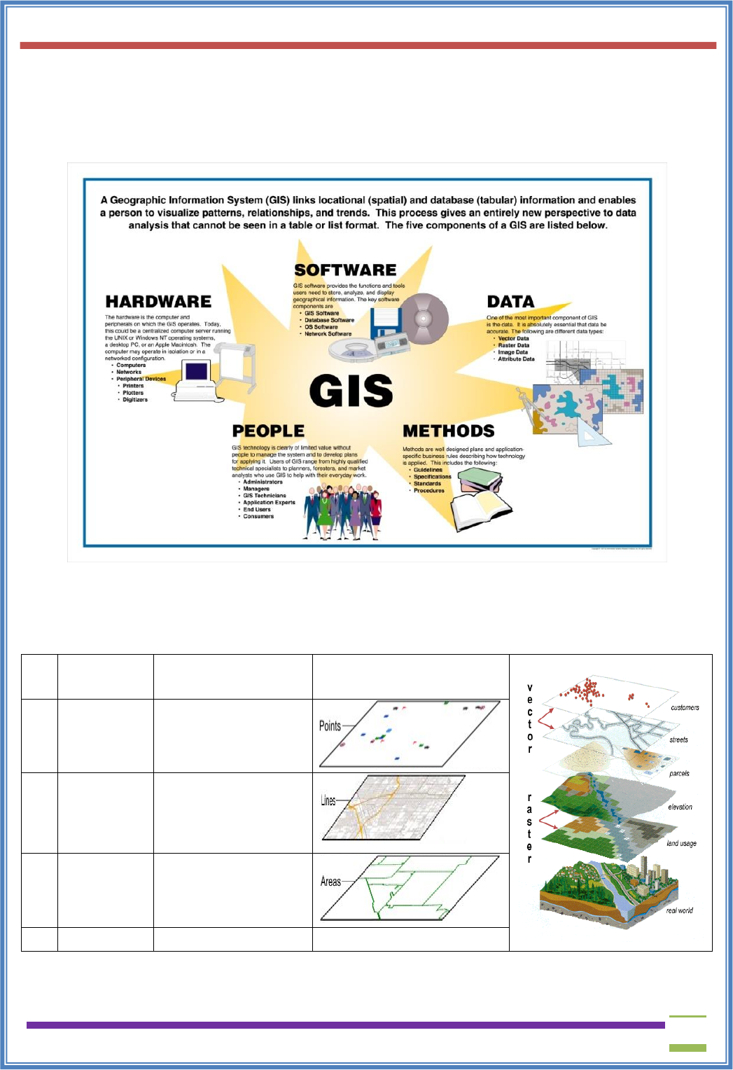
What is a Geographic Information System (GIS)?
A Geographical Information System (GIS) is an organized collection of computer hardware,
software and data used to link, analyze and display geographically referenced information.
The foundation of GIS is the ability to locate objects and events (streams, villages, disease
cases) and link them with appropriate information in order to identify patterns and provide a basis for
map making and analysis. Key types of geographical data, represented as separate map layers in a GIS,
are outlined in the table below.
Sr.
No
Data Type
Example
Layer on Map
1
POINT
Building, Hospital,
City, Well.
2
LINE
River, Road
3
POLYGON
Administrative
Boundaries, Census
tacts.
4
RASTER
Pixel or grid data
Vector data: A representation of the world using points, lines, and polygons. Vector models are useful
for storing data that has discrete boundaries, such as country borders, land parcels, and streets.

USIT6P4 (Discipline Specific Elective Practical) Principles of Geographic Information Systems Practical
T. Y. B. Sc. (Information Technology) SEMESTER VI Teacher’s Reference Manual
4
Point features: A map feature that has neither length nor area at a given scale, such as a city on a world
map or a building on a city map.
Line features: A map feature that has length but not area at a given scale, such as a river on a world
map or a street on a city map.
Polygon features: A map feature that bounds an area at a given scale, such as a country on a world
map or a district on a city map.
Raster data. A representation of the world as a surface divided into a regular grid of cells. Raster
models are useful for storing data that varies continuously, as in an aerial photograph, a satellite image,
a surface of chemical concentrations, or an elevation surface.
With a GIS application you can open digital maps on your computer, create new spatial information to
add to a map, create printed maps customised to your needs and perform spatial analysis.

USIT6P4 (Discipline Specific Elective Practical) Principles of Geographic Information Systems Practical
T. Y. B. Sc. (Information Technology) SEMESTER VI Teacher’s Reference Manual
5
Understanding QGIS
What is Quantum GIS?
Quantum GIS (QGIS) is a user friendly Open Source GIS application licensed under the GNU General
Public License. QGIS is an official project of the Open Source Geospatial Foundation (OSGeo). It runs
on Linux, Unix, Mac OSX, Windows and Android and supports numerous vector, raster, and database
formats and functionalities.
Like all GIS applications, QGIS provides a graphical user interface allowing display of map layers and
manipulation of data for analyses and map-making.
A Geographical Information System (GIS) is a collection of software that allows you to create,
visualize, query and analyze geospatial data. Geospatial data refers to information about the geographic
location of an entity. This often involves the use of a geographic coordinate, like a latitude or longitude
value. Spatial data is another commonly used term, as are: geographic data, GIS data, map data,
location data, coordinate data and spatial geometry data. Applications using geospatial data perform a
variety of functions. Map production is the most easily understood function of geospatial applications.
Mapping programs take geospatial data and render it in a form that is viewable, usually on a computer
screen or printed page. Applications can present static maps(a simple image) or dynamic maps that are
customized by the person viewing the map through a desktop program or a web page.
Many people mistakenly assume that geospatial applications just produce maps, but geospatial data
analysis is another primary function of geospatial applications. Some typical types of analysis include
computing:
1. Distances between geographic locations
2. The amount of area (e.g., square meters) within a certain geographic region
3. What geographic features overlap other features?
4. The amount of overlap between features
5. The number of locations within a certain distance of another
6. and so on...
These may seem simplistic, but can be applied in all sorts of ways across many disciplines. The results
of analysis may be shown on a map, but are often tabulated into a report to support management
decisions. The recent phenomena of location-based services promises to introduce all sorts of other
features, but many will be based on a combination of maps and analysis. For example, you have a cell
phone that tracks your geographic location. If you have the right software, your phone can tell you what
kinds of restaurants are within walking distance. While this is a novel application of geospatial
technology, it is essentially doing geospatial data analysis and listing the results for you.
System Requirements
Windows OS:
Minimum: Pentium III / 256 MB RAM.
Recommended: 1 GB of RAM and 1.6 GHz processor.
Operation System: Platforms Windows and Linux (Win XP or newer, Linux Suse 8.2/9.0/9.2, Linux
Debian (Lliurex))
MAC OS:
PC/Desktop with at least Pentium IV
Tiger OS, Leopard OS.
USIT6P4 (Discipline Specific Elective Practical) Principles of Geographic Information Systems Practical
T. Y. B. Sc. (Information Technology) SEMESTER VI Teacher’s Reference Manual
6
Installation of QGIS
Step By step procedure
1) Create a folder on your D:/ drive on your computer called QGISlab by right clicking on the D:
drive and navigating down to the New / Folder.
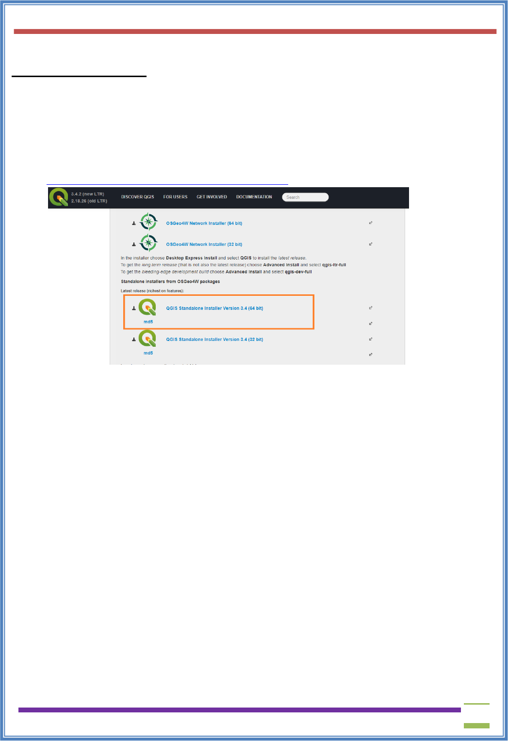
2) Go to the QGIS download page and download the latest 64bit version of QGIS for windows
which is QGIS 3.4 'Madeira’ by clicking once.
3) If you have a 32 bit machine or using another operating system search the bottom of the page
for your operating system and download the correct operating system version of QGIS.
http://www.qgis.org/en/site/forusers/download.html
4) You browser will download the file to the browsers default download directory. By pressing the
control key and the letter J at the same time a popup window will show you the folder where the
QGIS file has been downloaded. The QGIS file will be called:
QGIS-OSGeo4W-3.4.2-1-Setup-x86.exe
5) Move or copy the above file to your C:/QGISlab folder and double click on the file. You will
get a popup window with a security warning.
6) Hit the run button to start the installation process and follow the prompts. There is no need to
install the data sets suggested by QGIS.
USIT6P4 (Discipline Specific Elective Practical) Principles of Geographic Information Systems Practical
T. Y. B. Sc. (Information Technology) SEMESTER VI Teacher’s Reference Manual
7
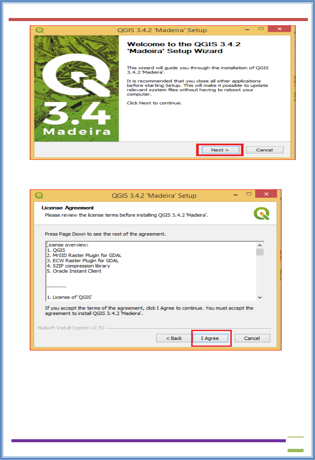
7) From the above window, click Next button and continue with the installation.
8) Please go through the license agreement and click on the button> I agree and proceed with the
installation as shown in the screen.
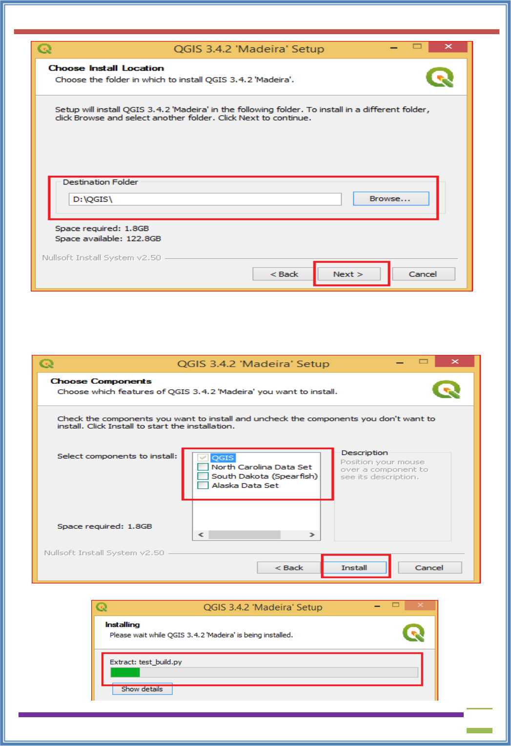
9) As the software is very heavy it is advisable to install it in the different drive other than the
windows drive. As per our example, we will be installing in QGIS folder on D:\ drive.
USIT6P4 (Discipline Specific Elective Practical) Principles of Geographic Information Systems Practical
T. Y. B. Sc. (Information Technology) SEMESTER VI Teacher’s Reference Manual
8
10) After browsing the folder click the Next button and proceed with the installation as shown in
above figure.
11) By default QGIS component is selected. Do not install any other data set at this point. Click
Install to proceed with installation.
12) You will see the progress of the installation on the screen.
USIT6P4 (Discipline Specific Elective Practical) Principles of Geographic Information Systems Practical
T. Y. B. Sc. (Information Technology) SEMESTER VI Teacher’s Reference Manual
9
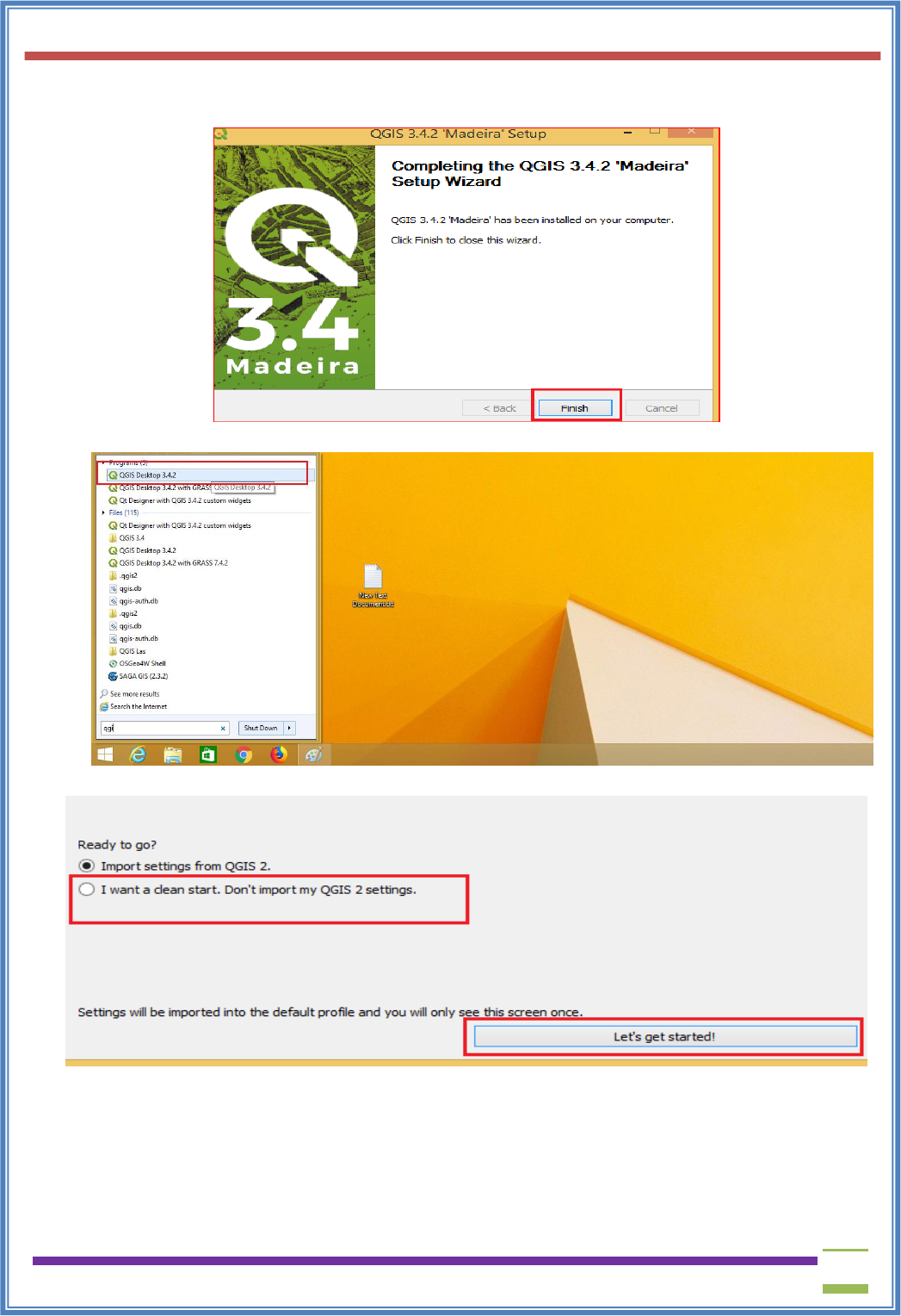
13) Please reboot your machine once the installation is completed. Click finish to complete the
installation.
14) After machine is restarted, type QGIS on Run and open QGIS Desktop 3.4.2.
15) It will open a new wizard for the first time after installation as shown in the figure below.
16) Select I want a clean start. Don’t import my QGIs 2 settings and click on let’s get started button.
You will be redirected now to the home screen of QGIS Desktop.
USIT6P4 (Discipline Specific Elective Practical) Principles of Geographic Information Systems Practical
T. Y. B. Sc. (Information Technology) SEMESTER VI Teacher’s Reference Manual
10
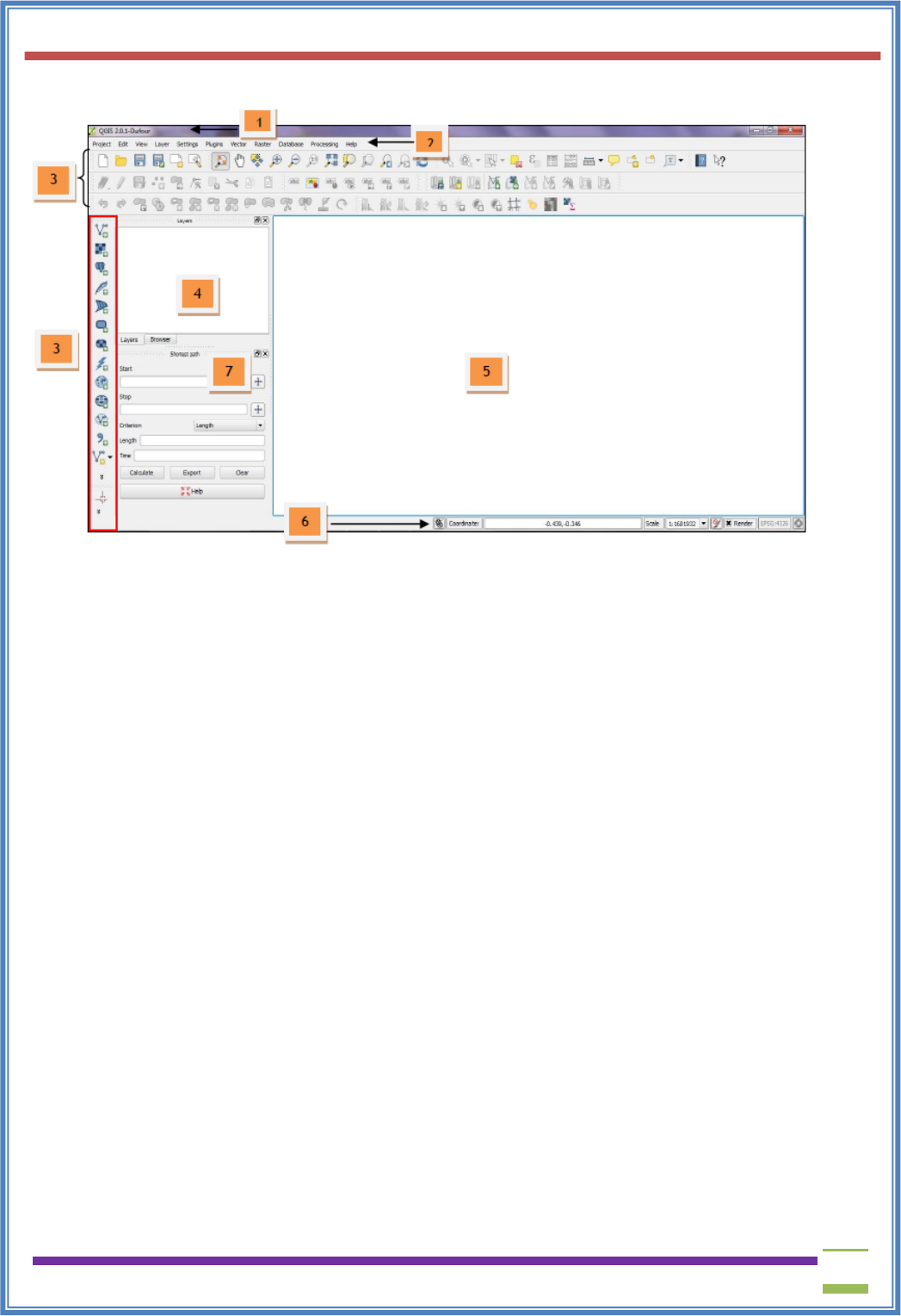
Understanding QGIS Desktop Environment.
Quantum GIS interfaces change from one project to another depending on the required interface of the
project. Below are the basic menus that you will encounter in Quantum GIS during the practicals.
1. Title of the Project - Shows the title of project that you are going to view.
2. Menu Bar – This provides access to various Quantum GIS features using a standard hierarchical
menu.
3. Toolbars – These provide access to most of the same functions as the menus, plus additional tools
for interacting with the map. It shows the command for zoom in, zoom out, pan, back to original
view, go back to previous extent, go to next extent, object-information, coordinate read-out,
measure, print and help.
4. Table of Contents/Map Legend (TOC) - Shows the layers that can be turned on or off and the
legend, attributes symbols and query symbols available for the corresponding project.
5. Display Window - Shows the feature/s that you have turn on from the TOC.
6. Status Bar - Shows you your current position in map coordinates (e.g. metres or decimal degrees)
as the mouse pointer is moved across the map view. To the left of the coordinate display in the
status bar is a small button that will toggle between showing coordinate position or the view
extents of the map view as you pan and zoom in and out.
7. Data sources browser – In previous versions, QGIS browser was only provided as an external
application which enables us to explore our spatial data sets. In QGIS 2.0.1-Dufour this
application is also integrated in the QGIS framework as an additional panel just below the Table
of Contents.
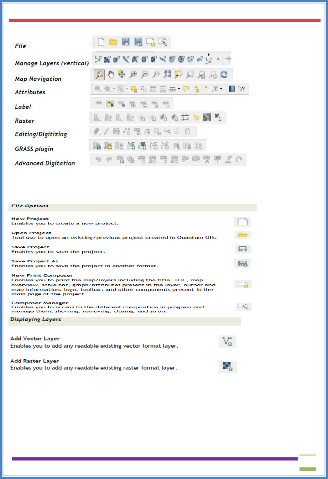
Quantum GIS toolbars and some other components
Toolbars are divided by thematic (greyed icons means they are inactive because the appropriate
conditions to use them are not fulfilled). Some of them are included by default in QGIS and others can
be added/removed from the interface:
USIT6P4 (Discipline Specific Elective Practical) Principles of Geographic Information Systems Practical
T. Y. B. Sc. (Information Technology) SEMESTER VI Teacher’s Reference Manual
11
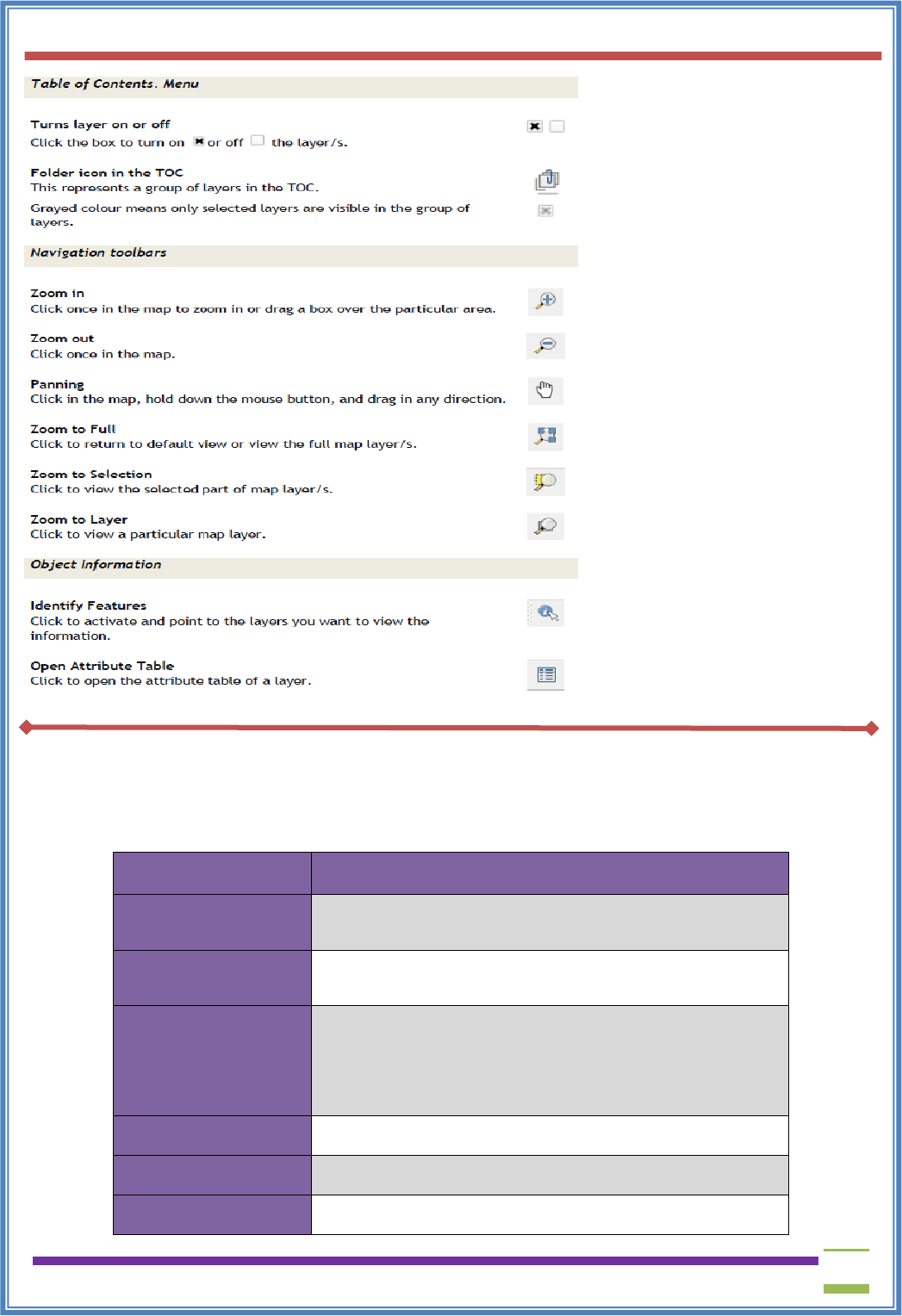
Key functions:
Here, you will learn how to QGIS‟ different mapping tools and other components that you‟ll be using
in this practical.
USIT6P4 (Discipline Specific Elective Practical) Principles of Geographic Information Systems Practical
T. Y. B. Sc. (Information Technology) SEMESTER VI Teacher’s Reference Manual
12
Principles of GIS T. Y. B. Sc. IT Semester VI
List of Sample/Data files used for Practical
Practical No.
Data set Name
1D
IND_rails.zip
IND_adm0.zip
2A
gl_gpwv3_pdens_00_ascii_one.zip
gl_gpwv3_pdens_90_ascii_one.zip
2C
FAS_India1.2018349.terra.367.2km.tif
FAS_India2.2018349.terra.367.2km.tif
FAS_India3.2018349.terra.367.2km.tif
FAS_India4.2018349.terra.367.2km.tif
3B
Sample.csv
4A
ne_10m_populated_places_simple.zip
4B
GMTED2010N10E060_300.zip
USIT6P4 (Discipline Specific Elective Practical) Principles of Geographic Information Systems Practical
T. Y. B. Sc. (Information Technology) SEMESTER VI Teacher’s Reference Manual
13
5A
ne_10m_populated_places_simple.zip
6A
IND_adm0.zip
Bombay_1990.jpg
6B
GateWay_Aerial_Imagery.tif
6C
Christchurch Topo50 map.tif
7A
tl_2013_06_tract.zip
ca_tracts_pop.csv
7B
OEM_NursingHomes_001.zip
nybb_12c.zip
7C
EarthQuakeDatabase.txt
ne_10m_admin_0_countries.zip
ne_10m_populated_places_simple.zip
7D
ne_10m_populated_places_simple.zip
ne_10m_rivers_lake_centerlines.zip
8A
ca_tracts_pop.csv
EarthQuakeDatabase.txt
ne_10m_populated_places_simple.zip
tl_2013_06_tract.zip
8B
us.tmax_nohads_ll_20140525_float.tif
2013_Gaz_ua_national.txt
tl_2013_us_county.shp
8C
tl_2013_us_county.shp
Boundary2004_550_stpl83.shp
9A
ne_10m_admin_0_countries.shp
ne_10m_admin_0_District.shp
ne_10m_admin_0_port.shp
ne_10m_admin_0_railroads.shp
9B
LC_hd_global_2001.tif.gz
9C
HI_Wetlands.shp.zip
10
Kenya admin.shp
Kenya_epidemiological_data.xls
Kenya_epidemiological_dict.xlsx
Kenya_school_dict.xlsx
Kenya_school_location.csv
The above data can be downloaded from:
www.muresults.net → TYBSc IT Sem VI eBooks →GIS→ Practicals
Or directly from: https://drive.google.com/drive/folders/191tJ4L7O-
VJm2Q2AB8dZDpIj7vyyPM3I?usp=sharing
USIT6P4 (Discipline Specific Elective Practical) Principles of Geographic Information Systems Practical
T. Y. B. Sc. (Information Technology) SEMESTER VI Teacher’s Reference Manual
14
PRACTICAL - 1
B. AIM : - Creating and Managing Vector Data:
a) Adding vector layer
b) Setting properties
c) Vector Layer Formatting
Procedure:
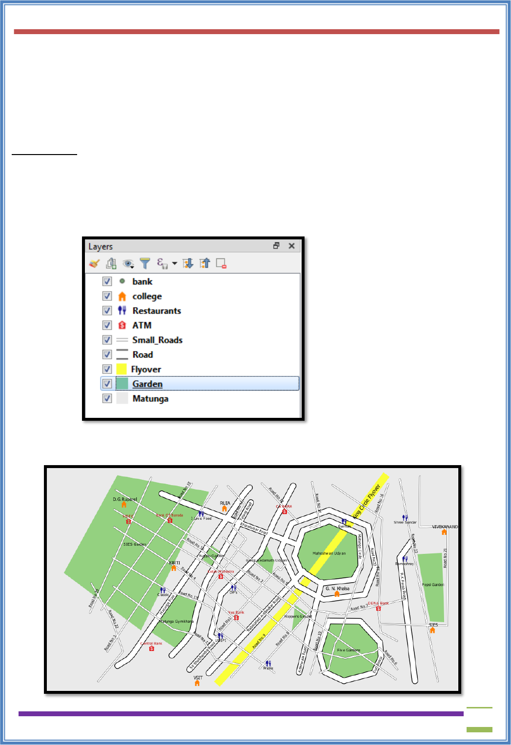
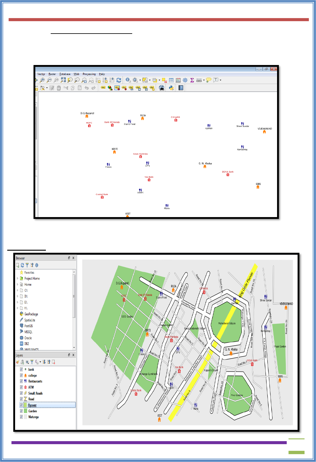
a. Adding vector layers (Polygon, Line, Points)
➢ Polygon layers (We have taken 2 layers Matunga, Garden)
➢ Line layers (We have taken 3 layers Small_Roads, Road, Flyover)
➢ Point layers (We have taken 4 layers bank,college,Restaurants,ATM)
b. Setting properties (Labeling, Symbolism)
➢ Our aim is to create map representing a location and its surrounding as
follows:
USIT6P4 (Discipline Specific Elective Practical) Principles of Geographic Information Systems Practical
T. Y. B. Sc. (Information Technology) SEMESTER VI Teacher’s Reference Manual
15
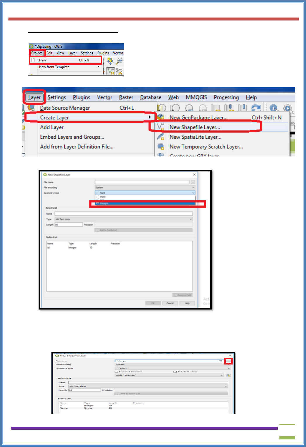
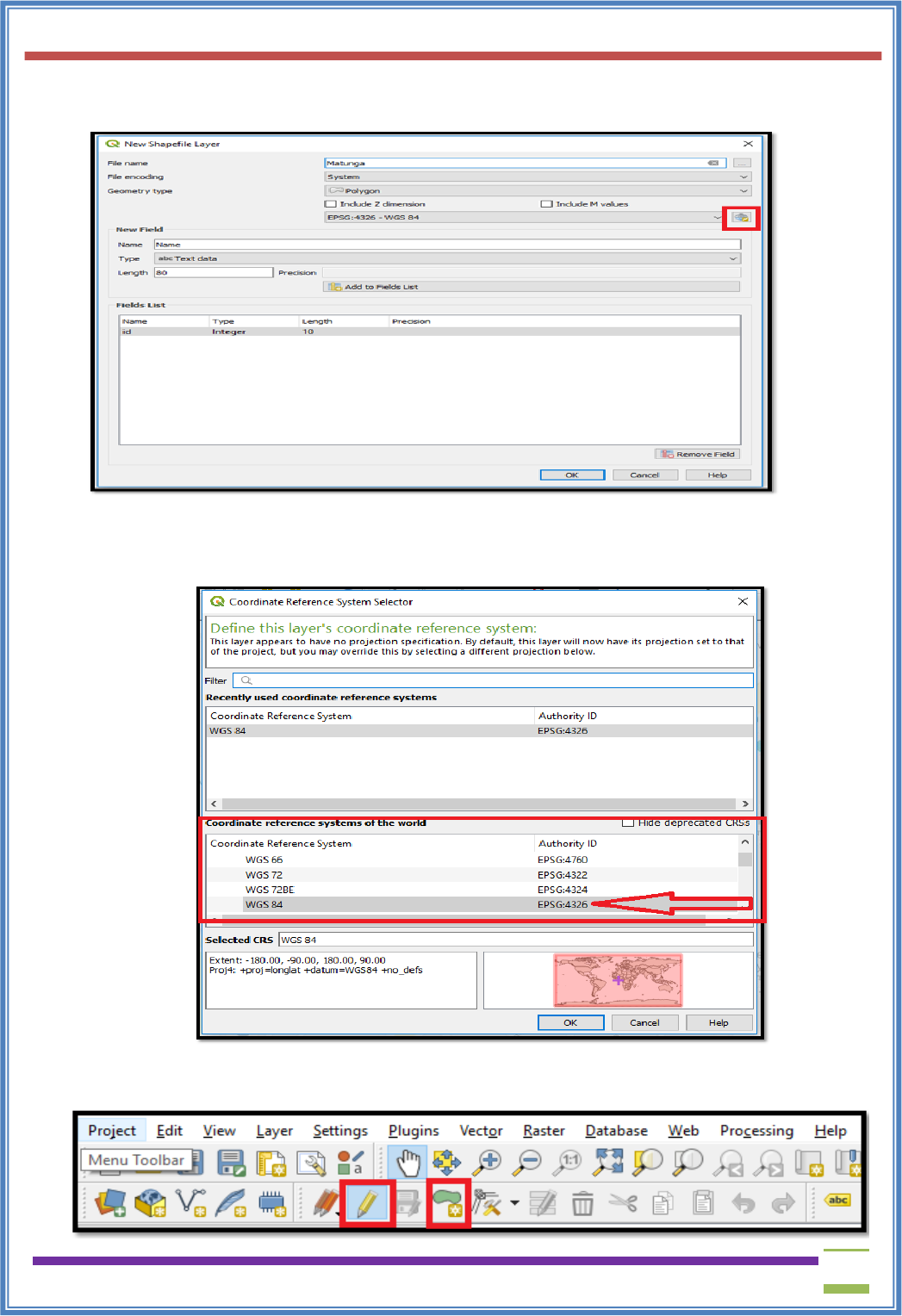
a) Creating Polygon vector layer
➢ Select Project→New
➢ Select Layer→Create Layer→New Shapefile Layer
➢ Following dialog box will appear on the screen. Select Polygon option from Geometry type.
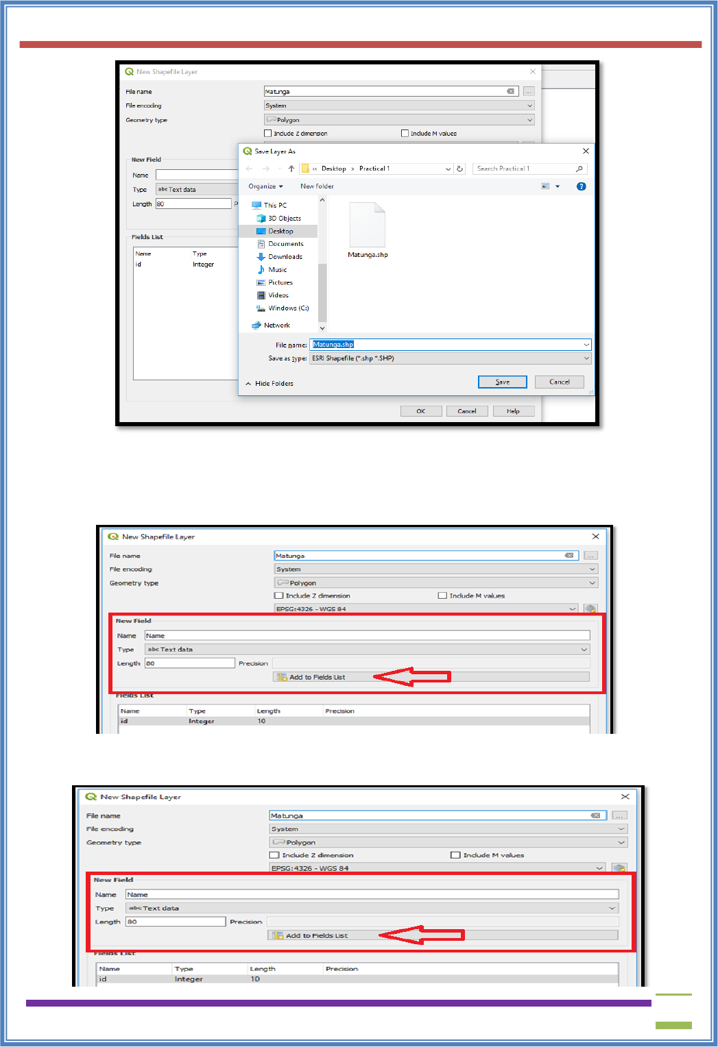
➢ Fill the appropriate information in each text box.
• File name :
▪ By default the file will be saved in bin folder.
▪ To avoid it click on following button to change the location of file.
USIT6P4 (Discipline Specific Elective Practical) Principles of Geographic Information Systems Practical
T. Y. B. Sc. (Information Technology) SEMESTER VI Teacher’s Reference Manual
16
➢ Field Panel
➢ Add the Attribute you want to show. (Column Name for Table)
b. Specify Type (DataType:Text Data/Decimal Data/Whole Number/Date) of Attribute
c. Specify the Length of the Attribute. Specify Precision (If Data Type is Decimal)
➢ Click on Add to Field List Button.
➢ You can add as many fields (Column Name) as you want for the layer.
USIT6P4 (Discipline Specific Elective Practical) Principles of Geographic Information Systems Practical
T. Y. B. Sc. (Information Technology) SEMESTER VI Teacher’s Reference Manual
17
➢ Select Geometry Type as follows
• Click on the following button
➢ The CRS dialog box will appear on screen. Click on the WGS84 option and it will be selected
as follows. click on OK
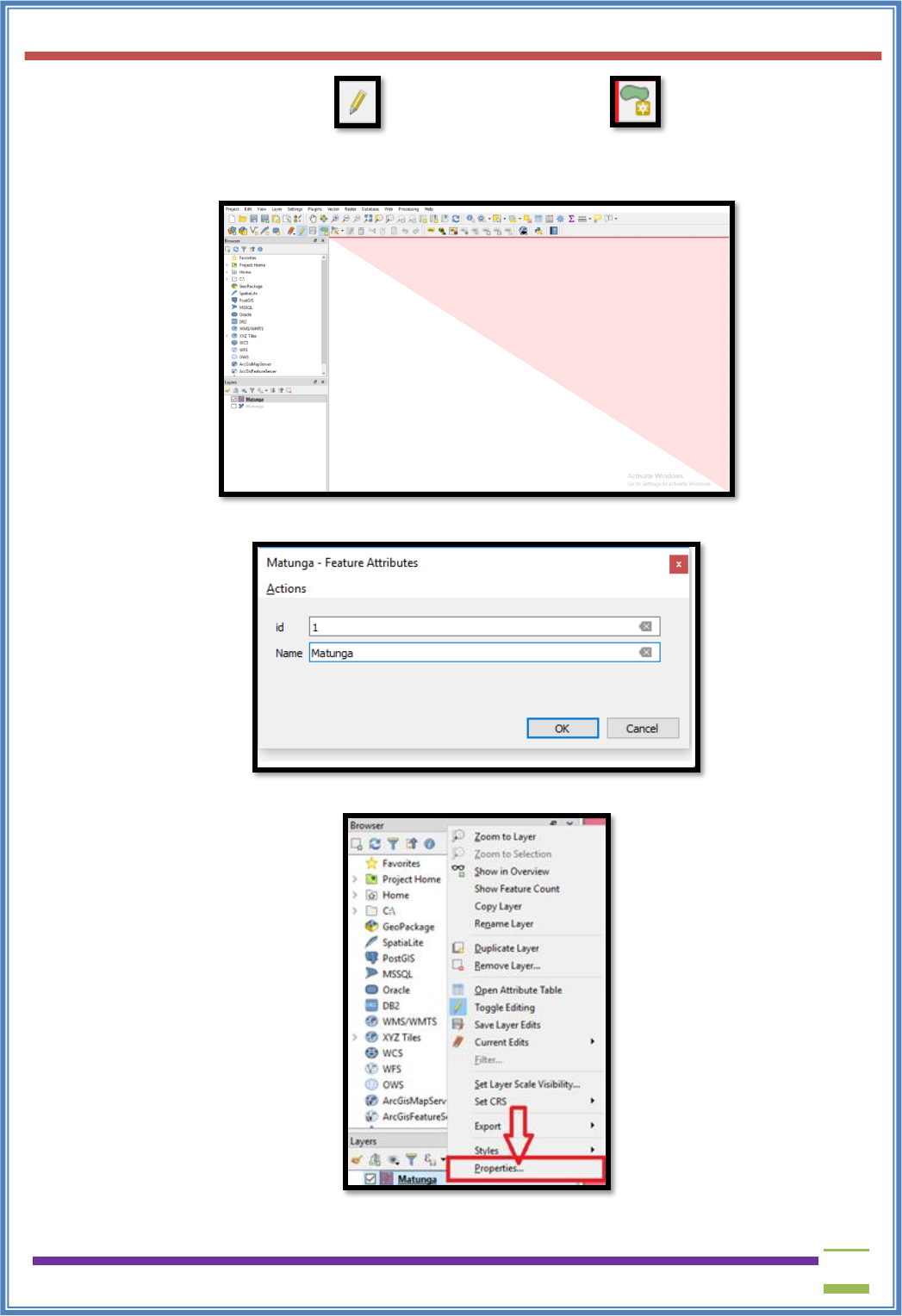
a) Follow the steps to plot Polygon features.
➢ Select the Polygon Feature( In our case it is Matunga for background) from layer panel
USIT6P4 (Discipline Specific Elective Practical) Principles of Geographic Information Systems Practical
T. Y. B. Sc. (Information Technology) SEMESTER VI Teacher’s Reference Manual
18
➢ Click Toggle Editing Button → Click on Add Polygon →Now place the cursor
at the location where you want to place the polygon. for polygon layer minimum 3 points
should be selected
➢ Save the newly added polygon as follows.
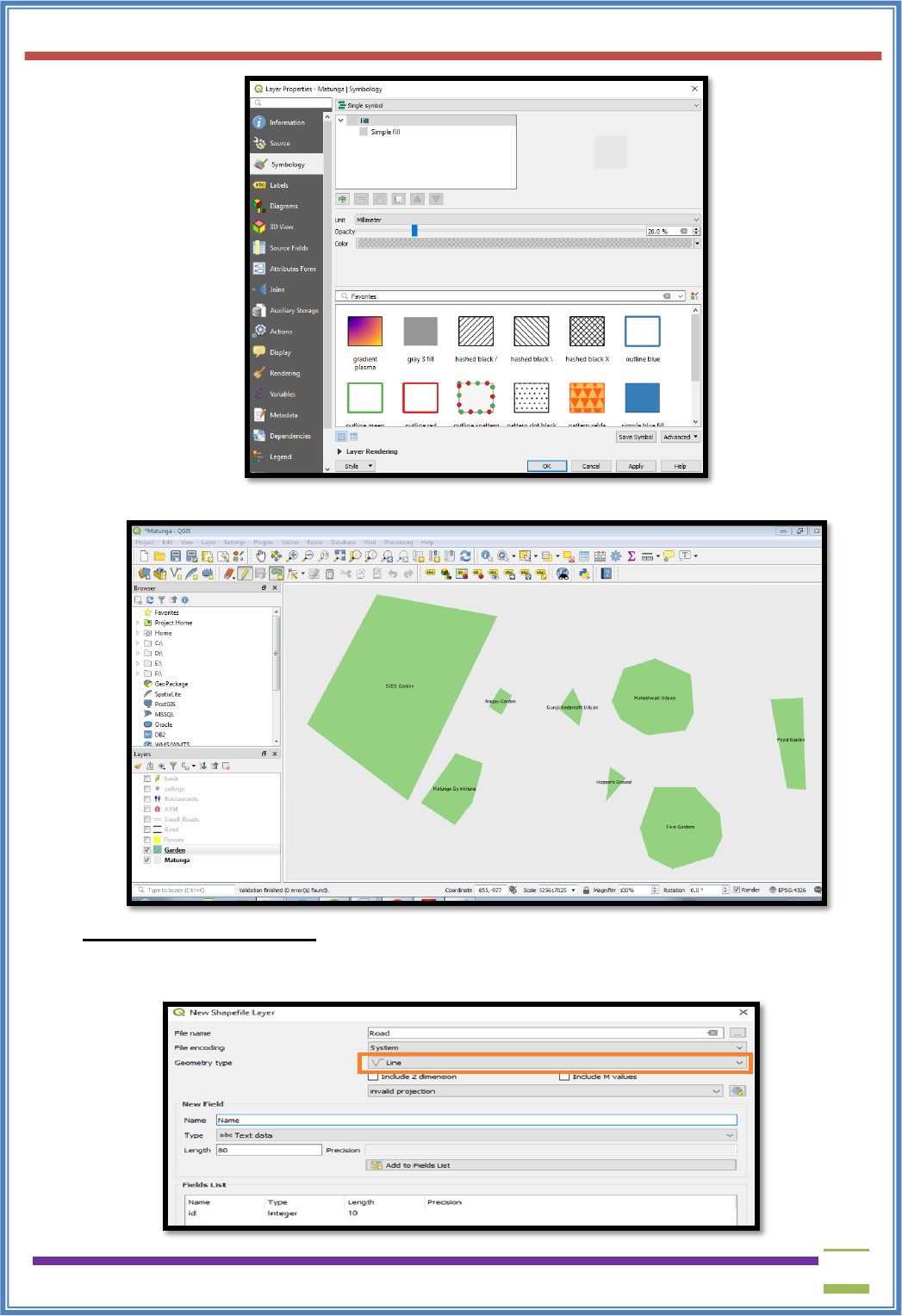
➢ Set style for polygon by using property window(Right click on Matunga Layer)
➢ Following screen will appear on the screen. Select pattern as you want and click on OK.
USIT6P4 (Discipline Specific Elective Practical) Principles of Geographic Information Systems Practical
T. Y. B. Sc. (Information Technology) SEMESTER VI Teacher’s Reference Manual
19
➢ Same way we can add one more polygon layer for Gardens.
b) Creating Line vector layer
➢ Repeat the same steps as we have done for polygon layer.
➢ Select geometry type Line.
USIT6P4 (Discipline Specific Elective Practical) Principles of Geographic Information Systems Practical
T. Y. B. Sc. (Information Technology) SEMESTER VI Teacher’s Reference Manual
20
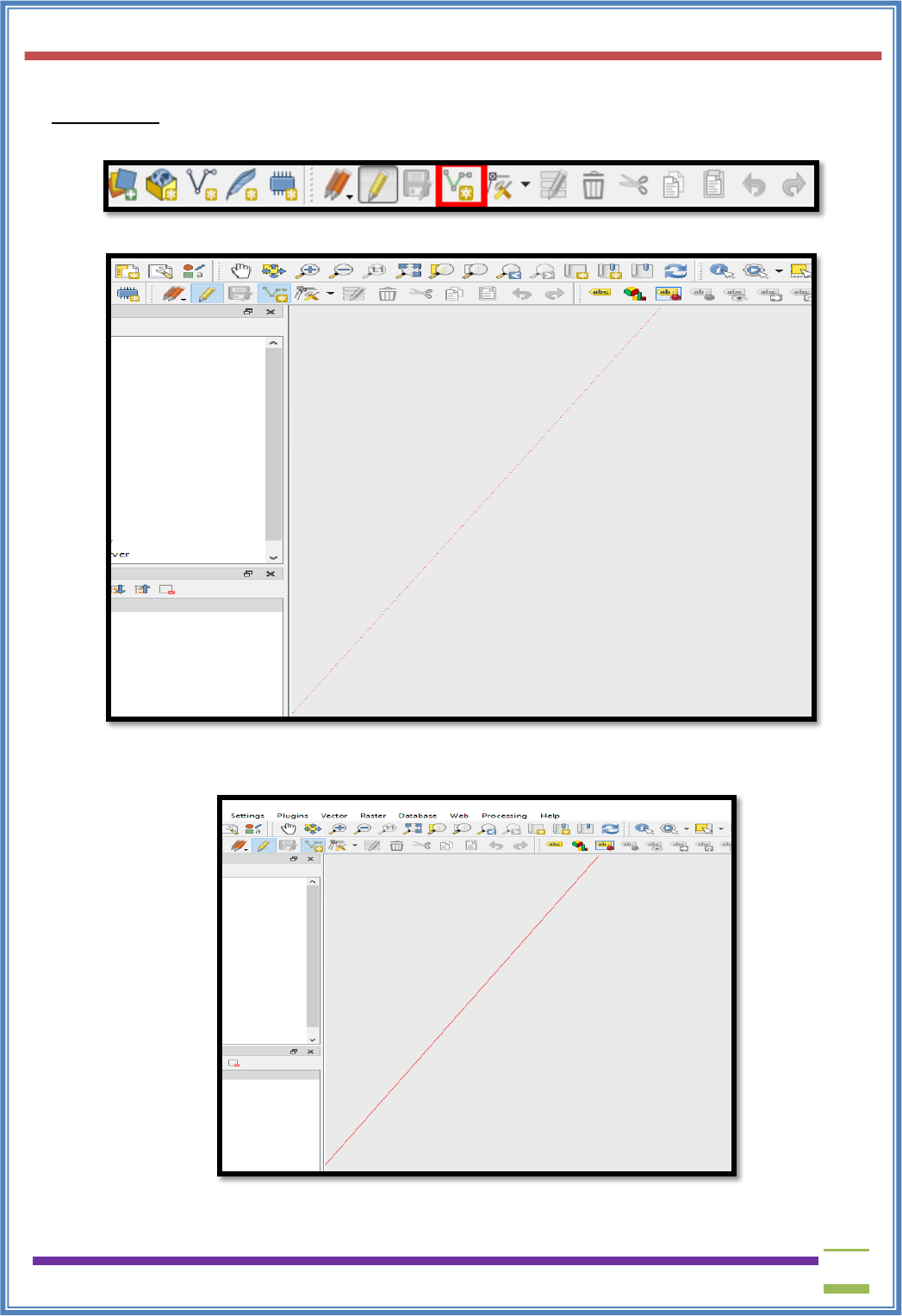
➢ Road layer :
➢ To plot road click on Add Line Feature.
➢ Click on the map where you want to draw line.
➢ Once you are done then right click on map (Dotted line turn into solid line)
➢ save your data
USIT6P4 (Discipline Specific Elective Practical) Principles of Geographic Information Systems Practical
T. Y. B. Sc. (Information Technology) SEMESTER VI Teacher’s Reference Manual
21
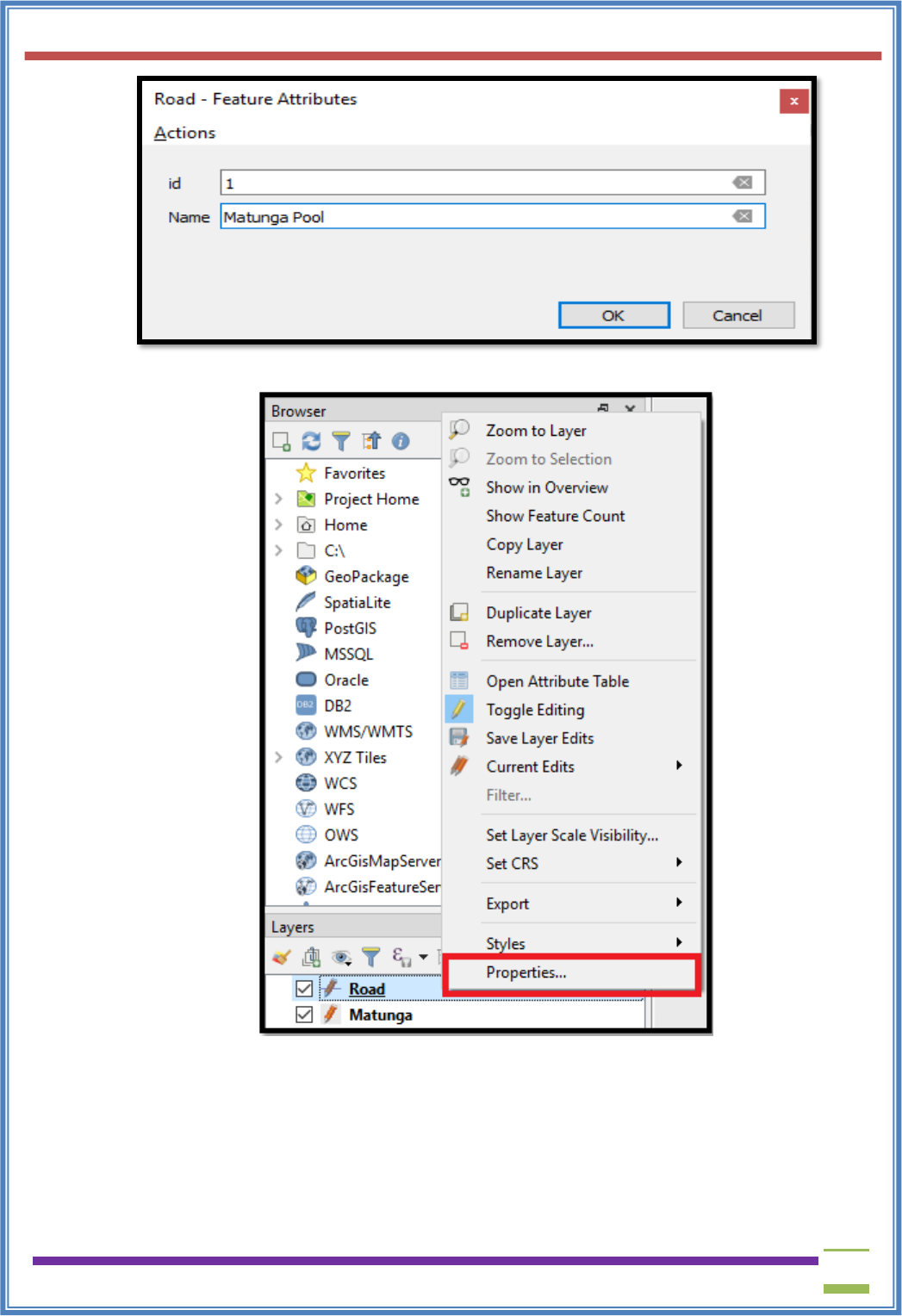
➢ set style for Roads in the same way as we have done for polygon
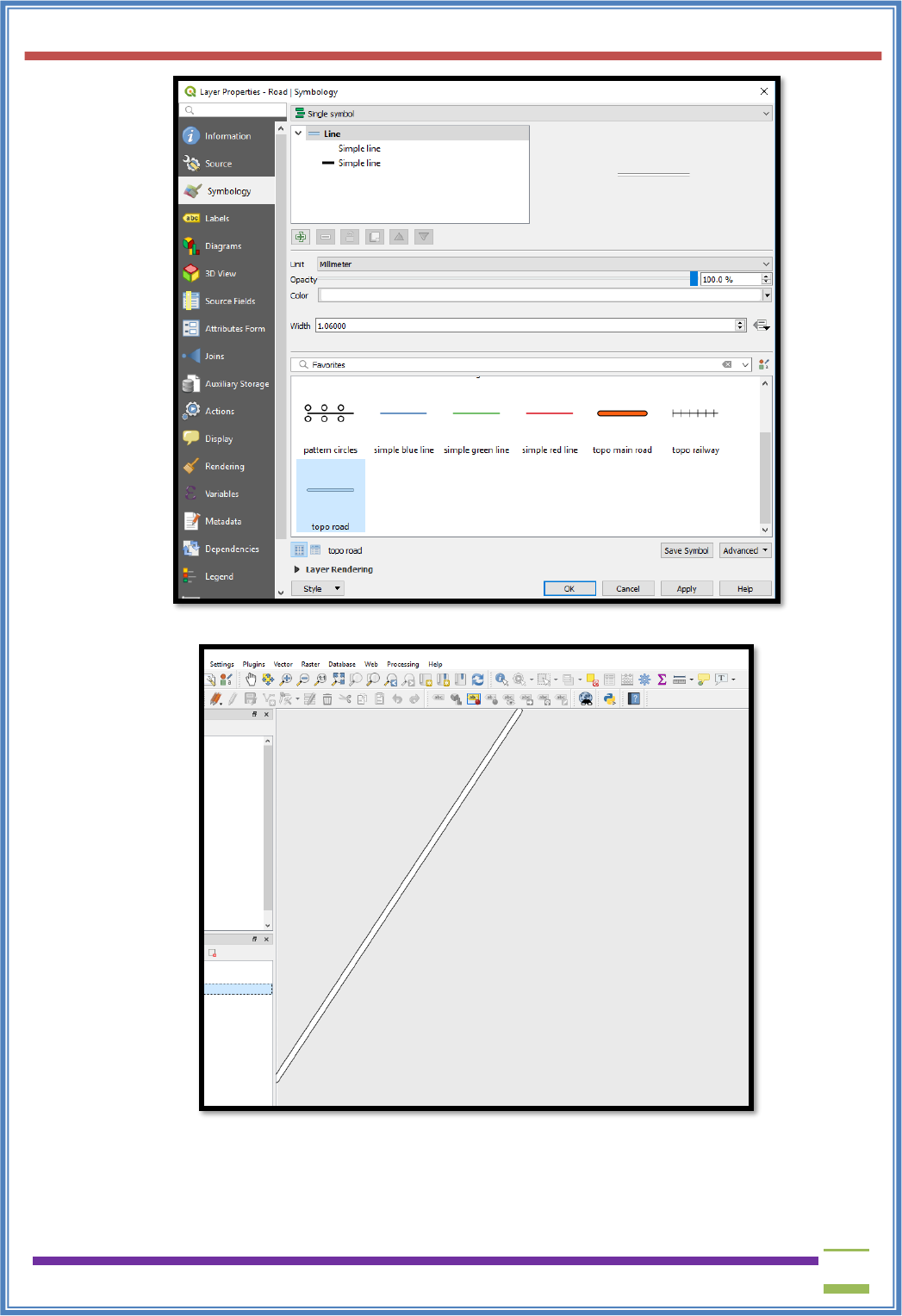
USIT6P4 (Discipline Specific Elective Practical) Principles of Geographic Information Systems Practical
T. Y. B. Sc. (Information Technology) SEMESTER VI Teacher’s Reference Manual
22
➢ Road will look as below
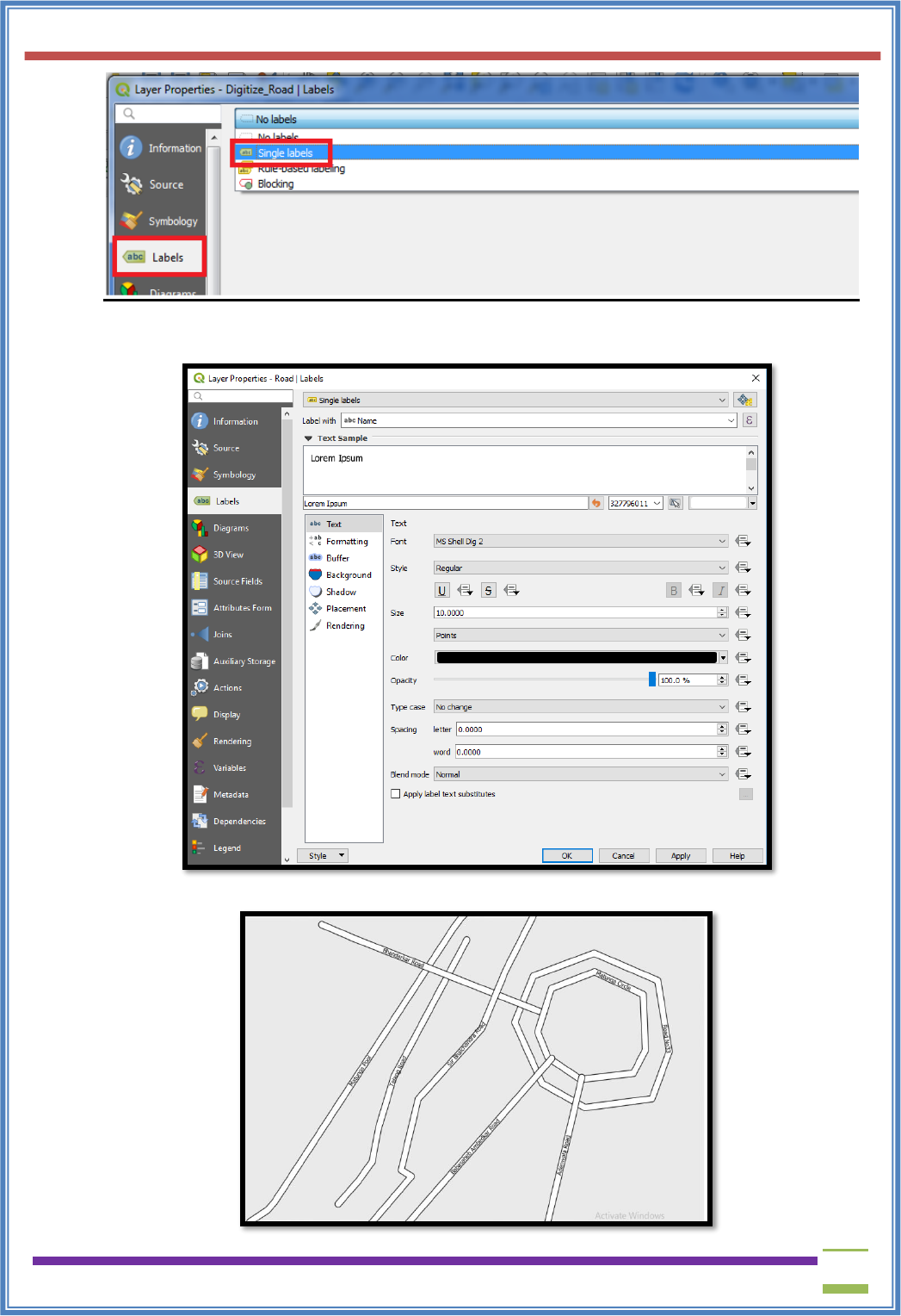
➢ To label your roads Right click on Road layer .Go to properties window then select label and
set single label property
USIT6P4 (Discipline Specific Elective Practical) Principles of Geographic Information Systems Practical
T. Y. B. Sc. (Information Technology) SEMESTER VI Teacher’s Reference Manual
23
➢ Following window will appear on the screen
➢ Roads will look like these
USIT6P4 (Discipline Specific Elective Practical) Principles of Geographic Information Systems Practical
T. Y. B. Sc. (Information Technology) SEMESTER VI Teacher’s Reference Manual
24
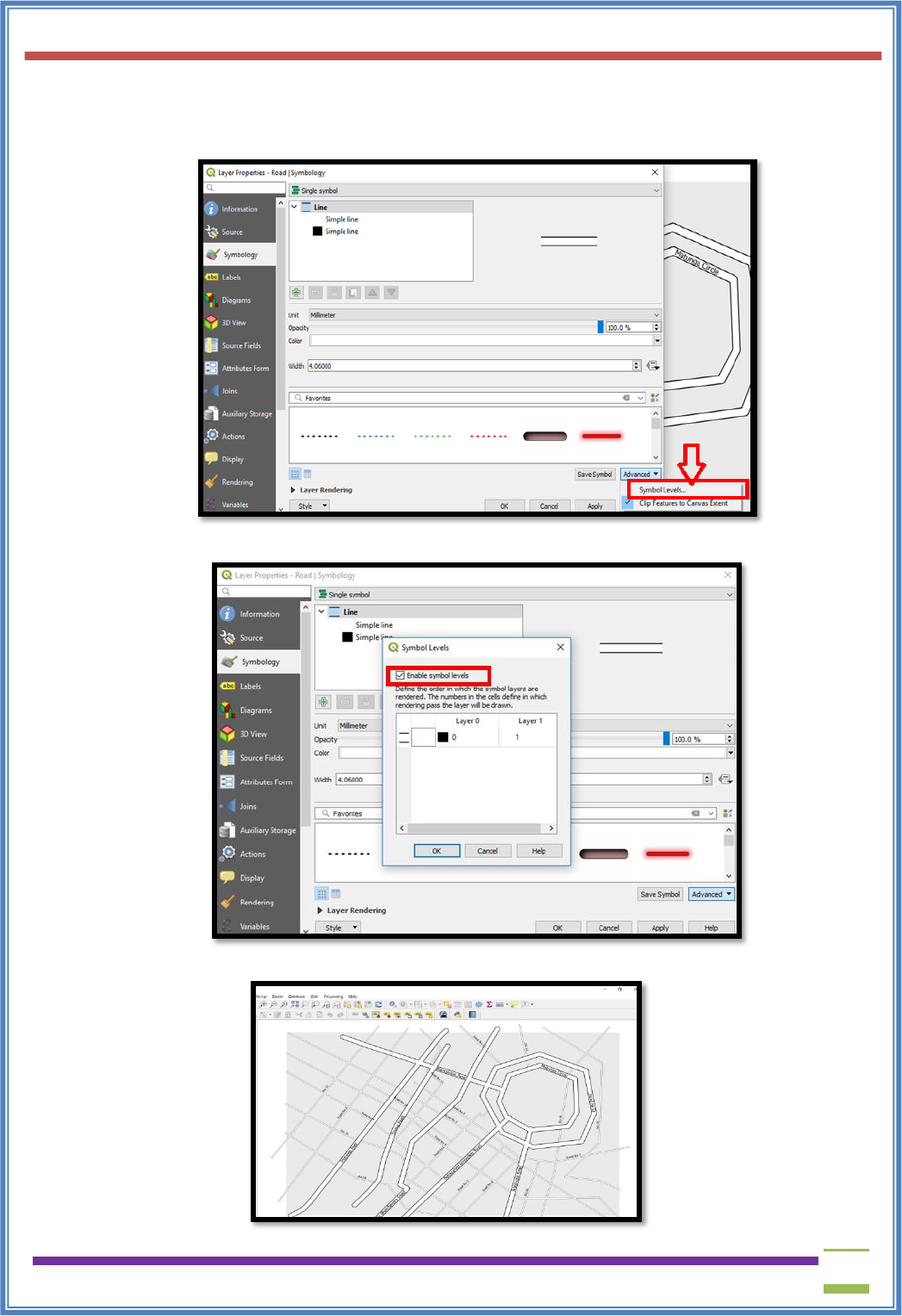
➢ To merge roads
• Go to properties of road then select symbology. Click on Advanced button select
Symbol levels.
➢ Check Enable symbol levels option
➢ Click ok & Road will appear as follows
USIT6P4 (Discipline Specific Elective Practical) Principles of Geographic Information Systems Practical
T. Y. B. Sc. (Information Technology) SEMESTER VI Teacher’s Reference Manual
25
C. Create Point vector layer
➢ Repeat same steps to add point layers as we have done in previous layers.(For
ATM, Restaurants, Banks, Bus Stops etc)
Final output:
USIT6P4 (Discipline Specific Elective Practical) Principles of Geographic Information Systems Practical
T. Y. B. Sc. (Information Technology) SEMESTER VI Teacher’s Reference Manual
26
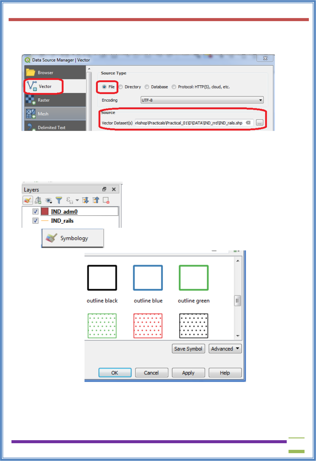
d) Calculating line lengths and statistics
➢ Go to Layer → Add Layer → Add Vector Layer
➢ Add the following file to project
"\GIS_Workshop\Practicals\Practical_01\D\DATA\IND_rrd\IND_rails.shp"
Press “ADD”
➢ Also add India Administrative Map
“GIS_Workshop\Practicals\Practical_01\D\DATA\IND_adm\IND_adm0.shp”
➢ Double Click on IND_adm0
Select → Select any outline style from below given options.
Press OK
➢ The display window will appear like
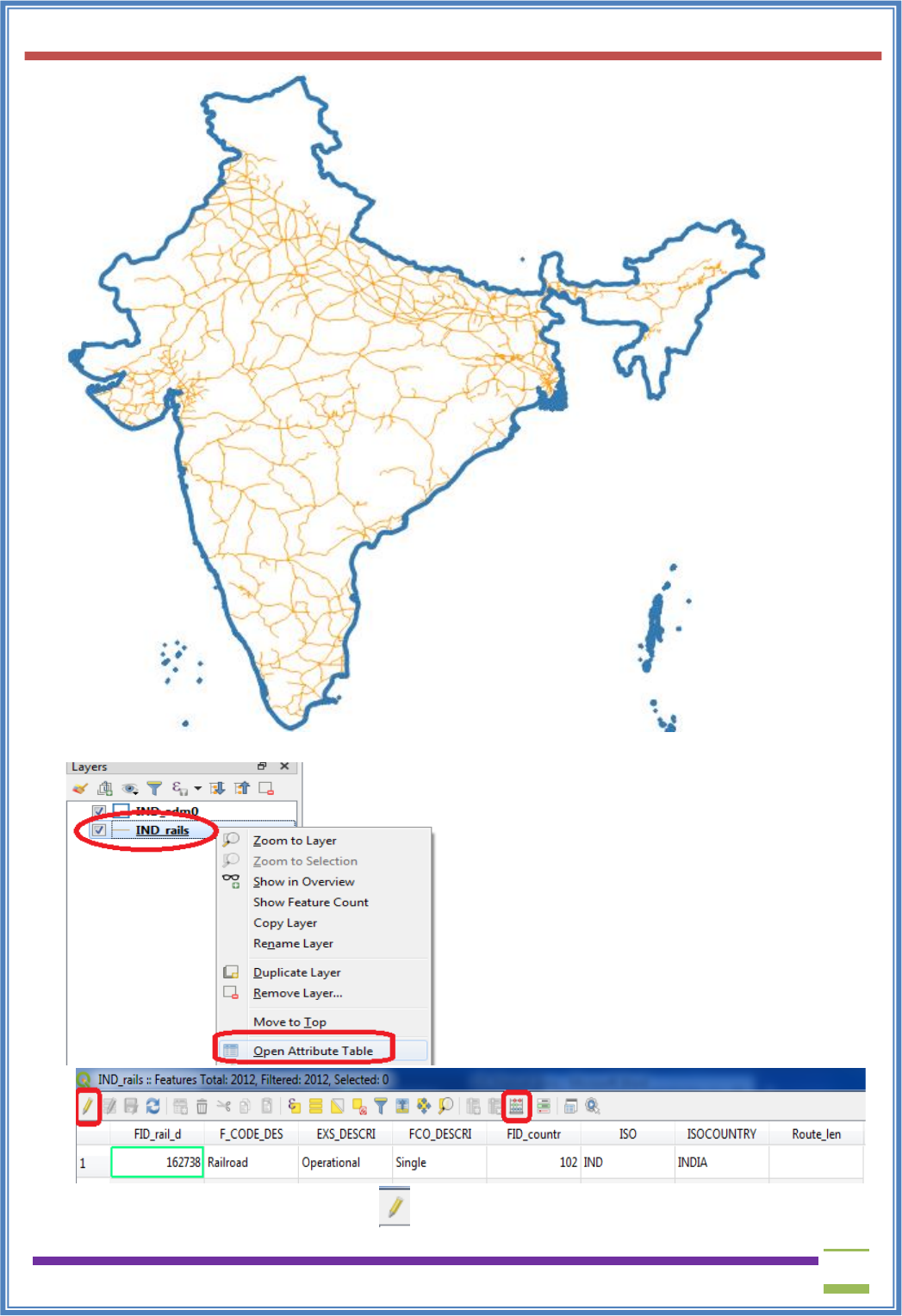
USIT6P4 (Discipline Specific Elective Practical) Principles of Geographic Information Systems Practical
T. Y. B. Sc. (Information Technology) SEMESTER VI Teacher’s Reference Manual
27
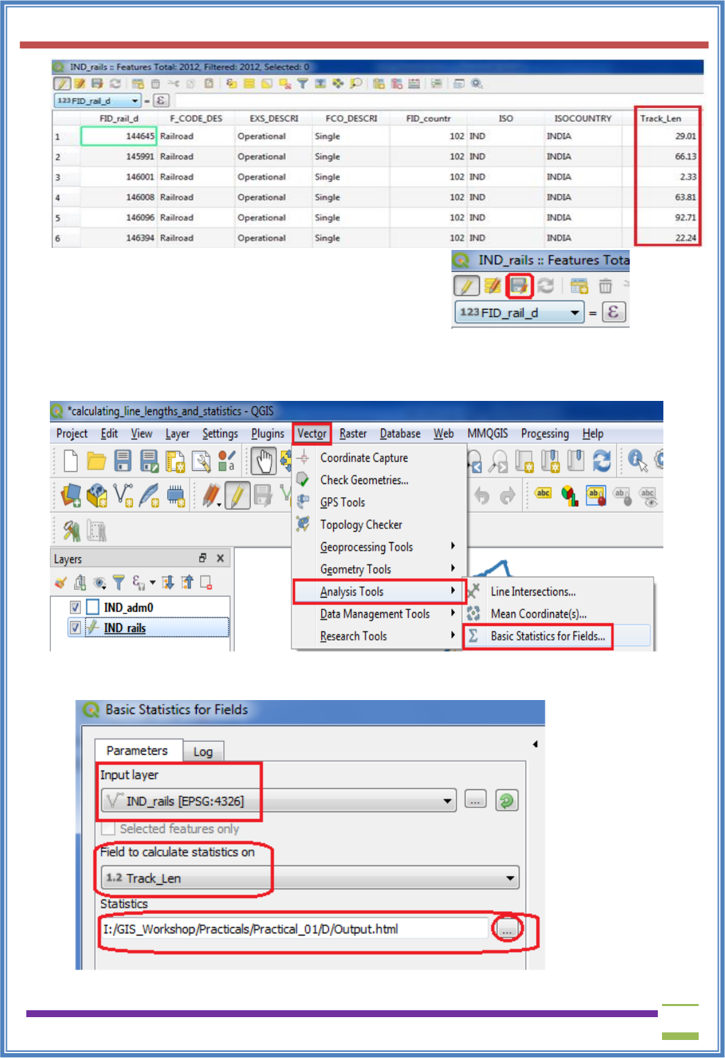
➢ In Layer Pane, Right click on IND_rails → Open Attribute Table
➢ Press Toggle Editing button using button, on Attribute table window toolbar.
USIT6P4 (Discipline Specific Elective Practical) Principles of Geographic Information Systems Practical
T. Y. B. Sc. (Information Technology) SEMESTER VI Teacher’s Reference Manual
28
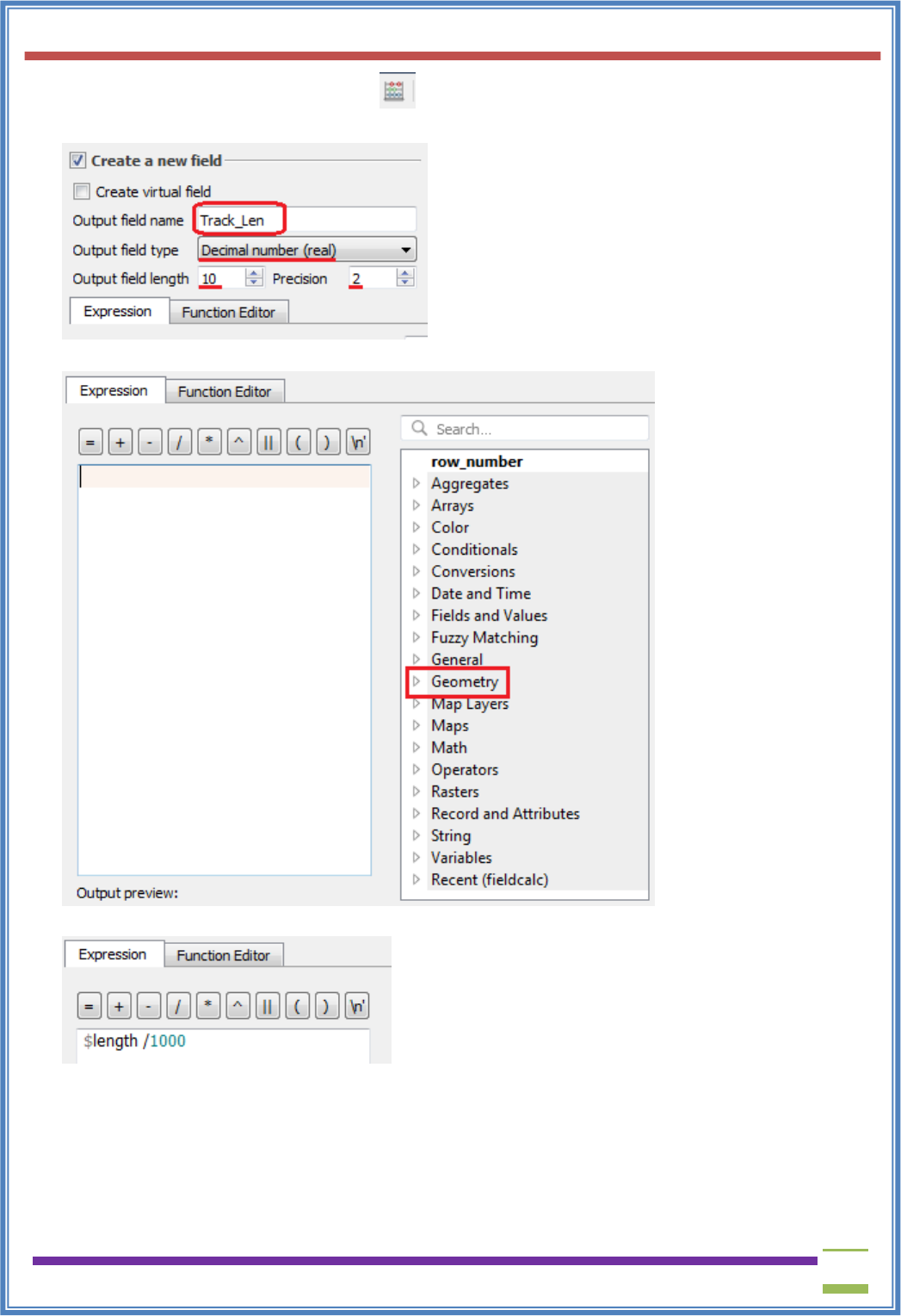
➢ Press Open Field Calculator using button.
➢ Set the output field as “Track_Len”, field type to “Decimal Number”.
➢ From Function List search $length or go to Geometry → Select $length
➢ Set expression as
Press “OK”
➢ A new column is added to the attribute table with value representing the length of track in KM.
USIT6P4 (Discipline Specific Elective Practical) Principles of Geographic Information Systems Practical
T. Y. B. Sc. (Information Technology) SEMESTER VI Teacher’s Reference Manual
29
➢ Press CTRL+S or click on Save Edits option on tool bar
➢ Close the attribute table window.
➢ For calculating the total length of Railway tracks in India.
➢ Select Vector→ Analysis Tools→ Basic Statics for Fields
➢ Select IND_rails layer from input layer. And select Track_Len in “Field to Calculate statistics
on”
➢ Press RUN
USIT6P4 (Discipline Specific Elective Practical) Principles of Geographic Information Systems Practical
T. Y. B. Sc. (Information Technology) SEMESTER VI Teacher’s Reference Manual
30
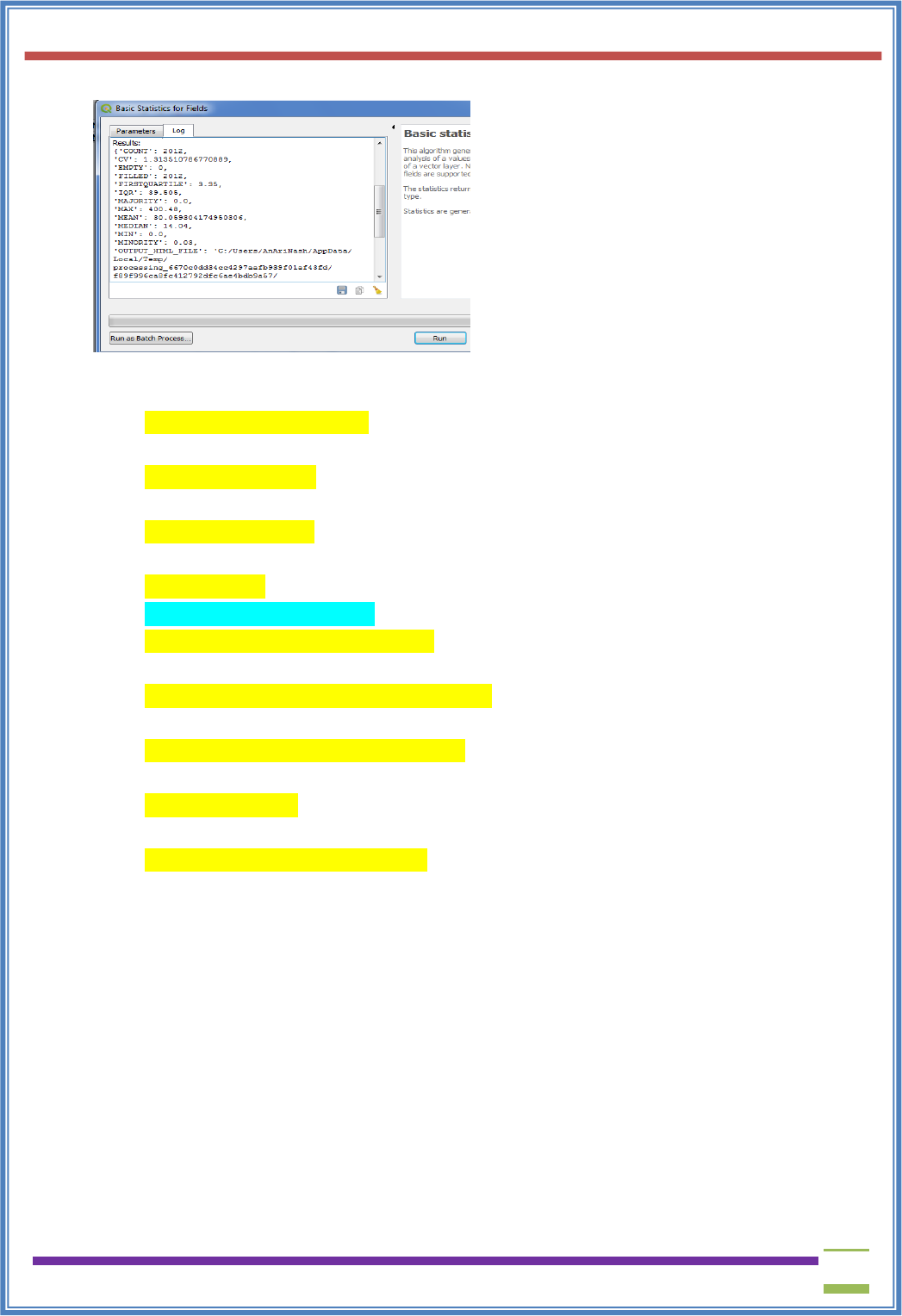
➢ The Result is
➢ Open the “output.html” file to get the field statistics.
Analyzed field: Track_Len
Count: 2012
Unique values: 1608
NULL (missing) values: 0
Minimum value: 0.0
Maximum value: 400.48
Range: 400.48
Sum: 60479.320000000014
Mean value: 30.059304174950306
Median value: 14.04
Standard deviation: 39.483220276624444
Coefficient of Variation: 1.313510786770889
Minority (rarest occurring value): 0.03
Majority (most frequently occurring value): 0.0
First quartile: 3.35
Third quartile: 42.855000000000004
Interquartile Range (IQR): 39.505
➢ The above statistics show that the total length of Railway track in India is 60,479.32 KM.
USIT6P4 (Discipline Specific Elective Practical) Principles of Geographic Information Systems Practical
T. Y. B. Sc. (Information Technology) SEMESTER VI Teacher’s Reference Manual
31
PRACTICAL - 2
Exploring and Managing Raster data:
a) Adding raster layers
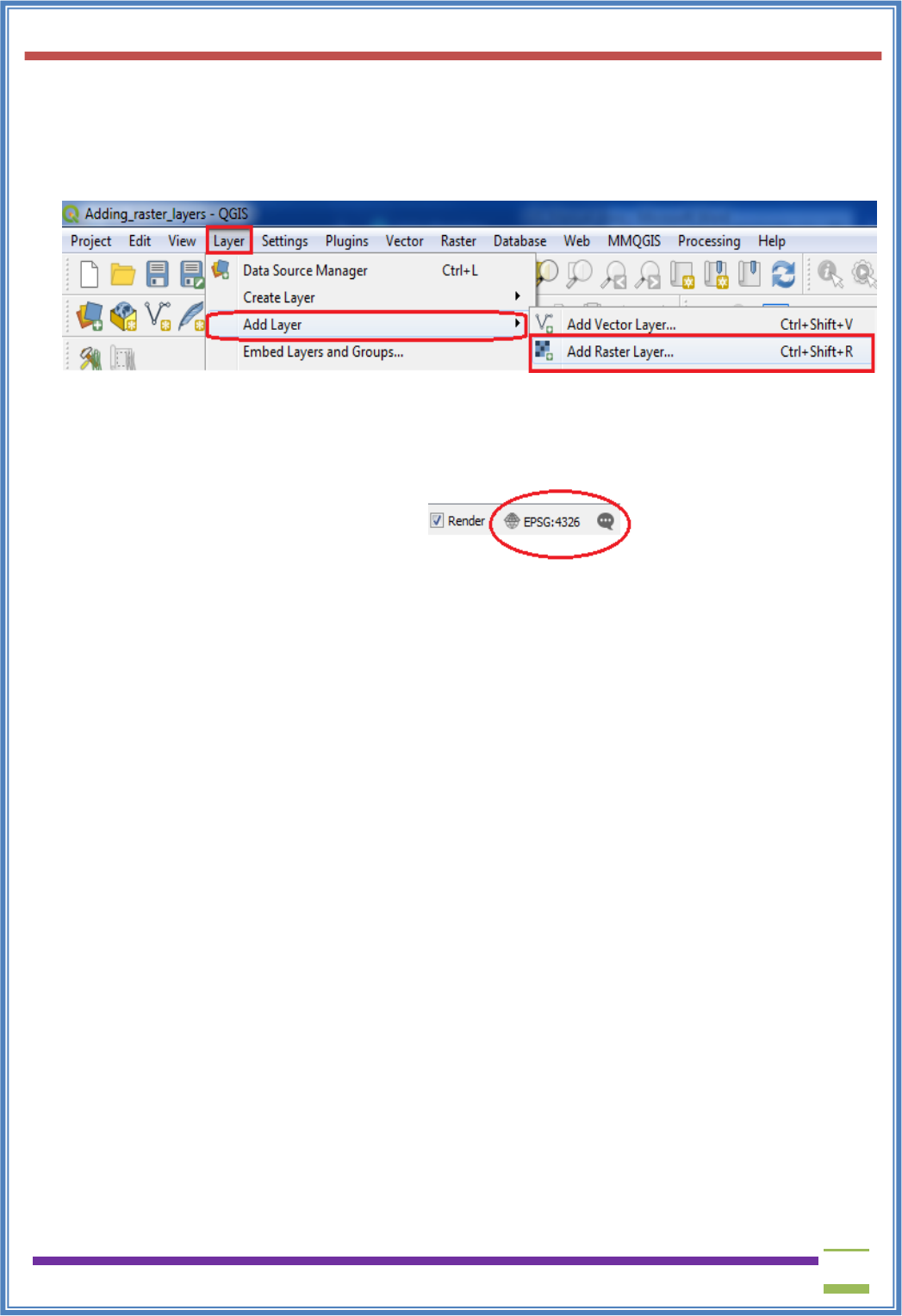
➢ From menu bar select Layer → Add Layer → Add Raster Layer
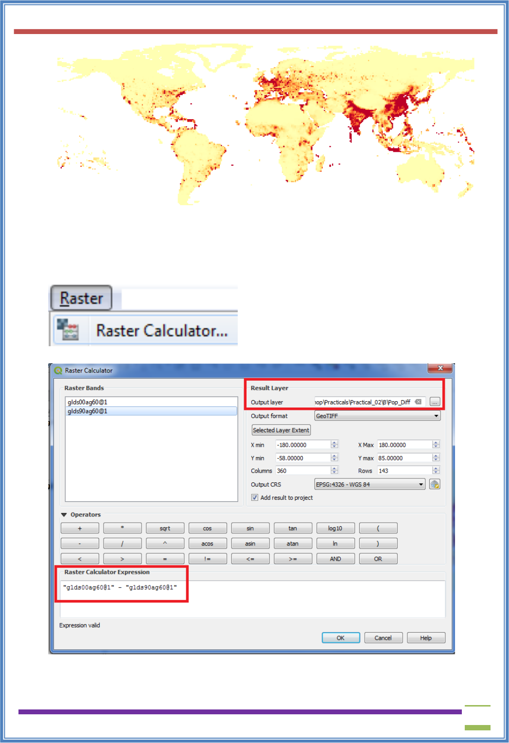
➢ Select Gridded Population of the World (GPW) v3 dataset from Columbia University,
Population Density Grid for the entire globe in ASCII format and for the year 1990 and 2000.
“\GIS_Workshop\Practicals\Practical_02\A\Data\gl_gpwv3_pdens_90_ascii_one\glds90ag60.asc”
“\GIS_Workshop\Practicals\Practical_02\A\Data\gl_gpwv3_pdens_90_ascii_one\glds00ag60.asc”
➢ Go to Project → Properties OR Press the Set CRS option on bottom
right corner.
Select WGS 84 EPSG: 4326 and Press OK
USIT6P4 (Discipline Specific Elective Practical) Principles of Geographic Information Systems Practical
T. Y. B. Sc. (Information Technology) SEMESTER VI Teacher’s Reference Manual
32
b) Raster Styling and Analysis
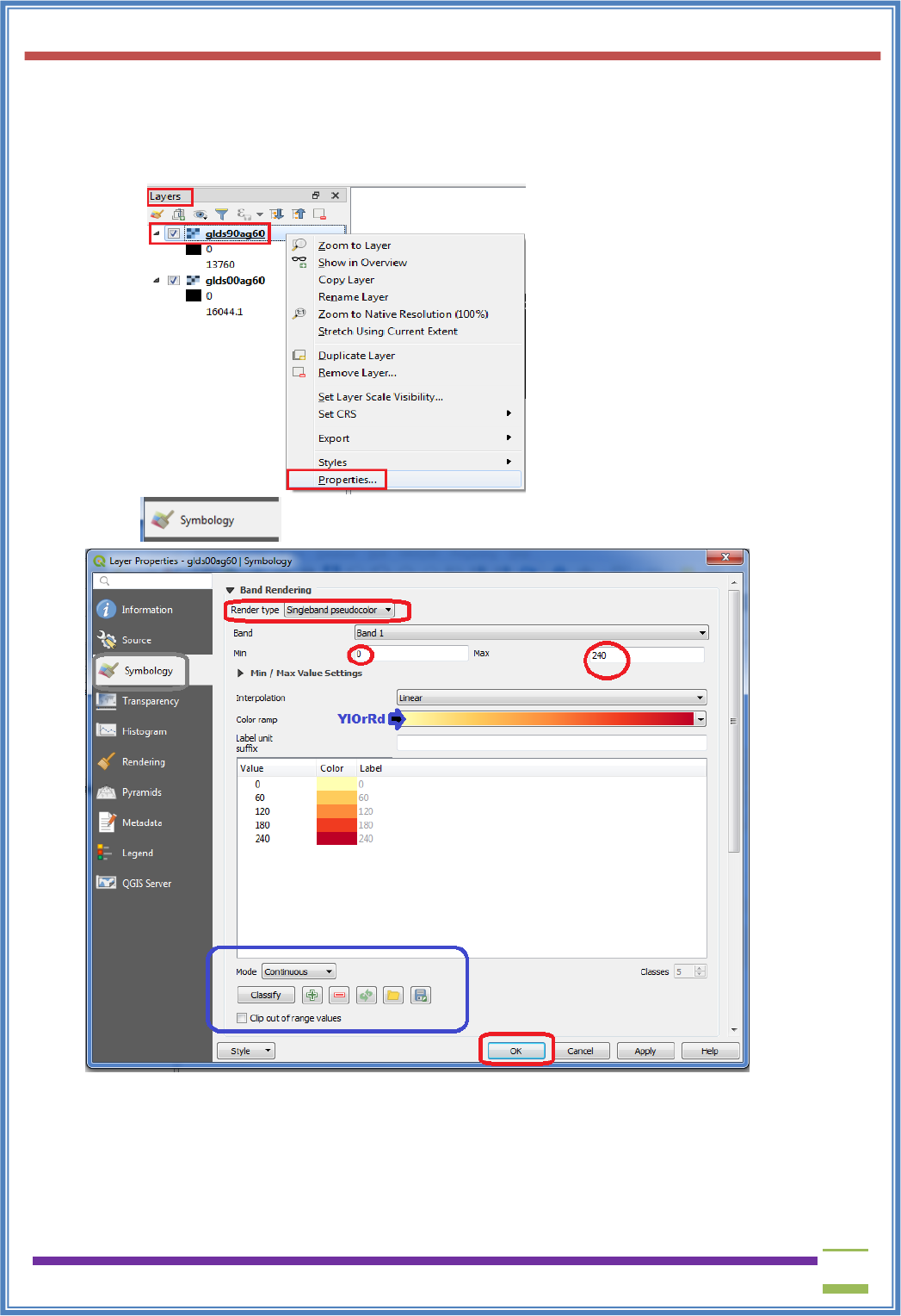
➢ To start with analysis of population data, convert the pixel from grayscale to Color.
➢ Select “glds90ag60.asc” Layer form layer Pane → select property OR double click on it.
➢ Select
➢ Press “APPLY”
➢ Repeat the same for “glds00ag60.asc” Layer
USIT6P4 (Discipline Specific Elective Practical) Principles of Geographic Information Systems Practical
T. Y. B. Sc. (Information Technology) SEMESTER VI Teacher’s Reference Manual
33
Layer output after applying style.
➢ The objective this experiment is to analyze raster data, as an example we will find areas with
largest population change between 1990 and 2000, by calculating the difference between each
pixel values.
➢ Go to Raster → Raster Calculator
➢ Put the expression "glds00ag60@1" - "glds90ag60@1"
➢ Select the output file location & name and Press OK.
USIT6P4 (Discipline Specific Elective Practical) Principles of Geographic Information Systems Practical
T. Y. B. Sc. (Information Technology) SEMESTER VI Teacher’s Reference Manual
34
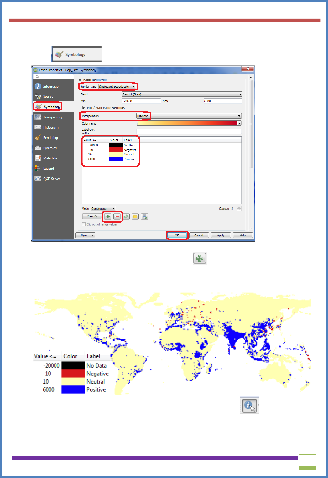
➢ Remove the other two layers i.e. glds00ag60.asc and glds90ag60.asc
➢ Double click on pop_diff layer.
➢ Select
➢ Set Render Type to “Single band Pseudo color”, Interpolation as Discrete, and remove all
classification and add as shown in figure above using button. After all settings press
“OK”.
➢ Layer will appear like
➢ Explore an area of your choice and check the raster band value using to verify the
classification rule.
➢ The red pixel shows negative changes and blue shows positive changes.
USIT6P4 (Discipline Specific Elective Practical) Principles of Geographic Information Systems Practical
T. Y. B. Sc. (Information Technology) SEMESTER VI Teacher’s Reference Manual
35
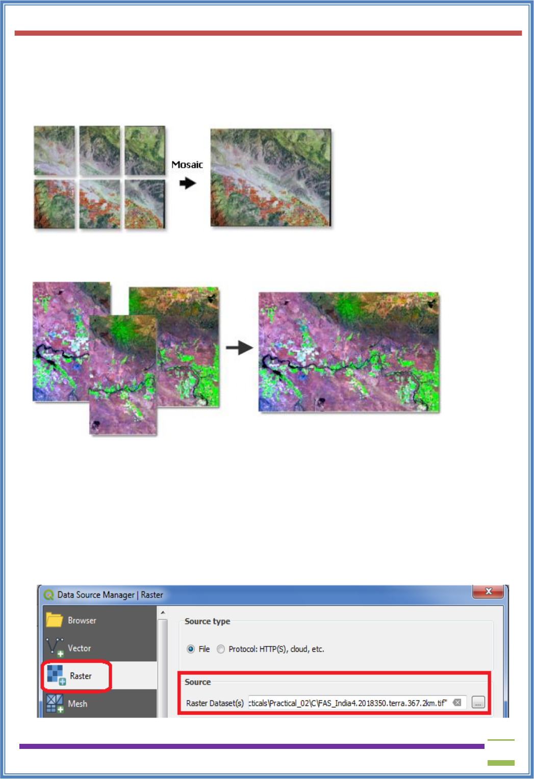
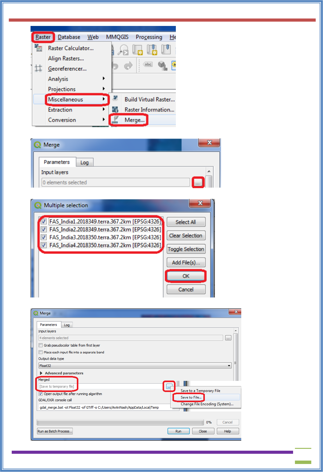
c) Raster Mosaicking and Clipping
A mosaic is a combination or merge of two or more images.
In GIS, a single raster dataset can be created from multiple raster datasets by mosaicking them
together.
In many cases, there will be some overlap of the raster dataset edges that are being mosaicked
together, as shown below.
These overlapping areas can be handled in several ways; for example, you can choose to only keep
raster data from the first or last dataset, you can blend the overlapping cell values using a weight-
based algorithm, you can take the mean of the overlapping cell values, or you can take the
minimum or maximum value. When mosaicking discrete data, the First, Minimum, or Maximum
options give the most meaningful results. The Blend and Mean options are best suited for
continuous data. If any of the input rasters are floating point, the output is floating point. If all the
inputs are integer and First, Minimum, or Maximum is used, the output is integer.
➢ Go to Layer → Add Layer → Add Raster Layer.
USIT6P4 (Discipline Specific Elective Practical) Principles of Geographic Information Systems Practical
T. Y. B. Sc. (Information Technology) SEMESTER VI Teacher’s Reference Manual
36
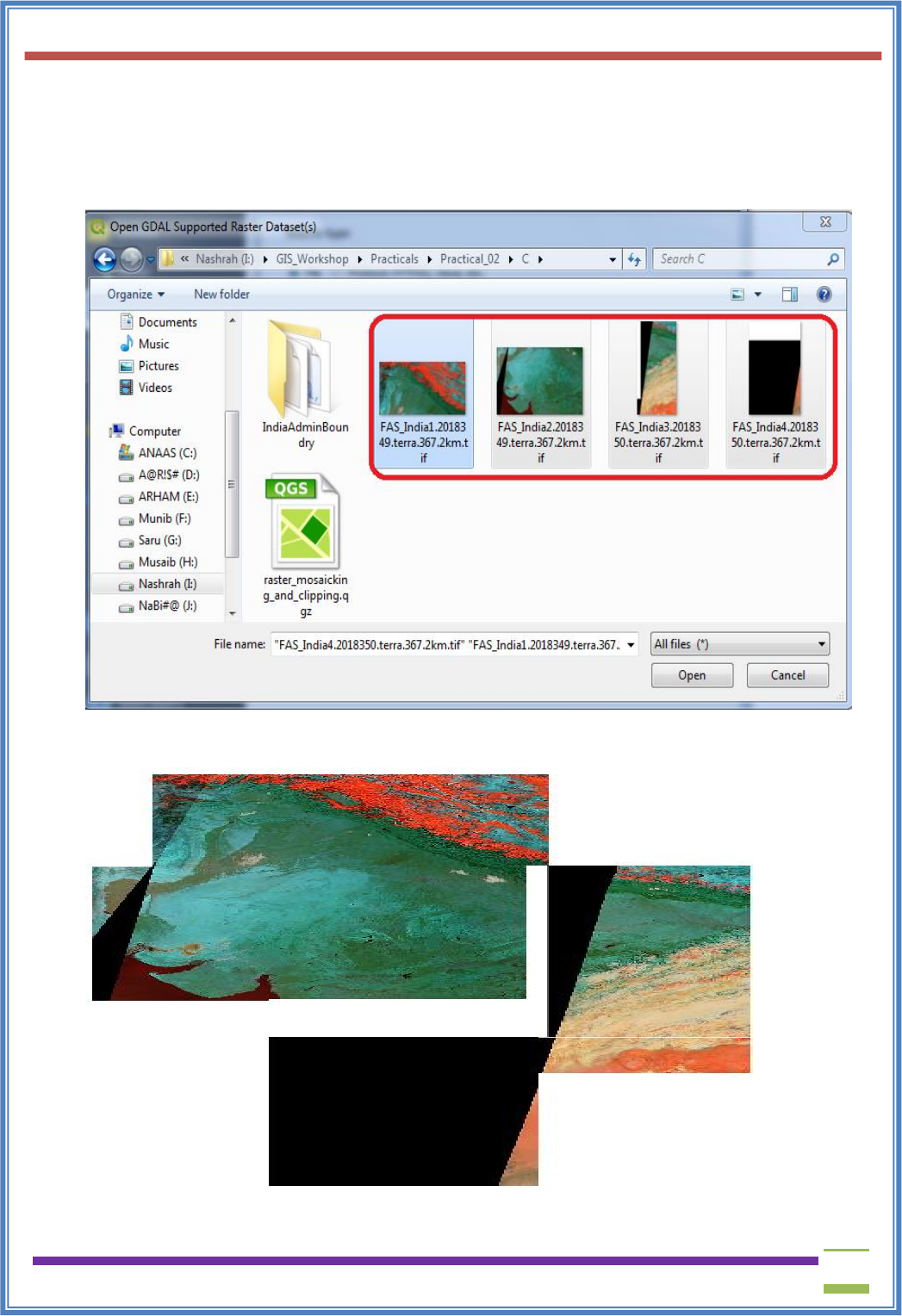
➢ Select the following “.tif” raster images for India from data folder.
FAS_India1.2018349.terra.367.2km.tif
FAS_India2.2018349.terra.367.2km.tif
FAS_India3.2018349.terra.367.2km.tif
FAS_India4.2018349.terra.367.2km.tif
➢ Press open
➢ In data source manager | Raster window click Add.
➢ Go to Raster → Miscellaneous → Merge
USIT6P4 (Discipline Specific Elective Practical) Principles of Geographic Information Systems Practical
T. Y. B. Sc. (Information Technology) SEMESTER VI Teacher’s Reference Manual
37
➢ In the Merge dialog window
➢ Select all layers and Press OK.
➢ In Merge dialog window select a file name and location to save merged images.
USIT6P4 (Discipline Specific Elective Practical) Principles of Geographic Information Systems Practical
T. Y. B. Sc. (Information Technology) SEMESTER VI Teacher’s Reference Manual
38
➢ Save the file to “GIS_Workshop/Practicals/Practical_02/C/” location with the name as
Merge_Files.tif
➢ Press Run and after completion of operation close the Merge window dialog box.
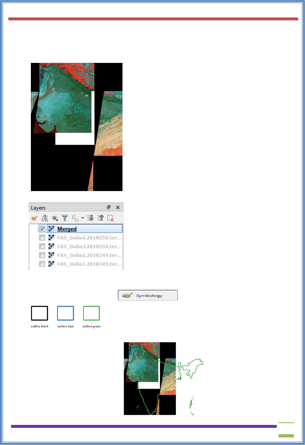
➢ You can now deselect individual layers from layer pane and only keep the merged raster file.
➢ Go to Layer→ Add Vector Layer → Select
\GIS_Workshop\Practicals\Practical_02\C\IndiaAdminBoundry\IND_adm0.shp file.
➢ From layer properties → select → select any one of the following
➢ The result will be
USIT6P4 (Discipline Specific Elective Practical) Principles of Geographic Information Systems Practical
T. Y. B. Sc. (Information Technology) SEMESTER VI Teacher’s Reference Manual
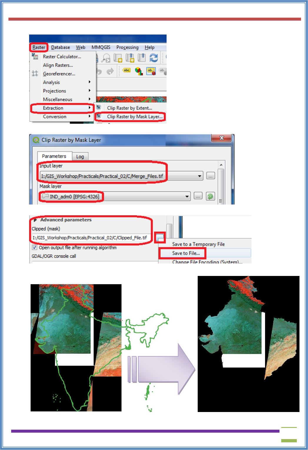
39
➢ Go to Raster → Extraction → Clip Raster by Mask Layer
➢ Select the merge raster image as input and Ind_adm0 as mask layer.
➢ Select a file name and location for clipped raster as /Practical_02/C/Clipped_File.tif.
➢ Press RUN.
After
Clipping
USIT6P4 (Discipline Specific Elective Practical) Principles of Geographic Information Systems Practical
T. Y. B. Sc. (Information Technology) SEMESTER VI Teacher’s Reference Manual
40
PRACTICAL - 3
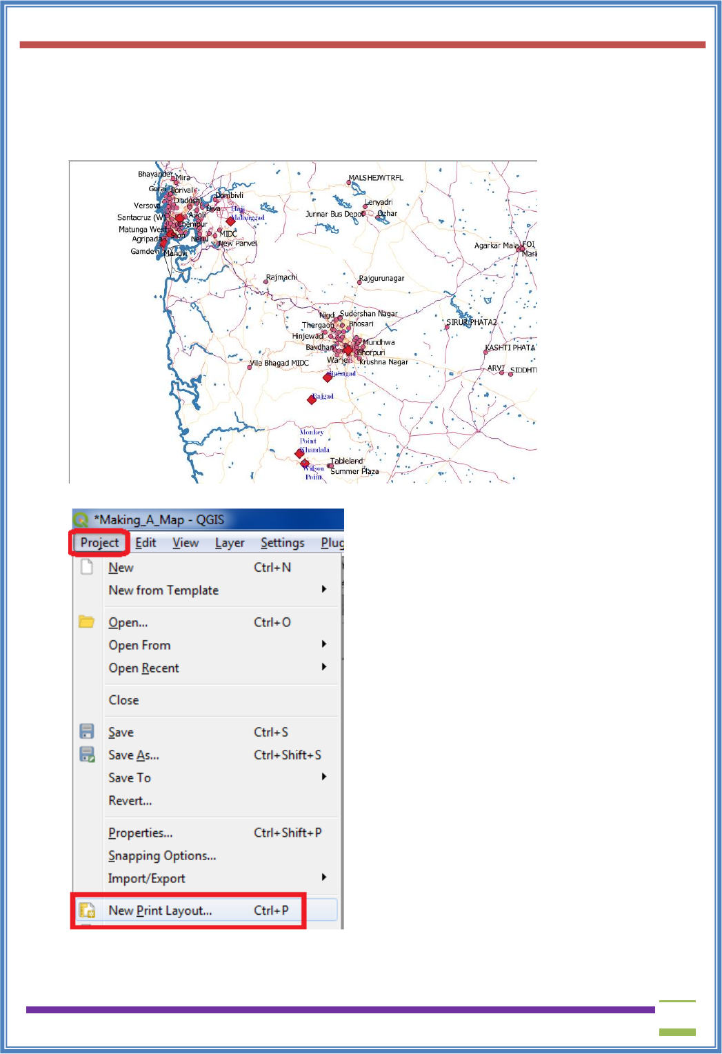
a) Making a Map
➢ Create a new Thematic Map or open and existing one
➢ Consider the following map as an example map
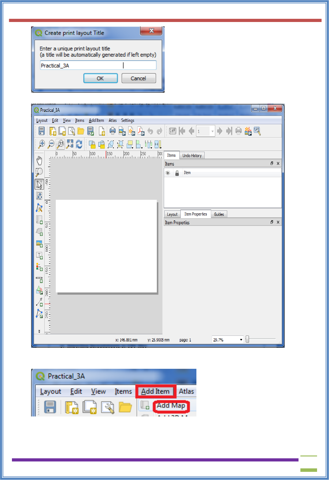
➢ Go to Project → New PrintLayout
➢ Insert a suitable title and press “OK”.
USIT6P4 (Discipline Specific Elective Practical) Principles of Geographic Information Systems Practical
T. Y. B. Sc. (Information Technology) SEMESTER VI Teacher’s Reference Manual
41
➢ A new Print Layout window will open
➢ Select Add Item → Add Map
USIT6P4 (Discipline Specific Elective Practical) Principles of Geographic Information Systems Practical
T. Y. B. Sc. (Information Technology) SEMESTER VI Teacher’s Reference Manual
42
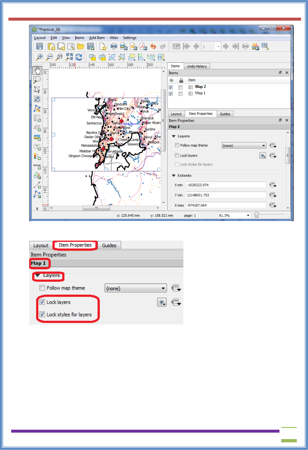
➢ After adding map go to ItemProperties → Map1→ Layers
Check on Lock Layers and Lock Styles for Layers
This will ensure that if any change in layers or change their styles, the Print Layout view will not
change.
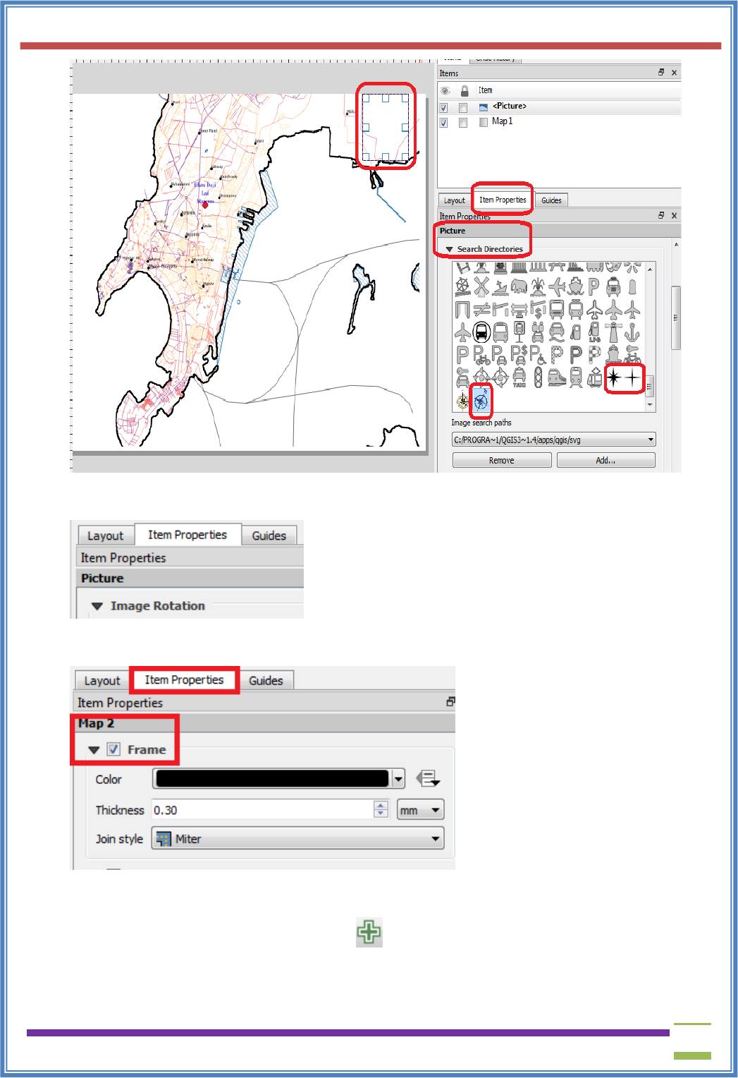
➢ Go to Add Item → Add Picture → Place a picture box at appropriate location.
USIT6P4 (Discipline Specific Elective Practical) Principles of Geographic Information Systems Practical
T. Y. B. Sc. (Information Technology) SEMESTER VI Teacher’s Reference Manual
43
➢ Also adjust Image Rotation to its appropriate value.
➢ Item Properties → Image Rotation
➢ Add an inset Using Add Item → Add Picture → Select an area to be highlighted on main Map.
➢ Set a frame for Inset by enabling the check box for Frame.
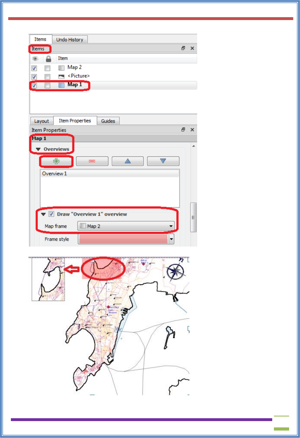
➢ To highlight the area shown in Inset
➢ Select the Picture representing main Map from Items pane.
➢ In Item Properties → Overviews → using icon add an overview.
➢ Select the checkbox Draw Overview
➢ Name the Picture object representing inset (Map1 in our case).
USIT6P4 (Discipline Specific Elective Practical) Principles of Geographic Information Systems Practical
T. Y. B. Sc. (Information Technology) SEMESTER VI Teacher’s Reference Manual
44
➢ The Print Layout will appear like
➢ Add Item → Add Label
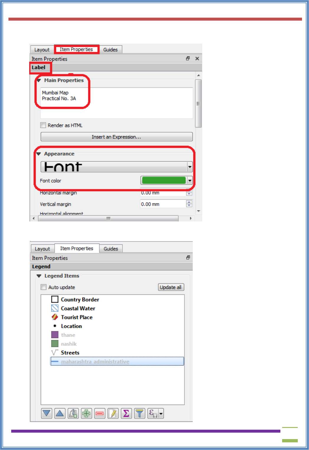
USIT6P4 (Discipline Specific Elective Practical) Principles of Geographic Information Systems Practical
T. Y. B. Sc. (Information Technology) SEMESTER VI Teacher’s Reference Manual
45
➢ Change the Label text To “Mumbai Map”, Set appropriate font size and color using Item
Properties→ Main Properties.
➢ Add Item → Add Legend→ Place the legend indicator at appropriate location.
➢ Uncheck auto update and use suitable legend indicator label.
USIT6P4 (Discipline Specific Elective Practical) Principles of Geographic Information Systems Practical
T. Y. B. Sc. (Information Technology) SEMESTER VI Teacher’s Reference Manual
46
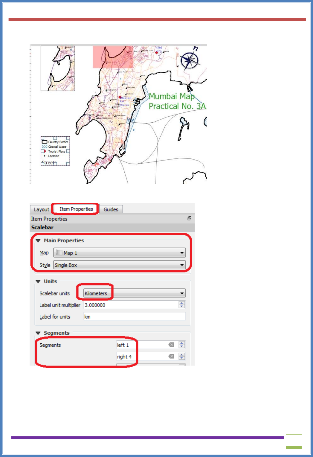
➢ The Print Layout will appear
➢ Add Item → Add Scale Bar
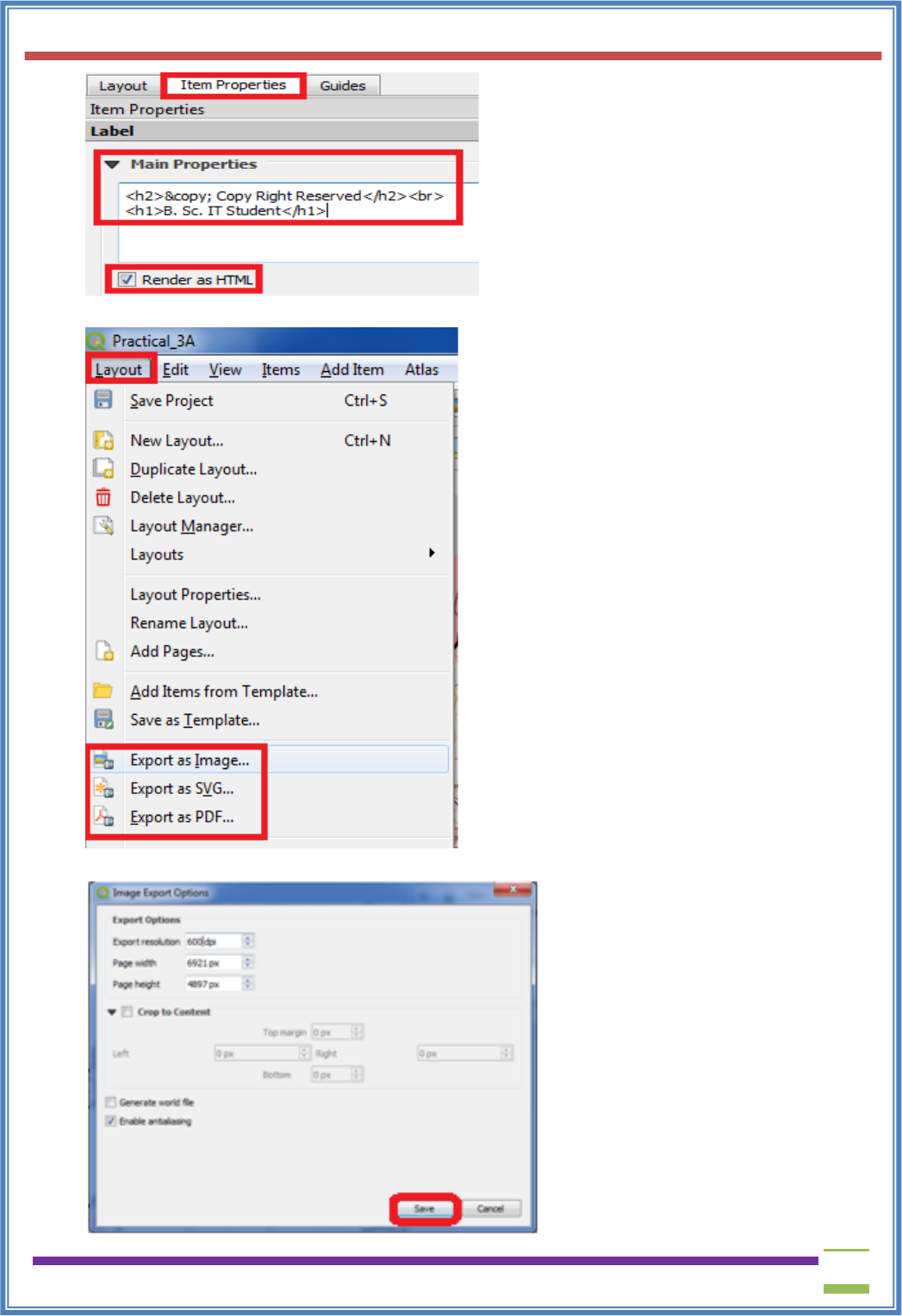
➢ Add Item → Add Label→Add a Label using HTML rendering
USIT6P4 (Discipline Specific Elective Practical) Principles of Geographic Information Systems Practical
T. Y. B. Sc. (Information Technology) SEMESTER VI Teacher’s Reference Manual
47
➢ A Map can be saved in Image or PDF using Layout → Export as Image / Export as PDF
➢ Save the Map to a location appropriate location as PDF or Image.
USIT6P4 (Discipline Specific Elective Practical) Principles of Geographic Information Systems Practical
T. Y. B. Sc. (Information Technology) SEMESTER VI Teacher’s Reference Manual
48
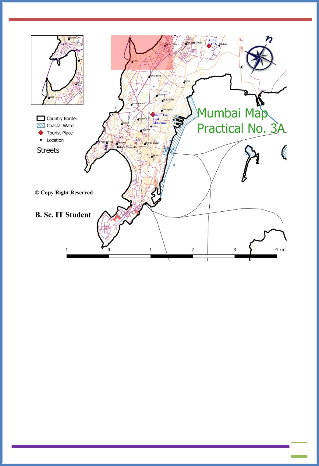
➢ Open the PDF or Image from location.
USIT6P4 (Discipline Specific Elective Practical) Principles of Geographic Information Systems Practical
T. Y. B. Sc. (Information Technology) SEMESTER VI Teacher’s Reference Manual
49
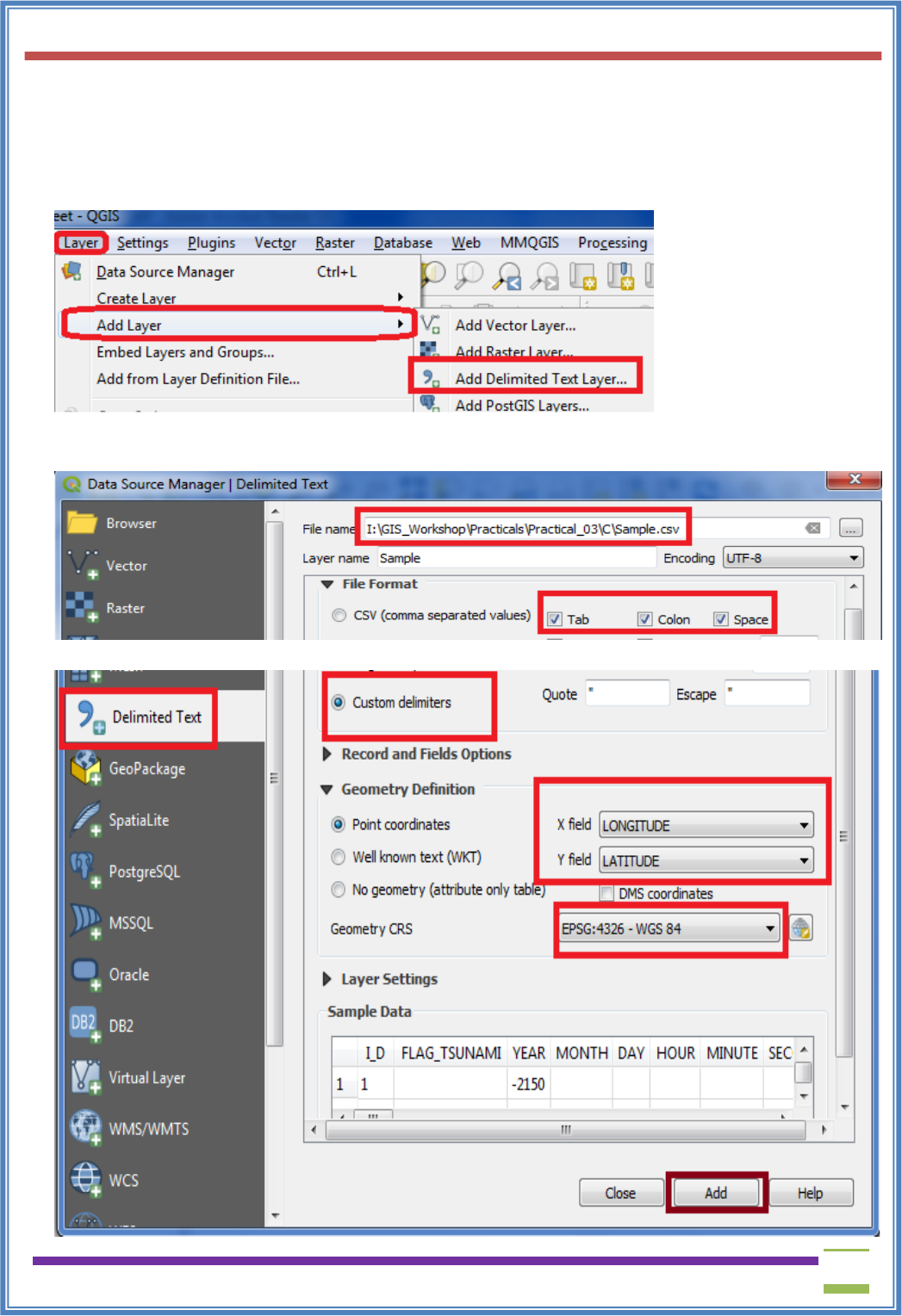
b) Importing Spreadsheets or CSV files
➢ Many times the GIS data comes in a table or an Excel spreadsheet or a list lat/long coordinates,
therefore it has to be imported in a GIS project.
➢ Sample file for Earthquake data will be used in this practical.
➢ Go to Layer → Add Layer → Add Delimited text Layer
➢ Data Source Manager | Delimited Text window will appear
➢ Select the \GIS_Workshop\Practicals\Practical_03\C\Sample.csv file from data folder.
USIT6P4 (Discipline Specific Elective Practical) Principles of Geographic Information Systems Practical
T. Y. B. Sc. (Information Technology) SEMESTER VI Teacher’s Reference Manual
50
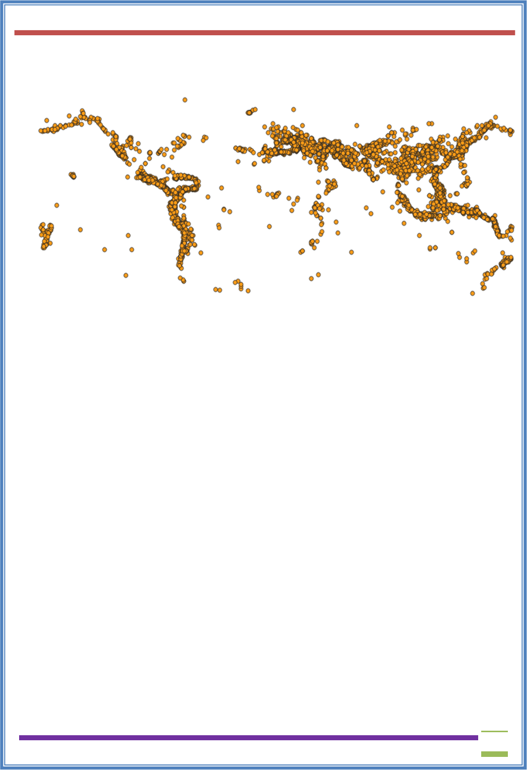
➢ Press ADD and close the window.
➢ Output:
USIT6P4 (Discipline Specific Elective Practical) Principles of Geographic Information Systems Practical
T. Y. B. Sc. (Information Technology) SEMESTER VI Teacher’s Reference Manual
51
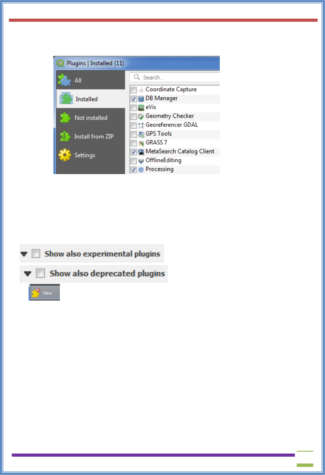
c) Using Plugins
➢ Core plugins are already part of the standard QGIS installation. To use these, just enable them.
➢ Open QGIS. Click on Plugins → Manage and Install Plugins....
➢ To enable a plugin, check on the checkbox next to Plugin. This will enable the plugin to use it.
➢ External plugins are available in the QGIS Plugins Repository and need to be installed by the users
before using them.
➢ Click on Not Installed or Install from ZIP.
➢ Once the plugin is downloaded and installed, you will see a confirmation dialog.
➢ Click on Plugins → <<new Plugin Name>>
➢ The Plugin if marked Experimental plugin can be installed, from Setting→ check on
or
➢ A tab will be added to Plugin Manager Window.
➢ Click on a plugin name and Click Install.
USIT6P4 (Discipline Specific Elective Practical) Principles of Geographic Information Systems Practical
T. Y. B. Sc. (Information Technology) SEMESTER VI Teacher’s Reference Manual
52
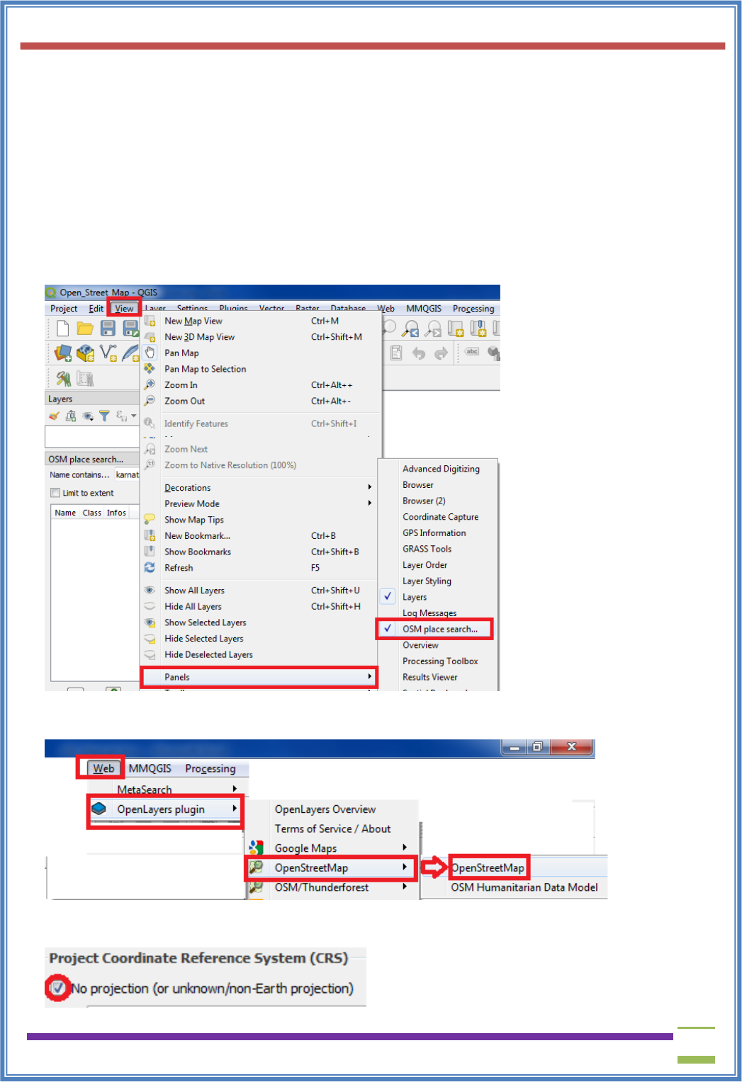
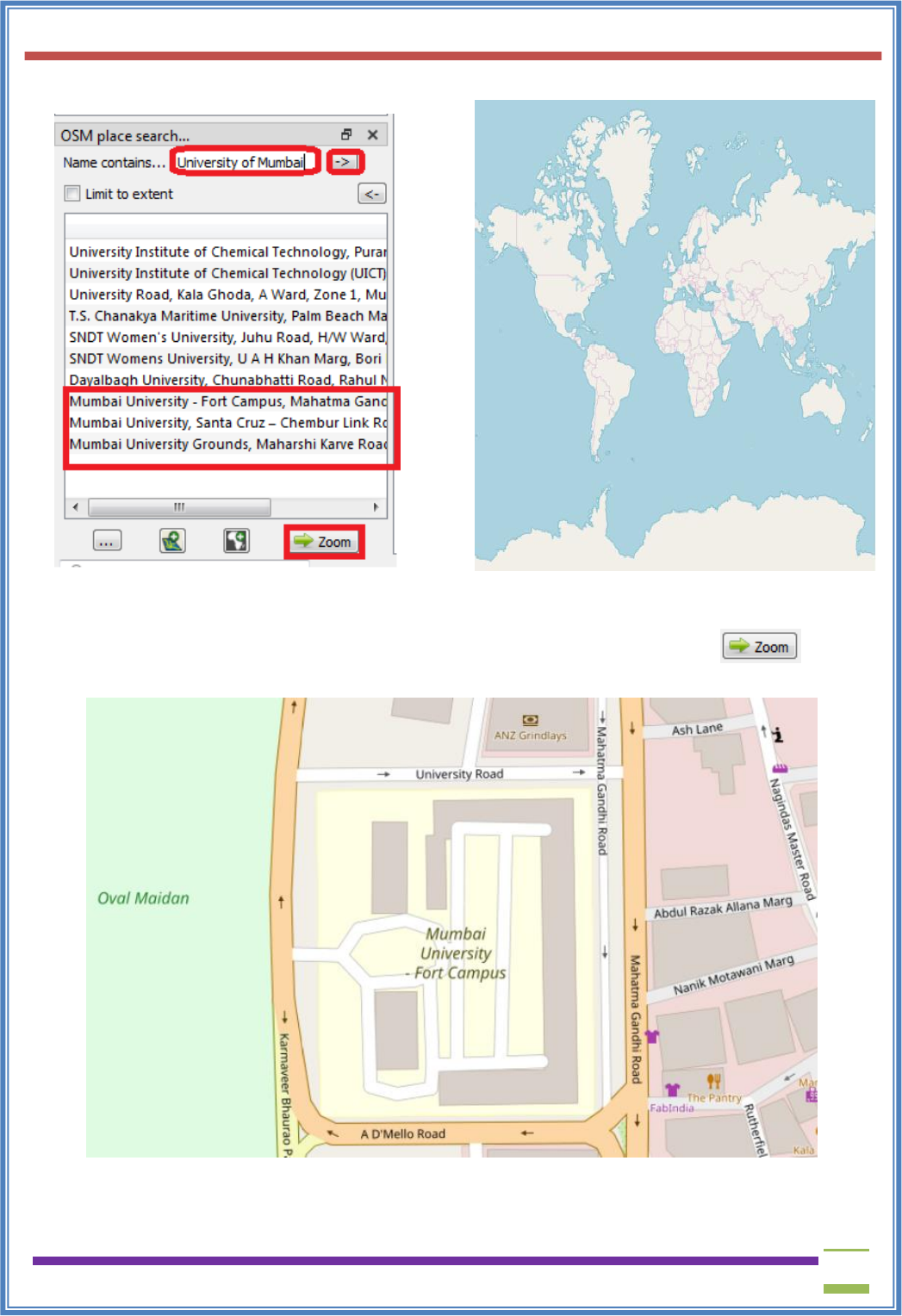
d) Searching and Downloading OpenStreetMap Data
OpenStreetMap (OSM) created by Steve Coast in the UK in 2004 is a collaborative project to
create a free editable map of the world. Rather than the map itself, the data generated by the project
is considered its primary output. The creation and growth of OSM has been motivated by
restrictions on use or availability of map information across much of the world, and the advent of
inexpensive portable satellite navigation devices.
➢ Add “Open Layer” and “OSM Search” Plugin from Not Installed option from Plugin Manager
Dialog Box.
➢ The OSM Place Search plugin will install itself as a Panel in QGIS, if not go to View → Panels →
select OSM Place Search.
➢ Go to Web → OpenLayer Plugin and select Open Street Map
➢ A World map will appear on screen.
➢ If an error occurs in loading maps, go to project properties → CRS →
USIT6P4 (Discipline Specific Elective Practical) Principles of Geographic Information Systems Practical
T. Y. B. Sc. (Information Technology) SEMESTER VI Teacher’s Reference Manual
53
➢ In OSM Place search Pane → Enter Mumbai or any place name to search
➢ Double click on the desired place in OSM Place search Panel or Click and press
Output:
USIT6P4 (Discipline Specific Elective Practical) Principles of Geographic Information Systems Practical
T. Y. B. Sc. (Information Technology) SEMESTER VI Teacher’s Reference Manual
54
PRACTICAL - 4
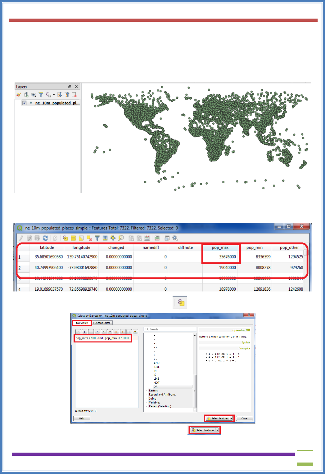
A. Working with attributes
➢ Start a new project.
➢ Go to Layer → Add Layer → Add Vector Layer
➢ Select “\GIS_Workshop\Practicals\Practical_04\A\Data\ne_10m_populated_places_simple.zip”
➢ Right click on Layer in Layer Panel → Open Attribute Table.
➢ Explore various attributes and their values in the Attribute table.
➢ To find the Place with maximum population click on “pop_max” file
➢ On clicking the Select feature using expression button the following window will appear.
➢ Enter pop_max>100 and pop_max<10000 and click button to get all the places with
population between 100 and 10000.
USIT6P4 (Discipline Specific Elective Practical) Principles of Geographic Information Systems Practical
T. Y. B. Sc. (Information Technology) SEMESTER VI Teacher’s Reference Manual
55
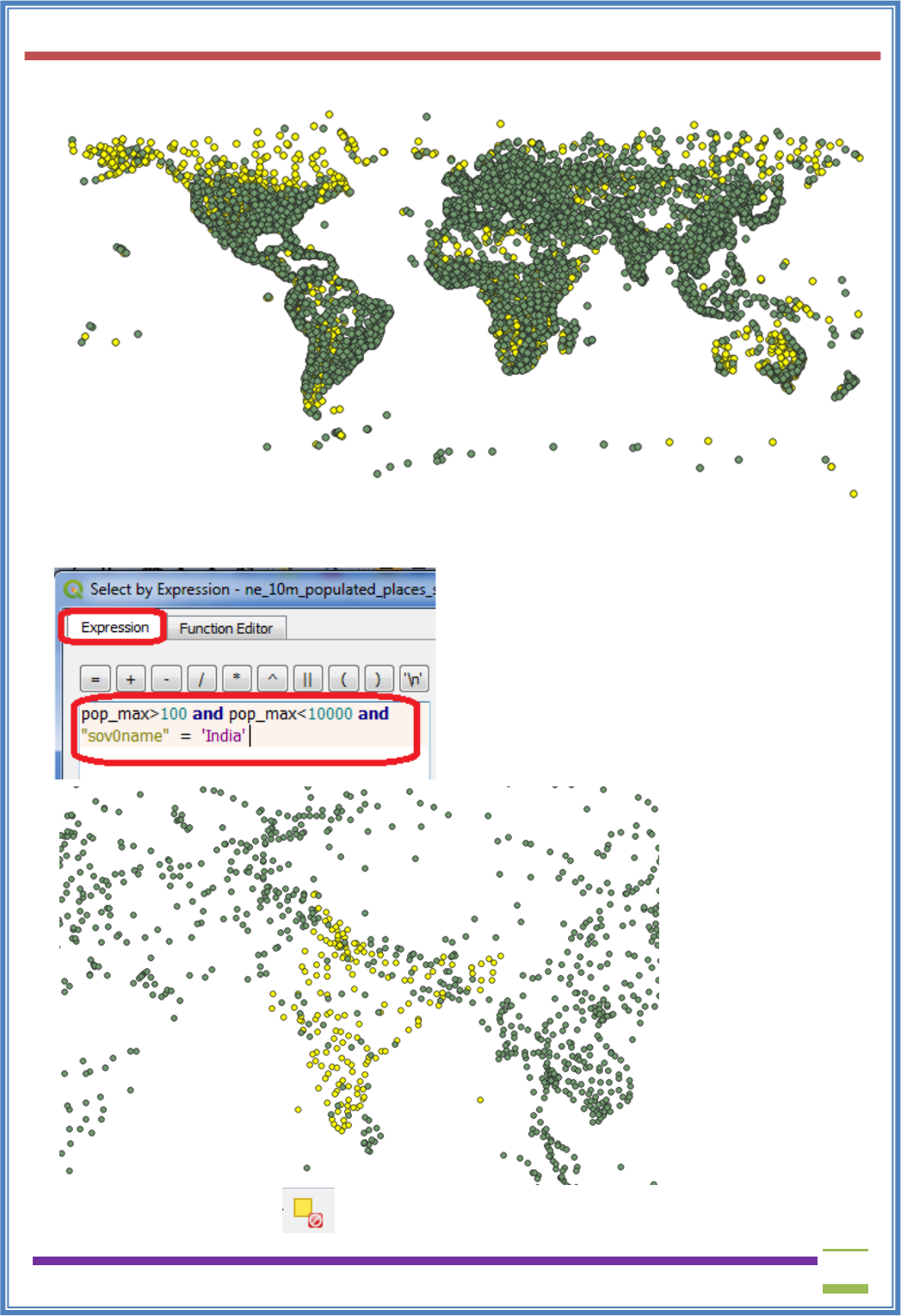
➢ The places matching the criteria will appear in different color.
➢ Different queries can be performed using the dataset.
➢ Try this
Will give
➢ Use the deselect button to deselect the feature to be rendered in original color.
USIT6P4 (Discipline Specific Elective Practical) Principles of Geographic Information Systems Practical
T. Y. B. Sc. (Information Technology) SEMESTER VI Teacher’s Reference Manual
56
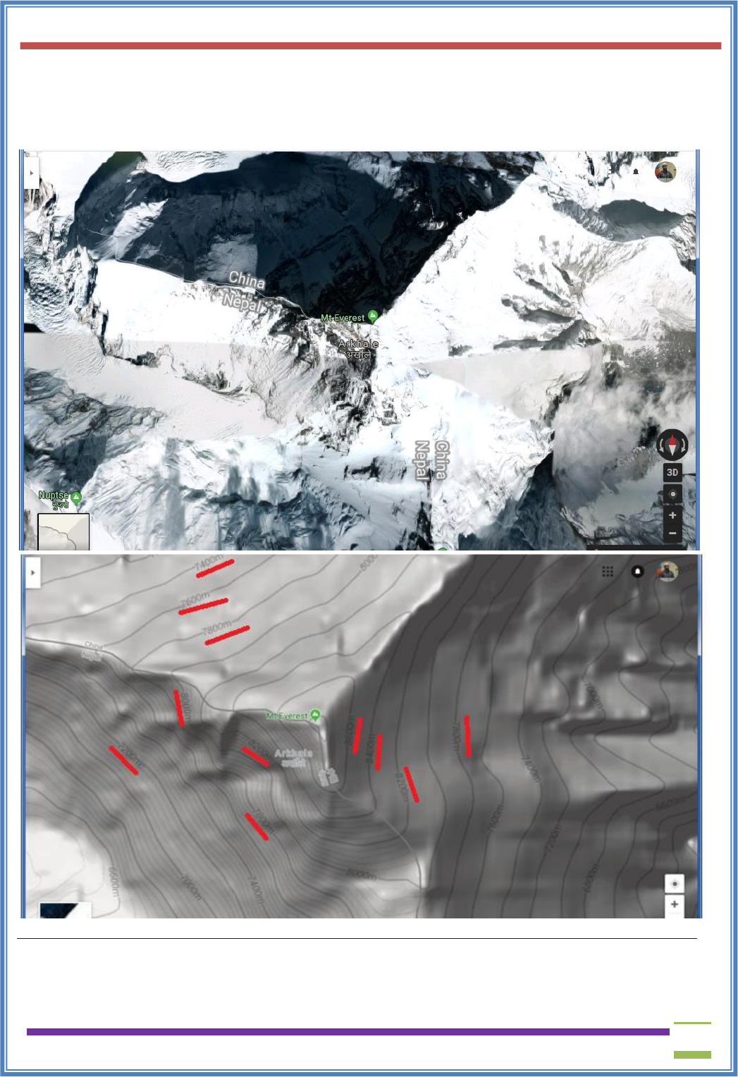
b) Terrain Data and Hill shade analysis
A terrain dataset is a multiresolution, TIN-based surface built from measurements stored as features
in a geodatabase. Terrain or elevation data is useful for many GIS Analysis like, to generate various
products from elevation data such as contours, hillshade etc.
https://www.google.com/maps/@27.9857765,86.9285378,14.75z/data=!5m1!1e4?hl=en-US
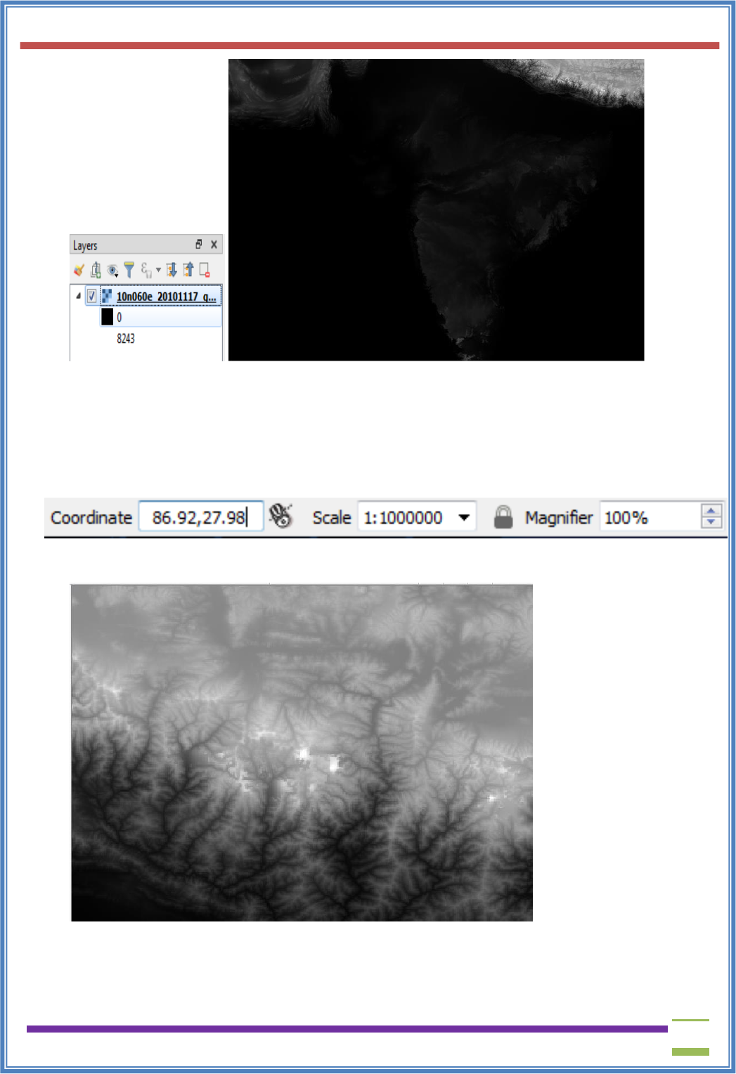
➢ Go to Layer → Add Raster Layer → select “10n060e_20101117_gmted_mea300.tif”, from
Data folder
USIT6P4 (Discipline Specific Elective Practical) Principles of Geographic Information Systems Practical
T. Y. B. Sc. (Information Technology) SEMESTER VI Teacher’s Reference Manual
57
➢ The Lower altitude regions are shown using dark color and higher using light shade as seen on
top region containing Himalaya and Mt Everest.
➢ Mt. Everest - is located at the coordinates 27.9881° N, 86.9253° E.
➢ Enter 86.92, 27.98 in the coordinate field, Scale 900000 and Magnifier 100% at the bottom of
QGIS.
➢ Press enter the view port will be centered on Himalaya Region.
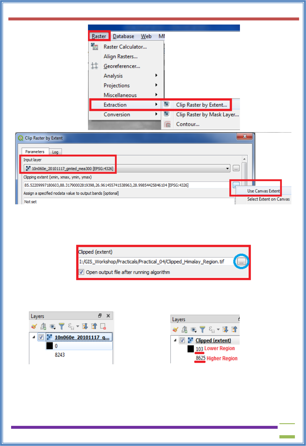
➢ Crop the raster layer only for the region under study.
➢ Go to Raster → Extraction→ Clip Raster by Extent
USIT6P4 (Discipline Specific Elective Practical) Principles of Geographic Information Systems Practical
T. Y. B. Sc. (Information Technology) SEMESTER VI Teacher’s Reference Manual
58
➢ Select the raster layer (if project contains multiple layers).
➢ Select the clipping area by selecting the option Use Canvas Extends if the visible part of map
is to be selected or manually select an area on canvas by using Select Extent on Canvas.
➢ Select the location and file name for storing clipped raster layer.
➢ Press RUN.
➢ Deselect the original layer and keep the clipped one.
➢ The Clipped raster layer is representing altitude are from 103 Meters.
Original Raster Clipped Raster
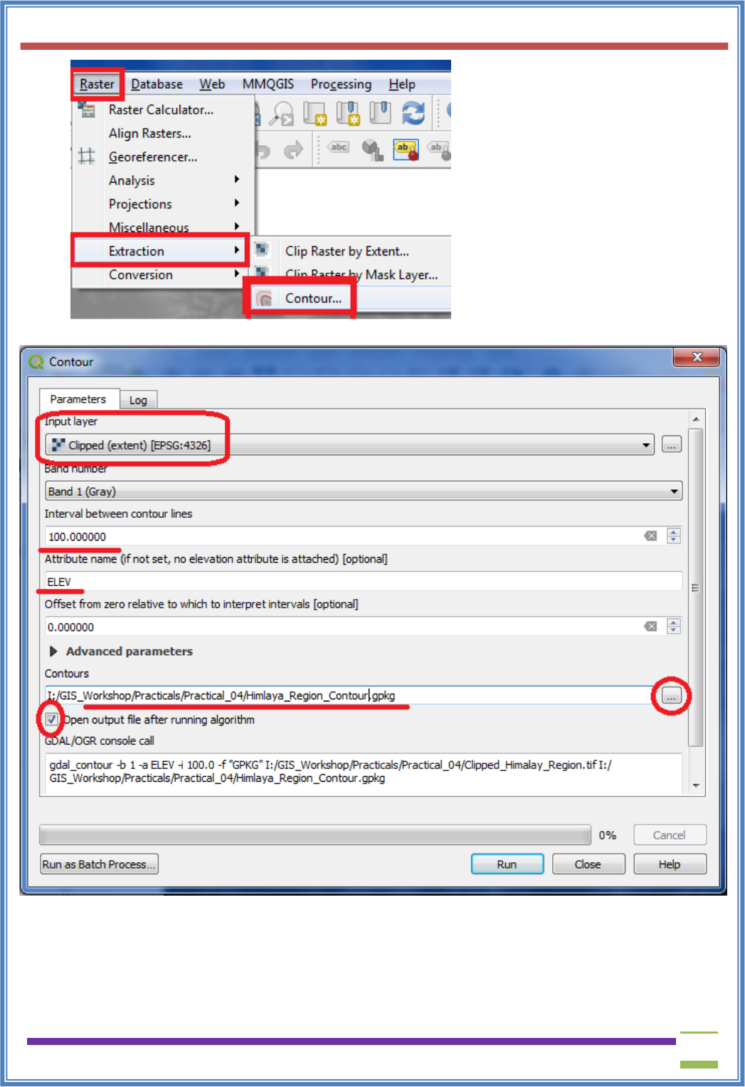
➢ Counter lines are the lines on a map joining points of equal height above or below sea level. A
contour interval in surveying is the vertical distance or the difference in the elevation between
the two contour lines in a topographical map.
➢ To derive counter lines from given raster.
➢ Go to Raster → Extraction→ Contour
USIT6P4 (Discipline Specific Elective Practical) Principles of Geographic Information Systems Practical
T. Y. B. Sc. (Information Technology) SEMESTER VI Teacher’s Reference Manual
59
➢ The Contour configuration window will appear
➢ Select the input raster layer name. Set contour interval 100.00 meters, select the output file
name & location and check the option to add output file to project after processing.
➢ Press “RUN”.
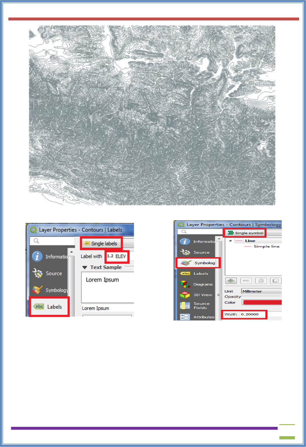
➢ The contour layer will appear like this
USIT6P4 (Discipline Specific Elective Practical) Principles of Geographic Information Systems Practical
T. Y. B. Sc. (Information Technology) SEMESTER VI Teacher’s Reference Manual
60
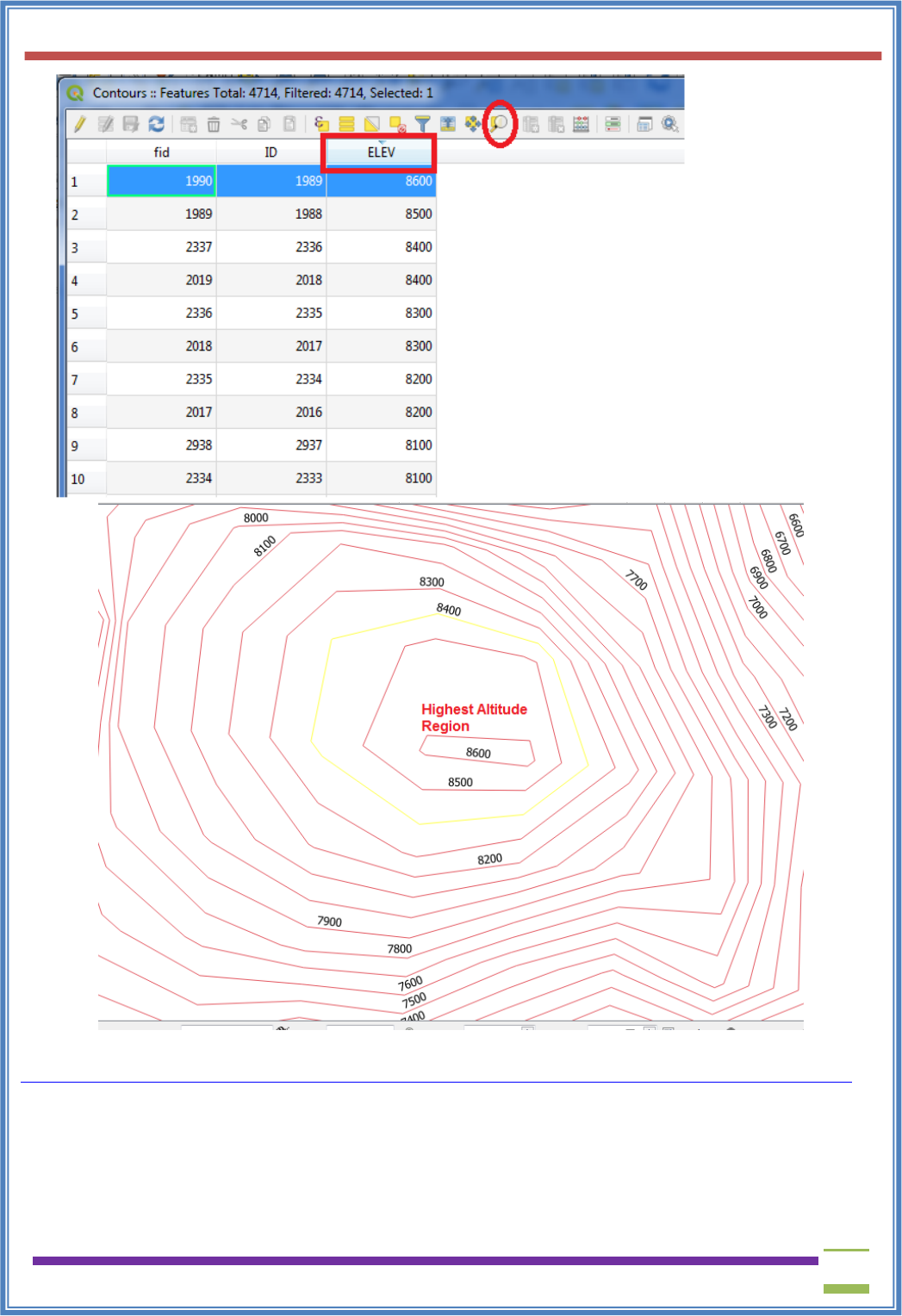
➢ Label the layer using “ELEV” field and set appropriate symbols for line.
➢ In the Layer panel right click on Contour Raster Layer and select “Open Attribute table”,
➢ Arrange the table in descending order based on the value of “ELEV” column.
➢
USIT6P4 (Discipline Specific Elective Practical) Principles of Geographic Information Systems Practical
T. Y. B. Sc. (Information Technology) SEMESTER VI Teacher’s Reference Manual
61
Compare the above counter line raster layer with the previous Google map image or visit
https://www.google.com/maps/@27.9857765,86.9285378,14.75z/data=!5m1!1e4?hl=en-US
➢ To verify the above contour files using Google Map
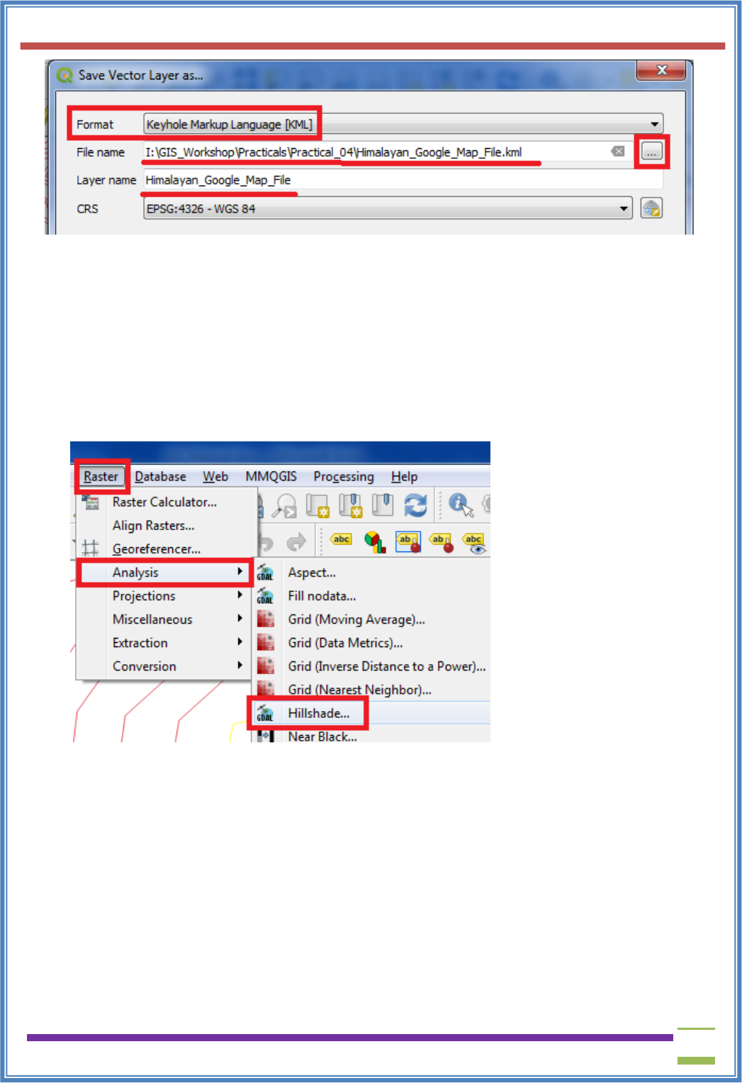
➢ Make a copy of Contour Layer, Go to Layer →Save As
➢ Select file format as “Keyhole Markup Language”, set file name, location and Layer Name.
➢ Also set CRS to WGS 84 EPSG:4326
USIT6P4 (Discipline Specific Elective Practical) Principles of Geographic Information Systems Practical
T. Y. B. Sc. (Information Technology) SEMESTER VI Teacher’s Reference Manual
62
➢ Go to the stored location on Hard Disk and open the “Himalayan_Google_Map_File.kml” with
Google Map.\
----------------------------------------------------------------------------------------------------------------------------
A Hillshade is a grayscale 3D representation of the surface, showing the topographical shape of hills
and mountains using shading (levels of gray) on a map, just to indicate relative slopes, mountain ridges,
not absolute height.
➢ For Hill Shade surface analysis
➢ Go to Plugin → Install Georeferencer GADL.
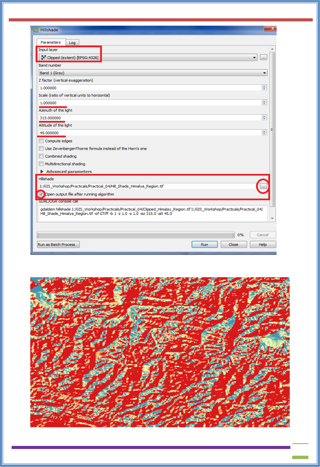
➢ After successful installation of plugin Go to Raster → Analysis → Hill Shade
➢ Select the input raster layer, select file name and location for storing Hill Shade output file.
USIT6P4 (Discipline Specific Elective Practical) Principles of Geographic Information Systems Practical
T. Y. B. Sc. (Information Technology) SEMESTER VI Teacher’s Reference Manual
63
➢ Press “RUN” and Close the Hill Shape Dialog window.
➢ After Raster styling the Output will appear like this.
USIT6P4 (Discipline Specific Elective Practical) Principles of Geographic Information Systems Practical
T. Y. B. Sc. (Information Technology) SEMESTER VI Teacher’s Reference Manual
64
PRACTICAL - 5
Working with Projections and WMS Data
A Web Map Service (WMS) is a standard protocol developed by the Open Geospatial Consortium in
1999 for serving georeferenced map images over the Internet. These images are typically produced by a
map server from data provided by a GIS database
➢ Start a new Project.
➢ Layer → Add Layer →Vector Layer
➢ Select “ne_10m_admin_0_countries.zip” Layer from data folder.
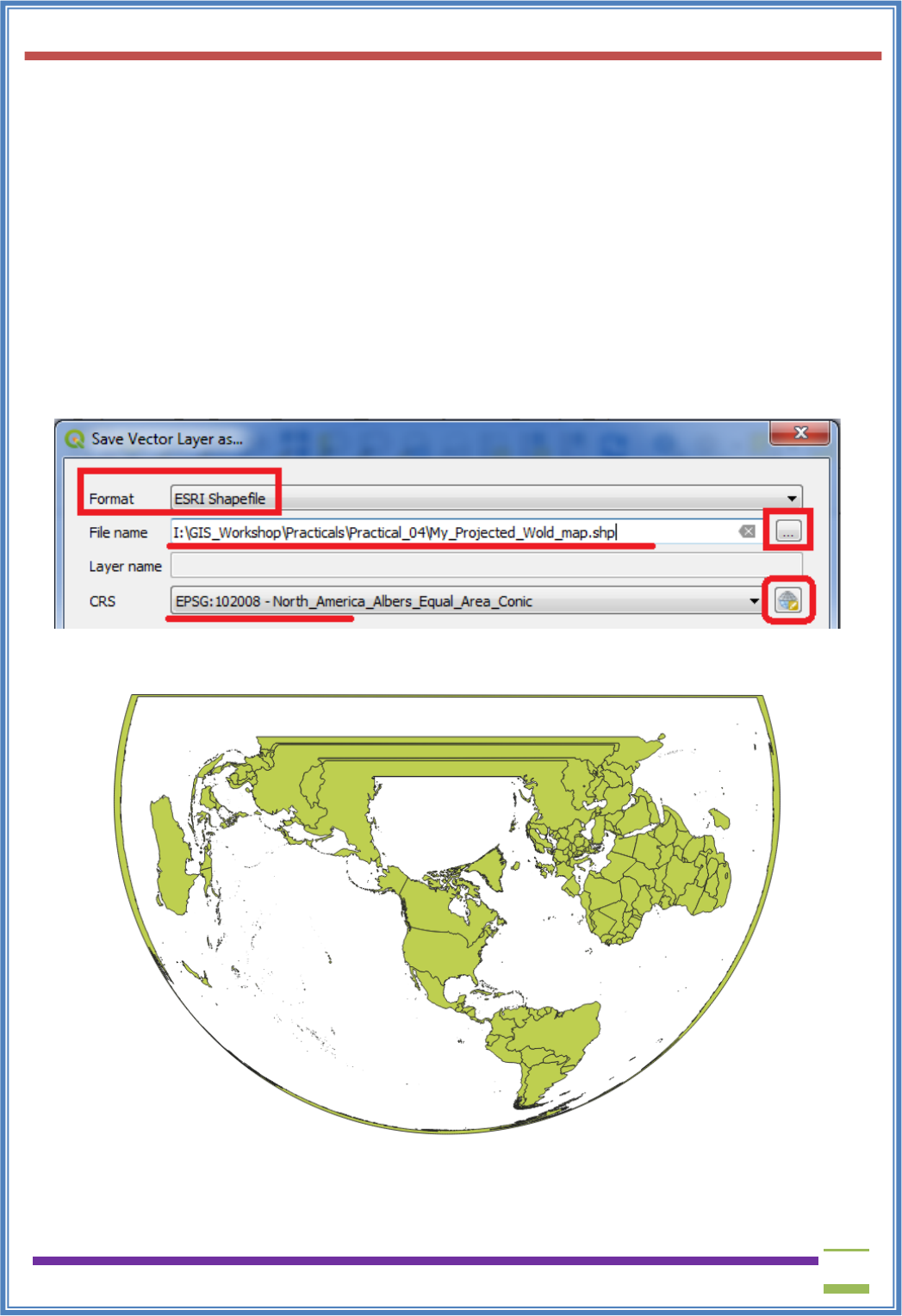
➢ Go to Layer → Save As
Select format as ESRI Shape File
Select folder location and file name
Set CRS North_America_Albers_Equal_Area_Conic EPSG: 102008
➢ Press “OK”.
➢ Deselect the original Image and keep the projected layer visible.
➢ Select Layer → Add Layer → Add Raster Layer → Select MiniScale_(standard)_R17.tif from
Location
USIT6P4 (Discipline Specific Elective Practical) Principles of Geographic Information Systems Practical
T. Y. B. Sc. (Information Technology) SEMESTER VI Teacher’s Reference Manual
65
“GIS_Workshop\Practicals\Practical_05\DATA\minisc_gb\minisc_gb\data\RGB_TIF_compres
sed\MiniScale_(standard)_R17.tif”
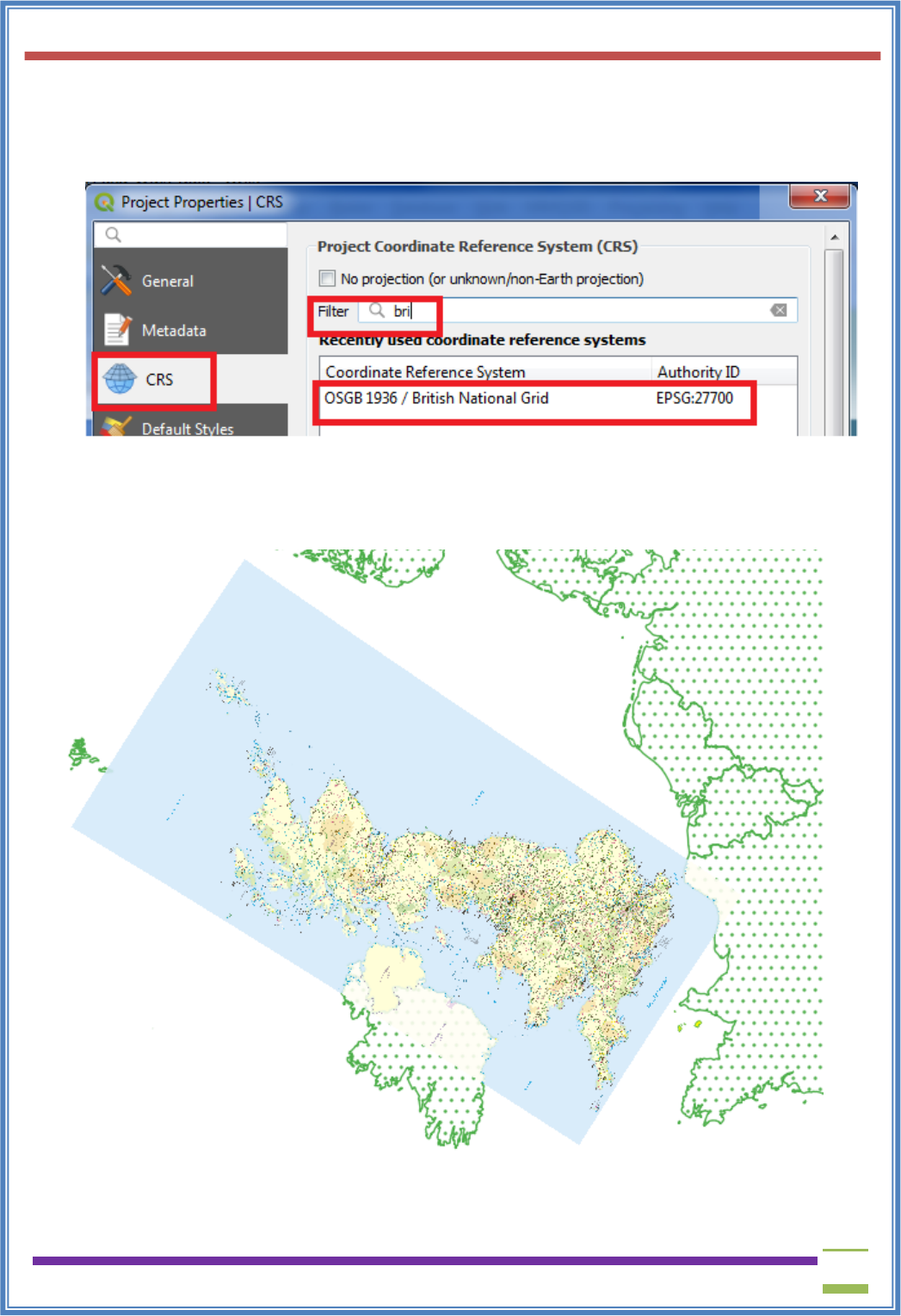
➢ The Layer appears on a different location than the location where Great Britain is shown on
Map.
➢ Open Layer Properties→CRS → Search bri → select British National Grid EPSG 27700.
➢ Processing may take some time.
➢ Locate United Kingdom on Layer; the vector layer exactly coincides by the raster layer
covering United Kingdom.
USIT6P4 (Discipline Specific Elective Practical) Principles of Geographic Information Systems Practical
T. Y. B. Sc. (Information Technology) SEMESTER VI Teacher’s Reference Manual
66
PRACTICAL - 6
➢ Georeferencing
A. Georeferencing Topo Sheets and Scanned Maps
➢ Start a new project
➢ Go to Layers → Add Layer → Add vector Layer
➢ Select GIS_Workshop\Manual\Prac06\IND_adm0.shp
➢ Zoom in to Mumbai region in the layer.
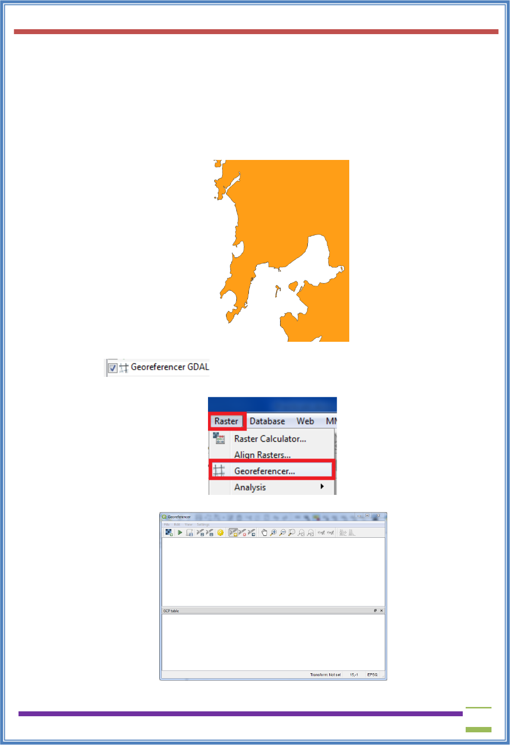
➢ Go to Plugins→ Manage and Install Plugins
➢ Ensure that is checked, if not install Georeferencer GDAL plugin.
➢ Go to Raster → Georefrencer
➢ A new Georeferencer window will open
➢ File → Open Raster
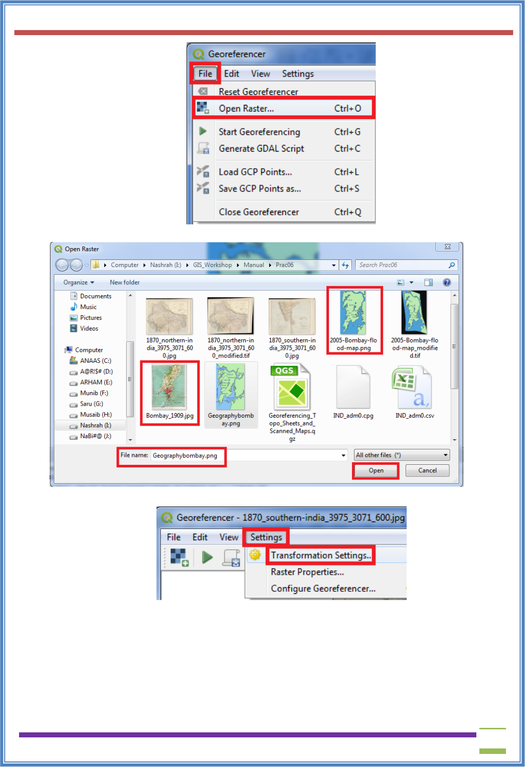
USIT6P4 (Discipline Specific Elective Practical) Principles of Geographic Information Systems Practical
T. Y. B. Sc. (Information Technology) SEMESTER VI Teacher’s Reference Manual
67
➢ Select file “1870_southern-india_3975_3071_600.jpg” from project data folder
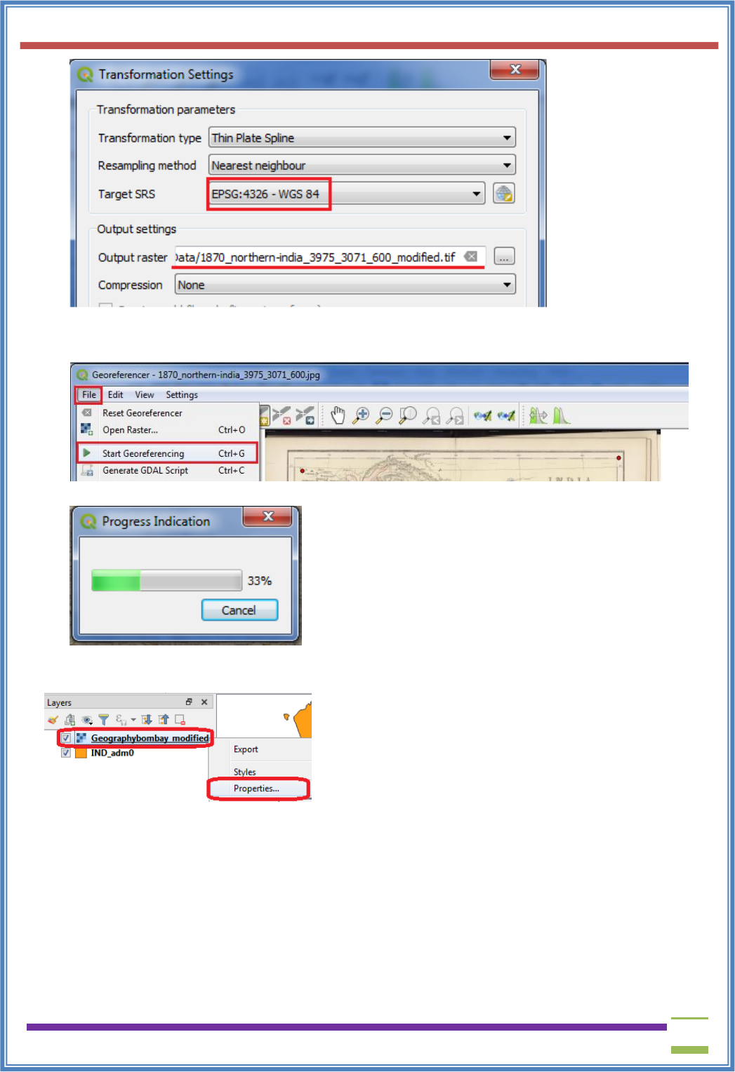
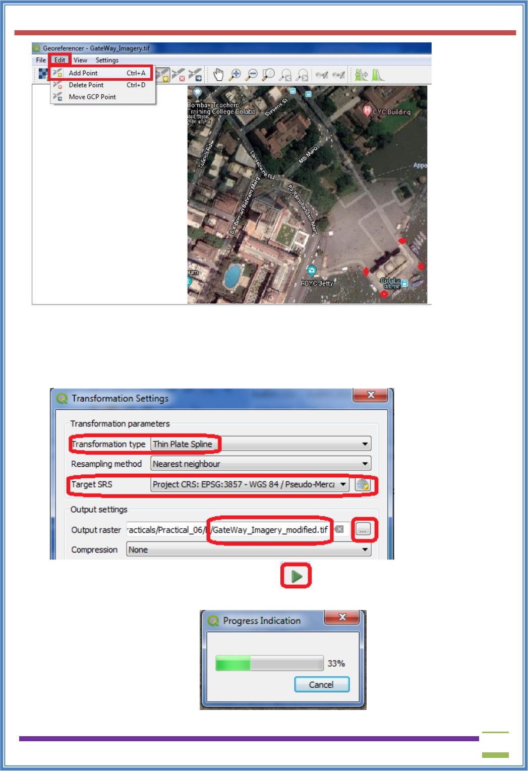
➢ Go to Settings →Transformation Settings
➢ In the Transformation Settings window
USIT6P4 (Discipline Specific Elective Practical) Principles of Geographic Information Systems Practical
T. Y. B. Sc. (Information Technology) SEMESTER VI Teacher’s Reference Manual
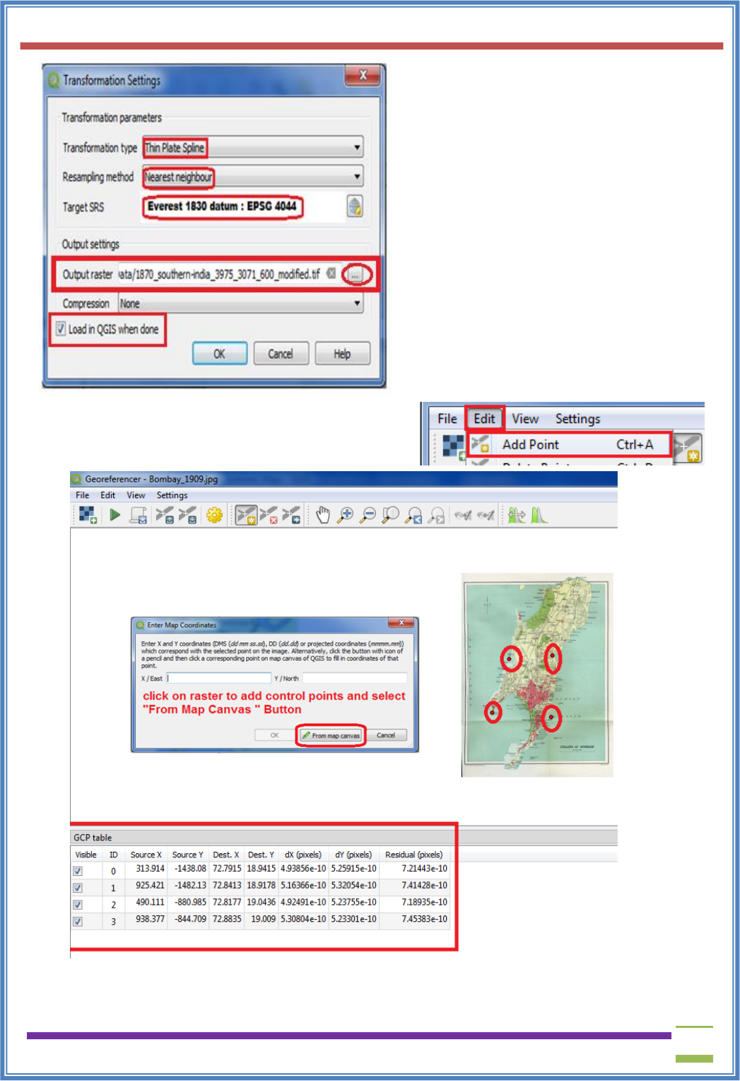
68
▪ Select Transformation type → Thin Plate
Spline
▪ Re-sampling Method → Nearest Neighbour
▪ Target TRS → Everest 1830 datum: EPSG
4044
▪ Select Output Raster Name and Location
▪ Check the Load in QGIS When Done
Option
▪ Press “OK”.
➢ In Georeferencer window Go to Edit → Add Points
➢ Select the set of control points.
➢ Go to, Setting → transformation settings.
USIT6P4 (Discipline Specific Elective Practical) Principles of Geographic Information Systems Practical
T. Y. B. Sc. (Information Technology) SEMESTER VI Teacher’s Reference Manual
69
➢ Press “RUN”
➢ In Georeferencing window go to → File → Start Georeferencing
➢ The progress indicator will appear
➢ The canvas area will now have the scanned map of Mumbai referenced with control points.
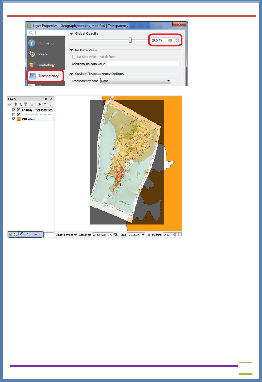
➢ Select the newly added layer in Layer Panel Right click and go to property.
➢ Set Transparency level of raster layer to appropriate level.
USIT6P4 (Discipline Specific Elective Practical) Principles of Geographic Information Systems Practical
T. Y. B. Sc. (Information Technology) SEMESTER VI Teacher’s Reference Manual
70
Output:
➢ The Scanned Image map coincides with the existing map.
USIT6P4 (Discipline Specific Elective Practical) Principles of Geographic Information Systems Practical
T. Y. B. Sc. (Information Technology) SEMESTER VI Teacher’s Reference Manual
71
B. Georeferencing Aerial Imagery
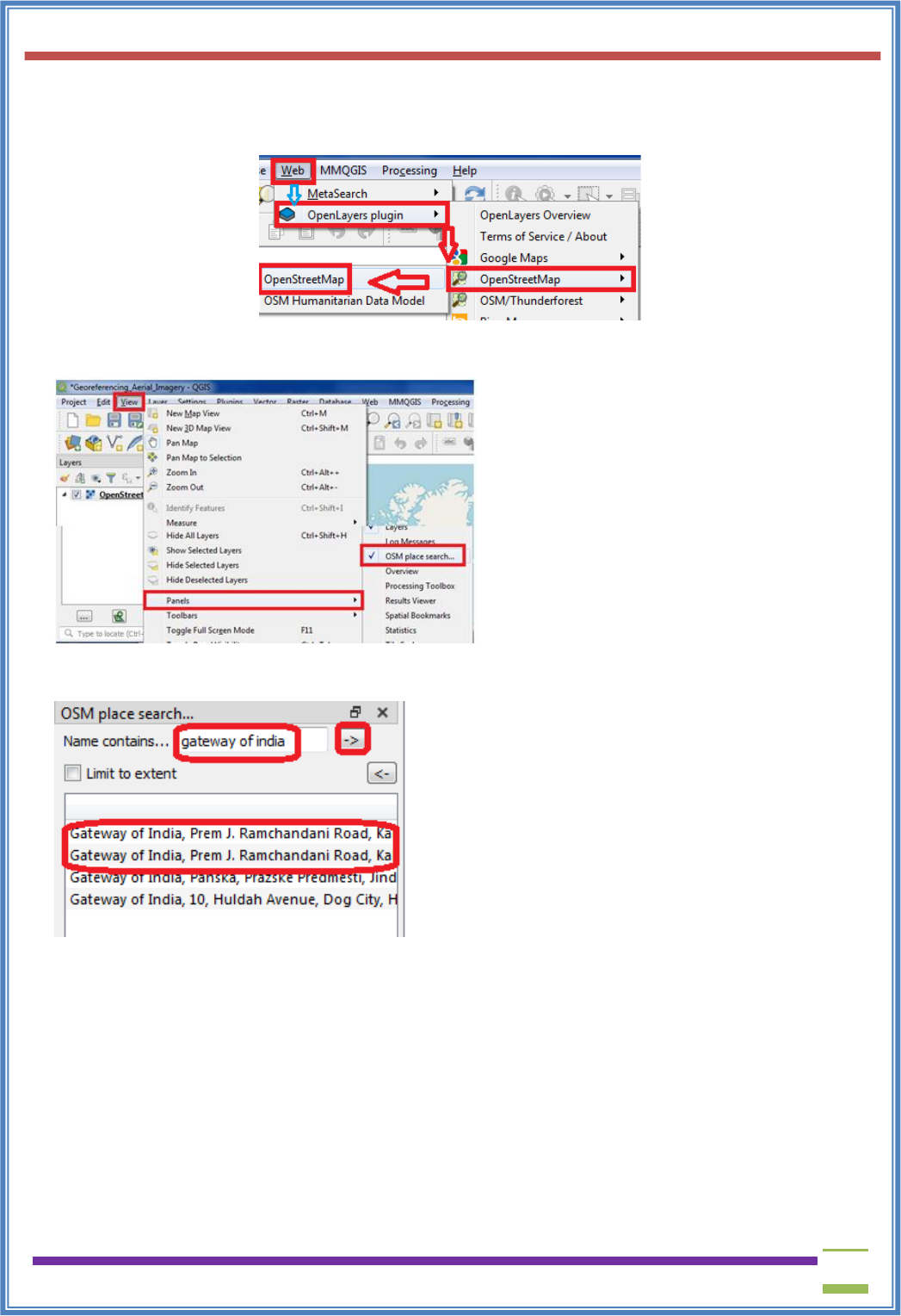
➢ Install plugin OpenStreetMap
➢ Go to Web Menu → OpenLayerPlugin → OpenStreetMap→ OpenStreetMap
➢ Go to Project → Properties → Set CRS to EPSG 3857
➢ Go to View → Panels → select OSM Place search
➢ The Gateway of India, Mumbai is located at 18.92°N 72.83°E
➢ Search Gateway of India in OSM Search Panel
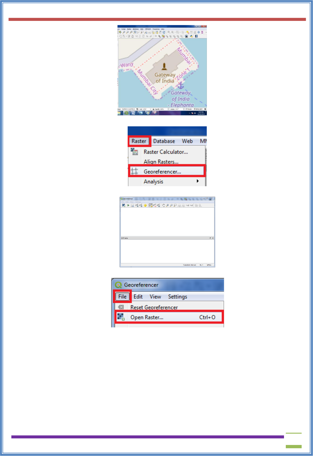
➢ Zoom in to appropriate level.
➢ The map will appear like this
USIT6P4 (Discipline Specific Elective Practical) Principles of Geographic Information Systems Practical
T. Y. B. Sc. (Information Technology) SEMESTER VI Teacher’s Reference Manual
72
➢ Go to Raster → Georefrencer
➢ A new Georeferencer window will open
➢ File → Open Raster
➢ Select file “Gateway_Imagery.tif” from project data folder
USIT6P4 (Discipline Specific Elective Practical) Principles of Geographic Information Systems Practical
T. Y. B. Sc. (Information Technology) SEMESTER VI Teacher’s Reference Manual
73
➢ Go to Edit → Add Point
➢ Select control points from map (Indicated in red color).
➢ Go to Setting → Transformation Setting
➢ Go to File → Start Georeferencing or Press the button in Georegerencing Window.
➢ The progress indicator will appear
USIT6P4 (Discipline Specific Elective Practical) Principles of Geographic Information Systems Practical
T. Y. B. Sc. (Information Technology) SEMESTER VI Teacher’s Reference Manual
74
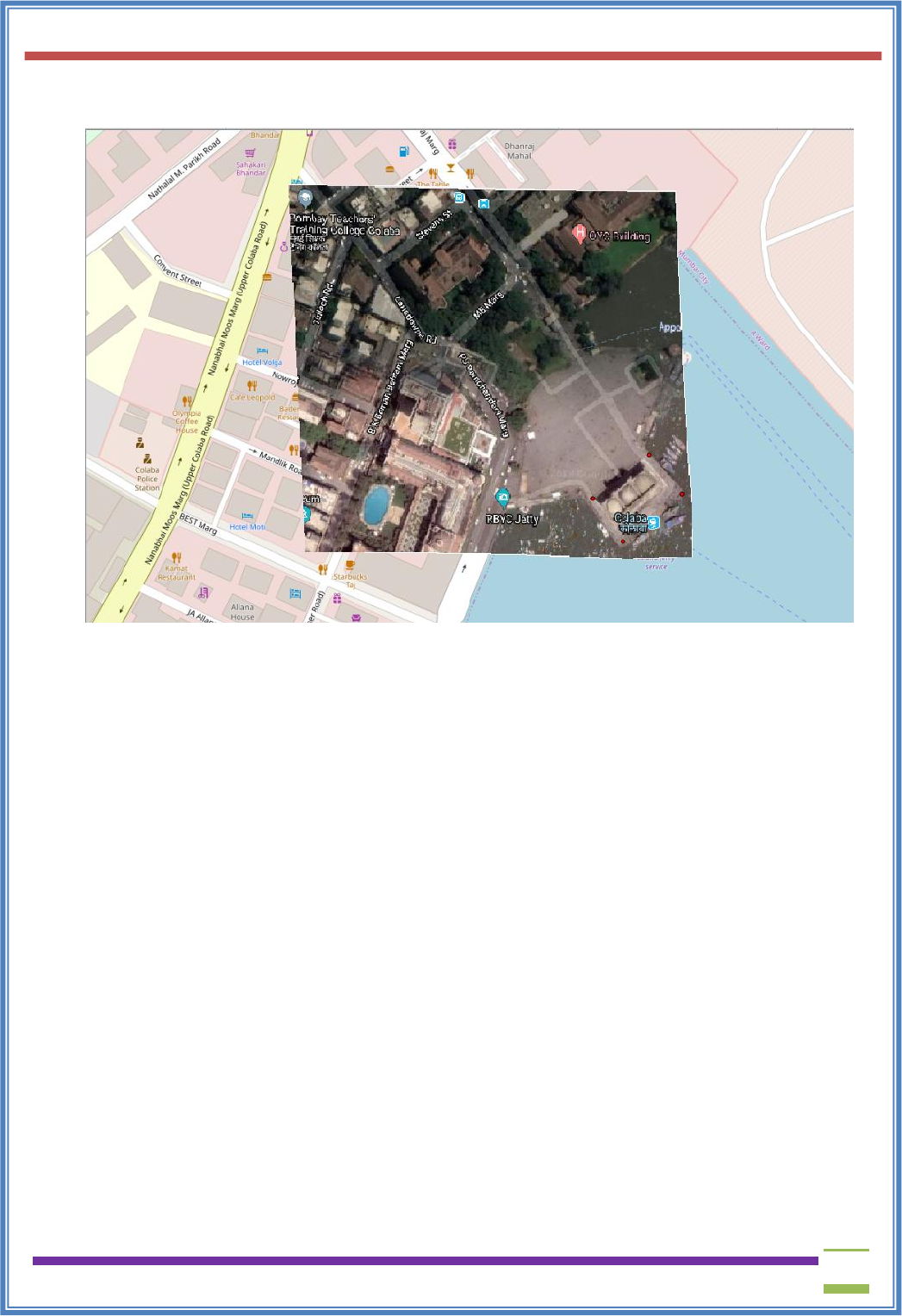
➢ Observe that the aerial image of the Gateway of India is georeferenced on OSM in the map
canvas.
USIT6P4 (Discipline Specific Elective Practical) Principles of Geographic Information Systems Practical
T. Y. B. Sc. (Information Technology) SEMESTER VI Teacher’s Reference Manual
75
C. Digitizing Map Data
Spatialite is an open database format similar to ESRI's geodatabase format. Spatialite database
is contained within a single file on your hard drive and can contain diferent types of spatial (point,
line, polygon) as well as non-spatial layers. This makes is much easier to move it around instead of
a bunch of shapefiles.
Digitizing Map Data
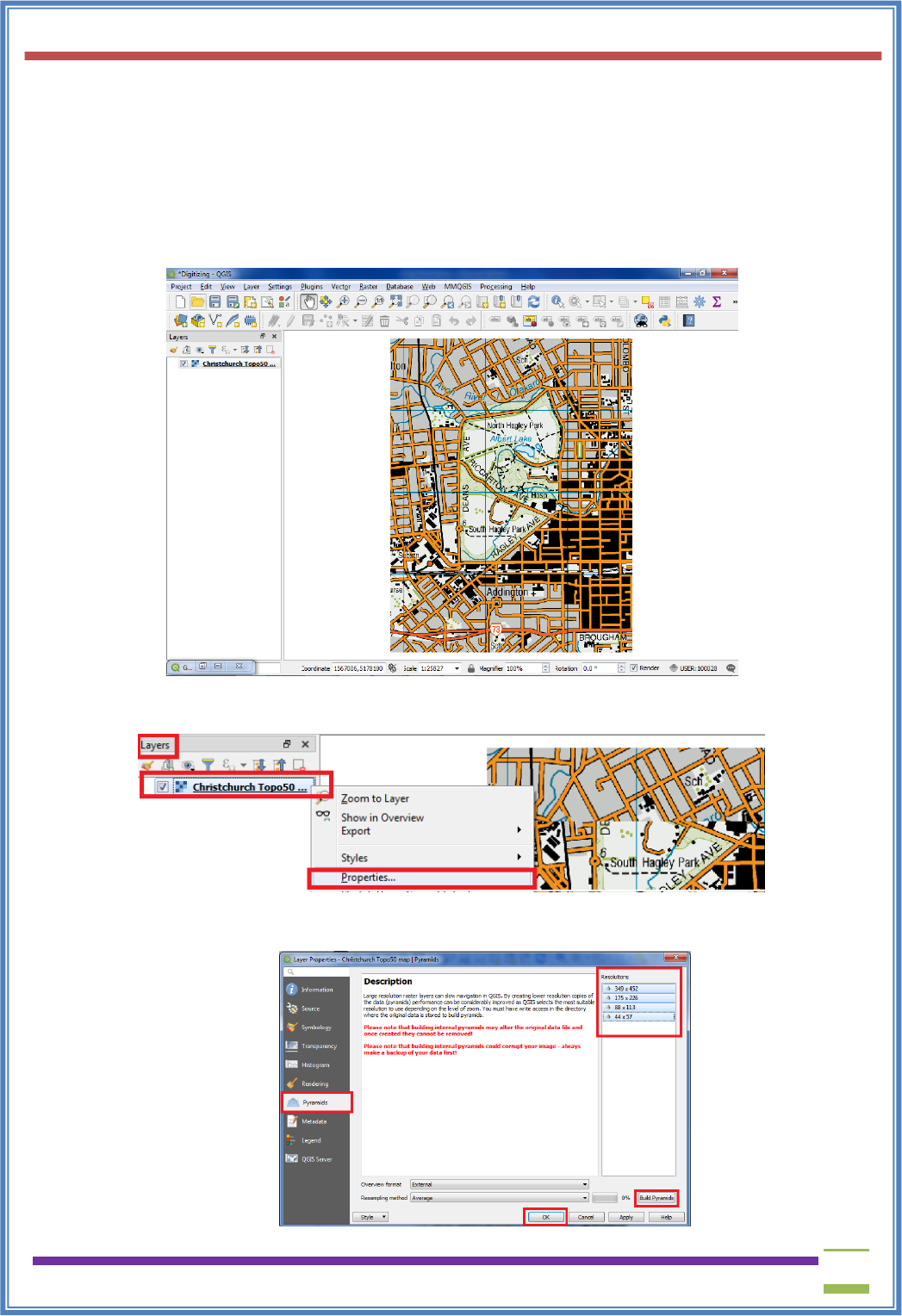
➢ Go to Layer ‣ Add Raster→ Select “Christchurch Topo50 map.tif” from project Folder.
➢ QGIS offers a simple solution to make raster load much faster by using Image Pyramids.
➢ Right-click the Christchurch Topo50 map.tif layer and select Properties.
➢ Choose the Pyramids tab. Hold the Ctrl key and select all the resolutions offered in the
Resolutions panel.
USIT6P4 (Discipline Specific Elective Practical) Principles of Geographic Information Systems Practical
T. Y. B. Sc. (Information Technology) SEMESTER VI Teacher’s Reference Manual
76
➢ Click Build pyramids. Then click OK.
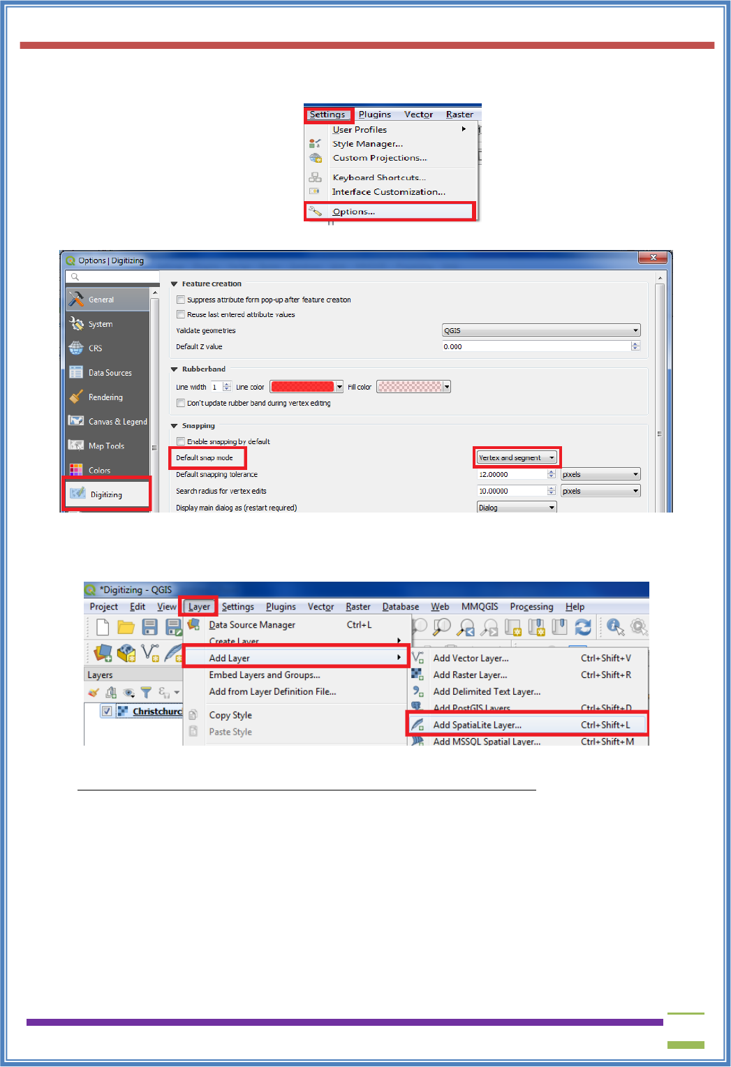
➢ Go to Settings →Options.... Select the Digitizing tab in the Options dialog.
➢ Set the Default snap mode to vertex and segment.
➢ Press OK.
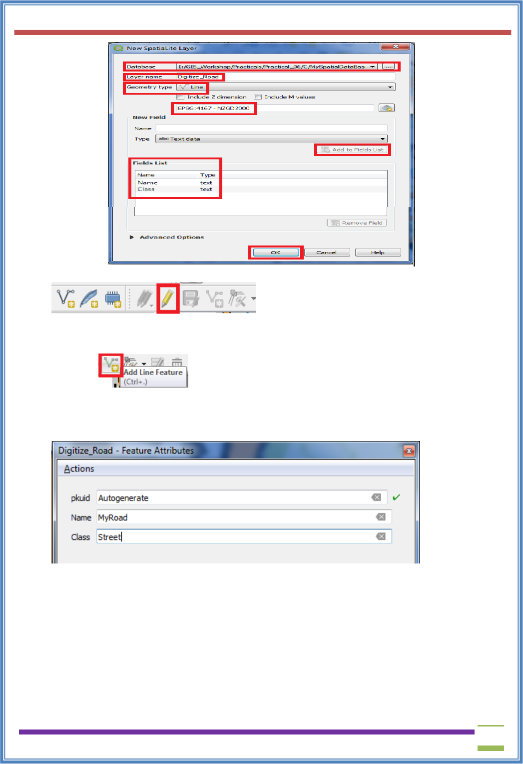
➢ Go to Layer → Add Layer → Add Spatialite Layer.
➢ Select the name and location for Spatial database eg:
“GIS_Workshop\Practicals\Practical_06\C\MySpatialDataBase.sqlite”.
➢ Name the Layer as “Digitized_Road
➢ Set Geometry type as “Line”
➢ Set CRS EPSG:4167 – NZGD2000
USIT6P4 (Discipline Specific Elective Practical) Principles of Geographic Information Systems Practical
T. Y. B. Sc. (Information Technology) SEMESTER VI Teacher’s Reference Manual
77
➢ Add “Name” and “Class” fields using “Add to Fields List”.
➢ Once the layer is loaded, click the Toggle Editing button to put the layer in editing mode.
➢ Click the Add feature button. Click on the map canvas to add a new vertex.
Add new vertices along the road feature. Once you have digitized a road segment, right-click to
end the feature.
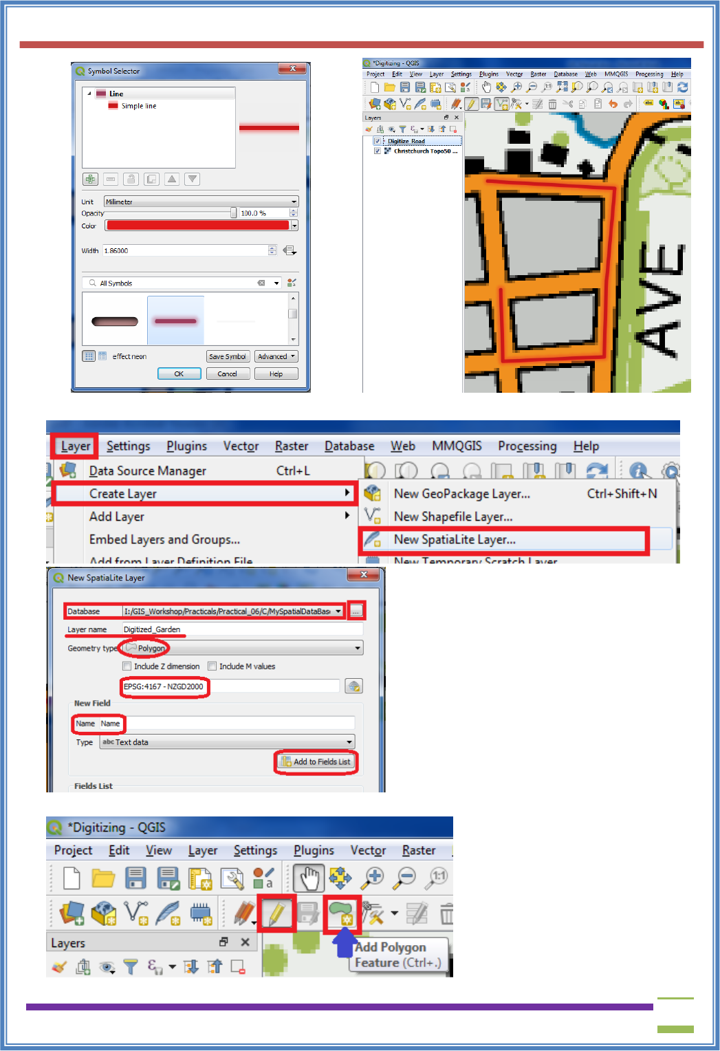
➢ On Layer Panel Right Click on Digitze_Road, Select the Style tab in the Layer Properties
dialog.
USIT6P4 (Discipline Specific Elective Practical) Principles of Geographic Information Systems Practical
T. Y. B. Sc. (Information Technology) SEMESTER VI Teacher’s Reference Manual
78
Result
➢ Select appropriate style to see the digitized road feature clearly.
➢ After creating a new Spatialite layer
USIT6P4 (Discipline Specific Elective Practical) Principles of Geographic Information Systems Practical
T. Y. B. Sc. (Information Technology) SEMESTER VI Teacher’s Reference Manual
79
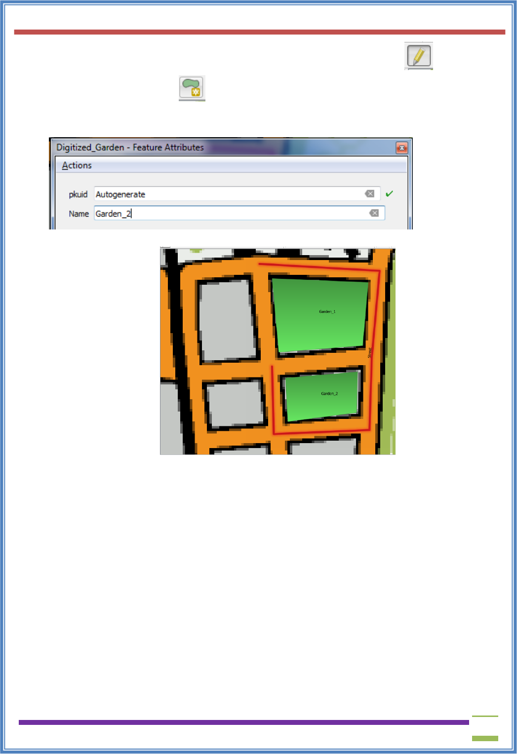
➢ Select Digitized_Garden layer in Layer Panel and click on Toggle Editing button and
then Add Polygon Feature button on Tool bar.
➢ Add two gardens to the region by adding polygon.
➢ The Layer will appear on map canvas
➢ Using the above procedure a point feature can also be digitized.
➢ The digitizing task is now complete. You can play with the styling and labeling options in layer
properties to create a nice looking map from the data you created.
USIT6P4 (Discipline Specific Elective Practical) Principles of Geographic Information Systems Practical
T. Y. B. Sc. (Information Technology) SEMESTER VI Teacher’s Reference Manual
80
PRACTICAL - 7
Managing Data Tables and Saptial data Sets:
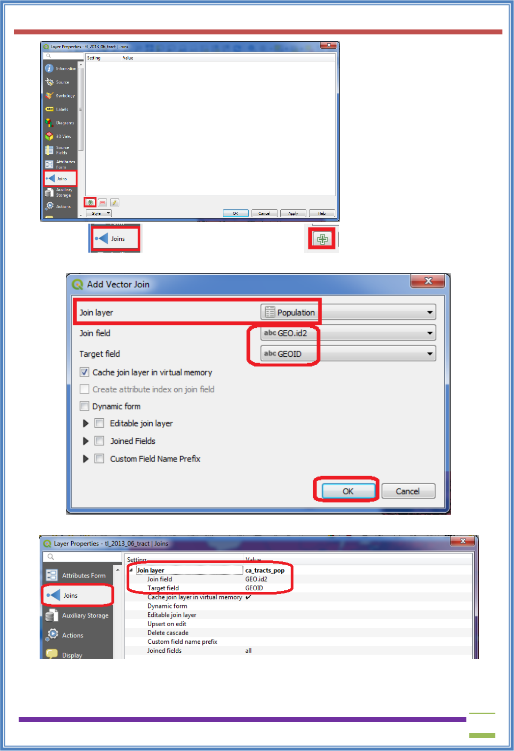
a) Table joins
➢ Start a new project
➢ Go to Layer → Add Layer → Add new Vector Layer
“I:\GIS_Workshop\Practicals\Practical_07\A\Data\tl_2013_06_tract.zip”
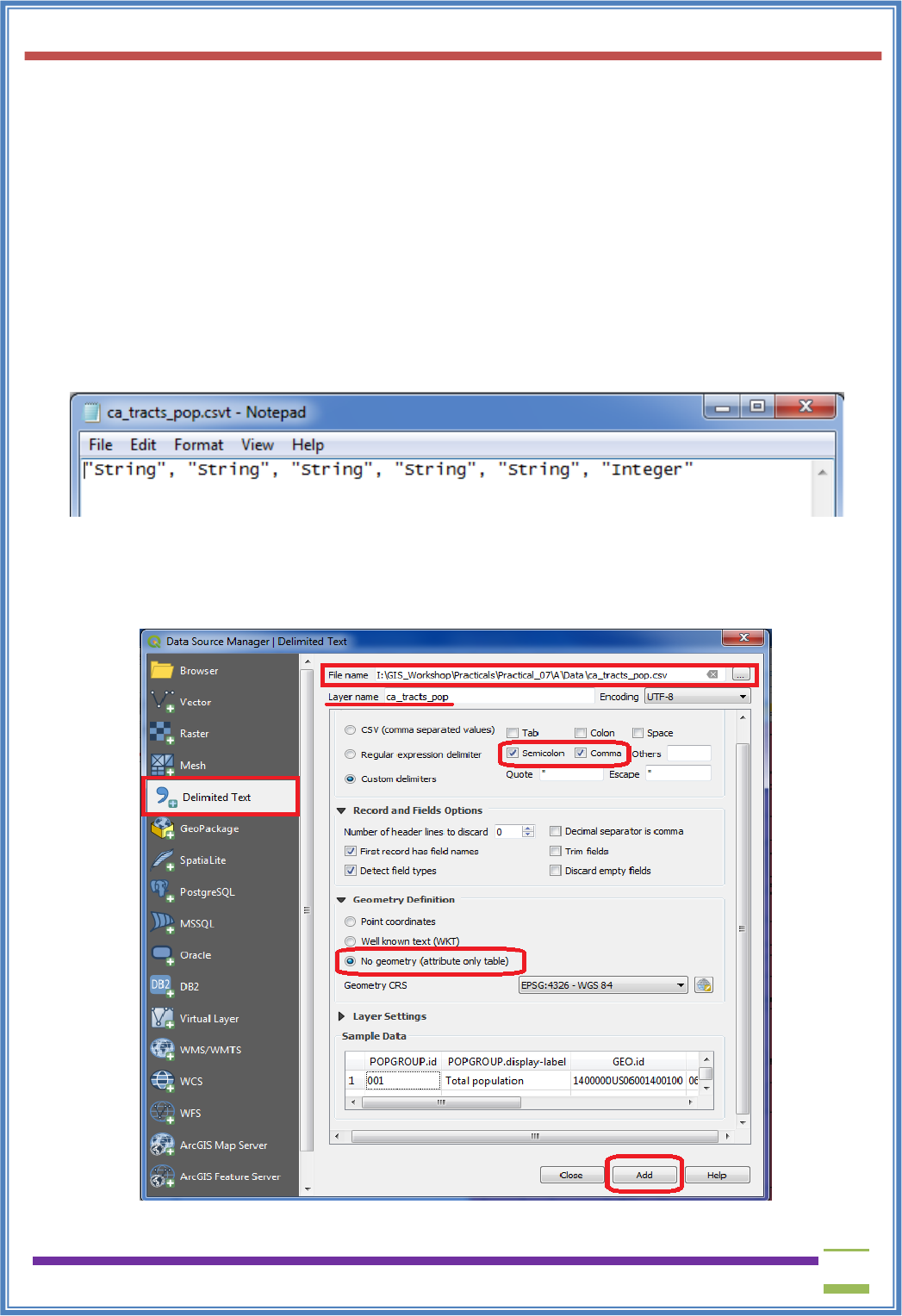
➢ We could import this csv file without any further action and it would be imported. But, the default
type of each column would be a String (text). That is ok except for the D001 field which contains
numbers for the population. Having those imported as text would not allow us to run any
mathematical operations on this column. To tell QGIS to import the field as a number, we need to
create a sidecar file with a .csvt extension.
➢ This file will have only 1 row specifying data types for each column. Save this file as
ca_tracts_pop.csvt in the same directory as the original .csv file.
➢ Go to Layer → Add Layer → Add Delimited Text Layer
And add I:\GIS_Workshop\Practicals\Practical_07\A\Data\ca_tacts_pop.csv”
➢ In the layer panel, Right click on “tl_2013_06_tract”, layer and select Properties
USIT6P4 (Discipline Specific Elective Practical) Principles of Geographic Information Systems Practical
T. Y. B. Sc. (Information Technology) SEMESTER VI Teacher’s Reference Manual
81
➢ Select the option in Properties, and click on button to add new table join.
➢ In the Add Vector Join window set the following properties and click OK.
➢ After performing join
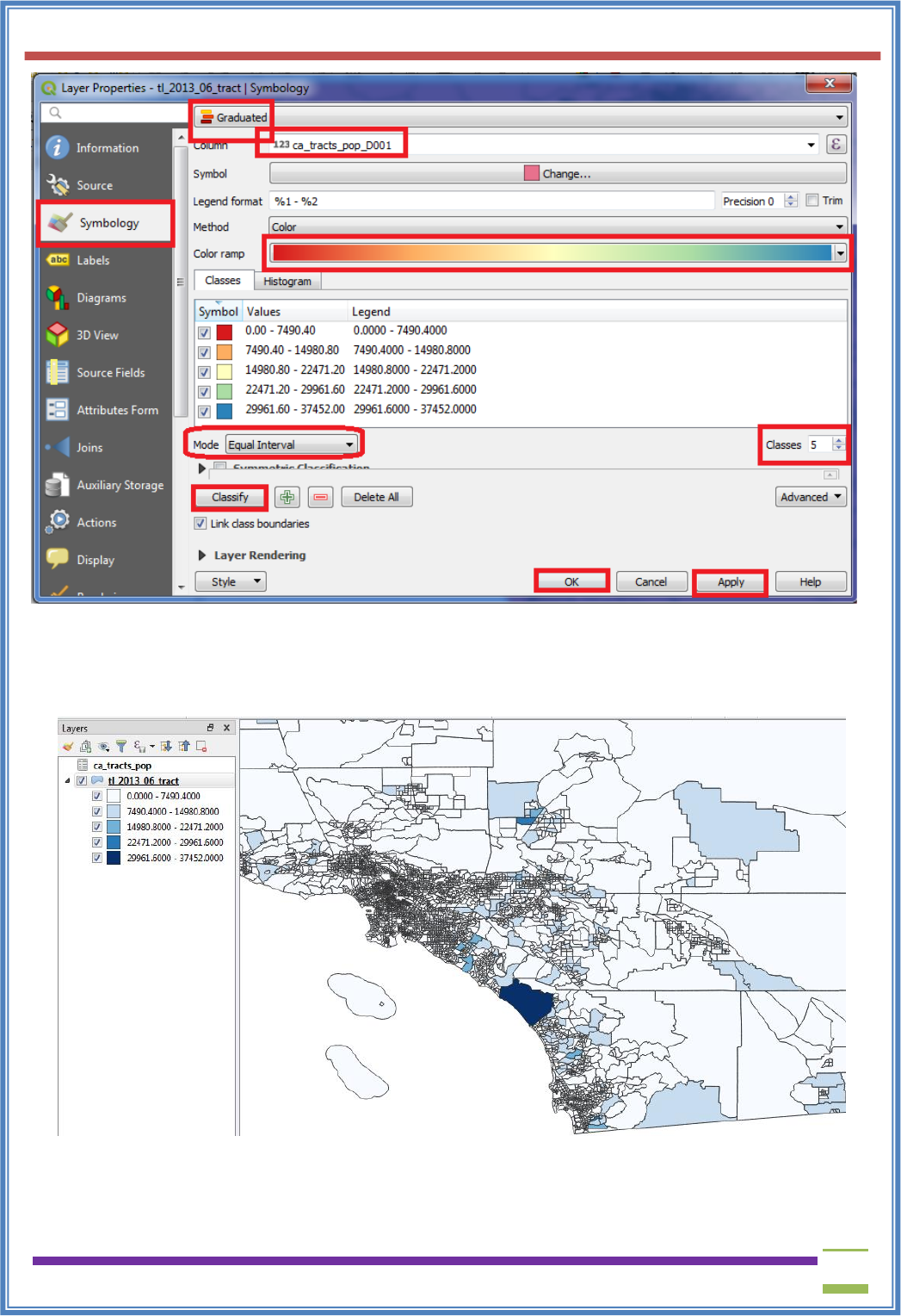
➢ For more clear output, select “tl_2013_06_tact” from Layer Panel, right click and select
properties. Go to Symbology and set the following properties.
USIT6P4 (Discipline Specific Elective Practical) Principles of Geographic Information Systems Practical
T. Y. B. Sc. (Information Technology) SEMESTER VI Teacher’s Reference Manual
82
➢ A detailed and accurate population map of California can be seen as the result. Same technique
can be used to create maps based on variety of census data.
USIT6P4 (Discipline Specific Elective Practical) Principles of Geographic Information Systems Practical
T. Y. B. Sc. (Information Technology) SEMESTER VI Teacher’s Reference Manual
83
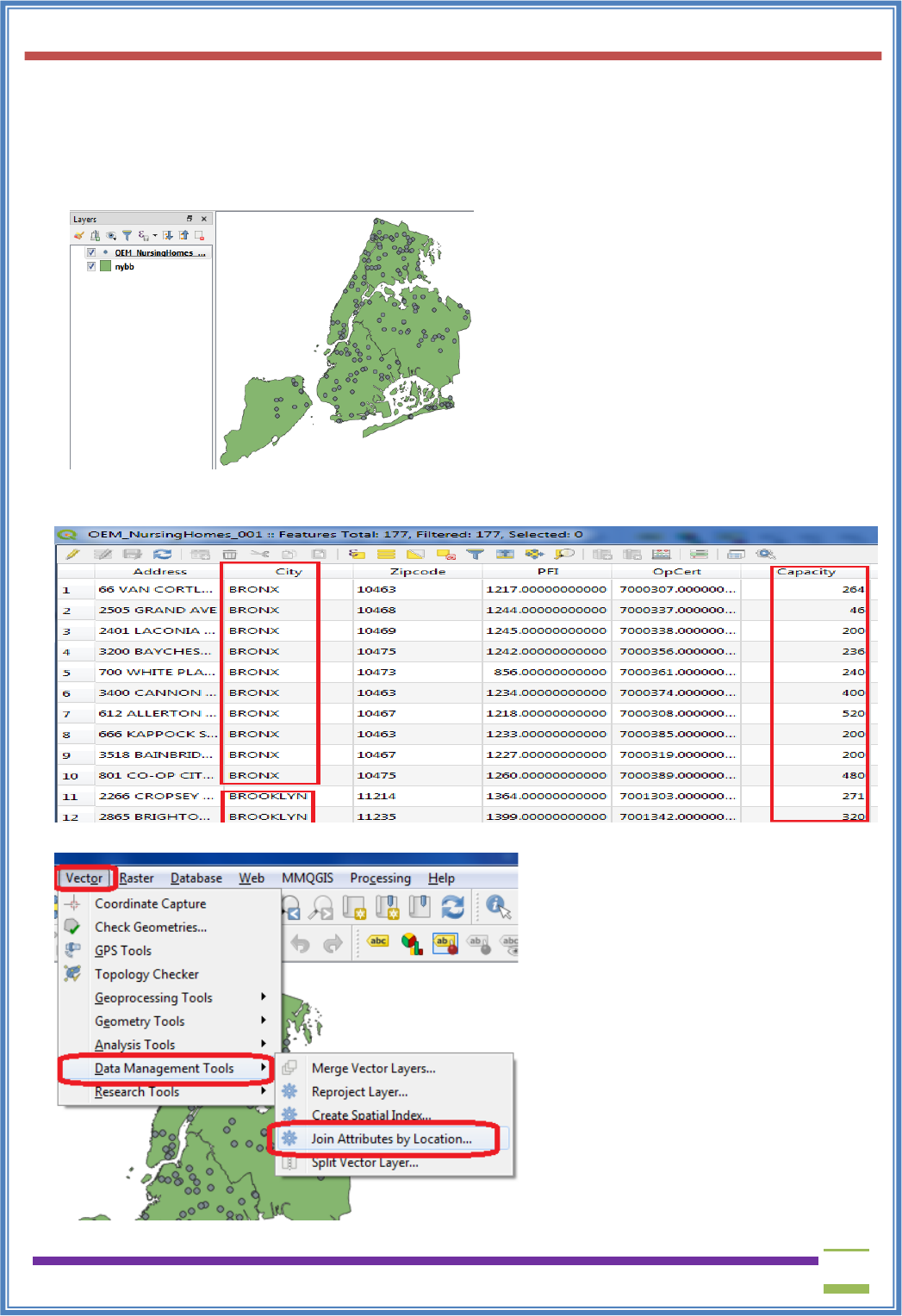
b) spatial joins
➢ Go to Layer → Add Layer → Add Vector Layer → Select
“I:\GIS_Workshop\Practicals\Practical_07\B\Data\nybb_12c\nybb_13c_av\nybb.shp” and
“I:\GIS_Workshop\Practicals\Practical_07\B\Data\OEM_NursingHomes_001\OEM_NursingHo
mes_001.shp”, from data folder.
➢ Go to attribute table and observe the data.
➢ Table before performing Join
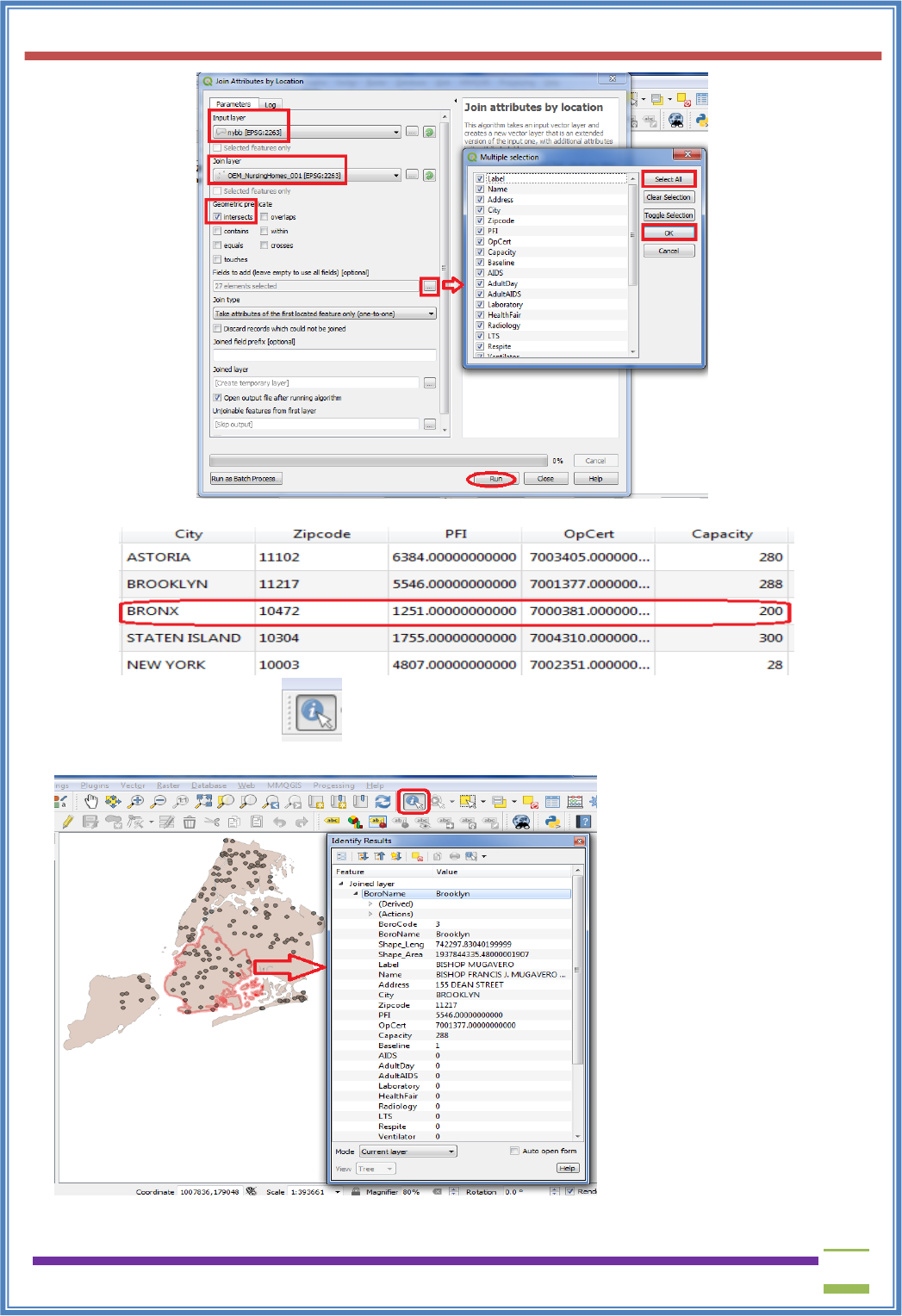
➢ Go to Vector → Data Management Tools → Join Attributes by Location
USIT6P4 (Discipline Specific Elective Practical) Principles of Geographic Information Systems Practical
T. Y. B. Sc. (Information Technology) SEMESTER VI Teacher’s Reference Manual
84
➢ Attribute table after join
➢ Use the Identify Feature Button to select a region to view join data on map Layer.
➢ Output
USIT6P4 (Discipline Specific Elective Practical) Principles of Geographic Information Systems Practical
T. Y. B. Sc. (Information Technology) SEMESTER VI Teacher’s Reference Manual
85
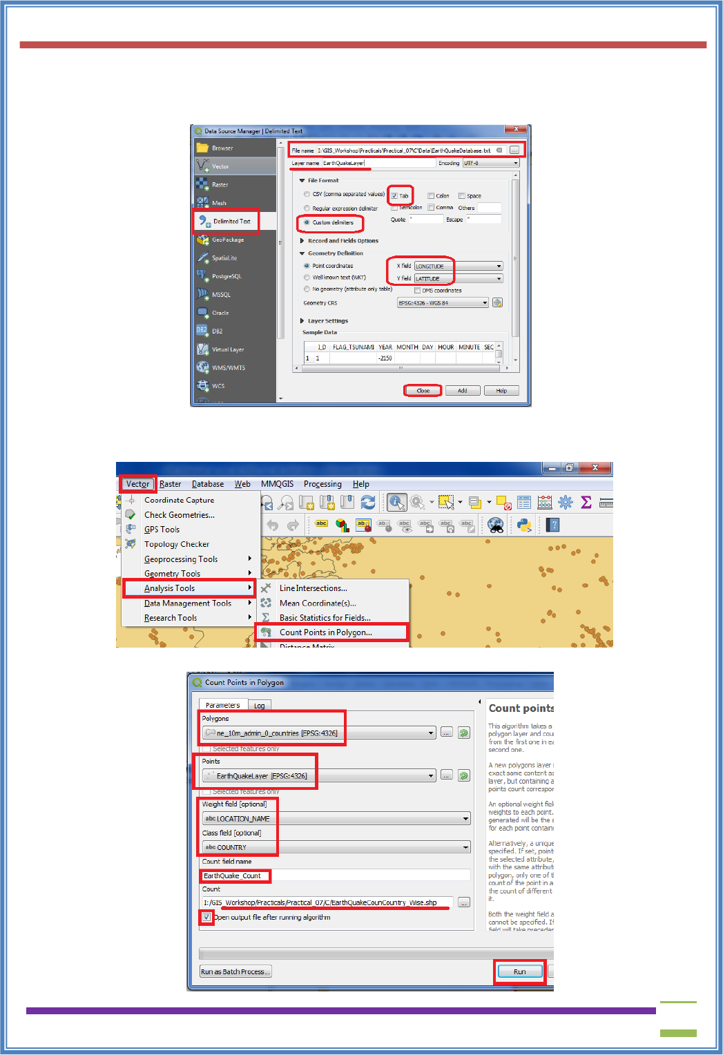
c) Points in polygon analysis
➢ Go to Layer → Add Layer → Add Delimited Text Layer
Select “EarthQuakeDatabase.txt”
➢ Go to Layer → Add Layer → Add Delimited Text Layer
“I:\GIS_Workshop\Practicals\Practical_07\C\Data\ne_10m_admin_0_countries.zip”
→
USIT6P4 (Discipline Specific Elective Practical) Principles of Geographic Information Systems Practical
T. Y. B. Sc. (Information Technology) SEMESTER VI Teacher’s Reference Manual
86
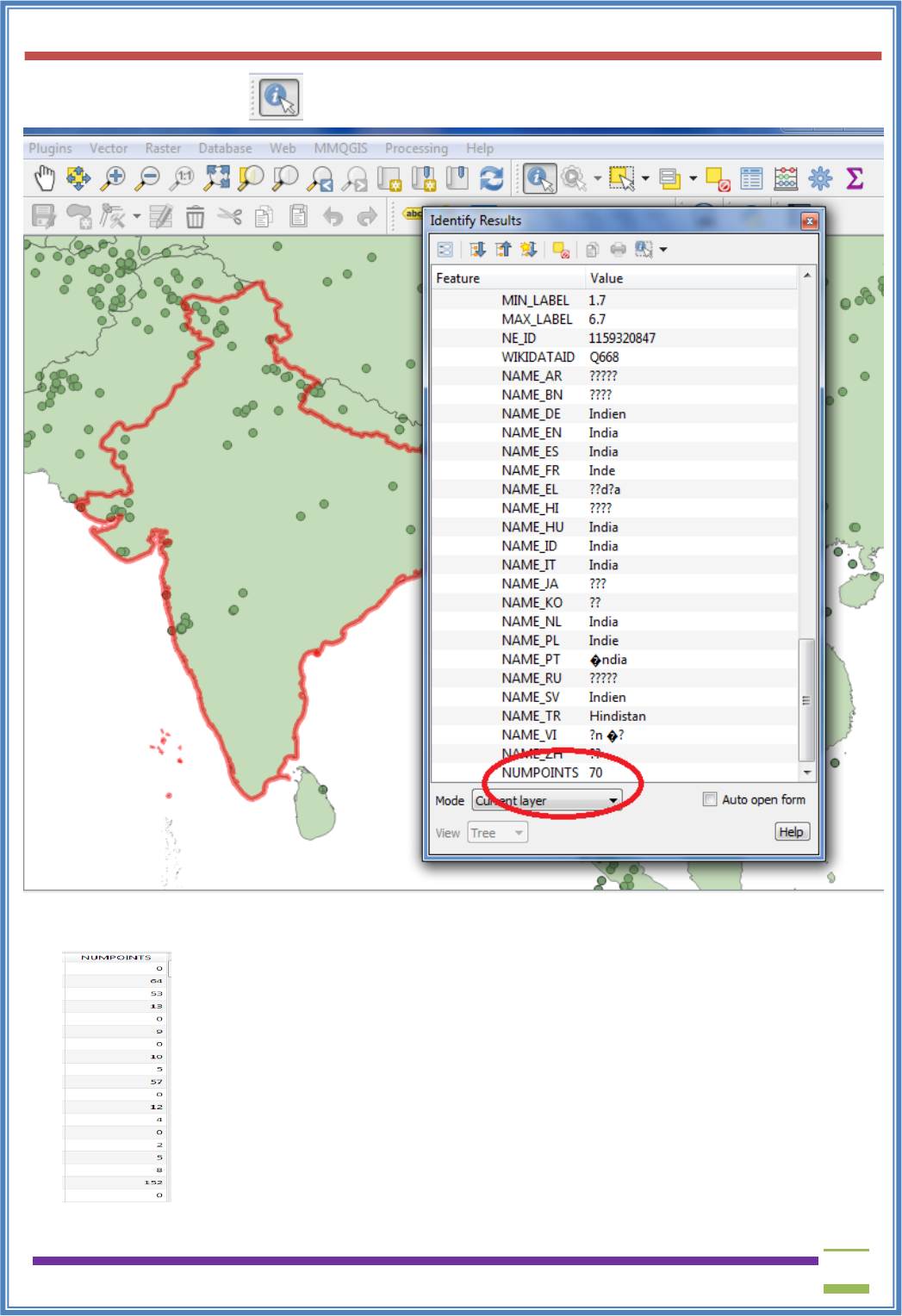
➢ Use the select Feature button to check country wise counting of Earthquakes.
➢ Also a new column is added to attribute table “NumPoints” indicating number of earth quake
points in each country.
USIT6P4 (Discipline Specific Elective Practical) Principles of Geographic Information Systems Practical
T. Y. B. Sc. (Information Technology) SEMESTER VI Teacher’s Reference Manual
87
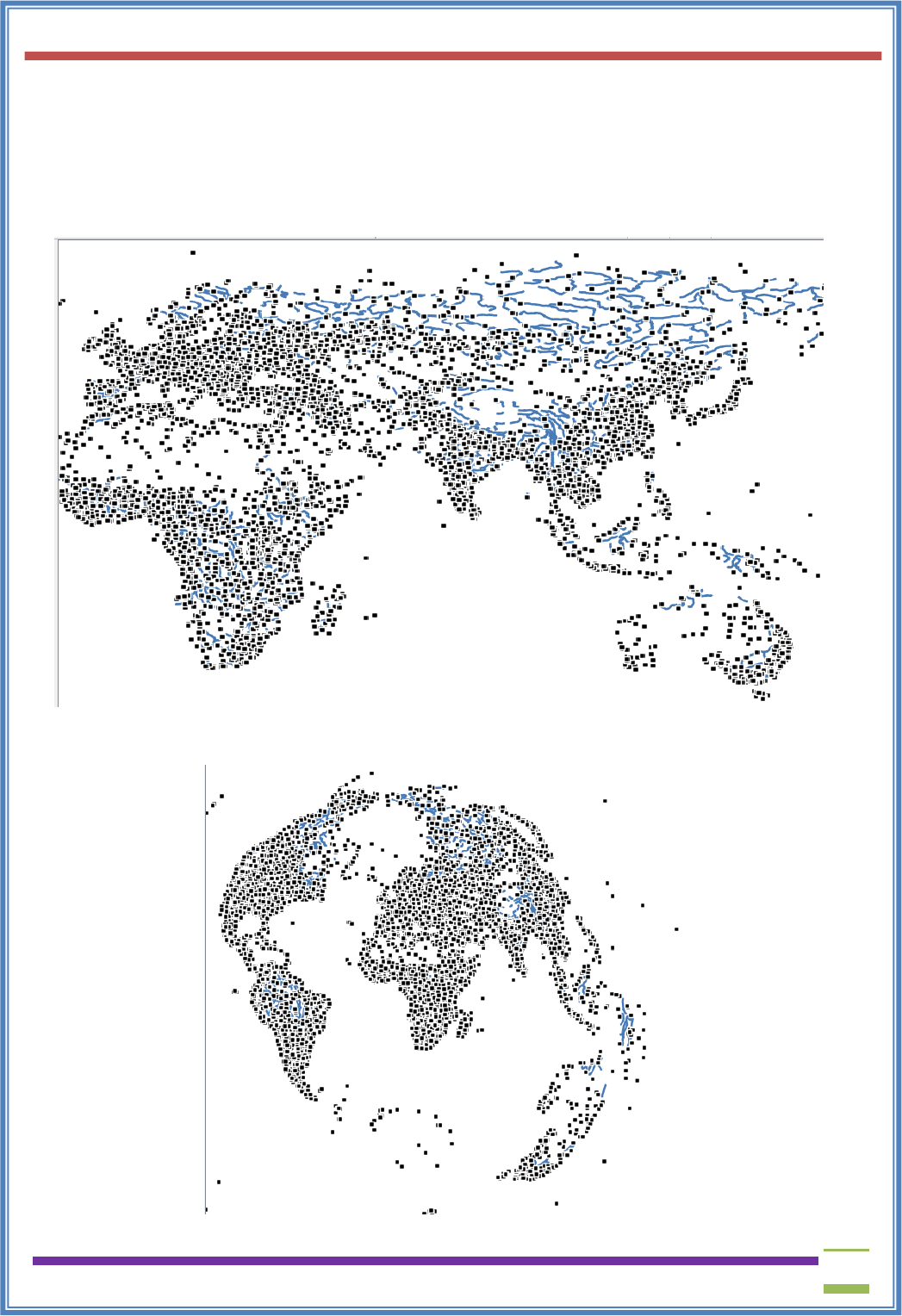
d) Performing spatial queries
➢ Go to Layer → Add Layer → Add Vector Layer and load
“\GIS_Workshop\Practicals\Practical_07\D\Data\ne_10m_populated_places_simple\ne_10m_popul
ated_places_simple.shp” and
“I:\GIS_Workshop\Practicals\Practical_07\D\Data\ne_10m_rivers_lake_centerlines\ne_10m_rivers
_lake_centerlines.shp” from project data folder.
➢ Open project Properties → Set CRS “World_Azimuthal_Equidistant EPSG 54032” . The map will
be re-projected as
USIT6P4 (Discipline Specific Elective Practical) Principles of Geographic Information Systems Practical
T. Y. B. Sc. (Information Technology) SEMESTER VI Teacher’s Reference Manual
88
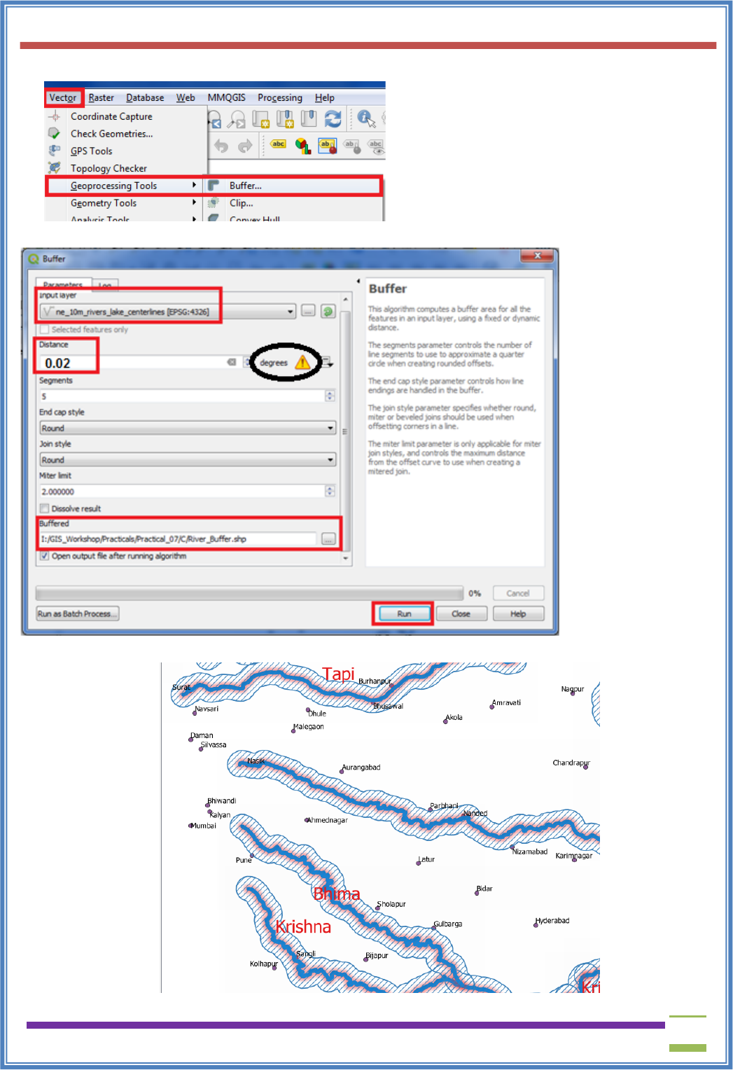
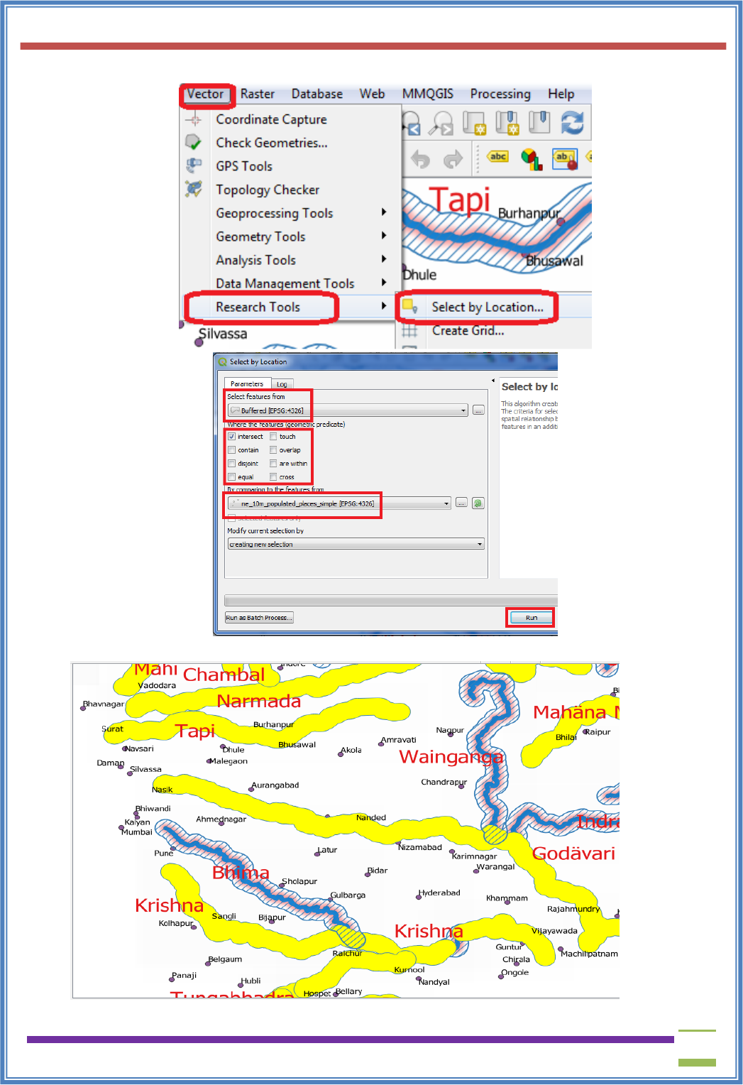
➢ Go to Vector → Geoprocessing Tool → Buffer
➢ Repeat the step to create River Buffer
➢ Create a buffer for River
USIT6P4 (Discipline Specific Elective Practical) Principles of Geographic Information Systems Practical
T. Y. B. Sc. (Information Technology) SEMESTER VI Teacher’s Reference Manual
89
➢ Go to Vector → Research Tool → Select By Location
➢ This will highlight only those rivers containing a populated place within 2 KM
USIT6P4 (Discipline Specific Elective Practical) Principles of Geographic Information Systems Practical
T. Y. B. Sc. (Information Technology) SEMESTER VI Teacher’s Reference Manual
90
PRACTICAL - 8
Advanced GIS Operations 1:
a) Nearest Neighbor Analysis
➢ Go to Layer → add Layer → add Delimited Text Layer and load “signif.txt” from data file.
➢ Go to Layer → Add Layer → Add vector Layer and from data folder
“\GIS_Workshop\Practicals\Practical_08\A\DATA\ne_10m_populated_places_simple.zip” load
the layer to the project and remove all rows from attribute table other than India.
USIT6P4 (Discipline Specific Elective Practical) Principles of Geographic Information Systems Practical
T. Y. B. Sc. (Information Technology) SEMESTER VI Teacher’s Reference Manual
91
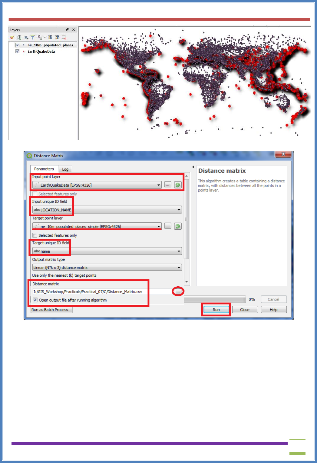
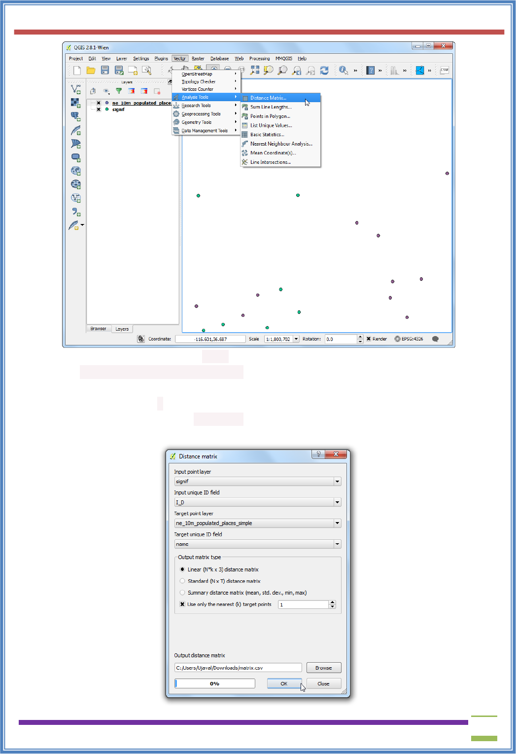
➢ Go to Vector→ Analysis tool → Distance Matrix
➢ Calculate the Distance matrix and perform Nearest Neighbor Analysis
➢ Now you will be able to see the content of our results. The InputID field contains the field name
from the Earthquake layer. The TargetID field contains the name of the feature from the
Populated Places layer that was the closest to the earthquake point. The Distance field is the
distance between the 2 points.
USIT6P4 (Discipline Specific Elective Practical) Principles of Geographic Information Systems Practical
T. Y. B. Sc. (Information Technology) SEMESTER VI Teacher’s Reference Manual
92
7. Here select the earthquake layer signif as the Input point layer and the populated
places ne_10m_populated_places_simpleas the target layer. You also need to select a unique
field from each of these layers which is how your results will be displayed. In this analysis, we
are looking to get only 1 nearest point, so check the Use only the nearest(k) target points, and
enter 1. Name your output file matrix.csv, and click OK. Once the processing finishes,
click Close.
USIT6P4 (Discipline Specific Elective Practical) Principles of Geographic Information Systems Practical
T. Y. B. Sc. (Information Technology) SEMESTER VI Teacher’s Reference Manual
93
8. Once the processing finishes, click the Close button in the Distance Matrix dialog. You can now
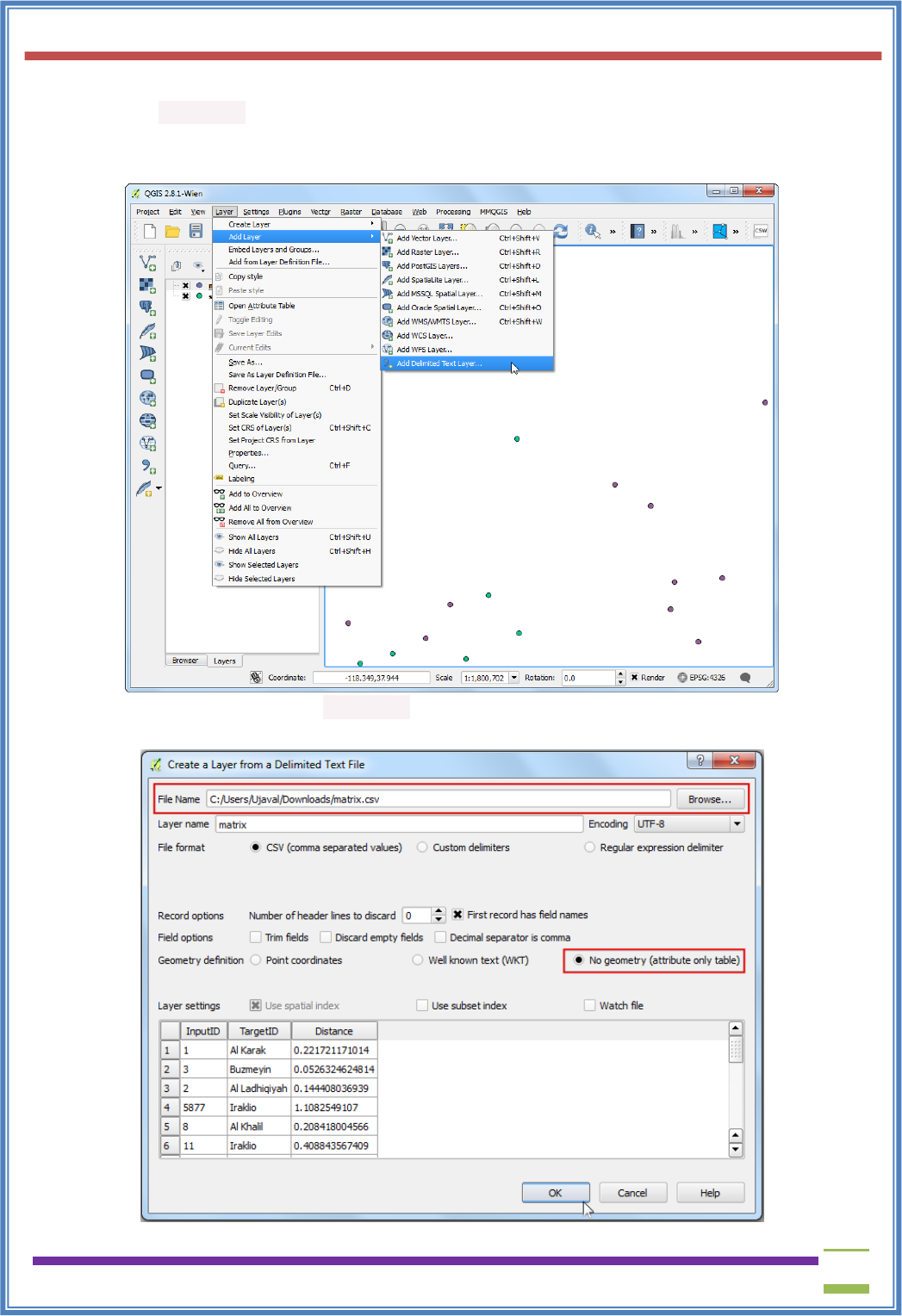
view the matrix.csv file in Notepad or any text editor. QGIS can import CSV files as well, so
we will add it to QGIS and view it there. Go to Layer ‣ Add Layer ‣ Add Delimited Text
Layer....
9. Browse to the newly created matrix.csv file. Since this file is just text columns, select No
geometry (attribute only table) as theGeometry definition. Click OK.
USIT6P4 (Discipline Specific Elective Practical) Principles of Geographic Information Systems Practical
T. Y. B. Sc. (Information Technology) SEMESTER VI Teacher’s Reference Manual
94
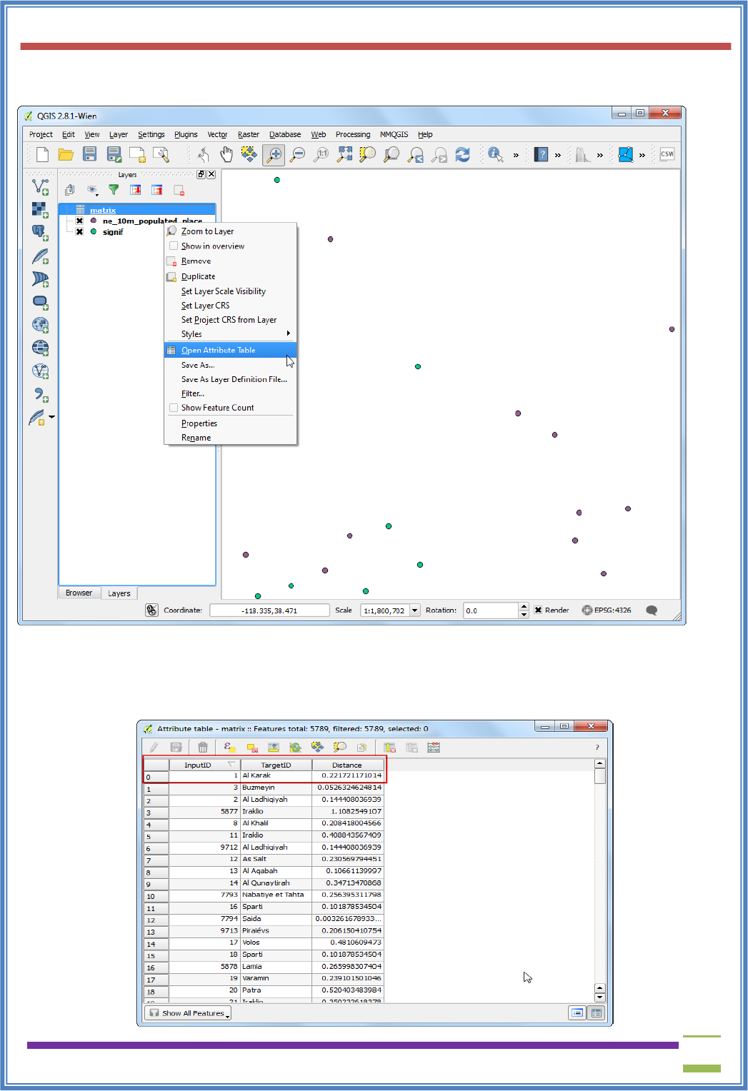
10. You will see the CSV file loaded as a table. Right-click on the table layer and select Open
Attribute Table.
11. Now you will be able to see the content of our results. The InputID field contains the field name
from the Earthquake layer. The TargetID field contains the name of the feature from the
Populated Places layer that was the closest to the earthquake point. The Distance field is the
distance between the 2 points.
USIT6P4 (Discipline Specific Elective Practical) Principles of Geographic Information Systems Practical
T. Y. B. Sc. (Information Technology) SEMESTER VI Teacher’s Reference Manual
95
12. This is very close to the result we were looking for. For some users, this table would be
sufficient. However, we can also integrate this results in our original Earthquake layer using
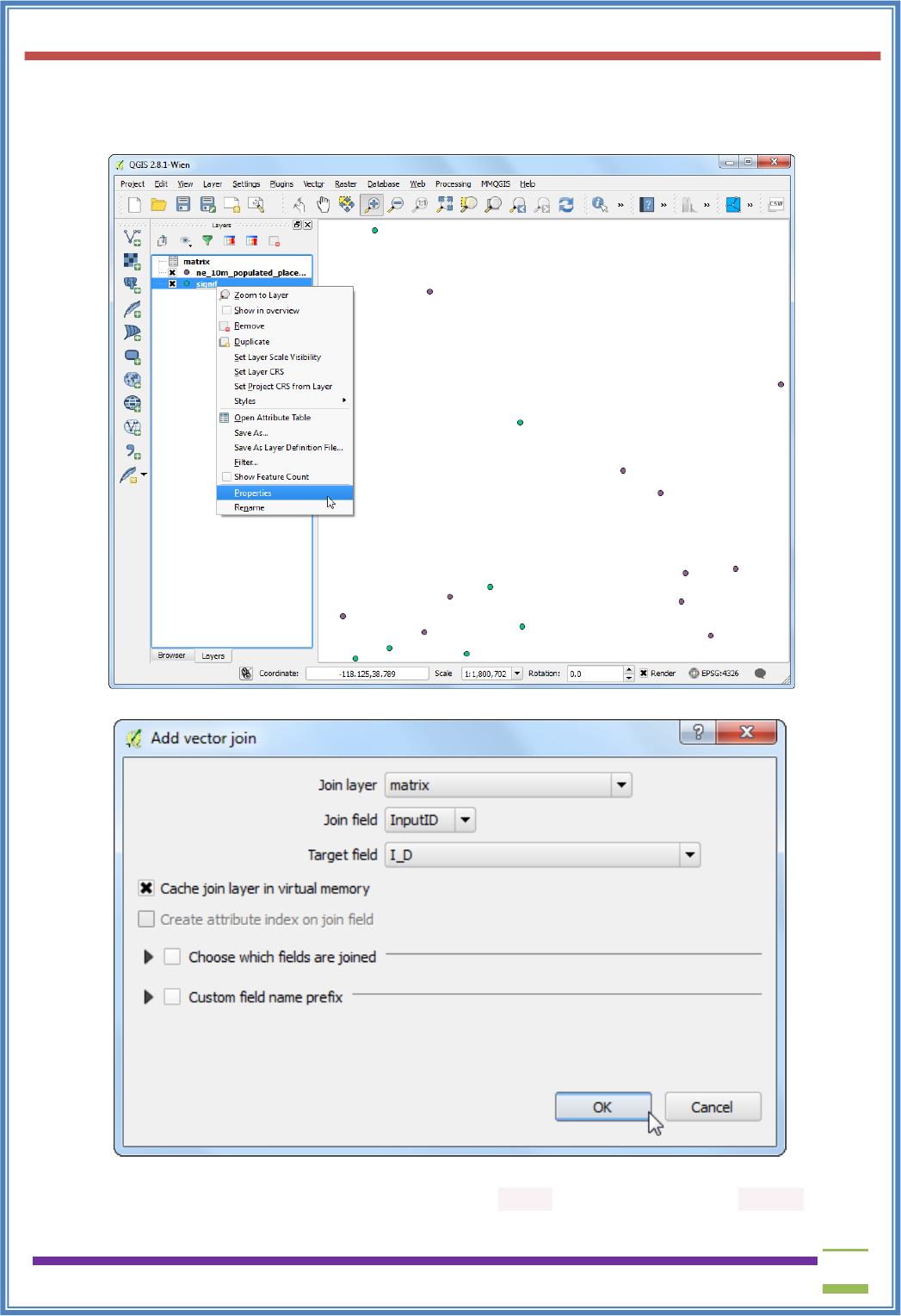
a Table Join. Right-click on the Earthquake layer, and select Properties.
13. Go to the Joins tab and click on the + button.
14. We want to join the data from our analysis result to this layer. We need to select a field from
each of the layers that has the same values. Select matrix as the Join layer` and InputID as
USIT6P4 (Discipline Specific Elective Practical) Principles of Geographic Information Systems Practical
T. Y. B. Sc. (Information Technology) SEMESTER VI Teacher’s Reference Manual
96
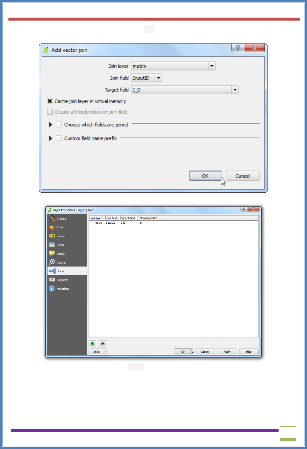
the Join field. The Target field would be I_D. Leave other options to their default values and
click OK.
15. You will see the join appear in the Joins tab. Click OK.
16. Now open the attribute table of the signif layer by right-clicking and selecting Open Attribute
Table.
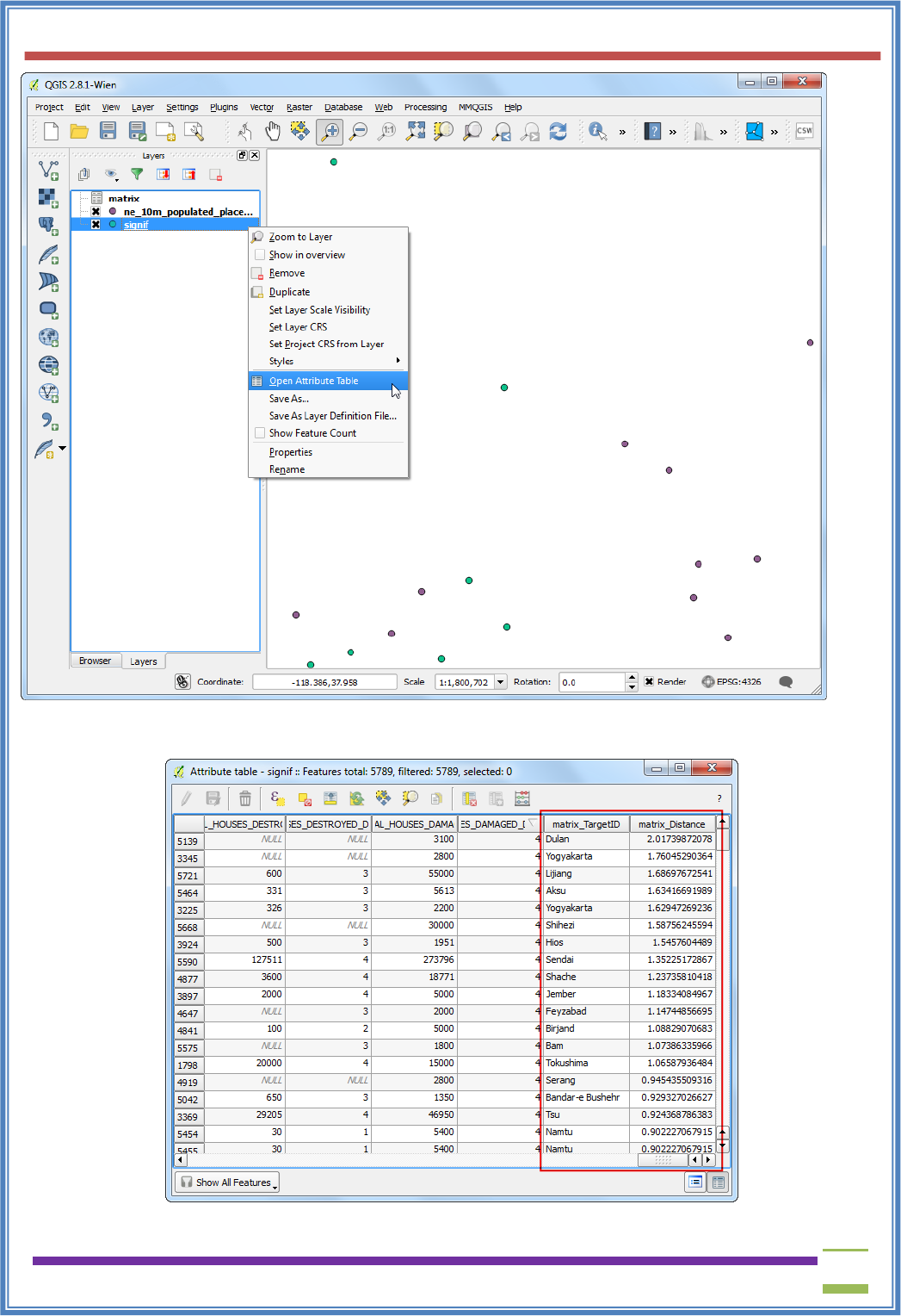
USIT6P4 (Discipline Specific Elective Practical) Principles of Geographic Information Systems Practical
T. Y. B. Sc. (Information Technology) SEMESTER VI Teacher’s Reference Manual
97
17. You will see that for every Earthquake feature, we now have an attribute which is the nearest
neighbor (closest populated place) and the distance to the nearest neighbor.
USIT6P4 (Discipline Specific Elective Practical) Principles of Geographic Information Systems Practical
T. Y. B. Sc. (Information Technology) SEMESTER VI Teacher’s Reference Manual
98
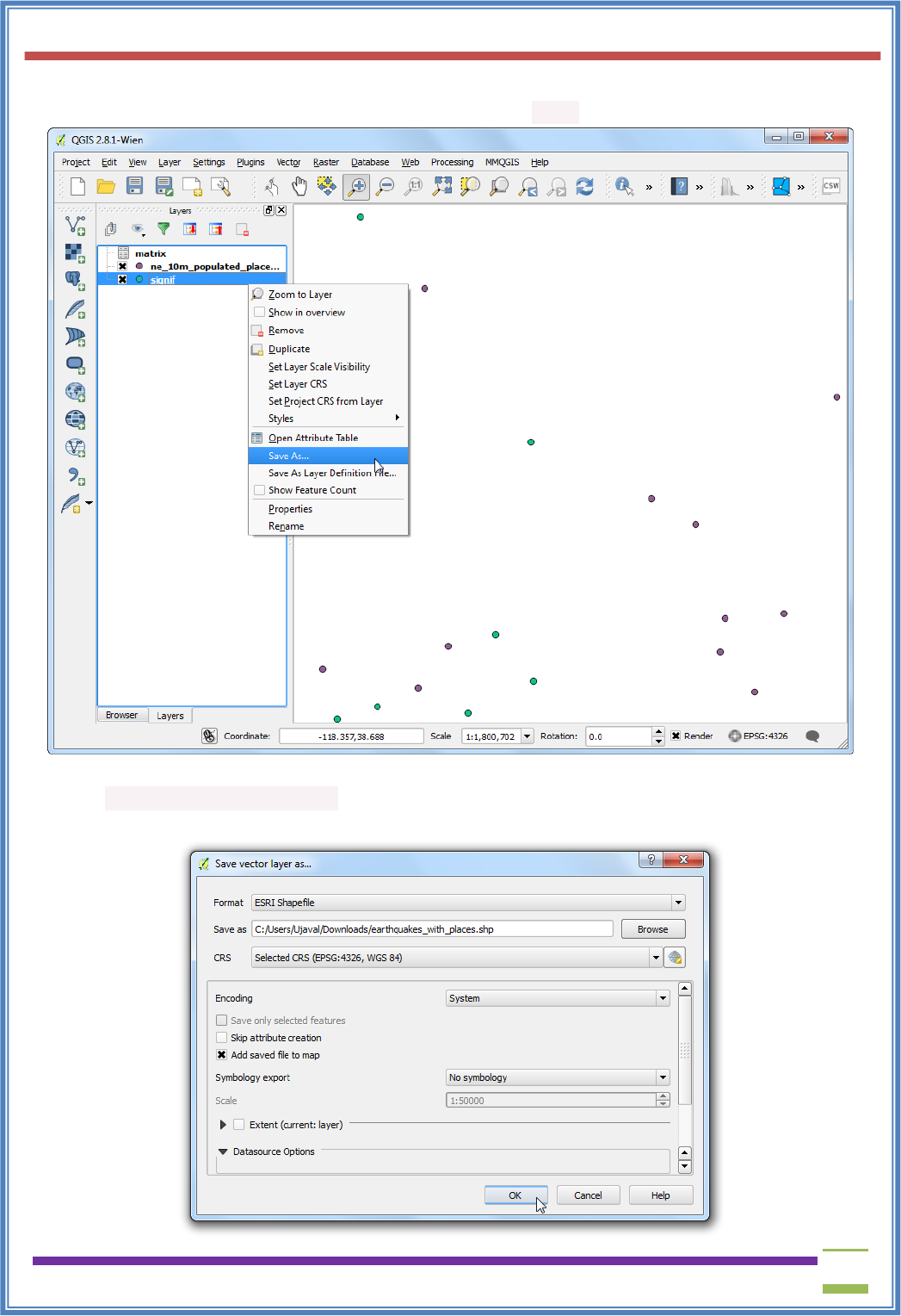
18. We will now explore a way to visualize these results. First, we need to make the table join
permanent by saving it to a new layer. Right-click the signif layer and select Save As....
19. Click the Browse button next to Save as label and name the output layer
as earthquake_with_places.shp. Make sure the Add saved file to map box is checked and
click OK.
USIT6P4 (Discipline Specific Elective Practical) Principles of Geographic Information Systems Practical
T. Y. B. Sc. (Information Technology) SEMESTER VI Teacher’s Reference Manual
99
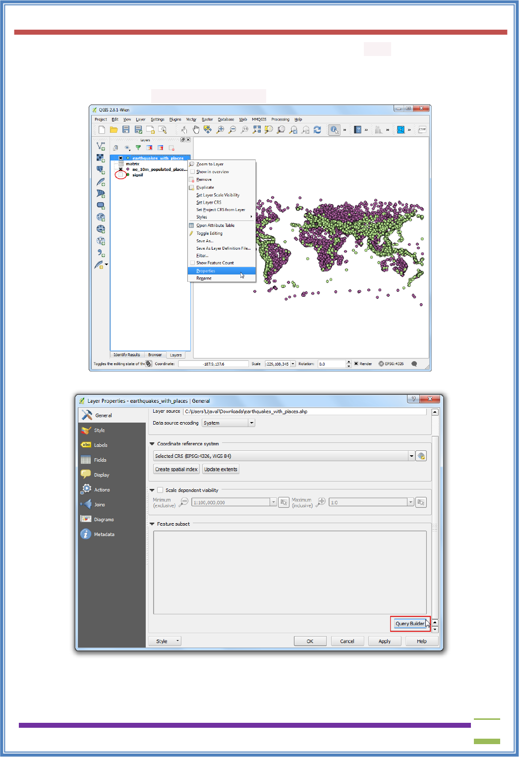
20. Once the new layer is loaded, you can turn off the visibility of the signif layer. As our dataset is
quite large, we can run our visualization analysis on a subset of the data. QGIS has a neat
feature where you can load a subset of features from a layer without having to export it to a new
layer. Right-click the earthquake_with_places layer and select Properties.
21. In the General tab, scroll down to the Feature subset section. Click Query Builder.
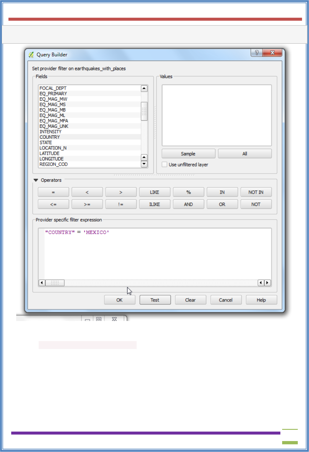
22. For this tutorial, we will visualize the earthquakes and their nearest populated places for
Mexico. Enter the following expression in the Query Builder dialog.
USIT6P4 (Discipline Specific Elective Practical) Principles of Geographic Information Systems Practical
T. Y. B. Sc. (Information Technology) SEMESTER VI Teacher’s Reference Manual
100
"COUNTRY" = 'MEXICO'
23. You will see that only the points falling within Mexico will be visible in the canvas. Let’s do
the same for the populated places layer. Right-click on
the ne_10m_populated_places_simple layer and select Properties.
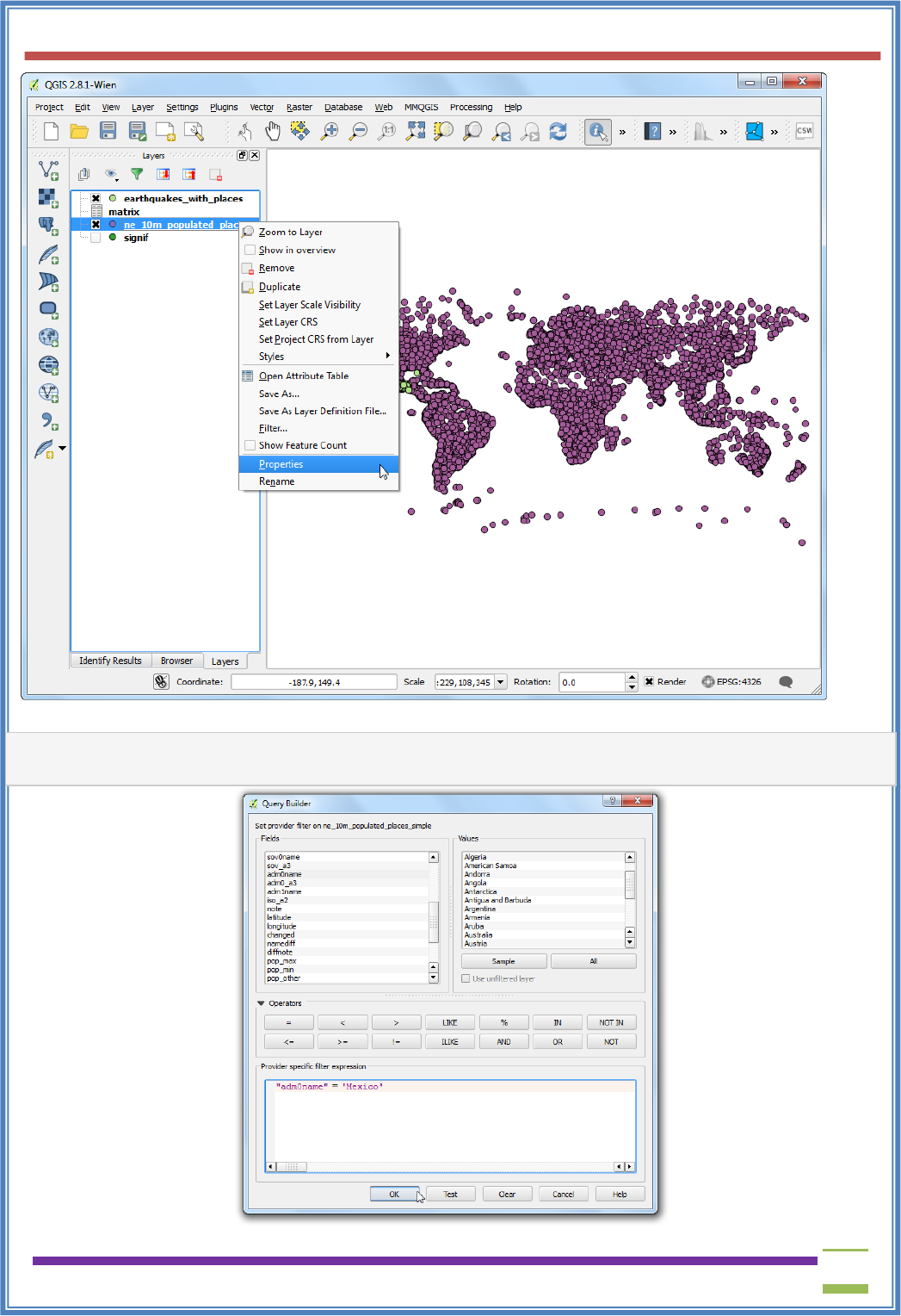
USIT6P4 (Discipline Specific Elective Practical) Principles of Geographic Information Systems Practical
T. Y. B. Sc. (Information Technology) SEMESTER VI Teacher’s Reference Manual
101
24. Open the Query Builder dialog from the General tab. Enter the following expression.
"adm0name" = 'Mexico'
USIT6P4 (Discipline Specific Elective Practical) Principles of Geographic Information Systems Practical
T. Y. B. Sc. (Information Technology) SEMESTER VI Teacher’s Reference Manual
102
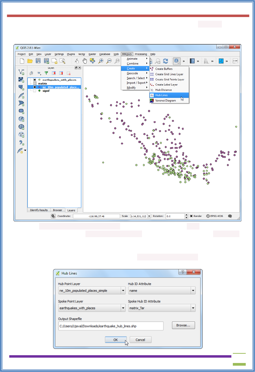
25. Now we are ready to create our visualization. We will use a plugin named MMQGIS. Find and
install the plugin. See Using Pluginsfor more details on how to work with plugins. Once you
have the plugin installed, go to MMQGIS ‣ Create ‣ Hub Lines.
26. Select ne_10m_populated_places_simple as the Hub Point Layer and name as the Hub ID
Attribute. Similarly, selectearthquake_with_places as the Spoke Point Layer and matrix_Tar as
the Spoke Hub ID Attribute. The hub lines algorithm will go through each of earthquake points
and create a line that will join it to the populated place which matches the attribute we specified.
Click Browse and name the Output Shapefile as earthquake_hub_lines.shp. Click OK to start
the processing.
USIT6P4 (Discipline Specific Elective Practical) Principles of Geographic Information Systems Practical
T. Y. B. Sc. (Information Technology) SEMESTER VI Teacher’s Reference Manual
103
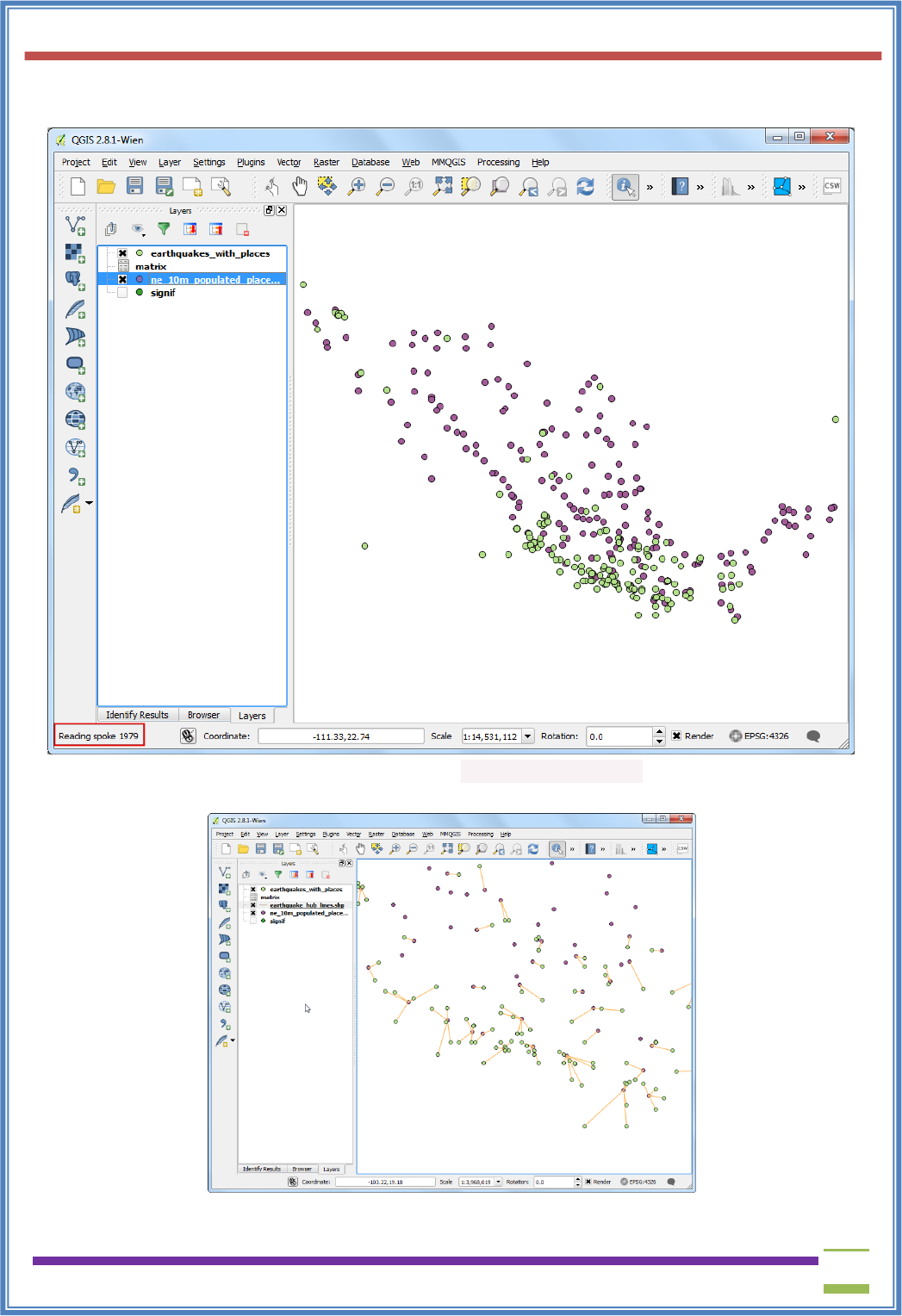
27. The processing may take a few minutes. You can see the progress on the bottom-left corner of
the QGIS window.
28. Once the processing is done, you will see the earthquake_hub_lines layer loaded in QGIS. You
can see that each earthquake point now has a line that connects it to the nearest populated place.
USIT6P4 (Discipline Specific Elective Practical) Principles of Geographic Information Systems Practical
T. Y. B. Sc. (Information Technology) SEMESTER VI Teacher’s Reference Manual
104
B) Sampling Raster Data using Points or Polygons
Many scientific and environmental datasets come as gridded rasters. Elevation data (DEM) is
also distributed as raster files. In these raster files, the parameter that is being represented is
encoded as the pixel values of the raster. Often, one needs to extract the pixel values at certain
locations or aggregate them over some area. This functionality is available in QGIS via two
plugins - Point SamplingTool and Zonal Statistics plugin.
Procedure
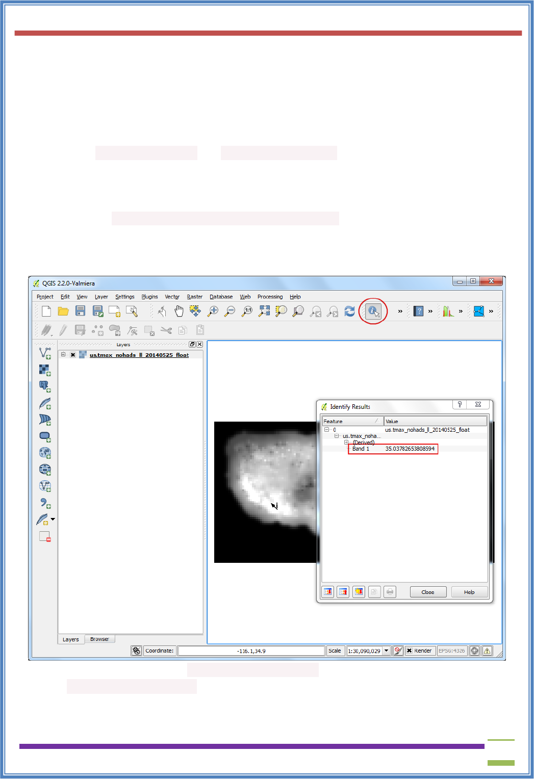
1. Go to Layer ‣ Add Raster Layer and browse to the
downloaded us.tmax_nohads_ll_{YYYYMMDD}_float.tif file and click Open.
2. Once the layer is loaded, select the Identify tool and click anywhere on the layer. You will see
the temperature value in celsius as the value or Band 1 at that location.
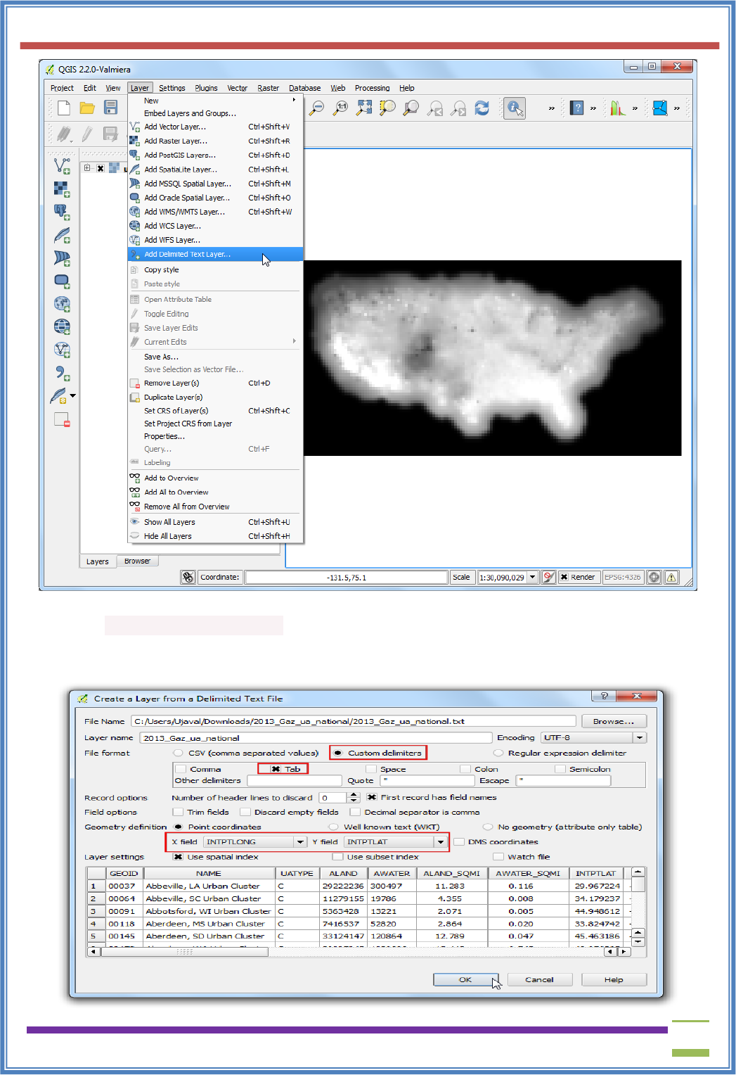
3. Now unzip the downloaded 2013_Gaz_ua_national.zip file and extract
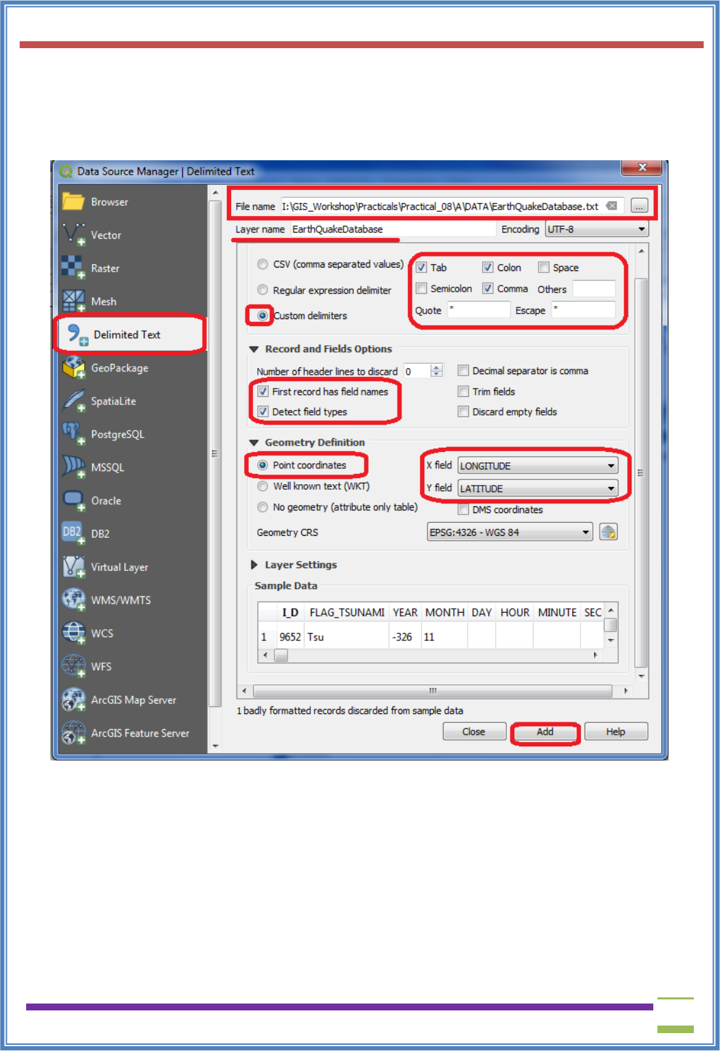
the 2013_Gaz_ua_national.txt file on your disk. Go to Layer ‣ Add Delimited Text Layer.
USIT6P4 (Discipline Specific Elective Practical) Principles of Geographic Information Systems Practical
T. Y. B. Sc. (Information Technology) SEMESTER VI Teacher’s Reference Manual
105
4. In the Create a Layer from Delimited Text File dialog, click Browse and
open 2013_Gaz_ua_national.txt. Choose Tab under Custom delimiters. The point coordinates
are in Latitude and Longitude, so select INTPTLONG as X field and INTPTLAT as Y field.
Check the Use spatial index box and click OK.
USIT6P4 (Discipline Specific Elective Practical) Principles of Geographic Information Systems Practical
T. Y. B. Sc. (Information Technology) SEMESTER VI Teacher’s Reference Manual
106
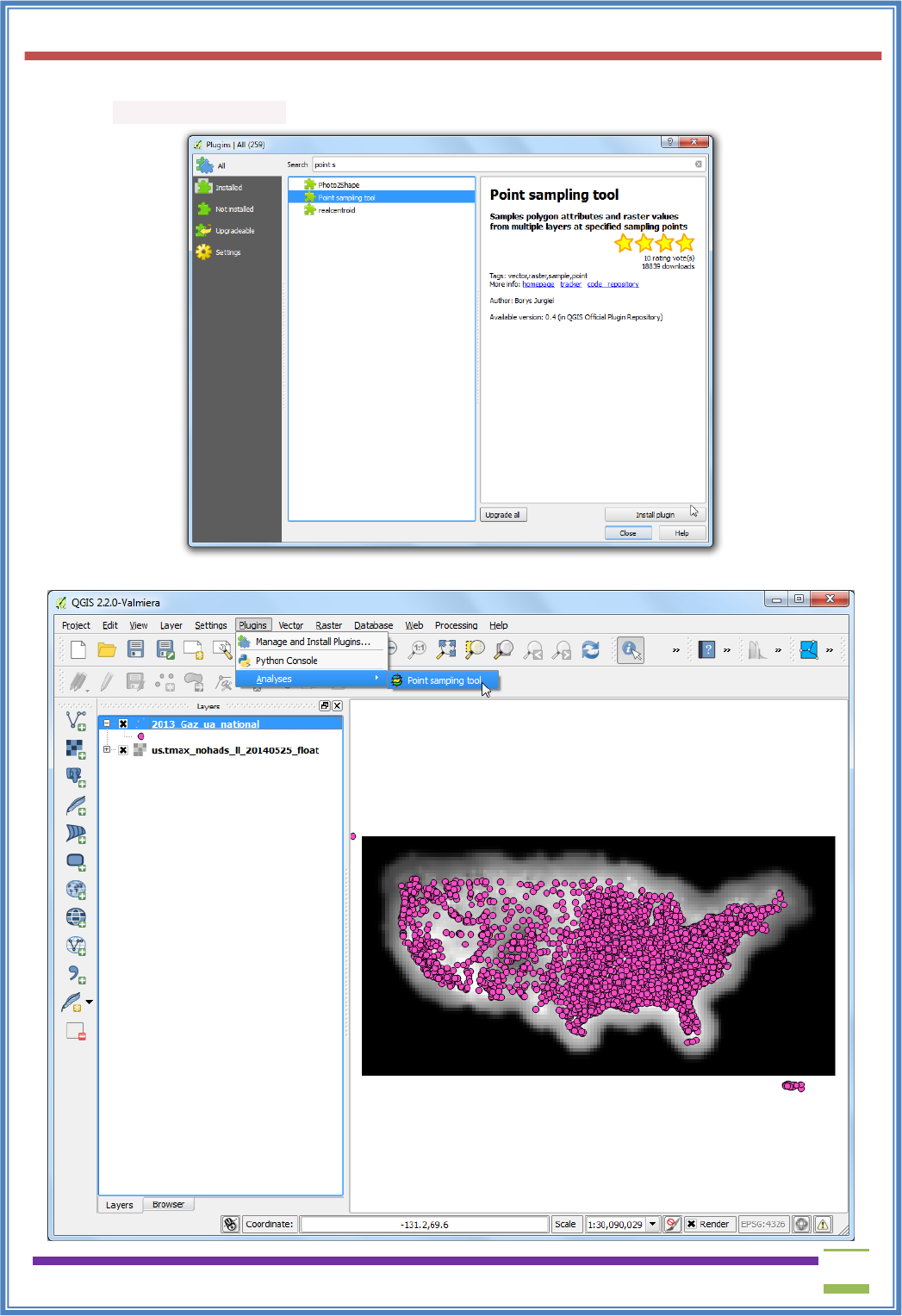
5. Now we are ready to extract the temperature values from the raster layer. Install
the Point Sampling Tool plugin. See Using Plugins for details on how to install plugins.
6. Open the plugin dialog from Plugins ‣ Analyses ‣ Point sampling tool.
USIT6P4 (Discipline Specific Elective Practical) Principles of Geographic Information Systems Practical
T. Y. B. Sc. (Information Technology) SEMESTER VI Teacher’s Reference Manual
107
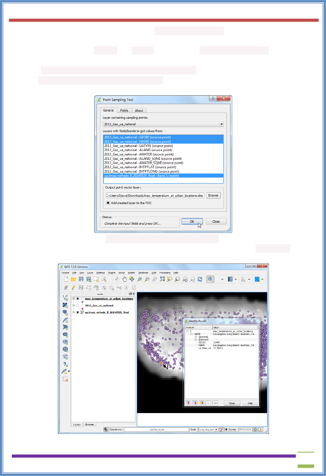
7. In the Point Sampling Tool dialog, select 2013_Gaz_ua_national as the Layer containing
sampling points. We must explicitely pick the fields from the input layer that we want in the
output layer. Choose GEOID and NAME fields from the2013_Gaz_ua_national layer. We can
sample values from multiple raster band at once, but since our raster has only 1 band, choose
the us.tmax_nohads_ll_{YYYYMMDD}_float: Band 1. Name the output vector layer
as max_temparature_at_urban_locations.shp. Click the OK to start the sampling process.
Click Close once the process finishes.
8. You will see a new layer max_temparature_at_urban_locations loaded in QGIS. Use
the Identify tool to click on any point to see the attributes. You will see the us.tmax_no field -
which contains the raster pixel value at the location of the point.
USIT6P4 (Discipline Specific Elective Practical) Principles of Geographic Information Systems Practical
T. Y. B. Sc. (Information Technology) SEMESTER VI Teacher’s Reference Manual
108
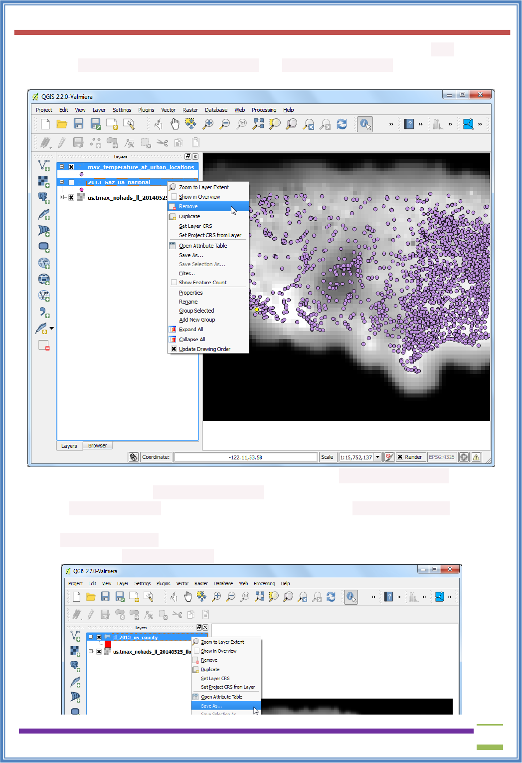
9. First part of our analysis is over. Let’s remove the unnecessary layers. Hold the Shift key and
select max_temparature_at_urban_locations and 2013_Gaz_ua_national layers. Right-click and
select Remove to remove them from QGIS TOC.
10. Go to Layer ‣ Add Vector Layer. Browse to the downloaded tl_2013_us_county.zip file and
click Open. Select thetl_2013_us_county.shp as the layer and click OK.
11. The tl_2013_us_county will be added to QGIS. This layer is in EPSG:4269 NAD83 projection.
This doesn’t match the projection of the raster layer. We will re-project this layer
to EPSG:4326 WGS84 projection.
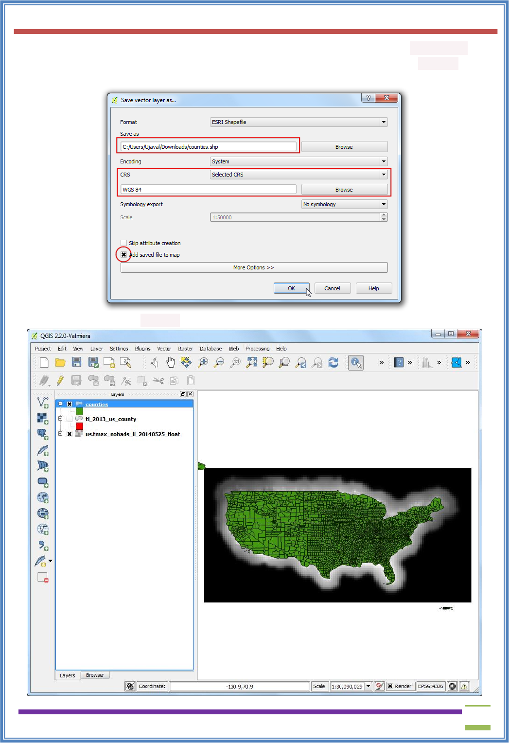
12. Right-click the tl_2013_us_county layer and select Save As...
USIT6P4 (Discipline Specific Elective Practical) Principles of Geographic Information Systems Practical
T. Y. B. Sc. (Information Technology) SEMESTER VI Teacher’s Reference Manual
109
13. In the Save Vector layer as.. dialog, click Browse and name the output file as counties.shp.
Choose Selected CRS from the CRS dropdown menu. Click Browse and select WGS 84 as the
CRS. Check the Add saved file to map and click OK.
14. A new layer named counties will be add to QGIS.
USIT6P4 (Discipline Specific Elective Practical) Principles of Geographic Information Systems Practical
T. Y. B. Sc. (Information Technology) SEMESTER VI Teacher’s Reference Manual
110
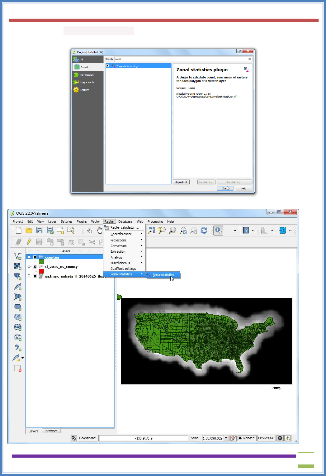
15. Enable the Zonal Statistics Plugins. This is a core plugin so it is already installed. See Using
Plugins to know to how enable core plugins.
16. Go to Raster ‣ Zonal statistics ‣ Zonal statistics.
USIT6P4 (Discipline Specific Elective Practical) Principles of Geographic Information Systems Practical
T. Y. B. Sc. (Information Technology) SEMESTER VI Teacher’s Reference Manual
111
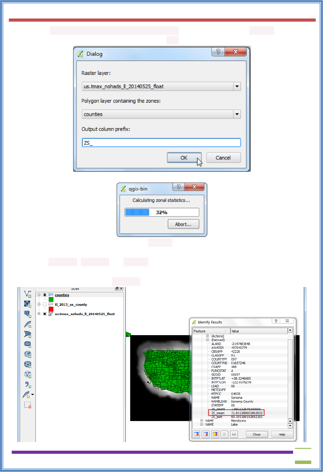
17. Select us.tmax_nohads_ll_{YYYYMMDD}_float as the Raster layer and counties as
the Polygon layer containing the zones. Enter ZS_ as the Output column prefix. Click OK.
18. The analysis may take some time depending on the size of the dataset.
19. Once the processing finishes, select the counties layer. Use the Identify tool and click on any
county polygon. You will see three new attributes added to the
layer: ZS_count, ZS_mean and ZS_sum. These attributes contain the count of raster pixels,
mean of raster pixel values and sum of raster pixel values respectively. Since we are interested
in average temperature, the ZS_meanfield will be the one to use.
USIT6P4 (Discipline Specific Elective Practical) Principles of Geographic Information Systems Practical
T. Y. B. Sc. (Information Technology) SEMESTER VI Teacher’s Reference Manual
112
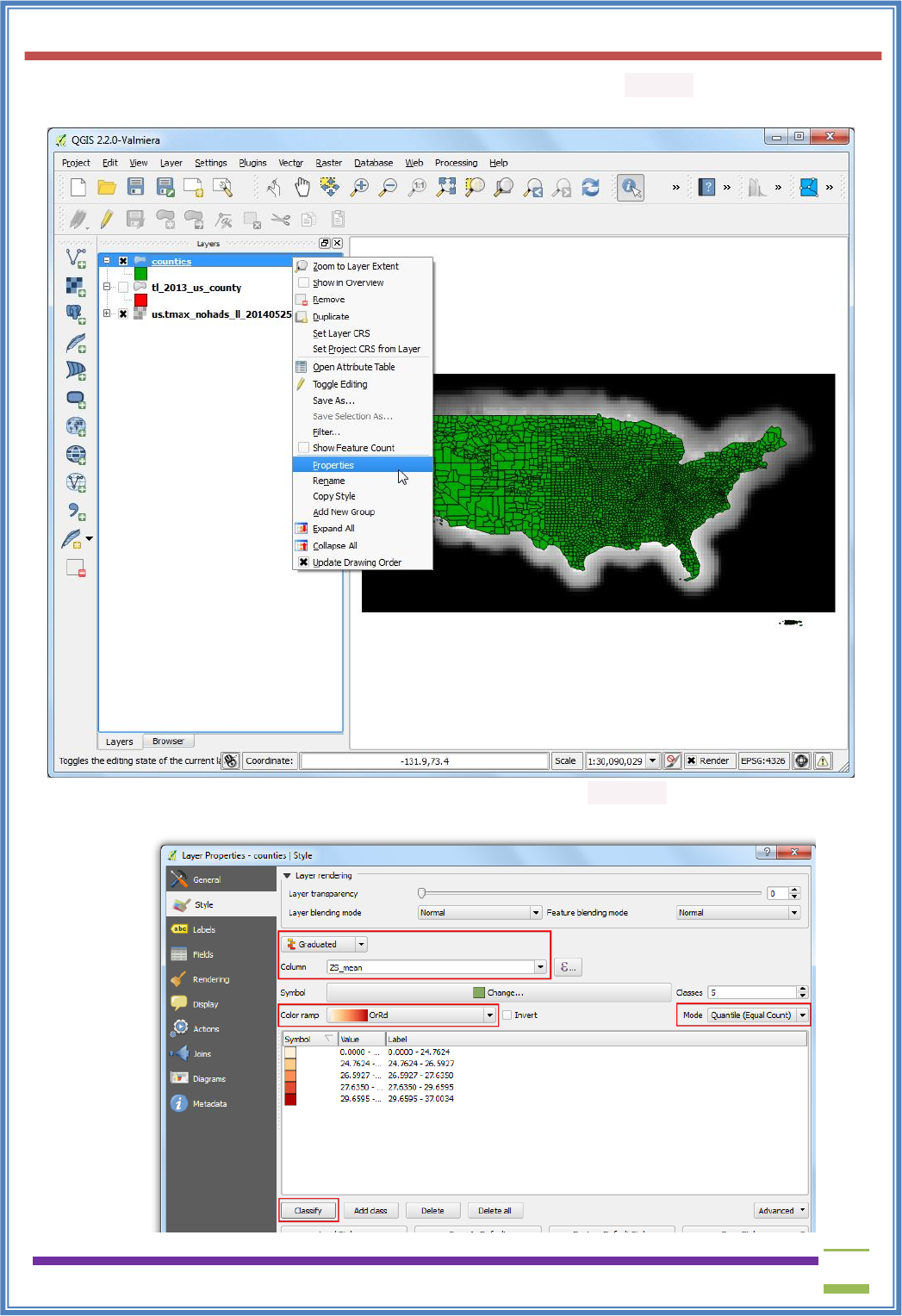
20. Let’s style this layer to create a temperature map. Right-click the counties layer and
select Properties.
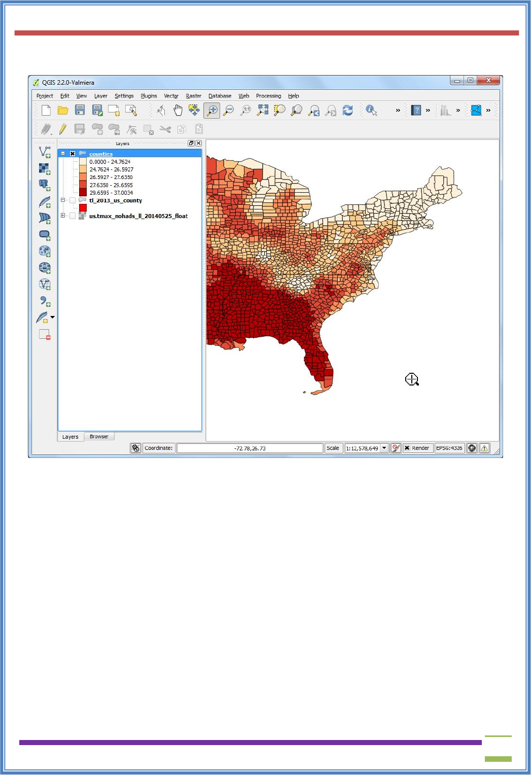
21. Switch to the Style tab. Choose Graduated style and select ZS_mean as the Column. Choose
a Color Ramp and Mode of your chose. Click Classify to create the classes. Click OK.
USIT6P4 (Discipline Specific Elective Practical) Principles of Geographic Information Systems Practical
T. Y. B. Sc. (Information Technology) SEMESTER VI Teacher’s Reference Manual
113
22. You will see the county polygons styled using average maximum temperature extracted from
the raster grid.
USIT6P4 (Discipline Specific Elective Practical) Principles of Geographic Information Systems Practical
T. Y. B. Sc. (Information Technology) SEMESTER VI Teacher’s Reference Manual
114
c) Interpolating Point Data
Procedure
1. Open QGIS. Go to Layer ‣ Add Layer ‣ Add Vector Layer..
2. Browse to the downloaded Shapefiles.zip file and select it. Click Open.
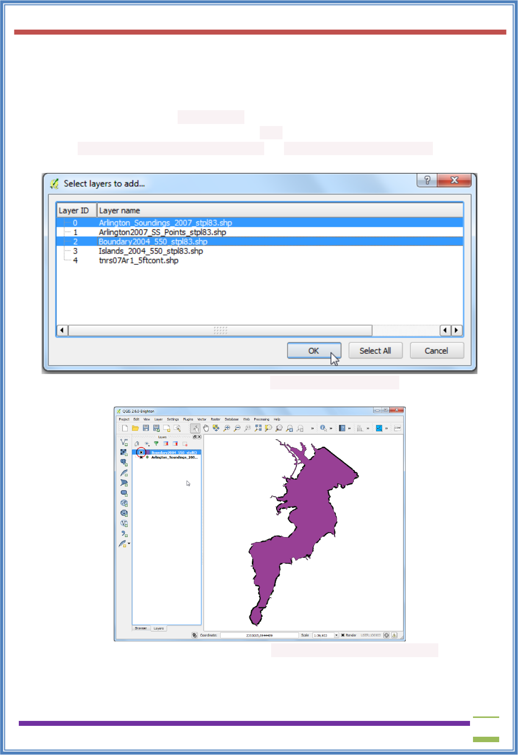
3. In the Select layers to add... dialog, hold the Shift key and
select Arlington_Soundings_2007_stpl83.shp andBoundary2004_550_stpl83.shp layers.
Click OK.
4. You will see the 2 layers loaded in QGIS. The Boundary2004_550_stpl83 layer represents the
boundary of the lake. Un-check the box next to it in the Table of Contents.
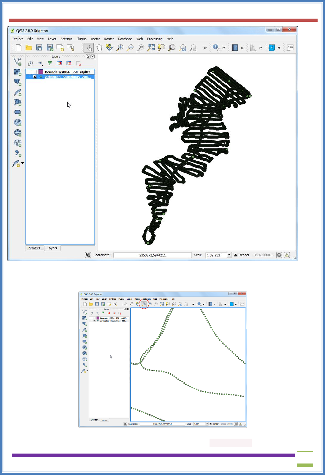
5. This will reveal the data from the second layer Arlington_Soundings_2007_stpl83. Though the
data looks like lines, it is a series of points that are very close.
USIT6P4 (Discipline Specific Elective Practical) Principles of Geographic Information Systems Practical
T. Y. B. Sc. (Information Technology) SEMESTER VI Teacher’s Reference Manual
115
6. Click the Zoom icon and select a small area on the screen. As you zoom closer, you will see the
points. Each point represents a reading taken by a Depth Sounder at the location recorded by
a DGPS equipment.
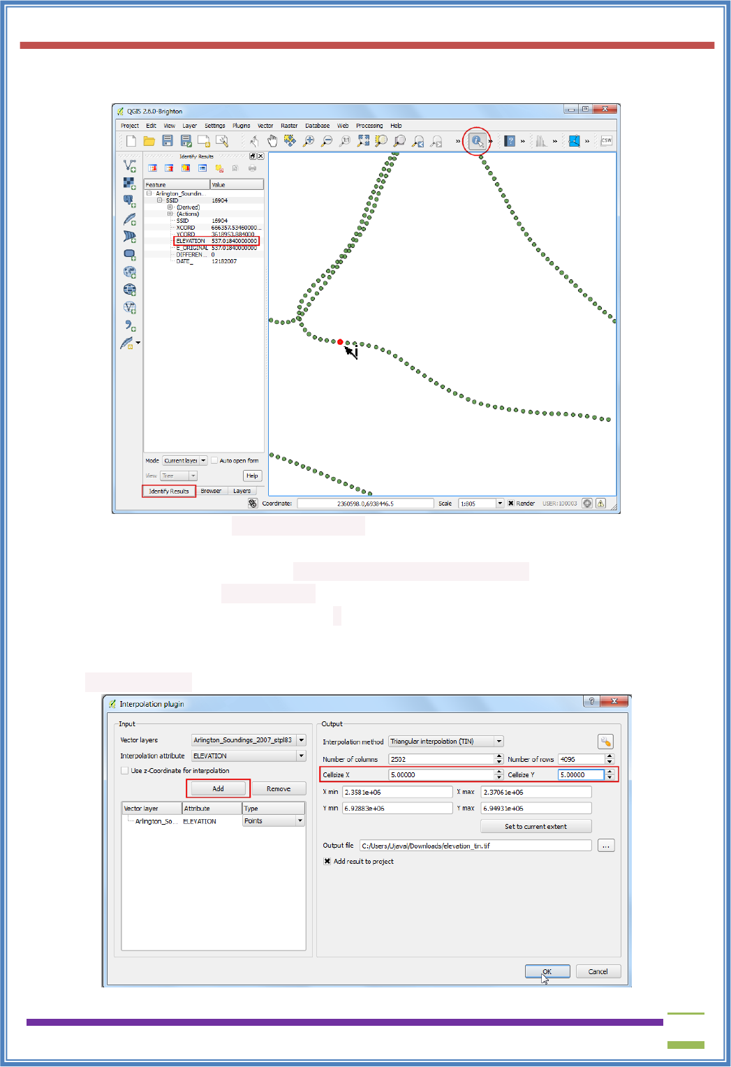
7. Select the Identify tool and click on a point. You will see the Identify Results panel show up on
the left with the attribute value of the point. In this case, the ELEVATION attribute contains the
USIT6P4 (Discipline Specific Elective Practical) Principles of Geographic Information Systems Practical
T. Y. B. Sc. (Information Technology) SEMESTER VI Teacher’s Reference Manual
116
depth of the lake at the location. As our task is to create a depth profile and elevation contours,
we will use this values as input for the interpolation.
8. Make sure you have the Interpolation plugin enabled. See Using Plugins for how to enable
plugins. Once enabled, go toRaster‣ Interpolation ‣ Interpolation.
9. In the Interpolation dialog, select Arlington_Soundings_2007_stpl83 as the Vector layers in
the Input panel. Select ELEVATION as the Interpolation attribute. Click Add. Change
the Cellsize X and Cellsize Y values to 5. This value is the size of each pixel in the output grid.
Since our source data is in a projected CRS with Feet-US as units, based on our selection, the
grid size will be 5 feet. Click on the ... button next to Output file and name the output file
as elevation_tin.tif. CLick OK.
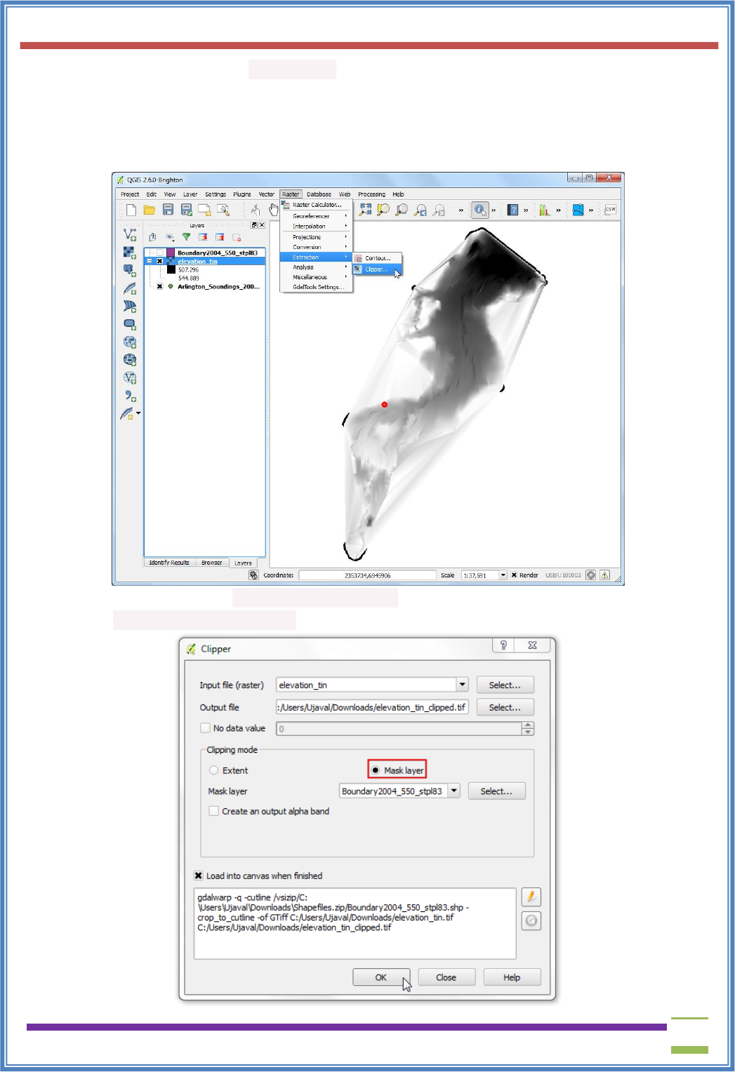
USIT6P4 (Discipline Specific Elective Practical) Principles of Geographic Information Systems Practical
T. Y. B. Sc. (Information Technology) SEMESTER VI Teacher’s Reference Manual
117
10. You will see the new later elevation_tin loaded in QGIS. Right-click the layer and select Zoom
to layer.
11. Now you will see the full extent of the created surface. Interpolation does not give accurate
results outside the collection area. Let’s clip the resulting surface with the lake boundary. Go
to Raster ‣ Extraction ‣ Clipper.
12. Name the Output file as elevation_tin_clipped.tif. Select the Cliiped mode as Mask layer.
Select Boundary2004_550_stpl83 as the Mask layer`. Click OK.
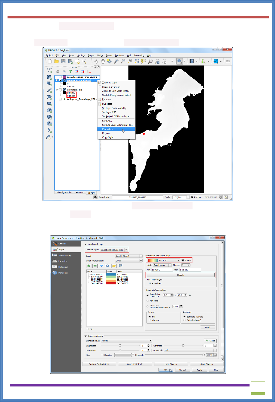
USIT6P4 (Discipline Specific Elective Practical) Principles of Geographic Information Systems Practical
T. Y. B. Sc. (Information Technology) SEMESTER VI Teacher’s Reference Manual
118
13. A new raster elevation_tin_clipped will be loaded in QGIS. We will now style this layer to
show the difference in elevations. Note the min and max elevation values from
the elevation_tin layer. Right-click the elevation_tin_clipped layer and select Properties.
14. Go to the Style tab. Select Render type as Singleband pseudocolor. In the Generate new color
map panel, select Spectralcolor ramp. As we want to create a depth-map as opposed to a height-
map, check the Invert box. This will assign blues to deep areas and reds to shallow areas.
Click Classify.
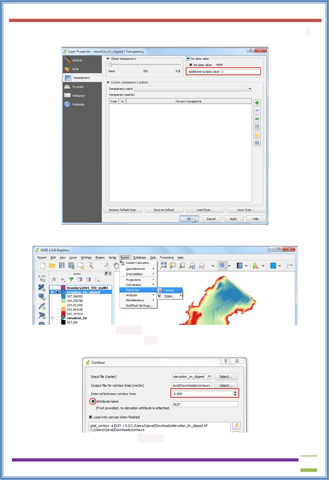
USIT6P4 (Discipline Specific Elective Practical) Principles of Geographic Information Systems Practical
T. Y. B. Sc. (Information Technology) SEMESTER VI Teacher’s Reference Manual
119
15. Switch to the Tranparency tab. We want to remove the black-pixels from our output. Enter 0 as
the Additional no data value. Click OK.
16. Now you have a elevation relief map for the lake generated from the individual depth readings.
Let’s generate contours now. Go to Raster ‣ Extraction ‣ Contours.
17. In the Contour dialog, enter contours as the Output file for contour lines. We will generate
contour lines at 5ft intervals, so enter 5.00 as the Interval between contour lines. Check
the Attribute name box. Click OK.
18. The contour lines will be loaded as contours layer once the processing is finished. Right-click
the layer and select Properties.
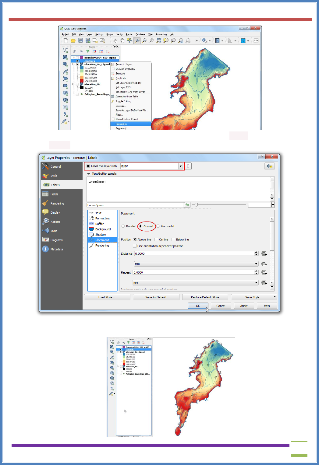
USIT6P4 (Discipline Specific Elective Practical) Principles of Geographic Information Systems Practical
T. Y. B. Sc. (Information Technology) SEMESTER VI Teacher’s Reference Manual
120
19. Go to the Labels tab. Check the Label this layer with box and select ELEV as the field.
Select Curved as the Placement type and click OK.
20. You will see that each contour line will be appropriately labeled with the elevation along the
line.
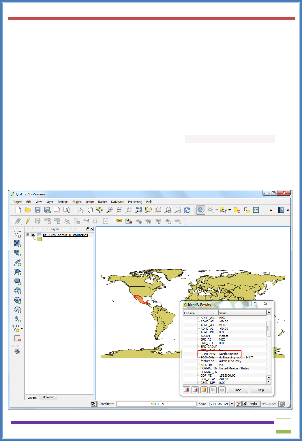
USIT6P4 (Discipline Specific Elective Practical) Principles of Geographic Information Systems Practical
T. Y. B. Sc. (Information Technology) SEMESTER VI Teacher’s Reference Manual
121
Practical 9
Advance GIS Operations 2:
a) Batch Processing using Processing Framework
b) Automating Complex Workflows using Processing Modeler
c) Automating Map Creation withPrint Composer Atlas
(a) Batch Processing using Processing Framework
Procedure
1. Go to Layer ‣ Add Vector Layer.
2. Browse to the downloaded Admin 0 Countries shapefile ne_10m_admin_0_countries.shp and
click Open.
3. As our task is to clip the global layers to the boundary of Africa, we need to first prepare a layer
containg a polygon for the entire continent. The countries layer has an attribute
called CONTINENT. We can use a geoprocessing concept called Dissolve to merge all
countries that have the same continent value and merge them to a single polygon.
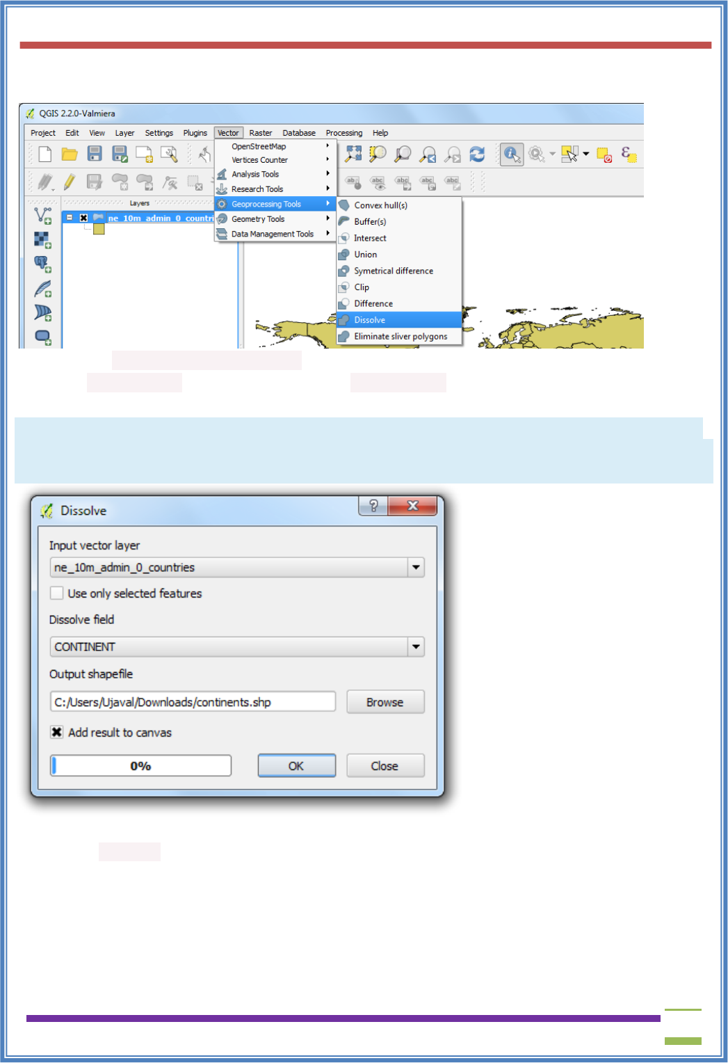
USIT6P4 (Discipline Specific Elective Practical) Principles of Geographic Information Systems Practical
T. Y. B. Sc. (Information Technology) SEMESTER VI Teacher’s Reference Manual
122
4. Open the Dissolve tool from Vector ‣ Geoprocessing Tools ‣ Dissolve.
5. Select ne_10m_admin_0_countries as the Input vector layer. The Dissolve field would
be CONTINENT. Name the output file as continents.shp and check the box next to Add result
to convas.
Note
If you want to merge ALL polygons regardless of their attributes, you can select – Dissolve All – as
the Dissolve field. This will combine all polygons in the layer and give you a single aggregate polygon.
6. The dissolve processing may take a while. Once the process finishes, you will see the
new continent layer added to QGIS. Use the Select Single Feature tool from the toolbar and
click on Africa to select the polygon representing the continent.
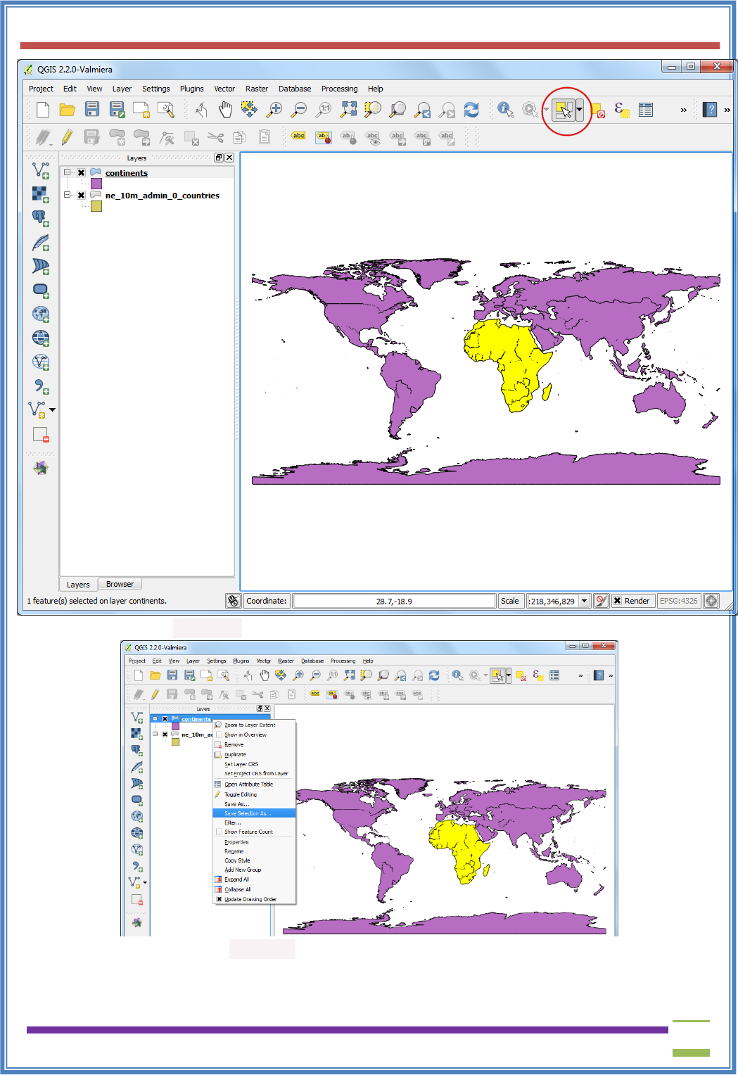
USIT6P4 (Discipline Specific Elective Practical) Principles of Geographic Information Systems Practical
T. Y. B. Sc. (Information Technology) SEMESTER VI Teacher’s Reference Manual
123
7. Right-click the continents layer and select Save Selection As....
8. Name the output file as africa.shp. Since we are only interested in the shape of the continent and
not any attributes, you may check the Skip attribute creation. Make sure the Add saved file to
map box is checked and click OK.
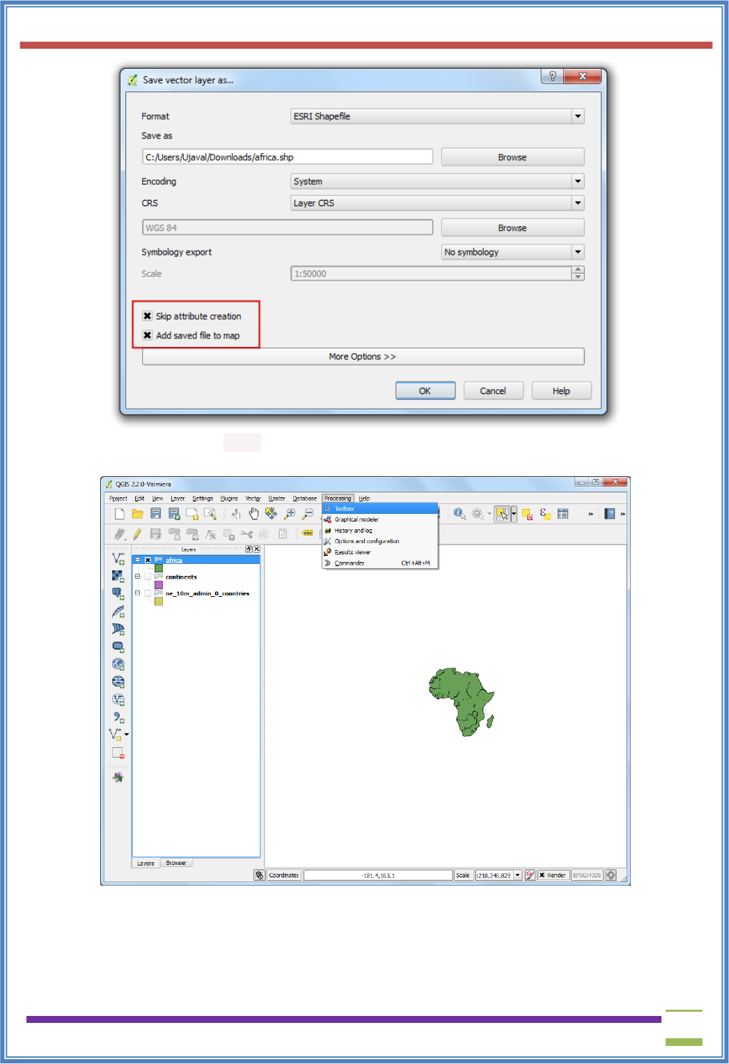
USIT6P4 (Discipline Specific Elective Practical) Principles of Geographic Information Systems Practical
T. Y. B. Sc. (Information Technology) SEMESTER VI Teacher’s Reference Manual
124
9. Now you will have the africa layer loaded in QGIS containing a single polygon for the entire
continent. Now, it’s time to start our batch clip process. Open Processing ‣ Toolbox.
10. Browse all available algorithms and find the Clip tool from QGIS geoalgorithms ‣ Vector
overlay tools ‣ Clip. You may also use the Search box to easily find the algorithm as well.
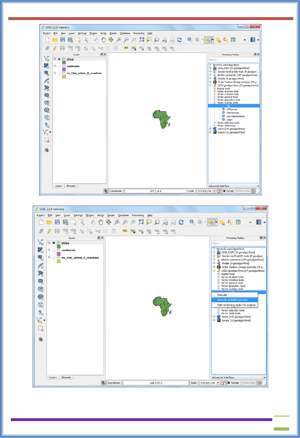
USIT6P4 (Discipline Specific Elective Practical) Principles of Geographic Information Systems Practical
T. Y. B. Sc. (Information Technology) SEMESTER VI Teacher’s Reference Manual
125
11. Right-click the Clip algorithm and select Execure as batch process.
12. In the Batch Processing dialog, the first tab is Parameters where we define out inputs. Click
the ... next to the first row in the Input layer column.
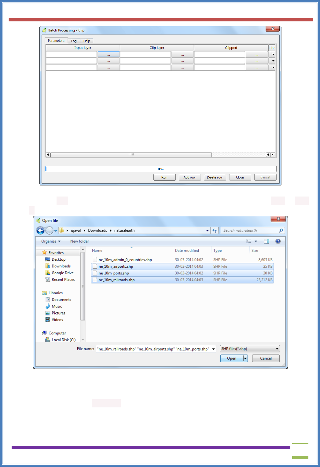
USIT6P4 (Discipline Specific Elective Practical) Principles of Geographic Information Systems Practical
T. Y. B. Sc. (Information Technology) SEMESTER VI Teacher’s Reference Manual
126
13. Browse to the directory containing the global transportation layers that you had downloaded.
Hold the Ctrl key and select all the layers that you want to clip. You may also use Shift or Ctrl-
A to make multiple selection. Click Open.
14. You will notice that the Input layer columns will be auto-populated with all layers you had
selected. You may use Add row button to add more rows and define more inputs. Next, we need
to select the layer containing the boundary to clip our input layers. Click the ... button for the
first row and add the africa.shp Clip layer. Since the clip layer is the same for all our inputs, you
can double-click the column header Clip layer and the same layer will be auto-filled for all the
rows. Next, we need to define our outputs. Click the ... buton next to the first row in
the Clipped column.
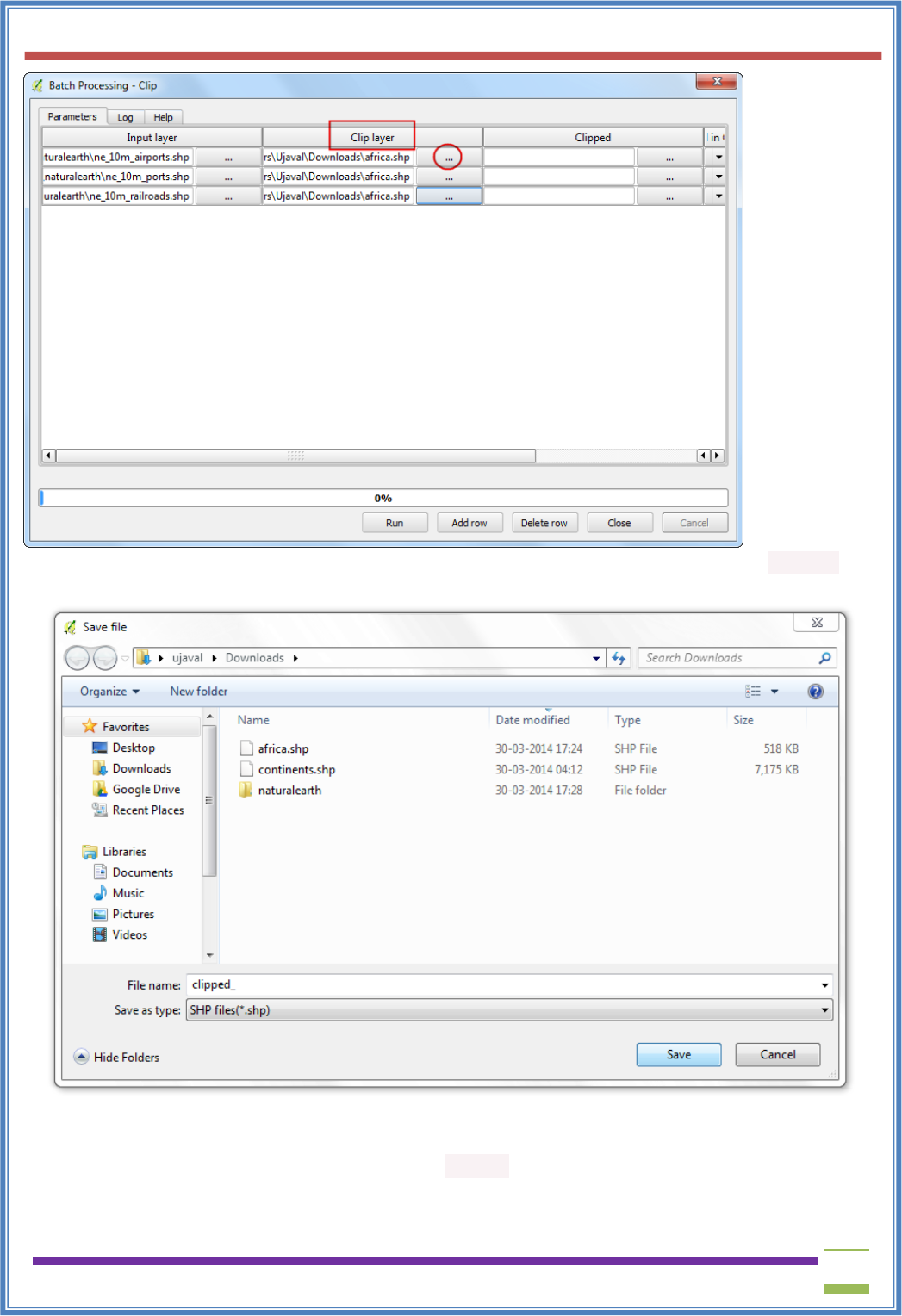
USIT6P4 (Discipline Specific Elective Practical) Principles of Geographic Information Systems Practical
T. Y. B. Sc. (Information Technology) SEMESTER VI Teacher’s Reference Manual
127
15. Browse the the directory where you want your output layers. Type the filename as clipped_ and
click Save.
16. You will see a new Autofill settings dialog pop up. Select Fill with parameter values as
the Autofill mode. Select Parameter to useas Input layer. This setting will add the input file
name to the output along with the specified output_ filename. This is important to ensure all the
output files have unique names and they do not overwrite each other.
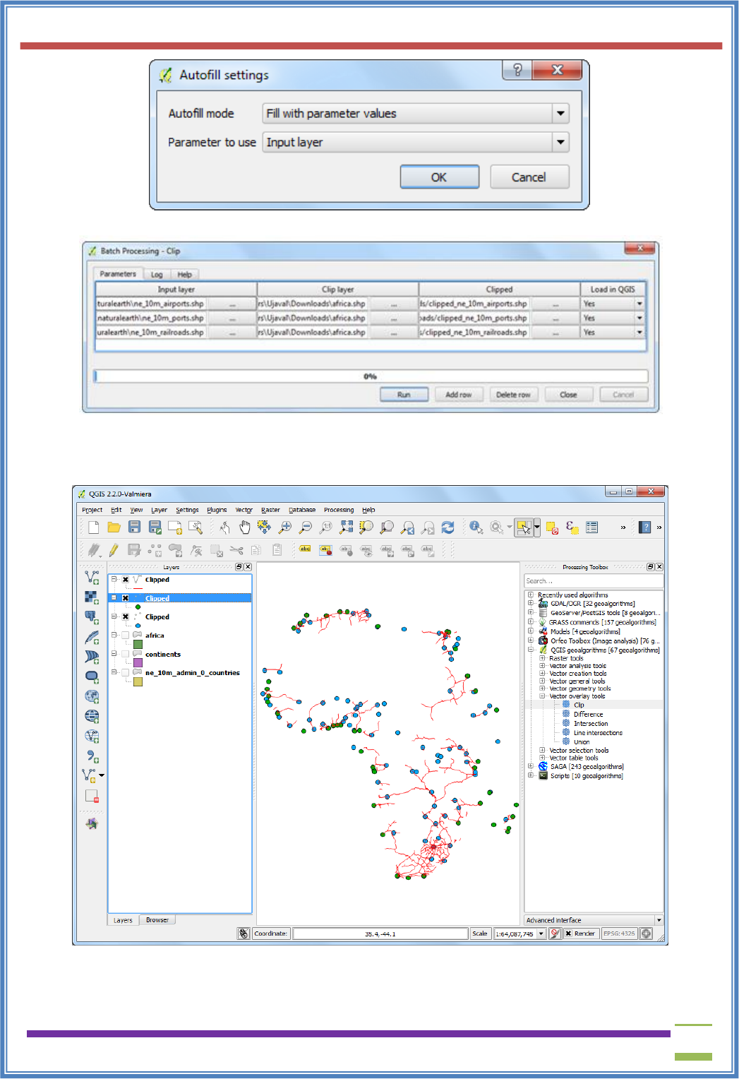
USIT6P4 (Discipline Specific Elective Practical) Principles of Geographic Information Systems Practical
T. Y. B. Sc. (Information Technology) SEMESTER VI Teacher’s Reference Manual
128
17. Now we are ready to start the batch procesing. Click Run.
18. The clip algorithm will run for each of the inputs and create output files are we have specified.
Once the batch process finishes, you will see the layers added to QGIS canvas. As you will
notice, all the global layers are properly clipped to the continent boundary that we had specified.
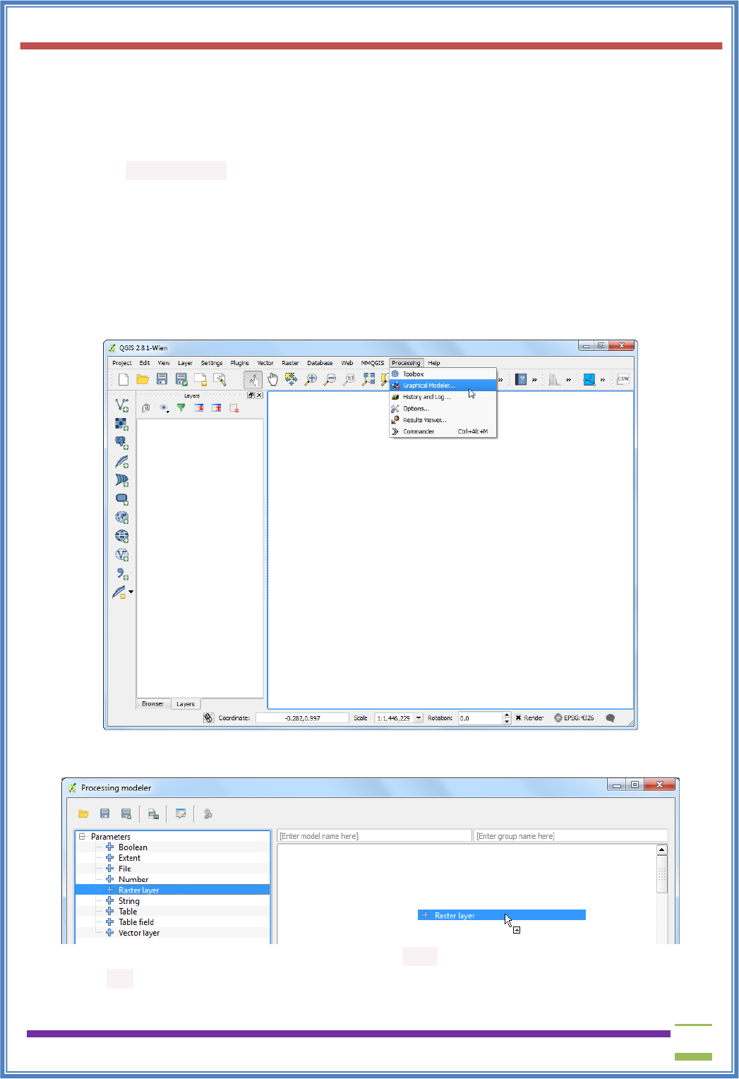
USIT6P4 (Discipline Specific Elective Practical) Principles of Geographic Information Systems Practical
T. Y. B. Sc. (Information Technology) SEMESTER VI Teacher’s Reference Manual
129
(B)
Automating Complex Workflows using Processing Modeler
Procedure
Our workflow for this exercise will have the following steps.
• Apply a Majority Filter algorithm to the input landcover raster. This will reduce noise in our
output by eliminating isolated pixels.
• Convert the resulting raster to a polygon layer.
• Query for a class value from the attribute table of the polygon layer and create a vector layer for
that class.
The following steps outline the process to code the above process into a model and run it on the
downloaded datasets.
1. Launch QGIS and go to Processing ‣ Graphical Modeler....
2. The Processing modeler dialog contains a left-hand panel and a main canvas. Select
the Inputs tab in the left-hand panel and drag the + Raster layer to the canvas.
3. A Parameter definition dialog will pop-up. Enter Input as the Parameter name and
mark Yes to Required. Click OK.
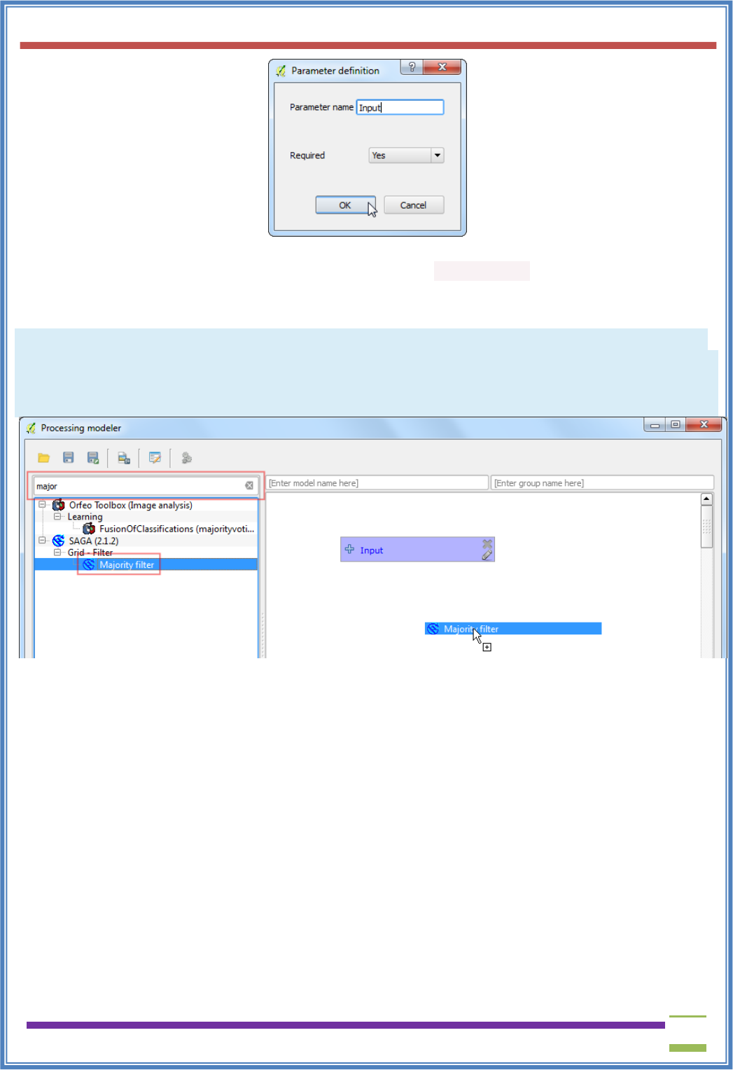
USIT6P4 (Discipline Specific Elective Practical) Principles of Geographic Information Systems Practical
T. Y. B. Sc. (Information Technology) SEMESTER VI Teacher’s Reference Manual
130
4. You will see a box with the name Input appear in the canvas. This represents the landcover
raster that we will use as input. Next step is to apply a Majority filter algorithm. Switch to
the Algorithm tab from the bottom-left corner. Search for the algorithm and you will find it
listed under SAGA provider. Drag it to the canvas.
Note
If you do not see this algorithm or any of the subsequent algorithms mentioned in thi tutorial, you may
be using the Simplified Interface of the Processing Toolbox. Switch to the Advanced Interface by using
the dropdown at the bottom of the Processing Toolbox in the main QGIS window.
5. A configuration dialog for Majority Filter will be presented. Leave the values to their default
and click OK.
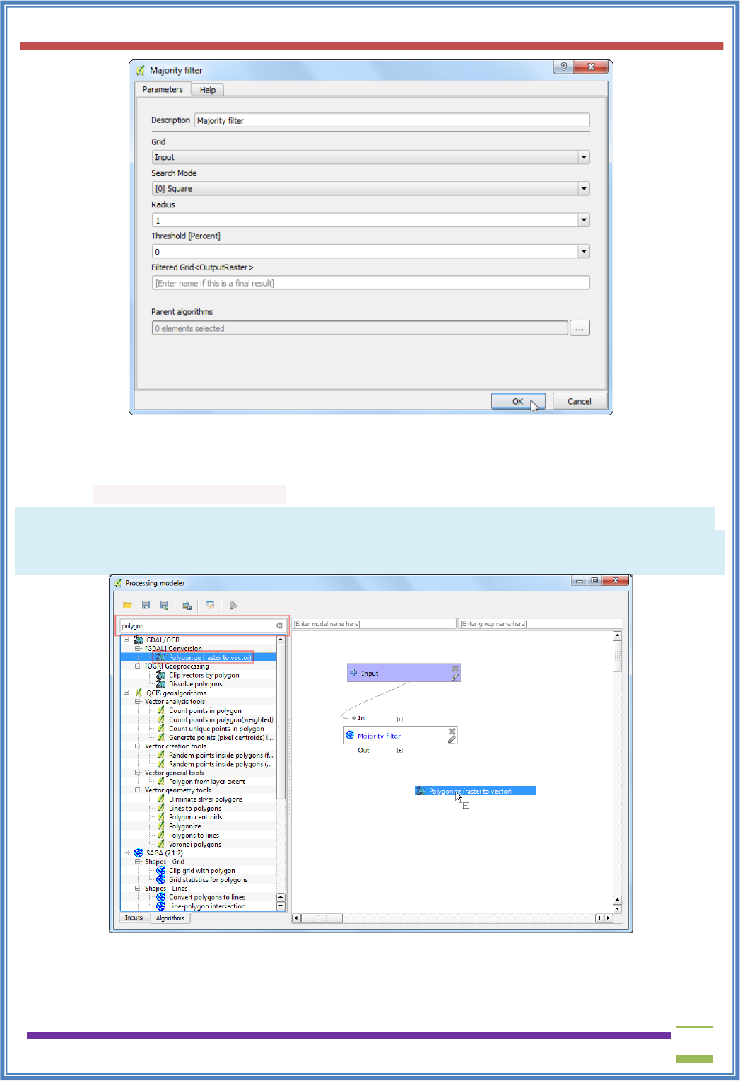
USIT6P4 (Discipline Specific Elective Practical) Principles of Geographic Information Systems Practical
T. Y. B. Sc. (Information Technology) SEMESTER VI Teacher’s Reference Manual
131
6. You will note that there is now a new box named Majority Filter in the canvas and it is
connected to the Input box. This is because the Majority Filter algorithm uses the Input raster as
its input. The next step in our workflow is to convert the output of majority filter to vector. Find
the Polygonize (raster to vector) algorithm and drag it to the canvas.
Note
The boxes can be moved and arranged by clicking on it and dragging it while holding the left mouse
button. You can also use the scroll-wheel to zoom in and out in the model canvas.
7. Select ‘Filtered Grid’ from algorithm ‘Majority Filter’ as the value for Input layer. Click OK.
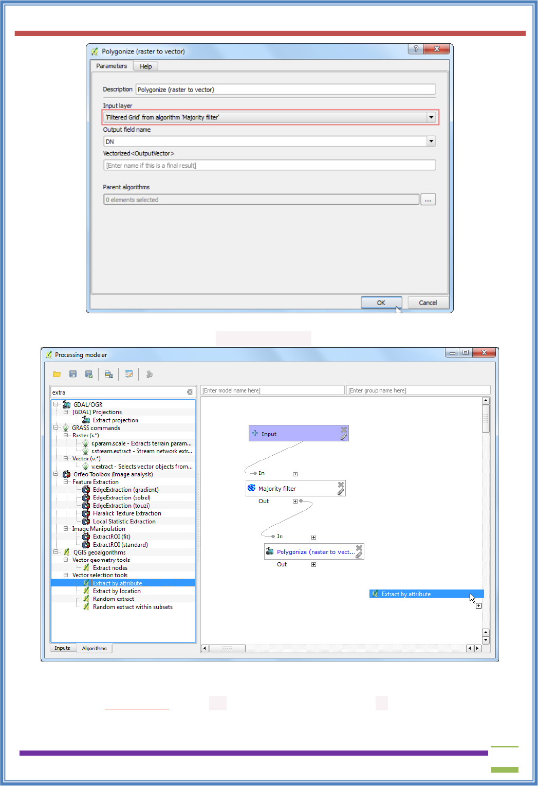
USIT6P4 (Discipline Specific Elective Practical) Principles of Geographic Information Systems Practical
T. Y. B. Sc. (Information Technology) SEMESTER VI Teacher’s Reference Manual
132
8. The final step in the workflow is to query for a class value and create a new layer from the
matching features. Search for the Extract by attribute algorithm and drag it the canvas.
9. Select ‘Vectorized’ from algorithm ‘Polygonize (raster to vector) as the Input Layer. We want
to extract the pixels that represent Croplands. The corresponding pixel value for this class will
be 12. (see Code Values). Enter DN as the Selection attribute and 12as the value. As the output
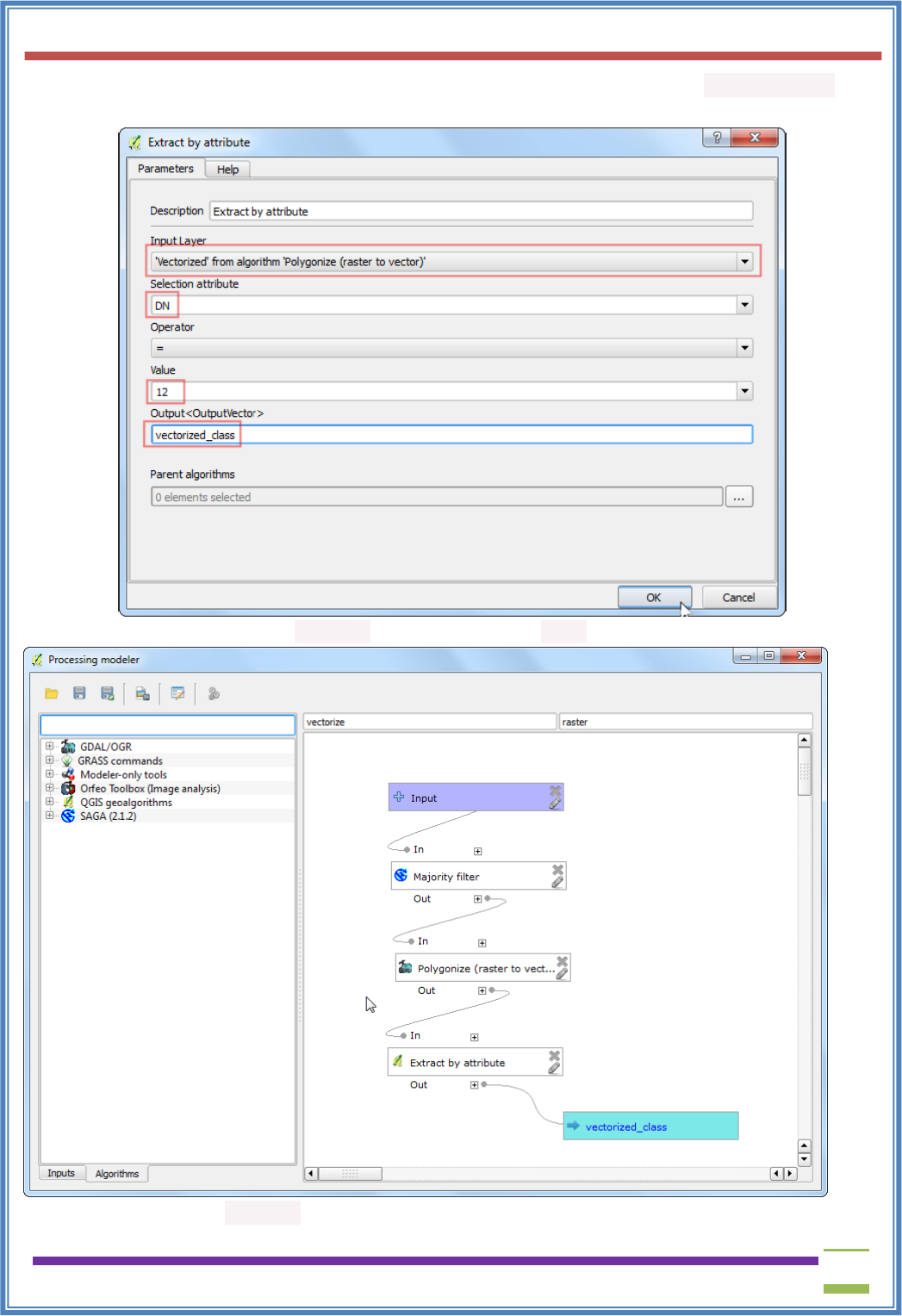
USIT6P4 (Discipline Specific Elective Practical) Principles of Geographic Information Systems Practical
T. Y. B. Sc. (Information Technology) SEMESTER VI Teacher’s Reference Manual
133
of this operation will be the final result, we need to name the output. Enter vectorized class as
the Output.
10. Enter the Model name as vectorize and Group name as raster. Click the Save button.
11. Name the model vectorize and click Save.
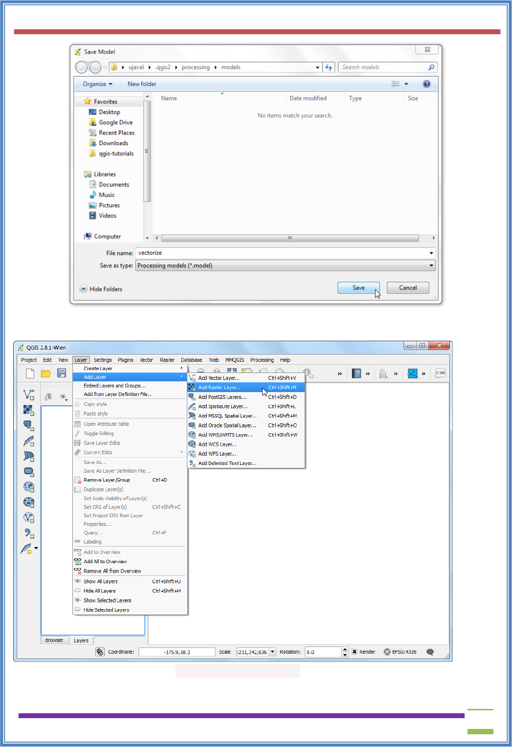
USIT6P4 (Discipline Specific Elective Practical) Principles of Geographic Information Systems Practical
T. Y. B. Sc. (Information Technology) SEMESTER VI Teacher’s Reference Manual
134
12. Now it is time to test our model. Close the modeler and switch to the main QGIS window. Go
to Layer ‣ Add Layer ‣ Add Raster Layer....
13. Browse to the downloaded LC_hd_global_2001.tif.gz file and click Open. Once the raster is
loaded, go to Processing ‣ Toolbox.
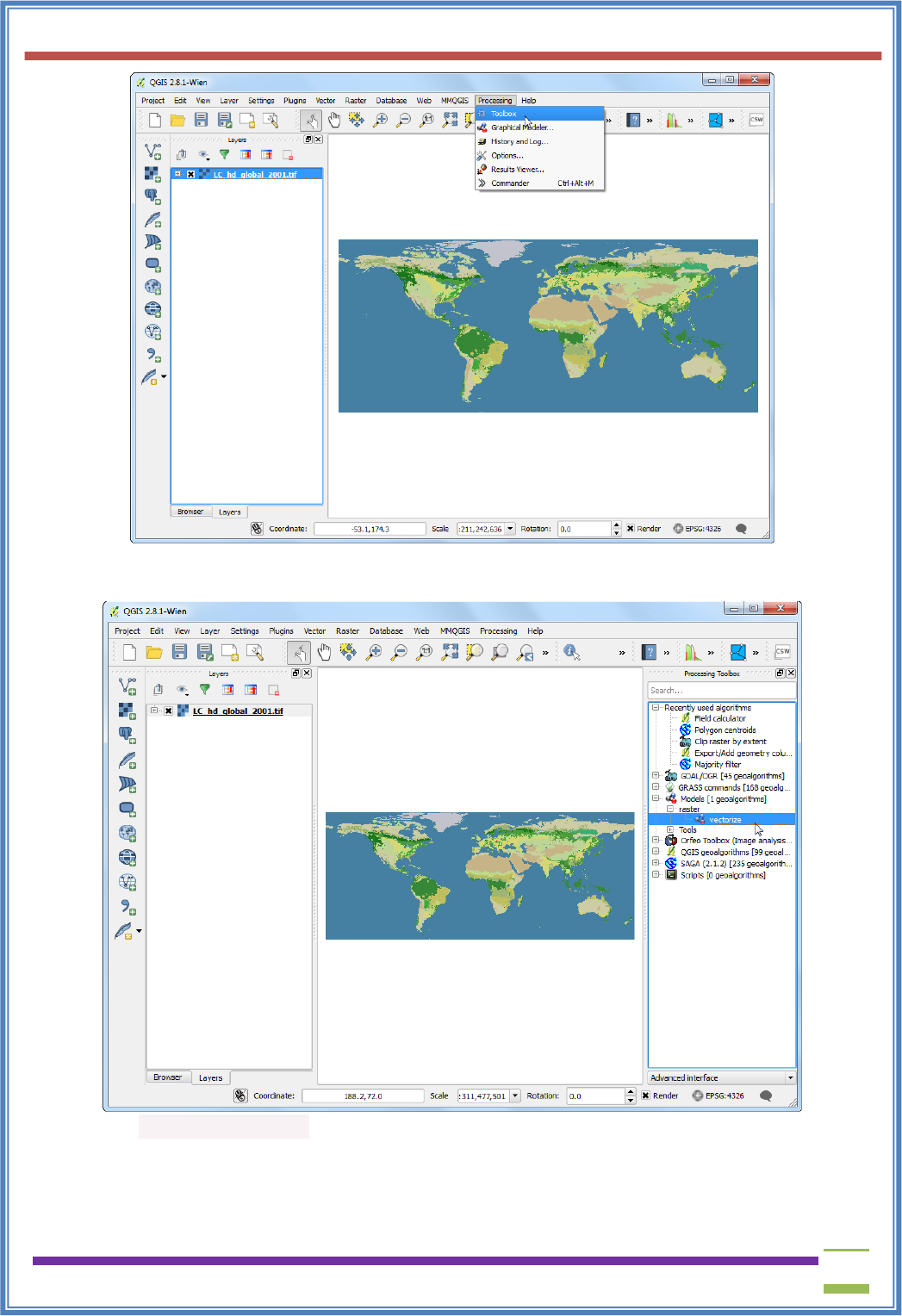
USIT6P4 (Discipline Specific Elective Practical) Principles of Geographic Information Systems Practical
T. Y. B. Sc. (Information Technology) SEMESTER VI Teacher’s Reference Manual
135
14. Find the newly created model under Models ‣ raster ‣ vectorize. Double-click to launch the
model.
15. Select LC_hd_global_2001 as the Input and click Run.
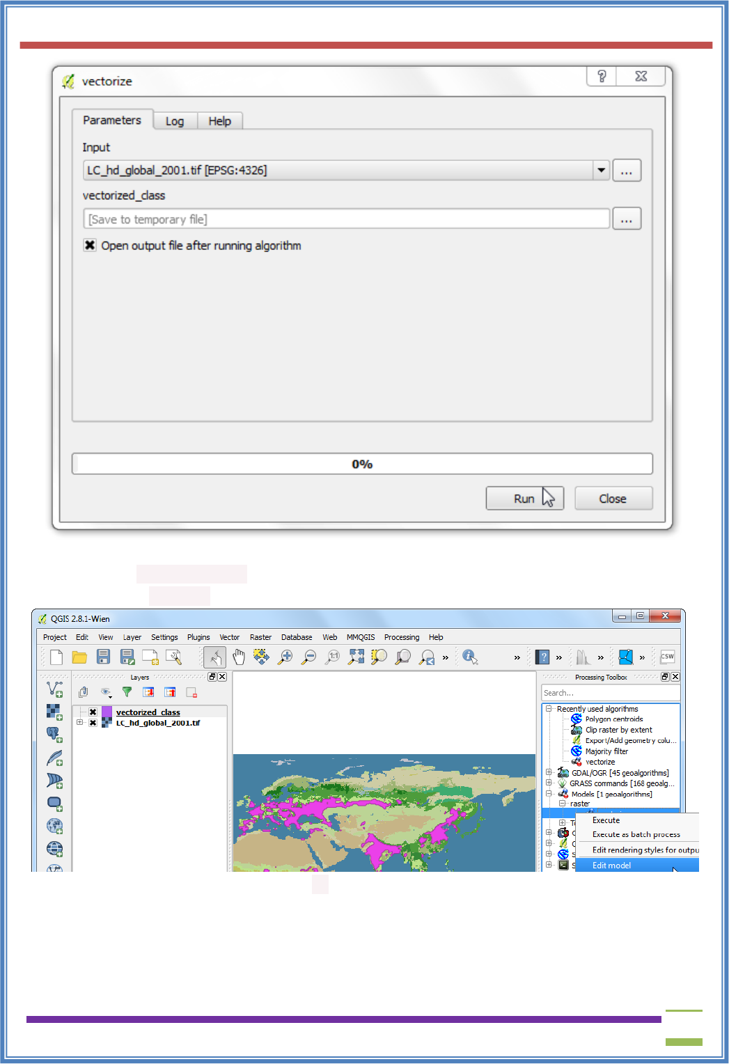
USIT6P4 (Discipline Specific Elective Practical) Principles of Geographic Information Systems Practical
T. Y. B. Sc. (Information Technology) SEMESTER VI Teacher’s Reference Manual
136
16. You will see all the steps being executed without any user input. Once the processing finishes, a
new layer vectorized_classwill be added to QGIS. Let’s improve the model a little bit. Right-
click on the vectorize model and select Edit model.
17. In Step 12, we hard-coded the value 12 as the class value. Instead, we can specify it as a input
parameter which the user can change. To add this, switch to the Inputs tab and drag the +
String to the model.
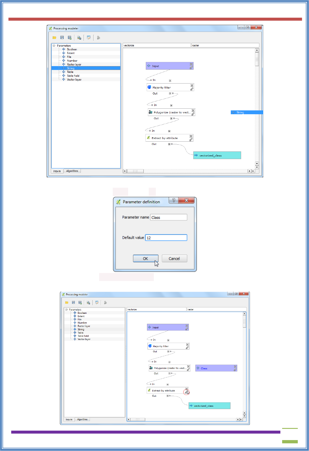
USIT6P4 (Discipline Specific Elective Practical) Principles of Geographic Information Systems Practical
T. Y. B. Sc. (Information Technology) SEMESTER VI Teacher’s Reference Manual
137
18. Enter the Parameter Name as Class. Enter 12 as the Default value.
19. We will now change the Extract by attribute algorithm to use this input instead of the hard-
coded value. Click the Edit button next to the Extract by attribute box.
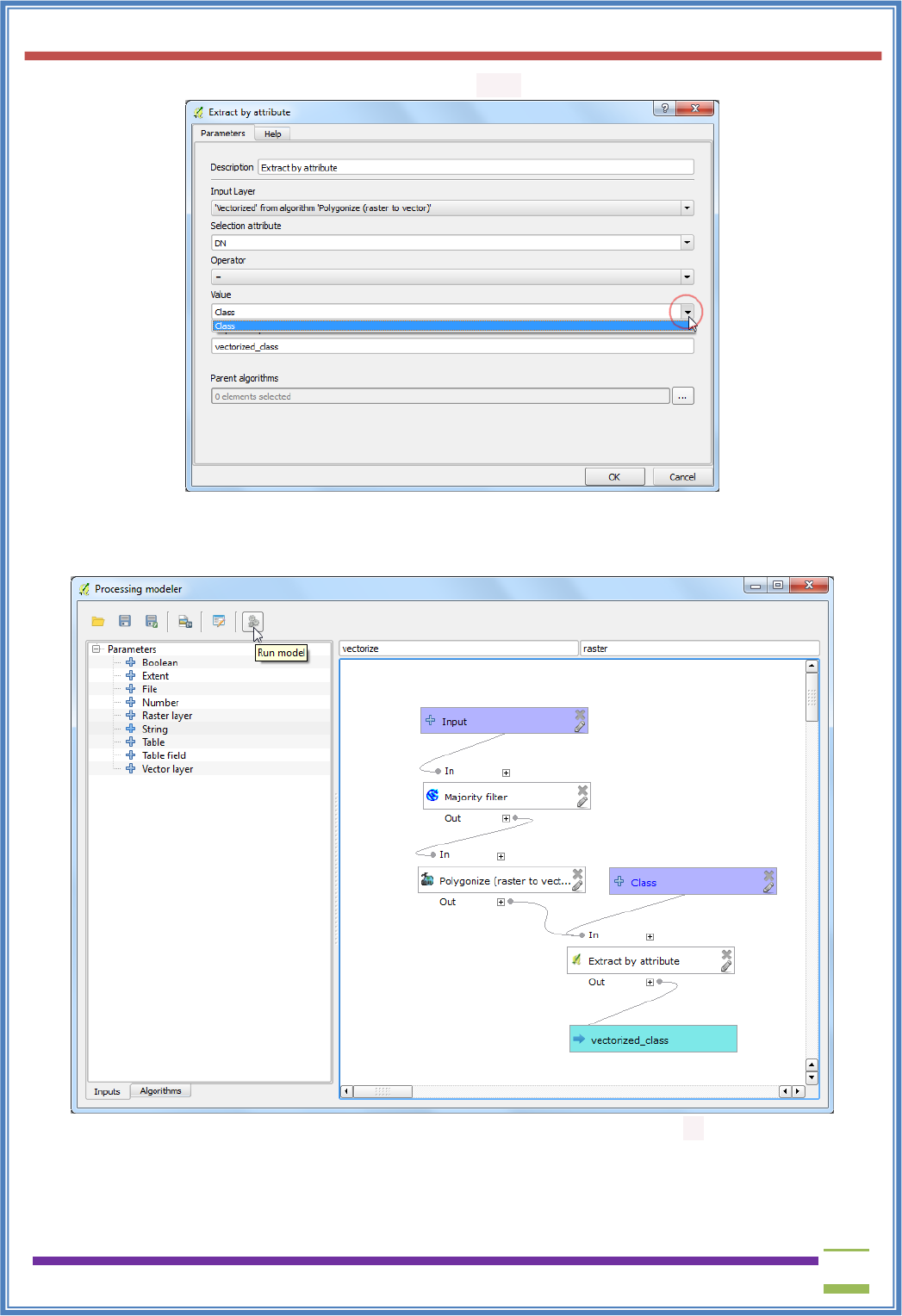
USIT6P4 (Discipline Specific Elective Practical) Principles of Geographic Information Systems Practical
T. Y. B. Sc. (Information Technology) SEMESTER VI Teacher’s Reference Manual
138
20. Click the dropdown arrow for Value and select Class. Click OK.
21. You will see from the model diagram that the Extract by attribute algorithm now uses 2 inputs.
The modeler has a shortcut to launch the model and test it. Click the Run button from the
toolbar.
22. Notice that the model dialog has a new editable field called Class. Enter 16 as the Class value
and click Run.
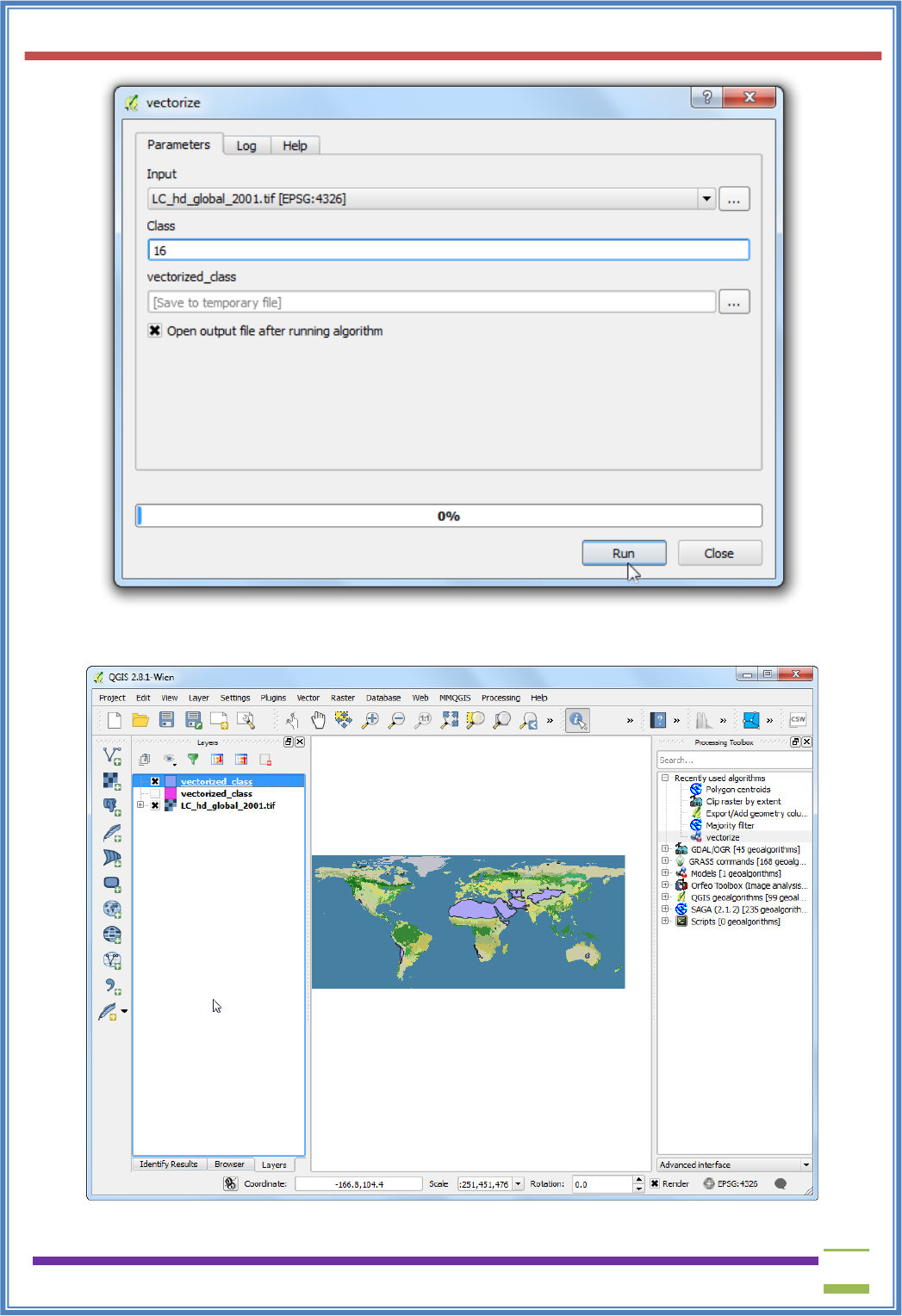
USIT6P4 (Discipline Specific Elective Practical) Principles of Geographic Information Systems Practical
T. Y. B. Sc. (Information Technology) SEMESTER VI Teacher’s Reference Manual
139
23. Once the processing finishes, you will see that with just a click of a button we were able to run a
complex workflow and extract the area for class 16.
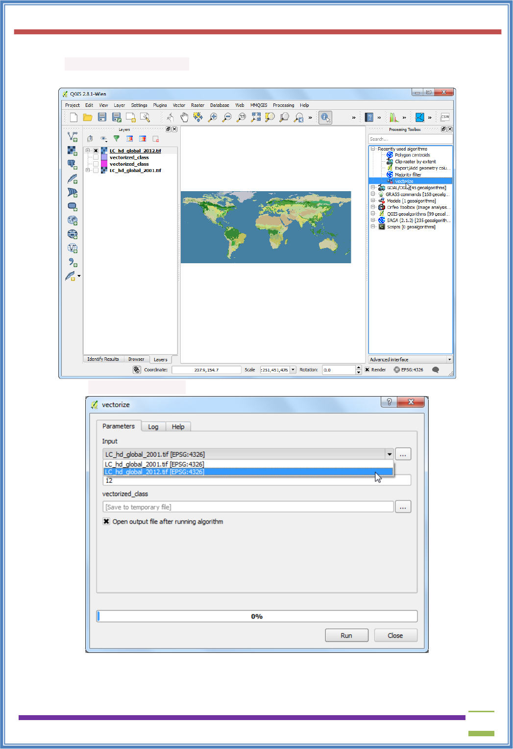
USIT6P4 (Discipline Specific Elective Practical) Principles of Geographic Information Systems Practical
T. Y. B. Sc. (Information Technology) SEMESTER VI Teacher’s Reference Manual
140
24. Now that our model is ready, we can run it just as easily on a new raster layer. Load
the LC_hd_global_2012.tif.gz file by going to Layer ‣ Add Layer ‣ Add Raster Layer.... Click
the vectorize` model from the Processing Toolbox panel.
25. Pick the LC_hd_global_2012 layer as the Input and click Run.
26. Once the new output is loaded, you can compare the changes in the Croplands from 2001 to
2012.
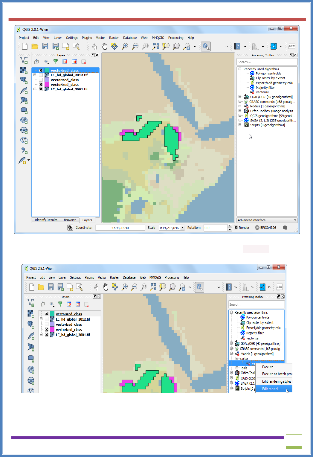
USIT6P4 (Discipline Specific Elective Practical) Principles of Geographic Information Systems Practical
T. Y. B. Sc. (Information Technology) SEMESTER VI Teacher’s Reference Manual
141
27. It is always a good idea to add documentation to your model. The modeler has a built-in Help
editor that allows you to embed help directly in the model. Right-click the vectorize model and
select Edit model.
28. Click the Edit model help button from the toolbar.
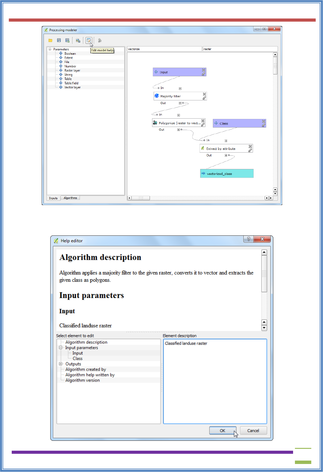
USIT6P4 (Discipline Specific Elective Practical) Principles of Geographic Information Systems Practical
T. Y. B. Sc. (Information Technology) SEMESTER VI Teacher’s Reference Manual
142
29. In the Help editor dialog, select any item from the Select element to edit panel and enter the
help text in Element description. Click OK. This help will be available in the Help tab when you
launch the model to run.
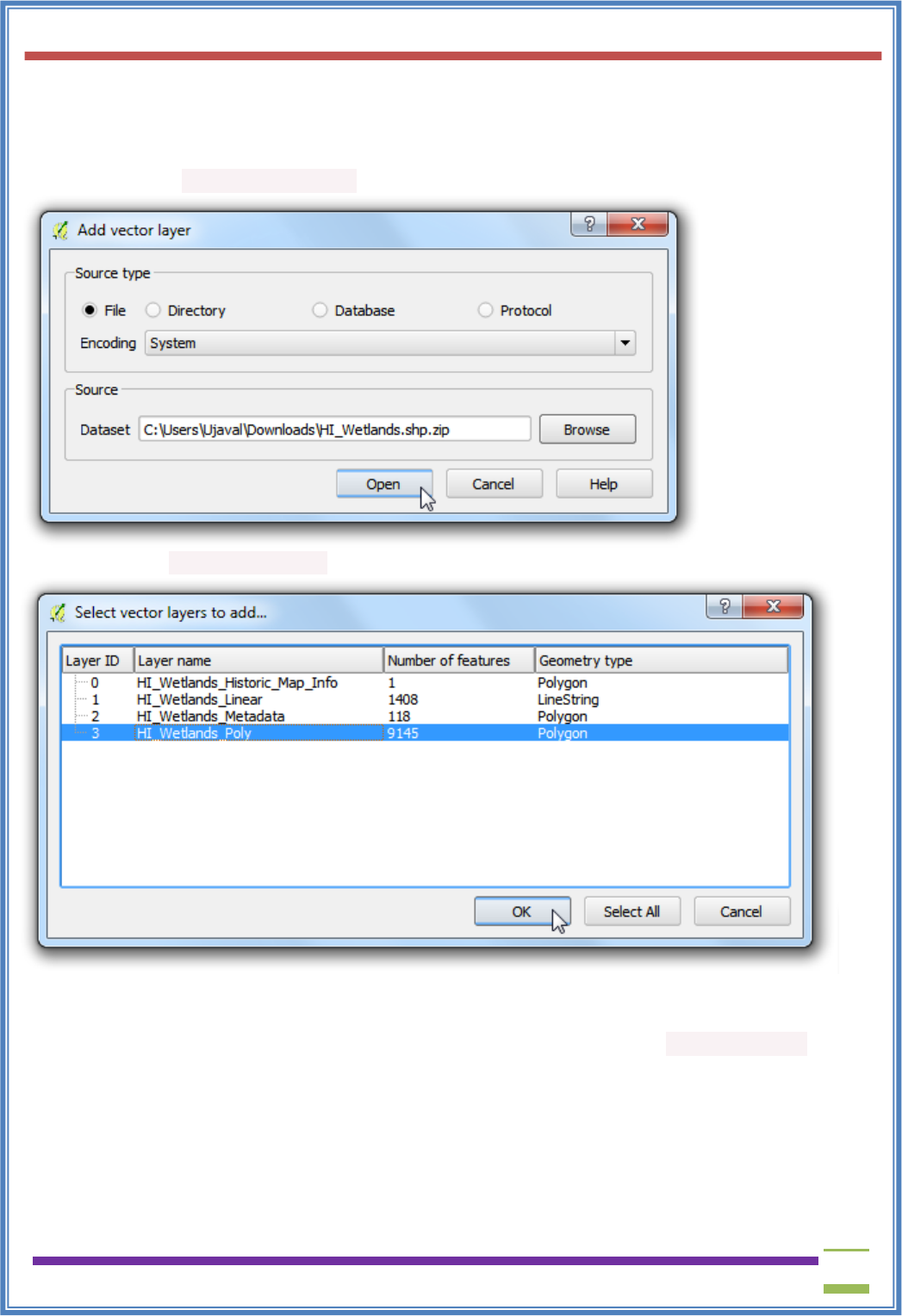
USIT6P4 (Discipline Specific Elective Practical) Principles of Geographic Information Systems Practical
T. Y. B. Sc. (Information Technology) SEMESTER VI Teacher’s Reference Manual
143
(c) Automating Map Creation with Print Composer Atlas
Procedure
1. Launch QGIS and go to Layer ‣ Add Layer ‣ Add Vector Layer.
2. owse to the HI_Wetlands.shp.zip file and click Open.
3. Select the HI_Wetlands_Poly layer and click OK.
4. You will see the polygons representing the wetlands in the entire state of Hawaii. Since we want
to make separate wetlands map for each county in the state, we will need the county boundaries
layer. Go to Layer ‣ Add Layer ‣ Add Vector Layer and browse to the county10.shp.zip file.
Click Open.
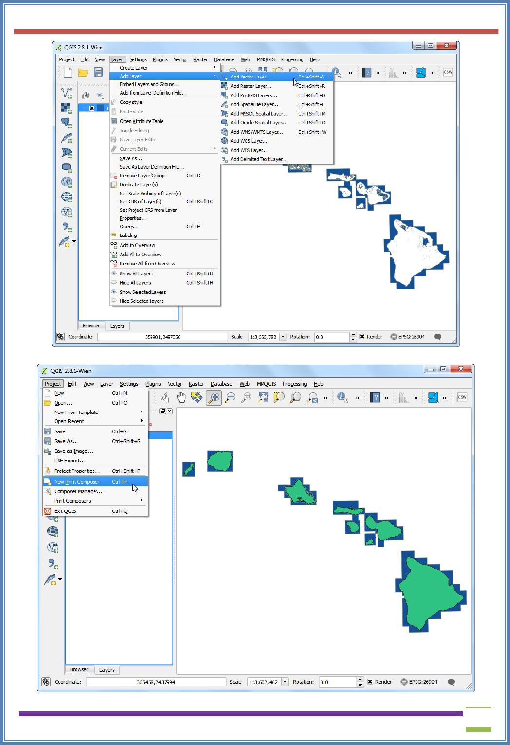
USIT6P4 (Discipline Specific Elective Practical) Principles of Geographic Information Systems Practical
T. Y. B. Sc. (Information Technology) SEMESTER VI Teacher’s Reference Manual
144
5. Go to Project ‣ New Print Composer.
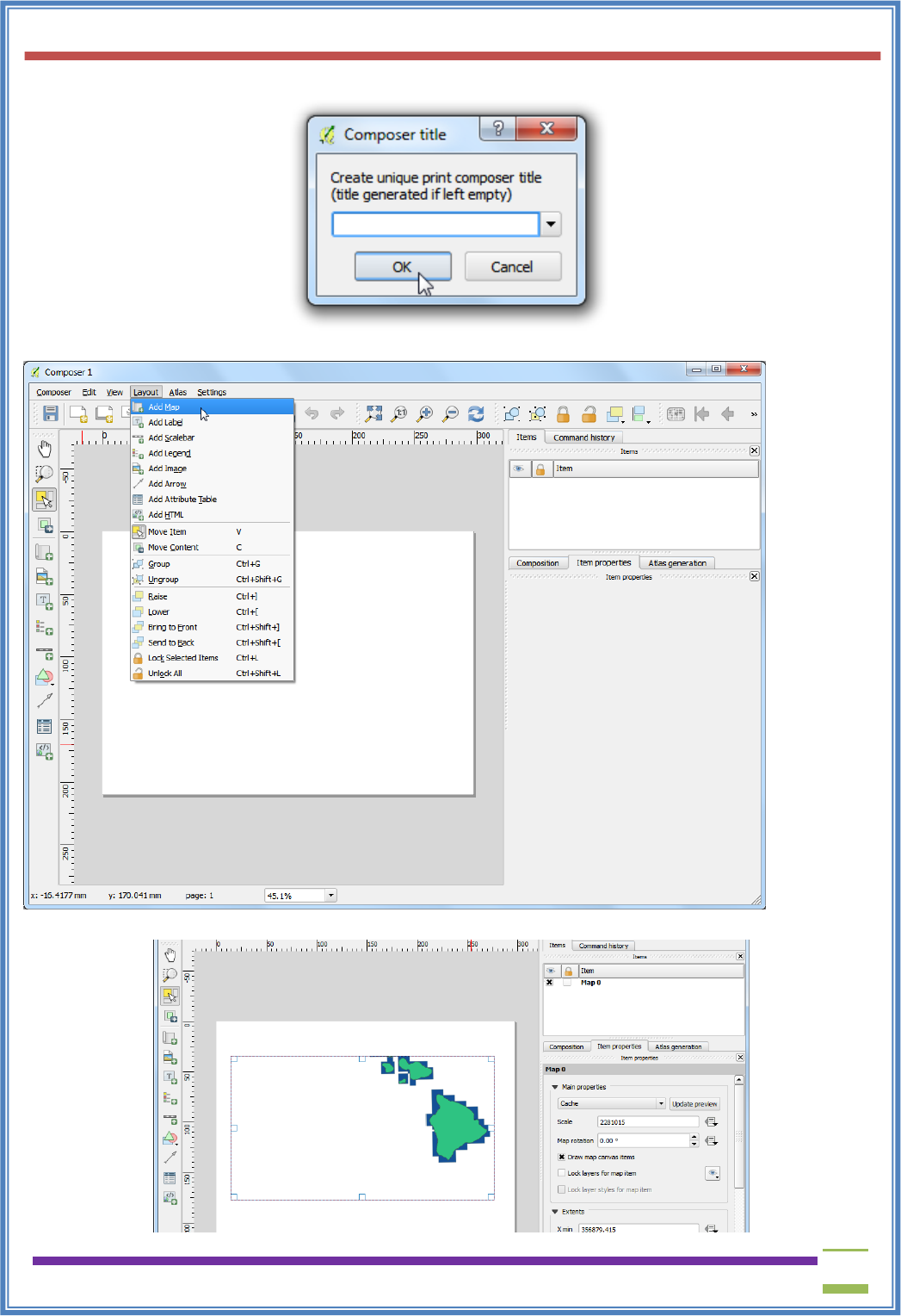
USIT6P4 (Discipline Specific Elective Practical) Principles of Geographic Information Systems Practical
T. Y. B. Sc. (Information Technology) SEMESTER VI Teacher’s Reference Manual
145
6. Leave the composer title field empty and click OK.
7. Go to Layout ‣ Add Map.
8. Drag a rectangle while holding the left mouse button where you would like to insert the map.
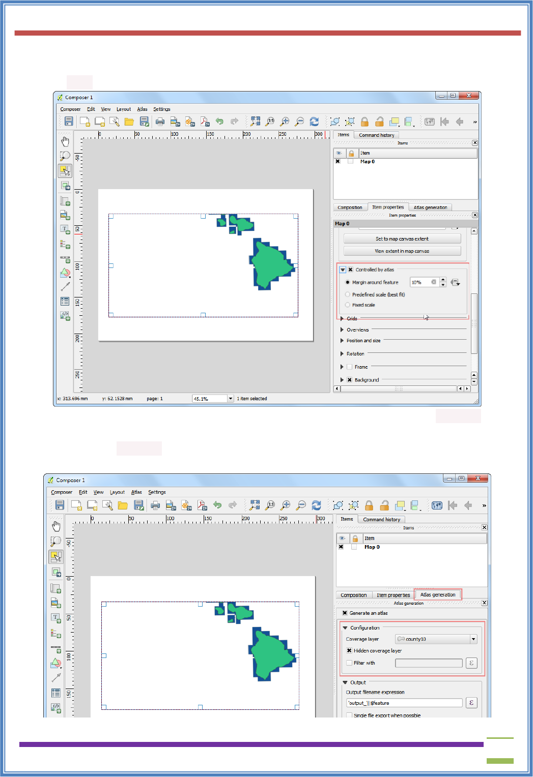
USIT6P4 (Discipline Specific Elective Practical) Principles of Geographic Information Systems Practical
T. Y. B. Sc. (Information Technology) SEMESTER VI Teacher’s Reference Manual
146
9. Scroll down in the Item Properties tab and check the Controlled by atlas box. This will indicate
the composer that the extent of the map displayed in this item will be determined by
the Atlas tool.
10. Switch to the Atlas generation tab. Check the Generate an atlas box. Select the county10 as
the Coverage layer. This will indicate that we want to create 1 map each for every polygon
feature in the county10 layer. You can also check the Hidden coverage layer so that the features
themselves will not appear on the map.
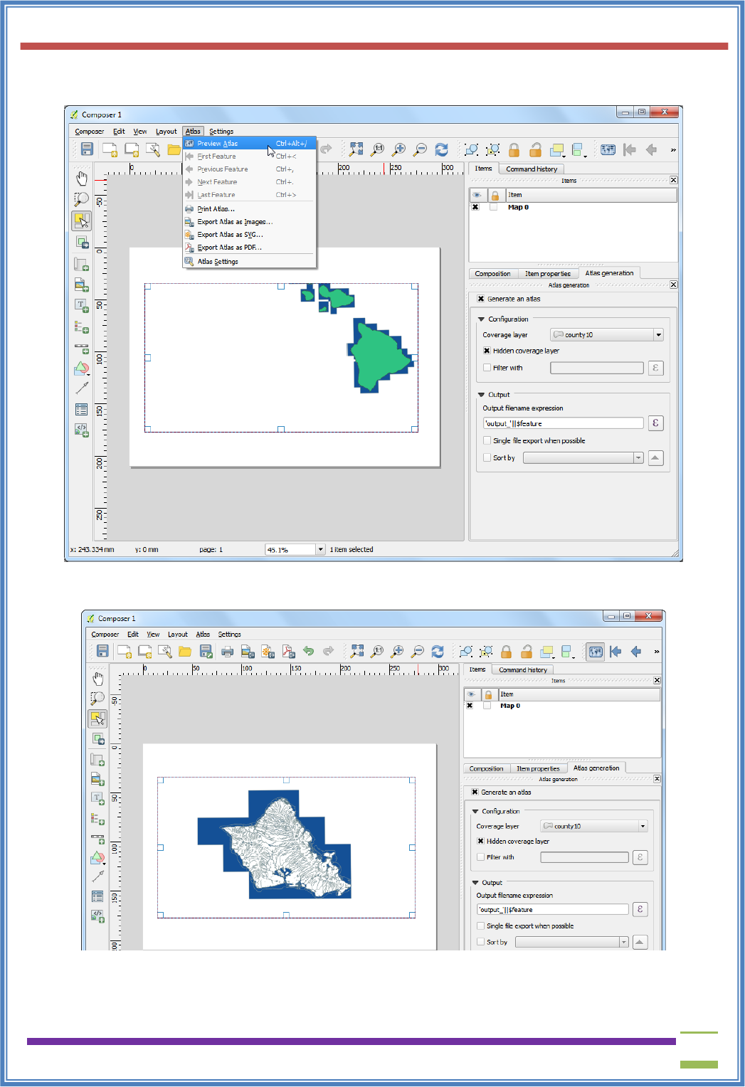
USIT6P4 (Discipline Specific Elective Practical) Principles of Geographic Information Systems Practical
T. Y. B. Sc. (Information Technology) SEMESTER VI Teacher’s Reference Manual
147
11. You will notice that the map image does not change after configuring the Atlas settings. Go
to Atlas ‣ Preview Atlas.
12. Now you will see the map refresh and show how individual map will look like. Notice that it
shows the current feature number from the coverage layer at the bottom right.
13. You can preview how the map will look for each of the county polygons. Go to Atlas ‣ Next
Feature.
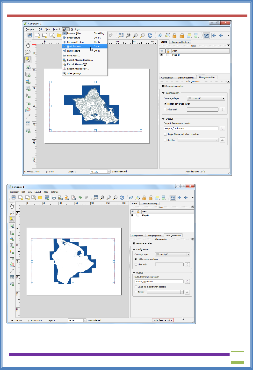
USIT6P4 (Discipline Specific Elective Practical) Principles of Geographic Information Systems Practical
T. Y. B. Sc. (Information Technology) SEMESTER VI Teacher’s Reference Manual
148
14. Atlas will render the map to the extent of the next feature in the coverage layer.
15. Let’s add a label to the map. Go to Layout ‣ Add Label.
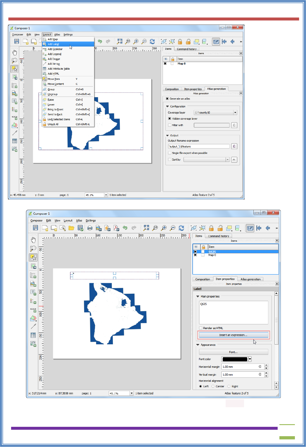
USIT6P4 (Discipline Specific Elective Practical) Principles of Geographic Information Systems Practical
T. Y. B. Sc. (Information Technology) SEMESTER VI Teacher’s Reference Manual
149
16. Under the Item properties tab, click Insert an expression... button.
17. The label of the map can use the attributes from the coverage layer.he concat function is used to
join multiple text items into a single text item. In this case we will join the value of
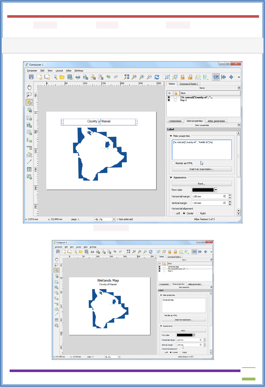
USIT6P4 (Discipline Specific Elective Practical) Principles of Geographic Information Systems Practical
T. Y. B. Sc. (Information Technology) SEMESTER VI Teacher’s Reference Manual
150
the NAME10 attribute of the county10 layer with the text County of. Add an expression like
below and click OK.
concat('County of ', "NAME10")
18. Adjust the font size to your liking.
19. Add another label and enter Wetlands Map under the Main properties. Since there is no
expression here, this text will remain the same on all maps.
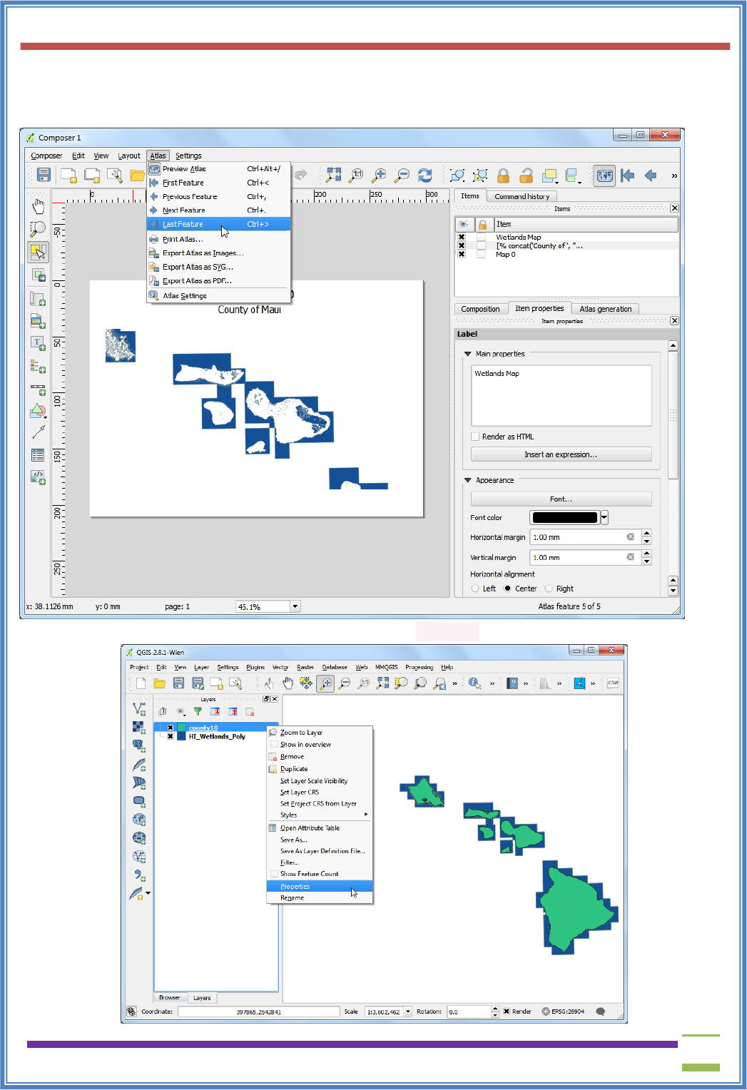
USIT6P4 (Discipline Specific Elective Practical) Principles of Geographic Information Systems Practical
T. Y. B. Sc. (Information Technology) SEMESTER VI Teacher’s Reference Manual
151
20. Go to Atlas ‣ Last Feature and verify that the map labels do work as intended. You will notice
that the wetland map has polygons extending out in the ocean that looks ugly. We can change
the style to that areas outside the county boundaries are hidden.
21. Switch to the main QGIS window. Right-click the county10 layer and select Properties.
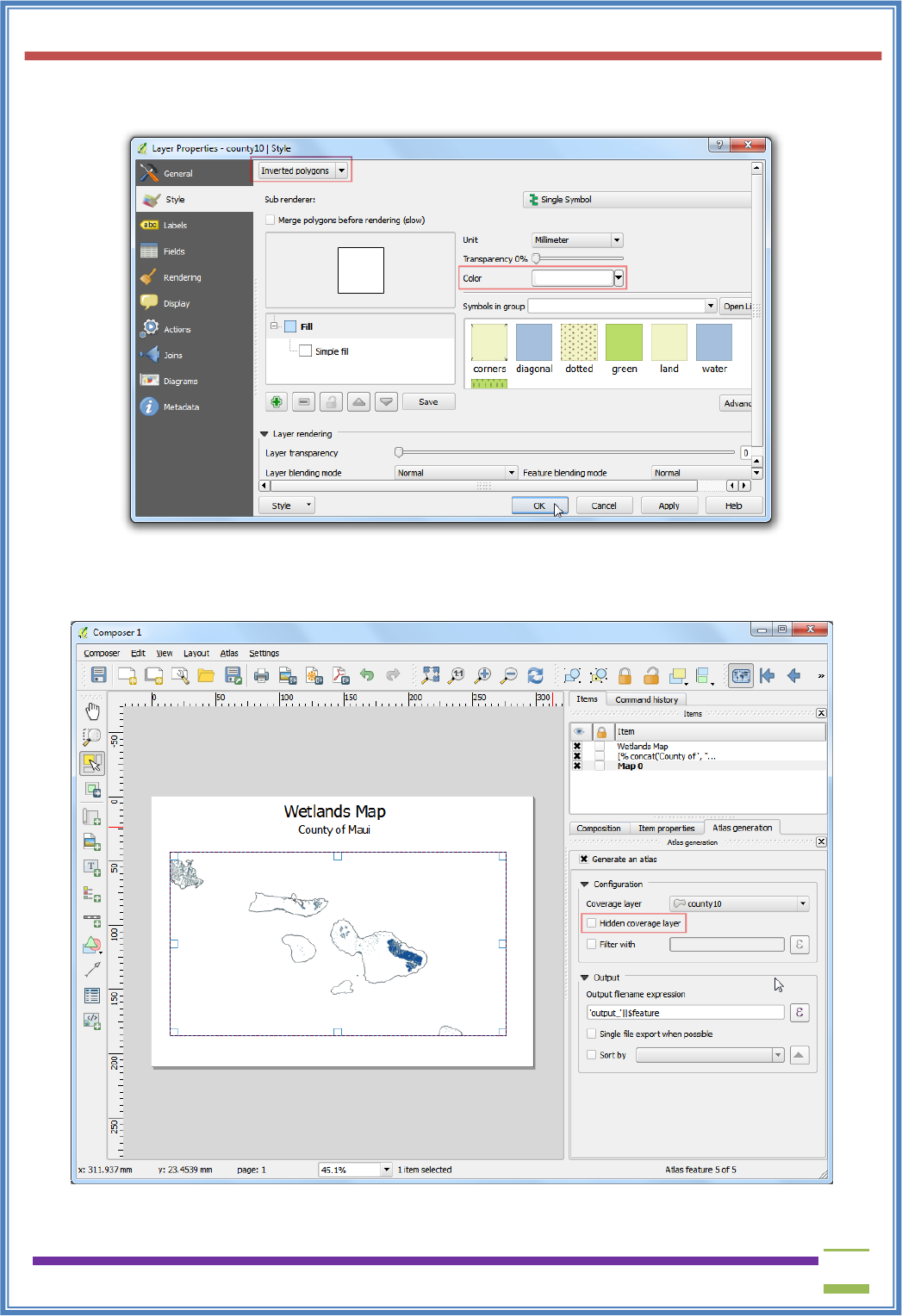
USIT6P4 (Discipline Specific Elective Practical) Principles of Geographic Information Systems Practical
T. Y. B. Sc. (Information Technology) SEMESTER VI Teacher’s Reference Manual
152
22. In the Style tab, select the Inverted polygons renderer. This renderer styles the outside of the
polygon - not inside. Select white as the fill color and click OK.
23. Switch to the Print Composer window. If we want the effect of the inverted polygons to show,
we need to uncheck the Hidden coverage layer box under Atlas generation. You will now see
that the rendered image is clean and areas outside the coverage polygon is not visible.
24. There is one problem though. You can see areas of the map that are outside the coverage layer
boundary but still visible. This is because Atlas doesn’t automatically hide other features. This
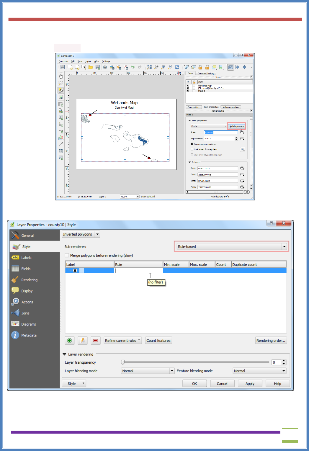
USIT6P4 (Discipline Specific Elective Practical) Principles of Geographic Information Systems Practical
T. Y. B. Sc. (Information Technology) SEMESTER VI Teacher’s Reference Manual
153
can be useful in some cases, but for our purpose, we only want to show wetlands of the county
whose map is being generated. To fix this, switch back to the main QGIS window and right-
click the county10 layer and select Properties.
25. In the Style tab, select Rule-based renderer as the Sub renderer. Double-click the area
under Rule.
26. Click the ... button next to Filter.
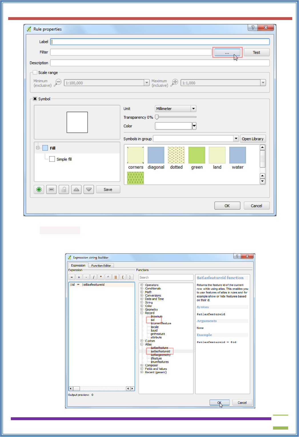
USIT6P4 (Discipline Specific Elective Practical) Principles of Geographic Information Systems Practical
T. Y. B. Sc. (Information Technology) SEMESTER VI Teacher’s Reference Manual
154
27. In the Expression string builder, expand the Atlas group of functions.
The $atlasfeatureid function will return the currently selected feature. We will construct an
expression that will select only the currently selected Atlas feature. Enter the expression as :
$id=$atlasfeatureid
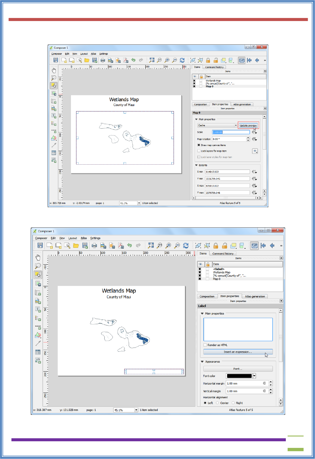
USIT6P4 (Discipline Specific Elective Practical) Principles of Geographic Information Systems Practical
T. Y. B. Sc. (Information Technology) SEMESTER VI Teacher’s Reference Manual
155
28. Back in the Print Composer window, click the Update preview button under Item properties tab
to see the changes. Notice that now only the area covering the county boundary is shown.
29. We will now add another dynamic label to show the current date. Go to Layout ‣ Add Label and
select the area on the map. ClickInsert an expression button.
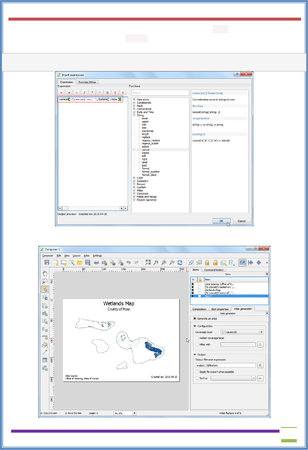
USIT6P4 (Discipline Specific Elective Practical) Principles of Geographic Information Systems Practical
T. Y. B. Sc. (Information Technology) SEMESTER VI Teacher’s Reference Manual
156
30. Expand the Date and Time functions group and you will find the $now function. This holds the
current system time. The function todate() will convert this to a date string. Enter the expression
as below:
concat('Created on: ', todate($now))
31. Add another label citing the data source. You may also add other map elements such as a north
arrow, scalebar etc. as described in Making a Map tutorial.
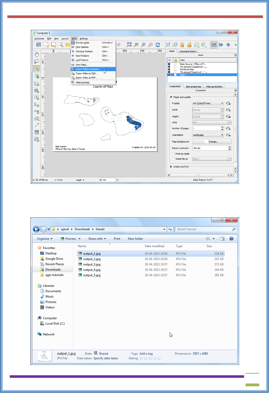
USIT6P4 (Discipline Specific Elective Practical) Principles of Geographic Information Systems Practical
T. Y. B. Sc. (Information Technology) SEMESTER VI Teacher’s Reference Manual
157
32. Once you are satisfied with the map layout, go to Atlas ‣ Export Atlas as Images.
33. Select a directory on your computer and click Choose.
34. The Atlas tool will now iterate through each feature in the coverage layer and create a separate
map image based on the template we created. You can see the images in the directory once the
process completes.
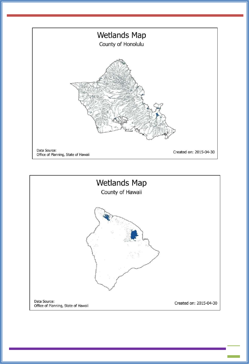
USIT6P4 (Discipline Specific Elective Practical) Principles of Geographic Information Systems Practical
T. Y. B. Sc. (Information Technology) SEMESTER VI Teacher’s Reference Manual
158
35. Here are the map images for refeence.
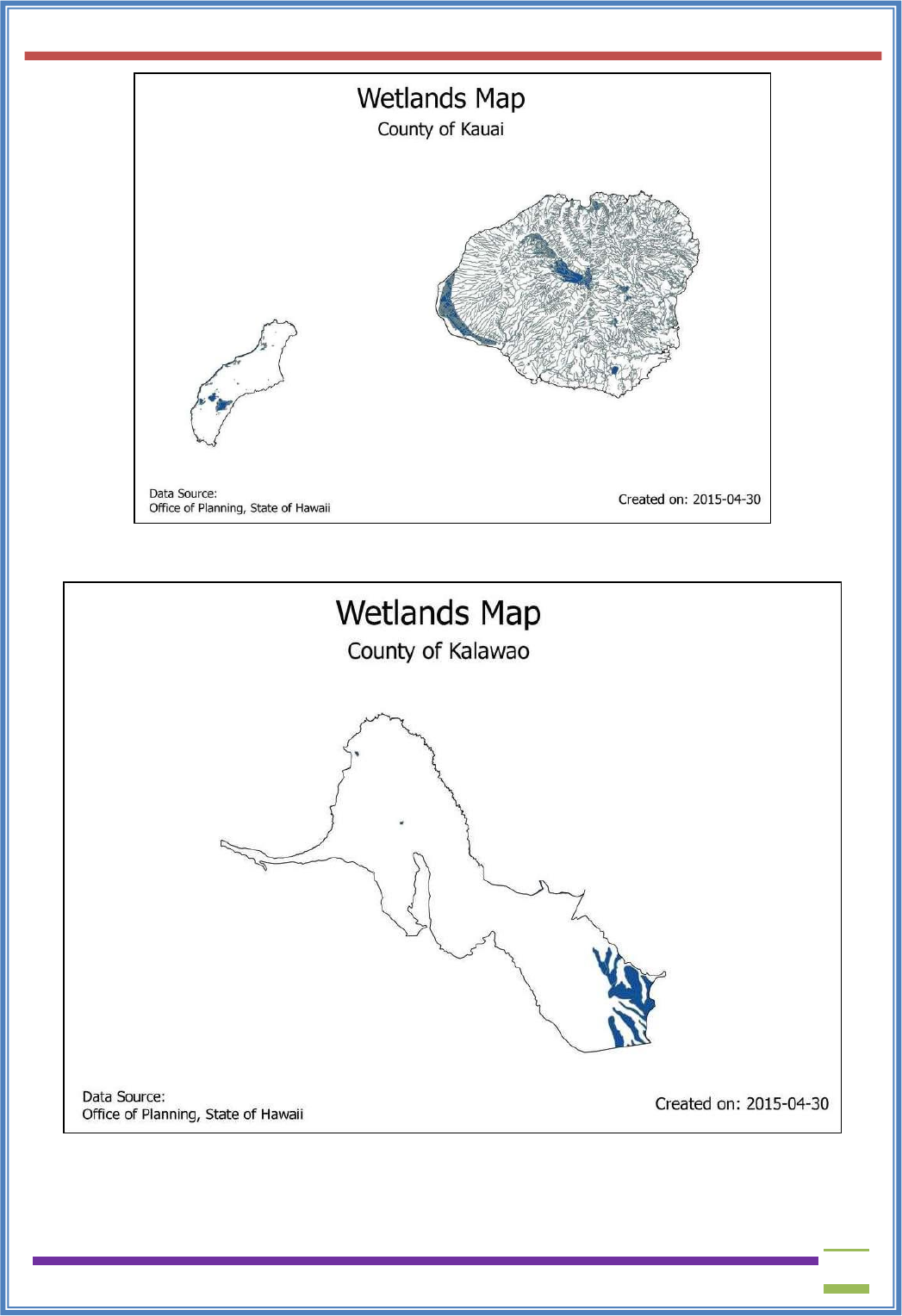
USIT6P4 (Discipline Specific Elective Practical) Principles of Geographic Information Systems Practical
T. Y. B. Sc. (Information Technology) SEMESTER VI Teacher’s Reference Manual
159
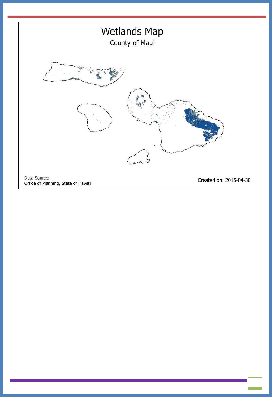
USIT6P4 (Discipline Specific Elective Practical) Principles of Geographic Information Systems Practical
T. Y. B. Sc. (Information Technology) SEMESTER VI Teacher’s Reference Manual
160

USIT6P4 (Discipline Specific Elective Practical) Principles of Geographic Information Systems Practical
T. Y. B. Sc. (Information Technology) SEMESTER VI Teacher’s Reference Manual
161
PRACTICAL - 10
A. Validating map data.
AIM: To validate Map data using Excel and QGIS.
Software Used: QGIS Desktop 3.4.2 and Microsoft Excel 2013.
Datasets Used: The following datasets are used
1. Kenya_epidemiological_data.xls
2. Kenya_epidemiological_dict.xls
Shape Files used: Kenya admin.
Theory
The aim of this practical is to focus on the validation steps that should be performed during data
cleaning. These include three types of checks:
1. Structural checks: e.g. unique ID, duplicates, format
2. Validation of plausibility - possible range of values e.g. min/max expected age
3. Logical checks - inconsistencies in answers e.g. occupation/age
The practical will be conducted using Microsoft Excel and QGIS software. The practical will be
performed in the following stages
1. Developing a data cleaning plan
2. Performing Structural data checks
3. Verifying the plausibility of data
4. Performing Logical data checks
5. Verifying coordinates of mapping data
6. Preparing data for mapping.
Procedure
The following steps we need to perform in the Stage I of developing a data cleaning plan
1. Open the “Kenya_epidemiological_data.xls” in Microsoft Excel. Additionally open the
corresponding dictionary “Kenya_epidemiological_dict.xls”, which contains a description of all
variables and information about their coding.
2. You should make note of the number of entries in your database, as you will need to keep track
of any changes e.g. when you remove duplicates at a later stage.
The following steps we need to perform in the Stage II of performing Structural Data checks
A. Format of the Database
B. Removing Duplicates
C. Coding of variables
2A Format of the database
Open Kenya_epidemiological_data.xls in excel.
Go to the View tab, click Freeze Panes and choose Freeze Top Row.
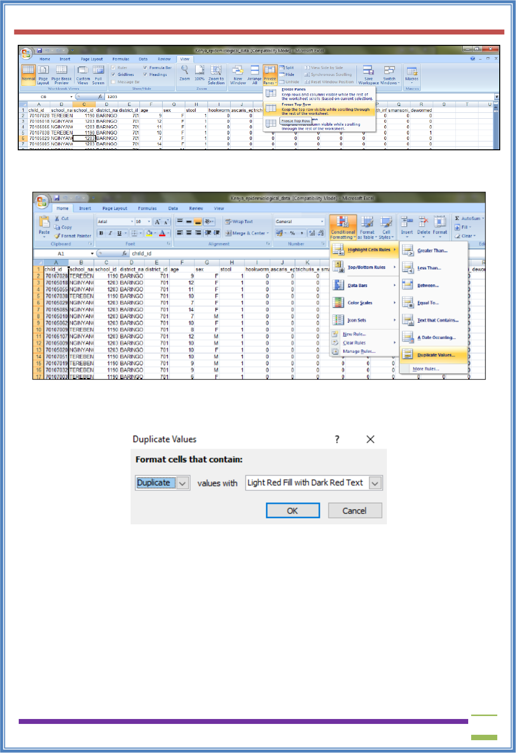
USIT6P4 (Discipline Specific Elective Practical) Principles of Geographic Information Systems Practical
T. Y. B. Sc. (Information Technology) SEMESTER VI Teacher’s Reference Manual
162
select the entire “child_id‟ column(first column),
Under Home Tab, click on Conditional formatting >Highlight Cell Rules> Select Duplicate values
Now select the first combo box and select Duplicate and select Light red fill with Dark red text in the
next combo box as shown in figure
2B Removing Duplicates
Select all the columns of existing worksheet
Now go to Data Tab and select Remove Duplicates
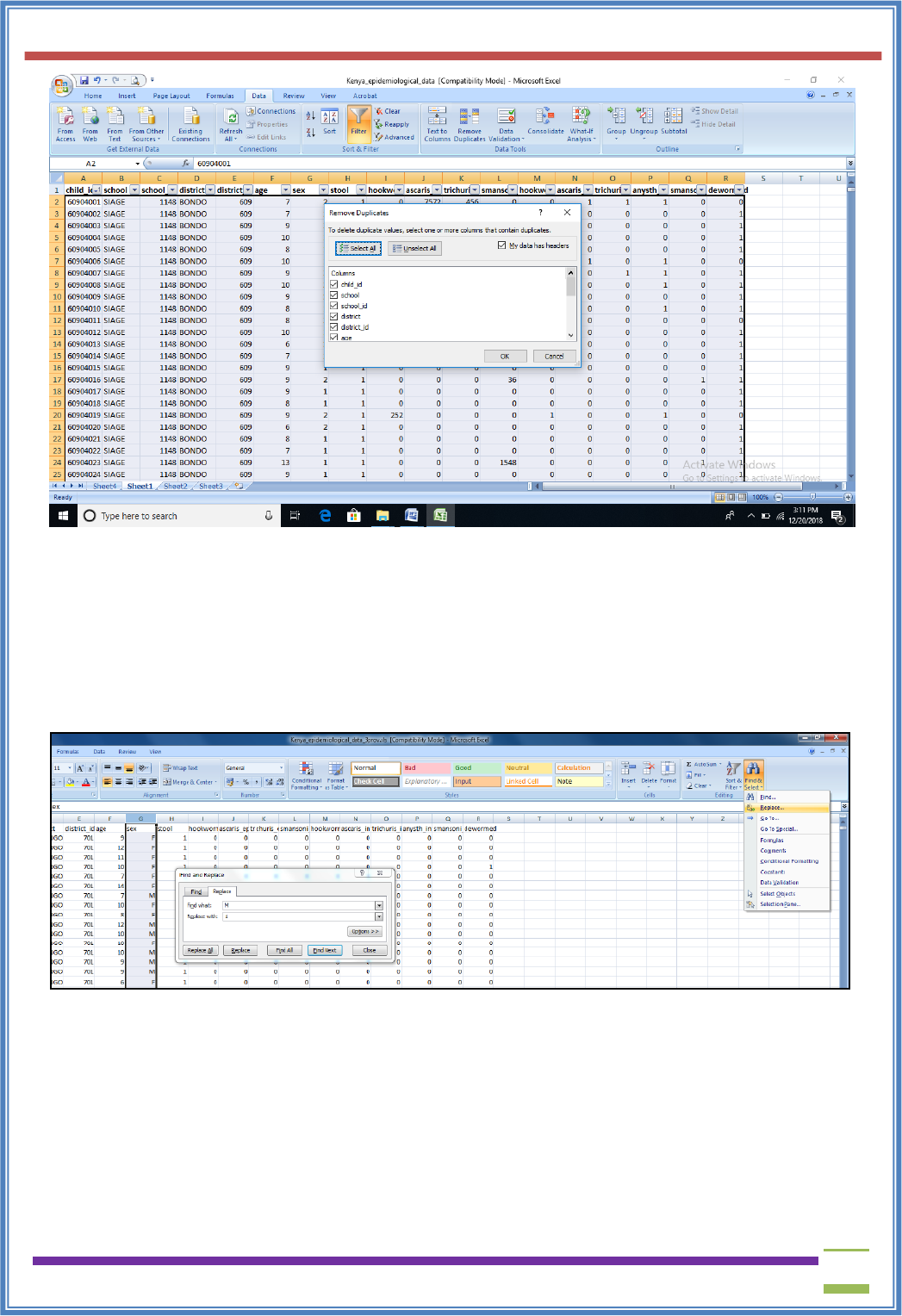
USIT6P4 (Discipline Specific Elective Practical) Principles of Geographic Information Systems Practical
T. Y. B. Sc. (Information Technology) SEMESTER VI Teacher’s Reference Manual
163
2C Coding of variables
In the current worksheet, select the sex column.
Now type Ctrl+F and use Replace Function and Replace as follows
M-1
F-2
Please keep track of how many values are getting replace.
Step 3 Verifying the plausibility of data
In this step, we perform two basic operations
A. Coding of variables
B. Using a filter to detect outliners
3A Coding of variables
Select the age column in the existing worksheet.
Now go to Insert tab and select Scatter. You will set chart as shown below
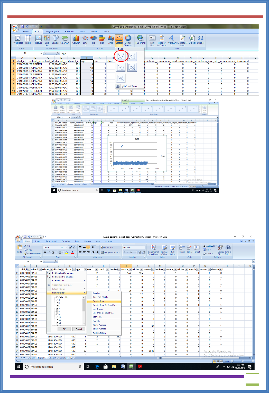
USIT6P4 (Discipline Specific Elective Practical) Principles of Geographic Information Systems Practical
T. Y. B. Sc. (Information Technology) SEMESTER VI Teacher’s Reference Manual
164
3B Using a filter to detect outliners
First go to the Home Tab>Sort and Filter>Filter. Click and apply the filter to all the columns of the
worksheet.
Now click on age filter and click on Number Filter> Greater Than option and type the value 20 in
greater than field.
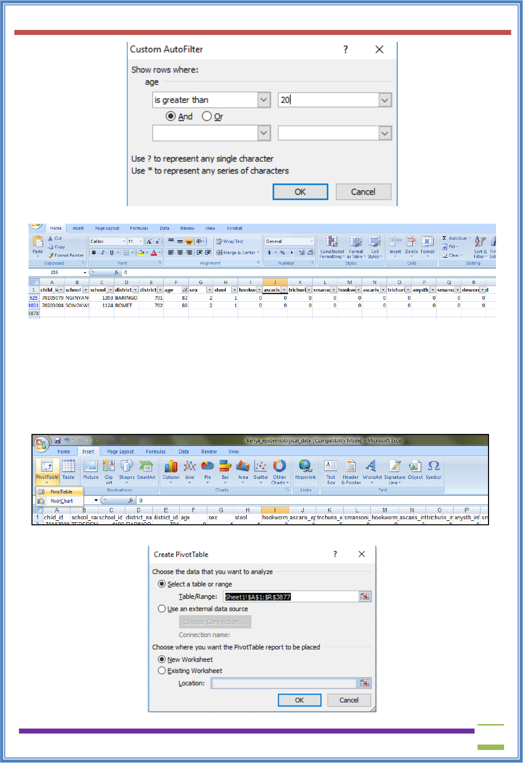
USIT6P4 (Discipline Specific Elective Practical) Principles of Geographic Information Systems Practical
T. Y. B. Sc. (Information Technology) SEMESTER VI Teacher’s Reference Manual
165
Step 4: Logical Data checks
In this step, we perform two basic operations
A. Cross Tabulations
B. Formulas
4A. Cross Tabulations
Open the existing worksheet. Now go to Insert Tab and select Pivot table function.
Select New Worksheet and click OK
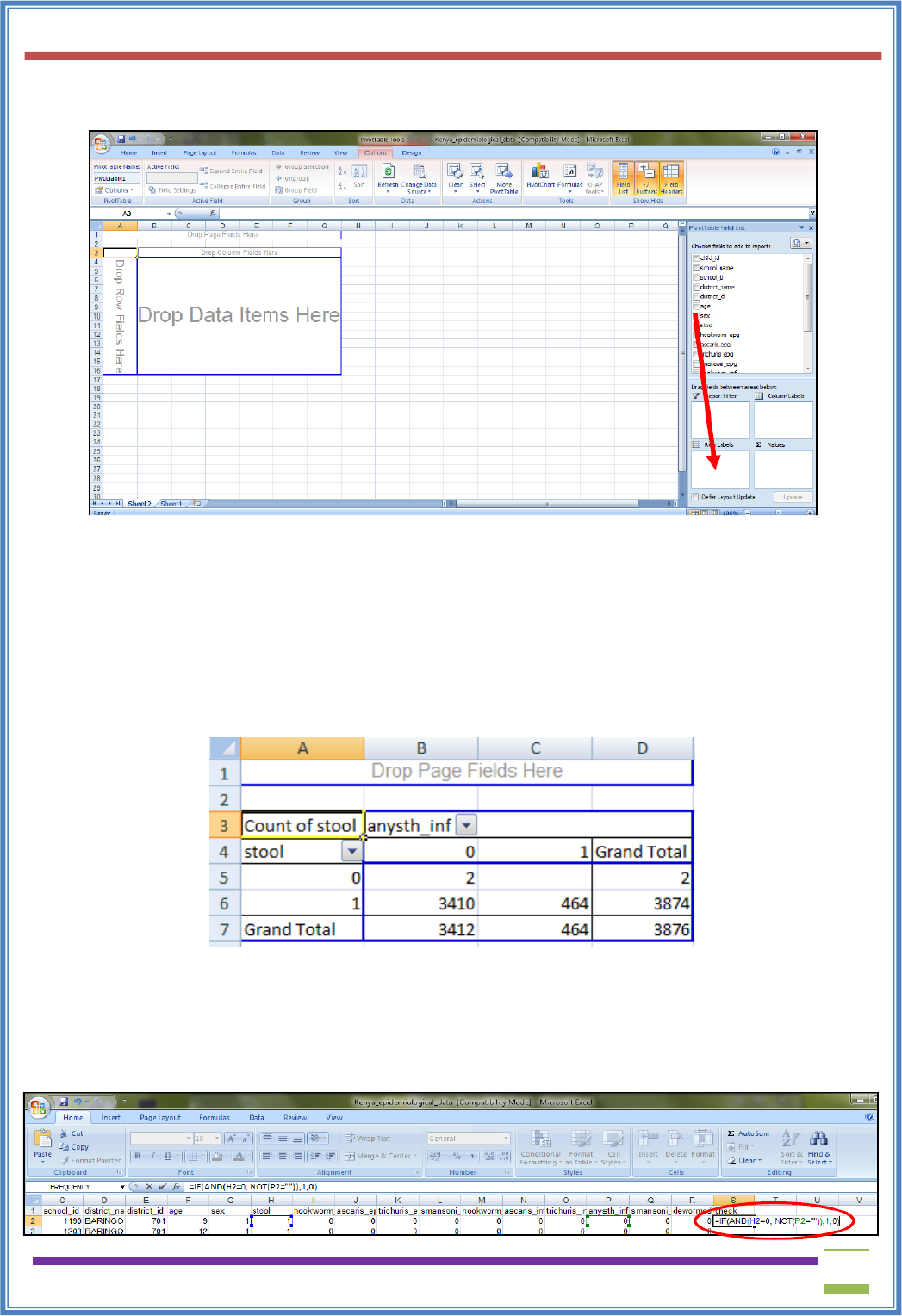
USIT6P4 (Discipline Specific Elective Practical) Principles of Geographic Information Systems Practical
T. Y. B. Sc. (Information Technology) SEMESTER VI Teacher’s Reference Manual
166
An empty table is inserted in a new sheet and a window will open on the right hand side named PIVOT
TABLE FIELD LIST.
From the PivotTable Field List, drag the “stool” item and drop it into the “Row Label” field as show
above.
Similarly, Click on anysth_inf and draw it into the “Column labels” and “Σ Values” field.
To include the count of observations in the table you might need to change the value field settings to
count.
Click on the combo box Sum of stools and Click on Value Field Settings.
Change the value in Summarize value filed by to Count and click OK. Table is updated with count
values as shown below
4B Formulas
Open the existing worksheet
Create a new column with the variable called check
Type the following formula in S2 column of worksheet =IF(AND(H2=0, NOT(P2="")),1,0)
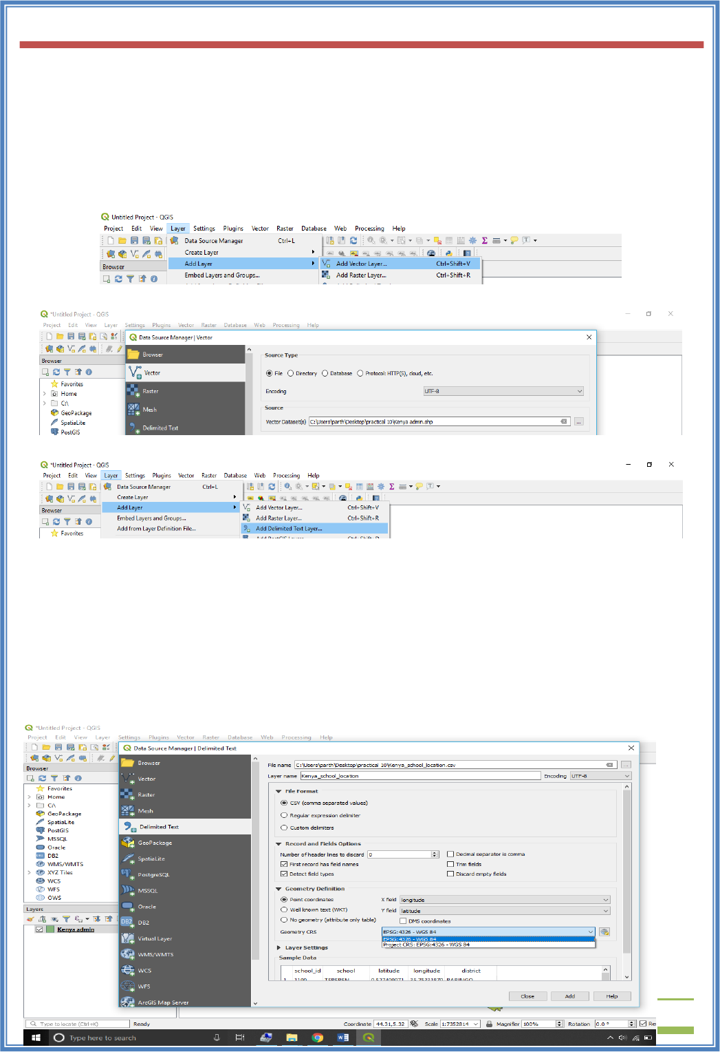
USIT6P4 (Discipline Specific Elective Practical) Principles of Geographic Information Systems Practical
T. Y. B. Sc. (Information Technology) SEMESTER VI Teacher’s Reference Manual
167
Now copy the formula to all other cells (ensure that the formula is copied to all rows in your dataset)
Now use the filter to show only entries with a check value of 1.
Step 5: Verifying the coordinates of mapping data
Create a New Project in QGIS Desktop 3.4.2.
Let’s add the files!
Navigate to Add Vector Layer and add file: Kenya_admin.shp
Similarly, navigate to Add Delimited Text Layer.
Here we have to add file: Kenya_school_location.csv. In the Geometry Definition section, there is a
field called Geometry CRS, in that we have to select WGS84 as coordinate system.
As you can see 2 points are not on the map.
To examine this, we need to save these layers as a Shapefile, to do that select both the layers
Kenya_school_location and Kenya admin, then right click on them and choose Save Features As…
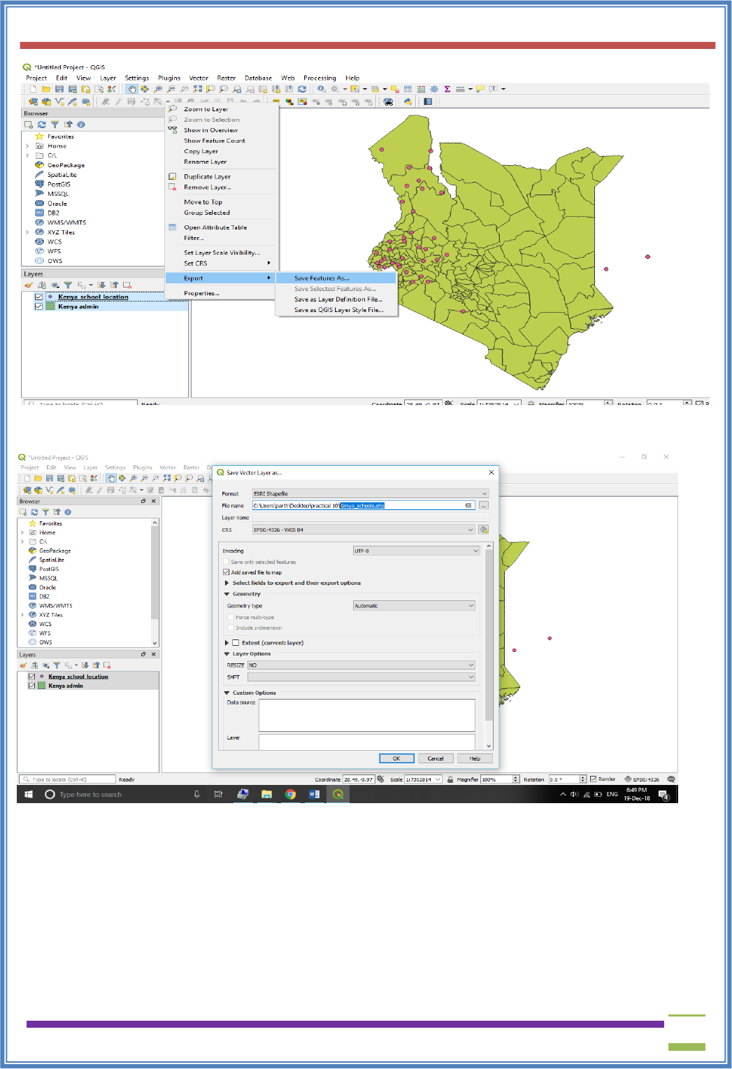
USIT6P4 (Discipline Specific Elective Practical) Principles of Geographic Information Systems Practical
T. Y. B. Sc. (Information Technology) SEMESTER VI Teacher’s Reference Manual
168
In the menu that comes up, set Format as ESRI Shapefile and put File Name as Kenya_schools.shp
After this is done you can uncheck the Kenya_school_location in the layers section.
Let’s try and get the details of these 2 points that are not on the map, select the Kenya_schools layer,
click on the Identify Features Tool button and then click on the points outside of Kenya to get their
details.
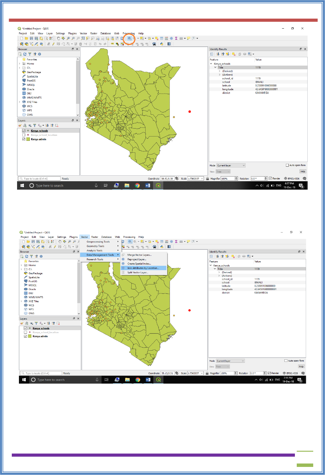
USIT6P4 (Discipline Specific Elective Practical) Principles of Geographic Information Systems Practical
T. Y. B. Sc. (Information Technology) SEMESTER VI Teacher’s Reference Manual
169
Now we want to add the district information to the map. Therefore, we will join information based on
the geographical localization.
In the menu click on Vector, then Data Management Tools, then select Join attributes by location.
Then select Kenya_schools as Input layer and Kenya_admin as Join layer.
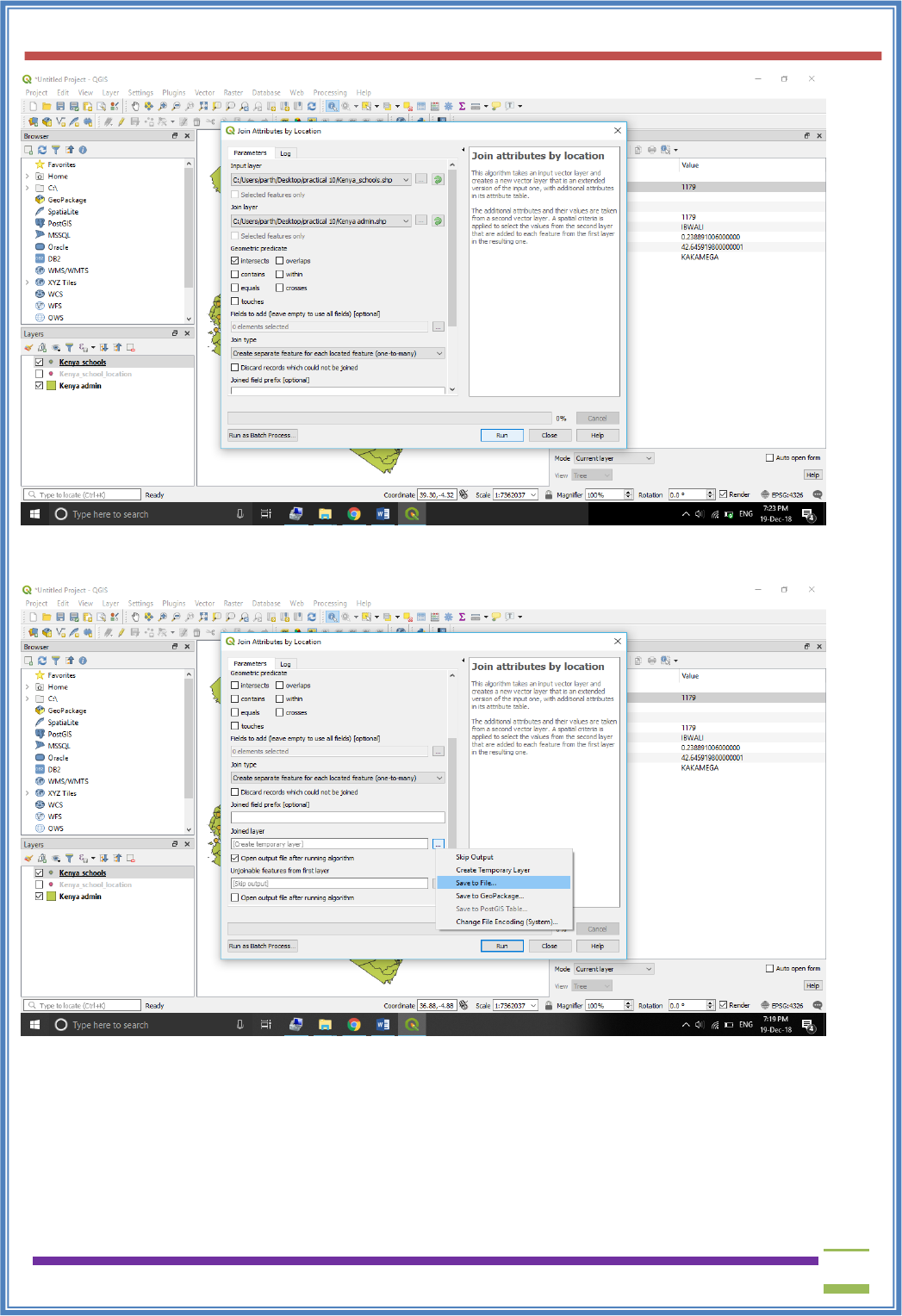
USIT6P4 (Discipline Specific Elective Practical) Principles of Geographic Information Systems Practical
T. Y. B. Sc. (Information Technology) SEMESTER VI Teacher’s Reference Manual
170
We also need to save the output so in Joined Layer, click “…”button to Browse location.
Save as Kenya_school_district.csv
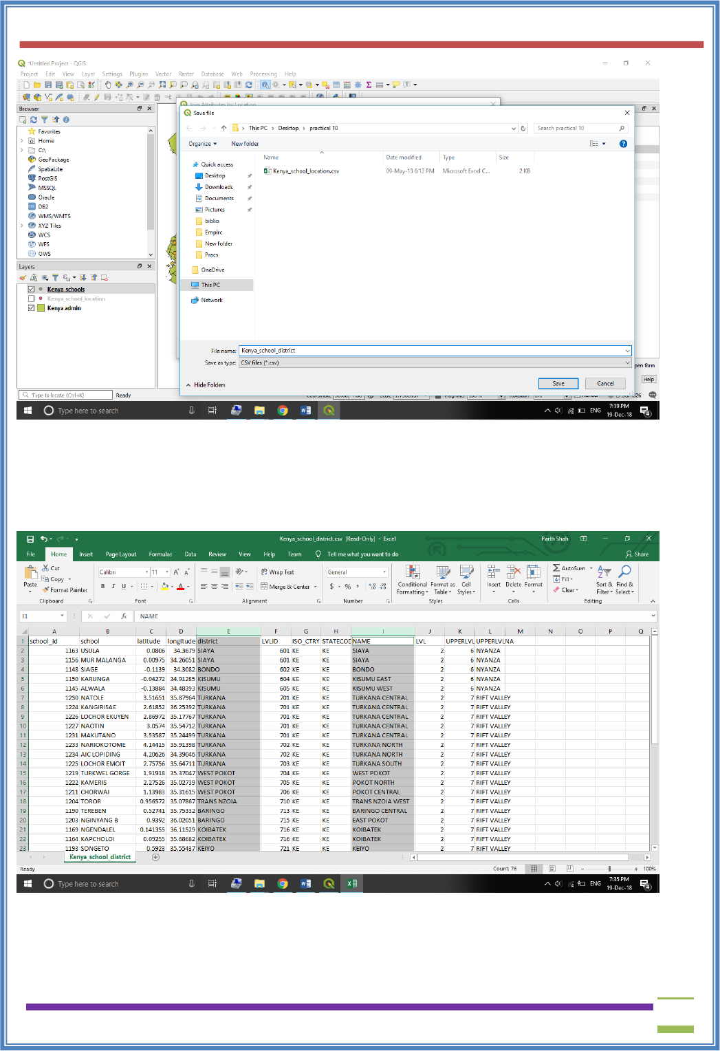
USIT6P4 (Discipline Specific Elective Practical) Principles of Geographic Information Systems Practical
T. Y. B. Sc. (Information Technology) SEMESTER VI Teacher’s Reference Manual
171
And then click run.
After it is done…
Navigate to the location of saved file Kenya_school_district.csvand open it, you should now be able to
compare both district and Name for discrepancies.
We need to change the co-ordinate of those 2 points which were not on the map. So, open the file
Kenya_school_location.csv and make the following changes, set:
IBWALI: Longitude 34.6459198
SIWOT: Longitude 35.35437012
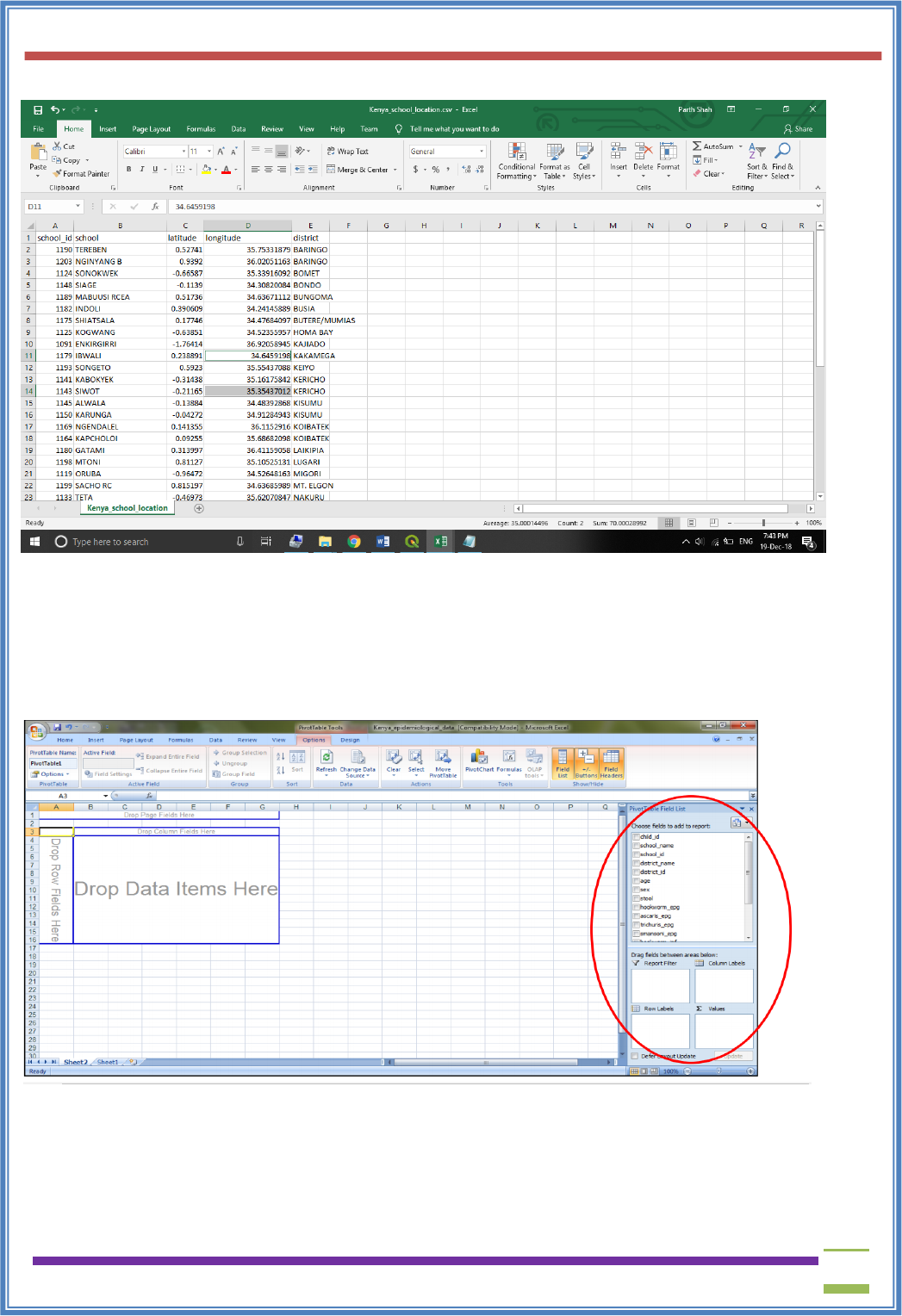
USIT6P4 (Discipline Specific Elective Practical) Principles of Geographic Information Systems Practical
T. Y. B. Sc. (Information Technology) SEMESTER VI Teacher’s Reference Manual
172
Save the file as: Kenya_school_location2.csv.
Step 6: Preparing data for mapping
Open Kenya_epidemiological_data_2.xls, select the entire sheet, go to Insert tab to create new
Pivot Table.
Tick New Worksheet to tell Excel that you want to place the table in a new sheet.
Now click on school_idtodragand drop it in the “Row labels” field at the bottom.
Add district_id to“Σ Values”and click on it, a drop down list will open, click on Value Field
Settings. Choose Average as type of calculation, because all children in the same school will have
same district_id.
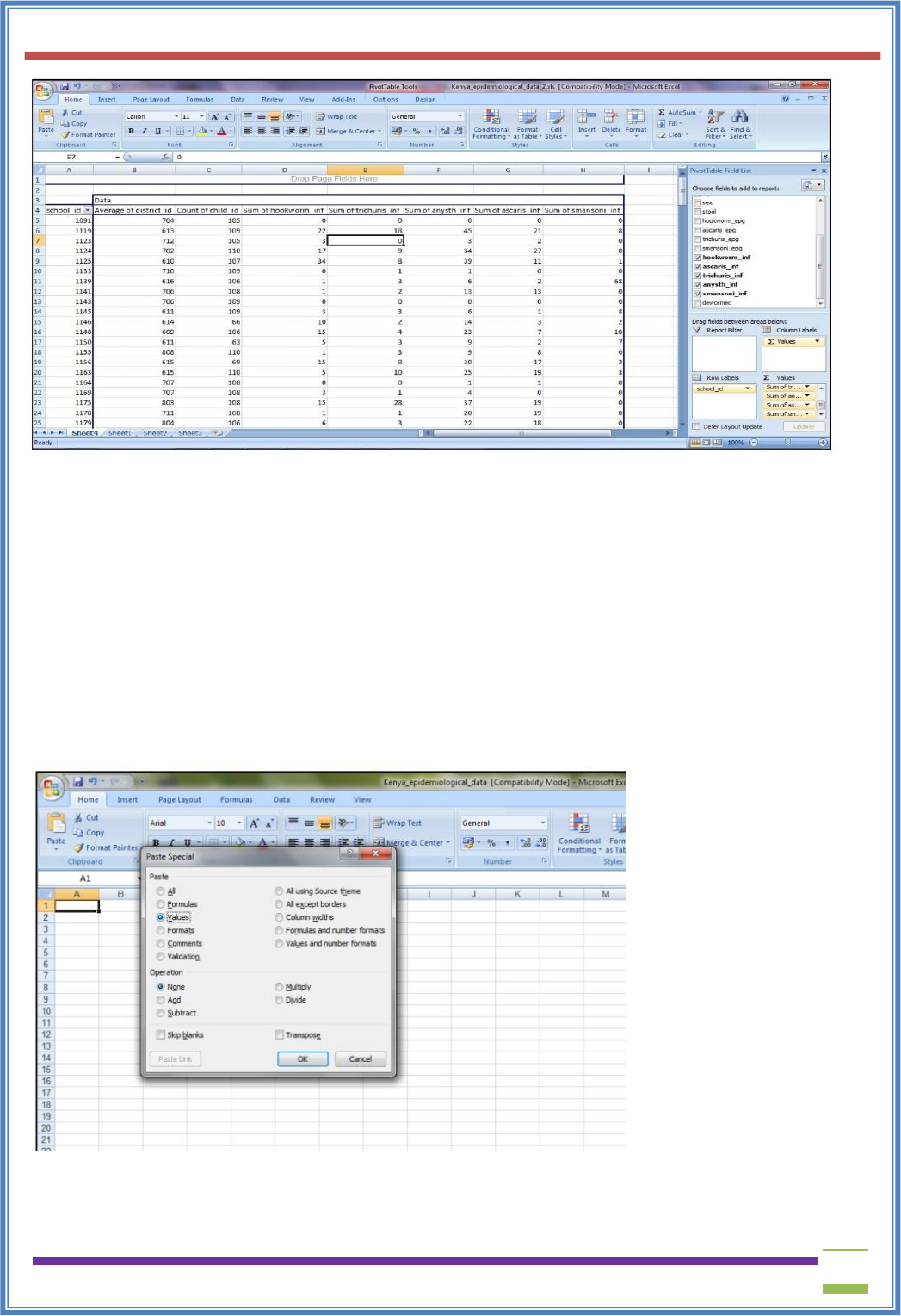
USIT6P4 (Discipline Specific Elective Practical) Principles of Geographic Information Systems Practical
T. Y. B. Sc. (Information Technology) SEMESTER VI Teacher’s Reference Manual
173
Now drag and dropchild_id into the “Σ Values” field, click on Value Field Settings and choose
Count to summarize the results. So, we come to know how many children per school are infected.
Similarly, Drag and dropanysth_inf into the field, click on Value Field Settingsand choose Sum. As,
infected is 1 and not affected is 0, the sum will give us the total number of infected children.
Now copy the table, open a new Excel file and paste the values into the new spreadsheet. Therefore,
click Paste in the Home tab, then choose Paste special and paste only the values.
Remove the last row which has Grand Total and other values.
Save this new data table as Kenya_school_STH_surveys.xlsx
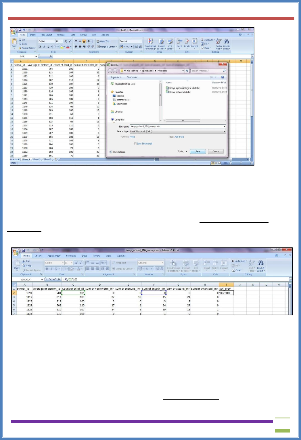
USIT6P4 (Discipline Specific Elective Practical) Principles of Geographic Information Systems Practical
T. Y. B. Sc. (Information Technology) SEMESTER VI Teacher’s Reference Manual
174
Now we need to know the total count of infected children, that is, the prevalence of STH.
So, w ecreate a new column:sth_previn which we are going to be dividing the number of infected
children by the number of children and multiplying by hundred to obtain a value in percent (%).
In the first cell under the heading type =F2/C2*100 (this assumes that your number of children is in
row C and the number of infected children in row F; you will need to adjust the column label
accordingly); then copy the formula to the other cells in the column.
Additionally, you could calculate the 95% confidence interval (CI) of your prevalence.
You will have to create a new column called “CIlow” (lower confidence limit) and “CIup”(upper
confidence limit)
You can calculate the limits by typing the formulas as follows and then copying to the other cells:
For CIlow: =I2 - (1.96*(SQRT((I2*(100-I2)/C2))))
For CIup: =I2 + (1.96*(SQRT((I2*(100-I2)/C2))))
Assuming I2 as sth_prev and C2 as Count of child_id, adjust accordingly.
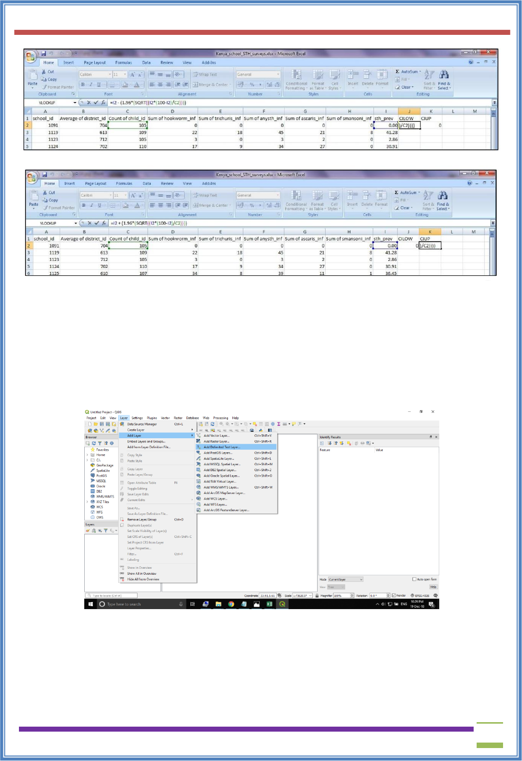
USIT6P4 (Discipline Specific Elective Practical) Principles of Geographic Information Systems Practical
T. Y. B. Sc. (Information Technology) SEMESTER VI Teacher’s Reference Manual
175
Save this file as Kenya_epidemiological_school.csv
Now that all the datasets are ready, let’s add them.
Open a new QGIS project.
First, add Kenya_school_location2.csv to the project. Click on Add Delimited text layer in the menu,
and browse to select the file.
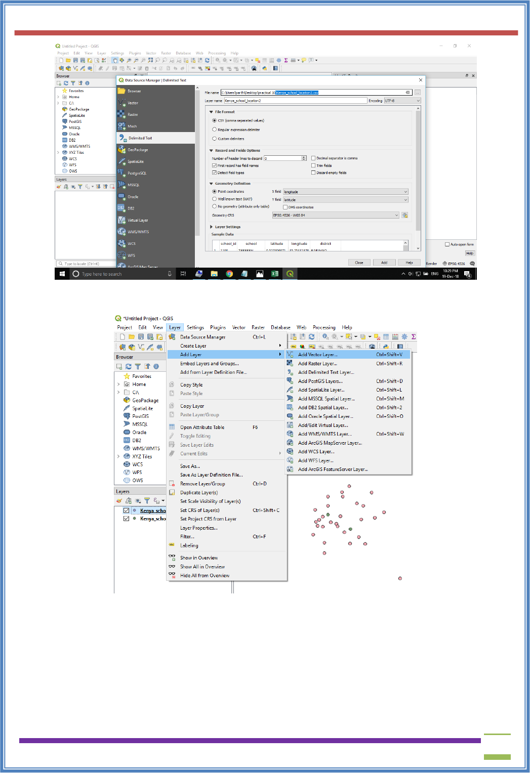
USIT6P4 (Discipline Specific Elective Practical) Principles of Geographic Information Systems Practical
T. Y. B. Sc. (Information Technology) SEMESTER VI Teacher’s Reference Manual
176
Similarly, Add Vector Layer and add Kenya_ epidemiological_school.csv
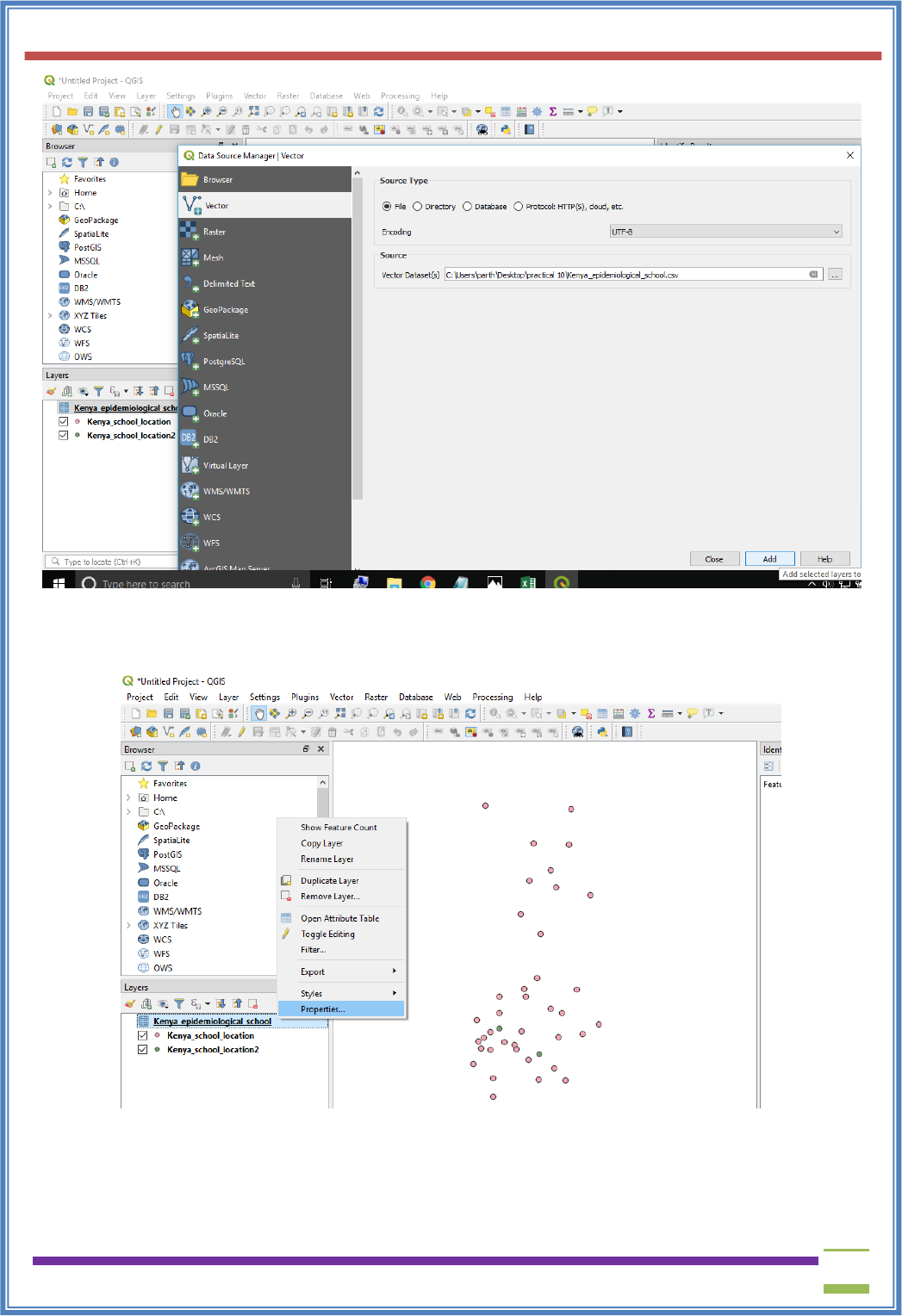
USIT6P4 (Discipline Specific Elective Practical) Principles of Geographic Information Systems Practical
T. Y. B. Sc. (Information Technology) SEMESTER VI Teacher’s Reference Manual
177
Now we’ll join the data.
Right click on Kenya _school_location2 layer and click on Properties
Go to the Joins section and click on the plus(+) button at the bottom
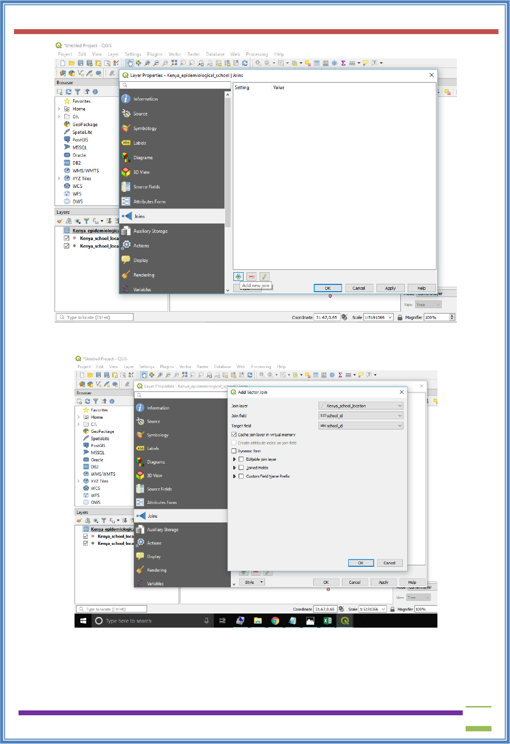
USIT6P4 (Discipline Specific Elective Practical) Principles of Geographic Information Systems Practical
T. Y. B. Sc. (Information Technology) SEMESTER VI Teacher’s Reference Manual
178
For “Join layer” chooseKenya_epidemiological_school and for“Join field” and “Target field” choose
school_id. Then click on OK.
Right click on Kenya_school_location2 layer and select Open Attribute Table.
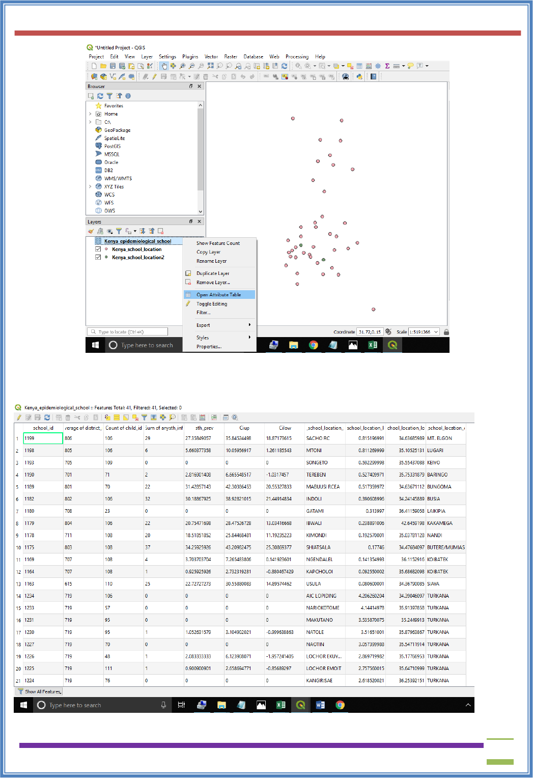
USIT6P4 (Discipline Specific Elective Practical) Principles of Geographic Information Systems Practical
T. Y. B. Sc. (Information Technology) SEMESTER VI Teacher’s Reference Manual
179
You will see that the epidemiological variables are included.
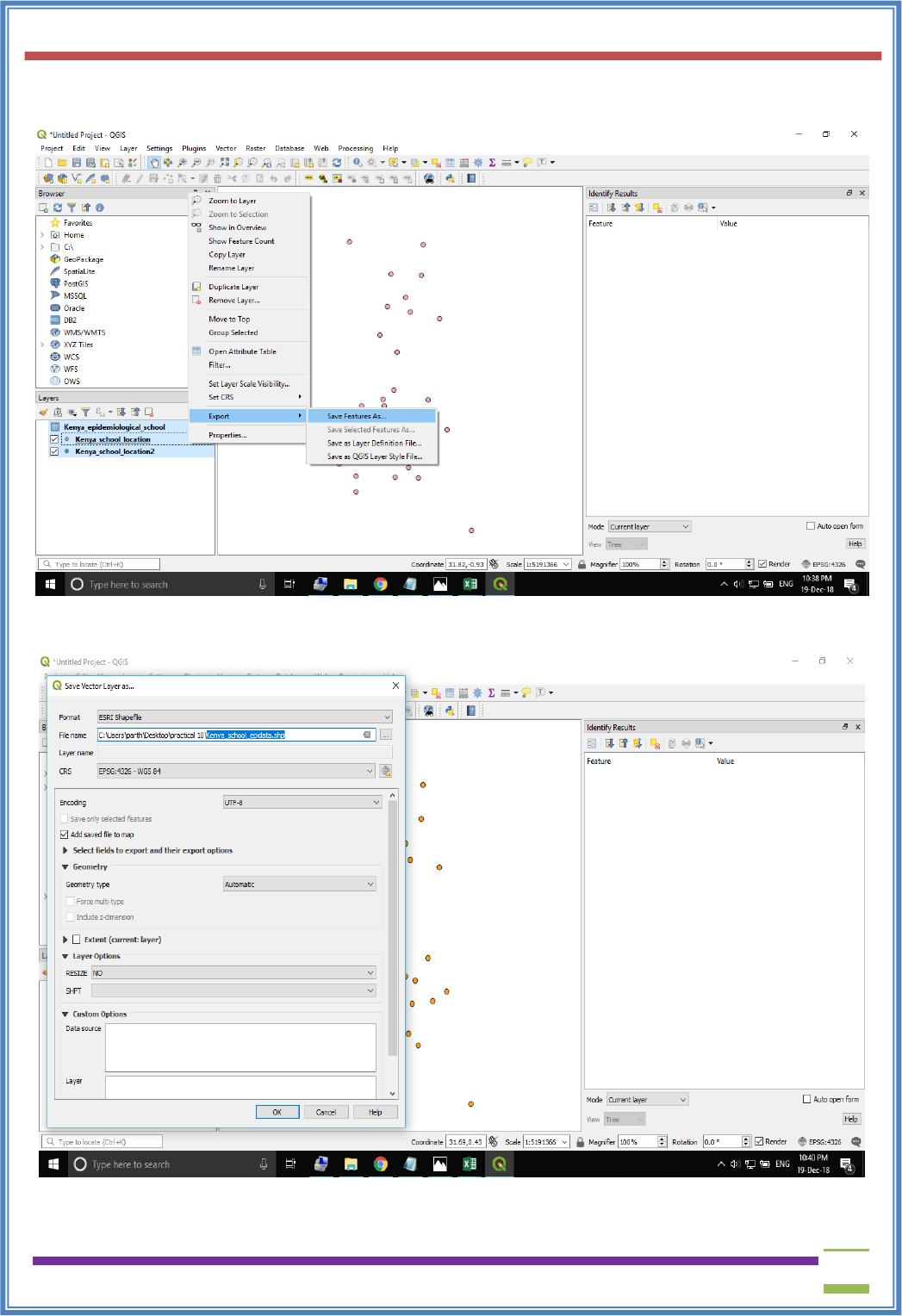
USIT6P4 (Discipline Specific Elective Practical) Principles of Geographic Information Systems Practical
T. Y. B. Sc. (Information Technology) SEMESTER VI Teacher’s Reference Manual
180
We are finally done, now we just have to save the files!!
Select all the layers, right-click on them and in Export select Save Features As.
Select Format as ESRI Shapefile and File Name as: Kenya_school_epidata.shp
-------------------------------

USIT6P4 (Discipline Specific Elective Practical) Principles of Geographic Information Systems Practical
T. Y. B. Sc. (Information Technology) SEMESTER VI Teacher’s Reference Manual
181
Links for Datasets:
1. For Multiple data sets : https://www.gadm.org/download_country_v3.html
2. For Multiple data sets : https://urs.earthdata.nasa.gov
3. Geological survey data : https://ers.cr.usgs.gov/register
4. Raster Mosaic: https://lance-modis.eosdis.nasa.gov/imagery/subsets/?project=fas
5. https://www.gadm.org/download_world.html
6. https://github.com/datameet/maps/tree/master/Survey-of-India-Index-Maps
7. https://bhuvan.nrsc.gov.in
8. For DEM :
http://viewfinderpanoramas.org/Coverage%20map%20viewfinderpanoramas_org3.htm
Dear Teacher, please send your valuable feedback and contribution to
make this manual more effective.
Please send on dandhiren@yahoo.co.in and/or shaikh.aa@rediffmail.com
