Graph Theory Package For Giac/Xcas Graphtheory User Manual
User Manual:
Open the PDF directly: View PDF ![]() .
.
Page Count: 136 [warning: Documents this large are best viewed by clicking the View PDF Link!]
- Introduction
- 1. Constructing graphs
- 2. Modifying graphs
- 3. Import and export
- 4. Graph properties
- 5. Traversing graphs
- 6. Visualizing graphs
- Bibliography
- Command Index

Graph theory
package for
Giac/Xcas
Reference manual
September 2018


Table of contents
Introduction ................................................. 7
1. Constructing graphs ....................................... 9
1.1. General graphs . . . . . . . . . . . . . . . . . . . . . . . . . . . . . . . . . . . . . . . . . . . . . . . 9
1.1.1. Undirected graphs . . . . . . . . . . . . . . . . . . . . . . . . . . . . . . . . . . . . . . . . . . 9
1.1.2. Directed graphs . . . . . . . . . . . . . . . . . . . . . . . . . . . . . . . . . . . . . . . . . . 10
1.1.3. Examples . . . . . . . . . . . . . . . . . . . . . . . . . . . . . . . . . . . . . . . . . . . . . . 10
Creating vertices . . . . . . . . . . . . . . . . . . . . . . . . . . . . . . . . . . . . . . . 10
Creating edges and arcs . . . . . . . . . . . . . . . . . . . . . . . . . . . . . . . . . . . 10
Creating paths and trails . . . . . . . . . . . . . . . . . . . . . . . . . . . . . . . . . . 11
Specifying adjacency or weight matrix . . . . . . . . . . . . . . . . . . . . . . . . . 11
Creating special graphs . . . . . . . . . . . . . . . . . . . . . . . . . . . . . . . . . . . 12
1.2. Cycle and path graphs . . . . . . . . . . . . . . . . . . . . . . . . . . . . . . . . . . . . . . . . . 13
1.2.1. Cycle graphs . . . . . . . . . . . . . . . . . . . . . . . . . . . . . . . . . . . . . . . . . . . . 13
1.2.2. Path graphs . . . . . . . . . . . . . . . . . . . . . . . . . . . . . . . . . . . . . . . . . . . . . 13
1.2.3. Trails of edges . . . . . . . . . . . . . . . . . . . . . . . . . . . . . . . . . . . . . . . . . . . 13
1.3. Complete graphs . . . . . . . . . . . . . . . . . . . . . . . . . . . . . . . . . . . . . . . . . . . . . 14
1.3.1. Complete graphs (with multiple vertex partitions) . . . . . . . . . . . . . . . . . . . . 14
1.3.2. Complete trees . . . . . . . . . . . . . . . . . . . . . . . . . . . . . . . . . . . . . . . . . . . 15
1.4. Sequence graphs . . . . . . . . . . . . . . . . . . . . . . . . . . . . . . . . . . . . . . . . . . . . . 15
1.4.1. Creating graphs from degree sequences . . . . . . . . . . . . . . . . . . . . . . . . . . . 15
1.4.2. Validating graphic sequences . . . . . . . . . . . . . . . . . . . . . . . . . . . . . . . . . . 16
1.5. Intersection graphs . . . . . . . . . . . . . . . . . . . . . . . . . . . . . . . . . . . . . . . . . . . 16
1.5.1. Interval graphs . . . . . . . . . . . . . . . . . . . . . . . . . . . . . . . . . . . . . . . . . . . 16
1.5.2. Kneser graphs . . . . . . . . . . . . . . . . . . . . . . . . . . . . . . . . . . . . . . . . . . . 16
1.6. Special graphs . . . . . . . . . . . . . . . . . . . . . . . . . . . . . . . . . . . . . . . . . . . . . . 17
1.6.1. Hypercube graphs . . . . . . . . . . . . . . . . . . . . . . . . . . . . . . . . . . . . . . . . . 17
1.6.2. Star graphs . . . . . . . . . . . . . . . . . . . . . . . . . . . . . . . . . . . . . . . . . . . . . 18
1.6.3. Wheel graphs . . . . . . . . . . . . . . . . . . . . . . . . . . . . . . . . . . . . . . . . . . . . 18
1.6.4. Web graphs . . . . . . . . . . . . . . . . . . . . . . . . . . . . . . . . . . . . . . . . . . . . . 18
1.6.5. Prism graphs . . . . . . . . . . . . . . . . . . . . . . . . . . . . . . . . . . . . . . . . . . . . 19
1.6.6. Antiprism graphs . . . . . . . . . . . . . . . . . . . . . . . . . . . . . . . . . . . . . . . . . 19
1.6.7. Grid graphs . . . . . . . . . . . . . . . . . . . . . . . . . . . . . . . . . . . . . . . . . . . . . 19
1.6.8. Sierpi«ski graphs . . . . . . . . . . . . . . . . . . . . . . . . . . . . . . . . . . . . . . . . . 21
1.6.9. Generalized Petersen graphs . . . . . . . . . . . . . . . . . . . . . . . . . . . . . . . . . . 22
1.6.10. LCF graphs . . . . . . . . . . . . . . . . . . . . . . . . . . . . . . . . . . . . . . . . . . . . 22
1.7. Isomorphic copies of graphs . . . . . . . . . . . . . . . . . . . . . . . . . . . . . . . . . . . . . . 23
1.7.1. Creating an isomorphic copy from a permutation . . . . . . . . . . . . . . . . . . . . . 23
1.7.2. Permuting vertices . . . . . . . . . . . . . . . . . . . . . . . . . . . . . . . . . . . . . . . . 24
1.7.3. Relabeling vertices . . . . . . . . . . . . . . . . . . . . . . . . . . . . . . . . . . . . . . . . 25
1.8. Subgraphs . . . . . . . . . . . . . . . . . . . . . . . . . . . . . . . . . . . . . . . . . . . . . . . . . 25
1.8.1. Extracting subgraphs . . . . . . . . . . . . . . . . . . . . . . . . . . . . . . . . . . . . . . . 25
1.8.2. Induced subgraphs . . . . . . . . . . . . . . . . . . . . . . . . . . . . . . . . . . . . . . . . 25
1.8.3. Underlying graphs . . . . . . . . . . . . . . . . . . . . . . . . . . . . . . . . . . . . . . . . 26
1.8.4. Fundamental cycles . . . . . . . . . . . . . . . . . . . . . . . . . . . . . . . . . . . . . . . . 26
1.9. Operations on graphs . . . . . . . . . . . . . . . . . . . . . . . . . . . . . . . . . . . . . . . . . . 28
1.9.1. Graph complement . . . . . . . . . . . . . . . . . . . . . . . . . . . . . . . . . . . . . . . . 28
1.9.2. Seidel switching . . . . . . . . . . . . . . . . . . . . . . . . . . . . . . . . . . . . . . . . . . 29
1.9.3. Transposing graphs . . . . . . . . . . . . . . . . . . . . . . . . . . . . . . . . . . . . . . . . 29
3

1.9.4. Union of graphs . . . . . . . . . . . . . . . . . . . . . . . . . . . . . . . . . . . . . . . . . . 30
1.9.5. Disjoint union of graphs . . . . . . . . . . . . . . . . . . . . . . . . . . . . . . . . . . . . . 30
1.9.6. Joining two graphs . . . . . . . . . . . . . . . . . . . . . . . . . . . . . . . . . . . . . . . . 30
1.9.7. Power graphs . . . . . . . . . . . . . . . . . . . . . . . . . . . . . . . . . . . . . . . . . . . . 31
1.9.8. Graph products . . . . . . . . . . . . . . . . . . . . . . . . . . . . . . . . . . . . . . . . . . 32
1.9.9. Transitive closure graph . . . . . . . . . . . . . . . . . . . . . . . . . . . . . . . . . . . . . 33
1.9.10. Line graph . . . . . . . . . . . . . . . . . . . . . . . . . . . . . . . . . . . . . . . . . . . . . 34
1.9.11. Plane dual graph . . . . . . . . . . . . . . . . . . . . . . . . . . . . . . . . . . . . . . . . . 34
1.10. Random graphs . . . . . . . . . . . . . . . . . . . . . . . . . . . . . . . . . . . . . . . . . . . . . 36
1.10.1. Random general graphs . . . . . . . . . . . . . . . . . . . . . . . . . . . . . . . . . . . . 36
1.10.2. Random bipartite graphs . . . . . . . . . . . . . . . . . . . . . . . . . . . . . . . . . . . 37
1.10.3. Random trees . . . . . . . . . . . . . . . . . . . . . . . . . . . . . . . . . . . . . . . . . . . 37
1.10.4. Random planar graphs . . . . . . . . . . . . . . . . . . . . . . . . . . . . . . . . . . . . . 40
1.10.5. Random graphs from the given degree sequence . . . . . . . . . . . . . . . . . . . . . 41
1.10.6. Random regular graphs . . . . . . . . . . . . . . . . . . . . . . . . . . . . . . . . . . . . 42
1.10.7. Random tournaments . . . . . . . . . . . . . . . . . . . . . . . . . . . . . . . . . . . . . . 43
1.10.8. Random network graphs . . . . . . . . . . . . . . . . . . . . . . . . . . . . . . . . . . . . 43
1.10.9. Randomizing edge weights . . . . . . . . . . . . . . . . . . . . . . . . . . . . . . . . . . . 44
2. Modifying graphs ......................................... 47
2.1. Promoting to directed and weighted graphs . . . . . . . . . . . . . . . . . . . . . . . . . . . . 47
2.1.1. Converting edges to arcs . . . . . . . . . . . . . . . . . . . . . . . . . . . . . . . . . . . . 47
2.1.2. Assigning weight matrix to unweighted graphs . . . . . . . . . . . . . . . . . . . . . . 47
2.2. Modifying vertices of a graph . . . . . . . . . . . . . . . . . . . . . . . . . . . . . . . . . . . . . 47
2.2.1. Adding and removing vertices . . . . . . . . . . . . . . . . . . . . . . . . . . . . . . . . . 47
2.3. Modifying edges of a graph . . . . . . . . . . . . . . . . . . . . . . . . . . . . . . . . . . . . . . 48
2.3.1. Adding and removing edges . . . . . . . . . . . . . . . . . . . . . . . . . . . . . . . . . . 48
2.3.2. Accessing and modifying edge weights . . . . . . . . . . . . . . . . . . . . . . . . . . . . 49
2.3.3. Contracting edges . . . . . . . . . . . . . . . . . . . . . . . . . . . . . . . . . . . . . . . . . 50
2.3.4. Subdividing edges . . . . . . . . . . . . . . . . . . . . . . . . . . . . . . . . . . . . . . . . . 50
2.4. Using attributes . . . . . . . . . . . . . . . . . . . . . . . . . . . . . . . . . . . . . . . . . . . . . 51
2.4.1. Graph attributes . . . . . . . . . . . . . . . . . . . . . . . . . . . . . . . . . . . . . . . . . 51
2.4.2. Vertex attributes . . . . . . . . . . . . . . . . . . . . . . . . . . . . . . . . . . . . . . . . . 52
2.4.3. Edge attributes . . . . . . . . . . . . . . . . . . . . . . . . . . . . . . . . . . . . . . . . . . 53
3. Import and export ........................................ 55
3.1. Importing graphs . . . . . . . . . . . . . . . . . . . . . . . . . . . . . . . . . . . . . . . . . . . . 55
3.1.1. Loading graphs from dot files . . . . . . . . . . . . . . . . . . . . . . . . . . . . . . . . . . 55
3.1.2. The dot file format overview . . . . . . . . . . . . . . . . . . . . . . . . . . . . . . . . . . 55
3.2. Exporting graphs . . . . . . . . . . . . . . . . . . . . . . . . . . . . . . . . . . . . . . . . . . . . 56
3.2.1. Saving graphs in dot format . . . . . . . . . . . . . . . . . . . . . . . . . . . . . . . . . . 56
3.2.2. Saving graph drawings in L
AT
E
X format . . . . . . . . . . . . . . . . . . . . . . . . . . . 56
4. Graph properties ......................................... 59
4.1. Basic properties . . . . . . . . . . . . . . . . . . . . . . . . . . . . . . . . . . . . . . . . . . . . . 59
4.1.1. Determining the type of a graph . . . . . . . . . . . . . . . . . . . . . . . . . . . . . . . 59
4.1.2. Listing vertices and edges . . . . . . . . . . . . . . . . . . . . . . . . . . . . . . . . . . . . 59
4.1.3. Equality of graphs . . . . . . . . . . . . . . . . . . . . . . . . . . . . . . . . . . . . . . . . 60
4.1.4. Vertex degrees . . . . . . . . . . . . . . . . . . . . . . . . . . . . . . . . . . . . . . . . . . . 61
4.1.5. Regular graphs . . . . . . . . . . . . . . . . . . . . . . . . . . . . . . . . . . . . . . . . . . . 62
4.1.6. Strongly regular graphs . . . . . . . . . . . . . . . . . . . . . . . . . . . . . . . . . . . . . 63
4.1.7. Vertex adjacency . . . . . . . . . . . . . . . . . . . . . . . . . . . . . . . . . . . . . . . . . 63
4.1.8. Tournament graphs . . . . . . . . . . . . . . . . . . . . . . . . . . . . . . . . . . . . . . . . 65
4.1.9. Bipartite graphs . . . . . . . . . . . . . . . . . . . . . . . . . . . . . . . . . . . . . . . . . . 65
4.1.10. Edge incidence . . . . . . . . . . . . . . . . . . . . . . . . . . . . . . . . . . . . . . . . . . 66
4Table of contents

4.2. Algebraic properties . . . . . . . . . . . . . . . . . . . . . . . . . . . . . . . . . . . . . . . . . . . 67
4.2.1. Adjacency matrix . . . . . . . . . . . . . . . . . . . . . . . . . . . . . . . . . . . . . . . . . 67
4.2.2. Laplacian matrix . . . . . . . . . . . . . . . . . . . . . . . . . . . . . . . . . . . . . . . . . 68
4.2.3. Incidence matrix . . . . . . . . . . . . . . . . . . . . . . . . . . . . . . . . . . . . . . . . . . 69
4.2.4. Weight matrix . . . . . . . . . . . . . . . . . . . . . . . . . . . . . . . . . . . . . . . . . . . 70
4.2.5. Characteristic polynomial . . . . . . . . . . . . . . . . . . . . . . . . . . . . . . . . . . . . 70
4.2.6. Graph spectrum . . . . . . . . . . . . . . . . . . . . . . . . . . . . . . . . . . . . . . . . . . 71
4.2.7. Seidel spectrum . . . . . . . . . . . . . . . . . . . . . . . . . . . . . . . . . . . . . . . . . . 71
4.2.8. Integer graphs . . . . . . . . . . . . . . . . . . . . . . . . . . . . . . . . . . . . . . . . . . . 72
4.3. Graph isomorphism . . . . . . . . . . . . . . . . . . . . . . . . . . . . . . . . . . . . . . . . . . . 72
4.3.1. Isomorphic graphs . . . . . . . . . . . . . . . . . . . . . . . . . . . . . . . . . . . . . . . . . 72
4.3.2. Canonical labeling . . . . . . . . . . . . . . . . . . . . . . . . . . . . . . . . . . . . . . . . 75
4.3.3. Graph automorphisms . . . . . . . . . . . . . . . . . . . . . . . . . . . . . . . . . . . . . . 75
4.4. Graph polynomials . . . . . . . . . . . . . . . . . . . . . . . . . . . . . . . . . . . . . . . . . . . 76
4.4.1. Tutte polynomial . . . . . . . . . . . . . . . . . . . . . . . . . . . . . . . . . . . . . . . . . 76
4.4.2. Chromatic polynomial . . . . . . . . . . . . . . . . . . . . . . . . . . . . . . . . . . . . . . 78
4.4.3. Flow polynomial . . . . . . . . . . . . . . . . . . . . . . . . . . . . . . . . . . . . . . . . . . 78
4.4.4. Reliability polynomial . . . . . . . . . . . . . . . . . . . . . . . . . . . . . . . . . . . . . . 79
4.5. Connectivity . . . . . . . . . . . . . . . . . . . . . . . . . . . . . . . . . . . . . . . . . . . . . . . 81
4.5.1. Connected, biconnected and triconnected graphs . . . . . . . . . . . . . . . . . . . . . 81
4.5.2. Connected and biconnected components . . . . . . . . . . . . . . . . . . . . . . . . . . 82
4.5.3. Vertex connectivity . . . . . . . . . . . . . . . . . . . . . . . . . . . . . . . . . . . . . . . . 83
4.5.4. Graph rank . . . . . . . . . . . . . . . . . . . . . . . . . . . . . . . . . . . . . . . . . . . . . 83
4.5.5. Articulation points . . . . . . . . . . . . . . . . . . . . . . . . . . . . . . . . . . . . . . . . 84
4.5.6. Strongly connected components . . . . . . . . . . . . . . . . . . . . . . . . . . . . . . . . 84
4.5.7. Edge connectivity . . . . . . . . . . . . . . . . . . . . . . . . . . . . . . . . . . . . . . . . . 85
4.5.8. Edge cuts . . . . . . . . . . . . . . . . . . . . . . . . . . . . . . . . . . . . . . . . . . . . . . 85
4.5.9. Two-edge-connected graphs . . . . . . . . . . . . . . . . . . . . . . . . . . . . . . . . . . . 86
4.6. Trees . . . . . . . . . . . . . . . . . . . . . . . . . . . . . . . . . . . . . . . . . . . . . . . . . . . . 87
4.6.1. Tree graphs . . . . . . . . . . . . . . . . . . . . . . . . . . . . . . . . . . . . . . . . . . . . . 87
4.6.2. Forest graphs . . . . . . . . . . . . . . . . . . . . . . . . . . . . . . . . . . . . . . . . . . . . 87
4.6.3. Height of a tree . . . . . . . . . . . . . . . . . . . . . . . . . . . . . . . . . . . . . . . . . . 88
4.6.4. Lowest common ancestor of a pair of nodes . . . . . . . . . . . . . . . . . . . . . . . . 88
4.6.5. Arborescence graphs . . . . . . . . . . . . . . . . . . . . . . . . . . . . . . . . . . . . . . . 89
4.7. Networks . . . . . . . . . . . . . . . . . . . . . . . . . . . . . . . . . . . . . . . . . . . . . . . . . . 89
4.7.1. Network graphs . . . . . . . . . . . . . . . . . . . . . . . . . . . . . . . . . . . . . . . . . . 89
4.7.2. Maximum flow . . . . . . . . . . . . . . . . . . . . . . . . . . . . . . . . . . . . . . . . . . . 90
4.7.3. Minimum cut . . . . . . . . . . . . . . . . . . . . . . . . . . . . . . . . . . . . . . . . . . . . 92
4.8. Distance in graphs . . . . . . . . . . . . . . . . . . . . . . . . . . . . . . . . . . . . . . . . . . . . 93
4.8.1. Vertex distance . . . . . . . . . . . . . . . . . . . . . . . . . . . . . . . . . . . . . . . . . . 93
4.8.2. All-pairs vertex distance . . . . . . . . . . . . . . . . . . . . . . . . . . . . . . . . . . . . . 93
4.8.3. Diameter . . . . . . . . . . . . . . . . . . . . . . . . . . . . . . . . . . . . . . . . . . . . . . 94
4.8.4. Girth . . . . . . . . . . . . . . . . . . . . . . . . . . . . . . . . . . . . . . . . . . . . . . . . . 95
4.9. Acyclic graphs . . . . . . . . . . . . . . . . . . . . . . . . . . . . . . . . . . . . . . . . . . . . . . 95
4.9.1. Acyclic graphs . . . . . . . . . . . . . . . . . . . . . . . . . . . . . . . . . . . . . . . . . . . 95
4.9.2. Topological sorting . . . . . . . . . . . . . . . . . . . . . . . . . . . . . . . . . . . . . . . . 96
4.9.3. st ordering . . . . . . . . . . . . . . . . . . . . . . . . . . . . . . . . . . . . . . . . . . . . . 96
4.10. Matching in graphs . . . . . . . . . . . . . . . . . . . . . . . . . . . . . . . . . . . . . . . . . . 97
4.10.1. Maximum matching . . . . . . . . . . . . . . . . . . . . . . . . . . . . . . . . . . . . . . . 97
4.10.2. Maximum matching in bipartite graphs . . . . . . . . . . . . . . . . . . . . . . . . . . 98
4.11. Cliques . . . . . . . . . . . . . . . . . . . . . . . . . . . . . . . . . . . . . . . . . . . . . . . . . . 99
4.11.1. Clique graphs . . . . . . . . . . . . . . . . . . . . . . . . . . . . . . . . . . . . . . . . . . . 99
4.11.2. Maximal cliques . . . . . . . . . . . . . . . . . . . . . . . . . . . . . . . . . . . . . . . . . 99
4.11.3. Maximum clique . . . . . . . . . . . . . . . . . . . . . . . . . . . . . . . . . . . . . . . . . 100
4.11.4. Minimum clique cover . . . . . . . . . . . . . . . . . . . . . . . . . . . . . . . . . . . . . 101
4.11.5. Clique cover number . . . . . . . . . . . . . . . . . . . . . . . . . . . . . . . . . . . . . . 101
Table of contents 5

4.12. Clustering and transitivity in networks . . . . . . . . . . . . . . . . . . . . . . . . . . . . . . 102
4.12.1. Counting triangles in graphs . . . . . . . . . . . . . . . . . . . . . . . . . . . . . . . . . 102
4.12.2. Clustering coefficient . . . . . . . . . . . . . . . . . . . . . . . . . . . . . . . . . . . . . . 103
4.12.3. Network transitivity . . . . . . . . . . . . . . . . . . . . . . . . . . . . . . . . . . . . . . . 104
4.13. Vertex coloring . . . . . . . . . . . . . . . . . . . . . . . . . . . . . . . . . . . . . . . . . . . . . 105
4.13.1. Greedy vertex coloring . . . . . . . . . . . . . . . . . . . . . . . . . . . . . . . . . . . . . 105
4.13.2. Minimal vertex coloring . . . . . . . . . . . . . . . . . . . . . . . . . . . . . . . . . . . . 106
4.13.3. Chromatic number . . . . . . . . . . . . . . . . . . . . . . . . . . . . . . . . . . . . . . . 107
4.13.4. Mycielski graphs . . . . . . . . . . . . . . . . . . . . . . . . . . . . . . . . . . . . . . . . . 107
4.13.5. k-coloring . . . . . . . . . . . . . . . . . . . . . . . . . . . . . . . . . . . . . . . . . . . . . 108
4.14. Edge coloring . . . . . . . . . . . . . . . . . . . . . . . . . . . . . . . . . . . . . . . . . . . . . . 109
4.14.1. Minimal edge coloring . . . . . . . . . . . . . . . . . . . . . . . . . . . . . . . . . . . . . 109
4.14.2. Chromatic index . . . . . . . . . . . . . . . . . . . . . . . . . . . . . . . . . . . . . . . . . 110
5. Traversing graphs ........................................ 113
5.1. Walks and tours . . . . . . . . . . . . . . . . . . . . . . . . . . . . . . . . . . . . . . . . . . . . . 113
5.1.1. Eulerian graphs . . . . . . . . . . . . . . . . . . . . . . . . . . . . . . . . . . . . . . . . . . 113
5.1.2. Hamiltonian graphs . . . . . . . . . . . . . . . . . . . . . . . . . . . . . . . . . . . . . . . . 113
5.2. Optimal routing . . . . . . . . . . . . . . . . . . . . . . . . . . . . . . . . . . . . . . . . . . . . . 114
5.2.1. Shortest unweighted paths . . . . . . . . . . . . . . . . . . . . . . . . . . . . . . . . . . . 114
5.2.2. Cheapest weighted paths . . . . . . . . . . . . . . . . . . . . . . . . . . . . . . . . . . . . 115
5.2.3. Traveling salesman problem . . . . . . . . . . . . . . . . . . . . . . . . . . . . . . . . . . 116
5.3. Spanning trees . . . . . . . . . . . . . . . . . . . . . . . . . . . . . . . . . . . . . . . . . . . . . . 118
5.3.1. Construction of spanning trees . . . . . . . . . . . . . . . . . . . . . . . . . . . . . . . . . 118
5.3.2. Minimal spanning tree . . . . . . . . . . . . . . . . . . . . . . . . . . . . . . . . . . . . . . 119
5.3.3. Counting the spanning trees in a graph . . . . . . . . . . . . . . . . . . . . . . . . . . . 119
6. Visualizing graphs ........................................ 121
6.1. Drawing graphs . . . . . . . . . . . . . . . . . . . . . . . . . . . . . . . . . . . . . . . . . . . . . . 121
6.1.1. Overview . . . . . . . . . . . . . . . . . . . . . . . . . . . . . . . . . . . . . . . . . . . . . . 121
6.1.2. Drawing disconnected graphs . . . . . . . . . . . . . . . . . . . . . . . . . . . . . . . . . 121
6.1.3. Spring method . . . . . . . . . . . . . . . . . . . . . . . . . . . . . . . . . . . . . . . . . . . 122
6.1.4. Drawing trees . . . . . . . . . . . . . . . . . . . . . . . . . . . . . . . . . . . . . . . . . . . 124
6.1.5. Drawing planar graphs . . . . . . . . . . . . . . . . . . . . . . . . . . . . . . . . . . . . . . 125
6.1.6. Circular graph drawings . . . . . . . . . . . . . . . . . . . . . . . . . . . . . . . . . . . . . 127
6.2. Vertex positions . . . . . . . . . . . . . . . . . . . . . . . . . . . . . . . . . . . . . . . . . . . . . 127
6.2.1. Setting vertex positions . . . . . . . . . . . . . . . . . . . . . . . . . . . . . . . . . . . . . 127
6.2.2. Generating vertex positions . . . . . . . . . . . . . . . . . . . . . . . . . . . . . . . . . . . 128
6.3. Highlighting parts of graphs . . . . . . . . . . . . . . . . . . . . . . . . . . . . . . . . . . . . . . 129
6.3.1. Highlighting vertices . . . . . . . . . . . . . . . . . . . . . . . . . . . . . . . . . . . . . . . 129
6.3.2. Highlighting edges and trails . . . . . . . . . . . . . . . . . . . . . . . . . . . . . . . . . . 129
6.3.3. Highlighting subgraphs . . . . . . . . . . . . . . . . . . . . . . . . . . . . . . . . . . . . . 130
Bibliography ................................................ 133
Command Index .............................................. 135
6Table of contents

Introduction
This document1contains an overview of the library of graph theory commands built in Giac
computation kernel and fully supported within Xcas GUI. The library provides an effective and
free replacement for the Graph Theory package in Maple with a high level of syntax compatibility
(although there are some minor differences).
For each command, the calling syntax is presented along with the detailed description of its
functionality. Several examples are also supplied to illustrate the usage.
In calling syntax, the square brackets [and ]are used for specifying that an argument should be
a list of particular elements, as well as to indicate that an argument is optional. The character |
stands for or .
The algorithms in this library are implemented according to the relevant scientific publications.
Although the development focus was on simplicity, the algorithms are reasonably fast. Naive imple-
mentations (just for the sake of having particular commands available) were avoided. To enable
some difficult tasks, such as traveling salesman problem, graph colorings and graph isomorphism
problem, freely available third party libraries are used, in particular GNU Linear Programming Kit
(GLPK) for solving linear programming problems and nauty for graph isomorphism. These libraries,
included in Giac/Xcas by default, are optional during the compilation. The majority of commands
has no dependencies save Giac itself.
This library was developed and documented by Luka Marohni¢ (luka.marohnic@tvz.hr). Spe-
cial thanks go to Bernard parisse, the Giac/Xcas project leader, and Jose Capco for their
interest, comments, suggestions and support.
1. This manual was written in GNU T
E
X
MACS, a scientific document editing platform. All the examples were entered
as interactive Giac sessions.
7


Chapter 1
Constructing graphs
1.1. General graphs
The commands graph and digraph are used for constructing general graphs.
1.1.1. Undirected graphs
Syntax: graph(n|V,[opts])
graph(V,E,[opts])
graph(E,[opts])
graph(V,T,[opts])
graph(T,[opts])
graph(V,T1,T2,T3,..,Tk,[opts])
graph(T1,T2,T3,..,Tk,[opts])
graph(A,[opts])
graph(V,E,A,[opts])
graph(V,Perm,[opts])
graph(Str)
The command graph accepts between one and three main arguments, each of them being one of
the following structural elements of the resulting graph:
¡number nor list of vertices V(a vertex may be any atomic object, such as an integer, a
symbol or a string); it must be the first argument if used,
¡set of edges E(each edge is a list containing two vertices), a permutation, a trail of edges
or a sequence of trails; it can be either the first or the second argument if used,
¡trail Tor sequence of trails T1; T2; :::; Tk,
¡permutation Perm of vertices,
¡adjacency or weight matrix A,
¡string Str, representing a special graph.
Optionally, the following options may be appended to the sequence of arguments:
¡directed = true or false,
¡weighted = true or false,
¡color = an integer or a list of integers representing color(s) of the vertices,
¡coordinates = a list of vertex 2D or 3D coordinates.
The graph command may also be called by passing a string Str, representing the name of a special
graph, as its only argument. In that case the corresponding graph will be constructed and returned.
The supported graphs and their names are listed below.
1. 2nd Blanu²a snark:blanusa
2. Clebsch graph:clebsch
3. Coxeter graph:coxeter
4. Desargues graph:desargues
9

5. Dodecahedral graph:dodecahedron
6. Dürer graph:durer
7. Dyck graph:dyck
8. Grinberg graph:grinberg
9. Grötzsch graph:grotzsch
10. Harries graph:harries
11. Harries–Wong graph:harries-wong
12. Heawood graph:heawood
13. Herschel graph:herschel
14. Icosahedral graph:icosahedron
15. Levi graph:levi
16. Ljubljana graph:ljubljana
17. McGee graph:mcgee
18. Möbius–Kantor graph:mobius-kantor
19. Nauru graph:nauru
20. Octahedral graph:octahedron
21. Pappus graph:pappus
22. Petersen graph:petersen
23. Robertson graph:robertson
24. Trunc. icosahedral graph:soccerball
25. Shrikhande graph:shrikhande
26. Tetrahedral graph:tehtrahedron
1.1.2. Directed graphs
The digraph command is used for creating directed graphs, although it is also possible with the
graph command by specifying the option directed=true. Actually, calling digraph is the same as
calling graph with that option appended to the sequence of arguments. However, creating special
graphs is not supported by digraph since they are all undirected.
Edges in directed graphs are called arcs.
1.1.3. Examples
Creating vertices. A graph consisting only of vertices and no edges can be created simply by
providing the number of vertices or the list of vertex labels.
>graph(5)
an undirected unweighted graph with 5 vertices and 0 edges
>graph([a,b,c])
an undirected unweighted graph with 3 vertices and 0 edges
The commands that return graphs often need to generate vertex labels. In these cases ordinal
integers are used, which are 0-based in Xcas mode and 1-based in Maple mode. Examples throughout
this manual are made by using the default mode (Xcas).
Creating edges and arcs. Edges/arcs must be specified inside a set so that it can be distin-
guished from a (adjacency or weight) matrix. If only a set of edges/arcs is specified, the vertices
needed to establish these will be created automatically. Note that, when constructing a directed
graph, the order of the vertices in an arc matters; in undirected graphs it is not meaningful.
>graph(%{[a,b],[b,c],[a,c]%})
an undirected unweighted graph with 3 vertices and 3 edges
Edge weights may also be specified.
>graph(%{[[a,b],2],[[b,c],2.3],[[c,a],3/2]%})
an undirected weighted graph with 3 vertices and 3 edges
10 Constructing graphs
If the graph contains isolated vertices (not connected to any other vertex) or a particular order of
vertices is desired, the list of vertices has to be specified first.
>graph([d,b,c,a],%{[a,b],[b,c],[a,c]%})
an undirected unweighted graph with 4 vertices and 3 edges
Creating paths and trails. A directed graph can also be created from a list of nvertices and
a permutation of order n. The resulting graph consists of a single directed cycle with the vertices
ordered according to the permutation.
>G:=graph([a,b,c,d],[1,2,3,0])
a directed unweighted graph with 4 vertices and 4 arcs
>draw_graph(G)
a
b
c
d
Alternatively, one may specify edges as a trail.
>digraph([a,b,c,d],trail(b,c,d,a))
a directed unweighted graph with 4 vertices and 3 arcs
Using trails is also possible when creating undirected graphs. Also, some vertices in a trail may be
repeated, which is not allowed in a path.
>G:=graph([a,b,c,d],trail(b,c,d,a,c))
an undirected unweighted graph with 4 vertices and 4 edges
>edges(G)
0
B
B
B
B
@
a c
a d
b c
c d
1
C
C
C
C
A
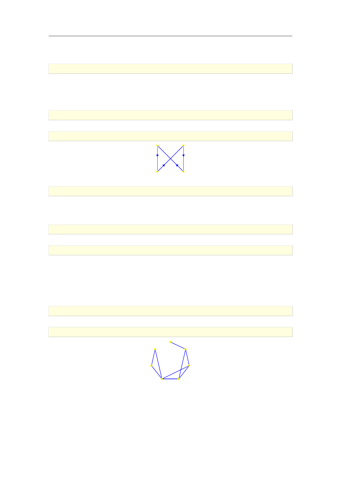
It is possible to specify several trails in a sequence, which is useful when designing more complex
graphs.
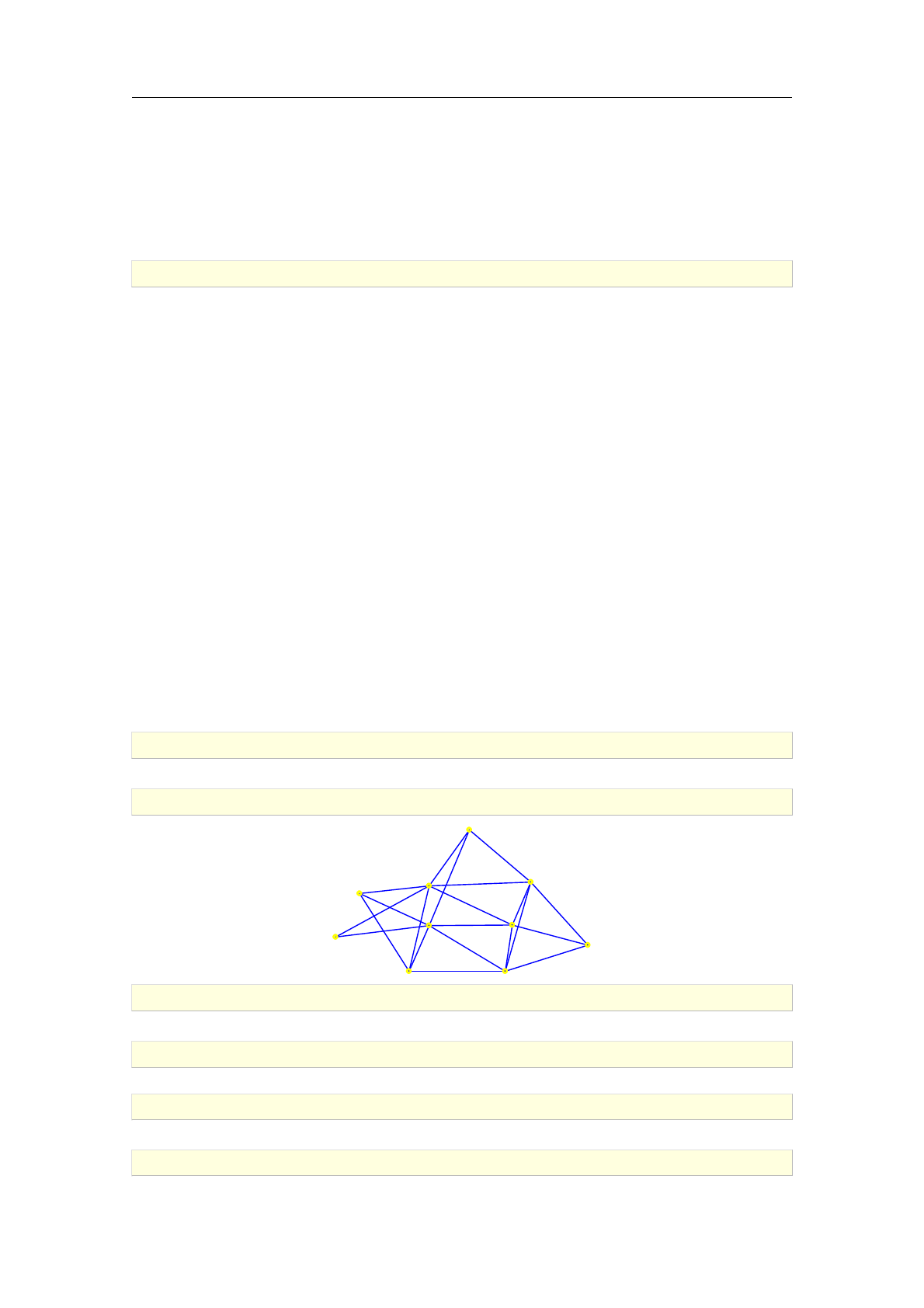
>G:=graph(trail(1,2,3,4,2),trail(3,5,6,7,5,4))
an undirected unweighted graph with 7 vertices and 9 edges
>draw_graph(G)
1
2
3
45
6
7
Specifying adjacency or weight matrix. A graph can be created from a single square matrix
A= [aij]nof order n. If it contains only ones and zeros and has zeros on its diagonal, it is assumed
to be the adjacency matrix for the desired graph. Otherwise, if an element outside the set f0;1gis
encountered, it is assumed that the matrix of edge weights is passed as input, causing the resulting
graph to be weighted accordingly. In each case, exactly nvertices will be created and i-th and
j-th vertex will be connected iff aij =/ 0. If the matrix is symmetric, the resulting graph will be
undirected, otherwise it will be directed.
1.1 General graphs 11
>G:=graph([[0,1,1,0],[1,0,0,1],[1,0,0,0],[0,1,0,0]])
an undirected unweighted graph with 4 vertices and 3 edges
>edges(G)
0
@
0 1
0 2
1 3 1
A
>G:=graph([[0,1.0,2.3,0],[4,0,0,3.1],[0,0,0,0],[0,0,0,0]])
a directed weighted graph with 4 vertices and 4 arcs
>edges(G,weights)
f[[0;1];1.0];[[0;2];2.3];[[1;0];4];[[1;3];3.1]g
List of vertex labels can be specified alongside a matrix.
>graph([a,b,c,d],[[0,1,1,0],[1,0,0,1],[1,0,0,0],[0,1,0,0]])
an undirected unweighted graph with 4 vertices and 3 edges
When creating a weighted graph, one can first specify the list of nvertices and the set of edges,
followed by a square matrix Aof order n. Then for every edge fi; j gor arc (i; j)the element aij
of Ais assigned as its weight. Other elements of Aare ignored.
>G:=digraph([a,b,c],%{[a,b],[b,c],[a,c]%},[[0,1,2],[3,0,4],[5,6,0]])
a directed weighted graph with 3 vertices and 3 arcs
>edges(G,weights)
f[[a; b];1];[[a; c];2];[[b; c];4]g
Creating special graphs. When a special graph is desired, one just needs to pass its name to
the graph command. An undirected unweighted graph will be returned.
>graph("petersen")
an undirected unweighted graph with 10 vertices and 15 edges
>G:=graph("coxeter")
an undirected unweighted graph with 28 vertices and 42 edges
>draw_graph(G)
a1
a2a7
z1
a3
z2
a4
z3
a5
z4
a6
z5
z6
z7
b1
b3b6
b2
b4
b7
b5
c1
c4c5
c2
c6 c3
c7
12 Constructing graphs
1.2. Cycle and path graphs
1.2.1. Cycle graphs
The command cycle_graph is used for constructing cycle graphs [23, pp. 4].
Syntax: cycle_graph(n)
cycle_graph(V)
cycle_graph accepts a positive integer nor a list of distinct vertices Vas its only argument and
returns the graph consisting of a single cycle on the specified vertices in the given order. If nis
specified it is assumed to be the desired number of vertices, in which case they will be created and
labeled with the first nintegers (starting from 0 in Xcas mode and from 1 in Maple mode). The
resulting graph will be given the name Cn, for example C4 for n= 4.
>C5:=cycle_graph(5)
C5: an undirected unweighted graph with 5 vertices and 5 edges
>draw_graph(C5)
0
1
23
4
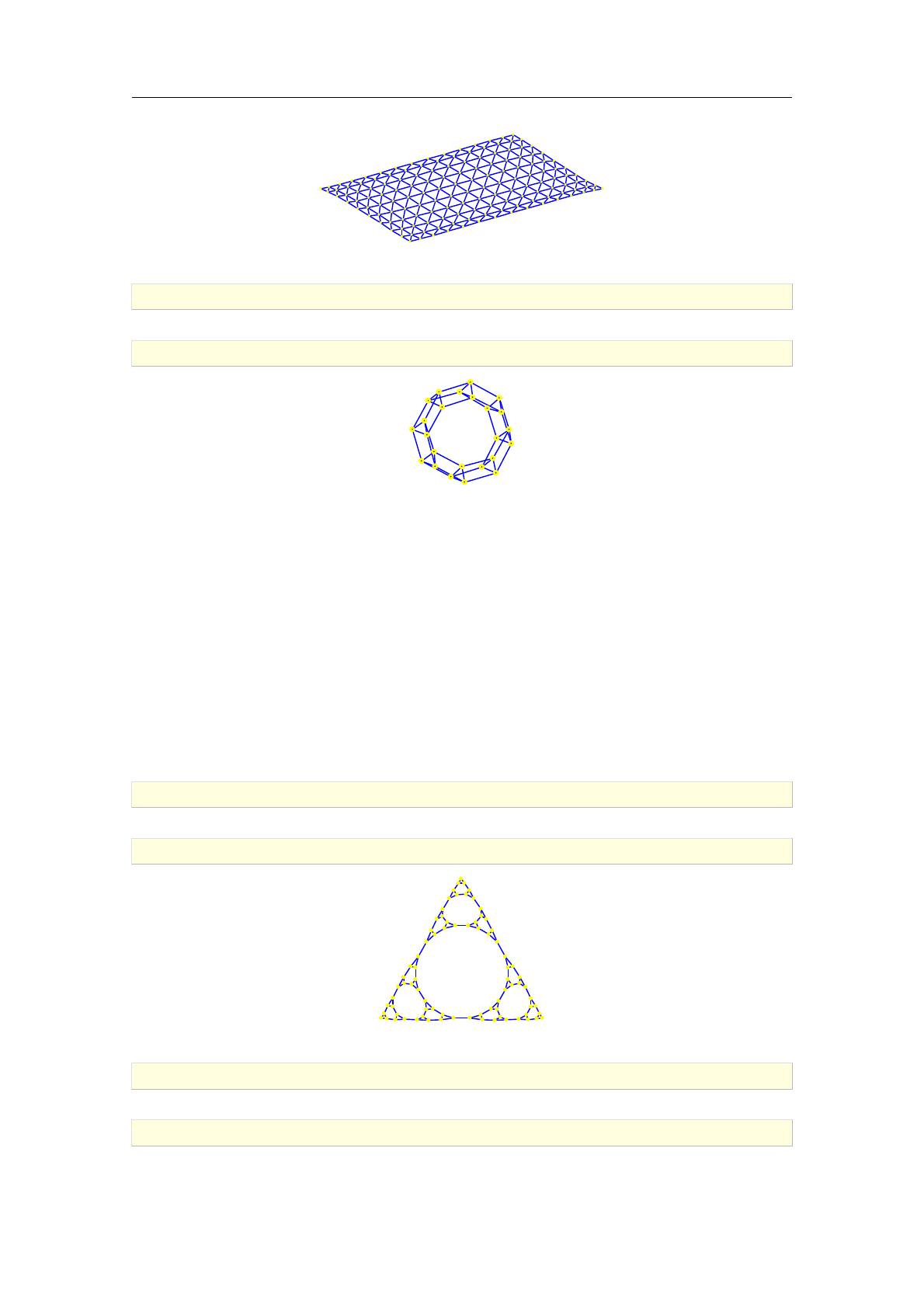
>cycle_graph(["a","b","c","d","e"])
C5: an undirected unweighted graph with 5 vertices and 5 edges
1.2.2. Path graphs
The command path_graph is used for constructing path graphs [23, pp. 4].
Syntax: path_graph(n)
path_graph(V)
path_graph accepts a positive integer nor a list of distinct vertices Vas its only argument and
returns a graph consisting of a single path on the specified vertices in the given order. If nis
specified it is assumed to be the desired number of vertices, in which case they will be created and
labeled with the first nintegers (starting from 0 in Xcas mode resp. from 1 in Maple mode).
Note that a path cannot intersect itself. Paths that are allowed to cross themselves are called trails
(see the command trail).
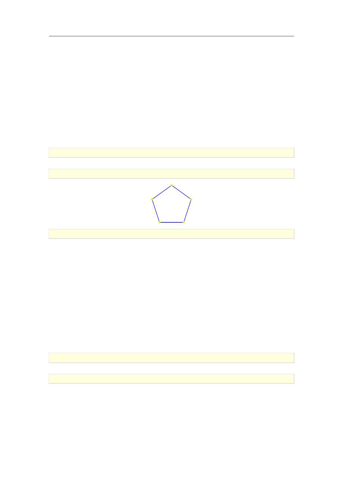
>path_graph(5)
an undirected unweighted graph with 5 vertices and 4 edges
>path_graph(["a","b","c","d","e"])
an undirected unweighted graph with 5 vertices and 4 edges
1.2.3. Trails of edges
Syntax: trail(v1,v2,..,vk)
trail2edges(T)
1.2 Cycle and path graphs 13
If the dummy command trail is called with a sequence of vertices v1; v2; :::; vkas arguments, it
returns the symbolic expression representing the trail which visits the specified vertices in the given
order. The resulting symbolic object is recognizable by some commands, for example graph and
digraph. Note that a trail may cross itself (some vertices may be repeated in the given sequence).
Any trail Tis easily converted to the corresponding list of edges by calling the trail2edges
command, which accepts the trail as its only argument.
>T:=trail(1,2,3,4,2):; graph(T)
Done;an undirected unweighted graph with 4 vertices and 4 edges
>trail2edges(T)
0
B
B
B
B
@
1 2
2 3
3 4
4 2
1
C
C
C
C
A
1.3. Complete graphs
1.3.1. Complete graphs (with multiple vertex partitions)
The command complete_graph is used for construction of complete (multipartite) graphs.
Syntax: complete_graph(n)
complete_graph(V)
complete_graph(n1,n2,..,nk)
complete_graph can be called with a single argument, a positive integer nor a list of distinct
vertices V, in which case it returns the complete graph [23, pp. 2] on the specified vertices. If integer
nis specified, it is assumed that it is the desired number of vertices and they will be created and
labeled with the first nintegers (starting from 0 in Xcas mode and from 1 in Maple mode).
If complete_graph is given a sequence of positive integers n1; n2; :::; nkas its argument, it returns
a complete multipartite graph with partitions of size n1; n2; :::; nk.
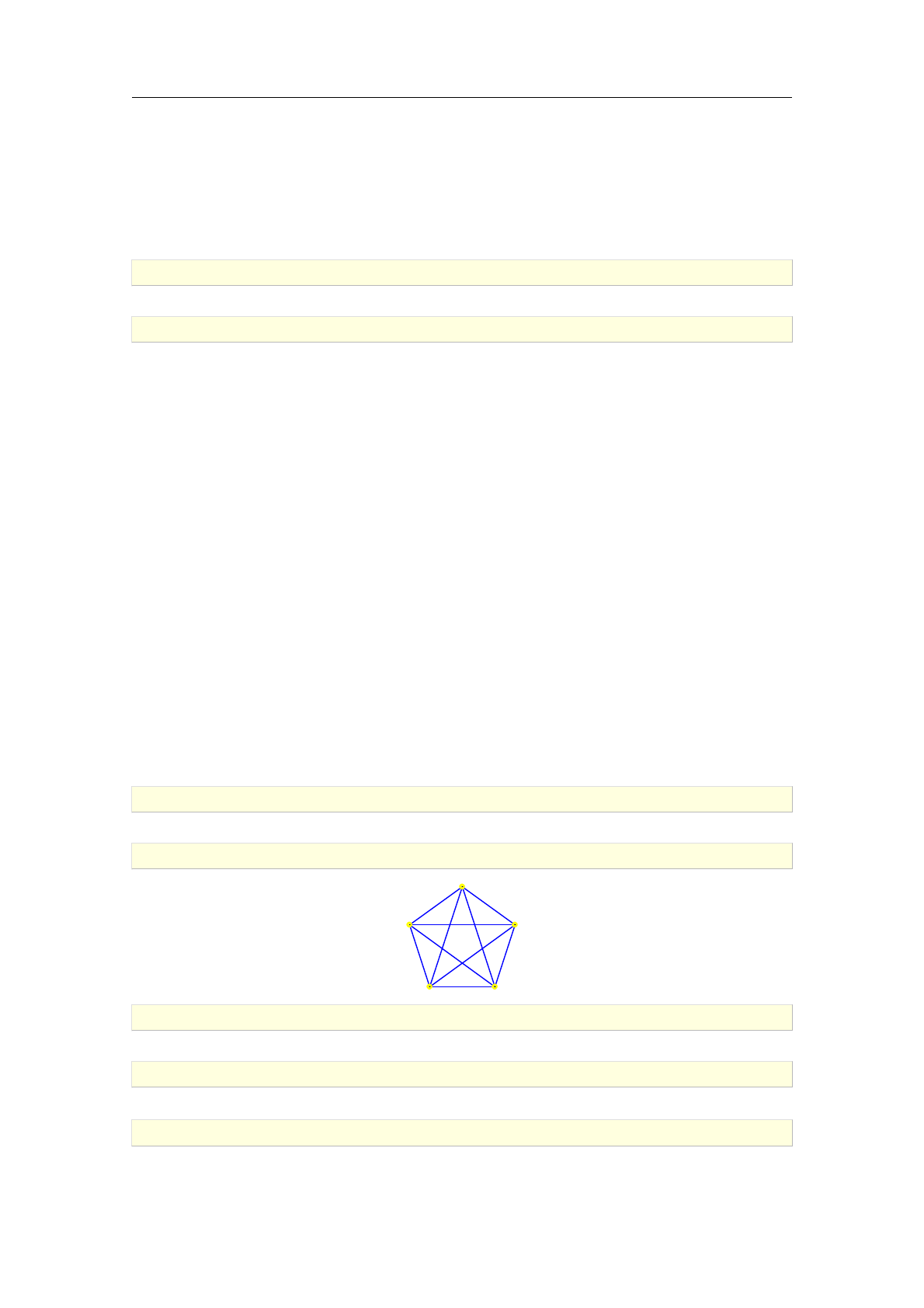
>K5:=complete_graph(5)
an undirected unweighted graph with 5 vertices and 10 edges
>draw_graph(K5)
0
1
23
4
>K3:=complete_graph([a,b,c])
an undirected unweighted graph with 3 vertices and 3 edges
>edges(K3)
f[a; b];[a; c];[b; c]g
>K33:=complete_graph(3,3)
an undirected unweighted graph with 6 vertices and 9 edges
14 Constructing graphs
>draw_graph(K33)
0 1 2
3 4 5
1.3.2. Complete trees
The commands complete_binary_tree and complete_kary_tree are used for construction of
complete binary trees and complete k-ary trees, respectively.
Syntax: complete_binary_tree(n)
complete_kary_tree(k,n)
complete_binary_tree accepts a positive integer nas its only argument and returns a complete
binary tree of depth n.
complete_kary_tree accepts positive integers kand nas its arguments and returns the complete
k-ary tree of depth n.
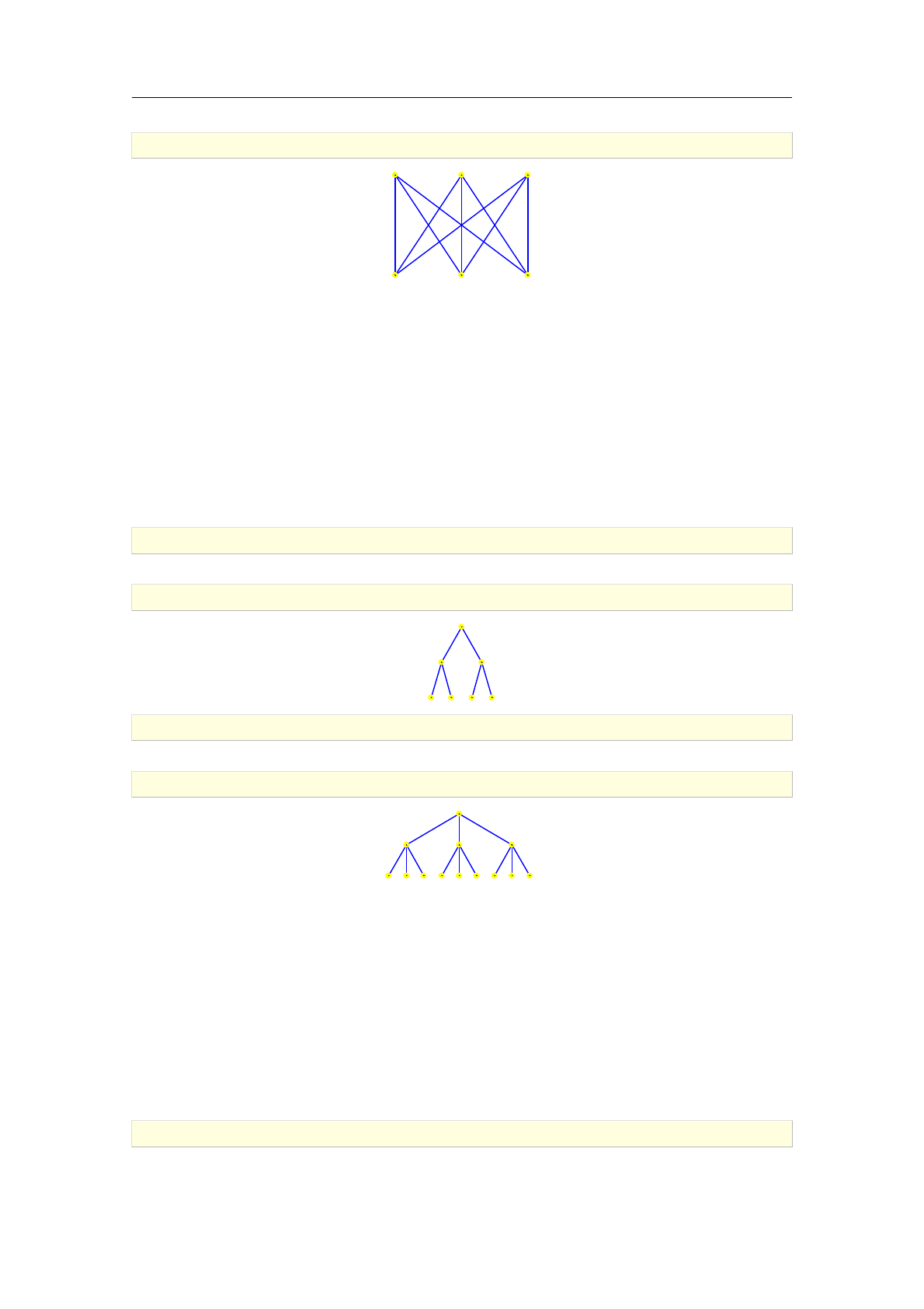
>T1:=complete_binary_tree(2)
an undirected unweighted graph with 7 vertices and 6 edges
>draw_graph(T1)
0
1 2
3 4 5 6
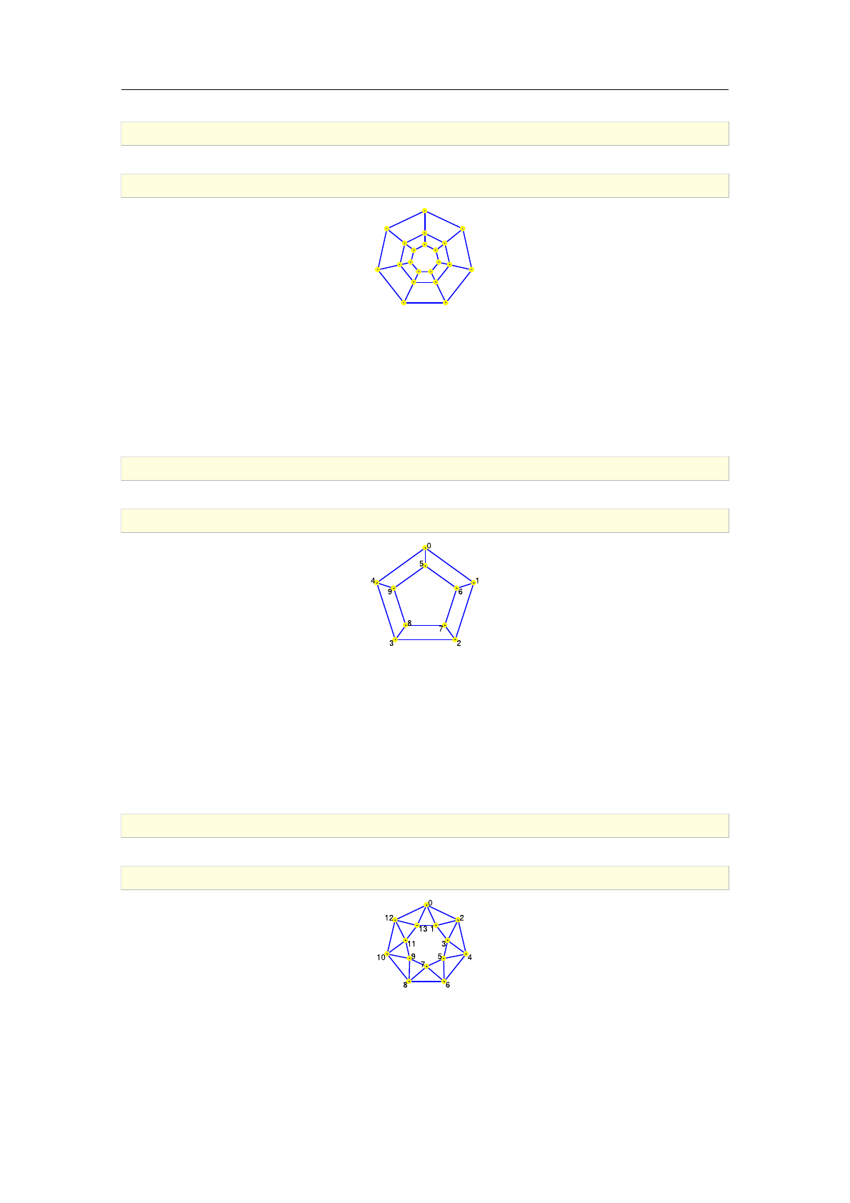
>T2:=complete_kary_tree(3,2)
an undirected unweighted graph with 13 vertices and 12 edges
>draw_graph(T2)
0
1 2 3
4 5 6 7 8 910 11 12
1.4. Sequence graphs
1.4.1. Creating graphs from degree sequences
The command sequence_graph is used for constructing graphs from degree sequences.
Syntax: sequence_graph(L)
sequence_graph accepts a list Lof positive integers as its only argument and, if Lrepresents a
graphic sequence, the corresponding graph Gwith jLjvertices is returned. If the argument is not
a graphic sequence, an error is returned.
>sequence_graph([3,2,4,2,3,4,5,7])
an undirected unweighted graph with 8 vertices and 15 edges
1.4 Sequence graphs 15
Sequence graphs are constructed in O(jLj2log jLj)time by applying the algorithm of Havel and
Hakimi [27].
1.4.2. Validating graphic sequences
The command is_graphic_sequence is used to check whether a list of integers represents the
degree sequence of some graph.
Syntax: is_graphic_sequence(L)
is_graphic_sequence accepts a list Lof positive integers as its only argument and returns true if
there exists a graph G(V ; E)with degree sequence fdeg v:v2Vgequal to Land false otherwise.
The algorithm, which has the complexity O(jLj2), is based on the theorem of Erd®s and Gallai.
>is_graphic_sequence([3,2,4,2,3,4,5,7])
true
1.5. Intersection graphs
1.5.1. Interval graphs
The command interval_graph is used for construction of interval graphs.
Syntax: interval_graph(L)
interval_graph accepts a sequence or list Lof real-line intervals as its argument and returns
an undirected unweighted graph with these intervals as vertices (the string representations of the
intervals are used as labels), each two of them being connected with an edge if and only if the
corresponding intervals intersect.
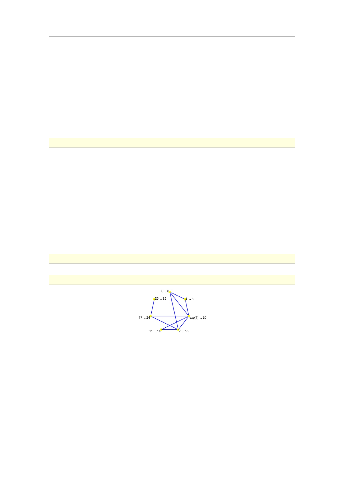
>G:=interval_graph(0..8,1..pi,exp(1)..20,7..18,11..14,17..24,23..25)
an undirected unweighted graph with 7 vertices and 10 edges
>draw_graph(G)
1.5.2. Kneser graphs
The commands kneser_graph and odd_graph are used for construction of Kneser graphs.
Syntax: kneser_graph(n,k)
odd_graph(d)
kneser_graph accepts two positive integers n≤20 and kas its arguments and returns the Kneser
graph K(n; k). The latter is obtained by setting all k-subsets of a set of nelements as vertices
and connecting each two of them if and only if the corresponding sets are disjoint. Therefore, each
Kneser graph is the complement of the corresponding intersection graph on the same collection of
subsets.
Kneser graphs can get exceedingly complex even for relatively small values of nand k. Note that
the number of vertices in K(n; k)is equal to n
k.
16 Constructing graphs
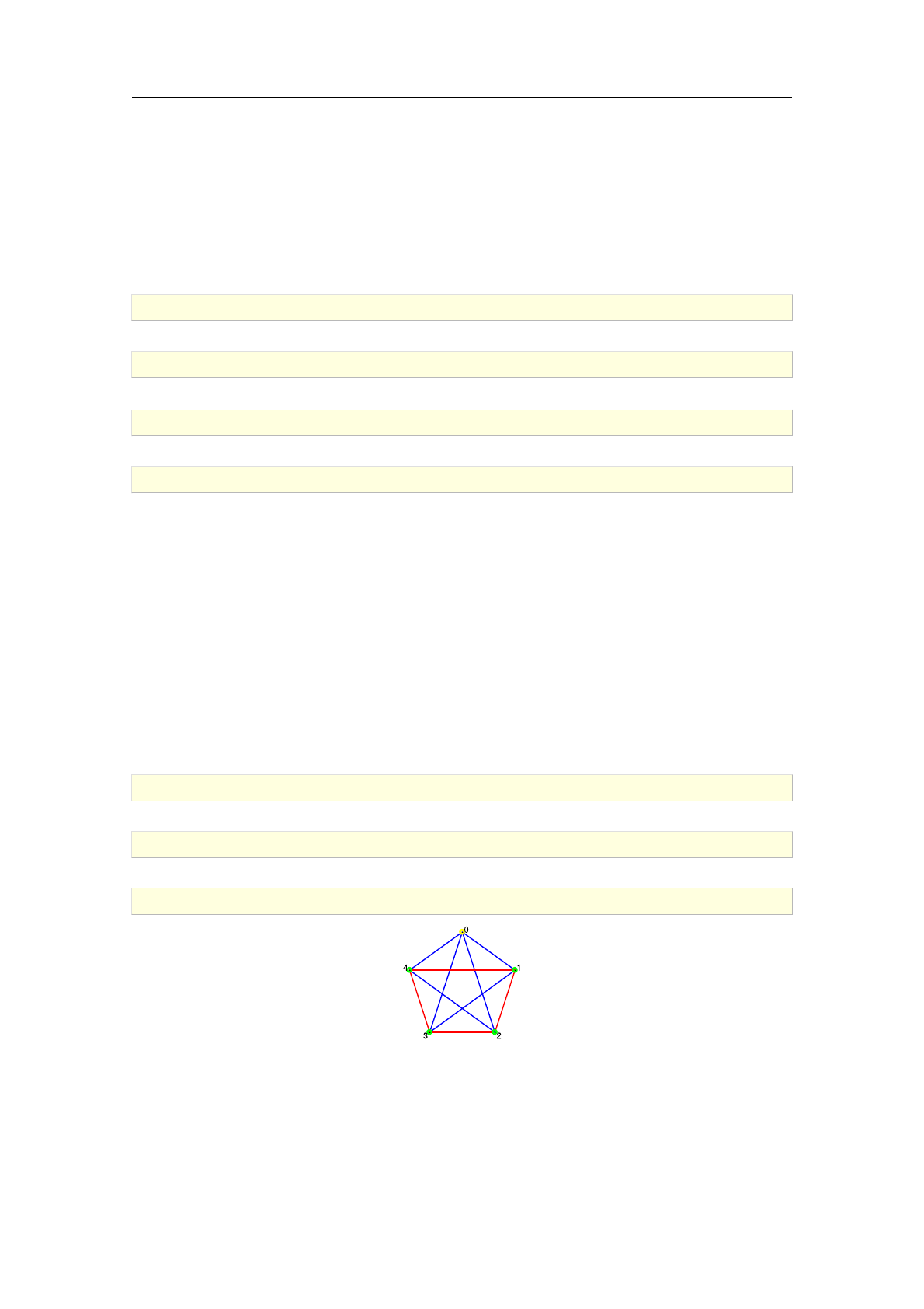
>kneser_graph(5,2)
an undirected unweighted graph with 10 vertices and 15 edges
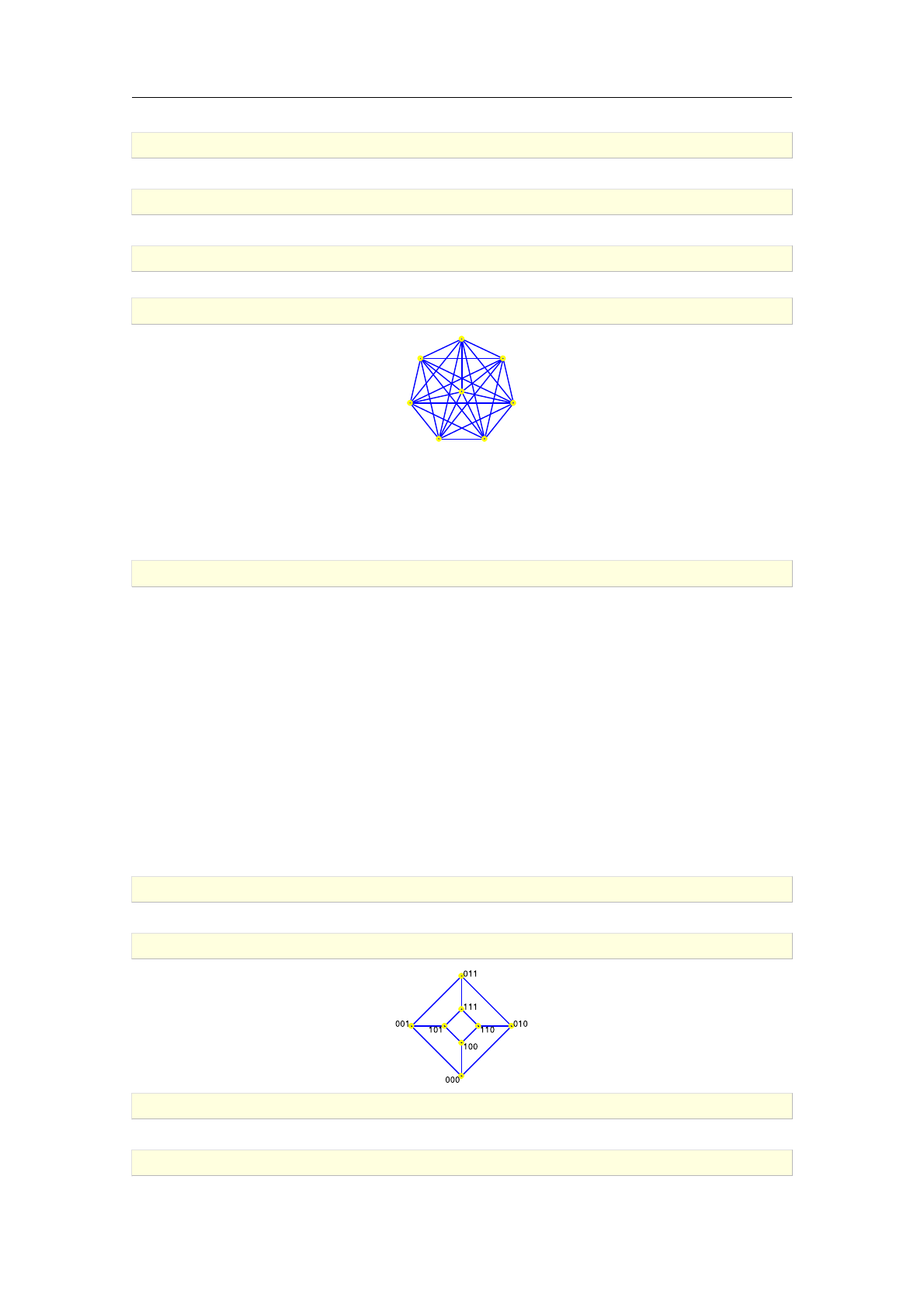
>G:=kneser_graph(8,1)
an undirected unweighted graph with 8 vertices and 28 edges
>is_clique(G)
true
>draw_graph(G,spring,labels=false)
The command odd_graph is used for creating odd graphs, i.e. Kneser graphs with parameters
n= 2 d+ 1 and k=dfor d>1.
odd_graph accepts a positive integer d≤8as its only argument and returns d-th odd graph
K(2 d+ 1; d). Note that the odd graphs with d > 8will not be constructed as they are too big to
handle.
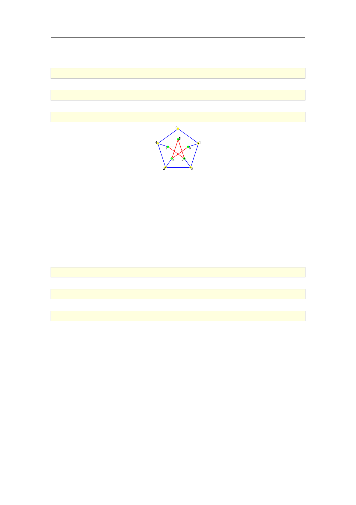
>odd_graph(3)
an undirected unweighted graph with 10 vertices and 15 edges
1.6. Special graphs
1.6.1. Hypercube graphs
The command hypercube_graph is used for construction of hypercube graphs.
Syntax: hypercube_graph(n)
hypercube_graph accepts a positive integer nas its only argument and returns the hypercube
graph of dimension non 2nvertices. The vertex labels are strings of binary digits of length n.
Two vertices are joined by an edge if and only if their labels differ in exactly one character. The
hypercube graph for n= 2 is a square and for n= 3 it is a cube.
>H:=hypercube_graph(3)
an undirected unweighted graph with 8 vertices and 12 edges
>draw_graph(H,planar)
>H:=hypercube_graph(5)
an undirected unweighted graph with 32 vertices and 80 edges
>draw_graph(H,plot3d,labels=false)
1.6 Special graphs 17
1.6.2. Star graphs
The command star_graph is used for construction of star graphs.
Syntax: star_graph(n)
star_graph accepts a positive integer nas its only argument and returns the star graph with n+ 1
vertices, which is equal to the complete bipartite graph complete_graph(1,n) i.e. a n-ary tree
with one level.
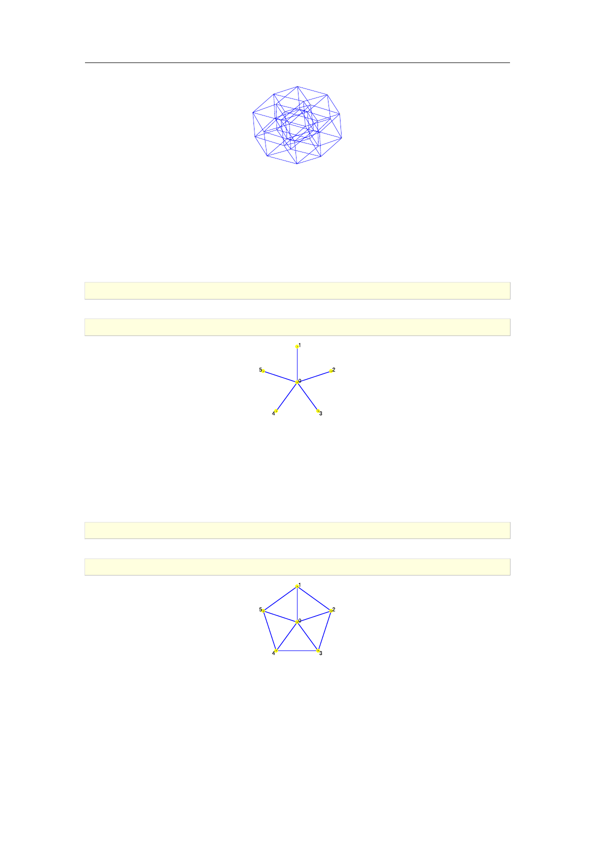
>G:=star_graph(5)
an undirected unweighted graph with 6 vertices and 5 edges
>draw_graph(G)
1.6.3. Wheel graphs
The command wheel_graph is used for construction of wheel graphs.
Syntax: wheel_graph(n)
wheel_graph accepts a positive integer nas its only argument and returns the wheel graph with
n+ 1 vertices.
>G:=wheel_graph(5)
an undirected unweighted graph with 6 vertices and 10 edges
>draw_graph(G)
1.6.4. Web graphs
The command web_graph is used for construction of web graphs.
Syntax: web_graph(a,b)
web_graph accepts two positive integers aand bas its arguments and returns the web graph with
parameters aand b, namely the Cartesian product of cycle_graph(a) and path_graph(b).
18 Constructing graphs
>G:=web_graph(7,3)
an undirected unweighted graph with 21 vertices and 35 edges
>draw_graph(G,labels=false)
1.6.5. Prism graphs
The command prism_graph is used for construction of prism graphs.
Syntax: prism_graph(n)
prism_graph accepts a positive integer nas its only argument and returns the prism graph with
parameter n, namely petersen_graph(n,1).
>G:=prism_graph(5)
an undirected unweighted graph with 10 vertices and 15 edges
>draw_graph(G)
1.6.6. Antiprism graphs
The command antiprism_graph is used for construction of antiprism graphs.
Syntax: antiprism_graph(n)
antiprism_graph accepts a positive integer nas its only argument and returns the antiprism
graph with parameter n, which is constructed from two concentric cycles of nvertices by joining
each vertex of the inner to two adjacent nodes of the outer cycle.
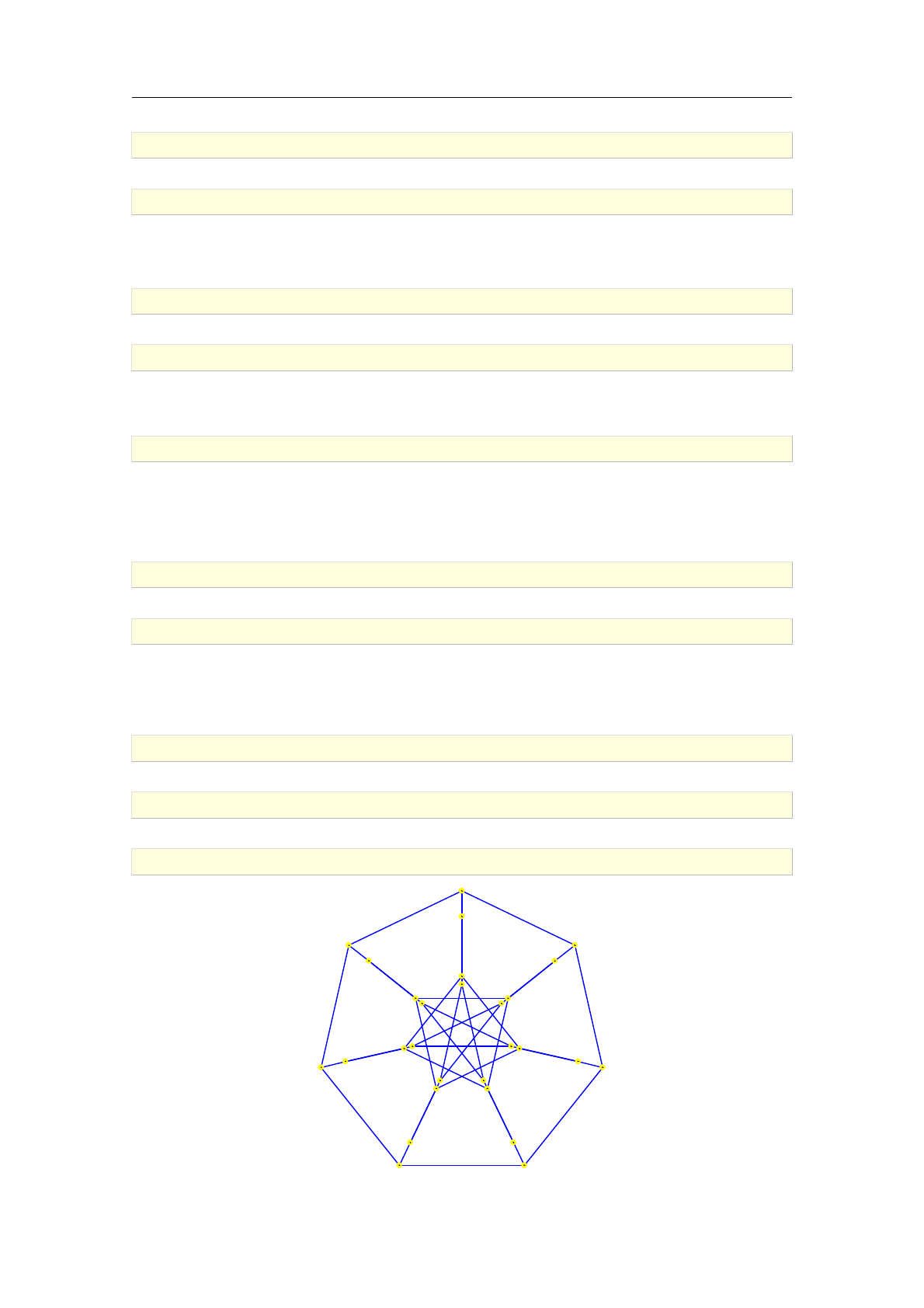
>G:=antiprism_graph(7)
an undirected unweighted graph with 14 vertices and 28 edges
>draw_graph(G)
1.6.7. Grid graphs
The command grid_graph resp. torus_grid_graph is used for construction of rectangular/trian-
gular resp. torus grid graphs.
1.6 Special graphs 19

Syntax: grid_graph(m,n)
grid_graph(m,n,triangle)
torus_grid_graph(m,n)
grid_graph accepts two positive integers mand nas its arguments and returns the mby ngrid on
m n vertices, namely the Cartesian product of path_graph(m) and path_graph(n). If the option
triangle is passed as the third argument, the returned graph is a triangular grid on m n vertices
defined as the underlying graph of the strong product of two directed path graphs with mand n
vertices, respectively [1, Definition 2, pp. 189]. Strong product is defined as the union of Cartesian
and tensor products.
torus_grid_graph accepts two positive integers mand nas its arguments and returns the mby n
torus grid on m n vertices, namely the Cartesian product of cycle_graph(m) and cycle_graph(n).
>G:=grid_graph(15,20)
an undirected unweighted graph with 300 vertices and 565 edges
>draw_graph(G,spring)
For example, connecting vertices in the opposite corners of the above grid yields a grid-like graph
with no corners.
>G:=add_edge(G,[["14:0","0:19"],["0:0","14:19"]])
an undirected unweighted graph with 300 vertices and 567 edges
>draw_graph(G,plot3d)
In the next example, the Möbius strip is constructed by connecting the vertices in the opposite
sides of a narrow grid graph.
>G:=grid_graph(20,3)
an undirected unweighted graph with 60 vertices and 97 edges
>G:=add_edge(G,[["0:0","19:2"],["0:1","19:1"],["0:2","19:0"]])
an undirected unweighted graph with 60 vertices and 100 edges
>draw_graph(G,plot3d,labels=false)
A triangular grid is created by passing the option triangle.
>G:=grid_graph(10,15,triangle)
an undirected unweighted graph with 150 vertices and 401 edges
>draw_graph(G,spring)
20 Constructing graphs
The next example demonstrates creating a torus grid graph with eight triangular levels.
>G:=torus_grid_graph(8,3)
an undirected unweighted graph with 24 vertices and 48 edges
>draw_graph(G,spring,labels=false)
1.6.8. Sierpi«ski graphs
The command sierpinski_graph is used for construction of Sierpi«ski-type graphs Sk
nand
STk
n[30].
Syntax: sierpinski_graph(n,k)
sierpinski_graph(n,k,triangle)
sierpinski_graph accepts two positive integers nand kas its arguments and optionally the
symbol triangle as the third argument. It returns the Sierpi«ski (triangle) graph with parameters
nand k.
The Sierpi«ski triangle graph STk
nis obtained by contracting all non-clique edges in Sk
n. To detect
such edges the variant of the algorithm by Bron and Kerbosch, developed by Tomita et al. in
[50], is used, which can be time consuming for n > 6.
>S:=sierpinski_graph(4,3)
an undirected unweighted graph with 81 vertices and 120 edges
>draw_graph(S,spring)
In particular, ST3
nis the well-known Sierpi«ski sieve graph of order n.
>sierpinski_graph(4,3,triangle)
an undirected unweighted graph with 42 vertices and 81 edges
>sierpinski_graph(5,3,triangle)
an undirected unweighted graph with 123 vertices and 243 edges
1.6 Special graphs 21
A drawing of the graph produced by the last command line is shown in Figure 3.1.
1.6.9. Generalized Petersen graphs
The command petersen_graph is used for construction of generalized Petersen graphs P(n; k).
Syntax: petersen_graph(n)
petersen_graph(n,k)
petersen_graph accepts two positive integers nand kas its arguments. The second argument may
be omitted, in which case k= 2 is assumed. The graph P(n; k), which is returned, is a connected
cubic graph consisting of—in Schläfli notation—an inner star polygon fn; kgand an outer regular
polygon fngsuch that the npairs of corresponding vertices in inner and outer polygons are
connected with edges. For k= 1 the prism graph of order nis obtained.
The well-known Petersen graph is equal to the generalized Petersen graph P(5;2). It can also be
constructed by calling graph("petersen").
>draw_graph(graph("petersen"))
To obtain the dodecahedral graph P(10;2), input:
>petersen_graph(10)
an undirected unweighted graph with 20 vertices and 30 edges
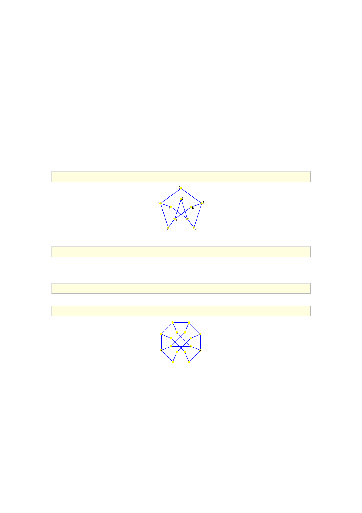
To obtain Möbius–Kantor graph P(8;3), input:
>G:=petersen_graph(8,3)
an undirected unweighted graph with 16 vertices and 24 edges
>draw_graph(G)
0 1
2
3
45
6
78 9
10
11
1213
14
15
Note that Desargues, Dürer and Nauru graphs are isomorphic to the generalized Petersen graphs
P(10;3),P(6;2) and P(12;5), respectively.
1.6.10. LCF graphs
The command lcf_graph is used for construction of cubic Hamiltonian graphs from LCF notation.
Syntax: lcf_graph(L)
lcf_graph(L,n)
lcf_graph takes one or two arguments, a list Lof nonzero integers, called jumps, and optionally
a positive integer n, called the exponent (by default, n= 1). The command returns the graph on
njLjvertices obtained by iterating the sequence of jumps ntimes.
22 Constructing graphs
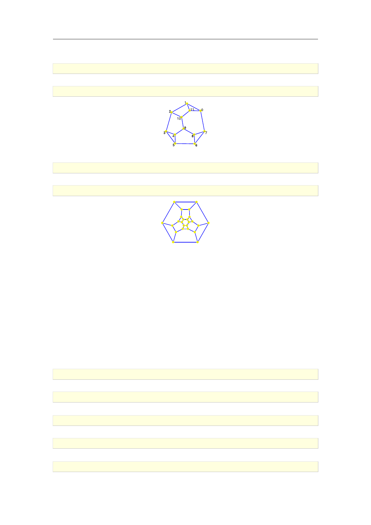
For example, the following command line creates Frucht graph.
>F:=lcf_graph([-5,-2,-4,2,5,-2,2,5,-2,-5,4,2])
an undirected unweighted graph with 12 vertices and 18 edges
>draw_graph(F,planar)
In the next example, the truncated octahedral graph is constructed from LCF notation.
>G:=lcf_graph([3,-7,7,-3],6)
an undirected unweighted graph with 24 vertices and 36 edges
>draw_graph(G,planar,labels=false)
1.7. Isomorphic copies of graphs
1.7.1. Creating an isomorphic copy from a permutation
To create an isomorphic copy of a graph use the isomorphic_copy command.
Syntax: isomorphic_copy(G,sigma)
isomorphic_copy(G)
isomorphic_copy accepts one or two arguments, a graph G(V ; E)and optionally a permutation
σof order jVj. It returns a new graph where the adjacency lists are reordered according to σor a
random permutation if the second argument is omitted. The vertex labels are the same as in G.
This command discards all vertex and edge attributes present in G.
The complexity of the algorithm is O(jVj+jEj).
>G:=path_graph([1,2,3,4,5])
an undirected unweighted graph with 5 vertices and 4 edges
>vertices(G), neighbors(G)
[1;2;3;4;5];f[2];[1;3];[2;4];[3;5];[4]g
>H:=isomorphic_copy(G)
an undirected unweighted graph with 5 vertices and 4 edges
>vertices(H), neighbors(H)
[1;2;3;4;5];f[2;3];[1;5];[1;4];[3];[2]g
>H:=isomorphic_copy(G,[2,4,0,1,3])
1.7 Isomorphic copies of graphs 23
an undirected unweighted graph with 5 vertices and 4 edges
>vertices(H), neighbors(H)
[1;2;3;4;5];f[4;5];[5];[4];[1;3];[1;2]g
>P:=prism_graph(3)
an undirected unweighted graph with 6 vertices and 9 edges
>draw_graph(P)
0
12
3
45
>H:=isomorphic_copy(P,[3,0,1,5,4,2])
an undirected unweighted graph with 6 vertices and 9 edges
>draw_graph(H,spring)
0
1
2
3 4
5
1.7.2. Permuting vertices
To create an isomorphic copy of a graph by providing the reordered list of vertex labels, use the
command permute_vertices.
Syntax: permute_vertices(G,L)
permute_vertices(G)
permute_vertices accepts one or two arguments, a graph G(V ; E)and optionally a list Lof
length jVjcontaining all vertices from V, and returns a copy of Gwith vertices rearranged in
order they appear in Lor at random if Lis not given. All vertex and edge attributes are copied,
which includes vertex position information (if present). That means the resulting graph will look
the same as Gwhen drawn.
The complexity of the algorithm is O(jVj+jEj).
>G:=path_graph([1,2,3,4,5])
an undirected unweighted graph with 5 vertices and 4 edges
>vertices(G), neighbors(G)
[1;2;3;4;5];f[2];[1;3];[2;4];[3;5];[4]g
>H:=permute_vertices(G,[3,5,1,2,4])
an undirected unweighted graph with 5 vertices and 4 edges
>vertices(H), neighbors(H)
[3;5;1;2;4];f[2;4];[4];[2];[1;3];[3;5]g
24 Constructing graphs
1.7.3. Relabeling vertices
To relabel the vertices of a graph without changing their order, use the command relabel_vertices.
Syntax: relabel_vertices(G,L)
relabel_vertices accepts two arguments, a graph G(V ; E)and a list Lof vertex labels of length
jVj. It returns a copy of Gwith Las the list of vertex labels.
The complexity of the algorithm is O(jVj).
>G:=path_graph([1,2,3,4])
an undirected unweighted graph with 4 vertices and 3 edges
>edges(G)
f[1;2];[2;3];[3;4]g
>H:=relabel_vertices(G,[a,b,c,d])
an undirected unweighted graph with 4 vertices and 3 edges
>edges(H)
f[a; b];[b; c];[c; d]g
1.8. Subgraphs
1.8.1. Extracting subgraphs
To extract the subgraph of a graph formed by a subset of the set of its edges, use the command
subgraph.
Syntax: subgraph(G,L)
subgraph accepts two arguments, a graph G(V ; E)and a list of edges L. It returns the subgraph
G0(V0; L)of G, where V0⊂Vis a subset of vertices of Gincident to at least one edge from L.
>K5:=complete_graph(5)
an undirected unweighted graph with 5 vertices and 10 edges
>S:=subgraph(K5,[[1,2],[2,3],[3,4],[4,1]])
an undirected unweighted graph with 4 vertices and 4 edges
>draw_graph(highlight_subgraph(K5,S))
1.8.2. Induced subgraphs
To obtain the subgraph of a graph induced by a subset of its vertices, use the command
induced_subgraph.
Syntax: induced_subgraph(G,L)
1.8 Subgraphs 25
induced_subgraph accepts two arguments, a graph G(V ; E)and a list of vertices L. It returns the
subgraph G0(L; E 0)of G, where E0⊂Econtains all edges which have both endpoints in L[23, pp. 3].
>G:=graph("petersen")
an undirected unweighted graph with 10 vertices and 15 edges
>S:=induced_subgraph(G,[5,6,7,8,9])
an undirected unweighted graph with 5 vertices and 5 edges
>draw_graph(highlight_subgraph(G,S))
1.8.3. Underlying graphs
For every graph G(V ; E)there is an undirected and unweighted graph U(V ; E0), called the under-
lying graph of G, where E0is obtained from Eby dropping edge directions. To construct U, use
the command underlying_graph.
Syntax: underlying_graph(G)
underlying_graph accepts a graph G(V ; E)as its only argument and returns an undirected
unweighted copy of Gin which all vertex and edge attributes, together with edge directions, are
discarded.
The complexity of the algorithm is O(jVj+jEj).
>G:=digraph(%{[[1,2],6],[[2,3],4],[[3,1],5],[[3,2],7]%})
a directed weighted graph with 3 vertices and 4 arcs
>U:=underlying_graph(G)
an undirected unweighted graph with 3 vertices and 3 edges
>edges(U)
f[1;2];[1;3];[2;3]g
1.8.4. Fundamental cycles
The command fundamental_cycle is used for extracting cycles from unicyclic graphs (also called
1-trees). To find a fundamental cycle basis of an undirected graph, use the command cycle_basis.
Syntax: fundamental_cycle(G)
cycle_basis(G)
fundamental_cycle accepts one argument, an undirected connected graph G(V ; E)containing
exactly one cycle (i.e. a unicyclic graph), and returns that cycle as a graph. If Gis not unicyclic,
an error is returned.
cycle_basis accepts an undirected graph G(V ; E)as its only argument and returns a basis
Bof the cycle space of Gas a list of fundamental cycles in G, with each cycle represented as
a list of vertices. Furthermore, jBj=jEj ¡ jVj+κ(G), where κ(G)is the number of connected
components of G. Every cycle Cin Gsuch that C2/Bcan be obtained from cycles in Busing
only symmetric differences.
26 Constructing graphs
The strategy is to construct a spanning tree Tof Gusing depth-first search and look for edges in
Ewhich do not belong to the tree. For each non-tree edge ethere is a unique fundamental cycle
Ceconsisting of etogether with the path in Tconnecting the endpoints of e. The vertices of Ce
are easily obtained from the search data. The complexity of this algorithm is O(jVj+jEj).
>G:=graph(trail(1,2,3,4,5,2,6))
an undirected unweighted graph with 6 vertices and 6 edges
>C:=fundamental_cycle(G)
an undirected unweighted graph with 4 vertices and 4 edges
>edges(C)
0
B
B
B
B
@
2 5
2 3
4 5
3 4
1
C
C
C
C
A
Given a tree graph Gand adding an edge from the complement Gcto Gone obtains a 1-tree graph.
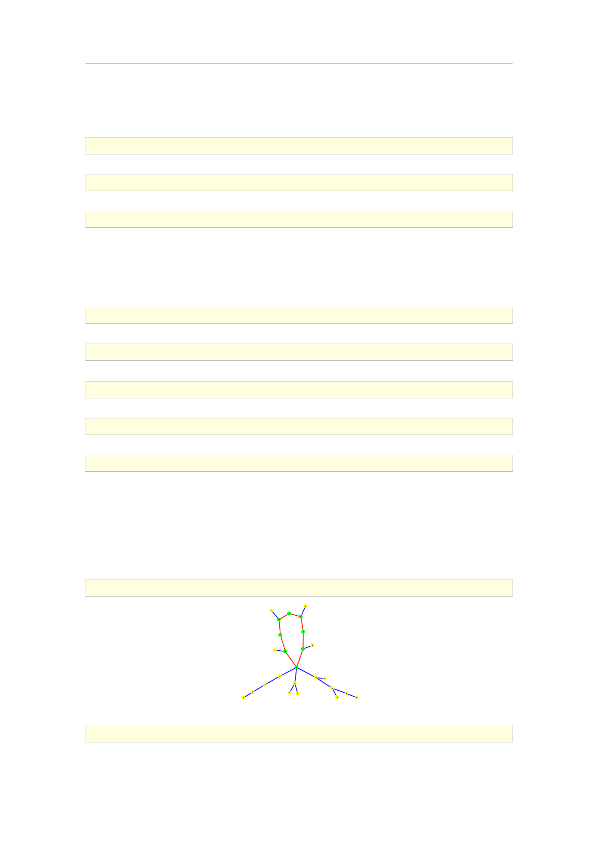
>G:=random_tree(25)
an undirected unweighted graph with 25 vertices and 24 edges
>ed:=choice(edges(graph_complement(G)))
[10;20]
>G:=add_edge(G,ed)
an undirected unweighted graph with 25 vertices and 25 edges
>C:=fundamental_cycle(G)
an undirected unweighted graph with 8 vertices and 8 edges
>edges(C)
0
B
B
B
B
B
B
B
B
B
B
B
B
B
B
B
B
B
B
B
B
@
10 20
010
120
1 2
224
13 24
713
0 7
1
C
C
C
C
C
C
C
C
C
C
C
C
C
C
C
C
C
C
C
C
A
>draw_graph(highlight_subgraph(G,C),spring)
0
1
2
34
5
6
7
8
9
10
11
12
13
14
15
16
17
18 19
20
21
22
23
24
In the next example, a cycle basis of octahedral graph is computed.
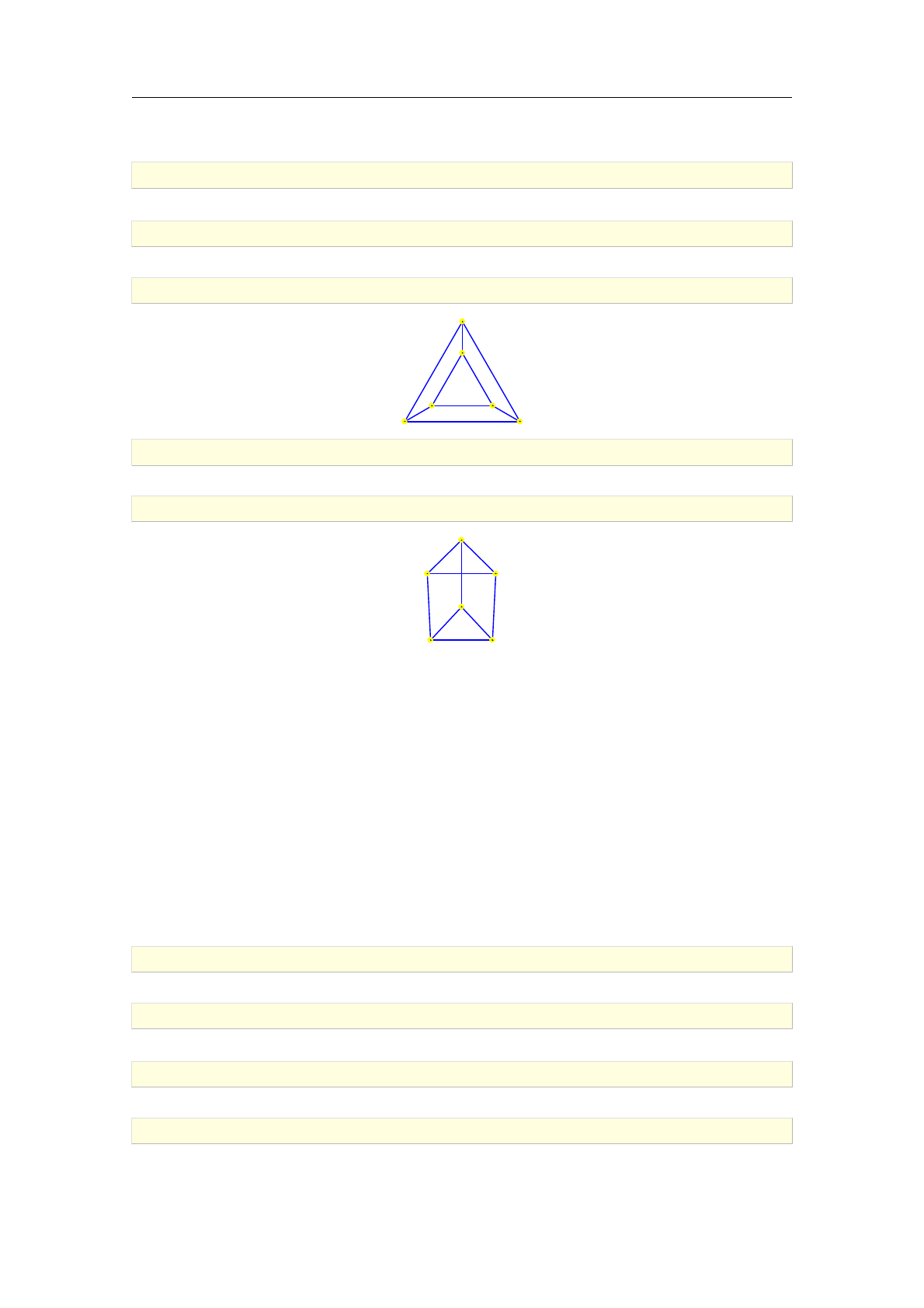
>G:=graph("octahedron")
an undirected unweighted graph with 6 vertices and 12 edges
1.8 Subgraphs 27
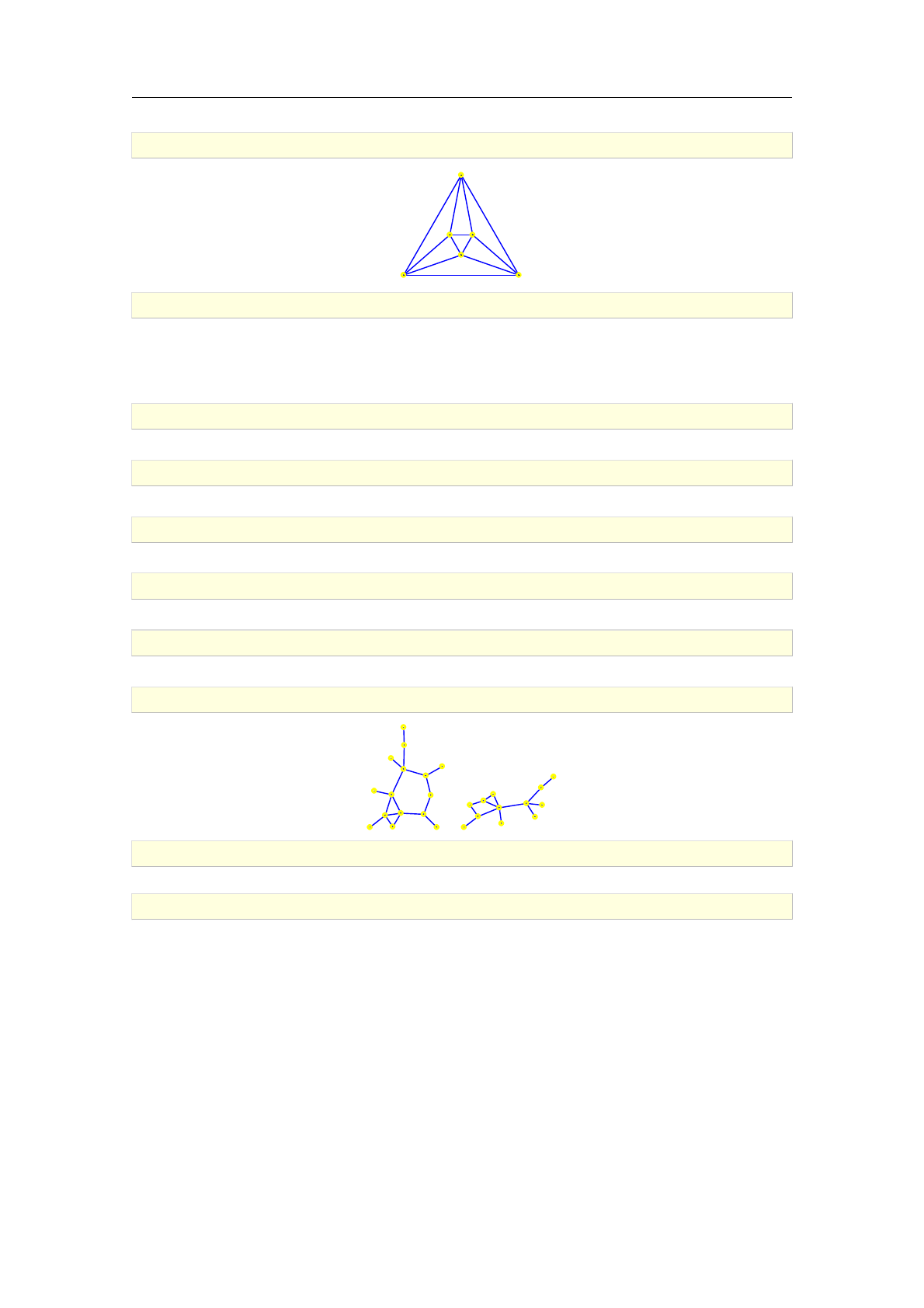
>draw_graph(G)
1 3
6
5
4 2
>cycle_basis(G)
f[6;3;1];[5;4;6;3;1];[4;6;3;1];[5;4;6;3];[2;5;4;6;3];[2;5;4;6];[2;5;4]g
Given a tree graph T, one can create a graph with cycle basis cardinality equal to kby simply
adding krandomly selected edges from the complement Tcto T.
>tree1:=random_tree(15)
an undirected unweighted graph with 15 vertices and 14 edges
>G1:=add_edge(tree1,rand(3,edges(graph_complement(tree1))))
an undirected unweighted graph with 15 vertices and 17 edges
>tree2:=random_tree(12)
an undirected unweighted graph with 12 vertices and 11 edges
>G2:=add_edge(tree2,rand(2,edges(graph_complement(tree2))))
an undirected unweighted graph with 12 vertices and 13 edges
>G:=disjoint_union(G1,G2)
an undirected unweighted graph with 27 vertices and 30 edges
>draw_graph(G,spring,labels=false)
>nops(cycle_basis(G))
5
>number_of_edges(G)-number_of_vertices(G)+nops(connected_components(G))
5
1.9. Operations on graphs
1.9.1. Graph complement
The command graph_complement is used for construction of complement graphs.
Syntax: graph_complement(G)
graph_complement accepts a graph G(V ; E)as its only argument and returns the complement
graph Gc(V ; Ec)of G, where Ecis the largest set containing only edges/arcs not present in G.
The complexity of the algorithm is O(jVj2).
28 Constructing graphs
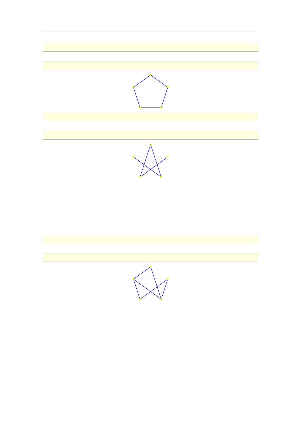
>C5:=cycle_graph(5)
C5: an undirected unweighted graph with 5 vertices and 5 edges
>draw_graph(C5)
0
1
23
4
>G:=graph_complement(C5)
an undirected unweighted graph with 5 vertices and 5 edges
>draw_graph(G)
0
1
23
4
1.9.2. Seidel switching
The command seidel_switch is used for Seidel switching in graphs.
Syntax: seidel_switch(G,L)
seidel_switch accepts two arguments, an undirected and unweighted graph G(V ; E)and a list
of vertices L⊂V. The result is a copy of Gin which, for each vertex v2L, its neighbors become
its non-neighbors and vice versa.
>S:=seidel_switch(cycle_graph(5),[1,2])
an undirected unweighted graph with 5 vertices and 7 edges
>draw_graph(S)
0
1
23
4
1.9.3. Transposing graphs
The command reverse_graph is used for reversing arc directions in digraphs.
Syntax: reverse_graph(G)
reverse_graph accepts a graph G(V ; E)as its only argument and returns the reverse graph GT(V ;
E0)of Gwhere E0=f(j; i): (i; j)2Eg, i.e. returns the copy of Gwith the directions of all edges
reversed.
Note that reverse_graph is defined for both directed and undirected graphs, but gives meaningful
results only for directed graphs.
GTis also called the transpose graph of Gbecause adjacency matrices of Gand GTare trans-
poses of each other (hence the notation).
1.9 Operations on graphs 29
>G:=digraph(6, %{[1,2],[2,3],[2,4],[4,5]%})
a directed unweighted graph with 6 vertices and 4 arcs
>GT:=reverse_graph(G)
a directed unweighted graph with 6 vertices and 4 arcs
>edges(GT)
f[2;1];[3;2];[4;2];[5;4]g
1.9.4. Union of graphs
The command graph_union is used for constructing unions of graphs.
Syntax: graph_union(G1,G2,..,Gn)
graph_union accepts a sequence of graphs Gk(Vk; Ek)for k= 1;2; :::; n as its argument and returns
the graph G(V ; E)where V=V1[V2[···[Vkand E=E1[E2[···[Ek.
>G1:=graph([1,2,3],%{[1,2],[2,3]%})
an undirected unweighted graph with 3 vertices and 2 edges
>G2:=graph([1,2,3],%{[3,1],[2,3]%})
an undirected unweighted graph with 3 vertices and 2 edges
>G:=graph_union(G1,G2)
an undirected unweighted graph with 3 vertices and 3 edges
>edges(G)
f[1;2];[1;3];[2;3]g
1.9.5. Disjoint union of graphs
To construct disjoint union of graphs use the command disjoint_union.
Syntax: disjoint_union(G1,G2,..,Gn)
disjoint_union accepts a sequence of graphs Gk(Vk; Ek)for k= 1;2; :::; n as its only argument
and returns the graph obtained by labeling all vertices with strings k:v where v2Vkand all edges
with strings k:e where e2Ekand calling the graph_union command subsequently. As all vertices
and edges are labeled differently, it follows jVj=Pk=1
njVkjand jEj=Pk=1
njEkj.6
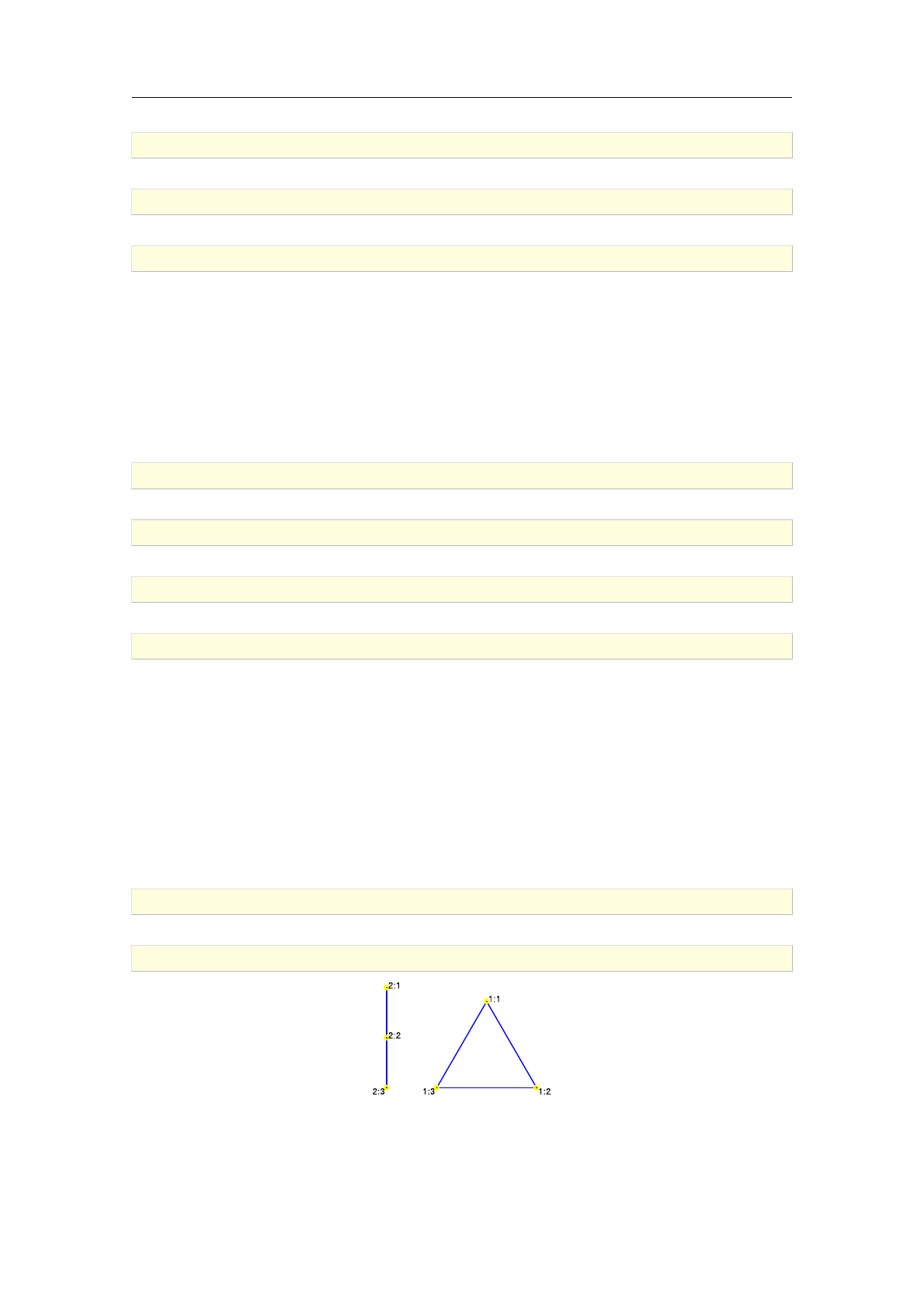
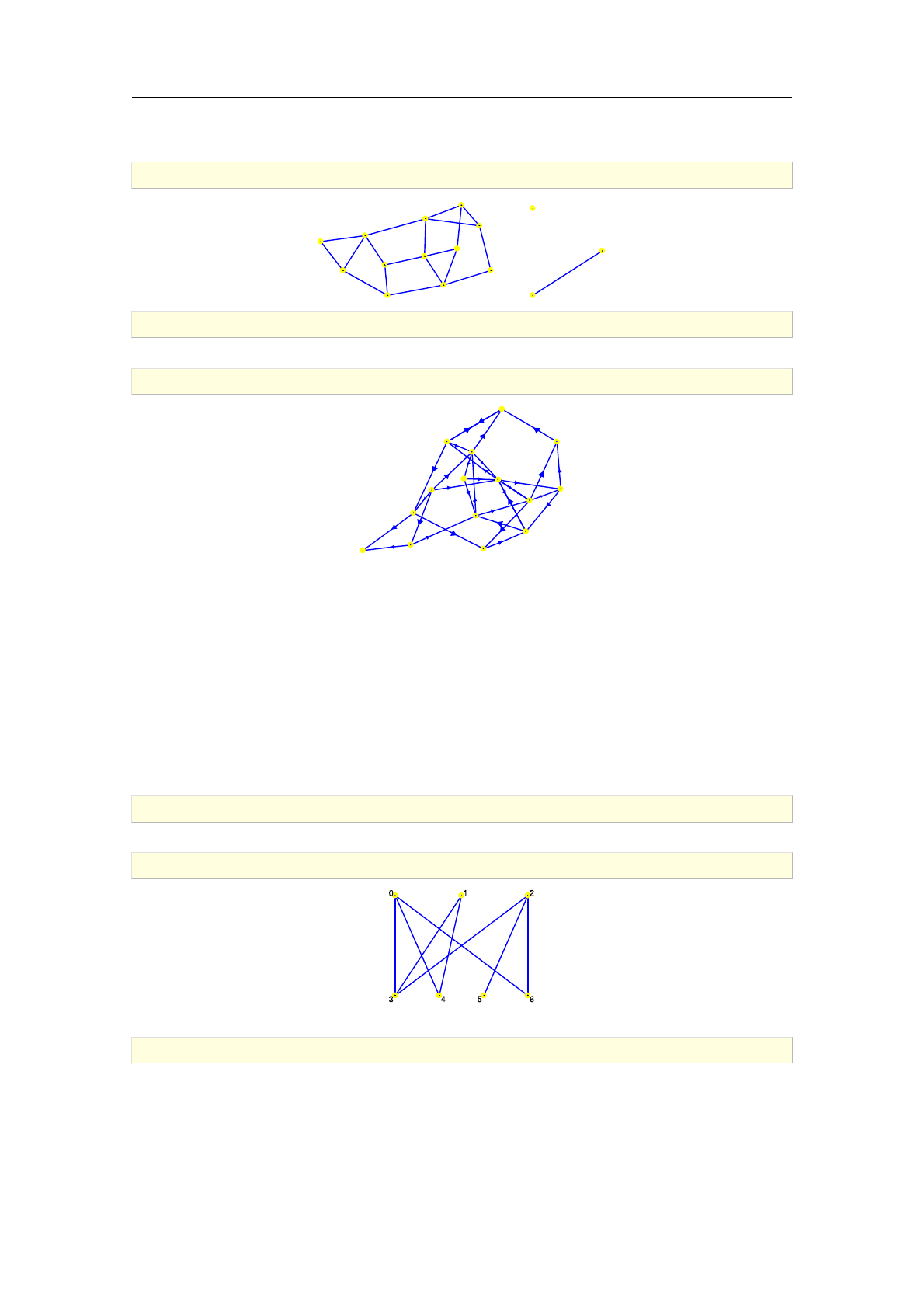
>G:=disjoint_union(cycle_graph([1,2,3]),path_graph([1,2,3]))
an undirected unweighted graph with 6 vertices and 5 edges
>draw_graph(G)
1.9.6. Joining two graphs
The command graph_join is used for joining two graphs together.
30 Constructing graphs
Syntax: graph_join(G,H)
graph_join accepts two graphs Gand Has its arguments and returns the graph G+Hwhich is
obtained by connecting all the vertices of Gto all vertices of H. The vertex labels in the resulting
graph are strings of the form 1:u and 2:v where uis a vertex in Gand vis a vertex in H.
>G:=path_graph(2)
an undirected unweighted graph with 2 vertices and 1 edge
>H:=graph(3)
an undirected unweighted graph with 3 vertices and 0 edges
>GH:=graph_join(G,H)
an undirected unweighted graph with 5 vertices and 7 edges
>draw_graph(GH,spring)
1:0
1:1
2:0
2:1 2:2
1.9.7. Power graphs
The command graph_power is used for computing powers of graphs.
Syntax: graph_power(G,k)
graph_power accepts two arguments, a graph G(V ; E)and a positive integer k. It returns the k-th
power Gkof Gwith vertices Vsuch that v; w 2Vare connected with an edge if and only if there
exists a path of length at most kin G.
The graph Gkis constructed from its adjacency matrix Akwhich is obtained by adding powers of
the adjacency matrix Aof G:
Ak=X
i=1
k
Ak:
The above sum is obtained by assigning Ak Aand repeating the instruction Ak (Ak+I)Afor
k¡1times, so exactly kmatrix multiplications are required.
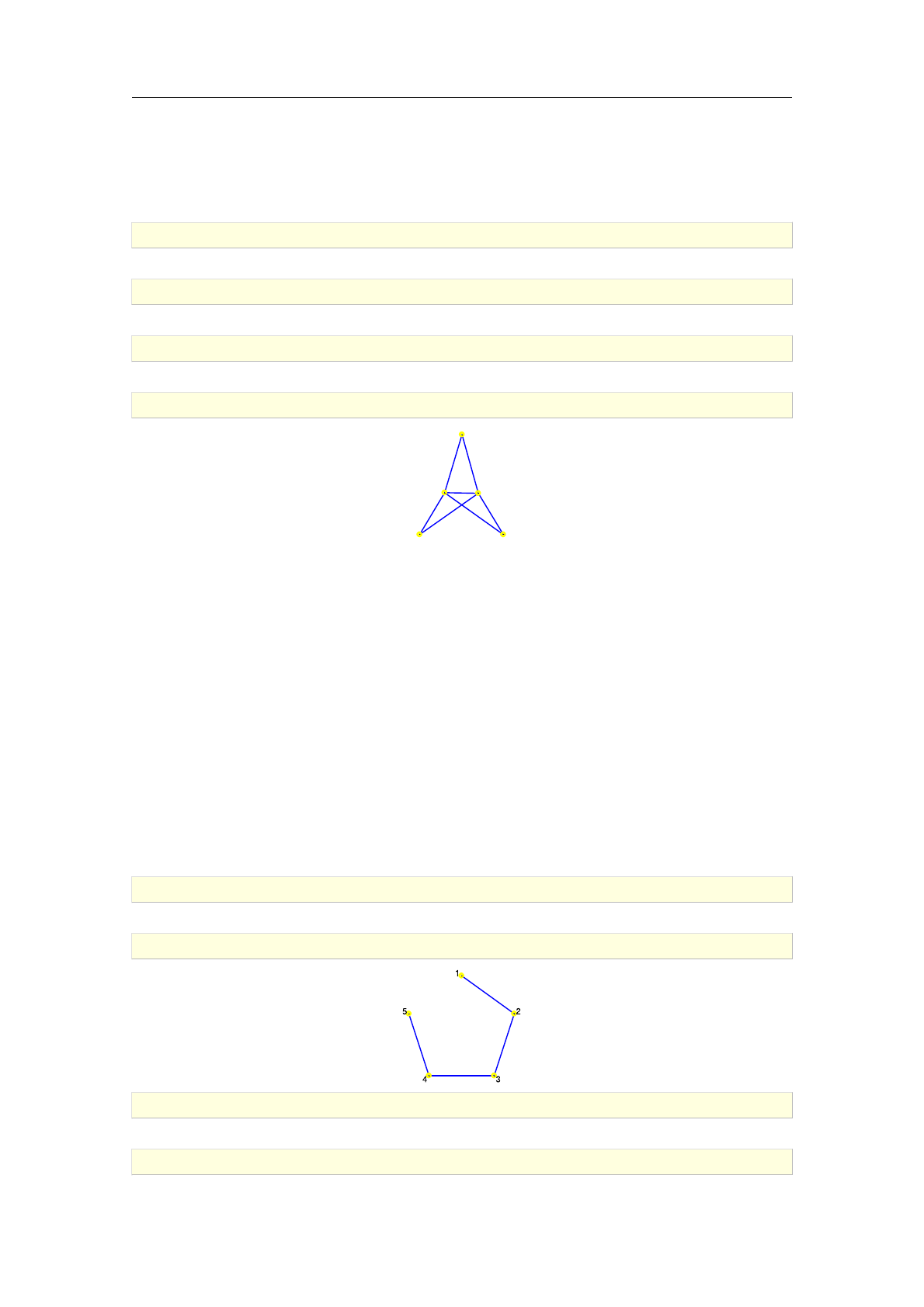
>G:=graph(trail(1,2,3,4,5))
an undirected unweighted graph with 5 vertices and 4 edges
>draw_graph(G,circle)
>P2:=graph_power(G,2)
an undirected unweighted graph with 5 vertices and 7 edges
>draw_graph(P2,circle)
1.9 Operations on graphs 31
>P3:=graph_power(G,3)
an undirected unweighted graph with 5 vertices and 9 edges
>draw_graph(P3,circle)
1.9.8. Graph products
There are two distinct operations for computing the product of two graphs: the Cartesian product
and the tensor product. These operations are available in Giac as the commands cartesian_pro-
duct and tensor_product, respectively.
Syntax: cartesian_product(G1,G2,..,Gn)
tensor_product(G1,G2,..,Gn)
cartesian_product accepts a sequence of graphs Gk(Vk; Ek)for k= 1;2; :::; n as its argument
and returns the Cartesian product G1×G2×···×Gnof the input graphs. The Cartesian product
G(V ; E) = G1×G2is the graph with list of vertices V=V1×V2, labeled with strings v1:v2 where
v12V1and v22V2, such that (u1:v1,u2:v2)2Eif and only if u1is adjacent to u2and v1=v2or
u1=u2and v1is adjacent to v2.
>G1:=graph(trail(1,2,3,4,1,5))
an undirected unweighted graph with 5 vertices and 5 edges
>draw_graph(G1,circle)
>G2:=star_graph(3)
an undirected unweighted graph with 4 vertices and 3 edges
>draw_graph(G2,circle=[1,2,3])
>G:=cartesian_product(G1,G2)
32 Constructing graphs
an undirected unweighted graph with 20 vertices and 35 edges
>draw_graph(G)
tensor_product accepts a sequence of graphs Gk(Vk; Ek)for k= 1;2; :::; n as its argument and
returns the tensor product G1×G2× ··· × Gnof the input graphs. The tensor product G(V ;
E) = G1×G2is the graph with list of vertices V=V1×V2, labeled with strings v1:v2 where v12V1
and v22V2, such that (u1:v1,u2:v2)2Eif and only if u1is adjacent to u2and v1is adjacent to v2.
>T:=tensor_product(G1,G2)
an undirected unweighted graph with 20 vertices and 30 edges
>draw_graph(T)
1.9.9. Transitive closure graph
The command transitive_closure is used for constructing transitive closure graphs.
Syntax: transitive_closure(G)
transitive_closure(G,weighted[=true or false])
transitive_closure accepts one or two arguments, a graph G(V ; E)and optionally the option
weighted=true (or simply weighted) or the option weighted=false (which is the default). The
command returns the transitive closure T(V ; E0)of the input graph Gby connecting u2Vto
v2Vin Tif and only if there is a path from uto vin G. If Gis directed, then Tis also directed.
When weighted=true is specified, Tis weighted such that the weight of edge v w 2E0is equal to
the length (or cost, if Gis weighted) of the shortest path from vto win G.
The lengths/weights of the shortest paths are obtained by the command allpairs_distance if G
is weighted resp. the command vertex_distance if Gis unweighted. Therefore Tis constructed
in at most O(jVj3)time if weighted[=true] is given and in O(jVjjEj)time otherwise.
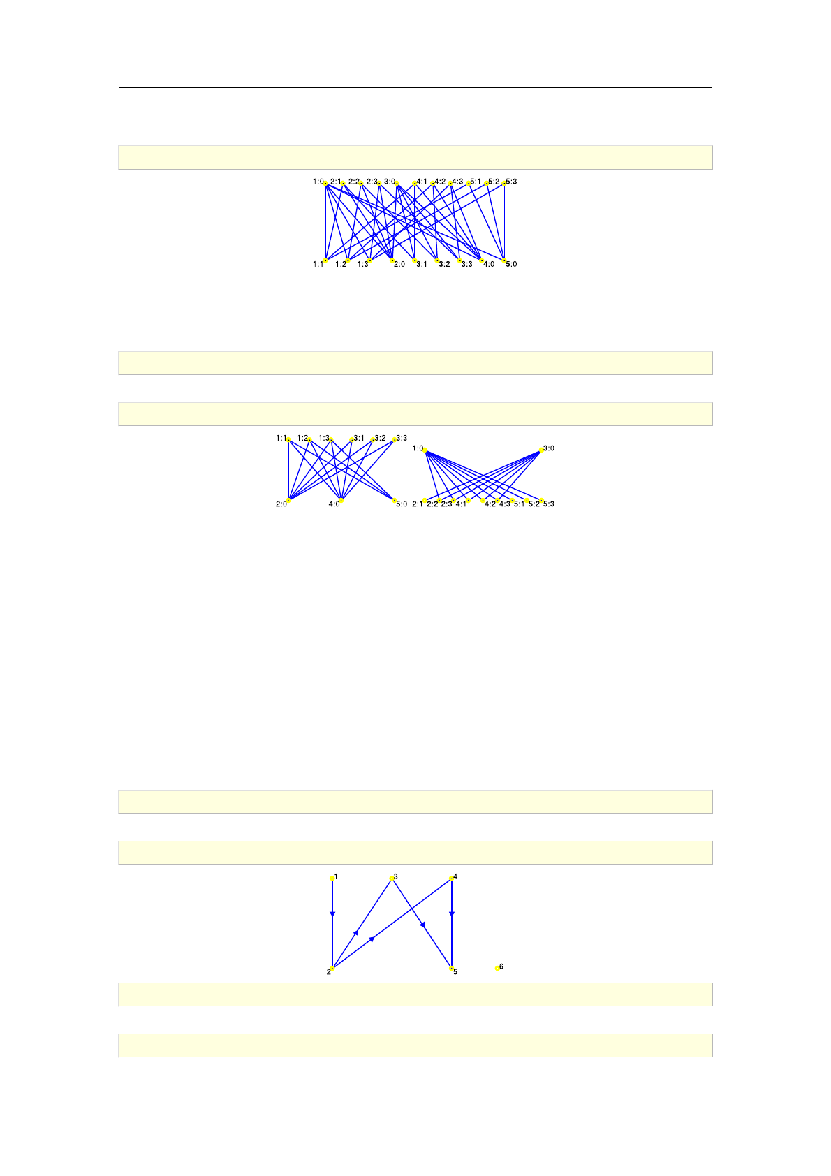
>G:=digraph([1,2,3,4,5,6],%{[1,2],[2,3],[2,4],[4,5],[3,5]%})
a directed unweighted graph with 6 vertices and 5 arcs
>draw_graph(G)
>T:=transitive_closure(G,weighted)
a directed weighted graph with 6 vertices and 9 arcs
>draw_graph(T)
1.9 Operations on graphs 33
>G:=assign_edge_weights(G,1,99)
a directed weighted graph with 6 vertices and 5 arcs
>draw_graph(G)
>draw_graph(transitive_closure(G,weighted=true))
1.9.10. Line graph
The command line_graph is used for construction of line graphs [23, pp. 10].
Syntax: line_graph(G)
line_graph accepts an undirected graph Gas its only argument and returns the line graph L(G)
with jEjdistinct vertices, one vertex for each edge in E. Furthermore, two vertices v1and v2in
L(G)are adjacent if and only if the corresponding edges e1; e22Ehave a common endpoint. The
vertices in L(G)are labeled with strings in form v-w, where e=vw 2E.
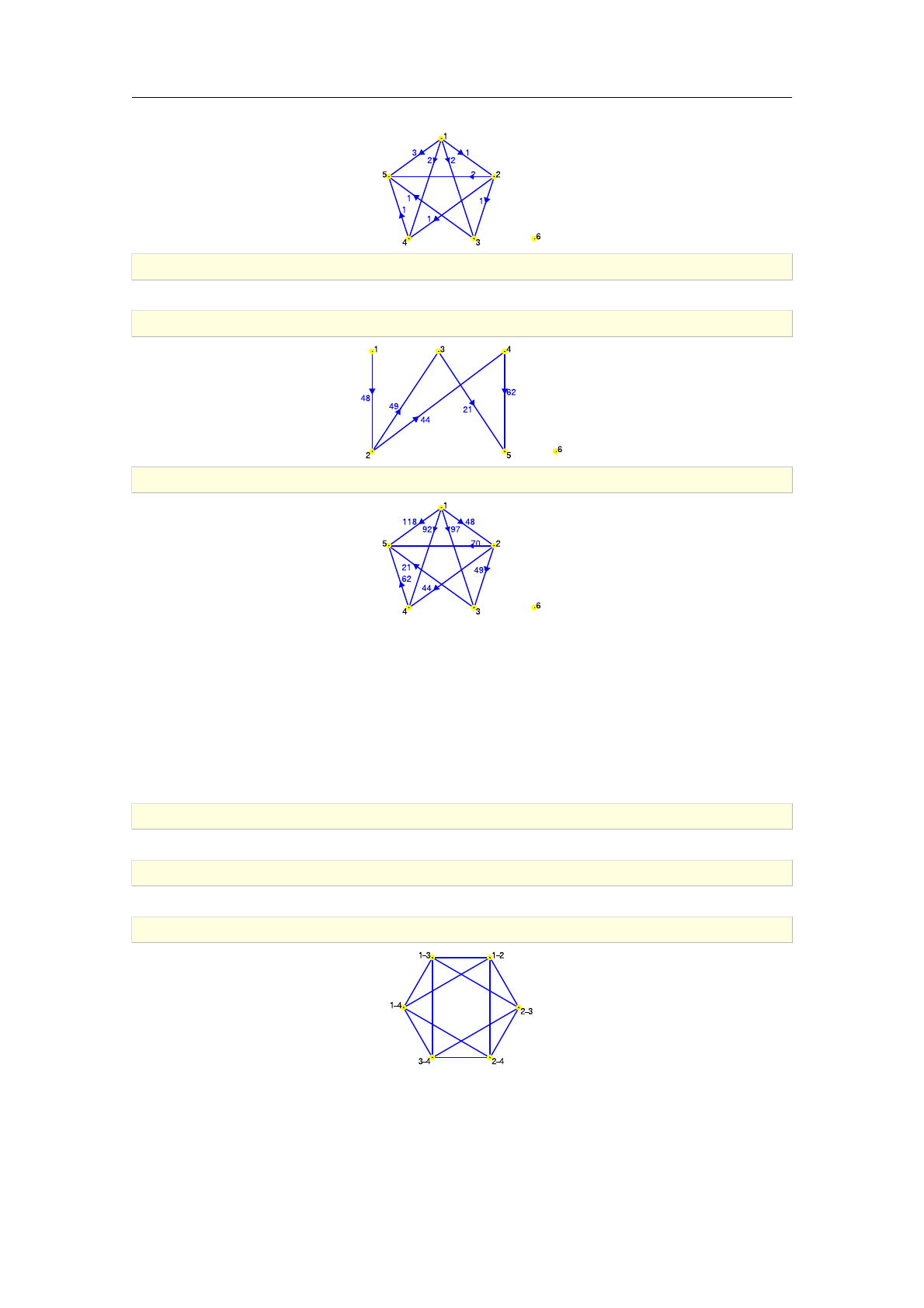
>K4:=complete_graph([1,2,3,4])
an undirected unweighted graph with 4 vertices and 6 edges
>L:=line_graph(K4)
an undirected unweighted graph with 6 vertices and 12 edges
>draw_graph(L,spring)
1.9.11. Plane dual graph
The command plane_dual is used for construction of dual graphs from undirected biconnected
planar graphs. To determine whether the given graph is planar [23, pp. 12] use the command
is_planar.
34 Constructing graphs
Syntax: plane_dual(G)
plane_dual(F)
is_planar(G)
is_planar(G,F)
plane_dual accepts a biconnected planar graph G(V ; E)or the list Fof faces of a planar embed-
ding of Gas its only argument and returns the graph Hwith faces of Gas its vertices. Two vertices
in Hare adjacent if and only if the corresponding faces share an edge in G. The algorithm runs
in O(jVj2)time.
Note that the concept of dual graph is normally defined for multigraphs. By the strict definition,
every planar multigraph has the corresponding dual multigraph; moreover, the dual of the latter
is equal to the former. Since Giac generally does not support multigraphs, a simplified definition
suitable for simple graphs is used; hence the requirement that the input graph is biconnected.
In the example below, the dual graph of the cube graph is obtained.
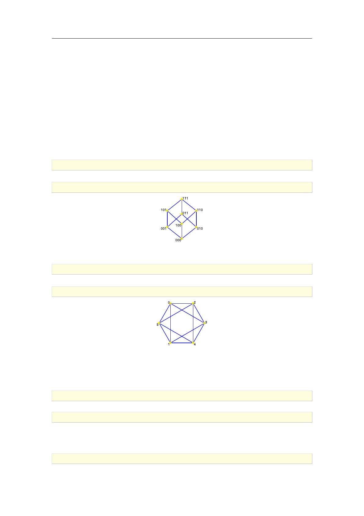
>H:=hypercube_graph(3)
an undirected unweighted graph with 8 vertices and 12 edges
>draw_graph(H,spring)
The cube has six faces, hence its plane dual graph Dhas six vertices. Also, every face obviously
shares an edge with exactly four other faces, so the degree of each vertex in Dis equal to 4.
>D:=plane_dual(H)
an undirected unweighted graph with 6 vertices and 12 edges
>draw_graph(D,spring)
is_planar accepts one or two arguments, the input graph Gand optionally an unassigned identi-
fier F. It returns true if Gis planar and false otherwise. If the second argument is given and G
is planar and biconnected, the list of faces of Gis stored to F. Each face is represented as a cycle
(a list) of vertices. The strategy is to use the algorithm of Demoucron et al. [22, pp. 88], which
runs in O(jVj2)time.
>is_planar(graph("petersen"))
false
>is_planar(graph("durer"))
true
In the next example, a graph isomorphic to Dis obtained when passing a list of faces of Hto the
plane_dual command. The order of vertices is determined by the order of faces.
>is_planar(H,F); F
1.9 Operations on graphs 35
true;
0
B
B
B
B
B
B
B
B
B
B
B
B
@
010 000 001 011
001 000 100 101
010 011 111 110
100 000 010 110
111 011 001 101
101 100 110 111
1
C
C
C
C
C
C
C
C
C
C
C
C
A
>is_isomorphic(plane_dual(F),D)
true
1.10. Random graphs
1.10.1. Random general graphs
The commands random_graph and random_digraph are used for generating general (di)graphs
uniformly at random according to Erd®s–Rényi model.
Syntax: random_graph(n|L,p)
random_graph(n|L,m)
random_digraph(n|L,p)
random_digraph(n|L,m)
random_graph and random_digraph both accept two arguments. The first argument is a positive
integer nor a list of labels Lof length n. The second argument is a positive real number p < 1
or a positive integer m. The return value is a (di)graph on nvertices (using the elements of Las
vertex labels) selected uniformly at random, i.e. a (di)graph in which each edge/arc is present with
probability por which contains exactly medges/arcs chosen uniformly at random.
The strategy is to use the algorithms of Bagatelj and Brandes [3, algorithms 1 and 2], which
operate in linear time.
>G:=random_graph(10,0.5)
an undirected unweighted graph with 10 vertices and 21 edges
>draw_graph(G,spring,labels=false)
>G:=random_graph(1000,0.05)
an undirected unweighted graph with 1000 vertices and 24870 edges
>is_connected(G)
true
>minimum_degree(G),maximum_degree(G)
20;71
>G:=random_graph(15,20)
36 Constructing graphs
an undirected unweighted graph with 15 vertices and 20 edges
>draw_graph(G,spring)
0
12
3
4
5
6
7
8
9
10
11
12
13
14
>DG:=random_digraph(15,0.15)
a directed unweighted graph with 15 vertices and 33 arcs
>draw_graph(DG,labels=false,spring)
1.10.2. Random bipartite graphs
The command random_bipartite_graph is used for generating bipartite graphs at random.
Syntax: random_bipartite_graph(n,p|m)
random_bipartite_graph([a,b],p|m)
random_bipartite_graph accepts two arguments. The first argument is either a positive integer
nor a list of two positive integers aand b. The second argument is either a positive real number
p < 1or a positive integer m. The command returns a random bipartite graph on nvertices (or
with two partitions of sizes aand b) in which each possible edge is present with probability p(or
medges are inserted at random).
>G:=random_bipartite_graph([3,4],0.5)
an undirected unweighted graph with 7 vertices and 8 edges
>draw_graph(G)
>G:=random_bipartite_graph(30,60)
an undirected unweighted graph with 30 vertices and 60 edges
1.10.3. Random trees
The command random_tree is used for generating tree graphs at random.
1.10 Random graphs 37
Syntax: random_tree(n|V)
random_tree(n|V,d)
random_tree(n|V,root)
random_tree(V,root=v)
random_tree accepts one or two arguments: a positive integer nor a list V=fv1; v2; :::; vngand
optionally an integer d>2or the option root[=v], where v2V. It returns a random tree T(V ; E)
on nvertices such that
¡if the second argument is omitted, then Tis uniformly selected among all unrooted unlabeled
trees on nvertices,
¡if dis given as the second argument, then ∆(T)6d, where ∆(T)is the maximum vertex
degree in T,
¡if root[=v] is given as the second argument, then Tis uniformly selected among all rooted
unlabeled trees on nvertices. If vis specified then the vertex labels in V(required) will be
assigned to vertices in Tsuch that vis the first vertex in the list returned by the command
vertices(T).
Rooted unlabeled trees are generated uniformly at random using RANRUT algorithm [38, pp. 274].
The root of a tree Tgenerated this way, if not specified as v, is always the first vertex in the list
returned by the command vertices(T). The average time complexity of RANRUT algorithm is
O(jVjlog jVj)[2].
Unrooted unlabeled trees, also called free trees, are generated uniformly at random using Wilf's
algorithm1.1 [56], which is based on RANRUT algorithm and runs in about the same time as
RANRUT itself.
Trees with bounded maximum degree are generated using a simple algorithm which starts with an
empty tree and adds edges at random one at a time. It is much faster than RANRUT but selects
trees in a non-uniform manner. To force the use of this algorithm even without vertex degree limit
(for example, if nis very large), one can set d= +1.
For example, the command line below creates a forest containing 10 randomly selected free trees
on 10 vertices.
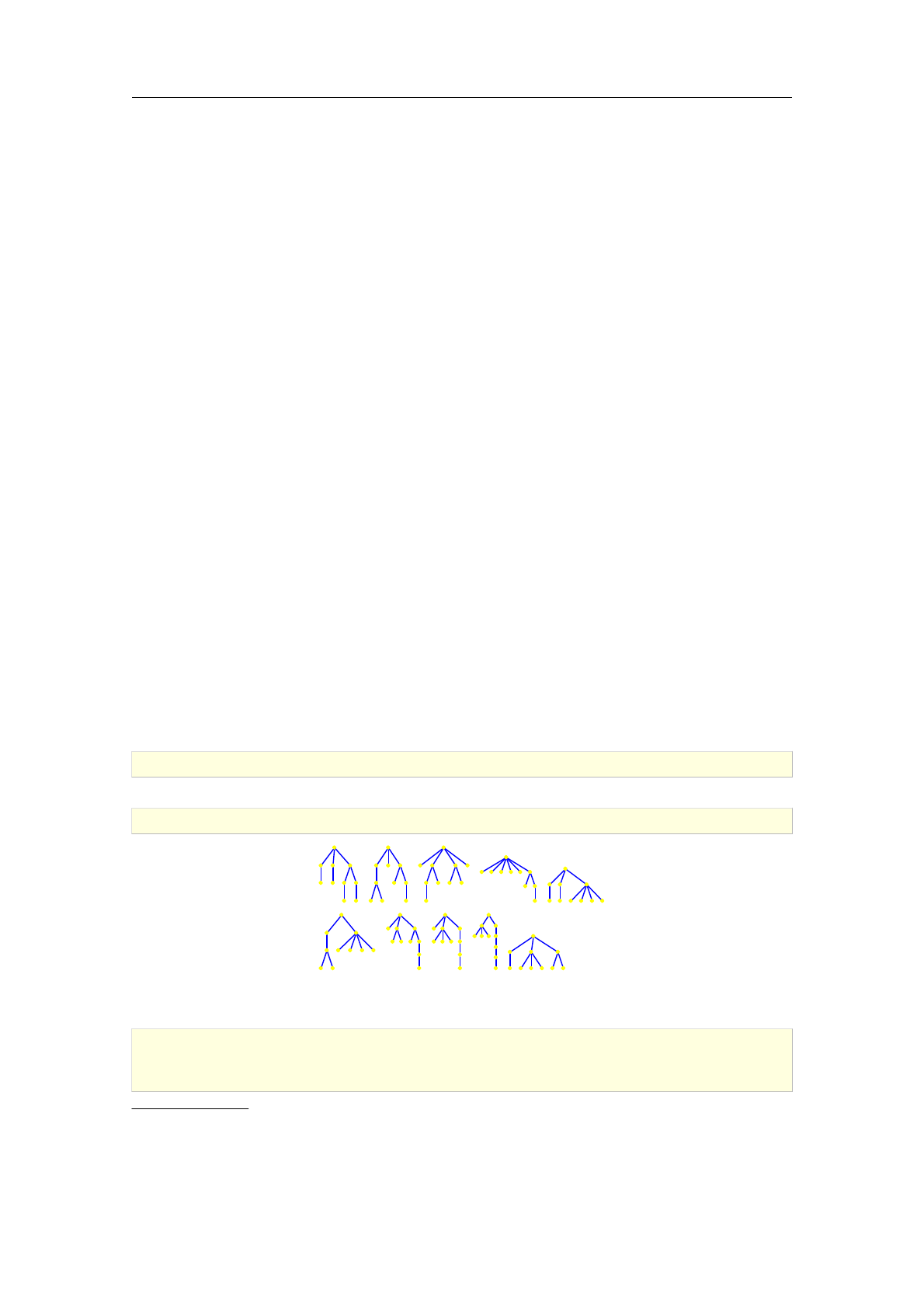
>G:=disjoint_union(apply(random_tree,[10$10]))
an undirected unweighted graph with 100 vertices and 90 edges
>draw_graph(G,tree,labels=false)
The following example demonstrates the uniformity of random generation of free trees. Letting
n= 6, there are exactly 6 distinct free trees on 6 vertices, created by the next command line.
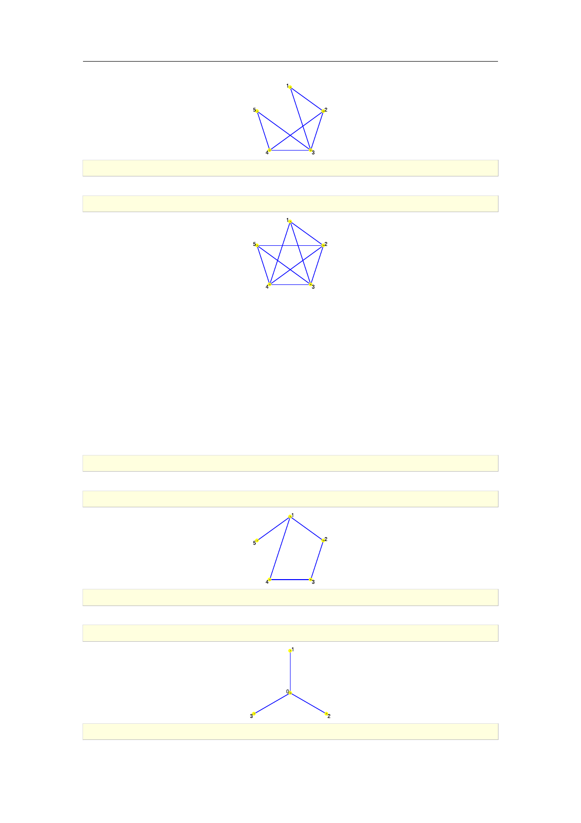
>trees:=[star_graph(5),path_graph(6),graph(trail(1,2,3,4),trail(5,4,6)),
graph(%{[1,2],[2,3],[2,4],[4,5],[4,6]%}),graph(trail(1,2,3,4),trail(3,5,6)),
graph(trail(1,2,3,4),trail(5,3,6))]:;
1.1. The original Wilf's algorithm has an error in the procedure Free, page 207. The formula p=1 + an/2
2/anin
step (T1) is wrong; instead of the denominator an, which is the number of all rooted unlabeled trees on nvertices,
one should put the number tnof all unrooted unlabeled trees. tncan be obtained from a1; a2; :::; anby applying the
formula in [40, pp. 589]. The Giac implementation includes this correction.
38 Constructing graphs
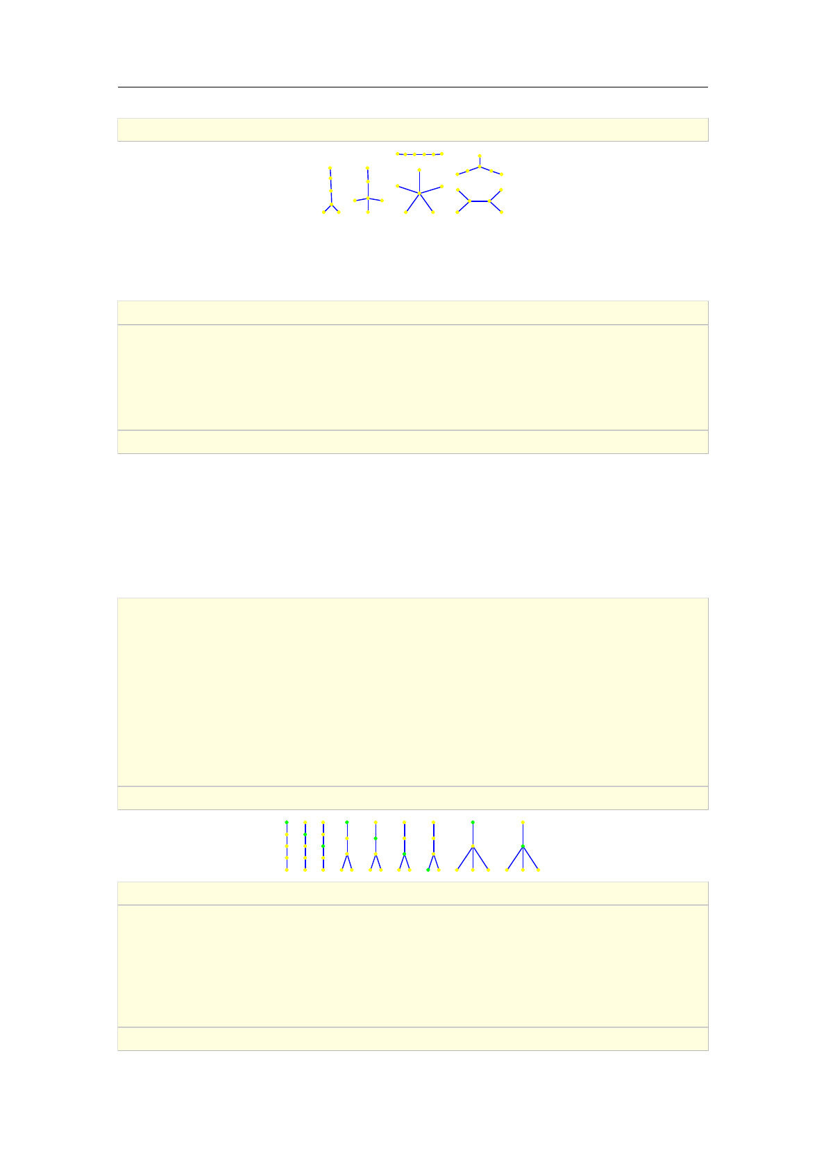
>draw_graph(disjoint_union(trees),spring,labels=false)
Now, generating a random free tree on 6nodes always produces one of the above six graphs, which
is determined by using is_isomorphic command. 1200 trees are generated in total and the number
of occurrences of trees[k] is stored in hits[k] for every k= 1;2; :::; 6(note that in Xcas mode it
is actually k= 0; :::; 5).
>hits:=[0$6]:;
>for k from 1 to 1200 do
T:=random_tree(6);
for j from 0 to 5 do
if is_isomorphic(T,trees[j]) then hits[j]++; fi;
od;
od:;
>hits
[198;194;192;199;211;206]
To show that the algorithm also selects rooted trees on nvertices with equal probability, one can
reproduce the example in [38, pp. 281], in which n= 5. First, all distinct rooted trees on 5 vertices
are created and stored in trees; there are exactly nine of them. Their root vertices are highlighted
to be distinguishable. Then, 4500 rooted trees on 5 vertices are generated at random, highlighting
the root vertex in each of them. As in the previous example, the variable hits[k] records how
many of them are isomorphic to trees[k].
>trees:=[
highlight_vertex(graph(trail(1,2,3,4,5)),1),
highlight_vertex(graph(trail(1,2,3,4,5)),2),
highlight_vertex(graph(trail(1,2,3,4,5)),3),
highlight_vertex(graph(trail(1,2,3),trail(4,3,5)),1),
highlight_vertex(graph(trail(1,2,3),trail(4,3,5)),2),
highlight_vertex(graph(trail(1,2,3),trail(4,3,5)),3),
highlight_vertex(graph(trail(1,2,3),trail(4,3,5)),4),
highlight_vertex(graph(trail(1,2,3),trail(4,2,5)),1),
highlight_vertex(graph(trail(1,2,3),trail(4,2,5)),2)
]:;
>draw_graph(disjoint_union(trees),labels=false)
>hits:=[0$9]:;
>for k from 1 to 4500 do
T:=random_tree(5,root);
HT:=highlight_vertex(T,vertices(T)[0]);
for j from 0 to 8 do
if is_isomorphic(HT,trees[j]) then hits[j]++; fi;
od;
od:;
>hits
1.10 Random graphs 39
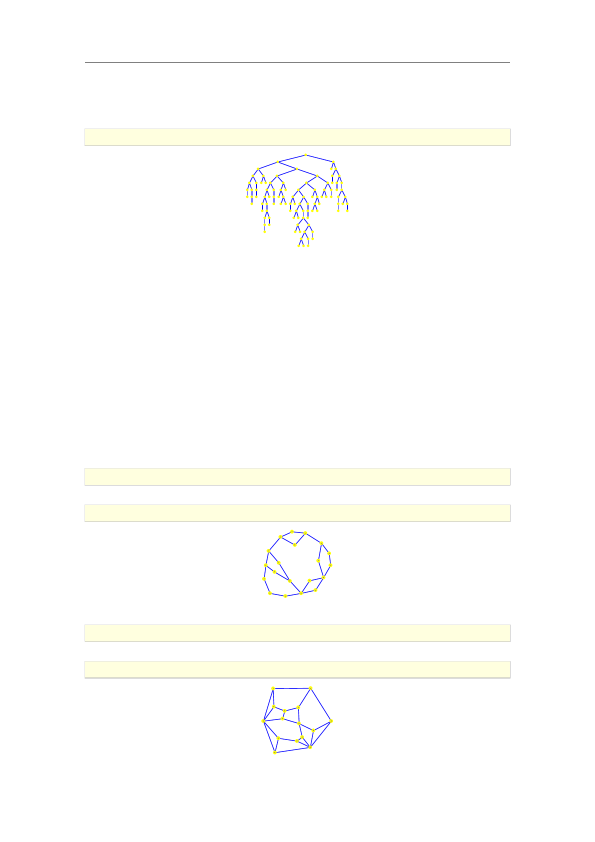
[534;483;486;485;496;521;498;489;508]
In the following example, a random tree on 100 vertices with maximum degree at most 3 is drawn.
>draw_graph(random_tree(100,3))
1.10.4. Random planar graphs
The command random_planar_graph is used for generating random planar graphs.
Syntax: random_planar_graph(n|L,p)
random_planar_graph(n|L,p,k)
random_planar_graph accepts two or three arguments, a positive integer n(or a list Lof length
n), a positive real number p < 1and optionally an integer k2f0;1;2;3g(by default, k= 1). The
command returns a random k-connected planar graph on nvertices (using the elements of Las
vertex labels).
The result is obtained by first generating a random maximal planar graph and then attempting
to remove each edge with probability p, maintaining the k-connectivity of the graph (if k= 0, the
graph may be disconnected). The running time is O(n)if k= 0,O(n2)if k2f1;2gand O(n3)if
k= 3.
The following command line generates a biconnected planar graph.
>G:=random_planar_graph(20,0.8,2)
an undirected unweighted graph with 20 vertices and 25 edges
>draw_graph(G,planar,labels=false)
The command line below generates a triconnected planar graph.
>G:=random_planar_graph(15,0.9,3)
an undirected unweighted graph with 15 vertices and 25 edges
>draw_graph(G,planar,labels=false)
40 Constructing graphs
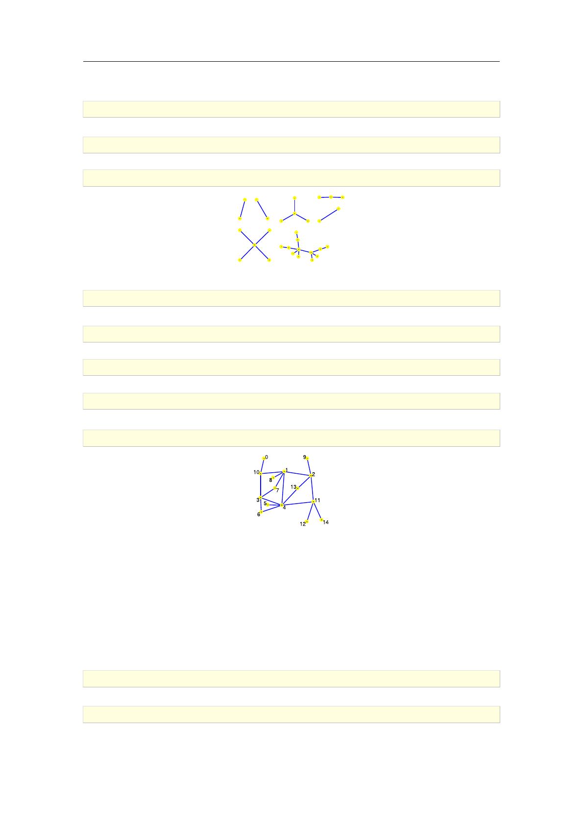
The next command line generates a disconnected planar graph with high probability.
>G:=random_planar_graph(30,0.9,0)
an undirected unweighted graph with 30 vertices and 23 edges
>is_forest(G)
true
>draw_graph(G,spring,labels=false)
By default, a connected planar graph is generated, like in the following example.
>G:=random_planar_graph(15,0.618)
an undirected unweighted graph with 15 vertices and 19 edges
>is_connected(G)
true
>is_biconnected(G)
false
>articulation_points(G)
[1;2;4;10;11]
>draw_graph(G,planar)
1.10.5. Random graphs from the given degree sequence
The command random_sequence_graph is used for generating a random undirected graph from
the given degree sequence.
Syntax: random_sequence_graph(L)
random_sequence_graph accepts the degree sequence L(a list of nonnegative integers) as its only
argument. It returns an asimptotically uniform random graph with the degree sequence equal to
Lin almost linear time, using the algorithm developed by Bayati et al. [4].
>s:=[1,3,3,2,1,2,2,2,3,3]:; is_graphic_sequence(s)
Done;true
>G:=random_sequence_graph(s)
an undirected unweighted graph with 10 vertices and 11 edges
1.10 Random graphs 41
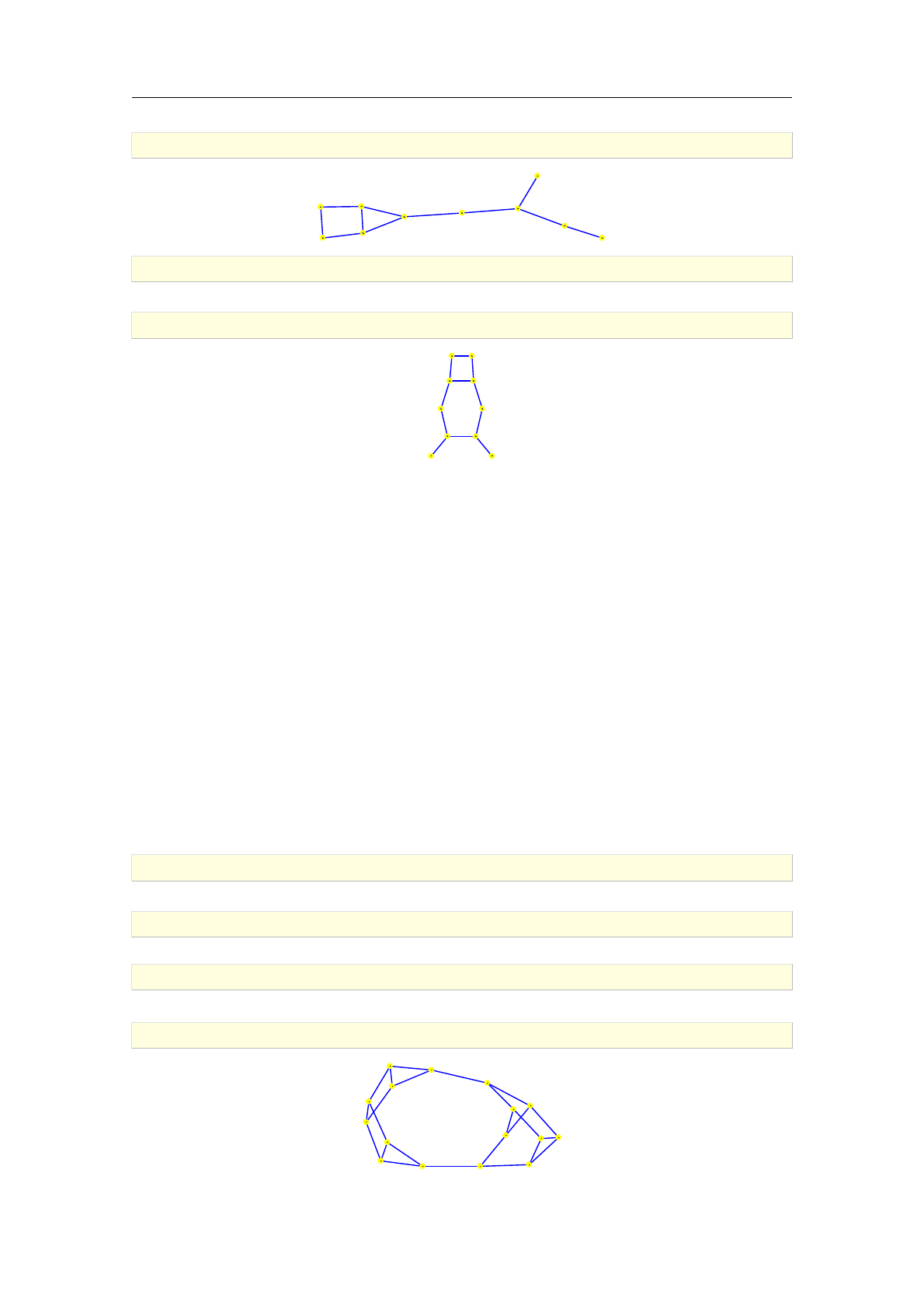
>draw_graph(G,spring)
0
1
2
3
45
6
7
8
9
>H:=random_sequence_graph(s)
an undirected unweighted graph with 10 vertices and 11 edges
>draw_graph(H,spring)
0
1
2
3
4
5
6
7
89
1.10.6. Random regular graphs
The command random_regular_graph is used for generating random regular graphs on the given
set of vertices.
Syntax: random_regular_graph(n or L,d)
random_regular_graph(n or L,d,connected)
random_regular_graph accepts two mandatory arguments, a positive integer n(or a list Lof
length n) and a nonnegative integer d. Optionally, the option connected may be specified as a
third argument, indicating that the generated graph must be connected. The command creates n
vertices (using elements of Las vertex labels) and returns a random d-regular (connected) graph
on these vertices.
Note that a d-regular graph on nvertices exists if and only if n > d + 1 and n d is even. If these
conditions are not met, random_regular_graph returns an error.
The strategy is to use the algorithm developed by Steger and Wormald [44, algorithm 2]. The
runtime is negligible for n6100. However, for n > 200 the algorithm is considerably slower. Graphs
are generated with approximately uniform probability, which means that for n!1 and dnot
growing so quickly with nthe probability distribution converges to uniformity.
>G:=random_regular_graph(16,3)
an undirected unweighted graph with 16 vertices and 24 edges
>is_regular(G)
true
>degree_sequence(G)
[3;3;3;3;3;3;3;3;3;3;3;3;3;3;3;3]
>draw_graph(G,spring)
0
1
2
3
4
5
6
7
8
9
10
11
12
13
14
15
42 Constructing graphs
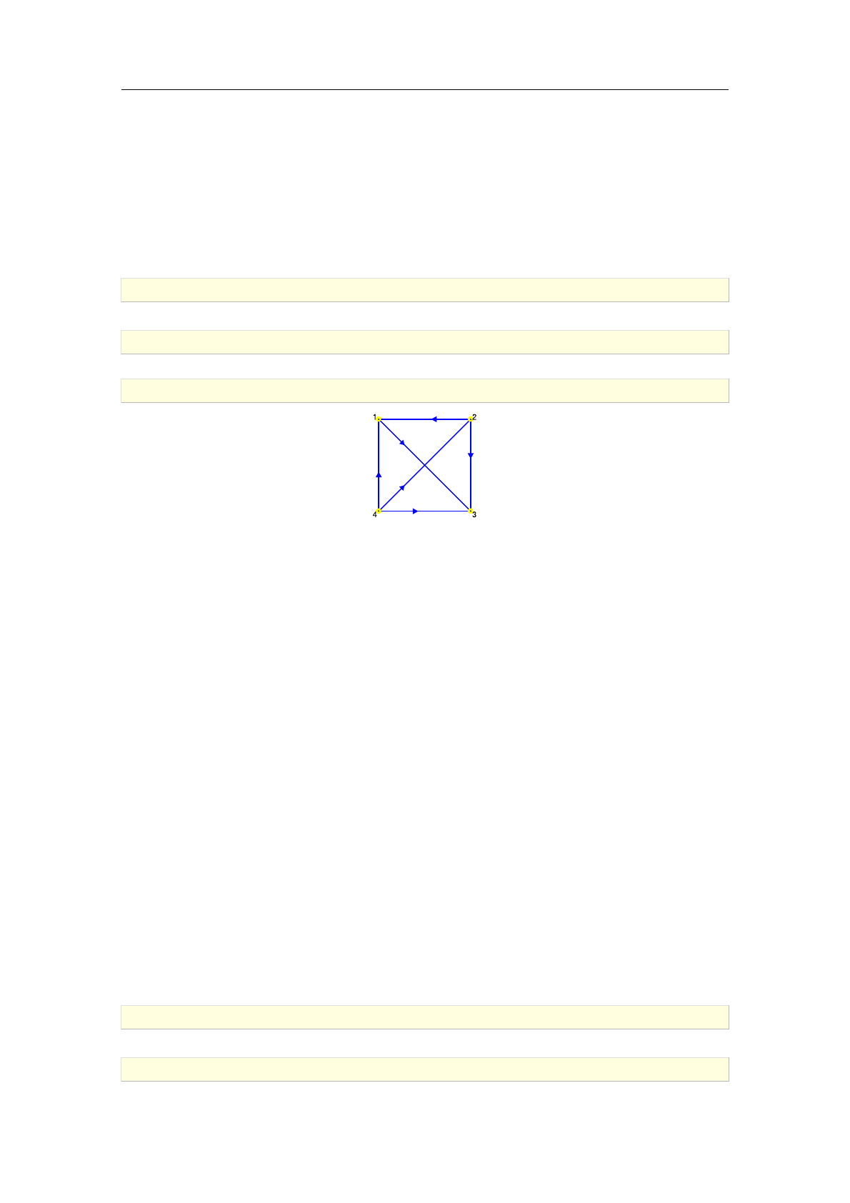
1.10.7. Random tournaments
The command random_tournament is used for generating random tournaments.
Syntax: random_tournament(n)
random_tournament(L)
random_tournament accepts a positive integer nor a list Lof length nas its only argument and
returns a random tournament on nvertices. If Lis specified, its elements are used to label the
vertices.
>G:=random_tournament([1,2,3,4])
a directed unweighted graph with 4 vertices and 6 arcs
>is_tournament(G)
true
>draw_graph(G)
1.10.8. Random network graphs
The command random_network is used for generation of random networks.
Syntax: random_network(a,b,[opts])
random_network(a,b,p,[opts])
random_network accepts two to four arguments: a positive integer a, a positive integer b, an
optional real number psuch that 0< p 61(by default p=0.5) and optionally a sequence of options
opts. The supported options are acyclic[=true|false] and weights=a..b.
The command returns a network graph with a2bvertices which is composed as follows (the method
of generating the network skeleton is due to Goldfarb and Grigoriadis [24]).
Firstly, grid graphs F1; F2; :::; Fb(called frames), each of them with a×avertices, are generated.
If the option acyclic[=true] is used (by default is acyclic=false), then an acyclic orientation
is computed for each frame using st-ordering (see Section 4.9.3) with two opposite corners of the
frame as source and sink, otherwise all vertices in the frame are connected to their neighbors (forth
and back). In addition, for each k < b the vertices of Fkare connected one to one with the vertices
of the next frame Fk+1 using a random permutation of those vertices. The first vertex of the first
frame is the source and the last vertex of the last frame is the sink of the network (some arcs may
have to be removed to achieve that). Finally, the removal of each arc is attempted with probability
1¡p(unless its removal disconnects the network), making each arc present with probability p.
if the option weights=a..b is specified, arc weights in the network are randomized in the interval
[a; b]⊂R. If a; b are integers, the weights are also integers.
For example, the command line below creates a random network, consisting of 3 frames of size
2×2, in which each arc is present with the probability 0.9.
>N1:=random_network(2,3,0.9)
a directed unweighted graph with 12 vertices and 25 arcs
>draw_graph(N1,spring)
1.10 Random graphs 43
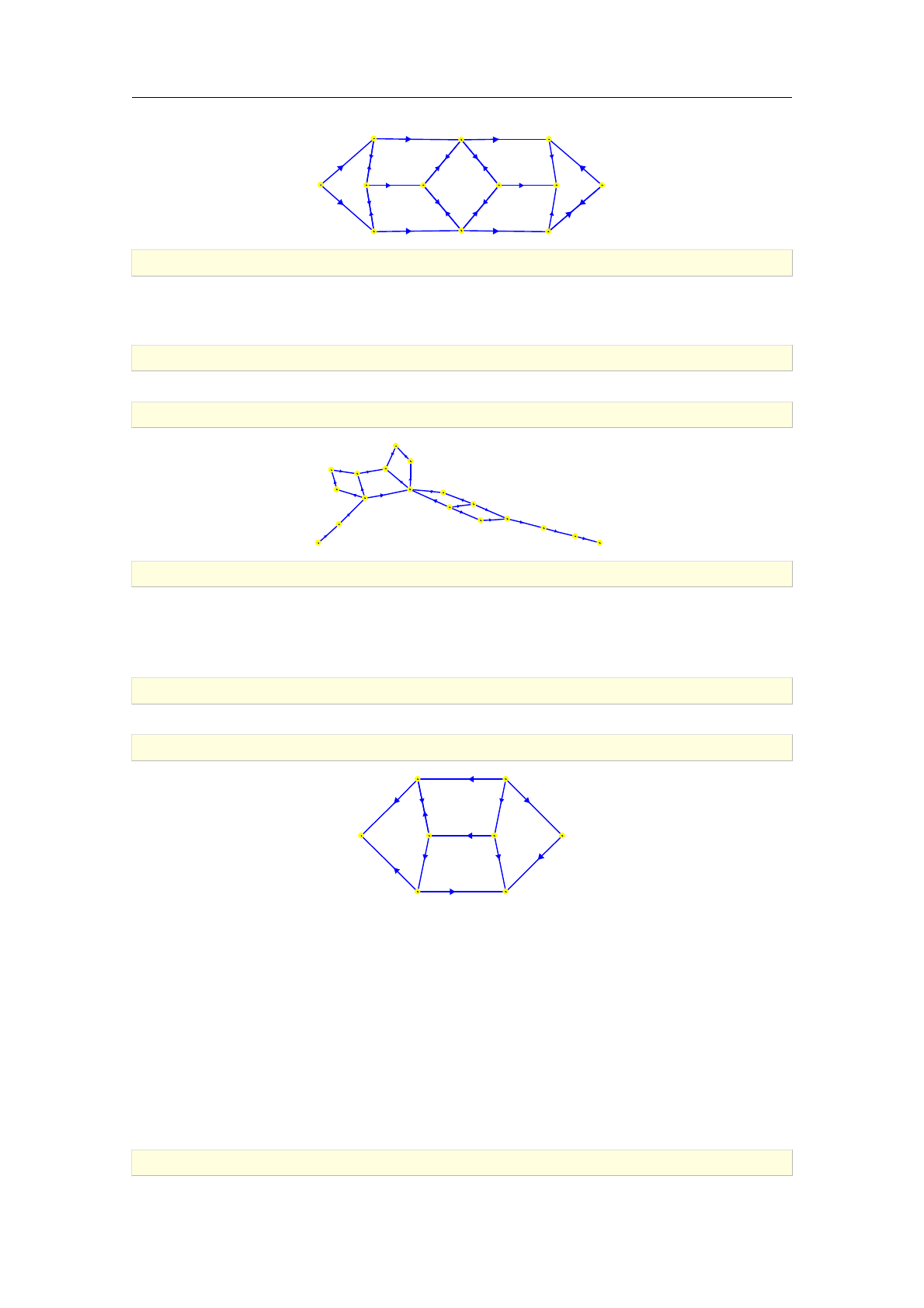
0
1
2
3
4
5
6
7
8
9
10
11
>is_network(N1)
[0];[11]
In the next example, passing the option acyclic forces the output graph to be acyclic.
>N2:=random_network(3,2,0.618,acyclic)
a directed unweighted graph with 18 vertices and 22 arcs
>draw_graph(N2,spring)
0
1
2
3
4
5
6
7
8
9
10
1112
13 14
15
16
17
>is_network(N2)
010
417
Arc weights can be randomized, as demonstrated below.
>N3:=random_network(2,2,0.75,weights=1..9)
a directed unweighted graph with 8 vertices and 12 arcs
>draw_graph(N3,spring)
5
85
43
3
6
4
8 1
6
7
01
2
3
4 5
6 7
1.10.9. Randomizing edge weights
The command assign_edge_weights is used for assigning weights to edges of graphs at random.
Syntax: assign_edge_weights(G,a..b)
assign_edge_weights(G,m,n)
assign_edge_weights accepts two or three arguments: a graph G(V ; E)and an interval a.. bof
real numbers or a sequence of two positive integers mand n. The command operates such that for,
each edge e2E, the weight of eis chosen uniformly from the real interval [a; b)or from the set of
integers lying between mand n, including both mand n. After assigning weights to all edges, a
modified copy of Gis returned.
>G:=assign_edge_weights(grid_graph(5,3),1,99)
44 Constructing graphs
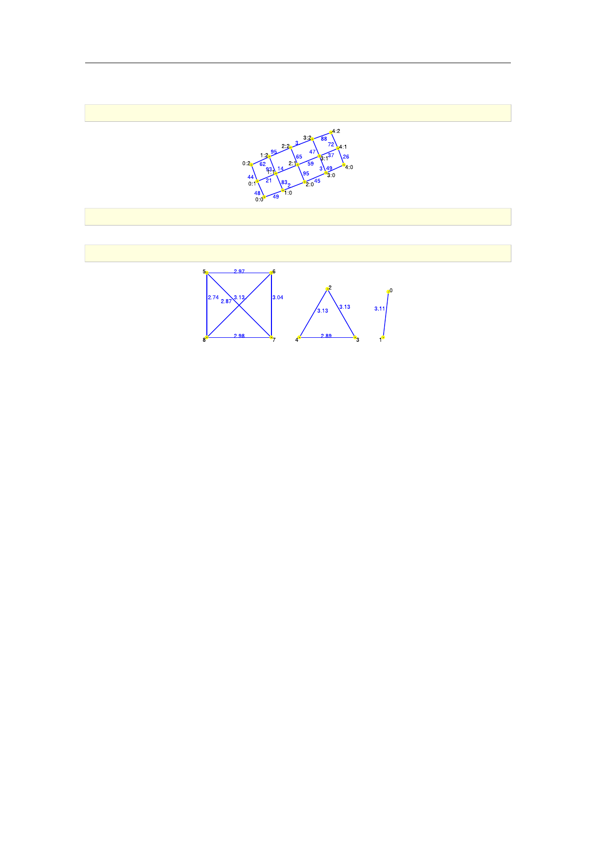
an undirected weighted graph with 15 vertices and 22 edges
>draw_graph(G,spring)
>G:=assign_edge_weights(graph_complement(complete_graph(2,3,4)),e..pi)
an undirected weighted graph with 9 vertices and 10 edges
>draw_graph(G)
1.10 Random graphs 45


Chapter 2
Modifying graphs
2.1. Promoting to directed and weighted graphs
2.1.1. Converting edges to arcs
To promote an existing undirected graph to a directed one, use the command make_directed.
Syntax: make_directed(G)
make_directed(G,A)
make_directed is called with one or two arguments, an undirected graph G(V ; E)and optionally a
numerical square matrix A=[aij]of order jVj. Every edge fi; j g2Eis replaced with the pair of arcs
(i; j)and (j; i)and, if matrix Ais specified, its elements aij and aji are assigned as weights of these
arcs, respectively. Thus a directed (weighted) copy of Gis constructed and subsequently returned.
>make_directed(cycle_graph(4))
C4: a directed unweighted graph with 4 vertices and 8 arcs
>make_directed(cycle_graph(4), [[0,0,0,1],[2,0,1,3],[0,1,0,4],[5,0,4,0]])
C4: a directed weighted graph with 4 vertices and 8 arcs
2.1.2. Assigning weight matrix to unweighted graphs
To promote an existing unweighted graph to a weighted one, use the command make_weighted.
Syntax: make_weighted(G)
make_weighted(G,A)
make_weighted accepts one or two arguments, an unweighted graph G(V ; E)and optionally a
square matrix A= [aij]of order jVj. If the matrix specification is omitted, a square matrix of ones
is assumed. Then a copy of Gis returned in which each edge/arc (i; j)2Egets the element aij in
Aassigned as its weight. If Gis undirected, it is assumed that Ais a symmetric matrix.
>make_weighted(graph(%{[1,2],[2,3],[3,1]%}), [[0,2,3],[2,0,1],[3,1,0]])
an undirected weighted graph with 3 vertices and 3 edges
2.2. Modifying vertices of a graph
2.2.1. Adding and removing vertices
For adding and removing vertices to/from graphs use the commands add_vertex and
delete_vertex, respectively.
Syntax: add_vertex(G,v|L)
delete_vertex(G,v|L)
The command add_vertex accepts two arguments, a graph G(V ; E)and a single label vor a list
of labels L, and returns the graph G0(V[fvg; E)or G00 (V[L; E)if a list Lis given.
47

>K5:=complete_graph([1,2,3,4,5])
an undirected unweighted graph with 5 vertices and 10 edges
>add_vertex(K5,6)
an undirected unweighted graph with 6 vertices and 10 edges
>add_vertex(K5,[a,b,c])
an undirected unweighted graph with 8 vertices and 10 edges
Note that vertices already present in Gwill not be added. For example:
>add_vertex(K5,[4,5,6])
an undirected unweighted graph with 6 vertices and 10 edges
The command delete_vertex accepts two arguments, a graph G(V ; E)and a single label vor a
list of labels L, and returns the graph
G0(Vnfvg;fe2E:eis not incident to vg)
or, if Lis given,
G00 (VnL; fe2E:eis not incident to any v2Lg):
If any of the specified vertices does not belong to G, an error is returned.
>delete_vertex(K5,2)
an undirected unweighted graph with 4 vertices and 6 edges
>delete_vertex(K5,[2,3])
an undirected unweighted graph with 3 vertices and 3 edges
2.3. Modifying edges of a graph
2.3.1. Adding and removing edges
For adding and removing edges or arcs to/from graphs use the commands add_edge or add_arc
and delete_edge or delete_arc, respectively.
Syntax: add_edge(G,e|E|T)
add_arc(G,e|E|T)
delete_edge(G,e|E|T)
delete_arc(G,e|E|T)
The command add_edge accepts two arguments, an undirected graph Gand an edge eor a list
of edges Eor a trail of edges T(entered as a list of vertices), and returns the copy of Gwith the
specified edges inserted. Edge insertion implies that its endpoints will be created if they are not
already present in G.
>C4:=cycle_graph(4)
C4: an undirected unweighted graph with 4 vertices and 4 edges
>add_edge(C4,[1,3])
C4: an undirected unweighted graph with 4 vertices and 5 edges
>add_edge(C4,[1,3,5,7])
48 Modifying graphs

C4: an undirected unweighted graph with 6 vertices and 7 edges
The command add_arc works similarly to add_edge but applies only to directed graphs. Note that
the order of endpoints in an arc matters.
>add_arc(digraph(trail(a,b,c,d,a)),[[a,c],[b,d]])
a directed unweighted graph with 4 vertices and 6 arcs
When adding edge/arc to a weighted graph, its weight should be specified alongside its endpoints,
or it will be assumed that it equals to 1.
>add_edge(graph(%{[[1,2],5],[[3,4],6]%}),[[2,3],7])
an undirected weighted graph with 4 vertices and 3 edges
The commands delete_edge and delete_arc accept two arguments, the input graph Gand an
edge/arc eor a list of edges/arcs Eor a trail of edges T. It returns a copy of Gin which the
specified edges/arcs are removed. Note that this operation does not change the set of vertices of G.
>K33:=relabel_vertices(complete_graph(3,3),[A,B,C,D,E,F])
an undirected unweighted graph with 6 vertices and 9 edges
>has_edge(K33,[A,D])
true
>delete_edge(K33,[A,D])
an undirected unweighted graph with 6 vertices and 8 edges
Note that Gitself is not changed.
>has_edge(K33,[B,D])
true
>delete_edge(K33,[[A,D],[B,D]])
an undirected unweighted graph with 6 vertices and 7 edges
>DG:=digraph(trail(1,2,3,4,5,2,4))
a directed unweighted graph with 5 vertices and 6 arcs
>delete_arc(DG,[[2,3],[4,5],[5,2]])
a directed unweighted graph with 5 vertices and 3 arcs
>delete_arc(DG,[3,4,5,2])
a directed unweighted graph with 5 vertices and 3 arcs
2.3.2. Accessing and modifying edge weights
The commands get_edge_weight and set_edge_weight are used to access and modify the weight
of an edge/arc in a weighted graph, respectively.
Syntax: set_edge_weight(G,e,w)
set_edge_weight(G,e)
set_edge_weight accepts three arguments: a weighted graph G(V ; E), edge/arc e2Eand the
new weight w, which may be any number. It returns the modified copy of G.
The command get_edge_weight accepts two arguments, a weighted graph G(V ; E)and an edge
or arc e2E. It returns the weight of e.
2.3 Modifying edges of a graph 49
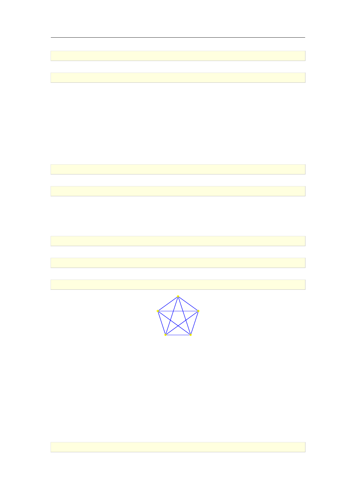
>G:=set_edge_weight(graph(%{[[1,2],4],[[2,3],5]%}),[1,2],6)
an undirected weighted graph with 3 vertices and 2 edges
>get_edge_weight(G,[1,2])
6
2.3.3. Contracting edges
The command contract_edge is used for contracting edges in undirected graphs.
Syntax: contract_edge(G,e)
contract_edge accepts two arguments, an undirected graph G(V ; E)and an edge e= (v; w)2E,
and merges vand wto a single vertex, deleting the edge e. The resulting vertex inherits the label
of v. The modified copy of Gis returned.
>K5:=complete_graph(5)
an undirected unweighted graph with 5 vertices and 10 edges
>contract_edge(K5,[1,2])
an undirected unweighted graph with 4 vertices and 6 edges
To contract a set fe1; e2; :::; ekg⊂Eof edges in G, none two of which are incident (i.e. when the
given set is a matching in G), one can use the foldl command. In the following example, the
complete graph K5is obtained from Petersen graph by edge contraction.
>P:=graph("petersen")
an undirected unweighted graph with 10 vertices and 15 edges
>G:=foldl(contract_edge,P,[0,5],[1,6],[2,7],[3,8],[4,9])
an undirected unweighted graph with 5 vertices and 10 edges
>draw_graph(G)
0
1
23
4
2.3.4. Subdividing edges
The command subdivide_edges is used for graph subdivision.
Syntax: subdivide_edges(G,e|S)
subdivide_edges(G,e|S,r)
subdivide_edges accepts two or three arguments: a graph G(V ; E), a single edge/arc e2Eor
a list of edges/arcs S⊂Eand optionally a positive integer r(which defaults to 1). Each of the
specified edges/arcs will be subdivided with exactly rnew vertices, labeled with the smallest
available nonnegative integers. The resulting graph, which is homeomorphic to G, is returned.
If the endpoints of the edge being subdivided have valid coordinates, the coordinates of the inserted
vertices will be computed accordingly.
>G:=graph("petersen")
50 Modifying graphs
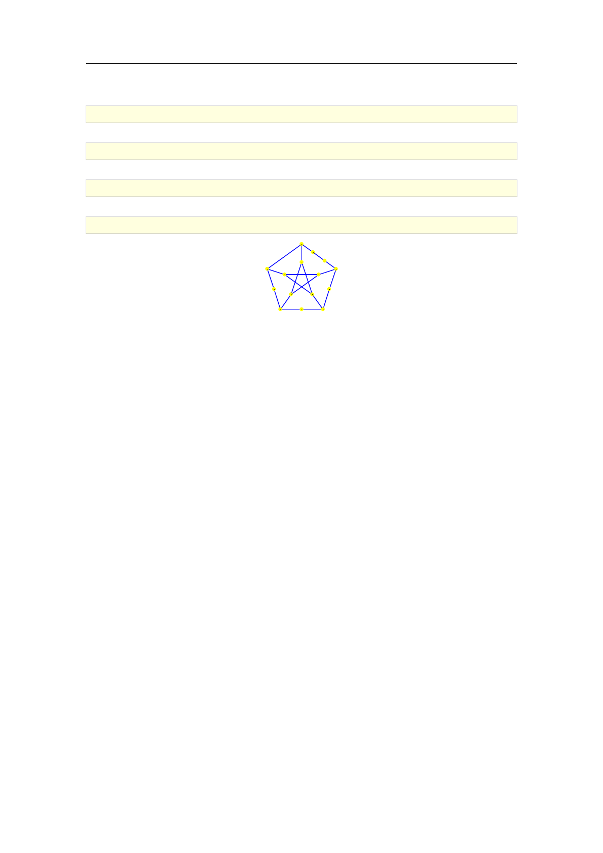
an undirected unweighted graph with 10 vertices and 15 edges
>G:=subdivide_edges(G,[2,3])
an undirected unweighted graph with 11 vertices and 16 edges
>G:=subdivide_edges(G,[[1,2],[3,4]])
an undirected unweighted graph with 13 vertices and 18 edges
>G:=subdivide_edges(G,[0,1],2)
an undirected unweighted graph with 15 vertices and 20 edges
>draw_graph(G)
0
1
23
4
5
6
78
9
10
11
12
13
14
2.4. Using attributes
2.4.1. Graph attributes
The graph structure maintains a set of attributes as tag-value pairs which can be accessed
and/or modified by using the commands set_graph_attribute,get_graph_attribute,
list_graph_attributes and discard_graph_attribute.
Syntax: set_graph_attribute(G,tag1=value1,tag2=value2,...)
set_graph_attribute(G,[tag1=value1,tag2=value2,...])
set_graph_attribute(G,[tag1,tag2,...],[value1,value2,...])
get_graph_attribute(G,tag1,tag2,...)
get_graph_attribute(G,[tag1,tag2,...])
list_graph_attributes(G)
discard_graph_attribute(G,tag1,tag2,...)
discard_graph_attribute(G,[tag1,tag2,...])
The command set_graph_attribute is used for modifying the existing graph attributes or adding
new ones. It accepts two arguments, a graph Gand a sequence or list of graph attributes in form
tag=value where tag is a string. Alternatively, attributes may be specified as a sequence of two
lists [tag1,tag2,...] and [value1,value2,...]. The command sets the specified values to the
indicated attribute slots, which are meant to represent some global properties of the graph G, and
returns the modified copy of G.
The previously set graph attribute values can be fetched with the command get_graph_attribute
which accepts two arguments: a graph Gand a sequence or list of tags. The corresponding values
will be returned in a sequence or list, respectively. If some attribute is not set, undef is returned
as its value.
To list all graph attributes of Gfor which the values are set, use the list_graph_attributes
command which takes Gas its only argument.
To discard a graph attribute, use the discard_graph_attribute command. It accepts two argu-
ments: a graph Gand a sequence or list of tags to be cleared, and returns the modified copy of G.
Two tags being used by the CAS commands are directed and weighted, so it is not advisable
to overwrite their values using this command; use the make_directed,make_weighted and
underlying_graph commands instead. Another attribute used internally is name, which holds
the name of the respective graph (as a string).
2.4 Using attributes 51

>G:=digraph(trail(1,2,3,1))
a directed unweighted graph with 3 vertices and 3 arcs
>G:=set_graph_attribute(G,"name"="C3","message"="this is some text")
C3: a directed unweighted graph with 3 vertices and 3 arcs
>get_graph_attribute(G,"message")
this is some text
>list_graph_attributes(G)
[directed =true;weighted =false;name =C3;message =this is some text]
>G:=discard_graph_attribute(G,"message")
C3: a directed unweighted graph with 3 vertices and 3 arcs
>list_graph_attributes(G)
[directed =true;weighted =false;name =C3]
2.4.2. Vertex attributes
For every vertex of a graph, the list of attributes in form of tag-value pairs is maintained, which can
be accessed/modified by using the commands set_vertex_attribute,get_vertex_attribute,
list_vertex_attributes and discard_vertex_attribute.
Syntax: set_vertex_attribute(G,v,tag1=value1,tag2=value2,...)
set_vertex_attribute(G,v,[tag1=value1,tag2=value2,...])
set_vertex_attribute(G,v,[tag1,tag2,...],[value1,value2,...])
get_vertex_attribute(G,v,tag1,tag2,...)
get_vertex_attribute(G,v,[tag1,tag2,...])
list_vertex_attributes(G,v)
discard_vertex_attribute(G,v,tag1,tag2,...)
discard_vertex_attribute(G,v,[tag1,tag2,...])
The command set_vertex_attribute is used for modifying the existing vertex attributes or
adding new ones. It accepts three arguments, a graph G(V ; E), a vertex v2Vand a sequence or
list of attributes in form tag=value where tag is a string. Alternatively, attributes may be specified
as a sequence of two lists [tag1,tag2,...] and [value1,value2,...]. The command sets the
specified values to the indicated attributes of the vertex vand returns the modified copy of G.
The previously set attribute values for vcan be fetched with the command get_vertex_attribute
which accepts three arguments: G,vand a sequence or list of tags. The corresponding values will
be returned in a sequence or list, respectively. If some attribute is not set, undef is returned as
its value.
To list all attributes of vfor which the values are set, use the list_vertex_attributes command
which takes two arguments, Gand v.
The discard_vertex_attribute command is used for discarding attribute(s) assigned to some
vertex v2V. It accepts three arguments: G,vand a sequence or list of tags to be cleared, and
returns the modified copy of G.
The attributes label,color,shape and pos are also used internally. These hold the vertex label, color,
shape and coordinates in a drawing, respectively. If the color is not set for a vertex, the latter is
drawn in yellow. The shape attribute may have one of the following values: square,triangle,diamond,
star or plus. If the shape attribute is not set or has a different value, the circled shape is applied
when drawing the vertex.
The following example shows how to change individual labels and colors.
52 Modifying graphs
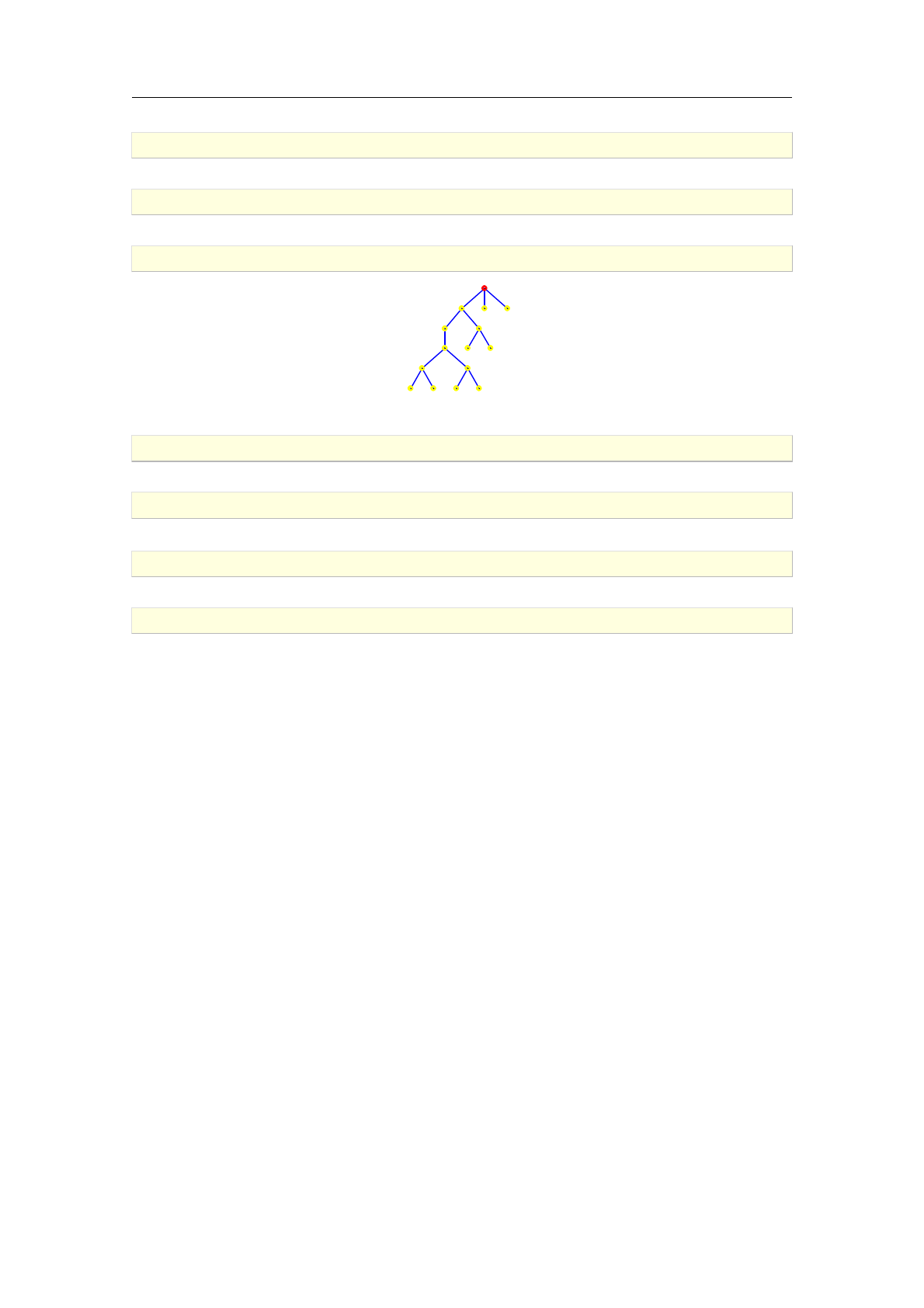
>T:=complete_binary_tree(3)
an undirected unweighted graph with 15 vertices and 14 edges
>T:=set_vertex_attribute(T,5,"label"="root","color"=red)
an undirected unweighted graph with 15 vertices and 14 edges
>draw_graph(T,tree="root")
0
1
2
3 4
root
6
7 8 9 10
11 12
13 14
A vertex may also hold custom attributes.
>T:=set_vertex_attribute(T,"root","depth"=3,"shape"="square")
an undirected unweighted graph with 15 vertices and 14 edges
>list_vertex_attributes(T,"root")
[label =root;color =r e d; shape =square;depth = 3]
>T:=discard_vertex_attribute(T,"root","color")
an undirected unweighted graph with 15 vertices and 14 edges
>list_vertex_attributes(T,"root")
[label =root;shape =square;depth = 3]
2.4.3. Edge attributes
For every edge of a graph, the list of attributes in form of key-value pairs is maintained, which can
be accessed and/or modified by using the commands set_edge_attribute,get_edge_attribute,
list_edge_attributes and discard_edge_attribute.
Syntax: set_edge_attribute(G,e,tag1=value1,tag2=value2,...)
set_edge_attribute(G,e,[tag1=value1,tag2=value2,...])
set_edge_attribute(G,e,[tag1,tag2,...],[value1,value2,...])
get_edge_attribute(G,e,tag1,tag2,...)
get_edge_attribute(G,e,[tag1,tag2,...])
list_edge_attributes(G,e)
discard_edge_attribute(G,e,tag1,tag2,...)
discard_edge_attribute(G,e,[tag1,tag2,...])
The command set_edge_attribute is used for modifying the existing edge attributes or adding
new ones. It accepts three arguments, a graph G(V ; E), an edge/arc e2Eand a sequence or list
of attributes in form tag=value where tag is a string. Alternatively, attributes may be specified
as a sequence of two lists [tag1,tag2,...] and [value1,value2,...]. The command sets the
specified values to the indicated attributes of the edge/arc eand returns the modified copy of G.
The previously set attribute values for ecan be fetched with the command get_edge_attribute
which accepts three arguments: G,eand a sequence or list of tags. The corresponding values will
be returned in a sequence or list, respectively. If some attribute is not set, undef is returned as
its value.
To list all attributes of efor which the values are set, use the list_edge_attributes command
which takes two arguments, Gand e.
2.4 Using attributes 53
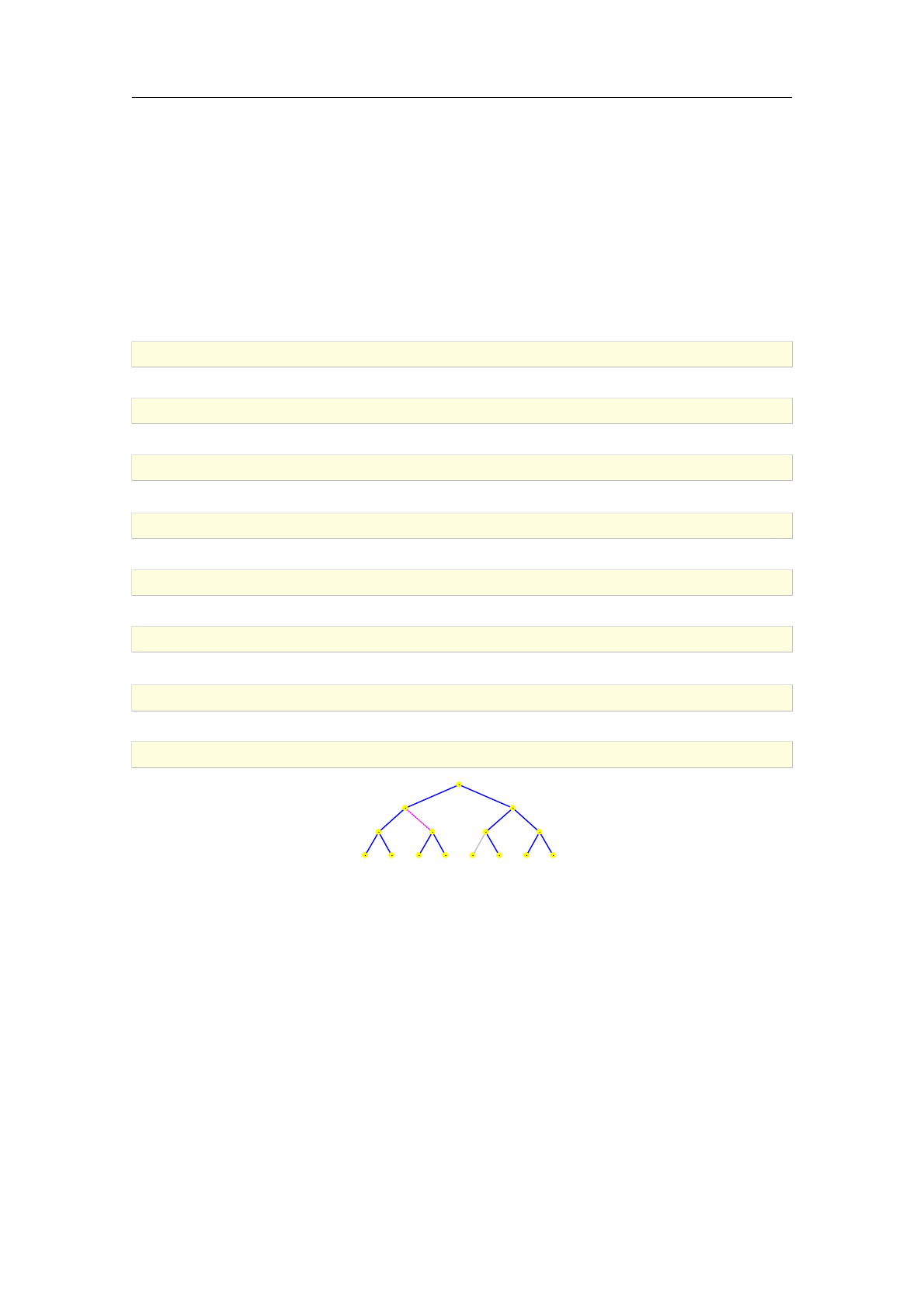
To discard attribute(s) assigned to ecall the discard_edge_attribute command, which accepts
three arguments: G,eand a sequence or list of tags to be cleared, and returns the modified copy
of G.
The attributes weight,color,style,pos and temp are also used internally. They hold the edge weight,
color, line style, the coordinates of the weight label anchor (and also the coordinates of the arrow)
and true if the edge is temporary. If the color attribute is not set for an edge, the latter is drawn
in blue, unless it is a temporary edge, in which case it is drawn in light gray. The style attribute
may have one of the following values: dashed,dotted or bold. If the style attribute is not set or has
a different value, the solid line style is applied when drawing the edge.
The following example illustrates the possibilities of using edge attributes.
>T:=complete_binary_tree(3)
an undirected unweighted graph with 15 vertices and 14 edges
>T:=set_edge_attribute(T,[1,4],"cost"=12.8,"message"="this is some text")
an undirected unweighted graph with 15 vertices and 14 edges
>list_edge_attributes(T,[1,4])
[cost =12.8;message =this is some text]
>T:=discard_edge_attribute(T,[1,4],"message")
an undirected unweighted graph with 15 vertices and 14 edges
>T:=set_edge_attribute(T,[1,4],"style"="dotted","color"=magenta)
an undirected unweighted graph with 15 vertices and 14 edges
>list_edge_attributes(T,[1,4])
[color =m a g e n t a; style =dotted;cost =12.8]
>T:=set_edge_attribute(T,[5,11],"temp"=true)
an undirected unweighted graph with 15 vertices and 14 edges
>draw_graph(T)
0
1 2
3 4 5 6
7 8 9 10 11 12 13 14
54 Modifying graphs
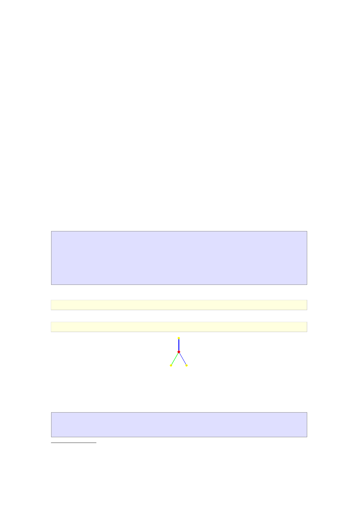
Chapter 3
Import and export
3.1. Importing graphs
3.1.1. Loading graphs from dot files
The command import_graph is used for importing a graph from text file in dot format.
Syntax: import_graph(filename)
import_graph accepts a string filename as its only argument and returns the graph constructed
from instructions written in the file filename or undef on failure. The passed string should contain
the path to a file in dot format. The file extension .dot may be omitted in the filename since dot
is the only supported format. The alternative extension is .gv3.1, which must be explicitly specified.
If a relative path to the file is specified, i.e. if it does not contain a leading forward slash, the
current working directory (which can be obtained by calling the pwd command) will be used as the
reference. The working directory can be changed by using the command cd.
For example, assume that the file example.dot is saved in the directory Documents/dot/ with the
following contents:
graph "Example graph" {
a [label="Foo"];
b [shape=diamond,color=red];
a -- b [style=bold];
b -- c [color=green];
b -- d [style=dotted];
}
To import the graph, input:
>G:=import_graph("Documents/dot/example.dot")
Example graph: an undirected unweighted graph with 4 vertices and 3 edges
>draw_graph(G)
Foo
b
c d
3.1.2. The dot file format overview
Giac has some basic support for dot language. Each dot file is used to hold exactly one graph and
should consist of a single instance of the following environment:
strict? (graph | digraph) name? {
...
}
3.1. Although it is recommended to use .gv as the extension for dot files to avoid a certain confusion between different
file types, Giac uses the .dot extension because it coincides with the format name. This may change in the future.
55
The keyword strict may be omitted, as well as the name of the graph, as indicated by the question
marks. The former is used to differentiate between simple graphs (strict) and multigraphs (non-
strict). Since Giac supports only simple graphs, strict is redundant.
For specifying undirected graphs the keyword graph is used, while the digraph keyword is used
for undirected graphs.
The graph/digraph environment contains a series of instructions describing how the graph should
be built. Each instruction ends with the semicolon (;) and has one of the following forms.
syntax creates
vertex_name [attributes]? isolated vertices
V1 <edgeop> V2 <edgeop> ::: <edgeop> Vk [attributes]? edges and trails
graph [attributes] graph attributes
Here, attributes is a comma-separated list of tag-value pairs in form tag=value,<edgeop> is
-- for undirected and -> for directed graphs. Each of V1,V2 etc. is either a vertex name or a set
of vertex names in form {vertex_name1 vertex_name2 ...}. In the case a set is specified, each
vertex from that set is connected to the neighbor operands. Every specified vertex will be created
if it does not exist yet.
Any line beginning with #is ignored. C-like line and block comments are recognized and skipped
as well.
Using the dot syntax it is easy to specify a graph with adjacency lists. For example, the following
is the contents of a file which defines the octahedral graph with 6 vertices and 12 edges.
# octahedral graph
graph "octahedron" {
1 -- {3 6 5 4};
2 -- {3 4 5 6};
3 -- {5 6};
4 -- {5 6};
}
3.2. Exporting graphs
The command export_graph is used for saving graphs to disk in dot or L
AT
E
X format.
Syntax: export_graph(G,filename)
export_graph(G,filename,latex[=<params>])
3.2.1. Saving graphs in dot format
export_graph accepts two mandatory arguments, a graph Gand a string filename, and writes G
to the file specified by filename, which must be a path to the file, either relative or absolute; in
the former case the current working directory will be used as the reference. If only two arguments
are given the graph is saved in dot format. The file name may be entered with or without .dot
extension. The command returns 1 on success and 0 on failure.
>export_graph(G,"Documents/dot/copy_of_example")
1
3.2.2. Saving graph drawings in L
A
T
E
X format
When calling the export_graph command, an optional third argument in form latex[=<params>]
may be given. In that case the drawing of G(obtained by calling the draw_graph command) will
be saved to the L
AT
E
X file indicated by filename (the extension .tex may be omitted). Optionally,
one can specify a parameter or list of parameters params which will be passed to the draw_graph
command.
56 Import and export
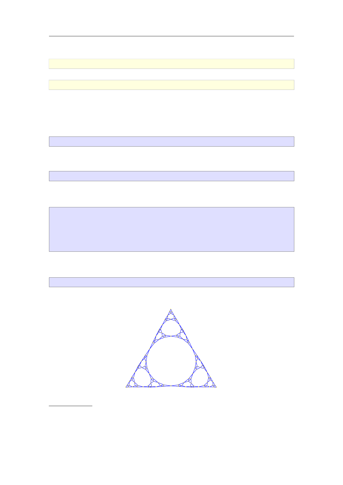
For example, let us create a picture of the Sierpi«ski sieve graph of order n= 5, i.e. the graph ST3
5.
>G:=sierpinski_graph(5,3,triangle)
an undirected unweighted graph with 123 vertices and 243 edges
>export_graph(G,"Documents/st53.tex",latex=[spring,labels=false])
1
The L
AT
E
X file obtained by exporting a graph is easily converted into an EPS file, which can
subsequently be inserted3.2 in a paper, report or some other document. A Linux user simply needs
to launch a terminal emulator, navigate to the directory in which the exported file, in this case
st53.tex, is stored and enter the following command:
latex st53.tex && dvips st53.dvi && ps2eps st53.ps
This will produce the (properly cropped) st53.eps file in the same directory. Afterwards, it is
recommended to enter
rm st53.tex st53.aux st53.log st53.dvi st53.ps
to delete the intermediate files. The above two commands can be combined in a simple shell script
which takes the name of the exported file (without the extension) as its input argument:
#!/bin/bash
# convert LaTeX to EPS
latex $1.tex
dvips $1.dvi
ps2eps $1.ps
rm $1.tex $1.aux $1.log $1.dvi $1.ps
Assuming that the script is stored under the name latex2eps in the same directory as st53.tex,
to do the conversion it is enough to input:
bash latex2eps st53
The drawing produced in our example is shown in Figure 3.1.
Fig. 3.1. drawing of the Sierpi«ski graph ST3
5using L
AT
E
X and PSTricks
3.2. Alternatively, a PSTricks picture from the body of the .tex file can be copied to some other L
AT
E
X document.
3.2 Exporting graphs 57


Chapter 4
Graph properties
4.1. Basic properties
4.1.1. Determining the type of a graph
The commands is_directed and is_weighted are used for determining the type of a graph:
whether is it directed or not resp. weighted or not.
Syntax: is_directed(G)
is_weighted(G)
Both commands accept a graph Gas their only argument. is_directed resp. is_weighted returns
true if Gis directed resp. weighted, else it returns false.
>G:=graph(trail(1,2,3,4,5,1,3))
an undirected unweighted graph with 5 vertices and 6 edges
>is_directed(G)
false
>is_directed(make_directed(G))
true
>is_weighted(G)
false
>is_weighted(make_weighted(G,randmatrix(5,5,99)))
true
4.1.2. Listing vertices and edges
The command vertices or graph_vertices resp. edges is used for extracting set of vertices
resp. set of edges from a graph. To obtain the number of vertices resp. the number of edges, use
the number_of_vertices resp. the number_of_edges command.
Syntax: vertices(G)
graph_vertices(G)
edges(G)
edges(G,weights)
number_of_vertices(G)
number_of_edges(G)
vertices or graph_vertices accepts a graph G(V ; E)as its only argument and returns the set
of vertices Vin the same order in which they were created.
edges accepts one or two arguments, a graph G(V ; E)and optionally the identifier weights. The
command returns the set of edges E(in a non-meaningful order). If weights is specified, each edge
is paired with the corresponding weight (in this case Gmust be a weighted graph).
number_of_vertices resp. number_of_edges accepts the input graph G(V ; E)as its only argu-
ment and returns jVjresp. jEj.
59

>G:=hypercube_graph(2)
an undirected unweighted graph with 4 vertices and 4 edges
>vertices(G)
[00;01;10;11]
>C:=graph("coxeter")
an undirected unweighted graph with 28 vertices and 42 edges
>vertices(C)
[a1; a2; a7; z1; a3; z2; a4; z3; a5; z4; a6; z5; z6; z7; b1; b3; b6; b2; b4; b7; b5; c1; c4; c5; c2; c6; c3; c7]
>number_of_vertices(C), number_of_edges(C)
28;42
>H:=digraph([[0,2.32,0,0.25],[0,0,0,1.32],[0,0.50,0,0],[0.75,0,3.34,0]])
a directed weighted graph with 4 vertices and 6 arcs
>edges(H)
f[0;1];[0;3];[1;3];[2;1];[3;0];[3;2]g
>edges(H,weights)
f[[0;1];2.32];[[0;3];0.25];[[1;3];1.32];[[2;1];0.5];[[3;0];0.75];[[3;2];3.34]g
4.1.3. Equality of graphs
Two graphs are considered equal if they are both (un)weighted and (un)directed and if the com-
mands vertices and edges give the same results for both graphs. To determine whether two
graphs are equal use the command graph_equal.
Syntax: graph_equal(G1,G2)
graph_equal accepts two arguments, graphs G1and G2, and returns true if G1is equal to G2
with respect to the above definition. Else, it returns false.
>G1:=graph([1,2,3],%{[1,2],[2,3]%})
an undirected unweighted graph with 3 vertices and 2 edges
>G2:=graph([1,3,2],%{[1,2],[2,3]%})
an undirected unweighted graph with 3 vertices and 2 edges
>graph_equal(G1,G2)
false
>G3:=graph(trail(1,2,3))
an undirected unweighted graph with 3 vertices and 2 edges
>graph_equal(G1,G3)
true
>G4:=digraph(trail(1,2,3))
a directed unweighted graph with 3 vertices and 2 arcs
>graph_equal(G1,G4)
false
60 Graph properties
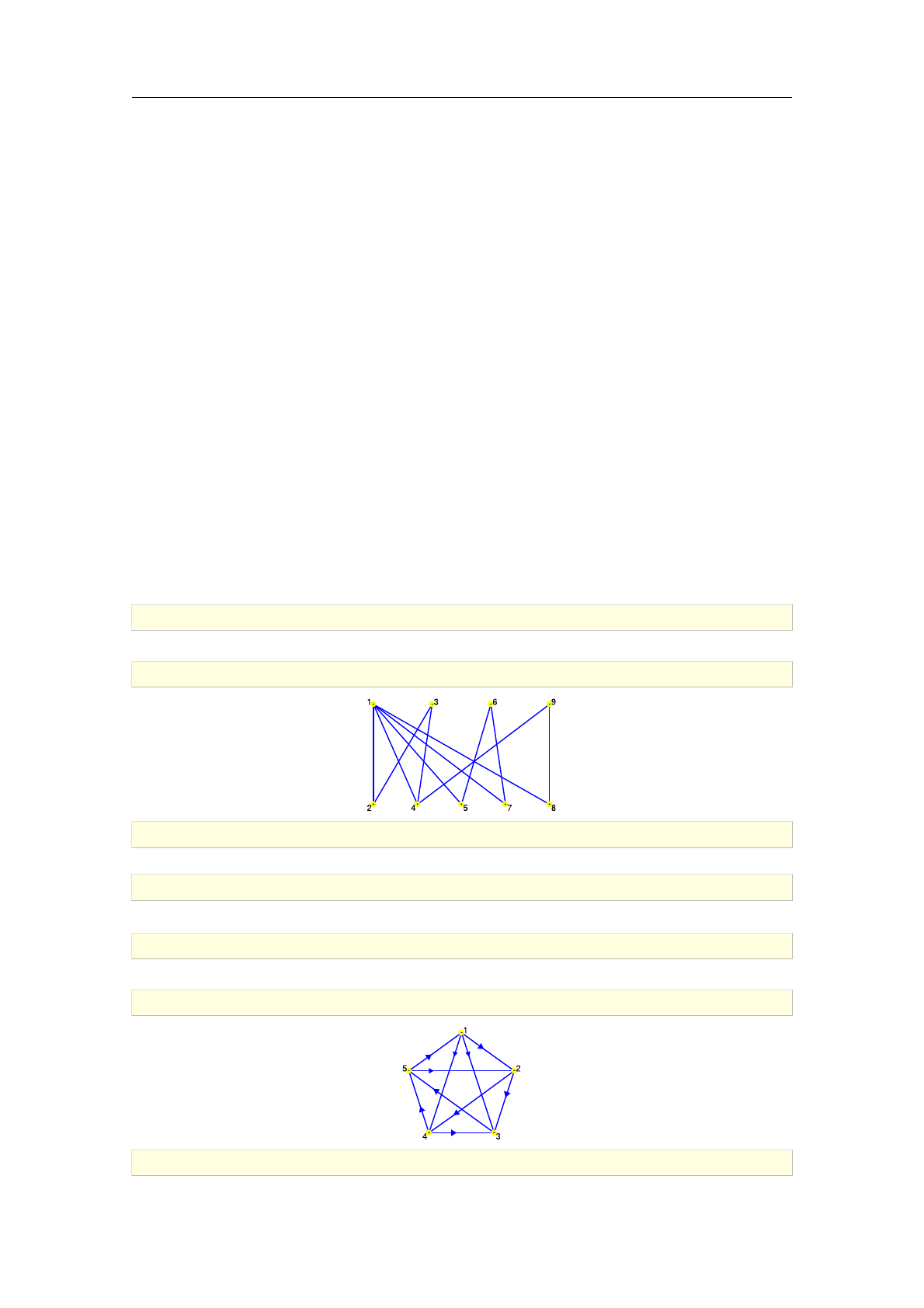
4.1.4. Vertex degrees
The command vertex_degree is used for computing the degree of a vertex, i.e. counting the vertices
adjacent to it. The related specialized commands are vertex_out_degree,vertex_in_degree,
degree_sequence,minimum_degree and maximum_degree.
Syntax: vertex_degree(G,v)
vertex_in_degree(G,v)
vertex_out_degree(G,v)
degree_sequence(G)
minimum_degree(G,v)
maximum_degree(G,v)
vertex_degree accepts two arguments, a graph G(V ; E)and a vertex v2V, and returns the
cardinality of the set fw2V: (v; w)2Eg, i.e. the number of vertices in Vwhich are adjacent to
v. Note that the edge directions are ignored in case Gis a digraph.
When dealing with directed graphs, one can also use the specialized command vertex_out_degree
resp. vertex_in_degree which accepts the same arguments as vertex_degree but returns the
number of arcs (v; w)2Eresp. the number of arcs (w; v)2E, where w2V.
To obtain the list of degrees of all vertices v2V, use the degree_sequence command which accepts
a graph G(V ; E)as its only argument and returns the list of degrees of vertices from Vin the same
order as returned by the command vertices. If Gis a digraph, arc directions are ignored.
To compute the minimum vertex degree δ(G)or the maximum vertex degree ∆(G)in an undirected
graph G, use the command minimum_degree or maximum_degree, respectively. Both commands
accept Gas the only argument and return δ(G)resp. ∆(G).
>G:=graph(trail(1,2,3,4,1,5,6,7,1,8,9,4))
an undirected unweighted graph with 9 vertices and 11 edges
>draw_graph(G)
>vertex_degree(G,1)
5
>degree_sequence(G)
[5;2;2;3;2;2;2;2;2]
>T:=random_tournament([1,2,3,4,5])
a directed unweighted graph with 5 vertices and 10 arcs
>draw_graph(T)
>vertex_out_degree(T,1)
4.1 Basic properties 61

3
>vertex_in_degree(T,5)
2
The command line below shows that Petersen graph is cubic (3-regular).
>P:=graph("petersen")
an undirected unweighted graph with 10 vertices and 15 edges
>minimum_degree(P), maximum_degree(P)
3;3
>is_regular(P,3)
true
4.1.5. Regular graphs
The command is_regular is used for determining whether the given graph is regular.
Syntax: is_regular(G)
is_regular(G,d)
is_regular accepts one or two arguments, a graph G(V ; E)and optionally a nonnegative integer
or an unassigned identifier d. If Gis undirected, the return value is true if δG= ∆G, i.e. if the
minimal vertex degree is equal to the maximal vertex degree in G, otherwise false is returned.
If Gis a digraph, it is also required for each vertex v2Vto have the same in- and out-degree. If
the second argument is given, Gis tested for d-regularity in case dis an integer, otherwise ∆Gis
written to din case the latter is an identifier and Gis regular.
The complexity of the algorithm is O(jVj).
>G:=graph("petersen")
an undirected unweighted graph with 10 vertices and 15 edges
>is_regular(G,d)
true
>d
3
>is_regular(G,2)
false
>is_regular(graph("grotzsch"))
false
>
G:=digraph(%{[1,5],[1,6],[2,3],[2,4],[3,1],[3,4],[4,1],[4,5],[5,2],[5,6],[6,
2],[6,3]%})
a directed unweighted graph with 6 vertices and 12 arcs
>draw_graph(G,spring)
1
5
6 2
3
4
62 Graph properties

>is_regular(G,4)
true
>H:=add_arc(delete_arc(G,[5,6]),[6,5])
a directed unweighted graph with 6 vertices and 12 arcs
>is_regular(H,4)
false
>is_regular(underlying_graph(H))
true
4.1.6. Strongly regular graphs
The command is_strongly_regular is used for determining whether the given graph is
strongly regular.
Syntax: is_strongly_regular(G)
is_strongly_regular(G,srg)
is_strongly_regular accepts one or two arguments, a graph G(V ; E)and optionally an unas-
signed identifier srg. It returns true if Gis regular and there are integers λand µsuch that every
two adjacent vertices resp. non-adjacent vertices in Vhave exactly λresp. µcommon neighbors.
Else, it returns false. If the second argument is given, the list [k; λ; µ], where kis the degree of
G, is stored to srg.
The complexity of the algorithm is O(kjVj2).
>G:=graph("clebsch")
an undirected unweighted graph with 16 vertices and 40 edges
>is_regular(G)
true
>is_strongly_regular(G)
true
>H:=graph("shrikhande")
an undirected unweighted graph with 16 vertices and 48 edges
>is_strongly_regular(H,s)
true
>s
[6;2;2]
>is_strongly_regular(cycle_graph(5))
true
>is_strongly_regular(cycle_graph(6))
false
4.1.7. Vertex adjacency
The command has_edge is used for checking whether two vertices in an undirected graph are
adjacent. For digraphs, there is an analogous command has_arc.
4.1 Basic properties 63

The command neighbors is used for obtaining the list of vertices in a graph that are adjacent to
the particular vertex or the complete adjacency structure of the graph, in sparse form.
The command departures resp. arrivals is used for obtaining all neighbors of a vertex vin a
digraph which are the heads resp. the tails of the corresponding arcs.
Syntax: has_edge(G,[u,v])
has_arc(G,[u,v])
neighbors(G)
neighbors(G,v)
departures(G)
departures(G,v)
arrivals(G)
arrivals(G,v)
has_edge accepts two arguments, an undirected graph G(V ; E)and a list [u,v] where u; v 2V.
The command returns true if uv 2Eand false otherwise. The syntax for has_arc is the same,
except now Gis required to be directed. Note, however, that the order of vertices uand vmatters
in digraphs. The complexity of both algorithms is O(log jVj).
neighbors accepts one or two arguments, a graph G(V ; E)and optionally a vertex v2V. The
command returns the list of neighbors of vin Gif vis given. Otherwise, it returns the list of lists
of neighbors for all vertices in V, in order of vertices(G). Note that edge directions are ignored
in case Gis a digraph.
departures resp. arrivals accepts one or two arguments, a digraph G(V ; E)and optionally a
vertex v2V, and returns the list Lvcontaining all vertices w2Vfor which vw 2Eresp. wv 2E.
If vis omitted, the list of lists Lvfor every v2Vis returned.
>G:=graph(trail(1,2,3,4,5,2))
an undirected unweighted graph with 5 vertices and 5 edges
>has_edge(G,[1,2])
true
>has_edge(G,[2,1])
true
>has_edge(G,[1,3])
false
>D:=digraph(trail(1,2,3,4,5,2,1))
a directed unweighted graph with 5 vertices and 6 arcs
>has_arc(D,[1,2])
true
>has_arc(D,[2,1])
true
>has_arc(D,%{1,2%})
true
>has_arc(D,[4,5])
true
>has_arc(D,[5,4])
false
>has_arc(D,%{4,5%})
64 Graph properties
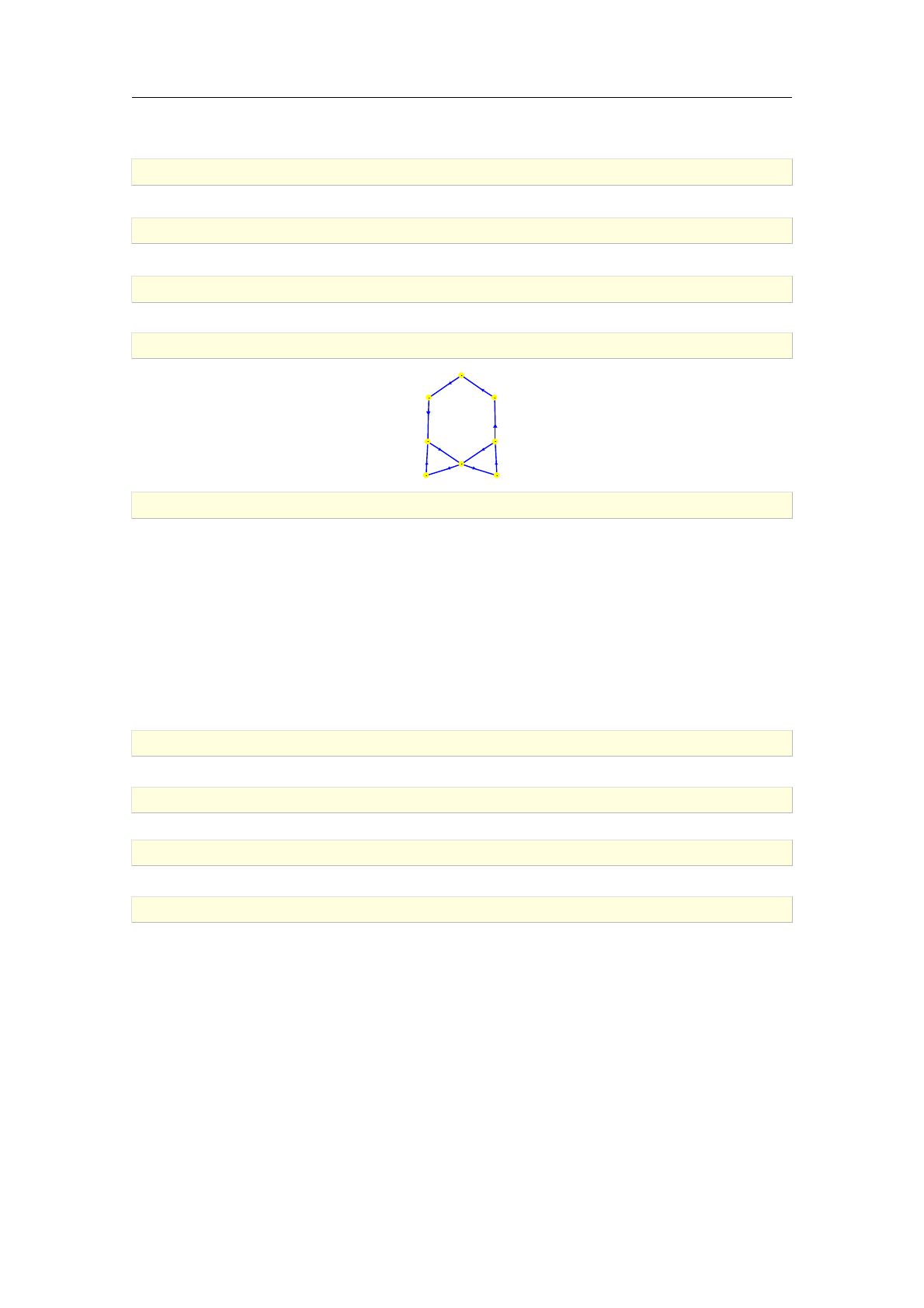
false
>neighbors(G,3)
[2;4]
>neighbors(G)
f[2];[1;3;5];[2;4];[3;5];[2;4]g
>G:=digraph(trail(1,2,3,4,2,5,1,6,7,8,4))
a directed unweighted graph with 8 vertices and 10 arcs
>draw_graph(G,spring)
1
2
3
4
5
6
7
8
>departures(G,2); arrivals(G,2); departures(G,1); arrivals(G,1)
[3;5];[1;4];[2;6];[5]
4.1.8. Tournament graphs
The command is_tournament is used for determining whether the given graph is a tournament.
Syntax: is_tournament(G)
is_tournament accepts a graph G(V ; E)as its only argument and returns true if Gis directed and
for each pair of vertices u; v 2Vit is either uv 2Eor vu 2E, i.e. there is exactly one arc between
uand v. Else, it returns false.
>T1:=digraph(%{[1,2],[2,3],[3,1]%})
a directed unweighted graph with 3 vertices and 3 arcs
>is_tournament(T1)
true
>T2:=digraph(%{[1,2],[2,3],[3,1],[1,3]%})
a directed unweighted graph with 3 vertices and 4 arcs
>is_tournament(T2)
false
4.1.9. Bipartite graphs
The command is_bipartite is used for determining if the given graph is bipartite.
Syntax: is_bipartite(G)
is_bipartite(G,P)
is_bipartite accepts one or two arguments, a graph G(V ; E)and optionally an unassigned
identifier P. It returns true if there is a partition of Vinto two sets Sand Tsuch that every edge
from Econnects a vertex in Sto one in T. Else, it returns false. If the second argument is given
and Gis bipartite, the partition of Vis stored to Pas a list of two lists of vertices, the first one
containing the vertices from Sand the second one containing vertices from T.
4.1 Basic properties 65

>K32:=complete_graph(3,2)
an undirected unweighted graph with 5 vertices and 6 edges
>is_bipartite(K32,bp)
true
>bp
[[0;1;2];[3;4]]
>draw_graph(K32,bipartite)
0 1 2
3 4
>adjacency_matrix(K32)
0
B
B
B
B
B
B
B
B
@
00011
00011
00011
11100
11100
1
C
C
C
C
C
C
C
C
A
>G:=cycle_graph(5)
an undirected unweighted graph with 5 vertices and 5 edges
>is_bipartite(G)
false
4.1.10. Edge incidence
The command incident_edges is used for obtaining edges incident to the given vertex in a graph.
Syntax: indcident_edges(G,v)
indcident_edges(G,L)
incident_edges accepts two argument, a graph G(V ; E)and a vertex v2Vor a list of vertices
L⊂V. The command returns the list of edges e1; e2; :::; ek2Ewhich have vas one of its endpoints.
Note that edge directions are ignored when Gis a digraph. To obtain only outgoing or incoming
edges, use the commands departures and arrivals, respectively.
>G:=cycle_graph([1,2,3,4,5])
C5: an undirected unweighted graph with 5 vertices and 5 edges
>incident_edges(G,1)
f[1;2];[1;5]g
>incident_edges(G,[2,4,5])
f[1;2];[1;5];[2;3];[3;4];[4;5]g
>G:=random_tournament([1,2,3,4,5])
a directed unweighted graph with 5 vertices and 10 arcs
>incident_edges(G,2)
66 Graph properties
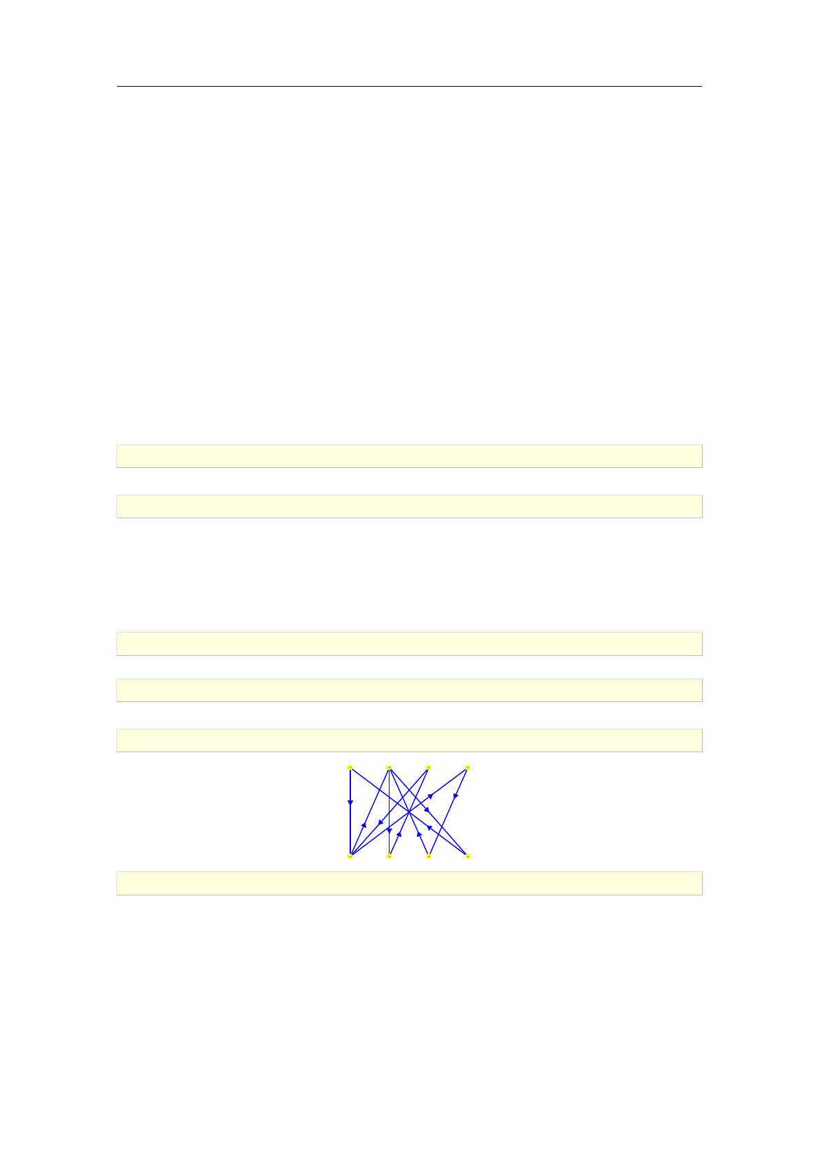
f[2;1];[2;3];[2;5];[4;2]g
4.2. Algebraic properties
4.2.1. Adjacency matrix
The command adjacency_matrix is used for obtaining the adjacency matrix of a graph.
Syntax: adjacency_matrix(G)
adjacency_matrix accepts a graph G(V ; E), where V=fv1; v2; :::; vng, as its only argument and
returns the square matrix A= [aij]of order nsuch that, for i; j = 1;2; :::; n,
aij =(1, if the set Econtains edge/arc vivj,
0;otherwise:
Note that tr (A) = 0. Also, the adjacency matrix of an undirected graph is always symmetrical.
>G:=graph("octahedron")
an undirected unweighted graph with 6 vertices and 12 edges
>A:=adjacency_matrix(G)
0
B
B
B
B
B
B
B
B
B
B
B
B
@
011110
101101
110011
110011
101101
011110
1
C
C
C
C
C
C
C
C
C
C
C
C
A
>transpose(A)==A
true
>D:=digraph(trail(1,2,3,4,5,2,6,7,3,8,1))
a directed unweighted graph with 8 vertices and 10 arcs
>draw_graph(D)
1
2
3
4
5 6
7 8
>A:=adjacency_matrix(D)
0
B
B
B
B
B
B
B
B
B
B
B
B
B
B
B
B
B
B
B
B
@
01000000
00100100
00010001
00001000
01000000
00000010
00100000
10000000
1
C
C
C
C
C
C
C
C
C
C
C
C
C
C
C
C
C
C
C
C
A
4.2 Algebraic properties 67
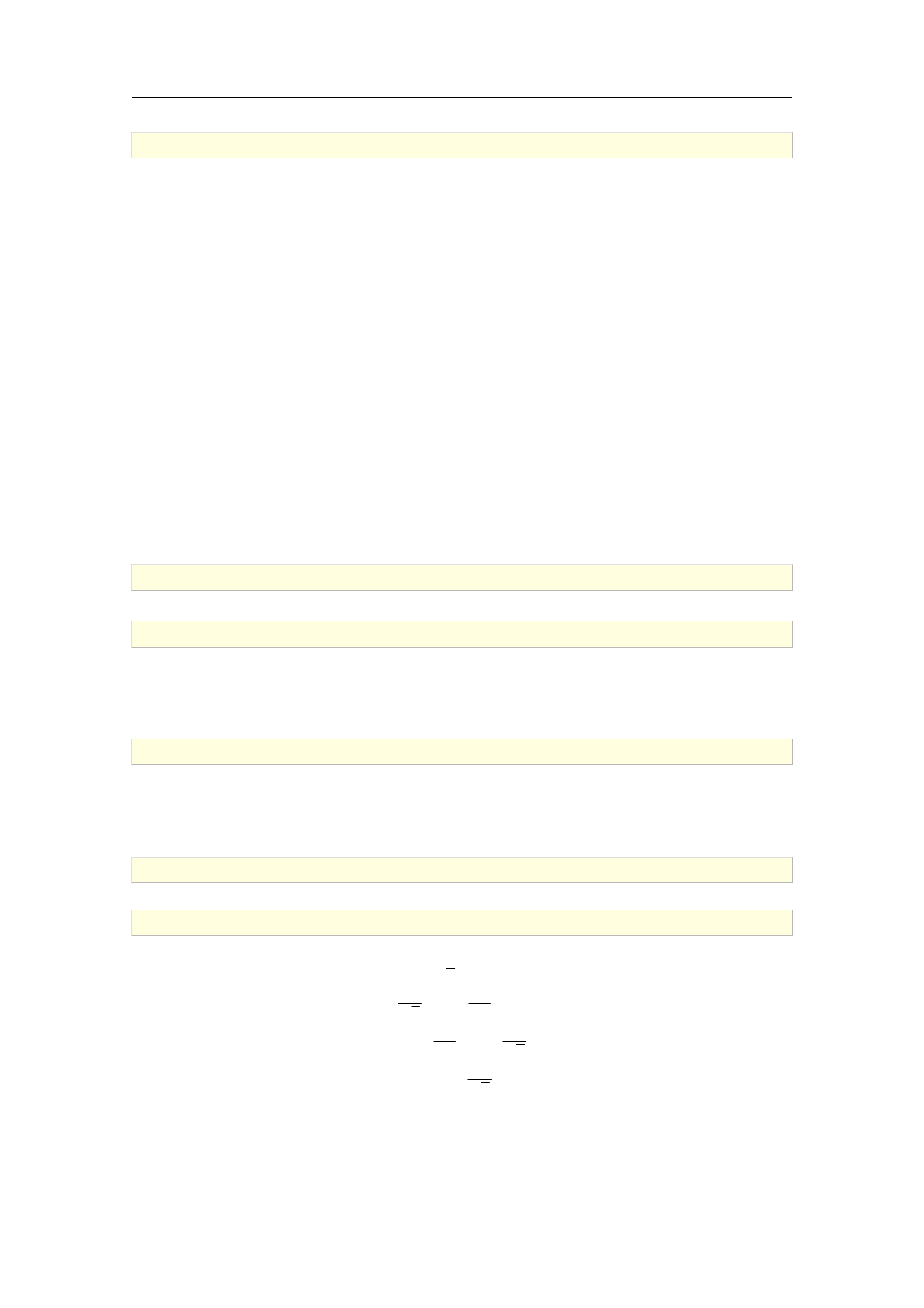
>transpose(A)==A
false
4.2.2. Laplacian matrix
The command laplacian_matrix is used for computing the Laplacian matrix of a graph.
Syntax: laplacian_matrix(G)
laplacian_matrix(G,normal)
laplacian_matrix accepts an undirected graph G(V ; E), where V=fv1; v2; :::; vng, and returns
the symmetric matrix L=D¡A, where Ais the adjacency matrix of Gand
D=0
B
B
B
B
B
B
@
deg(v1) 0 0 ··· 0
0deg(v2) 0 ··· 0
·
·
··
·
··
·
·····
·
·
0 0 0 ··· deg(vn)
1
C
C
C
C
C
C
A
:
The option normal may be passed as the second argument. In that case, the normalized Laplacian
Lsym := I¡D¡1/2 A D¡1/2 of Gis returned.
>G:=path_graph(4)
an undirected unweighted graph with 4 vertices and 3 edges
>A:=adjacency_matrix(G)
0
B
B
B
B
@
0 1 0 0
1 0 1 0
0 1 0 1
0 0 1 0
1
C
C
C
C
A
>L:=laplacian_matrix(G)
0
B
B
B
B
@
1¡1 0 0
¡12¡1 0
0¡12¡1
0 0 ¡1 1
1
C
C
C
C
A
>diag(degree_sequence(G))-A==L
true
>laplacian_matrix(G,normal)
0
B
B
B
B
B
B
B
B
B
B
B
B
B
B
B
B
B
B
B
B
B
B
@
1¡1
2
p0 0
¡1
2
p1¡1
20
0¡1
21¡1
2
p
0 0 ¡1
2
p1
1
C
C
C
C
C
C
C
C
C
C
C
C
C
C
C
C
C
C
C
C
C
C
A
The smallest eigenvalue of a Laplacian matrix of an undirected graph is always zero. Moreover,
its multiplicity is equal to the number of connected components in the corresponding graph [23,
pp. 280].
68 Graph properties
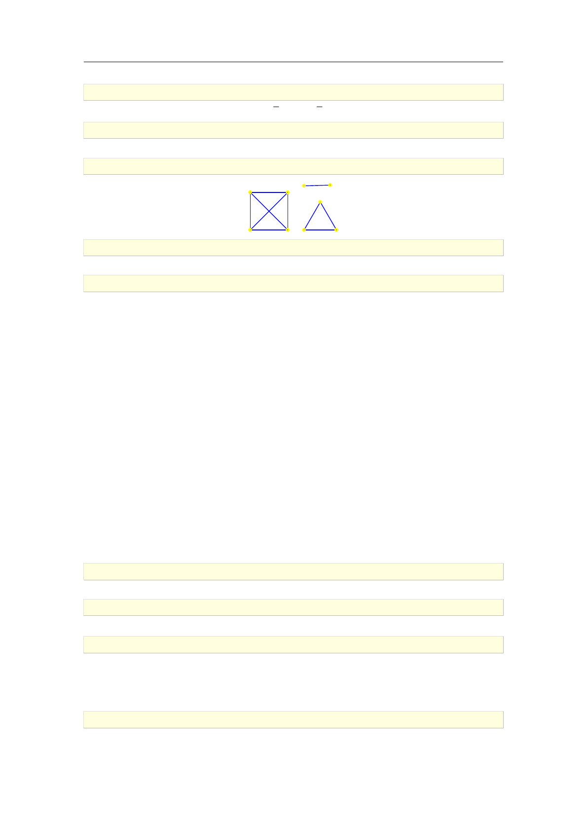
>sort(eigenvals(L))
0;¡2
p+ 2;2;2
p+ 2
>H:=disjoint_union(complete_graph(4),cycle_graph(3),path_graph(2))
an undirected unweighted graph with 9 vertices and 10 edges
>draw_graph(H,labels=false)
>eigenvals(laplacian_matrix(H))
0;0;0;4;4;4;3;3;2
>nops(connected_components(H))
3
4.2.3. Incidence matrix
The command incidence_matrix is used for obtaining the incidence matrix of a graph.
Syntax: incidence_matrix(G)
incidence_matrix accepts a graph G(V ; E), where V=fv1; v2; :::; vngand E=fe1; e2; :::; emg, as
its only argument and returns the n×mmatrix B= [bij]such that, for all i= 1;2; :::; n and j= 1;
2; :::; m,
bij =(1;if the vertex viis incident to the edge ej,
0;otherwise
if Gis undirected resp.
bij =8
>
>
<
>
>
:
1;if the vertex viis the head of the arc ej,
¡1;if the vertex viis the tail of the arc ej,
0;otherwise
if Gis directed.
>K4:=complete_graph([1,2,3,4])
an undirected unweighted graph with 4 vertices and 6 edges
>edges(K4)
f[1;2];[1;3];[1;4];[2;3];[2;4];[3;4]g
>incidence_matrix(K4)
0
B
B
B
B
@
111000
100110
010101
001011
1
C
C
C
C
A
>DG:=digraph(trail(1,2,3,4,5,3),trail(1,5,2,4,1))
a directed unweighted graph with 5 vertices and 9 arcs
4.2 Algebraic properties 69
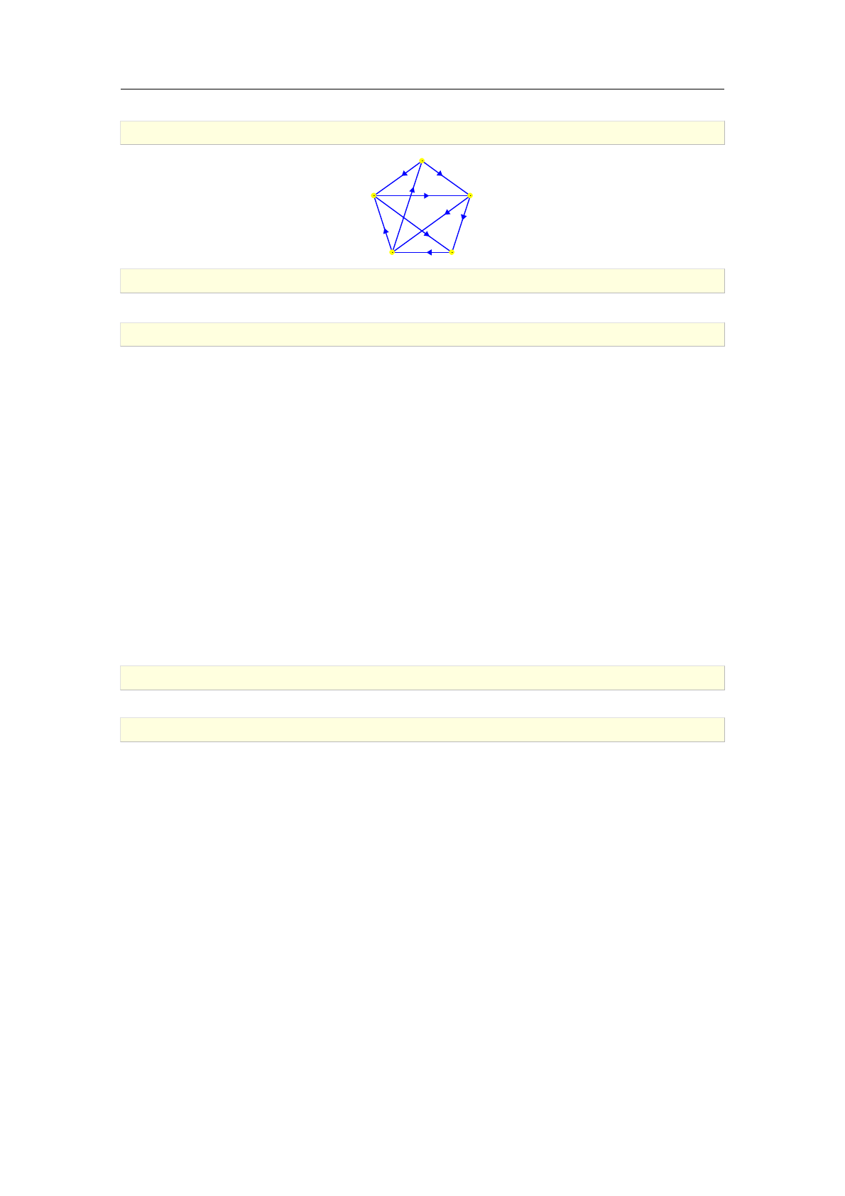
>draw_graph(DG)
1
2
34
5
>edges(DG)
f[1;2];[1;5];[2;3];[2;4];[3;4];[4;1];[4;5];[5;2];[5;3]g
>incidence_matrix(DG)
0
B
B
B
B
B
B
B
B
@
¡1¡10001000
1 0 ¡1¡100010
0010¡10001
00011¡1¡1 0 0
0100001¡1¡1
1
C
C
C
C
C
C
C
C
A
4.2.4. Weight matrix
The command weight_matrix is used for obtaining the weight matrix of a weighted graph.
Syntax: weight_matrix(G)
weight_matrix accepts a graph G(V ; E), where V=fv1; v2; :::; vng, as its only argument and
returns the square matrix M= [mij]of order nsuch that mij equals zero if viand vjare not
adjacent and the weight of the edge/arc vivjotherwise, for all i; j = 1;2; :::; n (note that the weight
of an edge/arc may be any real number).
Note that tr (M) = 0. Also, the weight matrix of an undirected graph is always symmetrical.
>G:=graph(%{[[1,2],1],[[2,3],2],[[4,5],3],[[5,2],4]%})
an undirected weighted graph with 5 vertices and 4 edges
>weight_matrix(G)
0
B
B
B
B
B
B
B
B
@
01000
10204
02000
00003
04030
1
C
C
C
C
C
C
C
C
A
4.2.5. Characteristic polynomial
The command graph_charpoly or charpoly is used for obtaining the characteristic polynomial
of an undirected graph.
Syntax: graph_charpoly(G)
graph_charpoly(G,x)
charpoly(G)
charpoly(G,x)
graph_charpoly or charpoly accepts one or two arguments, an undirected graph G(V ; E)and
optionally a value or symbol x. The command returns p(x), where pis the characteristic polynomial
of the adjacency matrix of G.
70 Graph properties
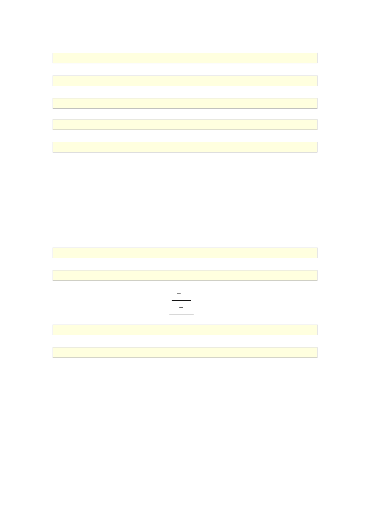
>G:=graph(%{[1,2],[2,3]%})
an undirected unweighted graph with 3 vertices and 2 edges
>charpoly(G,x)
x3¡2x
>charpoly(G,3)
21
>G:=graph("shrikhande")
an undirected unweighted graph with 16 vertices and 48 edges
>charpoly(G,x)
x16 ¡48 x14 ¡64 x13 +768 x12 +1536 x11 ¡5888 x10 ¡15360 x9+23040 x8+81920 x7¡
36864 x6¡245760 x5¡32768 x4+393216 x3+196608 x2¡262144 x¡196608
4.2.6. Graph spectrum
The command graph_spectrum is used for computing graph spectra.
Syntax: graph_spectrum(G)
graph_spectrum accepts a graph Gas its only argument and returns the list in which every element
is an eigenvalue of the adjacency matrix of Gpaired with its multiplicity.
>C5:=cycle_graph(5)
C5: an undirected unweighted graph with 5 vertices and 5 edges
>gs:=graph_spectrum(C5)
0
B
B
B
B
B
B
B
B
@
2 1
5
p¡1
22
¡5
p¡1
22
1
C
C
C
C
C
C
C
C
A
>p:=charpoly(C5,x)
x5¡5x3+ 5 x¡2
>expand(roots(p))==expand(gs)
true
The above result indicates that gs and roots(p) are equal.
4.2.7. Seidel spectrum
The command seidel_spectrum is used for computing Seidel spectra.
Syntax: seidel_spectrum(G)
seidel_spectrum accepts a graph G(V ; E)as its only argument and returns the list in which every
element is an eigenvalue of the Seidel adjacency matrix Spaired with its multiplicity. The matrix
S, which can be interpreted as the difference of the adjacency matrices of Gand its complement
Gc, is computed as J¡I¡2A, where Jis all-one n×nmatrix, Iis the identity matrix of order
n,Ais the adjacency matrix of Gand n=jVj.
4.2 Algebraic properties 71

>seidel_spectrum(graph("clebsch"))
¡310
5 6
>seidel_spectrum(graph("levi"))
0
B
B
B
B
B
B
B
B
@
¡5 9
¡110
3 9
5 1
23 1
1
C
C
C
C
C
C
C
C
A
4.2.8. Integer graphs
The command is_integer_graph is used for determining whether the given graph is an
integral graph.
Syntax: is_integer_graph(G)
is_integer_graph accepts a graph Gas its only argument and returns true if the spectrum of
Gconsists only of integers. Else it returns false.
>G:=graph("levi")
an undirected unweighted graph with 30 vertices and 45 edges
>is_integer_graph(G)
true
>factor(charpoly(G,x))
x10 (x¡3) (x¡2)9(x+ 2)9(x+ 3)
>graph_spectrum(G)
0
B
B
B
B
B
B
B
B
@
¡3 1
¡2 9
010
2 9
3 1
1
C
C
C
C
C
C
C
C
A
4.3. Graph isomorphism
4.3.1. Isomorphic graphs
The command is_isomorphic is used for determining whether two graphs are isomorphic.
Syntax: is_isomorphic(G1,G2)
is_isomorphic(G1,G2,m)
canonical_labeling(G)
is_isomorphic accepts two or three arguments: a graph G1(V1; E1), a graph G2(V2; E2)and option-
ally an unassigned identifier m. The command returns true if G1and G2are isomorphic and
false otherwise. If the third argument is given and G1and G2are isomorphic, the list of pairwise
matching of vertices in G1and G2, representing the isomorphism between the two graphs, is stored
to m.
72 Graph properties
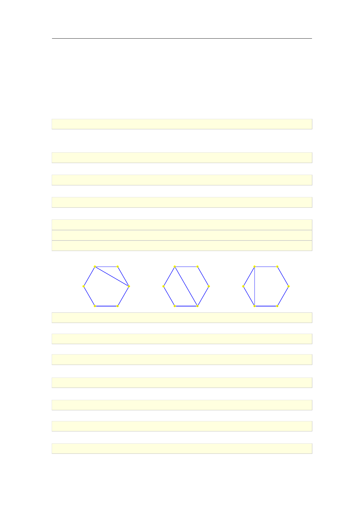
Note that the algorithm takes vertex colors into account. Namely, only vertices sharing the same
color can be mapped to each other. Vertex colors can be set by calling the highlight_vertex
command.
This command, as well as the commands canonical_labeling and graph_automorphisms described
later in this section, is using nauty library developed by Brendan McKay [35], which is one
of the fastest implementations for graph isomorphism.
For example, entering the command line below one shows that Petersen graph is isomorphic to
Kneser graph K(5;2).
>is_isomorphic(graph("petersen"),kneser_graph(5,2))
true
In the following example, G1and G3are isomorphic while G1and G2are not isomorphic.
>G1:=graph(trail(1,2,3,4,5,6,1,3))
an undirected unweighted graph with 6 vertices and 7 edges
>G2:=graph(trail(1,2,3,4,5,6,1,4))
an undirected unweighted graph with 6 vertices and 7 edges
>G3:=graph(trail(1,2,3,4,5,6,1,5))
an undirected unweighted graph with 6 vertices and 7 edges
>draw_graph(G1,circle)
>draw_graph(G2,circle)
>draw_graph(G3,circle)
The drawings are ordered from left to right.
1 2
3
45
6
1 2
3
45
6
1 2
3
45
6
>is_isomorphic(G1,G2)
false
>is_isomorphic(G1,G3)
true
>is_isomorphic(G1,G3,mapping):; mapping
Done;[1 = 5;2 = 6;3 = 1;4 = 2;5 = 3;6 = 4]
>H1:=highlight_vertex(G1,5):; H3:=highlight_vertex(G3,5):;
Done;Done
>is_isomorphic(H1,H3)
false
>H1:=highlight_vertex(H1,1):; H3:=highlight_vertex(H3,3):;
Done;Done
>is_isomorphic(H1,H3)
true
4.3 Graph isomorphism 73
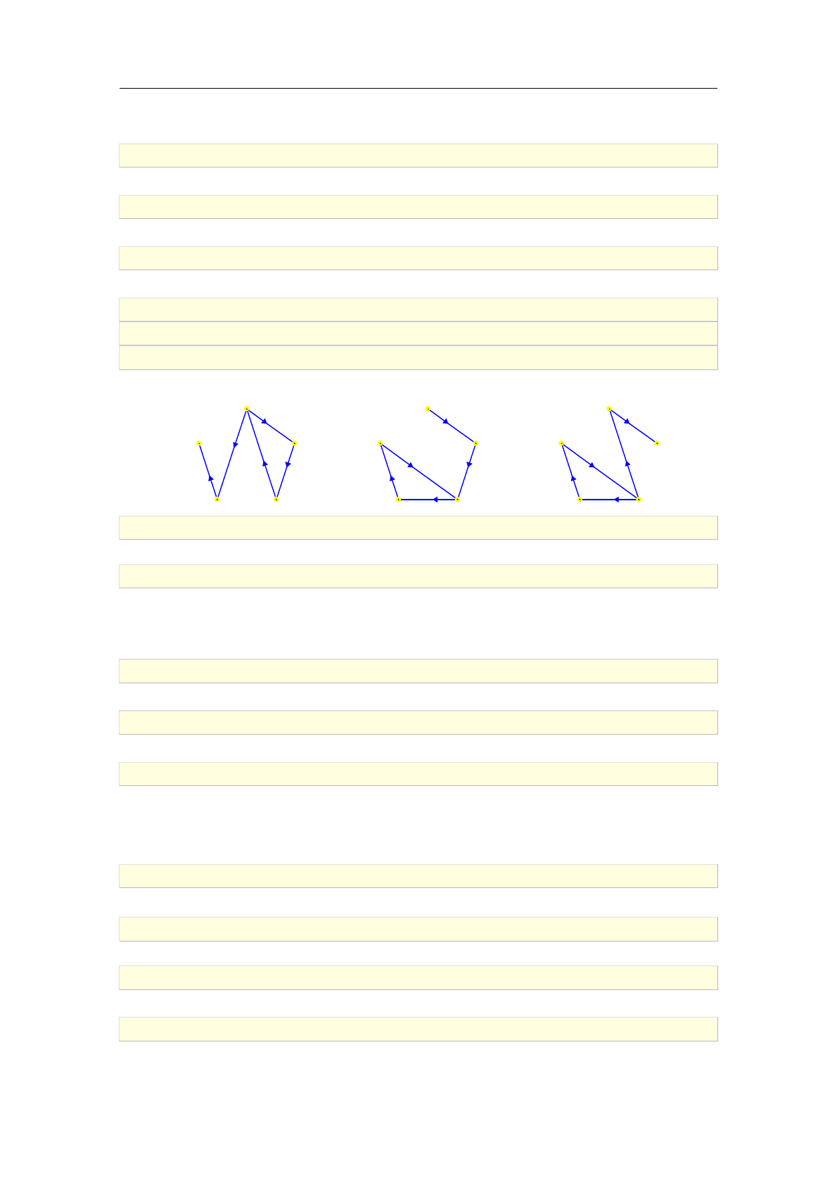
In the next example, D1and D3are isomorphic while D1and D2are not isomorphic.
>D1:=digraph(trail(1,2,3,1,4,5))
a directed unweighted graph with 5 vertices and 5 arcs
>D2:=digraph(trail(1,2,3,4,5,3))
a directed unweighted graph with 5 vertices and 5 arcs
>D3:=digraph([1,2,3,4,5],trail(3,4,5,3,1,2))
a directed unweighted graph with 5 vertices and 5 arcs
>draw_graph(D1,circle)
>draw_graph(D2,circle)
>draw_graph(D3,circle)
The drawings are ordered from left to right.
1
2
34
5
1
2
34
5
1
2
34
5
>is_isomorphic(D1,D2)
false
>is_isomorphic(D1,D3)
true
Isomorphism testing with nauty is very fast and can be used for large graphs, as in the example
below.
>G:=random_graph(10000,0.01)
an undirected unweighted graph with 10000 vertices and 499867 edges
>H:=isomorphic_copy(G,randperm(10000))
an undirected unweighted graph with 10000 vertices and 499867 edges
>is_isomorphic(G,H)
true
1.7 sec
To make the edge structures of Gand Hslightly different, a random edge from His “misplaced”.
>ed:=edges(H)[rand(number_of_edges(H))]
[813;3021]
>has_edge(H,[813,3022])
false
>H:=add_edge(delete_edge(H,ed),[813,3022])
an undirected unweighted graph with 10000 vertices and 499867 edges
>is_isomorphic(G,H)
false
74 Graph properties

4.3.2. Canonical labeling
Graph isomorphism testing in nauty is based on computing the canonical labelings for the input
graphs. The canonical labeling of Gis a particular ordering of the vertices of G. Rearranging
the vertices with respect to that ordering produces the canonical representation of G. Two
graphs are isomorphic if and only if their canonical representations share the same edge structure.
The command canonical_labeling is used for computing the canonical labeling as a permutation.
One can reorder the vertices by using this permutation with the isomorphic_copy command.
canonical_labeling accepts a graph G(V ; E)as its only argument and returns the permutation
representing the canonical labeling of G. Note that the colors of the vertices are taken into account.
In the next example it is demonstrated how to prove that G1and G3are isomorphic by comparing
their canonical representations C1and C3with the graph_equal command. Before testing C1and
C3for equality, their vertices have to be relabeled so that the command vertices gives the same
result for both graphs.
>L1:=canonical_labeling(G1)
[4;3;5;1;2;0]
>L3:=canonical_labeling(G3)
[2;1;3;5;0;4]
>C1:=relabel_vertices(isomorphic_copy(G1,L1),[1,2,3,4,5,6])
an undirected unweighted graph with 6 vertices and 7 edges
>C3:=relabel_vertices(isomorphic_copy(G3,L3),[1,2,3,4,5,6])
an undirected unweighted graph with 6 vertices and 7 edges
>graph_equal(C1,C3)
true
4.3.3. Graph automorphisms
The command graph_automorphisms is used for finding generators of the automorphism group of
a graph.
Syntax: graph_automorphisms(G)
graph_automorphisms accepts a graph Gas its only argument and returns a list containing the
generators of Aut(G), the automorphism group of G(see [23, pp. 4] and [5, pp. 115]). Each gener-
ator is given as a list of cycles, which can be turned to a permutation by calling the cycles2permu
command.
Note that vertex colors are taken into account. Only vertices sharing the same color can be mapped
to each other. The color of a vertex can be set by calling the highlight_vertex command.
>g:=graph_automorphisms(graph("petersen"))
f0
@
3 7
4 5
8 9 1
A;0
B
B
B
B
@
2 6
3 8
4 5
7 9
1
C
C
C
C
A
;0
B
B
B
B
@
1 4
2 3
6 9
7 8
1
C
C
C
C
A
;0
B
B
B
B
@
0 1
2 4
5 6
7 9
1
C
C
C
C
Ag
>cycles2permu(g[2])
[0;4;3;2;1;5;9;8;7;6]
>G:=graph("petersen")
4.3 Graph isomorphism 75

an undirected unweighted graph with 10 vertices and 15 edges
>G:=highlight_vertex(G,4)
an undirected unweighted graph with 10 vertices and 15 edges
>graph_automorphisms(G)
f0
@
2 6
3 9
7 8 1
A;0
B
B
B
B
@
1 5
2 7
3 9
6 8
1
C
C
C
C
A
;0
B
B
B
B
@
0 3
1 2
5 8
6 7
1
C
C
C
C
Ag
In the above result, all permutations map the vertex 4 to itself, because it is the single green-
colored vertex in G(it cannot be mapped to any other vertex because colors do not match).
Frucht graph (see the page 23) is an example of a graph with automorphism group containing only
the identity, so the set of its generators is empty:
>graph_automorphisms(lcf_graph([-5,-2,-4,2,5,-2,2,5,-2,-5,4,2]))
fg
4.4. Graph polynomials
4.4.1. Tutte polynomial
The command tutte_polynomial is used for computing Tutte polynomials.
Syntax: tutte_polynomial(G)
tutte_polynomial(G,x,y)
tutte_polynomial accepts one or three arguments, an undirected graph G(V ; E)and optionally
two variables or values xand y. It returns the the bivariate Tutte polynomial4.1 TGof Gor the
value TG(x; y)if the optional arguments are given. If Gis weighted, it is treated as a multigraph:
the weight wof an edge e, which must be a positive integer, is interpreted as the multiplicity of e,
for each e2E. Note, however, that loops are not supported.
The strategy is to apply the recursive definition of Tutte polynomial [25] together with the vorder
heuristic proposed by Haggard et al. [26] and improved by Monagan [36]. The subgraphs
appearing in the computation tree are cached and reused when possible, pruning the tree signifi-
cantly. Subgraphs are stored (and compared) in their canonical form, for which the nauty library
is used.
Note that finding Tutte polynomials is NP-hard in general, hence the problem becomes intractable
for larger and/or denser graphs.
>K4:=complete_graph(4)
an undirected unweighted graph with 4 vertices and 6 edges
>tutte_polynomial(K4,x,y)
x3+ 3 x2+ 4 x y + 2 x+y3+ 3 y2+ 2 y
>tutte_polynomial(K4,x,1)
x3+ 3 x2+ 6 x+ 6
>G:=graph("petersen")
4.1. See [25], [5, pp. 97] and [7, pp. 335].
76 Graph properties

an undirected unweighted graph with 10 vertices and 15 edges
>f:=tutte_polynomial(G)
x9+ 6 x8+21 x7+56 x6+12 x5y+114 x5+70 x4y+170 x4+30 x3y2+170 x3y+180 x3+
15 x2y3+105 x2y2+240 x2y+120 x2+10 x y4+65 x y3+171 x y2+168 x y +36 x+y6+ 9 y5+
35 y4+75 y3+84 y2+36 y
This result coincides with that in [5, pp. 103], which is supposed to be correct. Alternatively, it
can be verified by applying the recursive definition with an arbitrary edge e2E, as below.
>ed:=edges(G)[0]
[0;1]
>Gdelete:=delete_edge(G,ed)
an undirected unweighted graph with 10 vertices and 14 edges
>Gcontract:=contract_edge(G,ed)
an undirected unweighted graph with 9 vertices and 14 edges
>expand(f-tutte_polynomial(Gdelete)-tutte_polynomial(Gcontract))
0
The value TG(1;1) is equal to the number of spanning forests in G[7, pp. 345]—in this case, the
number of spanning trees in Petersen graph. For verification, the same number is computed by
using the specialized command number_of_spanning_trees, which uses a different (much faster)
algorithm.
>tutte_polynomial(G,1,1)
2000
>number_of_spanning_trees(G)
2000
For a graph Gand its dual G∗the following relation holds: TG(x; y) = TG∗(y; x). Therefore, if
TG(x; y) = TG(y; x)then Gand G∗are isomorphic (since Tutte polynomial is a graph invariant).
A simple example of such graph is tetrahedral graph. Since it is planar and biconnected, its dual
can be determined by using the plane_dual command.
>G:=graph("tetrahedron")
an undirected unweighted graph with 4 vertices and 6 edges
>is_biconnected(G) and is_planar(G)
true
>H:=plane_dual(G)
an undirected unweighted graph with 4 vertices and 6 edges
>T:=tutte_polynomial(G)
x3+ 3 x2+ 4 x y + 2 x+y3+ 3 y2+ 2 y
>expand(T-subs(T,[x,y],[y,x]))
0
>is_isomorphic(G,H)
true
Multiple edges can be specified as edge weights.
4.4 Graph polynomials 77

>M:=make_weighted(G)
an undirected weighted graph with 4 vertices and 6 edges
>M:=set_edge_weight(set_edge_weight(M,[1,2],2),[3,4],3)
an undirected weighted graph with 4 vertices and 6 edges
>edges(M,weights)
f[[1;2];2];[[1;3];1];[[1;4];1];[[2;3];1];[[2;4];1];[[3;4];3]g
>tutte_polynomial(M,x,y)
x3+x2y2+ 2 x2y+ 3 x2+ 3 x y3+ 6 x y2+ 6 x y + 2 x+y6+ 3 y5+ 6 y4+ 7 y3+ 5 y2+ 2 y
4.4.2. Chromatic polynomial
The command chromatic_polynomial, is used for computing chromatic polynomials.
Syntax: chromatic_polynomial(G)
chromatic_polynomial(G,t)
chromatic_polynomial accepts one or two arguments, an undirected unweighted graph G(V ; E)
and optionally a variable or value t. It returns the chromatic polynomial PGof Gor the value
PG(t)if the second argument is given.
PGand the Tutte polynomial TGsatisfy the following relation (see [25] and [7, pp. 346]):
PG(t) = (¡1)jVj¡κ(G)tκ(G)TG(1 ¡t; 0);(4.1)
where κ(G)is the number of connected components of G.chromatic_polynomial uses (4.1) to
compute PG.
The value PG(k), where k > 0is an integer, is equal to the number of all distinct k-colorings of
vertices in G. As shown in the example below, Petersen graph cannot be colored by using only two
colors, but is 3-colorable with 120 distinct colorings (all using the same three colors).
>P:=chromatic_polynomial(graph("petersen"),x)
x(x¡2) (x¡1) (x7¡12 x6+67 x5¡230 x4+529 x3¡814 x2+775 x¡352)
>subs(P,x=2)
0
>subs(P,x=3)
120
4.4.3. Flow polynomial
The command flow_polynomial is used for computing flow polynomials.
Syntax: flow_polynomial(G)
flow_polynomial(G,x)
flow_polynomial accepts one or two arguments, an undirected unweighted graph G(V ; E)and
optionally a variable or value x. It returns the flow polynomial QGof Gor the value QG(x)if the
second argument is given.
QGand the Tutte polynomial TGsatisfy the following relation (see [25] and [5, pp. 110]):
QG(x) = (¡1)jEj¡jVj+κ(G)TG(0;1¡x);(4.2)
78 Graph properties

where κ(G)is the number of connected components of G.flow_polynomial uses (4.2) to compute
QG.
The value QG(k), where k > 0is an integer, is equal to the number of all nowhere-zero k-flows
in G. In such flows, the total flow fventering and leaving vertex vis congruent modulo k, hence
fv2f1;2; :::; k ¡1gfor all v2V[7, pp. 347]. As shown in the example below, Petersen graph has
zero 4-flows and 240 5-flows.
>Q:=flow_polynomial(graph("petersen"))
x6¡15 x5+95 x4¡325 x3+624 x2¡620 x+240
>Q | x=4
0
>Q | x=5
240
4.4.4. Reliability polynomial
The command reliability_polynomial is used for computing reliability polynomials.
Syntax: reliability_polynomial(G)
reliability_polynomial(G,p)
reliability_polynomial accepts one or two arguments, an undirected graph G(V ; E)and option-
ally a variable or value p. It returns the all-terminal reliability polynomial RGof Gor the value
RG(p)if the second argument is given. If Gis weighted, it is treated as a multigraph: the weight
wof an edge e, which must be a positive integer, is interpreted as the multiplicity of e, for each e2E.
RGand the Tutte polynomial TGsatisfy the following relation [36]:
RG(p) = (1 ¡p)jVj¡κ(G)pjEj¡jVj+κ(G)TG(1; p¡1);(4.3)
where κ(G)is the number of connected components of G.reliability_polynomial uses (4.3) to
compute RG.
If Gis a connected network, then the value RG(p), where p2[0;1], is equal to the probability that
Gdoes not fail (i.e. stays connected) after removing each edge with probability p[23, pp. 354–355].
In the following example, it is clear that the graph Gwill stay connected with probability (1 ¡p)2
if each of its two edges is removed with probability p.
>G:=graph(%{[1,2],[2,3]%})
an undirected unweighted graph with 3 vertices and 2 edges
>R:=reliability_polynomial(G,p)
p2¡2p+ 1
>factor(R)
(p¡1)2
Adding a new edge should increase the reliability of G, since the latter is connected. Indeed, the
difference S¡Rbelow is positive for 0< p < 1.
>S:=reliability_polynomial(add_edge(G,[1,3]),p)
2p3¡3p2+ 1
>factor(S-R)
4.4 Graph polynomials 79
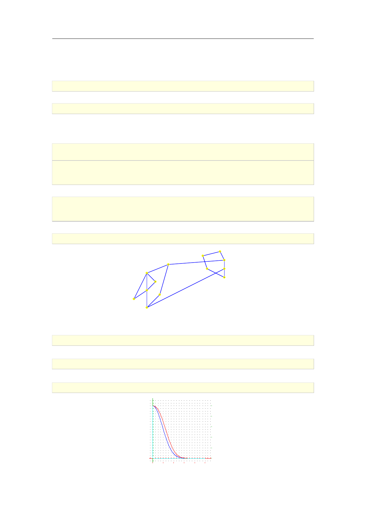
2p(p¡1)2
Multiple edges can be specified as edge weights.
>M:=graph(%{[[1,2],2],[[2,3],1],[[3,1],1]%})
an undirected weighted graph with 3 vertices and 3 edges
>factor(reliability_polynomial(M))
(x¡1)2(2 x2+ 2 x+ 1)
The following graph represents the Arpanet (early internet) in December 1970.
>
V:=["MIT","LINCOLN","CASE","CMU","HARVARD","BBN","UCSB","UCLA","STANFORD",
"SRI","RAND","UTAH","SDC"]:;
>
A:=graph(V,trail("BBN","HARVARD","CMU","CASE","LINCOLN","MIT","UTAH","SRI",
"STANFORD","UCLA","UCSB","SRI","UCLA","RAND","BBN","MIT"),trail("RAND","SDC",
"UTAH"))
an undirected unweighted graph with 13 vertices and 17 edges
>Arpanet:=set_vertex_positions(A,[[1.0,1.0],[0.9,1.2],[0.5,1.1],[0.6,0.8],[1.0,
0.6],[1.0,0.8],[-1.1,0.1],[-0.8,0.3],[-0.6,0.5],[-0.8,0.7],[-0.8,-0.1],[-0.3,
0.9],[-0.5,0.2]])
an undirected unweighted graph with 13 vertices and 17 edges
>draw_graph(Arpanet)
MIT
LINCOLN
CASE
CMU
HARVARD
BBN
UCSB
UCLA
STANFORD
SRI
RAND
UTAH
SDC
Which edge should be added to the Arpanet to improve the reliability the most? Below is an
analysis for the edge from Stanford to CMU.
>R:=reliability_polynomial(Arpanet,p)
(p¡1)12 (280 p5+310 p4+186 p3+63 p2+12 p+ 1)
>S:=reliability_polynomial(add_edge(Arpanet,["STANFORD","CMU"]),p)
(p¡1)12 (976 p6+1118 p5+703 p4+276 p3+72 p2+12 p+ 1)
>labels=["p","R,S"]; plot([R,S],p=0..1,color=[blue,red])
p
R,S
0 0.2 0.4 0.6 0.8 1
0
0.2
0.4
0.6
0.8
1
80 Graph properties

The improvement is defined as the area enclosed by the above two curves, which can be computed
as an integral.
>improvement:=integrate(S-R,p=0..1)
443879
10581480
>evalf(improvement)
0.0419486688063
4.5. Connectivity
4.5.1. Connected, biconnected and triconnected graphs
The commands is_connected,is_biconnected and is_triconnected are used for determining
if a graph is connected,biconnected or triconnected (3-connected), respectively.
Syntax: is_connected(G)
is_biconnected(G)
is_triconnected(G)
Each of the above commands accepts a graph G(V ; E)as its only argument and returns true if
Gpossesses the required level of connectivity. Else, it returns false.
If Gis directed, the edge directions are simply ignored (the commands operate on the underlying
graph of G).
The strategy for checking 1- and 2-connectivity is to use depth-first search (see [22, pp. 20] and [45]).
Both algorithms run in O(jVj+jEj)time. The algorithm for checking 3-connectivity is quite
simple but less efficient: it works by choosing a vertex v2Vand checking if the subgraph induced
by Vnfvgis biconnected, moving on to the next vertex if so, and repeating the process until all
vertices are visited exactly once or a non-biconnected subgraph is found for some v. In the latter
case the input graph is not triconnected. The complexity of this algorithm is O(jVjjEj).
>G:=graph_complement(complete_graph(2,3,4))
an undirected unweighted graph with 9 vertices and 10 edges
>is_connected(G)
false
>C:=connected_components(G)
f[0;1];[2;3;4];[5;6;7;8]g
>H:=induced_subgraph(G,C[2])
an undirected unweighted graph with 4 vertices and 6 edges
>is_connected(H)
true
>is_biconnected(path_graph(5))
false
>is_biconnected(cycle_graph(5))
true
>is_triconnected(graph("petersen"))
4.5 Connectivity 81
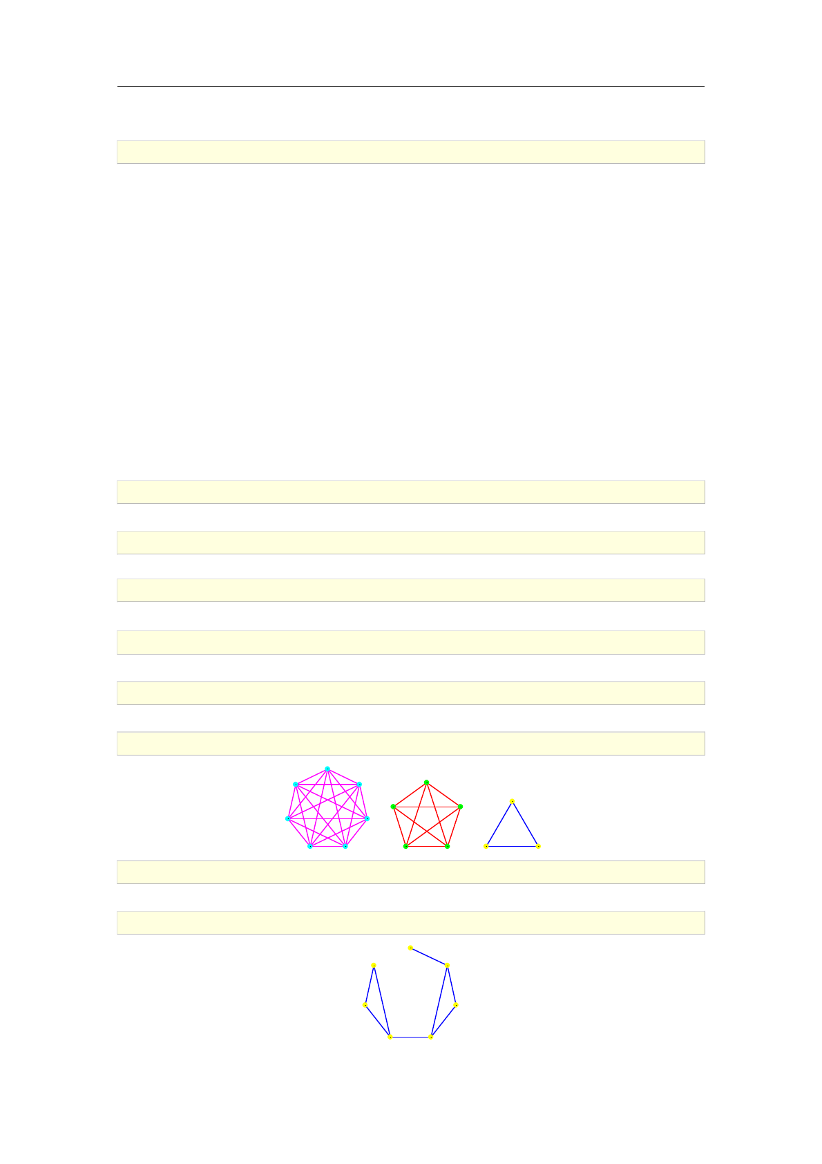
true
>is_triconnected(cycle_graph(5))
false
4.5.2. Connected and biconnected components
The command connected_components resp. biconnected_components is used for decomposing
a graph into connected resp. biconnected components.
Syntax: connected_components(G)
biconnected_components(G)
connected_components resp. biconnected_components accepts a graph G(V ; E)as its only argu-
ment and returns the minimal partition fV1; V2; :::; Vkgof Vsuch that the subgraph Gi⊂Ginduced
by Viis connected resp. biconnected for each i= 1;2; :::; k. The partition is returned as a list of
lists V1; V2; :::; Vk.
If Gis directed, the edge directions are simply ignored (the commands operate on the underlying
graph of G).
The connected components of Gare readily obtained by depth-first search in O(jVj+jEj)time.
To find the biconnected components of G,Tarjan's algorithm is used [45], which also runs in
linear time.
>G:=graph_complement(complete_graph(3,5,7))
an undirected unweighted graph with 15 vertices and 34 edges
>is_connected(G)
false
>C:=connected_components(G)
f[0;1;2];[3;4;5;6;7];[8;9;10;11;12;13;14]g
>G:=highlight_subgraph(G,induced_subgraph(G,C[1]))
an undirected unweighted graph with 15 vertices and 34 edges
>G:=highlight_subgraph(G,induced_subgraph(G,C[2]),magenta,cyan)
an undirected unweighted graph with 15 vertices and 34 edges
>draw_graph(G)
0
12
3
4
56
7
8
9
10
1112
13
14
>H:=graph(trail(1,2,3,4,2),trail(4,5,6,7,5))
an undirected unweighted graph with 7 vertices and 8 edges
>draw_graph(H)
1
2
3
45
6
7
82 Graph properties

>is_biconnected(H)
false
>biconnected_components(H)
f[1;2];[2;3;4];[4;5];[5;6;7]g
4.5.3. Vertex connectivity
The command vertex_connectivity is used for computing vertex connectivity in undirected
graphs.
Syntax: vertex_connectivity(G)
vertex_connectivity accepts an undirected connected graph G(V ; E)as its only argument and
returns the largest integer kfor which Gis k-vertex-connected, meaning that Gremains connected
after removing fewer than kvertices from V.
The strategy is to use the algorithm by Esfahanian and Hakimi [18], which is based on the
maximum-flow computing approach by Even [19, Section 6.2]. The algorithm makes jVj¡δ¡1 +
δ(δ¡1)
2calls to maxflow command, where δis the minimum vertex degree in G.
>vertex_connectivity(graph("petersen"))
3
>vertex_connectivity(graph("clebsch"))
5
>G:=random_planar_graph(1000,0.5,2)
an undirected unweighted graph with 1000 vertices and 1876 edges
>is_biconnected(G)
true
>vertex_connectivity(G)
2
3.28 sec
4.5.4. Graph rank
The command graph_rank is used for computing graph rank.
Syntax: graph_rank(G)
graph_rank(G,S)
graph_rank accepts one or two arguments, a graph G(V ; E)and optionally a set of edges S⊂E
(by default S=E), and returns jVj¡kwhere kis the number of connected components of the
spanning subgraph of Gwith edge set S.
>G:=graph(%{[1,2],[3,4],[4,5]%})
an undirected unweighted graph with 5 vertices and 3 edges
>graph_rank(G)
3
>graph_rank(G,[[1,2],[3,4]])
2
4.5 Connectivity 83
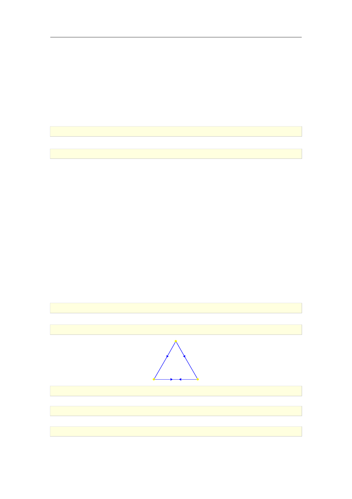
4.5.5. Articulation points
The command articulation_points is used for obtaining the set of articulation points (cut-
vertices) of a graph.
Syntax: articulation_points(G)
articulation_points accepts a graph G(V ; E)as its only argument and returns the list of
articulation points of G. A vertex v2Vis an articulation point of Gif the removal of vincreases
the number of connected components of G.
The articulation points of Gare found by depth-first search in O(jVj+jEj)time [22].
>articulation_points(path_graph([1,2,3,4]))
[2;3]
>length(articulation_points(cycle_graph(1,2,3,4)))
0
4.5.6. Strongly connected components
The command strongly_connected_components is used for decomposing digraphs into
strongly connected components. A digraph His strongly connected if for each pair (v; w)of dis-
tinct vertices in Hthere is a directed path from vto win H. The command is_strongly_connected
can be used to determine whether the given graph is strongly connected.
Syntax: strongly_connected_components(G)
is_strongly_connected(G)
strongly_connected_components accepts a digraph G(V ; E)as its only argument and returns
the minimal partition fV1; V2; :::; Vkgof Vsuch that the subgraph Gi⊂Ginduced by Viis strongly
connected for each i= 1;2; :::; k. The result is returned as a list of lists V1; V2; :::; Vk.
is_strongly_connected accepts a digraph Gas its only argument and returns true if Ghas
exactly one strongly connected component and false otherwise.
The strategy is to use Tarjan's algorithm for strongly connected components [45], which runs in
O(jVj+jEj)time.
>G:=digraph([1,2,3],%{[1,2],[1,3],[2,3],[3,2]%})
a directed unweighted graph with 3 vertices and 4 arcs
>draw_graph(G)
1
23
>is_connected(G)
true
>is_strongly_connected(G)
false
>strongly_connected_components(G)
f[1];[2;3]g
84 Graph properties
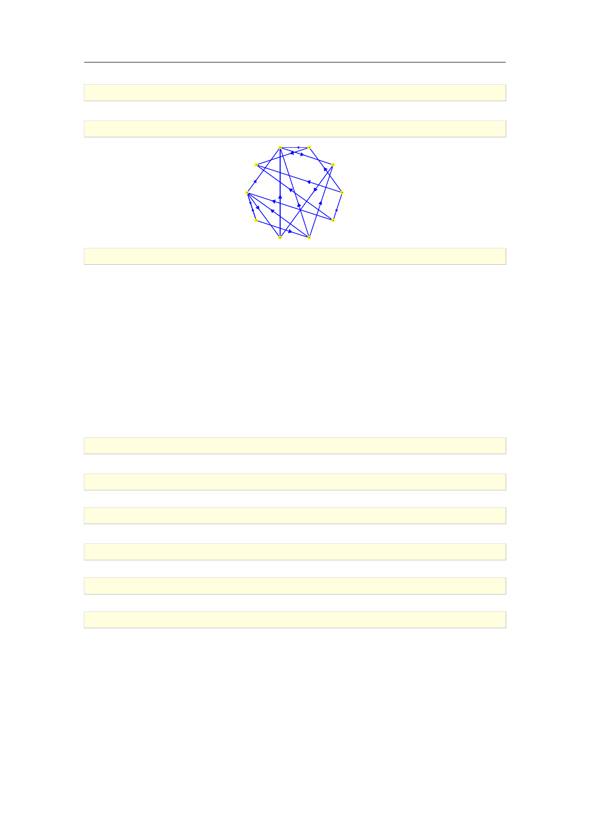
>G:=random_digraph(10,18)
a directed unweighted graph with 10 vertices and 18 arcs
>draw_graph(G)
0 1
2
3
4
56
7
8
9
>strongly_connected_components(G)
f[0;2;6];[1];[3];[4];[5;7;8];[9]g
4.5.7. Edge connectivity
The command edge_connectivity is used for computing the edge connectivity of an undirected
graph.
Syntax: edge_connectivity(G)
edge_connectivity accepts an undirected connected graph G(V ; E)as its only argument and
returns the largest integer kfor which Gis k-edge connected, meaning that Gremains connected
after fewer than kedges are removed from E.
The strategy is to apply Matula's algorithm [49, Section 13.3.1], which constructs a dominating
set D⊂Vand calls maxflow command jDj¡1times.
>G:=cycle_graph([1,2,3,4,5])
an undirected unweighted graph with 5 vertices and 5 edges
>edge_connectivity(G)
2
>K5:=complete_graph(5)
an undirected unweighted graph with 5 vertices and 10 edges
>edge_connectivity(K5)
4
>edge_connectivity(graph("petersen"))
3
>edge_connectivity(graph("clebsch"))
5
4.5.8. Edge cuts
The command is_cut_set is used for determining whether a particular subset of edges of the
given graph is an edge cut.
Syntax: is_cut_set(G,L)
is_cut_set accepts two arguments, a graph G(V ; E)and a subset L⊂Eof edges, and returns
true if the graph G0(V ; E nL)has more connected components than G. Else it returns false.
4.5 Connectivity 85
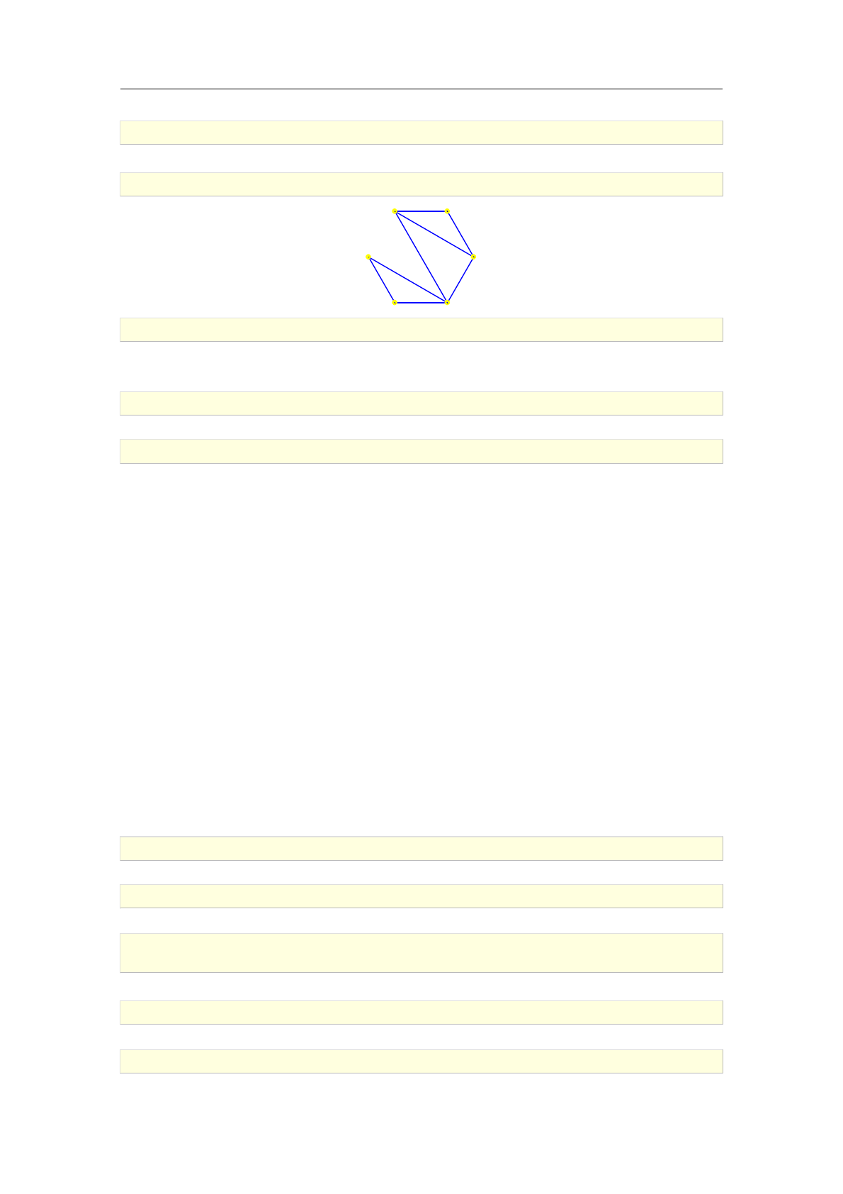
>G:=graph(trail(1,2,3,4,5,6,4,1,3))
an undirected unweighted graph with 6 vertices and 8 edges
>draw_graph(G)
1 2
3
45
6
>E:=[[1,4],[3,4]]
1 4
3 4
>is_cut_set(G,E)
true
>is_connected(delete_edge(G,E))
false
4.5.9. Two-edge-connected graphs
The command is_two_edge_connected is used for determining whether an undirected graph is
two-edge-connected. The command two_edge_connected_components is used for splitting a graph
into components having this property.
Syntax: is_two_edge_connected(G)
two_edge_connected_components(G)
is_two_edge_connected accepts an undirected graph G(V ; E)as its only argument and returns
true if Ghas no bridges, i.e. edges which removal increases the number of connected components
of G.
two_edge_connected_components accepts an undirected graph G(V ; E)and returns the list of
two-edge-connected components of G, each of them represented by the list of its vertices. To obtain
a component as a graph, use the induced_subgraph command.
The strategy for finding bridges [46] is similar to finding articulation points. Once the bridges of
Gare found, it is easy to split Ginto two-edge-connected components by removing the bridges
and returning the list of connected components of the resulting graph. Both algorithms run in
O(jVj+jEj)time.
>is_two_edge_connected(cycle_graph(4))
true
>is_two_edge_connected(path_graph(4))
false
>
G:=graph(%{["a","b"],["b","c"],["a","c"],["d","e"],["e","f"],["d","f"],["c",
"d"],["a","h"],["a","i"],["h","i"]%})
an undirected unweighted graph with 8 vertices and 10 edges
>is_two_edge_connected(G)
false
>draw_graph(G)
86 Graph properties
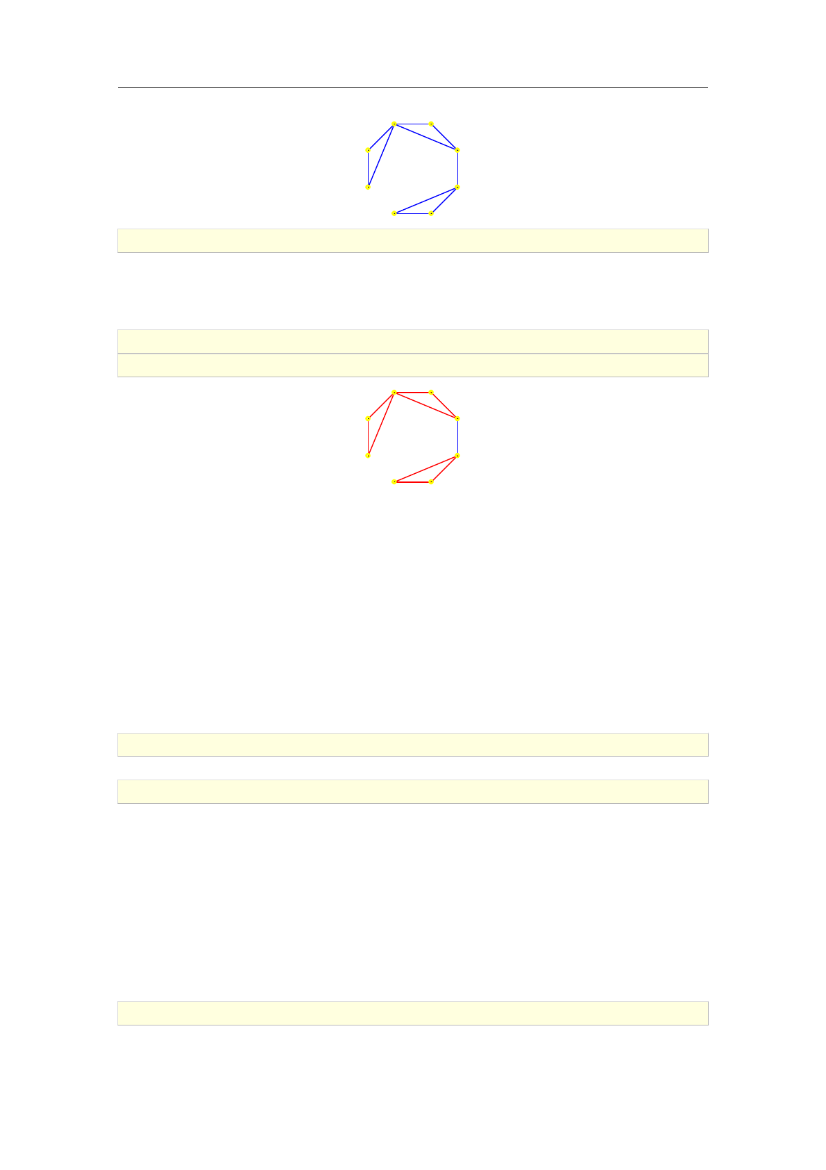
a b
c
d
ef
h
i
>C:=two_edge_connected_components(G)
f[a; b; c; h; i];[d; e; f ]g
To visualize the bridges of G, one can highlight the edges of each component. The remaining
(unhighlighted) edges are the bridges.
>for c in C do G:=highlight_edges(G,edges(induced_subgraph(G,c))); od:;
>draw_graph(G)
a b
c
d
ef
h
i
4.6. Trees
4.6.1. Tree graphs
The command is_tree is used for determining whether the given graph is a tree.
Syntax: is_tree(G)
is_tree accepts a graph G(V ; E)as its only argument and returns true if Gis undirected,
connected and jVj=jEj+ 1. Else it returns false.
The only expensive step in the algorithm is determining whether Gis connected. The condition
jVj=jEj+ 1 is checked first, hence the algorithm runs in O(jVj)time.
>is_tree(complete_binary_tree(3))
true
>is_tree(cycle_graph(5))
false
4.6.2. Forest graphs
The command is_forest is used for determining whether the given graph is a forest.
Syntax: is_forest(G)
is_forest accepts the a G(V ; E)as its only argument and returns true if every connected
component of Gis a tree and false otherwise.
The algorithm runs in O(jVj+jEj)time.
>F:=disjoint_union(apply(random_tree,[k$(k=10..30)]))
an undirected unweighted graph with 420 vertices and 399 edges
4.6 Trees 87

>is_connected(F)
false
>is_forest(F)
true
>draw_graph(F)
4.6.3. Height of a tree
The command tree_height is used for determining the height of a tree with respect to the specified
root node. The height of a tree Tis the length of the longest path in Tthat has the root node
of Tas one of its endpoints.
Syntax: tree_height(G,r)
tree_height accepts two arguments, a tree graph G(V ; E)and a vertex r2V, which is used as
the root node. The command returns the height of Gwith respect to r.
The strategy is to start a depth-first search from the root node and look for the deepest node.
Therefore the algorithm runs in O(jVj)time.
>G:=random_tree(1000)
an undirected unweighted graph with 1000 vertices and 999 edges
>r:=rand(1000)
296
>tree_height(G,r)
20
4.6.4. Lowest common ancestor of a pair of nodes
The command lowest_common_ancestor is used for computing the lowest common ancestor (LCA)
of a pair of nodes in a tree or for each element of a list of such pairs.
Syntax: lowest_common_ancestor(G,r,u,v)
lowest_common_ancestor(G,r,[[u1,v1],[u2,v2],..,[uk,vk]])
lowest_common_ancestor accepts two mandatory arguments, a tree graph G(V ; E)and the root
node r2V. There are two possibilities for specifying the nodes to operate on: either the nodes
u; v 2Vare given as the third and the fourth argument, or a list of pairs of nodes in form [[u1,
v1],[u2,v2],...,[uk,vk]], where ui; vi2Vand ui=/ vifor i= 1;2; :::; k, is given as the third
argument. The command returns the LCA of uand vor the list containing LCA of every pair of
nodes ui; vifor i= 1;2; :::; k. Note that this is much faster than calling lowest_common_ancestor
ktimes with one pair ui; viat a time.
The strategy is to use Tarjan's offline LCA algorithm [47], which runs in nearly linear time.
>G:=random_tree(25)
88 Graph properties
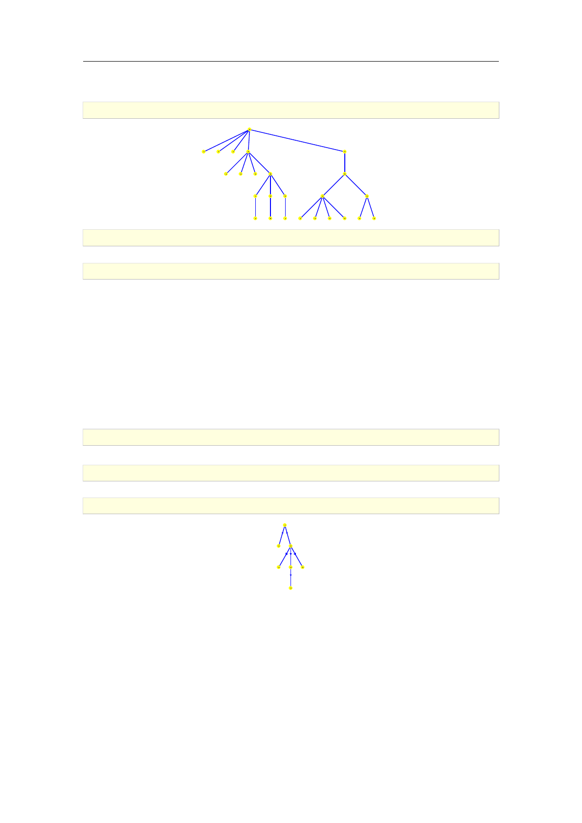
an undirected unweighted graph with 25 vertices and 24 edges
>draw_graph(G)
0
1234
5 6 7 8
9
10
11
12
13
14
15
16
17
18 19 20 21
22
23 24
>lowest_common_ancestor(G,0,19,22)
16
>lowest_common_ancestor(G,0,[[5,13],[17,24],[9,16]])
[4;16;0]
4.6.5. Arborescence graphs
The command is_arborescence is used for determining whether the given directed unweighted
graph is an arborescence (which is the digraph form of a rotted tree).
Syntax: is_arborescence(G)
is_arborescence accepts a digraph G(V ; E)as its only argument and returns true if there is a
vertex u2Vsuch that for any other v2Vthere is exactly one directed path from uto v. Else it
returns false.
>T:=digraph(%{[1,2],[1,3],[3,4],[3,5],[3,6],[5,7]%})
a directed unweighted graph with 7 vertices and 6 arcs
>is_arborescence(T)
true
>draw_graph(T)
1
23
456
7
4.7. Networks
4.7.1. Network graphs
The command is_network is used for determining whether the given graph is a flow network. In
this context, a flow network is directed, connected graph with at least one vertex with in-degree 0
(the source) and at least one vertex with out-degree 0 (the sink).
Syntax: is_network(G)
is_network(G,s,t)
4.7 Networks 89
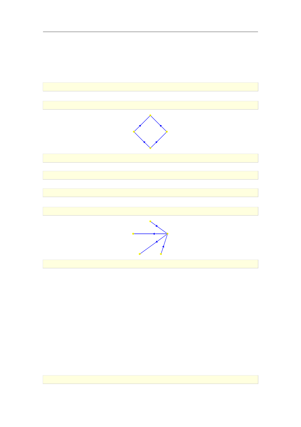
is_network accepts one or three arguments, a digraph G(V ; E)and optionally the source vertex
sand the sink vertex t. If these vertices are given, the command returns true if Gis a network
with respect to s,tand false otherwise. If the graph Gis given as the only argument, the
command returns a sequence of two objects, the list of all sources in Gand the list of all sinks in
G, respectively. If one of these lists is empty, then Gis implicitly not a network (both lists are
empty if Gis not connected).
>N:=digraph(%{[1,2],[1,3],[2,4],[3,4]%})
a directed unweighted graph with 4 vertices and 4 arcs
>draw_graph(N,spring)
1
23
4
>is_network(N,1,4)
true
>is_network(N,2,3)
false
>G:=digraph(%{[1,3],[2,3],[3,4],[3,5]%})
a directed unweighted graph with 5 vertices and 4 arcs
>draw_graph(G,circle)
1
3
24
5
>is_network(G)
1 2
4 5
4.7.2. Maximum flow
The command maxflow is used for computing the maximum flow in a network.
Syntax: maxflow(G,s,t)
maxflow(G,s,t,M)
maxflow accepts three or four arguments: a network graph G(V ; E), the source s2V, the sink
t2Vand optionally an unassigned identifier M. It returns the optimal value for the maximum flow
problem for the network (G; s; t). If the fourth argument is given, an optimal flow is written to M
in form of a matrix.
The strategy is to use the algorithm of Edmonds and Karp [17], which solves the maximum flow
problem in O(jVjjEj2)time.
>A:=[[0,1,0,4,0,0],[0,0,1,0,3,0],[0,1,0$3,1],[0,0,3,0,1,0],[0$3,1,0,4],[0$6]]
90 Graph properties
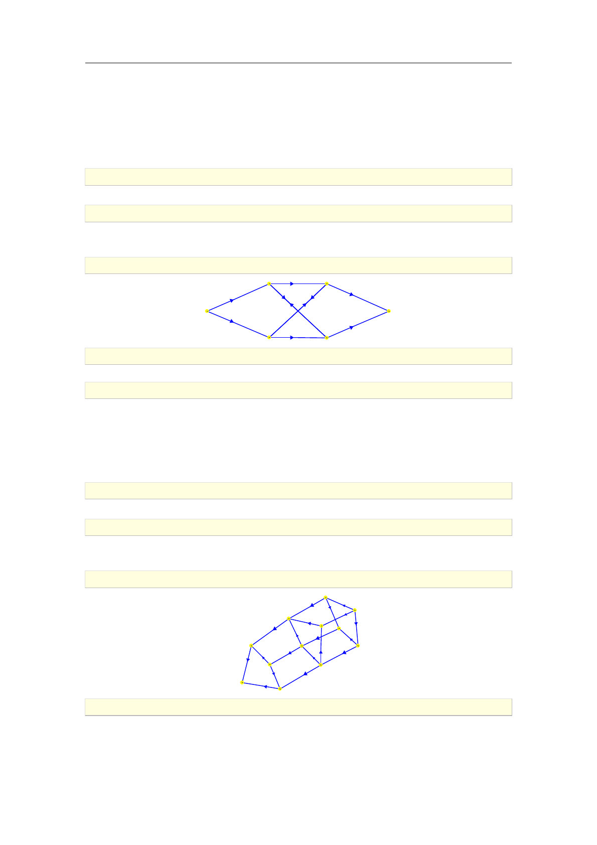
0
B
B
B
B
B
B
B
B
B
B
B
B
@
010400
001030
010001
003010
000104
000000
1
C
C
C
C
C
C
C
C
C
C
C
C
A
>N:=digraph([1,2,3,4,5,6],A)
a directed weighted graph with 6 vertices and 10 arcs
>is_network(N)
1
6
>draw_graph(N,spring)
1
41
3
11
3
1
1
4
1
2
34
5
6
>maxflow(N,1,6,M)
4
>M
0
B
B
B
B
B
B
B
B
B
B
B
B
@
010300
000020
010001
002010
000003
000000
1
C
C
C
C
C
C
C
C
C
C
C
C
A
>N:=random_network(2,3,0.9,acyclic,weights=5..15)
a directed weighted graph with 12 vertices and 19 arcs
>is_network(N)
0
11
>draw_graph(N,spring)
7
10
6
11
15
15
14
10
9
8
12
7
9
13
9
13
10
13
5
0
1
2
3
4
5
6
7
8
9
10
11
>maxflow(N,0,11,F)
17
To visualize the optimal flow F, one can use the highlight_subgraph command with the option
weights to display the actual flow in the highlighted edges. Non-highlighted edges have zero flow.
4.7 Networks 91
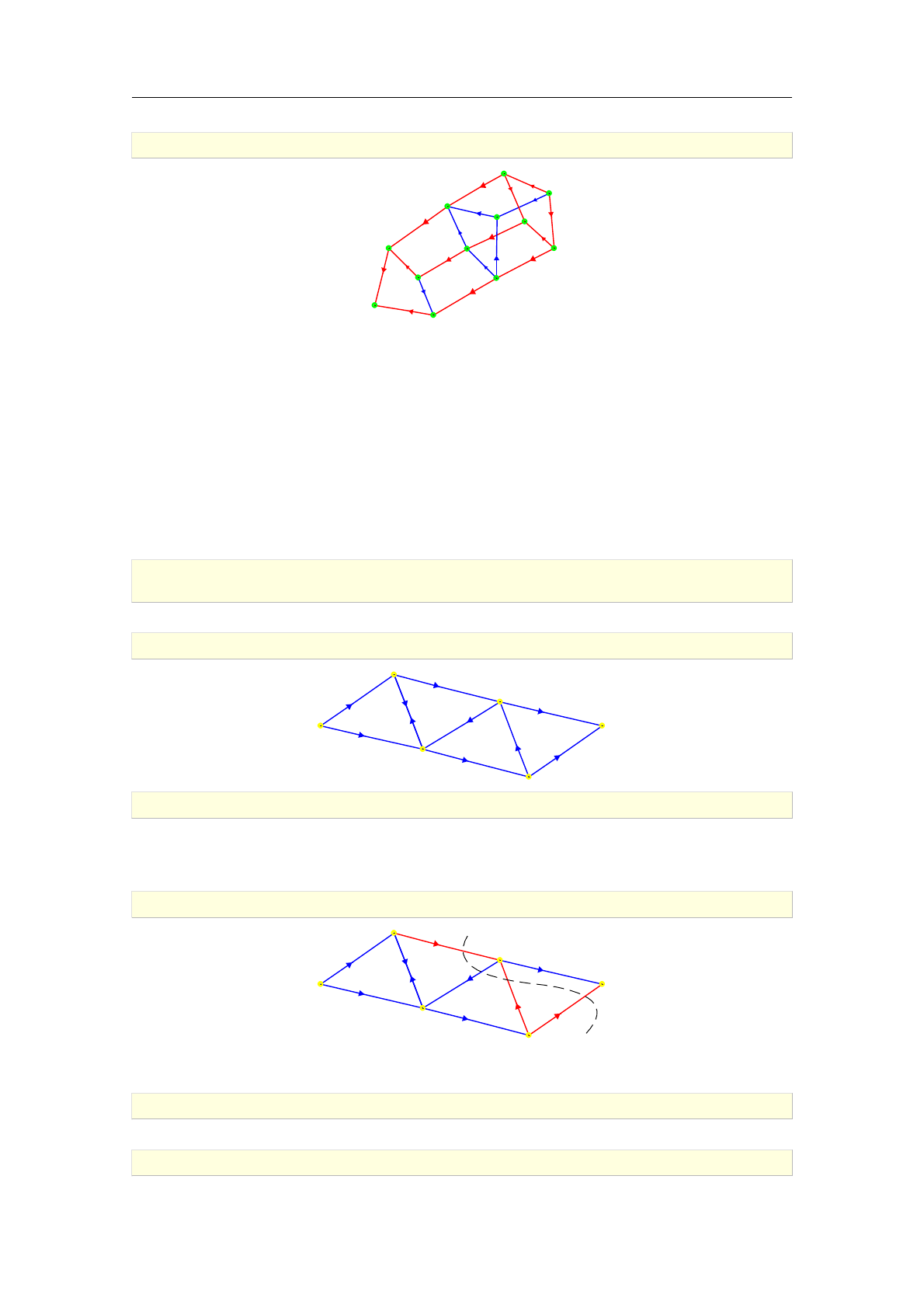
>draw_graph(highlight_subgraph(N,digraph(vertices(N),F),weights),spring)
7
10
6
2
5
1
9
3
9
8
5
7
9
3
9
3
10
12
5
0
1
2
3
4
5
6
7
8
9
10
11
4.7.3. Minimum cut
The command minimum_cut is used for obtaining minimum cuts in networks.
Syntax: minimum_cut(G,s,t)
minimum_cut accepts three arguments, a digraph G(V ; E)and two vertices s; t 2Vsuch that
(G; s; t) is a network with source sand sink t. The returned value is a list of edges in Erepresenting
a minimum cut in the network.
The strategy is to apply the maxflow command, which finds a maximal flow, and to run depth-
first search on the corresponding residual graph to find a S ; T partition of V. The minimum cut
is then the set of all arcs vw 2Esuch that v2Sand w2T. The algorithm runs in O(jVjjEj2)time.
>G:=digraph(%{[[0,1],16],[[0,2],13],[[1,2],10],[[1,3],12],[[2,1],4],[[2,4],14],
[[3,2],9],[[3,5],20],[[4,3],7],[[4,5],4]%})
a directed weighted graph with 6 vertices and 10 arcs
>draw_graph(G,spring)
16
13
10
12
4
14
9
20
7
4
0
1
2
3
4
5
>cut:=minimum_cut(G,0,5)
0
@
1 3
4 3
4 5 1
A
>draw_graph(highlight_edges(G,cut),spring)
16
13
10
12
4
14
9
20
7
4
0
1
2
3
4
5
By the max-flow min-cut theorem, the sum of edge weights in minimum cut is equal to the value
of maximum flow.
>w:=0:; for ed in cut do w:=w+get_edge_weight(G,ed); od:; w
Done;Done;23
>maxflow(G,0,5)
92 Graph properties

23
4.8. Distance in graphs
4.8.1. Vertex distance
The command vertex_distance is used for computing the length of the shortest path(s) from the
source vertex to some other vertex/vertices of a graph.
Syntax: vertex_distance(G,v,w)
vertex_distance(G,v,L)
vertex_distance accepts three arguments, a graph G(V ; E), a vertex v2Vcalled the source and
a vertex w2Vcalled the target or a list L⊂Vnfvgof target vertices. The command returns
the distance between vand was the number of edges in a shortest path from vto w, or the list
of distances if a list of target vertices is given.
The strategy is to use breadth-first search [22, pp. 35] starting from the source vertex. Therefore,
the algorithm runs in O(jVj+jEj)time.
>G:=graph("petersen")
an undirected unweighted graph with 10 vertices and 15 edges
>vertex_distance(G,1,3)
2
>vertex_distance(G,1,[3,6,9])
[2;1;2]
4.8.2. All-pairs vertex distance
The command allpairs_distance is used for computing the matrix of distances between all pairs
of vertices in the given (weighted) graph.
Syntax: allpairs_distance(G)
allpairs_distance accepts a graph G(V ; E)as its only argument and returns a square matrix
D= [dij]with n=jVjrows and columns such that dij =distance(vi; vj)for all i; j = 1;2; :::; n,
where v1; v2; :::; vnare the elements of V. If vivj2/E, then dij = +1. The strategy is to apply the
algorithm of Floyd and Warshall [20], which runs in O(jVj3)time.
Note that, if Gis weighted, it must not contain negative cycles. A cycle is negative if the sum of
weights of its edges is negative.
>G:=graph([1,2,3,4,5],%{[1,2],[1,3],[1,4],[1,5],[2,3],[3,4],[4,5],[5,2]%})
an undirected unweighted graph with 5 vertices and 8 edges
>allpairs_distance(G)
0
B
B
B
B
B
B
B
B
@
01111
10121
11012
12101
11210
1
C
C
C
C
C
C
C
C
A
>H:=digraph(%{[1,2],[1,3],[1,4],[1,5],[2,3],[3,4],[4,5],[5,2]%})
a directed unweighted graph with 5 vertices and 8 arcs
4.8 Distance in graphs 93
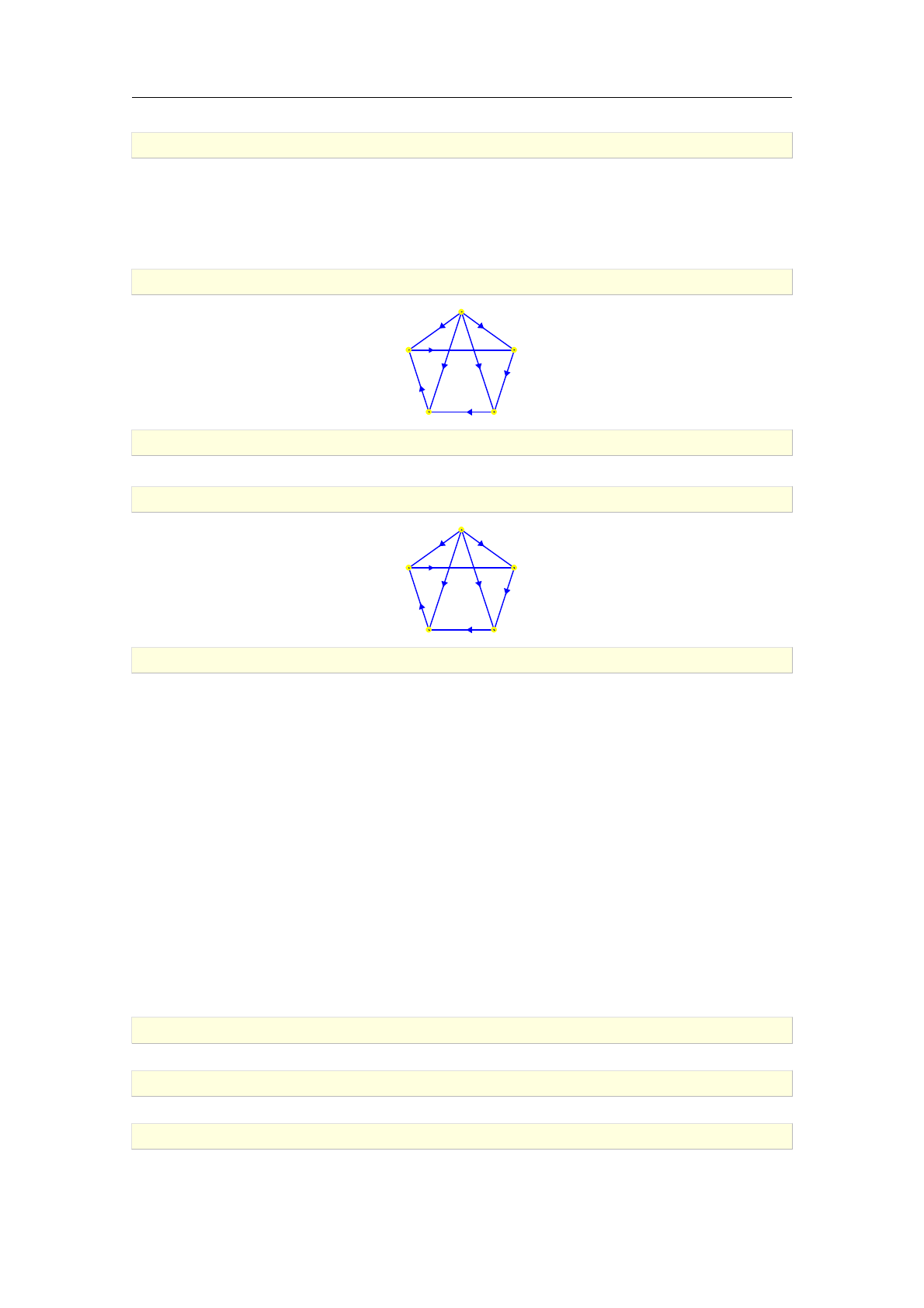
>allpairs_distance(H)
0
B
B
B
B
B
B
B
B
@
0 1 1 1 1
+10 1 2 3
+13 0 1 2
+12 3 0 1
+11 2 3 0
1
C
C
C
C
C
C
C
C
A
>draw_graph(H)
1
2
34
5
>H:=assign_edge_weights(H,5,25)
a directed weighted graph with 5 vertices and 8 arcs
>draw_graph(H)
24
1818
8
14
11
5
25
1
2
34
5
>allpairs_distance(H)
0
B
B
B
B
B
B
B
B
@
024 18 18 8
+1014 25 30
+141 011 16
+130 44 0 5
+125 39 50 0
1
C
C
C
C
C
C
C
C
A
4.8.3. Diameter
The command graph_diameter is used for determining the maximum distance among all pairs of
vertices in a graph.
Syntax: graph_diameter(G)
graph_diameter accepts a graph G(V ; E)as its only argument and returns the number
max fdistance(u; v) : u; v 2Vg. If Gis disconnected, +1is returned.
This command calls allpairs_distance and picks the largest element in the output matrix. Hence
the complexity of the algorithm is O(jVj3).
>graph_diameter(graph("petersen"))
2
>graph_diameter(cycle_graph(19))
9
>graph_diameter(disjoint_union(graph("petersen"),cycle_graph(19)))
+1
94 Graph properties

>G:=graph(%{[[1,2],0.2],[[2,3],0.3],[[3,4],0.4],[[4,1],1.1]%})
an undirected weighted graph with 4 vertices and 4 edges
>draw_graph(G)
0.2
1.1
0.3
0.4
1
2
3
4
>graph_diameter(G)
0.9
>dijkstra(G,1,4)
[[1;2;3;4];0.9]
4.8.4. Girth
The commands girth and odd_girth are used for computing the (odd) girth of an undirected
unweighted graph.
Syntax: girth(G)
girth resp. odd_girth accepts a graph G(V ; E)as its only argument and returns the girth
resp. odd girth of G. The (odd) girth of Gis defined to be the length of the shortest (odd)
cycle in G. If there is no (odd) cycle in G, the command returns +1.
The strategy is to apply breadth-first search from each vertex of the input graph. The runtime is
therefore O(jVjjEj).
>girth(graph("petersen"))
5
>G:=hypercube_graph(3)
an undirected unweighted graph with 8 vertices and 12 edges
>G:=subdivide_edges(G,["000","001"])
an undirected unweighted graph with 9 vertices and 13 edges
>girth(G)
4
>odd_girth(G)
5
>girth(complete_binary_tree(2))
+1
4.9. Acyclic graphs
4.9.1. Acyclic graphs
The command is_acyclic is used for checking for absence of directed cycles in digraphs. A
directed graph with no directed cycle is said to be acyclic.
4.9 Acyclic graphs 95
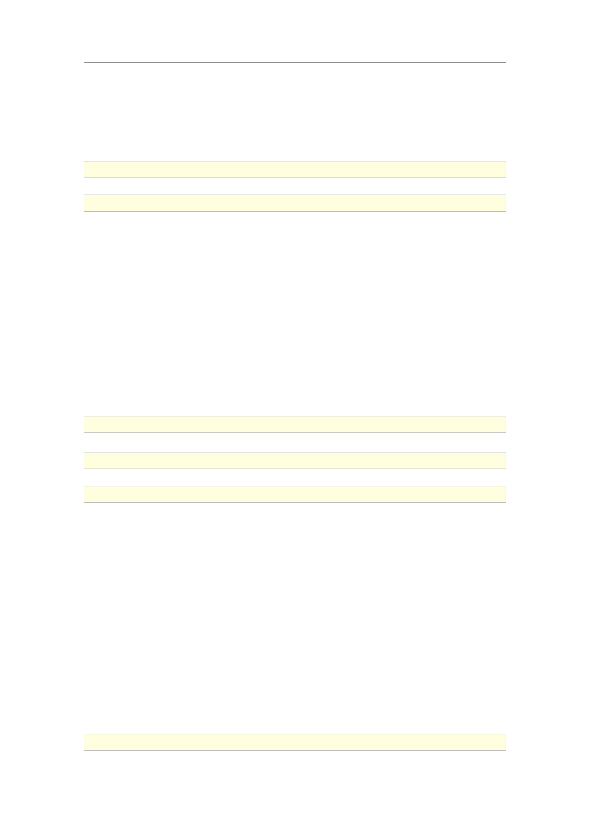
Syntax: is_acyclic(G)
is_acyclic accepts a digraph G(V ; E)as its only argument and returns true if Gis acyclic and
false otherwise.
The algorithm attempts to find topological order for its vertices. If that succeeds, the graph is
acyclic, otherwise not. The algorithm runs in O(jVj+jEj)time.
>is_acyclic(digraph(trail(1,2,3,4,5)))
true
>is_acyclic(digraph(trail(1,2,3,4,5,2)))
false
4.9.2. Topological sorting
The command topologic_sort or topological_sort is used for finding a linear ordering of
vertices of an acyclic digraph which is consistent with the arcs of the digraph. This procedure is
called topological sorting.
Syntax: topologic_sort(G)
topological_sort(G)
topologic_sort accepts a graph G(V ; E)as its only argument and returns the list of vertices of
Gin a particular order: a vertex uprecedes a vertex vif u v 2E, i.e. if there is an arc from uto v.
Note that topological sorting is possible only if the input graph is acyclic. If this condition is not
met, topologic_sort returns an error. Otherwise, it finds the required ordering by applying
Kahn's algorithm [34], which runs in O(jVj+jEj)time.
>G:=digraph(%{[c,a],[c,b],[c,d],[a,d],[b,d],[a,b]%})
a directed unweighted graph with 4 vertices and 6 arcs
>is_acyclic(G)
true
>topologic_sort(G)
[c; a; b; d]
4.9.3. st ordering
The command st_ordering is used for finding st-orderings in undirected biconnected graphs.
Syntax: st_ordering(G,s,t)
st_ordering(G,s,t,D)
st_ordering accepts three or four arguments: an undirected biconnected graph G(V ; E), a vertex
s2Vcalled the source, a vertex t2Vcalled the sink such that st 2Eand optionally an unassigned
identifier D. The command returns the permutation σof the vertex set V. Now, an orientation of
each e=uv 2Ecan be determined by the ordinals nand mof its endpoints uand v, respectively,
which are assigned by the permutation σ: if n < m, then uis the head and vis the tail of the
corresponding arc, and vice versa otherwise. If the fourth argument is given, a copy of G, which
is made directed according to these orientations, is stored to D.
The strategy is to apply Tarjan's algorithm [48] which runs in O(jVj+jEj)time. Note that, since
the input graph is biconnected, st-ordering can be computed for any pair s; t 2Vsuch that st 2E.
>G:=graph(%{[a,b],[a,c],[a,d],[b,c],[b,d],[c,d]%})
96 Graph properties
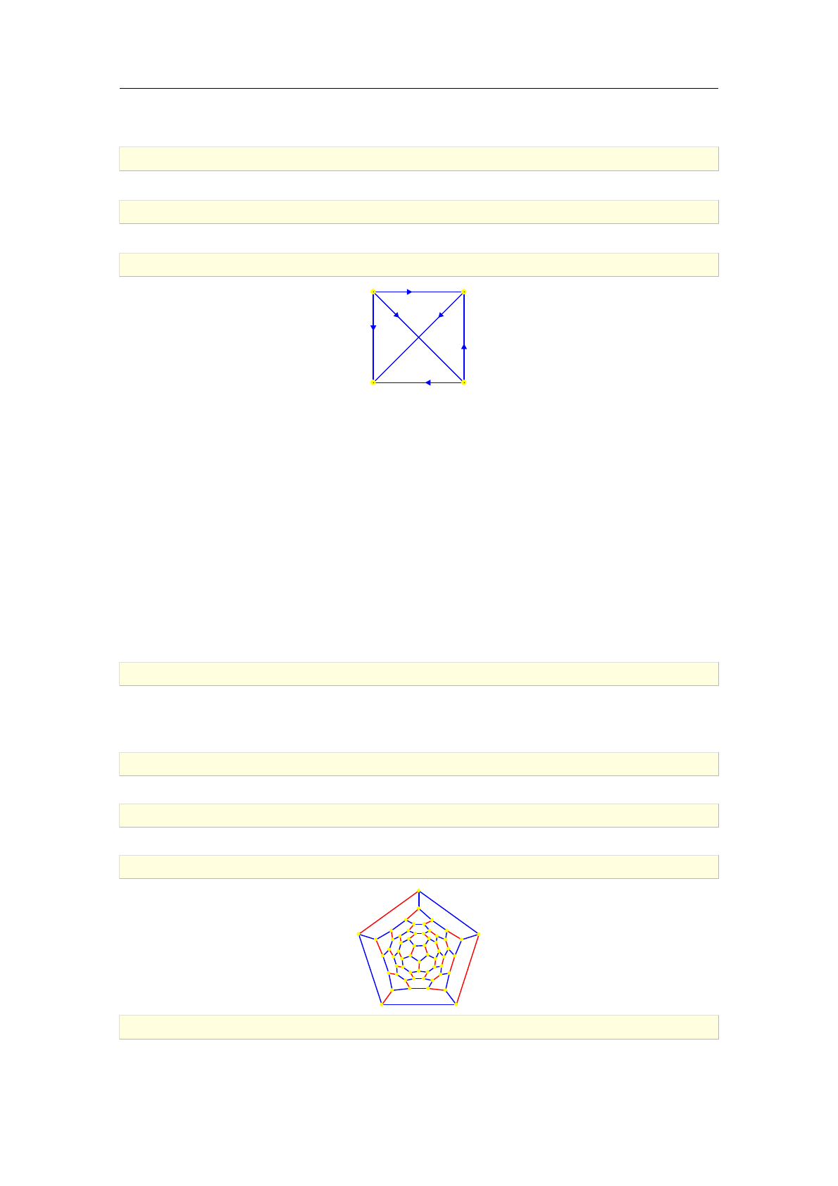
an undirected unweighted graph with 4 vertices and 6 edges
>vertices(G)
[a; b; c; d]
>st_ordering(G,a,d,D)
[0;2;1;3]
>draw_graph(D)
a b
cd
4.10. Matching in graphs
4.10.1. Maximum matching
The command maximum_matching is used for finding maximum matchings [23, pp. 43] in undirected
unweighted graphs.
Syntax: maximum_matching(G)
maximum_matching accepts an undirected graph G(V ; E)as its only argument and returns a list of
edges e1; e2; :::; em2Esuch that eiand ejare not adjacent (i.e. have no common endpoints) for all
16i < j 6mand that mis maximal. The return value can be interpreted as the list of matched
pairs of vertices in G.
The strategy is to apply the blossom algorithm of Edmonds [16], which runs in O(jVj2jEj)time.
>maximum_matching(graph("octahedron"))
0
@
1 6
3 2
5 4 1
A
>G:=graph("soccerball")
an undirected unweighted graph with 60 vertices and 90 edges
>M:=maximum_matching(G):; length(M)
Done;30
>draw_graph(highlight_edges(G,M),labels=false)
>G:=random_graph(100,1000)
an undirected unweighted graph with 100 vertices and 1000 edges
4.10 Matching in graphs 97
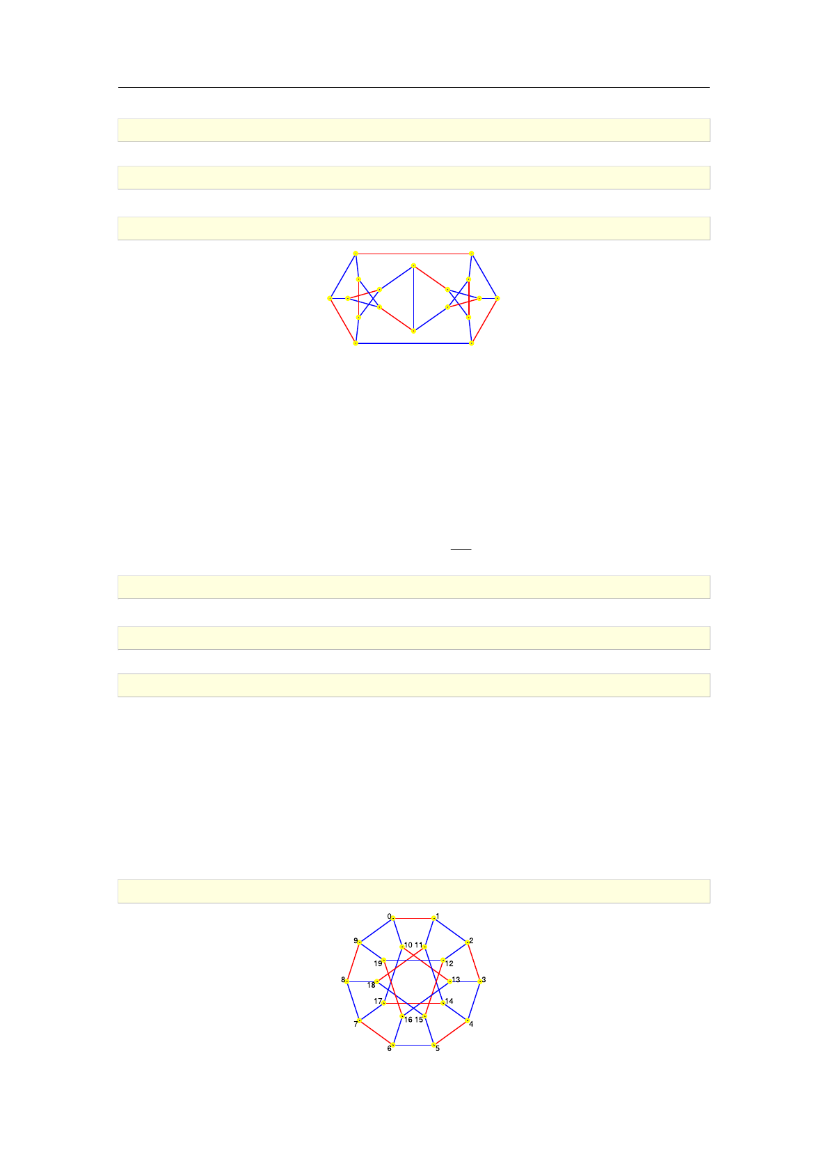
>length(maximum_matching(G))
50
>G:=graph("blanusa")
an undirected unweighted graph with 18 vertices and 27 edges
>draw_graph(highlight_edges(G,maximum_matching(G)),labels=false)
4.10.2. Maximum matching in bipartite graphs
The command bipartite_matching is used for finding maximum matchings in undirected,
unweighted bipartite graphs. It applies the algorithm of Hopcroft and Karp [31], which is
more efficient than the general algorithm used by the command maximum_matching.
Syntax: bipartite_matching(G)
bipartite_matching accepts an undirected bipartite graph G(V ; E)as its only argument and
returns a sequence containing two elements: the size of the matching and the list of edges connecting
matched pairs of vertices. The algorithm runs in O¡jVj
pjEjtime.
>G:=graph("desargues")
an undirected unweighted graph with 20 vertices and 30 edges
>is_bipartite(G)
true
>M:=bipartite_matching(G)
0
B
B
B
B
B
B
B
B
B
B
B
B
B
B
B
B
B
B
B
B
B
B
B
B
B
B
B
B
@
0 1
2 3
4 5
6 7
8 9
10 13
11 18
12 15
14 17
16 19
1
C
C
C
C
C
C
C
C
C
C
C
C
C
C
C
C
C
C
C
C
C
C
C
C
C
C
C
C
A
>draw_graph(highlight_edges(G,M))
98 Graph properties

4.11. Cliques
4.11.1. Clique graphs
To check whether an undirected graph is complete, one can use the is_clique command.
Syntax: is_clique(G)
is_clique accepts an undirected graph G(V ; E)as its only argument and returns true if every
pair of distinct vertices is connected by a unique edge in E. Else, it returns false.
>K5:=complete_graph(5)
an undirected unweighted graph with 5 vertices and 10 edges
>is_clique(K5)
true
>G:=delete_edge(K5,[1,2])
an undirected unweighted graph with 5 vertices and 9 edges
>is_clique(G)
false
4.11.2. Maximal cliques
Given an undirected graph G(V ; E), a subset S⊂Vis called a clique in Gif any two distinct
vertices from Sare adjacent in G, i.e. if the subgraph of Ginduced by the set Sis complete. A
clique is maximal if it cannot be extended by adding more vertices from Vto it. To count all
maximal cliques in a graph one can use the clique_stats command.
Syntax: clique_stats(G)
clique_stats(G,k)
clique_stats(G,m..n)
clique_stats accepts an undirected graph G(V ; E)as the mandatory first argument. If no other
arguments are given, the command returns a list of pairs, each pair consisting of two integers: clique
cardinality k(first) and the number nk>0of k-cliques in G(second). Therefore, the sum of second
members of all returned pairs is equal to the total count of all maximal cliques in G. Furthermore,
a second argument may be passed to clique_stats; if so, it must be a positive integer kor an
interval with integer bounds m.. n. In the first case only the number of k-cliques for the given kis
returned; in the second case, only cliques with cardinality between mand n(inclusive) are counted.
The strategy used to find all maximal cliques is a variant of the algorithm of Bron and Kerbosch
developed by Tomita et al. [50]. Its worst-case running time is O(3jVj/3). However, the perfor-
mance usually takes only a moment for graphs with 100 vertices or less.
>G:=random_graph(50,0.5)
an undirected unweighted graph with 50 vertices and 588 edges
>clique_stats(G)
0
B
B
B
B
B
B
B
B
B
B
B
B
@
314
4185
5370
6201
747
8 5
1
C
C
C
C
C
C
C
C
C
C
C
C
A
>G:=random_graph(100,0.5)
4.11 Cliques 99
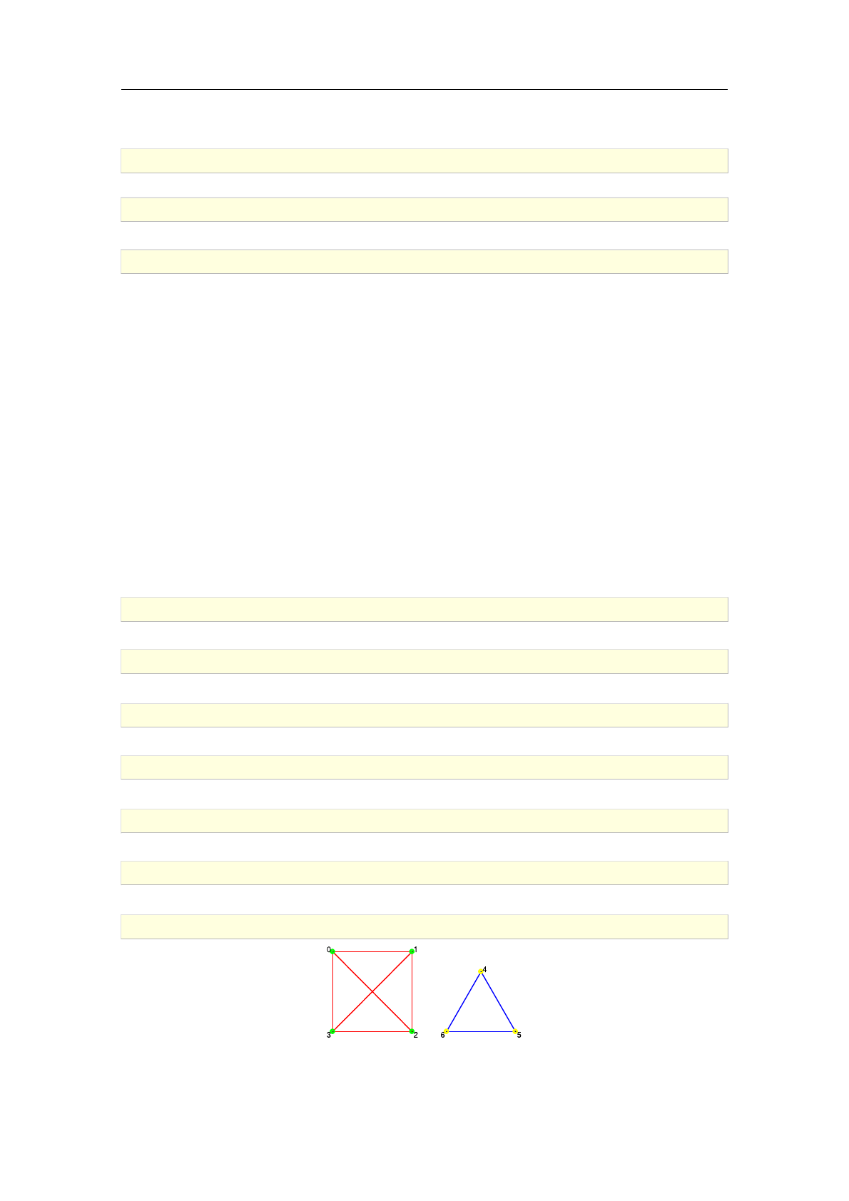
an undirected unweighted graph with 100 vertices and 2461 edges
>clique_stats(G,5)
3124
>G:=random_graph(500,0.25)
an undirected unweighted graph with 500 vertices and 30991 edges
>clique_stats(G,5..7)
0
@
5144544
616268
7267 1
A
4.11.3. Maximum clique
Any largest maximal clique in an undirected graph is called maximum clique. The command
maximum_clique can be used to find one in the given graph. If only the size of a maximum clique
is desired, one can use the command clique_number.
Syntax: maximum_clique(G)
clique_number(G)
maximum_clique accepts an undirected graph Gas its only argument and returns a maximum
clique in Gas a list of vertices. The clique may subsequently be extracted from Gusing the
command induced_subgraph.
The strategy used to find maximum clique is an improved variant of the classical algorithm by
Carraghan and Pardalos developed by Östergård [39].
In the following examples the results were obtained almost instantly.
>G:=sierpinski_graph(5,5)
an undirected unweighted graph with 3125 vertices and 7810 edges
>maximum_clique(G)
[1560;1561;1562;1563;1564]
>G:=random_graph(300,0.3)
an undirected unweighted graph with 300 vertices and 13380 edges
>maximum_clique(G)
[46;64;144;183;208;241;244;261]
>G:=graph_complement(complete_graph(4,3))
an undirected unweighted graph with 7 vertices and 9 edges
>cliq:=maximum_clique(G)
[0;1;2;3]
>draw_graph(highlight_subgraph(G,induced_subgraph(G,cliq)))
clique_number accepts an undirected graph Gas its only argument and returns the number of
vertices forming a maximum clique in G.
100 Graph properties

>clique_number(G)
4
4.11.4. Minimum clique cover
Aminimum clique cover for an undirected graph Gis any minimal set S=fC1; C2; :::; Ckgof
cliques in Gsuch that for every vertex vin Gthere exists i6ksuch that v2Ci. Such a cover can
be obtained by calling the clique_cover command.
Syntax: clique_cover(G)
clique_cover(G,k)
clique_cover accepts an undirected graph G(V ; E)as its mandatory argument and returns the
smallest possible cover. Optionally, a positive integer kmay be passed as the second argument.
In that case the requirement that kis less or equal to the given integer is set. If no such cover is
found, clique_cover returns empty list.
The strategy is to find a minimal vertex coloring in the complement Gcof G(note that these two
graphs share the same set of vertices). Each set of equally colored vertices in Gccorresponds to a
clique in G. Therefore, the color classes of Gcmap to the elements C1; :::; Ckof a minimal clique
cover in G.
There is a special case in which Gis triangle-free, which is computed separately in the algorithm.
In that case, Gcontains only 1- and 2-cliques. Therefore, every clique cover in Gconsists of a set
M⊂Eof matched edges together with the singleton cliques (i.e. the isolated vertices in Vwhich
remain unmatched). The total number of cliques in the cover is equal to jVj¡jMj, hence to find a
minimal cover one just needs to find a maximum matching in G, which can be done in polynomial
time.
>G:=random_graph(30,0.2)
an undirected unweighted graph with 30 vertices and 89 edges
>clique_cover(G)
f[0;21];[1;17];[2;25;28];[3;7;10];[4;8];[5;11;20];[6;13;14];[9;16;23];[12;15;19];[18;22];[24;
26];[27;29]g
>clique_cover(graph("octahedron"))
136
245
The vertices of Petersen graph can be covered with five, but not with three cliques.
>clique_cover(graph("petersen"),3)
[]
>clique_cover(graph("petersen"),5)
0
B
B
B
B
B
B
B
B
@
0 1
2 3
4 9
5 7
6 8
1
C
C
C
C
C
C
C
C
A
4.11.5. Clique cover number
The command clique_cover_number is used for computing the clique cover number of a graph.
4.11 Cliques 101

Syntax: clique_cover_number(G)
clique_cover_number accepts an undirected graph G(V ; E)as its only argument and returns the
minimum number of cliques in Gneeded to cover the vertex set V. (More precisely, it calls the
clique_cover command and returns the length of the output list.) This number, denoted by θ(G),
is equal to the chromatic number χ(Gc)of the complement graph Gcof G.
>clique_cover_number(graph("petersen"))
5
>clique_cover_number(graph("soccerball"))
30
>clique_cover_number(random_graph(40,0.618))
7
4.12. Clustering and transitivity in networks
4.12.1. Counting triangles in graphs
The command number_of_triangles is used for counting triangles in graphs.
Syntax: number_of_triangles(G)
number_of_triangles accepts a graph Gas its only argument and returns the number nof 3-
cliques in Gif Gis undirected resp. the number mof directed paths of length 3 if Gis directed.
The strategy is to compute the trace of A3, where Ais the adjacency matrix of G(encoded as
a sparse matrix). This number is equal to 6nif Gis undirected resp. to 3mif Gis directed. If
tr (A3) = 0, then Gis triangle-free (i.e. it contains no triangular subgraphs).
The matrix Ais kept in sparse form and only the computation of A2needs to be carried out
completely. To obtain tr (A3), one needs to compute only the elements of A3lying on its diagonal.
Hence the algorithm requires O(jVjjEj)time and O(jEj)space.
>number_of_triangles(graph("tetrahedron"))
4
>G:=digraph([1,2,3,4],%{[1,2],[1,4],[2,3],[2,4],[3,1],[4,3]%})
a directed unweighted graph with 4 vertices and 6 arcs
>draw_graph(G,spring)
1 2
3
4
>number_of_triangles(G)
2
>G:=sierpinski_graph(7,3,triangle)
an undirected unweighted graph with 1095 vertices and 2187 edges
>number_of_triangles(G)
102 Graph properties
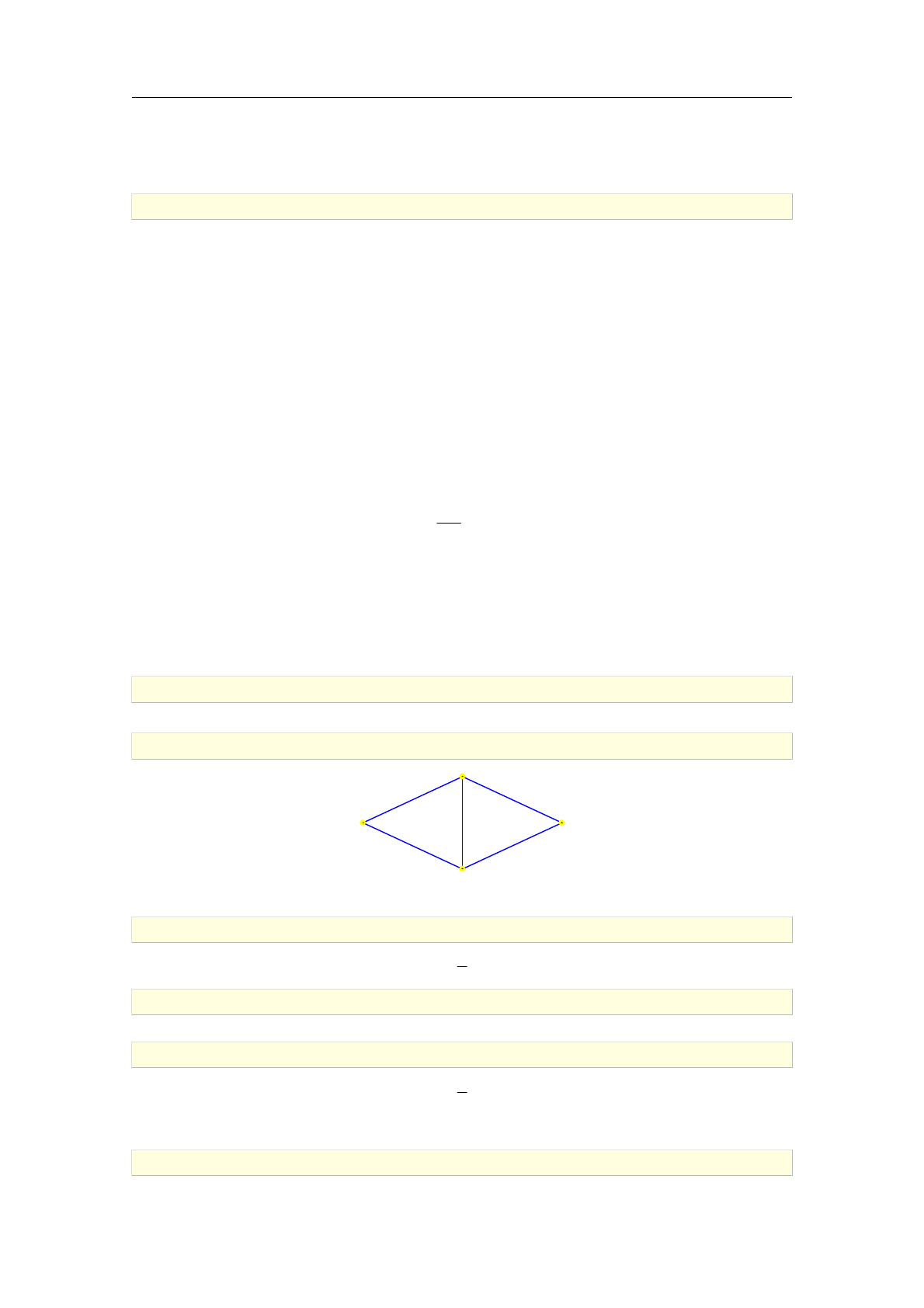
972
The truncated icosahedral graph is triangle-free.
>number_of_triangles(graph("soccerball"))
0
4.12.2. Clustering coefficient
The command clustering_coefficient is used for computing the average clustering coefficient
of an undirected graph as well as the local clustering coefficient of a particular vertex.
Syntax: clustering_coefficient(G)
clustering_coefficient(G,v)
clustering_coefficient accepts one or two arguments, an undirected graph G(V ; E)and option-
ally a vertex v2V. It returns the average clustering coefficient c(G)[8, pp. 5] if vis not given and
the local clustering coefficient cG(v)of v[8, pp. 4] otherwise. The returned value is, by definition,
a rational number in the range [0;1] in both cases. The number c(G)can be computed from cG(v)
using the following relation:
c(G) = 1
jVjX
v2V
cG(v):
In the context of social networks, c(G)can be interpreted as the probability that if v; w 2Vare
friends and w; z 2Vare friends then vand zare friends (note that friendship is a symmetric
relation). The number cG(v)has the same interpretation but in a local context: it measures how
probable the friendship transitivity is for a particular node v2V.
The complexity of computing c(G)is O(∆GjEj), where ∆Gis the maximum vertex degree in G.
>G:=graph(%{[1,2],[2,3],[2,4],[3,4],[4,1]%})
an undirected unweighted graph with 4 vertices and 5 edges
>draw_graph(G,spring)
1
2
3
4
The command lines below compute c(G),cG(1) and cG(2).
>clustering_coefficient(G)
5
6
>clustering_coefficient(G,1)
1
>clustering_coefficient(G,2)
2
3
The next example demonstrates the performance of clustering_coefficient on large graphs.
>G:=random_graph(5000,500000)
4.12 Clustering and transitivity in networks 103
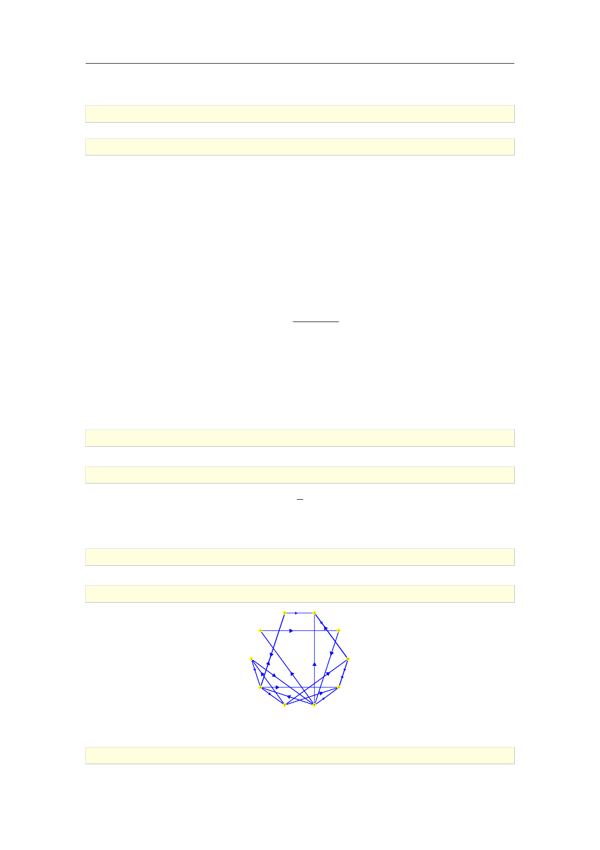
an undirected unweighted graph with 5000 vertices and 500000 edges
>cf:=clustering_coefficient(G):;
2.14 sec
>evalf(cf)
0.0400370165471
The probability that friendship is transitive in the network Gabove is therefore about 4%.
4.12.3. Network transitivity
The command network_transitivity is used for computing the transitivity (also called triangle
density or the global clustering coefficient) of a network.
Syntax: network_transitivity(G)
network_transitivity accepts a graph Gas its only argument and returns the transitivity T(G)
of G[8, pp. 5]. By definition, it is a rational number in the range [0;1]:
T(G) = 3Ntriangles
Ntriplets :
If Gis undirected, Ntriangles is the number of closed triplets (3-cliques) of vertices in Vwhile Ntriplets
is the number of all triplets (two-edge paths). If Gis directed, a triplet in Gis any directed path
(v; w; z). For example, in a Twitter-like network this could mean that vfollowing wand wfollowing
z. The triplet (v; w; z)is closed if vz 2E, i.e. if valso follows z[53, pp. 243]. Therefore, T(G)is
a measure of transitivity of a non-symmetric relation between the vertices of a network.
The complexity of computing T(G)is O(∆GjEj), where ∆Gis the maximum vertex degree in G.
>G:=graph(%{[1,2],[2,3],[2,4],[3,4],[4,1]%})
an undirected unweighted graph with 4 vertices and 5 edges
>network_transitivity(G)
3
4
Observe that the above result is different than c(G)obtained in Section 4.12.2. Hence c(G) =/ T(G)
in general [8, pp. 5].
>G:=random_digraph(10,20)
a directed unweighted graph with 10 vertices and 20 arcs
>draw_graph(G)
0 1
2
3
4
56
7
8
9
In the above digraph, the triplet (5;7;6) is open while the triplet (7;6;4) is closed. Triangles (2;5;9)
and (6;8;7) are not closed by definition.
>network_transitivity(G)
104 Graph properties
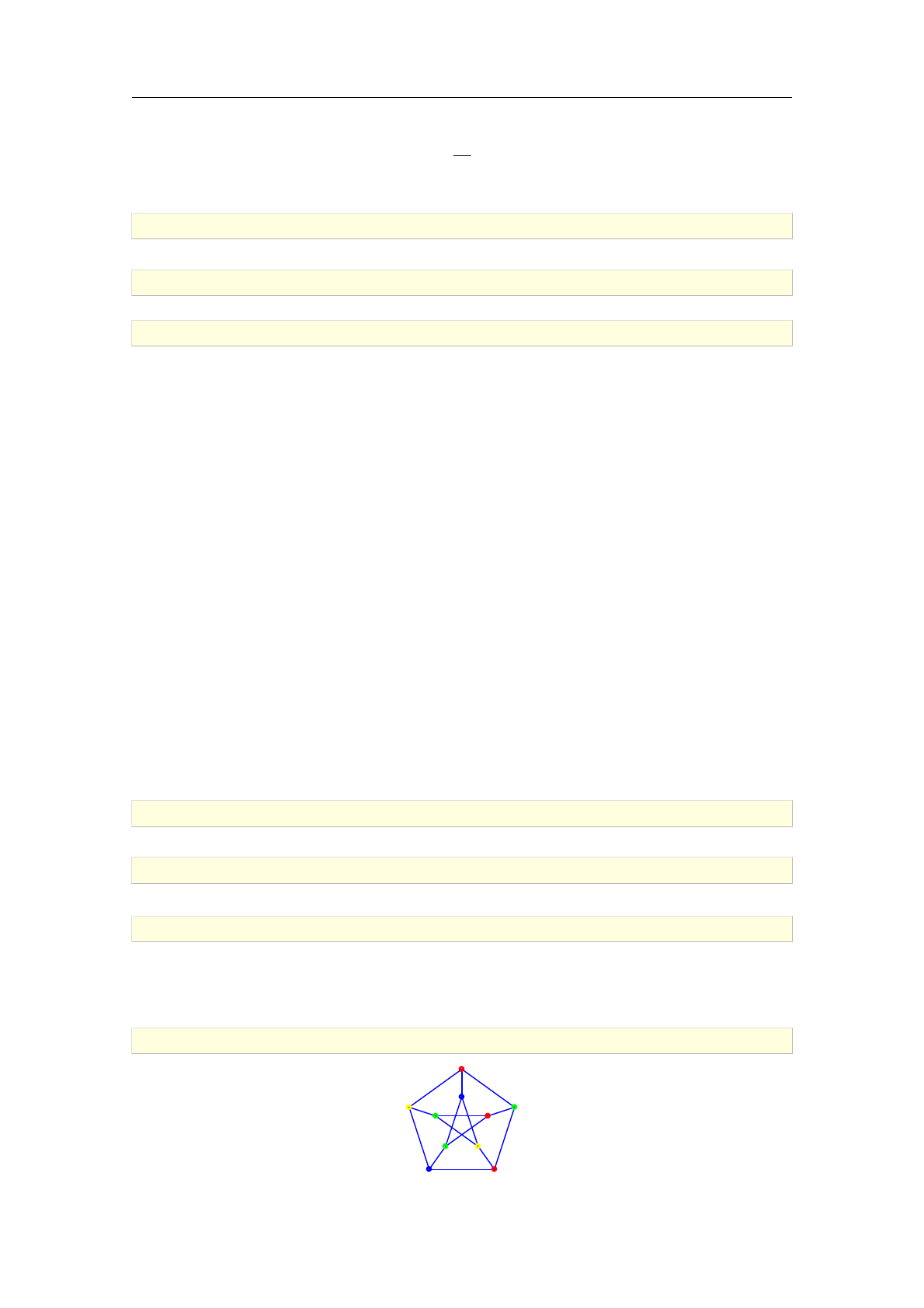
5
33
The algorithm is usable on large networks, as shown in the example below.
>G:=random_digraph(1000,500000)
a directed unweighted graph with 1000 vertices and 500000 arcs
>nt:=network_transitivity(G):;
3.5 sec
>evalf(nt)
0.500492245999
4.13. Vertex coloring
To color vertices of a graph G(V ; E)means to assign to each vertex v2Va positive integer. Each
integer represents a distinct color. The key property of graph coloring is that the colors of a pair
of adjacent vertices must be mutually different. Two different colorings of Gmay use different
number of colors.
4.13.1. Greedy vertex coloring
The command greedy_color is used for coloring vertices of a graph in a greedy fashion.
Syntax: greedy_color(G)
greedy_color(G,p)
greedy_color accepts one mandatory argument, a graph G(V ; E). Optionally, a permutation p
of order jVjmay be passed as the second argument. Vertices are colored one by one in the order
specified by p(or in the default order if pis not given) such that each vertex gets the smallest
available color. The list of vertex colors is returned in the order of vertices(G).
Generally, different choices of permutation pproduce different colorings. The total number of
different colors may not be the same each time. The complexity of the algorithm is O(jVj+jEj).
>G:=graph("petersen")
an undirected unweighted graph with 10 vertices and 15 edges
>greedy_color(G)
[1;2;1;2;3;2;1;3;3;2]
>L:=greedy_color(G,randperm(10))
[1;2;1;4;3;4;1;3;2;2]
Observe that a different number of colors is obtained by executing the last command line. To
display the colored graph, input:
>draw_graph(highlight_vertex(G,vertices(G),L),labels=false)
4.13 Vertex coloring 105
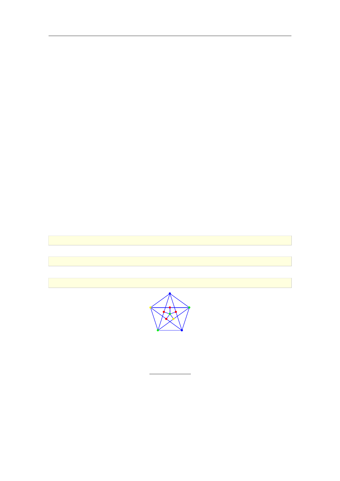
The first six positive integers are always mapped to the standard Xcas colors, as indicated in
Table 4.1. Note that the color 0 (black) and color 7 (white) are swapped; a vertex with color 0 is
white (uncolored) and vertex with color 7 is black. Also note that Xcas maps numbers greater than
7 to colors too, but the number of available colors is limited.
4.13.2. Minimal vertex coloring
The vertex coloring of Gis minimal (or optimal) if the smallest possible number of colors is
used. To obtain such a coloring use the command minimal_vertex_coloring.
Syntax: minimal_coloring(G)
minimal_coloring(G,sto)
minimal_vertex_coloring accepts one mandatory argument, a graph G(V ; E)where V=fv1;
v2; :::; vng. Optionally, a symbol sto may be passed as the second argument. The command returns
the vertex colors c1; c2; :::; cnin order of vertices(G) or, if the second argument is given, stores
the colors as vertex attributes and returns the modified copy of G.
Giac requires the GLPK library to solve the minimal vertex coloring problem (MVCP), which is
converted to the equivalent integer linear programming problem and solved by using the branch-
and-bound method with specific branch/backtrack techniques [14]. Lower and upper bounds for the
number of colors nare obtained by finding a maximal clique (ncannot be lower than its cardinality)
and by using the heuristic proposed by Brélaz in [9] (which will use at least ncolors), respectively.
Note that the algorithm performs some randomization when applying heuristics, so coloring a graph
several times will not take the same amount of computation time in each instance, generally.
In the following example, the Grötzsch graph is colored with the minimal number of colors by first
finding the coloring and then assigning it to the graph by using the highlight_vertex command.
>G:=graph("grotzsch")
an undirected unweighted graph with 11 vertices and 20 edges
>coloring:=minimal_vertex_coloring(G)
[4;2;3;1;1;4;1;3;2;1;2]
>draw_graph(highlight_vertex(G,vertices(G),coloring),labels=false)
Solving MVCP for different graphs of exactly the same size (but which do not share the same edge
structure) may take quite different time in each instance. Also note that, since vertex coloring
problem is NP hard, the algorithm may take exponential time on some graphs.
value color
1 red
2 green
3 yellow
4 blue
5 magenta
6 cyan
7 black
Table 4.1. interpretation of abstract vertex/edge colors in Xcas
106 Graph properties

4.13.3. Chromatic number
The command chromatic_number is used for exact computation or approximation of the
chromatic number of a graph.
Syntax: chromatic_number(G)
chromatic_number(G,c)
chromatic_number(G,approx or interval)
chromatic_number accepts one mandatory argument, a graph G(V ; E), and optionally a second
argument. To obtain only upper and lower bound for the chromatic number (which is much
faster than computing exactly) the option approx or interval should be passed as the second
argument. Alternatively, an unassigned identifier cis passed as the second argument; in that case
the corresponding coloring will be stored to it in form of a list of colors of the individual vertices,
ordered as in vertices(G).
The command returns the chromatic number χGof the graph Gin the case of exact computation.
If the option approx or interval is given, an interval lb..ub is returned, where lb is the best
lower bound and ub the best upper bound for χGfound by the algorithm.
The strategy is call minimal_vertex_coloring in the case of exact computation. When approxi-
mating the chromatic number, the algorithm will establish the lower bound by finding a maximum
clique. The timeout for this operation is set to 5 seconds as it can be time consuming. If no
maximum clique is not found after that time, the largest clique found is used. Then, an upper
bound is established by by using the heuristic proposed by Brélaz in [9]. Obtaining the bounds
for χGis usually very fast; however, their difference grows with jVj.
Unless the input graph is sparse enough, the algorithm slows down considerably for, say, jVj>40.
>chromatic_number(graph("grotzsch"),cols)
4
>cols
[4;2;3;1;1;4;1;3;2;1;2]
>G:=random_graph(30,0.75)
an undirected unweighted graph with 30 vertices and 313 edges
>chromatic_number(G)
10
>G:=random_graph(300,0.05)
an undirected unweighted graph with 300 vertices and 2196 edges
>chromatic_number(G,approx)
4..7
4.13.4. Mycielski graphs
The command mycielski is used for constructing Mycielski graphs.
Syntax: mycielski(G)
mycielski accepts an undirected graph G(V ; E)as its only argument and returns the corre-
sponding Mycielski graph M(also called the Mycielskian of G) with 2jVj+ 1 vertices and
3jEj+jVjedges. If Gis triangle-free then Mis also triangle-free and χM=χG+ 1.
>P:=graph("petersen")
an undirected unweighted graph with 10 vertices and 15 edges
4.13 Vertex coloring 107

>M:=mycielski(P)
an undirected unweighted graph with 21 vertices and 55 edges
>apply(number_of_triangles,[P,M])
[0;0]
>chromatic_number(P)
3
>chromatic_number(M)
4
mycielski can be applied iteratively, producing arbitrarily large graphs from the most simple ones.
For example, Grötzsch graph is obtained as the Mycielskian of a cycle graph on 5 vertices, which
is the Mycielskian of a path graph on two vertices.
>G1:=path_graph(2)
an undirected unweighted graph with 2 vertices and 1 edge
>G2:=mycielski(G1)
an undirected unweighted graph with 5 vertices and 5 edges
>is_isomorphic(G2,cycle_graph(5))
true
>G3:=mycielski(G2)
an undirected unweighted graph with 11 vertices and 20 edges
>is_isomorphic(G3,graph("grotzsch"))
true
All three graphs are triangle-free. Since it is obviously χG1= 2, it follows χG2= 3 and χG3= 4.
>apply(chromatic_number,[G1,G2,G3])
[2;3;4]
4.13.5. k-coloring
The command is_vertex_colorable is used for determining whether the vertices of a graph can
be colored with at most kcolors.
Syntax: is_vertex_colorable(G,k)
is_vertex_colorable(G,k,c)
is_vertex_colorable accepts two or three arguments: a graph G(V ; E), a positive integer kand
optionally an unassigned identifier c. The command returns true if Gcan be colored using at most
kcolors and false otherwise. If the third argument is given, a coloring using at most kcolors is
stored to cas a list of vertex colors, in the order of vertices(G).
The strategy is to first apply a simple greedy coloring procedure which runs in linear time. If
the number of required colors is greater than k, the heuristic proposed by Brélaz in [9] is used,
which runs in quadratic time. If the number of required colors is still larger than k, the algorithm
attempts to find the chromatic number χGusing kas the upper bound in the process.
>G:=graph("grotzsch")
an undirected unweighted graph with 11 vertices and 20 edges
108 Graph properties

>is_vertex_colorable(G,3)
false
>is_vertex_colorable(G,4)
true
>G:=random_graph(70,0.2)
an undirected unweighted graph with 70 vertices and 469 edges
>chromatic_number(G,approx)
5..6
>is_vertex_colorable(G,5)
false
818 msec
From the results of the last two command lines it follows χG= 6. Finding χGby utilizing the next
command line is simpler, but requires much more time.
>chromatic_number(G)
6
92.7 sec
4.14. Edge coloring
4.14.1. Minimal edge coloring
The command minimal_edge_coloring is used for finding a minimal coloring of edges in a graph,
satisfying the following two conditions: any two mutually incident edges are colored differently and
the total number nof colors is minimal. The theorem of Vizing [15, pp. 103] implies that every
simple undirected graph falls into one of two categories: 1if n= ∆ or 2if n= ∆ + 1, where ∆is
the maximum degree of the graph.
Syntax: minimal_edge_coloring(G)
minimal_edge_coloring(G,sto)
minimal_edge_coloring accepts one or two arguments, a graph G(V ; E)and optionally the
keyword sto. If the latter is given, a minimal coloring is stored to the input graph (each edge e2E
gets a color cestored as an attribute) and a modified copy of Gis returned. Else, the command
returns a sequence of two objects: integer 1or 2, indicating the category, and the list of edge colors
ce1; ce2; :::; cemaccording the order of edges e1; e2; :::; em2Eas returned by the command edges.
The strategy is to find a minimal vertex coloring of the line graph of Gby using the algorithm
described in Section 4.13.2.
>G:=graph("petersen")
an undirected unweighted graph with 10 vertices and 15 edges
>minimal_edge_coloring(G)
2;[1;2;3;2;3;3;4;1;2;3;1;4;1;4;2]
>H:=minimal_edge_coloring(graph("grotzsch"),sto)
an undirected unweighted graph with 11 vertices and 20 edges
>draw_graph(H,labels=false)
4.14 Edge coloring 109
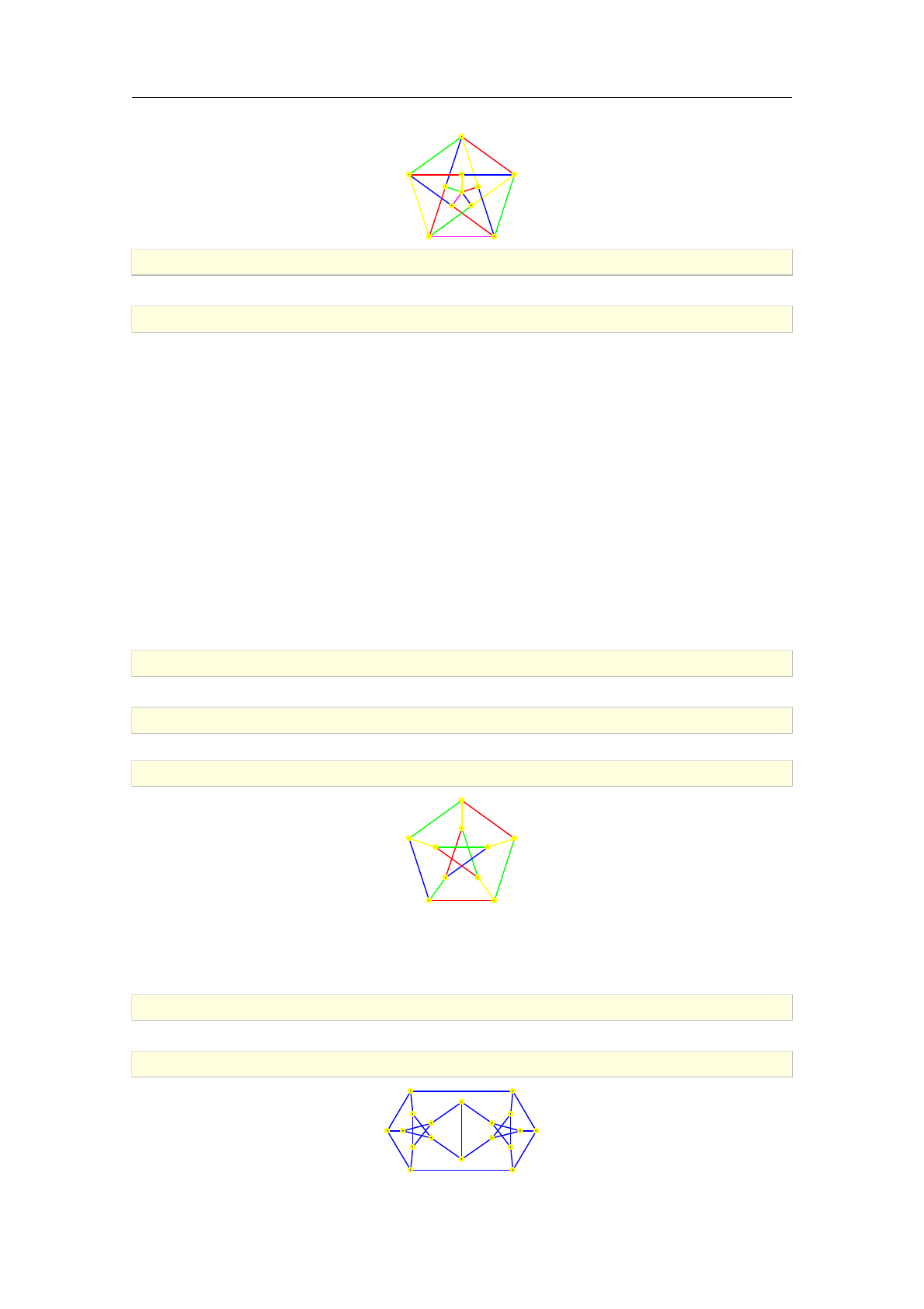
>G:=random_graph(100,0.1)
an undirected unweighted graph with 100 vertices and 499 edges
>minimal_edge_coloring(G):;
20.24 sec
4.14.2. Chromatic index
The command chromatic_index is used for computing the chromatic index of an undirected graph.
Syntax: chromatic_index(G)
chromatic_index(G,c)
chromatic_index accepts one or two arguments, an undirected graph G(E; V )and optionally an
unassigned identifier c. The command returns the minimal number χ0(G)of colors needed to color
each edge in Gsuch that two incident edges never share the same color. If the second argument
is given, it specifies the destination for storing the coloring in form of a list of colors according to
the order of edges in Eas returned by the command edges.
The example below demonstrates how to color the edges of a graph with colors obtained by passing
unassigned identifier cto chromatic_index as the second argument.
>G:=graph("petersen")
an undirected unweighted graph with 10 vertices and 15 edges
>chromatic_index(G,c)
4
>draw_graph(highlight_edges(G,edges(G),c))
Blanu²a snarks, the two graphs with 18 vertices found in 1946 by Danilo Blanu²a, were the
second and third snarks discovered [6]. For almost fifty years, Petersen graph was the only known
snark. The second Blanu²a snark is available in Giac by passing the string "blanusa" to the graph
command.
>G:=graph("blanusa")
an undirected unweighted graph with 18 vertices and 27 edges
>draw_graph(G,labels=false)
110 Graph properties

>minimum_degree(G),maximum_degree(G)
3;3
To prove that Blanu²a snark is bridgeless, it is enough to show that it is biconnected, since each
endpoint of a bridge is an articulation point (unless being of degree 1).
>is_biconnected(G)
true
>girth(G)
5
>chromatic_index(G)
4
4.14 Edge coloring 111

Chapter 5
Traversing graphs
5.1. Walks and tours
5.1.1. Eulerian graphs
The command is_eulerian is used for determining whether an undirected graph contains an
Eulerian trail.
Syntax: is_eulerian(G)
is_eulerian(G,T)
is_eulerian accepts one or two arguments, an undirected graph G(V ; E)and optionally an
unassigned identifier T, and returns true if Gis Eulerian and false otherwise. If the second
argument is given, the corresponding Eulerian trail is stored to T.
A graph Gis Eulerian if it has a trail covering all its edges. Such a trail is called Eulerian trail.
An Eulerian trail may be closed, in which case it is called Eulerian cycle. Note that every edge
e2Emust be visited, i.e. “strolled through”, exactly once [23, pp. 395]. The edge endpoints (i.e. the
vertices in G) may, however, be visited more than once.
The strategy is to apply Hierholzer's algorithm for finding an Eulerian path [29]. It works by
covering one cycle at a time in the input graph. The required time is O(jEj).
>is_eulerian(complete_graph(4))
false
>is_eulerian(complete_graph([1,2,3,4,5]),T); T
true;[1;2;3;4;1;5;2;4;5;3;1]
>is_eulerian(graph("tetrahedron"))
false
>is_eulerian(graph("octahedron"))
true
5.1.2. Hamiltonian graphs
The command is_hamiltonian is used for checking hamiltonicity of an undirected graph. The
command can also construct a Hamiltonian cycle in the input graph if the latter is Hamiltonian.
Syntax: is_hamiltonian(G)
is_hamiltonian(G,hc)
is_hamiltonian accepts one or two arguments, an undirected graph G(V ; E)and optionally an
unassigned identifier hc. The command returns true if Gis Hamiltonian and false otherwise.
When failing to determine whether Gis Hamiltonian or not, is_hamiltonian returns undef. If
the second argument is given, a Hamiltonian cycle is stored to hc.
113
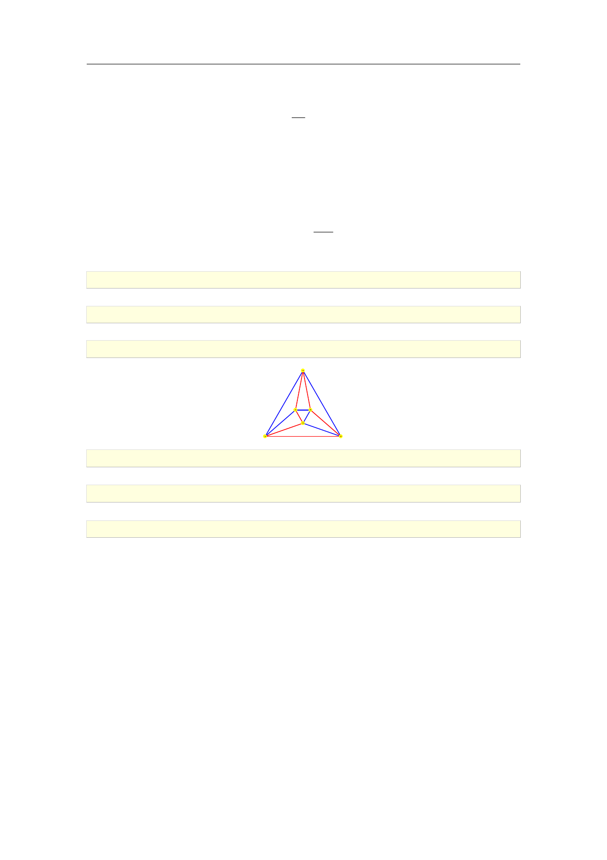
The strategy is to apply some hamiltonicity criteria presented in DeLeon [13] before resorting
to the definitive but NP-hard algorithm. If Gis not biconnected, it is not Hamiltonian. Else,
the criterion of Dirac is applied: if δ(G)>jVj
2, where δ(G) = min fdeg(v) : v2Vg, then Gis
Hamiltonian. Else, if Gis bipartite with vertex partition V=V1[V2and jV1j=/ jV2j, then Gis not
Hamiltonian. Else, the criterion of Ore is applied: if deg(u) + deg(v)>nholds for every pair u; v
of non-adjacent vertices from V, then Gis Hamiltonian. Else, the theorem of Bondy and Chvátal
is applied: if the closure cl(G)of G(obtained by finding a pair u; v of non-adjacent vertices from
Vsuch that deg(u) + deg(v)>n, adding a new edge uv to Eand repeating the process until
exhaustion) is Hamiltonian, then Gis Hamiltonian. (Note that in this case the previously tried
criteria are applied to cl(G); since the vertex degrees in cl(G)are generally higher than those in
G, the probability of success also rises.) Else, if the edge density of Gis large enough, the criterion
of Nash and Williams is applied: if δ(G)>max n+ 2
3; β, where βis the independence number
of G, then Gis Hamiltonian. If all of the above criteria fail, the command traveling_salesman
is called, either to find a Hamiltonian cycle in Gor to determine that none exist.
>is_hamiltonian(graph("soccerball"))
true
>is_hamiltonian(graph("octahedron"),hc)
true
>draw_graph(highlight_trail(graph("octahedron"),hc))
1 3
6
5
4 2
>is_hamiltonian(graph("herschel"))
false
>is_hamiltonian(graph("petersen"))
false
>is_hamiltonian(hypercube_graph(9))
true
6.04 sec
5.2. Optimal routing
5.2.1. Shortest unweighted paths
The command shortest_path is used for finding shortest paths in unweighted graphs.
Syntax: shortest_path(G,s,t)
shortest_path(G,s,T)
shortest_path accepts three arguments: an undirected unweighted graph G(V ; E), the source
vertex s2Vand the target vertex t2Vor a list Tof target vertices. The shortest path from source
to target is returned. If more targets are specified, the list of shortest paths from the source to
each of these vertices is returned.
114 Traversing graphs
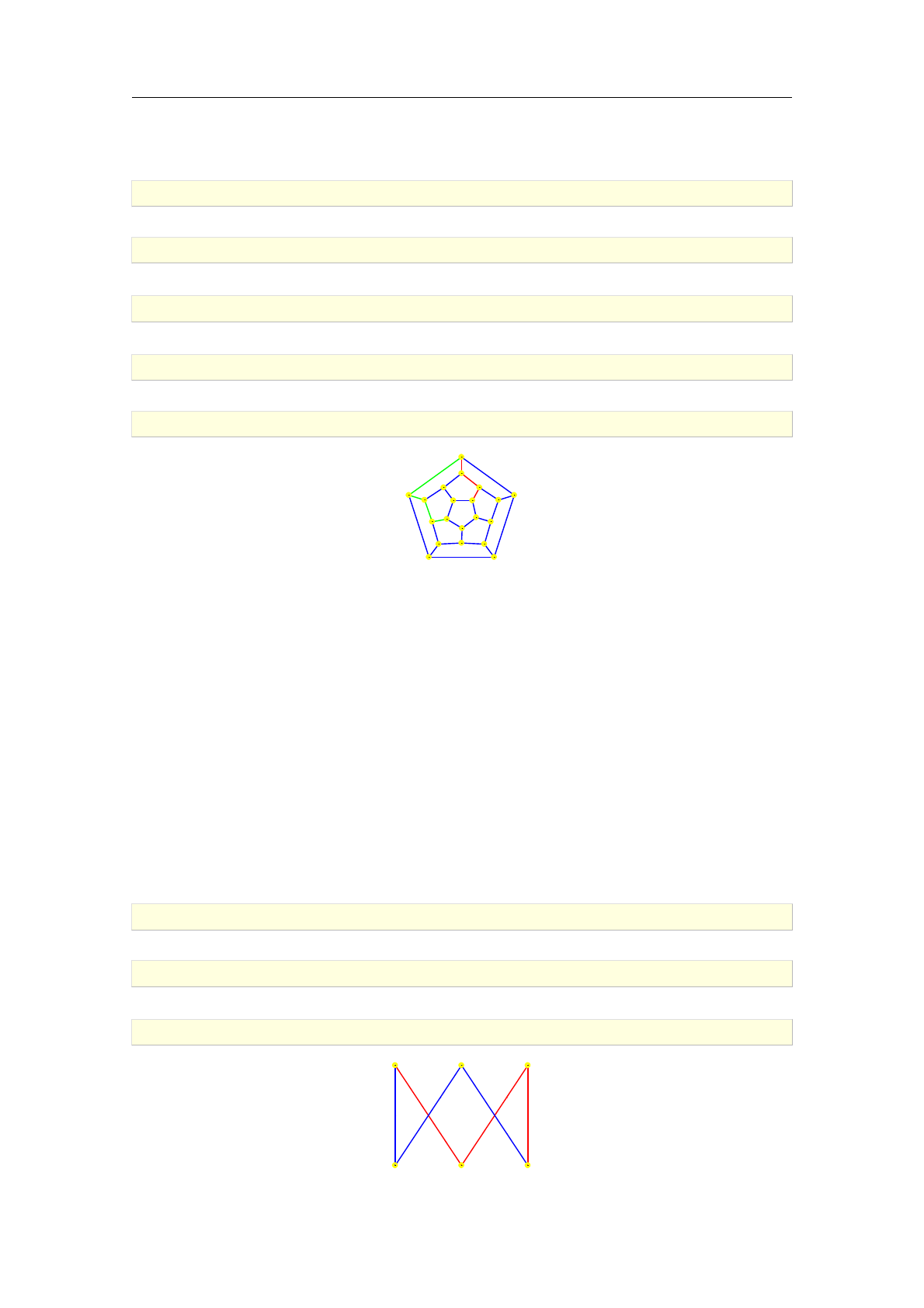
The strategy is to run breadth-first traversal on the graph Gstarting from the source vertex s.
The complexity of the algorithm is therefore O(jVj+jEj).
>G:=graph("dodecahedron")
an undirected unweighted graph with 20 vertices and 30 edges
>shortest_path(G,1,16)
[1;6;11;16]
>paths:=shortest_path(G,1,[16,19])
f[1;6;11;16];[1;5;10;14;19]g
>H:=highlight_trail(G,paths,[red,green])
an undirected unweighted graph with 20 vertices and 30 edges
>draw_graph(H)
1
25
6
3
7
4
89
10
1115
12
13
14
16
17
18
19
20
5.2.2. Cheapest weighted paths
The command dijkstra is used for finding cheapest paths in weighted graphs.
Syntax: dijkstra(G,s,t)
dijkstra(G,s,T)
dijkstra accepts two or three arguments: a weighted graph G(V ; E)with nonnegative weights, a
vertex s2Vand optionally a vertex t2Vor list Tof vertices in V. It returns the cheapest path
from sto tor, if more target vertices are given, the list of such paths to each target vertex t2T,
computed by Dijkstra's algorithm in O(jVj2)time. If no target vertex is specified, all vertices in
Vnfsgare assumed to be targets.
A cheapest path from sto tis represented with a list [[v1,v2,...,vk],c] where the first element
consists of path vertices with v1=sand vk=t, while the second element cis the weight (cost) of
that path, equal to the sum of weights of its edges.
>G:=graph(%{[[1,2],1],[[1,6],3],[[2,3],3],[[3,4],7],[[4,5],3],[[5,6],3]%})
an undirected weighted graph with 6 vertices and 6 edges
>res:=dijkstra(G,1,4)
[[1;6;5;4];9]
>draw_graph(highlight_trail(G,res[0]))
1
3
33
7
3
1
2 6
3
4
5
5.2 Optimal routing 115
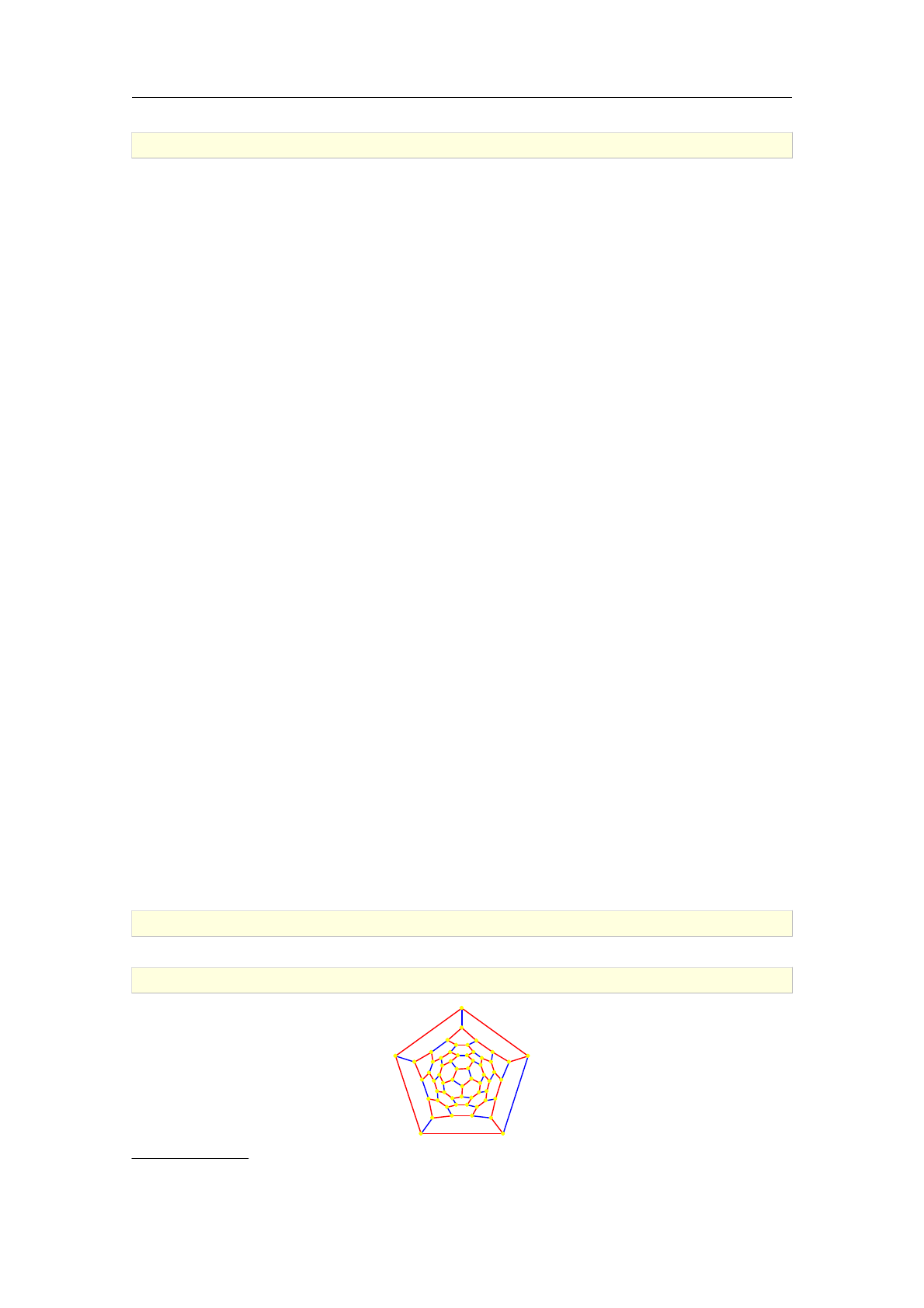
>dijkstra(G,1)
[[1];0];[[1;2];1];[[1;6];3];[[1;2;3];4];[[1;6;5;4];9];[[1;6;5];6]
5.2.3. Traveling salesman problem
The command traveling_salesman is used for solving traveling salesman problem (TSP)5.1.
Syntax: traveling_salesman(G,[opts])
traveling_salesman(G,M,[opts])
traveling_salesman accepts the following arguments: an undirected graph G(V ; E), a weight
matrix M(optional) and a sequence of options (optional). The supported options are approx and
vertex_distance.
If the input graph Gis unweighted and Mis not specified, a Hamiltonian cycle (tour) is returned
(the adjacency matrix of Gis used for the edge weights). If Gis weighted, two objects are returned:
the optimal value for the traveling salesman problem and a Hamiltonian cycle which achieves the
optimal value. If Mis given and Gis unweighted, Mis used as the weight matrix for G.
If the option vertex_distance is passed and Mis not specified, then for each edge e2Ethe
Euclidean distance between its endpoints is used as the weight of e. Therefore it is required for
each vertex in Gto have a predefined position.
If the option approx is passed, a near-optimal tour is returned. In this case it is required that G
is a complete weighted graph. For larger graphs, this is significantly faster than finding optimal
tour. Results thus obtained are usually only a few percent larger than the corresponding optimal
values, despite the fact that the reported guarantee is generally much weaker (around 30%).
The strategy is to formulate TSP as a linear programming problem and to solve it by branch-and-
cut method, applying the hierarchical clustering method of Pferschy and Stan¥k [42] to generate
subtour elimination constraints. The branching rule is implemented according to Padberg and
Rinaldi [41]. In addition, the algorithm combines the method of Christofides [11], the method
of farthest insertion and a variant of the powerful tour improvement heuristic developed by Lin
and Kernighan [28] to generate near-optimal feasible solutions during the branch-and-cut process.
For Euclidean TSP instances, i.e. in cases when Gis a complete graph with vertex distances as
the edge weights, the algorithm usually finishes in a few seconds for TSP with up to, say, 42 cities.
For problems with 100 or more cities, the option approx is recommended as finding the optimal
value takes a long time. Note that TSP is NP-hard, meaning that no polynomial time algorithm
is known. Hence the algorithm may take exponential time to find the optimum in some instances.
The following example demonstrates finding a Hamiltonian cycle in the truncated icosahedral
(“soccer ball”) graph. The result is visualized by using the highlight_trail command.
>G:=graph("soccerball")
an undirected unweighted graph with 60 vertices and 90 edges
>draw_graph(highlight_trail(G,traveling_salesman(G)),labels=false)
5.1. For the details on traveling salesman problem and a historical overview see [12].
116 Traversing graphs
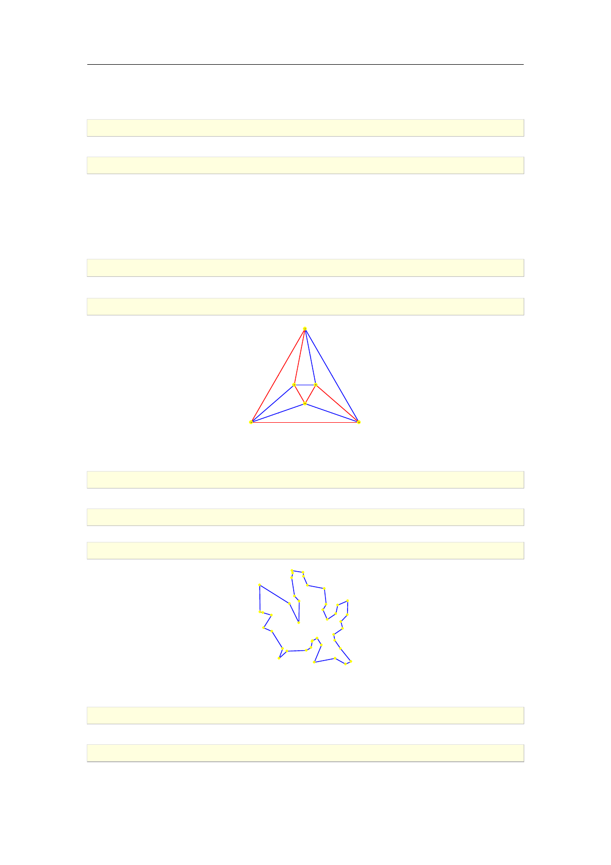
A matrix may be passed alongside an undirected graph to specify the edge weights. The alternative
is to pass a weighted graph as the single argument.
>G:=graph("octahedron")
an undirected unweighted graph with 6 vertices and 12 edges
>M:=randmatrix(6,6,25)
0
B
B
B
B
B
B
B
B
B
B
B
B
@
713 15 10 17 6
17 723 317 5
15 24 19 15 20 24
316 10 18 1 3
920 9 2 19 15
17 819 20 15 15
1
C
C
C
C
C
C
C
C
C
C
C
C
A
>c,t:=traveling_salesman(G,M)
57.0;[4;5;2;3;1;6;4]
>draw_graph(highlight_trail(make_weighted(G,M),t))
13
15
10
17
23
3
5
20 24
1 3
15
1 3
6
5
4 2
In the next example, an instance of Euclidean TSP with 42 cities is solved to optimality. The
vertex positions are pairs of integers randomly chosen on the grid [0;1000]×[0;1000]2Z2.
>G:=set_vertex_positions(complete_graph(42),[randvector(2,1000)$(k=1..42)])
an undirected unweighted graph with 42 vertices and 861 edges
>c,t:=traveling_salesman(G,vertex_distance):;
10.01 sec
>draw_graph(subgraph(G,trail2edges(t)),labels=false)
For large instances of Euclidean TSP the approx option may be used, as in the following example
with 555 cities.
>H:=set_vertex_positions(complete_graph(555),[randvector(2,10000)$(k=1..555)])
an undirected unweighted graph with 555 vertices and 153735 edges
>ac,t:=traveling_salesman(H,vertex_distance,approx):;
49.34 sec
5.2 Optimal routing 117
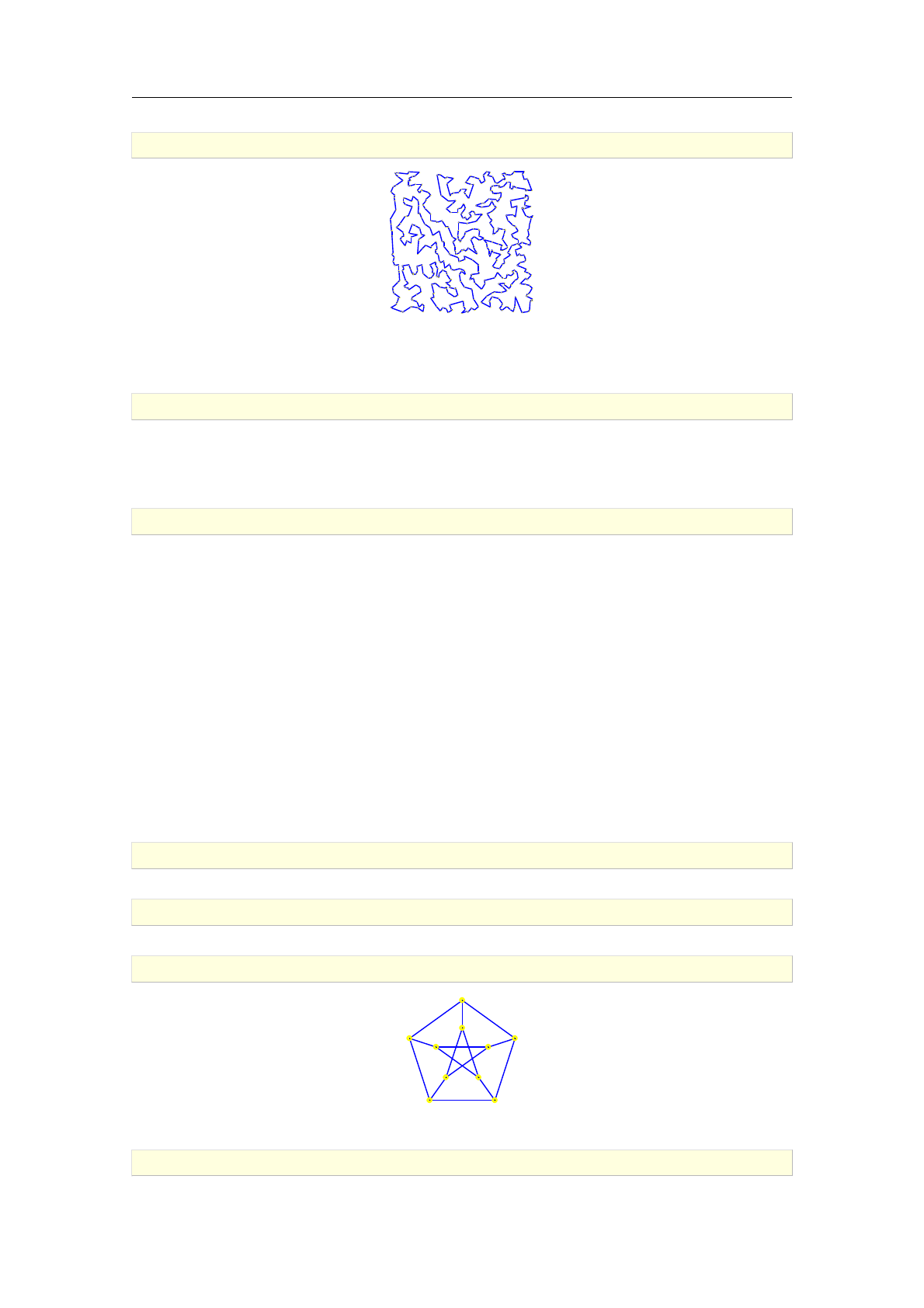
>draw_graph(subgraph(H,trail2edges(t)))
Near-optimal tours produced by the approx option are usually only slightly more expensive than
the optimal ones. For example, a sub-optimal tour for the previous instance Gwith 42 cities is
obtained by the following command.
>ac,st:=traveling_salesman(G,vertex_distance,approx):;
The tour cost is within 28% of the optimal value
Although it is guaranteed that the near-optimal cost ac is for at most 28% larger than c(the
optimum), the actual relative difference is smaller than 3%, as computed below.
>100*(ac-c)/c
2.7105821877
5.3. Spanning trees
5.3.1. Construction of spanning trees
The command spanning_tree is used for construction of spanning trees in graphs.
Syntax: spanning_tree(G)
spanning_tree(G,r)
spanning_tree accepts one or two arguments, an undirected graph G(V ; E)and optionally a
vertex r2V. It returns the spanning tree T(rooted in r) of G, obtained by depth-first traversal
in O(jVj+jEj)time.
>P:=graph("petersen")
an undirected unweighted graph with 10 vertices and 15 edges
>T1:=spanning_tree(P)
an undirected unweighted graph with 10 vertices and 9 edges
>draw_graph(P)
0
1
23
4
5
6
78
9
By extracting T1from Pas a subgraph, it inherits vertex positions from P.
>draw_graph(subgraph(P,edges(T1)))
118 Traversing graphs

0
1
23
4
9
5
78
6
>T2:=spanning_tree(P,4)
an undirected unweighted graph with 10 vertices and 9 edges
>edges(T1), edges(T2)
0
B
B
B
B
B
B
B
B
B
B
B
B
B
B
B
B
B
B
B
B
B
B
B
B
@
0 1
1 2
2 3
3 4
4 9
5 7
5 8
6 8
6 9
1
C
C
C
C
C
C
C
C
C
C
C
C
C
C
C
C
C
C
C
C
C
C
C
C
A
;
0
B
B
B
B
B
B
B
B
B
B
B
B
B
B
B
B
B
B
B
B
B
B
B
B
@
0 1
0 4
1 2
2 3
3 8
5 7
5 8
6 9
7 9
1
C
C
C
C
C
C
C
C
C
C
C
C
C
C
C
C
C
C
C
C
C
C
C
C
A
5.3.2. Minimal spanning tree
The command minimal_spanning_tree is used for obtaining minimal spanning trees in undirected
graphs.
Syntax: minimal_spanning_tree(G)
minimal_spanning_tree accepts an undirected graph G(V ; E)as its only argument and returns
its minimal spanning tree as a graph. If Gis not weighted, it is assumed that the weight of each
edge in Eis equal to 1.
The strategy is to apply Kruskal's algorithm which runs in O(jEjlog jVj)time.
>A:=[[0,1,0,4,0,0],[1,0,1,0,4,0],[0,1,0,3,0,1],[4,0,3,0,1,0],[0,4,0,1,0,4],[0,
0,1,0,4,0]]:;
>G:=graph(A)
an undirected weighted graph with 6 vertices and 8 edges
>T:=minimal_spanning_tree(G)
an undirected weighted graph with 6 vertices and 5 edges
>edges(T,weights)
f[[0;1];1];[[1;2];1];[[2;5];1];[[2;3];3];[[3;4];1]g
>draw_graph(highlight_subgraph(G,T))
1
414
3
1
1
4
0
1
2
3
4
5
5.3.3. Counting the spanning trees in a graph
The command number_of_spanning_trees is used for counting spanning trees in a graph.
5.3 Spanning trees 119

Syntax: number_of_spanning_trees(G)
number_of_spanning_trees accepts an undirected graph G(V ; E)as its only argument and returns
the total number nof (labeled) spanning trees in G.
The strategy is to use Kirchhoff's Theorem [55, Theorem 2.2.12, pp. 86]. The number of spanning
trees is equal to the first principal minor of the Laplacian matrix of G.
>number_of_spanning_trees(graph("octahedron"))
384
>number_of_spanning_trees(graph("dodecahedron"))
5184000
>number_of_spanning_trees(hypercube_graph(4))
42467328
>number_of_spanning_trees(graph("soccerball"))
375291866372898816000
120 Traversing graphs

Chapter 6
Visualizing graphs
6.1. Drawing graphs
The draw_graph command is used for visualizing graphs. It is capable to produce a drawing of
the given graph using one of the several built-in methods.
Syntax: draw_graph(G)
draw_graph(G,opts)
6.1.1. Overview
draw_graph accepts one or two arguments, the mandatory first one being a graph G(V ; E). This
command assigns 2D or 3D coordinates to each vertex v2Vand produces a visual representation
of Gbased on these coordinates. The second (optional) argument is a sequence of options. Each
option is one of the following:
¡labels=true or false: controls the visibility of vertex labels and edge weights (by default
true, i.e. the labels and weights are displayed)
¡spring: draw the graph Gusing a multilevel force-directed algorithm
¡tree[=r or [r1,r2,...]]: draw the tree or forest G, optionally specifying root nodes for
each tree
¡bipartite: draw the bipartite graph Gkeeping the vertex partitions separated
¡circle[=L] or convexhull[=L]: draw the graph Gby setting the hull vertices from list
L⊂V(assuming L=Vby default) on the unit circle and all other vertices in origin,
subsequently applying a force-directed vertex placement algorithm to generate the layout
while keeping the hull vertices fixed
¡planar or plane: draw the planar graph Gusing a force-directed algorithm
¡plot3d: draw the connected graph Gas if the spring option was enabled, but with vertex
positions in 3D instead of 2D
¡any unassigned identifier P: when given, the vertex coordinates will be stored to it in form
of a list
The style options spring,tree,circle,planar and plot3d cannot be mixed, i.e. at most one can
be specified. The option labels may be combined with any of the style options. Note that edge
weights will not be displayed when using plot3d option when drawing a weighted graph.
When no style option is specified, the algorithm first checks if the graph Gis a tree or if it is
bipartite, in which cases it is drawn accordingly. Otherwise, the graph is drawn as if the option
circle was specified.
Tree, circle and bipartite drawings can be obtained in linear time with a very small overhead,
allowing graphs to be drawn quickly no matter the size. The force-directed algorithms are more
expensive and operating in the time which is quadratic in the number of vertices. Their performance
is, nevertheless, practically instantaneous for graphs with several hundreds of vertices (or less).
6.1.2. Drawing disconnected graphs
When the input graph has two or more connected components, each component is drawn separately
and the drawings are subsequently arranged such that the bounding box of the whole drawing has
the smallest perimeter under condition that as little space as possible is wasted inside the box.
121
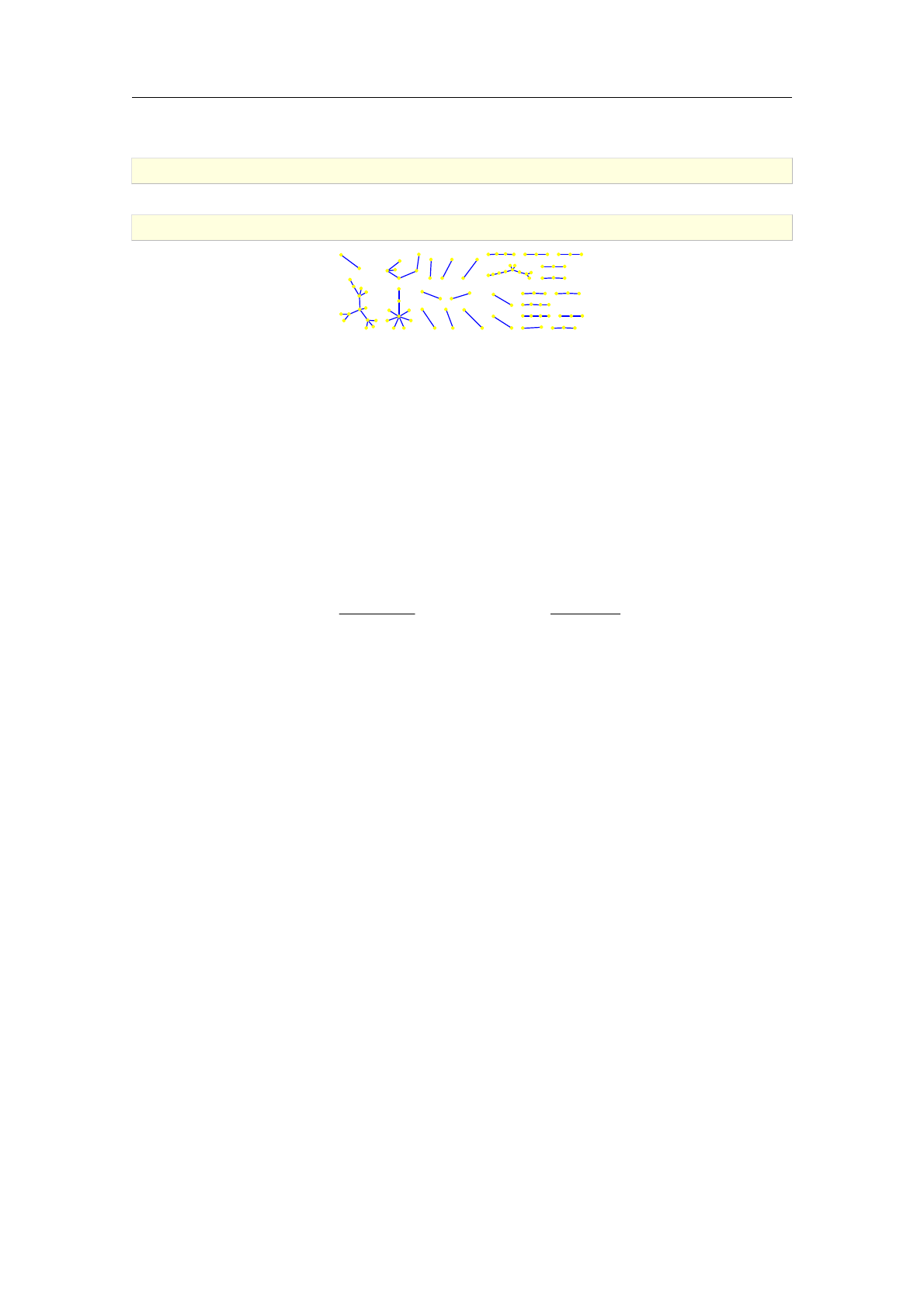
For example, the command lines below draw a sparse random planar graph.
>G:=random_planar_graph(100,0.9,0)
an undirected unweighted graph with 100 vertices and 74 edges
>draw_graph(G,planar)
6.1.3. Spring method
When the option spring is specified, the input graph is drawn using the force-directed algorithm
described in [32] (for an example of such a drawing see Figure 3.1). The idea, originally due to
Fruchterman and Reingold [21], is to simulate physical forces in a spring-electrical model
where the vertices and edges represent equally charged particles and springs connecting them,
respectively.
In a spring-electrical model, each vertex is being repulsed by every other vertex with a force
inversely proportional to the distance between them. At the same time, it is attracted to each of its
neighbors with a force proportional to the square of the distance. Assuming that xvis the vector
representing the position of the vertex v2V, the total force Fvapplied to vis equal to
Fv=X
w2Vnfvg¡C K2
kxv¡xwk2(xv¡xw) + X
w2N(v)
kxv¡xwk
K(xv¡xw);
where N(v)is the set of neighbors of vand C,Kare certain positive real constants (actually, K
may be any positive number, it affects only the scaling of the entire layout). Applying the forces
iteratively and updating vertex positions in each iteration (starting from a random layout) leads the
system to the state of minimal energy. By applying a certain “cooling” scheme to the model which
cuts down the force magnitude in each iteration. the layout “freezes” after a number of iterations
large enough to achieve the minimal energy state.
The force-directed method is computationally expensive and for larger graphs the pleasing layout
cannot be obtained most of the time since the algorithm, starting with a random initial layout,
gets easily “stuck” in the local energy minimum (ideally, the vertex positions should settle in the
global minimal energy constellation). To avoid this a multilevel scheme is applied. The input graph
is iteratively coarsened, either by removing the vertices from a maximal independent vertex set
or contracting the edges of a maximal matching in each iteration. Each coarsening level is then
processed by the force-directed algorithm, starting from the deepest (coarsest) one and “lifting” the
obtained layout to the first upper level, using it as the initial layout for that level. The lifting is
achieved by using the prolongation matrix technique described in [33]. To support drawing large
graphs (with 1000 vertices or more), the matrices used in the lifting process are stored as sparse
matrices. The multilevel algorithm is significantly faster than the original, single-level one and
usually produces better results.
Graph layouts obtained by using force-directed method have a unique property of reflecting sym-
metries in the design of the input graph, if any. Thus the drawings become more appealing and
illustrate the certain properties of the input graph better. To make the symmetry more prominent,
the drawing is rotated such that the axis, with respect to which the layout exhibits the largest
symmetry score, becomes vertical. As the symmetry detection is in general very computationally
expensive—up to O(jVj7)when using the symmetry measure of Purchase [54], for example—the
algorithm deals only with the convex hull and the barycenter of the layout, which may not always
be enough to produce the optimal result. Nevertheless, this approach is very fast and seems to
work most of the time for graphs with a high level of symmetry.
122 Visualizing graphs
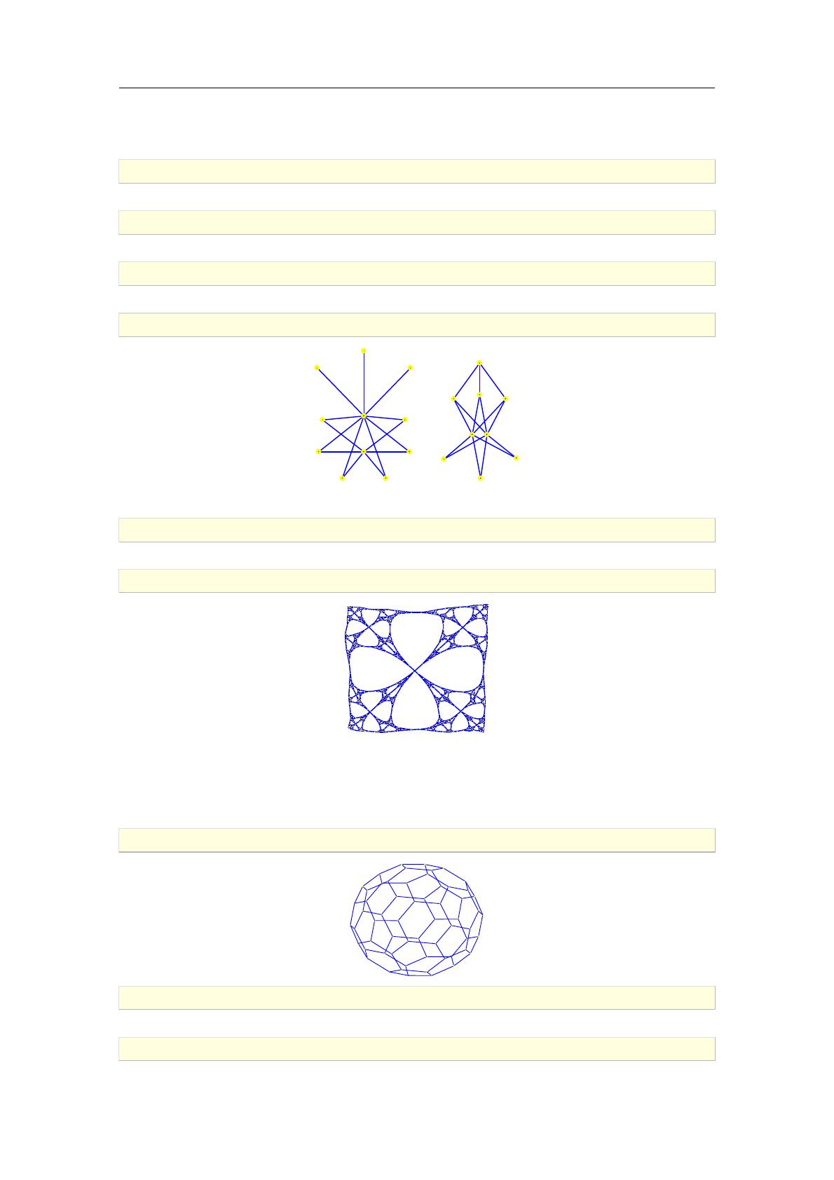
For example, the following command lines produce a drawing of the tensor product of two graphs
using the force-directed algorithm.
>G1:=graph(trail(1,2,3,4,5,2))
an undirected unweighted graph with 5 vertices and 5 edges
>G2:=star_graph(3)
an undirected unweighted graph with 4 vertices and 3 edges
>G:=tensor_product(G1,G2)
an undirected unweighted graph with 20 vertices and 30 edges
>draw_graph(G,spring,labels=false)
The following example demonstrates drawing a much larger graph.
>S:=sierpinski_graph(5,4)
an undirected unweighted graph with 1024 vertices and 2046 edges
>draw_graph(S,spring)
Note that vertex labels are automatically suppressed because of the large number of vertices. On
our system, the algorithm took less than two seconds to produce the layout.
The spring method is also used for creating 3D graph layouts, which are obtained by passing the
option plot3d to the draw_graph command.
>draw_graph(graph("soccerball"),plot3d,labels=false)
>G1:=graph("icosahedron"):; G2:=graph("dodecahedron"):;
Done;Done
>G1:=highlight_edges(G1,edges(G1),red)
6.1 Drawing graphs 123
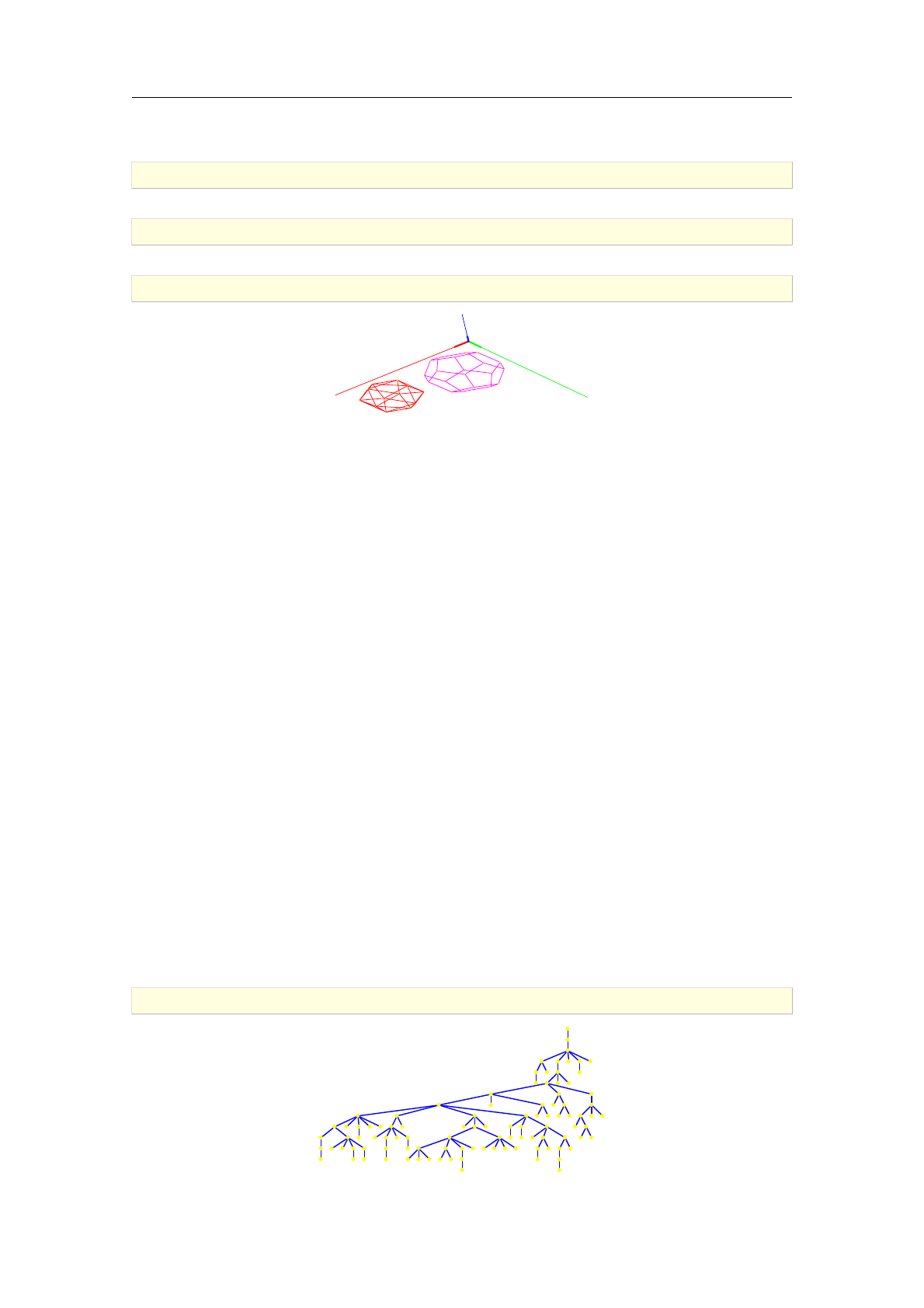
an undirected unweighted graph with 12 vertices and 30 edges
>G2:=highlight_edges(G2,edges(G2),magenta)
an undirected unweighted graph with 20 vertices and 30 edges
>G:=disjoint_union(G1,G2)
an undirected unweighted graph with 32 vertices and 60 edges
>draw_graph(G,plot3d,labels=false)
y
x
z
6.1.4. Drawing trees
When the tree[=r] option is specified and the input graph Gis a tree (and r2V), it is drawn using
a fast but simple node positioning algorithm inspired by the well-known algorithm of Walker [52],
using the first vertex (or the vertex r) as the root node. When drawing a rooted tree, one usually
requires the following aesthetic properties [10].
A1. The layout displays the hierarchical structure of the tree, i.e. the y-coordinate of a node is
given by its level.
A2. The edges do not cross each other.
A3. The drawing of a sub-tree does not depend on its position in the tree, i.e. isomorphic sub-
trees are drawn identically up to translation.
A4. The order of the children of a node is displayed in the drawing.
A5. The algorithm works symmetrically, i.e. the drawing of the reflection of a tree is the reflected
drawing of the original tree.
The algorithm implemented in Giac generally satisfies all the above properties but A3. Instead,
it tries to spread the inner sub-trees evenly across the available horizontal space. It works by
organizing the structure of the input tree into levels by using depth-first search and laying out
each level subsequently, starting from the deepest one and climbing up to the root node. In the
end, another depth-first traversal is made, shifting the sub-trees horizontally to avoid intersections
between their edges. The algorithm runs in O(jVj)time and uses the minimum of horizontal space
to draw the tree with respect to the specified root node r.
For example, the following command line produces the drawing of a random tree on 100 nodes.
>draw_graph(random_tree(100))
124 Visualizing graphs
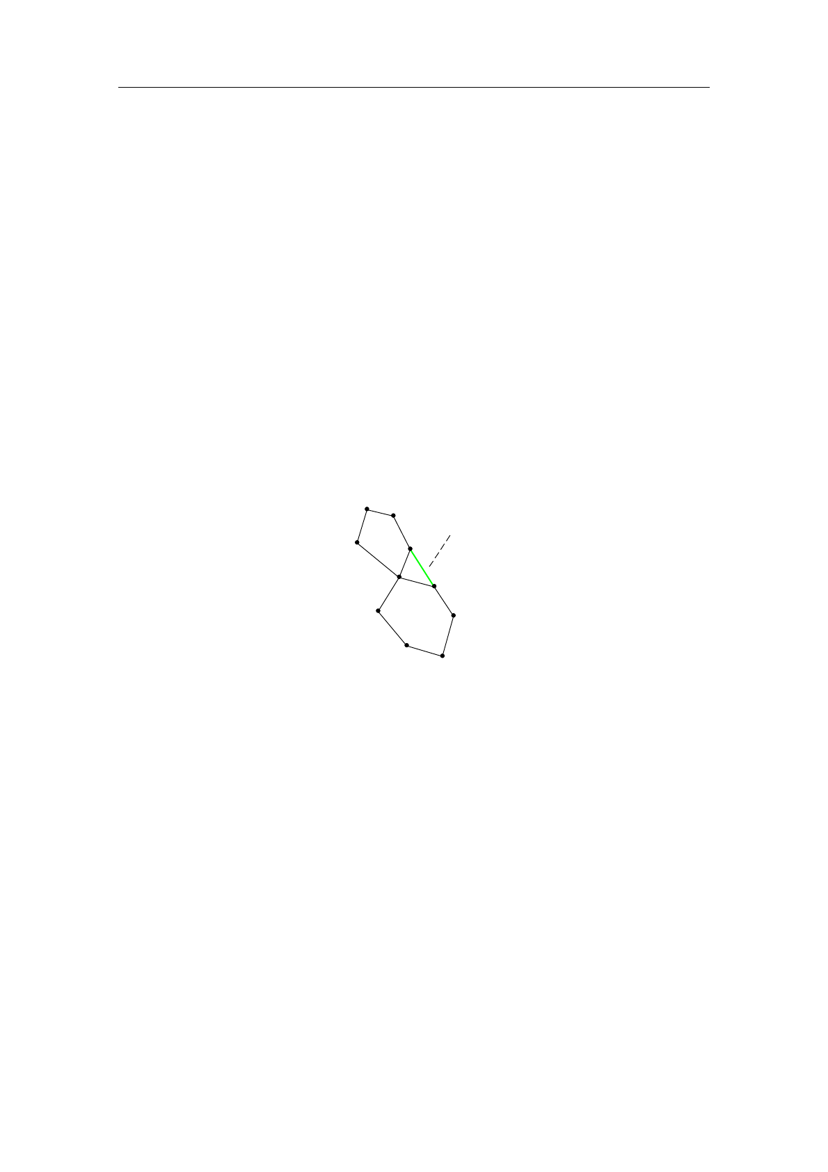
6.1.5. Drawing planar graphs
The algorithm implemented in Giac which draws planar graphs uses augmentation techniques to
extend the input graph Gto a graph G0, which is homeomorphic to some triconnected graph,
by adding temporary edges. The augmented graph G0is then drawn using Tutte's barycentric
method (see [51] and [23, pp. 293]) which puts each vertex in the barycenter of its neighbors. It
is guaranteed that a (non-strict) convex drawing will be produced, without edge crossings. In the
end, the duplicate of the outer face and the temporary edges inserted during the augmentation
stage are removed.
Tutte's algorithm requires that the vertices of the chosen outer face are initially fixed somewhere
the boundary of a convex polygon. In addition, to produce a more flexible layout, the outer face is
duplicated such that the subgraph induced by the vertices on both the outer face and its duplicate
is a prism graph. Then only the duplicates of the outer face vertices are fixed, allowing the outer
face itself to take a more natural shape. The duplicate of the outer face is removed after a layout
is produced.
The augmentation process consists of two parts. Firstly, the input graph Gis decomposed into
biconnected components (blocks) using the depth-first search [22, pp. 25]. Each block is then
decomposed into faces (represented by cycles of vertices) using Demoucron's algorithm (see [22,
pp. 88] and [37]). Embeddings obtained for each blocks are then combined by adding one temporary
edge for each articulation point, joining the two corresponding blocks. Figure 6.1 shows the outer
faces of two blocks B1and B2, connected by an articulation point (cut vertex). The temporary
B1
B2
temp. edge
Fig. 6.1. Joining two block by adding a temporary edge.
edge (shown in green) is added to join B1and B2into a single block. After “folding up” the tree
of blocks, the algorithm picks the largest face in the resulting biconnected graph to be the outer
face of the planar embedding.
The second part of the augmentation process consists of recursively decomposing each non-convex
inner face into several convex polygons by adding temporary edges. An inner face f= (v1; :::; vn)
is non-convex if there exist kand lsuch that 16k < l ¡1< n and either vkvl2E, in which case
the edge vkvlis a chord (see Figure 6.2 for an example) or there exists a face g= (w1; w2; :::; vk; :::;
vl; :::; wm¡1; wm)such that the vertices vk+1; :::; vl¡1are not contained in g(see Figure 6.3 for an
example). In Figures 6.1,6.2 and 6.3, the temporary edges added by the algorithm are drawn in
green.
This method of drawing planar graphs operates in O(jVj2)time. Nevertheless, it is quite fast
for graphs up to 1000 vertices, usually producing results in less than a second. The drawback of
this method is that it sometimes creates clusters of vertices which are very close to each other,
resulting in a very high ratio of the area of the largest inner face to the area of the smallest inner
face. However, if the result is not satisfactory, one should simply redraw the graph and repeat the
process until a better layout is found. The planar embedding will in general be different each time.
Another drawback of this method is that sparse planar graphs are sometimes drawn poorly.
The following example shows that the above described improvement of the barycentric method
handles non-triconnected graphs well.
6.1 Drawing graphs 125
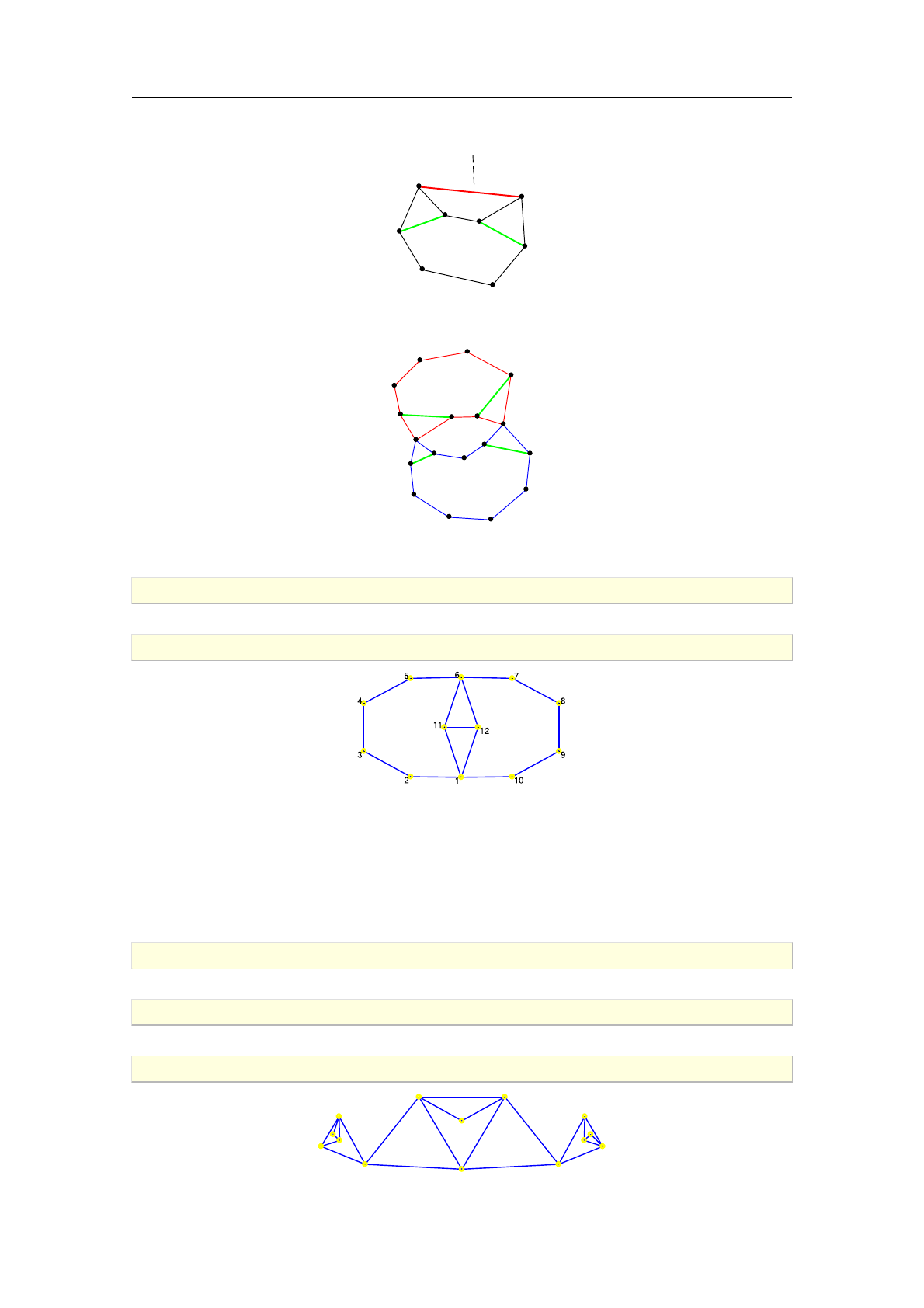
f
chord
Fig. 6.2. A chorded face.
f
g
vl
vk
Fig. 6.3. Two faces sharing a pair of vertices and no edges between them.
>G:=graph(trail(1,2,3,4,5,6,7,8,9,10,1),trail(11,12,6,11,1,12))
an undirected unweighted graph with 12 vertices and 15 edges
>draw_graph(G,planar)
Note that the inner diamond-like shape in the above drawing would end up flattened—making the
two triangular faces invisible—if the input graph was not augmented. It is so because the vertices
with labels 11 and 12 are “attracted” to each other (namely, the two large faces are “inflating”
themselves to become convex), causing them to merge eventually.
In the following example the input graph Gis connected but not biconnected (it has two articu-
lation points). It is obtained by removing a vertex from the Sierpi«ski triangle graph ST3
3. Note
that the syntax mode is set to Xcas in this example, so the first vertex label is zero.
>G:=sierpinski_graph(3,3,triangle)
an undirected unweighted graph with 15 vertices and 27 edges
>G:=delete_vertex(G,3)
an undirected unweighted graph with 14 vertices and 23 edges
>draw_graph(G,planar,labels=false)
126 Visualizing graphs
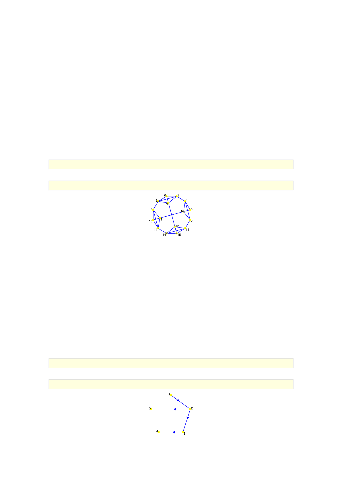
In the above example, several redraws were required to obtain a good planar embedding.
6.1.6. Circular graph drawings
The drawing method selected by specifying the option circle=L or convexhull=L when calling
draw_graph on a triconnected graph G(V ; E), where L⊂Vis a set of vertices in G, uses the
following strategy. First, positions of the vertices from Lare fixed so that they form a regular
polygon on the unit circle. Other vertices, i.e. all vertices from VnL, are placed in origin. Then
an iterative force-directed algorithm [43], similar to Tutte's barycentric method, is applied to
obtain the final layout.
This approach gives best results for symmetrical graphs such as generalized Petersen graphs. In
addition, if the input graph is planar, the drawing will also be planar (there is a possibility, however,
that some very short edges may cross each other as the number of force update iterations is limited).
In the following example the Sierpi«ski graph S4
2is drawn using the above method. Note that the
command lines below are executed in Xcas mode.
>G:=sierpinski_graph(2,4)
an undirected unweighted graph with 16 vertices and 30 edges
>draw_graph(G,circle=[0,1,4,5,7,13,15,14,11,10,8,2])
6.2. Vertex positions
6.2.1. Setting vertex positions
The command set_vertex_positions is used to assign custom coordinates to vertices of a graph
to be used when drawing the graph.
Syntax: set_vertex_positions(G,L)
set_vertex_positions accepts two arguments, a graph G(V ; E)and the list Lof positions to be
assigned to vertices in order of vertices(G). The positions may be complex numbers, lists of coor-
dinates or points (geometrical objects created with the command point). set_vertex_positions
returns the copy G0of Gwith the given layout stored in it.
Any subsequent call to draw_graph with G0as an argument and without specifying the drawing
style will result in displaying vertices at the stored coordinates. However, if a drawing style is
specified, the stored layout is ignored (although it stays stored in G0).
>G:=digraph([1,2,3,4,5],%{[1,2],[2,3],[3,4],[2,5]%})
a directed unweighted graph with 5 vertices and 4 arcs
>draw_graph(G,circle)
6.2 Vertex positions 127
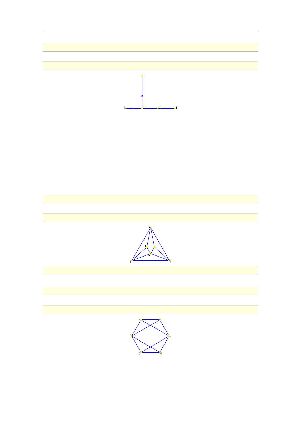
>H:=set_vertex_positions(G,[[0,0],[0.5,0],[1.0,0],[1.5,0],[0.5,1]])
a directed unweighted graph with 5 vertices and 4 arcs
>draw_graph(H)
6.2.2. Generating vertex positions
Vertex positions can be generated for a particular graph Gby using the draw_graph command with
the additional argument Pwhich should be an unassigned identifier. After the layout is obtained,
it will be stored to Pas a list of positions (complex numbers for 2D drawings or points for 3D
drawings) for each vertex in order of vertices(G).
This feature combines well with the set_vertex_positions command, as when one obtains the
desired drawing of the graph Gby calling draw_graph, the layout coordinates can be easily stored
to the graph for future reference. In particular, each subsequent call of draw_graph with Gas an
argument will display the stored layout. The example below illustrates this property by setting a
custom layout to the octahedral graph.
>G:=graph("octahedron")
an undirected unweighted graph with 6 vertices and 12 edges
>draw_graph(G)
>draw_graph(G,P,spring):;
Now Pcontains vertex coordinates, which can be permanently stored to G:
>G:=set_vertex_positions(G,P)
an undirected unweighted graph with 6 vertices and 12 edges
>draw_graph(G)
It should be noted that, after a particular layout is fixed, it stays valid when some edges or vertices
are removed or when an edge is contracted. The stored layout becomes invalid only if a new vertex
is added to the graph (unless its position is specified by set_vertex_attribute upon the creation)
or if the position attribute of an existing vertex is discarded.
128 Visualizing graphs
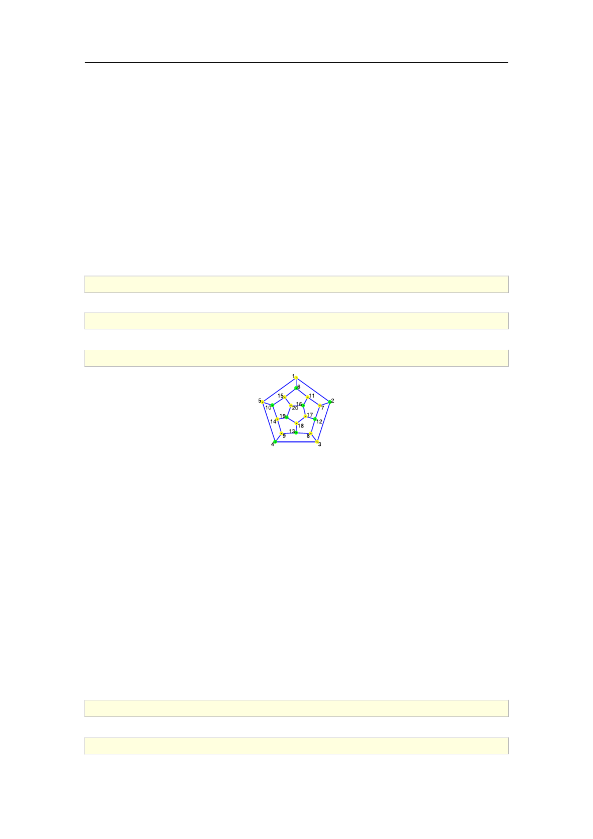
6.3. Highlighting parts of graphs
6.3.1. Highlighting vertices
The command highlight_vertex is used for changing color of one or more vertices in a graph.
Syntax: highlight_vertex(G,v)
highlight_vertex(G,v,c)
highlight_vertex(G,[v1,v2,..,vk])
highlight_vertex(G,[v1,v2,..,vk],c)
highlight_vertex(G,[v1,v2,..,vk],[c1,c2,..,ck])
highlight_vertex accepts two or three arguments: a graph G(V ; E), a vertex v2Vor a list of
vertices v1; v2; :::; vk2Vand optionally the new color cor a list of colors c1; c2; :::; ckfor the selected
vertices (the default color is green). It returns a modified copy of Gin which the specified vertices
are colored with the specified color.
>G:=graph("dodecahedron")
an undirected unweighted graph with 20 vertices and 30 edges
>L:=maximum_independent_set(G)
[2;4;6;12;13;10;16;19]
>draw_graph(highlight_vertex(G,L))
6.3.2. Highlighting edges and trails
To highlight an edge or a set of edges in a graph, use the highlight_edges command. If the edges
form a trail, it is usually more convenient to use the highlight_trail command (see below).
Syntax: highlight_edges(G,e)
highlight_edges(G,e,c)
highlight_edges(G,[e1,e2,..,ek])
highlight_edges(G,[e1,e2,..,ek],c)
highlight_edges(G,[e1,e2,..,ek],[c1,c2,..,ck])
highlight_trail(G,T)
highlight_trail(G,T,c)
highlight_trail(G,[T1,T2,..,Tk])
highlight_trail(G,[T1,T2,..,Tk],c)
highlight_trail(G,[T1,T2,..,Tk],[c1,c2,..,ck])
highlight_edges accepts two or three arguments: a graph G(V ; E), an edge e2Eor a list of
edges e1; e2; :::; ek2Eand optionally the new color cor a list of colors c1; c2; :::; ckfor the selected
edges (the default color is red). It returns a modified copy of Gin which the specified edges are
colored with the specified color.
>M:=maximum_matching(G)
f[1;2];[5;4];[6;11];[3;8];[7;12];[9;13];[10;15];[14;19];[16;17]g
>draw_graph(highlight_edges(G,M))
6.3 Highlighting parts of graphs 129
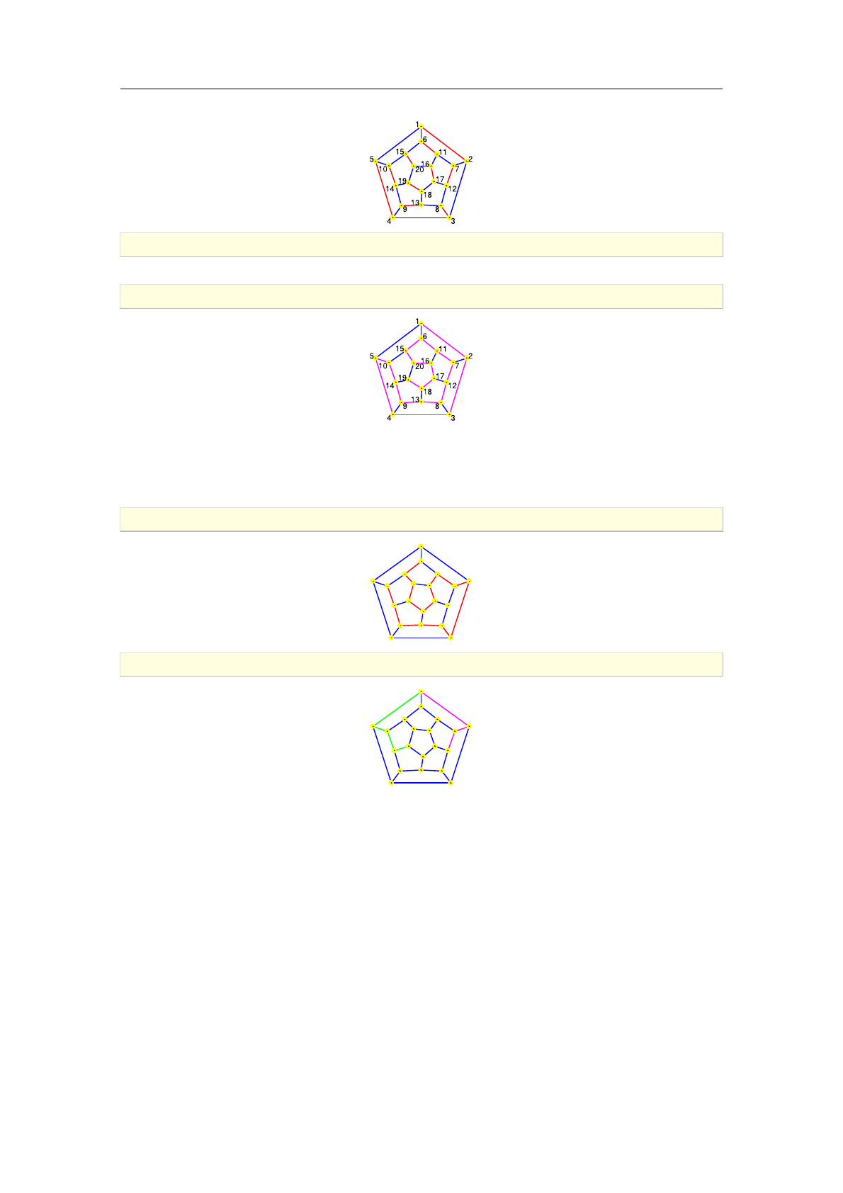
>S:=spanning_tree(G)
an undirected unweighted graph with 20 vertices and 19 edges
>draw_graph(highlight_edges(G,edges(S),magenta))
highlight_trail accepts two or three arguments: a graph G(V ; E), a trail Tor a list of trails T1;
T2; :::; Tkand optionally the new color cor a list of colors c1; c2; :::; ck. The command returns the
copy of Gin which edges between consecutive vertices in each of the given trails are highlighted
with color c(by default red) or the trail Tiis highlighted with color cifor i= 1;2; :::; k.
>draw_graph(highlight_trail(G,[6,15,20,19,18,17,16,11,7,2,3,8,13,9,14,10]))
1
25
6
3
7
4
89
10
1115
12
13
14
16
17
18
19
20
>draw_graph(highlight_trail(G,shortest_path(G,1,[19,12]),[green,magenta]))
1
25
6
3
7
4
89
10
1115
12
13
14
16
17
18
19
20
6.3.3. Highlighting subgraphs
The command highlight_subgraph is used for highlighting subgraph(s) of the given graph.
Syntax: highlight_subgraph(G,S,[weights])
highlight_subgraph(G,S,c1,c2,[weights])
highlight_subgraph(G,[S1,S2,..,Sk])
highlight_subgraph(G,[S1,S2,..,Sk],c1,c2)
highlight_subgraph accepts two or four arguments: a graph G(V ; E), a subgraph S(V0; E0)of
Gor a list of subgraphs S1; S2; :::; Skin Gand optionally the new colors c1; c2for the edges and
vertices of the selected subgraph(s), respectively. It returns a modified copy of Gwith the selected
subgraph(s) colored as specified. If colors are not given, red and green are used, respectively.
The option weights may be passed as an additional argument if Gand Sare weighted graphs.
In that case, the weights of edges in E0⊂Ein Gare overwritten with those defined in Sfor the
same edges.
130 Visualizing graphs
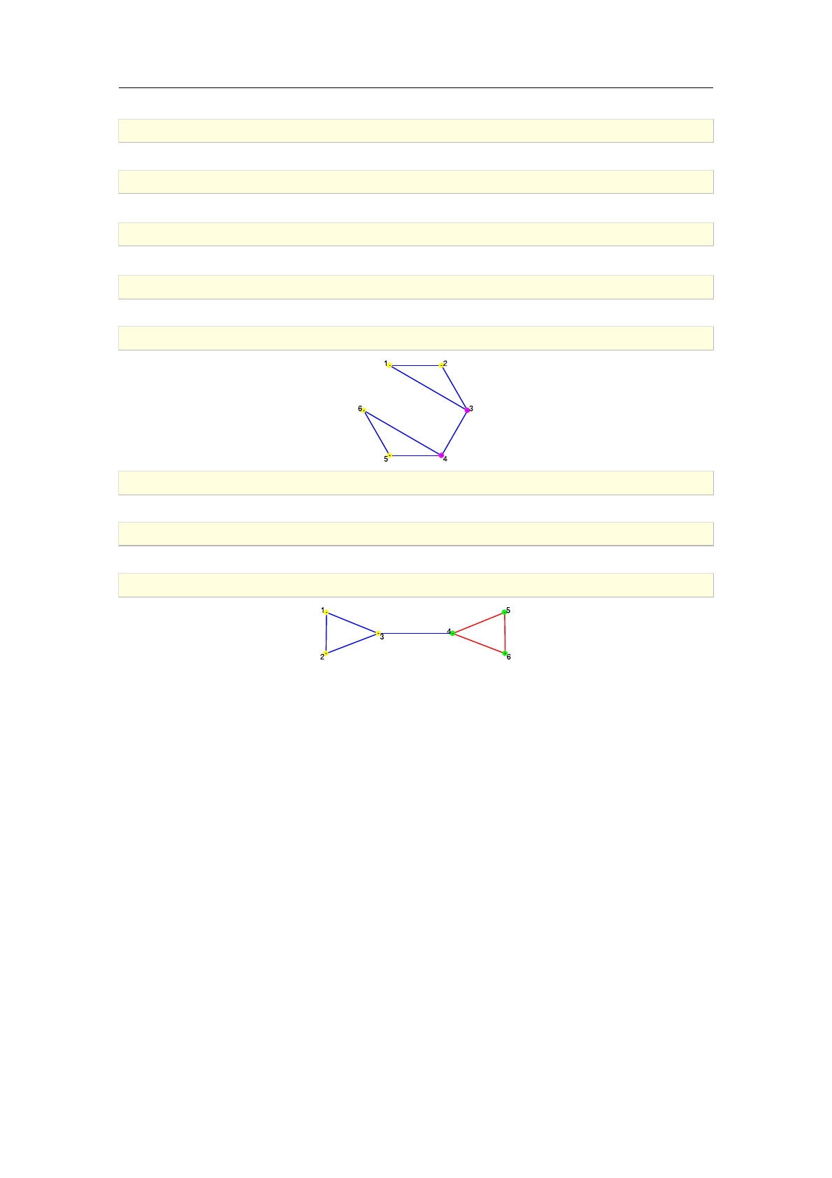
>G:=graph(%{[1,2],[2,3],[3,1],[3,4],[4,5],[5,6],[6,4]%})
an undirected unweighted graph with 6 vertices and 7 edges
>A:=articulation_points(G)
[3;4]
>B:=biconnected_components(G)
[[4;6;5];[3;4];[1;3;2]]
>H:=highlight_vertex(G,A,magenta)
an undirected unweighted graph with 6 vertices and 7 edges
>draw_graph(H)
>S:=induced_subgraph(G,B[0])
an undirected unweighted graph with 3 vertices and 3 edges
>H:=highlight_subgraph(G,S)
an undirected unweighted graph with 6 vertices and 7 edges
>draw_graph(H,spring)
6.3 Highlighting parts of graphs 131


Bibliography
[1] Shehzad Afzal and Clemens Brand. Recognizing triangulated Cartesian graph products. Discrete Mathe-
matics, 312:188–193, 2012.
[2] L. Alonso and R. Schott. Random Unlabelled Rooted Trees Revisited. In Proc. Int. Conf. on Computing and
Information 1994, pages 1352–1367.
[3] Vladimir Bagatelj and Ulrik Brandes. Efficient generation of large random networks. Physical Review E,
71:036113, 2005.
[4] Mohsen Bayati, Jeong Han Kim, and Amin Saberi. A Sequential Algorithm for Generating Random Graphs.
Algorithmica, 58:860–910, 2010.
[5] Norman Biggs. Algebraic graph theory. Cambridge University Press, Second edition, 1993.
[6] Danilo Blanu²a. Problem £etiriju boja. Glasnik Mat.-Fiz. Astr. Ser. II , 1:31–32, 1946.
[7] Béla Bollobás. Modern Graph Theory. Graduate Texts in Mathematics. Springer, Corrected edition, 2002.
[8] Coen Boot. Algorithms for Determining the Clustering Coefficient in Large Graphs. Bachelor's thesis, Faculty
of Science, Utrecht University, 2016.
[9] Daniel Brélaz. New Methods to Color the Vertices of a Graph. Communications of the ACM, 22:251–256,
1979.
[10] Cristoph Buchheim, Michael Jünger, and Sebastian Leipert. Improving Walker's Algorithm to Run in Linear
Time. In M. T. Goodrich and S. G. Kobourov, editors, Graph Drawing 2002, Lecture Notes in Computer
Science vol 2528 , pages 344–353. Springer-Verlag Berlin Heidelberg, 2002.
[11] Nicos Christofides. Worst-case analysis of a new heuristic for the traveling salesman problem. Report 388,
Graduate School of Industrial Administration, 1976.
[12] William J. Cook. In Pursuit of the Traveling Salesman: Mathematics at the Limits of Computation. Princeton
University Press, 2012.
[13] Melissa DeLeon. A Study of Sufficient Conditions for Hamiltonian Cycles. Rose-Hulman Undergraduate
Mathematics Journal, 1, Article 6, 2000. https://scholar.rose-hulman.edu/rhumj/vol1/iss1/6.
[14] Isabel M. Díaz and Paula Zabala. A Branch-and-Cut Algorithm for Graph Coloring. Discrete Applied Math-
ematics, 154:826–847, 2006.
[15] Reinhard Diestel. Graph Theory. Springer-Verlag, New York, 1997.
[16] Jack Edmonds. Paths, Trees, and Flowers. In Gessel I. and GC. Rota, editors, Classic Papers in Combina-
torics, pages 361–379. Birkhäuser Boston, 2009. Modern Birkhäuser Classics.
[17] Jack Edmonds and Richard M. Karp. Theoretical improvements in algorithmic efficiency for network flow
problems. Journal of the ACM, 19:248–264, 1972.
[18] Abdol H. Esfahanian and S. Louis Hakimi. On computing the connectivities of graphs and digraphs. Networks,
14:355–366, 1984.
[19] Shimon Even. Graph Algorithms. Computer software engineering series. Computer Science Press, 1979.
[20] Robert W. Floyd. Algorithm 97: Shortest path. Communications of the ACM, 5:345, 1962.
[21] T. M. J. Fruchterman and E. M. Reingold. Graph Drawing by Force-Directed Placement. Software: Practice
and Experience, 21:1129–1164, 1991.
[22] Alan Gibbons. Algorithmic graph theory. Cambridge University Press, 1985.
[23] Chris Godsil and Gordon F. Royle. Algebraic graph theory. Graduate Texts in Mathematics. Springer, First
edition, 2001.
[24] Donald Goldfarb and Michael D. Grigoriadis. A computational comparison of the dinic and network simplex
methods for maximum flow. Annals of Operations Research, 13:81–123, 1988.
[25] Gary Haggard, David J. Pearce, and Gordon Royle. Computing Tutte Polynomials. ACM Transactions on
Mathematical Software, 37, 2010. Article No. 24.
[26] Gary Haggard, David J. Pearce, and Gordon Royle. Edge-Selection Heuristics for Computing Tutte Polyno-
mials. Chicago Journal of Theoretical Computer Science, 2010. Article 6.
[27] S. L. Hakimi. On realizability of a set of integers as degrees of the vertices of a linear graph. I. Journal of
the Society for Industrial and Applied Mathematics, 10:496–506, 1962.
[28] Keld Helsgaun. General k-opt submoves for the Lin–Kernighan TSP heuristic. Math. Prog. Comp., 1:119–163,
2009.
[29] Carl Hierholzer. Ueber die möglichkeit, einen Linienzug ohne Wiederholung und ohne Unterbrechung zu
umfahren. Mathematische Annalen, 6:30–32, 1873.
[30] Andreas M. Hinz, Sandi Klavºar, and Sara S. Zemlji£. A survey and classification of Sierpi«ski-type graphs.
Discrete Applied Mathematics, 217:565–600, 2017.
[31] John E. Hopcroft and Richard M. Karp. An n5/2 algorithm for maximum matchings in bipartite graphs.
SIAM Journal on Computing, 2:225–231, 1973.
[32] Yifan Hu. Efficient and High Quality Force-Directed Graph Drawing. Mathematica Journal, 10:37–71, 2005.
[33] Yifan Hu and Jennifer Scott. A Multilevel Algorithm for Wavefront Reduction. SIAM Journal on Scientific
Computing, 23:1352–1375, 2001.
133

[34] Arthur B. Kahn. Topological sorting of large networks. Communications of the ACM, 5:558–562, 1962.
[35] B. D. McKay and A. Piperno. Practical Graph Isomorphism, II. J. Symbolic Computation, 60:94–112, 2013.
[36] Michael Monagan. A new edge selection heuristic for computing Tutte polynomials. In Proceedings of FPSAC
2012, pages 839–850.
[37] Wendy Myrwold and Willian Kocay. Errors in graph embedding algorithms. Journal of Computer and System
Sciences, 77:430–438, 2011.
[38] Albert Nijenhuis and Herbert S. Wilf. Combinatorial Algorithms. Computer Science and Applied Mathe-
matics. Academic Press, Second edition, 1978.
[39] Patric R. J. Östergård. A fast algorithm for the maximum clique problem. Discrete Applied Mathematics,
120:197–207, 2002.
[40] Richard Otter. The Number of Trees. The Annals of Mathematics, 2nd Ser., 49:583–599, 1948.
[41] Manfred Padberg and Giovanni Rinaldi. A Branch-and-Cut Algorithm for the Resolution of Large-Scale
Symmetric Traveling Salesman Problems. SIAM Review, 33:60–100, 1991.
[42] Ulrich Pferschy and Rostislav Stan¥k. Generating subtour elimination constraints for the TSP from pure
integer solutions. Central European Journal of Operations Research, 25:231–260, 2017.
[43] Bor Plestenjak. An Algorithm for Drawing Planar Graphs. Software: Practice and Experience, 29:973–984,
1999.
[44] Angelika Steger and Nicholas C. Wormald. Generating random regular graphs quickly. Combinatorics Prob-
ability and Computing, 8:377–396, 1999.
[45] R. E. Tarjan. Depth-First Search and Linear Graph Algorithms. SIAM Journal on Comp., 1:146–160, 1972.
[46] R. E. Tarjan. A note on finding the bridges of a graph. Information Processing Letters, 2:160–161, 1974.
[47] R. E. Tarjan. Applications of path compression on balanced trees. Journal of the ACM, 26:690–715, 1979.
[48] R. E. Tarjan. Two streamlined depth-first search algorithms. Fundamenta Informaticae, 9:85–94, 1986.
[49] K. Thulasiraman, S. Arumugam, A. Brandstädt, and T. Nishizeki, editors. Handbook of Graph Theory,
Combinatorial Optimization, and Algorithms. CRC Press, 2016.
[50] Etsuji Tomita, Akira Tanaka, and Haruhisa Takahashi. The worst-case time complexity for generating all
maximal cliques and computational experiments. Theoretical Computer Science, 363:28–42, 2006.
[51] W. T. Tutte. How to draw a graph. Proceedings of the London Mathematical Society, s3-13:743–767, 1963.
[52] John Q. Walker II. A nodepositioning algorithm for general trees. Software: Practice and Experience,
20:685–705, 1990.
[53] Stanley Wasserman and Katherine Faust. Social Network Analysis: Methods and Applications. Cambridge
University Press, 1994.
[54] E. Welch and S. Kobourov. Measuring Symmetry in Drawings of Graphs. Computer Graphics Forum,
36:341–351, 2017.
[55] Douglas B. West. Introduction to Graph Theory. Pearson Education, 2002.
[56] Herbert S. Wilf. The Uniform Selection of Free Trees. Journal of Algorithms, 2:204–207, 1981.
134 Bibliography

Command Index
add_arc ....................... 48
add_edge ...................... 48
add_vertex ..................... 47
adjacency_matrix ................. 67
allpairs_distance . . . . . . . . . . . . . . . . 93
antiprism_graph .................. 19
arrivals ...................... 64
articulation_points ............... 84
assign_edge_weights ............... 44
biconnected_components ............. 82
bipartite_matching . . . . . . . . . . . . . . . . 98
canonical_labeling . . . . . . . . . . . . . . . . 75
cartesian_product . . . . . . . . . . . . . . . . 32
chromatic_index ................. 110
chromatic_number . . . . . . . . . . . . . . . . 107
chromatic_polynomial ............... 78
clique_cover ................... 101
clique_cover_number . . . . . . . . . . . . . . 101
clique_number . . . . . . . . . . . . . . . . . . 100
clique_stats .................... 99
clustering_coefficient . . . . . . . . . . . . 103
complete_binary_tree ............... 15
complete_graph .................. 14
complete_kary_tree . . . . . . . . . . . . . . . . 15
connected_components ............... 82
contract_edge ................... 50
cycle_basis .................... 26
cycle_graph .................... 13
degree_sequence .................. 61
delete_arc ..................... 48
delete_edge .................... 48
delete_vertex ................... 47
departures ..................... 64
digraph ....................... 10
dijkstra ..................... 115
discard_edge_attribute ............. 53
discard_graph_attribute ............. 51
discard_vertex_attribute . . . . . . . . . . . . 52
disjoint_union .................. 30
draw_graph . . . . . . . . . . . . . . . . . . . . 121
edge_connectivity . . . . . . . . . . . . . . . . 85
edges ........................ 59
export_graph .................... 56
flow_polynomial .................. 78
fundamental_cycle . . . . . . . . . . . . . . . . 26
get_edge_attribute . . . . . . . . . . . . . . . . 53
get_edge_weight .................. 49
get_graph_attribute ............... 51
get_vertex_attribute ............... 52
girth ........................ 95
graph ......................... 9
graph_automorphisms ............... 75
graph_charpoly .................. 70
graph_complement ................. 28
graph_equal .................... 60
graph_join ..................... 30
graph_power .................... 31
graph_rank ..................... 83
graph_spectrum . . . . . . . . . . . . . . . . . . 71
graph_union .................... 30
graph_vertices . . . . . . . . . . . . . . . . . . 59
greedy_color ................... 105
grid_graph ..................... 19
has_arc ....................... 63
has_edge ...................... 63
highlight_edges . . . . . . . . . . . . . . . . . 129
highlight_subgraph . . . . . . . . . . . . . . . 130
highlight_trail . . . . . . . . . . . . . . . . . 129
highlight_vertex . . . . . . . . . . . . . . . . 129
hypercube_graph . . . . . . . . . . . . . . . . . . 17
import_graph .................... 55
incidence_matrix ................. 69
incident_edges . . . . . . . . . . . . . . . . . . 66
induced_subgraph ................. 25
interval_graph . . . . . . . . . . . . . . . . . . 16
is_acyclic ..................... 95
is_arborescence . . . . . . . . . . . . . . . . . . 89
is_biconnected . . . . . . . . . . . . . . . . . . 81
is_bipartite .................... 65
is_clique ..................... 99
is_connected .................... 81
is_cut_set ..................... 85
is_directed .................... 59
is_eulerian ................... 113
is_forest ..................... 87
is_graphic_sequence ............... 16
is_hamiltonian . . . . . . . . . . . . . . . . . 113
is_integer_graph ................. 72
is_isomorphic ................... 72
is_network ..................... 89
is_planar ..................... 34
is_regular ..................... 62
is_strongly_connected . . . . . . . . . . . . . . 84
is_strongly_regular ............... 63
is_tournament ................... 65
is_tree ....................... 87
is_triangle_free . . . . . . . . . . . . . . . . 102
is_triconnected . . . . . . . . . . . . . . . . . . 81
is_two_edge_connected . . . . . . . . . . . . . . 86
is_vertex_colorable . . . . . . . . . . . . . . 108
is_weighted .................... 59
isomorphic_copy . . . . . . . . . . . . . . . . . . 23
kneser_graph .................... 16
laplacian_matrix ................. 68
lcf_graph ..................... 22
line_graph ..................... 34
list_edge_attributes ............... 53
list_graph_attributes . . . . . . . . . . . . . . 51
list_vertex_attributes ............. 52
lowest_common_ancestor ............. 88
make_directed ................... 47
make_weighted ................... 47
maxflow ....................... 90
maximum_clique . . . . . . . . . . . . . . . . . 100
maximum_degree . . . . . . . . . . . . . . . . . . 61
135

maximum_matching ................. 97
minimal_edge_coloring . . . . . . . . . . . . . 109
minimal_spanning_tree . . . . . . . . . . . . . 119
minimal_vertex_coloring . . . . . . . . . . . . 106
minimum_cut .................... 92
minimum_degree .................. 61
mycielski . . . . . . . . . . . . . . . . . . . . 107
neighbors ..................... 64
network_transitivity . . . . . . . . . . . . . . 104
number_of_edges .................. 59
number_of_spanning_trees . . . . . . . . . . . 119
number_of_vertices . . . . . . . . . . . . . . . . 59
odd_girth ..................... 95
odd_graph ..................... 16
path_graph ..................... 13
permute_vertices ................. 24
petersen_graph .................. 22
plane_dual ..................... 34
prism_graph .................... 19
random_bipartite_graph ............. 37
random_digraph .................. 36
random_graph .................... 36
random_network .................. 43
random_planar_graph ............... 40
random_regular_graph ............... 42
random_sequence_graph . . . . . . . . . . . . . . 41
random_tournament . . . . . . . . . . . . . . . . 43
random_tree .................... 37
relabel_vertices ................. 25
reliability_polynomial ............. 79
reverse_graph ................... 29
seidel_spectrum .................. 71
seidel_switch ................... 29
sequence_graph .................. 15
set_edge_attribute . . . . . . . . . . . . . . . . 53
set_edge_weight . . . . . . . . . . . . . . . . . . 49
set_graph_attribute ............... 51
set_vertex_attribute ............... 52
set_vertex_positions . . . . . . . . . . . . . . 127
shortest_path . . . . . . . . . . . . . . . . . . 114
sierpinski_graph ................. 21
spanning_tree . . . . . . . . . . . . . . . . . . 118
st_ordering .................... 96
star_graph ..................... 18
strongly_connected_components ......... 84
subdivide_edges . . . . . . . . . . . . . . . . . . 50
subgraph ...................... 25
tensor_product . . . . . . . . . . . . . . . . . . 32
topologic_sort . . . . . . . . . . . . . . . . . . 96
topological_sort ................. 96
torus_grid_graph ................. 19
trail ........................ 14
trail2edges .................... 14
transitive_closure . . . . . . . . . . . . . . . . 33
traveling_salesman . . . . . . . . . . . . . . . 116
tree_height .................... 88
tutte_polynomial ................. 76
two_edge_connected_components ......... 86
underlying_graph ................. 26
vertex_connectivity ............... 83
vertex_degree ................... 61
vertex_distance . . . . . . . . . . . . . . . . . . 93
vertex_in_degree ................. 61
vertex_out_degree . . . . . . . . . . . . . . . . 61
vertices ...................... 59
web_graph ..................... 18
weight_matrix ................... 70
wheel_graph .................... 18
136 Command Index
