Gridsim Manual
User Manual:
Open the PDF directly: View PDF ![]() .
.
Page Count: 15

Contents
1 Simulator description 5
2 Installation 7
2.1 Parallel launcher compilation ............................. 8
2.2 Documentation generation ............................... 8
3 Execution 9
3.1 Parallel launcher .................................... 9
3.2 Experiment configuration ............................... 9
3.2.1 Visualization definition ............................ 10
3.2.2 Structure definition .............................. 11
3.3 Parallel experiment configuration ........................... 13
4 Examples 15
4.1 MuFCO demo ...................................... 15

4 CONTENTS

Chapter 1
Simulator description
GridSim1is an open source simulator developed to analyze the power balances on a virtual
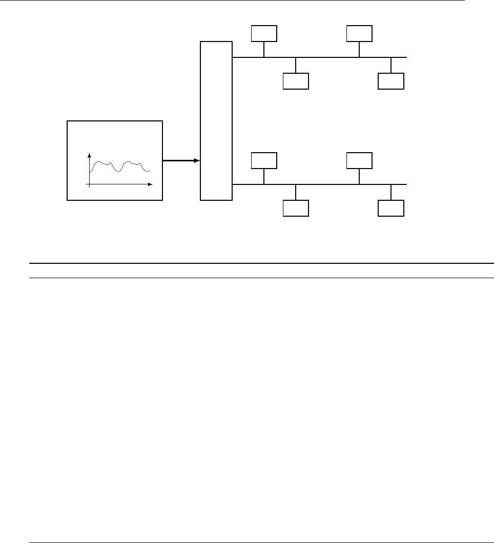
electrical grid. Figure 1.1 shows a scheme of its modular architecture. The grid is composed by
lines. A line represents a set of nodes with the same features. The nodes are complex elements
connected to the lines which can be equipped with different types of consumption, Distributed
Energy Resources (DER) technologies and control systems. These nodes can represent from a
single device which only consumes as a single device to a complex microgrid. In addition, a base
consumption function can be added to the grid. It represents an uncontrollable consumption
which is added to the aggregated consumption of the simulated grid.
The structure of a grid is defined by an XML file. In this file, the number of lines and the
number of nodes per line can be defined. Each line has a concrete type of node; it means that all
the nodes of each line have the same features. GridSim can run multiple executions in parallel.
This feature of the simulator has been implemented by making use of the MPI2protocol.
GridSim calculates the power balances of every node and they are aggregated in their
common line. The aggregated consumption of the virtual electrical grid is calculated as the
sum of the power balances of every line plus the base consumption function. The nodes can be
equipped with different controllers to control the possible elements which a node is composed of.
For example, the charge power of the storage system can be controlled by a battery controller.
The controllers can obtain information from every element of the GridSim simulator.
Algorithm 1describes the operation of GridSim. In the first place, the simulator is
initialized—see from line 1 to 3 . The virtual electrical grid is created by using a configuration
file which indicates structure of the grid. In addition, the counter of time steps is set to zero.
A time step is one execution of the main loop of the simulator. It is the virtual clock of a
simulation which marks the events that happen. A time step is related to an amount of time
in the real world. For example, if a time step represents one minute, in each execution of the
1GridSim is released under GPLv3.0. It can be downloaded from: https://github.com/Robolabo/gridSim.git
2Message Passing Interface (MPI) is a standardized and portable message-passing system designed by a group
of researchers from academia and industry to function on a wide variety of parallel computers. The standard
defines the syntax and semantics of a core of library routines useful to a wide range of users writing portable
message-passing programs in different computer programming languages.
6 1. Simulator description
Grid
Line 1
Node
Node
. . .
. . .
Node
Node
. . .
Line i
Node
Node
. . .
. . .
Node
Node
t
p(t)
Base consumption
Figure 1.1: Scheme of the modular architecture of GridSim simulator.
Algorithm 1 High-level description of the main loop of GridSim simulator.
1: /* Initialization */
2: createGrid(< configurationF ile >)
3: T imeStep ←0
4: /* Main Loop */
5: while T imeStep < T imeStepLimit do
6: /* Execute main control function */
7: mainControlFunction()
8: /* Execute virtual user functions on all nodes */
9: for i < numNodes do
10: node[i]→userFunction()
11: end for
12: /* Execute control functions on all nodes */
13: for i < numNodes do
14: node[i]→controlFunction()
15: end for
16: /* Execute grid energy balance - physics engine */
17: gridExecutionFunction()
18: T imeStep + +
19: end while
main loop, the power balances are calculated for one minute in the real world. The lower the
amount of time in the real world is, the higher the accuracy of the simulator is, but also the
greater the computing power. After GridSim is initialized, the main loop begins. The main loop
simulates the virtual electrical grid, the virtual users and controllers in each time step. The
counter of time steps is increased at the end of this loop. When the main loop finishes, the
simulation finishes. This condition is satisfied when the counter of time steps reaches a certain
value indicated in the configuration file—see the condition of line 5.

Chapter 2
Installation
GridSim is open source simulator of electrical grids released under GPLv3.0. It can be
downloaded from: https://github.com/Robolabo/gridSim.git. The repository can also be
directly downloaded from github in your computer:
$ g i t c l o n e h t tp s : / / g ithub . com/ Robolabo / gridS im . g i t
Once the simulator has been downloaded, you can attempt to install it.
GridSim must be compile in your computer. It is preapared to be compile and executed
in Linux, this manual does not indicate how to install GridSim in other operating systems. In
addition, this manual describes the instllation process for an Ubuntu distribution. GridSim is
programmed in C++, thus, the C++ compiler is required. The simulator’s compilation has been
teste for g++ compiler version 4.4 or higher. The installation of this compiler is recommended:
$ sudo apt−get i n s t a l l g++
The compilation of GridSim is performed by autotools with libtool. Therefore, these tools
should be installed in your computer:
$ sudo apt−g et i n s t a l l automake a u t o t o o l s −dev l i b t o o l
There is a compilation script which prepare the compilation folder and compile the simulator.
To execute this script:
$ . / b u i l d s i m u l a t o r . sh
It creates the build folder. All compilation files are in this folder. After the compilation, the
executable file is copied in the main folder of GridSim. This file is called gridSim.

8 2. Installation
2.1 Parallel launcher compilation
Different instances of GridSim can be launched in parallel. It allows to use the possibilities of a
multicore machine or a cluster. This parallel execution is based on MPI. Thus, MPI should be
installed in your computer:
$ sudo apt−get i n s t a l l openmpi−bin mpi−default−dev
There is a compilation script for the compilation of the parallel launcher:
$ ./ b u i l d s i m u l a t o r p a r a l l e l . sh
After the compilation, the executable file is copied in the main folder of GridSim. It is called
gridSim parallel.
2.2 Documentation generation
This manual can be compile from the L
A
T
E
X sources. The L
A
T
E
X packages should be installed in
your computer:
$ sudo apt−get i n s t a l l t e x l i v e −la te x −ex t ra t e x l i v e −latex−recommended
texlive−bibtex−e xt ra t e x l i v e −math−e x t r a
There is compilation script for the documentation compilation:
$ . / b u i l d d o c . sh
After the compilation, the documentation file is copied in the main folder of GridSim. It is
called gridsim manual.pdf.

Chapter 3
Execution
GridSim is executed by using its executable file gridSim. The execution requires a configuration
file to configure the experiment that you want to simulate. The content of this file is explained
in Section 3.2. It is launch through:
$ ./ gridSim −p<CONFIGURATION FILE>
The simulator is launched during the stipulated time.
3.1 Parallel launcher
The parallel launcher of GridSim is based on MPI. The parallel executin must be configured with
an independent file. The content of this file is explained in Section 3.3. It is launch through:
$ mpirun −np <N PROCESS>./ gridSim parallel
−p<PARALLEL sCONFIGURATION FILE>
where < N P ROCESS > is the number of process launched in parallel. Notice that the
parallel execution requires a master process which does not calculate nothing, it is only a job
dealer. Therefore, < N P ROCESS > should be at least 2, one master dealing job and a slave
simulating.
3.2 Experiment configuration
The experiments are configured by using the xml configurations files. These files have the
following main structure:
<?xml version="1.0"?>
<GridSim>
<Simulation
seed="SED_NUMBER"
length="LENGTH"

10 3. Execution
sampling="SMP_PERIOD"
fft_lng="FFT_LENFGTH"
data_folder="DATA_FOLDER"
/>
<Visualization
active="FLAG_ACTIVE"
rf_rate="RF_RATE" >
WINDOWS_DEF
...
</Visualization>
<Grid
file="GRID_PROFILE"
amp="GRID_AMP"
/>
<Structure>
STRUCTURE_DEF
</Structure>
<Writer file="OUTPUT_FILE" />
<Main_control name="MAIN_CONTROLLER" />
</GridSim>
Table 3.1 shows the definition of the configurable parameters previously defined.
Name Description Data
type
SED NUMBER The initial random number seed int
LENGTH Duration of experiment in real world in minutes int
SMP PERIOD Sampled period for DFT int
FFT LENFGTH DFT window length int
DATA FOLDER Data folder address string
FLAG ACTIVE 0 deactivate visualization; 1 activate visualization bool
RF RATE Refresh rate for visualization int
WINDOWS DEF Definition of windows (see Section 3.2.1)
GRID PROFILE Base consumption profile file name string
GRID AMP Amplitude of the base consumption float
STRUCTURE DEF Definition of structure (see Section 3.2.2)
OUTPUT FILE Output file name string
MAIN CTR Main controller name string
Table 3.1: Experiment configuration parameters.
3.2.1 Visualization definition
The windows for visualization are defined with the following structure in the xml file:
<scr
title="TITLE"
x_lng="X_LENGTH"
y_ini="Y_INI"
y_end="Y_END"
/>

3.2. Experiment configuration 11
Table 3.2 shows the definition of the configurable parameters previously defined.
Name Description Data
type
TITLE Title of the window string
X LENGTH Length of the x-axis in samples int
Y INI Initial y-axis value int
Y END Final y-axis value int
Table 3.2: Window configuration parameters.
3.2.2 Structure definition
The structure of the simulated grid is defined with the following structure in the xml file:
<Structure lines="LINES_NUMBER" >
<line_X nodes="NODES_NUMBER" type="NODE_NAME"/>
...
<NODE_NAME>
ELEMENTS
</NODE_NAME>
</Structure>
Table 3.3 shows the definition of the configurable parameters previously defined.
Name Description Data
type
LINES NUMBER Number of lines int
line X Definition of line X int
NODES NUMBER Number on nodes int
NODE NAME Definition of the nodes of the line string
ELEMENTS Elements in the node (explained below)
Table 3.3: Structure configuration parameters.
The structure of the simulated node is defined with the following structure in the xml file:
<NODE_NAME>
<load
type_nd = "ND_TYPE"
amp_nd = "ND_AMP"
file_nd = "ND_FILE"
/>
<pv
type = "PV_TYPE"
gen = "PV_PROFILE"
frc = "PV_FR_PROFILE"
power = "PV_AMP"

12 3. Execution
/>
<bat
cap = "CAP"
num_inv = "NUM_INV"
/>
<ctr
name="CTR_NAME"
CTR_CONF
/>
</NODE_NAME>
Table 3.4 shows the definition of the configurable parameters previously defined.
Name Description Data
type
ND TYPE No deferrable consumption type (see Table 3.5) int
ND AMP No deferrable consumption amplitude float
ND FILE No deferrable consumption file string
PV TYPE PV type (see Table 3.6) int
PV PROFILE PV profile file string
PV FR PROFILE PV forecast file string
PV AMP PV inverter nominal power float
CAP Storage system capacity float
NUM INV Storage system number of inverters int
CTR NAME Node controller name string
CTR CONF Configuration of the node controller
Table 3.4: Node configuration parameters.
Table 3.5 shows the different types of no deferrable consumption.
Number Description
0 Constant consumption; ND AMP indicates its amplitude
1 Consumption defined by a file; ND FILE indicates the address
2 Consumption defined by the base consumption profile
Table 3.5: No deferrable types.
Table 3.6 shows the different types of PV generation.
Number Description
0 PV profile defined by file; PV PROFILE indicates the adress
1 PV profile generated by internal model
Table 3.6: No deferrable types.

3.3. Parallel experiment configuration 13
3.3 Parallel experiment configuration

14 3. Execution

Chapter 4
Examples
4.1 MuFCO demo
The configuration file for the MuFCO demo experiment can be executed with:
$ ./ gridSim −p c n f /mufco demo . xml
The MuFCO demo has the following configuration parameters:
Name Description Data
type Range
ctr act time Simulation step after which the controllers
start running int [0, int length]
wt beg Simulation step after which data starts
being written int [0, int length]
wt end Simulation step when data stops to be
written int [0, int length]
Table 4.1: MuFCO demo configuration parameters.
