Guide
User Manual:
Open the PDF directly: View PDF ![]() .
.
Page Count: 121 [warning: Documents this large are best viewed by clicking the View PDF Link!]
- Introduction
- Quickstart
- Input Languages
- Multi-shot Solving
- Theory Solving
- Examples
- Command Line Options
- Errors, Warnings, and Infos
- Meta-Programming
- Heuristic-driven Solving
- Optimization and Preference Handling
- Solver Configuration
- Future Work
- Complementary Resources
- Differences to the Language of gringo 3
- References
- Index

Martin Gebser
Roland Kaminski
Benjamin Kaufmann
Marius Lindauer
Max Ostrowski
Javier Romero
Torsten Schaub
Sven Thiele
University of Potsdam


Abstract
This document provides an introduction to the Answer Set Programming (ASP) tools
gringo,clasp, and clingo, developed at the University of Potsdam. The basic idea
of ASP is to express a problem in the form of a logic program so that its logical
models, called answer sets, provide the solutions to the original problem. The first
tool, gringo, is a so-called grounder translating user-provided logic programs (with
variables) into equivalent propositional logic programs (without variables). The sec-
ond tool, clasp, is a so-called solver computing the answer sets of the propositional
programs issued by gringo. The third tool, clingo, combines the functionalities of
gringo and clasp, and additionally integrates the scripting languages Lua and Python
either through libraries or embedded code. This guide, for one, aims at enabling ASP
novices to make use of the aforementioned tools. For another, it provides a reference
of the tools’ features that ASP adepts might be tempted to exploit.
This is version 2.1.0 of the Potassco guide; it upgrades all code to clingo series 5.
As well, Section 11.2 describes asprin 3.0.
Please make sure that you have corresponding (or later) versions available.
This document includes many illustrative examples.
For convenience, they can be saved to disk by clicking their file names.
Depending on the viewer, a right or double-click should initiate saving.
Second edition, version 2.1.0, October 5, 2017
http://potassco.org

Contents 4
Contents
1 Introduction 9
1.1 Download and Installation . . . . . . . . . . . . . . . . . . . . . . 9
1.2 Outline ................................ 10
2 Quickstart 12
2.1 ProblemInstance ........................... 12
2.2 ProblemEncoding .......................... 13
2.3 ProblemSolution ........................... 15
2.4 Summary ............................... 16
3 Input Languages 17
3.1 Input Language of gringo and clingo ................. 17
3.1.1 Terms............................. 17
3.1.2 Normal Programs and Integrity Constraints . . . . . . . . . 19
3.1.3 Classical Negation . . . . . . . . . . . . . . . . . . . . . . 21
3.1.4 Disjunction.......................... 22
3.1.5 Double Negation and Head Literals . . . . . . . . . . . . . 23
3.1.6 Boolean Constants . . . . . . . . . . . . . . . . . . . . . . 24
3.1.7 Built-in Arithmetic Functions . . . . . . . . . . . . . . . . 24
3.1.8 Built-in Comparison Predicates . . . . . . . . . . . . . . . 25
3.1.9 Intervals............................ 27
3.1.10 Pooling ............................ 28
3.1.11 Conditions and Conditional Literals . . . . . . . . . . . . . 28
3.1.12 Aggregates .......................... 30
3.1.13 Optimization ......................... 37
3.1.14 External Functions . . . . . . . . . . . . . . . . . . . . . . 39
3.1.15 Meta-Statements . . . . . . . . . . . . . . . . . . . . . . . 42
3.2 Input Language of clasp ....................... 47
4 Multi-shot Solving 48
5 Theory Solving 49
5.1 ASP and Difference Constraints . . . . . . . . . . . . . . . . . . . 49
5.2 ASP and Linear Constraints . . . . . . . . . . . . . . . . . . . . . . 49
5.3 ASP and Constraint Programming . . . . . . . . . . . . . . . . . . 49
5.3.1 ASP and Constraint Programming with clingcon ...... 49
5.3.2 ASP and Constraint Programming with gringo ....... 50
5.3.3 Solving CSPs with aspartame ................ 51
6 Examples 52
6.1 n-Coloring .............................. 52
6.1.1 Problem Instance . . . . . . . . . . . . . . . . . . . . . . . 52
6.1.2 Problem Encoding . . . . . . . . . . . . . . . . . . . . . . 52

Contents 5
6.1.3 Problem Solution . . . . . . . . . . . . . . . . . . . . . . . 53
6.2 Traveling Salesperson . . . . . . . . . . . . . . . . . . . . . . . . . 54
6.2.1 Problem Instance . . . . . . . . . . . . . . . . . . . . . . . 54
6.2.2 Problem Encoding . . . . . . . . . . . . . . . . . . . . . . 55
6.2.3 Problem Solution . . . . . . . . . . . . . . . . . . . . . . . 56
6.3 Blocks World Planning . . . . . . . . . . . . . . . . . . . . . . . . 57
6.3.1 Problem Instance . . . . . . . . . . . . . . . . . . . . . . . 58
6.3.2 Problem Encoding . . . . . . . . . . . . . . . . . . . . . . 59
6.3.3 Problem Solution . . . . . . . . . . . . . . . . . . . . . . . 60
7 Command Line Options 62
7.1 gringo Options ............................ 62
7.2 clingo Options............................. 63
7.3 clasp Options ............................. 64
7.3.1 General Options . . . . . . . . . . . . . . . . . . . . . . . 64
7.3.2 Solving Options . . . . . . . . . . . . . . . . . . . . . . . 65
7.3.3 Fine-Tuning Options . . . . . . . . . . . . . . . . . . . . . 67
8 Errors, Warnings, and Infos 70
8.1 Errors ................................. 70
8.1.1 Parsing Command Line Options . . . . . . . . . . . . . . . 70
8.1.2 Parsing and Checking Logic Programs . . . . . . . . . . . . 71
8.1.3 Parsing Logic Programs in smodels Format . . . . . . . . . 72
8.1.4 Multi-shot Solving . . . . . . . . . . . . . . . . . . . . . . 73
8.2 Warnings ............................... 73
8.2.1 File Included Multiple Times . . . . . . . . . . . . . . . . . 73
8.2.2 Unbounded CSP Variables . . . . . . . . . . . . . . . . . . 74
8.3 Infos.................................. 74
8.3.1 Undefined Operations . . . . . . . . . . . . . . . . . . . . 74
8.3.2 UndefinedAtoms....................... 74
8.3.3 Global Variables in Tuples of Aggregate Elements . . . . . 75
9 Meta-Programming 76
10 Heuristic-driven Solving 77
10.1 Heuristic Programming . . . . . . . . . . . . . . . . . . . . . . . . 77
10.1.1 Heuristic modifier sign ................... 77
10.1.2 Heuristic modifier level .................. 78
10.1.3 Dynamic heuristic modifications . . . . . . . . . . . . . . . 79
10.1.4 Heuristic modifiers true and false ............ 79
10.1.5 Priorities among heuristic modifications . . . . . . . . . . . 80
10.1.6 Heuristic modifiers init and factor ........... 81
10.1.7 Monitoring domain choices................. 81
10.1.8 Heuristics for Blocks World Planning . . . . . . . . . . . . 82

List of Figures 6
10.2 Command Line Structure-oriented Heuristics . . . . . . . . . . . . 84
10.3 Computing Subset Minimal Answer Sets with Heuristics . . . . . . 85
11 Optimization and Preference Handling 86
11.1 Multi-objective Optimization with clasp and clingo ......... 86
11.2 Preference Handling with asprin ................... 86
11.2.1 Computing optimal answer sets . . . . . . . . . . . . . . . 86
11.2.2 Computing multiple optimal answer sets . . . . . . . . . . . 88
11.2.3 Input language of asprin ................... 89
11.2.4 Preference relations and preference types . . . . . . . . . . 92
11.2.5 asprin library......................... 93
11.2.6 Implementing preference types . . . . . . . . . . . . . . . . 98
12 Solver Configuration 105
12.1 Portfolio-Solving with claspfolio ................... 105
12.2 Problem-oriented Configuration of clasp with piclasp ........ 106
13 Future Work 109
A Complementary Resources 110
B Differences to the Language of gringo 3 111
References 112
Index 120
List of Figures
1 Towers of Hanoi: Initial and Goal Situation. . . . . . . . . . . . . . 12
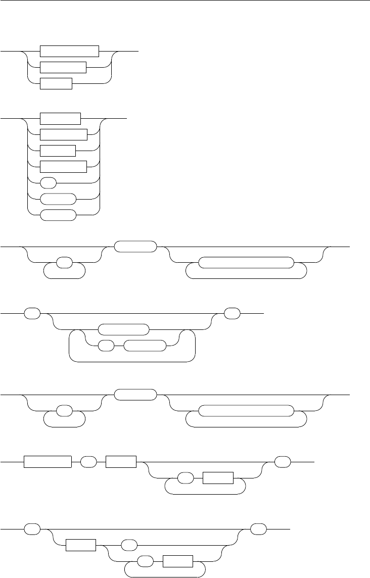
2 GrammarforTerms. ......................... 18
3 A Directed Graph with 6 Nodes and 17 Edges. . . . . . . . . . . . . 53
4 A 3-Coloring for the Graph in Figure 3. . . . . . . . . . . . . . . . 54
5 The Graph from Figure 3 along with Edge Costs. . . . . . . . . . . 55
6 A Minimum-cost Round Trip. . . . . . . . . . . . . . . . . . . . . 56
Listings
examples/tohins.lp ............................. 12
examples/tohenc.lp............................. 13
examples/fly.lp ............................... 20
examples/bird.lp............................... 21
examples/flycn.lp .............................. 22
examples/flynn.lp .............................. 23

Listings 7
examples/bool.lp .............................. 24
examples/arithf.lp.............................. 24
examples/arithc.lp.............................. 25
examples/symbc.lp ............................. 25
examples/define.lp ............................. 26
examples/unify.lp .............................. 26
examples/int.lp ............................... 27
examples/pool.lp .............................. 28
examples/cond.lp .............................. 29
examples/sort.lp............................... 29
examples/aggr.lp .............................. 35
examples/opt.lp ............................... 39
examples/gcd–lua.lp............................. 40
examples/gcd–py.lp............................. 40
examples/gcd.lp............................... 40
examples/rng–lua.lp............................. 41
examples/rng–py.lp ............................. 41
examples/rng.lp............................... 41
examples/term–lua.lp ............................ 42
examples/term–py.lp ............................ 42
examples/term.lp .............................. 42
examples/showa.lp ............................. 43
examples/showt.lp.............................. 43
examples/const.lp.............................. 44
examples/ext.lp ............................... 45
examples/part.lp............................... 45
examples/part–lua.lp ............................ 46
examples/part–py.lp............................. 46
examples/include.lp............................. 46
examples/queensC.lp ............................ 50
examples/queensCa.lp............................ 50
examples/graph.lp.............................. 52
examples/color.lp .............................. 53
examples/costs.lp .............................. 54
examples/ham.lp .............................. 55
examples/min.lp............................... 56
examples/world0.lp............................. 58
examples/blocks.lp ............................. 59
examples/psign.lp.............................. 77
examples/nsign.lp.............................. 78
examples/level.lp .............................. 78
examples/dynamic.lp ............................ 79
examples/priority.lp............................. 80
examples/blocks–heuristic.lp . . . . . . . . . . . . . . . . . . . . . . . . 82

Listings 8
examples/base.lp .............................. 87
examples/preference1.lp . . . . . . . . . . . . . . . . . . . . . . . . . . 87
examples/preference2.lp . . . . . . . . . . . . . . . . . . . . . . . . . . 88
examples/c1.lp ............................... 89
examples/preference3.lp . . . . . . . . . . . . . . . . . . . . . . . . . . 94
examples/min.lp............................... 95
examples/preference4.lp . . . . . . . . . . . . . . . . . . . . . . . . . . 96
examples/preference5.lp . . . . . . . . . . . . . . . . . . . . . . . . . . 96
examples/preference6.lp . . . . . . . . . . . . . . . . . . . . . . . . . . 97
examples/preference7.lp . . . . . . . . . . . . . . . . . . . . . . . . . . 98
examples/preference1.lp . . . . . . . . . . . . . . . . . . . . . . . . . . 98
examples/preference2.lp . . . . . . . . . . . . . . . . . . . . . . . . . . 99
examples/subset.lp ............................. 101
examples/basic.lp .............................. 101
examples/pareto.lp ............................. 102
examples/preference8.lp . . . . . . . . . . . . . . . . . . . . . . . . . . 102
examples/subset.lp ............................. 102
examples/less–cardinality.lp . . . . . . . . . . . . . . . . . . . . . . . . 102
examples/subset.lp ............................. 104

1 Introduction 9
1 Introduction
The “Potsdam Answer Set Solving Collection” (Potassco; [26, 31, 73]) gathers a va-
riety of tools for Answer Set Programming (ASP; [2, 7, 11, 46, 47, 48, 62, 67, 69]),
including grounder gringo, solver clasp, and their combination within the integrated
ASP system clingo. Their common goal is to enable users to rapidly solve compu-
tationally difficult problems in ASP, a declarative programming paradigm based on
logic programs and their answer sets.
This guide, for one, aims at enabling ASP novices to make use of the afore-
mentioned tools. For another, it provides a reference of the tools’ features that ASP
adepts might be tempted to exploit. A formal introduction to (a large fragment of)
the input language of gringo (and clingo) and its precise semantics is given in [24].
The foundations and algorithms underlying the grounding and solving technology
used in gringo and clasp is described in detail in [31]. For further aspects of ASP we
refer the interested reader to the literature [7, 47].
In fact, we focus in this guide on ASP and thus the computation of answer sets of
a logic program [49]. Moreover, clasp can be used as a full-fledged SAT, MaxSAT,
or PB solver (see [9]), accepting propositional CNF formulas in (extended) DIMACS
format as well as PB formulas in OPB and WBO format.
1.1 Download and Installation
The Potassco tools gringo,clasp, and clingo are written in C++ and published un-
der the GNU General Public License [53]. Source packages as well as precom-
piled binaries for Linux, MacOS, and Windows are available at [73]. For build-
ing the tools from sources, please download the most recent source package, con-
sult the included README file, and make sure that the machine to build on has
all required software installed. If you still encounter problems in the building
process, please consult the support pages at [73] or use the Potassco mailing list:
potassco-users@lists.sourceforge.net.
An alternative way to install the tools is to use a package manager. Currently,
packages and ports are available for Debian, Ubuntu, Arch Linux (AUR), and for
MacOS X (via Homebrew or MacPorts). Note that packages installed this way are
not always up to date; the latest versions are available at our Sourceforge page at [73].
Afterward, one can check whether everything works fine by invoking the tool
with flag --version (to get version information) or with flag --help (to see
the available command line options). For instance, assuming that a binary called
gringo is in the path (similarly with the other tools), you can invoke the following
two commands:
gringo --version
gringo --help
Note that gringo,clasp, and clingo run on the command line (Linux shell, Win-
dows command prompt, or the like). To invoke them, their binaries can be “installed”

1.2 Outline 10
simply by putting them into some directory in the system path. In an invocation, one
usually provides the file names of input (text) files as arguments to either gringo or
clingo, while the output of gringo is typically piped into clasp. Thus, the standard
invocation schemes are as follows:
gringo [ options | files ] | clasp [ options | number ]
clingo [ options | files | number ]
A numerical argument provided to either clasp or clingo determines the maximum
number of answer sets to be computed, where 0means “compute all answer sets”.
By default, only one answer set is computed (if it exists).
1.2 Outline
This guide introduces the fundamentals of using gringo,clasp, and clingo. In partic-
ular, it aims at enabling the reader to benefit from them by significantly reducing the
“time to solution” on difficult computational problems. To this end, Section 2 pro-
vides an introductory example that serves both as a prototype of problem modeling
using logic programs and also as an appetizer of the modeling language of gringo.
The main part of this document, Section 3, is dedicated to the input languages of
our tools, where Section 3.1 details the joint input language of gringo and clingo,
while solver formats supported by clasp are not supposed to be written directly by a
user and just briefly described in Section 3.2. Then, the control capacities of clingo
needed for multi-shot solving are detailed in Section 4. For further illustration, Sec-
tion 6 describes how three well-known example problems can be solved with our
tools. Practical aspects are also in the focus of Section 7 and 8, where we elaborate
and give some hints on the available command line options as well as input-related
errors and warnings. The following sections address adept extensions of the ba-
sic modeling language and control capacities. In particular, Section 9 elaborates
meta-programming functionalities that allow for reinterpreting logic programs by
means of ASP. Techniques for incorporating domain-specific heuristics into the ASP
solving process are presented in Section 10. Section 11 is dedicated to advanced
methods for preference handling and optimization. Moreover, Section 5.3 provides
concepts developed particularly for dealing with multi-valued variables and quantita-
tive constraints. In order to tune efficiency, Section 12 further introduces principled
approaches to solver configuration. Finally, we conclude with a summary in Sec-
tion 13.
For readers familiar with the gringo 3 series, Appendix B lists the most promi-
nent differences to the current series. Otherwise, gringo and clingo series 4 should
accept most inputs recognized by gringo 3 (and the seminal grounder lparse [79]1).
The input of solver clasp can be generated by all versions of gringo (as well as
lparse). Be aware that there are some syntactic and semantic changes between the
language of the series 3 and 4, so already existing encodings have to be adapted to
be used with series 4. Throughout this document, we provide illustrative examples.
1A grounder that constitutes the traditional front-end of solver smodels [77]

1.2 Outline 11
Many of them can actually be run. You find instructions on how to accomplish this
(or sometimes meta-remarks) in margin boxes, like the one on the right. Occurrences I am a margin box. Me and my
friends provide you with hints.
When I write ‘\’, it means that
I break a continuous line to stay
within margins.
of ‘\’ usually mean that text in a command line, broken for space reasons, is actually
continuous.
After all these preliminaries, it is time to start our guided tour through the main
Potassco [73] tools. We hope that you will find it enjoyable and helpful!

2 Quickstart 12
1
2
3
4
a b
1
2
3
4
c
Figure 1: Towers of Hanoi: Initial and Goal Situation.
2 Quickstart
As an introductory example, we consider a simple Towers of Hanoi puzzle, consist-
ing of three pegs and four disks of different size. As shown in Figure 1, the goal is
to move all disks from the left peg to the right one, where only the topmost disk of a
peg can be moved at a time. Furthermore, a disk cannot be moved to a peg already
containing some disk that is smaller. Although there is an efficient algorithm to solve
our simple Towers of Hanoi puzzle, we do not exploit it and below merely specify
conditions for sequences of moves being solutions.
In ASP, it is custom to provide a uniform problem definition [67, 69, 76]. Follow-
ing this methodology, we separately specify an instance and an encoding (applying
to every instance) of the following problem: given an initial placement of the disks,
a goal situation, and a number n, decide whether there is a sequence of nmoves that
achieves the goal. We will see that this problem can be elegantly described in ASP
and solved by domain-independent tools like gringo and clasp. Such a declarative
solution is now exemplified.
2.1 Problem Instance
We describe the pegs and disks of a Towers of Hanoi puzzle via facts over the pred-
icates peg/1and disk/1(the number denotes the arity of the predicate). Disks are
numbered by consecutive integers starting at 1, where a disk with a smaller num-
ber is considered to be bigger than a disk with a greater number. The names of the
pegs can be arbitrary; in our case, we use a,b, and c. Furthermore, the predicates
init_on/2and goal_on/2describe the initial and the goal situation, respectively.
Their arguments, the number of a disk and the name of a peg, determine the location
of a disk in the respective situation. Finally, the predicate moves/1specifies the
number of moves in which the goal must be achieved. When allowing 15 moves,
the Towers of Hanoi puzzle shown in Figure 1 is described by the following facts:You can save this instance lo-
cally by clicking its file name:
.
Depending on your viewer, a
right or double-click should do.
1peg(a;b;c).
2disk(1..4).
3init_on(1..4,a).
4goal_on(1..4,c).
5moves(15).
toh_ins.lp

2.2 Problem Encoding 13
Note that the ‘;’ in the first line is syntactic sugar (detailed in Section 3.1.10) that
expands the statement into three facts: peg(a).,peg(b)., and peg(c). Simi-
larly, ‘1..4’ used in Line 2–4 refers to an interval (detailed in Section 3.1.9). Here,
it abbreviates distinct facts over four values: 1,2,3, and 4. In summary, the facts in
Line 1–5 describe the Towers of Hanoi puzzle in Figure 1 along with the requirement
that the goal ought to be achieved within 15 moves.
2.2 Problem Encoding
We now proceed by encoding Towers of Hanoi via schematic rules, i.e., rules con-
taining variables (whose names start with uppercase letters) that are independent of
a particular instance. Typically, an encoding can be logically partitioned into a Gen-
erate, a Define, and a Test part [62]. An additional Display part allows for restricting
the output to a distinguished set of atoms, and thus, for suppressing auxiliary predi-
cates. We follow this methodology and mark the respective parts via comment lines
beginning with ‘%’ in the following encoding: You can also save the encod-
ing by clicking this file name:
.
We below explain how to run the
saved files in order to solve our
Towers of Hanoi puzzle.
1% Generate
2{ move(D,P,T) : disk(D), peg(P) } = 1 :- moves(M),
T = 1..M.
3% Define
4move(D,T) :- move(D,_,T).
5on(D,P,0) :- init_on(D,P).
6on(D,P,T) :- move(D,P,T).
7on(D,P,T+1) :- on(D,P,T), not move(D,T+1),
not moves(T).
8blocked(D-1,P,T+1) :- on(D,P,T), not moves(T).
9blocked(D-1,P,T) :- blocked(D,P,T), disk(D).
10 % Test
11 :- move(D,P,T), blocked(D-1,P,T).
12 :- move(D,T), on(D,P,T-1), blocked(D,P,T).
13 :- goal_on(D,P), not on(D,P,M), moves(M).
14 :- { on(D,P,T) } != 1, disk(D), moves(M), T = 1..M.
15 % Display
16 #show move/3.
Note that the variables D,P,T, and Mare used to refer to disks, pegs, the number of
a move, and the length of the sequence of moves, respectively.
The Generate part, describing solution candidates, consists of the rule in Line 2.
It expresses that, at each point Tin time (other than 0), exactly one move of a disk D
to some peg Pmust be executed. The head of the rule (left of ‘:-’) is a so-called
cardinality constraint (see Section 3.1.12). It consists of a set of literals, expanded
using the conditions behind the colon (detailed in Section 3.1.11), along with the
guard ‘= 1’. The cardinality constraint is satisfied if the number of true elements
is equal to one, as specified by the guard. Since the cardinality constraint occurs
toh_enc.lp

2.2 Problem Encoding 14
as the head of a rule, it allows for deriving (“guessing”) atoms over the predicate
move/3to be true. In the body (right of ‘:-’), we define (detailed in Section 3.1.8),
T = 1..M, to refer to each time point Tfrom 1to the maximum time point M. We
have thus characterized all sequences of Mmoves as solution candidates for Towers
of Hanoi. Up to now, we have not yet imposed any further conditions, e.g., that a
bigger disk must not be moved on top of a smaller one.
The Define part in Line 4–9 contains rules defining auxiliary predicates, i.e.,
predicates that provide properties of a solution candidate at hand. (Such properties
will be investigated in the Test part described below.) The rule in Line 4 simply
projects moves to disks and time points. The resulting predicate move/2can be used
whenever the target peg is insignificant, so that one of its atoms actually subsumes
three possible cases. Furthermore, the predicate on/3captures the state of a Towers
of Hanoi puzzle at each time point. To this end, the rule in Line 5 identifies the
locations of disks at time point 0with the initial state (given in an instance). State
transitions are modeled by the rules in Line 6 and 7. While the former specifies
the direct effect of a move at time point T, i.e., the affected disk Dis relocated to
the target peg P, the latter describes inertia: the location of a disk Dcarries forward
from time point Tto T+1 if Dis not moved at T+1. Observe the usage of not
moves(T) in Line 7, which prevents deriving disk locations beyond the maximum
time point. Finally, we define the auxiliary predicate blocked/3to indicate that
a smaller disk, with a number greater than D-1, is located on a peg P. The rule in
Line 8 derives this condition for time point T+1 from on(D,P,T), provided that T
is not the maximum time point. The rule in Line 9 further propagates the status of
being blocked to all bigger disks on the same peg. Note that we also mark D-1 = 0,
not referring to any disk, as blocked, which is convenient for eliminating redundant
moves in the Test part described next.
The Test part consists of the integrity constraints in Line 11–14, rules that elim-
inate unintended solution candidates. The first integrity constraint in Line 11 asserts
that a disk Dmust not be moved to a peg Pif D-1 is blocked at time point T. This
excludes moves putting a bigger disk on top of a smaller one and, in view of the def-
inition of blocked/3, also disallows that a disk is put back to its previous location.
Similarly, the integrity constraint in Line 12 expresses that a disk Dcannot be moved
at time point Tif it is blocked by some smaller disk on the same peg P. Note that we
use move(D,T) here because the target of an illegal move does not matter in this
context. The fact that the goal situation, given in an instance, must be achieved at
maximum time point Mis represented by the integrity constraint in Line 13. The final
integrity constraint in Line 14 asserts that, for every disk Dand time point T, there is
exactly one peg Psuch that on(D,P,T) holds. Although this condition is implied
by the definition of on/3in Line 6 and 7 with respect to the moves in a solution,
making such knowledge explicit via an integrity constraint turns out to improve the
solving efficiency.
Finally, the meta-statement (detailed in Section 3.1.15) of the Display part in
Line 16 indicates that only atoms over the predicate move/3ought to be printed,
thus suppressing the predicates used to describe an instance as well as the auxiliary

2.3 Problem Solution 15
predicates move/2,on/3, and blocked/3. This is for more convenient reading of
a solution, given that it is fully determined by atoms over move/3.
2.3 Problem Solution
We are now ready to solve our Towers of Hanoi puzzle. To compute an answer set
representing a solution, invoke one of the following commands: clingo or gringo and clasp
ought to be located in some
directory in the system path.
Also, and
(click file name
to save) should reside in the
working directory.
clingo
gringo | clasp
The output of the solver, clingo in this case, should look somehow like this:
clingo version 4.4.0
Reading from toh_ins.lp ...
Solving...
Answer: 1
move(4,b,1) move(3,c,2) move(4,c,3) move(2,b,4) \
move(4,a,5) move(3,b,6) move(4,b,7) move(1,c,8) \
move(4,c,9) move(3,a,10) move(4,a,11) move(2,c,12) \
move(4,b,13) move(3,c,14) move(4,c,15)
SATISFIABLE
Models : 1+
Calls : 1
Time : 0.017s (Solving: 0.01s 1st Model: 0.01s \
Unsat: 0.00s)
CPU Time : 0.010s
The first line shows the clingo version. The following two lines indicate clingo’s
state. clingo should print immediately that it is reading. Once this is done, it prints
Solving... to the command line. The Towers of Hanoi instance above is so
easy to solve that you will not recognize the delay, but for larger problems it can
be noticeable. The line starting with Answer: indicates that the (output) atoms of
an answer set follow in the next line. In this example, it contains the true instances
of move/3in the order of time points, so that we can easily read off the following
solution from them: first move disk 4to peg b, second move disk 3to peg c, third
move disk 4to peg c, and so on. We use ‘\’ to indicate that all atoms over move/3
actually belong to a single line. Note that the order in which atoms are printed
does not bear any meaning (and the same applies to the order in which answer sets
are found). Below this solution, we find the satisfiability status of the problem,
which is reported as SATISFIABLE by the solver.2The ‘1+’ in the line starting
with Models tells us that one answer set has been found.3Calls to the solver The given instance has just one
solution. In fact, the ‘+’ from
‘1+’ disappears if you compute
all solutions by invoking:
clingo \
0
or alternatively:
gringo \
| clasp 0
2Other possibilities include UNSATISFIABLE and UNKNOWN, the latter in case of an abort.
3The ‘+’ indicates that the solver has not exhaustively explored the search space (but stopped upon
finding an answer set), so that further answer sets may exist.
toh_ins.lp
toh_enc.lp
toh_ins.lp
toh_enc.lp
toh_ins.lp
toh_enc.lp
toh_ins.lp
toh_enc.lp
toh_ins.lp
toh_enc.lp

2.4 Summary 16
are of interest in multi-shot solving (see Section 4). The final lines report statistics
including total run-time (wall-clock Time as well as CPU Time) and the amount
of time spent on search (Solving), along with the fractions taken to find the first
solution (1st Model) and to prove unsatisfiability4(Unsat). More information
about available options, e.g., to obtain extended statistics output, can be found in
Section 7.
2.4 Summary
To conclude our quickstart, let us summarize some “take-home messages”. For solv-
ing our Towers of Hanoi puzzle, we first provided facts representing an instance.
Although we did not discuss the choice of predicates, an appropriate instance repre-
sentation is already part of the modeling in ASP and not always as straightforward
as here. Second, we provided an encoding of the problem applying to any instance.
The encoding consisted of parts generating solution candidates, deriving their essen-
tial properties, testing that no solution condition is violated, and finally projecting
the output to characteristic atoms. With the encoding at hand, we could use off-the-
shelf ASP tools to solve our instance, and the encoding can be reused for any further
instance that may arise in the future.
4No unsatisfiability proof is done here, hence, this time is zero. But for example, when enumerating
all models, this is the time spent between finding the last model and termination.

3 Input Languages 17
3 Input Languages
This section provides an overview of the input languages of grounder gringo, com-
bined grounder and solver clingo, and solver clasp. The joint input language of
gringo and clingo is detailed in Section 3.1. Finally, Section 3.2 is dedicated to the
inputs handled by clasp.
3.1 Input Language of gringo and clingo
The tool gringo [45] is a grounder capable of transforming user-defined logic pro-
grams (usually containing variables) into equivalent ground (that is, variable-free)
programs. The output of gringo can be piped into solver clasp [37, 42], which then
computes answer sets. System clingo internally couples gringo and clasp, thus, it
takes care of both grounding and solving. In contrast to gringo outputting ground
programs, clingo returns answer sets.
Usually, logic programs are specified in one or more (text) files whose names are
provided as arguments in an invocation of either gringo or clingo. In what follows,
we describe the constructs belonging to the input language of gringo and clingo.
3.1.1 Terms
Every (non-propositional) logic program includes terms, mainly to specify the argu-
ments of atoms (see below). The grammar for gringo’s (and clingo’s) terms is shown
in Figure 2.
The basic building blocks are simple terms: integers,constants,strings, and
variables as well as the tokens ‘_’, #sup, and #inf. An integer is represented by
means of an arithmetic expression, further explained in Section 3.1.7. Constants and
variables are distinguished by their first letters, which are lowercase and uppercase,
respectively, where leading occurrences of ‘_’ are allowed (may be useful to cir-
cumvent name clashes). Furthermore, a string is an arbitrary sequence of characters
enclosed in double quotes ("¨"), where any occurrences of ‘\’, newline, and double
quote must be escaped via ‘\\’, ‘\n’, or ‘\"’, respectively.
While a constant or string represents itself, a variable is a placeholder for all
variable-free terms in the language of a logic program.5Unlike a variable name
whose recurrences within a rule refer to the same variable, the token ‘_’ (not fol-
lowed by any letter) stands for an anonymous variable that does not recur anywhere.
(One can view this as if a new variable name is invented on each occurrence of ‘_’.)
In addition, there are the special constants #sup and #inf representing the greatest
and smallest element among all variable-free terms6, respectively; we illustrate their
use in Section 3.1.12.
5The set of all terms constructible from the available constants and function symbols is called
Herbrand universe.
6Their is a total order defined on variable-free terms; for details see Section 3.1.8.
3.1 Input Language of gringo and clingo 18
term
simpleterm
function
tuple
simpleterm
integer
constant
string
variable
_
#sup
#inf
constant
_
[a-z]
[A-Za-z0-9_’]
string
"
[ˆ\"ê]
\ [\"n]
"
variable
_
[A-Z]
[A-Za-z0-9_’]
function
constant (term
,term
)
tuple
(
term ,
,term
)
Figure 2: Grammar for Terms.

3.1 Input Language of gringo and clingo 19
Next, (uninterpreted) functions are complex terms composed of a name
(like a constant) and one or more terms as arguments. For instance,
at(peter,time(12),X) is a function with three arguments: constant peter,
another function time(12) with an integer argument, and variable X. Finally, there
are tuples, which are similar to functions but without a name. Examples for tuples
are: the empty tuple () and the tuple (at,peter,time(12),X) with four ele-
ments. Tuples may optionally end in a comma ‘,’ for distinguishing one-elementary
tuples. That is, (t,) is a one-elementary tuple, while a term of form (t)is equiva-
lent to t. For instance, (42,) is a one-elementary tuple, whereas (42) is not, and
the above quadruple is equivalent to (at,peter,time(12),X,).
3.1.2 Normal Programs and Integrity Constraints
Rules of the following forms are admitted in a normal logic program (with integrity
constraints):
Fact: A0.
Rule: A0:- L1,. . . ,Ln.
Integrity Constraint: :- L1,. . . ,Ln.
The head A0of a rule or a fact is an atom of the same syntactic form as a constant
or function. In the body of a rule or an integrity constraint, every Ljfor 1ďjďn
is a literal of the form Aor not A, where Ais an atom and the connective not
denotes default negation. We say that a literal Lis positive if it is an atom, and
negative otherwise. While the head atom A0of a fact must unconditionally be true,
the intuitive reading of a rule corresponds to an implication: if all positive literals in
the rule’s body are true and all negative literals are satisfied, then A0must be true.
On the other hand, an integrity constraint is a rule that filters solution candidates,
meaning that the literals in its body must not jointly be satisfied.
A set of (propositional) atoms is called a model of a logic program if it satisfies
all rules, facts, and integrity constraints. Atoms are considered true if and only if
they are in the model. In ASP, a model is called an answer set if every atom in the
model has an (acyclic) derivation from the program. See [49, 46, 63] for formal
definitions of answer sets of logic programs.
To get the idea, let us consider some small examples.
Example 3.1. Consider the following logic program:
a :- b.
b :- a.
When aand bare false, the bodies of both rules are false as well, so that the rules
are satisfied. Furthermore, there is no (true) atom to be derived, which shows that
the empty set is an answer set. On the other hand, if ais true but bis not, then
the first rule is unsatisfied because the body holds but the head does not. Similarly,
the second rule is unsatisfied if bis true and ais not. Hence, an answer set cannot

3.1 Input Language of gringo and clingo 20
contain only one of the atoms aand b. It remains to investigate the set including both
aand b. Although both rules are satisfied, aand bcannot be derived acyclically: a
relies on b, and vice versa. That is, the set including both aand bis not an answer
set. Hence, the empty set is the only answer set of the logic program. We say that
there is a positive cycle through aand bsubject to minimization.
Consider the following logic program:
a :- not b.
b :- not a.
Here, the empty set is not a model because both rules are unsatisfied. However, the
sets containing only aor only bare models. To see that each of them is an answer
set, note that ais derived by the rule a :- not b. if bis false; similarly, bis
derived by b :- not a. if ais false. Note that the set including both aand bis not
an answer set because neither atom can be derived if both are assumed to be true:
the bodies of the rules a :- not b. and b :- not a. are false. Hence, we have
that either aor bbelongs to an answer set of the logic program.
To illustrate the use of facts and integrity constraints, let us augment the previous
logic program:
a :- not b.
b :- not a.
c.
:- c, not b.
Since c. is a fact, atom cmust unconditionally be true, i.e., it belongs to every
model. In view of this, the integrity constraint :- c, not b. tells us that bmust be
true as well in order to prevent its body from being satisfied. However, this kind of
reasoning does not provide us with a derivation of b. Rather, we still need to make
sure that the body of the rule b :- not a. is satisfied, so that atom amust be false.
Hence, the set containing band cis the only answer set of our logic program.
In the above examples, we used propositional logic programs to exemplify the
idea of an answer set: a model of a logic program such that all its true atoms are
(acyclically) derivable. In practice, logic programs are typically non-propositional,
i.e., they include schematic rules with variables. The next example illustrates this.
Example 3.2. Consider a child from the south pole watching cartoons, where it sees
a yellow bird that is not a penguin. The child knows that penguins can definitely not
fly (due to small wingspread), but it is unsure about whether the yellow bird flies.
This knowledge is generalized by the following schematic rules:
1fly(X) :- bird(X), not neg_fly(X).
2neg_fly(X) :- bird(X), not fly(X).
3neg_fly(X) :- penguin(X).
The first rule expresses that it is generally possible that a bird flies, unless the con-
trary, subject to the second rule, is the case. The definite knowledge that penguins
cannot fly is specified by the third rule.

3.1 Input Language of gringo and clingo 21
Later on, the child learns that the yellow bird is a chicken called “tweety”, while
its favorite penguin is called “tux”. The knowledge about these two individuals is
represented by the following facts:
4bird(tweety). chicken(tweety).
5bird(tux). penguin(tux).
When we instantiate the variable Xin the three schematic rules with tweety
and tux, we obtain the following ground rules:
fly(tweety) :- bird(tweety), not neg_fly(tweety).
fly(tux) :- bird(tux), not neg_fly(tux).
neg_fly(tweety) :- bird(tweety), not fly(tweety).
neg_fly(tux) :- bird(tux), not fly(tux).
neg_fly(tweety) :- penguin(tweety).
neg_fly(tux) :- penguin(tux).
Further taking into account that tweety and tux are known to be birds, that tux
is a penguin, while tweety is not, and that penguins can definitely not fly, we can
simplify the previous ground rules to obtain the following ones: The reader can reproduce these
ground rules by invoking:
clingo --text \
or alternatively:
gringo --text \
fly(tweety) :- not neg_fly(tweety).
neg_fly(tweety) :- not fly(tweety).
neg_fly(tux).
Now it becomes apparent that tweety may fly or not, while tux surely does not
fly. Thus, there are two answer sets for the three schematic rules above, instantiated
with tweety and tux.To compute both answer sets,
invoke:
clingo \
0
or alternatively:
gringo \
| clasp 0
The above example illustrated how variables are used to represent all instances
of rules with respect to the language of a logic program. In fact, grounder gringo (or
the grounding component of clingo) takes care of instantiating variables such that an
equivalent propositional logic program is obtained. To this end, rules are required to
be safe, i.e., all variables in a rule must occur in some positive literal (a literal not
preceded by not) in the body of the rule. For instance, the first two schematic rules
in Example 3.2 are safe because they include bird(X) in their positive bodies. This
tells gringo (or clingo) that the values to be substituted for Xare limited to birds.
Up to now, we have introduced terms, facts, (normal) rules, and integrity con-
straints. Before we proceed to describe handy extensions to this simple core lan-
guage, keep in mind that the role of a rule (or fact) is that an atom in the head can be
derived to be true if the body is satisfied. Unlike this, an integrity constraint imple-
ments a test, but it cannot be used to derive any atom. This universal meaning still
applies when more sophisticated language constructs, as described in the following,
are used.
3.1.3 Classical Negation
The connective not expresses default negation, i.e., a literal not Ais assumed
to hold unless atom Ais derived to be true. In contrast, the classical (or strong)
bird.lp
fly.lp
bird.lp
fly.lp
bird.lp
fly.lp
bird.lp
fly.lp

3.1 Input Language of gringo and clingo 22
negation of an atom [50] holds only if it can be derived. Classical negation, indicated
by symbol ‘-’, is permitted in front of atoms. That is, if Ais an atom, then -Ais
an atom representing the complement of A. The semantic relationship between A
and -Ais simply that they must not jointly hold. Hence, classical negation can
be understood as a syntactic feature allowing us to impose an integrity constraint
:- A, -A.without explicitly writing it in a logic program. Depending on the
logic program at hand, it may be possible that neither Anor -Ais contained in an
answer set, thus representing a state where the truth and the falsity of Aare both
unknown.
Example 3.3. Using classical negation, we can rewrite the schematic rules in Ex-
ample 3.2 in the following way:
1fly(X) :- bird(X), not -fly(X).
2-fly(X) :- bird(X), not fly(X).
3-fly(X) :- penguin(X).
Given the individuals tweety and tux, classical negation is reflected by the fol-
lowing (implicit) integrity constraints:By invoking:
clingo --text \
or alternatively:
gringo --text \
the reader can observe that the
integrity constraint in Line 4 is
indeed part of the grounding.
The second one in Line 5 is not
printed; it becomes obsolete by
a static analysis exhibiting that
tux does surely not fly.
4:- fly(tweety), -fly(tweety).
5:- fly(tux), -fly(tux).
There are still two answer sets, containing -fly(tux) and either fly(tweety)
or -fly(tweety).
Now assume that we add the following fact to the program:
fly(tux).
Then, fly(tux) must unconditionally be true, and -fly(tux) is still derived by
an instance of the third schematic rule. Since every answer set candidate contain-
ing both fly(tux) and -fly(tux) triggers the (implicit) integrity constraint in
Line 5, there is no longer any answer set.
3.1.4 Disjunction
Disjunctive logic programs permit connective ‘;’ between atoms in rule heads.7
Fact: A0;...;Am.
Rule: A0;...;Am:- L1,. . . ,Ln.
A disjunctive head holds if at least one of its atoms is true. Answer sets of a
disjunctive logic program satisfy a minimality criterion that we do not detail here
(see [20, 34] for an implementation methodology in disjunctive ASP). We only men-
tion that the simple disjunctive program a;b. has two answer sets, one containing a
and another one containing b, while both atoms do not jointly belong to an answer
7Note that disjunction in rule heads was not supported by clasp and clingo versions before series 3
and 4, respectively.
bird.lp
flycn.lp
bird.lp
flycn.lp

3.1 Input Language of gringo and clingo 23
set. After adding the rules of Example 3.1, a single answer set containing both a
and bis obtained. This illustrates that disjunction in ASP is neither strictly exclusive
or inclusive but subject to minimization.
In general, the use of disjunction may increase computational complexity [19].
We thus suggest to use “choice constructs” (detailed in Section 3.1.12) instead of
disjunction, unless the latter is required for complexity reasons.
3.1.5 Double Negation and Head Literals
The input language of gringo also supports double default negated literals, written
not not A. They are satisfied whenever their positive counterparts are. But like
negative literals of form not A, double negated ones are also preceded by not and
do thus not require an (acyclic) derivation from the program; it is sufficient that they
are true in the model at hand.
Consider the logic program:
a :- not not b.
b :- not not a.
This program has an empty answer set, like the program in Example 3.1, as well
as the additional answer set containing both aand b. This is because neither ‘not
not a’ nor ‘not not b’ requires an acyclic derivation from the program. Note
that, in contrast to Example 3.1, the above program does not induce mutual positive
dependencies between aand b. Given this, aand bcan thus be both true or false,
just like in classical logic.
Also, negative literals are admitted in the head of rules. When disregarding
disjunction, this offers just another way to write integrity constraints, putting the
emphasis on the head literal. In fact, the rule not A0:- L1,. . . ,Ln.is equiva-
lent to :- L1,. . . ,Ln,not not A0., and with double negation in the head, rule
not not A0:- L1,. . . ,Ln.is equivalent to :- L1,. . . ,Ln,not A0.
Example 3.4. Consider the logic program: To compute both answer sets,
invoke:
clingo \
0
or alternatively:
gringo \
| clasp 0
1fly(X) :- bird(X), not not fly(X).
2not fly(X) :- penguin(X).
The possibility that a bird flies is expressed with a double negation in the first line.
Solutions with flying penguins are filtered out in the second line. Like in Exam-
ple 3.2 there are two answer sets, but without an explicit atom to indicate that a bird
does not fly. Hence, the answer set where tweety does not fly contains no atoms over
predicate fly/1.
Remark 3.1. Note that negative head literals are also supported in disjunctions. For
more information see [64].
bird.lp
flynn.lp
bird.lp
flynn.lp

3.1 Input Language of gringo and clingo 24
3.1.6 Boolean Constants
Sometimes it is useful to have literals possessing a constant truth value. Literals over
the two Boolean constants #true and #false, which are always true or false,
respectively, have a constant truth value.
Example 3.5. Consider the following program:The unique answer set of the
program, can be inspected by in-
voking:
clingo 0
or alternatively:
gringo \
| clasp 0
Note that this program simply
produces an empty grounding:
clingo --text \
or alternatively:
gringo --text \
1#true.
2not #false.
3not not #true.
4:- #false.
5:- not #true.
6:- not not #false.
The first rule uses #true in the head. Because this rule is a fact, it is trivially
satisfied. Similarly, the rules in Line 2 and 3 have satisfied heads. The bodies of
the last three integrity constraints are false. Hence, the constraints do not cause a
conflict. Note that neither of the rules above derives any atom. Thus, we obtain the
empty answer set for the program.
See Example 3.14 below for an application of interest.
3.1.7 Built-in Arithmetic Functions
Besides integers (constant arithmetic functions), written as sequences of the digits
0...9possibly preceded by ‘-’, gringo and clingo support a variety of arithmetic
functions that are evaluated during grounding. The following symbols are used for
these functions: +(addition), -(subtraction, unary minus), *(multiplication), /
(integer division), \(modulo), ** (exponentiation), |¨|(absolute value), &(bitwise
AND), ?(bitwise OR), ˆ(bitwise exclusive OR), and ˜(bitwise complement).
Example 3.6. The usage of arithmetic functions is illustrated by the program:The unique answer set of the
program, obtained after evaluat-
ing all arithmetic functions, can
be inspected by invoking:
clingo --text \
or alternatively:
gringo --text \
1left (7).
2right (2).
3plus ( L + R ) :- left(L), right(R).
4minus ( L - R ) :- left(L), right(R).
5uminus ( - R ) :- right(R).
6times ( L *R ) :- left(L), right(R).
7divide ( L / R ) :- left(L), right(R).
8modulo ( L \ R ) :- left(L), right(R).
9absolute(| - R|) :- right(R).
10 power ( L ** R ) :- left(L), right(R).
11 bitand ( L & R ) :- left(L), right(R).
12 bitor ( L ? R ) :- left(L), right(R).
13 bitxor ( L ˆ R ) :- left(L), right(R).
14 bitneg ( „R ) :- right(R).
bool.lp
bool.lp
bool.lp
bool.lp
arithf.lp
arithf.lp

3.1 Input Language of gringo and clingo 25
Note that the variables Land Rare instantiated to 7and 2, respectively, before
arithmetic evaluations. Consecutive and non-separative (e.g., before ‘(’) spaces can
optionally be dropped. The four bitwise functions apply to signed integers, using
two’s complement arithmetic.
Remark 3.2. An occurrence of a variable in the scope of an arithmetic function
only counts as positive in the sense of safety (cf. Page 21) for simple arithmetic
terms. Such simple arithmetic terms are terms with exactly one variable occurrence
composed of the arithmetic functions ‘+’, ‘-’, ‘*’, and integers. Moreover, if mul-
tiplication is used, then the constant part must not evaluate to 0for the variable
occurrence to be considered positive. E.g., the rule q(X) :- p(2*(X+1)). is
considered safe, but the rule q(X) :- p(X+X). is not.
3.1.8 Built-in Comparison Predicates
Grounder gringo (and clingo) feature a total order among variable-free terms (with-
out arithmetic functions). The built-in predicates to compare terms are =(equal), !=
(not equal), <(less than), <= (less than or equal), >(greater than), and >= (greater
than or equal). Comparison literals over the above comparison predicates are used
like other literals (cf. Section 3.1.2) but are evaluated during grounding.
Example 3.7. The application of comparison literals to integers is illustrated by the
following program: The simplified ground program
obtained by evaluating built-ins
can be inspected by invoking:
clingo --text \
or alternatively:
gringo --text \
1num(1). num(2).
2eq (X,Y) :- X = Y, num(X), num(Y).
3neq(X,Y) :- X != Y, num(X), num(Y).
4lt (X,Y) :- X < Y, num(X), num(Y).
5leq(X,Y) :- X <= Y, num(X), num(Y).
6gt (X,Y) :- X > Y, num(X), num(Y).
7geq(X,Y) :- X >= Y, num(X), num(Y).
8all(X,Y) :- X-1 < X+Y, num(X), num(Y).
9non(X,Y) :- X/X > Y*Y, num(X), num(Y).
The last two lines hint at the fact that arithmetic functions are evaluated before com-
parison literals, so that the latter actually compare the results of arithmetic evalua-
tions.
Example 3.8. Comparison literals can also be applied to constants and functions, as
illustrated by the following program: As above, by invoking:
clingo --text \
or alternatively:
gringo --text \
one can inspect the simplified
ground program obtained by
evaluating built-ins.
1sym(1). sym(a). sym(f(a)).
2eq (X,Y) :- X = Y, sym(X), sym(Y).
3neq(X,Y) :- X != Y, sym(X), sym(Y).
4lt (X,Y) :- X < Y, sym(X), sym(Y).
5leq(X,Y) :- X <= Y, sym(X), sym(Y).
6gt (X,Y) :- X > Y, sym(X), sym(Y).
7geq(X,Y) :- X >= Y, sym(X), sym(Y).
arithc.lp
arithc.lp
symbc.lp
symbc.lp

3.1 Input Language of gringo and clingo 26
Integers are compared in the usual way, constants are ordered lexicographically,
and functions both structurally and lexicographically. Furthermore, all integers are
smaller than constants, which in turn are smaller than functions.
The built-in comparison predicate ‘=’ has another interesting use case. Apart
from just testing whether a relation between two terms holds, it can be used to define
shorthands (via unification) for terms.
Example 3.9. This usage is illustrated by the following program:The simplified ground program
can be inspected by invoking:
clingo --text \
or alternatively:
gringo --text \
1num(1). num(2). num(3). num(4). num(5).
2squares(XX,YY) :-
XX = X*X, Y*Y = YY, Y’-1 = Y,
Y’*Y’ = XX+YY, num(X), num(Y), X < Y.
The body of the rule in Line 2 defines four comparison predicates over ‘=’, which
directly or indirectly depend on Xand Y. The values of Xand Yare obtained via
instances of the predicate num/1. The first comparison predicate depends on Xto
provide shortcut XX. Similarly, the second comparison predicate depends on Yto
provide shortcut YY. The third comparison predicate provides variable Y’ because it
occurs in a simple arithmetic term, which is solved during unification. The last com-
parison predicate provides no variables and, hence, is just a test, checking whether
its left-hand and right-hand sides are equal.
Example 3.10. This example illustrates how to unify with function terms and tuples:
The simplified ground program
can be inspected by invoking:
clingo --text \
or alternatively:
gringo --text \
1sym(f(a,1,2)). sym(f(a,2,4)). sym(f(a,b)).
2sym( (a,1,2)). sym( (a,2,4)). sym( (a,b)).
3unify1(X) :- f(a,X,X+1) = F, sym(F).
4unify2(X) :- (a,X,X+1) = T, sym(T).
Here, f(a,X,X+1) or (a,X,X+1), respectively, is unified with instances of the
predicate sym/1. To this end, arguments of sym/1with matching arity are used to
instantiate the variable Xoccurring as the second argument in terms on the left-hand
sides of =. With a value for Xat hand, we can further check whether the arithmetic
evaluation of X+1, occurring as the third argument, coincides with the corresponding
value given on the right-hand side of ‘=’.
Remark 3.3. Note that comparison literals can be preceded by not or not not.
In the first case, this is equivalent to using the complementary comparison literal
(e.g., ‘<’ and ‘>=’ complement each other). In the second case, the prefix has no
effect on the meaning of the literal.
An occurrence of a variable in the scope of a built-in comparison literal
over ‘!=’, ‘<’, ‘<=’,‘>’, or ‘>=’ does not count as a positive occurrence in the
sense of safety (cf. Page 21), i.e., such comparison literals are not considered to be
positive.
define.lp
define.lp
unify.lp
unify.lp

3.1 Input Language of gringo and clingo 27
Unlike with the built-in comparison literals above, comparisons predicates
over ‘=’ are considered as positive (body) literals in the sense of safety (cf. Page 21),
so that variables occurring on one side can be instantiated. However, this only works
when unification can be made directionally, i.e., it must be possible to instantiate
one side without knowing the values of variables on the other side. For example,
the rule p(X) :- X = Y, Y = X. is not accepted by gringo (or clingo) because val-
ues for Xrely on values for Y, and vice versa. Only simple arithmetic terms can be
unified with (cf. Remark 3.2). Hence, variable Xin literal X*X=8 must be bound by
some other positive literal.
3.1.9 Intervals
Line 1 of Example 3.9 contains five facts of the form num(k). over consecutive
integers k. For a more compact representation, gringo and clingo support integer
intervals of the form i..j. Such an interval, representing each integer ksuch that iď
kďj, is expanded during grounding. An interval is expanded differently depending
on where it occurs. In the head of a rule, an interval is expanded conjunctively, while
in the body of a rule, it is expanded disjunctively. So we could have simply written
num(1..5). to represent the five facts.
Example 3.11. Consider the following program: The simplified ground program
obtained from intervals can be
inspected by invoking:
clingo --text
or alternatively:
gringo --text
1size(3).
2grid(1..S,1..S) :- size(S).
Because all intervals in the second rule occur in the rule head, they expand
conjunctively. Furthermore, the two intervals expand into the cross product
(1..3)ˆ(1..3), resulting in the following set of facts:
2grid(1,1). grid(1,2). grid(1,3).
grid(2,1). grid(2,2). grid(2,3).
grid(3,1). grid(3,2). grid(3,3).
Similarly, intervals can be used in a rule body. Typically, this is done using compar-
ison literals over ‘=’, which expand disjunctively:
2grid(X,Y) :- X = 1..S, Y = 1..S, size(S).
This rule expands into the same set of facts as before. But intervals in comparison
literals have the advantage that additional constraints can be added. For example,
one could add the comparison literals X-Y!=0 and X+Y-1!=S to the rule body to
exclude the diagonals of the grid.
Remark 3.4. An occurrence of a variable in the specification of the bounds of an
integer interval, like Sin Line 2 of Example 3.11, does not count as a positive oc-
currence in the sense of safety (cf. Page 21). Hence, such a variable must also have
another positive occurrence elsewhere; here in size(S).
int.lp
int.lp

3.1 Input Language of gringo and clingo 28
3.1.10 Pooling
The token ‘;’ admits pooling alternative terms to be used as arguments of an atom,
function, or tuple. Argument lists written in the form (. . . ,X;Y,. . . )abbreviate
multiple options: (. . . ,X), (Y,. . . ). Pools are expanded just like intervals, i.e.,
conjunctively in the head and disjunctively in the body of a rule. In fact, the interval
1..3 is equivalent to the pool (1;2;3).8
Example 3.12. The following program makes use of pooling. It is similar to Exam-
ple 3.11 but with the difference that, unlike intervals, pools have a fixed size:The simplified ground program
obtained from pools can be in-
spected by invoking:
clingo --text \
or alternatively:
gringo --text \
1grid((1;2;3),(1;2;3)).
Because all pools in this rule occur in the head, they are expanded conjunctively.
Furthermore, the two pools expand into the cross product (1..3)ˆ(1..3), re-
sulting again in the following set of facts:
grid(1,1). grid(1,2). grid(1,3).
grid(2,1). grid(2,2). grid(2,3).
grid(3,1). grid(3,2). grid(3,3).
Like intervals, pools can also be used in the body of a rule, where they are expanded
disjunctively:
1grid(X,Y) :- X = (1;2;3), Y = (1;2;3).
This rule expands into the same set of facts as before. As in Example 3.11, additional
constraints involving Xand Ycan be added.
For another example on pooling, featuring non-consecutive elements, see Sec-
tion 6.1.1.
3.1.11 Conditions and Conditional Literals
Aconditional literal is of the form
L0:L1,. . . ,Ln
where every Ljfor 0ďjďnis a literal,L1,. . . ,Lnis called condition, and ‘:’
resembles mathematical set notation. Whenever n“0, we get a regular literal and
denote it as usual by L0.
For example, the rule
a:-b:c.
8We make use of the fact that one-elementary tuples must be made explicit by a trailing ‘,’ (cf.
Section 3.1.1). E.g., (1;1,) expands into (1) and (1,), where (1) is equal to the integer 1. On
the other hand, note that the rule p(X) :- X = (1,2;3,4). is expanded into p((1,2)). and
p((3,4))., given that (1,2) and (3,4) are proper tuples, and the same facts are also obtained
from p((1,2;3,4)). Unlike that, p(1,2;3,4). yields p(1,2). and p(3,4). because ‘;’
here splits an argument list, rather than a tuple.
pool.lp
pool.lp

3.1 Input Language of gringo and clingo 29
yields awhenever either cis false (and thus no matter whether bholds or not) or
both band care true.
Remark 3.5. Logically, L0and L1,. . . ,Lnact as head and body, respectively,
which gives L0:L1,. . . ,Lnthe flavor of a nested implication (see [56] for details).
Together with variables, conditions allow for specifying collections of expres-
sions within a single rule or aggregate. This is particularly useful for encoding con-
junctions (or disjunctions) over arbitrarily many ground atoms as well as for the
compact representation of aggregates (detailed in Section 3.1.12).
Example 3.13. The following program uses, in Line 5 and 6, conditions in a rule
body and in a rule head, respectively:
1person(jane). person(john).
2day(mon). day(tue). day(wed). day(thu).
day(fri).
3available(jane) :- not on(fri).
4available(john) :- not on(mon), not on(wed).
5meet :- available(X) : person(X).
6on(X) : day(X) :- meet.
The rules in Line 5 and 6 are instantiated as follows: The reader can reproduce these
ground rules by invoking:
clingo --text \
or alternatively:
gringo --text \
meet :- available(jane), available(john).
on(mon); on(tue); on(wed); on(thu); on(fri) :- meet.
The conjunction in the body of the first ground rule is obtained by replacing Xin
available(X) with all ground terms tsuch that person(t)holds, namely, with
t“jane and t“john. Furthermore, the condition in the head of the rule in Line 6
turns into a disjunction over all ground instances of on(X) such that Xis substituted
by terms tfor which day(t)holds. That is, conditions in the body and in the head
of a rule are expanded to different basic language constructs.9
Further following set notation, a condition can be composed by separating liter-
als with a comma, viz. ‘,’. Note that commas are used to separate both literals in
rule bodies as well as conditions. To resolve this ambiguity, a condition is terminated
with a semicolon ‘;’ (rather than ‘,’) when further body literals follow.
Example 3.14. The following program uses a literal with a composite condition in
the middle of the rule body. Note the semicolon ‘;’ after the condition:
1set(1..4).
2next(X,Z) :- set(X), #false : X < Y, set(Y), Y < Z;
set(Z), X < Z.
9Recall our suggestion from Section 3.1.4 to use “choice constructs” (detailed in Section 3.1.12)
instead of disjunction, unless the latter is required for complexity reasons. This also means that condi-
tions must not be used outside of aggregates in rule heads if disjunction is unintended.
cond.lp
cond.lp

3.1 Input Language of gringo and clingo 30
The conditional literal in the second rule evaluates to false whenever there is an
element Ybetween Xand Z. Hence, all rule instantiations where Xand Zare not
direct successors are discarded because they have a false body. On the other hand,
whenever Xand Zsucceed each other, the condition is false for all elements Y. This
means that the literal with condition stands for an empty conjunction, which is true:The reader can reproduce these
ground rules by invoking:
clingo --text \
or alternatively:
gringo --text \
set(1). set(2). set(3). set(4).
next(1,2). next(2,3). next(3,4).
We obtain an answer set where the elements of set/1are ordered via next/2.
Remark 3.6. There are three important issues about the usage of conditions:
1. Any variable occurring within a condition does not count as a positive occur-
rence outside the condition in the sense of safety (cf. Page 21). Variables oc-
curring in atoms not subject to any condition are global. Each variable within
an atom in front of a condition must be global or have a positive occurrence
on the right-hand side of the condition.
2. During grounding, the instantiation of global variables takes precedence over
non-global ones, that is, the former are instantiated before the latter. As a
consequence, variables that occur globally are substituted by terms before a
condition is further evaluated. Hence, the names of variables in conditions
must be chosen with care, making sure that they do not accidentally match the
names of global variables.
3. We suggest using domain predicates [79] or built-ins (both used in Line 3
of Example 3.14) in conditions. Literals over such predicates are completely
evaluated during grounding. In a logic program, domain predicates can be
recognized by observing that they are neither subject to negative recursion
(through not) nor to disjunction or “choice constructs” (detailed in Sec-
tion 3.1.12) in the head of any rule. The domain predicates defined in Ex-
ample 3.14 are set/1and next/1. Literals with such conditions expand to
arbitrary length disjunctions or conjunctions in the head or body of a rule, re-
spectively. Otherwise, conditions give rise to nested implications. For further
details see [56].
3.1.12 Aggregates
Aggregates are expressive modeling constructs that allow for forming values from
groups of selected items. Together with comparisons they allow for expressing con-
ditions over these terms. For instance, we may state that the sum of a semester’s
course credits must be at least 20, or that the sum of prizes of shopping items should
not exceed 30 Euros.
sort.lp
sort.lp

3.1 Input Language of gringo and clingo 31
More formally, an aggregate is a function on a set of tuples that are normally
subject to conditions. By comparing an aggregated value with given values, we can
extract a truth value from an aggregate’s evaluation, thus obtaining an aggregate
atom. Aggregate atoms come in two variants depending on whether they occur in a
rule head or body.
Body Aggregates The form of an aggregate atom occurring in a rule body is as
follows:
s1ă1α{t1:L1;. . . ;tn:Ln}ă2s2
Here, all tiand Li, forming aggregate elements, are tuples of terms and literals
(as introduced in Section 3.1.1), respectively. If a literal tuple is empty and the
corresponding term tuple is non-empty, then the colon can be omitted. αis the name
of some function that is to be applied to the term tuples tithat remain after evaluating
the conditions expressed by Li. Finally, the result of applying αis compared by
means of the comparison predicates ă1and ă2to the terms s1and s2, respectively.
Note that one of the guards ‘s1ă1’ or ‘ă2s2’ (or even both) can be omitted; left
out comparison predicates ă1or ă2default to ‘<=’, thus interpreting s1and s2as
lower or upper bound, respectively.
Currently, gringo (and clingo) support the aggregates #count (the number of
elements; used for expressing cardinality constraints), #sum (the sum of weights;
used for expressing weight constraints), #sum+ (the sum of positive weights), #min
(the minimum weight), and #max (the maximum weight). The weight refers to the
first element of a term tuple. Aggregate atoms, as described above, are obtained by
writing either #count,#sum,#sum+,#min, or #max for α. Note that, unlike the
other aggregates, the #count aggregate does not require weights.
For example, instances of the natural language examples for aggregates given at
the beginning of this section can be expressed as follows.
20 <= #sum { 4 : course(db); 6 : course(ai);
8 : course(project); 3 : course(xml) }
#sum { 3 : bananas; 25 : cigars; 10 : broom } <= 30
Both aggregate atoms can be used in the body of a rule like any other atom, possibly
preceded by negation. Within both aggregate atoms, atoms like course(ai) or
broom are associated with weights. Assuming that course(db),course(ai)
as well as bananas and broom are true, the aggregates inner sets evaluate to t4;6u
and t3;10u, respectively. After applying the #sum aggregate function to both sets,
we get 20 <= 10 and 13 <= 30; hence, in this case, the second aggregate atom
holds while the first one does not.
As indicated by the curly braces, the elements within aggregates are treated as
members of a set. Hence, duplicates are not accounted for twice. For instance, the
following aggregate atoms express the same:
#count { 42 : a; t : not b } = 2

3.1 Input Language of gringo and clingo 32
#count{42:a;42:a;t:notb;t:notb}=2
That is, if aholds but not b, both inner sets reduce to t42;tu; and so both aggregate
atoms evaluate to true. However, both are different from the aggregate
#count{42:a;t:notb;s:notb}=2
that holds if both aand bare false, yielding #counttt;su= 2.
Likewise, the elements of other aggregates are understood as sets. Consider the
next two summation aggregates:
#sum { 3 : cost(1,2,3); 3 : cost(2,3,3) } = 3
#sum { 3,1,2 : cost(1,2,3);
3,2,3 : cost(2,3,3) } = 6
As done in Section 6.2.1, an atom like cost(1,2,3) can be used to represent
an arc from node 1to 2with cost 3. If both cost(1,2,3) and cost(2,3,3)
hold, the first sum evaluates to 3, while the second yields 6. Note that all term
tuples, the singular tuple 3as well as the ternary tuples 3,1,2 and 3,2,3 share
the same weight, viz. 3. However, the set property makes the first aggregate count
edges with the same cost only once, while the second one accounts for each edge
no matter whether they have the same cost or not. To see this, observe that after
evaluating the conditions in each aggregate, the first one reduces to #sumt3u, while
the second results in #sumt3,1,2;3,2,3u. In other words, associating each cost
with its respective arc enforces a multi-set property; in this way, the same cost can
be accounted for several times.
Head Aggregates Whenever a rule head is a (single) aggregate atom, the derivable
head literals must be distinguished. This is done by appending such atoms (or in
general literals) separated by an additional ‘:’ to the tuples of the aggregate elements:
s1ă1α{t1:L1:L1;. . . ;tn:Ln:Ln}ă2s2
Here, all Liare literals as introduced in Section 3.1.2, while all other entities are as
described above. The second colon in ti:Li:Liis dropped whenever Liis empty,
yielding ti:Li.
Remark 3.7. Aggregate atoms in the head can be understood as a combination of
unrestricted choices with body aggregates enforcing the constraint expressed by the
original head aggregate. In fact, when producing smodels format, all aggregate atoms
occurring in rule heads are transformed away. For details consult [77, 31].
Shortcuts There are some shorthands that can be used in the syntactic representa-
tion of aggregates. The expression
s1ă1{L1:L1;. . . ;Ln:Ln}ă2s2

3.1 Input Language of gringo and clingo 33
where all entities are defined as above is a shortcut for
s1ă1#count {t1:L1:L1;. . . ;tn:Ln:Ln}ă2s2
if it appears in the head of a rule, and it is a shortcut for
s1ă1#count {t1:L1,L1;. . . ;tn:Ln,Ln}ă2s2
if it appears in the body of a rule. In both cases, all tiare pairwise distinct term tuples
generated by gringo whenever the distinguished (head) literals Liare different. Just
like with aggregates, the guards ‘s1ă1’ and ‘ă2s2’ are optional, and the symbols
‘ă1’ and ‘ă2’ default to ‘<=’ if omitted.
For example, the rule
{ a; b }.
is expanded to
#count { 0,a : a; 0,b : b }.
Here, gringo generates two distinct term tuples 0,a and 0,b. With clingo, we
obtain four answer sets representing all sets over aand b.
Recurrences of literals yield identical terms, as we see next. The rule
{ a; a }.
is expanded to
#count { 0,a : a; 0,a : a }.
In fact, within the term tuple produced by gringo, the first term indicates the
number of preceding default negations, and the second reproduces the atom as a
term in order to make the whole term tuple unique. To see this, observe that the
integrity constraint
:- { a; not b; not not c } > 0.
is expanded to
:- #count { 0,a : a;
1,b : not b;
2,c : not not c } > 0.
Remark 3.8. By allowing the omission of #count, so-called “cardinality con-
straints” [77] can almost be written in their traditional notation (without keyword,
yet different separators), as put forward in the lparse grounder [79].
Having discussed head and body aggregate atoms, let us note that there is a
second way to use body aggregates: they act like positive literals when used together
with comparison predicate ‘=’. For instance, variable Xis safe in the following rules:

3.1 Input Language of gringo and clingo 34
cnt(X) :- X = #count { 2 : a; 3 : a }.
sum(X) :- X = #sum { 2 : a; 3 : a }.
pos(X) :- X = #sum+ { 2 : a; 3 : a }.
min(X) :- X = #min { 2 : a; 3 : a }.
max(X) :- X = #max { 2 : a; 3 : a }.
Under the assumption that atom aholds, the atoms cnt(2),sum(5),pos(5),
min(2), and max(3) are derived by the above rules. If adoes not hold, we de-
rive cnt(0),sum(0),pos(0),min(#sup), and max(#inf). Here, the spe-
cial constants #sup and #inf (introduced in Section 3.1.1), obtained by applying
#min and #max to the empty set of weights, indicate the neutral elements of the
aggregates. These constants can also be used as weights, subject to #min and #max
(in order to exceed any other ground term):
bot :- #min { #inf : a } -1000.
top :- 1000 #max { #sup : a }.
Assuming that atom aholds, the atoms bot and top are derived by the above rules
because both #inf <= -1000 and 1000 <= #sup hold (cf. Section 3.1.8 for
details how terms are ordered).
Remark 3.9. Although it seems convenient to use aggregates together with the
‘=’ predicate, this feature should be used with care. If the literals of an aggregate
belong to domain predicates (see Remark 3.6) or built-ins, the aggregate is evaluated
during grounding to exactly one value. Otherwise, if the literals do not belong to do-
main predicates, the value of an aggregate is not known during grounding, in which
case gringo or clingo unwraps all possible outcomes of the aggregate’s evaluation.
The latter can lead to a space blow-up, which should be avoided whenever possible.
For instance, unwrapping the aggregate in
{ a; b; c }.
:-#sum{1:a;2:b;3:c}=N,N>3.
yields three integrity constraints:
:-#sum{1:a;2:b;3:c}=4.
:-#sum{1:a;2:b;3:c}=5.
:-#sum{1:a;2:b;3:c}=6.
Such duplication does not happen when we use a comparison predicate instead:
:-#sum{1:a;2:b;3:c}>3.
Hence, it is advisable to rather apply comparison predicate ‘>’ directly. In general,
aggregates should only be used to bind variables if they refer solely to domain pred-
icates and built-ins.
Non-ground Aggregates After considering the syntax and semantics of ground
aggregate atoms, we now turn our attention to non-ground aggregates. Regarding

3.1 Input Language of gringo and clingo 35
contained variables, only variable occurrences in the guards give rise to global vari-
ables. Hence, any variable in an aggregate element must be bound by either a posi-
tive global occurrence or a variable that occurs positively in its condition Li. Vari-
able names in aggregate elements have to be chosen carefully to avoid clashes with
global variables. Furthermore, pools and intervals in aggregate elements give rise
to multiple aggregate elements; very similar to the disjunctive unpacking of pools
and intervals in rules. The following example, making exhaustive use of aggregates,
demonstrates a variety of features (note that it ignores Remark 3.9).
Example 3.15. Consider a situation where an informatics student wants to enroll for
a number of courses at the beginning of a new term. In the university calendar, eight
courses are found eligible, and they are represented by the following facts:
1course( 1,1,5; 1,2,5 ).
2course( 2,1,4; 2,2,4 ).
3course( 3,1,6; 3,3,6 ).
4course( 4,1,3; 4,3,3; 4,4,3 ).
5course( 5,1,4; 5,4,4 ).
6course( 6,2,2; 6,3,2 ).
7course( 7,2,4; 7,3,4; 7,4,4 ).
8course( 8,3,5; 8,4,5 ).
In an instance of course/3, the first argument is a number identifying one of the
eight courses, and the third argument provides the course’s contact hours per week.
The second argument stands for a subject area: 1corresponding to “theoretical in-
formatics”, 2to “practical informatics”, 3to “technical informatics”, and 4to “ap-
plied informatics”. For instance, atom course(1,2,5) expresses that course 1
accounts for 5contact hours per week that may be credited to subject area 2(“practi-
cal informatics”). Observe that a single course is usually eligible for multiple subject
areas.
After specifying the above facts, the student starts to provide personal constraints
on the courses to enroll. The student’s first condition is to enroll in 3to 6courses:
93 { enroll(C) : course(C,S,H) } 6.
Instantiating the above #count aggregate yields the following ground rule: The full ground program is ob-
tained by invoking:
clingo --text \
or alternatively:
gringo --text \
3 <= #count { 0,enroll(1) : enroll(1);
0,enroll(2) : enroll(2);
0,enroll(3) : enroll(3);
0,enroll(4) : enroll(4);
0,enroll(5) : enroll(5);
0,enroll(6) : enroll(6);
0,enroll(7) : enroll(7);
0,enroll(8) : enroll(8) } <= 6.
aggr.lp
aggr.lp

3.1 Input Language of gringo and clingo 36
Observe that an instance of atom enroll(C) is included for each instantiation of C
such that course(C,S,H) holds for some values of Sand H. Duplicates resulting
from distinct values for Sare removed, thus obtaining the above set of ground atoms.
The next constraints of the student regard the subject areas of enrolled courses:
10 :- #count { C,S : enroll(C), course(C,S,H) } 10.
11 :- 2 #count { C,2 : not enroll(C), course(C,2,H) }.
12 :- 6 #count { C,3 : enroll(C), course(C,3,H);
13 C,4 : enroll(C), course(C,4,H) }.
Each of the three integrity constraints above contains a #count aggregate, in which
‘,’ is used to construct composite conditions (introduced in Section 3.1.11). Re-
call that aggregates operate on sets and thus duplicates are removed; hence, we use
term tuples to take into account courses together with their subject areas. Thus, the
integrity constraint in Line 10 is instantiated as follows:10
10 :- 10 >= #count { 1,1 : enroll(1); 1,2 : enroll(1);
2,1 : enroll(2); 2,2 : enroll(2);
3,1 : enroll(3); 3,3 : enroll(3);
4,1 : enroll(4); 4,3 : enroll(4); 4,4 : enroll(4);
5,1 : enroll(5); 5,4 : enroll(5);
6,2 : enroll(6); 6,3 : enroll(6);
7,2 : enroll(7); 7,3 : enroll(7); 7,4 : enroll(7);
8,3 : enroll(8); 8,4 : enroll(8) }.
Note that courses 4and 7count three times because they are eligible for three sub-
ject areas, viz., there are three distinct instantiations for Sin course(4,S,3) and
course(7,S,4), respectively. Comparing the above ground instance, the mean-
ing of the integrity constraint in Line 10 is that the number of eligible subject areas
over all enrolled courses must be more than 10. Similarly, the integrity constraint in
Line 11 expresses the requirement that at most one course of subject area 2(“prac-
tical informatics”) is not enrolled, while Line 12 stipulates that the enrolled courses
amount to less than six nominations of subject area 3(“technical informatics”) or 4
(“applied informatics”).
The remaining constraints of the student deal with contact hours. To express
them, we first introduce an auxiliary rule and a fact:
14 hours(C,H) :- course(C,S,H).
15 max_hours(20).
The rule in Line 14 projects instances of course/3to hours/2, thereby, dropping
courses’ subject areas. This is used to not consider the same course multiple times
within the following integrity constraints:11
10Because contact hours are uniquely associated to a course, gringo’s shortcut expansion of
:- { course(C,S,H) : enroll(C) } 10. is equivalent to the rule in Line 10 here. Similar
equivalences hold for the other #count aggregates.
11Alternatively, we could also use course(C,_,H).

3.1 Input Language of gringo and clingo 37
16 :- not M-2 #sum { H,C : enroll(C), hours(C,H) } M,
max_hours(M).
17 :- #min { H,C : enroll(C), hours(C,H) } 2.
18 :- 6 #max { H,C : enroll(C), hours(C,H) }.
As illustrated in Line 16, we may use default negation via ‘not’ in front of aggregate
atoms, and bounds may be specified by terms with variables. In fact, by instantiat-
ing Mto 20, we obtain the following ground instance of the integrity constraint in
Line 16:
16 :- not 18 <= #sum {
5,1 : enroll(1); 4,2 : enroll(2);
6,3 : enroll(3); 3,4 : enroll(4);
4,5 : enroll(5); 2,6 : enroll(6);
4,7 : enroll(7); 5,8 : enroll(8) } <= 20.
The above integrity constraint states that the #sum of contact hours per week must lie
in-between 18 and 20. Note that the #min and #max aggregates in Line 17 and 18,
respectively, work on the same set of aggregate elements as in Line 16. While the
integrity constraint in Line 17 stipulates that any course to enroll must include more
than 2contact hours, the one in Line 18 prohibits enrolling for courses of 6or more
contact hours. Of course, the last two requirements could also be formulated as
follows:
17 :- enroll(C), hours(C,H), H <= 2.
18 :- enroll(C), hours(C,H), H >= 6.
Finally, the following rules illustrate the use of aggregates together with compar-
ison predicate ‘=’.
19 courses(N) :- N = #count { C : enroll(C) }.
20 hours(N) :- N = #sum { H,C : enroll(C), hours(C,H) }.
The role of aggregates here is different from before, as they now serve to bind an
integer to variable N. The effect of Line 19 and 20, which do not follow the recom-
mendation in Remark 3.9, is that the student can read off the number of courses to
enroll and the amount of contact hours per week from instances of courses/1and
hours/1belonging to an answer set. In fact, running clingo or clasp shows that a To compute the unique answer
set of the program, invoke:
clingo 0
or alternatively:
gringo | \
clasp 0
unique collection of 5courses to enroll satisfies all requirements: the courses 1,2,
4,5, and 7, amounting to 20 contact hours per week.
Remark 3.10. Users familiar with gringo 3 may remember that conditions in ag-
gregates had to be either literals over domain predicates or built-ins. This restriction
does not exist anymore in gringo and clingo 4.
3.1.13 Optimization
Optimization statements extend the basic question of whether a set of atoms is an
answer set to whether it is an optimal answer set. To support this reasoning mode,
aggr.lp
aggr.lp

3.1 Input Language of gringo and clingo 38
gringo and clingo adopt dlv’s weak constraints [13]. The form of weak constraints is
similar to integrity constraints (cf. Section 3.1.2) being associated with a term tuple:
:„L1,. . . ,Ln. [w@p,t1,. . . ,tn]
The priority ‘@p’ is optional. For simplicity, we first consider the non-prioritized
case omitting ‘@p’. Whenever the body of a weak constraint is satisfied, it con-
tributes its term tuple (as with aggregates, each tuple is included at most once) to
a cost function. This cost function accumulates the integer weights wof all con-
tributed tuples just like a #sum aggregate does (cf. Section 3.1.12). The semantics
of a program with weak constraints is intuitive: an answer set is optimal if the ob-
tained cost is minimal among all answer sets of the given program. Whenever there
are different priorities attached to tuples, we obtain a (possibly zero) cost for each
priority. To determine whether an answer set is optimal, we do not just compare two
single costs but lexicographically compare cost tuples whose elements are ordered
by priority (greater is more important). Note that a tuple is always associated with a
priority; if it is omitted, then the priority defaults to zero. A weak constraint is safe
if the variables in its term tuples are bound by the atoms in the body and the safety
requirements for the body itself are the same as for integrity constraints.
As an alternative way to express an optimization problem, there are optimization
statements. A minimize statement of the form
#minimize {w1@p1,t1:L1,. . . ,wn@pn,tn:Ln}.
represents the following nweak constraints:
:„L1. [w1@p1,t1]. . . :„Ln. [wn@pn,tn]
Moreover, maximize statements can be viewed as minimize statements with inverse
weights. Hence, a maximize statement of the form
#maximize {w1@p1,t1:L1,. . . ,wn@pn,tn:Ln}.
represents the following nweak constraints:
:„L1. [-w1@p1,t1]. . . :„Ln. [-wn@pn,tn]
As with weak constraints, the priorities ‘@pi’ are optional and default to zero.
Example 3.16. To illustrate optimization, we consider a hotel booking situation
where we want to choose one among five available hotels. The hotels are identified
via numbers assigned in descending order of stars. Of course, the more stars a hotel
has, the more it costs per night. As ancillary information, we know that hotel 4
is located on a main street, which is why we expect its rooms to be noisy. This
knowledge is specified in Line 1–7 of the following program:

3.1 Input Language of gringo and clingo 39
1{ hotel(1..5) } = 1.
2star(1,5). cost(1,170).
3star(2,4). cost(2,140).
4star(3,3). cost(3,90).
5star(4,3). cost(4,75). main_street(4).
6star(5,2). cost(5,60).
7noisy :- hotel(X), main_street(X).
8#maximize { Y@1,X : hotel(X), star(X,Y) }.
9#minimize { Y/Z@2,X : hotel(X), cost(X,Y), star(X,Z) }.
10 :„noisy. [ 1@3 ]
Line 8–9 contribute optimization statements in inverse order of significance, accord-
ing to which we want to choose the best hotel to book. The most significant opti-
mization statement in Line 10 states that avoiding noise is our main priority. The
secondary optimization criterion in Line 9 consists of minimizing the cost per star.
Finally, the third optimization statement in Line 8 specifies that we want to max-
imize the number of stars among hotels that are otherwise indistinguishable. The
optimization statements in Line 8–10 are instantiated as follows: The full ground program is ob-
tained by invoking:
clingo --text
or alternatively:
gringo --text
8:„hotel(1). [-5@1,1]
:„hotel(2). [-4@1,2]
:„hotel(3). [-3@1,3]
:„hotel(4). [-3@1,4]
:„hotel(5). [-2@1,5]
9:„hotel(1). [34@2,1]
:„hotel(2). [35@2,2]
:„hotel(3). [30@2,3]
:„hotel(4). [25@2,4]
:„hotel(5). [30@2,5]
10 :„noisy. [ 1@3 ]
If we now use clasp or clingo to compute an optimal answer set, we find that hotel 4To compute the unique optimal
answer set, invoke:
clingo 0
or alternatively:
gringo | \
clasp 0
is not eligible because it implies noisy. Thus, hotel 3and 5remain as optimal
with respect to the second most significant optimization statement in Line 9. This tie
is broken via the least significant optimization statement in Line 8 because hotel 3
has one star more than hotel 5. We thus decide to book hotel 3offering 3stars to
cost 90 per night.
3.1.14 External Functions
Utilizing the scripting languages Lua or Python12,gringo’s input language can be
enriched by arbitrary functions. We focus on functions that are evaluated during
grounding here. In Section 4, we explain how to take complete control of the ground-
ing and solving process using the scripting API. We do not give an introduction to
12http://lua.org and http://python.org
opt.lp
opt.lp
opt.lp
opt.lp

3.1 Input Language of gringo and clingo 40
Lua or Python here (there are numerous tutorials on the web), but give some ex-
amples showing the capabilities of this integration. In the following, we show code
snippets for both scripting languages. Note that our precompiled binaries ship with
Lua support and can be used to run the Lua examples. To enable Python support,
gringo and clingo have to be compiled from source (cf. Section 1.1). A complete
reference for the Python scripting API is available at: 13
http://potassco.org/clingo
Example 3.17. The first example shows how to add a simple arithmetic function:
1#script (lua)
3clingo = require("clingo")
4N = clingo.Number
6function gcd(a, b)
7if a.number == 0 then
8return b
9else
10 na = a.number
11 nb = b.number
12 nc = nb % na
13 return gcd(N(nc), a)
14 end
15 end
17 #end.
1#script (python)
3import clingo
4N = clingo.Number
6def gcd(a, b):
7if a.number == 0:
8return b
9else:
10 na = a.number
11 nb = b.number
12 nc = N(nb % na)
13 return gcd(N(nc), a)
17 #end.
In Line 6, we add a function that calculates the greatest common divisor of two
numbers. Integers from a logic program are returned as objects of type Symbol14
— a variant type capturing ground terms. The numeric value can be accessed using
the number property in both Lua and Python. To construct a numeric term, the
Number constructor is used. The gcd function can then be used in a logic program:To inspect the unique answer set
of the program, invoke:
gringo --text \
or:
gringo --text \
Calls to clingo are similar.
1p(210,213).
2p(1365,385).
3gcd(X,Y,@gcd(X,Y)) :- p(X,Y).
The function is called in Line 3 and the result stored in predicate gcd/3. Note that
external function calls look like function terms but are preceded by ‘@’. As with non-
simple arithmetic terms according to Remark 3.2, variable occurrences in arguments
to external functions do not count as positive in the sense of safety (cf. Page 21). In
13The API of clingo series 4 is described at http://potassco.sourceforge.net/
gringo.html.
14Strictly speaking there are no classes in Lua, the Userdata type together with a metatable is used
to emulate classes.
gcd.lp
gcd-lua.lp
gcd.lp
gcd-py.lp

3.1 Input Language of gringo and clingo 41
Line 3, values for Xand Yare thus obtained from p(X,Y) in order to apply the gcd
function to them.
Example 3.18. This example shows how to return multiple values from a function:
1#script (lua)
3function rng(a, b)
4ret = {}
5na = a.number
6nb = b.number
7for i = na,nb do
8table.insert(ret, i)
9end
10 return ret
11 end
13 #end.
1#script (python)
3def rng(a, b):
4na = a.number
5nb = b.number
10 return range(na, na+1)
13 #end.
In Line 3, we add a function that emulates an interval. Instead of just returning one
number, this function returns a table of numbers in Lua and a list of numbers in
Python, respectively. The rng function can then be used in a logic program: To inspect the unique answer set
of the program, invoke:
gringo --text \
or:
gringo --text \
Calls to clingo are similar.
1p(1,3).
2p(5,10).
3rng(X,Y,@rng(X,Y)) :- p(X,Y).
The function is called in Line 3 and the result stored in predicate rng/3. The values
in the table or list returned from a call to rng(X,Y) are then successively inserted.
In fact, this function behaves exactly like the interval X..Y.
An interesting use case for returning multiple values is to pull whole instances
from external sources, like for example a database or some text file not already in
fact format.
As we have seen in the previous example, the number property is used to get the
numeric representation of a term from objects of type Symbol. In fact, all terms are
captured by the Symbol class. Similarly to numeric terms, the string property is
used to get the representation of quoted strings. For constants and functions, there
is the property name to access the string representation of the constant or the name
of the function term. Furthermore, the arguments of a function term can be accessed
using the arguments property. Note that constants as well as tuples are considered
as special cases of function terms. The former have an empty argument list and the
latter an empty name. Finally, the terms #sup and #inf are mapped to the constants
Sup and Inf. Both are subclasses of class Symbol, too. Unlike other terms both
are captured by unique objects.
To construct terms from within the scripting language, the global
functions Function(name, arguments),Number(number), and
rng.lp
rng-lua.lp
rng.lp
rng-py.lp

3.1 Input Language of gringo and clingo 42
String(string) are used. All of them (and their advanced usage) are
fully documented in the Python API documentation.
Example 3.19. This example shows how to inspect and create terms:
1#script (lua)
3clingo = require("clingo")
4F = clingo.Function
6function g(c, f)
7n = c.name
8r = F(n, f.arguments)
9return r
10 end
12 #end.
1#script (python)
3import clingo
4F = clingo.Function
6def g(c, f):
7n = c.name
8r = F(n, f.arguments)
9return r
12 #end.
In Line 6, we add a function gthat takes a constant and a tuple as arguments and
returns a function term with the name of the constant and the tuple as arguments.
The gfunction can then be used in a logic program:To inspect the unique answer set
of the program, invoke:
gringo --text \
or:
gringo --text \
Calls to clingo are similar.
1p(f, (1,2)).
2p(g, (a,b)).
3g(X,Y,@g(X,Y)) :- p(X,Y).
The function is called in Line 3 and the result stored in predicate g/3. Using this
scheme, new terms that cannot be constructed by means of plain ASP can be created
during grounding. Another interesting application might be string concatenation.
Remark 3.11.
1. The grounder assumes that all external functions are deterministic. That is,
when a function is called multiple times with the same arguments during
grounding, then it should return the same values. Adding functions that do
not comply with this assumption can lead to undesired results.
2. If an error occurs during the evaluation of an external function, a warning is
printed and the current instance of a rule or condition is dropped. For example,
this happens when the gcd function from Example 3.17 is applied to non-
integer arguments.
3.1.15 Meta-Statements
After considering the language of logic programs, we now introduce features going
beyond the contents of a program.
term.lp
term-lua.lp
term.lp
term-py.lp

3.1 Input Language of gringo and clingo 43
Comments To annotate the source code of a logic program, a logic program file
may include comments. A comment until the end of a line is initiated by symbol ‘%’,
and a comment within one or over multiple lines is enclosed in ‘%*’ and ‘*%’. As
an abstract example, consider:
tos(jim). %*enclosed comment *% tos(spock).
tos(bones). % comment till end of line
tos(scotty). tos(chekov).
%*
comment over multiple lines
*%
tos(uhura). tos(sulu).
Show Statements Usually, only a subset of the atoms belonging to an answer set
characterizes a solution. In order to suppress the atoms of “irrelevant” predicates
from the output or even to show arbitrary terms, the #show directive can be used.
There are three different kinds of such statements:
Show atoms: #show p/n.
Show terms: #show t:L1,. . . ,Ln.
Show nothing: #show.
The first #show statement is the most commonly used form. Whenever there is at
least one statement of this form, all atoms are hidden, except for those over predi-
cates p{ngiven by the respective #show statements. The second form can be used
to show arbitrary terms. The term tis part of the output if the literals in the condition
after the ‘:’ hold. Unlike the previous form, this statement does not automatically
hide all atoms. To hide all atoms in this case and only show selected terms, the
last statement (mnemonic: show nothing) can be added to suppress all atoms in the
output.
Example 3.20. This example illustrates the common use case to selectively show
atoms: To inspect the output, invoke:
clingo 0
or alternatively:
gringo | \
clasp 0
1p(1). p(2). p(3).
2{ q(X) : p(X) }.
3a :- q(1).
4#show a/0.
5#show q/1.
Only atoms over q/1and aappear in the output here.
Example 3.21. This example illustrates how to show terms: To inspect the output, invoke:
clingo 0
or alternatively:
gringo | \
clasp 0
1p(1). p(2). p(3).
2{ holds(q(X)) : p(X) }.
showa.lp
showa.lp
showt.lp
showt.lp

3.1 Input Language of gringo and clingo 44
3holds(a) :- holds(q(1)).
4#show.
5#show X : holds(X).
When running this example, the same output as in the previous example is pro-
duced. This feature is especially handy when applying meta-programming tech-
niques (cf. Section 9) where the signatures of the reified atoms are not fixed and
holds(¨)atoms would just clutter the output.
Remark 3.12. The second form of #show statements to show terms may contain
variables. Regarding safety (cf. Page 21), it behaves similar to a rule, where the
term ttakes the role of the head and the condition after the colon the role of the
body.
Const Statements Constants appearing in a logic program may actually be place-
holders for concrete values provided by a user. An example of this is given in Sec-
tion 6.1. Via the #const directive, one may define a default value to be inserted
for a constant. Such a default value can still be overridden via command line option
--const (cf. Section 7.1). Syntactically, #const must be followed by an assign-
ment having a constant on the left-hand side and a term without variables, pools, and
intervals on the right-hand side.
Example 3.22. This example is about using the grounder as a simple calculator:
1#const x = 42.
2#const y = f(x,z).
3p(x,y).
Try running this example using the following calls:
gringo --text
gringo --text -c x=6 -c z=6
gringo --text -c x=6+6 -c y=6
gringo --text -c x="6+6*6"
Note that quotes have to be added to prevent the shell from expanding the ‘*’ in the
last call or from interpreting parentheses in functions.
External Statements External statements are used to declare atoms that should
not be subject to certain simplifications. Namely, atoms marked external are not
removed from the bodies of rules, conditions, etc., even if they do not appear in
the head of any rule. The main use case is to implement extensions to plain ASP
solving, like multi-shot solving detailed in Section 4. An #external statement
has the following form:
#external A:L1,. . . ,Ln.
const.lp
const.lp
const.lp
const.lp

3.1 Input Language of gringo and clingo 45
Here, Ais an atom over some predicate and the part following the ‘:’ is a condition.
The condition is instantiated to obtain a set of external atoms. Note that the condition
is discarded after grounding, hence, it is a good idea to use only domain predicates
or built-ins after the colon.15
Example 3.23. Consider the following example: To inspect the instantiation of
externals, invoke:
clingo --text
or alternatively:
gringo --text
1p(1). p(2). p(3).
2#external q(X) : p(X).
3q(1).
4r(X) :- q(X).
The #external statement in Line 2 gives rise to three external atoms, which ap-
pear accordingly in the text output. With these three atoms, the rule in Line 4 yields
three ground instantiations, where atoms q(2) and q(3) appear in the body. Be-
cause we have the fact q(1) in Line 3, the atom q(1) is still subject to simplifica-
tion and removed from the body of the respective instantiation of the rule in Line 4.
The idea here is that no matter how q(1) is supplied externally, there can never be
an answer set that does not contain q(1).
Remark 3.13. External statements that contain variables have very similar require-
ments regarding safety as rules (cf. Page 21). The atom Atakes the role of the head
and the condition after the colon the role of the body.
Program Parts A logic program can be organized in multiple program parts. To
begin a new program part, we write a statement
#program p(s1,...,sn).
where pis the program part name and the parameters siare constants. If nis zero,
then the parentheses can be omitted. All rules, external statements, and show state-
ments for terms up to the next #program statement or the end of the file belong to
the program part p{n. Rules that are not subject to any such directive are included
in the base/0part.
The default behavior of gringo is to ground (and solve in the case of clingo) the
base/0part. Using the scripting API (cf. Section 4), we can ground other parts than
base/0, too. Occurrences of constants that are parameters of a part are replaced
with ground terms when instantiating the program part.
Example 3.24. The following example shows how to instantiate program parts:
1a.
2#program a(s,t).
3b(s,t).
4#program base.
5c.
15Non-domain predicates are supported, too, because in some situations it might be inconvenient to
specify domain predicates.
ext.lp
ext.lp

3.1 Input Language of gringo and clingo 46
The above program is organized in two parts, base/0and a/2. Note that the fact
in the first line is implicitly in the base/0part. Solving the program as is results
in answer set ta,cu, because the base/0part is instantiated by default. Scripts to
instantiate the a/2part as well are as follows:To inspect the instantiation of
program parts, invoke:
gringo --text \
or:
gringo --text \
Calls to clingo are similar.
1#script (lua)
3add = table.insert
5function main(prg)
6p = {}
7add(p, {"base",{}})
8add(p, {"a",{1,3}})
9prg:ground(p)
10 prg:solve()
11 end
13 #end.
1#script (python)
5def main(prg):
6p = []
7p.append(("base",[]))
8p.append(("a",[1,3]))
9prg.ground(p)
10 prg.solve()
13 #end.
In Line 9, the script grounds the base/0part (Line 7) as well as the a/2part with
parameters 1and 3(Line 8). The call in Line 10 is essential to solve the program
with clingo, and even in gringo some post-processing happens, e.g., printing the
symbol table of the smodels format [79].
Remark 3.14. Program parts are mainly interesting for incremental grounding and
solving of logic programs detailed in Section 4. For single-shot solving, program
parts are not needed. The feature is merely listed for completeness here.
Include Statements Include statements allow for including files from within an-
other file. They have the form
#include "file".
where file is a path to another encoding file. When including a file it is first looked
up relative to the current working directory. If it is not found there, then it is looked
up relative to the file it was included from. Note that program part declarations do
not affect the inclusion of files, that is, including a file is equivalent to passing it on
the command line.
Example 3.25. Suppose that we have a file with the following statement:To inspect the instantiation, in-
voke:
clingo --text \
or alternatively:
gringo --text \
1#include "bird.lp".
We can simply pass the file on the command line to include file from Ex-
ample 3.2. Since files are included from the current working directory as well
as relative to the file with the include statement, an invocation like ‘clingo
examples/include.lp’ works with either of the following directory layouts:
part.lp
part-lua.lp
part.lp
part-py.lp
include.lp
include.lp
include.lp
bird.lp

3.2 Input Language of clasp 47
.
|-- bird.lp
\-- examples
\-- include.lp
.
\-- examples
|-- bird.lp
\-- include.lp
3.2 Input Language of clasp
Solver clasp [35] (or ‘clingo --mode=clasp’) accepts logic programs in as-
pif format [61] and smodels format [79] (for backward compatibility), SAT and
MaxSAT instances in DIMACS-cnf16 and DIMACS-wcnf17 format, and PB prob-
lems in OPB/WBO18 format.
For ASP solving, clasp is typically invoked in a pipe reading a logic program
output by gringo (or clingo):
gringo [ options | files ] | clasp [ options | number ]
clingo [ options | files | number ]
Note that number may be provided to specify a maximum number of answer sets to
be computed, where 0makes clasp compute all answer sets. This maximum number
can also be set via option --models or its abbreviation -n (cf. Section 7.3). By
default, clasp computes one (optimal) answer set (if it exists).
To solve a problem in one of the supported formats stored in a file, an invoca-
tion of clasp looks as follows:
clasp [ options | number ] file
clingo --mode=clasp [ options | number ] file
In general, clasp autodetects the input format. However, option --opt-sat is
necessary to distinguish a MaxSAT instance in DIMACS-wcnf format from a plain
SAT instance in DIMACS-cnf format.
16http://www.satcompetition.org/2009/format-benchmarks2009.html
17http://www.maxsat.udl.cat/12/requirements/index.html
18http://www.cril.univ-artois.fr/PB12/format.pdf

4 Multi-shot Solving 48
4 Multi-shot Solving
This section is not yet ready for publishing and will be included in one of the forth-
coming editions of this guide.
Information on multi-shot solving with clingo can be obtained at the following
references.
• Literature: [61, 33]
• Examples: /examples/clingo/ in gringo/clingo distribution
• API reference: http://potassco.org/clingo

5 Theory Solving 49
5 Theory Solving
This section is not yet ready for publishing and will be included in one of the forth-
coming editions of this guide.
Information on theory solving with clingo can be obtained at the following ref-
erences.
• Literature: [28, 61]
• Examples: /examples/clingo/ in gringo/clingo distribution
• API reference: http://potassco.org/clingo
5.1 ASP and Difference Constraints
• Literature: [59]
• URL: http://github.org/potassco/clingoDL
• Description: clingo[DL] deals with integer and real variables
5.2 ASP and Linear Constraints
• Literature: [59]
• URL: http://github.org/potassco/clingoLP
• Description: clingo[LP]
–deals with integer and real variables
–relies on cplex and lpsolve, respectively
5.3 ASP and Constraint Programming
5.3.1 ASP and Constraint Programming with clingcon
• URL: http://potassco.org/clingcon
• Literature: [6]
• Description: clingo[LP]
–deals with integer variables
–uses propagators for lazy constraint propagation (based on the order-
encoding)

5.3 ASP and Constraint Programming 50
5.3.2 ASP and Constraint Programming with gringo
Grounder gringo features some experimental means for expressing finite linear con-
straint satisfaction problems within ASP’s modeling language. The linear constraints
are compiled into normal rules following the order encoding [80, 5]. Hence, off-the-
shelf ASP solvers like clasp can be used to solve such problems.
CSP constraints in gringo are build over constraint terms, which have form
c1$*$v1$+ ¨ ¨ ¨ $+ cn$*$vn
where ną0, and each ci(integer factor) and vi(name of a constraint variable) are
terms. If a factor is one, then the ‘ci$*’ part can be omitted. Similarly, it is possible
to just add a factor in which case the ‘$*vi’ part can be omitted.
Linear constraints in gringo are syntactically similar to built-in comparison
predicates (cf. Section 3.1.8) but relation symbols have to be preceded with a $
symbol
t0$ă1¨ ¨ ¨ $ăntn
where ną0, each ăiis a comparison predicate, and each tiis a constraint term.
In addition, there is the global disjoint constraint
#disjoint {t1:c1:L1;. . . ;tn:cn:Ln}
where ně0,tiand Liare given as in Section 3.1.12, and each ciis a constraint
term. The idea is that sets of values labeled with the same term(s) must be disjoint.
To compute both answer sets,
invoke:
clingo \
-c n=30
or alternatively:
gringo \
-c n=30 | clasp 0
Example 5.1. For illustration, consider the following encoding of the n-queens puz-
zle:
11 $<= $queen(1..n) $<= n.
3$queen(X) $!= $queen(Y) :- X=1..n, Y=1..n, X<Y.
4X $+ $queen(Y) $!= Y $+ $queen(X) :- X=1..n, Y=1..n, X<Y.
5X $+ $queen(X) $!= Y $+ $queen(Y) :- X=1..n, Y=1..n, X<Y.
The first line fixes the domain of the integer variables $queen(1) to
$queen(n). Line 3 forbids queens on the same columns and the last two lines
address queens on the same diagonals.
Example 5.2. The next encoding uses the global #disjoint constraint:To compute both answer sets,
invoke:
clingo \
-c n=300
or alternatively:
gringo \
-c n=300 | clasp 0
11 $<= $queen(1..n) $<= n.
3#disjoint { X : $queen(X) : X=1..n }.
4#disjoint { X : $queen(X) $+ X : X=1..n }.
5#disjoint { X : $queen(X) $- X : X=1..n }.
queensC.lp
queensC.lp
queensCa.lp
queensCa.lp

5.3 ASP and Constraint Programming 51
Remark 5.1. The current implementation of constraints in gringo requires that all
constraint variables appearing in a program must have finite domains inferable from
the grounded program. Hence, rules like in Line 1 of Example 5.1 fixing the domain
of a constraint variable have to be added for each constraint variable.
5.3.3 Solving CSPs with aspartame
This section is not yet ready for publishing and will be included in one of the forth-
coming editions of this guide.
Information on constraint programming with aspartame can be obtained at the
following references.
• URL
–http://potassco.org/labs
–http://www.cs.uni-potsdam.de/aspartame
• Literature: [5]
• Description: aspartame solves finite linear CSPs (in XCSP and sugar format)
in ASP

6 Examples 52
6 Examples
We exemplarily solve the following problems in ASP: n-coloring (Section 6.1), trav-
eling salesperson (Section 6.2), and blocks world planning (Section 6.3).19 While
the first problem could likewise be solved within neighboring paradigms, the second
one requires checking reachability, something that is quite cumbersome to encode in
either Boolean Satisfiability [9] or Constraint Programming [74]. The third problem
coming from the area of planning illustrates incremental solving with clingo.
6.1 n-Coloring
As already mentioned in Section 2, it is custom in ASP to provide a uniform problem
definition [67, 69, 76]. We follow this methodology and separate the encoding from
an instance of the following problem: given a (directed) graph, decide whether each
node can be assigned one of ncolors such that any pair of adjacent nodes is colored
differently. Note that this problem is NP-complete for ně3(see, e.g., [71]), and
thus it seems unlikely that a worst-case polynomial time algorithm can be found.
In view of this, it is convenient to encode the particular problem in a declarative
problem solving paradigm like ASP, where efficient off-the-shelf tools like gringo
and clasp are available.
6.1.1 Problem Instance
We consider directed graphs specified via facts over predicates node/1and
edge/2.20 The graph in Figure 3 is represented by the following set of facts:
1% Nodes
2node(1..6).
3% (Directed) Edges
4edge(1,(2;3;4)). edge(2,(4;5;6)). edge(3,(1;4;5)).
5edge(4,(1;2)). edge(5,(3;4;6)). edge(6,(2;3;5)).
Recall from Section 3.1 that ‘..’ and ‘;’ in the head expand to multiple rules, which
are facts here. Thus, the instance contains 6 nodes and 17 directed edges.
6.1.2 Problem Encoding
We now proceed by encoding n-coloring via non-ground rules that are independent
of particular instances. Typically, an encoding consists of a generate, a define, and
atest part [62]. As n-coloring has a rather simple pattern, the following encoding
does not contain any define part:
19The above examples are also discussed in [31]; you may also like the videos at [73].
20Directedness is not an issue in n-coloring, but we will reuse our directed example graph in Sec-
tion 6.2.
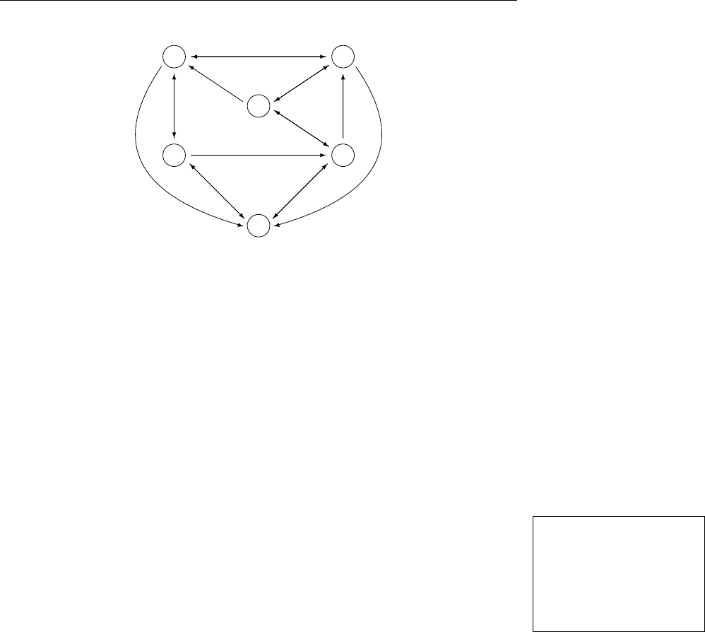
6.1 n-Coloring 53
1
3
4
6
2
5
Figure 3: A Directed Graph with 6 Nodes and 17 Edges.
1% Default
2#const n = 3.
3% Generate
4{ color(X,1..n) } = 1 :- node(X).
5% Test
6:- edge(X,Y), color(X,C), color(Y,C).
In Line 2, we use the #const directive, described in Section 3.1.15, to install 3
as default value for constant nthat is to be replaced with the number nof colors.
(The default value can be overridden by invoking gringo with option --const
n=n.) The generate rule in Line 4 makes use of the shortcut for count aggregates
(cf. Section 3.1.12). For our example graph and 1substituted for X, we obtain the
following ground rule: The full ground program is ob-
tained by invoking:
clingo --text \
or alternatively:
gringo --text \
#count { 0,color(1,1) : color(1,1);
0,color(1,2) : color(1,2);
0,color(1,3) : color(1,3) } = 1.
Note that node(1) has been removed from the body, as it is derived via a corre-
sponding fact, and similar ground instances are obtained for the other nodes 2to 6.
Furthermore, for each instance of edge/2, we obtain nground instances of the in-
tegrity constraint in Line 6, prohibiting that the same color Cis assigned to adjacent
nodes. Given n=3, we get the following ground instances due to edge(1,2):
:- color(1,1), color(2,1).
:- color(1,2), color(2,2).
:- color(1,3), color(2,3).
Again note that edge(1,2), derived via a fact, has been removed from the body.
6.1.3 Problem Solution
Provided that a given graph is colorable with ncolors, a solution can be read off an
answer set of the program consisting of the instance and the encoding. For the graph
color.lp
graph.lp
color.lp
graph.lp
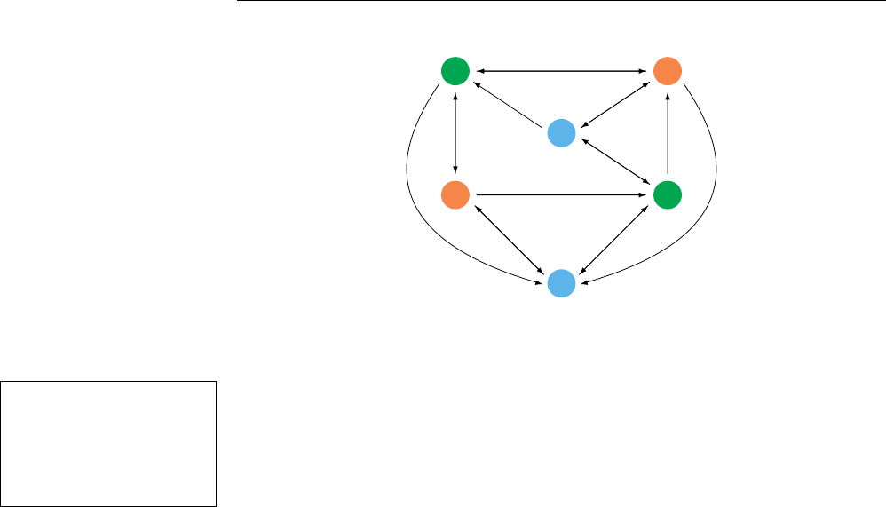
6.2 Traveling Salesperson 54
1
3
4
6
2
5
Figure 4: A 3-Coloring for the Graph in Figure 3.
in Figure 3, the following answer set can be computed:To find an answer set, invoke:
clingo \
or alternatively:
gringo \
| clasp
Answer: 1
... color(1,2) color(2,1) color(3,1) \
color(4,3) color(5,2) color(6,3)
Note that we have omitted the atoms over node/1and edge/2in order to emphasize
the actual solution, which is depicted in Figure 4. Such output projection can also
be specified within a logic program file by using the directive #show, described in
Section 3.1.15.
6.2 Traveling Salesperson
We now consider the well-known traveling salesperson problem (TSP), where the
task is to decide whether there is a round trip that visits each node in a graph exactly
once (viz., a Hamiltonian cycle) and whose accumulated edge costs must not exceed
some budget B. We tackle a slightly more general variant of the problem by not a
priori fixing Bto any integer. Rather, we want to compute a minimum budget B
along with a round trip of cost B. This problem is FPNP-complete (cf. [71]), that is,
it can be solved with a polynomial number of queries to an NP-oracle. As with n-
coloring, we provide a uniform problem definition by separating the encoding from
instances.
6.2.1 Problem Instance
We reuse graph specifications in terms of predicates node/1and edge/2as in Sec-
tion 6.1.1. In addition, facts over cost/3are used to define edge costs:
1% Edge Costs
2cost(1,2,2). cost(1,3,3). cost(1,4,1).
3cost(2,4,2). cost(2,5,2). cost(2,6,4).
4cost(3,1,3). cost(3,4,2). cost(3,5,2).
color.lp
graph.lp
color.lp
graph.lp

6.2 Traveling Salesperson 55
1
3
4
6
2
5
2
3
1 2
2
4
2
2
2
13
Figure 5: The Graph from Figure 3 along with Edge Costs.
5cost(4,1,1). cost(4,2,2).
6cost(5,3,2). cost(5,4,2). cost(5,6,1).
7cost(6,2,4). cost(6,3,3). cost(6,5,1).
Figure 5 shows the graph from Figure 3 along with the associated edge costs. Sym-
metric edges have the same costs here, but differing costs would also be possible.
6.2.2 Problem Encoding
The first subproblem consists of describing a Hamiltonian cycle, constituting a can-
didate for a minimum-cost round trip. Using the generate-define-test pattern [62],
we encode this subproblem via the following non-ground rules:
1% Generate
2{ cycle(X,Y) : edge(X,Y) } = 1 :- node(X).
3{ cycle(X,Y) : edge(X,Y) } = 1 :- node(Y).
4% Define
5reached(Y) :- cycle(1,Y).
6reached(Y) :- cycle(X,Y), reached(X).
7% Test
8:- node(Y), not reached(Y).
9% Display
10 #show cycle/2.
The generate rules in Line 2 and 3 assert that every node must have exactly one
outgoing and exactly one incoming edge, respectively, belonging to the cycle. By
inserting the available edges for node 1, Line 2 and 3 are grounded as follows: The full ground program is ob-
tained by invoking:
clingo --text \
\
or alternatively:
gringo --text \
\
#count { 0,cycle(1,2) : cycle(1,2),
0,cycle(1,3) : cycle(1,3),
0,cycle(1,4) : cycle(1,4) } = 1.
#count { 0,cycle(3,1) : cycle(3,1),
0,cycle(4,1) : cycle(4,1) } = 1.
ham.lp
min.lp
costs.lp
graph.lp
ham.lp
min.lp
costs.lp
graph.lp
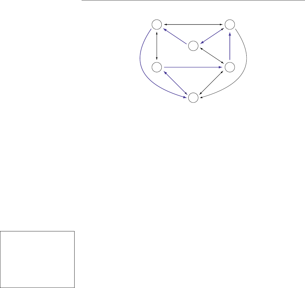
6.2 Traveling Salesperson 56
1
3
4
6
2
5
2
3
12
2
4
2
2
2
13
Figure 6: A Minimum-cost Round Trip.
Observe that the first rule groups all outgoing edges of node 1, while the second
one does the same for incoming edges. We proceed by considering the define rules
in Line 5 and 6, which recursively check whether nodes are reached by a cycle
candidate produced via the generate part. Note that the rule in Line 5 builds on the
assumption that the cycle “starts” at node 1, that is, any successor Yof 1is reached
by the cycle. The second rule in Line 6 states that, from a reached node X, an
adjacent node Ycan be reached via a further edge in the cycle. This definition leads
to positive recursion among the ground instances of reached/1, in which case a
ground program is called non-tight [22, 23]. The fact that the atoms of an answer
set must be derivable is here exploited to make sure that all nodes are reached by
a global cycle from node 1, thus, excluding isolated subcycles. In fact, the test in
Line 8 stipulates that every node in the given graph is reached, that is, the instances
of cycle/2in an answer set must be the edges of a Hamiltonian cycle. Finally,To compute the Hamiltonian cy-
cles for the graph in Figure 3, in-
voke:
clingo \
0
or alternatively:
gringo \
| clasp 0
the additional display part in Line 10 states that answer sets should be projected to
instances of cycle/2, as only they are characteristic for a solution. So far we have
not considered edge costs. Answer sets for the above part of the encoding correspond
to Hamiltonian cycles, that is, candidates for a minimum-cost round trip.
In order to minimize costs, we add the following optimization statement:
11 % Optimize
12 #minimize { C,X,Y : cycle(X,Y), cost(X,Y,C) }.
Here, edges belonging to the cycle are weighted according to their costs. After
grounding, the #minimize statement in Line 12 ranges over the 17 instances of
cycle/2, one for each weighted edge in Figure 5.
6.2.3 Problem Solution
Finally, we explain how the unique minimum cost round trip (depicted in Figure 6)
can be computed. The catch is that we are now interested in optimal answer sets,
rather than in arbitrary ones. In order to determine the optimum, we can start by
ham.lp
graph.lp
ham.lp
graph.lp

6.3 Blocks World Planning 57
gradually decreasing the costs associated with answer sets until we cannot find a
strictly better one anymore. By default, clasp (or clingo) successively enumerates
better answer sets with respect to the provided optimization statements (cf. Sec-
tion 3.1.13). Any answer set is printed as soon as it has been computed, and the last
one is optimal. If there are multiple optimal answer sets, an arbitrary one among
them is computed. For the graph in Figure 5, the optimal answer set (cf. Figure 6) is
unique and its computation can proceed as follows: To compute the minimum-cost
round trip for the graph in Fig-
ure 5, invoke:
clingo \
\
or alternatively:
gringo \
\
| clasp
Answer: 1
cycle(1,3) cycle(2,4) cycle(3,5) \
cycle(4,1) cycle(5,6) cycle(6,2)
Optimization: 13
Answer: 2
cycle(1,2) cycle(2,5) cycle(3,4) \
cycle(4,1) cycle(5,6) cycle(6,3)
Optimization: 11
Given that no answer is obtained after the second one, we know that 11 is the opti-
mum value, but there might be further optimal answer sets that have not been com-
puted yet. To compute all optimal answer sets, we can change clasp’s optimization
mode using option ‘--opt-mode=optN’. In this mode, clasp first prints the tenta-
tive answer sets where optimality is not yet proven and afterwards prints the optimal
answer sets. Note that the first optimal answer set is printed twice in this mode. To
omit tentative answer sets in the output and only print optimal answer sets, we can
add option ‘--quiet=1’. The full invocation is:
clingo \
\
\
--opt-mode=optN \
--quiet=1
or alternatively:
gringo \
\
| clasp \
--opt-mode=optN \
--quiet=1
After obtaining only the second answer given above, we are sure that this is the
unique optimal answer set, whose associated edge costs (cf. Figure 6) correspond to
the reported optimization value 11. Note that, with #maximize statements in the
input, this correlation might be less straightforward because they are compiled into
#minimize statements in the process of generating smodels format [79]. Further-
more, if there are multiple optimization statements or priorities, respectively, clasp
(or clingo) will report separate optimization values ordered by priority.
6.3 Blocks World Planning
The blocks world is a well-known planning domain where finding shortest plans
has received particular attention [55]. With the single-shot grounding and solving
approach we have used in the previous examples, a bound on the plan length must
be fixed before search can proceed. This is usually accomplished by including some
constant tin an encoding, which is then replaced with the actual bound during
grounding. Of course, if the length of a shortest plan is unknown, an ASP system
must repeatedly be queried while varying the bound. With a traditional ASP system,
processing the same planning problem with a different bound involves grounding
and solving from scratch.
In order to reduce such redundancies, clingo’s scripting API (cf. Section 4) can
ham.lp
min.lp
costs.lp
graph.lp
ham.lp
min.lp
costs.lp
graph.lp
ham.lp
min.lp
costs.lp
graph.lp
ham.lp
min.lp
costs.lp
graph.lp

6.3 Blocks World Planning 58
be used to solve problems in an incremental fashion. Because planning problems
where the search horizon is gradually increased are quite common, clingo provides
an easy to use built-in solving and grounding mode for such problems. We use
blocks world planning to illustrate the exploitation of clingo’s incremental computa-
tion mode.
6.3.1 Problem Instance
As with the other two problems above, an instance is given by a set of facts, here
over block/1(declaring blocks), init/1(defining the initial state), and goal/1
(specifying the goal state). A well-known blocks world instance is described by:21
1% Sussman Anomaly
2%
3block(b0).
4block(b1).
5block(b2).
6%
7% initial state:
8%
9% 2
10 % 0 1
11 % -------
12 %
13 init(on(b1,table)).
14 init(on(b2,b0)).
15 init(on(b0,table)).
16 %
17 % goal state:
18 %
19 % 2
20 % 1
21 % 0
22 % -------
23 %
24 goal(on(b1,b0)).
25 goal(on(b2,b1)).
26 goal(on(b0,table)).
Note that the facts in Line 13–15 and 24–26 specify the initial and the goal state
depicted in Line 9-11 and 19–22, respectively. Here we use (uninterpreted) function
on/2to illustrate another important feature available in gringo and clingo, namely,
the possibility of instantiating variables to compound terms.
21Blocks world instances worldi.lp for iP t0,1,2,3,4uare adaptations of the instances pro-
vided at [21].

6.3 Blocks World Planning 59
6.3.2 Problem Encoding
Our blocks world planning encoding for clingo makes use of #program directives
defining subprograms base,step(t), and check(t), separating the encoding
into a static part, a specification of state transitions, and a part for checking the goal
situation and state constraints, respectively. The base part is instantiated at step
zero, the step(t) part is instantiated for steps tą0, and the check(t) part for
steps tě0.
Each of them can be further refined into generate, define, test, and display con-
stituents, as indicated in the comments below:
1#include <incmode>.
3#program base.
4% Define
5location(table).
6location(X) :- block(X).
7holds(F,0) :- init(F).
9#program step(t).
10 % Generate
11 { move(X,Y,t) : block(X), location(Y), X != Y } = 1.
12 % Test
13 :- move(X,Y,t), holds(on(A,X),t-1).
14 :- move(X,Y,t), holds(on(B,Y),t-1), B != X, Y != table.
15 % Define
16 moved(X,t) :- move(X,Y,t).
17 holds(on(X,Y),t) :- move(X,Y,t).
18 holds(on(X,Z),t) :- holds(on(X,Z),t-1), not moved(X,t).
20 #program check(t).
21 % Test
22 :- query(t), goal(F), not holds(F,t).
24 % Display
25 #show move/3.
The first line enables clingo’s incremental computation mode. Next, the base
part in Line 3–7 defines blocks and the constant table as instances of predicate
location/1. Moreover, we use instances of init/1to initialize holds/2for the
initial state at step 0, thus specifying the setup before the first state transition. Note
that variable Fis instantiated to compound terms over function on/2.
The step subprogram in Line 9–18 declares constant tas a placeholder for
step numbers in the program part below. Remember that the step(t) part is not
instantiated for t“0. Hence, it can always refer to two successive time steps at t

6.3 Blocks World Planning 60
and t-1. The generate rule in Line 11 states that exactly one block Xmust be moved
to a location Y(different from X) for each state transition at step t. The integrity
constraints in Line 13 and 14 are used to test whether moving block Xto location Y
is possible at step t. The first integrity constraint ensures that block Xcannot be
moved if there is another block Aon top of it. Furthermore, the second integrity
constraint excludes all moves where the target block Yis occupied by some other
block B. Because the number of blocks that can be put on the table is not limited, the
condition is only checked if Yis a block, viz., ‘Y != table’. Also, this constraint
allows for void moves, that is, it only eliminates solutions where the block Xbeing
moved is different from B, viz., ‘B != X’. The rule in Line 16 marks the block that
is moved via predicate moved/1. Finally, the rule in Line 17 propagates a move to
the state at step t, while the rule in Line 18 states that a block Xstays at a location Z
if it is not moved.
The subprogram check in Line 20–22 specifies goal conditions to be checked
for each state. Note the use of atom query(t). This atom, provided in incremental
mode, allows for posting queries; for each incremental step, there is only one atom
over query/1that is true, namely, query(t) for the current step t.
Note that the #show meta-statement in Line 25 does not belong to any program
part but affects the visibility of atoms in all program parts.22 Furthermore, rules not
subject to a #program directive are associated with the base program by default.
Hence, we do not have to use such directives in instance files because the base part
is exactly where we want the facts from an instance to be included.
Finally, let us stress important prerequisites for obtaining a well-defined incre-
mental computation result from clingo. First, the ground instances of head atoms of
rules in each step must be pairwise disjoint. This is the case for our encoding because
atoms over move/3,moved/2, and those over holds/2include tas an argument
in the heads of rules in Line 11–18. As the smallest step number to replace twith
is 1, there is also no clash with the ground atoms over holds/2obtained from the
head of the static rule in Line 7. Further details on the sketched requirements and
their formal background can be found in [27]. Arguably, many problems including
a mutable bound can be encoded such that this prerequisite applies. Some attention
should of course be spent on putting rules into the right program parts.
6.3.3 Problem Solution
We can now use clingo to incrementally compute the shortest sequence of moves that
brings us from the initial to the goal state depicted in the instance in Section 6.3.1:To this end, invoke:
clingo \
0
Furthermore, you can try:
, ,
,
Answer: 1
move(b2,table,1) move(b1,b0,2) move(b2,b1,3)
This unique answer set tells us that the given problem instance can be solved by
moving block b2 to the table in order to then put b1 on top of b0 and finally b2
on top of b1. This solution is computed by clingo in four grounding and solving
22Not so for #show statements to show terms. These are tied to the program parts they occur in.
blocks.lp
world0.lp
world1.lp
world2.lp
world3.lp
world4.lp

6.3 Blocks World Planning 61
steps, where, starting from the base and the check part in which tis replaced
with 0, the constant tis successively replaced with step numbers 1,2, and 3in
the step and check parts. While the goal conditions in the check part cannot be
fulfilled in steps 0,1, and 2,clingo stops its incremental computation after finding
an answer set in step 3. The scheme of iterating steps until finding some answer set
is the default behavior of the incremental mode.
Sometimes it might be interesting to inspect the grounding of an incremental
program. This can be achieved using option --lparse-debug=plain. Adding
this option, clingo solves as usual but additionally prints the grounded rules to the
standard error stream. The rules are printed in the same format as the text output but
preceded with ‘%’.

7 Command Line Options 62
7 Command Line Options
In this section, we briefly describe the meaning of some selected command line op-
tions supported by gringo (Section 7.1), clingo (Section 7.2), and clasp (Section 7.3).
Each of these tools display their available options when invoked with flag --help
or -h.23 The approach of distinguishing long options, starting with ‘--’, and short
ones of the form ‘-l’, where lis a letter, follows the GNU Coding Standards [52].
For obvious reasons, short forms are made available only for the most common
(long) options. Some options, also called flags, do not take any argument, while
others require arguments. An argument arg is provided to a (long) option opt by
writing ‘--opt=arg’ or ‘--opt arg’, while only ‘-l arg’ is accepted for a
short option l. For each command line option, we below indicate whether it requires
an argument, and if so, we also describe its meaning.
7.1 gringo Options
An abstract invocation of gringo looks as follows:
gringo [ options | files ]
Note that options and filenames do not need to be passed to gringo in any particular
order. If neither a filename nor an option that makes gringo exit (see below) is
provided, gringo reads from the standard input. In the following, we list and describe
the options accepted by gringo along with their particular arguments (if required):
--help,-h
Print help information and exit.
--version,-v
Print version information and exit.
--verbose[=n],-V
Print additional (progress) information during computation. Verbosity level
one and two are currently not used by gringo. The flag implies level three.
Level three prints internal representations of the logic program.
--const,-c c=t
Replace occurrences (in the input program) of constant cwith term t. This
overrides constant definitions in a source file without a warning.
--text,-t
Output ground program in (human-readable) text format.
23Note that our description of command line options is based on gringo and clingo series 4 as well as
clasp series 3. While it is rather unlikely that command line options will disappear in future versions,
additional ones might be introduced. We will try to keep this document up-to-date, but checking the
help information shipped with a new version is always a good idea.

7.2 clingo Options 63
--lparse-rewrite
Can be used in conjunction with the --text option to print a program in a
(human-readable) similar to the smodels format, which is otherwise passed to
the solver.
--lparse-debug={none,plain,lparse,all}
This option enables additional debugging output to the standard error stream.
The available arguments are:
none No additional output is printed.
plain Prints rules as with --text but prefixed with %.
lparse Prints rules as with --text and --lparse-rewrite but
prefixed with %%.
all Combines argument plain and lparse.
--warn,-W [no-]w This option can be used to enable and disable warnings.
To disable a warning, the argument has to prefixed with no-. To enable or
disable multiple warnings, this option can be passed multiple times with dif-
ferent arguments. By default all warnings are enabled. The available values
for argument ware:
file-included See Section 8.2.1.
variable-unbounded See Section 8.2.2.
operation-undefined See Section 8.3.1.
atom-undefined See Section 8.3.2.
global-variable See Section 8.3.3.
When calling gringo without options, it outputs a ground program in smodels for-
mat [79], which is a common input language for propositional ASP solvers.
7.2 clingo Options
ASP system clingo combines grounder gringo and solver clasp via an internal inter-
face. An abstract invocation of clingo looks as follows:
clingo [ options | files | number ]
The optional numerical argument allows for specifying the maximum number of
answer sets to be computed (0standing for all answer sets). As with gringo, the
number, options, and filenames do not need to be passed to clingo in any particular
order. Given that clingo combines gringo and clasp, it accepts all options described
in the previous section and in Section 7.3. In particular, (long) options --help and
--version make clingo print the desired information and exit, while --text
instructs clingo to output a ground program (rather than solving it) like gringo. If
neither a filename nor an option that makes clingo exit (see Section 7.1) is provided,

7.3 clasp Options 64
clingo reads from the standard input. Beyond the options described in Section 7.1
and 7.3, clingo has a single additional option:
--mode=m
Choose the mode in which clingo should run. Available values for mare:
clingo Explicitly select clingo mode (the default).
gringo In this mode clingo behaves like gringo.
lparse In this mode clingo behaves like clasp.
Finally, the default command line when invoking clingo consists of all clasp defaults
(cf. Section 7.3).
7.3 clasp Options
Stand-alone clasp [35] is an ASP solver for ground logic programs that can also be
used as a SAT, MaxSAT, or PB solver (cf. Section 3.2). An abstract invocation of
clasp looks as follows:
clasp [ options | files | number ]
As with clingo and iclingo, a numerical argument specifies the maximum number
of answer sets to be computed, where 0stands for all answer sets. (The number of
requested answer sets can likewise be set via long option --models or its short
form -n.) If neither a filename nor an option that makes clasp exit (see below) is
provided, clasp reads from the standard input.24 In fact, it is typical to use clasp in a
pipe with gringo in the following way:
gringo [ options | files ] | clasp [ options | number ]
In such a pipe, gringo instantiates an input program and outputs the ground rules in
smodels format, which is then fed to clasp that computes and outputs answer sets.
Note that clasp offers plenty of options to configure its behavior. In the follow-
ing, we present only some important options and categorize them according to their
functionalities.
7.3.1 General Options
We below group some general options of clasp, used to configure its global behavior.
--help[=n],-h
Print help information and exit.
Argument ndetermines the level of detail that is shown. If nis not given or
is equal to 1, only major options are shown. Level n=2 also prints advanced
search options. Finally, n=3 prints the full help information.
24In earlier versions of clasp, filenames had to be given via option --file or its short form -f.

7.3 clasp Options 65
--version,-v
Print version information and exit. The version information also includes
whether or not clasp was built with support for parallel solving via multi-
threading.
--verbose[=n],-V
Configure printing of (progress) information during computation. Argument
n=0disables progress information, while n=1and n=2print basic informa-
tion. Extended information is printed for n>2, where levels 4and 5are only
relevant when solving disjunctive logic programs. Finally, the flag -V implies
the largest available verbosity level.
--outf=n
Configure output format. Available values for ninclude 0for clasp’s default
output format, 1for solver competition (ASP, SAT, PB) output, and 2for
output in JSON25 format.
--quiet[=models[,costs][,calls]],-q
Configure printing of computed models, associated costs (in case of optimiza-
tion), and individual call statistics (for multi-shot solving). Arguments are
integers in the range 0..2, where 0means print all, 1means print last, and 2
means do not print any models, costs, or individual call statistics. If --quiet
or -q is given as a flag, all arguments are implicitly set to 2.
--stats[={1,2}],-s
Maintain and print basic (1) or extended (2) statistic information.
--time-limit=t
Force termination after tseconds.
--solve-limit=n[,m]
Force termination after either nconflicts or mrestarts.
--pre
Run ASP preprocessor then print preprocessed input program and exit.
--print-portfolio
Print default portfolio and exit (cf. --parallel-mode).
7.3.2 Solving Options
The options listed below can be used to configure the main solving and reasoning
strategies of clasp.
--models,-n n
Compute at most nmodels, n=0standing for compute all models.
25http://json.org/

7.3 clasp Options 66
--project
Project answer sets to named atoms and only enumerate unique projected so-
lutions [41].
--enum-mode,-e mode
Configure enumeration algorithm applied during solving. Available values for
mode are:
bt Enable backtrack-based enumeration [36].
record Enable enumeration based on solution recording. Note that this
mode is prone to blow up in space in view of an exponential
number of solutions in the worst case.
domRec Enable subset enumeration via domain-based recording (cf. Sec-
tion 10).
brave Compute the brave consequences (union of all answer sets) of a
logic program.
cautious Compute the cautious consequences (intersection of all answer
sets) of a logic program.
auto Use bt for enumeration and record for optimization.
Note: The option is only meaningful if --models is not equal to 1. Further-
more, modes brave and cautious require --models=0, which is also
the default in that case.
--opt-mode=mode
Configure handling of optimization statements. Available values for mode
are:
opt Compute an optimal model (requires --models=0).
enum Enumerate models with costs less than or equal to some fixed bound
(cf. --opt-bound).
optN Compute optimum, then enumerate optimal models.
ignore Ignore any optimization statements during computation.
--opt-bound=n1[,n2,n3...]
Initialize objective function(s) to minimize with n1[,n2,n3...].
--opt-sat
Treat input in DIMACS-(w)cnf format as MaxSAT optimization problem.
--parallel-mode,-t n[,mode]
Enable parallel solving with nthreads [43], where mode can be either
compete for competition-based (portfolio) search or split for splitting-
based search via distribution of guiding paths.

7.3 clasp Options 67
7.3.3 Fine-Tuning Options
The following incomplete list of options can be used to fine-tune certain aspects of
clasp. For a complete list of options, call clasp with option --help=3.
--configuration=c
Use cas default configuration, where ccan be:
frumpy Use conservative defaults similar to those used in earlier clasp ver-
sions.
jumpy Use more aggressive defaults.
tweety Use defaults geared towards typical ASP problems.
trendy Use defaults geared towards industrial problems.
crafty Use defaults geared towards crafted problems.
handy Use defaults geared towards large problems.
<file> Use configuration file to configure solver(s).
Note that using a configuration file enables freely configurable solver portfo-
lios in parallel solving. For an example of such a portfolio, call clasp with
option --print-portfolio.
--opt-strategy={bb,usc}[,n]Configure optimization strategy. Use ei-
ther branch-and-bound-based optimization [29] (bb) or unsatisfiable-core-
based optimization [1] (usc). The optional argument ncan be used to fine-
tune the selected strategy. For example, bb,1 enables hierarchical (multi-
criteria) optimization [29], while usc,1 enables some form of preprocessing
during unsatisfiable-core-based optimization. For further details, call clasp
with option --help=2. Finally, note that the optimization strategy can be
set on a per-solver basis in the context of parallel solving, thus allowing for
optimization portfolios.
--restart-on-model
Restart the search after finding a model. This is mainly useful during opti-
mization because it often ameliorates the convergence to an optimum.
--heuristic={Berkmin,Vmtf,Vsids,Unit,None,Domain}
Use BerkMin-like decision heuristic [54] (with argument Berkmin), Siege-
like decision heuristic [75] (with argument Vmtf), Chaff -like decision heuris-
tic [68] (with argument Vsids), Smodels-like decision heuristic [77] (with ar-
gument Unit), or (arbitrary) static variable ordering (with argument None).
Finally, argument Domain enables a domain-specific decision heuristic as de-
scribed in Section 10.
--save-progress[=n]
Enable alternative sign heuristic based on cached truth values [72] if available.
Cache truth values on backjumps ąn.

7.3 clasp Options 68
--restarts,-r sched
Choose and parameterize a restart policy, where sched can be:
no Disable restarts.
F,nRun fixed sequence, restarting every nconflicts.
*,n,fRun a geometric sequence [18], restarting every n˚ficonflicts,
where iis the number of restarts performed so far.
+,n,mRun an arithmetic sequence, restarting every n`m˚iconflicts,
where iis the number of restarts performed so far.
L,nRestart search after a number of conflicts determined by a universal
sequence [66], where nconstitutes the base unit.
D,n,fUse a dynamic policy similar to the one of glucose [4]. Given the n
most recently learned conflict clauses and their average quality Qn,
a restart is triggered if Qn ˚fąQ, where Qis the global average
quality.
The geometric and arithmetic sequences take an optional limit lim ą0to
enable a nested policy [8]. If given, the sequence is repeated after lim `j
restarts, where jcounts how often the sequence has been repeated so far.
--eq=n
Run equivalence reasoning [38] for niterations, n“-1 and n“0standing
for run to fixpoint or do not run equivalence reasoning, respectively.
--trans-ext={choice,card,weight,scc,integ,dynamic,all,no}
Compile extended rules [77] into normal rules (cf. Section 3.1.2). Arguments
choice,card, and weight state that all “choice rules”, “cardinality rules”
or “weight rules”, respectively, are to be compiled into normal rules, while
all means that all extended rules and no that none of them are subject to
compilation. If argument dynamic is given, clasp heuristically decides
whether or not to compile individual “cardinality” and “weight rules”. Finally,
scc limits compilation to recursive “cardinality” and “weight rules”, while
integ only compiles those “cardinality rules” that are integrity constraints.
--sat-prepro[={0,1,2,3}][,x1]...[,x5]
Configure SatElite-like preprocessing [17]. Argument 0(or no) means that
SatElite-like preprocessing is not to be run at all, while 1enables basic pre-
processing and 2and 3successively enable more advanced preprocessing in-
cluding, for example, blocked clause elimination [60]. If --sat-prepro is
given as a flag, 2is assumed. The optional arguments x1,...,x5 can be used
to set fine grained limits, for example, regarding iterations and runtime. For
further details, call clasp with option --help=2.
Let us note that switching the above options can have dramatic effects (both
positively and negatively) on the search performance of clasp. If performance bot-
tlenecks are observed, it is worthwhile to first give the different prefabricated default


8 Errors, Warnings, and Infos 70
8 Errors, Warnings, and Infos
This section explains the most frequent errors, warnings, and info messages related
to inappropriate inputs or command line options. All messages are printed to the
standard error stream. Errors lead to premature termination, while warnings and info
messages provide hints at possibly corrupt input that can still be processed further.
8.1 Errors
Most of the errors in the following start with the prefix:
*** ERROR: (System)
where System is either gringo,clingo, or clasp depending on the system.
In the following sections, we use Error to denote this prefix. All of the errors with
this prefix are fatal and lead to immediate termination.
8.1.1 Parsing Command Line Options
We start with errors emmited during command line parsing, which are handled
equally by gringo,clasp, and clingo. All our tools try to expand incomplete (long)
options to recognized ones. Parsing command line options may nonetheless fail due
to the following three reasons:
Error: In context ’Context’: unknown option: ’Option’
Error: In context ’Context’: \
ambiguous option: ’Option’ could be:
Option1
Option2
...
Error: In context ’<Context>’: \
’Arg’: invalid value for: ’Option’
*** Info : (System): Try ’--help’ for usage information
The first error means that the option Option could not be expanded to one that is
recognized. While the second error expresses that the result of expanding Option
is ambiguous. It is followed by a list of option canditates Option1,Option2,...,
all sharing the same prefix. Finally, the third error occurs if the argument Arg is
invalid for option Option. All three error messages include a context Context
in which the option is parsed. Often, this is simply the system name but can also
be the name of a configuration in a portfolio file or the string tester for errors in
options regarding the disjunctive tester. The last line is printed in all three cases. It
indicates that option --help can be used to display the available options and their
arguments.

8.1 Errors 71
8.1.2 Parsing and Checking Logic Programs
Next, we consider errors emitted during the parsing and checking of logic programs.
Unlike the error messages in the previous section, such errors include location in-
formation to ease finding and fixing the problem. Each of the error messages below
begins with a location followed by the string error and a short description of the
error in Message:
File:Line:Column-Column: error: Message
Information
File:Line:Column-Column: note: Message
Information
...
The location refers to a string in a source file, specified by file name File, line
number Line, and beginning and ending column number Column (column nrefers
to the n-th symbol in a line). Error messages are sometimes followed by further
desriptions in the string Information indented by two spaces. An optional list
of similarly structured notes, discernable via the string note, can follow this part.
Such notes typically refer to locations that are in conflict with the object referred to
in the location of the error message. Multiple error messages of this kind might be
reported; each error message is terminated with two newlines after the notes.
Logic Program Parsing We start our description with errors that may be encoun-
tered during parsing, where the following one indicates a syntax error in the input:
Location: error: syntax error, unexpected Token
To correct this error, please investigate the indicated location and check whether
something looks strange there (like a missing period, an unmatched parenthesis,
etc.). Note that the parser tries to recover from a syntax error. This typically means
that everything up to the next period is ignored.
Safety Checking The next error occurs if an input program is not safe:
Location: error: unsafe variables in
Rule
Location: note: ’Var’ is unsafe
...
Along with the error message, the affected rule Rule and a list of all unsafe variable
occurrences Var are reported. The first action to take usually consists of checking
whether variable Var is actually in the scope of any atom (in the positive body of
Rule) that can bind it.26 Also check for variables that occur in aggregate elements
26Recall from Section 3.1.7 and 3.1.8 that variables in the scope of built-in arithmetic functions are
only bound by their corresponding atoms in some special cases and that built-in comparison predicates
do not bind variables.

8.1 Errors 72
(cf. Section 3.1.12) or conditional literals (cf. Section 3.1.11); you might have to
bind them with additional positive atoms in the conditions.
Script Execution and Parsing If an error in an embedded script occurs (cf. Sec-
tion 3.1.14), the following error message is printed:
Location: error: failed to execute script:
Information
...
The information printed depends on the error that occurred when executing the em-
bedded script. This can for example be parse errors or errors that occurred when
executing the script. Typically, the information contains a trace where the error oc-
curred.
Defining Constants There are three errors associated to #const statements
(cf. Section 3.1.15).
Location: error: cyclic constant definition:
Constant
Location: note: cycle involves definition:
Constant
...
Location: error: redefinition of constant:
Constant
Location: note: constant also defined here:
Constant
...
The strings Constant provide the affected #const statements. The first error is
printed if the statements rely on each other cyclically. Each statement involved in
the cycle is printed in the corresponding notes. The second error message is printed
if a constant is defined more than once. The location of the conflicting definition is
printed in the note.
If at least one of the errors above is reported, then gringo or clingo terminates
after parsing and checking with the error message:
Error: grounding stopped because of errors
Remark 8.1. No more than 20 errors are printed. If this limit is exceeded, the
application stops parsing or safety checking and terminates.
8.1.3 Parsing Logic Programs in smodels Format
The following error message is issued by (embedded) clasp:

8.2 Warnings 73
Error: parse error in line Line:Message
This error means that the input does not comply with smodels’ numerical for-
mat [79]. If you are using gringo to ground logic programs, this error should never
occur.
8.1.4 Multi-shot Solving
The following error is issued by (embedded) clasp if an atom is defined (it appears
in the head of a rule) in two different grounding steps:
Error: redefinition of atom <Atom,Id>
Information
where Atom is the string representation of the atom that is redefined and Id is the
unique identifier of the atom introduced when translating the logic program into
smodels format. If the scripting API (cf. Section 4) is used for grounding, then the
error message is followed by a trace, indicating the source code location where the
program has been grounded.
Remark 8.2. Only the case that an atom is redefined is checked by clasp. The case
when there is a positive cycle over two or more incremental steps is not detected,
which possibly leads to unwanted answer sets.
8.2 Warnings
This section describes warnings that may be reported by gringo or clingo. Unlike
errors, warnings do not terminate the application but rather hint at problems, which
should be investigated. A program with warnings might lead to unexpected results;
there are no guarantees regarding the semantics of such programs. Most warnings
have a similar format as the errors described in Sections 8.1.2; the only difference is
that the location is followed by the string warning.
Remark 8.3. No more than 20 warnings are printed. If this limit is exceeded, you
should definitely fix some warnings.
8.2.1 File Included Multiple Times
If a file is included multiple times, either on the command line or with an include
directive, then the following warning is emitted:
Location: warning: already included file:
Filename
Remark 8.4. Only the first include of a file is considered. All additional includes
are ignored.

8.3 Infos 74
8.2.2 Unbounded CSP Variables
In the current implementation, a bound has to be supplied for each CSP variable
(cf. Section 5.3.1). For variables with bounds, the following warning is issued:
warning: unbounded constraint variable:
domain of Variable is set to Domain
where Variable is the variable lacking a domain specification and Domain is an
(arbitrary) domain chosen for the variable.
8.3 Infos
This section describes information messages that may be reported by gringo or
clingo. Info messages indicate issues in the input that have a well defined semantics
but are possibly unintended by the user.
An information message is preceded with the string info.
Remark 8.5. Up to 20 info messages are printed. There might me further issues but
these will be silently ignored.
8.3.1 Undefined Operations
These may occur within an arithmetic evaluation (cf. Section 3.1.7) or if an error
occurs while evaluating an external function (cf. Section 3.1.14):
Location: info: term undefined:
Term
...
It typically means that either a (symbolic) constant or a compound term (over an un-
interpreted function) has occurred in the scope of some built-in arithmetic function.
The string Term provides the term that failed to evaluate. The message might be fol-
lowed by further notes. For example, if the evaluation of an external function failed,
by a trace indicating the location of the error within the source code of the external
function. Typically, it is simple to fix occurrences of this message - for example,
if the term ‘X/Y’ causes a message, it can be silenced by adding the comparison
literal ‘Y!=0’ to the body of a rule (or condition). We suggest to silence all of these
message in this manner and not simply to disable the message.
Remark 8.6. Instantiations of rules, #show statements, #external statements,
weak constraints, aggregate elements, and conditional literals that contain undefined
terms are discarded.
8.3.2 Undefined Atoms
This message is emitted if an atom appears in the body of a rule or condition that is
never defined in the head of a rule or external statement:

8.3 Infos 75
Location: info: atom is undefined:
Atom
where Atom is the atom occurrence without a definition. Often, this message indi-
cates that a predicate has been misspelled or that an argument has accidentally been
omitted.
8.3.3 Global Variables in Tuples of Aggregate Elements
This message is emitted if a variable occurs globally in a tuple of an aggregate ele-
ment:
Location: info: global variable in tuple of \
aggregate element:
Variable
where Variable is the variable that occurs globally. Typically, this message oc-
curs if a there is a name clash between a global and a local variable because in most
situations it should not be necessary to put global variables into the tuples of aggre-
gate elements.

9 Meta-Programming 76
9 Meta-Programming
This section is not yet ready for publishing and will be included in one of the forth-
coming editions of this guide.
Information on meta-programming can be obtained at the following references.
• Meta-programming relying on reified logic programs was introduced with
gringo 3; details can be found at:
–[34]
–http://www.cs.uni-potsdam.de/wv/metasp
•gringo ships with a small tool called reify to reify logic programs in aspif
format [61].
Moreover, it offers a dedicated output format for reification, viz.
--output=reify to output logic programs as sets of facts
Also, gringo 5 features options --reify-sccs to add strongly connected
components to reified output and --reify-steps to add step numbers to
reified output.
An advantage of using the reify tool is that it can be combined with clasp’s
pre-processor.

10 Heuristic-driven Solving 77
10 Heuristic-driven Solving
clasp and clingo provide means for incorporating domain-specific heuristics into
ASP solving. This allows for modifying the heuristic of the solver from within a
logic program or from the command line. A formal description can be found in [39].
The framework is implemented as a new heuristic, named Domain, that
extends the Vsids heuristics of clasp and can be activated using option
--heuristic=Domain (cf. Section 7.3.3). In what follows, we first describe
how to modify the solver’s heuristic from within a logic program, then we explain
how to apply modifications from the command line, and finally we show how to
compute subset minimal answer sets with heuristics.
The following description conforms with clingo 5.
10.1 Heuristic Programming
Heuristic information is represented within a logic program my means of heuristic
directives of the form
#heuristic A:B. [w@p,m]
where Ais an atom, Ba rule body, and w,pand mare terms. The priority ‘@p’ is
optional. Different types of heuristic information can be controlled using the modi-
fiers sign,level,true,false,init and factor for m. We introduce them
below step by step.
10.1.1 Heuristic modifier sign
The modifier sign allows for controlling the truth value assigned to variables sub-
ject to a choice within the solver.
The Domain heuristic associates with each atom an integer sign value, which
by default is 0. When deciding which truth value to assign to an atom during a
choice, the atom is assigned to true, if its sign value is greater than 0. If the sign
value is less than 0, it is assigned to false. And if it is 0, the sign is determined by
the default sign heuristic.
In order to associate a positive sign with atom a, we can use the following heuris-
tic directive:
#heuristic a. [1,sign]
This associates a positive sign with aand tells the solver that upon deciding the
atom a, it should be set to true.
Example 10.1. Consider the following program:
#heuristic a. [1,sign]
{a}.

10.1 Heuristic Programming 78
To inspect the output, invoke:
clingo \
--heuristic=Domain
or alternatively:
gringo \
| clasp \
--heuristic=Domain
At the start of the search, the solver updates its heuristic knowledge about atom a
assigning to it the sign value 1. Then, it has to decide on a, making it either true or
false. Following the current heuristic knowledge, the solver makes atrue and returns
the answer set {a}.
Remark 10.1. The result would be the same if in the heuristic directive we used any
positive integer instead of 1.
Example 10.2. In the next program, the #heuristic directive gives aa negative
sign and thus asserts that when deciding upon ait should be set to false:
#heuristic a. [-1,sign]
{a}.
To inspect the output, invoke:
clingo \
--heuristic=Domain
or alternatively:
gringo \
| clasp \
--heuristic=Domain
As above, the solver starts updating its heuristic knowledge, then decides on atom a
making it false, and finally returns the empty answer set.
These two examples illustrate how the heuristic directives allow for modifying
the decisions of the solver, leading to either finding first the answer set with aor the
one without it. However, the program’s overall answer sets remain the same. For
example, if we ask for all answer sets in Example 10.1, we obtain one without a
and one with a, and the same happens with Example 10.2, although in this case the
answer sets are computed in opposite order.
10.1.2 Heuristic modifier level
The Domain heuristic assigns to each atom a level, and it decides first upon
atoms of the highest level. The default value for each atom is 0, and both positive
and negative integers are valid.
Example 10.3. In this example, level 10 is assigned to atom a:
#heuristic a. [ 1, sign]
#heuristic b. [ 1, sign]
#heuristic a. [10,level]
{a;b}.
:- a, b.
To inspect the output, invoke:
clingo \
--heuristic=Domain
or alternatively:
gringo \
| clasp \
--heuristic=Domain
The first obtained answer set is {a}. The solver starts updating its heuristic knowl-
edge, and given that the level of ais greater than that of b, it decides first on a(with
positive sign) and then bis propagated to false. If we added the directive
#heuristic b. [20,level]
we would first obtain the answer set containing binstead of a. This would also be
the case if we replaced 10 by -10 in the third heuristic directive.
Remark 10.2. The Domain heuristic is an extension of the Vsids heuristic, so
when there are many unassigned atoms with the highest level, the heuristic decides,
among them, on the one with the highest Vsids score.
psign.lp
psign.lp
nsign.lp
nsign.lp
level.lp
level.lp

10.1 Heuristic Programming 79
10.1.3 Dynamic heuristic modifications
Heuristic directives only affect the solver when their bodies are true. This allows
representing dynamic heuristic modifications.
Example 10.4. In the next program, the heuristic directive for cdepends on b:
#heuristic a. [ 1, sign]
#heuristic b. [ 1, sign]
#heuristic a. [10,level]
{a;b}.
:- a, b.
{c}.
#heuristic c : b. [ 1,sign]
#heuristic c : not b. [-1,sign]
To inspect the output, invoke:
clingo \
--heuristic=Domain
or alternatively:
gringo \
| clasp \
--heuristic=Domain
The first obtained answer set is {a}. At first, the solver proceeds as in Example 10.3.
Then, after propagating bto false, the heuristic knowledge is updated assigning the
sign value -1 to c. So, when deciding upon c, it gets assigned to false. If we
added the directive
#heuristic b. [20,level]
the first answer set would contain band cinstead of a.
10.1.4 Heuristic modifiers true and false
The modifiers true and false allow us to refer at the same time to the level
and the sign of an atom. Internally, a heuristic directive with the form
#heuristic A:B. [w@p,true]
becomes
#heuristic A:B. [w@p,level]
#heuristic A:B. [1@p,sign]
and
#heuristic A:B. [w@p,false]
becomes
#heuristic A:B. [w@p,level]
#heuristic A:B. [-1@p,sign]
For instance, the program of Example 10.4 can be rewritten as:
dynamic.lp
dynamic.lp

10.1 Heuristic Programming 80
#heuristic b. [ 1,sign]
#heuristic a. [10,true]
{a;b}.
:- a, b.
{c}.
#heuristic c : b. [ 1,sign]
#heuristic c : not b. [-1,sign]
In this case, the directive
#heuristic a. [10,true]
stands for the previous
#heuristic a. [ 1, sign]
#heuristic a. [10,level]
10.1.5 Priorities among heuristic modifications
The Domain heuristic allows for representing priorities between different heuristic
directives that refer to the same atom. The priority is optionally represented by
a positive integer pin ‘@p’. The higher the integer, the higher the priority of the
heuristic atom. For example, the following are valid heuristic directives:
#heuristic c. [ 1@10,sign]
#heuristic c. [-1@20,sign]
With both, the sign assigned to cis -1 (because priority 20 overrules 10).
Example 10.5. Consider the following program:
#heuristic b. [ 1,sign]
#heuristic a. [10,true]
{a;b}.
:- a, b.
{c}.
#heuristic c. [ 1@10,sign]
#heuristic c : not b. [-1@20,sign]
To inspect the output, invoke:
clingo \
--heuristic=Domain
or alternatively:
gringo \
| clasp \
--heuristic=Domain
The first obtained answer set is {a}. First the solver proceeds as in Example 10.3.
Then, after setting bto false by propagation, the heuristic knowledge about cis
updated. Given that priority 20 is greater than 10, the sign value of atom cis -1.
So, when deciding upon c, it is assigned to false. If we added the directive
#heuristic c. [1@30,sign]
the first answer set would also contain atom c.
Remark 10.3. Whenever we do not explicitly state a priority, the assigned priority
is the absolute value of the modifiers’ value. For example, with these directives
priority.lp
priority.lp

10.1 Heuristic Programming 81
#heuristic c. [-10,level]
#heuristic c. [ 5,level]
the level of cis -10 because |-10|ą|5|.
10.1.6 Heuristic modifiers init and factor
The modifiers init and factor allow for modifying the scores assigned to atoms
by the underlying Vsids heuristic. Unlike the level modifier, init and factor
allow us to bias the search without establishing a strict ranking among the atoms.
With init, we can add a value to the initial heuristic score of an atom. For
example, with
#heuristic a. [2,init]
a value of 2is added to the initial score that the heuristic assigns to atom a. Note
that as the search proceeds, the initial score of an atom decays, so init only affects
the beginning of the search.
To bias the whole search, we can use the factor modifier that multiplies the
heuristic score of an atom by a given value. For example, with
#heuristic a. [2,factor]
the heuristic score for atom ais multiplied by 2.
10.1.7 Monitoring domain choices
The Domain heuristic extends clasp and clingo’s search statistics produced with
command line option --stats. After ‘Domain:’, it prints how many decisions
where made on atoms appearing inside #heuristic directives. For instance, the
statistics obtained in Example 10.4 read as follows:
...
Models : 1+
Calls : 1
Time : 0.003s (Solving: 0.00s ...)
CPU Time : 0.000s
Choices : 2 (Domain: 2)
Conflicts : 0
Restarts : 0
...
The line about Choices tells us that two decisions were made and that both where
made on atoms contained in #heuristic directives.

10.1 Heuristic Programming 82
10.1.8 Heuristics for Blocks World Planning
We now apply the Domain heuristic to Blocks World Planning. For simplicity, we
adapt the encoding of Section 6.3.2 for one-shot solving27:
time(1..lasttime).
location(table).
location(X) :- block(X).
holds(F,0) :- init(F).
% Generate
{ move(X,Y,T) : block(X), location(Y), X != Y } = 1
:- time(T).
% Test
:- move(X,Y,T), holds(on(A,X),T-1).
:- move(X,Y,T), holds(on(B,Y),T-1), B != X, Y != table.
% Define
moved(X,T) :- move(X,Y,T).
holds(on(X,Y),T) :- move(X,Y,T).
holds(on(X,Z),T) :- holds(on(X,Z),T-1), not moved(X,T).
% Test
:- goal(F), not holds(F,lasttime).
% Display
#show move/3.
Constant lasttime bounds the plan length, and we assume it is provided by com-
mand line (for example, with option -c lasttime=3). In this encoding, once all
the values for predicate move/3 are given, the values of moved/2 and holds/2
are determined and may be propagated by the solver. This suggests that deciding
only on move/3 may be a good strategy. We can do that with the Domain heuristic
adding the following heuristic directive:
#heuristic move(B,L,T) : block(B),location(L),time(T). [1,level]
Given that the level of move/3 is higher, the solver decides first on atoms of that
predicate, and the values of the other predicates are propagated.
We may prefer to soften the heuristic modification to simply bias the search
towards the move/3 predicate, without establishing a strict preference towards it.
For that, we can use, for example, the directive
#heuristic move(B,L,T) : block(B),location(L),time(T). [2, init]
or
27Heuristics may also be applied in the incremental setting of Section 6.3.2, but we introduce them
this way for clarity.

10.1 Heuristic Programming 83
#heuristic move(B,L,T) : block(B),location(L),time(T). [2,factor]
or the combination of both. The first directive adds 2to the initial score of move/3
atoms, while the second multiplies the heuristic score of move/3 by 2.
Whenever we decide on making a move/3 atom true, the other move/3 atoms
for the same time/1 are determined to be false, and can be propagated by the
solver. So, deciding on true move/3 atoms may be a good idea. For that, we can
either use the true modifier to express a strict preference
#heuristic move(B,L,T) : block(B),location(L),time(T). [1,true]
or just bias the search with init and sign
#heuristic move(B,L,T) : block(B),location(L),time(T). [2,init]
#heuristic move(B,L,T) : block(B),location(L),time(T). [1,sign]
or with factor and sign
#heuristic move(B,L,T) : block(B),location(L),time(T). [2,factor]
#heuristic move(B,L,T) : block(B),location(L),time(T). [1,sign]
So far, we have given the same heuristic values to all move/3 atoms, but other
options may be interesting. For example, we may prefer to decide first on earlier
move/3 atoms, so that the solver performs a forward search. This can be repre-
sented with the following rule:
#heuristic move(B,L,T) : block(B), location(L), time(T).
[lasttime-T+1,true]
For lasttime=3, the rule ranks move/3 atoms at time 1at level 3, those at time
2at level 2, and those at time 3at level 1, while always assigning a positive sign.
In this manner, the solver decides first on setting a move/3 atom at time 1to true,
then one at time 2, and so on.
Another strategy is to perform a backwards search on move/3 from the last to
the first time instant, directed by the goals. For this purpose, we can use the following
dynamic heuristic directive:
#heuristic move(B,L,T) : holds(on(B,L),T). [true,T]
As before, the directive can be softened using sign with init or factor. At the
start of the search, the goal’s holds/2 atoms are true at the last time step. With
this rule, the solver decides on a move/3 atom that makes one of them true. Then,
some holds/2 atoms are propagated to the previous time step, and the process is
repeated until reaching the first time instant.
We can also choose to promote atoms of the holds/2 predicate. For example,
this can be achieved with any of the following directives.
#heuristic holds(on(B,L),T) : block(B),location(L),time(T).
[1,level]
#heuristic holds(on(B,L),T) : block(B),location(L),time(T).
[2,init]
#heuristic holds(on(B,L),T) : block(B),location(L),time(T).
[3,factor]

10.2 Command Line Structure-oriented Heuristics 84
Another interesting alternative is the following heuristic directive, that proved to
be very useful in practice (see [39]):
#heuristic holds(on(B,L),T-1) : holds(on(B,L),T).
[lasttime-T+1,true]
The idea is to make the goal’s holds/2 atoms persist backwards, one by one, from
the last time step to the first one. Note that a higher level is given to atoms at earlier
time instants. First, the solver decides on one of the goal’s holds/2 atoms at the
last but one time step, then it decides to make it persist to the previous situation,
and so on. Later, it makes persist backwards another holds/2 atom from the goal.
With this heuristic, the idea is not to decide on atoms that lead to much propagation
(as with move/3 atoms) but rather to make correct decisions, given that usually the
values of holds/2 atoms persist by inertia.
10.2 Command Line Structure-oriented Heuristics
The Domain heuristic also allows us to modify the heuristic of the solver from the
command line. For this, it is also activated with option --heuristic=Domain,
but now the heuristic modifications are specified by option:
--dom-mod=<mod>[,<pick>]
where <mod> ranges from 0to 5and specifies the modifier:
<mod> Modifier <mod> Modifier
0None 1 level
2 sign (positive) 3 true
4 sign (negative) 5 false
<pick> specifies bit-wisely the atoms to which the modification is applied:
0Atoms only
1Atoms that belong to strongly connected components
2Atoms that belong to head cycle components
4Atoms that appear in disjunctions
8Atoms that appear in optimization statements
16 Atoms that are shown
Whenever <mod> equals 1,3or 5, the level of the selected atoms depends
on <pick>. For example, with option --dom-mod=2,8, we apply a pos-
itive sign to atoms appearing in optimization statements, and with option
--dom-mod=1,20, we apply modifier level to both atoms appearing in dis-
junctions as well as shown atoms. In this case, atoms satisfying both conditions are
assigned a higher level than those that are only shown, and these get a higher level
than those only appearing in optimization statements.
Compared to programmed heuristics, the command line heuristics do not allow
for applying modifiers init or factor and cannot represent dynamic heuristics.

10.3 Computing Subset Minimal Answer Sets with Heuristics 85
On the other hand, they allow us to directly refer to structural components of the
program and do not require any additional grounding. When both methods are com-
bined, the atoms modified by the #heuristic directive are not affected by the
command line heuristics.
10.3 Computing Subset Minimal Answer Sets with Heuristics
Apart from boosting solver performance, domain specific heuristics can also be used
for computing subset minimal answer sets (cf. [15, 16]). This can be achieved by
assigning false with value 1to the atoms to minimize.
Example 10.6. Consider the following program:
1 {a(1..3)}. a(2) :- a(3). a(3) :- a(2). {b(1)}.
#show a/1.
Both the command line option ‘--dom-mod=5,16’ as well as the addition of the
heuristic directive
#heuristic a(1..3). [1,false]
guarantee that the first answer set produced is subset minimal with respect to the
atoms of predicate a/1. Moreover, both allow for enumerating all subset minimal
solutions in conjunction with option --enum-mod=domRec. In our example, we
obtain the answer sets ta(1)uand ta(2),a(3)u. Note that in this case solutions
are projected on shown atoms.
It is worth mentioning that the enumeration mode domRec relies on solution
recording and is thus prone to an exponential blow-up in space. In practice, how-
ever, this often turns out to be superior to enumerating subset minimal model via
disjunctive logic programs, which is guaranteed to run in polynomial space.

11 Optimization and Preference Handling 86
11 Optimization and Preference Handling
This section shows how quantitative and qualitative preferences can be used for com-
puting optimal answer sets. While Section 11.1 summarizes the standard optimiza-
tion capacities of clasp,gringo, and clingo dealing with lexicographic optimization
of linear objective functions, Section 11.2 provides a tutorial introduction to asprin’s
general preference handling framework.
11.1 Multi-objective Optimization with clasp and clingo
This subsection is not yet ready for publishing and will be included in one of the
forthcoming editions of this guide.
Some information on multi-objective optimization can be obtained at the follow-
ing references.
• Optimization [30, 29, 34, 1]
• Video series on clasp’s optimization capacities http://potassco.org/
doc/videos
• Consult Section 3.1.13 for language constructs expressing multi-criteria opti-
mization.
• Consult Section 7.3.2 and 7.3.3 for relevant clasp options configurating the
optimization process.
11.2 Preference Handling with asprin
asprin provides a general framework for optimizing qualitative and quantitative pref-
erences in ASP. It allows for computing optimal answer sets of logic programs
with preferences. While asprin comes with a library of predefined preference types
(subset,pareto, etc.), it is readily extensible by new customized preference
types. For a formal description of asprin, please consult [10].
The following description conforms with asprin 3.0, which uses clingo 5.
11.2.1 Computing optimal answer sets
Similar to common optimization in ASP, where objective functions are added to logic
programs via minimize statements or weak constraints, a preference specification is
added to a logic program to single out the optimal answer sets with respect to the
given preferences. However, as with minimize statements, such a specification is not
part of the program but rather a meta statement referring to its answer sets. Hence,
preference specifications are directives and thus preceded by #. For clarity, we also
refer to the underlying program as the base program (also in view of distinguishing it
from the preference program, implementing the preference specification; see below).

11.2 Preference Handling with asprin 87
To begin with, let us consider a simple example providing a holistic view on
preference handling with asprin.
Example 11.1. Consider the following base program. To inspect the output, invoke:
clingo 0
or alternatively:
gringo \
| clasp 0
dom(1..3).
{ m(1..3) } = 1.
a(1) :- m(1). a(1..2) :- m(2). a(3) :- m(3).
b(1..3) :- m(1). b(1) :- m(2). b(2..3) :- m(3).
#show m/1. #show a/1. #show b/1.
We obtain three answer sets, one with m(1),m(2), and m(3), respectively, and
refer to them as X1,X2, and X3.
Remark 11.1. Base programs are gringo and clingo programs as specified in Sec-
tion 3.1, except that weak constraint and minimize and maximize statements are not
allowed.
For a first example, we can use asprin to compute the answer sets of the base
program that are subset minimal with respect to atoms of predicate a{1. This can be
done with the following preference specification (available in ):
1#preference(p1,subset){ a(X) : dom(X) }.
2#optimize(p1).
Line 1 contains a preference statement of name p1 and type subset that contains
a single (non-ground) preference element. Intuitively, the preference statement p1
defines a preference of type subset over atoms of predicate a/1. Line 2 contains
an optimization directive that instructs asprin to compute answer sets that are optimal
with respect to p1.
Remark 11.2. Unlike gringo’s native optimization statements and weak constraints
(cf. Section 3.1.13), asprin separates the declaration of preferences from the actual
optimization directive.
To compute an answer set of the base program that is optimal with respect to
p1, an implementation of the preference type subset must be provided. This is
comprised in asprin’s preference library, contained in the file asprin lib.lp,
which is automatically loaded by the system unless option --no-asprin-lib is
issued. The computation can then be performed by the following command: clingo Python module must be
importable via the environment
variable PYTHONPATH, and the
related file asprin ought to
be located in some directory
in the system path. The
file asprin lib.lp is first
looked up in the current direc-
tory. If it is not found there,
then it is looked up in the root
directory of the distribution, i.e.,
in the directory of the main file
asprin.py.
asprin
The output should look like this:
asprin version 3.0.0
Reading from base.lp ...
base.lp
base.lp
preference1.lp
base.lp
preference1.lp

11.2 Preference Handling with asprin 88
Solving...
Answer: 1
m(2) a(1) a(2) b(1)
Answer: 2
m(1) a(1) b(1) b(2) b(3)
OPTIMUM FOUND
Models : 2+
Optimum : yes
...
At first, asprin finds the answer set X2of the base program. Then, it looks for an
answer set that is preferred to X2and it finds X1. In the last step, asprin looks for
an answer set that is preferred to X1, and given that none is found the optimality of
X1is established. In total, two answer sets were enumerated in the computation of
an optimal solution.
Alternatively, we can minimize the extension of predicates a/1 and b/1 with
the following preference specification.
#preference(p2,subset){ a(X) : dom(X); b(X) : dom(X) }.
#optimize(p2).
Now, we obtain that X2is already an optimal answer set:To inspect the output, invoke:
asprin \Answer: 1
m(2) a(2) a(1) b(1)
OPTIMUM FOUND
11.2.2 Computing multiple optimal answer sets
In analogy to clasp and clingo,asprin allows for computing noptimal answer sets by
adding the number nto the command line; as well, 0is used to compute all optimal
answer sets.
Example 11.2. For instance, the command
asprin 0
results in the output:
Answer: 1
m(2) a(2) a(1) b(1)
Answer: 2
m(1) a(1) b(3) b(2) b(1)
OPTIMUM FOUND
Answer: 3
m(3) a(3) b(3) b(2)
OPTIMUM FOUND
base.lp
preference2.lp
base.lp
preference1.lp

11.2 Preference Handling with asprin 89
The computation of the first optimal answer set, X1, is the same as above. Then,
asprin searches for an answer set of the base program that is not worse than X1,
finds X3, and proves that it is optimal. In the last step, asprin looks for some answer
set that is not worse than X1and X3, and given that there is none, it terminates.
Adding the following choice rule (via file ) to the above optimization
process
{c(1)}.
#show c/1.
yields two additional optimal answer sets, both containing c(1):To inspect the output, invoke:
asprin \
\
0
Answer: 1
m(2) a(2) a(1) b(1)
Answer: 2
m(1) a(1) b(3) b(2) b(1)
OPTIMUM FOUND
Answer: 3
m(1) a(1) b(3) b(2) b(1) c(1)
OPTIMUM FOUND *
Answer: 4
m(3) a(3) b(3) b(2)
OPTIMUM FOUND
Answer: 5
m(3) a(3) b(3) b(2) c(1)
OPTIMUM FOUND *
When asprin looks for an answer set that is not worse than X1, it first looks for
answer sets that interpret atoms appearing in the preference statements in the same
way as X1. In this way, it finds the second optimal model, that contains c(1), and
prints it followed by the line ‘OPTIMUM FOUND *’. Then, it continues searching,
finds X3and the process continues.
Finally, we can project optimal answer sets on the formulas of the preference
statements by asprin’s option --project. This yields only the three optimal an- To inspect the output, invoke:
asprin \
\
0 --project
swer sets not containing c(1).
11.2.3 Input language of asprin
asprin’s input language extends the one described in Section 3 by constructs for
expressing qualitative and quantitative preferences.
Aweighted formula is of the form
t::F
where tis a term tuple, and Fis a either a Boolean formula or a naming atom.
We may drop :: and simply write Fwhenever tis empty. If Fis missing28,
28Note that empty weighted formulas are not allowed.
c1.lp
base.lp
preference1.lp
c1.lp
base.lp
preference1.lp
c1.lp

11.2 Preference Handling with asprin 90
we interpret is as the Boolean constant #true. Boolean formulas are formed
from atoms, possibly preceded by classical negation (‘-’), using the connectives
not (default negation), &(conjunction) and |(disjunction). Parentheses can be
written as usual29, and when omitted, negation has precedence over conjunction,
and conjunction over disjunction. Furthermore, if Fis a conjunction of the form
F1&. . . &Fn, it can also we written using the body notation F1,. . . ,Fn. Naming
atoms of form **s, where sis a term, refer to the preference associated with prefer-
ence statement s(see below). Examples of weighted formulas are ‘42::a’, ‘a(X)
& b(X)’, ‘C::edge(X,Y), cost(X,Y,C)’, ‘W,(X,Y)::not a(W,X) |
b(Y)’, and ‘X::**p(X)’.
If F1,..., Fnare weighted formulas, then
{F1;. . . ;Fm}
is a set of weighted formulas. We may drop the curly braces if m“1.
Apreference element is of the form
F1ąą . . . ąą Fm|| F:B
where each Frand Fis a set of weighted bodies, and Bis a rule body where
all literals belong to domain predicates (see Page 30) or built-ins. We may drop
‘>>’ if m“1, and ‘|| F’ and ‘:B’ whenever Fand/or Bare empty, respec-
tively. Intuitively, rgives the rank of the respective set of weighted bodies. This
can be made subject to condition Fby using the conditional ‘||’. Preference
elements provide a (possible) structure to a set of weighted bodies by giving a
means of conditionalization and a symbolic way of defining pre-orders (in addi-
tion to using weights). Examples of preference elements are ‘42::a’, ‘a(X),
b(X):c(X)’, ‘X::**p(X)’, ‘{a(X);b(X)}>> {c(X);d(X)}’, and ‘a(X)
>> b(X) || c(X) : dom(X)’.
Remark 11.3. Here and below, the rule body Bis intended exclusively to provide
instantiations for the variables appearing in the expressions to its left. Accordingly,
the literals in Bmust be built-ins or belong to domain predicates of the accompa-
nying logic program. This ensures that Bcan be fully evaluated during grounding.
Remark 11.4. If the body Bof a preference element eis empty, asprin auto-
matically replaces it with a body providing the domains of the atoms appearing
in e, consisting of new atoms dom(a)for every atom with variables ain e,
and new atoms pref dom(s)for every naming atom with variables **sin e.
For example, ‘X::**p(X)’ becomes ‘X::**p(X) : pref dom(p(X))’,
and ‘{a(X);b(X)}>> {c(X);d(X)}’ becomes ‘{a(X);b(X)}>>
{c(X);d(X)}:dom(a(X)),dom(b(X)),dom(c(X)),dom(d(X))’. For
defining those atoms, asprin extends the base program with facts dom(agr). for
29Except that they are not allowed around atoms.

11.2 Preference Handling with asprin 91
every ground instace agr of aobtained by clingo after grounding the base program.
Similarly, asprin adds facts pref dom(sgr ). for every ground instance sgr of s
obtained by clingo while grounding the preference specification.
Remark 11.5. Preference elements are required to be safe, i.e., all variables in a
preference element must occur in some positive literal in its body or in the body of
the preference statement containing it (see below). Note that preference elements
whose body is missing are always safe, due to the new body automatically added by
asprin (see previous Remark 11.4).
Apreference statement is of the form
#preference(s,t){e1;. . . ;en}:B.
where sis a term giving the preference name, tis a term providing the preference
type, and each ejis a preference element. The rule body Bhas the same form and
purpose as above. That is, the body Bof a preference statement is used to instantiate
the variables of s,tand each ei. For safety, all variables appearing in sand tmust
also appear in a positive literal in B.
Example 11.3. Given the logic program
dom(1..2).
{ a(X,Y) : dom(X), dom(Y)}.
the preference statement
#preference(p(X),subset){ a(X,Y) : dom(Y) } : dom(X).
stands for the following two ground preference statements:
#preference(p(1),subset){ a(1,1) ; a(1,2) }.
#preference(p(2),subset){ a(2,1) ; a(2,2) }.
Preference statements are accompanied by optimization directives such as
#optimize(s) : B.
where Bis as above, telling asprin to restrict its reasoning mode to the preference
relation declared by s.
Apreference specification is a set of preference statements along with an op-
timization directive. It is valid, if grounding results in acyclic and closed naming
dependencies along with a single optimization directive (see [10] for details). If a
preference specification is not valid, asprin reports an error and exits. As mentioned
before, the purpose of such a specification is to define the optimal answer sets of an
underlying base logic program.

11.2 Preference Handling with asprin 92
Remark 11.6. When grounding results in no optimization directive, asprin prints
a warning and computes (possibly non optimal) stable models of the base program.
Additionally, asprin allows clingo minimize and maximize statements (cf. Section
3.1.13) instead of a preference specification. In this case, using asprin’s library, the
system computes optimal stable models following the semantics of clingo.30
Example 11.4. Consider a preference specification about leisure activities (without
base program).
1#preference(costs,less(weight)){
2C :: sauna : cost(sauna,C);
3C :: dive : cost(dive,C)
4}.
5#preference(fun,superset){ sauna; dive; hike; not bunji }.
6#preference(temps,aso){
7dive >> sauna || hot;
8sauna >> dive || not hot
9}.
10 #preference(all,pareto){**costs; **fun; **temps}.
12 #optimize(all).
Intuitively, the relation expressed by the preference statement costs in Line 1
aims at optimizing the sum of weights of its preference elements, viz.
C::sauna:cost(sauna,C) and C::dive:cost(dive,C). The preference
type less(weight) is very similar to the one used by native minimization direc-
tives (cf. Section 3.1.13). The preference type superset provides a set inclusion
based relation and the one refereed to as aso amounts to answer set optimization
as put forward in [12]. These three basic preference relations are combined accord-
ing to the pareto principle in Line 10. And this combined preference relation is
declared subject to optimization in Line 12.
Remark 11.7. All four preference types in Example 11.4 are predefined in asprin’s
preference library and take different syntactic restrictions of preference elements as
arguments.
11.2.4 Preference relations and preference types
A ground preference statement declares a strict partial order over answer sets.31 This
order is called a preference relation.
30The minimize and maximize statements are translated into preference statements of type
clingo minimize. wihch is implemented in asprin’s library according to the semantics of clingo.
Hence, using the library, the system computes clingo optimal stable models. However, it is possible
to provide a different implementation of the type clingo minimize (see Section 11.2.6), thereby
providing new semantics to minimize and maximize statements.
31A strict partial order is a transitive and irreflexive relation.

11.2 Preference Handling with asprin 93
Example 11.5. The preference statement of Example 11.1 stands for the following
ground preference statement:
#preference(p1,subset){ a(1); a(2); a(3) }.
It declares the following preference relation:
Xąp1 Yiff teP ta(1),a(2),a(3)u | X|ù eu
Ă teP ta(1),a(2),a(3)u | Y|ù eu
In Example 11.1, we get X1ąp1 X2because {a(1)}Ă{a(1),a(2),a(3)}
and X3ąp1 X2given that {a(2),a(3)}Ă{a(1),a(2),a(3)}; however, we
have X1čp1 X3since {a(1)}Ć{a(2),a(3)}.
An answer set Xof a base program Pis optimal with respect to a preference
relation ąif there is no other answer set Yof Psuch that YąX. In Example 11.1,
X1and X3are optimal, whereas X2is not because X1ąp1 X2(and X3ąp1 X2).
asprin computes answer sets of the base program that are optimal with respect to the
preference relation defined by the preference statement selected for optimization.
Hence, in the example it produces X1and X3.
But how does a preference statement declare a preference relation? This is ac-
complished by the preference type that maps a set Eof ground preference elements
into a preference relation. For example, the type subset maps Einto
XąYiff tePE|X|ù euĂtePE|Y|ù eu
And when applied to the preference elements of p1 in Example 11.1, we obtain ąp1.
The full generality of preference elements is not always needed. For example,
for subset we are only interested in preference elements that are Boolean formu-
las. For this reason, we specify for each preference type its domain, i.e., the ground
preference elements for which the preference type is well defined. Hence, the do-
main of subset consists of Boolean formulas. Furthermore, a ground preference
statement
#preference(s,t){e1;. . . ;en}.
is admissible if every eibelongs to the domain of t. If a ground preference statement
is not admissible, asprin reports an error and exits.
Example 11.6. In Example 11.1, the preference statement p1 is admissible because
a(1),a(2), and a(3) are Boolean formulas and thus belong to the domain of
subset. If we added the preference elements 1::a(1) or **p2, the statement
would not be admissible any more.
11.2.5 asprin library
asprin’s preference library implements the following basic preference types:
•subset and superset

11.2 Preference Handling with asprin 94
•less(cardinality) and more(cardinality)
•less(weight) and more(weight)
•minmax and maxmin
•aso (Answer Set Optimization, [12])
•poset (Qualitative Preferences, [16])
We have already given the definition of subset. The preference types
superset,less(cardinality), and more(cardinality) share the do-
main of subset. Given a set of ground preference elements E, their semantics is
defined as follows:
•superset maps Eto the preference relation
XąYiff tePE|X|ù euĄtePE|Y|ù eu
•less(cardinality) maps Eto the preference relation
XąYiff tePE|X|ù euătePE|Y|ù eu
•more(cardinality) maps Eto the preference relation
XąYiff tePE|X|ù euątePE|Y|ù eu
An example of preference type superset is given in Line 5 of Example 11.4.
To inspect the output, invoke:
asprin \Example 11.7. We can use the type less(cardinality) to minimize the car-
dinality of the atoms of predicate b/1 in Example 11.1 as follows:
#preference(p3,less(cardinality)){ b(X) : dom(X) }.
#optimize(p3).
This yields the unique optimal answer set X2.
Preference types less(weight) and more(weight) are similar to
#minimize and #maximize statements. However, they do not comprise pri-
orities but apply to general Boolean formulas. Their common domain consists of
sets of ground preference elements of the form:
w,t::F
Here, wis an integer, ta term tuple, and Fa Boolean formula. We may drop
‘,’ when tis empty. Their meaning is defined with respect to a set Eof ground
preference elements:
base.lp
preference3.lp

11.2 Preference Handling with asprin 95
•less(weight) maps Eto the preference relation
XąYiff ÿ
pw,tqPtw,t|w,t::FPE,X|ùFu
wăÿ
pw,tqPtw,t|w,t::FPE,Y |ùFu
w
•more(weight) maps Eto the preference relation
XąYiff ÿ
pw,tqPtw,t|w,t::FPE,X|ùFu
wąÿ
pw,tqPtw,t|w,t::FPE,Y |ùFu
w
For illustrating the similarity to optimization statements, consider the following
#minimize statement from Section 6.2.2.
#minimize { C,X,Y : cycle(X,Y), cost(X,Y,C) }.
With preference type less(weight), this can be expressed as follows.
#preference(myminimize,less(weight))
{ C,X,Y :: cycle(X,Y), cost(X,Y,C) }.
#optimize(myminimize).
The similarity between preference type more(weight) and #maximize state-
ments is analogous. Recall also Remarks 11.2 and 11.6 from above. Another exam-
ple of preference type less(weight) is given in Lines 1-4 of Example 11.4.
Preference types minmax and maxmin are closely related to less(weight)
and more(weight), respectively. The idea is to have a set of sums, and to mini-
mize the maximum value of all sums with minmax, or to maximize their minimum
value with maxmin. Their common domain consists of sets of ground preference
elements of the form:
s,w,t::F
where sis a term, wan integer, ta term tuple, and Fa Boolean formula. As before,
we may drop ‘,’ when tis empty. The terms sname different sums, whose value
is specified by the rest of the element ‘w,t::F’ (similar to less(weight) and
more(weight)). For a set Eof ground preference elements, the value of sum s
in Xis:
vps, Xq “ ÿ
pw,tqPtw,t|s,w,t::FPE,X|ùFu
w
Then:
•minmax maps Eto the preference relation
XąYif maxtvps, Xq | sis a sum of Eu ă maxtvps, Y q | sis a sum of Eu
•maxmin maps Eto the preference relation
XąYif mintvps, Xq | sis a sum of Eu ą mintvps, Y q | sis a sum of Eu

11.2 Preference Handling with asprin 96
To inspect the output, invoke:
asprin \Example 11.8. The following preference statement expresses a preference for min-
imizing the maximum number of atoms of the predicates a/1 and b/1:
#preference(p4,minmax){
a,1,X :: a(X) : dom(X);
b,1,X :: b(X) : dom(X)
}.
#optimize(p4).
Together with the base program in Example 11.1, this yields optimal answer sets X2
and X3. Using maxmin (simply adding -c minmax=maxmin to the command
line) we obtain also X1.
The preference type aso implements answer set optimization [12] and relies
upon ground preference elements of the form:
F1>> . . . >> Fm|| F
where each Fiand Fare Boolean formulas. Preference elements of this form are
called aso rules. The semantics of aso is based on satisfaction degrees. In a nut-
shell, the satisfaction degree of an aso rule rin an answer set X, written vXprq,
is 1if Xdoes not satisfy the body B, or if Xdoes not satisfy any Fi, and it
is mintk|X|ù Fk,1ďkďnuotherwise. Then, a set of aso rules Eis
mapped to the preference relation defined as follows: XľYif for all rules rPE,
vXprq ď vYprq, and XąYif XľYbut YńX. See [12] for a more detailed
introduction.
To inspect the output, invoke:
asprin \Example 11.9. The following preference statement of type aso expresses a prefer-
ence for atoms of predicate a/1 over atoms of predicate b/1.
#preference(p5,aso){ a(X) >> b(X) : dom(X) }.
#optimize(p5).
Together with the base program in Example 11.1, this yields the unique optimal
answer set X2.
Another example of preference type aso is given in Lines 6-9 of Example 11.4.
The preference type poset implements the approach to qualitative preferences
put forward in [51]. Such preferences are modeled as a strict partially ordered set
pS, ąq of literals. The literals in Srepresent propositions that are preferably satis-
fied and the strict partial order ąon Sgives their relative importance. The asprin
implementation of poset extends the original approach by allowing preferences
over Boolean formulas. The domain of poset consists of the sets Eof ground
preference elements of the form
F.
or
F>> F1.
base.lp
preference4.lp
base.lp
preference5.lp

11.2 Preference Handling with asprin 97
where Fand F1are Boolean formulas. To give a glimpse of the formal underpin-
nings, consider a set Eof such ground preference statements. The set SEconsists of
all Boolean formulas appearing in Eand the partial order ąEis the transitive closure
of the order specified by the preference elements of the second type. Then, XąY
holds if there is some formula FPSEsuch that X|ù Fand Y|ù F, and for every
formula FPSEsuch that Y|ù Fand X|ù F, there is a formula F1PSsuch that
F1ąEFand X|ù F1but Y|ù F1. The interested reader is referred to [51] for full
details. To inspect the output, invoke:
asprin \
Example 11.10. We apply the preference type poset to the preference statement
of Example 11.9:
#preference(p6,poset){ a(X) >> b(X) : dom(X) }.
#optimize(p6).
This expresses a preference for the truth of both a/1 and b/1, preferring a/1 over
b/1. With the base program in Example 11.1, we obtain three optimal answer sets
X1,X2and X3.
The library of asprin implements furthermore the following composite prefer-
ence types, which amount to the ones defined in [78]:
•neg
•and
•pareto
•lexico
Preference types and and pareto deal with sets of ground naming atoms
**s
For neg, these sets must be singleton. And for lexico, each naming atom has an
attached tuple w:
w::**s
Given a naming atom **s, let ąs,ľs,“s,ĺs,ăsbe the strict, non-strict, equal,
and inverse preference relations associated with preference statement s. Then, the
semantics of each composite preference type is defined as follows:
•neg maps E“{**s}to the preference relation
XąYiff YăsX
•and maps E“{**s1;. . .;**sn}to the preference relation
XąYiff ľ
**sPE
pXąsYq
base.lp
preference6.lp

11.2 Preference Handling with asprin 98
•pareto maps E“{**s1;. . .;**sn}to the preference relation
XąYiff ľ
**sPE
pXľsYq ^ ł
**sPE
pXąsYq
•lexico maps E“{w1::**s1;. . .;wn::**sn}to the preference relation
XąYiff ł
w::**sPE
ppXąsYq^ ľ
v::**s’PE,vąw
pX“s’ Yqq
Example 11.11. Consider the following preference specification, where p1 and p3
are defined as before:
#preference(p1,subset){ a(X) : dom(X) }.
#preference(p3,less(cardinality)){ b(X) : dom(X) }.
#preference(p7,neg){ **p1 }.
#preference(p8,and){ **p1; **p3 }.
#preference(p9,pareto){ **p1; **p3 }.
#preference(p10,lexico){ 1::**p1; 2::**p3 }.
To inspect the output, invoke:
asprin \
\
0
Along with the base program of Example 11.1 and adding the fact
#optimize(p7),asprin produces answer sets X2and X3. If instead we optimize
over p8 or p9, we obtain the three answer sets X1,X2and X3, while optimizing on
p10 we get only X2.
11.2.6 Implementing preference types
In asprin, preference types are implemented by logic programs called preference
programs. In a nutshell, a preference type decides if, given a preference statement
s, an answer set Xis better than another answer set Y. To represent that decision by
a preference program, the three involved elements s,X, and Yare translated into
facts and rules. Let us first look at some simple translations of preference statements.
Example 11.12. Recall the preference statement p1 of Example 11.1:
#preference(p1,subset){ a(X) : dom(X) }.
This is translated into:32
1preference(p1,subset).
2preference(p1,(1,1,(X)),1,for(atom(a(X))),()) :- dom(X).
Line 1 states the name and the type of the preference statement. Line 2 can be read
as follows: the preference statement p1, appearing as the first preference statement
of the program, in the first element has variables tXu, and in the first position of
the element there is a Boolean formula a(X) that has an empty list of associated
weights. The translation of
32Using option --print-programs,asprin prints the result of the translation.
base.lp
preference7.lp
optimize p7.lp

11.2 Preference Handling with asprin 99
#preference(p2,subset){ a(X) : dom(X); b(X) : dom(X) }.
replaces p1 with p2 in Line 1 and 2, and adds:
preference(p2,(1,2,(X)),1,for(atom(b(X))),()) :- dom(X).
Number 2in (1,2,(X)) tells us that this is the second preference element.
Example 11.13. The preference statement of Example 11.3:
#preference(p(X),subset){ a(X,Y) : dom(Y) } : dom(X).
is translated into the rules:
preference(p(X),subset) :- dom(X).
preference(p(X),(1,1,(Y,X)),1,for(atom(a(X,Y))),()) :-
dom(Y), dom(X).
Observe how dom(X) is appended to both rules.
In general, a weighted formula t::Foccurs in some set
Fi“{F1;. . . ;Fm}
of a preference element ejof the form
F1ą. . . ąFn|| F0:Bj
that belongs itself to a preference statement sof the form
#preference(s,t){e1;. . . ;eo}:B.
appearing as the k-th preference statement of the program. Accordingly, the
weighted formula is translated into a rule of the form
preference(s,(k,j,v),i,for(tF),t) :- Bj,B.
where iand jare the indexes of Fiand ej, respectively, vis a term tuple contain-
ing all variables appearing in the rule, and tFis a term representing the Boolean
formula Fby using function symbols atom/1,neg/1,and/2, and or/2 in pre-
fix notation. For example, the formula (not a(X) | b(X)) & c(X) is trans-
lated into and(atom(c(X)),or(not(atom(a(X))),atom(b(X)))). For
representing the condition F0,iis set to 0. A naming atom **sis represented
analogously, except that for(tF)is replaced by name(s). The translation of a
preference statement of the form mentioned above comprises the translation of all
weighted formulas appearing in it along with the rule:
preference(s,t) :- B.
Optimization directives are translated similarly:
#optimize(s) : B.
becomes:
optimize(s) :- B.

11.2 Preference Handling with asprin 100
Remark 11.8. All bodies Bjand Bconsist of domain predicates or built-ins. Hence,
after grounding, all rules generated in the translation become facts.
Example 11.14. The preference specification of Example 11.4 is translated into the
following rules:
preference(costs, less(weight)).
preference(costs, (1,1,(C)), 1, for(atom(sauna)), (C))
:- cost(sauna,C).
preference(costs, (1,2,(C)), 1, for(atom(dive)), (C))
:- cost(dive,C).
preference(fun, superset).
preference(fun, (2,1,()), 1, for(atom(sauna)), ()).
preference(fun, (2,2,()), 1, for(atom(dive)), ()).
preference(fun, (2,3,()), 1, for(atom(hike)), ()).
preference(fun, (2,4,()), 1, for(neg(atom(bunji))), ()).
preference(temps, aso).
preference(temps, (3,1,()), 1, for(atom(dive)), ()).
preference(temps, (3,1,()), 2, for(atom(sauna)), ()).
preference(temps, (3,1,()), 0, for(atom(hot)), ()).
preference(temps, (3,2,()), 1, for(atom(sauna)), ()).
preference(temps, (3,2,()), 2, for(atom(dive)), ()).
preference(temps, (3,2,()), 0, for(neg(atom(hot))), ()).
preference(all, pareto).
preference(all, (4,1,()), 1, name(costs), ()).
preference(all, (4,2,()), 1, name(fun), ()).
preference(all, (4,3,()), 1, name(temps), ()).
optimize(all).
A preference program implementing a preference type tcompares two answer
sets Xand Ygiven a preference statement sof type t. To allow for this comparison,
asprin provides for every term for(tF)appearing in the translation of sthe fact
holds(tF)whenever Xsatisfies the Boolean formula F. Analogously, asprin
provides the fact holds’(tF), if Ysatisfies F.
Example 11.15. For the preference statement p1 of Example 11.1,
translated in Example 11.12, asprin provides the following facts.
For deciding whether X1ąp1 X2is true, asprin adds the facts
holds(atom(a(1))),holds’(atom(a(1))),holds’(atom(a(2))),

11.2 Preference Handling with asprin 101
and holds’(atom(a(3))). Similarly, for testing X3ąp1 X2,asprin provides
holds(atom(a(2))),holds(atom(a(3))),holds’(atom(a(1))),
holds’(atom(a(2))) and holds’(atom(a(3))). And for
X1ąp1 X3, atoms holds(atom(a(1))),holds’(atom(a(2))) and
holds’(atom(a(3))) are established.
We have seen how asprin provides the translation of the preference statement s
of type tand the facts of predicates holds/1 and holds’/1 for every pair of
answer sets Xand Ythat may be compared. Then the preference program imple-
menting thas two parts. In the first part, we define the predicate better/1 in such
a way that better(s) is true iff XąsY. In the second part, we add a constraint
stating that if sis optimized then better(s) must be true.
Example 11.16. The preference type subset can be implemented as follows (see
file ).
#program preference(subset).
better(S) :- preference(S,subset),
not holds(A), holds’(A), preference(S,_,_,for(A),_),
not holds(B) : not holds’(B), preference(S,_,_,for(B),_).
Consider that we want to compare two answer sets Xand Yfor which we have the
corresponding holds/1 and holds’/1 facts. Intuitively, better(s) is true if
Xbetter than Ywith respect to a preference statement sof type subset. More
formally, better(s) is true if there is one formula Aappearing in sthat is false
in Xand true in Y, and every formula Bin sthat is false in Yis also false in X.
In addition, the following integrity constraint enforces the optimization with re-
spect to a given optimization directive: (included in file ):
#program preference.
:- not better(P), optimize(P).
This cardinality constraint makes sure that better(P) holds whenever Pis opti-
mized. Given that this rule is shared by many preference programs, it is included in
a preference-type independent program named preference.
Instead of using asprin’s library, viz. asprin lib.lp, we can now directly
use the above preference program as follows: To inspect the output, invoke:
asprin
--no-asprin-lib \
\
\
\
0
asprin --no-asprin-lib \
0
As before, we obtain X1and X3as optimal answer sets.
Remark 11.9. asprin relies on the correctness of preference programs. In other
words, if a preference program correctly implements the corresponding preference
type, then asprin also functions correctly. Otherwise, the behavior of asprin is un-
defined.
subset.lp
basic.lp
base.lp
preference1.lp
subset.lp
basic.lp
base.lp
preference1.lp
subset.lp
basic.lp

11.2 Preference Handling with asprin 102
For implementing composite preference types we also define predicate
better/1, but in this case the implementation relies on predicates that must be
defined by other preference types.
Example 11.17. The preference type pareto is implemented by the following
preference program:
#program preference(pareto).
better(P) :- preference(P,pareto),
better(Q), preference(P,_,_,name(Q),_),
bettereq(R) : preference(P,_,_,name(R),_).
The program uses predicates better/1 and bettereq/1, representing the rela-
tions ąand ľ, respectively. They must be defined by the implementations of the
preference types of the named preference statements. To illustrate this, recall the
preference statements p1,p3 and p8 of Example 11.11, that we put together in the
file preference8.lp along with an optimization directive for p9:
#preference(p1,subset){ a(X) : dom(X) }.
#preference(p3,less(cardinality)){ b(X) : dom(X) }.
#preference(p9,pareto){ **p1; **p3 }.
#optimize(p9).
Given that p9 refers to p1 and p3, which are of type subset and
less(cardinality), the implementations of these preference types must de-
fine better/1 and bettereq/1. For subset, we already have the defini-
tion of better/1 from Example 11.16, so we just have to add to the program
preference(subset) the following rule:
bettereq(S) :- preference(S,subset),
not holds(B) : not holds’(B), preference(S,_,_,for(B),_).
For less(cardinality), the following preference program provides the imple-
mentation:
#program preference(less(cardinality)).
better(P) :- preference(P,less(cardinality)),
1 #sum { -1,X : holds(X), preference(P,_,_,for(X),_);
1,X : holds’(X), preference(P,_,_,for(X),_)}.
bettereq(P) :- preference(P,less(cardinality)),
0 #sum { -1,X : holds(X), preference(P,_,_,for(X),_);
1,X : holds’(X), preference(P,_,_,for(X),_)}.
Putting all this together, we can compute the optimal answer sets of the program
with the following command:To inspect the output, invoke:
asprin
--no-asprin-lib
0
asprin --no-asprin-lib \
\
0
As in Example 11.11 (optimizing p9), we obtain X1,X2and X3.
base.lp
preference8.lp
basic.lp
subset.lp
less-cardinality.lp
pareto.lp
base.lp
preference8.lp
basic.lp
subset.lp
less-cardinality.lp
pareto.lp

11.2 Preference Handling with asprin 103
Remark 11.10. The correctness of the implementation of a composite preference
type relies on the correctness of the implementations of the preference types to which
it relates via naming atoms. For the preference types that the asprin library im-
plements, it provides correct definitions of predicates better/1,bettereq/1,
eq/1,worseeq/1, and worse/1, representing relations ą,ľ,“,ĺ, and ă,
respectively.
Remark 11.11. Preference programs of type tstart with a directive
#program preference(t).
and end with another program directive or at the end of a file (cf. Section 3.1.15).
For every preference type tappearing in a preference statement s, there must be a
preference program block starting with:
#program preference(t).
If there is no such block, asprin prints an error and exits. Additionally, “generic”
preference program blocks starting with the directive
#program preference.
can be used. These are intended to provide rules shared by all preference programs.
asprin loads all “generic” preference programs along with the preference programs
for the types appearing in the preference statements of the program.
Remark 11.12. There are some restrictions to the form of preference programs:
• atoms of predicates preference/2,preference/5,holds/1,
holds’/1 and optimize/1 may not appear in the heads of rules.
• heuristic directives (see Section 10) for predicate holds’/1 are not allowed,
and for holds/1 they are only allowed if the body consists of domain predi-
cates or built-ins.
Remark 11.13. Command line option --const (cf. Section 7.1) and constant
statements (cf. Page 44) appearing in the base program affect only the base pro-
gram. Similarly, constant statements appearing in preference programs affect only
preference programs.
Remark 11.14. When using asprin to compute many optimal answer sets the syntax
of preference programs is limited to that of stratified logic programs [3]. This ex-
cludes preference programs with disjunctions, choices, or aggregates in rule heads.
Recall from the previous section that we define a set of admissible preference
elements for each preference type. The respective notion of admissibility is defined
in asprin using predicate error/1. That is, error(X) is true whenever the pref-
erence statement is not admissible. In this case, asprin exits and prints the error

11.2 Preference Handling with asprin 104
message bound to X. For coherence, the corresponding rules are also included in the
corresponding preference program.
Example 11.18. The preference program ( ) includes the following
rules to define the admissibility of subset preference statements:
error(("preference:",P,
": error: preference specification error, type ’",
"subset",
"’ does not allow naming atoms.")) :-
preference(P,subset), preference(P,_,_,name(_),_).
error(("preference:",P,
": error: preference specification error, type ’",
"subset",
"’ does not allow weights.")) :-
preference(P,subset), preference(P,_,_,_,W), W != ().
error(("preference:",P,
": error: preference specification error, type ’",
"subset",
"’ does not allow using >>.")) :-
preference(P,subset), preference(P,_,R,_,_), R > 1.
error(("preference:",P,
": error: preference specification error, type ’",
"subset",
"’ does not allow sets.")) :-
preference(P,subset),
preference(P,E,S,X,_), preference(P,E,S,Y,_), X > Y.
error(("preference:",P,
": error: preference specification error, type ’",
"subset",
"’ does not allow using ’||’.")) :-
preference(P,subset), preference(P,_,0,_,_).
The first rule checks preference elements containing naming atoms, the second the
ones containing weights, and the last three those that contain more than one Boolean
formula.
Remark 11.15. The predicate error/1 must be defined using domain predi-
cates, built-ins or the special predicates preference/2,preference/5 and
optimize/1 (not using holds/1 or holds’/1).
subset.lp

12 Solver Configuration 105
12 Solver Configuration
clasp has more than 80 performance relevant parameters, some of which are shown
in Section 7.3. Even if only a discrete subset of all possible parameter settings is
considered, this amounts to approximately 1059 configurations. In such a huge con-
figuration space, it is a tedious and time-consuming task to manually determine a
well-performing configuration. Two complementary ways to automatically address
this issue for clasp are the automatic configuration selection solver claspfolio [57]
and the automatic configuration tool piclasp.Both tools are written in
Python 2.7 and require some
external packages – please see
README.
The following description conforms with claspfolio 2.2 and piclasp 1.2, respec-
tively.
12.1 Portfolio-Solving with claspfolio
The targeted use-case of claspfolio is to solve a set of heterogeneous problem in-
stances. In such a case, there is no single well-performing configuration for all
instances but a well-performing configuration has to be selected for each individ-
ual instance. Therefore, claspfolio should be used either in scenarios involving in-
stances with different characteristics, e.g., due to different encodings, different sizes
or changing constraints, or simply to get a first impression of a well-performing
configuration on a (homogeneous) benchmark set.
The basic idea of claspfolio consists of using numerical characteristics of in-
stances to select a well-performing configuration from a given set of pre-selected
configurations by using machine learning techniques in order to solve a given
(ground) logic program at hand. These so-called instance features are computed
by claspre.
For illustration, consider to use claspfolio to solve an instance of the ricochet
robots problem [25], i.e., examples/ricochet robots.lp.gz. To invoke
claspfolio, we have simply to pass the instance via stdin and tell claspfolio to read
from sdtin (-I -).
$ zcat examples/ricochet_robots.lp.gz | \
python ./src/claspfolio.py -I -
[...]
Time : 3.288s
Comparing the performance of clasp’s default configuration and the configura-
tion selected by claspfolio shows a 9.1-fold speedup.
$ zcat examples/ricochet_robots.lp.gz | clasp
[...]
Time : 30.080s
Another way to use claspfolio is to select a configuration for a given set of in-
stances. In such a setting, claspfolio scores each configuration on each instance and
averages over the scores of each configuration. Such a robust and well-performing

12.2 Problem-oriented Configuration of clasp with piclasp 106
configuration of clasp can than be used without further use of claspfolio which saves
some overhead produced by claspfolio (e.g., computing the instance features).
$ python ./src/claspfolio.py --oracle_dir <INSTANCE_DIR>
% [...]
% >>> Algorithm Scores <<<
%
% 1-th ranked solver: <CONFIGURATION NAME>
% Call: <CMD CALL>
% Score: <SCORE>
% ...
claspfolio lists all configuration sorted by its performance score — starting with
predicted best-performing configuration. Please note that claspfolio minimizes
<SCORE>.
Remark 12.1. claspfolio is trained for a runtime cutoff of 600 seconds. It will most
likely perform well for smaller runtime cutoffs but performance could get worse with
larger runtime cutoffs.
Remark 12.2. claspfolio is trained only on decision problems. Therefore, claspfo-
lio does not cover enumeration and optimization related parameters in its selected
configurations.
claspfolio provides also an interface to retrain machine learning models on other
problem instances (e.g., to get an claspfolio for enumeration applications). To this
end, claspfolio supports the Algorithm Selection Library format.33 To determine
a well-performing training configuration of claspfolio, we recommend the use of
autofolio [65].
12.2 Problem-oriented Configuration of clasp with piclasp
piclasp allows for identifying a single well-performing parameter configuration in
the complete parameter configuration space of clasp. To this end, piclasp opti-
mizes clasp’s configuration with the automatic algorithm configuration framework
smac [58]. In the process of determining a configuration, piclasp has to assess the
performance of different clasp configurations on different instances. Therefore, pi-
clasp needs a lot more computational resources than claspfolio but has the advantage
of adapting clasp even better to a given application.
piclasp has two required parameters:
--instances,-I a directory containing a set of grounded instances on which
the performance of clasp will be optimized.
--cutoff,-c defines the runtime cutoff of each run of clasp.
33www.aslib.net

12.2 Problem-oriented Configuration of clasp with piclasp 107
We recommend that clasp’s default configuration solves at least 50% of the
given instances with this cutoff. The runtime of piclasp (i.e., the configuration
budget) will be approx. 200 times this runtime cutoff to determine a well-
performing configuration of clasp.
To install all required packages of piclasp, please run ‘bash install.sh’.
This locally installs clasp,smac,runsolver and claspre.
For illustration, consider to use piclasp to determine a well-performing
configuration again for the ricochet robots problem, you have to pro-
vide a directory with the grounded instances, e.g., a directory with
examples/ricochet robots.lp.gz
Running piclasp with a budget of 3300 seconds (-b 3300) and a runtime cutoff
of 33 seconds per clasp run on this one instance yields the following result.
$ python piclasp.py -b 3300 -c 33 -I <INSTANCE_DIR>
Found 1 instances
[...]
Result of piclasp:
Performance: 0.094000
--backprop --eq=0 --no-gamma --trans-ext=all
--sat-prepro=0 --init-watches=2
--heuristic=Domain --score-other=1
--sign-def=0 --rand-freq=0.05
--strengthen=local,1 --lookahead=no
--otfs=2 --reverse-arcs=3 --dom-mod=5,0
--save-progress=129 --restarts=no
--partial-check=50 --score-res=1
--update-lbd=0 --deletion=no
--loops=common --del-grow=0
--init-moms --contraction=no
Comparing the performance of clasp’s default configuration and the configura-
tion determined by piclasp shows a 295-fold speedup.
$ zcat examples/ricochet_robots.lp.gz | clasp
[...]
Time : 30.080s
$ zcat examples/ricochet_robots.lp.gz | \
clasp <PICLASP CONFIGURATION>
[...]
Time : 0.102s
Interestingly, the configuration determined by piclasp changes nearly all param-
eters of clasp. However, we do not know which of these changes (resp. which
combination) is necessary for the performance improvement.

12.2 Problem-oriented Configuration of clasp with piclasp 108
Remark 12.3. To improve the performance of piclasp, we recommend to run piclasp
with at least 10 independent smac runs (option --repetition,-R). More smac
runs or a larger configuration budget (option --budget,-B) should always lead to
better results.
Remark 12.4. Algorithm configuration and hence also piclasp works especially well
on homogeneous instance sets (e.g., [25]), that is, there is one configuration that
performs well on all given instances. On heterogeneous instance sets, piclasp will
most likely need a lot more smac runs and a larger configuration budget, and it will
still find only configurations with small performance improvements, since clasp’s
default configuration is already optimized to have a robust performance on a large
variety of instances.
Remark 12.5. Using piclasp, the performance of clasp on the given instance set
will improve. However ultimately, the performance of clasp should improve on new
(unseen) instances. Therefore, we strongly recommend to use another (disjoint) set
of instances to assess the performance of the obtained clasp configuration.
Remark 12.6. We recommend that piclasp optimizes the performance of clasp on
at least 100 instances (in contrast to our mini example above). On smaller instance
sets, the determined configuration may not perform well on yet unseen instances.

13 Future Work 109
13 Future Work
We conclude this guide with a brief outlook on the future development of
gringo [45], clasp [42], and clingo [32, 28]. An important goal of future releases
will be improving usability by adding functionalities that make some errors and
warnings obsolete. In particular, we consider adding support for arbitrary positive
loops as well as language constructs that allow for redefining atoms in incremental
logic programs. Aggregates in clasp that are involved in non-HCF components are
currently compiled into normal rules, adding support for native treatment of such
aggregates is an interesting topic. Systems like clingcon [44, 70] support multi-
valued variables and constraints that cannot be encoded efficiently in plain ASP in
a straightforward manner. This will be addressed in the near future by including
constraint processing capacities into grounding as well as solving. The asprin sys-
tem [10] supports complex preferences that go beyond simple cardinality or subset
minimization. We are planning to extend the input language of gringo to be able to
express general aggregate-like language constructs, which allow for representing the
multitude of constraints available in Constraint Programming [74] as well as com-
plex preferences, as treated by asprin. For the representation of ground programs,
we are working on a new intermediate language format to fix some shortcomings of
the smodels format and also to represent general language constructs.

A Complementary Resources 110
A Complementary Resources
Books [7, 31, 47]
Language Standard [14]
Semantics of gringo’s input language [24]
Potassco publications
Articles http://www.cs.uni-potsdam.de/wv/publications/
index.html
Potassco book http://potassco.org/book
Potassco mailing lists
potassco-users http://sourceforge.net/p/potassco/
mailman/potassco-users
potassco-announce http://sourceforge.net/p/
potassco/mailman/potassco-announce
Potassco videos http://potassco.org/doc/videos
Potassco teaching material http://potassco.org/teaching
Potassco FAQ http://potassco.org/doc/faq
Potassco issues
Clasp http://github.com/potassco/clasp/issues
Clingo http://github.com/potassco/clingo/issues
or find the respective project among the various gits at http://github.
com/potassco

B Differences to the Language of gringo 3 111
B Differences to the Language of gringo 3
This section is not yet ready for publishing and will be included in one of the forth-
coming editions of this guide.
Information on differences between the languages of gringo 3 and 4 can be ob-
tained here:
•NOTES in gringo/clingo distribution
Removed features
•#hide statements
•#domain statements
•#compute statements
• aggregates
–multiset semantics
–#avg
–#even/#odd

References 112
References
[1] B. Andres, B. Kaufmann, O. Matheis, and T. Schaub. Unsatisfiability-based
optimization in clasp. In A. Dovier and V. Santos Costa, editors, Technical
Communications of the Twenty-eighth International Conference on Logic Pro-
gramming (ICLP’12), volume 17, pages 212–221. Leibniz International Pro-
ceedings in Informatics (LIPIcs), 2012. 67, 86
[2] C. Anger, K. Konczak, T. Linke, and T. Schaub. A glimpse of answer set
programming. K¨
unstliche Intelligenz, 19(1):12–17, 2005. 9
[3] K. Apt, H. Blair, and A. Walker. Towards a theory of declarative knowledge.
In J. Minker, editor, Foundations of Deductive Databases and Logic Program-
ming, chapter 2, pages 89–148. Morgan Kaufmann Publishers, 1987. 103
[4] G. Audemard and L. Simon. GLUCOSE: A solver that predicts learnt clauses
quality. In D. Le Berre, O. Roussel, L. Simon, V. Manquinho, J. Argelich,
C. Li, F. Many`
a, and J. Planes, editors, SAT 2009 competitive events booklet:
preliminary version, pages 7–8, 2009. Available at http://www.cril.
univ-artois.fr/SAT09/solvers/booklet.pdf. 68
[5] M. Banbara, M. Gebser, K. Inoue, T. Schaub, T. Soh, N. Tamura, and M. Weise.
Aspartame: Solving constraint satisfaction problems with answer set program-
ming. In M. Fink and Y. Lierler, editors, Proceedings of the Sixth Workshop
on Answer Set Programming and Other Computing Paradigms (ASPOCP’13),
volume abs/1312.6113. CoRR, 2013. 50, 51
[6] M. Banbara, B. Kaufmann, M. Ostrowski, and T. Schaub. Clingcon: The next
generation. Theory and Practice of Logic Programming, 17(4):408–461, 2017.
49
[7] C. Baral. Knowledge Representation, Reasoning and Declarative Problem
Solving. Cambridge University Press, 2003. 9, 110
[8] A. Biere. PicoSAT essentials. Journal on Satisfiability, Boolean Modeling and
Computation, 4:75–97, 2008. 68
[9] A. Biere, M. Heule, H. van Maaren, and T. Walsh, editors. Handbook of Sat-
isfiability, volume 185 of Frontiers in Artificial Intelligence and Applications.
IOS Press, 2009. 9, 52
[10] G. Brewka, J. Delgrande, J. Romero, and T. Schaub. asprin: Customizing
answer set preferences without a headache. In B. Bonet and S. Koenig, editors,
Proceedings of the Twenty-Ninth National Conference on Artificial Intelligence
(AAAI’15), pages 1467–1474. AAAI Press, 2015. 86, 91, 109
[11] G. Brewka, T. Eiter, and M. Truszczy´
nski. Answer set programming at a
glance. Communications of the ACM, 54(12):92–103, 2011. 9

References 113
[12] G. Brewka, I. Niemel¨
a, and M. Truszczy´
nski. Answer set optimization. In
G. Gottlob and T. Walsh, editors, Proceedings of the Eighteenth International
Joint Conference on Artificial Intelligence (IJCAI’03), pages 867–872. Morgan
Kaufmann Publishers, 2003. 92, 94, 96
[13] F. Buccafurri, N. Leone, and P. Rullo. Enhancing disjunctive datalog by con-
straints. IEEE Transactions on Knowledge and Data Engineering, 12(5):845–
860, 2000. 38
[14] F. Calimeri, W. Faber, M. Gebser, G. Ianni, R. Kaminski, T. Krennwall-
ner, N. Leone, F. Ricca, and T. Schaub. ASP-Core-2: Input language for-
mat. Available at https://www.mat.unical.it/aspcomp2013/
ASPStandardization, 2012. 110
[15] T. Castell, C. Cayrol, M. Cayrol, and D. Le Berre. Using the Davis and Putnam
procedure for an efficient computation of preferred models. In W. Wahlster, ed-
itor, Proceedings of the Twelfth European Conference on Artificial Intelligence
(ECAI’96), pages 350–354. John Wiley & sons, 1996. 85
[16] E. Di Rosa, E. Giunchiglia, and M. Maratea. Solving satisfiability problems
with preferences. Constraints, 15(4):485–515, 2010. 85, 94
[17] N. E´
en and A. Biere. Effective preprocessing in SAT through variable and
clause elimination. In F. Bacchus and T. Walsh, editors, Proceedings of the
Eighth International Conference on Theory and Applications of Satisfiability
Testing (SAT’05), volume 3569 of Lecture Notes in Computer Science, pages
61–75. Springer-Verlag, 2005. 68
[18] N. E´
en and N. S¨
orensson. An extensible SAT-solver. In E. Giunchiglia and
A. Tacchella, editors, Proceedings of the Sixth International Conference on
Theory and Applications of Satisfiability Testing (SAT’03), volume 2919 of
Lecture Notes in Computer Science, pages 502–518. Springer-Verlag, 2004.
68
[19] T. Eiter and G. Gottlob. On the computational cost of disjunctive logic pro-
gramming: Propositional case. Annals of Mathematics and Artificial Intelli-
gence, 15(3-4):289–323, 1995. 23
[20] T. Eiter and A. Polleres. Towards automated integration of guess and check pro-
grams in answer set programming: a meta-interpreter and applications. Theory
and Practice of Logic Programming, 6(1-2):23–60, 2006. 22
[21] E. Erdem. The blocks world. http://people.sabanciuniv.edu/
esraerdem/ASP-benchmarks/bw.html. 58
[22] E. Erdem and V. Lifschitz. Tight logic programs. Theory and Practice of Logic
Programming, 3(4-5):499–518, 2003. 56

References 114
[23] F. Fages. Consistency of Clark’s completion and the existence of stable models.
Journal of Methods of Logic in Computer Science, 1:51–60, 1994. 56
[24] M. Gebser, A. Harrison, R. Kaminski, V. Lifschitz, and T. Schaub. Abstract
Gringo. Theory and Practice of Logic Programming, 15(4-5):449–463, 2015.
Available at http://arxiv.org/abs/1507.06576. 9, 110
[25] M. Gebser, H. Jost, R. Kaminski, P. Obermeier, O. Sabuncu, T. Schaub, and
M. Schneider. Ricochet robots: A transverse ASP benchmark. In P. Cabalar
and T. Son, editors, Proceedings of the Twelfth International Conference on
Logic Programming and Nonmonotonic Reasoning (LPNMR’13), volume 8148
of Lecture Notes in Artificial Intelligence, pages 348–360. Springer-Verlag,
2013. 105, 108
[26] M. Gebser, R. Kaminski, B. Kaufmann, M. Ostrowski, T. Schaub, and
M. Schneider. Potassco: The Potsdam answer set solving collection. AI Com-
munications, 24(2):107–124, 2011. 9
[27] M. Gebser, R. Kaminski, B. Kaufmann, M. Ostrowski, T. Schaub, and
S. Thiele. Engineering an incremental ASP solver. In M. Garcia de la Banda
and E. Pontelli, editors, Proceedings of the Twenty-fourth International Con-
ference on Logic Programming (ICLP’08), volume 5366 of Lecture Notes in
Computer Science, pages 190–205. Springer-Verlag, 2008. 60
[28] M. Gebser, R. Kaminski, B. Kaufmann, M. Ostrowski, T. Schaub, and
P. Wanko. Theory solving made easy with clingo 5. In M. Carro and A. King,
editors, Technical Communications of the Thirty-second International Confer-
ence on Logic Programming (ICLP’16), volume 52, pages 2:1–2:15. Open Ac-
cess Series in Informatics (OASIcs), 2016. 49, 109
[29] M. Gebser, R. Kaminski, B. Kaufmann, and T. Schaub. Multi-criteria opti-
mization in answer set programming. In J. Gallagher and M. Gelfond, editors,
Technical Communications of the Twenty-seventh International Conference on
Logic Programming (ICLP’11), volume 11, pages 1–10. Leibniz International
Proceedings in Informatics (LIPIcs), 2011. 67, 86
[30] M. Gebser, R. Kaminski, B. Kaufmann, and T. Schaub. Multi-criteria opti-
mization in ASP and its application to Linux package configuration. Available
at http://www.cs.uni-potsdam.de/wv/publications/, 2011.
http://www.cs.uni-potsdam.de/wv/pdfformat/gekakasc11b.pdf. 86
[31] M. Gebser, R. Kaminski, B. Kaufmann, and T. Schaub. Answer Set Solving in
Practice. Synthesis Lectures on Artificial Intelligence and Machine Learning.
Morgan and Claypool Publishers, 2012. 9, 32, 52, 110
[32] M. Gebser, R. Kaminski, B. Kaufmann, and T. Schaub. Clingo = ASP + con-
trol: Preliminary report. In M. Leuschel and T. Schrijvers, editors, Technical

References 115
Communications of the Thirtieth International Conference on Logic Program-
ming (ICLP’14), volume 14(4-5) of Theory and Practice of Logic Program-
ming, Online Supplement, 2014. Available at http://arxiv.org/abs/
1405.3694v1. 109
[33] M. Gebser, R. Kaminski, B. Kaufmann, and T. Schaub. Multi-shot ASP solving
with clingo. CoRR, abs/1705.09811, 2017. 48
[34] M. Gebser, R. Kaminski, and T. Schaub. Complex optimization in answer set
programming. Theory and Practice of Logic Programming, 11(4-5):821–839,
2011. 22, 76, 86
[35] M. Gebser, B. Kaufmann, A. Neumann, and T. Schaub. clasp: A conflict-driven
answer set solver. In C. Baral, G. Brewka, and J. Schlipf, editors, Proceedings
of the Ninth International Conference on Logic Programming and Nonmono-
tonic Reasoning (LPNMR’07), volume 4483 of Lecture Notes in Artificial In-
telligence, pages 260–265. Springer-Verlag, 2007. 47, 64
[36] M. Gebser, B. Kaufmann, A. Neumann, and T. Schaub. Conflict-driven answer
set enumeration. In C. Baral, G. Brewka, and J. Schlipf, editors, Proceedings of
the Ninth International Conference on Logic Programming and Nonmonotonic
Reasoning (LPNMR’07), volume 4483 of Lecture Notes in Artificial Intelli-
gence, pages 136–148. Springer-Verlag, 2007. 66
[37] M. Gebser, B. Kaufmann, A. Neumann, and T. Schaub. Conflict-driven an-
swer set solving. In M. Veloso, editor, Proceedings of the Twentieth Interna-
tional Joint Conference on Artificial Intelligence (IJCAI’07), pages 386–392.
AAAI/MIT Press, 2007. 17
[38] M. Gebser, B. Kaufmann, A. Neumann, and T. Schaub. Advanced preprocess-
ing for answer set solving. In M. Ghallab, C. Spyropoulos, N. Fakotakis, and
N. Avouris, editors, Proceedings of the Eighteenth European Conference on
Artificial Intelligence (ECAI’08), pages 15–19. IOS Press, 2008. 68
[39] M. Gebser, B. Kaufmann, R. Otero, J. Romero, T. Schaub, and P. Wanko.
Domain-specific heuristics in answer set programming. In M. desJardins and
M. Littman, editors, Proceedings of the Twenty-Seventh National Conference
on Artificial Intelligence (AAAI’13), pages 350–356. AAAI Press, 2013. 77, 84
[40] M. Gebser, B. Kaufmann, and T. Schaub. The conflict-driven answer set solver
clasp: Progress report. In E. Erdem, F. Lin, and T. Schaub, editors, Proceedings
of the Tenth International Conference on Logic Programming and Nonmono-
tonic Reasoning (LPNMR’09), volume 5753 of Lecture Notes in Artificial In-
telligence, pages 509–514. Springer-Verlag, 2009. 69
[41] M. Gebser, B. Kaufmann, and T. Schaub. Solution enumeration for projected
Boolean search problems. In W. van Hoeve and J. Hooker, editors, Proceed-

References 116
ings of the Sixth International Conference on Integration of AI and OR Tech-
niques in Constraint Programming for Combinatorial Optimization Problems
(CPAIOR’09), volume 5547 of Lecture Notes in Computer Science, pages 71–
86. Springer-Verlag, 2009. 66
[42] M. Gebser, B. Kaufmann, and T. Schaub. Conflict-driven answer set solving:
From theory to practice. Artificial Intelligence, 187-188:52–89, 2012. 17, 109
[43] M. Gebser, B. Kaufmann, and T. Schaub. Multi-threaded ASP solving with
clasp. Theory and Practice of Logic Programming, 12(4-5):525–545, 2012. 66
[44] M. Gebser, M. Ostrowski, and T. Schaub. Constraint answer set solving. In
P. Hill and D. Warren, editors, Proceedings of the Twenty-fifth International
Conference on Logic Programming (ICLP’09), volume 5649 of Lecture Notes
in Computer Science, pages 235–249. Springer-Verlag, 2009. 109
[45] M. Gebser, T. Schaub, and S. Thiele. Gringo: A new grounder for answer set
programming. In C. Baral, G. Brewka, and J. Schlipf, editors, Proceedings of
the Ninth International Conference on Logic Programming and Nonmonotonic
Reasoning (LPNMR’07), volume 4483 of Lecture Notes in Artificial Intelli-
gence, pages 266–271. Springer-Verlag, 2007. 17, 109
[46] M. Gelfond. Answer sets. In V. Lifschitz, F. van Harmelen, and B. Porter,
editors, Handbook of Knowledge Representation, chapter 7, pages 285–316.
Elsevier Science, 2008. 9, 19
[47] M. Gelfond and Y. Kahl. Knowledge Representation, Reasoning, and the De-
sign of Intelligent Agents: The Answer-Set Programming Approach. Cam-
bridge University Press, 2014. 9, 110
[48] M. Gelfond and N. Leone. Logic programming and knowledge representation
— the A-Prolog perspective. Artificial Intelligence, 138(1-2):3–38, 2002. 9
[49] M. Gelfond and V. Lifschitz. The stable model semantics for logic program-
ming. In R. Kowalski and K. Bowen, editors, Proceedings of the Fifth Inter-
national Conference and Symposium of Logic Programming (ICLP’88), pages
1070–1080. MIT Press, 1988. 9, 19
[50] M. Gelfond and V. Lifschitz. Classical negation in logic programs and disjunc-
tive databases. New Generation Computing, 9:365–385, 1991. 22
[51] E. Giunchiglia and M. Maratea. Algorithms for solving satisfiability problems
with qualitative preferences. In E. Erdem, J. Lee, Y. Lierler, and D. Pearce,
editors, Correct Reasoning: Essays on Logic-Based AI in Honour of Vladimir
Lifschitz, volume 7265 of Lecture Notes in Computer Science, pages 327–344.
Springer-Verlag, 2012. 96, 97

References 117
[52] GNU coding standards. Free Software Foundation, Inc. http://www.gnu.
org/prep/standards/standards.html. 62
[53] GNU general public license. Free Software Foundation, Inc. http://www.
gnu.org/copyleft/gpl.html. 9
[54] E. Goldberg and Y. Novikov. BerkMin: A fast and robust SAT solver. In
Proceedings of the Fifth Conference on Design, Automation and Test in Europe
(DATE’02), pages 142–149. IEEE Computer Society Press, 2002. 67
[55] N. Gupta and D. Nau. On the complexity of blocks-world planning. Artificial
Intelligence, 56(2-3):223–254, 1992. 57
[56] A. Harrison, V. Lifschitz, and F. Yang. The semantics of gringo and infini-
tary propositional formulas. In C. Baral, G. De Giacomo, and T. Eiter, edi-
tors, Proceedings of the Fourteenth International Conference on Principles of
Knowledge Representation and Reasoning (KR’14). AAAI Press, 2014. 29, 30
[57] H. Hoos, M. Lindauer, and T. Schaub. claspfolio 2: Advances in algorithm
selection for answer set programming. Theory and Practice of Logic Program-
ming, 14(4-5):569–585, 2014. 105
[58] F. Hutter, H. Hoos, and K. Leyton-Brown. Sequential model-based optimiza-
tion for general algorithm configuration. In Proceedings of the Fifth Interna-
tional Conference on Learning and Intelligent Optimization (LION’11), vol-
ume 6683 of Lecture Notes in Computer Science, pages 507–523. Springer-
Verlag, 2011. 106
[59] T. Janhunen, R. Kaminski, M. Ostrowski, T. Schaub, S. Schellhorn, and
P. Wanko. Clingo goes linear constraints over reals and integers. Theory and
Practice of Logic Programming, 2017. To appear. 49
[60] M. J¨
arvisalo, A. Biere, and M. Heule. Blocked clause elimination. In J. Es-
parza and R. Majumdar, editors, Proceedings of the Sixteenth International
Conference on Tools and Algorithms for the Construction and Analysis of Sys-
tems (TACAS’10), volume 6015 of Lecture Notes in Computer Science, pages
129–144. Springer-Verlag, 2010. 68
[61] R. Kaminski, T. Schaub, and P. Wanko. A tutorial on hybrid answer set solving
with clingo. In G. Ianni, D. Lembo, L. Bertossi, W. Faber, B. Glimm, G. Gott-
lob, and S. Staab, editors, Proceedings of the Thirteenth International Summer
School of the Reasoning Web, volume 10370 of Lecture Notes in Computer
Science, pages 167–203. Springer-Verlag, 2017. 47, 48, 49, 76
[62] V. Lifschitz. Answer set programming and plan generation. Artificial Intelli-
gence, 138(1-2):39–54, 2002. 9, 13, 52, 55

References 118
[63] V. Lifschitz. Twelve definitions of a stable model. In M. Garcia de la Banda and
E. Pontelli, editors, Proceedings of the Twenty-fourth International Conference
on Logic Programming (ICLP’08), volume 5366 of Lecture Notes in Computer
Science, pages 37–51. Springer-Verlag, 2008. 19
[64] V. Lifschitz, L. Tang, and H. Turner. Nested expressions in logic programs.
Annals of Mathematics and Artificial Intelligence, 25(3-4):369–389, 1999. 23
[65] M. Lindauer, H. Hoos, F. Hutter, and T. Schaub. AutoFolio: An automati-
cally configured algorithm selector. Journal of Artificial Intelligence Research,
53:745–778, 2015. 106
[66] M. Luby, A. Sinclair, and D. Zuckerman. Optimal speedup of Las Vegas algo-
rithms. Information Processing Letters, 47(4):173–180, 1993. 68
[67] V. Marek and M. Truszczy´
nski. Stable models and an alternative logic pro-
gramming paradigm. In K. Apt, V. Marek, M. Truszczy´
nski, and D. Warren,
editors, The Logic Programming Paradigm: a 25-Year Perspective, pages 375–
398. Springer-Verlag, 1999. 9, 12, 52
[68] M. Moskewicz, C. Madigan, Y. Zhao, L. Zhang, and S. Malik. Chaff: Engi-
neering an efficient SAT solver. In Proceedings of the Thirty-eighth Conference
on Design Automation (DAC’01), pages 530–535. ACM Press, 2001. 67
[69] I. Niemel¨
a. Logic programs with stable model semantics as a constraint pro-
gramming paradigm. Annals of Mathematics and Artificial Intelligence, 25(3-
4):241–273, 1999. 9, 12, 52
[70] M. Ostrowski and T. Schaub. ASP modulo CSP: The clingcon system. Theory
and Practice of Logic Programming, 12(4-5):485–503, 2012. 109
[71] C. Papadimitriou. Computational Complexity. Addison-Wesley, 1994. 52, 54
[72] K. Pipatsrisawat and A. Darwiche. A lightweight component caching scheme
for satisfiability solvers. In J. Marques-Silva and K. Sakallah, editors, Pro-
ceedings of the Tenth International Conference on Theory and Applications
of Satisfiability Testing (SAT’07), volume 4501 of Lecture Notes in Computer
Science, pages 294–299. Springer-Verlag, 2007. 67
[73] Potassco website. https://potassco.org. 9, 11, 52
[74] F. Rossi, P. van Beek, and T. Walsh, editors. Handbook of Constraint Program-
ming. Elsevier Science, 2006. 52, 109
[75] L. Ryan. Efficient algorithms for clause-learning SAT solvers. Master’s thesis,
Simon Fraser University, 2004. 67
[76] J. Schlipf. The expressive powers of the logic programming semantics. Journal
of Computer and System Sciences, 51:64–86, 1995. 12, 52

References 119
[77] P. Simons, I. Niemel¨
a, and T. Soininen. Extending and implementing the stable
model semantics. Artificial Intelligence, 138(1-2):181–234, 2002. 10, 32, 33,
67, 68
[78] T. Son and E. Pontelli. Planning with preferences using logic programming.
Theory and Practice of Logic Programming, 6(5):559–608, 2006. 97
[79] T. Syrj¨
anen. Lparse 1.0 user’s manual, 2001. 10, 30, 33, 46, 47, 57, 63, 73
[80] N. Tamura, A. Taga, S. Kitagawa, and M. Banbara. Compiling finite linear
CSP into SAT. Constraints, 14(2):254–272, 2009. 50

Index 120
Index
aggregate, 30
average, #avg, 111
body, 31
condition, 28
count, #count, 31
even, #even, 111
head, 32
maximum, #max, 31
minimum, #min, 31
odd, #odd, 111
sum plus, #sum+, 31
sum, #sum, 31
arithmetic function, 24
absolute value, |¨|, 24
addition, +, 24
bitwise and, &, 24
bitwise complement, ˜, 24
bitwise or, ?, 24
bitwise xor, ˆ, 24
division, /, 24
exponentiation, **, 24
modulo, \, 24
multiplication, *, 24
subtraction, -, 24
unary minus, -, 24
atom, see also literal, 19
see aggregate
Boolean constant, 24
see comparison predicate
see pooling
comparison predicate, 25
greater or equal, >=, 25
greater, >, 25
inequality, !=, 25
less or equal, <=, 25
less, <, 25
conditional literal, 28
domain predicate, 30
external function, 39
heuristic predicate, 77
factor, 81
false, 79
init, 81
level, 78
sign, 77
true, 79
literal, see also atom, 19
conditional, 28
head, 23
logic program, 19
disjunctive, 22
normal, 19
lua, 39
meta-statement, 42
comment, 43
const, #const, 44
external, #external, 44
see optimization
program part, #program, 45
show, #show, 43
negation, see also literal
classical, 21
default, 19
double, 23
optimization, 37
maximize, #maximize, 37
minimize, #minimize, 37
optimization directive, 89
preference program, 98
preference specification, 89
preference element, 89
preference statement, 89
weighted formula, 89
see preference type
weak constraint, 37
pooling, ;, 28

Index 121
preference type, 92
and, 97
aso, 93
less(cardinality), 93
less(weight), 93
lexico, 97
maxmin, 93
minmax, 93
more(cardinality), 93
more(weight), 93
neg, 97
pareto, 97
poset, 93
subset, 93
superset, 93
python, 39
rule
disjunctive, 22
fact, 19
integrity constraint, 19
normal, 19
safety, 21
aggregate, 35
arithmetic function, 25
comparison predicate, 27
external, #external, 45
interval, 27
maximize, #maximize, 38
minimize, #minimize, 38
preference statement, 91
show, #show, 44
weak constraint, 38
term, 17
#inf, 17
#sup, 17
anonymous variable, 17
see arithmetic function
constant, 17
see external function
function, 17
integer, 17, 24
interval, 27
see pooling
string, 17
variable, 17
