Gulp4.4 Manual

gulp4.4_manual

User Manual:

Open the PDF directly: View PDF .
Page Count: 173 [warning: Documents this large are best viewed by clicking the View PDF Link!]

General Utility Lattice Program

Version 4.4

Julian D. Gale

Nanochemistry Research Institute, Curtin Institute for Computation,

Department of Chemistry,

Curtin University,

P.O. Box U1987, Perth, WA 6845,

Australia

email: gulpcode@curtin.edu.au

Chapter 1

Introduction & background

The General Utility Lattice Program (GULP) is designed to perform a variety of

tasks based on force ﬁeld methods. The original code was written to facilitate the

ﬁtting of interatomic potentials to both energy surfaces and empirical data. How-

ever, it has expanded now to be a general purpose code for the modelling of con-

densed phase problems. While version 1.0 focussed on solids, clusters and embed-

ded defects, the latest version is also capable of handling surfaces, interfaces, and

polymers.

As with any large computer program (and GULP currently runs to about 460,000

lines) there is always the possibility of bugs. While every attempt is made to ensure

that there aren’t any and to trap incorrect input there can be no guarantee that a user

won’t ﬁnd some way of breaking the program. So it is important to be vigilant and

to think about your answers - remember GIGO! Immature optimising compilers can

also be a common source of grief. As with most programs, the author accepts no

liability for any errors but will attempt to correct any that are reported.

As from GULP3.4, the program has migrated to Fortran 90 and should compile

with any standard f90 compiler. From version 4.0 the code included several ma-

jor additions, the most signiﬁcant of which are the addition of the ReaxFF reactive

force ﬁeld and also the facility to use continuum dielectric solvation in multiple

dimensions through the COSMIC algorithm, derived as the name would suggest

from COSMO. A further major improvement is the addition of a stochastic thermo-

stat/barostat with a new integrator in molecular dynamics. This is far more robust

than the old schemes used and less sensitive to the choice of parameters. Finally,

the ability to calculate PDF data has been added courtesy of Beth Cope and Mar-

tin Dove (University of Cambridge at the time; now Queen Mary, University of

London). In version 4.2 the calculation of thermal conductivity has been added

based on the Allen-Feldman approach for diffusons. This was achieved through a

collaboration with Jason Larkin (Carnegie Mellon, Pittsburgh).

1.1 References for GULP

The following papers describe various aspects of GULP:

Basic algorithms and symmetry adaption:

•J.D. Gale, J.C.S. Faraday Transactions, 93, 629-637 (1997)

Detailed background theory:

•J.D. Gale and A.L. Rohl, Molecular Simulation, 29, 291-341 (2003)

Free energy minimisation:

•J.D. Gale, J. Phys. Chem. B, 102, 5423 (1998)

Review of status and functionality:

•J.D. Gale, Z. Krist., 220, 552-554 (2005)

Solvent models in GULP:

•J.D. Gale and A.L. Rohl, Molecular Simulation, 33, 1237-1246 (2007)

ReaxFF in GULP:

•J.D. Gale, P. Raiteri and A.C.T. van Duin, PCCP, 13, 16666-16679 (2011)

Pair Distribution Functions in GULP:

•E.R. Cope and M.T. Dove, J. Appl. Cryst., 40, 589-594 (2007)

Thermal conductivity in GULP:

•J.M. Larkin and A.J.H. McGaughey, Phys. Rev. B, 89, 144303 (2014)

1.2 Overview of program

The following is intended to act as a brief summary of the capabilities of GULP to

enable you to decide whether your required task can be performed without having

to read the whole manual. Alternatively it may suggest some new possibilities for

calculations!

System types

•0-D (clusters and embedded defects)

•1-D (polymers, screw dislocations)

•2-D (slabs, surfaces, grain boundaries, interfaces)

•3-D (bulk materials)

Energy minimisation

•constant pressure / constant volume / unit cell only / isotropic / orthorhombic

•thermal/optical calculations

•application of external isotropic or anisotropic pressure

•user speciﬁcation of degrees of freedom for relaxation

•relaxation of spherical region about a given ion or point

•symmetry constrained relaxation

•unconstrained relaxation

•constraints for fractional coordinates and cell strains

•Newton/Raphson, conjugate gradients or Rational Function optimisers

•BFGS or DFP updating of hessian

•limited memory variant of BFGS for large systems

•search for minima by genetic algorithms with simulated annealing

•free energy minimisation with analytic ﬁrst derivatives

•choice of regular or domain decomposition algorithms for ﬁrst derivatives

•minimisation of gradient/force norm instead of energy

•uniaxial stress

Transition states

•location of n-th order stationary points

•mode following

Crystal properties

•elastic constants

•bulk modulus (Reuss/Voigt/Hill conventions)

•shear modulus (Reuss/Voigt/Hill conventions)

•Young’s modulus

•Poisson ratios

•compressibility

•piezoelectric stress and strain constants

•static dielectric constants

•high frequency dielectric constants

•frequency dependent dielectric constants

•static refractive indices

•high frequency refractive indices

•NMR chemical shifts

•stress tensor

•phonon frequencies

•phonon densities of states (total and projected)

•phonon dispersion curves

•S/P-wave velocities

•Born effective charges

•zero point vibrational energies

•heat capacity (constant volume)

•entropy (constant volume)

•Helmholtz free energy

•pair distribution function (PDF) calculation

•thermal conductivity (Allen-Feldman model)

•Raman susceptibility tensors

Molecular properties

•centre of mass

•moment of inertia tensor

•rotational partition function

•translational partition function

•rotational/translational free energy

Defect calculations

•vacancies, interstitials and impurities can be treated

•explicit relaxation of region 1

•implicit relaxation energy for region 2

•energy minimisation and transition state calculations are possible

•defect frequencies can be calculated (assuming no coupling with 2a)

Surface calculations

•calculation of surface and attachment energies

•multiple regions allowed with control over rigid or unconstrained movement

•can be used to simulate grain boundaries and interfaces

•calculation of phonons allowed for region 1

•continuum solvation of surfaces

Fitting

•empirical ﬁtting to structures, energies and most crystal properties

•ﬁt to multiple structures simultaneously

•simultaneous relaxation of shell coordinates during ﬁtting

•ﬁt to structures by either minimising gradients or displacements

•variation of potential parameters, charges and core/shell charge splits

•constraints available for ﬁtted parameters

•simplex or BFGS minimisation algorithms for ﬁtting

•generate initial parameter sets by the genetic algorithm for subsequent reﬁne-

ment

•ﬁt to quantum mechanically derived energy hypersurfaces

•bond lengths, bond angles, volume and reaction energies now available as

observables

Structure analysis

•calculate bond lengths/distances

•calculate bond angles

•calculate torsion angles

•calculate improper torsion angles

•calculate out of plane distances

•calculation of the density and cell volume

•electrostatic site potentials

•electric ﬁeld gradients

Structure manipulation

•convert centred cell to primitive form

•creation of supercells

Electronegativity equalisation method

•use EEM to calculate charges for systems containing H, C, N, O, F, Al, Si, P

•use QEq to calculate charges for any element

•new modiﬁed scheme for hydrogen within QEq that has correct forces

•Gasteiger charge calculation based on bond increments

•calculation of charges from ReaxFF

Generation of ﬁles for other programs

•GDIS (.gin/.res)

•THBREL/THBPHON/CASCADE (.thb)

•MARVIN (.mvn)

•Insight (.xtl ﬁle)

•Insight (.arc/.car ﬁles)

•G-Vis (.xr)

•Cerius2 (.arc/.xtl/.cssr)

•Materials Studio

•COSMO solvent accessible surface for Materials Studio

•SIESTA (.fdf)

•Molden (.xyz)

•QMPOT (.frc)

•General (.cif/.xml)

•DLV (.str)

•lammps_pot (Table of potentials for use in LAMMPS)

Output ﬁles for post-processing

•Pressure tensor (.pre)

•Oscillator strengths

•Pair distribution function (.pdf)

•Charges and bond orders (.qbo)

•MD trajectory ﬁle (.trg)

Interatomic potentials available

•Buckingham

•Four-range Buckingham

•Lennard-Jones (with input as A and B)

•Lennard-Jones (with input in εand σformat)

•Lennard-Jones (with ESFF combination rules)

•Morse potential (with or without Coulomb subtract)

•Harmonic (with or without Coulomb subtract)

•General potential (Del Re) with energy and gradient shifts

•Spline

•Spring (core-shell)

•Spring with cosh functional form

•Coulomb subtract

•Coulomb with erfc

•Coulomb with short range taper

•Inverse Gaussian

•Damped dispersion (Tang-Toennies)

•Rydberg potential

•Covalent exponential form

•Breathing shell harmonic

•Breathing shell exponential

•Coulomb with complementary error function

•Coulomb with short range taper

•Covalent-exponential

•Fermi-Dirac form

•Three body potentials - harmonic with or without exponential decay

•Exponential three-body potential

•Urey-Bradley three-body potential

•Stillinger-Weber two- and three-body potentials

•Stillinger-Weber with charge softening

•Axilrod-Teller potential

•Four-body torsional potential

•Ryckaert-Bellemans cosine expansion for torsional potential

•Out of plane distance potential

•Tsuneyuki Coulomb correction potential

•Squared harmonic

•Mei-Davenport twobody

•Glue potential

•Short range potentials based on (complementary) error functions

•Embedded atom method for metals (Sutton-Chen potentials and others)

•Modiﬁed Embedded Atom Method of Baskes and co-workers

•Two-body potentials can be intra- or inter-molecular, or both

•Two-body potentials can be tapered to zero using cosine, polynomial or Voter

forms

•Universal force ﬁeld functional forms for three-, four-body cases and out of

plane

•Universal force ﬁeld combination rules available

•Angle-angle cross out of plane potential

•Lennard-Jones potential between atoms and a plane

•Radial force between all atoms and a point in space

•Sixbody out of plane - out of plane cross potentials

•Grimme C6 damped dispersion

•Environmentally Dependent Interatomic Potential (EDIP)

•ReaxFF

•Central Force Model (CFM) potentials

•Baskes twobody potential

•Ziegler-Biersack-Littmark (ZBL) potential

•Torsion potentials can be speciﬁed as improper

•Externally deﬁned potentials via OpenKIM

Coulomb summations

•Ewald sum for 3-D

•Parry sum for 2-D

•Saunders et al sum for 1-D

•Cell multipole method for 0-D

•Wolf et al sum for 0-,1-,2-, & 3-D

Molecular dynamics

•Shell model (dipolar and breathing) molecular dynamics

•Finite mass or adiabatic algorithms

•Forward extrapolation of shells added for adiabatic algorithms

•NVE or NVT (Fixed cell) or NPT (Variable cell shape)

•Stochastic integrator with thermostat/barostat

•isotropic or orthorhombic cell constraints

•Atom-based potential energy decomposition and forces added to trajectory

ﬁle

Monte Carlo

•Rigid molecules allowed for

•Displacement or rotation of species

•NVT or Grand Canonical ensembles allowed

1.3 Introduction

The simulation of ionic materials has a long history going back over most of the

last century. It began with lattice energy calculations based on experimental crys-

tal structures through the use of Madelung’s constant [1]. This was then expanded

through the inclusion of short-range repulsive interactions, as found in the work

of Born-Lande and Born-Mayer [2], in order that the crystal structure be a mini-

mum with respect to isotropic expansion or compression. For many simple ionic

materials a reasonable estimate of the lattice energy may even be obtained without

knowledge of the structure, as demonstrated by the work of Kapustinskii [3]. Over

the last few decades atomistic simulation, in which we are only concerned with

atoms, rather than electrons and sub-atomic particles, has developed signiﬁcantly

with the widespread use of computers. Correspondingly the ﬁeld has evolved from

one that was initially concerned with reproducing experimental numbers, to one

where predictions are being made, and insight is being offered.

The widespread use of atomistic simulation for solid state materials clearly re-

sulted from the availability of computer programs for the task, just as much as the

advent of the hardware to run the calculations. In the early days of solid state

forceﬁeld simulation for ionic materials much of the work in the UK was centred

around the Atomic Energy Authority at Harwell. Consequently a number of com-

puter codes arose from this work, such as HADES [4], MIDAS [5], PLUTO [6],

METAPOCS and CASCADE [7]. Eventually these migrated into the academic

domain, leading to the THB suite of codes, including THBREL, THBFIT and

THBPHON from Leslie. Further development of these programs led to the PARA-

POCS code from Parker and co-workers [8], for free energy minimisation of solids

using numerical derivatives, and the DMAREL code from the group of Price for

the simulation of molecular crystals through the use of distributed multipoles [9].

There were also several other prominent codes developed contemporaneously to the

above family, in particular the WMIN code of Busing [10], the PCK series of pro-

grams from Williams [11], and the UNISOFT program of Eckold et al [12]. While

the codes mentioned above focus speciﬁcally on static lattice and quasiharmonic

approaches to simulation, it should not be forgotten that there was a much larger,

parallel, development of forceﬁeld software for performing molecular dynamics

simulation leading to programs such as GROMOS [13], AMBER [14], CHARMM

[15], and DL_POLY [16, 17], to name but a few.

This article focuses on the General Utility Lattice Program which began devel-

opment in the early 90’s, and is therefore subsequent to much of the aforemention

software, but implements many of the same ideas. However, there are increasingly

many new, and unique, developments as well. The key philosophy was to try to

bring together many of the facilities required for solid state simulation, with partic-

ular emphasis on static lattice/lattice dynamical methods, in a single package, and

to try to make it as easy to use as possible. Of course, this is an aim and the degree

of success depends on the perspective of the end user! It is important to also men-

tion here the programs METADISE from Parker and co-workers[18], and SHELL

from the group of Allan [19], which are also contemporary simulation codes sharing

some of the same ideas.

In this work, the speciﬁc aim is to document the very latest version of GULP,

4.0, which includes many new features over previous versions. Firstly, we detail

the background theory to the underlying methods, some of which is not readily

available in the literature. Secondly, we present a brief review of the utilisation of

the code to date, in order to highlight the scope of its previous application. Finally,

we present some results illustrating the new capabilities of the latest version.

1.4 Methods

The starting point for the majority simulation techniques is the calculation of the

energy, and so will it be for this article. Most methods are based around the ini-

tial determination of the internal energy, with subsequent treatment of the nuclear

degrees of freedom in order to determine the appropriate free energy to the ensem-

ble of interest. In principle, the internal energy of a solid is a manybody quantity

that explicitly depends upon the positions and momenta of all electrons and nuclei.

However, this is an intractable problem to solve at any level of theory, and thus ap-

proximations must be made to simplify the situation. To tackle this we assume that

the effect of the electrons will largely be subsumed into an effective atom, and that

the energy can be decomposed into an expansion in terms of interactions between

different subsets of the total number of atoms, N:

∑

i=1

Ui+1

∑

i=1

∑

j=1

Ui j +1

∑

i=1

∑

j=1

∑

k=1

Ui jk +....

where the ﬁrst term represents the self energies of the atoms, the second the pairwise

interaction, etc. This decomposition is exact if performed to a high enough order.

However, we know that the contribution from higher order terms becomes progres-

sively smaller for most systems, and so we choose to neglect the terms beyond

a certain point and introduce a degree of parameterisation of the remaining terms

to compensate. Justiﬁcation for this is forthcoming from quantum mechanics. It

is well known that the Hartree-Fock method is a reasonable ﬁrst approximation for

the description of many systems, albeit with a systematic quantitative error for most

observables. Here the highest term included is a four-centre integral, which indi-

cates that including up to four-body terms should be reasonable approach, which is

indeed found to be the case for most organic systems, for example. Furthermore, it

is intuitively obvious that the further apart two atoms are, the weaker their interac-

tion will be. Thus the introduction of distance cut-offs is a natural way to simplify

the computational task.

The form of the explicit interaction between atoms is usually chosen based on

physical insights as to the nature of the forces between the particles. For instance, if

considering a covalent diatomic molecule the natural representation of the potential

energy surface would be a Morse potential since this is harmonic at the minimum

and leads to dissociation at large bond lengths, in accord with spectroscopic ob-

servation. In the following sections we will review some of the common types

of potential that are widely used, as well as some novel approaches which point

towards the future of forceﬁeld methods.

1.4.1 Coulomb interaction

When considering ionic materials, the Coulomb interaction is by far the dominant

term and can represent, typically, up to 90% of the total energy. Despite having the

simplist form, just being given by Coulomb’s law;

UCoulomb

i j =qiqj

4πε0ri j

it is in fact the most complicated to evaluate for periodic systems (subsequently

atomic units will be employed and the factor of 4πε0will be omitted). This is be-

cause the Coulomb energy is given by a conditionally convergent series, i.e. the

Coulomb energy is ill-deﬁned for an inﬁnite 3-D material unless certain additional

conditions are speciﬁed. The reason for this can be readily understood - the inter-

action between ions decays as the inverse power of r, but the number of interacting

ions increases with the surface area of a sphere, which is given by 4πr2. Hence, the

energy density of interaction increases with distance, rather than decaying. One so-

lution to the problem, proposed by Evjen [20], is to sum over charge-neutral groups

of atoms. However, by far the most widely employed approach is the method of

Ewald [21] for three-dimensional materials. Here the conditions of charge neu-

trality and zero dipole moment are imposed to yield a convergent series with a

well-deﬁned limit. To accelerate the evaluation, the Coulomb term is subjected to

a Laplace transformation and then separated into two components, one of which

is rapidly convergent in real space, and a second which decays quickly in recipro-

cal space. Conceptually, this approach can be viewed as adding and subtracting a

Gaussian charge distribution centred about each ion [22]. The resulting expressions

for real and reciprocal space, as well as the self-energy of the ion, are given below:

Ureal =1

∑

i=1

∑

j=1

qiqj

ri j

er f cη1

2ri j

Urecip =1

∑

i=1

∑

j=1∑

4π

VqiqjexpiG.ri jexp−G2

4η

Usel f =−

∑

i=1

iη

π1

Uelectrostatic =Ureal +Urecip +Usel f

Here qis the charge on an ion, Gis a reciprocal lattice vector (where the special

case G=0 is excluded), Vis the volume of the unit cell, and ηis a parameter that

controls the division of work between real and reciprocal space. It should also be

noted that although the reciprocal space term is written as a two-body interaction

over pairs of atoms, it can be rewritten as a single sum over ions for more efﬁ-

cient evaluation. The above still leaves open the choice of cut-off radii for real and

reciprocal space. One approach to deﬁning these in a consistent fashion is to min-

imise the total number of terms to be evaluated in both series for a given speciﬁed

accuracy, A[23]. This leads to the following expressions:

ηopt =Nwπ3

V21

rmax =−ln(A)

η1

Gmax =2η1

2(−ln(A))1

Note that the above expressions contain one difference from the original derivation,

in that a weight parameter, w, has been included that represents the relative com-

putational expense of calculating a term in real and reciprocal space. Tuning of

this parameter can lead to signiﬁcant beneﬁts for large systems. There have been

several modiﬁcations proposed for the basic Ewald summation that accelerate its

evaluation for large systems, most notably the particle-mesh [24], and fast multi-

pole methods [25, 26]. Furthermore, there are competitive approaches that operate

purely in real space for large unit cells and that scale linearly with increasing size,

such as the hierarchical fast multipole methods, though care must be taken to ob-

tain the same limiting result by imposing the zero dipole requirement. This latter

approach can also be applied to accelerating the calculation of the Coulomb energy

of ﬁnite clusters.

In principle, it is possible to calculate the Coulomb energy of a system with a

net dipole, µ, as well. The nature of the correction to the Ewald energy can be

determined as a function of the shape of the crystal, and the formula below can also

be employed [27]:

Udipole =2π

3Vµ2

However, the complication of using the above correction is that it depends on the

macroscopic dipole of the crystal, and even on any compensating electric ﬁeld due

to the environment surrounding the particle. Hence the dipole moment is usually

ill-deﬁned, since it depends on the surfaces, as well as the bulk material. Even if

we neglect surface effects, the deﬁnition of the dipole moment is ambiguous since

the operator is not invariant under translation of atomic images by a lattice vector.

Consequently, we will take the Ewald result as being deﬁnitive.

Similarly, it is possible to relax the charge neutrality constraint, and to perform

calculations on charged supercells [28], provided care is taken when constructing

thermodynamic cycles. This is often used when probing defect energetics as an

alternative to the Mott-Littleton method. Here the net charge, Q(Q=∑qi)is neu-

tralised by a uniform background charge, leading to an energy correction of:

Ubackground =−π

2VηQ2

It should be noted that this correction ensures that a consistent Ewald sum energy

is computed regardless of the value of eta. However, to correct the energy to the

limit of no net interaction between the charged cells (and therefore no cell stress)

requires the addition of a positive Madelung correction. For the special case of a

simple cubic lattice, the correction is given by:

Umadelung =2.837297

2aεQ2

Here the value 2.837297 is the Madelung constant, ais the cell length and εis the

dielectric constant. The general situation is more complex and therefore only the

simple cubic case correction can be automatically added at present.

So far we have only considered how to handle inﬁnite 3-D solids, but the same

issues exist for lower dimensionalities. Again for a 2-D slab, the Coulomb sum

is only conditionally convergent and so an analogous approach to the Ewald sum

is usually taken, originally devised by Parry [29, 30]. Here the slab, or surface,

is taken so as to be oriented with the surface vectors in the xy plane and with the

surface normal lying parallel to z. The energy contributions in real and reciprocal

space are given by:

Ureal =1

∑

i=1

∑

j=1

qiqj

ri j

er f cη1

2ri j

Urecip

1=1

∑

i=1

∑

j=1∑

qiqjexpiG.ri j

|G|"exp|G|zi jer f c |G|

2η1

+η1

2zi j!+

exp−|G|zi jer f c |G|

2η1

2−η1

2zi j!#

Urecip

2=−1

∑

i=1

∑

j=1

2πqiqj

A

zi j.er f η1

2zi j+

exp−ηz2

i j

(πη)1

2



Usel f =−

∑

i=1

iη

π1

Note, there are now two terms in reciprocal space involving the 2-D reciprocal

lattice vector, G, and here Ais the surface area of the repeat unit, while zi j is the

component of the distance between two ions parallel to the surface normal. Again

it is possible to relax the dipolar and charge neutrality constraints within the repeat

directions. However, the approach to correcting the energy is far more uncertain,

and it is necessary to make approximations [31]. As per the 3-D case, the optimum

value of the convergence parameter can also be determined [32]:

ηopt =πw

Recently, another approach has been proposed for the calculation of the 2-D Coulomb

sum, which is reported to be faster than the Parry method for all cases, and espe-

cially beneﬁcial as the number of atoms increases [33].

Lowering the dimensionality further, we arrive at 1-D periodic systems which

represents a single polymer strand, for example. At this dimensionality the Coulomb

sum becomes absolutely convergent, though at a very slow rate when performed di-

rectly in real space. Summing over charge neutral units accelerates the process,

though convergence is still somewhat tardy. While there have been several pro-

posed approaches to accelerating the Coulomb sum, we ﬁnd that the method pro-

posed by Saunders et al [34], in which a neutralising background charge is applied,

is effective. Here there are three contributions to the energy given by:

Ureal

1=1

∑

m=−M

∑

i=1

∑

j=1

qiqj

ri j +ma

Ureal

2=−1

∑

i=1

∑

j=1

qiqj

alnq(u+x)2+y2+z2+u+x+

lnq(u−x)2+y2+z2+u−x−2lna

Ureal

3=1

∑

i=1

∑

j=1

qiqjξM,ri j+ξM,−ri j

where the ﬁrst term is summed over all images of iand jin the unit cells from −M

to M,ais the 1-D repeat parameter in the xdirection, and the remaining variables

and functions are deﬁned as below:

u=aM+1

2

ξM,ri j=−

∑

i=1

Eia2i−1W2i−1u+x,y2+z2

Wn(u+x,α) = ∂

∂un(u+x)2+α−1

Although the required extent of the summations, given by M, to achieve a given

precision is not known a priori, the method can be implemented in an iterative

fashion so that the degree of convergence is tested as the number of lattice repeats

is increased.

One alternative approach to the above methods for performing the Coulomb sum

in any dimensionality is that due to Wolf et al [35]. Their approach involves a purely

real space summation that is asymptotic to the Ewald limit given a suitable choice

of convergence parameters. It is based around the concept of ensuring that the sum

of the charges of all ions within a spherical cut-off region is equal to zero and that

the potential goes smoothly to zero at that cut-off. This is achieved by placing an

image of every ion that a given atom interacts with at the cut-off boundary, but in

the diametrically opposite direction. While this approach can be applied directly to

the Coulomb potential, convergence is slow. Better results are obtained by using

a damped form of the potential, which is chosen to be equivalent to the real space

component of the Ewald sum, with subtraction of the associated self-energy of the

corresponding Gaussian. In this form the expression for the energy is:

UWol f =1

2∑

∑

qiqj er f cαri j

ri j −lim

ri j→rcut (er f c αri j

ri j )!−

∑

ier f c(αrcut )

2rcut

+α

π1

2

where αis the convergence parameter, closely related to the factor ηin the Ewald

sum, and rcut is the cut-off radius. There is a trade-off to be made in the choice

of parameters within this sum. The smaller the value of α, the closer the con-

verged value will be to the Ewald limit. However, the cut-off radius required to

achieve convergence is also increased. This summation method has been imple-

mented within GULP for 1-D, 2-D and 3-D calculations, though by default the

term due to the limit of the distance approaching the cut-off is omitted from the

derivatives in order to keep them analytically correct at the expense of the loss of

smoothing.

Before leaving the topic of how Coulomb interactions are evaluated, it is impor-

tant to note the special case of molecular mechanics forceﬁelds. Here the Coulomb

interaction, and usually the dispersion one too, is subtracted for interactions which

are between neighbours (i.e. bonded or 1-2) and next nearest neighbours (i.e.

which have a common bonded atom, 1-3) according to the connectivity. This is

done so that the parameters in the two- and three-body potentials can be directly

equated with experimentally observable quantities, such as force constants from

spectroscopy. Furthermore, long-range interactions for atoms that are 1-4 con-

nected are often scaled, usually by 1

So far we have discussed the methods for evaluating Coulomb sums. However,

we have yet to comment on how the atomic charges are determined. In most simu-

lations, the charges on ions are ﬁxed (i.e. independent of geometry) for simplicity

and their magnitude is determined parametrically along with other forceﬁeld pa-

rameters, or extracted from quantum mechanical information. In the later situation

there is the question as to what is the appropriate charge to take since it depends

on how the density matrix is partitioned. Although Mulliken analysis [36] is com-

monly used as a standard, this is not necessarily the optimum charge deﬁnition for

use in a forceﬁeld. Arguably a better choice would be to employ the Born effective

charges [37] that describe the response of the ions to an electric ﬁeld, about which

more will be said later. If the charges are purely regarded as parameters then the use

of formal charges is convenient as it removes a degree of freedom and maximises

the transferability of the forceﬁeld, especially to charged defects.

An alternative to using ﬁxed charges is to allow the charges to be determined as

a function of the geometry. It is well documented that this environment dependance

of the charge is very important in some cases. For example, the binding energy of

water in ice is much greater than that in the water dimer. This arises due to the

increased ionicity of the O-H bond in the solid state and cannot be described cor-

rectly by a simple two-body model. In order to implement a variable charge scheme,

a simple Hamiltonian is needed that is practical for forceﬁeld simulations. Conse-

quently most approaches to geometry-dependent charges have been based around

the concept of electronegativity equalisation [38]. Here the energy of an atom is

expanded with respect to the charge, q, where the ﬁrst derivative of the energy with

respect to charge is the electronegativity, χ, and the second is the hardness, µ:

Ui=U0

i+χ0

i(qi−q0) + 1

2µ0

i(qi−q0)2+1

2qiVi

The ﬁnal term in the above expression is the interaction with the Coulomb potential

due to other atoms within the system. In this equation the term q0is the charge

about which electronegativity parameters are assumed to be quadratic. Usually this

is value is 0 (i.e. the parameters are determined from the ionisation potential and

ﬁrst electron afﬁnity of the neutral atom). However, an exception will be noted

below.

By solving the coupled set of equations for all atoms simultaneously, this leads

to a set of charges that balance the chemical potential of the system. There are two

variants of this method in general use. In the ﬁrst, typiﬁed by the work of Mortier

and co-workers [39], the Coulomb interaction, J, is described by a simple 1

rform.

The alternative, as used by Rappe and Goddard in their QEq method [40], is to

use a damped Coulomb potential that allows for the fact that at short distances the

interaction arises from the overlap of electron density, rather than from just simple

point ions. Hence, in QEq the potential is calculated based on the interaction of s

orbitals with appropriate exponents. A further variant tries to encapsulate the short

range damping of the Coulomb interaction in a mathematically more efﬁcient form

[41];

Ji j =1

r3

i j +γ−3

i j 1

where the pairwise terms γi j are typically determined according to combination

rules in order to minimise the number of free parameters:

γi j =√γiγj

In the case of hydrogen, the variation of charge is so extreme between the hy-

dride and proton limits that it was necessary to make the electronegativity a func-

tion of the charge itself in the original QEq scheme. As a result, the solution for

the charges now requires an iterative self-consistent process. Here we propose a

modiﬁed formulation from that of Rappe and Goddard that drastically simpliﬁes

the calculation of analytic derivatives:

UH=U0

H+χ0

HqH+1

2J0

HH 1+2qH

3ζ0

Hq2

H+1

2qHVH

The reason for the simpliﬁcation is based on the Hellmann-Feynman theorem and

can be understood as follows. If we consider the Cartesian ﬁrst derivatives of the

variable charge energy we arrive at:

dU

dα=∂U

∂ α q

+∂U

∂qα∂q

∂ α 

where the ﬁrst term represents the conventional ﬁxed charge derivative, and the sec-

ond term is the contribution from the variation in charge as a function of structure.

However, if the charges at each geometry are chosen so as to minimise the total

energy of the system, then the ﬁrst derivative of the internal energy with respect to

charge is zero and so the correction disappears. Consequently it only becomes nec-

essary to evaluate the ﬁrst derivatives of the charges with respect to position when

calculating the second derivative matrix.

A variant of the QEq method has been proposed, known as EQeq [42]. This

method is essentially the same as the QEq method, except that the charge about

which the quadratic expansion of the energy as a function of charge is made (i.e.

q0) is no longer zero for all elements.

An alternative parameterisation of electronegativity equalisation has been de-

veloped by Marc Henry known as PACHA [43]. The parameters for this method

are also included in GULP. Through the PACHA formalism it is now possible to

estimate NMR chemical shifts for groups of species based on the PACHA variable

charges [44].

1.4.2 Dispersion interactions

After the Coulomb energy, the most long-ranged of the energy contributions is usu-

ally the dispersion term. From quantum theory we know that the form of the inter-

action is a series of terms in increasing inverse powers of the interatomic distance,

where even powers are usually the most signiﬁcant:

Udispersion

i j =−C6

i j −C8

i j −C10

r10

i j −.....

The ﬁrst term represents the instanteous dipole - instanteous dipole interaction en-

ergy, and the subsequent terms correspond to interactions between higher order

ﬂuctuating moments. Often in simulations only the ﬁrst term, C6

r6, is considered as

the dominant contribution. Again, the dispersion term can cause difﬁculties due

to the slow convergence with respect to a radial cut-off. Although the series is

absolutely convergent, unlike the Coulomb sum, the fact that all contributions are

attractive implies that there is no cancellation between shells of atoms. The problem

can be remedied by using an Ewald-style summation [45] to accelerate convergence

for materials where the dispersion term is large:

Urecip

C6=−1

∑

i=1

∑

j=1

Ci j π3

12V!∑

expiG.ri jG3"π1

2er f c G

2η1

2!+

4η3

G3−2η1

G!exp−G2

4η#

Ureal

C6=−1

∑

i=1

∑

j=1

Ci j

r6 1+ηr2

i j +η2r4

i j

2!exp−ηr2

i j

Usel f

C6=1

∑

i=1

∑

j=1−Ci j

3V(πη)3

∑

i=1

Ciiη3

There can also be problems with the dispersion energy at short-range since it

tends to negative inﬁnity faster than some expressions for the repulsion between

atoms, thus leading to collapse of the system. This can be resolved by recognising

that the above expansion for the dispersion energy is only valid for non-overlapping

systems, and that at short-range the contribution decays to zero as it becomes part

of the intrinsic correlation energy of the atom. To allow for this, Tang and Toennies

[46] proposed that the dispersion energy is exponentially damped as the distance

tends to zero according to the function:

f2nri j=1−(2n

∑

k=0bri jk

k!)exp−bri j

1.4.3 Two-body short-range interactions

Contributions to the energy must be included that represent the interaction between

atoms when they are bonded, or ions when they are in the immediate coordination

shells. For the ionic case, a repulsive potential is usually adequate, with the most

common choices being either a positive term which varies inversely with distance,

or an exponential form. These lead to the Lennard-Jones and Buckingham poten-

tials, respectively, when combined with the attractive C6term:

UBuckingham

i j =Aexp−ri j

ρ−C6

i j

ULennard−Jones

i j =Cm

i j −C6

i j

The Buckingham potential is easier to justify from a theoretical perspective

since the repulsion between overlapping electron densities, due to the Pauli princi-

ple, which take an exponential form at reasonable distances. However, the Lennard-

Jones potential, where the exponent is typically 9-12, is more robust since the re-

pulsion increases faster with decreasing distance than the attractive dispersion term.

For covalently bonded atoms, it is often preferable to Coulomb subtract the

interaction and to describe it with either a harmonic or Morse potential. In doing

so, the result is a potential where the parameters have physical signiﬁcance. For

instance, in the case of the Morse potential the parameters become the dissociation

energy of the diatomic species, the equilibrium bond length and a third term, which

coupled with the dissociation energy, is related to the vibrational frequency for the

stretching mode.

This does not represent an exhaustive list of the forms used to describe short-

range interactions, but most other forms are closely related to the above functional

Table 1.1: Common two-body interatomic potentials currently available within

GULP. Here rrepresents the interatomic distance of which the potential is a func-

tion. All other values are parameters of the potentials.

Potential name Functional form

Buckingham Aexp−r

ρ−C

Lennard-Jones A

rm−B

Lennard-Jones (ε,σ)ε n

m−nσ

rm−m

m−nσ

rn

Lennard-Jones (ε,σ)zero εhn

m−nm

nm

m−nσ

rm−m

m−nm

nn

m−nσ

rni

Lennard-Jones buffered A

(r+r0)m−B

(r+r0)n

Morse Deh(1−exp(−a(r−r0)))2−1i

Harmonic 1

2k2(r−r0)2+1

6k3(r−r0)3+1

24k4(r−r0)4

Coulomb-subtract -qiqj

Stillinger-Weber 2-body Aexpρ

r−rcuto f f B

r4−1

Polynomial c0+c1r+c2r2+c3r3+c4r4+c5r5

Spring 1

2k2r2+1

24k4r4

Breathing shell harmonic 1

2k(r−r0)2

Squared harmonic 1

4kr2−r2

02

forms, with the exception of the use of a spline function, which consists of a tab-

ulation of function values versus distance. A full list of the two-body potential

functional forms presently available is given in Tables 1.1, 1.2 and 1.3.

1.4.4 Polarisability

The Coulomb interaction introduced previously is just the ﬁrst term of an expansion

involving moments of the charge density of an atom which includes the monopole,

dipole, quadrupole, etc. Unlike the monopole term, it is generally unreasonable to

assume that the dipole moment of an atom is ﬁxed, since both the magnitude and

direction readily alter within the crystalline environment according to the polaris-

ability of the species. There are two approaches to modelling the polarisability that

have been widely used, which we will now introduce.

The ﬁrst, and most intuitive model is to use a point ion dipolar polarisability, α,

which, in the presence of an electric ﬁeld, Vf, will give rise to a dipole moment, µ,

and energy of interaction as given below:

µ=αVf

Upolarisation =−1

2αV2

Table 1.2: Less common two-body interatomic potentials currently available within

GULP. Here rrepresents the interatomic distance of which the potential is a func-

tion, and qdenotes the atomic charge of the species. All other values are parameters

of the potentials.

Potential name Functional form

General/Del Re Aexp−r

ρ

rm−C

Four-range Buckingham Aexp−r

ρ,a0+a1r+a2r2+a3r3+a4r4+a5r5

b0+b1r+b2r2+b3r3,−C

Inverse Gaussian −Aexp−b(r−r0)2

Tang-Toennes −C6

r6f6(r)−C8

r8f8(r)−C10

r10 f10 (r)

Qtaper qiqj

rf(r) +C(1−f(r)) where f(r)is a taper function

Polynomial-harmonic (c0+c1r+c2r2+c3r3+c4r4+c5r5)(r−r0)2

Qerfc qiqj

rer f cr

ρ

Covalent exponential −Dexp−a(r−r0)2

2r

Rydberg −A1+Br

r0−1exp−Br

r0−1

Fermi-Dirac A

(1+exp(B(r−r0)))

Cosh-spring k2d2coshr

d−1

Tsuneyuki - form 1 (Q1Q2−q1q2)g(r)

where g(r) = (1+ζr)exp(−2ζr)

Tsuneyuki - form 2 (Q1Q2−q1q2)g(r)

where g(r) = 1+11ζr

8+3(ζr)2

4+(ζr)3

6exp(−2ζr)

Q over r2 QiQj

Force constant d2E

da.db = (KL−KT)a.b

r2+δabKT

where a,bare Cartesian coordinates

Erf-Erfc Aer f (r

α)er f c(r

β)

Repulsive Erfc Aer f c(r

β)

Erf Aer f (r

β)

Table 1.3: More of the less common two-body interatomic potentials currently

available within GULP. Here rrepresents the interatomic distance of which the

potential is a function. All other values are parameters of the potentials.

Potential name Functional form

Short-range glue a14(r−d)4+a13(r−d)3+a12(r−d)2+a11(r−d) + a10 if r<d

a26(r−d)6+a25(r−d)5+a24(r−d)4+a23(r−d)3+

a22(r−d)2+a21(r−d) + a20 if d<r<rmax

Mei-Davenport −φ0(1+δ(r

r0−1))exp(−γ(r

r0−1))

Baskes 2-body −2

Z(1+a+d∗a3)exp(−a)−Ax lnx

where x=ρre f (r)

ρ0

and a=α

r0(r−r0)

VBO 2-body Nexp −γ

1−q(r

δ)!

where N=2exp γ

1−q(r0

δ)!

Exp powers AexpB0+B1r+B2r2+B3r3

Grimme C6 −C6fdamp(r)

where fdamp (r) = 1

1+exp−dr

r0−1

CFM_harmonic 1

2k(r−r0)2(1−t(r))

where t(r) = 1

21+tanhr−R

w

CFM_Gaussian kexp−ζ(r−r0)2t(r)

where t(r) = 1

21+tanhr−R

w

CFM_power A

rnt(r)

where t(r) = 1

21+tanhr−R

w

CFM_Fermi k

1+exp(ζ(r−r0))t(r)

where t(r) = 1

21+tanhr−R

w

GCoulomb −A

(r3+γ)1

This approach has the advantage that it is readily extended to higher order polar-

isabilities, such as quadrupolar, etc [47]. It has been applied both in the area of

molecular crystals, though often ﬁxed moments are sufﬁcient here [48], and, more

recently, to ionic materials by Wilson, Madden and co-workers [49]. The only

disadvantage of this approach is that the polarisability is independent of the envi-

ronment, which implies that it is undamped at extreme electric ﬁelds and can lead

to a polarisation catastrophy. It is well documented that the polarisability of the

oxide ion is very sensitive to its location, since in the gas phase the second electron

is unbound and only associates in the solid state due to the Madelung potential [50].

A further complication is that the scheme must involve a self-consistency cycle if

the induced multipoles on one atomic centre are allowed to interact with those on

another, though in some approaches this is neglected for simplicity.

The second approach to the inclusion of dipolar polarisability is via the shell

model ﬁrst introduced by Dick and Overhauser [51]. Here a simple mechanical

model is used, whereby an ion is divided into a core, which represents the nucleus

and inner electrons of the ion and therefore has all of the mass associated with

it, and a shell, which mimics the valence electrons. Although it is convenient to

think in terms of this physical picture, it should not be taken too literally as in

some situations the shell can carry a positive charge, particularly for metal cations.

The core and shell are Coulombically screened from each other, but coupled by a

harmonic spring of force constant kcs. If the shell charge is qs, then the polarisability

of the ion in vacu is given by;

α=q2

kcs

By convention, the short-range forces are speciﬁed to act on the shell, while the

Coulomb potential acts on both. Hence, the short-range forces act to damp the po-

larisability by effectively increasing the spring constant, and thus the polarisability

is now environment dependent. The shell model has been widely adopted within the

ionic materials community, particularly within the UK. Although the same issue ex-

ists as for point ion polarisabilities, namely that self-consistency has to be achieved

for the interaction of the dipoles due to the positions of the shells, the problem is

transformed into a coordinate optimisation one. This can be solved concurrently

with the optimisation of the atomic core positions. The main disadvantage of this

approach is that is not naturally extensible to higher order moments, though some

attempts have been made, such as the spherical and elliptical breathing shell models.

Furthermore, when performing molecular dynamics special treatment of the shells

must be made by either using an adiabatic approach, in which the shells are opti-

mised at every timestep, or by using a technique analoguous to the Car-Parrinello

method [52], in which a ﬁctious mass is assigned to the shell [53].

As a ﬁnal note on the topic of polarisability, it is impossible to distinguish from

a phenomenological point of view between on site ion polarisation and charge trans-

fer between ions. This may explain why the combination of formal charges with the

shell model has been so successful for modelling materials that are quite covalent,

such as silica polymorphs. Provided the crystal symmetry is low enough, the shell

model could be viewed as representing charge transfer/covalency.

1.4.5 Radial interactions

There is a reﬁnement to the conventional point particle shell model, which is the so-

called breathing shell model, that introduces non-central ion forces [54]. Here the

ion is assigned a ﬁnite radius, R0, and then all the short-range repulsion potentials

act upon the radius of the ion, rather than the nuclear position. A radial constraining

potential is then added which represents the self-energy of the ion. Two functional

forms are most commonly used:

UBSM−Harmonic

i=1

2KBSM (Ri−R0)2

UBSM−Exponential

i=K0

BSM (exp(ρ(Ri−R0)) + exp(−ρ(Ri−R0)))

This model has two important consequences. Firstly, it allows the change of radius

between two different coordination environments to be modelled - for example,

octahedral versus tetrahedral. This represents an alternative to using different re-

pulsive parameters in the Buckingham potential by scaling the Aterm according to

exp(−ρtet /ρoct )to correct for this effect. Secondly, the coupling of the repulsive

interactions via a common shell radius creates a many-body effect that is able to

describe the Cauchy violation (C12 6=C44)for rock salt structured materials.

1.4.6 Three-body interactions

There are two physical interpretations for the introduction of three-body terms, de-

pending on whether you take a covalent or ionic perspective. Within the former

view, as adopted by molecular mechanics, the three-body potential represents the

repulsion between bond pairs, or even occasionally lone pairs. Hence, the form

chosen is usually a harmonic one that penalises deviation from the expected angle

for the coordination environment, such 120ofor a trigonal planar carbon atom:

Ui jk =1

2k2(θ−θ0)2

At the other end of the spectrum, ionic materials possess three-body forces due to

the three-centre dispersion contribution, particularly between the more polarisable

anions. This is typically modelled by the Axilrod-Teller potential [55]:

Ui jk =k1+3cosθi jkcosθjkicosθki j

i jr3

jkr3

As with two-body potentials, there are many variations on the above themes, such

as coupling the three-body potential to the interatomic distances, but the physical

reasoning is often the same. A full tabulation of the three-body potentials is given

in Table 1.4.

1.4.7 Four-body interactions

Speciﬁc four-body interactions are usually only included in molecular mechanics

forceﬁelds where they act to describe torsional angles. Hence the functional form

usually involves the cosine of the torsional angle with factors that reﬂect the equi-

librium torsional angle, φ0, and the periodicity with respect to rotation about the

central bond. The most widely used form is therefore:

Ui jkl =k4(1+mcos(nφ−φ0))

The other form of torsional potential more occasionally found is one that employs

a harmonic potential to describe the out of plane bending mode of a central atom

that has a planar coordination geometry. This is of utility when describing aromatic

systems, and has also been used in the modelling of the carbonate anion. An al-

ternative to this potential is to use so-called improper torsions, where the planar

geometry is maintained by specifying a torsional potential between atoms that are

not bonded. The option of specifying a sub-option of improper has been added to

some torsional potentials to allow them to be handled using the bonding topology.

A full list of the available functional forms of four-body potential is given in Table

1.5.

1.4.8 Six-body interactions

Although for many molecular systems four-body interactions are the highest order

needed to describe the properties, there are some cases where six-body interactions

are important. The many case is for two sp2or resonant atoms that are bonded

together, where the six-body interaction aims to keep the both groups of atoms in

the same plane and to prevent rotation about the resonant or double bond.

At present there is only one potential type for this kind of interaction, which is

the cross out of plane potential that couples two out of plane interactions for groups

of atoms that share a common bond and the energy takes the form of the product of

the out of plane distances times a constant.

1.4.9 Many-body interactions

Some important interactions for particular systems cannot be described within the

above forceﬁeld framework. Below we describe a few selected higher order inter-

action potentials that are of signiﬁcance and that are becoming more widely used,

despite the greater computational cost.

Table 1.4: Three-body interatomic potentials currently available in GULP. For po-

tentials with a unique pivot atom, this atom is taken to be atom 1 and θis the angle

between the vectors r12 and r13. All terms other than θ,θ123,θ231,θ312,r12,r13,

r23 are parameters of the potential.

Potential name Functional form

Three (harmonic) 1

2k2(θ−θ0)2+1

6k3(θ−θ0)3+1

24k4(θ−θ0)4

Three (exponential-harmonic) 1

2k2(θ−θ0)2exp−r12

ρ12 exp−r13

ρ13 

Three (exponential) kexp−r12

ρ12 exp−r13

ρ13 exp−r23

ρ23 

Axilrod-Teller k(1+3cos(θ123)cos(θ231)cos(θ312))

12r3

13r3

Stillinger-Weber 3-body kexpρ12

r12−rcuto f f

+ρ13

r13−rcuto f f

13 (cos(θ)−cos(θ0))2

Bcross kr12 −r0

12r13 −r0

13

Urey-Bradley 1

2k2r23 −r0

232

Vessal k2((θ0−π)2−(θ−π)2)2

8(θ0−π)2exp−r12

ρ12 exp−r13

ρ13 

Cosine-harmonic 1

2k2(cos(θ)−cos(θ0))2

Murrell-Mottram kexp(−ρQ1)fMM (Q1,Q2,Q3)

fMM =c0+c1Q1+c2Q2

1+c3Q2

2+Q2

3+c4Q3

1+c5Q1Q2

2+Q2

3+

(c6+c10Q1)Q3

3−3Q3Q2

2+c7Q4

1+c8Q2

1Q2

2+Q2

3+c9Q2

2+Q2

32

Q1=R1+R2+R3

√3,Q2=R2−R3

√2,Q3=2R1−R2−R3

√6

R1=r12−r0

12 ,R2=r13−r0

13 ,R3=r23−r0

BAcross k12 r12 −r0

12+k13 r13 −r0

13(θ−θ0)

Linear-three-body k(1±cos(nθ))

Bcoscross k(1+bcosm(nθ))r12 −r0

12r13 −r0

13

Hydrogen-bond (A

rm−B

rn)(cosθ)pif θ>900, else 0

Equatorial 2K

n2(1−cos(nθ)) + 2Kexp(−β(r13 −r0))

UFF3 K(C0+C1cosθ+C2cos2θ)

BAcoscross k12 r12 −r0

12+k13 r13 −r0

13(cos(θ)−cos(θ0))

3Coulomb −sQ2Q3

r23

exp2 Kexp(−ρ1(r12 −r0))exp(−ρ13 (r13 −r0))

g3coulomb −A

(r3+γ)1

Table 1.5: Four-body interatomic potentials currently available in GULP. Here the

potential acts on the sequence of atoms 1-2-3-4 (except for the out of plane poten-

tial), where the torsion angle φlies between the plane containing atoms 1-2-3 and

atoms 2-3-4, θi jk is the angle between the vectors rji and rjk, and drepresents the

distance of atom 1 out of the plane of atoms 2-3-4. Note, the standard torsional

and ESFF forms can also be multiplied by exponential decays or taper functions to

create smooth potentials.

Potential name Functional form

Torsional k4(1±cos(nφ−φ0))

Ryckaert-Bellemanns ∑5

n=0cncosnφ

Out of plane k2d2+k4d4

ESFF torsion k1sin2θ123 sin2θ234 +k2sinnθ123 sinnθ234 cos(nφ)

Torsional harmonic 1

2k2(φ−φ0)2

Inversion k(1−cosφ)

Inversion squared 1

2(k

sin2(k0))(cosφ−cosk0)2

UFF4 1

2k(1−cosnφcosnφ0)

Angle-angle cross k213/4(θ213 −θ0,213)(θ214 −θ0,214) + k312/4(θ312 −θ0,312)(θ314 −θ0,314)+

k412/3(θ412 −θ0,412)(θ314 −θ0,314)

UFF out of plane k(c0+c1cosφ+c2cos2φ)

Torsion-angle cross kcosφ(θ−θo)(θ0−θ0

1.4.9.1 The Embedded Atom Method

The Embedded Atom Model (EAM) is an approach that has been successful in the

description of metallic systems. Its foundations lie within density functional theory,

and is based on the tenet that the energy is a function of the electron density. To

simplify things, the EAM considers that the electron density is a superposition of

the atomic densities, and that instead of integrating the density across all space it is

sufﬁcient just to express the energy as a function of the density at the nucleus of an

atom, summed over all particles:

UEAM =−

∑

i=1

f(ρi)

The above equations encapsulate the idea that the interaction between any given

pair of atoms is dependent on the number of other atoms within the coordination

sphere. Within this generic scheme there are a number of variations, based around

different functionals of the density (Table 1.6) and different representations of how

the density varies with distance (Table 1.7).

In the original work of Sutton and Chen [57], which developed and extended the

ideas of Finnis and Sinclair [58], a square root was used as the density functional,

while the density itself was represented as an inverse power of the interatomic dis-

tance. The densities from the paper of Finnis and Sinclair, both the quadratic and

Table 1.6: Density functionals available within the Embedded Atom Method.

Functional Functional form

Power law f(ρ) = Aρ1

Banerjea and Smith [56] f(ρ) = c01−1

nlnρ

ρ0ρ

ρ01

n+c1ρ

ρ0

Numerical splined data from data ﬁle

Johnson f(ρ) = F0(1−ln(x))x+F1y

where x= ( ρ

ρ0)α

βand y= ( ρ

ρ0)

Glue f(ρ) = c14(ρ−ρ1)4+c13(ρ−ρ1)3+c12(ρ−ρ1)2+c11(ρ−ρ1) + c10 if ρ<ρ1

f(ρ) = c24(ρ−ρ2)4+c23(ρ−ρ2)3+c22(ρ−ρ2)2+c21(ρ−ρ2) + c20 if ρ1<ρ<ρ2

f(ρ) = c33(ρ−ρ2)3+c32(ρ−ρ2)2+c31(ρ−ρ2) + c30 if ρ>ρ2

Foiles f(ρ) = F0ρ2+F1ρ+F2ρ5

F3+ρ

Mei-Davenport −Ech1−α

βln(ρ)iρα

β+

∑3

m=1φ0sm

2exp(−γ(√m−1))h1+δ(√m−1)−δ√mlnρ

βiρ

γ√m

Baskes AE0xln(x)

where x=ρ

ρ0

VBO f(ρ) = Aρrn

Spline f(ρ) = A(ρ−ρ0)3+B(ρ−ρ0)2+C(ρ−ρ0) + D

combined quadratic-cubic form, can both also be used. One of the beauties of the

EAM is that, in principle, once the metal is parameterised it can be studied in other

environments, such as alloys, without further modiﬁcation. On the downside, the

prediction of the relative stability of phases can be sensitive to the cut-off radius

chosen, though if care is taken this problem can be surmounted [59].

1.4.9.2 The Modiﬁed Embedded Atom Method

In the Embedded Atom Method it is assumed that the density of an atom is spheri-

cally symmetric. However, for some atoms, such as transition metals, this may not

be such a good approximation. In the Modiﬁed Embedded Atom Method (MEAM)

of Baskes [60] the density becomes a sum of terms including higher order contri-

butions:

ρ0=∑

ρ0

ρ12=∑

α ∑

ρ1

ri!2

ρ22=∑

α,β ∑

ρ2

ri!2

−1

3 ∑

ρ2

i!2

Table 1.7: Functional forms for the distance dependence of the atomic density avail-

able within the Embedded Atom Method.

Density Functional form

Power law ρi j =cr−n

i j

Fractional power ρi j =cr−rn

i j

Exponential ρi j =crn

i j exp−dri j −r0

Gaussian ρi j =crn

i j exp−dri j −r02

Cubic ρi j =cri j −r03for ri j <r0

Quadratic ρi j =cri j −r02for ri j <r0

Quartic ρi j =cri j −r04for ri j <r0

Voter-Chen cr6

i j exp−βri j+29exp−2βri j

EVoter cr6

i j exp−βri j+29exp−2βri jexp(−1

rmax−ri j )

Glue ρi j =b13(r−r1)3+b12(r−r1)2+b11(r−r1) + b10 if r<r1

ρi j =b23(r−r2)3+b22(r−r2)2+b21(r−r2) + b20 if r1<r<r2

ρi j =b33(r−rm)3+b32(r−rm)2+b31(r−rm) + b30 if r2<r<rm; else 0

Mei-Davenport ∑5

l=0cl

12(r

r0)l

Baskes ρi j =Aexp−βri j−r0

r0

VBO ρi j =cNσexp −γ

1−qri j

δ!

where N=exp γ

1−qr0

δ!

ρ32=∑

α,β,γ ∑

ρ3

ri!2

The total density is then the combination of these terms weighted by a separate

coefﬁcient, tmfor each order, m:

ρ=

∑

m=0

tmρm

ρ02

The radial forms of the density and the embedding expressions closely resemble

those found for the EAM scheme and so they are not repeated here.

In the MEAM approach the interaction between a pair of atoms is weighted by a

screening function that naturally truncates the terms at long-range in the solid. Un-

like the more common use of a taper function, the screening function for MEAM

is a many-body term that depends on the neighbours of the pair of atoms. The idea

is that any neighbouring atom that comes between a pair of atoms will shield the

interaction. Because of the somewhat complex nature of this many-body screen-

ing function, which is then coupled with the many-body embedding potential, at

present only analytic ﬁrst derivatives are available for MEAM when the screening

function is employed. In the absence of this term, analytic second derivatives are

also available. Both the MEAM-1NN (ﬁrst nearest neighbour) and MEAM-2NN

(second nearest neighbour) schemes can be used in GULP.

1.4.9.3 Bond Order Potentials

Related in many ways to the embedded atom method, but with a more sophisticated

formalism, are so-called bond order potentials. It was recognised by Abell [61] that

the local binding energy could be expressed as follows:

UBO =

∑

i=2

i−1

∑

j=1hUrepulsive ri j−Bi jUattractive ri ji

where Bi j is the bond order between the atoms iand j. The bond order is dependent

on the local environment of both atoms and thereby converts an apparent two-body

interaction into a many-body one. Several different formulations have been pro-

posed, most notably by Tersoff [62, 63], and also more recently by Pettifor and

co-workers [64], where the latter use a more extensive analysis of the contributions

to the bond order and appeal to ﬁrst principles methods to extract the parameters.

One particular model has had an enormous impact in recent years due to its appli-

cability to carbon polymorphs and hydrocarbon systems, that due to Brenner and

co-workers [65]. Unsurprisingly, it has been extensively applied to fullerenes, nan-

otubes and diamond, as systems of topical interest. One of the other reasons for the

popularity of the model is the fact that Brenner makes his code freely available. An

independent implementation of the Brenner model has been made within GULP,

since the capabilities of the program require that analytic derivatives to at least sec-

ond order, and preferably third, are present, which is not the case for the existing

code. To date, there exist three published variants of the Brenner potentials, but we

have implemented just the latest of these models since it superceeds the previous

two [66].

The terms in the expression for the energy in the Brenner model are expressed

as follows:

Urepulsive (r) = A f c(r)1+Q

rexp(−αr)

Uattractive (r) = fc(r)

∑

n=1

Bnexp(−βnr)

where A,Q,α,B1−3, and β1−3are parameterised constants that depend on the

atomic species, C or H, involved and fc(r)is a cosine tapering function to ensure

that the potential goes smoothly to zero of the form:

1r<rmin

fc(r) = 1

21+cos(r−rmin)

(rmax−rmin)π rmin <r<rmax

0r>rmax

The bond order term itself is composed of several terms;

Bi j =1

2bσ−π

i j +bσ−π

ji +1

2ΠRC

i j +bDH

i j 

Note that the above expression for Bi j differs from the one given in the deﬁning

manuscript due to the factor of a half for the second term, but is required to obtain

results that agree with those quoted. The ﬁrst two terms in the above equation

represent the inﬂuence of local bond lengths and angles about the atoms i and j,

respectively, while the third term is a correction for radical character, and the fourth

one for the inﬂuence of dihedral angles. Both of the last two terms are related to the

degree of conjugation present. Full deﬁning equations for these terms, along with

the parameters, can be found in the original reference and the subsequent errata.

In the above many-body contributions to the bond order, bicubic and tricubic

splines are used to interpolate parameter values. For the distributed Brenner po-

tential code, the spline coefﬁcients are precomputed and supplied as data ﬁles. In

the present implementation the splines are performed internally on the ﬂy. This has

two advantages in that it both avoids possible transcription errors, as well as loss

of precision through I/O, and allows for the possibility of parameter ﬁtting to be

readily implemented.

Because of the short-ranged nature of the Brenner potential we have imple-

mented two different algorithms for the evaluation of the interactions. The ﬁrst

involves a conventional search over all atoms to ﬁnd neighbours with a non-zero

interaction. The second uses a spatial decomposition of the system into cubes of

side length equal to the maximum range of the potential. Consequently only atoms

within neighbouring cubes can possibly interact. This leads to a linear scaling al-

gorithm that is far more efﬁcient for large systems. A comparison is presented in

the results section.

While the Brenner model does have many strengths, such as its ability to de-

scribe bond dissociation, there are also a few limitations. Perhaps the most sig-

niﬁcant is the difﬁculty in describing long-range forces. For instance, there is no

bonding between the sheets for graphite. There have been a number of remedies

proposed, including adding on two-body potentials to describe these effects, either

only between different molecules, or with a tapering that removes the interaction at

short-range so as not to invalidate the parameterisation. However, there are limita-

tions to these approaches, though a more sophisticated expression for removing the

contribution of long-range forces where the existing interactions due to the Brenner

potential are signiﬁcant shows promise [67]. As yet, this is still to be implemented.

1.4.9.4 ReaxFF

The ReaxFF force ﬁeld is a reactive bond order potential model that explicitly in-

cludes long-range interactions and electrostatic effects. Developed by Adri van

Duin and co-workers, this is model is far more sophisticated (and therefore com-

plex) than the other bond order potentials currently available in GULP. The bond

order can contain separate contributions for σ,πand π−πbonding. From this

bond order, several energy contributions are calculated:

•Bond energy

•Bond penalty energy

•Lone pair energy

•Overcoordination energy

•Undercoordination energy

•Three-body valence energy

•Three-body penalty energy

•Torsional energy

•Conjugation energy

•Hydrogen bonding

On top of these terms, there are energy contributions from van der Waals inter-

actions that are damped at short-range where the bonding terms are important. In

addition, a charge equilibration calculation is performed to determine geometry de-

pendent charges, and thereby electrostatic and self energy contributions. It should

be noted that the electrostatics in ReaxFF use a screened Coulomb expression:

UCoulomb =1

∑

i=1

∑

j=1

qiqj

r3

i j +1

γi j 31

fri j

In the interests of speed, the Coulomb and van der Waals interactions are truncated

at 10 Å by use of taper function, f, and so no Ewald or Parry summation is nec-

essary. This is an implicit part of ReaxFF and so any errors associated with this

truncation are subsumed into the parameterisation. When computing the charges

there are two approaches available in GULP. The default method is to solve the

matrix equations directly. Alternatively an iterative approach can be used which

employs sparse matrix storage of the Coulomb interactions. For medium to large

systems the iterative method will be far more efﬁcient and is recommended. When

running in parallel then the iterative approach must be used. It is worth noting that

the domain decomposition in GULP is particularly effective for ReaxFF because

of the relatively short cut-off. Using the spatial keyword in combination with

setting a domain size of 2-2.5 Å can often lead to maximum efﬁciency.

For full details of the ReaxFF formalism we refer the reader to the original

paper by van Duin et al [68]. There are a few important points to note though relat-

ing to the implementation in GULP. Firstly, the formalism for ReaxFF has evolved

since the original paper and some of the expressions for the bond order terms have

changed. Therefore older parameter sets from the literature (approximately pre-

2006) may not give exactly the right results. Secondly, at present there are only

analytic ﬁrst derivatives implemented for this force ﬁeld. However, second deriva-

tive properties can be computed using ﬁnite difference methods with the caveat that

there will be some numerical error.

Because there are a large number of parameters for a ReaxFF force ﬁeld then

the easiest way to run calculations is by using a library ﬁle. A number are provided

already with GULP and more can be generated from the format of Adri van Duin’s

program (fﬁeld/fort.4) using a utility that is provided. When testing converted pa-

rameter ﬁles it is important to note that the cut-offs for bond order terms (which are

in the control ﬁle of Adri’s program) can make a signiﬁcant difference and so it is

important to set these values to be the same. Furthermore, there is some additional

tapering of terms added in GULP for smoothness that might lead to small changes

in the values. The verbose keyword can be useful for checking as this causes GULP

to print the energy decomposition and all the bond orders that arise from ReaxFF.

1.4.9.5 EDIP

Another form of bond-order potential that is supported is the Environment-Dependent

Interatomic Potential (EDIP). This was originally proposed by Bazant et al [69] and

parameterised for silicon, including defective structures [70]. It consists of two- and

three-body energy terms that depend on interatomic distances and the coordination

number, which in turn is determined by a sum over neighbouring atoms. The origi-

nal form of the potential was extended to carbon by Marks [71], which involved the

addition of πcontributions to the coordination number and a modiﬁcation of the

three-body term. Both forms of EDIP are supported by GULP and library ﬁles are

provided containing the parameters.

1.4.10 One-body interactions

Going to the other extreme of complexity from many-body interactions, we have the

simplist possible atomistic model, namely the Einstein model [72]. This approach

deviates from those that have gone before in that there is no interaction between

particles and all atoms are simply tethered to their lattice site by harmonic springs:

UEinstein =1

∑

i=1

kixi−x0

i2+yi−y0

i2+zi−z0

i2

This model acts as a reference state since all interactions are purely harmonic and

consequently the phonon density of states, and also the structure, are independent

of temperature. This implies that all the quantities that can be derived from the

vibrational partition function can be analytically determined for any temperature

without approximation, unlike other potential models. Even a structure that con-

sistents of atoms coupled together by a series of harmonic potentials has implied

anharmonicity that arises from the derivatives of the transformation matrix from

the bond-oriented pairwise frame of reference to the Cartesian one.

Given that the results of the Einstein model can be derived without recourse to a

structural description, there is no need to employ an atomistic simulation program

in order to calculate the required quantities. However, it can be useful to combine

the Einstein model with a conventional, more accurate, representation of the in-

teractions for use in thermodynamic integration [73]. Since the free energy of the

Einstein crystal is known under any conditions, it is possible to extract free ener-

gies from molecular dynamics via a series of perturbative runs in which the Einstein

model is introduced to an anharmonic potential in a series of steps, as a function

of a switching parameter, λ, in order to obtain the difference relative to the known

value.

It is worth highlighting the differences between the Einstein model and all others

within the program. Because of the lack of interatomic interactions, there can be

no optimisation of the structure and no strain related properties calculated. For

the same reason, there is no phonon dispersion across the Brillouin zone. Finally,

because the particles are tethered to lattice sites there is no translational invariance,

and consequently all vibrational frequencies are positive and non-zero (assuming

all force constants are speciﬁed to be likewise).

1.4.11 External forces

All of the above interactions are the result of interatomic forces. However, it is

sometimes useful to include external forces on a system. One of the most common

scenarios is to applied an external electric ﬁeld. While the application of an electric

ﬁeld is allowed in any arbitrary direction, it is usually only sensible to apply this in a

non-periodic direction. Only attempt to apply an electric ﬁeld in a periodic direction

if you are an expert and really know what you are doing. You have been warned!

For example, in a slab calculation then a ﬁeld can be applied normal to the surface

leading to a polarisation of the atoms based on their charges. There are several

important points to note when using an electric ﬁeld. Firstly, when optimising the

system it is important to ﬁx at least one atom other the force will cause the system

to translate indeﬁnitely since translational invariance is broken. Secondly, because

a ﬁeld will generally not conform to the space group of a material, the turning off of

symmetry is enforced when a ﬁeld is applied. Finally, there is no absolute energy of

interaction with an electric ﬁeld and so the energy is computed relative to the initial

conﬁguration, α0:

Uf ield =

∑

i=1∑

qiVααi−αi

0

A consequence of this relative deﬁnition of the energy is that there will be a discon-

tinuity in the absolute energy, but not the forces, on restarting.

In the same way that an external force can be applied by an electric ﬁeld, it is

also possible to specify an external force on speciﬁc atoms without reference to their

charge. This can be static or time-dependent if performing molecular dynamics. For

the time-dependent case, the force is of the oscillatory form;

F=Acos(2π(Bt +C))

where trepresents the time.

1.4.12 Potential truncation

As previously mentioned, all potentials must have a ﬁnite range in order to be cal-

culable. However, there are a range of conditions for a potential to act between

two species, as well as various methods for handling the truncation of potentials.

Hence, it is appropriate to describe a few of these issues here.

1.4.12.1 Radial truncation

The natural way to truncate a potential is through the use of a spherical cut-off

radius. It is also possible to specify a minimum radius from which the potential

should act too. Hence, it is possible to create multiple distance ranges within a

potential with different forceﬁeld parameters, as well as to overlay different poten-

tials. Of course, where there is a cut-off boundary, there will be a discontinuity in

the energy for most interaction terms, unless the potential smoothly tends to zero

at that distance by design. This can lead to problems during energy minimisation,

since the point of lowest energy may not be a point of zero force anymore, and in

other simulation techniques, such as molecular dynamics, where energy conserva-

tion will be affected by discontinuities. Other than increasing the cut-off radius,

there are several approaches to minimising these difﬁculties as described brieﬂy in

the subsequent subsections.

1.4.12.2 Cut and shift

To avoid a discontinuity in the energy at the potential cut-off, a constant shift can

be added to the potential so that the energy at the cut-off boundary becomes zero:

Ushi f ted

i j ri j=Ui j ri j−Ui j (rcut )

where rcut is the cut-off radius. However, the gradient is still discontinuous at the

cut-off distance, so the procedure can be extended by adding a linear term in the

distance such that the gradient is also zero at this point. While in principle this

method can be applied to make any order of derivative go exactly to zero at the

boundary by construction, the increasing powers of distance lead to the correction

terms modifying the variation of the potential with distance more strongly as the

order rises. This characteristic, that the potential is modiﬁed away from the point

of cut-off, makes this method of smoothing less desirable than some.

1.4.12.3 Tapering

In this approach, the potential is multiplied by a smooth taper function that goes

to zero, both for its value and its derivatives typically up to second order. This

is usually applied over a short range from an inner radius, rtaper, to the cut-off

distance:

Ui j ri jri j <rtaper

Ui j ri jftaper ri jrtaper <ri j <rcut

0ri j >rcut

Hence, within rtaper the potential is unchanged. There are numerous possible

functional forms that satisfy the required criteria for a taper function. Perhaps the

two most commonly used are a ﬁfth order polynomial or a cosine function with a

half a wavelength equal to rcut −rtaper. Both of these are available within GULP as

part of the overall two-body potential cut-off.

1.4.12.4 Molecular mechanics

In the simulation of molecular systems, it is often preferable to use a molecular

mechanics forceﬁeld. This implies that certain cut-offs are determined by connec-

tivity, rather than by distance alone. For example, particular potentials may only act

between those atoms that are bonded, such as a harmonic force constant, whereas

others may speciﬁcally only act between those that aren’t covalently linked. Fun-

damental to this is the notion of a bond between atoms. Within GULP these can

either be determined automatically by comparing distances between pairs of atoms

with the sum of the covalent radii, multiplied by a suitable tolerance factor, or alter-

natively the connectivity can be user speciﬁed. From this information, it is possible

for the program to determine the number of molecules and, in the case of periodic

systems, their dimensionality.

A number of options are possible that control how both the potentials and the

Coulomb terms act, as described below:

•Bonded: A potential may act only between atoms that are bonded (1-2).

•Exclude 1-2: The case of bonded atoms is speciﬁcally omitted from the al-

lowed interactions.

•Exclude 1-3: Interactions between bonded atoms and those with a common

bonded atom are excluded.

•Only 1-4: Potentials only act between atoms that are three bonds apart. This

can be useful in the description of torsional interactions.

•1-4 and greater: Potentials only act between atoms that are three bonds apart

or further. This can be useful in the description of torsional interactions.

•Intramolecular: Only interactions within a given molecule are permitted for

the potential.

•Intermolecular: Only interactions between atoms of different molecules are

allowed.

•Bond order: An interaction may be limited to bonds of a speciﬁc order. Valid

bond orders are; single, double, triple, quadruple, resonant, amide, custom,

half, quarter and third. Note, that the automatic bond calculation assigns all

bonds to be single bonds. Hence, to use this facility it is necessary to use the

connect option to set the bond order between particular atoms.

•Molecular Coulomb subtraction: All electrostatic interactions between atoms

within the same molecule are excluded. This implies that the charges on the

atoms within a molecule purely serve to describe its interaction with other

molecules.

•Molecular mechanics Coulomb treatment: This implies that Coulomb terms

are excluded for all 1-2 and 1-3 interactions. In addition, it is sometimes

desirable to remove, or scale down, 1-4 electrostatic interactions too. The

beneﬁt of this is that the parameters of the intramolecular potentials then have

a direct correspondance with the equilibrium bond lengths, bond angles and

localised vibrational frequencies. It should be noted that two-body potentials

can also be scaled for the 1-4 interaction, if so desired.

1.4.13 Partial occupancy

Many materials have complex structures which include disorder of one form or an-

other. This can typically consist of partial occupancy where there are more symme-

try degenerate sites than there are ions to occupy them, or where there are mixtures

of ions that share the same structural position. In principle, the only way to accu-

rately model such systems is to construct a supercell of the material containing a

composition consistent with the required stoichiometry and then to search through

conﬁguration space for the most stable local minima, assuming the system is in

thermodynamic equilibrium (which may not always be the case). This includes al-

lowing for the contribution from the conﬁgurational entropy to the relative stability.

While this approach has been taken for several situations, most notably some of the

disordered polymorphs of alumina [74, 75], it is demanding because of the shear

number of possibilities which increases with a factorial dependance.

There is an approximate approach to the handling of disorder, which is to intro-

duce a mean-ﬁeld approach. Here all atoms are assigned an occupancy factor, oi,

where 0 ≤oi≤1, and all interactions are then scaled by the product of the relevant

occupancies:

Um−f

i j =oiojUi j

Um−f

i jk =oiojokUi jk

and so on for high order terms. This approach can be utilised in any atomistic

simulation program by scaling all the relevant potential parameters according to

the above rules. However, for complex forceﬁelds this can be tedious, and it also

precludes ﬁtting to multiple structures where the occupancies of ions of the same

species are different. Hence, the inclusion of partial occupancies has been auto-

mated in GULP so that only the site occupancies have to be speciﬁed and every-

thing else is handled by the program. This includes the adding of constraints so

that atoms that share the same site move together as a single particle, as well as

checking that the sum of the occupancies at any given site do not exceed one. It

should be noted that the handling of partial occupancies requires particular care in

determining phonons where the matrix elements for all coupled species must be

condensed in order to obtain the correct number of modes.

The use of a mean ﬁeld model is clearly an approximation. For structures, it can

often work quite well, since crystallography returns an average anyway. However,

for other quantities, such as thermodynamic data it has limitations. For example,

the excess enthalpy of mixing of two phases is typically overestimated since the

stabilisation that arises from local structural distortions to accommodate particular

species is omitted [76].

1.4.14 Structural optimisation

Having deﬁned the internal energy of a system, the ﬁrst task to be performed is to

ﬁnd the minimum energy structure for the present material. To be more precise,

this will typically be a local minimum on the global potential energy surface that

the starting coordinates lie closest to. Trying to locate the global energy minimum

is a far more challenging task and one that has no guarantee of success, except for

the simplist possible cases. There are several approaches to searching for global

minima, including simulated annealing [77], via either the Monte Carlo or molec-

ular dynamics methods, and genetic algorithms [78, 79]. Here we will focus the

quest for a local minimum.

At any given point in conﬁguration space, the internal energy may be expanded

as a Taylor series:

U(x+δx) = U(x) + ∂U

∂xδx+1

∂2U

∂x2(δx)2+...

where the ﬁrst derivatives can be collectively written as the gradient vector, g, and

the second derivative matrix is referred to as the Hessian matrix, H. This expan-

sion is usually truncated at either ﬁrst or second order, since close to the minimum

energy conﬁguration we know that the system will behave harmonically.

If the expansion is truncated at ﬁrst order then the minimisation just involves

calculating the energy and ﬁrst derivatives, where the latter are used to determine

the direction of movement and a line search is used to determine the magnitude of

the step length. In the method of steepest descents this process is then repeated

until convergence. However, this is known to be an inefﬁcient strategy since all the

previous information gained about the energy hypersurface is ignored. Hence it is

far more efﬁcient to use the so-called conjugate gradients algorithm [80] where sub-

sequent steps are made orthogonal to the previous search vectors. For a quadratic

energy surface, this will converge to the minimum in a number of steps equal to the

number of variables, N.

If we expand the energy to second order, and thereby use a Newton-Raphson

procedure, then the displacement vector, ∆x, from the current position to the mini-

mum is given by the expression;

∆x=−H−1g

which is exact for a harmonic energy surface (i.e. if we know the inverse Hessian

matrix and gradient vector at any given point then we can go to the minimum in one

step). For a realistic energy surface, and starting away from the region close to the

minimum, then the above expression becomes increasingly approximate. Further-

more, there is the danger that if the energy surface is close to some other stationary

point, such as a transition state, then simply applying this formula iteratively may

lead to a maximum, rather than the minimum. Consequently, the expression is

modifed to be

∆x=−αH−1g

where αis a scalar quantity which is determined by performing a line search along

the search direction to ﬁnd the one-dimensional minimum and the procedure be-

comes iterative again, as per conjugate gradients.

By far, the most expensive step of the Newton-Raphson method, particularly

once the size of the system increases, is the inversion of the Hessian. Furthermore,

the Hessian may only vary slowly from one step to the next. It is therefore wasteful

and undesirable to invert this matrix at every step of the optimisation. This can be

avoided through the use of updating formulae that use the change in the gradient and

variables between cycles to modify the inverse Hessian such that it approaches the

exact matrix. Two of the most widely employed updating schemes are those due to

Davidon-Fletcher-Powell (DFP) [81] and Broyden-Fletcher-Goldfarb-Shanno [82],

which are given below:

HDFP

i+1=HDFP

i+∆x⊗∆x

∆x.∆g−HDFP

i.∆g⊗HDFP

i.∆g

∆g.HDFP

i.∆g

HBFGS

i+1=HBFGS

i+∆x⊗∆x

∆x.∆g−HBFGS

i.∆g⊗HBFGS

i.∆g

∆g.HBFGS

i.∆g+

h∆g.HBFGS

i.∆giv⊗v

v=∆x

∆x.∆g−HBFGS

i.∆g

∆g.HBFGS

i∆g

The BFGS algorithm is generally recognised as the more efﬁcient one and so is

the default optimiser. However, if performing a transition state search then DFP

is preferred due to the different tendances of the updates with regard to targetting

a positive deﬁnite character for the Hessian. The practical approach taken in a

BFGS optimisation is to initialise the Hessian by performing an exact inversion

of the second derivatives and then subsequently updating for a number of cycles.

Occassionally it is necessary to calculate the exact inverse Hessian again. This is

triggered by one of a number of possible situations:

•The maximum number of cycles for updating is exceeded

•The angle between the gradient vector and the search vector exceeds a given

threshold

•The energy has dropped by more than a certain threshold in one cycle, so the

curvature is likely to have altered

•The energy cannot be lowered by line minimisation along the current search

vector

There is one variation upon the BFGS strategy above, in which, rather than calcu-

lating the exact second derivative matrix and inverting it, the Hessian is initialised

approximately and then updated such that it tends to the true Hessian. Two possible

starting approximations to the Hessian are either to use a unit matrix or to perform a

ﬁnite difference estimate of the on-diagonal elements only in order to achieve better

preconditioning. By taking this approach the cost is similar to conjugate gradients,

though with a higher memory requirement, but the convergence is typically twice as

fast since more information from previous energy/gradient evaluations is retained.

The choice of appropriate algorithm for minimisation depends on the size of the

system and number of variables. For small systems, the Newton-Raphson meth-

ods that use second derivatives will be far more efﬁcient. As the size of system

increases, the computational cost of building and inverting the Hessian matrix will

ultimately grow as N3while the memory requirements also increase as N(N+1)/2

for lower-half triangular storage. Hence, ultimately it will become necessary to use

ﬁrst the unit Hessian approach and then ultimately the conjugate gradients method

as Ncontinues to increase. This balance may also be inﬂuenced by the use of

symmetry, where possible, as will be discussed later. A further issue is that for

minimisation where the initial structure lies outside the harmonic region, Newton-

Raphson methods may not be particularly advantageous, whereas they will be as

convergence is approached. Hence GULP includes the facility to change the min-

imiser from, for example, conjugate gradients, to BFGS when a criterion is met,

such as the gradient norm falling below a speciﬁed threshold.

Aside from the minimisation algorithm itself, something should be said about

the criteria for convergence of an optimisation. Typically some or all of the follow-

ing can be checked for convergence:

•the gradient norm (root mean square gradient per variable)

•the maximum individual gradient component

•the norm of the estimated displacement vector

•the change in the function (energy, enthalpy or free energy) between succes-

sive cycles

•the change in the variables between successive cycles

Normally all of these quantities are well converged (and often excessively so - i.e.

well beyond chemical accuracy) with Newton-Raphson optimisation for a force-

ﬁeld. Occassionally convergence is not achieved, which is nearly always indicative

of a signiﬁcant discontinuity in the energy surface, such as that caused by inter-

atomic potential cut-offs. Ideally all potentials should be tapered so that their value,

ﬁrst and second derivatives go smoothly to zero at the cut-off radius. In practice,

most repulsive potentials are negligibly small by a typical cut-off distance of 10

Angstroms and so it is usually the attractive potentials that mimic dispersion that

are responsible. The other common cause are discontinuities in bonding - i.e. an

atom is displaced beyond a bond cut-off during minimisation and so the whole

nature of the interaction potential changes. While this can be overcome by main-

taining a ﬁxed connectivity list, the real issue is that the forceﬁeld is inadequate for

the system being modelled.

All of the above discussion has related to the search for a local minimum where

the ﬁrst derivatives are zero and the second derivative matrix is positive deﬁnite.

However, there are many instances in which it is necessary to locate other stationary

points on the potential energy surface, and in particular transition states, such as for

ion diffusion. There are a number of algorithms available for locating transition

states, of which the most widely used class in solid state optimisations tend to be

constrained minimisations. Here the reaction path is discretised in some way and

the system minimised so that the variable changes are orthogonal to the direction

of the pathway. Arguably the most successful and widely used approach is the

Nudged Elastic Band method [83]. However, the disadvantage of these constrained

techniques is that some assumption usually has to be made about the nature of the

mechanism before the calculations are performed. In contrast, there are algorithms

which use Newton-Raphson techniques in order to locate stationary points with an

arbitrary number of negative eigenvalues for the Hessian (where a transition state is

the special case of a single negative eigenvalue). In the case of GULP, the method

implemented is so-called Rational Functional Optimisation (RFO) [84].

In the RFO method, the inverse Hessian matrix is diagonalised to obtain the

eigenvalues and eigenvectors. From the eigenvalues it is possible to examine whether

the matrix has the required characteristics for the stationary point being sought. If

the number of negative eigenvalues is incorrect, then the spectrum is level-shifted to

correct this and the search direction constructed appropriately. By default, the Hes-

sian modes with the smallest eigenvalues are followed towards the corresponding

stationary point. However, eigenvector following can also be performed in which

different modes from the spectrum are selected. Hence the RFO optimiser will,

in principle, locate various possible transition states starting from a given position.

There are a few provisos though, most notably that there must be a non-zero pro-

jection of the gradient vector in the search direction leading to the stationary point.

Furthermore, the step size must be quite small in order to ensure convergence to a

transition state. Since the line search can no longer be used, the optimisation relies

on a ﬁxed proportion of the search vector to achieve convergence. In the implemen-

tation in GULP, this step magnitude is correlated to the gradient norm, so that as the

calculation approaches convergence, and therefore enters the harmonic region, the

proportion of the search vector used approaches 100%. Hessian updating can also

be applied while optimising towards a transition state. However, because the rate of

convergence depends more critically on the inverse Hessian being accurate, more

frequent exact calculations are usually required. RFO can also be used to accelerate

optimisations to minima once the harmonic region is approached, since it is able

to better handle soft modes. In extreme cases, the number of cycles is reduced by

an order of magnitude by use of RFO towards the end of an optimisation, as well

conﬁrming that the Hessian has the required structure. A ﬁnal note of caution is

that this method does not guarantee that a local minimum has been achieved, even

if the Hessian is conﬁrmed as having all positive eigenvalues. This is because the

Hessian only spans the space of the allowed optimisation variables and there may

be directions of negative curvature with respect to constrained degrees of freedom.

Hence, a Γ-point phonon calculation should always be used as a ﬁnal validation.

Often it is desirable to apply external forces to a system when performing a

minimisation. The most common example is the application of an isotropic external

pressure, such as used in the determination of the equation of state for a material.

This situation can be straightforwardly handled by making the objective function

for minimisation the enthalpy instead of the internal energy:

H=U+pV

More complex is the case when an external force is to be applied to individual

atoms. This arises when the program is being coupled to a separate quantum

mechanical calculation as part of a QM/MM method (i.e. a quantum mechan-

ics/molecular mechanics coupled calculation). Here the forces on the forceﬁeld

atoms arise from the quantum mechanical region, which is not explicitly consid-

ered in the present calculation. Adding the negative of the external forces to the

internal derivatives is simple to implement. However, for minimisation the inter-

nal energy is no longer a well-behaved objective function (i.e. the minimum of

the internal energy does not correspond to a conﬁguration of zero gradients). One

solution to this would be to minimise the gradient norm instead, but this requires

either one order higher of energy derivatives or that conjugate gradients are used to

minimise, which is less efﬁcient.

The approach implemented within GULP to handle the application of external

forces is to deﬁne a new additional term in the internal energy, which is the work

due to the external force:

Uexternal =−Zf inal

initial

Fexternal .α

where αrepresents the vector of atomic coordinates and Fexternal is the vector of

external forces. With this correction to the internal energy, the minimum coincides

with force balance and so the full range of standard minimisers are applicable. How-

ever, the ﬁnal energy is an arbitrary quantity unless taken with respect to a standard

reference set of atomic positions.

The framework of structural optimisation in GULP is designed to be ﬂexible and

to allow the user as much freedom as possible to control the degrees of freedom.

Intrinsically, there are four main classes of variables possible within the forceﬁeld

models available, namely, atomic coordinates, the unit cell periodicity (for poly-

mers, surfaces, and bulk materials), shell coordinates, and breathing shell radii.

Each variable can be controlled by optionally specifying a binary ﬂag that indicates

whether it is to be varied or held ﬁxed. Alternatively there are keywords that select

default settings of the ﬂags, such that those quantities not constrained by symmetry

are allowed to vary. In particular, the defaults automatically handle the fact that one

atom must be ﬁxed in order to remove the three translational degrees of freedom.

For bulk systems, the ﬁrst atom is usually the one chosen to be ﬁxed, since the

choice is arbitrary. In the case of slab calculations, the atom nearest the centre of

the slab is ﬁxed since this is the one least likely to move by a substantial amount.

When there is a centre of symmetry in the space group, then there is no need to ﬁx

any atoms since the origin is already immoveable. The default optimisation options

also automatically construct the constraints necessary to preserve the space group

symmetry as the atoms are displaced.

When minimising periodic systems there are a couple of choices that have to be

made. The ﬁrst concerns the representation of the unit cell. This can be achieved

through either the unit cell parameters, a,b,c,α,β,γ, or via the Cartesian cell

vectors as a (3x3) matrix. Correspondly, when optimising the unit cell this can

be done with respect to the cell parameters directly, the Cartesian cell vectors or

by using a strain tensor. Here we chose to use the Voigt strain tensor to scale the

Cartesian lattice vectors:

1+ε11

2ε61

2ε5

2ε61+ε21

2ε4

2ε51

2ε41+ε3

Through using the six Voigt strains as the variables, we have the same advan-

tage as working with the unit cell parameters in that cell rotation is eliminated by

construction. However, as will be demonstrated later, the derivatives with respect

to strain are closely related to the Cartesian internal derivatives and therefore read-

ily calculated at almost no extra cost. We should note that when strain derivatives

are taken, they are done so with respect to inﬁnitesimal strain about the current

conﬁguration, rather than with respect to a single constant reference cell. For 2-D

systems, the strain tensor is correspondingly reduced to a (2x2) matrix and for poly-

mers there is a single scalar strain value. At this point we should also comment on

the absolute spatial orientation of systems, since this a matter of convention, rather

than an absolute choice. For 3-D systems, GULP orients the acell vector along the

x-axis, the bcell vector in the xy-plane, and then the orientation of the ccell vector

is ﬁxed, except for an issue of chirality, which is resolved by selecting the orienta-

tion that has a positive dot product with the z-axis. For 2-D systems, the same two

conventions are followed for the surface vectors, which leaves the surface normal

parallel to the z-axis. Finally, for 1-D systems, the repeat direction is taken to lie

along the x-axis.

1.4.15 Genetic algorithms

The approach to minimisation of a structure has already been discussed when con-

sidering the case of a local stationary point. Now we turn to consider the quest for a

global minimum. In order to do this, a technique is required that allows barriers to

be overcome in some way. While hyperdynamic [85]and basin-ﬁlling approaches

are becoming increasingly useful, the more traditional approach has been to employ

methods that incorporate random changes in the structure with a tendancy to min-

imise a so-called cost function. Here the cost function is a quantity that represents a

measure of the quality of the structure. In the most obvious case, this might be just

the total energy of the system. However, because stochastic processes require many

moves, it is often convenient to use a more computationally efﬁcient cost function.

For example, one form that has previously been successfully used for oxides is a

combination of bond-valence sum rules with a short-ranged Coulomb penalty that

prevents ions of like charge approaching each other [86].

There are two main approaches to the global optimisation of structures via a

random walk - the Monte Carlo method [87] and Genetic Algorithms (GAs) [78,

86]. Although both are in principle equally capable of performing the task, it could

be argued that genetic algorithms are more naturally suited to coarse grained global

optimisation, while the Monte Carlo technique is also able to yield an integration

within the phase space of a statistical ensemble. Here we will concentrate on the

use of GAs.

In the genetic algorithm, each optimisation variable is discretised within a spec-

iﬁed range. This is particularly well suited to fractional coordinates where there are

natural bounds of 0 and 1. Then all that need be speciﬁed is the number of allowed

intervals within the range. If a coarse grid of points is speciﬁed then conﬁgura-

tion space will be rapidly searched, but the solution will be very approximate and

the global minimum may not be resolvable with the level of resolution available.

Conversely, if a ﬁne grid is utilised then the search is capable of locating a more

accurate estimate of the global minimum. However, because of the large number of

possible conﬁgurations, the optimal state may never be visited. Clearly a hierarchi-

cal approach may be ideal, where a coarse discretisation is initially used and then

reﬁned as the process progresses. The state of each conﬁguration is represented by

a binary number which is a concatination of the binary representations of the grid

point numbers for each individual variable.

The fundamental idea behind genetic algorithms is to perform a process that

mimics natural selection through survival of the ﬁttest. Here the concept of ﬁtness

equates to the value of the chosen cost function. Each cycle of the GA begins with

an even number of so-called parents. In the ﬁrst step these are typically randomly

chosen initial conﬁgurations. These parents then are randomly paired up in order to

breed to produce two children in order to maintain the size of the population. This is

the tournament phase, in which a probability is set for the parent with the lower cost

function to go through to the next generation and to form the children. A random

number is chosen and compared to this probability in order to make the decision.

Choosing this probability threshold is a balance between wanting to ensure that the

better conﬁgurations survive against trying to maintain diversity in the population

during the initial stages. More sophisticated tournament procedures have also been

proposed where an exponential weighting is used in favour of the ﬁtter candidates.

Usually the number of children is set equal to the number of parents in order to

maintain a stable population size.

Apart from the tournament phase, there are two other processes that can occur,

which are mutation and crossover. In the mutation phase, a number of binary digits

are changed from 0 to 1 or vice versa. Again the chance of this occuring is de-

termined by comparison of a random number to the mutation probability. During

crossover, two conﬁgurations are selected, the binary strings split at a random point,

and the two parts switched between conﬁgurations. Both mutation and crossover

represent genetic defects that are designed to introduce randomness with the aim of

exploring conﬁguration space.

The above three genetic algorithm steps are applied repeatedly with the aim

of gradually reducing the cost functions of the population down and focussing in

on the global minimum. When the procedure is stopped after the speciﬁed num-

ber of steps, then hopefully the conﬁguration with the lowest cost function will be

the global minimum, though this can never been known for certain for complex

systems. If the cost function used was an approximation to the total energy that

is ultimately desired to be the criterion for selection, then a selection of the best

conﬁgurations can be subsequently minimised according to the total energy and

hopefully the global minimum will lie amongst this set, even though it is not the

structure with the absolutely lowest cost function.

There are several possible reﬁnements to the genetic algorithm procedure, which,

somewhat appropriately, is itself still evolving. However, the above basic formu-

lation is capable of correctly predicting the atomic coordinates of binary, and even

some ternary oxides, given the unit cell. Indeed, the method had an early success

through assisting in the solution of the previously unknown structure of Li3RuO4

[79]. More details of the background to, and application of, the genetic algorithm

for solid state structural optimisation can be found elsewhere [86].

1.4.16 Calculation of bulk properties

Having determined the optimised structure for a material it is then possible to cal-

culate a wide range of physical properties based on the curvature of the energy

surface about the minimum. These include both mechanical properties, such as the

bulk modulus and elastic constants, as well as dielectric properties. The expres-

sions used for the calculation of the individual properties that may be determined

routinely from the second derivative matrix are detailed below.

1.4.16.1 Elastic constants

The elastic constants represent the second derivatives of the energy density with

respect to strain:

Ci j =1

V∂2U

∂ εi∂ ε j

thereby describing the mechanical hardness of the material with respect to deforma-

tion. Since there are 6 possible strains within the notation scheme we employ, the

elastic constant tensor is a 6 x 6 symmetric matrix. The 21 potentially independent

matrix elements are usually reduced considerably by symmetry [88]. For example,

for a cubic material the only unique elements are C11,C12, and C44. The calculation

of elastic constants is potentially very useful, since the full tensor has only been

measured experimentally for a very small percentage of all known solids. This is

primarily because the practical determination typically requires single crystals with

a size of a few micrometres at least.

In calculating the second derivatives of the energy with respect to strain it is

important to allow for the response of all internal degrees of freedom of the crystal

to the perturbation. If we introduce the following notation for the second derivative

matrices:

Dεε =∂2U

∂ ε∂ ε internal

Dεi=∂2U

∂ ε∂ αiε

Di j =∂2U

∂ αi∂ β jε

then the full expression for the elastic constant tensor can be written as:

C=1

VDεε −DεiD−1

i j Djε

The elastic compliances, S, can be readily calculated from the above expression by

inverting the matrix (i.e. S=C−1). The above expressions are valid for adiabatic

conditions and at zero pressure. The adiabatic elastic constants can be extended to

the case of ﬁnite external pressure according to the corrections:

Cαβ γζ =1

V ∂2U

∂ εαβ ∂ εγζ !+p

22δαβ δγζ −δαζ δβγ −δαγ δβ ζ 

Here the strains are expressed directly in terms of the Cartesian components, as

opposed to in the Voigt notation, so as to make the corrections more transparent.

Under isothermal conditions the expressions for the elastic constant tensor are

analogus, except for the fact that the differentials are with respect to the Helmholtz

free energy, rather than the internal energy. Because the evaluation of the isothermal

elastic constants requires the fourth derivative of the internal energy with respect to

internal coordinates and strains, this is not presently implemented within GULP

analytically. However, ﬁnite differences may be used in combination with free

energy minimisation in order to determine this tensor.

1.4.16.2 Bulk and shear moduli

Like the elastic constant tensor, the bulk (K) and shear (G) moduli contain infor-

mation regarding the hardness of a material with respect to various types of de-

formation. Experimentally a bulk modulus is much more facile to determine than

the elastic constant tensor. If the structure of a material is studied as a function of

applied isotropic pressure, then a plot of pressure versus volume can be ﬁtted to an

equation of state where the bulk modulus is one of the curve parameters. Typically

a third or fourth order Birch-Murgnahan equation of state is utilised. Alternatively,

the bulk and shear moduli are also clearly related to the elements of the elastic con-

stant. However, there is no unique deﬁnition of this transformation. Here we give

three different deﬁnitions due to Reuss, Voigt and Hill [88]. Below are the equa-

tions for the Reuss and Voigt deﬁnitions, while the Hill values are deﬁned as the

average of the other two:

KVoigt =1

9(C11 +C22 +C33 +2(C12 +C13 +C23))

KReuss = (S11 +S22 +S33 +2(S12 +S13 +S23))−1

GVoigt =1

15 (C11 +C22 +C33 +3(C44 +C55 +C66)−C12 −C13 −C23)

GReuss =15

4(S11 +S22 +S33 −S12 −S13 −S23) + 3(S44 +S55 +S66)

1.4.16.3 Young’s moduli

When a uniaxial tension is applied to a material then the lengthening of the material

is measured according to the strain. The ratio of stress to strain deﬁnes the value of

the Young’s modulus for that axis:

Yα=σαα

εαα

Since a material will always increase in length under tension, the value of this quan-

tity should always be positive. The Young’s moduli in each of the Cartesian direc-

tions can be calculated from the elastic compliances:

Yx=S−1

Yy=S−1

Yz=S−1

1.4.16.4 Poisson’s ratio

Complementary to Young’s modulus is the Poisson ratio, which measures the change

in a material at right angles to the uniaxial stress. Formally it is deﬁned as the ratio

of lateral to longitudinal strain under a uniform, uniaxial stress. The expression

used to calculate this property, assuming an isotropic medium, is given below [88]:

σα(β) = −Sααβ βYβ

Because most materials naturally shrink orthogonal to an applied tension this leads

to positive values for Poisson’s ratio, with a theoretical maximum of 0.5. Typi-

cal values for many materials lie in the range 0.2-0.3, though negative values are

also known. For an isotropic material this quantity can also be related to the bulk

modulus:

K=1

(1−2σ)

1.4.16.5 Acoustic velocities

The acoustic velocities are key quantities in the interpretation of seismic data. The

polycrystalline averages of these acoustic velocities in a solid can be derived from

the bulk and shear moduli of the material, as well as the density, ρ. There are two

values, that for a transverse wave, Vs, and that for a longitudinal wave, Vp, which

are given by:

Vs=sG

Vp=s4G+3K

3ρ

As to be expected, there is some degree of variability in the calculated values ac-

cording to the deﬁnition of the bulk and shear moduli employed.

1.4.16.6 Static and high frequency dielectric constants

The dielectric properties of a material are of crucial importance in many contexts,

including those beyond the strictly bulk properties. For example, the response of

a solid to a charged defect depends on the inverse of the dielectric constant. The

actual value of the dielectric constant varies according to the frequency of the elec-

tromagnetic ﬁeld applied. Commonly two extreme values are quoted, namely the

static and high frequency dielectric constants. In the static limit all degrees of free-

dom of the crystal, both nuclear and electronic, are able to respond to the electric

ﬁeld and therefore to provide screening. At the high frequency limit the oscillation

is greater than the maximum vibrational frequency of the material and therefore

only the electrons are able to respond to the perturbation fast enough. Here we

describe how to calculate these extremal values, while the case of intermediate fre-

quencies will be presented later.

The static dielectric constant (3 x 3) tensor can be determined from the Cartesian

second derivative matrix of all particles, Dαβ , and the vector, q, containing the

charges of all particles:

ε0

αβ =δαβ +4π

VqD−1

αβ q

The expression for the high frequency dielectric constant is identical to that for the

static equivalent, except that the second derivative matrix, Dαβ , now only includes

the Cartesian components for any shells present within the model. If a core only

model is being used then the high frequency dielectric tensor is just a unit matrix.

Hence information regarding the high frequency dielectric constants is particularly

useful in determining the parameters of a shell model due to the relatively direct

correlation.

Because the dielectric constant tensor depends on the inverse second derivative

matrix, it has many of the characteristics of the Hessian matrix and is therefore

quite a sensitive indicator of whether a potential model is sensible. Extreme values,

particularly negative ones, instantly point to the fact that the potential model is

inadequate or that the system wishes to undergo a symmetry change.

1.4.16.7 Refractive indices

The refractive indices of a material, n, are simply related to the dielectric constant

by:

n=√ε

For orthorhombic, tetragonal or cubic unit cells, in the standard orientation, this

represents a trivial mapping since the dielectric constant tensor is a diagonal matrix

and so the square roots can be taken directly. For other crystal systems it is neces-

sary to diagonalise the tensor ﬁrst and then ﬁnd the refractive indices in this new

axis eigensystem.

1.4.16.8 Raman susceptibility tensors

The calculation of Raman intensities uses the Raman susceptibilities. Here the key

quantities are related to the derivatives of the high frequency dielectric constant

tensor with respect to the atomic displacements through the quantity χ:

χ=ε∞−δ

4π

If the keyword is speciﬁed to compute the Raman properties then the derivatives of

χwith respect to the Cartesian coordinates of each atom in the system are output in

units of inverse Angstroms. Because this requires the use of analytical third deriva-

tives this functionality will only work for a subset of force ﬁeld models where the

third derivatives are available, which includes two-, three- and four-body potentials.

Note that because this is the derivative of the high frequency dielectric constant then

this is only useful if you are working with a shell model, otherwise the answer will

be zero. Strictly speaking the derivatives output are components of the Raman sus-

ceptibility tensor and they must be projected onto the eigenvectors of the phonons

and scaled by a volume factor to get the true susceptibility tensor. If the Raman

susceptibilities are computed then these will be used to determine the intensities of

the vibrations, if this keyword is speciﬁed. The Raman intensity depends on the

direction of the incoming and outgoing wave, which can be set using an option.

1.4.16.9 Piezoelectric constants

The piezoelectric constants are key quantities in many technological applications,

since they govern the correlation between strain in a material and applied elec-

tric ﬁeld for non-centrosymmetric materials (centrosymmetric materials necessarily

have zero for all piezoelectric constants). There are several different types of piezo-

electric constant too, depending on whether it is the polarisation being induced by

a given strain that it is being considered or the stress/strain induced by an applied

electric ﬁeld. In GULP, both the piezoelectric stress constants, d, and the piezoelec-

tric strain constants, e, are calculated:

dαi=∂P

∂ σi

eαi=∂P

∂ εi

The two sets are related by a transformation involving either the elastic constant, or

the elastic compliance tensor, depending on the direction. The piezoelectric strain

constants are calculated from the Cartesian second derivative matrices according to:

eαi=−

N−1

∑

k=1"4π

Vqk∂2U

∂ α∂ β −1∂2U

∂ β ∂ εi#

The above piezoelectric strain constants can be readily transformed into piezoelec-

tric stress constants by multiplication by the elastic compliance tensor.

1.4.16.10 Electrostatic potential, electric ﬁeld and electric ﬁeld gradients

The electrostatic site potential is a measure of the Coulomb interaction per unit

charge experienced by an ion at a given position in space. This can be formally

deﬁned by;

Vi=

∑

j=1

ri j

where the summation explicitly excludes the case where i=j. Clearly this is closely

deﬁned to the deﬁnition of the electrostatic energy, the two simply being related by;

Uelectrostatic =1

∑

i=1

qiVi

Similar considerations also apply with regard to periodic systems (i.e. an appropri-

ate charge summation technique must be utilised with a net charge and dipole of

zero).

The electrostatic potential is a useful quantity for qualitative predictions as to

certain properties of a material. For instance, if a structure contains several distinct

oxygen sites one might expect that there would be a correlation between site poten-

tial and basicity. However, the limitations of the point ion, or dipolar shell, model

must be kept in mind. Certainly the absolute site potential will be totally dependent

on the choice of charges in the potential model, and therefore will be arbitrary, so

at best only trends should be considered.

Based on the calculation of the site potential, the electric ﬁeld, and the electric

ﬁeld gradient may also be determined as the ﬁrst and second derivatives, respec-

tively, of this quantity, while again excluding the case where i=j;

∂Vi

∂ α =

∑

j=1−qj

i j

αi j

∂2Vi

∂ α∂ β =

∑

j=13αi jβi j −r2

i jδαβ 

i j

The electric ﬁeld gradient tensor is perhaps the most useful quantity since it may

be transformed into the so-called asymmetry parameter, η, which can be important

in the interpretation of solid state NMR data [89]. If we represent the tensorial

components of the electric ﬁeld gradient as Vαβ , then ﬁrst the (3x3) matrix can be

diagonalised to yield the three principal axis components, Vxx,Vyy, and Vzz. If the

components are labelled V1,V2, and V3, such that |V3|>|V2|>|V1|, then the asymmetry

parameter is deﬁned as;

η=|V2|−|V1|

|V3|

which ensures that the values lie in the range 0-1. A high symmetry site, such as

one of Ohpoint group where all components are equal, would therefore have an

asymmetry of zero.

1.4.16.11 Born effective charges

The quantiﬁcation of the charges associated with atoms/ions is one of the most

problematic tasks in theoretical chemistry. Given that the atomic charge is not a

direct quantum mechanical observable, it is therefore an artiﬁcial quantity, but one

that is nonetheless useful in the development of understanding from quantitative

results. Not surprisingly there are many different deﬁnitions of charge, the most

famous of which is that due to Mulliken [36], where overlap density is apportioned

equally to both nuclear centres. More recently, there has been considerable interest

in Bader analysis [90] as a means of partitioning electron density. Both of these

aforementioned schemes are based on the analysis of the density matrix, or the

density itself. However, there is another family of charge deﬁnitions which deﬁne

the atomic charges in terms of the response of the dipole moment of the system

with respect to perturbations. Since the dipole is a genuine observable, such charge

deﬁnitions are particularly attractive for forceﬁelds as they describe the charges that

are consistent with the response of the material to atomic displacements.

The most widely used deﬁnition in this second category is the Born effective

charge:

qBorn

i=∂ µα

∂ βi

Here the charge of an atom is now a symmetric (3x3) tensorial quantity since it

describes the derivative of the three Cartesian components of the dipole moment

with respect to the three Cartesian atomic displacements. While the deﬁnition of

the dipole moment is complicated by the choice of the particular images of each

ion, this complication doesn’t affect the derivatives of the dipole moment within

the present model. Differentiation of the dipole moment leads to the following

expression for the Born effective charge;

qBorn

i=qcore

iδαβ −Dcore−shellD−1

shell−shell qshelli

where the ﬁrst term on the right-hand side is the core charge of the ion, and the sec-

ond term is the corresponding component of the product of the core-shell second

derivative matrix with the inverse of the shell-shell second derivative matrix, scaled

by the vector of shell charges, qshell . Physically, the second term corresponds to the

response of all the shells present to the atomic displacement of atom i, or in other

words, the electronic contribution. Hence for a rigid ion model, the Born effective

charge tensor is equal to a diagonal matrix with all the diagonal elements equal

to the core charge. Increasingly the Born effective charges are being determined

from ab initio calculations, thus creating a new avenue for determining shell model

parameters beyond the ﬁtting of dielectric constants. Beyond this, the Born effec-

tive charges are also especially important in the determination of Γ-point phonon

frequencies, as will be discussed in the next section.

1.4.16.12 Phonons

Atoms must constantly be in motion as a consequence of the Heisenberg uncertainty

principle and this is achieved through vibrations. At low temperatures the vibrations

correspond to simple harmonic motion about the position of minimum energy, while

as the temperature increases they become increasingly anharmonic.

For a molecule, there will be 3N−6 vibrational modes (or 3N−5 for a linear

system). The remaining modes consistent of three translations and either 2 or 3

rotations depending on whether the molecule is linear or not. It should be noted

that for molecules the rotations can sometimes contaminate the vibrations of the

system. In GULP there is the option to explicitly remove rotation and translation

by using an Eckart transformation [91].

In the case of an inﬁnitely perfect 3D solid, there will be a corresponding inﬁnite

number of phonons. These phonons are described by calculating their values at

points in reciprocal space, usually within the ﬁrst Brillouin zone. Hence we will

obtain 3Nphonons per k-point. The lowest three modes represent the so-called

acoustic branch which tend to values of zero at the centre of the Brillouin zone

(k=0,0,0), known as the Γ-point. At this point, the acoustic modes correspond to

the pure translation of the crystal lattice, and thus they are modes of zero frequency.

A plot of the vibrational frequencies versus kgives rise to phonon dispersion curves.

To calculate the vibrations or phonons of a system, the starting point is the

force constant matrix, given by the second derivatives with respect to the atoms

in Cartesian space. In the case of a solid, the terms must be multiplied by the

corresponding phase factor, exp(ik.r). Thus the force constant matrix, F, between

two atoms iand jis given by;

Fiαjβ(k) = ∑

R∂2U

∂ α∂ β expik ri j +R

The summation over Rrepresents the sum over lattice vectors within the cut-off

radius. This matrix of force constants is then converted to the dynamical matrix, D,

by multiplying by the inverse square root masses of the ions:

Diαjβ(k) = 1

mimj1

Fiαjβ(k)

The origin of the three acoustic phonons at the Γ-point for a solid, or in the

regular vibrational spectrum for a molecule, arises from the sum rules that govern

the energy derivatives. Firstly, the sum of all ﬁrst derivatives, or alternatively forces,

must be equal to zero in the absence of an external force:

∑

i=1∂U

∂ αi=0

Secondly, by further differentiating the above expression, it can be shown that the

on-diagonal elements of the force constant matrix are equal to the negative sum of

the off-diagonal elements:

∂2U

∂ αi∂ βi=−∑0N

j=1∂2U

∂ αi∂ β j

where the summation now excludes the case when i=j. It should be noted that if

a phonon calculation is performed for a surface using a two-region strategy, as will

be discussed later, then there will no longer be three modes of zero frequency at

the zone-centre. This is because the inﬂuence of region 2 acts as an external force,

which breaks the translational invariance.

In forming the dynamical matrix from the force constant matrix there are a

number of issues relating to particular forceﬁelds and system types. The most com-

mon issue relates to the use of the shell model, in which the shells have zero mass.

Since the number of vibrational modes is strictly given by three times the num-

ber of atoms, which in this case also corresponds the number of cores, then the

shell co-ordinates cannot appear directly in the dynamical matrix. Instead the shell

contributions are factored into the force constants of the cores according to the ex-

pression:

Ftotal

cc =Fcc −FcsF−1

ss Fsc

where Fcc,Fss, and Fsc are the core-core, shell-shell and shell-core force constant

matrices, respectively, and Fcs is just the transpose of Fsc. In the case of the breath-

ing shell model, the shell index is extended to run over the shell radius, as well as

its Cartesian co-ordinates.

At the Γ-point there is an extra complication in the calculation of the phonons.

In materials where the atoms possess a charge, the degeneracy of the Transverse

Optical (TO) and Longitudinal (LO) Optical modes is broken due to the electric

ﬁeld that is generated during vibration. This effect is not allowed for in the usual

analytic evaluation of the dynamical matrix. Furthermore, the precise splitting that

occurs also depends on the direction of approach to the Γ-point in reciprocal space,

kΓ(i.e. the LO and TO modes are likely to be discontinuous at this point in phonon

dispersion plots). If the Born effective charges are known then this non-analytic

term [92] can be corrected for by adding a correction to the dynamical matrix [37]:

Dna

iαjβ=4π

Vmimj1

2kΓ.qborn

iαkΓ.qborn

jβ

(kΓε∞kΓ)αβ

where terms have the meanings as previously deﬁned. As to be expected, the in-

ﬂuence of the charges on the splitting is mediated in inverse proportion to the high

frequency dielectric constant tensor.

Two scenarios arise with regard to the calculation of the Γ-point phonons. If the

value for a speciﬁc direction of approach is required, such as in the case of a phonon

dispersion curve, then the value of kΓmay be explicitly speciﬁed. The direction

of approach is automatically set equal to the direction of the phonon dispersion

curve when the Γ-point is part of one in GULP. Alternatively, if the intention is to

compute the infra-red spectrum as a polycrystalline average, then the phonons at

this point should be a spherical average over all possible orientations. To allow for

this last possibility, there is the possibility within GULP to perform a numerical

integration by sampling the phonon modes as a function of θand φin spherical

polar coordinates and then averaging the resulting frequencies.

1.4.16.13 Vibrational partition function

Statistical mechanics allows the connection to be made between microscopic quan-

tum energy levels and macroscopic thermodynamic observables [93]. Pivotal to

this process is the partition function, Ztot , for the system. In order to determine

this quantity we make the assumption that all forms of energy are independent and

therefore that the total energy is just the sum of contributions from translation, ro-

tation, vibration and the electronic state. In the case of a solid, we can neglect

the translational and rotational components, and furthermore since we are consid-

ering forceﬁeld methods the electronic energy is not directly calculated. Hence,

the problem reduces down to one of determining the vibration energy levels, and

subsequently the corresponding partition function.

The vibrational energy levels for a harmonic oscillator for the mth mode are

simply given by;

Uvib

m(n,k) = n+1

2hω(m,k)

if the frequency is speciﬁed in Hz. By summing over all energy levels it is possible

to show that the vibrational partition function is equal to;

Zvib =∑

∑

exp−hω

2kBT

1−exp−hω

kBT

Here, and subsequently, the explicit dependance of the frequency on mode and

k-point has been dropped for brevity. Substituting this expression into the various

statistical mechanical expressions fors thermodynamic quantities, we obtain the fol-

lowing relationships:

Uvib =∑

∑

wk



2hω+hω

exphω

kBT−1



Avib =∑

∑

wk1

2hω+kBTln1−exp−hω

kBT

Cvib

v=∑

∑

wkkBhω

kBT2exp−hω

kBT

exp−hω

kBT−12

Note that the ﬁrst term in the internal energy is just the zero point vibrational energy.

In the above equations a sum over points in the Brillouin zone is included and

the term wkrepresents the weight of that particular point, such that the sum of all

weights is equal to one. Formally speaking, this sum should be an integration over

the phonon density of states. In practice, a discrete sum of points is typically used

to numerically integrate the quantities.

There are a number of different choices possible for the set of points in the

Brillouin zone for integration of the thermodynamic properties, just as there are for

integration of the band structure in an electronic calculation. For high symmetry

materials there are occasionally special point(s), such as those due to Baldereschi

[94], and Chadi and Cohen [95]. However, the most appropriate in general is usually

the Monkhorst-Pack scheme [96]. This involves an evenly spaced mesh of k-points,

given by three so-called shrinking factors, one along each axis of the Brillouin zone.

This still leaves the issue of the translational position of the mesh relative to the

origin. The optimal choice is to maximise the distance of all points from the origin

along each axis by using an offset of half a mesh spacing from there to the ﬁrst

mesh point. The beneﬁts of this choice are that it increases the rate of convergence

as a function of increasing shrinking factor, as well as avoiding the issue of the

non-analytic correction to the LO/TO splitting at the Γ-point.

If the space group symmetry has been speciﬁed for the material, then it is pos-

sible to determine the Patterson group, which is the equivalent of the space group

in reciprocal space. Note that all systems have at least inversion symmetry (also

known as time-reversal symmetry) in the Brillouin zone - a fact that is always used

to accelerate the Ewald sum. By using the Patterson group, it is only necessary to

sum over k-points that lie within the asymmetric wedge of the Brillouin zone, with

appropriate weighting of points situated on the boundary [97]. This can lead to

substantial computational savings for systems with small unit cells (and therefore

high shrinking factors) and high symmetry.

When calculating thermodynamic quantities it is important to ensure conver-

gence to the desired precision with respect to the shrinking factors. Because the

mesh is in reciprocal space, the shrinking factor required for a given precision is

inversely proportional to the unit cell length along that axis.

1.4.16.14 Frequency-dependent dielectric constants and reﬂectivity

We have already seen that the limiting dielectric properties in the static and high-

frequency limits can be readily calculated for a system. However, the dielectric

constant may also be calculated as an explicit function of the frequency of applied

ﬁeld, ωf. In order to determine this, ﬁrst it is necessary to calculate the oscillator

strength, Ω, for each vibrational mode based on the Born effective charges and the

eigenvector, e, for that mode:

Ωαβ =



∑

i=1

qBorn

iαγ eiγ







∑

i=1

qBorn

iβγ eiγ





The dielectric constant at the applied ﬁeld is then given by:

εαβ ωf=εαβ (∞) + 4π

V



modes

∑

m=1

Ωm

αβ

ω2

m−ω2

f



From the form of the above relationship, it can be readily seen that there is a sin-

gularity in the dielectric constant when the applied frequency exactly matches that

of one of the vibrational modes of the system. The limiting behaviour of the above

expression is such that the results are equivalent to the previously calculated values

for the dielectric constant as the frequency of the applied ﬁeld tends to both zero

and inﬁnity.

One further property can be readily extracted from the above data, which is the

bulk reﬂectivity. This measures the ratio of the reﬂected to absorbed power at a

given frequency. While the frequency-dependent dielectric constant is a tensor, the

reﬂectivity, R, has a value for each speciﬁc direction of incidence, kin, and reﬂection,

kout , typically speciﬁed as vectors in reciprocal space:

Rωf=

qεωf−1

qεωf+1



εωf=kinεωfkout

1.4.16.15 Thermal Conductivity

Heat transport in materials is an important property that is quantiﬁed through the

thermal conductivity. Because this depends on phonon-phonon scattering processes,

the usual methods to calculate this property typically involve molecular dynamics

simulations. However, a number of approximate schemes have been proposed that

work within the framework of lattice dynamics. The method implemented in GULP

is that of Allen and Feldman [98] and describes the contribution to thermal conduc-

tivity of so-called diffusons. Here the phonons are calculated for a supercell and by

broadening the phonon density of states using a Lorentzian the thermal conductiv-

ity, κ, can be computed according to the following expression:

κ=1

modes

∑

i=1

Ci(T)Di

Here Vis the cell volume, Ci(T)is the heat capacity of mode iat temperature T,

and Di, is the mode diffusivity. The full equations for the method are given in the

original reference [98]. The key points to note is that the method, as implemented

in GULP, uses the phonons at the Γpoint only and therefore the size of the super-

cell needs to checked for convergence. Furthermore, the ﬁnal value will depend

on the broadening factor used for the density of states, and to a lesser extent the

drop tolerance for the Lorentzian broadening. Since the Allen-Feldman approach

in ﬁnite super cells only captures the higher frequency contributions to the thermal

conductivity, the correct approach is to only compute the contribution above a cut-

off frequency that is given by the omega_af option. The propagating contribution

due to the acoustic branch below this cut-off frequency can then be computed more

accurately by a number of approximate formulae that describe the quadratic nature

of the density of states as it tends to zero frequency.

1.4.16.16 Pair Distribution Functions

Another use of the phonon information is in the calculation of the Pair Distribution

Function (PDF). This has been used (under various names) for many years to pro-

vide an understanding of both structure and dynamics on the atomic scale. It was

initially developed for liquids [99], and has continued to be useful with amorphous

materials [100]. As early as the 1960’s, workers were making use of the dynamic

contributions to the PDF [101]. More recently it has become an important tool for

use with crystalline materials [102].

The PDF, and related correlations functions (see Pair Distribution Functions in

Further Background section), are found experimentally through a Fourier transform

of the observed total scattering on neutron or X-ray diffraction experiments, such

as those performed on the GEM diffractometer [103] at the ISIS pulsed neutron

source. Total scattering experiments involve collecting the complete diffraction

pattern; diffuse scattering as well as Bragg peaks. A Fourier transform of the exper-

imental data gives the relative probability of ﬁnding a pair of atoms of type mand n

separated by a distance between rand r+δr. The atomic positions that contribute

to the Bragg peaks in the elastic scattering give the peak positions in the PDF, the

crystal arrangement (number of neighbours) gives the area under each peak, while

the dynamic properties of the material are responsible for the width of the peak.

Working within harmonic lattice dynamics, the PDF can be modelled using Gaus-

sians. Recently, Chung and Thorpe [104] proposed a method for calculating these

Gaussian peak widths from phonon calculations, thus providing the phonon-based

model of PDFs implemented here.

Taking advantage of crystal symmetry, every atom within the primitive unit cell

is used to generate atomic pairs up to a given maximum radius. Phonon informa-

tion for every k-point within a sufﬁciently dense Monkhorst-Pack grid is used to

calculate the contribution to the width of the PDF peak from that pair. These are

summed and suitably averaged to give the total ρPDF(r)function, which is con-

verted into each of the total correlation functions described in Further Background

section. The contributions from all pairs of each type are also used to output the

partial PDFs. Other useful data and statistics are included in the standard out-

put. Standard neutron scattering lengths are supplied with the program, available in

the eledata Library ﬁle, but can be overwritten using bbar and siginc with the

element input option.

There are two main applications for this new modelling approach. First, to assist

in the design of experiments, giving a theoretical model of experimental outcome.

Second, to ‘experiment’ on the model, for example changing cation distribution, or

investigating different phonon contributions.

Citation: Please cite the primary reference [105] in any publications produced

using the PDF module, together with the citation for the main GULP program [106].

1.4.17 Calculation of surface properties

The properties of the surfaces of materials are every bit as important as the bulk

properties, since they control the interaction between the substance and the external

environment. At the most obvious level, the very shape of the particles or crys-

tallites formed is determined by the properties of the surface relative to the bulk,

while catalysis and reactions of the material also predominantly occur at the sur-

face. From the earlier discussion of electrostatics, it is apparent that the surface

structure is a key factor in determining the bulk polarisation and net dipole of the

material, which has consequences even for the bulk region.

Due to the interest in surface phenomena, the history of modelling surfaces us-

ing atomistic simulation is also a long one spanning a number of different computer

codes. Of the recent era, the dominant computer code for surface simulation of ionic

materials has been MARVIN [107], which has been developed alongside GULP for

many years. However, to ensure the maximum integration of functionality between

bulk and surface simulations, both in terms of forceﬁeld models, as well as accessi-

ble properties, it was decided to incorporate much of the functionality of MARVIN

into GULP to produce a single code capable of simulating systems with any type of

boundary condition from 0-D, through to 3-D. Here we describe the methodology

employed for surface calculations.

There are two phases to any surface calculation, namely the creation of the sur-

face from the bulk material and the subsequent calculation of its optimised struc-

ture and properties. Each surface is speciﬁed by at least two pieces of information.

Firstly, there are the Miller indices (hkl)of the plane that deﬁnes the orientation of

the bulk cleavage. Secondly, there is the so-called shift - i.e. the displacement of

the plane relative to the unit cell origin. For simple cases, such as the (001)surface

of a rock salt structure there is only one unique choice of shift. However, for more

complex cases there may be several shifts for a given plane that lead to distinct sur-

faces. When cleaving surfaces there are also other important considerations to take

into account, in particular the type of surface. As illustrated in Figure 1.1, there

are three basic types of surface. In type 1, the atomic structure consists of charge

neutral sheets of ions parallel to the surface plane and thus all shifts are guaranteed

to yield a surface with no dipole moment in the direction of the surface normal. For

type 2 surfaces, there are combinations of layers of cations and anions that possess

zero net dipole in the appropriate direction. Hence for well chosen values of the

shift a non-dipolar surface can be obtained. Finally, for type 3, all cleavage planes

result in a dipolar surface, which is therefore likely to be less stable. While dipolar

surfaces can exist, this normally leads to twinning of crystals or strong solvation

in order to anul the dipole. Alternatively, the surfaces can reconstruct in order to

remove the dipole. This typically involves the creation of cation or anion vacancies

at the surface or chemical modiﬁcation. When an ion is conceptually removed, in

practice it is moved to the bottom of the surface slab in a calculation in order to

maintain charge neutrality [108]. Real examples of the three types of surface are

presented for polymorphs of calcium carbonate in Figure 1.2.

From the above, it can be seen that often the creation of the surface is a signif-

icant task in its own right and can be a complex process. In previous programs for

surface calculations, the structure manipulation has usually been performed via the

input deck of the code. Clearly, when reconstructions are involved this can become

rather unwieldy. As a result, a different strategy has been adopted for use with

GULP. All construction of the surface and structural manipulation is performed in-

dependently from the main forceﬁeld engine by graphical means. This is achieved

through an interface to the freely available program GDIS developed by Dr Sean

Fleming (http://gdis.seul.org/). This interface allows surfaces to be speciﬁed by

their Miller indices, valid shifts to be searched for, and the geometries then to be

Figure 1.1: The three types of surface as categorised by Tasker (a) type I, where

each layer consists of coplanar anions and cations, and all planar cuts lead to a

nonpolar surface; (b) type IIa, where the anions and cations comprising the layers

are not coplanar, but which allows for some surface cuts to split the layers in such

a way as to produce no dipole; (c) type IIb, which is as per type IIa, except that

some ions must be moved from the surface to the bottom of region 2 in order to

achieve zero dipole; and (d) type III, where there are alternating layers of cations

and anions, and all possible planar cuts result in a surface with a dipole moment.

(a) (b)

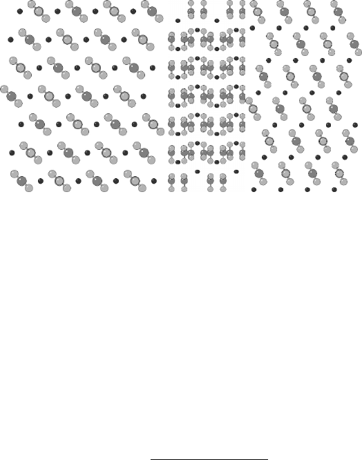
Figure 1.2: The examples of the three types of surface illustrated using polymorphs

of calcium carbonate; (a) type I (b) type II and (c) type III. The type I and III

surfaces illustrated are from the crystal structure of calcite, which due to its high

symmetry has no type II surfaces present. The type II example is from aragonite.

(a) Type I (b) Type II (c) Type III

manipulated, if necessary. Once the desired surface structure has been generated,

then the necessary GULP calculation can be performed.

1.4.17.1 Surface energy

The thermodynamic penalty for cleaving a surface from a bulk material is measured

according to the surface energy. Given a bulk energy of Ubulk and an energy for the

same system with a surface created of Usur f ace, then the surface energy, ∆USE , is

deﬁned as an intensive quantity according to:

∆USE =Usur f ace −Ubulk

where Ais the resulting surface area. By deﬁnition, for any stable material the sur-

face energy will be endothermic. A calculated negative surface energy implies that

a material should dissociate, i.e. the crystal should disperse into the surrounding

medium.

There are two practical approaches that are widely used to determine the surface

energy by computational means. In the ﬁrst, a two-dimensional slab of material is

created from the bulk, thus creating two surfaces overall. This method has the ad-

vantage that it can be used within programs that only allow for three-dimensional

boundary conditions through the introduction of a sufﬁcently large vacuum gap

between the images, such that the surfaces don’t interact across the vacuum. In

addition, it becomes necessary to assess whether the slab is also thick enough since

the properties must converge to those of the bulk at the centre of the slab. In the

second method, a single surface is created by employing a two region strategy, as

shown in Figure 1.3. Here the solid is divided into region 1, which contains the sur-

face and all layers of atoms below it that exhibit a signiﬁcant atomic relaxation, and

region 2, which contains the rest of the bulk material where it is assumed that no

displacements from the three-dimensional crystal structure are induced. In practice,

only the atoms of region 2 that have an interaction with region 1 need be explicitly

considered, and so the depth of region 2 is controlled by the cut-offs of the force-

ﬁeld and the Parry sum used for the electrostatics. This second method is the most

efﬁcient and precise for atomistic techniques. However, it is considerably harder

to extend to quantum mechanical methods since the electronic perturbations may

extend further into the bulk and embedding, typically via Green’s functions, is re-

quired to determine the inﬂuence of the electronic structure of region 2 on region

1. Through the GDIS interface, it is possible to automatically estimate the required

region 1 and 2 sizes needed to converge the surface energy (with a default toler-

ance of 0.001J/m2) based on the unrelaxed surface energies. However, if there

are strong relaxations of the surface, it may be necessary to further verify that the

relaxed surface energy is sufﬁciently converged.

The total energy for a surface calculation comprising two regions can be written

in terms of the interaction energies within, and between, the different regions:

Utot =U11 +U12 +U22

The energy of region 2 with itself, U22, is not particularly meaningful, since the re-

gion 2 is just a partial representation of the effectively inﬁnite bulk material below,

and any given particle within this region will not experience the full set of interac-

tions that it should. However, this term is just an additive constant that is unaltered

on energy minimisation, or any other displacement of region 1. Consequently it

can be ignored in calculations. In the two region model, the energy required to

determine the surface energy is given by:

Usur f ace =U11 +1

2U12

Note that while the above energy only includes half of the region 1-region 2 in-

teraction energy, the objective quantity for energy minimisation is the total energy,

which includes the full value of U12. This is because the energy change of region 2

must be allowed for when optimising.

1.4.17.2 Attachment energy

The surface energy, described above, provides a measure of the thermodynamic

stability of a cleavage plane. However, there is a widely used alternative criterion

which is the attachment energy. This is the energy associated with the addition of a

stoichiometric layer of material on to the surface cut:

Uattachment =Un+1

tot −Un

tot −U1

tot

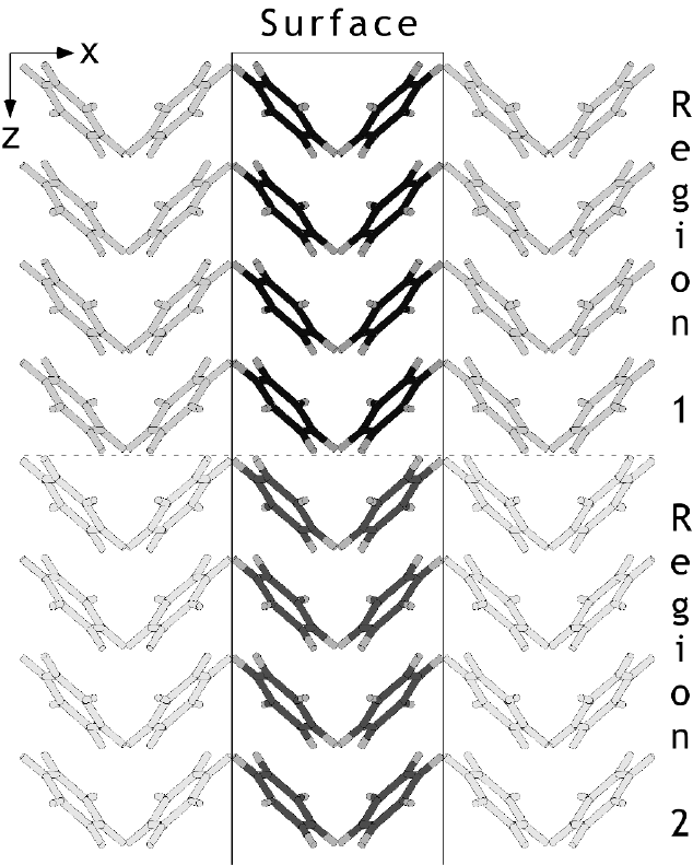
Figure 1.3: The two region surface simulation cell viewed at right angles to the

surface normal, where solid vertical lines denote the boundaries between two-

dimensional periodic images of the cell and the dash line indicates the boundary

between region 1 and the frozen region 2.

where Un

tot represents the total internal energy of a surface model consisting of n

growth layers, and U1

tot is the energy of the growth layer alone. For any stable

material, this implies that the attachment energy must be an exothermic quantity.

In practice, the calculation of the attachment energy is obtained from the energy of

interaction of the growth layer at the surface with the rest of the underlying material.

This beneﬁts from the fact that the attachment energy can be obtained from a single

calculation, just as is the case for the surface energy, rather than by performing the

actual addition of a layer as part of a multistage process.

Although the attachment energy is also a strictly thermodynamic quantity, it is

often regarded as representing the kinetics of crystal growth because of the concep-

tual link between the ease of the addition of a growth layer and the rate at which a

surface is added to. Consequently, those faces where the attachment energy is most

exothermic will tend to grow most rapidly.

1.4.17.3 Morphology

The morphology of a crystal is the macroscopic shape that it adopts. Because this

can be readily observed for nearly all materials, either under an electron micro-

scope or, in the case of many naturally occuring minerals, by visual inspection with

the naked eye, it should provide a ready means to test the validity of a simulation

model. Of course, the reality is rather more complex, since the morphology is sen-

sitive to the presence of impurities, the nature of the solvent used as the growth

medium, and many other factors relating to the sample preparation. Consequently

there are materials where many different morphologies can be observed for the same

compound. A classic example, is that of calcite (CaCO3), where there are both sev-

eral different polymorphs of the bulk material and several hundred different known

morphologies. Many of these variations result from biomineralisation by different

species. Despite this, for many pure inorganic materials morphological prediction

using atomistic techniques is surprisingly successful.

Crystal morphologies can be calculated based on either the surface energy or

attachment energy, which are typically taken to represent growth under conditions

of thermodynamic and kinetic control, respectively. In order to do this, it is ﬁrst

necessary to determine the objective quantity for all signiﬁcant faces. Given that

dipolar faces are usually unstable, the number of likely cleavage planes for most

materials is actually considerably smaller than initially might be conceived of based

on permutations of the Miller indices. Furthermore, where there is space group

symmetry present for the bulk, many surface planes are equivalent, thus reducing

the number of unique faces. Finally, only those faces with the largest interplanar

spacings are likely to appear in the morphology [109]. The actual morphology is

generated as a three-dimensional Wulff plot [110]. Here the ratio of the surface

normal distances of all planes from the centre of the polyhedron are determined

according to the either the surface or attachment energy. The ﬁnal shape of the

polyhedron is then determined by the intersection of the cleavage planes. Unstable

surfaces lie outside the polyhedron and never intersect. Morphological plots can

also be produced through the GDIS interface to GULP.

In the equilibrium morphology approach, the contribution of a given plane to

the total surface area is inversely proportional to its surface energy [111]. For the

growth morphology methodology [112], the surface area contribution is again in-

versely proportional, but now to the negative of the attachment energy. This is

because surfaces with a highly exothermic attachment energy will rapidly grow out

of the morphology to leave the slow growing bounding faces.

1.4.17.4 Surface phonons

The calculation of the phonons of a 2-D slab is exactly analogous to that for the

three dimensional case, except that the Brillouin zone is also now two dimensional

leading to dispersion only in the xy-plane (taking zto be the direction of the surface

normal).

Turning to consider the standard two region surface model, there are some im-

portant issues to consider. Because region 2 is quasi-inﬁnite, it is only possible to

determine the phonons for the particles in region 1. Therefore, the dynamical ma-

trix is constructed based on region 1 alone, but with contributions to the on-diagonal

matrix blocks from the potential experienced due to a rigid, non-vibrating region 2.

Consequently it is assumed that the vibrations of the two regions are completely

decoupled. Since this is an approximation, the frequencies near the interface of

the regions will be slightly in error, particularly in the low frequency regime where

coupling is generally strongest. However, the surface modes, which are usually the

ones of primary interest, will be less affected. As always, it is essential to monitor

the convergence of all quantities with respect to increasing the region 1 depth. Fi-

nally, because region 1 is vibrating under the inﬂuence of an external potential, the

ﬁrst three frequencies at the Γ-point will no longer be zero, though they typically

will be small.

1.4.18 Continuum solvation of surfaces

In the above description of surface properties the surface is always assumed to be

in contact with vacuum. However, the properties of surfaces in contact with solvent

are equally as important. While the interface between a solid and liquid is most

accurately studied using molecular dynamics simulations, there are some situations

where more approximate methods are valuable. For example, to predict the solvent

dependent morphology of a crystal only requires the ratio of the surface energies

to be correct and not the absolute magnitude. To perform molecular dynamics to

extract the relative free energies of solvation for a large collection of surface is very

challenging and time consuming. Here the use of a more approximate approach is

valuable.

In GULP the option to employ a continuum solvation model has been added.

Here the solvent accessible surface is described using a grid of points and the re-

sponse of the solvent due to its dielectric properties calculated at this surface in

response to the electrostatic potential of the solid. Full details of the method im-

plemented in GULP can be found in the literature [113]. In brief, the method uses

the COnductor-like Screening MOdel (COSMO) of Klamt and Schuurmann [114],

but with a few modiﬁcations. The solvent accessible surface (SAS) is smoothed by

use of tapering functions, and octahedral triangulation is used to generate the points

in order to maximise symmetry. Furthermore, the frame of a molecule (if applied

in 0-D) is rotated according to the eigenvectors of the moment of inertia tensor

in order to ensure rotational invariance. The ﬁnal change is more signiﬁcant; be-

cause the induced charge on the solvent accessible surface is unconstrained the total

charge of a surface and solvent could be non-zero (and non-integer). When work-

ing within periodic boundary conditions it is essential to maintain charge-neutrality

such that a convergent electrostatic energy can be obtained. To do this GULP uses

the COSMO method under the constrain of Integer Charge (COSMIC) to ensure

that the electrostatics remain valid.

The current implement of the COSMIC continuum solvation model can be ap-

plied to surfaces, polymers, solids and molecules. Both analytic ﬁrst and second

derivatives are available, though phonons can only be evaluated at the gamma point

at present.

1.4.19 Free energy minimisation

One of the most important issues in solid state modelling is the variation of ma-

terials properties with the applied conditions. While isotropic external pressure is

trivial to incorporate, as has already been shown, inclusion of the effect of temper-

ature is more complex. This process is exacerbated by the fact that the majority of

potentials have been derived through the use of some empirical (i.e. experimental)

data which has been measured under a given set of conditions. Hence the force-

ﬁeld itself can often already contain an implicit temperature, or worse, if multiple

pieces of experimental data have been employed that were measured at different

conditions, it can be a convolution of several temperatures. One solution to this is

to extract forceﬁelds from quantum mechanical methods so that everything is ob-

tained explicitly at absolute zero. For now, we will assume that the forceﬁeld has

been derived so as to be free of implicit temperature effects, by whatever means.

There are several distinct approaches to the inclusion of temperature into simu-

lations. Which one is most appropriate depends on the particular temperature and

nature of the system. In the low temperature regime, the atoms of the crystal struc-

ture just execute vibrations about their lattice sites, which in the limit of absolute

zero will be purely harmonic. This situation is best described through the use of

lattice dynamics, which is the quasi-static approach to treating a vibrating lattice.

As the temperature increases, the motions will become increasingly anharmonic.

In principle, this can be handled, to a point, through the use of anharmonic correc-

tions to the harmonic lattice dynamics, in order to allow for weak phonon-phonon

coupling. However, when the temperature becomes sufﬁciently high that diffusion

can occur it is necessary to switch to an alternative approach. Typically one of two

approaches can then be employed. If detailed information is required concerning

the atomic motions and related properties, then the method of choice is molecular

dynamics [115]. This propagates Newton’s equations of motion through time using

a ﬁnite difference formalism. Hence it retains time correlation functions and the

trajectories of all atoms. Its strength is that anharmonic effects are fully included.

However, since it regards nuclei as classical particles, it is invalid at low temper-

atures due to the neglect of the quantisation of vibration and zero point motion,

unless the Path-Integral formalism is employed. It can be seen therefore that lattice

dynamics and molecular dynamics are largely complementary in their regions of

applicability. Although GULP also includes the capability to perform molecular

dynamics, this topic will not be discussed here since this area, in regard to other

codes, has been discussed elsewhere [16], and the more unique, static, features

will be focussed on here. Likewise, the effect of temperature can also be explored

through Monte Carlo simulation [87], if the focus is integration over phase space,

with no regard to timescale or kinetic factors, but this topic will not be discussed

further because it is not one of the more novel features of GULP.

Concentrating now on the use of lattice dynamics for examining the temper-

ature dependance of crystal properties, the dominant effect is the change in the

crystal structure. When heated, most materials undergo thermal expansion which

correspondingly leads to softening of many of the mechanical properties. There are

a few celebrated examples of materials that actually contract on heating, through

the rotation of quasi-rigid polyhedra, which is technologically very important in the

quest for zero thermal expansion composites.

It has already been shown that it is possible to calculate the Helmholtz free en-

ergy for a given structure as a function of temperature through the determination of

the vibrational partition function from the phonon density of states. Hence, a nat-

ural approach to determine the dependance of structure on temperature is through

free energy minimisation. Here the key foundation is the quasi-harmonic approxi-

mation, which assumes that the vibrational frequencies can be determined as if the

atoms are vibrating purely harmonically while the cell parameters are adjusted to

minimise the free energy. Previous studies have indicated that this is a reasonable

approximation until a temperature of approximately half the melting point has been

reached.

The major barrier to free energy minimisation is that we have already seen that

efﬁcient optimisation requires at least the ﬁrst derivatives of the quantity with re-

spect to the structural variables. Hence a number of approaches evolved for tackling

this problem. LeSar et al [116] developed a method whereby the atoms where rep-

resented as Gaussian distributions, whose width represented the vibrational motion.

The Gaussian exponent was then regarded as a variational parameter that minimised

the free energy. Hence the free energy could be obtained without direct recourse

to a phonon density of states, making derivatives straight forward. While this ap-

proach is easy to apply to metals, the extension to a more complex ionic systems

is more demanding. A method that approximated the phonon density of states was

introduced by Sutton [117], which involved taking moments of the dynamical ma-

trix, as pioneered by Montroll [118] several decades earlier, and in the spirit of tight

binding theory. This approach has the advantage that the derivatives are taken of

the dynamical matrix elements, rather than of phonon frequencies, which are the

product of a matrix diagonalisation.

In the ﬁeld of ionic materials, Parker and Price [8] pioneered the use of free

energy minimisation through the use of numerical derivatives. Here central ﬁnite

differences were taken with respect to the cell strains, with the internal degrees of

freedom being formally optimised at every point. This approach had the advantage

over the other methods that no approximation was being introduced beyond the

quasiharmonic one. However, because this requires (2N+1)optimisations and

phonon evaluations per energy/gradient evaluation with respect to the free energy,

the minimisation was restricted to the strains alone in order to reduce the number

of variables, N, to a maximum of six.

More recently, Kantorovich [119] has derived expressions for the analytical

derivatives of the free energy, which were implemented contemporaneously in the

program SHELL of Allan and co-workers [120], and in GULP [121]. If we consider

the differential with respect to strain, though the expressions would be identical for

any degree of freedom, then the ﬁrst derivative of the free energy is given by:

∂A

∂ ε =∂Ustatic

∂ ε +∑

∑

m





2ω



2+1

exphω

kBT−1

∂ ω2

∂ ε 





where the expression is written in terms of the derivatives of the square of the

frequencies, since these values represent the eigenvalues of the dynamical matrix.

Their derivatives can be calculated through the application of perturbation theory

and expressed as the derivatives of the dynamical matrix projected onto the corre-

sponding eigenvectors:

∂ ω (k,m)2

∂ ε !=e∗

m(k)∂D(k)

∂ ε em(k)

In order to determine the derivatives of the phonon frequencies, we therefore require

the phased third derivatives of the energy with respect to either three Cartesian

coordinates, or two Cartesian coordinates and one strain. for internal and external

variables, respectively.

For the most efﬁcient optimisers, based on Newton-Raphson techniques, we

strictly need the second derivatives with respect to the free energy, which corre-

sponds to the fourth derivatives of the internal energy. However, this is considerably

more expensive and complex, so the Hessian matrix is usually approximated by the

conventional internal energy Hessian by assuming that the free energy contribution

to the curvature is small. Furthermore, the use of updating formulae will ultimately

correct for the discrepancy given sufﬁcient optimisation steps.

With the advent of analytical derivatives, it is now possible to consider two types

of free energy minimisation. The ﬁrst has been christened the Zero Static Internal

Stress Approximation (ZSISA) by Allan and co-workers [122], which resembles the

approach taken with numerical ﬁrst derivatives (i.e. the unit cell is minimised with

respect to the free energy, while maintaining the internal degrees of freedom at a

minimum with respect to the internal energy). When working within this formalism

there is an additional contribution to the strain derivatives, which corrects for the

fact that internal degrees of freedom are not at a minimum with respect to the free

energy:

∂A

∂ ε ZSISA

=∂A

∂ ε −∂2A

∂ ε∂ α  ∂2A

∂ α∂ β −1∂A

∂ β 

Here the approximation is again made that the second derivative matrices can be

approximated by neglecting the free energy contribution; an approximation that

should be enhanced by the cancelation that results from taking a ratio. The second

type of optimisation can be called full free energy minimisation (FFEM), in which

the internal degrees of freedom are also minimised with respect to the free energy.

This is potentially appealing since sometimes it is the details of the internal changes

that might be of interest, for example, the nature of an adsorption complex within a

microporous material.

Results for silicate materials show a number of interesting features regarding

the merits of both approaches. Firstly, in the case of α-quartz where accurate ex-

perimental data is available for comparison, it appears that the ZSISA approach

underestimates the thermal expansion, while the FFEM method is more accurate,

though of course this is subject to the limitations of the speciﬁc potential model cho-

sen [121]. However, for all silicates tried so far the full minimisation approach goes

catasrophically wrong at about ambient conditions. This is illustrative of a general

problem with this approach which tends to drive systems to instability. This can

be readily understood, since the free energy is minimised by creating phonons that

tend to zero frequency and hence the structure is motivated to create soft modes.

This behaviour does not tend to happen in the ZSISA approach where only the cell

strains are directly coupled to the free energy and thus the relaxations tend to lead

only to a scaling of modes, rather than more individual changes. Hence the use of

ZSISA is far more robust and generally recommended for most purposes.

1.4.20 Monte Carlo

An alternative approach to including temperature into results, if one is not inter-

ested in the time correlation properties, just the ensemble averages, is Monte Carlo

simulation. Here the distribution of positions according to a Boltzmann distribu-

tion is determined numerically for a speciﬁed temperature and conditions. Under

the Metropolis importance sampling scheme, if a randomly chosen move for the

system leads to a lowering in the energy then the move is accepted and the system

evolves to the new state. If the energy increases, then the move is accepted with a

probability given by:

P=exp−∆U

kBT

where ∆Uis the energy change associated with the move. There are several types

of move available for a system as listed below:

•Translation - this allows atoms or molecules to move in x, y or z, according

to the ﬂags set

•Rotation - for rigid molecules, this allows the molecule to sample the rota-

tional distribution

•Creation/destruction - in the Grand Canonical ensemble, molecules can be

inserted or removed to a reservoir of molecules whose chemical potential is

speciﬁed

Note that the Monte Carlo feature is relatively new and should be considered as a

beta release available to those who wish to test.

1.4.21 Defect calculations

While the simulation of bulk material properties is important, just as crucial is the

study of both intrinsic and extrinsic defects. Many of the key applications of solid

state systems, such as catalysis, electronic and ionic conductivity, ion exchange and

waste immobilisation, critically depend on the utlisation of the characteristics of de-

fect centres. Consequently, from the early days of the ﬁeld of atomistic simulation

defect studied have been one of the most vigorously pursued topics.

There are two widely used approaches for performing defect calculations on

solids; the supercell and the cluster methods, with or without embedding in the

latter case. Both approaches have their merits and demerits. Putting computational

implementation factors aside, the use of embedded clusters is ideal for the inﬁnitely

dilute limit, while the supercell method is more appropriate for high concentrations

of defects where there exists signiﬁcant defect-defect interaction. In practice, the

nature of the computational method often biases the method of choice. However,

with atomistic techniques both approaches are feasible. Since the supercell method

is simply the extension of a bulk calculation, we will focus here on the embedded

cluster approach. In this particular context, the technique is generally referred to

as the Mott-Littleton method [123], after the authors of the pioneering work in the

ﬁeld, though the implementational details differ a little from their original work.

The basis of the Mott-Littleton method is the so-called two region strategy. Here

a point called the defect centre is deﬁned, which typically lies at a point concentric

with the initial defect site, or, where there is more than one defect, at the mid-

point of the ensemble of point defects. The crystal around the defect centre is

divided into two spherical regions, with the inner sphere being labelled region 1,

and the outer spherical shell of ions being region 2a. Atoms outside of these spheres

belong to region 2b, which then extends to inﬁnity. The dimensions of these regions

are typically speciﬁed either by their radii or the number of ions contained within

them. The ions in region 1 are assumed to be strongly perturbed by the defect

and therefore are relaxed explicitly with respect to their Cartesian coordinates. In

contrast, the ions in region 2 are assumed to be weakly perturbed and therefore

their displacements, with the associated energy of relaxation, can be approximated

in some way. Clearly, as the region 1 radius is increased these approximations will

become increasingly valid, and thus an important stage of a defect calculation is

to ensure that the defect energy is sufﬁciently converged with respect to the region

radii. In some cases the convergence of the absolute defect energy can be slow, in

which case it may be sufﬁcent to monitor the convergence of relative defect energies

instead. As a guideline, the radius of region 1 and the difference of the radii of

regions 1 and 2 should be both be greater than the short-range potential cut-off to

achieve convergence, though for charged defects this may not be adequate.

Within the Mott-Littleton scheme, we can express the total energy of the two

region system as the sum of contributions from the energies within the regions and

between them:

Utot (x,ξ) = U11 (x) +U12 (x,ξ) +U22 (ξ)

where U11 (x)represents the energy of region 1 as a function of the Cartesian coor-

dinates, x,U22 (ξ)represents the energy of region 2 as a function of the Cartesian

displacements, ξ, and U12 (x,ξ)is the energy of interaction between the two re-

gions. At this stage we do not distinguish between regions 2a and 2b. If the forces

acting on region 2 are small, then we can assume that the response of the atoms in

this region will be purely harmonic. Hence, the energy of region 2 can be written

as:

U22 (ξ) = 1

2ξTH22ξ

where H22 is the Hessian matrix for region 2. If we now apply the condition that the

displacements in region 2 will be the equilibrium values this yields the following

condition: ∂Utot (x,ξ)

∂ ξ x

=∂U12 (x,ξ)

∂ ξ x

+H22ξ=0

Combining this equation, and the previous one, it is possible to eliminate the energy

of region 2 from the total energy without direct recourse to the Hessian matrix

(which would be of inﬁnite dimension):

Utot (x,ξ) = U11 (x) +U12 (x,ξ)−1

2∂U12 (x,ξ)

∂ ξ x

Thus the problem of calculating the energy of region 1 in the potential of region 2

has been reduced to evaluating the energy of region 1 and its interaction with region

2, without having to evaluate the self energy of region 2. Furthermore, in order to

lead to partial cancellation of terms, the quantity calculated is the defect energy -

i.e. the difference between the energy of the perfect region 1 and 2, Up

tot , and the

defective case, Ud

tot , rather than the individual contributions:

Ude f ect (x,ξ) = Ud

tot (x,ξ)−Up

tot (x,ξ)

It should be noted that it is assumed that the energy of any species removed or

added during the formation of the defect has an energy of zero at inﬁnite separation.

If this is not the case, then the defect energy must be corrected a posteriori for

this. However, such corrections have no inﬂuence on the outcome of the defect

calculation itself.

There is one important consequence of the above formulation of the total de-

fect energy, in that it becomes necessary to ﬁnd the optimised energy with respect

to the Cartesian coordinates of region 1 by force balance, rather than by energy

minimisation. The point at which the forces tend to zero is usually only slightly

different from the minimum in the internal energy, depending on the degree of per-

turbation of region 2. Hence, during an optimisation of the defect energy GULP

initially minimises the energy, as per a conventional Newton-Raphson procedure.

Once the gradient norm falls below a speciﬁed tolerance, and region 1 lies within

the harmonic region, then the harmonic displacements according to the Hessian and

gradients are applied without the use of a line search until the forces drop below the

speciﬁed tolerance.

A further important point relates to the state of the bulk crystal when performing

defect calculations. Because of the use of displacements in region 2, it is crucial

that the bulk structure is at an energy minimium with respect to the internal co-

ordinates before performing a defect calculation. Hence the bulk crystal must be

relaxed to equilibrium at least at constant volume, if not at constant pressure. Fur-

thermore, it is also important that there are no imaginary phonon modes within the

Brillouin zone otherwise the displacements in region 2 may correspond to unsta-

ble harmonic equilibrium. The presence of such modes is the most common cause

of unphysical results, for instance obtaining negative defect energies for intrinsic

defects. Because the presence of defects lowers the symmetry, a Mott-Littleton

calculation may encounter instabilities not apparent for the bulk material.

Now it is necessary to consider the treatment of region 2 in more detail, and

in particular the difference between regions 2a and 2b. In region 2a, the forces on

the individual ions due to short-range interatomic potentials and the Coulomb term

are explicitly calculated and the local displacement evaluated. While the forces on

region 2a are technically due to all ions in region 1, a commonly used approximation

is to evaluate the forces due to defect species only. This is the approach taken in the

default calculation method for compatability with earlier results.

In contrast to the above situation for region 2a, for region 2b the energy of

relaxation must be determined implicitly since this region extends to inﬁnity. It is

assumed that in region 2b the only force acting is that due to the Coulomb potential

in order to simplify the problem. By choosing the radius of region 2a to always

be greater than that of region 1 by the short-range potential cut-off this can always

be arranged to be valid. Even having retained only the Coulomb interaction in

the perturbation of region 2b, this still leaves many interactions to consider. To

simplify the problem, the electrostatic potential due to defects in region 1 can be

represented by the multipole moments of the deformation situated at the defect

centre. If region 2a is sufﬁciently large, then the only signiﬁcant term will be the

monopole moment of the defect (i.e. the net charge). Hence, the energy of region

2b is evaluated as the induced relaxation energy due to the net charge of the defect

situated at the speciﬁed defect centre. While this is a signiﬁcant approximation, it

usually works well in practice and again becomes valid with increasing region sizes.

In the original Mott-Littleton method, the interaction with region 2b was described

by a continuum approximation. However, in subsequent implementations a sum of

the induced polarisation energy is performed over the atomic sites. For the general

case of an anisotropic dielectric constant tensor [124], the energy of region 2b is

calculated as:

U2b=−1

2Q2 ∑

i∈2b

∑

αβ

Mαβ

irα

cirβ

ci !

where Qis the net charge of the defect, rci is the distance of the ith atom from the

defect centre, and Mαβ

iis a 3 x 3 matrix for each atomic site, in the Cartesian frame,

that represents the on-site polarisability. The quantitative deﬁnition of the matrix

elements Mαβ

iis [4]:

Mαβ

i=∑

γD−1αγ qiε−1γβ

where D−1

irepresents the on-diagonal block of a modiﬁed inverse second derivative

matrix and εis the static dielectric constant tensor. Note that the inverse of the

second derivative matrix is singular and therefore a further approximation must

be made. Physically, this problem corresponds to the division of the polarisation

between the sublattices being arbitrary. The usual solution taken is to assume that

the polarisation is divided equally between the cation and anion sublattices, with

the second derivative matrix being modiﬁed correspondingly. In the special case of

a cubic crystal, the expression for the region 2b energy can be simpliﬁed to:

U2b=−1

2Q2 ∑

i∈2b

ci !

where miis the average of the diagonal elements of the matrix M(for the cubic case

these will all be equal, but if the isotropic formula were to be applied in a non-cubic

case this would not be so).

Because the expression for the region 2b energy is not particularly short-ranged,

it is appropriate to evaluate it using lattice summation techniques analogous to those

applied to the monopole-monopole term. Hence the term is summed to convergence

based on a perfect inﬁnite lattice and then the contributions from ions in regions 1

and 2a are subtracted off. The distance dependent factor within the expression for

the energy can be rewritten as:

rαrβ

r6=1

8



∂21

r4

∂rα∂rβ

+δαβ

41

r4

Hence, by evaluating the equivalent of the Ewald summation for the inverse fourth

power of distance, and its second derivatives with respect to Cartesian displace-

ments, it is possible to achieve a rapidly convergent expression for the energy of

region 2b.

Having described how defect energies are calculated in theory, we mention a

few practical points. There are three types of defect that can be speciﬁed within

GULP:

•Vacancy

•Interstitial

•Impurity

The last one of these three is clearly the combination of a vacancy and an intersti-

tial at the same atomic position in the structure. The location of a vacancy or an

impurity can be speciﬁed by reference to either a spatial position or an atom po-

sition by referencing the site. An interstitial, by its very nature, must be speciﬁed

by coordinates. When an atom is designated to be vacant, then both the core and

shell will be removed automatically since it would not be sensible to leave one or

the other present in the system. It is also possible to specify that a whole molecule

be removed from the system, when the connectivity has been deﬁned.

Most types of calculation, that are logically applicable, can also be applied to

defect runs, such as optimisation to a minimum or a transition state. In the case of

vibrations, the frequencies are calculated for a dynamical matrix based on region

1. In must be noted that this is a large approximation, since any modes that are

coupled between regions 1 and 2 will not be properly described. Only localised

modes relating to atoms near the centre of region 1 will be correctly predicted.

Consequently such calculations of vibrations must be interpreted cautiously.

Finally, a degree of point group symmetry may be utilised during defect calcu-

lations. An automatic search for common symmetry elements is performed about

the defect centre, including mirror planes and C2axes that are aligned with, or be-

tween, the Cartesian axes. Such symmetry is used to reduce the number of region

1 and region 2 atoms stored, thereby reducing the number of degrees of freedom

for optimisation, as well as taking advantage of symmetry adapted algorithms to

accelerate the calculation of the energy and its derivatives.

1.4.22 Derivation of interatomic potentials

One of the major challenges facing anyone wishing to use forceﬁeld methods is to

determine the functional form and parameters required to calculate the energy and

properties. In the ﬁeld of organic chemistry and biomolecules, there are a number

of well-established forceﬁelds, such as MM3 [125], and those associated with the

programs AMBER [14], and CHARMM [15], which are, in principle, capable of

handling most elements typically found in these systems (C, H, O, N, S, P, etc)

in their common hybridisation states. These are constructed around the molecular

mechanics approach where the forceﬁeld is connectivity driven and interactions are

described in terms of two-, three-, and four-body bonding terms, plus long-range

Coulomb and non-bonded interactions. While there have been several attempts to

generate general forceﬁelds that cover the entire periodic table, such as UFF [126],

ESFF [127], etc, none have been completely successful. Because of the enormity

of the amount of data required when spanning the whole range of elements, it is

impractical to determine such a universal forceﬁeld by empirical ﬁtting. Instead

general rules must be used to predict parameters based on extrapolations and intrin-

sic properties of the element that are known - for instance the electronegativity. Not

surprisingly, this leads to limitations in the quality of the results. For most inor-

ganic systems it is usually necessary to derive a forceﬁeld for the speciﬁc material,

or family of materials, of interest.

There are two means by which a forceﬁeld can generally be derived, if we ex-

clude rule based extrapolations. Firstly, it is possible to obtain parameters by ﬁtting

to a potential energy surface obtained from a non-empirical theoretical method.

This would typically consist of results from ab initio calculations, ideally on the

periodic solid [128], or perhaps on a gas phase cluster, or even better, both of the

aforementioned sources. The potential energy surface can be ﬁtted either as a se-

quence of geometries with their corresponding energies, or derivatives of the energy

could also be included to maximise the amount of information from each higher

level calculation. Many of the early forceﬁelds for ionic materials were determined

using electron gas methods [129], in which the energies of interaction between pairs

of ions were determined by a density functional calculation using the overlapping

ionic electron densities, where the anion is conﬁned in an appropriate potential well.

Secondly, parameters can be obtained by empirical ﬁtting in which the normal pro-

cess of using a forceﬁeld to determine the properties of a material is inverted. This

approach depends on the availability of a range of experimental data. Knowledge

of the crystal structure is a deﬁnite prerequisite for this method, but is insufﬁcient

alone since information is required as to the curvature of the energy surface about

the minimum. This later data may come from quantities such as elastic constants,

bulk moduli, piezoelectric constants, dielectric constants, or phonon frequencies.

In order to perform a ﬁt, ﬁrst it is necessary to deﬁne a quantity that measures

the quality of the results, known as the sum of squares;

Nobs

∑

i=1

wifobs

i−fcalc

i2

where Nobs is the number of observables, fobs

iand fcalc

iare the ﬁtted and calculated

values of the observable, respectively, and wiis the weighting factor for the given

observable. Because of the weighting factor, there are an inﬁnite number of possible

solutions all of which are equally valid. Hence, one of the most important skills

is knowing how to choose appropriate and sensible weighting factors. There are

several criteria that can be used for guidance though. Firstly, if ﬁtting experimental

data, the weighting factor should be inversely proportional to the uncertainty in the

measured value. Obviously trusted, precise values should be given more priority

than data where there are large error bars. Secondly, the weight factor should be

inversely proportional to the magnitude of the observable squared. This ensures

that all values are ﬁtted on an equal footing, regardless of units. For example,

ﬁtted vibrational frequencies in wavenumbers are typically two to three orders of

magnitude larger than structural variables.

The ﬁtting process itself involves minimising the above function F. To do this,

the default approach is similar to that used in optimisation. For many terms, the

evaluation of the derivatives of the sum of squares with respect to the variables is

complex, and in some of the ﬁtting algorithms that will be discussed subsequently

it is even impossible. As a result, numerical derivatives are employed during ﬁtting

since it greatly simpliﬁes the process. Because of this, the default optimiser is to

use a BFGS update of an initial on-diagonal only Hessian, obtained by ﬁnite dif-

ferences, in a Newton-Raphson process. However, for particularly difﬁcult cases,

where correlation between variables is strong, there is the option to use a full Hes-

sian matrix, again obtained by ﬁnite differences.

Now we turn to speciﬁcally consider the ﬁtting methodology for the case of

empirical data. Traditionally, the experimental structure is ﬁtted by varying the po-

tential parameters so as to minimise the forces at this conﬁguration, and this is the

default strategy. Other observables, such as elastic constants etc, are then calcu-

lated at the experimental structure too. When working with the shell model, either

dipole or breathing shell, there is an additional complication though in that while

the cores are fully speciﬁed since they are equated with the nuclei of the ions, the

positions/radii of the shells are undeﬁned. One approach is to ﬁt with the shells po-

sitioned to be concentric with the cores. However, this is unphysical since it implies

that there is no ionic polarisation, which defeats the object of including the model

in the ﬁrst place. A second approach might be to place the shell according to spec-

iﬁed ion dipoles, but this information is almost impossible to come by. Only data

about the total polarisation of the unit cell is typically available and a unique atomic

decomposition is not possible. In order to handle this issue, the simultaneous re-

laxation of shells approach was introduced into GULP [130]. Here the shells are

allowed to move during ﬁtting. Formally, the most correct approach is to allow the

shells to be energy minimised at every evaluation of the ﬁtting function. However,

a simpler approach has been implemented in which the shell forces are added as ob-

servables and the shell positions become ﬁtting variables. In this way, the shells are

minimised directly within the ﬁtting procedure. In the absence of any observables

other than the structure, this is exactly equivalent to minimising the shells at every

step of ﬁtting. When observables are present there will be small differences, but

these are usually an acceptable price to pay for the greater ease of implementation.

There is actually a more fundamental ﬂaw with the approach of ﬁtting forces at

the experimental geometry as a method of ﬁtting. Often we judge the quality of a ﬁt

by the percentage error in the structural variables rather than the forces. Although

lowering the forces during a ﬁt generally improves the optimised structure with

respect to experiment, this is not guaranteed to be the case (and indeed we have

found examples where it is not). This can be understood by making a harmonic

estimate of the atomic displacements, x, based on the forces, f:

x=H−1f

It can be readily seen that the magnitude of the displacements also depends on the

inverse of the Hessian matrix. Thus if the forces improve, but the description of

the curvature about the minimum deteriorates, then the errors can potentially in-

crease. If curvature information is included in the ﬁt, then this can tend to reduce

this problem. However, there is a further difﬁculty here. Formally speaking, the ex-

pressions for the elastic constants and other properties are deﬁned about a position

of zero stress and zero internal derivative. Therefore, calculating the properties at

the experimental structure when the forces are non-zero leads to errors also. The

solution to both of these dilemas is to use the so-called relax ﬁtting methodology

[130] in which the structure is fully optimised at every evaluation of the ﬁtting func-

tion and the properties calculated at the optimised conﬁguration. Obviously this is

a far more expensive procedure, but does yield the most reliable results. Also there

is the requirement that the initial potential set is reasonable enough to actually give

a valid minimisation of the structure.

Having obtained an apparently successful ﬁt, it is important to assess the qual-

ity of the results, since there are plenty of pitfalls and so convergence shouldn’t be

taken to represent a good quality solution. Firstly, the potential model should be

tested for all reasonable properties, not just those used in the ﬁt. It could easily be

the case that a forceﬁeld reproduces a high symmetry structure and, say, a single

curvature observable, such as the bulk modulus. However, examination of the full

elastic constant tensor, dielectric properties and phonons might reveal that the sys-

tem is unstable with respect to a lowering of symmetry which wouldn’t show up in

the ﬁt. Secondly, the forceﬁeld could be transferred to a different material, not used

in the original ﬁt, to test whether the results are sensible. Finally, it is important to

look at the potential parameters and assess whether the numbers are physically sen-

sible. For instance, it is not uncommon for dispersion terms to become extremely

large if allowed to ﬁt unconstrained. While this might have improved the sum of

squares for one particular system, it means all hope of transferability has been lost.

Similarly, there can often be problems with ﬁtting Aand ρof a Buckingham poten-

tial concurrently due to the strong correlation coefﬁcent between the parameters.

The focus above has been primarily on empirical derivation of interatomic po-

tentials. However, with the increasing ability to perform periodic ab initio calcula-

tions on solids an attractive alternative is to derive forceﬁelds that attempt to repro-

duce the results of such methods. There are several reasons to take this approach.

Firstly, by ﬁtting the outcomes of a single Hamiltonian it is possible to guarantee

that the training set is fully consistent (i.e. there are no differences in temperature,

pressure, sample quality, or variable uncertainities in the observables). Secondly,

data can be obtained for materials were no experimental information exists or at ge-

ometries that are signiﬁcantly perturbed from the equilibrium one. Thirdly, the data

from quantum mechanical methods is free of statistical mechanical effects, such

as thermal vibrations and zero point motion. Hence, if the aim is to perform free

energy minimisation then the interatomic potentials will represent a proper starting

point for the inclusion of these quantities.

Fitting of quantum mechanical data can be performed in one of two ways, either

by proceeding in the same fashion as for empirical derivation, or by use of an energy

hypersurface. In the latter case, this is achieved by specifying a series of structures

with their corresponding energies, and optionally ﬁrst derivatives. Typically the

structures would include the equilibrium conﬁguration and as many distinct dis-

tortions about this point in order to probe as many different interatomic distances

between atoms as possible. Perhaps the most difﬁcult decision is how to weight

the conﬁgurations. Unless the forceﬁeld is able to reproduce the ab initio data

very accurately, then it is usually desirable to weight the ﬁt in favour of conﬁgura-

tions nearer the equilibrium structure. One approach that has been taken is to use a

Boltzmann factor weighting based on the energy difference to the minimum energy

conﬁguration, with an appropriate choice of temperature to the task ultimately to be

performed [131]. However, there are many other possible choices too. A further is-

sue concerns the ﬁtting of quantum mechanical energies. Unless these values have

been converted to a binding or lattice energy with reference to the dissociated state

of the species within the system then it is inappropriate to ﬁt the absolute values

of the energies. Consequently, the easiest solution is to include an additive energy

shift parameter in the ﬁt, such that only relative energies are actually ﬁtted.

Finally, the option exists within GULP to perform ﬁtting using genetic algo-

rithms as well as via least squares techniques. This may be potentially useful in

cases where a complex system is being ﬁtted when there is no reasonable starting

approximation to the forceﬁeld available or where there may be multiple local min-

ima in the parameter space. However, to date we have yet to encounter a situation

where this approach has proved beneﬁcial over the more conventional methodology.

This emphasizes that there is no substitute for making physically sensible choices

for the functional form of the forceﬁeld and the initial parameters.

1.4.23 Calculation of derivatives

In order to be able to optimise structures efﬁciently and to calculate many proper-

ties requires the availability of derivatives. While ﬁnite difference methods can be

used to determine these, this is both inefﬁcient and inaccurate for forceﬁelds, since

numerical errors can cause problems, especially when potentials do not go exactly

to zero at the cut-off distance. Consequently all derivatives are determined ana-

lytically in GULP. All functional forms for the energy have up to analytic second

derivatives available, while two-, three- and four-body interactions include third

derivatives. In addition, analytic third derivatives can be calculated for the embed-

ded atom method, but currently not for any other many-body potential functions.

Because the determination of derivatives is central to many quantities, a brief

description of the approach to their calculation is given here, while fuller details can

be found in both the original Harwell Report [132], and the subsequent publication

of many of these details[133]. Ultimately two types of derivative are required -

those with respect to atomic degrees of freedom and those with respect to the unit

cell. In GULP, all atomic coordinate derivatives are calculated in the Cartesian

frame of reference and then transformed to the fractional coordinate derivatives,

when appropriate to the periodicity. For the unit cell, strain derivatives are taken as

previously described.

Both the Cartesian and strain derivatives can be related to a set of pivotal quanti-

ties, which are the ﬁrst derivatives with respect to the interatomic distances, divided

by the distance:

∂U

∂ α =1

∂U

∂rα

∂U

∂ ε =1

∂U

∂rαβ

where, in the expression for the strain derivative, the components αand βare the

appropriate Cartesian directions for the given strain (e.g. ε4implies α=yand

β=z). It is implicit that all quantities are subscripted with i j to indicate that the

terms refer to a speciﬁc pairwise interaction. Let us introduce the shorthand:

U1=1

∂U

∂r

U2=1

∂

∂r1

∂U

∂r

U3=1

∂

∂r1

∂

∂r1

∂U

∂r

The second derivatives can then be obtained by differentiating the above expres-

sions once more and written as:

∂2U

∂ α∂ β =U2αβ +U1δαβ

∂2U

∂ α∂ ε =U2αβ γ +U1βδαγ +γδαβ 

∂2U

∂ εαβ ∂ εγζ

=U2αβ γζ +U1δαβ δγζ +1

4U1δαγ β ζ +δαζ βγ +δβ γ αζ +δβ ζ αγ

Likewise, the third derivatives can be obtained by further differentiation:

∂3U

∂ α∂ β ∂ γ =U3αβ γ +U2αδβ γ +β δαγ +γδαβ 

∂3U

∂ α∂ β ∂ εγζ

=U3αβ γζ +U2αγδβ ζ +ζ δβ γ +βγδαζ +ζ δαγ +γζ δαβ +U1δαγ δβ ζ +δαζ δβ γ 

Note that for free energy minimisation, which is were the third derivatives are re-

quired, only the derivatives with respect to two Cartesian coordinates and one strain,

or three Cartesian coordinates are needed.

In both three-body and four-body terms there exist derivatives with respect to

either a trignometric function of an angle, or the angle itself. These derivatives can

be converted into the above forms through the use of the cosine rule:

cos(θ) = r2

12 +r2

13 −r2

2r12r13

where θis the angle at the pivot atom 1, lying between the vectors r12 and r13.

Derviatives with respect to angles are therefore obtained through the expression:

∂ θ

∂r=−1

sin(θ)

∂cos(θ)

∂r

Care must be taken in handling the limit as θtends to either 0oor 180o.

1.4.24 Crystal symmetry

An important topic, particularly in the context of optimisation, is crystal symmetry.

For periodic crystals, there is the option to specify the solid via the asymmetric unit

atoms, the space group number/symbol, and the origin setting. It should be noted

that the use of space group symbols is preferable since it distinguishes between dif-

ferent settings of the same space group. Apart from the building of the full unit cell

from the asymmetric unit, the symmetry can be utilised to greatly accelerate the

structural optimisation through several different means. The ﬁrst beneﬁt of sym-

metry is that it lowers the number of independent geometric variables, since many

atomic coordinates are related via a roto-translation operation. Furthermore, the

existence of special positions implies that some coordinates are not allowed to vary,

typically for sites such as 1

2,1

2, and that in other cases coordinates are not inde-

pendent and must be related by constraints. Even larger reductions in scale can be

achieved by using unit cell centring to reduce the centred-cell down to the primitive

representation, thereby reducing the number of atoms by a factor or between 2 and

4. All of these factors reduce the number of variables, and since the rate of con-

vergence is usually correlated to the number of independent variables, depending

on the algorithm, this can lead to fewer optimisation steps being required. Further-

more, the amount of memory to store the Hessian matrix is reduced, as well as there

being a large improvement in the cost of inverting this matrix.

The second gain from the use of symmetry is that it is possible to use new algo-

rithms to calculate the energy and its derivatives that involve fewer computations,

provided the symmetry is high enough [134]. Considering a two-body potential

model, instead of looping over all possible pairs of atoms in order to compute the

energy, when symmetry is present it is sufﬁcient to only calculate the interactions

between the atoms of the asymmetric unit and all other atoms. For a system of

Nfatoms in the full unit cell and Naatoms in the asymmetric unit, then the execu-

tion times for the algorithms, Tfand Ta, respectively, will be given by:

Tf∝1

2NfNf+1

Ta∝NaNf

It can therefore be seen that provided the number of atoms in the asymmetric unit

is roughly less than half the number in the full unit cell then the symmetry adapted

algorithm will be faster. The extension of symmetry to other types of potential

is also straightforward. For example, for a three-body angular potential it is only

necessary to calculate the terms that arise when an asymmetric unit atom lies within

a valid triad of species.

While the symmetry-adapted evaluation of the energy is trivial, more care is

required for the derivatives since these are vector/tensorial properties. For the ﬁrst

derivatives with respect to atomic positions, it is sufﬁcient to again only evaluate

the derivatives with respect to the asymmetric unit atoms and then to scale these

terms by the number of symmetry-equivalent atoms in the full cell. Conversely,

the ﬁrst derivatives with respect to cell strain are more complex, since although the

interaction of the asymmetric unit with all other atoms spans all possible unique

derivatives, the orientation of the terms now matters. In short, the strain derivatives

will violate the crystal symmetry if the terms are evaluated for the asymmetric unit

interacting with the rest of the crystal alone. However, given that the crystal sym-

metry is speciﬁed and that the sum of the terms is correct, when again scaled by

the site multiplicities, it is possible to obtain the correct ﬁrst strain derivatives by

appropriate averaging.

Turning now to the second derivatives, the symmetry-adapted generation of the

Hessian matrix is more complex. Considering the process by which the Hessian is

generated in the absence of symmetry, there are three steps. Firstly, the Cartesian

derivatives that are initially generated have to be transformed into fractional space

by multiplying each 3 x 3 block by the unit cell vector matrix and its transpose.

This generates the matrix Df f , where the subscript fsigniﬁes a dimension equal to

number of atomic coordinates in the full unit cell. Secondly, Df f is reduced to the

smaller matrix Daa, where the subscript anow signiﬁes that the dimension is equal

to the number of atomic coordinates in the asymmetric unit. This is achieved using

the transformation matrix, Tf a, and its transpose:

Daa =Ta f Df f Tf a

The transformation matrix is sparse and contains 3 x 3 blocks between each asym-

metric unit atom and its symmetry equivalent images, which are just the rotation

matrices, R, that created those images. The third, and ﬁnal, step is to reduce the

matrix Daa according to any constraints that are present between coordinates. It

is possible to combine the second and third steps into one by pre-multiplying the

transformation matrix by the constraint matrix.

All the symmetry unique information concerning the second derivatives is con-

tained within the columns between the asymmetric unit and the full cell. Hence,

it is more efﬁcient just to calculate the sub-matrix Df a instead. This can then by

transformed to the required matrix according to:

Daa =Sa f Df a

This not only reduces the computational effort in calculating the second derivatives,

but also reduces the memory required and lowers the number of matrix multiplica-

tions required to form the Hessian. The 3 x 3 blocks of the required transformation

matrix are given by:

Sa f =1

eqv

∑

n=1

R−1

nRf0

where Na

eqv is the number of symmetry equivalent atoms to the asymmetric unit

atom a, and f0is the atom to which the atom fmaps under the transformation

R−1

n. Again the second derivatives with respect to strain-strain and strain-internal

are more complex since they are initially generated such that symmetry is violated.

However, resymmetrisation by averaging symmetry related matrix elements solves

this problem.

The use of crystal symmetry in reciprocal space is even more straightforward

than in real space. Because the Ewald sum can be written to be a sum over one-

centred terms in reciprocal space, instead of a pairwise expression, the only change

necessary is to restrict the sum to the asymmetric unit with appropriate weighting

for site multiplicity. The same strategy is used in the symmetrisation of other one-

centre terms in real space, such as the Einstein model. Crystal symmetry is also

exploited in the calculation of charges via the electronegativity equalisation method,

which is thereby accelerated, especially through the reduction of the size of the

matrix to be inverted.

1.4.25 Code details

The original version of GULP [134] was written in Fortran 77 since the more recent

standards had yet to be released. This implied that memory was statically allocated

via a series of parameters. Subsequently, non-standard extensions were introduced

to allow the second derivative arrays to be dynamically declared, since they repre-

sented the dominant use of memory. For the current version Fortran 90 has now

been adopted leading to full use of dynamic memory.

The program has been compiled and tested for most Unix-style operating sys-

tems, including Linux and Apple-Macintosh OS X (under which it is developed),

using most Fortran 90 compilers (g95, gfortran, ifort, etc). While compilation un-

der MS-DOS is in principle possible, this operating system is not supported since it

is the only operating system that cannot be automatically catered for within a single

standard Makeﬁle.

The code has also been parallelised for the evaluation of the energy and ﬁrst

derivatives using MPI, based upon a replicated data paradigm. When performing

calculations on sufﬁciently large systems that require the use of parallel computers,

then the most appropriate types of calculation are usually either conjugate gradient

optimisation or molecular dynamics. Hence, the absence of second derivatives is

less critical. However, a distributed data algorithm for the second derivatives us-

ing Scalapack for matrix diagonalisation/inversion would be feasible and may be

implemented in the future. Because GULP is currently targetted primarily at crys-

talline systems, where unit cells are typically small, the distribution of parallel work

does not use a spatial decomposition. Instead the Brode-Ahlrichs algorithm [135]

is used for the pairwise loops in real space in order to try to ensure load balancing

over the processors. A similar approach is used for the four-body potentials based

on the ﬁrst two atoms of the sequence of four. In the case of three-body potentials,

the work is divided by a straight distribution of pivot atoms over the nodes. Paral-

lelisation in reciprocal space is achieved by an equal division of reciprocal lattice

vectors over nodes. Given that the number of operations per k-vector is equal, this

should guarantee load balancing as long as the number of reciprocal lattice vectors

is large compared with the number of processors (which is almost always the case).

Chapter 2

Results

In this section we present a few illustrations of the application of the new function-

ality within GULP, including validation studies to compare with previous imple-

mentations.

2.0.26 Mechanical properties

The range of mechanical, and related, properties computed by GULP has been sig-

niﬁcantly extended for the present version. Since no article on simulations of ionic

materials would be complete without a mention of the ubiquitous and evergreen

perennial MgO, we choose to take this well-studied system as an example.

Magnesium oxide adopted the cubic rock salt structure and possesses the well-

known characteristic of exhibiting a Cauchy violation in the elastic constants (i.e.

C12 6=C44). No simple two-body forceﬁeld is capable of reproducing this many

body effect. Consequently, it is necessary to use a breathing shell model to describe

this material accurately. While there have been previous breathing shell models

for MgO [136], we choose to ﬁt a new set of potentials here that reproduce the

structure, elastic constants, and high and low frequency dielectric constants under

ambient conditions. The resulting potential model is described in Table 2.1, while

the calculated properties are given in Table 2.2.

The calculated properties for magnesium oxide can be seen to be in excellent

agreement with experiment under ambient conditions, with the exception of the

Poisson ratio. Of course, this agreement is a consequence of ﬁtting a model with

the correct essential physics to a subset of the experimental data. The disagreement

in the Poisson ratios is because the values are calculated using different expressions.

If the Poisson ratio is evaluated based on the sound velocities according to:

σ=Vp

Vs2−2

2Vp

Vs2−1

Table 2.1: Breathing shell model for magnesium oxide. Here “shel” denotes a

potential that acts on the central position of the shell, while “bshel” denotes an

interaction that acts on the radius of the shell which was ﬁxed at 1.2Å. The charge

on Mg is +2, while the core and shell charges for Oare +0.8 and −2.8, respectively.

Species 1 Species 2 A(eV) ρ(Å) C6(eVÅ6)kcs(eVÅ−2)kBSM(eVÅ−2)

Mg core O bshel 28.7374 0.3092 0.0 - -

O shel O shel 0.0 0.3 54.038 - -

O core O shel - - - 46.1524 -

O shel O bshel - - - - 351.439

Table 2.2: Calculated and experimental properties for magnesium oxide under am-

bient conditions. All experimental elastic properties are taken from reference [137].

Note, for the calculated bulk (K)and shear (G)moduli the Hill value is taken,

though the variation between deﬁnitions is small.

Properties Experiment Calculated

a(Å) 4.212 4.2123

C11 (GPa)297.0 297.1

C12 (GPa)95.2 95.1

C44 (GPa)155.7 155.7

ε09.86 9.89

ε∞2.96 2.94

K(GPa)162.5 162.4

G(GPa)130.4 130.9

Vs(km/s)6.06 6.05

Vp(km/s)9.68 9.70

σ0.18 0.24

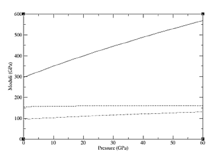
Figure 2.1: The variation of the elastic constants of magnesium oxide with applied

pressure as determined by breathing shell model calculation. C11,C12, and C44 are

presented by a solid, dashed and dot-dashed line, respectively.

then our calculated value becomes 0.182 in good agreement with the determination

of Zha et al [137].

To provide a test of the model, it is possible to calculate the variation of the elas-

tic properties of magnesium oxide as a function of applied pressure. The variation

of the elastic constants up to 60 GPa is shown in Figure 2.1.

When compared to the experimental results of Zha et al, the calculated trend in

the value of C11 is in good agreement in that it consistently increases under pressure

and approximately doubles in magnitude by the time that 60 GPa is reached. Unfor-

tunately, the trends for the other elastic constants are not so good, since the curve for

C12 ﬂattens with increasing pressure, rather than becoming steeper, and the curve

for C44 passes through a maximum which is not observed in the experimental data

from the aforementioned group. However, the calculated trends do match the ex-

trapolated behaviour based upon the results of ultrasonic measurements [138].

2.0.27 Born effective charges

The Born effective charges represent a useful means of characterising the response

of a potential model to perturbations, particularly those that create an electric ﬁeld.

Table 2.3: Born effective charges (in a.u.) calculated according to the shell model

of Sanders et al [139] and from ﬁrst principles techniques [140]. Values are shown

for the asymmetric unit atoms with the approximate positions of the Si atom at

(0.46,0,0) and the O atom at (0.41,0.27,0.11) in space group 154, with the origin set

to (0,0,1/3).

Si O

3.122 0.0 0.0 -1.406 0.368 0.252

Shell model 0.0 3.530 0.292 0.364 -1.920 -0.517

0.0 -0.171 3.422 0.176 -0.568 -1.711

3.016 0.0 0.0 -1.326 0.429 0.222

LDA 0.0 3.633 0.282 0.480 -1.999 -0.718

0.0 -0.324 3.453 0.298 -0.679 -1.726

Increasingly values are becoming available from ab initio techniques for solids

through the application of linear response methods. Hence, this quantity can pro-

vide a useful comparison between the results of formal-charge shell model calcula-

tions and more accurate ﬁrst principles methods.

One of the ﬁrst materials for which the Born effective charges were determined

using planewave techniques is α-quartz. In Table 2.3 the values obtained from the

shell model of Sanders et al [139] are compared with those yielded by a planewave

calculation using the Local Density Approximation and norm-conserving pseu-

dopotentials [140].

The comparison of the Born effective charge tensors demonstrates that the oxy-

gen shell model is surprisingly successful at reproducing the quantum mechanical

data, especially in comparison to rigid ion models, which would yield a diagonal

matrix with all components equivalent. Furthermore, the polarisability of the shell

leads to the ions behaving as partially charged species with realistic magnitudes.

Consequently, this explains why the seemingly unreasonable use of a formal charge

for Si4+actually works extremely well in practice. Similar observations have been

previously made for perovskite materials [141].

2.0.28 Frequency-dependent optical properties

Ever since the early days of atomistic simulation within the shell model context it

has been routine to calculate the static and high frequency dielectric constant ten-

sors. Indeed this data has often been used during the ﬁtting process as well. How-

ever, the values obtained from experiment will always be measured at a particular

frequency and this will never exactly correspond to the limiting values determined

by the direct means of calculation. As described in the background theory section,

it is possible to evaluate the dielectric properties and refractive indices as a function

of radiation frequency for the gamma point.

Here we present results for the frequency variation of the dielectric constant

tensor of quartz, shown in Figure 2.2, as calculated using the previously mentioned

shell model potential of Sanders et al [139]. Note that the limiting values are the

same as the ones obtained without reference to the phonon frequencies.

In accord with experiment, the dielectric constant decreases slowly with the fre-

quency of measurement until the highest phonon mode of quartz - the Si-O stretch

- is approached. At frequencies below this the curve contains considerable vari-

ation caused by the discontinuities when a lattice phonon mode is reached. For

simplicity, the curve shown is for the dielectric constant in the ab plane only. The

corresponding curve for the principal tensor component parallel to the 001 direc-

tion is almost identical, except that the limiting values are slightly different and the

positions of the discontinuities due to coincidence with phonons are displaced to

higher frequency.

While the qualitative agreement with experimental data is good, there is a quan-

titative discrepancy in the dielectric constant variation. This is a result of the im-

perfection of the original ﬁt to the dielectric data for quartz, though there are also

issues concerning the variation with temperature since the calculations are formally

performed at absolute zero, while the experiment data was measured at 293 K. How-

ever, the use of empirical ﬁtting implies that the interatomic potentials do partially

account for the temperature difference already. At the lowest measured frequency,

the calculated values are an almost perfect match due to the faster rate of decrease

of the dielectric constant in the experiment data.

2.0.29 Surface calculations

Before applying GULP to surfaces problems that were previously not possible, it

must ﬁrst be validated. Firstly, we focus on comparing our results to MARVIN,

starting with the simple inorganic salt corundum. In the original MARVIN paper

[107], the twelve faces with the lowest interplanar spacings were identiﬁed and their

surfaces relaxed using several different potential models. The calculations utilis-

ing the QM5 model were repeated using both MARVIN with the BFGS minimiser

and the same surfaces generated using GDIS and minimised in GULP using its

BFGS minimiser. The unrelaxed surface and attachment energies were compared

and both sets of calculations agreed to better than 0.0001Jm−2for the surface en-

ergies and within 0.0001eV mol−1for the attachment energies. This indicates that

the 2-D Ewald sum incorporated into GULP is correct. Next the relaxed surface

and attachment energies were compared. Except for the (310) face, all the GULP

calculations returned the same relaxed surface energy as the corresponding MAR-

VIN run to within 0.0001Jm−2. The relaxed attachment energies agreed to within

0.003eV mol−1. Excluding the (310) face, the MARVIN calculations took 138 s on a

1133MHz Intel Pentium III CPU Linux system, whilst the GULP calculations took

just 108 s. This difference in timing is primarily due to the faster energy calculation

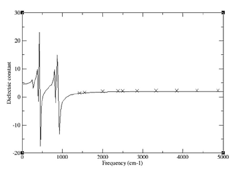
Figure 2.2: The on-diagonal component of the dielectric constant tensor for α-

quartz in the ab plane as a function of frequency of measurement. The solid line

represents the calculated shell model values, while the crosses represent values es-

timated from experimental measurements of the refractive index as a function of

frequency.

time in GULP since the MARVIN minimiser is based on the GULP algorithm and

consequently the number of cycles to minimise a face in GULP and MARVIN only

differed by at most one cycle, except for the (21-1) where GULP took 31 cycles ver-

sus the 24 for MARVIN. The (310) face is interesting as the relaxed surface energy

calculated by GULP is the same as that reported in the original paper [107] and it

is the minimised surface energy from the present calculation with MARVIN that is

different. Although not stated in the MARVIN paper, the minimisations were done

using a combination of minimisers; conjugate gradients until the gradient norm is

unity, followed by a BFGS minimisation. If the MARVIN calculations are repeated

with this combination, all surface energies between MARVIN and GULP agree to

within 0.0001Jm−2. In conclusion then, we can say that for this simple inorganic

system, GULP and MARVIN produce essentially the same results.

As an example of the application of the new GULP surface capabilities, they

have been recently utilised to search for surface reconstructions of the (10-14)

cleavage plane of calcite [142]. The previous modelling studies have not found

any evidence of surface reconstructions, despite the LEED results of Stipp [143].

A very efﬁcient and assumption free way of ﬁnding reconstructions is to determine

the surface phonon dispersion across the Brillouin zone, where the presence of any

imaginary phonons will indicate that a reconstruction wants to occur. This calcula-

tion was performed on the cleavage plane of calcite, using a new calcite potential

model that we have recently developed. An imaginary mode was found to be present

at (1/2, 0) in reciprocal space, which indicates that the system is unstable within the

(1x1) surface cell and that the reconstruction requires the formation of a (2x1) su-

percell. On creation of the surface supercell, the system was perturbed along the

eigenvector of the imaginary mode and reminimised using the rational function op-

timisation technique to ensure that the ﬁnal Hessian matrix had the correct character

for an energy minimum. Finally, the optimised (2x1) cell was examined to ensure

that there were no imaginary phonon modes anywhere within the Brillouin zone.

The calculations were repeated using other calcite models in the literature, which

were found not to possess any imaginary modes.

In the reconstructed surface, as shown in Figure 2.3, every second row of sur-

face carbonate anions are found to rotate. The rotation moves the O atom of each

carbonate such that it is 13ocloser to the vertical. This is accompanied by signiﬁ-

cant change in the carbonate geometry with an increase of the O-C-O angle of 3o,

where the two oxygen atoms are those pointing out of the surface and a compensat-

ing decrease in the other two O-C-O angles. Finally, we note that the reconstruction

is conﬁned to the top layer of the surface. In order to conﬁrm the correct nature of

the surface reconstruction, we have calculated the LEED pattern that would result,

which is found to be an excellent match to the experimental pattern measured by

Stipp under low pressure conditions.

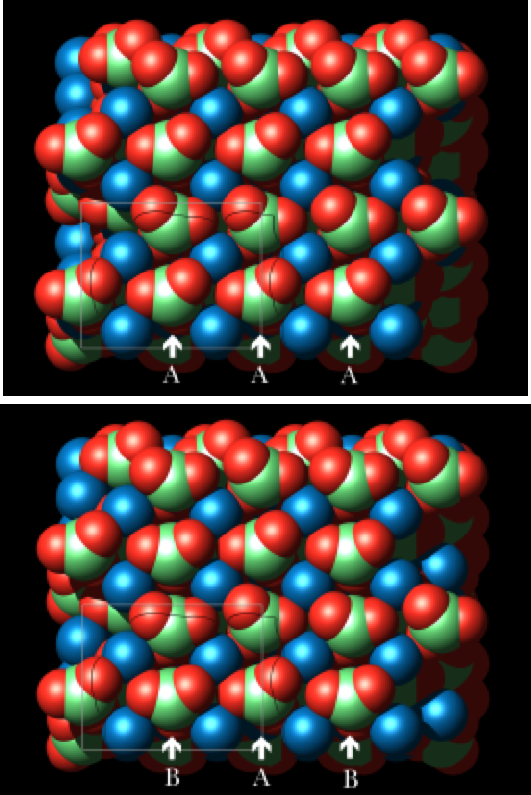
Figure 2.3: Comparison of the geometry for (a) a doubled unit cell of the (1x1)

structure for the (10-14) surface of calcite and (b) the optimised (2x1) reconstruc-

tion of the same surface. The reconstruction results in every second vertical row,

labelled B, adopting a different conﬁguration to the unreconstructed rows, labelled

(a)

(b)

Table 2.4: Calculated properties of diamond based on the model of Brenner et al

[66]. Note that the calculated values for the bond length and energy are not quoted

in the original reference. However, since the experimental values were part of the

ﬁtted data, we take these values to be equal to the observed ones.

Property Experiment Original value GULP value

Bond length(Å) 1.54 1.54 1.5441

Bond energy (eV) 3.68 3.68 3.684

C11(GPa) 10.8 10.7 10.75

C12(GPa) 1.3 1.0 1.26

C44(GPa) 5.8 6.8 7.21

2.0.30 Bond-order potentials

Given that new implementation of the Brenner model has been introduced into

GULP we present here some results for diamond, Table 2.4, as previously studied

in the original paper [66], in order to validate the code. For the second derivative

properties, there is also the difference that the values obtained here are fully analytic

whereas the published values are obtained via ﬁnite differences. This may explain

the small discrepancies in the elastic constants.

As stated in the background section, two algorithms have been implemented for

the evaluation of the Brenner potential based on either pairwise atom looping or a

spatial decomposition in order to determine the neighbour list. The computational

cost of the two approaches for increasing supercells of diamond are illustrated in

Figure 2.4. The linear scaling behaviour of the spatial decomposition can clearly

be seen, as can the fact that this algorithm is effectively superior in performance for

systems containing beyond a 100 atoms. Obviously this trade off point is dependent

on the density of the system, though there are few cases for hydrocarbons where the

density is greater than that of diamond. For systems much below a 100 atoms the

cost of evaluating the Brenner potential is so negligible in comparison to other tasks,

such as a matrix inversion for property calculation, that the choice of algorithm is

irrelevant.

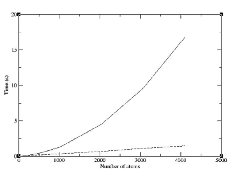
Figure 2.4: A comparison of the computer times required for a single energy-force

evaluation using the Brenner model according to whether the algorithm used in-

volves a pairwise sum (solid line) or a spatial decomposition (dashed line) to eval-

uate the neighbour list. Timings given are for a Mac PowerBook G4 laptop with a

clock speed of 700 MHz.

Chapter 3

Further background

In this section some of the theory behind GULP is explained and references are

supplied for those who require a more detailed description of the methods involved.

3.0.30.1 Cut-offs and molecules

All short-ranged two-, three- and four-bodied potentials have ﬁnite cut-offs in real

space which must be set by the user in some way. Unless the cut-off chosen is so

large that convergence is genuinely achieved then it effectively becomes a param-

eter of the potential. Hence when publishing new potentials it is good practice to

publish the cut-offs. Similarly, if you are trying to reproduce the results of previ-

ously published potentials make sure you use the same cut-offs.

The main effect of ﬁnite cut-offs is to introduce discontinuities into the energy

surface as atoms move across the boundary. Generally speaking, the energy min-

imisation procedure in GULP is not too sensitive to these because of the use of

analytical second derivatives. However, if working with only ﬁrst derivatives or

particularly short cut-offs this can be the reason for a minimisation failing to satisfy

the required convergence criteria.

An important difference between GULP and some other programs is that it is

perfectly allowable for potentials to overlap, i.e. two or more potentials can act be-

tween the same species at the same distance. Hence, there are no resulting restric-

tions for the cut-offs and complex potential functions can be built by combining

several potentials together. Conversely, it is important not to duplicate potentials

when not intended.

For some types of potential the cut-offs may correspond to chemical criteria

such as bond lengths or they may only need to act between molecules or conversely

only within them. In such cases it is best not to use distance cut-offs to achieve

the correct effect, but instead to use the molecule handling facilities within GULP.

There are three keywords which when speciﬁed activate the molecule facility within

the program - molecule, molq and molmec. If any of these words are present

100

Table 3.1: Common functional forms for two-body interatomic potentials incorpo-

rated into GULP (where rrepresents the distance between two atoms iand j). For

full documentation see help.txt.

Potential Name Formula Units for input

Buckingham Aexp(−r/ρ)−Cr−6Ain eV, ρin Å, Cin eVÅ6

Lennard-Jones†Ar−m−Br−nAin eVÅm,Bin eVÅn

ε(c1(σ

r)m−c2(σ

r)n)εin eV, σin Å

c1= (n/(m−n))(m/n)(m/(m−n))

c2= (m/(m−n))(m/n)(n/(m−n))

Harmonic?1

2k2(r−r0)2+1

6k3(r−r0)3+1

12k4(r−r0)4k2in eVÅ−2,r0in Å

k3in eVÅ−3,k4in eVÅ−4

Morse D{[1−exp(−a(r−r0))]2−1}Din eV, ain Å−2,r0in Å

Spring (core-shell) 1

2k2r2+1

24k4r4k2in eVÅ−2,k4in eVÅ−4

Cosh-spring k2r2(cosh(r

/d)−1)k2in eVÅ−2

General Aexp(−r/ρ)r−m−Cr−nAin eVÅm,ρin Å,

Cin eVÅn

Stillinger-Weber Aexp(ρ/(r−rmax))(Br−4−1)Ain eV, ρin Å, Bin Å4

(sw2)

†combination rules permitted

?k3,k4are optional

101

Table 3.2: Common functional forms for three-body potentials incorporated into

GULP (where rrepresents the distance between two atoms iand j,θi jk represents

the angle between the two interatomic vectors i-jand j-k). For full documentation

of all the functional forms available see help.txt.

Potential Name Formula Units for input

Stillinger-Weber Kexp(ρ/(r12 −rmax) + ρ/(r13 −rmax))(cos(θ213)−cos(θ0))2K in eV,

(sw3) ρin Å

Three-body †1

2k2(θ−θ0)2+1

6k3(θ−θ0)3+1

12k4(θ−θ0)4θ0in ◦

k2in eVrad−2

k3in eVrad−3

k4in eVrad−4

Three-body?1

2k2(θ213 −θ0)2exp(−r12/ρ)exp(−r13/ρ)k2in eVrad−2

θ0in ◦,ρin Å

Axilrod-Teller K(1+3cosθ213 cosθ123 cosθ132)/(r12r13r23)3Kin eVÅ9

Exponential Aexp(−r12/ρ)exp(−r13/ρ)exp(−r23/rho)Ain eV, rin Å

Urey-Bradley 1

2k(r23 −r0)2kin eVÅ−2

r0in Å

Cosine-harmonic 1

2k2(cosθ−cosθ0)2k2in eV

Linear3 (lin3) k(1±cos(nθ)) kin eV

Hydrogen-bond (A

rm−B

rn)cospθA in eVÅm, B in eVÅn

UFF3 K(C0+C1cosθ+C2cos2θ)Kin eV

Equatorial 2K

n2(1−cos(nθ)) + 2Kexp(−β(r13 −r0)) Kin eV, βin Å−1

Bond-angle cross k1ri j −r0

i j+k2rjk −r0

jk(θ−θ0)k1&k2in eV Å−1deg−1

(bacross)

Bond cos cross k1ri j −r0

i jrjk −r0

jk(1+bcos(nθ)2)k1in eV Å−2

Bond cross k1ri j −r0

i jrjk −r0

jk k1in eVÅ−2

†harmonic, option three

?harmonic + exponential, option three expo

102

Table 3.3: Common functional forms for four-body potentials incorporated into

GULP (where φi jkl is the torsional angle between the planes i jk and jkl). For full

documentation see the ﬁle help.txt.

Potential Name Formula Units for input

Torsion k(1+cos(nφ−φ0)) kin eV, φ0in ◦

ESFF torsion k1sin2

1sin2

2±k2sinn

1sinn

2cos(nφ)kin eV

Ryckaert-Bellemans ∑kn(cosφ)nknin eV

Tortaper/torexp As per torsion multiplied by taper or exponential decay

Torharm 1

2k(φ−φ0)2kin eV rad−2,φ0in rad

UFF4 k

2(1−cos(nφ0)cos(nφ)) kin eV

Torangle kcos(φ)(θ123 −θ0

123)(θ234 −θ0

234)kin eV rad−2

Torcosangle kcos(φ)(cos(θ123)−cos(θ0

123))(cos(θ234)−cos(θ0

234)) kin eV

Out of plane k2d2+k4d4k2in eVÅ−2,k4in eVÅ−4

Inversion k(1−cos(φ)) kin eV

Cross angle (xangleangle) k213/4(θ213 −θ0

213)(θ214 −θ0

214)+ k213/4,k312/4,k412/3in eV rad−2

k312/4(θ312 −θ0

312)(θ314 −θ0

314)+

k412/3(θ412 −θ0

412)(θ413 −θ0

413)

Cross angle cosine (xcosangleangle) k213/4(cos(θ213)−cos(θ0

213))(cos(θ214)−cos(θ0

214))+ k213/4,k312/4,k412/3in eV

k312/4(cos(θ312)−cos(θ0

312))(cos(θ314)−cos(θ0

314))+

k412/3(cos(θ412)−cos(θ0

412))(cos(θ413)−cos(θ0

413))

UFF out of plane k(c0+c1cos(φ) + c2cos(2φ)) kin eV

then a search will be performed to locate any molecules within the structures input.

This is done by searching for bonds based on the sum of the covalent radii plus a

percentage tolerance factor. For most common compounds the default covalent radii

will be sufﬁcient to locate all the bonds - if this is not the case then it is possible for

the user to either increase the tolerance factor or to adjust the covalent radii using

the covalent option from the element group of commands.

An alternative scenario is that atoms become bonded which shouldn’t be. For

example, metal atoms often can become bonded in ionic compounds because the

covalent radii is no longer relevant for a positively charged ion. These bonds can be

removed either by manually setting the radii of the element to zero or by using the

nobond option to exclude the formation of certain bond types. Whether the correct

molecules have been located or not can be seen from the molecule print out in the

output ﬁle. The three molecule-based keywords mentioned above differ in what

they imply for the treatment of intramolecular electrostatics:

molecule ⇒exclude all Coulomb interactions within the molecule

molq ⇒retain all Coulomb interactions within the molecule

molmec ⇒exclude all Coulomb interactions between atom which are

bonded (1-2) or two bonds away (1-3)

The speciﬁcation of molmec does not automatically imply that all potentials will

be treated in a molecular mechanics fashion, only the electrostatic terms. Provid-

ing one of the above three terms is present then optional words may be added to a

103

potential speciﬁcation line which control aspects of the potential cut-offs. Below

is a list of the words that are available and whether it is necessary to still give any

cut-offs on the potential parameter line:

Option Effect Cut-offs?

intra only act within a molecule yes

inter only act between molecules yes

bond only act between bonded atoms no

x12 do not act between bonded atoms yes

x13 do not act between 1-2 and 1-3 atoms yes

o14 only act between 1-4 atoms yes

g14 act between 1-4 atoms and beyond yes

single only act where atoms are singly bonded no

resonant only act where atoms are resonantly bonded no

double only act where atoms are doubly bonded no

triple only act where atoms are triply bonded no

quadruple only act where atoms are quadruply bonded no

amide only act where atoms are part of an amide group no

custom only act where atoms are joined by a custom bond no

half only act where atoms are half bonded no

quarter only act where atoms are a quarter bonded no

third only act where atoms are one third bonded no

In addition to atoms being bonded, GULP now offers the ability to specify a bond

type for each bond. This can be used so a potential only acts between two species

when they have a particular bond order. At present the bond order has to be speciﬁed

via the connect option (see below).

Although with some options it is necessary to still specify a cut-off for gener-

ality, the value may not be important any more. For example, if an O-H potential

for water is speciﬁed as being intramolecular then as long as the maximum dis-

tance cut-off is greater than about 1.0 Å then it doesn’t matter particularly what it

is. Similarly for a potential which is given as being x12 then it doesn’t matter if the

minimum cut-off distance is zero - the potential won’t act between bonded atoms.

By default, GULP dynamically calculates the molecular connectivity during a

calculation. The reason for this is that it ensures that the restart ﬁle will yield the

same answer as the point in the calculation where it left off. However, sometimes

difﬁculties occur because a bond becomes too long and the molecule breaks into

two. When this happens GULP will stop with an error message as this often in-

dicates that the potential model is not working well for the system under study. If

the user wants to proceed regardless then there is a keyword fix which tells the

program to ﬁx the connectivity as that at the starting geometry and not to update it.

This means that the program will never stop with this error, but it does mean that

a restart may not give the same answer as the initial run if atoms have moved too

104

far. There is now also the option for the user to specify the connectivity explicitly

in the input deck using the connect option. Note that when using symmetry the

connect option must be speciﬁed based on the full cell atom numbers and for all

images at present.

In the case of ionic materials where the user would like to try to remove some

of the numerical problems associated with cut-offs then there are some other op-

tions. The normal way of doing this is with a cut-and-shifted potential. In this

approach the potential is forced to go to zero at the cut-off by adding a constant

to the energy. This makes the energy continuous, but the gradient still has a dis-

continuity. Again this can be resolved by adding a second term which shifts the

gradient to be zero at the cut-off. In GULP this takes the form of a linear term in

the distance which, provided the cut-off isn’t very short, will have minimal effect in

the region of the potential minimum. These corrections are activated using the po-

tential options energy or gradient after the potential type, but are only currently

applicable to certain two-body potentials where it is appropriate. It should be noted

that some potential functions go to zero by construction at the cut-off, for example

the Stillinger-Weber two- and three-body potentials.

3.0.30.2 Combination rules

When using Lennard-Jones potentials it is common to use combination rules to

determine the interaction parameters between two species. This means that the

parameters for the interaction are determined from one-centre only parameters by

some form of averaging. The main advantage of this approach is that it reduces the

number of parameters to be determined and aids transferability of potentials. Con-

versely, the resulting potentials may not be as accurate for any one given system.

There are two types of combination rule used, depending on whether the potential

is being used in the ε/σor A/B format (see Table 2 for details). If the potentials are

being used in the A/B form then the average is taken using a geometric mean:

Ai j =pAiAj

Bi j =pBiBj

However, if the ε/σform is being employed then a more complex relationship is

needed:

εi j =2(εiεj)1

2(σ3

iσ3

(σ6

i+σ6

σi j = σ6

i+σ6

2!1

Within GULP it is possible to specify the parameters by species, rather than by

pairs of species, using the atomab or epsilon options. If the word combine is

105

added to the speciﬁcation of a lennard-type potential then the parameters can be

omitted from the input and they will be generated using the appropriate combination

rules. In turn this makes it possible to ﬁt potentials based on combination rules

without having to do this via a series of constraints.

3.0.30.3 Mean ﬁeld theory

One of the biggest problems that can face someone attempting to simulate complex

materials is the fact that often they can be partly disordered or involve partial occu-

pancies of sites. One approach to treating such systems is to generate a supercell

so that lots of permutations can be examined. However, the number of possibili-

ties is usually too large to examine each one individually to locate the most stable

conﬁguration. Furthermore, this process may alter the symmetry of crystal. Fitting

potentials to such structures also becomes rather difﬁcult.

An alternative approach to handling partial occupancies is to use mean ﬁeld

theory. The effect of this is that each site experiences a potential which is the

mean of all possible conﬁgurations on the disordered positions. In doing so we are

assuming that all possible conﬁgurations are equally as likely, i.e. the less stable

conﬁgurations are equally as likely as the more stable ones. This may apply to

materials were there is little energetic difference between conﬁgurations or to ones

which were formed under kinetic rather than thermodynamic control and haven’t

had the chance to achieve a Boltzmann distribution. It must be decided for any

given material whether it is therefore appropriate to use this approach.

The practical upshot of the mean ﬁeld method is that all interactions just become

scaled by the site occupancies of both atoms. This has been implemented in GULP

such that the user can specify the site occupancy in addition to the coordinates (see

the later section on the input for further details) and the program will automatically

handle most aspects of the mean ﬁeld approach. This includes ensuring the total

occupancy on a site does not exceed unity and where two different ions share a site

with partial occupancy they are constrained to move as a single ion in optimisations.

One important word of warning - it is important that the user thinks through

interactions carefully when using the partial occupancy feature to ensure that ev-

erything is handled properly. The biggest danger comes in systems where there are

two partially occupied sites very close to each other such that in the real system

their occupancy would be mutually exclusive. When this happens it is often nec-

essary to speciﬁcally exclude potentials between these atoms to obtain the correct

behaviour.

3.0.30.4 Algorithms for energy and derivative evaluations

GULP actually contains several different algorithms for calculating the energy and

its ﬁrst and second derivatives. By default the program will try to choose the most

efﬁcient for any given system, excluding possibilities such as the cell multipole

106

method which would actually lead to slight changes in the answer. Normally the

user will need to know nothing about what algorithm is being used, so this section

is really for the curious.

Usually real-space interactions are calculated in a lower-half triangular fashion

to avoid double counting of interactions which would give rise to loops of the form

shown below:

do i= 2, numat

do j= 1, i-1

[Calculate interaction between iand j]

enddo

If there is the possibility of self-terms or interactions between periodic replica-

tions of the same atom then the i=jterm would not be excluded, though it may

be more efﬁcient to handle this case in a separate loop. For solids where there is

signiﬁcant space group symmetry then a different algorithm may be more efﬁcient:

do i= 1, nasym

do j= 1, numat

[Calculate interaction between iand j]

enddo

where nasym is the number of species in the asymmetric unit and numat is the

number of atoms in the full unit cell. Both the symmetry adapted and standard

algorithms are present in GULP with selection being made based on the amount

of symmetry in the crystal. The use of symmetry can result in up to an order of

magnitude speed-up in favourable cases and therefore is well worth using. More

details concerning the use of symmetry, in particular with respect to the calculation

of derivatives, can be found elsewhere [11].

The second algorithmic aspect to mention applies to the situation when a con-

stant volume optimisation is being performed and some atoms are held ﬁxed. Typ-

ical cases where this occurs are in an optical calculation, in which only shells are

relaxed, or where a molecule is docked within a rigid microporous material. In

this case the energy of interaction between certain atoms is a constant term and the

forces on them are ignored. When this happens these atoms are excluded or frozen

out of the energy calculation after the ﬁrst point to save computational expense.

107

3.0.31 Phonons

3.0.31.1 Phonon density of states

We may also be interested in the phonon density of states for a solid as the num-

ber of frequencies versus frequency value becomes a continuous function when

integrated across the Brillouin zone. While full analytical integration across the

Brillouin zone is not readily carried out, this integral can be approximated by a

numerical integration. We can imagine calculating the phonons at a grid of points

across the Brillouin zone and summing the values at each point multiplied by the

appropriate weight (which for a simple regular grid is just the inverse of the number

of grid points). As the grid spacing goes to zero the result of this summation tends

to towards the true result.

For performing these integrations GULP uses a standard scheme developed by

Monkhorst and Pack [16] for choosing the grid points. This is based around three

so-called shrinking factors, n1,n2and n3- one for each reciprocal lattice vector.

These specify the number of uniformly spaced grid points along each direction.

The only remaining choice is the offset of the grid relative to the origin. This is

chosen so as to maximise the distance of the grid from any special points, such as

the gamma point as this gives more rapid convergence.

In many cases it is not necessary to utilise large numbers of points to achieve

reasonable accuracy in the integration of properties, such as phonons, across the

Brillouin zone. For high symmetry systems several schemes have been devised to

reduce the number of points to a minimum by utilising special points in kspace.

However, because GULP is designed to be general the Monkhorst-Pack scheme is

used. The user can input special points instead, if known for the system of interest.

Often it is not necessary to integrate across the full Brillouin zone due to the

presence of symmetry. By using the Patterson group (the space group of the recip-

rocal lattice) GULP reduces the integration region to that of the asymmetric wedge

which may only be 1/48-th of the size of the full volume [17].

When producing plots of the phonon density of states the critical factor, apart

from the resolution of the integration grid, is the ‘box’ size. The continuous density

of states curve has to be approximated by a series of ﬁnite regions of frequency or

boxes. Each phonon mode at each point in k space is assigned to the box whose

frequency region it falls into. The smaller the box size the better the resolution of

the plot. However, more points will be needed to maintain a smooth variation of

number density.

3.0.31.2 Infra-red phonon intensities

In order to make comparison between theoretically calculated phonon spectra and

experiment it is important to know something about the intensity of the vibrational

modes. Of course the intensity depends on the technique being used to determine

108

the frequency as different methods have different selection rules. While Raman in-

tensities are not readily calculable from most potential models, due normally to the

absence of polarisabilities higher than dipolar ones, approximate values for infra-

red spectra can be determined [18]:

IIR ∝(∑

all species

qd)2

where qis the charge on each species and dis the Cartesian displacement asso-

ciated with the normalised eigenvector.

3.0.31.3 Pair Distribution Functions

The calculation of Pair Distribution Functions is in accordance with the theory of

Chung and Thorpe [104]. It makes use of phonon information calculated within

GULP, for an optimised structure, using a Monkhorst-Pack grid (as described in

section 3.0.28.1).

Chung and Thorpe [104] state that the probability of ﬁnding a pair of atoms i

and j, with position riand rjrespectively, at position ris given by

ρi j(r) = δ(r−(rj−ri))(3.1)

where <··· >is the statistical average implying both conﬁgurational and thermal

averages. Summing over all such pairs gives the density function ρ(r), which is

averaged by using each atom in turn as the starting point. Working with a crystal

lattice, the complexity of such calculations is reduced because only atoms in the ﬁrst

unit cell are used as starting points. Moreover, GULP reduces the crystal symmetry

to a primitive cell, minimizing the required number of calculations. (It is, of course,

still possible to speciﬁc a conventional cell and use these k points instead.)

Consider a lattice of unit cells each containing natoms. Denote the position of

atom iin the original unit cell as ri0and similarly atom jin the `th unit cell as rj`.

Deﬁne the pair separation vector between two atoms i0(in the original unit cell)

and j`(in the `th unit cell) as ri0j`=rj`−ri0.

The density function (with units of 1/volume) is the weighted sum over all pairs

between atom i0and atom jin all unit cells, averaged over the number of atoms

in the unit cell, n. The spherical average is taken, dividing by 4πr2, to remove

orientational dependence.

ρ(r) = 1

4πr2n∑

` ∑

∑

wi jρi0j`(r)!(3.2)

where the prime indicates i06=j0(i.e. ri0j`6=0). The guassian peak (with units of

1/length), is given in equation 3.8. The weighting is dependent on the fraction of

109

atoms of type i,ci, and coherent bound scattering length, ¯

bi, and is expressed as

wi j =¯

bi¯

∑n

k=1ck¯

bk2(3.3)

As suggested by equation 3.1, if the atoms were completely stationary, the density

function would be a series of delta functions located at the interatomic spacings. To

account for thermal motion, Chung and Thorpe [144] demonstrated that, within the

harmonic approximation, the Debye-Waller theorem can be used to justify the use

of a series of weighted Gaussian peaks ρi j(r), centred at ri j with width σi j. Taking

ˆri j to be the unit vector between atoms iand j, and ui j =uj−ujwhere uiis the

displacement of atom i, then the width is given by

σi j =Dui j ·ˆri j2E1

2(3.4)

This can be expressed in terms of phonon modes as

σ2

i0j`=¯

2N∑

k,ν

2n[ω(ν,k)] + 1

ω(ν,k)|ri0j`|2|uj`(ν,k)−ui0(ν,k)·ri0j`|2(3.5)

where the displacements ui`are as given in equation 3.6. It should be noted that

this corrects a typographical error by Reichard et al [145] equation 3, where the

numerator is multiplied by a factor of √mirather than divided by it.

ui`=esigi(ν,k)exp[ik·ri`]

√mi

(3.6)

Nis the number of k-points, νis the mode index, n[ω(ν,k)] is the Bose occupation

number

n=1

exp(¯

hω

kT )−1(3.7)

ω(ν,k)is the frequency from the eigenvalues of the dynamical matrix, and esigi(ν,k)

is the eigenvector for atom i(see section 3.0.32). The mass of atom iis mi. When

this is implemented within GULP, a Monkhorst-Pack grid [96] of a speciﬁed density

is used to generate an even distribution of k-points.

In summary, the Gaussian peak (with units of 1/length) for each pair is calcu-

lated from the width

ρi0j`(r) = 1

q2πσ2

i0j`

exp"|ri0j`|−r

2σ2

i0j`#(3.8)

These are summed and averaged as in equation 3.2to give the Chung & Thorpe

(1999) density function (with units of 1/volume). The partial density function for

atomic pair i j is the contribution from ρi0jl(r)for that pair: the sum of all partials

is the total density function

110

3.0.32 Eigenvectors

Within the literature, there are two commonly used settings for calculating the dy-

namical matrix depending on whether the atomic position in the unit cell is included

in the eigenvector, or taken out as a phase factor. The default setting in GULP is

the same as that used by Lovesey [146], where the eigenvector of atom jat a given

k-point is phased by the position of the atom in the unit cell (rj0). Lovesey [146]

writes this as σ, but we have used esig here to avoid confusion with peak widths.

This is the eigenvector used by Chung and Thorpe[144] and here. Lovesey [146]

also describes an alternative setting, written as e, used in several books e.g. Willis &

Pryor [147] and Dove[148]. The two settings are related by the phase factor shown

(from eq. 4.28 in Lovesey [146])

esig j(ν,k) = ej(ν,k)·expik·rj0(3.9)

3.0.33 Commonly Used Correlation Functions

A number of different formalisms for PDFs exist in the literature. Keen [149] per-

formed an extensive survey of these and we follow his recommendations. The three

main real space correlation functions, G(r),D(r)and T(r)are variously used de-

pending on the purpose. T(r), which scales as rat large r, is often used for peak

ﬁtting, and for analyzing structural detail at low r(e.g. in amorphous systems).

D(r)is similar to T(r), but has a term subtracted that scales with r, making it the

correlation function of choice for studying mid to high r structural detail. G(r)is

also used as it makes the low r peaks prominent. A comparison of the different

forms is given by Dove [150].

Keen [149] writes the density function of Chung and Thorpe [104] as ρPDF (r).

It is the same as that used in the PDFFIT program [151] as well as by several current

workers in this ﬁeld, e.g. [152] [153]. This real space correlation function tends to

ρoat high rand is zero below the minimum interpair spacing.

The PDFFIT program also outputs a radial distribution function [144], also

known as a pair distribution function [104], with units of 1/area. It is written as

GPDF (r)by Keen [149], and deﬁned as

GPDF (r) = 4πrρPDF (r)−ρo(3.10)

where ρo=n

Vunitcell , the average number density (units of 1/volume). While ρPDF (r)

oscillates around the number density, GPDF (r)oscillates around zero. This can be

converted to a Keen [149] total radial distribution function,G(r), which has units

of area. At values of rless than the minimum interpair spacing, this function tends

to −(∑n

i=1cibi)2, and to ∞at high r.

G(r) = GPDF (r)(∑n

i=1cibi)2

4πrρo

(3.11)

111

G(r)is often expressed in units of Barns (1×10−28 m2=1×10−8Å2), but in the

GULP output we use Å2to be consistent with the other correlation functions.

The differential correlation function,D(r), and total correlation function,T(r),

are used as part of the ATLAS suit of programs [154], as used at the ISIS pulsed

spallation neutron source, and deﬁned as

D(r) = 4πrρoG(r)(3.12)

=GPDF (r) n

∑

i=1

cibi!2

(3.13)

T(r) = D(r) + 4πrρo n

∑

i=1

cibi!2

(3.14)

=GPDF (r) + 4πrρo n

∑

i=1

cibi!2

(3.15)

D(r)and T(r)have units of 1/length.

In addition to the total pair distributions functions written to the .pdfs ﬁle, a .pdfs

ﬁle is produced for every pair-type (root_pairnumber_atom1_atom2.pdfs) contain-

ing a selection of partial pair distribution functions. First, the weighted ρij(r)func-

tion: the sum of all of these is the total pair distribution function of Chung and

Thorpe. Secondly, a weighted version of gij(r), which again sums directory to

give G(r). Finally, an unweighted (true) gij(r), which corresponds to the gij(r)of

Keen[149]. This output can be supressed using the nopartial keyword.

3.0.33.1 Thermodynamic quantities from phonons

There are a range of quantities that can be readily calculated from the phonon den-

sity of states. The accuracy with which they are determined though clearly depends

on the kpoints or shrinking factors selected for the Brillouin zone integration. For

systems with large unit cells a small number of kpoints, perhaps even the Γ-point

alone, will be sufﬁcient. However, for those systems with small to medium unit

cells it is important to examine how converged the properties calculated are with

respect to the grid size.

If a phonon calculation is performed then GULP will automatically print out

the relevant thermodynamical quantities. This output depends partly on whether a

temperature has been speciﬁed for the given structure. If the calculation is set for

zero Kelvin then only the zero point energy is output:

ZPE =∑

k−points

wk∑

all modes

2hν

where wkis the weight associated with the given kpoint. In principal, the zero

point energy should be added to the lattice energy when determining the relative

112

stability of two different structures. However, because the derivatives of the zero

point energy are non-trivial it is normally neglected in an energy minimisation.

For temperatures above absolute zero we can calculate the vibrational partition

function, which in turn can be readily used to calculate three further properties:

Vibrational partition function:

Zvib =∑

k−points

wk∑

all modes 1−exp−hν

kT −1

Vibrational entropy:

Svib =RlnZvib +RT ∂lnZvib

∂T

Helmholtz free energy:

A=U−T Svib

where

U=Ulattice energy +Uvibrational energy

Heat capacity at constant volume:

Cv=RT 2∂lnZvib

∂T+T∂2lnZvib

∂T2

3.0.34 Free energies

Although the most common methods for studying the properties of materials as a

function of temperature are molecular dynamics and Monte Carlo simulations, there

is an alternative based on static methods within the quasi-harmonic approximation.

This is to directly minimise the free energy of the system at a given temperature,

where the free energy is calculated from the lattice energy combined with contribu-

tions from the phonons including the entropy and zero point energy.

The advantages of working with free energy minimisation are that MD simula-

tions are quite expensive due to the need to reduce the uncertainty by sampling large

amounts of phase space. Molecular dynamics and free energy minimisation are in

fact complementary techniques. The latter approach breaks down at high tempera-

tures as anharmonic effects become important - typically it works at temperatures

up to half the melting point as a rough guide. Conversely, molecular dynamics is

not strictly valid at low temperatures because the zero point motions and quantum

nature of the vibrational levels is ignored.

Although in principle it is possible to analytically fully minimise the free energy

of a solid, in practice this is extremely difﬁcult as it requires the fourth derivatives

of the energy with respect to the Cartesian coordinates. Hence, a number of ap-

proximations are normally made - the main one being that the principal effect of

113

temperature is to expand or contract the unit cell and the effect on internal degrees

of freedom is less important.

When changing unit cell parameters we are concerned with the Gibbs free en-

ergy as this is appropriate to a constant pressure calculation. This quantity is related

to the Helmholtz free energy, whose relationship to the vibrational entropy has al-

ready been given previously, by the expression;

G=A+PV

with

P=P

ext −P

int

where Pis the pressure. The pressure has two components - any external applied

pressure plus the internal phonon pressure coming from the vibrations. The phonon

pressure is given by:

int =−∂A

∂V

In order to calculate the Gibbs free energy it is therefore necessary to calculate

the derivative of the Helmholtz free energy with respect to the unit cell volume.

This can be done numerically by ﬁnite differences. Central differencing is more

expensive than using forward differences. However, it is generally necessary to

determine the phonon pressure with sufﬁcient accuracy. In turn each calculation of

the Helmholtz free energy requires a constant volume minimisation for the given

set of unit cell parameters, followed by a phonon calculation.

Once the Gibbs free energy has been calculated then the next stage of a free

energy minimisation is to isotropically expand or contract the unit cell until the ex-

ternal pressure balances the internal pressure. Having done this then the derivatives

of the Gibbs free energy can be evaluated numerically by ﬁnite differences and the

unit cell optimised with respect to this quantity.

Because of the three levels of optimisation plus phonon calculations involved,

free energy minimisations are rather expensive and shouldn’t be undertaken lightly!

Due to the numerical nature of several of the derivatives it may be necessary for the

user to adjust the ﬁnite differencing interval for a calculation to work optimally.

Also the calculations are very sensitive to the quality of the underlying energy sur-

face. Potentials with short cutoffs, leading to discontinuities, and soft modes can

cause difﬁculties for the method, so always check your model well before starting.

Free energy minimisation can be used in conjunction with ﬁtting to allow a

series of structures at different temperatures to be ﬁtted with inclusion of the thermal

effects, though again this is an expensive procedure. It is important to note that a

free energy minimisation at 0 K is not the same as an ordinary static calculation.

This is due to the presence of the zero point energy in the former method.

114

3.0.35 Defects

3.0.35.1 The Mott-Littleton method

The calculation of defect energies is more difﬁcult and approximate than the calcu-

lation of bulk properties. In theory, a defect can cause very long range perturbations,

particularly if it is not charge-neutral. Consequently the user must always check the

convergence of the approximations made.

The simpliﬁcation in the modelling of defects is to divide the crystal that sur-

rounds the defect into three spherical regions known as regions 1, 2a and 2b [19-

21]. In region 1 all interactions are treated exactly at an atomistic level and the

ions are explicitly allowed to relax in response to the defect. Except in the case of

very short-ranged defects it is not generally possible to achieve the desired degree

of convergence by increasing region 1 before running out of computer resources.

Consequently, in region 2a some allowance is made for the relaxation of ions but in

a way that is more economical.

In region 2a the ions are assumed to be situated in an harmonic well and they

subsequently respond to the force of the defect accordingly [22]. This approxima-

tion is only thus valid for small perturbations and also requires that the bulk lattice

has been optimised prior to the defect calculation. For region 2a individual ion dis-

placements are still considered, whereas for region 2b only the implicit polarisation

of sub-lattices, rather than speciﬁc ions, is considered.

If the vector xrepresents the positions of ions in region 1, while ζrepresents

the displacements of ions in region 2a, then the total energy of the system may be

written as:

E=E1(x) + E12(x,ζ) + E2(ζ)

where E1and E2are the energies of regions 1 and 2 respectively, and E12 is the

energy of interaction between them. We now assume that the energy of region 2 is

a quadratic function of the displacements:

E2(ζ) = 1

2ζTWζ

We also know that we wish to obtain the displacements in region 2 for which

the energy is a minimum:

∂E

∂ ζ =0=∂E12(x,ζ)

∂ ζ +Wζ

This expression can be used to eliminate E2from the total energy, leaving it

purely in terms of E1and E12:

E=E1(x) + E12(x,ζ)−1

∂E12(x,ζ)

∂ ζ ζ

115

The displacements in region 2 are formally a function of xfor region 1 which

makes the minimisation of the total energy with respect to both the positions of

region 1 and the displacements of region 2 potentially complicated. This problem

can be avoided by using force balance in region 1 as the criteria for convergence

(i.e. all forces on ions in region 1 must be zero), rather than purely minimising the

energy. The two approaches are equivalent provided that region 2 is at equilibrium

also. This will be achieved provided that the displacements in region 2 are small

enough that they are genuinely quadratic.

In terms of the minimisation procedure employed for defect calculations the

force balance process leads to a slightly different approach to the bulk optimisation.

Initially the same Newton-Raphson procedure with BFGS hessian updating and

line searches is employed to avoid convergence to stationary points which are not

minima. After at least one cycle of the above and when the gradient norm falls

below a certain threshold the minimiser abandons the line search procedure and

aims purely to reduce the gradients to zero, regardless of the energy. In practice

positive changes in the energy near convergence are only ever small.

The defect energy is now the difference in the total energies for the defective

and perfect lattice, Edand Eprespectively, with corrections due to the energy of

any interstitial or vacancy species at inﬁnite separation from the lattice, E∞:

Edefect =Ed−Ep+E∞

Two ﬁnal aspects must be dealt with in order to obtain the ﬁnal working equa-

tions for the defect energy. Firstly, due to the slow convergence of electrostatic

terms in real space alone we cannot evaluate the region 1 - region 2 energy directly.

Instead we must calculate the energy of region 1 interacting with the perfect lattice

to inﬁnity and then explicitly subtract and add back the terms due to ions which

are no longer on their perfect lattice sites. Secondly, because the displacements in

region 2 depend on the force acting on a given ion, which in turn is a function of

other region 2 ions, there is in fact a linear dependency of the energy on ζ. By suit-

able manipulation of the energy terms this may be removed to leave the following

expression for the defect energy:

Edefect =E11(dd)−E11(d p) + E1∞(d p)−E1∞(pp)

+E12a(dd)−E12a(d p) + E12a(pp)−E12a(pd)

−∑∂E12a(dd)

∂r−∂E12a(pd)

∂r

where the general symbol Ei j(kl)denotes the energy of interaction summed

over all ions in region iinteracting with ions in region jwhere iand jcan be 1,

2a or ∞(signifying a sum over 1, 2a and 2b out to inﬁnity). The letters kand l

indicate whether the energy is for the perfect or defective coordinates in regions i

and jrespectively, depending on whether they are por d.

116

3.0.35.2 Displacements in region 2a

Expanding the energy as a Taylor series and truncating at second order gives the

Newton-Raphson estimate of the vector from the current ion position to the energy

minimum position in terms of the force, g, acting on the ion:

ζ=−W−1g

Hence if we know the local second derivative matrix and the force acting on

the ion we can calculate its displacement. There are a number of possible ways of

calculating the force acting on the ions in region 2a. The most common approach

is to use the electrostatic force due to only the defect species - i.e. the force due

to any interstitial species based on their current positions, less the force due to any

vacancies at the position of the original vacant site. In this way region 2a responds

to the change in the multipole moments of the defect species in region 1, but not the

inﬂuence of other forces. Hence for this approximation to strictly hold the distance

between any defects and the boundary of region 2a should be greater than the short-

range cutoff.

3.0.35.3 Region 2b energy

Region 2b is assumed to be sufﬁciently far from the defects that the ions only re-

spond by polarising according to the electrostatic ﬁeld resulting from the total defect

charge placed at the centre of region 1. This can be written for cubic systems as

follows:

E2b=−1

2Q2∑

i6=1,2a

qimi

Because this expression is just dependent on the distance and a couple of lattice

site related parameters the region 2b energy can be evaluated using a method analo-

gous to the Ewald sum and then subtracting off the contribution from ions in regions

1 and 2a. An alternative more general, but still not completely general, expression is

the following where the lattice site dependent property is now an anisotropic tensor,

rather than a scalar [23]:

E2b=−1

2Q2∑

i6=1,2a

∑

αβ

qiMαβ

iRα

iRβ

This can again be calculated by partial reciprocal space transformation based on the

second derivatives of the R−4lattice sum.

117

3.0.36 Fitting

3.0.36.1 Fundamentals of ﬁtting

Before any production runs can be performed with an interatomic potential program

it is necessary to obtain the potential parameters. If you are lucky there may be good

parameters for your system of interest already published in the literature so you can

just type them in and get going straight away. Unfortunately most people are not

so lucky! The ﬁtting facility within GULP [24] allows you to derive interatomic

potentials in either of two possible ways. Firstly, you can determine the parameters

by ﬁtting to data from some higher quality calculation, such as an ab initio one,

normally by attempting to reproduce an energy hypersurface. Secondly, you could

attempt to derive empirical potentials by trying to reproduce experimental data.

Regardless of which method of ﬁtting you are using the key quantity is the ’sum

of squares’ which measures how good your ﬁt is. Ideally this should be zero at the

end of a ﬁt - in practice this will only happen for trivial cases where the potentials

can be guaranteed to completely reproduce the data (for example ﬁtting a Morse

potential to a bond length, dissociation energy and frequency for a diatomic should

always work perfectly). The sum of squares, F, is deﬁned as follows:

F=∑

all observables

w(fcalc −fobs)2

where fcalc and fobs are the calculated and observed quantities and wis a weighting

factor. There is no such thing as a unique ﬁt as there are an inﬁnite number of pos-

sible ﬁts depending on the choice of the weighting factors. The choice of weighting

factor for each observable depends on several factors such as the relative magnitude

of the quantities and the reliability of the data (for instance a crystal structure will

generally be more reliable than an elastic constant measurement).

The aim of a ﬁt is to minimise the sum of squares by varying the potential

parameters. There are several standard techniques for solving least squares prob-

lems. By default GULP uses a Newton-Raphson functional minimisation approach

to solving the problem, rather than the more conventional methods. This is because

it avoids storing the co-variance matrix. The downside is that near-redundant vari-

ables are not eliminated. Currently the minimisation of the sum of squares is per-

formed using numerical ﬁrst derivatives. The reason for using numerical derivatives

is because many of the properties, particularly those derived from second deriva-

tives, are rather difﬁcult to implement analytical derivatives for. Consequently the

value of the gradient norm output during ﬁtting should only be taken as a rough

guide to convergence. In cases where the numerical gradients prove noisy then

the use of the simplex algorithm for ﬁtting can be useful as this requires only the

function.

The choice of which potential parameters to ﬁt belongs to the user and is con-

trolled by a series of ﬂags on the potential input line (0 ⇒ﬁx, 1 ⇒vary). There are

118

also options contained within the variables sub-section for allowing more general

parameters to ﬁt, such as charge distributions. Note that when ﬁtting charges at

least two charges must be varied to have any effect as the program eliminates one

variable due the charge neutrality constraint. There is also the option to vary the

charge split between a core and shell while maintaining a constant overall charge

on the ion. The user may also impose their own constraints on ﬁtting variables

through the constrain fit option.

It is generally recommended that a small number of parameters are ﬁtted ini-

tially and the number gradually increased in subsequent restarts. Often if all pa-

rameters are allowed to vary from the start unphysical parameters may result. Dis-

persion terms of Buckingham or Lennard-Jones potentials are particularly prone to

poor behaviour during ﬁtting, as they tend to go to zero or become exceedingly

large. It is generally recommended that such terms are set equal to a physically

sensible value (based on quantum mechanical estimates or polarisability-based for-

mulae) and held ﬁxed until everything else is reﬁned.

A ﬁnal check that the program looks for is that the total number of variables

being ﬁtted is less than the total number of observables!

3.0.36.2 Fitting energy surfaces

To ﬁt an energy surface it is basically necessary to input all the structures and the en-

ergies that correspond to them. To do this it is just a matter of putting one structure

after another in the input ﬁle (within the limit of the maximum number of structures

for which the program is dimensioned). It is possible to ﬁt the gradients acting on

the atoms as well the energy of each structure, though often just the energies are

ﬁtted. If the latter is the case, then the easiest way to turn off the ﬁtting of the

gradients is to specify noflag as a keyword to prevent the program for looking for

gradient ﬂags in the absence of a keyword to specify them.

Perhaps the only unique feature of ﬁtting an energy surface is the need to in-

clude an energy shift in some cases. This is a single additive energy term which is

the same for all structures and just moves the energy scale up and down. The justi-

ﬁcation for this is that often it is impossible to calculate the energy that corresponds

exactly to the interatomic potential one from a quantum mechanical calculation

[25]. Most commonly this arises where the potential model has partial charges in

which case there is an unknown term in the lattice energy due to ionisation poten-

tials and electron afﬁnities for fractions of an electron.

To simplify the speciﬁcation of this shift value in the input, if you give the shift

option after the ﬁrst structure then this value will apply to all subsequent structures

until a different value is input. Similarly, its magnitude can be altered by using the

variables sub-section to specify the shift as a variable and this will apply to all

structures. It is generally recommended that the shift is ﬁtted ﬁrst and allowed to ﬁt

through out the procedure.

119

3.0.36.3 Empirical ﬁtting

An alternative to ﬁtting quantum mechanical data to derive an interatomic potential

is to actually ﬁt experimental data. In this case the procedure serves two purposes.

Firstly, the degree to which all the data can be reproduced may serve as some guide

as to the physical correctness of the model used. Secondly, it provides a means of

extrapolation of experimental data for one system to a different one where the data

may not be known, or alternatively to unknown properties of the same material.

Any of the properties that can be calculated for the bulk solid or gas phase

molecule can also be used in reverse to ﬁt a potential to. Obviously the essential

ingredient in the ﬁt is the experimental structure, without which you won’t get very

far! The conventional way to ﬁt the structure is by requiring that the forces on the

atoms are zero. This is clearly not a perfect strategy as it could be satisﬁed by a

transition state rather than a minimum, though in practice it is rare, except when

symmetry constraints are imposed.

Normally a good ﬁt requires some second derivative information as well as the

structure. For very high symmetry systems, such as rock salt, the structural data

alone is completely inadequate. If we imagine a potential as being a binomial ex-

pansion about the experimental geometry, then unless the ﬁrst and second deriva-

tives are reasonably well reproduced by our model then the range of applicability

will be almost zero. Typical sources of second derivative information are elastic,

dielectric and piezoelectric (where applicable) constants. Also vibrational frequen-

cies contain far more information than any of the above. However, the ﬁtting of

frequencies is not straightforward. To ﬁt the frequency magnitudes is certainly pos-

sible, however, you have no guarantee that the correct mode has been ﬁtted to the

correct eigenvalue. Hence, frequency ﬁtting only tends to be useful from empirical

data for special cases, such as O-H stretching modes which are well separated from

other modes and for diatomics where there is no problem in assignment!

One other case where frequency ﬁtting can be useful is at the lower end of the

spectrum. For an isolated molecule or a solid at its Γpoint the ﬁrst three modes

should have zero frequency as they are just translations. In some cases there may

be imaginary modes due the potentials not correctly reproducing the true symmetry.

Hence by ﬁtting the ﬁrst three modes to be zero it is possible to encourage the

potentials to yield the correct symmetry.

3.0.36.4 Simultaneous ﬁtting

There is one main difﬁculty in the conventional scheme for ﬁtting in which the

forces on the atoms are minimised by variation of the potential parameters which

arises when using a shell model. Normally we don’t know what the shell coor-

dinates are at the outset unless the ions are sited at centres of symmetry. In the

past people have tried ﬁtting with the shells placed on top of the cores. However,

this means that the potentials are tuned to minimise the polarisation in the system

120

and leads to the shell model having only a small beneﬁcial effect. It also doubles

the number of observables connected with gradients, but only introduces a small

number of extra variables thus making it harder to get a good ﬁt.

The solution to this problem is allow the shell positions to evolve in some way

during the ﬁt. There are two possibilities - either we can minimise the shell posi-

tions at every point during the ﬁt or we can added the shell coordinates as ﬁtting

parameters. In the case where only structural data is being ﬁtted the two meth-

ods are equivalent except in the way that they evolve towards the answer. When

other properties are included the second approach is not strictly correct, though the

difference is usually small.

After experimenting with several test cases it was found that the second scheme

in which the shell coordinates become ﬁtted variables was far more stable in con-

vergence and more efﬁcient. Hence this is the scheme that has been adopted and

is referred to as ’simultaneous’ ﬁtting due to the concurrent ﬁtting of shell posi-

tions. Whenever working with shell models it is recommended that the keyword

simultaneous is added during conventional ﬁtting - it can improve the sum of

squares by several orders of magnitude! Not only does this scheme apply to the

coordinates of shells, but also to the radii of breathing shells as well.

3.0.36.5 Relax ﬁtting

It has been observed that sometimes in conventional ﬁtting getting an improved sum

of squares doesn’t always get you what is considered to be a better quality ﬁt. This

is because people often use different criteria to make their judgement to the ones

input into the ﬁtting process. In particular they look at the difference between the

optimised structural parameters and those from experiment, rather than looking at

the forces. The reason why the forces can be lower, but lead to a worse structure is

because in a harmonic approximation the displacements in the structure are given

by the gradient vector multiplied by the inverse hessian. Hence, if the gradients get

smaller but the inverse hessian gets much larger then the situation may get worse.

The solution to this problem is to ﬁt according to the criteria by which the struc-

tures are judged - this is what relax ﬁtting does. This means that at every point in

the ﬁt the structure is optimised and the displacements of the structural parameters

calculated instead of the gradients. In this approach the shell model is naturally

handled correctly and so there is no need for simultaneous ﬁtting. The downside is

that it is much more expensive in computer time than conventional ﬁtting. Also you

can only start a relax ﬁt once you have a reasonable set of potential parameters - i.e.

one which will give you a valid minimisation. Hence a conventional ﬁt is often a

prerequisite for a relax ﬁt.

There is a further beneﬁt to using relax ﬁtting. In a conventional ﬁt the prop-

erties are calculated at the experimental structure normally with non-zero gradients

which is not strictly correct. In a relax ﬁt the properties are calculated for the opti-

121

mised structure where they are valid.

3.0.37 Genetic algorithms

Conventional minimisation techniques based upon methods such as Newton-Raphson

are excellent ways of locating local minima. However, they are of limited use in

ﬁnding global minima. For example, if we know the chemical composition of a

compound and its unit cell, but don’t know the structure then we would want to

locate the most stable arrangement for placing the atoms within the unit cell. To

search systematically for a reasonable set of atomic coordinates may take a very

long time by hand. Genetic algorithms [26] are a method by which we can search

for global minima rather than local minima, though there can never be an guarantee

of ﬁnding a global minimum. In many respects it resembles Monte Carlo methods

for minima searching, though is regarded by some as being more efﬁcient.

The concept behind the method, as the name might suggest, is to carry out a

’natural selection’ procedure within the program in the same way that nature does

this in real life. We start off with an even numbered sample of randomly chosen

conﬁgurations. This is our trial set which is allowed to evolve according to a num-

ber of principles described below. Before we can do this we need to consider how

to represent our data for each conﬁguration. To do this we encode each number as

a binary string by dividing the range between the maximum and minimum possi-

ble values (for example 1 and 0 for fractional coordinates) into a series of intervals

where the number of such intervals is an integer power of 2. Given this data repre-

sentation the system now evolves according to the following steps:

(a) Reproduction (tournament) - pairs of conﬁgurations are chosen at random and

the parameters which measure the relative quality of the two are compared (this is

the energy for genetic optimisation or the sum of squares for genetic ﬁtting). The

best conﬁguration goes forward to the next iteration, except that there is a small

probability, which can be set, for the weaker conﬁguration to win the tournament.

This process is repeated as many times as there are conﬁgurations so that the total

number remains constant.

(b) Crossover - a random point is chosen at which to split two binary strings, after

which the two segments are swapped over.

This can help to search for alternative local minima.

The default output from a genetic algorithm run is a given number of the ﬁnal

conﬁgurations, where the ones with the best ﬁtness criteria are selected. However,

unless the run smoothly progresses to the region of a single minimum it may be

122

more interesting to look at a sample of the best conﬁgurations from the entire run.

This can be done with GULP using the best option.

Genetic algorithms can only locate minima to within the resolution allowed by

the discretisation used in the binary representation. Also they are very slow to

converge within the region of a minimum. Hence, the genetic algorithm should be

used to coarsely locate the regions associated with minima on the global surface,

after which conventional Newton-Raphson methods will most efﬁciently pin-point

the precise minimum in each case.

123

3.1 Getting started

3.1.1 Setting environment variables

In previous versions of GULP it was necessary to specify where library ﬁles and

the documentation could be found by editing the source code. This has now been

replaced by the use of two environment variables, GULP_LIB and GULP_DOC,

respectively. Under tcsh these can be set as follows:

setenv GULP_DOC /Users/myname/gulp4.2/Docs

setenv GULP_LIB /Users/myname/gulp4.2/Libraries

or by using appropriate commands under other Unix shells.

3.1.2 Running GULP

Under UNIX:

To run GULP on a machine with the UNIX operating system simply type:

<directory>gulp < inputfile

where <directory> is the path name for the location of gulp on your machine, or

if the executable is in your current directory or lies in your path then this may be

omitted. In this case the output will come to your terminal. If you wish to save it to

an output ﬁle then type

<directory>gulp < inputfile > outputfile

You may like to try using one of the example input ﬁles (called exampleN, where N

is a number) to see what happens! Input may also be typed directly into the program

line by line if no input ﬁle is speciﬁed. Having ﬁnished typing all the required input

just type ‘start’ to commence the run.

3.1.3 Getting on-line help

To obtain on-line help on GULP type

help <CR>

A list of all the possible help topics can then be accessed by typing topics or

alternatively just type the particular keyword or option that you require help on.

124

Only sufﬁcient characters to specify a unique topic are required. To ﬁnish with help

type stop if you wish to exit the program or quit if you want to return to interactive

use.

If the help command fails to work it means that the path for the location of the

ﬁle help.txt (which is an ordinary ASCII text ﬁle containing all the help informa-

tion) has not been set at compile time and that the ﬁle is not in the present directory

either.

An alternative way of accessing help is to generate an HTML ﬁle using the

gulp2html utility (courtesy of Dr. Jörg-R. Hill) which produces a ﬁle help.html

which can then be inspected with a suitable browser, such as netscape.

3.1.4 Example input ﬁles

With the program you should have received a number of sample input ﬁles which

illustrate how GULP works for a number of particular run types. They also serve as

a test to ensure that the program works correctly on your machine type. Please note

that the interatomic potentials should not be taken as correct for general use - some

are made up for the purposes of demonstration only! Below is a brief description

of what each example ﬁle is doing.

Table 3.4: List of examples provided

example1 optimises the structure of alumina to constant pressure and then calculates the properties

at the ﬁnal point

example2 simultaneous ﬁt of a shell model potential to the structure of α-quartz, followed by an

optimisation with the ﬁtted potentials - the general potential is used with energy and

gradient shifts for the Si-O instead of the usual Buckingham potential

example3 an electronegativity equalisation calculation is used to derive partial charges for quartz

and are then used to calculate the electrostatic potential and electric ﬁeld gradients at

each site - bond lengths are also calculated

example4 simultaneous ﬁt of a shell model potential to La2O3 using an Ewald-style sum to evaluate

the C6 terms, followed by an optimisation with the production of a table comparing the

initial and ﬁnal structures at the end

example5 calculation of a phonon dispersion curve for MgO from 0,0,0 to 1/2,1/2,1/2 - note that

normally the structure should be optimised ﬁrst and that although a phonon density of

states curve is produced this may not be accurate due to restricted sampling of k space.

example6 calculation of the defect energy for replacing a Mg2+ ion in MgO by a Li+ ion to create

a negatively charged defect

example7a location of the transition state for a magnesium cation migrating to a vacant cation site in

MgO in a defect calculation

example7b this shows an alternative way of obtaining the same result as in 7a by starting the magne-

sium in a special position and using the resulting symmetry constraints to allow a ordinary

minimisation to the saddle point

125

example8 a molecular defect calculation in which a sulphate anion is removed from BaSO4 - note

that the use of the mole keyword to Coulomb subtract within the sulphate anion.

example9 an example of how to use a breathing shell model for MgO - including ﬁtting the model,

optimising the structure and calculating the properties

example10 optimisation of urea showing how to handle intermolecular potentials

example11 an example of how to map out the potential energy surface for the migration of a sodium

cation parallel to the c axis through a crystal of quartz with an aluminium defect using the

translate option

example12 optimisation of two structures within the same input ﬁle - also illustrates the use of the

name option

example13 shows how to use a library to access potentials for an optimisation of corundum

example14 relaxed ﬁt to structure and properties

example15 simple NVE molecular dynamics

example16 example of constant pressure shell model MD

example17 Sutton-Chen calculation for bulk Ni

example18 example of shell model MD in NVT ensemble

example19 shell model MD run for a zeolite with ﬁnite mass

example20 shell model MD run for a zeolite with adiabatic algorithm

example21 charged defect optimisation in a supercell

example22 energy surface ﬁt for a molecular crystal

example23 evaluation of the cost function for a particular structure

example24 example of structure prediction for polymorphs of TiO2

example25 free energy minimisation of quartz within the ZSISA approximation

example26 Using the "ditto" option to run the same structure at 3 pressures in the same ﬁle

example27 Interface calculation in which a rigid block of MgO is optimised over the 001 surface of

MgO

example28 Tersoff model calculation on bulk silicon followed by a vacancy defect calculation

example29 Streitz-Mintmire model calculation on bulk alumina

example30 REBO model calculation for a diamond surface

example31 Constant pressure optimisation of a corundum slab with a 2-D phonon calculation

example32 1-D calculation on MgO using manual speciﬁcation of ﬂags and the switch minimiser

option

example33 Grand Canonical Monte Carlo for a single species being introducted into a box

example34 Grand Canonical Monte Carlo for a rigid molecule being introducted into a box

example35 Voter-Chen EAM for Ag

example36 Frequency dependent property calculation for quartz

example37 SiH4 molecule using the Smith and Dyson REBO 1 model

example38 Electric ﬁeld applied to a slab from example31

example39 Glue potential for Au with print out of EAM atomic densities and energy contributions

example40 Simple example of 3coulomb potential for a water molecule for validation

example41 Force calculation for a urea molecule in the presence of a continuum solvent model with

qsas keyword

126

example42 Optimisation of the (001) surface of urea in the presence of a continuum solvent model

example43 Example of PDF calculation for MgO - phonons < wmax

example44 Example of PDF calculation for MgO - full phonon range

example45 Example of PDF calculation for MgO - phonons > wmin only

example46 Example of PDF calculation for (Ca,Sr)TiO3

example47 Example of Eckart keyword for removing rotation/translation from molecular vibrations

example48 Fitting of vibration modes using speciﬁc eigenvectors for a water molecule

example49 UFF input ﬁle with manual speciﬁcation of bonds for meta-xylene

example50 Example of Dreiding input

example51 Example of a thermal conductivity calculation for Allen-Feldman diffusons in amorphous

silicon

example52 Example of a thermal conductivity calculation that uses estimated B and v_s from prop-

erties

example53 Calculation of Raman intensities for the vibrations of alpha-quartz

example54 Example of ReaxFF for an ethene molecule

example55 Example of a MEAM-2NN calculation for FCC Cu metal

3.2 Guide to input

3.2.1 Format of input ﬁles

On the whole it is only necessary to use up to the ﬁrst four letters of any word,

unless this fails to specify a unique word, and the input is not case sensitive as all

characters are converted to lower case on being read in.

The ﬁrst line of the input is the only special line and is referred to as the key-

word line. Keywords should all be given on this line. These consist of control words

which require no further parameters and generally specify the tasks to be performed

by the program. For example a typical keyword line would look like:

optimise conp properties phonon

or in abbreviated form:

opti conp prop phon

This combination of words tells GULP to do a constant pressure optimisation

and then to calculate the lattice properties and phonons at the optimised geometry.

The order of words within the keyword line is not signiﬁcant.

All subsequent lines can be given in any order unless that line relates to a pre-

vious piece of input. Such lines contain ‘options’ which generally also require the

speciﬁcation of further information. This information can normally follow on the

127

same line or on the subsequent line. For example the pressure to be applied to a

structure could be input as either

pressure 10.0 or pressure

10.0

In many cases the units may also be speciﬁed if you don’t wish to use the default:

pressure 1000 kbar

Any lines beginning with a ‘#’ and anything that follows a ‘#’ part way through

a line is treated as a comment and as such is ignored by the program.

When performing runs with multiple structures any structure dependent options

are assumed to apply to the last structure given, or the ﬁrst structure if no struc-

ture has yet been speciﬁed. Some options should be speciﬁed as sub sections of

a particular option. For example, elastic, sdlc, hfdlc, piezo, energy and

gradients all are sub sections of the observables command and should appear

as follows:

observables

elastic 2

1 1 54.2

3 3 49.8

hfdlc

1 1 2.9

end

Provided there is no ambiguity, GULP will accept these options even if observables

is omitted, however, it makes the input more readable if the section heading is in-

cluded.

GULP reads only the ﬁrst 80 characters on a line in an input ﬁle. Should an

input line be two long to ﬁt within this limit then the line can be continued on a

second or further lines by adding the continuation character ‘&’ to the end of the

line.

3.2.2 Atom names

Many parts of the input to GULP require the speciﬁcation of atom names, be it when

giving their coordinates or when specifying potential parameters. The convention

adopted in GULP is that an atom should be referred to by its element symbol,

optionally followed by a number to distinguish different occurrences of the same

element. Numbers between 1 and 999 are valid numbers. Hence examples of valid

128

atom speciﬁers are Si,Si12, O3 and H387. Something like Si4+ would not be a

valid symbol. The reason for using the element symbol is because several calcu-

lations use elemental properties such as the mass or covalent radii in dynamical or

molecular runs, respectively.

Sometimes it is desirable to label all the atoms in the structure with numbers

to identify them, but with the same interatomic potential acting on them. To avoid

having to input the potential multiple times for each symbol there is a convention

within GULP which it is important to know. Any reference to just an atomic symbol

applies to all occurrences of that element, whereas any reference to an atom type

with a number only applies to that speciﬁc species. For example a Buckingham

potential speciﬁed as follows:

buck

Si core O core 1283.0 0.299 10.66 0.0 12.0

would apply to all Si atoms, regardless of whether they are called Si or Si1 etc.

However, the following potential:

buck

Si1 core O core 1283.0 0.299 10.66 0.0 12.0

would only act on Si1. It is important to remember this as people have labelled

one atom Si and the Si1 in the past and put potentials for both which resulted in

twice the potential acting on Si1 as there should have been. If the potential had

been speciﬁed as just acting on Si then the correct answer would be obtained as it

would act on both atoms once.

In addition to the atom label there is optionally a species type speciﬁer which

should be one of the following:

core - represents the main part of an atom including all its mass

shel - represents the mass-less component in a shell model

bcor - a core, but with a spherical breathing radius

bshe - a shell, but with a spherical breathing radius

If not given, then core is the default type. Note that the bcor and bshe types

only need to be used in the structure speciﬁcation. There after they can be treated

as an ordinary core or shell in the potential speciﬁcation and the program will select

whether the potential should act on the radius or the centre of the species.

129

3.2.3 Input of structures

The structure for a three-dimensional solid requires the input of three main sets of

information - the unit cell, the fractional coordinates and types of the atoms, and

ﬁnally the space group symmetry. Taking these in order, the unit cell can be input

either as the cell parameters:

cell

4.212 4.212 4.212 90.0 90.0 90.0

or as the cell vectors:

vectors

4.212 0.000 0.000

0.000 4.212 0.000

0.000 0.000 4.212

Normally it is easiest to use the cell parameter form and this is recommended.

The main reason why you might chose to use the cell vectors is because you want to

calculate the properties in a non-standard reference frame (given that quantities such

as the elastic constants depend on the unit cell orientation relative to the Cartesian

frame). If the cell parameters are input, then the acell vector is aligned along the

xaxis, the bcell vector in the xy plane and the ccell vector in the general xyz

direction.

If the keywords conp or conv are not speciﬁed, then the program will expect

6 ﬂags to indicate how the unit cell is to be optimised. Here a ﬂag of 1 implies

that a degree of freedom should be allowed to vary and 0 will imply that it should

be kept ﬁxed. Because GULP works with the strain tensor, these ﬂags refer to the

strain components in the order xx, yy, zz, yz, xz and xy, respectively. Examples of

how to input the ﬂags for the case given above when only the on-diagonal strain

components are to be varied are given below:

cell

4.212 4.212 4.212 90.0 90.0 90.0 1 1 1 0 0 0

or as the cell vectors:

vectors

4.212 0.000 0.000

0.000 4.212 0.000

0.000 0.000 4.212

111000

130

When GULP transposes a system between the primitive and centred unit cells

the orientation of the atoms is preserved so that any properties calculated will be

the same regardless of the cell used. It is recommend that the cell parameters be

used for input where possible as this ensures that symmetry can be used to acceler-

ate optimisations. Turning now to the internal coordinates of the atoms, these can

again be given either in fractional or Cartesian form, though the former is the more

natural for a periodic system. Each line of input must contain at least the atom label

followed by the coordinates, in which ever units. For example for the case of MgO:

fractional

Mg core 0.0 0.0 0.0

O core 0.5 0.5 0.5

Note that if the space group symmetry is to be given then it is only necessary to

specify the atoms of the asymmetric unit. Furthermore in any cases where a frac-

tional coordinate is a recurring decimal, such as 1/3, then it is necessary to specify

this value to six decimal places to be sure of it being recognised correctly as a

special position. If we were to include a shell model for oxygen then the input of

coordinates would now look like the following:

fractional

Mg core 0.0 0.0 0.0

O core 0.5 0.5 0.5

O shel 0.5 0.5 0.5

There is no need to specify the number of atoms to be input or to terminate the

section as this is automatically done when the program ﬁnds something which is

not an element symbol or a special character at the start of a line.

If a shell model has been speciﬁed for a given atom in the species section (see

later), but the shells are omitted from the input for the structure then GULP will

attempt to add them automatically. When this happens, the shell be placed at the

same location as the core by default.

In addition to the coordinates, there are a number of optional parameters which

can follow the zcoordinate on the line. These are, in order, the charge, the site oc-

cupancy (which defaults to 1.0), the ion radius for a breathing shell model (which

defaults to 0.0) and 3 ﬂags to identify geometric variables (1 ⇒vary, 0 ⇒ﬁx). Note

that the ﬂags will only be read if there is no keyword to specify the geometric vari-

ables (e.g. conp or conv). Hence in full the input for MgO could look as follows:

fractional

Mg core 0.0 0.0 0.0 2.00000 1.0 0.0 0 0 0

131

O core 0.5 0.5 0.5 0.86902 1.0 0.0 0 0 0

O shel 0.5 0.5 0.5 -2.86902 1.0 0.0 0 0 0

In the case of MgO all the ﬂags can be set to 0 as there are no geometric variables

within the unit cell by symmetry.

If we wanted to run a breathing shell calculation for MgO then the input might

look like the following for a constant pressure run:

fractional

Mg core 0.0 0.0 0.0 2.00000 1.0 0.0

O core 0.5 0.5 0.5 0.86902 1.0 0.0

O bshe 0.5 0.5 0.5 -2.86902 1.0 1.2

or for a mean ﬁeld calculation of the energy of a 40/60 MgO/CaO material:

fractional

Mg core 0.0 0.0 0.0 2.00000 0.4 0.0

Ca core 0.0 0.0 0.0 2.00000 0.6 0.0

O core 0.5 0.5 0.5 0.86902 1.0 0.0

O shel 0.5 0.5 0.5 -2.86902 1.0 0.0

The space group symmetry can be speciﬁed either through the space group num-

ber or through the standard Hermann-Mauguin symbol. Again for MgO, either of

the following would be valid:

space

225

or space

F M 3 M

In general it is better to use the symbol rather than the number as the structure

may be in a non-standard setting. The help ﬁle contains a full list of the standard

symbols for each space group to illustrate how the symbol should be written in the

input, though further non-standard settings will be accepted. The space option is

not compulsory in the input of a structure and if it is absent then GULP will assume

that the structure is in P 1 (i.e. no symmetry).

Related to the space option is the origin option which allows non-standard

origins to be handled. The input for this option can take the form of a single integer

(1 or 2) if you want to select one of the standard alternative origin settings. Alter-

natively if three ﬂoating point numbers are input then they are taken to be an origin

shift in fractional coordinates, or if three integer numbers are input then they are

divided by 24 to obtain the shift.

The structural input for a molecular system is just the Cartesian coordinates.

Currently the use of point group symmetry is unavailable for isolated systems so

132

there is no equivalent command to space for molecules. There is unlikely to be

much beneﬁt from the addition of point group symmetry as most molecular calcu-

lations are much faster than their solid state analogues.

Multiple structures can be included in the same ﬁle by placing one after another,

including mixtures of solid and molecular compounds. A useful option for keeping

track of different structures is the name option. This must precede the structure and

allows the user to give a one word name to the compound which will then be used

as a label in the output ﬁle. Using this the structural input for a ﬁle containing both

corundum and quartz might look as follows:

name corundum

cell

4.7602 4.7602 12.9933 90.0 90.0 120.0

frac

Al core 0.00000 0.0 0.35216

O core 0.30624 0.0 0.00000

space

167

name quartz

cell

4.91485 4.91485 5.40629 90.0 90.0 120.0

frac

Si core 0.4682 0.0000 0.333333

O core 0.4131 0.2661 0.213100

space

152

In the situation where you want to run the same structure at several different condi-

tions then the ditto option can be particularly useful to avoid repeating the struc-

ture. For example, to run corundum at a pressure of 1 GPa and 2 GPa you could use

the following input for the structures:

name corundum

cell

4.7602 4.7602 12.9933 90.0 90.0 120.0

frac

Al core 0.00000 0.0 0.35216

O core 0.30624 0.0 0.00000

space

167

pressure 1 GPa

ditto structure

133

pressure 2 GPa

3.2.4 Species / libraries

In the input for the coordinates there was the option to input the species charge for

each individual atom in the asymmetric unit or even the full cell. Normally this

is unnecessary as all atoms of the same type have the same charge. In this latter

case the charges can be assigned by the species option. So for a zeolite structure,

for example, where there may be lots of different Si and O sites we could assign

charges as follows:

species

Si core 4.00000

O core 0.86902

O shel -2.86902

The species command can also serve another purpose which is to assign poten-

tial library symbols to each atom type. Quite often we may simulate a whole series

of materials with a standard set of potentials. Rather than typing them in every time

we can call a library. GULP at present comes with two libraries - one for zeolite and

aluminophosphate type systems [3,28,29] and one for metal oxides from the work

of Bush et al [30]. All we need to do to call these potentials is to assign the poten-

tial types to the types in the library ﬁles. In the case of bush.lib, there is no need

to do anything as the symbols are just the metal element symbols. For the zeolitic

materials there is more than one kind of some atom types and so an assignment is

needed. Using this our input would look like:

species

Si core Si

O core O_O2-

O shel O_O2-

library catlow.lib

3.2.5 Input of potentials

The various types of potentials available in GULP have been tabulated earlier and

detailed descriptions of the input format for each one can be found in the on-line

help. This section will therefore just contain some general pointers as to how to

input potentials.

134

Let us take the example of a Buckingham potential which acts between magne-

sium cores and oxygen shells with the parameters A=1280.0eV, ρ=0.300Å, C=4.5

eVÅ6and acts over the range of 0 to 12 Å. The input for this would look as follows

for an optimisation run:

buck

Mg core O shel 1280.0 0.3 4.5 0.0 12.0

If we want to perform a ﬁtting run then it is also necessary to specify the ﬂags

which indicate which parameters are to be variables (1) and which ones are not (0).

There is one ﬂag for each potential parameter and the order of the ﬂags matches

that of the parameters. Hence a ﬁt in which we want to vary A only would look as

follows:

buck

Mg core O shel 1280.0 0.3 4.5 0.0 12.0 1 0 0

It would not matter if we had put the ﬂags on the end of the line in the input

for an optimisation run - they would have just been ignored. For most potential

types some parameters are optional and can be omitted, normally when they are

zero. There is always a hierarchy to the order of omission of values. For example,

for most two-body potentials if one number is missing then this is assumed to be

the minimum cut-off radius and this value is zero (as it quite commonly is). For a

Buckingham potential, if a second number is omitted then this is assumed to be the

C term which again is often zero. If you are going to omit values it is important to

remove the ﬂags when not needed from the input as this may confuse matters. If in

doubt give all values!

The number of input parameters can also vary according to any options speci-

ﬁed after the potential type. For example, if we wanted the above potential to only

act between atoms which are bonded then the input would be:

buck bond

Mg core O shel 1280.0 0.3 4.5

No potential cut-offs are needed as these are set by the fact that the atoms

must be bonded. Similarly for a Lennard-Jones potential when given as lennard

combine then no potential parameters will appear on the input line as these are

determined by combination rules.

More than one potential can be speciﬁed for each occurrence of the potential

type. Hence the following would be perfectly valid:

buck

135

Mg core O shel 1280.0 0.3 4.5 0.0 12.0

Ca core O shel 1420.0 0.3 6.3 0.0 10.0

If the input for one potential is too long to ﬁt on one line then it may be continued

on to the next line by using the continuation character ‘&’ at the end of the line.

For two-body potentials there is no ambiguity about the order of the atoms as

both are equivalent. For some three-body potentials and all four-body potentials

it is important to be aware of the convention regarding the order of input. For a

three-body potential which has a unique pivot atom, typically at which the angle is

measured, then this pivot atom must be given ﬁrst and then the two terminal atoms

in any order. Hence the O-Si-O angle bending term widely used for zeolites is input

as:

three

Si core O shel O shel 2.09 109.5 1.9 1.9 3.6

In the case of four-body terms there is no unique pivot and so the atoms are

input in the order which they are connected. A piece of good advice is that three-

and four-body terms are often most readily dealt with using connectivity based cut-

offs as part of the molecule set of options.

3.2.5.1 Input of PDF settings

Appropriate keywords for normal GULP operation should be used. Importantly,

the potential model needs to be properly optimised using opti. To run the PDF

module, the keyword PDF should be added. This automatically enables the phonon

and eigenvector keywords, calculating the necessary phonon information. It also

activates the keyword makeEigenArrays (which stores all phonon data in internal

arrays), and rephase which rephases the (complex) eigenvectors so that the com-

ponent with the largest magnitude is all real for all eigenvectors and also checks

the normalisation. This rephasing is a rotation in the complex plane that does

not change the results of the PDF calculations performed using the eigenvectors,

but helps with visualisation. To ensure that the entire Monkhorst-Pack grid of k-

points is used (not the symmetry reduced one), noksymmetry is also enabled. It

is often useful to use the nokpoints keyword to prevent the output of all the k-

points used (a typical PDF calculation may require 8000 k-points before conver-

gence is acheived). Similarly, suppression of phonon output is useful: the keyword

nophonon is used.

In addition to calculating the PDF from the full phonon data, it is possible to

restrict the frequencies (ω) used. A cut-off of ωmin/ωmax can be set in the op-

tions (see below). When the keyword PDFcut or PDFbelow is used, all frequencies

above/below the cut-off frequency are excluded. (There is no need to enter the PDF

136

keyword separately as it is assumed). Alternatively, all frequencies above/below the

cut-off frequency can be set to the cut-off frequency by the addition of PDFkeep.

3.2.5.2 Options

The conﬁguration should be set up in the normal way. Importantly, in addition to

specifying the structure and potentials, a Monkhorst-Pack grid of k-points must be

generated using the shrink option (as described in section 3.0.28.1). (Convergence

of phonon properties with number of k-points is essential before results can be

considered accurate. If the width of all pairs of type xi−yj, as given in the .wid ﬁle

are divergent increase the density of the grid.)

As with other output ﬁles, the GULP option output can be used to specify the

ﬁlename:

output pdf <filename>

It is important to specify an output ﬁle for all conﬁgurations, otherwise the root

<pdf >or <pdf_config_# >will be used. Two ﬁlestypes are produced

.wid ﬁle Lists every atomic pair and the width (use of keyword nowidth supresses

this)

.pdfs ﬁle Outputs Pair Distribution Functions up to rmax with the number of bins

speciﬁed at input

Within the literature, there are a number of different correlation functions; the

module expresses the results in several of these: rho(r),GPDF(r),G(r),D(r), and

T(r). More details are available in the ‘Further Background’ section of this manual.

Where phonon selection has been used, ωmax/ωmin is also stated in the output ﬁles,

using the frequency units speciﬁed (see below), together with the temperature and

number of k-points.

All other input options for PDF calculations are entered in lower case within a

pdf input block.

The pdf input block is opened with the word pdf and closed with the word end.

i.e.

pdf

end

When working with multiple conﬁgurations, it is possible to open the pdf block with

"pdf all": it then operates on all conﬁgurations, ensuring that comparable PDFs are

produced with the same cut-offs, maximum radius and binning. Alternatively, a

seperate pdf block can be given for each conﬁguration.

For PDFs, the maximum radius (in Å) should be speciﬁed (default = 5 Å), and

the number of bins used for the output (default = 100). These can be set, within the

pdf input block, using rmax and rbins respectively, or the default values used.

137

pdf

rmax [real]

rbins [int]

end

When using the frequency cut-off facility, either wmin or wmax (as appropriate)

must be set, again in the pdf input block. While the default units for frequency

input/output in the PDF module is THz, it can (optionally) be changed as shown

using the units options: (cm or wav can be used for wavenumbers)

pdf

rmax [real]

rbins [int]

units freq [rad/Thz/cm/wav/meV]

wmin [real]

wmax [real]

end

In neutron scattering, advantage is often taken of the different scattering lengths

of different isotopes. The library ﬁle only contains element information. However,

this can be overwritten using the element option input block with bbar or siginc

(mass, ionic radius, etc, can also be changed in this way, see command help for

more). The units are Å and Å squared. NB. The Sears table, used to produce the

eledata Library ﬁle, uses Fm and Barns (=1×10−28m).

3.2.6 Defects

In this section we shall cover the basic input required to perform a Mott-Littleton

calculation for an isolated defect in an otherwise perfect solid, as activated by the

presence of the keyword defect. The main run type that we will be concerned

with for defects is optimisation as we normally wish to obtain the defect energy and

structure. We may also wish to locate transition states for the migration of defects

- this follows the same approach as an optimisation, but with the keyword trans

rather than opti. There is currently no facility to ﬁt to defect quantities.

The ﬁrst issue to consider is the bulk calculation that must precede a defect

calculation. For a correct calculation the bulk structure must be optimised at least to

constant volume otherwise negative defect energies may result from the removal of

bulk forces, rather than defect related ones. If you intend to perform several defect

calculations and the bulk unit cell is a reasonable size it is sensible to optimise

the bulk as a ﬁrst job and then use the restart ﬁle for the defect calculations to

avoid wasted effort. There are also other reasons for optimising the bulk separately.

Firstly, if you want to perform a transition state run then the trans keyword will try

138

to be applied to the bulk as well as the defect with strange results (this can avoid by

using the bulk_noopt keyword). Secondly, when creating defects it is important

to know where the bulk atoms are so that they can be placed correctly.

At the end of the bulk calculation a property evaluation must be performed as

the second derivatives and dielectric constants are needed for the response tensors

of region 2. This is automatically invoked and there is no need to add the keyword

property. Again for some materials the calculation of the properties can be ex-

pensive. Hence, if multiple defect calculations are to be performed then this step

can be minimised by adding the keyword save to the ﬁrst run (which will write

out a temporary ﬁle fort.44 which contains the quantities needed for future runs in

a binary form to save space) and the keyword restore to subsequent runs (which

will cause them to read in the information from fort.44 rather than re-calculating

it).

Having dealt with the preliminaries, we are now ready to consider how to input

the details of the defect calculation. Remember, the following commands should

appear after the structure to which they refer. Firstly, we need to determine the

defect centre around which the regions are based. This is given using the option

centre (center will also work for the beneﬁt of those of you who are American-

minded!). The defect centre is normally placed at the same position as the defect,

in the case of a single defect site, or at the middle of a series of defects so as to

maximise the distance between any defect and the region 1 boundary. Symmetry

is not explicitly input by the user for a defect calculation. However, the program

will automatically try to search for any simple symmetry elements. These can then

be used to accelerate the calculation. In order to do this it requires that the defect

centre is chosen so as to maximise the point group symmetry about itself. This is

worth keeping in mind when choosing the location of the defect centre. A gen-

eral feature of the centre option, and those which specify the positions of defect

species, is that there are a number of alternative methods for specifying the location:

(a) Atom symbol : this is the label for a species within the unit cell. It is best to use

a unique speciﬁer (by changing the type number of one atom if necessary) - if there

is ambiguity the program will normally chose the ﬁrst occurrence of the symbol.

centre Mg2 core

This will place the defect centre at the ﬁnal bulk position of the Mg2 core.

(b) Atom number : here the position is given by the number of the atom in the

asymmetric unit as input.

centre 3

139

This will place the defect centre at the ﬁnal bulk position of the third atom in the

asymmetric unit.

- the frac option in the following command is optional as it is the default:

centre frac 0.25 0.25 0.25

(d) Cartesian coordinates: here the position is explicitly given in Cartesian coor-

dinates, the origin of the unit cell being at 0,0,0:

centre cart 1.5 2.4 0.8

(e) Molecule number: this places the defect centre at the middle of the molecule

whose number is given (which corresponds to that in the output):

centre mol 2

Having located the defect centre the next thing we need to do is to specify the region

1 and region 2a radii. This is done with the size command:

size 4.0 10.0

would result in a region 1 radius of 4.0 Å and a region 2a radius of 10.0 Å. It is im-

portant to check how sensitive the defect energy is to these values and to increase

them until satisfactory convergence is achieved. One way of doing this while min-

imising computational expense is by using the restart ﬁle. If we wanted to restart a

defect calculation run with the above radii, but with region 1 increased to 6.0 Å and

region 2a to 12.0 Å then we would just need to edit the restart ﬁle to contain the new

values, plus the old region 1 size (needed for correct restarting) at the end of the line:

size 6.0 12.0 4.0

We now have speciﬁed the regions - next we need to create some defects. There

are three options for this:

vacancy - removes an ion from the structure to inﬁnity

interstitial - inserts an ion into the structure from inﬁnity

impurity - replaces one ion with a different one

The last one, an impurity, is obviously just a short-cut combination of the other two.

The actual input for each option for specifying the ion(s) involved follows that for

centre in that the atom label, atom number, fractional or Cartesian coordinates can

be used. The molecule number can also be used with the vacancy option, in which

140

case it removes all the atoms of the molecule from the structure (see example8).

Note that when molecules are removed and inserted it is important to correct the

defect energy for the molecule at inﬁnity, if this is not zero, as this is not done

automatically.

An important part of the interstitial and impurity commands is to specify the

type of species to be inserted. For example, the impurity command to replace O2

with Swould be:

impurity S O2

The key thing to note is that the inserting species is always speciﬁed ﬁrst. To

make life easy shells are handled automatically in most cases. So if both O2 and S

were speciﬁed as shell model atoms then the above command would remove both

the O2 core and shell, and also insert the S core and shell (initially at the same

position). It becomes important when introducing species with a type different to

any of the bulk species that all the necessary properties of the inserting ion are given

in the species option otherwise the atom will be assumed to have no charge and

no shell.

There is one further option when introducing an interstitial to make life easier.

For example, imagine we want to protonate an oxygen (typically in a zeolite frame-

work) to generate a hydroxyl group at O2. This can be readily achieved using the

bond option:

interstitial H bond O2

this will place the H into the structure at the sum of the covalent radii from O2. To

determine the direction for the bond the program maximises the angles to any other

atoms to which O2 has bonds.

Putting all these keywords together, we shall illustrate how a lithium impurity

could be created in magnesium oxide to generate a negatively charged defect. For

the purposes of this example we will work with the full unit cell structure as given

by the following:

opti conp defect

cell

4.212 4.212 4.212 90.0 90.0 90.0

frac

Mg core 0.0 0.0 0.0

Mg core 0.0 0.5 0.5

Mg1 core 0.5 0.0 0.5

Mg core 0.5 0.5 0.0

O core 0.5 0.5 0.5

141

O core 0.5 0.0 0.0

O core 0.0 0.5 0.0

O core 0.0 0.0 0.5

species

Mg core 2.0

O core -2.0

Li core 1.0

Based on the above basic input (+ interatomic potentials) all the following

would be valid ways of creating the defect:

(a)

centre Mg1

size 6.0 12.0

vacancy Mg1

interstitial Li 0.5 0.0 0.5

(b)

centre Mg1

size 6.0 12.0

impurity Li Mg1

(c)

centre 0.5 0.0 0.5

size 6 12

impurity Li 0.5 0.0 0.5

(d)

centre 3

size 6 12

impurity Li cart 2.106 0.0 2.106

There are more permutations than this, but hopefully it gives you the general idea.

3.2.7 Restarting jobs

Because on the whole GULP doesn’t require very much CPU time per step (the ex-

ceptions normally being second derivative calculations on large systems) it doesn’t

maintain a binary dumpﬁle with all the details for a restart from exactly where it

left off. Instead there is the option to dump out a restart ﬁle which is just a copy

of the original input (slightly rearranged!) but with any coordinates or potential

parameters updated as the run progresses. The frequency with which this is written

142

out can be controlled by the user. If the following is speciﬁed:

dump every 4 gulp.res

then a restart ﬁle will be written after every 4 cycles. If the ‘4’ is omitted then it

defaults to being one - i.e. a dumpﬁle is written after every cycle. As the cost of

writing out this ﬁle is normally small compared to the cost of a cycle this is the

usual choice. If the every option is omitted then the restart ﬁle is written just at the

end of the run.

3.2.8 Memory management

From version 3.4 of GULP the code was written in Fortran90 and therefore pretty

much all memory is dynamically allocated. Hence there should rarely be any need

to alter the code to increase a parameter. The only main parameter in the code is the

number of elements, which is set to 107 by default. In the event that you wish to

study elements further down the periodic table than this, you need to edit this value,

add the appropriate element data and recompile.

Even though the code is fully dynamic, you can still exhaust the memory of

your computer under certain circumstances. Remember that any runs that require

the analytic second derivatives, such as phonons or Newton-Raphson optimisation,

will cause a memory requirement of roughly 5

2(3N+6)2double precision words.

Hence if you run out of memory or the machine starts swapping you should ﬁrst

of all try to reduce the memory demands by using an optimisation algorithm that

doesn’t require full second derivatives, such as unit-Hessian based BFGS, limited

memory BFGS or conjugate gradients.

143

3.2.9 Summary of keywords

The following is a concise summary of all the valid keywords available in GULP -

for more detail consult the on-line help.

Table 3.5: Valid keywords in GULP

angle calculate valid three body angles

anneal perform simulated annealing

average output average bond lengths

bond calculate valid bond lengths based on covalent radii

breathe only calculate gradients for breathing shell radii

broaden_dos apply Lorentzian broadening to density of states data

bulk_noopt ﬁx bulk structure prior to a defect calculation

c6 calculate C6 terms using lattice sum method

cartesian output Cartesian coordinates for initial structure

cellonly only calculate gradients for and optimise cell parameters

cmm calculate cluster electrostatics using cell multipole method

compare produce a table comparing the initial and ﬁnal geometries

conjugate use conjugate gradients

conp perform constant pressure calculation - cell to vary

conv perform constant volume calculation - hold cell ﬁxed

coreinfo output atomic information (for cores not shells) used in phonon calculations

cosmo use the COSMO continuum solvation model

cosmic use the COSMIC continuum solvation model

cost perform cost function calculation

dcharge output the ﬁrst derivatives of the atomic charges

defect perform a defect calculation after bulk calculation

dfp use Davidon-Fletcher-Powell update rather than BFGS

dipole add the dipole correction energy for the unit cell

distance calculate interatomic distances

eem calculate charges using electronegativity equalisation

efg calculate the electric ﬁeld gradients

eigenvectors write out eigenvectors for phonons/frequencies

fit perform a ﬁtting run

fix_molecule ﬁx connectivity for molecules at start and do not update

free_energy perform a free energy instead of internal energy calc

frequency calculate defect frequencies

full write out structure as full rather than primitive cell

gear use the Gear ﬁfth order algorithm for molecular dynamics

genetic perform a genetic algorithm run

global after global optimisation, dump out restart ﬁle before opt

gradients perform a single point calculation of energy and gradients

144

hessian output hessian matrix

hexagonal write out structure as hexagonal rather than rhombohedral

hideshells suppress output of shells

include_imaginary include imaginary frequencies in phonon DOS/dispersion output

intensity calculate IR intensities for phonon/vibrational modes

isotropic allow cell parameters to vary isotropically

linmin output details of line minimisation

lower_sym try to lower the symmetry using imaginary modes

madelung include the Madelung correction for a charged simple cubic system

makeeigenarrays store all eigenvectors and frequencies after calculation

md perform a molecular dynamics run

minimum_image use the minimum image convention during MD

molecule locate molecules and coulomb subtract within them

molmec locate molecules and coulomb subtract 1-2 and 1-3

molq locate molecules for intramolecular potentials only

montecarlo perform a Monte Carlo simulation

noaddshells do not automatically add missing shells

noanisotropic use isotropic formula for region 2b energy

nobreathe freeze breathing shell radii during optimisation

nod2sym do not use symmetry for second derivatives

nodpsym do not use symmetry for defect potential calculation

noelectrostatics turns off Ewald sum even when charges are present

noenergy do not calculate the energy - useful for debugging datasets

noexclude do not use atom freezing algorithm during optimisation

nodensity do not output density of state plot after phonon calculation

nodsymmetry do not use symmetry during a defect calculation

nofirst_point skip ﬁrst point in a translate run

noflags no variable ﬂags are present and all variables to be excluded

nofrequency do not print out frequencies at each k point

nokpoints do not print out k point list

noksymmetry do not use Patterson symmetry in Brillouin zone

nolist_md do not use list method for 3- and 4-body terms in MD

nomcediff controls algorithm for Monte Carlo energy evaluation

nomolecularinternalkeremove initial intramolecular kinetic energy in MD

nononanal exclude non-analytic correction at gamma point

nopartial suppress output of partial PDFs

noreal exclude all real space two-body interactions

norecip exclude all reciprocal space two-body interactions

norepulsive do not truncate repulsive terms based on Ewald accuracy

norxQ turn off charge calculation in ReaxFF

nosasinitevery do not initialise solvent accessible surface at each step

nosderv do not use symmetry for gradient calculations

145

nosymmetry turn off symmetry once unit cell has been generated

nowidth suppress output of peak widths for PDF calculations

nozeropt exclude zero point energy from free energy calculation

numdiag estimate on-diagonal hessian elements numerically

numerical forces use of numerical second derivatives for properties

operators print out listing of symmetry operators used

optimise minimise the energy with respect to geometrical variables

outcon output constraints in restart ﬁle

pacha compute variable charges using the PACHA formalism of Marc Henry

PDF calculate the peak widths for each atomic pair and the Pair Distributions

PDFcut as per PDF but cut-off all phonon contributions greater than ωmax

PDFbelow as per PDF but cut-off all phonon contributions below ωmin

PDFkeep as with PDFcut and PDFbelow but set all ω>ωmax to ωmax (or ω<ωmin to

ωmin)

phonon calculate the lattice phonon modes and cluster frequencies

positive force hessian to remain positive on the diagonal

pot calculate the electrostatic potential at the atomic sites

potgrid calculate the electrostatic potential over a grid

predict perform structure prediction calculation

property calculate the bulk lattice properties

pureq use pure Coulomb potential in COSMO/COSMIC molecular case

qeq calculate charges using the QEq scheme of Rappe and Goddard

qiter solve for charges using iterative algorithms rather than matrix diagonalisation

qok run with a non-charge neutral unit cell

qsas causes charges and details of solvent accessible surface to be output

raman causes calculation and output of Raman susceptibility tensors

regi_before output region 1 coordinates before defect calculation

relax use relax ﬁtting

rephase change the eigenvector phases so largest magnitude component is all real for

all eigenvectors and renormalize to unity

restore read in defect calculation restart info and skip property calcn

rfo use the rational function optimisation method

save write out defect calculation restart information

shell only calculate gradients for and optimise shell positions

site_energy output energy per atomic site

simultaneous simultaneously optimise shells while ﬁtting

simplex use simplex algorithm for ﬁtting

single perform a single point calculation of the energy

sopt output shell iterations during molecular dynamics

static_first perform a static optimisation before a free energy one

spatial use domain decomposition algorithm where possible

146

thermalconductivity calculate the Allen-Feldman thermal conductivity for diffusons in an amor-

phous solid

torsion calculate valid four body torsion angles

transition_state optimise using RFO to ﬁrst order transition state

unit use a unit matrix as the initial hessian for optimisation

zero_potential set average potential across lattice sites to zero

zsisa use the ZSISA approximation in a free energy minimisation

3.2.9.1 Groups of keywords by use

(a) Control of calculation type

angle, bond, cosmo, cosmic, cost, defect, distance, eem, efg, fit,

free_energy, gasteiger, genetic, gradients, md, montecarlo, noautobond,

noenergy, optimise, pacha, pot, predict, preserve_Q, property, phonon,

qeq, qbond, raman, single, sm, static_first, thermalconductivity,

torsion, transition_state

(b) Geometric variable speciﬁcation

breathe, bulk_noopt, cellonly, conp, conv, isotropic, orthorhombic,

nobreathe, noflags, shell, unfix

c6, dipole, fbfgs, fix_molecule, full, hill, kfull, marvinSE, madelung,

minimum_image, molecule, molmec, molq, newda, noanisotropic_2b, nod2sym,

nodsymmetry, noelectrostatics, noexclude, nofcentral, nofirst_point,

noksymmetry, nolist_md, nomcediff, nonanal, noquicksearch, noreal,

norecip, norepulsive, nosasinitevery, nosderv, nozeropt, numerical,

qiter, qok, spatial, sopt, storevectors, nomolecularinternalke, voigt,

zsisa

(d) Optimisation method

conjugate, dfp, lbfgs, numdiag, positive, rfo, unit

(e) Output control

average, broaden_dos, cartesian, compare, conserved, dcharge, dynamical_matrix,

eigenvectors, global, hessian, hexagonal, include_imaginary, intensity,

linmin, meanke, nodensity_out, nodpsym, nofirst_point, nofrequency,

nokpoints, operators, outcon, prt_eam, prt_two, prt_regi_before, qsas,

restore, save, site_energy, terse

(f) Structure control

full, hexagonal, lower_symmetry, nosymmetry

147

(f) PDF control

PDF, PDFcut, PDFbelow, PDFkeep, coreinfo, nowidth, nopartial

(g) Miscellaneous

nomodcoord, oldunits, zero_potential

3.2.9.2 Summary of options

The following is a concise summary of all the valid options available in GULP - for

more detail consult the on-line help.

Table 3.6: Valid options in GULP

14_scale speciﬁes the 1-4 scaling factor for molecular mechanics

accuracy speciﬁes the accuracy of the Ewald summation

atomab speciﬁes the one-centre A and B terms for combination rules

axilrod-teller speciﬁes an Axilrod-Teller three-body potential

bacoscross speciﬁes a bond-angle cosine cross term three-body potential

bacross speciﬁes a bond-angle cross term three-body potential

bagcross speciﬁes a bond-bond-angle general cross term three-body potential

balcross speciﬁes a bond-bond-angle linear cross term three-body potential

bbar used within element input block to overwrite default scattering length

best output best N conﬁgurations from genetic algorithm run

bcross speciﬁes a bond-bond cross term three-body potential

both all subsequent potentials are both inter- and intra-molecular

box specify box size/number for dispersion and DOS plots

brenner speciﬁes that the Brenner REBO energy be calculated

broaden_dos alters the default DOS broadening factor

bsm speciﬁes radial parameters for a breathing shell model

buck4 speciﬁes a four range Buckingham potential

buckingham speciﬁes a Buckingham potential

bulk_modulus gives the experimental bulk modulus for ﬁtting (cubic only)

cartesian input crystal structure using Cartesian coordinates

cell input unit cell as a, b, c, alpha, beta, gamma

centre speciﬁes location of defect centre

charge vary speciﬁed atomic charges during ﬁtting

cmm selects cell multipole method for Coulomb terms and order

configurations controls the number of conﬁgurations in genetic algorithm

constrain input constraints between variables (ﬁtting and optimisation)

contents speciﬁes the unit cell contents for structure prediction

cosmoframe manually speciﬁes frame of reference for a molecular COSMO/COSMIC run

148

cosmoshape selects between octahedral or dodecahedral triangulation in

COSMO/COSMIC

cost set the parameters for the cost function

coulomb speciﬁes a coulomb subtraction potential

covalent speciﬁes the covalent radii for an element

covexp speciﬁes the covalent-exponential potential

crossover speciﬁes the crossover probability in the genetic algorithm

cutd cutoff for distance calculation

cutp overall interatomic potential cutoff

cuts core-shell cutoff distance

cv speciﬁes the constant volume heat capacity for ﬁtting

cwolf controls the Wolf summation used in the COSMO/COSMIC methods

damped_dispersion C6 and C8 potentials with short range damping

deflist input defect species list for restart

delay_field delay start of time-dependent ﬁeld in MD

delay_force delay start of time-dependent force in MD

delf maximum energy change before hessian is recalculated

delta speciﬁes the differencing interval for numerical gradients

discrete speciﬁes the discretisation interval for the genetic algorithm

dispersion produces phonon dispersion curves

ditto copy information from previous conﬁguration to current one

dump write out a dumpﬁle for restarts

eam_density speciﬁes the form and parameters for the Embedded Atom density

eam_functional speciﬁes the functional form of the Embedded Atom Method

edip_accuracy speciﬁes truncation of exponential terms in EDIP

edip_coordination speciﬁes coordination number parameters in EDIP

edip_threebody speciﬁes angular parameters in EDIP

edip_twobody speciﬁes pairwise parameters in EDIP

edip_zmax speciﬁes coordination number truncation parameter in EDIP

elastic speciﬁes elastic constant values for ﬁtting

electroneg input new parameters for electronegativity equalisation

element opens the element parameter options section

end_field stop time for time-dependent ﬁeld in MD

end_force stop time for time-dependent force in MD

energy speciﬁes the lattice energy for ﬁtting

ensemble selects either the NVE or NVT ensemble for MD

entropy speciﬁes the entropy for ﬁtting

epsilon/sigma speciﬁes the one-centre ε/σfor combination rules

equilibriation length of equilibriation period in a molecular dynamics run

erferfc speciﬁes the parameters of an erf x erfc potential

erfpot speciﬁes the parameters of an erf potential

ewaldrealreadius speciﬁes target real space cut-off for Ewald sum

149

exponential speciﬁes an exponential three-body potential

factor temperature reduction factor for simulated annealing

fangle speciﬁes a bond angle as a ﬁtting observable

fbond speciﬁes a bond length as a ﬁtting observable

field apply an electric ﬁeld in a non-periodic direction

finite use ﬁnite differences to evaluate numerical derivatives

forceconstant speciﬁes a force constant model

fractional input crystal structure using fractional coordinates

ftol speciﬁes the function tolerance for optimisations

gamma_angular controls the spherical averaging for non-analytic corrections

gamma_direction speciﬁes the direction of approach to gamma for non-analytic corrections

gastiter sets the maximum number of iterations for the Gasteiger method

gasttol sets the charge tolerance for the Gasteiger method

gcmcexistingmoleculesallows existing GCMC molecules to be speciﬁed

gcmcmolecule speciﬁes molecules for GCMC

gcmcspecies speciﬁes species for GCMC

gdcrit controls change from energy to force balance in defect calculation

general speciﬁes a general interatomic potential

genetic general option for genetic algorithm sub-options

gexp speciﬁes expotential weights for genetic algorithms

gradients speciﬁes gradients that are to be used in ﬁtting

grid speciﬁes the grid for genetic algorithms

gtol speciﬁes the gradient tolerance for optimisations

harmonic speciﬁes an harmonic potential

hfdlc speciﬁes high frequency dielectric constants for ﬁtting

hfrefractive speciﬁes the high frequency refractive index for ﬁtting

ignore tells the program to ignore input until "erongi" is found

impurity replace one ion by another for a defect calculation

index_k speciﬁes the maximum range of vectors in reciprocal space

intconserved speciﬁes the integral of the conserved quantity - restart option

integrator speciﬁes MD integrator algorithm to use

intermolecular all subsequent potentials are intermolecular only

interstitial insert an interstitial for a defect calculation

intramolecular all subsequent potentials are intramolecular only

ionic speciﬁes the ionic radii for an element

iterations speciﬁes that the number of cycles of shell optimisation in MD

keyword allows the input of keywords on any line

kpoints specify explicit k points for phonon calculation

lennard speciﬁes a Lennard-Jones potential

library speciﬁes a ﬁle containing a library of interatomic potentials

lin3 speciﬁes parameters for the ESFF linear three-body potential

line maximum number of points in a line minimisation

150

lorentzian_tolerance sets the drop tolerance for the Lorentzian broadening

lowest_mode sets the lowest and highest modes to be included in the free energy

manybody speciﬁes that a manybody potential should act between two atoms

marvin input commands to be passed through to a Marvin run

mass speciﬁes the atomic mass for an element

maxcyc speciﬁes the maximum number of cycles

maximum upper bound for genetic algorithm parameters

maxone limits size of second derivative arrays for dynamic memory

mcchemicalpotential controls the chemical potential during Grand Canonical Monte Carlo

mccreate controls the creation probability during Monte Carlo

mcdestroy controls the destruction probability during Monte Carlo

mclowest speciﬁes the lowest energy found during Monte Carlo - restart option

mcmaxdisplacement controls the maximum displacement during Monte Carlo

mcmaxrotation controls the maximum rotation during Monte Carlo

mcmaxstrain controls the maximum strain to be trialled during Monte Carlo

mcmeans speciﬁes running means for Monte Carlo

mcmove controls the translation probability during Monte Carlo

mcoutfreq controls the output frequency during Monte Carlo

mcrotate speciﬁes rotation probability for Monte Carlo

mcsample controls the sampling frequency during Monte Carlo

mcstep speciﬁes step number for Monte Carlo restart

mcstrain speciﬁes strain probability for Monte Carlo

mcswap controls the atom swap probability during Monte Carlo

mctrial speciﬁes the number of trial events during Monte Carlo

mcvolume speciﬁes the volume used in a Grand Canonical Monte Carlo

mdarchive speciﬁes the name for an MD archive ﬁle

mdmaxtemp speciﬁes the maximum temperature allowed for an MD run

mdmaxvolume speciﬁes the maximum volume allowed for an MD run

meam_density speciﬁes the form and parameters for the Modiﬁed Embedded Atom Method

density

meam_functional speciﬁes the functional form of the Modiﬁed Embedded Atom Method

meam_rhotype speciﬁes the functional form of the density for MEAM

meam_screening speciﬁes the Cmin Cmax parameters for the MEAM screening function

mei-davenport speciﬁes the parameters of the Mei-Davenport potential

minimum lower bound for genetic algorithm parameters

mode2a allows the user to chose how region 2a is treated

morse speciﬁes a Morse potential

move_2a_to_1 after a defect calc region 2a ions are moved to region 1

murrell-mottram species parameters for the Murrell-Mottram 3-body potential

mutation speciﬁes the mutation probability in the genetic algorithm

name give a one-word name to a structure

nor speciﬁes the NMR parameters for a species in a PACHA calculation

151

nobond excludes bond formation between species in molecule run

observables opens the observables option section

odirection controls in/out directions for frequency dependent properties

omega controls calculation of frequency dependent properties

omega_damping damping factor in frequency dependent properties

omega_af minimum frequency for Allen-Feldman thermal conductivity

outofplane out of plane distance four-body potential

origin gives the origin setting number or explicit origin

output creates dumpﬁles for input to other programs

parallel controls parallel algorithm being used

pdf start of input block used for PDF options

piezo speciﬁes the piezoelectric constants for ﬁtting

plane_lj speciﬁes a Lennard-Jones potential between an atom and a plane

pointsperatom controls number of points on solvent accessible surface

poisson_ratio speciﬁes a Poisson ratio for ﬁtting

polynomial speciﬁes a polynomial potential

potential inputs electrostatic potential at a point for ﬁtting

potgrid speciﬁes a grid of points at which to calculate the potential

pressure speciﬁes the applied external pressure

production controls the length of the production time for MD run

project_dos generate projected densities of states

qeqiter speciﬁes maximum number of iterations for QEq charges

qeqradius sets the radius at which two-centre integrals switch to 1/r

qeqtol tolerance for convergance of QEq charges for H

qerfc speciﬁes that an erfc screened Coulomb terms should be used

qincrement speciﬁes the bond charge increment for the Gasteiger method

qiterations speciﬁes the convergence parameters for an iterative charge solve

qmmm controls the QM/MM embedding scheme used in the energy calculation

qoverr2 speciﬁes the parameters of a charge over distance squared potential

qtaper tapers Coulomb term at short range to a constant value

radial_force speciﬁes a force acting between all atoms and a point in space

random speciﬁes the number of random number calls made - used in restarting

rangeforsmooth controls the smoothing of the solvent accessible surface

rbins sets number of bins to be used in PDF output (pdf block)

rcspatial controls the region size for domain decomposition

rdirection speciﬁes the in and out directions of waves for Raman intensities

reaction speciﬁes a reaction energy as a ﬁtting observable

reaxfftol speciﬁes tolerances for ReaxFF

reaxff_chi speciﬁes element speciﬁc electronegativity for ReaxFF

reaxff_mu speciﬁes element speciﬁc hardness for ReaxFF

reaxff_gamma speciﬁes element speciﬁc Coulomb screening parameter for ReaxFF

reaxff0_bond speciﬁes non-element speciﬁc bond parameters for ReaxFF

152

reaxff0_over speciﬁes non-element speciﬁc over-coordination parameters for ReaxFF

reaxff0_valence speciﬁes non-element speciﬁc valence parameters for ReaxFF

reaxff0_penalty speciﬁes non-element speciﬁc penalty parameters for ReaxFF

reaxff0_torsion speciﬁes non-element speciﬁc torsion parameters for ReaxFF

reaxff0_vdw speciﬁes non-element speciﬁc VDW parameters for ReaxFF

reaxff0_lonepair speciﬁes non-element speciﬁc lonepair parameters for ReaxFF

reaxff1_radii speciﬁes element speciﬁc radii for ReaxFF

reaxff1_valence speciﬁes element speciﬁc valence information for ReaxFF

reaxff1_over speciﬁes element speciﬁc over-coordination parameters for ReaxFF

reaxff1_under speciﬁes element speciﬁc under-coordination parameters for ReaxFF

reaxff1_lonepair speciﬁes element speciﬁc lonepair parameters for ReaxFF

reaxff1_angle speciﬁes element speciﬁc three-body angle parameters for ReaxFF

reaxff1_morse speciﬁes element speciﬁc two-body Morse parameters for ReaxFF

reaxff2_bo speciﬁes pair-wise bond order parameters for ReaxFF

reaxff2_bond speciﬁes pair-wise bond energy parameters for ReaxFF

reaxff2_over speciﬁes pair-wise over-coordination parameters for ReaxFF

reaxff2_morse speciﬁes pair-wise Morse parameters for ReaxFF

reaxff2_pen speciﬁes pair-wise penalty parameters for ReaxFF

reaxff3_angle speciﬁes angular valence energy parameters for ReaxFF

reaxff3_pen speciﬁes angular penalty energy parameters for ReaxFF

reaxff3_conjugation speciﬁes angular conjugation parameters for ReaxFF

reaxff3_hbond speciﬁes hydrogen-bonding parameters for ReaxFF

reaxff4_torsion speciﬁes torsional energy parameters for ReaxFF

region_1 explicit speciﬁcation of region ions for defect calculation

reldef maps defect region 1 atoms to perfect ones for restarting

reperfc speciﬁes the parameters of a repulsive erfc potential

rmax sets maximum radius for a PDF calculation (pdf block)

rspeed controls the balance between real and reciprocal space

rtol speciﬁes the bond length tolerance for molecule generation

rydberg speciﬁes the parameters for a Rydberg potential

ryckaert speciﬁes a Ryckaert-Bellemans four-body potential

sample controls sampling frequency during an MD run

sasexclude excludes atoms from being part of the solvent accessible surface

sasparticles controls handling of shell charge in COSMO/COSMIC run

scale speciﬁes scaling factor for vectors and Cartesian coordinates

scmaxsearch sets maximum search range for many body potentials in FEM

sdlc speciﬁes static dielectric constants for ﬁtting

seed speciﬁes seed for random number generator

segmentsperatom controls the number of segments on the solvent accessible surface

shear_modulus speciﬁes the shear modulus for ﬁtting (cubic case only)

shellmass speciﬁes the proportion of atoms mass for the shell in MD

shift adds an offset to the energy for ﬁtting energy hypersurfaces

153

shrink specify shrinking factors for Brillouin zone integration

siginc used within element input block to overwrite default incoherent cross section

size speciﬁes the sizes of regions 1 and 2a for a defect calculation

solventepsilon speciﬁes the dielectric constant in a COSMO/COSMIC run

solventradius sets the solvent radius in a COSMO/COSMIC run

solventrmax sets the cut-off between use of segments vs points in COSMO/COSMIC

spacegroup gives either the space group number or symbol

species speciﬁes the charges for all atomic species

spline speciﬁes spline potential and splining data

split vary speciﬁed core-shell charge split during ﬁtting

spring speciﬁes core-shell spring constant

srefractive speciﬁes the static refractive index for ﬁtting

srglue inputs parameters for the short-range part of the glue model

start tells the program to ignore the remaining input and to begin

stepmx controls the maximum step during a minimisation

stop tells the program to stop executing immediately

stress speciﬁes stress values as observables for ﬁtting

strain_derivative speciﬁes strain derivative values as observables for ﬁtting

supercell creates a supercell

sw2 speciﬁes a Stillinger-Weber two-body potential

sw3 speciﬁes a Stillinger-Weber three-body potential

switch_minim changes the minimiser according to a given criteria

symbol changes element symbol from those in eledata

symmetry_number speciﬁes the symmetry number for the rotational partition function

tau_barostat controls the relaxation time for the stochastic barostat

tau_thermostat controls the relaxation time for the stochastic thermostat

td_field applies a time-dependent electric ﬁeld during MD

temperature speciﬁes temperature for thermodynamic properties and MD

terse suppresses output during run

tether speciﬁes atoms to be ﬁxed during MD instead of ﬂags

three speciﬁes a three-body potential

time places a limit on the run time for the job

timestep controls the timestep in a molecular dynamics run

title inputs title lines for a job

torsion speciﬁes a four-body potential

tournament deﬁnes the tournament probability for the genetic algorithm

tpxo species two point crossover in genetic algorithms

translate scans a potential energy surface by translating atoms

tscale controls the temperature scaling in a molecular dynamics run

ttol speciﬁes minimum temperature for simulated annealing

uff_bond allows the user to change the bond orders used in UFF for each bond type

uff1 speciﬁes the species-wise parameters for UFF combination rules

154

uff3 speciﬁes a three-body potential of UFF form

uff4 speciﬁes a four-body potential of UFF form

uffoop speciﬁes an out of plane potential of UFF form

unfreeze sets optimisation ﬂags to 1 within a spherical region

unique sets cost function difference for structures to be unique

units sets the units for quantities (currently only for frequencies in PDF)

update sets the maximum number of hessian updates

urey-bradley speciﬁes a Urey-Bradley three-body potential

vacancy creates a vacancy for a defect calculation

variables opens the variables option section

vectors input lattice vectors to deﬁne unit cell

volume speciﬁes the cell volume as a ﬁtting observable for a 3-D system

weight changes the weights of observables in ﬁtting

wmax sets maximum phonon frequency for PDF calculation (pdf block)

wmin sets minimum phonon frequency for PDF calculation (pdf block)

write controls the frequency of writing for the MD dumpﬁle

xangleangle speciﬁes a angle-angle cross potential

xtol controls the parameter tolerance in optimisation

youngs_modulus speciﬁes a Youngs modulus for ﬁtting

zbl speciﬁes a Ziegler-Biersack-Littmark potential

3.3 Guide to output

3.3.1 Main output

Hopefully, if you understand what has gone into the input for the calculation the

output will be largely self-explanatory! Hence this section will give only a few

brief pointers as to the nature of the output. Many pieces of the output are speciﬁc

to particular options. The following is a guide to the order which things will appear

in the output ﬁle, which in turn mirrors the order in which runtypes are executed:

Banner gives the version number of the program

Keywords the program echoes the keywords it has found in the input with the

exception of some debugging keywords which only affect the more ver-

bose pieces of output

Title if input by the user

155

Structural output for each conﬁguration (structure) in turn the program will echo the

structural information that was input and any derived quantities in the

following order:

•Formula for compound (excluding shells)

•Number of species in the asymmetric unit

•Total number of species in the primitive cell

•Dimensionality of system

•Charge if not zero

•Solvation model parameters (if applicable)

•For 3-D systems only

–Symmetry information

–Cell vectors for primitive cell

–Cell parameters for primitive and full cell

–Cell volume

•For non 3-D systems only

–Dipole moment in non-periodic directions

•Electric ﬁeld (if applicable)

•Shrinking factors for reciprocal space

•Temperature

•Pressure or pressure tensor

•Coordinates (fractional for 3-D / Cartesian for 0-D), including the

site occupancy and charge. Where applicable, coordinates which

are free to vary are indicated by an asterisk following them

•Molecule listing (if requested)

•Geometry analysis output (if requested)

Species output contains all species/element speciﬁc data

Electrostatic accuracy

parameter

156

Time limit for run

Interatomic potentials

Fitting output ﬁtting involves all structures and precedes all other calculation types so

that they can use the optimised parameters

Translate output as translate performs the runtype for each point along the speciﬁed path

it precedes the run type output

Runtype output the output appears for each conﬁguration in the following order subject

to the runtype having been requested by the user:

•Electronegativity equalisation

•Optimisation / energy / gradient calculation - for non-primitive

unit cells values are given for the primitive cell unless speciﬁed

otherwise

•Property calculation

•Phonon calculations

•Electrostatic potential and derivatives

•Molecular dynamics

•Defect calculation

Timing information

File output information

3.3.2 Files for graphical display

Both phonon dispersion and phonon density of states calculations produce infor-

mation which is suitable for graphic display. Although there is a crude picture gen-

erated in the GULP output it is rather limited by the text nature of the output ﬁle.

The command output phonon can be used to dump the data generated by GULP

to two ﬁles with the extensions ‘.dens’ and ‘.disp’ which can then be exported into

a graph plotting program (after suitable modiﬁcation) to produce proper plots.

3.3.3 Input ﬁles for other programs

The output option allows the user to generate input ﬁles for a number of other

programs, both for displaying crystal structures and for other types of run. The ﬁle

types available are summarised below:

157

Marvin (.mvn) for a surface calculation

THBREL (.thb) for a calculation using the program THBREL

xtl (.xtl) for input to the Insight graphical interface from Accerlys Inc. Only

applicable to solids.

xr (.xr) for input to the G-Vis interface from Oxford Materials (modiﬁed CSSR

ﬁle format)

arc (.arc/.car) for input to the Materials Studio graphical interface from Accelrys Inc.

Available for bulk, cluster and defect calculations (each type produces

a separate ﬁle with the type appended to the name). This ﬁle can be

generated to contain multiple structures for visualisation as a movie.

cssr (.cssr) for input into the Cerius2interface from Accelrys Inc and other pro-

grams. Available for bulk calculations

xyz (.xyz) for input into a range of other molecule codes, such as Molden.

fdf (.fdf) contains the structural information in a form suitable for SIESTA

cif (.cif) writes out a simple cif ﬁle for input into many other crystallographic

codes

drv (.drv) writes a ﬁle with the derivatives - useful for linking to QM/MM codes

frc (.frc) writes a ﬁle with the force constants - useful for linking to QM/MM

codes

str (.str) writes out a ﬁle in the CRYSTAL98 format for reading by DLV

history (.his) writes out a ﬁle in DLPOLY history ﬁle format

Note that when generating input ﬁles for other programs there is no guarantee of

compatibility due to differences in features or because of changes in format.

3.3.4 Temporary ﬁles

Some use is made by GULP of binary scratch ﬁles for certain run types. Most are

transient ﬁles which are removed before the end of a run. The normal reason for

their existence is to economise on memory by allowing large arrays to be overlaid.

The following is a list of the Fortran channels that may be used and what they are

used for (a ‘D’ in brackets indicates that the ﬁle should be automatically deleted

before successful completion of a job):

31/32 restart ﬁles for a molecular dynamics run

44 restart ﬁle for a defect calculation to avoid bulk property calcn

51 storage of frequencies for passing between routines (D)

59 projection of phonons needed for project_dos option (D)

158

3.4 Guide to installation

3.4.1 Environment variables

In previous versions of GULP it was necessary to edit the ﬁle local.F (now lo-

cal.F90) to set the location of the library ﬁles and help text. This is no longer

necessary since the location is now speciﬁed by environment variables:

GULP_LIB - speciﬁes the directory path for the libraries

GULP_DOC - speciﬁes the directory path for the documentation for GULP

If you are working in tcsh/csh then you can set these by putting the following lines

in your .cshrc:

setenv GULP_LIB /Users/julian/progs/gulp3.4/Libraries

setenv GULP_DOC /Users/julian/progs/gulp3.4/Docs

3.4.2 Setting compilation options

All of the settings required for compilation of GULP are contained in the ﬁle "get-

machine". Once this is correctly set then all that is needed to compile is to type

"make".

You may need to edit the ﬁle getmachine to set the options according to your

particular type of f90 compiler. After this all you need to do on most Unix machines

is type "make".

The ﬁle getmachine has separate settings for different machine types based on

the result of the command "uname -s". The following is a guide to the environment

variables that can be set in this ﬁle:

RUNF90 = name of Fortran compiler

RUNCC = name of C compiler (only needed if compiling with certain options)

FFLAGS = Fortran compile ﬂags unrelated to optimisation - must include "-I.."

CFLAGS = C compiler ﬂags

LDFLAGS = ﬂags for use at link time

LIBS = Any libraries that need to be linked against (not usually needed)

OPT = Default optimisation ﬂags for Fortran (e.g. -O2)

OPT1 = Optimisation ﬂags for Fortran routines that need a lower level of optimisa-

tion (e.g. -O1)

OPT2 = Optimisation ﬂags for Fortran routines that need a higher level of optimi-

159

sation

BAGGER = Flags for debugging code (e.g. -g -Wall -fbounds_check)

LAPACK = This is the source of lapack routines. By default it is "lapack.o" but

could be an optimised library

BLAS = This is the source of blas routines. By default it is "blas.o" but could be an

optimised library

DEFS = Sets ﬂags that enable optional pieces of code during compilation

PLUMEDDEFS = Sets ﬂags that enable optional code for the package PLUMED

(if applicable)

3.4.3 Compiling for parallel execution

If you wish to run the program in parallel using MPI then you will need to alter

the ﬁle "getmachine" accordingly. The usual changes would be to add to DEFS the

"-DMPI" option and in some cases change the compiler name (for example to the

wrappers mpif77/mpif90) or include the MPI libraries in the link stage (i.e. add

"-lmpi" to LIBS).

3.4.4 Trapping of Control C

An optional feature during GULP compilation is to enable trapping of Control C

so that the program exits either from optimisation or ﬁtting cycles. This allows the

user to cleanly exit an iterative process that is going nowhere. A second execution

of Control C will then stop the program as normal. To enable this feature you need

to add the -DCTRLC ﬂag to DEFS in getmachine, and also uncomment the 2 refer-

ences to csignal in the Makeﬁle.

3.4.5 Building with OpenKIM

There is now support for energy and forces to be provided to GULP by an external

routine using the OpenKIM standard. To build GULP for use with OpenKIM you

need to modify getmachine in several places:

a) Add -DKIM to DEFS

b) Ensure that the location of the OpenKIM application is deﬁned using KIM_DIR

as an environment variable.

c) Deﬁne the variable "KFLAGS=-I’$KIM_DIR/KIM_API’"

d) Deﬁne the variable "KLIBS=-L’$KIM_DIR/KIM_API’ -lkim -lstdc++"

160

3.4.6 Building with PLUMED

The PLUMED package for metadynamics can be used within GULP. To do this a

C compiler is required that will cross compile with Fortran (e.g. gfortran) and the -

DPLUMED ﬂag must be part of DEFS. In addition, you should set "PLUMEDDEFS=-

DDL_POLY" for the beneﬁt of PLUMED. The PLUMED code should be placed in

a sub-directory "Plumed" of Src in the GULP distribution.

161

Bibliography

[1] E. Madelung. Das elektrische feld in systemen von regelmaessig angeord-

neten punktladungen. Phys. Z., 19:524–532, 1918.

[2] M. Born and J.E. Mayer. Zur gittertheorie der ionenkristalle. Z. Physik,

75:1–18, 1932.

[3] A.F. Kapustinskii. Lattice energy of ionic crystals. Quart. Rev. Chem. Soc.,

10:283–294, 1956.

[4] M.J. Norgett. A user’s guide to hades. Technical Report AERE-R7015,

AERE Harwell Laboratory, 1972.

[5] J.H. Harding. A guide to midas. Technical Report AERE-R13127, AERE

Harwell Laboratory, 1988.

[6] J.H. Harding. A guide to the harwell pluto program. Technical Report

AERE-R10546, AERE Harwell Laboratory, 1982.

[7] M. Leslie. Cascade. Technical Report DLSCITM36T, Daresbury Laboratory,

1984.

[8] S.C. Parker and G.D. Price. Computer modelling of phase transitions in

minerals. Adv. Solid State Chem., 1:295–327, 1989.

[9] D.J. Willock, S.L. Price, M. Leslie, and C.R.A. Catlow. The relaxation of

molecular crystal structures using a distributed multipole electrostatic model.

J. Comp. Chem., 16:628–647, 1995.

[10] W.R. Busing. Wmin, a computer program to model molecules and crystals

in terms of potential energy functions. Technical Report ORNL-5747, Oak

Ridge National Laboratory, 1981.

[11] D.E. Williams. Molecular packing analysis. Acta Cryst. A, 28:629–635,

1972.

[12] G. Eckold, M. Stein-Arsic, and H.J. Weber. Unisoft - a program package for

lattice dynamical calculations. J. Appl. Cryst., 20:134–139, 1987.

162

[13] W.F. van Gunsteren and H.J.C. Berendsen. Groningen molecular simulation

(gromos) library manual. Technical report, Biomos, Groningen, 1987.

[14] D.A. Pearlman, D.A. Case, J.W. Caldwell, W.S. Ross, T.E. Cheatham III,

S. DeBolt, D. Ferguson, G. Seibel, and P. Kollman. Amber, a package of

computer programs for applying molecular mechanics, normal mode analy-

sis, molecular dynamics and free energy calculations to simulate the struc-

tural and energetic properties of molecules. Comput. Phys. Commun., 91:1–

41, 1995.

[15] B.R. Brooks, R.E. Bruccoleri, B.D. Olfson, D.J. States, S. Swaminathan, and

M. Karplus. Charmm: A program for macromolecular energy, minimization,

and dynamics calculations. J. Comp. Chem., 4:187–217, 1983.

[16] W. Smith and T.R. Forester. Dl_poly_2.0: A general purpose parallel molec-

ular dynamics simulation package. J. Mol. Graphics, 14:136–141, 1996.

[17] W. Smith, C.W. Yong, and P.M. Rodger. Dl_poly: application to molecular

simulation. Mol. Simul., 28:385–471, 2002.

[18] G. Watson, E.T. Kelsey, N.H. de Leeuw, D.J. Harris, and S.C. Parker. Atom-

istic simulation of dislocations, surfaces and interfaces in mgo. J. Chem.

Soc., Faraday Trans., 92:433–438, 1996.

[19] M.B. Taylor, G.D. Barrera, N.L. Allan, T.H.K. Barron, and W.C. Mackrodt.

Shell: A code for lattice dynamics and structure optimisation of ionic crys-

tals. Comp. Phys. Commun., 109:135–143, 1998.

[20] H.M. Evjen. On the stability of certain heteropolar crystals. Phys. Rev.,

39:675–687, 1932.

[21] P.P. Ewald. Die berechnung optischer und elektrostatisher gitterpotentiale.

Ann. Phys., 64:253–287, 1921.

[22] M.P. Tosi. Cohesion of ionic solids in the born model. Solid State Phys.,

16:1–120, 1964.

[23] R.A. Jackson and C.R.A. Catlow. Computer simulation studies of zeolite

structure. Mol. Simul., 1:207–224, 1988.

[24] U. Essmann, L. Perera, M.L. Berkowitz, T. Darden, H. Lee, and L.G. Peder-

sen. A smooth particle mesh ewald method. J. Chem. Phys., 103:8577–8595,

1995.

[25] L. Greengard and V. Rokhlin. A fast algorithm for p@article simulations. J.

Comput. Phys., 73:325–348, 1987.

163

[26] H.G. Petersen, D. Soelvason, J.W. Perram, and Smith E.R. A very fast mul-

tipole method. J. Chem. Phys., 101:8870–8876, 1994.

[27] S.W. de Leeuw, J.W. Perram, and E.R. Smith. Simulation of electrostatic sys-

tems in periodic boundary conditions. i. lattice sums and dielectric constants.

Proc. R. Soc. London, Ser. A, 373:27–56, 1980.

[28] M. Leslie and M.J. Gillan. The energy and elastic dipole tensor of defects

in ionic-crystals calculated by the supercell method. J. Phys. C, Solid State

Phys., 18:973–982, 1985.

[29] D.E. Parry. The electrostatic potential in the surface region of an ionic crys-

tal. Surf. Sci., 49:433–440, 1975.

[30] D.E. Parry. Errata: The electrostatic potential in the surface region of an

ionic crystal. Surf. Sci., 54:195–195, 1976.

[31] E. Wasserman, J.R. Rustad, and A.R. Felmy. Molecular modeling of the

surface charging of hematite i. the calculation of proton afﬁnities and acidites

on a surface. Surf. Sci., 424:19–27, 1999.

[32] J.H. Harding. A guide to midas. Technical Report AERE R-13127, AERE

Harwell Laboratory, 1988.

[33] A. Arnold and C. Holm. A novel method for calculating electrostatic in-

teractions in 2d periodic slab geometries. Chem. Phys. Lett., 354:324–330,

2002.

[34] V.R. Saunders, C. Freyia-Fava, R. Dovesi, and C. Roetti. On the electrostatic

potential in linear periodic polymers. Comp. Phys. Commun., 84:156–172,

1994.

[35] D. Wolf, P. Keblinski, S.R. Philpot, and J. Eggebrecht. Exact method for

the simulation of coulombic systems by spherically truncated, pairwise r−1

summation. J. Chem. Phys., 110:8254–8282, 1999.

[36] R.S. Mulliken. Electronic population analysis on lcao-mo molecular wave

functions. i. J. Chem. Phys., 23:1833–1840, 1955.

[37] S. Baroni, S. de Gironcoli, A. Dal Corso, and P. Giannozzi. Phonons and

related crystal properties from density-functional perturbation theory. Rev.

Mod. Phys., 73:515–562, 2001.

[38] R.T. Sanderson. An interpretation of bond lengths and a classiﬁcation of

bonds. Science, 114:670–672, 1951.

164

[39] K.A. van Genechten, W.J. Mortier, and P. Geerlings. Intrinsic framework

electronegativity: A novel concept in solid state chemistry. J. Chem. Phys.,

86:5063–5071, 1987.

[40] A.K. Rappe and W.A. Goddard III. Charge equilibration for molecular dy-

namics simulations. J. Phys. Chem., 95:3358–3363, 1991.

[41] S.L. Njo, J.F. Fan, and B. van de Graaf. Extending and simplifying the

electronegativity equalization method. J. Mol. Catal. A, 134:79–88, 1998.

[42] C.E. Wilmer, K. Chul Kim, and R.Q. Snurr. An extended charge equilibration

method. J. Phys. Chem. Lett., 3:2506–2511, 2012.

[43] M. Henry. Nonempirical quantiﬁcation of molecular interactions in

supramolecular assemblies. Chem. Phys. Chem., 3:561–569, 2002.

[44] H. Senouci, B. Millet, C. Volkringer, C. Huguenard, F. Taulelle, and

M. Henry. Full spectroscopic characterization of an hydrolytically stable

and colored ti(iv)-precursor in solution. Comptes Rendus Chemie, 13:69–96,

2010.

[45] D.E. Williams. Accelerated convergence treatment of r−nlattice sums. Cryst.

Rev., 2:3–25, 1989.

[46] K.T. Tang and J.P. Toennies. An improved simple-model for the van der

waals potential based on universal damping functions for the dispersion co-

efﬁcients. J. Chem. Phys., 80:3726–3741, 1984.

[47] J. Applequist. A multipole interaction theory of electric polarization of

atomic and molecular assemblies. J. Chem. Phys., 83:809–826, 1985.

[48] T. Beyer, G.M. Day, and S.L. Price. The prediction, morphology, and me-

chanical properties of the polymorphs of paracetamol. J. Am. Chem. Soc.,

123:5086–5094, 2001.

[49] P.A. Madden and M. Wilson. ’covalent’ effects in ’ionic’ systems. Chem.

Soc. Rev., pages 339–350, 1996.

[50] J.H. Harding and N.C. Pyper. The meaning of the oxygen 2nd-electron afﬁn-

ity and oxide potential models. Phil. Mag. Lett., 71:113–121, 1995.

[51] B.G. Dick and A.W. Overhauser. Theory of the dielectric constants of alkali

halide crystals. Phys. Rev., 112:90–103, 1958.

[52] R. Car and M. Parrinello. Uniﬁed approach for molecular-dynamics and

density-functional theory. Phys. Rev. Lett., 55:2471–2474, 1985.

165

[53] P.J.D. Lindan and M.J. Gillan. Shell-model molecular-dynamics simulation

of superionic conduction in ca f2.J. Phys. Condens. Matter, 5:1019–1030,

1993.

[54] U. Schroeder. A new model for lattice dynamics (breathing shell model).

Solid State Commun., 4:347–349, 1966.

[55] P.M. Axilrod and E. Teller. Interaction of the van der waals type between

three atoms. J. Chem. Phys., 11:299–300, 1943.

[56] A. Banerjea and J.R. Smith. Origins of the universal binding-energy relation.

Phys. Rev. B, 37:6632–6645, 1988.

[57] A.P. Sutton and J. Chen. Long-range Finnis-Sinclair potentials. Phil. Mag.

Lett., 61:139–146, 1990.

[58] M.W. Finnis and J.E. Sinclair. A simple empirical n-body potential for tran-

sition metals. Phil. Mag. A, 50:45–55, 1984.

[59] J. Cai and Y.Y. Ye. Simple analytical embedded-atom-potential model in-

cluding a long-range force for fcc metals and their alloys. Phys. Rev. B,

54:8398–8410, 1996.

[60] M.I. Baskes. Modiﬁed embedded-atom potentials for cubic materials and

impurities. Phys. Rev. B, 46:2727–2742, 1992.

[61] G.C. Abell. Empirical chemical pseudopotential theory of molecular and

metallic bonding. Phys. Rev. B, 31:6184–6196, 1985.

[62] J. Tersoff. New empirical-model for the structural-properties of silicon. Phys.

Rev. Lett., 56:632–635, 1986.

[63] J. Tersoff. New empirical-approach for the structure and energy of covalent

systems. Phys. Rev. B, 37:6991–7000, 1988.

[64] D.G. Pettifor, I.I. Oleinik, D. Nguyen-Manh, and V. Vitek. Bond-order po-

tentials: bridging the electronic to atomistic modelling hierarchies. Comp.

Mater. Sci., 23:33–37, 2002.

[65] D.W. Brenner. Empirical potential for hydrocarbons for use in simulating the

chemical vapor deposition of diamond ﬁlms. Phys. Rev. B, 42:9458–9471,

1990.

[66] D.W. Brenner, O.A. Shenderova, J.A. Harrison, S.J. Stuart, B. Ni, and S.B.

Sinnott. A second-generation reactive empirical bond order (rebo) potential

energy expression for hydrocarbons. J. Phys.: Condens. Matter, 14:783–802,

2002.

166

[67] J. Che, T. Cagin, and W.A. Goddard III. Generalized extended empirical

bond-order dependent force ﬁelds including nonbond interactions. Theor.

Chem. Acc., 102:346–354, 1999.

[68] A.C.T. van Duin, S. Dasgupta, F. Lorant, and W.A. Goddard III. Reaxff: A

reactive force ﬁeld for hydrocarbons. J. Phys. Chem. A,, 105:9396–9409,

2001.

[69] M.Z. Bazant, E. Kaxiras, and J.F. Justo. Phys. Rev. B, 56:8542–8552, 1997.

[70] J.F. Justo, M.Z. Bazant, E. Kaxiras, V.V. Bulatov, and S. Yip. Interatomic

potential for silicon defects and disordered phases. Phys. Rev. B, 58:2539–

2550, 1998.

[71] N.A. Marks. Generalizing the environment-dependent interaction potential

for carbon. Phys. Rev. B, 63:035401, 2000.

[72] A. Einstein. Die plancksche theorie der strahlung und die theorie der spezi-

ﬁschen waerme. Ann. Phys., 22:180–190, 1907.

[73] D. Frenkel and A.J.C. Ladd. New monte carlo method to compute the free en-

ergy of arbitrary solids. application to the fcc and hcp phases of hard spheres.

J. Chem. Phys., 81:3188–3193, 1981.

[74] G. Paglia, A.L. Rohl, C.E. Buckley, and J.D. Gale. A computational inves-

tigation of the structure of κ-alumina using interatomic potentials. J. Mater.

Chem., 11:3310–3316, 2001.

[75] G.W. Watson and D.J. Willock. The enumeration of structures for γ-alumina

based on a defective spinel structure. Chem. Commun., pages 1076–1077,

2001.

[76] N.L. Allan, G.D. Barrera, M.Y. Lavrentiev, I.T. Todorov, and J.A. Purton.

Ab initio calculation of phase diagrams of ceramics and minerals. J. Mater.

Chem., 11:63–68, 2001.

[77] P.J.M. van Laarhoven and E.H.L. Aarts. Simulated annealing: Theory and

applications. Reidel, 1987.

[78] J.H. Holland. Adaption in natural and artiﬁcial systems. The University of

Michigan Press, 1975.

[79] T.S. Bush, C.R.A. Catlow, and P.D. Battle. Evolutionary programming tech-

niques for predicting inorganic crystal-structures. J. Mater. Chem., 5:1269–

1272, 1995.

167

[80] W.H. Press, S.A. Teukolsky, W.T. Vetterling, and B.P. Flannery. Numerical

recipes in Fortran: The art of scientiﬁc computing. Cambridge University

Press, 1986.

[81] R. Fletcher and M.J.D. Powell. A rapidly convergent descent method for

minimization. Comput. J., 6:163–168, 1964.

[82] D.F. Shanno. Conditioning of quasi-newton methods for function minimiza-

tion. Math. Comput., 24:647–656, 1970.

[83] G. Mills, H. Jonsson, and G.K. Schenter. Reversible work transition-state

theory - application to dissociative adsorption of hydrogen. Surf. Sci.,

324:305–337, 1995.

[84] A. Banerjee, N. Adams, J. Simons, and R. Shepard. Search for stationary

points on surfaces. J. Phys. Chem., 89:52–57, 1985.

[85] A.F. Voter, F. Montalenti, and T.C. Germann. Extending the time scale in

atomistic simulation of materials. Ann. Rev. Materials Research, 32:321–

346, 2002.

[86] S.M. Woodley, P.D. Battle, J.D. Gale, and C.R.A. Catlow. The prediction of

inorganic crystal structures using a genetic algorithm and energy minimisa-

tion. Phys. Chem. Chem. Phys., 1:2535–2542, 1999.

[87] D. Frenkel and B. Smit. Understanding molecular simulation: from algo-

rithms to applications. Academic Press, 2001.

[88] J.F. Nye. Physical properties of crystals. Oxford University Press, 1957.

[89] J.W. Akitt. NMR and chemistry. Chapman and Hall, 1983.

[90] R.F.W. Bader, T.T. Nguyendang, and Y. Tal. A topological theory of

molecular-structure. Rep. Prog. Phys., 44:893–948, 1981.

[91] C. Eckart. Some studies concerning rotating axes and polyatomic molecules.

Phys. Rev., 47:552–558, 1935.

[92] W. Cochran and R.A. Cowley. Dielectric constants and lattice vibrations. J.

Phys. Chem. Solids, 23:447–450, 1962.

[93] J.M. Seddon and J.D. Gale. Thermodynamics and statistical mechanics.

Royal Society of Chemistry, 2002.

[94] A. Baldereschi. Mean-value point in the brillouin zone. Phys. Rev. B,

7:5212–5215, 1973.

168

[95] D.J. Chadi and M.L. Cohen. Special points in the brillouin zone. Phys. Rev.

B, 8:5747–5753, 1973.

[96] H.J. Monkhorst and J.D. Pack. Special points for brillouin-zone integrations.

Phys. Rev. B, 13:5188–5192, 1976.

[97] R. Ramirez and M.C. Boehm. The use of symmetry in reciprocal space inte-

grations - asymmetric units and weighting factors for numerical-integration

procedures in any crystal symmetry. Int. J. Quantum Chem., 34:571–594,

1988.

[98] P.B. Allen and J.L. Feldman. Phys. Rev. B, 48:12581–12588, 1993.

[99] F. Zernike and J.A. Prins. Die beugung von roentgenstrahlen in ﬂuessigkeiten

als effekt der molekuelanordnung. Z. Physik A Hadrons and Nuclei, 41:184–

194, 1927.

[100] B.E. Warren. Calculation of powder-pattern intensity distributions. J. Appl.

Crystallogr., 11:695–698, 1978.

[101] R. Kaplow, B. L. Averbach, and S. L. Strong. Pair correlations in solid lead

near the melting temperature. J. Phys. Chem. Solids, 25(11):1195–1204,

1964.

[102] T. Egami, J.D. Jorgensen, B.H. Toby, and M.A. Subramanian. Observa-

tion of a local structural-change at tc for tl2ba2cacu2o8 by pulsed neutron-

diffraction. Phys. Rev. Lett., 64:2414–2417, 1990.

[103] W. G. Williams, R. M. Ibberson, P. Day, and J. E. Enderby. GEM - General

Materials Diffractometer at ISIS. Physica B, 241:234–236, 1997.

[104] J.S. Chung and M.F. Thorpe. Local atomic structure of semiconductor alloys

using pair distribution functions. ii. Phys. Rev. B, 59:4807–4812, 1999.

[105] E.R. Cope and M.T. Dove. Pair distribution functions calculated from inter-

atomic potential models using the general utility lattice program. J. Appl.

Crystallogr., 40:589–594, 2007.

[106] J.D. Gale and A.L. Rohl. The General Utility Lattice Program (GULP). Mol.

Simul., 29:291–341, 2003.

[107] D.H. Gay and A.L. Rohl. Marvin: A new computer code for studying sur-

faces and interfaces and its application to calculating the crystal morpholo-

gies of corundum and zircon. J. Chem. Soc., Faraday Trans., 91:926–936,

1995.

169

[108] P.W. Tasker. The stability of ionic crystal surfaces. J. Phys. C, 12:4977–4984,

1979.

[109] J.D.H. Donnay and D. Harker. A new law of crystal morphology extending

the law of bravais. Am. Miner., 22:446–467, 1937.

[110] G. Wulff. Zur frage der geschwindigkeitb des wachsthums und der auﬂosung

der krystallﬂachen. Z. Kryst., 34:449–530, 1901.

[111] J.W. Gibbs. Collected works. New York, Longman, 1928.

[112] P. Hartman and P. Bennema. The attachment energy as a habit controlling

factor 1. theoretical considerations. J. Crystal Growth, 49:145–156, 1980.

[113] J.D. Gale and A.L. Rohl. An efﬁcient technique for the prediction of solvent-

dependent morphology: the cosmic method. Mol. Simul., 33:1237–1246,

2007.

[114] A. Klamt and G. Schueuermann. J. Chem. Soc., Perkin Trans. 2, pages 799–

805, 1993.

[115] M.P. Allen and D.J. Tildesley. Computer simulation of liquids. Oxford Uni-

versity Press, 1987.

[116] R. LeSar, R. Najafabati, and D.J. Srolovitz. Thermodynamics of solid and

liquid embedded-atom-method metals - a variational study. J. Chem. Phys.,

94:5090–5097, 1991.

[117] A.P. Sutton. Direct free-energy minimization methods - application to grain-

boundaries. Phil. Trans. R. Soc. London A, 341:233–245, 1992.

[118] E.W. Montroll. Frequency spectrum of crystalline solids. J. Chem. Phys.,

10:218–229, 1942.

[119] L.N. Kantorovich. Thermoelastic properties of perfect crystals with non-

primitive lattices. 1. general-theory. Phys. Rev. B, 51:3520–3534, 1995.

[120] M.B. Taylor, G.D. Barrera, N.L. Allan, and T.H.K. Barron. Free-energy

derivatives and structure optimization with quasiharmonic lattice dynamics.

Phys. Rev. B, 56:14380–14390, 1997.

[121] J.D. Gale. Analytical free energy minimization of silica polymorphs. J. Phys.

Chem. B, 102:5423–5431, 1998.

[122] N.L. Allan, T.H.K. Barron, and J.A.O. Bruno. The zero static internal stress

approximation in lattice dynamics, and the calculation of isotope effects on

molar volumes. J. Chem. Phys., 105:8300–8303, 1996.

170

[123] N.F. Mott and M.J. Littleton. Conduction in polar crystals. i. electrolytic

conduction in solid salts. Trans. Faraday Soc., 34:485–499, 1938.

[124] C.R.A. Catlow, R. James, W.C. Mackrodt, and R.F. Stewart. Defect energet-

ics in α−al2o3and rutile tio2.Phys. Rev. B, 25:1006–1026, 1982.

[125] N.L. Allinger, X.F. Zhou, and J. Bergsma. Molecular mechanics parameters.

J. Mol. Struct. (Theochem), 118:69–83, 1994.

[126] A.K. Rappe, C.J. Casewit, K.S. Colwell, W.A. Goddard III, and W.M. Skiff.

Uff, a full periodic table force ﬁeld for molecular mechanics and molecular

dynamics simulations. J. Am. Chem. Soc., 114:10024–10035, 1992.

[127] S. Barlow, A.L. Rohl, S.G. Shi, C.M. Freeman, and D. O’Hare. Molecular

mechanics study of oligomeric models for poly(ferro cenylsilanes) using the

extensible systematic forceﬁeld (esff). J. Am. Chem. Soc., 118:7578–7592,

1996.

[128] J.D. Gale, C.R.A. Catlow, and W.C. Mackrodt. Periodic ab initio determina-

tion of interatomic potentials for alumina. Modelling Simul. Mater. Sci. Eng.,

1:73–81, 1992.

[129] R.G. Gordon and Y.S. Kim. Theory for the forces between closed-shell atoms

and molecules. J. Chem. Phys., 56:3122–3133, 1972.

[130] J.D. Gale. Empirical potential derivation for ionic materials. Phil. Mag. B,

73:3–19, 1996.

[131] T.J. Grey, J.D. Gale, and D. Nicholson. Parameterization of a potential func-

tion for the ca2+−ne and ca2+−n2interactions using high-level ab initio

data. Mol. Phys., 98:1565–1573, 2000.

[132] C.R.A. Catlow and M.J. Norgett. Lattice structure and stability of ionic ma-

terials. Technical Report AERE-M2936, AERE Harwell Laboratory, 1976.

[133] C.R.A. Catlow and W.C. Mackrodt. Theory of simulation methods for lattice

and defect energy calculations in crystals. Lecture Notes in Physics, 166:3–

20, 1982.

[134] J.D. Gale. Gulp: A computer program for the symmetry-adapted simulation

of solids. J. Chem. Soc., Faraday Trans., 1:629–637, 1997.

[135] S. Brode and R. Ahlrichs. An optimized md program for the vector computer

cyber-205. Comp. Phys. Commun., 42:51–57, 1986.

171

[136] C.R.A. Catlow, I.D. Faux, and M.J. Norgett. Shell and breathing shell model

calculations for defect formation energies and volumes in magnesium oxide.

J. Phys. C: Solid State Phys., 9:419–429, 1976.

[137] C.-S. Zha, H.-K. Mao, and R.J. Hemley. Elasticity of mgo and a primary

pressure scale to 55 gpa. Proc. Natl. Acad. Sci., 97:13494–13499, 2000.

[138] I. Jackson and H. Niesler. In High pressure research in geophysics. Center

for Academic Publishing, Tokyo, 1982.

[139] M.J. Sanders, M. Leslie, and C.R.A. Catlow. Interatomic potentials for sio2.

J. Chem. Soc. Chem. Commun., pages 1271–1273, 1984.

[140] X. Gonze, D.C. Allan, and M.P. Teter. Dielectric tensor, effective charges,

and phonons in α-quartz by variational density-functional perturbation the-

ory. Phys. Rev. Lett., 68:3603–3606, 1992.

[141] Ph. Ghosez, J.-P. Michenaud, and X. Gonze. Dynamical atomic charges: The

case of abo3compounds. Phys. Rev. B, 58:6224–6240, 1998.

[142] A.L. Rohl, K. Wright, and J.D. Gale. Evidence from surface phonons for the

(2x1) reconstruction of the (10-14) surface of calcite from computer simula-

tion. Am. Miner., page in press, 2003.

[143] S.L.S. Stipp. Toward a conceptual model of the calcite surface: Hydra-

tion, hydrolysis, and surface potential. Geochimica Cosmochimica Acta,

63:3121–3131, 1999.

[144] J.S. Chung and M.F. Thorpe. Local atomic structure of semiconductor alloys

using pair distribution functions. Phys. Rev. B, 55:1545–1553, 1997.

[145] W. Reichardt and L. Pintschovius. Inﬂuence of phonons on the pair dis-

tribution function deduced from neutron powder diffraction. Phys. Rev. B,

63:174302, 2001.

[146] S.W. Lovesey. Theory of Neutron Scattering from Condensed Matter. Volume

1: Nuclear Scattering. Oxford University Press, 1984.

[147] B.T.M. Willis and A.W. Pryor. Thermal Vibrations in Crystallography. Cam-

bridge University Press, Cambridge, 1975.

[148] M.T. Dove. Introduction to Lattice Dynamics. Cambridge University Press,

Cambridge, 1993.

[149] D.A. Keen. A comparison of various commonly used correlation functions

for describing total scattering. J. Appl. Crystallogr., 34:172–177, 2001.

172

[150] M.G. Tucker, M.T. Dove, and D.A. Keen. Neutron total scattering method:

simultaneous determination of long-range and short-range order in disor-

dered materials. Eur. J. Mineral., 14:331–348, 2002.

[151] T. Proffen and S.J.L. Billinge. PDFFIT, a program for full proﬁle structural

reﬁnement of the atomic pair distribution function. J. Appl. Crystallogr.,

32:572–575, 1999.

[152] S.J.L. Billinge and T. Egami. Short-range atomic-structure of

Nd(2−x)CexCuO(4−y)determined by real-space reﬁnement of neutron-

powder-diffraction data. Phys. Rev. B, 47:14386–14406, 1993.

[153] S.J.L. Billinge, T. Egami, T. Proffen, and D. Louca. Structural analysis of

complex materials using the atomic pair distribution function - a practical

guide. Z. Krist., 218:132–143, 2003.

[154] W.S. Howells, A.K. Soper, and A.C. Hannon. ATLAS - Analysis of Time-of-

Flight Diffraction Data from Liquid and Amorphous Samples, 1989. 1989.

173

Gulp4.4 Manual

gulp4.4_manual

Navigation menu

Versions of this User Manual:

Views

Navigation