GYRO Technical Guide Manual
User Manual:
Open the PDF directly: View PDF ![]() .
.
Page Count: 74
- Navigation of Key Results
- Flux-surface Geometry
- Introduction
- Field-aligned coordinates and flux functions
- Local Grad-Shafranov equilibria
- Required operators
- Metric coefficients
- Mercier-Luc coordinates
- Solution of the Grad-Shafranov equation
- Magnetic field derivatives
- Calculation of the eikonal function
- Gyrokinetic drift velocity in Mercier-Luc coordinates
- Perpendicular Laplacian in Mercier-Luc coordinates
- Coriolis drift terms
- Detailed catalogue of shape functions
- Required operators in terms of shape functions
- Pressure-gradient effects in the drift velocity
- Specification of the plasma shape
- The Gyrokinetic Model
- Normalization of Fields and Equations
- Spatial Discretization
- Temporal Discretization
- Source and Boundary Conditions
- Collisions
- Maxwell Dispersion Matrix Eigenvalue Solver
GYRO Technical Guide
J. Candy and E. Belli
General Atomics, P.O. Box 85608, San Diego, CA 92186-5608, USA
December 3, 2018
Contents
1 Navigation of Key Results 1
2 Flux-surface Geometry 2
2.1 Introduction ......................................... 2
2.2 Field-aligned coordinates and flux functions ....................... 3
2.2.1 Clebsch representation ............................... 3
2.2.2 Periodicity constraints ............................... 4
2.2.3 Toroidal and poloidal flux ............................. 4
2.2.4 Flux-surface averaging and the divergence theorem ............... 5
2.2.5 Additional flux functions ............................. 5
2.3 Local Grad-Shafranov equilibria .............................. 6
2.3.1 Required operators ................................. 7
2.3.2 Metric coefficients ................................. 7
2.3.3 Mercier-Luc coordinates .............................. 8
2.3.4 Solution of the Grad-Shafranov equation ..................... 10
2.3.5 Magnetic field derivatives ............................. 11
2.3.6 Calculation of the eikonal function ........................ 11
2.3.7 Gyrokinetic drift velocity in Mercier-Luc coordinates .............. 12
2.3.8 Perpendicular Laplacian in Mercier-Luc coordinates .............. 13
2.3.9 Coriolis drift terms ................................. 13
2.3.10 Detailed catalogue of shape functions ...................... 13
2.3.11 Required operators in terms of shape functions ................. 15
2.3.12 Pressure-gradient effects in the drift velocity .................. 15
2.4 Specification of the plasma shape ............................. 16
2.4.1 Model flux-surface shape .............................. 16
2.4.2 General flux-surface shape ............................. 16
2.4.3 A measure of the error ............................... 17
3 The Gyrokinetic Model 21
3.1 Foundations and Notation ................................. 21
3.2 Reduction of the Fokker-Planck Equation ........................ 21
3.2.1 Lowest-order constraints .............................. 22
3.2.2 Equilibrium equation and solution ........................ 23
3.2.3 The drift-kinetic equation ............................. 23
3.2.4 The gyro-kinetic equation ............................. 23
3.3 The Gyrokinetic Equation in Detail ........................... 24
3.3.1 Ordering ...................................... 25
iii
3.3.2 Rotation and rotation shear parameters ..................... 25
3.3.3 Comment on the Hahm-Burrell shearing rate .................. 25
3.4 Maxwell equations ..................................... 26
3.5 Transport Fluxes and Heating ............................... 27
3.5.1 Ambipolarity and Exchange Symmetries ..................... 27
3.6 Entropy production ..................................... 27
3.7 Simplified fluxes and field equations with operator notation .............. 28
3.7.1 Operator notation ................................. 28
3.7.2 Maxwell equations: Ha-form ........................... 29
3.7.3 Maxwell equations: ha-form ............................ 29
3.7.4 Transport coefficients ............................... 29
4 Normalization of Fields and Equations 30
4.1 Dimensionless fields and profiles .............................. 30
4.2 Velocity space normalization ............................... 31
4.2.1 Velocity variables .................................. 31
4.2.2 Dimensionless velocity-space integration ..................... 31
4.3 Dimensionless equations .................................. 32
4.3.1 Normalized gyrokinetic equation ......................... 32
4.3.2 Normalized Maxwell equations .......................... 32
4.3.3 Normalized Transport Fluxes ........................... 33
4.3.4 Diffusivities ..................................... 33
4.3.5 GyroBohm normalization ............................. 33
5 Spatial Discretization 34
5.1 Foreword .......................................... 34
5.2 Spectral Decomposition in Toroidal Direction ...................... 34
5.2.1 Expansion of fields ................................. 34
5.2.2 Poloidal wavenumber ................................ 35
5.3 Operator Discretization Methods ............................. 35
5.3.1 Finite-difference operators for derivatives .................... 35
5.3.2 Upwind schemes .................................. 35
5.3.3 Banded pseudospectral gyro-orbit integral operators .............. 36
5.3.4 Banded Approximations .............................. 38
5.4 Discretization of the gyrokinetic equation ........................ 38
5.4.1 Parallel motion on an orbit-time grid ....................... 39
5.4.2 Ershear ....................................... 40
5.4.3 Drift motion .................................... 40
5.4.4 Diamagnetic effects ................................. 41
5.4.5 Poisson bracket nonlinearity ............................ 41
5.5 Blending-function expansion for fields .......................... 42
5.6 Velocity-Space Discretization ............................... 45
5.6.1 Decomposition of FV............................... 45
5.6.2 Energy Integration ................................. 45
5.6.3 λIntegration .................................... 46
5.6.4 Discretization Summary .............................. 47
5.7 Connection to Ballooning Modes ............................. 47
General Atomics Report GA-A26818 iv
6 Temporal Discretization 49
6.0.1 Reduction to canonical form ............................ 49
6.0.2 IMEX-RK-SSP schemes of Pareschi and Russo ................. 50
6.0.3 Implementation in GYRO ............................. 51
6.0.4 Procedural summary ................................ 53
6.0.5 Time-Integration Considerations ......................... 53
7 Source and Boundary Conditions 54
7.1 Radial Domain and Boundary Conditions ........................ 54
7.1.1 Periodic ....................................... 54
7.1.2 Nonperiodic ..................................... 54
7.2 Long-wavelength Source .................................. 56
7.2.1 Formulation of the problem ............................ 56
7.2.2 Solution by damping ................................ 56
8 Collisions 58
8.1 Pitch-angle Scattering Operator .............................. 58
8.1.1 The Radial Basis Function (RBF) Method .................... 59
8.1.2 Basic RBF expansion ............................... 60
8.1.3 Influence of boundaries .............................. 60
8.1.4 The method in detail ................................ 60
8.1.5 Additional comments ............................... 61
8.2 Conservative Krook Operator ............................... 62
9 Maxwell Dispersion Matrix Eigenvalue Solver 63
9.1 Motivation and Related Work ............................... 63
9.2 The Linearized Gyrokinetic Equation ........................... 64
9.3 Construction of the Dispersion Matrix .......................... 64
9.4 Discretization and Implementation in LAPACK ..................... 65
General Atomics Report GA-A26818 v
Chapter 2
Flux-surface Geometry
2.1 Introduction
The goal of this chapter is to present a self-contained derivation and cataloguing of all geometrical
quantities required for gyrokinetic or neoclassical simulation of plasmas with an arbitrary cross-
sectional shape. The method represents a refinement and generalization of a class of approaches
which fall under the category of local equilibrium techniques [ML74]. These have a long history of
application to ballooning mode analysis [GC81,BKC+84,MCG+98], and are described in historical
detail by Miller [MCG+98]. The unified method we propose can be consistently applied to either
a local or global equilibrium, and to flux-surfaces of model or general shape. A global equilibrium,
in this context, refers to a preexisting numerical solution of the Grad-Shafranov equation over
the entire plasma volume, whereas a local equilibrium refers to Grad-Shafranov force-balance at a
single surface only, without reference to adjacent surfaces. The latter scenario has proven to be a
powerful tool for understanding the effect of plasma shape [KWC07,BHD08] on transport.
The unified approach requires that the major radius R(Ψt, θ) and elevation Z(Ψt, θ) along a
given flux-surface contour are tabulated as functions of the poloidal angle θ(or, more generally,
any parameter that labels position on the flux surface at constant toroidal angle). In the local case,
the toroidal flux, Ψt, need not be specified, and geometrical quantities can be evaluated up to an
unknown constant (the so-called effective field,Bunit), with flux-surfaces labeled by the midplane
minor radius,r. Both Bunit and rwill be precisely defined later. If a global plasma equilibrium
exists, such that the toroidal flux, Ψt, has been computed, then the functions r=r(Ψt) and Bunit(r)
can be uniquely determined for all r(i.e., on each flux-surface). A special case, in which Rand
Zare approximated by up-down symmetric contours with finite ellipticity and triangularity (the
so-called Miller geometry method [MCG+98]), is treated by numerous codes worldwide [DJKR00,
CW03,CPC+03]. Unfortunately, the implementations of this method are not standardized, and
documentation is typically unavailable. For example, in certain cases, the model shape is assumed
but Grad-Shafranov force balance is not enforced. This gives rise to implementation differences
which significantly complicate code benchmarking exercises. The challenges are further amplified
for the consistent treatment of general (numerically-generated) flux-surface shape corresponding to
global plasma equilibria [XMJ+08]. Then, not only is there an even greater liklihood of significant
implementation difference, but the connections to the local limit and to the limit of model shape
are obscured. The present work is an attempt to define a standard approach which unifies the
treatment of local and global equilibria, as well as model and general flux-surface shape. By using
a general Fourier-series expansion for the flux-surface shape, we show how to estimate the error in
approximating a general closed contour with a model shape (often referred to as the Miller shape
2
[MCG+98,WM99]). We also show how to consistently identify the local limit of a global equilibrium
on each flux surface. The results herein modify certain conventions in the local equilibrium theory
and, further, correct a variety of sign and typographical errors in an earlier paper by Waltz and
Miller [WM99].
In Sec. 2.2, we give the most general definitions of coordinates and associated flux functions. In
Sec. 2.3, we use the local equilibrium method to compute all geometrical quantities required for gy-
rokinetic or neoclassical simulation of plasmas, given (R, Z) coordinates and associated derivatives
on a flux-surface. We specialize these results, in Sec. 2.4, to the specific cases of model (Miller) and
general (Fourier series) flux-surface parameterizations, and provide error estimates for each method.
Finally, in the appendix, we give a large-aspect-ratio expansion of the geometry coefficients, useful
for purposes of code checking, and to make contact with the s-αmodel [CHT78].
2.2 Field-aligned coordinates and flux functions
2.2.1 Clebsch representation
In what follows we adopt the right-handed, field-aligned coordinate system (ψ, θ, α) together with
the Clebsch representation [KK58] for the magnetic field
B=∇α× ∇ψsuch that B· ∇α=B· ∇ψ= 0 .(2.1)
The angle αis written in terms of the toroidal angle ϕas
α.
=ϕ+ν(ψ, θ).(2.2)
In Eqs. (2.1) and (2.2), ψ(as we will show) is poloidal flux divided by 2π, and θrefers simultaneously
to (a) an angle in the poloidal plane (at fixed ϕ), or (b) a parameterization of distance along a field
line (at fixed α). In these coordinates, the Jacobian is
Jψ.
=1
∇ψ× ∇θ· ∇α=1
∇ψ× ∇θ· ∇ϕ.(2.3)
Since the coordinates (ψ, θ, α) and (ψ, θ, ϕ) form right-handed systems, the Jacobian Jψis positive-
definite. In the latter coordinates, the magnetic field becomes
B=∇ϕ× ∇ψ+∂ν
∂θ ∇θ× ∇ψ(2.4)
Using the definition of the safety factor, q(ψ), we may deduce
q(ψ).
=1
2πZ2π
0
B· ∇ϕ
B· ∇θdθ =1
2πZ2π
0−∂ν
∂θ dθ =ν(ψ, 0) −ν(ψ, 2π)
2π.(2.5)
For concreteness, we choose the following boundary conditions for ν:
ν(ψ, 2π) = −2π q(ψ),(2.6)
ν(ψ, 0) = 0 .(2.7)
By writing Bin the standard form for up-down symmetric equilibria,
B=∇ϕ× ∇ψ+I(ψ)∇ϕ , (2.8)
General Atomics Report GA-A26818 3
we can derive the following integral for ν:
ν(ψ, θ) = −I(ψ)Zθ
0Jψ|∇ϕ|2dθ . (2.9)
We remark that in the case of concentric (unshifted) circular flux surfaces, one will obtain the
approximate result ν(ψ, θ)∼ −q(ψ)θ.
2.2.2 Periodicity constraints
The periodicity requirements for physical functions are a potential source of confusion. Consider a
physical function – for example, potential or density – represented by the (real) field z(ψ, θ, α). In
terms of the physical angle ϕ, we have
z(ψ, θ, α) = z(ψ, θ, ϕ +ν[ψ, θ]) (2.10)
We impose the following topological requirements on the function z:
1. zis 2π/∆n-periodic in ϕfor fixed ψand θ,
2. zis 2π-periodic in θfor fixed ψand ϕ.
From this point onwards, we will refer to ψand χtsimply and the poloidal and toroidal fluxes,
respectively.
2.2.3 Toroidal and poloidal flux
We can start from the general forms of the toroidal and poloidal fluxes [DHCS91]
Ψt.
=ZZ
St
B·dS=1
2πZZZ
Vt
B· ∇ϕ dV , (2.11)
Ψp.
=ZZ
Sp
B·dS=1
2πZZZ
Vp
B· ∇θ dV . (2.12)
Explicitly inserting the field-aligned coordinate system of the previous section, and differentiating
these with respect to ψ, gives
dΨt
dψ =1
2πZ2π
0
dϕ Z2π
0
dθ B· ∇ϕJψ,(2.13)
=1
2πZ2π
0
dϕ Z2π
0
dθ B· ∇ϕ
B· ∇θ,(2.14)
= 2π q(ψ),(2.15)
dΨp
dψ =1
2πZ2π
0
dϕ Z2π
0
dθ B· ∇θJψ,(2.16)
=1
2πZ2π
0
dϕ Z2π
0
dθ , (2.17)
= 2π . (2.18)
General Atomics Report GA-A26818 4
Thus, ψis the poloidal flux divided by 2π. For this reason, it is useful to also define the toroidal
flux divided by 2π:
χt.
=1
2πΨt.(2.19)
According to these conventions,
dΨt=q dΨpand dχt=q dψ . (2.20)
2.2.4 Flux-surface averaging and the divergence theorem
It is also convenient to define a related Jacobian
Jr=1
∇r× ∇θ· ∇ϕ=∂ψ
∂r Jψ,(2.21)
where ris the midplane minor radius. The flux-surface average of a function fcan be expressed as
F(f).
=1
V0Idθ dϕ Jrfwhere V0(r) = Idθ dϕJr.(2.22)
The normalizing factor V0is evidently the derivative of the flux-surface volume with respect to
r. The element of flux-surface volume can be written as dV =dn dS =dr dθ dϕ Jrwhere dS is
the element of surface area on a flux-surface, and nis the length along the normal vector n. The
relation between nand ris given by dr = (∂r/∂n)dn =|∇r|dn. This allows one to write a form of
the divergence theorem useful for the derivation of transport equations. Integrating the divergence
of an arbitrary vector Aover volume gives
ZdV ∇ · A=IdS A·n=IdS
|∇r|A· ∇r=V0(r)F(A· ∇r),(2.23)
where we have used
F(f) = 1
V0IdS
|∇r|fand V0(r) = IdS
|∇r|.(2.24)
2.2.5 Additional flux functions
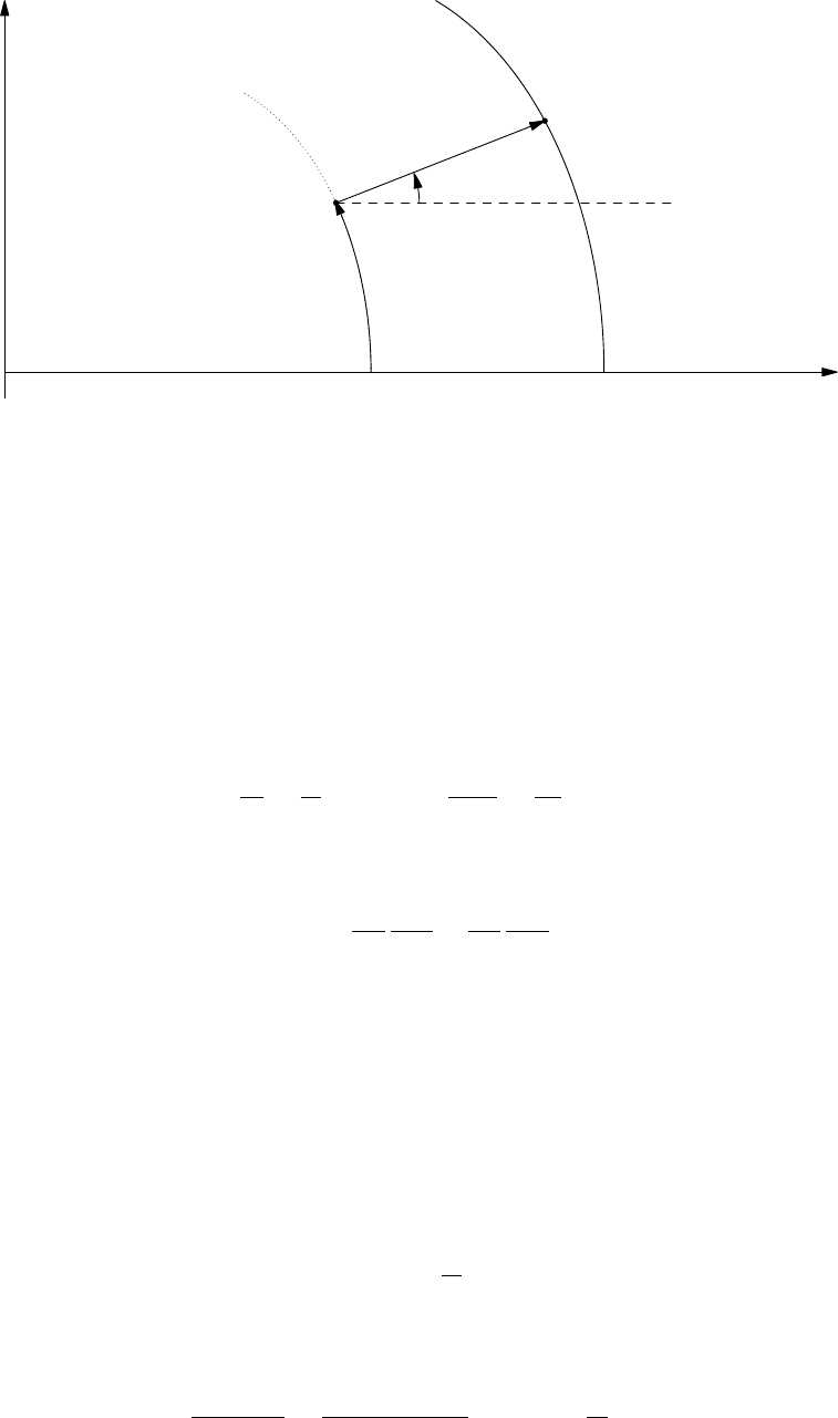
Recall that we have assumed that the coordinates (R, Z) of a each flux-surface are known via a one-
dimensional parameterization (the arc length, for example). As a robust measure of the flux-surface
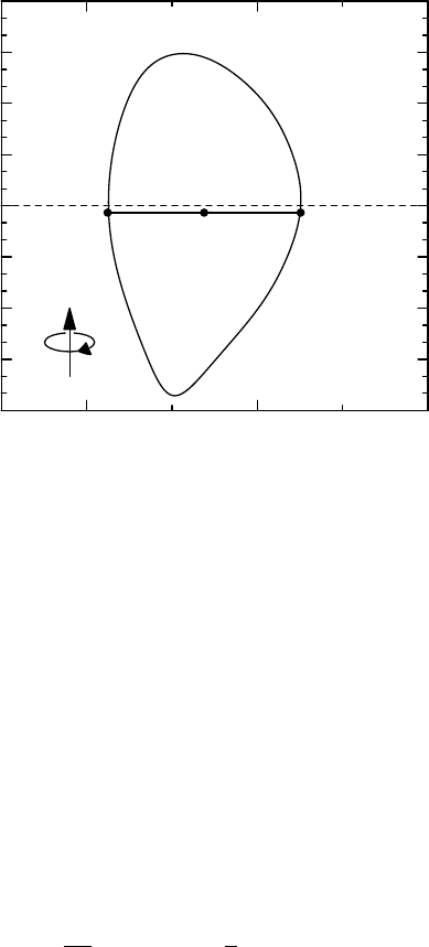
elevation, we use the elevation of the centroid, defined as
Z0.
=IdZ RZ
IdZ R
.(2.25)
In terms of the centroid elevation, the effective minor radius,r, is defined as the half-width of the
flux surface at the elevation, Z0:
r.
=R+−R−
2.(2.26)
The quantities R+and R−are the points of intersection of the flux surface with the line Z=Z0,
as illustrated in Fig. 2.1. We further define the effective major radius,R0= (R++R−)/2, and the
effective field strength,Bunit, as
Bunit .
=1
r
dχt
dr =q
r
dψ
dr .(2.27)
General Atomics Report GA-A26818 5
−120
−90
−60
−30
0
30
60
90
120
Z(cm)
100 200 300
R(cm)
(R−, Z0) (R+, Z0)
(R0, Z0)
r r
ϕ
Z
Figure 2.1: Illustration of the centroid elevation, Z0, the effective major radius, R0, and the effective
minor radius, r, for a near-separatrix flux surface in DIII-D. The orientation of the toroidal angle,
ϕ, is also indicated, such that (R, Z, ϕ) is a right-handed system.
The concept of an effective field was introduced by Waltz [WM99], and represents the equivalent
field that would be obtained if the flux surface was deformed to a circle with the penetrating flux
held fixed. It is emphasized that one must have access to a global equilibrium, not just the local
flux-surface shape, to determine Bunit. An important feature of the unified approach is that the
definitions of rand Bunit are the same in both cases; that is, for both the model Grad-Shafranov
(i.e., Miller) and general Grad-Shafranov equilibria to be defined shortly.
As an alternative to working with the toroidal flux directly, we introduce a function ρ, with
units of length, which parameterizes the toroidal flux:
χt=1
2πZB·dS=1
2Bref ρ(r)2,(2.28)
In the expression above, Bref is some reference field. While this would normally be the vacuum
toroidal field, or something similar, it is important to keep in mind that the choice is ultimately
arbitrary, but by knowing Bref and ρ, one may calculate χt. In terms of ρ, the area enclosed by a
flux surface is approximately given by A'πρ2so long as Bref is approximately equal to the on-axis
toroidal field strength. In this sense, ρis more intuitive, and so in certain cases more convenient,
than χt.
2.3 Local Grad-Shafranov equilibria
The aim of this section is to compute convenient, standardized expressions for the common differ-
ential and integral operators appearing in the drift-kinetic and gyrokinetic equations.
General Atomics Report GA-A26818 6
2.3.1 Required operators
Below we collect, in coordinate-free form, the full set of differential and integral operators which
are to be evaluated. In what follows, Ωca =zaeB/(mac) is the gyroradius of species aand p=
PanakBTais the total plasma pressure.
Perpendicular drift:
vd· ∇⊥=v2
k+v2
⊥/2
ΩcaB2B× ∇B· ∇⊥+4πv2
k
ΩcaB2b× ∇p· ∇⊥+2vkω0
Ωca
b×s· ∇⊥,(2.29)
Perpendicular Laplacian: ∇2
⊥= (∇ − bb · ∇)2,(2.30)
Radial gradient of eikonal: ∇ψ
|∇ψ|· ∇α=∇ψ· ∇ν
|∇ψ|,(2.31)
Binormal gradient of eikonal: b×∇ψ
|∇ψ|· ∇α=−B
|∇ψ|,(2.32)
Parallel gradient: b· ∇ =1
JψB
∂
∂θ ,(2.33)
Flux-surface average: hfi=dV
dψ −1Idθ dϕ Jψf . (2.34)
The perpendicular drift operator, Eq. (2.29), is a sum of curvature and grad-B terms. This par-
ticular form, which neglects the parallel part of the drift response (see, for example, Eq. (54) of
Ref. [HW06] or Eq. (12) of Ref. [BC08]), is sufficient to recover all standard results of gyrokinetic
and neoclassical theory. In Eq. (2.34), hfidenotes the flux-surface average of the function f, and
dV
dψ =Idθ dϕ Jψ,(2.35)
where Vis the volume enclosed by the flux surface. In the drift velocity, sis the following dimen-
sionless vector
s=1
JψB
∂R
∂θ eϕ−I
RB ∇R . (2.36)
which is discussed in more detail later.
2.3.2 Metric coefficients
Define a right-handed Cartesian coordinate system (x, y, z) via intermediate (R, Z, ϕ) coordinates
as
x=R(r, θ) cos(−ϕ),(2.37)
y=R(r, θ) sin(−ϕ),(2.38)
z=Z(r, θ).(2.39)
In this geometry the covariant basis vectors are
ˆ
er.
=∂r
∂r ,ˆ
eθ.
=∂r
∂θ and ˆ
eϕ.
=∂r
∂ϕ ,(2.40)
General Atomics Report GA-A26818 7
where r= (x, y, z). The corresponding contravariant basis vectors are
ˆ
er.
=∇r , ˆ
eθ.
=∇θand ˆ
eϕ.
=∇ϕ . (2.41)
With this information we can write the covariant and contravariant components of the metric tensor
gas gij =ˆ
ei·ˆ
ejand gij =ˆ
ei·ˆ
ej. It is illustrative to write this in matrix form as
gij =
grr grθ 0
grθ gθθ 0
0 0 gϕϕ
,(2.42)
where
grr =∂R
∂r 2
+∂Z
∂r 2
,(2.43)
grθ =∂R
∂r
∂R
∂θ +∂Z
∂r
∂Z
∂θ ,(2.44)
gθθ =∂R
∂θ 2
+∂Z
∂θ 2
.(2.45)
gϕϕ =R2(2.46)
Since we also know that gij ·gij =I, where Iis the identity matrix, we can easily determine the
contravariant counterpart by calculating the inverse of gij. This yields
gij =1
J2
r
gθθgϕϕ −grθgϕϕ 0
−grθgϕϕ grrgϕϕ 0
0 0 grrgθθ −g2
rθ
(2.47)
=
(∇r)2∇r· ∇θ0
∇r· ∇θ(∇θ)20
0 0 (∇ϕ)2
.(2.48)
Here, the Jacobians are
Jr.
=∂(x, y, z)
∂(r, θ, ϕ)=∂ψ
∂r Jψand Jψ.
=∂(x, y, z)
∂(ψ, θ, ϕ),(2.49)
where explicitly
Jr= det gij =R∂R
∂r
∂Z
∂θ −∂R
∂θ
∂Z
∂r >0.(2.50)
Metric coefficients can then be computed straightforwardly. For example,
|∇r|=g1/2
θθ ∂R
∂r
∂Z
∂θ −∂R
∂θ
∂Z
∂r −1
.(2.51)
2.3.3 Mercier-Luc coordinates
Consider a reference flux surface ψ=ψsand the corresponding one-dimensional curve x(`) =
(Rs, Zs) defined by the intersection of that surface and the plane ϕ= 0. If we choose `to be the
arc length along x, then the tangent vector
t.
=dx
d` =dRs(`)
d` ,dZs(`)
d` (2.52)
General Atomics Report GA-A26818 8
Z
R
(Rs, Zs)
(R, Z)
̺
ℓ
u
Figure 2.2: Mercier-Luc coordinate system.
is a unit vector. We can further define the unit tangent and unit (inward) normal vectors in terms
of a frame angle u[Gug77] as
t.
= (−sin u, cos u) and n.
= (−cos u, −sin u).(2.53)
This definition of the frame angle is different than that used in Ref. [MCG+98] and [WM99]. We
believe the present convention is the natural choice, since in the circular limit we have u=θand
`=rθ. The radius of curvature, rc, satisfies the equation
dt
d` =n
rc
so that 1
rc(`)=du
d` .(2.54)
Some algebra shows that the curvature can be written as
rc(θ) = g3/2
θθ ∂R
∂θ
∂2Z
∂θ2−∂Z
∂θ
∂2R
∂θ2−1
.(2.55)
Following Mercier and Luc [ML74], we introduce a right-handed, orthogonal coordinate system
(%, `, ϕ) which is defined in relation to the reference flux surface ψ=ψsthrough
R(r, θ) = Rs(`) + %cos u , (2.56)
Z(r, θ) = Zs(`) + %sin u . (2.57)
The orientations of `and uare shown in Fig. 2.2. The metric tensor in this case is diagonal, with
g%% = 1 ,(2.58)
g`` =1 + %
rc2
,(2.59)
gϕϕ =R2.(2.60)
The Jacobian is
J%=∂(x, y, z)
∂(%, `, ϕ)=1
∇%× ∇`· ∇ϕ=R1 + %
rc>0.(2.61)
General Atomics Report GA-A26818 9
By differentiating Eqs. (2.56) and (2.57) with respect to r, and evaluating the result at %= 0, we
obtain the following identities valid on the surface ψ=ψs:
∂ρ
∂r ψ=ψs
= cos u∂R
∂r + sin u∂Z
∂r ,(2.62)
∂`
∂r ψ=ψs
= cos u∂Z
∂r −sin u∂R
∂r .(2.63)
Differentiation with respect to θyields
∂ρ
∂θ ψ=ψs
= 0 ,(2.64)
∂`
∂θ ψ=ψs
=s∂Z
∂θ 2
+∂R
∂θ 2
=√gθθ .(2.65)
On the surface, the Jacobian is equal to
Jr=R
|∇r|
∂`
∂θ .(2.66)
2.3.4 Solution of the Grad-Shafranov equation
The solution of Grad-Shafranov equation determines the poloidal flux, ψ, as a function of sources
fand p:
R2∇ · ∇ψ
R2=−4πR2p0(ψ)−II0(ψ).(2.67)
The lefthand side can be written as
R2∇ · ∇ψ
R2=∇2ψ−2
R∇R· ∇ψ . (2.68)
We wish to obtain a solution valid in a neighborhood of %= 0 and so expand
ψ=ψs+ψ1(`)%+ψ2(`)%2+··· .(2.69)
The required operators can then be evaluated to leading order in %as
∇R=1
h%
∂R
∂% ˆ
e%+1
h`
∂R
∂` ˆ
e`∼ˆ
e%cos u−ˆ
e`sin u+O(%),(2.70)
∇ψ=1
h%
∂ψ
∂% ˆ
e%+1
h`
∂ψ
∂` ˆ
e`∼ψ1ˆ
e%+O(%),(2.71)
∇2ψ=1
h%h`hϕ∂
∂% h`hϕ
h%
∂ψ
∂% +∂
∂` h%hϕ
h`
∂ψ
∂% ,(2.72)
∼∂2ψ
∂%2+∂ψ
∂%
1
h`hϕ
∂
∂ρ (h`hϕ) + O(%),(2.73)
where hi.
=√gii. Combining these results gives
R2∇ · ∇ψ
R2∼ψ1
rc−ψ1
Rs
cos u+ 2ψ2+O(%).(2.74)
General Atomics Report GA-A26818 10
The solution for ψ1is obtained from
B2
p=|∇ϕ|2|∇ψ|2∼1
R2
s∂ψ
∂ρ 2
+O(%),(2.75)
from which it is evident that
ψ1=RsBps ,(2.76)
where Bps =Bp(ψs). The solution of the Grad-Shafranov equation then gives an explicit expression
for ψ2:
ψ2=1
2Bpcos u−BpR
rc−4πR2p0−II0ψ=ψs
.(2.77)
2.3.5 Magnetic field derivatives
We can start with the exact expressions
B2
p=1
R2"∂ψ
∂% 2
+1
h`
∂ψ
∂` 2#,(2.78)
B2
t=I(ψ)
R2
.(2.79)
Expanding the poloidal flux gives
R2B2
t∼I2
s+ 2%ψ1IsI0
s+O(%2),(2.80)
R2B2
p∼ψ2
1+ 4%ψ1ψ2+O(%2),(2.81)
where Is=I(ψs). Expanding Rand taking derivatives gives
∂
∂%B2
t∼1
R2
s−2I2
s
Rs
cos u+ 2IsI0
sψ1,(2.82)
∂
∂%B2
p∼1
R2
s−2ψ2
1
Rs
cos u+ 4ψ1ψ2.(2.83)
Adding these contributions together gives, finally:
∂
∂%B2∼ −2I2
R3cos u−2B2
p
rc−8πRBpp0!ψ=ψs
.(2.84)
2.3.6 Calculation of the eikonal function
In order to compute radial derivatives required for the evaluation of the drift and Laplacian, we
need to determine the radial dependence of ν. Using the expansion, Eq. (2.69), for the poloidal
flux, together with the eikonal expansion
ν=νs+ν1(`)%+··· ,(2.85)
we solve the equation
∇ν× ∇ψ=f∇ϕ(2.86)
General Atomics Report GA-A26818 11
order-by-order in %. First, an expansion of the gradients yields
∇ψ∼(ψ1+ 2%ψ2)∇%+%∂ψ1
∂` ∇`+O(%2),(2.87)
∇ν∼ν1∇%+∂νs
∂` +%∂ν1
∂` ∇`+O(%2).(2.88)
Replacing these formulae into Eq. (2.86) and dotting with ∇ϕyields
−∂νs
∂` ψ1+%ν1
∂ψ1
∂` −∂ν1
∂` ψ1−2∂νs
∂` ψ2∼Is+%I0
sψ1
Rs+%cos u1 + %
rc.(2.89)
At each order in %, we have
O(1) : −∂νs
∂` ψ1=Is
Rs
,(2.90)
O(%) : −ψ1
∂
∂` ν1
ψ1= 2 ∂νs
∂`
ψ2
ψ1
+I0
s
Rs
+Is
Rsrcψ1−Iscos u
R2
sψ1
.(2.91)
Thus, the solution for νsis
νs(`) = −Z`
0
d`0
R2
sBps
Is.(2.92)
Some additional algebra shows that
ν1(`) = Rs(`)Bps(`)D0(`) + D1(`)II0+D2(`)p0,(2.93)
where the Diintegrals are:
D0=−Z`
0
d`0
R2
sBps 2
rcRsBps −2 cos u
R2
sBps Is(2.94)
D1=−Z`
0
d`0
R2
sBps B2
B2
ps 1
Is
,(2.95)
D2=−Z`
0
d`0
R2
sBps 4π
B2
ps Is.(2.96)
We want to eliminate II0in favour of q0. Writing `(2π).
=L, and expanding Eq. (2.6), we find
−2π(qs+q0
s%ψ1)∼νs(L) + %ν1(L) + O(%2).(2.97)
Therefore, we have the connection
−2π q0
s=D0(L) + D1(L)II0+D2(L)p0.(2.98)
2.3.7 Gyrokinetic drift velocity in Mercier-Luc coordinates
In this case, we work out the dominant part of the drift operator acting on a function f(ψ, θ, α).
This limit is appropriate for standard gyrokinetics. We proceed by simplifying Eq. (2.29) in the
Miller equilibrium case by beginning from the Mercier-Luc representation. On the surface ψ=ψs
we have
Bs=Bps∇`+Is∇ϕ . (2.99)
General Atomics Report GA-A26818 12
Note that Eq. (2.99) cannot be used to obtain ∂B/∂ψ because the limit %→0 has already been
taken. To evaluate ∇B, we must write
∇B=∂B
∂% ∇%+∂B
∂` ∇` , (2.100)
and then make use of Eq. (2.84). Taking the cross product of the above two quantities gives
Bs× ∇B=−Bps
∂B
∂% ∇%× ∇`+Is
∂B
∂% ∇ϕ× ∇%+Is
∂B
∂` ∇ϕ× ∇` . (2.101)
Then, the perpendicular gradient operator, accurate to O(%), can be written as
∇⊥∼ ∇%∂
∂% +∇ϕ+∂νs
∂` ∇`+ν1∇%+O(%)∂
∂α .(2.102)
The final result, valid on the surface ψ=ψs, is
B× ∇B· ∇ =−IsBps
∂B
∂`
∂
∂ψ +−B2
RsBps
∂B
∂% −Isν1
Rs
∂B
∂` ∂
∂α .(2.103)
2.3.8 Perpendicular Laplacian in Mercier-Luc coordinates
To evaluate the perpendicular Laplacian, we square Eq. (2.102) and simplify, where it is sufficiently
accurate to ignore variation of coefficients
∇2
⊥∼∂2
∂%2+ 2ν1
∂
∂%
∂
∂α +"1
R2+ν2
1+∂ν0
∂` 2#∂2
∂α2.(2.104)
2.3.9 Coriolis drift terms
Some algebra show that
b×s· ∇⊥=−sin u∂
∂ρ +I
R2Bp
cos u−ν1sin u∂
∂α ,(2.105)
where we have used the relation
sin u=−∂R
∂θ ∂`
∂θ −1
.(2.106)
2.3.10 Detailed catalogue of shape functions
For convenience, we give a complete summary of the equations needed to compute all the relevant
shape functions. In the expressions below, Rand Zare taken to be functions of rand θ, and the
subscript scan be safely omitted.
∂`
∂θ =s∂R
∂θ 2
+∂Z
∂θ 2
,(2.107)
Jr=R∂R
∂r
∂Z
∂θ −∂R
∂θ
∂Z
∂r ,(2.108)
General Atomics Report GA-A26818 13
|∇r|=R
Jr
∂`
∂θ ,(2.109)
rc(θ) = ∂`
∂θ 3∂R
∂θ
∂2Z
∂θ2−∂Z
∂θ
∂2R
∂θ2−1
,(2.110)
I(r)
Bunit
= 2π r ZL
0
d`0
R|∇r|−1
,(2.111)
Bt(r, θ)
Bunit(r)=I
RBunit
,(2.112)
Bp(r, θ)
Bunit(r)=r
R|∇r|
q,(2.113)
B(r, θ)
Bunit(r)= sgn(Bunit)sBp
Bunit 2
+Bt
Bunit 2
,(2.114)
gsin(r, θ).
=Bt
BR0
B
∂B
∂` ,(2.115)
gcos(r, θ).
=−R0
B
∂B
∂% = gcos1+ gcos2,(2.116)
gcos1(r, θ) = B2
t
B2
R0
Rcos u+B2
p
B2
R0
rc
,(2.117)
gcos2(r, θ) = −1
2
B2
unit
B2R0|∇r|β∗,(2.118)
usin(r, θ) = sin u , (2.119)
ucos(r, θ) = Bt
Bcos u , (2.120)
E1(r, θ)=2Z`(θ)
0
d`0
R|∇r|
Bt
Bpr
rc−r
Rcos u(2.121)
E2(r, θ) = Z`(θ)
0
d`0
R|∇r|B2
B2
p,(2.122)
E3(r, θ) = 1
2Z`(θ)
0
d`0
R
Bt
BpB2
unit
B2
p,(2.123)
f∗(r) = 1
E2(r, 2π)2πqs
r−1
rE1(r, 2π) + β∗E3(r, 2π)(2.124)
Θ(r, θ).
=−RBp
Bν1=RBp
B|∇r|1
rE1+f∗E2−β∗E3(2.125)
Gq(r, θ).
=1
qrB
RBp,(2.126)
Gθ(r, θ).
=JψB
qR0
=B
Bunit
R
R0
1
r|∇r|
∂`
∂θ .(2.127)
General Atomics Report GA-A26818 14
2.3.11 Required operators in terms of shape functions
Perpendicular drift:
vd· ∇⊥=−ikθGq v2
k+µB
ΩcaR0![gcos1+ gcos2+ Θ gsin]
+ikθGq v2
k
ΩcaR0!gcos2− v2
k+µB
ΩcaR0!|∇r|gsin ∂
∂r ,
−ikθGq2vkω0R0
ΩcaR0[ucos + Θ usin] −2vkω0R0
ΩcaR0|∇r|usin ∂
∂r ,(2.128)
Perpendicular Laplacian:
∇2
⊥=|∇r|2∂2
∂r2+ 2iΘkθGq|∇r|∂
∂r −k2
θG2
q1+Θ2,(2.129)
Radial gradient of eikonal: n∇ψ
|∇ψ|· ∇α=−kθGqΘ,(2.130)
Binormal gradient of eikonal: nb×∇ψ
|∇ψ|· ∇α=−kθGq,(2.131)
Parallel gradient: b· ∇ =1
Gθ
1
qR0
∂
∂θ ,(2.132)
Flux-surface average: hfi=Z2π
0
dθ Gθ
Bf(θ)
Z2π
0
dθ Gθ
B
.(2.133)
Above, we have introduced the binormal wavenumber, kθ=i(q/r)∂/∂α.
2.3.12 Pressure-gradient effects in the drift velocity
In cases where compressional magnetic perturbations are neglected, one may also wish to ignore
finite-pressure effects in the drift velocity [WM99]. This is done by setting gcos2= 0 in Eq. (2.128).
General Atomics Report GA-A26818 15
2.4 Specification of the plasma shape
It is assumed throughout that we have access to a global equilibrium for which the poloidal and
toroidal fluxes are known over the entire range of r. Then, we consider two general ways in which
to specify the plasma shape via a closed contour in the (R, Z) plane: (1) a model parameterization,
and (2) a general Fourier expansion.
In addition to the plasma shape, we also need to know the plasma pressure gradient, which we
will define via the effective inverse beta-gradient scale length:
β∗(r).
=−8π
B2
unit
∂p
∂r >0.(2.134)
The safety factor q=dψ/dχtand the magnetic shear s= (r/q)dq/dr can be obtained directly via
numerical differentiation.
2.4.1 Model flux-surface shape
A popular model for the flux-surface shape in (R, Z) coordinates was introduced by Miller [MCG+98].
We generalize that model to include the effects of elevation and squareness. In particular, finite
elevation is required very close to r= 0, where the flux surface may lie entirely above the midplane
at Z= 0. Specifically, let
R(r, θ) = R0(r) + rcos(θ+ arcsin δsin θ),(2.135)
Z(r, θ) = Z0(r) + κ(r)rsin(θ+ζsin 2θ),(2.136)
where κis the elongation, δis the triangularity, ζis the squareness and Z0is the elevation
[TLLM+99]. In order to evaluate the required quantities ∂R/∂r and ∂Z/∂r, we also need to
know the radial derivatives of R0,Z0,δ,κand ζ. To this end, we define the associated shape
functions
sκ.
=r
κ
∂κ
∂r , sδ.
=r∂δ
∂r , sζ.
=r∂ζ
∂r .(2.137)
Note that this definition of sδdiffers slightly from Refs. [MCG+98] and [WM99]. Thus, to compute
the shape functions for the flux-surface at raccording to this model, we require the 10 parameters
R0,dR0
dr , Z0,dZ0
dr , κ, sκ, δ, sδ, ζ, sζ.(2.138)
2.4.2 General flux-surface shape
In this case the flux-surface shape is an expansion of the form
R(r, θ) = 1
2aR
0(r) +
N
X
n=1 aR
n(r) cos(nθ) + bR
n(r) sin(nθ),(2.139)
Z(r, θ) = 1
2aZ
0(r) +
N
X
n=1 aZ
n(r) cos(nθ) + bZ
n(r) sin(nθ).(2.140)
Here, Nis an integer which evidently controls the accuracy of the expansion, and is in principle
arbitrary. If (R, Z) are known as functions of arc length, then one can simply set θ= 2π`/L. To
compute the shape functions for the flux-surface at r, we require the 8(N+ 1) parameters
aR
n, bR
n, aZ
n, bZ
n,daR
n
dr ,dbR
n
dr ,daZ
n
dr ,dbZ
n
dr .(2.141)
General Atomics Report GA-A26818 16

2.4.3 A measure of the error
It is beyond the scope of the present paper to give a detailed assessement of the error in neoclassical
or turbulent transport calculations caused by errors in the flux-surface shape. Nevertheless, we can
define the error in the flux-surface approximation of the discrete data {Ri, Zi}nd
i=1 as
ε.
=1
ndr
nd
X
i=1
min
θq[R(θ)−Ri]2+ [Z(θ)−Zi]2.(2.142)
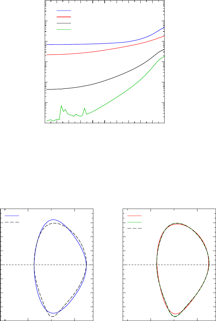
Figure 2.3 shows the flux-surface fitting error for DIII-D discharge 132010. This discharge is part
of a series of experiments designed to accurately measure profiles across the entire confined plasma,
including the edge barrier region. Discharge 132010 is a standard DIII-D H-mode plasma, with
typical values of the magnetic field (Bt= 2.1T), current (Ip= 1.2MA), elongation (κ= 1.8)
and triangularity (δ= 0.3). The width of the edge barrier (∼3% in r/a), height of the edge
barrier (∼11kP a), and global pressure (βN∼2) are all fairly typical of DIII-D H-Modes. The
Grad-Shafranov equillbrium was computed by EFIT using a 129 ×129 mesh, and then mapped to
very-high-resolution (R, Z)-contours (400 flux surfaces, each with 512 points equally-spaced in arc
length along the surface) using the ELITE code. The Miller-type model equilibrium is seen to be
significantly less accurate, according to the metric defined in Eq. 2.142, at all radii than even the
N= 4 Fourier expansion (red curve). The N= 8 (solid black curve) and N= 12 (green curve)
results are also shown. In the region r/a < 0.4, the accuracy of the Fourier expansion probably
exceeds the accuracy of the original equilibrium solution, and is therefore limited by it. This result
shows that N > 12 is probably a good default choice for N. A further comparison of actual flux
surface shapes at r/a = 0.99 (i.e., very close to the separatrix) is shown in Fig. 2.4.
For core plasma parameters, our limited experience is that the difference, with respect to linear
growth rates, between general and model flux-surfaces is insignificant in moderately-shaped DIII-D
plasmas (roughly 5% at r/a = 0.9, and less than that deeper in the core). However, this relies on
the accuracy of the fitting procedure used to obtain the model parameters κ,δ, etc. If the model
flux-surface shape is poorly calculated, the absolute error can be significant.
General Atomics Report GA-A26818 17
10−6
10−5
10−4
10−3
10−2
10−1
100
ε
0 0.1 0.2 0.3 0.4 0.5 0.6 0.7 0.8 0.9 1
r/a
Parameterized
N= 4
N= 8
N= 12
Figure 2.3: Error, ε, in the flux-surface fits for DIII-D discharge 132010. The Miller-type model
equilibrium is seen to be significantly less accurate at all radii than even the N= 4 Fourier expansion
(red curve). The N= 8 (solid black curve) and N= 12 (green curve) results are also shown. In
the region r/a < 0.4, the accuracy of the Fourier expansion probably exceeds the accuracy of the
original equilibrium solution, and is therefore limited by it.
−120
−90
−60
−30
0
30
60
90
120
Z(cm)
100 200
R(cm)
Parameterized
Exact
−120
−90
−60
−30
0
30
60
90
120
Z(cm)
100 200
R(cm)
N= 4
N= 12
Exact
Figure 2.4: Comparison of exact flux-surface (dashed curve) to parameterized (left) and general
Fourier expansion (right) at r/a = 0.99.
General Atomics Report GA-A26818 18
Appendix A: Large-aspect-ratio expansion
Consider a shifted-circle (Shafranov) flux-surface shape:
R(r, θ) = R0+ ∆(r) + rcos θ , (2.143)
Z(r, θ) = rsin θ . (2.144)
Let ∆(r) = ar2/(2R0) be the Shafranov shift, with aan O(1) constant, so that ∂∆/∂r =a(r/R0).
It is instructive to calculate the shape functions as Taylor series in the small parameter r/R0. To
first order in r/R0, we find
|∇r| ∼ 1−ar
R0
cos θ , (2.145)
Bt(r, θ)
Bunit(r)∼1−r
R0
cos θ , (2.146)
Bp(r, θ)
Bunit(r)∼r
qR01−(a+ 1) r
R0
cos θ,(2.147)
B(r, θ)
Bunit(r)∼1−r
R0
cos θ , (2.148)
gsin(r, θ)∼sin θ1−r
R0
cos θ,(2.149)
gcos1(r, θ)∼cos θ−r
R0cos2θ−1
q2,(2.150)
Θ(r, θ)∼sθ −q2R0β∗sin θ+ Θ1
r
R0
,(2.151)
Gq(r, θ)∼1+(a−1) r
R0
cos θ , (2.152)
Gθ(r, θ)∼1 + ar
R0
cos θ . (2.153)
Here, Θ1is the function
Θ1= (1 −2a)sθ sin θ+ sin θ(3a−1)s−2(1 + a) + 1
2(a−3)q2R0β∗cos θ.(2.154)
Since the formulae do not represent an exact Grad-Shafranov equilibrium, but rather an equilibrium
accurate only first order in r/R0, they should not be used for simulation purposes. However, they
can be used to provide a convenient asymptotic check of the numerical routines used to compute
the shape functions in the general case.
Finally, for completeness, we can make contact with the popular s-αequilibrium model [CHT78].
First, recall that
αMHD .
=q2R0β∗=−q2R0
8π
B2
unit
dp
dr .(2.155)
To recover the usual s-αformulae, we must take the limit r/R0→0 in all the expressions above,
except for B, which is taken to be B/Bunit =R0/R. Evidently, the result is not a Grad-Shafranov
equilibrium (not even to first order in r/R0). In practice, simulation results obtained using a
model circular equilibrium (sometimes called a “Miller circle”) can differ significantly from the
corresponding s-αresult. For example, Kinsey [KWC07] has shown that the nonlinear electron
energy flux increases by more than a factor of 1.5 when using a Miller circle instead of s-αgeometry.
General Atomics Report GA-A26818 19
Appendix B: Translation to GS2 Geometry Variables
The normalizing magnetic field in GS2, BT0, is defined as
I(ψ) = RBt.
=RGEOBT0,(2.156)
where RGEO is a reference radius (input). For simplicity, let’s assume that RGEO =R0(this appears
to be a typical choice), in which case we can then relate BT0to Bunit according to
Bunit
BT0
=R0I
Bunit −1
,(2.157)
where I/Bunit is given by Eq. (2.111). Explicitly, we can write this as
Bunit
BT0
=R0
2πr Z2π
0
dθ
R∂R
∂r
∂Z
∂θ −∂R
∂θ
∂Z
∂r ,(2.158)
'κ1 + sκ
2−1
2
dR0
dr
r
R0.(2.159)
Whereas Eq. (2.158) is exact, Eq. (2.159) is approximate and is given here only as an intuitive aid.
In practice the required integral is computed to high accuracy by GYRO and the result available
in the normalized GEO interface variable GEO f. Specifically,
Bunit
BT0
=R0
a
1
GEO f .(2.160)
General Atomics Report GA-A26818 20
Chapter 3
The Gyrokinetic Model
3.1 Foundations and Notation
The definitive works in terms of the complete derivation of the gyrokinetic-Maxwell equations for
evolution of fluctuations, and the neoclassical equations for evaluation of collisional transport, are
due to Sugama and coworkers [SH97,SH98]. For historical reasons, the notation and presentation
here differ in some respects from these papers. Nevertheless, what is documented here should be
completely consistent with the formulae given in Ref. [SH98]. We prefer when applicable to use
Gaussian CGS units1. Roughly speaking, the gyrokinetic approach [AL80,CTB81,FC82] is based
on the assumption that equilibrium quantities are slowly varying, while perturbations are smaller
but more rapidly varying in space. To describe this ordering, it is convenient to introduce the
parameters
cs=rTe
mi
ion-sound speed (3.1)
ρs=cs
Ωci
ion-sound gyroradius (3.2)
where Ωci is the ion cyclotron frequency. The derivation of the gyrokinetic equation proceeds by
expanding the primitive Fokker-Planck equation in the small parameter, ρ∗.
=ρs/a, where ais the
plasma minor radius.
3.2 Reduction of the Fokker-Planck Equation
The details of the derivation of the gyrokinetic (and neoclassical) equations is beyond the scope of
this manual. Still, we attempt to sketch the essential details. The Fokker-Planck equation provides
the fundamental theory for plasma equilibrium, fluctuations, transport. In this section, we use
Sugama’s notation. The FP equations is written as
∂
∂t +v· ∇ +ea
ma(E+ˆ
E) + v
c×(B+ˆ
B)·∂
∂v(fa+ˆ
fa) = Ca(fa+ˆ
fa) + Sa(3.3)
where fais the ensemble-averaged distribution, ˆ
fais the fluctuating distribution, Saare sources
(beams, RF, etc), and
Ca=X
b
Cab(fa+ˆ
fa, fb+ˆ
fb) (3.4)
1See http://wwwppd.nrl.navy.mil/nrlformulary/NRL FORMULARY 06.pdf
21
is the nonlinear collision operator. The general approach is to separate the FP equation into
ensemble-averaged, A, and fluctuating, F, components:
A=d
dtens
fa− hCaiens −Da−Sa,(3.5)
F=d
dtens
ˆ
fa+ea
maˆ
E+v
c׈
B·∂
∂v(fa+ˆ
fa)−Ca+hCaiens +Da,(3.6)
where d
dtens
.
=∂
∂t +v· ∇ +ea
maE+v
c×B·∂
∂v,(3.7)
Da.
=−ea
ma*ˆ
E+v
c׈
B·∂ˆ
fa
∂v+ens
.(3.8)
such that Dais the fluctuation-particle interaction operator. Ensemble averages are expanded in
powers of ρ∗as
fa=fa0+fa1+fa2+. . . , (3.9)
Sa=Sa2+. . . (transport ordering),(3.10)
E=E0+E1+E2+. . . , (3.11)
B=B0.(3.12)
Fluctuations are also expanded in powers of ρ∗as
ˆ
fa=ˆ
fa1+ˆ
fa2+. . . , (3.13)
ˆ
E=ˆ
E1+ˆ
E2+. . . , (3.14)
ˆ
B=ˆ
B1+ˆ
B2+. . . . (3.15)
3.2.1 Lowest-order constraints
The lowest-order ensemble-averaged equation gives the constraints
A−1=0: E0+1
cV0×B= 0 and ∂fa0
∂ξ = 0 (3.16)
where ξis the gyroangle. The only zeroth-order flow (i.e., sonic) flow that persists on the fluctuation
timescale is a purely toroidal flow [HW85], which we write as
V0=V0eϕ=R ω0(ψ)eϕwhere ω0.
=−c∂φ−1
∂ψ .(3.17)
The first-order flow V1contains both toroidal and poloidal components which are self-consistenly
calculated by as moments of the ensemble averaged first-order distribution, fa1(that is, they are
computed within the context of neoclassical theory).
General Atomics Report GA-A26818 22

3.2.2 Equilibrium equation and solution
The gyrophase average of the zeroth order ensemble-averaged equation gives the collisional equi-
librium equation: Z2π
0
dξ
2πA0=0: V0+v0
kb· ∇fa0=Ca(fa0) (3.18)
where v0=v−V0is the deviation from the mean flow velocity. The exact solution for fa0is a
Maxwellian in the rotating frame, such that the centrifugal force causes the density to vary on the
flux surface:
fa0=na(ψ, θ)
(2πTa/ma)3/2exp −ma(v0)2
2Ta=naFMa .(3.19)
It is important to note here that to account for sonic rotation in the equilibrium, we do not
use the shifted Maxwellian approach [WSCH07]. Although the use of a shifted Maxwellian gives
rise to errors which are probably not significant for typical operating parameters, the approach is
conceptually incorrect. Instead, we work in the shifted velocity frame v0=v−V0. The latter
approach was first used in the context of neoclassical transport by Hinton and Wong [HW85].
Beyond this point, we limit our attention to the moderate flow regime, such that ρ∗V0/cs1.
Operationally, this means that we will ignore terms quadratic in V0/cs, whilst retaining all terms
which are linear in V0/cs. Physically, this approach will not capture centrifugal effects like the
poloidal variation of density, since
na(ψ, θ)∼na(ψ) + O(V2
0/c2
s),(3.20)
but will correctly retain the symmetry-breaking effects of radial electric field shear, rotation shear
drive, and the Coriolis drift.
3.2.3 The drift-kinetic equation
Taking a gyroaverage of the first-order ensemble-averaged component A1gives expressions for the
gyroangle-dependent and independent distributions, ˜
fa1and ¯
fa1:
Z2π
0
dξ
2πA1=0: fa1=˜
fa1+¯
fa1,˜
fa1=1
ΩaZξ
dξ
]
Lfa0(3.21)
The function ¯
fa1is determined by the solution of the drift kinetic equation.
3.2.4 The gyro-kinetic equation
The gyroaverage of first-order F1gives an expression for first-order fluctuating distribution, ˆ
fa1, in
terms of the distribution of the gyrocenters, Ha(R):
Z2π
0
dξ
2πF1=0: ˆ
fa1(x) = −eaδφ(x)
Ta
fa0+Ha(R),(3.22)
where x=R+ρis the particle position, ρ=b×v0/Ωca is the gyroradius vector, Ωca =eaB/(mac)
is the cyclotron frequency, and R(Xin Ref. [SH98]) is the guiding-center position. The function
Ha(R) (ha(R) in Ref. [SH98]) is determined by solution of the nonlinear gyrokinetic equation. Also
note that the perturbed potential δφ appears as ˆ
φin Ref. [SH98].
General Atomics Report GA-A26818 23
3.3 The Gyrokinetic Equation in Detail
In what follows, we will drop the prime notation in reference to the velocity coor-
dinates. To bring the gyrokinetic equation into a form convenient for numerical integration, we
introduce the function ha(R):
Ha(R) = eafa0
Ta
Ψa(R) + ha(R) (3.23)
where Ψa(ˆ
ψain Ref. [SH98]) is the following gyrophase average (or, more simply, gyroaverage) at
fixed R:
Ψa(R).
=δφ(R+ρ)−1
c(V0+v)·δA(R+ρ)R
.(3.24)
The gyroaverage can be defined formally as
hz(R, ξ)iR
.
=Idξ
2πz(R, ξ),(3.25)
for any function, z. Also, we note the following identities
b· ∇V0=ω0s(3.26)
b· ∇V0+∇V0·b=I
B∇ω0,(3.27)
where sis the dimensionless vector
s=1
JψB
∂R
∂θ eϕ−I
RB ∇R . (3.28)
We use a form of the gyrokinetic equation which can be obtained, after some rearrangement, from
Eq. (46) of Ref. [SH98].
∂ha
∂t +vkb+vd· ∇Ha+vE0 · ∇ha+δva· ∇ha
+δva·∇fa0+mavkfa0
Ta
I
B∇ω0=CGL
a[Ha].(3.29)
The velocities are
vd.
=v2
k+µB
ΩcaBb× ∇B+2vkω0
Ωca
b×s+4πv2
k
ΩcaB2b× ∇p(3.30)
vE0 .
=c
Bb× ∇φ−1,(3.31)
δva.
=c
Bb× ∇Ψa.(3.32)
In this result, sis a dimensionless vector which is not exactly in the grad-Bdirection. The correct
form of scannot be obtained using the shifted Maxwellian model. This form of the drift matches
Brizard’s result, and the resulting expression for vd· ∇ψmatches the familiar result from Hinton
and Wong [HW85]. By setting ω0= 0, we recover the usual diamagnetic rotation ordering. For
normalization purposes it is useful to note that
Zd3v FMa = 1 .(3.33)
General Atomics Report GA-A26818 24
Various terms can be simplified without refering to the geometry model. Within the accuracy of
the gyrokinetic ordering, we have
vE0 · ∇ha=c
Bb× ∇φ−1· ∇ha∼ω0
∂ha
∂α ,(3.34)
δva· ∇fa0=c
Bb× ∇Ψa· ∇fa0∼c∂fa0
∂ψ
∂Ψa
∂α ,(3.35)
δva· ∇ha=c
Bb× ∇Ψa· ∇ha∼c∂ha
∂ψ
∂Ψa
∂α −c∂ha
∂α
∂Ψa
∂ψ .(3.36)
Using these expression, we find
∂ha
∂t +vk
JψB
∂Ha
∂θ +vd· ∇Ha+ω0
∂ha
∂α +c[ha,Ψa]ψ,α
+c∂fa0
∂ψ +mavk
Ta
I
B
∂ω0
∂ψ fa0∂Ψa
∂α =CGL
a[Ha].(3.37)
The expansion and simplification of the remaining operators has been treated in Chap. 2.
3.3.1 Ordering
We remark that the gyrokinetic ordering requires that
eaΨa
Ta∼ha
fa0∼ω−k⊥·V0
Ωca ∼kkρs∼ρ∗.(3.38)
3.3.2 Rotation and rotation shear parameters
Recalling the definition of the rotation frequency:
ω0.
=−c∂φ−1
∂ψ ,(3.39)
we define the Mach number, the Ershearing rate and the rotation shearing rate respectively as
M.
=ω0R0
cs
,(3.40)
γE.
=−r
q
∂ω0
∂r ,(3.41)
γp.
=−R0
∂ω0
∂r .(3.42)
These parameters are defined in this way for legacy reasons and are not independent; rather, we
have the constraint
γp=R0
qr γE.(3.43)
3.3.3 Comment on the Hahm-Burrell shearing rate
Note that the shearing rate defined in Eq. (3.41) is not in general equal to the familiar Hahm-Burrell
shearing rate [Bur97]
γHB
E
.
=(RBp)2
B
∂
∂ψ Er
RBp,(3.44)
General Atomics Report GA-A26818 25
where Eris the radial electric field
Er.
=−ˆ
er· ∇φ−1=−|∇r|∂φ−1
∂r .(3.45)
In terms of the Miller geometry coefficients, γHB
Ecan be written as
γHB
E=|∇r|
Gq
r
q
∂
∂r c
Bunit
q
r
∂φ−1
∂r =|∇r|
Gq
γE.(3.46)
3.4 Maxwell equations
Defining the scalar electromagnetic fields δAk.
=b·δAand δBk.
=b·∇×δA, we can write an
equation for each of the fields (δφ, δAk, δBk) (see Appendix A, [SH98]). In each case, the species
summation runs over all species a(ions and electrons).
Poisson equation
− ∇2
⊥δφ(x)=4πX
a
ezaδna= 4πX
a
eaZd3vˆ
fa1(x).(3.47)
Parallel Amp`ere’s Law
− ∇2
⊥δAk(x) = 4π
cX
a
δjk,a =4π
cX
a
eaZd3v vkˆ
fa1(x).(3.48)
Perpendicular Amp`ere’s Law
∇⊥δBk(x)×b=4π
cX
a
δj⊥,a =4π
cX
a
eaZd3vv⊥ˆ
fa1(x) (3.49)
The righthand sides can be written in terms of Haaccording to
Zd3vˆ
fa1(x) = −naea
Ta
δφ(x) + Zd3v Ha(x−ρ),(3.50)
Zd3v vkˆ
fa1(x) = Zd3v vkHa(x−ρ) (3.51)
Zd3vv⊥ˆ
fa1(x) = Zd3vv⊥Ha(x−ρ) (3.52)
General Atomics Report GA-A26818 26
3.5 Transport Fluxes and Heating
For each species separately, we define a particle flux, a toroidal angular momentum flux, an energy
flux, and an exchange power density:
Γa(r) = FZd3v H∗
a(R)δva· ∇r , (3.53)
Qa(r) = FZd3v H∗
a(R)δva· ∇r1
2mav2,(3.54)
Πa(r) = FZd3v H∗
a(R)
[maR(V0+v)·eϕ]c
Bb× ∇δφ(x)−1
c(V0+v)·δA(x)· ∇rR
(3.55)
Sa(r) = FZd3v H∗
a(R)ea∂
∂t +V0(x)·∂
∂xδφ(x)−1
c(V0+v)·δA(x)R
(3.56)
3.5.1 Ambipolarity and Exchange Symmetries
By summing the particle fluxes over species and using the Maxwell equations, one can prove the
exact ambipolarity property X
a
ea¯
Γa= 0 ,(3.57)
where an overbar denotes a perpendicular spatial and time average taken in the flux-tube limit.
Similarly, summing the exchange power density over species and using the Maxwell equations, one
can prove the net heating is zero: X
a
¯
Sa= 0 .(3.58)
Note that the time-average is only required to prove the exchange property, not the ambipolarity
property. Both these conditions are in general violated if profile variation is allowed.
3.6 Entropy production
The balance equation for entropy production is given by
σa− F Zd3vH∗
a
fa0
∂Ha
∂t +FZd3vH∗
a
fa0
CGL
a+FZd3vH∗
a
fa0
Dτ+FZd3vH∗
a
fa0
Dr→0,(3.59)
where Dτand Drrepresent the (artificial) upwind dissipation terms added in the numerical dis-
cretization. The function σais
σa.
=1
Lna −3
2
1
LT a Γa+1
LT a
Qa
Ta
+∂ω0
∂r
Πa
Ta
+Sa
1
Ta
.(3.60)
On taking a radial average, and the time-average over sufficiently long times, the sum of terms
should approach zero.
General Atomics Report GA-A26818 27
3.7 Simplified fluxes and field equations with operator notation
3.7.1 Operator notation
It is useful at this point to discuss the general spectral representation of fields and operators. First,
expanding an arbitrary field in a spectral (Fourier) basis gives
z(R).
=X
k⊥
eiS(R)˜z(k⊥),(3.61)
where k⊥=∇⊥S. In this case, the gyrophase dependence in Fourier space is harmonic
z(R+ρ) = X
k⊥
eiS(R)eik⊥·ρ˜z(k⊥),(3.62)
and the gyroaverage becomes
hz(R+ρ)iR=X
k⊥
eiS(R)J0(k⊥ρa) ˜z(k⊥),(3.63)
where ρa.
=v⊥/Ωca. Thus, in real space, the gyroaverage can be represented as a linear operator
G0awhose spectral representation is J0(k⊥ρa).
Now, we can write the field defined in Eq. 3.24 using operator notation. Moreover, we also
define a new field which is useful for calculation of momentum transport coefficients. These are
Ψa(R).
=G0ahδφ(R)−vk
cδAk(R)i+v2
⊥
ΩcacG1aδBk(R),(3.64)
Xa(R).
=G2ahδφ(R)−vk
cδAk(R)i+v2
⊥
ΩcacG3aδBk(R).(3.65)
Although we will construct explicit discrete approximations to the operators G0a,G1aand G2ain
the next chapter, it can be shown that they have the following spectral representations:
G0a→J0(γa),(3.66)
G1a→1
2[J0(γa) + J2(γa)] ,(3.67)
G2a→ − ikxρa
2[J0(γa) + J2(γa)] ,(3.68)
G3a→ikxρa
γ2
a
[J0(γa)−J1(γa)/γa],(3.69)
where γa.
=k⊥ρa, and kxis defined explicitly in Sec. 5.3. The expressions above are adapted
directly from Sugama [SH98]. However, to make use of Sugama’s results, we use the following
identities, where ϕ=eϕ:
k⊥k⊥: (Rˆ
ϕ)(∇ψ) = [k⊥·(Rˆ
ϕ)] [k⊥· ∇ψ],(3.70)
k⊥· ∇ψ=−iRBp|∇r|∂
∂r −q
rGqΘ∂
∂α=RBpkx,(3.71)
k⊥·(Rˆ
ϕ) = −i∂
∂α ,(3.72)
where Eq. (2.102) has been used to expand ∇⊥.
General Atomics Report GA-A26818 28
3.7.2 Maxwell equations: Ha-form
The Maxwell equations are simplest when written in terms of Ha:
Poisson equation
−1
4π∇2
⊥δφ =X
a
ea−naea
Ta
δφ +Zd3vG0aHa(3.73)
Parallel Amp`ere’s Law
−1
4π∇2
⊥δAk=X
a
eaZd3vvk
cG0aHa(3.74)
Perpendicular Amp`ere’s Law
−1
4πδBk=X
a
eaZd3vv2
⊥
ΩcacG1aHa(3.75)
3.7.3 Maxwell equations: ha-form
For time-integration purposes, we will need to write the field equations in terms of ha:
Poisson equation
−1
4π∇2
⊥δφ +X
a
na
e2
a
TaZd3v FMa (1 − G2
0a)δφ
−X
a
na
e2
a
TaZd3v FMaG0aG1a
v2
⊥
ΩcacδBk=X
a
eaZd3vG0aha(3.76)
Parallel Amp`ere’s Law
−1
4π∇2
⊥δAk+X
a
na
e2
a
TaZd3vv2
k
c2FMaG2
0aδAk=X
a
eaZd3vvk
cG0aha(3.77)
Perpendicular Amp`ere’s Law
1
4πδBk+X
a
na
e2
a
TaZd3v FMa v2
⊥
ΩcacG1a2
δBk
+X
a
na
e2
a
TaZd3v FMa
v2
⊥
ΩcacG1aG0aδφ =−X
a
eaZd3vG1a
v2
⊥
Ωcacha(3.78)
3.7.4 Transport coefficients
Some algebra yields the simplifications:
Γa(r) = c
ψ0FZd3v H∗
a(R)∂Ψa
∂α ,(3.79)
Qa(r) = c
ψ0FZd3v H∗
a(R)1
2mav2∂Ψa
∂α ,(3.80)
Πa(r) = c
ψ0FZd3v H∗
a(R)maRV0+vk
Bt
B∂Ψa
∂α +v⊥
Bp
B
∂Xa
∂α ,(3.81)
Sa(r) = c
ψ0FZd3v H∗
a(R)ea∂
∂t +ω0
∂
∂αΨa.(3.82)
General Atomics Report GA-A26818 29
Chapter 4
Normalization of Fields and Equations
4.1 Dimensionless fields and profiles
For consistency, we will use an overbar to denote reference quantities; that is, quantities which are
evaluated at the reference radius, ¯r. Explicitly,
¯
Te=Te(¯r) (4.1)
¯ne=ne(¯r) (4.2)
¯cs=s¯
Te
mi
(4.3)
Here, miis the mass of the main ion species (in practice, this will often be deuterium). Next, we
introduce the normalized fields
ˆ
ha.
=ha
¯neFMa(r)(4.4)
δˆ
φ.
=eδφ
¯
Te
(4.5)
δˆ
Ak.
=¯cs
c
eδAk
¯
Te
,(4.6)
δˆ
Bk.
=δBk
Bunit(r),(4.7)
and the normalized profiles
ˆna(r).
=na(r)
¯ne
,(4.8)
ˆ
Ta(r).
=Ta(r)
¯
Te
,(4.9)
ˆω0(r).
=a
¯cs
ω0(r),(4.10)
ˆγE(r).
=a
¯cs
γE(r),(4.11)
ˆγp(r).
=a
¯cs
γp(r).(4.12)
30
We also have the additional normalized quantities
ˆ
B.
=B(r, θ)
Bunit(r)(4.13)
ˆvka.
=vk
¯cs
(4.14)
For quantities which depend on the magnetic field strength, it is necessary to define unit quan-
tities:
ρs,unit(r) = ¯cs
eBunit(r)/(mic),(4.15)
βe,unit(r) = 8πneTe
B2
unit
.(4.16)
At the reference radius, these are written as ¯ρs,unit and ¯
βe,unit. To measure the radial variation of
Bunit, we introduce the parameter
Gr(r) = Bunit(r)
Bunit(¯r).(4.17)
4.2 Velocity space normalization
4.2.1 Velocity variables
We also use the normalized velocity-space coordinates (ε, λ, ς), defined as
ε=mav2
2Ta
,(4.18)
λ=v2
⊥
v2ˆ
B,(4.19)
ς= sgn(ˆvka).(4.20)
Let us also note the identities
v2
k=v21−λˆ
B,(4.21)
v2
⊥=v2λˆ
B= 2µB . (4.22)
The pair (ε, λ) are unperturbed constants of motion. The sign of the parallel velocity, ς, is required
to separate two populations of trapped particles for each value of λ. With these definitions, the
normalized parallel velocity becomes
ˆvka=±rmi
maq2εˆ
Ta(1 −λˆ
B).(4.23)
4.2.2 Dimensionless velocity-space integration
At this point, we must introduce the dimensionless velocity-space integration operator V[·]
V[z].
=X
ς=±1
1
2√πZ∞
0
dε e−ε√εZ1
0
d(λˆ
B)
p1−λˆ
B
z(R, λ, ε, ς),(4.24)
where ς= sgn (ˆvka) = ±1. It can be verified that V[1] = 1. In writing Eq. (4.24), we explicitly rule
out consideration of non-Maxwellian particle distributions.
General Atomics Report GA-A26818 31
4.3 Dimensionless equations
4.3.1 Normalized gyrokinetic equation
The normalized gyrokinetic equation is
∂ˆ
ha
∂ˆ
t+ˆvka
Gθq(R0/a)
∂ˆ
Ha
∂θ +vd
¯cs·ˆ
∇ˆ
Ha+ ˆω0
∂ˆ
ha
∂α +q¯ρs,unit
rGr
a[ˆ
ha,ˆ
Ψa]r,α
−ˆna
q¯ρs,unit
rGra
Lna
+ (ε−3/2) a
LT a
+maˆvka
miˆ
Ta
BtR
BR0
ˆγp∂ˆ
Ψa
∂α =ˆ
CGL
ahˆ
Hai,(4.25)
where
ˆ
Ha=ˆ
ha+zaαaˆ
Ψa,(4.26)
ˆ
Ψa=G0aδˆ
φ−ˆvkaδˆ
Ak+2ελ ˆ
Ta
zaG1aδˆ
Bk,(4.27)
αa= ˆna/ˆ
Ta,(4.28)
and ea=eza. The inverse gradient scale lengths are defined as
1
Lna
=−1
na
∂na
∂r ,(4.29)
1
LT a
=−1
Ta
∂Ta
∂r .(4.30)
4.3.2 Normalized Maxwell equations
Poisson equation:
−¯
λ2
D∇2
⊥δˆ
φ+X
a
αaz2
aVh1− G2
0aδˆ
φi−2X
a
zaˆnaVhG0aG1aελδ ˆ
Bki=X
a
zaV[G0aˆ
ha].(4.31)
Above, ¯
λDis the Debye length at the reference radius
¯
λD=¯
Te
4π¯nee21/2
.(4.32)
Parallel Amp`ere’s Law
−2¯ρ2
s,unit
¯
βe,unit ∇2
⊥δˆ
Ak+X
a
αaz2
aV[ˆv2
kaG2
0aδˆ
Ak] = X
a
zaV[ˆvkaG0aˆ
ha].(4.33)
We remind the reader that the Amp`ere cancellation problem [CW03] will occur if one attempts to
set V[ˆv2
ka] = 1 rather than evaluate it numerically.
Perperdicular Amp`ere’s Law
G2
r
δˆ
Bk
¯
βe,unit
+ 2 X
a
ˆnaˆ
TaVhG2
1aε2λ2δˆ
Bki+X
a
zaˆnaVhG1aG0aελδˆ
φi=−X
a
ˆ
TaVhG1aελˆ
hai.(4.34)
General Atomics Report GA-A26818 32
4.3.3 Normalized Transport Fluxes
The normalized particle flux is
ˆ
Γa(r) = Γa
¯ne¯cs
=q¯ρs,unit
r GrFV"ˆ
H∗
a
∂ˆ
Ψa
∂α #.(4.35)
The normalized energy flux is
ˆ
Qa(r) = Qa
¯ne¯
Te¯cs
=ˆ
Ta
q¯ρs,unit
r GrFV"ˆ
H∗
a
∂ˆ
Ψa
∂α ε#.(4.36)
The normalized toroidal momentum flux is
ˆ
Πa(r) = Πa
¯nemi¯c2
sa,(4.37)
=ma
mi
q¯ρs,unit
r GrFV"ˆ
H∗
a
R
a(V0
¯cs
+ ˆvka
Bt
B∂ˆ
Ψa
∂α + ˆv⊥
Bp
B
∂ˆ
Xa
∂α )# (4.38)
Finally, the normalized anomalous energy exchange is
ˆ
Sa(r) = Sa
¯ne¯
Te¯cs/a =za
1
Gr
q¯ρs,unit
r GrFVˆ
H∗
a∂
∂ˆ
t+ ˆω0
∂
∂αˆ
Ψa.(4.39)
Above, FVrepresents the flux-surface average of the dimensionless velocity-space integration op-
erator. The discrete respresentation of the product FVwill be described in detail in the next
chapter.
4.3.4 Diffusivities
In terms of the fluxes, we further define a particle diffusivity Daaccording to
Γa=−Da
∂na
∂r ,(4.40)
and an energy diffusivity χaaccording to
Qa=−naχa
∂Ta
∂r .(4.41)
4.3.5 GyroBohm normalization
In GYRO, the output fluxes and diffusivites also carry the so-called gyroBohm normalization. That
is, for output, we use
Γa
ΓGB
where ΓGB .
= ¯ne¯cs(¯ρs,unit/a)2,(4.42)
Πa
ΠGB
where ΠGB .
= ¯nea¯
Te(¯ρs,unit/a)2,(4.43)
Qa
QGB
where QGB .
= ¯ne¯cs¯
Te(¯ρs,unit/a)2,(4.44)
Sa
SGB
where SGB .
= ¯ne(¯cs/a)¯
Te(¯ρs,unit/a)2,(4.45)
χa
χGB
,Da
χGB
where χGB,.
= ¯ρ2
s,unit¯cs/a . (4.46)
General Atomics Report GA-A26818 33
Chapter 5
Spatial Discretization
5.1 Foreword
The original explicit version of GYRO has been partially documented in a previous article [CW03].
This report supercedes that document in all respects. Among many other changes and improve-
ments over [CW03], the current version of GYRO includes
1. the option to treat the fast electron parallel motion implicitly,
2. an improved and simplified treatment of boundary conditions,
3. a fully Arakawa-like nonlinear discretization scheme,
4. a generalization to an arbitrary number of kinetic impurities.
For an exhaustive, chronological list of changes, always refer to the CHANGES file with each
GYRO release.
5.2 Spectral Decomposition in Toroidal Direction
5.2.1 Expansion of fields
We expand the perturbed quantities (δˆ
φ, δ ˆ
Ak, δ ˆ
Bk,ˆ
ha) as Fourier series in α. For example, the
potential is written as
δˆ
φ(r, θ, α) =
Nn−1
X
j=−Nn+1
δφn(r, θ)e−inαeinω0twhere n=j∆n . (5.1)
In GYRO,
Nn→TOROIDAL GRID
∆n→TOROIDAL SEP
The hat is omitted on n-space quantities for brevity. Here, ω0is a suitably-averaged rotation
frequency. In GYRO, this is taken to be the rotation frequency at the domain center. The θ-
periodicity condition (see condition 2, Sec. 2.2.2) requires that
δˆ
φ(r, 0, ϕ +ν[ψ, 0]) = δˆ
φ(r, 2π, ϕ +ν[ψ, 2π]) .(5.2)
34
So, although the physical field, δˆ
φ, is 2π-periodic in θ, the Fourier representation has the implication
that the coefficients, δφn, are nonperiodic, and satisfy the phase condition
δφn(r, 0) = e2πinq(r)δφn(r, 2π).(5.3)
Since δˆ
φis real, the Fourier coefficients satisfy the relation δφ∗
n=δφ−n. The spectral form given in
Eq. (5.1) is
1. (2π/∆n)-periodic in αat fixed (r, θ)
2. (2π/∆n)-periodic in ϕat fixed (r, θ).
5.2.2 Poloidal wavenumber
We choose to define the poloidal wavenumber so that it is a proper flux-surface function:
kθ=nq(r)
r.(5.4)
5.3 Operator Discretization Methods
5.3.1 Finite-difference operators for derivatives
The differential band width in the radial direction is denoted by the parameter id. First and second
derivatives can be discretized using nd-point centered differences, where nd.
= 2id+ 1. These are
Dii0
1(nd,∆x)fi0=1
∆x
id
X
ν=−id
c1νfi+ν,(5.5)
Dii0
2(nd,∆x)fi0=1
(∆x)2
id
X
ν=−id
c2νfi+ν,(5.6)
where
c1ν=X
p6=ν
1
ν−pY
j6=ν,p
(−j)
ν−j,(5.7)
c2ν=X
p6=ν
1
ν−pX
q6=ν,p
1
ν−qY
j6=ν,q,p
(−j)
ν−j.(5.8)
The argument ndin the operators refers to the number of points in the stencil, not the order or
accuracy of the stencil. The formal truncation error for both D1and D2is O(∆x)nd−1; in other
words, these stencils are said to be order-(nd−1) accuracte. A typical case would be nd= 5; that
is, 5-point, 4th-order
5.3.2 Upwind schemes
To construct an arbitrary-order upwind scheme, we begin by writing the centered (nd−1)th deriva-
tive as
Dii0
∗(nd,∆x)fi0=−1
(∆x)nd−1
id
X
ν=−id
(−1)νnd−1
ν+idfi+ν.(5.9)
General Atomics Report GA-A26818 35
The (nd−2)th-order upwind discretization (we will lose one order in accuracy because of the added
dissipation) of an advective derivative is then written as
v∂
∂x →vDii0
1(nd,∆x)−γ|v|Dii0
∗(nd,∆x) where γ.
=|c1id|(∆r)nd−2.(5.10)
The choice above for the dissipation, γ, recovers the usual first, third and higher-order upwind
schemes. For a more complete discussion of the discretization given in Eq. (5.10), see [CW03]. So,
we define a smoothing stencil
Sii0(nd,∆x).
=|c1id|(∆r)nd−2Dii0
∗(nd,∆x).(5.11)
In GYRO, we add an adjustable parameter cto the upwind scheme:
v∂
∂x →vDii0
1(nd,∆x)−c|v|Sii0(nd,∆x),(5.12)
such that c= 1 gives the standard 1st-order and 3rd-order upwind schemes in the case nd= 3 and
nd= 5, respectively.
5.3.3 Banded pseudospectral gyro-orbit integral operators
In this section, we derive explicit forms for the gyroaverage and associated operators which were
introduced in Sec. 3.7.1. The gyroaverage of a function z(x) is defined as
G0az(R) = Z2π
0
dξ
2πz[R+ρa(ξ)] .(5.13)
To perform the loop integral, we write the velocity and gyrovector as
ρa=v⊥
Ωca
(excos ξ+eysin ξ) (5.14)
v⊥=v⊥(exsin ξ−eycos ξ) (5.15)
where ex=∇r/|∇r|and ey=b×ex. Then, we write zin spectral form
z(R) = X
n
nr/2−1
X
p=−nr/2
znp(θ)e2πipr/Le−inα ,(5.16)
z(R+ρa) = X
n
nr/2−1
X
p=−nr/2
znp(θ)e2πipr/Le−inαe2πipρa·∇r/Le−inρa·∇α.(5.17)
We have neglected the θ-variation of the integrand, consistent with the gyrokinetic ordering (i.e.,
low parallel wavenumber). Some algebra shows
ρa· ∇r=v⊥
Ωca |∇r|cos ξ , (5.18)
ρa· ∇α=v⊥
Ωca
(ex· ∇αcos ξ+ey· ∇αsin ξ).(5.19)
In terms of local equilibrium functions, we have
ex· ∇α=−q
rGqΘ,(5.20)
ey· ∇α=−q
rGq.(5.21)
General Atomics Report GA-A26818 36
So, if we define
kx= 2πp|∇r|
L+nq
rGqΘ,(5.22)
ky=nq
rGq(5.23)
with ρa=v⊥/Ωca, then the gyroaveraged potential for a single harmonic becomes
G0a,nzn=
nr/2−1
X
p=−nr/2
znp(θ)e2πipr/Le−inα Z2π
0
dξ
2πei(kxρacos ξ+kyρasin ξ),(5.24)
=
nr/2−1
X
p=−nr/2
znp(θ)e2πipr/Le−inαJ0(k⊥ρa),(5.25)
where k⊥=qk2
x+k2
y. To evaluate the gyroaverage explicitly, we assume that zis known on a
uniform mesh rj=j∆r:
(zn)j=
J−1
X
p=−J
znp e2πiprj/L ,(5.26)
where Lis the radial domain size. The radial domain and boundary conditions are described in
more detail in Sec. 7.1. The Fourier decomposition is easily inverted to yield
znp =1
nr
nr/2−1
X
j=−nr/2
(zn)je−2πiprj/L ,(5.27)
so that
Gjj0
0a,nzj0
n=
J−1
X
p=−J
e2πiprj/LJ0(k⊥ρa)r=rjznp ,(5.28)
where J0is a Bessel function of the first kind, and
k⊥=q(2πp|∇r|/L +kθGqΘ)2+ (kθGq)2.(5.29)
The result gives the pseudospectral forms of the gyroaverage operator:
Gjj0
0a,n =1
nr
nr/2−1
X
p=−nr/2
wj−j0
pJ0(k⊥ρa)r=rj,(5.30)
where indices {j, j0}run from −nr/2 to nr/2−1, and
wp.
= exp(2πip/nr).(5.31)
In terms of normalized quantities,
ρa= ¯ρs,unitrma
mip2εˆ
Taλˆ
B
zaˆ
BGr
(5.32)
General Atomics Report GA-A26818 37
Additional required operators are
(G2)jj0
0a,n =1
nr
nr/2−1
X
p=−nr/2
wj−j0
pJ2
0(k⊥ρa),(5.33)
Gjj0
1a,n =1
nr
nr/2−1
X
p=−nr/2
wj−j0
p
1
2[J0(k⊥ρa) + J2(k⊥ρa)] ,(5.34)
Gjj0
2a,n =1
nr
nr/2−1
X
p=−nr/2
wj−j0
p
i
2kxρa[J0(k⊥ρa) + J2(k⊥ρa)] ,(5.35)
5.3.4 Banded Approximations
The matrix Gjj0
0a,n is diagonally-dominant, such that elements {j, j0}for which |j−j0|> jg, where
jgis some sufficiently large integer, can be neglected. Thus, to convert the operators in Eqs. (5.30)
to banded form, it is enough to set
b
Gjj0
0a,n =(Gjj0
0a,n if |j−j0| ≤ jg
0 if |j−j0|> jg
(5.36)
For n= 0, an additional correction is required. One must ensure that the long-wavelength limit is
asymptotically correct:
G0a,0·1=1.(5.37)
This is accomplished by making a small correction to the diagonal term
b
Gjj
0a,0→b
Gjj
0a,0+ 1 −
j+jg
X
j0=j−jgGjj0
0a,0(5.38)
The size of this correction (the sum above) decreases rapidly as igis increased. We have observed
excellent results using these banded approximations for the various averaging operators, even when
the radial domain is nonperiodic. Physically, the validity of this method relies on the observation
that the numerical contribution to the averages decays rapidly at distances beyond a few gyroradii
from the gyrocenter. For linear benchmarks, when the radial domain is only one period of the
ballooning mode, we generally use full pseudospectral representations.
5.4 Discretization of the gyrokinetic equation
Upon spectral decomposition, the gyrokinetic equation finally takes the form which is solved in
GYRO. We write this symbolically as
∂ha,n
∂ˆ
t−icωθHa,n −icωdHa,n −icωEha,n −icω∗Ψa,n +q¯ρs,unit
rGr
a{ˆ
ha,ˆ
Ψa}=ˆ
CGL
a[Ha,n],(5.39)
where the various toroidal harmonics are given by
Ha,n =ha,n +zaαaΨa,n ,(5.40)
Ψa,n =G0a,n δφn−ˆvkaδAkn+2ελ ˆ
Ta
zaG1a,nδBkn.(5.41)
The Poisson bracket {·,·} is defined in Eq. (5.60) of Sec. 5.4.5, the geometry functions Gθ,Gq, gsin,
gcos and Θ are defined in Sec. 2.3.10, and the profile function Gris defined in Eq. (4.17).
General Atomics Report GA-A26818 38
5.4.1 Parallel motion on an orbit-time grid
The parallel advection term is written
−icωθHa,n =ˆvka
Gθq(R0/a)
Ha,n
∂θ .(5.42)
The presence of field quantities in the definition of Ha,n complicates the matter of poloidal dis-
cretization as we will discuss shortly. Equation (5.42) is subject to short-wavelength instability in
regions where the variation of ˆvka(θ) is sufficiently strong. This property is well-known [Dur99],
and time-explicit schemes must normally include dissipative smoothing if a solution is sought on an
equally-spaced θ-grid. Moreover, at bounce points θb, where vk(θb) = 0, the distribution function
may develop cusps, bringing into question the accuracy of any finite-difference scheme on such a
grid.
This leads us to the observation that the poloidal angle, θ, is a potentially poor variable for
numerical solution of the GK equation. The obvious solution is to remove these cusps analytically
using the normalized orbit time for discretization in the poloidal direction. To this end, define
τ0(λ, θ).
=
Zθ
−θb
Gθ(θ)dθ0
q1−λˆ
B(θ0)
if λ≤1
ˆ
B(π)(trapped) ,
Zθ
−π
Gθ(θ)dθ0
q1−λˆ
B(θ0)
if λ > 1
ˆ
B(π)(passing) ,
(5.43)
where θbis the solution of ˆ
B(θb) = 1/λ.τ0(λ, θ) must be computed numerically for general plasma
equilibria — a tedious but straightforward exercise in numerical analysis. Note that in Eq. (5.43),
and in the rest of this section, we suppress the radial dependence of τ0(λ, r, θ), ˆ
B(r, θ) and Gθ(r, θ)
for brevity.
Next, we introduce a normalized orbit time, τ, which runs from 0 to 2 for a given λand
describes both signs of velocity. In this way τparameterizes the solution on both Riemann sheets
by subsuming the two signs of velocity:
τ(λ, θ).
=(τ0(λ, θ)/¯τfor 0 ≤τ≤1 (ς= 1) ,
2−τ0(λ, θ)/¯τfor 1 < τ ≤2 (ς=−1) ,(5.44)
where ¯τ=τ0(λ, θb) for trapped particles, and ¯τ=τ0(λ, π) for passing particles. The parallel
advection operator is reduced to one with constant velocity
ˆvka
Gθq(R0/a)
Ha,n
∂θ = Ωa(ε, λ)∂Ha,n
∂τ ,where Ωa(ε, λ).
=rmi
ma
1
q(R0/a)p2ˆ
Taε
¯τ.(5.45)
High-accuracy numerical discretization schemes for this form of the equation are well-documented.
Boundary conditions on physical distributions can be stated very simply:
•trapped are periodic on the interval [0,2);
•co-passing are periodic on [0,1);
•counter-passing are periodic on [1,2).
General Atomics Report GA-A26818 39
However, the Fourier representation of Eq. (5.3)] requires that the functions hdescribing the passing
population are not periodic, but subject to phase conditions: h(1) = Ph(0) for co-passing, and
h(2) = Ph(1) for counter-passing. The important result is that as a function of τ, the trapped
distribution will be not only continuous, but also smooth, across bounce points no matter what
order difference scheme is used. The obvious physical interpretation of the location of orbit-time
gridpoints is that they are equally spaced in time, not space, along an orbit. In particular, because
they are highly stagnant near θ=±π, particles close to the trapped-passing boundary benefit from
equal-time spacing.
For finite-nmodes, we write the continuous derivative as the sum of a centered 4th-order 1st
derivative plus a 4th derivative smoother:
Ωa
∂Ha,n
∂τ j
= ΩaDjj0
1(5,∆τ)Hj0
a,n −c|Ωa|Sjj0(5,∆τ)hj0
a,n .(5.46)
The grid spacing for the parallel motion is taken to be ∆τ.
= 2/nτ, and cis a parameter which
measures the amount of numerical disipation. When c= 1 (and Ψa,n = 0) we are left with the
usual third-order upwind method. We have shown previously that in this scheme finite dissipation
is required to give proper Landau damping of n= 0 GAMs [CW03]. Conversely, dissipation-free
schemes suffer from recurrence problems. Note that the dissipation, above, acts on ha,n but not
Ha,n. In fact, attempting to add upwind diffusion to Ha,n (that is, also to fields) will generate
numerical modes with growth rate proportional to the square of the radial box size. The difference
scheme given in Eq. (5.46) is applied only if the species is to be integrated in time explicitly. When
implicit integration is used, we set c= 0.
5.4.2 Ershear
Since we have already shifted to a frame rotating with the mean frequency ¯ω0, the remaining
shearing term is
−icωEha,n =−in [ω0(r)−ω0]ha,n .(5.47)
In a simulation with fixed shearing rate, this can be approximated as
−icωEha,n → −in∂ω0
∂r (r−¯r)ha,n =ikθγE(r−¯r)ha,n .(5.48)
5.4.3 Drift motion
Using the geometry formulae presented in Sec. 2.3.11, we write the drift operator as
−icωdHa,n =−iGqkθ(Rk+R⊥) (gcos1+ gcos2+ Θgsin) Ha,n (5.49)
+iGqkθRkgcos2Ha,n (5.50)
−iGqkθRc(ucos + Θusin) Ha,n (5.51)
− |∇r|(Rk+R⊥)gsin ∂Ha,n
∂r (5.52)
− |∇r|Rcusin ∂Ha,n
∂r ,(5.53)
General Atomics Report GA-A26818 40

where the dimensionless quantities Rk/a,R⊥/a and Rc/a are defined as
Rk
a
.
=v2
k
¯caΩcaR0
=¯ρs,unit
R0
2εˆ
Ta
zaGrˆ
B1−λˆ
B,(5.54)
R⊥
a
.
=µB
¯caΩcaR0
=¯ρs,unit
R0
2εˆ
Ta
zaGrˆ
B λˆ
B
2!,(5.55)
Rc
a
.
=2vkω0R0
¯caΩcaR0
=¯ρs,unit
R0
ma
mi
2ˆvka(ω0R0/¯cs)
zaGrˆ
B.(5.56)
The derivative operator is discretized according to:
gsin a∂Ha,n
∂r i
= gsin Dii0
1(nd,∆r/a)Hi0
a,n −c|gsin|Sii0(nd,∆r/a)hi0
a,n ,(5.57)
where
nd= 2 ×RADIAL DERIVATIVE BAND + 1 (5.58)
5.4.4 Diamagnetic effects
The spectral form of the diamagnetic term is simply
−icω∗Ψa,n =iˆna
kθ¯ρs,unit
Gra
Lna
+ (ε−3/2) a
LT a
+maˆvka
miˆ
Ta
BtR
BR0
ˆγpΨa,n .(5.59)
5.4.5 Poisson bracket nonlinearity
Numerical discretizations of the nonlinear E×Bmotion (including electrstatic, flutter and com-
pressional components) are subject to short-wavelength instabilities. A numerical scheme which
preserves continuous conservation laws for domain-integrated number, energy and enstrophy (and
thereby prevents both instability and a cascade to short wavelengths) was proposed by Arakawa in
1966 [Ara66]. We adapt this scheme to a semi-spectral variant suitable for use with GYRO. First,
let us begin by writing the continuous form of the bracket appearing in the gyrokinetic equation:
{F, G}=∂F
∂α
∂G
∂r −∂G
∂α
∂F
∂r .(5.60)
Eq. (5.60) can be recast into the following alternative but equivalent forms
{F, G}=∂
∂α F∂G
∂r −∂
∂r F∂G
∂α ,(5.61)
and
{F, G}=−∂
∂α G∂F
∂r +∂
∂r G∂F
∂α .(5.62)
The trick, first proposed by Arakawa, is to sum these and divide by 3 to yield
{F, G}=1
3∂
∂α F∂G
∂r −G∂F
∂r +∂
∂r G∂F
∂α −F∂G
∂α +∂F
∂α
∂G
∂r −∂G
∂α
∂F
∂r .(5.63)
General Atomics Report GA-A26818 41
Using the spectral decomposition of the bracket together with the discrete form of the derivative
operator, Dii0
N(∆r/a), gives the final discrete form
{F, G}i
n=1
3X
n0
(n+n0)Fi
n0Dii0
1Gi0
n−n0−Gi
n0Dii0
1Fi0
n−n0
+1
3X
n0
n0Dii0
1Gi0
n−n0Fi0
n0−Fi0
n−n0Gi0
n0.(5.64)
This is the expression used in GYRO. Now, let us assume, in what follows, that the radial domain
is periodic. Deviations from the results below will as a consequence be solely limited to boundary
effects.
Lowest order invariant
The lowest integral invariant, which measures the rate of change of the distribution along the
nonlinear flow, is Zdα Zdr {F, G}=X
i{F, G}i
0= 0 .(5.65)
Using Eq. (5.64), the sum above vanishes for all DNwhich satisfy PiDii0
Nai0= 0 for all vectors a.
Centered-difference formulae of all orders for DNwill satsify this condition.
Higher-order invariants
Some algebra shows that the additional quantities vanish:
Zdα Zdr G {F, G}=X
nX
i
Gi
n{F, G}i
−n= 0 ,(5.66)
Zdα Zdr F {F, G}=X
nX
i
Fi
n{F, G}i
−n= 0 .(5.67)
5.5 Blending-function expansion for fields
Since the distribution function ha,n is computed at a different set of points {θj}for each discrete
value of λ, there is no natural way to solve the Maxwell equations using finite-difference methods
on a fixed poloidal grid. Instead, we adopt a function-space approach, and expand the fields
(δφn, δAkn, δBkn) in series of uniform polynomial blending functions. We will show that basis
functions which incorporate the complex phase conditions [see Eq. (5.3)] at −πand πcan be
constructed from pairs of these blending functions. Equations for the expansion coefficients are
then obtained using the well-known Galerkin method.
In computing the poloidal dependence of the fields, there are a number of separate discretization
effects to consider. Since the fields are sums (integrals in the continuum limit) of distribution
functions, low velocity-space resolution will lead to poor poloidal accuracy — even if the there are
no other sources of discretization error. Conversely, even when a very large number of velocity-space
grids are used, discretization error in the orbit-time integration of ha,n will lead to poor poloidal
accuracy — even if the function-space method of the present section was exact. Thus, achieving an
absolute level of accuracy in the θ-dependence of the fields requires sufficient convergence in both
velocity-space and in orbit-time.
General Atomics Report GA-A26818 42
Examples of blending functions
A finite number of blending functions, Nm(s), are used to provide a basis for the field expansion.
An important feature of the Nm, however, is that they are all translates of a single function N(s),
such that N(s−m) = Nm(s). In practise, we use one of the following three types of blending
functions:
Piecewise linear:
N(2)(s).
=(sif 0 ≤s≤1,
2−sif 1 ≤s≤2.(5.68)
Piecewise quadratic:
N(3)(s).
=
s2/2 if 0 ≤s≤1,
−(3/2) + 3s−s2if 1 ≤s≤2,
(3 −s)2/2 if 2 ≤s≤3.
(5.69)
Piecewise cubic:
N(4)(s).
=
(1/6)s3if 0 ≤s≤1,
(2/3) −2s+ 2s2−(1/2)s3if 1 ≤s≤2,
−(22/3) + 10s−4s2+ (1/2)s3if 2 ≤s≤3,
(1/6)(4 −s)3if 3 ≤s≤4.
(5.70)
Representation of a quasi-periodic function
It remains to construct meaningful set of basis vectors from the prototype blending functions given
above. Let us begin by considering a function z(θ) which is not periodic in θ, but satisfies a phase
condition z(θ+ 2π) = Pz(θ). On the infinite domain (−∞,∞) we can write
z(θ) =
∞
X
m=−∞
cmNm(θ/∆θ),(5.71)
=
nblend
X
m=1
[··· +cm−nblend Nm−nblend +cmNm+cm+nblend Nm+nblend +···],(5.72)
where Nm(θ/∆θ) = N(θ/∆θ−m), ∆θ.
= 2π/nblend, and nblend is the number of basis functions
used to represent one 2π-segment of the function z. The phase condition in θtranslates into an
equivalent phase condition for the blending coefficients themselves; namely cm+nblend =Pcm. The
function zis therefore completely described by the coefficients {c1, . . . , cnblend }and basis functions
{F1, . . . , Fnblend }according to
z(θ) =
nblend
X
m=1
cmFm(θ) where Fm(θ) = N(θ/∆θ−m) + PN(θ/∆θ−m−nblend).(5.73)
In choosing a value of the parameter nblend, one is constrained by the number of points used in
the orbit time discretization, nτ. Given that a passing particle is described by nτ/2 orbit points,
choosing values of nblend larger than nτ/2 will lead to a breakdown of the method since there will
be less than one orbit point per blending function segment. For the simulations presented in this
General Atomics Report GA-A26818 43
-π0π
θ
F1
F2
F3
F4
F5
F6
Figure 5.1: Quadratic basis functions, Fm(θ), for nblend = 6 and phase P=−1.
paper, we have found that nblend = 6 and nτ= 20 are efficient choices. However, we expect that
the simulation of plasmas with strong equilibrium shaping, will require a simultaneous increase of
both nblend and nτ.
Figure 5.1 shows the nblend = 6 quadratic basis functions {F1, . . . , F6}for P=−1. We remark
that since Pis generally a complex number, and is a function of radius, the basis functions are also
complex and functions of radius. Knowing this, we can write the expansion of fields in terms of
the basis functions, with explicit radial dependence indicated, as
δφn(ri, θ) =
nb
X
m=1
˜
φi
mFi
m(θ) (5.74)
δAkn(ri, θ) =
nb
X
m=1
˜
Ai
mFi
m(θ) (5.75)
δBkn(ri, θ) =
nb
X
m=1
˜
Bi
mFi
m(θ) (5.76)
Although the blending expansion coefficients ˜
φand ˜
Adepend on the toroidal mode number n, we
supress this dependence for brevity. A few well-known but important observations concerning the
approximation properties of the linear, quadratic and cubic functions should be stated. In a region
of extremely rapid field variation, the cubic approximation is the least robust — suffering from
overshoot/undershoot oscillations. Conversely, as the fields become progressively smoother, the
linear approximation will give the poorest interpolation accuracy. A further undesireable property
of the linear approximation is its discontinuous first derivative. Although there is no general rule or
obviously best interpolation order for all situations, we find that the piecewise quadratic functions
are sufficiently accurate and robust for all cases studied to date.
General Atomics Report GA-A26818 44
5.6 Velocity-Space Discretization
To solve the Maxwell equations, and to compute the transport fluxes, we will need to develop a
discrete representation of the operator FV. In the present section, we discuss quadrature methods
for evaluation of these operators. Since the techniques which follow apply independently to all
species, we omit species indices for brevity.
5.6.1 Decomposition of FV
Since V[1] = 1, it follows automatically that FV[1] = 1. An equivalent statement of this result is
embodied in the identity
1
2√πZ∞
0
dε e−ε√εZλ∗
0
dλ ¯τIdτ =J0,(5.77)
with λ∗= 1/ˆ
B(r, 0) the maximum possible value of λ, and J0defined in Sec. 2.2.4. Above, we have
used the integral identity
X
σZπ
−π
dθ Gθ(r, θ)Z1/ˆ
B(r,θ)
0
dλ
q1−λˆ
B(r, θ)
=Zλ∗
0
dλ ¯τIdτ . (5.78)
Since the numerical evaluation of integrals of this type will involve separate integration weights in
each of the variables ε,λand τ, it is useful to make the decomposition
FV=Vε×Vλ×Vτ,(5.79)
with factors
Vε[h].
=2
√πZ∞
0
dε e−ε√ε h , (5.80)
Vλ[h].
=1
2J0Zλ∗
0
dλ ¯τ h , (5.81)
Vτ[h].
=1
2Idτ h . (5.82)
These are normalized so that Vε[1] = Vλ[1] = Vτ[1] = 1. The task at hand, now, is the construction
of discrete forms of these operators, and therefore of FV.
5.6.2 Energy Integration
To develop a quadrature method for the energy integral, we split the interval of integration in Vε
— defined in Eq. (5.80) — into two regions: [0, ε∗) and [ε∗,∞), where ε∗is the maximum energy
gridpoint (input). Integration over the first interval is done by changing variables according to
x(ε).
=2
√πZε
0
dε e−ε√ε . (5.83)
We let x0.
=x(ε∗), and evaluate the integral using Gauss-Legendre integration [BF85] over nε−1
points: Zx0
0
dx h[ε(x)] '
nε−1
X
i=1
wih[ε(xi)] .(5.84)
General Atomics Report GA-A26818 45
nε= 4, ε∗= 3.0nε= 6, ε∗= 4.0
i εiwiεiwi
1 0.2924572707 0.2467749375 0.1625303849 0.1130127375
2 1.0404041729 0.3948399000 0.5442466206 0.2283030745
3 2.2531263847 0.2467749375 1.1228428641 0.2713566704
4 3.0000000000 0.1116102251 1.9784353093 0.2283030745
5 3.2361246631 0.1130127375
6 4.0000000000 0.0460117057
Table 5.1: Sample energy abscissae and weights
The abscissae and weights (xi, wi) are the usual Gauss-Legendre ones. Note that we must solve the
nonlinear equations xi=x(εi) for εito obtain the energy gridpoints. With the dominant part of
the energy integration done, we evaluate the remaining, infinite integral according to
2
√πZ∞
ε∗
dε e−ε√ε h(ε)'h(ε∗)2
√πZ∞
ε∗
dε e−ε√ε= (1 −x0)h(ε∗).(5.85)
This gives the final weight 1 −x0at the energy gridpoint ε∗, for a total of nεgridpoints. We remark
that this method has the desireable property
nε
X
i=1
wi= 1 such that ∀i, wi>0.(5.86)
Some sample abscissae and weights are given in Table 5.1 to limited precision (10 significant
digits). Note that it is straightforward to generate these, and thus to enforce the sum in Eq. (5.86),
to machine precision. The abcissae and weights are unique for a given nεand ε∗. Outside of this
section, to avoid ambiguity, we will use index iεand weight w(ε)
iεto refer to energy integration.
5.6.3 λIntegration
The λintegration follows essentially the same strategy as the energy integration, with only minor
differences. First, introduce the integration variable
x(λ).
=1
J0Zλ
0
dλ0¯τ(λ0).(5.87)
Then, then Vλcan be expressed as
Vλ[h] = Z1
0
dx h[x(λ)] .(5.88)
Because his rapidly-varying across the trapped-passing boundary at xt=x(λt), where λt= 1/B(π),
it is wise to split the previous integral into two regions:
Z1
0
dx h[x(λ)] = Zxt
0
dx h[x(λ)] + Z1
xt
dx h[x(λ)] .(5.89)
Gauss-Legendre rules are then applied to each integral separately to determine abscissae and weights
(xi, wi). Then, as before, the equations xi=x(λi) must be inverted numerically to obtain the
gridpoints λi.
General Atomics Report GA-A26818 46

i xiλiwi
1 0.0701916516 0.1353809983 0.1730025988
2 0.3114046777 0.5237287429 0.2768041580
3 0.5526177038 0.7871934230 0.1730025988
4 0.6653193692 0.8581589333 0.1047751790
5 0.8114046777 0.9778736670 0.1676402866
6 0.9574899862 1.1217887702 0.1047751790
Table 5.2: Sample λweights for npass =ntrap = 3.
We emphasize that there is no assumption of continuity across the trapped passing boundary.
In fact, in the collisionless limit, we do not expect the distribution to be continuous there. With
weak collisions, we expect the formation of of a boundary layer around x=xt. In the latter case,
we expect good layer resolution because the Gauss-Legendre scheme puts integration abcissae very
close to (but not on) xt. When combined with the orbit-time grid, the λintegration abcissae
provide the (θ, vk/v) gridpoint distribution shown in Fig. 8.1.
Sample values of abscissae and weights are given in Table 3 for a circular equilibrium with
r/R0= 1/6. Outside of this section, to avoid ambiguity, we will use index iλand weight w(λ)
iλto
refer to pitch-angle integration.
5.6.4 Discretization Summary
Our methods for solution of the Maxwell equations have the implication that it is not Vbut FVfor
which a discrete form is required. But we have already done enough to show that the discretization
takes the form
FV[h]→
nε
X
iε=1
w(ε)
iε
nλ
X
iλ=1
w(λ)
iλ
nτ
X
iτ=1
w(τ)
iτhiεiλiτ,(5.90)
where, so far, no radial discretization has been employed. The τ-weights are simply w(τ)
iτ=
(1/2)∆τ= 1/nτ. The numerical representation of the weights is such that when h= 1, the
sum in Eq. (5.90) is unity to machine precision.
5.7 Connection to Ballooning Modes
In what follows, we limit our discussion to s−αgeometry. Recall the form of a toroidal harmonic
when expanded in a radial Fourier series
δφn(r, θ)e−inα =e−in[ϕ−q(r)θ]X
p
e2πipr/Lδφnp(θ) (5.91)
where L, the radial domain size, is written as a multiple, M, of the natural quantization length,
1/(nq0
0), of the ballooning mode:
L.
=M1
nq0
0
=Mr0
nq0s0
.(5.92)
General Atomics Report GA-A26818 47
So we can write
δφn(r, θ)e−inα =e−in[ϕ−q(r)θ]X
p
e2πipr(nq0
0/M)δφnp(θ),(5.93)
=e−in[ϕ−q(r)θ]X
p
e2πip(nq/M)Φ`
B(θ+ 2πp0).(5.94)
where we have introduced the ballooning potential Φ`
Bvia
δφnp(θ)=Φ`
B(θ+ 2πp0)e2πinq0p/M .(5.95)
This transformation is motivated by the fact that the function δφn(r, θ) is not periodic but instead
satisfies the phase condition in Eq. (5.3). The meanings of p0and `are not yet specified. Writing
p=Mp0+`, and breaking the sum into parts yields
δφn(r, θ)e−inα =e−in[ϕ−q(r)θ]
M−1
X
`=0 X
p0
einq(θ`
B+2πp0)Φ`
B(θ+ 2πp0),(5.96)
=e−inϕ
M−1
X
`=0 X
p0
einq(θ+θ`
B+2πp0)Φ`
B(θ+ 2πp0),(5.97)
where the function Φ`
B(θ) is continuous and bounded over the domain −∞ < θ < ∞. The usual
equation for Φ`
Bcan be obtained by substituting Eq. (5.97) into the gyrokinetic equation, and then
solving for Φ`
Bfor a given value of `on the infinite θ-domain. Here, θ`
B= 2π(`/M ) is the ballooning
angle. In GYRO, we have
M=BOX MULTIPLIER .(5.98)
On a discrete grid, the indices have the following ranges of variation:
p=−nr
2,...,nr
2−1,(5.99)
p0=−nr
2M,..., nr
2M−1,(5.100)
`= 0, . . . , M −1.(5.101)
such that the discrete Fourier transform of the potential is
δφnp(θ) = 1
nr
nr/2−1
X
j=−nr/2
δφn(rj, θ)e−2πipj/nr.(5.102)
In conclusion, over the interval
−πnr
M+ 1≤θ < π nr
M−1,(5.103)
we have the reconstruction algorithm
`= 0 : Φ0
B(θ+ 2πp0) = δφn,Mp0(θ)e−2πinq0p0,(5.104)
`= 1 : Φ1
B(θ+ 2πp0) = δφn,Mp0+1(θ)e−2πinq0p0e−2πinq0(1/M),(5.105)
`= 2 : Φ2
B(θ+ 2πp0) = δφn,Mp0+2(θ)e−2πinq0p0e−2πinq0(2/M),(5.106)
.
.
. (5.107)
`=M−1 : ΦM−1
B(θ+ 2πp0) = δφn,Mp0+M−1(θ)e−2πinq0p0e−2πinq0(M−1)/M .(5.108)
General Atomics Report GA-A26818 48

Chapter 6
Temporal Discretization
The gyrokinetic treatment of electrons is problematic in simulations because of the emergence of
a host of numerical instabilities connected with the discretization of the electron parallel motion.
The presence of the electrostatic and magnetic potentials in the advection term,
∂ˆ
ha
∂ˆ
t+ˆvka
Gθq(R0/a)
∂
∂θ ˆ
ha+zaαaˆ
Ψa+··· (6.1)
for a=egive rise to stability considerations much more troublesome than the simple electron
parallel Courant limit. Physically, the parallel term gives rise to the high-frequency electrostatic
Alfv´en wave [LLHL01] at β= 0. In the slab limit, one can show
ωH=kk
krrmi
me
Ωci .(6.2)
This mode is physically pathological, because the frequency increases indefinitely as medecreases,
and also as krdecreases – that is, as the radial box size grows. While nonzero βprovides a
cutoff, the stable numerical treatment of this term is nontrivial.1To overcome this severe and
intrinsic simulation difficulty, we were persuaded to treat the electron advection implicitly. We
experimented with a variety of implicit-explicit (IMEX) Runge-Kutta (RK) schemes that were
popular in the period 2001-2003 [ARW95,ARS97,PR00,PR02,KC03], settling on an IMEX-SSP
scheme of Pareschi and Russo [PR02].
6.0.1 Reduction to canonical form
For brevity, we suppress the toroidal harmonic index and abbreviate ha,n as ha. With all spatial
operators discretized, the GKM system has the form
˙
ha=e
Ha({ha}, he), a = 1, . . . , nion (6.3)
˙
he=e
He({ha}, he) + He({ˆ
ha}, he),(6.4)
where {ha}=h1, . . . , hnion . In Eqs. (6.3) and (6.4), the use of a tilde on the RHS represents a
nonstiff term, while the absence of a tilde indicates a stiff term. The IMEX-RK schemes are written
for equations in the canonical form
˙y=e
Y(y) + Y(y),(6.5)
1The ability of Eulerian codes to treat this term both accurately and stably has been a major contributor to the
relative success of Eulerian solvers in comparison to their PIC counterparts.
49
with e
Ythe explicit RHS and Ythe implicit RHS. Thus, we have the connection
y={ˆ
ha}
hee
Y="{e
Ha}
e
He#Y=0
He.(6.6)
Now, there is some hidden complexity in how we have written the GKM equations, as the functions
Hdepend on the distribution function hboth directly, and indirectly through the fields. We
emphasize that it is only the fast electron advection term, He, which we wish to (or are able to)
treat implicitly:
He.
=−ˆvke(r, θ, ε)a
qR0Gθ
∂
∂θ hˆ
he−αeδˆ
φ−ˆvkeδˆ
Ak−ελ ˆ
Teδˆ
Bki (6.7)
=−Ω(r, θ, ε)∂τhˆ
he−αeδˆ
φ−ˆvkeδˆ
Ak−ελ ˆ
Teδˆ
Bki,(6.8)
where from this point forward we suggest that the reader consider the object ∂τas a matrix.
6.0.2 IMEX-RK-SSP schemes of Pareschi and Russo
The second-order IMEX schemes we consider can be summarized in Butcher tableau form as
Explicit
0
˜a21 0
˜a31 ˜a32 0
˜w1˜w2˜w3
Implicit
a11
a21 a22
a31 a32 a33
w1w2w3
This notation corresponds to the following explicit evolution equations:
y1=y+ ∆t a11Y1(6.9)
y2=y+ ∆t(˜a21 e
Y1+a21Y1)+∆t a22Y2(6.10)
y3=y+ ∆t(˜a31 e
Y1+ ˜a32 e
Y2+a31Y1+a32Y2)+∆t a33Y3(6.11)
¯y=y+ ∆t
3
X
k=1
˜wke
Yk+ ∆t
3
X
k=1
wkYk.(6.12)
Above, yis the old field vector (time t) and ¯yis the new field vector (time t+ ∆t). In GYRO, we
currently use the SSP2(3,2,2) scheme:
SSP2(3,2,2)
Explicit
0
0 0
0 1 0
0 1/2 1/2
Implicit
1/2
−1/2 1/2
0 1/2 1/2
0 1/2 1/2
Since the diagonal coefficients of the implicit stages are equal, we need to solve the same implicit
system at each stage. It would be good at some point to implement the SSP2(3,3,2) scheme, which
requires the solution of two different implicit problems, but has half the advective Courant limit in
explicit part.
SSP2(3,3,2)
Explicit
0
1/2 0
1/2 1/2 0
1/3 1/3 1/3
Implicit
1/4
0 1/4
1/3 1/3 1/3
1/3 1/3 1/3
General Atomics Report GA-A26818 50

6.0.3 Implementation in GYRO
The complication which arisese when applying these methods to GYRO are connected with the
field solve. For all the so-called SDIRK methods, the implicit equations at each stage have a generic
form. In the present case, at each integrator stage (k= 1,2,3), we are faced with:
(ha)k=ha+ ∆tX
p<k
˜akp(e
Ha)p,(6.13)
(he)k=he+ ∆tX
p<k
˜akp(e
He)p+ ∆tX
p<k
akp(He)p+ ∆t akk(He)k.(6.14)
Because Hedepends on the fields, we must advance the Maxwell equations at each stage before
determining the (he)k. However, we can compute all (ha)kfor a= 1, . . . , nion before solving the
implicit problem. First, solve formally for (he)k:
(he)k= (δhe)k+αe
c0∆tΩ∂τ
1 + c0∆tΩ∂τδˆ
φ−ˆvkeδˆ
Ak−ελ ˆ
Teδˆ
Bkk(6.15)
where (δhe)kis the explicitly-known quantity
(δhe)k=1
1 + c0∆tΩ∂τ
he+ ∆tX
p<k
˜akp(e
He)k+ ∆tX
p<k
akp(He)k
.(6.16)
Now, substitute the analytic expression for (he)kinto the Maxwell equations. This substitution
gives a version of the Maxwell equations that looks like the standard explicit forms, but with added
field terms arising from the second term on the RHS of Eq. (6.15). If we multiply the Maxwell
equations by F∗i
m(θ), and operate with the bounce-velocity summation operator FV(noting that
V V =V), we obtain ∆t-coupled Poisson-Amp`ere equations.
(MP P )ii0
mm0˜
φi0
m0+ (MP B)ii0
mm0˜
Bi0
m0= (SP)i
m+ (IPP)i
mm0˜
φi
m0+ (IPA)i
mm0˜
Ai
m0+ (IPB)i
mm0˜
Bi
m0(6.17)
(MAA)ii0
mm0˜
Ai0
m0= (SA)i
m+ (IAP)i
mm0˜
φi
m0+ (IAA)i
mm0˜
Ai
m0+ (IAB)i
mm0˜
Bi
m0(6.18)
(MBP )ii0
mm0˜
φi0
m0+ (MBB )ii0
mm0˜
Bi0
m0= (SB)i
m+ (IBP)i
mm0˜
φi
m0+ (IBA)i
mm0˜
Ai
m0+ (IBB)i
mm0˜
Bi
m0(6.19)
Here the field matrices are:
(MP P )ii0
mm0=FVF∗i
m(θ(τq))Lii0
P P (θ(τq))Fi0
m0(θ(τq))(6.20)
(MP B)ii0
mm0=FVF∗i
m(θ(τq))Lii0
P B(θ(τq))Fi0
m0(θ(τq))(6.21)
(MAA)ii0
mm0=FVF∗i
m(θ(τq))Lii0
AA(θ(τq))Fi0
m0(θ(τq))(6.22)
(MBB )ii0
mm0=FVF∗i
m(θ(τq))Lii0
BB (θ(τq))Fi0
m0(θ(τq))(6.23)
(MBP )ii0
mm0=FVF∗i
m(θ(τq))Lii0
BP (θ(τq))Fi0
m0(θ(τq))(6.24)
General Atomics Report GA-A26818 51
where
LP P =¯
λ2
D∇2
⊥+αe+
nion
X
a=1
αaz2
aV1− G2
0a(6.25)
LP B =
nion
X
a=1 −2zaˆnaV[ελG0aG1a] (6.26)
LAA =−2¯ρ2
s,unit
¯
βe,unit ∇2
⊥+
nion
X
a=1
αaz2
aV[ˆv2
kG2
0a] (6.27)
LBB =1
¯
βe,unit
+
nion
X
a=1
2ˆnaˆ
TaV[λ2G2
1aε2] (6.28)
LBP =
nion
X
a=1
zaˆnaV[ελG1aG0a].(6.29)
The advection matrices are:
(IP P )i
mm0=αi
eFVF∗i
m(θ(τq))Oi
qq0Fi
m0(θ(τq0))(6.30)
(IP A)i
mm0=−αi
eFVF∗i
m(θ(τq))Oi
qq0Fi
m0(θ(τq0))ˆvke(θ(τq0))(6.31)
(IP B)i
mm0=−αi
eˆ
Ti
eFVF∗i
m(θ(τq))Oi
qq0Fi
m0(θ(τq0))ελ(6.32)
(IAP )i
mm0=αi
eFVˆvke(θ(τq))F∗i
m(θ(τq))Oi
qq0Fi
m0(θ(τq0))(6.33)
(IAA)i
mm0=−αi
eFVˆvke(θ(τq))F∗i
m(θ(τq))Oi
qq0Fi
m0(θ(τq0))ˆvke(θ(τq0))(6.34)
(IAB)i
mm0=−αi
eˆ
Ti
eFVˆvke(θ(τq))F∗i
m(θ(τq))Oi
qq0Fi
m0(θ(τq0))ελ(6.35)
(IBP )i
mm0=1
2αi
eˆ
Ti
eFVF∗i
m(θ(τq))Oi
qq0Fi
m0(θ(τq0))ελ(6.36)
(IBA)i
mm0=−1
2αi
eˆ
Ti
eFVF∗i
m(θ(τq))Oi
qq0Fi
m0(θ(τq0))ˆvke(θ(τq0))ελ(6.37)
(IBB )i
mm0=−1
2αi
e(ˆ
Ti
e)2FVF∗i
m(θ(τq))Oi
qq0Fi
m0(θ(τq0))ε2λ2(6.38)
Next, the source matrices are
(SP)i
m=FVF∗i
m(θ(τq))Hi
P(θ(τq))− FVhF∗i
m(θ(τq))δˆ
hi
e(θ(τq))i(6.39)
(SA)i
m=FVF∗i
m(θ(τq))Hi
A(θ(τq))− FVhˆvke(θ(τq))F∗i
m(θ(τq))δˆ
hi
e(θ(τq))i(6.40)
(SB)i
m=FVF∗i
m(θ(τq))Hi
B(θ(τq))−1
2ˆ
TeFVhελF ∗i
m(θ(τq))δˆ
hi
e(θ(τq))i(6.41)
where
HP.
=
nion
X
a=1
zaG0aˆ
ha(6.42)
HA.
=
nion
X
a=1
zaˆvkG0aˆ
ha(6.43)
HB.
=
nion
X
a=1 −ˆ
TaG∞aˆ
haελ . (6.44)
General Atomics Report GA-A26818 52

In the preceeding expressions, we have omitted the stage number, k, for brevity. The advection
matrix Oqq0is defined as
Oqq0(r, λ, ε).
=1
1 + c0∆tΩ∂τqq0
.(6.45)
We reorganize the equations into a single partitioned system suitable for solution with a direct
sparse solver (the current implementation uses UMFPACK). Solve the system with UMFPACK
(SP,SAand SBneed to be computed at each step).
MP P 0MP B
0MAA 0
MBP 0MBB
˜
φ
˜
A
˜
B
=
SP
SA
SB
+
IP P IP A IP B
IAP IAA IAB
IBP IBA IBB
˜
φ
˜
A
˜
B
(6.46)
6.0.4 Procedural summary
Having precomputed the matrices Mand I, for k= 1,...,3:
1. Evaluate (ha)kusing Eq. (6.13).
2. Evaluate (δhe)kusing Eq. (6.16).
3. Evaluate SP,SAand SBusing Eqs. (6.39) through (6.41), respectively.
4. Solve Eq. (6.46) for ˜
φ,˜
Aand ˜
B.
5. Evaluate (he)kusing Eq. (6.15).
With all stage values, k= 1,2,3, computed, evaluate ¯y= ({¯
ha},¯
he)Tusing Eq. (6.12). Then,
synchronize the fields using an explicit field update.
6.0.5 Time-Integration Considerations
Ad-hoc semi-implicit schemes (for example, first order splitting) are normally a mixed-blessing,
offering improved stability of stiff terms at the expense of accuracy and/or stability loss for the
explicit terms. Higher order splittings can be constructed but are susceptible to a severe accuracy
loss in the stiff limit. The IMEX schemes we describe herein [PR00] are:
•Asymptotic Preserving: the difference scheme is asymptotically correct in the stiff limit.
•Asymptotically Accurate: the explicit integrator retains its order for the limiting differential-
algebraic system in the stiff limit.
•Strong-Stability-Preserving: we recover an SSP-ERK [GST] scheme in the stiff limit.
General Atomics Report GA-A26818 53
Chapter 7
Source and Boundary Conditions
7.1 Radial Domain and Boundary Conditions
GYRO has the option of treating periodic (variously called flux-tube, or local) or nonperiodic
(global) boundary conditions on (δφn, δAkn, hσ,n).
ri= ¯r−L
2+ ∆r(i−1) for i= 1, . . . , nr.(7.1)
where
∆r.
=(L/nrperiodic; BOUNDARY METHOD=1 ,
L/(nr−1) nonperiodic; BOUNDARY METHOD=2 .(7.2)
The central radius, ¯r, is specified by the INPUT parameter RADIUS.
7.1.1 Periodic
Flux-tube boundary conditions effectively eliminate the inner and outer radial boundaries by mak-
ing the quantities periodic in r. For example,
δφn(r1, θ) = δφn(rnr, θ).(7.3)
Use of this boundary condition is very useful for local linear analyses (all the linear results presented
in this report use flux-tubes) and computationally efficient for restricted nonlinear studies. However,
the flux-tube mode of operation is incompatible with variation of the equilibrium profiles.
7.1.2 Nonperiodic
In order to study physical effects associated with profile variation and rotation shear, it is necessary
to abandon flux-tubes and use some type of nonperiodic radial boundary condition. In the design
of nonperiodic end conditions, we have attempted to minimize as much as possible the effect of the
boundaries on the interior dynamics. To this extent, our goal was to construct “benign” rather
than physical end conditions. First, to make the notation less cumbersome, let us write
ra→r1,(7.4)
rbuffer
a→rp,(7.5)
rbuffer
b→rnr−p+1 ,(7.6)
rb→rnr,(7.7)
54
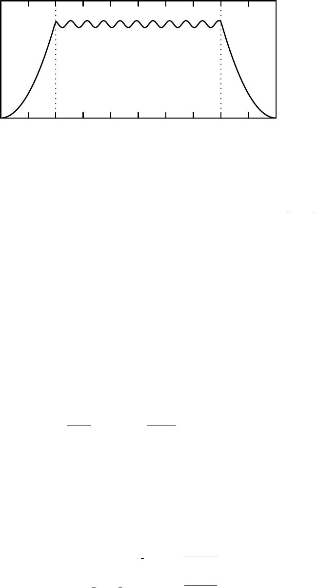
h
rarbuffer
arbuffer
brb
r
Figure 7.1: Illustration of placement of boundary buffer regions.
where the width of the buffer region, p, is set by the input parameter EXPLICIT DAMP GRID. Ex-
perience shows that this number (which is an integer number of gridpoints) should be no smaller
than about 8ρi. GYRO has a diagnostic to warn the user if this condition is not satisfied.
First, at the extreme edges of the computational domain, r=raand r=rb, we impose Dirichlet
boundary conditions on all toroidal harmonics.
ha,n(ra, θ) = δφn(ra, θ) = 0 ,(7.8)
ha,n(rb, θ) = δφn(rb, θ) = 0 .(7.9)
Experience shows that these boundary conditions, in the absence of any other tricks, will give
rise to strong oscillations at the boundaries. The effect of these oscillations will be felt well into
the interior of the computational domain and so various techniques were explored in an effort to
mitigate the corruption of the interior solution. One solution that works well is the imposition of
a “buffer” region; that is, a region near the boundary where we impose an explicit damping on
the n= 0 evolution equation. Generally speaking, we modify the normalized gyrokinetic equation,
Eq. (5.39), according to
∂hσ,0
∂ˆ
t= RHS0−aνσ(r)
¯cs
Hσ,0,(7.10)
where
νσ(r).
=
νbuffer
σif ra≤r≤rbuffer
a,
0 if rbuffer
a< r < rbuffer
b,
νbuffer
σif rbuffer
b≤r≤rb.
(7.11)
An illustration of the effect of this technique on computed fields is given in Fig. 7.1. In GYRO, the
strength of the damping in the buffer is controlled by the following INPUT parameters
EXPLICIT DAMP →aνbuffer
i
¯cs
,(7.12)
EXPLICIT DAMP ELECTRON →aνbuffer
e
¯cs
.(7.13)
General Atomics Report GA-A26818 55
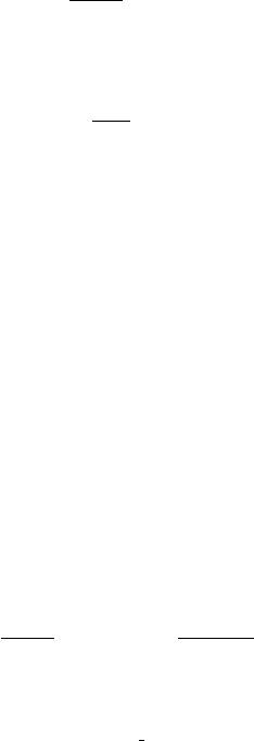
7.2 Long-wavelength Source
One dramatic benefit of flux-tube simulations is that no special techniques are required to keep
the equilibrium from evolving. In this case, the equilibrium is analytically separable from the
fluctuations and there is no coupling between them. In a global simulation there is no such pos-
sibility for separability and short-wavelength radial fluctuations are coupled to long-wavelength
equilibrium-scale dynamics. In this note we propose a method to partially decouple equilibrium
from fluctuations so as to keep the equilibrium profiles from changing.
7.2.1 Formulation of the problem
As in the previous section, we write the n= 0 component of the gyrokinetic equation for fluctuations
as ∂hσ,0
∂ˆ
t= RHS0(r).(7.14)
If the system were periodic in r, we could write the Fourier space expression
∂e
hp
∂ˆ
t=
]
RHSp,(7.15)
where
hσ,0(r) = X
pe
hpe−2πipr/L .(7.16)
Then, in a flux-tube simulation, we would simply set e
h0= 0, which corresponds to zero radial
average of the n= 0 fluctuations. Since the p= 0 equations decouples from the rest of the problem
(the p= 0 component of the E×Bnonlinearity is identically zero), this is allowed. However, in a
global simulation, there is no way to cleanly separate the equilibrium from the fluctuations, because
there is no exact analogue of e
h0.
7.2.2 Solution by damping
Instead of ignoring p= 0 as in a flux-tube simulation, we can instead damp the long-wavelength
components. This will drain, in a nonconservative fashion, any pumping that the equilibrium-
scale distribution receives from nonlinear coupling. In real space, then, we modify the gyrokinetic
equation according to ∂hσ,0
∂ˆ
t= RHS0−aνsource
¯cshhσ,0i,(7.17)
where the angle brackets denote a projection onto long wavelengths only. For example,
hhσ,0(r)i=
N SOURCE+4
X
p=1
cpFp(r).(7.18)
The expansion coefficients satisfy Mpp0cp0=Spwhere
Mpp0=Zrb
ra
dr Fp(r)Fp0(r) and Sp=Zrb
ra
dr hσ,0(r)Fp(r).(7.19)
In GYRO, we take the Fpto be quadratic finite elements. These are defined as scaled translates of
the function N(3) given in Eq. (5.69). We also include partial elements in order to satisfy general
General Atomics Report GA-A26818 56
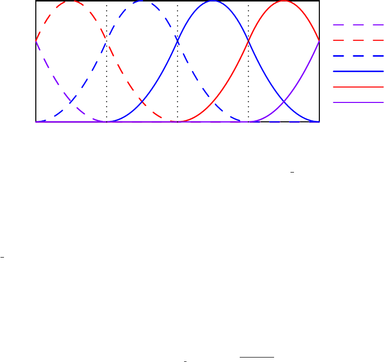
rarb
r
p= 1
p= 2
p= 3
p= 4
p= 5
p= 6
Figure 7.2: Illustration of quadratic finite-element basis for N SOURCE=2. Note that p= 1,2 and
p= 5,6 are partial elements.
nonperiodic boundary conditions, rather than Dirichlet boundary conditions. The reason for doing
this is to most gracefully accomodate the rapid variation of hin the buffer regions. The choice of
N SOURCE is somewhat arbitrary but should be small enough to hold only the longest wavelengths
fixed (i.e., between 1 and 3).
Note that if the time rate of change is slow, ∂t→0, and the steady-state solution for the
long-wavelength component is
hhσ,0(r)i=hRHS0i/νsource ,(7.20)
which can be made arbitrarily small by increasing νsource. In GYRO, the strength of the source is
controlled by
NU SOURCE →aνsource
¯cs
.(7.21)
General Atomics Report GA-A26818 57

Chapter 8
Collisions
8.1 Pitch-angle Scattering Operator
The treatment of collisions in gyrokinetic simulations is not as intricate as that required in neo-
classical simulations. In the former case, the dominant effect of collisions is pitch-angle scattering
in the electron equation. Below we outline the implementation of this effect, and of the associated
ion pitch-angle scattering operators.
Treating the collision operator ˆ
Cby operator splitting leaves us with the following evolution
equation ∂ha,n
∂ˆ
t=ˆ
Cha,n −zaαaˆvkaGaδAk,n.(8.1)
This has the alternative form
∂fa,n
∂ˆ
t+zaαaˆvkaGaδ˙
Ak,n =ˆ
C[fa,n],(8.2)
where
fa,n =ha,n −zaαaˆvkaGaδAk,n .(8.3)
We must take care to avoid the Amp`ere cancellation problem when solving this equation. Fur-
thermore, due to the viscous Courant limit on the timestep imposed by the operator ˆ
Cnear the
trapped-passing boundary, we use an implicit technique. For typical time steps and 8-point pitch-
angle grids, it appears that we are probably very close to the explicit stability limit at νei ∼cs/a.
Multiplying Eq. (8.1) by zaˆvka, summing over species and integrating gives
−2¯ρ2
s,unit
¯
βe,unit ∇2
⊥δ˙
Ak,n +X
a
αaz2
aV[ˆv2
kaG2
aδ˙
Ak,n] = X
a
zaVhˆvkaˆ
C[Gafa,n]i.(8.4)
It is sufficiently accurate to take ˆ
Cto be the pitch-angle scattering operator
ˆ
C= ˆνa
∂
∂ξ (1 −ξ2)∂
∂ξ ,(8.5)
with the corresponding identity
Vhξˆ
Cfi=−2ˆνaV[ξf ].(8.6)
For ions, it is convenient, and probably more realistic physically, to assume that ˆ
Calso conserves
momentum, so that
V[ξˆ
Cf]=0.(8.7)
58
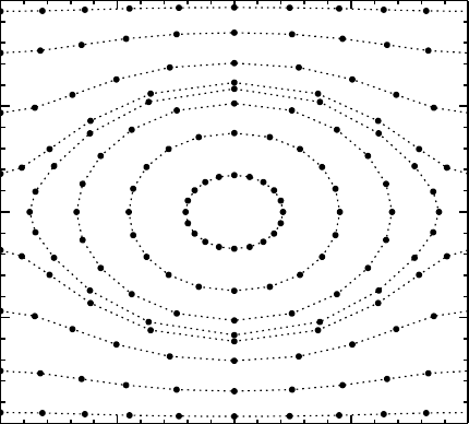
We can write the following equation for ˙
δAk=∂δAk/∂t:
LAδ˙
Ak,n =V2ˆvk,e ˆνefe,n.(8.8)
Then, we solve Eq. (8.2) with a semi-implicit advance
1−ˆ
C∆t¯
fa,n =fa,n −zaαaˆvkaGaδ˙
Ak,n∆t , (8.9)
=ha,n −zaαaˆvkaGa(δAk,n +δ˙
Ak,n∆t).(8.10)
Currently, in GYRO, we set Ga= 1 in the final equation, since the ion collisional effects are weak
and already rather approximate.
8.1.1 The Radial Basis Function (RBF) Method
We are interested in developing a method of function approximation suitable for evaluating differ-
ential and integral operators on an irregular mesh in the (θ, ξ) plane. The mesh itself is determined
by features of the collisionless dynamics and cannot be altered to suit the evaluation of the collision
operator. We will formulate the problem such that the θ-dependence is periodic on the interval
−π≤θ < π. In the ξdomain, there are no boundary conditions (only regularity of the solution)
on the interval −1≤ξ≤1.
−π −π/2 0 π/2 π
θ
-1.0
-0.5
0.0
0.5
1.0
ξ
Figure 8.1: Irregular mesh in the (θ, ξ)-plane.
In reality the functions to be approximated is not in general a periodic function of θ, but rather
satisfied a phase condition of the type f(θ+ 2π) = f(θ)e2πiα. Since it is highly desireable to
approximate a periodic function to eliminate boundary-related headaches, one can instead consider
the associated function g(θ) = f(θ)e−iαθ, which is periodic.
General Atomics Report GA-A26818 59

8.1.2 Basic RBF expansion
We start by briefly describing the basic RBF approximation. Given a function φ(r), r≥0, centers
x1,...,xN, and data fi=f(xi), the basic form of the RBF approximation is
F(x) =
N
X
i=1
ciφ(|x−xi|),(8.11)
where |·|is a positive-definite norm on the vector space of interest. The ciare then chosen so that
F(xi) = fi. Typical RBF choices are
Table 8.1: Typical basis functions
φ(r) name smoothness
r3cubic RBF piecewise smooth
r5quintic RBF piecewise smooth
r2log rthin-plate spline piecewise smooth
p1+(r)2multiquadric infinitely smooth
e−(r)2Gaussian infinitely smooth
In practice, the infinitely smooth RBFs are difficult to use because the associated coefficient
matrices Aij =φ(|xj−xi|) are notoriously ill-conditioned in the limit →0, although theoretically
they are capable of spectral convergence and thus remarkably accurate approximation in this limit.
Testing, nevertheless indicates that the cubic and quintic RBFs are much more robust and therefore
appropriate for the mesh sizes of interest in the collision problem. In one dimension, there is a
simple relationship between cubic and quntic RBFs and cubic and quintic B-splines. Thus, the
remedy for boundary inaccuracy is one that is already known from the theory of spline interpolation.
8.1.3 Influence of boundaries
It is well-known that near boundaries, the accuracy of RBF approximation – like all function
approximation near boundaries – can suffer a significant loss of accuracy, and can lead to stability
problems when used for operator discretization in time-dependent problems. We have indeed
verified that accuracy loss at the boundary is a serious issue in the ξdirection.
Curing the boundary instability problem first requires generalizing somewhat the RBF expan-
sion in Eq. (8.11). We need to allow the locations of the centers to deviate in some cases from the
locations of the fixed mesh points – even allowing them to move outside the simulation domain
−1≤ξ≤1. So, we write
F(x) =
N
X
i=1
ciφ(|x−ˆ
xi|),(8.12)
where as before the ciare chosen so that F(xi) = fi. Mesh points xinear the boundaries at ξ=±1
are moved outside the boundary in an analog of the Super Not-a-Knot (SNaK) approach.
8.1.4 The method in detail
The domain of interest is topologically equivalent to the surface of a cylinder, so there is a natural
the distance function
ri=|x−ˆ
xi|=q2−2 cos(θ−θi)+(ξ−ˆ
ξi)2(8.13)
General Atomics Report GA-A26818 60
For s= 3,5, . . ., we write
φ(ri) = rs
i
.
=R0(θ−θi, ξ −ˆ
ξi;s) (8.14)
∂
∂ξ φ(ri) = srs−2
i(ξ−ˆ
ξi).
=R1(ξ−ˆ
ξi, θ −θi;s) (8.15)
∂2
∂ξ2φ(ri) = rs−4
ihs(s−2)(ξ−ˆ
ξi)2+sr2
ii.
=R2(ξ−ˆ
ξi, θ −θi;s) (8.16)
Lf=∂
∂ξ (1 −ξ2)∂
∂ξ f(θ, ξ) (8.17)
= (1 −ξ2)X
i
ciR1(ξ−ˆ
ξi, θ −θi;s)−2ξX
i
ciR2(ξ−ˆ
ξi, θ −θi;s) (8.18)
.
=X
i
ciL(θ, ξ, θi,ˆ
ξi) (8.19)
Thus, in matrix notation, we can write
(Lf)i=Lijcj=Lij (R−1
0)jkfk.
=Dikfk(8.20)
The matrices are
Lij =L(θi, ξi, θj,ˆ
ξj) (8.21)
(R0)ij =R0(θi−θj, ξi−ˆ
ξj;s) (8.22)
Implementation of the Crank-Nicholson scheme for the equation
∂f
∂t =νLf(8.23)
is then written as
fi(t+ ∆t) = 1−ν∆t
2D−1
ij 1 + ν∆t
2Djk
fk(t) (8.24)
.
=Mikfk(t) (8.25)
In GYRO, we compute and store the matrix Mat start-up, reducing the collision step to a matrix-
vector multiply. The drawback of course is the storage, which is significant for a matrix of this
type.
8.1.5 Additional comments
For a fixed number of meshpoints, the condition number of the matrix (R0)ij grows rapidly. So,
although the method is mathematically correct for s= 3,5,7, . . ., in practice the scheme is probably
limited to s= 3 and 5.
General Atomics Report GA-A26818 61
8.2 Conservative Krook Operator
The operator is an annhiliation term −νf plus a restoring term δC.
Cf =−νf +δC (8.26)
number:FV[F∗
m(θ)δC] = FV[F∗
m(θ)νf].
=S(1)
m(8.27)
momentum:FVF∗
m(θ)vkδC=FVF∗
m(θ)vkνf.
=S(2)
m(8.28)
energy:FV[F∗
m(θ)εδC] = FV[F∗
m(θ)ενf].
=S(3)
m(8.29)
To determine the restoring term, expand
δC =X
m
c1
mFm(θ) + vk(θ)X
m
c2
mFm(θ) + εX
m
c3
mFm(θ) (8.30)
Now we must determine each cmas a function of the Sm.
A11
mm0c1
m0+A13
mm0c3
m0=S(1)
m(8.31)
A22
mm0c2
m0=S(2)
m(8.32)
A31
mm0c1
m0+A33
mm0c3
m0=S(3)
m(8.33)
where
A11
mm0=FVF∗
mF0
m(8.34)
A13
mm0=FVF∗
mεF 0
m(8.35)
A31
mm0=FVF∗
mεF 0
m=A13
mm0(8.36)
A33
mm0=FVF∗
mε2F0
m(8.37)
A22
mm0=FVhF∗
mv2
kF0
mi(8.38)
General Atomics Report GA-A26818 62
Chapter 9
Maxwell Dispersion Matrix
Eigenvalue Solver
9.1 Motivation and Related Work
In high-beta, strongly shaped plasmas like in the National Spherical Torus Experiment (NSTX)
[OKP+00], numerous branches of closely-spaced unstable eigenmodes exist. In our experience,
when modes are closely spaced, it is difficult and time-consuming to resolve the most unstable
mode using the linear initial-value approach. To overcome these and other difficulties encountered
in simulating NSTX plasmas, we have developed a new, more efficient method to compute unsta-
ble linear eigenvalues and eigenvectors. The method is valid for tokamak plasmas with arbitrary
shape, and can retain both the compressional and transverse components of the magnetic pertur-
bation. The new method is a simple extension of the GYRO code [CW03], and reuses the existing
discretization schemes in both real and velocity space. Existing methods for solving the linear gy-
rokinetic eigenvalue problem fall into two general categories: gyrokinetic eigenvalue solvers, which
use an iterative approach to compute eigenvalues of the relatively large gyrokinetic response matrix
[KMJ08,Bas09], and field dispersion-relation solvers, which compute the zeros of the much smaller
dielectric matrix using a direct method. The former solvers are too expensive for routine linear
analysis and are not discussed further. On the other hand, there are numerous examples in the
literature of the latter method, the earliest and still one of the most capable being due to Rewoldt
[RTC82]. Certain solvers distinguish themselves with a particular capability: for example, global
capability [FVV03] or the ability to compute stable eigenmodes [Sug99]. The present solver is
unique in that all the linear physics capabilities of GYRO can be retained, including pitch-angle
collisions (although at significantly increased computational expense), global effects (since the bal-
looning transform is not used), finite plasma rotation, general plasma shape and compressional
magnetic perturbations. The solver is also parallelized, with all costly matrix operations (LU de-
composition, inverse, matrix-matrix multiply) implemented fully in BLAS and LAPACK. A typical
collisionless electromagnetic eigenvalue and eigenvector can be computed at standard resolution in
about 5 seconds on a single 2.66GHz core.
63
9.2 The Linearized Gyrokinetic Equation
Just as in the initial-value formulation of the nonlinear gyrokinetic equation, here we expand
fluctuating quantities in Fourier series, for example
Ψa=X
n
e−inαΨa,n .(9.1)
We remark that because of the symmetry properties of the equations, it is natural to label toroidal
eigenmodes with kθρsrather than n, where kθ.
=nq/r. For a single toroidal harmonic, the gyroki-
netic equation is written symbolically as
∂ha,n
∂t −i(ωθ+ωd+ωC)Ha,n −iω∗(eaf0a
Ta
Ψa,n) = 0 (9.2)
where ωθ,ωdand ωCare differential operators:
−iωθ=vk(b· ∇θ)∂
∂θ ,(9.3)
−iωd=−in(vd· ∇α)+(vd· ∇r)∂
∂r ,(9.4)
−iωC=−νa
2
∂
∂ξ 1−ξ2∂
∂ξ ,(9.5)
−iω∗=ivta
akθρaa
Lna
+v2
2v2
ta −3
2a
LT a .(9.6)
9.3 Construction of the Dispersion Matrix
The Laplace transform [Zay96] of a function f(t), which we assume to be differentiable on (0,∞),
is
e
f(s).
=Lf=Z∞
0
f(t)e−stdt (9.7)
whenever the integral exists for at least one value of s. In the present case, the integral will converge
for s > s0, where s0is the maximum linear growth rate. The inversion formula is given by the
Bromwich integral
f(t).
=L−1e
f=1
2πi Zc+i∞
c−i∞e
f(s)estds , 0<t<∞.(9.8)
It will be convenient to use the variable ω=is in subsequent formulae. Now, it is then easy to
show that
e
Ha(ω) = LHa,n =1
ω+ωθ+ωd+ωC
iha(0) + ω−ω∗
ω+ωθ+ωd+ωCeaf0a
Tae
Ψa,(9.9)
where e
Ψa=LΨa,n. Upon substitution into the Laplace transform of the Maxwell equations, we
are left with a system of the form
Mσσ0(ω)Φσ0(ω) = Sσ(ω) (9.10)
General Atomics Report GA-A26818 64
where σand σ0are field indices which run from 1 to 3. The field matrix and source are given by
Mσσ0(ω) = δσσ0Lσ−X
a
e2
a
TaZd3v f0aGσa ω−ω∗
ω+ωθ+ωd+ωC
Gσ0a,(9.11)
Sσ(ω) = X
a
eaZd3v Gσa 1
ω+ωθ+ωd+ωC
iha(0) .(9.12)
We have defined the additional 3-index vectors:
Φ1,Φ2,Φ3.
=e
δφ, g
δAk,g
δBk,(9.13)
L1, L2, L3.
= −1
4π∇2
⊥+X
a
e2
a
TaZd3v f0a,1
4π∇2
⊥,−1
4π!,(9.14)
G1a, G2a, G3a=G0a,−vk
cG0a,v2
⊥
ΩcacG1a.(9.15)
In what follows, we will refer to M(ω) as the Maxwell dispersion matrix. The roots of the equation
det M(ω) = 0 correspond to the normal modes of the system. When the velocity integrals are
taken along the real velocity axes, the integrals used to compute Mdefine a function of sanalytic
in region s > 0, which corresponds to the upper-half ω-plane. This means that unstable modes can
be readily computed using the same (real) velocity discretization as in the initial-value problem.
Calculation of stable normal modes, on the other hand, would require analytic continuation of
M(ω) into the lower half-plane, Im(s)≤0, by deformation of the contour in velocity space, or
perhaps by numerical analytic continuation.
The numerical implementation of the eigenvalue solver, which employs the existing GYRO
spatial discretization methods, is described in detail in the Appendix. Here, we remark that the
size of the final matrix problem is small, with rank(M) = nσnrnb, with nσthe number of fields,
nrthe number of radial gridpoints, and nbthe number of poloidal finite elements. For a basic
electrostatic case, this can be as small as rank(M) = 24. The dominant cost is therefore not
computing det M(ω), but rather computing the inverse P−1, where Pis the matrix representation
of the propagator P=ω+ωθ+ωd+ωC.
9.4 Discretization and Implementation in LAPACK
The spatial discretization of the differential operators required for construction of the Maxwell field
matrix follows precisely the same approach as for the GYRO initial-value solver, with the various
stencils and quadrature methods discussed in detail in Ref. [CW03]. The velocity-space variables
in GYRO are
λ.
=Bunit
v2
⊥
Bv2and ε.
=mav2
2Ta
(9.16)
Fluctuating quantities are evaluated on a species-independent mesh with radial nodes {ri}nr
i=1,
pitch-angle nodes {λk}nλ
k=1, energy nodes {εµ}nε
µ=1 and orbit-time nodes {τm}nτ
m=1. The gyroaverage
of the effective potential e
Ψa, for species a, has the discrete representation
(e
Ψa)µ
ikm =X
i0σ
Gσaµ
ii0kmΦσ
i0km ,(9.17)
General Atomics Report GA-A26818 65
where the three-potential Φσat the same point in configuration space is given by the complex
Galerkin representation
Φσ
ikm =X
j
cσ
ijFij (θkm).(9.18)
Here, cσ
ij are the so-called blending coefficients, and Fij the basis functions defined in Sections 5.2
and 5.3 of Ref. [CW03]. The propagator has the matrix form
Paµ
ii0kk0mm0=ωδii0kk0mm0+ (ωθ)aµ
ikmm0δii0kk0+ (ωd)aµ
ii0kmδmm0kk0+ (ωC)aµ
ikk0mm0δii0.(9.19)
We can write the nonadiabatic distribution e
Hain terms of the inverse of the propagator as
e
Ha
fMa !aµ
ikm
=eana
Ta
(P−1)aµ
ii0kk0mm0(ω−ωaµ
∗i0k0m0)X
σ
Gσaµ
i0i00k0m0X
j
cσ
i00jFi00 j(θk0m0).(9.20)
Constructing the Galerkin projections of all three Maxwell equations, using the technique described
in Section 5.3 of Ref. [CW03], yields the matrix equation
Mσσ0
ii0jj0cσ0
i0j0=hAσ
ii0jj0δσσ0−Bσσ0
ii0jj0(ω)icσ0
i0j0= 0 ,(9.21)
where
Aσ
ii0jj0=X
km
F∗
ijkmLσ
ii0kmF∗
i0j0km (9.22)
and
Bσσ0
ii0jj0(ω) = X
aµ X
i000km X
i00k0m0
e2
ana
Ta
wµ
kmF∗
ijkmGσaµ
ii000km(P−1)aµ
i000i00 kk0mm0(ω−ωaµ
∗i00k0m0)Gσ0aµ
i00i0k0m0Fi0j0k0m0
(9.23)
=X
aµ X
p,p0
Uaµ
qp (P−1)aµ
pp0Vaµ
p0q0(9.24)
=Bσσ0
qq0.(9.25)
Here, the weights wµ
km are the products of the energy, pitch-angle and orbit-time weights defined
in Eq. (72) of Ref. [CW03]. In terms of these weights, the flux-surface average of the velocity-space
integration is written as
FZd3vfMaΨa→X
kmµ
wµ
km(Ψa)µ
ikm with X
kmµ
wµ
km = 1 .(9.26)
In addition, we have defined the lumped indices p= (i000, k, m), p0= (i00, k0m0), q= (i, j, σ) and
q0= (i0, j0, σ0). High performance is achieved by computing the inverse P−1using the LAPACK
routines ZGETRF (LU decomposition) followed by ZGETRI (inverse), with the subsequent matrix
triple-product UP −1Vevaluated using two sequential calls to the BLAS ZGEMM kernel. Finally,
det(M) is computed by the formula
det(M) = ±Y
q
Lqq (9.27)
where Lis the lower-triangular matrix returned by the ZGETRF factorization. The upper (lower)
sign is taken if an even (odd) number of row permutations were made in the factorization.
General Atomics Report GA-A26818 66
Acknowledgements
This work was supported by the U.S. Department of Energy under DE-FG02-95ER54309.
67
Bibliography
[AL80] T. Antonsen and B. Lane. Kinetic equations for low frequency instabilities in inhomo-
geneous plasmas. Phys. Fluids, 23:1205, 1980.
[Ara66] A. Arakawa. Computational design for long term numerical integration of the equations
of fluid motion: Two-dimensional incompressible flow. J. Comput. Phys., 1:119, 1966.
[ARS97] U.M. Ascher, S.J. Ruuth, and R.J. Spiteri. Implicit-explicit runge-kutta methods
for time-dependent partial differential equations. Applied Numerical Mathematics,
25:151–167, 1997.
[ARW95] U.M. Ascher, S.J. Ruuth, and B.T. Wetton. Implicit-explicit methods for time-
dependent pdes. SIAM J. Numer. Anal., 32:797–823, 1995.
[Bas09] E.M. Bass. Bull. Am. Phys. Soc., 54:344, 2009.
[BC08] E.A. Belli and J. Candy. Kinetic calculation of neoclassical transport including self-
consistent electron and impurity dynamics. Plasma Phys. Control. Fusion, 50:095010,
2008.
[BF85] R.L. Burden and J.D. Faires. Numerical Analysis. Prindle, Weber and Schmidt,
Boston, 1985.
[BHD08] E.A. Belli, G.W. Hammett, and W. Dorland. Effects of plasma shaping on nonlinear
gyrokinetic turbulence. Phys. Plasmas, 15:092303, 2008.
[BKC+84] C.M. Bishop, P. Kirby, J.W. Connor, R.J. Hastie, and J.B. Taylor. Ideal MHD bal-
looning stability in the vicinity of a separatrix. NF, 24:1579, 1984.
[Bur97] K.H. Burrell. Effects of E×Bvelocity shear and magnetic shear on turbulence and
transport in magnetic confinement devices. Phys. Plasmas, 4:1499, 1997.
[CHT78] J.W. Connor, R.J. Hastie, and J.B. Taylor. Shear, periodicity and plasma balloning
modes. Phys. Rev. Lett., 40:396, 1978.
[CPC+03] Y. Chen, S.E. Parker, B.I. Cohen, A.M. Dimits, W.M. Nevins, D. Schumaker, V.K.
Decyk, and J.N. Leboeuf. Simulations of turbulent transport with kinetic electrons
and electromagnetic effects. Nucl. Fusion, 43:1121, 2003.
[CTB81] P.J. Catto, W.M. Tang, and D.E. Baldwin. Ion transport in toroidally rotating toka-
mak plasmas. Plasma Phys., 23:639, 1981.
[CW03] J. Candy and R.E. Waltz. An Eulerian gyrokinetic-Maxwell solver. J. Comput. Phys.,
186:545, 2003.
68
[DHCS91] W.D. D’haeseleer, W.N.G. Hitchon, J.D. Callen, and J.L. Shohet. Flux coordinates
and magnetic field structure. Springer-Verlag, Berlin, 1991.
[DJKR00] W. Dorland, F. Jenko, M. Kotschenreuther, and B.N. Rogers. Electron temperature
gradient turbulence. Phys. Rev. Lett., 85:5579, 2000.
[Dur99] D.R. Durran. Numerical methods for wave equations in geophysical fluid dynamics.
Springer-Verlag, New York, 1999.
[FC82] E.A. Frieman and L. Chen. Nonlinear gyrokinetic equations for low-frequency electro-
magnetic waves in general plasma equilibria. Phys. Fluids, 25:502, 1982.
[FVV03] G.L. Falchetto, J. Vaclavik, and L. Villard. Global-gyrokinetic study of finite βeffects
on linear microinstabilities. Phys. Plasmas, 10:1424, 2003.
[GC81] J.M. Greene and M.S. Chance. Nucl. Fusion, 21:453, 1981.
[GST] S. Gottlieb, C.-W. Shu, and E. Tadmor. Strong stability preserving high order time
discretization methods. SIAM Review, 43:97.
[Gug77] H.W. Guggenheimer. Differential Geometry. Dover, New York, 1977.
[HW85] F.L. Hinton and S.K. Wong. Neoclassical ion transport in rotating axisymmetric
plasmas. Phys. Fluids, 28:3082, 1985.
[HW06] F.L. Hinton and R.E. Waltz. Gyrokinetic turbulent heating. Phys. Plasmas, 13:102301,
2006.
[KC03] C.A. Kennedy and M.H. Carpenter. Additive runge-kutta schemes for convection-
diffusion-reaction equations. Applied Num. Math, 44:139, 2003.
[KK58] M.D. Kruskal and R.M. Kulsrud. Equilibrium of a magnetically confined plasma in a
toroid. Phys. Fluids, 1:265, 1958.
[KMJ08] M. Kammerer, F. Merz, and F. Jenko. Exceptional points in linear gyrokinetics. Phys.
Plasmas, 15:052102, 2008.
[KWC07] J.E. Kinsey, R.E. Waltz, and J. Candy. The effect of plasma shaping on turbulent
transport and E×B shear quenching in nonlinear gyrokinetic simulations. Phys. Plas-
mas, 14:102306, 2007.
[LLHL01] W.W. Lee, J.L.V. Lewandowski, T.S. Hahm, and Z. Lin. Shear Alfv´en waves in
gyrokinetic plasmas. Phys. Plasmas, 8:4435, 2001.
[MCG+98] R.L. Miller, M.S. Chu, J.M. Greene, Y.R. Lin-liu, and R.E. Waltz. Noncircular, finite
aspect ratio, local equilibrium model. Phys. Plasmas, 5:973, 1998.
[ML74] C. Mercier and N. Luc. Technical report, Commission of the European Communities,
Report No. EUR-5127e 140, Brussels, 1974.
[OKP+00] M. Ono, S.M. Kaye, Y.-K.M. Peng, G. Barnes, W. Blanchard, M.D. Carter,
J. Chrzanowski, L. Dudek, R. Ewig, D. Gates, R.E. Hatcher, T. Jarboe, S.C. Jardin,
D. Johnson, R. Kaita, M. Kalish, C.E. Kessel, H.W. Kugel, R. Maingi, R. Majeski,
J. Manickam, B. McCormack, J. Menard, D. Mueller, B.A. Nelson, B.E. Nelson,
General Atomics Report GA-A26818 69
C. Neumeyer, G. Oliaro, F. Paoletti, R. Parsells, E. Perry, N. Pomphrey, S. Ramakr-
ishnan, R. Raman, G. Rewoldt, J. Robinson, A.L. Roquemore, P. Ryan, S. Sabbagh,
D. Swain, E.J. Synakowski, M. Viola, M. Williams, J.R. Wilson, and NSTX Team.
Exploration of spherical torus physics in the nstx device. Nucl. Fusion, 40:557, 2000.
[PR00] L. Pareschi and G. Russo. Implicit-explicit runge-kutta schemes for stiff systems of
differential equations. In L. Brugnano and D. Trigante, editors, Recent Trends in
Numerical Analysis, pages 269–289. Nova Science, 2000.
[PR02] L. Pareschi and G. Russo. High order asymptotically strong-stability-preserving meth-
ods for hyperbolic systems with relaxation. In Hyperbolic problems: Theory, Numerics,
Applications. Springer, 2002.
[RTC82] G. Rewoldt, W.M. Tang, and M.S. Chance. Electromagnetic kinetic toroidal eigen-
modes for general magnetohydrodynamic equilibria. Phys. Fluids, 25:480, 1982.
[SH97] H. Sugama and W. Horton. Neoclassical electron and ion transport in toroidally
rotating plasmas. Phys. Plasmas, 4:2215, 1997.
[SH98] H. Sugama and W. Horton. Nonlinear electromagnetic gyrokinetic equation for plas-
mas with large mean flows. Phys. Plasmas, 5:2560, 1998.
[Sug99] H. Sugama. Damping of toroidal ion temperature gradient modes. Phys. Plasmas,
6:3527, 1999.
[TLLM+99] A.D. Turnbull, Y.R. Lin-Liu, R.L. Miller, T.S. Taylor, and T.N. Todd. Improved mag-
netohydrodynamic stability through optimization of higher order moments in cross-
section shape of tokamaks. Phys. Plasmas, 6:1113, 1999.
[WM99] R.E. Waltz and R.L. Miller. Ion temperature gradient turbulence simulations and
plasma flux surface shape. Phys. Plasmas, 6:4265, 1999.
[WSCH07] R.E. Waltz, G.M. Staebler, J. Candy, and F.L. Hinton. Gyrokinetic theory and simu-
lation of angular momentum transport. Phys. Plasmas, 14:122507, 2007.
[XMJ+08] P. Xanthopoulos, D. Mikkelsen, F. Jenko, W. Dorland, and O. Kalentev. Verification
and application of numerically generated magnetic coordinate systems in gyrokinetics.
Phys. Plasmas, 15:122108, 2008.
[Zay96] A. Zayed. Handbook of Function and Generalized Function Transformations. CRC
Press, Boca Raton, 1996.
General Atomics Report GA-A26818 70
