Instructions F61

User Manual:

Open the PDF directly: View PDF .
Page Count: 29

Nuclear Magnetic Resonance F61/F62

Manual 2.0, april 14, 2010

R. Schicker, Phys. Inst., Philosophenweg 12, 69120 Heidelberg

Prerequisites:

The knowledge of the following physical concepts is required for F61/F62:

•Classical mechanics: angular momentum, torque

•Electrodynamics: Magnetic dipole, interaction magnetic dipole with mag-

netic ﬁeld, magnetization, precession, Larmor frequency, Helmholtz coils, Biot-

Savart law

•Thermodynamics: Fermi-Dirac statistic, Boltzmann statistic

•Quantum mechanics: Perturbation theory

The physics lab experiment F61/F62 is organized into three parts. The measure-

ments of the ﬁrst two parts are carried out with a Bruker minispec p20 apparatus

whereas the third part is measured with a newer Bruker minispec mq7.5 model. The

experimental program of F61 and F62 is identical. Due to the organization of this

lab experiment into three parts with two Nuclear Magnetic Resonance analyzers,

F61 starts monday whereas the starting day of F62 is wednesday.

The three parts of this experiment are the following:

•Measurement of relaxation times

The spin-lattice relaxation time T1and the spin-spin relaxation time T2are

measured. The spin-spin relaxation time is measured by the spin echo as well

as by the Carr-Purcell method.

•Measurement of chemical shift

The chemical shift of protons is measured and used to identify ﬁve diﬀerent

substances.

•Imaging measurements in one and two dimensions

Nuclear Magnetic Resonance techniques are used for imaging measurements

in one and two dimensions. The ﬂow of oil in sand is measured as a time de-

pendent process in one dimension. Two dimensional measurements are carried

out to map the inner volume of substances which contain oil or water.

Contents

1 Basics of Nuclear Magnetic Resonance 4

2 NMR Signal 7

2.1 Hardware . . . . . . . . . . . . . . . . . . . . . . . . . . . . . . . . . 7

2.2 Signal generation . . . . . . . . . . . . . . . . . . . . . . . . . . . . . 7

2.3 Calibration high frequency pulses . . . . . . . . . . . . . . . . . . . . 7

3 Part I: Relaxation time 9

3.1 Bloch equations . . . . . . . . . . . . . . . . . . . . . . . . . . . . . . 9

3.2 Spin-spin relaxation T2by spin echo method . . . . . . . . . . . . . 9

3.3 Spin-spin relaxation T2by Carr-Purcell sequence . . . . . . . . . . . 12

3.4 Spin-lattice relaxation T1. . . . . . . . . . . . . . . . . . . . . . . . 12

3.5 Measurements of relaxation times . . . . . . . . . . . . . . . . . . . . 13

3.5.1 Measurement T2by spin echo method . . . . . . . . . . . . . 13

3.5.2 Measurement T2by Carr-Purcell sequence . . . . . . . . . . . 14

3.5.3 Measurement T1. . . . . . . . . . . . . . . . . . . . . . . . . 14

3.6 Systematics of relaxation times . . . . . . . . . . . . . . . . . . . . . 14

4 Part II: Chemical shift 15

4.1 Measurement chemical shift . . . . . . . . . . . . . . . . . . . . . . . 16

5 Part III: Imaging with NMR 18

5.1 One dimensional imaging . . . . . . . . . . . . . . . . . . . . . . . . 18

5.1.1 Frequency coding . . . . . . . . . . . . . . . . . . . . . . . . . 18

5.1.2 Phase coding . . . . . . . . . . . . . . . . . . . . . . . . . . . 19

5.1.3 One dimensional imaging measurements . . . . . . . . . . . . 20

5.1.4 One dimensional data display . . . . . . . . . . . . . . . . . . 21

5.1.5 One dimensional measurements . . . . . . . . . . . . . . . . . 21

5.2 Two dimensional imaging . . . . . . . . . . . . . . . . . . . . . . . . 22

5.2.1 Slice selection . . . . . . . . . . . . . . . . . . . . . . . . . . . 22

5.2.2 Two dimensional Fourier method . . . . . . . . . . . . . . . . 22

5.2.3 Two dimensional imaging measurements . . . . . . . . . . . . 23

5.2.4 Two dimensional data display . . . . . . . . . . . . . . . . . . 24

5.2.5 Two dimensional measurements . . . . . . . . . . . . . . . . . 25

6 NMR applications 25

A Appendix A: Minispec p20 Electronic Unit 26

B Appendix B: Minispec p20 Magnet 27

List of Figures

1 Proton magnetic dipole moment in external ﬁeld ~

B0. . . . . . . . . 4

2 Ground state magnetization ~

Malong ~

B0. . . . . . . . . . . . . . . . 5

3 Magnetization Mkand M⊥. . . . . . . . . . . . . . . . . . . . . . . . 5

4 Precession of M⊥around ~

B0. . . . . . . . . . . . . . . . . . . . . . . 6

5 High frequency pulse along x-direction. . . . . . . . . . . . . . . . . . 6

6 Dephasing of transverse magnetization M⊥. . . . . . . . . . . . . . . 10

7 Pulse sequence 900-1800with τ=10 ms. . . . . . . . . . . . . . . . . 11

8 Carr-Purcell sequence with τ=10 ms. . . . . . . . . . . . . . . . . . . 12

9 Pulse sequence 1800-900with τ=20 ms. . . . . . . . . . . . . . . . . 13

10 Chemical shifts δiof compounds relative to TMS. . . . . . . . . . . . 15

11 Five substances for identiﬁcation. . . . . . . . . . . . . . . . . . . . . 16

12 Timing diagram for the two dimensional Fourier method. . . . . . . 23

13 The p20 electronic unit. . . . . . . . . . . . . . . . . . . . . . . . . . 26

14 The p20 magnet. . . . . . . . . . . . . . . . . . . . . . . . . . . . . . 28

Printer utilities

The display of the data is done with LabVIEW in all three parts of the experiment.

Two printers are available for printing the LabVIEW front panels:

•fplaserjet: This black and white printer is located in the same room.

•schiele (og2): This printer is a color printer and is located at the other end of

the hallway in the small room with the copy machine.

The LabVIEW programs display the data on graphics panels. You can save the

display of a panel in encapsulated postscript format (eps) in the following way:

•right click on the panel which you want to save

•click on “Export Simpliﬁed Image”, left click “Encapsulated Postscript (.eps)”

•left click on the folder symbol next to the empty string ﬁeld, ﬁnd the folder

where you want to save the ﬁle and specify the ﬁle name, click “OK”.

•click “Save”, the ﬁle now exists in the speciﬁed folder. You can view the

contents of the ﬁle by double clicking on it.

1 Basics of Nuclear Magnetic Resonance

Nuclear Magnetic Resonance (NMR) techniques are based on the fact that nuclei

with spin J unequal zero possess a magnetic dipole moment

~µ = ¯hγ ~

J(1)

The quantity γis called the gyromagnetic ratio of the nucleus. In the following, we

restrict the discussion to the case of protons for which

γP roton = 2.6752 ·108sec−1T esla−1(2)

The magnetic dipole ~µ interacts with an external magnetic ﬁeld ~

∆E=−~µ ·~

B0(3)

This interaction results in a parallel µ+or antiparallel µ−orientation of the proton

magnetic dipole in the external ﬁeld ~

B0.

Figure 1: Proton magnetic dipole moment in external ﬁeld ~

B0.

A macroscopic sample containing N protons will populate the parallel and anti-

parallel state with occupation numbers N+and N−where N=N++N−. The

occupation numbers N+and N−follow Dirac statistics, but can here be approxi-

mated by a Boltzmann distribution

N±=N0e−E0±∆E

kt (4)

Here, N0is a normalization factor. The parallel state is energetically favorable,

hence N+>N−. The surplus of protons in the parallel state leads to a macroscopic

magnetization ~

The magnetization can be calculated as the sum of magnetic dipole moments per

unit volume:

M=1

~µi=1

V(N+−N−)|~µ|~ez(5)

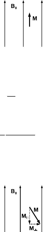
Figure 2: Ground state magnetization ~

Malong ~

B0.

This sum can be evaluated and yields

M=µN

Vsinh(µB/kT )~ez(6)

For weak ﬁelds (µB<< kT), which is the case here, the sinh function (sinus hyper-

bolicus) can be expanded and the law of Curie follows:

M=N

¯h2γ2I(I+ 1)

3kT ~

B0∼~

B0/T (7)

The macroscopic state characterized by a magnetization ~

Mparallel to the external

magnetic ﬁeld ~

B0as shown above minimizes the energy.

In general, the magnetization can have an arbitrary direction relative to the external

ﬁeld.

Figure 3: Magnetization Mkand M⊥.

The magnetization ~

Mshown in Fig. 3 represents a macroscopic state diﬀerent

from the ground state. This state will therefore dissipate its excitation energy and

reach the ground state asymptotically on a characteristic time scale. For further

discussion, the magnetization ~

Mis decomposed into components Mkparallel and

M⊥perpendicular to the external ﬁeld. In particular, Mkcan be antiparallel to the

external ~

B0ﬁeld.

The interaction between the external magnetic ﬁeld ~

B0and the magnetization ~

as expressed by eq. 3 results in a torque ~τ acting on the magnetization.

~τ =~

M∧~

B0(8)

Inserting the components Mkand M⊥into eq. 8 results in the torque acting only

on M⊥. Without relaxation processes, the rate of change of M⊥is given by

M⊥

dt =−γ~

M⊥∧~

B0(9)

The quantity d~

M⊥

dt is perpendicular to ~

M⊥and ~

B0, hence it follows that ~

M⊥precesses

around ~

B0. The angular frequency ωis called the Larmor frequency ωL.

Figure 4: Precession of M⊥around ~

B0.

By inserting an Ansatz ~

M= (M⊥cos(ωLt), M⊥sin(ωLt),0) into eq. 9, the Larmor

frequency ωLis deduced as

ωL=γB0(10)

A magnetization M⊥perpendicular or Mkantiparallel to ~

B0can be generated by

applying a high frequency pulse to the ground state magnetization ~

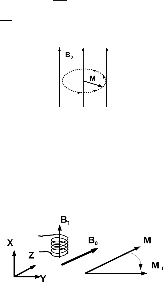
Figure 5: High frequency pulse along x-direction.

Consider the situation as shown in Fig. 5 above. The external static magnetic ﬁeld

B0is pointing in z-direction. A coil is oriented along the x-direction. Applying a

sinusoidal voltage of frequency ωHF on the coil results in a solenoidal magnetic ﬁeld

B1which is longitudinally polarized along the x-direction. Setting up the equations

of motion it can be shown that the ground state magnetization ~

Mprecesses around

the x-axis during the high frequency pulse. During a time interval ∆tthe angle α

of precession is given by

α=γB1∆t(11)

If the time interval is chosen such that α=900, then the ground state magnetization ~

is rotated into a perpendicular component M⊥along the y-axis. Such a pulse is called

a 900pulse. Similarly, the time interval of the high frequency pulse can be chosen

such that the ground state magnetization ~

Mis rotated by α=1800. The resulting

magnetization is then antiparallel to the static ﬁeld ~

B0.

2 NMR Signal

2.1 Hardware

Make yourself familiar with the hardware by reading Appendix A and B. Remove

the styrofoam shielding of the magnet and have a look inside.

2.2 Signal generation

The probes are located within the volume of the coil shown in Fig. 5 when the glass

tubes are inserted into the magnet (see Fig. 14 of Appendix B). The high frequency

pulses of frequency ωHF are generated in the electronic unit shown and explained in

Appendix A. A transverse magnetization M⊥precesses around ~

B0with the Larmor

frequency ωL. The diﬀerence between ωHF and ωLis on the order of a few hundred

Hertz and is called the working frequency. Note that ωHF is of ﬁxed value whereas

the Larmor frequency ωLcan be changed by turning the screw W1 of the magnet as

explained in Appendix B. Due to the precession of M⊥, the magnetic ﬂux through

the coil is modulated by the Larmor frequency. The coil therefore generates an

induction signal of this frequency which is fed back to the electronic unit. This

coil signal is subsequently mixed with the high frequency signal ωHF . The mixing

generates two signals, one with a frequency of the sum and one with the frequency

of the diﬀerence, ie the working frequency. The corresponding signal of the working

frequency is available for analysis.

2.3 Calibration high frequency pulses

Before you can start with the measurements you need to deﬁne Puls I and Puls II

as 900and 1800pulse, respectively.

Find the box with the label duplexer which is sitting on the table above the elec-

tronics unit. This duplexer box has three connections:

•Signal in/Puls out: This cable connects the duplexer box with the connector

C illustrated in the Appendix B of the magnet.

•Signal out: This cable transmits the signal induced in the coil back to the

electronic unit.

•Puls in: This connector takes the high frequency pulse of the electronic unit.

Proceed in the following order to see the high frequency pulses on the oscilloscope:

•Make sure that the electronic unit does not produce any pulses. The OPER-

ATE button of S1 has to be OUT and the S2 switch has to be in OFF mode

(see Appendix A for meaning of S1 and S2).

•Find the attenuator box with label ATT U1 on the Puls in connector of the

duplexer box. Unplug the cable which connects this attenuator box with the

electronic unit where the cable carries the label Duplexer Puls in. Find the

box with label ABSCHWAECHER 45,5 db. Connect this box on the A

side with the cable with label Duplexer Puls in. Take the cable on the B

side of the 45.5 db attenuator and connect to the input of the oscilloscope.

•Generate pulses by pushing the OPERATE button into IN position and switch

S2 into “periodic” mode. Select Puls I by pushing the Puls I button of the

S1 switch. Generate 1000 pulses per second by pushing the S3 switch into the

1 ms position.

•Look at the high frequency pulse on the scope. Choose an appropriate time

base and select the trigger mode by triggering on the input channel with pos-

itive slope and trigger threshold of about 100 mV. What is the modulation

frequency of this pulse? Change the switch S6 to minimum value. Convince

yourself that the pulse duration is now minimum. Increase switch S6 slowly.

Check on the scope that the pulse duration increases correspondingly.

•Repeat the same for Puls II. Select Puls II by pushing the Puls II button of

the switch S1. Check the pulse duration by adjusting the S7 switch.

•Disable pulse generation by pushing the OPERATE button of S1 into OUT

position and the S2 switch into OFF position.

•Reconnect the cables properly.

In order to deﬁne the 900and 1800pulses proceed in the following order:

•Insert probe 1 into the magnet.

•Select Puls I on the S1 switch.

•Select one pulse every 3 seconds by an appropriate setting of the S3 switch.

•Generate pulses by pushing the OPERATE button of S1 into IN position and

the S2 switch into “periodic” mode. Look at the signal on the scope. You

expect a signal which is modulated by the working frequency νw. Choose a

time base for a working frequency of νw= 1 kHz and select trigger mode

external. Trigger on negative edge with a threshold of about -50 mV. Adjust

the working frequency to 1 kHz by turning the screw W1 explained in Appendix

B of the magnet.

•Increase the pulse duration of Puls I by increasing the value of switch S6.

Watch the amplitude of the signal on the scope. When is Puls I a 900pulse ?

•Repeat the same procedure for Puls II. Change the pulse length of Puls II by

varying the switch S7. When is Puls II a 1800pulse ?

3 Part I: Relaxation time

3.1 Bloch equations

The Bloch equations describe the time evolution of the magnetization subject to

relaxation. For further discussion, we introduce the rotating frame of the trans-

verse magnetization. In this frame, the transverse magnetization is constant if no

relaxation processes take place. The magnetization shown in Fig. 3 contains such

transverse magnetization, and the time evolution in the rotating frame is deﬁned by

dM⊥(t)

dt =−M⊥(t)

(12)

dMk(t)

dt =−Mk(t)−M0

(13)

These equations assume that the time evolution is dominated by a restoring force

which is proportional to the deﬂection from equilibrium. The constant T2in eq. 12

is the spin-spin relaxation time whereas T1in eq. 13 is the spin-lattice relaxation

time. M0denotes the ground state magnetization.

The time evolution of the magnetization ~

Min the laboratory system is related to

the time evolution of magnetization ~

Mrot in the rotating system by

dt =~

∂Mrot

∂t +~ω ∧~

M(14)

The Bloch equations in the laboratory system are hence written in the following way

dM⊥(t)

dt =γ(~

B∧~

M)⊥−M⊥(t)

(15)

dMk(t)

dt =γ(~

B∧~

M)k−Mk(t)−M0

(16)

3.2 Spin-spin relaxation T2by spin echo method

A transverse magnetization M⊥represents a state which contains excitation en-

ergy. First, the interaction of the magnetic dipoles with the external magnetic ﬁeld

contributes according to eq. 3. This term is called the spin-lattice contribution.

Second, the interaction energy of two magnetic dipoles depends on the orientation

of the dipoles. The antiparallel orientation is energetically favorable. A tranverse

magnetization hence contains the corresponding interaction energy when many mag-

netic dipoles are oriented parallel to each other. This term is called the spin-spin

contribution.

The time evolution of transverse magnetization is determined by the solution of eq.

12 and is given by

M⊥(t) = M0

⊥e−t

T2(17)

A 900pulse will create a transverse magnetization M⊥in y-direction. After the 900

pulse the transverse magnetization will precess around the static ﬁeld ~

B0with a Lar-

mor frequency ωLdeﬁned by eq. 10. Due to the inhomogeneity of the ﬁeld, protons

at diﬀerent positions in the probe will precess with diﬀerent Larmor frequencies. As

a consequence, a phase diﬀerence between the protons will develop. This phase dif-

ference results in a dephasing of the transverse magnetization on a time scale much

shorter than the relaxation time T2. A 1800pulse reverts the phases and can be

used for correction.

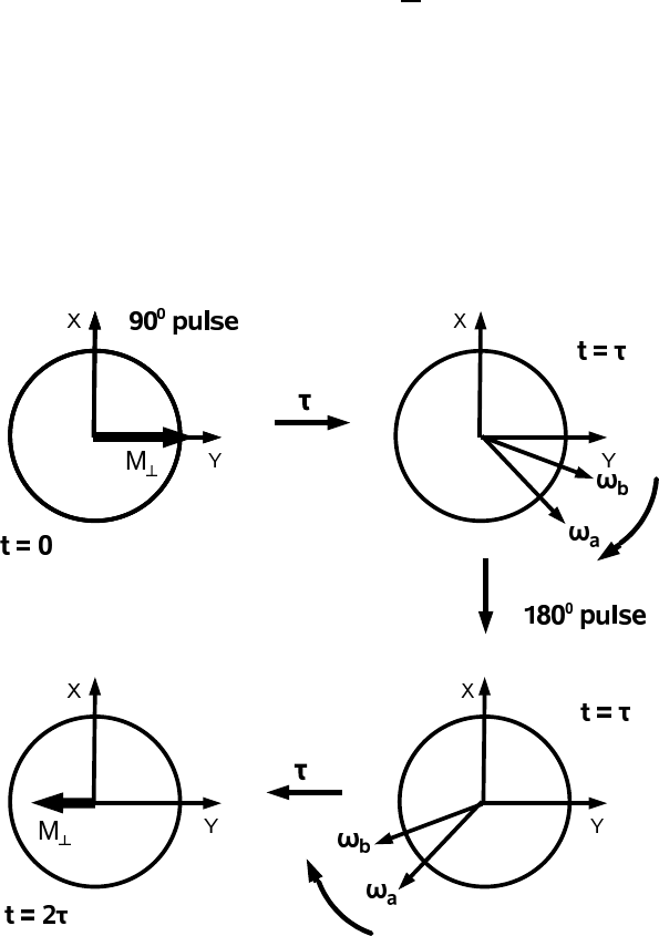
Figure 6: Dephasing of transverse magnetization M⊥.

Consider the pulse sequence 900-1800as illustrated in Fig. 6. A 900pulse at time

t=0 generates a transverse magnetization M⊥along the y-axis. Protons at diﬀerent

locations of the magnetic ﬁeld will have slightly diﬀerent Larmor frequencies due to

the inhomogeneity of the ﬁeld. Assume that the magnetic ﬁeld is larger at location

A than location B, hence ωA> ωB. Protons at location A precess with frequency

ωAwhereas protons at location B precess with frequency ωBin clockwise fashion.

At time t=τthe protons at locations A and B have acquired a phase diﬀerence. The

protons at location A are ahead of the protons at location B as illustrated in the

upper right corner. At time t=τa 1800pulse is applied. The eﬀect of this pulse is

to rotate the magnetic dipoles by 1800around the x-axis. The dipole orientation of

the protons at locations A and B is reversed after this 1800pulse. The protons at

location B are now ahead of the protons at location A as shown in the lower right

corner. The time duration of the 1800pulse is short as compared to the time τand

hence can be neglected. The protons continue to precess clockwise after the 1800

pulse. After another time interval τ, the protons at A and B are in phase again as

illustrated in the lower left corner. All the magnetic dipoles in phase build up the

magnetization M⊥at time t=2τ.

Select a pulse sequence I-II on pushbutton S1 and τ=10 ms on switch S4 and a

repetition rate of 1/3 Hz on S3. Insert probe 1 into the magnet and activate the

pulse sequence. Watch the signal on the scope.

Amplitude

1250

-250

250

500

750

1000

Time [ms]

0 5

10 15 20 25 30 35 40

amplitude

Plot 0

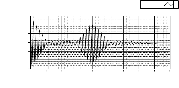
Figure 7: Pulse sequence 900-1800with τ=10 ms.

Fig. 7 displays the NMR signal of pulse sequence I-II with τ=10 ms. Visible at early

times t<5 ms is the decay of the transverse magnetization due to loss of coherence

as explained above. At later times the spin echo builds up and reaches its maximum

at time t=2τ. An evaluation of the maximum of the spin echo envelope at the

maximum is hence a measurement of the decay curve as deﬁned by eq. 17 at time

t=2τ. This decay curve can be measured at diﬀerent times by varying the parameter

τin the pulse sequence I-II.

The spin echo method as described above has limitations when measuring the decay

curve at large times. For such measurements, 2τis large hence also τis large. The

protons can move to diﬀerent locations due to molecular diﬀusion before the 1800

pulse is applied. The average Larmor frequencies in the time intervals 0 < t < τ and

τ < t < 2τcan hence be diﬀerent due to ﬁeld inhomogeneities. The magnetic dipoles

are in such case only approximately aligned along the negative y-axis at time t=2τ

as shown in Fig. 6 and hence only partial coherence is achieved. This limitation

leads to reduced signals at large times with a correspondingly reduced value for the

relaxation time T2.

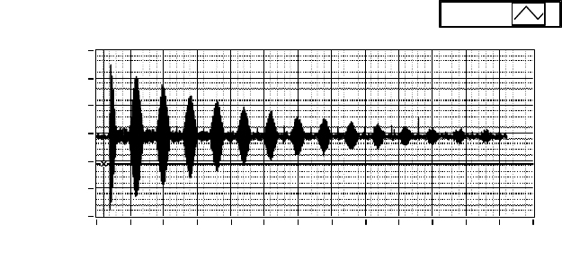
3.3 Spin-spin relaxation T2by Carr-Purcell sequence

The Carr-Purcell sequence minimizes the eﬀects of molecular diﬀusion and ﬁeld

inhomogeneities and hence improves considerably the limitation of the spin echo

method as described above. The Carr-Purcell sequence starts with a 900pulse to

generate a transverse magnetization. A 1800pulse is applied for correction after a

small time interval τ. At time t=2τthe system will be phase coherent. The system

then starts to loose the coherence again due to ﬁeld inhomogeneities. At time t=3τ

another 1800pulse is applied hence the system is phase coherent at time t=4τ. This

pattern of phase coherence at even multiples of τand generation of 1800pulses at

odd multiples repeats to large times as shown in Fig. 8. A measurement of the

spin-spin relaxation time by the Carr-Purcell method hence yields a value which is

closer to the true value of the system as compared to the measurement with the spin

echo method.

Amplitude

1250

-250

250

500

750

1000

Time [ms]

325

25 50 75

100 125 150 175 200 225 250 275 300

amplitude

Plot 0

Figure 8: Carr-Purcell sequence with τ=10 ms.

3.4 Spin-lattice relaxation T1

The spin lattice measurement starts with the generation of a 1800pulse. Such a pulse

produces a magnetization antiparallel to the external ~

B0ﬁeld. This magnetization

will undergo a time evolution as described by the solution of eq. 13

Mk(t) = M0(1 −2e−t/T1) (18)

The longitudinal magnetization Mk(t) does not produce a signal. The generation of

a 900pulse at time t will, however, transform Mk(t) into a transverse magnetization

which will induce a signal in the coil.

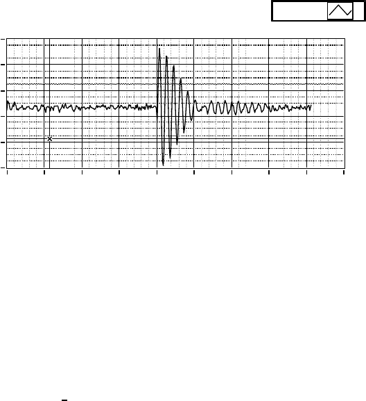
The signal from a pulse sequence 1800-900with a value τ=20 ms is shown in Fig. 9.

The envelope of the signal at time t=τis proportional to the longitudinal magne-

tization Mkat time t=τ. The decay curve of the longitudinal magnetization Mk(t)

can hence be measured at diﬀerent times by varying the value of τin the pulse

sequence 1800-900.

Amplitude

1000

200

400

600

800

Time [ms]

0 5

10 15 20 25 30 35 40

amplitude

Plot 0

Figure 9: Pulse sequence 1800-900with τ=20 ms.

3.5 Measurements of relaxation times

3.5.1 Measurement T2by spin echo method

Measure about 8-12 points of the decay curve given by eq. 17 by using the pulse

sequence I-II and by choosing appropriate τvalues. For these measurements use the

LabVIEW application “T2 meas.vi”. You can ﬁnd this program by clicking on the

link “LabVIEW day 1,2” on the desktop of the PC.

The information of this measurement is stored in a ﬁle. Find the link to the folder

“ss10” on the desktop of the PC. Here, “ss10” denotes summer semester 2010. For

later semesters corresponding folders will exist. In this folder, create a new folder and

rename this folder by your starting day of the experiment. Specify this folder in the

“folder” ﬁeld of the vi and choose a name for the data ﬁle of the measurement. The

analog signal will be sampled with the scanning frequency. A scanning frequency

of 10 kHz results in 10 data points per oscillation period of the signal which has a

frequency 1 kHz. Run the application.

This application contains the following subprograms:

1. Single measurement:

Enter the number of data points to be recorded (10 points per ms of data

acquisition time). Start this subprogram by clicking on “OK”. The data points

are displayed on the left. Enter the spin echo time in the ﬁeld “spin echo time”

and a time value of 6 in the ﬁeld “del T(+-)“. Run the subprogram again. On

the right, the data points within an interval ±del T around the spin echo time

are displayed. The diﬀerence between maximum and minimum value within

the time interval speciﬁed are calculated and shown above the plot. Proceed

to many measurements if the parameters are set correctly such that the spin

echo is centered in the display on the right.

2. Many measurements:

The signal to noise ratio can be improved by averaging over many measure-

ments. Enter 10 in the ﬁeld “ number”, then click “OK”. The program displays

the average and an associated error when the 10 measurements are made.

3. Write data to ﬁle, update plot:

Write this data point to the ﬁle by clicking “OK“. The program shows the

updated content of the ﬁle and the updated plot. You might have to rescale

the horizontal axis of the plot for displaying all the data points.

4. Don’t write data, update plot, no ﬁt:

If a data point has been entered erroneously, then the information of this data

point can be erased by editing the ﬁle and by removing the corresponding line.

Click “OK” for updating the plot and the display of the ﬁle content.

5. Fit:

Click “OK” for ﬁtting the relaxation time when you have measured all the

data points. The ﬁt value of T2and an associated error are shown.

3.5.2 Measurement T2by Carr-Purcell sequence

The measurement of the T2relaxation time by the Carrr Purcell sequence is done

with the LabVIEW application “CP meas.vi”.

The program has two modes:

•single measurement: This mode is active when the button “single meas” in

the top left corner is selected and highlighted in green. In this mode, one

measurement is made. Choose the parameter τfor the Carr-Purcell sequence

such that about 8-10 spin echos are visible. Enter a scanning frequency of

10 kHz and deﬁne the number of data points such that all spin echos are

measured. Enter the location of the spin echos in the bottom panel in the

column “peak”. Enter the number of peaks above the column.

•many measurements: This mode is active when the button “single meas” is not

highlighted in green. The signal to noise ratio can be improved by averaging

over many measurements. Enter 10 in the ﬁeld “number of measurements” and

run the vi. The program now takes 10 measurements and shows the average

value with an associated error for each spin echo. After the 10 measurements

the data points are plotted and the ﬁt value of the T2relaxation time is shown

with an associated error. You might have to rescale the axis of the plot for

displaying all the data points.

3.5.3 Measurement T1

The measurement of the T1relaxation time is done by “T1 meas.vi”. This vi follows

the same structure as the one for the T2measurement by the spin echo method

(“T2 meas.vi”) except that the ﬁtting routine is now deﬁned by eq. 18.

3.6 Systematics of relaxation times

Proceed with the measurements of the relaxation time T2by spin echo and Carr-

Purcell sequence and relaxation time T1for both probes 1 and 3. Write your mea-

surements with errors in a table and discuss the systematics of your results.

4 Part II: Chemical shift

The Larmor frequency ωLis given by eq. 10. If protons are bound in a molecule

then the total magnetic ﬁeld ~

Btot determines the Larmor frequency. This total ﬁeld

consists of the external ﬁeld ~

B0and a contribution ~

δB due to the electron orbitals.

δB =−σ~

B0(19)

The contribution ~

δB is proportional to the external ﬁeld ~

B0. The proportionality

factor σrepresents the magnetic shielding of the external ﬁeld ~

B0. This shielding fac-

tor characterizes the molecule and each nucleus within the molecule. If the modiﬁed

Larmor frequency is measured then this shielding factor can be determined.

ωi=ωL(1 −σi) (20)

Here, ωLrepresents the free Larmor frequency and ωithe frequency modiﬁed by the

chemical shift.

For identifying substances by the chemical shift, a reference substance is added.

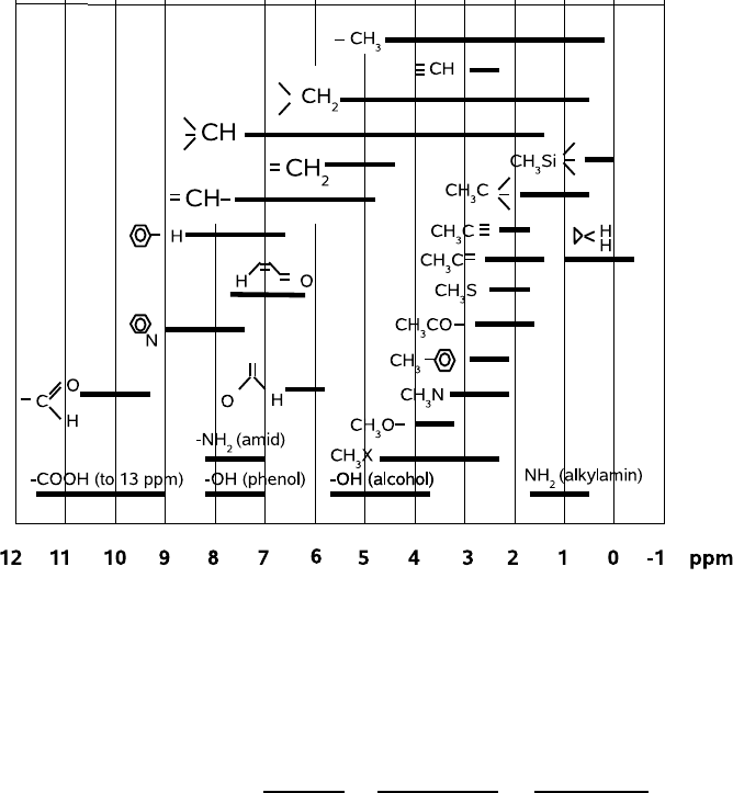
Figure 10: Chemical shifts δiof compounds relative to TMS.

In Fig. 10, the proton chemical shift in organic compounds relative to the reference

substance Tetra-Methyl-Silan (TMS) is shown in units ppm (part per million).

δi=σi−σT MS =ωL−ωi

ωL

−ωL−ωT MS

ωL

=ωT MS −ωi

ωL

(21)

4.1 Measurement chemical shift

Measure the chemical shift in the ﬁve probes A,B,C,D and E. Associate each probe

with one of the substances listed in Fig. 11.

Figure 11: Five substances for identiﬁcation.

Each probe exists with a label ’+’, for example there is a probe A and a probe

A+. The label ’+’ signiﬁes that the reference substance TMS is contained in the

probe. The Larmor frequency of the reference substance TMS can be identiﬁed by

comparing the measurement of the probe with the measurement of the probe plus

reference. The evaluation of the Larmor frequency relative to the reference gives the

shielding factor δiexpressed in eq. 21.

Use the measured chemical shifts δito identify the ﬁve substances of Fig. 11 based

on the information listed in Fig. 10. Toluol and p-xylol have the same chemical

shifts. Use the intensity of the measured frequency response to separate these two

substances.

Use the LabVIEW application “F61 scan 2 5Hz.vi” to measure the frequency re-

sponse. This program has two modes:

•Messen: This mode is active when the boolean switch “Messen” is selected

and highlighted in green. In this mode, the signal is sampled during some time

interval and the measured time signal is displayed in the topmost panel. The

Fourier transformation of the time signal is calculated in steps of 2 Hz and

displayed in the second panel from the top. In addition, the information of the

Fourier transform is saved in a ﬁle. The location and the name of this ﬁle have

to be speciﬁed in the top right corner of the vi. In general, it is good practice

to choose a ﬁle name which contains the information of the measured probe.

Run the vi. You can check the information of the data ﬁle by opening it with

a text editor. The ﬁle contains two columns. The ﬁrst column represents the

frequency values in steps of 2 Hz and the second column the corresponding

intensity in arbitrary units.

•Peak ﬁt: This mode is active when the boolean switch “Peak ﬁt” is selected

and highlighted in green. In this mode, the information in the data ﬁle is read

back and the intensity maxima can be ﬁtted with a Gaussian ﬁt. With these

ﬁts, the position of the peaks can be determined much more accurately than

the discrete Fourier step of 2 Hz. The information of the data ﬁle is displayed

in the bottom panel. Select a window where an intensity maximum is visible.

Specify the low edge of the window in the ﬁeld “W1-low” and the high edge in

the ﬁeld “W1-high”. The values of the low and high edge have to be entered as

multiples of 2 Hz. Run the vi. The location of the ﬁtted maximum is displayed

in the ﬁeld “peak1 [Hz]”. The units of this ﬁeld are Hertz. The ﬁeld “ppm1”

displays the same information but in units of ppm.

A maximum of four peaks can be ﬁtted simultaneously.

For the measurements of chemical shift, a working frequency of νw= 500 Hz is

needed. Check the working frequency on the oscilloscope and adjust if necessary.

Select the 900pulse with a repetition rate of 1/3 Hz to generate the response of

the probe. To get familiar with this measurement, insert probe 3 into the magnet.

Make a measurement. You should see intensity in the Fourier transform at around

500 Hz.

•Over what interval is this intensity distributed ?

•What determines this width ?

•Use the pressure air as explained in Appendix B to put probe 3 into rotation.

Repeat the measurement. Has the width of the frequency response changed ?

Proceed with the measurements by putting the probes A-E into the magnet. Use

the pressure air for accurate measurements.

•Identify the substances.

•Do the peaks you measure correspond to what you expect ?

5 Part III: Imaging with NMR

The imaging measurements are made with the new Bruker NMR analyzer mq7.5. In

order to carry out measurements which contain information on the position of the

produced NMR signal, a magnetic ﬁeld is necessary which has a position dependence.

In practice, gradient ﬁelds are used for one, two and three dimensional imaging

measurements. The gradient ﬁelds are superimposed to the static ﬁeld ~

B0which

deﬁnes the z-direction.

The gradient ﬁelds ~

Bx,~

By,~

Bzare deﬁned by the properties that the ﬁeld vector

points in z-direction and that the strength of the ﬁeld is linearly increasing as func-

tion of the corresponding coordinate.

B0= (0,0, B0)

Bx= (0,0, Gx·x)

By= (0,0, Gy·y)

Bz= (0,0, Gz·z)

A gradient ﬁeld can be produced by an arrangement of coils. For three dimen-

sional imaging, three coil systems are needed which can switch the gradient ﬁelds

Bx,~

By,~

Bzindependently. In the Bruker NMR analyzer mq7.5, the three coil sys-

tems are mounted on an insert which is ﬁxed by two screws in between the two pole

pieces which deﬁne the static ﬁeld ~

B0.

Open the cover of the magnet unit and have a look inside. You will see the tip of

one of the coil systems. On the desktop of the PC, you ﬁnd a link “Bruker pict”. In

the corresponding folder you ﬁnd some pictures of the coil insert which carries the

three coil systems.

5.1 One dimensional imaging

In one dimensional imaging, the position dependence of the NMR signal is generated

by applying a gradient ﬁeld which has a dependence in the corresponding direction,

and the Larmor frequency hence becomes position dependent. In the following, we

discuss one dimensional imaging along the z-direction.

5.1.1 Frequency coding

In one dimensional imaging along the z-direction, a gradient ﬁeld ~

Bzis superimposed

to the static ﬁeld ~

B0. The Larmor frequency hence becomes z-dependent

ωL(z) = γ(B0+Gz·z) = ω0

L+ωz(22)

For further discussion, we consider the rotating frame of the transverse magnetiza-

tion M⊥. In this frame, M⊥is given by eq. 17 and denoted by Mrot

⊥. The transverse

magnetization at a given z-position precesses with a Larmor frequency deﬁned by

eq. 10 and can thus be written as

M⊥(z, t) = Mrot

⊥(z, t)eiγ(B0+Gzz)t(23)

The produced NMR signal is deﬁned by

S(t)∝Z

M⊥(z, t)e−iωH F tdV =Z

Mrot

⊥(z, t)ei(ω0

L+ωz−ωHF )tdV

=eiΩtZ



Z

Mrot

⊥(z, t)dxdy

eiωztdz (24)

If the signal acquisition time T is much smaller than the relaxation time T2, then

the transverse magnetization Mrot

⊥(z, t) is constant during readout and can be set as

Mrot

⊥(z). The measured NMR signal S(t) is therefore, apart from the phase factor

eiΩt, the one dimensional Fourier transform of the transverse magnetization Mrot

⊥(z).

The quantity of interest, the magnetization Mrot

⊥(z), can therefore be deduced by a

one dimensional Fourier transformation of the measured NMR signal S(t).

In practice, the NMR signal S(t) is sampled at times tn=n∆tand hence yields a

set of N data points

S1=S(∆t), S2=S(2∆t, ), ....., SN=S(N∆t) (25)

A discrete Fourier transformation of the N data points SNwill result in N data

points MNdeﬁned by

M1=M⊥(∆z), M2=M⊥(2∆z), ....., MN=M⊥(N∆z) (26)

with ∆zdeﬁned by

∆z=Z

N=2π

γGzN∆t(27)

Here, Z denotes the full range of the position measurement.

5.1.2 Phase coding

In the frequency coding approach described above, the NMR signal is measured as a

function of time. During the readout time, the Larmor frequency at a given position

z is determimed by the applied gradient ﬁeld, and the transverse magnetization

precesses due to the gradient ﬁeld by an amount

∆φ(z) = φ(z)−φ(z= 0) = (γGzz)t=ωzt(28)

During the readout the position information is contained in the phase angle as

described by eq. 28. The phase angle can, however, also be varied by applying a

gradient ﬁeld which is of constant duration but whose strength is increased in steps

of ∆Gz. This equivalent approach is called phase coding.

Phase coding is achieved by applying a gradient ﬁeld Bz=Gzzduring a time

interval TP h before readout of the NMR signal. The phase acquired at position z

during this time interval TP h is given by

ϕ(z) = (γGzTP h)z=kzz(29)

The parameter kz=γGzTP h is the position frequency. After the phase coding

gradient is switched oﬀ, all components of the transverse magnetization precess

with the original Larmor frequency ω0

L=γB0but with a diﬀerent phase angle

which depends on the z-position. In phase coding, the diﬀerent components all

contribute to the NMR signal with the same frequencey but with diﬀerent phases.

The NMR signal is now deﬁned by

S(kx, t0)∝Z

M⊥(z, t0)e−iωH F t0dV =eiΩt0Z



Z

Mrot

⊥(z, t0)dxdy

eikzzdz (30)

The measurement of the phase coded NMR signal consists in making N measure-

ments with diﬀerent position frequencies kn=n∆k(1 ≤n≤N). As expressed in

eq. 30, the phase coded NMR signal only needs to be measured at time t0. After

the measurements, a set of N data points exists

S1=S(∆k, t0), S2=S(2∆k, t0), ....., SN=S(N∆k, t0) (31)

As in frequency coding, the magnetization Mrot

⊥(z) is deduced by a one dimensional

discrete Fourier transformation of the measured data points SN.

The two methods decribed above, frequency coding and phase coding, are mathemat-

ically equivalent. They diﬀer, however, in the time required for the data acquisition.

In frequency coding, the data points Sn=S(tn) as expressed in eq. 25 can be

recorded in one sequence. In phase coding, N sequences are necessary to record the

data points SNas expressed in eq. 31.

5.1.3 One dimensional imaging measurements

The Bruker minispec mq7.5 is fully computer controlled by a graphical user inter-

face. Your tutor will show you how to start the interface. The available application

programs are listed in the top right corner of the interface in the folder “minis-

pec Applications”. Double click on the application “proﬁle” for a one dimensional

imaging measurement. A graphics window “proﬁle.sig” will open which contains the

display of the measurement.

To start the measurement, click on the blue icon “Measure” (bottom left corner).

A menue “Application Conﬁguration Table” will open. In this menue, the gradient

directions are displayed on the left whereas the proﬁle parameters are shown on

the right. Choose the y-gradient for a measurement in vertical direction. The

pulse parameters contain default values which in general don’t need to be modiﬁed.

Click on the “OK” button after you marked the box “y-gradient”. The “proﬁle”

application is programmed such that a measurement is made every 10 seconds. This

measurement is made when the timer displayed in the lower left corner has reached

zero. Click on “STOP” for stopping the measurement. The data points of every

measurement are stored in a data ﬁle. The ﬁle name contains a label which denotes

the number of the measurement. These ﬁles “testProﬁlxx.txt” (xx = 1,2,3,..) are

written into the folder “C:/minispec/imagingdata”. You can ﬁnd this folder by

clicking on the link “minispec dataﬁles” on the desktop.

You have to save the data ﬁles of the measurements which you want to display. Click

on the link on the desktop “Shortcut to ss10”. Here, “ss10” denotes the summer

semester 2010. For later semesters, a corresponding link will exist. In that folder,

create your own folder and rename this folder to the day when you started the

experiment. Copy the ﬁles you want to display to your own folder and rename the

ﬁles such that you recognize the measurement by the ﬁle name.

5.1.4 One dimensional data display

A LabVIEW application “many proﬁles.vi” is available for reading back data ﬁles for

display. You can ﬁnd this LabVIEW application by clicking on the link “LabVIEW

day3” on the desktop. With the application “many proﬁles.vi”, you can superimpose

many measurements by reading back the corresponding data ﬁles from your folder.

In general, these ﬁles have a common prename, a label denoting the number of the

measurement and a common postname. Enter the corresponding information in the

front panel of ”many proﬁles.vi”. The labels of the diﬀerent ﬁles are entered in

the box “ﬁle names”. The strings “common prename”,”ﬁle names” and “common

postname” are concatenated for deﬁning the full name of the ﬁle which is read. In

addition you need to enter the number of ﬁles which should be read. If you want

to read back only one ﬁle, then the string “ﬁle names” has to be empty such that

the strings “common prename” and “common postname” concatenate to the full ﬁle

name.

5.1.5 One dimensional measurements

Make the following one dimensional measurements in vertical direction::

•Take the glass tube which is ﬁlled with about 15 mm of oil. What signal do

you expect? The ring on the glass tube should be positioned such that the

bottom of the tube corresponds to the zero position of the measurement. If

necessary, adjust the position by turning the ring with respect to the glass

tube and move it into the correct position.

•Take the glass tube which is ﬁlled with about 50 mm of water. In this mea-

surement, you can see the eﬀects of the nonlinearity of the gradient ﬁeld. From

this measurement, estimate in which vertical range the probe has to be located

for minimizing the eﬀect of nonlinearity of the gradient ﬁeld.

•Take the glass tube which contains the teﬂon structure immersed in oil. What

signal do you expect? (Teﬂon material does not produce a NMR signal)

•Take an empty glass tube, ﬁll it with about 15 mm of sand and add approxi-

mately 4 mm of oil on top. Put the glass tube into the magnet and measure

until you cannot see any changes from one measurements to the next. Su-

perimpose some of the measurements in the LabVIEW display in order to

illustrate the time development of the system. Can this process of oil mixing

with sand be understood as a diﬀusion process?

5.2 Two dimensional imaging

Two dimensional imaging measurements can be made by a two dimensional Fourier

method. In this approach, a slice is ﬁrst selected by an appropriate combination of

gradient ﬁeld and high frequency pulse. Within the slice, two dimensional position

information is derived by a combination of frequency and phase coding.

5.2.1 Slice selection

A slice in z-direction is deﬁned by the property that the z-coordinate of all the

points within the slice satisfy z1≤z≤z2. If a gradient ﬁeld Bzis switched on, then

every z-position is characterized by a Larmor frequency as deﬁned by eq. 22. The

positions z1and z2are characterized by frequencies ω1and ω2, respectively. If the

high frequency pulse F(ω) contains only frequencies ωsuch that ω1≤ω≤ω2, then

the slice z1≤z≤z2will be selectively excited. Such a pulse F(ω) corresponds to a

sinc pulse in the time domain

f(t)∝sin(at)

t(32)

After the sinc pulse of duration tp, the slice z1≤z≤z2contains excitation energy.

The Larmor frequency is diﬀerent for subslices at diﬀerent z-positions when the slice

selection gradient is switched on. The diﬀerent subslices are therefore out of phase

after the high frequency pulse. This dephasing can be compensated by switching

on the slice selection gradient with reversed polarity for a time interval tp/2 after

the high frequency pulse. This additional gradient is called the slice refocussing

gradient.

5.2.2 Two dimensional Fourier method

Within the selected slice, the two dimensional position information can be derived

by a combination of phase coding in x-direction and frequency coding in y-direction.

The imaging sequence is repeated N times for diﬀerent values of the phase coding

gradient Gx

n=n∆Gx(1 ≤n≤N). In each sequence, the NMR signal is read out at

times tmwith the readout gradient Gyswitched on. For each combination (kn, tm)

of the parameters kn=nγ∆GxTP h and tm=m∆ta data point S(kn, tm) exists.

From this matrix of N×Mdata points, the two dimensional matrix of the image

can be derived by a two dimensional Fourier transformation.

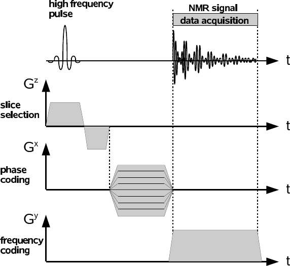
Figure 12: Timing diagram for the two dimensional Fourier method.

Fig. 12 shows the timing diagram of the high frequency pulse and the slice selection,

the phase and frequency coding gradient for the two dimensional Fourier method.

The high frequency pulse is applied while the slice selection gradient is switched on.

After this pulse, the slice refocussing gradient is switched on with reversed polarity.

The phase and frequency coding gradients are then switched on to record the two

dimensional matrix of data points.

5.2.3 Two dimensional imaging measurements

Select the application “msse” for the two dimensional measurements with the Fourier

method. The parameters for such a measurement are listed in a Conﬁguration Table.

The Bruker user interface lists a row of icons at the top of the graphical window. The

icon for the Conﬁguration Table is located almost in the center of this row. Click on

the icon, a graphical window “APPLICATION CONFIGURATION TABLE” will

open. On the left, a column is listed with Imaging Options. Here, you have to deﬁne

the orientation of the slice. The slice can be “Horizontal”, “Vertical Back to Front”

or “Vertical Left to Right”. Choose the orientation by clicking on the corresponding

box. On the right, the following Image Parameters are listed:

•Field of View [mm]: The physical dimension of the measurement. The glass

tube has an outer diameter of about 24 mm, hence the measurement will show

an edge of about 4 mm on the side if the Field of View is deﬁned as 32 mm.

•Image Size [points]: This value deﬁnes the number of pixels in the slice and is

set to 64. Do not change this value, the data points are stored as a 64x64

matrix.

•Slice Thickness [mm]: The thickness of the slice. For materials with a good

NMR signal like oil the minimum slice thickness is 2 mm. For materials with a

weak NMR signal the minimum slice thickness is larger. If the slice thickness

is deﬁned to be too thin, then the NMR signal is too weak and the program

will not ﬁnd valid data acquisition parameters.

•Center Slice Position [mm]: The location of the center of the slice along the

gradient direction. For slices which are deﬁned to be vertical, the center slice

position zero is deﬁned by the vertical axis of the glass tube. For a horizontal

slice, the center slice position zero is deﬁned by the height zero as shown in

the one dimensional measurement made with the “proﬁle” application.

•Number of Slices: This program can in principle record multiple slices simul-

taneously. The data format assumes that only one slice is recorded, hence this

parameter has to be set to one.

•Inter Slice Distance [mm]: Only of relevance when multiple slices are recorded.

•Echo time [ms]: Set to 10 ms. Do not change this value.

•Repetition time [s]: Set to 0.5 s. Do not change this value.

•Number of Averages: The number of measurements over which the average

is taken. Choose one measurement for checking whether the data acquisition

parameters are set correctly. Choose more than one if you want to have a

measurement with good contrast.

Click on the “OK” button in the bottom left corner when all the Image Parameters

are set correctly. To start the measurement, click on the blue icon “Measure” in the

bottom left corner of the minispec interface. A graphical window “TEXT INPUT

BOX” will now open. Here, you have to deﬁne the location and the name of the ﬁle

where the data points are stored. Enter your folder name and deﬁne the name of the

ﬁle such that you recognize this measurement when reading back the ﬁle for display.

Click “OK” when done. The program optimizes the slice refocussing gradient (see

Fig. 12) and then goes through the cycles of data acquisition. The program will

show “Data exported” when ﬁnished. You will now ﬁnd two ﬁles in your folder. The

ﬁle names contain some digits at the end added by the program with the information

of the date and the time. Remove these digits for easier further processing of the

ﬁles.

5.2.4 Two dimensional data display

A LabVIEW application “nmr 2d.vi” exists for displaying the data of your measure-

ment. You can ﬁnd this program by clicking on the link “LabVIEW day3” on the

desktop. Enter your folder name and the ﬁle name which you want to display. You

can print out the display by sending it to the color printer “schiele”.

Storing the display in a graphics ﬁle is possible by a WINDOWS screen shot (press

“Print Scrn” on the keypad) and by importing into a graphics program (Paint,

“Ctrl-V”).

5.2.5 Two dimensional measurements

Make the following measurements with the two dimensional Fourier method:

•Take the glass tube with the 15 mm oil and deﬁne a horizontal slice. What

picture do you expect? When reading back the data ﬁle with the LabVIEW

program, do you see what you expect? How does the image look when you

deﬁne a vertical slice left to right? Do you see what you expect?

•Take a peanut with shell and put it into an empty glass tube. Choose the

measurement parameters such that you can see the two peanuts within the

shell. Take a peanut out of the shell. Adjust the measurement such that the

air gap is visible in between the two halves of the peanut.

•Take a pecan nut and try to resolve the inner structure of this nut.

•Take a piece of celery and map the C-shaped form by using a horizontal slice.

6 NMR applications

NMR techniques are commonly used in many areas of basic and applied research as

well as in industrial applications. A few of these applications are listed below and

some links are given where further information is available.

•Spectroscopy of 31P: Nuclear Magnetic Resonance techniques can be applied

for spectroscopy of nuclei with spin not equal to zero. Of particular interest

is the spectroscopy of 31P due to the role of the adenosintriphosphat molecule

(ATP) in the energy balance of living cells. Energy can be gained by trans-

forming ATP into adenosindiphosphat (ADP). ATP contains three 31P nuclei

whereas ADP contains only two. The 31P nuclei can be identiﬁed in these

molecules by their chemical shift. For a particular application of 31P spec-

troscopy see http://www.nmr.uni-duesseldorf.de/main/menergie.html

•Magnetic Resonance Imaging: The application of NMR techniques in medical

research or for medical diagnosis is known as Magnetic Resonance Imaging

(MRI). YouTube lists a multitude of video clips of MRI pictures for the diag-

nosis of knee injuries and brain tumors (http://www.youtube.com).

•Biomagnetism: The Bio Imaging Laboratory at the University of Antwerpen

concentrates its research activity on high resolution in vivo MRI.

(http://webh01.ua.ac.be/biomag/)

•Surface quality control: Special hand held devices have been developed for

measurements in the near surface volume, as is required for example in quality

control for production processes of car tires.

(http://www.brukeroptics.com/proﬁler.html)

•Digital ﬁsh library: The Digital Fish Library (DFL) at the University of Cal-

ifornia San Diego gives access to the three dimensional information of many

ﬁsh species which have been scanned by NMR techniques.

(http://www.digitalﬁshlibrary.org)

A Appendix A: Minispec p20 Electronic Unit

The electronic unit of the minispec p20 is connected to electrical power through a

transformer. This transformer is located under the table. The power cable of the

transformer should be disconnected from the power net when not in use. When dis-

connected, the transformer power cable is attached to a hook in the wall. Connect

the transformer power cable to the power outlet, then switch on the transformer

by pushing the button indicated by a red arrow with label ON/OFF (OFF is when

button is OUT, ON is when button is IN). When you are ﬁnished with the measure-

ment, proceed in reverse order: First push the ON/OFF button into OFF position,

then disconnect the power cable of the transformer and attach it to the hook.

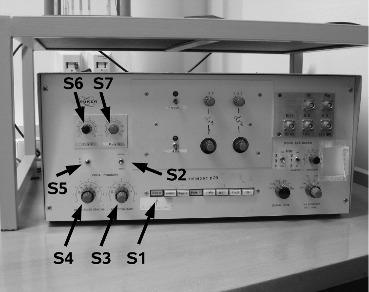
Figure 13: The p20 electronic unit.

The front panel of the electronic unit has diﬀerent switches which have the following

functions:

S1: A row of 8 push buttons for selecting the function of the minispec p20. From

left to right these buttons are labeled

•Stand by: Don’t touch this button ! This button should always be in IN

position.

•OPERATE: When pushed IN, the electronics generates pulses. To stop gen-

erating pulses, push this button into OUT position.

•Puls I: This button selects Puls I.

•Puls II: This button selects Puls II.

•I - I: This button selects a pulse sequence Puls I - Puls I (not used in F61/F62).

•II - I: This button selects a pulse sequence Puls II - Puls I.

•I - II: This button selects a pulse sequence Puls I - Puls II.

•CP: This button selects a Carr-Purcell sequence.

S2: In “single” mode, this switch speciﬁes that your selection done in S1 is generated

only once. In “periodic” mode, your selection of S1 will be generated many times in

time intervals speciﬁed by the S3 switch.

S3: This switch speciﬁes the time interval at which your pulses are produced when

S2 is in “periodic” mode. This switch S3 consists of an inner and outer knob. The

outer knob in black is in logarithmic scale and has settings 100 µs, 1 ms, 10 ms,

100 ms, 1 s and 10 s. The inner knob in red is in linear mode and multiplies the

setting deﬁned by the black knob. Turn the red knob counterclockwise until it locks

in position 1. Every click in clockwise rotation increases the multiplicative factor by

one unit up to the maximum value of 9.

S4: This switch is active when a I-II, II-I or CP sequence is selected by S1. The value

of S4 speciﬁes the time interval between the two pulses of the sequence. The switch

S4 consists of an inner and outer knob. The outer knob in black is in logarithmic

scale and has settings 10 µs, 100 µs, 1 ms, 10 ms, 100 ms and 1 s (Do not use the 1 s

setting, it doesn’t work !). The inner knob in red is in linear mode and multiplies

the setting deﬁned by the black knob. Turn the red knob counterclockwise until it

locks in position 1. Every click in clockwise rotation increases the multiplicative

factor by one unit up to the maximum value of 9.

S5: The switch S5 has three positions and is a multiplicative factor to the value

deﬁned by S4. In upper position, the factor is one. In middle position, the factor is

two whereas in lower position the factor is four.

S6: This knob deﬁnes the time duration of Puls I. Turn the knob counterclockwise

until it is in position 1. This minimal value of S6 deﬁnes the minimum duration of

Puls I. Turning the knob clockwise increases the time duration of Puls I.

S7: This knob deﬁnes the time duration of Puls II. Turn the knob counterclockwise

until it is in position 1. This minimal value of S7 deﬁnes the minimum duration of

Puls II. Turning the knob clockwise increases the time duration of Puls II.

B Appendix B: Minispec p20 Magnet

The minispec p20 magnet is sitting on its own table and is connected to the p20

electronics by a cable. This cable transmits the high frequency pulses generated

by the electronics to the coil inside the magnet. In addition, the cable transmits

the signal induced in the coil back to the electronics. The magnet is shielded by

styrofoam material for minimal temperature variation when in use. Remove the top

cover of the styrofoam to have a look into the magnet assembly.

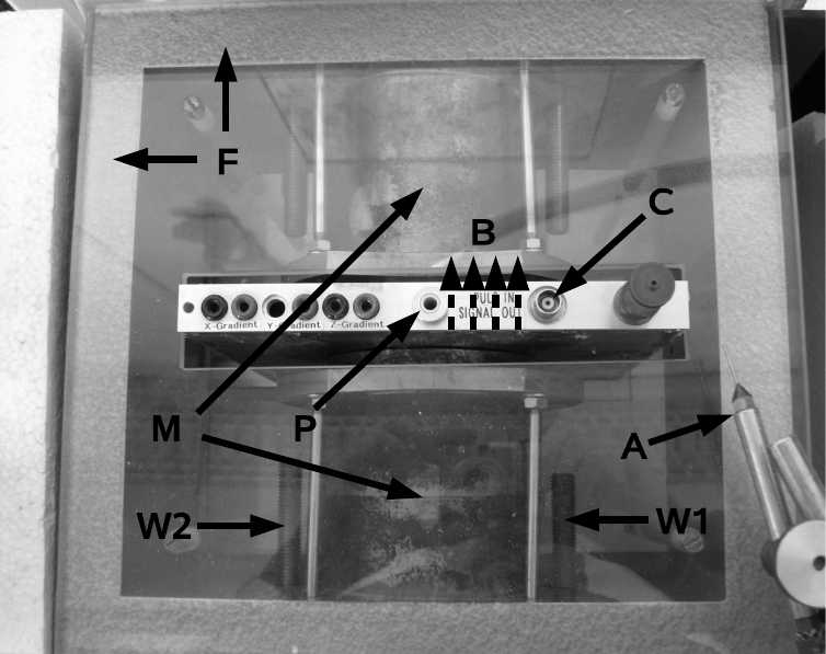
Figure 14: The p20 magnet.

The magnet consists of the following pieces:

•M: The two pole pieces consist of iron material. The two pieces are mounted

with an air gap in between where the probes are put for the measurements.

•B: The iron conﬁguration produces a magnetic ﬁeld of approximately 0.5 Tesla

in the air gap. This ~

Bﬁeld points from one pole shoe to the other.

•F: An iron frame holds the two pole shoes in position. This iron frame is used

as return yoke for the ~

B-ﬁeld lines.

•W1,W2: Two movable iron screws inside the frame are used to change the

magnetic fringe ﬁeld inside the frame. Since the moving of the screws changes

the magnetic ﬁeld conﬁguration, the magnetic ﬁeld in the gap can be adjusted.

In particular, the screw W1 is adjustable from the outside by turning a knob.

(W2 can only be changed with a screw driver, you shouldn’t touch W2).

•P: The position P indicates where the glass tubes with the probes are posi-

tioned for the measurements.

•C: Connector for the cable.

•A: The needle for pressure air can be adjusted such that the glass tubes are

put into rotation for the measurement of chemical shift. Adjust the orientation

of the needle such that it points onto the small plastic ring on the tubes.

References

[1] The basics of NMR are discussed in an online book by Joseph P. Hornak

(http://www.cis.rit.edu/htbooks/nmr)

[2] Magnetresonanztomographie, G. Brix, Chap.11 in Medizinische Physik, eds. W.

Schlegel, J. Bille, Band 2, Springer Verlag, ISBN 3-540-65254

[3] Magnetresonanzspektroskopie, P. Bachert, Chap.12 in Medizinische Physik,

eds. W. Schlegel, J. Bille, Band 2, Springer Verlag, ISBN 3-540-65254

[4] Fundamentals of MRI, An Interactive Learning Approach, E. Berry, A. Bulpitt,

CRC Press, ISBN 978-1-58488-901-4 (a copy of this book is available at F61 for

browsing)

Instructions F61

Navigation menu

Versions of this User Manual:

Views

Navigation