WANDL Router Feature Guide For NPAT And IP/MPLSView JUNOS OS 10.4 Ip Mplsview Routers
User Manual: JUNOS OS 10.4
Open the PDF directly: View PDF ![]() .
.
Page Count: 532 [warning: Documents this large are best viewed by clicking the View PDF Link!]
- WANDL
- Router Feature Guide For NPAT and IP/MPLSView
- About the Documentation
- Table of Contents
- Document Conventions
- Router Data Extraction
- Offline Traffic Processing
- Routing Protocols
- Equal Cost Multiple-Paths
- Static Routes
- Policy Based Routes
- Border Gateway Protocol*
- BGP Peering Analysis*
- Virtual Private Networks*
- GRE Tunnels
- Multicast*
- Class of Service*
- Resilient Packet Ring
- Voice Over IP*
- Backbone Design for OSPF Area Networks*
- Routing Instances*
- Traffic Matrix Solver*
- Metric Optimization
- LSP Tunnels*
- Optimizing Tunnel Paths*
- Tunnel Sizing and Demand Sizing*
- LSP Configlet Generation*
- LSP Delta Wizard*
- Tunnel Path Design*
- Inter-Area MPLS-TE*
- Point-to-multipoint (P2MP) TE*
- Diverse Multicast Tree Design*
- DiffServ Traffic Engineering Tunnels*
- Fast Reroute*
- Cisco Auto-Tunnels*
- Integrity Check Report*
- Compliance Assessment Tool*
- Configuration Revision*
- Virtual Local Area Networks
- Overhead Calculation
- Router Reference

2 May 2014
Release
6.1.0
Copyright © 2014, Juniper Networks, Inc.
WANDL
Router Feature Guide For NPAT and IP/MPLSView

ii Copyright © 2014, Juniper Networks, Inc.
Juniper Networks, Inc.
1194 North Mathilda Avenue
Sunnyvale, California 94089
USA
408-745-2000
www.juniper.net
Juniper Networks, Junos, Steel-Belted Radius, NetScreen, and ScreenOS are registered trademarks of Juniper Networks, Inc. in the United
States and other countries. The Juniper Networks Logo, the Junos logo, and JunosE are trademarks of Juniper Networks, Inc. All other
trademarks, service marks, registered trademarks, or registered service marks are the property of their respective owners.
Juniper Networks assumes no responsibility for any inaccuracies in this document. Juniper Networks reserves the right to change,
modify,transfer, or otherwise revise this publication without notice.
WANDL Router Feature Guide For NPAT and IP/MPLSView
Copyright © 2014, Juniper Networks, Inc.
All rights reserved.
The information in this document is current as of the date on the title page.
YEAR 2000 NOTICE
Juniper Networks hardware and software products are Year 2000 compliant. Junos OS has no known time-related limitations through the year
2038. However, the NTP application is known to have some difficulty in the year 2036.
END USER LICENSE AGREEMENT
The Juniper Networks product that is the subject of this technical documentation consists of (or is intended for use with) Juniper Networks
software. Use of such software is subject to the terms and conditions of the End User License Agreement (“EULA”) posted at
http://www.juniper.net/support/eula.html. By downloading, installing or using such software, you agree to the terms and conditions of that
EULA.

Copyright © 2014, Juniper Networks, Inc. Documentation and Release Notes iii
About the Documentation
About the Documentation
Documentation and Release Notes
To obtain the most current version of all Juniper Networks® technical documentation,
see the product documentation page on the Juniper Networks website at
http://www.juniper.net/techpubs/.
If the information in the latest release notes differs from the information in the documentation,
follow the product Release Notes. Juniper Networks Books publishes books by Juniper Networks
engineers and subject matter experts. These books go beyond the technical documentation to
explore the nuances of network architecture, deployment, and administration. The current list can
be viewed at http://www.juniper.net/books.
Documentation Feedback
We encourage you to provide feedback, comments, and suggestions so that we can
improve the documentation. You can provide feedback by using either of the following methods:
-Online feedback rating system—On any page at the Juniper Networks Technical
Documentation site at http://www.juniper.net/techpubs/index.html, simply click the
stars to rate the content, and use the pop-up form to provide us with information about your
experience. Alternately, you can use the online feedback form at
https://www.juniper.net/cgi-bin/docbugreport/.
-E-mail—Send your comments to techpubs-comments@juniper.net. Include the
document or topic name, URL or page number, and software version (if applicable).
Requesting Technical Support
Technical product support is available through the Juniper Networks Technical Assistance Center
(JTAC). If you are a customer with an active J-Care or JNASC support contract, or are covered under
warranty, and need post-sales technical support, you can access our tools and resources online or
open a case with JTAC.
-JTAC policies—For a complete understanding of our JTAC procedures and policies,
review the JTAC User Guide located at
http://www.juniper.net/us/en/local/pdf/resource-guides/7100059-en.pdf.
-Product warranties—For product warranty information, visit
http://www.juniper.net/support/warranty/.
-JTAC hours of operation—The JTAC centers have resources available 24 hours a day, 7
days a week, 365 days a year.

About the Documentation
iv Requesting Technical Support Copyright © 2014, Juniper Networks, Inc.
Self-Help Online Tools and Resources
For quick and easy problem resolution, Juniper Networks has designed an online self-service portal
called the Customer Support Center (CSC) that provides you with the following features:
-Find CSC offerings: http://www.juniper.net/customers/support/
-Search for known bugs: http://www2.juniper.net/kb/
-Find product documentation: http://www.juniper.net/techpubs/
-Find solutions and answer questions using our Knowledge Base: http://kb.juniper.net/
-Download the latest versions of software and review release notes:
http://www.juniper.net/customers/csc/software/
-Search technical bulletins for relevant hardware and software notifications:
http://kb.juniper.net/InfoCenter/
-Join and participate in the Juniper Networks Community Forum:
http://www.juniper.net/company/communities/
-Open a case online in the CSC Case Management tool: http://www.juniper.net/cm/
-To verify service entitlement by product serial number, use our Serial Number Entitlement (SNE)
Tool: https://tools.juniper.net/SerialNumberEntitlementSearch/
Opening a Case with JTAC
You can open a case with JTAC on the Web or by telephone.
-Use the Case Management tool in the CSC at http://www.juniper.net/cm/.
-Call 1-888-314-JTAC (1-888-314-5822 toll-free in the USA, Canada, and Mexico). For
international or direct-dial options in countries without toll-free numbers, see
http://www.juniper.net/support/requesting-support.html.

Copyright © 2014, Juniper Networks, Inc. Contents-1
. . . . .
. . . . .
. . . . . . . . . . . . . . . . . . . . . . . . . . . . . . . . . . .
Table of Contents
I Introduction I-1
Interior Gateway Protocols (IGP) I-1
Equal Cost Multiple Paths (ECMP) I-1
Static Routes I-1
Policy Based Routes (PBR) I-1
Border Gateway Protocol (BGP) I-1
Virtual Private Networks (IP VPN) I-1
Class of Service (CoS) I-2
Multicast I-2
VoIP I-2
OSPF Area Design I-2
Multi-Protocol Label Switching (MPLS) Tunnels for Traffic Engineering I-2
Path Placement I-2
Modification I-2
Net Grooming I-2
Configlet Generation I-2
Path Diversity Design I-2
Fast Reroute (FRR) I-2
Inter-Area MPLS-TE I-2
DiffServ TE Tunnels I-3
Following Along with the Examples in this Manual I-3
1 Document Conventions 1-1
Document Conventions 1-1
Keyboard, Window, and Mouse Terminology and Functionality 1-1
The Keyboard 1-2
The Mouse 1-2
Information Labels 1-2
Changing the Size of a Window 1-2
Moving a Window 1-2
2 Router Data Extraction 2-1
When to use 2-1
Prerequisites 2-1
Related Documentation 2-1
Recommended Instructions 2-1
Graphical User Interface Mode 2-1
Text Mode (Alternative) 2-1
MPLS Tunnel Path Import 2-1
Detailed Procedures 2-2

Contents-2 Copyright © 2014, Juniper Networks, Inc.
Getipconf - Router Configuration Extraction 2-2
Graphical User Interface 2-2
Default Inputs 2-3
Advanced Options 2-5
Bandwidth 2-5
Text Mode 2-14
MPLS Tunnel Extraction* 2-15
Command Line Version: rdjpath 2-16
Appendix - File Format 2-17
Delay Measurement File 2-17
Updating Link Information 2-17
PE-CE Connection File 2-18
3 Offline Traffic Processing 3-1
When to use 3-1
Prerequisites 3-1
Recommended Instructions 3-1
Detailed Procedures 3-2
Preparing the Traffic Data: Step One 3-2
Creating the Daily Directories 3-3
Daily Directories Structure 3-3
Convintftraf (the Traffic Conversion Utility) 3-3
Using the WANDL client to Import Traffic Data 3-5
Computation Method 3-8
Roll-up / Aggregation Defined 3-8
Viewing Summarized Traffic Statistics on the Map 3-9
Related Spec file parameters 3-9
4 Routing Protocols 4-1
When to use 4-1
Prerequisites 4-1
Related Documentation 4-1
Recommended Instructions 4-1
Detailed Procedures 4-2
View Routing Protocol Details from the Map 4-2
Set the IGP Routing Method 4-3
Routing Protocol Details 4-4
RIP 4-4
IGRP and EIGRP 4-4
OSPF 4-5
ISIS and ISIS2 4-6
MPLS-TE 4-6
Updating Link Properties from a File 4-6
5 Equal Cost Multiple-Paths 5-1
When to use 5-1
Related Documentation 5-1
Recommended Instructions 5-1
Detailed Procedures 5-1

Copyright © 2014, Juniper Networks, Inc. Contents-3
. . . . .
Identifying Equal Cost Multiple-Paths 5-1
Reducing Equal Cost Multiple Paths 5-4
Splitting a Flow into Sub-Flows 5-6
Set ECMP Subflows Based on Bandwidth 5-8
6 Static Routes 6-1
When to use 6-1
Prerequisites 6-1
Related Documentation 6-1
Outline 6-1
Detailed Procedures 6-1
View Static Routes 6-1
Interpreting the Static Routing Table 6-2
Add/Modify/Delete Static Routes 6-3
Adding a Static Route 6-3
Modifying a Static Route 6-3
Deleting a Static Route 6-3
Case Study 6-4
Defining the Demand 6-4
Creating the Static Route Table 6-6
Verify the New Route 6-7
7 Policy Based Routes 7-1
When to use 7-1
Prerequisites 7-1
Related Configuration Commands 7-1
Recommended Instructions 7-1
Detailed Procedures 7-2
Importing the Config Files 7-2
Viewing PBR Details from the Link Window 7-2
Path Placement 7-2
Modifying Link PBR Field 7-3
Example 7-3
8 Border Gateway Protocol* 8-1
Related Documentation 8-1
Recommended Instructions 8-1
Definitions 8-2
Detailed Procedures 8-3
BGP Data Extraction 8-3
BGP Reports 8-3
BGP Options 8-3
BGP Map 8-4
Logical Layout 8-4
Grouping 8-5
AS Legend 8-6
BGP Map Subviews 8-6
BGP Live Status Check 8-8
BGP Routing Table 8-9
BGP Routes Analysis 8-11

Contents-4 Copyright © 2014, Juniper Networks, Inc.
BGP Information at a Node 8-12
BGP Neighbor 8-13
View Neighbor Information 8-13
Properties Tab 8-14
In and Out Policies Tabs 8-14
Add BGP Peering relationship 8-15
Apply, Modify, or Add BGP Polices 8-17
Applying Policies 8-17
Modify BGP Policy 8-18
Adding a BGP Policy 8-20
BGP Subnets* 8-21
Live BGP Routing Tables* 8-24
getipconf Usage Notes 8-25
Syntax 8-25
BGP-related flags 8-25
BGP Files Generated 8-25
Corresponding Spec File Keywords 8-25
dparam File 8-26
bgpnode format 8-26
bgplink format 8-26
aclist format 8-26
bgpnbr file 8-27
Subnet File 8-27
BGP Report 8-28
9 BGP Peering Analysis* 9-1
Related Documentation 9-1
Recommended Instructions 9-1
Detailed Procedures 9-2
Network Preparation 9-2
Preparing BGP Routing Table Object File 9-2
Import Configuration Files 9-2
Import Tunnel Path Files 9-2
Read a Demand File 9-2
BGP Peering Analysis Wizard 9-3
Process BGP Routing Tables and Create Reference Reports 9-3
Corresponding Command Line Utilities 9-4
Process Routeviews Data for a New Peer and Create Reports 9-7
Corresponding Command Line Utilities 9-8
Example of Applying Peering Policies 9-10
Generate Peering Analysis Comparison Reports 9-12
Appendix. Preparing the Demand File 9-14
Preparing the Service Type File from Host_Property File (Optional) 9-14
Preparing the Demand File Based on Service Type File, Traffic File, and bblink file 9-14
Output Files 9-15
Examples 9-15
10 Virtual Private Networks* 10-1
Related Documentation 10-1

Copyright © 2014, Juniper Networks, Inc. Contents-5
. . . . .
Outline 10-1
Detailed Procedures 10-2
Importing VPN Information from Router Configuration Files 10-2
Viewing the Integrity Checks Reports 10-3
Accessing VPN Summary Information 10-4
Accessing Detailed Information for a Particular VPN 10-5
VPN Topology View 10-6
Route-target Export/Import Relationships 10-8
Additional Methods to Access VPN Information 10-12
VPN Path Tracing 10-13
VPN Design and Modeling using the VPN Wizard 10-14
L3 (Layer 3) VPN 10-15
L3 Hub-and-Spoke VPN 10-21
Merging Hub and Spokes 10-21
Adding a New Layer 3 Hub-and-Spoke VPN 10-23
L2M (Layer2-Martini) VPN 10-26
L2K (Layer2-Kompella) VPN 10-30
VPLS-BGP VPN (for Juniper) 10-32
VPLS-LDP VPN 10-34
L2CCC (Circuit Cross-Connect) VPN 10-38
Inter-AS VPN 10-40
Forming Customer Groups 10-41
Deleting or Renaming VPNs 10-42
VPN Configlet Generation* 10-43
Adding Traffic Demands in a VPN via the Add Demands Windows 10-46
VPN Traffic Generation 10-47
VPN-Related Reports 10-49
VPN Monitoring and Diagnostics (also requires Online Module) 10-51
11 GRE Tunnels 11-1
Cisco 11-1
Juniper 11-1
Example intfmap entry 11-1
Example tunnel entry 11-1
Example bblink entry 11-1
When to use 11-2
Prerequisites 11-2
Related Documentation 11-2
Outline 11-2
Detailed Procedures 11-2
Importing GRE Tunnel Information from Router Configuration Files 11-2
Adding a GRE Tunnel 11-2
Assigning IP addresses to nodes/Interfaces 11-2
Adding a GRE Tunnel Interface 11-3
Adding a GRE Tunnel 11-3
Adding a GRE Link 11-3
Troubleshooting a GRE Link/Tunnel Definition 11-4
Using Static Routes to Route over a GRE Tunnel 11-4
Viewing GRE Tunnels 11-5
Viewing Demands over GRE Tunnels 11-6

Contents-6 Copyright © 2014, Juniper Networks, Inc.
12 Multicast* 12-1
When to use 12-1
Prerequisites 12-1
Related Documentation 12-1
Recommended Instructions 12-1
Detailed Procedures 12-1
Creating Multicast Groups 12-1
Creating Multicast Demands 12-2
Viewing Multicast Demands in the Network 12-3
Comparing Multicast with Unicast 12-6
Multicast SPT Threshold 12-7
Reports 12-8
Simulation 12-8
Collecting Multicast Path Data from Live Network 12-8
Importing Multicast Path Data 12-10
Data Processing 12-10
Viewing Multicast Trees 12-12
13 Class of Service* 13-1
Prerequisite 13-1
Related Documentation 13-1
When to use 13-1
Recommended Instructions 13-1
Detailed Procedures 13-2
The QoS Manager 13-2
How to Input CoS Parameters 13-4
Define Class Maps 13-4
DEFAULT class 13-5
PRIORITY class 13-5
Related Cisco commands: 13-5
Create Policies for Classes 13-6
Related Cisco commands: 13-9
HWRR Policies 13-9
To Add a Scheduler Node 13-10
To Add a Queue 13-10
Attach Policies to Interfaces 13-11
Adding Traffic Inputs 13-12
Using text editor 13-13
Reporting module 13-13
IP Flow Information 13-15
Link information 13-16
Traffic Load Analysis 13-17
Animated Traffic load display 13-17
Traffic Load by Policy Class 13-18
Appendix 13-19
CoS Alias File 13-19
bblink File 13-19
Policymap file 13-20
Demand File 13-21
Traffic Load File 13-22

Copyright © 2014, Juniper Networks, Inc. Contents-7
. . . . .
14 Resilient Packet Ring 14-1
When to use 14-1
Related Documentation 14-1
Recommended Instructions 14-1
Detailed Procedures 14-1
Deriving RPR from config and srp topology data 14-1
RPR Map 14-1
RPR Network Information 14-2
Path Analysis 14-2
Modifying an RPR Ring 14-3
Adding Routers to an RPR Ring 14-3
Removing a Router from an RPR Ring 14-4
15 Voice Over IP* 15-1
Related Documentation 15-1
Recommended Instructions 15-1
Definitions 15-2
Detailed Procedures 15-3
Build a VoIP Network by Assigning VoIP Attributes to Nodes 15-3
Assigning H.323 Gatekeepers (GKs) 15-3
Assigning H.323 Media Gateways (MGWs) 15-3
Assigning SIP Servers 15-4
Assigning SIP-UAs (SIP User Agents) 15-4
VoIP Topology Map 15-5
VoIP Call Setup and Actual Call Path Trace 15-6
Traffic Classes 15-9
VoIP Traffic Specification 15-10
Adding a Single VoIP Demand 15-10
Adding Multiple VoIP Demands 15-12
Using the VoIP Traffic Generation Tool 15-15
Creating a Traffic Profile via the VoIP Traffic Generation Wizard 15-15
Using the No File Option 15-17
Using an End-to-end Traffic Matrix Input File 15-24
Using an End-to-end Traffic Matrix Input File with a Homing File15-27
Reporting VoIP Information 15-30
VoIP Call Setup Report 15-31
VoIP Node Traffic Summary Report 15-32
E-Model R-factor Voice Quality Assessment 15-33
16 Backbone Design for OSPF Area Networks* 16-1
When to use 16-1
Prerequisites 16-1
Related Documentation 16-1
Recommended Instructions 16-1
Detailed Procedures 16-1
Specifying Design Properties for Multiple-Area OSPF Networks 16-2
Specifying AREA0 as the Design Property for a Node 16-2
Specifying a Non-Backbone Area as the Design Property for a Node16-3
Performing a Design 16-4
Performing a Diversity Design 16-5

Contents-8 Copyright © 2014, Juniper Networks, Inc.
17 Routing Instances* 17-1
When to use 17-1
Recommended Instructions 17-1
Detailed Procedures 17-1
Creating Routing Instances 17-1
Path Analysis 17-5
Reports 17-5
File Format 17-6
ROUTEINSTANCE File 17-6
18 Traffic Matrix Solver* 18-1
Related Documentation 18-1
Recommended Instructions 18-1
Detailed Procedures 18-2
Input Interface Traffic 18-2
Interface Traffic File Format 18-2
Example Interface Traffic File 18-2
Input TrafficLoad File 18-3
Input Seed Demands 18-3
Creating a Full Mesh of Demands 18-4
Unplaced Test Demands 18-4
Running the Traffic Matrix Solver 18-5
Viewing the Results 18-6
Trafficload 18-6
Console 18-6
Reports 18-7
Summary Tab 18-8
Links Tab 18-8
Viewing Differences Graphically 18-9
Troubleshooting 18-10
Appendix 18-11
Choosing a Period of Interface Traffic 18-11
Resetting Demand Bandwidth According to Demand Trafficload File 18-11
Traffic Matrix Parameters 18-11
19 Metric Optimization 19-1
When to use 19-1
Prerequisites 19-1
Related Documentation 19-1
Recommended Instructions 19-1
Detailed Procedures 19-1
Setting Up for Metric Optimization 19-1
Setting Up Protocol Information 19-1
Setting Up Max Delay Constraints 19-1
Metric Optimization Parameters 19-2
Metric Optimization Design 19-5
Metric Optimization Results 19-5
Viewing the Detailed Link Information After Metric Optimization 19-6
Metric Optimization Link Utilization Results in Chart Format 19-7
Changed Demands after Metric Optimization 19-8

Copyright © 2014, Juniper Networks, Inc. Contents-9
. . . . .
Accepting or Rejecting Metric Changes 19-8
Saving a Metric Optimization Design 19-8
20 LSP Tunnels* 20-1
Prerequisites 20-1
Related Documentation 20-1
Outline 20-1
Detailed Procedures 20-2
Viewing Tunnel Info 20-2
Viewing Primary and Backup Paths 20-2
Viewing Tunnel Utilization Information from the Topology Map 20-3
Viewing Tunnels Through a Link 20-4
Viewing Demands Through a Tunnel 20-5
Viewing Link Attributes/Admin-Group 20-6
Viewing Tunnel-Related Reports 20-7
Adding Primary Tunnels 20-9
Adding Multiple Tunnels 20-10
Mark MPLS-Enabled on Links along Path 20-11
Modifying Tunnels 20-11
Path Configuration 20-11
Specifying a Dynamic Path 20-12
Configuring a Dynamic Route Between Source and Destination 20-12
Configuring a Loose Route 20-12
Configuring an Explicit Route Based On Current Route 20-12
Excluding Network Elements from a Path (for Cisco Routers) 20-12
Specifying Alternate Routes, Secondary and Backup Tunnels 20-13
Specifying Alternate Routes (for Cisco Routers) 20-13
Specifying Secondary and Standby Tunnels (for Juniper Routers) 20-14
Path Config Options 20-15
Adding and Assigning Tunnel ID Groups 20-16
Making Specifications for Fast Reroute 20-19
Specifying Tunnel Constraints (Affinity/Mask or Include/Exclude)20-20
Cisco 20-20
Juniper 20-20
WANDL Modeling of Tunnel Constraints 20-20
Tunnel Attribute/Admin Group Names 20-21
Setting Link Attributes 20-21
Tunnel Affinity and Mask (Cisco) 20-22
Including and Excluding Admin-Groups (Juniper) 20-23
Adding One-Hop Tunnels 20-24
Tunnel Layer and Layer 3 Routing Interaction 20-26
Appendix 20-26
Commands Modeled Using Affinity and Mask Feature 20-26
21 Optimizing Tunnel Paths* 21-1
When to use 21-1
Prerequisites 21-1
Related Documentation 21-1
Recommended Instructions 21-1
Detailed Procedures 21-1

Contents-10 Copyright © 2014, Juniper Networks, Inc.
Network Grooming 21-2
22 Tunnel Sizing and Demand Sizing* 22-1
When to use 22-1
Prerequisites 22-1
Definitions 22-1
Related Documentation 22-1
Recommended Instructions 22-1
Detailed Procedures 22-2
Calculation of the New Tunnel Bandwidth 22-8
23 LSP Configlet Generation* 23-1
When to use 23-1
Prerequisites 23-1
Related Documentation 23-1
Recommended Instructions 23-1
Detailed Procedures 23-2
Viewing the Configlet 23-2
Creating LSP Configlets for All Routers 23-3
Using Tunnel Templates 23-4
Creating a Tunnel Numbering Scheme 23-6
24 LSP Delta Wizard* 24-1
When to use 24-1
Prerequisites 24-1
Related Documentation 24-1
Recommended Instructions 24-1
Running the LSP Delta Wizard 24-2
Checking the Names of Paths that Exclude Nodes 24-3
Identifying Unused FRR Backup Tunnels 24-4
Tables for New, Modified, and Deleted LSP Tunnels 24-6
Generating LSP Deltas and XML 24-7
Saving Files to the Server 24-10
25 Tunnel Path Design* 25-1
When to use 25-1
Prerequisites 25-1
Related Documentation 25-1
Recommended Instructions 25-1
Detailed Procedures 25-1
Tunnel Path Design 25-1
Backup Path Configuration Options 25-2
Dynamic Primary Path 25-3
Explicit Primary Path with Dynamic Secondary Path 25-3
Explicit Primary and Explicit Standby Path 25-3
Explicit Primary and Explicit Standby Path with Dynamic Tertiary Path 25-3
Default Diversity Level 25-3
Evaluate/Tune Options 25-3
Advanced Options 25-4

Copyright © 2014, Juniper Networks, Inc. Contents-11
. . . . .
Viewing Design Results 25-5
Tunnel Modifications 25-6
General Path Options 25-6
Diversity Group Configuration Groups 25-6
Backup Path Configuration Options 25-7
Exporting and Importing Diverse Group Definitions 25-7
Advanced Path Modification 25-7
Delta Configlets 25-8
26 Inter-Area MPLS-TE* 26-1
When to use 26-1
Prerequisites 26-1
Related Documentation 26-1
Recommended Instructions 26-1
Detailed Procedures 26-2
Viewing OSPF Areas 26-2
Adding Multiple Tunnels Between Areas 26-3
Tunnel Type Configuration Options Related to Areas 26-4
Viewing Inter-Area Tunnels 26-5
Configuring a Loose Route 26-6
27 Point-to-multipoint (P2MP) TE* 27-1
When to use 27-1
Prerequisites 27-1
Related Documentation 27-1
Recommended Instructions 27-1
Detailed Procedures 27-2
Import a network that already has P2MP LSP tunnels configured in the network 27-2
Examine the P2MP LSP tunnels 27-2
Create P2MP LSP Tunnels and Generate Corresponding LSP Configlets 27-4
Examine P2MP LSP tunnel link utilizations to observe efficient replication. 27-7
Perform failure simulation and assess the impact of the failure on P2MP LSPs. 27-8
28 Diverse Multicast Tree Design* 28-1
When to use 28-1
Prerequisites 28-1
Related Documentation 28-1
Recommended Instructions 28-1
Detailed Procedures 28-3
Open a network that already has a Multicast Trees (i.e., P2MP trees) configured in the network 28-3
Set the two P2MP trees of interest to be in the same Diversity Group 28-3
Use the Multicast Tree Design feature to design multicast trees that are diverse from each other in each Diversity
Group 28-5
Use the Multicast Tree Design feature to tune an existing tree in order to reduce its cost. 28-9
29 DiffServ Traffic Engineering Tunnels* 29-1
When to use 29-1
Prerequisites 29-1
Related Documentation 29-1

Contents-12 Copyright © 2014, Juniper Networks, Inc.
Definitions 29-1
Using DS-TE LSP 29-2
Hardware Support for DS-TE LSP 29-2
Overview 29-2
Class Type 29-2
EXP Bits 29-2
Forwarding Class 29-2
Scheduler Map 29-3
Bandwidth Model 29-3
Operation 29-3
WANDL Support for DS-TE LSP 29-4
Overview 29-4
Class types 29-4
EXP bits 29-4
CoS Classes 29-4
Cos Policies 29-4
Bandwidth Model 29-5
Using WANDL to Model DS-TE LSPs 29-6
Configuring the Bandwidth Model and Default Bandwidth Partitions 29-6
Forwarding Class to Class Type Mapping 29-7
Link Bandwidth Reservation 29-8
Creating a new multi-class or single-class LSP 29-10
Configuring a DiffServ-aware LSP 29-10
Tunnel Routing 29-11
Link Utilization Analysis 29-11
30 Fast Reroute* 30-1
Overview 30-1
Graphical Display 30-1
What-If Studies and Path Design 30-1
Failure Simulation 30-1
Supported Vendors 30-1
Juniper 30-1
Cisco 30-2
When to use 30-2
Prerequisites 30-2
Related Documentation 30-2
Outline 30-2
Detailed Procedures 30-3
Import Config and Tunnel Path 30-3
Viewing the FRR Configuration 30-3
Cisco 30-3
Juniper 30-3
Viewing FRR Backup Tunnels protecting a Primary Tunnel 30-5
Viewing Primary Tunnels Protected by a Bypass Tunnel 30-6
Modifying Tunnels to Request FRR Protection 30-7
Modifying Links to Configure Multiple Bypasses (Juniper only) 30-8
Modifying Links to Trigger FRR Backup Tunnel Creation (Cisco) 30-9
Example 30-9
FRR Design 30-10

Copyright © 2014, Juniper Networks, Inc. Contents-13
. . . . .
Tune FRR Backup Tunnels fields 30-11
Options 30-11
Auto Design Parameters 30-12
Advanced Options for Cisco 30-13
Advanced Options for Juniper 30-13
Other Options 30-14
FRR Auto Design 30-14
FRR Design Report 30-15
FRR Design Report Fields 30-15
View Created FRR Backup Tunnels 30-16
FRR Tuning 30-17
Filtering in the FRR Tuning Window 30-19
Viewing Created Backup Tunnels 30-20
Generating LSP Configlets for FRR Backup Tunnels 30-20
Failure Simulation: Testing the FRR Backup Tunnels 30-21
Simulating Local Protection 30-21
Simulating Head-end Reroute or Use of Backup Route 30-21
Using the Run Button 30-22
Resulting Link Utilizations 30-22
Exhaustive Failure 30-23
Appendix: Link, Site and Facility Diverse Paths 30-24
Link Diversity 30-24
Site Diversity 30-24
Facility Diversity (SRLG)* 30-25
31 Cisco Auto-Tunnels* 31-1
When to use 31-1
Prerequisites 31-1
Related Documentation 31-1
Outline 31-2
Detailed Procedures 31-2
Importing Cisco Auto-tunnel Information from Router Configuration Files 31-2
Auto-tunnel Creation 31-4
Tunnel Path Data Collection and Import for Auto-tunnels 31-7
Reporting for Verification 31-9
32 Integrity Check Report* 32-1
When to use 32-1
Prerequisites 32-1
Related Documentation 32-1
Recommended Instructions 32-1
Detailed Instructions 32-1
Viewing the Integrity Check Report 32-1
Using the Report Viewer 32-3
Error Source 32-3
Customizing the Severity Level 32-3
Scheduling Integrity Checking in Task Manager 32-4
Integrity Check Task 32-4
Report Options 32-5
Integrity Check Options Tab 32-6

Contents-14 Copyright © 2014, Juniper Networks, Inc.
Network Options 32-6
Filter by Category 32-6
Filter by Message 32-6
Filter by Router 32-6
Filter by Group 32-7
Filter by Severity 32-7
Additional Report Options 32-7
Appendix A. Integrity Check Descriptions 32-9
Access List and Prefix List Integrity Checks 32-9
BGP Integrity Checks 32-9
EIGRP/IGRP Integrity Checks 32-10
IP Integrity Checks 32-10
ISIS Integrity Checks 32-12
RIP Integrity Checks 32-12
OSPF Integrity Checks 32-12
QoS Integrity Checks 32-13
LINK Integrity Checks 32-14
MISCELLANEOUS Integrity Checks 32-14
MPLS Integrity Checks 32-16
RSVP Integrity Checks 32-17
Static Routes Integrity Checks 32-17
Tunnel Integrity Checks 32-18
VPN Integrity Checks 32-18
VLAN Integrity Checks 32-19
33 Compliance Assessment Tool* 33-1
Prerequisites 33-1
Related Documentation 33-1
Recommended Instructions 33-1
Detailed Procedures 33-2
Compliance Assessment Tool 33-2
CAT Testcase Design 33-4
Creating a New Project 33-5
Loading the Configuration Files 33-5
Creating Conformance Templates 33-7
Editing the Conformance Template 33-10
Reviewing and Saving the Template 33-10
Saving and Loading Projects 33-11
Run Compliance Assessment Check 33-12
Compliance Assessment Results 33-14
Detailed Tab 33-14
Summary By Device Tab 33-14
By Rule Tab 33-15
Saving and Printing Compliance Assessment Results 33-15
Publishing Templates 33-16
Running External Compliance Assessment Scripts 33-18
Scheduling Configuration Checking in Task Manager 33-18
Building Templates 33-20
Cisco IOS Example 33-20
Juniper JUNOS Example 33-20

Copyright © 2014, Juniper Networks, Inc. Contents-15
. . . . .
Match Ordered, Unordered, or Exact 33-21
Template Syntax 33-22
Flow Control Syntax 33-24
Built-In Functions For Use Within a Rule 33-26
Special Built-In Functions 33-29
Wildmask Conversion for Cisco 33-29
Convert ISIS system ID to IPv4 33-29
WANDL Keywords For Use Within a Rule 33-30
Header Syntax - conform statements 33-34
More on Regular Expressions 33-34
Ignore IP Addresses 33-35
IP Manipulation 33-36
Subnet match checking 33-36
Interface IP handling for Cisco 33-36
34 Configuration Revision* 34-1
Related Documentation 34-1
Recommended Instructions 34-1
Detailed Procedures 34-1
Creating New Revisions 34-1
Setting Up the Revision Manager 34-1
Edit and Check-In Files 34-3
Comparing Different Revisions 34-3
Retrieving Files From The Revision Repository 34-4
Removing Files From The Revision Repository 34-4
Purging Files From The Revision Repository 34-4
Scheduling Configuration Checking in Task Manager 34-5
Network File Revision 34-5
35 Virtual Local Area Networks 35-1
Prerequisites 35-1
Detailed Procedures 35-1
Importing VLAN and Spanning Tree Information 35-1
Viewing VLAN Details 35-2
Accessing Layer2 information 35-2
Accessing VLAN Information 35-3
Accessing VLAN Report 35-4
Accessing Devices Information 35-5
Accessing Layer2 Links Information 35-6
Accessing STP Information 35-7
Accessing STP Ports Information 35-8
Accessing STP Ports information for a particular node 35-8
Viewing VLAN Topology 35-9
VLAN Topology View 35-9
Spanning Tree Topology View 35-10
VLAN Modification and Design 35-12
Defining an Access Domain 35-12
Modifying an access domain 35-13
Deleting an access domain 35-13
Assigning Nodes to Access Domain 35-13

Contents-16 Copyright © 2014, Juniper Networks, Inc.
Adding Layer2 Links 35-14
Adding VLAN Design and Modeling using VLAN Wizard 35-15
Appendix - File Format 35-21
36 Overhead Calculation 36-1
Prerequisites 36-1
Background 36-1
Procedures 36-3
37 Router Reference 37-1
Application Options 37-1
Config Editor 37-1
Design Options > BGP 37-1
Design Options > MPLS DS-TE 37-1
Design Options > Path Placement 37-1
Design Options > Tunnel Sizing 37-2
Design Options > VoIP 37-2
Failure Simulation > FRR 37-2
Integrity Checks 37-2
LSP Tunnel Attributes 37-2
The Node Window 37-3
Properties Tab 37-3
Design Properties Tab 37-3
Modify Nodes, BGP Tab / View Nodes, Protocols Tab 37-3
Modify Nodes, IP Tab / View Nodes, Protocols Tab 37-4
The Link Window 37-5
Modify Link, Properties Tab / View Link, General Tab 37-5
Location Tab 37-5
Modify Link, Multicast Tab / View Link, Protocols Tab 37-5
MPLS/TE Tab 37-6
Protocols Tab 37-7
Attributes Tab 37-7
CoS Policy Tab 37-7
PBR (Policy Based Routing) Tab 37-7
Modify Link, VoIP Tab / View Link, Protocols Tab 37-7
The Interface Window 37-8
General Tab 37-8
Advanced Tab - Layer 3 37-8
Advanced Tab - Layer 2 37-9
The Demand Window 37-10
Demand Type Parameter Generation 37-10
The Tunnel Window 37-11
Details 37-11
Tunnel Type Parameter Generation 37-12
FRR Tab 37-13
MPLS-DS TE tab 37-13
AutoBW tab 37-13
Virtual Trunk tab 37-14
Diversity Tab 37-14

Copyright © 2014, Juniper Networks, Inc. I-1
. . . . .
. . . . . . . . . . . . . . . . . . . . . . . . . . . . . . . . . . .
I
NTRODUCTION
I
his guide will provide you with details on the router modules of NPAT and IP/MPLSView. An overview of
some of the router features modeled, such as BGP, CoS, FRR, IP VPN, and MPLS, is provided further
below.
Interior Gateway Protocols (IGP)
•Modeling of OSPF, ISIS, EIGRP, IGRP, and RIP routing protocols
•OSPF two-layer hierarchy (backbone area and areas off of the backbone area)
•Routing metric modification by modifying variables like the cost, reference bandwidth, interface bandwidth, and
delay, according to each routing protocol’s metric calculation formula.
•Metric optimization to automate metric changes to reduce the worst-case link utilization.
Equal Cost Multiple Paths (ECMP)
•Path analysis displaying ECMP routes between two nodes
•ECMP report listing ECMP routes in the network
•Load balancing by splitting flows into subflows with equal cost paths.
Static Routes
•Extraction of static route tables
•What-if studies upon adding or modifying static routes
Policy Based Routes (PBR)
•Extraction of PBR details (access list, policy route map)
•What-if analyses by modifying the policy to use on an interface
Border Gateway Protocol (BGP)
•Extraction of BGP speakers, AS numbers, Peering points for both IBGP and EBGP, Route Reflectors, BGP
communities, Weight, Local preference, Multi-exit discriminator, AS_PATH, and BGP next hop from router config
files
•Key integrity checks are performed such as finding BGP unbalanced neighbors and checking IBGP mesh
connectivity
•Implementation of the BGP route selection rules and bottleneck analysis to troubleshoot routing failures
•BGP attribute modification for what-if studies
•BGP map logical view of EBGP and IBGP connections
Virtual Private Networks (IP VPN)
•Modeling of MPLS VPNs such as L3 VPN, L2 Kompella, L2 Martini, L2 CCC, and VPLS
•VPN extraction from router configuration files
•VPN topology display and reports
•VPN-related integrity checks
•Design and modeling of VPN via a VPN Wizard
•Adding of VPN traffic demands
•VPN monitoring and diagnostics (when used in conjunction with the Online Module)
T

I-2 Copyright © 2014, Juniper Networks, Inc.
I
Class of Service (CoS)
•Extract of CoS classes and policies from router config files
•Create and modify CoS classes and policies and assign policies for link interfaces.
•View Link and Demand CoS reports and Link Load reports by CoS Policy
Multicast
•Create, view and modify multicast groups
•Create multicast demands and analyze their paths.
•PIM modes including sparse mode, dense mode, bidirectional PIM, and SSM
VoIP
•Define H.323 media gateways/gatekeepers, SIP user agents/servers, and codecs.
•Perform a call setup path analysis and view a report of call setup delays.
•Use the traffic generation wizard to generate traffic starting from Erlangs
OSPF Area Design
Design of the backbone network based on the following settings:
•Specify which nodes to use as gateways and the areas accessible to this gateway
•Specify administrative weights to be used for designed links from the Admin Weight feature
Multi-Protocol Label Switching (MPLS) Tunnels for Traffic Engineering
PATH PLACEMENT
•Routing of LSP (label switched path) tunnels over physical links
•Routing of traffic demand flows (forwarding equivalence class, or, FEC) over LSP tunnels and links
MODIFICATION
•Modification of LSP tunnel preferred/explicit routes and media requirements (Bandwidth constraints, QoS
requirements, Priority and preemption, affinity/mask and include-any/include-all/exclude admin-groups)
•Addition of Secondary/Standby Routes
NET GROOMING
•Network grooming of tunnel paths
CONFIGLET GENERATION
•Configlets created based on added and modified tunnels
•Templates can be specified
PATH DIVERSITY DESIGN
•Design primary and secondary/standby tunnel paths to be link-diverse, site-diverse, or facility-diverse.
•View or tune the resulting paths.
Fast Reroute (FRR)
•Specification of tunnels requesting FRR protection and FRR backup tunnels.
•Simulation of routing according to FRR during link failure
•Design of FRR backup tunnels for LSP tunnels requesting FRR protection according to site or facility diversity
requirements
Inter-Area MPLS-TE
•Design LSP tunnels between different OSPF areas for multi-area networks.
Copyright © 2014, Juniper Networks, Inc. I-3
. . . . .
DiffServ TE Tunnels
•Create and model Juniper Networks’ single-class and multi-class LSPs.
•Configure bandwidth model (RDM, MAM) and bandwidth partitions.
•Define scheduler maps (CoS policies) and assign them to links.
Following Along with the Examples in this Manual
1. Many of the chapters in this user guide will use a sample network to illustrate step by step procedures that you
can follow along with. These networks are located in the $WANDL_HOME/sample folder on your server,
where $WANDL_HOME is the directory in which the server was installed (typically /u/wandl). In the sample
directory are two folders, “atm” and “router”. In the File Manager, navigate to the “router” folder and then a
subdirectory, such as “fish”. Double-click on the “spec.mpls-fish” file. This opens the network project.
2. At this moment, you may encounter a popup message, as shown below. This message indicates that either you
do not have an appropriate router password within your license file to open this network, or your password
license has expired.
Note: To examine your password license, view the npatpw file located on your server, in
$WANDL_HOME/db/sys/npatpw. If your license has expired (see the line “expire_date=”), please contact
Juniper support. Otherwise, proceed to the next step.
Figure I-1 Typical Missing Password Warning
3. In this example, we will use the network in /u/wandl/sample/IP/fish to illustrate. If you see such a warning as in
Figure I-1, you will need to edit the sample network files slightly to accommodate the network hardware types
for which you do have a license to. Because the sample network files are not writeable, the following procedure
is the simplest one to get your sample network up and running.
4. Log into your server machine. Then do the following at the prompt, denoted by “>” below:
> cd /u/wandl/sample/IP
> cp -r fish fish1
> cd fish1
> chmod 666 *
The above commands first makes a complete copy of the fish folder into a new folder called “fish1”, and then
changes the permissions of all the files so that they are writeable, or editable, by you.
Instead of “fish1”, you may wish to specify a different location. For example:
> cp -r fish /export/home/john/myexamples/fish
5. Now, return to your client application and navigate within the File Manager to the newly created folder. Right-
click on the “spec.mpls-fish” file and select Spec File > Modify Spec from the popup menu.
6. Within the Spec File Generation window, click on the Design Parameters tab. Within this tab, press the
“Reset dparam File” button. Click “Yes” to any popup dialog windows that appear at this time. Notice that
the Hardware Type dropdown box is now enabled. Select a type from this dropdown box. What is displayed in
this list will vary, depending on the hardware types present in your password license. Most users will probably
have only one or two types listed.

I-4 Copyright © 2014, Juniper Networks, Inc.
I
7. Press the “Done” button. The Specfile Status window will appear. In the Specfile Status window, click on
the “Load Network” button. Press “Yes” to overwrite both the spec.mpls-fish and dparam.mpls-fish files. The
sample network will now be launched successfully.

Copyright © 2014, Juniper Networks, Inc. 1-1
. . . . .
. . . . . . . . . . . . . . . . . . . . . . . . . . . . . . . . . . .
D
OCUMENT
C
ONVENTIONS
1
his chapter explains the document conventions used in the WANDL software documentation set delivered
with and as part of the WANDL software product.
Document Conventions
•Keyboard keys are represented by bold text appearing in brackets; for example <Enter>.
•Window titles, field names, menu names, menu options, and Graphical User Interface buttons are represented in a
bold, sans serif font.
•Command line text is indicated by the use of a constant width type.
Keyboard, Window, and Mouse Terminology and Functionality
The WANDL software documents are written using a specific sort of “vocabulary.” Descriptions of the more
important parts of this vocabulary follow.
Note: In the user documentation, mouse button means left mouse button unless otherwise stated.
•Window. Any framed screen that appears on the interface.
•Cursor. The symbol marking the mouse position that appears on the workstation interface. The cursor symbol
changes; e.g., in most cases, it is represented as an arrow; in a user-input field, the cursor symbol is represented as a
vertical bar.
•Click. Refers to single clicking (pressing and releasing) a mouse button. Used to select (highlight) items in a list,
or to press a button in a window.
•Double-click. Refers to two, quick clicks of a mouse button.
•Highlight. The reverse-video appearance of an item when selected (via a mouse click).
•Pop-up menu. The menu displayed when right-clicking in or on a specific area of a window. This menu is not a
Main Window window menu. Drag the cursor down along the menu to the menu option you want to select and
release the mouse button to make the selection.
•Pull-down menu. The Main Window window menus that are pulled down by clicking and holding down the
left mouse button. Drag the cursor down the menu to your selection and release the mouse button to make the
selection.
•Radio button. An indented or outdented button that darkens when selected.
•Checkbox. A square box inside of which you click to alternately check or uncheck the box; a checkmark
symbol is displayed inside the box when it is “checked.” The checkmark symbol disappears when the box is
“unchecked.”
Figure 1-1 Radio button (left) and Checkbox (right)
•Navigation. When you type text into a field, use the <Tab> key or the mouse to move to the next logical field.
Click inside a field using the mouse to move directly to that field.
•Grey or Greyed-out. A button or menu selection is described as grey or “greyed-out” when it is available in
this release of the WANDL software but currently has been inactivated so that the user cannot use it or select it.
T

DOCUMENT CONVENTIONS
1-2 Copyright © 2014, Juniper Networks, Inc.
1
The Keyboard
The cursor keys located on the lower two rows of this keypad perform cursor movement functions for the window
cursor. They are labeled with four directional arrows on the key caps. The WANDL software makes use of these keys
for cursor movement within files.
The following keys or key combinations can be used in the WANDL software windows except where noted:
•Click on a file then hold down the <Shift> key while clicking on another file to select the file first clicked on and
all files in between.
•Click on a file and then hold down the <Ctrl> key while clicking on another file to select the file first clicked on
and the file next clicked on without selecting any of the files in between. You can continue to <Ctrl>-click to select
additional, single files.
The Mouse
The PC mouse has two buttons; the workstation mouse has three buttons. The WANDL software makes use of the
left and right mouse buttons on both the PC and the workstation. The workstation’s middle mouse button is not used.
The following terms describe operations that can be performed with the mouse.
•Point. Position a mouse pointer (cursor) on an object.
•Click. Quickly press and release the left mouse button without moving the mouse pointer.
•Right-click. Quickly press and release the right mouse button without moving the mouse pointer.
•Double-click. Quickly click a mouse button twice in succession without moving the mouse pointer.
•Press. Hold down the mouse button.
•Release. Release a mouse button after it has been pressed.
•Drag. Move the mouse while a mouse button is pressed and an item is selected.
Information Labels
Information labels are special notes placed in a document to alert you of an important point or hazard. This
document makes use of the following information label:
Note: Emphasizes an important step or special instruction. Notes also serve as supplemental information about a
topic or task.
Changing the Size of a Window
You can change the size of many of the WANDL software windows (with some exceptions, such as dialog boxes),
by pointing to a border or corner of the window’s frame, pressing the left mouse button, and dragging the window’s
frame until the window has reached the size and you want it to be. You also can click on the minimize, maximize,
and exit buttons in the upper right-hand portion of the window:
Figure 1-2 Minimize, Maximize, and Exit Window Buttons
Moving a Window
You can move a window by pressing your mouse down when your pointer is on a window’s top border. Keep your
mouse’s left button pressed down and drag the selected window to the place of your choice. When you are satisfied,
release the mouse button.

Copyright © 2014, Juniper Networks, Inc. 2-1
. . . . .
. . . . . . . . . . . . . . . . . . . . . . . . . . . . . . . . . . .
R
OUTER
D
ATA
E
XTRACTION
2
n the WANDL software, you can construct a network model and topology by simply importing router
configuration files for the network. This chapter describes how the network project spec file can be
automatically generated from a set of router configuration files both in text mode (BBDsgn) and from the
graphical client interface.
Note: Terms such as “Import Router Configuration”, “Configuration File Import”, “Configuration File Extraction”
and the text mode command, “getipconf” (short for “get IP configurations”), all refer to the same thing.
When to use
Use these procedures to create a network project spec file (see definition below) from a set of router configuration
files. Afterwards, you can open the network project directly from the client by double-clicking on the spec file from
within the File Manager.
Prerequisites
You should have access to a set of router configuration files.
Related Documentation
For information on importing traffic data into your network model, please refer to the “Traffic” chapter of the
General Reference Guide.
For a list of supported router devices, please refer to the “Intro” chapter of the General Reference Guide.
Recommended Instructions
Following is a high-level, sequential outline of the spec file creation process from router configuration files and the
associated, recommended procedures.
GRAPHICAL USER INTERFACE MODE
1. Select File > Create Network > From Collected Data for the Network Data Import Wizard to create a new
network model with a selected set of configuration files as described in Graphical User Interface on page 2-2.
2. Specify the necessary directories and options for importing configuration files.
TEXT MODE (ALTERNATIVE)
3. Open a console window on or a telnet window to the server that has the WANDL software installed.
4. Navigate to the directory containing the configuration files, and make sure the ownership and permissions of
those files are set properly.
5. Run the command-line program, getipconf as described in Text Mode on page 2-14.
6. Open the spec file on the WANDL client and recalculate the layout.
MPLS TUNNEL PATH IMPORT
7. Using the Import Data Wizard, extract actual MPLS tunnel path information using data input from the chosen
data directory as described in MPLS Tunnel Extraction* on page 2-15.
I
ROUTER DATA EXTRACTION
2-2 Copyright © 2014, Juniper Networks, Inc.
2
Detailed Procedures
Getipconf - Router Configuration Extraction
The getipconf (“get IP configurations”) program is located in $WANDL_HOME/bin/getipconf (e.g.
/u/wandl/bin/getipconf). When run, this utility extracts information to create the corresponding WANDL network
model files for the network nodes, links, interfaces, tunnels, bgp, vpn and so on. This utility is also available through
the WANDL client though running getipconf from the command line offers a few more options not available in the
graphical interface. Both methods for importing configuration files into the WANDL software, command line and
WANDL client, are described in the following sections.
GRAPHICAL USER INTERFACE
1. Select File > Create Network > From Collected Data to open the “Import Network Wizard.” Click Next.
Figure 2-1 Import Network Wizard - Introduction Page
2. Use the Import Type “Routers and Switches”.
Figure 2-2 Selecting the Import Type (Options vary)
ROUTER DATA EXTRACTION
Copyright © 2014, Juniper Networks, Inc. 2-3
. . . . .
3. The Default Import Directory is the default directory in which to search for network input directories for
config, interface, bridge, tunnel_path, equipment_cli, tunnel_path, transit_tunnel, etc. The default directory for
the live network is /u/wandl/data/collection/.LiveNetwork.
4. Enter in the output directory and runcode for the new project. The output directory is where the network project
will be created during the import. It is recommended to use a different directory from the import directory. The
Runcode is the file extension identifier that will be appended to all the generated WANDL network files. (Note
that spaces are not allowed in the runcode.)
5. Click Next to continue.
Default Inputs
1. The next page contains tabs that allow the user to specify different options that will be applied when importing
configuration files.
Figure 2-3 Selecting the Output Directory and Runcode
2. On the Default tab are shown the most common import directory options. The subdirectories will be
automatically populated if they have the following names: config, interface, bridge, tunnel_path, transit_tunnel,
equipment_cli. Otherwise, click on the magnifying glass to browse for the directory. To select more than one
directory, select the button with 2 magnifying glasses. In the advanced browser, a subfolder can be expanded or
collapsed by clicking on the “+” or “-” hinges to the left of each entry. Select the desired subdirectories to be
involved in the config import by clicking on the box or circle to the left of each.
3. The following information can be collected via WANDL’s online module, or a third party collection software.

ROUTER DATA EXTRACTION
2-4 Copyright © 2014, Juniper Networks, Inc.
2
Option Description
Corresponding
Text Interface
Option
Config Directory This directory contains your router configuration files (obtained
using commands like “show configuration | display inheritance”
(Juniper) and “show running-config” (Cisco).
Interface
Directory
This directory contains interface bandwidth data retrieved using
CLI commands. Read the CLI results of “show interface” on the
router to get the bandwidth of the interfaces and save it to a file.
The CLI commands are: Cisco:
# show running | include hostname
# show interfaces
Juniper:
# show configuration | match “host-name”
# show interfaces | no-more
-i interfaceDir
VLAN Discovery
directory
This directory contains the intermediate results after parsing
SNMP output of layer 2 switches collected by IP/MPLSView,
usually in the “intermediates” directory. Alternatively, the raw
SNMP results collected by IP/MPLSView in the “bridge” directory
can be specified here, and the parsing will be done to create the
intermediates directory before importing it using this config
extraction wizard.
-vlandiscovery
vlandir
Switch CLI
directory
This directory contains CLI output of layer 2 switches, which can
be used to stitch up the physical and Layer 2 topology. e.g.,
“show cdp neighbor detail” for Cisco. Each file should be
preceded with a line indicating the hostname, e.g., “hostname
<hostname>” for Cisco.
-EXSW EXSWdir
Tunnel path MPLS Tunnel Extraction retrieves the actual placement of the
tunnel and the status (up or down) of the LSP paths by parsing
the output of the Juniper JUNOS command:
show mpls lsp statistics ingress extensive
Or the Cisco IOS command:
show mpls traffic-eng tunnels
Each file should be preceded with a line indicating the hostname,
e.g., “hostname <hostname>” for Cisco.
Transit Tunnel This option is similar to Tunnel path, except that in addition to
ingress tunnels, it also includes FRR tunnels. This directory
includes the output of the Juniper JUNOS command:
show rsvp session ingress detail
show rsvp session transit detail
Or the Cisco IOS command:
show mpls traffic-eng tunnels backup
Each file should be preceded with a line indicating the hostname,
e.g., “hostname <hostname>” for Cisco.
Equipment CLI This directory contains the output of CLI commands related to
equipment inventory, one file per router. See
/u/wandl/db/command/<vendor>.cli to see the list of commands.
Equipment
SNMP
This directory contains the output of SNMP commands related to
equipment inventory which can be collected by the online
module via Inventory > Hardware Inventory, Load > Collect
Inventory into /u/wandl/data/collection/.LiveNetwork/equipment.
ROUTER DATA EXTRACTION
Copyright © 2014, Juniper Networks, Inc. 2-5
. . . . .
Advanced Options
BANDWIDTH
4. Click on the next tab, Bandwidth. The interface bandwidth of the network model will be derived from any files
specified here, and different options can be selected for data conversion.
Under Select Bandwidth Sources, there is a list of six sources from which the program can derive interface
bandwidth. As there are multiple sources that can be supplied, the first source in the list from which the
bandwidth value can be retrieved for a particular interface will be used. These sources are described in detail in
the table below.
Click on “Browse” to select the appropriate file or directory for each source. Then, if you want to deselect a
file or directory as a source, use the drop-down selection box and choose <none selected>.
Figure 2-4 Bandwidth Tab
5. In the Select Bandwidth Options section, click in the checkboxes to select any of the desired options. A
description of these options is listed in the table below.

ROUTER DATA EXTRACTION
2-6 Copyright © 2014, Juniper Networks, Inc.
2
Option Description
Corresponding
Text Interface
Option
MPLS Topology
File
This is the file that contains the topology information of the
network obtained from the following commands:
show mpls traf topology (Cisco)
show ted database extensive (Juniper)
-t topfile
Interface
Directory
This directory contains interface bandwidth data retrieved using
CLI commands. Read the CLI results of “show interface” on the
router to get the bandwidth of the interfaces and save it to a file.
The CLI commands are: Cisco:
# show running | include hostname
# show interfaces
Juniper:
# show configuration | match “host-name”
# show interfaces | no-more
-i interfaceDir
SNMP Directory This directory contains interface bandwidth data retrieved from
SNMP data. SNMP data is collected by the WANDL SNMP data
collector. The file names should be hostname.suffix or
ipaddress.suffix.
-snmp snmpDir
Config Directory This directory contains your router configuration files (obtained
using commands like “show configuration | display inheritance”
(Juniper) and “show running-config” (Cisco).
Use the first
word of the
interface
description for
trunk type
This option is for certain users who indicate the trunk type in the
description line for an interface. If checked, the first word of the
interface description will be used to set the trunk type of that
interface, if it is a valid trunk type. If it is not a valid trunk type,
then the Trunk Type File, $WANDL_HOME/db/misc/bwconv,
will be used to set the trunk type.
For example, suppose you have the following statement in the
interface section for a Serial link:
description T3 to N2 (Cisco)
description “T3 to N2”; (Juniper)
If you select this option, that link will be assigned the trunktype
T3.
-commentBW
Trunk Type File This file is used primarily to define a mapping from interface
types not recognized by the WANDL software into trunk types
that are recognized. The default bwconvfile is located in
$WANDL_HOME/db/misc/bwconv and is editable.
-b bwconvfile
Use STM
instead of OC
for trunk type
Trunk types in the generated WANDL bblink file will be given
“STM” prefixes rather than “OC” prefixes.
-STM
Use average
ATM bandwidth
(Retired option) In a router, if there are ATM interfaces, e.g. ATM1/0,
ATM1/0.1, ATM1/0.2 and ATM1/0.3, their bandwidth will be derived
using the following simple formula(if this option is selected):
Maximum BW of these interfaces / # of interfaces and subinterfaces
If ATM1/0 is 20M, ATM1/0.1 is 0, ATM1/0.2 is 2M, and ATM1/0.3 is
10M, then each bandwidth will be calculated as 20M/4 = 5M.
-atmbw
TSolve
Bandwidth
If the interface utilization at the time of collecting “show interface”
exceeds this bandwidth, a link will be created for this interface to a
dummy node (e.g., AS1000xxx).
-TSolveBW bw
ROUTER DATA EXTRACTION
Copyright © 2014, Juniper Networks, Inc. 2-7
. . . . .
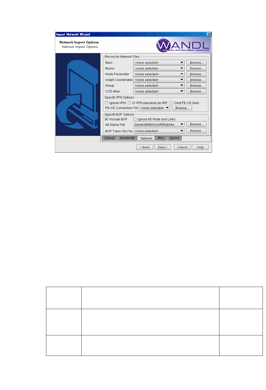
Figure 2-5 Network Tab
6. Next, click on the Network tab. During configuration import, if you supplied a runcode that already exists in
the specified output directory (i.e. you are importing over an existing network model), some WANDL network
files may be overwritten. To preserve or append to the original files, specify them in the Reconcile Network
Files section.
For example, you may have previously painstakingly arranged your network nodes on the topology map. This
information is saved into the Graph Coordinates (graphcoord) file. To ensure that you do not lose all your
hard work from overwriting the file, specify the desired graph coordinates file in the Reconcile Network
Files section.
Note: At this time, incremental configuration import is not supported. If you import over an existing network
model (i.e. you use the same runcode), you must specify the location where the entire set of configuration files
are located, not just a subset. Alternatively, you can perform the new import into a new WANDL network
project (corresponding to a different spec file and runcode), and then use File > Load Network Files to read
in WANDL files (such as the graphcoord file) from a previous import or network project. After doing so, be
sure to save your new network project (File > Save Network...).
7. There are additional options the user can select that are related to VPNs and BGPs. The description of these
options are explained in the table below.
Option Description
Corresponding
Text Interface
Option
Spec This is the file that lists, or specifies, all files related to a
particular network project. If specified, the following files from
specFile will be preserved: ratedir, datadir, site, graphcoord,
graphcoordaux, usercost, linkdist, fixlink, domain, and group.
-spec specFile
Muxloc This is the file that contains additional location information of the
nodes such as NPA, NXX, latitude and longitude. If specified, the
existing muxloc file will be preserved or appended to.
-n muxloc

ROUTER DATA EXTRACTION
2-8 Copyright © 2014, Juniper Networks, Inc.
2
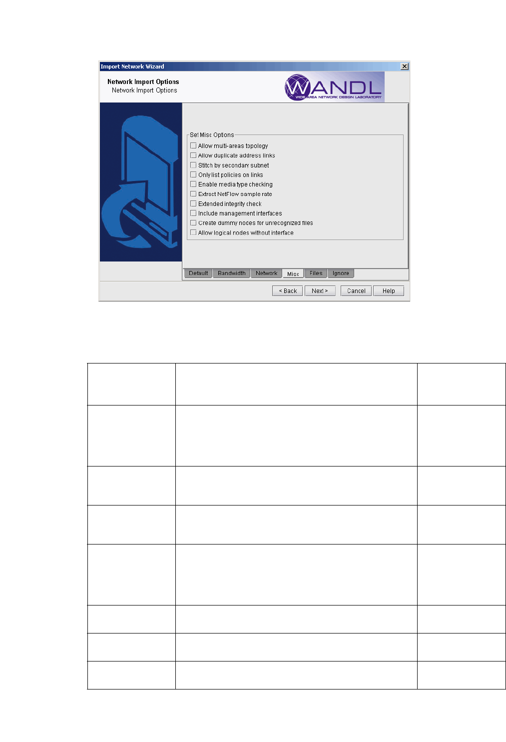
8. Click on the next tab, Misc. Here, you may set other desired options during the conversion of the router
configuration files to the WANDL network model.
Node
Parameter
This is the file that specifies the parameters — node ID,
hardware, IP address — of each node. If specified, the existing
“nodeparam” file will be preserved or appended to.
-p nodeparam
Graph
Coordinates
This is the file that contains any existing graph coordinates
information. If specified, the existing “graphcoord” file will be
preserved or appended to. This file will overwrite the graphcoord
file in the Spec option, if a spec file is also specified in the
“Reconcile Network Files” section.
-coord coordFile
Group This is the file that contains any existing grouping information. If
specified, the existing “group” file will be preserved or appended
to. This file will overwrite the group file in the Spec option.
-group groupFile
CoS Alias A router network may have more than eight CoS names defined,
but only eight or fewer real CoS classes, as each router is at
liberty to assign its own CoS name. The CoS Alias file matches
CoS names that are used for the same CoS class.
-cosalias
CoSAliasFile
Ignore VPN When selected, VPN statements will be ignored and will not be
imported.
-noVPN
ID VPN
elements by
VRF
When selected, this option will match Virtual Private Networks
(VPNs) by looking up the VPN Routing and Forwarding Instance
(VRF) names instead of matching import/export route targets.
-vpnName
Omit PE-CE
links
When selected, the program will omit links between Provider
Edge (PE) routers and Customer Edge (CE) routers.
-noCE
PE-CE
Connection
File
This file can be used to specify PE and CE connectivity, and is
only necessary for networks that re-use private ip
addresses for their VRF interfaces. For such networks, this file
is needed in order to stitch up the PE-CE links correctly. See PE-
CE Connection File on page 2-18 for file format information.
-PECE
Ignore AS
Node and
Links
Selecting this option will ignore AS nodes and AS links during
the data extraction. This option can improve performance by
reducing the number of pseudo-links on the map and reducing
the policymap file when there are policies on the AS links.
-noASNodeLink
AS Name File The user can specify a different Autonomous System (AS) name
file, ASNameFile, mapping an AS name (rather than just a
number) to the name of the AS nodes for display on the topology
map. If left unspecified, a default file located at
/u/wandl/db/misc/ASNames is used. Note however that this file
may not be entirely up to date.
-as ASNameFile
BGP Table
Obj File*
The BGP routing table object file is used by the routing engine to
perform BGP table lookup. To create the BGP Table Obj File
from the live network, BGP routing tables are needed, with the
hostname prepended in the first line of each file preceded by the
word ‘hostname’. Run the following commands (for Juniper BGP
routing table output ) to create the object file output_object_file
for this option.
/u/wandl/bin/prefixGroup -firstAS routingtablefiles
/u/wandl/bin/routeGroup -o output_object_file -g group.firstAS
routingtablefiles
See Chapter 8, Border Gateway Protocol*.
-bgpGroupTable
ROUTER DATA EXTRACTION
Copyright © 2014, Juniper Networks, Inc. 2-9
. . . . .
Figure 2-6 Misc Tab
Option Description
Corresponding
Text Interface
Option
Allow multiple-area
topologies
This option is useful if you have multiple OSPF areas. If this
option is checked, users can import more than one MPLS
TE topology file to cover all the areas in the network. These
files should be placed in the same directory as the
configuration files.
-tn
Allow duplicate
address links
This option will print those links that have duplicated IP
addresses in other links. By default, these links are
commented out.
-printDup
Stitch by secondary
subnet
For ethernets which have secondary addresses, if their
primary addresses do not match any subnet, the program
will try to match their secondary addresses.
-secondary
Only list policies on
link
Only the CoS policies on links in the network will be
processed and saved to the policymap file. This option can
be used to speed up performance by reducing the number
of policies to only the ones that are relevant to
routing/dimensioning.
-policyOnLink
Enable media type
checking
This option will match nodes that have different media types
but are within the same subnet.
-noMedia (to disable
this option)
Extract NetFlow
sample rate
This option will read in the user-specified NetFlow sample
rate
-iptraf
Extended Integrity
Check
This option will cause the set of extended integrity checks
to be performed
-exIC

ROUTER DATA EXTRACTION
2-10 Copyright © 2014, Juniper Networks, Inc.
2
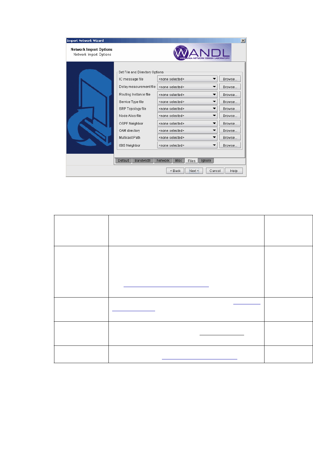
9. Click on the Files tab.
Include
management
interfaces
By default, management interfaces, e.g., fxp0 for Juniper,
will not be stitched together to form links. If it is desired to
stitch together management interfaces based on IP address
subnets, check this icon.
-mgnt
Create dummy
nodes for
unrecognized files
If you would like to include hosts other than routers and
switches in your network model, check the option
-dummyNode
Allow logical nodes
without interface
If this option is selected, logical nodes without any
interfaces configured will be parsed and displayed as an
isolated node. By default, this option is not selected, and
logical nodes lacking interfaces will not be displayed.
-nodewoIntf
Use IPv6 addresses
to stitching links
If this option is selected IPv6 addresses will be used to stich
links.
-IPv6
Mark operational
down links as
deleted
If this option is selected, links that are operationally down
will be marked as deleted in the bblink file.
-operStatus
Delete existing data
with duplicated
hostname
If this option is selected, and a config file is collected for the
same hostname twice, one of the config files will be
deleted.
Ignore VRF when
stitching links
The data extraction program uses various rules to stitch
links, some of which are intelligent guesses based on
BGP/VPNv4 information. If this option is selected, those
VRF-related rules will be ignored, and links will not be
stitched based on VRF information.
-ignoreVRFOnLink
Remove JUNOS RE
extension in
hostname
For JUNOS dual routing engine support, by default the RE
extension in the router name is removed for the Node ID
and Node Name, but not the hostname. To also remove it
from the hostname, select this option.
Use shutdown
interfaces/tunnel for
links
If this option is selected, then shutdown links will be used
for stitching up the backbone links. By default, these links
are not used for link stitch-up.
Option Description
Corresponding
Text Interface
Option
ROUTER DATA EXTRACTION
Copyright © 2014, Juniper Networks, Inc. 2-11
. . . . .
Figure 2-7 Files Tab
IC message file The IC message file is the integrity check profile file that
allows the user to define the severity of a check as well as
whether or not to include a particular check in the generated
report.
-IC
Delay measurement
file
A delay measurement file provides an easier method of
inputting delay statistics into the network model. (Alternatively,
delay information can be specified in the bblink link file.)
Supplying the actual link delay measurements enables the
program to accurately compute delays of end-to-end paths.
See Delay Measurement File on page 2-17 for file format
information.
-delay delayFile
Routing instance file A file containing routing instance definitions. See Chapter 17,
Routing Instances* for more information on this feature
including the file format.
-routeInstance
routeinstanceFile
Service Type File The service type file is used to match demands with services
such as email, ftp, etc. Refer to the File Format Guide for
more details on the servicetype file format.
-srvcType
serviceTypeFile
SRP Topology File Output of “show srp topology” used for RPR rings. For more
information, refer to Chapter 14, Resilient Packet Ring
-srp srpTopoFile

ROUTER DATA EXTRACTION
2-12 Copyright © 2014, Juniper Networks, Inc.
2
Node Alias File This file can be used when there are devices with dual routing
engines to indicate that two routing engine hostnames belong
to the same device. For Juniper, this is only needed if the
names do not follow the standard naming convention of
ending with re0 or re1.
Each line of the node alias file should contain the mapping
from the routing engine(s) to the corresponding AliasName
that will represent the device on the topology.
<AliasName> <RoutingEngine0’s Hostname>
<RoutingEngine1’s Hostname>
-nodealias
nodealiasFile
OSPF Neighbor Either a directory or file can be specified for this option. If a
directory neighborDir is specified, the program will read all the
files in that directory. The text files should contain the results
of a Cisco IOS router’s “show ip ospf neighbor” statement or
Juniper router’s “show ospf neighbor | no-more” statement.
See /u/wandl/db/command for the statements for additional
vendors like Cisco CRS and Tellabs. This additional
information helps connect the devices on the topology view.
Each file should be preceded by the hostname, e.g.,
“hostname <hostname>” for Cisco or “host-name
<hostname>;” for Juniper. In some cases, it may be possible
to extract the hostname from the prompt if the line
"[hostname]>show ip ospf neighbor" is included before its
results. Note that the prompt can be either “>” or “#” and that
the short form, “sh ip ospf nei” is also recognized.
-ospfnbr
neighborDir
or
-ospfnbr
neighborFile
OAM directory OAM can be used for connectivity checking for Juniper
and Zyxel at the MAC address layer. The OAM directory
can be collected from the Scheduling Live Network
Task (online users), or manually via the commands in
/u/wandl/db/command/*.oam.
-oam oamDir
Multicast Path Output of “show ip mroute” (Cisco IOS) or “show multicast
route” (Junos). Each file should be begin with the router
hostname information.
ISIS Neighbor If a directory is specified, containing the outputs of “show isis
database detail” (for Cisco) or \“show isis database extensive”
(for Juniper), the program will read these files to stitch
together devices on the topology view.
Each file’s command outputs should be preceded by the
hostname, e.g., “hostname <hostname>” for Cisco or “host-
name <hostname>;” for Juniper.
-isisnbr
neighborDir
ROUTER DATA EXTRACTION
Copyright © 2014, Juniper Networks, Inc. 2-13
. . . . .
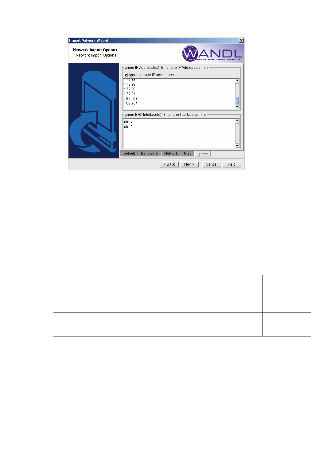
Figure 2-8 Ignore Options Tab
10. Click on the final tab, the Ignore Options tab. Here, you specify the IP addresses and ERX interfaces you
want to ignore. If you select the Ignore private IP addresses checkbox, then the following blocks of IP
addresses will be ignored during the import:
•10.0.0.0 - 10.255.255.255
•172.16.0.0 - 172.31.255.255
•192.168.0.0 - 192.168.255.255
•169.254.0.0 - 169.254.255.255
11. When all the options are selected as desired, click Next > to begin importing the configuration files. The
generated network model will be automatically loaded if there is not already a spec file open. Otherwise, the
program will ask if you want to close the current network.
12. When complete with the configuration import, click Finish to close the wizard.
Ignore IP Addresses This is the option to instruct the program that the IP address
ipaddr should be ignored. The user can specify more than one
IP address. This option is useful when the user has private IP
addresses for which it is not desirable to include in the
analysis.
-ignore ipaddr
Ignore ERX
Interfaces
This is the option to instruct the program to ignore certain
interfaces. The user can specify more than one interface.
Interfaces are matched based on substring.
-ignoreIntf
interface

ROUTER DATA EXTRACTION
2-14 Copyright © 2014, Juniper Networks, Inc.
2
TEXT MODE
1. Open a console window or a telnet window to the WANDL server. If you are not already the WANDL user,
switch to the WANDL user. For example, if user ID is wandl, type in “su - wandl” and enter the password.
2. Type /u/wandl/bin/getipconf to see the command options:
usage: /u/wandl/bin/getipconf[-as asNameFile] [-b bwconvfile] [-baseIntf baseIntf] [-cat selected category for
report] [-checkMedia] [-commentBW] [-coord graphCoordFile] [-cosalias cosaliasFile] [-delay delayFile] [-
deltaIntf deltaIntf] [-dparam dparam] [-dummyNode] [-exIC] [-filter filter for report] [-group groupFile] [-
greTunnel] [-i interfaceDir] [-IC ICmessageList file name] [-ignore ipaddr] [-ignoreIPUnnumbered] [-intf
intfmap] [-iptraf] [-IPv6] [-isisnbr neighborDir] [-layer2CLI EXSWdir] [-LSPDir lspDir] [-mgnt] [-n muxloc [-
p nodeparam]] [-noASNodeLink] [-noCPDNode] [-noCE] [-nodealias nodealiasFile] [-nodewoIntf] [-
noVLANLink] [-noVPN] [-oam oamDir] [-ospf ospfdatabase] [-ospfnbr neighborDir] [-PECE PECEfile] [-
policyOnLink] [-printDup] [-probe probeFile] [-profile profile] [-r runcode] [-routeInstance routeInstanceFile]
[-router selected router for report] [-secondary] [-snmp SNMPDir] [-spec spec] [-srp srpTopoFile] [-srvcType
file] [-STM] [-t topfile] [-vlan vlanfile] [-vlandiscovery vlanDir] [-hostdiscovery hostDir] [-vpnName] [-vrf
vrffile] [-user username] [-dir configDir] [ config1 config2 ... [-tn topofiles...]
3. Run the program /u/wandl/bin/getipconf with the appropriate command-line variables. For example, if your
configuration files all have the “.cfg” suffix, then type in the directory containing your configuration files:
$ /u/wandl/bin/getipconf *.cfg
Refer to the tables above for other corresponding command-line options available. Running getipconf in the
command line offers more options. These are listed in the table below.
4. Log onto the WANDL client and go to the directory containing the getipconf output files.
5. Open the newly created spec file and perform Layout>Recalculate Layout from the right-click menu of the
map.
Option Description
-ospf ospfdatabase
(Cisco and Juniper)
This uses the OSPF database for topology information. The CLI
command used to retrieve the OSPF database is: show ip ospf
database (for Cisco) and show ospf database router extensive
(for Juniper).
This option is also available from File > Import Data wizard, Import
Type, “OSPF Database”.
-ignoreIPUnnumbered This option is used for performance issues. This option will cause
interfaces that are “ip unnumbered” to be ignored.
-baseIntf baseIntf,
-deltaIntf deltaIntf
These options are used for performance issues when importing a
large set of config files, and are normally not modified. baseIntf
(default=8192) controls the base hash table size. deltaIntf
(default=2048) indicates the delta size by which the hash table should
be increased after the hash table capacity has been reached.
-IPv6 This uses IPv6 addresses for link stitching. The default is not to use
IPv6 for link stitching.
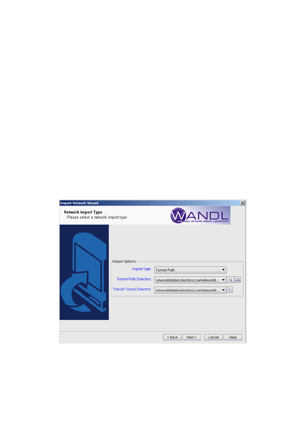
ROUTER DATA EXTRACTION
Copyright © 2014, Juniper Networks, Inc. 2-15
. . . . .
MPLS Tunnel Extraction*
MPLS Tunnel Extraction retrieves the actual placement of the tunnel and the status (up or down) of the LSP paths by
parsing the output of the Juniper JUNOS tunnel_path command:
show mpls lsp statistics extensive
Or the Cisco IOS command:
show mpls traffic-eng tunnels
This feature shows the exact network view of tunnel paths. This is useful if the LSPs can be dynamic (as opposed to
explicit). The WANDL software will display the current status and routing of the LSP tunnels within the defined
network.
*Note that this feature requires a special password that supports tunnels.
1. To user this feature, you must specify a directory that contains the output of these commands, one file per router.
With your network model already open, select File > Import Data to access the Import Wizard. Click Next >
to go to the second page of the wizard.
2. First, under Import Type, click on the drop-down selection box to choose Tunnel Path. Then, specify the
import directory for the Tunnel Path directory. Note that there is also a directory for Transit Tunnels. This is
used to collect additional information for Fast Reroute.
3. Click on the “Browse” button to open up a Directory Chooser window. Navigate to the directory that
contains the files and press “Select”.
Figure 2-9 Importing Tunnel Paths Into Existing Network Model
4. Click “Next >” to begin the extraction.
Note: In order to see the Tunnel Path import type option inside the Import Wizard, a network model should
already be opened. You will be importing the tunnel path information into this network model.
This should generate a WANDL format file of the tunnel paths and status called tunnelpath.runcode, where
runcode is the file extension of your network model. This will also be automatically loaded into the network model.
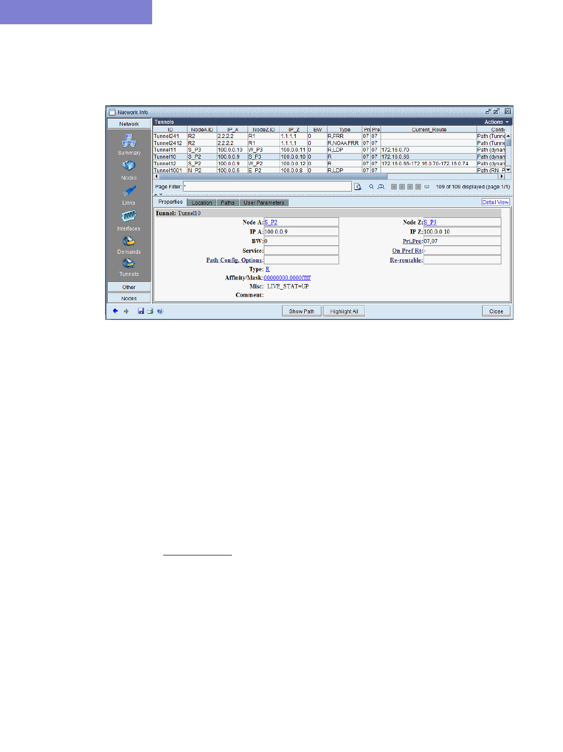
ROUTER DATA EXTRACTION
2-16 Copyright © 2014, Juniper Networks, Inc.
2
5. When the import action is complete, click “Finish” to close the wizard.
6. As a result of the import of tunnel paths, the tunnel path information as well as tunnel status can be seen from
Network > Elements > Tunnels.
Figure 2-10 Imported Tunnels
7. The status can be seen in the Misc field of the Properties tab:
•LIVE_STAT=UP: The tunnel is up
•LIVE_STAT=DOWN: The tunnel is down
•LIVE_STAT=MISSING: The status of the tunnel has not been collected, so the information is unknown.
8. The path can be seen from the Current_Route column of the Tunnels table.
9. Select a tunnel and click “Show Path” to view the tunnel graphically on the Standard Map.
COMMAND LINE VERSION: RDJPATH
The program /u/wandl/bin/rdjpath can be used to automate the tunnel info extraction. The command line options are
as follows: /u/wandl/bin/rdjpath -r runcode tunnel_path_dir
Substitute the runcode with the same file extension used by your network project and tunnel_path_dir with the
directory containing the tunnel path files collected from the router.
The resulting file, tunnelpath.runcode can be imported into the network via /u/wandl/bin/bbdsgn, option M.
MPLSView, 3. Read MPLS Tunnel Path. This can also be automated via input trace file. For more information, refer
to the File Format Guide chapter, “WANDL Scripting.”

ROUTER DATA EXTRACTION
Copyright © 2014, Juniper Networks, Inc. 2-17
. . . . .
Appendix - File Format
DELAY MEASUREMENT FILE
A link latency file can be specified as an input to getipconf using the -delay <delayFile> option. This file is used to
indicate the delay measurement from nodeA to nodeZ via a particular interface on nodeA. This information will be
stored in the bblink file after the config file import via getipconf. For online users, the Link Latency Task provides
one way to collect delay measurement information. See the Management & Monitoring Guide for more details.
The following is an example of a link latency file with a customized header line followed by contents. In the
example below, ATL and LDN2600 are connected.
#!NodeA,Interface,LatencyA2Z,BW
LDN2600,Ethernet0/1,50,100m
ATL,fe-0/1/3.0,50,100m
The format of the link latency file is flexible. The customizable column headers should be specified in a comma-
separated list following a “#!”. The column headers on this line must be one of the following reserved keywords in
order to be recognized.
•NodeA, NodeZ, Interface, InterfaceZ
•LatencyA2Z: Latency from NodeA to NodeZ (ms). For microseconds, use decimals.
•LatencyZ2A:Latency from NodeZ to NodeA (ms). For microseconds, use decimals.
•RoundTripLatency: This number will be divided by two to get the latency
•BW-K: The bandwidth in K
•BW: The bandwidth in bits
•ISIS2Metric: The ISIS level 2 metric
Note that the data for one link could also be represented in one line instead of two. For example, the above link
latency file entry for the link between LDN2600 and ATL could be shortened to one line by including the
LatencyZ2A column, as shown below:
#!NodeA,Interface,LatencyA2Z,LatencyZ2A,BW
LDN2600,Ethernet0/1,50,50,100m
The RoundTripLatency could also be specified as an alternative to the Latency in one direction.
#!NodeA,Interface,RoundTripLatency,BW
LDN2600,Ethernet0/1,100,100m
For backwards compatibility, the following fixed format is also supported:
#RouterA,Type,RouterZ,Interface,Interface IP,Bandwidth(K),Metric,LatencyZ2A
conf1,,,Ethernet0,10.0.0.1,,,10
For the fixed format, the only attributes that are required are RouterA, Interface, and Latency, as shown in the
example above. Note that the direction of Latency here is from NodeZ to NodeA.
UPDATING LINK INFORMATION
Delay information can also be entered in interactively through the text mode version after importing the
configuration files. This file format is also flexible and can support the following fields:
NodeA, NodeZ, Node, InterfaceA, InterfaceZ, Interface, DelayAZ, DelayZA, LatencyA2Z, LatencyZ2A, Delay,
IPaddrZ, IPaddr, RoundTripDelay, linkname, OSPFMetric, ISIS2Metric, ISIS1Metric, LinkName, BWType, Node,
Interface, DelayAZ, DelayZA
The first line should specify the columns using a comma separated list of the above keywords, including a column
for the node and the interface or IP address at the minimum. The subsequent lines should specify the Node/Interface
or Node/IP pair and the other relevant columns to update. See the link latency file in the last section for an example.
From the File > Load Network Files menu, select the file type linkdataupdate under the Network Files tab,
Device Specific Files section. Click the Browse button to indicate the location of the file to use for updating the
links.

ROUTER DATA EXTRACTION
2-18 Copyright © 2014, Juniper Networks, Inc.
2
Alternatively, in a console window, type /u/wandl/bin/bbdsgn specfilepath. Select from the Main menu: 5. Modify
Configuration > 4. Link Configuration > u. Update Link Properties from a File. Select ? for the help
menu for information on the input file format. Select 2. Input File Name and enter in the location of the file to use
for updating the links (absolute or relative path is acceptable here). Select 3. Error Output Name to enter the
location of an optional file for outputing errors. Select 4. Operation to indicate which fields to update based on the
input file (the default includes all fields) and q to exit this menu. Select 5. Update link configuration to perform
the actual update based on the specified input file. To save the changes, exit until you reach the Main Menu and use
the 2. Save Files menu.
PE-CE CONNECTION FILE
#PE PE-interface PE-intf-address vrf CE CE-intf-address
PE1 so-0/0/1.121 10.200.138.5 aaa-251001 CE100 10.200.138.6
PE1 so-0/0/1.120 10.200.133.5 bbb-258001 CE200 10.200.133.6

Copyright © 2014, Juniper Networks, Inc. 3-1
. . . . .
. . . . . . . . . . . . . . . . . . . . . . . . . . . . . . . . . . .
O
FFLINE
T
RAFFIC
P
ROCESSING
3
his chapter describes how to import traffic that was measured at the interface or at the tunnel source. This
chapter then describes how the tunnel/interface traffic can be loaded offline for viewing the load and
utilization in the WANDL client, or for creating reports. Offline traffic processing also allows the flexibility
to summarize collected traffic data over a selected series of dates and to report statistical results.
When to use
The following are example applications of offline traffic processing:
•Generating a report of the 95th percentile interface or tunnel traffic statistics for all weekdays in January
•Load traffic statistics into the WANDL client to view the resulting link utilization, or generate summary reports.
Prerequisites
•Offline traffic processing assumes that you have already collected traffic data and have prepared it in the format
described in Preparing the Traffic Data: Step One on page 3-2.
•You should also have a set of WANDL format network files for your network (particularly the “intfmap” file and
optionally the “tunnel” file). There are a few ways to generate these files. 1) Run the getipconf utility that
intelligently converts router configuration files into a corresponding set of WANDL format network files. This is
described in Getipconf - Router Configuration Extraction on page 2-2. 2) Alternatively, if you used the WANDL
online network collection to automatically retrieve your network topology and then saved the results to a directory,
then the WANDL format network files can be found already generated in the output directory. This is described in
detail in the IP/MPLSView Network Management User Guide.
Recommended Instructions
Following is a high-level, sequential outline of the process of importing interface or tunnel traffic data and the
associated, recommended detailed procedures.
1. Prepare traffic data in the format described in Preparing the Traffic Data: Step One on page 3-2
2. Run the convintftraf (“convert interface traffic”) utility to create binary daily directories as described in
Convintftraf (the Traffic Conversion Utility) on page 3-3
3. Use the WANDL client to import this data into a daily directory repository, as described in Using the WANDL
client to Import Traffic Data on page 3-5
4. Aggregate or “roll-up” traffic data for selected days (for example, all the Mondays in February), as described in
Roll-up / Aggregation Defined on page 3-8.
5. View the summarized traffic statistics on the topology map as link utilizations, as described in Viewing
Summarized Traffic Statistics on the Map on page 3-9
T

OFFLINE TRAFFIC PROCESSING
3-2 Copyright © 2014, Juniper Networks, Inc.
3
Detailed Procedures
Preparing the Traffic Data: Step One
1. Below is a simple example of the required traffic data file format. It shows a clipping from a file that includes
two samples, spaced roughly 5 minutes apart.
#RouterIP,InterfaceName,inBitsPerSec,outBitsPerSec
StartTime:Wed Jan 15 19:49:48 EST 2003
EndTime:Wed Jan 15 19:54:47 EST 2003
162.51.225.1,Ethernet0,45,50
162.51.225.1,GigabitEthernet4/0,105330704,21984624
StartTime:Wed Jan 15 19:54:47 EST 2003
EndTime:Wed Jan 15 19:59:47 EST 2003
162.51.225.1,Ethernet0,50,46
162.51.225.1,GigabitEthernet4/0,114779210,21764904
...
2. Each sample begins with a “StartTime” and “EndTime”, followed by a list of router interfaces and their
incoming and outgoing traffic in bits per second. The following explains the format for each sample in detail:
The first line of each sample begins with the keyword "StartTime:", followed by the date and time in the following
format:
"DDD#MMM#dd#HH:mm:SS#ZZZ#YYYY"
where #=<space>,D=Day, M=Month, d=date, H=hour, m=minute, S=seconds, Z=TimeZone, Y=year
The second line of each sample begins with the keyword "EndTime:", followed by the date and time in the same
format as above.
All interfaces/tunnels are then listed with four comma-separated fields per entry.
For interfaces, the format is:
<IP Address>, <Interface Name>,<In bits per second>,<Out bits per second>
For tunnels, the format is:
<IP Address>, <Tunnel ID>, <Out bits per second>
Field Description
<IP Address> The IP address enables the WANDL software to map the entry to the
corresponding source router by doing a look-up in the interface map
(intfmap) file.
For interfaces, the IP address is often the Loopback address of the router,
but it may be the IP address of any interface in the router as long as it is
present in the interface map (intfmap) file. This file is automatically
generated when the router configuration files are parsed as described in
Getipconf - Router Configuration Extraction on page 2-2.
<Interface Name> For interfaces only, this is the equivalent of the SNMP variable “ifDescr”
that holds the “interface description”. These interface descriptions should
also match the interface names in the interface map (intfmap) file.

OFFLINE TRAFFIC PROCESSING
Copyright © 2014, Juniper Networks, Inc. 3-3
. . . . .
ORGANIZING YOUR TRAFFIC SAMPLES
These samples can be spread out in multiple files in a special directory. One recommended way of organizing them is
by creating one file per router per day, where that file contains only the daily traffic samples associated with that
router’s interfaces. You can also create subdirectories in order to categorize the traffic by particular days, weeks, etc.
Use a meaningful naming scheme for the files, incorporating the router name or IP address.
Creating the Daily Directories
DAILY DIRECTORIES STRUCTURE
3. Using the WANDL convintftraf (“convert interface traffic”) utility, WANDL software takes the traffic data as
input (in the format described in Preparing the Traffic Data: Step One on page 3-2) and converts it into a concise
binary format, organized by “daily directories”, that is suitable for rapid aggregation using any of a choice of
statistical computation methods. For example, it allows you to "roll-up" a week's worth of data into 24 hourly
periods and display the hourly utilization based on the 95th percentile.
The following explains the structure of the daily directories. These directories have names in date format such as:
MAR19.01
MAR20.01
MAR21.01
In each of these daily directories is a number of files- one file per device for which traffic was collected on that
particular day.
For example,
>ls MAR19.01
ROUTER1 ROUTER2 ROUTER3
Thus, if interface traffic for Router1 was collected on all three days, there will be a binary file for Router1 under each
of the three daily directories. These files are named by the router hostname rather than an IP address. The
conversion from IP address to router hostname was done by referencing the interface map (“intfmap”) file generated
during getipconf configuration extraction, as described in Getipconf - Router Configuration Extraction on page 2-2.
CONVINTFTRAF (THE TRAFFIC CONVERSION UTILITY)
4. The convintftraf utility takes the following arguments.
Usage: convintftraf outtrafficdir router_interface_traffic_data1 router_interface_traffic_data2 ... -i intfmap
or
Usage: convintftraf outtrafficdir router_interface_traffic_data1
router_interface_traffic_data2 ... -i intfmap -t tunnel_file
Example:
convintftraf myOutput myData/*.dat -i intfmap.x -t tunnel.x
<Tunnel ID> For tunnels only, the Tunnel ID should match the tunnel ID in the tunnel
file. The tunnel file, containing all tunnel definitions in the network, is
automatically created when the config files are parsed as described in
Getipconf - Router Configuration Extraction on page 2-2.
<In bits per second> This is the Ingress traffic rate in bits per second.
<Out bits per second> This is the Egress traffic rate in bits per second.
Field Description

OFFLINE TRAFFIC PROCESSING
3-4 Copyright © 2014, Juniper Networks, Inc.
3
Note: Creating the daily directories may take several hours for large data sets, depending on the number of days of
traffic being processed and the number of interfaces/tunnels. This procedure should be executed only once on any
given set of traffic data. If traffic for a large number of days or interfaces is to be processed at once, it is
recommended that the task be run overnight.
In order to check the progress of this function, the user can repeatedly check the contents of the outtrafficdir, to
see what daily directories (e.g. “MAR19.01”) have been created so far.
Parameters Description
outtrafficdir An output directory that will be the “repository” for the
generated daily directories.
router_interface_traffic_d
ata1...n
A list of the input files in the format described in Preparing the
Traffic Data: Step One on page 3-2. These can be listed
separately on the command line, or by using wildcards to
specify all the files in a particular directory, as shown in the
example.
intfmap This is the interface map file (usually named
“intfmap.runcode”), that is generated during configuration
extraction as described in Getipconf - Router Configuration
Extraction on page 2-2.
tunnel_file This file contains information on each tunnel in your network.
It is also generated during the getipconf configuration
extraction.
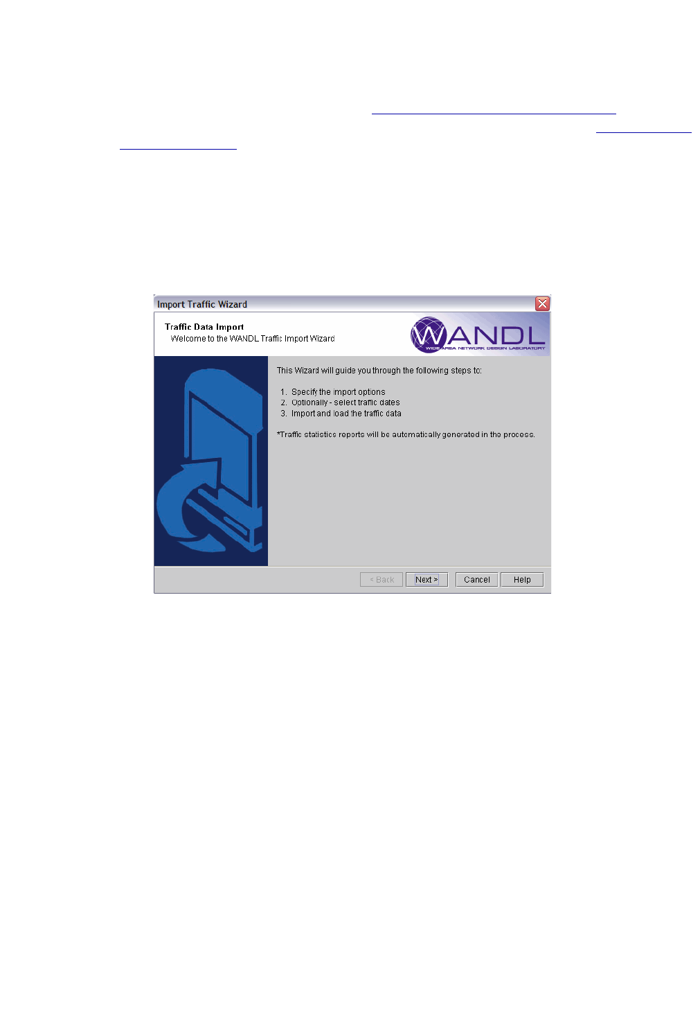
OFFLINE TRAFFIC PROCESSING
Copyright © 2014, Juniper Networks, Inc. 3-5
. . . . .
Using the WANDL client to Import Traffic Data
5. This step assumes that you have already:
•Prepared traffic data in the format described in Preparing the Traffic Data: Step One on page 3-2.
•Run the convintftraf utility on this data to create the binary daily directories, as described in Creating the Daily
Directories on page 3-3.
In the following steps, WANDL takes this data as input and converts it into a concise binary format, organized
by router in a set of “daily directories”, that is suitable for rapid aggregation and summary statistical reports.
For example, it allows you to "roll-up" a week's worth of data into 24 hourly periods and display the hourly
utilization based on the 95th percentile.
6. Open the spec file corresponding to your network.
7. Select Traffic > Import Traffic to open the Import Traffic Wizard.
Figure 3-1 Introduction Page of the Import Traffic Wizard
8. From the first page of the wizard, click Next > to continue.
9. First of all, select the directory in which the set of daily directories are saved by clicking on the Browse button
in the “Select Import Directory” section. Left click on the checkbox next to a directory to include that
directory only. Right click on the checkbox to include that directory and all subdirectories within that directory.
10. Next, under “Select Import Type,” select WANDLTraffic Data. If the WANDL Standalone Data Collector
(SDC) was used, then select the SDC options.
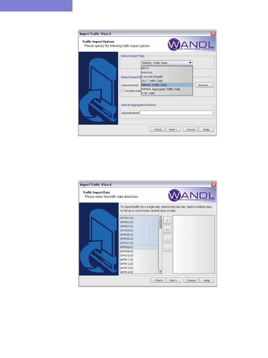
OFFLINE TRAFFIC PROCESSING
3-6 Copyright © 2014, Juniper Networks, Inc.
3
Figure 3-2 Selecting Import Directory, Import Type, and Output Directory
11. In “Specify Aggregate Directory,” select the directory in which the converted WANDL traffic files will be
saved. When done, click Next > to continue.
Figure 3-3 Selecting Dates from Daily Directories
12. In the Select Dates tab of the next page, use <Ctrl> or <Shift>-click to select the dates of traffic you wish to
aggregate. If selecting only one 24 hour period, select only one date. After the dates are highlighted, click on the
> button to moved them to the selected dates table on the right. To select all dates, click on >> to move all of
them to the other table. Then, click Next.
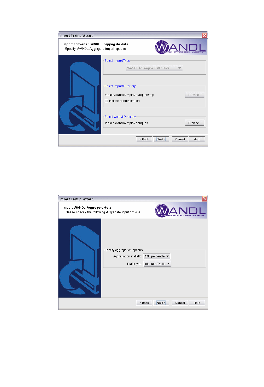
OFFLINE TRAFFIC PROCESSING
Copyright © 2014, Juniper Networks, Inc. 3-7
. . . . .
Figure 3-4 Importing Aggregate Traffic Data
13. Now the wizard will aggregate all the selected traffic data. Once aggregated, you will be able to import WANDL
Aggregate Traffic Data from the aggregate directory specified earlier. This is shown above. Click Next to
continue.
Figure 3-5 Select a Computation Method
14. Next, select a Computation Method : Max, Average, 80th percentile, 90th percentile, 95th percentile, 99th
percentile. These are explained below.

OFFLINE TRAFFIC PROCESSING
3-8 Copyright © 2014, Juniper Networks, Inc.
3
COMPUTATION METHOD
•Max - For each of the 24 hours, the maximum of the sample values within that hour is used.
•Average - For each of the 24 hours, the samples within that hour are averaged. If there are N samples within an
hour, the result is the sum of the all the sample values divided by N.
•95th percentile - For each of the 24 hours, the 95th percentile value of the samples within that hour is used.
The 95th percentile is computed from the equation:
Average + 1.645 * stddev
where Average refers to the average of the samples in that hour and stddev is the standard deviation. Another way of
thinking about this is that 95 percent of the sample values lie below the calculated value.
The corresponding equation for the 90th percentile is:
Average + 1.282 * stddev
and so on.
15. When both fields are specified, click on the Next > button.
ROLL-UP / AGGREGATION DEFINED
The intention of traffic aggregation is to summarize the network traffic data that is generated across several days of
collection. Selected days or a range of days can be specified to be included in the aggregated result. For example,
one can aggregate all Mondays in the month of January, weekdays only, or aggregate all the days in an entire month,
months, or year.
For example, in the aggregated data for a particular interface, there are 24 values representing the 24 hours. For that
particular interface, all sample points in hour 1 (In bps and Out bps values) across all the days are grouped together,
all sample points in hour 2 across all the days are grouped together, and so on. The 95th percentile for hour 1 then
takes into consideration as sample points, all the sample points for that interface during hour 1 on all the selected
days.
Note: Aggregate directories have the same format as the daily directories and can also be aggregated. This might be
useful when performing the offline traffic processing incrementally as more traffic data becomes available. However
it is up to the user to remember exactly which days of traffic were aggregated - usually by supplying a meaningful
name for the directory.
16. If multiple days have been selected, then a “roll-up/aggregation” will be performed and the newly generated
directory of binary files will be saved in the specified “Aggregate directory”. The status will be displayed in the
final page of the wizard.
17. Generating the interface/tunnel traffic files should be very quick, in a matter of minutes or less. Corresponding
WANDL format ingress and egress interface traffic files or tunnel traffic files will be generated and loaded into
the system if the user checks “Load traffic data”. Once completed, click on the Finish button. To access the
Load/Util window shown in Figure 3-6, first make sure you switch to the appropriate layer if the option is
available (Layer 3 for viewing Interface traffic and Tunnel Layerfor viewing Tunnel traffic). Then, select
from the main menu bar, Traffic > Traffic Load to bring up the Load/Util window.

OFFLINE TRAFFIC PROCESSING
Copyright © 2014, Juniper Networks, Inc. 3-9
. . . . .
Viewing Summarized Traffic Statistics on the Map
18. From the Standard map, select the legend Utilization Legends > Measured Link Util to view the measured
interface traffic per period, based on the egress/ingress files.
19. Alternatively, in the Traffic > Traffic Load window shown in Figure 3-6, click on the Interface radio button
(or Tunnel radio button if you are importing tunnel traffic).
Figure 3-6 Load/Util window with Traffic Load “slider”
Then, click on Run button for an animated 24-period link utilization display. The 24 periods represent 24 hourly
values. You can also drag the slider to a particular period and view the corresponding link utilization on the
topology map. The second “tick” on the slider shows the Worst period. Worst represents the highest value of
the 24 periods.
20. Right-clicking on a link will also display the 24-hour interface traffic barchart.
For interface traffic, select from the popup menu Traffic Load > Measured Interface Traffic to bring up the
corresponding traffic barchart.
For tunnel traffic, select from the popup menu Traffic Load > Tunnel Traffic on Link to bring up the
corresponding traffic barchart.
Refer to Traffic Load Analysis on page 13-17 for more information about traffic load analysis by CoS.
Related Spec file parameters
21. If you want to save the imported traffic in your network scenario, go to File > Save in Spec Dir, for example,
to save any new configurations to the spec file.
In the File Manager, right click on the newly created (or refreshed) spec file and select from the popup menu
Spec File > Modify Spec, or select Edit to view the text version of the spec.
The traffic-related spec file parameters are described below.
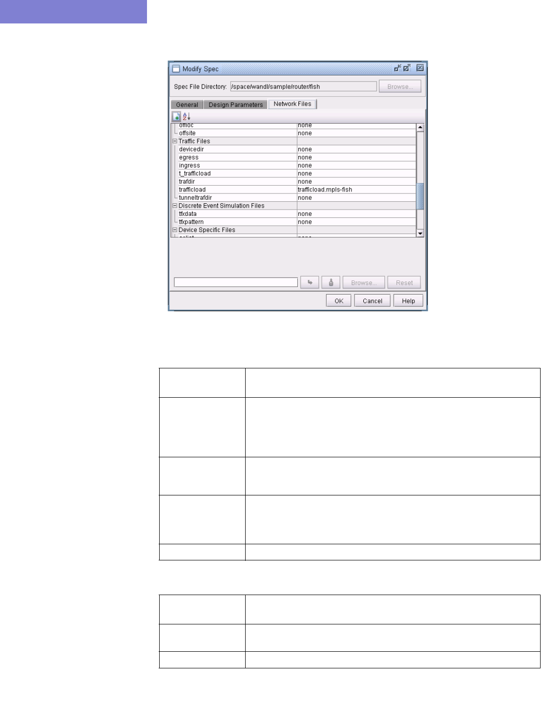
OFFLINE TRAFFIC PROCESSING
3-10 Copyright © 2014, Juniper Networks, Inc.
3
Figure 3-7 Spec file
Interface Traffic
Parameters Description
egress The egress file contains egress traffic of the network’s interface load.
Egress traffic specifies traffic that is going out of the network’s interfaces.
This data is used for calculating link utilization and load.
Results can be viewed graphically from the Standard map’s “Utilization
Legends > Measured Link Util” legend.
ingress The ingress file contains ingress traffic of the network’s interface load.
Ingress traffic specifies traffic that is going into the network’s interfaces.
This data is used for calculating link utilization and load.
trafficload 24-period traffic measured on interfaces. When importing traffic, the
trafficload file is automatically named trafficload.runcode and placed in the
trafdir. Results can be viewed graphically from the Standard map’s
“Utilization Legends > Demand Cos Util” legend.
trafdir The location of the interface traffic daily directories repository.
Tunnel traffic
Parameters Description
t_trafficload 24-period tunnel traffic file. When importing traffic, the tunnel traffic file is
automatically named tunneltraf.runcode and placed in the tunneltrafdir.
tunneltrafdir The location of the tunnel traffic daily directories repository.

Copyright © 2014, Juniper Networks, Inc. 4-1
. . . . .
. . . . . . . . . . . . . . . . . . . . . . . . . . . . . . . . . . .
R
OUTING
P
ROTOCOLS
4
his chapter describes how to model routing protocols using the WANDL software, in particular, interior
gateway protocols such as OSPF, ISIS, EIGRP, IGRP, and RIP.
When to use
Follow these guidelines to add and modify routing protocol information.
Prerequisites
If you wish to perform this task in the WANDL client, you should have a router spec file open before you begin. To
follow along with this tutorial, you can open the spec.mpls-fish spec file located in your
$WANDL_HOME/sample/IP/fish directory. ($WANDL_HOME is /u/wandl by default).
If you have an existing set of config files, use getipconf or the Import Data Wizard (via File > Import Data) to
parse your config files and create a set of WANDL input files which contain router interfaces.
Related Documentation
For general step-by-step instructions on how to use the WANDL software, please refer to the Design & Planning
Guide.
For an overview of the WANDL software or for a detailed description of each feature and the use of each window,
refer to the General Reference Guide or Chapter 37, Router Reference.
For more information about data extraction, refer to Chapter 2, Router Data Extraction.
Recommended Instructions
Following is a high-level, sequential outline of the process of viewing/modifying protocol information and the
associated, recommended detailed procedures.
1. View the routing protocols and metrics in the network from the map’s Subviews > Protocols pane.
2. Change the active routing method from Tools > Options > Design, Path Placement options pane.
3. Modify routing protocol details from the Modify Link window’s Protocols tab and the Modify Node
window’s IP tab.
T
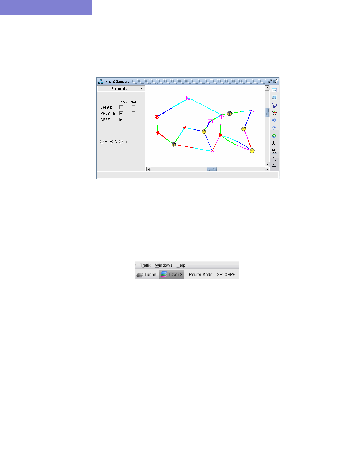
ROUTING PROTOCOLS
4-2 Copyright © 2014, Juniper Networks, Inc.
4
Detailed Procedures
View Routing Protocol Details from the Map
1. Select the Subviews > Protocols menu from the Standard Map. The protocols enabled in the network will be
displayed in the left pane of the map window as shown in the figure below.
Figure 4-1 Routing Protocols
With the ‘=’ radio button selected, clicking a checkbox next to a single protocol will display links enabled for
that protocol. When selecting the ‘&’ or ‘or’ radio buttons, logical combinations of protocols can be viewed. For
example, in the above, only links that have both MPLS and OSPF enabled are displayed.
2. To view the link metrics on the map, right-click the map and select Labels>Link Labels>Show Link Dist.
Note that this will display the metrics for the current routing method used. The current IGP routing method is
displayed in the upper right of the application next to the Tunnel later/layer 3 buttons.
Figure 4-2 Current IGP: OSPF
Alternatively, the link metric can be labelled by selecting Labels>Link Labels>Link Labels... and then
Customize... In addition to Metric_AZ and Metric_ZA, the following keys are also available: OSPF_AZ,
OSPF_ZA, ISIS1_AZ, ISIS1_ZA, ISIS2_AZ, and ISIS2_ZA. Select the keys desired and click Add-> to add
those keys to the list of keys to display. Then select a display format and click OK.
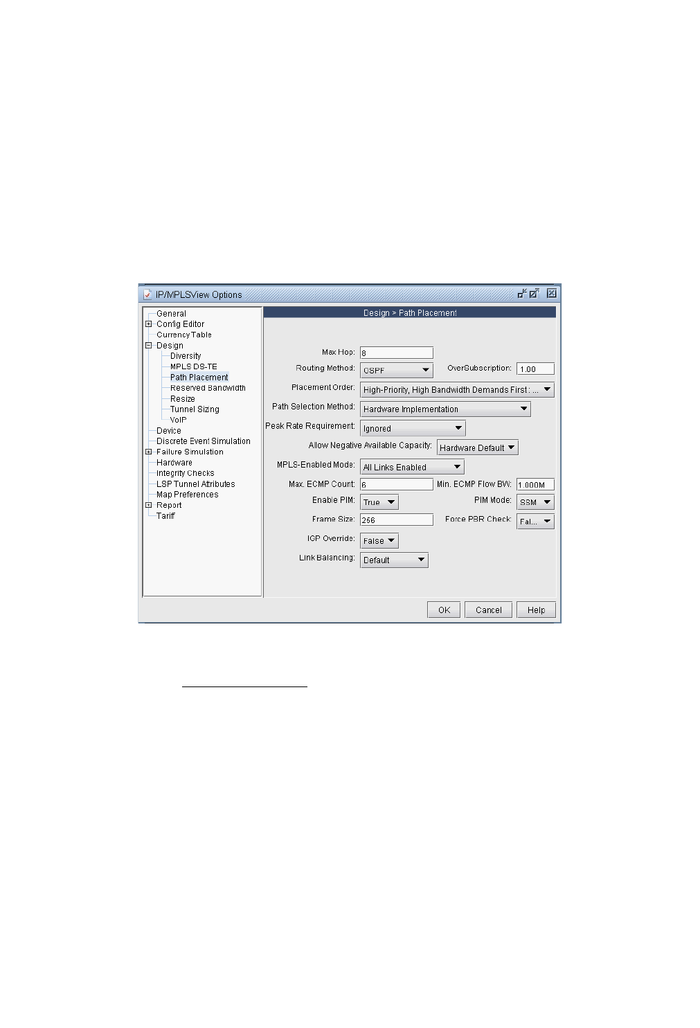
ROUTING PROTOCOLS
Copyright © 2014, Juniper Networks, Inc. 4-3
. . . . .
Set the IGP Routing Method
3. To change the current IGP routing method , select the Applications>Options>Design, Path Placement
options pane. For the Routing Method, the following IGPs can be selected: OSPF, IGRP, EIGRP, and ISIS. To
select RIP, use the Constant Distance routing method. Upon changing a routing method, the routing metrics for
that routing method will be displayed on the map. (The exception to the rule is if the user hard-coded a metric
for each link regardless of the protocol.)
4. The Max Hop parameter can also be configured from this window to indicate any hop limits for the selected
protocol.
5. Note also the item for “MPLS-Enabled Mode.” If “All Links Enabled” is selected, the program will allow LSP
tunnels to be routed on any link. If “User-Specified Per Link” is selected, the program will only allow LSP
tunnels to be routed on a link on which MPLS-TE (MPLS traffic engineering) is explicitly enabled.
Figure 4-3 Routing Method
Refer to the General Reference Guide, “The Application Menu” chapter for more details on the other Path Placement
options.
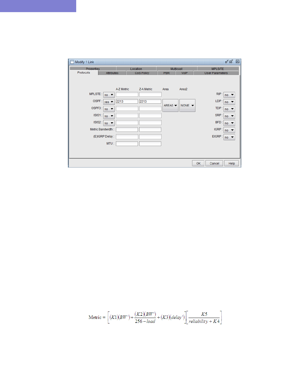
ROUTING PROTOCOLS
4-4 Copyright © 2014, Juniper Networks, Inc.
4
Routing Protocol Details
6. To modify protocol information on a link, select Modify > Elements > Links... in Modify mode. Select one
or more links to be modified and click the Modify button. In the resulting Modify Links window, select the
Protocols tab.
Figure 4-4 Modify Link Protocols Tab
7. To enable a protocol, select “yes” to the right of the protocol. To enter in a metric for a particular protocol, such
as MPLS-TE, OSPF, ISIS, or ISIS2, enter it in the “A-Z Metric” and “Z-A Metric” columns to the right of the
protocol. These metrics correspond to the A and Z interfaces of the link as indicated on the Locations tab.
Note that when routing for a specific IGP, metrics should be entered in the Protocols tab rather than the
Properties tab.
The following sections provide more details about configuring protocol-specific information.
RIP
No metrics need to be entered for RIP since the metrics will all be the same.
In the Tools > Options > Design, Path Placement options pane, the routing method should be set to
Constant Distance and the Max Hop should be configured to 15.
IGRP AND EIGRP
For IGRP and EIGRP, the metric can be changed via the Metric Bandwidth and (E)IGRP Delay fields. These fields
are based on the bandwidth and delay interface statements and should be distinguished from the physical bandwidth
and propagation delay given on the link Properties tab. The units should be entered into the textbox, e.g. “10M”
for 10Mbps and “100us” for 100 microseconds. These values will be used to calculate the metric according to the
following formula:
Figure 4-5 EIGRP/IGRP Metric Calculation
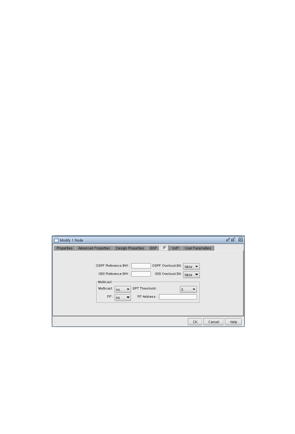
ROUTING PROTOCOLS
Copyright © 2014, Juniper Networks, Inc. 4-5
. . . . .
By default, the program sets K1=K3=1 and K2=K4=K5=0 in the formula above. In this case, only the bandwidth and
delay are used to calculate the IGRP and EIGRP metric, using a function of the slowest interface bandwidth and the
sum of the delays of the outgoing interfaces on the path. To obtain delay’ in the formula above, the interface delays
(in microseconds) that are summed together will be divided by 10 for IGRP and then multiplied by 256 for EIGRP.
To obtain bandwidth’, 10^7 will be divided by the interface bandwidth in Kbps for IGRP and then multiplied by 256
for EIGRP.
To change the K-values from the text file before opening the network, the following line can be added to or edited in
the dparam file: IGRP_param1= TOS:0,K1:1,K2:0,K3:1,K4:0,K5:0
In the Tools > Options > Design, Path Placement options pane, the routing method should be set to IGRP or
EIGRP. The Max Hop, can also be configured here (e.g., 100 for IGRP) according to the metric maximum-hops
command.
OSPF
OSPF metrics can be directly changed by setting the cost to the right of the OSPF row (or OSPF3 row in the case of
OSPF version 3) under the “A-Z Metric” and “Z-A Metric” columns.
Otherwise, if this number is not configured, the program will use the interface bandwidth (corresponding to the
bandwidth statement for the interface) and the OSPF reference bandwidth to calculate the metric using the formula:
reference_bandwidth/interface_bandwidth, where the default reference_bandwidth=10^8.
•To modify the interface bandwidth for metric calculation purposes, enter it in the Metric Bandwidth fields. The
left textbox is for the interface for Node A and the right textbox is for the interface for Node Z. (The Location tab
will indicate which node is Node A and which node is Node Z.) Again, note that the metric bandwidth can be
different from the physical bandwidth. The default unit is bps but can be modified by adding to the number a suffix
of K for Kbps, M for Mbps, and G for Gbps.
•To change the reference bandwidth from the default value, select the Nodes view from the Network Info
window. Select the node(s) to modify and click the Modify button. Then select the IP tab and enter in an OSPF
Reference BW. The default unit is bps but can be modified by adding to the number a suffix of K for Kbps, M for
Mbps, and G for Gbps.
Figure 4-6 Entering in the Reference BW from the Modify Nodes, IP Tab
•To specify which area the link belongs to, select it from the Area drop-down box. A secondary area can also be
specified in the Area2 drop-down box if the link belongs to more than one area. If there is no area available in the
drop-down box, an area can be first added from Modify > Protocols > OSPF Areas. Click Add. AREA0 will
automatically be added. Subsequently you can enter in additional areas.
To set the OSPF overload bit, select the Nodes view from the Network Info window. Select the node(s) to modify
and click the Modify button. Then select the IP tab and change the OSPF Overload Bit to true. If the OSPF
overload bit is set, transit OSPF traffic will not be routed through the router.

ROUTING PROTOCOLS
4-6 Copyright © 2014, Juniper Networks, Inc.
4
ISIS AND ISIS2
In the Modify > Elements >Links window, Protocols tab, the ISIS level 1 metrics can be changed in the “A-Z
Metric” and “Z-A Metric” columns to the right of ISIS1 . ISIS level 2 metrics can be changed in the “A-Z Metric”
and “Z-A Metric” columns to the right of ISIS2.
To view a node’s ISIS System ID, right-click the Nodes table header column and select Table Options... Next,
select ISIS_System_ID, and add it to the columns to be displayed. Other ISIS related column options for the Nodes
view include ISIS_Area, ISIS_Overload_Bit, and ISIS_Ref_BW. The ISIS Area can also be viewed from the
Protocols tab in the Nodes view.
To change the ISIS reference bandwidth from the default value, select the Nodes view from the Network Info
window. Select the node(s) to modify and click the Modify button. Then select the IP tab and enter in an ISIS
Reference BW. The default unit is bps but can be modified by adding to the number a suffix of K for Kbps, M for
Mbps, and G for Gbps.
To set the ISIS overload bit, select the Nodes view from the Network Info window. Select the node(s) to modify
and click the Modify button. Then select the IP tab and change the ISIS Overload Bit to true. If the ISIS overload
bit is set, transit ISIS traffic will not be routed through the router.\
MPLS-TE
The tunnel metric for MPLS-TE can be changed in the “A-Z Metric” and “Z-A Metric” columns to the right of
MPLS-TE. LSP tunnels that are not set to route according to the current IGP routing protocol will be routed
according to these metrics.
UPDATING LINK PROPERTIES FROM A FILE
Link delay and OSPF/ISIS metric information can also be modified in batch through the text mode version. This file
format also flexible and can support the following fields:
NodeA, NodeZ, Node, InterfaceA, InterfaceZ, Interface, DelayAZ, DelayZA, LatencyA2Z, LatencyZ2A, Delay,
IPaddrZ, IPaddr, RoundTripDelay, linkname, OSPFMetric, ISIS2Metric, ISIS1Metric, LinkName, BWType, Node,
Interface, DelayAZ, DelayZA
The first line should specify the columns using a comma separated list of the above keywords, including a column
for the node and the interface or IP address at the minimum. The subsequent lines should specify the Node/Interface
or Node/IP pair and the other relevant columns to update. For example:
#!NodeA,Interface,LatencyA2Z,LatencyZ2A,OSPFMetric
LDN2600,Ethernet0/1,50,50,10
To load in this file, select Tools > Text/ASCII Mode or in a console window, type /u/wandl/bin/bbdsgn
specfilepath.
Select from the Main menu: 5. Modify Configuration > 4. Link Configuration > u. Update Link
Properties from a File. Select ? for the help menu for information on the input file format.
Select 2. Input File Name and enter in the location of the file to use for updating the links (absolute or relative path
is acceptable here). Select 3. Error Output Name to enter the location of an optional file for outputing errors.
Select 4. Operation to indicate which fields to update based on the input file (the default includes all fields) and q
to exit this menu.
Select 5. Update link configuration to perform the actual input based on the specified input file.
After the update is finished, type ‘q’ until the Main Menu is reached. In text mode, select 2. Save Files menu to save
the changes, or in Java graphics mode, quit out of the menu and save via File > Save Network...
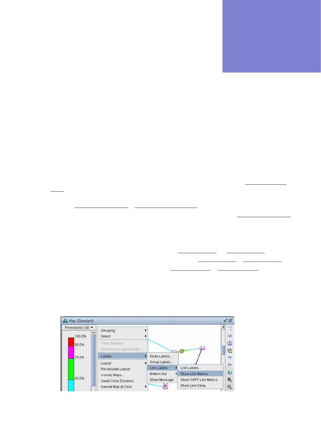
Copyright © 2014, Juniper Networks, Inc. 5-1
. . . . .
. . . . . . . . . . . . . . . . . . . . . . . . . . . . . . . . . . .
E
QUAL
C
OST
M
ULTIPLE
-P
ATHS
5
his chapter describes several Equal Cost Multiple-Paths (ECMP) features and walks through a scenario
where it is useful. The user will be able to display all the equal cost multiple-paths in the network as well as
view any equal cost paths between two given nodes in detail. The user can also split flows into sub-flows.
Note that parallel links between two nodes do not count towards ECMP’s.
When to use
Sometimes it is desirable to reduce the number of Equal Cost Multiple-Paths in order to improve the predictability of
how demands will be routed in the network. At other times it is desirable to split flows into sub-flows with Equal
Cost Multiple-Paths in order to perform load balancing. The WANDL software will place these flows on routing
paths that have identical costs.
Related Documentation
For general step-by-step instructions on how to use the WANDL software, please refer to the Design & Planning
Guide.
For an overview of the WANDL software or for a detailed description of each feature and the use of each window,
refer to the General Reference Guide or Chapter 37, Router Reference.
For more information on the Report Manager, refer to the Report Manager chapter of the Design & Planning Guide.
Recommended Instructions
Following is a high-level, sequential outline of the Equal Cost Multiple-Paths features and the associated,
recommended procedures.
1. Open the Equal Cost Multi-Paths Report as described in step 3 on page 5-2 and step 4 on page 5-2.
2. View the equivalent cost paths between two nodes as described in step 5 on page 5-3 to step 9 on page 5-4.
3. Create sub-flows between two nodes as described in step 10 on page 5-6 to step 13 on page 5-6.
Detailed Procedures
Identifying Equal Cost Multiple-Paths
1. Right-click on the topology map and select Labels > Link Labels > Show Link Metrics.
Figure 5-1 Show Link Distance
T
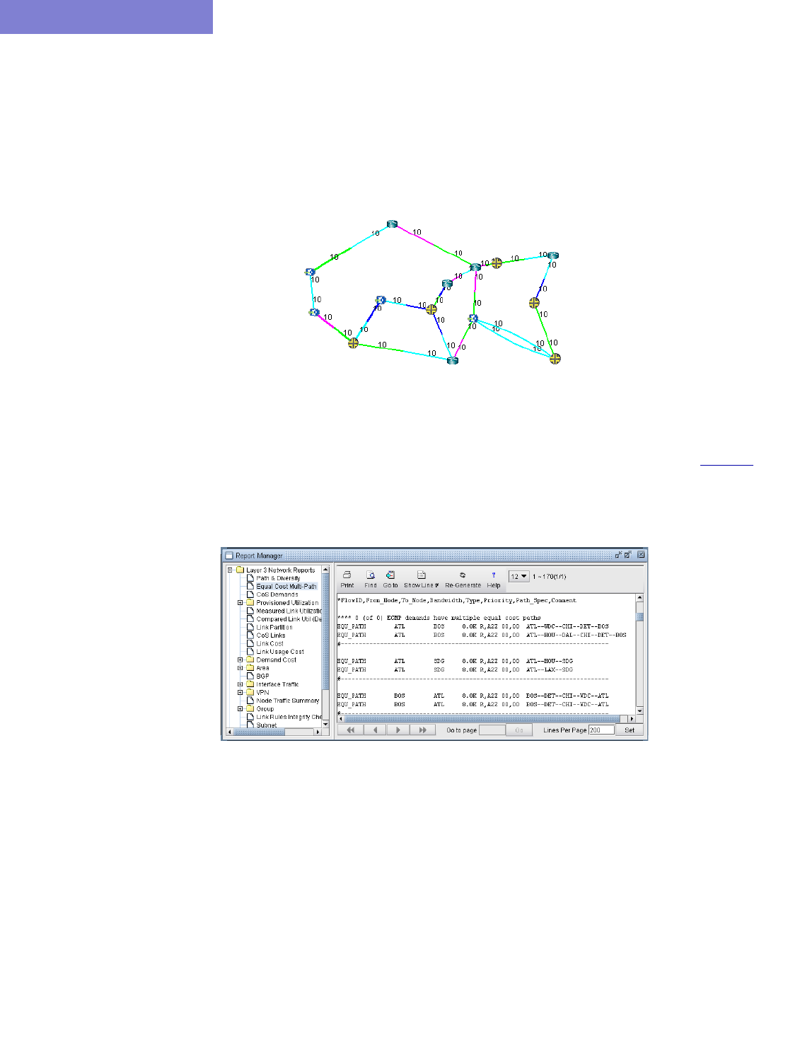
EQUAL COST MULTIPLE-PATHS
5-2 Copyright © 2014, Juniper Networks, Inc.
5
2. The link distances will be displayed and we can see that in this network, every metric has been set to 10. This is
very likely to cause numerous equal cost multiple-paths to exist.
Note: To reproduce this example, use the fish network in /u/wandl/sample/IP/fish/spec.mpls-fish. Go to
Modify mode and select Modify > Elements > Links. Press the “Select All” button to select all links, and
then press “Modify”. In the Modify Links window, switch to the Protocols tab, set OSPF to “yes” and enter
“10” for both the OSPF A-Z and Z-A Metrics. Click “OK”. Then, switch back to View mode, and the network
will be updated.
Figure 5-2 Topology Map with Link Distances
3. Select Report > Report Manager to open up the Report Manager.
4. Select Network Reports > Demand Reports > Equal Cost Multi-Path Report from the left panel to
bring up the report listing all of the equal cost multiple-paths of the network. As can be seen in Figure 5-3, there
are many such paths. This report is also saved on the server as EQPATHRPT.runcode. Note that the ECMP paths
are calculated based on IP metric only, and do not factor in the influence of MPLS traffic engineering tunnels on
the demand routing.
Figure 5-3 Equal Cost Multiple-Paths Report
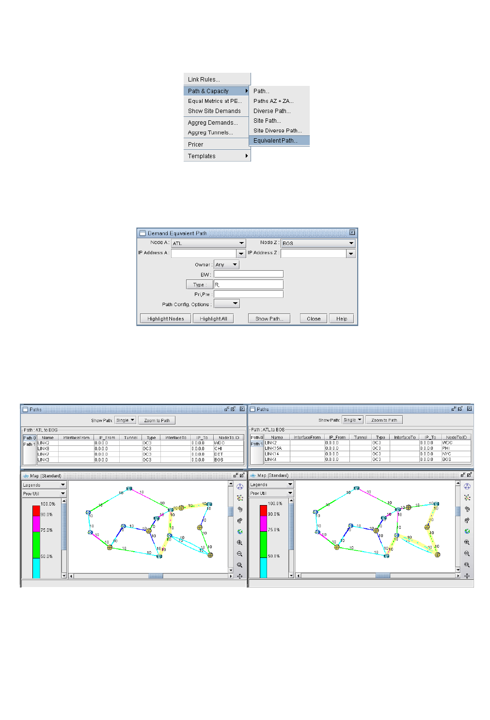
EQUAL COST MULTIPLE-PATHS
Copyright © 2014, Juniper Networks, Inc. 5-3
. . . . .
5. Select Network > Path & Capacity > Equivalent Path to bring up the Demand Equivalent Path window.
Figure 5-4 Network > Path & Capacity > Equivalent Path
6. Select Node A and Node B, then click Show Path. The Path window will be displayed.
Figure 5-5 Demand Equivalent Path
7. All of the equivalent paths between the two selected nodes will be displayed in the Paths window. Select a path
to view its detailed information and highlight it on the topology map.
Figure 5-6 Equivalent Cost Paths
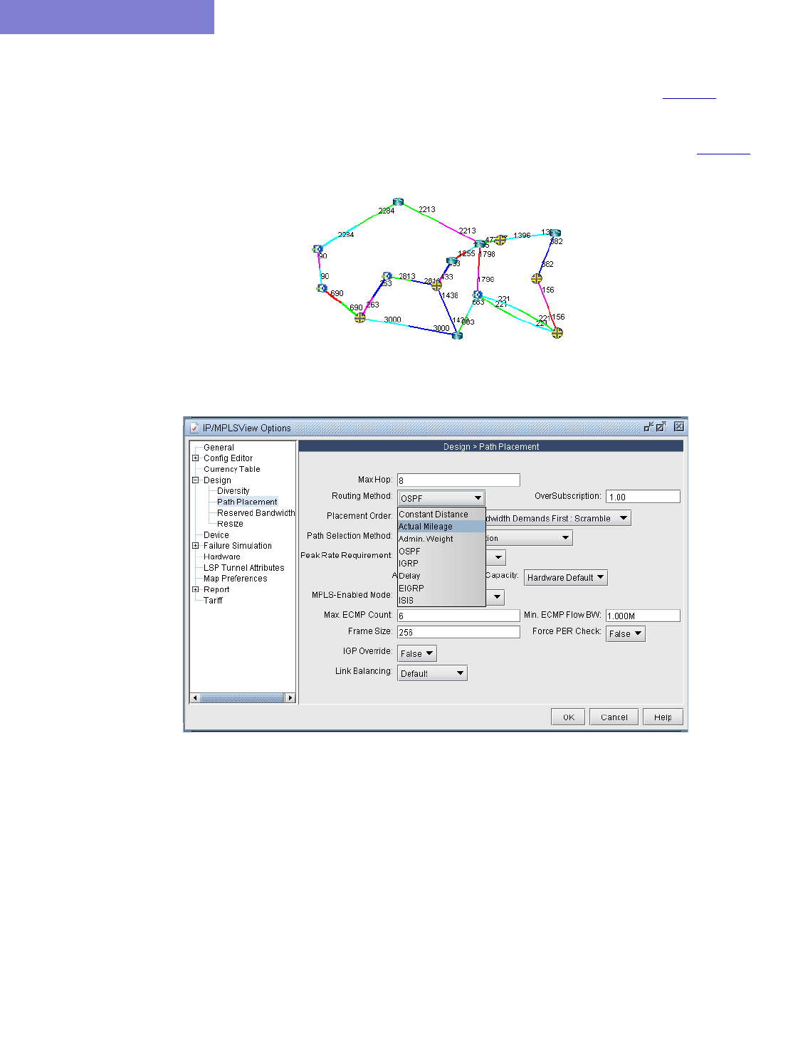
EQUAL COST MULTIPLE-PATHS
5-4 Copyright © 2014, Juniper Networks, Inc.
5
Reducing Equal Cost Multiple Paths
8. If you choose your link metrics wisely (such as using the real distance in miles like in Figure 5-7), you can
increase the variability of the path costs which will make it less likely for equal cost multiple-paths to occur.
Tip: To use actual mileage to represent the metric, go to Tools > Options > Design, select the Path
Placement options, and change the Routing Method to “Actual Mileage”, as shown in Figure 5-8.
Figure 5-7 Topology Map With New Link Distances
Figure 5-8 Routing according to Actual Mileage
9. Open up the Equal Cost Multi-Path Report again and you will see that there are no longer any equal cost
multiple-paths in the network with the new link metrics.
Note: If your Report Manager is already open, you may need to regenerate, or refresh, the ECMP Report. To
do so, either press the “Re-Generate” button at the top of the ECMP Report. Or, right-click on the “Equal
Cost Multi-Path” entry on the left side of the Report Manager, and select “Re-Generate Report”.
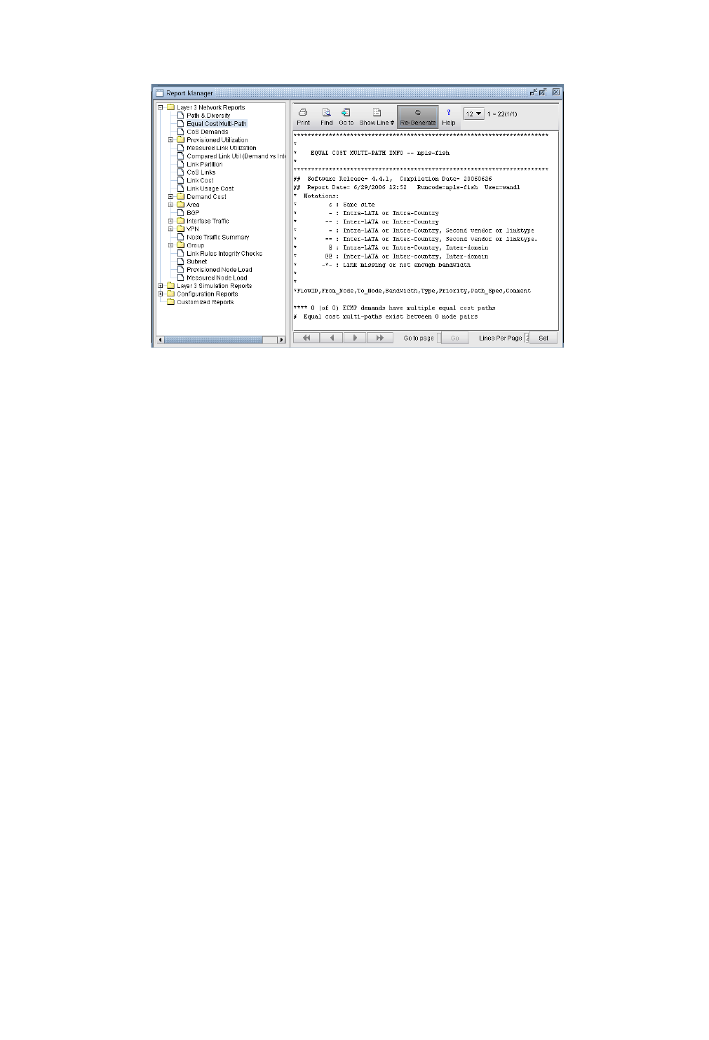
EQUAL COST MULTIPLE-PATHS
Copyright © 2014, Juniper Networks, Inc. 5-5
. . . . .
Figure 5-9 New Equal Cost Multiple-Paths Report
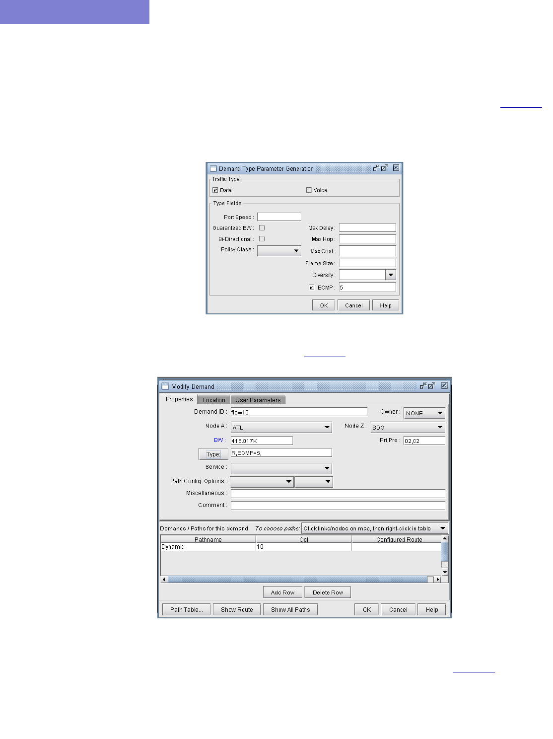
EQUAL COST MULTIPLE-PATHS
5-6 Copyright © 2014, Juniper Networks, Inc.
5
Splitting a Flow into Sub-Flows
10. Switch to Modify mode and select Modify > Elements > Demands... to bring up the Demands window.
Double-click the flow you want to modify (or select the flow and select Modify > Selected...) to bring up the
Modify Demand window.
11. Click the Type button to bring up the Demand Type Parameter Generation Window as shown in Figure 5-10.
Select the ECMP checkbox and enter the number of sub-flows desired. The default number of sub-flows is 6 if
no value is entered, or it can be set based on the bandwidth using the ECMPcntByBW parameter. Then click
OK.
Figure 5-10 Demand Type Parameter Generation Window
12. Notice the new value in the Type field in Figure 5-11.
Figure 5-11 Modify Demand Window
13. Switch back to View mode and select Network > Elements > Demands to bring up the Demands window.
Sub-flows are displayed differently in the Type column in View mode, as shown in Figure 5-12. Rn means that
n sub-flows share the same routing path. In this example, the original flow called flow10 was divided into 3
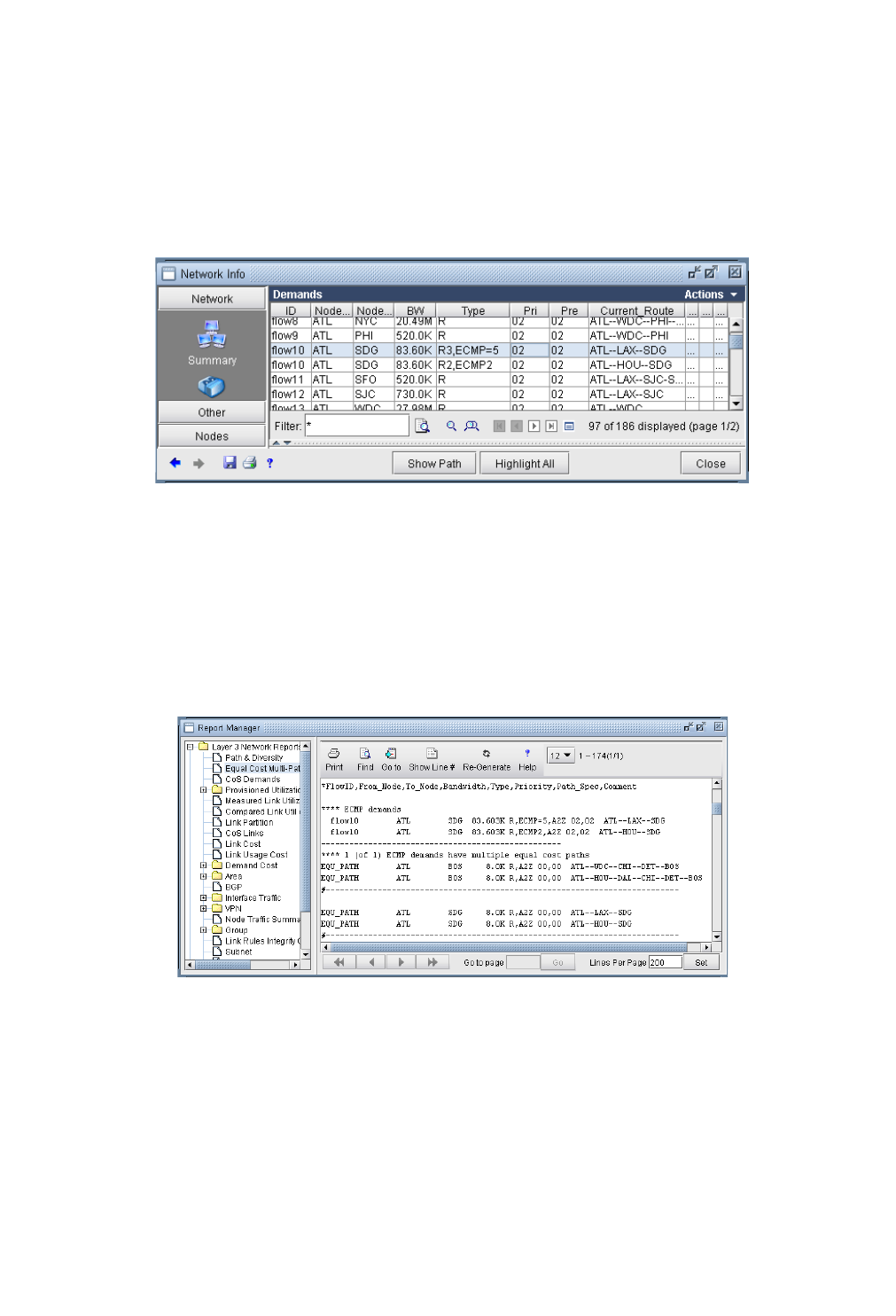
EQUAL COST MULTIPLE-PATHS
Copyright © 2014, Juniper Networks, Inc. 5-7
. . . . .
flows on the first ECMP and 2 flows on the second ECMP. The first entry for flow10 also says “ECMP=5”, to
indicate that 5 subflows were created from the original flow. The second entry for flow10 also contains a special
keyword, “ECMPN” or “ECMP2”. “ECMPN” is simply a reserved keyword used by the program to identify
subflows that are associated with another “original” flow but whose routing path is different. To elaborate, if
there were three different ECMP’s, then there would be three entries for flow10; the first would indicate
“ECMP=n” and the latter two would show special keyword “ECMPN”. This simply helps the program associate
these subflows with one another.
Figure 5-12 Demand Window in View mode
14. Open the ECMP Report again in the Report Manager. This time it will display the newly created ECMP
demands in the report.
Note: Although there are several discrete ECMP subflows (i.e. 5 in this example, 2 routing one way and 3
routing another), and technically the program could report an ECMP comparing each of the 2 with each of the 3,
such information is not very useful. Therefore, the ECMP report only reports a single entry for flow10,
comparing the two different routing paths.
Figure 5-13 Equal Cost Multiple-Paths Demand Report

EQUAL COST MULTIPLE-PATHS
5-8 Copyright © 2014, Juniper Networks, Inc.
5
Set ECMP Subflows Based on Bandwidth
15. Users can manually define the number of subflows as defined above. Alternatively, they can use the default
ECMP behaviour, which is to create 6 flows for every ECMP demands without count specification.
16. The default number of ECMP flows to be created for an ECMP demand can also be configured based on
demand bandwidth via the ECMPcntByBW parameter in the project’s dparam file by adding in an entry with the
format “ECMPcntByBW=[bandwidth:ECMPcount][|bandwidth:ECMPcount]*”
17. For example, ECMPcntByBW=300M:72|100M:32|50K:6 would be interpreted as follows:
•An ECMP demand with bandwidth>=300M is split into 72 flows,
•An ECMP demand with bandwidth>=100M is split into 32 flows,
•An ECMP demand with bandwidth>=50K is split to 6 flows.
•An ECMP demand with bandwidth<50K is kept as one flow.
18. This parameter can also be set in /u/wandl/db/misc/dparam.txt to change rtserver's default behaviour when
ECMPcntByBW is not specified in the project’s dparam file.
19. For the changes to the dparam file to have effect, close the network before changing the parameter, and reopen
the network after changing this parameter.

Copyright © 2014, Juniper Networks, Inc. 6-1
. . . . .
. . . . . . . . . . . . . . . . . . . . . . . . . . . . . . . . . . .
S
TATIC
R
OUTES
6
his chapter covers how to view and modify static route tables. Static routes are used in IP networks and
allow very precise control over traffic going through a router. By default, static routes take precedence over
routing protocols such as RIP or OSPF to communicate routing information between routers. Static routes
are ideal for small networks with a limited number of paths and are particularly well suited for peripheral routers that
are connected to one or more networks via only one router. A disadvantage of static routes is its inability to adapt to
router or link failures.
When to use
In Modify mode, the user may add, modify or delete any entry in any existing static route table. In all other modes,
the user is allowed to view the entries of any existing static route table. Whether or not to use static routes is
dependent on the type of network involved and the specific situation. General guidelines for using static routes are
described above, and more information can be found in online tutorials and network design literature.
Prerequisites
Prior to beginning this chapter, start up the WANDL software and open up a network (e.g., the spec.mpls-fish spec
file located in your $WANDL_HOME/sample/IP/fish directory, where $WANDL_HOME is /u/wandl by default).
You should also have a general understanding of where and when to use static routes.
Related Documentation
For an overview of the WANDL software or for a detailed description of each feature and the use of each WANDL
clientwindow, refer to the General Reference Guide.
Outline
1. View Static Routes on page 6-1
2. Add/Modify/Delete Static Routes on page 6-3
3. Case Study on page 6-4
Detailed Procedures
View Static Routes
1. To view the static route table of a node, you must be in either View, Design, or Simulation mode.
2. From the Map window, right-click on the node of interest and select View>Static Route Table. Alternatively,
select Network > Protocols > Static Route Table.
T
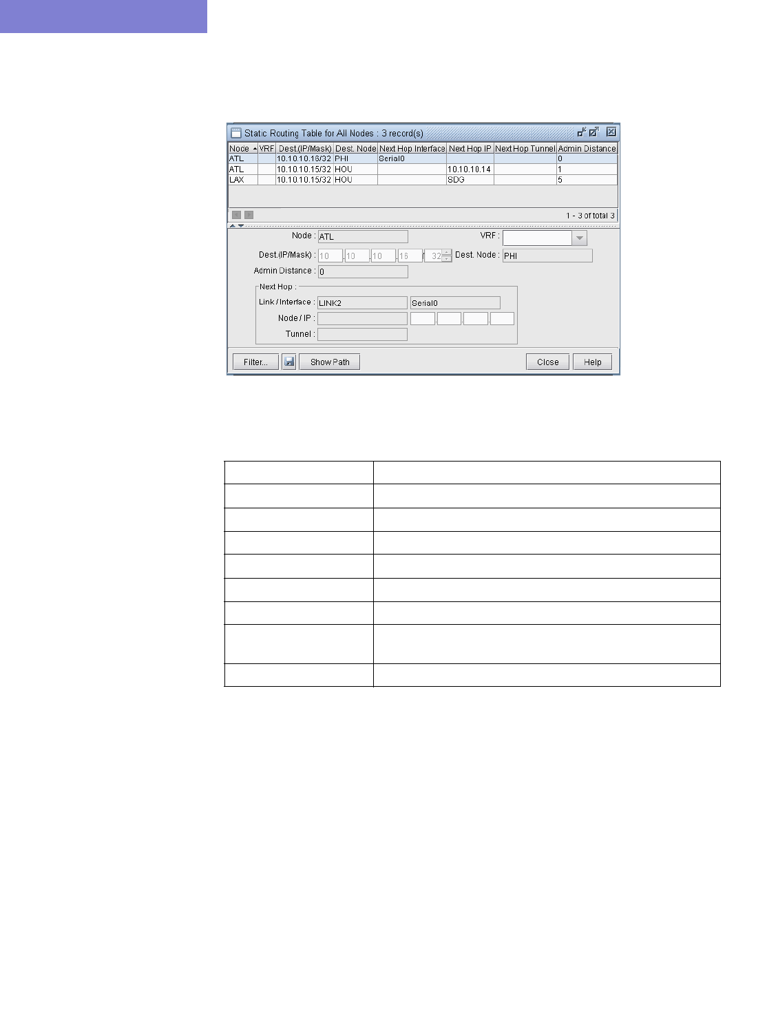
STATIC ROUTES
6-2 Copyright © 2014, Juniper Networks, Inc.
6
INTERPRETING THE STATIC ROUTING TABLE
3. A Static Routing Table window will be displayed as shown below.
Figure 6-1 Viewing static routes
4. Select a static route to view its details in the lower half of the window.
5. Click the Show Path button to highlight the static route path in the Map window.
Field Description
Node The node from which the static route starts.
VRF Virtual Routing Forwarding identification.
Dest. (IP/Mask) The IP of the final destination.
Dest. Node The node name of the final destination.
Admin Distance The admin distance associated with the static route.
Next Hop Link / Interface The next immediate link name or interface in the static route.
Next Hop Node / IP The next node name or IP address in the static route. This
may also be the final destination node in some cases.
Next Hop Tunnel The next immediate tunnel in the static route.
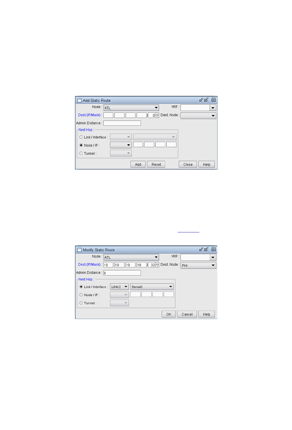
STATIC ROUTES
Copyright © 2014, Juniper Networks, Inc. 6-3
. . . . .
Add/Modify/Delete Static Routes
6. Switch to Modify mode.
7. From the Map window, right-click on the node of interest and select Modify Static Route Table.
Alternatively, select Modify > Protocols > Static Route Table from the main menu.
ADDING A STATIC ROUTE
8. In the Static Routing Table window, click on the Add button to open the Add Static Route window shown
below.
Figure 6-2 Adding a static route
9. Fill in the appropriate fields. Click OK when finished. The Static Routing Table window should now contain
a new entry reflecting the newly added static route.
MODIFYING A STATIC ROUTE
10. To modify a static route table entry, highlight the row(s) you want to edit and click the Modify button.A
Modify Static Route window will appear as shown in Figure 6-3 below.
Figure 6-3 Modifying a static route
11. Edit the appropriate fields. Click OK when finished.
12. The modifications to the static route should be reflected in the Static Routing Table window.
DELETING A STATIC ROUTE
13. To delete static route(s), select the desired entries from the Static Routing Table window and click the
Delete button.
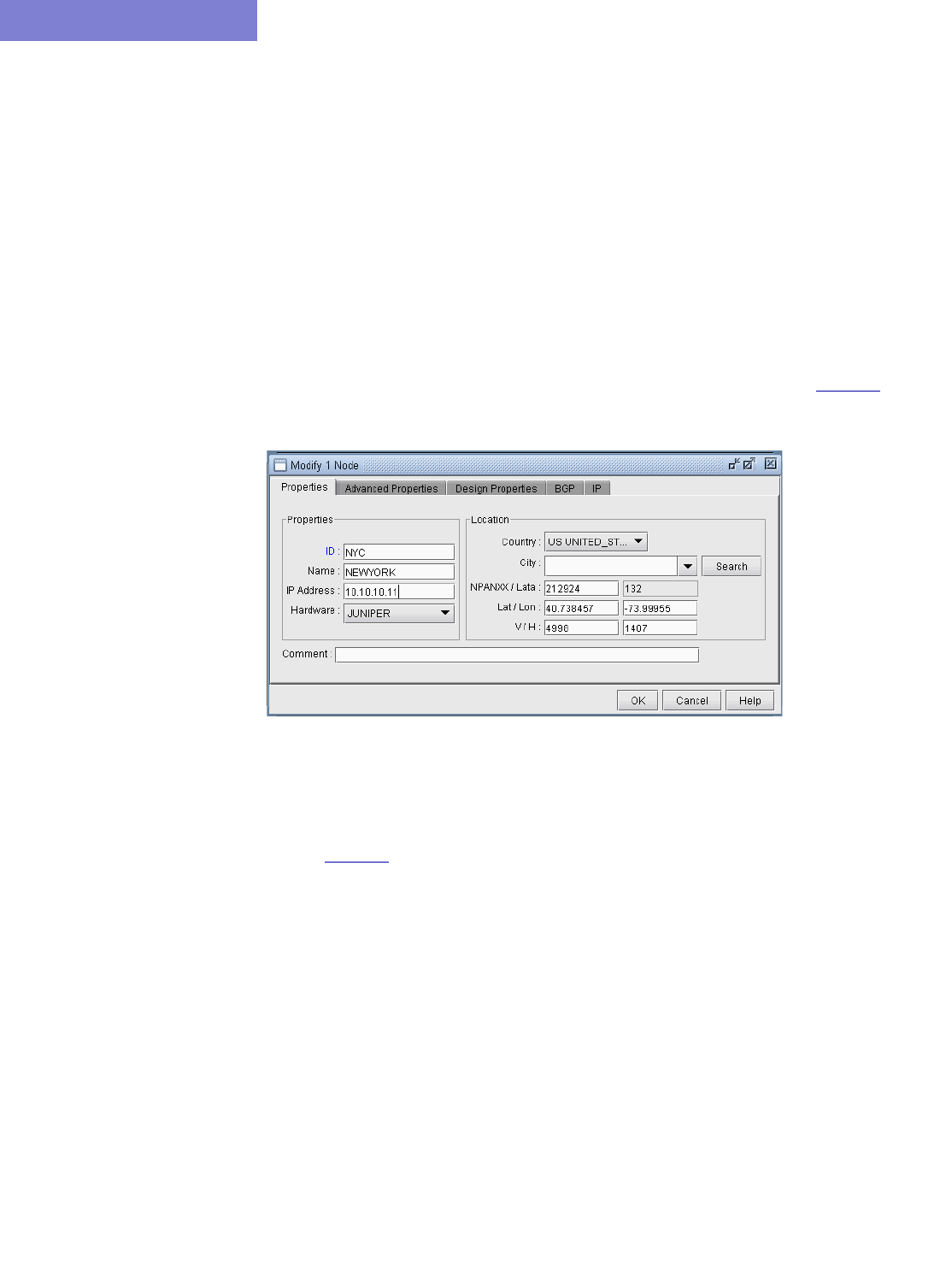
STATIC ROUTES
6-4 Copyright © 2014, Juniper Networks, Inc.
6
Case Study
In this section we will define a demand with a destination IP and let the program route the demand according to the
options and hardware settings present in the network. We will then define a new path for the demand and enforce this
path using a static route. After defining the static routes, the demand path will be observed again to verify that it does
indeed follow the defined static route. Note that for static routes to be successful in routing a demand, the demand
must have an IP address associated with its destination, not simply a node name. This is due to the way static routes
are defined in actual router configuration files.
DEFINING THE DEMAND
14. Open the sample Fish network in /u/wandl/sample/IP/fish by double clicking the spec.mpls-fish file in the
File Manager window.
15. Switch to Modify mode. In this case study we are interested in demands terminating at node NYC. In order for
static routes to work, there must be an IP address associated with the destination node. Click on the Modify
menu and select Nodes. Scroll down until you see node NYC. Highlight it and click the Modify button to
bring up the Modify Node window. Type in 10.10.10.11 for the IP address as shown in Figure 6-4. Click OK
when finished.
Figure 6-4 Assign an IP address to node NYC
16. Go to Modify > Elements > Demands... and select the demand xflow79 between SFO and NYC. Double-
click this entry or click the Modify > Selected... button to modify this demand.
17. Modify the demand by typing in the Location tab the corresponding IP address for its destination node as
shown in Figure 6-5. In this case, the IP address is 10.10.10.11 for NYC. Click “OK” to continue.
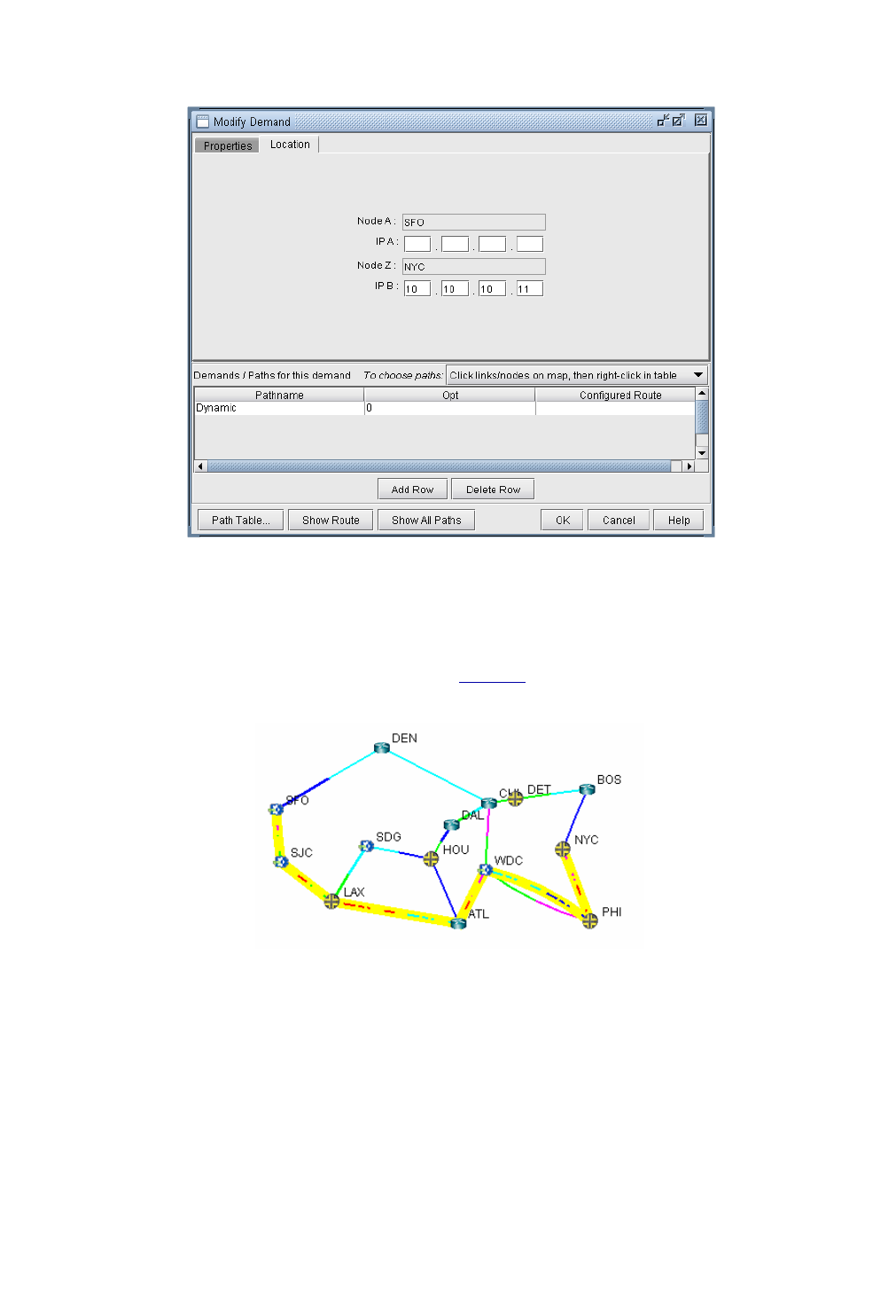
STATIC ROUTES
Copyright © 2014, Juniper Networks, Inc. 6-5
. . . . .
Figure 6-5 Fill in the IP address for the destination node
18. Update the network by clicking the Update button or by selecting Modify > Update Network State. Reopen
the Demands window by selecting Network > Elements > Demands. Now you can display the path of the
demand xflow79 by selecting the demand and clicking the Show Path button. The current path will be
displayed in the Map window as shown in Figure 6-6 below.
Figure 6-6 Path of demand xflow79, from SFO to NYC
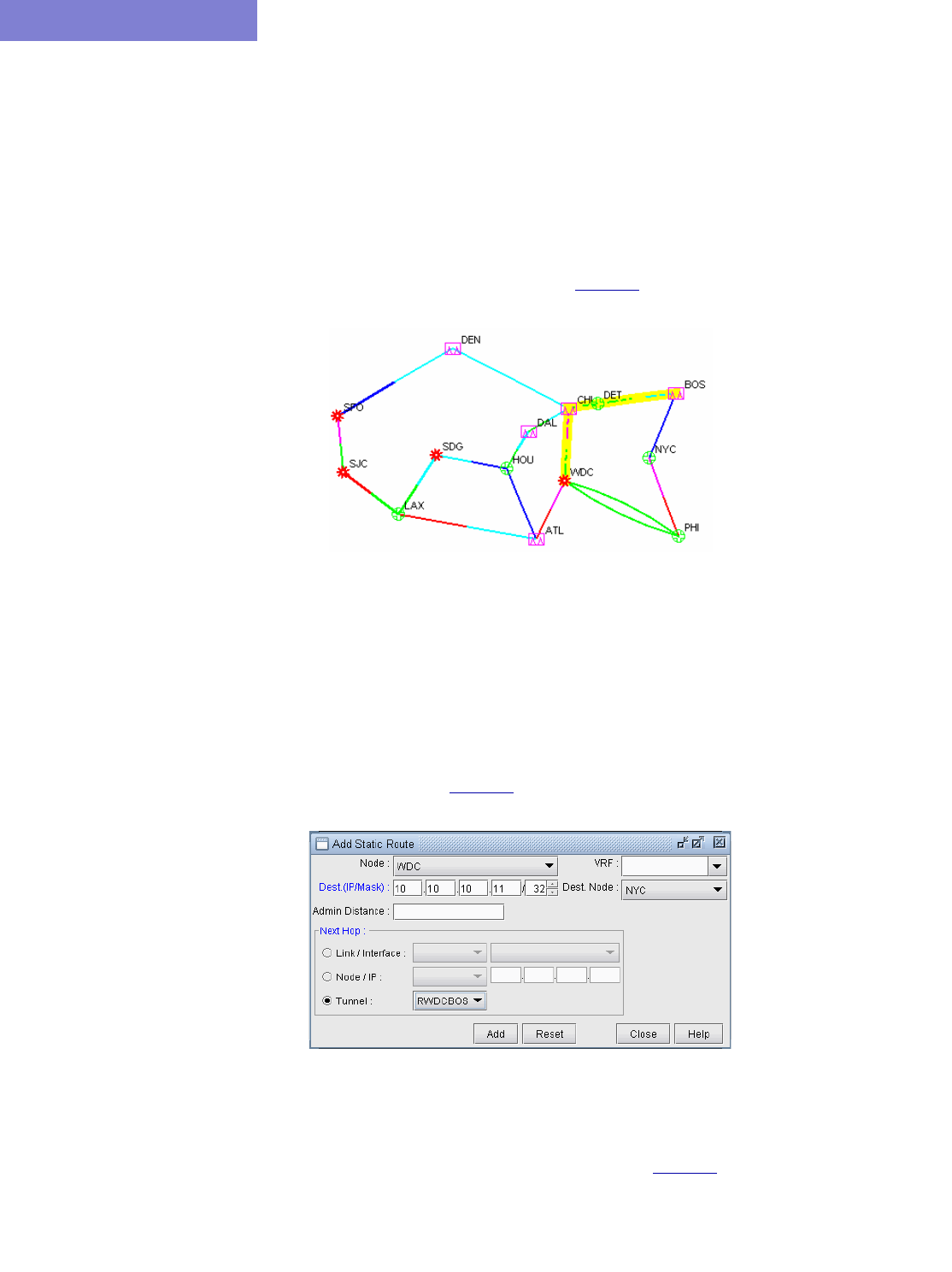
STATIC ROUTES
6-6 Copyright © 2014, Juniper Networks, Inc.
6
CREATING THE STATIC ROUTE TABLE
Suppose it has been decided that the demand xflow79 and other such demands going to node NYC (10.10.10.11)
are to be rerouted to go through node CHI instead of PHI. This could be due to the fact that the link between PHI and
NYC is being heavily utilized, as indicated by the red/purple colored link. Thus, it is necessary to create a static route
table at node WDC to enforce this route.
19. First, identify if there are any tunnels available starting from node WDC that go through CHI. To do this, switch
to View mode, right click on node WDC, and select View>Tunnels On/Thru Node.
20. In the new Tunnels at Node: WDC(WDC) window, notice that the tunnel RWDCBOS goes from node
WDC to node BOS. Highlight this tunnel and click the Show Path button. The path of this tunnel will be
displayed in the Map window, as shown below in Figure 6-7:
Figure 6-7 Path of tunnel RWDCBOS from WDC to BOS
This is a good choice for the next hop of a static route at node WDC for the purpose of this example, since it will
route all demands through nodes CHI, DET, and BOS rather than through node PHI.
21. In Modify mode, right click on the WDC node and select Modify Static Route Table.
22. Click the Add button to bring up the Add Static Route window.
23. Select NYC from the Dest. Node dropdown menu. The Dest. (IP/Mask) field will be automatically filled in.
Then, in the Next Hop section, check the radio button next to Tunnel and then select RWDCBOS from the
dropdown menu, as shown in Figure 6-8.
Figure 6-8 Adding a static route at node WDC
24. Click the Add button to add this entry to the static route table for node WDC. You should see this entry updated
in the Static Routing Table for WDC window, as shown in Figure 6-9 below:
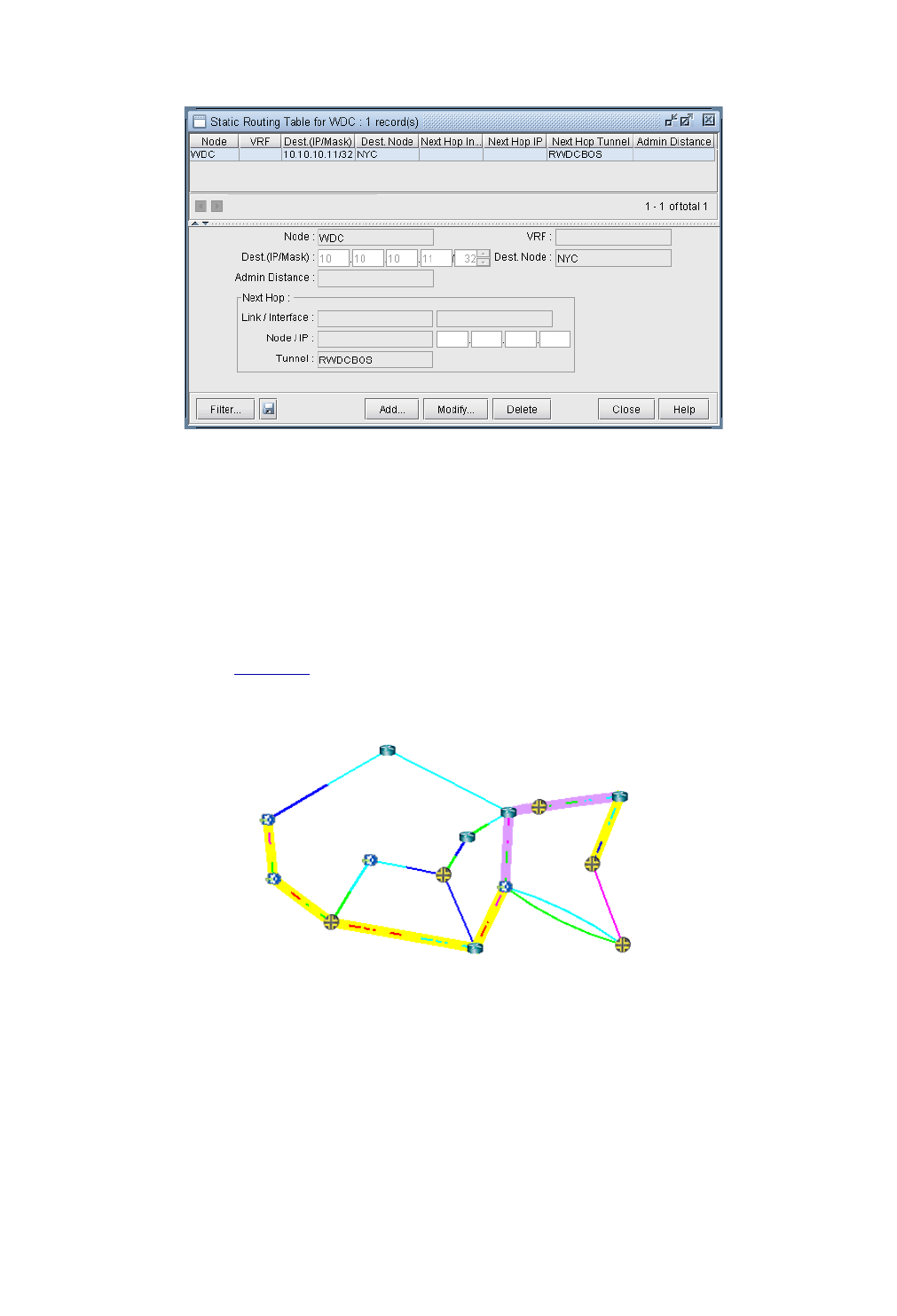
STATIC ROUTES
Copyright © 2014, Juniper Networks, Inc. 6-7
. . . . .
Figure 6-9 Updated static touting table for WDC
VERIFY THE NEW ROUTE
Now that the static route has been defined, it is time to test whether or not the demands will route as planned.
25. Switch to View mode. When it asks if you want to “Reroute demands from scratch,” click Yes.
26. Select the Network > Elements > Demands menu.
27. Locate the demand, xflow79, and highlight it. Click Show Path to display its new path in the Map window.
Below (Figure 6-10) is a screenshot of what it should look like. Notice that the new path takes the route
specified by the static route table created at node WDC.
Figure 6-10 New route following static route specifications
28. Information on static routes is stored in a pathtable.runcode file. This can be verified by opening the File
Manager window, navigating to the directory where the network files are stored (i.e.
/u/wandl/sample/IP/fish) and opening the pathtable file (i.e. pathtable.mpls-fish). For this case study, the file
will look as follows.

STATIC ROUTES
6-8 Copyright © 2014, Juniper Networks, Inc.
6
Figure 6-11 Static route information is stored in a pathtable file

Copyright © 2014, Juniper Networks, Inc. 7-1
. . . . .
. . . . . . . . . . . . . . . . . . . . . . . . . . . . . . . . . . .
P
OLICY
B
ASED
R
OUTES
7
his chapter covers how to view and modify policy based routes. Policy based routing provides additional
control above that of routing protocols. A policy can be applied to an interface so that packets coming in
through the interface meeting a given criteria will be forwarded out to a given interface, tunnel, or next hop.
The criteria that must be met, if any, is specified in a route map statement. The information that must be matched can
be specified in an access list, such as source IP address, destination IP address, port numbers, and protocol. The route
map statement also sets the outgoing interface, tunnel, or next hop.
When to use
Policy Based Routes can be used to implement QoS-specific routing, protocol-sensitive routing, source-sensitive
routing, or routing based on dedicated links.
Prerequisites
To use this feature, you should have Cisco router configuration files with statements for policy based routing such as
those given in the following table.
Related Configuration Commands
Recommended Instructions
Following is a high-level, sequential outline of the following sections.
1. Use the configuration files import to create your network.
2. View policies from the link window.
3. Check how the policies will affect routing by performing a path analysis.
4. Modify the link PBR field to perform what-if studies.
Command Example Formats
Configure for a router the
access list(s) that will be
referenced in the route-map
statement(s)
1. Sample standard access list:
access-list <access-list-id> permit|deny <ip-address>
<mask>
2. Extended access lists can be used as well
access-list <access-list-id> permit|deny
<protocol><source-ip> <source-mask> <destination-ip>
<destionation-mask> [protocol parameters]
Specify for an interface on the
router, the route-map to be
applied
3. ip policy route-map <route-map-name>
Define the route-map for the
router
4. Specify route map name and number:
route-map <route-map-name> permit|deny <number to
indicate relative order of application>
5. Specify an access list ID to match against if any:
match ip address <access-list-id>
6. Specify the outgoing interface or else the next-hop:
set interface <interface_name>
set ip next-hop <ip-address>
T
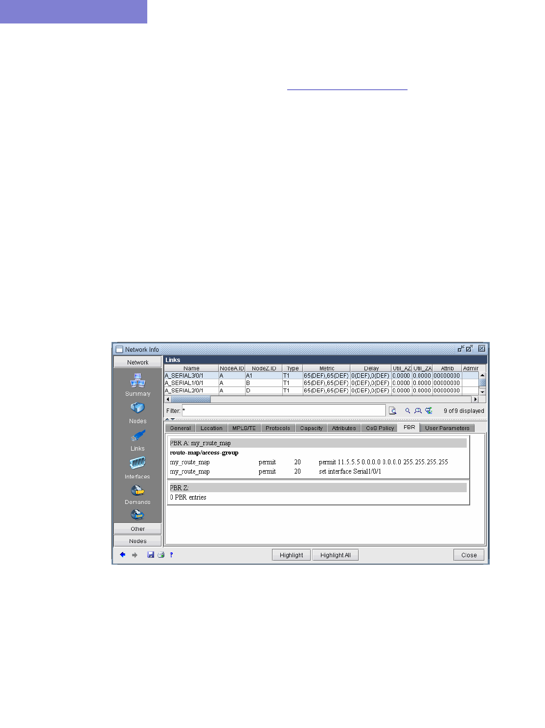
POLICY BASED ROUTES
7-2 Copyright © 2014, Juniper Networks, Inc.
7
Detailed Procedures
Importing the Config Files
1. Import the config files as described in Chapter 2, Router Data Extraction. Note that for a what-if study, you can
also edit your config files to add, modify, or delete policies and then re-import the config files.
2. Go to Tools > Options > Design. On the Path Placement option pane, set Force PBR Check (on the
lower right corner of the window) to “True”.
3. Click “Yes” when asked to reroute from scratch.
Viewing PBR Details from the Link Window
4. Select the Network > Elements > Links menu. To display the PBR route map in the link table summary
pane, right-click on a column header and select Table Options. Select PBR_A and PBR_Z from the
Available items window and click “Add>” to move them to the Selected Item(s) window and then click
“OK”.
PBR_A and PBR_Z refer to the route-map names in both directions on the link. PBR_A refers to the direction
from Node A to Node Z, while PBR_Z refers to the direction from Node Z to Node A.
5. Scroll so that you can see the PBR_A and PBR_Z headings. Click on the columns to sort the columns and see
which interfaces have policies on them.
6. Select a link row for a link that has an interface with a policy applied to it. Then click the PBR tab. The tab is
divided into a section for the interface on Node A and a section for the interface on Node Z. Each section
contains the PBR information, including the route-map, sequence number, match criteria, and the action to
perform if there is a match.
Figure 7-1 PBR Tab
Path Placement
7. To perform a path placement, select Network > Path&Capacity > Path. Optionally specify a source and/or
destination IP address (to match against the route map) that corresponds to a node’s loopback address or one of
its interface addresses. Then click on the map the from-node followed by the to-node.
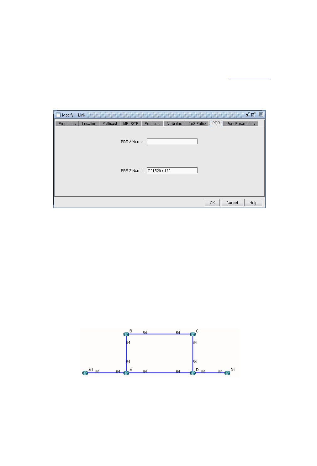
POLICY BASED ROUTES
Copyright © 2014, Juniper Networks, Inc. 7-3
. . . . .
8. The Path window will be displayed. In addition, the Console window will display the relevant policy based
routing information.
Modifying Link PBR Field
9. You can modify a link to specify which policy to use on an interface. To do so, go to Modify mode and select
Modify > Elements > Links... You can sort on the PBR_A and PBR_Z column to quickly see which links
have policies attached to them. The instructions are the same as given in step 4 on page 7-2.
10. Select the link you wish to modify from the table and click Modify... to open the following Modify 1 Link
window. Click on the PBR tab.
Figure 7-2 Modify Link, PBR Tab
11. Enter in the name of the Policy for the interface in the node A to node Z direction or vice versa. The policy name
should correspond to a route-map on node A for the AZ direction or node Z for the reverse direction. If the
policy typed in is invalid, an error message will pop up. Click “OK” and view the Console message to see
possible PBR policies to apply for the link interface. When you are finished modifying the link, click OK. You
can then retry a path analysis.
Example
The following 6-router network will explain a case of policy based routing that checks the source IP address of
incoming packets against the match condition of the route-map statement to determine whether to take the action in
the route-map statement. (Note that more sophisticated policies can be used to check other properties such as the
destination IP address, protocol information, etc.)
In this example, router A has applied the following route-map on its interface to A1:
route-map my_route_map permit 20
match ip address 111
set interface Serial1/0/1
!
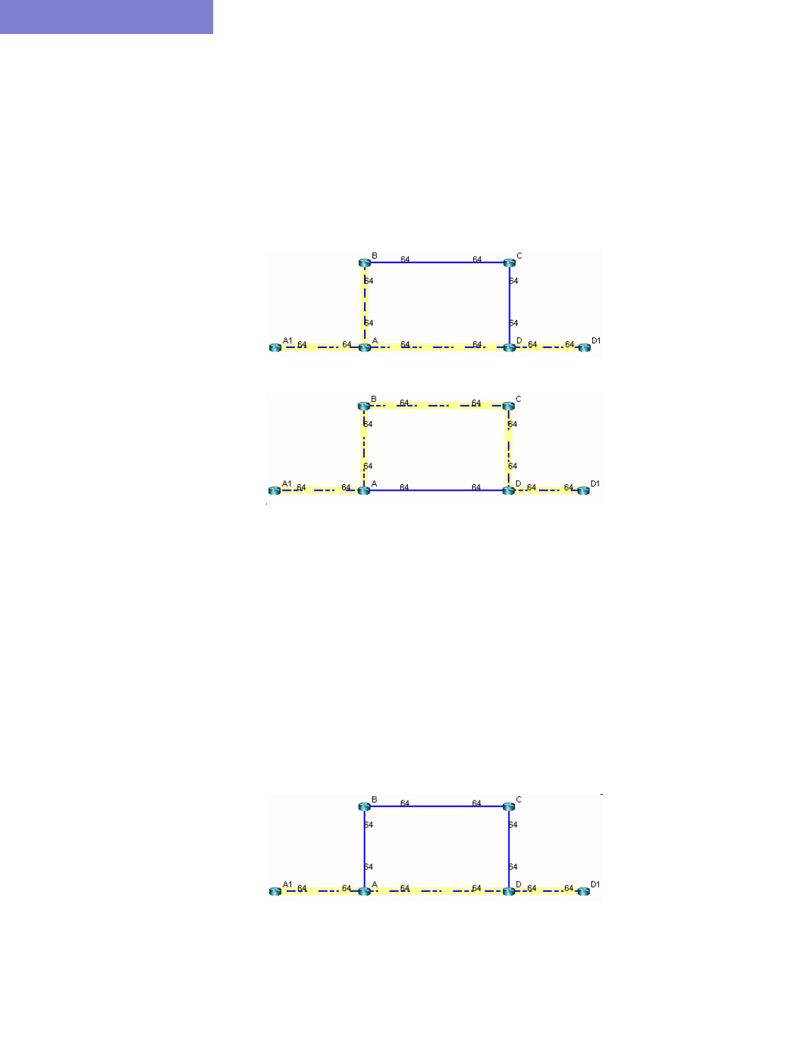
POLICY BASED ROUTES
7-4 Copyright © 2014, Juniper Networks, Inc.
7
The corresponding match condition is specified in the access list (111) as follows: “access-list 111 permit 11.5.5.5
0.0.0.0.” The corresponding interface to forward to in case the match condition is satisfied is Serial1/0/1, which
connects A to B. As a result of the policy, router A will forward any packet coming from A1 with a source IP address
of 11.5.5.5 out the interface Serial1/0/1 toward B. A Path analysis is used to verify the routing behavior.
12. Suppose a path analysis is performed from A1 to D1 by selecting Network > Path & Capacity > Paths. The
source and destination IP addresses must be entered in to simulate Policy Based Routing. In this case, we use
11.5.5.5 as the source IP address (router A1’s IP address). The packet is then forwarded to router B. This
example uses OSPF and the links have equal OSPF metric, so after the packet is forwarded to B, it may equally
well go from B to C to D to D1 as back to A and then to D to D1.
Figure 7-3 Results of Using an IP Address Matching the Route Map Criteria
The results are also displayed in the Console. The Console messages for the left figure above are as follows:
* * * A1(A1) - D1(D1): bw= 0 * * *
-- Find path from A1 to D1 (0.0.0.0)
-- Apply PBR my_route_map at A:
Set interface to Serial1/0/1
PBR route from A to B
new 11.5.5.5 D1 0 R,A2Z 02,02 A1--A--B--C--D--D1
(OSPF) Route-cost=325. Max_Path_Bw= 1.536M
Tunnels matching search criteria: 0
13. On the other hand, suppose a path analysis is performed from A1 to D1 using another interface IP address at A1
such as 10.10.10.17. In this case, the source IP address no longer matches the route-map condition and hence the
routing table (OSPF in this case) is used instead:
Figure 7-4 Results of Using an IP Address Not Matching the Route Map Criteria
The corresponding Console message appears as follows:

POLICY BASED ROUTES
Copyright © 2014, Juniper Networks, Inc. 7-5
. . . . .
* * * A1(A1) - D1(D1): bw= 0 * * *
-- Find path from A1 to D1 (0.0.0.0)
-- Apply PBR my_route_map at A:
new 10.10.10.17 D1 0 R,A2Z 02,02 A1--A--D--D1
(OSPF) Route-cost=195. Max_Path_Bw= 1.536M

POLICY BASED ROUTES
7-6 Copyright © 2014, Juniper Networks, Inc.
7

Copyright © 2014, Juniper Networks, Inc. 8-1
. . . . .
. . . . . . . . . . . . . . . . . . . . . . . . . . . . . . . . . . .
B
ORDER
G
ATEWAY
P
ROTOCOL
*
8
he de facto routing protocol that is currently used to maintain connectivity between ASes (Autonomous
Systems) is Border Gateway Protocol (BGP) version 4 (based on RFC 1771). When BGP is used between
ASes, it is refered to as EBGP (External BGP). BGP can also be used within an AS -- known as IBGP
(Internal BGP) -- to primarily propagate BGP information learned from other ASes. WANDL’s Border Gateway
Protocol (BGP) module allows network planners to quickly investigate various BGP routing and peering scenarios
via BGP policy and attribute modifications. After running configuration import to extract BGP information, the
impact of changing BGP routing policies and attributes on inter-Autonomous System (inter-AS) traffic can be
assessed.
*Note that a special password is required for the BGP feature. Please contact your Juniper representative for more
information.
Related Documentation
For general step-by-step instructions on how to use the WANDL software, please refer to the Design & Planning
Guide.
For an overview of the WANDL software or for a detailed description of each feature and the use of each window,
refer to the General Reference Guide or Chapter 37, Router Reference.
For details on how to create a spec file by extracting, or importing, information from the router configuration files,
please refer to Chapter 2, Router Data Extraction.
Recommended Instructions
1. Import your network’s configuration files as described in BGP Data Extraction on page 8-3.
2. Analyse the BGP reports for integrity checks errors as described in BGP Reports on page 8-3.
3. View BGP options as described in BGP Options on page 8-3.
4. Open the BGP Map to view EBGP and IBGP peering relationships as described in BGP Map on page 8-4.
5. View routing table information and perform path analyses as described in BGP Routing Table on page 8-9 and
BGP Routes Analysis on page 8-11.
6. View BGP information associated with a node from the BGP Routes Analysis on page 8-11.
7. View, add, or modify BGP neighbor information as described in BGP Routing Table on page 8-9.
8. Apply, modify or add BGP policies as described in Apply, Modify, or Add BGP Polices on page 8-17.
9. Learn how the subnet file works as described in BGP Subnets* on page 8-21, and work through an example
where the AS_PATH attribute is used to influence routing.
10. Import and route according to live BGP routing tables as described in Live BGP Routing Tables* on page 8-24.
11. Learn about getipconf’s bgp-related usage notes and bgp-related files as described getipconf Usage Notes on
page 8-25.
T
BORDER GATEWAY PROTOCOL*
8-2 Copyright © 2014, Juniper Networks, Inc.
8
Definitions
Term Definition
Autonomous
Systems (AS)
A set of routers under a single technical administration, identified by its AS
number (1 to 64,511 for registered Internet numbers and 64,512 to 65,534 for
private AS numbers.)
EBGP External BGP - BGP running between different ASes
IBGP Internal BGP - BGP running within one AS
Peers or
Neighbors
Two routers are called peers or neighbors if they exchange BGP information
through an opened TCP (Transmission Control Protocol) connection.
Confederations BGP confederations are used to reduce the number of IBGP connections
needed in the full-mesh requirement. An AS’s routers are divided into multiple
smaller private ASes, and the smaller private ASes come together to produce a
public AS.
Route Reflectors A route reflector is a BGP speaker that is specially configured and used to pass
IBGP learned routes to a set of IBGP neighbors. This eases the fully meshed
requirement of IBGPs and reduces the number of IBGPs peering within an AS.
Community A community is a group of destinations that share common BGP attributes,
filters, and policies. Routing decisions can be applied to the community (the
group of routes).
Peer Groups Instead of setting up a community (a group of routes), a peer group (a group of
peer routers) can be established and configured with the same update policies,
which simplifies configuration tasks and makes updating more efficient.
AS_PATH BGP carries the AS numbers of the ASes that have been traversed, using the
AS_PATH attribute in order to reject updates containing its own AS number to
prevent loops.
LOCAL_PREF When there is more than one path to a network destination outside of the
current AS, each of the routers that link outside the AS can set a preference
value (via the LOCAL_PREF attribute) for routes advertised into the AS. The
LOCAL_PREF attribute is used to influence traffic leaving an AS.
MULTI_EXIT_DISC The MULTI_EXIT_DISC (MED) is used between EBGP peers when there are
multiple paths from one AS to another. It indicates to external neighbors which
path is preferred into an AS. The MED attribute influences traffic entering an AS.
Weight A Cisco-specific attribute in which higher-weight routes are preferred. Router-
originated routes have a weight of 32768 by default and other routes have a
weight of zero. Weight works similarly to LOCAL_PREF except that it only
applies to routes within the box and is not communicated to other peers.
Cluster ID A route reflector and its clients form a cluster. Usually a cluster has a single
route reflector. For redundancy, a cluster may have more than one route
reflector. When a cluster has more than one route reflector, all of the route
reflectors in the cluster need to be configured with the same cluster ID.

BORDER GATEWAY PROTOCOL*
Copyright © 2014, Juniper Networks, Inc. 8-3
. . . . .
Detailed Procedures
BGP Data Extraction
1. Select File>Import Data to import a set of configuration files. Alternatively, you may run the getipconf
program in text mode.
2. In the Default tab, under Config Directory, click “Browse” to select a directory containing the config files.
Notice that the Include BGP box under the Specify BGP Options section of the Network Options tab is
checked by default.
3. To ignore IP addresses with particular prefixes, such as 192.168., type in the IP addresses (partial string
allowed) under the Misc Options tab. Click “OK” to begin the extraction.
4. You can optionally modify the /u/wandl/db/misc/ASnames file used to derive the AS name labels shown on the
network map.
Refer to getipconf Usage Notes on page 8-25 and Chapter 2, Router Data Extraction for more details on data
extraction.
BGP Reports
5. After the configuration files are imported, select Report > Report Manager and select the Network
Reports > Protocols > BGP > BGP Report to check and make sure that the network has no obvious BGP
configuration errors. The BGP report includes the following sections:
•BGP Integrity Check Report -- Includes various BGP statistics, including BGP speakers, neighbors, and
policies.
•Neighbor AS Specification Error Check Report -- Shows errors related to incorrectly-specified ASes.
•Unbalanced BGP Neighbor Check Report -- Reports any unbalanced neighbor relationships between
BGP speakers.
•IBGP Mesh Connectivity Check Report -- Reports if any AS is not fully meshed for IPV4 or VPNV4
address families.
•Route Reflector Statistics Report -- Includes route reflector related information such as hierarchy level
and redundancy for IPV4, VPNV4, and L2VPN address families.
Please refer to the end of this chapter for more detailed descriptions and examples of these reports.
BGP Options
6. Select the Tools > Options > Design, Path Placement > BGP options pane to view the BGP-related
network parameter defaults.
•The Check IBGP Policy option is also set to false by default. Setting this to true turns on hop by hop IBGP
policy checking for the special case where the BGP next hop is modified as a result of IBGP policies.
Because this option is a special case and involves a lot of extra processing, it is not turned on by default.
However, if it is being used in your network, this option needs to be turned on.
•The IGP override option is set to false by default. This means that for external paths, BGP will be treated as
having a higher administrative distance/preference than the IGP such as OSPF. If this is not the case, this
parameter can be set to true.
•The Use Live BGP Table if Available option can be used to take advantage of routing table information
extracted from collected BGP routing tables for traffic routing. Note that this is an advanced BGP feature
which requires a special license. Please contact your Juniper representative for more information.
•The Peering AS Number(s) field will be filled in when running the BGP peering analysis. It is used to
specify the AS that the network will be newly peering with. Hence, for that AS, information from the subnet
file is needed to derive the BGP routing table. For more information on the subnet file, refer to BGP Subnets*
on page 8-21. BGP Peering Analysis is also an advanced BGP feature requiring a special license.
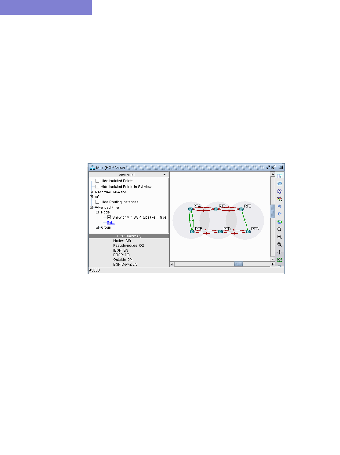
BORDER GATEWAY PROTOCOL*
8-4 Copyright © 2014, Juniper Networks, Inc.
8
BGP Map
7. To open the BGP map (as opposed to the standard map), select Network > Protocols > BGP > BGP Map or
Network > Maps > Map (BGP View). In the Include Which AS Values? window select which ASes you
want to view in your map. The ASes are listed in order, with the number of nodes and number of neighbors
shown in parentheses. This window indicates the number of nodes, neighbors, or ASnodes for each AS. Use
<Ctrl>-click and/or <Shift>-click to select multiple AS values.
8. The BGP map displays the network in terms of BGP speakers (routers that are running BGP) and their peering
relationships (shown via a connection with an arrow in the middle and pointed away from the speaker). Two
BGP routers become peers (neighbors) once they have both established a peering relationship with each other
(shown via two directed arrows or via a connection with a diamond in the middle if the Draw Mult. Links as
Curves box is unchecked in the Tools > Options > Map Preferences window).
9. When the BGP map is first brought up, all routers (including BGP speakers and non-BGP speakers) are shown
on the BGP map. You may wish to filter the BGP map by selecting the Filters > Advanced menu. Select
Hide Isolated Points, or to look only at the BGP speakers, open up the Advanced Filter > Node section.
Click the Set link to set BGP_Speaker = true. Then select the corresponding checkbox to turn on the filter.
The following figures show a BGP map filtered to show the BGP speakers.
Figure 8-1 BGP Map filtered for BGP speakers
LOGICAL LAYOUT
10. To view the logical relationships amongst BGP neighbors more clearly, including route-reflector hierarchical
relationships, right-click on the map and select Layout>Logical Layout.
For example, in the figure below, the network on the left shows two ASes, each with fully meshed IBGP
relationships. These ASes are connected to each other using EBGP. Meanwhile the network on the right shows
one AS with hierarchical route-reflectors. The innermost arc of routers are route reflectors for the middle ring of
routers, and some of the routers in the middle ring are route reflectors for the outermost arc of routers.
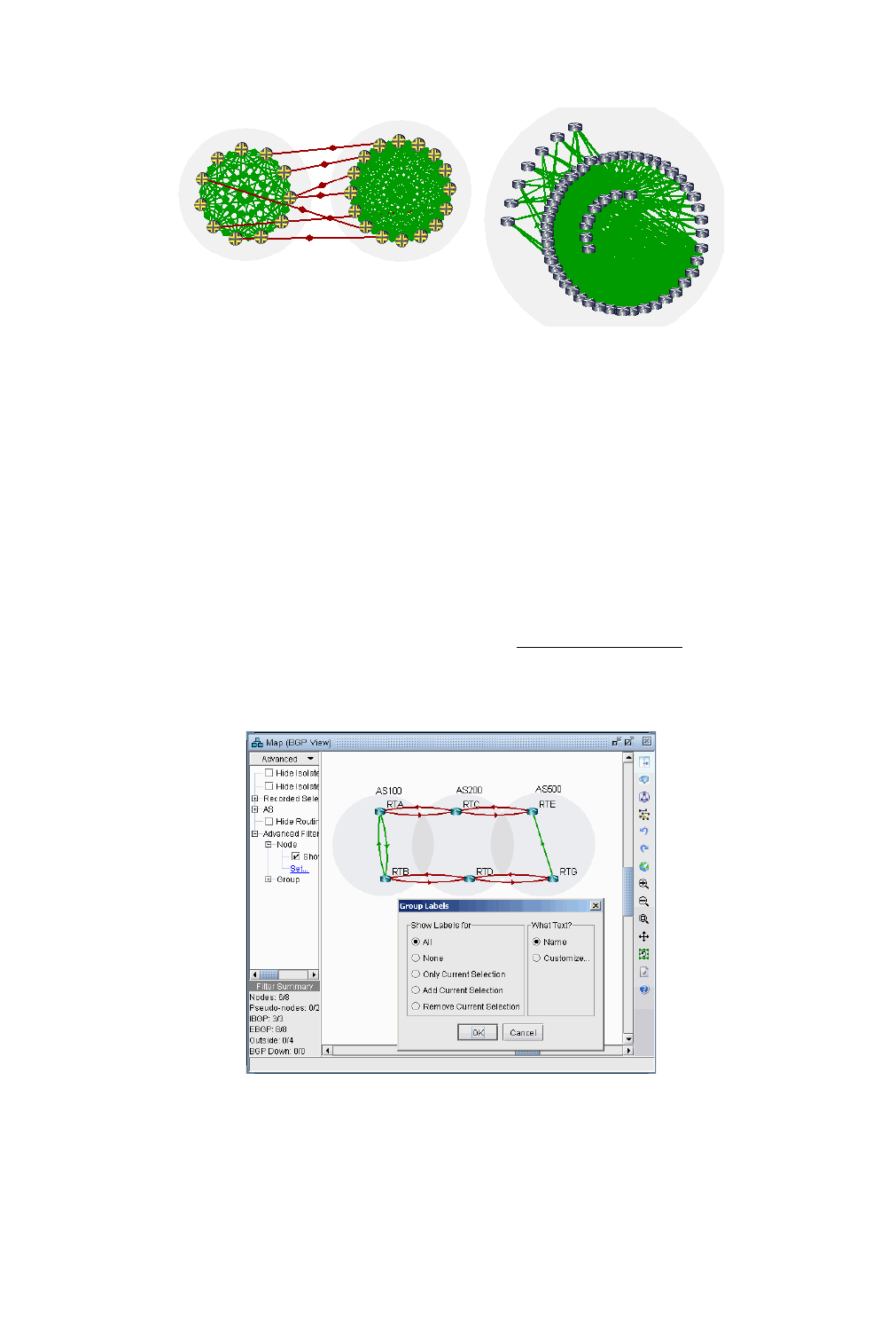
BORDER GATEWAY PROTOCOL*
Copyright © 2014, Juniper Networks, Inc. 8-5
. . . . .
Figure 8-2 BGP Logical Views
11. To return back to the current view, right-click on the map and select Layout>Back to Original.(Note that you
can use the Network > Maps > Copy Map Layout option to transfer the graphical coordinates from the
BGP Map to the Standard Map or vice versa.)
GROUPING
12. In the BGP map, each AS of the network is represented by a grouping disc (from the right-click menu, select
Grouping > Collapse All or Grouping > Expand All to collapse or expand the disc). Each AS which is
outside of the network and has an EBGP peering relationship with BGP speakers of the network is called an
ASnode and is represented by a little square.
13. Note that you can change the grouping arrangement in either BGP Map or Standard Map using the map
right-click window’s Grouping>Autogroup option. Here you can group by Confed AS first and then
subgroup by AS. For more information, refer to the Design & Planning Guide, Topology chapter.
14. To turn on AS group labels, choose Group Labels... from the right-click menu and select Name as shown in
the following figure.
Figure 8-3 AS Group Labels
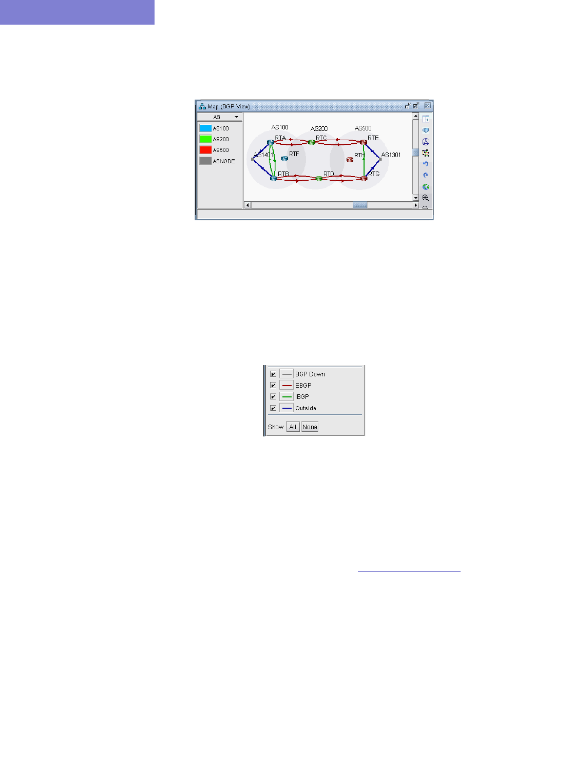
BORDER GATEWAY PROTOCOL*
8-6 Copyright © 2014, Juniper Networks, Inc.
8
AS LEGEND
15. If you select the Subviews > AS menu, you can color the network nodes according to the ASes they belong to
as shown in the following figure. You may click on the color icon to select a different color if desired.
Figure 8-4 Color nodes according to AS
BGP MAP SUBVIEWS
16. Select the Subviews > Type menu of the BGP map. Note the coloring of the different peering relationships:
•Gray lines denote IBGP peering relationships within the same AS hat are down
•Maroon lines denote EBGP peering relationships from one AS to another
•Green lines denote IBGP peering relationships within the same AS
•Blue lines denote EBGP peering relationships that go to ASes outside of the network, represented by ASNODES
because of limited information.
Figure 8-5 Types Subview
17. Select the Subviews > Protocols menu of the BGP map. The choices are as follows:
•All – This is the default subview, which shows both EBGP and IBGP types of relations.
•EBGP/Outside – This shows only EBGP relations.
•IBGP (RR client) – This shows IBGP relations that are route reflections from Route Reflectors to their clients.
Usually there is an arrow for the IBGP neighbor relations in each direction, but for this particular subview, only one
direction is shown from the route reflector to the route reflector client to make it clear which devices are the route
reflectors and which devices are the route reflector clients. To see an even clearer view of the route reflector
relationships, use the Logical Layout view as described in Logical Layout on page 8-4.
•IBGP (no RR) – This shows IBGP without route reflections.
•L2VPN – This shows IBGP relations related to the l2vpn address family.
•VPNv4/Inet-VPN – This shows IBGP relations related to VPNv4 or Inet-VPN address family.
•IPv4 - This shows IBGP relations related to IPv4 address family.
•Symmetric Peering – This shows balanced BGP neighbor relationships
•Asymmetric Peering – This shows unbalanced BGP neighbor relationships, i.e., the neighbor relationship is
only defined on one of the two routers. For a full report of unbalanced BGP neighbor relationships, refer to the
Report Manager, BGP report.
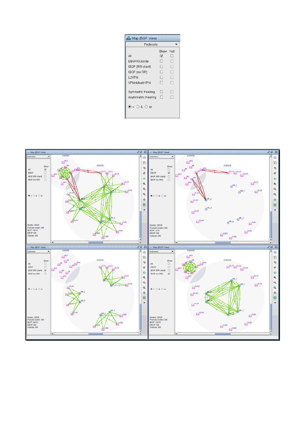
BORDER GATEWAY PROTOCOL*
Copyright © 2014, Juniper Networks, Inc. 8-7
. . . . .
Figure 8-6 Protocols Subview
Figure 8-7 Different BGP Subviews (the Juniper routers are route reflectors in this example)
18. You can select a router from the map to highlight the BGP peering relationships for that router.
19. If you hover your pointer over a logical link, the basic information of that neighbor relationship is shown at the
bottom bar of the BGP map window.
20. Double-clicking a link will bring up a window that describes the neighbor relationship.
21. You can also right-click a node and select “View Nhbrs at Node” to view the neighbors for a router.
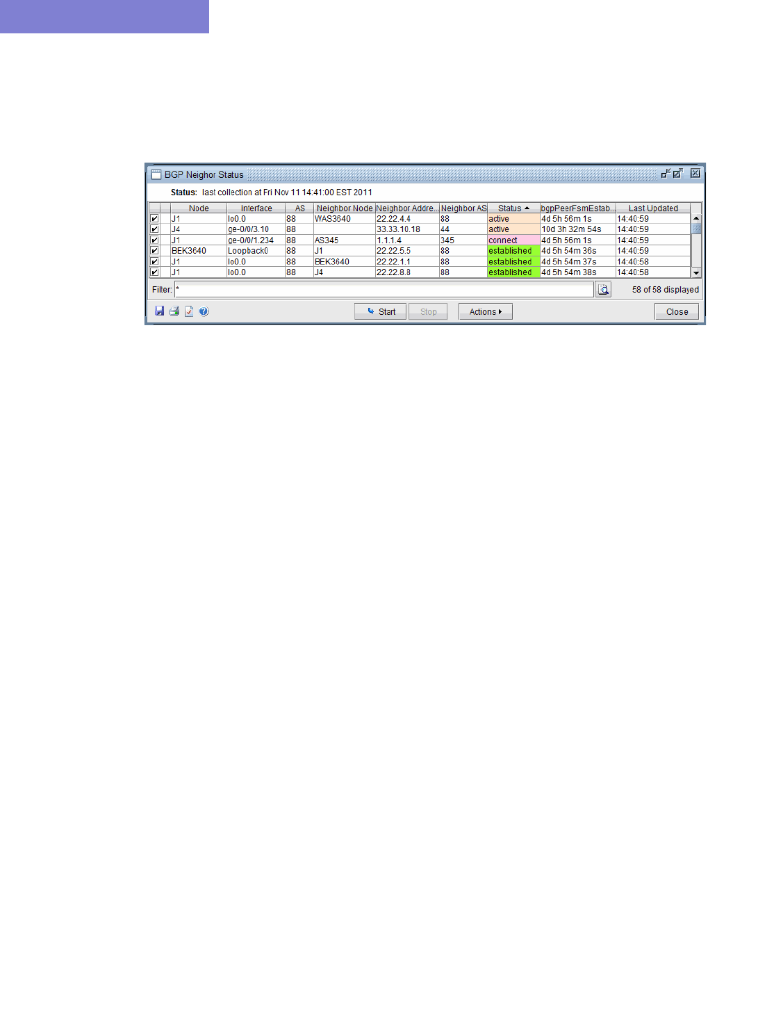
BORDER GATEWAY PROTOCOL*
8-8 Copyright © 2014, Juniper Networks, Inc.
8
BGP Live Status Check
The BGP Live Status Check window displays the current BGP peering’s operational status in real time via SNMP
collection. It is accessed by right-clicking on the BGP Map and selecting Live Status Check. Select the desired Node
Peers using the checkboxes and press Start to begin the SNMP collection.
Figure 8-8 BGP Live Status Check
•Status returns the value from MIB OID bgpPeerState: idle, connect, active, opensent, openconfirm, or
established. Established is the key state which indicates peers are operationally up and BGP route updates are freely
exchanged. BGP Peering Operation Status = Up only if peering state = Established. Any other peering state collected
(idle, connect, active, opensent, or openconfirm) implies BGP Peering Operational Status = Down.
•bgpPeerFsmEstablishedTime indicates how long this peer has been in the Established state or how long
since this peer was last in the Established state. It is set to zero when a new peer is configured or the router is booted.
•LastUpdated is the last collection time.
BORDER GATEWAY PROTOCOL*
Copyright © 2014, Juniper Networks, Inc. 8-9
. . . . .
BGP Routing Table
The Find BGP Routing Table window, as shown in the following figure, will appear when the Network >
Protocols > BGP > BGP Routing Table function is selected. The BGP Routing Table window is used to
display all BGP routing from the specified source node to the specified destination node/IP address.
Figure 8-9 Find BGP Routing Table
22. Choose a source node and a destination node (and/or destination IP address) from two different autonomous
systems from the drop down lists and then click on the Show Routing Table button. Selecting the SrcAS and
DestAS is not required but is only used to filter the Src Node and Dest Node lists. (The Dest AS will be ignored
if it is in a different AS than the Destination IP Address entered.) Selecting a blank SrcAS and DestAS field can
be done to retrieve back all source and destination nodes from the node drop down lists.
Note that different destination IP addresses may have different attributes and associated routing policies. The
destination IP address can be directly entered or populated by first selecting the Dest Node. To load additional
IP addresses at that node found in the BGP Subnet window into the drop down list (Network > Protocols >
BGP > BGP Subnets...), check “List BGP Subnets.” Note that if you already know the IP address, you can
skip selecting the matching Dest Node or Dest AS, which can be derived from the IP address. Note also that this
destination IP address should either be included in one of the BGP subnets (see BGP Subnets* on page 8-21 for
more information), or defined on the destination node.
23. Another method of choosing the source and destination nodes is to use the mouse and the Standard (not BGP)
map. After selecting the Network > Protocols > BGP > BGP Routing Table function, move the mouse
over the map. Notice that the arrow of the mouse turns into a cross hair. Click on the first node, which will be the
source node. Move the cross hair to another node and click on it to specify the destination node. Then move to
the Find BGP Routing Table window and click on the OK button.
Tip: To clearly see which nodes belong to which ASes from the map, go to the Standard map’s Filter menu and
make sure that the box for Hide ASNodes/Links is unchecked. You might also use the map’s right-click menu’s
Grouping>AutoGroup option and group your nodes by AS and go to the Subviews > AS menu to color the
nodes by AS.
Troubleshooting: In some cases the BGP routing table search does not return any results. Make sure that the
SrcAS and Dest AS are different. Additionally, check the EBGP neighbor relationships from the BGP map in
Network > Maps > Maps (BGP View) to verify whether two routers can communicate using EBGP. Finally,
check that the destination IP address is either assigned to the destination node, or a BGP subnet originated from that
node.
24. The BGP Routing Table window shows all possible routes from the specified source node to the specified
destination node/IP address. The fields shown on the window are:
Field Description
Src IP Address The IP address of the source node.
Src Node The name of the source node.
Dest IP Address The IP address of the destination node.
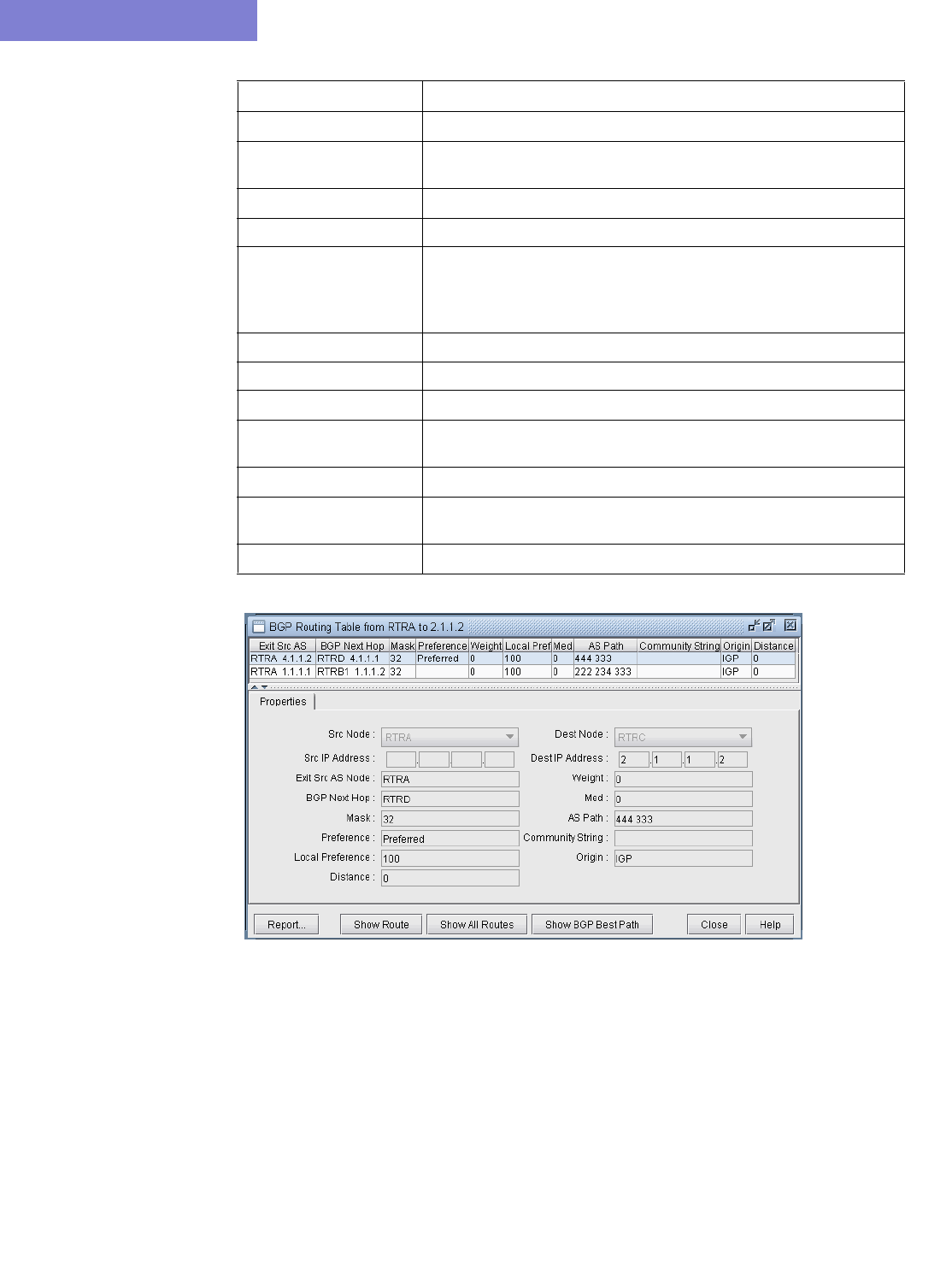
BORDER GATEWAY PROTOCOL*
8-10 Copyright © 2014, Juniper Networks, Inc.
8
Figure 8-10 BGP Routing Table
25. Highlight a BGP route entry and then click on the Show Route button to display the route on the standard
map. Or select Show All Routes to display routes for all the BGP Routing Table entries displayed. Note that
the gray line symbolizes the connection to the BGP next hop. Click “Show Path” to show the actual path that
would be used.
Dest Node The name of the destination node.
Exit Src AS This shows the router name and IP address for the last BGP speaker
on the path before it exits the AS of the source node.
BGP Next Hop The router name and IP address of the BGP next hop.
Mask The corresponding mask of the destination IP address.
Preference This is not a BGP property, but is used to indicate the preferred BGP
next hop chosen by the BGP route selection process when there is
more than one possible path. Possible values are “Preferred”,
“Blocked”, or blank.
Weight The weight attribute
Local Preference The local preference number.
Med The Multi-Exit Discriminator attribute
AS Path The AS path attribute, which consists of AS numbers of all ASes that
the route traverses, the most recently traversed one displayed first.
Community String The Community Attribute
Origin The origin attribute indicates how a route was learned (e.g., IGP,
EGP, or Incomplete)
Distance Total metric of the IGP route from the router to the Exit Src AS router
Field Description
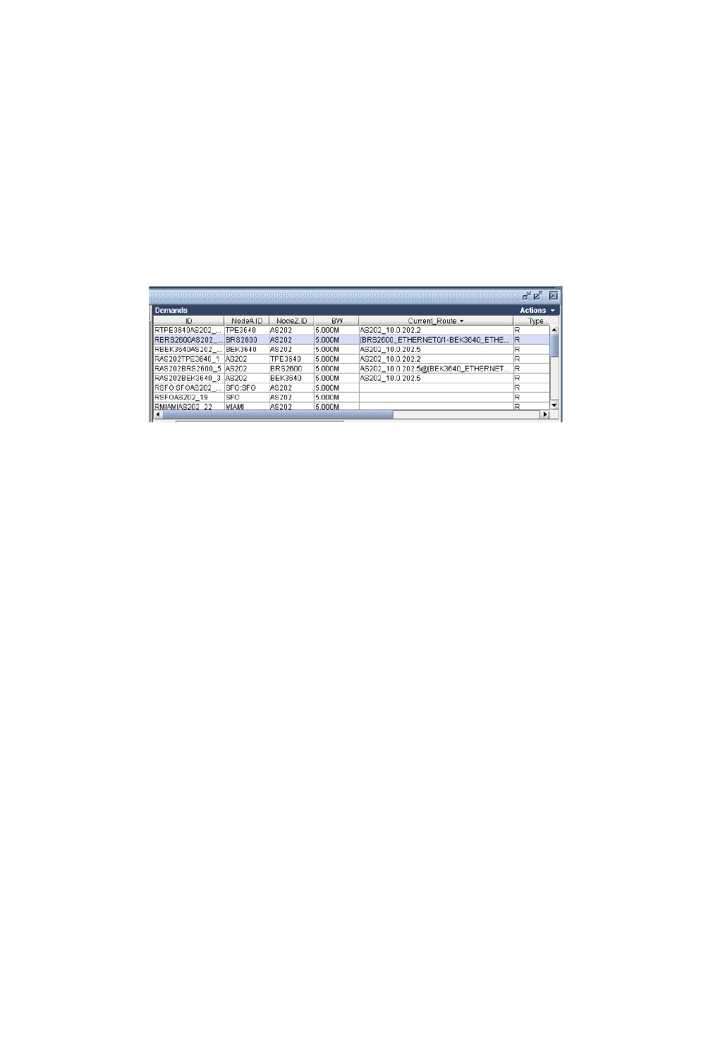
BORDER GATEWAY PROTOCOL*
Copyright © 2014, Juniper Networks, Inc. 8-11
. . . . .
BGP Routes Analysis
BGP routing is a complex process because it involves numerous attributes. Analyzing BGP routes helps the network
planner to understand their network better (e.g., to find out where the bottlenecks are). The BGP Module provides
the users techniques to investigate BGP routes. In general, BGP routes can be analyzed by investigating point-to-
point routing or by generating demands and then examining the ways that demands get routed.
26. To use demands to observe routes, change to Modify mode, add multiple demands (via Modify > Elements >
Demands, Add > Multiple Demands) and change back to Design mode to get the demands routed. Then
look at demands using Network > Elements > Demands... to see how they are routed or why they are
unplaced.
27. The following figure shows the demands in the network. Notice that some demands are routed while others are
not, as indicated by an empty “Current Route” column.
Figure 8-11 Demands Added
28. Highlight a demand and click on the Show Path button in the Demands window. The routing of the
highlighted demand would be shown on the map.
29. Check the Console window for details regarding the BGP next hops chosen along the path that are indicated
after the arrow “->”. The sample console output below of a path analysis from RTRA to 2.1.1.2 (RTRC)
indicates that RTRA chooses BGP next hop 1.1.1.2 on RTRB1 which is directly connected. RTRB1
subsequently chooses BGP next hop 2.1.1.2(RTRC) which is reached via the IGP next hop of 2.1.1.1 (RTRB2)
found by recursive lookup.
RTRA->1.1.1.2(RTRB1)
RTRB1->2.1.1.2(RTRC) via 2.1.1.1(RTRB2)
30. Looking at unplaced demands will help you to determine where the bottlenecks are and why. From the
Demands window, find an unplaced demand and then click on the Bottlenecks button. Examine the main
topology map as well as the console to help you to determine the reason for the unplaced demand, e.g. a missing
BGP routing table entry or being blocked by a policy.
31. You can investigate the originating nodes of unplaced demands to determine the reasons for the bottlenecks. For
example, it may be because the status of a peering relationship is down or because a community list is denied.
The console window can provide details about why a demand failed. For example, it can indicate at which step
the route was blocked due to out policies or in policies when troubleshooting why a BGP next hop was not
found.
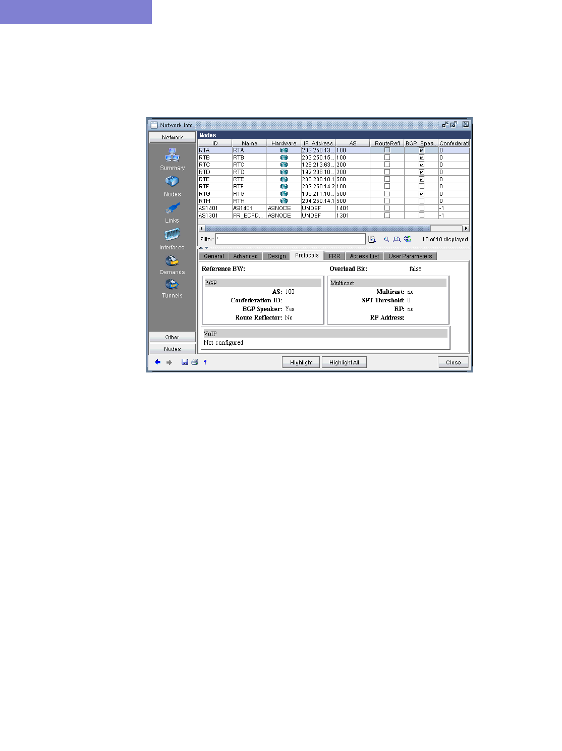
BORDER GATEWAY PROTOCOL*
8-12 Copyright © 2014, Juniper Networks, Inc.
8
BGP Information at a Node
32. From the node window’s Protocols tab, a variety of information related to BGP is available in a table format.
For instance, the following figure shows a particular node’s BGP-related properties, including AS number, BGP
Speaker, Route Reflector, Confederation ID, etc.
Figure 8-12 BGP Information at a node
33. The Advanced Filter from this window contains the following keys that can be used to filter for nodes with
particular BGP properties: AS, BGP_Speaker, Cluster_ID, Confederation_ID, and Route_Reflector.
34. These keys can also be used to label the Standard map using Labels>Node Labels, Customize... from the
Standard map’s right-click menu.
BORDER GATEWAY PROTOCOL*
Copyright © 2014, Juniper Networks, Inc. 8-13
. . . . .
BGP Neighbor
VIEW NEIGHBOR INFORMATION
BGP neighbors are routers that communicate BGP routing information to one another. You can query for a BGP
neighbor relationship from the Network > Protocols > BGP > BGP Neighbor menu in View or Design action
mode. Alternatively, you can right-click a particular node in the map and select View>BGP Nhbrs at Node
(Standard map) or View Nhbrs at Node (BGP map).
35. Click on Network > Protocols > BGP > BGP Neighbor and the BGP Neighbors window will appear.
36. The BGP Neighbors window displays all neighboring relationships. The top section of this window lists all
BGP speakers with their neighbors and properties. The lower half has three tabs: Properties, In Policy, and
Out Policy.
Figure 8-13 BGP Neighbors Details
37. Click on Show Neighbor to highlight the link between the selected neighbor pair.
38. With the Filter button, you can search for neighbors based on various parameters, such as AS numbers,
Interface, Weight, etc. After filling in search criteria, click on the Fetch button and it will bring up the BGP
Neighbor window, which shows all neighbors that match the search criteria.
Note: For the Node field, you must choose a real node and not an AS (pseudo-node). To search on an AS, you can
use the AS, Neighbor AS, and Neighbor Node fields. Note that the search for AS uses exact match on the AS
number. For example, you must type in 111 rather than AS111 or 1 or 1*. Wildcards are not supported in this field.
39. Right-click on an entry to see the options Show “Neighbor Address = Group” and “Show peergroups
with no members”.
•Show “Neighbor Address = Group”: These entries list the group underneath the neighbor address column.
They are intended to provide information regarding the default settings of a BGP group, e.g., configured under [edit
protocols bgp group ibgp_peers] for Juniper. These default settings may be overridden for a particular neighbor
within the group.
•“Show peergroups with no members”: This option will display any BGP groups which have no neighbors
listed in them.

BORDER GATEWAY PROTOCOL*
8-14 Copyright © 2014, Juniper Networks, Inc.
8
PROPERTIES TAB
The Properties tab has the following fields:
IN AND OUT POLICIES TABS
The In Policy tab shows all policies that are applied to incoming routes to the node from the highlighted neighbor.
The Out Policy tab shows all policies that are applied to outgoing routes from the node. (Note that different
literature may refer to in/out policy as import/export policy; they are equivalent.)
Note: You should have more than one AS in your network in order to see policies.
For Cisco routers, the routing policies may specify route filtering and attribute manipulation, which use route maps,
access lists, AS_path access lists, community lists, distribute lists, and filter lists.
For Juniper routers, policy statements and community lists are used. When either the In Policy tab or the Out
Policy tab is selected, the policy window has the following fields:
Field Description
AS The node AS.
Neighbor AS The neighbor node AS.
Interface The interface that is used to connect to the neighbor.
Node The name of the node (BGP speaker).
Status Status of the neighbor. It is either up or down.
Group The name of the peer group if it is applicable.
Multihop The optional TTL (Time to Live) number from the IOS command:
neighbor {ip-address | peer-group-name} ebgp-multihop [ttl]
VRF The virtual routing and forwarding instance name.
Neighbor Address The IP address of the neighbor.
Neighbor Node The name of the neighbor.
RR Client Indicates whether the neighbor is a route reflector client or not.
Cluster ID The cluster ID if it is applicable.
Address Family Indicates if an address family such as VPNv4 or Inet-VPN is used.
Confederation ID Indicates the BGP Confederation ID that the AS belongs to, if any.
Multipath Indicates if BGP multipath has been configured for load balancing
purposes.
Next-hop self Indicates if the router is configured as the next hop for the BGP
neighbor. “
Field Description
Policy Name of the policy
Term/Sequence The term number is used in the policy statement for Juniper.
The sequence number is applicable to the route map for
Cisco.
Action Permit or deny
BORDER GATEWAY PROTOCOL*
Copyright © 2014, Juniper Networks, Inc. 8-15
. . . . .
Figure 8-14 In Policy
40. When a particular policy in either the In Policy or Out Policy tab is selected, the lower right pane displays the
relevant statements for that policy. For instance, the in policy localonly for router RTB is shown in the figure
above.
ADD BGP PEERING RELATIONSHIP
WANDL software offers two ways to add BGP peering relationships; you can use either the Modify > Protocols >
BGP > BGP Neighbor... menu or the Modify > Protocols > BGP > Add Multiple BGP Neighbors... menu.
41. To define a BGP peering relationship from a node to its neighbor node, switch to Modify mode, and bring up the
BGP Neighbors window via the Modify > Protocols > BGP > BGP Neighbor... menu. Then click on the
Add button to bring up the Add BGP Neighbors window as shown in the following figure.
Figure 8-15 Add BGP Neighbor Window
42. Choose the AS number and Node from the AS and Node dropdown menus. Similarly, choose the Neighbor AS
number and the Neighbor Node from the Neighbor AS and Neighbor Node dropdown menus. Clicking OK
results in a BGP peer being established from the Node to the Neighbor Node. To establish a BGP peering
relationship in the opposite direction, simply perform the same steps but swap the AS and Node selections with
the Neighbor AS and the Neighbor Node selections. Note that if you are adding a bgp neighboring relationship
from a route reflector to its client, be sure to check the RR Client box and specify the Cluster ID.
BORDER GATEWAY PROTOCOL*
8-16 Copyright © 2014, Juniper Networks, Inc.
8
43. To add multiple BGP peering relationships between a node and it neighbor, use the Modify > Protocols >
BGP > Add Multiple BGP Neighbors... menu to bring up the Add Multiple BGP Neighbors window.
The Type dropdown menu includes Intra AS and Inter AS options. The following figure shows how the Add
Multiple BGP Neighbors window with Type selected as Intra AS is used to create a full mesh of IBGP
neighboring relationships within the AS. Note that balanced neighbors (neighboring relationships established in
both directions) are created.
Figure 8-16 Add Multiple BGP neighbors window
BORDER GATEWAY PROTOCOL*
Copyright © 2014, Juniper Networks, Inc. 8-17
. . . . .
Apply, Modify, or Add BGP Polices
APPLYING POLICIES
44. BGP policies that have already been defined at a router can be applied as an in policy or as an out policy. To
bring up the Modify BGP Neighbors window, first switch to the Modify action mode. Then select the
Modify > Protocols > BGP > BGP Neighbors ... function to bring up the BGP Neighbors window, from
which a row can be selected. Double-click on a selected row or click on the Modify button to bring up the
Modify BGP Neighbors window as shown in the following figure.
Figure 8-17 Modify BGP Neighbors
45. Select either the In Policy tab or the Out Policy tab to see the Available Policies at that node and the
Applied Policies lists. Selected policies in the Available Policies list can be moved to the Applied
Policies list by clicking on the Add-> button and, vice versa, selected policies in the Applied Policies list
can be moved to the Available Policies list by clicking on the <-Remove button. The following figure shows
an example of a BGP policy (setlocalpref) that has been moved to the router’s Applied Policies list.
Figure 8-18 Applying an In Policy
In some cases, shorthands are used to describe the policies, in the format Match Type: Match Name, where the
Match types are interpreted as follows:
•AC - Access List
•AL - AS-path access list
•CL - Community List
•DL - Distribute List
•PL - Prefix List
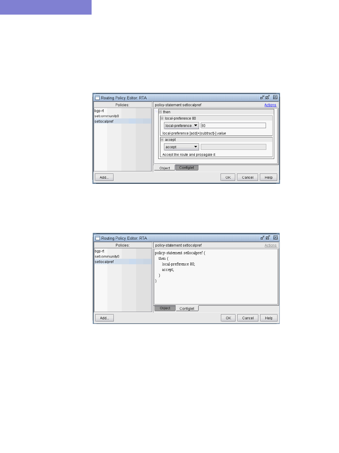
BORDER GATEWAY PROTOCOL*
8-18 Copyright © 2014, Juniper Networks, Inc.
8
MODIFY BGP POLICY
46. To modify a BGP policy at the router, click on the Policy Editor... button to bring up the Routing Policy
Editor window as shown in the following figure. Then select a particular policy from the left pane to display
corresponding policy commands in the right pane.
47. The + button expands a selection, while the - button collapses it. Dropdown menus and text fields allow you to
modify the policy. The following figure shows an example of a BGP policy that is used to set the local-
preference to a value of 80.
Figure 8-19 Modifying a BGP Policy
48. To see the generated configlet for the BGP policy, click on the Configlet tab. The following figure shows the
generated configlet corresponding to a BGP policy (setlocalpref).
Figure 8-20 The Generated Configlet for a BGP Policy
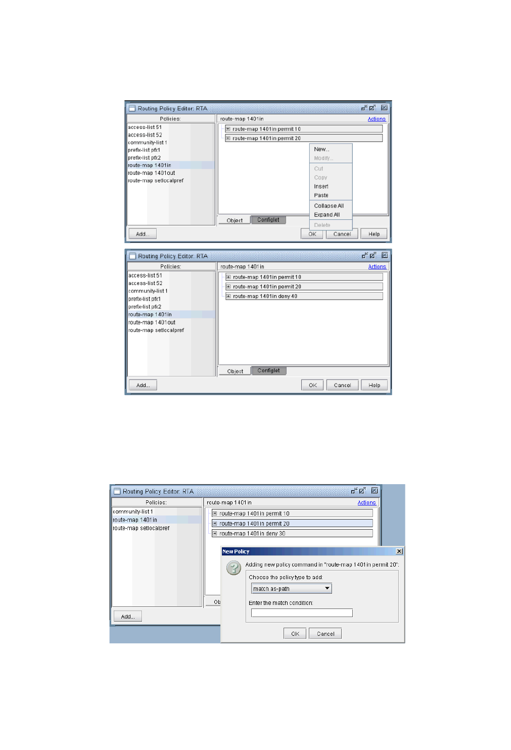
BORDER GATEWAY PROTOCOL*
Copyright © 2014, Juniper Networks, Inc. 8-19
. . . . .
49. The right-click menu or the Actions menu offers further options for modifying the routing policy. To add a new
term to a policy, first select the policy. Then from the right pane, select New from either the Action menu or the
right-click menu. Note in the following figure that after selecting New, a new item was added to the policy.
Figure 8-21 Adding a term to a policy
50. For route map policies, you can add commands underneath a particular term. Highlight the term, right-click, and
select New... to open up the following dialog. Add “match” or “set” commands as shown in the following
figure. Note that to deselect an item, simply click on a white space in the right pane.
Figure 8-22 Adding a match command to a term of a route-map
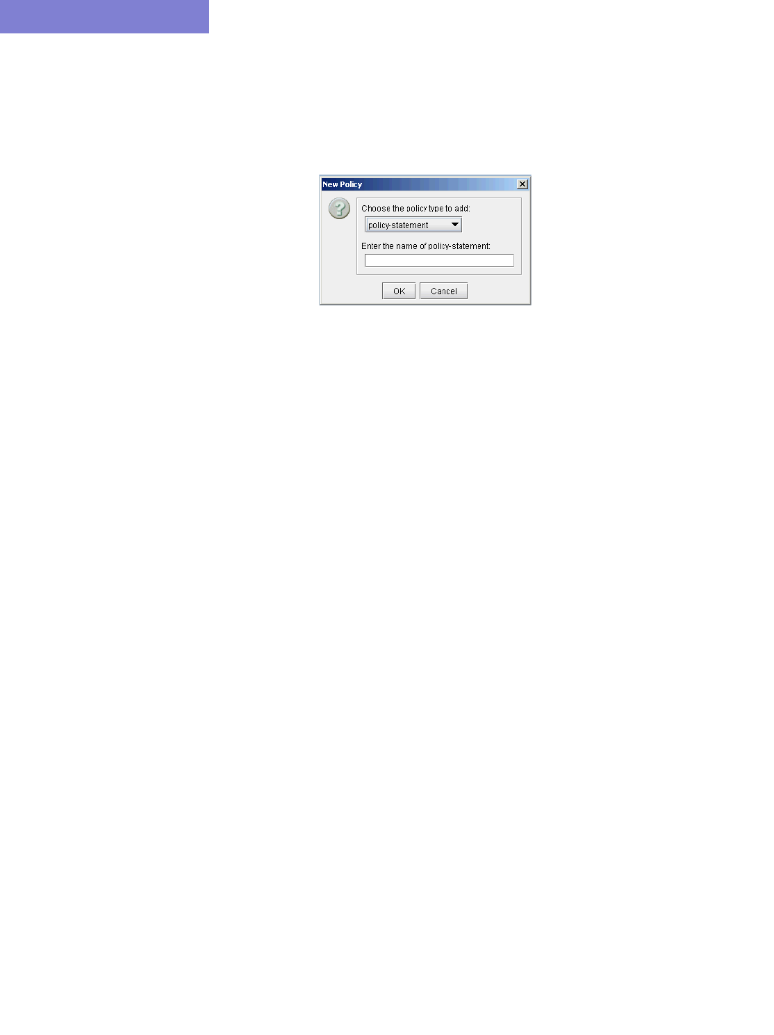
BORDER GATEWAY PROTOCOL*
8-20 Copyright © 2014, Juniper Networks, Inc.
8
ADDING A BGP POLICY
51. To add a new BGP policy, click on the Add... button in the lower left hand corner of the window to bring up the
New Policy window (shown in the following figure), and proceed the same way as is done in modifying a BGP
policy. Here you have a choice of five different types of policies: route-map, access-list, as-path access-list,
community-list, and prefix-list. Note that the options may vary depending on the policy type.
Figure 8-23 New Policy Window
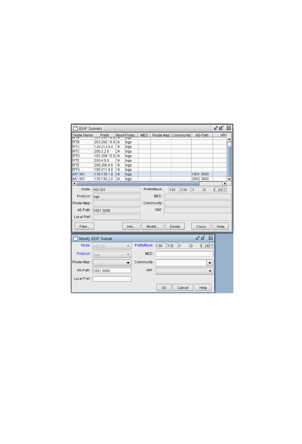
BORDER GATEWAY PROTOCOL*
Copyright © 2014, Juniper Networks, Inc. 8-21
. . . . .
BGP Subnets*
The BGP subnets list can be used to list prefixes, or subnetworks (whose router configuration files are unavailable)
originated from a particular router or AS node. Various BGP attributes associated with the subnetwork can be
defined in the subnet file.
*Note that a separate password is required for BGP subnets. Please contact your Juniper representative for more
information. Note also that if useliveBGPrtbl=1 is set in the dparam file, or in Tools > Options > Design, Path
Placement > BGP, then the subnets information will be ignored.
52. The subnet file can be viewed from the File Manager or from Network > Protocols > BGP > BGP
Subnets... menu. To add, modify, or delete BGP subnets in the subnet file, first switch into the Modify action
mode. Then bring up the BGP Subnets window via the Modify > Protocols > BGP > BGP Subnets...
menu. The following figure shows a subnet entry for AS node, AS1301, being modified.
Figure 8-24 Modifying a BGP Subnet
53. Note the Protocol field, which defaults to bgp. Specifying “bgp” indicates that this is the prefix advertised from
the router. In-policies still need to be applied to this route by the router receiving the route. Specifying “bgptbl”
in this field indicates the route that is in the router’s routing table. It has already been accepted by the router’s in
policy, but may or may not be the preferred route. This option is used for routes received from other
Autonomous Systems, since their configuration files may not be available.
To illustrate how to use the BGP subnet list (accessed via Network > Protocols > BGP > BGP Subnets...), a
sample network and the corresponding BGP subnet list are shown in the following two figures. Note that within the
BGP subnet list, ASnode AS1301 is declaring that it can reach subnet 130.130.1.0/24, which has an AS_PATH
attribute that includes 1001. ASnode AS1301 is also declaring that it can reach subnet 130.130.2.0/24, which has an
AS_PATH attribute that includes 2002.
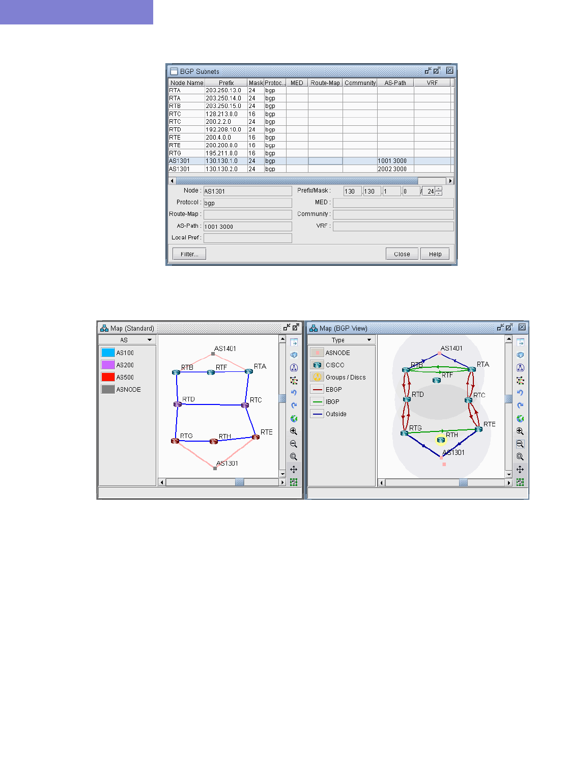
BORDER GATEWAY PROTOCOL*
8-22 Copyright © 2014, Juniper Networks, Inc.
8
Figure 8-25 View BGP Subnets Window
Figure 8-26 Main View and BGP View of the network
54. To see the BGP InPolicy defined at a router RTE, bring up the BGP Neighbors table and switch to the In
Policy tab, as shown in the following figure. In this particular example, the InPolicy at router RTE is defined by
a Cisco route-map and says that if an incoming route has 1001 included in its AS_PATH attribute, then set the
LOCAL_PREF attribute to 123; otherwise, set the LOCAL_PREF attribute to 89. The InPolicy at router RTG is
the same except that 2002 is matched for instead of 1001.
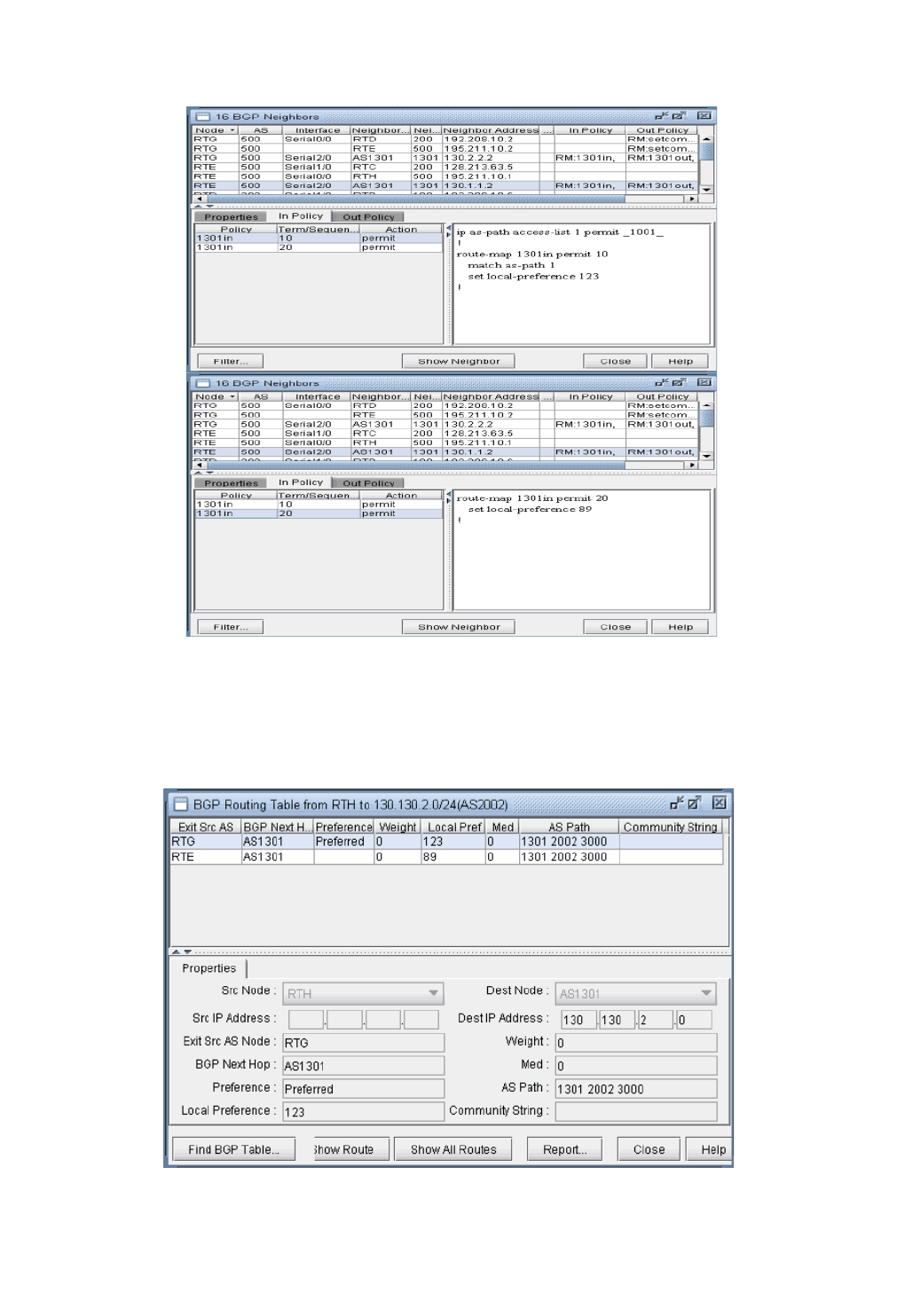
BORDER GATEWAY PROTOCOL*
Copyright © 2014, Juniper Networks, Inc. 8-23
. . . . .
Figure 8-27 BGP In Policy for RTE
55. Continuing with our example, we bring up our BGP routing table to verify that the LOCAL_PREF attribute got
set correctly to 123 for AS1301’s subnetwork 130.130.2.0/24, which has 2002 included in its AS_PATH
attribute.
Figure 8-28 BGP Routing table from RTH to AS1301 subnet 130.130.2.0/24
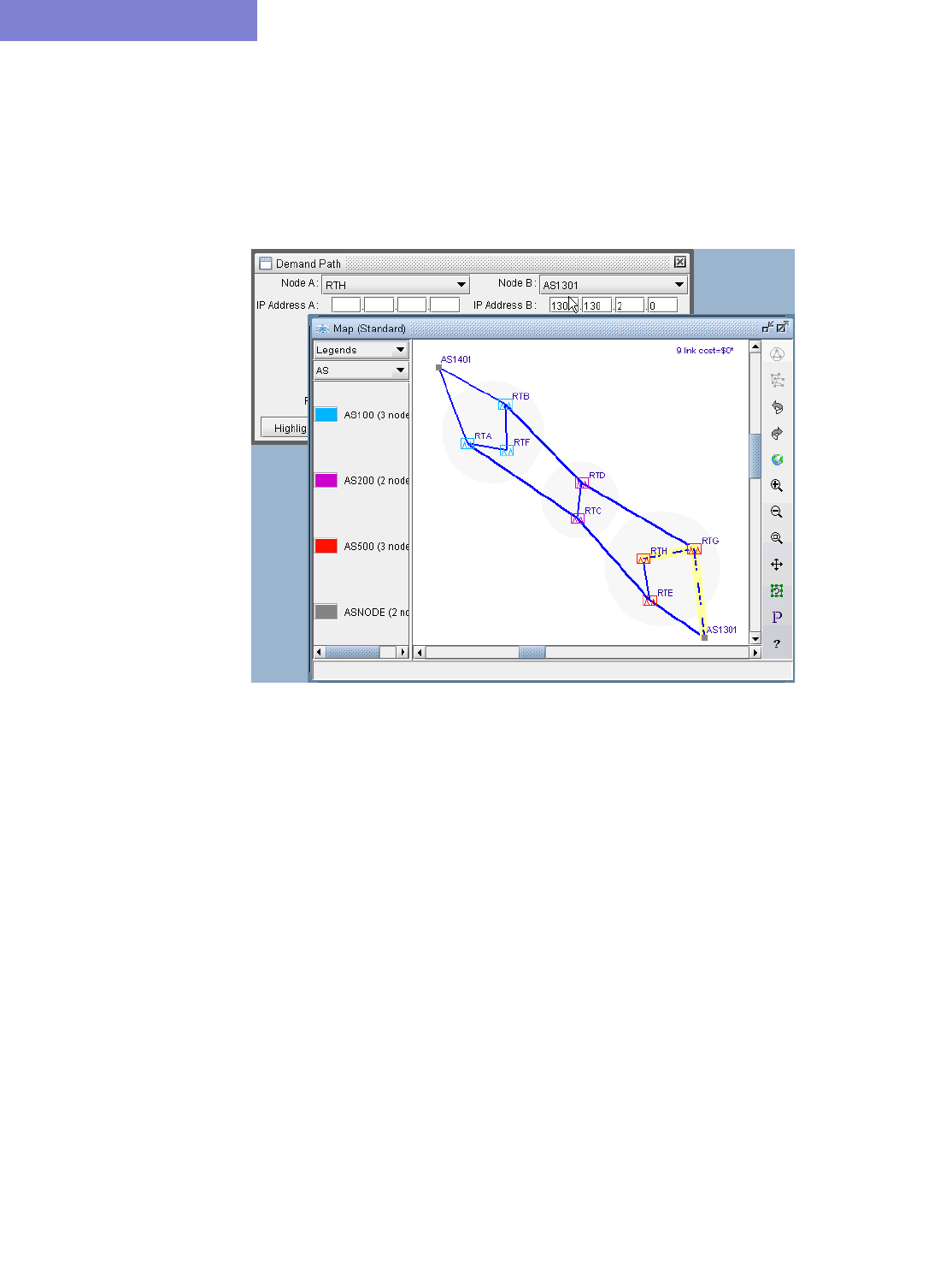
BORDER GATEWAY PROTOCOL*
8-24 Copyright © 2014, Juniper Networks, Inc.
8
Note: In Internet routing, community is another commonly-used attribute to tag a particular route. Each
service provider can define its own policy based on this attribute of the incoming route. The subnet file helps
the user to simulate routing behaviour to various Internet destinations.
56. Finally, we can do a path trace from a router, say RTH, in AS 500 (which includes routers RTH, RTE, RTG) to
AS1301’s subnetwork 130.130.2.0 and verify that RTG is indeed the preferred exit point for AS500, as indicated
by the higher LOCAL_PREF value of 123. The following figure shows the path trace.
Figure 8-29 Path trace illustrating the RTG being the preferred exit point
Live BGP Routing Tables*
*Note that a separate password is required for BGP live routing table import. Please contact your Juniper
representative for more information.
The BGP routing table object file can be used by the routing engine to perform BGP table lookup according to the
router’s actual BGP routing table. This routing table may include routes to IP addresses in other ASes for which
there is insufficient information within the existing set of config files. To create the BGP Table Obj File from the live
network, BGP routing tables are needed from each router.
The following are the instructions for importing Juniper BGP routing tables:
57. Put each router’s routing table output into a separate file and set the first line to be the word ‘hostname’ followed
by the router’s hostname. If the file is too large, this can be done by concatenating a file with the hostname
information with the file containing the router’s routing table output.
58. Run the following commands to create the BGP routing table object file output_object_file .
The following command creates the intermediate file group.firstAS:
/u/wandl/bin/prefixGroup -firstAS routingtablefiles
Next, use the group.firstAS file in combination with the routing table files to create the output BGP object file:
/u/wandl/bin/routeGroup -o output_object_file -g group.firstAS routingtablefiles
59. In the spec file, reference the output object file using the keyword livebgprtblobj=output_object_file

BORDER GATEWAY PROTOCOL*
Copyright © 2014, Juniper Networks, Inc. 8-25
. . . . .
60. After loading the network, you can decide whether or not to route according to the live BGP routing tables or
not through the Tools > Options > Design, Path Placement > BGP options pane, by setting “Use Live
BGP Table if Available” to true.
getipconf Usage Notes
SYNTAX
getipconf [-r runcode] [-t topfile] [-b bwconvfile] [-n muxloc] [-p nodeparam]
[-noBGP] [-i interfaceDir] [-snmp SNMPDir] [-commentBW] [-ignore ipaddr] [-
ospf ospfdatabase] [-atmbw] [-cdp cdpfile1 cdpfile2 ... -conf] config1 config2
...
BGP-RELATED FLAGS
BGP FILES GENERATED
In addition to the standard files like the spec, muxloc, and bblink files, the following are five output files related to
BGP that are generated by getipconf: aclist.x, controllist.x, bgpobj.x, bgpnode.x, bgplink.x, bgpnbr.x, and subnet.x
(assuming the runcode is x). Below is a brief explanation of the contents of these files:
•aclist.x contains information about as-path, access-list, and community-list
•controllist.x contains information about access-lists and prefix-list. The controllistobj.x file is a binary file.
•bgpnode.x contains information for BGP speakers
•bgplink.x contains information for BGP neighbors
•bgpnbr.x is a text file that contains all information about neighbors.
•bgpobj.x contains information about BGP neighbors shown in bgpnbr.x and route map structure. The bgpobj file
is a binary file designed to save space and to speed up performance of the software. It is partially replaced by
bgplink.x and bgpnode.x. How the program decides whether to read the bgpobj file or the bgplink and bgpnode file
is explained below.
•subnet.x is used to list those subnetworks originated by a particular router or AS node.
CORRESPONDING SPEC FILE KEYWORDS
In the spec file, the keywords for the first four of these files will be listed as aclist, bgpobj, bgpnode, and bgplink.
The bgpnbr file is for informational purposes only and is not included in the spec file.
For an example of the spec file entries related to BGP, see the following example:
# Files used by IP network
bgpobj= bgpobj.x
bgpnode= bgpnode.x
bgplink= bgplink.x
dparam= dparam.x
aclist= aclist.x
BGP-Related Flags Description
-noBGP If this optional flag is specified, BGP information will not be
generated.
-ignore <ipaddress> All IP addresses of the type 10.x.x.x, 127.x.x.x, and
192.168.x.x are local addresses. To prevent matching
interfaces in one network with interfaces in another network,
this optional ignore flag is provided. For example, if the user
specifies the following:
getipconf -ignore 192.168 -ignore 10. -ignore 127. *
then all the links with addresses matching these patterns are
commented out. However, if the addresses are all from the
same network, this flag should not be included.

BORDER GATEWAY PROTOCOL*
8-26 Copyright © 2014, Juniper Networks, Inc.
8
jpoBGP=jpoBGP.x
subnet= subnet.x
livebgprtblobj=livebgp.obj
controllistobj=controllistobj.x
Usage Note
Users need to comment out the specification of the bgpobj file in the spec file if they plan to edit BGP attributes
manually. When loading the network, the rtserver (or bbdsgn) program reads the bgpobj file, if it is specified,
ignoring the bgpnode and bgplink files. However, if the bgpobj file is not specified or it is commented out, rtserver
will read the bgpnode and bgplink files instead. When saving the network, all three files: bgpobj, bgpnode and
bgplink will be saved.
DPARAM FILE
The following are some of the BGP-related parameters in the dparam file that you may want to change. They can
also be changed through the Tools > Options menu as described in BGP Options on page 8-3.
chkIBGPflag = 1 # 0: skip IBGP policy checking
IGPoverride= 0 # IGP over ride BGP
useliveBGPrtbl = 1
simskipAS= 1 # 1: skip AS nodes and link down simulation
•If IBGP policies are used in the network to influence routing, set the chkIBGPflag parameter to 1. By default, it
is set to 0 to speed up routing.
•The useliveBGPrtbl option is an advanced feature discussed in Live BGP Routing Tables* on page 8-24.
•The simskipAS parameter is set to 1 by default, meaning that AS nodes and links will not be brought down in an
exhaustive failure simulation performed from Simulation > Predefined Scenarios. If you wish to check the
impact of an AS node or AS link failure on traffic routing, change the value to 0. Note, however, that if there are a lot
of AS nodes, this may greatly increase the time it takes to perform the simulation. To indicate that only a subset of
the AS nodes should be failed and the rest of the AS nodes should be ignored, mark the AS nodes or AS links to
ignore with the FAIL=0 flag. This parameter can be set in the Modify > Elements > Nodes, Design properties
tab (or add it to the end of the muxloc file entry) or Modify > Elements > Links, Properties tab (or add it to the
miscellaneous field of the bblink file entry).
muxloc entry: SDG SANDIEGO 760 277 US 32.883434 -117.167480 FAIL=0
bblink entry: LINK7 CHI DET DEF 1 OC3 MPLSTE,OSPF=477,FAIL=0 AREA=AREA0
•The IGPoverride option is false (0) by default, meaning that for external paths, BGP will be treated as having a
higher administrative distance/preference than the IGP such as OSPF. If this is not the case, this parameter can be set
to true (1).
BGPNODE FORMAT
#Node ASno ConfedID clusterID misc
N3 222 0 0 RR
BGPLINK FORMAT
#lineID nodeA nodeZ Z_AS MED weight local_pref multi_hop RRclient
NBR1 N1 N2 111 0 0 0 -1 0
Note: Due to the complexity, peer group and policy are not defined in these two files now.
ACLIST FORMAT
# AS path and community lists
# column 1 - router_name separated by comma
# column 2 - AS number
# column 3 - access modifier 1-permit, 0-deny
# column 4 - type a-AS path, c-Community list
# column 5 - regular expression
router1, 9999 0 a ".*"

BORDER GATEWAY PROTOCOL*
Copyright © 2014, Juniper Networks, Inc. 8-27
. . . . .
BGPNBR FILE
The bgpnbr file is for information purposes and is not read into the spec file. See the following table for a description
of the fields in the bgpnbr file.
#Status,AS,Intf,Node,Z_AS,Z_intf,Z_Node,PeerGroup,RRclient,Cluster,Multihop,L
ocal Pref,Weight,Med, InPolicy,OutPolicy,VRF,Confederation_ID,MultiPath
up,111,Loopback1,S36,111,"allow_ixp",,"allow_ixp",0, ,-1,0,0,0," "," ",
ASes that are outside of the network and have EBGP peering relationship with BGP speakers of the network are
represented by ASnodes in the muxloc file (the node file of the WANDL software).
SUBNET FILE
A snippet of a sample subnet file is shown here. The address/mask field denotes the subnetwork originated by the
node. The misc field is used to specify any BGP attributes associated with the subnetwork.
#Node address/mask protocol misc
RTA 200.200.1.0/24 bgp
AS111 130.130.1.0/24 bgp as-path=1111 3000
AS111 130.130.2.0/24 bgp as-path=2002 3000
AS222 140.140.10.0/24 bgp community=1401:10
AS222 140.140.20.0/24 bgp community=1401:20
Field Description
Status Status of the neighbor, either up or down
AS The AS number of the BGP speaker
Intf The IP address of the interface used to connect to the neighbor
Node The name of the BGP speaker
Z_AS The AS number of the neighbor
Z_intf The IP address of the interface on the neighbor router
Z_Node The name of the neighbor
PeerGroup The peer group name if it is applicable
RRclient The indicator to indicate whether the neighbor is a route reflector client or
not
Cluster The cluster ID if it is applicable
Multihop The optional TTL (Time to Live) number from the IOS command:
neighbor {ip-address | peer-group-name} ebgp-multihop [ttl]
LocalPref The Local Preference attribute
Weight The weight attribute
Med The Multi-Exit Discriminator attribute
InPolicy The names of policies for incoming routes
OutPolicy The names of policies for outgoing routes

BORDER GATEWAY PROTOCOL*
8-28 Copyright © 2014, Juniper Networks, Inc.
8
BGP Report
When the client session is opened for the first time, the BGP Report should be checked to make sure that the network
has no obvious BGP configuration errors.
The output file that is written to the output directory is called “BGPRPT.runcode”.
BGP INTEGRITY CHECK REPORT:
BGP statistics – This section shows:
•The total number of BGP speakers in the network
•The total number of neighbors
•The total number of policies
•The list of all ASes and the number of their BGP speakers
******************************************************
* BGP Integrity Check Report
******************************************************
-- 17 BGP speakers,89 neighbors,283 members,183 policies
-- 3 local AS:
ASno 222: 9 routers
ASno 111: 7 routers
ASno 555: 1 routers
NEIGHBOR AS SPECIFICATION ERROR CHECK REPORT
This section shows any errors about ASes that are not specified correctly. For example, router A declares that its
neighbor, router B, is in AS1243, but router B is actually in AS4312.
*****
Neighbor AS Specification Error Check Report
AS Location Nbr_AS Nbr_IP_Addr Nbr-Location ValidAS Comments
111 X39 224 69.49.226.34 Q39 222
*** 1 AS specification errors
In the example above, the Neighbor AS Specification Error Check Report shows that there is an error in the node
(Location) X39. The neighbor node(Nbr-Location) is Q39 and the neighbor AS (Nbr_AS) is 224, which should be
222 as shown in the ValidAS field.
UNBALANCED BGP NEIGHBOR CHECK REPORT
The BGP protocol requires that if router A declares router B to be its neighbor, then router B also has to declare that
router A is its neighbor. If not, then an unbalanced neighbor occurs. This section reports any unbalanced neighbors
between BGP speakers within the network.
*****
Unbalanced BGP Neighbor Check Report
# Unbalanced BGP Neighbor = 2
AS Location Nbr_AS Nbr-Location
111 S39 111 X39
111 W39 111 X39
The Unbalanced BGP Neighbor Check Report shows that there are two unbalanced neighbors. On the first record
S39 declares that X39 is its neighbor but X39 does not declare that S39 is its neighbor. The second record shows a
similar error.
IBGP MESH CONNECTIVITY CHECK REPORT
All IBGP speakers within an AS have to be fully meshed, unless route reflectors or confederation are used. This
section shows if any AS is not fully meshed. A full mesh for both IPV4 and VPNV4 address families are checked.
*****
IBGP Mesh Connectivity Check Report
AS222: #IPV4 IBGP neighbor=0. Check mesh definition for VPNV4 address family
AS 222: passed mesh connectivity checking

BORDER GATEWAY PROTOCOL*
Copyright © 2014, Juniper Networks, Inc. 8-29
. . . . .
---- VPNV4 AS111: S39 is not defined as X39's neighbor
IPV4 VPNV4 AS111: W39 is not defined as X39's neighbor
AS111: 2 neighbor definition missing
AS333: IPV4, VPNV4, L2VPN IBGP neighbors are not defined
AS 555: passed mesh connectivity checking
The IBGP Mesh Connectivity Check Report above shows the following
•AS222 is fully meshed for the VPNV4 address family but no IBGP neighbors exist for IPV4 address family.
•AS111 is not fully meshed for IPV4 and VPNV4. For the VPNV4 address family, S39 and W39 are not defined
as X39’s neighbors. For the IPV4 address family, W39 is not defined as X39’s neighbor.
•AS555 passes the mesh connectivity check for both IPV4 and VPNV4.
•AS333 is missing IBGP neighbors for the IPV4, VPNV4, and L2VPN address families.
IPV4/VPNV4/L2VPN ROUTE REFLECTOR STATISTICS
These three sections indicate the route reflector statistics, including number of route reflectors, number of route
reflector clients, and hierarchical route reflector information. Route reflector clients with only one route reflector are
listed as a warning that they do not have redundant route reflectors defined. The following is an example of the IPV4
route reflector statistics:
IPV4 Route Reflector Statistics: 200 BGP Speakers, 8 Route Reflectors, 100 Route Reflector Clients
Redundant Route Reflectors are not defined at 2 RR Clients
1. WDC1, RR= PHI1
2. WDC2, RR= PHI1
#Route Reflector Hierarchy Level= 3
Top Level: 4RR(s)
1. NYC1,
2. NYC2,
3. BOS1,
4. BOS2,
Level 2: 3RR(s)
1. PHI1, RR= NYC1 NYC2
1. PHI2, RR= NYC1 NYC2
2. BOS3, RR= BOS1 BOS2
Level 3: 1RR(s)
1. TRE1, RR= PHI1 PHI2
VPNV4 and L2VPN route reflector statistics are similarly provided.
It is recommended that all errors reported in the BGP Report file get fixed before carrying on further analysis. One
way to do it is to correct the errors on the configuration files and then run through getipconf again.

BORDER GATEWAY PROTOCOL*
8-30 Copyright © 2014, Juniper Networks, Inc.
8

Copyright © 2014, Juniper Networks, Inc. 9-1
. . . . .
. . . . . . . . . . . . . . . . . . . . . . . . . . . . . . . . . . .
BGP P
EERING
A
NALYSIS
*
9
he BGP Peering Analysis module can be used to study the impact of adding a new BGP peer to an existing
network. In particular, users can study the changes in node traffic and link traffic upon addng a new BGP
peer and setting up the BGP policies or BGP attributes for the new peer.
In addition to configuration files and traffic information, data required for the BGP peering analysis module includes
the following:
•BGP routing tables collected from routers contain the information from the actual BGP routing table, from
which the BGP Peering Analysis module will extract necessary information to construct a (a) live BGP table object
file and a (b) subnet file. The live BGP table object file is used to route flows according to the actual BGP routing
table. The subnet file, is used to store the prefixes known to each router and the associated BGP attributes such as the
AS PATH, local pref, and origin. The subnet file can be used by the WANDL routing engine to recalculate the BGP
routing table for what-if studies involving BGP policy changes or the addition of new peers.
•RouteViews archive data, obtained from the University of Oregon’s Routeviews project, provides a method for
Internet operators to obtain real-time information about the global routing system from the perspectives of several
different backbones and locations around the Internet. The BGP peering analysis module will extract routes from
Routeviews data on prefixes reachable by another AS, which would be advertised to the user network upon
establishing BGP peering with this AS. For more information, refer to www.routeviews.org and
archive.routeviews.org. An additional tier 1 definition file, indicating a list of tier 1 Service Providers defined by the
user, is also required for the RouteViews data analysis.
Upon processing the BGP routing tables and RouteViews data, customized link utilization and node traffic reports
can be compared for the following two scenarios:
•Current routing based on the BGP routing tables collected from the routers before adding a peer.
•Routing based on Routeviews data, after adding a new peer to the existing network.
*Note that a special password is required for the BGP Peering Analysis feature. Please contact your Juniper
representative for more information.
Related Documentation
For an overview of available BGP features, refer to Border Gateway Protocol* on page 8-1.
For details on how to create a spec file by extracting, or importing, information from the router configuration files,
please refer to Chapter 2, Router Data Extraction.
Recommended Instructions
1. Prepare the network data as described in Network Preparation on page 9-2.
2. Import BGP tables, load the BGP tables, and then create reference reports as described in Process BGP Routing
Tables and Create Reference Reports on page 9-3.
3. Import Routeviews data, supply information about the new peer and peering policies, and then generate new
reports as described in Process Routeviews Data for a New Peer and Create Reports on page 9-7.
4. Generate comparison reports between the reference reports (before adding the new peer) and the new reports
(after adding the new peer) as described in Generate Peering Analysis Comparison Reports on page 9-12.
T

BGP PEERING ANALYSIS*
9-2 Copyright © 2014, Juniper Networks, Inc.
9
Detailed Procedures
Network Preparation
PREPARING BGP ROUTING TABLE OBJECT FILE
1. For each Juniper router, save the output of the command “show route” to a file. Alternatively, for cases requiring
additional detail, save the output of the command “show route detail” to a file. If the file is too large, it can be
compressed using gzip. The BGP routing table parser will accept either the plain text file or gzipped file as its
input.
2. Next, insert the hostname to the beginning of each BGP routing table file. If the routing table file is too large to
edit, create a separate file with the hostname and then concatenate the BGP routing table to the end of the file.
For example, suppose the original BGP routing table output is in the file rtr1.route. The following will create a
new file rtr1.route.fixed with the line “hostname rtr1”, followed by the routing table.
> echo “hostname rtr1” > rtr1.route.fixed
> cat rtr1.route >> rtr1.route.fixed
IMPORT CONFIGURATION FILES
The following steps assume that the user has collected the configuration files (e.g., “show config” (JUNOS) or
“show running-config” (IOS)) for each router, and an MPLS topology file (e.g., “show ted database extensive”
(JUNOS) or “show mpls traf topology” (IOS)). Note that this step can also be automated in text mode.
3. Select File>Import Data to import a set of configuration files. Alternatively, you may run the getipconf
program in text mode.
4. Select Import Type “Router Configuration”. For the Import Directory, click “Browse” to select a directory
containing the config files.
5. Click Next. Specify the Output Directory, where the network model files will be saved on the server. Also
specify the runcode, which will be the filename extension of the created network model files.
6. On the Bandwidth tab, specify the location of the MPLS Topology File. This corresponds to “show ted
database extensive” (JUNOS) or “show mpls traf topology” (IOS)
7. On the Network tab, optionally specify the BGP Table Obj File. ***
You can optionally modify the /u/wandl/db/misc/ASnames file used to derive the AS name labels shown on the
network map.
8. If you have a previously created graph coordinates file (graphcoord.<runcode>), with a saved topology layout
from a previous session, it can also be specified in the Network tab.
9. On the Misc tab, optionally specify the location of the Service Type file.
10. Click Next to start the import. When the import is complete, click Finish to exit the Import Network Wizard.
Refer to Chapter 2, Router Data Extraction for more details on data extraction.
IMPORT TUNNEL PATH FILES
11. Once importing the config files, select File > Import to import a set of tunnelpath files. Select Import Type
“Tunnel Path”. For the Import Directory, click “Browse” to select a directory containing the tunnel path files.
READ A DEMAND FILE
The demand file is used to study the impact of BGP peering on the traffic loading in the network. The demand file
should contain the source, destination IP address, and bandwidth for different flows, and can optionally contain other
parameters such as the service type. For information on creating the demand file, see Appendix. Preparing the
Demand File on page 9-14 or refer to “The Traffic Menu” chapter of the Reference Guide to extract data from
collected third-party traffic data, such as Netflow,
12. Select File > Load Network Files, click on the Network Files tab, and import the demand file. Select the
demand file, and click Browse and select the demand file. When prompted to load the demands, click “Yes”.
13. Select File > Save Network and specify a runcode, to save the network.
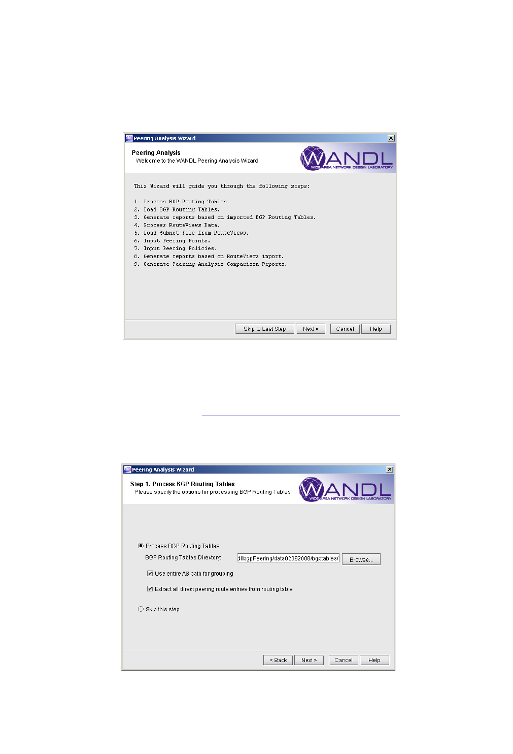
BGP PEERING ANALYSIS*
Copyright © 2014, Juniper Networks, Inc. 9-3
. . . . .
BGP Peering Analysis Wizard
The following instructions describe how to import BGP routing table information and RouteViews information via
the graphical user interface. Note that these data processing steps can also be performed in text mode.
14. After the configuration and tunnel path files are imported and the demand file is read in, select Design >
Peering Analysis Wizard...
Figure 9-1 BGP Peering Analysis Wizard
Process BGP Routing Tables and Create Reference Reports
15. Click Next to open Step 1. Process BGP Routing Tables. Specify the directory containing the BGP
routing tables collected in Preparing BGP Routing Table Object File on page 9-2. Note that the parser requires
“hostname <hostname>” in the beginning of the file. It is recommended to select both options “Use entire AS
path for grouping” and “Extract all direct peering route entries from routing table” below.
Figure 9-2 Process BGP Routing Tables

BGP PEERING ANALYSIS*
9-4 Copyright © 2014, Juniper Networks, Inc.
9
•Use entire AS path for grouping (vs. Group by first AS): If this option is checked, prefixes in the BGP
routing table will be grouped together if all their AS paths and BGP attributes (MED, local preference, etc.) are the
same. This option should be checked if the user wants to perform what-if studies involving BGP policy modification
or the addition of new peers, in which case IP/MPLSView’s routing engine needs to calculate the routing tables
based on the subnet file. If this option is unchecked, prefixes will be grouped together if the first AS of the AS path
and the BGP attributes are the same. The latter option “Group by first AS” would reduce the number of groups
significantly, and is sufficient for studying backbone loading and failure simulation based on live BGP tables, but
would be inadequate for what-if studies involving BGP policy modification and the addition of new peers.
•Extract all direct peering route entries from routing table (vs. Extract only the active route): If this
option is checked, the Subnet file will store all possible direct exit points for a given prefix learned from outside. If
this option is unchecked, then only the active route will be extracted from the BGP routing table. This will reduce the
size of the subnet file and, as a result, speed up the routing process, but may be inadequate to analyze BGP load
balancing amongst the AS links or the impact of AS node failure.
This step will extract prefix, local pref, MED, next-hop, as-path, and origin info from the BGP routing tables, and
create bgpgroup, livebgprtblobj, and subnet files for the rtserver program. Note that this step may take some time as
it is CPU intensive. The memory requirement is proportional to the number and size of the routing tables. Due to its
potentially large size, the object file is not copied during “Save Network” operation. Instead, rtserver saves the
absolute path of the file in the spec. Currently, the subnet file is copied during “Save Network” operation.
Note: If the BGP routes do not change much for a given network, users can re-use the previously imported files by
selecting Skip this step and specifying the paths of previously generated files in the following step.
When the data extraction is in progress, the standard outputs from the corresponding command line scripts
prefixGroup and routeGroup are dumped to the console window, so user may monitor the progress. It is
recommended for the user to run “top” command on the server to monitor memory usage.
CORRESPONDING COMMAND LINE UTILITIES
As an alternative to running the BGP routing tables processing from the graphical interface, users can also run the
commands prefixGroup and routeGroup scripts from a telnet or SSH window.
aFirst create a group file (e.g., bgpgroup.x) based on the BGP routing tables. First run /u/wandl/bin/prefixGroup
to see usage information:
Usage: /u/wandl/bin/prefixGroup [-o <ouput>] [-firstAS] routingTables...
Here is an example using the first AS rather than the entire AS path for grouping:
> /u/wandl/bin/prefixGroup -o bgpgroup.x -firstAS /export/home/wandl/bgpPeering/data02092008/bgptables/*
b. Next, create the live BGP object file (e.g., livebgprtblobj.x) and subnet file (e.g., subnet.x) based on the BGP
routing tables and the group file from the last step (bgpgroup.x). First run /u/wandl/bin/routeGroup to see usage
information:
Usage: /u/wandl/bin/routeGroup [-o <outputFile>] [-s <subnetFile> ] [ -a ] [ -g <group> ] routingTables...
Note the -a option for extracting all direct peering route entries from the BGP routing table should always be
used. Here is an example of creating a livebgprtblobj.x and subnet.x file.
>/u/wandl/bin/routeGroup -o livebgprtblobj.x -a -s subnet.x -g bgpgroup.x /export/home/wandl/bgpPeering/
data02092008/bgptables/*
BGP PEERING ANALYSIS*
Copyright © 2014, Juniper Networks, Inc. 9-5
. . . . .
16. Click Next to open Step 2. Load BGP Routing Tables. After processing BGP tables in step 1, the resulting
subnet and livebgprtblobj files are automatically populated in the next step for loading. Otherwise, if step 1 was
skipped, previously generated files can be browsed for in this window.
Figure 9-3 Load BGP Routing Tables
Only the BGP Routing Table Object file is required if user just wants to perform routing based on current BGP
table lookup. The demand placement is relatively fast because no policy evaluation is needed.
However, if the user wishes to perform what-if studies on BGP policy changes or on adding a new peer, then
both the BGP Routing Table Object file and BGP Subnet File should be specified. For simulation, the live
routing table is no longer valid, and rtserver needs to recalculate the routing table based on the subnet file. (The
live routing table object file is still required because it contains the grouping info for the subnet file.)
Loading could take a while depending on the file size, and the existing subnet and object files will be cleared
from the memory. Note that this is the same operation as selecting File > Load Network Files and browsing
for the subnet and livebgprtblobj files in the Network Files tab.
BGP PEERING ANALYSIS*
9-6 Copyright © 2014, Juniper Networks, Inc.
9
17. Click Next for Step 3. Generate reports based on Imported BGP Routing Tables. This step will
trigger the placement of all demands in the memory. Based on the demand placement, link utilization and node
traffic reports are generated and saved in the spec directory, and they are used as references for comparison
reports. User may also generate reports for future usage by exiting the wizard after this step.
The “Use Live BGP Table” checkbox reflects the current setting under “Tools > Options > Design, Path
Placement > BGP” tab, and users can change it here before generating reports. It is recommended to keep the
checkbox checked. If checked, traffic will be routed according to the live BGP routing table object. If
unchecked, the program will recalculate the BGP routing table based on information in the subnet file, and route
accordingly. Demand placement may take a while depending on the size and the routing option chosen (live
BGP table object file vs. subnet file).
Figure 9-4 Generate Reports based on BGP Routing Tables
The reports generated in this step will be saved to the server. To view the reports, browse to the report files in
the File Manager, right click on the file, and select Open in Report Viewer from the right click menu. You
must generate these reports in order to create the comparison reports at the end of the wizard.
BGP PEERING ANALYSIS*
Copyright © 2014, Juniper Networks, Inc. 9-7
. . . . .
Process Routeviews Data for a New Peer and Create Reports
18. Click Next. for Step 4. Process RouteViewsData. This step will parse the routeviews table file and tier
service provider file to create a new WANDL subnet file. It is also the step in which to specify the AS to peer
with for what-if analysis.
Figure 9-5 RouteViews Data
•Enter a new AS to peer with whose routes need to be extracted from Routeviews archives.
Users could also run the /u/wandl/bin/ASsubnet script in command line for import.
•Enter in the RouteViews table file. The Routeviews data needs to be in a pipe delimited format. Three lines of
a sample file after processing data from the routeviews website are shown below:
TABLE_DUMP|1202568110|B|96.4.0.55|11686|0.0.0.0/0|11686 4436|IGP|96.4.0.55|0|0||NAG||
TABLE_DUMP|1202568110|B|213.140.32.148|12956|0.0.0.0/0|12956|IGP|213.140.32.148|0|0||NAG||
TABLE_DUMP|1202568110|B|81.209.156.1|13237|3.0.0.0/8|13237 3320 1239 701 703
80|IGP|81.209.156.1|0|0|1239:666 1239:667 1239:1000 1239:1014 3320:1840 3320:2020 3320:9020 13237:44049
13237:46068|NAG||
To create this file, obtain the route_btoa program, which can be compiled after downloading source code from
sourceforge for MRT (http://sourceforge.net/project/showfiles.php?group_id=9585). The following is an
example compilation on Solaris of the third-party MRT software:
$ cd mrt-2.2.2a/src
$ ./configure --disable-ipv6 --disable-mrouting --disable-qrouting
$ vi Make.include
add the flag -DNDEBUG to the end of CPPFLAGS
$ vi include/config.h
add the line “#define SOLARIS28”
$ make depend
$ make all
$ su
# make install

BGP PEERING ANALYSIS*
9-8 Copyright © 2014, Juniper Networks, Inc.
9
Next, download an archived .bz2 file from http://archive.routeviews.org, e.g.,
http://archive.routeviews.org/bgpdata/2008.05/RIBS/rib.20080505.1317.bz2. This data is archived every 2 hours
and stored in bz2 format. Unzip this .bz2 file using the /usr/bin/bunzip2 command, e.g.,
$ bunzip2 rib.20080505.1317.bz2
Then run route_btoa on the unzipped file to create the Routeviews table file in pipe-delimited format:
$ route_btoa -m -i rib.20080505.1317 > rib.20080505.1317.out
•The Tier1 Service Provider file contains a list of the tier-1 Service Providers’ Autonomous System numbers
that are already peering with the user network, and this list will significantly impact the route extraction results. The
tree building will stop at any AS that is part of the tier1 list specified by the user. The assumption is that the user
already peers with these Service Providers, and peering with any descendant AS will not be advantageous. Prefix,
AS path, origin, and community are extracted from RouteViews data. For example, the following is a portion of a
sample Tier 1 service provider list in the file “tier1”:
209
701
1239
3549
7018
CORRESPONDING COMMAND LINE UTILITIES
As an alternative to running the Routeviews processing from the graphical interface, users can also run the command
/u/wandl/bin/ASsubnet from a telnet or SSH window.
First run the following command:
> export LD_LIBRARY_PATH=/u/wandl/lib/thirdparty:$LD_LIBRARY_PATH
Then check the usage information by running /u/wandl/bin/ASsubnet:
> Usage: /u/wandl/bin/ASsubnet [ -T <Tier1> ] [ -AS <ASNumber> [ -o <subnetFile> ]] [ -dump <dumpFile ]
<routeViewTable>
Here is an example of using ASsubnet on the rib file created after running route_btoa, for peering with AS 123 and
referencing the tier1 service provider file. The output for the following command will be saved to subnet.123.auto:
> /u/wandl/bin/ASsubnet -T /export/home/wandl/bgpPeering/routeviews/tier1 -AS 123 -o subnet.123.auto
/export/home/wandl/bgpPeering/routeviews/rib.20080505.1317.out
BGP PEERING ANALYSIS*
Copyright © 2014, Juniper Networks, Inc. 9-9
. . . . .
19. Click Next. for Step 5. Load Subnet File from RouteViews. In this step you will load the subnet file from
the last step and provide the new AS an IP address.
Figure 9-6 RouteViews Subnet
•The New AS to peer with and Subnet File info will be carried over from step 4 if routeviews import was
performed. Otherwise, users can also enter info for the subnet file that was generated from a previous routeviews
import operation.
•The AS IP Address for the neighbor is required by rtserver for the creation of the BGP neighbor relationship,
and it should not be an existing address (e.g., 1.2.3.4).
20. Click Next for Step 6. Input Peering Points. Here you can specify a couple of peering points for the new
AS. Select from the list of available candidates on the left panel, and add them to the right panel. This step will
create a new ASNODE for the new AS, ASLINKs between the ASNODE and all gateway routers, and BGP
neighbor relationships between the ASNODE and all gateway routers.
Figure 9-7 Select Peers
BGP PEERING ANALYSIS*
9-10 Copyright © 2014, Juniper Networks, Inc.
9
21. Click Next for Step 7. Input Peering Policies. This step gives you the option of applying new peering
policies for nodes that peer with the new AS or modifying individual subnet properties.
Figure 9-8 Apply Peering Policies
•Apply Peering Policies: From the BGP Neighbor window, users can create or apply an in-policy onto the
newly created BGP neighbors to manipulate the route attributes and influence the routing. If this is done, then all the
prefixes from the routeviews import will be associated with the ASNODE, and rtserver will apply the specified
policy when performing routing. This is the preferred way to create or apply an existing policy onto the new peer.
Selecting this option and clicking Next will open up the BGP Neighbors window.
•Modify BGP Subnets: If instead of applying existing BGP policies, you want to simply modify the subnet
properties such as local preference, AS PATH, and MED directly, you can select this option to manually modify the
subnets from the routeviews import to mimic the end result of applying the in-policy. In this case, all the new
prefixes will be associated with individual gateway routers. Note that this step may take longer, as more data needs to
be loaded from the server. When clicking Next, this will open the BGP Subnets window outside of the wizard.
Select the subnet to modify and click the Modify button. Then you can change desired BGP properties. Click Close
when you are done.
EXAMPLE OF APPLYING PEERING POLICIES
If Applying Peering Policies is selected, clicking Next will open the following BGP Neighbors window. Select
one or more entries and click Modify to open modify BGP neighbor window. The peering wizard will perform a
filter in the background to only display common policies defined on the gateway routers. Select the In Policy tab.
Here, users can choose from a list of available policies on the left panel and move them to the right panel, or click the
Policy Editor button to create/modify a policy. Note that when modifying a policy, that it will also be used for other
BGP neighboring relationships that have applied the same policy. Click Close when you are done modifying the
BGP Neighbors.
BGP PEERING ANALYSIS*
Copyright © 2014, Juniper Networks, Inc. 9-11
. . . . .
Figure 9-9 Apply BGP Policy
22. Click Next for Step 8. Generate reports based on Routeviews Import. This step will place again all
demands in the memory, using the combined set of subnets after the Routeviews import. A new set of link
utilization and node traffic reports will be generated with the data from Routeviews and the new AS and peering
points in place. This report is needed to create the comparison reports at the end of the wizard.
Figure 9-10 Report Based on RouteViews
Note that the “Check IBGP Policy” checkbox reflects the current setting under “Tools > Options >
Design, Path Placement > BGP” options pane. If selected, the routing engine will take into account IBGP
policies when calculating the routes. If there are no IBGP policies in the network, this checkbox can be
unchecked, which may speed up the processing time for this step.
The reports generated in this step will be saved to the server. To view the reports, browse to the report files in
the File Manager, right click on the file, and select Open in Report Viewer from the right click menu.
BGP PEERING ANALYSIS*
9-12 Copyright © 2014, Juniper Networks, Inc.
9
Generate Peering Analysis Comparison Reports
23. Click Next for Step 9. Generate Peering Analysis Comparison Reports. Comparison reports can be
created between the reports generated from the BGP routing tables before adding the new BGP peer and the
reports generated from the RouteViews data after adding the new BGP peer. These reports will automatically be
populated if they were generated in the same wizard session. Users may also use this window to compare any
two reports.
Figure 9-11 Peering Analysis Comparison Reports
24. Click Finish to close the Peering Analysis Wizard.
25. In the Report Manager, you can see the Node and LinkUtil comparison reports in the Network Reports >
Protocols > Peering Analysis folder (Compare Node Traffic (After - Before) and Compare Link
Util (After - Before)). You can drag and drop columns or click the “Select Columns...” button to select and
rearrange the columns of the report.
•The Compare Node Traffic report compares the originating, transit, terminating, and total traffic between the
state after adding the new peer and before adding the new peer. Sort and then reverse sort on the
“Diff:#Demand(total)” or “Diff:DemandBW(Total)” columns to see the shifting of traffic between the AS peers
(given in the Node ID and Node Name columns). A positive value in the Difference column indicates new traffic on
a peer. A negative value in the Difference column indicates lost traffic on a peer.
•For the Compare Link Util report, you can sort and then reverse sort on the “Diff:Util(AZ)” or
“Diff:Util(ZA)” columns. Note that some changes could also be due to ECMP.
BGP PEERING ANALYSIS*
Copyright © 2014, Juniper Networks, Inc. 9-13
. . . . .
Figure 9-12 Traffic Gained at New Peering AS (Descending Sort)
Figure 9-13 Traffic Lost from Original Peering AS’s (Ascending Sort)
26. For additional analyses, you can right-click over a node (such as the new ASNODE) or link and view the
demands routed over it (View>Demands on/thru Node or View>Demands on/thru Link).
27. To investigate a particular demand routed over it further, you can enter in the source node and destination prefix
into the Network > Protocols > BGP > BGP Routing Table to see which BGP route was chosen to be the
active route and why.
Figure 9-14 BGP Route Using New Peering AS

BGP PEERING ANALYSIS*
9-14 Copyright © 2014, Juniper Networks, Inc.
9
Appendix. Preparing the Demand File
The following describes one method of preparing the demand file, given the following two files. (Note that if you
already have a demand file, you can skip this section.)
(a) A host_property file listing the host IP address and associated service, and
#host property
10.10.0.1 ads
10.20.0.1 search
(b) A traffic data file of the following format:
#host prefix routerName:ifName %bytes traffic
10.10.0.1 3.3.3.3 NWK:fe0/0/1.111 0.00123 35000
First, the host_property file is used to create a servicetype file. Next, the host_property file, servicetype file, bblink
file, and traffic file are used to create a demand file.
PREPARING THE SERVICE TYPE FILE FROM HOST_PROPERTY FILE (OPTIONAL)
The service type file of the following format can be created based on the host_property file given above. Note that
dashes are not allowed in the service names and must be replaced by an underscore or other character:
ads - - 1 R,A2Z,SRVC=ads 02,02
search - - 1 R,A2Z,SRVC=search 02,02
A host_property file with the host IP address and the associated service as shown below can be converted to the
above service type file format using scripting. An example conversion command using nawk and sort is as follows:
> cat host_property | tr -s ‘[:lower:]’ ‘[:upper:]’ > host_property_caps
> nawk ‘/[0-9]+/ {print $2}’ host_property_caps | sort -u | nawk ‘{gsub(/-
/,”_”); print $1 “ - - 1 R,A2Z,SRVC=“ $1 ” 02,02”}’ > srvctype.x
The first step above converts the characters to upper case to avoid duplicate entries caused by different capitalization
of the same service.
PREPARING THE DEMAND FILE BASED ON SERVICE TYPE FILE, TRAFFIC FILE, AND
BBLINK FILE
Suppose you have the host_property file and servicetype file in the last step, and that you have a traffic file in the
following format:
#host prefix routerName:ifName %bytes traffic
10.10.0.1 3.3.3.3 NWK:fe0/0/1.111 0.00123 35000
Flows from a given host to a given prefix will be recorded at multiple interfaces according to the links traversed by
the flow. A flow should be created only from the source router to the destination router, and not between
intermediate routers to the destination router. To avoid double-counting, an internal bblink file should be specified to
indicate which links are considered internal links in the backbone network. Traffic originating from interfaces
defined in the internal bblink file will be treated as internal and will not be included in the generated demand file.
To create the demand file, use the Java class called AggDemand.class which should have been supplied to you. Put
this file along with the traffic, host_property, and bblink files into the same directory. This is to be run from a Unix
shell or Windows command prompt, with the following basic command:
/u/wandl/java/bin/java AggDemand [options] linkFile hostFile trafficFiles
This will create WANDL demand with the option to aggregate similar flows into single demands. Traffic originating
from interfaces listed in the linkFile will be ignored. Demands will be labeled by service based on their source host
and the corresponding host-service entry in the hostFile (host property file).

BGP PEERING ANALYSIS*
Copyright © 2014, Juniper Networks, Inc. 9-15
. . . . .
The linkFile (bblink.<runcode>)can be created by running the configuration import as described in Import
Configuration Files on page 9-2. The hostFile is the host_property file explained at the beginning of this appendix.
In case there is a lot of data, you may wish to increase the memory that Java can use, e.g., “/u/wandl/java/bin/java -
Xmx512M -Xms512M YahooDemand ...”
There are several options that can be specified in the [options] field. These are described below.
•-as: Ignore AS links in the linkFile. Traffic coming from AS links will not be treated as internal traffic, and will
be included in the generated demand file.
•-ag: Ignore aggregate links in the linkFile. Traffic coming from aggregate links will not be treated as internal
traffic, and will be included in the generated demand file.
•-i: Aggregate flows with the same source and destination.
•-a: Aggregate flows with the same source, destination, and service.
•-b bw: Do not aggregate flows if their bandwidth is greater than bw (bps). This option takes precedence over the
options above.
•-d bw: Discard demands if, after aggregation, their bandwidth is smaller than bw (bps).
•-x bw: Demands with bandwidth greater than bw will be broken into smaller demands with bandwidths not
exceeding bw (bps).
•-e “[bw necmp]*”: Demands with bandwidth greather than bw will be broken into necmp demands.
Example: -e “1m 2 10m 4 100m 6 1g 10”
•-src ASfile: The ASfile is a file created (ASsources) when parsing the BGP tables, and it indicates the
originating and peering ASes corresponding to a given prefix. Specifying this parameter will aggregate flows
according to the AS nodes if the AS node can be determined based on the prefix. Otherwise, the program will
aggregate the flows through the routers.
•-mux MUXfile: Specify the muxloc file (for use with the -src option). AS nodes not found in this list will instead
be represented by a router.
•-origas: Use the Originating AS instead of the Peering AS from the AS file.
•-debug: Creates a .debug file for each input traffic file indicating which entries were aggregated together
(through the AggID identifier), which can be correlated to the demand file.
•-o output: Demands will be written to the output file specified here.
OUTPUT FILES
The program will create two outputs:
•demand: Contains traffic coming from outside the backbone (This is the demand file that should be read into the
program)
•demand.internal: Contains traffic coming from inside the backbone (This demand file contains the “double-
counted” traffic, and can be discarded.)
EXAMPLES
Below are some examples of using the demand generation program.
Example 1:
> java AggDemand -as -ag -a -o demand.y bblink.y host_property *.dax
The above command will aggregate demands by source, destination, and service (as defined in the host_property
file), while ignoring traffic coming in from all interfaces defined in the bblink.y file, except for AS links and
aggregate links.
Example 2:
> java AggDemand -as –i –b 10m –d 10k -o demand.y bblink.y host_property *.dax
The above command will aggregate demands by source and destination while ignoring traffic coming in from all
interfaces defined in the bblink.y file, except for AS links and aggregate links. It will not aggregate flows with
bandwidth greater than 10 mbps, and will discard (comment out) aggregated flows less than 10 kbps.

BGP PEERING ANALYSIS*
9-16 Copyright © 2014, Juniper Networks, Inc.
9
Example 3:
> java AggDemand -as –i –x 100m -o demand.y bblink.y host_property *.dax
The above command will aggregate demands by source and destination while ignoring traffic coming in from all
interfaces defined in the bblink.y file, except for AS links and aggregate links. It will also break apart demands
greater than 100 mbps such that each individual demand does not exceed 100 mbps.
Example 4:
> java AggDemand -as -i -src ASsources -mux muxloc.auto -e “1m 2 10m 4 100m 6 1g 10” -d 50k -debug -o
demand.y bblink.y host_property *.dax
•The above command will aggregate demands by source AS if available, and destination prefix while ignoring
traffic coming in from all interfaces defined in the bblink.y file, except for AS links. For prefixes that cannot be
mapped to an AS in the muxloc file, a router will be used instead.
•For demands between 1m and 10m, they will be split into 2 subflows, i.e., using the ECMP=2 parameter .
Demands between 10m and 100m will be split into 4 subflows, demands between 100m and 1g will be split into 6
subflows, and demands over 1g will be split into 10 subflows. Demands with bandwidth less than 50k will be
discarded.
•Debugging information will be provided for each source traffic file to indicate how they were aggregated by
peering AS.

Copyright © 2014, Juniper Networks, Inc. 10-1
. . . . .
. . . . . . . . . . . . . . . . . . . . . . . . . . . . . . . . . . .
V
IRTUAL
P
RIVATE
N
ETWORKS
*
10
his chapter describes WANDL’s VPN module (also known as VPNView) capabilities, which include VPN
construction via router configuration extraction, VPN topology display and reporting, VPN-related integrity
checking, and VPN design and modeling. When used in conjunction with the Online module, the VPN
module also allows the user to perform VPN monitoring and diagnostics.
The types of VPNs supported include Layer3 (L3), Layer2 Kompella (L2K), Layer2 Martini (L2M), Layer2 Circuit
Cross-Connect (L2CCC), and VPLS (both LDP-based and BGP-based VPLS). VPNView supports hub-and-spoke
and other complex VPNs. Depending on the type of VPN, different information is extracted from the router
configuration files to construct the different type of VPN. For instance, the extracted information for L3 VPNs based
on RFC 2547bis would include PE routers and CE devices (if managed), export/import route targets, route
distinguisher, interfaces, protocols, etc.
Besides VPN construction via configuration import, the VPN module also offers the network planner the ability to
construct VPNs from scratch via a VPN Wizard. Once VPNs have been constructed in the network, VPN traffic can
be added (by adding traffic demands or via a gravity model using the VPN Traffic Generation feature), and its effect
on the network can be studied. The VPN module’s VPN configlet generation feature can be used to create
configuration statements that can pushed onto the router by the network engineer.
Depending on the type of VPN (e.g. for L3 VPNs, L2K VPNs, and VPLS-BGP VPNs), various rules (e.g. based on
export/import route-targets) are used to determine when two routers can talk with each other; the VPN path tracing
feature can be used to study the routing between two routers. WANDL’s VPN module features help the network
engineer to understand, design, and analyze various types of VPNs.
*Note that special passwords are required for the VPN module and for the Online module. Please contact your
Juniper representative for more information.
Related Documentation
For general step-by-step instructions on how to use the WANDL software, please refer to the Design & Planning
Guide.
For an overview of the WANDL software or for a detailed description of each feature and the use of each window,
refer to the General Reference Guide or Chapter 37, Router Reference.
For details on how to extract VPN information from the router configuration files when creating a spec file, please
refer to Chapter 2, Router Data Extraction.
Outline
1. Importing VPN Information from Router Configuration Files on page 10-2.
2. Viewing the Integrity Checks Reports on page 10-3
3. Accessing VPN Summary Information on page 10-4
4. Accessing Detailed Information for a Particular VPN on page 10-5
5. VPN Topology View on page 10-6
6. Route-target Export/Import Relationships on page 10-8
7. VPN Export-Import report on page 10-11
8. VPN Path Tracing on page 10-13
9. VPN Design and Modeling using the VPN Wizard on page 10-14
10. L3 (Layer 3) VPN on page 10-15
11. L3 Hub-and-Spoke VPN on page 10-21, and Merging Hub and Spokes on page 10-21
T
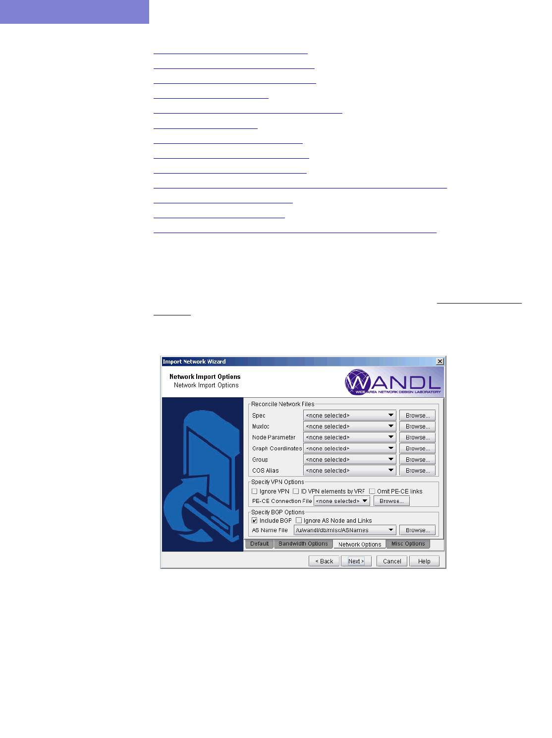
VIRTUAL PRIVATE NETWORKS*
10-2 Copyright © 2014, Juniper Networks, Inc.
10
12. L2M (Layer2-Martini) VPN on page 10-26
13. L2K (Layer2-Kompella) VPN on page 10-30
14. VPLS-BGP VPN (for Juniper) on page 10-32
15. VPLS-LDP VPN on page 10-34
16. L2CCC (Circuit Cross-Connect) VPN on page 10-38
17. Inter-AS VPN on page 10-40
18. Forming Customer Groups on page 10-41
19. Deleting or Renaming VPNs on page 10-42
20. VPN Configlet Generation* on page 10-43
21. Adding Traffic Demands in a VPN via the Add Demands Windows on page 10-46
22. VPN Traffic Generation on page 10-47
23. VPN-Related Reports on page 10-49
24. VPN Monitoring and Diagnostics (also requires Online Module) on page 10-51
Detailed Procedures
Importing VPN Information from Router Configuration Files
1. To import the router configuration files, select File>Import Data and follow the Import Network Wizard.
Alternatively, you may run the getipconf program in text mode. Please refer to Chapter 2, Router Data
Extraction for more detailed information.
The Network Options tab contains the Specify VPN Options section shown in the following figure.
Figure 10-1 Configuration Import and VPN Options
•To extract VPN information from the config files, the user should leave the Ignore VPN checkbox unchecked.
•Typically, VPNs are constructed by matching import/export route targets; if the ID VPN elements by VRF
checkbox is checked, then VRF names will be used for the matching instead.
•If the Omit PE-CE links checkbox is checked, then links between PE routers and CE routers will be omitted.
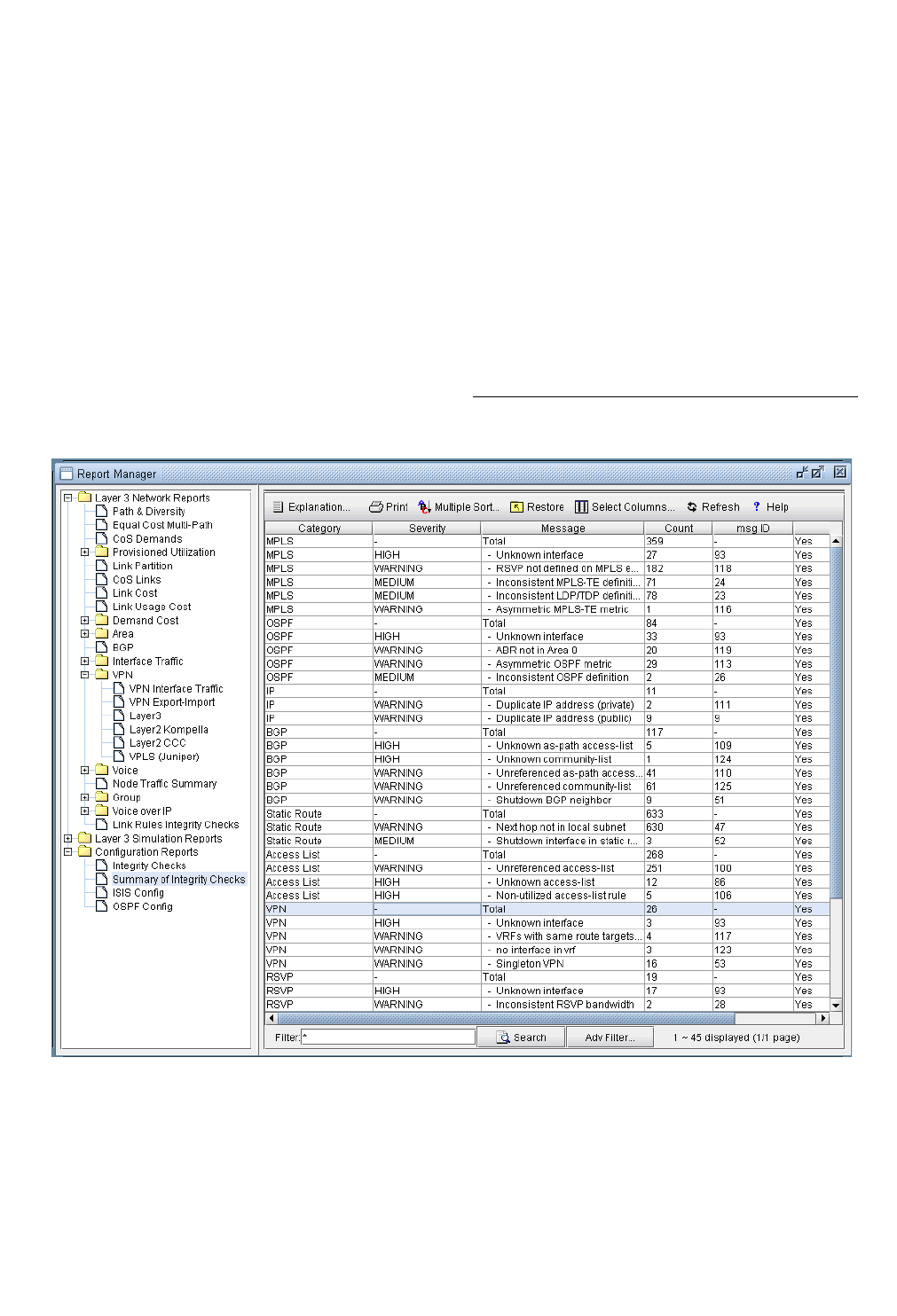
VIRTUAL PRIVATE NETWORKS*
Copyright © 2014, Juniper Networks, Inc. 10-3
. . . . .
•The user can also specify a PE-CE Connection file that contains information used to stitch up PE-CE links.
This is useful when the network re-uses private IP subnets for PE-CE links. The format of the PE-CE Connection
file is:
PE_name PE_VRF_intf IP_addr_of_PE_VRF_intf VRF
CE_name IP_addr_of_CE_intf
pe0 serial2/1 203.55.1.65/30 vrf-a ce0 203.55.1.66/30
Once all of the options in the different tabs have been selected, click Next> to begin importing the router config
files. The generated network model will then be loaded into IP/MPLSView.
Viewing the Integrity Checks Reports
2. Once the network model has been loaded, the user may wish to examine the Configuration Reports
(accessible via the Report > Report Manager menu) to check for any potential VPN configuration issues.
The following figure shows an example of a Summary of Integrity Checks report, where certain VPN
integrity checks are reported. Please refer to Chapter 22, Configuration Conformance & Integrity Checks for
more information about integrity checks.
Figure 10-2 View the Integrity Checks Reports to Check for Potential VPN Configuration Issues
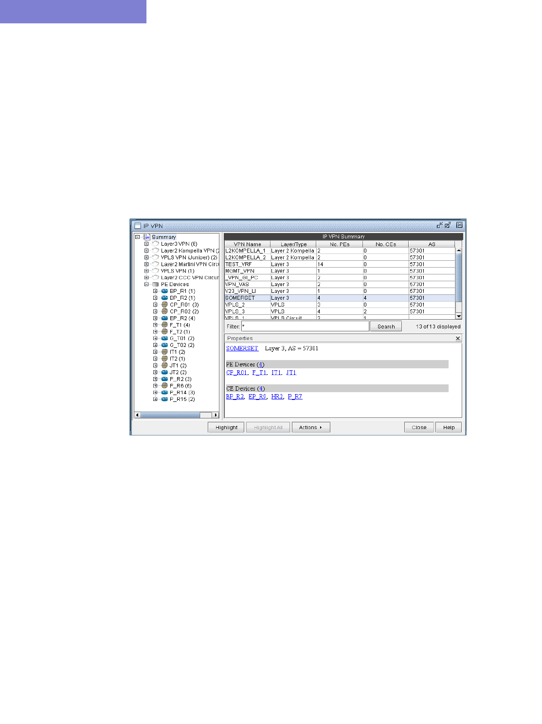
VIRTUAL PRIVATE NETWORKS*
10-4 Copyright © 2014, Juniper Networks, Inc.
10
Accessing VPN Summary Information
3. To see a summary view of all of the VPNs that are present in the current network, bring up the IP VPN
Summary window (via the Network > Services > VPN menu) as shown in the following figure.
The window will provide a list of all the different types of VPNs in the network and a list of all the PE routers
that make up the VPNs. The number in the parentheses following each VPN type in the tree view on the left
pane of the window describes the number of VPNs in that category. For instance, Layer2 Kompella VPN (2)
means that there are two L2K VPNs configured in the model. The + box can be used to expand a VPN type in
order to see the list of VPNs for each type. Similarly, the number in the parentheses following each PE router
indicates the number of VPNs that the PE router is a part of.
You may click on a particular VPN of interest, and then more summary information for that VPN will be
presented in the Properties box of the window. For instance, the figure shows a L3VPN with its list of four
PEs and four CEs.
Figure 10-3 IP VPN Window’s Properties Box for a selected VPN
4. With a particular VPN selected, you may also click on the Highlight button to see all of the routers associated
with the VPN highlighted on the main topology map.
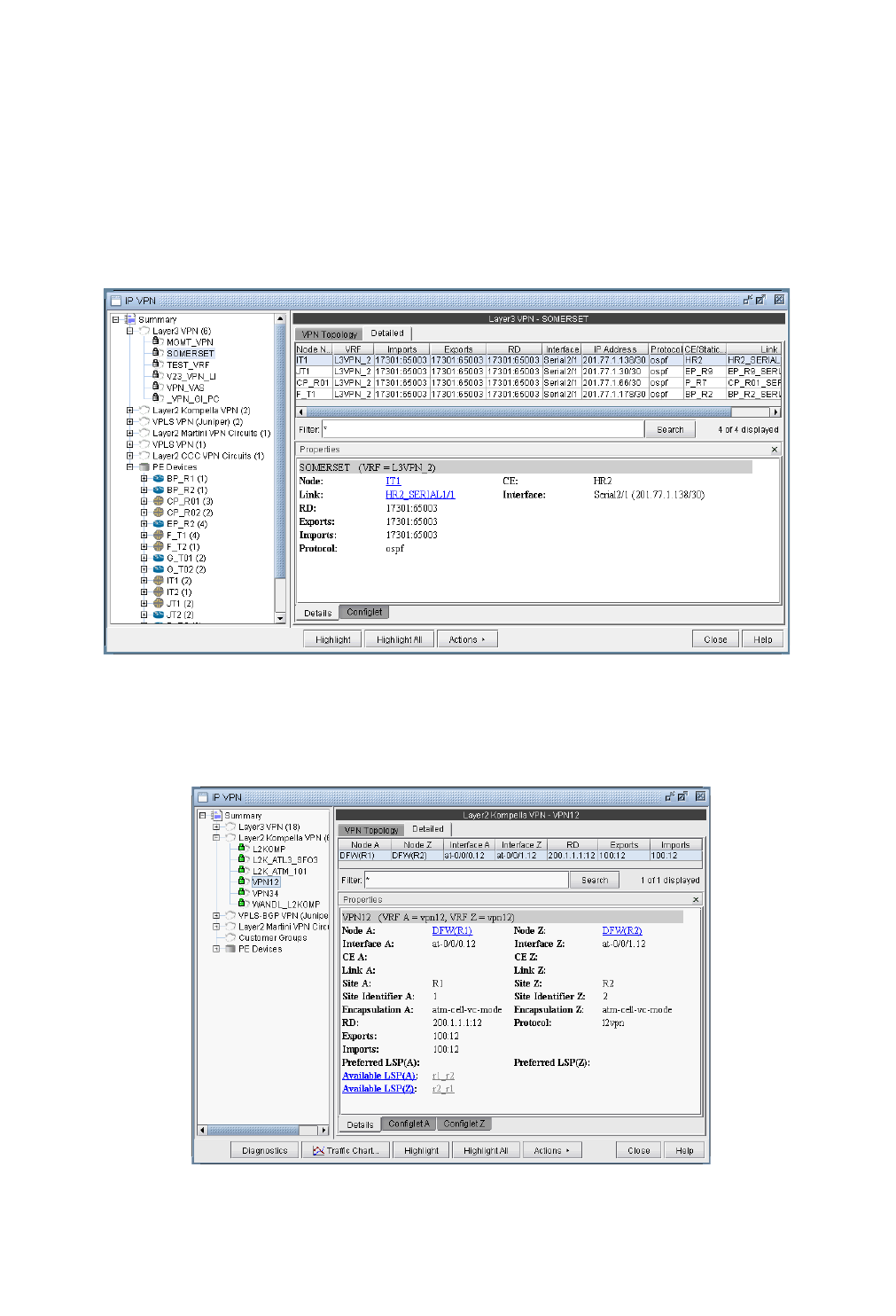
VIRTUAL PRIVATE NETWORKS*
Copyright © 2014, Juniper Networks, Inc. 10-5
. . . . .
Accessing Detailed Information for a Particular VPN
5. To show the detailed information for a VPN, you may either double-click on a particular VPN in the IP VPN
Summary window, or you may navigate through the VPN tree list on the left part of the window until the
particular VPN is found. The following figure shows the detailed information for a VPN called SOMERSET.
To see information for a particular node in the VPN, simply select the node from the table, and the Properties
box will display the information. The figure shows the information for the router IT1. You can also click on
Highlight All to have all the nodes in the VPN highlighted on the main topology map. If a particular node is
selected, then you can click Highlight to only highlight that selected node.
Figure 10-4 Detailed View for a particular router of the selected VPN (SOMERSET)
6. Although the detailed information for each VPN type is different, the procedure for accessing the information
remains the same. The following figure shows the detailed information for a L2K VPN.
Figure 10-5 Detailed VPN Information for a L2 Kompella VPN
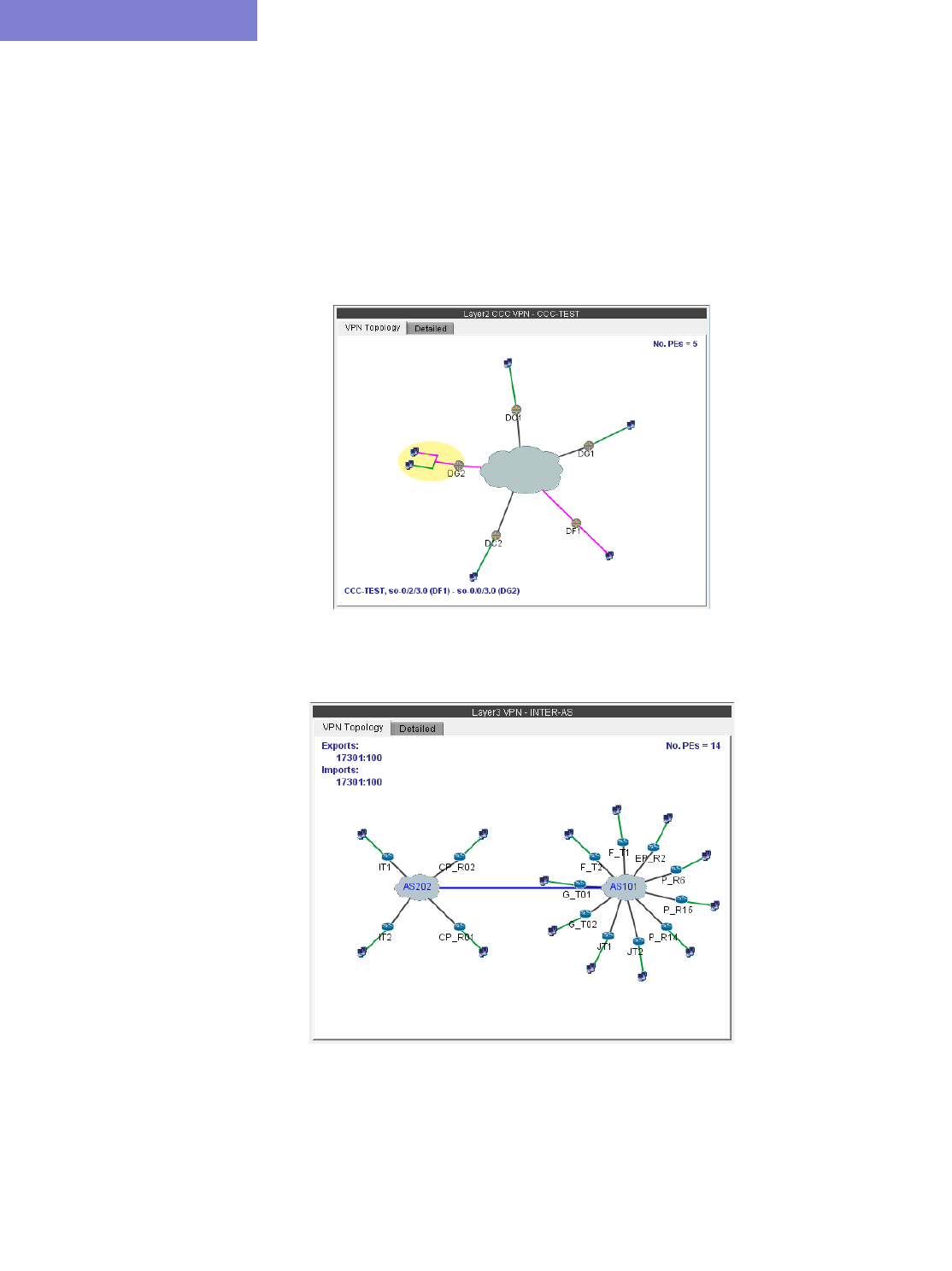
VIRTUAL PRIVATE NETWORKS*
10-6 Copyright © 2014, Juniper Networks, Inc.
10
Note that for layer 2 circuits, there is a list of the assigned LSPs for each direction, if applicable. Otherwise, if no
specific LSP has been assigned, a list of the available LSPs in each direction will be displayed.
VPN Topology View
The VPN Topology View (or VPN View) presents to the user a clear, logical view of each individual VPN.
7. To display a logical topology view of any particular VPN, simply click on the VPN Topology tab (next to the
Details tab). You may also move the nodes around as desired in the VPN topology view map. The following
figures show the VPN View for various VPNs. Note that CEs are shown as router icons when the config file is
available; otherwise, a computer icon is shown.
Figure 10-6 VPN View for a L2CCC VPN (with the selected circuit highlighted in pink)
Figure 10-7 VPN View for an Inter-AS VPN (called INTER-AS)
8. You may also display additional information (i.e., RD, Route Targets, interface) for a node by clicking on it for
a pop-up window to appear, as shown in the following figure.
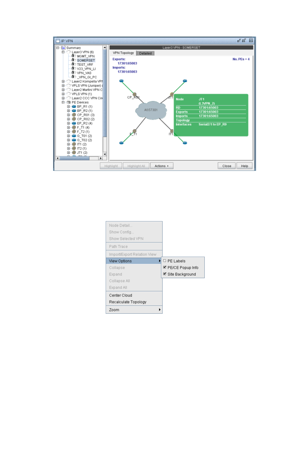
VIRTUAL PRIVATE NETWORKS*
Copyright © 2014, Juniper Networks, Inc. 10-7
. . . . .
Figure 10-8 Green pop-up information window for a node
9. There is also a right-click menu that you can use to perform basic functions to manipulate the topology and the
labels.
Figure 10-9 Right-click menu showing topology and label functions
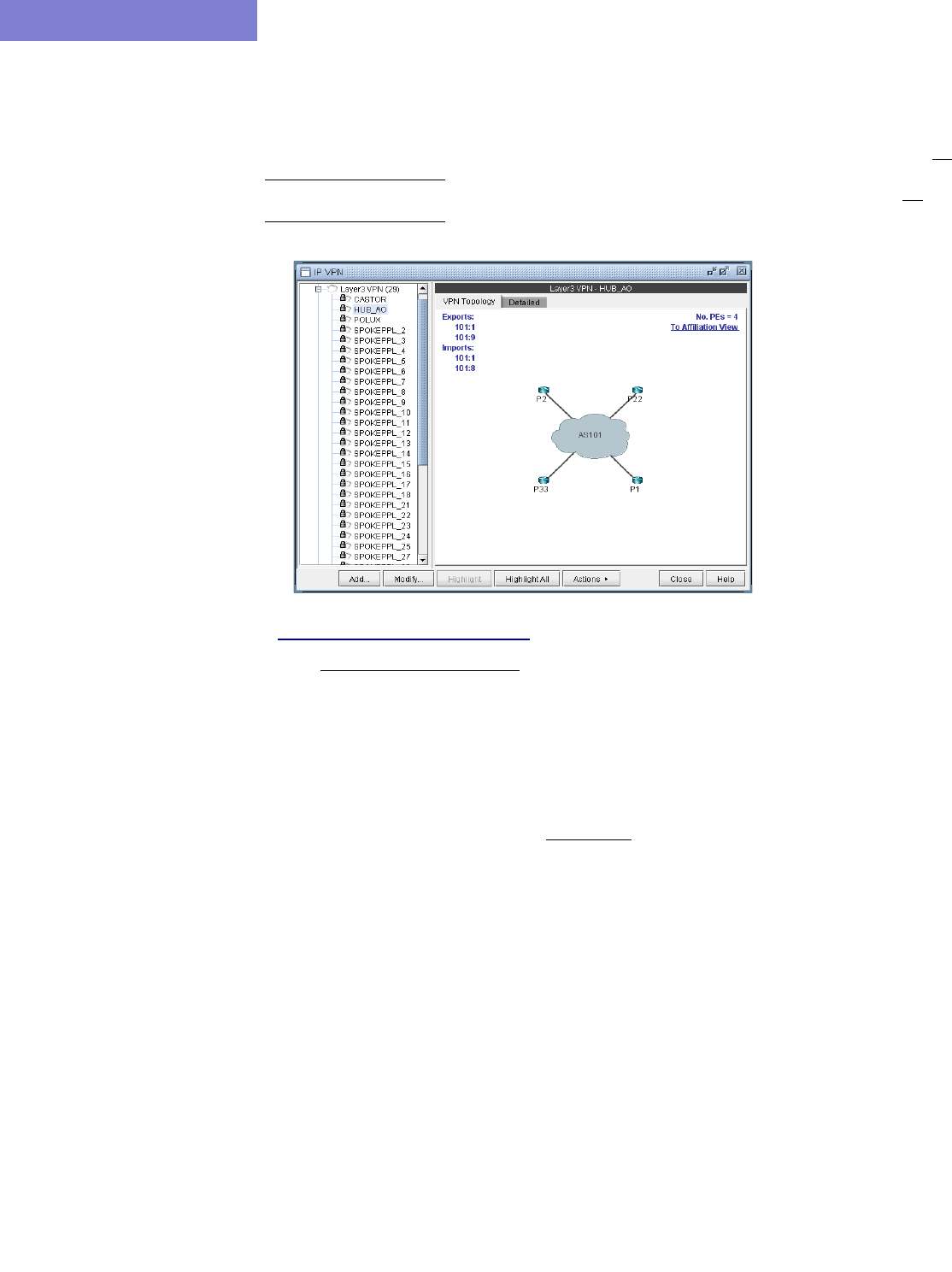
VIRTUAL PRIVATE NETWORKS*
10-8 Copyright © 2014, Juniper Networks, Inc.
10
Route-target Export/Import Relationships
10. The VPN View also shows route target export/import relationships that exist between VPNs. A visual picture
helps the network planner or engineer to clearly and quickly identify relationships between VPNs (e.g. hub-and-
spoke or extranet VPN relationships). When there are export/import relationships with other VPNs, then the To
Import/Export Relation View selection in the upper right-hand corner of the VPN View becomes visible. The
following figure shows that VPN HUB_AO has export/import relationships with other VPNs, since the To
Import/Export Relation View selection is visible.
Figure 10-10 Click on To Import/Export Relation View to see import/export relationships with other VPNs
11. Click on To Import/Export Relation View to get to the Import/Export Relation View. The blue circle icon with a
triangle inside is a grouping icon represents the current VPN (HUB_A0), while the yellow dot icons represent
other VPNs (in this example, the SPOKEPPL_* VPNs) that have export/import relationships with the current
VPN.
12. To see how other VPNs (the yellow dots) are related to the current VPN, you can click on a yellow dot to see the
route targets that are being exported and imported. For instance the following figure shows that VPN
SPOKEPPL_7 is exporting 101:8 and importing 101:9, while HUB_A0 is exporting 101:9 and importing 101:8.
The Import/Export Relation View allows you to clearly see relationships between VPNs. Note that you can go
back to the regular VPN View by clicking on To VPN View.
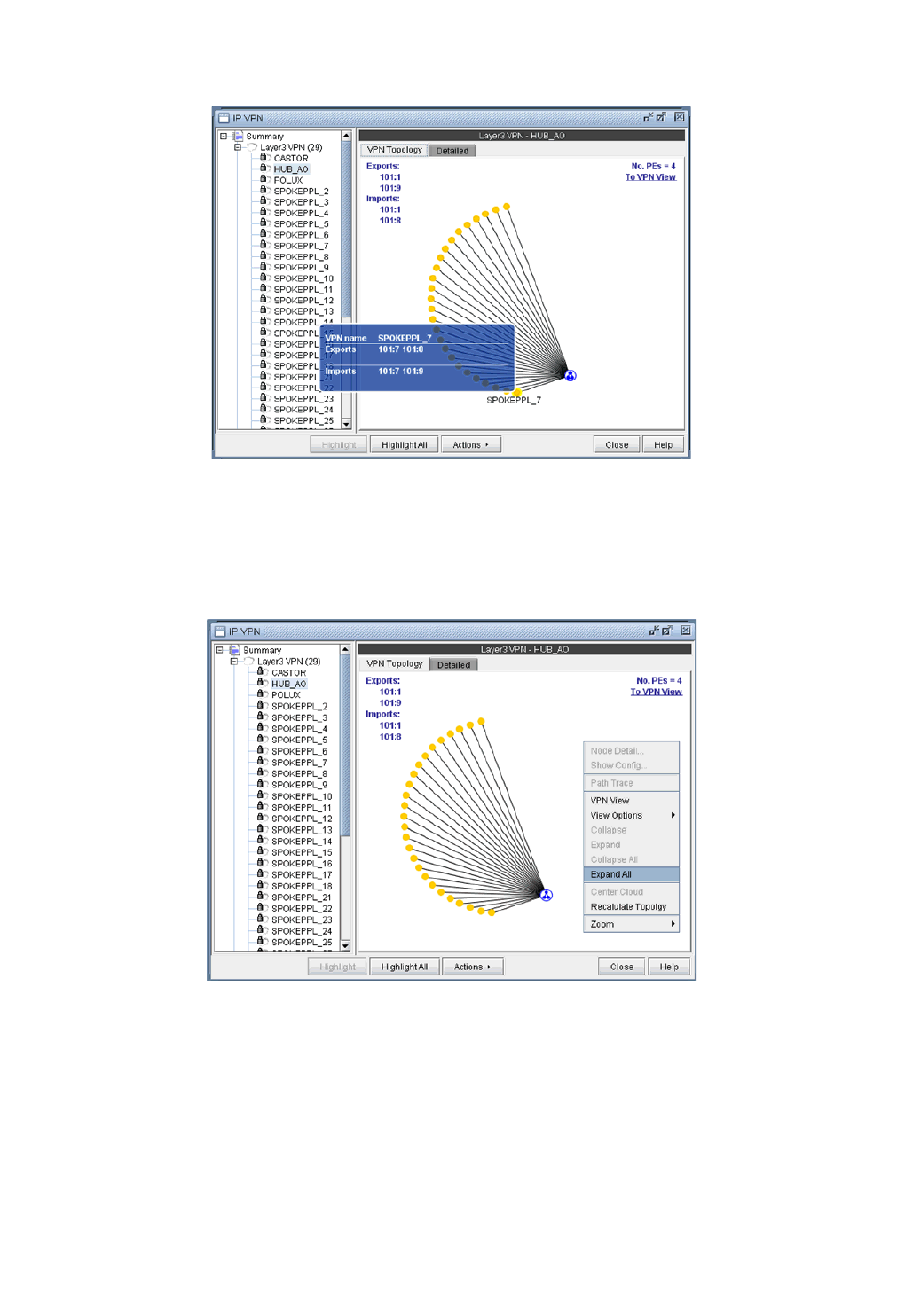
VIRTUAL PRIVATE NETWORKS*
Copyright © 2014, Juniper Networks, Inc. 10-9
. . . . .
Figure 10-11 Click on another VPN (a yellow dot) to see its relationship to the current VPN
13. The right-click menu of the Import/Export Relation View gives you the option to expand the currently collapsed
VPN (HUB_AO) which is represented by the blue circle icon with a triangle in it. Selecting Expand All would
reveal all the nodes with in the VPN.
Figure 10-12 Right-click menu in the Import/Export Relation View
14. The following figure shows you the Import/Export Relation View with the nodes in VPN HUB_AO expanded.
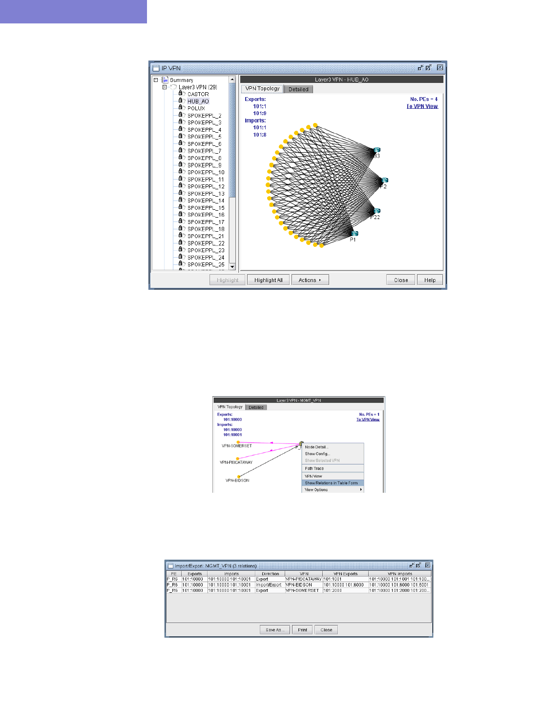
VIRTUAL PRIVATE NETWORKS*
10-10 Copyright © 2014, Juniper Networks, Inc.
10
Figure 10-13 Import/Export Relation View with nodes of VPN HUB_AO expanded
15. You can also move the icons around. Control-click to select multiple icons.
16. Instead of the visual display showing the import/export relationships that is in the Import/Export Relation View,
you can also access the same information in table form. As shown in the following figure, you would choose
Show Relations in Table Form from the right-click menu.
Figure 10-14 Show Relations in Table Form from the r-click menu for VPN MGMT_VPN
17. Once Show Relations in Table Form is chosen, the Export/Import table for the VPN is shown.
Figure 10-15 Export /Import table for VPN MGMT_VPN
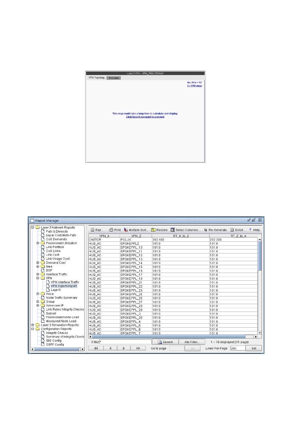
VIRTUAL PRIVATE NETWORKS*
Copyright © 2014, Juniper Networks, Inc. 10-11
. . . . .
18. In instances when there are a large number of export/import relations and you click on To Import/Export
Relation View, you will be prompted with the “This map could take a long time to calculate and display.”
message. If you would be willing to wait and still want to see the export/import relations in graphical form, then
click on “Click here if you want to proceed.” Instead, you may choose to view the import/export relations
in table form, as described in the previous step.
Figure 10-16 A particular VPN could have a large number of export/import relations with other VPNs
19. The Report Manager includes a VPN Export-Import report under Network Reports > VPN, as shown in
the following figure, that shows all of the route target export/import relationships that exist between VPNs in the
network.
Figure 10-17 VPN Export-Import report
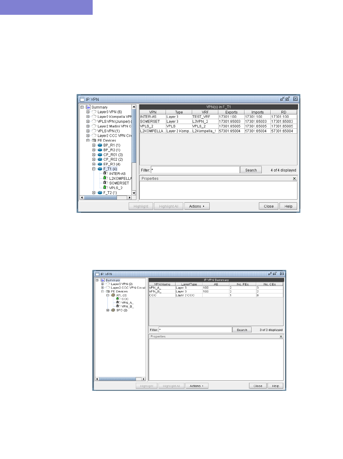
VIRTUAL PRIVATE NETWORKS*
10-12 Copyright © 2014, Juniper Networks, Inc.
10
Additional Methods to Access VPN Information
20. There are multiple ways of accessing VPN information. To access it for a specific VPN or a specific router, you
can select an option from the relevant map’s right-click menu. For instance, from the IP VPN map, you can
right-click on a VPN and select View VPN in View mode. From the Standard map, you can right-click on a
router and select View>IP VPN at Node to bring up the IP VPN window, with the selected router in expanded
view. For instance, the following figure shows the window view displayed when you right-click on the router
F_T1 and then select View>IP VPN at Node.
Figure 10-18 Viewing all the VPNs at a Node by right-clicking on a node
21. Another way to view all of the associated VPNs for a particular router is to expand on the router by clicking on
the + box from the tree view in the IP VPN window. The following picture shows that router ATL is associated
with three different VPNs (CCC, VPN_A_, and VPN_B_).
Figure 10-19 Viewing all the VPNs at a Node by navigating the tree view
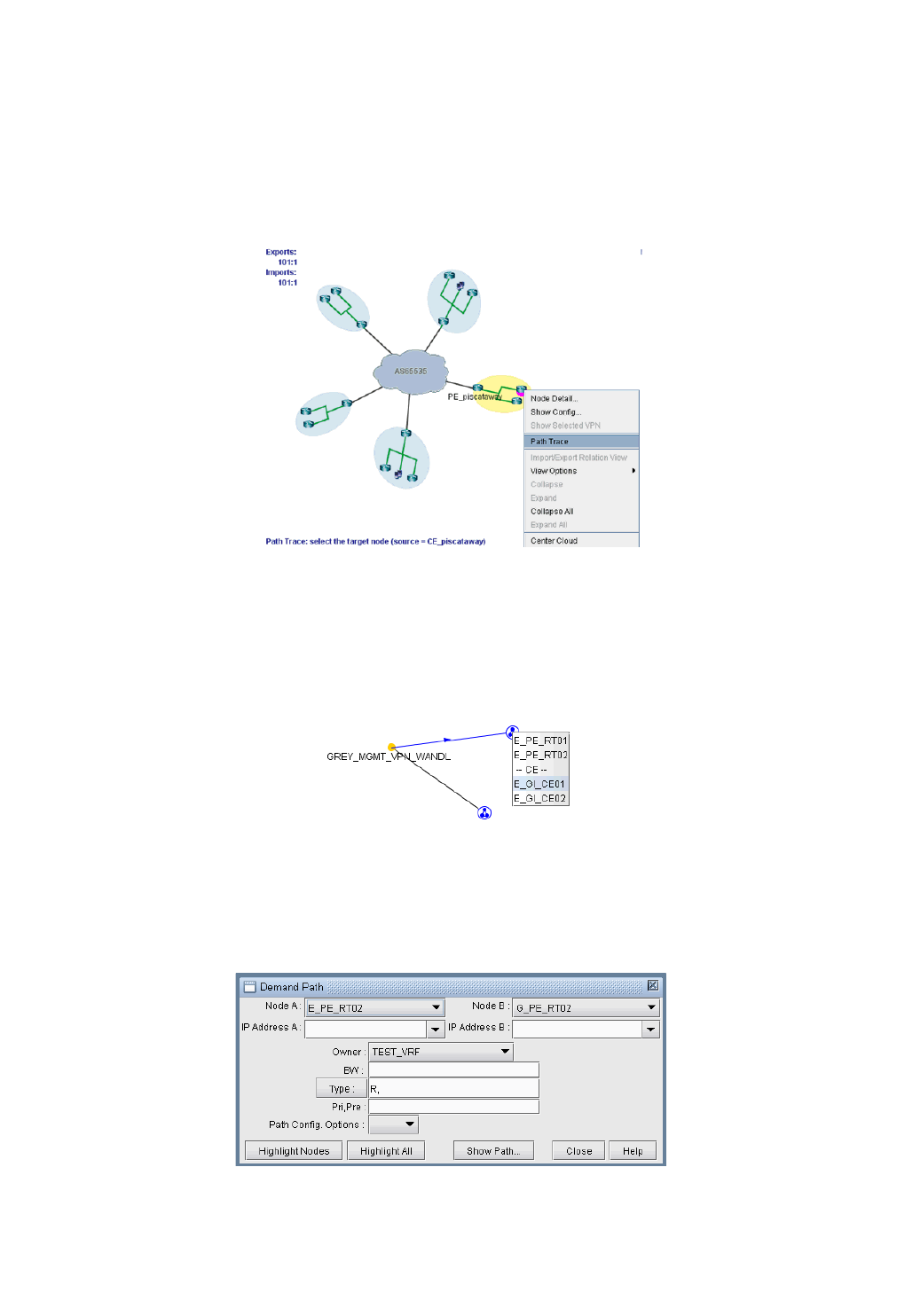
VIRTUAL PRIVATE NETWORKS*
Copyright © 2014, Juniper Networks, Inc. 10-13
. . . . .
VPN Path Tracing
22. VPN path tracing allows you to see the routing path between two nodes belonging to a VPN. A VPN path trace
can be performed by selecting the Path Trace option of the right-click menu in the VPN Topology View. To
use this feature, right-click over the source node, select Path Trace, and then click the destination node. The
routing path details will then be shown on the main topology map. The following figure shows the VPN path
trace feature being performed between CE_piscataway and another node of the VPN.
Figure 10-20 VPN Path Tracing in VPN View
23. VPN Path Tracing in Import/Export Relations View is performed in a similar fashion. Right-click over a group,
and select Path Trace to reveal a drop-down menu of PEs and CEs (if any), as shown in the following figure.
Double-click to select a particular PE or CE as the source node. Then do the same to select the destination node.
Figure 10-21 VPN Path Tracing in Import/Export Relations View
24. Alternatively, a VPN path trace can be performed between PEs (and CEs if managed) of a VPN via the
Network > Path & Capacity > Path menu as shown in the following figure.
Figure 10-22 Demand Path window
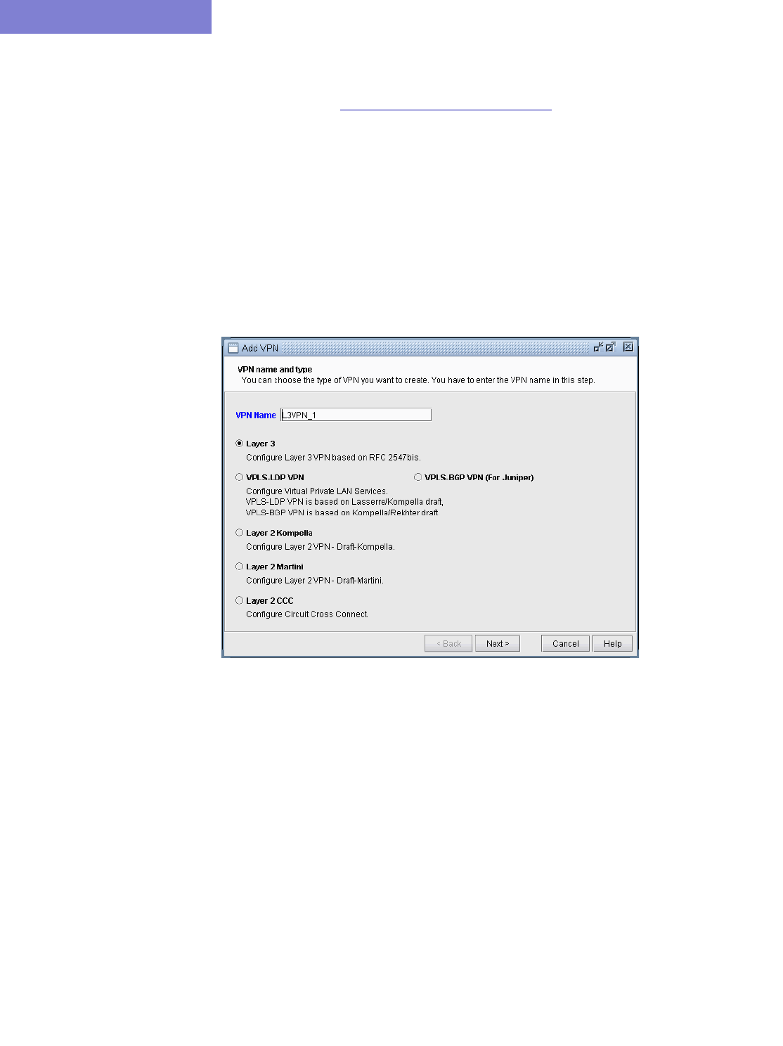
VIRTUAL PRIVATE NETWORKS*
10-14 Copyright © 2014, Juniper Networks, Inc.
10
25. To perform a VPN path trace instead of a regular path trace, first choose the desired VPN from the Owner
dropdown selection. Note that if the VPN is not listed in the owner selection, you should at it first from the VPN
window as described in Forming Customer Groups on page 10-41. Click on Highlight All to display all the
nodes for the selected VPNNext, click on two of the highlighted nodes in order to see the routing being
performed. PEs are highlighted yellow, and CEs (if any) are highlighted blue.
VPN Design and Modeling using the VPN Wizard
Besides the ability to derive the VPNs via network configuration import, the VPN Module allows the network
planner to construct and model a VPN from scratch, and to modify or add to existing VPNs. The procedures
described below on how to add VPNs also apply for modifying existing VPNs. First switch to Modify mode, and
then choose Modify > Services > VPN. Then select a particular VPN and click on the Modify button.
To add any VPN, click on the Add button from the VPN window. To modify a VPN, first select a particular VPN
and then click on the Modify button. When you click on Add, the VPN Wizard’s Add VPN window, shown in
the following figure, is launched.
Figure 10-23 VPN Wizard’s Add VPN window
You may choose to create different types of VPNs, including Layer 3, VPLS (both BGP and LDP flavors), Layer 2
Kompella, Layer 2 Martini, and Layer 2 CCC. Additionally, you may create inter-AS VPNs and hub-and-spoke
VPNs.
The following sections will go through how a user would design and model several different types of VPNs using
WANDL’s VPN module. Successive sections will provide less detail when a particular usage scenario has already
been described in an earlier section.
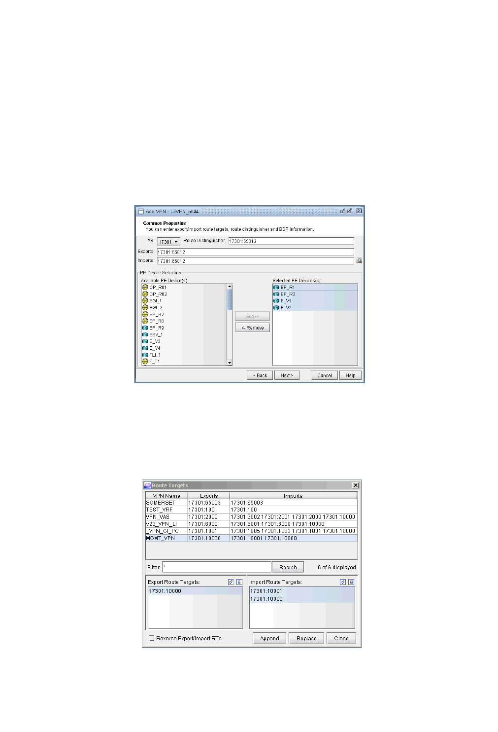
VIRTUAL PRIVATE NETWORKS*
Copyright © 2014, Juniper Networks, Inc. 10-15
. . . . .
L3 (Layer 3) VPN
The L3 VPN is based on the IETF RFC 2547bis draft. To configure a L3 VPN (full-meshed version), the user would
perform the following sequence of steps. Additional steps that are applicable only to configuring a L3 Hub-and-
Spoke VPN are described in the subsequent section.
26. Assign a VPN/VRF name by bringing up the Add VPN window and selecting Layer 3. Then type in a name
for the VPN (e.g. L3VPN_ph44).
27. Click on Next to bring up the window where you would choose the PEs of the VPN from the “Available PE
Device(s)” list and add them to the right hand side “Selected PE Device(s)” list. Note that a node must be
an iBGP speaker in order to make it into this list.
28. Here, you can also assign the Route Distinguisher, Route Target Exports, and Route Target Imports for the
selected AS. The program automatically recommends initial values, which you may change.
Figure 10-24 Adding a Full Meshed L3 VPN
Additionally, you may look up a list of Route Targets that are defined in the network by clicking on the
magnifying glass icon to the right of the Import field to bring up the Route Targets Table shown below, which
lists all the RTs (grouped by VPNs) in the network.
Figure 10-25 Route Targets Table
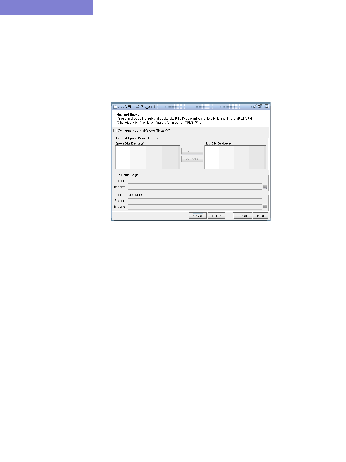
VIRTUAL PRIVATE NETWORKS*
10-16 Copyright © 2014, Juniper Networks, Inc.
10
The Export Route Targets list and Import Route Targets list are populated with the route targets for the
particular VPN selected. You may then choose any or all of the route targets to either append to or replace the route
targets of the VPN you are currently adding. The Route Targets Table will help you to construct a VPN with
various export/import relationships (e.g. extranet or hub-and-spoke type of relationships) with other VPNs. For our
current example, we will be constructing a simple full-meshed L3 VPN, so we will not need to use the Route
Targets table now.
29. Clicking on Next takes you to the following screen, in which you can configure a Hub-and-Spoke VPN. Since
we are configuring a full-meshed L3 VPN, click Next to skip over this step.
Figure 10-26 Click Next to skip over Hub-and-Spoke configuration step
30. Click on Next to bring up the following window where you may add more PEs and assign the PE facing CE
interfaces.
•The middle part of the window shows the topology area, where selected PE routers are placed.
•The Selected Objects area, as the name implies, lists those routers that have been selected as PEs.
•The Available Devices box lists those routers for the currently chosen AS that are eligible (i.e., they must be
iBGP speakers) to be selected as PE routers.
•The Properties box lists all the interfaces for a particular router when it is highlighted (a router is highlighted
when it is clicked on either from the Available Devices list, the topology area of the window, or from the
Selected Objects list).
The window is designed to be as user-friendly as possible, with drag/drop capabilities built in. The following figure
shows the four PEs that we have already added in the previous step.
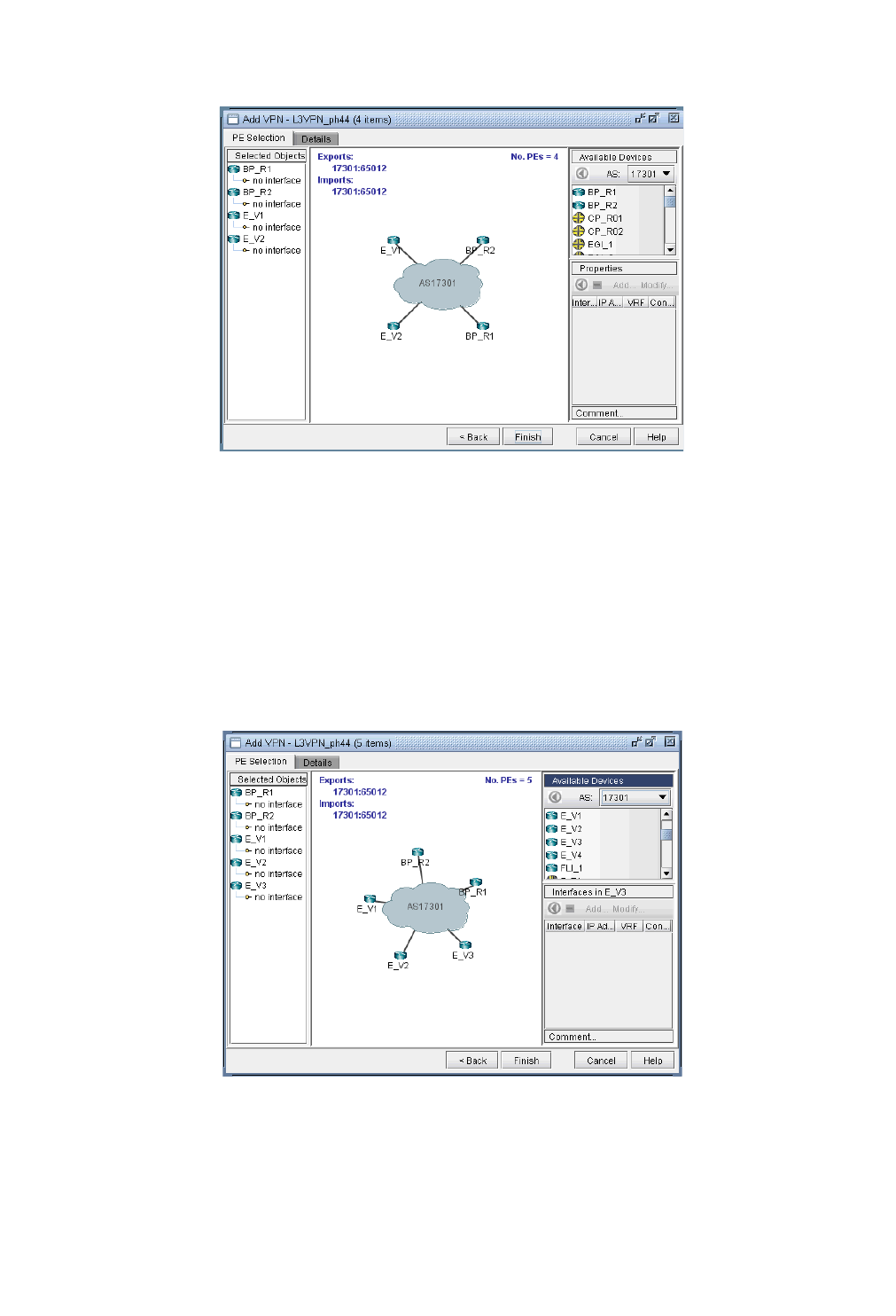
VIRTUAL PRIVATE NETWORKS*
Copyright © 2014, Juniper Networks, Inc. 10-17
. . . . .
Figure 10-27 Assigning more PEs and PE facing CE Interfaces
31. In more detail, you may add additional PE routers to the VPN from the Available Devices box via one of two
methods:
•Select one or more routers (at which point the icon that has the left arrow with a circle around it will change color
from gray to blue), and then click on the blue arrow/circle icon to move it to the topology area part of the window
(middle of the window).
•Alternatively, you could simply drag and drop PEs from the Available Devices list into the topology area of the
window.
32. The following figure shows you the result of adding the fifth PE router (E_V3) to the VPN.
Figure 10-28 An L3 VPN with five PEs
33. To assign the PE facing CE interfaces, first select a particular PE router in order to have all its interfaces shown
in the Properties box. A PE is selected when it is clicked on from the Selected Objects list or from the
topology area of the map. As shown in the following figure, the Properties box is now renamed as
Interfaces in BP_R1, since the PE router BP_R1 has been selected. Another icon worth mentioning is the
VIRTUAL PRIVATE NETWORKS*
10-18 Copyright © 2014, Juniper Networks, Inc.
10
“–“/”+” button next to the arrow/circle button. Click on it to switch between “-“ and “+”. “-“ means to show
all interfaces, while “+” means to only display interfaces that are unassigned or not shutdown.
Figure 10-29 How to assign interfaces to PEs
34. To assign an interface, you need to drag and drop a particular interface over to a no interface item under a
particular PE. Alternatively, you can select the PE from the left hand side, and then select an interface from the
interface list on the bottom right hand side, and click the blue arrow in the Interfaces section. The following
figure shows the window after the interfaces have been assigned to the PE routers.
Figure 10-30 Assigning Interfaces to the PEs
35. Note also the Add and Modify buttons in the Interface section. This can be used to add an additional interface,
e.g., if you need to add a new subinterface, or to modify an existing interface.
VIRTUAL PRIVATE NETWORKS*
Copyright © 2014, Juniper Networks, Inc. 10-19
. . . . .
36. Next click on the Details tab to assign the PE-CE protocol. After selecting a row, you can choose OSPF, RIP,
Static, BGP or connected as the protocol. The following figure shows OSPF being assigned as the PE-CE
protocol.
Figure 10-31 Assigning the PE-CE Protocol in the Details tab
To assign BGP as the PE-CE protocol, first click on the BGP checkbox and then bring up the Add BGP Neighbor
window (click on the icon to the left of PE->CE Neighbor IP or the icon to the left of CE->PE Neighbor IP),
shown in the following figure. Please refer to Ch 21, Border Gateway Protocol for more information about how to
create BGP neighboring relationships.
Figure 10-32 Add BGP Neighbor window
To assign Static as the PE-CE protocol, first click on the Static checkbox and then click on the icon to the right of
Static to bring up the Add Static Route window. Please refer to Ch 14, Static Routes for more information about
how to configure static routes.
To assign OSPF as the PE-CE protocol, first click on the OSPF checkbox and then click on the icon to the right of
OSPF to bring up a dialog prompt, which allows you to enter in the associated OSPF PID (Cisco-only) and OSPF
Protocol. The OSPF PID should be different from that of the network core, and the area should match the CE’s area.
37. Finally, click Finish to complete the adding of the L3VPN. The summary window then displays the VPN that
you just added, as shown in the following figure.
VIRTUAL PRIVATE NETWORKS*
10-20 Copyright © 2014, Juniper Networks, Inc.
10
Figure 10-33 L3VPN_ph44 has been added
38. With the detailed view shown (select the Detailed tab) in the upper portion of the window, click the Configlet
tab (next to the Details tab) to generate and display the configlet for the VPN that you just added. Please also
see the VPN Configlet section of the document for more information about configlet generation.
VIRTUAL PRIVATE NETWORKS*
Copyright © 2014, Juniper Networks, Inc. 10-21
. . . . .
L3 Hub-and-Spoke VPN
MERGING HUB AND SPOKES
For the existing hub-and-spoke VPNs, WANDL does not automatically group together the vrf associated with the
hub and the vrf associated with the spoke. This should not affect routing, but for readability purposes, users can
manually group together the hub and spoke into one VPN using the following procedures.
39. If you are in the Online mode, click the Offline button to switch into the Offline mode.
40. Next, select the Modify mode button to switch into Modify mode.
41. Select Modify > Services > VPN, and identify the vrf’s to combine. If you select the To Import/Export
Relation View from the VPN Topology tab, it will show you which other instances to combine together.
Figure 10-34 Spoke View
Figure 10-35 Import/Export Relation View (Spoke -> Hub)
Since some hub-and-spoke VPN’s can have an upstream and downstream spoke, it may be best to check the
Import/Export Relation View of the hub.
42. Select the hub-and-spoke components from the Summary > Layer 3 VPN list on the right pane and use the
Actions > Set Service menu to provide a name for the hub-and-spoke VPN.
VIRTUAL PRIVATE NETWORKS*
10-22 Copyright © 2014, Juniper Networks, Inc.
10
Figure 10-36 Specifying the Hub and Spoke VPN via “Set Service”
43. Select the newly defined service from the Services category to view the VPN topology of the hub and spoke
VPN.
Figure 10-37 Hub and Spoke VPN Topology
44. For the combined VPN, select the Modify > Protocol. To identify the Hub PE node, right-click the table
column header and select Table Options, and add the property “Hub” to the “Selected Items” list on the right-
hand side, to see the Hub checkbox column.
VIRTUAL PRIVATE NETWORKS*
Copyright © 2014, Juniper Networks, Inc. 10-23
. . . . .
45. By looking at the Exports and Imports, you can identify 2 sets of nodes with opposite imports and exports. One
set of nodes should be specified as the Hub PE. For the Node which is a Hub PE, select the row corresponding to
the outgoing interface, and then select the “Set to Hub PE” checkbox. Click OK when you are done.
46. To update the network, select Modify > Update Network State. Then reopen the VPN window from Modify
> Services > VPN.
47. If you are working on the live network (online module), you will want to preserve this setting for future use, so
that it does not have to be repeated. To do this, first create the directory /u/wandl/data/.network_plan from the
File Manager, if it does not exist.
48. Click the Design mode button to switch back to Design mode.
49. Save the network to /u/wandl/data/.network_plan via the File > Save Network... menu using the default
runcode x.
50. Now that the network is saved into the .network_plan directory, switch back to Online mode.
51. From Admin > Task Manager, New Task, rerun a Scheduling Live Network Collection task. Be sure
to select the checkbox option “Consolidate with existing WANDL data.” At this point, it is only necessary
to process the network configuration files and not to recollect the entire network, so for the “Data to Be
Collected or Processed”, you can “Deselect All” and select only the “Process” checkbox for the
Configuration type. Select Next and then Finish.
52. Once the task is complete, open Network > Services > VPN and check to ensure that the changes have been
preserved.
ADDING A NEW LAYER 3 HUB-AND-SPOKE VPN
Configuring a L3 Hub-and-Spoke VPN is similar to configuring a regular L3 full-meshed VPN, except for the
following additional steps.
53. First follow the steps outlined in previous section on L3 VPN configuration until you reach the Hub-and-Spoke
configuration window. Click on the checkbox that says Configure Hub-and-Spoke MPLS VPN, and then
move each PE to the appropriate list (Spoke Site Device(s) list or Hub Site Device(s) list) by using the Hub->
and <-Spoke buttons. The VPN Wizard automatically suggests RT exports and imports for both the hub sites
and the spoke sites in order to establish a hub-and-spoke relationship. As before, you have the option to change
VIRTUAL PRIVATE NETWORKS*
10-24 Copyright © 2014, Juniper Networks, Inc.
10
the RT list by editing the suggested export or import values or by using RTs from the Route Targets table (by
clicking on the magnifying glass icon).
Figure 10-38 Hub-and-spoke VPN configuration
54. Click on Next to get to the window where you would configure PE facing CE interfaces as described in the
previous section on L3 VPN configuration. The following figure shows what the configuration looks like after
the interfaces have been assigned. Notice that GI_C2 is configured as the hub site.
Figure 10-39 Assigning PE facing CE interfaces in the Hub-and-Spoke VPN
VIRTUAL PRIVATE NETWORKS*
Copyright © 2014, Juniper Networks, Inc. 10-25
. . . . .
55. After configuring the PE-CE protocol details under the Details tab (as described in the previous section on L3
VPN configuration), the resultant L3 hub-and-spoke VPN is shown in the following figure. Notice that Import
RT 17301:65016 is highlighted to indicate that it is only an import RT for the HuB site(s).
Figure 10-40 Newly created Hub and Spoke VPN
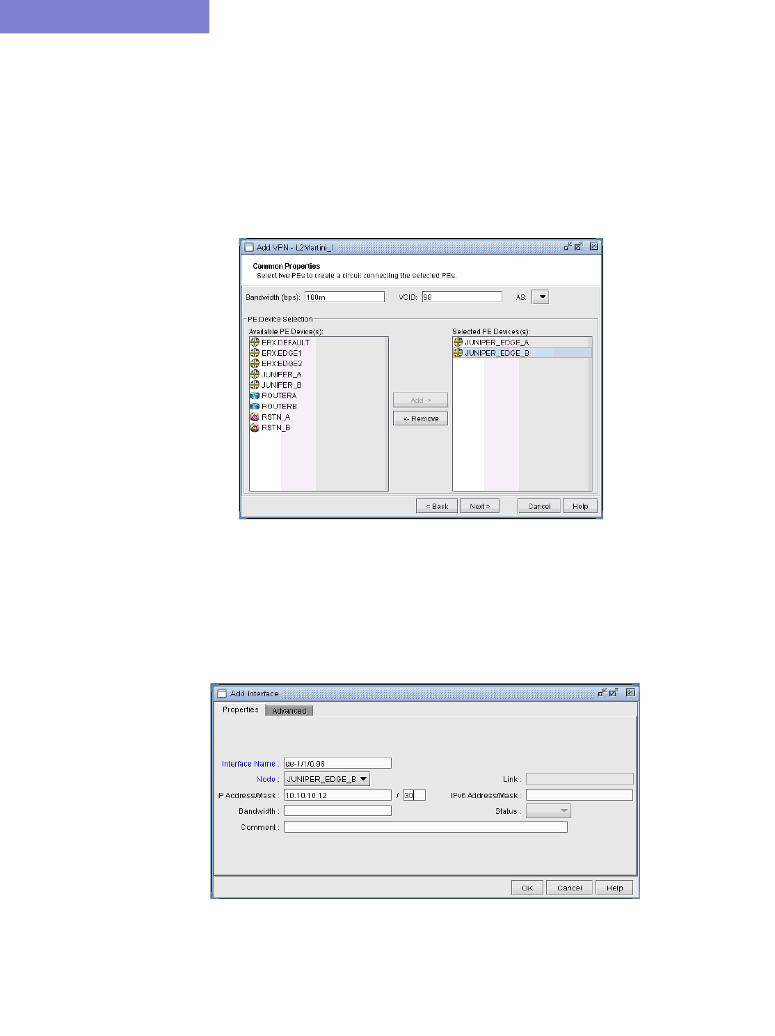
VIRTUAL PRIVATE NETWORKS*
10-26 Copyright © 2014, Juniper Networks, Inc.
10
L2M (Layer2-Martini) VPN
The L2M (Layer2 Martini) VPN, based on the IETF Martini set of drafts, supports the configuration of Layer2
Martini, AToM (Any Transport Over MPLS), and VLL (Virtual Leased Line) VPNs. The following steps illustrate
how to configure a L2M VPN:
56. Bring up the Add VPN window by selecting Layer 2 Martini. Then type in a circuit name by filling in the
Ckt.Name box (e.g., L2Martini_1).
57. Click on Next to take you to the Common Properties window to select the two PEs. You may then assign a
VCID for the circuit. You may also optionally assign a bandwidth value for the circuit.
Figure 10-41 Select two PEs and assign a bandwidth value
58. Click on Next to take you to the screen where you can specify or add the (PE facing CE) interfaces as needed.
The following figures illustrate the adding of the interface ge-1/1/0.98 and assigning of the Vlan ID 98 to the
JUNIPER_EDGE_B router. This window is opened by selecting the JUNIPER_EDGE_B router from the upper
left list of PEs and then clicking the “Add” button above the lower right list of interfaces for the selected router.
The same steps are used to add the interface and to assign the Vlan ID to the JUNIPER_EDGE_A router.
Figure 10-42 Add a gigabit ethernet interface, ge-1/1/0.98
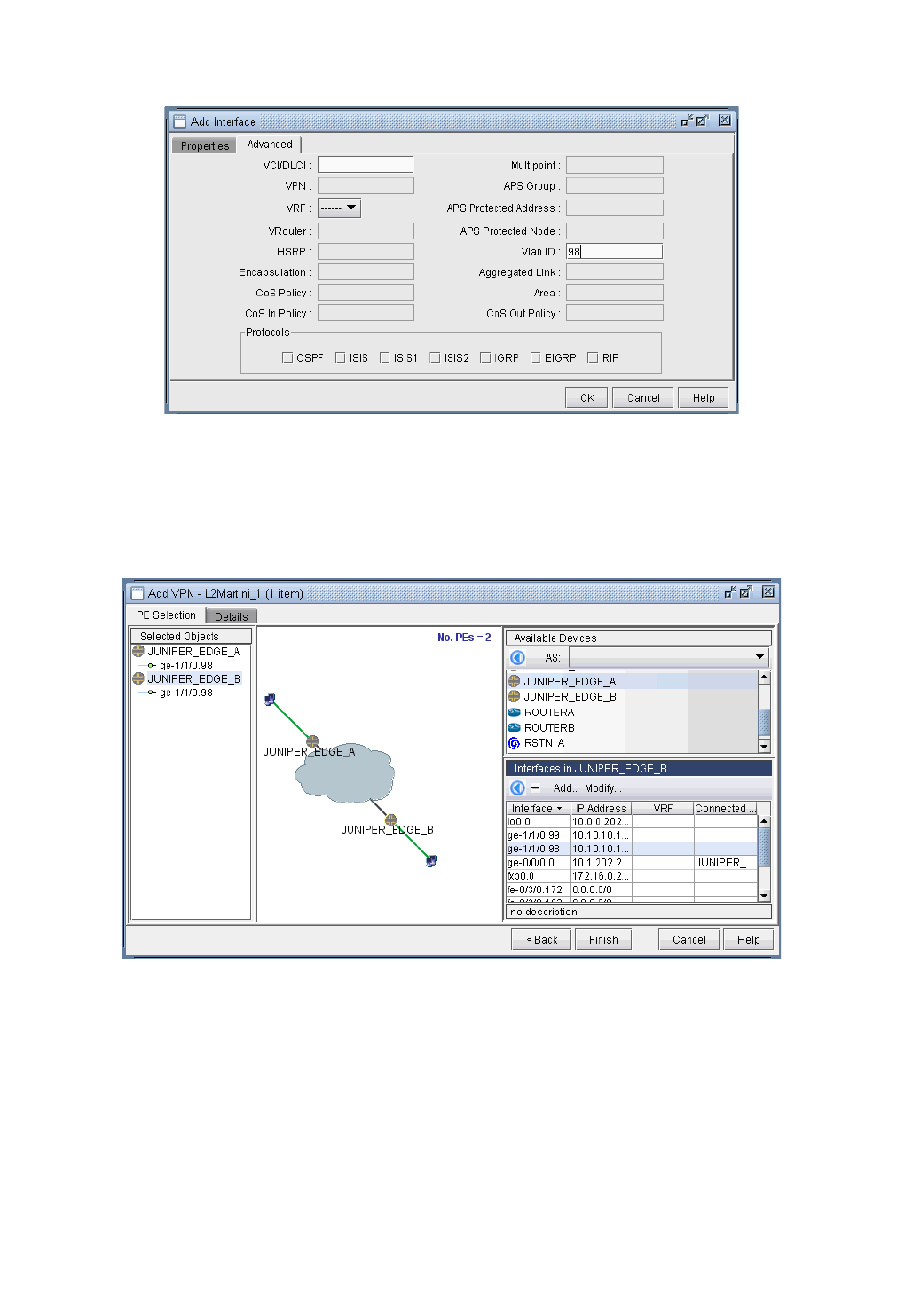
VIRTUAL PRIVATE NETWORKS*
Copyright © 2014, Juniper Networks, Inc. 10-27
. . . . .
Figure 10-43 Assigning a Vlan ID of 98 to the interface ge-1/1/0.98
59. The following figure shows the result of both interfaces assigned, after selecting each PE router, adding the
appropriate sub-interface to the interface list in the bottom right, and then dragging and dropping that new
interface to the appropriate PE in the PE list.
Figure 10-44 Finished assigning interfaces on the PEs
60. Next, click on the Details tab to take you to the following screen, where the VCID and Encapsulation can be
assigned. Note that the VCID only needs to be assigned if it was not already done so in the Common
Properties window. The LSPs can also be assigned if necessary.
The following figure shows both the VCID and the encapsulation assigned.
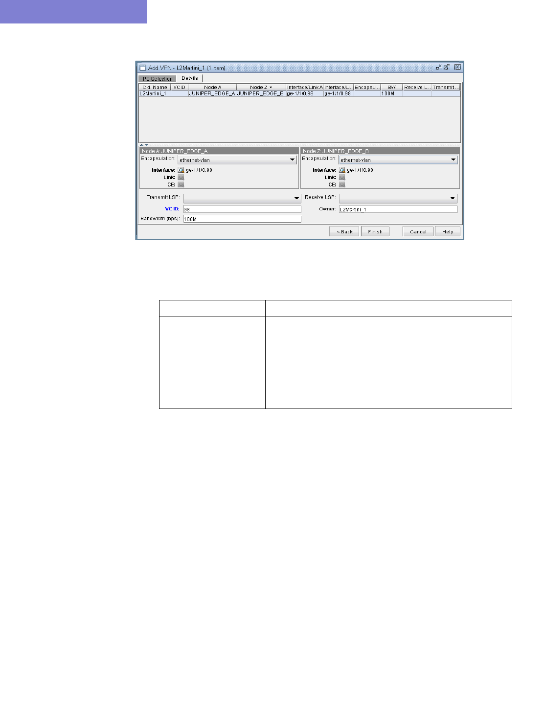
VIRTUAL PRIVATE NETWORKS*
10-28 Copyright © 2014, Juniper Networks, Inc.
10
Figure 10-45 Encapsulation and VCID assigned
Note that the Encapsulation dropdown can take on the values as described in the following table.
61. Next click Finish to complete the adding of the L2M VPN. The following figures show both the single and
summary topology (with the added Martini circuit highlighted in pink) views for the L2M VPN just added.
Field Description
Encapsulation For Juniper, the interface encapsulation types include: aal0,
atm-aal5, atm-ccc-vc-mux, atm-cell, atm-cell-port-mode, atm-
cell-vc-mode, atm-cell-vp-mode, cisco-hdlc, ethernet,
ethernet-vlan, frame, frame-relay, frame-relay-ccc,
interworking, and ppp.
For Cisco, the interface encapsulation types include: aal0,
aal5, dot1Q, frame-relay, hdlc, and ppp.
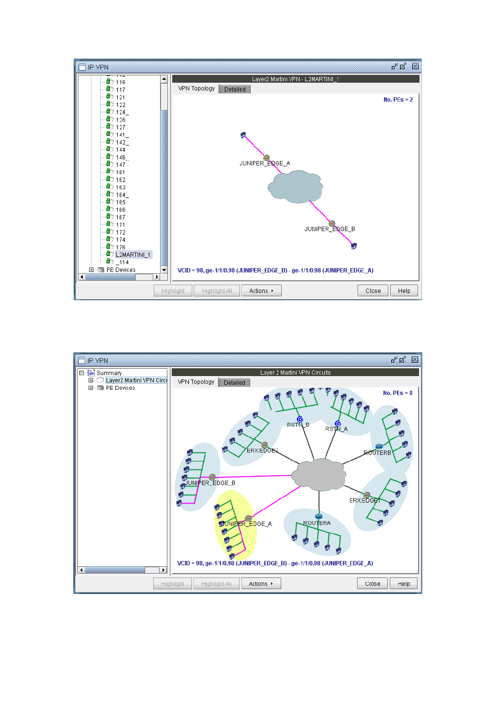
VIRTUAL PRIVATE NETWORKS*
Copyright © 2014, Juniper Networks, Inc. 10-29
. . . . .
Figure 10-46 Topology view for the L2M VPN added
Figure 10-47 L2M VPN summary topology view with newly-added circuit (VCID 98) highlighted
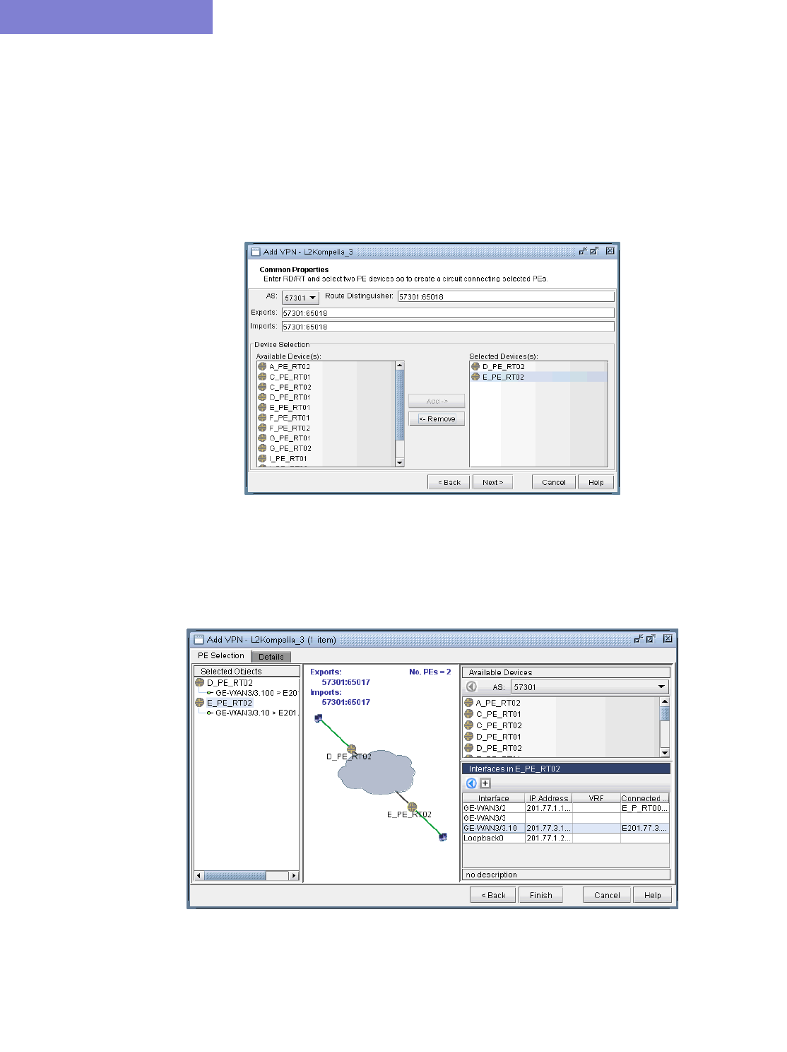
VIRTUAL PRIVATE NETWORKS*
10-30 Copyright © 2014, Juniper Networks, Inc.
10
L2K (Layer2-Kompella) VPN
The L2K (Layer2 Kompella) VPN, based on the IETF Kompella draft, is implemented by Juniper only. To configure
a L2K VPN, the user would perform the following sequence of steps:
62. Bring up the Add VPN window and selecting Layer 2 Kompella. Then type in a name for the VPN (e.g.
L2Kompella_3).
63. Click on Next to bring up the Common Properties window where you can assign the Route Distinguisher,
Route Target Exports, and Route Target Imports for the chosen AS and PEs. The program automatically
recommends values based on the chosen AS or you may provide your own.
Figure 10-48 For the chosen AS, select RD, RT, and two PEs
64. Click on Next to bring up the following window where you would identify PEs and assign the PE facing CE
interfaces (in the same manner as described under the L3 (Layer 3) VPN section). The following figure shows
the result of the assignment of the interfaces.
Figure 10-49 Interfaces have been assigned to the PEs
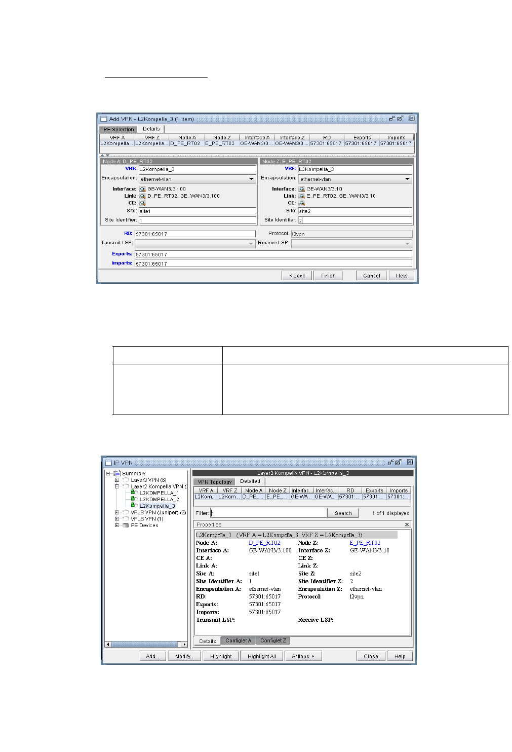
VIRTUAL PRIVATE NETWORKS*
Copyright © 2014, Juniper Networks, Inc. 10-31
. . . . .
65. Next, click on the Details tab to specify the Encapsulation, Site, Site Identifier. Optionally, you may also
specify the Transmit LSP and the Receive LSP (for more information on how to set up LSPs, please refer to
Chapter 6, Modeling Tunnel). The following figure shows that Site, Site Identifier, and Encapsulation have been
assigned.
Figure 10-50 Details tab showing the completed assignment of Site, Site ID, and Encapsulation
Note that the Encapsulation dropdown can take on the values as described in the following table.
66. Finally, click on Finish to complete the adding of the L2K VPN.
Figure 10-51 Newly added L2K VPN
Field Description
Encapsulation For Juniper, the interface encapsulation types include: aal0, atm-aal5,
atm-ccc-vc-mux, atm-cell, atm-cell-port-mode, atm-cell-vc-mode, atm-
cell-vp-mode, cisco-hdlc, ethernet, ethernet-vlan, frame, frame-relay,
frame-relay-ccc, interworking, and ppp.
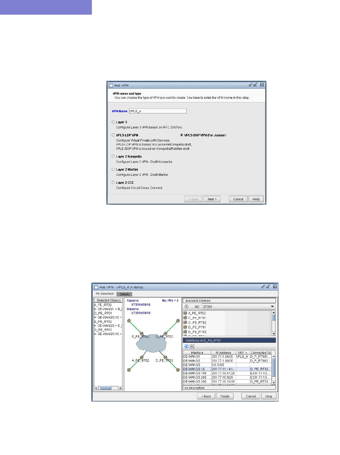
VIRTUAL PRIVATE NETWORKS*
10-32 Copyright © 2014, Juniper Networks, Inc.
10
VPLS-BGP VPN (for Juniper)
The VPLS-BGP VPN is based on the IETF Kompella/Rekher draft. To configure a VPLS-BGP VPN (implemented
by Juniper only), the user would perform the following sequence of steps:
67. Bring up the Add VPN window and select VPLS-BGP VPN (For Juniper). Then type in a name for the
VPN (e.g. VPLS_4) as shown in the following figure.
Figure 10-52 VPLS-BGP VPN
68. Click on Next to bring up the window where you can choose PEs and assign the Route Distinguisher, Route
Target Exports, and Route Target Imports for a chosen AS as described under the L3 (Layer 3) VPN section).
The program automatically recommends values or you may provide your own.
69. Click on Next to bring up the following window where you would assign the PE facing CE interfaces (in the
same manner as described under the L3 (Layer 3) VPN section). The following figure shows the result of the
assignment of the interfaces.
Figure 10-53 Interfaces assigned to the PEs
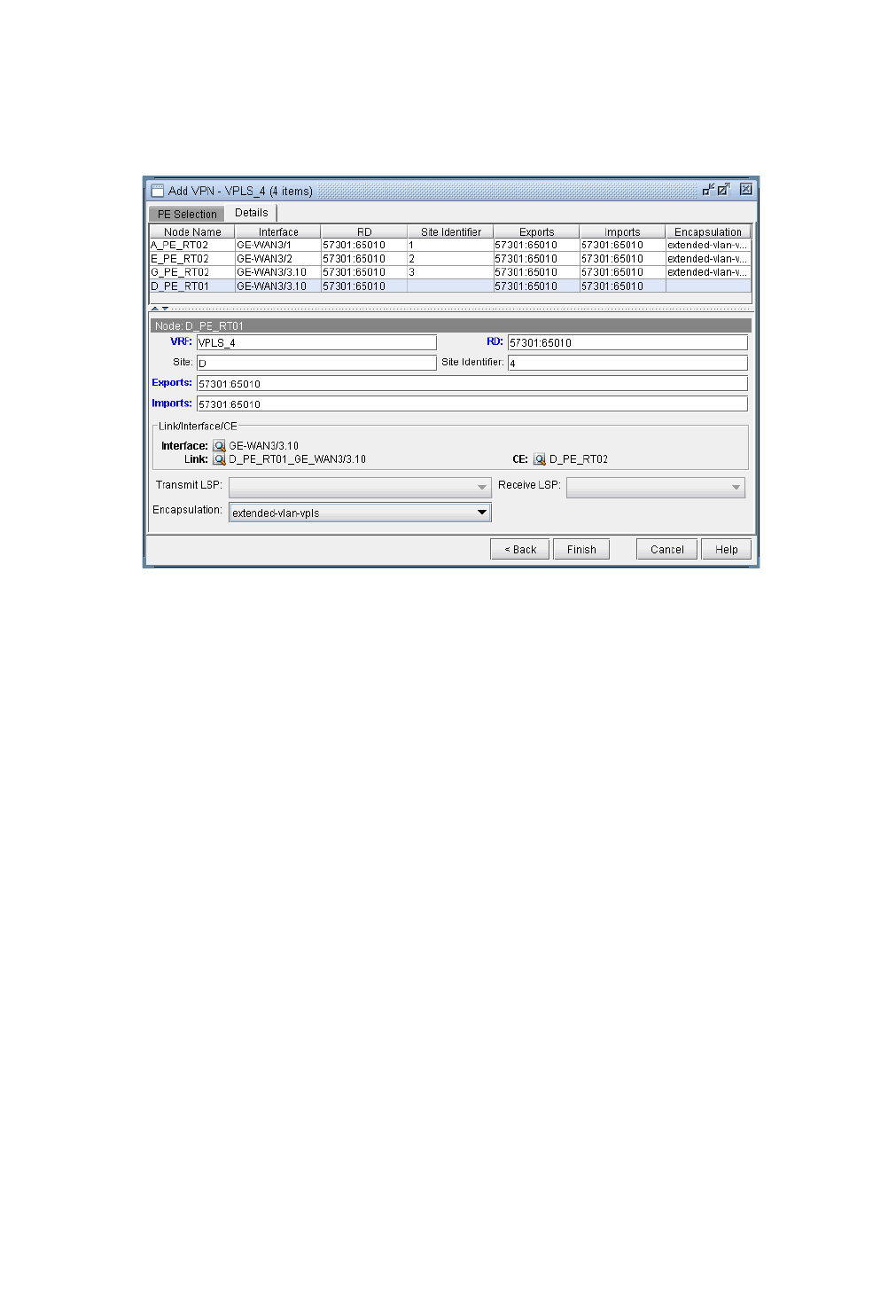
VIRTUAL PRIVATE NETWORKS*
Copyright © 2014, Juniper Networks, Inc. 10-33
. . . . .
70. Next, click on the Details tab to specify the Encapsulation, Site, Site Identifier. The LSPs may also be
specified, as appropriate. The following figure shows assignments completed for three nodes and in-progress
for the fourth node.
Figure 10-54 Details tab showing Site, Site ID, and Encapsulation being assigned for D_PE_RT01
The Encapsulation drop-down includes the following values from which the user can select: ethernet-vpls, ether-
vpls-over-atm-llc, extended-vlan-vpls, and vlan-vpls.
71. Finally click on Finish to complete the creation of a Juniper VPLS VPN.
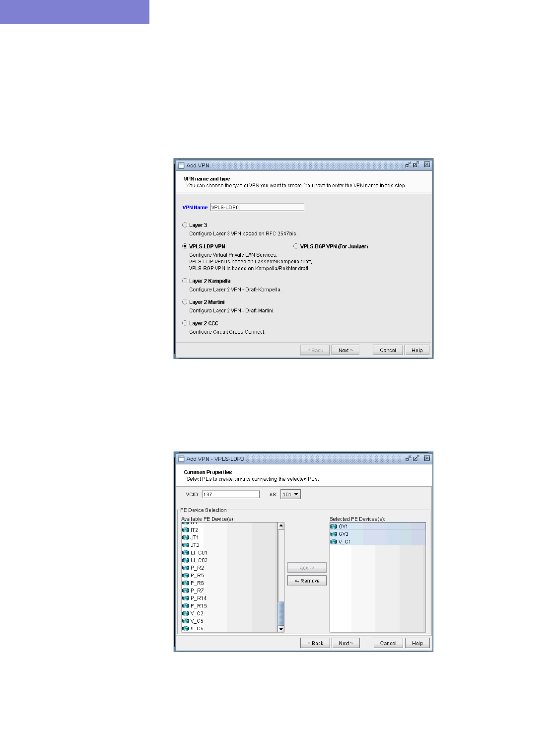
VIRTUAL PRIVATE NETWORKS*
10-34 Copyright © 2014, Juniper Networks, Inc.
10
VPLS-LDP VPN
The VPLS-LDP VPN, based on the IETF Lasserre/Kompella draft, is implemented by Cisco and all other vendors
except Juniper. To configure a VPLS-LDP VPN, the user would perform the following sequence of steps:
72. First identify, for the VPLS-LDP, a set of PEs with available PE-facing-CE interfaces that can be assigned as
VPLS attachment circuits.
73. Next, bring up the Add VPN window and select VPLS-LDP VPN. In this example, we will configure a VPLS
instance named VPLS-LDP0.
Figure 10-55 Creating a VPLS-LDP VPN
74. Click on Next to take you to the screen to specify a VCID and to select the PEs for the VPLS instance, as shown
in the following screen. If you prefer, you may select some or all the PEs in the PE Selection tab in the next
screen, as described in the next step. Click on Next to continue.
Figure 10-56 Select PEs and Specify a VCID
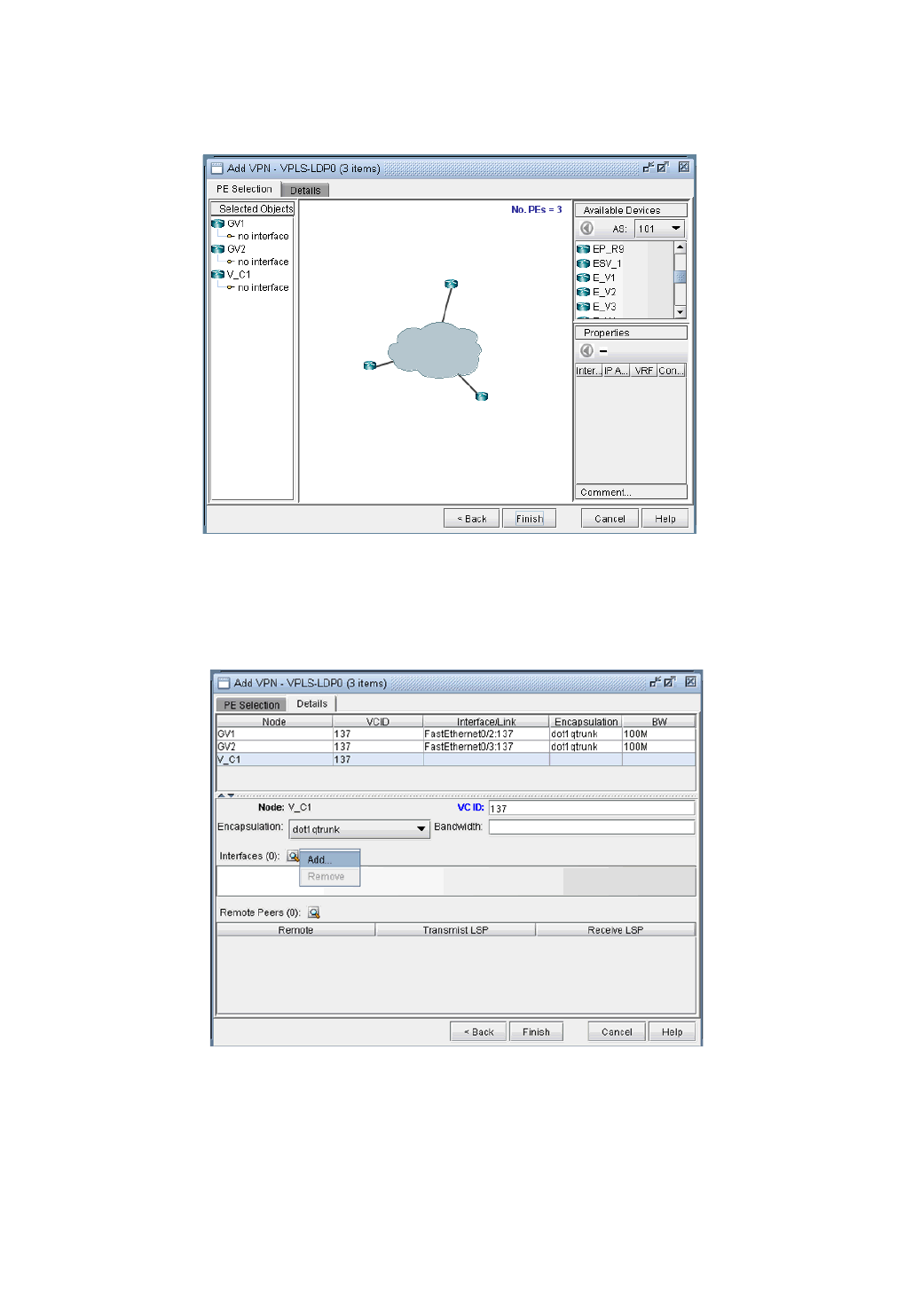
VIRTUAL PRIVATE NETWORKS*
Copyright © 2014, Juniper Networks, Inc. 10-35
. . . . .
75. As described in the previous step, you may select PEs in the PE Selection tab, as shown in the following
screen. If you have already selected all the PEs in the previous step, then click on the Details tab to continue.
Figure 10-57 Additional PEs may be select in the PE Selection tab
76. Next, you are ready to configure the PE-facing-CE attachment circuits; this includes specifying the interface and
circuit ID, bandwidth, and encapsulation.
Figure 10-58 Configure VPLS-LDP Details
The encapsulation types for various vendors are:
•Cisco: dot1qaccess, dot1qtunnel, dot1qtrunk.
•Foundry: tagged, untagged.
•Tellabs, Riverstone: tagged, untagged, q-in-q.
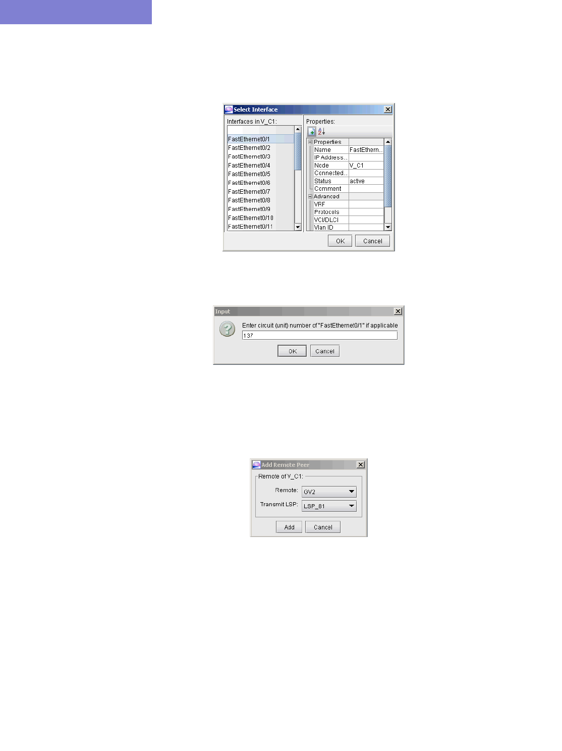
VIRTUAL PRIVATE NETWORKS*
10-36 Copyright © 2014, Juniper Networks, Inc.
10
The following figures show how an interface is assigned: First, click on the magnifying glass next to Interfaces and
choose Add. Then in the Select Interface window, pick an available interface. Finally, type in the VCID for the
interface
Figure 10-59 Select an interface
Figure 10-60 Assign the Circuit ID to the interface
77. Next, you will specify, in turn, each remote peer and the transmit LSP used to reach the peer. Click on the
magnifying glass next to Remote Peers to bring up the Add Remote Peer window, where you can choose
the remote peer and the transmit LSP from the dropdown selection menus.
Figure 10-61 Configure PE peers
78. The following figure shows the assignment details completed for our VPLS instance, VPLS-LDP0. Click on
Finish to add the VPLS instance to the model.
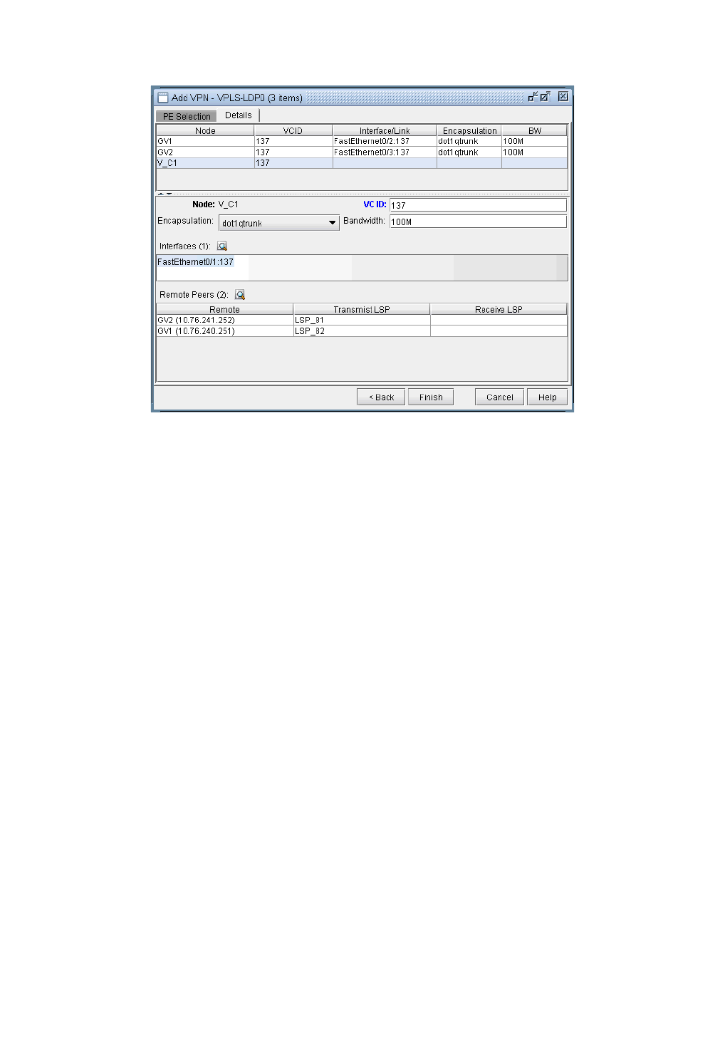
VIRTUAL PRIVATE NETWORKS*
Copyright © 2014, Juniper Networks, Inc. 10-37
. . . . .
Figure 10-62 VPLS-LDP instance details configured
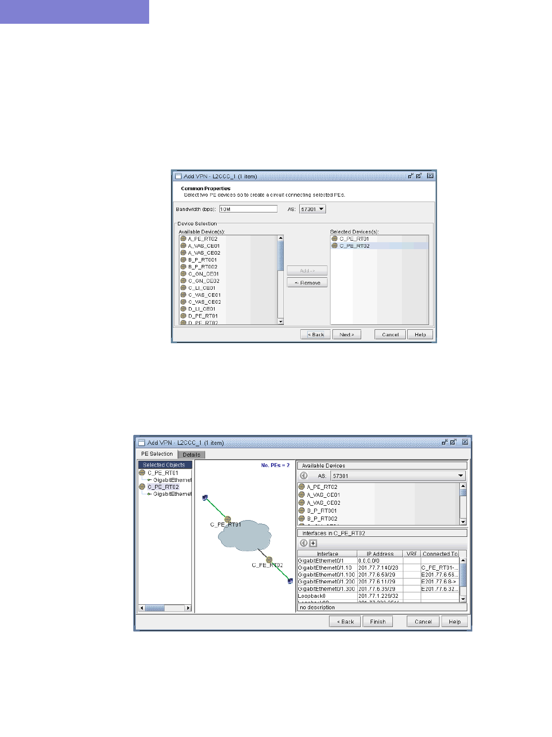
VIRTUAL PRIVATE NETWORKS*
10-38 Copyright © 2014, Juniper Networks, Inc.
10
L2CCC (Circuit Cross-Connect) VPN
Circuit Cross-Connect (IETF draft-kompella-ccc-02.txt), an early Layer 2 VPN technology implemented by Juniper,
is still in many production networks today. To configure a L2CCC VPN, the user would perform the following
sequence of steps:
79. First bring up the Add VPN window and select Layer 2 CCC. Then type in a circuit name by filling in the
Ckt.Name box (e.g., L2CCC_1).
80. Click on Next to take you to the screen to select the two PEs. Also assign a bandwidth value for the circuit. The
following figure shows a bandwidth of 10M for two chosen routers from AS 57301.
Figure 10-63 Choosing two PEs and specifying the circuit bandwidth
81. Click on Next to bring up the following window where you would identify PEs and assign the PE facing CE
interfaces (in the same manner as described under the L3 (Layer 3) VPN section). The following figure shows
the result of the assignment of the interfaces.
Figure 10-64 Interfaces assigned to PEs
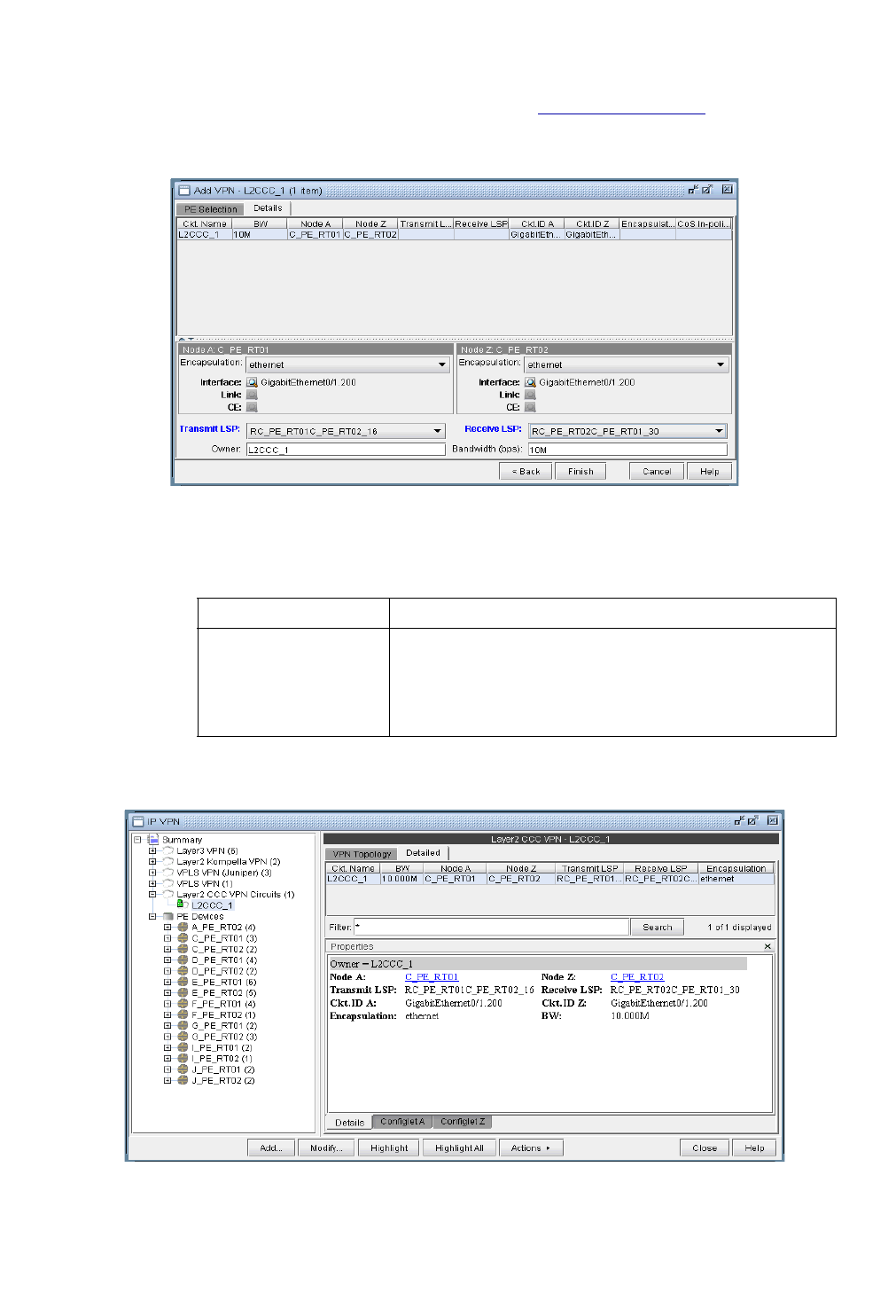
VIRTUAL PRIVATE NETWORKS*
Copyright © 2014, Juniper Networks, Inc. 10-39
. . . . .
82. Next, click on the Details tab to specify the Encapsulation, the Transmit LSP, and the Receive LSP (For
more information on how to set up LSPs, please refer to Chapter 20, LSP Tunnels*). The following figure shows
the completed assignments.
Figure 10-65 Assigning Transmit/Receive LSPs and Encapsulation
Note that the Encapsulation drop-down can take on the values as described in the following table.
83. Finally, click on Finish to complete the creation of a L2CCC VPN.
Figure 10-66 Details of the newly-added L2CCC VPN
Field Description
Encapsulation For Juniper, the interface encapsulation types include: aal0,
atm-aal5, atm-ccc-vc-mux, atm-cell, atm-cell-port-mode, atm-
cell-vc-mode, atm-cell-vp-mode, cisco-hdlc, ethernet,
ethernet-vlan, frame, frame-relay, frame-relay-ccc,
interworking, and ppp.
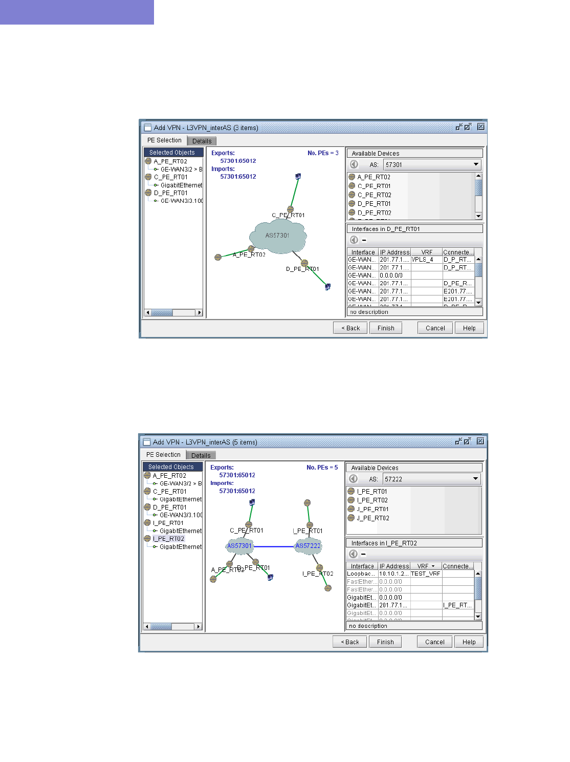
VIRTUAL PRIVATE NETWORKS*
10-40 Copyright © 2014, Juniper Networks, Inc.
10
Inter-AS VPN
84. To construct an inter-AS VPN, you would follow the same steps as those used to construct a L3 VPN, with the
additional step of specifying routers from more than one AS. The following figure shows three PEs (along with
completed interface assignments) from a particular AS (57301) already added.
Figure 10-67 An inter-AS VPN being constructed, with three PEs from AS 57301 already added
85. The next step would be to choose another AS (from the AS dropdown box under Available Devices), and
then select routers from it. As the following figure shows, two routers from AS 57222 were added to the VPN to
create an inter-AS VPN. Interfaces were then assigned to the two routers to complete the process.
Figure 10-68 Adding two more PEs from another AS (57222)
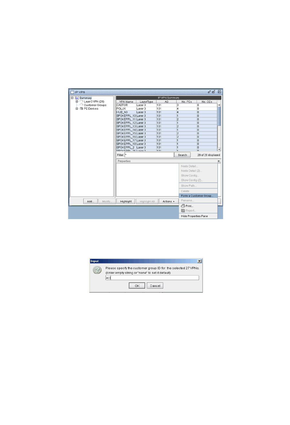
VIRTUAL PRIVATE NETWORKS*
Copyright © 2014, Juniper Networks, Inc. 10-41
. . . . .
Forming Customer Groups
Often times, many VPNs belong to the same customer, so you may group together multiple VPNs into a Customer
Group. Once a particular Customer Group has been formed, you may create demands for it. Reports can also be
filtered to show information relavant to the group only. The following steps describe how to form Customer Groups.
86. First go to Summary to see a list of all the VPNs. Select one or more VPNs and choose Form a Customer
Group from the Actions menu. As shown in the following figure, VPNs HUB_AO and SPOKEPPL_* have
been selected to be grouped into a Customer Group.
Figure 10-69 Forming a Customer Group
87. Next, supply a customer group ID for the selected VPNs to group together as shown in the following figure.
Figure 10-70 Supply a customer ID
88. In the following figure, the resultant Customer Group, AO, is shown expanded in the structured list.
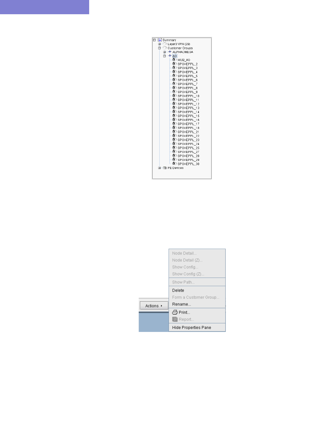
VIRTUAL PRIVATE NETWORKS*
10-42 Copyright © 2014, Juniper Networks, Inc.
10
Figure 10-71 Customer Group AO
Deleting or Renaming VPNs
89. In case you want to rename a particular VPN, simply select a VPN, click on Actions, and choose Rename.
Then specify a new name for the VPN when prompted.
90. In case you want to delete a particular VPN, simply select a VPN, click on Actions, and choose Delete.
Figure 10-72 VPN Rename and Delete actions
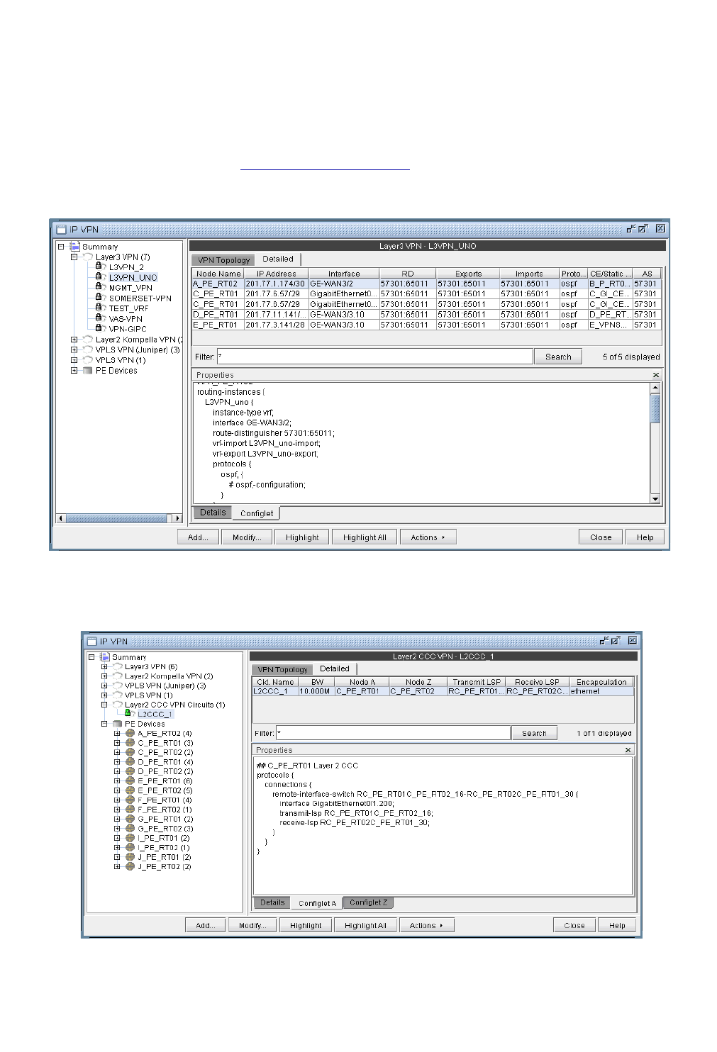
VIRTUAL PRIVATE NETWORKS*
Copyright © 2014, Juniper Networks, Inc. 10-43
. . . . .
VPN Configlet Generation*
Note that a special password is required for VPN configlet generation. Please contact your Juniper representative for
more information.
91. As mentioned earlier under the sections under VPN Design and Modeling using the VPN Wizard, the
VPN Module gives you the ability to generate VPN configlets for a particular VPN. For instance, the last step
under the section, L3 (Layer 3) VPN on page 10-15, describes how to generate and display the configlet for a
L3VPN. The following figures show configlets generated for two of the VPNs discussed earlier.
Figure 10-73 A configlet generated for a L3VPN
Figure 10-74 A configlet generated for a L2CCC VPN
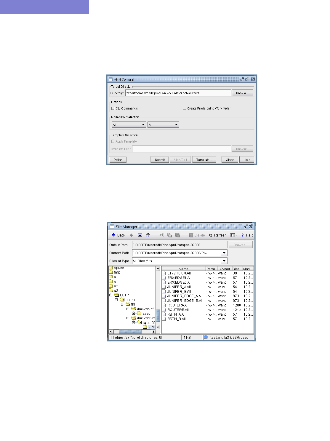
VIRTUAL PRIVATE NETWORKS*
10-44 Copyright © 2014, Juniper Networks, Inc.
10
92. In order to generate configlets in batch for several of the VPNs in a network, you may use the VPN Configlet
window (accessed via the Design > Configlets/Delta > VPN Configlet menu), shown in the following
figure, where you can specify a particular directory (specified in the Directory box) to store the generated VPN
configlets. In addition, you may also choose to generate configlets for particular nodes or VPNs via the
Node/VPN dropdowns.
Figure 10-75 VPN Configlet menu
Select “CLI Commands” before clicking “Submit” to also generate the corresponding CLI commands
corresponding to the configlet.
The following figure shows a VPN directory that contains all of the generated VPN configlets for the network.
Figure 10-76 VPN directory with the generated VPN configlets
An example of a generated VPN configlet is shown in the following figure.
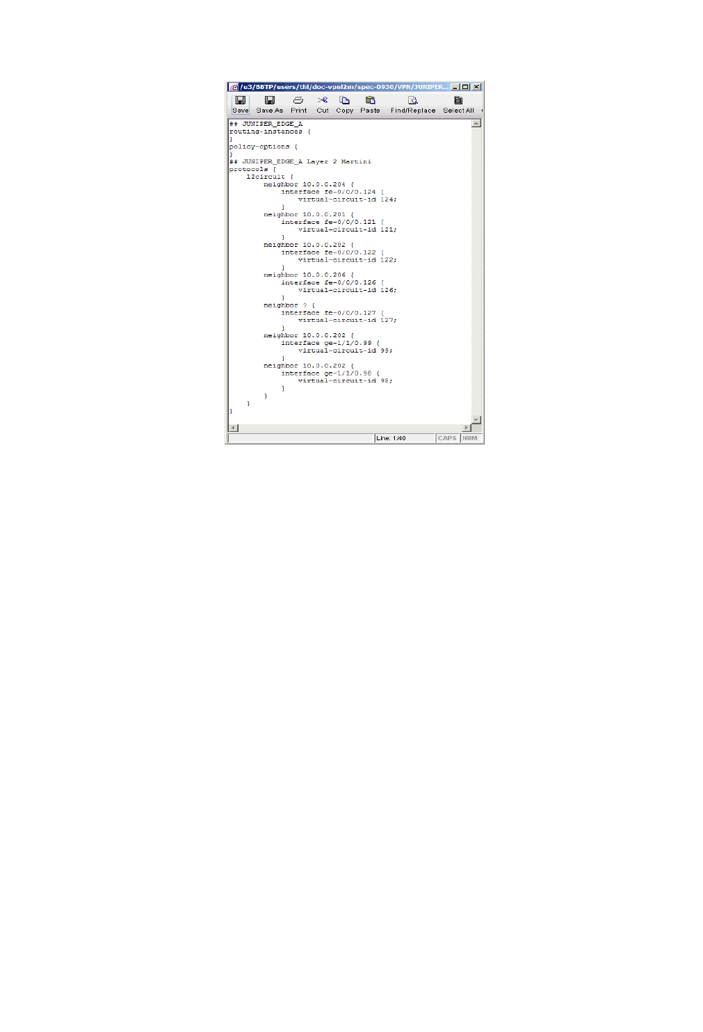
VIRTUAL PRIVATE NETWORKS*
Copyright © 2014, Juniper Networks, Inc. 10-45
. . . . .
Figure 10-77 The configlet generated for JUNIPER_EDGE_A
VIRTUAL PRIVATE NETWORKS*
10-46 Copyright © 2014, Juniper Networks, Inc.
10
Adding Traffic Demands in a VPN via the Add Demands Windows
For what-if studies, you can add multiple traffic demands between routers in the same VPN via the Add Multiple
Demands window and single traffic demands via the Add Demand window.
93. To add multiple demands for a VPN, select Modify > Elements > Demands, Add > Multiple Demands.
From the Type select box in the Placement (A x Z) section, choose the desired VPN type. Then select a VPN to
automatically populate the NodeA and NodeZ columns with routers from the selected VPN.
94. Fill out the rest of the window with the desired specifications and then click “Add” to add the demands. The
following figure shows an example where a full-mesh of 182 1M demands are added between the PE routers in
a L3 VPN called INTER-AS.
Figure 10-78 Adding a full-mesh of demands in the VPN called INTER-AS VPNs
95. To add a single VPN demand, bring up the Add Demand window and find the particular VPN of interest under
the Owner dropdown selection box. Note that if the owner is not listed, you may need to create it from the VPN
window as explained in Forming Customer Groups on page 10-41. Once a particular VPN (Owner) has been
selected, proceed to specify node A and node Z routers, and any relevant attributes, as you would for any other
demand. The following figure shows a demand being added for the VPN called L3VPN_PH44.
VIRTUAL PRIVATE NETWORKS*
Copyright © 2014, Juniper Networks, Inc. 10-47
. . . . .
Figure 10-79 Adding a single VPN demand
VPN Traffic Generation
96. Alternatively, you may add demands within the VPNs using the VPN Traffic Generation tool. Select Traffic
> Demand Generation > VPN to open the window as shown in Figure 10-80.
Figure 10-80 VPN Traffic Generation
97. Select, in the VPN table, one or more VPNs for which you wish to generate demands.
98. Next, specify the traffic source to use for the gravity model (either the Configured Interface BW or the Interface
Traffic Load). The Interface Traffic Load corresponds to the egress/ingress files in the File > Load Network
Files window, and the interfaceLoad_out and interfaceLoad_in files in the spec file. If selecting the Interface
Traffic Load, select which period to use (Mean, Peak, or specific period.)

VIRTUAL PRIVATE NETWORKS*
10-48 Copyright © 2014, Juniper Networks, Inc.
10
99. Specify the subscription ratio in percentages in the L3/L2K/VPLS and L2M/L2CCC textboxes. The subscription
ratio is a percentage of the router’s PE-CE interface bandwidth utilized for VPN traffic. The formula used to
calculate the demand is dependent on the type of VPN that is being applied.
100.“Generate demand between nodes instead of interfaces” can be selected to generate node-to-node
demands instead of interface-to-interface demands. In this case, demands are aggregated so that only one
demand is generated from nodeA to nodeB, instead of generating multiple demands from all interfaces on
nodeA to all interfaces on nodeB
101.Specify the demand file name. This can be an existing demand file, or the program will create the file if it does
not already exist.
102.If you are using an existing demand file, click on a radio button to select whether you wish to append the new
demands, or overwrite the file with the new demands. Note: If the demand file specified in the Demand file
name textbox does not exist, then either one of these selections will create the file for you.
103.Click on the Generate Demands button to generate a set of demands for the VPNs selected. The generated
demands will have uniquely assigned names and assigned with the owner of the VPN that it belongs to.
104.Use the File Manager to view the new demands in the specified demand file.
105.To import the new demands into the network model, open the File > Load Network Files window and select
the generated demand file in the “newdemand” field.
Layer 3 VPN, Layer 2
Kompella VPN, or VPLS
(Juniper) VPN
A gravity model is used to create a set of fully-meshed
demands for this type of VPN. The program takes the
configured interface bandwidth of all the interfaces in the
routers and calculates a bandwidth for the circuits using a
gravity formula. If the subscription ratio is not specified, the
default value is 10%.
Gravity model:
1. For each router in the VPN, add up the traffic load of all of
the interfaces that are associated with the VPN. This is the
weight of the router.
2. Let Wi be the weight of router i. Then the traffic from router i
to router j is Wi * Wj / (-Wi + W1+W2...Wn), where n is the
number of routers in the VPN.
3. The bandwidth of the demand is calculated by multiplying
the result of the previous step by the subscription ratio.
Layer 2 Martini VPN or
Layer 2 CCC VPN
One demand is generated for each circuit that belongs in this
type of VPN. The bandwidth of the demand is based on the
interface bandwidth multiplied by the percentage specified by
the user in the subscription ratio field. If the subscription ratio
is not specified, the default value is 10%.
VIRTUAL PRIVATE NETWORKS*
Copyright © 2014, Juniper Networks, Inc. 10-49
. . . . .
VPN-Related Reports
To study and analyze the VPNs, as well as the impact that VPN traffic creates in your network, you may use the
information from variety of reports that can be found in the Report Manager (accessible via Report > Report
Manager).
106.You can view the Demand Route Cost Report under the Network Reports > Demand Reports folder
to view demand information per VPN.
107.To view planned bandwidth and worst delay information for VPN-related demands, select the CoS Demands
Report and find the VPN of interested (listed in the Owner column).
108.To view details of the particular types of VPNs in your network, select the appropriate report from the Network
Reports > VPN folder (e.g. the Layer 3 report).
The following figures show a few VPN-related reports that can be generated.
Figure 10-81 L2 Martini VPN Report generated in the VPN Section of the Report Manager
VIRTUAL PRIVATE NETWORKS*
10-50 Copyright © 2014, Juniper Networks, Inc.
10
Figure 10-82 A L3 VPN Report generated in the VPN Section of the Report Manager
Figure 10-83 VPN Export-Import report
VIRTUAL PRIVATE NETWORKS*
Copyright © 2014, Juniper Networks, Inc. 10-51
. . . . .
VPN Monitoring and Diagnostics (also requires Online Module)
The VPN Module together with the Online Module provides you with VPN monitoring and diagnostics
capabilities for a live router network. For detailed information about how to use the Online Module for a real
network, please refer to the Management & Monitoring Guide.
109.First you would need to perform network data collection using the Task Manager (please refer to the
Management & Monitoring Guide for more information about how to use the Task Manager for auto
network discovery and network data collection). Upon completion of network configuration collection, the
program constructs the network model that includes all the configured VPNs in the network.
110. For a PE router, you may run “show” commands (accessible via the Run CLI... menu by right-clicking on a
node in the topology map). Click the arrow next to the Commands list to select a VPN category to view the
available CLI commands for VPNs.
111. To observe the network traffic condition (e.g. between PE and CE), periodic sampling of interface traffic
statistics is performed by the Task Manager. The collected interface data can then be accessed in the form or
reports and charts. The following figure shows a PE->CE interface traffic chart for router SFO.
Figure 10-84 PE->CE interface traffic chart (for PE router SFO)
112. In the Report Manager, a VPN Interface Traffic report is available under Network Reports > VPN that
lets you see the interface traffic for each node of each VPN, as shown in the following figure.
VIRTUAL PRIVATE NETWORKS*
10-52 Copyright © 2014, Juniper Networks, Inc.
10
Figure 10-85 VPN Interface Traffic report
113. To verify connectivity and to measure delay and loss, you can also perform VPN diagnostics (e.g., CE-CE Ping
and Traceroute) as shown in the following figures.
Figure 10-86 In live mode, perform ping/trace routebetween routers from the IP VPN window
114. From the right-click menu of the VPNView topology, you can many functions (e.g. path tracing, running CLI
commands, and connect to device).
VIRTUAL PRIVATE NETWORKS*
Copyright © 2014, Juniper Networks, Inc. 10-53
. . . . .
115. With Java Web Start installed, you may also perform VPN monitoring and diagnostic functions from a web
browser, as well as to access VPN-related reports and charts. The following figures are meant illustrate just
some of the web features available. Please consult the Management & Monitoring Guide more detailed
information.
Figure 10-87 VPN view from the web for VRF, RT, RD, PE-CE interface, VPN traps information
VIRTUAL PRIVATE NETWORKS*
10-54 Copyright © 2014, Juniper Networks, Inc.
10
Figure 10-88 View PE->CE interface traffic from the web
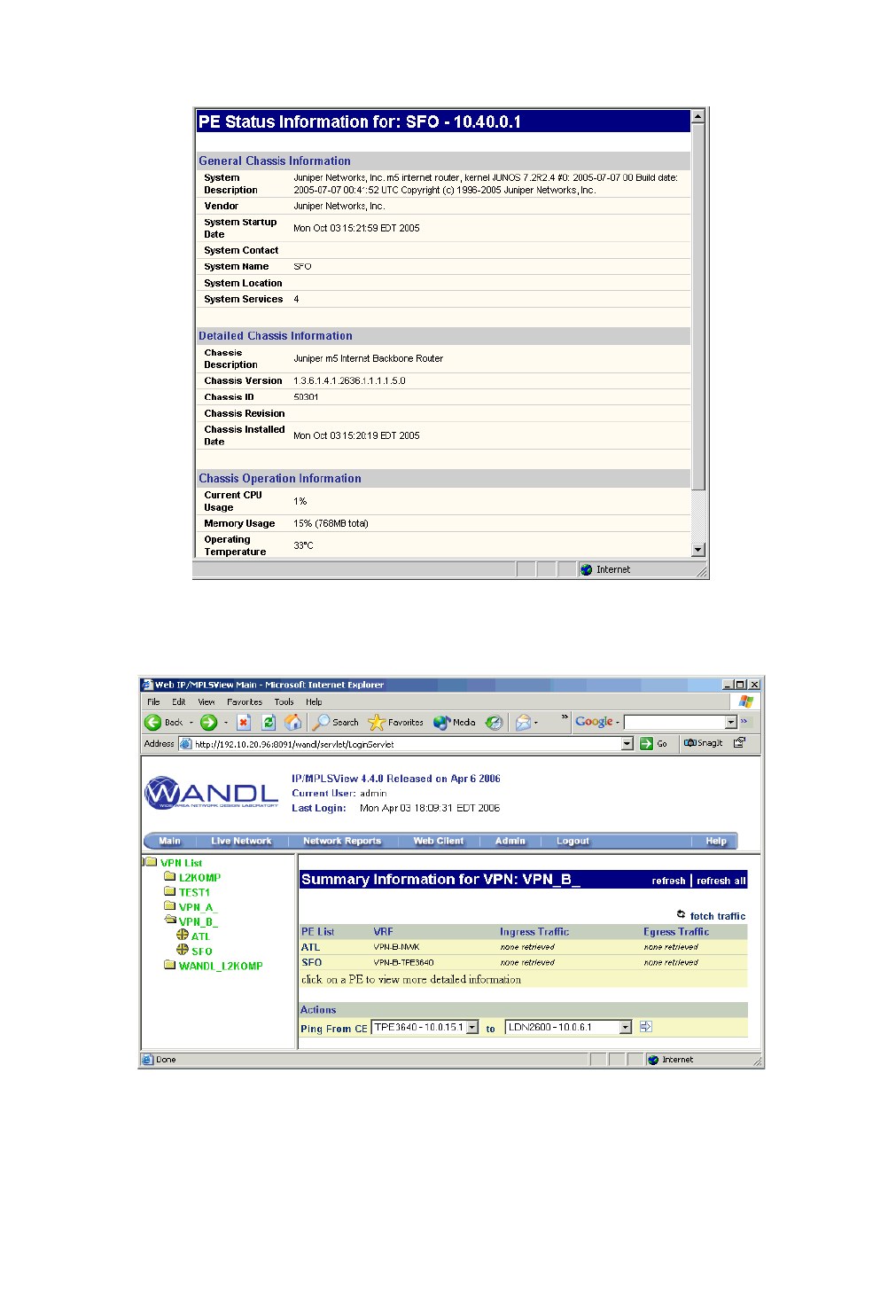
VIRTUAL PRIVATE NETWORKS*
Copyright © 2014, Juniper Networks, Inc. 10-55
. . . . .
Figure 10-89 Show PE status (system, CPU/memory, etc)
Figure 10-90 Access VPN summary information

VIRTUAL PRIVATE NETWORKS*
10-56 Copyright © 2014, Juniper Networks, Inc.
10

Copyright © 2014, Juniper Networks, Inc. 11-1
. . . . .
. . . . . . . . . . . . . . . . . . . . . . . . . . . . . . . . . . .
GRE T
UNNELS
11
eneric Routing Encapsulation Tunnels (GRE) can either be imported from the router configuration
files, or created from the WANDL Graphical Interface for what-if studies. Afterwards, the GRE tunnel
path and details can be viewed, as well as the details and paths of the demands routed over the GRE
tunnel. The GRE tunnel can also be referenced as the next hop of a static routing table.
The following GRE statements are parsed during the config import:
CISCO
interface Tunnel<id>
ip address <ip-address> <mask>
tunnel source (ip-address|type number)
tunnel destination ip-address {hostname | ip-address}
JUNIPER
[edit interfaces interface-name unit logical-unit-number tunnel] level:
gr-1/2/0 {
unit 0 {
tunnel {
source <ip-address>;
destination <ip-address>;
}
}
}
WANDL maps these statements into entries in the intfmap (interface), tunnel, and bblink file.
EXAMPLE INTFMAP ENTRY
0.0.0.0/0,ATL,Tunnel4,active, ,,0, , , ,,,,,,,,,,,,0,,
0.0.0.0/0,BOS,Tunnel5,active, ,,0, , , ,,,,,,,,,,,,0,,
EXAMPLE TUNNEL ENTRY
#Tunnel Src Destination BW Type_Field
Tunnel4 ATL 172.16.1.2 0 R,A2Z,GRE,SOURCE=172.16.1.6,MASK=0000ffff 7,7
Tunnel5 BOS 172.16.1.6 0 R,A2Z,GRE,SOURCE=172.168.1.2,MASK=0000ffff 7,7
In the tunnel entry, note that the tunnel source of Tunnel4 matches the destination IP address of Tunnel5, and the
tunnel source of Tunnel5 matches the destination IP address of Tunnel4.
EXAMPLE BBLINK ENTRY
#Linkname NodeA NodeZ Vendor Count TrunkType [MISC]
ATL_TUNNEL4 ATL BOS DEF 1 GRELINK C1=Tunnel4 C2=Tunnel5 # UP #!
Each GRELINK entry references one GRE tunnel interface for the A to Z direction using C1=<interface> and one
GRE tunnel interface for the Z to A direction using C2=<interface>. By default, the status of a link of type
GRELINK will be down/deleted if one of the tunnels fails to be routed. If both tunnels are routed, the GRE link is
considered to be up, and traffic over a GRELINK will then be routed over the links traversed by the GRE tunnel.
In some cases, however, the software fails to route the GRE tunnel due to incomplete information. In those cases, the
GRELINK may actually be up but there is no information to determine whether the tunnels are successfully placed.
G

GRE TUNNELS
11-2 Copyright © 2014, Juniper Networks, Inc.
11
For example, the the config files for the routers necessary to route the GRE tunnel may be missing if they belong to
another service provider. To avoid setting the GRELINK status to down in this scenario, set virtualgrelink=0 in the
dparam file to treat GRELINKs as normal links.
When to use
Use these procedures if you have Cisco GRE tunnels configured in your network.
Prerequisites
If you wish to perform this task, you should have a set of router configuration files with GRE tunnels configured.
Related Documentation
For a detailed description of the IP/MPLSView client windows, refer to Chapter 37, Router Reference.
Outline
1. Importing GRE Tunnel Information from Router Configuration Files on page 11-2
2. Adding a GRE Tunnel on page 11-2
3. Using Static Routes to Route over a GRE Tunnel on page 11-4
4. Viewing GRE Tunnels on page 11-5
5. Viewing Demands over GRE Tunnels on page 11-6
Detailed Procedures
Importing GRE Tunnel Information from Router Configuration Files
1. To import the router configuration files, select File>Import Data and follow the Import Network Wizard.
Alternatively, you may run the getipconf program in text mode. Please refer to Chapter 2, Router Data
Extraction for more detailed information.
2. After importing the config files, view the Integrity Checks report by selecting Report > Report Manager and
then selecting the Configuration Report>Summary of Integrity Checks Report item.
The “Asymmetric GRE tunnels” integrity check will appear if there is a GRE tunnel defined at one end of
the tunnel but not the other. Additionally, the “Inconsistent GRE tunnels protocol” integrity check will
appear if the IGP protocol defined on one end of the GRE tunnel is different than the IGP protocol defined on
the other end. These integrity checks are included under the TUNNEL category. To view the details of an
integrity check, right-click on the row and select Display item(s) for this msg ID/Category.
Adding a GRE Tunnel
If the configuration files are available, GRE tunnels can be added to the configuration files by adding two tunnel
interfaces and specifying the tunnel source and destination, and then importing the configuration files as described in
Importing GRE Tunnel Information from Router Configuration Files on page 11-2.
However, if the configuration files are not available, a what-if study can still be performed by adding the GRE tunnel
interfaces, tunnels, and corresponding GRE link through the Java interface as explained below.
ASSIGNING IP ADDRESSES TO NODES/INTERFACES
Before starting, IP addresses should be assigned to the nodes/interfaces that will be used as the source and
destination of the GRE tunnel.
3. Select the Modify button to enter Modify action mode.
4. To add an IP address for a node, select Modify > Elements > Nodes and double-click a node entry. In the
Properties tab, fill in the IP address field and click OK.
5. To add an interface, select Modify > Elements > Interfaces and click the Add button. Enter in the interface
name according to the convention of the hardware vendor of the router. Then enter the router it resides on and
the interface IP address and click OK.
GRE TUNNELS
Copyright © 2014, Juniper Networks, Inc. 11-3
. . . . .
ADDING A GRE TUNNEL INTERFACE
6. Select the Modify button to enter Modify action mode. Then select Modify > Elements > Interfaces...
7. Next, add two interfaces for the GRE tunnels, one at each end node of the tunnel. Note that vendor-specific
naming conventions should be followed here, e.g., Tunnel1 for Cisco, or gr-1/0/2 for Juniper.
ADDING A GRE TUNNEL
8. Select Modify > Elements > Tunnels... and select Add > One Tunnel.
9. Use the same name for the Tunnel ID that was used for the GRE interface, and use the same case, as this field is
case-sensitive. Then select the source and destination nodes of the tunnel.
10. Add “,GRE,SOURCE=<ip-address | interface_name>” to the comma-separated Type field, using the name or
IP-address of the interface or the IP-address of the node that will be the GRE tunnel source, e.g.
GRE,SOURCE=172.16.1.3 or GRE,SOURCE=FastEthernet1/1. This IP address or interface name should either
be defined on the node or interface as explained in Assigning IP addresses to nodes/Interfaces on page 11-2.
11. Click the Location tab and enter in the IP address of the destination node.
12. The Bandwidth (BW) field can be set to 0.
13. Create another tunnel for the reverse direction.
Figure 11-1 Adding a GRE Tunnel
ADDING A GRE LINK
Associated with the GRE tunnel pair should be a GRE link that can be advertised to the IGP to be used for routing.
The following steps indicate how to add a GRE link through the Java interface.
14. Select Modify > Elements > Links... and click “Add...” in the resulting window to open the Add Link
window.
15. Provide a name for the GRE link. For the Trunk field, select GRELINK.
16. Select the Location tab. Click the “...” button next to the Interface A field and select the GRE tunnel for the A-
>Z direction. Click the “...” button next to the Interface Z field and select the GRE tunnel for the A->Z direction.
If the GRE tunnel does not appear in the list, make sure that the GRE tunnel interfaces are named according to
the convention of the appropriate hardware vendor.

GRE TUNNELS
11-4 Copyright © 2014, Juniper Networks, Inc.
11
Figure 11-2 Specifying the GRE Tunnels used to form the GRE Link
17. Select the Protocols tab to specify the IGP that this tunnel is advertised to. Set the desired IGP protocol to
“Yes.” If no protocol is selected, then no demand will route over this link unless a static routing table is entered
setting the next hop to the GRE tunnel.
18. Click the Design mode button to switch to Design mode.
TROUBLESHOOTING A GRE LINK/TUNNEL DEFINITION
19. If the GRE tunnel and link are defined correctly, the GRELINK status should be “Planned.” If not, check the
Console window for diagnostics messages. The two interfaces of the link need to be associated with GRE
tunnels of the same name and those GRE tunnels should be routed. Check that the tunnel name has the same
case as the interface (e.g., Tunnel1 notTUNNEL1).
20. If the GRE tunnel is not routed due to the fact of incomplete network information, i.e., missing configuration
files, you can force the link to be treated as a normal link. First save the network using File>Save Network...
and close the network. Then edit the dparam.<runcode> file from the File Manager, and set virtualgrelink=0.
Then reopen the network and check that the statuses of links with trunktype GRELINK status are no longer
“Deleted.”
Using Static Routes to Route over a GRE Tunnel
21. Select Modify > Protocols > Static Route Table.. and then click “Add.”
22. For the Node field, select the tunnel’s source node.
23. Select a destination node and admin weight.
24. For the Next Hop, select the radio button for Tunnel and then select the GRE tunnel at the node.
GRE TUNNELS
Copyright © 2014, Juniper Networks, Inc. 11-5
. . . . .
Figure 11-3 Static Route with GRE Tunnel as Next Hop
25. Note that for the static route to be used, the demands that will take the static route must include an IP address for
the destination node in the Demand window’s Location tab.
Viewing GRE Tunnels
26. Select Network > Elements > Tunnels... in View or Design mode.
27. To filter for all GRE tunnels, click the Filter icon and type GRE in the Type field. (Alternatively, filter on
“Type=GRE” in the Advanced Filter).
Figure 11-4 Filtered GRE Tunnels
28. Select the GRE tunnel to view and then click Show Path to view its path.
Figure 11-5 GRE Tunnel routed over LSP Tunnel
GRE TUNNELS
11-6 Copyright © 2014, Juniper Networks, Inc.
11
Note that a tunnel itself can route over a tunnel (in this case, an LSP tunnel). The portion that travels over
another tunnel is colored in purple.
Viewing Demands over GRE Tunnels
29. Right-click over the GRE link either on the map or in the Network Info window, Links view pane. Select
“View > Demands on/thru Link” to view the demands routed over the GRE link.
30. Select a Demand and click “Show Path” to view its path over the GRE tunnel.
Figure 11-6 Demand Routed Over GRE Tunnel via Static Route

Copyright © 2014, Juniper Networks, Inc. 12-1
. . . . .
. . . . . . . . . . . . . . . . . . . . . . . . . . . . . . . . . . .
M
ULTICAST
*
12
his chapter describes how to use the Multicast feature of the WANDL software. Internet Protocol (IP)
multicast is a bandwidth-conserving technology that allows a single stream of data to be simultaneously
delivered to multiple recipients, resulting in tremendous savings on server resources and efficient use of
network bandwidth.
When to use
Using the Multicast feature will provide a good picture of how the network will perform under different scenarios of
multicasting as well as highlight potential problems when running multicast in the network. Since multicast offers
enhanced efficiency and optimized performance, it is often used in financial applications, streaming multimedia,
enterprise resource applications, and any one-to-many data push applications.
Prerequisites
Prior to beginning this task, you should have started up the WANDL software and opened a spec file.
*Note that a special password is required for the Multicast feature. Please contact your Juniper representative for
more information.
Related Documentation
For an overview of the WANDL software or for a detailed description of each feature and the use of each window,
refer to the General Reference Guide.
Recommended Instructions
Following is a high-level, sequential outline of the functionalities of the Multicast feature.
1. Open the advanced dog network in $WANDL_HOME/sample/original/router/advanced/dog.
2. Create a multicast group as described in step 1 on page 12-1 through step 5 on page 12-1.
3. Create multicast demands as described in step 6 on page 12-2 through step 8 on page 12-3.
4. View information on effects of multicast demands in the network, such as paths and link utilization, in step 9 on
page 12-3 through step 13 on page 12-5.
5. Compare a network using multicast with one using unicast as shown in step 15 on page 12-6 through step 21 on
page 12-6.
Detailed Procedures
The following steps will guide the user through the process of creating multicast groups, creating demands for
multicast groups, viewing the paths of the multicast demands, and viewing reports of the multicast demands.
Creating Multicast Groups
1. First, for the sake of simplicity, delete all the demands in the advanced dog network. This will make it easier to
view the multicast demands that will be added later in this guide. To do this, switch to Modify mode and select
Modify > Elements > Demands.... In the resulting window, click the Delete button and then select “All
Entries”.
2. In Modify mode, click on Modify > Protocols > Multicast > Multicast Group to bring up the Multicast
Group window.
3. Click the Add button in the Multicast Group window to bring up the Add Multicast Group window.
4. Enter in a Destination IP Address, Name, and RP (Rendezvous Point) Address for the multicast group. In
this example, 10.10.10.8 (WDC) will be used as the RP. If RP Addresses are already defined on Nodes, then
T

MULTICAST*
12-2 Copyright © 2014, Juniper Networks, Inc.
12
they will be populated in this drop-down box. Then, add the first six routers from the list of Available Routers
to the Selected Routers list. See Figure 12-1 below for how the window should look at this point.
Figure 12-1 Adding a Multicast Group
5. Click the Add button when all the properties of the multicast group have been set correctly. This will add the
multicast group to the network. Close the Add Multicast Group and the Multicast Group windows as they
are no longer needed.
Creating Multicast Demands
6. Click on Modify > Elements > Demands, Add > Multiple Demands. In this section, you will add six
100M flows from node SFO to all nodes in the multicast group.
7. For BW, type in “100M”. In the Type field, we want to indicate that the new flows are multicast flows. Click on
the Type button. This will bring up the Demand Type Parameter Generation window. In this window,
select the Multicast checkbox and “225.1.1.1”. Set PIM Mode to “PIM-SM” (Protocol Independent Multicast
- Sparse Mode). Back in the Add Multiple Demands window, we will now specify that the new flows be
created from node “SFO” to all nodes in multicast group 225.1.1.1. To do this, populate the NodeA list with
just “SFO” by using one of the Filter buttons. For the NodeZ list, select 225.1.1.1 from the dropdown menu
just above it to select the multicast group; all the nodes in the multicast group 225.1.1.1 will appear in the
NodeZ list. See figure Figure 12-2 below.
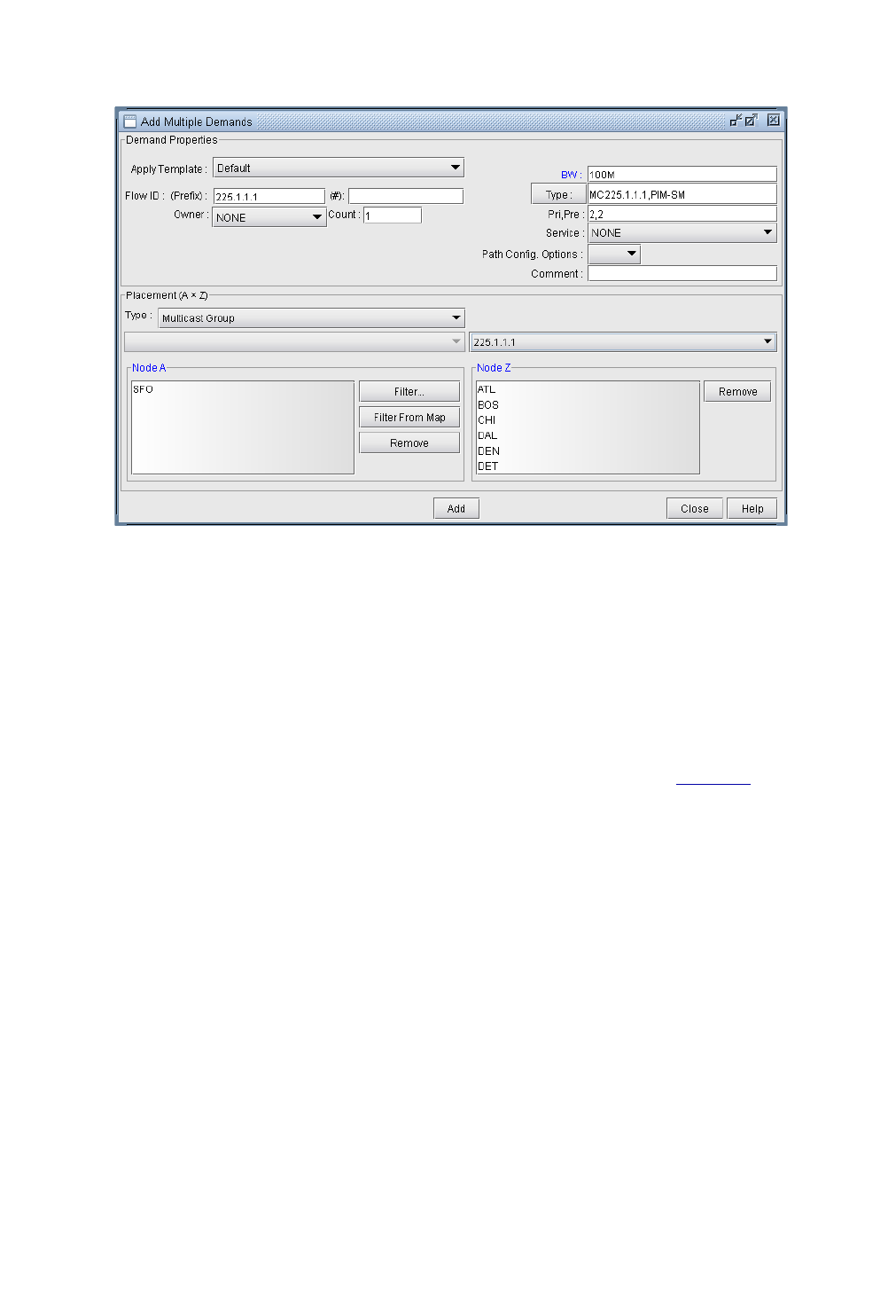
MULTICAST*
Copyright © 2014, Juniper Networks, Inc. 12-3
. . . . .
Figure 12-2 Adding Multicast Demands
8. When all the parameters above have been set correctly, click the Add button to add these six multicast flows to
the network.
Viewing Multicast Demands in the Network
9. At this point, a multicast group has been defined and demands, or flows, to the multicast group have been
created. Now, information on these demands and how they fit into the network can be examined. First, switch to
View mode. When the program asks whether or not to Update Demand Routing Tables, click Yes.
10. The first thing to notice is that, even though there are multiple recipients of the 100M flows from node SFO, the
link utilization appears uniform throughout all the utilized links, as shown in Figure 12-3 below. This is typical
of multicast networks and is a good example of the advantage of multicast over traditional unicast networks. In
traditional unicast networks, one would expect “high” utilization near the source and “lower” utilization as the
flows fan out to the recipients. Here, the utilization is “low” everywhere.
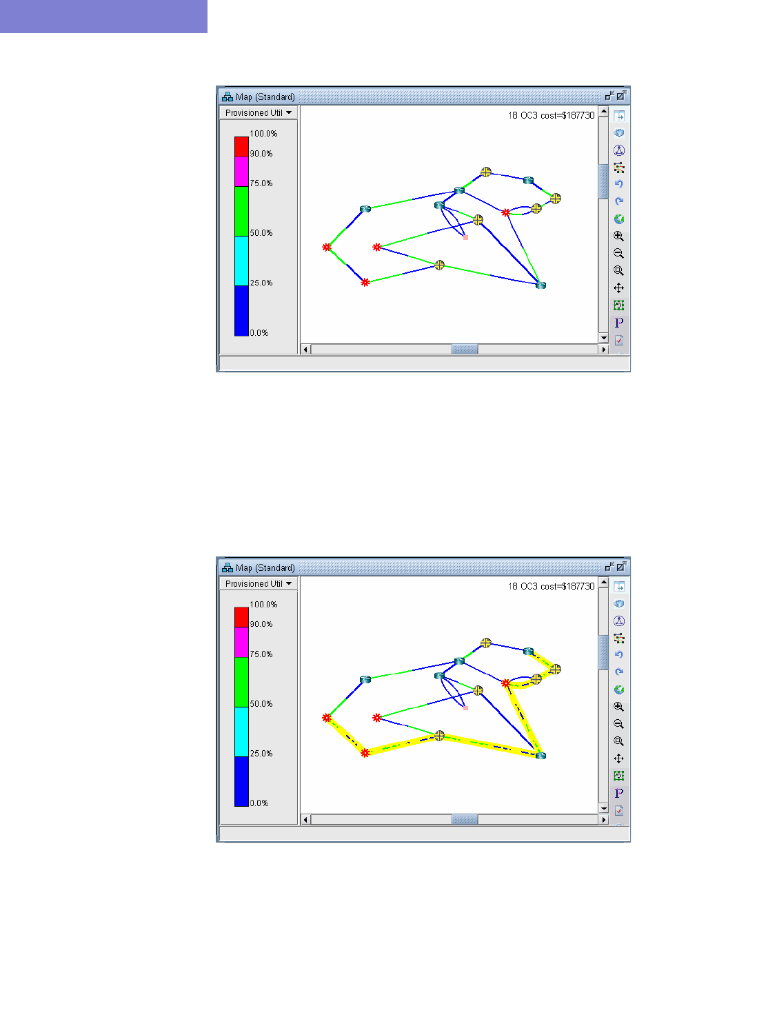
MULTICAST*
12-4 Copyright © 2014, Juniper Networks, Inc.
12
Figure 12-3 Link Utilization in a Multicast Network
11. Now, click on Network > Elements > Demands. The Demands window lists all the demands in the
network, which in this example should all be multicast demands.
12. Highlight any of the rows in the demands table and click the Show Path button. This will display the path
taken by the demand according to the unicast protocol being used. The default protocol is PIM-SM (Protocol
Independent Multicast - Sparse Mode). This can be changed for each demand by modifying the demand’s Type
field.
Figure 12-4 Path of a Demand from SFO to BOS
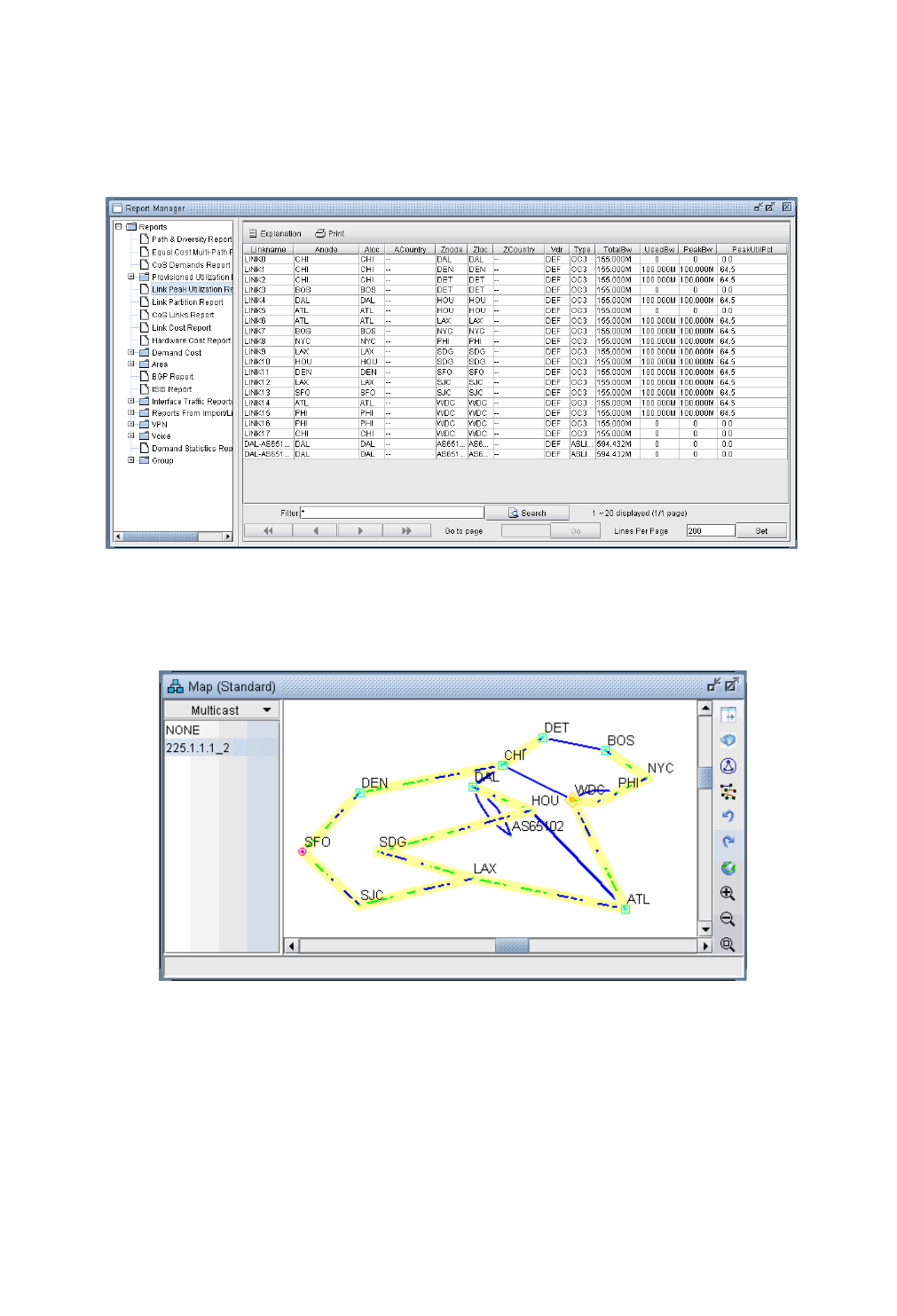
MULTICAST*
Copyright © 2014, Juniper Networks, Inc. 12-5
. . . . .
13. Detailed information on link utilization resulting from the multicast demands can be viewed through the Peak
Link Utilization Report under Simulation Reports > Network StatisticsTo do this, click on Report >
Report Manager, then select Peak Link Utilization from the list of reports in the Report Manager
window. Notice in the example below that all the utilized links display a utilization of 100M.
Figure 12-5 Link Peak Utilization Report for a Multicast Network
14. Select Subviews > Multicast from the map to view the multicast tree graphically.
Figure 12-6 Multicast Subview
Note the special icons used for the source (SFO), the Rendezvous Point (WDC) and the subscribers.
If there are multiple trees listed, you can <Ctrl>-click to highlight multiple trees at once. Each multicast tree will
have a different color, e.g., yellow, green, blue. Overlaps between trees will also have a unique color, e.g.,
orange.
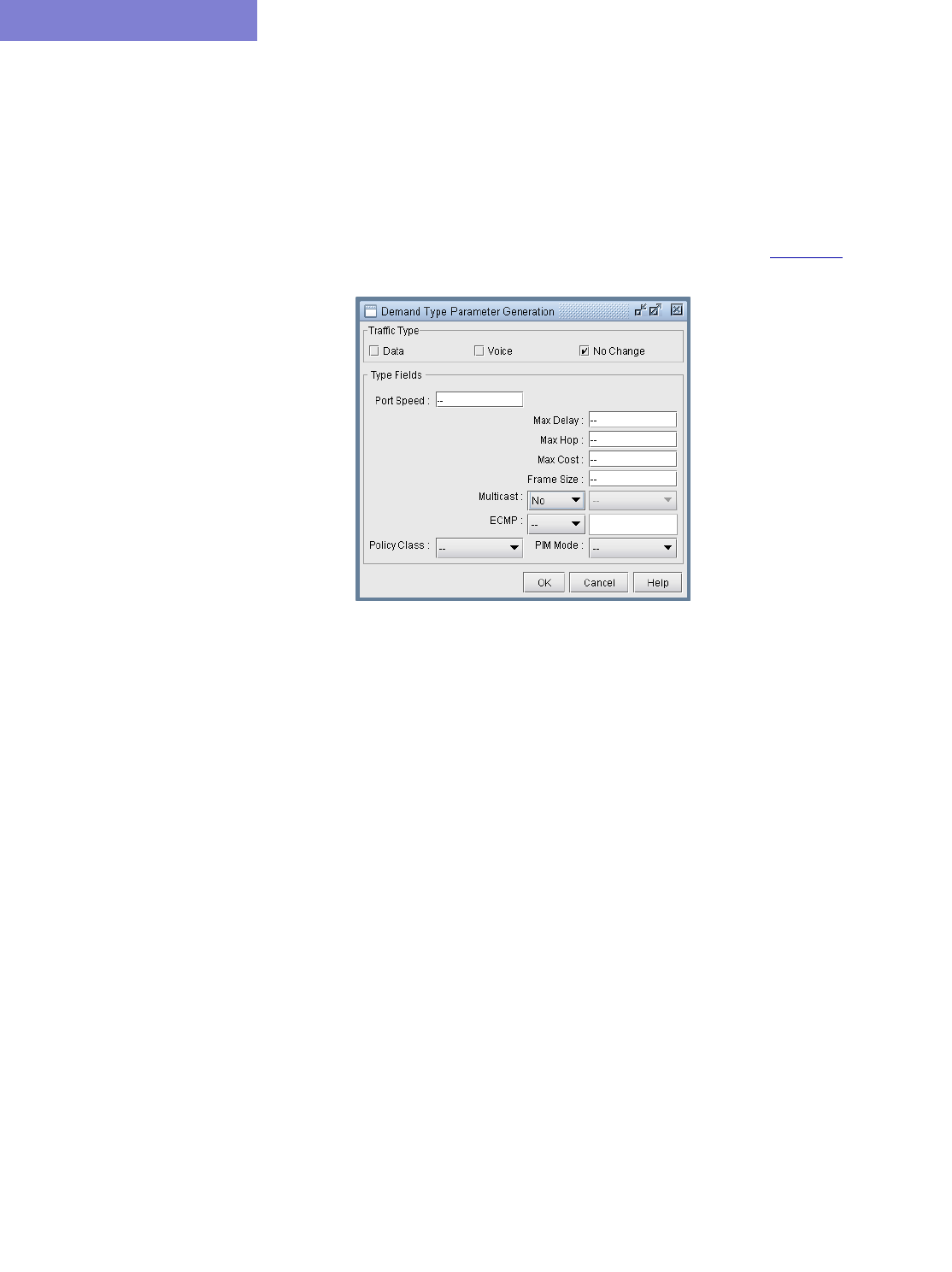
MULTICAST*
12-6 Copyright © 2014, Juniper Networks, Inc.
12
Comparing Multicast with Unicast
15. It may be of interest to see what the network would look like if, instead of multicast, all the demands were
routed according to traditional unicast protocols. This can be done easily by disabling multicast on all the
demands. To do this, first switch to Modify mode and click on Modify > Elements > Demands....
16. In the Demands window, click the Modify button and then select “All Entries”.
17. A Modify Demands window will appear. Click the Type button in this window to bring up the Demand
Type Parameter Generation window.
18. Click the dropdown menu next to the Multicast field and select No, as shown in Figure 12-7 below.
Figure 12-7 Modifying the Demand Type to Disable Multicast
19. Click the OK button in the Demand Type Parameter Generation window, then click the OK button in the
Modify Demands window. Multicast will now be disabled on all the demands, which will now be routed
according to traditional unicast protocols.
20. Click the Update button on the main menu bar. This is required to force the program to recalculate paths for
demands after they have been modified.
21. Now the link utilization displayed in the Map window will reflect the unicast “version” of the network. Notice
the difference between the link utilization colors of this network and those of the multicast network. In
particular, note that the links near the source, SFO, all appear to be overutilized in the unicast network, whereas
in the multicast network the links near the source were only moderately utilized, similar to the links near the
recipients.
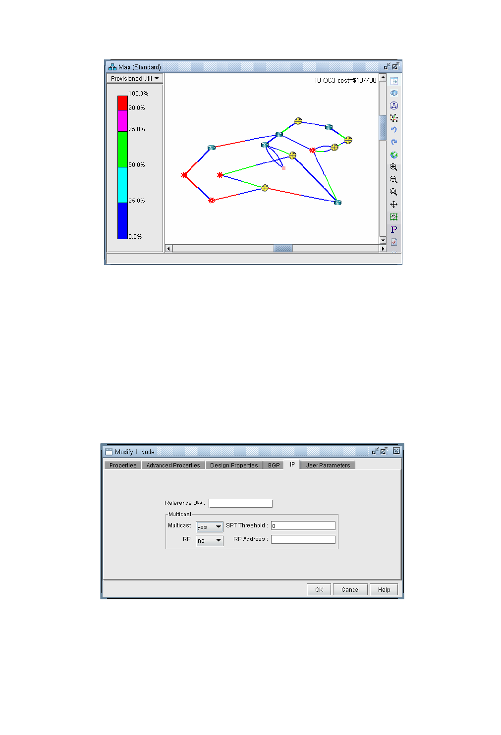
MULTICAST*
Copyright © 2014, Juniper Networks, Inc. 12-7
. . . . .
Figure 12-8 Link Utilization in a Unicast Network
Multicast SPT Threshold
When using sparse mode multicast, the SPT Threshold value can be set for a particular node to determine whether
the Rendezvous Point (RP) or the Shortest Path Tree is used for routing. If the SPT Threshold is set to 0, the RP
will be ignored, and the Shortest Path Tree will always be used. If the SPT Threshold is set to “Infinity” then the
RP will always be used, and the Shortest Path Tree will never be considered. To set the SPT Threshold for a node,
right click on a node in Modify mode and select Modify Nodes. Then, click on the IP tab to display the SPT
Threshold input field. Here, the user can enter “0” or “Infinity” as described above.
Figure 12-9 Modify Node: Setting the SPT Threshold
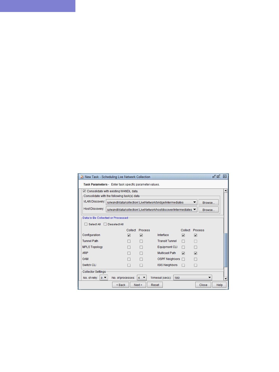
MULTICAST*
12-8 Copyright © 2014, Juniper Networks, Inc.
12
Reports
For reporting purposes, each source-destination pair is listed as one entry in the Network Reports > Demand
Reports > Demand Path & Diversity report (PATHRPT) in the Report Manager.
Summary info is reported in the explanation portion of the report including the total number of multicast trees
and bandwidth information. Click the Explanation... button for this summary info. An example is shown
below:
* 1 MCtrees (Tree Bandwidth=100.000M), Average # of leaves=6.00
* 1 routed(Bandwidth=100.000M, average #link/tree=13.00)
Here, the leaves refer to the destination nodes of the multicast tree. The links per tree indicate the number of
links used by the tree.
Simulation
During a simulation, each source-destination pair for the multicast tree is by default counted as a separate demand.
To count the entire tree and its bandwidth as belonging to one multicast demand, add the following design parameter
in the dparam file: “MCsimrptopt=1”.
Collecting Multicast Path Data from Live Network
In the Schedule Live Network Collection task in the Task Manager, check the Multicast Path box as shown in the
following figure. This ensures that the multicast routing table is collected. The multicast tree and subsequent display
is constructed via the olist and ilist that is contained in the collected multicast routing table.
Figure 12-10 Multicast Path Collection Option

MULTICAST*
Copyright © 2014, Juniper Networks, Inc. 12-9
. . . . .
The collected data is stored in directory /u/wandl/data/collection/.LiveNetwork/multicast_path/. The following is an
example for IOS of the multicast routing table that is collected.
show running | include hostname
hostname BEK3640
BEK3640#show ip mroute
IP Multicast Routing Table
Flags: D - Dense, S - Sparse, B - Bidir Group, s - SSM Group, C - Connected,
L - Local, P - Pruned, R - RP-bit set, F - Register flag,
T - SPT-bit set, J - Join SPT, M - MSDP created entry,
X - Proxy Join Timer Running, A - Candidate for MSDP Advertisement,
U - URD, I - Received Source Specific Host Report,
Z - Multicast Tunnel, z - MDT-data group sender,
Y - Joined MDT-data group, y - Sending to MDT-data group
Outgoing interface flags: H - Hardware switched, A - Assert winner
Timers: Uptime/Expires
Interface state: Interface, Next-Hop or VCD, State/Mode
(*, 239.1.1.1), 1w4d/00:02:43, RP 22.22.1.1, flags: S
Incoming interface: Null, RPF nbr 0.0.0.0
Outgoing interface list:
Ethernet2/1.2, Forward/Sparse, 1w4d/00:02:43
(22.22.2.2, 239.1.1.1), 1w4d/00:03:23, flags: T
Incoming interface: Ethernet2/1.6, RPF nbr 88.88.0.18
Outgoing interface list:
Ethernet2/1.2, Forward/Sparse, 1w4d/00:02:43
(22.22.3.3, 239.1.1.1), 22:10:01/00:02:57, flags: PT
Incoming interface: Ethernet2/1.2, RPF nbr 88.88.0.2
Outgoing interface list: Null
(*, 224.0.55.59), 2d23h/00:03:06, RP 22.22.1.1, flags: S
Incoming interface: Null, RPF nbr 0.0.0.0
Outgoing interface list:
Ethernet2/1.2, Forward/Sparse, 2d23h/00:03:06
(10.33.3.2, 224.0.55.59), 00:22:58/00:02:34, flags: PT
Incoming interface: Ethernet2/1.5, RPF nbr 88.88.0.6
Outgoing interface list: Null
(*, 224.0.1.40), 1w4d/00:02:59, RP 22.22.1.1, flags: SJCL
Incoming interface: Null, RPF nbr 0.0.0.0
Outgoing interface list:
Ethernet2/1.5, Forward/Sparse, 2d16h/00:02:18
Ethernet2/1.2, Forward/Sparse, 1w4d/00:02:36
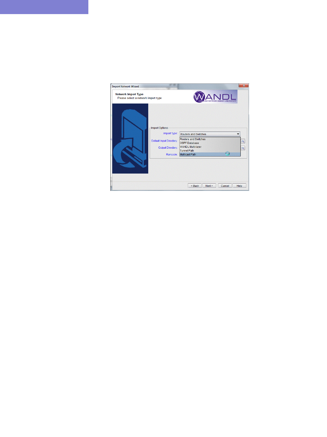
MULTICAST*
12-10 Copyright © 2014, Juniper Networks, Inc.
12
Importing Multicast Path Data
If the multicast path data is available by methods other than Schedule Live Network Collection, this data can be
imported using Import Network Wizard and selecting the Multicast Path option. This import feature currently
supports Cisco, Juniper, and Alcatel-Lucent vendors. The data collected from the multicast routing table should
contain information about the (S,G) or (*,G) groups in the Multicast Tree (e.g. for Cisco the command: show ip
mroute).
Figure 12-11 Import Network Wizard
Data Processing
After collecting specific multicast show commands for Cisco, Juniper and ALU, the file
called mcpath.x is created and automatically loaded to describe the multicast flows. The names of the flows are
derived from the multicast group IP address as follows:
•source_MulticastGroupAddress for (S,G)
•*_MulticastGroupAddress for (*,G)
The bandwidth of the multicast flow is derived differently depending on the vendor:
•for IOS, it is extracted from the Rate line from command “show ip mroute active”
•for IOS-XR, it is extracted from bps_in and bps_out from command "show mfib route rate". The average of
these two values is calculated as the flow bandwidth.
•for ALU, it is extracted from the Curr Fwding Rate line from command "show router pim group detail"
When multicast paths are imported, messages that point to errors or potential errors are written to the
Import_MCTree_log.runcode file located in the Log directory of the project spec file.
This Import_MCTree_log.runcode log file contains the following columns: Lineno, Error Code, Error Message,
Action, LineDetail. The Lineno column references which exact line within the mcpath.runcode file that is
referenced; the line at Lineno from mcpath.runcde itself is shown in the LineDetail column.
Various values for the Error Code column may be possible. Example; Path Ignored indicates that the path
specification is ignored; Path Error indicates that errors were encountered such as invalid IP addresses, Tunnel name
specified in path specification does not exist, there's a gap in the path specification, etc.

MULTICAST*
Copyright © 2014, Juniper Networks, Inc. 12-11
. . . . .
If a Path Error is encountered, the program may take one of the following actions:
•Ignored: Error detected, path specification ignored.
•Warning: Errors detected, no action taken. Example, some of the IP addresses in an explicit path specification
may not be defined in the network. The invalid IP addresses would still be remembered (i.e. would still be displayed
and saved) and the Warning code is printed.
•Fixed: For paths imported from tunnelpath.x file, the program would try to fix the paths if possible. The contents
of tunnelpath.x file are based on the CLI outputs of routers. The format can vary for each vendor. There are cases
where links between two different vendor nodes are not specified. If "Fixed" is printed, that means the a link is
automatically added by the program to account for the unspecified link.
For an explicit path specification, some of the IP addresses defined in the path specification may not be defined in
the network. In this case, the invalid IP addresses would be remembered (i.e. would still be displayed and saved) but
won't have effect on the routing simulation.
Tracing through the error messages may require reviewing the paths hop-by-hop (IP address by IP address), and
checking the raw multicast path data used to construct the tree. The Import_MCTree_log.runcode log file is meant to
assist in the troubleshooting.
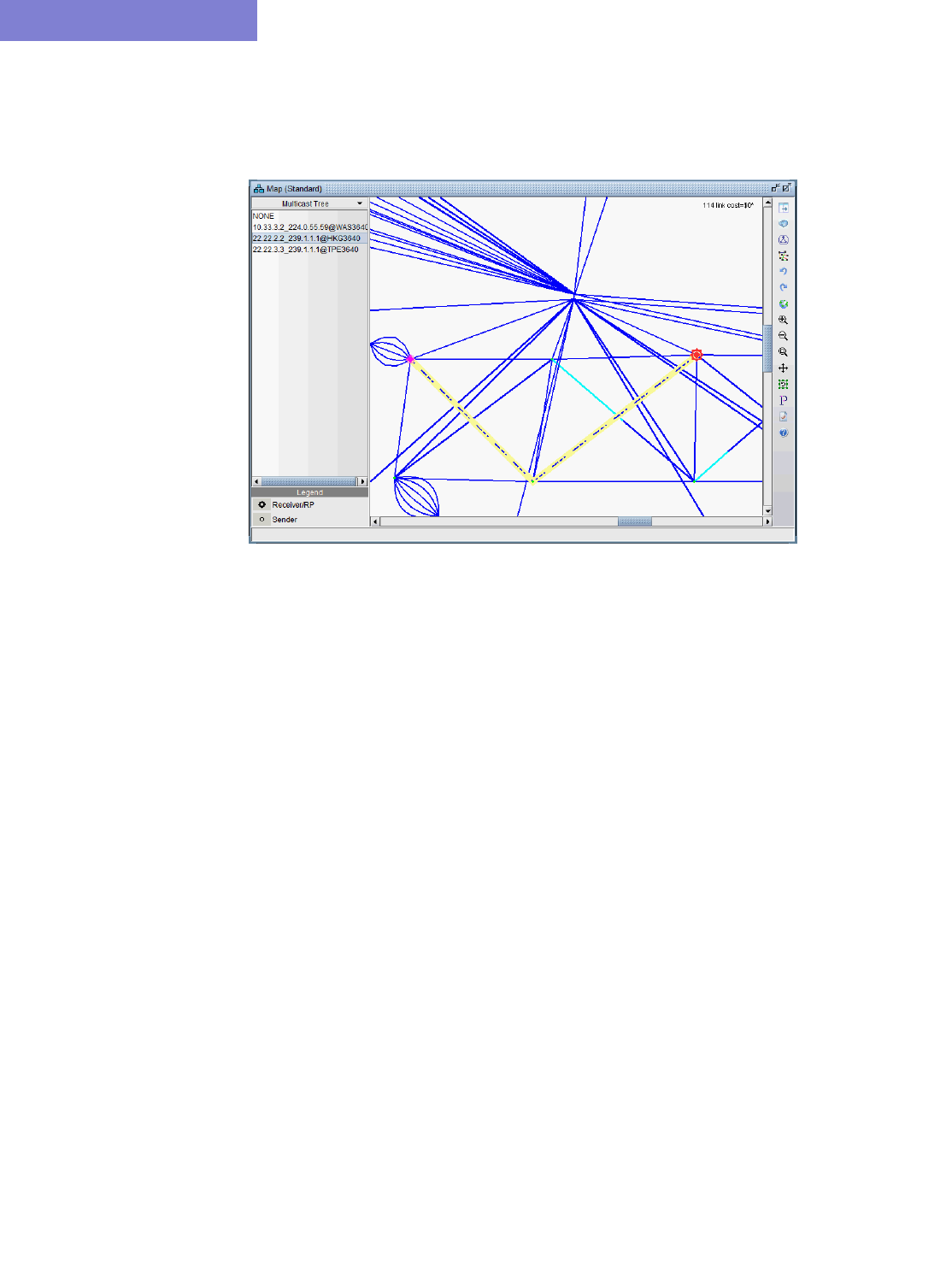
MULTICAST*
12-12 Copyright © 2014, Juniper Networks, Inc.
12
Viewing Multicast Trees
To view the multicast trees configured in the network, on the main topology map select Subview > Multicast Tree as
shown in the following figure. From this subview, the (S,G) or (*,G) tree can be selected at a particular node.
Figure 12-12 Multicast Tree
Since the mcpath.x file uses the same format as the demand file; it can be used for network planning (as known
flows) or for failure simulation. For example, links can be failed and the multicast tree (more specifically the
demands making up the multicast tree) will be rerouted.

Copyright © 2014, Juniper Networks, Inc. 13-1
. . . . .
. . . . . . . . . . . . . . . . . . . . . . . . . . . . . . . . . . .
C
LASS
OF
S
ERVICE
*
13
his document describes how the WANDL network design software can be used to model Class of Service
(CoS). CoS plays a key part in making sure that services can be transported over a connectionless IP
network and can meet the customer Service Level Agreement.
CoS can be implemented on each interface of a router. Users define traffic classes based on “match criteria,” such as
a particular protocol, access control list, or a specified input interface on which packets arrive. When a packet arrives
at a router, it is classified according to the class whose criteria it successfully matches. This packet then constitutes
the traffic for that class. At the router, there is a reserved queue for each class, and any traffic belonging to a class is
directed to the corresponding queue. Users can also define characteristics of each class’s queue based on bandwidth
and queue limit.
*Note that a special password is required for the CoS feature. Please contact your Juniper representative for more
information.
Prerequisite
If you have an existing set of config files, use getipconf or the Import Data Wizard (via File > Import Data) to
parse your config files and create a set of WANDL input files.
In order to use this feature, you must have also obtained the password for this module.
Related Documentation
For general step-by-step instructions on how to use the WANDL software, please refer to the Design & Planning
Guide.
For an overview of the WANDL software or for a detailed description of each feature and the use of each window,
refer to the General Reference Guide or Chapter 37, Router Reference.
When to use
Use this feature if you want to:
•Check and validate that the current network configuration can handle customer traffic (even before customer
implementation).
•Identify bottlenecks and adjust the network design by performing What-if Studies
The what-if capabilities in WANDL software may have to be used in order to correct the network design. For
instance, if too many packets are dropped during the simulation, the following actions can be investigated:
•Increasing the queue size limit for a given class
•Decreasing the bandwidth of lower priority traffic classes
•Locally increasing link bandwidth
Recommended Instructions
1. Add CoS data by importing/parsing router config files via the graphical user interface, or by directly editing the
related text input files.
2. Add to or modify CoS with the following steps:
•Define class maps
•Create policies for classes
•Attach policies to interfaces
3. Add CoS traffic.
4. Generate reports:
T
CLASS OF SERVICE*
13-2 Copyright © 2014, Juniper Networks, Inc.
13
•Demand oriented reports which supply users with end-to-end delay and the total bandwidth of dropped packets.
•Link oriented reports which provide information regarding propagation, queueing delays, and the total bandwidth
of dropped packets.
5. View traffic load information either via the network map color coded link utilizations or via traffic load bar
charts for statistics on a specific link.
Detailed Procedures
To use the CoS feature in the WANDL software, the user can import the configuration files to extract CoS related
details. Alternatively, the user can define the CoS classes, CoS policy maps, and specify which policy is configured
per interface.
The QoS Manager
6. To extract CoS details from a set of network configuration files, close any currently open network baselines and
select File > Import Data. Follow the instructions in Chapter 2, Router Data Extraction to import the
configuration files after they have been uploaded to the IP/MPLSView server.
7. Once the import is finished, the network baseline will be opened.
8. Select Network > QoS... to open the QoS Manager window.
9. Select Forwarding Class to see a list of CoS classes defined on the network. IP/MPLSView supports 8
classes. If there are more than 8 classes, the additional classes can be mapped to one of the 8 CoS aliases.
Figure 13-1 QoS Manager
CLASS OF SERVICE*
Copyright © 2014, Juniper Networks, Inc. 13-3
. . . . .
10. Select “CoS Policy > by Policy Name” to see a summary list of the CoS policies in the network.
Figure 13-2 CoS Policy
11. The policies are organized by policy name or by node. You can select a policy under CoS Policy > by Policy
Name to see the details for the policy, and the nodes which have the given policy, or select a node under CoS
Policy > by Node to see the policies configured on a given node.
12. Select Rate Limit Policy > by Policy Name to see a summary view of rate limiting policies in the network.
Select a policy under Rate Limit Policy > by Policy Name to see the details for a given policy and the nodes
which belong to the policy, or select a node under Rate Limit Policy > by Node to see the rate limiting
policies configured on a given node.
Figure 13-3 Rate Limit Policy
CLASS OF SERVICE*
13-4 Copyright © 2014, Juniper Networks, Inc.
13
How to Input CoS Parameters
To input CoS parameters, the user can create CoS classes and policy maps and then specify classes that belong to a
particular policy together with their bandwidths and queue sizes. Finally, the user has to specify what policy is to be
used for each interface.
Define Class Maps
1. The first thing to do is to define the names of the CoS classes. In Modify mode, select Modify > QoS > CoS
Classes for the CoS Classes window.
Figure 13-4 Names of CoS Classes
If router configuration files with CoS class definitions were parsed, the classes defined in the configuration files will
appear here. Only eight unique classes (default, priority, and six additional classes) can be defined in the network
model-- these eight classes are called primary classes. In a network with more than eight classes, each additional
class must be mapped as an alias of one of the eight primary classes. When importing configuration files, the parser
will automatically perform the alias mapping through a best-approximation algorithm that takes into account the
EXP, IP Precedence, and DSCP bits assigned to each class. If this approximation is off, the user can modify the alias
mappings here.
2. Click on the Add button to add a new class. Enter a class name, select an alias from the CoS Alias drop-down
box, and choose whether or not you want it to be a primary class by checking the Make Primary Class box.
Then click on the OK button. You may add as many CoS classes as needed.
Figure 13-5 Add CoS Class
Note that you can have multiple CoS Classnames that correspond to the same CoS Alias. However, one and exactly
one of these must be declared as the Primary Class for each CoS Alias. These CoS Classnames that are declared as
the Primary Class will be populated in the Primary Classes panel.
3. To modify a CoS class, select it from the “All Classes” panel and click on the Modify button. After all
changes have been made to the CoS class, click on the OK button.

CLASS OF SERVICE*
Copyright © 2014, Juniper Networks, Inc. 13-5
. . . . .
DEFAULT CLASS
If traffic does not satisfy the match criteria of other classes included in the policy map, then that traffic is treated as
part of the “default” traffic.
PRIORITY CLASS
The entry after “default” would be considered the “priority” class, however it may be changed. The Priority class
is for priority queueing, which is also called Low Latency Queueing. Packets belonging to the priority class are sent
before other packets.
4. You may check to see if there are any errors in the CoS class definitions or any conflicts with CoS policies by
clicking on the Check button.
5. When done, click OK to submit changes to the server.
RELATED CISCO COMMANDS:
Router(config) # class-map class-map-name
Note: In WANDL’s modeling, there is no direct specification of class-map match criteria such as protocol type,
input interface or access group. Instead, traffic modeling with CoS policies is accomplished by allowing the user to
assign a single CoS class to particular demands/traffic as described in Adding Traffic Inputs on page 13-12 . If a
demand/traffic is routed over a particular interface, then it will be treated according to the policies defined for that
class in the interface’s policy map, if any.
Button Description
Check This checks to verify that all CoS classes are assigned to an
alias; all non-empty aliases have a primary class defined; and
that there are no “gaps” between the definition of aliases. For
example, if class 3 is defined without having class 2 defined,
the program will shift class 3 classes to class 2.
OK This saves the changes made to the CoS class mapping and
closes the window.
Cancel This discards any changes made to the CoS class mapping
and closes the window.
CLASS OF SERVICE*
13-6 Copyright © 2014, Juniper Networks, Inc.
13
Create Policies for Classes
6. Select Modify > QoS > CoS Policies to define CoS policies.
Figure 13-6 CoS Policies Window
7. Click on the Add button to add a new CoS policy.
Field Description
Router ID This specifies one of the existing routers that this CoS Policy is
applied to. The "-" means that the policy will be applied to all
routers.
Policy Name This specifies the name of this CoS Policy.
Type This specifies the type of queueing algorithm used for this CoS
Policy. The types include the following: CBWFQ, MDRR, MDRR
strict, MDRR alternate, ERX.
Status This displays the status of the CoS Policy, whether or not it contains
CoS classes that do not have a CoS alias defined, or contains
multiple CoS classes that are in the same CoS alias. It will show
either “Valid” or “Invalid”. To make an invalid policy valid, the user
must fix whatever problems exist in the CoS Classes window. The
Check button in the CoS Classes window is useful for listing all
problems with CoS class definitions.
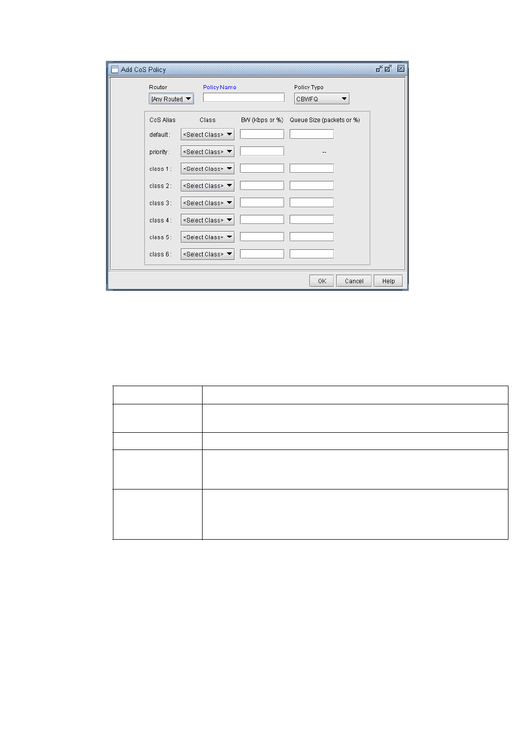
CLASS OF SERVICE*
Copyright © 2014, Juniper Networks, Inc. 13-7
. . . . .
Figure 13-7 Add CoS Policy Window
In the above example there are four defined classes: voice, first_class_data, business_data, and economy_data.
This window has the following fields:
Field Description
Router This is a drop down menu that lets the user choose one of the existing
routers. “[Any router]” means that the policy will be applied to all routers.
Policy Name CoS Policy Name
Type This is a drop down menu that lets the user select the type of queueing
algorithm that this CoS policy uses: CBWFQ, MDRR, MDRR strict, MDRR
alternate, or HWRR.
Class For each class entry, the user can select the class name to be displayed
from the drop down menu. Each drop down menu only contains the class
names that have been defined for that particular CoS alias in the CoS
Classes window.

CLASS OF SERVICE*
13-8 Copyright © 2014, Juniper Networks, Inc.
13
BW (Kbps) If the queueing algorithm Type is set to CBWFQ:
For the priority class, this is the maximum bandwidth allowed for that
class. Packets over that limit are dropped.
For other classes, this is the guaranteed minimum bandwidth for the class
during congestion. Packets over that limit may be accepted.
Default unit is Kbps (Kilobits per second).
To specify bandwidth reservation for a CoS policy, you can specify the
actual bandwidth (e.g. 3M) or a percentage of the trunk bandwidth (e.g.
30%)
You can also specify remaining % of bandwidth not already reserved by
other CoS classes using rX%. Example, to specify 100% of remaining BW
use r100% and to specify 30% of remaining BW use r30%.
Note: The total of all the bandwidths defined in the class policies of the
policy map must be less than 75% of the capacity of the link.
Weight This field appears in place of the BW field if the type is set to MDRR (strict
or alternate). Each MDRR queue can be assigned a relative weight that
determines relative bandwidth for each queue when congestion occurs. If
no Weight is specified then the default value of 10 is used. The priority
class for MDRR strict policies cannot have a weight defined.
Queue Size
(packets)
The maximum number of packets allowed in the queue for the specified
class.
Note 1: The priority class has no queue, so the user cannot specify its
queue size. Queue sizes for other classes can be specified by the user.
Note 2: The maximum allowable value is 64 packets.
Field Description
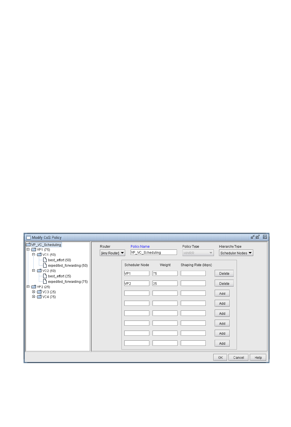
CLASS OF SERVICE*
Copyright © 2014, Juniper Networks, Inc. 13-9
. . . . .
RELATED CISCO COMMANDS:
At the config level the command used to create policies is:
Router(config) # policy-map policy-map-name
Then, a class has to be specified by the following command.
Router(config-pmap) # class class-name
The policy is now applied for that class. After the above command, bandwidth and queue-limit can be specified to
characterize the class’s queue. The commands to do that are:
Router(config-pmap-c) # bandwidth bandwidth-kbps
Router(config-pmap-c) # bandwidth percent percentage
Router(config-pmap-c) # queue-limit number-of-packets
Example:
Router(config) # policy-map policy1
Router(config-pmap) # class class1
Router(config-pmap-c) # bandwidth 3000
Router(config-pmap-c) # queue-limit 30
Router(config-pmap) # class class2
Router(config-pmap-c) # bandwidth percent 10
HWRR POLICIES
For HWRR policies, the user is presented with a more advanced policy configuration window. Because ERX HWRR
policies can contain multiple levels of scheduler nodes, the user has the ability to define two types of objects in the
HWRR policy editor: nodes and queues.
Figure 13-8 CoS HWRR Policy Window - Scheduler Nodes
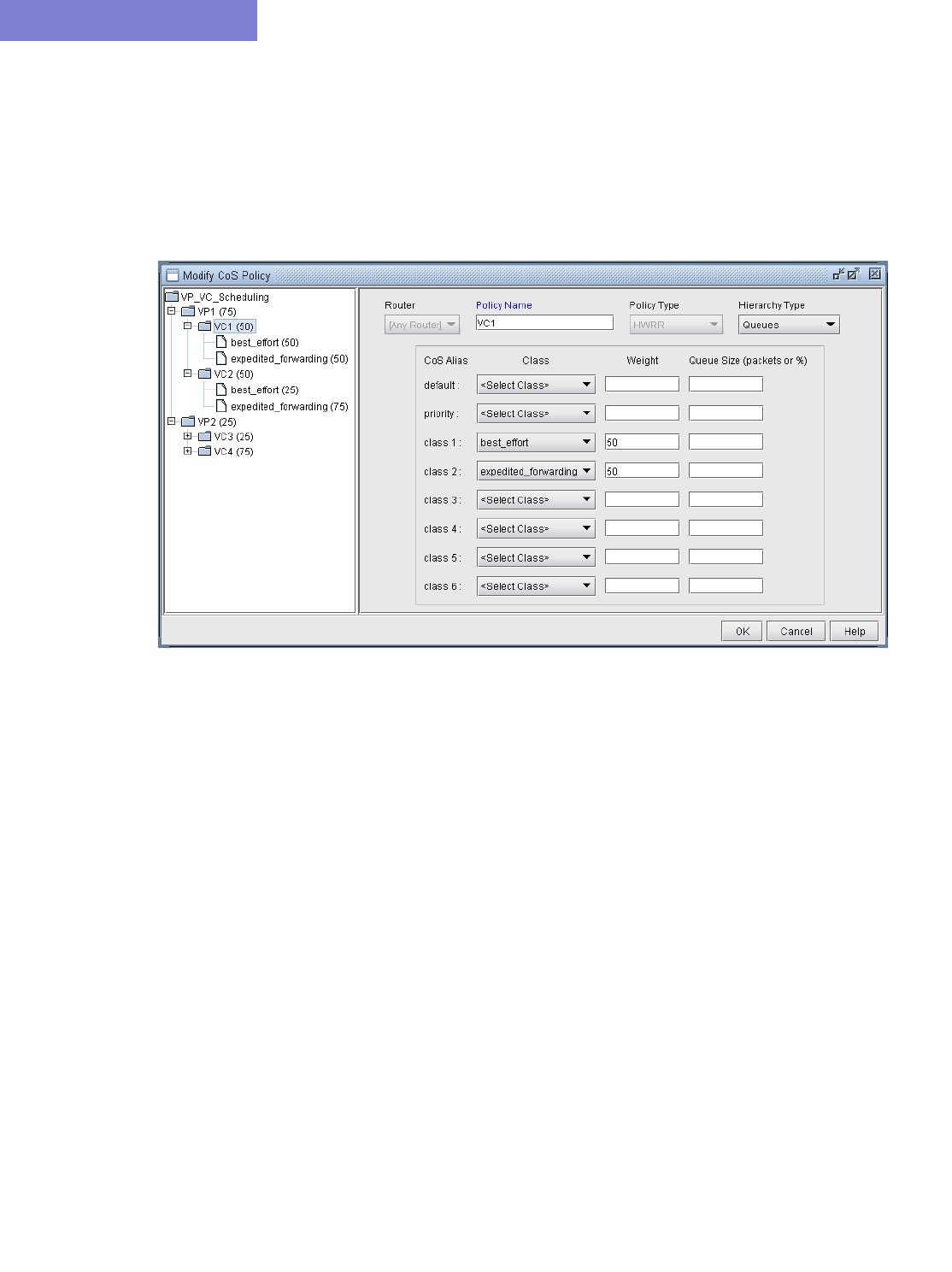
CLASS OF SERVICE*
13-10 Copyright © 2014, Juniper Networks, Inc.
13
TO ADD A SCHEDULER NODE
•Select the parent node in the left tree under which the new scheduler node will be added.
•Select Scheduler Nodes from the Hierarchy Type dropdown menu.
•Enter a name for the new scheduler node into the Scheduler Node column.
•(Optional) Enter a Weight for the new scheduler node.
•(Optional) Enter a Shaping Rate for the new scheduler node.
•Click the Add button to add the new scheduler node.
Figure 13-9 CoS HWRR Policy Window - Queues
TO ADD A QUEUE
•Select the node in the left tree under which the new queue will be added.
•Select Queues from the Hierarchy Type dropdown menu.
•Select a class for the new queue from the Class dropdown menu.
•(Optional) Enter a Weight for the new queue.
•(Optional) Enter a Queue Size for the new queue.
•Click OK, or continue editing the policy. The queues are saved automatically.
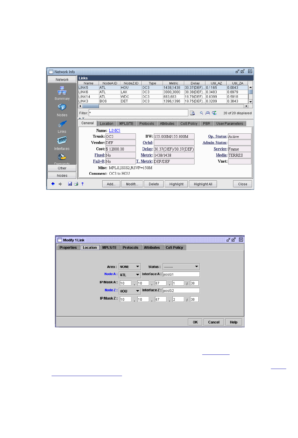
CLASS OF SERVICE*
Copyright © 2014, Juniper Networks, Inc. 13-11
. . . . .
Attach Policies to Interfaces
8. The last step is to attach policies to interfaces. A link between routers is composed of two interfaces so two
policies can be attached per link. Click on the Modify > Elements > Links item menu to bring up the link
listing.
Figure 13-10 Modify Links
9. Click on the Modify button and select the Location tab to enter the IP addresses and interface names of the
two end-points, if available.
Figure 13-11 Modify Link Location
Finally, click on the CoS Policy tab to attach policies to interfaces. In Figure 13-12 below, you can specify policies
on the Node A and Node Z endpoints of a link. Note that only the CoS Policies that are applicable to the Node A
router will be listed under the Node A Policy drop-down menu, and likewise for Node Z. Recall that in Create
Policies for Classes on page 13-6, the user can specify a particular router or “[Any Router]” for each newly created
policy.
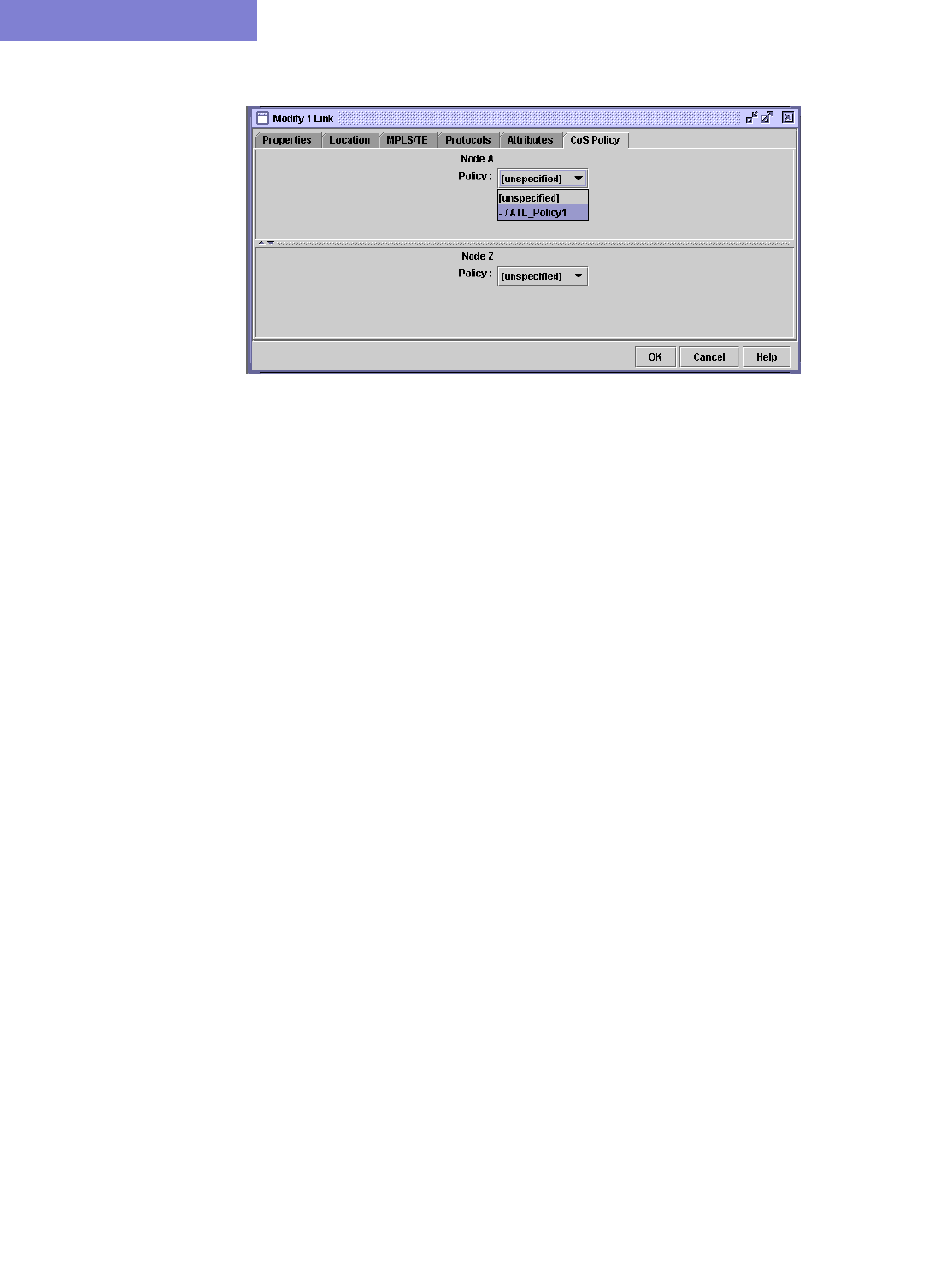
CLASS OF SERVICE*
13-12 Copyright © 2014, Juniper Networks, Inc.
13
Figure 13-12 CoS Policy for Link Interfaces
Related Cisco commands:
At the interface level (config-if) the command to attach a policy to an interface is:
Router(config-if) # service-policy {input| output} policy-map
where input is to indicate the input interface, output for output interface, and policy-map is the name of the policy-
map defined somewhere else in the config file.
Example:
Router(config) # interface e1/1
Router(config-if) # service-policy output policy1
Adding Traffic Inputs
The user can input traffic information for different classes through the WANDL client. When creating or modifying
a particular demand, the user may assign a particular CoS Class to that demand in the Demand Types window, as
explained below. The policies for that class are then applied to the demand/traffic.
10. While adding or modifying a demand, click on the Type button in the Demand window. The Demand Type
Parameter Generation window will appear. From this window, choose a class from the Policy Class drop
down menu and then click the OK button.
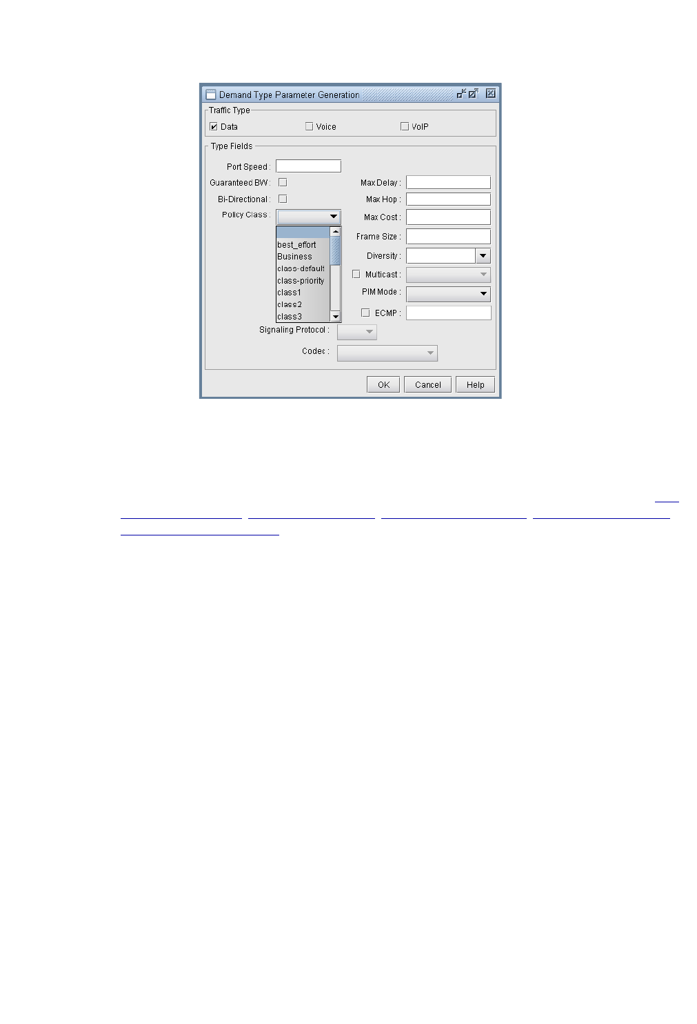
CLASS OF SERVICE*
Copyright © 2014, Juniper Networks, Inc. 13-13
. . . . .
Figure 13-13 Demand Type Parameter Generation Window
Using text editor
The user can also manually input CoS parameters into the WANDL format files via text editors. The bblink file has
to be modified and a new file, policymap, has to be created. For more information on file formats refer to CoS
Alias File on page 13-19, bblink File on page 13-19, Policymap file on page 13-20, Demand File on page 13-21, and
Traffic Load File on page 13-22.
Reporting module
There are three types of reports providing interface load and queueing delays per Class of Service:
•Demand CoS
•Tunnel CoS*
•Link CoS
*Note: To get tunnel CoS information, select the Tunnel layer button from the main menu bar and then reopen the
Report Manager.
11. To generate these reports, go to Report > Report Manager.
12. Under the Network Reports category, clicking on either the Demand Reports > CoS Demands Report
or the Link Reports > CoS Links Report will cause the following window to appear.
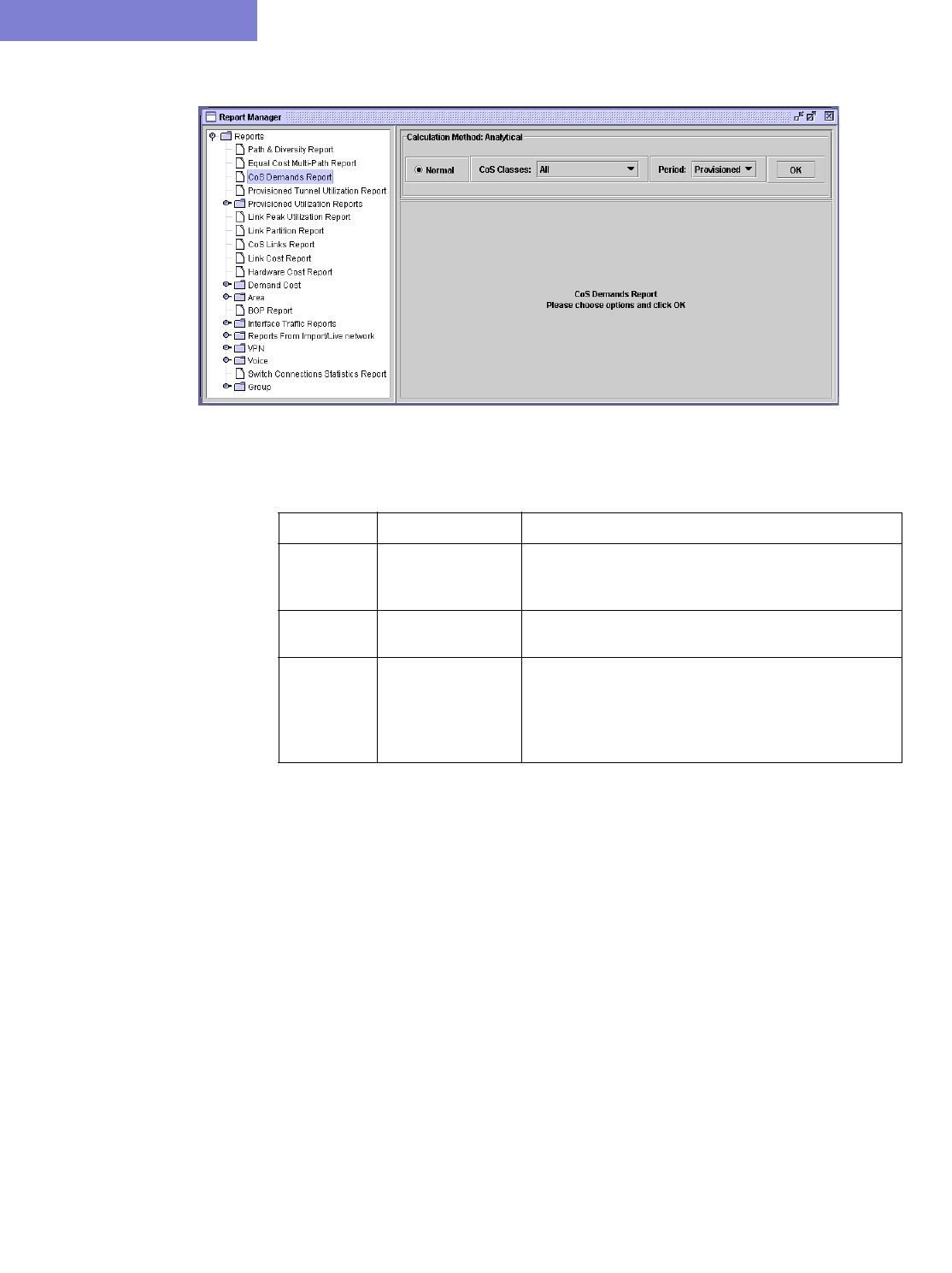
CLASS OF SERVICE*
13-14 Copyright © 2014, Juniper Networks, Inc.
13
Figure 13-14 Query Window
Before the report is generated, the user must first specify three things:
Parameters Definition Explanation
Traffic Mode Normal or Peak Normal traffic means the network does not experience
any failure/outages. Peak means that failure
simulation reports are going to be used.
CoS Classes All or one specific
Class of Traffic
Reports can be issued for all Classes of Traffic or for a
particular one (e.g. the Priority class)
Period Planned, Worst or
All
Planned means the report is generated using the
interface load calculated based on the demand file
values. Worst means that the report is generated using
the interface load calculated based on the worst traffic
load.
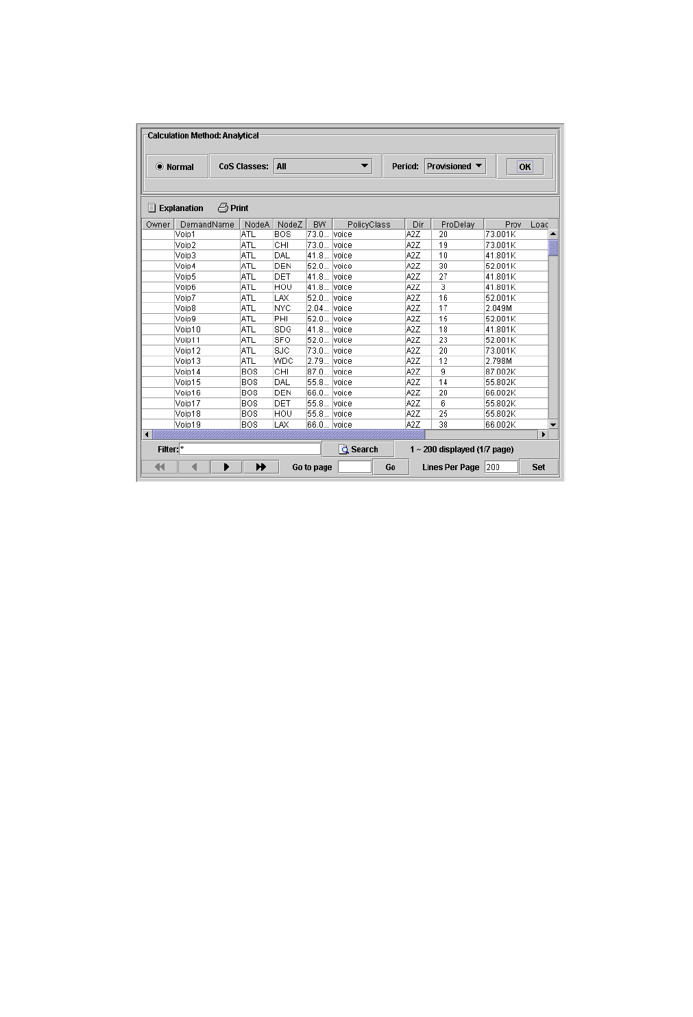
CLASS OF SERVICE*
Copyright © 2014, Juniper Networks, Inc. 13-15
. . . . .
IP Flow Information
13. After selecting the CoS Report Options, click the OK button and the report will appear as follows.
Figure 13-15 CoS Demands Report
CLASS OF SERVICE*
13-16 Copyright © 2014, Juniper Networks, Inc.
13
Link information
14. After selecting parameters on the CoS Report Options window, click the OK button and the report will
appear as follows.
Figure 13-16 Link CoS Report
CLASS OF SERVICE*
Copyright © 2014, Juniper Networks, Inc. 13-17
. . . . .
Traffic Load Analysis
Network planners can visualize how network resources are used according to the traffic load input. In the WANDL
software, there are two ways for the user to view network utilization with traffic load information through the
WANDL client:
1) Network map color-coded link utilizations
2) Traffic load bar charts
The user can also supply a “trafficload” file, which specifies measured or predicted traffic loads per demand during
as many as 24 distinct periods. These periods can represent summarized daily traffic (in bits per second), or hourly
traffic, for example. The WANDL software can then simulate the load on the links during each period. More detail
on the format of the traffic load file can be found in Traffic Load File on page 13-22
ANIMATED TRAFFIC LOAD DISPLAY
15. To view an animation of traffic load on the network map, select the Utilization Legends > Demand CoS
Util legend. The user can choose various options:
1) Normal or Peak
2) Utilization, QDelay or Drop Percentage
3) All CoS classes or one particular class
Select a period to update the link colors on the map to reflect the link load that results when the demand traffic for
that period is routed over the network. Link utilization colors can be modified on the link utilization map legend.
Figure 13-17 Demand CoS Util Legend
Alternatively, find the equivalent options from the Traffic > Traffic Load window. In this window are two extra
ticks on the slidebar for the current load and the worst load. Select Run to automatically step through each period.
Please refer to the Reference Guide for a more detailed explanation on these available Traffic Load options.
CLASS OF SERVICE*
13-18 Copyright © 2014, Juniper Networks, Inc.
13
Traffic Load by Policy Class
Bar charts are used to view the traffic load on a link in more detail.
16. Click on Network > Elements > Links. Righ-click a link in the list and select Traffic Chart > Demand
Traffic Load by CoS from the popup menu. Alternatively, you may also right-click on a link on the topology
map and select Traffic Load > Demand Traffic Load by CoS from the popup menu.
17. Following is an example of a traffic load chart according to CoS class. The interface utilization is provided for
24 periods. The “Planned” bar reports the interface utilization calculated based on the bandwidths specified in
the demand file. The “Worst” bar displays the highest load experienced during the 24 periods. The interface
utilization for periods 1 through 24 are derived from routing the demand traffic in the traffic load file, described
in further detail in Traffic Load File on page 13-22. Please refer to the Reference Guide for a more detailed
explanation on the available Traffic Load options.
Figure 13-18 Traffic Load Bar Chart
18. You may view the traffic load by normal or peak, utilization or delay or drop percentage, and by CoS classes.
There is also a tab to view the load in the A to Z direction or the Z to A direction on the link.
19. Holding the mouse over a bar brings up a tool tip with more detail of the traffic load breakdown for that
particular period.

CLASS OF SERVICE*
Copyright © 2014, Juniper Networks, Inc. 13-19
. . . . .
Appendix
CoS Alias File
Each line of the CoS Alias file lists an alias followed by the associated class names, with the primary class name
coming first. An example is:
#Alias Class1 Class2 ...
class-default
class-priority voice
class1 first_class_data gold
class2 business_data silver
class3 economy_data
This can also be accomplished through the WANDL client in Define Class Maps on page 13-4.
After creating the CoS Alias file the user has to let the system know where that file is. Add in the spec file the
following line:
CoSAlias = CoSAlias_filename
where CoSAlias_filename is the name of the CoS Alias file just created above.
bblink File
Policy information can be added to the bblink (link) file for a link entry by adding the following into an entry:
POLICY1=policy_name1 POLICY2=policy_name2
where policy_name1 and policy_name2 are names of the policies applied to the interfaces on both sides of the link,
interface_name1 and interface_name2, respectively. This can also be accomplished through the WANDL client in
Attach Policies to Interfaces on page 13-11. If making these modifications through the WANDL client, saving the
network environment will automatically update the bblink file.
Example:
#linkname nodeA nodeZ vendor count [ C1= interface_name_1 C2=interface_name_2 ] [ IP1=IP_address_1
IP2=IP_address_2 ] [ POLICY1=policy1 POLICY2=policy2 ]
Link345 Paris2 London4 DEF 1 C1=Serial2/0/0 C2=Serial5/0/1 IP1=192.10.20.218/30 IP2=192.10.20.217/30
POLICY1=polA1 POLICY2=polZ3
Note: There should be no space between the keywords, the equal sign, and the name. Also the names should not
include space.
For example, the following are incorrect specifications:
C1 = Serial2/0/0
C1=Serial 2/0/0
The following is the correct specification:
C1=Serial2/0/0
After creating the bblink file the user has to let the system know where that file is.
There are two ways of pointing to the bblink file:
1) Add in the spec file the following line:
bblink = bblink_filename
where bblink_filename is the name of the bblink file just created above.
2) In the Spec File Generation window of the WANDL client, click on the Network Files tab and then click on
bblink button to select or input the bblink file just created above.

CLASS OF SERVICE*
13-20 Copyright © 2014, Juniper Networks, Inc.
13
Policymap file
The policymap file is used to list the mapping of classes to policies and routers. In the policymap file, there is one
line for each policy of a router. One router can have several policy maps. This policymap file is automatically created
after performing the Create Policies for Classes on page 13-6 in the WANDL client and then saving the network
environment.
Each line in the policy map file contains information about the policy name, router name, defined classes and class
policies (such as bandwidth and queue length). The priority class is always listed before the other classes. The format
of each record is:
#Type|GlobalParameters|Router|Policyname|PriorityClass,Bandwidth(Kb),-
{|Classname,Bandwidth,QueueLength,bitmap,expbitmap,dscpbitmap,dscpbitmap1,bc,be,pir}
The following table provides the definition of each field (fields are separated by a vertical “|” line):
The priority class is for Low Latency Queueing or Priority Queueing. Packets belonging to this class have higher
priority than other classes. There is no queue limit for this class. That is why there is the dash “-“ in the third
subfield.
Examples:
CBWFQ| |Node0|policy_N0|voice,64,-|business_data,400,32|economy_data,100,16|
CBWFQ| |Node1|policy_N1|voice,64,-,-,-|business_data,30%,32,-,-|economy_data,20%,16,-,-|
MDRR strict| |-|policy1|first_class_data,6,-|business_data,3,30|class-default,1,40|
The following table explains the first line of the example:
Field Description
Type The type of queueing algorithm. Valid types are “CBWFQ”,
“MDRR”, “MDRR strict”, “MDRR alternate”, “ERX”.
Global Parameters Reserved for future use. This field may be left empty for now.
Router Name of the router. This corresponds to the Node ID field in
the muxloc file. A ‘-’ in this field indicates ‘Any Router’.
Policyname Name of a policy defined for the router
PriorityClass,
Bandwidth(Kbps), -
Name of the priority class. This is followed by the bandwidth in
Kbps, or the maximum bandwidth of the priority class. For
MDRR queueing, this field should be substituted with the
weight value.The ‘-’ indicates that this field (typically used for
queue length) is not applicable for the priority class.
Classname, Bandwidth,
QueueLength,
bitmap,
dscpbitmap,
expbitmap,
dscpbitmap1,
bc,
be,
pir
This field defines the policy for each class. It is repeatable for
up to 6 classes, not including the priority class.
Classname
Bandwidth is in kbps. For MDRR queueing, this field should
be substituted with the weight value. It is not necessary to fill
in all sub-fields. The dash “-“ tells the system to use the
default values.
QueueLength is the size of the queue of the specified class.
The unit of the queue length is the number of packets.
bitmap and dscpbitmap are fields reserved for future use,
and may be left empty for now.

CLASS OF SERVICE*
Copyright © 2014, Juniper Networks, Inc. 13-21
. . . . .
After creating the policymap file, the user has to let the system know where that file is. There are two ways of
pointing to the policymap file:
1) Add in the spec file the following line:
policymap = policymap_filename
where policymap_filename is the name of the policymap file just created above.
- or -
2) From the WANDL client edit the spec file. Click on Network Files tab of the Spec File Generation window.
Select the policymap entry in the Device-Specific Files category, click Browse to locate the file, and then click
the Set button.
Demand File
In addition to the regular fields of the demand file, the user needs only to specify classes for demands. Note that
classes specified here have to match with classes defined earlier.
Example:
RNYCDEN NYC DEN 128000 R,A2Z,voice 02,02
RNYCATL NYC ATL 128000 R,A2Z,voice 02,02
RNYCWAS NYC WAS 100000 R,A2Z,first_class_data 02,02
RNYCEWR NYC EWR 200000 R,A2Z,first_class_data 02,02
RDENNYC DEN NYC 150000 R,A2Z,business_data 02,02
RDENWAS DEN WAS 200000 R,A2Z,business_data 02,02
RATLNYC ATL NYC 150000 R,A2Z,business_data 02,02
Field Value
Type CBWFQ
Router name Node0
Policy name policy_N0
Priority class name voice
bandwidth 64 kbps
Class name business_data
bandwidth 400 kbps
Queue length 32 packets
Class name economy_data
bandwidth 100 kbps
queue 16 packets

CLASS OF SERVICE*
13-22 Copyright © 2014, Juniper Networks, Inc.
13
Traffic Load File
This file aims at refining the traffic load granularity of the demands in the demand file. For example, it can be used
to input the traffic load over 24 distinct consecutive periods. These periods can be hourly, daily, weekly, or any time
interval the user decides. Each demand can have up to 24 traffic load numbers specified in the traffic load file. The
format of each record is:
demand_name direction – traffic0 [traffic1 … traffic23]
where demand_name is the demand ID (it has to match with one of those in the demand file), direction is either A2Z
or Z2A, and traffic0 … traffic23 are the traffic values in bits per second for 24 periods.
Example:
RATLNYC A2Z - 150.0 20.0 30.0 27.0 40.0 60.0 45.0
RDENWAS A2Z - 310.0 200.0 300.0 27.0 40.0 60.0 45.0
After creating the traffic load file the user has to let the system know where that file is. There are two ways of
pointing to the traffic load file:
1) Add in the spec file the following line:
trafficload = trafficload_filename
where trafficload_filename is the name of the traffic load file just created above.
2) From the WANDL client edit the spec file. Click on the Network Files tab of the Spec File Generation window
and then select the trafficload entry from the Traffic Files section. Then click “Browse...” to select the traffic load
file and then select the Load button ( ).

Copyright © 2014, Juniper Networks, Inc. 14-1
. . . . .
. . . . . . . . . . . . . . . . . . . . . . . . . . . . . . . . . . .
R
ESILIENT
P
ACKET
R
ING
14
his chapter describes how to use the Resilient Packet Ring feature of the WANDL software. Resilient
Packet Ring (RPR) is a MAC-level Ethernet-based technology for IP and Ethernet service delivery
designed for metro networks. RPR offers greater bandwidth efficiency than traditional TDM technology by
allowing for bandwidth sharing of links. Additionally, it offers fast ring protection similar to traditional transport
rings.
*Note that a special password is required for the RPR feature. Please contact your Juniper representative for more
information.
When to use
RPR data can be parsed from a set of config files or added from the WANDL client. SRP topology information
should also be provided in order to correctly order the nodes of the ring.
Related Documentation
For an overview of the WANDL software or for a detailed description of each feature and the use of each window,
refer to the General Reference Guide.
Recommended Instructions
Following is a high-level, sequential outline of the functionalities of the RPR feature.
1. Import config files, if any, to obtain information from interface statements. Use additional information from
commands such as “show srp topology” to determine the ring topology as described in Deriving RPR from
config and srp topology data on page 14-1.
2. Once the information is parsed, view RPR information from the topology as described in RPR Map on page 14-
1 and RPR Network Information on page 14-2.
3. Perform a path analysis in Design or Simulation mode as described in Path Analysis on page 14-2.
4. Try adding nodes to an RPR ring, or removing nodes from an RPR ring as described in Modifying an RPR Ring
on page 14-3.
Detailed Procedures
Deriving RPR from config and srp topology data
1. To import RPR data from configuration files, users should have both the router config files and the output of
“show srp topology”. Use the config import wizard from File>Import Data as described in Chapter 2, Router
Data Extraction. This will extract SRP interface information from the “interface SRP” statement.
2. The config files alone do not contain enough information to determine the ring topology and therefore the users
should also supply information from the “show srp topology” command.
RPR Map
3. A pseudonode is created for each SRP interface as shown in the figure below.
4. The labels for the nodes and links can be turned on from the map’s right-click menu, Labels>Node Labels...
and Labels>Link>Link Labels... options.
T
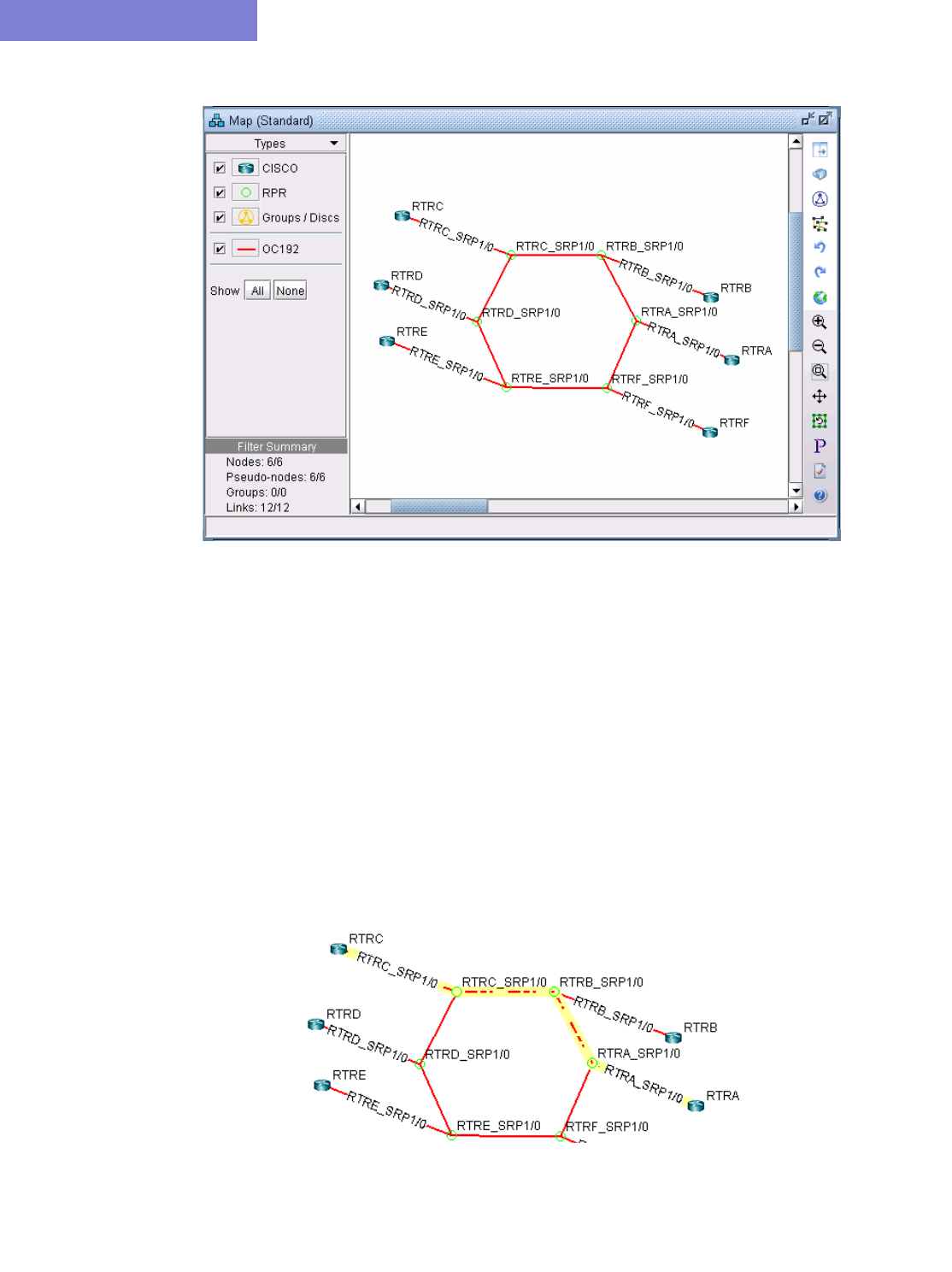
RESILIENT PACKET RING
14-2 Copyright © 2014, Juniper Networks, Inc.
14
Figure 14-1 RPR Ring
5. Select the Subviews > Protocols menu and select the checkbox for SRP to show only the SRP-related links.
RPR Network Information
6. Double-click an RPR pseudo-node on the map. In the Properties tab, note that RPR is listed with the hardware
“RPR”.
7. Double-click a link connecting two RPR pseudo-nodes and select the Protocols tab. Note that SRP is enabled
on the link, as indicated by a “Yes.”
8. View the interface info from Network > Elements > Interfaces and note that the SRP interfaces will be
listed there along with other information such as the IP address and associated node.
Path Analysis
9. To perform a path analysis, select Network > Path & Capacity > Path... Then click a source router attached
to an SRP interface and a destination router attached to an SRP interface. Note that the resulting demand will be
on the shortest path.
Figure 14-2 Shortest Path on RPR ring from RTRC to RTRA
RESILIENT PACKET RING
Copyright © 2014, Juniper Networks, Inc. 14-3
. . . . .
10. Try failing the link connecting pseudo-nodes RTRC_SRP1/0 and RPRB_SRP1/0. Now a path analysis reveals
that the path now wraps around the other side of the ring.
Figure 14-3 Routing after Failing Link between RTRC_SRP1/0 ato RTRB_SRP1/0
Modifying an RPR Ring
ADDING ROUTERS TO AN RPR RING
11. To add routers already existing in the model to an RPR ring, first add a pseudo-node of hardware type RPR for
each router to be added to the ring. To do so, select Modify > Elements > Nodes...., click Add... in the
Nodes window. In the Add Node window, specify an ID/Name and specify RPR as the Hardware in the
Properties tab. Then click a location on the map and click “Add”.
Figure 14-4 Add Node Window
12. Next, add a link between the router and the newly added RPR pseudo-node. Select Modify > Elements >
Links... and then select Add... to open the Add Links window. In the Properties tab, specify the trunk type
(e.g., OC12) of the RPR ring. In the Protocols tab, enable SRP and the main routing protocol (e.g., OSPF) by
selecting “yes” for SRP and OSPF. Select “Auto Add on Mouse Clicks” and click on the RPR pseudo-node
and its corresponding router in succession to add the link.
RESILIENT PACKET RING
14-4 Copyright © 2014, Juniper Networks, Inc.
14
Figure 14-5 Link with SRP and OSPF enabled
13. Without closing the Add Link window, add two more links similarly enabled for SRP and the main routing
protocol (e.g., OSPF) and with the same trunk type. With the “Auto Add on Mouse Clicks” option still selected,
click the RPR pseudo-node followed by one of its neighboring RPR pseudo-nodes. Then click the RPR pseudo-
node followed by the other neighboring RPR pseudo-node. Now that the ring is formed, you can delete the old
SRP link, if any, that was replaced when adding new nodes to the ring. To delete the link, right-click over the
link and select Delete Link.
REMOVING A ROUTER FROM AN RPR RING
14. To remove a router from an RPR ring, remove the links connecting the router’s RPR pseudo-node to its two
neighboring RPR pseudo-nodes.
15. Then create a link between those two pseudo-nodes which are now disconnected, enabling them for SRP and the
main routing protocol (e.g., OSPF) in the Protocol tab and selecting the ring’s trunk type.
16. You can delete the RPR pseudo-node of the router removed from the ring, as well as the link from the router to
the RPR pseudo-node. This represents removing the SRP interface.

Copyright © 2014, Juniper Networks, Inc. 15-1
. . . . .
. . . . . . . . . . . . . . . . . . . . . . . . . . . . . . . . . . .
V
OICE
O
VER
IP*
15
he WANDL VoIP module allows network planners to build up a VoIP network by assigning nodes as
gatekeepers, media gateways, SIP-servers, and SIP-UAs. The two most widely deployed VoIP
signaling protocols – H.323 and SIP – are supported. The network engineer can analyze a call by
using the VoIP path trace feature to study both the call setup as well as the actual call. VoIP traffic demands (in
bits per second or in Erlangs) can be specified for the network in several ways, and then loaded into the network
for further analysis. Finally, other IP/MPLSView modules (e.g., MPLS-TE, CoS, VPN) can be used in
conjunction with the VoIP module to help the network designer to create a high-quality VoIP solution for their
network.
*Note that a special password is required for the VoIP feature. Please contact your Juniper representative for
more information.
Related Documentation
For general step-by-step instructions on how to use the WANDL software, please refer to the Design &
Planning Guide.
For an overview of the WANDL software or for a detailed description of each feature and the use of each
window, refer to the General Reference Guide or Chapter 37, Router Reference.
For details on how to create a spec file by extracting, or importing, information from the router configuration
files, please refer to Chapter 2, Router Data Extraction.
Recommended Instructions
1. Build a VoIP Network by Assigning VoIP Attributes to Nodes on page 15-3
2. Assigning H.323 Gatekeepers (GKs) on page 15-3
3. Assigning H.323 Media Gateways (MGWs) on page 15-3
4. Assigning SIP Servers on page 15-4
5. Assigning SIP-UAs (SIP User Agents) on page 15-4
6. VoIP Topology Map on page 15-5
7. VoIP Call Setup and Actual Call Path Trace on page 15-6
8. Traffic Classes on page 15-9
9. VoIP Traffic Specification on page 15-10
10. Adding a Single VoIP Demand on page 15-10
11. Adding Multiple VoIP Demands on page 15-12
12. Using the VoIP Traffic Generation Tool on page 15-15
13. Creating a Traffic Profile via the VoIP Traffic Generation Wizard on page 15-15
14. Using the No File Option on page 15-17
15. Using an End-to-end Traffic Matrix Input File on page 15-24
16. Using an End-to-end Traffic Matrix Input File with a Homing File on page 15-27
17. Reporting VoIP Information on page 15-30
18. VoIP Call Setup Report on page 15-31
19. VoIP Node Traffic Summary Report on page 15-32
20. E-Model R-factor Voice Quality Assessment on page 15-33
T

VOICE OVE R IP*
15-2 Copyright © 2014, Juniper Networks, Inc.
15
Definitions
Please refer to ITU-T H.323 Recommendation and RFC 3261 for detailed information about the H.323 and SIP
protocols.
Term Definition
VoIP Voice Over Internet Protocol
H.323 signaling protocol based on the ITU-T Rec. H.323 standard used in VoIP
MGW refers to the H.323 media gateway as described in the standard
GK refers to the H.323 gatekeeper as described in the standard
GK-direct refers to the H.323 call setup mechanism where the gatekeeper is involved
in direct call signaling
GK-routed refers to the H.323 call setup mechanism where the gatekeeper is involved
in gatekeeper routed call signaling
SIP a signaling protocol based on RFC 3261 (SIP: Session Initiation Protocol)
used in VoIP
SIP-UA refers to the SIP User Agents as described in the RFC
SIP Proxy refers to the SIP proxy server as described in the RFC
SIP Redirect refers to the SIP redirect server as described in the RFC
Codec refers to the algorithms used to compress voice packets
IP/RTP/UDP voice call packets are carried over at IP, RTP, and UDP protocols
VOICE OVER IP*
Copyright © 2014, Juniper Networks, Inc. 15-3
. . . . .
Detailed Procedures
Build a VoIP Network by Assigning VoIP Attributes to Nodes
The first step in planning and designing a VoIP network is to identify those nodes to which you want to assign
VoIP attributes to. A VoIP attribute identifies a node as a GK, MGW, SIP-server, or SIP-UA. For H.323 calls,
GKs and MGWs are used. For SIP calls, SIP-servers and SIP-UAs are used. Once you have identified those
nodes related to VoIP, then you are ready to assign VoIP attributes to the nodes.
Assigning H.323 Gatekeepers (GKs)
1. To assign a particular node as an H.323 gatekeeper, switch to Modify mode and then double-click on the
node to bring up its Node Window. Switch to the VoIP tab and choose H.323 by selecting the checkbox
next to H.323 under the Protocol column.
Figure 15-1 Assigning an H.323 Gatekeeper
2. Next click on the dropdown box under the Component column, and choose either GK-direct or GK-routed.
When gatekeepers are used in H.323 call setup, the signaling protocol pattern can following either one of
two methods – direct call signaling (the GK-direct option) or gatekeeper routed call signaling (the GK-
routed option). After selecting either GK-direct or GK-routed (depending on whether the GK is involved
in direct call signaling or gatekeeper routed call signaling), click OK to complete the assignment of the
current node as an H.323 gatekeeper
3. Repeat the previous steps as needed for each of nodes that you wish to designate as an H.323 gatekeeper.
Assigning H.323 Media Gateways (MGWs)
4. To assign a particular node as an H.323 media gateway, switch to Modify mode and then double-click on
the node to bring up its Node Window. Switch to the VoIP tab and select the checkbox next to H.323 under
the Protocol column.
5. Next click on the dropdown box under the Component column and choose MGW from the list. When
MGW is chosen, the Associated Controllers dropdown boxes and the Delay (ms) box become activated.
6. Fill in the Delay (ms) box with a vendor-specific media gateway delay value (e.g. hardware device-specific
processing delay) if applicable.
7. Under the Associated Controllers column, click on the Primary dropdown box to see the list of gatekeepers
that have been assigned in the network. Select an appropriate gatekeeper from the list in order to associate
it with the current media gateway. In the example shown in the following figure, the gatekeepers in the
network include P_R2, E_V3, and E_V1.
VOICE OVE R IP*
15-4 Copyright © 2014, Juniper Networks, Inc.
15
Figure 15-2 Selecting one of the GKs defined in the Network
8. Optionally, you may also assign up to two alternate gatekeepers to be associated with the current media
gateway. (An alternate gatekeeper is used in the event that the primary gatekeeper fails)
9. Repeat the previous steps as needed for each of nodes that you wish to designate as an H.323 media
gateway. Once you have associated two or more MGWs with a GK, then VoIP traffic can be added from
one MGW to another.
Assigning SIP Servers
10. To assign a particular node as a SIP-server, switch to Modify mode and then double-click on the node to
bring up its Node Window. Switch to the VoIP tab and choose SIP by selecting the checkbox next to SIP
under the Protocol column.
11. Next click on the dropdown box under the Component column, and choose either SIP-proxy server or SIP-
redirect server. The SIP call setup signaling flow differs depending on the type of SIP server. After
selecting either SIP-proxy server or SIP-redirect server (please refer to RFC 3261 for more details on the
difference between the two types of SIP servers), click OK to complete the assignment of the current node
as a SIP server.
Figure 15-3 SIP component selection
12. Repeat the previous steps as needed for each of nodes that you wish to designate as a SIP server.
Assigning SIP-UAs (SIP User Agents)
13. To assign a particular node as a SIP-UA, switch to Modify mode and then double-click on the node to bring
up its Node Window. Switch to the VoIP tab and choose SIP by selecting the checkbox next to SIP under
the Protocol column.
14. Next click on the dropdown box under the Component column and choose SIP-UA from the list. When
SIP-UA is chosen, the Associated Controllers dropdown boxes and the Delay (ms) box become activated.
15. Fill in the Delay (ms) box with vendor-specific media gateway delay information as appropriate.
16. Under the Associated Controllers column, click on the Primary dropdown box to see the list of SIP servers
that have been assigned in the network. Select an appropriate SIP server from the list in order to associate
it with the current SIP-UA. In the example shown in the following figure, the SIP servers in the network
include JT1, JT2.
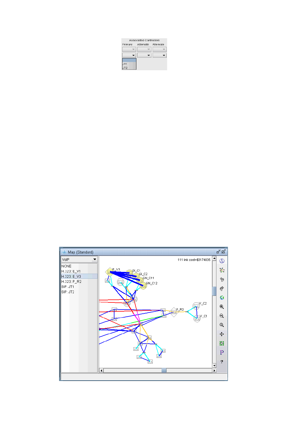
VOICE OVER IP*
Copyright © 2014, Juniper Networks, Inc. 15-5
. . . . .
Figure 15-4 Select one of the SIP-servers defined in the network
17. Optionally, you may also assign up to two alternate SIP servers to be associated with the current media
gateway. (An alternate SIP server is used in the event that the primary SIP server fails)
18. Repeat the previous steps as needed for each of nodes that you wish to assign as a SIP-UA.
VoIP Topology Map
In order to make it convenient for the user to visually identify VoIP component relationships, a VoIP view has
been added to the main topology window.
19. To switch to the VoIP view on the Map window, select Subviews > VoIP from the map’s upper left menu.
20. In a network in which nodes have already been assigned VoIP attributes (i.e., GK, MGW, SIP server, or
SIP-UA), using the VoIP view allows the user to see which GK is associated with which MGWs, and which
SIP server is associated with which SIP-UAs. When you first switch to the VoIP view, you will see
diamonds drawn around GKs or SIP servers and circles drawn around MGWs or SIP-UAs. For instance,
the following figure shows the gatekeeper E_V3 with a diamond drawn around it and the media gateway
GI_C1 with a circle drawn around it.
21. The VoIP view presents the user with a list of H.323 GKs and SIP servers. When a particular H.323 GK is
selected, all MGWs associated with the GK are highlighted and lines are drawn between the MGWs and
the GK. Similarly, when a particular SIP Server is selected, all of the SIP-UAs associated with the SIP
server are highlighted and lines are drawn between the SIP-UAs and the SIP Server. In the following
figure, an H.323 gatekeeper, E_V3, and the four media gateways associated with it are highlighted.
Figure 15-5 VoIP view of an H.323 zone (gatekeeper is E_V3)
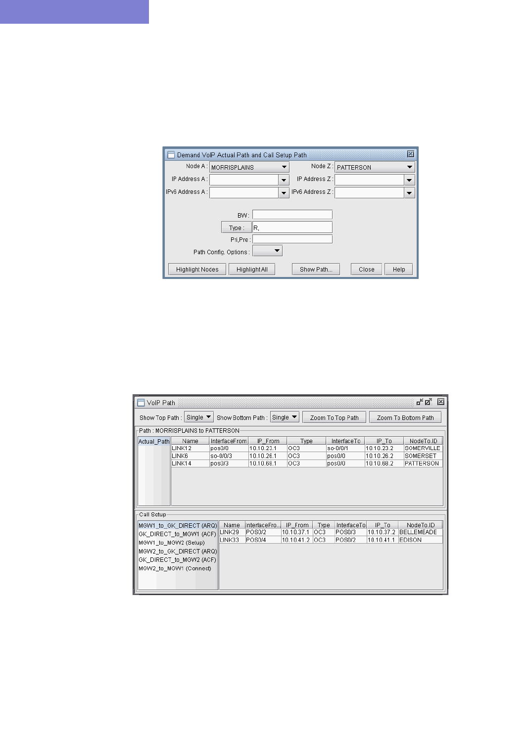
VOICE OVE R IP*
15-6 Copyright © 2014, Juniper Networks, Inc.
15
VoIP Call Setup and Actual Call Path Trace
22. 1.The VoIP module allows the user to examine various VoIP call flow scenarios along with the paths – both
the call setup path as well as the actual call path. Select Network > Path & Capacity > VoIP Path.
23. Once the Demand VoIP Actual Path and Call Setup Path window (shown in the following figure)
comes up, the user can examine the call setup and actual call paths taken between two nodes. The two
nodes must be H.323 media gateways or SIP-UAs, because VoIP traffic start and end at these nodes.
Figure 15-6 VoIP Path Trace Window for Call Setup and Actual Call
24. The nodes can be selected by using the drop-down combo boxes in the Demand VoIP Actual Path and Call
Setup Path window. Another way to select the nodes is by clicking the left mouse button on the two nodes
in the main topology map window. If a path can be found when the two end points have been chosen, then
the VoIP Path window will be displayed. The following figure shows what the VoIP Path window looks
like when the user selects two H.323 media gateways, MORRISPLAINS and PATTERSON.
Figure 15-7 VoIP Path Trace Details
Notice that the VoIP Path window is divided into a top half and a bottom half. The top half of the window
shows the path information for the actual call, while the bottom half of the window shows the call setup
signaling path information.
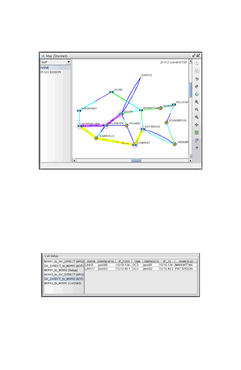
VOICE OVER IP*
Copyright © 2014, Juniper Networks, Inc. 15-7
. . . . .
25. The actual call path segments are displayed in yellow, while the call setup path segments are shown in
purple. The following figure shows the topology map display of an example VoIP path trace between two
H.323 media gateways, MORRISPLAINS and PATTERSON.
Figure 15-8 VoIP Path Analysis(H.323)
26. In order to clearly see the detailed information of the actual call path, the user may click on the Zoom to
Top Path button to zoom in on the actual call path or Zoom to Bottom Path button to zoom in on the
call setup path. The user may also click on a particular row in the VoIP Path window order to further
zoom in on and highlight a particular segment of the path.
27. In the bottom half of the VoIP Path window, the transaction-level call setup information is displayed. In
the H.323 call example, the media gateways MORRISPLAINS and PATTERSON are both registered with
the gatekeeper, EDISON, which is using direct call signaling. Accordingly, the call setup would then
include the transactions (ARQ, ACF, Setup, Connect) shown below. When the user clicks on a transaction,
details of each transaction are displayed.
Figure 15-9 Call setup transaction details
The following table shows some of the basic call setup signaling flow patterns used in H.323 and SIP. Please
refer to ITU-T H.323 Recommendation and RFC 3261 for detailed information about the transactions used in
the H.323 and SIP protocols.

VOICE OVE R IP*
15-8 Copyright © 2014, Juniper Networks, Inc.
15
Table 15-1 Table showing some basic call setup signaling flows
Call Setup Type Signaling Flow (Transaction)
GK-direct MGW1 to GK-direct (ARQ)
GK-direct to MGW1 (ACF)
MGW1 to MGW2 (Setup)
MGW2 to GK-direct (ARQ)
GK-direct to MGW2 (ACF)
MGW2 to MGW1 (Connect)
GK-routed MGW1 to GK-routed (ARQ)
GK-routed to MGW1 (ACF)
MGW1 to GK-routed (Setup)
GK-routed to MGW2 (Setup)
MGW2 to GK-routed (ARQ)
GK-routed to MGW2 (ACF)
MGW2 to GK-routed (Connect)
GK-routed to MGW1 (Connect)
SIP-proxy server SIP-UA1 to SIP-Proxy (INVITE)
SIP-Proxy to SIP-UA2 (INVITE)
SIP-UA2 to SIP-Proxy (200 OK)
SIP-Proxy to SIP-UA1 (200 OK)
SIP-UA1 to SIP-Proxy (ACK)
SIP-Proxy to SIP-UA2 (ACK)
SIP-redirect server SIP-UA1 to SIP-Redirect (INVITE)
SIP-Redirect to SIP-UA1 (302 Moved)
SIP-UA1 to SIP-Redirect (ACK)
SIP-UA1 to SIP-UA2 (INVITE)
SIP-UA2 to SIP-UA1 (200 OK)
SIP-UA1 to SIP-UA2 (ACK)
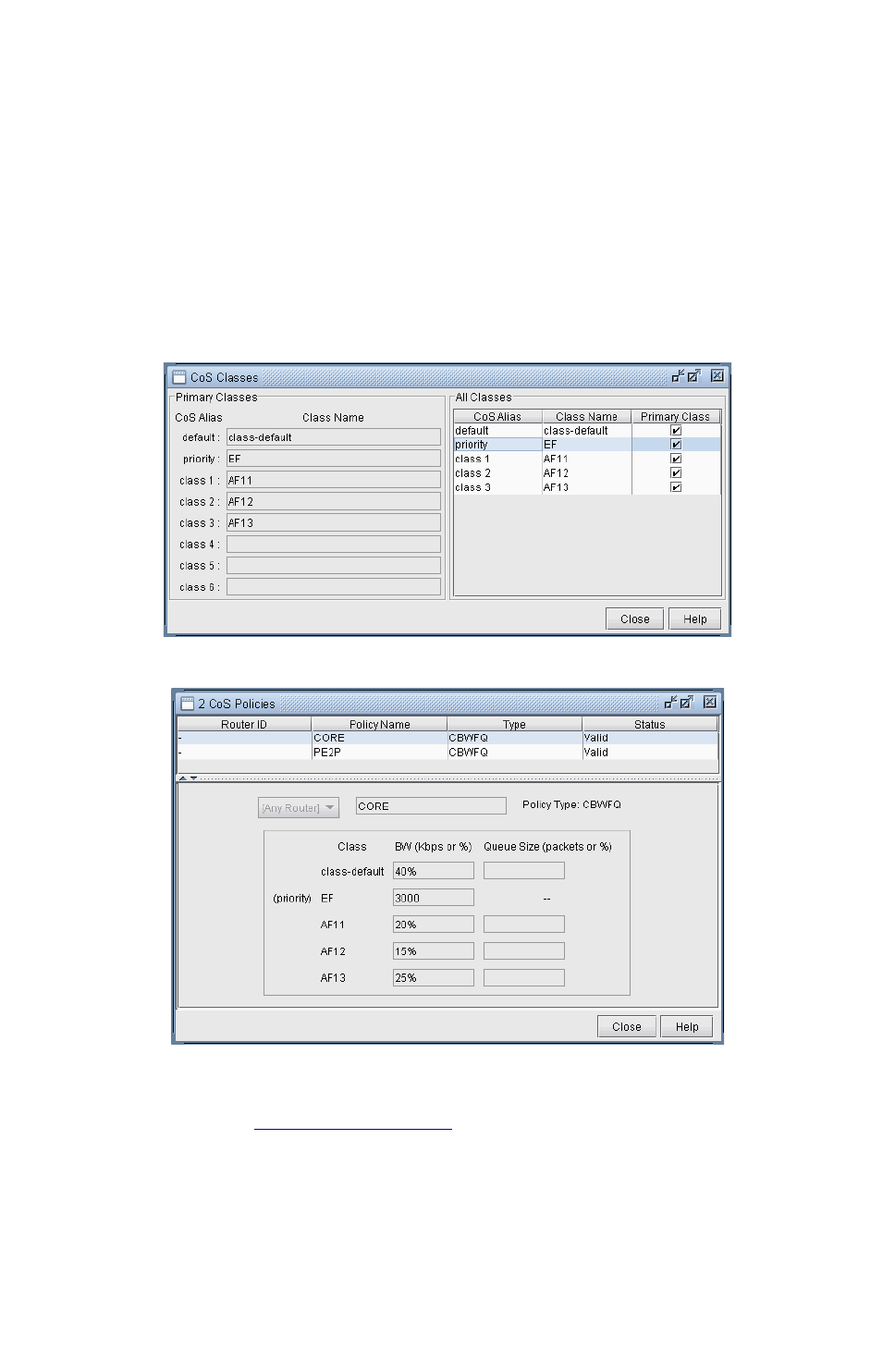
VOICE OVER IP*
Copyright © 2014, Juniper Networks, Inc. 15-9
. . . . .
Traffic Classes
To ensure high voice quality, actual voice traffic should be delivered with low delay and jitter, while voice call
setup traffic should be delivered without loss. DiffServ specifies an EF (Expedited Forwarding) PHB to create
a low latency/loss/jitter service in which traffic (e.g. actual voice packets) are processed as quickly as possible.
The AF (Assured Forwarding) PHB specified in DiffServ is used for sending traffic (e.g. call setup packets) that
require a low-drop precedence. Both EF and AF traffic should be sent out of a low latency queue for best
results.
IP/MPLSView allows the user to define various CoS classes (including EF and AF classes) and then create CoS
policies that are attached to interfaces so that traffic will be forwarded based on class. For instance, the
following figures show EF and AF classes in the CoS Classes and CoS Policies windows.
Figure 15-10 CoS Classes and CoS Policies windows
Please refer to Chapter 13, Class of Service* for more information about CoS classes and policies.
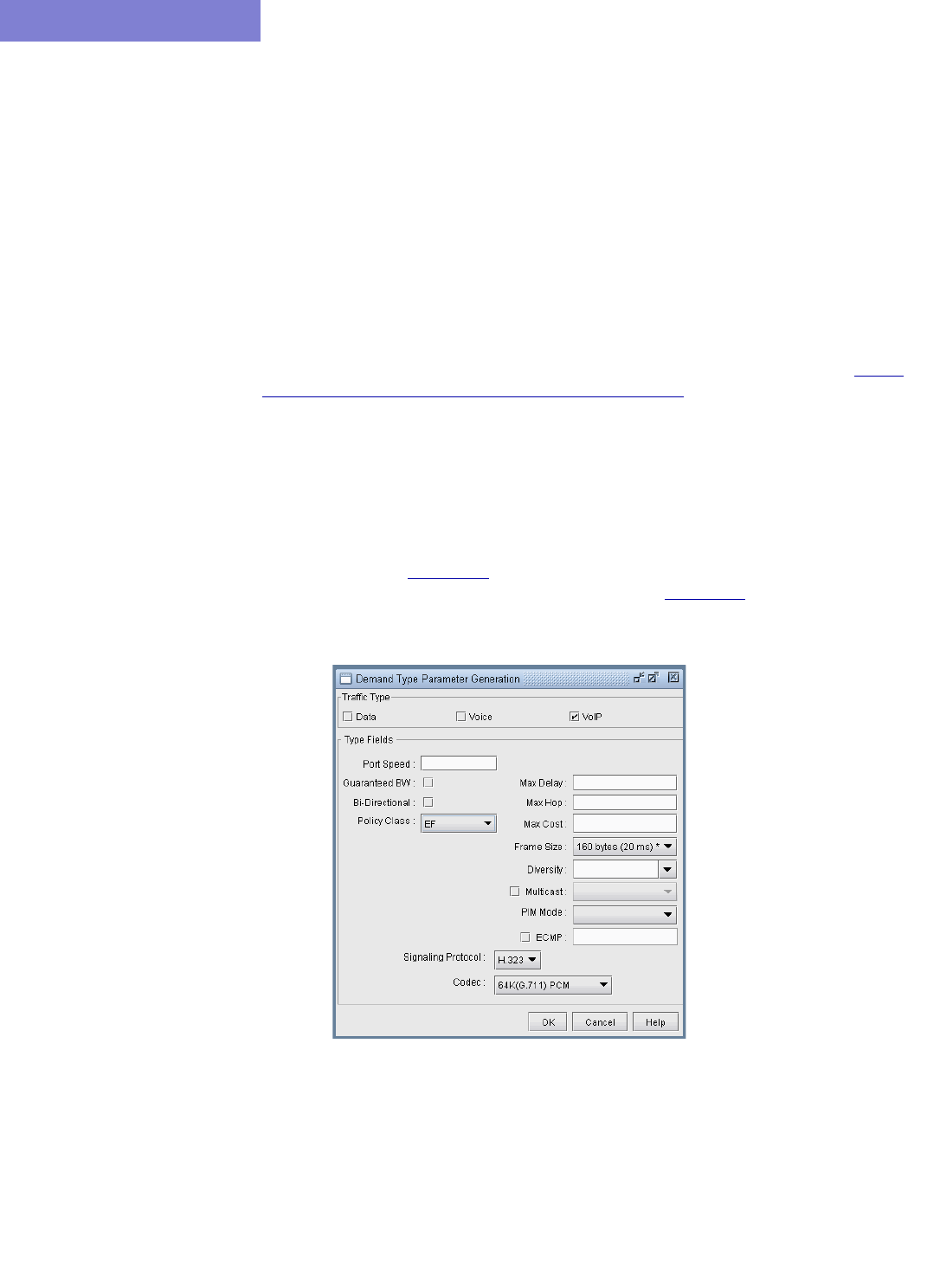
VOICE OVE R IP*
15-10 Copyright © 2014, Juniper Networks, Inc.
15
VoIP Traffic Specification
IP/MPLSView’s VoIP Module allows the user to specify VoIP traffic in one of three ways:
•Adding single VoIP demands via the Demands window (Modify > Elements > Demands, Add > One
Demand...)
•Adding multiple VoIP demands through the Add Multiple Demands window (Modify > Elements >
Demands, Add > Multiple Demands...)
•Using the VoIP Traffic Generation Tool (accessible via the Traffic > Demand Generation > VoIP
menu)
Adding a Single VoIP Demand
To add a single VoIP demand between two H.323 media gateways or between two SIP-UAs, the user needs to
perform the following sequence of steps:
28. Complete the designation of certain nodes in the network as VoIP components. See the section Build a
VoIP Network by Assigning VoIP Attributes to Nodes on page 15-3 for details.
29. In Modify mode, bring up the Demands window (Modify > Elements > Demands, Add > One
Demand...) and click on the Type button to bring up the Demand Type Parameter Generation
window.
30. When the Demand Type Parameter Generation window comes up, click on the VoIP check box to
enable both the Signaling Protocol dropdown box and the Codec dropdown box.
The Signaling Protocol dropdown box allows the user to choose H.323, SIP, or none. The Codec
dropdown box allows the user to chose from the many standard voice Codecs that are supported by the
VoIP module shown in Figure 15-12. If CoS classes (e.g., EF, AF) have been defined in the network, then
they may also be selected via the Policy Class dropdown box. Figure 15-11 shows H.323 being chosen
for the signaling protocol, 64K(G.711) PCM chosen for the Codec, and EF selected as the Policy Class.
Figure 15-11 Specifying VoIP parameters via the Demand Type Parameter Generation window
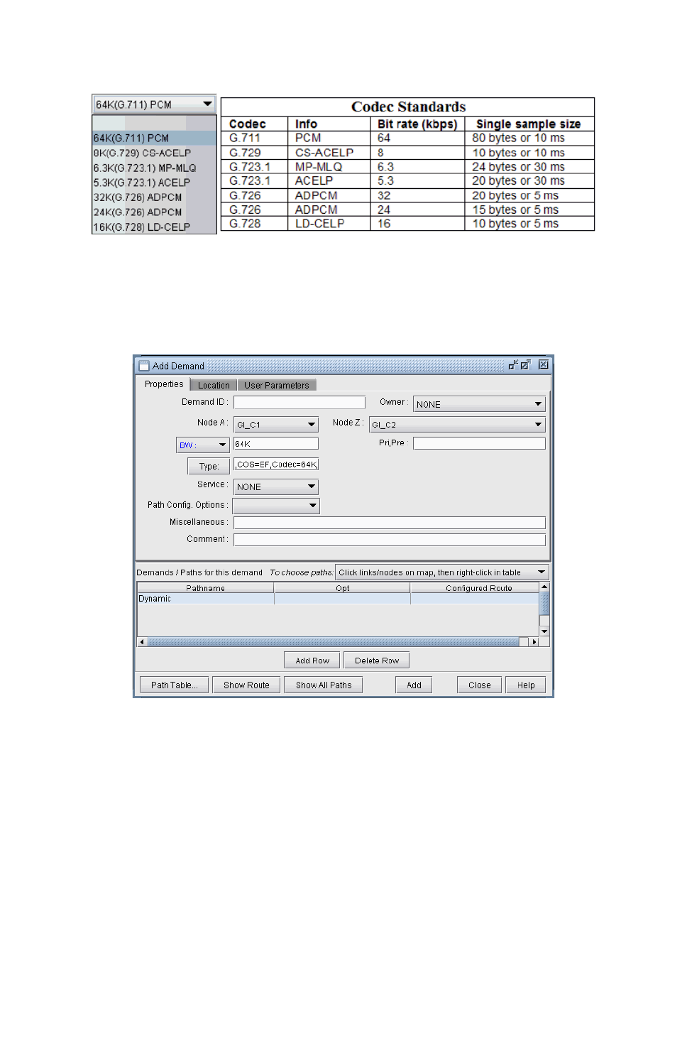
VOICE OVER IP*
Copyright © 2014, Juniper Networks, Inc. 15-11
. . . . .
Figure 15-12 Codec dropdown and Codec standards supported by VoIP module
31. Next click OK to accept the settings and return to the Demands window.
Figure 15-13 Add Demand window with Type box filled in
Notice that the Type box is now filled in with the string, “VOIP=H.323,COS=EF,Codec=64K,” Since
H.323 was chosen as the VoIP signaling protocol, NodeA and NodeZ dropdown boxes have been filtered
to display only H.323 media gateways. As shown in the figure, GI_C1 and GI_C2 were chosen as the
media gateways. (If SIP were chosen for the VoIP signaling protocol, then NodeA and NodeZ dropdown
boxes would be filtered to display SIP-UAs instead.)
Notice also that the BW field has now become a dropdown selection button; clicking on this button will
reveal two choices: BW or Erlangs. The user may specify traffic in either BW or in Erlangs. If Erlangs is
chosen, then the GoS field must also be specified. In the following figure, the user has specified 100
Erlangs with a GoS of 1%.
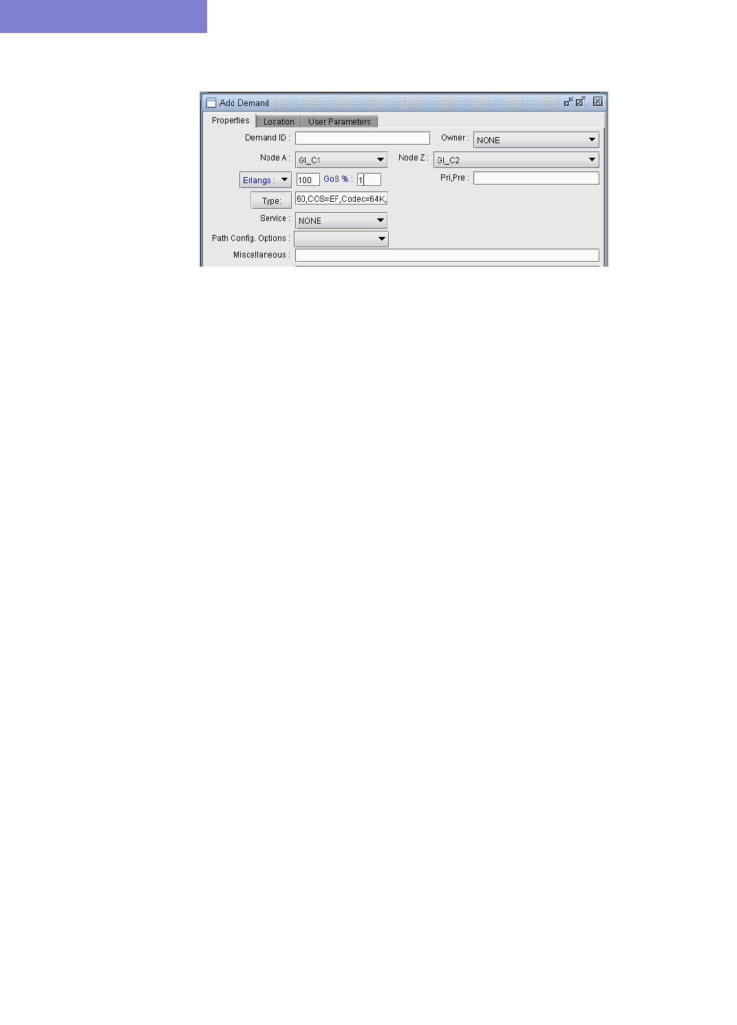
VOICE OVE R IP*
15-12 Copyright © 2014, Juniper Networks, Inc.
15
Figure 15-14 Specifying Erlangs and GoS in the Add Demand window
32. Next click on Add to add the single VoIP demand. For our example, a 7.488M demand is added between
GI_C1 and GI_C2 because 100 Erlangs with a GoS of 1% comes out to be 117 circuits via the Erlang B
formula. Since the codec size in this case is 64K, the demand payload is 117*64k=7.488M.
Adding Multiple VoIP Demands
To add multiple VoIP demands between H.323 media gateways or between SIP-UAs, the user needs to perform
the following sequence of steps:
33. Complete the designation of certain nodes in the network as VoIP components. Please see the section
Assigning VoIP Attributes to Nodes for details on how to assign attributes (i.e., H.323 MGW, H.323
GK, SIP-UA, or SIP-server) to nodes.
34. In Modify mode, bring up the Add Multiple Demands window (Modify > Demands, Add >
Multiple Demands) and click on the Type button to bring up the Demand Type Parameter
Generation window.
35. When the Demand Type Parameter Generation window comes up, click on the VoIP check box to
enable both the Signaling Protocol dropdown box and the Codec dropdown box. If CoS classes (e.g.,
EF, AF) have been defined in the network, then they may also be selected via the Policy Class dropdown
box.
36. Next, click OK to return to the Add Multiple Demands window, and notice that the Type box is now
filled in with the string, “VOIP=H.323,COS=EF,Codec=64K,”
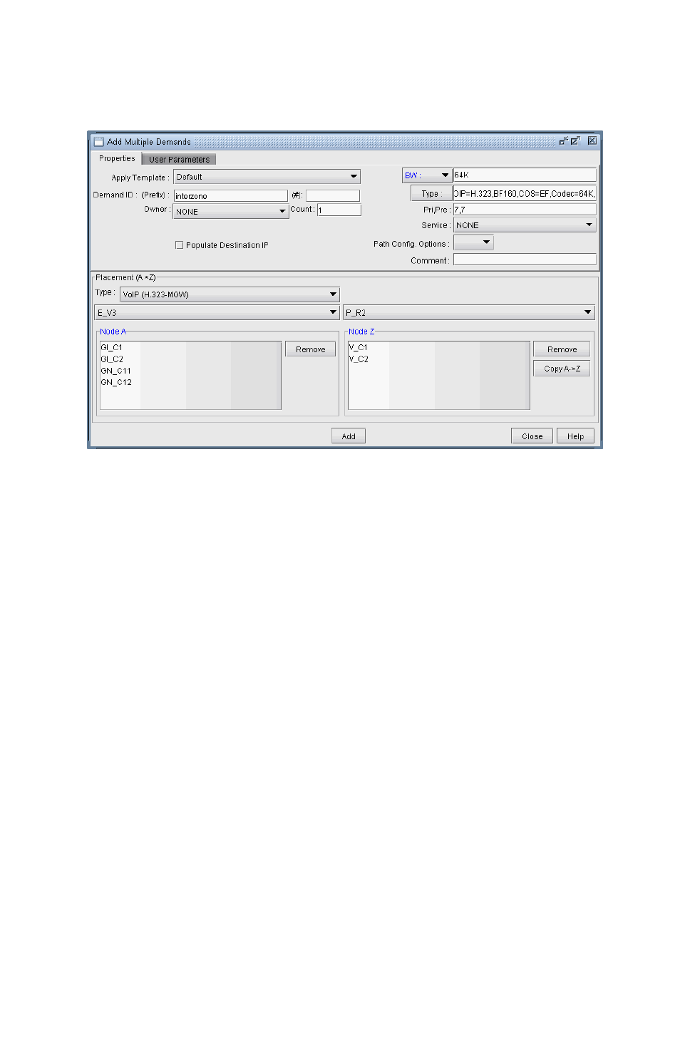
VOICE OVER IP*
Copyright © 2014, Juniper Networks, Inc. 15-13
. . . . .
37. Under the Placement (AxZ )section, change the type from Node to VoIP (H.323-MGW) as shown in the
following figure.
Figure 15-15 Filtering H.323 MGWs in the Add Multiple Demands window
With VoIP (H.323-MGW) as the chosen type, the dropdown boxes above the Node A and Node Z
listboxes are filtered to list the H.323 gatekeepers. When a particular gatekeeper is chosen in step 1, then
Node A and Node Z listboxes are filtered to include only those media gateways associated with the
chosen gatekeeper. The result is that the listboxes are filtered to display just the media gateways associated
with a particular H.323 zone.
(Note that if VoIP (SIP-UA) were the chosen type, then one-step filtering would be performed, the
dropdown boxes above the Node A and Node Z listboxes would be deactivated, and the Node A and
Node Z listboxes would be filtered to display all of the SIP-UAs.)
The figure above shows how the user would add multiple VoIP demands between media gateways between
two H.323 zones (one associated with the gatekeeper, E_V3, and another associated with the gatekeeper,
P_R2).
38. Notice that just as with the Add Demands window, the Add Multiple Demands window also allows you to
specify the traffic in either BW or in Erlangs. For this example we will just use the BW value. Next click on
Add to add the multiple VoIP demands.
39. Next you can bring up the Demands window, shown in the following figure, to see the demands that were
just added.
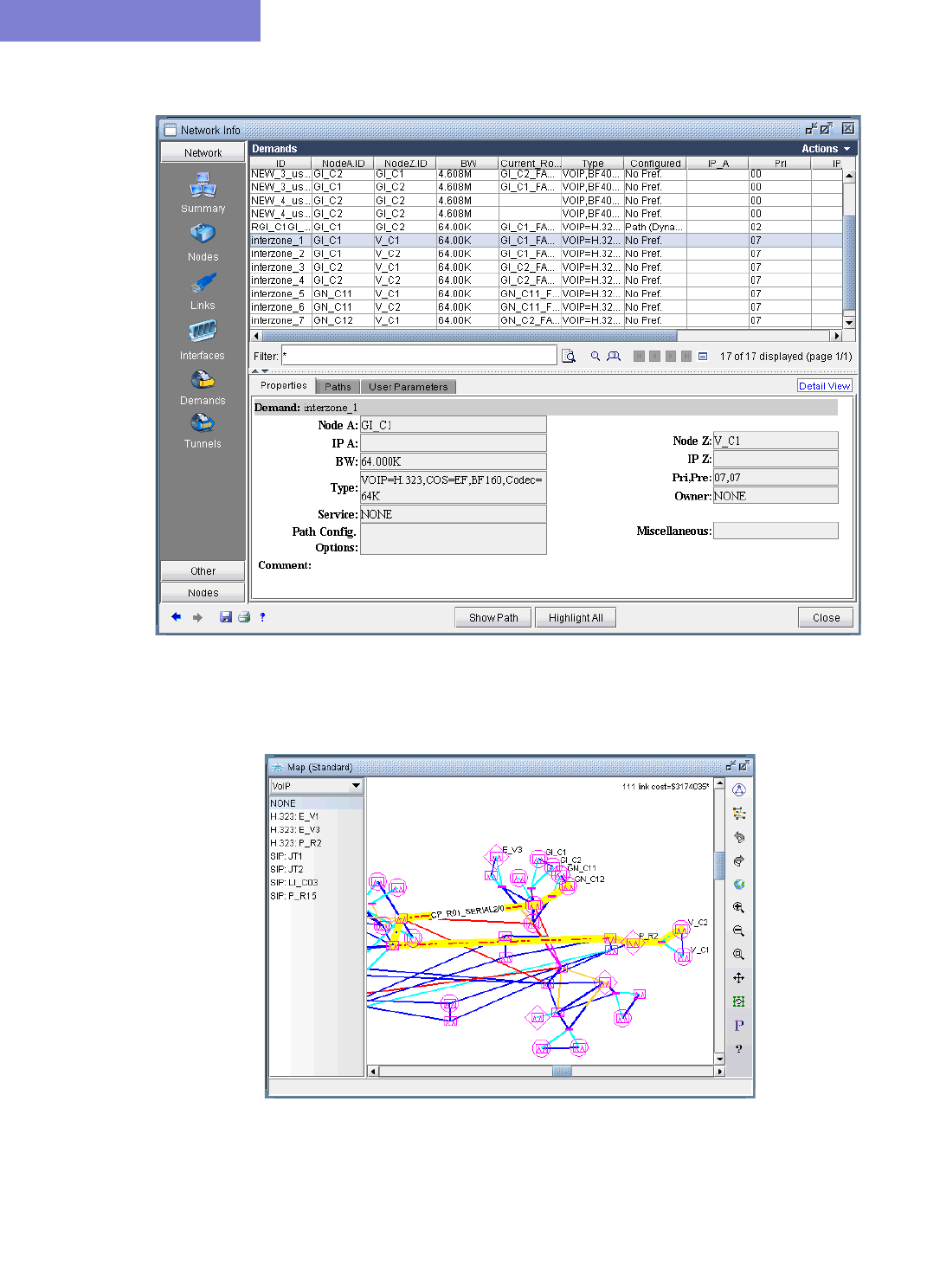
VOICE OVE R IP*
15-14 Copyright © 2014, Juniper Networks, Inc.
15
Figure 15-16 Demand window showing VoIP demands added
40. Next, you can click on the Show Path button to display the actual call path.
Figure 15-17 Call path of one of the added VoIP demands
41. You can also view the Network Reports > Link Reports > Planned Link Utilization report from the
Report Manager to view the utilization for a link that was used to carry the voice traffic.
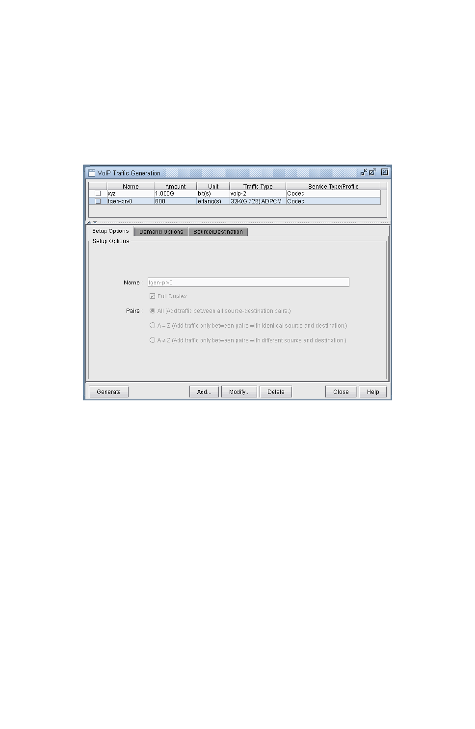
VOICE OVER IP*
Copyright © 2014, Juniper Networks, Inc. 15-15
. . . . .
Using the VoIP Traffic Generation Tool
The third way to specify VoIP traffic using IP/MPLSView’s VoIP module is via the VoIP Traffic
Generation Tool (accessible via the Traffic > Demand Generation > VoIP menu). This tool is derived
from the general Traffic Generation Tool and includes VoIP-specific functionality, such as specifying traffic
in Erlangs. The following figure shows the tool’s main window. The top half of the window displays a list of
the traffic profiles that have already been created, while the bottom half includes three tabs that each contains
various options related to the selected traffic profile. Notice that the figure shows two existing traffic profiles,
one in which the units are specified in bits per sec and the other in Erlangs.
Figure 15-18 VoIP Traffic Generation Tool main window
For more detailed information on IP/MPLSView’s general traffic demand generation capabilities, please
consult the chapter titled The Traffic Menu that is located in the Reference Guide.
Creating a Traffic Profile via the VoIP Traffic Generation Wizard
To specify VoIP traffic, the user first needs to go through the following sequence of steps to create a new traffic
profile that will contain all of the demand generation options.
42. Click on Add to bring up the VoIP Traffic Generation Wizard. As the following figure shows, the first
screen of the wizard describes the options and steps it will walk the user through.

VOICE OVE R IP*
15-16 Copyright © 2014, Juniper Networks, Inc.
15
Figure 15-19 VoIP Traffic Generation Wizard overview screen
43. Clicking on Next takes the user to the step where the source and destination locations are specified. The
user has the option of specifying the locations via a file or via the WANDL client (the No File option). If an
input file is specified, then the Wizard will compute end-to-end traffic demands between the MGWs (or
SIP-UAs) based on the end-to-end traffic matrix that was specified. Notice that as you mouse over an input
file type icon, a small popup box appears to illustrate the input file format. Otherwise, if the WANDL client
(the No File option) is selected, then the total traffic and node weights must be specified by the user as
inputs to IP/MPLSView’s gravity model function, which will output estimated end-to-end traffic demands.
First, we will go through the latter option using the WANDL client. Sections on how to specify the usage of
end-to-end traffic matrix input files then follow.
Figure 15-20 Popup box illustrating input file format
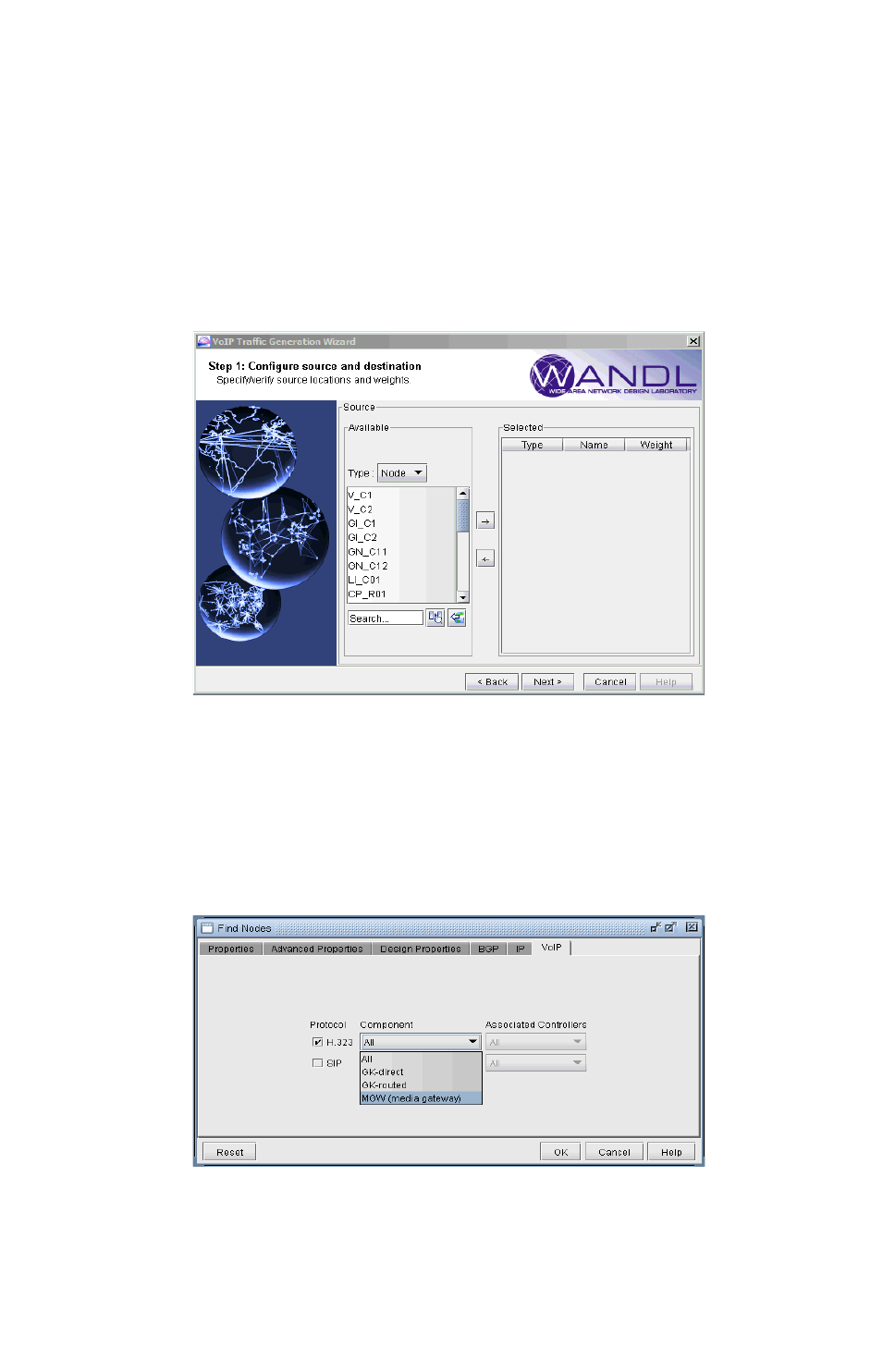
VOICE OVER IP*
Copyright © 2014, Juniper Networks, Inc. 15-17
. . . . .
Using the No File Option
44. With the No File option selected, click the Next button to continue on to the source-node selection screen,
from which the user would specify the source location(s)/weight(s). The list of Available nodes is pre-
filtered for nodes that have either an H.323 MGW or SIP-UA VoIP attribute. From the Available list of
nodes, the user would select a group of nodes, and click on the right-arrow button to move it into the
Selected list. As shown in the following figure, there are two icons next to the search box that provide
alternative filtering for the user; one icon allows the user to filter using the Find Nodes window, the other
using the filter from map function (please refer to the General Traffic Generation chapter of the
General Reference Guide for more details on node filtering).
Figure 15-21 Selecting source nodes in the VoIP Traffic Generation Wizard
For instance, clicking on the magnifying glass icon next to the Search box would bring up the Find Nodes
window, from which the user may perform filtering operations for nodes with VoIP attributes. For instance,
the user can filter for all nodes that have the H.323 MGW attribute as shown in the following figure. The
Associated Controllers dropdown selection box allows the user to further limit the search -- e.g. to filter for
all the MGWs for a particular GK controller.
Figure 15-22 Find Node window’s VoIP tab
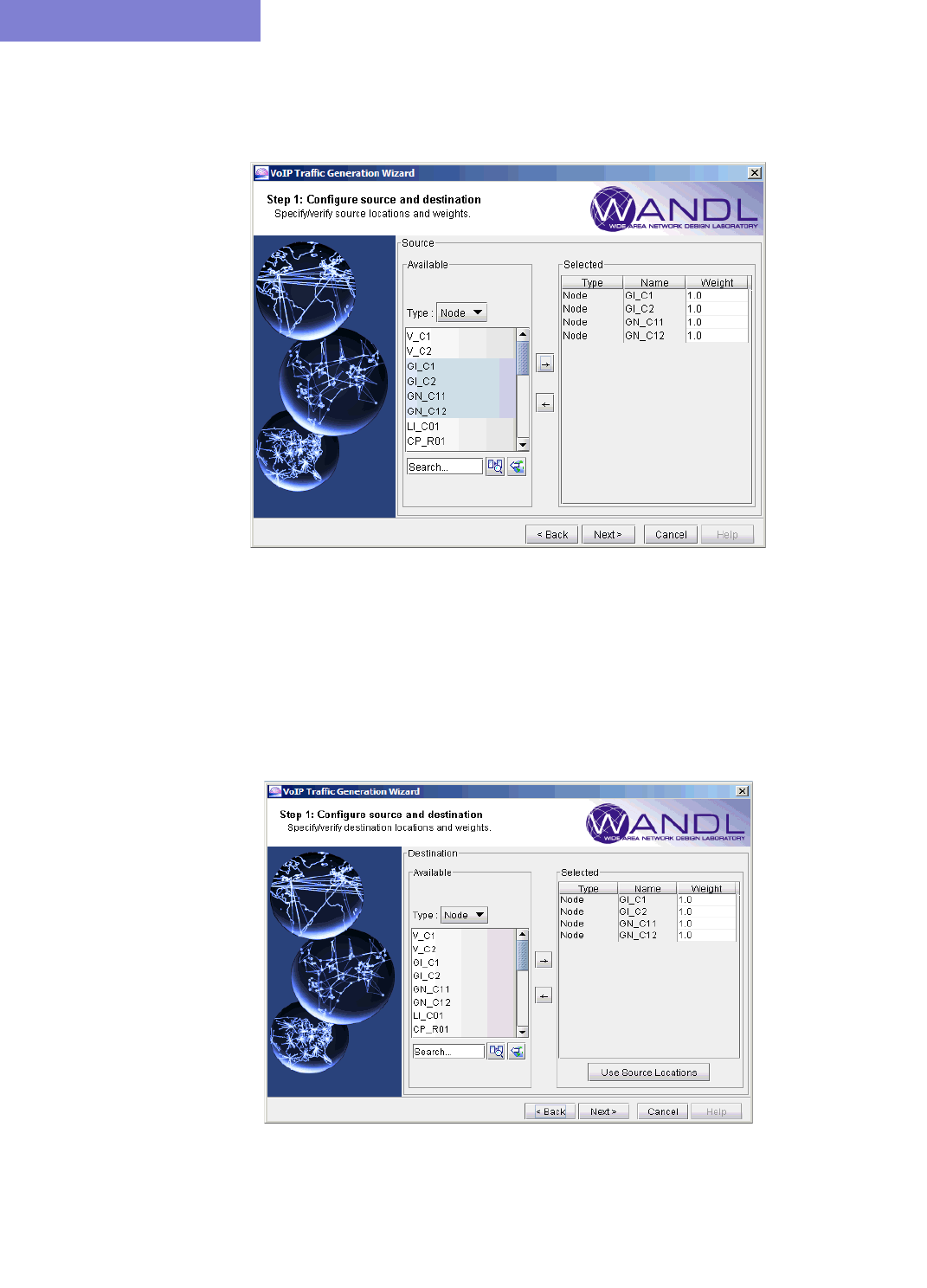
VOICE OVE R IP*
15-18 Copyright © 2014, Juniper Networks, Inc.
15
45. Next, the user would select the list of nodes from the listbox and click on the right-arrow icon to move it
into the Selected table on the right.
Figure 15-23 Selecting source nodes and weights
Each selected node has a weight parameter (please refer to the general Traffic Generation document for
detailed information about weights) in the Weight column that is used in the gravity model calculations
and may be changed by the user to another weight as desired.
46. Clicking on Next takes the user to the destination-node selection screen, from which the same steps used in
the source-node selection screen would be repeated. If the user wishes to select the same nodes for the
destination list as the source list, then simply click on the Use Source Locations button.
Figure 15-24 Selecting destination nodes and weights
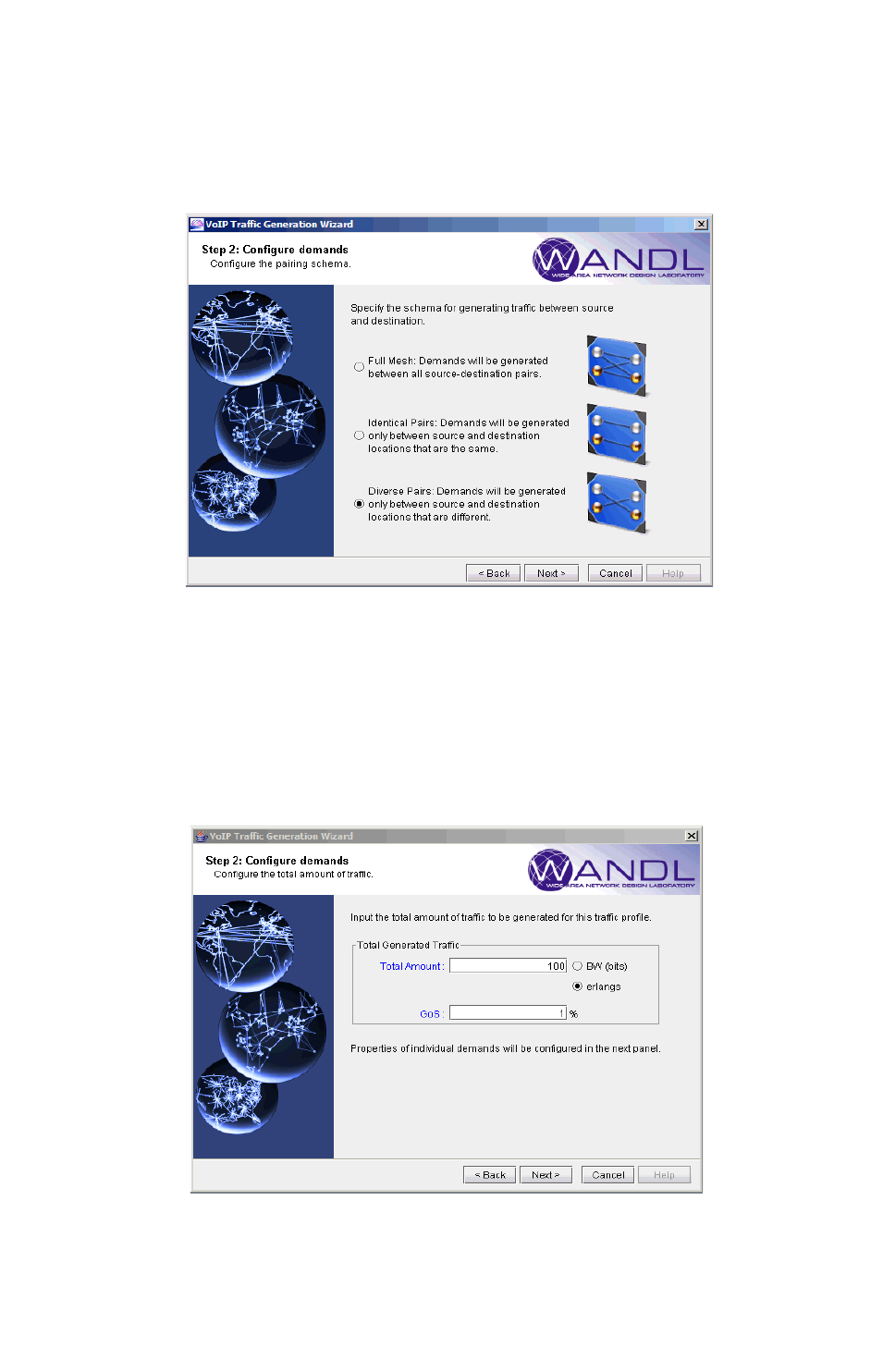
VOICE OVER IP*
Copyright © 2014, Juniper Networks, Inc. 15-19
. . . . .
47. Clicking on Next takes the user to the pairing schema screen. Here, the user may choose that the traffic
demands will be generated in a full-mesh fashion, between identical pairs, or between diverse pairs. The
following figure shows Diverse Pairs being chosen, so that traffic demands will be created end-to-end
between different nodes (MGWs or SIP-UAs).
Figure 15-25 Choosing the pairing schema for traffic demand generation
48. The next window that follows is where the user would specify the total amount of traffic demands that will
be generated. Traffic can be specified in terms of bandwidth (bits per sec) or in terms of Erlangs. If
Erlangs is chosen, then the user would also fill in a GoS (Grade of Service) or blocking factor percentage.
Given traffic in Erlangs and a GoS, the Erlang-B formula is used by IP/MPLSView internally to compute
the number of circuits needed. The following figure shows 100 Erlangs of total traffic being specified,
with a GoS of 1%.
Figure 15-26 Specifying the total amount of Elrang voice traffic and the GoS
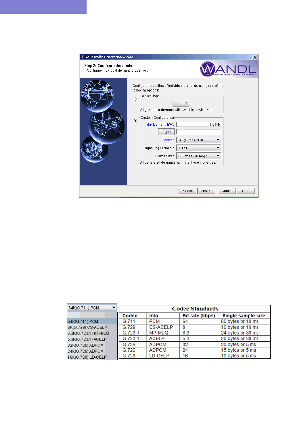
VOICE OVE R IP*
15-20 Copyright © 2014, Juniper Networks, Inc.
15
49. Clicking on the Next button then brings the user to the screen used to configure all the options needed to
compute the bandwidth per call (circuit).
Figure 15-27 Specifying options used to compute bandwidth per call
The following describes each of the options that can be specified by the user:
•Max Demand BW: This specifies the maximum bandwidth of an individual demand that will be
generated. The purpose for this parameter is to aggregate multiple, smaller circuits (calls) into a larger one, so
that fewer overall demands would need to get routed. In the above figure, many calls can be aggregated into a
demand of size up to a T1 (1.544M).
•Type: Click on this button to bring up the Demand Type Parameter Generation window, where you can
specify additional parameters, such as the CoS policy class.
•Codec: This dropdown box allows the user to choose from the many standard voice Codecs that are
supported by the VoIP module. The following table summarizes the Codecs and the associated options that are
available in the VoIP module.
Figure 15-28 Codec standards supported by the VoIP module
•Signaling Protocol: The user may choose either none, H.323, or SIP as the VoIP signaling protocol.
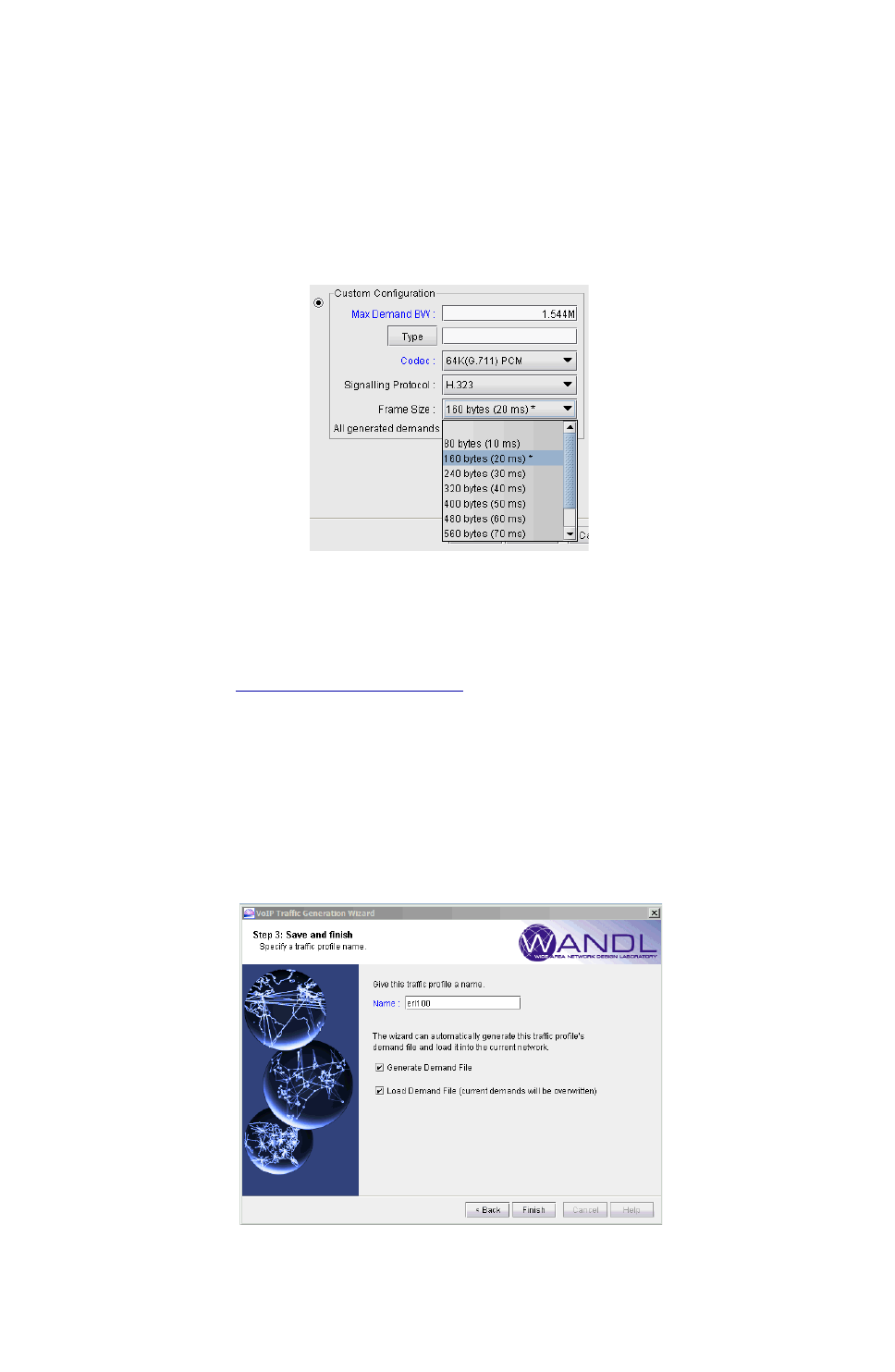
VOICE OVER IP*
Copyright © 2014, Juniper Networks, Inc. 15-21
. . . . .
•Frame Size: Also known in the industry as Payload Size or Payload Duration or Packetization
Delay, this value is a multiple of the single sample size (since a voice packet consists of multiple samples). For
instance, the G.711 codec would have Frame Size values of 80bytes, 160bytes, 240bytes, etc. Notice that Frame
Size can be specified in terms of bytes or ms; the conversion formula is: Frame Size (ms) = Frame Size
(bytes) / Codec bit rate (kbps)
The following figure shows the Frame Size dropdown box, with the recommended value marked with an
asterisk (*) next to it.
Figure 15-29 Choosing a Frame Size for a particular Codec
The recommended size is based on the general rules of packing several samples into a voice packet to keep the
overhead percentage lower, while at the same time keeping the delay under 30 ms.
As noted in Chapter 36, Overhead Calculation, IP/MPLSView factors in encapsulation overhead whenever
Frame Size is specified. Note that VoIP actual call traffic is carried over IP/UDP/RTP, so the encapsulation
overhead would need to include:
20bytes(IP) + 8bytes(UDP) + 12bytes(RTP) = 40bytes
50. Clicking on the Next button then takes the user to the final screen where the user specifies a name for the
traffic profile, which will be saved in the spec file. The user may also choose to generate the demand file
and even to load the demands into the current network. If the traffic was specified in units of Erlangs, then
an Erlang file is also generated.
Figure 15-30 Saving the traffic generation profile and choosing whether to generate demands
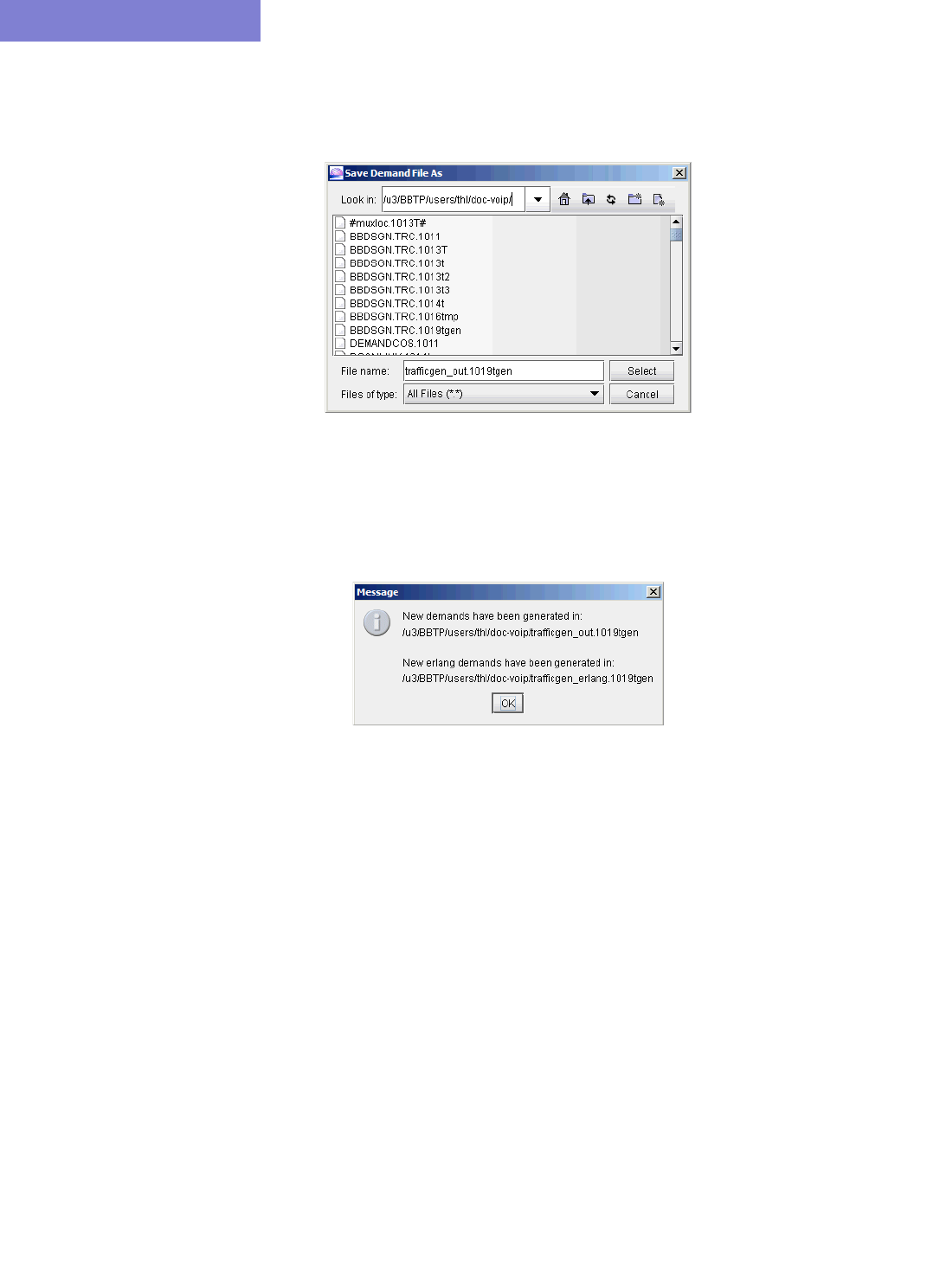
VOICE OVE R IP*
15-22 Copyright © 2014, Juniper Networks, Inc.
15
51. If the Generate Demand File option has been checked, then when the user clicks on the Finish button, the
following window will appear to prompt the user to specify where the generated demand file will be saved.
Figure 15-31 Specifying where to save the generated demand file
If the traffic was specified in units of Erlangs, then an additional window will appear to prompt the user to
specify where the generated Erlang file will be saved.
A message will then pop up to inform the user of where the generated files have been saved.
Figure 15-32 Message showing location of the generated demand and Erlang files
Using the running example in this chapter, the generated demand and Erlang files are shown in the following
figure.
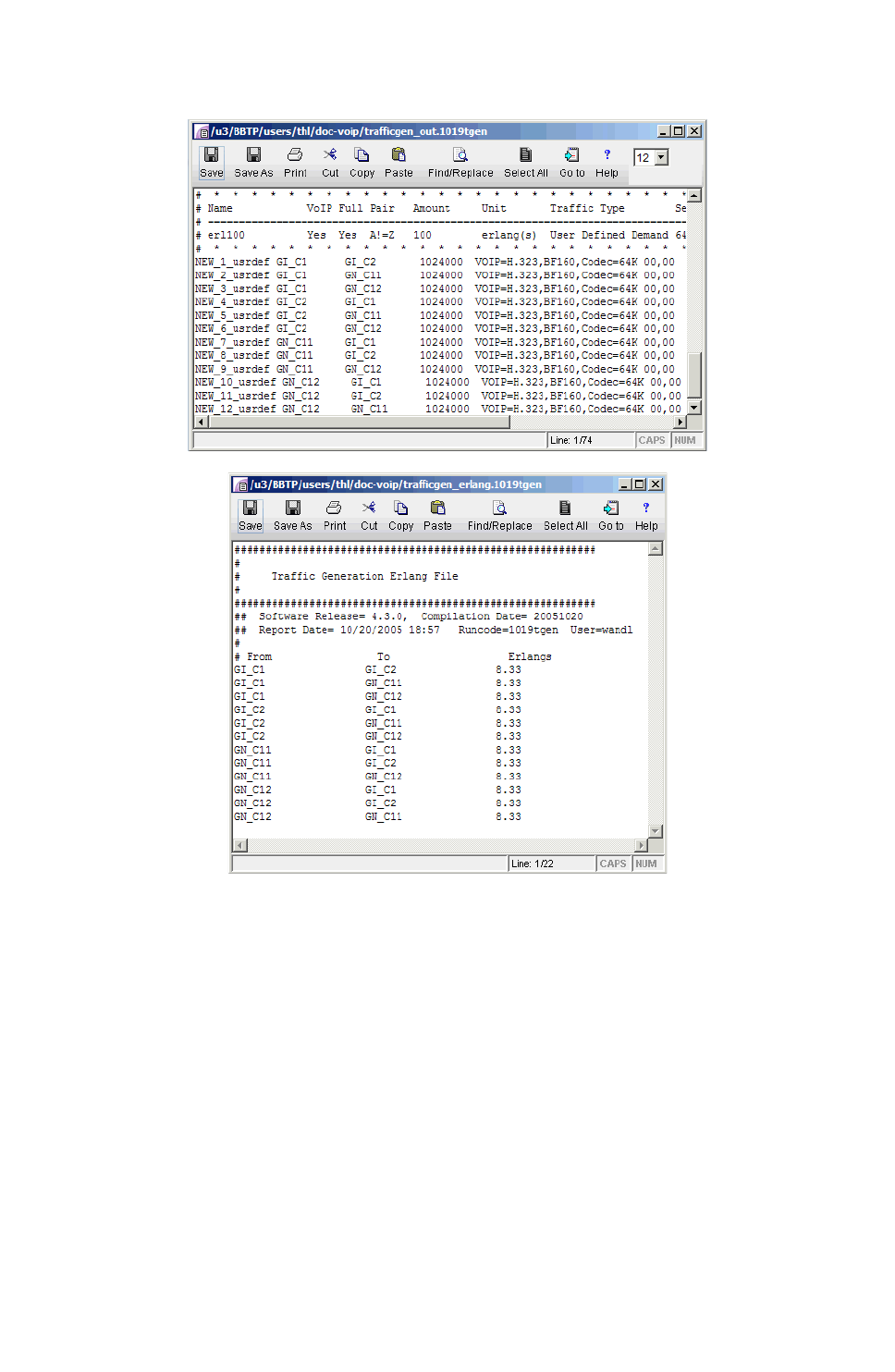
VOICE OVER IP*
Copyright © 2014, Juniper Networks, Inc. 15-23
. . . . .
Figure 15-33 The demand and Erlang files generated
52. The following figure shows the traffic profile that was just created by the VoIP Traffic Generation
Wizard. To generate demands for one or more of the profiles, click on the checkbox next to the profile and
then click on Generate.
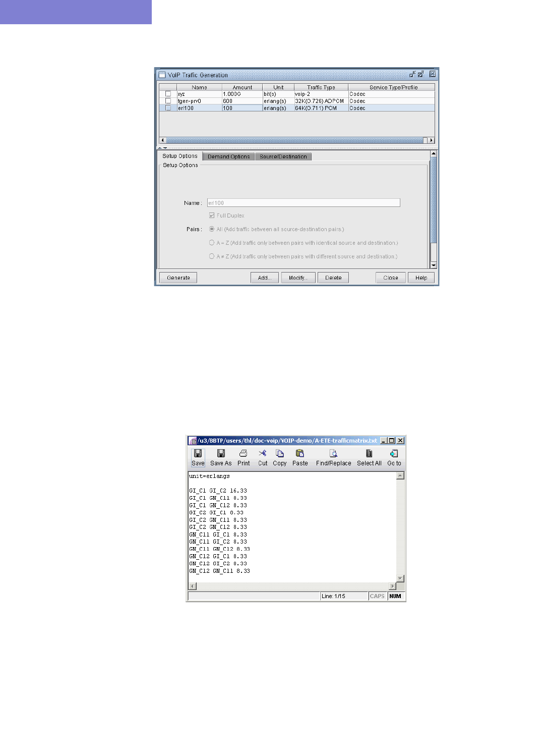
VOICE OVE R IP*
15-24 Copyright © 2014, Juniper Networks, Inc.
15
Figure 15-34 Traffic Profiles that can be selected for generation
Using an End-to-end Traffic Matrix Input File
53. If you have an end-to-end traffic matrix input file where the ends points are MGWs (or SIP-UAs), then you
can select it under the Select Source/Destination Input File section. If your file includes lines in the
form of source, destination, amount triplets, then click on the third icon from the left under the Choose
Input File Type section. Under Input File Units, specify either bps or Erlangs depending on your input
file units. If Erlangs is chosen as the units, then you also need to specify the GoS. The following figures
show the input data file used for this example and the corresponding selections to choose in the Wizard.
Figure 15-35 End-to-end (MGW-to-MGW) Erlang traffic matrix input file
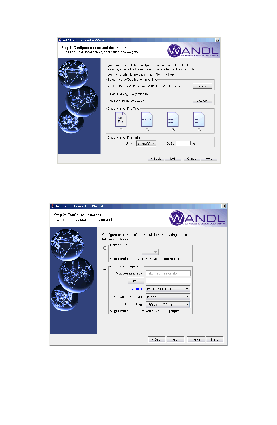
VOICE OVER IP*
Copyright © 2014, Juniper Networks, Inc. 15-25
. . . . .
Figure 15-36 Specifying the end-to-end traffic matrix file input options
54. Next, configure the options for the demands as previously described.
Figure 15-37 Configuring options for the demands
55. Finally, specify a name for the traffic profile and then generate and load the demand file.
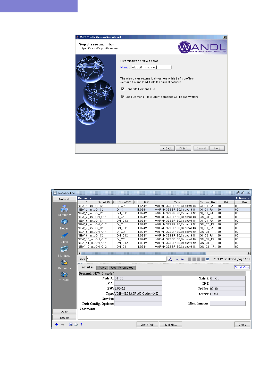
VOICE OVE R IP*
15-26 Copyright © 2014, Juniper Networks, Inc.
15
Figure 15-38 Saving the traffic profile and loading the demands
56. The corresponding generated demands are shown in the following figure.
Figure 15-39 Demands created by the wizard
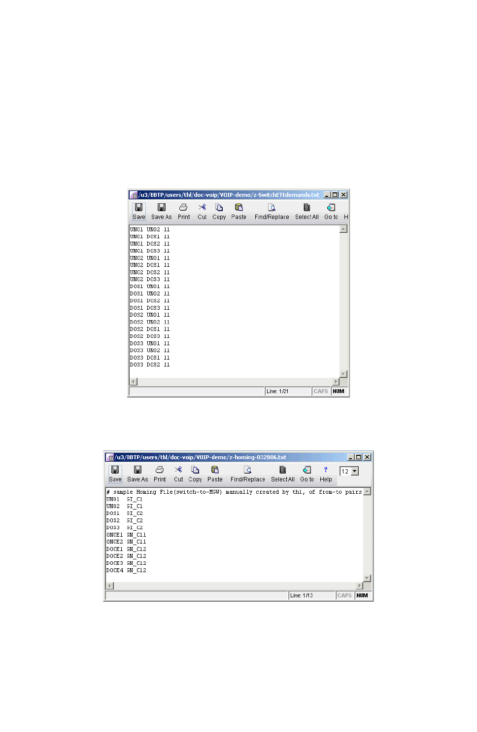
VOICE OVER IP*
Copyright © 2014, Juniper Networks, Inc. 15-27
. . . . .
Using an End-to-end Traffic Matrix Input File with a Homing File
57. If you have an end-to-end traffic matrix input file in which the end points are switches (that home to
MGWs or SIP-UAs), then you must specify two files. Under the Select Source/Destination Input File
section, specify the end-to-end traffic matrix input file. Similarly, select the homing file under the Select
Homing File section. If your file includes lines in the form of source, destination, amount triplets, then
click on the third icon from the left under the Choose Input File Type section. Under Input File Units,
specify either bps or Erlangs depending on your input file units. If Erlangs is chosen as the units, then you
also need to specify the GoS. The following figures show the input data files (both the end-to-end traffic
file as well as the homing file) used for this example and the corresponding selections to choose in the
Wizard.-
Figure 15-40 End-to-end (switch-to-switch) Erlang traffic matrix input file
Figure 15-41 Switch-to-MGW Homing file
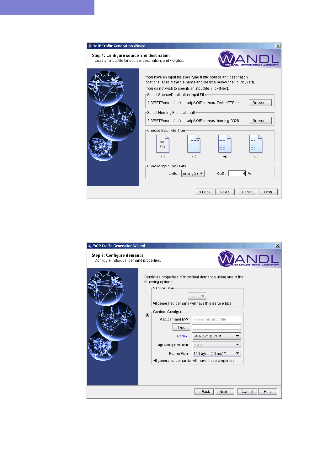
VOICE OVE R IP*
15-28 Copyright © 2014, Juniper Networks, Inc.
15
Figure 15-42 Specifying the end-to-end traffic matrix and homing file input options
58. Next, configure the options for the demands as previously described.
Figure 15-43 Configuring options for the demands
59. Finally, specify a name for the traffic profile and then generate and load the demand file.
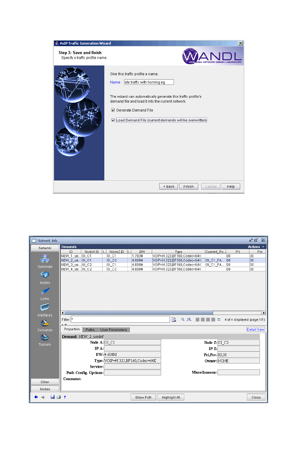
VOICE OVER IP*
Copyright © 2014, Juniper Networks, Inc. 15-29
. . . . .
Figure 15-44 Saving the traffic profile and loading the demands
60. The corresponding generated demands are shown in the following figure.
Figure 15-45 Demands created by the wizard
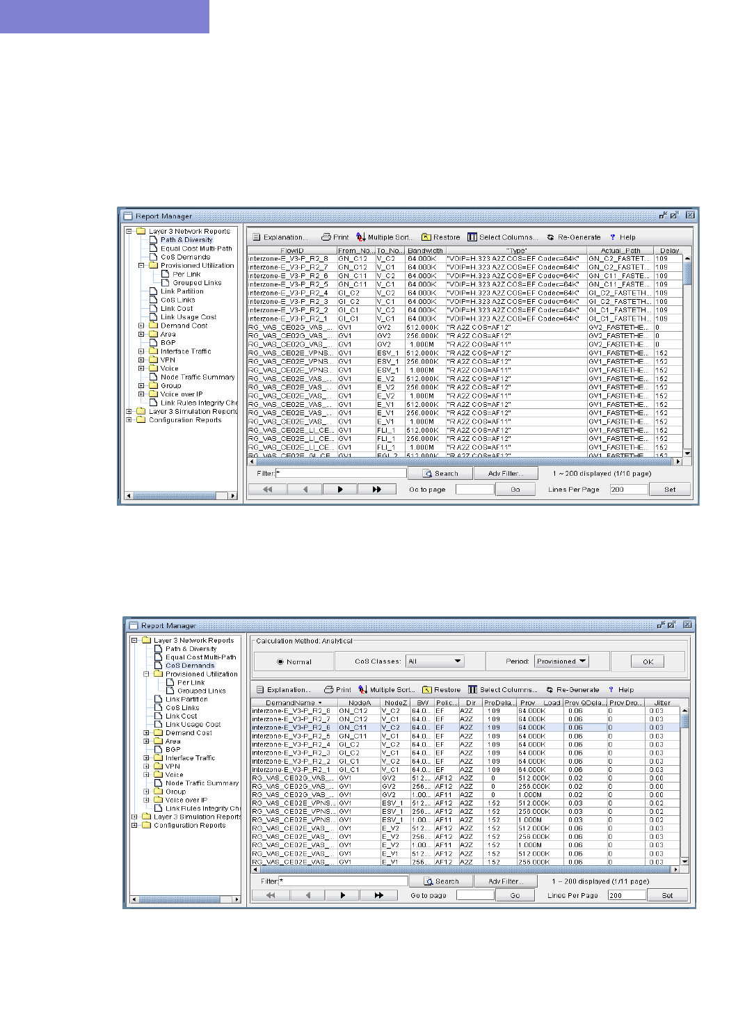
VOICE OVE R IP*
15-30 Copyright © 2014, Juniper Networks, Inc.
15
Reporting VoIP Information
A variety of reports are available from the Report Manager to help the user to analyze the effects of VoIP
traffic on the network.
61. Under Network Reports > Demand Reports, the Path & Diversity report allows the user to see
delay and path information related to VoIP demands. For instance the following figure shows the report
with eight interzone VoIP demands.
Figure 15-46 Path & Diversity report showing VoIP demands
62. The following figure shows the CoS Demands report and includes queuing delay and jitter information
for the EF class of VoIP demands.
Figure 15-47 CoS Demands Report that include queuing delay and jitter information
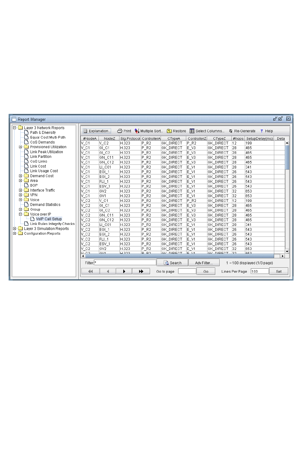
VOICE OVER IP*
Copyright © 2014, Juniper Networks, Inc. 15-31
. . . . .
VoIP Call Setup Report
63. The Report Manager includes a VoIP-specific report category, “Voice over IP”. Below this category,
you will find the VoIP Call Setup report.
When the user chooses the VoIP Call Setup report, rtserver will create a full mesh of calls between H.323
MGWs and between SIP-UAs, and then report the result in the VoIP Call Setup report. As shown in the
following figure, the Call Setup report gives information about the two endpoint nodes (H.323 MGWs or SIP-
UAs), the controller (Gatekeeper or SIP server), the number of hops, and the Setup Delay. When a call cannot
be placed, additional information is provided in the Details column to help the user to determine the reason for
its failure to be placed.
Figure 15-48 Report Manager, VoIP Call Setup Report
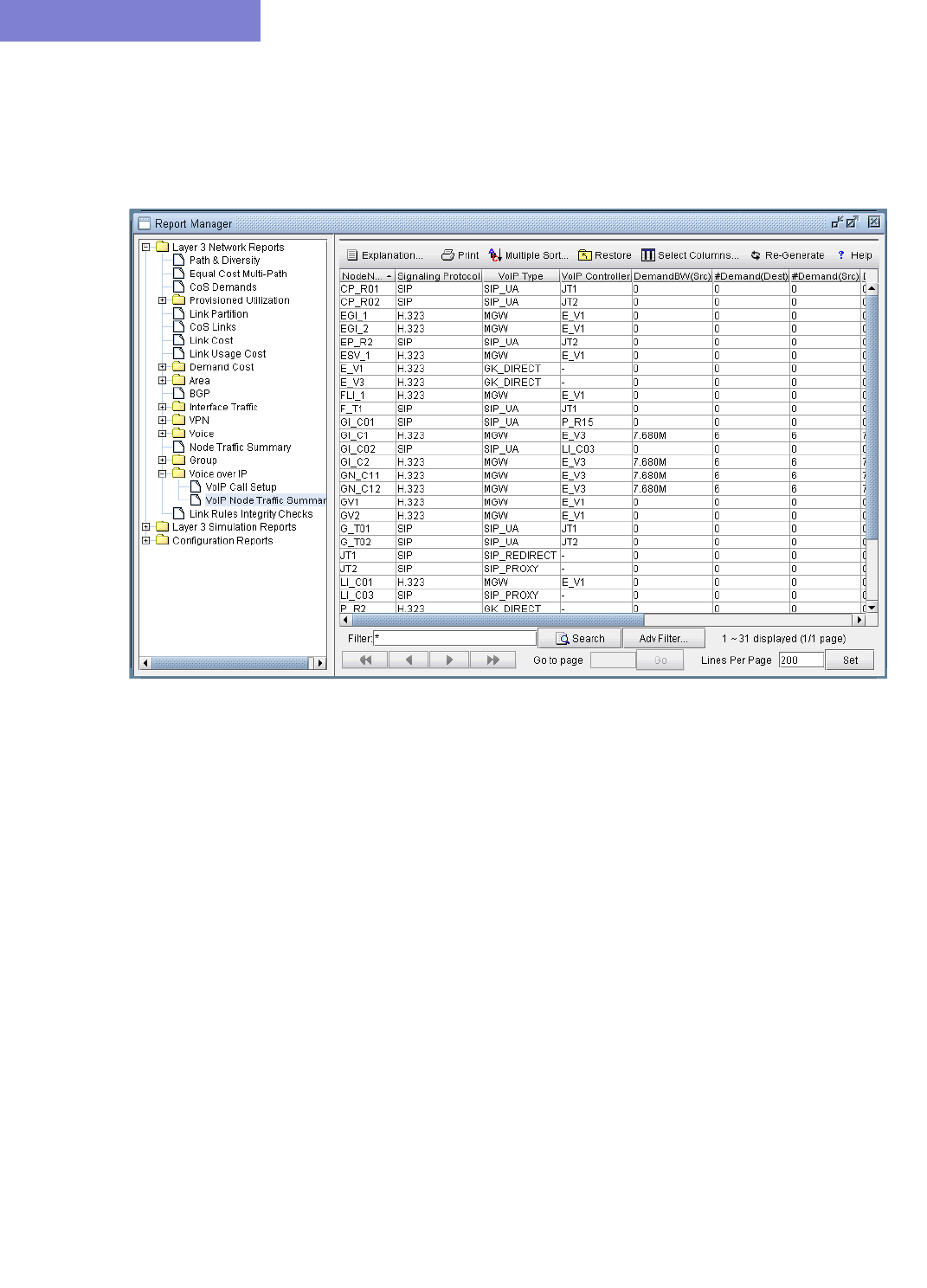
VOICE OVE R IP*
15-32 Copyright © 2014, Juniper Networks, Inc.
15
VoIP Node Traffic Summary Report
64. Below the Voice over IP category, you will also find the VoIP Node Traffic Summary report. This
report gives you VoIP-related information for a node, such as MGW or SIP-UA loading (traffic demands
originating and terminating at a node).
Figure 15-49 Report Manager, VoIP Node Traffic Summary Report
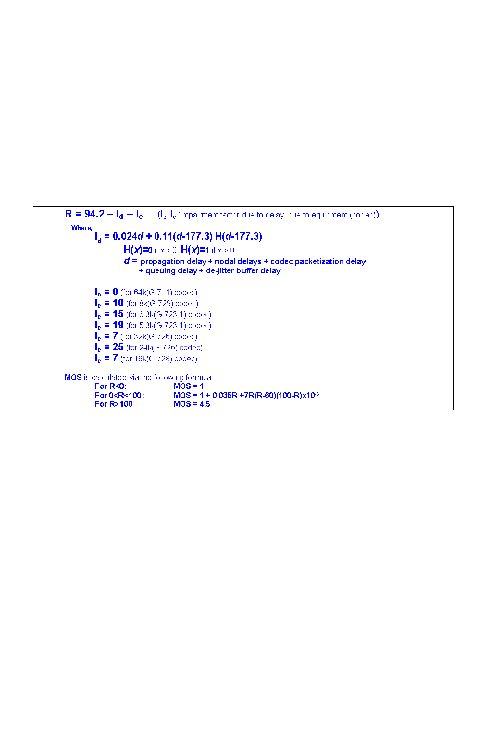
VOICE OVER IP*
Copyright © 2014, Juniper Networks, Inc. 15-33
. . . . .
E-Model R-factor Voice Quality Assessment
Perceived voice quality can be measured by the Mean Opinion Score (MOS), a subjective quality rating that
ranges from a scale of 5 (excellent) to 1 (unacceptable). The perceived quality of a voice call depends on many
factors, including delay, jitter, choice of codec, and loss. The ITU-T E-model for voice quality assessment is
used to estimate call quality based on measured parameters. It defines an R-factor that combines different
aspects of voice quality impairments into an equation; the main sources of impairment are the latency
parameters, which include propagation, nodal, queuing, packetization, and de-jitter buffer delays. Once the R-
factor has been computed, the MOS can also be derived. The VoIP module includes a VoIP E-Model report
that computes both the R-factor and the MOS for the VoIP call demands in the network. The following figure
shows the standard E-Model equation set that is used by the WANDL tool. The impairment factor (Ie) values
are taken from the ITU-T G.108 Recommendation document.
Figure 15-50 E-Model R-factor Equation Set
The report allows you to readily assess the quality of the network for VoIP. In cases where VoIP demands have
poor R-factor/MOS scores, the report can help the user to determine the reason for the poor rating. For instance,
too many hops could result in a large propagation delay value, contributing to a poor R-factor/MOS.
You can access the VoIP E-Model report from the Report Manager's Voice over IP folder's VoIP E-Model
report as shown in the following figure.
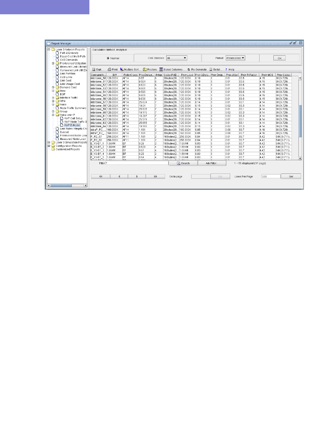
VOICE OVE R IP*
15-34 Copyright © 2014, Juniper Networks, Inc.
15
Figure 15-51 VoIP E-Model Voice Quality Report

Copyright © 2014, Juniper Networks, Inc. 16-1
. . . . .
. . . . . . . . . . . . . . . . . . . . . . . . . . . . . . . . . . .
B
ACKBONE
D
ESIGN
FOR
OSPF A
REA
N
ETWORKS
*
16
his chapter describes how to design links for a multiple-area OSPF network. the WANDL software supports
both single area design and multiple area design. It can be specified per node what areas the node can be
connected to. In addition, the admin weight tool and linkdist files can be used to set the link admin weights
for new links.
*Note that a special password is required for the OSPF Design feature. Please contact your Juniper representative for
more information.
When to use
Use these procedures when you have multiple OSPF areas in your network and want to optimally purchase or place
links for a multiple OSPF area network.
Prerequisites
If you wish to perform this task in the WANDL client, you should have a router spec file open before you begin. To
follow along with this tutorial, you can open the spec.area spec file located in your
$WANDL_HOME/sample/IP/ospfdesign directory. ($WANDL_HOME is the program’s home directory. It is
/u/wandl by default.)
Related Documentation
Note that this feature is an optional feature and requires a special password for OSPF area design.
For an overview of the WANDL software or for a detailed description of each feature and the use of each WANDL
client window, refer to the General Reference Guide or Chapter 37, Router Reference.
Refer to the Design & Planning Guide chapter on Design for more details about setting various factors such as link
admin weights.
Recommended Instructions
Following is a high-level, sequential outline of the process of designing the network for OSPF, and the associated,
recommended detailed procedures.
1. Specify for each node an area to use when assigning an area for a link created at that node.
2. Set the distance default for the OSPF protocol. This can be done on a site to site basis in the admin weight tool
or using the linkdist files.
3. Perform a design and diversity design.
Detailed Procedures
1. Select Tools > Options > Design. Then in the Path Placement option pane, select OSPF as the routing
method. Note that once this is done, links must be able to communicate OSPF to carry traffic. To ensure this, go
to Modify > Elements > Links and examine the “Protocols” tab. Select the links on which you wish to enable
OSPF, click the Modify button, and set the OSPF protocol to “Yes”. When doing so, the area of the link should
also be specified. (The default, if unspecified, will be AREA0).
Note: If you are following along with the ospfdesign sample network, the initial network contains no links.
T
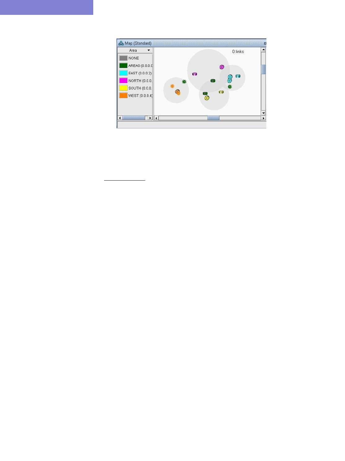
BACKBONE DESIGN FOR OSPF AREA NETWORKS*
16-2 Copyright © 2014, Juniper Networks, Inc.
16
Figure 16-1 Initial Network, Subviews > Area legend
2. If you want to design a multi-area network, you need to have areas in your network. You can add area entries
using the Modify > Protocols > OSPF Areas option. Specify here the AreaID and corresponding IP
Address (e.g.,0.0.0.1). Alternatively, you can enter this information through a file (see the domain file format in
the File Format Guide).
3. You can categorize nodes as belonging to AREA0 or another area in the Design Properties tab of the Modify
> Elements > Nodes window. In OSPF, the area assignment is associated with links. However, for design
purposes only, the WANDL software also allows areas to be assigned to nodes so that even when performing a
design from scratch, the program can decide what area to assign a link based upon the areas of its endpoints.
Specifying Design Properties for Multiple-Area OSPF Networks
When the program adds a link between two nodes, the area assignment for the link follows these rules:
•If both nodes have specified the same area, use that area.
•If one node has specified AREA0 and the other has specified a different area, use the latter area.
SPECIFYING AREA0 AS THE DESIGN PROPERTY FOR A NODE
4. You can specify AREA0 for nodes that should be connected by AREA0 links.
5. Among the nodes that specify AREA0 for this design property, you can indicate those that are to be used as
gateways to specific areas. These nodes that can talk to one or more areas in addition to the backbone area are
referred to as area border routers (ABR). Note that only nodes with AREA0 for the design property should be
specified as gateways.
To specify a node to be an ABR, in the “Design Properties” tab of the “Modify Node” window, you should
select “True” in the Gateway selection box and then, in the Accessible Area List, checkmark each of the areas
the node can be a gateway to, or ALL if it can be a gateway to all areas.
BACKBONE DESIGN FOR OSPF AREA NETWORKS*
Copyright © 2014, Juniper Networks, Inc. 16-3
. . . . .
Figure 16-2 Specifying Node as a Gateway to Specific Areas (for Design Purposes)
SPECIFYING A NON-BACKBONE AREA AS THE DESIGN PROPERTY FOR A NODE
6. You can also specify if a node should be considered by the design to be in a non-backbone area. To do so, assign
an area to use for design other than AREA0 and make sure the Gateway field is set to “False” or left empty. In
this case, the design will only connect these non-backbone area nodes to nodes of the same area or nodes of the
backbone area.
Figure 16-3 Specifying that links must go to other Nodes in the area “SOUTH” or AREA0
7. When you have finished making these specifications, you may also want to set an admin weight scheme using
the Modify > More > Admin Weight feature or the linkdist file. See the Design chapter of the Design &
Planning Guide and the control files section of the File Format Guide for further details.
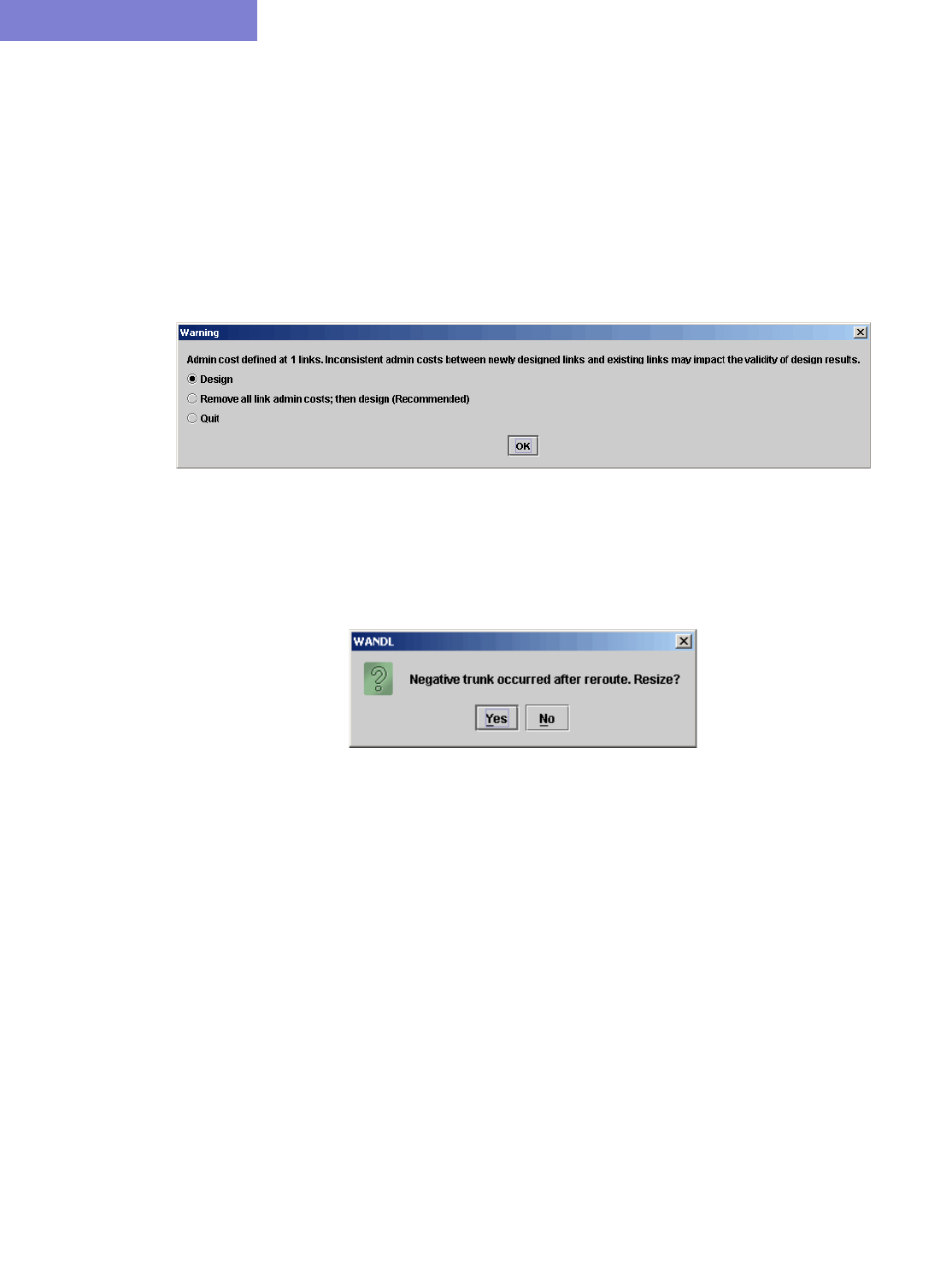
BACKBONE DESIGN FOR OSPF AREA NETWORKS*
16-4 Copyright © 2014, Juniper Networks, Inc.
16
Performing a Design
8. Switch to Design mode.
9. Before you begin your design, you can specify a fixlink file in the File>Read menu. This specifies those
existing links in your network that you do not want to delete during design.
10. Select Design > Backbone > Reset/Clear Links if you wish to do a design from scratch (greenfield
design). Otherwise, skip this step.
11. Select Design > Backbone > Perform Design to begin your design.
12. If you have links with admin weights already configured, you will be asked whether or not to remove them.
Select the “Remove” option and click OK.
Figure 16-4 Warning about Configured Admin Costs
13. Answer Yes when asked to remove potentially redundant links.
14. If there are still any negative trunks (utilization > 100%) you will be automatically asked to resize your network.
Answer Yes.
Figure 16-5 Negative Trunk
15. To view the final areas in your network, click the Subviews > Area menu of the topology map.
16. Your new links will be saved in the DSGNLINK.runcode file of your output directory.
17. You can perform an AutoGroup by Area using the Topology Window’s right-click menu
Grouping>AutoGroup menu and label the areas using the right-click menu’s Labels>Group Labels
option. Note that AREA0 will not be grouped together.
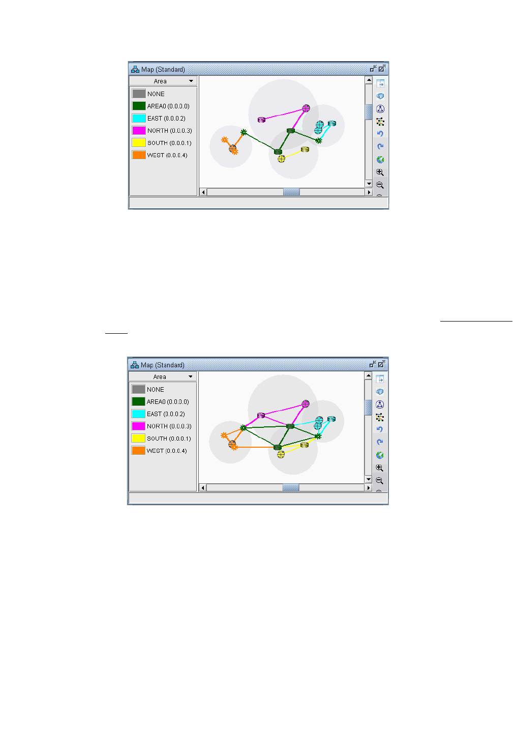
BACKBONE DESIGN FOR OSPF AREA NETWORKS*
Copyright © 2014, Juniper Networks, Inc. 16-5
. . . . .
Figure 16-6 Map After a Greenfield Design (Design from Scratch)
18. Before running the diversity design, you can rename your DSGNLINK file, which contains the current links in
your network, to avoid overwriting it in the diversity design. Or you can select File>Save Network File >
Links.
Performing a Diversity Design
19. Select Design > Backbone > Diversity Design to run a diversity design. (Refer to the Design & Planning
Guide’s Design chapter to understand more about the purpose and goals of design and diversity design.)
Figure 16-7 Map After a Diversity Design

BACKBONE DESIGN FOR OSPF AREA NETWORKS*
16-6 Copyright © 2014, Juniper Networks, Inc.
16

Copyright © 2014, Juniper Networks, Inc. 17-1
. . . . .
. . . . . . . . . . . . . . . . . . . . . . . . . . . . . . . . . . .
R
OUTING
I
NSTANCES
*
17
his chapter describes how to use OSPF processes, or routing instances, to partition a backbone network into
multiple networks which do not talk to each other. Because OSPF process IDs or routing instance names
can be defined per interface, multiple OSPF processes can be configured on each router. Only interfaces in
the same process can send packets and routing tables to each other, even if they are on the same router. Routing
Instance rules and OSPF process routing rules affect how demands are routed over the network.
*Note that a special password is required for the Routing Instance feature. Please contact your Juniper representative
for more information.
When to use
Use these procedures when you wish to model multiple logical topologies on a single physical network.
Recommended Instructions
Following is a high-level, sequential outline of the process of using the Routing Instance feature.
1. Create, import, or open a router network.
2. Create Routing Instances as described in Creating Routing Instances on page 17-1.
3. Associated Routing Instances with demands or path traces to see how they affect the routing in the network as
described in Path Analysis on page 17-5.
4. View the Routing Instance integrity check report in Reports on page 17-5.
Detailed Procedures
The following steps will guide the user through the process of creating Routing Instances, observing the effects of
the Routing Instances on the network, and viewing routing instance integrity reports.
Creating Routing Instances
1. If you have configuration files for your network, you can import the configuration files to create a network
model using the File>Import Data menu as described in Router Data Extraction on page 2-1. The interfaces
will automatically be associated with the routing-instance or process IDs that they belong to.
For Juniper routers, the interfaces listed under the [edit routing-instances routing-instance-name] block will be
assigned that routing-instance-name. Similarly, for Cisco routers, the interfaces whose addresses are advertised
under the network statements of the “router ospf <processID>” block will be assigned that processID.
Note that if an interface is not enabled for OSPF, it will be assigned to a reserved category called “NOPROT”
when the network is loaded. Similarly, if the interface is enabled for OSPF but has no process ID, it will be
assigned to a reserved category called “NOID” when the network is loaded.
To view the associations of routing instances to interfaces, select Network > Elements > Interfaces... When
selecting an interface, the bottom pane’s Advanced tab will show the process ID/routing instance in the OSPF
PID field. To view the routing instance as a column of the table, right-click on the header row and select Table
Options... Then add OSPF PID from the Available Item(s) list to the Selected Item(s) list.
2. OSPF process IDs (PID) or routing instance names can also be associated with interfaces via the Modify
Interface window’s Advanced tab for what-if testing, as shown in Figure 17-1. To access this window, click
the Modify action mode button to switch to Modify mode and then select Modify > Elements > Interfaces.
Then select the interfaces you want to modify and click Modify. An OSPF process on a Cisco router is an
integer number, while an OSPF process on a Juniper router is usually a name.
T
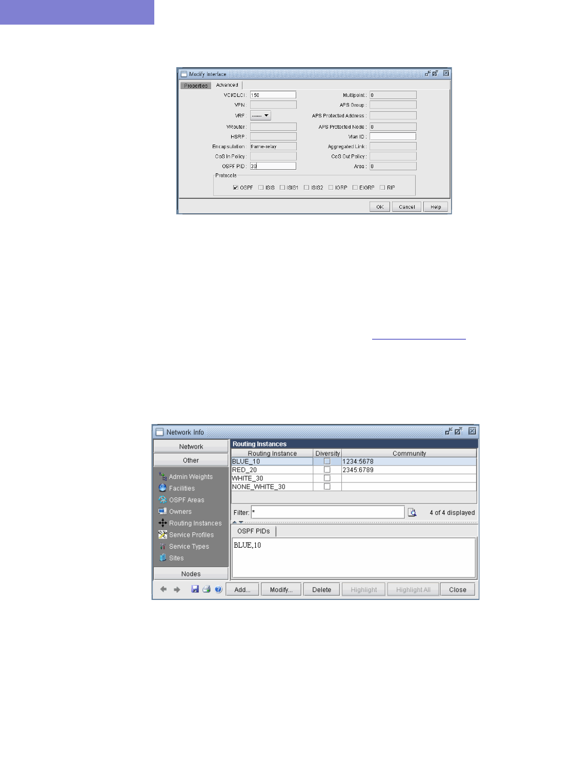
ROUTING INSTANCES*
17-2 Copyright © 2014, Juniper Networks, Inc.
17
Figure 17-1 Modify Interface Window
3. By default, multiprocess checking is turned off. To turn on multiprocess checking for routing instance analyses,
select the Tools > Options > Design, Path Placement options pane and set Ignore Multiprocess in the
lower right corner to “False”. Alternatively, you can add the parameter ignoremultiprocess=0 to the project’s
dparam.runcode file. To turn on multiprocess checking by default for all new network projects, create or edit the
file /u/wandl/db/misc/dparam.txt and add the line “ignoremultiprocess=0”.
4. To visualize Routing Instances/OSPF PIDs on the map by associating them together with a color, you can
specify a routeinstance file in the spec file as indicated in File Format on page 17-6 by adding the entry
“routeinst=filename” to the spec file while the network is closed, substituting filename with the name of the
route instance definition file . This file can also be indicated during a Configuration file Import (File>Import)
by specifying the RouteInstance file on the Misc tab of the Import Network Wizard. Alternatively, you can
make the association for the current network session by selecting Modify > Protocols > OSPF/ISIS
Routing Instance from the main menu while in Modify mode.
Figure 17-2 Routing Instance Window
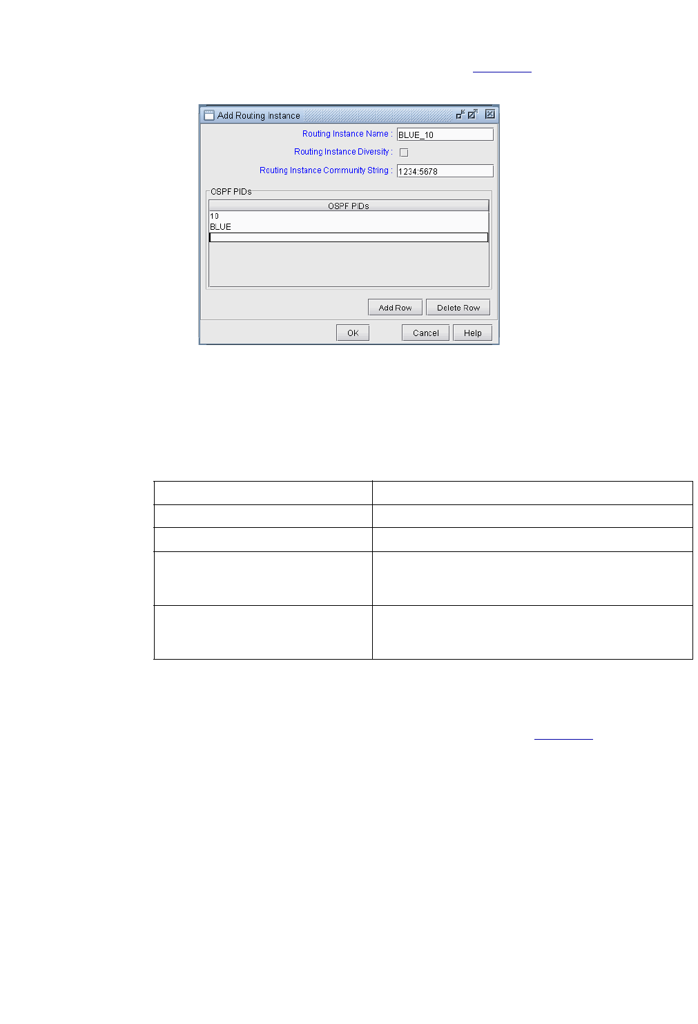
ROUTING INSTANCES*
Copyright © 2014, Juniper Networks, Inc. 17-3
. . . . .
5. Click the Add button, and a new window will appear as shown in Figure 17-3.
Figure 17-3 Add Routing Instance Window
Enter in the routing instance name. Then click Add Row for each OSPF process ID (for Cisco) or routing-
instance-name (for Juniper) that should be mapped to this routing instance.
6. Once the routing instance has been defined through the route instance file or through the Modify > Protocols
> OSPF/ISIS Routing Instance menu, links can also be associated with a Routing Instance via the Modify
Link window (accessed through Modify > Elements > Links), as shown in Figure 17-4. However, this
setting will be overriden if the interfaces attached to the links are also associated with a Routing Instance in the
Modify > Elements > Interfaces window. Interfaces on both ends of a link should belong to the same
Routing Instance.
Field Description
Routing Instance Name The name used to identify the partitioned network.
Routing Instance Diversity Not currently used
Routing Instance Community String Community Strings are used for BGP next-hop checking
to make sure that the BGP next hop is in the desired
routing instance
OSPF PIDs The OSPF process IDs and names belonging to this
routing instance. The same OSPF PID cannot be used in
more than one Routing Instance.
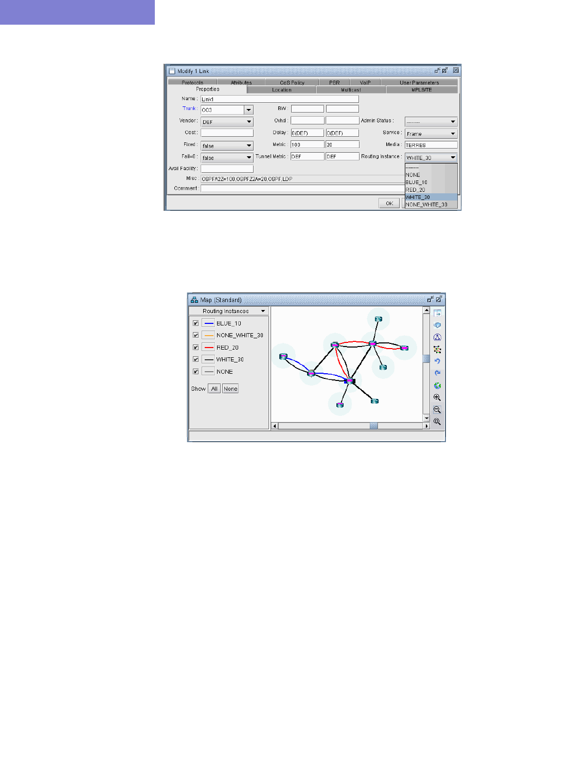
ROUTING INSTANCES*
17-4 Copyright © 2014, Juniper Networks, Inc.
17
Figure 17-4 Modify Link Window
7. If you select Subviews > Routing Instances in the Topology Map, the links will be displayed using the
color specified for the corresponding routing instance.
Figure 17-5 Topology Map - Routing Instance
You can toggle the checkmark next to a routing instance to turn on or off the display of links whose interfaces
are defined to be in that routing instance. Additionally, you can modify the color associated with a routing
instance on the map by clicking the color box next to the routing instance name.
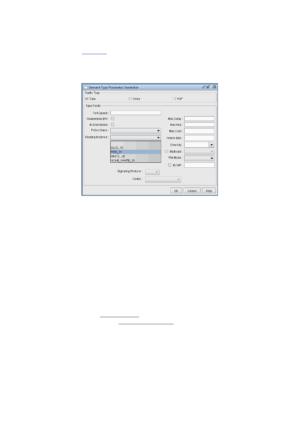
ROUTING INSTANCES*
Copyright © 2014, Juniper Networks, Inc. 17-5
. . . . .
Path Analysis
8. To see how Routing Instances affect the routing in a network, assign a Routing Instance to the Demand Type
of demands (Modify > Elements > Demands) or path traces (Network > Path & Capacity > Path) as
shown in Figure 17-6. This window is accessed by clicking on the Type button of the Modify Demand or
Demand Path window. Demands with a Routing Instance assignment can only be routed over links with the
same Routing Instance setting.
Figure 17-6 Demand Type Window
Reports
9. While in View or Design mode, select Report > Report Manager from the main menu. Select the Route
Instance report from Network Reports > Protocols. This report (RTINSTRPT) displays several integrity
checks:
•Asymmetric Route Instance Definition: Indicates links whose interfaces are associated with different
Routing Instances
•Unexpected OSPF process number: Indicates if an unexpected OSPF process number is defined
•Site Diverse Statistics: An Isolated Site is defined as a site which has the given routing instance
configured on at least one of its routers, but that site is not accessible via this routing instance from outside the
site. A Single Link Site is defined as a site which only has one link of the given routing instance that can be
used to reach the site from outside the site. If that link goes down, there is no other way to access that site for this
routing instance. (Note that for this integrity check, the user should have defined sites either through the site file
as described in the File Format Guide, or through the Modify > Elements > Sites and Modify > Elements >
Nodes as explained in the Design & Planning Guide. )
•BGP community definition errors: Indicates if the next-hop for any given community is in a different
Routing Instance
•Isolated colored PoP: Indicates if a Routing Instance has no outgoing link
Note that routing instance definitions via the routeinstance file or the Modify > Protocols > OSPF/ISIS
Routing Instance menu are prerequisites to generating the report.
ROUTING INSTANCES*
17-6 Copyright © 2014, Juniper Networks, Inc.
17
Figure 17-7 Routing Instance Integrity Check Report
File Format
ROUTEINSTANCE FILE
#name assigned_color OSPF_PID route-instance-name community
blue_10 color=BLUE 10 BLUE community=1234:5678
red_20 color=RED 20 RED community=2345:6789|3456:7890
white_30 color=GREEN 30 NOID
This file should be referenced in the spec file as “routeinst=filename”.
Note: Because OSPF process names do not need to be specified for Juniper routers, a special keyword “NOID” is
used, as seen in the third entry. The keyword “NOID” indicates that the interface is OSPF-enabled but is not listed in
the [edit routing-instances] section for a Juniper router.

Copyright © 2014, Juniper Networks, Inc. 18-1
. . . . .
. . . . . . . . . . . . . . . . . . . . . . . . . . . . . . . . . . .
T
RAFFIC
M
ATRIX
S
OLVER
*
18
n your network model, a set of end-to-end demands/flows is needed to perform various design and
simulation studies. A few sources, such as Cisco’s NetFlow/TMS, Juniper’s JFlow, LDP traffic statistics,
and LSP tunnel traffic statistics from SNMP, can provide end-to-end traffic information. However, this is
usually CPU intensive, so the data is often partial. Most traffic collection systems, including MRTG, Infovista,
and Concord eHealth, and WANDL’s traffic collector, provide interface traffic information. If you only have
access to interface traffic data and/or partial end-to-end flow traffic data, you can still derive a reasonable set of
end-to-end demands using the WANDL Traffic Matrix Solver.
The WANDL Traffic Matrix Solver addresses the following problem:
Given (a) the interface traffic utilizations in the network, (b) an optional trafficload file
defining the bandwidth for a subset of the flows in the network, and (c) a set of flows
indicating the sources and sinks in the network, determine the bandwidth of these flows
to produce the given interface traffic utilization values.
This problem has no one right answer. Mathematically, it has infinitely many solutions. However, by supplying
a little extra information, you can influence the WANDL Traffic Matrix solver to choose a solution that better
fits the characteristics of your network. For example, you can indicate which nodes are sources and sinks of
traffic (e.g., edge nodes). The remaining transit nodes will be limited to carrying “pass-through” traffic.
Once a possible traffic matrix solution has been derived, you can perform numerous traffic engineering studies.
For example, you can run simulations to study whether the traffic flows can be rerouted safely during network
failures. Or, you can use WANDL’s design capabilities to determine how to optimize cost and reliability for the
given traffic. You may have collected interface utilization data for multiple periods. For each period, you can
compute a set of end-to-end demands, especially times with heavy usage. Using this data, you can begin to
build a picture of how your network traffic changes over time.
*Note that this traffic matrix solver feature requires a special password. Please contact your Juniper
representative for more information.
Related Documentation
For information on interface traffic file formats, please refer to the “Demand/Traffic Files” chapter of the File
Format Guide.
Recommended Instructions
1. Specify the interface traffic file against which the traffic matrix will be computed as described in Input
Interface Traffic on page 18-2. The interface traffic file format is described in Interface Traffic File Format
on page 18-2.
2. Optionally, specify already known flow bandwidth as described in Input TrafficLoad File on page 18-3.
3. Create a set of “seed” demands to identify the possible end-to-end pairs whose bandwidths must be solved
for as described in Input Seed Demands on page 18-3.
4. Run T-Solve to compute a traffic matrix that would yield interface traffic results similar to the interface
traffic file as described in Running the Traffic Matrix Solver on page 18-5.
5. Compare the load derived from the new traffic matrix against the interface traffic.
I

TRAFFIC MATRIX SOLVER*
18-2 Copyright © 2014, Juniper Networks, Inc.
18
Detailed Procedures
The two inputs required by the T-Solve tool are the demand file and the interface traffic file. The Traffic Matrix
Solver will look at the origination/destination information from the demands in the demand file and suggested
bandwidths, and then assign new bandwidth values to these demands in order to match a period of measured
interface traffic on the network.
Input Interface Traffic
1. The interface traffic file can have one of the following two formats.
INTERFACE TRAFFIC FILE FORMAT
#NodeID Interface Direction - Per1 Per2 Per3 ...
NODE3 ATM1/0.1 A2Z - 192320 204960 30263 ...
NODE4 Ethernet0 A2Z - 381 382 539 ...
#LinkName Direction - Per1 Per2 Per3 ...
LINK1 A2Z - 192320 204960 30263 ...
The period data (Per1, Per2, ... Pern) indicates the traffic measured on the interface over several
consecutive periods. By default, the units is in bits per second. Note that the number of periods is not
limited to 24.
Before running the Traffic Matrix Solver, you will be asked to choose the desired period of traffic that the
Traffic Matrix tool should try to match when generating its traffic matrix solution.
Note: For your reference, the first two lines of the ingress or egress interface traffic files usually indicate
the collection time for the first period of data and the interval (e.g. 5 minutes) between periods, as shown in
the example below.
EXAMPLE INTERFACE TRAFFIC FILE
#Starting Time : 6/28/07 9:50 PM
#Interval : 5 minutes
NODE11 GigabitEthernet3/0/1 A2Z 0 243836792 239290424 240655400 245699408 253939296 249574480
250319920 247234760 249261400 248431176 246328192 246079952 241803032 245348992 244634288
245710200 242983256 241388720 239512760 238729992 239829624 238082232 234324288 231259912
For further options on the file format, please refer to the “Demand/Traffic Files” chapter of the File Format
Guide.
2. After opening the network project, select Traffic > Import Traffic to open the Import Traffic Wizard to
convert data from third-party measurements, such as MRTG, InfoVista, Concord eHealth, into WANDL’s
format.
3. Specify the interface traffic file to use for the traffic matrix computation by switching to View or Design
mode. Go to File>Read, click on the “Network Files” tab, scroll down to the “Traffic Files” section of
the window, and click on either the “egress” (outgoing interface traffic) or “ingress” (incoming
interface traffic) entry. If both files are specified, the egress file’s value will be checked first. If the value is
unspecified in the egress file, the ingress file will then be checked. Browse for the desired file on the server,
and click the blue arrow icon to load it into your network model.
4. Once you have loaded the file into your network model and saved your network environment (via
File>Save Network...), the ingress and egress traffic files will be saved and available the next time you
open that network project, or spec file.
TRAFFIC MATRIX SOLVER*
Copyright © 2014, Juniper Networks, Inc. 18-3
. . . . .
Figure 18-1 Load an Egress File
Input TrafficLoad File
For a subset of the flows in the network, you may already have measured end-to-end flow bandwidth, e.g., from
Netflow, JFlow, LDP statistics data, or other sources. In this case, you can specify the measured flow bandwidth
through the trafficload file. The format is as follows:
#DemandID Direction AvgFrameSize Per1 Per2 Per3 etc...
Flow1 A2Z - 6852 2341 3456 3456 3568 3852
After opening the network model, select Traffic > Import Traffic to import data from third-party systems
such as Netflow 9 xml, Arbor xml, TMS, and Juniper LDP Stat, into WANDL file format.
Make sure that the demand ID here matches that of the demand file.
Input Seed Demands
The seed demands are used to identify the possible source-destination pairs in the network and provide
suggested bandwidth information. Given this information, the Traffic Matrix Solver will assign bandwidth
values to the demands, such that, when routed over the network, these demands produce link utilizations that
closely match a period of the user-specified measured interface traffic data.
Some of the flows you may already have the information for, and these can be entered into the trafficload file
discussed in the previous section. A corresponding demand entry with the same DemandID should be included
in the demand file.
For any other flows, for which you do not have bandwidth information for, you can also enter them into the
same demand file. Alternatively, to keep things better organized, it is recommended to separate both sets of
flows into two separate demand files, “demand” and “newdemand”, with one file for the flows with known
bandwidth, and the other file with the flows whose bandwidth are to be derived.
When defining the flows that need to be solved for, information or assumptions regarding the traffic patterns of
these demands in the network can help to provide a more accurate traffic matrix. For example, if you have a
good idea which nodes are the source and sink (origination and termination) nodes of the traffic, you can create

TRAFFIC MATRIX SOLVER*
18-4 Copyright © 2014, Juniper Networks, Inc.
18
a full mesh between only those source and sink nodes to create a more limited set of “test” demands. In this
way, the traffic solver will avoid creating originating or destinating traffic at transit routers. For example, if the
traffic sources and sinks are in the edge routers, but not in the core routers, you can create a full mesh of flows
between those edge routers. For VPNs, you might want to use only the Provider Edge (PE) and Customer Edge
(CE) routers as sources and sinks, assuming that the Provider (P) routers are transit routers where almost all the
traffic is pass-through, with very little originating or terminating traffic. The instructions in the next section
indicate how to create a full mesh of demands between a set of nodes, such as the PE’s.
Additionally, if you have some idea of the relative bandwidth proportions for different demands, you can also
enter in suggested bandwidths. This bandwidth information will be used to create a “shaping” matrix against
which possible solutions will be compared. The shaping matrix (Src x Dest) will indicate the percentage of
traffic to different destinations. If you have no assumptions to make here, you can set the bandwidths to be the
same, e.g., 1k bandwidth.
CREATING A FULL MESH OF DEMANDS
5. To create a full mesh of demands between traffic sources and sinks, switch to Modify mode and select
Modify > Elements > Demands, Add > Multiple Demands.... Select the source and destination
nodes from the Node A and Node Z boxes, respectively. You can filter on special criteria using the Adv
Filter... button, e.g., using the criteria “isPE = true” to select the PE routers. Select “Populate
Destination IP.” Then, enter in a bandwidth, such as 1k. Note that this will be overwritten after running
the traffic solver.
6. If you want to provide different bandwidths to different demands, you can select multiple demands from
the Network window, Demands view pane, and select Modify > Selected... to modify their bandwidth.
Note: If you have made any modifications to your currently loaded demand file during this network
session, you may wish to save a copy of your demand file before using the Traffic Matrix tool. The Traffic
Matrix tool will modify the bandwidth of demands in your network. To save your network environment, go
to File>Save Network.... To save just the demand file, go to File>Save Network File>Demands....
7. If you have an already created demand or newdemand file, you can also read it in from File > Load
Network Files and save the network so that you do not have to read it in again each time you open up the
network. Alternatively, you can edit the spec file to add the line “demand = <path>” substituting <path>
with the location of the demand file, or “newdemand = <path>” substituting <path> with the location of the
newdemand file.
UNPLACED TEST DEMANDS
8. If there are a significant number of demands which are unplaced, it is an indication that there may be some
routing issues that need to be resolved first before proceeding. Go to Network > Elements >
Demands, press the Search (magnifying glass) icon and search for just Unplaced demands. Select one
of the unplaced demands and press the Show Path button to highlight the route. Any bottleneck
information or clues will be displayed in the Console.
TRAFFIC MATRIX SOLVER*
Copyright © 2014, Juniper Networks, Inc. 18-5
. . . . .
Running the Traffic Matrix Solver
9. Click the Design button to switch to Design mode and then select Design > T-Solve.
Figure 18-2 T-Solve
•Interface Egress File, Interface Ingress File, Known Demand Traffic Load File: The General
tab will show the egress, ingress, and trafficload input files, which should have been loaded into the spec file
prior to running the Traffic Matrix Solver, either through File > Load Network Files, or by specifying the file
locations in the spec file.
•Select the Period (1 to 24) from these input files for which the traffic matrix should be solved.
Note: If the period of “All” is selected, the design will be performed for all periods.
•The Demand Shape Weight is used for traffic shaping based on the suggested bandwidths assigned to the
flows in the demand file. By default, you can leave this number at 0.
•The Design Loop Count is the number of iterations that the program will loop through as it converges on
a traffic matrix solution that matches the measured interface and measured demand traffic results. The default
value is 100.
•The Minimum Seed Demand Bandwidth: Any flow with bandwidth less than this value will be
changed to this value. The minimum seed demand bandwidth should be used if you wish for seed demands
assigned zero bandwidth to be solved for. Default value is 1 bps.
•The Maximum Bandwidth Difference Ratio is used to constrain the designed bandwiidth to be within a
certain percentage of the measured flow bandwidth. It provides the maximum allowed ratio between the
modeled demand bandwidth and trafficload (measured flow) bandwidth, as a fraction. For example, 0.1 would
be used for 10% and 0.2 for 20%. You can use -1 for “don’t care” for the first iteration. If you trust the measured
flow bandwidth, you can set this ratio to 0.
10. After entering in the desired parameters, the Traffic Matrix tool is now ready to compute the bandwidths to
assign to the demands in the network. Click the Design button to begin.
11. If one of the provided inputs is the trafficload file, you will be prompted with a question such as the
following: “Set demand bandwidth to traffic load at period <n>?” Answer “Yes” if you wish to
initialize the demand bandwidths to the bandwidths given by the traffic load file for the selected period.
Answer “No” if you wish to use initialize the demand bandwidths to the seed demand bandwidths. For
TRAFFIC MATRIX SOLVER*
18-6 Copyright © 2014, Juniper Networks, Inc.
18
either answer, the program will still take the trafficload file into account. Note that this initial demand
matrix will also be used to derive the shaping matrix.
12. After running the design, check the results as described in the following sections. If you want to later undo
the changes and restore the original state prior to running the traffic matrix solver, click the “Restore to
Original” button.
Viewing the Results
TRAFFICLOAD
If the period “All” was designed for, then not only will the demands be updated, but also the trafficload file
which includes the designed bandwidth of the demand for multiple periods. The T-Solve window will only
display the results for the final period. However, the per-period results can be viewed per link after the design
by right-clicking the link on the map and selecting Traffic Load > Interface vs Demand. Select Bar/Line
to view the chart as a line chart. This chart will show how well the utilization based on the designed trafficload
bandwidth matches with the actual interface load.
Figure 18-3
Save the network to a new directory using File > Save Network... Navigate to this directory in the File
Manager and open the designed trafficload file to see the bandwidths designed for each period.
CONSOLE
13. Intermediate results will be displayed in the console. In each successive iteration, the program attempts to
minimize the cost function, which is based on the linkDiff + shape weight * shapeDiff, where the linkDiff
is a function of the sum of the differences between measured interface traffic and an interface’s total
demand bandwidth over the sum of the link bandwidths.
14. The following information is also indicated to provide warnings regarding incomplete data. The links
indicated below will not be considered into the cost function. These should be checked to see if that is the
desired behavior or not, or if additional information can be supplied.
•#link_interface without traffic and demands=n: Indicates number of links with no seed demands nor
measured interface traffic.

TRAFFIC MATRIX SOLVER*
Copyright © 2014, Juniper Networks, Inc. 18-7
. . . . .
•#link_interface without traffic=n: Indicates number of links with seed demands routed over it, but no
measured interface traffic.
•#link_interface without demands=n: Indicates number of links with measured interface traffic, but
without seed demands routed over it. If these are links that are important, then it may be a good idea to add the
appropriate flow(s) that goes through this link into the demand file. In some cases, however, you may not worry
about the link, in which case it can be ignored. For example, this might be the case if you are only concerned
about running designs and simulations for Area 0 traffic and link loading, but this is a link in a different area.
REPORTS
15. After the iterations are completed, the following output files will be saved to the server:
•TMLINK.runcode: The Tomogravity Link Traffic Comparison Report provides information (per link)
regarding differences between measured interface traffic and the interface’s total demand load (see Links Tab on
page 18-8)
•TMShape.runcode: The Tomgravity Demand Traffic Shape Report provides information regarding the
shape matrix and the traffic matrix.
•TMPATH.runcode: Provides Path Placement and bandwidth Information
•TMLOAD.runcode: The T-solve Demand Bandwidth vs Demand Load Comparison Report provides
information (per flow) about the difference between model demand bandwidth and measured demand
bandwidth from the trafficload file
16. Once complete, select Network > Elements > Demands to view the changed demand bandwidths
assigned by the Traffic Matrix Solver.
TRAFFIC MATRIX SOLVER*
18-8 Copyright © 2014, Juniper Networks, Inc.
18
SUMMARY TAB
17. Click the Summary tab to see a summary of the statistics from the links tab.
Figure 18-4 Summary Tab
•linkDiff: Sum of the differences between the measured interface traffic and interface’s total demand load
divided by the sum of the link bandwidth
•ShapeError: The shaping error is based on a comparison the shaping matrix derived from normalizing the
seed demands’ bandwidth matrix, against the shaping matrix derived from normalizing the demands’ new
bandwidth matrix.
•WorstLinkDiff: Indicates the largest difference between the measured and model utilization percentage,
i.e., the highest value for Abs Diff Util % in the Links tab.
18. When evaluating the fit of the new traffic matrix to the interface traffic file, the linkDiff provides an
averaged difference, and the worst link diff provides the worst case difference for a particular link. Ideally,
these two numbers should be as close to zero as possible.
LINKS TAB
19. Select the Links tab of the T-Solve window.
Figure 18-5 Links Tab
20. Here, you can view statistics comparing the original measured interface traffic file (Measured Traffic
and Measured Util %) with the traffic load and utilizations computed based on the set of end-to-end
demands (Model Traffic and Model Util %).
•Name: Link’s name
•Direction: A2Z or Z2A direction of the link
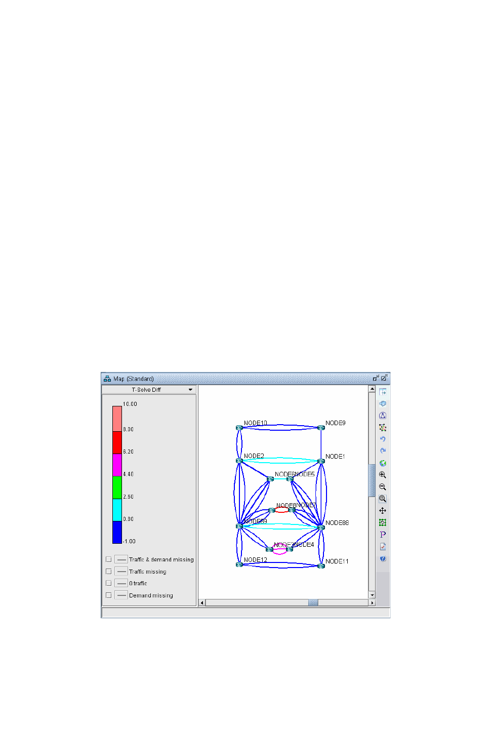
TRAFFIC MATRIX SOLVER*
Copyright © 2014, Juniper Networks, Inc. 18-9
. . . . .
•Node,Interface: The node and interface corresponding to the given direction on the link
•Remote Node: The other end node of the link
•Type: The link’s Trunk Type
•Known Model Traffic: Traffic load on the link based on measured flow bandwidth (based on the
trafficload file)
•Measured Traffic: Traffic load on the link according to measured interface traffic file (based on the
egress/ingress files)
•Model Traffic: Traffic load on the link according to the sum of bandwidth of demands over the link (based
on the demand file
•Diff Traffic: The difference between Model Traffic and Measured Interface Traffic. Note that the values -1,
-2, -3, and -4 have special meanings here: “-4” means that there is measured interface traffic, but model traffic is
0, “-3” means that there is model traffic, but measured interface traffic is 0, “-2” means that there is model
traffic but measured traffic is missing, and “-1” means the model traffic is 0, but measured interface traffic is
missing.
•Measured Util %: Percentage Utilization of the link according to measured interface traffic file (based on
the egress/ingress files)
•Model Util %: Percentage Utilization of the link according to the sum of bandwidth of demands over the
link (based on the demand file0
•Diff Util %: Model Util % - Measured Util %
•Abs Diff Util %: The absolute value of Diff Util % (This number will always be positive)
Viewing Differences Graphically
21. To view the differences between the measured interface traffic and model traffic, click the “Show Diff
Util” button on the Links tab.
Figure 18-6 Difference Between Measured and Model Traffic
22. Note that you can right-click over the color bar to filter for particular colors (version 5.2).
TRAFFIC MATRIX SOLVER*
18-10 Copyright © 2014, Juniper Networks, Inc.
18
Figure 18-7 Popup Window
•Show Selected Color: Toggles the display of this color.
•Show All: Shows all colors
•Show None: Hides all original colors, showing gray instead
23. For example, you can first select “Show None” and then right-click the topmost color and select “Show
Selected Color” to see the links with the most differences.
24. The legend at the bottom also allows you to graphically view the links for which there is missing data.
•Traffic & demand missing: Both measured interface and model traffic are missing
•Traffic missing: Measured interface traffic is missing, but not model traffic
•0 traffic: Measured interface traffic is zero
•Demand missing: Measured interface traffic is present, but no demands are routed over the link
Troubleshooting
25. If the WorstLinkDiff is high, e.g., over 10%, you should analyze the Links tab. Sort on the Diff Util %
Column to see the links with the worst link diffs. You can select the rows for these links and click the
Highlight button to highlight the links on the map, and to check for reasons why the difference is high.
26. If “Measured Traffic” (actual load) on a link is extremely high but the traffic matrix tool places 0 traffic
on that link (Model Traffic), this may be an indication of a routing scenario that needs to be resolved
before proceeding. That is, you need to determine why the system is not routing any flow across that link.
There are numerous possible reasons, and it varies from network to network. For example, there may be
too many parallel links in part of the network, but the ECMP value is set too low.
27. The typical way to troubleshoot is by using the “P” Path button on the Map window, or via Network >
Path & Capacity > Path, selecting two points, and analyzing the source of the bottleneck.
28. In some cases, you may have supplied an inaccurate set of sources and sinks. That is, the sources and sinks
you specified for the traffic matrix flows does not match the locations where traffic is present, as indicated
by your interface traffic file. Please consider adding a larger mesh of demands.
29. There can also be problems if the interface traffic data that you supplied is unknown or “0” on the vast
majority of interfaces and the test demands are placed on these links. In this case, there is insufficient data
to solve for a traffic matrix solution. Please check your interface traffic file.
30. Another problem is if you did not add seed demands to the network. You can do so either by loading in the
demand file via File>Read, or adding more demands into the network using Modify > Elements >
Demands. Once this is done, restart the Traffic Matrix operation.

TRAFFIC MATRIX SOLVER*
Copyright © 2014, Juniper Networks, Inc. 18-11
. . . . .
Appendix
CHOOSING A PERIOD OF INTERFACE TRAFFIC
31. Which period of interface traffic data should you use? Currently, it is recommended to select a few periods
(for example, include one during general heavy load and one at light load), and run the Traffic Matrix tool
once for each set of traffic data to create a couple different sets of end to end flows.
32. Avoid choosing the period called “Worst,” as the worst/peak case may occur at different times for different
links, which is not as suitable for the Traffic Matrix tool. Rather, it is better to determine a few specific
period numbers for which the loading was heavy.
33. There are a few ways to load traffic data into the network model. Note that the following applies to those
users who use the online module / WANDL data collectors to collect live traffic:
•If you created your initial network project by saving it out from the live network view (File > Save
Network), then the last 24 samples of traffic data at the time you saved it out will already be recorded in the
default interfaceTraffic.in and interfaceTraffic.out ingress and egress files associated with your network project
•If you have existing ingress and egress traffic files, you can read them in via File > Load Network Files
(specify them in the Traffic Files section)
•To retrieve historic traffic data, in View or Design mode, go to Traffic > Traffic Load, and select
“Interface”. Select the “Start From” time and press “Fetch”. At this point, if you do File > Save Network,
the corresponding interfaceTraffic.in and interfaceTraffic.out files will be created. Then, close and reopen the
network project, or else use File > Load Network Files to load in the interface traffic files, before proceeding
to the Traffic Matrix tool.
34. If you do not have the online module or an interface traffic file, but want to generate one based on the
current network demands, select Traffic > Traffic Matrix > Save Interface Traffic.
RESETTING DEMAND BANDWIDTH ACCORDING TO DEMAND TRAFFICLOAD FILE
35. At any point in time you can reset the demand bandwidths to be the same as that of a specified period of the
measured demand bandwidth in the trafficload file. Any demand that does not have measured demand
bandwidth will not be changed in this process.
36. To do this, first select the General tab and select the desired Period of the Traffic Load File. Then click
“Show Results.” A popup window will show how many demands have a current model bandwidth that is
different from the measured demand bandwidth.
37. When asked to update the different entries, click Yes in order to update the model bandwidths to be exactly
the same as the specified period of the traffic load. The Summary tab will be updated to reflect the changes.
38. Note that during the design, if you had set the Maximum Bandwidth Difference Ratio between the
modeled demand bandwidth and the measured trafficload bandwidth to 0, then there should not be any
differences when clicking “Show Results” if you are using the same trafficload period.
TRAFFIC MATRIX PARAMETERS
The following parameters can be added to your project’s dparam file to stop the Traffic Matrix Solver when the
solution is deemed good enough or if not enough improvements can be found per iteration.
•TM_linkdiff = <ratio>: Stop earlier than the loopcount if the target LinkDiff is reached ( the difference
between calculated demand traffic load and measured link used bandwidth.)
•TM_minimprovement = <number>: Stop earlier than the loopcount if the improvement per iteration is
less than this number for 100 iterations.

TRAFFIC MATRIX SOLVER*
18-12 Copyright © 2014, Juniper Networks, Inc.
18

Copyright © 2014, Juniper Networks, Inc. 19-1
. . . . .
. . . . . . . . . . . . . . . . . . . . . . . . . . . . . . . . . . .
M
ETRIC
O
PTIMIZATION
19
his chapter describes how to use WANDL software to optimize link metrics to reduce network congestion.
When to use
Follow these guidelines to automate IGP metric changes to reduce the utilizations of congested links in the network.
Prerequisites
You should have a router spec file open before you begin. To follow along with this tutorial, you can open the
spec.mpls-fish spec file located in your $WANDL_HOME/sample/IP/fish directory. ($WANDL_HOME is /u/wandl
by default).
*Note that a special license is required for metric optimization. Please contact your Juniper representative for more
information.
Related Documentation
If you would prefer instead to manually change the IGP metrics, refer to Chapter 4, Routing Protocols or the “Route
Optimization Wizard” section of “The Design Menu” chapter in the General Reference Guide.
Recommended Instructions
Following is a high-level, sequential outline of the process of metric optimization and the associated, recommended
detailed procedures.
1. Select the IGP for which to optimize metrics and ensure that the links to optimize are enabled for that IGP.
2. Open the metric optimization window.
3. Select the candidate links that can be modified, the links to be ignored, the metric optimization method, and
various other parameters.
4. View the results of the metric optimization and decide whether or not to accept or reject the changes.
Detailed Procedures
Setting Up for Metric Optimization
SETTING UP PROTOCOL INFORMATION
1. Before starting metric optimization, select the IGP for which you will optimize metrics (e.g., OSPF or ISIS)
from the Tools > Options > Design, Path Placement options pane, Routing method.
2. Check that the links you want to allow metric modification for are enabled for that IGP. For example, to enable
OSPF on a link, switch to Modify mode and select Modify > Elements > Links.... Then select the links to
enable for OSPF and click the Modify button. In the Modify Links window, select the Protocols tab. Select
“yes” to the right of the OSPF protocol and click OK.
SETTING UP MAX DELAY CONSTRAINTS
3. If you wish to set specific maximum delay constraints on a per demand basis (rather than on a global basis) first
select Tools > Options > Design, Path Placement options pane. At the bottom of the window, select True
for Ignore Max Delay. Otherwise, the routing engine will use the max delay field as a routing constraint and
demands that violate the max delay will be unplaced. To avoid setting this each time, save the network after
making this change, or add a line for “maxdelaycheck=2” in the network’s dparam file.
T
METRIC OPTIMIZATION
19-2 Copyright © 2014, Juniper Networks, Inc.
19
4. Next modify the specific demands from Modify > Elements > Demands.... Select the demands to modify
and click Modify > Selected... In the demand modification window, click the Type button. Then specify the
Max Delay field, e.g., “30ms” for 30 milliseconds. Note that this can also be specified in the demand file before
opening the network project, by indicating MAXDELAY=30ms in the comma separated type field (e.g.,
R,A2Z,MAXDELAY=30ms).
Metric Optimization Parameters
5. Switch to Design mode and select Design > Metric Optimization to open the following window.
Figure 19-1 Metric Optimization Parameters
Parameter Description
Candidates for Link
Metric Changes
Select the links whose metrics can be modified. By default, all links
will be used as candidates.

METRIC OPTIMIZATION
Copyright © 2014, Juniper Networks, Inc. 19-3
. . . . .
Links to Ignore This option allows users to specify links whose utilizations can be
ignored for the purpose of metric design. For example, for local
Ethernet cables, it may be cheap to buy/upgrade cables in case the
link is or becomes highly utilized. Hence, it may be desired to ignore
high utilizations for local links during the design.
Note that if a link is listed as both a candidate and as a link to be
ignored, the former will override the latter. To avoid confusion, click
the Select Duplicates button to highlight the duplicates, and remove
them from either the candidate link list or list of links to ignore.
Design for Normal Util /
Peak Util
Normal Util: This option optimizes the link utilizations under the
assumption that there is no link failure.
Peak Util: This option optimizes the link utilizations during failure.
Each link’s peak util reflects the worst utilization that can occur on that
link during any single link failure. Select the element types whose
failure will be simulated.
Show Intermediate
Results on Map
Display the new (normal) utilizations on the map by color (for the
Utilization Legends > Planned Util legend) each time a metric
change is made. This may be turned off for larger networks to speed
up the performance.
Keep A-Z Z-A metrics
symmetric
By default, this option is checked so that both interfaces on a link will
be set to the same metric whenever a link’s metrics are modified. To
enable asymmetric link metrics during link modification, uncheck this
option.
Target Utilization (%)
Target Peak Utilization
(%)
When designing link metrics to optimize normal utilizations, the
Target Utilization should be set. The default value is 50%. What this
means is that any utilizations under 50% will be treated as
acceptable, and any utilizations above 50% will be given a penalty
depending upon how high the utilization is. Once all the links are
below this target utilization, the metric design will stop.
When designing link metrics to optimize peak utilizations, the Target
Peak Utilization should be set. The default value is 100%. Any
utilizations under the target peak utilization will be treated as
acceptable, and any peak utilizations above this target peak utilization
will be given a penalty depending upon how high the peak utilization
is. Once all the links are below this target peak utilization, the metric
design will stop.
Max Percentage Metric
Increase (+%)
The maximum increase in a link’s IGP metric allowed, based on a
percentage of the starting metrics. For example, if the starting metric
is 100 and the Max Percentage Metric Increase is 300%, then the
metric will not exceed 400.
Max Percentage Metric
Decrease (-%)
The maximum decrease in a link’s IGP metrics allowed, based on the
starting metrics. For example, if the starting metric is 100 and the Max
Percentage Metric Decrease is 50%, then the metric will not be lower
than 50.
Max Percentage Delay
Increase (+%)
The maximum percentage increase in a demand’s end-to-end delay,
based on the original delay.
Global Max Delay
Constraint (ms)
A link metric change will not be accepted if the change will cause a
demand to exceed the global max delay constraint.
Parameter Description

METRIC OPTIMIZATION
19-4 Copyright © 2014, Juniper Networks, Inc.
19
6. Note that the speed of the algorithm depends on the number of candidate links and number of demands. By
default, you can try using all of the links in the network as link candidates. However, if needed, you can narrow
down the candidate links (links whose metrics can be changed):
a) You could select a particular region by <Ctrl>-clicking the links on the map or by dragging a box around a
region. Then click the Filter from Map button.
b) You could select only OC-/STM- links by clicking the Adv Filter button and entering a query string such as
“Type = OC” or “Type = STM.”
c) Alternatively, you could select only a few highly utilized links by filtering on link utilization. Click the Adv
Filter button and enter a query string such as “Util_AZ > 0.7 or Util_ZA > 0.7”. Note, however, that when the
utilizations change in the middle of the optimization, the originally selected links may no longer be the highest
utilized links. Hence, it may be more useful to select regions as specified in section (a).
d) You can also tune on one link at a time and filter only a single link candidate.
7. You could similarly select the links to ignore if there are some links whose utilizations are not critical, e.g., high
utilizations on such links could be easily fixed by adding or upgrading local cables at a small cost.
Use Individual Demand
max delay settings
A link metric change will not be accepted if it will cause a demand to
exceed the max delay constraint specified for that demand as
described in Setting Up Max Delay Constraints on page 19-1.
Discourage creation of
Equal Cost Paths
If this option is selected, the program will try to avoid increasing link
metrics causing a demand to have an equal cost path (ECMP)
alternative.
Parameter Description
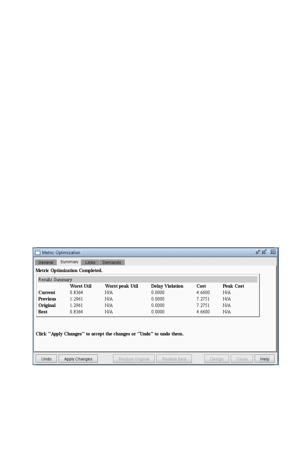
METRIC OPTIMIZATION
Copyright © 2014, Juniper Networks, Inc. 19-5
. . . . .
Metric Optimization Design
8. Select whether to design for Normal Util or Peak Util. (Before running a design to optimize peak utilizations,
it is recommended to first run the design to optimize the normal utilization and accept the changes.)
9. Click Design to begin the metric optimization process. Intermediate results are displayed in console. The
Console will indicate how many candidate links are being used. Note that some selected candidate links may not
be used as candidates if a) they are not enabled for the selected protocol, or b) they do not belong to a cycle of
links, since their utilization in that case cannot be improved by modifying link metrics alone (assuming all
demands are routed). After the metric optimization is completed, the table in the links tab will indicate any such
warnings in the Description column.
10. Once the design is in progress, a progress monitor will be displayed, and the Pause button will be displayed in
lieu of the Design button. The Pause button can be used to interrupt the metric optimization at any time, after
which the user can decide whether or not to apply or undo the changes made up to that point. Check the
intermediate status in the Console window for intermediate metric changes to decide when to pause.
11. The metric optimization will stop either when the user interrupts the design with the Pause button, when the
target utilization is reached (in the cause of designing for the Normal Util), or when the target peak utilization is
reached (in the case of designing for the peak utilization).
12. The Accept Changes and Undo buttons will then be enabled, so the user can select whether or not to accept
the recommended metric changes or to cancel them.
13. To decide whether or not to accept or undo the changes, summary statistics are provided in the Summary tab
and more detailed results can be browsed in the Links and Demands tabs. Additionally, two report files,
METRICOP_CHANGES and METRICOP_RESULTS will also be saved in the Output Dir.
METRICOP_CHANGES indicates information such as the links changed, their original metrics, and new
metrics. The METRICOP_RESULTS report indicates the before and after utilization and metrics of all the links
in the network.
Metric Optimization Results
14. The following are example Summary statistics following a metric design to optimize the normal utilization.
Figure 19-2 Metric Optimization Statistics (Design Run for Normal Util)
Note that there are four rows: Current, Previous, Original, and Best. The Current statistics are the statistics
after running the design and the previous statistics are the statistics before clicking the Design button. The
design may be run multiple times, so the summary statistics will also remember the very original statistics when
the metric optimization was first run, as well as the best statistics.
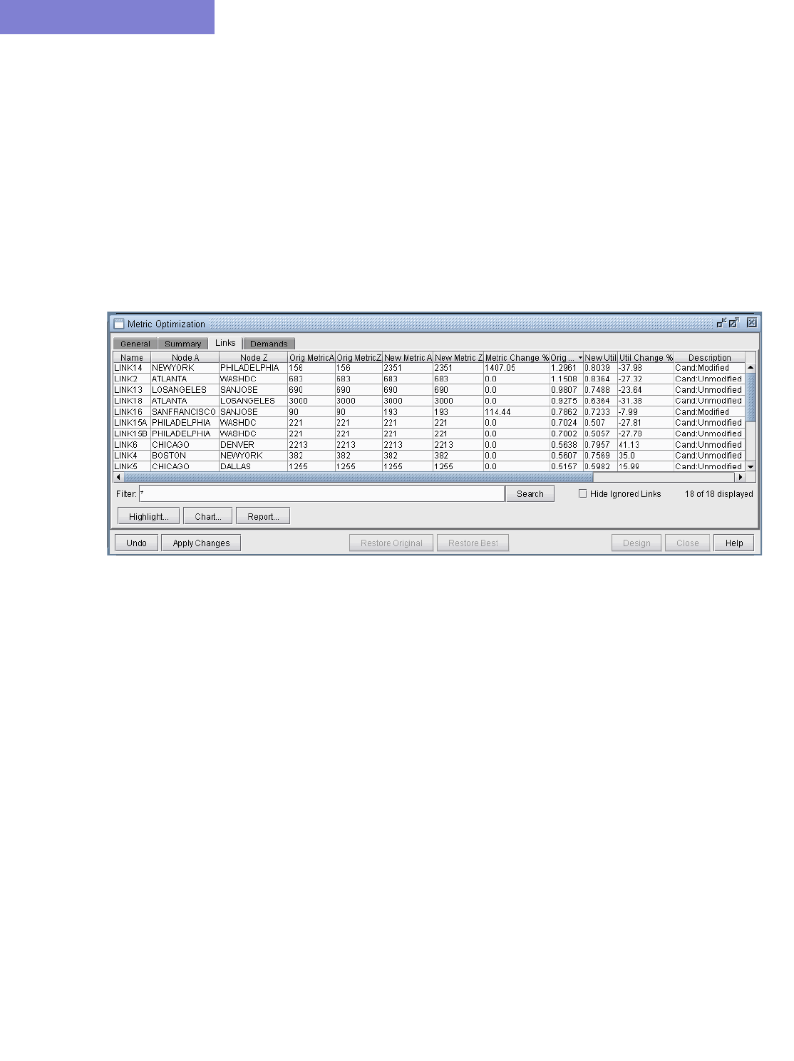
METRIC OPTIMIZATION
19-6 Copyright © 2014, Juniper Networks, Inc.
19
The four columns indicate the statistics for each scenario:
•The Worst utilization and Worst peak utilization are the highest utilization and peak utilization among the
links in the network (excluding the links to be ignored).
•The Delay Violation indicates a penalty when the maximum delay constraint is violated (in normal mode,
without failure).
•The Cost and Peak Cost functions provide indicators to improvements overall in the utilization load balancing.
For example, there may be scenarios where the link with the worst utilization cannot be improved, but other links’
utilizations can be improved. Those improvements will be reflected if the Cost or Peak Cost numbers decrease
between the previous and current states.
Viewing the Detailed Link Information After Metric Optimization
15. Select the Links tab for the following display.
Figure 19-3 Links Tab (Design Run for Normal Util)
This tab lists all the links in the network, including the following details:
•Metrics: Original metrics, new metrics, and the percentage change between old and new metrics
•Utilizations: Original utilizations, new utilizations, and the percentage change between old and new utilizations
•Peak Utilizations: Original peak utilizations, new peak utilizations, and the percentage change between old and
new peak utilizations (requires running a design for the peak utilization)
•Description: This field indicates details about a link’s status, e.g., it will indicate if a link is a candidate or a link
to be ignored, whether a candidate link’s metric has been modified or not, and any warnings for links such as if the
link is not enabled for the selected IGP protocol, or if it cannot be optimized because it does not belong to a cycle of
links of the selected IGP protocol.
16. By default, only the maximum of the A->Z and Z->A utilizations on the link are displayed. To display the
utilization per link interface, right-click on the table header, select Table Options... and in the subsequent
window, move the additional desired columns to the list of selected items, and reorder them as desired.
17. Click the New Util or New Peak Util column headers to sort by the link utilization. You can select the top
utilized links and click the Highlight button to view those links graphically on the map. Check the
Description field for warnings, such as if a link is not enabled for the selected protocol, or not part of a cycle
enabled for the selected protocol, in which case the link cannot be further improved.
18. Click the Report button to save the links table into a comma-separated file that can be opened in the File
Manager’s report viewer or loaded into Microsoft Excel.
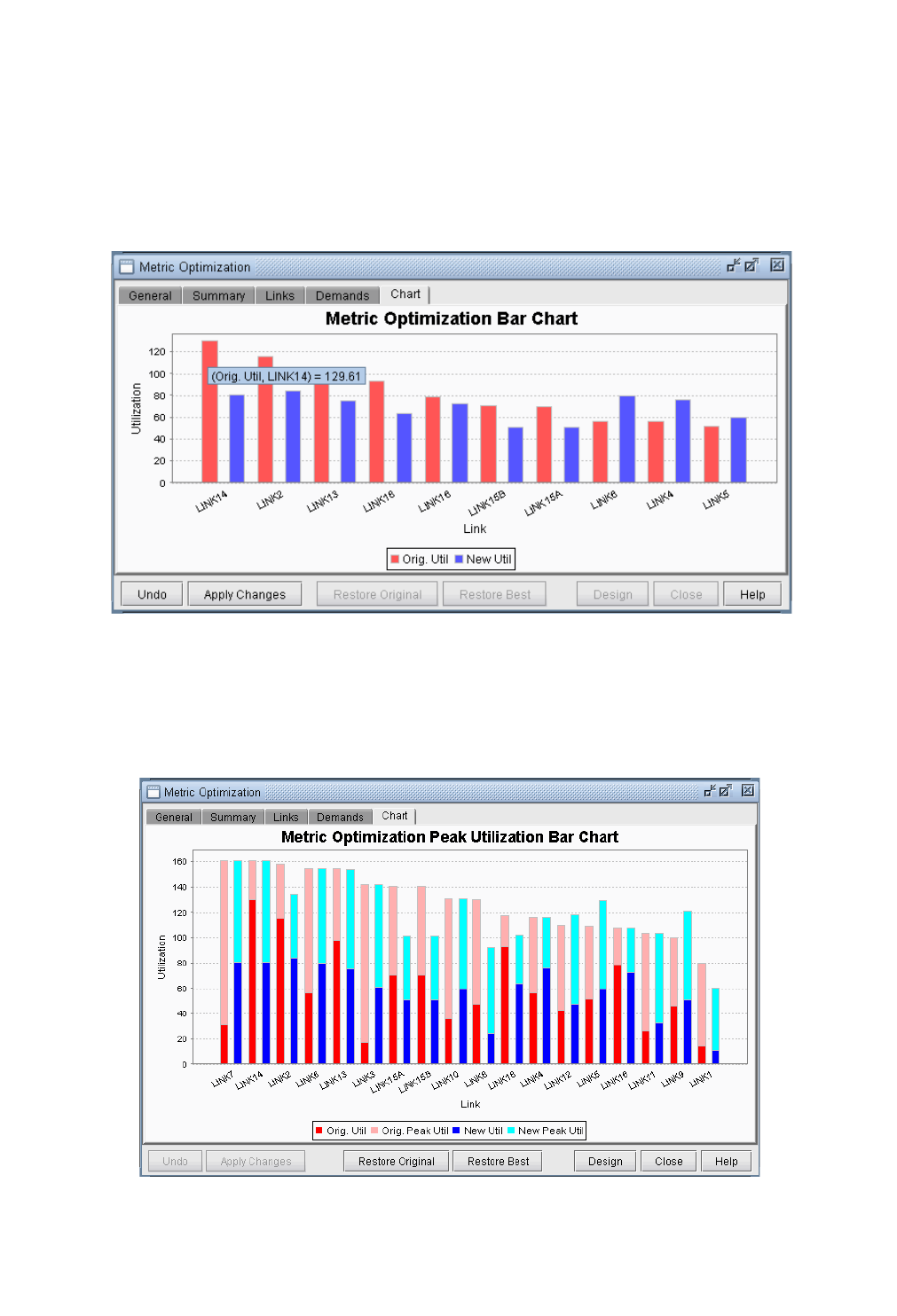
METRIC OPTIMIZATION
Copyright © 2014, Juniper Networks, Inc. 19-7
. . . . .
Metric Optimization Link Utilization Results in Chart Format
19. In the Links tab, when designing for normal util, click the Orig Util column headers to sort by the original link
utilization in reverse order, from highest to lowest. Then select the rows for the top 10 links, for example, and
click the Chart button.
20. Note that there are two bars for each link-- a red bar to indicate the original utilization and a blue bar to indicate
the current utilization.
Figure 19-4 Metric Optimization Bar Chart (Design for Normal Util)
21. When designing for peak util, click the Orig Peak Util column headers to sort by the original link utilization in
reverse order, from highest to lowest. Then select the rows for the links you would like to display in the chart,
and click the Chart button. The links will be displayed in the same order as they are listed.
Figure 19-5 Metric Optimization Peak Utilization Bar Chart
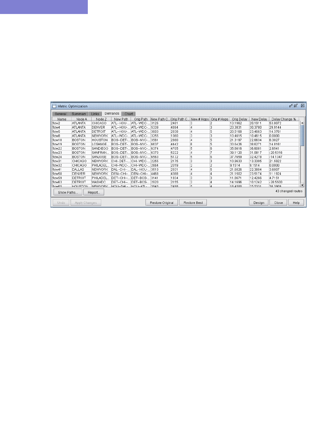
METRIC OPTIMIZATION
19-8 Copyright © 2014, Juniper Networks, Inc.
19
Again, there are two bars for each link. The first one indicates the original utilization (red) and peak utilization
(pink) and the second one indicates the current utilization (blue) and peak utilization (cyan). Note in the above
image that although the worst peak utilization could not be improved, there are other links whose peak
utilizations were improved.
Changed Demands after Metric Optimization
22. Click the Demands tab for the following window: This window indicates only demands that changed as a
result of the metric optimization. It will indicate the previous and new path, the previous and new hop count,
previous and new delay, and percentage change in the delay value.
Figure 19-6 Routes Changed
Select a demand and click “Show Paths...” to view a demand’s route or “Report” to save the route changes to
a file.
Accepting or Rejecting Metric Changes
23. Click Accept Changes to accept the new metrics or Undo the reject them.
24. Afterwards, you can still restore the very original metrics by clicking “Restore Original” or the metrics giving
the best results by clicking “Restore Best.”
Saving a Metric Optimization Design
25. The new link metrics can be saved to a file either by saving the entire network (File>Save Network...) or by
saving only the link file (File>Save Network File>Link).
26. The metric optimization design parameters, including the candidate and ignore links can also be saved to the
network project by saving the entire network (File>Save Network...).
•The candidate and ignore links will be indicated in the bblink file using the BMCAND or BMIGNORE keyword
in the miscellaneous field.
•The rest of the parameters are saved in the dparam file and the keywords are prefixed with “BM_”. In this way,
the next time the project is loaded, the design parameters will be remembered.

Copyright © 2014, Juniper Networks, Inc. 20-1
. . . . .
. . . . . . . . . . . . . . . . . . . . . . . . . . . . . . . . . . .
LSP T
UNNELS
*
20
his chapter describes how to view and modify Label Switched Path (LSP) tunnel information using the
WANDL software. This includes secondary/standby and backup paths, affinity and mask. If you have a
Multiprotocol Label Switching (MPLS) network, then you should familiarize yourself with this chapter.
*Note that a special password is required for the tunnel feature. Please contact your Juniper representative for more
information.
Prerequisites
If you wish to perform this task in the WANDL client, you should have a router spec file open before you begin. To
follow along with this tutorial, you can open the spec.mpls-fish spec file located in your
$WANDL_HOME/sample/IP/fish directory ($WANDL_HOME is the program’s home directory. It is /u/wandl by
default).
Related Documentation
For general step-by-step instructions on how to use the WANDL software, please refer to the Design & Planning
Guide.
For an overview of the WANDL software or for a detailed description of each feature and the use of each WANDL
client window, please refer to the General Reference Guide or Chapter 37, Router Reference.
Outline
Following is a high-level, sequential outline of the process of viewing, adding, and modifying tunnels.
1. Viewing Tunnel Info on page 20-2
2. Viewing Primary and Backup Paths on page 20-2
3. Viewing Tunnel Utilization Information from the Topology Map on page 20-3
4. Viewing Tunnels Through a Link on page 20-4
5. Viewing Demands Through a Tunnel on page 20-5
6. Viewing Link Attributes/Admin-Group on page 20-6
7. Viewing Tunnel-Related Reports on page 20-7
8. Adding Primary Tunnels on page 20-9
9. Adding Multiple Tunnels on page 20-10
10. Modifying Tunnels on page 20-11
11. Path Configuration on page 20-11
12. Specifying a Dynamic Path on page 20-12
13. Specifying Alternate Routes, Secondary and Backup Tunnels on page 20-13
14. Adding and Assigning Tunnel ID Groups on page 20-16
15. Making Specifications for Fast Reroute on page 20-19
16. Specifying Tunnel Constraints (Affinity/Mask or Include/Exclude) on page 20-20
17. Adding One-Hop Tunnels on page 20-24
18. Tunnel Layer and Layer 3 Routing Interaction on page 20-26
19. Appendix on page 20-26
T
LSP TUNNELS*
20-2 Copyright © 2014, Juniper Networks, Inc.
20
Detailed Procedures
1. Load the /u/wandl/sample/IP/fish/spec.mpls-fish network example if you wish to follow along with this tutorial.
When prompted, “Update demand routing tables?”, press “Yes”.
Viewing Tunnel Info
2. In View or Design action mode, select Network > Elements > Tunnels. Right-click a tunnel to view the
various options available for tunnels.
Figure 20-1 All Tunnels Window
3. Click the “Show Path” button to see the tunnel highlighted on the map, including all defined routes.
Note: If more than one tunnel are selected, only their primary paths will be highlighted together on the map.
In the resulting path window, there will be 2 colors, including a special color for the currently highlighted tunnel
in the path window.
Viewing Primary and Backup Paths
4. To view primary and backup tunnels together on the map, select an entry from the Tunnels window that is a
primary tunnel (not marked Standby in the Type column), right-click and select Show Path. By default both
tunnels are shown highlighted. To highlight only one path at a time, change from Highlight All Paths to
Highlight a Selected Path.
Figure 20-2 Tunnel Paths on Map
LSP TUNNELS*
Copyright © 2014, Juniper Networks, Inc. 20-3
. . . . .
5. The diverse paths of a tunnel can also be viewed from Network > Elements > Tunnels Diverse Status or
Design > TE Tunnels > Path Design in Design mode and tunnel layer.
6. From the Diverse Path Design window, Check the “Div Level” column to see the current level of diversity
satisfied between primary and backup paths.
7. Select a tunnel and click “Show Paths” to view the primary and backup tunnels.
8. Select “Hide Unrelated Nodes” to display only those nodes and links which are on the primary and backup
tunnels.
Figure 20-3 Show Primary and Backup Paths
Viewing Tunnel Utilization Information from the Topology Map
9. Select the Tunnel layer button from the main menu bar. On the map window left pane, select the Utilization
Legends > Planned Util menu item. Because of the low planned link utilization of tunnels in this example,
you will need to adjust the dividers in the Planned Util legend in order to see any color differentiation on the
map.
Figure 20-4 Planned Tunnel Utilization (Tunnel Layer View)
•Tunnel BW / Link BW: Displays the sum of the configured bandwidths of the tunnels over the link, divided by
the link bandwidth.c
•Tunnel BW / RSVP BW: Displays the sum of the configured bandwidths of the tunnels over the link, divided
by the link’s configured RSVP bandwidth.

LSP TUNNELS*
20-4 Copyright © 2014, Juniper Networks, Inc.
20
Viewing Tunnels Through a Link
10. Right-click on a link on the map or in the Network Info window with a planned utilization greather than 0 and
select View>Tunnels on/thru Link.
11. The example below shows tunnels through the CHI-WDC link. Select the Actions menu at the upper rightto
further filter the tunnels according to direction.
Figure 20-5 Tunnels through Link Window
LSP TUNNELS*
Copyright © 2014, Juniper Networks, Inc. 20-5
. . . . .
Viewing Demands Through a Tunnel
12. To view all demands routed over a tunnel, right-click over the tunnel and select “Show Demands Routed on
Tunnel.”
13. In the Demands window, examine the Current Route column which indicates the path taken bythe demands.
Open and closed brackets in the path indicate where a tunnel is entered and exited.
Figure 20-6 Demands (or Flows) Routed Through a Particular Tunnel
In Figure 20-6, the selected demand between HOU and NYC. has the route HOU[--DAL--CHI--]WDC--PHI--NYC,
indicating that the demand traversed a tunnel from Houston (HOU) to Washington D.C. (WDC).
14. Clicking on “Show Path” displays the path of the demand on the map. Notice that a purple color is used to
indicate the portion where the demand is travelling through a tunnel.
Figure 20-7 Path of Demand Through a Tunnel
LSP TUNNELS*
20-6 Copyright © 2014, Juniper Networks, Inc.
20
Viewing Link Attributes/Admin-Group
15. Select the Map legend: Subviews > Attributes/Admin Group to view the links’ RSVP resource
group/color, also known as link attributes for Cisco, and admin-group for Juniper.
16. The legend can be used to filter the map display to show only links that satisfy a particular criteria, comprised of
logical “all”, “or” and “not” operations.
•To display links which satisfy one specific color, select under the “all” column only the checkbox for that color.
•More complicated logical combinations can also be specified. For example, selecting “red” and “yellow” under
the any column and “green” for the “not” column, will filter the display to show only links that have red or yellow
color and do not have green.
Figure 20-8 Attributes/Admin Group Legend
17. An alternative way to input the filter criteria is via the “all”, “any”, and “not” hexadecimals in the Control
section at the bottom of the legend. This corresponds to Juniper’s “include-all”, “include-any”, and “exclude”
statements. After typing in the full hexadecimal, press the <Enter>/<Return> key to load the change on the
map.
18. A Cisco tunnel’s affinity/mask requirements can be translated into “all” or “not” criteria. If the mask is “1” for a
bit, then an affinity of “1” for that bit would translate into an “all” for that bit and an affinity of “0” for that bit
would translate into a “not” for that bit.

LSP TUNNELS*
Copyright © 2014, Juniper Networks, Inc. 20-7
. . . . .
Viewing Tunnel-Related Reports
The following lists and describes the tunnel-related reports accessible from the Report Manager (Report >
Report Manager).
Report/Category Description
Tunnel Path & Diversity Displays each of the tunnel’s requirements and routed path specification.
Tunnel Route Cost Displays the calculated cost for each tunnel in the network based on the
sum of the link costs.
Demand Traffic on Tunnel Displays the values of the reserved tunnel bandwidth verses the flow
bandwidth and their difference ratio.
Tunnel Traffic This report has to do with multiple-period traffic load on the tunnels.
Tunnel-Link This report breaks up each tunnel into each interface segment of the
tunnel path.
Tunnel RSVP BW on Link
Tunnel RSVP BW on Node
Pair
Link: Displays the Amount of Link RSVP bandwidth used by tunnels per
link
Node Pair: Displays the Amount of Link RSVP bandwidth used by tunnels
per node pair
Tunnel Traffic vs Interface
Traffic
Compares aggregate tunnel traffic load versus the measured interface
traffic.
Link Partition This report breaks up the link bandwidth into partitions (RSVP and
GB=Guaranteed Bandwidth, GlobalPool and SubPool, or CT partitions for
DiffServ-TE) and shows the tunnel bandwidth for each partition.
Measured Link Util (based
on T_trafficload)
Per Node Pair (Measured)
In the live network mode, this report provides the aggregate tunnel traffic
load on the link.
Per Node Pair (Measured): In the live network mode, this report provides
the aggregate tunnel traffic load on the node pair.
Peak Tunnel Traffic on
Links
Found under Tunnel Layer Simulation Reports > Tunnel Layer Network
Statistics, This report is only useful after having run a failure simulation on
the network. Displays the peak utilization of the links that is reserved by
tunnels.

LSP TUNNELS*
20-8 Copyright © 2014, Juniper Networks, Inc.
20
Tunnel Layer Group Group Tunnel Summary by Group Pair: Displays summary information
for tunnels between two groups.
Group Tunnel Detail by Group Pair: Displays detailed information for
each tunnel that is between two groups or within one group.
Group Tunnel Traffic on Link Summary: Displays summary information
on tunnel traffic between two groups or within one group.
Group Tunnel Traffic on Link Detail: Displays detailed information for
tunnel traffic that is between two groups or within one group.
Group Interface Load Summary: Displays summary information
between interfaces of nodes in two groups or within one group.
Group Interface Load Detail: Displays detailed information between each
interface pair where the nodes are in two groups or within one group.
Group Tunnel Bandwidth Distribution: View the distribution of
Originating, Terminating, Transit, and Local tunnel bandwidth
Planned Tunnel RSVP BW
Per Node
Found under Tunnel Layer Network Reports > Node, this report provides
information on local, non-local and transit tunnels at each node. A local
tunnel is one that starts and ends at itself, and a non-local tunnel is one
that originates or terminates at the node.
Measured Tunnel Traffic
Per Node
Found under Tunnel Layer Network Reports > Node, this report provides
measured inbound and outbound traffic per node.
Report/Category Description
LSP TUNNELS*
Copyright © 2014, Juniper Networks, Inc. 20-9
. . . . .
Adding Primary Tunnels
19. To switch to modify mode, click on “Modify” mode button. The Modify pull-down menu gets activated.
20. Select Modify > Elements > Tunnels from the Modify pull-down menu. In the Tunnels window, click
Add and select One Tunnel.... The Add Tunnel window is displayed as shown in Figure 20-9.
Figure 20-9 Add Tunnel Window
21. In the Properties tab, specify a TunnelID, the BW (bandwidth) for the tunnel, and the Pri,Pre (setup
priority/holding priority) fields. Also select the source and destination nodes (Node A and Node Z).
22. In the Paths tab, Note the different ways of configuring a path under the To choose paths field.
Figure 20-10 Different Methods of Choosing Paths
How to specify a configured and/or dynamic route is described later in this chapter.
23. After you have specified your route, click “Add” to add the tunnel. A yellow line between the source and
destination will be drawn on the map to represent the logical tunnel. Note that the routing of the tunnel has not
been performed yet.
LSP TUNNELS*
20-10 Copyright © 2014, Juniper Networks, Inc.
20
Adding Multiple Tunnels
The Add Multiple Tunnels window can be used to add a mesh of tunnels between two sets of nodes.
24. Select Modify > Elements > Tunnels, Add > Multiple Tunnels from the Modify pull-down menu.
Alternatively, select Add>Multiple Tunnels from the Network Info window Tunnels view. An Add
Multiple Tunnels window should appear, similar to the one shown below.
Figure 20-11 Add Multiple Tunnel Window
25. The generated tunnel names will consist of a prefix defined in the Tunnel ID (Prefix) field and an
incrementing number that starts with the number specified in the Tunnel ID (#) field. If no start number is
specified, the tunnels will be named according to the NodeA and NodeZ endpoints.
26. Various options can be configured in the top right section of the window, including BW, Type, Affinity/Mask
(Cisco) or Include-All/Exclude/Include-Any (Juniper), Pri,Pre (setup priority/holding priority), Service,
Path. Config. Options, and a user definable Comment field.
27. A tunnel will be created for each NodeA - NodeZ pair defined in the bottom half of the window where NodeA
is the source and NodeZ is the destination. The NodeA and NodeZ boxes can populated using the Filter or
Filter From Map button. The Filter button opens a Find Nodes window to specify what nodes to add. The
Filter From Map button adds the nodes highlighted on the map. The Remove button removes the selected
node(s) from the Node A or Node Z list. The Copy A-> Z button copies the nodes that are on the Node A list to
the Node Z list.
As a shortcut, users may also select a particular category from the Type menu in the Placement (A * Z)
section such as Group, Area, VPN, or Multicast Group. This will activate the drop-down menu(s) above the the
NodeA and NodeZ boxes with available entries for the selected category. Selecting an entry from the selection
will automatically update the NodeA and NodeZ boxes.
28. The Create tunnels in both directions option will generate an additional full mesh of tunnels from Z to A.
This option is useful when the Node A and Node Z list are not the same. Selecting the Incremental Full Mesh
option is recommended when there is overlap between the Node A and Node Z list, to avoid creating more than
one tunnel for the same source-destination pair.
29. The Incremental Full Mesh option will only generate tunnels needed for the full mesh.
Note that you can also choose to create an incremental full mesh for tunnels within a particular tunnel ID range.
To do this, first create a Tunnel user parameter and tunnel ID group based on that user parameter before opening
the Add Multiple Tunnels window as discussed in Adding and Assigning Tunnel ID Groups on page 20-16.
LSP TUNNELS*
Copyright © 2014, Juniper Networks, Inc. 20-11
. . . . .
Then select the User Parameters tab of the Add Multiple Tunnels window and select that tunnel ID group.
Tunnels will be treated as already existing in the mesh if they have a source and destination listed in the
Placement section and they are named “Tunnel<id>” where <id> is a number within the ID range of the
selected tunnel ID group.
Mark MPLS-Enabled on Links along Path
30. When tunnels are placed by the routing engine, it checks the protocol on the link to determine if it is mpls-
enabled to allow placement of the tunnel. One method of setting a link to be mpls-enabled is through the Modify
Tunnel window. Switch to Modify mode and select Modify > Elements > Tunnels to open the Modify
Tunnel window. Choose a tunnel, right-click, and select “Mark MPLS-enabled on links along path.” This
will set all links as mpls-enabled on the first Configured Route. If the first Configured Route is dynamic, then no
links will be set as mpls-enabled.
Modifying Tunnels
31. To modify a tunnel, select Modify > Elements > Tunnels from the Modify pull-down menu. To modify a
single tunnel, select the tunnel from the table and click “Modify”. If multiple tunnels all require the same
modification, then select those tunnels in the table (using the <SHIFT> and <CTRL> keys for multiple
selection) and click “Modify”. If all tunnels in the network require the same modification, then click “Modify”
and select “All Entries”.
32. In the window that is displayed, specify only those fields you wish to modify. If a field is left blank, no changes
will be made to that field.
Path Configuration
When adding or modifying a single tunnel, a particular path can be configured in the Paths tab of the Add or
Modify Tunnel window shown below.
Figure 20-12 Configuring the Tunnel Path (Options may vary)
33. First select the desired source and destination nodes from the Node A and Node Z fields.
34. Next, click on the first row of the table in the Tunnels/Paths for the tunnel section to highlight it. To
configure a route for the tunnel, double-click on the cell in the Pathname column and remove the word
Dynamic. There are various methods to add routes described below.
a. Click links/nodes on map, then right-click in table:
This method can be selected from the To choose paths dropdown box, and allows the user to choose the links
making up the path and lets the program piece them together in the right order from source to destination. After
selecting this option, click on the links (holding down the <CTRL> key for multiple selections) making up the
path from the source node to the destination in any order so that they are highlighted.
Tips: Note that if you accidentally highlight a link, you can unhighlight it by holding down the <CTRL> key
and clicking on it a second time. If a region is too crowded you can zoom into that region to facilitate selection.
When you are done selecting the links of the path, right-click on the table row and select Use Map Sel’n from
the popup menu.

LSP TUNNELS*
20-12 Copyright © 2014, Juniper Networks, Inc.
20
b. Click consecutive nodes starting at Node A:
After selecting this option, select the map window. Note that your cursor will appear as a cross-hair on the
topology map. Click each node of the path starting from the beginning node and proceeding sequentially to the
end node. When you have reached the last node, double-click on the map to stop. The path is automatically
filled in for the highlighted row of the Add Tunnel window in the Configured Route column.
Note: If there are parallel links, this method, unlike method (a) will not specify which parallel link to use.
c. Tunnel Path Selection window:
To open the Tunnel Path Selection window, right-click over the row for an existing path and select “Edit
Route.” This option will allow users to add a route by selecting the nodes or links of the path from a list. For
more information, refer to the Reference Guide, “The Network and Modify Menus” chapter section on
Demands. The Tunnel Path Selection window has the same functionality as the Demand Path Selection
window.
d. Directly typing in the path:
Another option is to directly type in the path in the Configured Route column by double-clicking the cell in that
column and entering in a path with nodes delimited with the ‘-’ symbol for a strict route (or ‘**’ for a loose
route). To specify a specific link between two nodes, intermediate segments can be specified using linknames.
For example, SFO-LINK10-LINK6-LINK8-LINK15B could be used to specify a path from San Francisco
(SFO) to Philadelphia (PHI)..
Specifying a Dynamic Path
CONFIGURING A DYNAMIC ROUTE BETWEEN SOURCE AND DESTINATION
35. To add a tunnel with a dynamic route between two nodes, after you have configured the source, destination,
bandwidth, priority and preempt fields, simply click the “Add” button.
Note: The word “Dynamic” should be displayed under the pathname column.
CONFIGURING A LOOSE ROUTE
36. To add in a loose route, double-click the cell under the Configured Route and type in a route. Where the route
is “loose”, enter in two asterisks as the delimiter. For example, CHI-DAL**HOU**LAX**ATL would be an
example of a loose route, where the only fixed portion is the path from Chicago (CHI) to Dallas (DAL). Since
the exact route is not specified, it will be up to the hardware to choose a route going from DAL to HOU, HOU to
LAX, and LAX to ATL.
37. Alternatively, you can specify a Loose Route through the Tunnel Path Selection window by right-clicking
the row and selecting Edit Route. In the Tunnel Path Selection window, select the Loose Route radio
button. You will then have a wider array of options to choose from when you are adding nodes or links to your
route. Note that the nodes should still be in sequential order. When you have added the destination router, the
OK button will be enabled to allow you to finish adding the loose route.
CONFIGURING AN EXPLICIT ROUTE BASED ON CURRENT ROUTE
38. To cause the Current Route to be set as the Configured Route, select “Add” “Config” in the Path Config.
Options explained in Path Config Options on page 20-15.
EXCLUDING NETWORK ELEMENTS FROM A PATH (FOR CISCO ROUTERS)
You can specify dynamic routes that avoid particular nodes or links. However, for accurate modeling of your
network, you should only choose this option if your hardware supports this feature. Cisco routers implement this
with the “exclude-address” command.
39. To choose nodes or links to exclude from the map, select Click links/nodes on map, then right-click in
table from the To choose paths: menu.
40. Next, click on the network elements you want to exclude from the route to highlight them. Note that you can
hold down <CTRL> or <SHIFT> keys while clicking network elements to select more than one.
LSP TUNNELS*
Copyright © 2014, Juniper Networks, Inc. 20-13
. . . . .
41. After you have selected the elements to exclude, right-click on the row of the table that you want to modify and
select Use Map Sel’n as Excluded (Sel’n is an abbreviation for Selection). This will cause a statement to be
entered into the Configured Route field like the following: EXCLUDE-NODEA-LINK1-LINK8-LINK14.
42. Alternatively, you can double-click the Configured Route field and type in a string starting with
“EXCLUDE” and containing the IDs of the elements that are to be excluded separated by dashes ‘-’ (one dash
separates each element). After you have entered in some text, click on a different table cell in order to turn the
editing mode off.
43. To visualize which elements you are excluding in a particular row, click on a table cell in that row that you are
not editing. Then click “Show Route” to view the excluded elements on the Map, which will be marked with
an X as shown in Figure 20-13.
Figure 20-13 Marked Elements to Avoid in Route
Specifying Alternate Routes, Secondary and Backup Tunnels
For a tunnel, WANDL provides the option to add alternate routes in case the primary route fails.
SPECIFYING ALTERNATE ROUTES (FOR CISCO ROUTERS)
44. In the table in the lower half portion of the Add or Modify Tunnel windows, you can specify one or more routes
using one or more of the methods explained above. Click Add Row to add an alternate path.
45. For each route you can enter in a priority for the route. In the case that the tunnel cannot be routed on the
primary path, it will attempt to route on the path with the next highest priority. (The lower the Opt value, the
higher the priority.) You can click on a cell beneath the Opt heading and overtype this field to enter in a number
from 0 to 10. For each of these added rows, you can also configure a route or leave it as is for a dynamic route.
Note: In the configlet generation, the Opt number will be displayed for Cisco in the “tunnel mpls traffic-eng path-
option ...” command. For Juniper’s configlets, no Opt number will be displayed, but the tunnels will be specified in
an order corresponding to the Opt field.
46. The user can add up to 10 paths for this tunnel. The user simply fills in the fields that are different from the
default parameters in the top half of the window.
Not all fields are available for inputting. If your originating node is a Juniper node then all fields are available
(Pathname, Opt, Configured, BW, Type, Affinity, Mask, Pri,Pre, Comment). If it is Cisco then only the first 3
fields are used (Pathname, Opt, and Configured). This is due in part to the way the device vendor implements
the tunnels.
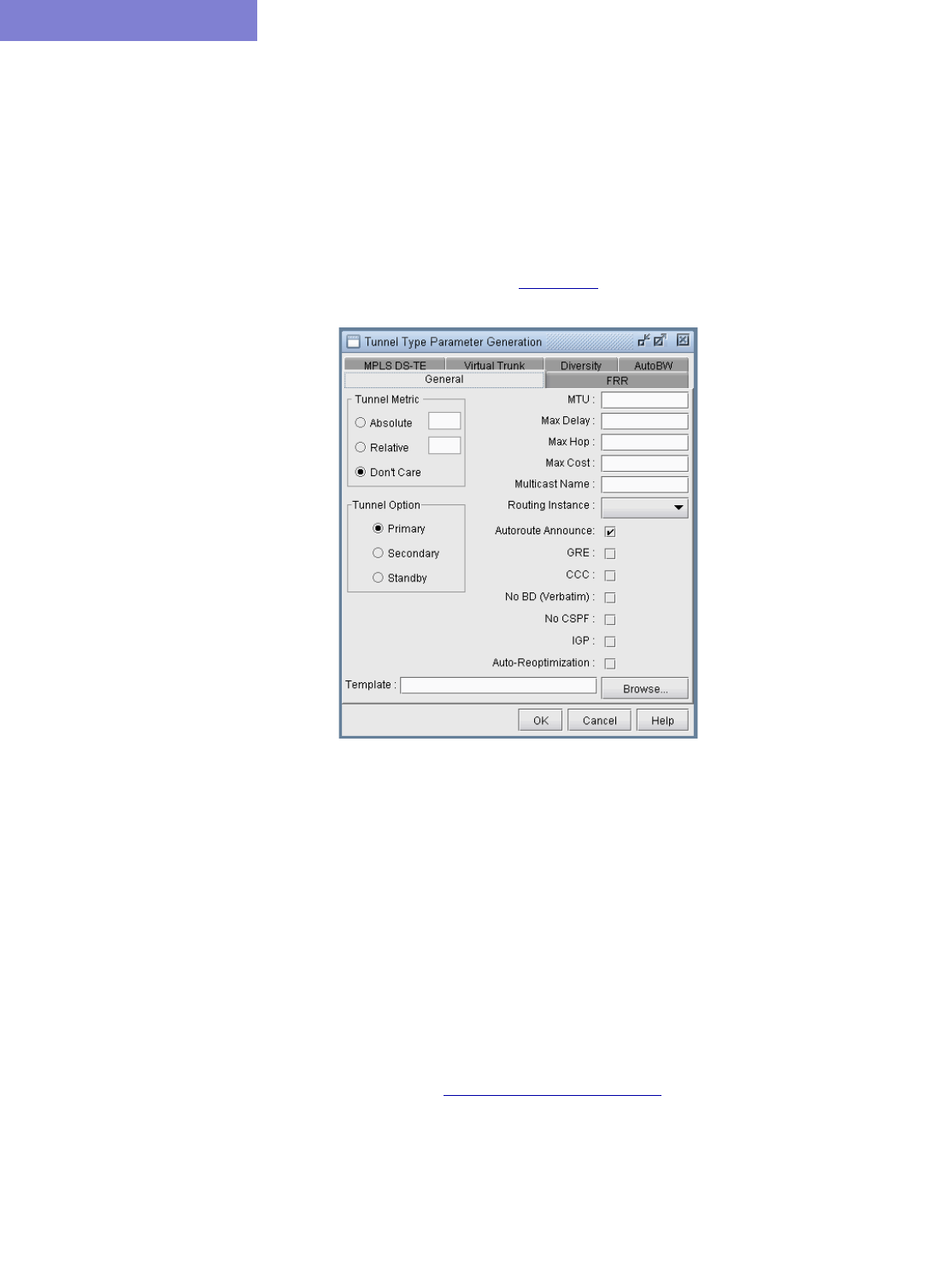
LSP TUNNELS*
20-14 Copyright © 2014, Juniper Networks, Inc.
20
SPECIFYING SECONDARY AND STANDBY TUNNELS (FOR JUNIPER ROUTERS)
47. The tunnel ID, from node, to node, and IP address of the secondary/standby tunnel should be identical to that of
the primary tunnel. Thus, to add a secondary or standby tunnel, you should first have the desired primary tunnel
open in the Add Tunnel or Modify Tunnel windows.
48. In the fish sample network, open up the Modify Tunnel window for RHOUWDC (where HOU, the source
node, is a Juniper router). In the bottom half of the window where it says Tunnels/Paths for this tunnel,
click on “Add Row.” Note that the source node should be of a type that supports secondary or standby tunnels.
49. Right-click on the newly-added row and select the Edit Type menu option. The Tunnel Type Parameter
Generation window will appear, from which you can select Secondary or Standby instead of Primary as
shown in the Tunnel Option section of Figure 20-14. Click “OK”.
Figure 20-14 Tunnel Type Parameter Generation Window for Juniper Routers (Options may vary)
For more details on other type options, see the Reference Guide, chapter on The Network and Modify Menus,
Tunnels, Tunnel Type Parameter Generation.
Secondary and standby tunnels are used when the primary tunnel fails. The difference is as follows:
•A secondary tunnel is not routed until the primary tunnel fails.
•A standby tunnel is routed while the primary tunnel is up.
Note: Secondary and standby tunnels should be listed immediately after the primary tunnel in the tunnel file.
Furthermore, they should have the same tunnel ID, from node, to node and IP address.
50. For a secondary or standby path for Juniper, you only need to change the fields that are different from the
primary path. You can highlight a row for a secondary or standby path by clicking on it. After highlighting it,
right-click and select Edit Route, Edit Type, or Edit Affinity to bring up a window where you can make
these modifications.
51. Another option is to have the program automatically add a diverse standby or secondary tunnel by using the Path
Config. Options indicated in Path Config Options on page 20-15. In the Add Tunnel window, after specifying
the primary tunnel parameters, select Div.Stdby or Div.Sec/Dynamic in the Path Config. Options drop-
down menu to add a standby or secondary tunnel. Click OK to add the tunnel and its secondary or standby
tunnel.
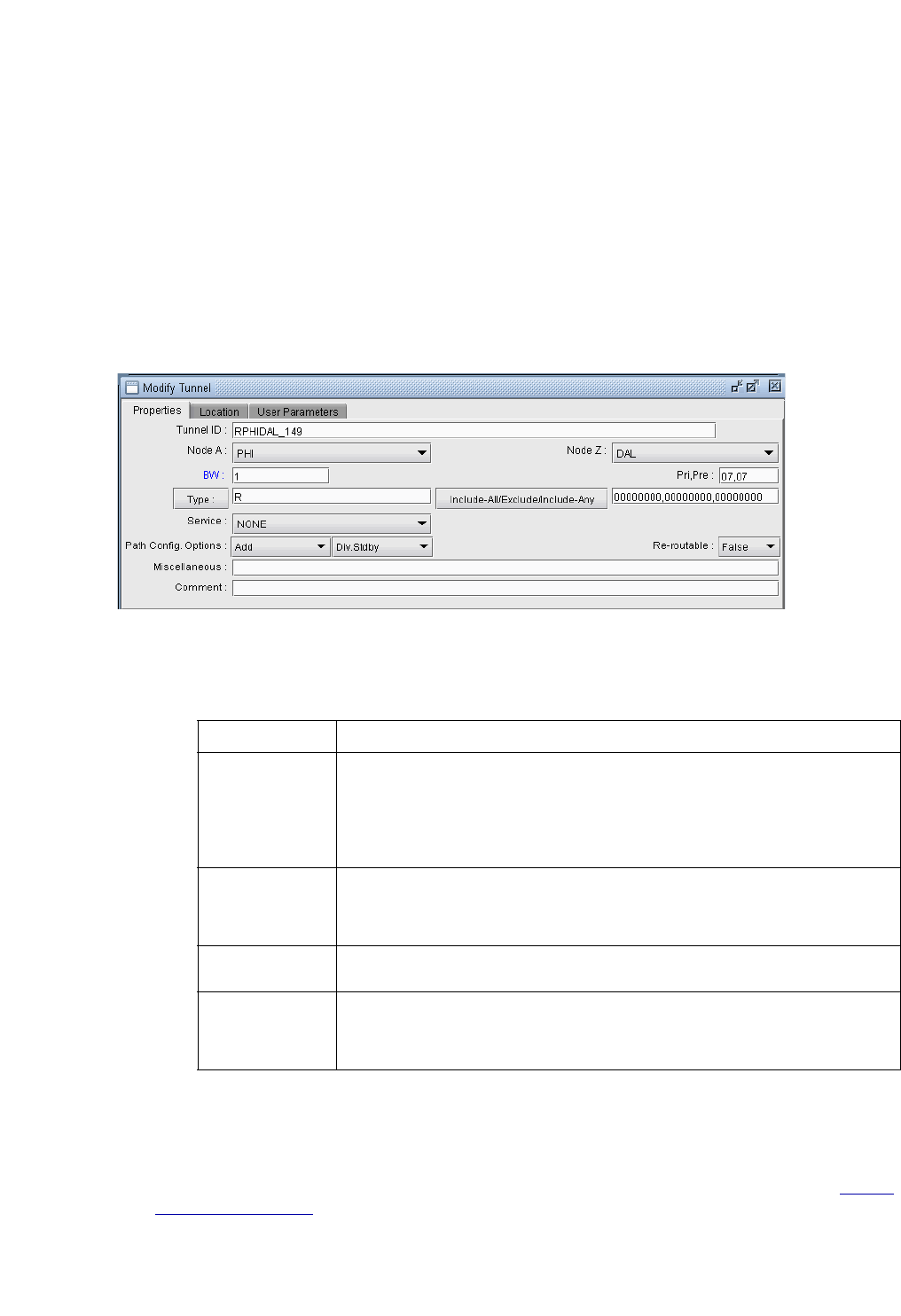
LSP TUNNELS*
Copyright © 2014, Juniper Networks, Inc. 20-15
. . . . .
52. If the tunnel(s) are already in the network, then select tunnels to modify and click Modify... and then select
“Selected Entries.” In the Modify Tunnel window, select “Add” followed by Div.Stdby or
Div.Sec/Dynamic in the Path Config. Options to add a standby or secondary tunnel. Click OK to add the
secondary or standby tunnel.
Note: Note that this is an Add operation, meaning that if the tunnel already had a standby tunnel and you add a
secondary tunnel, it will consequently have both a standby and secondary tunnel. If you only wanted to select one of
the types and not both, you should perform a subsequent modification specifying “Remove” followed by the original
type (standby or secondary) that you want to remove and clicking “OK”.
PATH CONFIG OPTIONS
53. The Path Config Options and Re-routable dropdown selections can be used to specify requirements for
secondary/standby paths as described in the table below.
Figure 20-15
If Div. Sec. or Div. Stdby are specified, the WANDL software will automatically create path entries for the
secondary or standby paths of the primary tunnel, respectively. In order to specify the paths, you can either do so
manually using the methods described in this chapter, or you can have the WANDL software design the paths for you
in Design > TE Tunnels > Path Design.
Note: The Path Diversity Design feature requires a special license. For more on this feature, please refer to Chapter
25, Tunnel Path Design*.
Field Description
Config Specifying Config will cause the Current Route to be set as the Configured Route.
Afterwards, the user may generate LSP configlets based on the explicit path to be
pushed back to the router.
To add configured routes based on the loopback IP addresses of nodes, as opposed to
interface IP addresses, specify configloopaddrinpath=1 in the dparam file prior to
opening the network baseline.
Div.
Sec./Dynamic
This option will cause the WANDL software to automatically add a secondary path
entry for this LSP tunnel. (Note that “Div.Sec.” is indicative of Juniper because the
word “secondary”, where as “Dynamic” is indicative of CISCO because the same word
is used in IOS).
Div. Stdby This option will cause the WANDL software to automatically create a hot standby path
entry for this LSP tunnel.
Re-routable Re-routable. This is a convenient way to indicate that if a tunnel is unable to route
according to its other specified routes, then the originating node will search for a path
not following the configured routes. This is equivalent to setting up a secondary route
that is Dynamic.
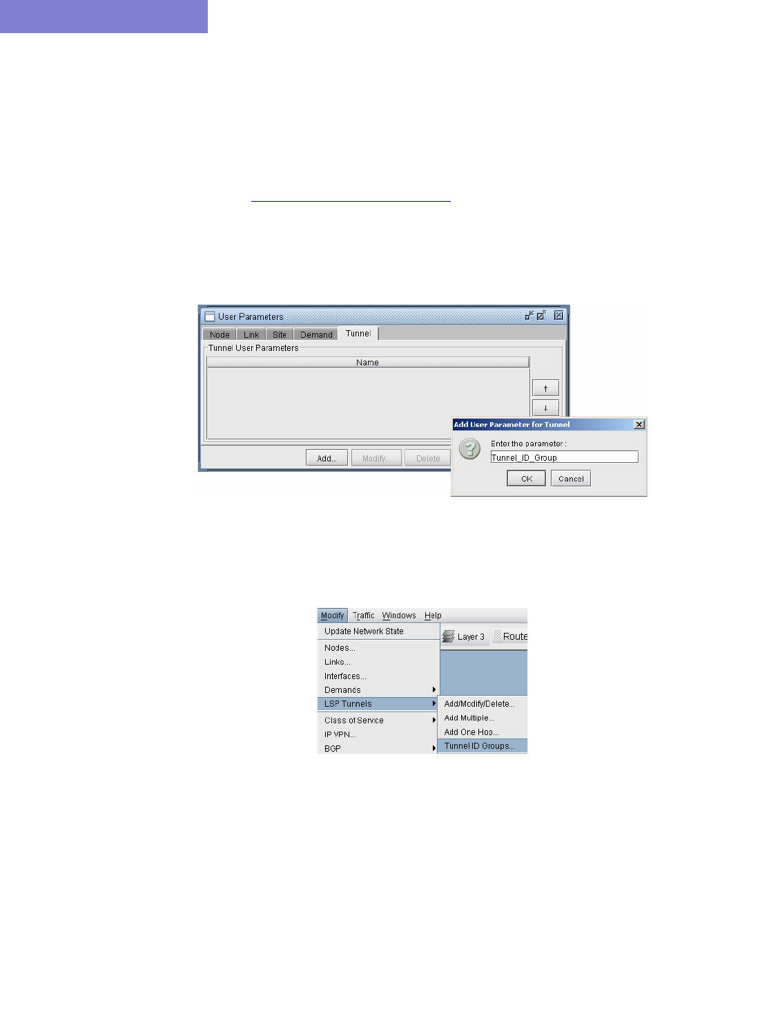
LSP TUNNELS*
20-16 Copyright © 2014, Juniper Networks, Inc.
20
Adding and Assigning Tunnel ID Groups
Tunnel ID Groups are used to configure tunnel IDs that conform to Cisco’s default tunnel names when creating LSP
configlets or using the LSP Delta wizard. Cisco default tunnel IDs are of the form, Tunnel#, where the # is unique
for each tunnel and is referred to as the tunnel ID. The tunnel ID assigned to an LSP tunnel is determined by the
tunnel ID group to which that LSP tunnel belongs. Therefore, two items need to be configured: 1) the tunnel ID
group, which contains a range of tunnel IDs, and 2) the LSP tunnel, which needs to be assigned to a tunnel ID group.
Once you have a tunnel ID group, it can also be used to create an incremental full mesh of tunnels for that group as
descibed in Adding Multiple Tunnels on page 20-10.
54. The first step is to create a user parameter to be used for assigning tunnel ID groups to LSP tunnels. This is done
through the Modify > Elements > User Parameters menu in Modify mode, which will open the User
Parameters window. In this window, activate the Tunnel tab, then click the Add button and specify a name
for the new tunnel user parameter. In the example below, the name “Tunnel_ID_Group” is used.
Figure 20-16 Adding a Tunnel ID Group User Parameter
55. The next step is to create a tunnel ID group. In Modify mode, select Modify > Elements > Tunnel ID
Groups.
Figure 20-17 Creating Tunnel ID Groups
56. To add a tunnel ID group, in the Tunnel ID Groups window click the Add button, then give the new group a
name and an ID range as shown below. Also be sure to select a Tunnel User Parameter to use for assigning
tunnel ID groups to LSP tunnels.
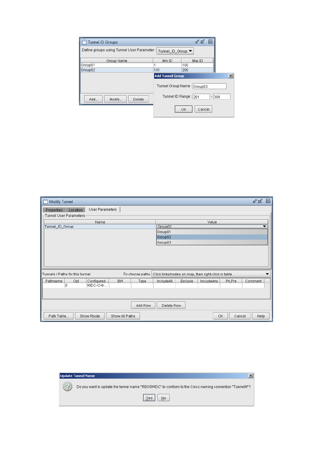
LSP TUNNELS*
Copyright © 2014, Juniper Networks, Inc. 20-17
. . . . .
Figure 20-18 Adding a Tunnel ID Group
57. Now that a tunnel ID group has been created, and a tunnel ID group user parameter has been created, the user
can modify LSP tunnels to assign a tunnel ID group to that LSP tunnel’s tunnel ID group user parameter. To do
this, go to Modify > Elements > Tunnels, select a LSP tunnel, and click the Modify button. Then in the
Modify Tunnel window, select the User Parameters tab, then click the Value field of the tunnel ID group
user parameter to activate a dropdown menu of all existing Tunnel ID Groups. Select a tunnel ID group from the
list, then click OK.
Figure 20-19 Assigning a Tunnel ID Group to an LSP Tunnel
Tunnel ID groups are used in functions such as generating LSP configlets. When generating a configlet, the user will
be prompted with the following window:
Figure 20-20 Option for Updating Tunnel Names

LSP TUNNELS*
20-18 Copyright © 2014, Juniper Networks, Inc.
20
If Yes is selected, the tunnel name will be modified to match the Cisco naming convention, with the ID number
selected from the tunnel ID group assigned to that tunnel. An example of a configlet with the tunnel name modified
to the Cisco naming convention is shown below.
!! BOS
interface Tunnel0123
description from BOS to WDC
ip unnumbered Loopback0
tunnel destination 10.10.10.8
tunnel mode mpls traffic-eng
tunnel mpls traffic-eng autoroute announce
tunnel mpls traffic-eng priority 2 2
tunnel mpls traffic-eng bandwidth 10000
tunnel mpls traffic-eng path-option 10 explicit name Tunnel0.p0
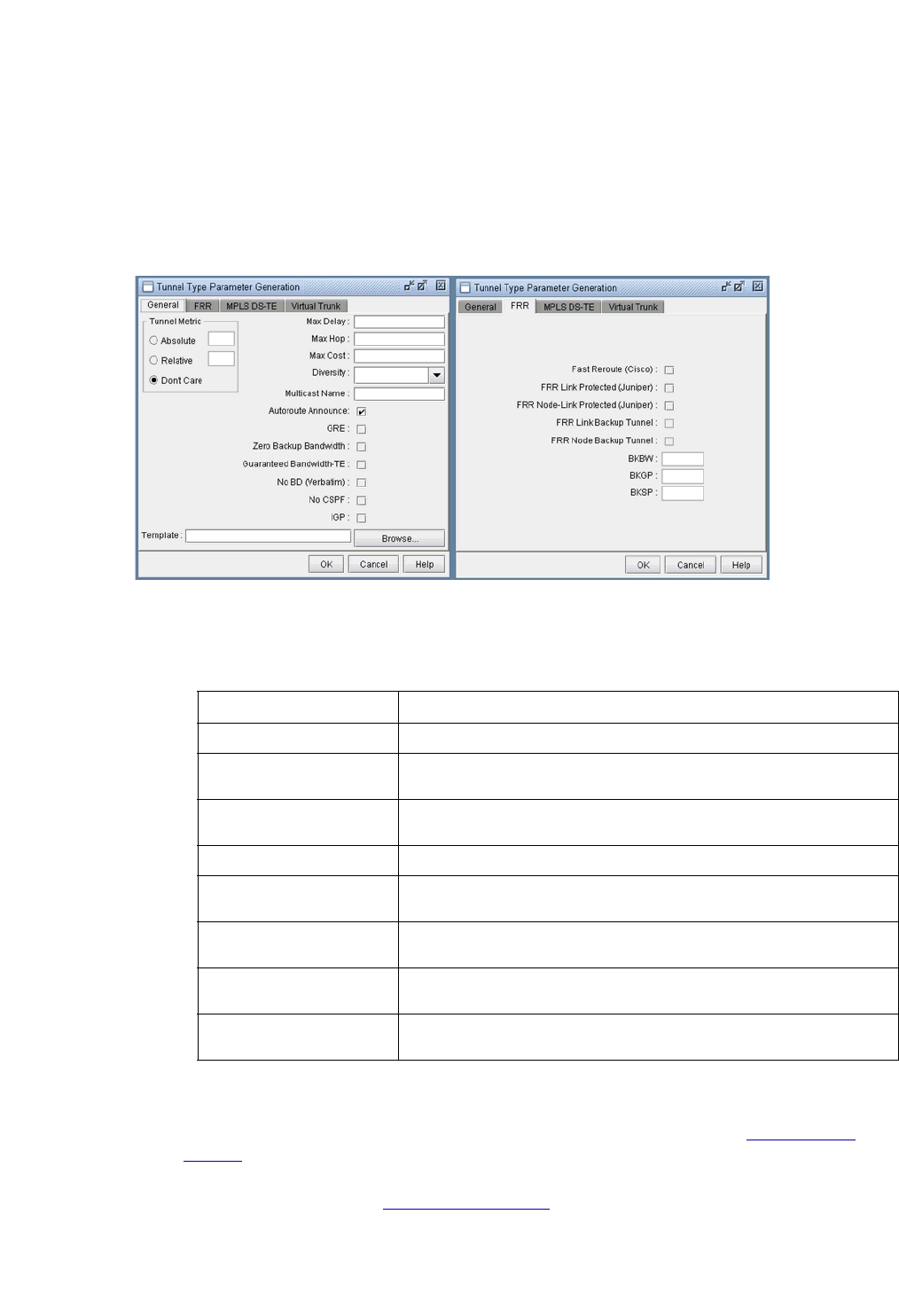
LSP TUNNELS*
Copyright © 2014, Juniper Networks, Inc. 20-19
. . . . .
Making Specifications for Fast Reroute
Suppose a tunnel has requested fast reroute (FRR) protection, and one of the links on which it is routed over fails.
The information about the link failure may take a while to reach the tunnel’s source node. In this case, data routed
over the tunnel will continue to head toward the failed link. With fast reroute, you can specify a backup tunnel
around the protected link. Then the traffic can go along the backup tunnel to get around the failed link until the
tunnel reroutes in a way that avoids the failed link.
Note: The fast reroute option should only be used for hardware that supports fast reroute.
Figure 20-21 Tunnel Type Parameter Generation window
58. To specify that a tunnel has requested for fast reroute protection, select the Fast Reroute checkbox in the
Tunnel Type window.
59. To add backup tunnels for links carrying the tunnels requesting FRR protection, refer to Chapter 30, Fast
Reroute*. Note that the FRR Backup Tunnel checkboxes in the Tunnel Type window are grayed out but will
reflect changes when you successfully add the FRR_A or FRR_Z field in the link window MPLS TE tab. .
For further details on FRR, refer to Chapter 30, Fast Reroute*.
FRR Tab Field Description
Fast Reroute (Cisco) Specifies that this tunnel requires FRR protection.
FRR Link Protected
(Juniper)
Indicates that the Juniper primary tunnel is subject to link protection.
FRR Node-Link
Protected (Juniper)
Indicates that the Juniper primary tunnel is subject to node-link protection.
FRR Link Backup Tunnel Specifies that this tunnel is created for FRR Link Backup purposes.
FRR Node Backup
Tunnel
Specifies that this tunnel is created for FRR Node Backup purposes.
BKBW Indicates how much bandwidth the FRR backup tunnel is configured to
protect.
BKGP Indicates how much Global Pool bandwidth the FRR backup tunnel is
configured to protect. This is for Cisco only.
BKSP Indicates how much Sub Pool bandwidth the FRR backup tunnel is
configured to protect. This is for Cisco only.

LSP TUNNELS*
20-20 Copyright © 2014, Juniper Networks, Inc.
20
Specifying Tunnel Constraints (Affinity/Mask or Include/Exclude)
Constraint-based tunnel routing is implemented in Cisco and Juniper by coloring links and specifying which link
colors a tunnel can or cannot route over. For Cisco, the links can be colored using 32 link attributes, each
represented by a bit. The tunnel routing constraints are then specified per tunnel using affinity and mask. Juniper,
on the other hand, uses the term admin groups to represent link colors. For Juniper, the tunnel routing constraints
can be specified per tunnel using include and exclude statements. Below is a brief summary of how to specify
affinity/mask for Cisco routers and include/exclude for Juniper routers. Please see Commands Modeled Using
Affinity and Mask Feature on page 20-26 to see which commands are being modeled.
CISCO
Link attributes contain 32 bits as the colors. A tunnel’s 32-bit mask specifies which of the tunnel’s 32 affinity bits are
required to match the link attributes. If the match is successful, the tunnel is allowed to route through the trunk
provided that the other routing requirements (such as capacity) are also satisfied. If the match is unsuccessful, the
tunnel is not allowed to route over the trunk. In other words, a tunnel can route over a link if tunnel_affinity =
(link_attribute & tunnel_mask).
JUNIPER
For Juniper, the terminology and options are slightly different. For Juniper, you can have up to 32 administrative
groups as the colors. For each link, you can assign one or more administrative groups as the link color. Then for each
tunnel, you can add groups to an “exclude” or “include” list (or, in recent versions of JUNOS, there an “include-all”
and “include-any” list). For a tunnel to route over a link, that link cannot have any of the excluded groups and must
have at least one of the included groups (for include or include-any) or all of the included groups (for include-all).
Note that for Juniper, you can have an include and exclude list for secondary paths as well as primary paths.
WANDL MODELING OF TUNNEL CONSTRAINTS
In the WANDL client, the Tunnel Attributes window can be used to assign names to link attributes as described in
Tunnel Attribute/Admin Group Names on page 20-21. For Juniper tunnels, admin-groups can be entered here. For
Cisco tunnels, the names can be left as is or changed for informational purposes.
Following this, the link attributes/admin-groups can be assigned to links from the Modify Links window as
described in Setting Link Attributes on page 20-21.
Finally, the tunnel routing constraints can be specified from the Modify Tunnels window by clicking the
Affinity/Mask button (for Cisco) as described in Tunnel Affinity and Mask (Cisco) on page 20-22or Include-
All/Exclude/Include-Any button (for Juniper) as described in Including and Excluding Admin-Groups (Juniper)
on page 20-23.
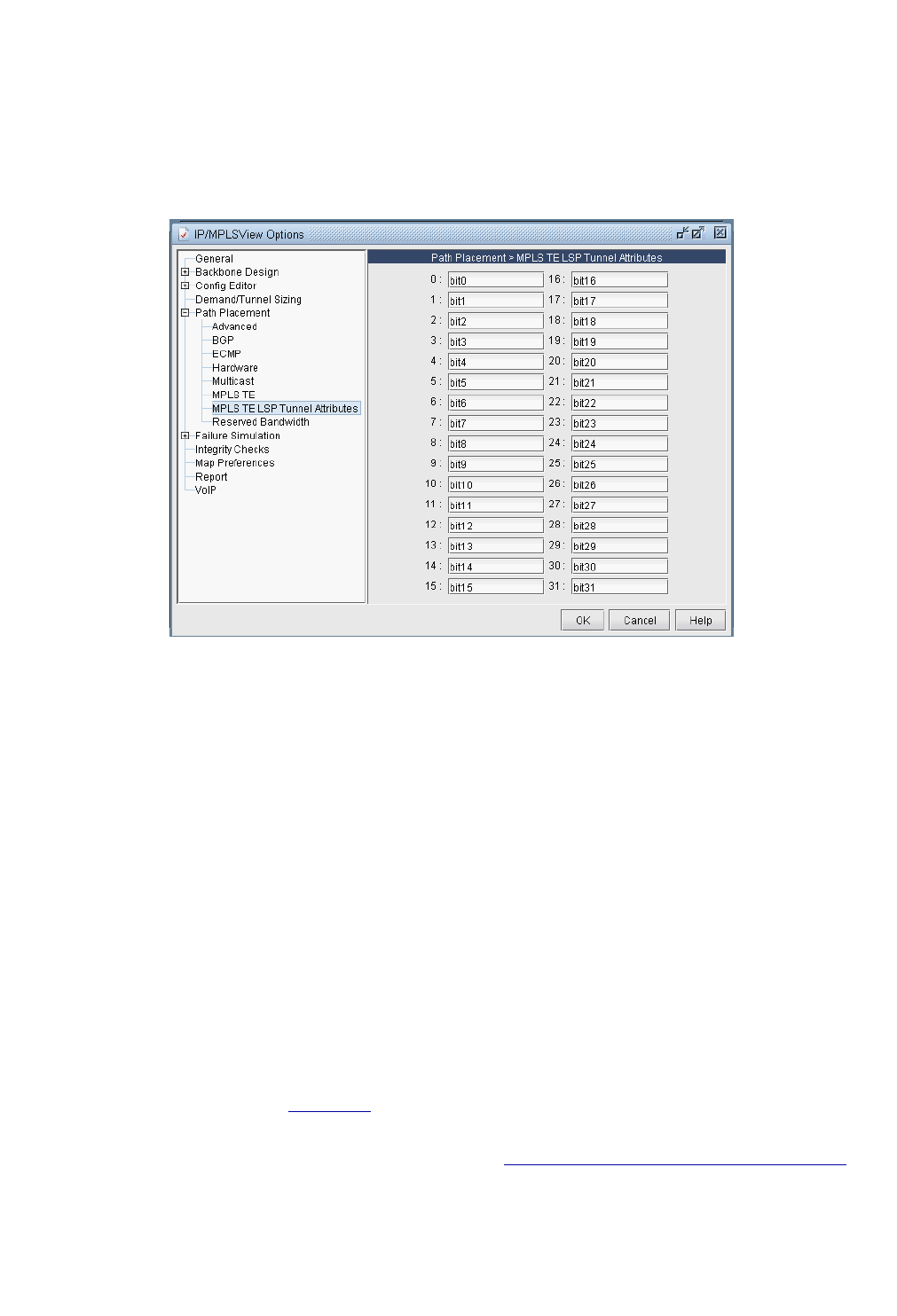
LSP TUNNELS*
Copyright © 2014, Juniper Networks, Inc. 20-21
. . . . .
TUNNEL ATTRIBUTE/ADMIN GROUP NAMES
60. If you want to give meaningful global names to one of the 32 link attributes/admin groups, you can select Tools
> Options > General..., Path Placement > MPLS TE LSP Tunnel Attributes options pane for the
following window. For Juniper switches, enter in the admin-group names here. The default names are bit0, bit1,
bit2, etc. Click “OK” to save your changes.
Figure 20-22 Tunnel Options Window
SETTING LINK ATTRIBUTES
61. To change the attributes for a single link, right-click that link on the map and select Modify >Links under
Pointer. Then select the Attributes tab. To set the same link attribute for both directions on the link, leave the
default setting “Symmetric.” Then check off the link’s attributes. This will set the corresponding bit for that
attribute to 1.
To set different link attributes for the two directions on the link, select “Asymmetric.” Then select the direction
“A to Z” or “Z to A” that you want to modify and select the attributes for that direction.
62. To change the affinity attributes for multiple links at a time, select Modify > Elements > Links. In the Links
table, select the desired rows by using the <Shift> and <Ctrl> keys. To select all rows, click “Select All” or
click in the table and press <Ctrl>-A. Then, press Modify. You will get a window like the one shown below.
Note that the Match field appears only when multiple links are selected for modification. It is not a property of
the link but is for the user to indicate which bits to modify for the selected links. Bits that are not matched will
not be touched in the modification.
To specify a bit that you want to change for all the selected links, click the button for that bit to activate the
checkbox for that bit. This will also turn the button text blue. Then check or uncheck the adjacent box to turn on
or off the attribute, i.e., to set the value for that attribute to 1 or 0.
For example, in Figure 20-23, three links are being modified. For each of these links, the GOLD attribute is set
to 0 and the ECONOMY attribute is set to 1. No other attributes on any of these links will be modified.
Note: To customize the attribute names, refer back to Tunnel Attribute/Admin Group Names on page 20-21.
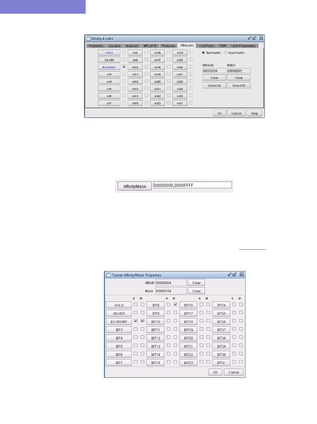
LSP TUNNELS*
20-22 Copyright © 2014, Juniper Networks, Inc.
20
Figure 20-23 Global Modify of Link Attributes
TUNNEL AFFINITY AND MASK (CISCO)
63. Affinity and mask for a tunnel can be specified through the Add Tunnel or Modify Tunnel windows. In these
windows, there is a textfield to the right of the “Affinity/Mask” button, in which you can directly enter a
hexadecimal for the affinity and mask. The affinity and mask should be separated by a comma.
Figure 20-24 Directly entering in Tunnel Affinity and Mask
Alternatively, if you want to specify the affinity and mask by selecting the relevant bits from which the
hexadecimal number is derived, click on the “Affinity” button. The Tunnel Affinity/Mask Properties
window will appear, as shown below.
The mask specifies which attributes a link must match in order for the tunnel to be routed over that link. The
affinity specifies whether that attribute is turned on or off. For example, in Figure 20-25, the tunnel is configured
so that it can only route over links that have the ECONOMY attribute set to 1 and the BIT8 attribute set to 0.
Figure 20-25 Tunnel Affinity/Mask Properties
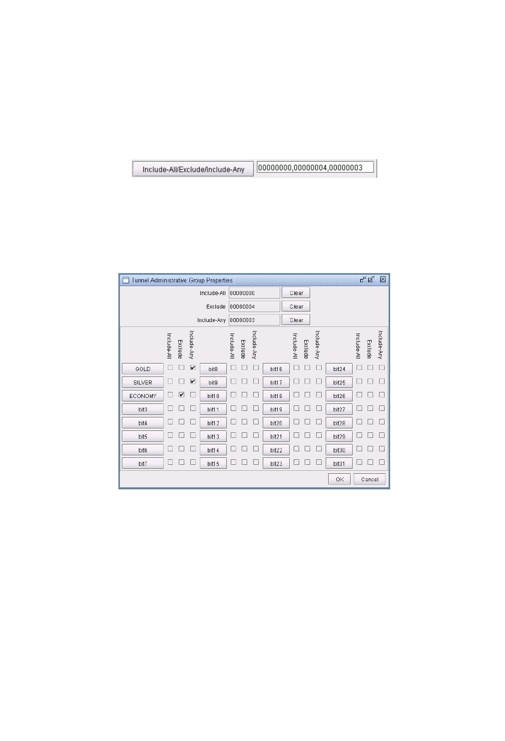
LSP TUNNELS*
Copyright © 2014, Juniper Networks, Inc. 20-23
. . . . .
64. The Affinity and mask are both hexadecimals. Each digit can go from 0 to F and is made up of 4 bits. Check off
the bits that you want to set. This will change the affinity and mask listed on top. If you press “Clear” all the
bits will be unchecked and the number will be reset to 00000000.
INCLUDING AND EXCLUDING ADMIN-GROUPS (JUNIPER)
65. For Juniper, include and exclude constraints can be specified through the Add Tunnel or Modify Tunnel
windows. You can directly specify these properties next to the Include-All/Exclude/Include-Any button in
the form of hexadecimals.
Figure 20-26 Directly Entering in Include/Exclude Constraints
Alternatively, you can check off the attributes in the following window. In the example below, the constraint is
that this tunnel must route over a link with at least one of the admin-groups GOLD or SILVER but not the admin
group ECONOMY.
Figure 20-27 Tunnel Include/Exclude Constraints
LSP TUNNELS*
20-24 Copyright © 2014, Juniper Networks, Inc.
20
Adding One-Hop Tunnels
Using the one-hop tunnel feature, users can create a pair of one-hop tunnels for each link, one for each direction.
These tunnels are created with an explicit route that force them to use the direct link.
The following commands are the corresponding Cisco commands for creating one-hop tunnels:
mpls traffic-eng auto-tunnel primary onehop
mpls traffic-eng auto-tunnel primary tunnel-num [min num] [max num]
mpls traffic-eng auto-tunnel primary config unnumbered-interface interface
Note: The one-hop tunnel feature should only be used for networks where an IGP is deployed on the interfaces for
which a one-hop tunnel will be created.
66. Select Modify > Elements > User Parameters. Click on the Tunnel tab. Then click “Add...” and add a
user parameter to store the Tunnel Group ID, such as TunnelGroupID.
Figure 20-28 Adding a User Parameter for TunnelGroupID.
67. Select Modify > Elements > Tunnel ID Groups... In the selection menu, select the tunnel user parameter
that was just created. Then click Add... to enter in a group name and ID range. The One Hop Tunnels you create
will be given the group name as prefix and a number in the ID range as suffix.
Figure 20-29 Adding a Tunnel ID Group
68. Note that you can only add one-hop tunnels for links that have an IGP enabled. To enable an IGP protocol,
modify the links through Modify > Elements > Links... and click the Modify button. In the Protocols tab
turn on either OSPF or ISIS and click OK.
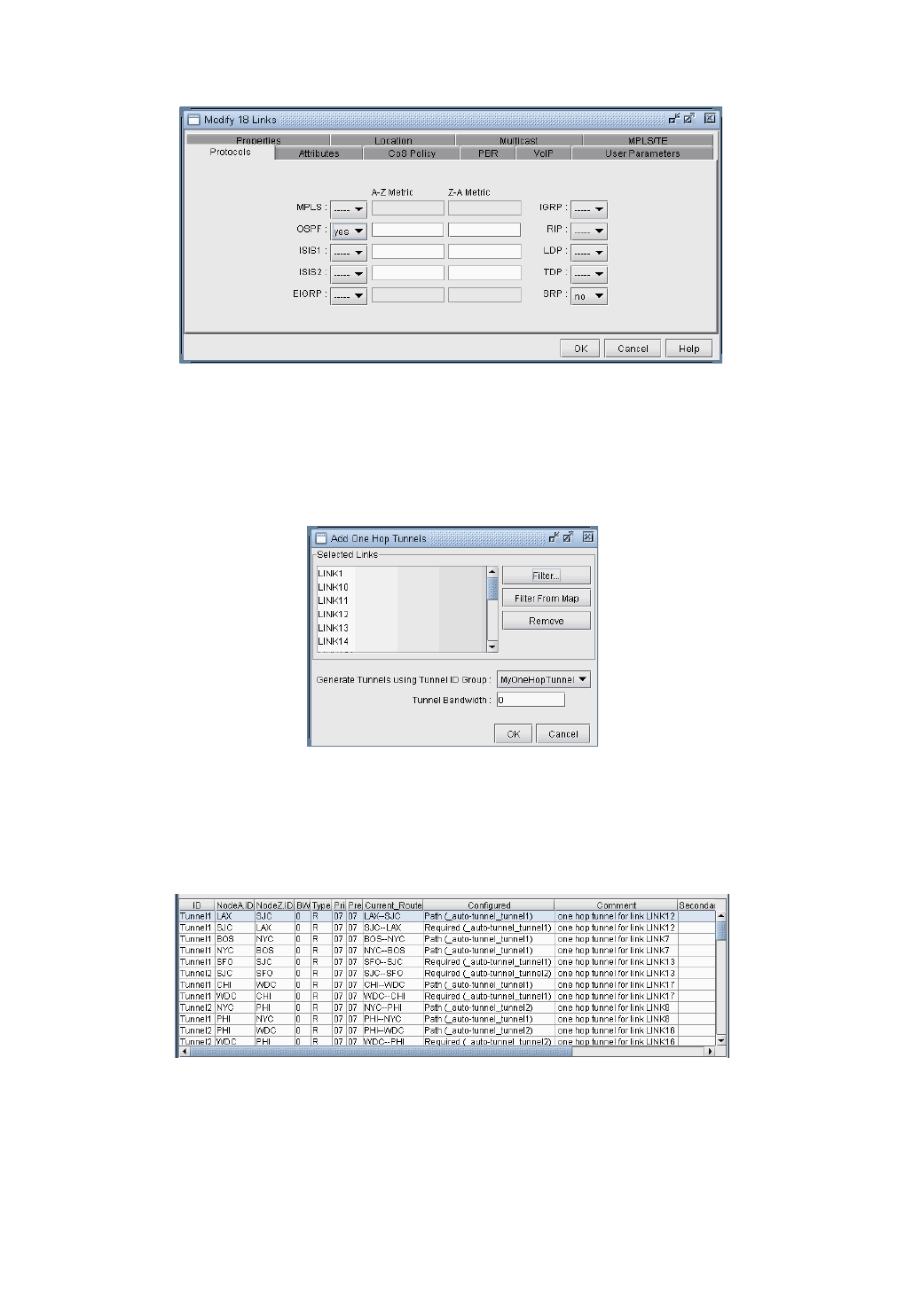
LSP TUNNELS*
Copyright © 2014, Juniper Networks, Inc. 20-25
. . . . .
Figure 20-30 Enabling OSPF or ISIS on the Links
69. Select Modify > Elements >Tunnels, Add > One Hop Tunnels... Select some links by filtering for them.
An easy way is to highlight them on the map and then click Filter from Map. Select the Tunnel ID Group to
use to create the one hop tunnels and add a tunnel bandwidth. Click “OK” to add the one hop tunnels.
Figure 20-31 Add One Hop Tunnels
Select Modify > Elements > Tunnels to view the newly added one hop tunnels. Several nodes can have
tunnels with the same TunnelID but different tunnels originating from a node should have unique tunnelIDs.
Figure 20-32 Results of One Hop Tunnel Additions
Note the explicit path given in the Configured column of the following table. Double-click on a newly added
one-hop tunnel to view the configured route. Then select the User Parameters tab. The tunnel user parameter
for Tunnel ID Group is specified here.

LSP TUNNELS*
20-26 Copyright © 2014, Juniper Networks, Inc.
20
70. To generate configlets for these one hop tunnels, switch to Tunnel Layerand Design mode and then select
Design > Configlets/Delta > LSP Configlet... Click “Submit” in the resulting window. The configlet
includes in the description line the interface name used for the first hop of the tunnel.
Tunnel Layer and Layer 3 Routing Interaction
Modifications to the network model (e.g. tunnels, demands/flows, network elements, design options) usually
require tunnels or flows to be rerouted. In the WANDL software, this rerouting occurs in the following order:
•If you are in Layer 3 and a reroute is triggered, tunnels will be rerouted first, followed by demands/flows.
•If you are in Tunnel Layer and a reroute is triggered, then only tunnels will be rerouted while in Tunnel layer. The
moment you switch into Layer 3, however, the Layer 3 demands/flows will then be rerouted.
Appendix
COMMANDS MODELED USING AFFINITY AND MASK FEATURE
Corresponding Cisco Commands
Setting link attributes mpls traffic-eng attribute-flags attributes
Setting tunnel affinity and
mask
tunnel mpls traffic-eng affinity affinity [ mask mask ]
Corresponding Juniper Commands for the mpls protocol
Defining
Administrative
Groups
admin-groups {
group-name 1;
group-name 2;
...
}
Selecting admin
groups for a link interface interface name {
admin-group [ group-name group-name ... ];
}
Setting admin
groups for a
tunnel
label-switched-path lsp-path-name {
to address;
...
primary path-name {
admin-group {
exclude [ group-name group-name ... ];
include [ group-name group-name ... ];
include-all [ group-name group-name ... ];
include-any [ group-name group-name ... ];
}
}

Copyright © 2014, Juniper Networks, Inc. 21-1
. . . . .
. . . . . . . . . . . . . . . . . . . . . . . . . . . . . . . . . . .
O
PTIMIZING
T
UNNEL
P
ATHS
*
21
his chapter describes how to optimize your tunnel paths using the net grooming feature.
*Note that a special password is required for the tunnel feature. Please contact your Juniper representative
for more information.
When to use
Use this chapter to learn how to improve the routing of tunnels in your network.
Prerequisites
If you wish to perform this task in the WANDL client, you should have already added tunnels to your network. You
may use the spec.mpls-fish spec file located in your $WANDL_HOME/sample/IP/fish directory (where
$WANDL_HOME is /u/wandl by default).
Related Documentation
For general step-by-step instructions on how to use the WANDL software, please refer to the Design & Planning
Guide.
For an overview of the WANDL software or for a detailed description of each feature and the use of each window,
refer to the General Reference Guide or Chapter 37, Router Reference.
For instructions on how to view or modify the tunnels in your network, refer to Chapter 20, LSP Tunnels*
Recommended Instructions
1. Set up the network for network grooming.
2. Run network grooming.
Detailed Procedures
1. To switch to design mode, click on the “Design” button on the main menu bar as shown in Figure 21-1. The
Design pull-down menu gets activated. To switch to Tunnel layer mode, select the “Tunnel Layer” button on
the layer selection bar.
Figure 21-1 Switching to Design Mode, and Tunnel Layer
2. Before using the network grooming feature, you should change the tunnel path settings from “required” to
“preferred” for those paths that you want to improve the routes of. To do this for all of your tunnels, select
Design > Route Paths > Interactive Mode. From the console, select “Update Preferred Path Setting”
for the following menu.
Preferred Path Modification Menu:
1. # Tunnel with Preferred Path setting= 0 primary, 0 secondary
2. # Tunnel with Required Path setting= 5 primary, 0 secondary
3. Use current routes as preferred/required paths
Select:
T
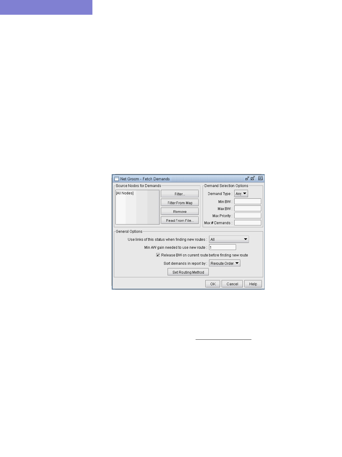
OPTIMIZING TUNNEL PATHS*
21-2 Copyright © 2014, Juniper Networks, Inc.
21
If any tunnels have the required setting, select 2. You will then be asked to apply changes to the primary tunnels,
secondary/standby tunnels, or all. Select 3 for all.
Apply Changes to 1: Primary only, 2. Secondary/Standby only, 3. All
3
Required Paths Modification Menu:
1. Change to Preferred, 2. Remove All Required Paths, 3. No Change
Select:
Select 1 to change the paths to preferred paths. Press <Enter> repeatedly until you exit out of the console.
Note: You can also manually apply the changes to tunnels on an individual basis by modifying the tunnel file,
changing the Path Required PR(path) statements to Path Select PS(path) statements. You then need to use the
File>Read option to read in these changes to the tunnel file.
Network Grooming
3. The objective of network grooming is to reroute the paths to minimize the distance metric of the paths using
available bandwidth in the network. Select the Design > TE Tunnels > Net Groom pull-down menu. The
Net Groom window will appear:
Figure 21-2 Network Grooming Window for Tunnel Paths
4. Specify the Source Nodes for Tunnels to narrow down the set of tunnels to be optimized. Otherwise, by
default, all tunnel paths will be optimized. Specify Tunnel Selection Options to further narrow down the set
of tunnels.
5. Specify any General Options. Refer to the General Reference Guide for more information on the Net Groom
window options. To change the distance calculation method to OSPF, RIP, Delay, ISIS, or CDV, simply click on
the “Set Routing Method” button and enter the desired choice in the console. Once all options are set, click
OK.
Note that AW is an abbreviation here for “Admin Weight”, which is the same thing as “Admin Cost” or “Link
Metric”. Network grooming assumes that the smaller the path’s total admin weight, the better.
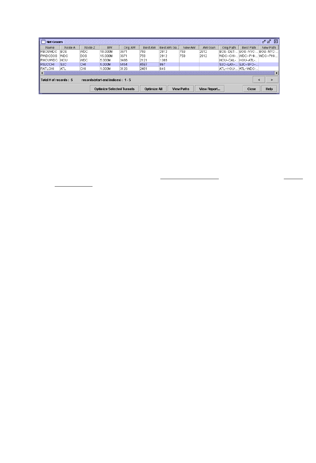
OPTIMIZING TUNNEL PATHS*
Copyright © 2014, Juniper Networks, Inc. 21-3
. . . . .
Figure 21-3 Net Groom - Potential Admin Weight (AW) Gain for Tunnel Path
6. By comparing the Original Admin Weight (AW) with the potential Best (smallest) AW, you can decide which
tunnels should have their paths changed or optimized. You can click on the Best AW Gain column header to
sort according to the highest reduction in the total admin weight. Click on “View Paths” button to compare the
Orig Path and Best Path using the Paths window.
7. Select multiple tunnels for optimization and click the “Optimize Selected Tunnels” button. The New AW
and AW Gain columns will be populated for the selected tunnels with the actual achieved admin weight. The
LSP tunnel paths are updated to the new ones discovered by the WANDL software.
Refer to the Network Grooming chapter of the Design & Planning Guide or the Design chapter in the General
Reference Guide for more details about network grooming.

OPTIMIZING TUNNEL PATHS*
21-4 Copyright © 2014, Juniper Networks, Inc.
21

Copyright © 2014, Juniper Networks, Inc. 22-1
. . . . .
. . . . . . . . . . . . . . . . . . . . . . . . . . . . . . . . . . .
T
UNNEL
S
IZING
AND
D
EMAND
S
IZING
*
22
his chapter describes how to resize a network’s LSP tunnels based upon the measured traffic on the tunnel
or to resize a network’s demands based upon the traffic load.
From the Report Manager, you can identify tunnels in the network where the planned tunnel bandwidth is
greater than or less than the actual transported layer 3 traffic. For such cases, you may then wish to change those
tunnels’ bandwidths to make sure that sufficient bandwidth is allocated to carry traffic to meet Service Level
Agreements (SLAs). The Tunnel Sizing feature in the WANDL software provides an automated solution for resizing
these tunnels.
When to use
Use this chapter to learn how to automate tunnel bandwidth sizing and demand bandwidth sizing.
Prerequisites
If you wish to perform this task in the WANDL client, you should have already added tunnels and/or demands to
your network. You should also have either end-to-end layer 3 demands defined for the network model (in the
demand file) or else actual measured tunnel traffic statistics (in the T_trafficload file). You may wish to use the
spec.mpls-fish spec file located in $WANDL_HOME/sample/IP/fish directory (where $WANDL_HOME is
/u/wandl by default) as a starting point.
Note: This feature requires both the MPLS-TE password and the loadanalysis password in your npatpw.
Definitions
It should be noted that in this document, the word “tunnel” is used in the context of traffic engineering (TE) tunnels.
Also, the word “tunnel load” refers to the amount of IP traffic transported by the tunnel.
Planned/Configured Bandwidth: The current bandwidth allotted to the tunnel or demand.
Flow Bandwidth: The traffic load through the tunnel or demand; sometimes called “used bandwidth”.
New Bandwidth: The new bandwidth size of the tunnel or demand calculated by this feature.
Related Documentation
For general step-by-step instructions on how to use the WANDL software, please refer to the Design & Planning
Guide.
For an overview of the WANDL software or for a detailed description of each feature and the use of each window,
refer to the General Reference Guide or Chapter 37, Router Reference.
For instructions on how to view or modify the tunnels in your network, refer to Chapter 20, LSP Tunnels*.
Recommended Instructions
Note: Although the steps below are for tunnel sizing, demand sizing works the same way.
1. Open a network that contains tunnels.
2. Switch to Tunnel layer.
3. View current tunnel utilization in the Report Manager.
4. Specify Tunnel Sizing default options in the Demand/Tunnel Sizing option pane of Tools > Options >
Design.
5. Select Design > Tunnel Sizing to bring up the “Find Tunnels” window. Specify the search criteria for
tunnels.
T

TUNNEL SIZING AND DEMAND SIZING*
22-2 Copyright © 2014, Juniper Networks, Inc.
22
6. Adjust the new tunnel bandwidth value if necessary by entering a new value in the tunnel’s “New BW” field or
clicking on the “Recalculate Selected” button.
7. Save the new bandwidth values by clicking on “Confirm Selected” or “Confirm All”. This will save the new
bandwidth values as the tunnel’s bandwidth.
Detailed Procedures
Note: Although the steps below are for tunnel sizing, demand sizing works the same way.
1. Open a network project spec that contains tunnels, by double-clicking on the spec file in the File Manager.
2. Since the tunnel sizing feature is designed for use in Tunnel layer, switch to Tunnel layer mode by clicking on
the Tunnel layer button on the main menu bar, as shown below.
Figure 22-1 Tunnel Layer Button
3. If you plan to resize your tunnels based upon the bandwidth of routed end to end flows, you should have
demands defined in your network, in the demand file. If not, you can add some by switching into Modify mode,
and selecting Modify > Elements > Demands... and selecting Add > Multiple Demands....
4. If you plan to resize your tunnels based upon actual measured tunnel traffic statistics, then you should have read
in the WANDL formatted tunnel traffic load file. To read it in, go to File > Load Network Files and select the
entry T_trafficload (for “tunnel trafficload”) and click Browse to find the desired input file. Alternatively, you
can simply include the tunnel trafficload file into your spec file with the following line:
T_trafficload = T_trafficload.runcode
The following shows the tunnel traffic load format for one tunnel, named tunDenDet, originating at node DEN
and with three periods of measured tunnel traffic:
DEN:tunDenDet A2Z - 3.0M 4.0M 9.1K
For more information on the tunnel traffic load file format, please refer to the “Demand/Traffic Files” section of
the File Format Guide.
5. Select Report > Report Manager to open the Report Manager window. At least one of the following
reports will be of interest to you.
6. If you plan to resize your tunnels based upon the bandwidth of routed end to end flows, click on the “Demand
Traffic on Tunnel” report in the left pane under Tunnel Layer Network Reports > Tunnel Reports to
generate and view it in the right-pane. This report provides information on existing tunnels such as the tunnel’s
planned bandwidth (Bandwidth), the total bandwidth of flows traversing the tunnel (FlowBW), and the
difference between those two values (BW_Diff). This report identifies network inefficiencies by allowing the
user to see the under-booked and over-booked tunnels in the network. The tunnel sizing feature can then
automate an adjustment of these tunnels’ bandwidths according to user-specified settings.
TUNNEL SIZING AND DEMAND SIZING*
Copyright © 2014, Juniper Networks, Inc. 22-3
. . . . .
Figure 22-2 Demand raffic on Tunnel Report (formerly Planned Tunnel Util)
7. If you plan to resize your tunnels based upon actual measured tunnel traffic statistics, click on the “Measured
Tunnel Traffic” report. This displays the measured tunnel traffic load numbers, as read in from the
T_trafficload file, in tabular format.
8. In Design mode, select Design > TE Tunnels > Tunnel Sizing. If you did not switch to Tunnel layer earlier,
the program will ask you to switch to Tunnel layer. Click “Yes” to continue.
9. A Find Tunnels window will appear as shown in Figure 22-3. In addition to the regular options, there are
options specific to tunnel sizing. Those fields are described in the table below.
Figure 22-3 Find Tunnels for Tunnel Sizing

TUNNEL SIZING AND DEMAND SIZING*
22-4 Copyright © 2014, Juniper Networks, Inc.
22
10. The next step is to check your tunnel sizing options. In the Find Tunnels window, select the “Sizing
Parameters” tab.
Note: Alternatively, you can set the sizing parameters globally via Tools > Options > Design and click on
the “Demand/Tunnel Sizing” options pane. When the options in the Design Options window are set, click
“OK”. A window will ask you whether to reroute the tunnels. You can click “No” since changing the tunnel
sizing options does not affect tunnel routing. (You are prompted because the program is aware that you have
modified the design options. Though the tunnel sizing options do not affect routing, other design options might.)
Field Description
BW Diff (KB) greater
than
If the absolute value of the difference between the tunnel
bandwidth and total flow bandwidth is greater than this value
(expressed in kilobits), then those tunnels are fetched.
BW Diff Ratio greater
than
If the absolute value of the ratio of bandwidth difference to
tunnel bandwidth is greater than this value, then those tunnels
are fetched.
Sort Field Sorts the displayed tunnels by either bandwidth difference or
bandwidth difference ratio.
Sort Order Sorts the displayed tunnels according to the type in the Sort
field; sorts either in decreasing order or in decreasing order of
the absolute value.
BW Source Specifies the source of traffic: “Layer 3 Demands” or “Traffic
Load” (measured tunnel traffic). This parameter will show up
as the “FlowBW” field in the Tunnel Sizing window. It is also
used as the flow bandwidth of the new bandwidth calculation.
Traffic Period This field specifies the time period of traffic to be used. If the
BW Source is Layer 3 Demands, then the Planned traffic from
the demand file is used. If the BW Source is Tunnel Traffic
Load, then possible values are Period1 through Period24, and
Peak. Peak indicates the heaviest/worst load experienced
among any of these 24 traffic periods.
# Tunnels Per Page Specifies how many tunnels to display per page.
TUNNEL SIZING AND DEMAND SIZING*
Copyright © 2014, Juniper Networks, Inc. 22-5
. . . . .
Figure 22-4 Tunnel Sizing Parameters
Set the sizing parameters to your preferred setting. The table below describes each field.
When the options have been selected, click “OK” to fetch tunnels that match the specified criteria. Those tunnels
will then be displayed in the Tunnel Sizing window as shown in Figure 22-5.
Field Description
Parameter in
Dparam File
Minimum Tunnel
BW
The minimum value to be assigned for any new
tunnel bandwidth. If the calculated bandwidth is less
than this value, then this value is used as the new
bandwidth.
minSizingBW
Maximum Tunnel
BW
The maximum value to be assigned for any new
tunnel bandwidth. If the calculated bandwidth is
greater than this value, then this value is used as
the new bandwidth.
maxSizingBW
Tunnel BW
Increment
The increment by which the bandwidth will be
increased. Basically, the calculated bandwidth will
be rounded up to the nearest multiple of this value.
incSizingBW
Tunnel Growth
Multiplier
This value is multiplied by the total flow bandwidth
to calculate the new bandwidth. For example, 1.00
will generate a new tunnel bandwidth assignment
that is 100% of the total flow bandwidth traversing
the tunnel, and 1.5 will generate a value that is150%
of the traffic load bandwidth.
sizing_growthmulti
plier
TUNNEL SIZING AND DEMAND SIZING*
22-6 Copyright © 2014, Juniper Networks, Inc.
22
Figure 22-5 Tunnel Sizing Window
11. In the Tunnel Sizing window, each entry in the table represents a tunnel. The “Bandwidth” column indicates
the planned tunnel bandwidth. The “Flow BW” column indicates the actual measured traffic load on that tunnel
based upon the inputs in the T_trafficload file. The “New BW” column, in white, will automatically be
populated with a proposed new bandwidth value for each tunnel, based upon the Tunnel Sizing option settings
specified in the Design Options window. If a “New BW” column field is blank, that indicates that the Tunnel
Sizing conditions were not met for this particular demand, and no new value is proposed. For more information
on how exactly this field is calculated, see Calculation of the New Tunnel Bandwidth on page 22-8.
12. The proposed “New BW” values for the tunnels is not taken into effect until you confirm, or approve of the
changes. To do so, you can either press “Confirm All” to approve all the proposed changes. Once an entry is
confirmed, the “Bandwidth” column will be replaced by the value in the “New BW” column, and the “New
BW” column will be cleared. You can also highlight just the desired entries in the table (using <SHIFT>-click
and <CTRL>-click for multiple selection), and press the “Confirm Selected” button to approve just the
changes in the selected rows.
To adjust the Tunnel Sizing options for selected tunnels, you can do so directly in the Tunnel Sizing window, by
selecting the desired table entries, and pressing the “Recalculate Selected” button. You will then be
prompted to enter the desired Tunnel Sizing parameters, which will be applied only to the selected tunnels. Enter
the new values here and click “OK” to recalculate.
Tunnel Growth
Constant
A constant offset to add in the calculation of the new
bandwidth.
sizing_growthcons
tant
Standby Tunnel
BW %
If the primary tunnel being resized has an
associated standby tunnel, then use this field to
indicate a percentage value of the new primary
tunnel bandwidth that should be used to set the
standby tunnel bandwidth. The default is 100%, or
the same as the primary tunnel bandwidth.
sizing_standbypct
Resize Option The “Only Increase” option is for sizing only
overbooked tunnels. When this option is set, a new
bandwidth will only be calculated if the total flow
bandwidth is greater than or equal to the current
planned tunnel bandwidth.
When the “Fit to Traffic” option is set, a new
bandwidth will always be calculated.
sizing_resizeopt
Field Description
Parameter in
Dparam File
TUNNEL SIZING AND DEMAND SIZING*
Copyright © 2014, Juniper Networks, Inc. 22-7
. . . . .
Figure 22-6 Options Window To Recalculate Selected Tunnels
13. Once you are satisfied with your changes in the Tunnel Sizing window, press the “OK” button. Any changes
that were confirmed should now be in effect. Any new bandwidth value that was not confirmed will not be saved
when the Tunnel Sizing window is closed.
During the confirmation process, the server will determine if the tunnel using the new bandwidth value can be
placed. If it cannot be placed, the tunnel will keep its old bandwidth, and an error message will be displayed in
the console.
The following sections describe some other features available in the Tunnel Sizing window.
14. The columns in the Tunnel Sizing table can be customized to show or hide certain fields. Right-click on the table
and select “Customize Current View” from the pop-up menu (Figure 22-7). A window will appear that
allows the user to select the desired columns for display.
Figure 22-7 Right-click Pop-up Menu
15. The table can also be sorted by any column by clicking on the column header. This sorts the tunnels currently
displayed in the table.
16. If there are multiple pages of tunnels, the user may wish to sort the tunnels across all the pages by either BW diff
or BW diff ratio in order to see the most overbooked tunnels on one page. This can be done in the previous
“Find Tunnels” window. If the tunnels have already been fetched, you may sort by right-clicking on the body of
the table and selecting “Sort Globally”. A window will appear as shown in Figure 22-8 allowing you to select
the sorting options.
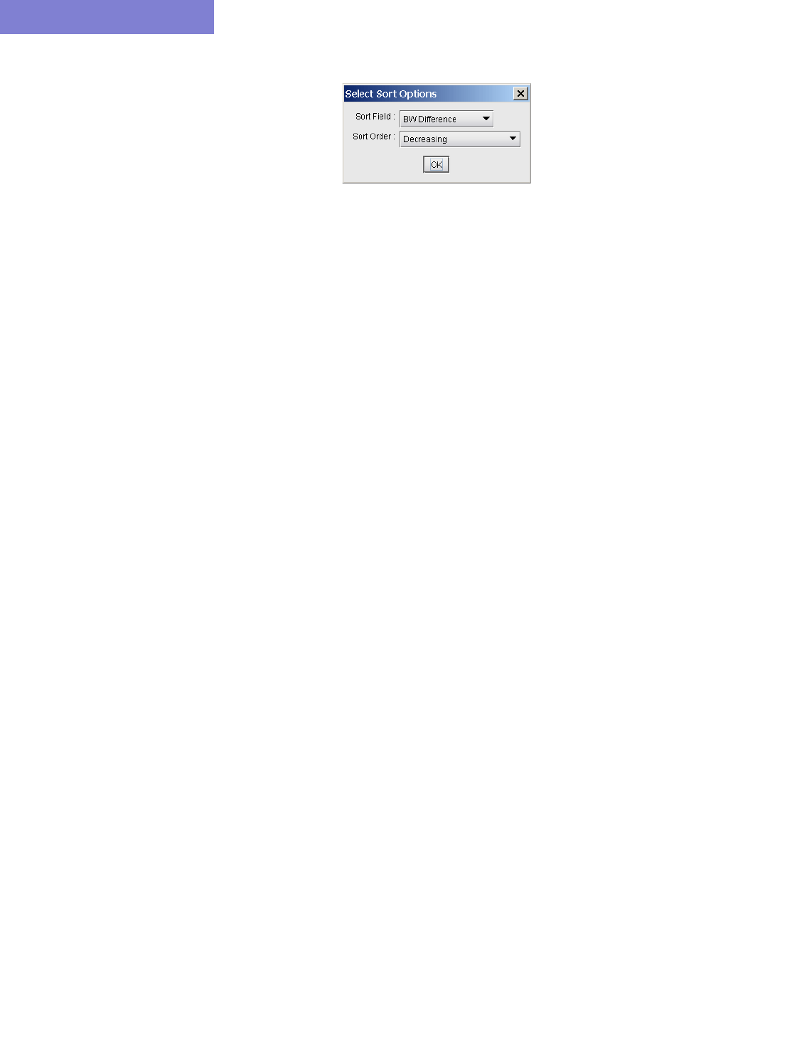
TUNNEL SIZING AND DEMAND SIZING*
22-8 Copyright © 2014, Juniper Networks, Inc.
22
Figure 22-8 Select Sort Options Window
17. You may override the suggested new bandwidth by typing in a new value directly into the table. To do this,
either double-click on the tunnel’s “New BW” field. The table cell will then become editable. Alternatively,
right-click on the selected tunnel(s) and choose “Replace New BW Values”. You will then be prompted to
enter a new BW value for those tunnel(s).
Calculation of the New Tunnel Bandwidth
The calculation of the new tunnel bandwidth works in the following way:
If the resize option is set to “Only Increase” (in the Design Options window) and the tunnel’s planned bandwidth
is strictly greater than the total flow or measured tunnel traffic bandwidth, then the tunnel will not be resized.
Otherwise, a new bandwidth will be calculated using the following procedure:
1. First, compute:
Temp = (Flow Bandwidth * Growth Multiplier) + Growth Constant
2. Round up the temp value to the nearest multiple of the Tunnel Bandwidth Increment, as specified in the tunnel
sizing design options.
3. If this value is less than the Minimum Tunnel Bandwidth, then the new bandwidth is set to the value of the
minimum tunnel BW.
4. If this value is greater than the Maximum Tunnel Bandwidth, then the new bandwidth is set to the value of the
maximum tunnel BW.
5. Otherwise, simply use the new rounded up bandwidth value.

Copyright © 2014, Juniper Networks, Inc. 23-1
. . . . .
. . . . . . . . . . . . . . . . . . . . . . . . . . . . . . . . . . .
LSP C
ONFIGLET
G
ENERATION
*
23
his chapter describes how to generate LSP configlets. The LSP Configlet window is a useful tool that
allows the user to generate a configlet for any specified LSP tunnel on the network and save it to a file on
the server to be copied later into a configuration file. As the network grows, some of the pre-configured
LSP paths may become outdated. The LSP Configlet feature allows you to perform the network-grooming task with
ease. New LSP paths are generated and saved into router format, ready to be loaded back into the network.
*Note that a special password is required for the tunnel feature. Please contact your Juniper representative for more
information.
When to use
Use this chapter after you have made modifications to your tunnels or designed your tunnel paths.
Prerequisites
If you wish to perform this task in the WANDL client, you should have already added tunnels to your network. You
may wish to use the spec.mpls-fish spec file located in your $WANDL_HOME/sample/IP/fish directory (where
$WANDL_HOME is /u/wandl by default) to follow along.
Related Documentation
For general step-by-step instructions on how to use the WANDL software, please refer to the Design & Planning
Guide.
For an overview of the WANDL software or for a detailed description of each feature and the use of each window,
refer to the General Reference Guide or Chapter 37, Router Reference.
For instructions on how to view or modify the tunnels in your network, refer to Chapter 20, LSP Tunnels*.
Recommended Instructions
1. View existing tunnels in the network and view the configlets for a tunnel.
2. Generate all configlets in the LSP directory.
3. Use tunnel templates in the Modify Tunnel window.
T
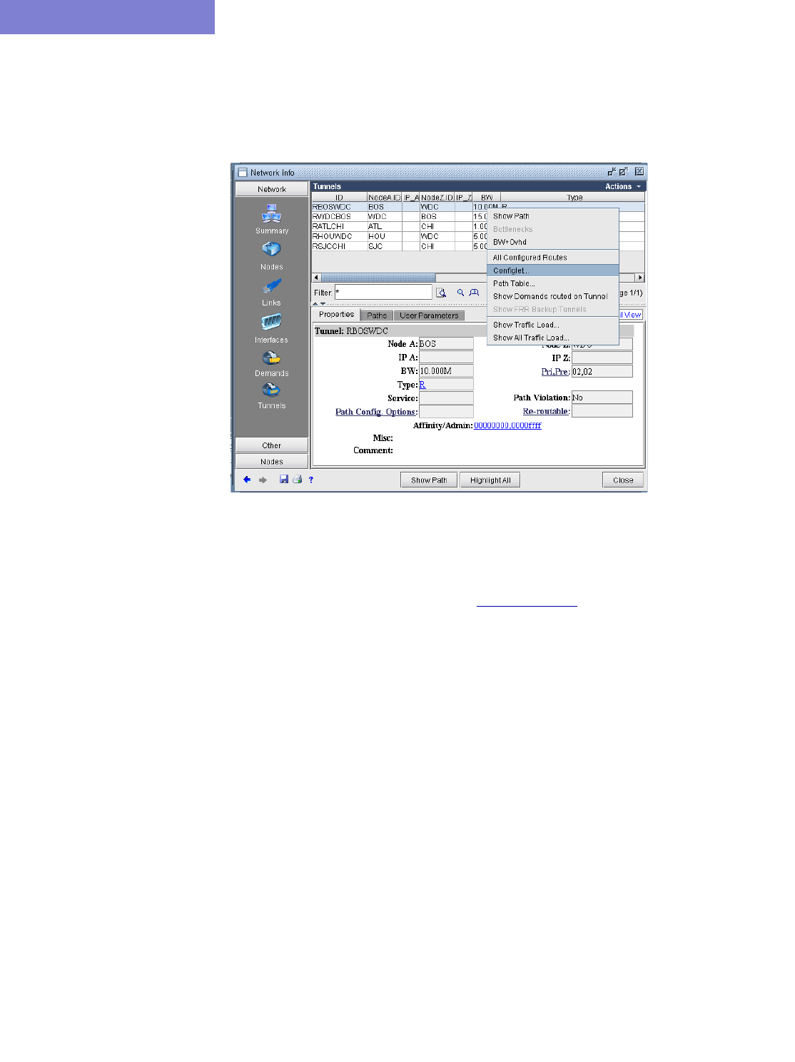
LSP CONFIGLET GENERATION*
23-2 Copyright © 2014, Juniper Networks, Inc.
23
Detailed Procedures
Viewing the Configlet
1. In View or Design action mode, select Network > Elements > Tunnels.
Figure 23-1 Tunnel Details Window
2. Right-click on the desired tunnel in the table, and select Configlet from the popup menu to generate its
configlet in the /tmp directory. The generated configlet will be immediately available for viewing.
Note 1: The configlet generated here is not saved to the LSP directory. To do so, you should run Design >
Configlets/Delta > LSP Configlet as described in step 4 on page 23-3.
Note 2: If an IP address of a node is not available, the node name may be used in its place even though this may not
be allowed in the router. To fix this, you should configure IP addresses for nodes and/or links in your network. This
can be done in the Properties tab of the node modification window or the Location tab of the Link Modification
window.
Here is an example of a generated configlet for node BOS, a Cisco router:
!! BOS
interface Tunnel1001
description from BOS to WDC
ip unnumbered Loopback0
tunnel destination 10.10.10.8
tunnel mode mpls traffic-eng
tunnel mpls traffic-eng autoroute announce
tunnel mpls traffic-eng priority 2 2
tunnel mpls traffic-eng bandwidth 10000
tunnel mpls traffic-eng affinity 0x00000000 mask 0x00000000
tunnel mpls traffic-eng path-option 10 explicit name Tunnel1001.p0
!
!
ip explicit-path name Tunnel1001.p0 enable
next-address 10.10.10.9
next-address 10.10.10.4
next-address 10.10.10.8
LSP CONFIGLET GENERATION*
Copyright © 2014, Juniper Networks, Inc. 23-3
. . . . .
Creating LSP Configlets for All Routers
3. To create LSP configlets for all routers, make sure you are in the Design action mode. (The configlet
generation capability is not available in View mode.)
4. Select Design > Confligets/Delta > LSP Configlet for the following window:
Figure 23-2 LSP Configlet Window
Field Description
Target Directory This is the directory in which the LSP configlet will be saved.
File Format Specify whether the configlet should be saved as Router Config
Statements or in XML format.
Node/Tunnel Selection Select the node and tunnel that you wish to generate a configlet for.
From the first pull-down box, select the node. The tunnels at that
node will then be populated in the second pull-down box. Choose a
specific tunnel, or “All”.
Update Tunnel Names Tunnels with a Cisco router as the head-end will automatically be
renamed if the tunnel name is not in the format “Tunnel<number>”.
For all such tunnels, the “Update Tunnel Names” option allows
the user to use a customized numbering scheme. Refer to Creating
a Tunnel Numbering Scheme on page 23-6 for more details on
specifying the numbering scheme.
Filter Only
Nodes/Tunnels with
changes
This option will only generate LSP configlets for the Nodes/Tunnels
that were actually modified, as opposed to all Nodes/Tunnels.
LSP CONFIGLET GENERATION*
23-4 Copyright © 2014, Juniper Networks, Inc.
23
5. In the first Node/Tunnel Selection box, select “All” to create configlets for all nodes. Note that you can also
select a specific tunnel source node to create configlets for. Then you can select a specific tunnel in the second
selection box.
6. You can add additional statements for inclusion in the configlet by entering them in the appropriate tab: Cisco
or Juniper. This process can be facilitated by specifying template files for particular tunnels, as described in
Using Tunnel Templates on page 23-4.
7. Click Submit to generate the configlet in the Target Directory.
8. You can view the generated configlets from the File Manager by navigating to the chosen target directory
(named “LSP” by default). You may need to click on the Refresh button within the File Manager to see the
new LSP directory. Inside the LSP directory you will find a configlet named after the router and possibly
interface to which the configlet applies. Double-click it to view the configlet in a text editor.
Using Tunnel Templates
9. In the File Manager, traverse to $WANDL_HOME/data/templates (which typically is set to
/u/wandl/data/templates). In that directory you can create files containing commands that will be added to the
configlets during generation time.
10. In Modify mode, use Modify > Elements >Tunnels and select the tunnels you want to modify. Next, click
“Modify” and select “Selected Entries” to modify the selected tunnels or and select “All Entries” to modify
all displayed tunnels. (To highlight a subset, select a tunnel and then use <Shift>-click to select a range of
tunnels and/or <Ctrl>-click to add or remove individual tunnels to the selection.) In the resulting window, click
the Type button in the middle of the “Modify Tunnel” window for the following window.
Figure 23-3 Tunnel Type Parameter Generation Window (Options may vary)
11. Use the “Browse” button at the bottom right to enter in the location of the template you created.
12. Click “OK” to submit your changes.
13. Then click “OK” in the “Modify Tunnel” window to modify the selected tunnels.
Default Statement(s) Use this space to specify any statements to be included in the
configlet.
Submit Submit an LSP configlet generation task and save the configlet to
the target directory.
View View the existing configuration file for the selected router. This
button is not available if more than one router is selected.
Field Description

LSP CONFIGLET GENERATION*
Copyright © 2014, Juniper Networks, Inc. 23-5
. . . . .
14. Now if you generate LSP configlets from Design > Confligets/Delta > LSP Configlets in Design mode
and view your configlets in the target directory, you should be able to see the added statements from your
template.
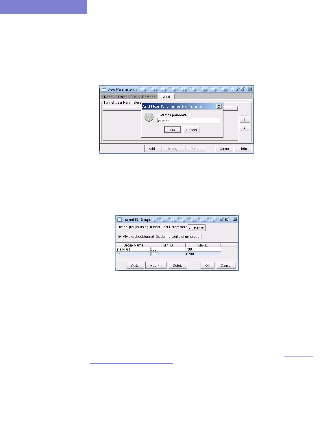
LSP CONFIGLET GENERATION*
23-6 Copyright © 2014, Juniper Networks, Inc.
23
Creating a Tunnel Numbering Scheme
You can customize the tunnel numbering range that is generated by the LSP configlets. This feature makes use
of both Tunnel ID Groups and User Parameters.
15. In Modify mode, first create a tunnel user parameter. To do so, go to Modify > Elements > User
Parameters. Select the Tunnel tab. Then, click the “Add” button. Specify any name for your parameter (e.g.
“cluster”) in the popup dialog. Then, click “OK” and press “Close” to close the User Parameters window.
Figure 23-4 Adding a Tunnel User Parameter
16. Go to Modify > Elements > Tunnel ID Groups to open up the Tunnel ID Groups window. Click on the
“Add” button to create new groups, specifying a numeric range for each type of tunnel. At the top of the
window, indicate the Tunnel User Parameter, created earlier, to be associated with the newly defined tunnel
ID groups.
Figure 23-5 Specifying Range in Tunnel ID Groups
17. Now, go to Modify > Elements > Tunnels. In the Tunnels window, click on the “Modify” button and select
“All Entries”. In the resulting window, switch to the User Parameters tab, and set the value for the new
tunnel parameter, or “cluster” in this example. Press “OK”.
18. Note that the tunnel id numbering scheme is not immediately applied to the tunnels that you have just modified.
That is, tunnel ids are not updated at this stage. Bear in mind that the tunnel numbering scheme is local, meaning
that a tunnel such as “tunnel501” is not necessarily unique; it is unique only within the configlet, or at the head
end router.
19. Switch to Design mode and go to Design > Confligets/Delta > LSP Configlet. In the LSP Configlet
window, be sure to check the Update Tunnel Names checkbox. Follow the instructions in Creating LSP
Configlets for All Routers on page 23-3. Once the configlets are submitted, the tunnels will take on their new
IDs according to your numbering scheme. Configlets that are generated will obey the same tunnel ID numbering
scheme.

Copyright © 2014, Juniper Networks, Inc. 24-1
. . . . .
. . . . . . . . . . . . . . . . . . . . . . . . . . . . . . . . . . .
LSP D
ELTA
W
IZARD
*
24
he LSP Delta wizard detects changes made to the LSP configurations in a network since the network was
loaded, including added, modified, and deleted LSP tunnels. A table is created displaying all new, modified,
and deleted LSPs. From this table you may create LSP deltas or XML files describing those changes.
•LSP Deltas are configuration statements that will provision LSP configuration changes in a live network, whether
it be adding a new LSP, modifying an existing LSP, or removing an existing LSP.
•The generated XML file, is a file that describes LSP configuration changes, and which can be imported to
MetaSolv’s IP Service Activation system. In the case of Alcatel 7750 routers, the XML files generated are SOAP
ready and formatted to be sent to a SAM server for deployment.
An additional capability that the wizard provides is the detection of FRR backup tunnels that are no longer bound to
an interface. This feature is useful to detect tunnels that either need to be reconfigured or that can be deleted.
This chapter describes the steps for using the LSP Delta wizard. Sample LSP Deltas and XML files will be provided,
and the XML schema will be explained.
When to use
This feature is useful for examining LSP changes made to a network model, whether it be newly added LSPs,
modified LSPs, or deleted LSPs. The LSP Deltas are useful for configuring LSP changes on Alcatel, Cisco, and
Juniper systems.
Prerequisites
The LSP Tunnel Delta wizard compares the current network model with the baseline network model, where the
baseline network model is the state of the network model when it is first opened in the software. This means that if
the user adds a new LSP tunnel and then deletes that LSP tunnel, or if the user modifies an existing LSP tunnel and
then modifies that LSP tunnel again to return it to its original state, then the LSP Tunnel Delta wizard will not
generate any new LSP tunnel configuration data.
Related Documentation
For general step-by-step instructions on how to use the WANDL software, please refer to the Design & Planning
Guide.
For an overview of the WANDL software or for a detailed description of each feature and the use of each window,
refer to the General Reference Guide or Chapter 37, Router Reference.
For instructions on how to view or modify the tunnels in your network, refer to Chapter 20, LSP Tunnels*.
Recommended Instructions
1. Run the LSP Delta wizard.
2. Examine the tables of newly added, modified, and deleted LSPs.
3. Generate some LSP Deltas and examine their configuration statements.
4. Generate an XML output file, examine its contents, and import it into MetaSolv’s IP Service Activation system
or any other third party system that is capable of parsing XML data.
T
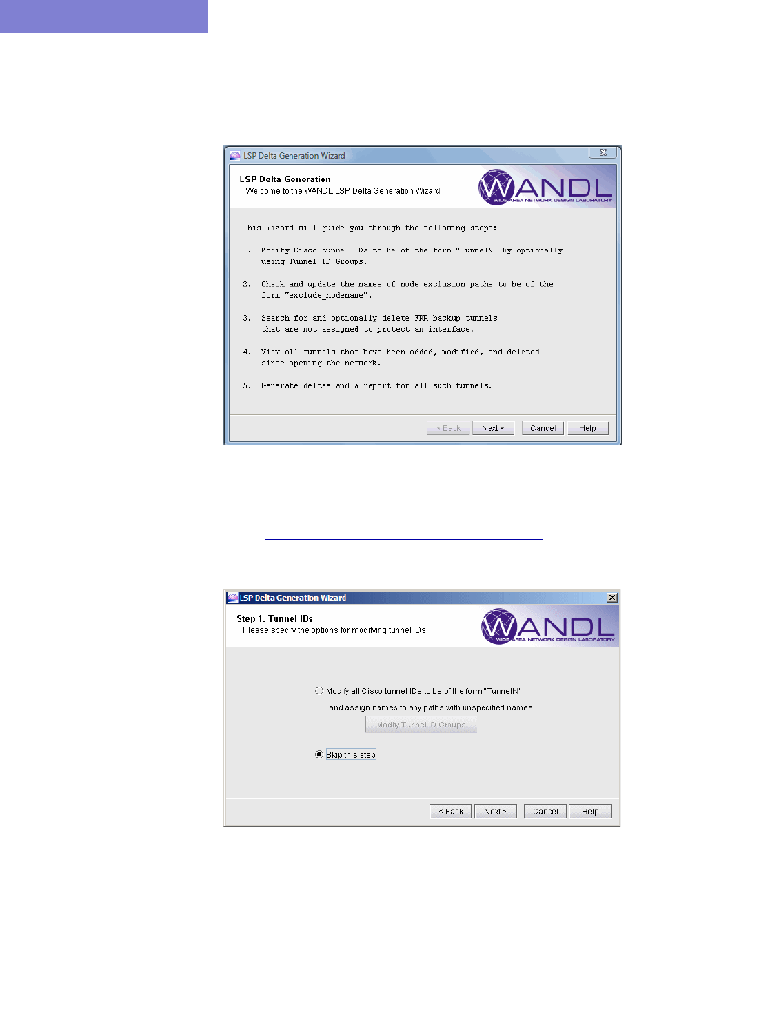
LSP DELTA WIZARD*
24-2 Copyright © 2014, Juniper Networks, Inc.
24
Running the LSP Delta Wizard
The LSP Delta wizard can be accessed in View or Design mode through the Design > Confligets/Delta > LSP
Delta Wizard menu item. The first window in the LSP Delta wizard is shown in Figure 24-1 below.
Figure 24-1 LSP Delta Wizard
The user has the option of changing the Tunnel names to Cisco default format in the next screen. This is performed
in conjunction with Tunnel ID groups, which are defined by the user. For more information on Tunnel ID groups,
please refer to Adding and Assigning Tunnel ID Groups on page 20-16. This step can be skipped by selecting “Skip
this step” as shown below.
Figure 24-2 Option to Modify Cisco Tunnel IDs
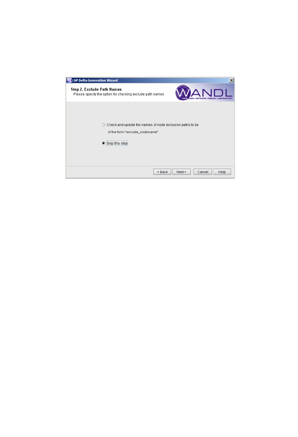
LSP DELTA WIZARD*
Copyright © 2014, Juniper Networks, Inc. 24-3
. . . . .
Checking the Names of Paths that Exclude Nodes
In the next step, all LSP paths that exclude a node (i.e . FRR node protection tunnels) can be checked to make sure
the name is set to "exclude_<protected_nodename>". Sometimes an exclude path is not named to begin with, in
which case "exclude_<protected_nodename>" is assigned to the path name. Sometimes the exclude path is named
"exclude_<node_ipaddress>," in which case this step figures out if the ipaddress is a node address and replaces it
with the node name.
Figure 24-3 Option to Update Node Exclusion Path Names
Changes made to LSP path names in this step are permanent, meaning once the LSP Delta Wizard has finished, the
LSP path names defined in the network model will reflect the changes made to the path names during this step.
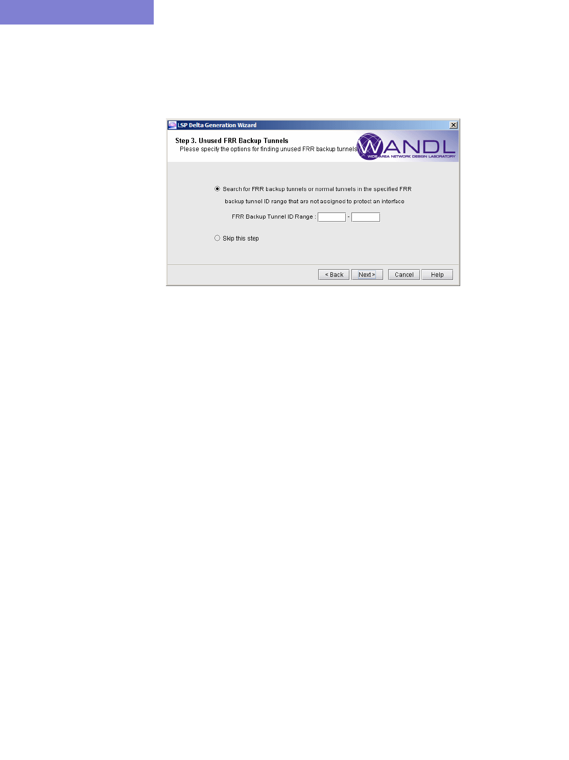
LSP DELTA WIZARD*
24-4 Copyright © 2014, Juniper Networks, Inc.
24
Identifying Unused FRR Backup Tunnels
The next step allows the user to identify unused FRR backup tunnels from the network. The wizard will search for
FRR backup tunnels that are not protecting an interface or tunnel within the tunnel ID range specified, and allow the
user to inspect and remove any or all of those tunnels from the network before going on to the next step.
Figure 24-4 Option to Prune Unused FRR Backup Tunnels
If the user chooses to prune unused FRR backup tunnels and enters an appropriate FRR backup tunnel ID range to
search, the wizard will return a list of FRR tunnels that are not currently being used to protect any existing LSP
tunnels, along with one possible reason. From WANDL tool’s generated LSP configuration statements, it is possible
to derive the element that a tunnel is intended to backup, and therefore to reverse engineer to determine a possible
cause of an unused tunnel. For example, the exclude statement, which can be used by a backup tunnel to avoid the
element being protected, may be used to determine the element being protected. Note, however, that for FRR backup
tunnels configured differently, e.g., with explicit path, information about the node or link being protected by an
unused tunnel may not be possible to derive from the configuration statements. In those cases the reason will be
shown as “Unknown”. Below is a explanation of reasons that can be indicated under the Possible Reason
column:
•Tunnel not bound to protected interface (inf_name): A backup tunnel was configured, and the intended
node or link to be protected was identified by the “exclude” path name. Either the protected link exists but the
backup tunnel is not bound to the local interface, or a link exists between the source node and the protected node, but
the backup tunnel is not bound to the local interface.
•Protected interface (inf_name) down: A backup tunnel was configured, and the intended node or link to be
protected was identified by the “exclude” path name. Either the protected link exists but the local interface is
shutdown, or a link exists between the source node and the protected node, but the local interface is shutdown.
•Excluded interface (inf_name) down: A backup tunnel was configured, and the intended node or link to be
protected was identified by the “exclude” path name. Either the protected link exists but the remote interface is
shutdown, or a link exists between the source node and the protected node, but the remote interface is shutdown
•Protected interface missing on source node (node_name):A backup tunnel was configured, and the
intended node or link to be protected was identified by the “exclude” path name. The protected link does not exist
due to missing interface at the source node.
•Excluded interface missing on remote node (node_name): A backup tunnel was configured, and the
intended node or link to be protected was identified by the “exclude” path name. The protected link does not exist
due to missing interface at the remote node
•Interface missing on either source node or protected node: For node protection tunnel, there was no
interface on <snode_name> that shared the same subnet with any interface on the protected node <pnode_name>.
This is likely caused by removal of interface on either node.
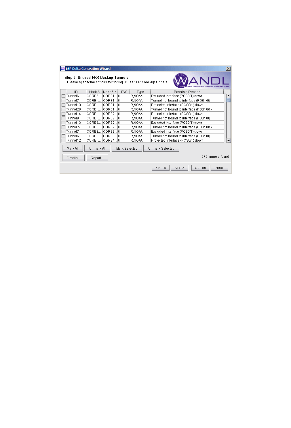
LSP DELTA WIZARD*
Copyright © 2014, Juniper Networks, Inc. 24-5
. . . . .
The user can then select from the list the FRR tunnels to delete. Details for a specific FRR tunnel can be viewed by
selecting the tunnel and clicking the Details button. A report of all the unused FRR tunnels can be saved to the
server by clicking the Report button. To view a saved report, browse to the report file in the File Manager
window, right click on the report file, and select Open in Report Viewer.
Figure 24-5 Select Unused FRR Backup Tunnels for Deletion
Note that this deletion of FRR tunnels from the network model is permanent. To avoid deleting any tunnels, simply
leave all tunnels unchecked (or select Unmark All to uncheck them) and click Next.
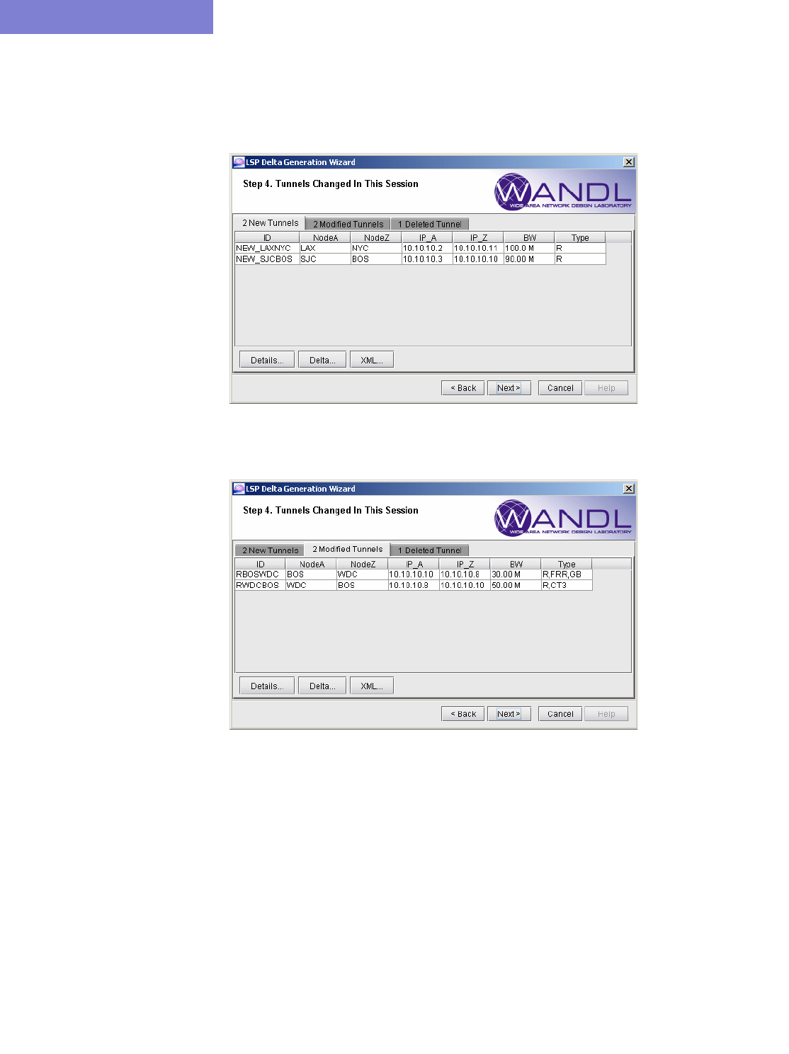
LSP DELTA WIZARD*
24-6 Copyright © 2014, Juniper Networks, Inc.
24
Tables for New, Modified, and Deleted LSP Tunnels
The next window shows the newly added, modified, and deleted LSP tunnels in three tables. Examples are shown
below:
Figure 24-6 Newly Added LSP Tunnels
Figure 24-7 Modified LSP Tunnels
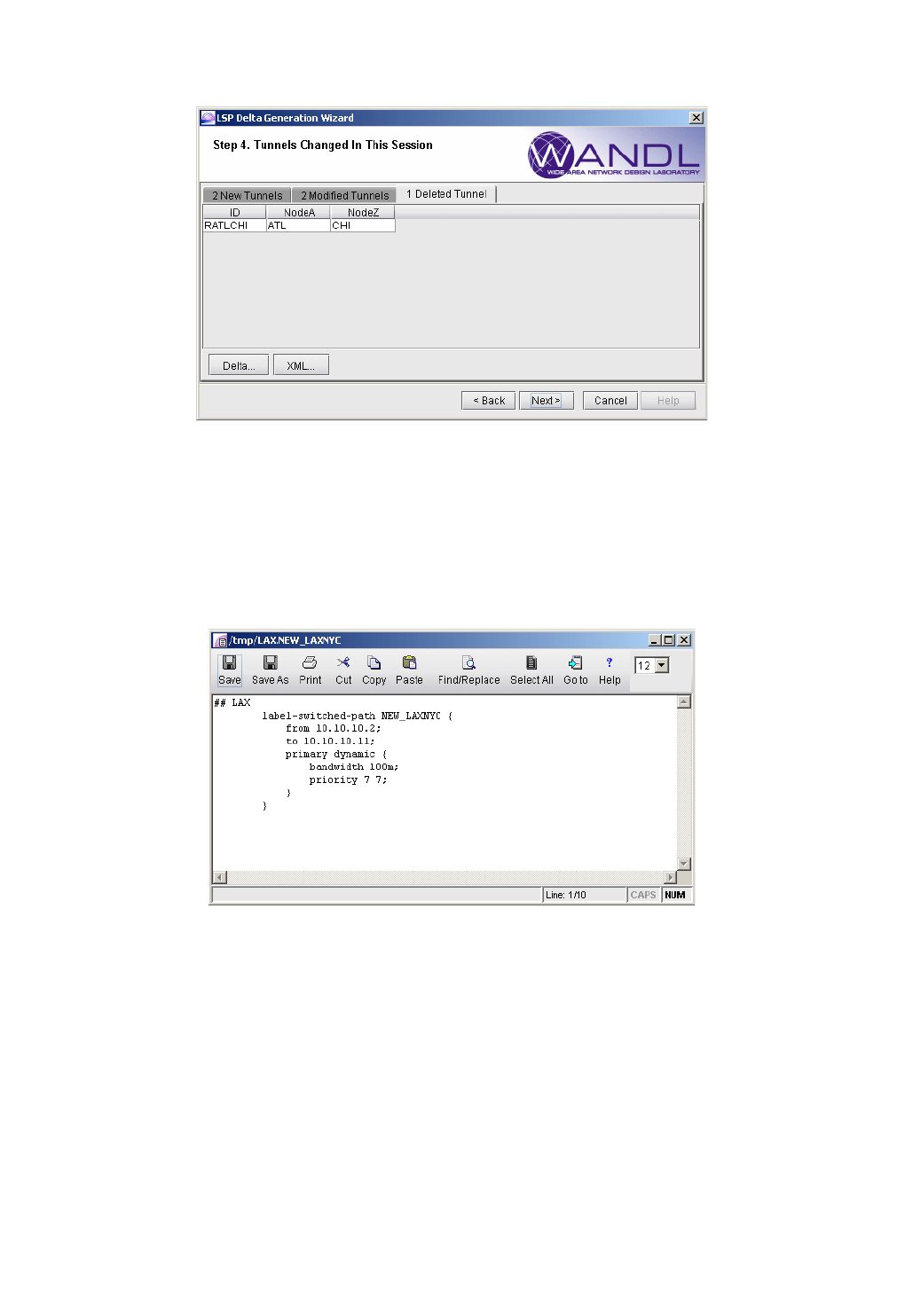
LSP DELTA WIZARD*
Copyright © 2014, Juniper Networks, Inc. 24-7
. . . . .
Figure 24-8 Deleted LSP Tunnels
Generating LSP Deltas and XML
LSP deltas and XML statements can be generated for any of the tunnels in the three tables. The LSP deltas are
configuration statements required to add, modify, or remove LSP tunnels for which they are generated. Three
example LSP deltas and their corresponding XML output are shown below.
Figure 24-9 LSP Delta for a New Juniper LSP Tunnel
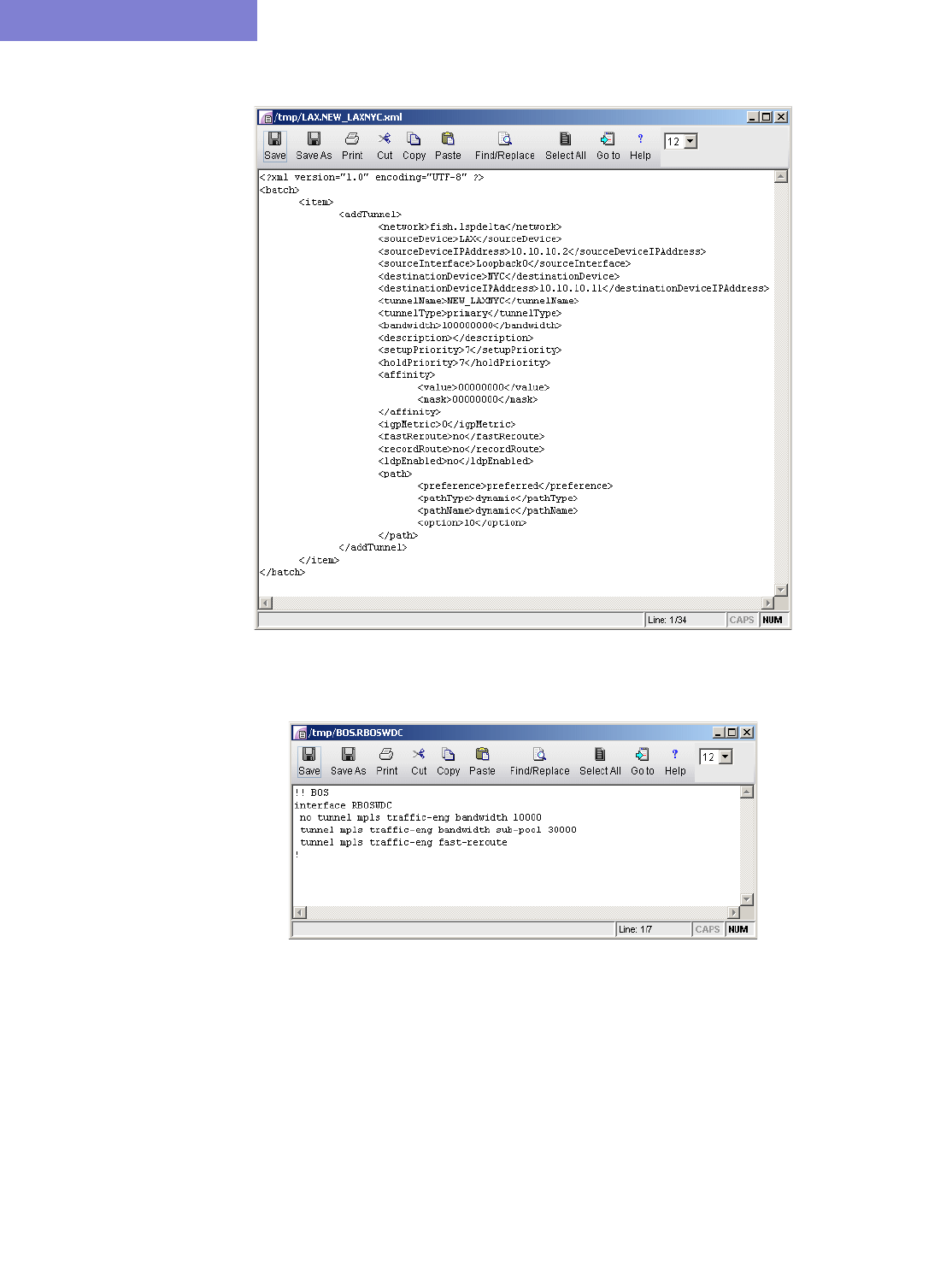
LSP DELTA WIZARD*
24-8 Copyright © 2014, Juniper Networks, Inc.
24
Figure 24-10 XML for a New Juniper LSP Tunnel
Figure 24-11 LSP Delta for a Modified Cisco LSP Tunnel
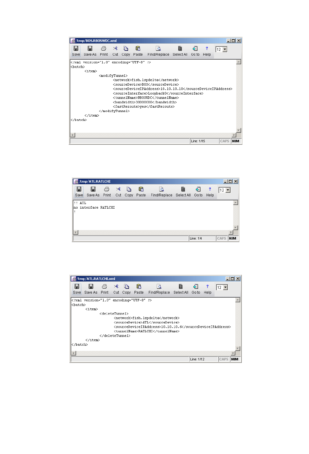
LSP DELTA WIZARD*
Copyright © 2014, Juniper Networks, Inc. 24-9
. . . . .
Figure 24-12 XML for a Modified Cisco LSP Tunnel
Figure 24-13 LSP Delta for a Deleted Cisco LSP Tunnel
Figure 24-14 XML for a Deleted Cisco LSP Tunnel
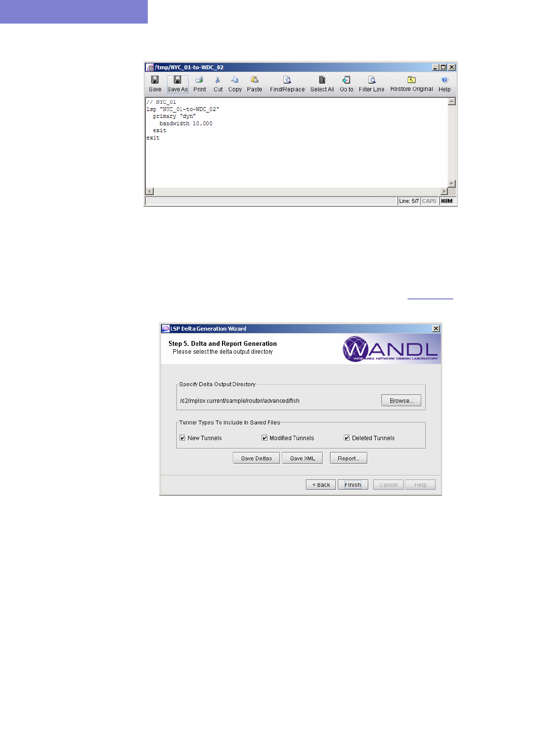
LSP DELTA WIZARD*
24-10 Copyright © 2014, Juniper Networks, Inc.
24
Figure 24-15 LSP Delta for a Modified Alcatel LSP Tunnel
Saving Files to the Server
The final step allows the user to generate XML files, LSP delta files, and a report file, which are saved to a directory
on the server. The user can select which tunnel types to include in these files by checking the appropriate check
boxes under Tunnel Types to Include in Saved Files. This is shown in Figure 24-16 below.
Figure 24-16 Saving Deltas, XML, and Report Files

Copyright © 2014, Juniper Networks, Inc. 25-1
. . . . .
. . . . . . . . . . . . . . . . . . . . . . . . . . . . . . . . . . .
T
UNNEL
P
ATH
D
ESIGN
*
25
his chapter describes the Path Design feature. Tunnel Path Design lets you design tunnel paths for path
diversity. Lsp tunnels can be designed such that their secondary/standby paths are routed in node-diverse,
site-diverse, link-diverse, or facility-diverse routes from their primary path. Additionally, two different
tunnels can also be designed such that their primary paths are also on diverse paths.
*Note that a special license for tunnels is required for this feature. Please contact your Juniper representative for
more information.
When to use
Use these procedures to design primary and backup tunnel paths.
Prerequisites
If you wish to perform this task in the WANDL client, you should have already added tunnels to your network.You
may wish to follow along by using the spec.mpls-fish spec file located in your $WANDL_HOME/sample/IP/fish
directory (where $WANDL_HOME is /u/wandl by default).
Related Documentation
For an overview of the Path Diversity Design window, refer to the General Reference Guide chapter on Design.
For instructions on how to view or modify the tunnels in your network, refer to Chapter 20, LSP Tunnels*.
For information on the meaning of the tunnel type fields, refer to the “tunnelfile” entry in the “Demand/Traffic Files”
chapter of the File Format Guide.
Recommended Instructions
Following is a high-level, sequential outline of the diversity path design feature and the associated, recommended
procedures.
1. Switch to Tunnel layer and open Design > TE Tunnels > Path Design.
2. Design selected tunnels for diversity.
3. View the resulting paths graphically or generate the Path & Diversity Report from the Report Manager.
Detailed Procedures
Tunnel Path Design
1. Select the Tunnel layer button to switch to the Tunnel layer.
2. In Design mode, select Design > TE Tunnels > Path Design to open the Tune Paths window. This window
lists all of the tunnels whose paths can be designed for. For each tunnel or group, the details of the first, second,
and third path are provided in this window. The Div Level column indicates the current level of diversity
satisfied between the 2 or 3 paths that belong to this tunnel or group.
T
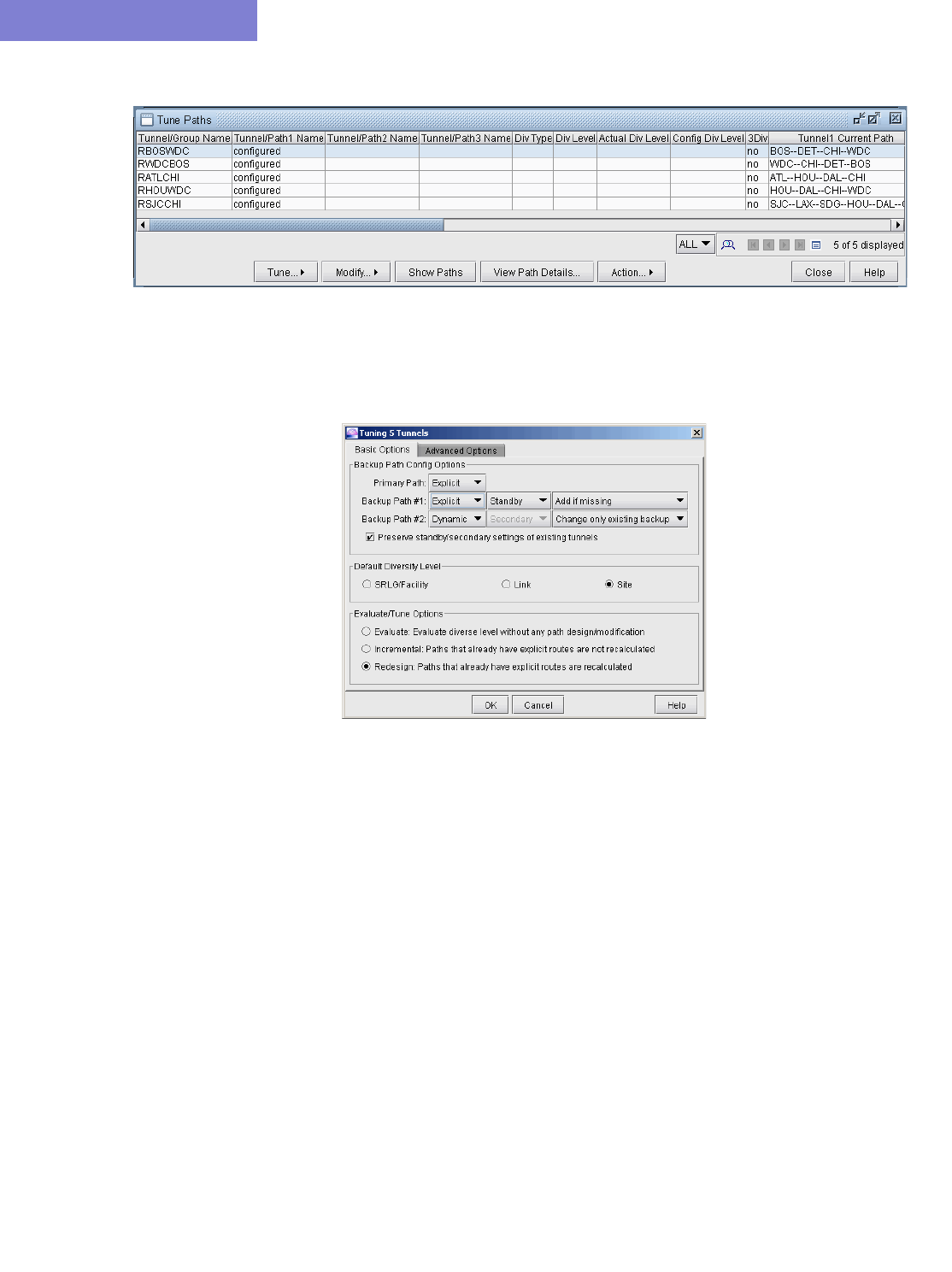
TUNNEL PATH DESIGN*
25-2 Copyright © 2014, Juniper Networks, Inc.
25
Figure 25-1 Diverse Paths Table
3. Select the tunnels to design and select Tune > Selected Paths. Alternatively, select Tune > All Paths to
design all tunnels for diversity. This will open up the following window.
Figure 25-2 Tuning Options
Backup Path Configuration Options
4. The Backup Path Config Options are provided to design a tunnel’s primary and backup paths. To create
backup paths, select “Add if not existing” for the Backup Path #1 and/or Backup Path #2.
Note that it is not required to design for both backup paths. To avoid creating new backup paths, select the
option “Change only existing backup” for Backup Path #1 and/or Backup Path #2. If the backup path does
not exist, no action will be taken.
Note also that backup paths cannot be removed from this window. To remove existing backup paths, use the
Tuning window option instead, Modify > Selected Paths, and set Max # Backup Paths to 0.
5. To avoid changing current backup path types (Standby vs. Secondary), select the option “Preserve
standby/secondary settings of existing tunnels”. In this case, the backup path type settings specified
will only be used when adding backup paths and not for existing backup paths. If instead you unselect
“Preserve the type of existing diverse paths”, this option will be used to change the backup path type
not only of the added backup paths but also of the already existing tunnel paths.
6. See the examples below on some common path design scenarios:

TUNNEL PATH DESIGN*
Copyright © 2014, Juniper Networks, Inc. 25-3
. . . . .
DYNAMIC PRIMARY PATH
7. Use the following settings to configure only a dynamic primary path:
•Primary Path: “Dynamic”
•Backup Path #1 and Backup Path #2: Select “Change only existing backup” to avoid creating a backup path
Note: Existing backup paths cannot be removed from this window. To remove existing backup paths, use the
Modify > Selected Paths and set Max # Backup Paths to 0.
EXPLICIT PRIMARY PATH WITH DYNAMIC SECONDARY PATH
8. Use the following settings to configure an explicit (nailed down) primary path with a dynamic secondary backup
path:
•Primary Path: “Explicit”
•Backup Path #1: “Dynamic” “Secondary” “Add if missing”
•Backup Path #2: “Change only existing backup” to avoid creating a tertiary path
Note: Existing backup paths cannot be removed from this window. To remove existing backup paths, use the
Modify > Selected Paths and set Max # Backup Paths to 0.
EXPLICIT PRIMARY AND EXPLICIT STANDBY PATH
9. Use the following settings to configure an explicit primary and explicit standby backup path:
•Primary Path: “Explicit”
•Backup Path #1: “Explicit” “Standby” “Add if missing”
•Backup Path #2: “Change only existing backup” to avoid creating a tertiary path
Note: Existing backup paths cannot be removed from this window. To remove existing backup paths, use the
Modify > Selected Paths and set Max # Backup Paths to 0.
EXPLICIT PRIMARY AND EXPLICIT STANDBY PATH WITH DYNAMIC TERTIARY PATH
10. Use the following settings to configure an explicit primary and standby backup path and dynamic tertiary path.
•Primary Path: “Explicit”
•Backup Path #1: “Explicit” “Standby” “Add if missing”
•Backup Path #2: “Dynamic” “Secondary” “Add if missing”
Default Diversity Level
11. If you are designing for two or three configured paths, select the Default Diversity Level to target (site, link,
or facility) between the paths in case it has not already been specified on a per-tunnel basis.
12. Site diversity means that the two paths do not intersect at any given site (besides the source and destination).
Link diversity means that the two paths do not intersect at any given link. Site diversity is always stronger than
link diversity as site diversity implies link diversity.
13. SRLG/Facility can be used for SRLG-diversity. In this case, the facilities should be defined before the Path
Design. This can be done in Modify mode via the Modify > Elements > SRLG/Facilities window, or by
creating a facility file and reading it in via File > Load Network Files in Design mode. Refer to the File
Format Guide for more information on the facility file format.
Evaluate/Tune Options
14. For the Evaluate/Tune Options, select Incremental to configure only tunnel paths that are not already
configured or Redesign to allow the recalculation of paths that have already been configured. By default
“Redesign” is selected to allow full flexibility of changing existing paths, which in some cases may be
necessary to improve the diversity between multiple paths.
15. To recalculate paths based on the loopback IP addresses of nodes, as opposed to interface IP addresses, specify
configloopaddrinpath=1 in the project’s dparam file prior to opening the network baseline.
16. The “Evaluate: Evaluate diverse level without any path design/modification” option is used to reevaluate the
currently satisfied diversity level, e.g., based on the criteria of SRLG/facility-diversity or site diversity.
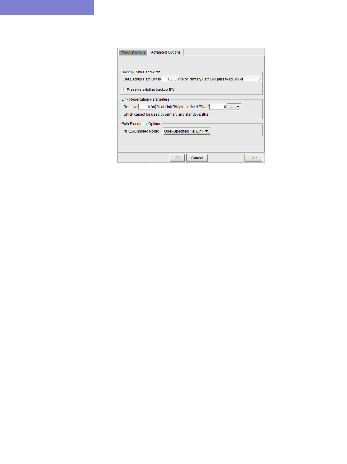
TUNNEL PATH DESIGN*
25-4 Copyright © 2014, Juniper Networks, Inc.
25
Advanced Options
Figure 25-3 Advanced Options
17. The Backup Path Bandwidth allows you to specify the bandwidth to use for the backup tunnel as a
percentage of the primary backup tunnel’s bandwidth plus a fixed number. For example, if you want the backup
path to have the same bandwidth as the primary path, set the percentage to 100. If you want the backup path to
have a specific bandwidth, enter it in as the fixed BW.
18. Deselect “Preserve existing backup bandwidth” to change an already existing backup tunnel’s
bandwidth. If the preserve option is selected, the program will only design the bandwidth for added backup
tunnels.
19. Use the Link Reservation Parameters to reserve bandwidth on the link that cannot be used by primary and
standby paths, as a function of the percentage of the link’s bandwidth plus a fixed number. Constraint based
routing will be used to route the tunnel paths on links that do have enough available bandwidth to accommodate
both the tunnel bandwidth and this reserved bandwidth.
20. The Path Placement Options effects how the tunnel is placed based on MPLS protocols in the network.
Selecting the User-Specified Per Link option will define the link as MPLS enabled or disabled based on the user
setting, and the tunnel can be placed only on enabled links. Selecting the All Links Enabled option will assume
all links as MPLS enabled, and the tunnel can be placed on any link.
21. Click OK to start the design.
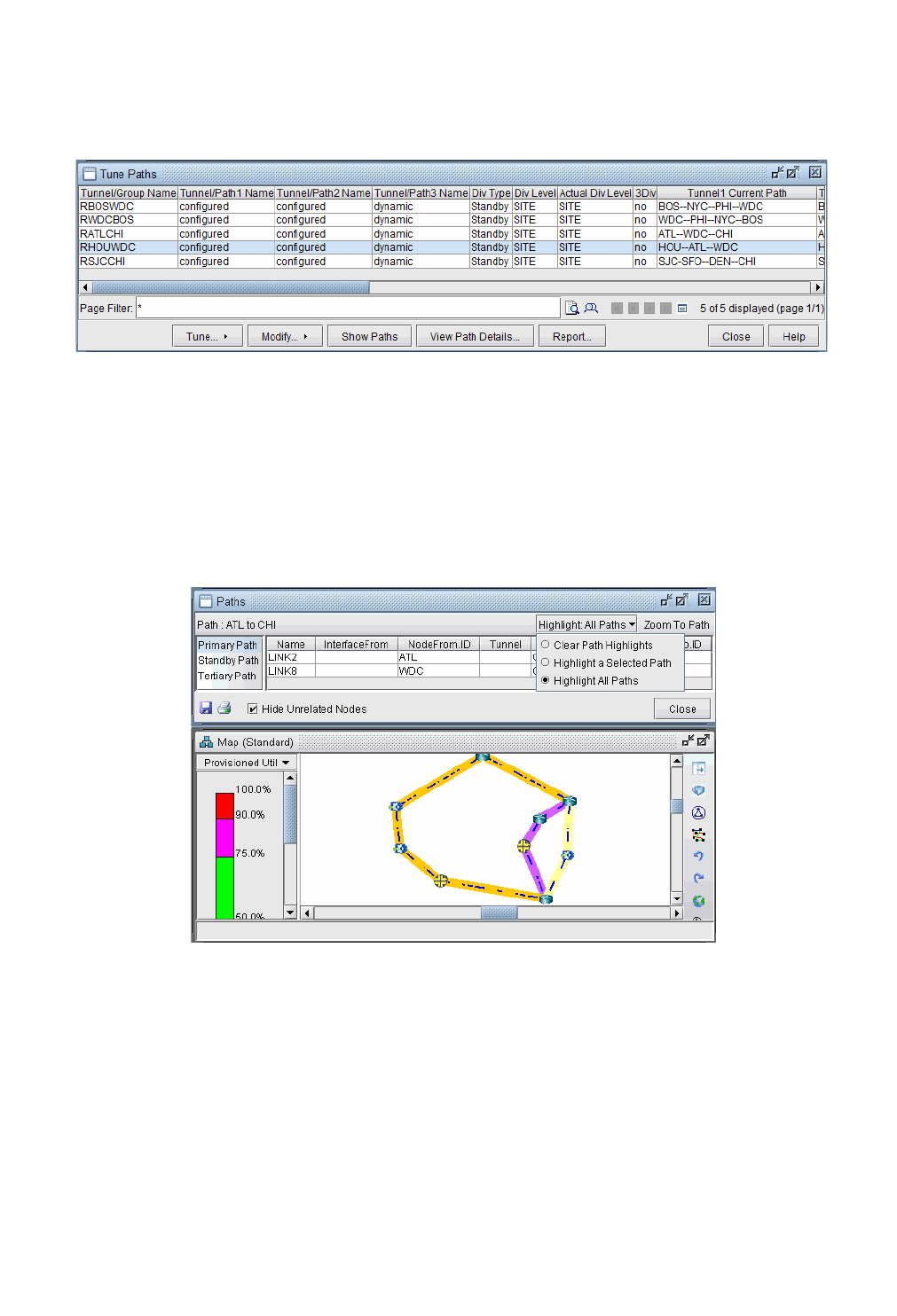
TUNNEL PATH DESIGN*
Copyright © 2014, Juniper Networks, Inc. 25-5
. . . . .
Viewing Design Results
22. After the design is complete, view the resulting Diversity Level achieved under the Div Level column.
Figure 25-4 Path Window, after Design for Diverse Standby + Dynamic Tertiary
23. Scroll to the right to see the paths to see the new paths (“Current Path” columns) for the backup tunnel paths,
and the paths that have been configured (“Config Path” columns)
24. Click on any row and select Show Paths to view the primary and secondary/standby paths on the topology
map. Note that the primary path is yellow, the secondary or standby path is purple, and the tertiary path is
orange. If the paths overlap, you may want to select “Highlight a Selected Path” to view one at a time.
•To focus only on the selected paths, select “Hide Unrelated Nodes.”
Figure 25-5 Paths after Design for Tertiary diverse path (3DIV)
25. Click on View Path Details... to view the tunnel details. If you designed for standby paths, there will be two
entries for the tunnel, one for the primary path and one for the standby path marked with STANDBY in the type
field. If you designed for secondary paths, the secondary path information is displayed in the same tunnel entry
as the primary path and is listed in the Paths tab.
Note: For secondary paths, the path name may not be specified. In that case, you may wish to enter a path name in
modify mode (Modify > Elements > Tunnels) to have the name displayed for the Secondary column.
26. Click Action... > Report... to save the contents of the Tune Paths window to a comma-separated file.
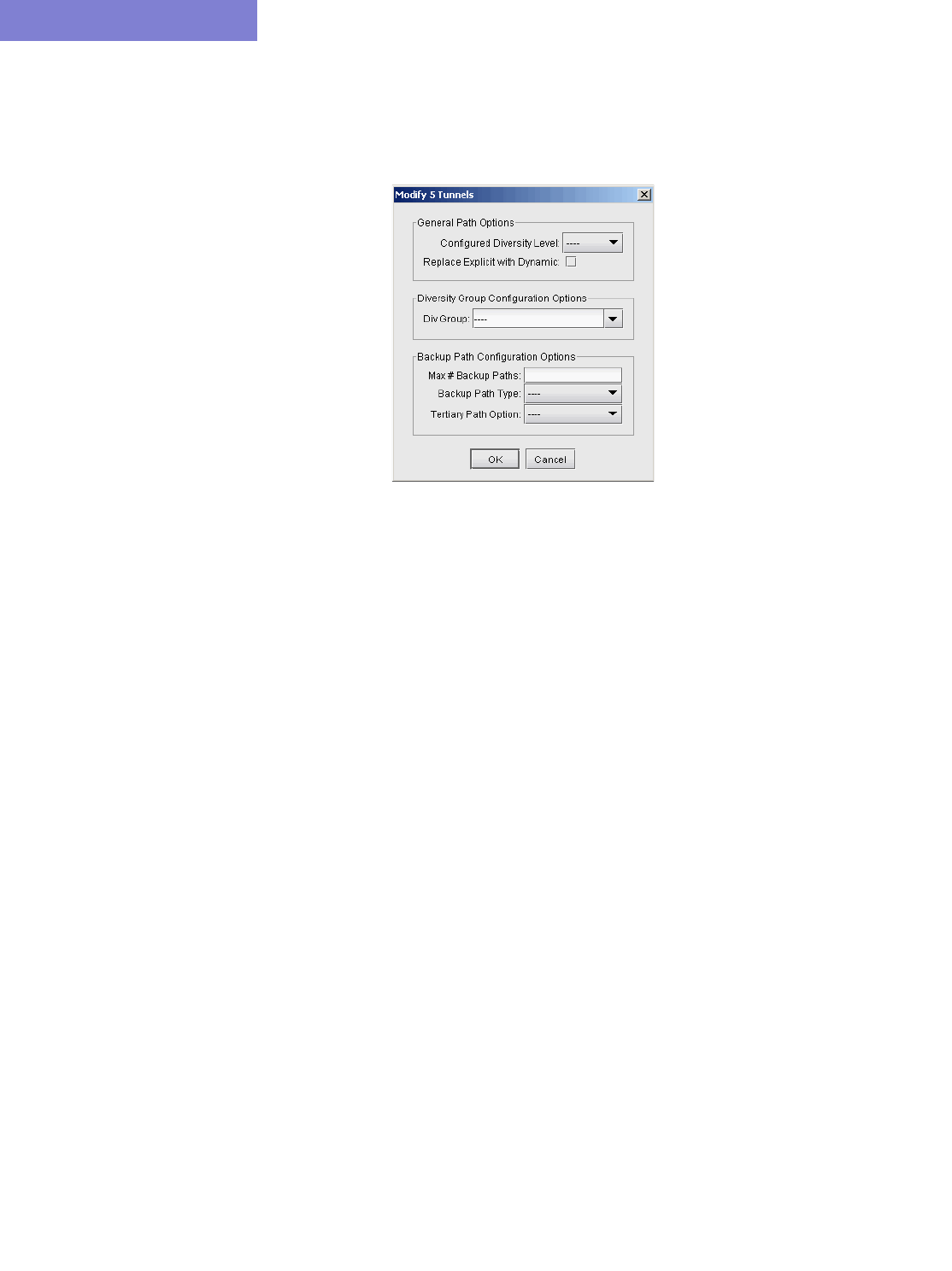
TUNNEL PATH DESIGN*
25-6 Copyright © 2014, Juniper Networks, Inc.
25
Tunnel Modifications
The following are some prerequisite steps that can be set up before running the Path Diversity Design, if desired.
27. Select Modify > Selected Paths or Modify > All Paths to view the following options:
Figure 25-6 Tunnel Modification Options
GENERAL PATH OPTIONS
28. You can set up per tunnel diversity requirements, to override the default diversity level. To do so, select the
desired tunnel(s), click Modify > Selected Paths, and select the Configured Diversity Level: FACDIV
(for SRLG/facility diversity), LINKDIV, or SITEDIV.
29. For the primary path, select “Replace Explicit with Dynamic” to convert the primary path from being
explicit (nailed down) to Dynamic (loose).
DIVERSITY GROUP CONFIGURATION GROUPS
In addition to designing for diversity between a primary and backup path of the same LSP tunnel, another diversity
option is to establish path diversity between different tunnels, which may or may not have the same source and
destination routers. Upon grouping these tunnels together, they will be paired off, so that each pair can be designed
for diversity.
30. To group a set of tunnels together, select the desired tunnel(s), click Modify > Selected Paths, and enter in a
name for the group under Div Group. All of the tunnels in this group will be paired off, so that each pair can be
designed for path diversity.
31. If you wish to group all tunnels that originate and terminate at the same sites, without creating a separate group
for each pair of sites, select the reserved Div Group “SITEPAIR”. Tunnels marked SITEPAIR will be paired off
with other tunnels marked as SITEPAIR that connect the same two sites. Each of these tunnel pairs can then be
designed so that the two separate tunnels are diverse from one another.
32. Note that any tunnel that is added to a Div Group pair will be listed as an entry in the Tune Paths window
under the associated group name, rather than under an entry for the tunnel name. If more than 2 tunnels are in
the same group, the different pairs will be indicated by the group name followed by a subindex. For example, if
there are six tunnels in group “test”, they may be paired off and appear in the table as “test”, “test.1” and
“test.2”. The tunnels in each pair can then be designed to be diverse from each other, but they will not be
designed individually for primary/backup diversity.
33. To perform path design for Diversity Groups rather than tunnels’ primary/backup path design, use the select
menu in the Tune Paths window to select the group category: “ALL” versus “DivGroup” versus the regular
entries for tunnel primary/backup design.
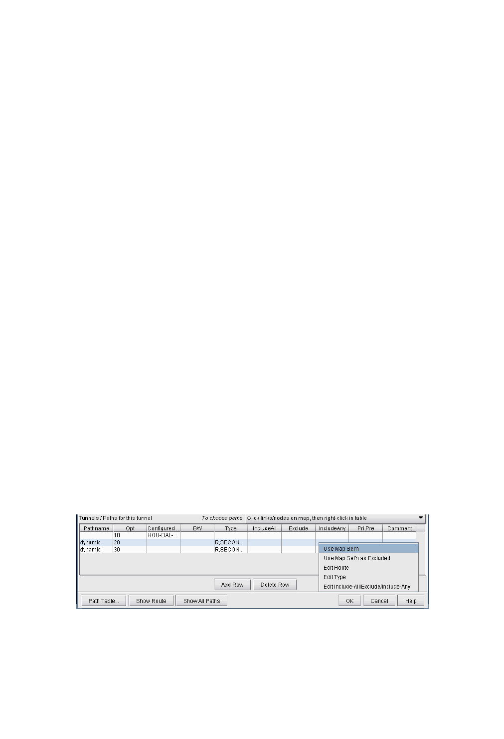
TUNNEL PATH DESIGN*
Copyright © 2014, Juniper Networks, Inc. 25-7
. . . . .
BACKUP PATH CONFIGURATION OPTIONS
34. After the path design, if you do not like the current backup paths configuration, you can delete the backup paths
and redesign. To delete backup paths, select the tunnels from the Tune Paths window, click the Modify >
Selected Paths button, and then specify the Maximum # Backup Paths to keep. For example, if you enter
in 0, this will remove all backup paths, leaving only the primary path. If you enter in 1, this will remove all but
the first backup path, leaving only one primary path and one backup path.
35. You can set up per tunnel diverse path types (Standby vs. Secondary) by entering in the “Backup Path Type”.
36. You can optionally specify that you want tertiary diverse design.
Exporting and Importing Diverse Group Definitions
37. To export the current diverse group definitions, select File > Save Network Files > Tunnel...
38. The output file, usertunneldef.runcode will be created in your output path, where runcode is substituted by the
runcode of your current network model. For example, the following is an example of a Diverse Group
Definition.
#
# Tunnel Diverse Group Definition
#
## Software Release= 5.5.1, 32 bits
## Platform=i86pc, OS=SunOS 5.10
## Report Date= 7/12/2010 04:55 Runcode=autosave User=telus
#NodeName TunnelName DivGroupName
BOS,RBOSWDC,test
WDC,RWDCBOS,test
AT L , R AT L C H I ,t e s t
HOU,RHOUWDC,test
39. To import the diverse group definition, select Action > Import DivPath Definition File from the Tune
Paths window.
Advanced Path Modification
40. After the path design, you may also wish to provide path names for some of the tunnel paths.
41. First, click the Modify mode button to switch to Modify mode.
42. Next, reopen Modify > Elements >Tunnels. Double-click a particular tunnel to view its details.
43. If desired you can enter unique pathnames for the backup routes under the Pathname column
44. For Cisco, the two alternate routes can be given different priorities using the “Opt” field (the defaults are
multiples of 10). For Juniper, specify for the two backup routes if they are secondary or standby in the Type
column by entering in R,STANDBY for a standby tunnel or R,SECONDARY for a secondary tunnel. Right-
click an entry and select Edit Type for more options.
Figure 25-7 Designing Three Paths

TUNNEL PATH DESIGN*
25-8 Copyright © 2014, Juniper Networks, Inc.
25
Delta Configlets
45. To generate delta configlets for the changes made to the LSP tunnels since opening the baseline, select Action
> LSP Delta Wizard.
46. For more information on the LSP Delta Wizard, refer to Chapter 25, Tunnel Path Design*.

Copyright © 2014, Juniper Networks, Inc. 26-1
. . . . .
. . . . . . . . . . . . . . . . . . . . . . . . . . . . . . . . . . .
I
NTER
-A
REA
MPLS-TE
*
26
ANDL supports the design of LSP tunnels for a multiple-area network. Unlike the router whose
knowledge of the network is limited to the area to which it belongs, the WANDL software has a global
view of the entire network topology and can therefore design both primary and diverse inter-area LSP
tunnels more intelligently. Once the LSP tunnels are designed, LSP configlets can be generated for loading into the
network.
WANDL supports Inter-Area MPLS-TE design for both Juniper and Cisco networks.
*Note that a special password is required for inter-area TE. Please contact your Juniper representative for more
information.
When to use
Use these procedures if you have multiple OSPF areas in your network and you want to quickly generate LSP
tunnels between the different areas.
Prerequisites
If you wish to perform this task in the WANDL client, you should have a router spec file open before you begin. You
should have also created multiple OSPF areas in your network and set the routing method to OSPF.
To do this, first create OSPF areas using Modify > Protocols > OSPF Areas. Then, set the area property
accordingly on your network links using Modify > Elements > Links (see the Location tab). You may follow
along by using any spec file with multiple OSPF areas defined in the network.
Check that the routing method is OSPF in Tools > Options > Design, Path Placement option pane.
Additionally, check that the links have OSPF enabled using Modify > Elements > Links (see the Protocols tab)
Related Documentation
Refer to Chapter 16, Backbone Design for OSPF Area Networks* for information on how to perform an automatic
multi-area OSPF network design.
Refer to Chapter 20, LSP Tunnels* for more information on LSP Tunnels and how to set their characteristics.
Refer to Chapter 23, LSP Configlet Generation* for more information on generating LSP configlets.
Refer to Chapter 25, Tunnel Path Design* for information on configuring a diverse standby or secondary tunnel.
Recommended Instructions
1. Examine the OSPF Areas in your network and AutoGroup nodes by area, as described from Viewing OSPF
Areas on page 26-2.
2. Add LSP tunnels between the areas, as described in Adding Multiple Tunnels Between Areas on page 26-3 and
view the tunnel options in Tunnel Type Configuration Options Related to Areas on page 26-4.
3. View the newly created LSP tunnels, as described in Viewing Inter-Area Tunnels on page 26-5
4. Configure the tunnel path and generate an LSP as described in Configuring a Loose Route on page 26-6
W
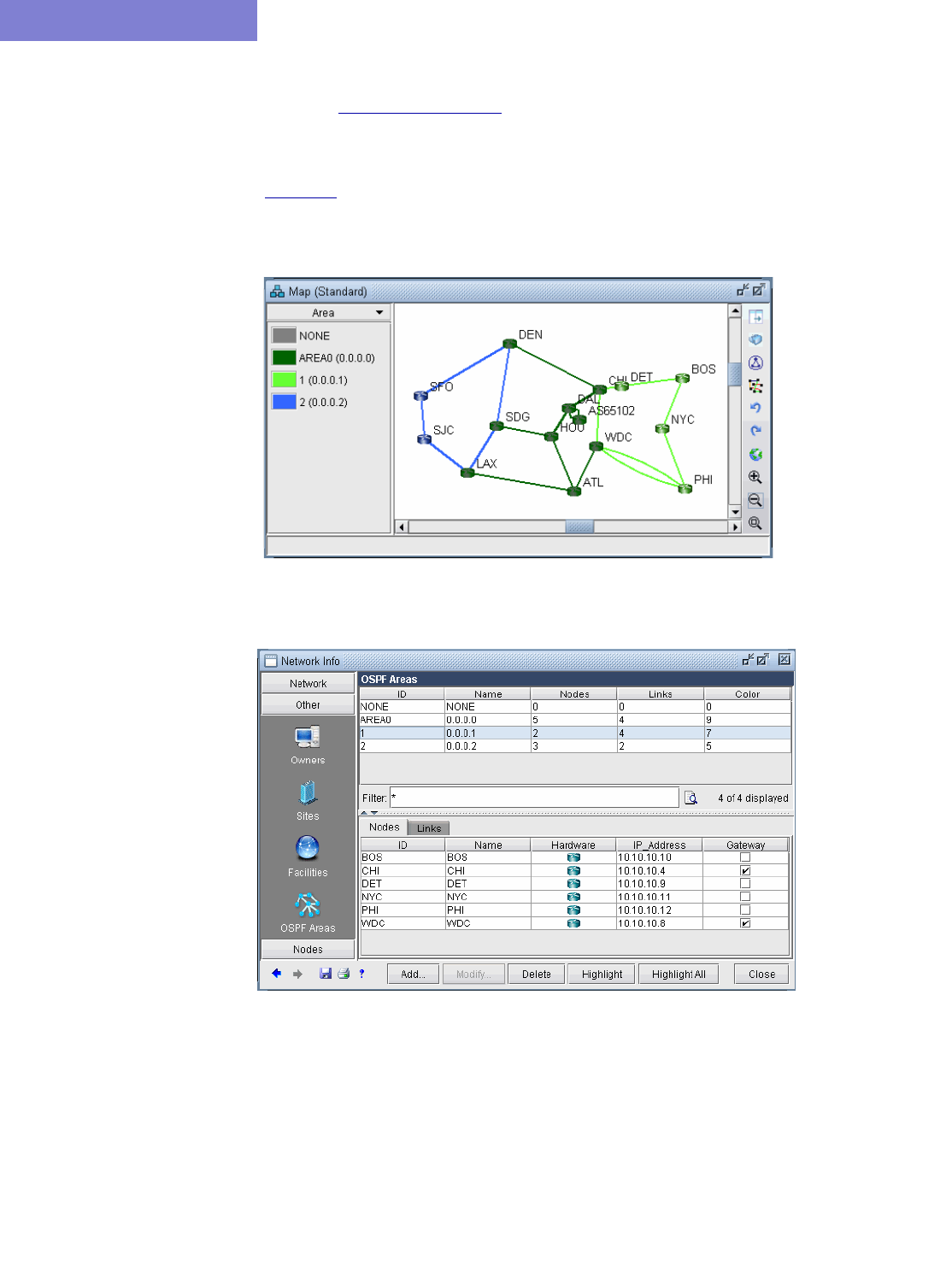
INTER-AREA MPLS-TE*
26-2 Copyright © 2014, Juniper Networks, Inc.
26
Detailed Procedures
1. Review the Prerequisites on page 26-1 to ensure that your network is configured properly.
Viewing OSPF Areas
2. To illustrate one method of adding Inter-Area LSP tunnels to a network, we will use the network shown in
Figure 26-1. There are three OSPF Areas in this network: AREA0, 1 and 2. This information can also be
retrieved by going to Network > Protocols > OSPF Areas in View mode, or Modify > Protocols >
OSPF Areas in Modify mode.
Figure 26-1 Initial Network with Area Legend
Figure 26-2 View of Areas from Modify > OSPF Areas
3. To facilitate the viewing of the OSPF areas, you can first group nodes by OSPF Area. Right-click on the Map
window and choose Grouping > AutoGroup from the popup menu. In the AutoGroup window, first choose
Area. Then, click Done.
4. The nodes are automatically grouped by Area and identified by Area ID. If you choose the Network Elements
> Nodes legend from the top selection box to the left of the Map, you will see a tree-view structure of the
newly created groups. Clicking on the groups in the tree view will expand the group and reveal the member
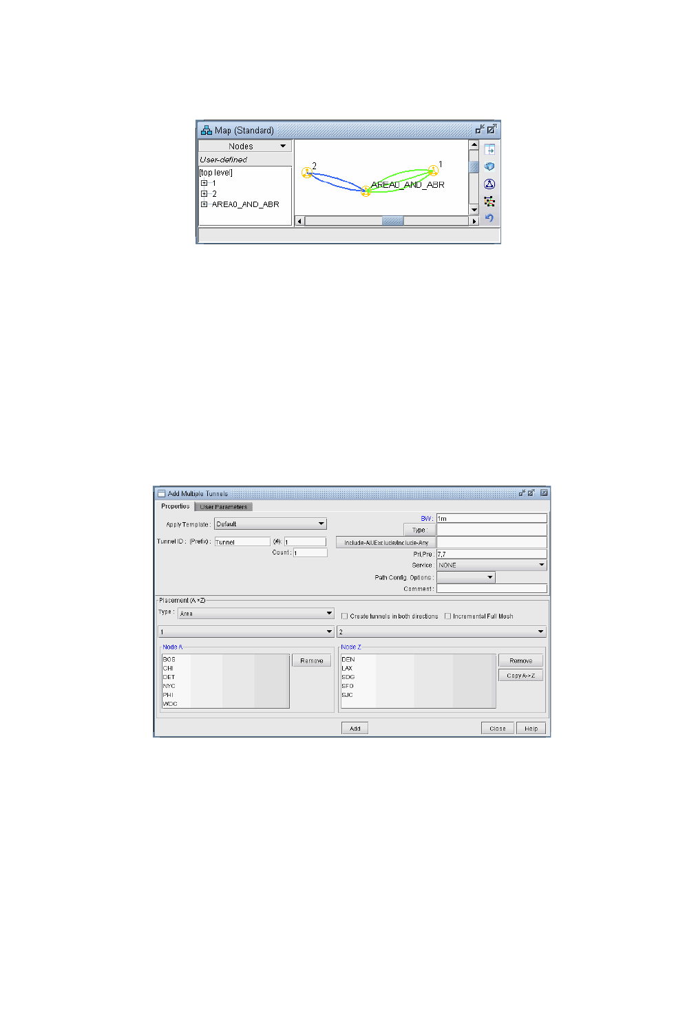
INTER-AREA MPLS-TE*
Copyright © 2014, Juniper Networks, Inc. 26-3
. . . . .
nodes. Alternatively, they can be expanded by right-clicking the Map window and selecting
Grouping>Expand All.
Figure 26-3 Grouped by OSPF Area
Adding Multiple Tunnels Between Areas
5. Next, to add tunnels, first make sure you are in Modify mode. For this example, choose Modify > Elements >
Tunnels, Add > Multiple Tunnels to add multiple tunnels between area 1 and area 2. (To add just a single
tunnel, you could also use Add > One Tunnel)
6. In the lower half of the Add Multiple Tunnels window, select Area from the Type selection box. Then, in
the selection boxes below that, choose “2” (the name of the Area 2 group) and “1” (the name of the Area
1group). The Node A and Node Z lists automatically become populated with the nodes belonging to the
respective areas. Fill in a Tunnel ID prefix, bandwidth (BW), and any other desired characteristics of the LSP
Tunnels using the top half of the window.
Figure 26-4 Adding Multiple LSP Tunnels between Groups
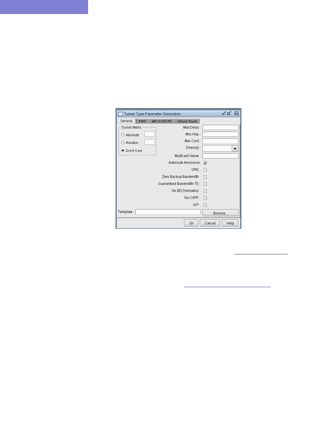
INTER-AREA MPLS-TE*
26-4 Copyright © 2014, Juniper Networks, Inc.
26
Tunnel Type Configuration Options Related to Areas
7. Select the Type button underneath the Bandwidth (BW) field to examine further options. There are two options
for routing tunnels:
•You can ignore OSPF Area definitions by checking the No BD checkbox. Routing will be performed assuming
the network is a flat OSPF network.
•You can take into account the traditional OSPF routing processes with bandwidth checking. This is the method
used by default.
Note: If users want to turn off bandwidth checking, then the checkbox No CSPF should be selected. In this
case, RSVP bandwidth will not be checked, for example.
Figure 26-5 Tunnel Type Window (Options May Vary)
To find out more about the Tunnel Type window, please refer to the General Reference Guide chapter, “The
Network and Modify Menus” section on Tunnel Type Parameter Generation.
8. Select “Cancel” to exit the Tunnel Type Parameter Generation window. Click “Add” to add the tunnels.
Note: The tunnels created are by default dynamic. Some routers do not support dynamic inter-area tunnels. In that
case, the route can be configured as described in Configuring a Loose Route on page 26-6.
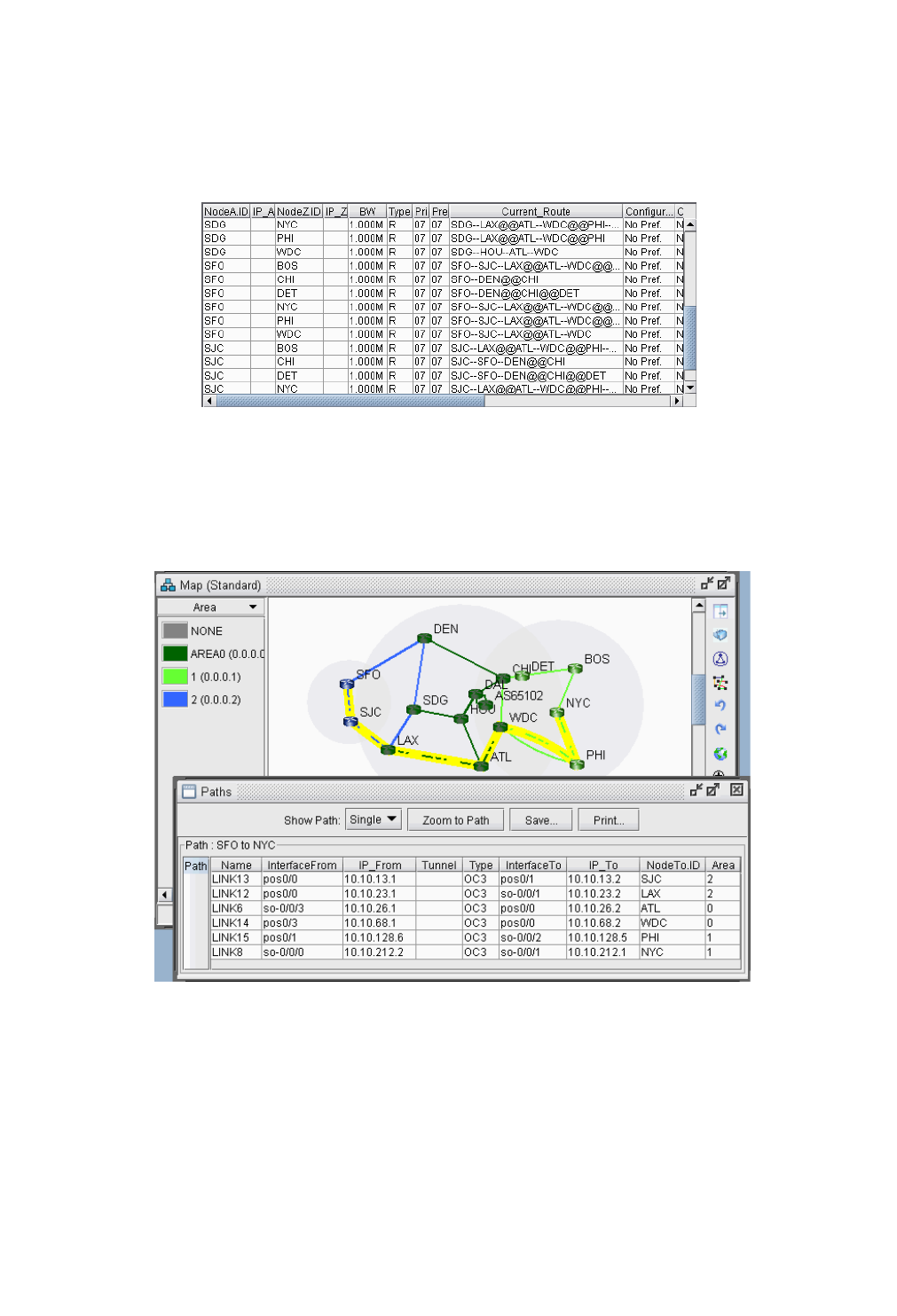
INTER-AREA MPLS-TE*
Copyright © 2014, Juniper Networks, Inc. 26-5
. . . . .
Viewing Inter-Area Tunnels
9. Once the LSP tunnels have been created, update the network state by clicking the “Update” button just below
the main menus. Then, select Modify > Elements > Tunnels. Notice the @@ symbol in the Current Route
field indicating the border between two areas.
Figure 26-6 Current Route of Newly Created Tunnels
10. Click “Show Path”. On the Paths window right-click a column header and select “Table Options” and add
the Area column as shown below.
Figure 26-7 Path of an Inter-Area LSP Tunnel between B2 and R2
11. You can also view a detailed report of the LSP Tunnels. Go to Report > Report Manager. In the Report
Manager, choose the Tunnel Path & Diversity Report under Tunnel Layer Network Reports > Tunnel
Reports.
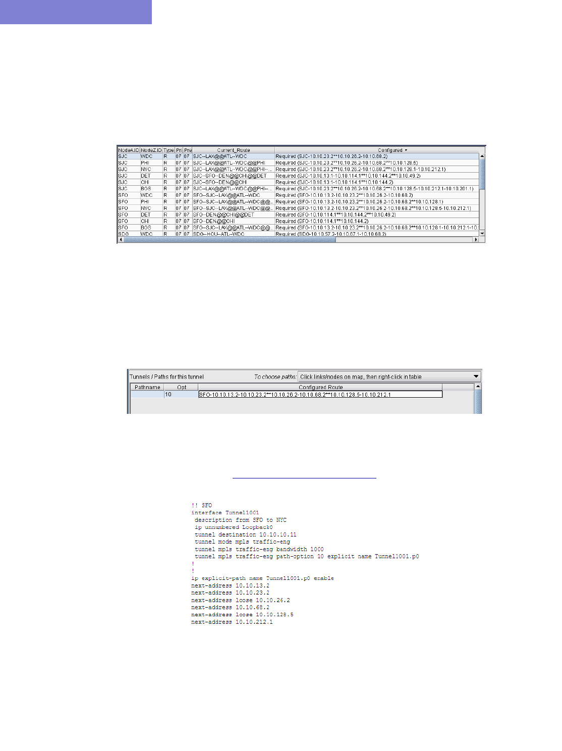
INTER-AREA MPLS-TE*
26-6 Copyright © 2014, Juniper Networks, Inc.
26
Configuring a Loose Route
12. The default setting for the tunnel is to route it dynamically. Note that for Cisco tunnels, the path should be
configured with loose routes to the ABR. To change the paths to configured loose routes, open the LSP Tunnel
window in Modify mode from Modify > Elements > Tunnels. Click Modify and then select “All Entries”
and change the Path Config. Options to “Add” “Config” to configure the route.
13. Notice that a loose route is now given in the Configured column, indicated by **.
Figure 26-8 Configured Loose Routes
14. A route can also be manually configured. For example, select a tunnel and click Modify and then select
“Selected Entries.” In the bottom half of the window, there is a table with the route for the tunnel. To
configure the path, double-click the cell underneath the column “Configured Route”. Here you can enter in the
path, using ** to indicate a loose route after the area border routers.
Note: The Exclude-IP-Address feature is not currently supported for inter-area tunnels.
Figure 26-9 Configuring a Route for a Specific LSP Tunnel
15. After configuring the routes as indicated in the previous step, LSP configlets can be generated for the newly
created LSP tunnels. This is accomplished in Design mode, through Design > Confligets/Delta > LSP
Configlet. Refer to Chapter 23, LSP Configlet Generation* for more details.
Figure 26-10 Example of an LSP Configlet

Copyright © 2014, Juniper Networks, Inc. 27-1
. . . . .
. . . . . . . . . . . . . . . . . . . . . . . . . . . . . . . . . . .
P
OINT
-
TO
-
MULTIPOINT
(P2MP) TE*
27
raditionally, high-quality video transmissions have been carried over either SDH/SONET or ATM where
the bandwidth can be guaranteed. However, the drive towards converged networks requires that these
signals must be carried over the carrier’s IP/MPLS network. Layer-3 IP multicast using PIM is adequate
only for IP TV which has a low customer price and corresponding customer expectations, and is not suitable for
high-quality video transmissions which have strict SLAs for packet loss and jitter.
Point-to-multipoint (P2MP) TE solutions have been developed in the IETF and are now deployed commercially in
production networks. P2MP TE allows for efficient traffic replication in the network, and offers many RSVP-TE
features – including explicit path specification and bandwidth specification -- available for point-to-point LSPs.
WANDL fully supports P2MP MPLS-TE tunnels for IP/MPLS networks. There’s ongoing work in the IETF in areas
such as P2MP resiliency, scalability, multicast VPN integration. As new P2MP features become available in
production networks, Juniper Networks will continue to enhance WANDL’s P2MP features support.
The following sections of this chapter describe the P2MP features that are currently supported by WANDL
IP/MPLSView.
*Note that P2MP requires a special license. Please contact your Juniper representative for more information.
When to use
Use these procedures if you have P2MP configured in your network or if you would like to use IP/MPLSView to
help you model P2MP LSP tunnels.
Prerequisites
If you wish to perform these tasks in the WANDL client, you should have an IP/MPLS network router spec file open
before you begin. Otherwise, you should have a set of router configuration files ready to be imported into the tool.
The chapter assumes the user is familiar with IP, MPLS, TE, P2MP concepts and terminology, and IP multicast PIM
concepts and terminology.
Related Documentation
Refer to Chapter 20, LSP Tunnels* for more information on LSP Tunnels and how to set their characteristics.
Refer to Chapter 23, LSP Configlet Generation* for more information on generating LSP configlets.
Refer to Chapter 12, Multicast*, for more information about IP multicast.
Refer to User Guide “Chapter 14 , Simulation”, for more information about failure simulation.
Recommended Instructions
1. Import a network with P2MP LSPs tunnels configured in the network. Examine the sub-LSPs belonging to a
particular P2MP LSP instance and visually display its path.
2. Use the tool to easily create P2MP LSP tunnels and generate LSP configlets which can later be provisioned into
the router network.
3. Examine P2MP LSP tunnel link utilizations to observe efficient replication.
4. Perform failure simulation and assess the impact of the failure on P2MP LSPs.
T
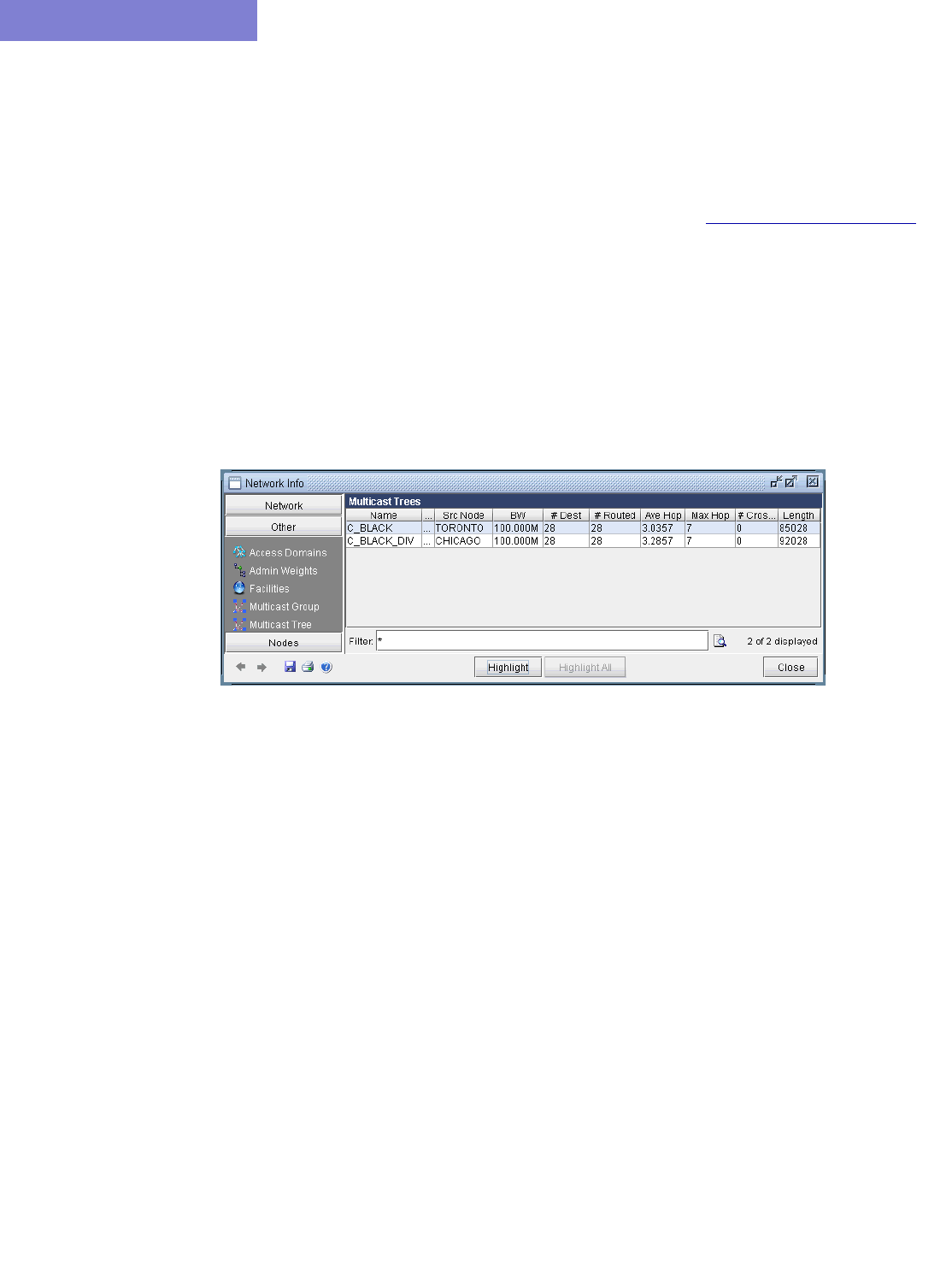
POINT-TO-MULTIPOINT (P2MP) TE*
27-2 Copyright © 2014, Juniper Networks, Inc.
27
Detailed Procedures
Import a network that already has P2MP LSP tunnels configured in the network
1. Review the Prerequisites to ensure that your network is configured properly with IP, MPLS and P2MP LSP
tunnels.
2. If you already have a spec file ready for the network, you may open it. Otherwise, if you have the set of router
configuration files, then you may follow the procedures as described in Chapter 2, Router Data Extraction, in
order to import the configuration files and create a WANDL spec network model.
Examine the P2MP LSP tunnels
3. After open an existing spec file or creating a new spec file after configuration file import, you are ready to
examine the P2MP LSP tunnels that are configured in your network. The tool allows you to easily examine the
sub-LSPs that belong to a particular P2MP. In IP/MPLSView, P2MP LSPs are appropriately and conveniently
represented as multicast trees. For instance, in the following sample network, two P2MP LSPs have been
defined in the network. Select the Tunnel layer button to switch into the Tunnel layer mode, to look at P2MP
multicast trees rather than IP multicast trees. Go to NetInfo > Multicast > Multicast Tree to bring up the
following window.
Figure 27-1 P2MP LSP tunnels
The window presents summary information – such as source node name and number of sub-LSPs -- for all of the
P2MP LSPs that are currently configured in the network.
4. To show the sub-LSPs that comprise the P2MP LSP, select the particular row corresponding to the P2MP2 LSP
of interest and then click on the Highlight button. As shown in the following figure, the P2MP LSP named
C_BLACK is highlighted in the topology map. On the P2MP LSP tree, a circle is drawn around the node that
represents the source node (the ingress LSR) of the tree, while boxes are drawn around the leaf nodes (the egress
LSRs for the sub-LSPs) of the tree.
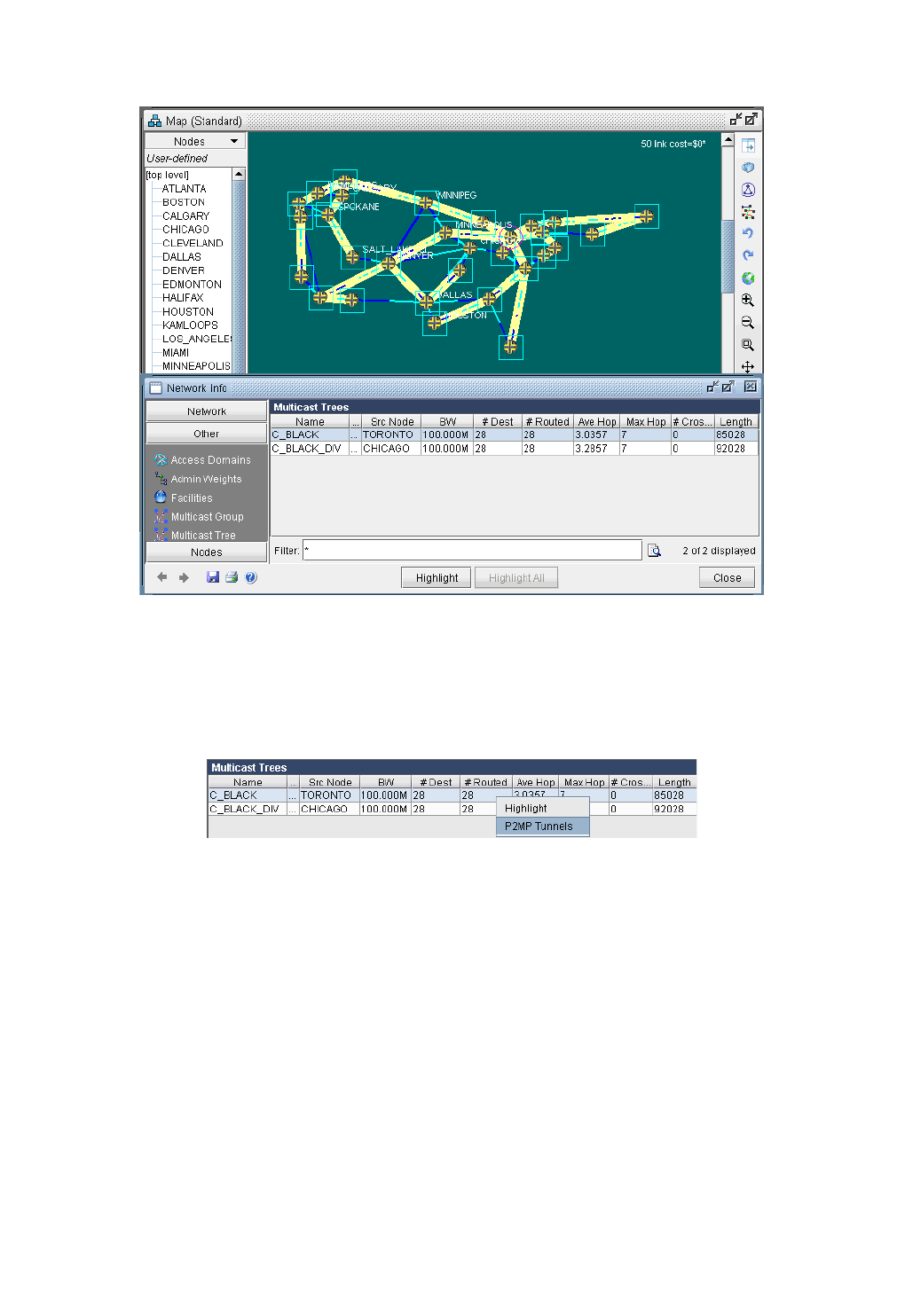
POINT-TO-MULTIPOINT (P2MP) TE*
Copyright © 2014, Juniper Networks, Inc. 27-3
. . . . .
Figure 27-2 Tree shown for the P2MP LSP named C_BLACK
5. To see a list of all the sub-LSPs that belong to a particular P2MP LSP tunnel, select P2MP Tunnels from the
right-click menu of the Multicast Trees window. Subsequently, the tunnels (the sub-LSPs) associated with the
particular P2MP LSP tunnel will be displayed.
Figure 27-3 P2MP Tunnels from the right-click menu
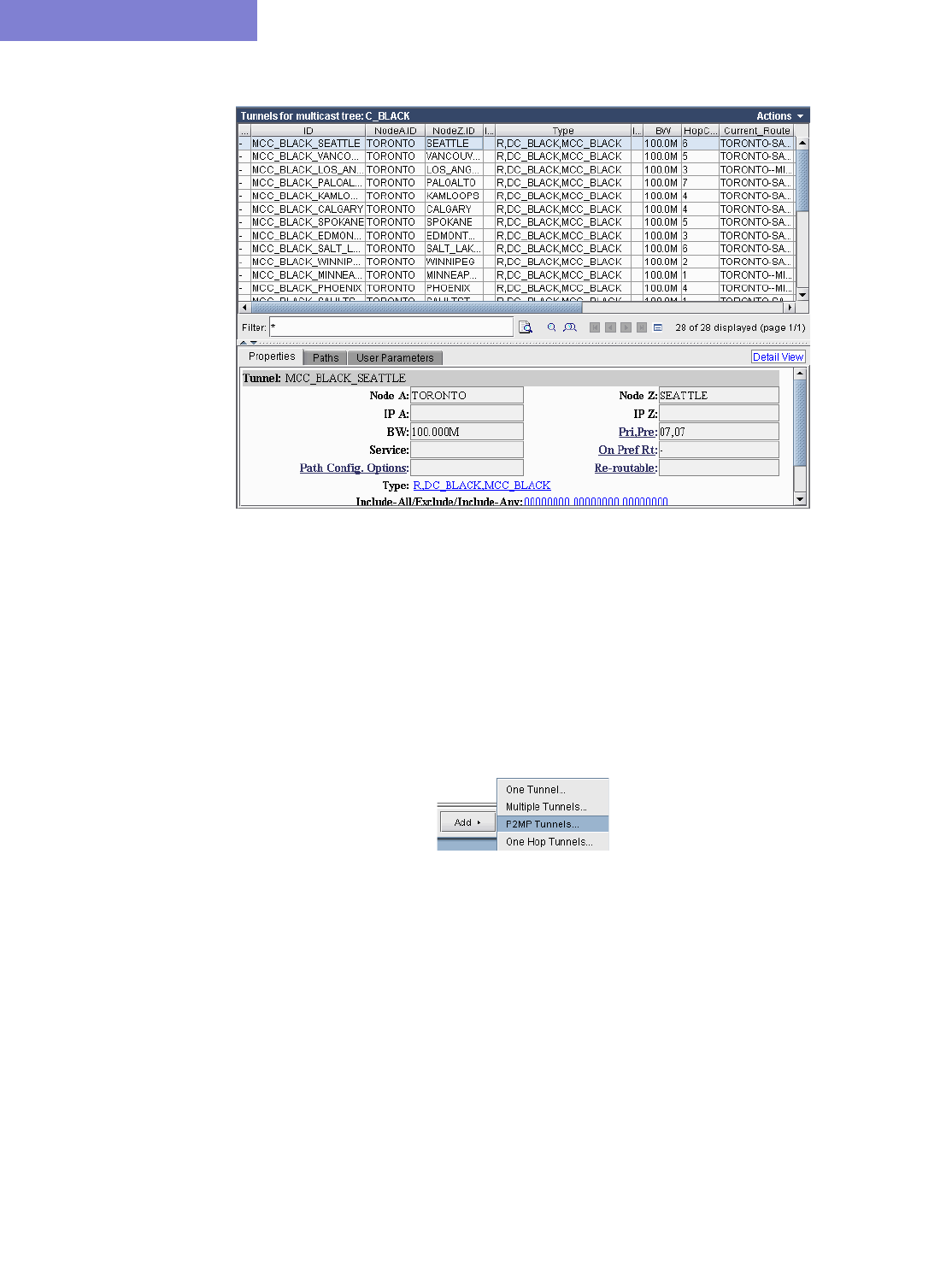
POINT-TO-MULTIPOINT (P2MP) TE*
27-4 Copyright © 2014, Juniper Networks, Inc.
27
Figure 27-4 Sub-LSPs associated with a particular P2MP LSP tunnel instance (e.g. C_BLACK)
In this particular example, the sub-LSPs associated with the P2MP LSP called C_BLACK are displayed. Notice
that in the type field, the sub-LSPs are marked with the MCC_BLACK. In IP/MPLSView, the sub-LSPs for a
particular P2MP LSP are marked with MC followed by the P2MP name in the type field.
Create P2MP LSP Tunnels and Generate Corresponding LSP Configlets
6. IP/MPLSView allows the user to create P2MP LSP tunnels. First, switch to Modify mode and then select
Modify > Elements > Tunnels to bring up the Tunnels Window. Then click on the Add button, and select
the P2MP Tunnels option to bring up the Add P2MP Tunnels window.
Figure 27-5 Selecting the P2MP Tunnels option in the Tunnels Window
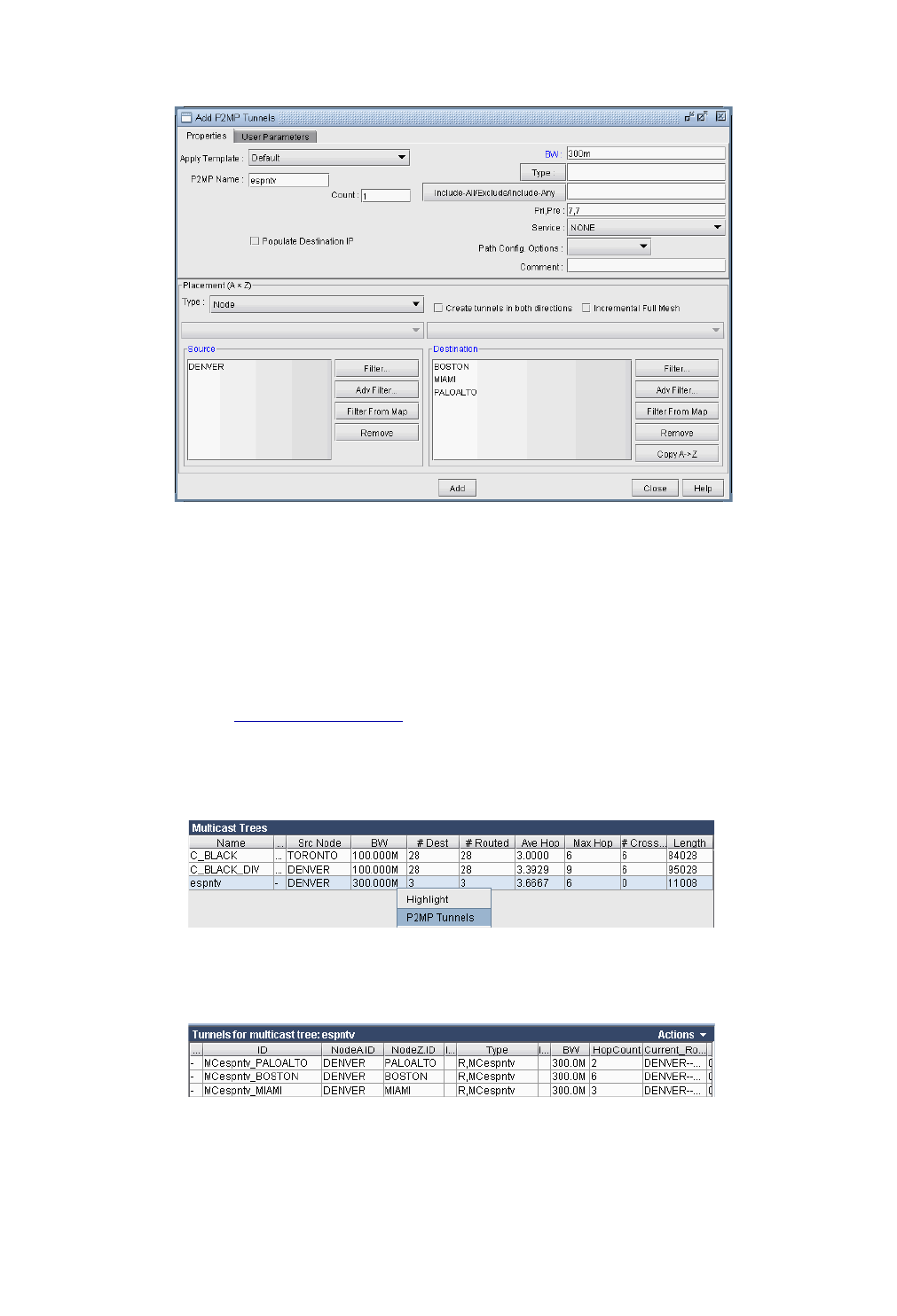
POINT-TO-MULTIPOINT (P2MP) TE*
Copyright © 2014, Juniper Networks, Inc. 27-5
. . . . .
Figure 27-6 Adding a P2MP LSP tunnel
As shown in the above figure, first specify a name for the P2MP LSP instance and then choose the source node
(ingress LSR) and the leaf nodes (egress LSRs for the sub-LSPs) for the P2MP tree. Then click on the Add
button, and the tool will automatically perform the P2MP LSP path computations necessary to place the sub-
LSPs associated with the P2MP LSP.
The user has the option to further specify TE constraints (such as bandwidth and explicit path) for each sub-LSP,
as can be done with any point-to-point LSP. For further information on how to specify tunnel parameters, please
refer to Chapter 20, LSP Tunnels*.
To see the newly-created P2MP LSP, switch out of Modify mode, and bring up the NetInfo > Multicast >
Multicast Trees window to see the P2MP LSP tunnels configured in the network.
Figure 27-7 Newly-added P2MP LSP called espntv.
Figure 27-8 The sub-LSPs for the P2MP LSP espntv
7. After using the IP/MPLSView to model P2MP LSPs, the P2MP LSPs can be rolled out according to the tool’s
P2MP LSP path computation calculations. This allows the P2MP LSPs created during network planning to be
translated into a series of actions that can be easily implemented by network operations. IP/MPLSView can be
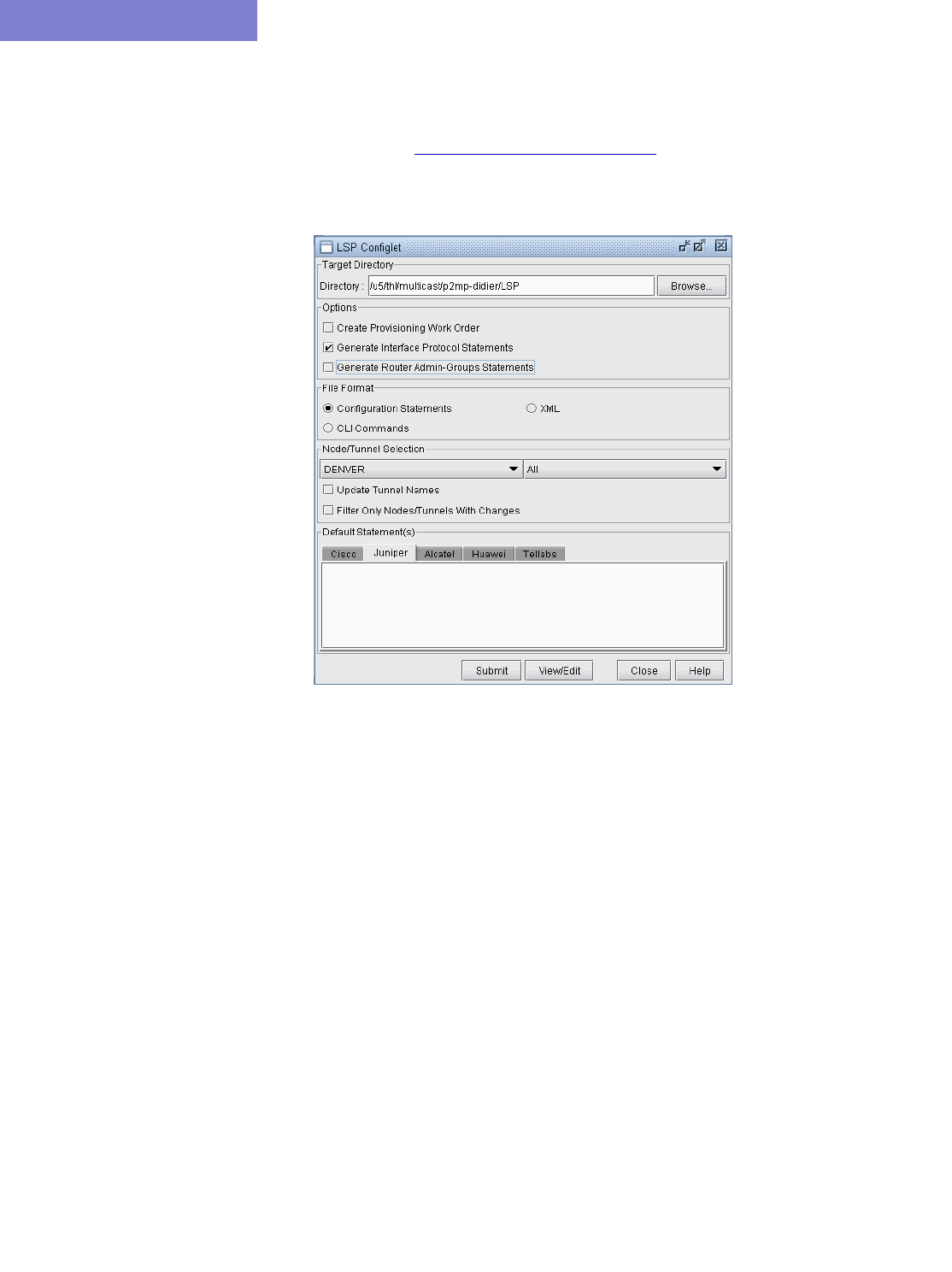
POINT-TO-MULTIPOINT (P2MP) TE*
27-6 Copyright © 2014, Juniper Networks, Inc.
27
used to easily convert the outputs of the network modeling into LSP configlets. A configlet is a small section of
the router configuration file that describes all the LSP attributes: bandwidth, admin-group, primary path, etc. To
generate the configlets, select Design > Confligets/Delta > LSP Configlet to bring up the LSP Configlet
window. Please refer to Chapter 23, LSP Configlet Generation* for details about how to use this window. After
the appropriate options have been specified, click on Submit button to generate the configlets for the selected
nodes/tunnels.
Figure 27-9 LSP Configlet generation window
8. The following figure shows the various statements listed in the configlet generated by IP/MPLSView for the
P2MP LSP (espntv) that was created above.
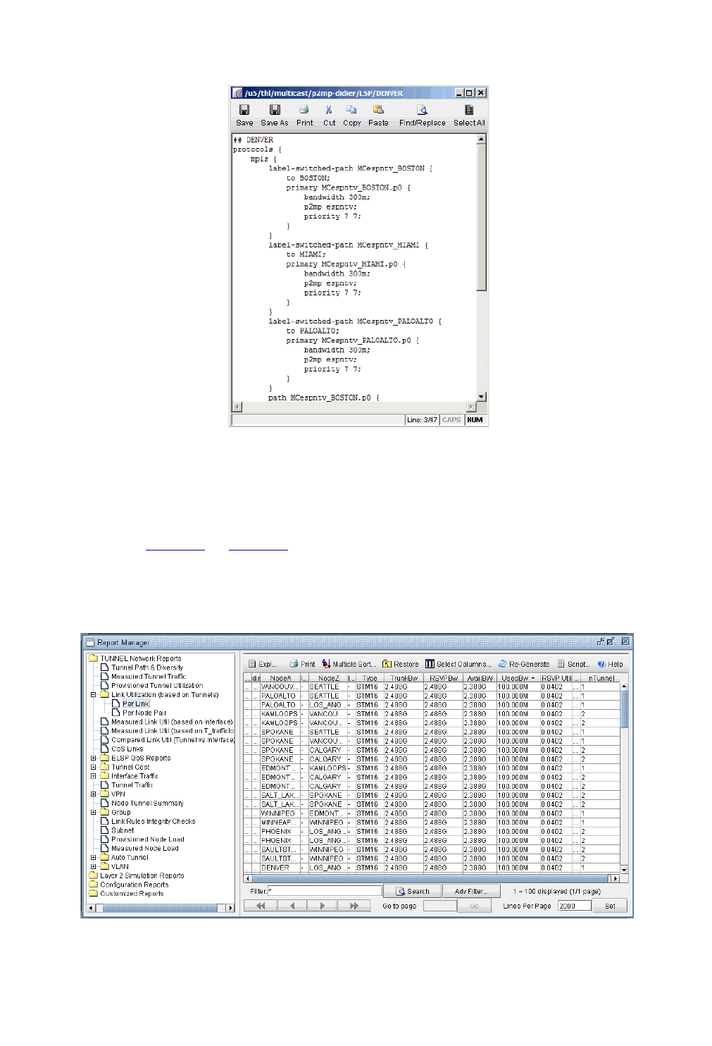
POINT-TO-MULTIPOINT (P2MP) TE*
Copyright © 2014, Juniper Networks, Inc. 27-7
. . . . .
Figure 27-10 configlet generated for the P2MP LSP espntv.
Examine P2MP LSP tunnel link utilizations to observe efficient replication.
9. In a P2MP tunnel distribution tree, packets are replicated at branch points. IP/MPLSView models this precisely
to give an accurate accounting of the amount of tunnel bandwidth occupied on the links. As shown in
Figure 27-2 and Figure 27-4 above, the P2MP LSP tunnel instance C_BLACK is comprised of 100M sub-LSPs.
As shown in the following figure, the Link Utilization (based on Tunnels) report shows that each link has 100M
of used BW. Thus using P2MP LSPs allows for traffic to be multicast from once source to multiple destinations
in a bandwidth efficient manner, as the source nodes does not need to send separate copies to each receiver.
Figure 27-11 Link utilization based on Tunnel Placement shows each link has 100M of occupied tunnel BW.
POINT-TO-MULTIPOINT (P2MP) TE*
27-8 Copyright © 2014, Juniper Networks, Inc.
27
Perform failure simulation and assess the impact of the failure on P2MP LSPs.
10. IP/MPLSView includes a full suite of capabilities that allow the user to perform both interactive and exhaustive
failure simulation. Please refer to the User Guide Chapter 14, Simulation, for detailed information about how to
use the failure simulation features. With regards to P2MP tunnels, one could fail for instance the link on which
certain sub-LSPs traverse in order to assess the impact of the damage on the recipients at those sub-LSPs. For
instance, the following two figures show the changes in placement of sub-LSPs after the link between
Edmonton and Winnipeg is failed. From the result of failure simulation runs, the user may find further design
for redundancy a necessity. Efforts are underway in the IETF to provide FRR support for P2MP tunnels. In
addition, application-level redundancy can be provided in the form of the design of a diverse multicast P2MP
tree.
Figure 27-12 Placement of sub-LSPs prior to link failure
Figure 27-13 Changes in placement of sub-LSPs after link failure

POINT-TO-MULTIPOINT (P2MP) TE*
Copyright © 2014, Juniper Networks, Inc. 27-9
. . . . .

POINT-TO-MULTIPOINT (P2MP) TE*
27-10 Copyright © 2014, Juniper Networks, Inc.
27

Copyright © 2014, Juniper Networks, Inc. 28-1
. . . . .
. . . . . . . . . . . . . . . . . . . . . . . . . . . . . . . . . . .
D
IVERSE
M
ULTICAST
T
REE
D
ESIGN
*
28
igh-quality video distribution (such as high-definition IP TV) with strict SLAs for packet loss and jitter
are continuing to be rolled out by major broadcast service providers across the globe. Such a video
distribution network requires that bandwidth be reserved along a fixed pre-allocated transmission path. There are
currently two possible solutions for protecting such a path:
1. Use pre-configured FRR LSPs to protect each LSP branch. However, the drawback to this approach is that large
spare capacity is needed for all the backup LSPs.
2. Use Diverse Multicast Trees. Here a separate multicast distribution tree is routed that is strictly diverse from the
main tree in order to achieve 1+1 protection. For two multicast trees to be diverse from each other, the paths (i.e., the
sub-LSPs of a P2MP multicast tree) to each destination from the source of each of the two trees have to not share any
link or site or facility, depending on the diversity level.
Designing diverse multicast trees is a complex network design problem; in fact, it is NP hard (Non-deterministic
Polynomial time hard) and not readily tractable for manual computation. A powerful and heuristics-based algorithm
is needed to solve the problem for large networks. WANDL IP/MPLSView comes to the rescue with a powerful
Multicast Tree Design module that allows the user to design separate multicast trees that are strictly diverse from
each other. The design solutions are as efficient as possible and can lead to large savings in capacity requirements
for the network planner.
The following sections of this chapter describe the Multicast Tree Design features that are currently supported by
WANDL IP/MPLSView.
*Note that this is a special license is required for Diverse Multicast Tree Design. Please contact your Juniper
representative for more information.
When to use
Use these procedures if you have multicast trees (i.e., P2MP trees) configured in your network and if you would like
to use IP/MPLSView to help you to design diverse multicast trees.
Prerequisites
If you wish to perform these tasks in the WANDL client, you should have an IP/MPLS network router spec file open
before you begin. Otherwise, you should have a set of router configuration files ready to be imported into the tool.
The chapter assumes the user is familiar with IP, MPLS, TE, P2MP, and IP multicast.
Related Documentation
Refer to Chapter 27, Point-to-multipoint (P2MP) TE* for more information on PM2P Tunnels modeling and
creation.
Refer to Chapter 20, LSP Tunnels* for more information on LSP Tunnels and how to set their characteristics.
Refer to Chapter 23, LSP Configlet Generation* for more information on generating LSP configlets.
Refer to Chapter 12, Multicast* for more information about IP multicast.
Refer to the User Guide “Chapter 14 , Simulation”, for more information about failure simulation.
Recommended Instructions
1. Open a network with multicast trees (i.e., P2MP trees) configured in the network.
2. Mark the two multicast trees as in the same Diversity Group.
H

DIVERSE MULTICAST TREE DESIGN*
28-2 Copyright © 2014, Juniper Networks, Inc.
28
3. Use the Multicast Tree Design feature to design and route multicast distribution trees within in a Diversity
Group that are strictly diverse from each other.
4. Use the Multicast Tree Design feature to tune a particular tree to reduce it’s cost.
DIVERSE MULTICAST TREE DESIGN*
Copyright © 2014, Juniper Networks, Inc. 28-3
. . . . .
Detailed Procedures
Open a network that already has a Multicast Trees (i.e., P2MP trees) configured in the network
1. Review the Prerequisites to ensure that your network is configured properly with IP, MPLS and P2MP LSP
tunnels.
2. If you already have a spec file ready for the network, you may open it. The spec file should already have P2MP
tree configured in it. For details about P2MP trees, including how to configure them using IP/MPLSView,
please refer to Chapter 27, Point-to-multipoint (P2MP) TE*. Alternatively, if you have the set of router
configuration files with P2MP trees configured in them, then you may follow the procedures as described in
Chapter 2, Router Data Extraction, in order to import the configuration files and create a WANDL spec network
model.
The following figure shows an example spec file that has two P2MP trees configured: one called C_BLACK
(centered at TORONTO) and another called C_BLACK_DIV (centered at DENVER). The two P2MP trees
have the same leaf nodes.
Figure 28-1 Two P2MP trees defined in the network shown in Main Topology map’s P2MP subview
Set the two P2MP trees of interest to be in the same Diversity Group
3. After opening an existing spec file or creating a new spec file after configuration file import, you are ready to
perform Diverse Multicast Tree design on two P2MP trees. The tool allows you to easily select the sub-LSPs
that belong to a particular P2MP tree and then specify its Diversity Group. Two trees belong to the same
Diversity Group if all the corresponding sub-LSPs have been marked with the same Diversity Group name.
4. To set the Diversity Group name for the sub-LSPs, first go to Modify mode and bring up the Modify Tunnels
window via Modify > Elements > Tunnels.
5. Next select all the sub-LSPs for the two P2MP trees of interest and click on Modify>Selected button.
6. From the Modify Tunnels Window, click on the Type button to bring up the Tunnel Type Parameter
Generation window.
7. Next, click on the Diversity tab and fill in a name inside the Diversity Group fill-in/dropdown combo button,
as shown in the following figure.
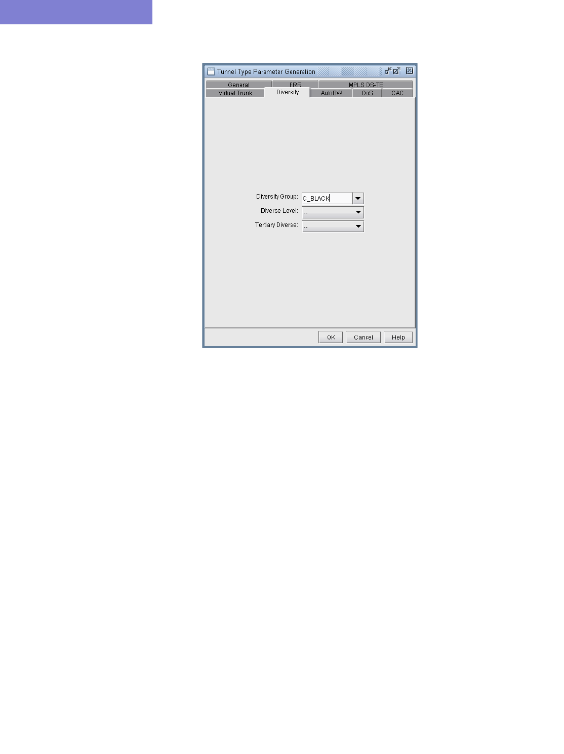
DIVERSE MULTICAST TREE DESIGN*
28-4 Copyright © 2014, Juniper Networks, Inc.
28
Figure 28-2 Specify Diversity Group (e.g. C_BLACK) for each sub-LSP for the two P2MP trees
8. After clicking OK, the Type field for each tunnel modified should contain the DC_BLACK flag in it, as shown
in the following figure. In IP/MPLSView, the sub-LSPs for a particular Diversity Group are marked with D
followed by the Diversity Group name in the type field.
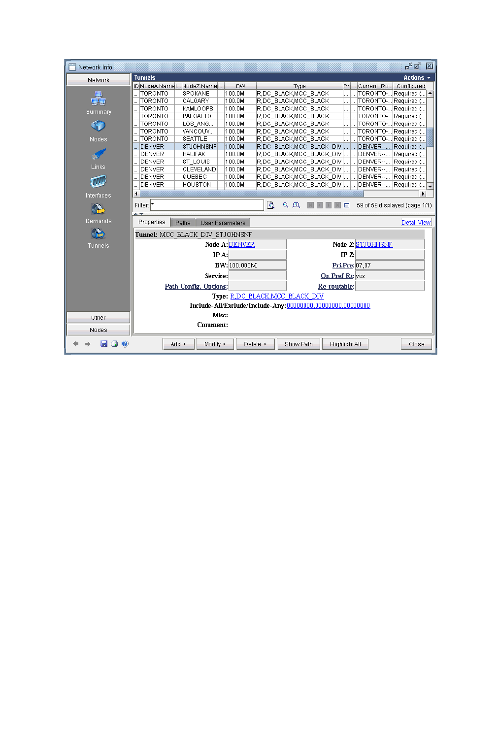
DIVERSE MULTICAST TREE DESIGN*
Copyright © 2014, Juniper Networks, Inc. 28-5
. . . . .
Figure 28-3 Type field contains DC_BLACK to indicate that it belongs to the Diversity Group C_BLACK
Use the Multicast Tree Design feature to design multicast trees that are diverse from each other in each
Diversity Group
9. Now that the two P2MP trees of interest have been marked to be in the same Diversity Group, you are ready to
perform a design. For two multicast trees to be diverse from each other, the paths (i.e., the sub-LSPs of a P2MP
multicast tree) to each destination from the source of each of the two trees have to not share any link or site or
facility, depending on the diversity level. By default, the algorithm tries the highest diversity level first; so it
will try to design for facility, then site, then link diversity. To perform the design, first go to Design Mode and
select Design > Multicast Tree Design to bring up the Multicast Tree Design window, as shown in the
following figure. The top part of the window displays the list of P2MP trees that are configured in the network.
The bottom part of the window shows the sub-LSPs that make up the P2MP tree selected on the top part of the
window.
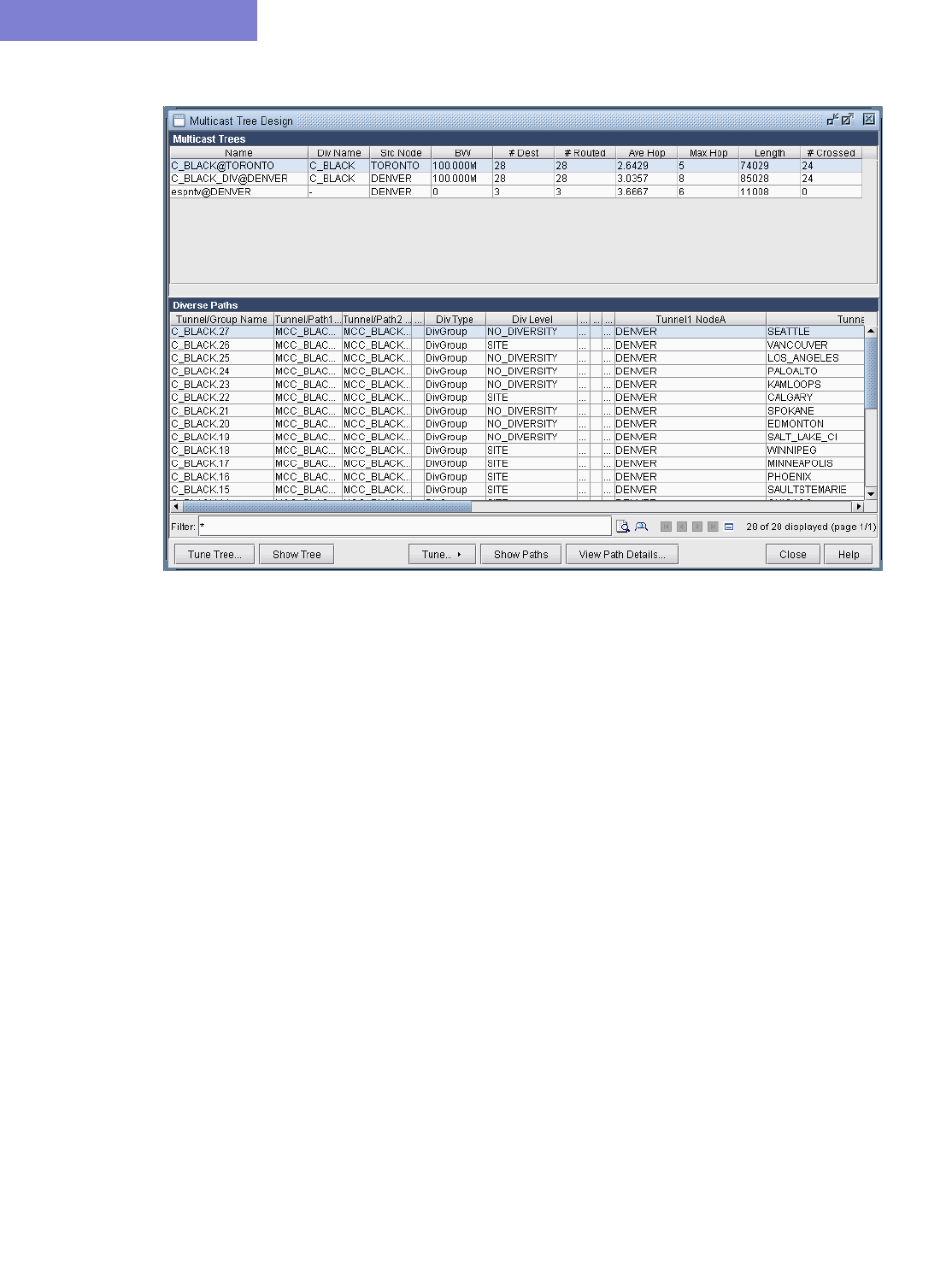
DIVERSE MULTICAST TREE DESIGN*
28-6 Copyright © 2014, Juniper Networks, Inc.
28
Figure 28-4 Multicast Tree Design window prior to Tuning Tree
The Div Level column indicates the current diversity level (FACILITY, SITE, LINK, or NO_DIVERSITY) for
the sub-LSP. The Show Paths button allows you to visually see two sub-LSPs that are diverse from each
other. For instance, the following figure shows that the sub-LSP from TORONTO to VANCOUVER and the
sub-LSP from DENVER to VANCOUVER are SITE-diverse from each other.
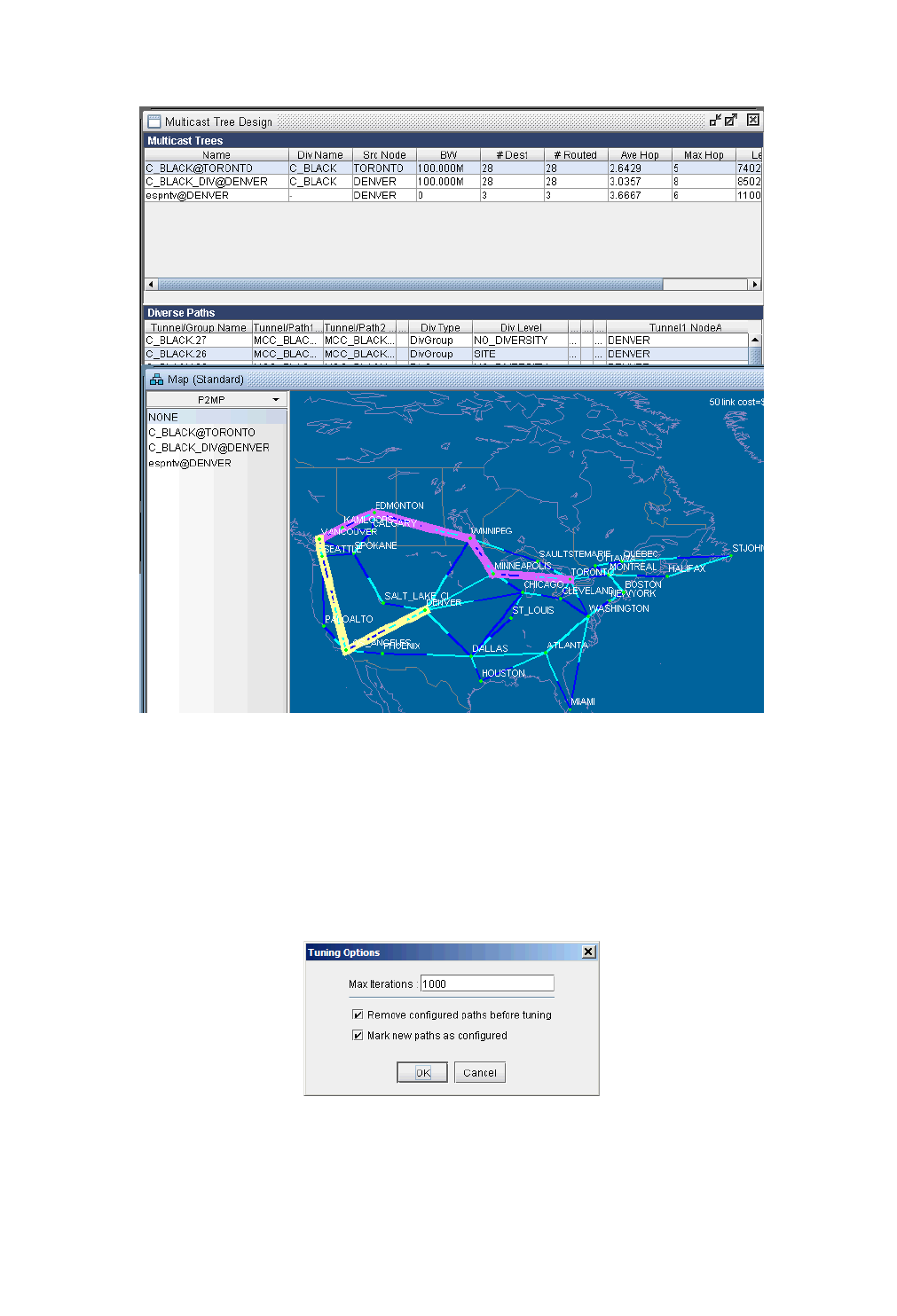
DIVERSE MULTICAST TREE DESIGN*
Copyright © 2014, Juniper Networks, Inc. 28-7
. . . . .
Figure 28-5 Example of sub-LSPs that are SITE diverse from each other.
10. Next you are ready to start the actual design run. Simply click on the Tune Tree button to bring up the Tuning
Options window, shown in the following figure. The Max Iterations box may be set to a higher value in
order for the design’s heuristics algorithm to perform more iteration runs, which leads to even better solutions.
The Remove configured paths before tuning option, which is checked by default, means that existing
P2MP sub-LSP paths will be overwritten by the program. The Mark new paths as configured option,
which is checked by default, means that the LSP will be explicitly routed by our optimization program.
Figure 28-6 The Max Iterations can be set to higher values to allow the design heuristics algorithm to run
longer and to lead to better solutions.
DIVERSE MULTICAST TREE DESIGN*
28-8 Copyright © 2014, Juniper Networks, Inc.
28
11. Next click on OK and allow IP/MPLSView to perform the design. This may take a short amount of time, such
as a few minutes; it may also take a much longer time. It all depends on the value that you specified for Max
Iterations.
Figure 28-7 After performing the design, the Diversity Level is satisfied.
Another thing to note is that the design is performed based on IGP cost (i.e., OSPF cost in this case). You may
also choose to have the design performed based on actual mileage cost, as real-time traffic is delay-sensitive.
Make sure that the lat/lon coordinates have been specified for the node locations if you want to perform the
design using the actual mileage. If that is the case, bring up the IP/MPLSView options window, select
Design>Path Placement and set the Routing Method to be Actual Mileage, as shown in the following
figure.
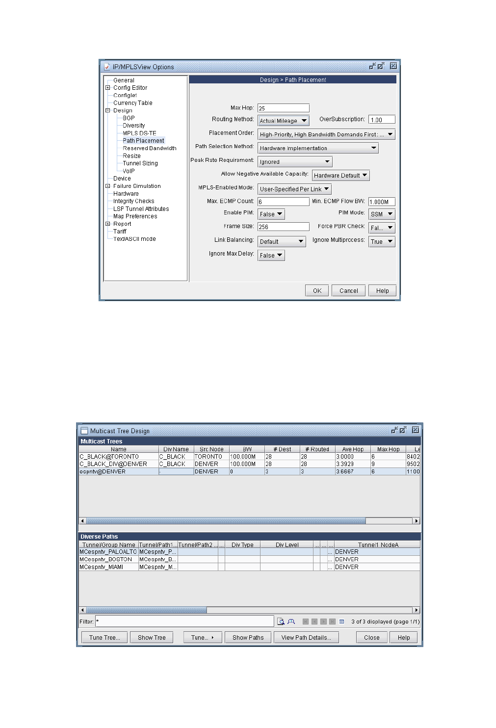
DIVERSE MULTICAST TREE DESIGN*
Copyright © 2014, Juniper Networks, Inc. 28-9
. . . . .
Figure 28-8 Setting Routing Method to use Actual Mileage
Use the Multicast Tree Design feature to tune an existing tree in order to reduce its cost.
12. For other P2MP multicast trees in the network that do not belong to a particular Diversity Group, you can still
select the tree and perform a tuning in order to reduce the multicast tree’s cost (which is defined the total length
(physical or admin-cost) of the tree). For instance, the following figure shows espntv P2MP tree is not part of
Diversity Group and is a candidate for tuning.
Figure 28-9 Tuning a single P2MP diverse multicast tree

DIVERSE MULTICAST TREE DESIGN*
28-10 Copyright © 2014, Juniper Networks, Inc.
28

Copyright © 2014, Juniper Networks, Inc. 29-1
. . . . .
. . . . . . . . . . . . . . . . . . . . . . . . . . . . . . . . . . .
D
IFF
S
ERV
T
RAFFIC
E
NGINEERING
T
UNNELS
*
29
his chapter discusses how Differentiated Services Aware Traffic Engineering LSPs (DS-TE LSPs) are
modeled in WANDL software. In order to provide the most value to users, WANDL’s modeling of DS-TE
LSPs are continually updated to reflect current vendor implementations and industry practices in this field.
Therefore, it is possible that the descriptions of DS-TE LSPs may not reflect the traditional DS-TE LSP models (E-
LSPs and L-LSPs) defined by IETF. For more information on traditional DS-TE LSP models, feel free to peruse
IETF RFC 3270. In this document, the DS-TE LSP behavior discussed is that which is currently implemented by
today’s hardware vendors. Currently, only Juniper Networks supports DS-TE LSPs.
*Note that a special license is required for diffserv TE. Please contact your Juniper representative for more
information.
When to use
Whereas standard traffic engineering works on an aggregate basis, DS-TE LSPs allow for traffic engineering at a
per-class level with different bandwidth constraints for different traffic class types. This makes it possible to
guarantee different levels of service and bandwidth to different classes across an MPLS network. Such advantages
allow you to provide ATM circuit emulation over IP, Voice over IP, class based services, and guaranteed bandwidth
services.
Prerequisites
Before reading this chapter, you should have a good understanding of how standard LSPs are provisioned on a
network, and you should be comfortable working with LSPs.
Related Documentation
For general step-by-step instructions on how to use the WANDL software, please refer to the Design & Planning
Guide.
For an overview of the WANDL software or for a detailed description of each feature and the use of each window,
refer to the General Reference Guide or Chapter 37, Router Reference.
For instructions on how to view or modify the tunnels in your network, refer to Chapter 20, LSP Tunnels*.
Definitions
It should be noted that in this document, the word “tunnel” is used in the context of traffic engineering (TE) tunnels.
Also, the word “tunnel load” refers to the amount of IP traffic transported by the tunnel.
Bandwidth model: The bandwidth model determines the values of the available bandwidth advertised by the
interior gateway protocols (IGPs).
Differentiated services: Also known as DiffServ, differentiated services make it possible to give different
treatment to traffic based on the experimental (EXP) bits in the MPLS header.
DSCP: The Differentiated Services Code Point refers to six bits in the ToS (Type of Service) byte of a packet header
that specify the particular PHB (Per Hop Behavior) to be applied to the packet.
DS-TE LSP: Differentiated-Services-aware Traffic Engineering LSP.
E-LSP: EXP-inferred LSP as defined in IETF RFC 3270.
L-LSP: Label-only-inferred LSP as defined in IETF RFC 3270.
Planned bandwidth: The current bandwidth allotted to the tunnel.
QoS: Quality of Service is a broad collection of networking technologies with the goal of providing guarantees on
the ability of a network to deliver predictable results beyond the best-effort delivery provided by default.
T

DIFFSERV TRAFFIC ENGINEERING TUNNELS*
29-2 Copyright © 2014, Juniper Networks, Inc.
29
Using DS-TE LSP
Imagine a scenario where you are migrating from ATM over to IP, and you want to provision tunnels on the IP
network to support the various classes of traffic in ATM, such as CBR, VBR, RT, NRT. To use WANDL software to
model this, you would follow these steps:
•Map the four types of ATM traffic to four class types.
•Partition bandwidth on your interfaces / links for these four classes.
•Create as many DS-TE LSPs as is necessary to carry the ATM traffic. Specify the class for each DS-TE LSP
according the type of ATM traffic it is supposed to carry.
•Route the DS-TE LSP tunnels over the network. This is done automatically by the tool.
•Examine where bottlenecks occur, where excess capacity exists, where you need to purchase more bandwidth,
etc.
This is just one example of how DS-TE LSPs can be used, but it illustrates many of the steps involved in setting up
and utilizing DS-TE LSPs in a network.
Hardware Support for DS-TE LSP
OVERVIEW
Juniper Networks supports two kinds of DS-TE LSPs: DiffServ-aware single-class LSPs and DiffServ-aware
multi-class LSPs. Single-class LSPs are similar to traditional L-LSPs, and support only one class per LSP. Multi-
class LSPs can be thought of as L-LSPs that can handle multiple classes. Each multi-class LSP can support up to
four classes with specific bandwidth reservation assigned to each class. When DiffServ-aware LSPs are routed on a
network, consideration is given to the amount of bandwidth reserved on each interface for each class. If there is
insufficient bandwidth on a particular interface for a given class on the multi-class or single-class LSP, the LSP will
not be routed over that interface.
CLASS TYPE
A class type is a collection of traffic flows that is treated equivalently in a DiffServ domain. A class type maps to a
queue and is much like a class-of-service (CoS) forwarding class in concept. It is also known as a traffic class.
DiffServ-aware single-class LSPs can only handle one class type, while DiffServ-aware multi-class LSPs are
capable of handling up to four class types.
EXP BITS
The Experimental bits, or EXP bits, in the MPLS header are used to define the class to which a packet belongs. A
unique EXP bit pattern is associated with each class type and forwarding class defined on a DiffServ-aware router.
FORWARDING CLASS
Forwarding classes are defined on each router and assigned to internal queues. The default forwarding classes are:
best-effort, expedited-forwarding, assured-forwarding, and network-control. Individual class types in DiffServ-
aware LSPs are mapped to individual forwarding classes at the router. The default mapping is shown in the table
below.
Class Type Forwarding Class Name
CT0 best-effort
CT1 expedited-forwarding
CT2 assured-forwarding
CT3 network-control

DIFFSERV TRAFFIC ENGINEERING TUNNELS*
Copyright © 2014, Juniper Networks, Inc. 29-3
. . . . .
SCHEDULER MAP
The treatment given to each forwarding class on an interface is defined by the scheduler map assigned to that
interface. The scheduler map includes a list of schedulers which map specific forwarding classes to specific
scheduler configurations. These determine the per-class bandwidth allocations on each interface, which are taken
into consideration when routing DiffServ-aware LSPs.
BANDWIDTH MODEL
A bandwidth model must be configured on all routers participating in the DiffServ domain. The three types of
bandwidth models supported by Juniper are MAM, Extended MAM, and RDM, which are defined in the following
table.
OPERATION
In order to take advantage of DiffServ-aware single-class and multi-class LSPs, each class type must be configured
consistently across the differentiated service domain. In other words, each router in the network must follow a
consistent class type configuration. On each node router, each class type is mapped to a queue. The available
bandwidth for a particular class type on a link is determined by the configuration of class of service queues for that
interface. Any DiffServ-aware LSP that requires bandwidth from a particular class cannot be established through
routers that do not understand the Classtype object. It is possible for DiffServ-aware LSPs and regular LSPs to be
established on the same router. In this case, the regular LSP will carry best-effort traffic by default. However, you
cannot simultaneously configure multi-class LSPs and single-class LSPs on the same router.
MAM Defined in Internet draft draft-ietf-tewg-diff-te-mam-03.txt
Extended-MAM A proprietary bandwidth model that behaves much like standard
MAM. If you configure multiclass LSPs, you must configure the
extended MAM bandwidth model.
RDM Makes efficient use of bandwidth by allowing the class types to
share bandwidth. RDM is defined in Internet draft draft-ietf-tewg-
diff-te-russian-05.txt

DIFFSERV TRAFFIC ENGINEERING TUNNELS*
29-4 Copyright © 2014, Juniper Networks, Inc.
29
WANDL Support for DS-TE LSP
OVERVIEW
The WANDL software supports both DiffServe-aware Single-Class LSPs and DiffServ-aware Multi-Class LSPs,
according to the specifications in existing hardware. These LSPs can be parsed from existing router configuration
files, or they can be manually created from scratch via the WANDL clientWANDL client for a paper network design.
CLASS TYPES
WANDL’s class type terminology corresponds with that used in JUNOS configurations. The four class type names
are CT0, CT1, CT2, and CT3. These class type names appear in the JUNOS configuration statements:
EXP BITS
The Experimental bits, or EXP bits, in the MPLS header are used to define the class to which a packet belongs. A
unique EXP bit pattern is associated with each class type and forwarding class defined on a DiffServ-aware router.
WANDL software allows the user to define the mapping between EXP bits, class types, and forwarding classes.
COS CLASSES
The CoS class defined in WANDL software is equivalent to the forwarding class configured in JUNOS, as in the
following configuration structure.
COS POLICIES
WANDL’s CoS policy is equivalent to the scheduler map defined in JUNOS. A CoS policy contains information on
how to treat each CoS class referenced by the CoS policy. The treatment given to each CoS class at a router is
determined by the CoS policy assigned to that router. Applying a CoS policy to a router is similar to applying
scheduler maps to the interfaces on that router, as in the configuration structure below.
Single-class LSP Multi-class LSP
label-switched-path lsp-name {
bandwidth {
ctnumber bandwidth;
}
}
label-switched-path lsp-name {
bandwidth {
ct0 bandwidth;
ct1 bandwidth;
ct2 bandwidth;
ct3 bandwidth;
}
}
interfaces {
interface-name {
scheduler-map map-name;
scheduler-map-chassis map-name;
unit logical-unit-number {
classifiers {
type (classifier-name | default);
}
forwarding-class class-name;
rewrite-rules {
type (rewrite-name | default);
}
}
}
}

DIFFSERV TRAFFIC ENGINEERING TUNNELS*
Copyright © 2014, Juniper Networks, Inc. 29-5
. . . . .
WANDL allows the user to define a robust set of Cos policies and to easily assign them to any router in a network.
The CoS Policy determines the amount of bandwidth reserved on a link for each traffic class contained in the policy.
The bandwidth reservation scheme for each router affects how DiffServ-aware LSPs are routed in the network.
BANDWIDTH MODEL
WANDL supports both MAM and RDM bandwidth models. The MAM bandwidth model used when configuring
DiffServ-aware LSPs in WANDL software is equivalent to the extended-MAM bandwidth model used in JUNOS
configuration, as shown below.
The choice of whether to use MAM or RDM in WANDL software affects the way in which bandwidth is assigned to
a multi-class LSP, and the manner in which bandwidth is reported for a link with bandwidth partitions for multiple
classes. For example, in a situation where CT0, CT1, CT2 and CT3 are all reserved 10M, the link partition will be
reported differently depending on whether the bandwidth model is MAM or RDM, as shown in the table below.
In the above example, for MAM, each class gets 10M. For RDM, each class also gets 10M. However, in RDM, CT2
has access to the 10M belonging to CT3, and thus has 20M total available. CT1 has its own 10M plus the 20M
available to CT2, and thus ends up with 30M total. Since CT0 is at the top of the stack, it receives its own 10M plus
all the bandwidth available to the classes below it, for a total of 40M.
Similarly, if one were to configure a multi-class LSP with 90M reserved for CT0 and 10M reserved for CT3, the
configuration would look differently depending on the bandwidth model used. This is shown in the table below.
interfaces {
interface-name {
scheduler-map map-name;
scheduler-map-chassis map-name;
unit logical-unit-number {
classifiers {
type (classifier-name | default);
}
forwarding-class class-name;
rewrite-rules {
type (rewrite-name | default);
}
}
}
}
bandwidth-model {
(extended-mam | mam | rdm);
}
MAM RDM
CT0: 10M
CT1: 10M
CT2: 10M
CT3: 10M
CT0: 40M
CT1: 30M
CT2: 20M
CT3: 10M
MAM RDM
CT0: 90M
CT1: 0M
CT2: 0M
CT3: 10M
CT0: 100M
CT1: 0M
CT2: 0M
CT3: 10M
DIFFSERV TRAFFIC ENGINEERING TUNNELS*
29-6 Copyright © 2014, Juniper Networks, Inc.
29
Using WANDL to Model DS-TE LSPs
CONFIGURING THE BANDWIDTH MODEL AND DEFAULT BANDWIDTH PARTITIONS
There are two global options that can be applied to the entire network. The first is the bandwidth model, which can
be either MAM (equivalent to Juniper’s extended-MAM) or RDM. The second is the default bandwidth partitions,
which will be applied to an interface when there is no CoS policy assigned to that interface. To configure these two
global settings, simply open the Design Options window under Tools > Options > Design. Then click on the
Path Placement > MPLS TE option pane to see the following window:
Figure 29-1 Configuring Bandwidth Model and Default Link Bandwidth Partition
Bandwidth Model Two types of Bandwidth Models are supported. MAM and
RDM. When configuring multi-class LSPs, the MAM model
should be used, which is equivalent to Juniper’s extended-
MAM.
Name These are the names of the four class types: ct0, ct1, ct2 and
ct3.
BW% This is the amount of bandwidth assigned to each class in
terms of percentage. These settings are applied to a link only
when no scheduler maps have been assigned to that link.
EXP DiffServ-aware routers use the EXP bits in the packet header
to determine the traffic class type, which is mapped to the
appropriate per-hop behavior (PHB). The mapping between
the EXP bits and the PHB is static, rather than being signaled
as in RSVP.
COS This corresponds to the class name used when configuring
scheduler maps in JUNOS.

DIFFSERV TRAFFIC ENGINEERING TUNNELS*
Copyright © 2014, Juniper Networks, Inc. 29-7
. . . . .
FORWARDING CLASS TO CLASS TYPE MAPPING
In order to specify the forwarding class to class type mappings, the following parameter, cos2ctmap, needs to be
included in the dparam file.
Example:
cos2ctmap=M-RT:CT3|1R,MC:CT2|2R,ME:CT1|4R,BE:CT0|6R
The cos2ctmap parameter takes a comma-separated list of tokens that can be specified in one of the following
formats:
•cosname:CTn: map demand with forwarding class cosname to CTn tunnel
•cosname:CTn|m : map demand with forwarding class cosname to tunnel with CTn and priority m
•cosname:CTn|mR : map demand with forwarding class cosname to tunnel with CTn and priority m. The "R" is
restrictive, meaning that if not available don't map to the tunnel
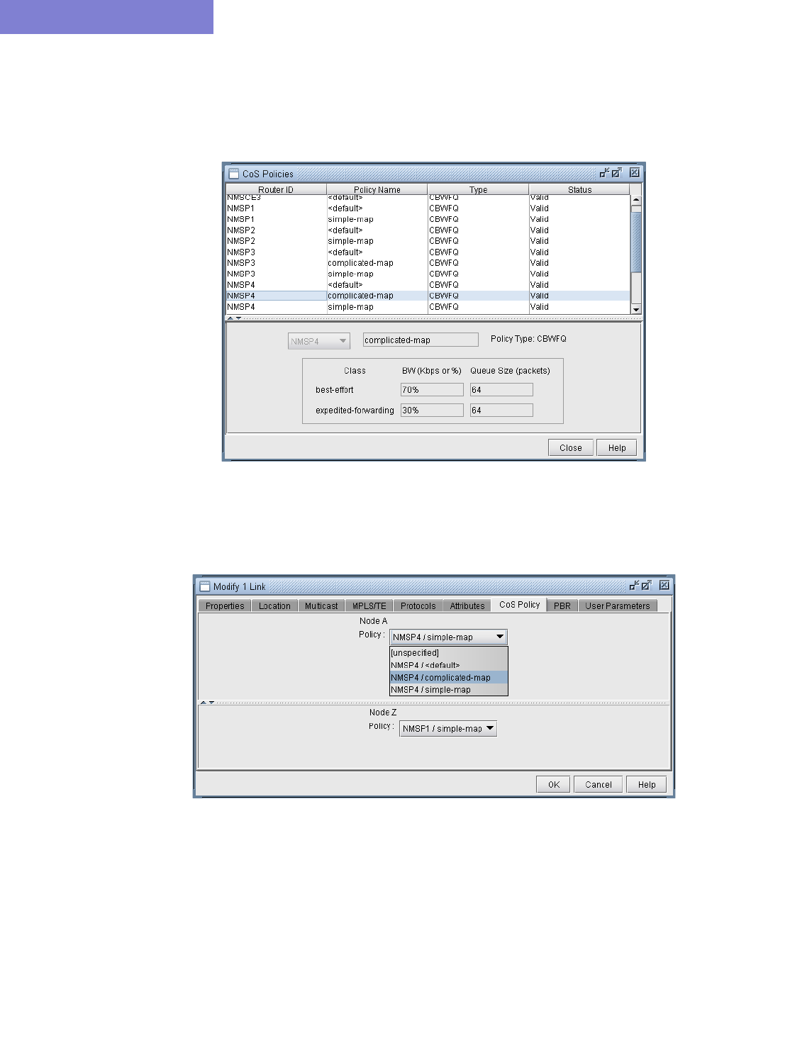
DIFFSERV TRAFFIC ENGINEERING TUNNELS*
29-8 Copyright © 2014, Juniper Networks, Inc.
29
LINK BANDWIDTH RESERVATION
Individual link bandwidth reservation schemes can be assigned to a link by applying a CoS policy to that link.
WANDL software allows the user to define a robust collection of CoS policies, which can be specific to a router or
generic to all routers.
Figure 29-2 Defining scheduler maps, or CoS policies
Once CoS policies, have been defined, they can be assigned to specific links. Since each link contains two interfaces,
one at each end, a policy can be assigned to each end of the link.
Figure 29-3 Assigning a scheduler map, or CoS policy, to a link
Once a policy has been assigned to a link, the capacity on the link will be updated to reflect the policy. The way in
which the bandwidth is displayed in the link capacity window can be controlled by Bandwidth Model option
described earlier. In the screenshot below, the Bandwidth Model being used is MAM.
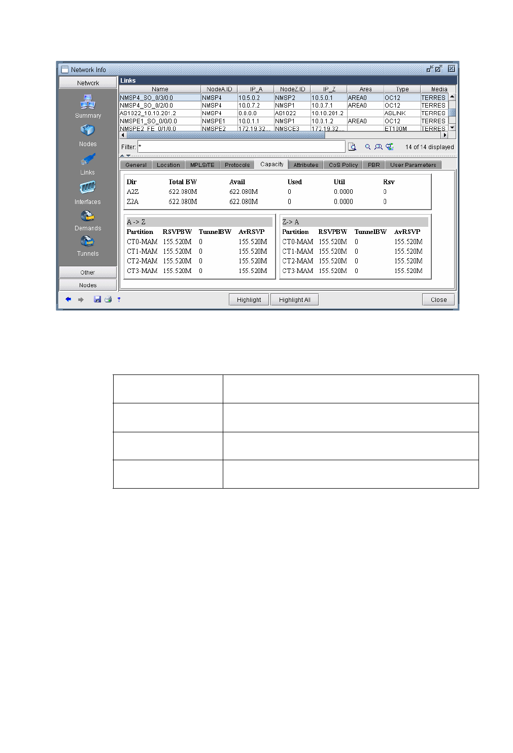
DIFFSERV TRAFFIC ENGINEERING TUNNELS*
Copyright © 2014, Juniper Networks, Inc. 29-9
. . . . .
Figure 29-4 Link capacity reflecting the assigned scheduler map, or CoS policy
Partition This corresponds to the class type associated with the policy
assigned to the interface.
RSVPBW This is the amount of bandwidth reserved for the
corresponding partition, as defined by the assigned policy.
TunnelBW This is the amount of tunnel bandwidth currently passing
through the interface.
AvRSVP This is the amount of available bandwidth remaining for the
corresponding partition.
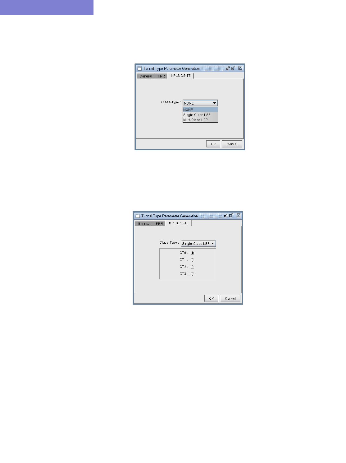
DIFFSERV TRAFFIC ENGINEERING TUNNELS*
29-10 Copyright © 2014, Juniper Networks, Inc.
29
CREATING A NEW MULTI-CLASS OR SINGLE-CLASS LSP
When creating a new tunnel object, there is an option to specify the type of LSP to create. The type can be Regular
(“NONE”), Single-Class LSP, or Multi-Class LSP.
Figure 29-5 Selecting the type of DiffServ-aware LSP
CONFIGURING A DIFFSERV-AWARE LSP
If Single-Class LSP is selected as the type of LSP, the user can specify the class type to be assigned to the single-
class LSP.
Figure 29-6 Assigning class type to a single-class LSP
If Multi-Class LSP is selected as the type of LSP, the user can specify the amount of bandwidth to be reserved for
up to four classes on the multi-class LSP.
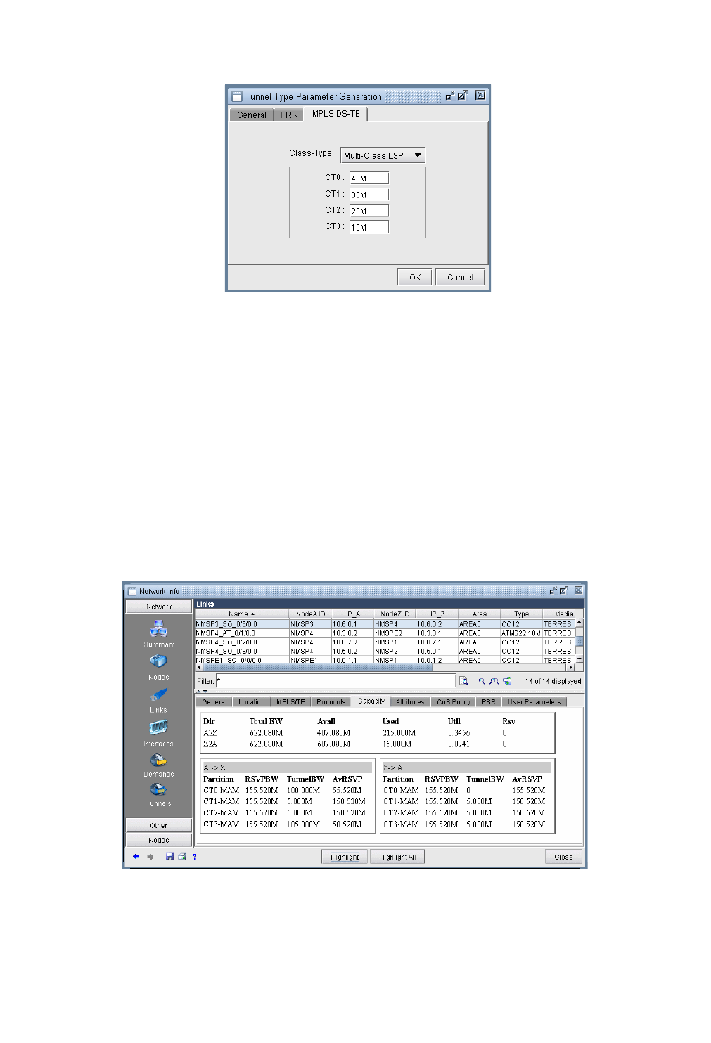
DIFFSERV TRAFFIC ENGINEERING TUNNELS*
Copyright © 2014, Juniper Networks, Inc. 29-11
. . . . .
Figure 29-7 Assigning bandwidth per class to a multi-class LSP
TUNNEL ROUTING
WANDL’s routing engine automatically determines the optimal placement of DiffServ-aware LSPs based on the
amount of bandwidth reserved per class on the LSP and the amount of bandwidth reserved per class on all available
links in the network. A DiffServ-aware LSP will not be routed over any interface that has insufficient bandwidth
allocated to any of the classes defined on the LSP.
LINK UTILIZATION ANALYSIS
With WANDL’s link object, it is easy to determine the amount of total bandwidth, used bandwidth, and available
bandwidth for each class on the link. In the screenshot below, each class is reserved 25% of the bandwidth on each
interface on the link. For the A-Z interface, 100 Mb of bandwidth is being used for DiffServ-aware LSPs that carry
CT-2 and CT-3 traffic. For the Z-A interface, 5 Mb of bandwidth is being used from the CT-0, CT-1, and CT-2
partitions.
Figure 29-8 Link capacity window showing tunnel traffic
It should be noted that the available bandwidth being reported in the window above is the available bandwidth for
tunnels with a pre-emption priority of seven. In other words, the model assumes that none of the existing tunnels
currently residing on the link can be bumped off the link by another tunnel.

DIFFSERV TRAFFIC ENGINEERING TUNNELS*
29-12 Copyright © 2014, Juniper Networks, Inc.
29

Copyright © 2014, Juniper Networks, Inc. 30-1
. . . . .
. . . . . . . . . . . . . . . . . . . . . . . . . . . . . . . . . . .
F
AST
R
EROUTE
*
30
his chapter describes how to design Fast Reroute (FRR) backup tunnels. Fast Reroute is a mechanism that
can be used to protect MPLS traffic engineering LSP tunnels in the event of node or link failures. It
accomplishes this with SONET-like restoration times by locally repairing the LSPs at the point of failure,
using backup tunnels that bypass the failure while waiting for the head-end routers to establish a new LSP. The short
restoration times are especially desirable for real-time applications such as voice over IP, which often cannot tolerate
high delays.
The WANDL software supports simulation and design of both FRR Node Protection and FRR Link Protection.
When a tunnel that has requested FRR protection fails at a particular network element and when there is a FRR
backup tunnel configured for that node or link, the packets can be diverted along the backup tunnel until the original
tunnel is able to reroute around the failed network element.
*Note that a special password is required for the FRR feature and for LSP tunnels. Please contact your Juniper
representative for more information.
Overview
GRAPHICAL DISPLAY
IP/MPLSView can be used to import existing tunnel path information collected through show commands and to
graphically display all the FRR backup tunnel paths protecting the links or nodes of a primary tunnel, and all the
primary tunnels being protected by a given FRR backup tunnel.
WHAT-IF STUDIES AND PATH DESIGN
Users can perform what-if studies by configuring primary tunnels to request FRR protection, and then allow
IP/MPLSView to design the FRR backup tunnels. IP/MPLSView can be used to simulate the creation of backup
tunnels in the case where it is automatically generated for what-if studies, or to help design diverse backup tunnels in
the case where the user wants to configure the backup tunnels to meet particular diversity requirements.
Consequently, LSP configlets can be generated to facilitate the process of updating the routers.
FAILURE SIMULATION
Furthermore, IP/MPLSView can also be used to perform failure analysis, showing whether the demands are
successfully protected through FRR during node or link failure, and then indicating the rerouted path onto the
backup path, if configured, whether it be secondary (passive) or standby (active/1+1). Users can view the peak
utilization when using FRR.
SUPPORTED VENDORS
This document covers Cisco and Juniper implementations in particular. However, IP/MPLSview also supports FRR
for additional router vendors, such as Alcatel and Tellabs.
JUNIPER
There are two methods of FRR protection for Juniper. One method is one-to-one (fast reroute) backup protection in
which case detour(s) are created to protect the nodes and links traversed by a single primary LSP. These detours are
dedicated in the sense that they can only be used for one primary LSP. To configure for one-to-one protection, the
user should configure the primary tunnel using the “fast-reroute” statement.
The other method of local protection for Juniper is many-to-one (facility) backup. In facility backup, a bypass tunnel
is used to route around a facility (node or link), and the bypass tunnel can be used to protect multiple primary LSPs
using the facility that are enabled for FRR. For Juniper’s facility backup, two things need to be configured:
T

FAST REROUTE*
30-2 Copyright © 2014, Juniper Networks, Inc.
30
(1) The primary tunnel is configured to enable link protection or node-link protection.
(2) The link interface(s) are configured to enable local protection. Node protection can be turned off for a particular
interface if only link protection desired.
After these configurations are made, bypass tunnels will be created for the FRR-enabled facilities along the paths of
the FRR-enabled primary tunnels-- either next-hop bypasses to circumvent the primary tunnel’s links in the case of
link-protection or next-next-hop bypasses to circumvent the primary tunnel’s nodes in the case of node-link-
protection. IP/MPLSView can be used to configure the primary tunnels for facility backup and to simulate the
creation of the bypass tunnels for each facility of the primary tunnel.
An additional feature provided by Juniper for facility backup is the option to use multiple bypass LSPs to protect an
interface. (By default, only one bypass LSP protects one interface.) In this case, the user can configure additional
parameters to specify the bandwidth and subscription factor of the multiple bypasses to be created. IP/MPLSView
can be used to simulate the creation of multiple bypasses or to design diverse paths for the multiple bypass tunnels
and to generate the corresponding LSP configlets.
Finally, for diffserv-te, users can also configure what type of LSPs to protect (single-class, multi-class or any). In the
case of single-class LSPs, the user can configure the class type (CT0, CT1, CT2, or CT3). In the case of multi-class
LSPs, users can configure a percentage for each class type.
CISCO
For Cisco’s FRR implementation, three things need to be configured:
•(1) The primary tunnel is configured to enable FRR
•(2) The backup tunnel is configured for each link of the primary tunnel, and
•(3) The protected link is configured to use the backup tunnel.
IP/MPLSView can be used to automate the creation of the backup tunnels given either the primary tunnel
configuration (1) or the links to be protected (3). Configlets can be created for the backup tunnels to help automate
the configuration of the backup tunnels.
An additional feature provided by Cisco is the option to specify the bandwidth pool (sub-pool, global-pool, or any)
the traffic must belong to in order to be protected by the backup tunnel.
When to use
Use WANDL’s Fast Reroute features to view or modify FRR configurations, to design FRR backup tunnels for your
network, and to generate configlets for primary and backup tunnels where applicable. You should also use this
feature to simulate and analyze the impact or effectiveness of your FRR backup tunnels on the network in the event
of network element failures.
Prerequisites
You should have LSP tunnels defined in your network model.
If you want your FRR backup tunnels to be routed over site-diverse or facility-diverse (SRLG) paths, you should
first create sites and facilities on your network. Please refer to the chapter on modification in the Design & Planning
Guide for more details on how to add sites and facilities.
Related Documentation
For general step-by-step instructions on how to use the WANDL software, including how to add sites and facilities,
please refer to the Design & Planning Guide.
For instructions on how to view or modify the tunnels in your network, refer to Chapter 20, LSP Tunnels* .
For general information on simulation, refer to the Simulation chapter of the Design & Planning Guide.
Outline
1. Import Config and Tunnel Path on page 30-3
2. Viewing the FRR Configuration on page 30-3
3. Viewing FRR Backup Tunnels protecting a Primary Tunnel on page 30-5

FAST REROUTE*
Copyright © 2014, Juniper Networks, Inc. 30-3
. . . . .
4. Viewing Primary Tunnels Protected by a Bypass Tunnel on page 30-6
5. Modifying Tunnels to Request FRR Protection on page 30-7
6. Modifying Links to Configure Multiple Bypasses (Juniper only) on page 30-8
7. Modifying Links to Trigger FRR Backup Tunnel Creation (Cisco) on page 30-9
8. FRR Design on page 30-10
9. FRR Auto Design on page 30-14
10. FRR Tuning on page 30-17
11. Viewing Created Backup Tunnels on page 30-20
12. Generating LSP Configlets for FRR Backup Tunnels on page 30-20 .
13. Failure Simulation: Testing the FRR Backup Tunnels on page 30-21
14. Exhaustive Failure on page 30-23
15. Appendix: Link, Site and Facility Diverse Paths on page 30-24.
Detailed Procedures
Import Config and Tunnel Path
1. In the Live Network, configuration file and tunnel path information can be automatically collected using the
Scheduling Live Network Collection task’s collection types “Configuration,” “Tunnel Path,” and “Transit
Tunnel.” Note that the online data collection requires a special password. Refer to the Management &
Monitoring Guide for more details.
2. Otherwise, in offline mode, collected configuration files and tunnel path information can be imported through
the Import Network Wizard via the File>Import Data menu.
3. To import configuration information in offline mode, select the import type “Router Configuration” and
select the Import Directory containing the configuration files. When performing an import of network
configuration data, the WANDL software automatically records those links that are FRR-enabled as well as
those LSP tunnels that request FRR protection. Refer to Chapter 2, Router Data Extraction for more details on
importing router configuration files.
4. To import the tunnel status and path information in offline mode, select the import type “Tunnel Path” and
select the Import Directory containing the tunnel path show command output. Refer to MPLS Tunnel
Extraction* on page 2-15 in Chapter 2, Router Data Extraction for more details on the commands to collect this
information.
Viewing the FRR Configuration
5. In offline mode, switch to Design mode by clicking on the “Design” button on the main menu bar.
6. Select Network > Elements > Tunnels.
7. The Type column can be used to determine the type of each tunnel, whether it is a primary tunnel requesting
FRR protection or an FRR backup tunnel.
CISCO
•For the Cisco FRR implementation, the Type field will indicate “FRR” for the primary tunnel to be protected and
“FRRLK” or “FRRND” respectively for the backup tunnels around the link or node to be protected.
JUNIPER
•For Juniper one-to-one (fast reroute) backup, the Type field will indicate “FRR” for the primary tunnel configured
with the “fast-reroute” statement.
•For Juniper many-to-one (facility) backup, the Type field will indicate “LP” or “NLP” corresponding to the “link-
protection” and “node-link-protection” statements, respectively. For the node and link bypass tunnels created for
facility backup, the Type field will indicate “FRRLK” or “FRRND” respectively for next-hop and next-next-hop
bypass tunnels.
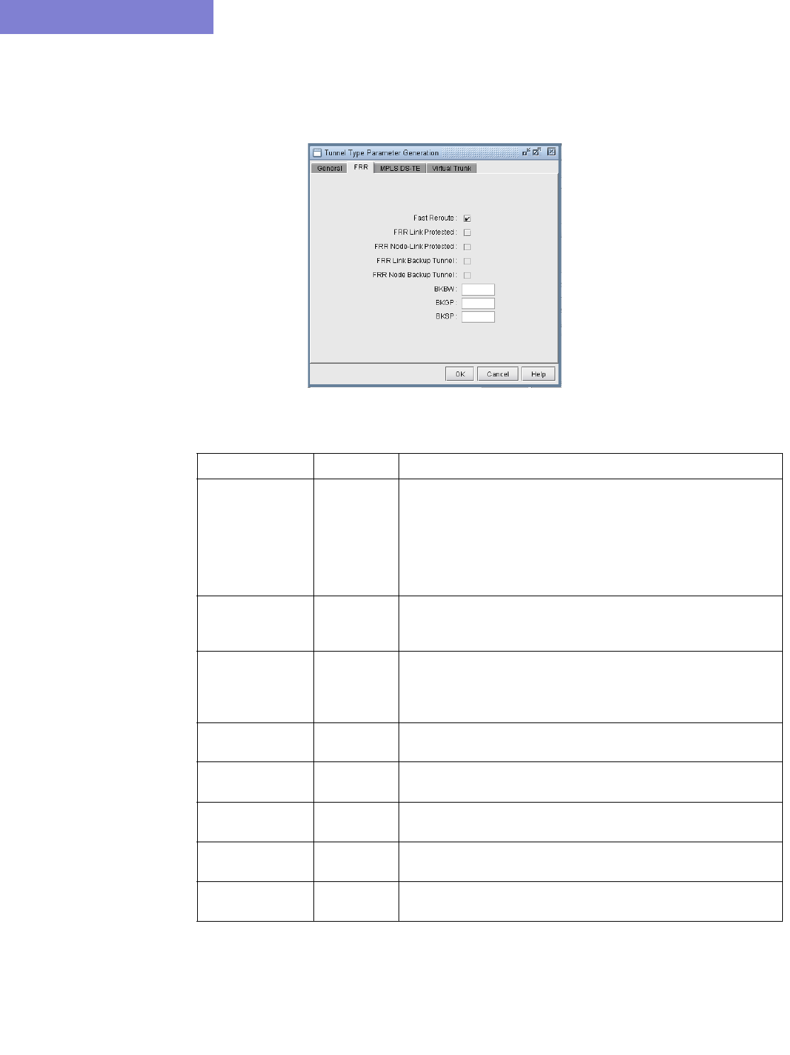
FAST REROUTE*
30-4 Copyright © 2014, Juniper Networks, Inc.
30
8. Click on a tunnel in the top half of the Tunnels window. In the Properties tab, click the link to the right of the
Type field to open the Tunnel Type Parameter Generation window. Select the FRR tab for the following
window, which is populated based on the Type field.
Figure 30-1 LSP Tunnel Requesting FRR Protection
Option Type Field Interpretation
Fast Reroute FRR For Juniper, this field indicates that the primary LSP is being
configured for one-to-one (fast reroute) backup, in which case the
created detour would protect only this tunnel.
For Cisco, this field is used to enable the primary tunnel to use a
backup tunnel (configured separately) in case of node or link
failure.
FRR Link
Protection
LP For Juniper, this field indicates the primary tunnel being configured
for many-to-one (facility) backup for link protection. The resulting
bypass paths could be used to protect many LSPs.
FRR Node-Link
Protection
NLP For Juniper, this field indicates the the primary tunnel being
configured for many-to-one (facility) backup for node-link
protection. The resulting bypass paths could be used to protect
many LSPs.
FRR Link Backup
Tunnel
FRRLK This field indicates the next-hop bypass tunnel which can bypass a
single link for multiple LSPs.
FRR Node Backup
Tunnel
FRRND This field indicates the next-next-hop bypass tunnel which can
bypass a single node for multiple LSPs.
BKBW BKBW=<bw> Indicates how much bandwidth the FRR backup tunnel is
configured to protect.
BKGP BKGP=<bw> For Cisco only. Indicates how much Global Pool bandwidth the
FRR backup tunnel is configured to protect.
BKSP BKSP=<bw> For Cisco only. Indicates how much Sub Pool bandwidth the FRR
backup tunnel is configured to protect.
FAST REROUTE*
Copyright © 2014, Juniper Networks, Inc. 30-5
. . . . .
Viewing FRR Backup Tunnels protecting a Primary Tunnel
9. To view the FRR backup tunnels protecting a primary tunnel configured for FRR, first identify a primary tunnel
marked with either FRR (for Cisco), LP (for Juniper), or NLP (for Juniper) in the Type field. To list only the
primary tunnels configured for fast reroute, you can click the “Search by Property” magnifying glass icon on
middle bar to perform a search. In the Find Tunnels window, click the “Type” button. Then, in the FRR tab of
the Tunnel Type Parameter Generation window, set the Fast Reroute selection box to say “Yes”. This
will filter on all primary tunnels configured for fast reroute, including primary tunnels configured for link
protection , node protection, and one-to-one protection. Click “OK” to close the Type window and then click
“OK” in the Find Tunnels window. All primary LSP tunnels requiring FRR Protection will be displayed in a
table. Select any tunnel and click “Show Path” to view the route of the selected tunnel.
10. Right-click on the primary tunnel configured for FRR to view the options “Show FRR Backup Tunnels” or
“FRR Detour.”
If the head-end router is a Cisco router, select “Show FRR Backup Tunnels” to view the Cisco backup
tunnel(s) protecting the primary tunnel.
If the head-end router is a Juniper router, select “Show FRR Backup Tunnels” to view the Juniper next-hop
or next-next-hop bypass tunnels created for many-to-one (facility) backup for the primary tunnel. Select “FRR
Detour” to view Juniper detour tunnel(s) created for one-to-one (fast reroute) backup for the primary tunnel.
Note that for a multi-vendor network, it may be helpful to display the router vendor as a column. Right-click on
the table column header and select Table Options... Then select “NodeA.Hardware” from the “Available
Item(s)” list and select the right arrow to move this to the “Selected Item(s)” list. Use the up and down arrows to
move “NodeA.Hardware” column up. Click OK. Right-click on the column header again and select “AutoFit.”
11. After selecting “Show FRR Backup Tunnels” or “FRR Detour,” a Path window will be displayed with
two sections. The top contains the primary tunnel being protected. The bottom contains the backup tunnels
protecting each applicable link (or node) of the primary tunnel. Click on an entry to highlight it on the map.
Figure 30-2 Primary Tunnel (Yellow) and One of Three Bypass Tunnels (Green)
Figure 30-3 Tunnel Paths Window
If the Top and Bottom path overlap, you may want to turn off the Top path display by selecting None next to Show
Top Path.
FAST REROUTE*
30-6 Copyright © 2014, Juniper Networks, Inc.
30
Viewing Primary Tunnels Protected by a Bypass Tunnel
12. To view primary tunnels protected by a bypass tunnel, in Design mode, select Design > TE Tunnels > FRR
Design.
13. This window indicates a list of all the node pairs (Node A, Node Z) in the network for which there could
potentially be a bypass tunnel originating from the Node A and terminating at the Node Z.
14. If a bypass tunnel exists, it will be displayed under the Backup Tunnel column. The Type column will
indicate the relevant element type being protected (node or link) and the Link Name and Protected Node
fields will be populated accordingly.
15. Select an entry with a bypass tunnel name listed under the Backup Tunnel column and a nonzero number of
protected primary tunnels under the # Prot Prim Tun column, and click “Show Paths.”
16. The resulting Path window indicates the bypass tunnel, the Protected Path (e.g., the link being protected), and
then the names of the primary tunnels protected by the bypass tunnel. Click on an entry in the Path window to
highlight the corresponding path on the map window.
Figure 30-4 Protected Tunnels
17. To view a list of Fast Reroute backup tunnels from the Tunnels window, perform a filter in the Network >
Elements > Tunnels window, this time setting either the FRR Link Backup Tunnel selection box or the
FRR Node Backup Tunnel selection box to “Yes”. Note that the corresponding type field for backup tunnels
is FRRLK and FRRND, respectively.
Figure 30-5 Filtering for all FRR-LK Backup Tunnels
You could also do an advanced filter (click the Advanced Search icon with the two magnifying glasses) using
the string “Type = FRRND or Type = FRRLK” to filter for both FRR link and node backup tunnels.
FAST REROUTE*
Copyright © 2014, Juniper Networks, Inc. 30-7
. . . . .
Modifying Tunnels to Request FRR Protection
The following steps illustrate how to set up the network model before running an FRR Design, in case you wish to
design for FRR using IP/MPLSView.
18. Switch to Modify mode by clicking on the “Modify” button on the main menu bar.
19. Go to Modify > Elements > Tunnels. In the Tunnels view pane,, select the tunnels for which you would like
to add FRR protection. You can do this by either using the “Search by Property” magnifying glass icon to
retrieve a subset of tunnels, or simply by highlighting the rows of interest in the main table (using <Ctrl>-click
or <Shift>-click for multiple selection).
20. For this example, select the tunnel(s) for modification. Then, press the “Modify” button and choose “Selected
Entries.”
21. The Modify Tunnel window will appear. Click on the “Type” button to modify the tunnel type specification.
The Tunnel Type Parameter Generation window will appear. Select the FRR tab.
Figure 30-6 LSP Tunnel Requesting FRR Protection
22. In the Tunnel Type Parameter Generation window, FRR tab, check off the appropriate option:
•“Fast Reroute” checkbox (for Cisco FRR or for Juniper one-to-one protection)
•“FRR Link Protected” or “FRR Node-Link Protected” (for Juniper many-to-one/facility protection)
23. Click “OK”. Notice that this merely populates the tunnel’s Type field with the word “FRR” (for Cisco) or “LP”
or “NLP” for Juniper, indicating that this is a primary tunnel that is FRR-enabled. This tunnel is requesting FRR
protection. You can also type this in directly in the comma-separated Type field rather than going through the
Tunnel Type Parameter Generation window. Make sure that properties listed in the Type field are comma-
separated, and that the Type field does not contain any spaces. For example, “R,FRR” is valid. However, “R,
FRR” is not.
24. Click OK to close the Modify Tunnel window and make the modification.
25. Having made this modification, an FRR Design (described later in this chapter) can be used to automatically
create either (a) FRR-Link Protection (FRR-LP) backup tunnels for each of the links that this tunnel traverses,
or (b) FRR-Node Protection (FRR-NP) backup tunnels for the intermediate nodes that this tunnel traverses,
depending upon whether the user selects to design for node or link protection.
FAST REROUTE*
30-8 Copyright © 2014, Juniper Networks, Inc.
30
Modifying Links to Configure Multiple Bypasses (Juniper only)
26. To generate multiple bypass tunnels to protect an interface, switch to Modify mode.
27. Select Modify > Elements > Links.
28. Select the links to be modified and click Modify....
29. Click the MPLS/TE tab.
Figure 30-7 Auto Bypass Parameters
30. In the MPLS/TE Parameters section, select “yes” from the FRR A and/or FRR Z selection boxes
depending upon which side of the link will be protected. This will enable the corresponding column in the Auto
Bypass Parameters section.
31. In the Auto Bypass Parameters section, the following fields can be configured:
•Max Num Bypasses: Indicates the maximum number of bypass tunnels for protecting an interface. This
statement enables multiple bypasses for link protection.
•Bandwidth: Indicates the bandwidth of each of the bypass tunnels created
•Subscription: Indicates the percentage of primary tunnel bandwidth that can be protected by each bypass
tunnel. For example, setting the subscription factor to 2000 % enables a bypass tunnel of bandwidth 50K to
protect a primary tunnel of bandwidth 1M.
•Node Protection: Indicates whether the bypass tunnels created will protect a node (if on) or link (if off)
FAST REROUTE*
Copyright © 2014, Juniper Networks, Inc. 30-9
. . . . .
Modifying Links to Trigger FRR Backup Tunnel Creation (Cisco)
32. Another way to trigger IP/MPLSView to create FRR Backup Tunnels during FRR Design (in addition to
modifying tunnels as described in the previous section) is to modify the MPLS/TE parameters in the Link
window. In this example, you will modify five links to require backup tunnels.
33. Select Modify > Elements > Links.
34. Select the links to be modified and click Modify....
35. Click the MPLS/TE tab.
36. In the MPLS/TE Parameters section, select “yes” from the FRR A and/or FRR Z selection boxes
depending upon which side of the link will be protected. This will enable the corresponding column in the Auto
Bypass Parameters section.
EXAMPLE
37. Suppose the following five links are selected, which are highlighted in the figure on the left, and that FRR A and
FRR Z were set to “yes” to indicate to the IP/MPLSView FRR Design to create backup tunnels for these
facilities.
Figure 30-8 Source-Destination Pairs for Possible FRR-LP tunnels (left) and FRR-NP tunnels (right)
38. During FRR Design, if designing for link protection, ten possible backup tunnels can be created (five in the A to
Z direction and five in the Z to A direction-- because both FRR A and FRR Z were set to “yes”).
39. If designing for node protection, ten possible backup tunnels can also be created; each originates at a Node A
and terminates at some next-next-hop. Again, five are created in the A to Z direction, and five in the Z to A
direction. This results in the star pattern in the fish network on the right in Figure 30-8. The FRR-NP (Node
Protection) tunnel will protect against a failure of the node in between the source and destination nodes,
bypassing it.
FAST REROUTE*
30-10 Copyright © 2014, Juniper Networks, Inc.
30
FRR Design
Once you have specified which tunnels (or links) require FRR backup tunnel protection, you can then proceed to run
the FRR Design. The FRR Design feature is powerful and flexible. Not only does it automate the design, but it also
allows you to specify a number of parameters to control various aspects of the design.
Note: You should have already specified which LSP tunnels require FRR protection, or have enabled the FRR flags
for the desired links as mentioned in the previous sections. As mentioned in the prerequisites, you should also have
created any facilities and sites if you want site-diverse or facility-diverse paths.
40. Switch to Design mode by clicking on the Design mode button. This feature is only available in Tunnel layer
mode. If you are not in Tunnel layer, you will automatically be switched into that layer first.
41. Then select Design > TE Tunnels > FRR Design to open up the Tune FRR Backup Tunnels window.
Figure 30-9 Tune FRR Backup Tunnels Window
42. If there are no FRR backup tunnels, a popup window will be displayed providing the option to automatically
generate the FRR backup tunnels. There are two options for design:
(a) You can either allow the program to perform an automatic design for all the tunnels and links requesting FRR
backup protection in this window by answering yes to the popup explained in the previous step. (If you answer
answer no, you can still come back to this automatic design option by clickng the Auto Design button.)
(b) Alternatively, you can selectively view or tune FRR Backup Paths from the Tuning window by selecting the
entry or entries of interest and then selecting Tune>Selected. For example, you can choose to create an FRR
link backup tunnel for an entry of type Link with a particular Link Name for the link to protect, or create an
FRR node backup tunnel for an entry of type Node with a particular Protected Node.

FAST REROUTE*
Copyright © 2014, Juniper Networks, Inc. 30-11
. . . . .
TUNE FRR BACKUP TUNNELS FIELDS
•Node A, Node Z: The source and destination node pair for a potential FRR Backup tunnel.
•Link Name: For Link Protection tunnels, this is the name of the link being protected. For Node Protection
tunnels, this is the name of the link between the Point of Local Repair (PLR) router and the node being protected.
•# Primary Tunnels: Indicates the number of FRR-enabled primary tunnels traversing through the link between
Node A and Node Z.
•Primary Tunnel BW: Indicates the total bandwidth of all the FRR-enabled primary tunnels traversing through
the link between Node A and Node Z.
•Backup Tunnel: The name of the newly created backup tunnel. This is automatically assigned by the WANDL
software. The backup tunnel name typically begins with “FRRLK” or “FRRND”.
•Backup BW: The amount of bandwidth the newly created backup tunnel can protect.
•Protected Pool: Indicates the type of primary tunnel that the newly created backup tunnel can protect: Sub-
pool or Global-pool
•# Prot Prim Tun: Indicates the number of FRR-enabled primary tunnels actually carried/protected by the
backup tunnel.
•Type: Indicates the type of backup tunnel: Link Protected or Node Protected.
•Protected Node: For FRR Node Protection tunnels, this indicates the node whose failure is being protected
against.
•Prot Prim Tun BW: Indicates the total bandwidth of the FRR-enabled primary tunnels actually carried by the
backup tunnel.
•RSVP BW: The actual bandwidth reserved for the tunnel
•Design BW: The bandwidth value that is used for constraint-based routing to determine the placement of the
backup tunnel during a design. This can be different from the RSVP BW actually configured on the backup tunnel
and the Backup BW.
•Div Level: Indicates whether the backup tunnel has a route that is Link-Diverse, Site-Diverse or Facility-Diverse
from the protected path. Use the Evaluate button to update the diversity level for a particular type of diversity
(Facility, Link, or Site)
•Path Violation: Indicates whether there is a path violation in the backup tunnel path
•Backup Route: The route for the newly created backup tunnel, if one is found. If no route is found, then this
field will say “Unplaced”.
OPTIONS
•Evaluate: Updates the Div Level column to show the diversity level between the protected path and its backup
tunnel. Available diversity evaluation options are Facility, Link, or Site. For example, if you want to see whether
the protected path is on a facility-diverse path from its backup tunnel, select Facility.
•Tune>Selected: Brings up a window with options for tuning the selected entries by creating or modifying the
backup tunnel for that entry
•Delete>Selected: Deletes the backup tunnel(s) listed in the selected entries
•Auto Design: Brings up a window with options for creating backup tunnels for all entries
•Show Paths: Displays paths of backup tunnel, protected segment, and protected tunnels. Select an entry with a
Backup Tunnel and positive value for # Prot Prim Tun before clicking this button.
•Show All: Displays node to node connections of all backup tunnels on the Map window.
•View Path Details: Opens up a Tunnel window listing only the FRR backup tunnel
•View Protected Tunnels: Opens up a Tunnel window listing only the primary FRR-enabled tunnels that the
selected FRR backup tunnel protects.
•Report: Saves the Tune FRR Backup Tunnels table into a comma separated report
Note: The columns of the Tune FRR Backup Tunnels window can be customized. That is, you can choose just a
subset of the many columns to appear. To access this feature, right click on a column header and choose Table
Options from the popup menu.
FAST REROUTE*
30-12 Copyright © 2014, Juniper Networks, Inc.
30
AUTO DESIGN PARAMETERS
Figure 30-10 FRR Design - Basic Options Tab
•Diversity Level: Select Link, Site, or Facility diversity for the link being protected and its FRR backup tunnel
to be routed on link-disjoint paths, site-disjoint paths, or facility-disjoint paths, respectively. For Site diversity,
the FRR backup tunnel is to avoid, if possible, nodes that are in the same site as the link and its endpoints.
Facility and Link diversity operate similarly. If Facility diversity level is selected, then the link and backup
tunnel route should not intersect at any of the nodes or links defined in the facility. Recall that a facility is a user-
defined group of nodes and links and is commonly used to represent Shared Risk Link Groups (SRLG). For more
information, refer to Appendix: Link, Site and Facility Diverse Paths on page 30-24
•Protection Type: Specify Link or Node/Node-Link to indicate whether you wish to design FRR Link
Protection or FRR Node Protection tunnels, respectively. Specify Auto Bypass to automate bypass creation for
Juniper based on the configuration parameters on the interface.
•Design Bandwidth (for Design/Placement): The Design Bandwidth is used for Design purposes only, to decide
where to place the tunnel, and is not used to set the actual RSVP bandwidth. The backup tunnels will be placed by
the program using constraint-based routing assuming that it would reserve a certain bandwidth along the tunnel
route for the tunnel to be placed. However, once the placement is done, the actual tunnel’s RSVP bandwidth can
be set to a different value, using the following Set RSVP Bandwidth option.
The Design Bandwidth is specified as a percentage of a Reference Bandwidth Source plus a fixed value. The
Reference Bandwidth Source can be the (a) Link Bandwidth:the entire link bandwidth, (b) Sub-Pool
Bandwidth: the subpool bandwidth allocated on the link (for Cisco only), or (c) Sum of FRR Primary
Tunnel Bandwidth: the sum of the bandwidth of all primary FRR-enabled tunnels that the backup tunnel
protects (for Juniper). By adjusting the % and fixed values (which default to the divpathbwpct and divpathbw in
the dparam file), you can perform overbooking.
Note: Regarding option (b), if the Reference Bandwidth Source is set to Sub-Pool and if the protected link has no
subpool partition, then a backup tunnel will not be designed.
•Set RSVP Bandwidth to: Specifies the actual bandwidth for the backup tunnel, as a percentage of the Design
bandwidth.
•Multiple FRR Tunnel Settings: You can create multiple backup tunnels by specifying either:
(a) Maximum bandwidth per tunnel: This is the maximum bandwidth allowed; tunnels will be split if the
design bandwidth exceeds this value.
(b) Number of tunnels per interface: You can specify directly how many backup tunnels to create on the
interface with each tunnel equally sharing the design bandwidth.
FAST REROUTE*
Copyright © 2014, Juniper Networks, Inc. 30-13
. . . . .
Figure 30-11 FRR Design - Advanced Options Tab
ADVANCED OPTIONS FOR CISCO
•Protect traffic of type: For the backup tunnels that are designed, you can specify the type of tunnel that they
are to protect. If you specify Global-Pool, then the backup tunnels can only protect primary tunnels that are
designated to carry Global-Pool traffic. If you specify Sub-Pool, then the backup tunnels designed can only
protect primary tunnels designated to carry Sub-Pool traffic. If Any is specified, then the backup tunnels
designed are allowed to carry either type of primary tunnel.
Note that if Global-Pool or Sub-Pool is specified, then the newly generated backup tunnel(s) will have “BKGP”
or “BKSP”, respectively, listed in the tunnels’ Type field parameters. By looking at the tunnel type parameters,
the Protected Tunnel Type can be identified. If there is no indication, then the default protected type is “Any”.
•Allocate Backup Bandwidth using: This selection allows you to specify whether the backup bandwidth for
the FRR backup tunnel should be allocated from the links’ Global-Pool or Sub-Pool at the time of failure.
If Sub-Pool is specified, then the newly generated backup tunnel(s) will have “GB” (Guaranteed Bandwidth) in
their Type field. A backup tunnel that does not contain “GB” is by default using Global-Pool bandwidth.
•Tunnel can protect unlimited amount of Backup Bandwidth: Indicates whether the amount of
bandwidth the backup tunnel can protect is limited or unlimited. If checked, this option will allow all primary
tunnels to be routed over the backup tunnel. This is the default. If unchecked, the backup bandwidth will be
limited to the value set in the Design Bandwidth section of the Basic Options tab. This limit is effective at the
time of failure when the backup tunnel is activated.
Note: Setting the Design Bandwidth to 0 is equivalent to allowing Unlimited backup bandwidth.
ADVANCED OPTIONS FOR JUNIPER
•Protect traffic of type: For the backup tunnels that are designed, you can specify the type of tunnel that they
are to protect. Values include Single-Class LSP, Multi-Class LSP, or Any. If Single-Class LSP is selected,
you should then specify one of the resulting options: CT0, CT1, CT2, or CT3. If Multi-Class LSP is selected,
enter in the percentage for each of the 4 classes. For more information about DiffServ-TE, refer to Chapter 29,
DiffServ Traffic Engineering Tunnels*.

FAST REROUTE*
30-14 Copyright © 2014, Juniper Networks, Inc.
30
OTHER OPTIONS
•Prompt to view FRR design report: Selecting this checkbox will cause the FRR Design report to be
automatically displayed once an FRR Design or View/Tune Paths operation has completed. This report is saved to
the Output Path in the File Manager under the name “FRRDSGNRPT.runcode”. To access it in the File Manager,
right-click on the file and choose “Open in Report Viewer”. For more information on the FRR design report,
see FRR Design Report on page 30-15.
FRR Auto Design
43. When the FRR Design parameters are submitted for Auto Design, the program will automatically create
backup tunnels as follows:
•If the Protection Type is set to Link, then FRR Auto Design will automatically design the FRR-LP backup
tunnels necessary to protect (1) Links along the paths of LSP tunnels requesting FRR protection, and (2)
Individual links that have been marked to request FRR protection.
•If the Protection Type is set to Node, then FRR Auto Design will automatically design the FRR-NP backup
tunnels necessary to protect (1) Nodes along the paths of LSP tunnels requesting FRR protection (excluding the
source and destination nodes) and (2) The destination node of links that have been marked to request FRR
protection.
Note 1: When selecting either Node Protection or Link Protection, the Auto Design will automatically
enable FRR for all the links along the paths of LSP tunnels requesting FRR protection. If this is not desired, users
should use tuning instead of auto design, or in the case of Juniper, select “Auto Bypass” as described below.
Note 2: If the Design Bandwidth Reference Bandwidth Source is set to Sub-Pool (for Cisco only) then
only the links that(1) require FRR protection and (2) have subpool bandwidth allocated will be considered for
protection in FRR Auto Design.
•If the Protection Type is set to Auto Bypass (for Juniper bypass creation), then FRR Auto Design will
automatically design the bypass tunnels for Juniper for FRR-enabled links along the paths of FRR-enabled LSP
tunnels. After selecting this option, you will be prompted with the option to design paths using (a) the RSVP
signalling bandwidth as the Design Bandwidth or (b) the Backup bandwidth as the Design Bandwidth. Select
option (a) if you wish to simulate Juniper’s auto bypass generation. Select option (b) to help ensure there is
enough bandwidth on the backup tunnel to protect the primary tunnels.
Note: The Auto Bypass Protection type will preserve the link’s FRR settings and avoid creating backup tunnels
for links not enabled for FRR.
44. Please read through the explanations of the Design options in the previous section carefully for a complete
description of each of the FRR Design options. Though the design options may initially appear complex,
understanding the function of each option will provide you with enormous flexibility. Once you have specified
the desired properties in the FRR Design window, click the “AUTO Design” button.
45. If you already have some existing fast reroute tunnels in the network, you may also see the following
confirmation windows: “Routes and bandwidth for all FRR link protection backup tunnels will be adjusted.
Continue?” or “Remove configured paths for 10 FRR link backup tunnels?”
46. In the Console window, the number of placed/unplaced/deactivated paths for the new tunnels will be displayed.
You should see something similar to this:
Diversity Level= SITE
Tunnel Site+Link-Diversity Link-Diversity No-Diversity Notplaced Deactivated
FRRBackup 10 0 0 0 0
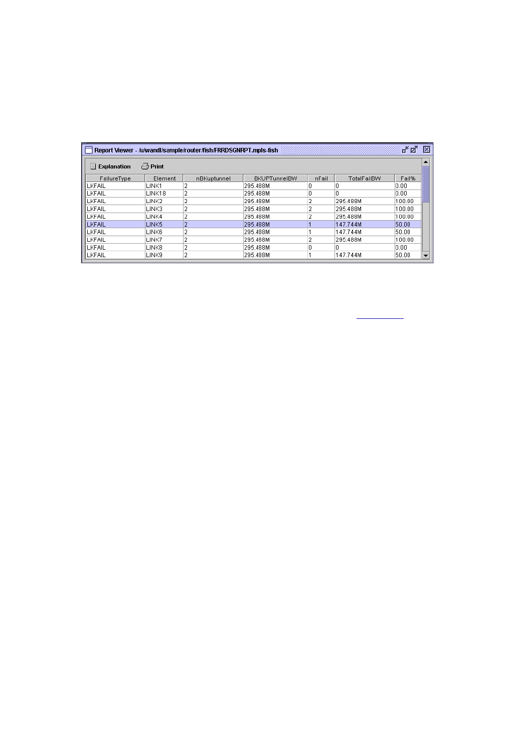
FAST REROUTE*
Copyright © 2014, Juniper Networks, Inc. 30-15
. . . . .
FRR DESIGN REPORT
47. When the design is completed, you will be asked whether you wish to view the FRR design report. The report is
saved as FRRDSGNRPT.runcode in your File Manager Output Path. To view this report at a later time,
right-click on the report in the File Manager and choose Open in Report Viewer from the popup menu.
Note: In order to see the FRRDSGNRPT report listed in the File Manager, you may need to refresh the File
Manager contents first, either by pressing the “Refresh” button or alternatively, the <F5> key.
Figure 30-12 FRR Design Report Generated from Auto Design
After the Auto Design has been performed and FRR backup tunnels created, the FRR Design Report displays
the result of failing each FRR-protected link or node. For example, in Figure 30-12, the highlighted table entry
indicates that when LINK5 is failed, there are two FRR-LP backup tunnels protecting the link. The total
bandwidth of these two backup tunnels is 295.488Mbps. Of these two, one failed to be placed during the link
failure. The total bandwidth of this failed backup tunnel is 147.744Mbps, accounting for 50% of the total
backup tunnel bandwidth.
FRR DESIGN REPORT FIELDS
•FailureType: Possible values are LKFAIL, NODEFAIL, and FACFAIL, indicating link, node or facility
failure.
If the Link Diversity Level was specified for the Auto Design, then the program will take down each node/link
individually and try to find a route that is both site-diverse and link-diverse. If there is none, it will try to find a
link-diverse route.
If the Site Diversity Level was specified for the Auto Design, then the program will take down each node/link
individually and try to find a site-diverse route. If there is none, it will try to find a link-diverse route. The
rationale is that even if site diversity is not met, a link-diverse route is better than no route at all.
If the Facility Diversity Level was specified for the Auto Design, then the program will take down each
node/link individually and try to find a route that is both facility-diverse and site-diverse. If there is none, it will
try to find a link-diverse route.
•Element: Indicates the failed element. If Node Protection Type (or Link Protection Type) was specified
for the Auto Design, then all nodes (or all the links) in the network will be failed and brought back up one at a
time.
•nBKuptunnel: Indicates the number of FRR backup tunnels that are routed through the network Element.
•BKUPTunnelBW: Indicates the total backup bandwidth of all the FRR backup tunnels protecting the failed
element.
•nFail: Indicates the number of backup tunnels that failed to be placed during the element failure.
•TotalFailBW: Indicates the total bandwidth of the backup tunnels that failed to be placed during the element
failure.
•Fail%: Indicates the percentage of backup tunnel bandwidth that failed to be placed during the element failure.
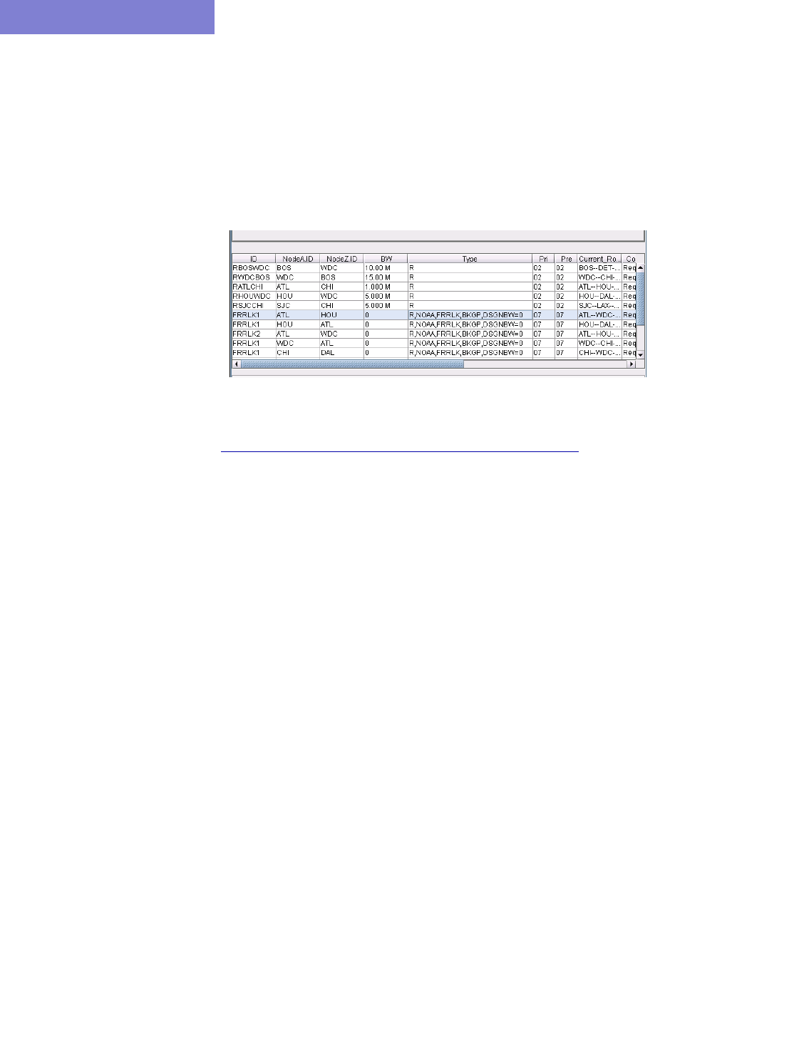
FAST REROUTE*
30-16 Copyright © 2014, Juniper Networks, Inc.
30
VIEW CREATED FRR BACKUP TUNNELS
48. To view the newly designed FRR backup tunnels, select Network > Elements > Tunnels to display all LSP
tunnels in the network. Notice that the Type field will indicate whether the FRR backup tunnels are for Link
Protection (“FRRLK”) or Node Protection (“FRRND”) and that the No Autoroute Announce flag (“NOAA”) is
automatically turned on.
Other possible type fields (for Cisco) are “BKSP” or “BKGP”, indicating that the backup tunnel carries Sub-
Pool or Global-Pool tunnels, respectively; this corresponds to the user’s settings of the Protected Tunnel
Type field in the FRR Design parameters.
Figure 30-13 View of LSP Tunnels after FRR-LP Design
49. You can further examine the FRR backup tunnels created from the View/Tune Paths window as described in
Viewing Primary Tunnels Protected by a Bypass Tunnel on page 30-6.

FAST REROUTE*
Copyright © 2014, Juniper Networks, Inc. 30-17
. . . . .
FRR Tuning
50. The Tune FRR Backup Tunnels window shows a list of the possible FRR-Link Protection or Node
Protection backup tunnels that can be created or optimized. Each entry is characterized by a source and
destination node pair, the Protected Node (if applicable), Link Name and protection Type. This list can be
customized by using the “Filter” button, described later in this section.
Note: You can rearrange columns by clicking and dragging column headers. You can move the Type and
Protected Node columns to the front so that you can see more clearly which tunnel entries are for link
protection or for node protection.
Each entry in the table corresponds to a potential FRR backup tunnel. Only after an FRR backup tunnel has been
designed or tuned will the rest of the columns in its table entry be filled in. To design FRR backup tunnels, select
only those desired entries from the table and then press the “Tune Selected” button. Or, you can press “Tune
All” to tune all the entries shown in the table. This will pop up the Tuning Options dialog window, allowing
you to adjust the FRR design parameters that will be immediately applied to the selected entries.
51. Most of the parameters in the Tuning Options window are identical to those in the FRR Design window,
with a few differences. For example, the following are additional options in Tuning:
Figure 30-14 Additional Options for Tuning (Basic Tab)
The “Create new tunnel(s) using selected tunnels as a template” option will create a new row in the
Tuning window with the same parameters but with an additional backup tunnel protecting the given link or
node. The original row will remain. The “Modify selected tunnel(s) using specific parameters” option
will modify the existing backup tunnel(s) rather than creating an additional backup tunnel.
Figure 30-15 Additional Options for Tuning (Advanced tab)
The “Remove configured paths for existing backup tunnels” option is used to allow for the backup
tunnels’ paths to be redesigned.
52. Specify the desired options in the Tuning Options window and click “OK”. In this example, we tune all the
rows. After tuning, the remainder of each row in the Tune FRR Backup Tunnels window is filled in.
Note: For rows that remain blank in the Tune FRR Backup Tunnels window after tuning for the row, this
indicates that a FRR backup tunnel was not designed. This could happen, for example, if the Reference BW
Source is set to Sub-Pool BW but none of the links listed in the Tune FRR Backup Tu.nnels table have Sub-
Pool BW
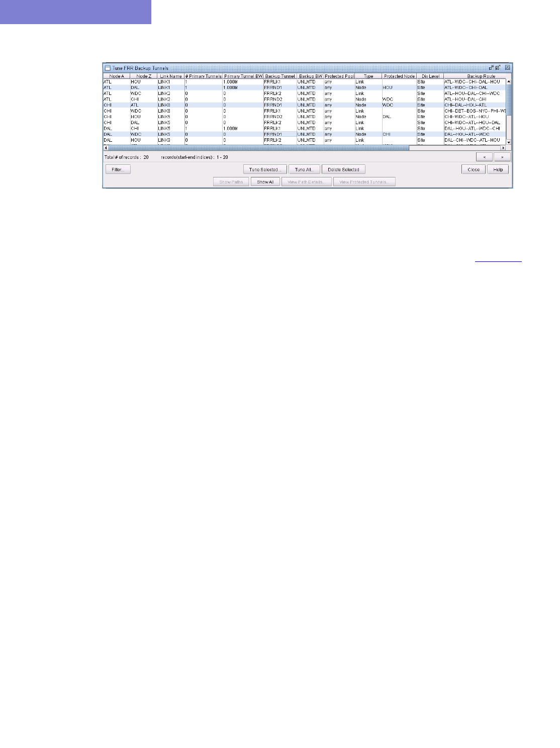
FAST REROUTE*
30-18 Copyright © 2014, Juniper Networks, Inc.
30
Figure 30-16 FRR Paths after Tuning is Complete
53. In this example, all FRR backup paths have been successfully created and are already added to the network.
Note: Backup tunnels created through FRR Design are automatically assigned a name of “FRRLKnum” for FRR
Link Protection tunnels and “FRRNDnum” for FRR Node Protection tunnels. Notice that, in Figure 30-16, there are
three backup tunnels named “FRRND1”. The reason is that tunnels are not required to have unique names unless the
head-end node of the tunnel is the same.
54. Once a tunnel has been “tuned”, the latter columns in the table will be filled in. If an FRR path is successfully
designed and placed, its path will show up in the Backup Route column of the Tune FRR Backup Tunnels
window. Select a row in the table and click on the “Show Paths” button. The path for this tunnel will then be
displayed in the Map window. A Paths window will also appear, allowing you to view either the backup path or
the path of the tunnel being protected.
The Console will also display summary information regarding the total number of placed or unplaced backup
tunnels for this tuning operation. If placed, the console window will indicate how many satisfied Site-Diversity
or Link-Diversity or whether No Diversity was satisfied. For example:
Diversity Level= SITE
Tunnel Site-Div Link-Div No-Div Unplaced Deactivated
FRRBackup 2 0 0 0 0
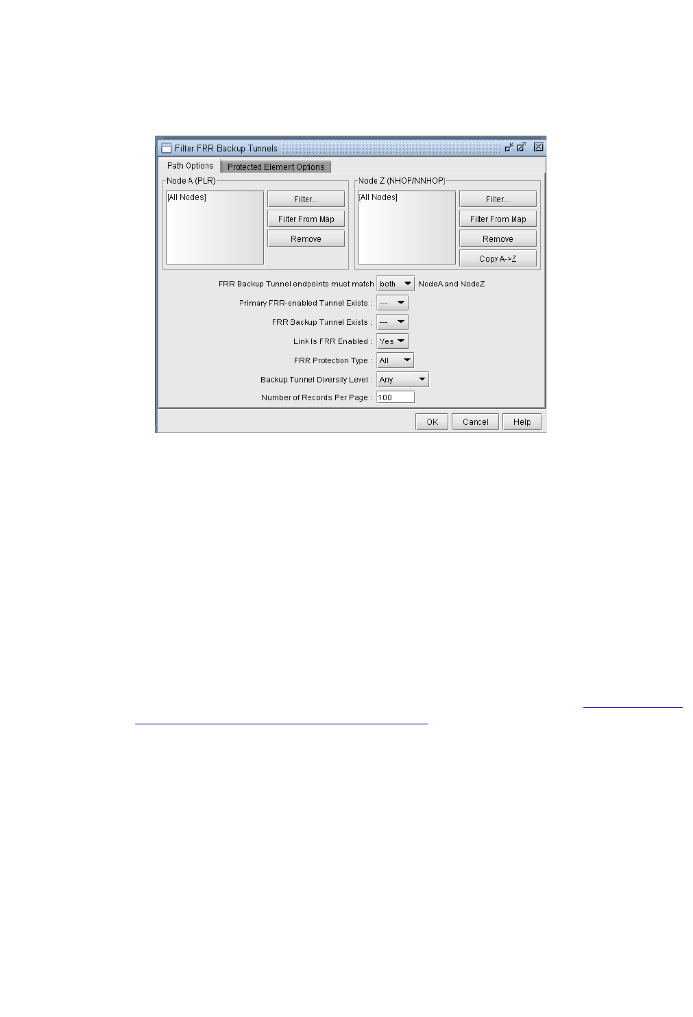
FAST REROUTE*
Copyright © 2014, Juniper Networks, Inc. 30-19
. . . . .
FILTERING IN THE FRR TUNING WINDOW
55. In the Tune FRR Backup Tunnels window, you can also use the “Filter” button to view a more selective set
of entries for which to tune. The following window will appear:
Figure 30-17 Filter for a more specific set of Tuning Entries
•Node A, Node Z:The node A and node Z panels are for selecting a subset of nodes to use for filtering FRR
paths. By default, all nodes in the network are used. Node A is the source, or Point of Local Repair (PLR). Node
Z represents the destination, or the Next Hop / Next Next Hop node.
•FRR Backup Tunnel endpoints must match (either/both) NodeA and NodeZ: This option allows you
to specify the strictness of the endpoint match. Select “either” to match either Node A and Node Z. Select
“both” to require a match of both.endpoints.
•Primary FRR-enabled Tunnel Exists: There are three options: yes, no and "---" which means “don't care”.
Selecting "Yes" means a path will be displayed only if the protected path is part of a primary FRR enabled tunnel.
Selecting "no" means the opposite, and selecting "---" will ignore this option during the filter.
•FRR Backup Tunnel Exists:There are three options: yes, no and "---" which means “don't care”. Selecting
"Yes" means a path is displayed only if a backup tunnel exists for the protected path. Selecting no means the
opposite, and selecting "---" will ignore this option during the filter.
•Link is FRR Enabled:There are three options: yes, no and "---" which means “don't care”. Selecting "Yes"
means a path is displayed only if the link is FRR-enabled, or requests FRR protection. See Modifying Links to
Trigger FRR Backup Tunnel Creation (Cisco) on page 30-9 for information on how to FRR-enable a link.
•FRR Protection Type: This option allows the user to fetch FRR Link Protection paths, FRR Node Protection
paths, or both types of FRR paths if “All” is specified.
•Backup Tunnel Diversity Level:This option allows the user to fetch paths that satisfy facility, link, site, any
or no diversity level.
•Protected Node:Located in the Protected Element Options tab, specifying a particular set of nodes will
bring up only those paths that protect these nodes.
•Protected Interface:Located in the Protected Element Options tab, specifying a particular set of
interface/link will bring up only those paths that protect these links.
•Facilities:Located in the Protected Element Options tab, specifying a particular set of facilities will bring
up only those backup paths that protect any of the nodes or links defined in the facility.
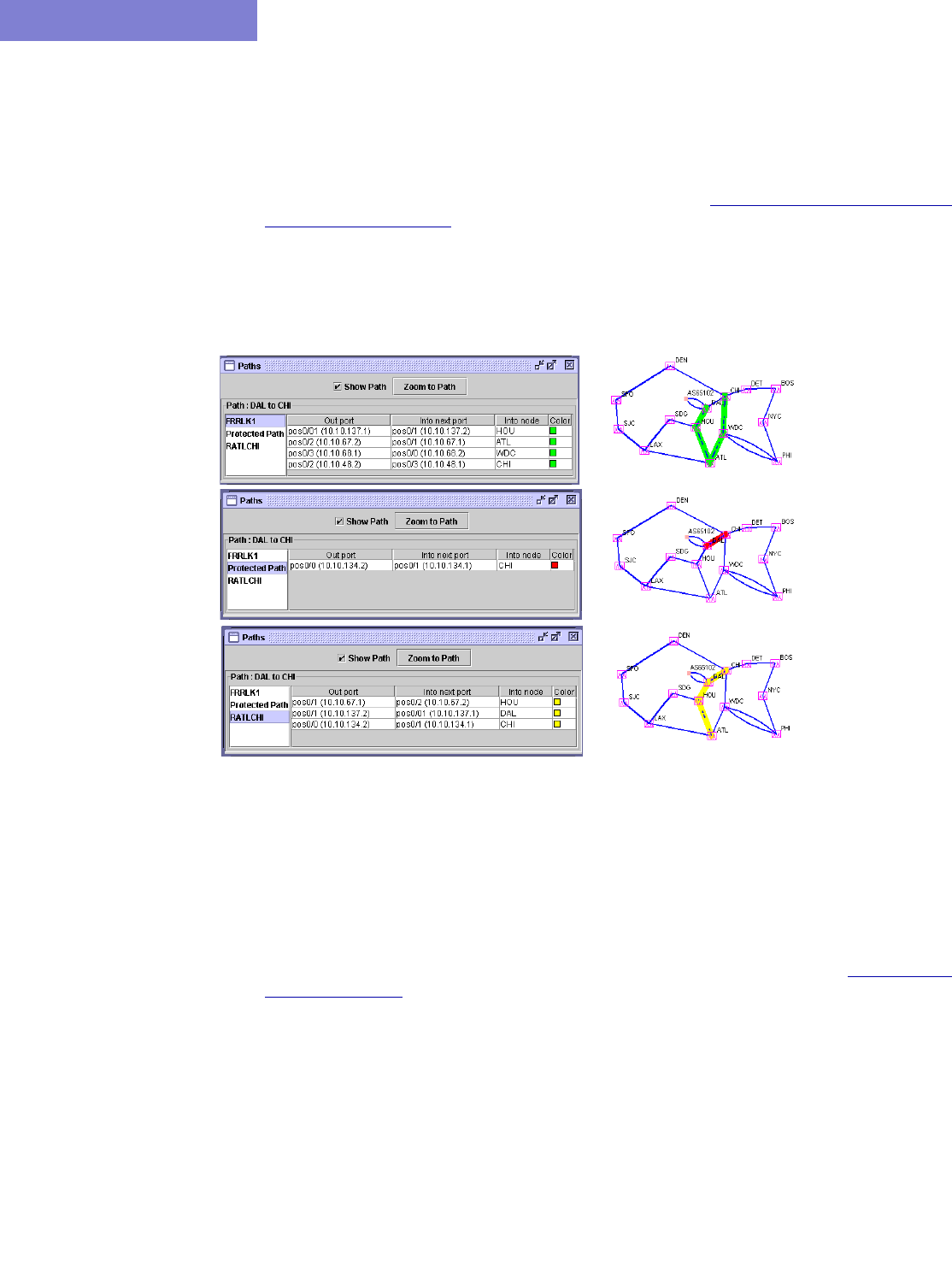
FAST REROUTE*
30-20 Copyright © 2014, Juniper Networks, Inc.
30
Viewing Created Backup Tunnels
56. After performing an FRR Design as described earlier in this chapter, find the created backup tunnel in the
Backup tunnel column. You can sort on this column by clicking on the column header to view existing backup
tunnels, or use the filter button.
57. Click on the “Show Paths” button in the Tune FRR Backup Tunnels window to view both the Protected Path
and the Newly designed Path on the Map window as described earlier in Viewing Primary Tunnels Protected by
a Bypass Tunnel on page 30-6.
58. The Paths window will appear. You can choose from the left-hand side of the window whether to view the path
for the newly designed backup path, FRRLK1, or the path that this backup is protecting (“Protected Path”). If
the protected path is part of LSP Tunnel(s) requiring FRR Protection, then you can also view the protected LSPs
tunnels’path(s). In this example, RATLCHI is the protected LSP Tunnel.
Figure 30-18 Paths Window
59. In the Tune FRR Backup Tunnels window, you can also click on the “View Path Details” button for a selected
entry. This will bring up a similar window to that accessed by Network > Elements > Tunnels. In this
window, click on “Details.” In the Tunnel window, select “Show Path” or “Highlight All” to display the path
on the map.
Generating LSP Configlets for FRR Backup Tunnels
60. Once you have designed the FRR backup tunnels, you may want to generate the corresponding LSP configlets
(statements of a router configuration file) that can then be uploaded to the router. Please refer to Chapter 23, LSP
Configlet Generation* for detailed information.
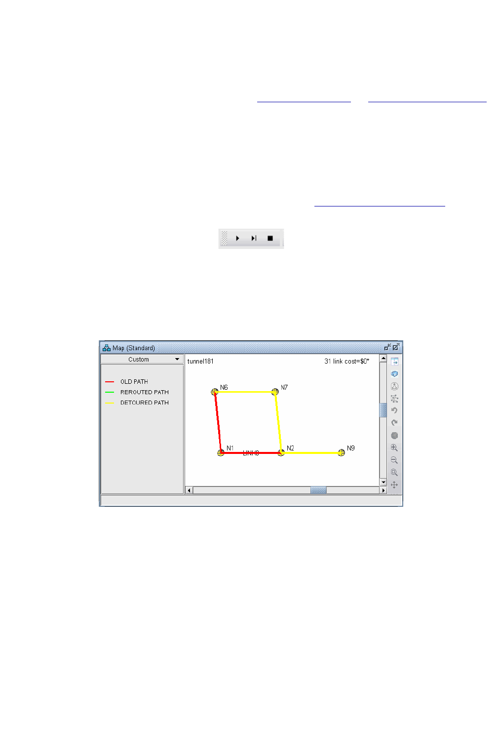
FAST REROUTE*
Copyright © 2014, Juniper Networks, Inc. 30-21
. . . . .
Failure Simulation: Testing the FRR Backup Tunnels
Interactive failure simulation can be performed to fail a set of node(s), link(s), and facilities at the same time. After
the failure, users can view the use of the FRR backup tunnel, followed by the head-end reroute if applicable, or else
the usage of the diverse 1+1 backup (standby) path if configured. For information on configuring diverse backup
paths (e.g., secondary or standby paths) refer to Chapter 20, LSP Tunnels* and Chapter 25, Tunnel Path Design*.
SIMULATING LOCAL PROTECTION
61. To run an interactive failure, click the Simulation button to switch to Simulation mode.
62. Select the desired node(s) or link(s) to fail together by <Ctrl>-clicking the nodes or links with your mouse.
63. Next, right-click over one of the selected node(s) and selecting “Fail Selected Nodes” or right-click over one
of the selected link(s) and select “Fail Selected Links.”
64. Click the step button “>|” on the simulation tool bar to step through each tunnel to see how it is locally rerouted.
(For a faster method, but without graphical display, refer to Using the Run Button on page 30-22.)
Figure 30-19 Simulation Toolbar with Run, Step, and Stop buttons
65. On the Standard map, the old path is highlighted in red and the new path using the backup tunnel is highlighted
in yellow. In this case, the original path was from N9-N2-N1-N6. However, due to the failure of LINK8 between
N2 and N1, the new path taken is N9-N2-N7-N6.
Figure 30-20 FRR Local Protection
66. Note the console menu which displays that the disconnected tunnel is now using the FRR protection path.
tunnel181 N9 N6 100M R,LP 07,00 N9--N2--N1--N6 #!delay=3ms DISCONNECTED
tunnel181 N9 N6 100M R,LP 07,00 N9--N2--N7--N6 #!delay=3ms #DETOURED
SIMULATING HEAD-END REROUTE OR USE OF BACKUP ROUTE
67. Click the Run button to finish stepping through the disconnected traffic and seeing how it gets rerouted locally.
After going through each tunnel to see whether it is detoured or not, there will be a console message indicating
how many tunnels were detoured and how many failed to be detoured.
68. After going through all local protection tunnels, the headend reroute is calculated and displayed on the Console:
tunnel181 N9 N6 100M R,LP 07,00 N9--N2--N7--N6 #!delay=3ms DETOURED
tunnel181 N9 N6 100M R,LP 07,00 N9--N8--N1--N6 #!delay=3ms REROUTED

FAST REROUTE*
30-22 Copyright © 2014, Juniper Networks, Inc.
30
Note that when there is an active backup tunnel, the text will be displayed as “DISCONNECTED, Diverse
pathUp” in which case the routing will switch over to the active backup (standby) tunnel.
In some cases, you may also see the word “RE-Optimized” in case the tunnel allows reoptimization and a
shorter path is found during the failure simulation.
USING THE RUN BUTTON
69. For faster performance, the interactive falure can be run without the graphical display.
70. To start a new simulation, select Simulation > Reset Simulation.
71. Before running through the simulation, select Tools > Options > Report. Under Failure
Simulation>Failure Report, select Yes for Trace File and Display Paths at Failed Nodes options.
This will save the reroute information to a file. Otherwise, only a summary will be displayed in the Console.
72. Select the node(s) and link(s) to fail, either from the map as described earlier, or by checking the checkbox for
the corresponding element from the Simulation > Interactive Scenarios > Fail Link, Fail Node, and Fail
Facility windows. Click the Run button.
73. Open Report > Report Manager while in Simulation mode. Select the Interactive Failure report and scroll
down to view the DETOURED and REROUTED information described earlier in a report rather than on the
console.
RESULTING LINK UTILIZATIONS
74. After running an interactive failure simulation, you can see the resulting link utilizations after the headend
reroute either through the Network > Elements > Link menu Util_AZ and Util_ZA columns and Capacity
tab or through the Report > Report Manager, Planned Link Utilization report under Network Reports
> Link Reports, Util column.
75. The Tools > Options > Failure Simulation window also contains a default FRR Mode option under the
Failure Simulation>FRR option pane. The default setting is FRR + Normal. Select “FRR Only” as the
FRR mode before running an interactive failure simulation to simulate only the FRR local protection and not
the headend reroute.
Figure 30-21 FRR Mode
76. After changing this setting, to start a new simulation, select Simulation > Reset Simulation. Fail the desired
nodes, links, or facilities and click the Run button.
77. To view the utilizations after the local rerouting and before the headend reroute (in the case that there is no 1+1
backup tunnel), go to Report > Report Manager.
78. Check the Interactive Failure report. Only the DETOURED routes should be displayed and not the
REROUTED tunnel routes.

FAST REROUTE*
Copyright © 2014, Juniper Networks, Inc. 30-23
. . . . .
Exhaustive Failure
79. To run an exhaustive failure, click the Simulation button to switch to Simulation mode.
80. Select the Simulation button and go to Simulation > Predefined Scenarios.
Figure 30-22 FRR Failure Simulation Options
During the failure simulation, the WANDL software keeps track of the peak, or worst utilization on each link.
Recall that during a failure, the FRR backup tunnel provides fast restoration times by locally repairing LSPs at
the point of failure, while waiting for the head-end routers to establish a new LSP. The WANDL software can
simulate a number of scenarios.
•Normal: Simulates the “normal” tunnel reroute. Does not consider the effect of the local repair during the
simulation. Peak utilization reflects that during the “normal” situation.
•FRR + Normal: Simulates the FRR local repair first followed by the normal primary tunnel reroute as
established at the head-end router. The resulting link peak utilization report identifies the worst utilization, or max
value of the transient detour and normal modes. Note: A primary tunnel being detoured is marked down if it
cannot be rerouted.
•FRR only: Simulates only the local repair. The resulting link peak utilization report reveals just the peak
utilization experienced during the local repair.
•FRR Design: In this mode, neither the FRR local repair nor the normal primary tunnel reroute is performed. For
each failure during the simulation, the backup tunnels associated with the failed links are turned “on”. That is, its
bandwidth is set to the Backup Tunnel BW (for Design/Placement), or “design bandwidth”. Recall that this
“design bandwidth” is used to determine the placement of FRR routes. In this way, you can determine what the
peak utilization is during the design/placement of the backup tunnels. For a singlefailure simulation, you can
determine where the bottleneck is. You can also use this mode to determine whether there is overbooking, or
whether there is enough bandwidth.
81. Under the Options section, select FRR and “FRR+Normal.” Then select one or more exhaustive single-
element failure scenarios under the Scripts section. (For more information regarding double-element failure
scenarios, refer to the Design & Planning Guide.
82. Next, to saved detailed reroute information including local protection and head-end rerouting to a report, select
Reroute Information under the Report Options.
83. Under Options, select Peak Utilization Report.
84. Click “Run” to start the exhaustive failure simulation.
85. Summary information is indicated in the Console, with the first entry for a failed element corresponding to the
tunnel layer and the second entry corresponding to the demand layer.
86. Go to Report > Report Manager to view the saved report file to view the detoured paths for all the primary
tunnels requiring FRR protection followed by the headend reroute.
87. Select the Peak Link Utilization report under Simulation Reports > Network Statistics to see the worst-
case utilization across all the failure scenarios and the scroll to the last column to view which element failure the
peak utilization occurred at.
88. On the Standard Map, select the Utilization Legends > Peak Util to view the peak utilizations graphically.
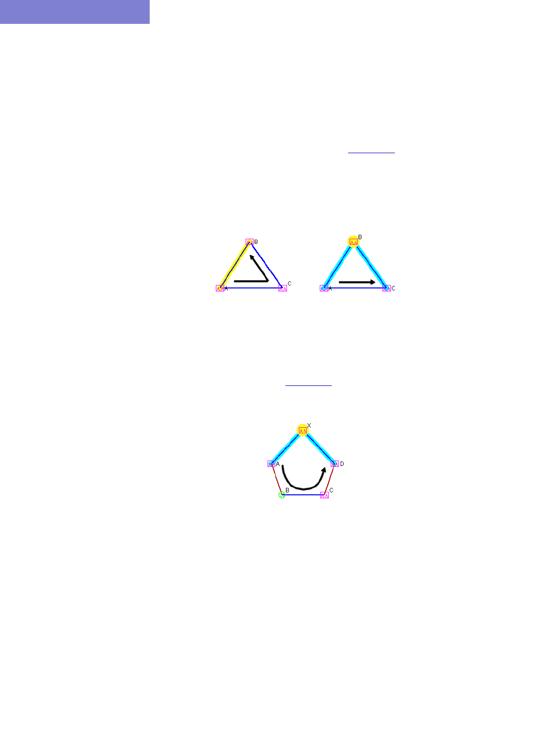
FAST REROUTE*
30-24 Copyright © 2014, Juniper Networks, Inc.
30
Appendix: Link, Site and Facility Diverse Paths
89. From the FRR Design window, the Diversity Level parameter allows you to specify whether the routes for the
FRR-designed backup paths should be Facility-diverse, Site-diverse or Link-diverse from the primary paths.
The WANDL software will then try its best to satisfy the requirements. If a diverse backup path cannot be found,
the software will still attempt to route the backup tunnel if possible. In this situation, if it is routed, this LSP
tunnel will fall into the No-Diversity category. If it cannot be routed, it will fall under the Unplaced category.
LINK DIVERSITY
90. Link diversity is the most fundamental diversity level. Figure 30-23 depicts a link-diverse route in the event of a
link failure or a node failure. In the diagram on the left, the protected link is the link between A and B. A FRR-
LP link-diverse route from A to B is any path that avoids the link between A and B.
The diagram at right depicts a protected node B on the path between nodes A and C. A FRR-NP link-diverse
route is technically any path that avoids both the link between A and B as well as node B.
Figure 30-23 Link Diverse Route for Protecting a Link (left) and Protecting a Node (right)
SITE DIVERSITY
91. A site is a user-defined group of nodes, specified in a site file. If no site file is specified, then by default sites are
mapped with individual routers listed in the node (muxloc) file. Sites are typically defined to indicate a group of
nodes that are likely to fail together. Figure 30-24 depicts a protected node X between A and D. For this
example, to establish a site-diverse route, nodes B and C must not belong to the same site as node X.
Figure 30-24 Site Diverse Route for Protecting a Node
If no site-diverse route exists, the program will attempt to find a link-diverse route, under the presumption that
an alternate route is better than none.
92. When completing an FRR Design with the Diversity Level set to Link or Site, the Console will report a
summary for all the FRR Backup tunnels, in a format similar to that below:
Diversity Level= Link or SITE
Tunnel Site-Diversity Link-Diversity No-Diversity Unplaced
FRRBackup 34 0 54 0
The Tune FRR Backup Tunnels window, if open, will also display Site, Link, or None, accordingly, in the
Diversity column.
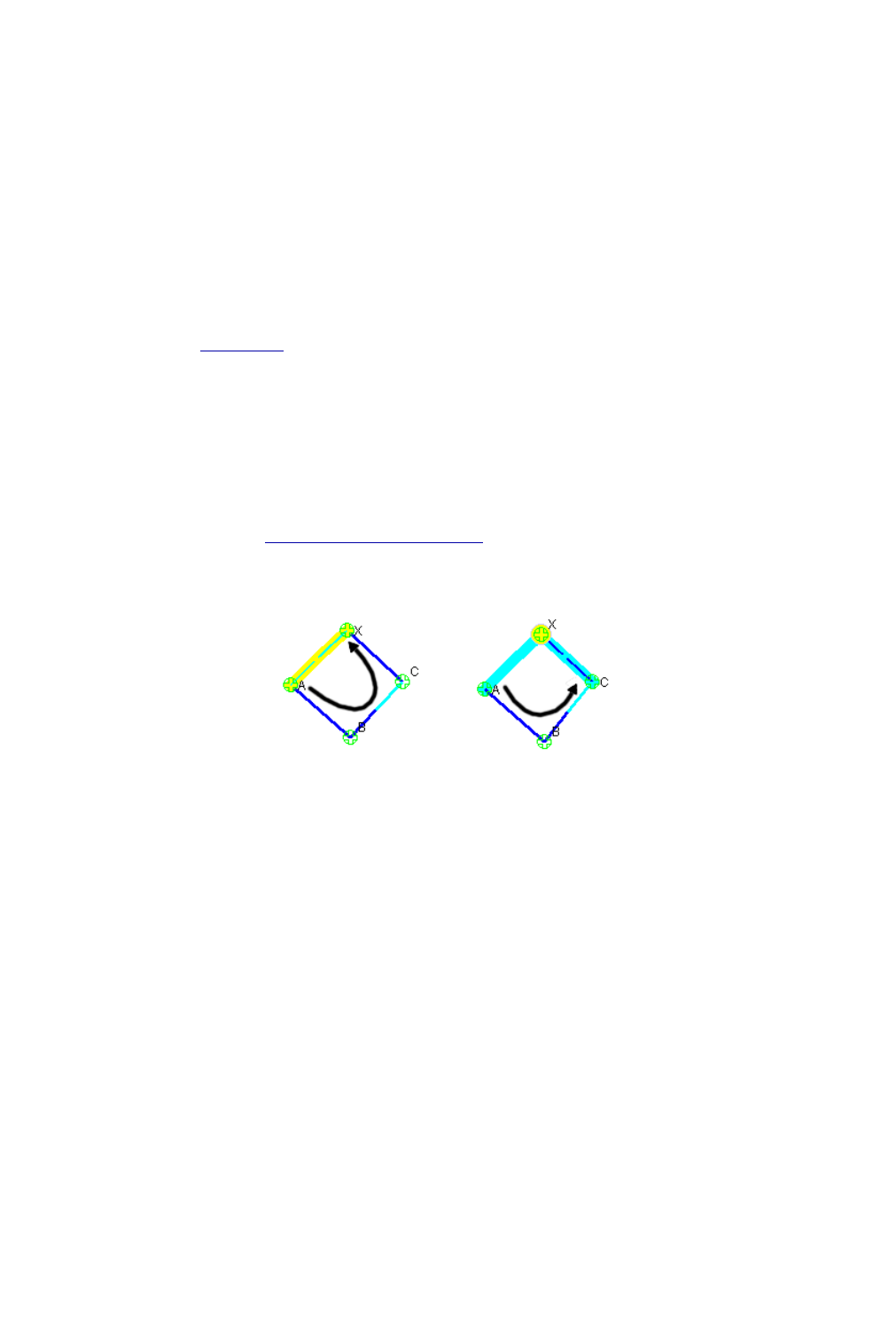
FAST REROUTE*
Copyright © 2014, Juniper Networks, Inc. 30-25
. . . . .
Note: Site-Diversity in this context simply means Site Diversity. It does not indicate Site + Facility Diversity
as is the case when the Diversity Level is set to Facility.
FACILITY DIVERSITY (SRLG)*
93. *You should have the Facility software license for this feature.
A Shared Risk Link Group (SRLG) can be represented by the concept of a facility in the WANDL software,
indicating a group of links that are likely to go down together in the event of a failure. In the WANDL software,
a facility can be defined in a special facility file as a group of links and nodes. A backup path that is facility-
diverse from its primary path will have a route that, aside from the source and destination, will traverse a path
that does not intersect with the primary path at any of a facility’s links or nodes.
In Figure 30-25, the diagram at left depicts a protected link between A and X, highlighted in yellow. The
alternate route depicted from A to X is only facility-diverse if links A->B, B->C, C->X, along with nodes B and
C do not belong to the same facility as link A->X. The diagram at right depicts a protected node X. The alternate
FRR-NP route depicted from A to C is only facility-diverse if links A->B, B->C and node B do not belong to the
same facility as either link A->X or node X.
If no facility-diverse route exists, the program will attempt to find a site-diverse route, under the presumption
that an alternate route is better than none.
Note: If the network model was built from the configuration files through the Import Data Wizard feature
described in Chapter 2, Router Data Extraction, then by default a facility will be set equivalent to all links
associated with a router card.
Figure 30-25 Facility-Diverse Route for Protecting a Link (left) and Protecting a Node (right)
When completing an FRR Design with the Diversity Level set to Facility, the Console will report a summary for
all the FRR Backup tunnels, in a similar format to that below:
Diversity Level= FACILITY
Tunnel Site-Diversity FAC-Diversity No-Diversity Unplaced
FRRBackup 37 0 51 0
The Tune FRR Backup Tunnels window, if open, will also display Site, Facility, or None, accordingly, in the
Diversity column.
Note: Site-Diversity in this context may be somewhat misleading. If the Diversity Level was set to Facility, then
Site-Diversity, both in the Console and in the Tune FRR Backup Tunnels window, actually indicates that Site
Diversity + Facility Diversity are both satisfied. This is stronger than simply Facility (FAC)-Diversity alone.

FAST REROUTE*
30-26 Copyright © 2014, Juniper Networks, Inc.
30

Copyright © 2014, Juniper Networks, Inc. 31-1
. . . . .
. . . . . . . . . . . . . . . . . . . . . . . . . . . . . . . . . . .
C
ISCO
A
UTO
-T
UNNELS
*
31
ANDL supports the modeling of Cisco's auto-tunnels, including both mesh group auto-tunnels and
backup auto-tunnels. The mesh group auto-tunnels feature automates the configuration of a mesh of
primary MPLS tunnels that share the same attributes. This feature can be used when creating a set of
fully-meshed MPLS tunnels, or when adding a new router to a meshed group. Configuration of mesh group auto-
tunnels involves building a template (via the interface auto-template statement) that identifies the attributes of the
primary tunnels to be created as well as the tunnel destinations (by using an access-list). Cisco's backup auto-tunnels
feature provides the capability to automatically build backup tunnels for the primary tunnel. These backup tunnels
are setup using NHOP or NNHOP protection. Configuration of backup auto-tunnels involves just one required
statement (mpls traffic-eng auto-tunnel backup). For detailed background information on how auto-tunnels work, as
well as on how to configure auto-tunnels, please refer to the appropriate Cisco documentation.
WANDL models auto-tunnels in the following way:
1. Configuration Import: Parse the configuration file to look for auto-tunnel related configuration statements
and store the auto-tunnel settings into a file called atconfig.runcode.
2. Auto-tunnels Creation: From the atconfig.runcode file, generate the corresponding auto-tunnels in the
network spec.
3. Tunnel Path Data Collection and Import: The output of the show mpls traffic-eng tunnels command may
be captured into a file for each router and then imported into the tool. The imported tunnel paths provide the
actual network view of the tunnel paths, and so are used to replace the tunnel paths and tunnel IDs generated by
the tool.
4. Verification: The tool provides three types of reports (Report Manager's Tunnel layer, Auto-tunnel folder) to
help the user to verify Cisco's auto-tunnels. The Discrepancy Report lists the modeled tunnels that are not
present in the collected tunnels. The Protection Report shows each interface that is protected by an auto-backup
tunnel. The Overlap Report shows interfaces that are protected by an autobackup tunnel and manual backup
tunnel.
5. Design (optional): Analysis of the reports may reveal that certain mesh group primary auto-tunnels and/or
backup auto-tunnels are missing from the actual router environment. In such cases, the tool may be used to
design for these missing tunnels.
When to use
Use these procedures if you have Cisco auto-tunnels configured in your network and you want to model them in the
WANDL tool.
Prerequisites
If you wish to perform this task, you should have a set of router configuration files with Cisco auto-tunnels
configured.
*Note that a special license is required for autotunnel. Please contact your Juniper representative for more
information.
Related Documentation
For general step-by-step instructions on how to use the WANDL software, please refer to the Design & Planning
Guide.
For an overview of the WANDL software or for a detailed description of each feature and the use of each window,
refer to the General Reference Guide.
For instructions on how to view or modify the tunnels in your network, refer to Chapter 20, LSP Tunnels*.
W

CISCO AUTO-TUNNELS*
31-2 Copyright © 2014, Juniper Networks, Inc.
31
For instructions on how to view or modify FRR configurations or to design FRR backup tunnels for your network,
refer to Chapter 30, Fast Reroute*
Outline
1. Importing Cisco Auto-tunnel Information from Router Configuration Files on page 31-2
2. Auto-tunnel Creation on page 31-4
3. Tunnel Path Data Collection and Import for Auto-tunnels on page 31-7
4. Reporting for Verification on page 31-9
Detailed Procedures
Importing Cisco Auto-tunnel Information from Router Configuration Files
1. To import the router configuration files, select File>Import Data and follow the Import Network Wizard.
Alternatively, you may run the getipconf program in text mode. Please refer to Chapter 2, Router Data
Extraction for more detailed information. The following table lists those mesh group auto-tunnel and backup
auto-tunnel related statements that are parsed during configuration import:
Figure 31-1 Cisco auto-tunnel statements parsed during configuration import
2. Once all of the options in the different tabs of Import Network Wizard have been selected, click Next> to
begin importing the router config files. As you reach the end of configuration import, you will be prompted
with a dialog box asking if you want to "Generate auto tunnels from atconfig file?", as shown in the
following figure. If you wish the tool to generate auto-tunnels, then click on Yes.
mesh group auto-tunnel statements
mpls traffic-eng auto-tunnel mesh
mpls traffic-eng auto-tunnel mesh tunnel-num min num max num
interface auto-template interface-num
tunnel destination access-list num
backup auto-tunnel statements
mpls traffic-eng auto-tunnel backup
mpls traffic-eng auto-tunnel backup nhop-only
mpls traffic-eng auto-tunnel backup tunnel-num [min num] [max num]
mpls traffic-eng auto-tunnel backup config unnumbered-interface interface
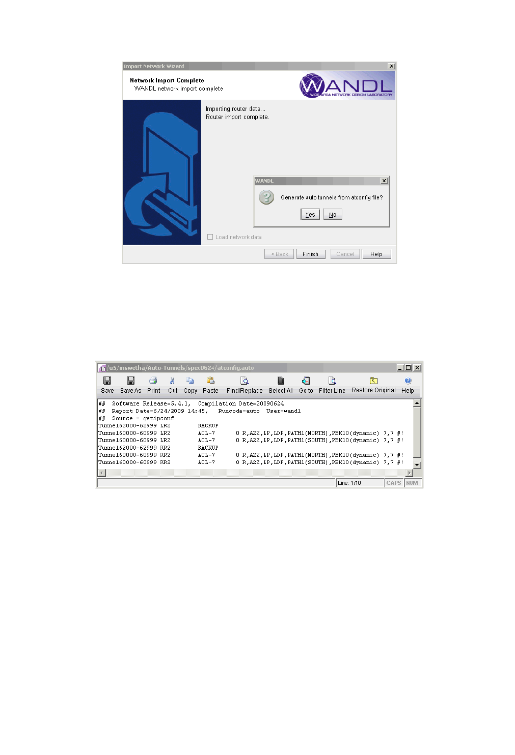
CISCO AUTO-TUNNELS*
Copyright © 2014, Juniper Networks, Inc. 31-3
. . . . .
Figure 31-2 Configuration import
The atconfig files store the auto-tunnels information parsed during configuration import. The following figure
shows an atconfig file that was created during configuration import for a network that has both mesh group and
backup auto-tunnels configured.
Figure 31-3 An atconfig file containing both mesh group and backup auto-tunnels
In the above figure, the line
Tunnel62000-62999 LR2 BACKUP
corresponds to the following backup auto-tunnel configuration statements:
mpls traffic-eng auto-tunnel backup
mpls traffic-eng auto-tunnel backup tunnel-num min 9000 max 9099
In the above figure, the line
Tunnel60000-60999 LR2 ACL-7 0 R,A2Z,LP,LDP,PATH1(NORTH),PBK10(dynamic) 7,7 #!
corresponds to the following mesh group auto-tunnel configuration statements:
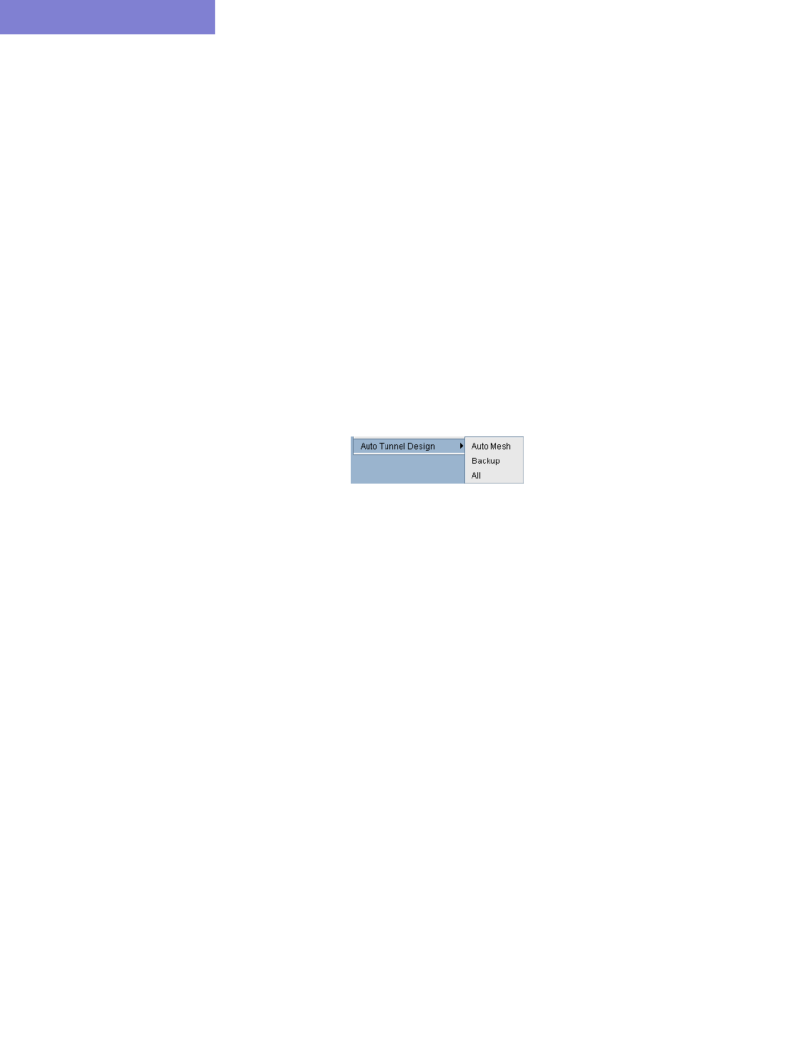
CISCO AUTO-TUNNELS*
31-4 Copyright © 2014, Juniper Networks, Inc.
31
mpls traffic-eng auto-tunnel mesh
mpls traffic-eng auto-tunnel mesh tunnel-num min 60000 max 60999
…
interface Auto-Template1
ip unnumbered Loopback0
mpls ip
tunnel destination access-list 7
tunnel mode mpls traffic-eng
tunnel mpls traffic-eng autoroute announce
tunnel mpls traffic-eng path-option 1 explicit name NORTH
tunnel mpls traffic-eng path-option 10 dynamic
tunnel mpls traffic-eng fast-reroute
!
Auto-tunnel Creation
3. If you choose No when prompted with "Generate auto tunnels from atconfig file?" in the previous step,
then the tool will not create any auto-tunnels. You may still generate the auto-tunnels at a later time by
switching to Design mode and then choosing one of the three options under the Auto Tunnel Design menu
(Design > TE Tunnels > Auto Tunnel Design) as shown in the following figure. Selecting Auto Mesh or
Backup will cause the tool to generate mesh group auto-tunnels or backup auto-tunnels, respectively. To
generate both mesh group and backup auto-tunnels, choose the All option.
Figure 31-4 Auto Tunnel Design Menu
4. If you choose Yes when prompted with "Generate auto tunnels from atconfig file?" in the previous step
and your network configuration files have auto-tunnels configured, then the tool proceeds to create auto-tunnels
using the information stored in the atconfig file. If backup auto-tunnels are configured in the network, then FRR
design is performed in the background to provide FRR node or FRR link protection for the primary tunnel. To
view the auto-tunnels created by the tool, bring up the Tunnels window (Network > Elements >Tunnels) as
shown in the following figure:
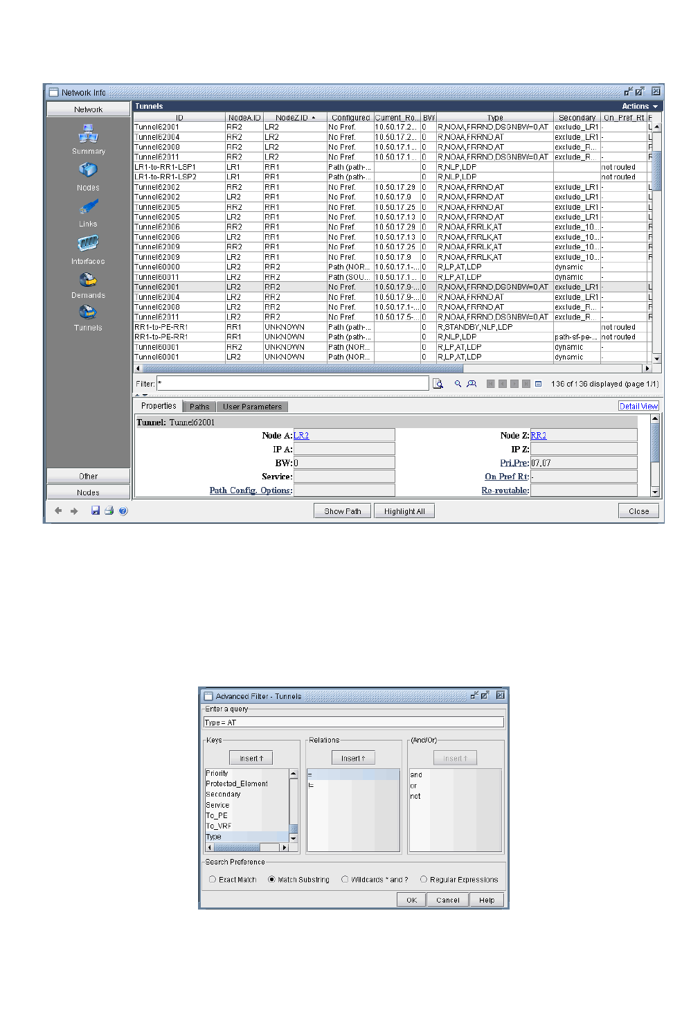
CISCO AUTO-TUNNELS*
Copyright © 2014, Juniper Networks, Inc. 31-5
. . . . .
Figure 31-5 Auto-tunnels are tagged with “AT” in the Type field
The figure has the Type column expanded to show that auto-tunnels have been tagged with an "AT" flag. In this
example, routers LR2 & RR2 have mesh group & backup auto-tunnels configured, as indicated by the corresponding
"AT" flag.
5. If you wish to filter for only auto-tunnels, you may use the advanced filter. Set "Type=AT" for the Enter
query box and choose Match Substring as the Search Preference, as shown in the following figure.
Figure 31-6 Filtering for auto-tunnels
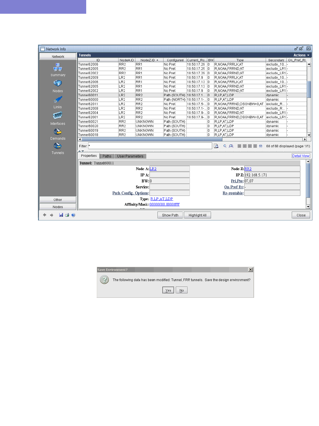
CISCO AUTO-TUNNELS*
31-6 Copyright © 2014, Juniper Networks, Inc.
31
The resulting filtered tunnels window is shown in the following figure:
Figure 31-7 Tunnels window showing only auto-tunnels
6. If auto-tunnels have been generated by the tool, and you exit without first saving, then you will be prompted
with the following popup message window.
Figure 31-8 Click Yes to save auto-tunnels
Clicking on Yes will cause the auto-tunnels to be saved and placed into an autotunnel.runcode file. An example is
shown in the following figure

CISCO AUTO-TUNNELS*
Copyright © 2014, Juniper Networks, Inc. 31-7
. . . . .
Figure 31-9 Auto-tunnels saved into the autotunnel.runcode file
Tunnel Path Data Collection and Import for Auto-tunnels
7. As described in the Network Data Import Wizard chapter of the Reference Guide, the actual tunnel paths taken
by tunnels can be extracted from the router and imported into the tool to provide an exact view of the network.
In addition, since auto-tunnels are generated by the router dynamically, the exact tunnel IDs will not be known
ahead of time. What is known is the tunnel ID range, so the tool creates auto-tunnels with tunnel IDs that fall
into the range. To use the Tunnel Path Import feature, prepare a directory that contains the output of the
following Cisco show command, one file per router: show mpls traffic-eng tunnels
8. With the spec file still open, bring up the Import Network Wizard window (File>Import Data), and select
Tunnel Path under Select Import Type, as shown in the following figure:
Figure 31-10 Tunnel Path Import
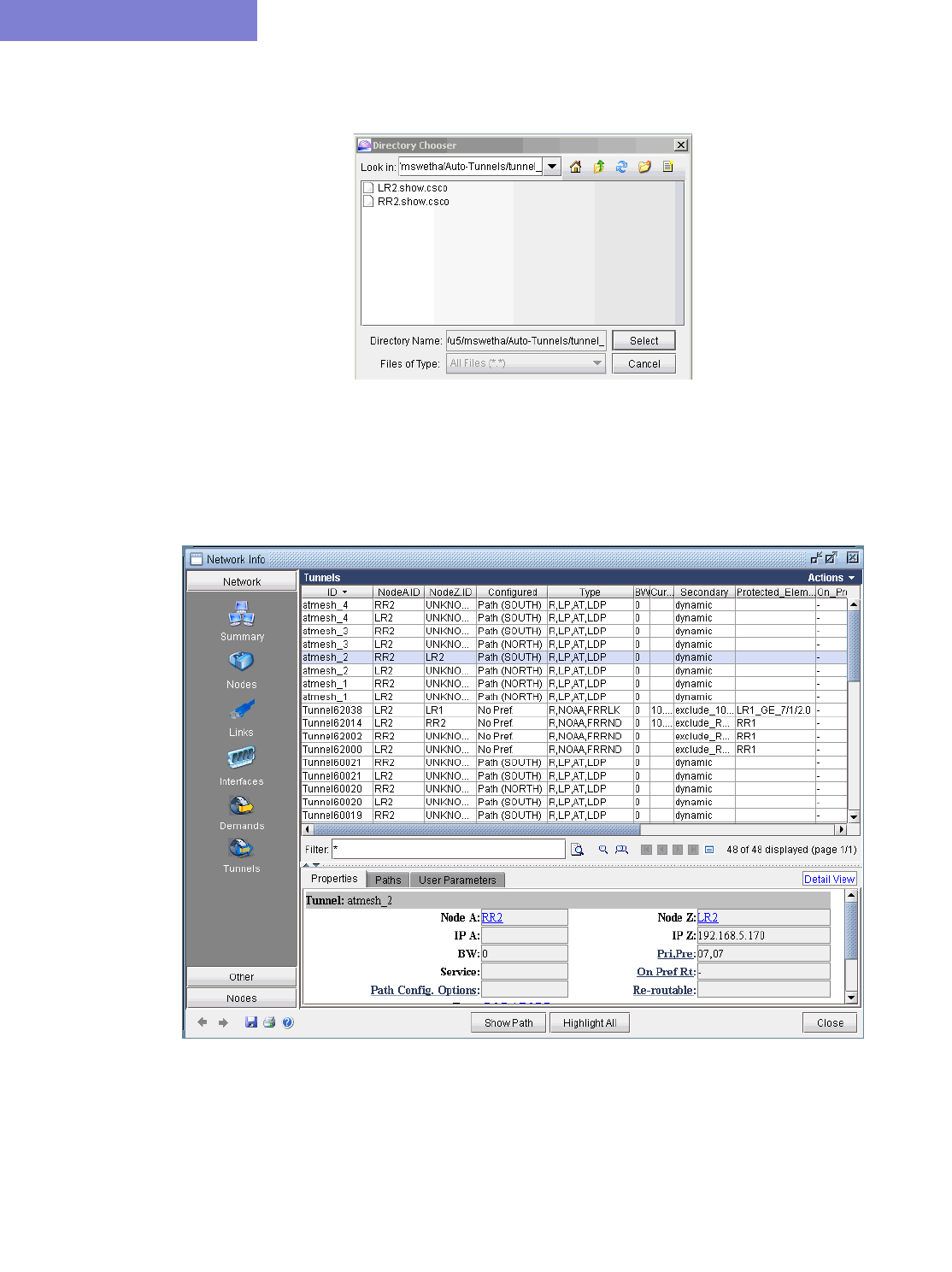
CISCO AUTO-TUNNELS*
31-8 Copyright © 2014, Juniper Networks, Inc.
31
Then click on Browse and navigate to the directory containing the show command output files:
Figure 31-11 Directory of show command output files
After specifying the import directory, click Next to import the tunnel paths into the model.
9. After tunnel path import, bring up the Tunnels window (Network > Elements >Tunnels) to examine the
changes. The following figure shows the Tunnels window up after tunnel path import.
Figure 31-12 Tunnels after Tunnel Path Import
10. Compared to the Tunnels window prior to tunnel path import, you can see that the tunnel IDs have been replaced
with the actual tunnel IDs assigned by the router. The modeled tunnel paths have also been updated by the
actual ones.
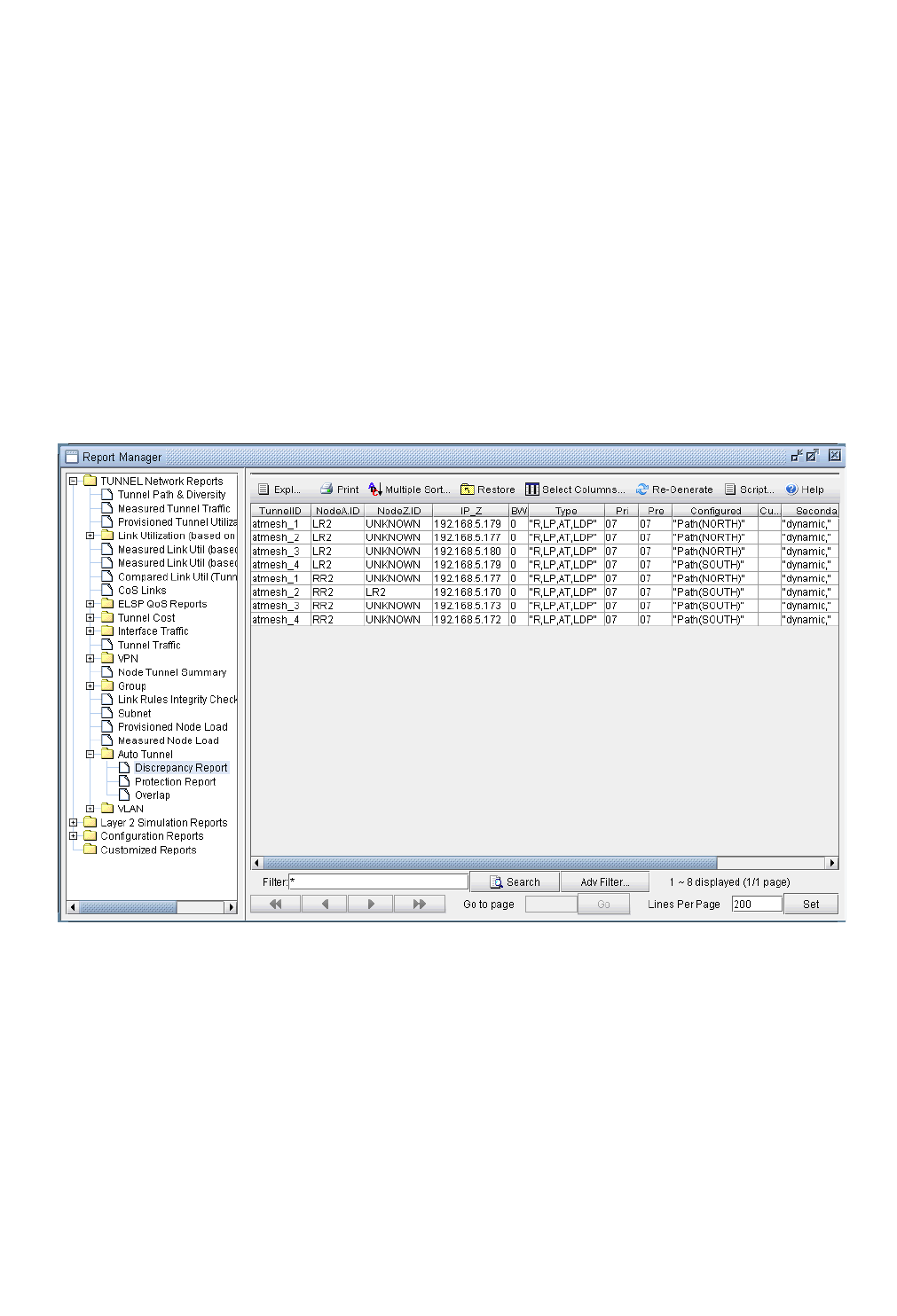
CISCO AUTO-TUNNELS*
Copyright © 2014, Juniper Networks, Inc. 31-9
. . . . .
11. After performing tunnel path import, if there are any tunnels modeled by the tool that do not appear on the actual
router, then those tunnel IDs are renamed to atbackup_n or atmesh_n depending on the auto-tunnel type.
For instance, the following figure shows that the mesh group auto-tunnel from RR2 to LR2 created by the tool
did not appear in the actual router (according to the show command output from tunnel path import). This could
be an indication that the Cisco router hardware did not correctly create the auto-tunnel.
Reporting for Verification
12. There are three reports created under the Report Manager's Auto Tunnel Folder specifically for Cisco
Auto Tunnel verification and analysis. Open the Report Manager (Report > Report Manager) and click
on any report under the Tunnel Layer Network Reports > Auto Tunnel folder. The Discrepancy
Report lists the auto-tunnels modeled by the tool that are not generated by the router. In particular, an extra
tunnel modeled in the tool will have its tunnel ID set to atbackup_n or atmesh_n depending on whether it is
a backup auto-tunnel or mesh group primary auto-tunnel. The following figure shows an example
Discrepency Report:
Figure 31-13 Discrepancy Report showing modeled auto tunnels not generated by routers
The Protection Report, as shown in the following figure, shows a list of all interfaces in the network that are
being protected along with other details like the tunnel which the interface is protecting and whether it is node
protecting or link protecting the tunnel.
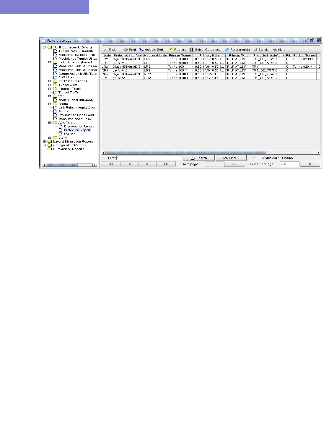
CISCO AUTO-TUNNELS*
31-10 Copyright © 2014, Juniper Networks, Inc.
31
Figure 31-14 Protection Report showing protected interfaces in the network
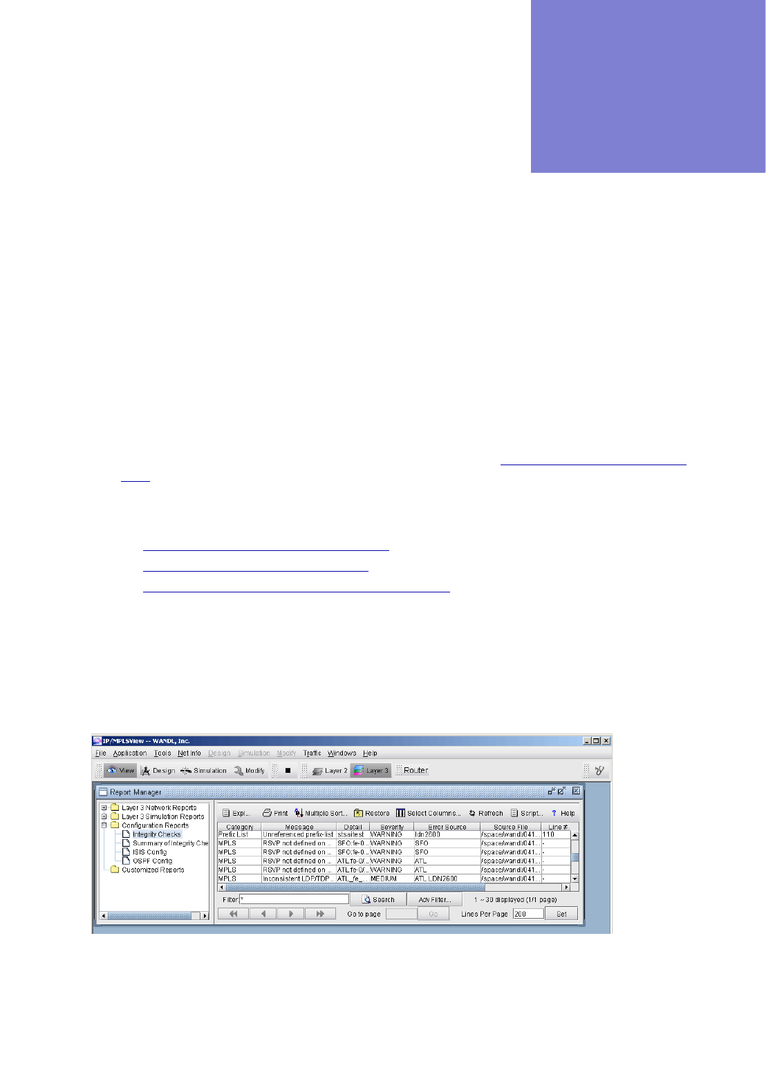
Copyright © 2014, Juniper Networks, Inc. 32-1
. . . . .
. . . . . . . . . . . . . . . . . . . . . . . . . . . . . . . . . . .
I
NTEGRITY
C
HECK
R
EPORT
*
32
his chapter describes the use of the Integrity Check Report to flag potential configuration errors found after
importing a set of router configuration files.
*Note that a special password is required for the integrity check feature. Please contact your Juniper representative
for more information.
When to use
Follow these guidelines to view, customize severity levels, and automate the integrity check reporting features.
Prerequisites
To use the integrity check tools, the user must have access to a copy of the network’s configuration files.
Related Documentation
To create one’s own configuration checking rules based on a template, view Chapter 33, Compliance Assessment
Tool*.
Recommended Instructions
Following is a high-level, sequential outline of the integrity check tool and the associated, recommended procedures.
1. Viewing the Integrity Check Report on page 32-1
2. Customizing the Severity Level on page 32-3
3. Scheduling Integrity Checking in Task Manager on page 32-4
Detailed Instructions
Viewing the Integrity Check Report
1. To view the Integrity Check Report select Report > Report Manager, and click on the Configuration
Reports folder, as shown in the following figure. Alternatively, the stethoscope icon located in the upper right-
hand corner in the main toolbar provides for a quick shortcut to the same report.
Figure 32-1 Config Import Reports
T
INTEGRITY CHECK REPORT*
32-2 Copyright © 2014, Juniper Networks, Inc.
32
2. Select the Integrity Checks Report to bring up the report listing all of the integrity checks that were activated
for the network. Select the Summary of Integrity Checks Report to bring up a summary of the Integrity
checks. The following figures show both reports, respectively.
Figure 32-2 Integrity Checks Report
Figure 32-3 Summary of Integrity Checks Report
INTEGRITY CHECK REPORT*
Copyright © 2014, Juniper Networks, Inc. 32-3
. . . . .
Using the Report Viewer
3. The Integrity Check Report can also be viewed using the Report Viewer. In the File Manager, right click on
the configLog.<runcode> file and select Open in Report Viewer in the pop-up menu.
4. Within the Report Viewer, right-clicking on the report allows the user to save the entire report or the report in its
current view to the client, or local machine.
Figure 32-4 Right-Click Menu
ERROR SOURCE
5. The Error Source and Source File columns indicate the router config file(s) that caused the particular
integrity check in question. When the user double-clicks on any line in the integrity check report, the associated
router config file(s) are brought up. For those local router integrity checks that involve just a single router, the
Line# and Line Content columns indicate the particular line in the router config file that is causing a problem.
Customizing the Severity Level
6. The Integrity Check Profile table is used by the user to modify the severity level of each type of integrity check
error, as well as to define whether or not to include a particular check in the generated Integrity Checks report.
Select Tools > Options > Integrity Checks... to open the following window.
Figure 32-5 Integrity Checks Profile Table
7. Click the cell in the Severity column that you wish to modify. A drop-down box will appear with choices for
HIGH, MEDIUM, LOW, and WARNING. The Include column has a check box for each integrity check. Keep
the box checked for integrity checks that you wish to remain in the report. Uncheck the boxes for those integrity
checks that you do not wish to be included in the integrity checks report. When you are finished making
changes, click OK and chose a file to save the profile to. The Restore Defaults button restores the table to the
default settings.

INTEGRITY CHECK REPORT*
32-4 Copyright © 2014, Juniper Networks, Inc.
32
Scheduling Integrity Checking in Task Manager
The Integrity Check Report task can be used to perform integrity checking on a set of configuration files at a
designated time interval
INTEGRITY CHECK TASK
8. Select Admin > Task Manager. Click the “New Task” button and select the “Integrity Check” task.
9. Enter a name for the task and click “Next”.
10. Select the “Integrity Check Options” tab. To schedule the task for the offline network, select “Use off-line
network” and specify the spec file name and the directory containing the config files.
11. You can also select options to filter the integrity checks by category, message, routers, topology groups, and
severity.
Note that in order to select specific topology groups, the spec file that was selected should reference a group file.
This group file can be created by saving the network after creating groups on the topology map.
12. Additionally, select “Save the report to make it available on the web” to view the report from the web interface.
For more details on the options, refer to Integrity Check Options Tab on page 32-6.
13. When scheduling the task for an offline network, select the “Conversion Options” tab to specify specific
import parameters. For more details on these options, refer to Chapter 2, Router Data Extraction.
14. Finally, select the “Report Options” tab and select whether to save the Integrity Check report to a file and/or
to e-mail the report. See Report Options on page 32-5 for more details.
15. Click “Next” and select the Schedule Type and interval parameters as necessary.
16. Then click “Finish”.
INTEGRITY CHECK REPORT*
Copyright © 2014, Juniper Networks, Inc. 32-5
. . . . .
Report Options
17. The Report Options tab specifies how the results of the Configuration Check Task will be saved each time the
configuration check task is run.
Figure 32-6 Report Options
Note that the resulting integrity report for “Save to a file” can be opened in table format using the Report Viewer as
described in Using the Report Viewer on page 32-3.
Save to a file Saves the results of the configuration check to a file.
Integrity Check Result Indicates the file location in which to save the results of the Integrity Check Report
task. Use the “Browse” button to navigate to a location on your server, or else
type the path directly in the textfield. If you are not running one of these tasks,
simply leave the corresponding textfield blank. If you mark the “Add time
stamp” checkbox, a timestamp will be appended to the end of the report file
name.
Send notification
emails
E-mails the results of the configuration check.
Mail server The IP address or name of your mail server.
Mail sender The e-mail address of the individual sending the e-mail.
Mail recipients List the email addresses of the individuals who will receive the results of the
integrity checking. Entries must be separated by a space.
Mail subject The text that will appear in the email subject line.

INTEGRITY CHECK REPORT*
32-6 Copyright © 2014, Juniper Networks, Inc.
32
Integrity Check Options Tab
The WANDL software automatically detects a variety of errors of various severity levels. Some of these warnings
may not be of interest, or are not a source of concern for your network. For this reason, a number of options are
provided in this tab to allow you to filter for just those integrity checks (ICs) that concern you.
NETWORK OPTIONS
The Network section of the window is used to specify the set of configuration files to perform the integrity
checking on. If you use the WANDL software to monitor the live network, you can select “Use live network”.
Alternatively, select “Use spec file” and specify the configuration file folder and corresponding spec file path created
by importing the configuration files.
FILTER BY CATEGORY
IC’s are organized into different categories, as listed in the window. You can mark the “Include All Categories”
checkbox if you wish to see IC’s belonging to all categories. Otherwise, highlight just those categories you are
interested in, in the “Select From” list on the left, and move them to the “Categories to be included” list on the
right via the “Add->” button. Pressing the “Add All >>” button is equivalent to selecting the “Include All
Categories” checkbox.
FILTER BY MESSAGE
You can filter the integrity check results according to specific IC messages. There is a predefined set of IC
messages, each assigned its own msg ID (or message ID), which is the number preceding the message. These are
listed in the left hand list of the Filter by Message section.
To customize the ICs to show, unselect “Include All Messages”, highlight just those categories you are interested
in, in the “Select From” list on the left, and move them to the “Messages to be included” list on the right via
the “Add->” button.
You can perform an additional filter on the messages to be included by entering text in the “And, optionally filter
message by matching substring” textfield. Only messages which include your text string will be considered.
FILTER BY ROUTER
In the Filter by Router section, you can choose to see only those IC’s pertaining to certain routers. To do so,
uncheck the “Include All Routers” checkbox, highlight the routers that you are interested in (corresponding to the
routers in the network you specified), and move them to the “Routers to be included” list on the right-hand side
using the “Add->”button.
You can perform an additional filter on the desired routers to be included by entering text in the “And, optionally
filter routers by matching substring” textfield. Only those router names which include your text string as part
of the name will be considered.
IC’s can also be categorized into two types:
•Router IC - an IC that pertains to a single router
•Network IC - an IC that pertains to two or more routers
For example, some users may wish to see:
•All Router ICs, but only those Network ICs pertaining to the selected router(s)
•All Network ICs, but only those Router ICs pertaining to the selected router(s)
•None of the Router ICs and only those Network ICs pertaining to the selected router(s)
•And so on.

INTEGRITY CHECK REPORT*
Copyright © 2014, Juniper Networks, Inc. 32-7
. . . . .
This explains why so many different options are provided. These options are explained below:
FILTER BY GROUP
In the Filter by Group section, you can choose to see only those IC’s pertaining to routers in certain topology
groups. To do so, uncheck the “Include All Groups” checkbox, highlight the groups that you are interested in
(corresponding to the routers in the network you specified), and move them to the “Groups to be included” list
on the right-hand side using the “Add->”button.
Note that in order to select specific topology groups, the map for the selected network spec file should contain
groups. Furthermore, these groups should be saved into the network baseline. If there are topology groups, but they
are not appearing in the list, save the network first using File > Save Network... before creating a task for the
Integrity Check report.
FILTER BY SEVERITY
ICs are assigned one of four severity levels: High, Medium, Low, Warning. You can select the severity of
integrity check errors to display. The severity levels corresponding to individual ICs can be set within the IC Profile
Table (Tools > Options > Integrity Checks). See Integrity Check Options Tab on page 32-6 for more
information.
ADDITIONAL REPORT OPTIONS
Router IC Filter
Include All regardless of the selected
routers (Show All)
Show all router ICs, even those pertaining to routers
that are not selected.
Include if a problem occurred in selected
routers (Show Only for Selected Routers)
Show only those router ICs pertaining to the selected
routers.
Exclude if a problem occurred in selected
router(s) (Show None)
Do not show any router ICs.
Network IC Filter Explanation
Include All regardless of the selected
routers (Show All)
Show all network ICs pertaining to all routers in the
network (that is, not just those selected)
Include if a problem occurred in selected
routers (Show Only for Selected Routers -
Strict match)
Show only those network ICs for which ALL involved
routers belong to the set of selected routers.
Include if a problem occurred in any of
selected routers (Show Only for Selected
Routers - Loose match)
Show only those network ICs for which at least one of
the involved routers belong to the set of selected
routers.
Exclude if a problem occurred in selected
router(s) (Show None)
Do not show any network ICs.
INTEGRITY CHECK REPORT*
32-8 Copyright © 2014, Juniper Networks, Inc.
32
Save the report to make
it available on the web
Make the IC report accessible for viewing via the WANDL Web interface.
Report with the Header Includes a header in the report that indicates the types of filters used to generate
the particular report. For example, the report might show that the user is filtering
by Category (only “OSPF” was selected), Message / msg ID (only message
93 was selected), Severity (all severity levels were selected), and Router /
Error Source (only router “NWK” was selected). Note that you can look up the
msg ID, or Message ID, in the Integrity Checks Profile Table. See Integrity
Check Options Tab on page 32-6 for more information.
Report Type (Full /
Compact)
Indicate the level of detail to be used in the report: Full or compact. Both reports
will display the following fields: Category, Message, Detail, Severity, Error
Source.
The Full report will contain some additional information to identify the source of
the error: Source File, Line #, Line Content, and msg ID.

INTEGRITY CHECK REPORT*
Copyright © 2014, Juniper Networks, Inc. 32-9
. . . . .
Appendix A. Integrity Check Descriptions
This appendix gives a description of some of the integrity checks (ICs) that are performed on the router
configuration files during configuration import. The IC descriptions are organized by category. For each IC, a brief
description, a msgID (corresponding to the msgID shown in the Integrity Checks reports), and the default severity
are given. A more detailed description then follows to give more information about the particular IC check. The
severity of the IC helps the network engineer to prioritize which ICs to look at first. High severity reports are critical
reports believed to potentially cause major network problems. Medium and Low severity reports describe problems
not considered severe, but should be fixed to prevent network problems or inadvertent side effects. Warning-level
reports describe potential network problems that the network engineer should examine to make sure that the network
is operating at its best.
ACCESS LIST AND PREFIX LIST INTEGRITY CHECKS
["Non-utilized access-list rule (Cisco)", msgID=106, High]
When access lists become long, preceding rules may be more general than subsequent rules. When this happens, the
later rules are never utilized. This check identifies situations when rules are not utilized.
["Unknown access-list (Cisco)", msgID=86, High]
This check identifies references to undefined access lists. Supported for IPv4 and IPv6.
["Unreferenced access-list (Cisco)", msgID=100, Warning]
An access-list was defined, but not referenced. Supported for IPv4 and IPv6.
["Unknown prefix-list (Cisco)", msgID=107, High]
This check identifies references to undefined prefix lists.
["Unreferenced prefix-list (Cisco)", msgID=108, Warning]
A prefix-list was defined, but not referenced.
BGP INTEGRITY CHECKS
["Disabled BGP protocol (Juniper)", msgID=5, Warning]
This check identifies situations where the BGP section is defined, but the disabled statement is present.
["Ignored 'community-list' statement due to unexpected 'permit'/'deny' location (Riverstone)", msgID=18,
Warning]
Because the permit/deny folLowing the "community-list <name>" command is missing, the community-list
statement is ignored.
["BGP neighbor shutdown", msgID=51, Warning]
This check identifies situations when the BGP neighbor is shutdown.
["Unknown as-path access-list", msgID=109, High]
This check identifies references to undefined as-path access lists.

INTEGRITY CHECK REPORT*
32-10 Copyright © 2014, Juniper Networks, Inc.
32
["Unreferenced as-path access-list (Cisco)", msgID=110, Warning]
An as-path access-list was defined, but not referenced.
["Unknown community-list", msgID=124, High]
This check identifies references to undefined community lists.
["Unreferenced community-list (Cisco)", msgID=125, Warning]
A community-list was defined, but not referenced.
["Unknown route-map action (Riverstone)", msgID=97, High]
This check identifies references to an undefined community-list in the "route-map <name> deny/match <>
community-list" command.
EIGRP/IGRP INTEGRITY CHECKS
["Inconsistent EIGRP definition", msgID=20, Medium]
This check finds EIGRP to be enabled on one end of a line but not the other end.
["Inconsistent IGRP definition", msgID=21, Medium]
This check finds IGRP enabled on one end of a line but not the other end.
["Invalid EIGRP inverse (wildcard) mask", msgID=61, High]
When configuring which networks EIGRP will advertise, the inverse (wildcard) mask must be correct. This check
identifies invalid EIGRP inverse mask values.
["Invalid IGRP inverse (wildcard) mask", msgID=62, High]
When configuring which networks IGRP will advertise, the inverse (wildcard) mask must be correct. This check
identifies invalid IGRP inverse masks values.
["Invalid EIGRP network address", msgID=65, High]
This check identifies invalid network addresses that EIGRP is trying to advertise.
["Unexpected IGRP network address", msgID=66, High]
This check identifies invalid network addresses that IGRP is trying to advertise.
IP INTEGRITY CHECKS
["Duplicate IP address (public)", msgID=9, High]
All IP addresses assigned to router interfaces are checked for duplication since duplicate IP addresses can result in
serious problems in a network.
["Duplicate IP address (private)", msgID=111, Warning]

INTEGRITY CHECK REPORT*
Copyright © 2014, Juniper Networks, Inc. 32-11
. . . . .
An IP address in one private address spaces can be duplicated in another (e.g., within different VPNs). This check
identifies duplicated IP addresses within the same private address space.
["Duplicate host name", msgID=10, High]
This check identifies duplicate config files for the same router. The duplicated config files are ignored.
["Error in address definition (Riverstone)", msgID=12, High]
This check identifies invalid IP address formats in the "interface create ip <name> address-netmask" command.
["Inconsistent media interfaces with same subnet address", msgID=19, Warning]
During configuration parsing, two interfaces are stitched up when
1. Their addresses are in the same subnet
2. Their media types are either Ethernet, SONET, or ATM and match on both sides.
This check identifies situations where condition 1 is true, but condition 2 is not.
["Inconsistent bandwidth", msgID=29, Low]
This check identifies the situation where there is a bandwidth mismatch between two terminating interfaces of a link.
["Missing host name", msgID=38, High]
This check sees that a host name was not specified after the "hostname" command.
["Multiple hostnames defined", msgID=45, High]
This check sees duplicate host names defined in the system section.
["Non-primary address matched", msgID=49, Warning]
This check alerts the user to the fact that secondary addresses were used for stitch up.
["Overlapped subnet addresses", msgID=50, High]
This check identifies overlapped subnet addresses.
["Unexpected IP address", msgID=63, High]
This check identifies invalid IP addresses in Juniper or Riverstone configs.
["Unexpected IP mask (Riverstone, Juniper)", msgID=64, High]
This check identifies invalid IP address masks in Juniper or Riverstone configs.
["Unknown VLAN (Riverstone)", msgID=83, High]
This check sees that the vlan specified in the "interface create ip <name> vlan" was not defined.

INTEGRITY CHECK REPORT*
32-12 Copyright © 2014, Juniper Networks, Inc.
32
ISIS INTEGRITY CHECKS
["Inconsistent ISIS definition", msgID=22, Medium]
This check sees that ISIS was enabled on one end of a line but not the other end.
["Asymmetric ISIS1 metric", msgID=114, Warning]
This check finds ISIS1 metrics to be different at the two ends of a link.
["Asymmetric ISIS2 metric", msgID=115, Warning]
This check finds ISIS2 metrics to be different at the two ends of a link.
["Overlapped network statements", msgID=164 Warning]
This check flags overlapping IP address ranges related to network statements under the OSPF or BGP protocol, for
Cisco and Huawei devices.
RIP INTEGRITY CHECKS
["Inconsistent RIP definition", msgID=112, Medium]
This check sees that RIP is enabled on one end of a line but not the other end.
OSPF INTEGRITY CHECKS
["Invalid OSPF/IGRP/EIGRP network address", msgID=69, High]
This check identifies invalid IP network prefixes in the OSPF, IGRP, or EIGRP sections.
["Duplicate area IDs defined (Riverstone)", msgID=6, High]
This check sees that duplicate non-backbone area IDs are defined.
["Inconsistent OSPF area definition", msgID=25, High]
This check sees that the two ends of an OSPF link are assigned to two different OSPF areas.
["Inconsistent OSPF definition", msgID=26, Medium]
This check sees OSPF enabled on one end of a link but not the other end.
["Multiple defined backbone areas (Riverstone)", msgID=44, High]
This check identifies situations in Riverstone configuration files where the backbone area0 is defined more than
once.
["Invalid OSPF network address", msgID=67, High]
This check identifies invalid OSPF network addresses.
["Unexpected OSPF inverse (wildcard) mask", msgID=68, High]
This check indentifies invalid inverse (wildcard) masks on the network statement in the OSPF section.

INTEGRITY CHECK REPORT*
Copyright © 2014, Juniper Networks, Inc. 32-13
. . . . .
["Unexpected area IP (Riverstone)", msgID=60, High]
Riverstone uses the 4-octet format for non-backbone OSPF area designation. This check identifies cases in which the
area entered in the "ospf create area" command was neither "backbone" nor a valid IP address.
["Unknown OSPF area (Riverstone)", msgID=81, High]
Riverstone uses the 4-octet format for non-backbone OSPF area designation. This check identifies cases in which the
area entered in the "ospf add interface to area" command was neither "backbone" nor a valid IP address.
["Asymmetric OSPF metric", msgID=113, Warning]
This check identifies the situation where the OSPF metrics defined on the two end interfaces are different.
["ABR not in Area 0", msgID=119, Warning]
This check finds an ABR that does not border Area 0.
["Unbalanced OSPF virtual-link", msgID=126, High]
This check sees that OSPF virtual-link is defined only in one end but not the other.
["OSPF virtual-links not in the same transit area", msgID=127, High]
OSPF virtual links can be used to establish OSPF routing in areas that can only be connected via non-backbone
(transit) areas. This check identifies the situation where the OSPF virtual-links going to and from the backbone
area are going through a different transit area.
["Asymmetric OSPF reference bandwidth", msgID=162, Low]
This check identifies the situation where the OSPF reference bandwidth defined on the two end interfaces are
different.
QOS INTEGRITY CHECKS
["Bandwidth and priority commands cannot be used in the same class within the same policy map (Cisco)",
msgID=3, severity=Medium]
Either the bandwidth or the priority option can be used for a particular class within a policy map to specify the
guaranteed bandwidth, but not both.
["Duplicate policy-Map", msgID=11, Low]
This check looks for duplicate policy-map names defined in a config file.
["Duplicate Class-Map", msgID=7, Low]
This check looks for duplicate class-map names defined in a config file.
["Duplicate CoS-Queue-Group", msgID=8, Low]
This check looks for duplicate CoS queue groups configured in a config file.
["Invalid IP precedence values", msgID=30, High]

INTEGRITY CHECK REPORT*
32-14 Copyright © 2014, Juniper Networks, Inc.
32
This check identifies IP precedence values that are outside of the allowed range of 0-7.
["Invalid MPLS EXP bit value", msgID=31, High]
MPLS uses the EXP bits in the shim header to support differentiated services. Valid EXP bit values are 0-7. This
check identifies invalid EXP bit values.
["Undefined class", msgID=55, Medium]
This check sees that the class referenced in a policy-map section was not configured by the class-map command.
["Unknown class name in scheduler-map", msgID=90, Low]
This check sees that the class name referenced in the scheduler-map section was not defined.
["Unknown scheduler name in scheduler-map", msgID=98, Low]
This check sees that the scheduler name referenced in the scheduler-map section was not defined.
["Reference to an unknown policy-map", msgID=135, Medium]
This check identifies references to an unknown policy-map name.
LINK INTEGRITY CHECKS
["Inconsistent PIM mode", msgID=27, High]
This check sees that PIM was enabled on one end of a line but not the other end.
["Undefined filter (Juniper)", msgID=56, High]
This check identifies situations where a filter is being applied to an interface, but the referenced filter is undefined.
["Unreferenced firewall filter", msgID=101, Warning]
This check identifies firewall filters that are never referenced
["Unknown ISIS area-tag (Cisco)", msgID=89, High]
This check identifies situations with Cisco ISIS configuration when a reference was made to an undefined area-tag.
["ip unnumbered command references an unknown interface (Cisco)", msgID=95, Medium]
The ip unnumbered command borrows the IP address from the specified interface to the interface on which the
command has been configured. This check identifies situations when the specified interface is unknown.
MISCELLANEOUS INTEGRITY CHECKS
["Invalid config file", msgID=33, Warning]
This check identifies those files that are not router configuration files.
["non-text file", msgID=34, Warning]
This check looks for files that contains too many unreadable characters.

INTEGRITY CHECK REPORT*
Copyright © 2014, Juniper Networks, Inc. 32-15
. . . . .
["Undefined interface", msgID=77, High]
This checks finds that the interface name entered in the "isis add interface" command was not defined by the
"interface create" command.
["Undefined IP address (Riverstone)", msgID=76, High]
This check looks for undefined IP addresses in Riverstone IP address statements.
["Undefined interface IP address", msgID=78, High]
This check saw an undefined interface IP address in "isis add interface" command.
["Undefined LSP", msgID=79, Low]
This check finds that the LSP name is not defined in the LSP section.
["Unknown interface", msgID=93, Low]
This general check finds situations where the referred to interface was not defined. This could happen in many
situations.
["vlan-id defined without configuration in vlan-tagging section(Juniper)", msgID=104, Medium]
This checks finds that the vlan-id defined in the interface section was not configured in the vlan-tagging section.
["Inconsistent ATM bandwidth and PVC mean value", msgID=105, Warning]
This check identifies situations in which the ATM bandwidth and PVC mean values are known, but the PVC mean
value is different from the ATM bandwidth value.
["Reference to an unknown card (Alcatel)", msgID=139, High]
This check identifies cases where references were made to an undefined card name.
["Reference to an unknown port (Alcatel)", msgID=140, High]
This check identifies cases where references were made to an undefined port name.
["Reference to an unknown SDP (Alcatel)", msgID=141, High]
This check identifies cases where references were made to an undefined SDP name.
["Reference to an unknown route-map (Cisco)", msgID=130, High]
This check identifies references to an unknown route-map.
["Tunnel is configured as both autoroute announced and forwarding-adjacency", msgID=131, High]
This checks identifies the situation where a tunnel is configured as both autoroute announced and forwarding-
adjacency.

INTEGRITY CHECK REPORT*
32-16 Copyright © 2014, Juniper Networks, Inc.
32
["No IGP on forwarding-adjacency tunnel", msgID=132, Medium]
This checks sees that ISIS or OSPF was not configured on a forwarding-adjacency tunnel.
["bandwidth may exceed physical interface capacity", msgID=128, Low]
This check looks for situations where the bandwidth value configured for an interface exceeds the physical interface
capacity. E.g., this check would identify the case where the bandwidth for a Fast Ethernet interface is configured as
1000000 (1G).
["Unreferenced route-map", msgID=152, Warning]
A route-map was defined, but not referenced.
["Unreferenced policy-map", msgID=153, Warning]
A policy-map was defined, but not referenced.
["Empty route-map(route-policy) statement", msgID=163, Warning]
A route-map statement was defined without any content. This integrity check applies to Cisco and Huawei devices.
["Hostname not configured", msgID=165, Warning]
The hostname was not configured on the device. This integrity check applies to the following devices with cisco-like
config: Cisco (IOS, IOS-XR), asa, casa, nxos, zte, oneaccess, adtran, hillstone, digitalchina, etc.
MPLS INTEGRITY CHECKS
["Multiple group-names assigned to the same group-value (Juniper)", msgID=4, severity=High]
This check identifies situations where the same group-value (tunnel bit value) is assigned to multiple group-names
under the admin-group statement.
["Inconsistent LDP/TDP definition", msgID=23, Medium]
This check sees that LDP/TDP was enabled on one end of a line but not the other end.
["Inconsistent MPLS-TE definition", msgID=24, Medium]
This check sees that MPLS-TE was enabled on one end of a line but not the other end.
["Invalid tunnelbit (Juniper)", msgID=32, High]
This check finds that the MPLS admin-group tunnelbit is not in the allowed range (1~31).
["Undefined admin-group", msgID=70, High]
This check finds that the admin-group referenced in the tunnel section was not configured.
["Invalid tunnel destination IP address format", msgID=72, High]
This checks identifies tunnel destination IP addresses that have an invalid format.

INTEGRITY CHECK REPORT*
Copyright © 2014, Juniper Networks, Inc. 32-17
. . . . .
["Invalid hop number", msgID=73, High]
This checks sees that the hop number is out of the valid range (1~255).
["Invalid tunnel source IP address format", msgID=75, High]
This check identifies tunnel Source IP addresses that have an invalid format.
["Unknown admin-group (Juniper, Alcatel)", msgID=87, High]
This check identifies a reference to an undefined admin-group for Juniper and Alcatel routers.
["Unknown Tunnel/LSP path", msgID=96, High]
This check finds references to unknown an tunnel/LSP path.
["RSVP not defined on MPLS enabled interface", msgID=118, Warning]
This check warns the user that RSVP was not defined on an MPLS enabled interface.
["MPLS-TE tunnel is not enabled on the device", msgID=142, High]
Prior to configuring MPLS-TE tunnels, the mpls traffic-eng tunnels statement is configured at the global level. This
check identifies situations where this statement is missing.
["Asymmetric MPLS-TE metric", msgID=116, Warning]
This check finds that the MPLS-TE metric to be different on the two ends.
RSVP INTEGRITY CHECKS
["Inconsistent RSVP bandwidth", msgID=28, Warning]
This check identifies situations where the RSVP bandwidth is different on the two sides on a link.
["Inconsistent RSVP definition", msgID=147, Medium]
RSVP was enabled on one end of a link but not the other end.
STATIC ROUTES INTEGRITY CHECKS
["Next hop not in local subnet", msgID=47, Warning]
This check sees that the next hop address defined by static route does not belong to any of the subnets configured on
the router.
["Shutdown interface in static route", msgID=52, Medium]
This check sees that the next hop interface for the static route was a shutdown interface on the local router.
["Unknown tunnel in static route", msgID=82, High]
The check finds the situation where the referenced next hop tunnel for the static route was not defined on the router.

INTEGRITY CHECK REPORT*
32-18 Copyright © 2014, Juniper Networks, Inc.
32
["Unknown interface in static route", msgID=94, High]
This check finds the situation where the referenced next hop interface for the static route was not defined on the
router.
["Next hop is local address", msgID=146, High]
This check sees that the next hop of the static route is a local address
TUNNEL INTEGRITY CHECKS
["Undefined Tunnel (Cisco)", msgID=80, Low]
This checks looks for a reference to an undefined tunnel in Cisco's 'mpls traffic-eng backup-path <tunnel ID>'
statement, where the <tunnel ID> was not defined.
["Unknown destination address in Tunnel", msgID=92, Warning]
This check any tunnel that has a destination address not in the given network.
["Asymmetric GRE tunnel", msgID=143, High]
This check sees that a GRE tunnel is defined only on one end but not the other.
["Inconsistent GRE tunnels protocol", msgID=144, High]
This check finds the GRE tunnel protocols to be defined inconsistently. If the GRE tunnel from the A end is in
OSPF (ISIS) protocol section, then the GRE tunnel from the Z end also needs to be in the OSPF (ISIS) protocol
section.
["autotunnel mesh groups not enabled", msgID=137, High]
To configure AutoTunnel mesh groups, you must first enable it using the
'mpls traffic-eng auto-tunnel mesh' statement. This check identifies situations in which this statement is missing.
["autotunnel backup not enabled", msgID=138, High]
To configure backup AutoTunnels, you must first enable it using the 'mpls traffic-eng auto-tunnel backup' statement.
This check identifies situations in which this statement is missing.
VPN INTEGRITY CHECKS
["No remote Layer 2 circuit", msgID=48, Medium]
This check finds situations where there's no remote layer2 circuit in L2M, VPLS, or L2 CCC VPNs.
["Singleton VPN", msgID=53, Warning]
This check found only one VRF statement in a particular VPN.
["VRFs with same meshed route targets", msgID=133, Warning]
This check lets the user know that different VRFs were found to have the mesh of route targets

INTEGRITY CHECK REPORT*
Copyright © 2014, Juniper Networks, Inc. 32-19
. . . . .
["VRF without import and export route targets", msgID=134, Low]
This check saw an incomplete VRF definition, which was missing import and export route targets.
["Missing route distinguisher", msgID=120, High]
This check saw a VRF definition missing the route distinguisher statement.
["Missing export route-target", msgID=121, High]
This check saw a VRF missing the route-target export statement.
["Missing import route-target" msgID=122, High]
This check saw a VRF missing the route-target import statement.
["No interface in VRF", msgID=123, Warning]
This check sees that a particular VRF is not used in any interface.
["No interface/circuit using bridge-instance (Tellabs)", msgID=136, Warning]
This check identifies Tellabs bridging-instances that are not referenced by any interfaces/circuits.
["Unknown policy-name", msgID=129, High]
This check identifies references to an undefined policy.
["VRFs with same route targets and route distinguisher", msgID=117, Warning]
This check identifies VRFs with same route targets and route distinguisher.
["Unknown VRF", msgID=85, High]
This check identifies references to an unknown VRF.
["Duplicated RDs in different VRFs", msgID=151, Medium]
This check identifies if two different VRFs have the same RD and their route targets have no intersection.
VLAN INTEGRITY CHECKS
["Undefined vlan (Riverstone)", msgID=59, High]
This check identifies in Riverstone configs references to a vlan that is undefined.
["Unknown smarttrunk", msgID=99, High]
This check finds that the smart trunk specified in the "smarttrunk add ports <name> to <smarttrunk>" command was
not defined.

INTEGRITY CHECK REPORT*
32-20 Copyright © 2014, Juniper Networks, Inc.
32

Copyright © 2014, Juniper Networks, Inc. 33-1
. . . . .
. . . . . . . . . . . . . . . . . . . . . . . . . . . . . . . . . . .
C
OMPLIANCE
A
SSESSMENT
T
OOL
*
33
his chapter describes the WANDL Compliance Assessment Tool and how it can help an auditing or
operations group check compliance of the network’s configuration files to user built customized rules. This
tool can be used to provide alerts when changes to a config file break one of the user-defined rules.
*Note that a special password is required for the compliance assessment tool. Please contact your Juniper
representative for more information.
Prerequisites
Access to a copy of the network’s configuration files.
Related Documentation
For more information on Regular Expressions, refer to the General Reference Guide Appendix on Search
Preferences.
Recommended Instructions
Following is a high-level, sequential outline of the compliance assessment tool usages and the associated,
recommended procedures.
1. Creating a New Project on page 33-5
2. Loading the Configuration Files on page 33-5
3. Creating Conformance Templates on page 33-7
4. Editing the Conformance Template on page 33-10
5. Reviewing and Saving the Template on page 33-10
6. Saving and Loading Projects on page 33-11
7. Run Compliance Assessment Check on page 33-12
8. Publishing Templates on page 33-16
9. Running External Compliance Assessment Scripts on page 33-18
10. Running External Compliance Assessment Scripts on page 33-18
11. Scheduling Configuration Checking in Task Manager on page 33-18
The following reference can be referred to for details regarding configuration rules and template syntax:
•Building Templates on page 33-20
•Flow Control Syntax on page 33-24
•Built-In Functions For Use Within a Rule on page 33-26
•WANDL Keywords For Use Within a Rule on page 33-30
•Header Syntax - conform statements on page 33-34
•More on Regular Expressions on page 33-34
•Ignore IP Addresses on page 33-35
T
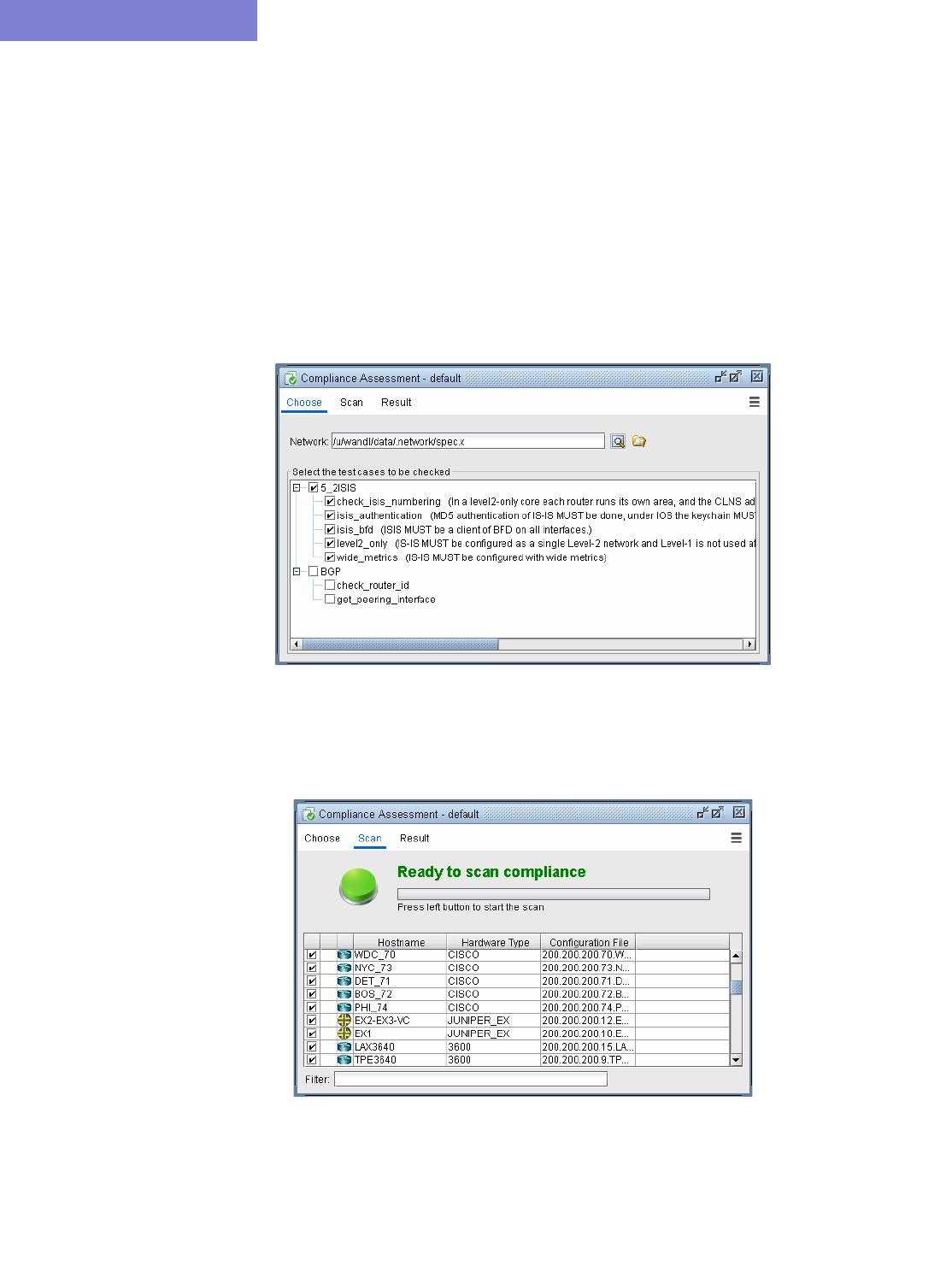
COMPLIANCE ASSESSMENT TOOL*
33-2 Copyright © 2014, Juniper Networks, Inc.
33
Detailed Procedures
Compliance Assessment Tool
To open the Compliance Assessment window, select Tools > Compliance Assessment. This window is used
primarily by network operators to run CAT scans on the network configuration files. The CAT scans are a collection
of test cases or rules that search the configuration files for keywords, strings, and statement matches or non-matches
to determine configuration compliance. These test cases are created using CAT template syntax by template
designers. The templates syntax can use logical operators, conditional expressions, and variables to support more
complex searches.
•The Choose screen allows for selection of the test case(s) and network for the CAT scan. Initially this screen
will have no test cases displayed until the test cases are created and published from the CAT Testcase Design
window. The CAT Testcase Design window is opened by clicking Manage Templates.
Figure 33-1 Compliance Assessment Choose screen
•The Scan screen allows for selection of the device(s) and their configuration files for the CAT scan. Press
the green button to start the scan.
Figure 33-2 Compliance Assessment Scan screen
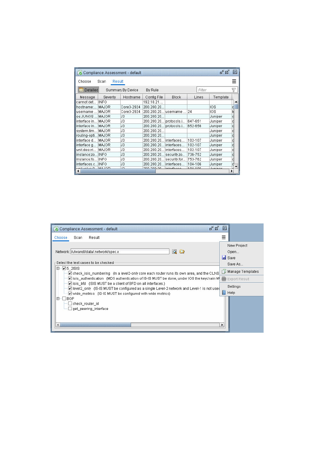
COMPLIANCE ASSESSMENT TOOL*
Copyright © 2014, Juniper Networks, Inc. 33-3
. . . . .
•The Result screen displays the results of the CAT scan. The results can be viewed in detailed, summarized
by device, or summarized by rule name. The summary reports also calculate a Score which represents the
device’s configuration compliance to the test cases. A higher score means better compliance, and a lower score
means worse compliance comparatively. The Score Weights can be defined under Settings.
Figure 33-3 Compliance Assessment Result screen
•The Actions button provides options to save and open projects, manage templates, and change the Results
Score Weight. Saving projects in this CAT window saves the selected test cases in the Choose screen.
Figure 33-4 Compliance Assessment Actions options
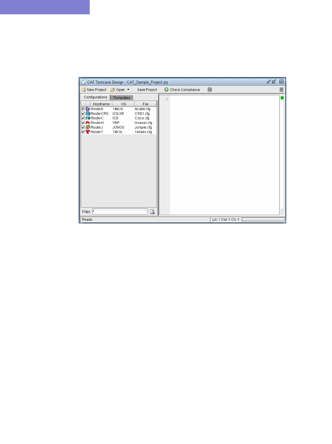
COMPLIANCE ASSESSMENT TOOL*
33-4 Copyright © 2014, Juniper Networks, Inc.
33
CAT Testcase Design
To open the CAT Design window, select Tools > CAT Testcase Design. This window is used primarily by
template designers to create templates or test cases, create projects which are a collection of templates and
configuration files, and publish those templates or test cases for network operators to use in the Compliance
Assessment window.
Figure 33-5 CAT Testcase Design window
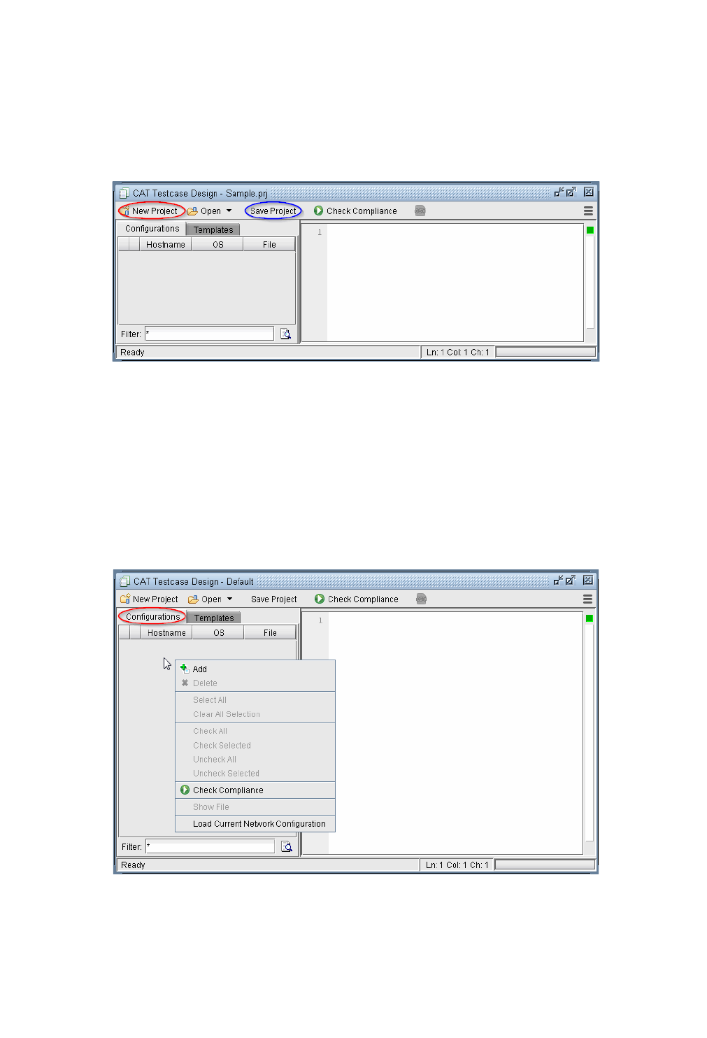
COMPLIANCE ASSESSMENT TOOL*
Copyright © 2014, Juniper Networks, Inc. 33-5
. . . . .
Creating a New Project
1. To create a new CAT project, click the New Project button in the CAT Testcase Design window.
2. The project title is listed in the title bar as “Default”. Click the Save Project button to save the project with a
name. This will open up the File Chooser window. Select a name for your project. CAT projects are saved with
file extension .prj
Figure 33-6 CAT Testcase Design creating new project
3. The next steps are to add configuration files and templates to the CAT project. It’s recommended to periodically
Save Project as you work.
Loading the Configuration Files
The following steps are to define the set of configuration files to be used in the CAT project.
4. Select the Configurations tab and right-click in the left panel.
Figure 33-7 Configurations tab right-click options
5. Select Load Current Network Configurations to load the configurations of the currently opened network.
This option is only available if the current network opened has imported configuration files.
COMPLIANCE ASSESSMENT TOOL*
33-6 Copyright © 2014, Juniper Networks, Inc.
33
6. If no network has been opened or if you want to load a different set of configuration files, select Add from the
pop-up menu. A file chooser will open that allows you to navigate to the directory on the server where the
configuration files are saved. Select the configuration file(s) to be added to the project.
Figure 33-8 Selecting Configuration Files to add to the Configurations Tab
Use <Shift>-click to select a range of items from the currently highlighted entry. Alternatively, use <Ctrl>-click
to select an individual entry. The shortcut Ctrl-A can also be used to select all configurations in the directory.
Click Select to add the configurations to the Configurations tab. A checkbox next to each file indicates if it
will be included in the compliance assessment.
7. The configuration files will now be populated in the Configurations tab. Right-click and select Show File will
display the configuration file in the right panel. Double-clicking opens the configuration file in the Config
Editor window.
Figure 33-9 Configuration File Loaded
8. Configuration files that are not desired in the project can be deleted by right-clicking and selecting Delete.
9. Click Save Project to save the changes to the project.
COMPLIANCE ASSESSMENT TOOL*
Copyright © 2014, Juniper Networks, Inc. 33-7
. . . . .
Creating Conformance Templates
The next step is to create the compliance assessment test cases or rules using the CAT template. The templates will
be used to load in the test cases or rules for the CAT scan.
10. To create a new template, select the Templates tab. Right-click in the left panel and select New Template.
Figure 33-10 Creating a New Template
11. A New Template window will open as shown below.
Figure 33-11 New Conformance Template window

COMPLIANCE ASSESSMENT TOOL*
33-8 Copyright © 2014, Juniper Networks, Inc.
33
Category, Name, and Location: Are identification properties of the template.
•Category: This field is to help organize or group templates into categories.
•Name: Enter the name of the template.
•Location: Type in the location on the server where the file will be saved or use the Browse button.
•File Name: The template file extension is .tpl. You can change the default naming here.
Types: Are device vendor properties of the template.
•Vendor/OS: Select the configuration file type: “Cisco IOS”, “Cisco IOS-XR”, “Juniper JUNOS”, “ALU
TiMOS”, “Huawei”, “Redback”, “Tellabs” or “ZTE.”. Note that Cisco-IOS based templates can only be used to
check compliance on Cisco configuration files, Juniper JUNOS templates on Juniper configuration files, and so
forth.
•Hardware: The hardware type is derived from the network model. Using this field means only the specified
hardware type can be used by the template. If the field is blank, then any hardware type can be used.
•OS Version: The OS version is derived from the configuration file. Using this field means only the
specified OS version can be used by the template. If the field is blank, then any OS version can be used. A range
of OS versions can be specified using the following syntax: +, -, *
12.2+ means version newer (higher number value) than 12.2 including 12.2
12.2- means version older (lower number value) than 12.2 including 12.2
12.2* means any version starting with 12.2
Options: Select the basic option(s) that will be applied to this template.
•Case-sensitive: If checked, upper and lower case must be matched in the compliance assessment.
•Do not use regular expression: By default regular expression syntax is supported in the template. If
this option is checked, then regular expression syntax such as wildcards “*” and “?” can be not used. See More
on Regular Expressions on page 33-34 for more information.
When using regular expressions, the “#conform ignore escchars” statement can be used to indicate which
characters to be treated as is, and not as special regular expression characters. Without this line, you would need
to precede those text characters with a backslash ‘\’ to avoid interpretation of the character as a regular
expression.
** Important note: The use regular-expression conform statement cannot be used with “ignore ipaddress” and
“ignore description” conform statements. If the regular-expression statement is included in the template, the
other two statements are automatically discarded. Those statements can be simulated using regular expressions.
For example, to ignore a description, include “description.*” in the template at the appropriate place.
12. Ignore IP address and mask: Any IP addresses will be ignored in the compliance assessment. See Ignore IP
Addresses on page 33-35 for more information.
13. Ignore description: The “description” line for an interface in the configuration file will be ignored in the
compliance assessment.
14. Click OK when you are done. The new template will appear in the Templates tab. A checkbox will be
displayed to the left of each file for selecting particular configuration files/templates to be used for the
compliance assessment.
15. Double-clicking an entry will open the template file in the right panel and the template can be directly edited.
COMPLIANCE ASSESSMENT TOOL*
Copyright © 2014, Juniper Networks, Inc. 33-9
. . . . .
Figure 33-12 Initial Template
16. The options that were selected from the previous window can be seen listed in the first few lines after the
reserved directive, or keyword, “#conform,” and will be applied when compliance is checked. By default,
anything else following the pound sign “#” that does not start with “conform” denotes a comment and is
ignored. For more details on the #conform statements, refer to the table at Header Syntax - conform statements
on page 33-34.
17. Advanced users whom are familiar with the template syntax can create the template via a text editor on the
server (or the File Manager) and then import it into CAT by right-clicking the Templates left panel and
selecting Add.
18. Once the template is created, test cases or rules must be written using template syntax.
For more details on template syntax available for defining patterns and rules, see the following tables:
•Building Templates on page 33-20
•Building Templates on page 33-20
•Flow Control Syntax on page 33-24
•Built-In Functions For Use Within a Rule on page 33-26
•WANDL Keywords For Use Within a Rule on page 33-30
COMPLIANCE ASSESSMENT TOOL*
33-10 Copyright © 2014, Juniper Networks, Inc.
33
Editing the Conformance Template
19. After loading the template file, it’s content can be edited directly in the right panel. Cut, Copy, Paste, and
Find and Replace functions can be accessed by right-clicking or via the shortcuts <Ctrl>-x for cut, <Ctrl>-c
for copy, and <Ctrl>-v for paste, and <Ctrl>-f for find.
Reviewing and Saving the Template
20. After you have added your rules, right-click in the right panel and select Save to save the template, or use the
shortcut <Ctrl>-s.
21. If the box in the upper right corner of the CAT Testcase Design window is green, it indicates that no errors have
been found in the template.
Figure 33-13 Template with green box indicates no errors
22. Otherwise, if an error has been found, the box in the upper right corner will be red. Double-click on the orange-
colored segment on the right hand side bar to jump to the line with the error. For example, the error could be
related to an incomplete if statement (with no matching “end” statement).
Figure 33-14 Template with red box indicates errors
23. Clicking Save Project will also save any changes to the template.
COMPLIANCE ASSESSMENT TOOL*
Copyright © 2014, Juniper Networks, Inc. 33-11
. . . . .
Saving and Loading Projects
24. Once you have created a set of templates and the configurations to apply them to, this information can be saved
in a Project by clicking Save Project. A Project is defined as a set of configurations, templates, and
settings. To save the project as a new name, click the Action menu and select Save Project As.
Figure 33-15 Action menu
25. To open a saved project, select Open from the toolbar to open the project file from the server. This will
automatically load the associated configurations and templates in the project. Most recent projects are also
displayed by clicking the Open down arrow button.
COMPLIANCE ASSESSMENT TOOL*
33-12 Copyright © 2014, Juniper Networks, Inc.
33
Run Compliance Assessment Check
26. Select the Configurations tab and check the configuration files on which you wish to perform a compliance
assessment check.
•The right-click pop-up menu provides shortcuts to perform selections or deselections on all or selected
configuration files.
•Keyboard shortcuts can select a range of rows using <Shift>-click. Individual row selection can be selected
with <Ctrl>-click. All rows can be selected with <Ctrl>-a.
•The Filter field can be used to filter on the hostname, OS, or file name. To reset the filter and show all
configuration files, enter wildcard * or leave the field blank and press <Enter>.
Figure 33-16 Configurations Filter field
27. Select the Templates tab to select the compliance assessment rules to apply.
28. It’s recommended to save the project before continuing.
29. Click Check Compliance from the toolbar. The program will automatically save your script changes. The
program will then begin to run a check of the selected template(s) on the selected configuration file(s).
COMPLIANCE ASSESSMENT TOOL*
Copyright © 2014, Juniper Networks, Inc. 33-13
. . . . .
Figure 33-17 Check Compliance Results
30. The results of the compliance assessment check are shown in the bottom panel.
31. The Detailed tab shows the specific details for each configuration check. Double-clicking an entry will open
the configuration file at the matching line. The Summary By Device tab provides statistics for the
configuration check per device. The By Rule tab provides statistics for the configuration check per template
rule.
32. Use the Filter field above the results table to filter the table by a given string. To reset the filter and show all
results, enter wildcard * or leave the field blank and press <Enter>.

COMPLIANCE ASSESSMENT TOOL*
33-14 Copyright © 2014, Juniper Networks, Inc.
33
Compliance Assessment Results
DETAILED TAB
SUMMARY BY DEVICE TAB
Detailed Tab Column Description
Message Displays information such as the general type of conformance match,
mismatch, or partial match. If there is a mismatch, the line missing from the
configuration is included in the Message. "not ordered" indicates that the
lines are present in the configuration file but their ordering is not consistent
with that of the template. "hardware type mismatch" indicates that the
template type (Cisco IOS or Juniper JUNOS) does not match the
configuration file type.
Severity There are five levels. Warning shows that compliance has failed for a given
line, for example if a line is missing or failed to match. Info indicates a
match or partial match. The user can also change these levels to be
displayed as Minor, Major, or Critical.
Hostname Device hostname
Config File Displays the configuration file for which this entry applies. Double-clicking
on a row will open this configuration file in the Main Pane.
Block The exact block of the configuration of the message
Lines Displays the corresponding start line and end line where the results entry
applies.
Template Displays the template that was used for this compliance assessment.
Rule Template Rule Name
Template Lines Range of Line numbers in which template rule occurs
Template Line For conform command, indicates the content of the line with violation
Template Line # For conform command, indicates the line number with violation
Category Template rule’s category (if specified)
Vendor Device vendor (e.g., Cisco, Juniper)
OS Device Operating System
Version Operating System Version, e.g., 12.2(53)SE
Summary By Device
Column
Description
Hostname Device name converted into WANDL format
Rules Applied Number of template rules applied to the device
Config Blocks Applied Number of config blocks for which the rule was applied
Issues Number of issues
Criticals Number of critical issues
Majors Number of major issues

COMPLIANCE ASSESSMENT TOOL*
Copyright © 2014, Juniper Networks, Inc. 33-15
. . . . .
BY RULE TAB
Saving and Printing Compliance Assessment Results
33. To save the contents in the results tab, select the Export to CSV icon in the toolbar to export to a CSV file, which
can be opened in Microsoft Excel. Enter in a filename. Note that 3 CSV files will be created -- one for each tab.
•filename_result.csv -- Detailed tab
•filename_Result_NODE.csv -- Summary By Device tab
•filename_Result_RULE.csv. -- By Rule tab
Minors Number of minor issues
Warnings Number of warnings
Infos Number of informational messages
Score Compliance score = 100 - (#criticals * 1/#rules * critical_weight) - (#majors
* 1/#rules * major_weight) - (#minors * 1/#rules * minor_weight) -
(#warnings * 1/#rules * warning_weight) - (#infos * 1/#rules * info_weight)
By Rule Column Description
Rule Name Template Rule Name
File Template File Name
Routers Applied Number of routers for which the rule was applied
Config Blocks Applied Number of config blocks for which the rule was applied
Issues Number of issues
Criticals Number of critical issues
Majors Number of major issues
Minors Number of minor issues
Warnings Number of warnings
Infos Number of informational messages
Score Compliance score = 100 - (#criticals * 1/#rules * critical_weight) - (#majors
* 1/#rules * major_weight) - (#minors * 1/#rules * minor_weight) -
(#warnings * 1/#rules * warning_weight) - (#infos * 1/#rules * info_weight)
Summary By Device
Column
Description
COMPLIANCE ASSESSMENT TOOL*
33-16 Copyright © 2014, Juniper Networks, Inc.
33
Publishing Templates
34. For most network operators, their focus is monitoring the network and running compliance assessment checks
(CAT scans). They normally do not need to learn the CAT template syntax or how to build test cases. This scope
of work to build the rules is normally done by the template designers. Thus network operators do not need to use
the CAT Testcase Design window and they can perform their work in the Compliance Assessment window.
35. Template designers can publish their templates from the CAT Testcase Design window to the Compliance
Assessment window. Check the templates you wish to publish, then click the Action menu and select Publish
Templates.
Figure 33-18 Publishing Templates
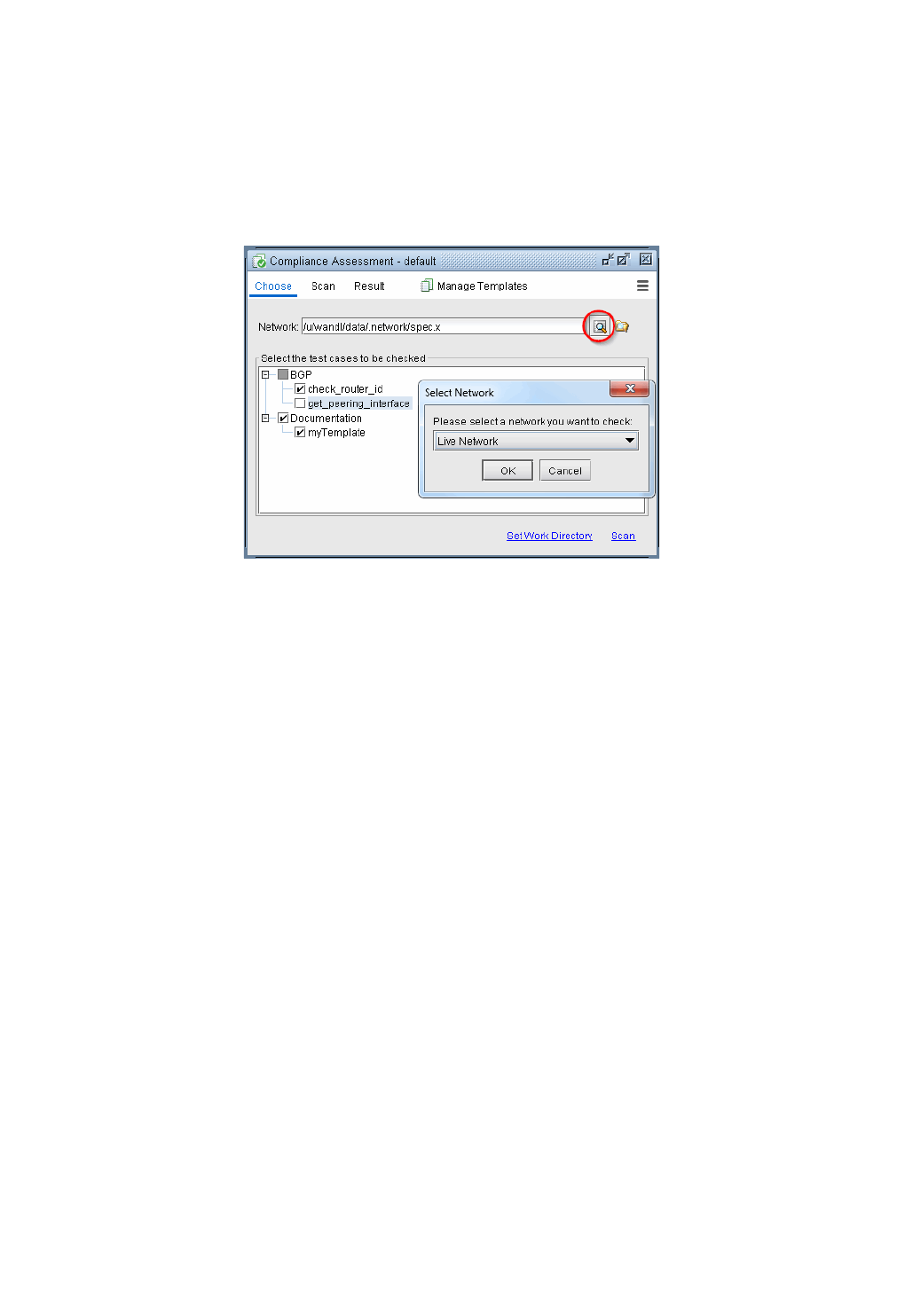
COMPLIANCE ASSESSMENT TOOL*
Copyright © 2014, Juniper Networks, Inc. 33-17
. . . . .
36. When templates are published, these will show up as “test cases” in the Compliance Assessment window. The
details of the template syntax language and associated vendor(s) are transparent for the network operators.
37. Network operators can run compliance assessment checks using the Compliance Assessment Scan screen and
view the results in the Results screen. One difference running CAT scans in this window is that all the
configuration files are selected from the Choose screen by selecting the associated network project instead of
selecting specific individual configuration file.
Figure 33-19 Choosing Network
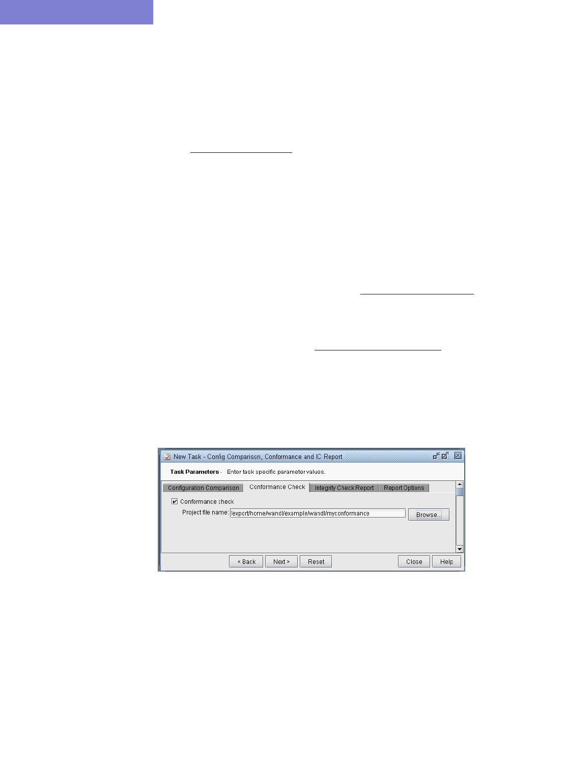
COMPLIANCE ASSESSMENT TOOL*
33-18 Copyright © 2014, Juniper Networks, Inc.
33
Running External Compliance Assessment Scripts
An external script can also be called by the conformance template. Any programming language can be used to write
the script as long as it can be called from the command line. In order to display the script results in the Compliance
Assessment window’s Detailed Results tab, the script’s output should be comma-separated, including the
following details on each line:
Message,Severity,Hostname,Config File,Block,Lines,Template,Rule,Template Lines,Template Line,Template Line
#,Category,Vendor,OS,Version
See the table Detailed Tab on page 33-14 for more details on each of these fields.
(Alternatively, the output could also be redirected to a separate file, rather than appended to the Detailed Results tab,
in which case it could be in any format.)
In the following example, the perl script myscript.pl would be executed using the spec file as one of its inputs. This
perl script checks to see if links of a given trunk type have the recommended ISIS metric for that trunk type. The perl
script’s output is then appended to the Detailed Results table.
#conform type cisco ios
@define external isis_metric_check output=append
./external/edit_check_isis_metric.pl ./spec/spec.auto
To see the example perl script used in this example, refer to IP Manipulation on page 33-36. Note that this particular
script parses link information from the bblink file. At the end of the script, the print statement outputs to the CSV
format with the appropriate fields to append to the compliance assessment detailed results table: print
"$msg,$severity,$node,$source,,,external,$rule_name,,,\n".
For further information on external scripts, see Building Templates on page 33-20.
Scheduling Configuration Checking in Task Manager
Compliance Assessment and integrity checks can be automatically performed at a designated time interval, using the
Configuration Check Report task of the Task Manager. Go to Admin > Task Manager. In the Task
Manager, press the “New Task” button. Select the Configuration Check Report task, enter a name for the task,
and then press “Next”.
Figure 33-20 Configuration Check Report Task
1. On the Conformance Check tab, select the checkmark for Conformance check and browse for the
conformance project file.
2. On the Report Options tab, indicate where the task results should be saved and whether or not to e-mail the
test results.
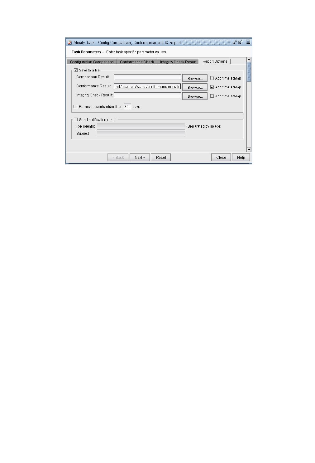
COMPLIANCE ASSESSMENT TOOL*
Copyright © 2014, Juniper Networks, Inc. 33-19
. . . . .
Figure 33-21 Compliance Assessment Report Options
3. Click “Next” and then specify the scheduling parameters, such as the interval at which to run this task.
4. Click “Finish” to submit the task.

COMPLIANCE ASSESSMENT TOOL*
33-20 Copyright © 2014, Juniper Networks, Inc.
33
Building Templates
A rule performs checking based upon patterns. Thus, to form a rule, you should define both pattern(s) and rule(s).
CISCO IOS EXAMPLE
The following is an example Cisco IOS template made up of two patterns “hasip” and “shutdown” followed by a rule
“Shutdown_or_noip” which checks the interface block based on the presence or absence of these two patterns. The
interface blocks (represented by keyword “interface”) are looped through with a “foreach” statement. If either
pattern “hasip” is not matched or pattern “shutdown” is matched, a severity level of “warning” is raised. Otherwise,
a severity level of “information” is raised via the print statement (equivalent of “raise info”).
#conform name ciscotemplate
#conform type cisco ios
@define hasip
ip address $(myip) *
@define shutdown
shutdown
@define rule Shutdown_or_noip
foreach interface do
if (!hasip || shutdown) then raise warning "$(interface.name) has no ip address or shutdown"
else print "$(interface.name) has an ip $(myip)"
end
end
Note: In the pattern hasip, note that the word following “ip address” is being saved into a variable with name
“myip”, so that the IP address can be printed out subsequently in the Shutdown_or_noip rule.
Note: Blank lines and white spaces in templates are ignored (except when used in regular expressions). So using
blank lines to separate blocks of text in the template are not necessary.
JUNIPER JUNOS EXAMPLE
The following is a simple Juniper example to check a global variable, the OS version, and raise different severity
levels depending upon the OS version. In this case, referencing a pattern is not necessary, since $(version) is a global
variable.
#conform name junipertemplate
#conform type juniper junos
#conform use regular-expression
@define rule junosversion
if $(version) ~= "7.*" then raise critical "version $(version)"
elseif $(version) ~= "8.*" then raise major "version $(version)"
elseif $(version) ~= "9.[1-3].*" then raise minor "version $(version)"
else print "version $(version)"
end
Because Junos contains a well-defined hierarchical structure defined by braces, it is possible to design configuration
compliance assessments at specific levels of the hierarchy. For example, the following rule check_rsvp checks for
the existence of traceoptions under the protocols rsvp clause of each device:
#conform type junos
@define rsvptraceoptions
traceoptions {
file rsvp.log size 10m;

COMPLIANCE ASSESSMENT TOOL*
Copyright © 2014, Juniper Networks, Inc. 33-21
. . . . .
flag error;
flag resv;
flag route;
flag resvtear;
flag all;
}
@define rule check_rsvp
foreach protocols.rsvp do
if rsvptraceoptions then raise info "matched rsvp trace options"
else raise major "no match for rsvp trace options in $(hostname)"
end
end
Note: For Junos pattern definitions, key structural characters like ‘{‘ and ‘;’ should not be substituted by a regular-
expression, since they have special meanings to the program.
For example, if there is a section for chassis as follows, the user can use the syntax chassis.fpc.pic to loop through
the pic’s as in “foreach chassis.fpc.pic do”:
chassis (
fpc 0 {
pic 0 {
}
}
}
If the next item in the hierarchy is an unknown name, such as for the interfaces {} block, under which are the
interface names such as ge-0/0/1, ge-0/0/2, etc. the keyword “child” can be used as follows, and its contents can be
printed using $(instance).
@define hasdescription
description $(intfdesc)
@define rule maindescription
foreach interfaces.child do
if (hasdescription) then print "$(instance) has description $(intfdesc)"
end
end
For more WANDL keywords, see WANDL Keywords For Use Within a Rule on page 33-30.
MATCH ORDERED, UNORDERED, OR EXACT
In addition to performing compliance assessments on specific blocks of code, there is a rule to check for lines within
the entire configlet, using the keyword “match”, or its equivalent keyword “conform.”
Suppose the config file contains five lines:
a
b
c
d
e
Then within the template file, we can define patterns, and rules to check for an exact match of the pattern, an ordered
match, or an unordered match:
@define block
a

COMPLIANCE ASSESSMENT TOOL*
33-22 Copyright © 2014, Juniper Networks, Inc.
33
b
d
@define block2
a
c
b
@define rule exactmatch
match exact block # not matched due to additional lines c and e
@define rule orderedmatch
match ordered block2 # not matched due to out of order lines (lines c and b)
@define rule exactmach2
match exact block2 # not matched by the same reason above (an exact match must also be ordered)
@define rule match
match block2 # matched
Template Syntax
@define <Pattern Name> Define a pattern of a block of text. It could contain one word, one line or
multiple lines.
- Wild card, *, can be used to match any text. Alternatively, regular
expression can be used if appropriate #conform use regular-expression
statement is included in the header.
- Note: The wild card should not be used to hide key syntax operators on
the first line such as braces ‘{‘ and semi-colons ‘;’
- $(<Variable Name>) can be used to capture and turn any text into a
variable, which can then be printed out in the subsequent rule.
Example:
@define pattern1
ip vrf $(vrf)
rd $(rd)
route-target export *
route-target import *
@define rule <Rule Name> Define a compliance assessment rule used for the syntax checking.
- Multiple rules can be defined within one template.
- Rules can be assigned to different categories by adding
category=<Category Name> in the end.
- Various flow control, loop, logic boolean, logic operator, print functions
can used in the rule.
- Additional flow controller keyword:
Exit: Once flow reaches exit statement, program will immediately stop
checking for the current rule and move on to the next rule if any.
Example:
@define rule BFD-Check category=Protocol

COMPLIANCE ASSESSMENT TOOL*
Copyright © 2014, Juniper Networks, Inc. 33-23
. . . . .
@define external <Rule Name>
output=[<path>|append]
Define a rule to execute an external program:
- A external program can be written in any language which uses stdout as
result output, e.g., a perl script could be used. Make sure this program is
executable from the command line.
- The result can be either output to a file or it can be appended to wandl’s
compliance assessment report if the result is in the same CSV format or
can be output to another separate file.
Example:
@define external rule1 output=/tmp/ls.csv
/usr/bin/ls -l
@define external rule2 output=append
/export/home/wandl/myscript.sh
@define description <Rule
Name>
Provide a description/explanation for the compliance assessment rule.
Example:
@define description
This rule checks whether the interface is shutdown or not

COMPLIANCE ASSESSMENT TOOL*
33-24 Copyright © 2014, Juniper Networks, Inc.
33
Flow Control Syntax
foreach <block> do
…
end
Define a loop function to go through each pattern block matched in
configuration, or to loop through each array element of an array. Flow
controller keywords to use within the loop function include the following:
- Next: Once flow reaches next statement, program will immediately stop
the current loop and move on to the next loop.
- Break: program will immediately leave the current foreach loop.
Note that nested loops can be used in configuration files with well-defined
hierarchical structures, such as Junos.
Example for array, using reserved keyword $(element):
foreach $(your_array) do
print $(element)
done
You can get an array element by using the subscript operation. It’s
syntax as follows:
$(array_name.array_index)
or
$(array_name.array_index_variable)
If $(array) is an array and $(index) is a number variable, then
$(array.index), $(array.0), $(array.1), are valid syntax.
$(array.length) will return the size of the array.
The keyword in can be used to check if a variable exists in an array
if $(string1) in $(array1) then...
Example for pattern block:
@define hasbandwidth
bandwidth $(bandwidth);
@define rule junosrule1 category=Interface
foreach interfaces.child.unit do
if hasbandwidth then print “$(interfaces.child) has bw $(bandwidth)”
end
end
Note: Nested loops are allowed for pattern blocks only if the nested loop
loops through a descendent of the parent loop. For example, the above
could be written as follows:
foreach interfaces.child do
for each unit do
if hasbandwidth then print “$(interfaces.child) has bw $(bandwidth)”
end
end
end

COMPLIANCE ASSESSMENT TOOL*
Copyright © 2014, Juniper Networks, Inc. 33-25
. . . . .
if (<boolean logic condition>)
then
…
elseif (<boolean logic condition>)
then
…
else
…
end
Define a boolean logic condition to separate flow into different scenarios
based on true or false boolean result.
- Both elseif and else statements are optional.
- Multiple elseif statements are allowed, if necessary.
- Additional Boolean logic operator keywords include the following:
&&: AND
==: EQUAL
||: OR
!=: NOT EQUAL
!: FALSE
~=: WILD CARD EQUAL
Example:
if (pattern1 && !pattern2) then print “pattern1 matched and pattern2
unmatched”
elseif (pattern1 && pattern2) then print "both pattern1 and pattern2
matched "
elseif (pattern3 ~= “Loopback*”) then print "loopback found in pattern3"
else print "none of above"
end

COMPLIANCE ASSESSMENT TOOL*
33-26 Copyright © 2014, Juniper Networks, Inc.
33
Built-In Functions For Use Within a Rule
$(<Variable Name>) To define a variable.
Example:
$(x)
“…” To define a string.
Example:
“This is a string”
set To assign a value to a variable.
Example:
set $(x) 1
+Arithmetic addition between number value or number variable or concatenate
between string and string variable.
Example1:
set $(count) $(count) + 1
Example2:
set $(string1) $(hostname) + "," + $(interface.name)
read To read in an external plain-text file containing multiple lines into a single degree
string array variable. One line per array member which can be used together
with “In: function.
Example:
read $(array1) "/tmp/interface-list.txt"
Note:
/tmp/interface-list.txt contains following lines
Router1,interface1
Router2,interface2
…
RouterN,interfaceN
add To add an element to an array.
add $(your_array) $(your_element)
Example:
foreach interfaces.child do
if $(instance) ~= "xe*" then
add $(full_interface_list) $(instance)
end
end

COMPLIANCE ASSESSMENT TOOL*
Copyright © 2014, Juniper Networks, Inc. 33-27
. . . . .
remove To remove an element from an array.
remove $(your_array) $(your_element)
Example:
foreach protocols.isis.interface do
if $(interface.name) ~= "xe*" then
if isis_disable then
remove $(full_interface_list) $(interface.name)
end
end
end
in To check if a string variable exists in a string array and yield true or false
boolean value.
Example:
if $(string1) in $(array1) then
raise info "$(string) is in the file"
end
raise To print a message entry to the compliance assessment result report with
severity assigned (pass, info, minor, major and critical)
Example:
raise major “This is a major event"
As a shortcut, a number can be used. The mapping between severities and
numbers are as follows:
- critical: 5
- major: 4
- minor: 3
- warning: 2
- info: 1
- pass: 0
Example:
raise 4 “This is a major event"
print Print is equivalent to raising an info message:
Example:
print “This is a info event"
child The “child” property can be used within a foreach loop to access the child item.
Example:
In the following configlet segment, ge-* and xe-* can be accessed using
“foreach class-of-service.interfaces.child do”
class-of-service {
interfaces {
ge-* {
}
xe-* {
}

COMPLIANCE ASSESSMENT TOOL*
33-28 Copyright © 2014, Juniper Networks, Inc.
33
element For arrays, a reserved variable to refer to the value of the current array object:
Example:
foreach $(your_array) do
print $(element)
done
conform <Pattern Name>
match <Pattern Name>
Looks for a match for the provided pattern and automatically raises a message
entry into the resulting report. The Detailed Results tab will show related line
numbers and line content under Template Line and Template Line #.
Matches if all lines and subblocks exists in config file. These lines do not have to
be in the same order for a match.
Example:
conform myconfiglet
conform ordered
<Pattern_name>
match ordered
<Pattern_name>
All template lines and block should be in configuration file. In addition, all the
lines must be ordered correctly. Note that config files may have additional lines
or subblocks.
Example:
conform ordered myconfiglet
conform exact
<Pattern_name>
match exact
<Pattern_name>
To match, the config file must contain the exact same section as the template. In
addition to having the lines ordered in the same way, no additional lines are
allowed in that section for a match.
Example:
conform exact myconfiglet

COMPLIANCE ASSESSMENT TOOL*
Copyright © 2014, Juniper Networks, Inc. 33-29
. . . . .
Special Built-In Functions
WILDMASK CONVERSION FOR CISCO
Use function called wildcardtocidr
Sample:
set $(converted) wildcardtocidr(ip, wildmask)
print "converting $(ip) wild mask $(wildmask) => $(converted)"
The result could be:
converting 62.179.128.0 wild mask 0.0.1.255 => 62.179.128.0/23
CONVERT ISIS SYSTEM ID TO IPV4
toipv4 (node.isis_system_id)
Sample:
toipv4(1921.6800.0001) will return 192.168.0.1
MATCH STRING VALUE
Use function called getmatch
Sample:
set $(interface.name) “Bundle-Ether1”
set $(number) getmatch(interface.name, “[0-9.]+”)
print “$(number)”
The result of the print out is “1”.
GET PHYSICAL INTERFACE FROM SUB INTERFACE
Use function called getphysical
Sample:
set $(logical) “ge-0/0/1.12”
set $(physical) getphysical(logical)
print “$(physical)
The result of the print out is “ge-0/0/1”.

COMPLIANCE ASSESSMENT TOOL*
33-30 Copyright © 2014, Juniper Networks, Inc.
33
WANDL Keywords For Use Within a Rule
The following are built-in convenient keywords available that can be used within a rule.
Keyword
Supported
Vendor Description and Example
$(hostname) All This keyword returns node’s hostname.
$(os) All This keyword returns node’s operating system name.
$(version) Vendors,
whose
configs
contains
the
version.
This keyword returns node’s operating system version
Note: Huawei and IOS-XR are example vendors where version
cannot be determined from configuration files, and thus this
keyword is not applicable for them.
$(node.isis_system_
id)
All This keyword returns the node’s ISIS system id.
$(node.hardware) or
$(node.type)
All This keyword returns the node’s hardware type.
$(instance) All This keyword is used to return the name of the instance you are
currently in. For example if your instance is family inet,
$(instance) will return “family inet”.
$(instance.name) All Only applicable when your instance name has two or more
words separated by space. This keyword is used to return the
name of the instance you are in minus the first word. For
example if your instance is family inet, $(instance.name) will
return “inet”.
Note: If your instance has two or more words separated by a
space, $(instance.name) will only return the second word. For
example, if your instance is interface ge-1/8/1/2 l2type vlan,
$(instance.name) will return “ge-1/8/1/2”.
$(instance.value) All Only applicable when your instance name has two or more
words separated by space. This keyword is used to return the
name of the instance you are currently in minus the first word.
For example, if your instance is “family inet”, $(instance.value)
will return “inet”
If your instance has more than two words separated by space,
$(instance.value) will return everything minus the first word. For
example, if your instance is “interface ge-1/8/1/2 l2type vlan”,
$(instance.value) will return “ge-1/8/1/2 l2type vlan”.
$(instance.[n])
where n is 0 to
unlimited.
All Useful when your instance name has two or more words
separated by space, and you want to choose which word you
would like to return. For example if your instance is “address-
family ipv4 vrf SHIELD_1”, $(instance.3) will return “SHIELD_1”.

COMPLIANCE ASSESSMENT TOOL*
Copyright © 2014, Juniper Networks, Inc. 33-31
. . . . .
$(keyword_instance
.name)
where
keyword_instance is
the first word of the
instance name.
All Only applicable when your instance name has two or more
words separated by space. This keyword is similar to
$(instance.name). For example if your instance name is “family
inet”, $(family.name) will return “inet”.
However, unlike $(instance.name) It can be used to return not
only the current instance name, but also the name of the
instance at the higher hierarchical level. For example:
policy-map core
class 5002
bandwidth percent 2
If your current instance is class 5002, $(policy-map.name) will
return “core”, while $(class.name) will return “5002”
Another example:
snmp {
v3 {
usm {
local-engine {
user wandl_usr {
authentication-md5 {
authentication-key "$xxxx";
...
If your current instance is authentication-md5, $(user.name) will
return wandl_usr.
$(keyword_instance
.value)
where
keyword_instance is
the first word of the
instance name.
All Only applicable when your instance name has two or more
words separated by space.
Similar to $(instance.value), for example if you instance name is
“interface ge-1/8/1/2 l2type vlan”, $(interface.value) will return
“ge-1/8/1/2 l2type vlan”.
However, unlike $(instance.value), this keyword can be used to
return not only the current instance name, but also the name of
the instance at the higher hierarchical level.
Example:
router bgp 88
address-family ipv4 vrf wandl2012
redistribute ospf 919 vrf wandl2012 match internal external 1
external 2
no synchronization
exit-address-family
!
If your current instance is “address-family ipv4 vrf wandl2012”,
$(router.value) will return “bgp 88”.
Keyword
Supported
Vendor Description and Example

COMPLIANCE ASSESSMENT TOOL*
33-32 Copyright © 2014, Juniper Networks, Inc.
33
$(keyword_instance
.child)
where
keyword_instance is
the parent name of an
instance.
Junos This keyword is useful when your instance has higher
hierarchical level of 2 or more and you want to return instance
name of the higher instance, excluding the top one.
In the following example, the “authentication-md5” instance has
a hierarchical level of 5 (snmp -> v3 -> usm -> local-engine ->
user wandl_usr).
snmp {
v3 {
usm {
local-engine {
user wandl_usr {
authentication-md5 {
authentication-key "$xxx";
When your instance is authentication-md5 , $(snmp.child) will
return “v3”, $(v3.child) will return usm, $(local-engine.child) will
return “user wandl_usr”.
Note: This variable does not work when the higher instance
name has two or more words separated by space. For example
$(user.child) is not valid as the instance has two words: “user
wandl_usr”. Basically, if your higher instance has a name (i.e
user.name), then it doesn’t have a child (i.e. user.child)
$(keyword) Junos Keyword is the first word of a line inside an instance. It is used
to return a line inside an instance minus the keyword.
In the following example, when your instance is system, then
$(host-name) will return J5, $(time-zone) will return EST, and
$(authentication-order) will return [ tacplus password ]
system {
host-name J5;
time-zone EST;
authentication-order [ tacplus password ];
}
$(keyword) will only return one line. If you have multiple lines
with the same keyword at the beginning of the line, only the first
one will be return
$(keyword) can also be used to return a line in the instance
above your current instance. For example:
firewall {
policer 10m {
if-exceeding {
bandwidth-limit 10m;
burst-size-limit 3k;
}
then discard;
}
}
When your instance is if-exceeding, $(then) will return “discard”.
It is not recommended to refer line in the higher instance using
$(keyword) directly. See $(keyword_instance.keyword).
Keyword
Supported
Vendor Description and Example

COMPLIANCE ASSESSMENT TOOL*
Copyright © 2014, Juniper Networks, Inc. 33-33
. . . . .
$(keyword_instance
.keyword)
where
keyword_instance is
the first word of an
instance, and keyword
is the first word of a
line inside an instance.
Junos It is used to return a line inside an instance, specified by
keyword_instance, minus the keyword. For example,
interfaces {
ge-0/0/0 {
description “physical interface”
unit 0 {
description "management interface for J1";
}
}
}
When your instance is unit 0, $(description) will return
“management interface” for j1, while $(ge-0/0/0.description) will
return “physical interface”. Note that $(unit.description) will also
return “management interface for j1”
While it is not recommended usage, when you are not inside
any instance, you can also use $(keyword_instance.instance) to
return a line inside a direct underneath instance. For example:
system {
host-name J1;
time-zone EST;
authentication-order [ tacplus password ];
}
routing-options {
router-id 22.22.0.5;
}
When your instance is global, $(system.host-name) will return
“J1”, $(system.timezone) will return “EST”,
$(system.authentication-order) will return “[ tacplus password ]”,
$(routing-options.route r-id) will return “22.22.0.5”
Keyword
Supported
Vendor Description and Example

COMPLIANCE ASSESSMENT TOOL*
33-34 Copyright © 2014, Juniper Networks, Inc.
33
Header Syntax - conform statements
The following are possible #conform statements that may appear in the template.
More on Regular Expressions
If the regular expressions option was selected when creating a new template, or equivalently, if the line #conform
use regular-expression is included at the top of a template, then regular expressions can be used when writing
the compliance assessment rules. A typical rule that uses a regular-expression will use the “~=” wildcard operator as
in the following example:
if $(interface.name) ~= "Lo*" then
print "$(interface.name) is a loopback interface"
end
Some of the most basic and most commonly used regular expression syntax are as follows:
#conform name <template_name> (Required) Identifies the template name.
#conform type <cisco ios| cisco ios-xr
juniper junos|alu timos|
huawei|redback|zte>
(Required) Indicates the vendor and operating system of the
configuration files for which the template will be used, e.g., Cisco IOS,
IOS-XR, Juniper Junos, etc.
#conform ignore ipaddress (Optional) Any IP addresses will be ignored in the compliance
assessment.
#conform ignore description (Optional) Ignores the “description” line for an interface in the
configuration file during the confomance check.
#conform use regular-expression (Optional) Recognizes regular expression syntax in the template. See
More on Regular Expressions on page 33-34.
#conform ignore escchars [](){}|+^$ (Optional) Characters specified after the “#conform ignore escchars”
will be treated as is, and not as special regular expression characters,
when regular expression use has been enabled. Without this line, you
would need to precede those text characters with a backslash ‘\’ to
avoid interpretation of the character as a regular expression. The
default characters that are ignored are: [](){}|+^$. You can customize
the list, or add additional ones as you see fit.
. Any single character. Note that to match a period exactly, precede the dot
with a backslash, “\.”
* Zero or more instances of the previous character
+ One or more of the previous character
? Zero or one of the previous character
[ ] Any character from the set. [ch]at matches “cat” or “hat”
[^] Any character not in the set.
( ) Groups patterns. (cat|hat) matches “cat” or “hat”
[a-zA-Z] Any character from a through z or A through Z, inclusive
[0-9] Any integer from 0 through 9, inclusive

COMPLIANCE ASSESSMENT TOOL*
Copyright © 2014, Juniper Networks, Inc. 33-35
. . . . .
Because some users may accidentally confuse wildcards with regular expressions, the Compliance Assessment
Tool automatically converts some statements, as shown in the following examples:
•“ATM*” is automatically converted to “ATM.*” - “ATM*” also matches “AT”, which is in most cases
unintended by the user.
•“*ATM” is automatically converted to “.*ATM” - “*ATM” is actually illegal regular expression syntax.
Note: When used in regular expressions, blank spaces are respected. They are not ignored.
Some examples are shown below:
For more examples using regular expressions, please refer to Appendix B: Search Preferences on page B-1 of
the General Reference Guide.
Ignore IP Addresses
If the #conform ignore ipaddress is included in the template, all IP addresses are ignored while performing the
compliance assessment. The following displays what is or is not recognized as an IP address
.
\ Used in front of a reserved regular expression character (such as “.” or “+”),
to match that particular character. For example, to match “tacacs+” exactly,
“tacacs\+” is required, as the plus sign has a special meaning in regular
expression syntax.
ip address.* To ignore the ip address. This can be used in place of the #conform ignore
ipaddress statement.
description.* To ignore the description. This can be used in place of the #conform ignore
description statement.
tacacs\+ To match “tacacs+” exactly, instead of just “tacacs”
version 12\..* To ensure the version begins with “12.”
net .*00 To ensure the net id ends with two zeros
router eigrp (100|299) To match “router eigrp 100” or “router eigrp 299”
tacacs-server host
192\.122\.[0-9]+\.[0-9]+
To ensure the IP address is declared 192.122.x.y where x and y are integers.
192.10.20.55/24 Is recognized as an IP address.
192.10.20.55 Is recognized as an IP address.
x.x.x.x Is recognized as an IP address (and therefore ignored). This special syntax can
match any ip address/mask combination and is therefore useful when the
#conform ignore ipaddress statement is used in a template.
For example, it will match “10.1.1.1/24”. Note that “x.x.x.x” will also match
“xx.1.xxxxx.99/xxx “ and “1.2.3.4”, so that these are ignored if present in a
configuration file. However, it will not match X.X.X.X (lower-case ‘x’ is required).
x.x.x.x/x Is recognized as an IP address. Behaves the same as “x.x.x.x”.
a.b.c.d Is NOT recognized as an IP address.

COMPLIANCE ASSESSMENT TOOL*
33-36 Copyright © 2014, Juniper Networks, Inc.
33
IP Manipulation
SUBNET MATCH CHECKING
Use keyword called in for subnet match checking
Examples:
"192.10.22.51" in "192.10.22.0/24" will return true
"192.10.22.51" in "192.10.22.51/32" will return true
"192.10.22.0/30" in "192.10.22.0/24" will return true
“10.0.0.1” in “10.0.0.2/30” will return true
INTERFACE IP HANDLING FOR CISCO
interface.ip - IP only
interface.mask - Mask only
interface.ipmask - CIDR form. Example, 10.0.0.1/24

Copyright © 2014, Juniper Networks, Inc. 34-1
. . . . .
. . . . . . . . . . . . . . . . . . . . . . . . . . . . . . . . . . .
C
ONFIGURATION
R
EVISION
*
34
his document describes how to use the Configuration Revision tool to check in new revisions, perform
comparisons, and view current or previous revision versions of a configuration file.
*Note that a special password is required for the configuration revision feature. Please contact your Juniper
representative for more information.
Related Documentation
For general step-by-step instructions on how to use the WANDL software, please refer to the Design & Planning
Guide.
For an overview of the WANDL software or for a detailed description of each feature and the use of each window,
refer to the General Reference Guide or Chapter 37, Router Reference.
Recommended Instructions
1. Setting Up the Revision Manager on page 34-1
2. Edit and Check-In Files on page 34-3
3. Comparing Different Revisions on page 34-3
4. Retrieving Files From The Revision Repository on page 34-4
5. Removing Files From The Revision Repository on page 34-4
6. Scheduling Configuration Checking in Task Manager on page 34-5
Detailed Procedures
The following steps will guide the user through the process of creating new revisions, comparing files from different
revisions, and retrieving files from the revision repository. Although the steps below describe the procedure for
Configuration Revision, the steps for WANDL File Revision follows similar steps. Use the Actions menu in
the upper right corner of the Revision Manager to switch between Config File Revision and Network File
Revision.
Creating New Revisions
Setting Up the Revision Manager
1. Identify the set of configuration files to be placed in the Revision Manager repository. Navigate to the folder of
the spec network project file associated with those configuration files. Click on the spec file to open the network
project.
Note: If you have not yet created a WANDL network project (spec) for your configuration files, you should
first do a configuration file import (File > Import Data). The project files will automatically be created and the
network project will be automatically opened.
2. Open the Revision Manager via Tools > Revision Manager. In the upper right corner of the window, click on
“Actions” and select “Configuration Revision” from the drop-down menu.
3. If you are accessing the configuration revision manager for the first time for the current network, you will see a
window as shown in Figure 34-1. Click on the Try again button to create a new revision repository for your
configuration files.
T
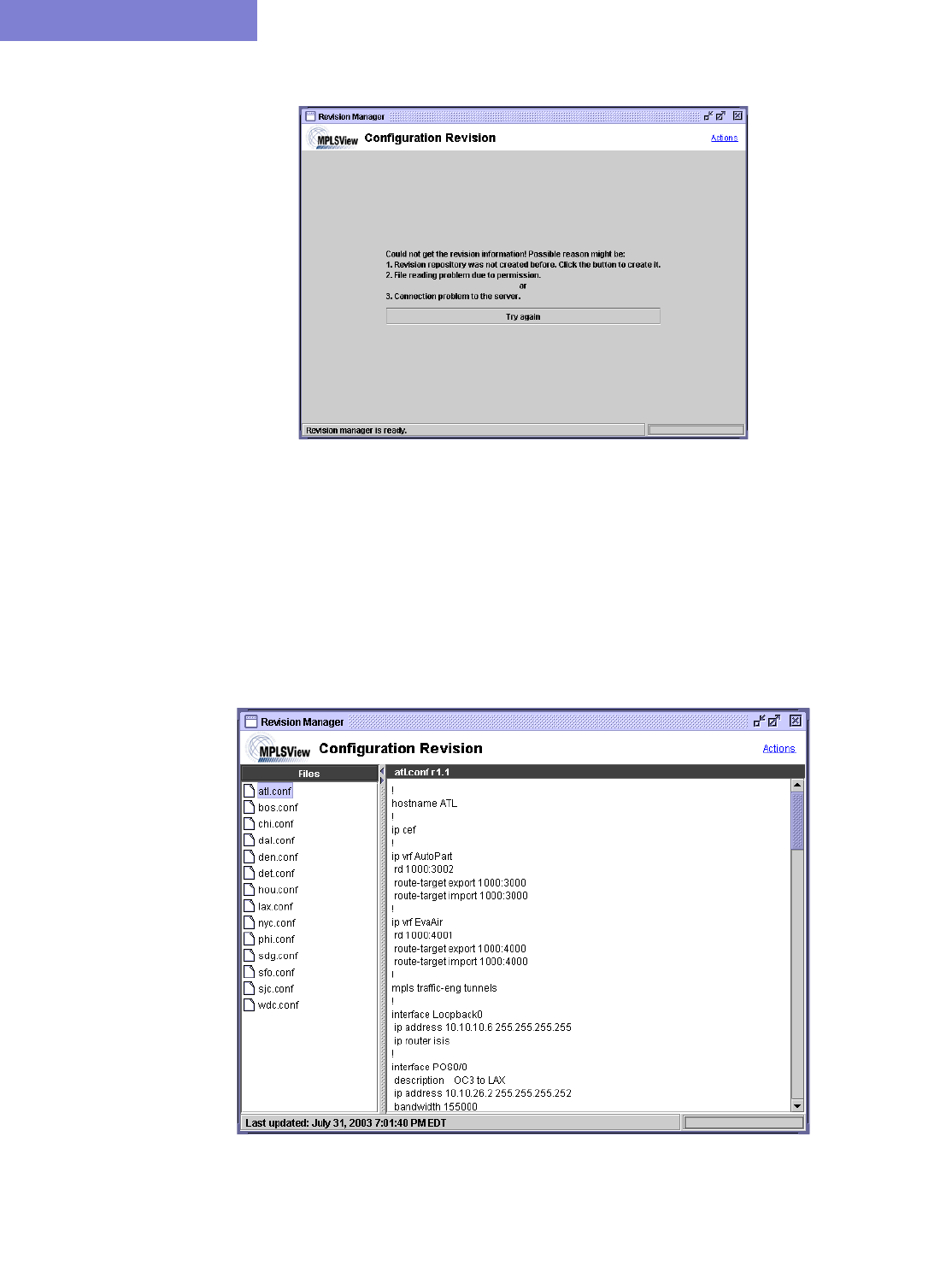
CONFIGURATION REVISION*
34-2 Copyright © 2014, Juniper Networks, Inc.
34
Figure 34-1 Initial Configuration Revision window
4. An information window will pop up telling you to select the configuration directory next. Click OK.
5. A “Directory Chooser” window will open up that allows you to select the directory in which the configuration
files are saved. Keep in mind that once this directory has been chosen, it will be used as the main directory from
which configuration revisions will be checked in. Navigate through the server directories to select the one
containing your configuration files. Click Select.
6. In the next window, the configuration revision manager will list the configuration files that are in the directory in
the left pane while the right pane will display the selected configuration file. Optionally you may right-click in
the left pane and select Sort by Hostname to display and sort the file list by the hostname.
Figure 34-2 Configuration Revision Manager
CONFIGURATION REVISION*
Copyright © 2014, Juniper Networks, Inc. 34-3
. . . . .
Edit and Check-In Files
7. The initial versions of the configuration files are labelled as “r1.1”. Any revisions following this will be labelled
“r1.2”, “r1.3”, etc.
8. On your server, edit the configuration file(s) as needed. After the modification, right-click on the left pane of the
Configuration Revision Manager and select Check In for the specific file you modified, or Check in All if
you want to check in all the files. The new revisions will now appear inside a folder for each configuration file.
9. Double-click on one of the folders to open it up. Click on “1.1” to view the file in the text pane.
Comparing Different Revisions
10. Compare the two revision files side-by-side by right-clicking on revision 1.1 and selecting Compare the
selection with revision....
11. In the dialog window, select revision 1.2 and click OK. The window should appear as shown in Figure 34-3.
Figure 34-3 Side-by-side comparison of two revision files
12. Similar to the Revision Manager, you may use the toolbar on the bottom to traverse through the differences
between the two files. Red signifies that the line was modified; green signifies that the line was deleted; and blue
signifies that the line was added.
13. Click on the right and left arrows on the bottom pane to traverse through the difference entries in a side-by-side
comparison.
CONFIGURATION REVISION*
34-4 Copyright © 2014, Juniper Networks, Inc.
34
Retrieving Files From The Revision Repository
14. To retrieve a file from the revision repository by timestamp, select “Retrieve by timestamp” from the right-
click menu in the left pane to bring up the “Retrieve revision” window as shown in the following figure.,
15. In the Target Directory box, specify the directory location where you would want the set of files for a
particular revision to be placed.
16. In the Retrieve Criteria section of the window, specify a date/time so that the latest version checked-in prior to
that specified date/time will be retrieved.
17. The Selection tab can be used to indicate which configuration files to collect. Right-click and select “Uncheck
All” or “Check All” to deselect or select all configuration files.
Removing Files From The Revision Repository
18. To remove a file from the revision repository, right-click on any of the revision files in the folder and select
Remove.
Purging Files From The Revision Repository
19. Select Actions > Schedule revision purge to choose to purge configuration revisions greater than the
specified interval (1 month, 2 month, 3 month, 6 month, 1 Year)
CONFIGURATION REVISION*
Copyright © 2014, Juniper Networks, Inc. 34-5
. . . . .
Scheduling Configuration Checking in Task Manager
20. Conformance checking and integrity checking can be automatically performed at a designated time interval,
using the Configuration Check Report task of the Task Manager. Go to Admin > Task Manager. In the
Task Manager, press the “New Task” button. Select the Configuration Check Report task, enter a name for
the task, and then press “Next”.
21. Select the “Report Options” tab and specify how the report will be saved as described in Report Options on page
32-5.
22. Select the “Configuration Comparison” tab and select the “Compare config files” checkbox. In the Revision
Manager, the set of config files are linked to a particular spec file, so this Spec file name must be used to
reference the set of config files against which comparisons will be made. See Setting Up the Revision Manager
on page 34-1 for more information on how to set up the configuration revision repository.
23. Alternatively, if you are using the online module, select “Use live network.”
Figure 34-4 Sources for Config File Comparison
24. Next, decide whether or not differences should be automatically checked in the Revision Manager.
25. Click “Next.” Specify the schedule parameters on the next page, such as the time interval at which to perform
the task.
26. Finally, click “Finish” to submit the task.
Network File Revision
Revision Manager supports revision tracking of network files for the Live Network. This is accessed by clicking
Actions > Network File Revision. It tracks bblink.x, intfmap.x, nodeparam.x, pathtable.x, and tunnel.x files. Read
Chapter 21, File Comparison Tools* for more detail on how to compare the network files.
•bblink file is a list of the links in the Live Network. See bblink file on page E-1 in the File Format Guide.
•intfmap file is a list of the interfaces in the Live Network.
•nodeparam file is a list of the nodes in the Live Network. See nodeparam file on page D-11 in the File Format
Guide.
•pathtable file is a list of paths and the corresponding route in the Live Network. See pathtable File* on page F-
17 in the File Format Guide.
•tunnel file is a list of the tunnels in the Live Network. See tunnel* (tunnelfile) (IP/MPLS only) on page F-28 in
the File Format Guide.

CONFIGURATION REVISION*
34-6 Copyright © 2014, Juniper Networks, Inc.
34

Copyright © 2014, Juniper Networks, Inc. 35-1
. . . . .
. . . . . . . . . . . . . . . . . . . . . . . . . . . . . . . . . . .
V
IRTUAL
L
OCAL
A
REA
N
ETWORKS
35
As modern metro Ethernet technologies mature and MPLS technologies such as VPLS are being used to extend
Layer-2 VLANs across the MAN and the WAN, there is an increasing need for a tool that provides visibility
into layer-2 VLANs in addition to the IP and MPLS layers. WANDL IP/MPLSView has risen to the challenge
by providing a whole suite of capabilities in support of VLANs. The tool automatically constructs the network's
VLANs via a VLAN Discovery task that uses a combination of SNMP MIBs polling and CLI show commands.
Combined with configuration file parsing, all the details related to each device, VLAN, and spanning tree are
derived by the tool and easily accessed by the user. Furthermore, the VLAN View window and the L2 STP
subview on the topology map allow the user to get a clear logical view as well as status information for each
individual VLAN and spanning tree. Besides gaining visibility into the VLANs in the network, IP/MPLSView
also allows the network planner to construct VLANs from scratch via the VLAN Wizard. If desired, the VLAN
configlet generation feature can be used to create configuration statements that can be pushed into the
router/switch by the network engineer.
Apart from just displaying the nodes and links that are part of a spanning tree, STP topology uses coloring to
signify the role of each node/link to make it easily understandable to the user. Devices that belong to a spanning
tree can be further grouped together by defining access domains to depict the real physical network. An access
domain is a group of physically connected layer 2 devices, where all the VLAN IDs are unique, i.e. devices that
have the same VLAN id in an access domain belong to the same VLAN. As direct physical connectivity cannot
be extracted, IPMPLSView, by default, groups all devices into the default domain. For networks with multiple
access domains, users should define the access domains and assign nodes into them properly as explained in the
VLAN Modification and Design on page 35-12.
*Note that special passwords are required for the VLAN module and for the Online module. Please contact
your Juniper representative for more information.
Prerequisites
Layer 2 VLAN information is accessible either in online or offline mode. In online mode, you should run the
Scheduled Live Network Collection task to collect switches’ Configuration and Switch CLI output. In addition,
you should also run the VLAN Discovery task for IPMPLSView to extract the spanning tree information from
the switches. Please refer to “Live Network Collection” chapter and “Reference” chapter of the
Management & Monitoring Guide for detailed steps on the Scheduling Live Network Collection and VLAN
Discovery Task
For offline mode, you can collect the configuration files using any third party collector. The SNMP polling on
the other hand, is recommended to be performed using our Standalone SNMP poller, as it requires real time
interpretation of ongoing polling results to determine the entire MIBs that needed to be polled, so that complete
spanning tree information can be obtained. Please contact your Juniper representative for details on the
Standalone SNMP poller availability.
Detailed Procedures
Importing VLAN and Spanning Tree Information
1. To import the files in offline mode, select File>Import Data and follow the Import Network Wizard.
2. For the Default Input Directory, choose the parent directory containing the network collection folders
(config, interface, etc.). For the Output Directory, choose the directory in which to save the project once
it is imported. Click Next.
VIRTUAL LOCAL AREA NETWORKS
35-2 Copyright © 2014, Juniper Networks, Inc.
35
3. In The Default tab, browse for the VLAN Discovery directory. This can be used to extract VLAN and
STP information. For this directory, you can either specify the Intermediates directory, generated from
running WANDL’s VLAN Discovery task in /u/wandl/data/collection/.LiveNetwork/bridge/intermediates.
Alternatively, you can specify the bridge directory, generated from running WANDL’s VLAN discovery,
with the SNMP output.
To also extract VLAN information from config files, the user can also import the config files, or specify a
dummy config file directory.
4. Once all the directories are selected, click Next> to begin importing the files in the chosen directories and
click Finish. The generated network model will then be loaded into IP/MPLSView.
Viewing VLAN Details
ACCESSING LAYER2 INFORMATION
5. To view a summary of all VLANs and STPs that are present in the current network, bring up the VLAN
Summary window (via the Network > Services > VLAN) as shown in the following figure.
The window will display the number of VLANs, STPs and layer2 switch nodes, present in the network on
the right panel. The Summary tree on the left panel has Access domains in the next level that contains
information of VLANs, VLAN devices’ layer2 details, spanning trees etc. More details on access domains
will be discussed later in the chapter.
Figure 35-1 VLAN View Summary window
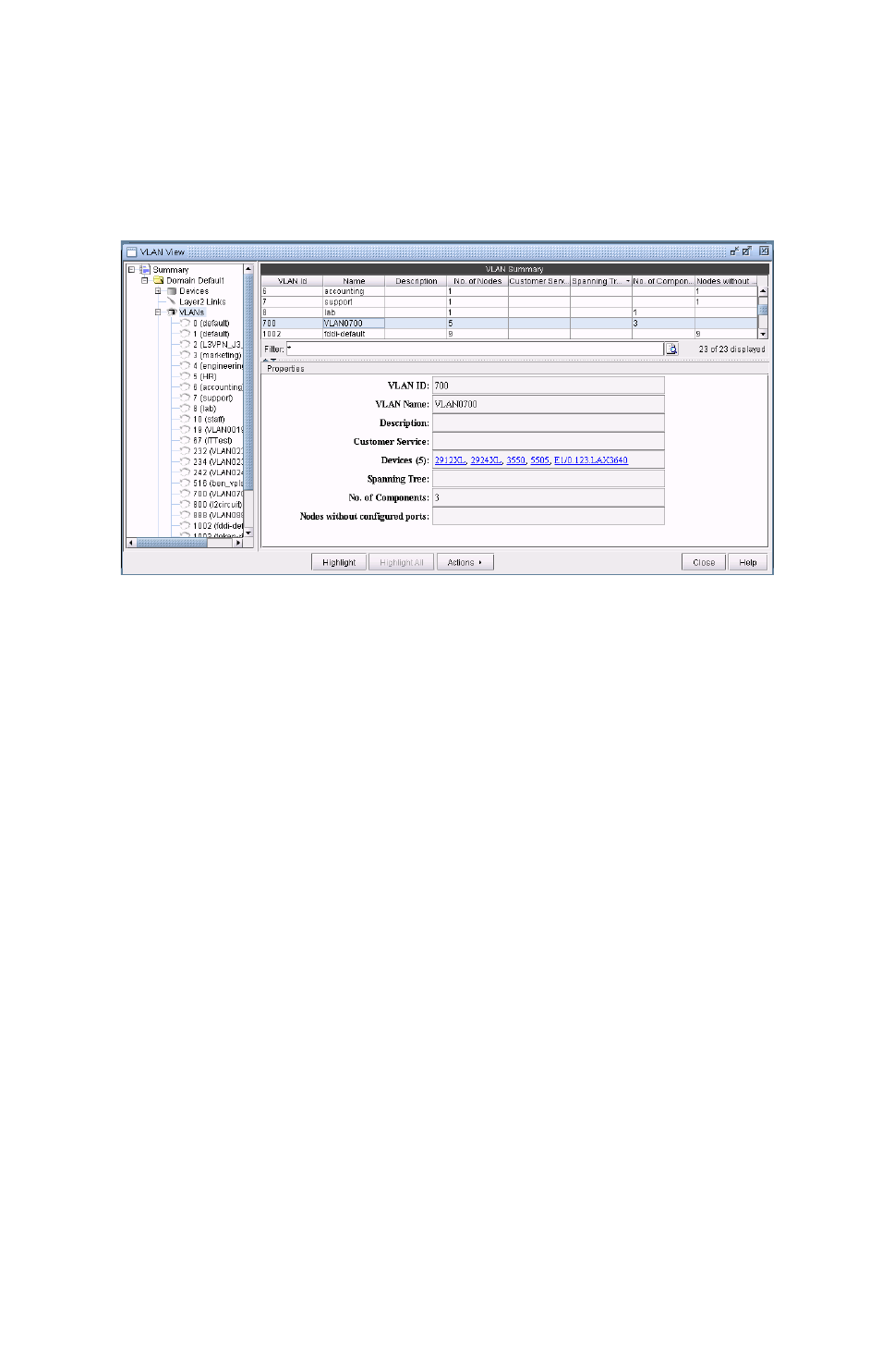
VIRTUAL LOCAL AREA NETWORKS
Copyright © 2014, Juniper Networks, Inc. 35-3
. . . . .
ACCESSING VLAN INFORMATION
6. To view VLANs that are present in the selected access domain, click on VLANs sub-tree.The window will
provide a list of all VLANs with details such as VLAN IDs, VLAN names, number of nodes in each VLAN
etc. on the right panel. Click on a row on the right panel to view the selected VLAN’s details under
Properties panel.
Figure 35-2 VLAN View window’s Properties pane for a selected VLAN: 700
7. With a particular VLAN selected, you may also click on the Highlight button to view all the devices
associated with the VLAN highlighted on the main topology map.
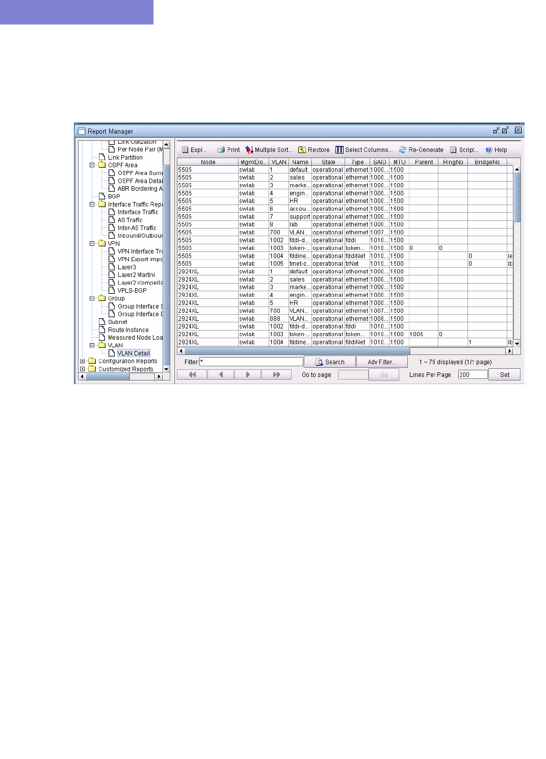
VIRTUAL LOCAL AREA NETWORKS
35-4 Copyright © 2014, Juniper Networks, Inc.
35
ACCESSING VLAN REPORT
8. A VLAN report is generated from running VLAN discovery task or importing intermediates directory into
the network. The generated report can be accessed from Actions > Report in VLAN View window or
through Report > Report Manager from the main menu.
Figure 35-3 VLAN Report
9. You may double-click on VLANs sub-tree or click the (+) icon next to VLANs sub-tree to view a list of all
VLANs in the selected access domain, where the VLANs are categorized by VLAN name.To view more
detailed information of a VLAN, click on a VLAN in the left panel.The Details tab, on the right panel,
lists all the devices that belong to the selected VLAN and each node’s details such as bridge addresses,
number of interfaces assigned to the VLAN, in/out policies etc. Click on a row on the right panel to view
the selected node’s VLAN details under Properties panel.
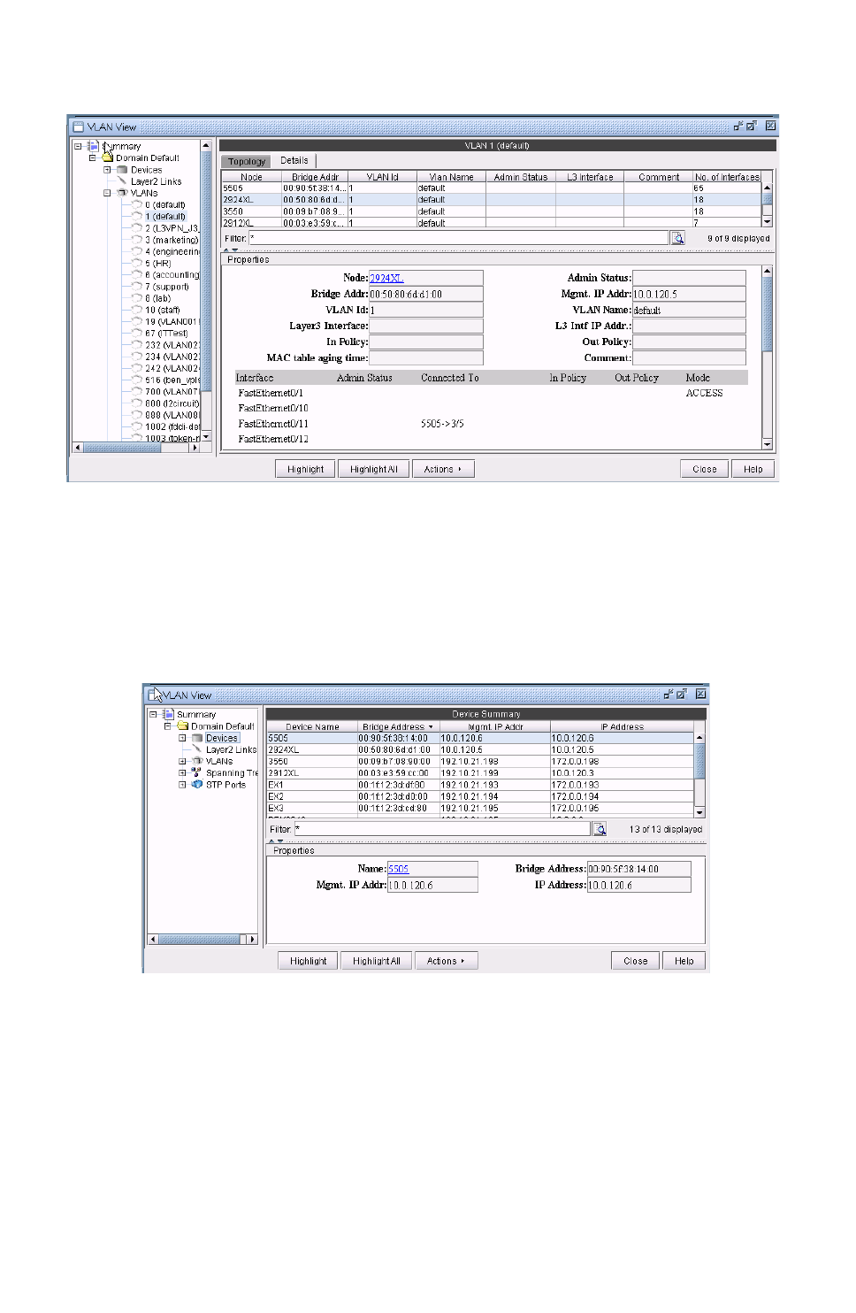
VIRTUAL LOCAL AREA NETWORKS
Copyright © 2014, Juniper Networks, Inc. 35-5
. . . . .
Figure 35-4 Detailed View of a selected node: 2924XL for the selected VLAN: 1
ACCESSING DEVICES INFORMATION
10. The Devices sub-tree lists all the devices that belong to VLANs in the selected access domain, with their
layer2 and layer3 address details.To view the devices, click on Devices sub-tree. Click on a row on the
right panel to view the selected device’s details under Properties panel.
Figure 35-5 VLAN Device’s details for a selected device: 3550
11. Expand Devices sub-tree to view a list of all Devices in the selected access domain. To view more detailed
information of a device, click on a device in the left panel.The Details tab, on the right panel, lists all the
VLANs and VLAN related configuration details associated with the selected node. Click on a row on the
right panel to view the selected VLAN’s configuration details under Properties panel.
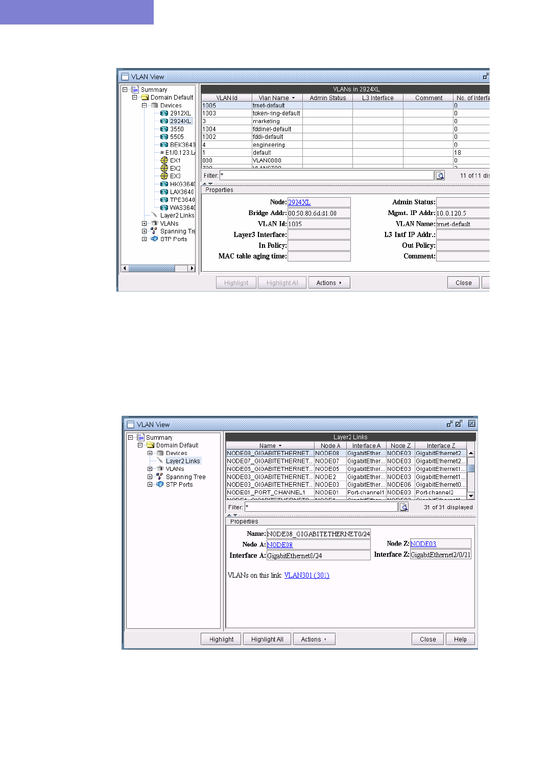
VIRTUAL LOCAL AREA NETWORKS
35-6 Copyright © 2014, Juniper Networks, Inc.
35
Figure 35-6 Detailed view of a selected VLAN: 1005 for the selected Device: 2924XL
ACCESSING LAYER2 LINKS INFORMATION
12. Click on Layer2 Links to view all layer2 physical links that are present between VLAN devices in the
selected access domain. For any aggregate links, such as Port-channel interfaces, right-click on the entry
and select “Show Related Interfaces” to identify the physical interfaces belonging to the Port-channel
interface.
Figure 35-7 Layer2 Links Details
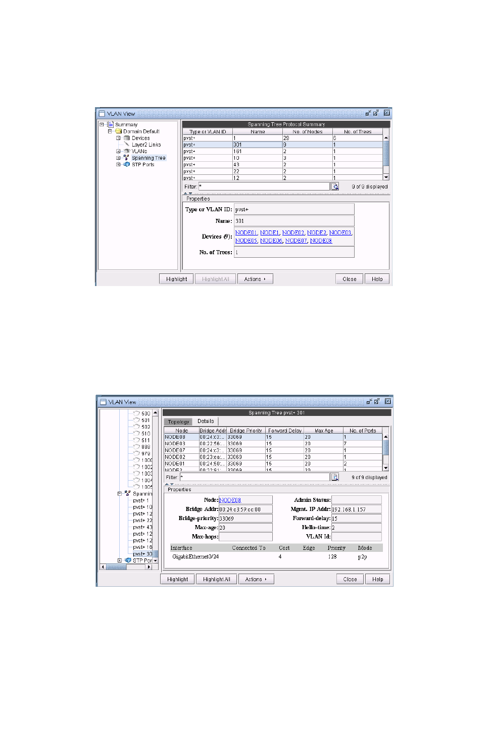
VIRTUAL LOCAL AREA NETWORKS
Copyright © 2014, Juniper Networks, Inc. 35-7
. . . . .
ACCESSING STP INFORMATION
13. To view spanning trees that are present in the selected access domain, click on Spanning Tree sub-
tree.The window will list all the spanning tree types.
Figure 35-8 Selected Spanning Tree: PVST+ 301details
14. Expand Spanning tree and you should see a list of all the spanning trees present in the selected access
domain with the following naming convention: STP-Type VLANID for PVSTs and STP-Type for other
spanning tree types. Select a spanning tree to view the list of nodes and spanning tree related configurations
associated with them.
Figure 35-9 Detailed view of a selected node: NODE08 for the selected spanning tree: PVST+ 301
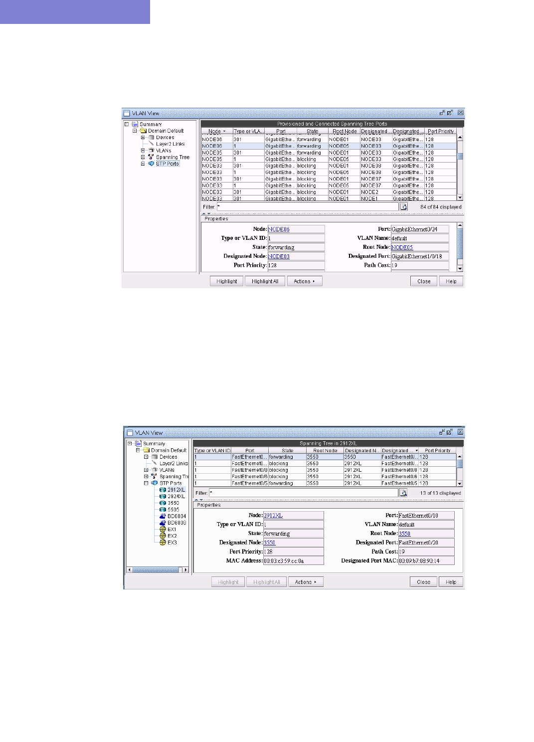
VIRTUAL LOCAL AREA NETWORKS
35-8 Copyright © 2014, Juniper Networks, Inc.
35
ACCESSING STP PORTS INFORMATION
15. STP Ports subtree displays all the node ports that are part of the spanning trees in the selected access
domain, with other details such as port types, states, priority etc.
Figure 35-10 Spanning tree port details of a selected port: GigabitEthernet0/24 for the selected node:
NODE06
ACCESSING STP PORTS INFORMATION FOR A PARTICULAR NODE
16. Expand STP Ports and you should see a list of all the devices present in the selected access domain.
Select a device to view the list of ports participating in spanning tree for that particular node, and the
related spanning tree information, such as the recorded root node, the recorded designated node, the port
state, etc.
Figure 35-11 Spanning Tree port Details of a selected node 2912XL

VIRTUAL LOCAL AREA NETWORKS
Copyright © 2014, Juniper Networks, Inc. 35-9
. . . . .
Viewing VLAN Topology
VLAN TOPOLOGY VIEW
17. The VLAN topology view (or VLAN View) presents to the user a clear, logical view of each individual
VLAN.To display logical topology view of any particular VLAN, simply click on the VLAN Topology
tab (next to the Details tab). You may also move the nodes around as desired in the VLAN topology view
map.
Figure 35-12 VLAN Topology View
18. There is also a right-click menu that you can use to perform basic functions to manipulate the topology and
the labels. Place the cursor on a node and do a right click to view node access and topology display options.
Figure 35-13 Right-click menu showing topology and label functions
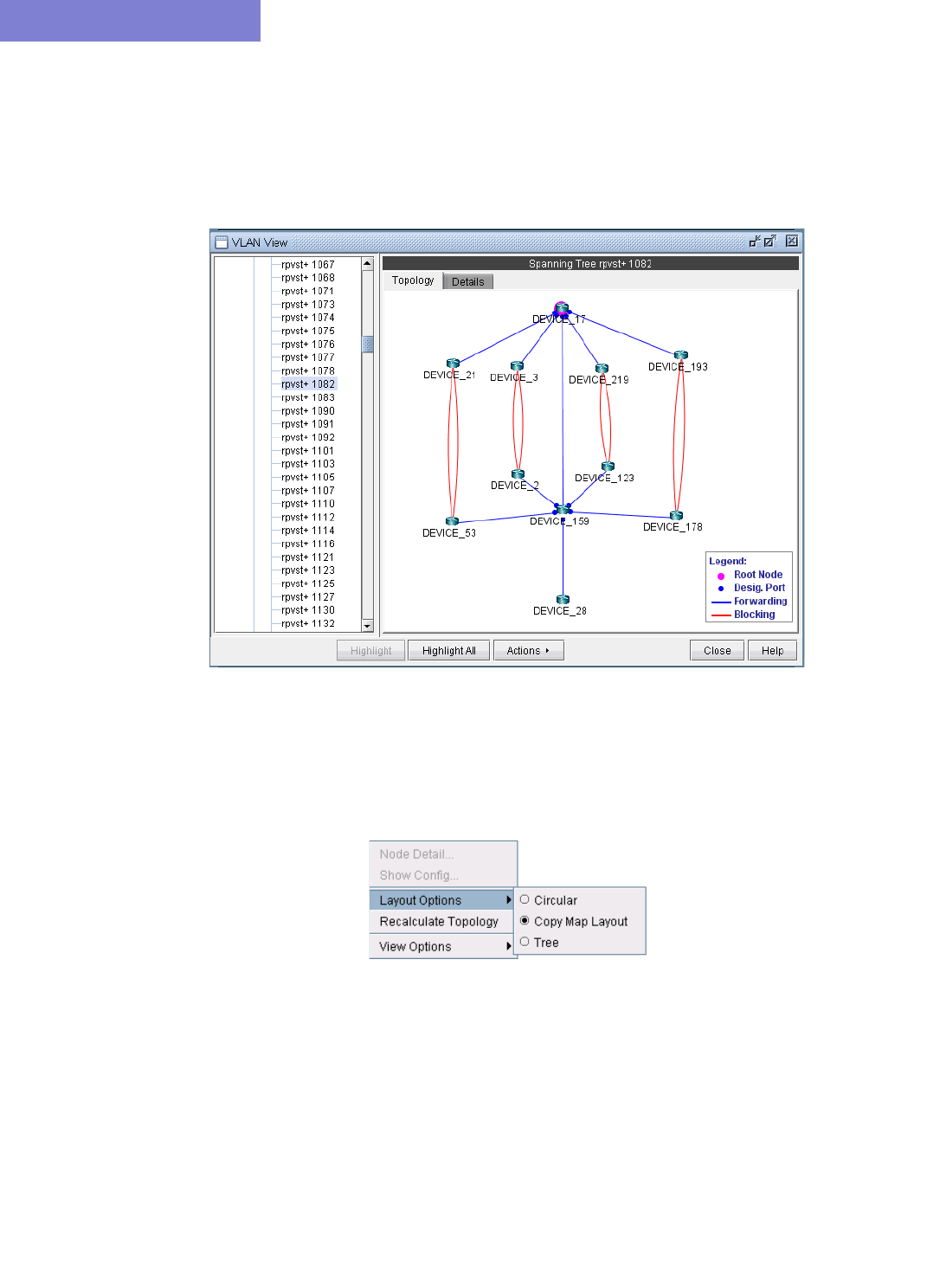
VIRTUAL LOCAL AREA NETWORKS
35-10 Copyright © 2014, Juniper Networks, Inc.
35
SPANNING TREE TOPOLOGY VIEW
19. The topology of each spanning tree can be viewed on VLAN View window and also on the topology map
with color coded links and nodes that identify root/designated nodes and port states.To view the topology
on VLAN View window, click on a spanning tree on the left panel and open Topology tab.The legends at
the bottom right corner explain the color codes.
Figure 35-14 Topology view of a Spanning tree: PVST 1082
20. There is also right click menu that allows you to change the spanning tree topology layout into either tree or
circular shape from the original MAP (standard) standard. Place the cursor on any point inside the
topology window and do a right click to change the topology layout.
Figure 35-15 Right Click Menu to re-layout the Spanning Tree Topology
21. The Spanning tree topology can also be viewed on the topology map. Choose Subviews > L2STP from
the top left drop-down menu on the Map (Standard) window.You should now view a list of all spanning
trees present in the existing network with the following naming conventions: VLANID (Root Node) for
PVSTs and STP-Type (Root Node) for all other types of spanning trees. Click on a spanning tree on the
left panel to view its topology on the map. The nodes and links of the selected spanning tree are colored
such that each color signifies their roles.
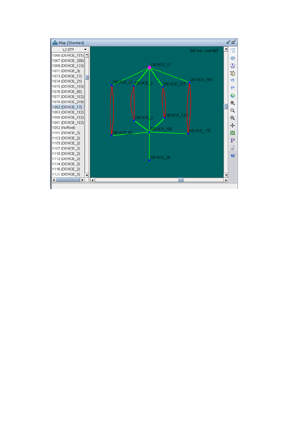
VIRTUAL LOCAL AREA NETWORKS
Copyright © 2014, Juniper Networks, Inc. 35-11
. . . . .
Figure 35-16 Topology view of a spanning tree: 1082 (DEVICE_17) on topology map
Below is a list of coloring conventions followed:
•Pink Colored Node: Root Node.
•Blue Colored Node: Designated Node.
•Green Colored Node: Non-STP Node.
•Green Colored Link: Ports on both ends of the link are in forwarding state.
•Red Colored Link: Ports on one or both ends of the link are in blocking state.
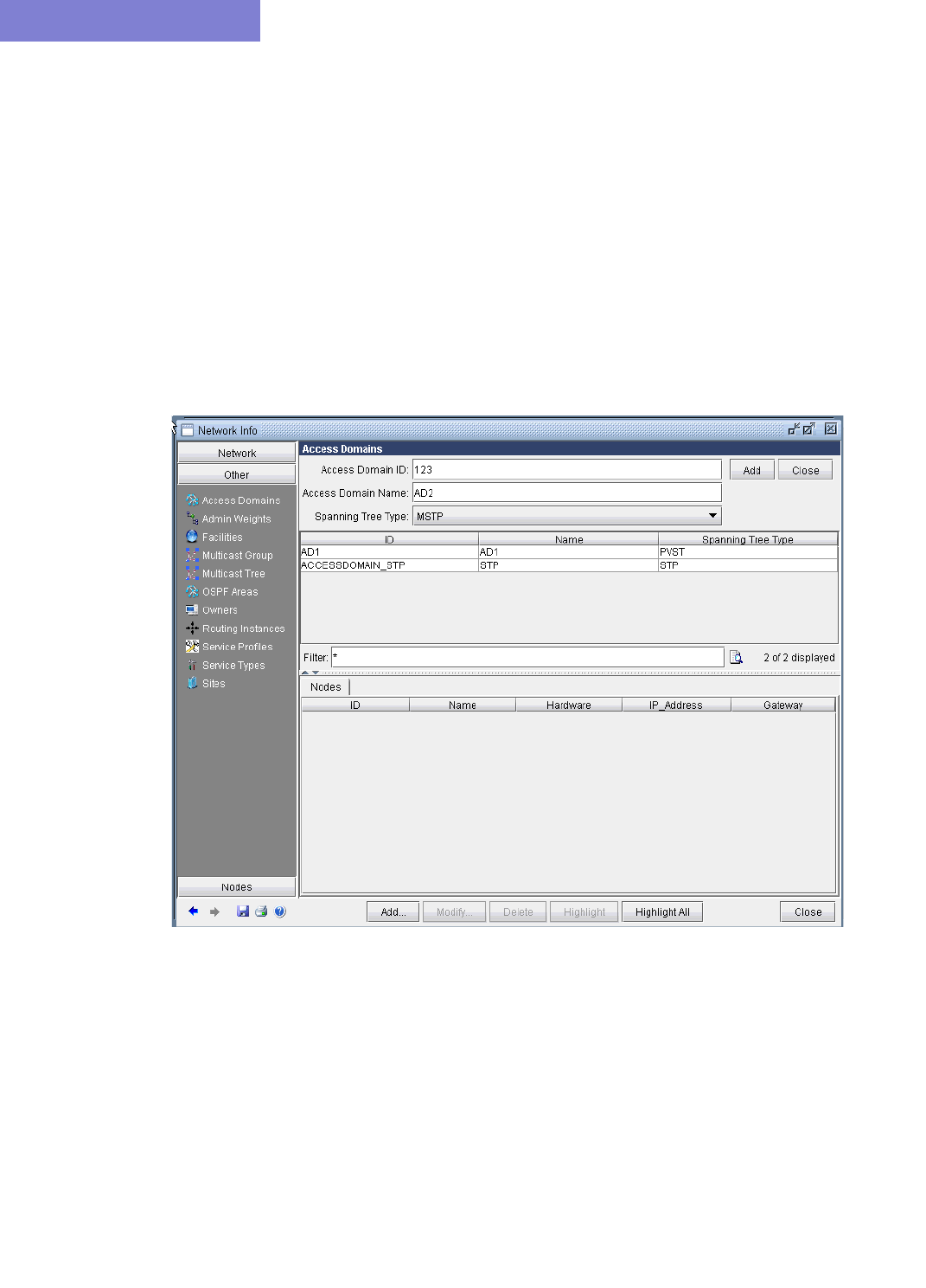
VIRTUAL LOCAL AREA NETWORKS
35-12 Copyright © 2014, Juniper Networks, Inc.
35
VLAN Modification and Design
DEFINING AN ACCESS DOMAIN
An access domain is a group of physically connected layer2 devices that use spanning tree or direct
connection to perform layer2 routing within the domain. Each access domain supports 4096 VLANs, thus
allowing identical VLANs across multiple access domains. As direct physical connectivity information
cannot be extracted from the config files, IP/MPLSView treats all the VLANs and STPs in the network as
part of a default domain. The user should define access domains and assign the nodes to access domains to
view VLAN and STP information categorised by access domains in VLAN View window.
To define an access domain, first switch to Modify mode and then choose Modify > Services > Access
Domains...
22. Enter Access Domain ID & Name details and choose spanning tree running across the access domain from
the Spanning Tree Type drop-down menu in the top panel as shown in the following figure.
Figure 35-17 Adding an Access Domain
23. Hit the Add button on the top right panel.The middle panel displays the list of all defined access domains
and the newly added access domain should now add to the list.
24. To view the nodes information of a particular access domain, click on an access domain in the middle panel
and the bottom panel displays the information as shown in the following figure.
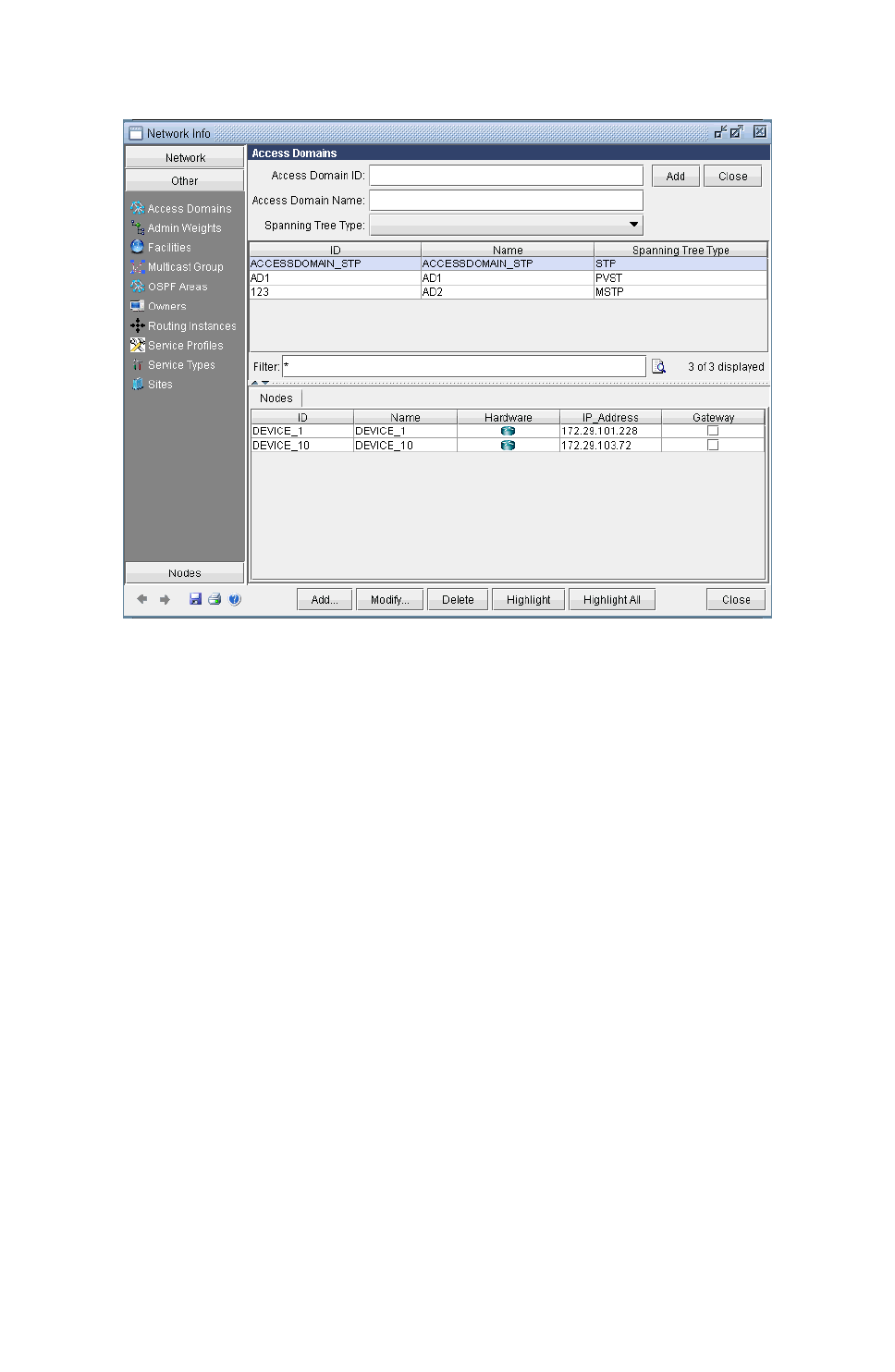
VIRTUAL LOCAL AREA NETWORKS
Copyright © 2014, Juniper Networks, Inc. 35-13
. . . . .
Figure 35-18 Access Domains and Nodes details
MODIFYING AN ACCESS DOMAIN
25. To modify an existing access domain, click on an accesss domain in the middle panel and hit Modify at the
bottom. After making changes to the access domain, hit Modify at the top right panel.
DELETING AN ACCESS DOMAIN
26. To delete an access domain, click on an access domain in the middle panel and hit Delete. To only view
the list of existing access domains and nodes details, hit Close on the top right panel.
27. After adding all access domains, hit Close at the bottom of Network Info window.
ASSIGNING NODES TO ACCESS DOMAIN
28. To assign nodes to an access domain, choose Modify > Elements > Nodes...
29. Select a node/ multiple nodes that are located in an access domain and hit Modify.
30. In the Modify Nodes window, select L2SW tab. Note that the L2SW tab is only available when a node is a
layer 2 device (Properties tab > L2SW is true). Choose the access domain that the selected nodes belong
to from the Access Domain drop-down menu, that lists access domain IDs, and hit OK. This completes the
assignment of nodes to access domain.
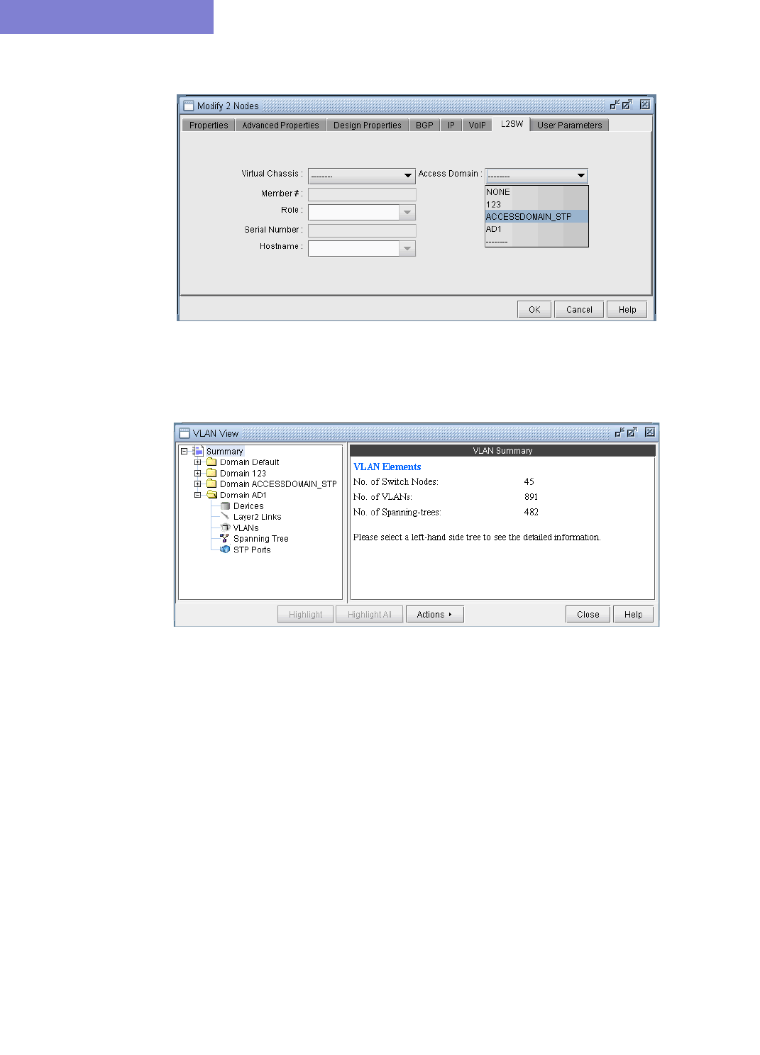
VIRTUAL LOCAL AREA NETWORKS
35-14 Copyright © 2014, Juniper Networks, Inc.
35
Figure 35-19 Assigning Access Domain to nodes
Below is a VLAN View window after adding access domains.
Figure 35-20 VLAN View window after defining Access Domains
ADDING LAYER2 LINKS
31. To add Layer 2 links between switches, choose Modify > Services > VLAN
32. Click on the Layer2 Links sub-tree under the access domain and then click on the Add button form the
VLAN View window
33. Select two switches and the corresponding interfaces for the new link, and click on the Add button s shown
in the following figure
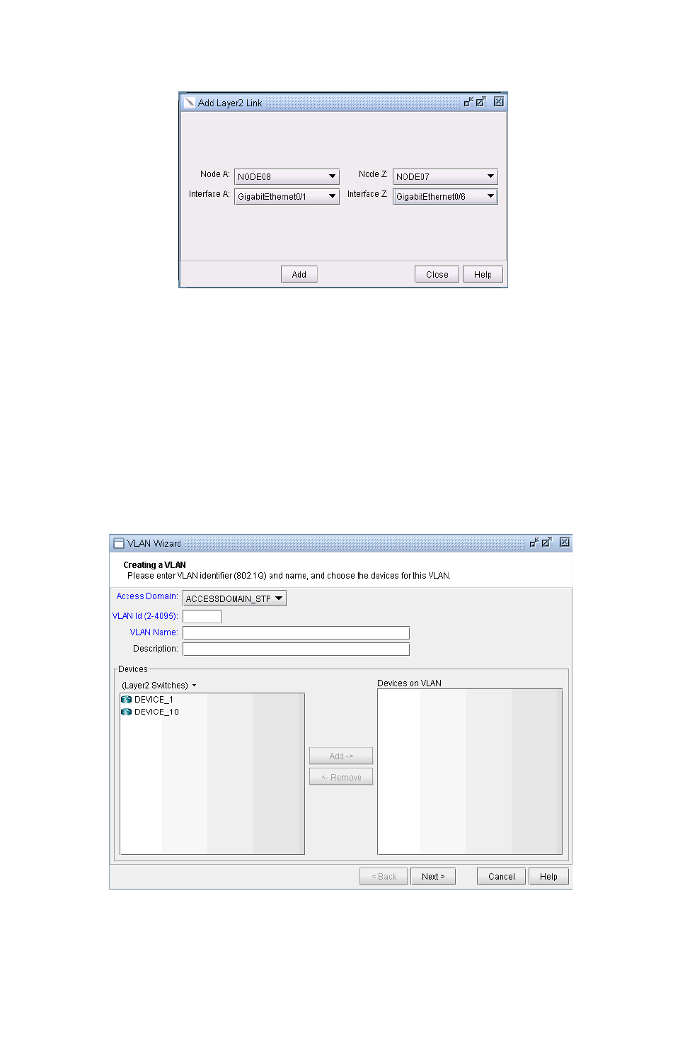
VIRTUAL LOCAL AREA NETWORKS
Copyright © 2014, Juniper Networks, Inc. 35-15
. . . . .
Figure 35-21 Adding Layer 2 Link between YGY_101 and BDN_001
ADDING VLAN DESIGN AND MODELING USING VLAN WIZARD
Besides the ability to derive the VLANs via network configuration import, the VLAN Module allows the
network planner to construct and model a VLAN from scratch, and to modify or add to existing VLANs. The
procedures described below on how to add VLANs also apply for modifying existing VLANs. First switch to
Modify mode, and then choose Modify > Services > VLAN.
To add any VLAN in an access domain, click on the VLAN sub-tree under the access domain and then click on
the Add button from the VLAN View window. To modify a VLAN, first select a particular VLAN and then
click on the Modify button. When you click on Add, the VLAN Wizard window, shown in the following figure,
is launched.
Figure 35-22 VLAN Wizard window
34. By default, the VLAN Wizard sets the access domain to the one you selected in the VLAN View window.
You may choose a different domain from the Access Domain drop-down menu and then enter the VLAN
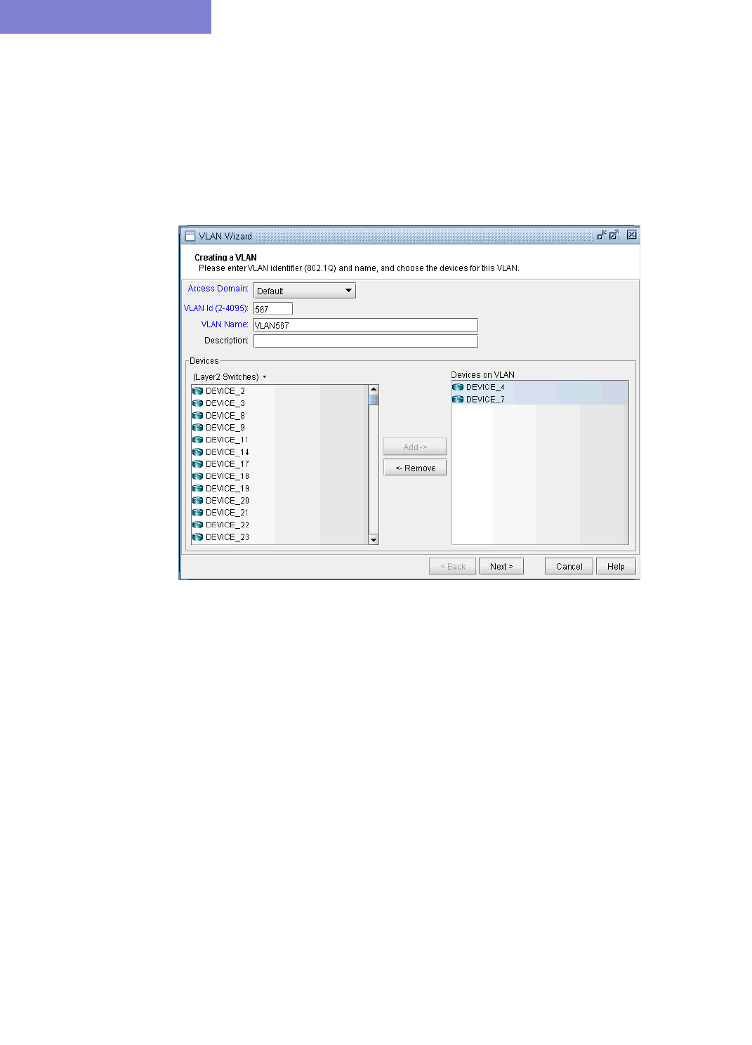
VIRTUAL LOCAL AREA NETWORKS
35-16 Copyright © 2014, Juniper Networks, Inc.
35
details in the respective fields.In order to accommodate for multivendor non-management VLAN IDs,
VLAN Wizard supports IDs above 2.
35. The Devices panel lists Layer2 Switches that belong to the selected Access domain. There is a drop-down
menu under Devices (down arrow besides Layer2 Switches) from which you can select the device types
you want to view and then add to Devices on VLANs. Choose the device type from the drop-down and use
Add button to add the selected devices in Devices to Devices on VLANs panel. VLAN wizard adds the
VLAN to the devices in Devices on VLANs.
Figure 35-23 Adding Devices to the VLAN
36. Click on Next to bring up the following window where you may add more devices and chosen devices
interfaces to assign to the VLAN.
•The middle part of the window show the topology area, where selected devices are placed.
•The Selected Objects area, as the name implies, lists those devices that have been selected as VLAN devices.
•The Available Devices box lists those routers for the currently chosen access domain.
•The Properties box lists all the interfaces for a particular device when it is highlighted (a device is
highlighted when it is clicked on either from the Available Devices list, the topology area of the window, or
from the Selected Objects list)
37. The window is designed to be as user-friendly as possible, with drag/drop capabilities built in. The
following figure shows the two devices that we have already added in the previous step.
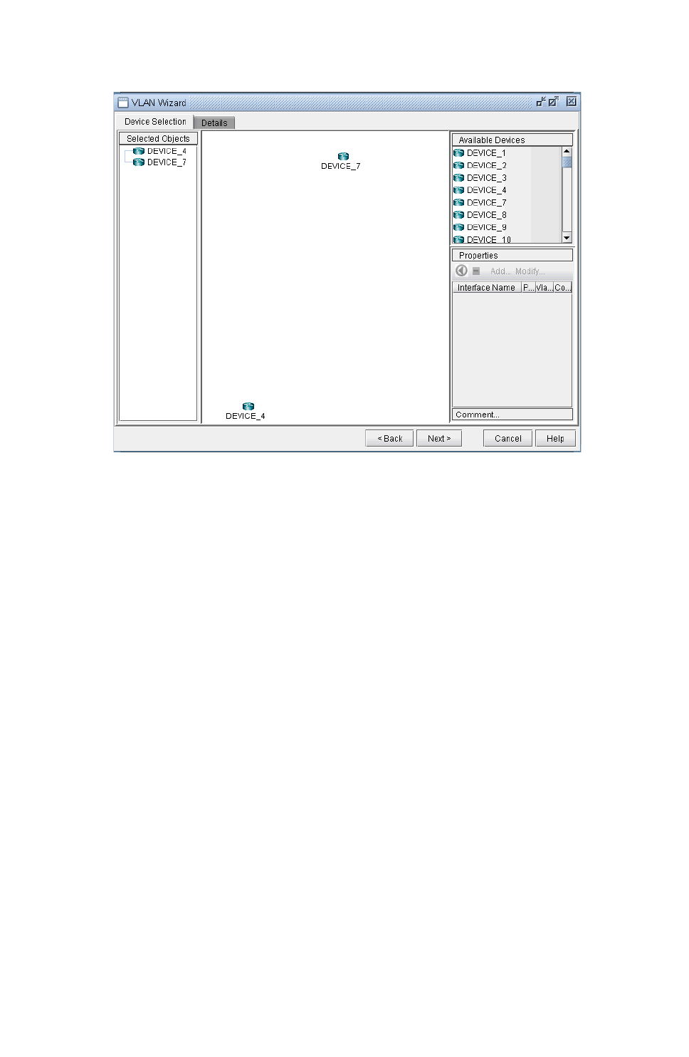
VIRTUAL LOCAL AREA NETWORKS
Copyright © 2014, Juniper Networks, Inc. 35-17
. . . . .
Figure 35-24 Assigning more devices and device interfaces to the VLAN
38. In more detail, you may add additional devcies to the VLAN from the Available Devices box via one of
two methods:
Select one or more devices (at which point the icon that has the left arrow with a circle around it will
change color from gray to blue), and then click on the blue arrow/circle icon to move it to the topology area
part of the window (middle of the window).
Alternatively, you could simply drag and drop devices from the Available Devices list into the topology
area of the window.
39. To assign interfaces to the selected devices, first select a particular device in order to have all its interfaces
shown in the Properties box. A device is selected when it is clicked on from the Selected Objects list or
from the topology area of the map. As shown in the following figure, the Properties box is now renamed as
Interfaces in AD101, since the device AD101 has been selected. Another icon worth mentioning is the "-
"/"+" button next to the arrow/circle button. Click on it to switch between "-" and "+". "-" means to show
all interfaces, while "+" means to only display interfaces that are unassigned or not shutdown.
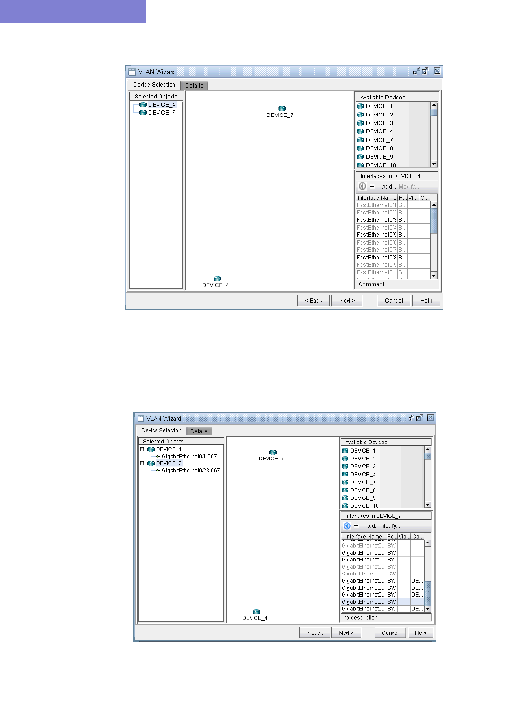
VIRTUAL LOCAL AREA NETWORKS
35-18 Copyright © 2014, Juniper Networks, Inc.
35
Figure 35-25 How to Assign Interfaces to VLAN devices
40. To assign an interface, you need to drag and drop a particular interface over to the device in the middle
panel. Alternatively, you can select the device from the left hand side, and then select an interface from the
interface list on the bottom right hand side, and click the blue arrow in the Interfaces section. The following
figure shows the window after the interfaces have been assigned to the devices.
Figure 35-26 Assigning Interfaces to the VLAN devices
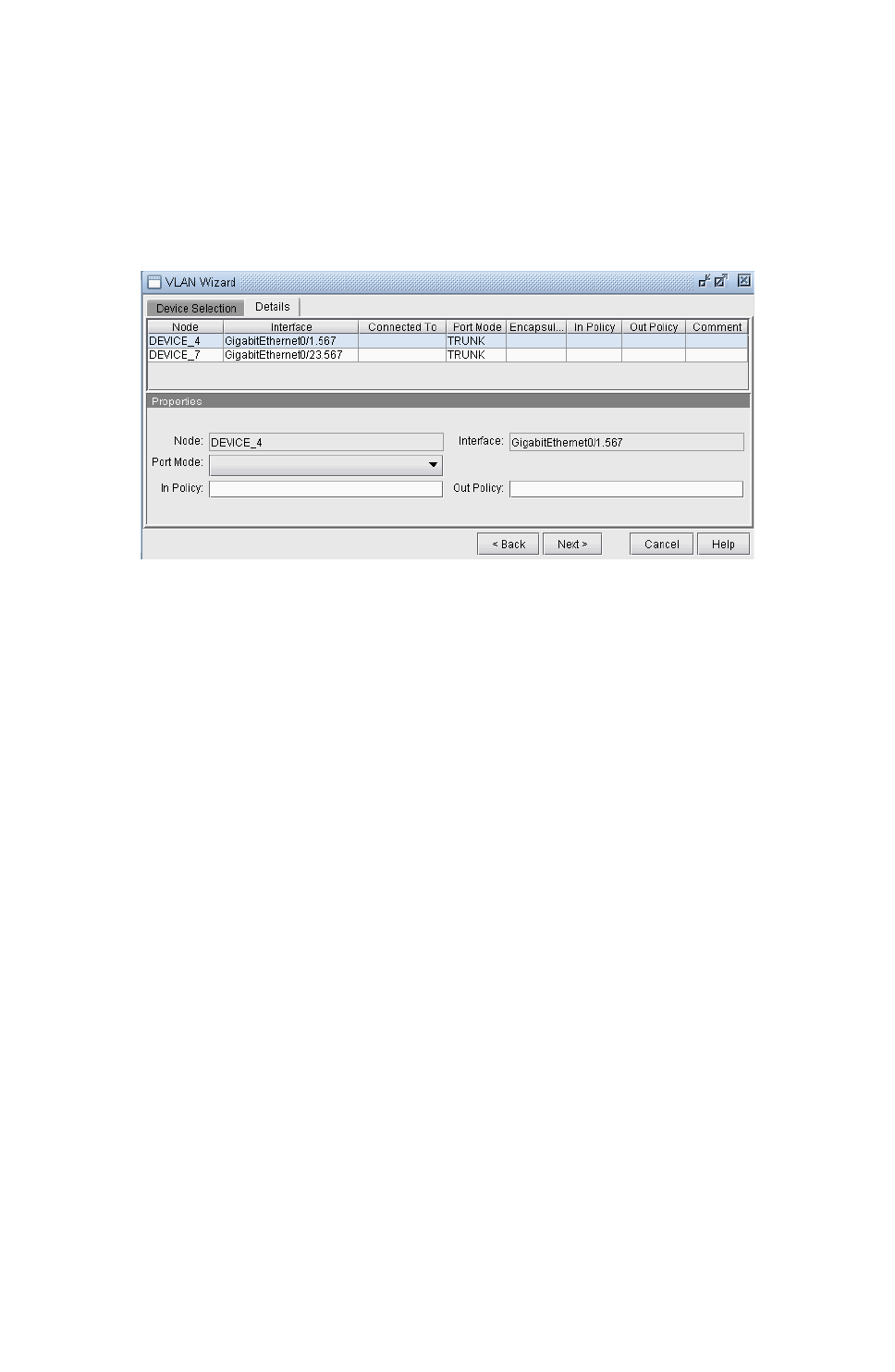
VIRTUAL LOCAL AREA NETWORKS
Copyright © 2014, Juniper Networks, Inc. 35-19
. . . . .
41. Note also the Add and Modify buttons in the Interface section. This can be used to add an additional
interface, e.g., if you need to add a new subinterface, or to modify an existing interface.
42. Click on the Details tab to assign in/out policies and port modes and then click Next. An interface’s port
mode decides if multiple VLANs can be defined on it. An interface with the port mode set to ACCESS can
belong to only one VLAN, while an interface with port mode set to TRUNK can belong to multiple
VLANs. In general, the interfaces that are facing the customer are set to access modes.
Figure 35-27 Assigning port modes and in/out policies to interfaces
43. The details entered in the final VLAN wizard window facilitates for layer3 inter-VLAN routing. Click on a
node in the left panel and choose a vlan interface from Layer3 Interface drop-down menu.
Layer3 interfaces are WANDL interfaces that should be created by the user to populate layer3 details in
VLAN Wizard window. The procedure to create a vlan interface is simlar to that of adding any new
interface, either from Modify > Elements > Interfaces or from the Add button in the VLAN wizard
window. Only rule is to begin the interface name with the keyword ‘vlan’ followed by VLAN ID.
IP address and in/out policies defined on the selected vlan interface will now be populated in the respective
fields. L3 Interface IP Addr. field is used as node idenfier while routing packets between VLANS with
the applied in/out policies.
VIRTUAL LOCAL AREA NETWORKS
35-20 Copyright © 2014, Juniper Networks, Inc.
35
Figure 35-28 Select Layer3 Interface for inter-VLAN routing
44. Click on Finish and you should now view the newly added VLAN to the VLANs sub-tree in the VLAN
View window. The link between the two nodes signifies a direct physical connection between them. Click
on the link to view the link details.
Figure 35-29 Newly Added VLAN’s Topology View

VIRTUAL LOCAL AREA NETWORKS
Copyright © 2014, Juniper Networks, Inc. 35-21
. . . . .
Appendix - File Format
he following are special parameters in the dparam file related to VLANs.
•keepl2stptree=1: Setting this value to 1 will keep the spanning tree information parsed from the file.
Setting this value to 0 will cause the program to be in a “smart” mode. For example, for isolated sections of a
spanning tree without a root node, a root node will be selected.
•addroot2treename=1: When setting this value to 1, the spanning tree name in the VLAN view will be
followed by the suffix @rootname to indicate the root node of the tree. If one tree is shown as multiple
components in the VLAN window’s spanning tree view, this is an indication of missing links.
The following are special parameters in the spec file related to VLANs.
•accdomain=filename: This file stores the region information for MST trees and is used to group trees by
region in the VLAN window’s spanning tree view. This file can be commented out in the spec file by preceding
the line in the spec file with a “#”.

VIRTUAL LOCAL AREA NETWORKS
35-22 Copyright © 2014, Juniper Networks, Inc.
35

Copyright © 2014, Juniper Networks, Inc. 36-1
. . . . .
. . . . . . . . . . . . . . . . . . . . . . . . . . . . . . . . . . .
O
VERHEAD
C
ALCULATION
36
verhead impacts how the available bandwidth per interface is calculated. Therefore, it plays a key part in
the capacity planning process. This chapter provides background on how the WANDL software computes
overhead.
Prerequisites
Note that overhead calculation applies to IP Layer 3 only.
Background
There are various categories of overhead in the WANDL software :
•Overhead triggered by the mapping of Layer 3 user frame into a lower level frame (e.g. IP over AAL5). This is
also called padding.
•Overhead triggered by the encapsulation method used by the interface (e.g. Frame Relay or ATM).
•Overhead triggered by the Layer 2 VPN encapsulation (e.g. Martini L2VPN).
•Overhead triggered by the transport protocol (e.g. POS).
Note : Unless Frame Size is specified for a demand (i.e. through the demand file or demand window), the WANDL
software will not consider encapsulation overhead for that demand.
As a general matter the overhead of a demand is the sum of the VPN overhead and the link overhead. A generic
value is used for all types of VPN; for the link overhead, a specific value is used.
The following table provides the list of interfaces and protocols supported by the WANDL software along with the
associated overhead. It has to be stressed that these values are used by default and can be modified by the user in the
last section of the WANDL dparam file.
Interface/Encapsulation
Type
Encapsulation overhead
(bytes)
AAL5 overhead 16
AAL0 overhead 16
PPP overhead 4
HDLC overhead 4
ETH overhead 18
VLAN overhead 18
FR overhead 8
DOT1Q overhead 18
SONET overhead 9
O

OVERHEAD CALCULATION
36-2 Copyright © 2014, Juniper Networks, Inc.
36
Here are some examples of the overhead calculation :
•The overhead for a demand whose average frame size is 100 bytes using a VPN routed over an Ethernet is 12 + 18
= 30 bytes
•The overhead for a demand whose average frame size is 100 bytes using a VPN routed over a POS is 12 + 9 = 21
bytes
•The overhead for a demand whose average frame size is 100 bytes using a VPN routed over a GRE tunnel is 12 +
24 = 36 bytes
For IP traffic over ATM, the following specific cascading procedure is applied to determine how much bandwidth is
required to transport customer traffic :
1.VPN overhead is added to the user frame if the demand is mapped with a particular VPN
2.MPLS overhead is added to the previous frame if a tunnel is used to transport the VPN traffic
3.AAL5 overhead is added to the previous frame
4.Then, the PDU is split into a number of ATM cells
Labelling overhead (bytes)
VPN overhead 12
MPLS overhead 4
GRE overhead 24
OVERHEAD CALCULATION
Copyright © 2014, Juniper Networks, Inc. 36-3
. . . . .
Procedures
The following procedures give the steps needed to specify the frame size for a demand.
1. In Modify mode, go to Modify > Elements > Demands. In the Demands window, double-click a demand, or
select a demand from the table and press the Modify > Selected... button. The Modify Demand window will
appear.
2. In the Modify Demand window, press the Type button to open up the Demand Type Parameter Generation
window.
Figure 36-1 Demand Type Parameters Window
3. In the Demand Type window, specify a number for the Frame Size. The unit is in bytes. Then, click OK.
4. For instance, by typing 256 in the Frame Size box and open up the demand file, you would see BF256 added to
the type field for a demand:
RLDN2600NWK_1 LDN2600 NWK 5000000 R,A2Z,PATH10(Dynamic),BF256 02,02
LDN2600_ETHERNET0/0
BF256 indicates that the average frame size is 256 bytes.

OVERHEAD CALCULATION
36-4 Copyright © 2014, Juniper Networks, Inc.
36

Copyright © 2014, Juniper Networks, Inc. 37-1
. . . . .
. . . . . . . . . . . . . . . . . . . . . . . . . . . . . . . . . . .
R
OUTER
R
EFERENCE
37
his chapter describes router-specific fields from the node, link, interface, demand, and tunnel windows as
well as the Application Options windows. For a description of general fields, please refer to the General
Reference Guide.
Application Options
Config Editor
Refer to the General Reference Guide for details on the available options.
Design Options > BGP
Refer to Chapter 8, Border Gateway Protocol* for details on the available options.
Design Options > MPLS DS-TE
Refer to Chapter 29, DiffServ Traffic Engineering Tunnels* for details on the available options.
Design Options > Path Placement
Option Description
Allow Negative Available
Capacity
This selection specifies whether the available bandwidth of
trunks will or will not be checked during path placement. When
yes is selected, it will not be checked. When no, it will be
checked. Hardware default selection will depend on the
hardware specification
MPLS-Enabled Mode This option allows the user to enable all links as MPLS-
enabled, or have them set as specified per link in the
Protocols tab of the Link window.
Max. ECMP Count This number specifies the maximum number of ECMP sub-
flows that can be split from one original flow.
Min. ECMP Flow BW This bandwidth value specifies the minimum bandwidth a flow
must have in order to split it into sub-flows.
PIM Mode This specifies the PIM mode for the multicast feature.
Enable PIM This option allows the user to enable or disable all links as
PIM-enabled.
T

ROUTER REFERENCE
37-2 Copyright © 2014, Juniper Networks, Inc.
37
Design Options > Tunnel Sizing
Refer to Chapter 22, Tunnel Sizing and Demand Sizing* for more details.
Design Options > VoIP
Refer to the General Reference Guide for details on the available options.
Failure Simulation > FRR
Refer to Chapter 30, Fast Reroute* for details on the available options.
Integrity Checks
Refer to Chapter 32, Integrity Check Report* for details on available options.
LSP Tunnel Attributes
To display the tunnel attributes from a customized network, the user should click Tools > Options > General,
LSP Tunnel Attributes and the Tunnel Options window is displayed. Type in the name for each tunnel attribute in
the textbox corresponding to the desired bit. For more details, refer to Specifying Tunnel Constraints (Affinity/Mask
or Include/Exclude) on page 20-20 of Chapter 20, LSP Tunnels*.

ROUTER REFERENCE
Copyright © 2014, Juniper Networks, Inc. 37-3
. . . . .
The Node Window
Properties Tab
Design Properties Tab
Modify Nodes, BGP Tab / View Nodes, Protocols Tab
Field Description File Format
IP Address IP address of node nodeparam file
IPADDR=ip_address
IPv6* IPv6 address of node
L2SW Indicates node is a layer 2 switch
Field Description File Format
Gateway Specifies if this node is an area gateway.
Area (for design only) OSPF Area for this node. If the node is in more
than one area, select AREA0. This field is used
for design purposes only. It sets what the area of
the node should be during a design, e.g., a
greenfield design starting from zero links.
domain file
Accessible Area List Specifies a list of areas that this node can be a
gateway to. This parameter is a constraint used
for design purposes. The areas should be
separated by commas.
Vnet Specifies the virtual network that this node
belongs to.
owner file
Routing Instance The OSPF routing instance or process ID. Refer
to Chapter 17, Routing Instances* for more details.
Field Description
AS Displays the autonomous system (AS) number that this node belongs to.
BGP Speaker Marks whether this node is a BGP speaker. A BGP speaker is a router
configured to support BGP.
Router Refl. Marks whether this node is a route reflector in this autonomous system.
Confederation ID Displays the confederation ID for this node.

ROUTER REFERENCE
37-4 Copyright © 2014, Juniper Networks, Inc.
37
Modify Nodes, IP Tab / View Nodes, Protocols Tab
Field Description File Format
OSPF Reference BW OSPF reference-bandwidth nodeparam file
OSPFREFBW=bandwidth
ISIS Reference BW ISIS reference bandwidth nodeparam file
ISISREFBW=bandwidth
OSPF Overload Bit If the overload bit is set, routers will avoid
sending transit traffic through the router.
nodeparam file
OSPF_OVERLOAD
ISIS Overload Bit If the overload bit is set, routers will avoid
sending transit traffic through the router.
nodeparam file
ISIS_OVERLOAD
Multicast RP Address: Rendezvous Point
SPT Threshold: If the source sends traffic
at a rate greater than this value, switch over
from the shared tree to the source-based
shortest path tree.
Refer to Chapter 12, Multicast* for more
details on multicast.

ROUTER REFERENCE
Copyright © 2014, Juniper Networks, Inc. 37-5
. . . . .
The Link Window
Modify Link, Properties Tab / View Link, General Tab
Location Tab
Modify Link, Multicast Tab / View Link, Protocols Tab
PIM Modes:
•SM: Sparse Mode
•DM: Dense Mode
•SDM: Sparse-Dense Mode
Field Description File Format
Metric IGP metric. bblink file
DIST=number
DISTA2Z=number
DISTZ2A=number
Tunnel Metric Link metric as seen by tunnels. Defaults to
IGP metric if not specified.
bblink file
TDIST=number
TDISTA2Z=number
TDISTZ2A=number
Routing Instance The OSPF routing instance or process ID
associated with this link. See Chapter 17,
Routing Instances*.
Field Description File Format
Area OSPF area
Interface A
Interface Z
Interface name for source and destination
nodes
bblink file
IP/Mask A
IP/Mask Z
IP Address and Mask of interface A and
interface Z
bblink file

ROUTER REFERENCE
37-6 Copyright © 2014, Juniper Networks, Inc.
37
MPLS/TE Tab
Field Description File Format
FRR A / FRR Z no/yes: Specifies if there is a fast reroute
backup tunnel for the Node A to Node Z
direction, or vice versa.
If yes, specify the fast reroute backup tunnel.
bblink file
FRR_A=backuptunnel
FRR_Z=backuptunnel
Auto Bypass
Parameters
Max Num Bypasses: Indicates the maximum
number of bypass tunnels for protecting an
interface. This statement enables multiple
bypasses for link protection.
Bandwidth: Indicates the bandwidth of each of
the bypass tunnels created
Subscription: Indicates the percentage of
primary tunnel bandwidth that can be protected
by each bypass tunnel. For example, setting
the subscription factor to 2000 % enables a
bypass tunnel of bandwidth 50K to protect a
primary tunnel of bandwidth 1M.
Node Protection: Indicates whether the
bypass tunnels created will protect a node (if
on) or link (if off)
See Chapter 30, Fast Reroute*.
GLB Pool / RSVP Tunnels cannot route over a link unless there
is available bandwidth in the global pool.
bblink file
(for Cisco)
GLBPOOL=bw
GLBPOOLA2Z=bw
GLBPOOLZ2A=bw
(for Juniper)
RSVP=bw
RSVPA2Z=bw
RSVPZ2A=bw
SUB Pool / GB “Guaranteed bandwidth” tunnels cannot route
over a link unless there is available bandwidth
in the subpool.
bblink file
(for Cisco)
SUBPOOL=bw
SUPOOLA2Z=bw
SUBPOOLZ2A=bw
(for Juniper)
GB=bw
GBA2Z=bw
GBZ2A=bw

ROUTER REFERENCE
Copyright © 2014, Juniper Networks, Inc. 37-7
. . . . .
Protocols Tab
The following protocols can be enabled or disabled in the Protocol tab by selecting “yes” or “no” in the dropdown
box to the right of the corresponding protocol: MPLS, OSPF, ISIS, EIGRP, IGRP, RIP, LDP, TDP. After enabling a
protocol on a link, the corresponding metric (if applicable) can be set underneath the A-Z Metric and Z-A Metric
columns, such as the tunnel metric for MPLS-TE and the cost for OSPF, ISIS1 and ISIS2. The metric for a given IGP
protocol will be used for routing the demands if the default routing protocol is set to that protocol in the Tools >
Options > Design, Path Placement options pane, Routing Method option.
Note that there are two additional entries, Metric Bandwidth and (E)IGRP delay that can also used to influence
the routing metric. The Metric Bandwidth is an informational and routing parameter corresponding to the
“bandwidth” statements for Cisco and Juniper interfaces. The (E)IGRP delay corresponds to the “delay” statement
for Cisco interfaces.
EIGRP and IGRP metrics can be influenced by changing the Metric Bandwidth or EIGRP Delay fields. Additionally,
K-values can be set from the dparam file. To change the K-values from the text file before opening the network, the
following line can be added to or edited in the dparam file:
IGRP_param1= TOS:0,K1:1,K2:0,K3:1,K4:0,K5:0
For OSPF, the Metric Bandwidth will be used to calculate the routing metric only if no cost is specified. The
reference bandwidth can be changed in Modify mode for Nodes in the IP tab.
For more details on the Protocols tab, refer to Chapter 4, Routing Protocols.
Attributes Tab
Tunnels can be prevented from routing over particular links if the link attributes, tunnel mask, and tunnel affinity are
set. Refer to Specifying Tunnel Constraints (Affinity/Mask or Include/Exclude) on page 20-20.
CoS Policy Tab
Specify the CoS policy attached to the interface of node A (source) or node Z (destination). For more details on CoS,
refer to Chapter 13, Class of Service*.
PBR (Policy Based Routing) Tab
Lists the route maps used for policy based routing. For more details on PBR, refer to Chapter 7, Policy Based
Routes.
Modify Link, VoIP Tab / View Link, Protocols Tab
cRTP Compression: None, 2 Bytes, or 4 Bytes

ROUTER REFERENCE
37-8 Copyright © 2014, Juniper Networks, Inc.
37
The Interface Window
The interface window is available from Network > Elements > Interfaces. See the Reference Guide for more
information.
General Tab
Advanced Tab - Layer 3
Field Description
Interface Name The interface name
IP Address/Mask The IP address and mask of the interface
Bandwidth The allocated bandwidth
Layer Layer 3 (IP) or Layer 2 (switches)
Node The node which contains the interface
Link The link which uses the interface
Oper Status The operational status of the interface (active, passive,
planned, down, unknown)
Admin Status The administration status of the interface (active passive,
planned, down)
Field Description
VCI/DLCI The virtual circuit identifier or the data link connection identifier
for ATM frame relay
VPN The VPN being used on the interface
VRF The virtual routing and forwarding instance name
VRouter The virtual router name
HSRP The hot standby routing protocol
Encapsulation The interface encapsulation type
CoS In/Out Policy See Chapter 13, Class of Service*.
OSPF PID See Chapter 17, Routing Instances*.
Multipoint The multipoint interface
APS Group The automatic protection switching group
APS Protected Address The automatic protection switching address
APS Protected Node The automatic protection switching node
Vlan ID The VLAN associated with this interface, if any
Aggregated Interface The aggregated interface (e.g., ae0, ae1 for Juniper)
associated with this interface.
ROUTER REFERENCE
Copyright © 2014, Juniper Networks, Inc. 37-9
. . . . .
To associate an interface with a link, modify the link’s Location tab. Click on the ... button next to each Interface
textbox to bring up the Select Interface window. Highlight the interface you wish to associate with that end of the
link and click “OK”.
Advanced Tab - Layer 2
Encapsulation The interface encapsulation type
Vlan ID The VLAN associated with this interface, if any
Redundant Trunk Group Redundant trunk groups can be configured on EX-series
switches so that when the active link in the group fails, a
secondary link will start forwarding data traffic.
Aggregated Interface The aggregated interface (e.g., ae0, ae1 for Juniper)
associated with this interface.
Port Mode Access (SW_ACCESS) or Trunk (SW_TRUNK)
CoS In/Out Policy See Chapter 13, Class of Service*.
Tagging Specifies the tagging type (For Juniper, VLAN_TAGGING is
for single tagging, STACKED_TAGGING is for double taggin,
and FLEX_TAGGING can be configured on the physical
interface to support different tagging types on different logical
interfaces of the same physical interface).

ROUTER REFERENCE
37-10 Copyright © 2014, Juniper Networks, Inc.
37
The Demand Window
For a description of general details for demands, refer to the General Reference Guide. For more details on VPN,
refer to Chapter 10, Virtual Private Networks*.
Demand Type Parameter Generation
For the remainder of the fields and their file format, refer to the File Format Guide chapter on “The Demand/Traffic
Files” and General Reference Guide.
Field Description File Format
VPN Virtual Private Network demand file, owner field
Field Description File Format
Guaranteed BW Specifies that the demand should
route over a Guaranteed Bandwidth
(e.g., subpool) tunnel
GB,
Bi-Directional If this checkbox is selected, the flow
will be routed along the same route
in both directions.
DUPLEX,
Policy Class CoS Policy.
See Chapter 13, Class of Service*
COS=policyname,
where policyname is substituted by
the CoS policy name
Routing Instance If this field is selected, the flow must
route only on interfaces of the given
OSPF routing instance/process ID.
See Chapter 17, Routing Instances*.
ROUTEINST=<nameorID>
Multicast If this checkbox is selected, specify
the destination IP in the adjacent
select menu.
MCip-address,
where ip-address is substituted by
the destination IP address
PIM Mode The following Protocol Independent
Multicast modes can be specified:
- PIM-DM (dense mode)
- PIM-SM (sparse mode)
- Bidir-PIM
- SSM
pim-mode,
where pim-mode is substituted by the
multicast mode (e.g., PIM-DM)
ECMP Specify that this demand can be
load-balanced to Equal Cost
Multiple Paths, by splitting the flow
into this number of sub-flows.
ECMP=n,
where n is substituted by an integer
Signaling Protocol When selecting VoIP as the traffic
type, you can select a signaling
protocol (e.g., H.323, SIP)
VOIP=protocol,
where protocol is the signaling
protocol (e.g., H.323, SIP)
Codec When selecting VoIP as the traffic
type, this offers a wide range of
codecs, such as 64K(G.711)
Codec=codec_bandwidth,
(e.g., Codec=64K)
ROUTER REFERENCE
Copyright © 2014, Juniper Networks, Inc. 37-11
. . . . .
The Tunnel Window
Details
For more detail on the fields in the bottom table, refer to Chapter 20, LSP Tunnels*.
•Path Table: This button will open the Path Table window for the selected source node. The Path Table window
lists the primary path from the source node to every other node in the network.
•Show Route: This button will highlight the current path of the tunnel on the topology map with a yellow line. If
the user sees a path displayed in gray then either the tunnel path is dynamically routed or is a loose route. This
representation is the start and finish of a loose or dynamic path. This path will be established by the hardware under
the parameters of the path and links.
•Show All Paths: This button will highlight all paths from the path options table on the topology map with a
yellow line. If the user sees a path displayed in gray then either the tunnel path is dynamically routed or is a loose
Field Description
Pathname This is the user-specified name of the route for this tunnel. If “Dynamic” is specified, the
route will be chosen dynamically and the user should not configure a path in that entry.
Otherwise, the user can specify a different
Opt This field indicates the priority of this path/route in the “Opt” field. In the “Opt” field, the
WANDL software will select the smallest number to be the primary route. For example,
the user may specified an Opt 2 for route “Backup1” and Opt 5 for “Backup2”. The
WANDL software will sort these two routes and select “Backup1” to be the primary route
since its Opt is smaller.
Configured This field displays the user-configured route/path for this tunnel.
The route consists of a sequence of node IDs or names separated by “--”. Different
delimiters are used to mark the distance relationship between nodes. A listed
configured route for a tunnel would be something like “ATL--WDC--HOU--NYC”. This
means the path of the tunnel begins at node Atlanta, goes to Washington DC, Houston,
and terminates at node New York City.
BW(J) This is the bandwidth required by the tunnel.
Type(J) Indicates the type of the tunnel as specified in the Tunnel Attributes window. The user
may edit this field by right-clicking on the table and selecting “Edit Type”.
Affinity/Mask
(C)
IncludeAll/
Exclude/
IncludeAny
(J)
Allows the user to set the affinity/mask of the tunnel for Cisco, or the include all,
exclude, and include-any settings for Juniper admin groups to prohibit particular tunnels
from routing on trunks with particular attributes (admin-groups). Trunk attributes
effectively color the trunk, whereas a tunnel’s affinity/mask or include-all, exclude, and
include-any settings determine which color trunks the tunnel is permitted to be placed
upon. The user may edit this field by right-clicking on the table and selecting “Edit
Affinity/Mask” for Cisco or “Edit Include-All/Exclude/Include-Any” for Juniper. For more
details, refer to Specifying Tunnel Constraints (Affinity/Mask or Include/Exclude) on page 20-
20.
Pri,Pre(J) The priority field of the circuit specification consists of two numbers separated by a
comma (,), or a back-slash (/). The first number defines the setup priority of the circuit,
and the second number the holding priority of the circuit. The holding priority should be
at the same or lower priority as the setup priority of the tunnel. It is assumed that this
tunnel can only be bumped by a tunnel with a setup priority higher than its holding
priority.
Comment(J) Displays any comments the user may be inclined to enter.

ROUTER REFERENCE
37-12 Copyright © 2014, Juniper Networks, Inc.
37
route. This representation is the start and finish of a loose or dynamic path. This path will be established by the
hardware under the parameters of the path and links.
Tunnel Type Parameter Generation
Field Description File Format
Tunnel Metric A tunnel metric (absolute, relative or don’t care) used by
IGP if Autoroute Announce is checked.
Absolute: Use tunnel metric as is
Relative: Set tunnel metric relative to IGP Metric (e.g.,
10 would mean tunnel metric = IGP metric + 10)
Don’t Care: Tunnel metric defaults to IGP metric.
ABS=absolute_metric
REL=relative_metric
Tunnel Option Specifies whether the tunnel is primary, secondary, or
standby. This option can be configured for a tunnel
originating at a Juniper router by selecting Edit Type
from the right-click menu of the bottom half of the Add
Tunnel or Modify Tunnel window.
MTU Indicates the tunnel’s Maximum Transmission Unit
(default unit is in Bytes).
MTU=<mtu>
Max Delay The maximum delay allowed for this tunnel. The max
delay will be calculated either from the delay inputted on
the links, or else the value set in the Delay Parameters
section of the Design Options window (by default, 1ms
per 100 miles).
MAXDELAY=<delay>
Max Hop The maximum number of hops allowed for this tunnel. H<hopcount>
Max Cost The maximum total admin cost (sometimes referred to
as “distance” or “admin weight”) allowed for this tunnel.
That is, the total admin cost of all the links that the tunnel
traverses should not exceed this value.
MAXCOST=<value>
Multicast Name The tunnel belongs to this multicast group. Tunnels with
the same multicast name are members of the same
P2MP tree.
MCmulticast_name
Routing Instance OSPF routing instance/process ID ROUTEINST=<inst>
Autoroute
Announce
Announces the presence of the tunnel by the routing
protocol. When Autoroute announce is enabled, the IGP
will include the tunnel in its shortest path calculation
when the tunnel is up
NOAA (No Autoroute
Announce)
corresponds to not
selecting this
checkbox
GRE Generic Router Encapsulation GRE
Zero Backup
Bandwidth
Cisco feature. During reroute, the tunnel bandwidth is 0.
If this is a backup tunnel, then selecting this option would
mean that bandwidth will not be reserved from the link(s) for
this tunnel.
0BW
Policy Class If there was a policy class established and applied to this
tunnel, it would appear here. The user can click on the
down arrow and review all policies that apply to the
tunnel.

ROUTER REFERENCE
Copyright © 2014, Juniper Networks, Inc. 37-13
. . . . .
For more detail on the use of this window, refer to Chapter 20, LSP Tunnels*. For the remainder of the fields and
their file format, refer to the File Format Guide chapter on “The Demand/Traffic Files” and General Reference
Guide.
FRR Tab
Refer to Chapter 30, Fast Reroute* for more details.
MPLS-DS TE tab
Refer to Chapter 29, DiffServ Traffic Engineering Tunnels* for more details.
AutoBW tab
•Enable AutoBW: Specifies an auto-bandwidth tunnel, which will adjust according to the bandwidth over the
tunnel
•Minimum Rate/ Maximum Rate: Specifies the minimum and maximum bounds for the LSP’s bandwidth
•Threshold: (percentage) The LSP’s bandwidth will be adjusted to the current flow bandwidth (MaxAvgBW) if
the percentage difference between the current flow bandwidth and the LSP’s bandwidth is greater than or equal to
this percentage.
•Sample interval: The adjust interval (in seconds)
Format: AUTOBW=MinRate:MaxRate:Threshold:SampleInterval,
Example: AUTOBW=10.000K:1.800G:40:300
Guaranteed
Bandwidth-TE
GB Tunnels can only be routed on trunks with available
bandwidth in the SubPool.
GB
CCC Circuit cross-connect. This means that this tunnel is
cross-connecting between two interfaces using CCC
No BD No Border Flag. This is an artificial parameter used for
design. When set, routing will not follow OSPF
constraints. That is, the whole network will be treated
like a flat network.
NOBD
No CSPF Indicates that administrative groups/link attributes will be
ignored by this tunnel.
NOCSPF
IGP If checked, the tunnel will be routed using the current
Interior Gateway Protocol’s metric rather than the tunnel
metric. The current routing method can be found in the
Design Options, Path Placement options pane.
IGP
Auto-Reoptimization Indicates that the LSP can be automatically reoptimized
if the existing path becomes suboptimal.
REOPT
Template Specifies a configlet template in the
$WANDL_HOME/data/templates or
/u/wandl/data/templates directory. This option allows the
user to select a manually-generated template to be used
for the configlet generation process. Select the directory
in which this template file is saved. See Chapter 23, LSP
Configlet Generation* for more information.
TMLT=templatename
LDP For LDP tunneling. VPN traffic can only route over LDP
enabled tunnels/links. For example, this will translate to
the ldp-tunneling; statement for Juniper configurations.
LDP
Field Description File Format

ROUTER REFERENCE
37-14 Copyright © 2014, Juniper Networks, Inc.
37
Virtual Trunk tab
The Virtual Trunk tab is used to indicate traffic engineering tunnels advertised as links in an IGP network (OSPF or
ISIS) and to indicate the corresponding metric assigned. Select the Virtual Trunk checkbox in order to configure the
relevant protocol, area, and/or metric for which the virtual trunk will apply.
For Cisco, the corresponding statement would be “show mpls traffic-eng forwarding-adjacency”.
For Juniper, the corresponding statement would be the “label-switched-path name metric metric” statement under
the hierarchcy level [edit protocols ospf area area-id] or “label-swiched-path name” under the hierarchy level [edit
protocols isis]
Diversity Tab
Virtual Trunk If a tunnel is marked as a virtual trunk, it is known to other
routers and its metric and available bandwidth information
will be broadcast to other routers as if it were a link. Just as
a link has interfaces defined on both ends, two tunnels
(one in each direction) must be defined as virtual trunks for
this setting to take effect. Otherwise, the virtual trunk will
be perceived as being “down”.
VT
or
VT_areanumber
Area The OSPF area assigned to the Virtual Trunk. This option
applies only if Virtual Trunk is selected and the network
uses OSPF routing (as opposed to, say, ISIS routing). A
tunnel that is marked as a virtual trunk will be advertised as
a link to other routers. If those routers perform OSPF area
routing, they need to know what area this virtual trunk
belongs to. Select the area from the pull-down box.
Diversity If SITEDIV is selected, the program will pair tunnels with
the same originating and terminating sites. Paired tunnels
are routed diversely.
This field can also be used to specify the name of a group
of tunnels this tunnel belongs to. When performing diverse
path design, the program will try to design the paths of the
tunnels in this group to be diverse.
DSITEDIV
Ddivgroupname
where divgroupname
is the name of a
group of tunnels for
which diverse paths is
desired
Diverse Level Allows users to specify path diversity requirements for
tunnels with standby or secondary paths.
Select the desired level of diversity
NODEDIV for node disjoint paths
LINKDIV for link disjoint paths
FACDIV for facility/SRLG disjoint paths
NODEDIV
LINKDIV
FACDIV
Tertiary Diverse Indicates that if there is a third path for this tunnel (e.g., in
the case of one primary plus two secondary paths), that all
three paths should be designed to be diverse.
Users should add an entry for the second and third path
and then design the path using the “Design > Tunnels >
Path Design” option for the WANDL software to design
this path. See Chapter 25, Tunnel Path Design* for more
details.
3DIV
