Jfm Instructions
User Manual:
Open the PDF directly: View PDF ![]() .
.
Page Count: 28
This draft was prepared using the LaTeX style file belonging to the Journal of Fluid Mechanics 1
Lagrangian statistics in compressible
turbulence: Evolution of deformation
gradient tensor and flow-field topology
Nishant Parashar1†, Sawan Suman Sinha 1and Balaji Srinivasan2
1Department of Applied Mechanics, Indian Institute of Technology Delhi, New Delhi 110016,
India
2Department of Mechanical Engineering, Indian Institute of Technology Madras, Chennai
600036, India
(Received xx; revised xx; accepted xx)
1. Introduction
The gradients of the small-scale velocity field and its dynamics in a turbulent flow
hold the key to understanding many important nonlinear turbulence processes like
cascade, mixing, intermittency and material element deformation. Thus, examination of
the velocity gradient tensor in several canonical turbulent flow fields have been pursued
using experimental measurements (L¨uthi et al. (2005)), direct numerical simulations
(DNS, Ashurst et al. (1987)), and even by employing simpler autonomous dynamical
models (ordinary differential equations, Vieillefosse (1982); Cantwell (1992) ) of velocity
gradients. The pioneering work done by these authors have been further followed up
extensively by several researchers for both incompressible (Girimaji (1991); Girimaji &
Speziale (1995); Ohkitani (1993); Pumir (1994); O’Neill & Soria (2005); Chevillard &
Meneveau (2006, 2011)) and compressible turbulence (Pirozzoli & Grasso (2004); Suman
& Girimaji (2009, 2010b, 2012); Danish et al. (2016a); Parashar et al. (2017a)). These
efforts have led to an improved understanding of small-scale turbulence.
Most DNS or experiment-based studies of fluid mechanics have so far been performed
using one-time Eulerian flow field. It is desirable to investigate the statistics following
individual fluid particles (the Lagrangian tracking). Such an investigation is especially
required from the point of view of developing/improving simple models like the restricted
Euler equation (REE) (Cantwell (1992); Girimaji & Speziale (1995); Meneveau (2011))
for incompressible flows and the enhanced homogenized Euler equation model of Suman
& Girimaji (2009) for compressible flows. Such simple models, in turn, can be used for
closure of Lagrangian PDF method of turbulence (Pope (2002)). An apt example of
how Lagrangian statistics can reveal deeper insights into velocity gradient dynamics
is the recent experimental study of Xu et al. (2011), wherein the authors provided
evidence of the so-called “Pirouette effect”. Even though the vorticity vector has always
been expected to align with the largest strain-rate eigenvector, Eulerian investigations
invariably reveal a counterintuitive picture of vorticity aligning most strongly with the
intermediate eigenvector of the instantaneous local strain-rate tensor. Xu et al. (2011),
with their experimental Lagrangian investigations, provided first-hand evidence that
indeed the vorticity vector dynamically attempts to align with the largest strain-rate
eigenvector at an initial reference time in order to cause intense vortex stretching, and
†Email address for correspondence: nishantparashar14@gmail.com
2N. Parashar, S. S. Sinha and B. Srinivasan
the alignment tendency as shown by Eulerian one time field (with the instantaneous
intermediate eigenvector) was merely a transient and incidental event.
In incompressible flows, Lagrangian studies using the direct numerical simulation of
decaying turbulence have earlier been performed by Yeung & Pope (1989), though the
authors’ focus was on Lagrangian statistics of velocity, acceleration and dissipation. In
compressible turbulence, Lagrangian statistics of velocity gradients have been recently
studied by Danish et al. (2016a) and Parashar et al. (2017a). While Danish et al. (2016a)
provided the first glimpse of compressibility effects on the alignment tendencies of the
vorticity vector, Parashar et al. (2017a) followed it up and made attempts at explaining
the observed behaviour in terms of the dynamics of the inertia tensor of fluid particles
and conservation of angular momentum of tetrads representing the fluid particles (using
the idea of Chertkov et al. (1999)). In continuation of our effort to develop deeper insight
into the dynamics of small-scale turbulence from a Lagrangian perspective, in this work,
we focus on another two important aspects of velocity gradient dynamics: (i) evolution
of the deformation gradient tensor, (ii) dynamics of flow field topology in compressible
turbulence.
Our primary motivation behind investigating the dynamics of the deformation gradient
tensor is that this quantity has been used in modelling the viscous processes in both
the linear Lagrangian deformation model (LLDM, Jeong & Girimaji (2003)) and the
enhanced homogenized Euler equation model (EHEE, Suman & Girimaji (2009)). While
the first model is the simple dynamical representation of velocity gradient dynamics in
incompressible flows, the EHEE model is the counterpart for compressible flows. Even
though the EHEE model employing the LLDM approach does capture various Mach
number and Prandtl number effects, further improvements are desirable (Danish et al.
(2014)). From this point of view, in the first part of this work, we subject the LLDM
modelling approach to a direct scrutiny by comparing its evolution history against that of
the exact process it represents−an examination that has not been previously attempted.
Direct numerical simulation data of decaying compressible turbulence over a wide range
of Mach number along with a well-validated Lagrangian particle tracker is employed for
the purpose. Further, the influence of compressibility−parameterized in terms of Mach
number, dilatation rate and topology is also investigated.
In the second part of this work, we examine the evolution of topology itself in
compressible turbulence following the exact Lagrangian trajectories of the invariants
of the velocity gradient tensors. The local topology of a compressible flow field depends
on the local state of the velocity gradient tensor. Topology can also be visualized as
the local streamline pattern as observed with respect to a reference frame which is
translating with the centre of mass of a local fluid particle (Chong et al. (1990)). Topology
actually depends on the nature of eigenvalues of the velocity gradient tensor, and can also
be readily determined by knowing the three invariants of the velocity gradient tensor.
Topology is not only be used for visualization of a flow field, it has been observed to reveal
deeper insights into various nonlinear turbulence processes as well (Cantwell (1993); Soria
et al. (1994)). Recently, Danish et al. (2016b) have also attempted developing models for
scalar mixing using topology as conditioning parameter.
Traditionally, due to the prohibitive demand of computational resources, dynamics
of topology have been studied employing an approximate surrogate method called the
conditional mean trajectories (CMT) proposed by Mart´ın et al. (1998). The authors
merely employed one-time velocity gradient data of the entire flow field and computed
bin-averaged rates-of-change of second and third invariants using the right-hand-side of
evolution equations of the invariants. These bin-averaged rates of change conditioned
upon their locations were subsequently used to plot trajectories in the Q-R space. The

Lagrangian statistics in compressible turbulence 3
authors called these trajectories as conditional mean trajectories (CMT) and used them
as a surrogate approach to study invariant dynamics. Several authors have employed the
CMTs to investigate various aspects of dynamic of topology both for incompressible (Ooi
et al. (1999); Meneveau (2011); Atkinson et al. (2012)) and compressible flows (Chu &
Lu (2013); Bechlars & Sandberg (2017)). Indeed the work done by previous researchers
employing the approximate approach of CMTs have improved our understanding of the
distribution and dynamics of topology in compressible turbulence. Even though CMTs
provide useful information about dynamics of invariants, CMTs are afterall an approx-
imation and merely a surrogate approach in teh absence of adequate computational
resources (Mart´ın et al. (1998)). An investigation of the exact Lagrangian dynamics in
compressible turbulence must be performed, if adequate computational resources are
available. Indeed such an investigation of invariants using exact Lagrangian trajectories
have been recently performed by Bhatnagar et al. (2016) for incompressible turbulence.
Thus, we identify the following objectives for the second part of this work: (i) identifying
and understanding the differences, if any, between CMT and the exact Lagrangian
trajectory (ELT) in compressible turbulence, and (ii) employing the ELTs to investigate
lifetime of topologies and their interconversion processes.
To address the identified objectives of both parts of this paper, we employ direct
numerical simulations of decaying isotropic compressible turbulence and over a wide
range of turbulent Mach number (0.5, 1.5) and a moderate range of Reynolds number
(70, 350). The exact Lagrangian dynamics are obtained using an almost time continuous
set of flow field along with spline-aided Lagrangian particle tracker (more details in §4).
This paper is organized into seven sections. In §2 we present the governing equations.
In §3 we provide details of our direct numerical simulations and the Lagrangian particle
tracker. In §4 we explain our study plan. In §5 we evaluate the LLDM model of Jeong
& Girimaji (2003) in terms of its ability to mimic the exact viscous diffusion process.
In §6 we study the dynamics of topology, compare CMT and ELT and quantify the life
of various flow-topologies existing in compressible turbulence. Section 7 concludes the
paper with a summary.
2. Governing Equations
The governing equations of compressible flow field of a perfect gas are the continuity,
momentum, energy and state equations:
∂ρ
∂t +Vk
∂ρ
∂xk
=−ρ∂Vk
∂xk
; (2.1)
∂Vi
∂t +Vk
∂Vi
∂xk
=−1
ρ
∂p
∂xi
+1
ρ
∂σik
∂xk
,(2.2)
∂T
∂t +Vk
∂T
∂xk
=−T(n−1)∂Vi
∂xi−n−1
ρR
∂qk
∂xk
+n−1
ρR
∂
∂xj
(Viσji),(2.3)
p=ρRT, (2.4)
where Vi, xi, ρ, p, T, R, σik, qk, n denote velocity, position, density, pressure,
temperature, gas constant, stress tensor, heat flux and ratio of specific heat values,
respectively. The quantities σij and qkobey the following constitutive relationships:
σij =µ∂Vi
∂xj
+∂Vj
∂xi+δij λ∂Vk
∂xk
; (2.5)

4N. Parashar, S. S. Sinha and B. Srinivasan
qk=−K∂T
∂xk
,(2.6)
where δij is the Kronecker delta, Krepresents the thermal conductivity, and µand λ
denote the first and second coefficients of viscosity respectively (λ=−2µ
3) .
The velocity gradient tensor is defined as:
Aij ≡∂Vi
∂xj
.
The evolution equation of Aij can be obtained by taking the gradient of momentum
equation 2.2, as
DAij
Dt =−AikAkj −∂
∂xj1
ρ
∂p
∂xi
| {z }
Pij
+∂
∂xj1
ρ
∂
∂xkµ∂Vi
∂xk
+∂Vk
∂xi−2
3
∂Vp
∂xp
δik
| {z }
Υij
,(2.7)
where, the operator D
Dt (≡∂
∂t +Vk∂
∂xk) stands for the substantial derivative, which
represents the rate of change following a fluid particle. In equation 2.7, the first term on
its right-hand side (RHS) represents the self-deformation process of velocity-gradients.
The term Pij is called the pressure Hessian tensor, whereas Υij represents the action of
viscosity on the evolution of the velocity gradient tensor.
3. Direct numerical simulations and particle tracking
In this work dynamics of invariants of the velocity gradient tensor (VGT) are studied
using the direct numerical simulation (DNS) of decaying turbulent flows. Our simulations
are performed using the gas kinetic method (GKM). The gas kinetic method (GKM) was
originally developed by Xu et al. (1996) has been shown to be quite robust in terms of
numerical stability and has the ability to capture shock without numerical oscillations for
simulating compressible turbulence (Kerimo & Girimaji 2007; Liao et al. 2009; Kumar
et al. 2013; Parashar et al. 2017b). Our computational domain is of size 2πwith a uniform
grid and periodic boundary conditions imposed on opposite sides of the domain.
The initial velocity field is generated at random with zero mean and having the
following energy spectrum E(κ):
E(κ) = A0κ4exp −2κ2/κ2
0,(3.1)
where κis wavenumber. Values for spectrum constants A0and κ0are provided in Table 1
for various simulations employed in this work. The relevant Reynolds number for isotropic
turbulence is the one based on Taylor micro-scale (Reλ):
Reλ=r20
3ν k, (3.2)
where k,, and νrepresent turbulent kinetic energy, its dissipation-rate, and kinematic
viscosity. For compressible isotropic turbulence, the relevant Mach number is the turbu-
lent Mach number (Mt):
Mt=r2K
nRT ,(3.3)
Lagrangian statistics in compressible turbulence 5
02468
t/τ
0
0.2
0.4
0.6
0.8
1
k/k0
A
B
C
D
E
F
G
H
I
(a)
02468
t/τ
-4
-2
-0.5
0
Su
A
B
C
D
E
F
G
H
I
(b)
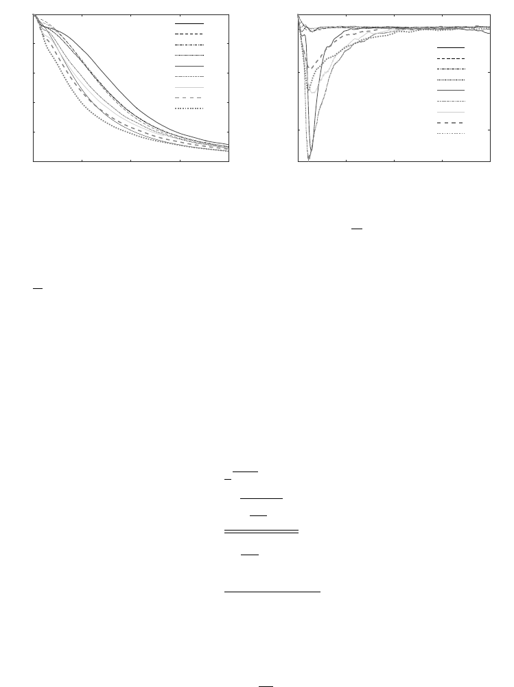
Figure 1. Evolution of (a) normalized turbulent kinetic energy k
k0and (b) Velocity derivative
skewness Su, in Simulations A-I: (Table 1).
where Trepresents mean temperature. Following the work of Kumar et al. (2013), we
have used 4th order accurate weighted-essentially-non-oscillatory (WENO) method for
interpolation of flow variables, in-order to simulate high Mach number compressible
turbulent flows. Our solver has been extensively validated with established DNS results
of compressible turbulent flows (Danish et al. (2016a)). In total, this study employs nine
different simulations (Simulations A-I). Descriptions of these simulations are presented
in Table 1.
In Figure 1(a) we present evolution of turbulent kinetic energy (K) observed in
Simulations A-F. In Figure 1(b), we present the evolution of skewness of the velocity
derivative (SV) defined as:
k=1
2ViVi; (3.4)
SVi=∂Vi
∂xi3
∂Vi
∂xi23/2,(3.5)
SV=SV1+SV2+SV3
3.(3.6)
Note that the time has been normalized using τ, which represents eddy turnover time
(Yeung & Pope 1989; Elghobashi & Truesdell 1992; Samtaney et al. 2001; Mart´ın et al.
2006).
τ=λ0
u0
0
; (3.7)
where u0
0and λ0are the root mean square (rms) velocity and integral-length-scale of
the initial flow field (at time, t= 0). Since turbulence is considered realistic for velocity
derivative skewness in the range of -0.6 to -0.4 (Lee et al. (1991)) over the Reλrange
employed in this work, we perform our study based on Lagrangian statistics for t/τ >0.5
while considering Simulations A-D and t/τ >4.0 for Simulations E-I (Figure 1(b)).
To extract Lagrangian statistics, a Lagrangian particle tracker (LPT) is used to extract
the full time-history of tagged fluid particles. Our LPT obtains the trajectory (X+(y,t))

6N. Parashar, S. S. Sinha and B. Srinivasan
Simulation ReλMtGrid size A0κ0
A. 70 0.075 12830.000023 4
B. 175 0.25 25630.00026 4
C. 175 0.40 25630.00066 4
D. 175 0.55 25630.0013 4
E. 350 0.6 102430.0015 4
F. 150 1.0 51230.0042 4
G. 100 1.0 51230.0042 4
H. 70 1.0 25630.0042 4
I. 70 1.5 25630.0094 4
Table 1. Initial parameters of DNS simulations.
of a fluid particle by solving the following equation of motion:
∂X+(t, y)
∂t =VX+(t, y), t,(3.8)
where the superscript “+” represents a Lagrangian flow variable, and yindicates the
label/identifier assigned to the fluid particle at a reference time (tref ). The initial value
of X+at a reference time is chosen at random. Using this initial condition, we then
integrate Equation 3.8 by employing second order Runge-Kutta method. However, upon
integration, the position of the fluid particle at a subsequent time instant may not fall
exactly on one of the grid points of computational domain used in the parent DNS.
Therefore, an interpolation method is required to find relevant flow quantities at the
particle’s subsequent locations. Following the work of Yeung & Pope (1988), we choose
cubic spline interpolation for this purpose. Like our DNS solvers, our LPT algorithm and
implementation have been adequately validated. Details are available in Danish et al.
(2016a).
4. Plan of study
In this section we present our plan of study and also explain the quantities that
are employed to perform the desired investigations. In §4.1 we present the study plan
for the first part of the work, which is the Lagrangian dynamics of the deformation
gradient tensor. In §4.2 we explain our study plan for the second part of this work,
which involves comparing CMT and ELT and consequently using these trajectories to
investigate interconversion processes of topologies existing in compressible turbulence.
4.1. Part I
Equation 2.7 represents the exact evolution of the velocity gradient dynamics in
compressible flows.
Υij =ν∂Aij
∂xk∂xk
| {z }
ΥI
+ν∂Akk
∂xi∂xj
| {z }
ΥII
−ν
ρ
∂ρ
∂xj∂Aik
∂xk
+1
3
∂Akk
∂xi
| {z }
ΥIII
(4.1)
In the first part of this work we focus on the viscous diffusion process (ΥI). From
the point of view of a dynamical equation of Aij (like REE of ) and HEE of )), the

Lagrangian statistics in compressible turbulence 7
viscous diffusion term ΥIrepresents a non-local, unclosed process. Jeong & Girimaji
(2003) proposed a model for this process. This model is called the linear Lagrangian
diffusion model (LLDM). The LLDM model approximates the viscous diffusion term ΥI
as:
ν∂Aij
∂xk∂xk≈C−1
kk
3τν
Aij ,(4.2)
where, Crepresents the right Cauchy Green tensor, which is derived from the deformation
gradient tensor D:
Dij ≡∂xi
∂Xj
.(4.3)
Cij ≡DkiDkj .(4.4)
Suman & Girimaji (2009) have employed the same LLDM model for the closure of their
enhanced homogenized Euler equation model (EHEE). Even though the LLDM achieves
a mathematically closed form, in this work we intend to perform a direct scrutiny of this
model using our DNS results. Such an investigation is required for a deeper understanding
of the model and may lead to further improvement in its performance.
Our interest is to examine how the viscous process ΥIundergoes changes in comparison
to its state at a reference time following a fluid particle. For monitoring this change we
define an amplification ratio r(t, tref :
r(t, tref ) = pΥIij (t)ΥIij (t)
pΥIij (tref )ΥIij (tref ),(4.5)
where, ΥIij (t) and ΥIij (tref ) are values of the quantity ΥIij associated with an identified
fluid particle at time tand reference time tref respectively. Since an individual particle
represents just one realization, we obtain a relevant statistics by calculating the mean of
r(t, tref ) over several identified fluid particles of a homogeneous flow field. The resulting
quantity is referred as hr(t, tref )i, and is truly a two-time Lagrangian correlation. Direct
numerical simulation of compressible decaying turbulence along with our Lagrangian
particle tracker (LPT) are employed to access hr(t, tref )i. A set of 1,000,000 particles
are identified at tref for the purpose. Further, to identify the role of turbulent Mach
number (Mt), normalized dilatation (aii) and topology (T), we also calculate hr(t, tref)i
conditioned upon selected particles with a specified Mt, or aii or Tat tref . These
conditional statistics are denoted as hr(t, tref )|Mti,hr(t, tref )|aiiiand hr(t, tref )|T i
respectively.
Further, we compare the Lagrangian statistics of the LLDM model term against that
of the exact viscous process ΥI. In order to understand the flaws in the LLDM model (if
any), we revisit the modelling assumptions by presenting the step-by-step derivation of
the LLDM model term from ΥI. Using Eulerian-Lagrangian change of variables, LLDM
approach of Jeong & Girimaji (2003) models the viscous term (ΥI) as follows:
ν∂2Aij
∂xk∂xk
=ν∂
∂xk∂Xn
∂xk
∂Aij
∂Xn(4.6)
ν∂2Aij
∂xk∂xk
=ν∂Xm
∂xk
∂Xn
∂xk
∂2Aij
∂Xm∂Xn
| {z }
A
+ν∂Aij
∂Xn
∂2Xn
∂xk∂xk
| {z }
B(neglected)
(4.7)
∂Xm
∂xk
∂Xn
∂xk
=D−1
mkD−1
nk (4.8)

8N. Parashar, S. S. Sinha and B. Srinivasan
∂Xm
∂xk
∂Xn
∂xk
= (DnkDmk)−1(4.9)
ν∂2Aij
∂xk∂xk≈νC−1
mn
∂2Aij
∂Xm∂Xn
(4.10)
ν∂2Aij
∂xk∂xk≈νC−1
kk
3δmn
∂2Aij
∂Xm∂Xn
(4.11)
ν∂2Aij
∂xk∂xk≈νC−1
kk
3
∂2Aij
∂Xm∂Xm
(4.12)
ν∂2Aij
∂xk∂xk≈νC−1
kk
3
Aij
(δX)2(4.13)
ν∂Aij
∂xk∂xk≈C−1
kk
3τν
Aij (4.14)
where x is the Eulerian position of a particle, initially located at the position X. D is
the deformation gradient tensor (Dij =∂xi
∂Xj) and C is the right Cauchy-Green tensor
(C=DTD). The evolution equation of the deformation gradient tensor (D) is:
dD
dt =DA. (4.15)
τνis the molecular viscous relaxation time scale, defined as:
τν=δX2/ν ≈λ2
τ/ν, (4.16)
where, λτis Taylor microscale.
The LLDM model of Jeong & Girimaji (2003) uses two major simplifications while
dealing with viscous term (A) in equation 4.1:
(i) In Equation 4.11, the inverse Cauchy Green tensor is approximated to be isotropic.
(ii) Term B in equation 4.7 is neglected.
Another possible way of deriving the LLDM model equation 4.14 from equation 4.11
could be through an alternate route by assuming ∂2Aij
∂Xm∂Xnto be isotropic:
ν∂2Aij
∂xk∂xk≈νC−1
mn
∂2Aij
∂Xm∂Xn
ν∂2Aij
∂xk∂xk≈νC−1
mnAij
δmn
3(δX)2(4.17)
ν∂Aij
∂xk∂xk≈C−1
kk
3τν
Aij (4.18)
The LLDM model has been further used in the enhanced homogenized Euler Equation
(EHEE) as well (Suman & Girimaji (2009)). In this work we plan to evaluate the
performance of the LLDM model in compressible decaying turbulence using a Lagrangian
particle tracker. Using the DNS data, a bunch of fluid particles are chosen at a reference
time, and the mean value of the following quantities are calculated following the same
set of identified fluid particles:
(i) Exact viscous term: ν∂Aij
∂xk∂xk
(ii) LLDM model term:
C−1
kk
3τνAij
In Section 5 we compare the evolutionary history of the exact viscous term and LLDM
model term (equation 4.18) directly following a set of identified fluid particles. To identify
the influence of compressibility on the evolutionary histories of the exact process and the

Lagrangian statistics in compressible turbulence 9
Acronyms p= 0 p < 0p > 0 Eigenvalues of aij
SFS r < 0r < 0 & S2>0r < 0 complex
UFC r > 0r > 0r > 0 & S2<0 complex
UNSS r > 0 & q < 0r > 0r > 0 & q < 0 real
SNSS r < 0 & q < 0r < 0 & q < 0r < 0 real
UFS — r < 0 & S2<0 — complex
UN/UN/UN — r < 0 & q > 0 — real
SFC — — r > 0 & S2>0 complex
SN/SN/SN — — q > 0 & r > 0 real
Table 2. Zones of various topologies on p−q−rspace, where acronyms are:
stable-focus-stretching (SFS), unstable-focus-compressing (UFC), unstable-node/saddle/saddle
(UNSS), stable-node/saddle/saddle (SNSS), unstable-focus-stretching (UFS), unstable-n-
ode/unstable-node/unstable-node (UN/UN/UN), stable-focus-compressing (SFC), stable-n-
ode/stable-node/stable-node (SN/SN/SN).
model, we examine the statistics of these quantities conditioned on (i) initial dilatation-
level and initial topology of fluid particles. We also examine the eigenvalues of C−1and
∂2Aij
∂Xm∂Xntensor. These eigenvalues are sorted in the order α > β > γ. Since our focus is
to examine whether the isotropic assumption of C−1and ∂2Aij
∂Xm∂Xnis realistic or not, we
examine the statistics of self-normalized eigenvalues:
Rα=|α|
pα2+β2+γ2
Rβ=|β|
pα2+β2+γ2
Rγ=|γ|
pα2+β2+γ2(4.19)
Like our previous works (Suman & Girimaji (2010a); Danish et al. (2016a); Parashar
et al. (2017a) ), the following locally normalized form of the dilatation-rate is used:
akk =Akk/pAij Aij .(4.20)
The normalized dilatation-rate of a fluid particle (henceforth, referred to as just “dilata-
tion”) represents the normalized rate of change in density of a local fluid particle:
1
ρ
dρ
dt0=1
ρ"∂ρ
∂t0+Vk
∂ρ
∂Xk#=−aii (4.21)
where dt0=dtpAij Aij represents time normalized with the local magnitude of the
velocity gradient tensor itself.
The topology of a fluid particle is the local streamline pattern as observed with respect
to a reference frame which is translating with the centre of mass of the fluid particle. The
topology of a fluid particle depends on the nature of eigenvalues of the velocity gradient
tensor. However, it can also be inferred with the knowledge of the three invariants of the
10 N. Parashar, S. S. Sinha and B. Srinivasan
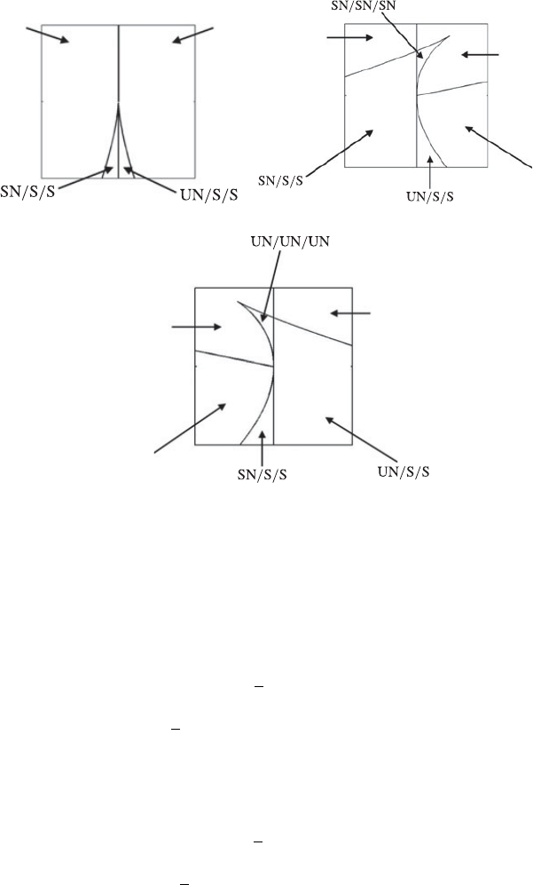
UFC
S2
S1bS1a
0
0
q
r
q-axis
SFS
(a)
S2
S1b
S1a
0
q
0r
q-axis
UFC
SFC
SFS
(b)
UFC
S2
S1b
S1a
0
q
0r
q-axis
UFS
SFS
(c)
Figure 2. Flow topologies represented in different p-planes: a) p= 0, b) p > 0 and c) p < 0.
(Figures to be reproduced with permission from Suman & Girimaji (2010a).)
velocity gradient tensor P, Q, R:
P=−Aii, Q =1
2P2−Aij Aji, and
R=1
3−P3+ 3P Q −Aij AjkAki.(4.22)
The normalized invariants (p,q,r) of the local velocity gradient tensor (a) are defined
as:
p=−aii, q =1
2p2−aij aji, and
r=1
3−p3+ 3pq −aij ajkaki.(4.23)
Determination of the topology of a fluid particle can also be done using the invariants
of the normalized velocity gradient tensor (a). Chen et al. (1989) categories topological
patterns (Table 2) that can be observed in an incompressible field into UNSS, SNSS, SFS,
UFC. In compressible flows additional four more topologies can exist: SFS and SNSNSN
in contracting fluid particles and UFS and UNUNUN in expanding fluid particles. Figure
2 shows different topologies existing in different p-planes in p-q-r space. Figure 3 present
schematics of these topological patterns.
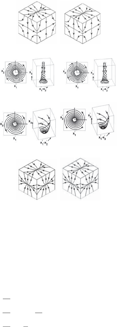
Lagrangian statistics in compressible turbulence 11
(a) (b)
(c) (d)
(e) (f)
(g) (h)
Figure 3. Flow patterns corresponding to different flow topologies: a) UNSS, b) SNSS, c)
SFS, d) UFC, e) UFS, f) SFC, g) SNSNSN and h)UNUNUN. (Figures to be reproduced with
permission from Suman & Girimaji (2010a).)
4.2. Part II
Since the value of three invariants of the velocity gradient tensor uniquely determines
the topology associated with the local fluid particle, the dynamics of topology can be
studied in terms of the dynamics of invariants themselves. Using the evolution equation
of the velocity-gradient-tensor (Equation 2.7), the time-evolution of invariants (P,Q,R)
of the velocity-gradient-tensor A can be found out (Bechlars & Sandberg (2017)):
dP
dt =P2−2Q−Sii,
dQ
dt =QP −2P
3Sii −3R−Aij S∗
ji,
dR
dt =−Q
3Sii +P R −P Aij S∗
ji)−Aik Akj S∗
ji (4.24)
where, S is the source term in the evolution equation of velocity-gradient-tensor

12 N. Parashar, S. S. Sinha and B. Srinivasan
(Equation 2.7) and S∗is the traceless part of S tensor defined as:
S=−P+Υ,
S∗=S−Skk
3.(4.25)
Here Pis the pressure hessian tensor and Υrepresents the contribution of viscosity in
the evolution equation of the velocity-gradient tensor (A), as shown in Equation 2.7. The
relation between non-normalized invariants (P,Q,R) and normalized invariants (p,q,r) is
shown in equation 4.26:
p=P
pAij Aij
,
q=Q
Aij Aij
,
r=R
(Aij Aij )3/2(4.26)
Subsequently, using equations (4.24 & 4.26), the evolution equation of normalized
invariants (p,q,r) can be derived:
dp
dt =d
dtP
pAij Aij =1
pAij Aij
dP
dt −P
(Aij Aij )3/2Aij
dAij
dt ,
dq
dt =d
dtQ
Aij Aij =1
Aij Aij
dQ
dt −2Q
(Aij Aij )2Aij
dAij
dt ,
dr
dt =d
dtR
(Aij Aij )3/2=1
(Aij Aij )3/2
dQ
dt −3R
(Aij Aij )5/2Aij
dAij
dt .(4.27)
While following a fluid particle in physical space and storing its velocity gradient
tensor information, we can indirectly track the p-q-r location of the fluid particle. We
refer to such a trajectory as the exact Lagrangian trajectory (ELT) of an individual
fluid particle. Mean Lagrangian trajectory (MLT) can be obtained by tracking the mean
position of a selected number of particles originating from the same location in p-q-r space
(within the specified tolerance) at some reference time (tref ). This procedure involves no
approximation while calculation of trajectories of fluid particles in p-q-r space.
As mentioned before, many researchers have adopted an alternate though approximate
procedure of examining trajectories in the p-q-r space. This alternative method does not
track the individual fluid particles, but use the averaged value of the RHS of Equation
4.27 conditioned on a chosen set of p,q,r. In this method, a one-time Eulerian dataset of
the flow field is used. The statistics thus obtained are essentially the conditional averages
of the rate of change of the invariants with the conditional parameters being the local
value of p,q,r in the p-q-r space. The trajectories thus obtained are basically instantaneous
streamlines in p-q-r space referred to as the conditional mean trajectories (CMT).
In Section 6 we first investigate dynamics of topology in compressible turbulence
employing the method of CMT. For plotting all CMTs we employ the flow field obtained
from different simulations at a time instant when velocity derivative skewness has settled
i.e. Su∈(−0.6,−0.4). A bin size of r∈r±0.01 and q∈q±0.025 is taken to compute all
CMTs. In §6.1 we present a comparison of CMT and MLT and identify the constraints
of the former. Subsequently in §6.2 we employ exact ELTs to estimate lifetime of various
topologies in compressible turbulence.
Lagrangian statistics in compressible turbulence 13
02468
(t−tref )/τ
0
0.5
1
1.5
2
-
-ν∂2A
∂xk∂xk
-
-t
-
-ν∂2A
∂xk∂xk)-
-tref
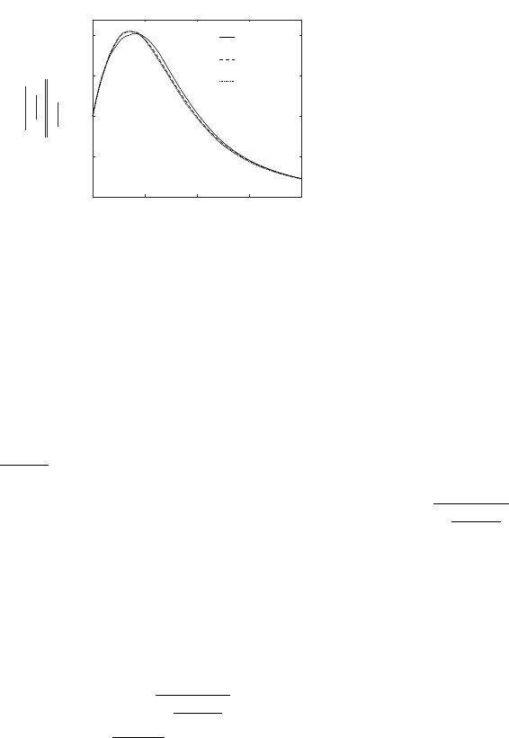
Mt= 0.55
Mt= 0.40
Mt= 0.25
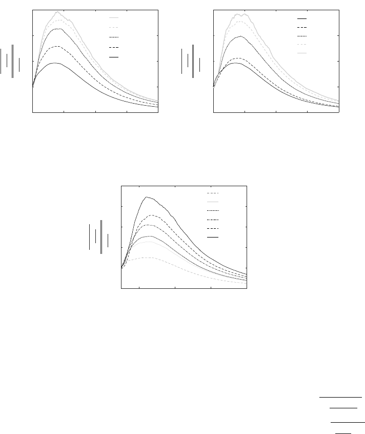
Figure 4. Mach number dependence on evolution of exact viscous term (tref = 0.5τ).
5. Lagrangian Evolution of deformation gradient tensor
We first analyze the evolution of the exact viscous term in §5.1. After understanding
the evolution characteristics of the exact viscous term, we then compare the performance
of the LLDM model term in approximating the exact viscous process in §5.2.
5.1. Analysis of the evolution of the exact viscous term
We first present the time evolution of the Lagrangian statistics of the exact viscous
diffusion process ν∂Aij
∂xk∂xkfrom simulations B-D in Figure 4. All these simulations
differ in terms of the initial Mach number. In each of these simulations, the exact
viscous process shows a two-stage evolution. In the first stage of evolution, ν∂Aij
∂xk∂xk
increases and reaches a peak value. In the second stage, it decays in magnitude. This
evolution is reminiscent of the evolution of dissipation itself. Indeed the time instant of
the peak of dissipation and that of the viscous process match (tpeak−dissipation = 2τ).
The amplification in the first stage can be attributed to steepening of gradients due
to the rapid spread of the spectrum. The decay in the second stage of evolution can
be attributed mainly to the decay in kinetic energy. Comparing the curves from these
three simulations it is clear that initial Mach number has little negligible influence on
the evolution of viscous diffusion term ν∂Aij
∂xk∂xk. Such behavior is analogous to the
variation in dissipation rate (=νAij Aij ) with varying Mt, which has been shown to
be negligible by Samtaney et al. (2001). The viscous diffusion term is basically a higher
order derivative of the dissipation rate. Hence such behaviour is in line with previously
observed behaviour for dissipation rate.
To further understand the influence of compressibility on the viscous process, we
present the results conditioned on dilatation. In Figure 5a we present results conditioned
on negative dilatation levels. Similarly in Figure 5b we present results conditioned on
positive levels of dilatation. All the results are from the Simulation C (Table 1). It can
be observed from Figure 5 that the intensity of viscous process is elevated at higher
dilatation levels (+/-). This is attributed to the higher gradients of velocity gradient
tensor for highly contracting and expanding fluid particles.
In Figure 6 we present results conditioned on initial flow topology. It can be observed
that the rotation based topologies (SFC, UFS, UFC, SFS) tend to show higher growth
rate in the first phase of evolution, reaching higher peaks as compared to strain-dominated
topologies (UNSS and SNSS). SFC topology shows the highest growth rate as compared
to all other topologies.
14 N. Parashar, S. S. Sinha and B. Srinivasan
02468
(t−tref )/τ
0
1
2
3
4
-
-ν∂2A
∂xk∂xk
-
-t
-
-ν∂2A
∂xk∂xk)-
-tref
aii =−0.4
aii =−0.3
aii =−0.2
aii =−0.1
aii = 0
(a)
02468
(t−tref )/τ
0
1
2
3
4
-
-ν∂2A
∂xk∂xk
-
-t
-
-ν∂2A
∂xk∂xk)-
-tref
aii = 0
aii = 0.1
aii = 0.2
aii = 0.3
aii = 0.4
(b)
Figure 5. Dependence of dilatation rate on evolution of exact viscous term (tref = 0.5τ).
2 4 6 8
(t−tref )/τ
0
1
2
3
4
5
-
-ν∂2A
∂xk∂xk
-
-t
-
-ν∂2A
∂xk∂xk)-
-tref
UN SS
SNSS
SF S
U F C
U F S
SF C
Figure 6. Dependence of topology on evolution of exact viscous term (tref = 0.5τ).
5.2. Evaluation of the LLDM model
Having examined the behaviour of the exact process following fluid particles, now we
examine the performance of the LLDM model of Jeong & Girimaji (2003), which intends
to capture the essential physics of the exact process. For this examination, we use the
results of Simulation C, but instead of computing the exact viscous process ν∂Aij
∂xk∂xk,
we compute the mean value of the magnitude of the LLDM model term
C−1
kk
τνA
following the same set of fluid particles which were selected for computing statistics of
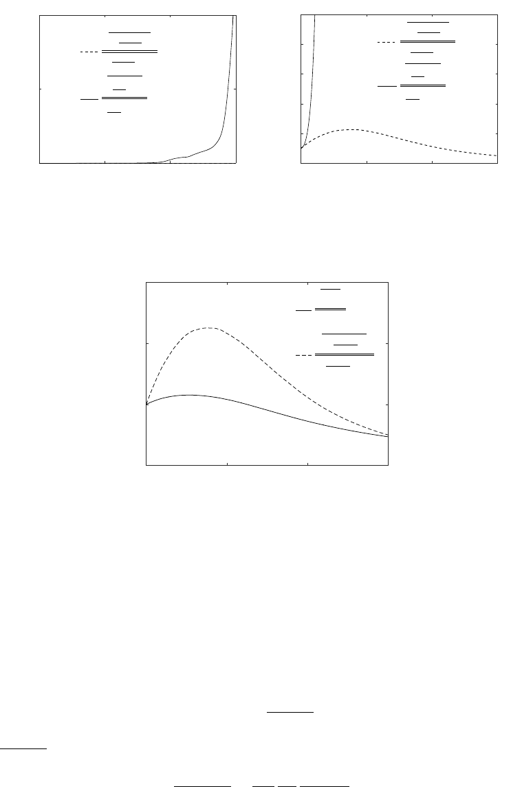
the exact process. In Figure 7, we compare the LLDM model with the exact viscous term.
We observe that unlike the evolution of the exact process, the LLDM model term shows
monotonic growth with time. At the early stages of evolution, the monotonic growth is
at least qualitatively the same as the exact process. However, at later stages (after the
dissipation peak event) this continued monotonic growth in is gross disagreement with
the decaying behaviour of the exact process after reaching a peak value. In Figure 8
we present the evolution of |A|with time. We observe that |A|does show a two-stage
behaviour and starts decaying after the peak dissipation event. Comparing Figure 7 and
Figure 8, it is clear that the coefficient C−1
kk of the LLDM model grossly overestimates
the influence of the C−1tensor.
To better understand the reason for the failure of the LLDM model, we revisit the
modelling assumptions. One of the assumptions used in the model is that the tensor C−1
is isotropic. To scrutinize whether this assumption is contributing to the model failure,
Lagrangian statistics in compressible turbulence 15
0246
(t−tref )/τ
0
1
2×10 11
-
-ν∂2A
∂xk∂xk
-
-t
-
-ν∂2A
∂xk∂xk)-
-tref
-
-
C−1
kk
3τν
A-
-t
-
-
C−1
kk
3τν
A-
-tref
(a)
0246
(t−tref )/τ
0
2
4
6
8
10
-
-ν∂2A
∂xk∂xk
-
-t
-
-ν∂2A
∂xk∂xk)-
-tref
-
-
C−1
kk
3τν
A-
-t
-
-
C−1
kk
3τν
A-
-tref
(b)
Figure 7. Comparison of LLDM model term and the exact viscous term: a) unscaled axis, b)
axis scaled to visualize the difference in growth rates of the two processes.
0246
(t−tref )/τ
0
1
2
3
-
-A-
-t
-
-A-
-tref
-
-ν∂2A
∂xk∂xk
-
-t
-
-ν∂2A
∂xk∂xk)-
-tref
Figure 8. Evolution of magnitude of velocity gradient tensor |A|.
we examine the eigenvalues of the C−1tensor. The C−1tensor is always symmetric (since
C=DDTis symmetric), hence the eigenvalues of C−1are always real. To examine the
validity of the isotropic assumption, we plot the mean evolution of the three eigenvalues
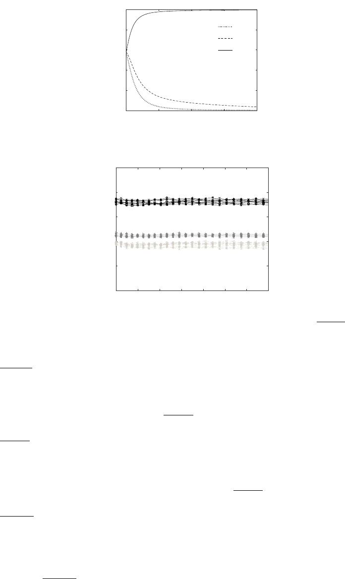
(α > β > γ). In Figure 9 we present the Lagrangian statistics of Rα,Rβand Rγas a
function of time. We observe that the eigenvalues begin to depart from each other. Rα
increases appreciably during the evolution phase, while Rβand Rγdecreases to negligible
values. This indicates that the C−1tensor is strongly biased towards α−eigenvector.
Thus, it is clear that the assumption of the isotropy of the tensor is incorrect.
As shown in §4, (Equation 4.17 and 4.18) viscous term in LLDM model can also be
recovered by assuming the 4th order tensor ∂2Aij
∂Xm∂Xnto be isotropic. However, it is not
possible to find the eigen-values of this tensor directly. By lagrangian change of variables,
∂2Aij
∂Xm∂Xncan be approximated as:
∂2Aij
∂Xm∂Xn≈xm
Xm
xn
Xn
∂2Aij
∂xm∂xn
(5.1)
Since a product of an anisotropic tensor with an isotropic tensor is always anisotropic,
16 N. Parashar, S. S. Sinha and B. Srinivasan
0 0.5 1 1.5 2
(t−tref )/τ
0
0.2
0.4
0.6
0.8
1
Rγ
Rβ
Rα
Figure 9. Evolution of locally normalized eigenvalues of C−1
0 0.5 1 1.5 2 2.5 3 3.5
(t−tref )/τ
0
0.2
0.4
0.6
0.8
1
Figure 10. Evolution of locally normalized real part of eigenvalues of ∂2Aij
∂xm∂xn. Three
different colors of the line plot viz. black, light gray, dark gray represents Rα, Rβand Rγ
respectively. Different markers represents eigenvalues corresponding to different 2nd order tensors
(components) of the original 4th order tensor. Rij represents ratio of normalized eigenvalue for
∂2Aij
∂Xm∂Xn. Different marker identifiers are −→ +: R11, o: R12 ,∗:R13,<:R21 ,>:R22 , x: R23 ,:
R31,7:R32 ,D:R33
we rather evaluate the eigenvalues of ∂2Aij
∂xm∂xntensor. Since, this tensor is of order 4, we
dissociate the tensor into 9 second-order tensors and analyze their eigenvalues. Since,
∂2Aij
∂xm∂xnis not symmetric, it is not guaranteed to have real eigenvalues. Indeed, the
eigenvalues of the tensor are not purely real with mean ratio of the imaginary part to
the real part for α, β and γeigenvalues to be 0.13, 0.77 and 0.17 respectively . However,
inorder to measure the extent of anisotropy, we plot the ratio of real part of the eigenvalues
in terms of Rα, Rβand Rγin Figure 10. Clearly the ∂2Aij
∂xm∂xntensor is anisotropic with
ratio of the eigenvalues as: α:β:γ:: 1.9 : 1.0 : 1.1. Hence, it can be concluded that the
∂2Aij
∂Xm∂Xntensor is also anisotropic.
In summary, our investigations reveal that the performance of the LLDM model is
unrealistic in the later stage of evolution of decaying turbulence. In the first stage of
evolution, even though qualitatively LLDM captures the right behaviour, it tends to
overestimate the value. Our investigations reveal that the isotropy assumption of the
C−1and ∂2Aij
∂Xm∂Xntensor is one of the major cause of the unrealistic behaviour of the
LLDM model term as compared to the exact viscous term.

Lagrangian statistics in compressible turbulence 17
100% UNSS 100% SNSS 100% SFS 100% UFC
UNSS SNSS SFS UFC UNSS SNSS SFS UFC UNSS SNSS SFS UFC UNSS SNSS SFS UFC
tref 100 0 0 0 0 100 0 0 0 0 100 0 0 0 0 100
tref + 3τ27 8 38 26 27 8 39 26 23 7 41 28 26 8 39 27
Table 3. Percentage topology composition for particles after 3 eddy-turnover time starting
with 100% UNSS, SNSS, SFS and UFC sample respectively.
6. Comparisons of Eulerian and Lagrangian investigations of flow
field topology
In §6.1 we present a comparative study between the CMT and MLT and highlight
some important differences between the two. Further in the §6.2 we study the life of
topology using ELTs and examine the influence of compressibility on it.
6.1. CMT vs. MLT
CMT has been extensively used as a method to predict particle trajectories in p-
q-r space. CMTs are basically instantaneous streamlines of particles in p-q-r space.
Several researchers have drawn conclusions based on the time-integrated behaviour of
CMT as a complete substitute of MLT. However, using CMT for predicting long-term
behaviour−such as finding the life of topology may not be as accurate as MLT. We present
a discussion here highlighting the shortcomings of CMT over MLT. As most of the CMT
based studies have been performed for incompressible flows (Ooi et al. (1999); Meneveau
(2011); Lozano-Dur´an et al. (2015)), we use nearly incompressible simulation (case A 1),
to demonstrate the difference between CMT and MLT. We further condition the data-set
at very small dilatation value (|aii|<0.01) to assert very weak compressibility effects.
To highlight the difference, we show CMT and MLT emerging from a small region in
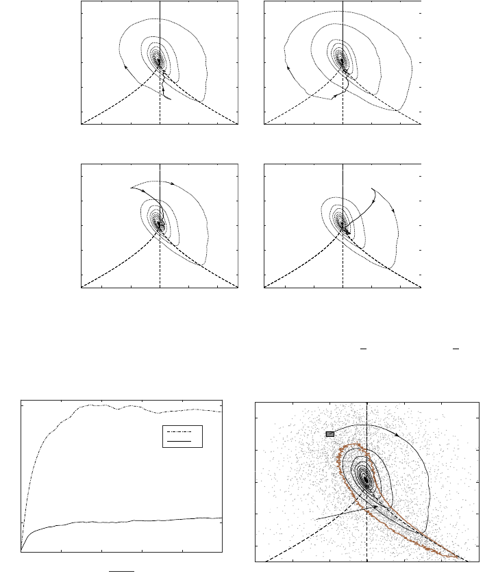
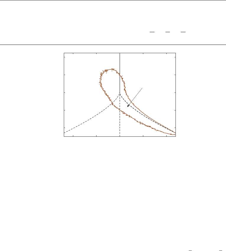
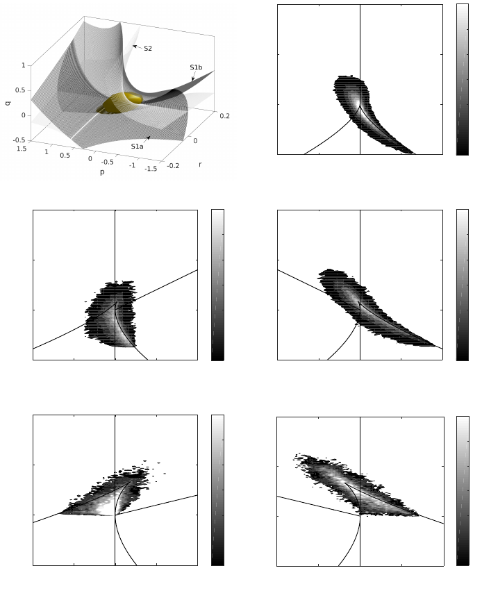
q-r plane (p= 0 ±0.01) in Figure 11(a-d) (for all four topologies that exist in this plane).
It is evident from Figure 11 that the instantaneous CMT does not coincide with the
MLT of fluid particles in q-r plane. There is no directional preference of fluid particles
to rotate in spiral order and converge to the origin of q-r plane, as inferred by CMT
(Figure 11(a-d)). In-fact the mean trajectory (MLT) converging directly to origin with
no tendency to rotate around the origin, explains no directional preference and a clear
tendency to randomly move in the q-r space. This argument is further supported by
Figure 12(a), where the root-mean-squared value of q and r is plotted with time.
Using the CMT approach, it can be shown that in around 3 eddy-turnover time, a fluid
particle completes one complete rotation around the origin (Ooi et al. (1999)). However, it
can be clearly seen in Figure 12(a), that in just 1 eddy-turnover time, the rms approaches
its maximum value (qrms ≈0.24 and rrms ≈0.05), indicating maximum spread of the
fluid particles in q-r plane. In-fact these RMS values are identical to the RMS of q and
r location of global unconditioned sample. To further understand this difference, we plot
the location of various fluid particles starting from a small region in q-r plane after 1
eddy-turnover time (Figure 12(b)). It can be observed that the population spread after
1 eddy-turnover time, is in-fact similar to the global spread of particles in q-r plane with
major concentration along the Vieillefosse tail.
Table 3 shows the percentage topology composition after 3 eddy-turnover times of
particles initially belonging to a distinct topology. It is evident that after 3 eddy-
turnover times the particles gets distributed throughout the q-r plane with the final
composition identical to global unconditioned sample. In fact, the composition after
3 eddy-turnover times is approximately equal to the global topology composition for
18 N. Parashar, S. S. Sinha and B. Srinivasan
-0.1 -0.05 0 0.05 0.1
r
-0.4
-0.2
0
0.2
0.4
q
(a)
-0.1 -0.05 0 0.05 0.1
r
-0.4
-0.2
0
0.2
0.4
q
(b)
-0.1 -0.05 0 0.05 0.1
r
-0.4
-0.2
0
0.2
0.4
q
(c)
-0.1 -0.05 0 0.05 0.1
r
-0.4
-0.2
0
0.2
0.4
q
(d)
Figure 11. Comparison of instantaneous CMTs (dotted line) and actual mean Lagrangian
trajectory MLT (solid line) of fluid particles with bin dimensions r∈r±0.01 and q∈q±0.025
for (a)UNSS, (b)SNSS, (c)SFS and (d)UFC topology. Dashed lines represent surfaces: S1a, S1b
and S2.
012345
0
0.05
0.25
RMS
q
r
(a)
-0.15 -0.1 -0.05 0 0.05 0.1 0.15
r
-0.4
-0.2
0
0.2
0.4
q
high concentration
(Vieillefosse tail)
(b)
Figure 12. (a) Evolution of root mean squared value of invariants q and r starting from a
bounded region r (-0.05 ±0.01) and q (0.3±0.025) (b) Instantaneous CMT (solid line) and final
spread of Lagrangian particles after 1 eddy-turnover time starting from the bounded region.
Sample size of conditioned particles in the bounded region ≈5000.
isotropic incompressible flow as reported by Suman & Girimaji (2009). This observation
challenges the CMT approach that approximates particle motion in the q-r plane using
instantaneous Eulerian flow field. Table 4 shows anticlockwise and clockwise movement
of particles starting from a particular topology using ELT approach. It can be seen that a
significant fraction of particles moves anti-clockwise (1/2 for SNSS topology and 1/3 for
UNSS, SFS and UFC topology). Therefore it can be concluded that the CMT approach
inaccurately predicts cyclic rotation of particles around the origin.
Hence, from the above analysis, we conclude that CMT does not represent actual
Lagrangian statistics in compressible turbulence 19
UNSS SNSS SFS UFC
% anticlockwise 32 51 33 33
% clockwise 68 49 67 67
Table 4. Clockwise and anti-clockwise movement of particles in q-r plane. [Note: This table
shows percentage transfer of particles. The topology composition remains invariant with time
i.e. Total particles moving in and out of a particular topology is same.]
0123
t−tref
τ
0
10
20
30
40
Topology %
UNSS
SNSS
SFS
UFC
UFS
SFC
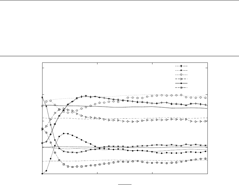
Figure 13. Evolution of topology-composition for particles initially conditioned at
p= +0.5±0.05 for 6 major topologies viz. UNSS, SNSS, SFS, UFC, UFS, SFS (Simulation E).
Initial composition at tref = 4τ: UNSS = 11.6%, SNSS = 28.9%, SFS = 25.6%, UFC = 16.7%,
UFS = 0%, SFC = 17.0%, SNSNSN = 0.2%, UNUNUN = 0%. Lines without markers represents
topology composition of global unconditioned sample.
motion of fluid particles in q-r plane for incompressible flow. In general, the fluid
particles move around randomly in q-r plane, such that at every time instant the overall
distribution of particles is identical, with major concentration along the Vieillefosse tail.
Although, the above analysis is performed for incompressible flow, we expect even for
compressible flow, the motion of fluid particles to be such that their topology composition
approach global topology composition with time. To prove this hypothesis, we show
time-evolution of percentage composition of particles originating from a discrete p-plane
(p= +0.5±0.05) for compressible simulation E (Table 1) in Figure 13. It can be seen
in Figure 13 that despite a significant variation in initial composition of topology as
compared to global composition, the particles moves around randomly in p-q-r space
such that their percentage composition tends toward the global composition.
6.2. Life of topology
In this section, we quantify the life-time of existence of particles in different topologies.
Starting with 10,00,000 particles, we tag the particles based on their topology at tref and
track them until they lose their initial topology. The life-time of each particle (lκ) in a
particular topology is measured as a fraction of Kolmogorov time, τκ(measured at tref ),
calculated by recording the time from tref to the instant the particle loses it’s initial

20 N. Parashar, S. S. Sinha and B. Srinivasan
UNSS SNSS SFS UFC
Sample % 25.2 5.4 43.5 25.9
Life of topology (κτ) 1.80 0.53 3.32 2.08
Life % 23.32 6.86 42.95 26.91
Table 5. Life of topology Lκfor nearly incompressible flow (case A). The sample is further
conditioned on dilatation (|aii|<0.01) to ensure strong incompressibility. Sample size ≈1,25,000
particles (conditioned).
topology. Further, we calculate the life-time of topology (Lκ) as the mean life-time of all
the particles in a particular topology (in terms of τκ):
Lκ=
N
X
i=1
lκi
N(6.1)
6.2.1. Incompressible flow
We first show life of topology for nearly incompressible simulation (case A) in Table
5. To assert very mild compressibility, we further condition our sample on dilatation
(|aii|=|p|<0.01). It can be observed that life of topology is proportional to the
percentage composition of topology. SFS topology is the most stable with average lifetime
of 3.3κτ, next is the UFC topology with average lifetime of 2κτ, next most stable is UNSS
with a lifetime of 1.8κτ. SNSS topology is found to be least stable with average lifespan
of 0.5κτ. Hence, for incompressible flow, the order of stability of topology is as follows:
SF S −→ UF C −→ UNSS −→ SN SS.
Table 6 shows the average velocity (|Upqr|=|∂p
∂t ˆp+∂q
∂t ˆq+∂r
∂t ˆr|) of particles in different
topologies in p-q-r space. It is interesting to observe that although the average velocity
for different topologies is comparable in magnitude, there is a significant difference in
their lifetimes (Lκ). It can also be seen in Table 5, that the proportion of life of different
topologies is identical to their percentage composition. To explain the variation in Lκ
for different topologies, we focus on the distribution of the population in various zones
of topology rather than just percentage composition. Figure 14 shows region of high
concentration of particles in q-r plane. This region of high particle concentration is also
termed “Vieillofosse tail”. It can be seen in Figure 14 that, while SFS and UFC region
have an equal area in the q-r plane, their population distribution is not alike. In UFC, the
population has a spread closer to the surfaces of unlike topologies, than for SFS topology.
Closer proximity to the nearby surfaces of unlike topologies explains the likelihood of UFC
to be more prone to change than SFS topology, having known that their average speeds
in p-q-r space are comparable in magnitude (Table 6). Similarly, UNSS and SNSS have
equal area, still, UNSS is found to be more stable than SNSS topology. This is because
for SNSS topology the bulk of the population is found closer to the origin where nearby
surfaces separating different topologies are closer leading to higher probability of particles
crossing the zone of SNSS topology into other topologies. However, in UNSS topology,
the population although highly concentrated near the origin, has significant population
spread away from the origin, where nearby surfaces for interconversion are not very close.
Hence, despite having comparable average velocities, different topologies have different
lifetimes (Lκ).
Lagrangian statistics in compressible turbulence 21
UNSS SNSS SFS UFC
average velocity |Uqr|0.23 0.28 0.23 0.26
(units: s−1)
Table 6. Average velocity of particles in p-q-r space (Upqr =∂p
∂t ˆp+∂q
∂t ˆq+∂r
∂t ˆr) for simulation
case A.
-0.1 -0.05 0 0.05 0.1
r
-0.4
-0.2
0
0.2
0.4
q
SNSS UNSS
Large particle concentration
(Vieillefosse tail)
UFC
SFS
Figure 14. Region of high concentration of particles in q-r space.
6.2.2. Compressible flow
We show average life-time of topology for compressible simulations (case E-I) in Table
7. It can be seen that the life-time of topology is again a strong function of particle
concentration. In-fact the percentage life of different topologies is almost identical to the
composition of their populations (Table 7). However, the order of stability seems to be
influenced by Mt(Table 7). For weakly compressible flow (simulation A), the order of
stability based on lifetime for 4 major topologies is SF S −→ UNSS −→ U F C −→
SN SS. However, global turbulent Mach number of the flow seems to affect the order of
stability.
To explain this variation in the order of stability with Mt, we now focus on the
localized origin of compressibility. As shown by Suman & Girimaji (2010a), the extent of
compressibility can be determined solely by the strength of dilatation (−√3< aii <√3).
Compressibility is a localized phenomenon i.e. regions of weak and strong compressibil-
ity are present in the flow field. However, statistically, by looking at the probability-
density-function (PDF) of dilatation one can determine the extent of compressibility. A
larger spread of the dilatation PDF, represent a high strength of compressibility. For
incompressible flow (aii =−p≈0), only 4 flow topologies exist viz. UNSS, SNSS,
SFS and UFC topology. But compressibility gives rise to new flow-topologies (Figure 2),
existing in p-q-r space in planes of non-zero dilatation (|p|>0). The population of these
topologies depend upon the spread of dilatation. Weak compressibility, accompanied by
low dilatation spread leads to a low population of topologies existing in non-zero p-planes
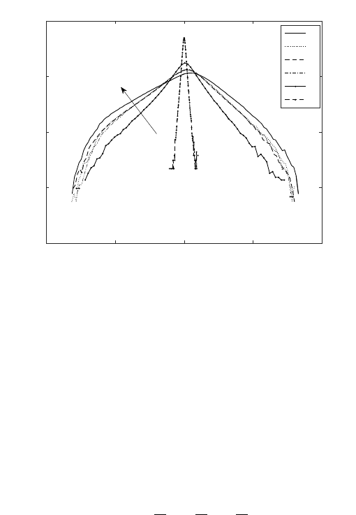
and vice-versa for highly compressible flow. In Figure 15, we show the PDF of dilatation
for different simulations. It can be seen that the dilatation spread increases with turbulent
Mach number, however, there seems to be little to no dependence on Reynolds number
as evident from simulations F-H (Figure 15).
22 N. Parashar, S. S. Sinha and B. Srinivasan
-2 -1 0 1 2
aii
10 -4
10 -2
10 0
10 2
PDF
I
H
G
F
E
A
Mt
Figure 15. PDF of noramilized dilatation aii for different simulations (Table 1).
From the above discussion, it can be concluded that there is no general order of stability
of topology for compressible flows. However, for major 4 topologies (UNSS, SNSS, SFS
and UFC), there is a particular order of stability:
SF S −→ UN SS −→ U F C −→ SNSS.
Further, at very high Mach numbers the order stability based on life-time of existence
is found to be as follows:
SF S −→ UN SS −→ U F C −→ U F S −→ SNSS −→ SF C −→ UNUNUN −→ SN SNSN.
In order to explain the variation of lifetime of topology with Mt, we report the
magnitude of mean velocities (Upqr =∂p
∂t ˆp+∂q
∂t ˆq+∂r
∂t ˆr) of particles in p-q-r space in
Table 8. It can be seen that |Upqr |increases with Mtfor all major topologies, while
for extreme topologies−UNUNUN and SNSNSN, the variation in |Upqr|, although most
likely opposite, seems less significant as compared to variation in rest of the 6 topologies.
For first 4 topologies (UNSS, SNSS, SFS, UFC), the decrease in life with increasing Mt
can be attributed to the increase in |Upqr |with increasing Mt. The rest of the topologies
come into existence only at high Mt, hence first their lifetime increases with Mt, but
further, with an increase in Mttheir lifetime tend to remain constant, despite variation
in Upqr.
Further, as can be inferred from simulations F-H in Table 7, the Reynolds number
show negligible influence on the lifetime/stability of topology.

Lagrangian statistics in compressible turbulence 23
Simulation UNSS SNSS SFS UFC UFS SFC SNSNSN UNUNUN
case A Sample % 25.2 5.4 43.5 25.9 0 0 0 0
M=0.075 Life of topology 1.80 0.53 3.32 2.08 0 0 0 0
R = 70 Life % 23.32 6.86 42.95 26.91 0 0 0 0
case E Sample % 24.68 8.35 33.78 21.67 5.17 4.53 0.09 0.09
M=0.6 Life of topology (κτ) 1.31 0.44 1.80 1.15 0.28 0.24 0.05 0.05
Re=350 Life % 24.62 8.27 33.83 21.62 5.26 4.51 0.01 0.01
case F Sample % 27.81 10.26 28.42 20.88 8.44 3.89 0.14 0.15
M=1 Life of topology (κτ) 1.04 0.31 1.13 0.85 0.35 0.24 0.06 0.11
Re=150 Life % 25.43 7.58 27.63 20.78 8.56 5.87 1.47 2.69
case G Sample % 26.61 9.82 26.26 21.50 8.39 4.14 0.14 0.14
M=1 Life of topology (κτ) 1.01 0.31 1.18 0.86 0.35 0.25 0.06 0.10
Re=100 Life % 24.51 7.52 28.64 20.87 8.50 6.07 1.46 2.43
case H Sample % 26.52 9.45 29.96 21.52 8.08 4.23 0.13 0.10
M=1 Life of topology (κτ) 1.00 0.29 1.20 0.86 0.33 0.24 0.06 0.08
Re=70 Life % 24.63 7.14 29.56 21.18 8.13 5.91 1.48 1.97
case I Sample % 26.07 10.10 27.44 21.16 10.49 4.32 0.23 0.21
M=1.5 Life of topology (κτ) 0.87 0.26 0.94 0.74 0.35 0.23 0.07 0.09
Re=70 Life % 24.51 7.32 26.48 20.85 9.86 6.48 1.97 2.54
Table 7. Life of topology for compressible flows (case A, E-I). Sample size = 10,00,000
particles.
Simulation UNSS SNSS SFS UFC UFS SFC SNSNSN UNUNUN
A 0.23 0.28 0.23 0.26 - - - -
E 0.58 0.88 0.60 0.66 0.62 0.96 2.6 1.80
F 0.86 1.39 0.95 1.00 0.82 1.55 2.15 1.33
G 0.84 1.35 0.92 0.99 0.80 1.49 2.35 1.21
H 0.88 1.37 0.97 1.03 0.87 1.46 1.87 1.37
I 1.01 1.57 1.13 1.18 0.90 1.76 1.94 1.27
Table 8. Average velocity of particles in p-q-r space (|Upqr |=|∂p
∂t ˆp+∂q
∂t ˆq+∂r
∂t ˆr|) for
simulations A and E-I.
6.2.3. Influence of initial dilatation
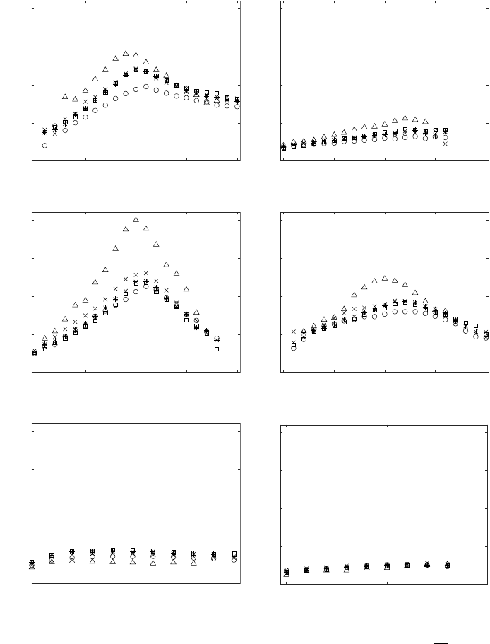
In Figure 16, we present the variation in Lκfor various topologies with initial dilatation
(aii). To explain the variation in Lκwith dilatation we show joint-PDF (JPDF) of particle
population in different planes of discrete dilatation in Figure 17. For UNSS topology, peak
life-times (Lκ) are observed at 0 dilatation (Figure 16(a)). Particles with UNSS topology
having initial positive dilatation have higher life as compared to those with initial negative
dilatation. This happens because for UNSS topology, the zone of existence in p-q-r space
shrinks along with decrease in population as dilatation decreases from high positive
dilatation to negative dilatation as shown in figure 17 (b-f). On the contrary, the region
of existence of SNSS topology widens while moving from high positive to high negative
population (17 (b-f)). This leads to lower population of SNSS topology at high positive
dilatations (Figure 16(b)).
24 N. Parashar, S. S. Sinha and B. Srinivasan
-1 -0.5 0 0.5 1
0.5
1
1.5
2
(a)
-1 -0.5 0 0.5 1
0.5
1
1.5
2
(b)
-1 -0.5 0 0.5 1
0.5
1
1.5
2
(c)
-1 -0.5 0 0.5 1
0.5
1
1.5
2
(d)
0 0.5 1
0.5
1
1.5
2
(e)
-1 -0.5 0
0.5
1
1.5
2
(f)
Figure 16. Variation of life of topology Lκτwith initial dilatation aii (bin size: aii ±0.05) for
6 major topologies: (a)UNSS, (b)SNSS, (c)SFS, (d)UFC, (e)UFS and (f)SFC. Symbol 4,,∗,
×, and O represents life-time of topology for simulations E, F, G, H and I respectively.
Life-times (Lκ) for SFS and UFC topology are shown in Figure 16(c) and 16(d)
respectively. It can be seen that both SFS and UFC topologies exhibit monotonic rise,
peaking in value for small positive dilatation, followed by monotonic fall while moving
from negative dilatation to positive dilatation. The variation is approximately symmetric,
slightly skewed towards positive values of dilatation. Variation ofLκwith initial dilatation
for UFS and SFC topology are shown in Figure 16(e) and 16(f) respectively. UFS and SFC
topologies have smaller Lκand shows small variation with dilatation in their respective
regions of existence (aii >0 for UFS and aii <0 for SFC).
Lagrangian statistics in compressible turbulence 25
(a)
-0.2 -0.1 0 0.1 0.2
r
-0.5
0
0.5
1
q
5
10
15
20
25
30
35
(b)
-0.2 -0.1 0 0.1 0.2
r
-0.5
0
0.5
1
q
5
10
15
20
25
30
35
(c)
-0.2 -0.1 0 0.1 0.2
r
-0.5
0
0.5
1
q
5
10
15
20
25
30
35
(d)
-0.2 -0.1 0 0.1 0.2
r
-0.5
0
0.5
1
q
5
10
15
20
25
30
35
(e)
-0.2 -0.1 0 0.1 0.2
r
-0.5
0
0.5
1
q
5
10
15
20
25
30
35
(f)
Figure 17. Population spread of particles in p-q-r space shown as (a) surface plot of region of
high density (>50% of maximum density) and Joint-PDF of population of particles at discrete
planes of dilatation: (b)aii = 0, (c)aii =−0.5, (d)aii = +0.5, (e)aii =−1, (f)aii = +1
Hence, effect of initial dilatation is found to be maximum in UNSS and SFS topologies,
followed by UFC topology, while other topologies, with low global life-times seem to
exhibit mild variation in their life-times with varying initial dilatation.
7. Conclusions
We investigate the performance of the LLDM model of Jeong & Girimaji (2003)
by comparing the evolution of the LLDM model term with the exact viscous term.
Further, we compare the mean Lagrangian trajectory of fluid particles (MLT) with CMT

26 N. Parashar, S. S. Sinha and B. Srinivasan
and investigate the lifetime of different topologies using exact Lagrangian trajectories
(ELTs). Well-resolved direct numerical simulations (up to 10243) of compressible de-
caying isotropic turbulence with Reynolds number up-to 350 and Mach number up-to
1.5 are employed to perform our studies. Along with this, a spline-interpolation based
Lagrangian particle tracker is used to track an identified set of fluid particles (at tref )
and extract their Lagrangian statistics.
We found that the time evolution of the exact viscous term
∂2Aij
∂xk∂xkshows a two-
stage behavior. Its evolution is independent of turbulent Mach number. However, it’s
evolution is intensified at an elevated magnitude of dilatation. Further, we find that the
exact viscous process occurs at an amplified rate for rotation dominated topologies as
compared to strain-dominated topologies.
While comparing LLDM model term with the exact viscous term, we found that LLDM
model grossly overestimates the exact viscous process. LLDM model term undergoes an
exaggerated monotonic rise with time, failing to replicate the 2-stage evolution behaviour
of the exact viscous term. We find that this anomaly in behaviour can be attributed to
the LLDM modelling assumption of the isotropy of the inverse right Cauchy Green tensor
C−1and the ∂2Aij
∂Xm∂Xntensor.
The actual motion of fluid particles in p-q-r space seems to show no particular tendency
to move in clockwise spiral orbit around the origin, as indicated by instantaneous CMTs.
In fact, there seems to be significant movement in the anticlockwise direction as well.
A group of chosen fluid particles are found to move randomly such that in very short
times (≈1 eddy-turnover time) the particles distribution mimics the global distribution,
which remains almost constant for fully developed turbulent flow. Computations for mean
life-time of topology reveals the following order of stability:
(i) Incompressible:
SF S −→ UF C −→ UNSS −→ SN SS
(ii) Mildly Compressible:
SF S −→ UN SS −→ U F C −→ SNSS −→ U F S −→ SF C −→ UNUNUN −→ SN SNSN.
(iii) Highly Compressible:
SF S −→ UN SS −→ U F C −→ U F S −→ SNSS −→ SF C −→ UNUNUN −→ SN SNSN.
The lifetime reduces with turbulent Mach number for topologies existing in the p= 0
plane (UNSS, SNSS, SFS, UFC). However, for topologies existing at high dilatation levels
viz. UFS, SFC, SNSNSN and UNUNUN, the lifetime first increases and later show little
variation with Mt. Reynolds number seems to have a negligible influence on the lifetime of
topology. Further, the lifetime of topology is found to decrease with increasing magnitude
of dilatation (|aii|).
The authors acknowledge the computational support provided by the High-
Performance Computing (HPC) Center of the Indian Institute of Technology Delhi, New
Delhi, India.
REFERENCES
Ashurst, Wm. T., Kerstein, A. R., Kerr, R. M. & Gibson, C. H. 1987 Alignment of
vorticity and scalar gradient with strain rate in simulated Navier–Stokes turbulence. Phys.
Fluids 30 (8), 2343–2353.
Atkinson, Callum, Chumakov, Sergei, Bermejo-Moreno, Ivan & Soria, Julio 2012
Lagrangian statistics in compressible turbulence 27
Lagrangian evolution of the invariants of the velocity gradient tensor in a turbulent
boundary layer. Phys. Fluids 24 (10), 105104.
Bechlars, P. & Sandberg, R. D. 2017 Evolution of the velocity gradient tensor invariant
dynamics in a turbulent boundary layer. J. Fluid Mech. 815, 223242.
Bhatnagar, Akshay, Gupta, Anupam, Mitra, Dhrubaditya, Pandit, Rahul &
Perlekar, Prasad 2016 How long do particles spend in vortical regions in turbulent
flows? Phys. Rev. E 94 (5), 1–8.
Cantwell, Brian J. 1992 Exact solution of a restricted Euler equation for the velocity gradient
tensor. Phys. Fluids A 4(4), 782–793.
Cantwell, Brian J. 1993 On the behavior of velocity gradient tensor invariants in direct
numerical simulations of turbulence. Phys. Fluids A 5(8), 2008–2013.
Chen, Hudong, Herring, Jackson R., Kerr, Robert M. & Kraichnan, Robert H. 1989
Non-Gaussian statistics in isotropic turbulence. Phys. Fluids A 1(11), 1844–1854.
Chertkov, Michael, Pumir, Alain & Shraiman, Boris I. 1999 Lagrangian tetrad dynamics
and the phenomenology of turbulence. Phys. Fluids 11 (8), 2394–2410.
Chevillard, Laurent & Meneveau, Charles 2006 Lagrangian dynamics and statistical
geometric structure of turbulence. Phys. Rev. Lett. 97 (17), 174501.
Chevillard, Laurent & Meneveau, Charles 2011 Lagrangian time correlations of vorticity
alignments in isotropic turbulence: Observations and model predictions. Phys. Fluids
23 (10), 101704.
Chong, M. S., Perry, A. E. & Cantwell, B. J. 1990 A general classification of three-
dimensional flow fields. Phys. Fluids A 2(5), 765–777.
Chu, You-Biao & Lu, Xi-Yun 2013 Topological evolution in compressible turbulent boundary
layers. J. Fluid Mech. 733, 414–438.
Danish, Mohammad, Sinha, Sawan Suman & Srinivasan, Balaji 2016aInfluence of
compressibility on the lagrangian statistics of vorticity–strain-rate interactions. Phys. Rev.
E94 (1), 013101.
Danish, Mohammad, Suman, Sawan & Girimaji, Sharath S 2016bInfluence of flow topology
and dilatation on scalar mixing in compressible turbulence. J. Fluid Mech. 793, 633–655.
Danish, Mohammad, Suman, Sawan & Srinivasan, Balaji 2014 A direct numerical
simulation-based investigation and modeling of pressure Hessian effects on compressible
velocity gradient dynamics. Phys. Fluids 26 (12), 126103.
Elghobashi, S. & Truesdell, G. C. 1992 Direct simulation of particle dispersion in a decaying
isotropic turbulence. J. Fluid Mech. 242, 655700.
Girimaji, S.S. 1991 Assumed β-pdf Model for Turbulent Mixing: Validation and Extension to
Multiple Scalar Mixing. Combustion Science and Technology 78 (4-6), 177–196.
Girimaji, Sharath S. & Speziale, Charles G. 1995 A modified restricted Euler equation
for turbulent flows with mean velocity gradients. Phys. Fluids 7(6), 1438–1446.
Jeong, Eunhwan & Girimaji, Sharath S. 2003 Velocity-gradient dynamics in turbulence:
Effect of viscosity and forcing. Theor. Comp. Fluid Dyn. 16 (6), 421–432.
Kerimo, Johannes & Girimaji, Sharath S. 2007 Boltzmann–BGK approach to simulating
weakly compressible 3D turbulence: comparison between lattice Boltzmann and gas kinetic
methods. J. Turbul. 8(46), 1–16.
Kumar, G., Girimaji, Sharath S. & Kerimo, J. 2013 WENO-enhanced gas-kinetic scheme
for direct simulations of compressible transition and turbulence. J. Comput. Phys. 234,
499–523.
Lee, Sangsan, Lele, Sanjiva K. & Moin, Parviz 1991 Eddy shocklets in decaying
compressible turbulence. Phys. Fluids A 3(4), 657–664.
Liao, Wei, Peng, Yan & Luo, Li-Shi 2009 Gas-kinetic schemes for direct numerical
simulations of compressible homogeneous turbulence. Phys. Rev. E 80 (4), 046702.
Lozano-Dur´
an, Adri´
an, Holzner, Markus & Jim´
enez, Javier 2015 Numerically accurate
computation of the conditional trajectories of the topological invariants in turbulent flows.
Journal of Computational Physics 295, 805–814.
L¨
uthi, Beat, Tsinober, Arkady & Kinzelbach, Wolfgang 2005 Lagrangian measurement
of vorticity dynamics in turbulent flow. J. Fluid Mech. 528, 87–118.
Mart
´
ın, Jes´
us, Ooi, Andrew, Chong, M.S. & Soria, Julio 1998 Dynamics of the velocity
gradient tensor invariants in isotropic turbulence. Phys. Fluids 10, 2336–2346.
28 N. Parashar, S. S. Sinha and B. Srinivasan
Mart
´
ın, M Pino, Taylor, Ellen M, Wu, Minwei & Weirs, V Gregory 2006 A bandwidth-
optimized WENO scheme for the effective direct numerical simulation of compressible
turbulence. J. Comput. Phys. 220 (1), 270–289.
Meneveau, Charles 2011 Lagrangian dynamics and models of the velocity gradient tensor in
turbulent flows. Annu. Rev. Fluid Mech. 43, 219–245.
Ohkitani, Koji 1993 Eigenvalue problems in three-dimensional Euler flows. Phys. Fluids A
5(10), 2570–2572.
O’Neill, Philippa & Soria, Julio 2005 The relationship between the topological structures
in turbulent flow and the distribution of a passive scalar with an imposed mean gradient.
Fluid Dyn. Res. 36 (3), 107–120.
Ooi, Andrew, Martin, Jesus, Soria, Julio & Chong, M.S. 1999 A study of the evolution
and characteristics of the invariants of the velocity-gradient tensor in isotropic turbulence.
J. Fluid Mech. 381, 141–174.
Parashar, N., Sinha, S. S., Danish, M. & Srinivasan, B. 2017aLagrangian investigations
of vorticity dynamics in compressible turbulence. Physics of Fluids 29 (10), 105110.
Parashar, N., Sinha, S. S., Srinivasan, B. & Manish, A. 2017bGpu-accelerated direct
numerical simulations of decaying compressible turbulence employing a gkm-based solver.
Int. J. Numer. Meth. Fluids 83 (10), 737–754.
Pirozzoli, S. & Grasso, F. 2004 Direct numerical simulations of isotropic compressible
turbulence: influence of compressibility on dynamics and structures. Phys. Fluids 16 (12),
4386–4407.
Pope, Stephen B. 2002 Stochastic Lagrangian models of velocity in homogeneous turbulent
shear flow. Phys. Fluids 14 (5), 1696–1702.
Pumir, Alain 1994 A numerical study of the mixing of a passive scalar in three dimensions in
the presence of a mean gradient. Phys. Fluids 6(6), 2118–2132.
Samtaney, Ravi, Pullin, Dale I. & Kosovic, Branko 2001 Direct numerical simulation of
decaying compressible turbulence and shocklet statistics. Phys. Fluids 13 (5), 1415–1430.
Soria, J., Sondergaard, R., Cantwell, B. J., Chong, M. S. & Perry, A. E. 1994 A
study of the fine-scale motions of incompressible time-developing mixing layers. Phys.
Fluids 6(2), 871–884.
Suman, S. & Girimaji, S. S. 2009 Homogenized Euler equation: a model for compressible
velocity gradient dynamics. J. Fluid Mech. 620, 177–194.
Suman, Sawan & Girimaji, Sharath S. 2010aOn the invariance of compressible Navier–
Stokes and energy equations subject to density-weighted filtering. Flow Turbul. Combust.
85 (3-4), 383–396.
Suman, Sawan & Girimaji, Sharath S. 2010bVelocity gradient invariants and local flow-field
topology in compressible turbulence. J. Turbul. 11 (2), 1–24.
Suman, Sawan & Girimaji, Sharath S. 2012 Velocity-gradient dynamics in compressible
turbulence: influence of Mach number and dilatation rate. J. Turbul. 13 (8), 1–23.
Vieillefosse, P. 1982 Local interaction between vorticity and shear in a perfect incompressible
fluid. J. Phys. 43 (6), 837–842.
Xu, Haitao, Pumir, Alain & Bodenschatz, Eberhard 2011 The pirouette effect in turbulent
flows. Nature Phys. 7(9), 709–712.
Xu, K., KIM, CHONGAM, MARTINELLI, LUIGI & JAMESON, ANTONY 1996 BGK-
based schemes for the simulation of compressible flow. Int. J. Comput. Fluid D. 7(3),
213–235.
Yeung, P. K. & Pope, S. B. 1988 An algorithm for tracking fluid particles in numerical
simulations of homogeneous turbulence. J. Comput. Phys. 79 (2), 373–416.
Yeung, P. K. & Pope, S. B. 1989 Lagrangian statistics from direct numerical simulations of
isotropic turbulence. J. Fluid Mech. 207, 531–586.
