Instructions For EES 3310/5310 Lab #3 03

lab_03_instructions

User Manual:

Open the PDF directly: View PDF .
Page Count: 16

Instructions for EES 3310/5310 Lab #3

Exercises with the MODTRAN Model

Jonathan Gilligan

Lab: Mon. Sept. 10. Due: Mon. Sept. 17.

Instructions

It would be good to print these instructions and bring them to lab on Monday, or else to have the

PDF with the instructions handy during lab.

For these exercises, I recommend that you work on them with the interactive web-based MODTRAN

models to get a feel for how the models apply to the exercise.

Once you are clear what you are doing, you can use the R scripts and RMarkdown to turn those

insights into reproducible research.

Using MODTRAN with RMarkdown.

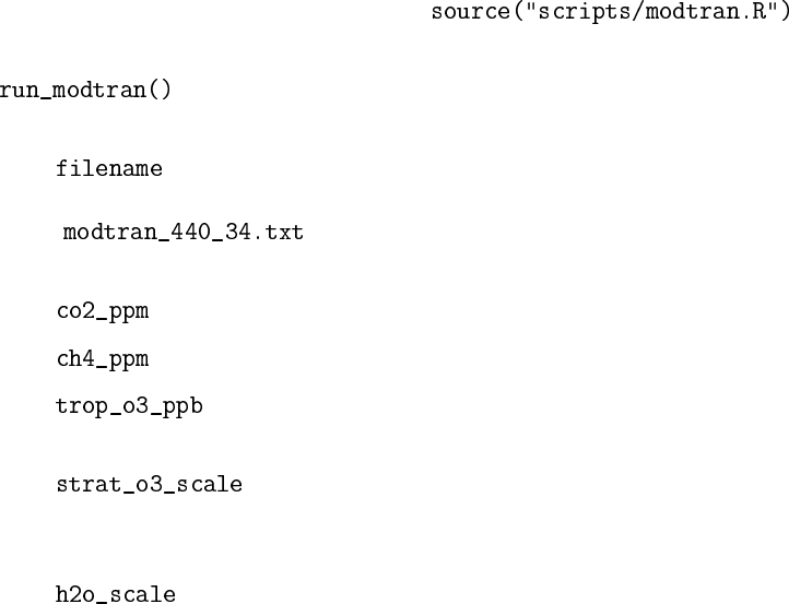
This RMarkdown document includes the line , which loads a

script with the following functions:

•

allows you to automatically download a file with the data from a MODTRAN

run. You call it with the following arguments:

–

is the name of the file to save the data to. I recommend giving it a meaningful

name: for instance, a run with 550 ppm CO2 and 3.4 ppm methane might be called

“ ”. Make up your own file names, but think about how you will

tell which is which.

–is the amount of CO2in parts per million. The default is 400.

–is the amount of methane in parts per million. The default is 1.7.

–

is the amount of ozone in the troposphere, in parts per billion. The default

is 28. You probably won’t change this unless you’re setting all greenhouse gases to zero.

–

is the amount of stratospheric ozone, relative to the naturally occur-

ring levels in the ozone layer. You probably won’t change this unless you’re setting all

greenhouse gases to zero.

–

is the amount of water vapor, relative to the naturally occurring levels in the

atmosphere. You probably won’t change this unless you’re setting all greenhouse gases

to zero.

1

–

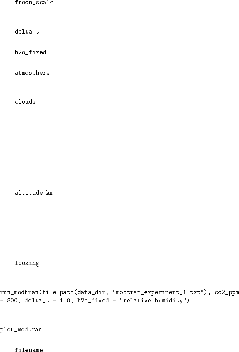
is the amount of freon chemicals (used for refrigerators and air condi-

tioners), relative to the current amounts. You probably won’t change this unless you’re

setting all greenhouse gases to zero.

–

is the temperature offset, in degrees C. You adjust this to restore radiative

equilibrium after you change the amount of CO2or other greenhouse gases.

–

is what quantity to hold fixed for water vapor. Possible values are “vapor

pressure” (the default), and “relative humidity”

–

is the locality in the MODTRAN model. Possible values are: “tropi-

cal” (the default), “midlatitude summer”, “midlatitude winter”, “subarctic summer”,

“subarctic winter”, and “standard” for the 1976 U.S. standard atmosphere.

–

is the specification of clouds and rain. Possible values are “none” (the default),

“cumulus”, “altostratus”, “stratus”, “stratocumulus”, “nimbostratus”, “drizzle”, “light

rain”, “medium rain”, “heavy rain”, “extreme rain”, “standard cirrus”, “subvisual cirrus”,

and “NOAA cirrus”.

Stratus clouds

are flat, opaque, and low-altitude.

Altostratus clouds

are flat and

medium altitude.

Cirrus clouds

are thin and high-altitude. They are hard to model,

so there are three different varieties.

Cumulus clouds

are thick and stretch from low

altitudes to medium altitudes.

Stratocumulus clouds

are like thunder clouds. They

are very tall and reach from low altitudes to the top of the troposphere.

Nimbostratus

clouds are low and thick, like stratus, but produce rain.

–

is the altitude, in kilometers above sea level, that you put your virtual

sensor in the model. The default is 70 km, which is above almost all of the atmosphere.

For some exercises, you may experiment with putting the sensor somewhere around 8 to

12 km, which is the top of the troposphere, below the stratospheric ozone layer.

For other exercises, you might want to put it at 0 km (ground level), and set it to look up

instead of down, so you can see the IR radiation coming down to the ground from the

atmosphere instead of looking at the IR radiation going out to space.

–

is the direction the sensor is looking. The options are “down” (the default) or

“up”.

Any arguments you don’t specify explicitly take on their default value. Thus,

would run with all the

default values, except for 800 ppm CO

2

, a temperature offset of 1

°

C, and holding relative

humidity fixed.

•

reads a MODTRAN output file and generates a plot. There are many argu-

ments, and I won’t explain them all here, but the important ones are:

–is the MODTRAN output file with the data to use for the plot.

2

–

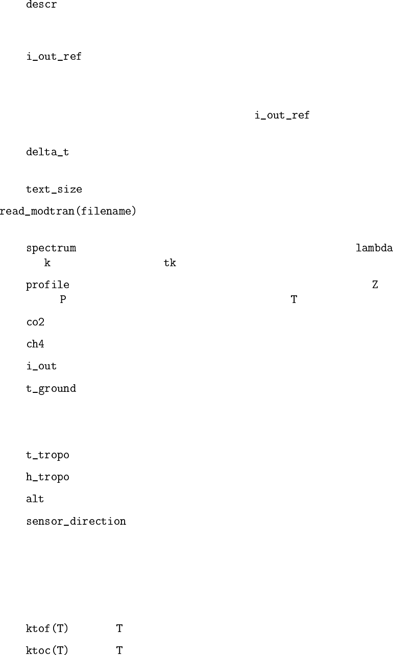
is an optional string to use for the title of the plot. If you don’t specify anything,

the function will make a title that indicates the CO2 concentration and the altitude of

the virtual sensor.

–

is a reference value for the outgoing infrared. If you don’t specify it, it’s

ignored, but if you specify it, then the plotting function adds an annotation to indicate

the difference in outgoing IR between the current run being plotted and the reference

value. Typically, you’d run a baseline run of MODTRAN with default parameters and

then use the upward IR flux from that run as when you change the CO

2

concentration or other model parameters.

–

is the temperature offset for this model run. If you specify it, the plotting

function adds an annotation to indicate it.

–

allows you to adjust the size of the text used for axis labels and the plot title.

•

allows you to read in a MODTRAN output file and examine the

data. This function returns a list with 7 elements:

–

is a data tibble with the spectral information (wavelength , wavenum-

ber , outgoing IR intensity , and a number of other variables.)

–

is the profile of the atmosphere: a tibble with three columns: is the altitude

in km, is the atmospheric pressure, in millibars, and is the temperature in Kelvin.

–is the atmospheric CO2concentration

–is the atmospheric methane concentration

–is the intensity of the outgoing IR radiation flux.

–

is the ground temperature (in Kelvin) used in the model run. (Remember that

this is something you set when you run the model. MODTRAN cannot calculate the

way ground temperature changes when you change greenhouse gases, clouds, or other

characteristics of the atmosphere.)

–is the temperature at the tropopause (in Kelvin).

–is the height of the tropopause (in km).

–is the altitude of the virtual sensor.

–is the direction of the virtual sensor (“up” or “down”).

Converting temperature units

•

Some handy functions for converting temperature measurements from one unit of measure-

ment to another are:

–converts from Kelvin to Fahrenheit.

–converts from Kelvin to Celsius.

3

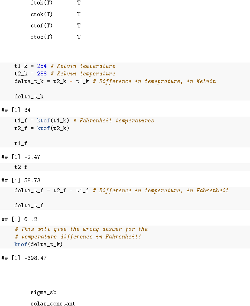
–converts from Fahrenheit to Kelvin.

–converts from Celsius to Kelvin.

–converts from Celsius to Fahrenheit.

–converts from Fahrenheit to Celsius.

But be aware that if you want to convert the difference between two temperatures, you need

to convert the temperatures and then take the difference:

You see that 58.73 − −2.47 6=−398.47.

• Some variables that I have defined for you are:

–is the Stefan-Boltzmann constant.

–

is the Solar Constant (the intensity of sunlight at the top of the

atmosphere).

4

Examples:

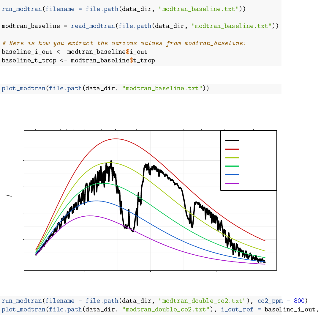
The baseline MODTRAN run has Iout =298.67 and Ttropopause =194.8.

Iout =298.67

78910121417202530354050100

0.0

0.1

0.2

0.3

0.4

0.5

400 800 1200

Wavelength (µm)

Wavenumber (cm−1)

Intensity (W m2cm−1)

MODTRAN

300 K

280 K

260 K

240 K

220 K

MODTRAN: 400 ppm CO2, 70 km altitude

5

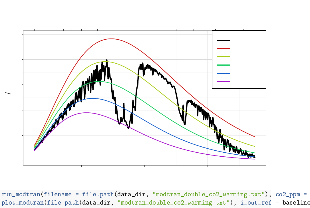
Iout =295.34 ∆Iout = −3.33

∆Tground =0K

78910121417202530354050100

0.0

0.1

0.2

0.3

0.4

0.5

400 800 1200

Wavelength (µm)

Wavenumber (cm−1)

Intensity (W m2cm−1)

MODTRAN

300 K

280 K

260 K

240 K

220 K

MODTRAN: 800 ppm CO2, 70 km altitude

6

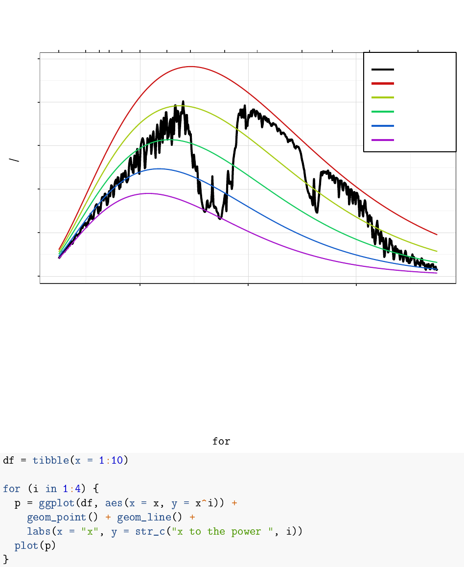
Iout =298.67 ∆Iout =0

∆Tground =0.76K

78910121417202530354050100

0.0

0.1

0.2

0.3

0.4

0.5

400 800 1200

Wavelength (µm)

Wavenumber (cm−1)

Intensity (W m2cm−1)

MODTRAN

300 K

280 K

260 K

240 K

220 K

MODTRAN: 800 ppm CO2, 70 km altitude

A few new R functions that we will use in this lab:

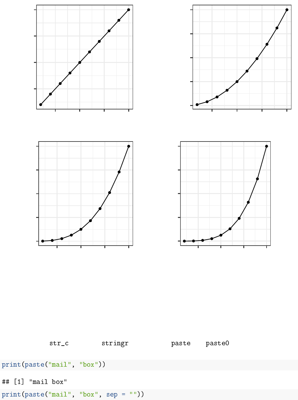
Iterating over a series

Sometimes you want to repeat something in R, executing the same commands for many different

values of a variable. We can do this with the command:

7

2.5

5.0

7.5

10.0

2.5 5.0 7.5 10.0

x

x to the power 1

0

25

50

75

100

2.5 5.0 7.5 10.0

x

x to the power 2

0

250

500

750

1000

2.5 5.0 7.5 10.0

x

x to the power 3

0

2500

5000

7500

10000

2.5 5.0 7.5 10.0

x

x to the power 4

Combining character variables

R has many functions for manipulating text. When R stores text, it stores it in character variables

(these are also sometimes called “strings” because text is like a string of characters). For instance,

we might want to make a label or a filename by combining several variables. Three functions that

we can use are , from the package and and , from basic R. All of

these work pretty much the same way:

8

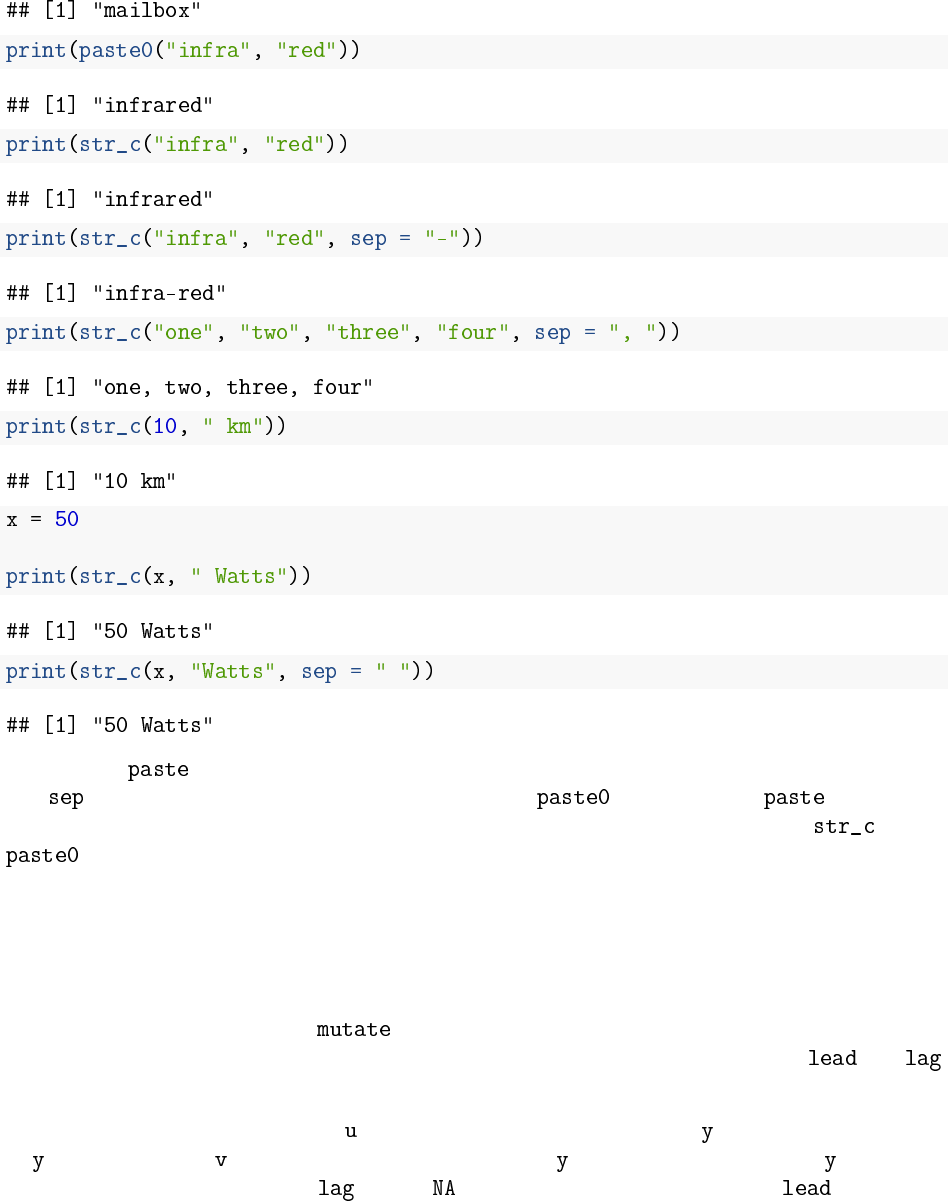
Notice how puts spaces between the strings when it combines them unless you specify

that (the separator) should be something different. works just like , except that

it doesn’t have a separator, so the variables are combined without an extra space. is like

, except that you can specify a separator if you do want something in between the different

variables.

Calculating with leads and lags

Sometimes, when we are using with a data tibble, we might want to look at differences

between a row and the row before or after it in the tibble. We can do this with the and

functions:

In the examnple below, the column gets the value of the current row of minus the previous row

of , and the column gets the value of the next row of minus the current row of . Note that

where there isn’t a previous row, returns (missing value), and similarly for when there

isn’t a next row.

9

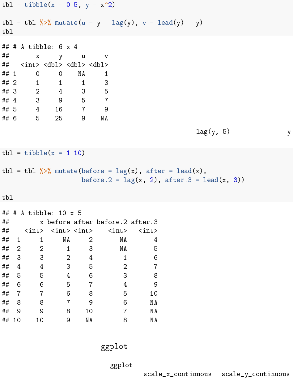
If you want to lead or lag by more than one row, you can just say, to get the value of

5 rows before the current one.

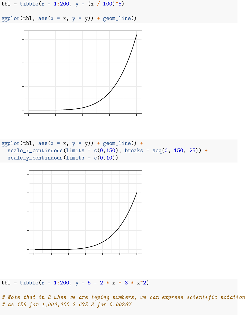
Modifying xand yaxes in

It is easy to modify the xor yaxis in . For instance, if you want to put specific limits on the

axis, or change where the labels go, you can use or :

10

0

10

20

30

0 50 100 150 200

x

y

0.0

2.5

5.0

7.5

10.0

0 25 50 75 100 125 150

x

y

11

1e+01

1e+03

1e+05

1 10 100 1000

x

y

Exercises for Lab #3

Chapter 4 Exercises

Exercise 4.1: Methane

Methane has a current concentration of 1.7 ppm in the atmosphere and is doubling at a faster rate

than CO2.

a)

Would an additional 10 ppm of methane in the atmosphere have a larger or smaller impact on

the outgoing IR flux than an additional 10 ppm of CO2at current concentrations?

b)

Where in the spectrum does methane absorb? What concentration does it take to begin to

saturate the absorption in this band? Explain what you are looking at to judge when the gas is

saturated.

Suggestion:

• Run MODTRAN with no greenhouse gases, except 0.4 ppm of methane.

•

Run MODTRAN several times, successively doubling the amount of methane: 0.4 ppm,

0.8 ppm, 1.6 ppm, . . . 102.4 ppm.

Hint: You can use the following R commands to do this: “‘ methane_data = tibble() #

create a blank data tibble

12

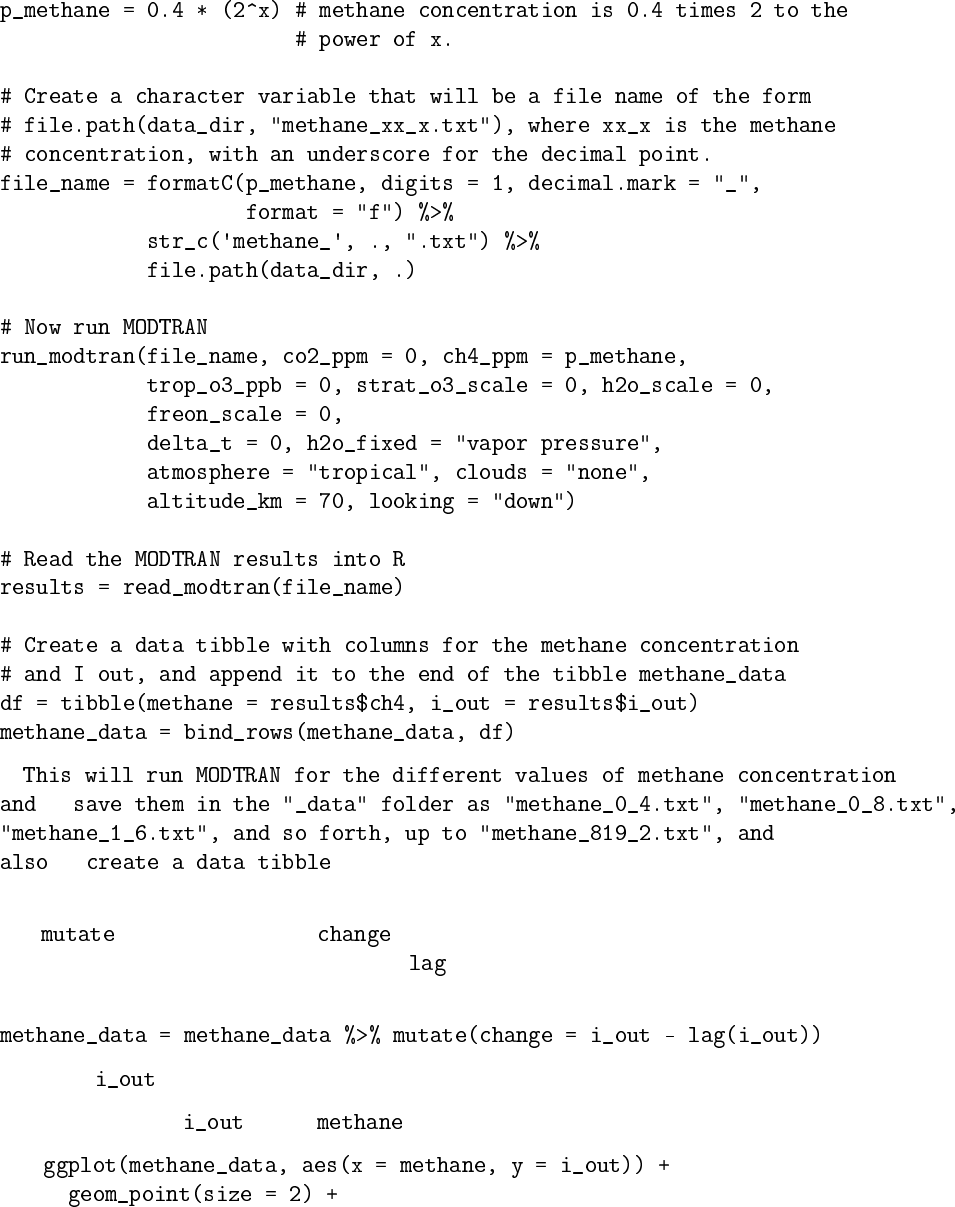
for (x in 0:11) { # Repeat everything between the braces “{}” for x taking on # each

value in 0, 1, 2, . . . , 11.

} “

methane_data‘ with a list of methane concentrations

and the corresponding Iout.

•

Use to add a new column , which contains the change in

Iout

between the

previous row and this one. You can use the command to calculate this, as described

above in the “new R functions” section.

Now plot versus the methane concentration several ways:

–First, just plot versus :

13

–

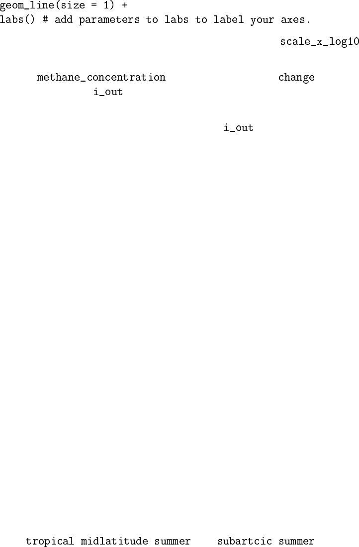
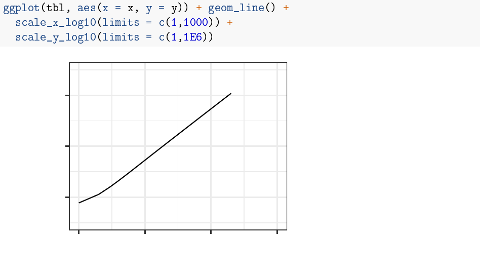
Next, plot the same data, but with a logarithmic x-axis (use , as

described above in the “New R Functions” section)

–

Next, plot , but assign the column to the yaxis,

instead of the column .

–

Think back to the slides I showed in class #6 about identifying band saturation. Do

you see a place where the successive changes in flatten out? Estimate the

concentration of methane where absorption saturates.

c)

Would a doubling of methane have as great an impact on the heat balance as a doubling of

CO2?

Suggestion:

• Run MODTRAN in its default configuration (400 ppm CO2and 1.7 ppm methane)

• Run it again with 10 ppm of extra methane

• Run it again with the default methane (1.7 ppm) but 10 ppm extra CO2.

• Compare Iout for the three runs.

d)

What is the “equivalent CO

2

” of doubling atmospheric methane? That is to say, how many

ppm of CO

2

would lead to the same change in outgoing IR radiation energy flux as doubling

methane? What is the ratio of ppm CO2change to ppm methane change?

Suggestion:

This is easier to do interactively with the web-based interface to MODTRAN

than by running it in R.

• Run MODTRAN in its default configuration (400 ppm CO2and 1.7 ppm methane)

• Run MODTRAN again with the methane doubled. Note Iout.

•

Return methane to the default value (1.7 ppm), and adjust CO

2

until

Iout

is the same as

it was for the doubled methane. Note what concentration of CO2does this.

•

Now you can use R to run MODTRAN with doubled methane and with the equivalent

concentration of CO2, and save these runs to the disk.

Exercise 4.2: CO2(Graduate students only)

a)

Is the direct effect of increasing CO

2

on the energy output at the top of the atmosphere larger

in high latitudes or in the tropics? Compare the change in

Iout

from doubling CO

2

with the

atmosphere set to , , and .

For each atmosphere, first record

Iout

with CO

2

at 400 ppm and then record the change when

you increase CO2to 800 ppm.

b)

Set pCO

2

to an absurdly high value of 10,000 ppm. You will see a spike in the CO

2

absorption

band. What temperature is this light coming from? Where in the atmosphere do you think

this comes from?

14

Now turn on clouds and run the model again. Explain what you see. Why are night-time

temperatures warmer when there are clouds?

Exercise 4.3: Water vapor

Our theory of climate presumes that an increase in the temperature at ground level will lead to an

increase in the outgoing IR energy flux at the top of the atmosphere.

a)

How much extra outgoing IR would you get by raising the temperature of the ground by 5

°

C?

What effect does the ground temperature have on the shape of the outgoing IR spectrum and

why?

•

Note the

Iout

for the default conditions. Then set to 5 and run MODTRAN

again, and note the new value of Iout.

• Plot the spectrum for both runs and compare.

b)

More water can evaporate into warm air than into cool air. Change the model settings to hold

the water vapor at constant relative humidity rather than constant vapor pressure (the default),

calculate the change in outgoing IR energy flux for a 5

°

C temperature increase. Is it higher or

lower? Does water vapor make the Earth more sensitive to CO2increases or less sensitive?

c) Now see this effect in another way.

• Starting from the default base case, record the total outgoing IR flux.

•

Now double pCO2. The temperature in the model stays the same (that’s how the model

is written), but the outgoing IR flux goes down.

•

Using constant water vapor pressure, adjust the temperature offset until you get the

original IR flux back again. Record the change in temperature

•

Now repeat the exercise, but holding the relative humidity fixed instead of the water

vapor pressure.

•

The ratio of the warming when you hold relative humidity fixed to the warming when

you hold water vapor pressure fixed is the feedback factor for water vapor. What is it?

Chapter 5 Exercise

Exercise 5.2: Skin Height

a)

Run the MODTRAN model in using the “Tropical” atmosphere, without clouds, and with

present-day pCO

2

(400 ppm). Use the ground temperature reported by the model to calculate

ε σ T4

ground

, the heat flux emitted by the ground. Assume

ε=1

, and I have already provided

the value of the Stefan-Boltzmann constant

σ

, as the R variable , which equals

5.67

×

10

-8

. (I defined it in the script “utils.R”, which I loaded in the “setup” chunk in the

RMarkdown document).

15

Next, look at the outgoing heat flux at the top of the atmosphere (70 km) reported by the

MODTRAN model. Is it greater or less than the heat flux that you calculated was emitted by

the ground?

b)

Use the outgoing heat flux at the top of the atmosphere to calcuate the skin temperature (use

the equation

Iout =ε σ T4

skin)

). What is the skin temperature, and how does it compare to the

ground temperature and the temperature at the tropopause, as reported by the MODTRAN

model?

Assuming an environmental lapse rate of 6K/km, and using the skin temperature that you

calculated above, and the ground temperature from the model, what altitude would you expect

the skin height to be?

c)

Double the CO

2

concentration and run MODTRAN again. Do not adjust the ground tem-

perature. Repeat the calculations from (b) of the skin temperature and the estimated skin

height.

What is the new skin temperature? What is the new skin height?

d)

Put the CO

2

back to today’s value, but add cirrus clouds, using the “standard cirrus” value for

the clouds. Repeat the calculations from (b) of the skin temperature and the skin height.

What is the new skin temperature? What is the new skin height? Did the clouds or the doubled

CO2have a greater effect on the skin height?

16