Lab Manual

ug-physics-lab-manual-17

User Manual:

Open the PDF directly: View PDF .
Page Count: 80

PHYSICS

LABORATORY

MANUAL

For Undergraduates

2016-17

The LNM Institute of Information Technology

Rupa ki Nangal, Post-Sumel, Via-Jamdoli,

Jaipur - 302031, Rajasthan, India

Laboratory Regulations

1. Attendance is compulsory and it carries 10%weightage on grade evaluation for

this course.

2. Students should be punctual. They will be marked absent if they are not present

within the ﬁrst ﬁve minutes of each laboratory session.

3. Experiments will be performed in groups deﬁned by the lab instructors. Students

are not allowed to change their partner during the semester under any circumstance.

4. It is compulsory to bring the lab manual and required graph papers. The lab

lab register with them after completion of the experiment. Such activities will be

penalized.

5. Pre-recorded audio visual demo for every experiment will be sent to you in due time.

Prior to performing each experiment, you should be familiar with the basic principles

from them. There will be no additional demo for any of the experiment

will be given during the lab session.

6. During each lab session you are expected to perform the experiment, record the

observed data in your lab register (not in any rough note book) and complete the

experiment including the written record. For each experiment, you have to write in

your lab register the purpose, description of apparatus, working formula (if

any), and tables for observations.

7. Students are supposed to handle the instruments carefully. In case of any technical

diﬃculty take help from the lab attendant. After performing the experiment hand

over the instrument(s)/components and or switch oﬀ (in case of electrical devices)

properly. Any intentional manhandling of any experimental set ups will lead to

disbarring of the student from the subsequent lab sessions depending on the severity.

8. Student while performing the experiments are supposed to get a few readings signed

by the respective instructor or TA in their lab register.

9. The lab register completed in all respects should be submitted at the end of each

lab session (take a note of the point4 above).

10. Laboratory evaluation will also depend on satisfactory performance in the viva which

will be conducted for each experiment.

11. The student is expected to be in the lab for the entire 3 hours. Leaving the laboratory

early without informing is liable for deduction in class performance marks.

Contents

A. Measurement & Instruments 5

B. Error bars on graphs 13

C. A comment of signiﬁcant digits 14

D. Vernier caliper & Screw Gauge 16

1. Introduction to Error Analysis and Graph Drawing 21

1.1. Finding τand initial voltage across capacitor . . . . . . . . . . . . . . . . . 21

1.2. ResonantRings.................................. 22

1.3. MassSpringSystem ............................... 22

1.4. Resistivity of a of nichrome wire . . . . . . . . . . . . . . . . . . . . . . . . 23

1.5. To measure the electrical resistance of a given material . . . . . . . . . . . . 24

2. Acceleration due to gravity by bar pendulum 26

3. e/m of electron by Thomson Method 32

4. Measurement of band gap of semiconductor 38

5. Refractive index of glass with the help of a prism 45

6. Wavelength of sodium light by Newton’s rings 54

7. Helmholtz coil 60

8. Electromagnetic induction 63

9. Mechanical waves 68

10. Fraunhoﬀer Diﬀraction 72

11. Diﬀraction grating 76

A. Measurement & Instruments

This section of the manual describes the basic measurements and allied instruments that

you will encounter in the laboratory.

Physical Measurements

In the grouping of physical measurements the quantities to be measured are length, mass,

angle and time.

Length

There are three basic instruments for the measurement of length, (i) the meter ruler, (ii)

the micrometer screw gauge and (iii) the vernier calipers. The table below details the

range and accuracy of these three instruments.

Name Range Accuracy

Meter Ruler 0−100 cm 1mm

Micrometer Screw Gauge 0−25 mm 0.01 mm

Vernier Calipers 0−150 mm 0.02 mm

Clearly, there is a wide variation in the range of the instruments and the ﬁrst lesson is

that the choice of instrument is determined by the length that is to be measured. If the

length is 50cm, then it clearly should be the Metre Ruler. The second lesson concerns the

accuracy. In principle, you can measure a length of 2cm with all three instruments but

the accuracy of your measurement will vary from 1mm to 0.01mm. The choice, then, is

also determined by the accuracy required. The accuracy of an instrument depends on its

construction & operation and this is now described for each instrument

Meter ruler: The principle of the metre ruler is very simple. A known length (1 metre)

is divided into 100 unit lengths of 1cm. and these are further subdivided into 10 unit

lengths of 1mm. The accuracy of the instrument is the smallest division, namely 1mm.

Operation: Place one end of the ruler (or an appropriate ‘zero’) at one end of the

length to be measured and read oﬀ the nearest value at the other end of the length to be

measured.

Micrometer screw gauge: The principle of the micrometer is the screw thread. The

pitch of the screw is 0.5mm. that is one complete rotation of the screw advances or retracts

the screw by 0.5mm. Underneath the rotating barrel of the gauge is a ruler with 0.5mm

divisions (actually two sets of 1mm divisions oﬀset by 0.5mm). The rotating barrel is

itself subdivided into 50 units, such that rotation of the barrel through one unit advances

or retracts the screw by 0.5/50 = 0.01mm; the accuracy of the instrument is therefore

0.01mm.

Operation: Place the object between the ﬁxed and moving end faces and rotate the

barrel until the object is in contact with both end faces. Always rotate using the small

slip knob at the end of the barrel. This will ensure contact without damage to the

object or the micrometer. The measured length is the reading on the ruler to the nearest

full 0.5mm unit plus the portion of this unit shown on the rotating barrel. Always check

the visible zero setting and all for any oﬀset from zero.

Vernier calipers: The principle of the Vernier calipers is two-fold. First, the sliding

piece allows the jaws to contact the sides of the object to be measured, in much the same

way as the micrometer. The distance moved by the sliding jaw is then read oﬀ the ﬁxed

ruler on the main body of the instrument. The accuracy of that ruler as such, however,

is only 1mm. The much improved accuracy is provided by the ’Vernier’ scale. This scale

is marked on the sliding jaw; it has 10 divisions, each subdivided into 5, ie a total of 50

subdivisions. These subdivisions look like 1mm in length. But if you compare the ﬁxed

and Vernier scales, you will see that the 50 subdivisions on the Vernier scale correspond

to 49 subdivisions (each of 1mm) on the ﬁxed scale! This is not a mistake but rather it

is deliberately designed so that a subdivision on the Vernier scale is smaller than that on

the ﬁxed scale by 1/50 = 0.02mm; this is the accuracy of the instrument. How a reading

with this accuracy is achieved in practice is detailed below:

Operation: With no object between the jaws, the zeros of the Vernier and ﬁxed scales

are coincident. There is an increasing mismatch between the marks of these two scales

until at the end of the Vernier scale there is again coincidence between the end mark on the

Vernier and the 49mm mark on the ﬁxed scale. Clearly, to obtain coincidence between the

ﬁrst subdivisions of the Vernier and of the ﬁxed scales it would be necessary to move the

sliding jaw by the deﬁcit of 0.02mm; coincidence between the second subdivisions would

require 2 x 0.02 = 0.04mm, and so on. A total of 50 x 0.02 = 1mm is required to achieve

coincidence between the end mark of the Vernier scale and the 50mm mark of the ﬁxed

scale. Conversely, a measurement of the length of an object in contact with the jaws is

the reading to the nearest full mm on the ﬁxed scale at the Vernier zero PLUS the reading

(in units of 0.02mm) on the Vernier scale where there is coincidence between the

vernier and ﬁxed scales.

Other vernier instruments: There are three other instruments in the laboratory which

incorporate Vernier scales. These are the travelling microscope, the weighing scales and

the spectrometer. The travelling microscope combines magniﬁed optical positioning with

a ruler accuracy of 0.01mm.

For the other two instruments some other parameter has been equated with a length

scale.

In the case of the weighing scales, mass can be equated with the length of the balance

arm that is divided into 10 units of 10g. The rotating scale adds up to a further 10gwith

an accuracy of 0.1gand the Vernier scale accuracy is 0.01g.

In the case of the spectrometer, angle can be equated with the length of a circular

scale that has an accuracy of 0.5 degree. The Vernier scale is in the natural sub-unit of

minutes of arc (60 minutes of arc = 1 degree) and the accuracy is one minute of arc (1’).

Time

The stop-clock has a start/stop/reset push-button device with a digital display. In prin-

ciple, the accuracy is the smallest digit, ie 0.01s, but the response time of the button is of

the order of 0.1sand that of the user may be signiﬁcantly longer, say, of the order of 1s.

Timing accuracy is further discussed later in the section Accuracy & Uncertainty.

Electrical Measurements

In the grouping of electrical measurements, the principal instruments are the multimeter,

oscilloscope, function generator and the power supply.

Multimeter

The multimeter provides conveniently in a single instrument a number of ranges of mea-

surement of voltage (DC/AC), current and resistance. It is necessary to select the appro-

priate quantity and range as well as the proper connections for the two input leads. The

AC ranges are distinguished from the DC ranges by the symbol (∼).

Voltage: The voltage ranges are marked V. The two input sockets are marked COM

and V,Ω.

Voltage is measured across a component, that is, the meter is connected in parallel

with the component. The meter displays the polarity of the voltage relative to the COM

connection.

Current: The current ranges are marked A. The two input sockets are marked COM

and either Aor 10A, depending on the magnitude to be measured; the Aconnection is

protected by a 2amp fuse and is only to be used for currents less than this limit. The 10A

connection is protected by a 10amp fuse, and is only to be used for currents up to this

limit. This latter connection only works with the current range marked 10.

Current is measured through a component, that is the meter is connected in series

with the component. The meter displays the polarity of the current entering the A(or

10A) socket.

Resistance: The resistance ranges are marked Ω. The two input sockets are marked

COM and V, Ω.

Resistance is measured across a component, that is, the meter is connected in parallel

with the component. There is no polarity associated with this measurement.

It is important to realize that resistance measurement is really the measurement of the

voltage resulting from a current supplied by the meter. Therefore, this mode of resistance

measurement cannot be carried out on components while they are in circuit.

Range & display: The maximum display of 1999 corresponds to the end of the range

selected. For example, selecting the voltage range marked 2 allows a measurement of

voltage up to 1.999 volts. The next voltage range is marked 20. This range is appropriate

for voltage between 2 and 20 volts.

The accuracy of the measurement is the least signiﬁcant digit (note how this digit may

arbitrarily change up or down by one unit during the reading). The best practice is to use

the range which is one setting above that at which the full 1999 shows.

Oscilloscope, function generator & power supply

The oscilloscope is probably the most important of all electronic measuring equipment.

Its main use is to display on a screen the variation or a potential diﬀerence (or voltage) as,

a function of time. The result is a graph with voltage on the vertical (or y) axis and time

along the horizontal (or x) axis. This is achieved by electrostatic deﬂection of an electron

beam striking the front face phosphor in the cathode ray tube in the oscilloscope.

You will learn about oscilloscope, function generator and power supply in your elec-

tronics laboratory.

Plotting graphs

A graph is useful way of displaying the results of an experiment in which one parameter

(call it x) is varied in well deﬁned steps and another parameter (call it y) is measured in

response. In this general case each (x, y) pair of values is represented by a point which is a

distance xalong the horizontal axis and a distance yalong the vertical axis. For example,

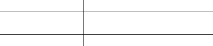
if the following data were obtained for the resistance of varying lengths of wire:

L (m) 1 2 3 4

R (Ω) 10 20 30 40

The data would be graphed as shown below:

Figure 1: Resistance (R) vs Length (L)

Note the title, the labeled axes (with units!). These elements are essential for any

graph! The usefulness of this particular graph is that it is clear at a glance that the

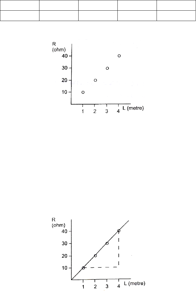
resistance of the wire is proportional to its length. This is formally shown in the graph

below where the data fall on a straight line through the origin.

Mathematically, this linear relation is expressed by the equation y=mx, where mis

the slope. The slope of the straight line is obtained by constructing a right-angle triangle

containing the straight line and lines parallel to the vertical and horizontal axes; the slope

is the ratio of the lengths of the vertical and horizontal sides (shown dashed below). Note

that for good accuracy the complete range of plotted data should be used.

Figure 2: Resistance (R) vs Length (L) showing slope

In this particular example the slope is (40-10)/(4-1) = 30/3 = 10.

The resistance per unit length of the wire is 10 ohm per metre or simply 10Ωm−1. (In

shorthand R(Ω)=10Ωm−1L(m).

This trivial example has been used to introduce you to the basics of graph plotting.

Only rarely will your experimental data be in this ready-to-graph form. For example,

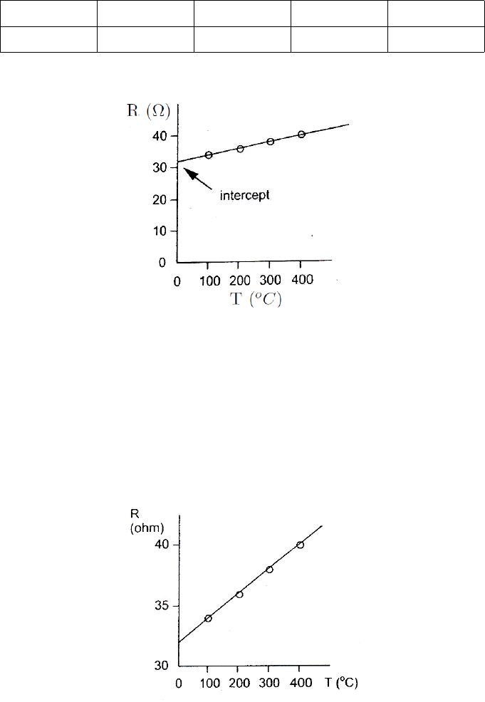
consider the following measurements of the resistance versus the temperature of a ﬁxed

length of the wire:

T (oC) 100 200 300 400

R (Ω) 34 36 38 40

The data could be plotted as shown in Fig. 3. This time, the straight line does not

Figure 3: Resistance (R) vs Temperature (T)

go through the origin and the mathematical expression is y=mx +C, where Cis the

intercept on the yaxis. In this case the intercept, Cis 32Ωand the slope, mis 2ΩoC−1.

We can therefore write R(Ω) = 2(ΩoC−1)T(oC) + 32Ω.

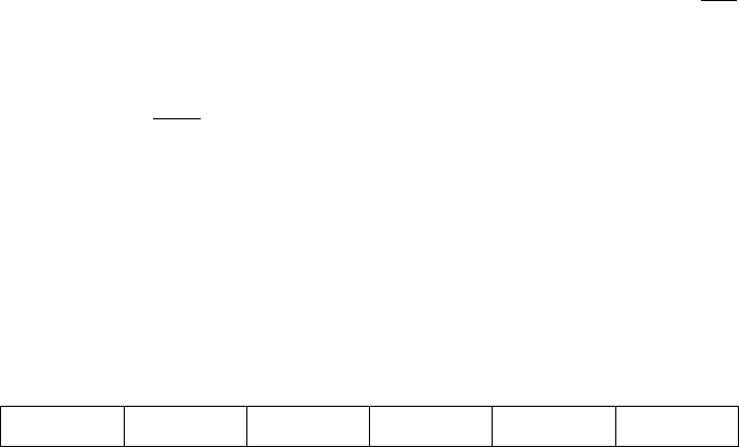
This example also illustrates an important value judgment about the axes of a graph.

As drawn above most of the graph page is wasted. A better graph (and a more accurate

one) is shown in ﬁgure on next page. The origin is now the point (30, 0) rather than (0,

Figure 4: Resistance (R) vs Temperature (T)

0) and the labeling must show that clearly! Clearly the choice is dictated by whether the

intercept is to be determined. Also, the intercept of interest may be on the horizontal

(or x) axis. These considerations apart, you should always aim to use the full size of the

available graph page.

What to do with a system which is not in linear form? A good example is the relation

between period (T) of a simple pendulum and its length (L). These are related by the

expression . When we plot a graph of Tvs Lwe get a curve. But if we plot a graph

of T2vs L, we should get a straight line of the form y=mx. That is, we re-write the

expression in the form of a straight line as T2= (4π2/g)L. In this way it is clear if our

data matches the theory. Moreover, from the measurement of the slope mwe obtain a

value of g= 4π2/m.

Finally, it is useful to start thinking of a graph as a way of averaging your data and

this concept will be fully discussed in the next section on Accuracy and Uncertainty.

Accuracy and uncertainty (and errors!)

A physical measurement is never exact. Its accuracy is always limited by the nature of

the apparatus used, the skill of the person using it and other factors. The best we can do

is report a range of values, so there remains some uncertainty. So typically we may write:

The velocity of the ball was found to be 5.13 ±0.02ms−1. This deﬁnes the range 5.11 to

5.15.

The end points of the range can rarely be assigned with much precision (in this labo-

ratory, at least), so if a calculated estimate of the uncertainty were to give us 0.018732 in

the above, we would make it 0.02, retaining just a single signiﬁcant ﬁgure. We must also

trim the digits of the main (central) value to the same point so that 5.128765 become 5.13

in the stated result.

The three rules for a measured (or calculated) value are:

•Include the uncertainty estimate to one signiﬁcant ﬁgure.

•Trim the digits of the value to the same signiﬁcant ﬁgure.

•Don’t forget the units.

How do we estimate uncertainty? In the case of most* individual measurements it

arises naturally from the fact that the instrument has a printed scale (*special cases are

discussed later!). A reasonable estimate of the uncertainty is plus-or-minus half the interval

of the scale, if you use it straightforwardly. In the case of modern instruments with an

electronic display, there may be a stated limit to the accuracy. In some such cases, if

you try to read out more digits the ones at the end will ﬂuctuate, telling you they are

unreliable.

To keep things simple it is recommended that you use plus-or-minus the

smallest interval of the scale.

But this is the start of a long story of statistics, to which we will pay little atten-

tion now. We will use our common sense and some very elementary mathematics. The

mathematical rules follow in a separate section. Remember they are intended for rough-

and-ready estimates–don’t labour over enormous calculations – use short cuts and mental

arithmetic whenever you can. If the person on the next bench gets ±0.2and you get ±0.3,

it’s unlikely to matter at all. Do it quickly.

FAQ on uncertainty and errors

1. Isn’t uncertainty called error?

Yes, it often is, alas. In fact it’s quite traditional. The unfortunate thing is that it

makes uncertainty sound like a mistake.

2. But don’t we make mistakes?

We all do. These will give rise to data points that don’t ﬁt into the overall pattern,

and can be checked and replaced. That’s one reason why we take sets of measure-

ments and ﬁt them to some sort of theory.

3. But suppose I keep making the same error, such as using an instrument

whose zero has not been set properly, or the wrong units?

Yes, we are all human. That would be called s systematic error. We’ve been talking

about random errors or uncertainty here. A systematic error is something you usually

don’t know about, so you cannot state it! If you can, you should be able to eliminate

it.

4. How can I detect a systematic error?

If experiment does not conform to theoretical expectations, one or the other needs to

be improved. In the case of the experiment, search for systematic errors. This dia-

logue between theory and experiment is how both progress and reliable measurement

techniques are developed.

5. How do I combine the errors from individual measurements?

There are basic rules for this as outlined below.

Combining errors of indivual measurements

If the measured values of Aand Bhave certain uncertainties, what are the consequent

uncertainties of AB,A+Band sin(A+B)?

For many, this is the hard part of the subject, but it boils down to a few simple rules

and procedures. It is much less painful if you remember precise calculations with rough

estimates make little or no sense. Feel free to take short cuts by making rough-and-ready

approximations as you go along, in order to arrive quickly at an estimate of the ﬁnal error.

Rules: Here we shall indicate the uncertainty of Aby ∆A. That is, the measured range

is A+ ∆A.

Rule 1: For addition (or subtraction) add the uncertainties.

If C=A+B, or C=A−B, then ∆C= ∆A+ ∆B.

Example: A= 50 ±1, B = 20 ±2, then A+B= 70 ±3and A−B= 30 ±3

Rule 2: For multiplication (or division) add the relative uncertainties to get the relative

uncertainty of the ﬁnal quantity.

If C=A×B, or C=A/B, then ∆C/C = ∆A/A + ∆B/B. Having found this

fraction, simply multiply by Cto get ∆C!

Example: A= 50 ±1, B = 20 ±2. For C=AB, C = 1000 ±120. for

C=A/B, C = 2.5±0.3

Note that, in particular, If C= 1/A, then ∆C/C = ∆A/A.

Rule 3: Dealing with functions.

There are two ways of dealing with functions, such as C= sin(A)or C= exp(A).

One can express the uncertainty in terms of the derivative of the function. Perhaps

you can see the logic of this. But a more straight forward approach, which should

almost always work, is as follows.

Work out the values of the function for A+∆Aand A−∆A, and take these to deﬁne

the range of values of the function C.

All of these rules can easily be justiﬁed by elementary mathematics, provided that the

relative uncertainties are small.

Four special cases:

1. Judgement errors

These arise in cases where the experimenter has to make a judgement about when

some condition is fulﬁlled in location or in time. Once the location or time is ﬁxed

it can be measured to a certain accuracy or error. However, this error may be much

less than the error associated with the judgement. A good example is the location

of the viewing screen in the experiment on the convex lens. The experimenter has

to make the judgement when the image on the screen is in focus and the error in

position associated with this judgement may be much larger than the measurement

error of the emphﬁnal position. The real error has to be estimated by gauging the

range of position over which the image appears to be still in focus.

2. Improving the timing error in a periodic system

The error associated with a single measurement can be dramatically reduced by

measuring the combination of many identical units. A good example of this is the

measurement of the period of a pendulum. Suppose the measurement of a single

swing is 20 ±1s(where the error of 1 includes the judgement error of when the

swing starts and ends). The total time for 10 swings of the pendulum might be

195sbut the error in this measurement would still be 1s. The period would be

(195 ±1)/10 or 19.5±0.1s. The latter is a more accurate result.

3. Improving the count rate error in a "random emission" system

Radioactive emission is random in time. This means that repeated measurement

of the emission, usually called the count in ﬁxed periods of time shows a range of

values (or error) which is related to the size of the count. The mathematics behind

this is quite complex but the result is very simple: The error in the count is the

square root of the count! For example, if the count is 100, the error is √100 = 10,

answer 100 ±10. Now, suppose this count is taken in a time of 1s. Ignoring any

error in the time, the count rate (as opposed to the count) is clearly 100 ±10s−1.

However, counting for the longer time of 10 s might yield a total count of 1020; the

associated error is √1020 = 32, i.e. the total count is 1020 ±32. The count rate is

(1020 ±32)/10 = 102 ±3. The latter is a more accurate result!

4. Average values of non-uniform parameter

Suppose you need to measure the diameter of a ball. A single measurement will

yield a value and associated error. However, a physical ball is not a perfect sphere

and a measurement of diameter at another orientation may yield a diﬀerent result.

The more useful value of diameter is the average value estimated from a number of

measurements. Suppose the following measurements are taken of the diameter:

25 ±1 23 ±1 28 ±1 22 ±1 24 ±1 23 ±1

The average value is clearly (25 + 23 + 28 + 22 + 24 + 23)/6 = 145/6 = 24.17 but

what is the error? This question brings us into the area of statistics and there is no

easy answer to this other than a full statistical analysis. One thing is certain: the

error in the average is NOT the average of the errors!

We recommend the following approximate method:

First, examine which is greater, the range of values or the error in any individual,

value. In the unlikely event that it is the latter then this is the error in the average! More

likely, the range of values is greater, as is the case here; the values range from 22 to 28, a

range of 6. A crude estimate of the error is therefore ±3. However, if you think about it,

increasing the number of measurements will only increase this estimate of error, whereas

the reverse would be the case in a proper statistical analysis. Visual inception of the data

above shows that 5 out of the 6 values lie within the range 24 ±2and this is a more

reasonable answer. When you encounter this type of error in an average, it is

suﬃcient to make a rough estimate along these lines!

B. Error bars on graphs

Whenever you enter data as a data point on a graph, the uncertainty in one or other of

the xand yvalues can be indicated by error bars, which show the range of values for

that parameter at each data point. This is helpful in judging by eye whether the data is

consistent with some theory, or whether some particular measurement should be repeated.

This applies to graphs drawn by hand or by computer. In practice, it may be simpliﬁed

in many cases. For example, if the relative uncertainty in xis much less that that in y–

or vice-versa – it is not worth representing the smaller error bar on the graph or it might

be that the uncertainty is too small to be visible, in that case there should be a statement

on the graph to that eﬀect.

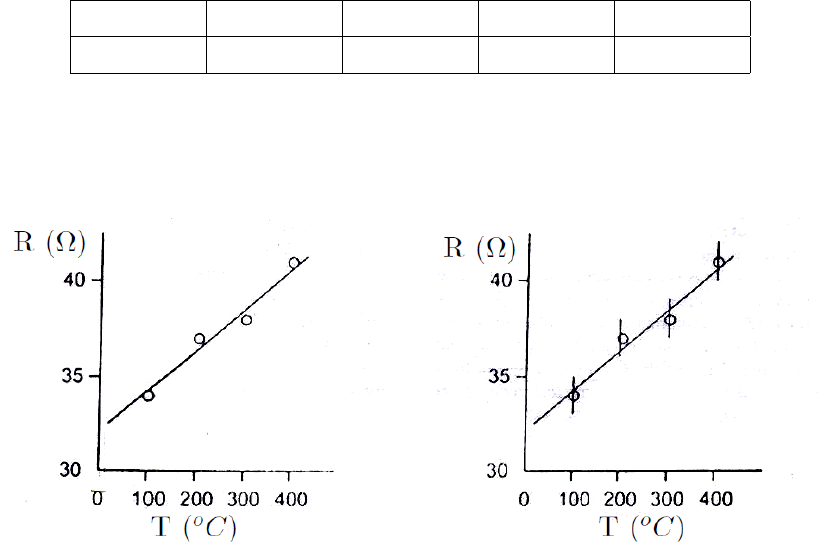
Consider the following modiﬁed data set for the resistance versus the temperature of

a ﬁxed length of the wire:

T(oC)100 ±1 200 ±1 300 ±1 400 ±1

R (Ω)34 ±1 37 ±1 38 ±1 41 ±1

When the bare data is graphed as shown in Fig 5(a) it is not possible to link the points

with a straight line. However, when error bars are included for the R values (the error

in T is much smaller) then it is possible to put a straight line through the error bars, as

shown in Fig 5(b). These data now verify the linear relation. The remaining question is

(a) (b)

Figure 5: Resistance (R) vs Temperature (T) (a) without error bars and (b) with error

bars

which straight line? It is clear that there is a smaller but ﬁnite range of lines of diﬀerent

slope which pass through the error bars. This is important if the slope is used to derive

some parameter, e. g. a value of g in the pendulum experiment.

The slope then becomes m±∆m. Again, this is another example of the error associated

with an average, as discussed above. Again too, it is diﬃcult to be exact about this.

C. A comment of signiﬁcant digits

In many cases the uncertainty of a number is not stated explicitly. Instead, the uncertainty

is indicated by the number of meaningful digits, or signiﬁcant ﬁgures, in the measured

value. If we give the thickness of the cover of this booklet as 3.94mm which has three

signiﬁcant ﬁgures. By this we mean that the ﬁrst two digits are known to be correct, while

the third digit is in the hundredths place, so the uncertainty is about 0.01mm. Two values

with the same number of signiﬁcant ﬁgures may have diﬀerent uncertainty, a distance given

as 253km also has three signiﬁcant ﬁgures, but the uncertainty is about 1km. When you

use the numbers having uncertainties to compute other numbers, the computed numbers

are also uncertain.

When we add and subtract numbers, it is the location of the decimal point that matters,

not the number of signiﬁcant ﬁgures. For example 123.62 + 8.9 = 132.5.

Although 123.62 has an uncertainty of about 0.01 and 8.9 has an uncertainty of about

0.1, so their sum has an uncertainty of about 0.1 and should be written as 132.5 and not

132.52.

Exercise:

1. State the number of signiﬁcant ﬁgures:

(a) 0.43

(b) 2.42 ×102

(d) 0.029

(e) 0.0003

2. A rectangular piece of iron is (3.70±0.01)cm long and (2.30±0.01)cm wide. Calculate

the area.

3. Mass of the planet Saturn is 5.69 ×1026kg and its radius is 6.6×107m. Calculate

its density.

4. Estimate the percent error in measuring

(a) A distance of about 56cm with a meter stick.

(b) mass of about 16gwith a chemical balance.

5. 3.1416 ×2.34 ×0.58 =

6. 2.56 + 16.4329 =

7. 16.4329 −2.56 =

D. Vernier caliper & Screw Gauge

Vernier caliper and screw gauge are used for measuring small lengths with precession.

Vernier caliper

Parts of the instrument1

01 2 3 4 5 6 7 8 9 10 11 12 13 14 15 16 17 cm

0 4 81/128

0 1 23456 7 8 9 01/20

123456

inch

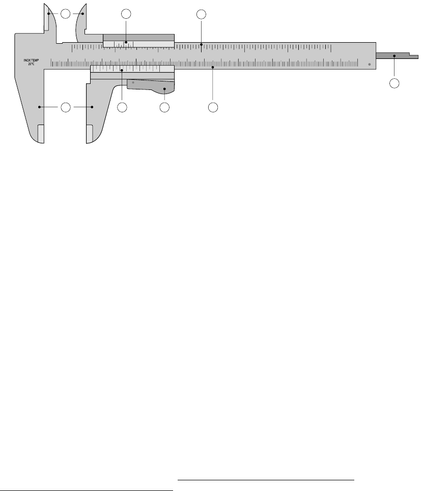
Figure 6: Parts of a vernier caliper

The parts of the calliper include:

1. Outside large jaws: used to measure external diameter or width of an object

2. Inside small jaws: used to measure internal diameter of an object

3. Depth probe: used to measure depths of an object or a hole

4. Main scale: scale marked every mm

5. Main scale: scale marked in inches and fractions

6. Vernier scale gives interpolated measurements to 0.1 mm or better

7. Vernier scale gives interpolated measurements in fractions of an inch

8. Screw/ Retainer: used to block movable part to allow the easy transferring of a

measurement.

Least count of the instrument

The least count is the smallest length you can measure with the help of the instrument.

For vernier caliper the least count is deﬁned as

Least count (LC) =Least count of main scale

Number of divisions on vernier scale

1Image source: https://en.wikipedia.org/wiki/Calipers

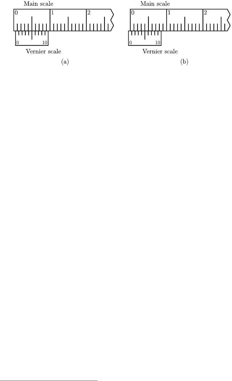
Figure 7: (a) Positive zero error in vernier caliper. (b) Negative zero error in vernier

caliper.

Measurement with the instrument

1. The outer jaws of the vernier caliper should be closed. In this position the zero of

the main scale should coincide with the zero of the vernier scale. If this is not the

case, then zero error correction has to be applied for each reading.

2. Loosen the screw and place the object to be measured in between the outer jaws.

Tighten the screw again so that the scale does not slide.

3. Note down the position of the zero mark on the main scale. Let it be MSR (Main

Scale Reading).

4. Note down the position of the vernier scale division which coincides with the main

scale division. Let it be VSR (Vernier Scale Reading).

5. The total length of the object is then

Length =MSR +VSR ×LC (1)

6. Repeat the steps 2-5 couple of times and take the average of the measured length.

7. Make sure to include proper units and zero correction if required.

Zero error2

Zero errors often arise due to fault in manufacturing. There are two types of zero errors.

Positive zero error

If the zero on the vernier scale is to the right of the main scale, then the error is said to

be positive zero error and so the zero correction should be subtracted from the reading

which is measured. See Fig. 7(a).

Negative zero error

If the zero on the vernier scale is to the left of the main scale, then the error is said to be

negative zero error and so the zero correction should be added from the reading which

is measured. See Fig. 7(b)

2Image source: http://educationsight.blogspot.in/2014/02/vernier-zero-error-and-its-correction.

html

Measurement principle of vernier scale

First of all consider the Fig. 8(a) where the diameter of an object needs to be measured

with the main scale which has least count (LC) of 1 mm. Since the diameter of the object is

exactly 5 mm there is no need of the vernier scale.

Figure 8: Vernier measurement

Now consider Fig. 8(b), where main scale

reading shows the diameter of the object is

slightly bigger than 5 mm which can not

be measured by main scale alone. Here,

vernier scale plays an important role. If

you watch closely the vernier scale you will

ﬁnd a vernier division is slightly smaller

than the main scale division. In the present

example,

10 Vernier Scale Divisions (VSD)

= 9 Main Scale Divisions (MSD)

Least count is therefore

LC = 1 MSD −1VSD

= 1 MSD −9

10 MSD

= 0.1MSD = 0.1mm

Therefore the diameter of the object being

measured in Fig. 8(b) is

D= 5 mm + (1 MSD −1VSD)

therefore D= 5.1mm

Now, to generalize the concept, consider

Fig. 8(c). In this case the diameter of

the object is slightly bigger than the pre-

vious case. To measure this extra length,

vernier constant can again be utilized. If

the ﬁfth division matches with one of the

main scale division that means the extra

distance over and above 5 mm is equal to

5×LC. So the generalized formula for mea-

surement would be

D=MSR +VSR ×LC

where MSR is the Main Scale Reading and VSR is the Vernier Scale Reading.

Screw Gauge

Parts of the instrument3

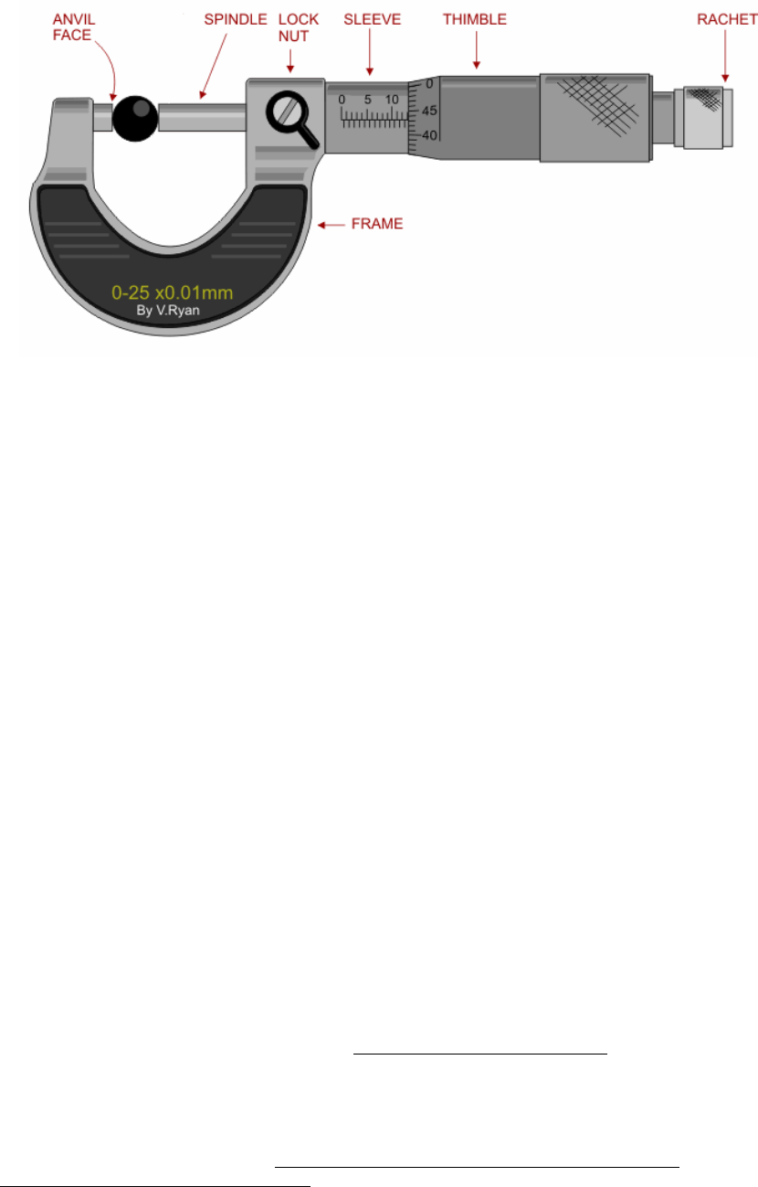
Figure 9: Parts of a screw gauge

The parts of the screw gauge include:

1. Frame: The C-shaped body that holds the anvil and barrel in constant relation to

each other.

2. Anvil: The shiny part that the spindle moves toward, and that the sample rests

against.

3. Spindle: The shiny cylindrical component that the thimble causes to move toward

the anvil.

4. Lock nut: The knurled component (or lever) that one can tighten to hold the spindle

stationary, such as when momentarily holding a measurement.

5. Sleeve: The stationary round component with the linear scale on it, sometimes with

vernier markings. In some instruments the scale is marked on a tight-ﬁtting but

movable cylindrical sleeve ﬁtting over the internal ﬁxed barrel.

6. Thimble: The component that one’s thumb turns. Graduated markings.

7. Ratchet: Device on end of handle that limits applied pressure by slipping at a

calibrated torque.

Least count of the instrument

The pitch of the screw is the distance moved by the spindle per revolution. It can be

represented as

Pitch of the screw =Distance moved by the screw

No. of full rotations given (2)

The least count (LC) is the distance moved by the tip of the screw, when the screw is

turned through 1 division of the head scale. It can be calculated using the formula

Least count (LC) =Pitch

Total number of divisions on the circular scale (3)

3Image source: https://scienceportfolio1p1.wikispaces.com/Term+1

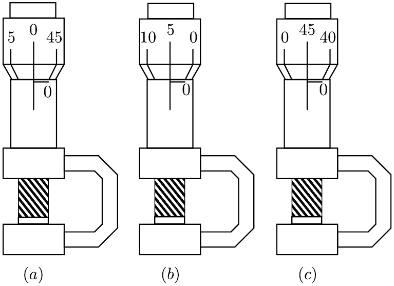
Figure 10: Screw gauge (a) without any zero error (b) with positive zero error (c) with

negative zero error.

Measurement with the instrument

1. Insert the object in between the anvil and the spindle and rotate the rachet until

the object is gently gripped between the anvil and the stud. Stop as soon as a click

sound is heard.

2. Note down the circular (CSR) and the linear/main scale (MSR) readings.

3. The length of the object is then given by

Length =MSR +CSR ×LC (4)

4. Repeat steps 1-3 three times and note the average reading.

Zero error

When the anvil and the spindle touch without any object between them, the zero of the

circular scale should coincide with the main scale line as shown in Fig. 10(a)

Positive zero error

However, if the circular scale zero is above the linear scale, the instrument has positive

zero error as shown in Fig. 10 (b) and the correction is negative.

Negative zero error

When the circular scale is below the linear scale, the instrument has negative zero error

as shown in Fig. 10(c) and the correction is positive.

Experiment 1

Introduction to Error Analysis

and Graph Drawing

1.1 Finding τand initial voltage across capacitor

You are given below the voltage decay as function of time across a capacitor in a RC

circuit.

1. Obtain the value of characteristic decay time constant by plotting the data in a

semi–logarithmic paper.

2. Obtain the initial value of the voltage across the capacitor.

Time (s) Voltage (V)

6.2 5.53

8.7 4.89

10.0 4.58

12.5 4.04

16.3 3.35

18.4 3.05

22.5 2.45

25.0 2.16

28.5 1.85

32.9 1.44

38.8 1.09

42.0 0.92

47.8 0.70

52.0 0.56

55.4 0.47

62.5 0.33

67.2 0.26

Table 1.1: Data of voltage decay in a capacitor as a function of time.

The equation governing the relation between voltage and time for the capacitor is as given

below.

v=voe−t/τ (1.1)

log v= log vo−log et/τ (1.2)

log v= log vo−t

τlog e(1.3)

From log10 vvs tplot, the value of τcan be obtained.

1.2 Resonant Rings

In an experiment, paper rings of diﬀerent diameter are mounted on a vibrating table to

study their resonant frequencies. Depending on the diameter, the rings show resonant

vibration for diﬀerent frequencies of the vibrating table. The data from this experiment

is given in Table 1.2. Use the formula F=CDn.

Diameter of the ring (cm) 3.4 4.6 6.4 8.7 10.9 13.2

Resonant frequency (Hz) 63.48 30.77 13.38 6.24 3.58 2.19

Table 1.2: Data of resonant frequencies as a function of diameter of the rings

1. Plot resonant frequency vs diameter of the ring in a log-log graph to obtain the

mathematical relationship between the two variables.

2. From your graph predict the resonant frequency for a ring of diameter 16 cm.

1.3 Mass Spring System

A spring (of mass 50 g) is suspended vertically. It is pulled slightly downward and time

for 20 free oscillations is observed. Repeat the observations for three times. Calculate the

average time period of this spring system. Now, using the equation, given below, calculate

the force constant kof the spring, to two decimal places.

T= 2πsmo+ (ms/3)

k(1.4)

where mois mass of weight hanged and msis the mass of the spring.

Observation table

Sl. T20 Mean T20 T k

– (sec) (sec) (sec) (N/m)

Table 1.3: Table to calculate the spring constant of a spring.

From the Eq. (1.4) the error in calculating kis obtained as follows. If m0= 0, then

squaring Eq. (1.4) and re-arranging the terms we have,

k=4π2

3ms

T2

Taking log on both sides,

log k= log 4π2

3!+ log ms−2 log T

Taking derivative on both sides,

∆k

k=∆ms

+ 2 ∆T

T(1.5)

where we have changed the sign of in front of ∆Tto calculate the maximum error.

1.4 Resistivity of a of nichrome wire

A homogeneous nichrome wire along with a digitial multimeter and a screw gauge is given

to you.

1. Measure the resistance of the nichrome wire for three diﬀerent lengths of the wire.

2. Use the screw gauge to determine the diameter of the wire.

3. Determine resistivity of the nichrome wire from your measurements using the formula

ρ=Rπd2/4

L,(1.6)

where, R=resistance of the nichrome wire,

d=diameter of the nichrome wire,

L=length of the nichrome wire.(1.7)

4. From Eq. (1.6) one can obtain ∆ρ

ρ=∆R

R+ 2∆d

d+∆L

Land ﬁnally obtain ∆ρfor this

experiment.

Observation table

Total number of circular scale (CS) divisions of the screw gauge = . . . . . .

One main scale division (MSD) = . . . . . . cm

Number of rotations required on the CS to cover 1 MSD = . . . . . .

Zero error on the CS = . . . . . .

Least count (l.c) of the screw gauge

l.c =One main scale division (1 MSD)

No. of rotations on the CS ×Total number of CS divisions cm (1.8)

Sl. No. MSR (a)CSR (b)Total (a+b×l.c)(cm)

Table 1.4: Table to calculate the diameter of the nichrome wire

Sl. L(cm) Resistance (Ω)ρ(Ωm)

Table 1.5: Table to calculate the resistivity of the wire

1.5 To measure the electrical resistance of a given material

The resistance of the wire is measured with the help of a Wheatstone bridge up to the

accuracy of three signiﬁcant ﬁgures. By using the relation.

Q=R

S(1.9)

where Sis a variable resistor and Ris an unknown resistor. If the ratio of the two known

resistances P/Q is equal to the ratio of the two unknown resistances R/S, then the voltage

diﬀerence between the points Aand Bwill be zero and no current would ﬂow through the

galvanometer G. In case there is a voltage diﬀerence between points Aand B, direction

of the current in the galvanometer indicates the direction of ﬂow of current through the

bridge. In this manager an unknown resistance Rcan be calculated to an accuracy of high

degree. Fig. 1.2 shows the experimental setup of a wheatstone bridge.

Observation table(No. of readings: 2 with diﬀerent lengths)

Sl. No. 1000 100 10 1 Multiplier R(Ω)

(Ω) (a) (Ω) (b) (Ω) (c) (Ω) (d) (m)

1 1

2 0.1

3 0.01

4 0.001

where R=m×(a×1000 + b×100 + c×10 + d×1) Ω. The value obtained on the bottom

right most cell in the above table is your ﬁnal answer to an accuracy of 0.001Ω. The ﬁnal

answer is NOT the average of all the Rvalues. Why?

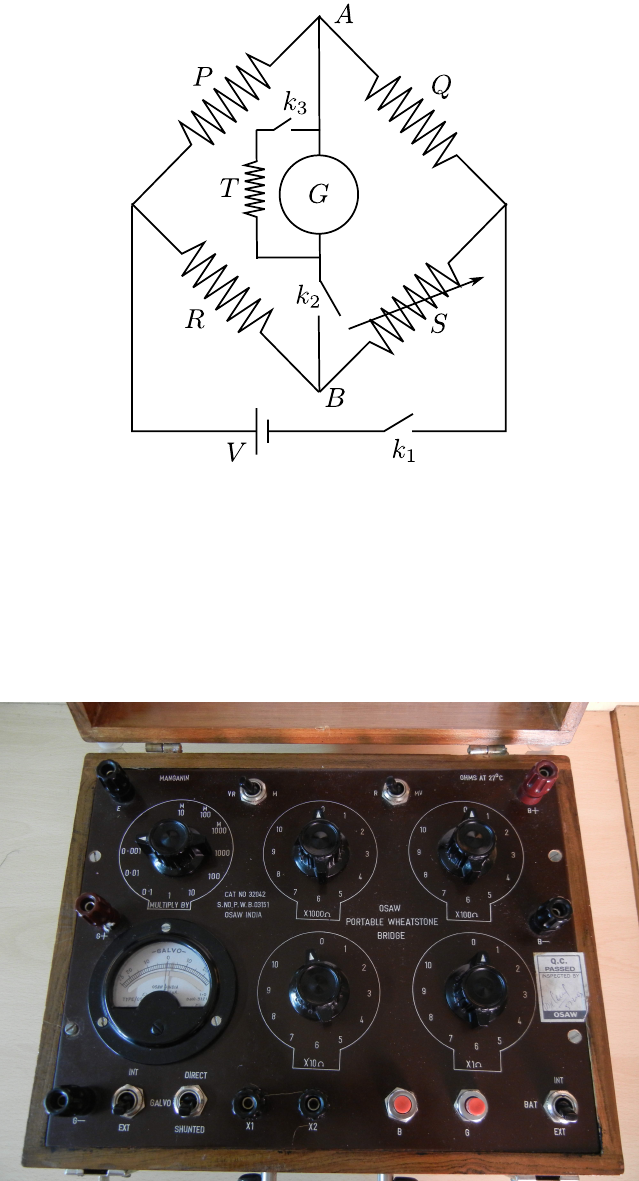
Figure 1.1: A wheatstone bridge.

Figure 1.2: A wheatstone bridge setup.

Experiment 2

Acceleration due to gravity by bar

pendulum

Purpose

To determine the value of acceleration due to gravity using angular oscillations of a long

bar.

Apparatus

Stop watch, long bar, meter scale, knife edge.

Theory

The purpose of this experiment is to use angular oscillations of rigid body in the form of a

long bar for determining the acceleration due to gravity. The particular form of the body

is chosen for the sake of simplicity in performing the experiment. The bar is hung from a

knife-edge through one of the many holes along the length. It is free to oscillate about the

knife-edge as axis. Any displacement θ, from the vertical position of equilibrium would

give rise to an oscillatory motion just as in the case of a simple pendulum. The diﬀerence

is that since this is rotating rigid body here we consider the torque of the gravitational

force giving rise to the angular acceleration.

The restoring torque τfor an angular displacement θis

τ=−Mgd sin θ(2.1)

where Mis the mass of the compound pendulum and dthe distance between the point of

suspension Oand the centre of mass of the bar C.

Since τis proportional to sin θ, rather than θ, the condition for simple angular harmonic

motion does not, in general, hold here. For small angular displacements, however, the

relation sin θ≈θis a good approximation, so that for small amplitudes in turn for small

values of θ.

τ=−Mgdθ =Id2θ

dt2(2.2)

where Iis the moment of inertia of the bar about the point of suspension O. The solution

of the above equation is given by

θ(t) = Asin(ωt +φ)(2.3)

where, ω =2π

T=sMgd

I(2.4)

is the angular velocity of the compound pendulum. Thus, the period of oscillation is given

T= 2πsI

Mgd (2.5)

Due to the parallel axis theorem we have

I=I0+Md2,(2.6)

where, I0is the moment of inertia of the pendulum about it’s center of gravity (C.G).

Inserting Eq. (2.6) in Eq. (2.5), we get the complete ddependence of the time period

Tas

T= 2πsI0+Md2

Mgd (2.7)

Since I0can be expressed as Mk2, where kis the radius of gyration, Eq. (2.7) can be

rewritten as

T= 2πsMk2+Md2

Mgd = 2πsk2+d2

gd .(2.8)

A simple pendulum consists of a mass mhanging at the end of a string of length L.

The time period of a simple pendulum is given by

T= 2πqL/g . (2.9)

So, the time period of a simple pendulum equals the time period of a compound pendulum

when

L=d2+k2

d(2.10)

Re-arranging the above equation

d2−Ld +k2= 0 (2.11)

gives us a quadratic equation in d. If d1and d2are the two solutions of the above equation,

then we ﬁnd

d1+d2=L(2.12)

d1d2=k(2.13)

Since both d1and d2are positive, we conclude that there are two point of suspensions

on one side of the C.G. of the compound pendulum where the time periods are equal.

Similarly, there are two points of suspension on the other side of the C.G where the time

periods are same. Thus, for a compound pendulum, there are four points of suspension,

two on either side of the C.G. where the time periods are equal. The simple equivalent

length Lis sum of two of these point of suspension located asymmetrically on two sides

of the C.G.

To facilitate further analysis it is useful to square Eq. (2.7) to get

T2= 4π2 I0+Md2

Mgd !(2.14)

In order to gain insight in the dependence of Ton dlet us ﬁrst look at the dependence

for (i) small dand (ii) large d. For small d(speciﬁcally for Md2I0) we have

T2∼4π2I0

Mgd (2.15)

T∼1

√d.(2.16)

Thus Tdecreases as dincreases. In the opposite limit i.e. for large d(speciﬁcally for

Md2I0) we have

T2∼4π2Md2

Mgd (2.17)

T∼√d(2.18)

Thus Tincreases as dincreases in this case. Physically the origins of d2in the numerator

is coming from the expression for the moment of inertia I∼d2.

It is then just a question of which eﬀect dominates for a given values of d. To under-

stand this better (or more quantitatively) let us looks at the turning point. The minimum

of the expression for T2as a function of dcan be determined by taking the taking deriva-

tive of T2with respect to dand setting it equal to zero (and ensuring the sign of the

second derivative term corresponds to a minimum). Following this procedure gives

d=sI0

M(2.19)

Eq. (2.19) can be written as I0=Md2. This relation is satisﬁed at the minimum or at

the turning point. Using this in Eq. (2.7) we ﬁnd that the turning point occurs when

the magnitude of the two terms of the numerator are equal. For M d2I0the I0

term dominates in the numerator and ddependence is given by the denominator. In the

region Md2I0the Md2term dominates in the numerator and so the ddependence is

dominated by the numerator.

History of the experiment

Galileo was the ﬁrst person to show that at any given place, all bodies fall freely when

dropped, with the same (uniform) acceleration, if the resistance due to air is negligible.

The gravitational attraction of a body towards the center of the earth results in the same

acceleration for all bodies at a particular location, irrespective of their mass, shape or

material, and this acceleration is called the acceleration due to gravity, g. The value of

gvaries from place to place, being greatest at the poles and the least at the equator.

However, direct measurement of the acceleration due to gravity is very diﬃcult.

Therefore, the acceleration due to gravity is often determined by indirect methods, for

example, using a simple pendulum or a compound pendulum. If we determine gusing

a simple pendulum, the result is not very accurate because an ideal simple pendulum

cannot be realized under laboratory conditions. Hence, a compound pendulum is used to

determine the acceleration due to gravity in the laboratory.

Procedure

•Balance the bar on sharp wedge and mark the position of its center of gravity (C.G.).

•Ensure that the frame on which movable knife edge / pivot is to be rested is hori-

zontal.

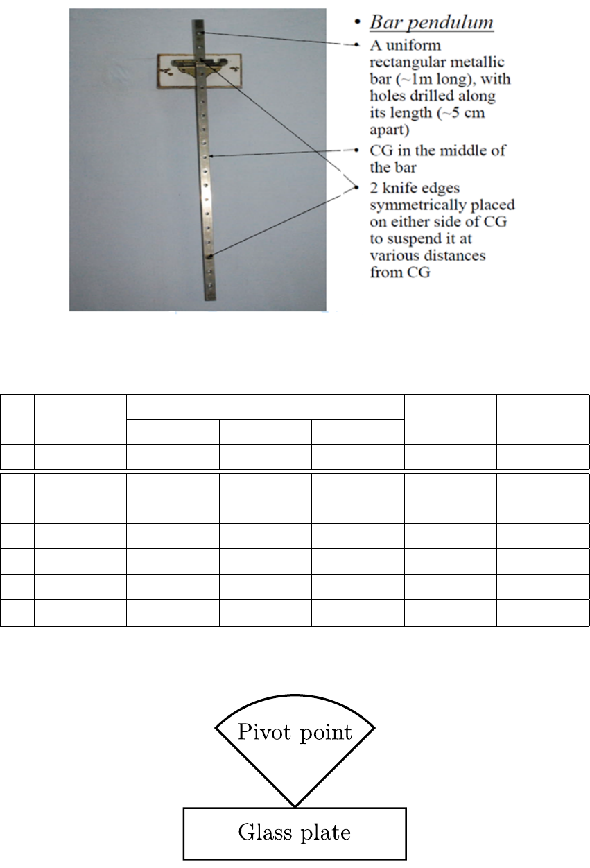
Figure 2.1: Image of a bar pendulum

Sl. dNo. of oscillations Mean T10 T

1 2 3

– (cm) (sec) (sec) (sec) (sec) (sec)

Table 2.1: Table to measure acceleration due to gravity via a compound pendulum.

Figure 2.2: Pivot or knife edge of the bar pendulum

•Suspend the pendulum in the ﬁrst hole. The knife edge or pivot should be placed

on the glass plate as shown in Fig. 2.2.

•The distance dis the distance between point of suspension (bottom of the hole) and

the C.G.

•Start the oscillation of the pendulum.

•Use the stop watch to measure the time for 10 oscillations. The time should be

measured after the pendulum has had a few oscillations and the oscillations have

become regular.

•Repeat the process by suspending the pendulum in the consecutive holes.

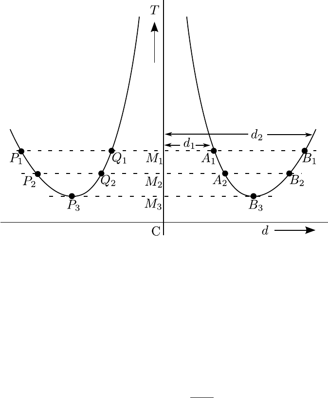
•Draw a graph by taking distance along X-axis and time period along Y-axis as

shown in Fig. 2.3. Shift the axes to draw a full page graph.

Figure 2.3: Plot of time vs distance from center of gravity of bar

Calculation

1. With the help of the graph, distance d1and d2can be measured from which the

value of gcan be calculated by using formulas

d1+d2=L(2.20)

g=4π2L

T2(2.21)

where d1and d2the distances M1A1,M1B1respectively and Tis the time CM1as

shown in Fig. 2.3. As there are two branches one could take the mean of Q1M1

and M1A1for the distance d1and mean of P1M1and M1B1for the distance d2for

substitution in this formula.

2. Choose another line P2B2and ﬁnd g2using Eqns. (2.20) and (2.21), where d1is the

mean of Q2M2and M2A2,d2is the mean of P2M2and M2B2and T=CM2.

3. At the minima, ensure that P3M3is equal to M3B3. Then calculate g3via the

formula

g= 4π2P3B3

CM2

(2.22)

4. Find the average value of g.

Theoretical error

Acceleration due to gravity (g)is given by the formula

g=4π2L

T2(2.23)

Taking log and diﬀerentiating ∂g

g=∂L

L+ 2∂T

T(2.24)

Thus, maximum possible error = ................%.

Results

•The standard value of g=..............m/sec2.

•Percentage error = ...............%.

Precaution

1. The Knife edge is made horizontal. If it is not perfectly horizontal the bar may be

twisted while swinging.

2. The motion of a bar should be strictly in a vertical plane.

3. The amplitude of the swing should be small.

4. The time period of oscillations should be determined by measuring time by large

number of oscillations with an accurate stop watch.

5. All distances should be measured and plotted from one end of the rod.

Experiment 3

e/m of electron by Thomson

Method

Purpose

Determining the value of speciﬁc charge e/m of an electron by Thomson Method

Apparatus

Deﬂection magnetometer, two bar magnets, cathode ray oscilloscope, stand arrangement.

Theory

In this method, a cathode ray tube is used in which the cathode emits electrons and the

anode accelerates them and passes them through a small hole, to another anode which

concentrates them into a ﬁne beam. Then they are passed between two parallel plates,

which can deﬂect the beam in a vertical plane by an electric ﬁeld Eapplied between both

the plates. The beam of electrons can also be deﬂected in the same plane by applying a

magnetic ﬁeld Bperpendicular to the plane of plates. This narrowed collimated beam of

accelerated electrons then strikes the ﬂuorescent screen to produce a glowing spot. Three

terms arise as follows:

1. If an electric ﬁeld Eis applied by a potential diﬀerence of Vvolts between the plates,

the electrons experience a force Fein a direction perpendicular to the direction of

motion of the beam.

Fe=Ee (3.1)

2. If Bis the uniform magnetic ﬁeld applied in an horizontal direction perpendicular

to the direction of the electron beam, the magnetic force Fmag experienced by the

electrons is

Fmag =e|~v ×~

B|=Bev sin 90◦=Bev (3.2)

where eis the electron charge and vis the velocity of the electrons. This force

Fmag acts perpendicular to the direction of Bas well as in the original direction

of electron motion (in accordance with Fleming’s left rule for electric motor). The

speed of electrons remains unchanged, but their path becomes circular, providing

the centripetal force

Fmag =Bev =mv2/r (3.3)

where mis the mass of an electron and ris the radius of the circular path. Thus

e/m =v/Br (3.4)

3. If an electric ﬁeld Eis applied to deﬂect the beam in OO0direction (see Fig. 3.1),

then a magnetic ﬁeld Bis applied to bring beam back to O. It means that the force of

the electrostatic ﬁeld is equal and opposite to applied magnetic ﬁeld, so Fe=Fmag,

and two forces null each other to bring the beam back to its original position. Thus

Ee =Bev

or, v=E/B (3.5)

Substituting value of vfrom Eq.3.5 into Eq. 3.4,

m=E

B2r(3.6)

According to Fig.3.1, the original electron beam proceeds on the straight path G, M,

O and impresses upon the screen at a point O. In the presence of magnetic ﬁeld, the beam

travels along a circular arc G, D whose radius is r. Beyond point D, the beam leaves the

magnetic ﬁeld and proceeds straight in the direction along the tangent KDO0(drawn on

the circular arc at point D). GN is normal to GKO and MDN is normal to KDO0. Let

these normals meet at point N. Then GN =ND =r=the radius of the circular arc. Let

the angles GND =OKO0=θ. Then in the triangle KOO0,

tan θ=OO0/KO (3.7)

and if the angle θis small enough,

θ= tan θ=y/L (3.8)

where Lis distance of the screen from the mid point of the magnetic ﬁeld region (generally

mid point of electric ﬁeld too). Again,

θ= tan θ= arc GD/r = GM/r, (3.9)

since GD is nearly equal to GM, or

θ=l/r (3.10)

where lis the length of the region of magnetic ﬁeld, equal to the region of electric ﬁeld.

By comparing both values of θ

l/r =y/L . (3.11)

r=lL/y (3.12)

Substituting the value of rinto Eq.3.6,

m=Ey

B2lL (3.13)

If a potential diﬀerence of Vvolts is applied between the plates P-P, and dis the gap

between both plates, then the electric ﬁeld is given by E=V/d. Therefore,

m=V y

B2lLd (3.14)

where yis the distance between spot positions displayed on the screen of CRT in centime-

ters, lis the length of the deﬂection plates, Lis the distance between screen and plates, d

is the distance between plates, Vis applied DC voltage across plates and Bis magnetic

ﬁeld strength determined by B=Htan θ, where His the horizontal component of earth’s

magnetic ﬁeld at that place.

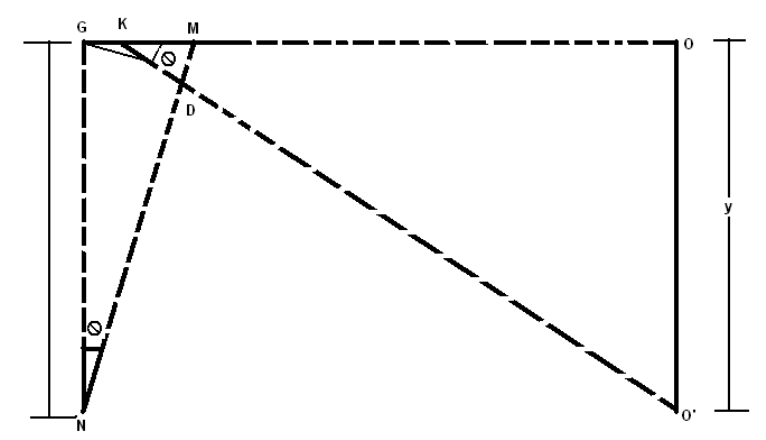
Figure 3.1: Electron beam diagram in magnetic ﬁeld

Procedure

1. Using compass needle, ﬁnd and note North-South and East-West directions. Place

CRT in between the stand in such a way that its screen is faced towards North and

both arms stand to East-West direction.

2. Adjust the Intensity and Focus potentiometer to its mid position.

3. Connect the CRT to octal socket of instrument (socket provided upon the panel).

Care should be taken while inserting CRT plug.

4. Keep instrument to south direction far from CRT.

5. Select polarity selector switch at ‘0’ position.

6. Set the deﬂection voltage potentiometer at anti-clockwise direction.

7. Switch on the power supply and wait for some time (3-5 minutes) to warm up the

CRT. A bright spot appears on the screen.

8. Adjust intensity and focus controls to obtain a sharp spot.

9. Bring the spot at the middle position of the CRT with the help of X-plate deﬂection

voltage pot given at the back-side of the instrument.

10. Set polarity selector to ‘+’ position, and adjust deﬂection voltage to deﬂect the spot

1 cm away towards upward. Note the deﬂection voltage from the meter as V1and

spot deﬂection as y.

11. Now place the bar magnets (on the stand arm) to both sides of CRT such that their

opposite poles face each other.

12. Adjust position of magnets to get spot back downward to original position.

13. Note the distances of bar magnet (poles facing the screen) as r1and r2from the

scale.

14. Now remove magnets from the arms of stand.

15. Select ‘−’ position of polarity switch. Apply DC voltage to deﬂect the spot 1 cm away

in downward direction. Note deﬂection voltage from display as V2and deﬂection as

16. Place bar magnets again and adjust the position of magnets to bring spot back to

original position. Note the distance of the magnets (poles facing the screen) as r0

and r0

17. Remove CRT and magnets. Place magnetometer arrangement in between the stand

such that its centre lies on the center of the stand arm.

Note: Position of stand should not be disturbed.

18. Rotate magnetometer and adjust the needle to read 0o−0o.

19. Now place magnets at a distance equal to r1and r2as previous polarity adjusted.

The pointer deﬂects along the scale. Note the deﬂections as θ1and θ2.

20. Repeat similar procedure placing magnets at r0

1and r0

2distances. Note the deﬂection

of compass needle as θ3and θ4.

21. Now we know that magnetic ﬁeld

B=Htan θ , (3.15)

where, θ=θ1+θ2+θ3+θ4

4(3.16)

and, H= 0.37 ×10−4Tesla (3.17)

22. Calculate e/m using the following formula

m=V y

B2lLd (3.18)

where, d=distance between plates = 1.4cm

l=length of plates = 3.23 cm

L=distance between screen and plates = 14.5cm

V=deﬂection voltage = (V1+V2)/2

y=deﬂection in cm = 1 cm

23. Take more readings by repeating the experiment and deﬂecting spot to other dis-

tances.

24. Calculate the percentage error as

(Standard value - Calculated value)/Standard value ×100 (3.19)

Note: While performing the experiment, keep other electronics equipment away from

the e/m setup.

Precautions and sources of error

•The cathode ray tube should be handled carefully. There should not be any magnetic

substance nearby the place of experiment.

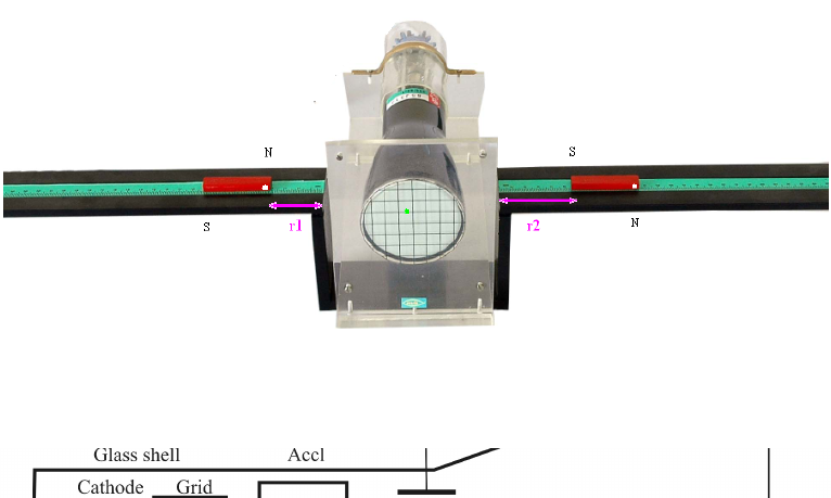
Figure 3.2: Set-up of Thomson Method experiment

Figure 3.3: Cathode ray tube used in Thomson Method

•Axis of magnets and axis of tube should lie perpendicular to each other in same

horizontal plane. To correct it, loosen the neck clamp of CRT and rotate CRT so

the spot deﬂects right up/down with deﬂection voltage.

•When magnets are placed upon the arms, it is better to move stand slightly back

and forth to obtain maximum magnetic ﬁeld at deﬂecting plates. It should be done

before bringing spot back to original position.

•Rotate magnet(s) on their axes if spot does not come back to its original position.

•When direction of spot is reversed the direction of magnets should also be reversed.

•The magnets should move tight to the scale in closest possible distances.

•The electric ﬁeld between plates cannot be uniform due to short distance between

them.

•The given constants are generally taken from data; there may be slight variations to

produce error.

Results

Standard Value of e/m: . . . . . . . . . C/Kg

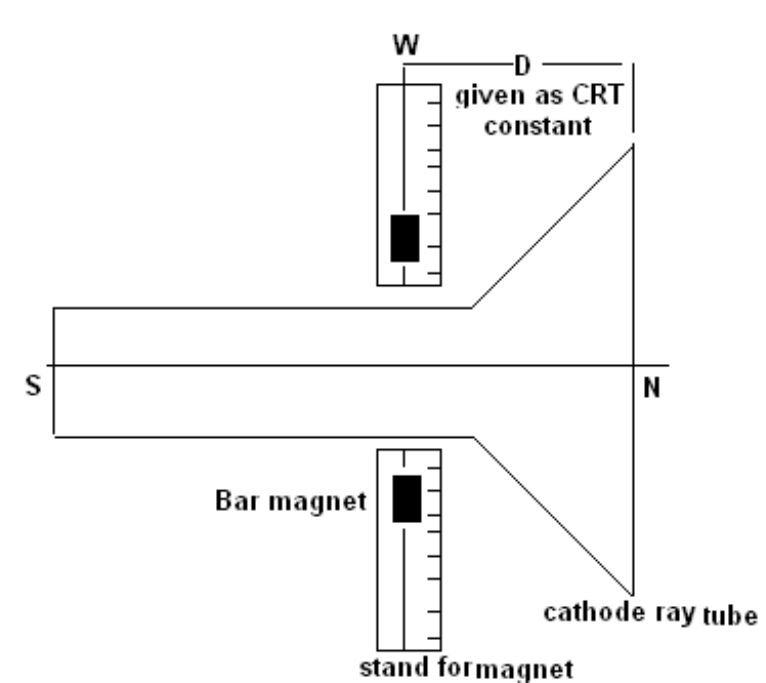
Figure 3.4: Way to place cathode ray tube

Experiment 4

Measurement of band gap of

semiconductor

Purpose

•Measurement of resistivity of a semiconductor at room temperature

•Measurement of variation of resistivity with temperature.

•Evaluation of band gap of the given semiconductor from the plotting of acquired

data.

•Understanding of the concept of four probe method.

Apparatus

Four probe experimental setup.

Theory

Semiconductor

Semiconductor is a very important class of materials because of wide applications in this

modern world. The following are the properties which gives a rough description of a

semiconductor.

1. The electrical conductivity of a semiconductor is generally intermediate in magnitude

between that of a conductor and an insulator. That means conductivity is roughly

in the range of 103to 10−8siemens per centimeter.

2. The electrical conductivity of a semiconductor varies widely with doping concentra-

tion, temperature and carrier injection.

3. Semiconductors have two types of charge carriers, electrons and holes.

4. Unlike metals, the number of charge carriers in semiconductors largely varies with

temperature.

5. Generally, in case of semiconductor, increase of temperature enhances conductivity

while in case of metals increase of temperature reduces conductivity.

6. The semiconductor can be best understood in the light of energy band model of

solid.

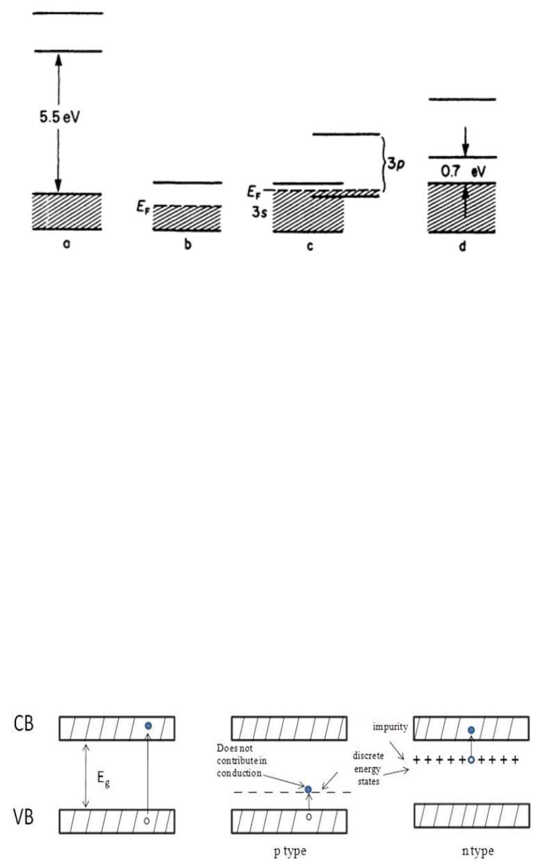
Figure 4.1: Band gaps shown for (a) Insulator (b) Alkali Metal (c) Other Metal (d) Ge-

semiconductor

Energy band structure of solid

Atom has discrete energy levels. When atoms are arranged in a periodic arrangement in

a solid the relatively outer shell electrons no longer remain in a speciﬁc discrete energy

level. Rather they form a continuous energy level, called energy band. In case of semicon-

ductor and insulator, at temperature 0Kall the energy levels up to a certain energy band,

called valence band, are completely ﬁlled with electrons, while next upper band (called

conduction band) remains completely empty. The gap between bottom of the conduction

band and top of the valence band is called fundamental energy band gap (Eg), which is

a forbidden gap for electronic energy states. In case of metals, valence band is either

partially occupied by electrons or valence band has an overlap with conduction band, as

shown in Fig. 4.1(b and c).

In case of semiconductor, the band gap (∼0−4eV ) is such that electrons can move

from valence band to conduction band by absorbing thermal energy. When electron moves

from valence band (VB) to conduction band (CB), it leaves behind a vacant state in

valence band, called hole. When electric ﬁeld is applied, movement of large number of

electrons in the valence band can be visualized by the movement of hole as a positive

charge particle. The Egis a very important characteristic property of semiconductor which

dictates it’s electrical, optical and optoelectrical properties. There are two main types of

Figure 4.2: Energy band diagram of a semiconductor

semiconductor materials: intrinsic and extrinsic. Intrinsic semiconductor doesn’t contain

impurity. Extrinsic semiconductors are doped with impurities. These discrete impurity

energy levels lie in the forbidden gap. In p-type semiconductor, acceptor impurity, which

can accept an electron, lies close to the valence band and in n-type semiconductor, donor

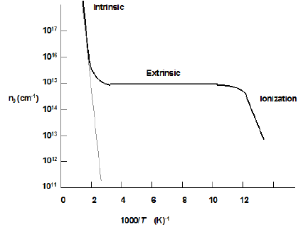
Figure 4.3: Temperature variation of carrier concentration

impurity, which can donate an electron lies close to conduction band.

Temperature variation of carrier concentration

Fig. 4.3 shows the variation of carrier concentration (concentration of holes) in a p-

type semiconductor with respect to 1000/T , where Tis the temperature. Initially as

temperature increases from 0K(i.e. ionization region), the discrete impurity vacant states

starts getting ﬁlled up from valence band, which creates holes in valence band. Beyond a

certain temperature all the impurity states will be ﬁlled up with electrons, which lead to

the saturation region.

As temperature increases to further higher values, electrons, in the valence band, get

suﬃcient energy to occupy empty states of conduction band (C.B). This region is called

intrinsic region. The temperature above which the semiconductor behaves like intrinsic

semiconductor is called “Intrinsic temperature”.

Conductivity of a semiconductor

The conductivity of a semiconductor is given by

σ=e(µnn+µpp)(4.1)

Where µnand µprefer to the mobilities of the electrons and holes, and nand prefer to

the density of electrons and holes, respectively. The mobility is drift velocity per electric

ﬁeld applied across the material, µ=Vd/E. Mobility of a charge carrier can get aﬀected

by diﬀerent scattering processes.

Eﬀects of temperature on conductivity of a semiconductor

In the semiconductor, both mobility and carrier concentration are temperature dependent.

So conductivity as a function of temperature can be expressed by

σ=e(µn(T)n(T) + µp(T)p(T)) (4.2)

One interesting special case is when temperature is above intrinsic temperature where mo-

bility is dominated by only lattice scattering (∝T−3/2). That means in this temperature

region mobility decreases with increase of temperature as T−3/2due to increase of thermal

vibration of atoms in a solid.

In the intrinsic region, n≈p≈ni, where niis the intrinsic carrier concentration. The

intrinsic carrier concentration is given by

ni(T) = 2 2πkT

h23/2

(m∗

nm∗

p)3/4exp −Eg

2kT ,(4.3)

where, m∗

nand m∗

pare eﬀective mass of electron and hole. Here the exponential temper-

ature dependence dominates ni(T). The conductivity can easily be shown to vary with

temperature as

σ∝exp −Eg

2kT .(4.4)

In this case, conductivity depends only on the semiconductor band gap and the tempera-

ture. In this temperature range, plot of ln σvs 1000/T is a straight line. From the slope

of the straight line, the band gap (Eg)can be determined. The procedure of measurement

of conductivity is given below.

Four probe technique

Four probe technique is generally used for the measurement of resistivity of semiconduc-

tor sample. Before we introduce four probe technique, it is important to know two probe

techniques by which you measured resistivity of a nicrome wire. In two probe technique,

two probes (wires) are connected to a sample to supply constant current and measure

voltage. In the case of nicrome wire (1st experiment), connections are made by pressing

the multimeter probes on nichrome wire. The contact between metal to metal probe of

multimeter does not create appreciable contact resistance. But in the case of semiconduc-

tor the metal – semiconductor contact gives rise to high contact resistance. If two probe

conﬁguration is followed for semiconductor sample, voltmeter measures the potential drop

across the resistance of the sample as well as the contact resistance. This is shown in the

Fig. 4.4(a).

The potential drop across high contact resistance can be avoided by using four probe

technique. In the four probe conﬁguration, two outer probes are used to supply current

and two inner probes are used to measure potential diﬀerence. When a digital voltmeter

with very high impedance is connected to the inner two probes, almost no current goes

through the voltmeter. So, the potential drop it measures, is only the potential drop

across the sample resistance. This is shown in the equivalent circuit diagram given in

Fig. 4.4(b). From the measurement of current supplied and voltage drop across the sample,

the resistance can be found out. Resistivity of a sample is given by ρ=cV/I, where cis

a constant.

For the speciﬁc arrangement, where the probes are equispaced with the distance be-

tween two successive probes as a, and the thickness of the sample is h, the resistivity can

be calculated by the following formulas.

Case I: ha. In this case it is assumed that the four probes are far from the edge of the

sample and the sample is placed on an insulating material to avoid leakage current.

The resistivity in this case is given by

ρ= 2πaV

I(4.5)

This is the setup used for our experiment.

Case II: ha. In this case the resistivity is given by

ρ=πh

ln 2 V

I(4.6)

Derivation for this is given at the end.

Figure 4.4: (a) Equivalent circuit for two probe measurement. R1, R2are the contact

resistances (b) Equivalent circuit for four probe measurement. R1, R2and R3, R4are the

contact resistances of current and voltage probes.

Once resistivity (ρ)is determined, conductivity (σ)can be calculated by taking recip-

rocal of it (σ= 1/ρ).

Advantages of using four probe method

•The key advantage of four-terminal sensing is that the separation of current and

voltage electrodes eliminates the impedance contribution of the wiring and contact

resistances.

•If the probes are separated by equal distance a, and ahthen resistivity can be

found out without knowing the exact shape and size of the sample.

Figure 4.5: Pictorial representations of ﬁeld lines generated by the applied potential.

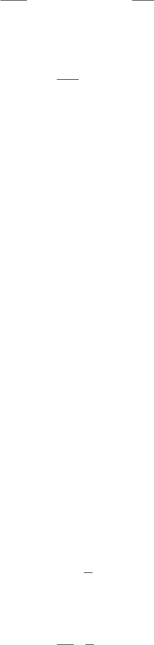
Description of the experimental set-up

Probes arrangement It has four individually spring loaded probes. The probes are

collinear and equally spaced. The probes are mounted in a teﬂon bush, which ensure

a good electrical insulation between the probes. A teﬂon spacer near the tips is also

provided to keep the probes at equal distance. The whole arrangement is mounted

on a suitable stand and leads are provided for the voltage measurement.

Sample Germanium crystal in the form of a chip.

Oven It is a small oven for the variation of temperature of the crystal from the room

temperature to about 200oC(max).

Figure 4.6: Four probe experimental setup.

Procedure

•Switch ON the band gap setup.

•Supply current to the crystal and keep it constant (3mA) throughout the experiment.

•Initially the temperature of the oven must be at room temperature (∼27oC).

•Switch on the oven to start increasing the temperature.

•Note the voltage and temperature at intervals of 5oCstarting from room tempera-

ture.

•When temperature reaches 140oCswitch oﬀ the oven and note the voltage and

temperature for decreasing temperature till it reaches room temperature.

•Find the mean of the two voltages, for increasing and decreasing temperatures.

Calculate ρfor each temperature.

•Convert the temperature scale from 0Cto the Kelvin scale (K). The plot of ln σvs

1/T should be a straight line. Calculate the slope (m) of the straight line and ﬁnally

the band gap Egfrom the given formula

σ=σoexp −Eg

2KT (4.7)

Observations

Sl. Temp (T) 1000/T I during inc.

temp.

Inc. volt. Inc. V/I ρ σ = 1/ρ ln σ

(oC)(K−1) (I) (mA) (V) (mV) (Ω) (Ωm) (S m−1)−−

Results

Experiment 5

Refractive index of glass with the

help of a prism

Purpose

•To understand the accurate leveling and focusing of a spectrometer.

•Investigation of the variation in the refractive index, µof a prism with wavelength

λ.

Apparatus

Spectrometer, prism, mercury light source, high voltage power supply, magnifying lens,

spirit level, torch light etc.

Theory

The fact that a prism is capable of dispersing light is due to the variation of its refractive

index with wavelength. In this experiment the refractive index is obtained for a variety of

wavelengths by measuring the minimum deviation angle of the prism for each wavelength.

To understand what is meant by the term angle of minimum deviation, consider Fig.

5.1. The incident parallel light beam is refracted by the prism in such a way that it is

deviated by the angle θdfrom the undeviated direction. The angle is known as the angle

of deviation and varies with both the wavelength and the angle at which the incident light

intersects the prism.

If the prism is rotated about the axis it is found that the angle of deviation changes but

never becomes less than a certain minimum value, δmin known as the angle of minimum

deviation i.e. no matter what the orientation of the prism, as long as it is in the path of the

incident light beam, the light beam will be deviated through at least this angle. When the

prism is oriented in such a way that the exit beam is deviated through the least possible

angle δmin, then further rotation of the prism in either direction will cause the exit beam

to move further away from the least deviated direction. Thus for each wavelength in a

spectral light source, there is a variation of the angle of deviation, θdwith the angle of

incidence, θiand at some value of the angle of incidence, the angle of deviation reaches a

minimum as seen in Fig. (5.3).

Relation between µand λ

The refractive index of the prism material, µis a function of the angle of minimum

deviation (δmin), the incident wavelength (λ)and the prism refracting angle (A). Thus,

Figure 5.1: Deviation of monochromatic

light ray due to prism.

Figure 5.2: Spectrum due to a prism.

Figure 5.3: Variation of the angle of deviation (θd)with the angle of incidence (θi)for a

particular wavelength.

by measuring δmin for a variety of wavelengths, the variation of µwith wavelength may

be determined.

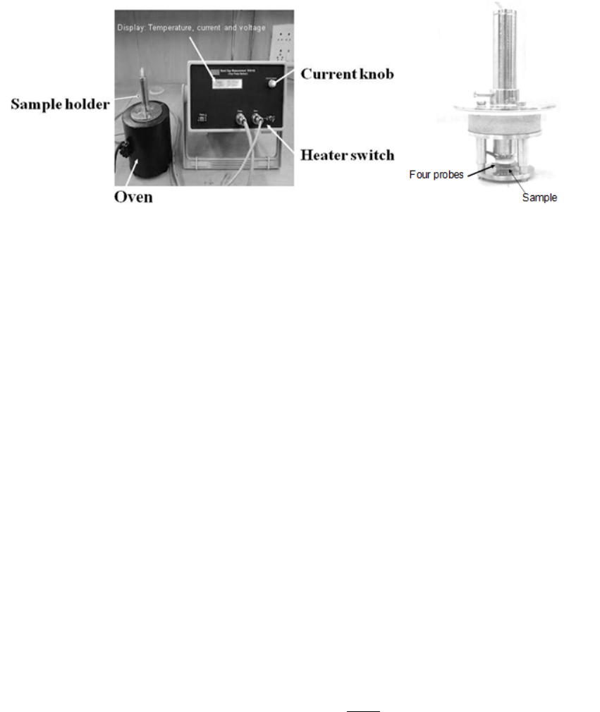
To derive the exact relationship, consider the prism as seen in Fig. (5.4). It can be

shown that the minimum value of the angle of deviation, δmin occurs when the ray passes

through the prism symmetrically i.e. when the angle at which the light emerges is equal

to the angle of incidence such that the ray passes parallel to the base of the prism as in

Fig. (5.4). At each face the ray changes direction by θi−θrand so the total minimum

deviation is

δmin = 2(θi−θr)(5.1)

From Fig. 5.4, it is shown that the angle 6MNO is the same as that of the refracting

angle of the prism. Referring to the triangle LMN it is obvious, using trigonometry, that

A= 2θr. Snell’s Law is of course µ= sin θi/sin θrbut θi=δmin/2 + θr, where θr=A/2

and hence we have

µ=sin ((A+δmin)/2)

sin(A/2) .(5.2)

An empirical equation of the form

µ=a+b

λ2+c

λ4(5.3)

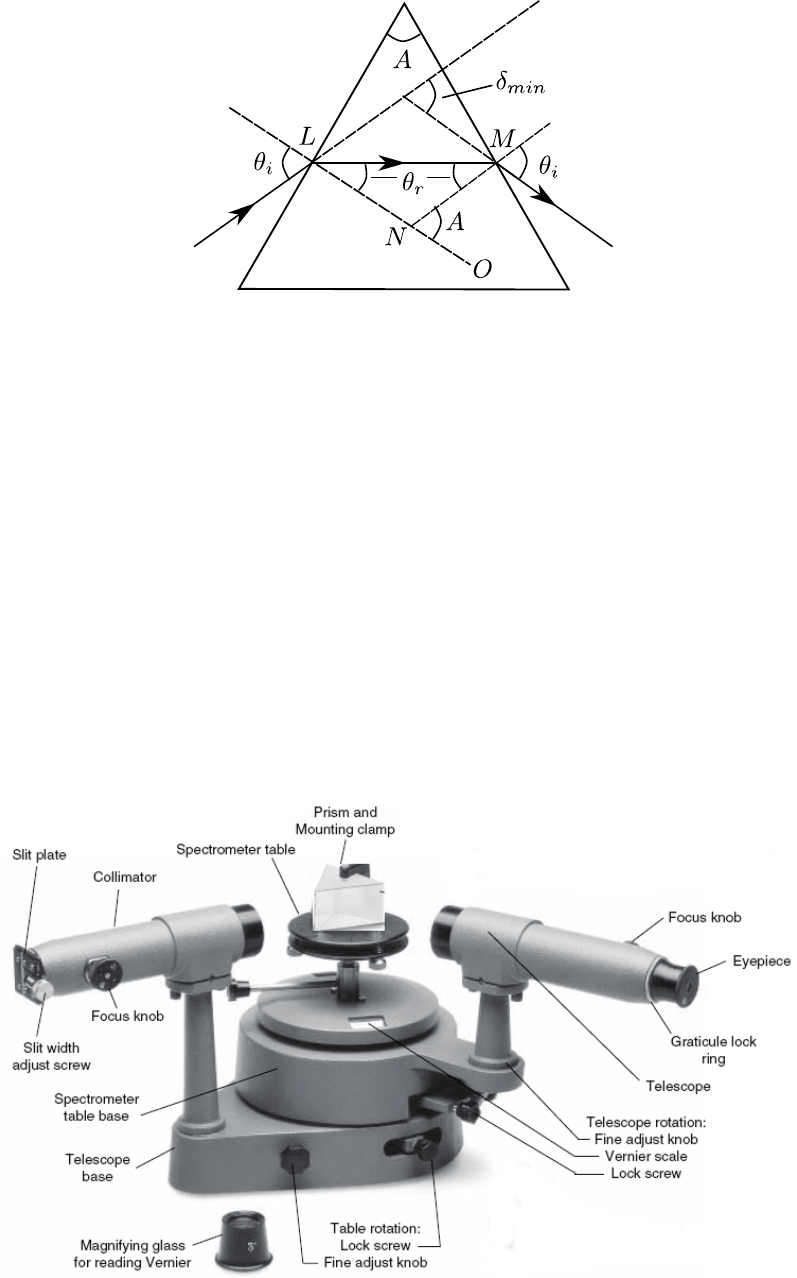
Figure 5.4: Condition for minimum deviation

was developed by Cauchy to describe the variation of µwith wavelength. Where a, b and

care constants and it is the purpose of this experiment to verify this equation (neglecting

terms of higher order than the second) and to derive the constants aand bfor the prism

material.

Note: As the variation in refractive index over the whole of the visible is only of

the order of 3% this means that δmin varies only very slowly with wavelength. Both a

fair degree of experimental skill and great care in making the various measurements are

necessary if reasonable results are to be attained.

Experimental procedure

Initially make sure you understand what each component of the spectrometer as detailed in

Fig. (5.5) does. The experimental setup consists of following parts. To obtain satisfactory

The Prism Spectrometer Page 4 of 8

Figure 4: Schematic diagram of the prism spectrometer.

In this experiment, we will use a prism spectrometer to measure the deviations of light

for various wavelength. The spectrometer is an instrument for studying optical spectra. A

schematic diagram of a prism spectrometer is shown in Figure 4. It consists of a collimator, a

telescope, a prism and a circular spectrometer table. The collimator holds an aperture at one

end that limits the light coming from the source to a narrow rectangular slit. A lens at the

other end focuses the image of the slit onto the face of the prism. The telescope magniﬁes the

light exiting the prism and focusses it onto the eyepiece. The prism, of course, disperses the

incident light into its constituent wavelengths. The vernier scale allows the angles at which

the collimator and telescope are located to be read oﬀ.

Physics Level 1 Laboratory Department of Physics

National University of Singapore

Figure 5.5: Spectrometer with its components

results the spectroscope requires some initial adjustments before the desired measure-

ments can be performed. For this experiment great care must be taken in adjusting the

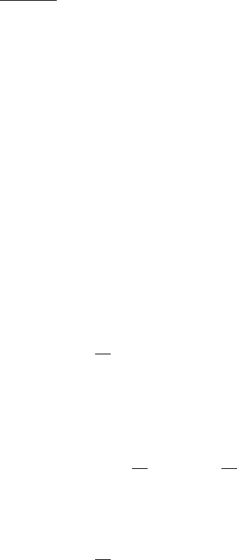
spectrometer so that the telescope is focused at inﬁnity and the collimator set to give an

accurately parallel beam. It is particularly important to ensure that the cross-hairs of the

telescope are sharply visible and that no parallax exists between them and the spectral

line images. The following steps should ensure this:

1. Focusing the telescope: Focus the telescope for the parallel rays from the distance

object by sliding the eyepiece looking through telescope in and out, until a sharp

image of object is seen. Due to the location of the laboratory this may not be possible

so the building opposite may be used for this purpose.

2. Levelling the collimator: Place the spirit level on the collimator tube with its axis

parallel to the axis of the tube. If the the bubble in the collimator is found to

be displaced from its central position, turn the levelling screws provided with the

collimator tube, in the same direction to bring the bubble back to its central position.

This make the axis of the collimator tube horizontal.

3. Levelling of the prism table: There are three levelling screws A, B, C just below

the prism table for levelling the table. There are parallel lines drawn on the prism

table parallel to the line joining the screws B and C. Place the spirit level parallel

to these lines and bring the bubble to the central position by turning the screws B

and C equally in opposite directions. Now place the spirit level perpendicular to the

line BC. If the bubble is not in the central position, then turn the A screw alone to

bring the bubble in the center. Continue this for a couple of times until the bubble

is in the center in both the positions. This makes the table vertical to the axis of

rotation.

4. Focusing the collimator: Place a discharge lamp (Mercury lamp as a visible light

source) in front of the spectroscope and turn the telescope until it is in line with and

pointing directly at the collimator. Looking through the telescope and adjusting the

position of the focusing screw on the collimeter until a sharp image of the slit is

observed in the telescope. The collimeter now gives parallel rays which will fall on

the prism.

Finding the least count for the spectrometer

It should be noted by the student that 30 vernier scale divisions (VSD) coincides with 29

circular scale divisions (CSD). So,

30 VSD = 29 CSD (5.4)

1VSD =29

30 CSD (5.5)

Therefore, the least count

LC = 1 CSD −1VSD (5.6)

=1−29

30CSD =1

30 CSD (5.7)

Since 1 CSD = (1/2)◦=300, we have

LC =1

30 ×300= 10(5.8)

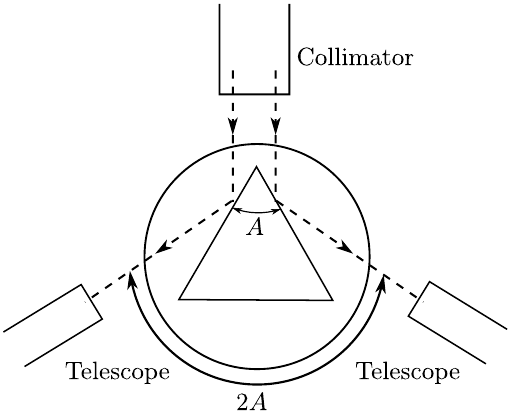
Figure 5.6: Measurement of the reﬂecting angle of prism.

Measurement of the angle of prism (A)

•Set up the prism and spectrometer as in Fig. (5.6). Lock the prism table.

•Place the telescope cross-hairs in turn on the image of the slit reﬂected from surface

AB and then surface AC.

•At each position record the angular position of the telescope on the vernier scale-

the angle between the two positions of the telescope is 2A, twice the apex angle of

the prism and hence Acan be found.

•Repeat above step 2 and 3 to get an average value for A(≈60o).

Viewing the spectrum due to refraction

The telescope and prism are rotated until the spectrum formed by refraction is found.

The approximate prism position is shown in Fig. 5.7.

Further rotation of the prism while viewing the spectrum through the telescope will

result in reaching the angle of minimum deviation. This is where the spectral lines “turn

back" on themselves i.e. move opposite to their initial direction of travel while the prism

is still being rotated in the same direction.

Position the prism and telescope so that the spectral lines are at the angle of minimum

deviation i.e. at the point where the spectral lines “turn back" on themselves.

Turning the prism towards the telescope, increases the angle of incidence, thus moving

to the right hand side of δmin in the curve of Fig. (5.3). Conversely turning the prism

towards the collimator, decreases the angle of incidence, hence moving through the angle

of minimum deviation to the left hand side of the curve of Fig. 5.3.

Measurement of the angle of minimum deviation, δmin for each wavelength

1. Using the Hg spectral lamp, observe the ﬁrst order ﬁeld of view of refracted spec-

trum. Find the point of minimum deviation for the Hg spectrum. The approximate

prism position is as shown in Fig. 5.7.

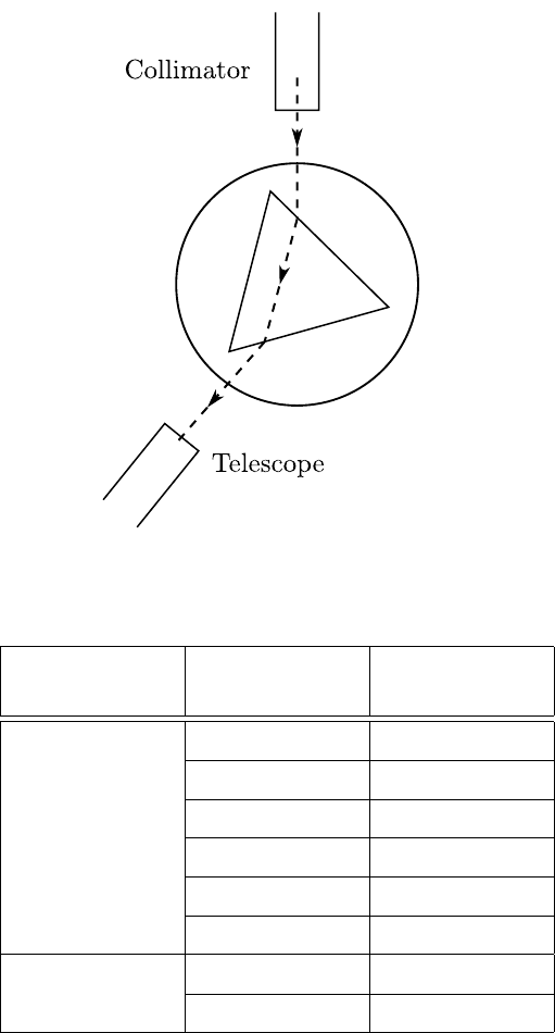
Figure 5.7: Prism position for viewing the spectrum due to refraction.

Lamp Colour Wavelength

(nm)

Mercury

Violet 380 -450

Blue 450 -495

Green 495 -570

Yellow 570 -590

Orange 590 -620

Red 620 -750

Sodium Yellow (D1)589.6

Yellow (D2)589.0

Table 5.1: Discharge lamp wavelengths

(Remember minimum deviation corresponds to the point at which movement of the

lines of the Hg spectrum over the ﬁeld of view of the telescope is reversed, although

direction of rotation of the telescope continues in the same sense.)

2. Several spectral lines should be in the ﬁeld of view of the telescope. Position the

telescope on the highest wavelength spectral line and lock the prism table and tele-

scope. It is essential that the prism and prism table remain in this position for the

remainder of the experiment.

3. Using the telescope ﬁne adjustment screw, position the crosshairs of the telescope

accurately on the spectral line of interest and read the vernier to the nearest minute

of arc.

4. The above step can be repeated for the other lines in the ﬁeld of view of the telescope

there should be enough movement in the telescope ﬁne adjustment screw to allow

positioning of the cross-hairs on all of the Hg spectral lines of Table 5.1 without

unlocking the telescope again. If this is not the case, just unlock the telescope

and reposition it such that the crosshairs of the eyepiece are on the spectral line of

interest. It is imperative that the prism and prism table remain in their original

ﬁxed position.

5. Rotate the telescope anticlockwise until the undeviated image of the slit through the

prism is in the ﬁeld of view. Again position the crosshairs on the centre of the clit

image and record the angular reading of the telescope on the vernier scale.

6. The actual value for δmin for each wavelength is the diﬀerence between the appro-

priate angular reading of the telescope position for minimum deviation and for the

undeviated (straight through) position as seen in Fig. (5.1)

Observation

Measurement of angle of prism (A)

Least count of the spectrometer (l.c.) = ..............

Sl. Position I Position II 2A=

θ1−θ2Prism

CSR VSR Total

reading

(θ1)

CSR VSR Total

reading

(θ2)

angle

(A)

– (deg) – (deg) (deg) – (deg) (deg) (deg)

Table 5.2: Table for measuring angle of prism (A). CSR - Circular scale reading, VSR -

Vernier scale reading.

Measurement of angle of minimum deviation (δmin)

Angle by undeviated ray (θ0) = . . . . . . (CSR) +. . . . . . (l.c) ×. . . . . . (VSR) =. . . . . . (Total)

Calculation

1. Calculate the refractive index µ, of the prism material for each wavelength using Eq.

5.2. Tabulate also a corresponding set of values for 1/λ2.

2. Draw a graph of µvs 1/λ2.

3. Extract values for the Cauchy constants, a(intercept) and b(slope), of Eq. 5.3 from

your graph. The least squares ﬁtting routine can be used to get a more accurate

value for a and b.

Results

•Calculate the refractive index for diﬀerent values of wavelengths.

Sl. Colour Angle by deviated ray δmin =θ0−θ µ

CSR VSR θ

– – (deg) – (deg) (deg) –

1 Violet

2 Green

3 Yellow

4 Red

Table 5.3: Table for measuring angle of minimum deviation. CSR - Circular scale reading,

VSR - Vernier scale reading.

Notes

Subtraction of angles (Mathematical)

Try to substract 45◦250from 90◦150. (Hint: Remember that 1◦= 600).

Note about calculators

•Some calculators are not able to handle degree and minutes. Make sure the degree

minutes in these cases are converted to fractional degree via the conversion 1◦= 600.

•Make sure your calculator is set to degree and not to radian or gradient.

Subtraction of angles (Geometrical)

Find the diﬀerence of angles ∆for these cases

•θ1= 100◦, θ2= 10

•θ1= 100◦, θ2= 350

(Hint: If the diﬀerence between two angles (∆) is more than 180◦, subtract ∆from 360◦.

See Fig. 5.8.)

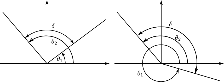
(a) (b)

Figure 5.8: Diﬀerence of angles in the two cases should be as follows: (a) ∆ = |θ2−θ1|

and (b) ∆ = (360 −θ1) + θ2= 360 −(θ1−θ2).

Experiment 6

Wavelength of sodium light by

Newton’s rings

Purpose

To determine the wavelength of sodium light by measuring the diameters of Newton’s

rings

Apparatus

Newton’s ring microscope, sodium vapour lamp, circular slit plate, light emitting diode

source

Theory

Fig. 6.1 shows the experimental setup of Newton’s ring. The formation of maximum inten-

sities at some points and minimum intensities at the other due to the superposition of two

coherent light waves (of same frequencies and constant phase diﬀerence) is called interfer-

ence of light. The interference fringes are observed as an alternate pattern of bright and

dark fringes. The interference at a point where the intensity of light is maximum, is called

constructive interference (corresponds to bright fringe). For constructive interference, the

two waves should have either same phase or a constant phase diﬀerence of

φ= 2nπ , (6.1)

where n= 0,1,2, . . .. Phase diﬀerence (φ)and path diﬀerence (∆) are related by the

equation

φ= (2π/λ)∆ ,(6.2)

where λis the wavelength of the incident light. So, for constructive interference the path

diﬀerence between the light waves should be

∆ = nλ . (6.3)

The interference at other point where the intensity of light is minimum, is called destructive

interference (corresponds to dark fringe). For destructive interference, the two waves

should have either same phase or a constant phase diﬀerence of

φ= (2n+ 1)π, (6.4)

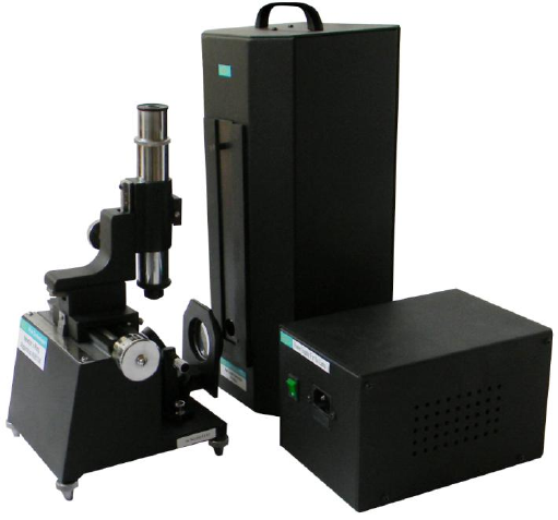
where n= 0,1,2, . . . or a constant path diﬀerence of

∆ = (2n+ 1)λ/2.(6.5)

Interference fringes are obtained by dividing the single coherent source into two sources.

This can be achieved by one of the following methods

1. by division of wave front, that is by taking (or considering) two secondary wavelets

on the same wave front and superposing them

2. by division of amplitude, that is by separating the amplitude of single wave and

reuniting them.

In the case of Newton’s ring interference is due to division of amplitude.

Figure 6.1: Experimental setup of Newton’s ring

When light is incident on a thin ﬁlm (thickness of the order of wave length of the

incident light), it suﬀers partial reﬂection and partial transmission at both upper as well

as lower surfaces of the thin ﬁlm. The transmitted light ray again suﬀers reﬂection at the

lower surface. Interference occurs between the rays in the reﬂected and transmitted parts.

Similarly, in a wedge-shaped ﬁlm, partial reﬂection as well as partial transmission also

takes place. Moreover, the path diﬀerence changes from point to point which results into

an interference fringe.

Fig. 6.2 shows an wedge-shaped air ﬁlm formed between the convex and plane glass

plate inclined at an angle say θ. The refractive index of the ﬁlm is µ. Ray AB is inci-

dent from a broad monochromatic source almost normally on the ﬁlm. It suﬀers partial

reﬂection (ray BE) and partial transmission (ray BC) on the convex surface. Ray BC

again suﬀers partial reﬂection (ray CF ) and partial transmission (not shown) on the plane

surface at C.

The bright rings in the Newton’s ring, as shown in Fig. 6.3, are due to constructive

interference between the reﬂected light rays BE and CF . The dark rings are caused by

destructive interference between the same light rays BE and CF .

For a wedge-shaped thin ﬁlm, the path diﬀerence between the rays BE and CF is

given by

∆=2µt cos α(6.6)

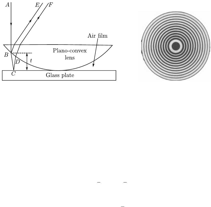
Figure 6.2: Schematic diagram of the light rays

in Newton’s ring

NV6104

Nvis Technologies Pvt. Ltd. 13

Pitch of the micrometer

screw, P (in cm)

Number of divisions on

the circular scale,

Least count of microscope,

P/N (in cm)

8 Take a view through the eye piece (E) of the tube as shown in Figure 6.

Figure 6

9 There are two type of movements provided in the microscope, coarse and fine. Align the

microscope tube, with the help of coarse movement knob no. 2 and 4 as shown in Figure 6, to

bring it over the glass plate P’.

10 Now move the microscope tube with the help of fine movement knob no. 3 close to the plate

P’ to obtain clear image of surface. Slowly move towards upward direction. Newton’s rings

pattern is observed. Adjust by moving the microscope to and fro, if necessary, to view the full

pattern. Adjust further for better contrast between bright and dark fringes as shown in Figure 7.

Figure 7

11 Bring the cross-wire, using knob no.1 shown in figure 6, in the central dark fringe such that their

centre should coincide with each other.

12 Slide the cross-wire to the left till the vertical cross-wire line lies tangentially at the 20th dark

ring. Note the reading on the main and circular scale using the light emitting diode.

13 Now slowly slide the microscope to the right and note the reading when the vertical cross-wire

lies tangentially at the 16th, 12th, 8th and 4th dark rings respectively.

14 Keep sliding the microscope to the right and again note the readings when the vertical cross-wire

lies tangentially at the 4th, 8th, 12th, 16th and 20th dark rings respectively.

Figure 6.3: Newton’s ring

Where tis the thickness of the ﬁlm at B(or at D) and αis the angle of refraction at B.

Since the angle of incidence is almost normal, we can assume cos α≈1. Note that here we

ignore the reﬂections from top of the plano-convex lens and bottom of the plane circular

glass plate since these reﬂections just contribute to the overall glare. The reﬂections of

interest are only those involving the surfaces in contact.

Now by Stoke’s law, there is no phase change at the glass-air interface of the convex

lens (because the wave is going from a higher to a lower refractive index medium), whereas

the reﬂection at the air-glass interface of the plane glass plate undergoes an additional path

diﬀerence of λ/2. Therefore, the net path diﬀerence is

∆ + λ

2= 2µt +λ

2(6.7)

Since for bright fringe, net path diﬀerence is nλ we have,

2µt = (2n+ 1)λ

2.(6.8)

Similarly, for dark fringe, the net path diﬀerence is (2n+ 1)λ/2and thus we have,

2µt =nλ . (6.9)

At the centre, no reﬂection occurs since the two glass surfaces are in intimate contact i.e.

t= 0 or 2µt = 0. This is the condition for dark fringe. Hence the center of the pattern is

always dark.

In the right-angled triangle OAB of Fig. 6.4,

OB2=OA2+AB2

or, R2= (R−t)2+r2

or, r2

n= 2Rt (6.10)

for t22Rt. Thus,

t=r2

n/2R

or, t=D2

n/8R(6.11)

where, rn=radius of nth ring,

Dn=diameter of the nth ring,

R=radius of curvature of the plano-convex lens.

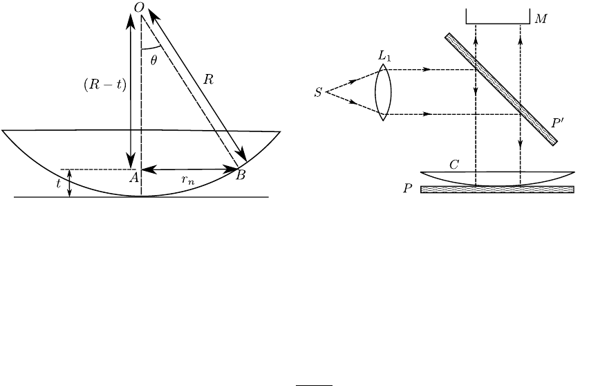
Figure 6.4: Schematic diagram of plano-

convex lens

Figure 6.5: Newton’s ring assembly

In practice, it is not possible to ﬁnd the exact centre of the bull’s eye in order to

obtain rn. Rather, the traveling microscope can measure an approximate diameter Dnfor

the interference ring. Therefore, substituting the value of tfrom Eq. 6.9, we obtain the

diameters of the nth dark fringe as

n=4nRλ

µ(6.12)

Since the human eye is more sensitive to small changes in low intensity, we will measure

positions of dark fringes throughout the experiment.

Procedure

1. The Newton’s ring microscope has two parts, (i) microscope with horizontal mea-

surement and (ii) a Newton’s ring assembly. First detach the Newton’s ring assembly

and clean the adjustable glass plate, plano-convex lens and its adjoining glass plate

with a clean cloth.

Note: Do not detach the plano-convex lens from glass plate frequently. It will disturb

the measurements.

2. Replace the plano-convex lens over the glass plate and tight them carefully with

the help of three leveling screws (if present). An interference ring pattern can be

observed with the naked eye.

Precaution: Avoid over-tightening of the screws. Tight the screws to bring the

central fringe at the centre. Adjust it’s diameter to around 3mm.

3. Arrange the Newton’s ring assembly as shown in Fig. 6.5. Note that the glass plate

P0should be inclined at 45◦with respect to the vertical plain.

4. First connect the sodium vapour lamp power supply with mains. Then connect it

with the light source box with the help of mains cord. Then switch ON the power

supply.

Precaution: Never connect the sodium vapour lamp directly to the main power

supply.

5. Wait for 30 minutes till the lamp glow bright yellowish.

6. Insert circular slit plate into the slit-holder. Adjust to fully illuminate glass plate P0

inclined at 45◦.

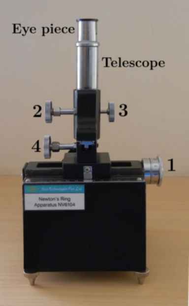
7. Calculate the least count of the traveling microscope (M). If pis the pitch of the

micrometer screw in cm, and mis the number of divisions on the circular scale, then

least count is p/m in cm.

8. Take a view through the eye piece of the tube as shown in Fig. 6.6.

9. There are two type of movements provided in the microscope, coarse and ﬁne. Align

the microscope tube, with the help of coarse movement knob nos. 2and 4as shown

in Fig. 6.6, to bring it over the glass plate P0.

Figure 6.6: Experimental setup of Newton’s ring showing the screws

10. Now move the microscope tube with the help of ﬁne movement knob no. 3close to

the plate P0to obtain clear image of surface. Slowly move towards upward direction.

Newton’s rings pattern is observed. Adjust by moving the microscope to and fro, if

necessary, to view the full pattern. Adjust further for better contrast between bright

and dark fringes.

11. Bring the cross-wire, using knob no. 1shown in Fig. 6.6, in the central fringe such

that their centre should coincide with each other.

12. Slide the cross-wire to the left till the vertical cross-wire line lies tangentially at the

20th ring. Note the reading on the main and circular scale using the light emitting

diode.

13. Now slowly slide the microscope to the right and note the reading when the vertical

cross-wire lies tangentially at the 16th, 12th, 8th and 4th rings respectively.

14. Keep sliding the microscope to the right and again note the readings when the vertical

cross-wire lies tangentially at the 4th, 8th, 12th, 16th and 20th rings respectively.

Sl.

Ring

no.

(n)

LHS RHS D=

b−a

MSR CSR Total

(a)

MSR CSR Total

(b)

(cm) (cm) (cm) (cm2)

1 20

2 16

3 12

4 8

5 4

Table 6.1: Table for measurement of the diameter of the dark rings. MSR - Main scale

reading, CSR - Circular scale reading.

15. The radius of curvature (R)of the plano-convex lens is 100 cm which can be calcu-

lated using the following formula

f= (µg−1) 1

R−1

Rp!,(6.13)

where, f=focal length of the lens = 200 cm,

µg=refractive index of the material of the lens (i.e glass) = 1.5,

R=Radius of curvature of one side the convex side of the plano-convex lens,

Rp=Radius of curvature of plane side of the plano-convex lens → ∞.

16. Plot the graph D2as a function of n. This should be a straight line passing through

the origin (See Eq. 6.12).

17. Find the slope of the line from the graph.

18. Find the wavelength of sodium light from this slope using Eq. 6.12.

Results

The wavelength of sodium light is nm.

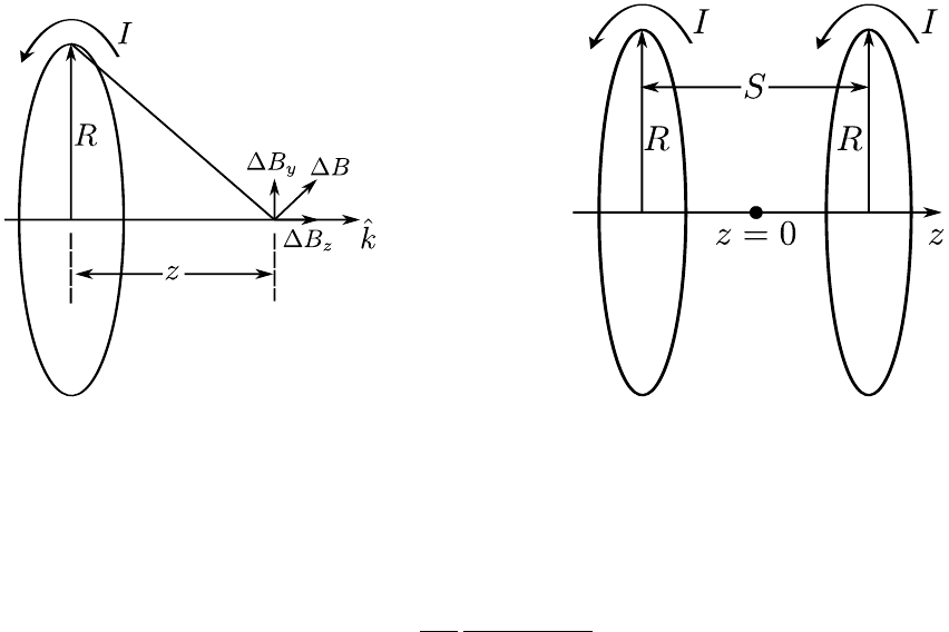
Experiment 7

Helmholtz coil

Purpose

To study the magnetic ﬁeld produced by current carrying coils.

Apparatus

Helmholtz coils, connecting wires, gaussmeter, regulated power supply, measuring scale,

etc.

Theory

Figure 7.1: Magnetic ﬁeld perpen-

dicular to a current carrying coil.

Figure 7.2: Helmholtz coil.

The magnetic induction of a circular coil of radius R, carrying a current I, at a distance

zfrom the center of the loop along the axis (see Fig. 7.1) is given by

B(z) = µoI

(R2+z2)3/2ˆ

k(7.1)

where µ0is the permeability of free space. At z= 0,~

B(0) = µoI/(2R)≡B10.

If there are two such parallel coils at a distance Ssuch that the current ﬂows in the

same direction in both the coils (see Fig. 7.2), then magnetic ﬁeld adds in the space

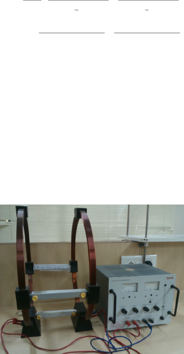
between them. Then we have

B(z) = µoIR2

2





(R2+S

2+z23/2+1

(R2+S

2−z23/2





(7.2)

=B10 





h(1 + (0.5st +zt)2i3/2+1

h(1 + (0.5st −zt)2i3/2



(7.3)

where, st =S/R,zt =z/R and B10 =µoI/(2R).

At the midpoint ∂~

B/∂z is zero. Further ∂2~

B/∂z2is also equal to zero at z= 0 if

S=R. Because of these properties, the axial magnetic ﬁeld is fairly constant over certain

region in the middle of the pair of coils. This arrangement is very popular in producing

uniform axial ﬁelds in regions easily accessible to experimental situations needing such

uniformity.

In this experiment we will study the magnetic ﬁeld variations for such a pair of

Helmholtz coils. The magnetic ﬁeld is measured using a Hall probe connected to a gauss-

meter.

Construction of Helmholtz coils

The two coils are made of copper wire windings in 14 layers, each of 11 turns, such that the

total number of turns (n) = 154. The sockets of the coil winding are cast into the plastic

foot of the coil and the connecting leads can be used to connect the coils in parallel or

series as required. The sockets are numbered (1,2) to make it easier to wire the coils. See

Fig. 7.3. In the Helmholtz arrangement, the coils are positioned by three spacer rails so

Figure 7.3: Experimental setup of Helmholtz coil.

that their axial spacing is equal to the average coil radius. The rails can be removed after

undoing knurled screws, allowing coils to be used individually or with variable spacing.

The coil of the diameter 400 mm

No of turns per coil 154

Coil resistance 2.1 Ω

Procedure

•Calibrate the Hall probe attached to the gaussmeter.

•Connect the coils with the power supply in such a way that both the coils have the

same current in proper direction. In no case the current should exceed 3A.

•Place the hall probe perpendicular to the magnetic ﬁeld and measure the readings

at regular intervals.

Observation

We study the magnetic ﬁeld in current carrying coil (Helmholtz coil) in three diﬀerent

scenarios:

(A) Magnetic ﬁeld along the axis of the coils when current is ﬂowing in

the same direction in both the coils

Sl. Distance (cm) Magnetic ﬁeld (Gauss)

I1=. . . AI2=. . . A

(B) Magnetic ﬁeld along the axis in a single coil

Sl. Distance (cm) Magnetic ﬁeld (Gauss)

I1=. . . AI2=. . . A

Sl. Distance (cm) Magnetic ﬁeld (Gauss)

I1=. . . AI2=. . . A

Plot the intensity of magnetic ﬁeld with distance along the coil for diﬀerent current value

for above describe three case.

Results

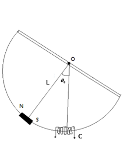
Experiment 8

Electromagnetic induction

Purpose

•To study the ﬂux and emf in the coil as a function of time

•To study the maximum emf and total ﬂux as a function of the velocity of the magnet.

•To demonstrate damping due to induced current.

Apparatus

Faraday setup, diode, capacitor, breadboard, connecting wire, CRO etc.

Theory

Faraday’s law of electromagnetic induction tells us that a change in magnetic ﬂux gives

rise to an induced emf εgiven by

ε=−dφ

dt ,(8.1)

where φis the magnetic ﬂux. A simple apparatus has been designed, whose schematic

Figure 8.1: Schematic of the coil moving in and out of the magnetic ﬁeld.

diagram is shown in Fig. (8.1), enables us to change θat diﬀerent rates through a coil of

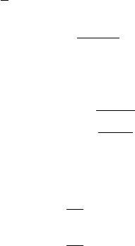
suitable area of cross-section. A rigid semicircular frame of aluminium is pivoted at the

centre of the semicircle. The whole frame can oscillate freely in its own plane, about a

horizontal axis passing through its centre. A bar magnet can be mounted at the centre of

the arc and the arc passes through a coil C.

It is very instructive to study the emf, induced in the coil as the magnet passes through

the coil while oscillating. In this experiment we will use a computer to monitor emf induced

as a function of time.

The rate of change of ﬂux through the coil is essentially proportional to the velocity

of the magnet, as it passes through the coil. Choosing diﬀerent amplitudes of oscillations

can vary the velocity.

If Iis the moment of inertia of the oscillatory system and ωis the angular velocity of

the magnet, then the kinetic energy of the system is Iω2/2and potential energy can be

represented by MgL(1 −cos θ)at any instant of time, where Lis the eﬀective length of

the corresponding simple pendulum. If θois the maximum angular amplitude and ωmax

is the maximum value of angular velocity, then

2Iω2

max =MgL(1 −cos θo)

or, ω2

max =2MgL

I(1 −cos θo)(8.2)

The motion can be regarded approximately as simple harmonic and its time period is

given by

T= 2πsI

MgL (8.3)

From Eq. (8.2) and (8.3), we get

ωmax =4π

Tsin(θo/2) (8.4)

vmax =4π

TLsin(θo/2) (8.5)

where vmax is the maximum linear velocity associated with ωmax. Angular amplitude θo

is directly measured from the instrument. Velocity is computed by measuring Tand θo.

Procedure

1. Charging of capacitor to obtain εmax

The induced emf can be measured by using a simple circuit as shown in Fig. 8.2.

The induced emf in the coil charges a capacitor C, through a resistance Rand a

diode Dand the voltage developed across Cis measured by voltmeter V. The diode

current can ﬂow only if the voltage at Ais greater than B. Thus once a capacitor

attains a voltage ε, current can ﬂow through the capacitor only if the induced emf is

greater than ε. If the time constant RC is not small compared to the time taken for

the magnet to cross the coil, the capacitor does not get fully charged in AC signal

oscillation. It may take several oscillations to do so.

Connect a resistor, diode and a capacitor given to you in series with the coil. Observe

the signal across resistor, diode and the capacitor as a function of time.

Calculate vmax using Eq. (8.5) and plot a graph between εmax vs vmax.εmax is the

maximum potential obtained in the CRO.

2. Induced emf as a function of velocity

You can use the computer interface provided to measure the voltage as a function

of time. The instructor will explain you how to use the software.

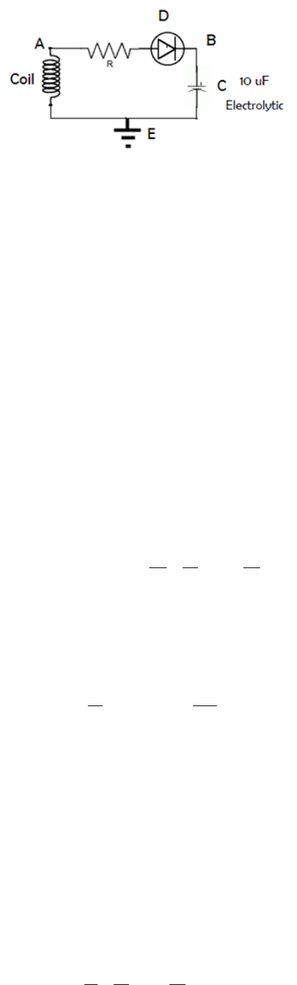
Figure 8.2: Circuit diagram for charging of a capacitor

•Ensure that the support for the apparatus is vertical by adjusting levelling

screws. Adjust the weights W1and W2mounted on the horizontal bar to make

zero of the scale as the mean position. Centre of the magnet must be inside

the coil.

•Measure time period T: First ﬁnd out the time period of the oscillation

T for the apparatus. Connect the terminals of the coil to interface (COBRA

3), and record couple of oscillations by releasing the magnet from small initial

amplitudes. Measure the time period from the plots on your computer screen.

Make sure you account for a whole one cycle while measuring the T.

•Plot of t vs φ(t):Record one or two oscillations. Focus on only one of them

by using magniﬁcation button. Use the integration feature of the software to

obtain ﬂux φas a function of time. You can integrate only half of the pulse,

since the pulse is highly symmetric. Plot this on a graph paper for the complete

pulse.

•vmax dependence of slope of ε(t)at mean position and φ:The emf

induced in the coil can be written as

ε=−dφ

dθ dθ

dt =−ωdφ

dθ (8.6)

Note that when the magnet is at its mean position, then ω=ωmax or velocity

is at its maximum since Vmax =ωmax R. However, dφ/dθ = 0 at that point.

Hence emf will go through a zero corresponding to the mean position. Also

note that

dε

dt Vmax

=− d2φ

dθ2!vmax

ω2

max (8.7)

Hence a plot of the slope of ε(t)at the zero, corresponding to the mean position

against v2

max would be linear. The proportionality constant depends only on

the geometry of the coil and the magnet.

For calculating Φuse “Show integral" mode as before.

3. Electromagnetic damping in an oscillating system

We observe that the successive oscillations are not of the same amplitude. This is

due to damping. Possible sources are: (i) air resistance, (ii) friction at the point of

suspension, and (iii) induced emf (Lenz’s law).

The system (for small θ) and for damping proportional to velocity would satisfy the

equation

dt dθ

dt +kdθ

dt +λθ = 0 (8.8)

where Iis moment of inertia about origin, kis damping coeﬃcient and λθ is restoring

couple (Mglθ), if treated as a simple pendulum of length 1.

The amplitude would exponentially decay only if kis a constant and damping term

depends linearly in velocity. Record a large number of oscillations starting from

initial amplitude of 300 to study the damping behaviour in the absence of induced

current in the coil. The plot seen on the screen may not be correct representation of

data since the number of points to be plotted is too large. Therefore divide the time

axis to approximately 8to 10 zones and take data after magnifying 1pulse from each

zone. Plot εmax and (dε/dt)(vmax)as a function of time or number of oscillations.

From your data calculate Qof this oscillator using A=Aoert/2and Q=ωo/r.

Now, connect a resistor of about 220 Ω (the coil resistance is around 900 Ω) in series

with the coil and record voltage dropped across the resistor as a function of time

(for large number of oscillations as in the previous case). Repeat analysis of data as

above.

4. Useful features of the software measure:

It is easy to use the software given to you. Take a few minutes to summarize yourself

with it before going to the detailed experiments. All you have to do is to click the

required icon given at the top. Some of the important ones are as follows:

ARROW: In this mode simply point the cursor at the required point to obtain

values of the coordinates.

MARK: Use this mark a portion of the curve. The x-coordinate of the mark portion

are shown on the bottom. The marked portion is highlighted in a diﬀerent

colour.

SURVEY: You can adjust the left bottom and right top coordinates of the cursor

box to obtain coordinates and their diﬀerences in this mode. You can use this

to calculate slopes around a point.

SHOW INTEGRAL: Mark the portion of the curve for which you need to calculate

the integral and then click this icon to obtain the value. If you need to start

from the origin, each time, take the cursor out of the plotting area and drag it

across the origin to ensure that starting point is the same.

SLOPE: Mark the required portion of the curve for which you need the slope and

then click this icon to get slope. However, we recommend use of survey mode

to get slope more accurate.

Observations

Sl. θ01 2 3 Avg

T20

Tmax vmax

(deg) T20

(sec)

max

(V)

T20

(sec)

max

(V)

T20

(sec)

max

(V)

(sec) (sec) (V) (m/s)

Sl. Angle θo(degree) Slope =dε/dt v2

max Φ(vmax)

Plots

1. εmax vs vmax

2. dε

dt max vs v2

max and report Φ(vmax).

3. εmax vs dε

dt max

Result

Write down the conclusion in your own words by analysing the graphs.

Experiment 9

Mechanical waves

Purpose

•Study wavelength (λ) as function of frequency (ν) and to ﬁnd out the phase velocity

vpof a traveling wave in a string.

•To measure linear mass density µof the string.

Apparatus

Function generator, ampliﬁer, mechanical oscillator, rubber rope, measuring tape, support

rod, support base, and weights.

Theory

A wave is an oscillation which propagates itself in space and time and usually periodically

through matter and space. One can diﬀerentiate between transverse and longitudinal

waves. In the case of transverse waves, the oscillation is perpendicular to the direction

of the propagation of the wave. In the case of longitudinal waves, the oscillation and the

propagation are in the same direction.

Our goal here is to ﬁnd out the phase velocity of a wave. In order to calculate the

velocity we need to know the frequency and the wavelength. Frequency is generated by

function generator and is an independent variable here. So our main task is to calculate

wavelength of the wave. Here in this experiment we calculate wavelength using a novel

technique.

A standing wave is created by reﬂecting the wave from its opposite end. The distance

between the nodes is measured and thus the wavelength is calculated.

A typical harmonic wave can be represented as,

y=Asin(kx −ωt)(9.1)

where, yis the displacement of the particle from its mean position at a position x and at a time t.

Ais the amplitude of the oscilation.

kis called the wave number and is related to the

wavelength λby the relation k= 2π/λ.

ωis called the angular frequency (measuered in

radians per meter) and is 2πtimes the frequency.

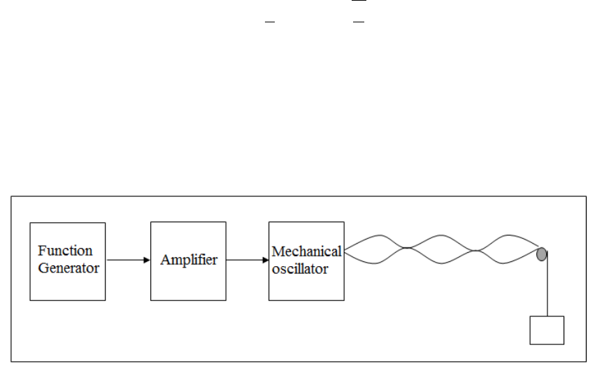
Now consider two transverse waves having same amplitude, frequency, and wavelength but

travelling in opposite directions in the same medium

y1=Asin(kx −ωt)

and y2=Asin(kx +ωt)(9.2)

where y1represents a wave traveling in the +xdirection and y2represents a wave traveling

in −xdirection. Adding these two functions gives the resultant wave function y

y=y1+y2(9.3)

=Asin(kx −ωt) + Asin(kx +ωt)

y= 2Asin(kx) cos(ωt)(9.4)

This represents a wave function of standing waves. The speed of a wave on a string which

is under tension Tand having a mass per unit length µis given by

vp=ω

k=fλ =sT

µ(9.5)

and is called the phase velocity.

Experimental setup

A schematic diagram of the experimental setup is shown in Fig. 9.1 while Fig. 9.2 shows

the various intruments of the experiment.

Figure 9.1: Schematic of standing wave generation

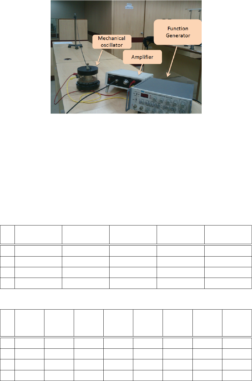
Figure 9.2: Experimental setup

Observation

For a given setup, record

1. Frequency from the function generator (10 Hz −25 Hz).

2. Tension from the weight attached to the rope through the pulley.

3. Wavelength from the position of the nodes.

For constant mass m=......... kg

Sl. Frequency (f)

(Hz)

Number of

loops (n)

Length (L)

(cm)

λ= 2L/n

(cm)

1/λ (cm−1)

For varying mass

Sl. Mass

(m)

(Kg)

Frequency

(f)

(Hz)

T=mg

(N)

Number

of loops

(n)

Length

(L)

(cm)

λ=

2L/n

(cm)

vp=fλ

(cm/s)

(cm/s)2

Calculation

1. Plot the 1/λ vs frequency graph. From this graph, the phase velocity vpshould be

determined. Keep the tension in the string constant i.e. mass is constant.

2. The phase velocity vpof the rope waves, which depends on the tensile stress (T) on

the rope, is to be measured for a given frequency. Plot v2

pvs Tand hence ﬁnd the

mass/unit length of the string using Eq. (9.5).

Results

1. Phase velocity (for constant mass) vp=.........

2. Mass per unit length (for constant frequency) µ=.........

Experiment 10

Fraunhoﬀer Diﬀraction

Purpose

•To understand what is meant by Fraunhoﬀer diﬀraction.

•To observe single slit diﬀraction patterns and plot the intensity proﬁle of the pattern.

•Determine slit width from the diﬀraction formula.

Apparatus

Digital Multi-meter (DMM), He-Ne laser source, sliding detector (photocell), optical rail

and mounts.

Theory

Diﬀraction is the wave phenomenon which describes the deviation from straight line prop-

agation of a wave when it encounters an obstruction. In the case of light waves both

opaque and transparent obstacles cause this eﬀect which results in shadow patterns on a

screen which are quite diﬀerent from those expected if light travelled only in straight lines.

There are basically two categories of diﬀraction eﬀects. The ﬁrst is Fraunhoﬀer diﬀrac-

tion, which occurs when the waves incident on the slit and the screen (detector) are plane

waves. This diﬀraction is produced when both the light source and screen are eﬀectively

at an inﬁnite distance from the given obstacle. Fresnel diﬀraction is the second type

and refers to diﬀraction produced when either the source or screen or both are at ﬁnite

distances from the obstacle.

We can observe Fraunhoﬀer diﬀraction experimentally by using a collimated light

source and (i) placing the viewing screen at the focal plane of a convex lens located

behind the obstacle or (ii) by placing the screen at a large distance from the obstacle. The

schematic of a single slit diﬀraction apparatus is shown in Fig. 10.1.

In this experiment we concentrate on Fraunhoﬀer diﬀraction patterns although you

can observe the diﬀerent patterns produced by Fresnel diﬀraction by placing the viewing

screen close to the diﬀraction slit used.

Fig. 10.1 shows a plane wave of wavelength λincident on a slit width a. The diﬀrac-

tion pattern, intensity versus yis plotted in the ﬁgure. Wave theory predicts that the

Fraunhoﬀer diﬀraction pattern intensity due to a rectangular slit will be of the form

I=Io

sin2β

β2(10.1)

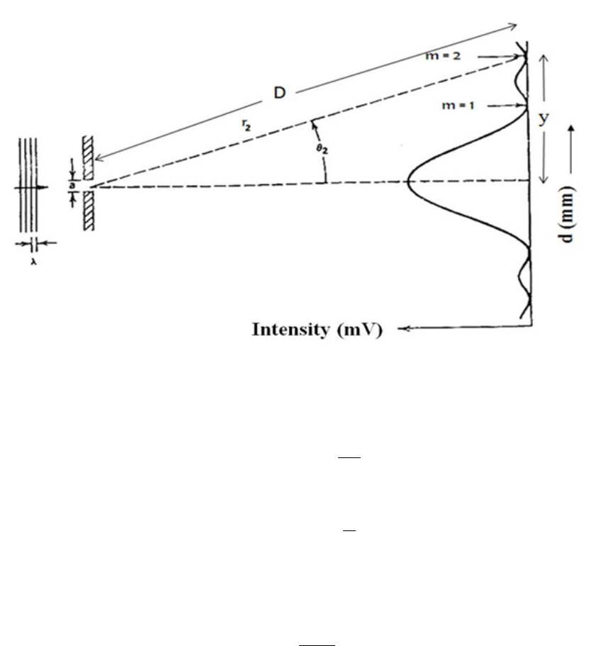
where β= (ka sin θ)/2, k = 2π/λ, a =slit width and θ=angle formed by the light ray

with respect to the system central axis. The minima in the diﬀraction pattern occurs

when I(θ)=0. This condition requires that

asin θm=mλ (10.2)

where, mis the order number in diﬀraction pattern and θmis angle measured with respect

to system central axis to the mth order minima. The shape of this pattern is shown in

Figure 10.1: The Fraunhoﬀer diﬀraction pattern of a single slit.

Fig. 10.1. If θmis small, then

sin θm≈θm=mλ

a.(10.3)

Further from geometry we have

sin θm≈θm=y

D.(10.4)

where y= the distance between central maxima to the mth order minima point and D=

distance between slit and photo diode (observed form instrument). Combining Eqs. 10.3

and 10.4, the slit width can be calculated as

a=mλD

y(10.5)

Experimental procedure

1. Let the laser warm up for at least ﬁfteen minutes before starting the experiment.

2. Position the laser at one end of the bench and align the beam so that it travels

parallel to and along the central axis of the bench all along its length.

3. Let the beam pass through a beam expander. Adjust the slit position until the laser

beam is incident on the full width of the slit.

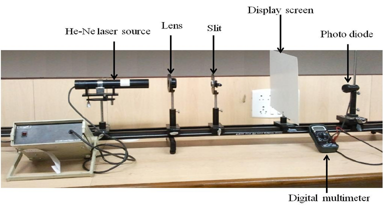
Figure 10.2: Experimental setup for single slit diﬀraction pattern

4. Attach the viewing screen to a component carrier and position it at the end of the

bench furthest from the laser.

5. Observe the diﬀraction pattern on the screen. Adjust the screen position if necessary

to obtain image clarity. Sketch the pattern observed for two diﬀerent slit widths.

What is the eﬀect of varying the slit width?

6. Now replace the screen with the sliding detector. Beware that the smallest division

on the sliding detector is 0.01 cm, and the detector can be moved over a distance of

4cm. Check that the un-obstructed laser beam is at the proper level to be incident

on the detector central slit-adjust if necessary.

7. Adjust the position of the slit along the optical bench until the central (principal)

maximum and the ﬁrst subsidiary maxima of the single slit diﬀraction pattern are

fully extended along the direction of travel of the detector–obviously the pattern

gets wider as the slit is moved closer to the laser and hence further away from the

detector.

8. Form a clear diﬀraction pattern and SLOWLY scan the pattern from the central

maxima to ﬁrst maxima on the one side with the sliding detector for every 25 divi-

sions of the circular scale.

9. Plot intensity versus position. How do your results agree with theoretical predic-

tions?

10. Calculate the slit width using the diﬀraction Eq 10.5.

Observation

Sl. No. Distance Intensity (mV)

MSR (mm) VSR Total reading

(mm)

Result

The calculated slit width from the diﬀraction pattern a=............. mm.

Precautions

1. Never look directly into the laser beam and take care to avoid reﬂections entering

your eyes.

2. Do not disturb the setup once the diﬀraction pattern has been obtained.

3. Do not use the backlight of the multimeter. This would drain the battery of the

multimeter.

4. Avoid stray light falling on the photo detector while measuring the instensity of light.

Experiment 11

Diﬀraction grating

Purpose

•To understand the diﬀraction, diﬀraction grating and how diﬀraction grating works

with the help of basic diﬀraction grating equations and experimental studies.

•To measure the wavelength of the light source with the help of diﬀraction grating.

Apparatus

Spectrometer, diﬀraction grating, mercury light source, high voltage power supply, mag-

nifying lens, spirit level, torch light, etc.

Theory

Preliminary discussion

Interference refers to the interaction of two or more wave trains of light having the same fre-

quency and having a phase diﬀerence which remains constant with time (coherent sources),

so that they may combine with the result that the energy is not distributed uniformly in

space but is a maximum at certain points and a minimum (perhaps zero) at others.

Diﬀraction phenomenon is described as the apparent bending of waves around small

obstacles and the spreading out of waves past small openings. Diﬀraction patterns are

marked by a rapid decrease in intensity with increasing distance from the center of the

pattern.

A diﬀraction grating is made by making many parallel scratches on the surface of a

ﬂat piece of transparent material. It is possible to put a large number of scratches per

centimeter on the material, e.g., the grating to be used has 6000 lines/cm on it. The

scratches are opaque but the areas between the scratches can transmit light. Thus, a

diﬀraction grating becomes a multitude of parallel slit sources when light falls upon it.

Diﬀraction grating equation

When parallel bundle of rays falls on the grating, these rays and their associated wave

fronts form an orthogonal set so the wave fronts are perpendicular to the rays and parallel

to the grating (as shown in Fig. 11.1). According to Huygens’ Principle, every point on a

wave front acts like a new source, each transparent slit becomes a new source so cylindrical

wave fronts spread out from each. These wave fronts interfere either constructively or

destructively depending on how the peaks and valleys of the waves are related.

Whenever the diﬀerence in path length between the light passing through diﬀerent slits

is an integral number of wavelengths of the incident light, the light from each of these slits

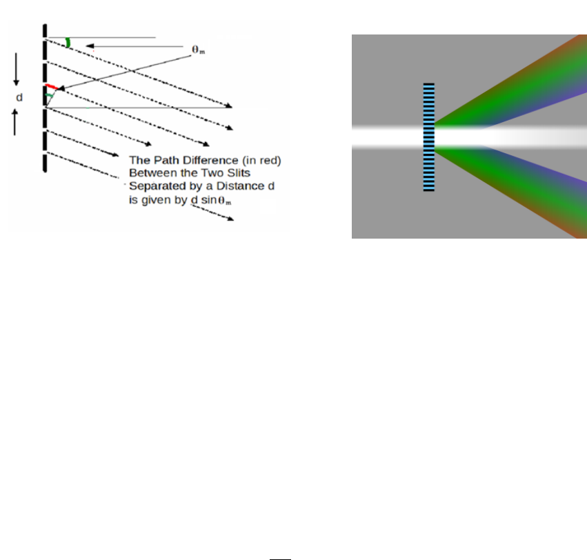
will be in phase, and then it will form an image at the speciﬁed location. Mathematically,

the relation is simple

mλ =dsin θm(11.1)

Eq. (11.1) is known as grating equation. The light that corresponds to direct transmission

Figure 11.1: Geometrical conditions for the

diﬀraction from multiline grating.

Figure 11.2: Spectrum due to a

grating.

(or specular reﬂection in the case of a reﬂection grating) is called the zero order, and is

denoted m= 0. The other maxima occur at angles which are represented by non-zero

integers m. Note that mcan be positive or negative, resulting in diﬀracted orders on both

side of the zero order beam.

Diﬀraction gratings are often used in monochromators, spectrometers, lasers, wave-

length division multiplexing devices, optical pulse compressing devices, and many other

optical instruments.

Resolving power of grating

This equation then leads to the following expression for the resolving power of the diﬀrac-

tion grating

R=λ

∆λ=mN (11.2)

Here λis the average of wavelength, ∆λis the diﬀerence between wavelengths, mis the

order and Nis the total number of slits on the grating.

Thus, the distance between maxima depends on the distance between slits and the res-

olution, the relative sharpness of the maxima, depends on the total number of slits. (Often

a grating is characterized by the number of slits per unit length. From this information

one can, of course, deduce the distance between the slits.

Procedure

As with many optical instruments, the spectroscope requires some initial adjustments

before the desired measurements can be performed. Focusing and levelling of the spec-

trometer for the parallel rays is to be done as per previous prism experiment.

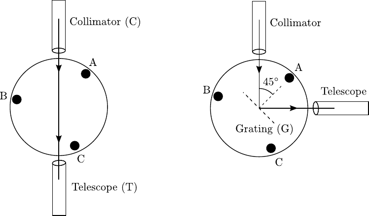
(a) (b)

Figure 11.3: Grating settings

To set the telescope axis perpendicular to that of the collimator:

Illuminate the slit with the light source. Turn the telescope of the spectrometer to view the

image of the illuminated slit directly as shown in Fig. 11.3(a). The source should directly

be in front of the slit such that maximum light falls on the slit. Adjust the cross-wires

such that the image of the slit falls in the middle of the intersection of the cross-wires.

Fix the prism table with the ﬁxing screw and read any of the two verniers. Let this angle

be α. Rotate the telescope by an amount 90 ±αsuch that it is exactly perpendicular to

the collimator. Fix the telescope in this position and unﬁx the prism table.

Fix the grating (G) in the grating holder such that the grating lines are perpendicular

to the prism table and the ruled surface extend equally on both sides of the center. The

grating is set parallel to the line joining the prism table screws B and C as shown in

Fig. 11.3. Turn the prism table such that light from the collimator is reﬂected into the

telescope. The reﬂection should be by the unruled surface of the grating. To determine

the unruled surface use the following procedure. Allow light to be reﬂected by both the

grating surface one at a time and view the corresponding image via the telescope. The

surface from which the image of the slit appears sharper is in fact the unruled surface of

the grating.

Once the unruled surface has been determined, view the reﬂection only via the unruled

surface while the setup is as shown in Fig. 11.3(b). If the center of the grating displace

either above or below the intersection of the cross-wires, then the grating surface is not

vertical. To ensure that the grating surface is vertical, turn the prism table screws B and C

equally in opposite directions until the center of the image coincides with the intersection

of the cross-wires.

Turn the unruled surface of the grating by an angle 45◦such that the light from the

collimator falls normally on the unruled surface of the grating. Fix the prism table in this

position and unﬁx the telescope.

Even though we have made the plane of the grating vertical and the rulings perpen-

dicular to the table surface, the rulings of the grating may not be vertical. In order to

set the rulings vertical, rotate the telescope in its own plane on both side of the central

image. On both sides on the central image diﬀerent orders of image are seen as shown in

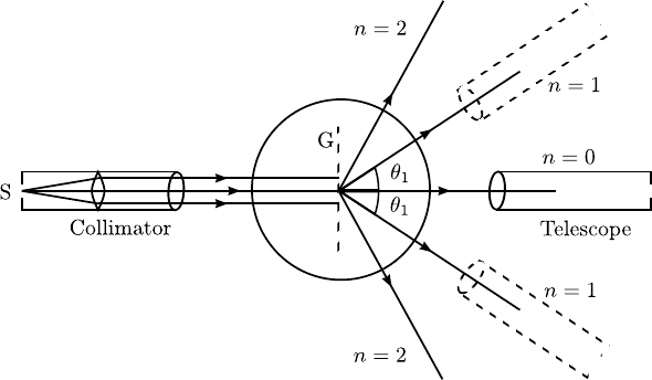
Fig. 11.4. In the ﬁrst order images on both sides, if the image on the left is higher than

Figure 11.4: Grating images of higher order

that of the image on the right or vice-versa, then turn the third screw A on the prism

table until the images on both the sides are on the same level.

Caution

•The diﬀraction grating is a photographic reproduction and should NOT be touched.

Make sure that the glassy base of grating shouldn’t faces towards the source light.

•Now your setup is ready to report the experimental observations.

Observation

1. Check to make sure that the grating is not too high or low relative to the collimator.

Aﬃrm maximum brightness for the straight through beam by adjusting the source

slit alignment. At this step, the slit should be narrow, perhaps a few times wider

than the hairline. Search for the spectrum by moving the telescope to one side or

the other. This spectrum should look much like the visible spectrum observed with

the prism. This is the ﬁrst order spectrum. Record for each color diﬀraction angle

θR(along right side) and θL(along left side) from the straight trough beam.

2. For each of the seven colors in the mercury spectrum, measure the angles θRand θL

to the nearest tenth of a degree by placing the hairline on the stationary side of the

slit.

3. You are expected to observe the 1st order diﬀraction pattern.

4. From your observations calculate various wavelengths of visible radiations from the

mercury source.

Calculation

1. Use the grating equation with d= (1/6000) cm to ﬁnd the wavelength λfor each

colour.

2. Calculate % error for your reported λmeasurement.

Sl. Colour LHS RHS 2θ=

θL−

θR

θ λ =

dsin θ

m=1

CSR VSR Total

(θL)

CSR VSR Total

(θR)

1 Violet

2 Indigo

3 Blue

4 Green

5 Yellow

6 Orange

7 Red

Table 11.1: For ﬁrst order (m= 1). CSR - Circular scale reading, VSR - Vernier scale

reading.

Result

1. Percentage measurement error for your analysis.

2. A certain colour emerges at 15oin the ﬁrst order spectrum. At what angle would

this same colour emerge in the second order if the same source and grating are used?

3. What could be causing any discrepancy?

4. Why is it necessary that the base side of the grating face toward the light source?

Draw a ray diagram for the two cases:

a) Base toward the source (correct).

b) Grating toward the source (incorrect).

5. Mention your special comments for each statement in your lab report as a part of

experimental outputs.

Lab Manual

ug-physics-lab-manual-17

Navigation menu

Versions of this User Manual:

Views

Navigation