Lab Manual

User Manual:

Open the PDF directly: View PDF .
Page Count: 51

ELEC350: Communications

Theory and Systems I

Laboratory Manual

Revision History

Revision 1.0 08 Mar 2013

Updated for GNU Radio 3.6.3.

Revision 1.1 27 Jun 2013

Updated for GNU Radio 3.6.5. The category structure was revised quite

a bit from earlier versions so the text has been updated to reflect that.

Revision 1.2 4 Jul 2013

Updated for GNU Radio 3.7.0. The category structure was revised yet again, text updated.

Revision 2.0 1 Sept 2014

Updated for 2014 deleting Softrock, retaining 4 labs only

Table of Contents

Introduction ........................................................................................................................ 1

Lab 1. GNU Radio Tutorials ................................................................................................. 2

Deliverables ............................................................................................................... 2

Tutorial 1: Using GNU Radio Companion ....................................................................... 3

Tutorial 2: Variables and Controls ................................................................................ 18

Tutorial 3A: AM Signal waveforms .............................................................................. 22

Tutorial 3B: Receiving AM Signals .............................................................................. 22

Tutorial 4: Complex Signals and Receiving SSB ............................................................. 32

Lab 2. FM, IQ and USRP Tutorial ....................................................................................... 40

Deliverables .............................................................................................................. 40

Setup ....................................................................................................................... 41

FM Signal waveforms ................................................................................................ 41

FM Receivers ........................................................................................................... 42

I/Q Receiver ............................................................................................................. 43

Carrier Wave Transmitter ........................................................................................... 45

Lab 3. FLEX Frame Synchronizer ........................................................................................ 45

Deliverables .............................................................................................................. 45

Frame Capture .......................................................................................................... 46

Bit and Frame Sync ................................................................................................... 48

Decoding text ........................................................................................................... 48

Other data signals ...................................................................................................... 48

Lab 4. PSK systems ........................................................................................................... 50

Deliverables .............................................................................................................. 50

Testing a PSK system ................................................................................................ 50

Introduction

The lab component of this course consists of several components:

• Lab 1. GNU Radio Tutorials.

• Lab 2. USRP [http://en.wikipedia.org/wiki/Universal_Software_Radio_Peripheral] Tutorials and FM

Receiver.

ELEC350: Communica-

tions Theory and Systems I

• Lab 3. Finding frame synchronization on the FLEX [http://en.wikipedia.org/wiki/FLEX_(protocol)]

pager network using the USRP and GNU Radio.

• Lab 4. Pulse shaping and PSK

• Optional activity

• Pass the amateur radio basic and advanced exams (contact Dr. Driessen)

• Decoding off-air signals not covered in the other lab activities.

The deliverables are described at the beginning of each section.

Lab 1. GNU Radio Tutorials

The following tutorials were adapted from Dr. Sharlene Katz' SDR Project [http://www.csun.edu/~skatz/

katzpage/sdr_project/sdrproject.html] website and updated for GNU Radio 3.7. They are designed to get

you familiar with various aspects of the GNU Radio Companion. You will also learn some basic tuning and

demodulation techniques. As you work through the material, try to keep these following questions in mind:

• What do the different colors of input and output terminals represent?

• How is the computer's audio input/output hardware represented in GRC?

• What is the Throttle block for? When should it be used?

• How are block parameters linked to GUI controls?

• How is an AM signal demodulated into an audio signal?

• How is an SSB signal demodulated into an audio signal?

• What methods are used to tune to a desired signal?

To understand how these demodulation techniques work, please review the theory of AM and SSB signals

[./data/Theory_AM_SSB.pdf].

Other tutorials are also available, see for example

• Video tutorials [http://www.ettus.com/kb/detail/software-defined-radio-usrp-and-gnu-radio-tutori-

al-set]

• Python and 5 GRC labs [http://files.ettus.com/tutorials/]

• gnuradio.org tutorials [http://gnuradio.org/redmine/projects/gnuradio/wiki/Tutorials]

• Gnuradio and RTL-SDR USB stick [http://www.rtl-sdr.com/tutorial-creating-fm-receiver-gnuradio-rtl-

sdr/?PageSpeed=noscript]

Deliverables

• GRC file of AM transmitter and receiver as described in Tutorial 3A.

• GRC file of AM receiver with AGC as described in Tutorial 3B.

ELEC350: Communica-

tions Theory and Systems I

• block diagram of AM receiver showing mathematical representation of signals at all points

• GRC file of SSB receiver using Weaver's method as described in Tutorial 4.

• block diagram of SSB receiver showing mathematical representation of signals at all points

• There are a number of questions included within the text. Written answers to these questions are not

required, but an effort should be made to think about and answer these questions as they are encountered.

Tutorial 1: Using GNU Radio Companion

Objectives

GNU Radio Companion (GRC) is a graphical user interface that allows you to build GNU Radio flow-

graphs. It is an excellent way to learn the basics of GNU Radio. This is the first in a series of tutorials that

will introduce you to the use of GRC. In this tutorial you will learn how to:

• launch the GNU Radio Companion (GRC) software.

• create and execute a GRC flowgraph.

• use basic blocks such as signal sources and graphical sinks.

• use the computer's audio hardware with GRC.

Launching GNU Radio Companion

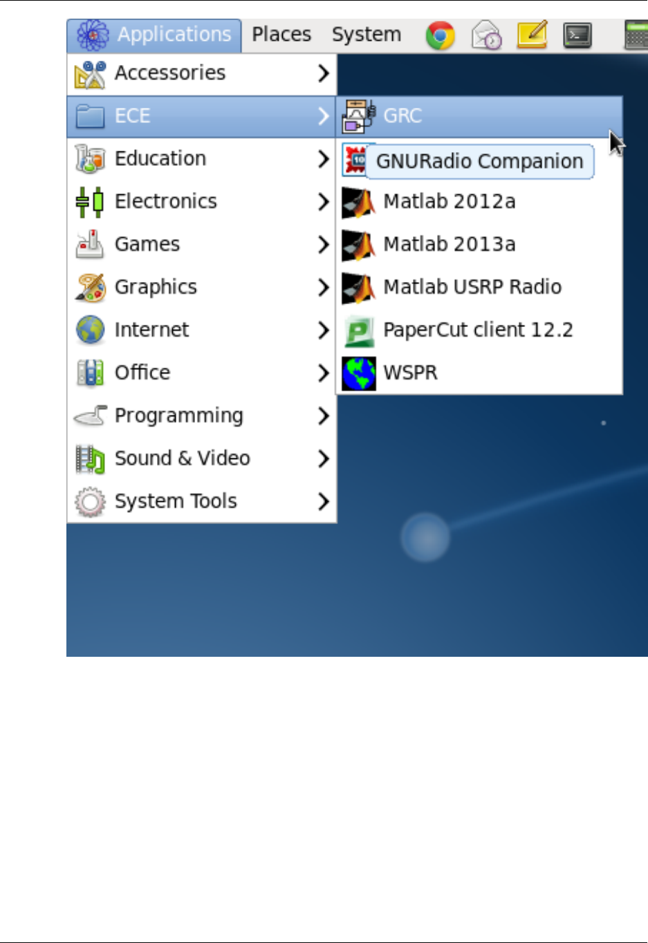
Launch GNU Radio companion by selecting Applications->ECE->GRC as shown below.

ELEC350: Communica-

tions Theory and Systems I

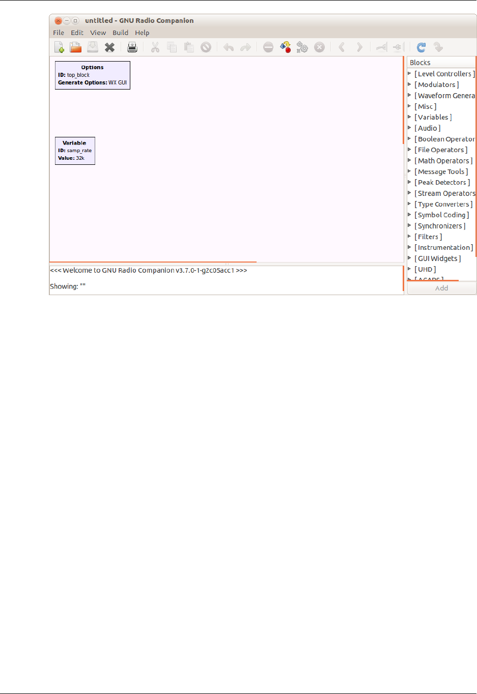
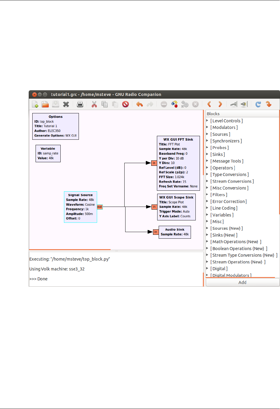
An untitled GRC window similar to the one below should open.

ELEC350: Communica-

tions Theory and Systems I

Configuring the Flowgraph

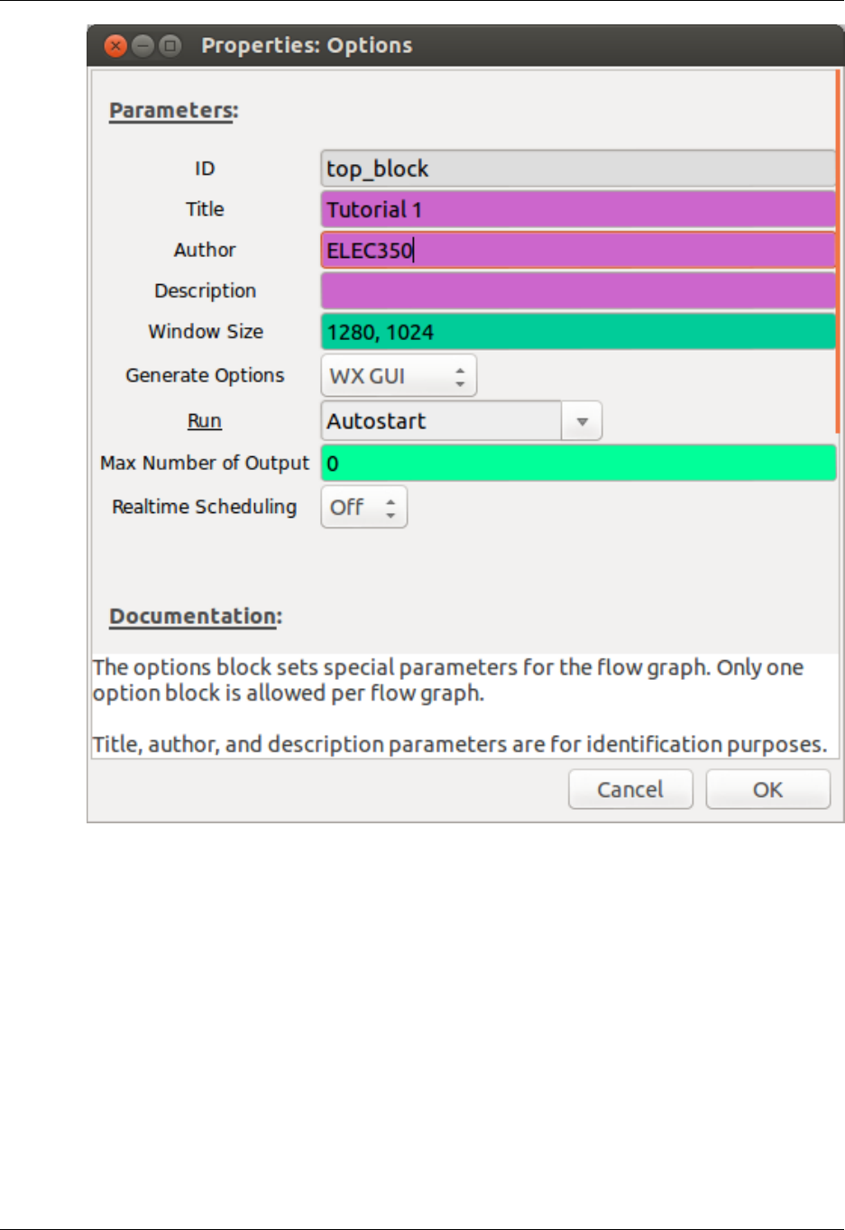
The Options block sets some general parameters for the flow graph. Double-click on the Options block.

You should now see a properties dialog similar to the one shown below.

ELEC350: Communica-

tions Theory and Systems I

• Leave the ID as "top_block".

• Enter "Tutorial 1" as the title.

• Enter your name as the Author.

• Set Generate Options to WX GUI, Run to Autostart, and Realtime Scheduling to Off.

• Click OK to close the properties dialog.

The other block in the flowgraph is a Variable block that sets the sample rate. Click on this block to see

the variable name and value. The variable block will be discussed later in the tutorial.

ELEC350: Communica-

tions Theory and Systems I

Adding Blocks to the Flowgraph

On the right side of the window is a list of the blocks that are available. By expanding any of the categories

(click on triangle to the left) you can see the blocks available. Explore each of the categories so that you

have an idea of what blocks are available.

You can also click anywhere in the GRC window and simply type a search term (e.g. receiver) to search

all categories. A small text window will come up in the bottom right of the screen in which your search

term will be entered. To see the search results, scroll down the list of blocks to below the Resamplers to

see a block called Search: receiver, where receiver is your search term and a list of blocks with receiver

in the name will come up. Try a few searches such as filter and source to see what comes up.

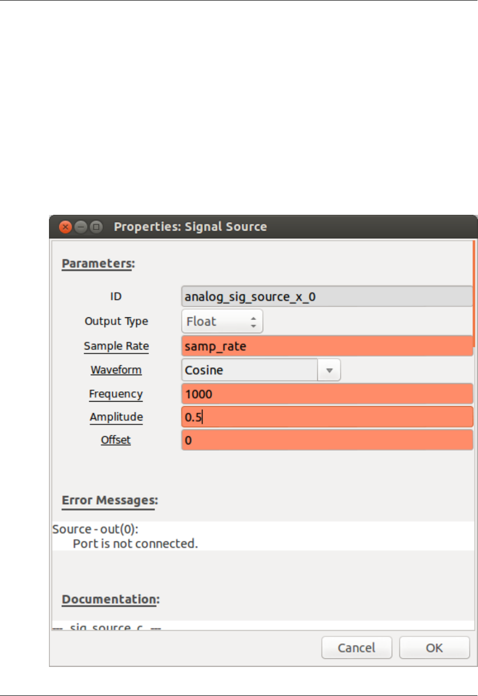
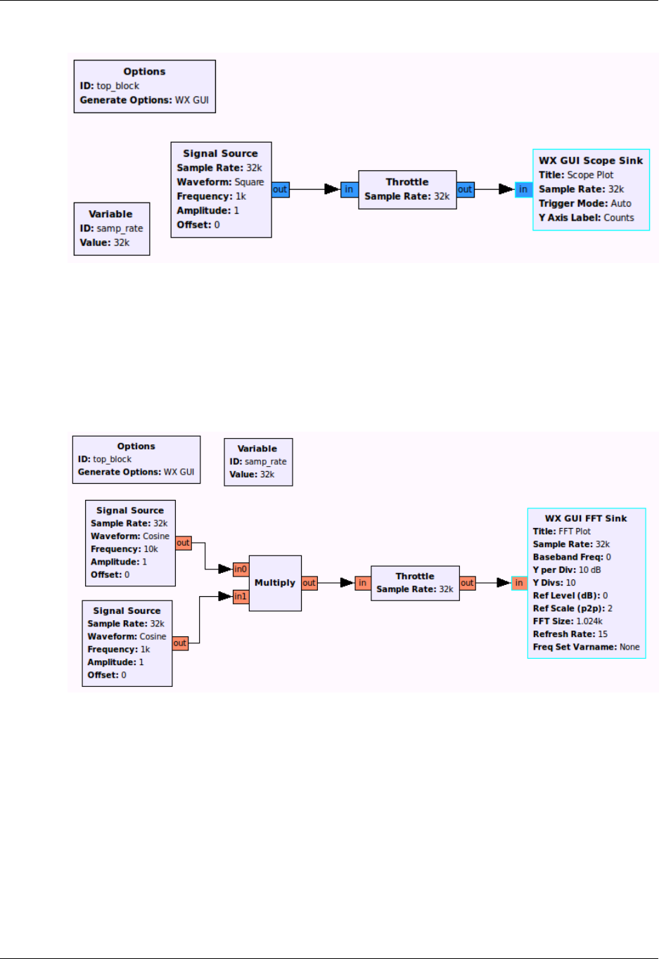
Open the Waveform Generators category and double-click on the Signal Source. Note that a Signal Source

block will now appear in the main window. Double-click on the Signal Source block and the properties

dialog will open. Adjust the settings to match those as shown in the figure below and close the dialog. This

Signal Source is now set to output a real-valued 1 kHz sinusoid with a peak amplitude of 0.5.

ELEC350: Communica-

tions Theory and Systems I

In the flowgraph, the Signal Source block will have an orange output tab, representing a float (real) data

type. If the block settings is chosen as complex instead of float, then the output tab will be blue. In order to

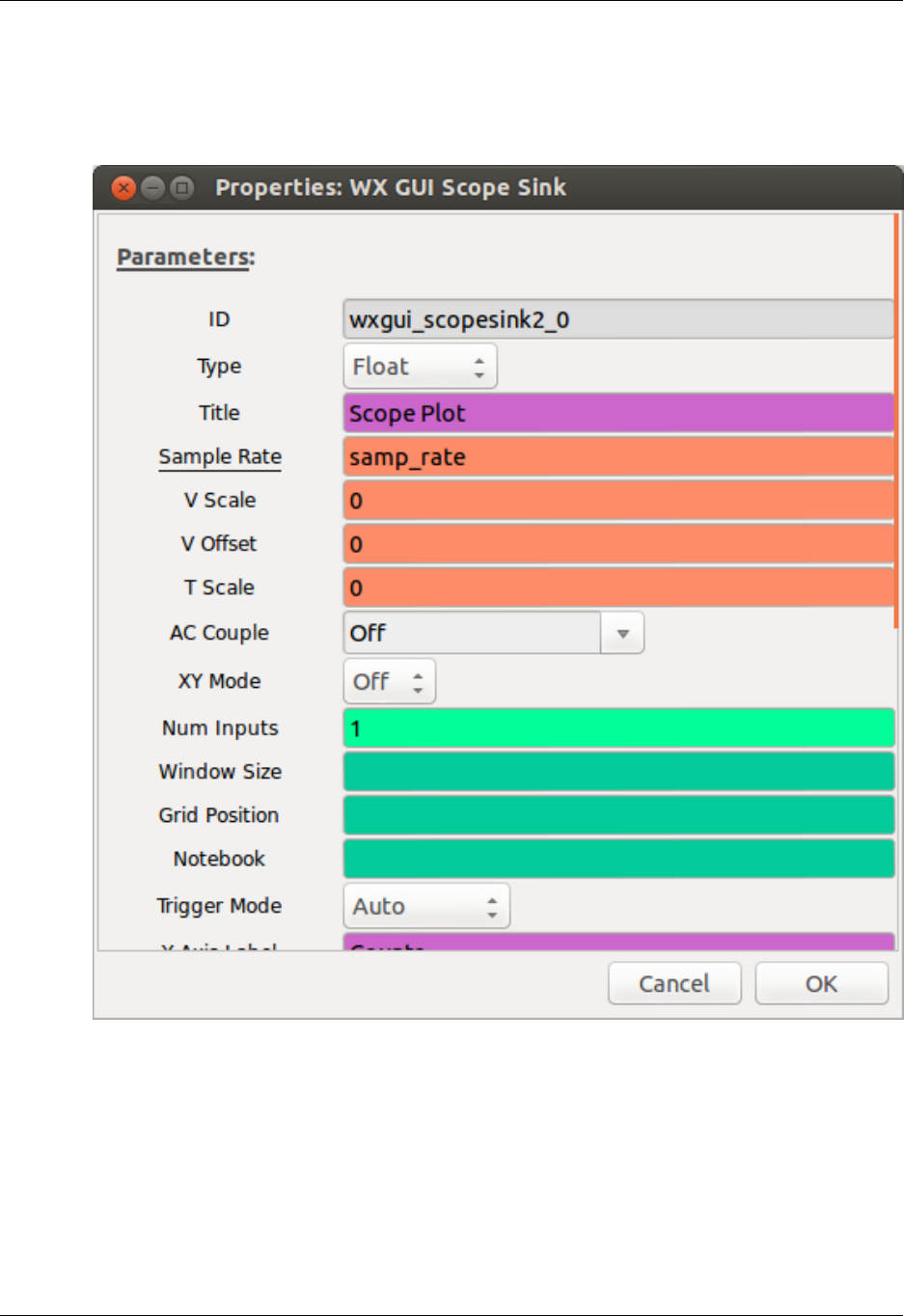
view this wave we need one of the graphical sinks. Expand the Instrumentation category and then the WX

subcategory. Double-click on the WX GUI Scope Sink. It should appear in the main window. Double-click

on the block and change the Type to Float. Leave the other Parameters at their default values as shown

below. Click OK to close the properties dialog.

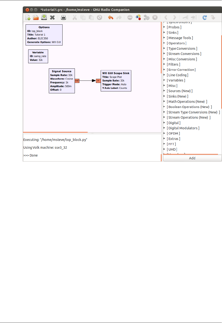
In order to connect these two blocks, click once on the out port of the Signal Source, and then once on the

in port of the Scope Sink. The following flow graph should be displayed.

ELEC350: Communica-

tions Theory and Systems I

The problem with this flowgraph is that although the sample rate is set to 32000, there is no block which

enforces this sample rate. Therefore, the flowgraph will consume as much of the computer's resources as

it possibly can which can cause the GRC software to lock up. To fix this problem, disconnect the Signal

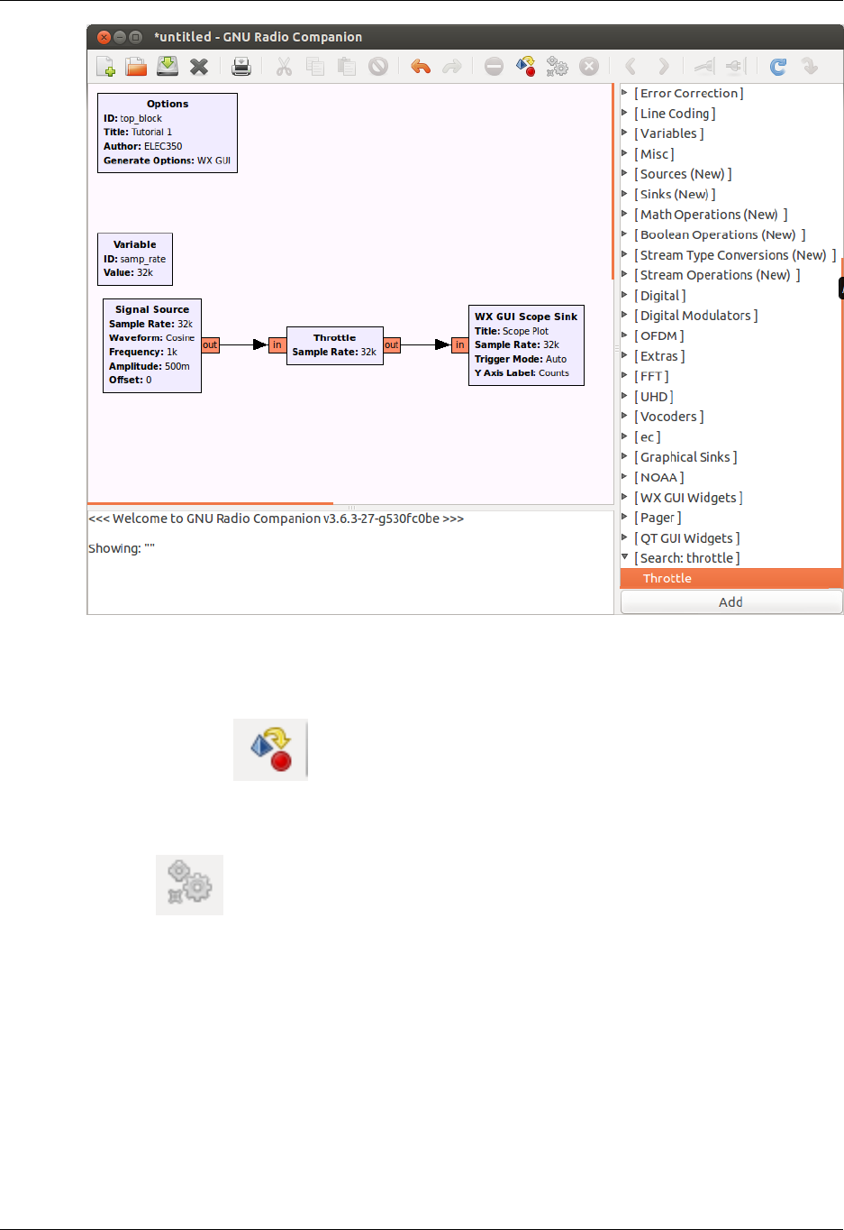
Source from the WX GUI Scope Sink by clicking on the arrow and pressing the Delete key. Expand the

Misc category and double-click on the Throttle. Connect this block between the Signal Source and the WX

GUI Scope Sink as shown in the figure below (click once on the out port of one block and the in port of

the next block). Note that the input and output arrowheads will change to red. This indicates a problem

with the flowgraph, in this case, the data types do not match. To fix the problem, double-click the Throttle

and change the Type to Float.

ELEC350: Communica-

tions Theory and Systems I

Executing the Flowgraph

In order to observe the operation of this simple system we must generate the flowgraph and then execute

it. Click first on the icon (or press F5) to generate the flowgraph. If the flowgraph has not yet

been saved, a file dialog will appear when you click this button. Name this file tutorial1.grc and save it.

The generation stage converts your flowgraph into executable Python code.

Click the icon (or press F6) to execute the flowgraph. The execution stage runs the Python code

that was generated in the previous step. A scope plot should open displaying several cycles of the sinusoid.

Confirm that the frequency and amplitude match the value that you expect. What is the period of one cycle

of the sine wave, and thus what is the frequency? Experiment with the controls on the scope plot.

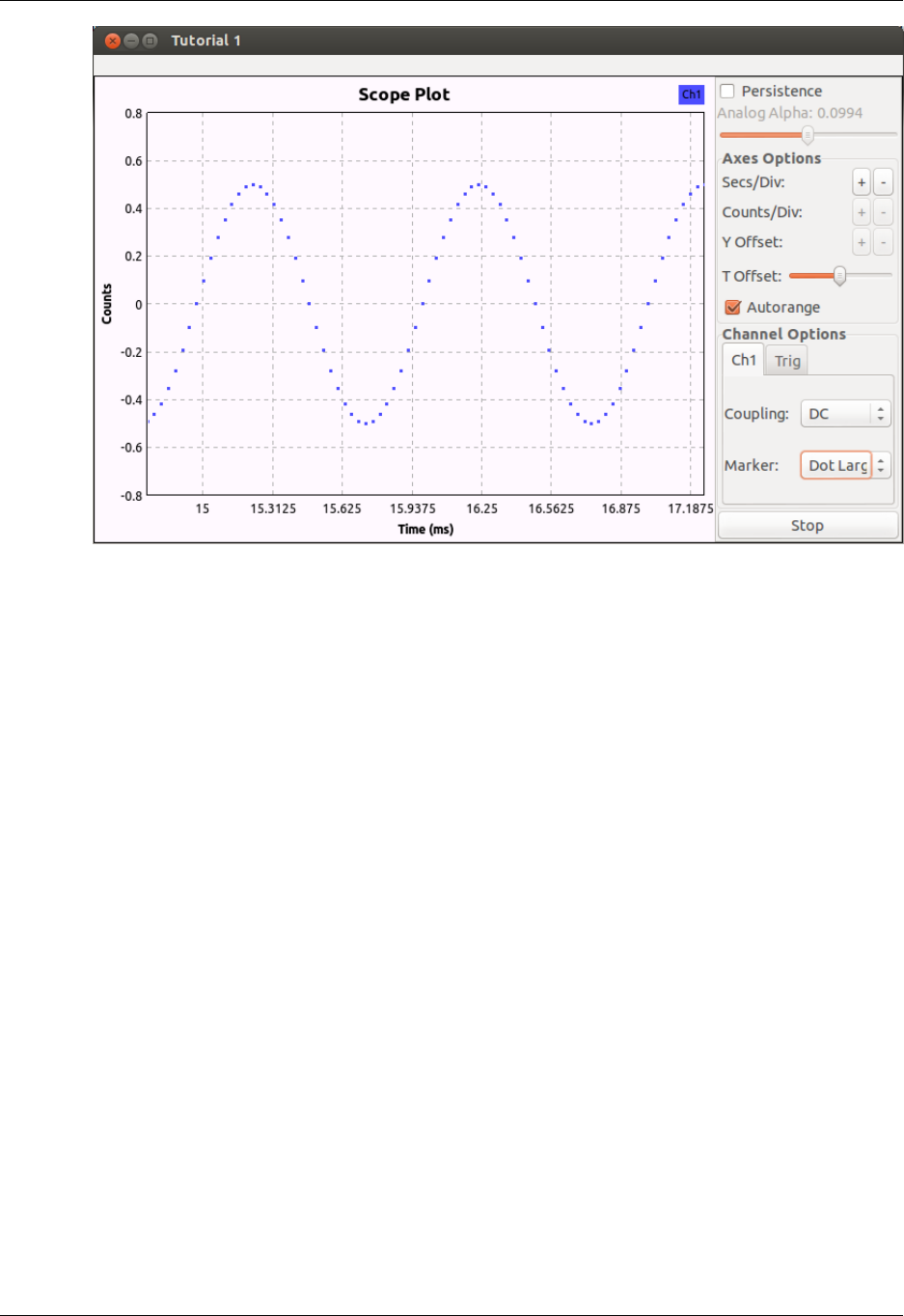
Working with the Scope Sink

Change the Channel Options / Marker setting to Dot Large. Now you can see the actual sample values.

Recall that the Variable block set the sampling rate to 32000 samples/second or 32 samples/ms. Note that

there are in fact 32 samples within one cycle of the wave.

ELEC350: Communica-

tions Theory and Systems I

Close the scope and reduce the sample rate to 10000 by double-clicking on the Variable block and entering

10e3 in the Value box. Note that you can use this exponential notation anywhere that GNURadio requires

a number.

Re-generate and execute the flow graph. Note that there are now fewer points per cycle. How low can

you drop the sample rate? Recall that the Nyquist sampling theorem requires that we sample at more than

two times the highest frequency. Experiment with this and see how the output changes as you drop below

the Nyquist rate.

Working with the FFT Sink

The FFT Sink acts as a Spectrum Analyzer by doing a short time discrete Fourier transform (STFT).

Review the theory of the Spectrum Analyzer [data/Theory_Spectrum_Analyzer.pdf]

Close the scope and change the sample rate back to 32000. Add a WX GUI FFT Sink (under Instrumenta-

tion->WX) to your window. Change the Type to Float and leave the remaining parameters at their default

values.

Connect this to the output of the Signal Source by clicking on the out port of the Throttle and then the in port

of the WX GUI FFT Sink. Generate and execute the flow graph. You should observe the scope as before

along with an FFT plot correctly showing the frequency of the input at 1KHz. Close the output windows.

Explore other graphical sinks (WX GUI Number Sink, WX GUI Waterfall Sink, and WX GUI Histo Sink)

to see how they display the Signal Source.

The number sink is typically used to monitor slowly-changing signals such as the RMS input level. In

this example, the sine wave changes too fast for the numbers to keep up. The waterfall sink is used to

display amplitude vs. frequency vs. time with amplitude represented as a variation in color. The waterfall

is a time frequency diagram with time on the vertical axis. Note that for a single 1 Khz sine wave input,

the frequency does not change with time, thus a vertical line is displayed at 1 Khz. The histo sink displays

ELEC350: Communica-

tions Theory and Systems I

a histogram of the input values, which can be used to monitor the symbol distribution in a digital signal

or the distribution of a noise source.

Working with Audio I/O

Create the flow graph shown below. The Audio Sink is found in the Audio category. The Audio Sink block

directs the signal to the audio card of your computer. Note that the sample rate is set to 48000, a sample

rate that is commonly supported by computer audio hardware. Other commonly-supported rates are 8000,

11025, 22050 and 44100. Some audio hardware may support higher rates such as 88200 and 96000. Also

note that there is no Throttle block. This is because the audio hardware enforces the desired sample rate

by only accepting samples at this rate.

Generate and execute this flow graph. The graphical display of the scope and FFT should open as before.

However, now you should also hear the 1 kHz tone. If you do not hear the tone, ensure that the output

from the computer is connected to the speakers and that the volume is turned up.

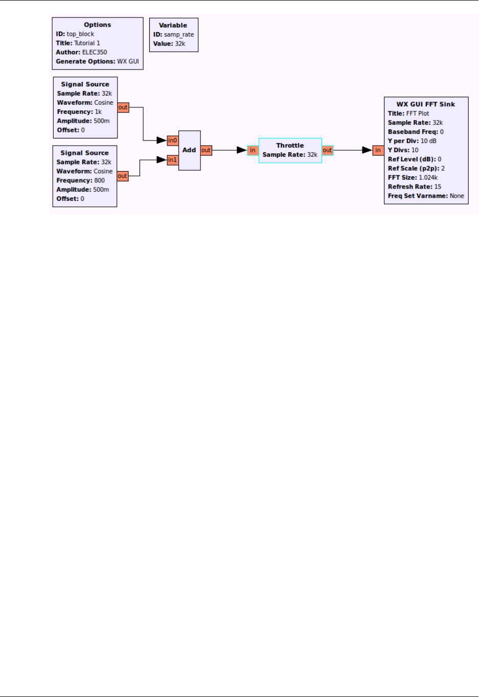
Math Operations

Construct the flow graph shown below. Set the sample rate to 32000. The two Signal Sources should have

frequencies of 1000 and 800, respectively. The Add block is found in the Math Operators category.

ELEC350: Communica-

tions Theory and Systems I

Generate and execute the flow graph. On the Scope plot you should observe a waveform corresponding

to the sum of two sinusoids. On the FFT plot you should see components at both 800 and 1000 Hz. Un-

fortunately, the FFT plot does not provide enough resolution to clearly see the two distinct components.

Note that the maximum frequency displayed on this plot is 16 kHz. This is one-half of the 32 kHz sample

rate. In order to obtain better resolution, we can lower the sample rate. Try lowering the sample rate to 10

kHz. Recall that for an FFT, the frequency resolution f0=fs/N where fs is the sample rate and N is the FFT

block size. Thus for fixed value of N, f0 goes down as fs goes down.

Replace the Add block with a Multiply block. What output do you expect from the product of two sinusoids?

Confirm your result on the Scope and FFT displays.

Take note of the other math operations under the Math Operators category and experiment with a few to

see if the result is as expected.

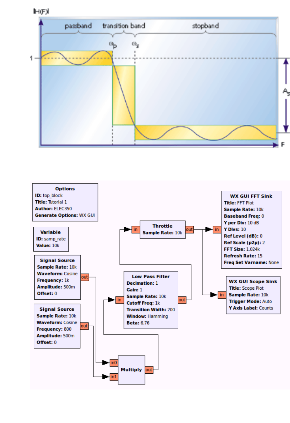
Filters

Modify the flow graph to include a Low Pass Filter block as shown in the figure below. This block is

found in the Filters category and is the first Low Pass Filter listed. Recall that the Multiply block outputs

a 200 Hz and a 1.8 kHz sinusoid. We want to create a filter that will pass the 200 Hz and block the 1.8 kHz

component. Double-click the block to open the properties dialog. Set the low pass filter to have a cutoff

frequency of 1 kHz and a transition width of 200 Hz.

ELEC350: Communica-

tions Theory and Systems I

Select the FIR Type to be Float->Float (Decimating). Generate and execute the flow graph. You should

observe that only the 200 Hz component passes through the filter and the 1.8 KHz component is attenuated.

How many dB down is the 1.8. KHz wave compared to the 200 Hz wave? Experiment with the High Pass

Filter.

ELEC350: Communica-

tions Theory and Systems I

Using the same flow graph, change the sample rate variable to 20000. Change the Decimation in the Low

Pass Filter to 2. Decimation decreases the number of samples that are processed. A decimation factor of

two means that the output of the filter will have a sample rate equal to one-half of the input sample rate,

or in this case only 10000 samples/sec. This is a sufficient sample rate for the frequencies that we are

dealing with. Generate and execute the flow graph. What frequency do you observe on the FFT? Measure

it precisely by letting the cursor hover over the peak of the observed component.

You should have observed that the FFT is now measuring a signal around 400 Hz, rather than the expected

200Hz. Why is this error occurring? It is because the sample rate on the FFT has not been adjusted to

properly measure its input. Double-click on the FFT Sink block and change the sample rate to samp_rate/2.

Generate and execute the flow graph. You should now read the correct frequency. It is important to be

aware of the sample rate in each branch of your flowgraph. Decimation and Interpolation options decrease

and increase the sample rate respectively.

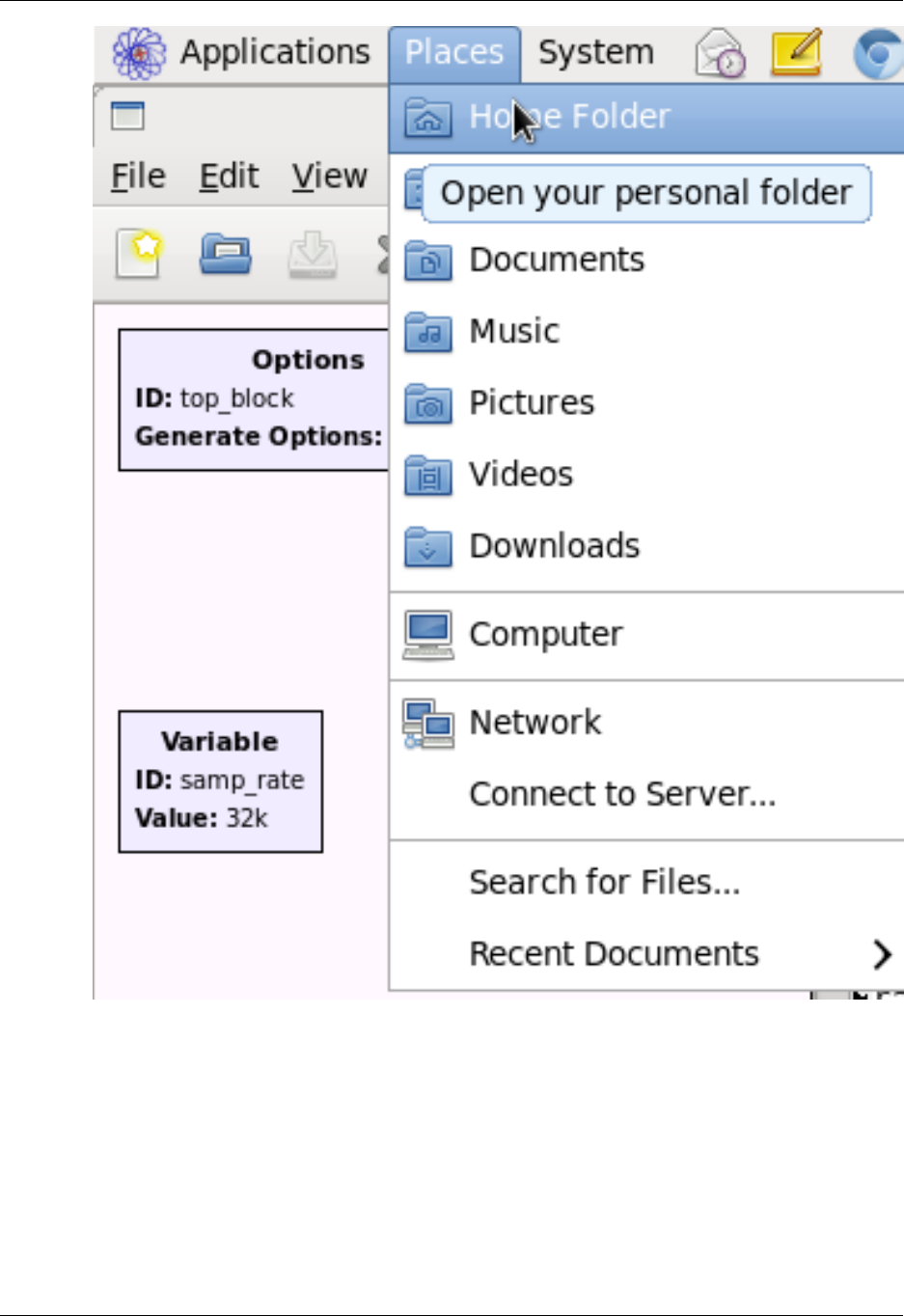
Running Generated Python Code

Open a file browser by going to Places->Home Folder as shown below.

ELEC350: Communica-

tions Theory and Systems I

Browse to the directory that contains the GRC file that you have been working on. If you are unsure as to

where this is, the path to this file is shown in the bottom portion of the GRC window. In addition to saving

a ".grc" file with your flow graph, note that there is also a file titled "top_block.py". This is the Python file

that is generated by GRC. It is this file that is being run when you execute the flow graph.

ELEC350: Communica-

tions Theory and Systems I

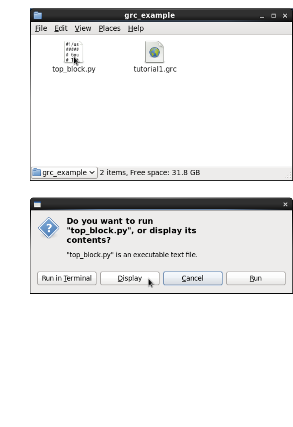
Double-click on this file. You will be given the option to Run or Display this file.

Select Display. You can modify this file and run it from the terminal window. This allows you to use

features that are not included in GRC. Keep in mind that every time you run your flow graph in GRC, it

will overwrite the Python script that is generated. So, if you make changes directly in the Python script

that you want to keep, save it under another name.

To learn more about writing flowgraphs directly in Python, see this code example [http://gnuradio.org/

redmine/projects/gnuradio/wiki/TutorialsWritePythonApplications#A-first-working-code-example].

It is possible to change the file name of the generated Python code by changing the ID field in the

flowgraph's Options block.

Conclusions

In this tutorial, you have learned several of the basic concepts in using GRC. Make a brief list of these

concepts. When you are comfortable with this material, feel free to move on to tutorial 2.

ELEC350: Communica-

tions Theory and Systems I

Tutorial 2: Variables and Controls

Objectives

This tutorial illustrates some of the features available in GNU Radio Companion such as sliders and other

variable input options. In this tutorial you will learn how to:

• add GUI controls such as sliders and radio buttons to your flowgraph.

• use variables to connect controls to different flowgraph parameters.

Working with Sliders

Launch GRC as done in the previous tutorial. If GRC is already open, simply create a new flowgraph by

selecting File->New.

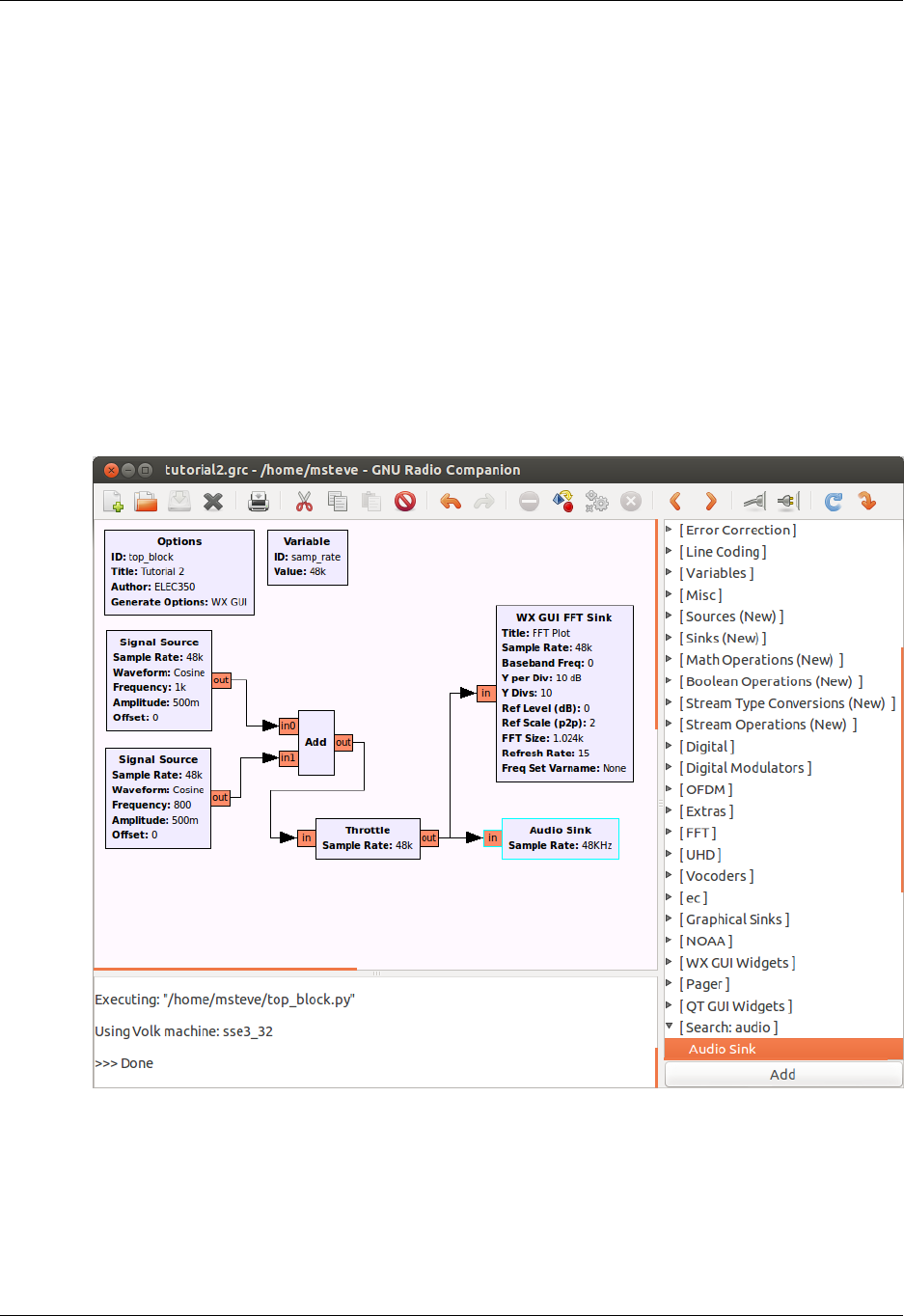
Construct the flow graph shown below. Note that the sample rate is set to 48000 in this example.

Execute the flow graph. You should hear the composite tone and see the FFT sink display of the spectrum.

Experiment with the FFT size in the FFT sink. It should be a power of two. Note that as you increase the

FFT size the resolution of the display increases. Reset the FFT size to 1024 when you are done.

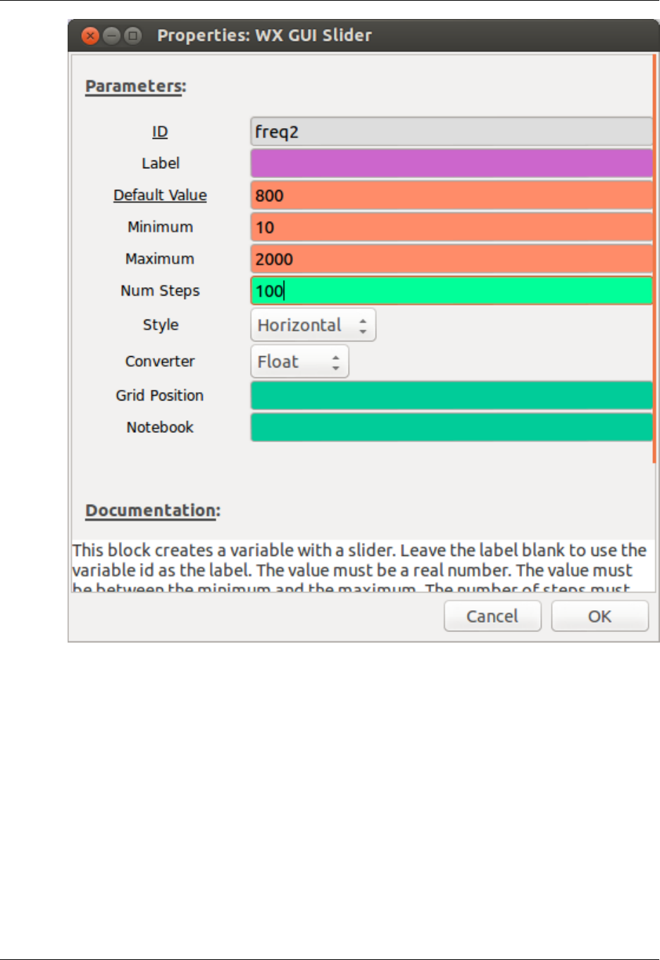
Add a WX GUI Slider (from the GUI Widgets->WX category) to the flow graph. Double-click on the block

and set the parameters as shown below.

ELEC350: Communica-

tions Theory and Systems I

Execute the flow graph. This time when the FFT sink display opens you will see a horizontal slider at

the top. Move the slider back and forth to change the value of freq2 between 10 and 2000. You should

observe that this does not change the spectrum or the sound. This is because freq2 has not been assigned

to control anything.

Double-click on the bottom Signal Source (the one set to 800 Hz). Replace the frequency (800) with freq2.

Execute the flow graph. You should now observe that both the spectrum and the sound change as you vary

the frequency of the Signal Source using the slider.

Working with Text Boxes

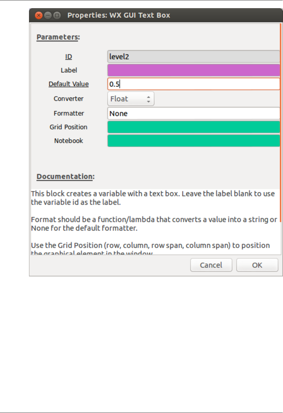
Add a WX GUI Text Box to the flow graph (GUI Widgets->WX category). Set the parameters as shown

in the figure below.

ELEC350: Communica-

tions Theory and Systems I

Double-click on the bottom Signal Source and replace the Amplitude (0.5) with the variable, level2. Exe-

cute the flow graph. Note that a text box will now appear in the display. The default value of 0.5 will be

entered. Change the value to 0.1 followed by Enter. The volume of the 800 Hz tone will decrease and this

will be reflected on the spectrum plot. Do not vary the level above 1.0.

Working with Choosers

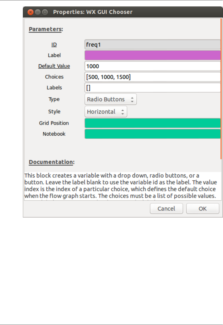
Add a WX GUI Chooser block to the flow graph. This block will add either a drop down menu, radio

buttons or a button. Input the parameters as shown in the figure below.

ELEC350: Communica-

tions Theory and Systems I

Change the Frequency of the top Signal Source (1 kHz) to freq1. Execute the flow graph and change the

frequency of the top Signal Source using the radio buttons. Experiment with the Drop Down menu and

the Button to see how they work.

Working with Notebooks

Add a WX GUI Notebook block to the flow graph. This control allows you to arrange large GUI components

(scope, FFT, waterfall, etc) into a tabbed notebook.

Set the ID field to notebook_0 (this should be the default). Set the Labels field to ['Scope', 'Spectrum'].

Note that this field is entered in Python list syntax and is expecting a list of strings. The square brackets

indicate the list while the single quotes indicate the string. The comma is the separator between list items.

Add a WX GUI Scope Sink to the flowgraph and connect it to the output of the Throttle block. Double click

this block and set the Type to Float and set the Notebook to notebook_0,0, where notebook_0 indicates

the notebook control where you would like the element to appear and the second 0 indicates the list index

ELEC350: Communica-

tions Theory and Systems I

of the label you would like it to appear under. In this case, 0 points to the list index of 'Scope'. Close the

properties dialog.

Double click the WX GUI FFT Sink to open the properties dialog. Set the Notebook to notebook_0,1. The

1 points to the list index of 'Spectrum' that was configured in the Labels field of notebook_0. Close the

properties dialog.

Execute the flowgraph. The scope and FFT views should now be visible on separate tabs labeled "Scope"

and "Spectrum" repsectively.

Conclusions

In this tutorial you have learned how to add GUI controls to your flowgraph and how to use them to control

different parameters of the flowgraph. These skills will be useful when creating a tunable AM receiver in

the next tutorial. When you feel comfortable with this material, please feel free to move on to Tutorial 3.

Tutorial 3A: AM Signal waveforms

Objectives

This tutorial is a guide to AM signal waveforms. In this tutorial you will learn:

• Theory and equations of AM signals and the complex mixer

• How to construct an AM transmitter flowgraph to generate an AM waveform with a sinusoidal message

and observe the waveform and spectrum

• Construction of AM transmitter flowgraphs with square wave and pseudo-random data messages

• AM receivers are covered in the next Tutorial 3B

AM flowgraphs

Review the theory in the AM transmitter theory [data/AM_theory_TX2.pdf]

Carry out the steps in the AM Transmitter procedures [data/AM_procedures_TX.pdf]

The following GRC files will be a useful starting point:

• AM_TX.grc [data/AM_TX.grc]

• different_waveforms.grc [data/different_waveforms.grc]

Start GRC as was done in the previous tutorials. If GRC is already open, simply create a new flowgraph

by selecting File->New.

Tutorial 3B: Receiving AM Signals

Objectives

This tutorial is a guide to building a practical AM receiver for receiving real AM signals. For the first

part, it uses a data file with one AM signal in it, generated using the flowgraphs in section 3A. In this first

part, you will learn how to:

ELEC350: Communica-

tions Theory and Systems I

• demodulate an AM signal using only real signals.

For the second part, we use a data file that contains several seconds of recorded signals from the AM

broadcast band. In this second part you will learn how to:

• use a pre-recorded file as the input to your flowgraph.

• tune to a specific (desired) AM signal on a given carrier frequency.

• filter out the undesired signals using other (different) carrier frequencies.

• demodulate the desired AM signal using complex signals.

Real signals, basic AM receiver

Review the theory of AM receivers using real signals [data/AM_theory_RX.pdf]

Carry out the steps in the AM receiver procedures [data/AM_procedures_RX.pdf]

Complex signals, receiver with channel selection (tuning)

Review the theory of AM receivers using complex signals [data/AM_theory_RX2.pdf]

Click here [data/am_usrp710.dat] to download the data file used in this tutorial. Save it in a location that

you can access later. This file was created using a USRP receiver.

The following GRC file will be a useful starting point:

• AM_PB_RX.grc [data/AM_PB_RX.grc]

Start GRC as was done in the previous tutorials. If GRC is already open, simply create a new flowgraph

by selecting File->New.

Playing a Data File

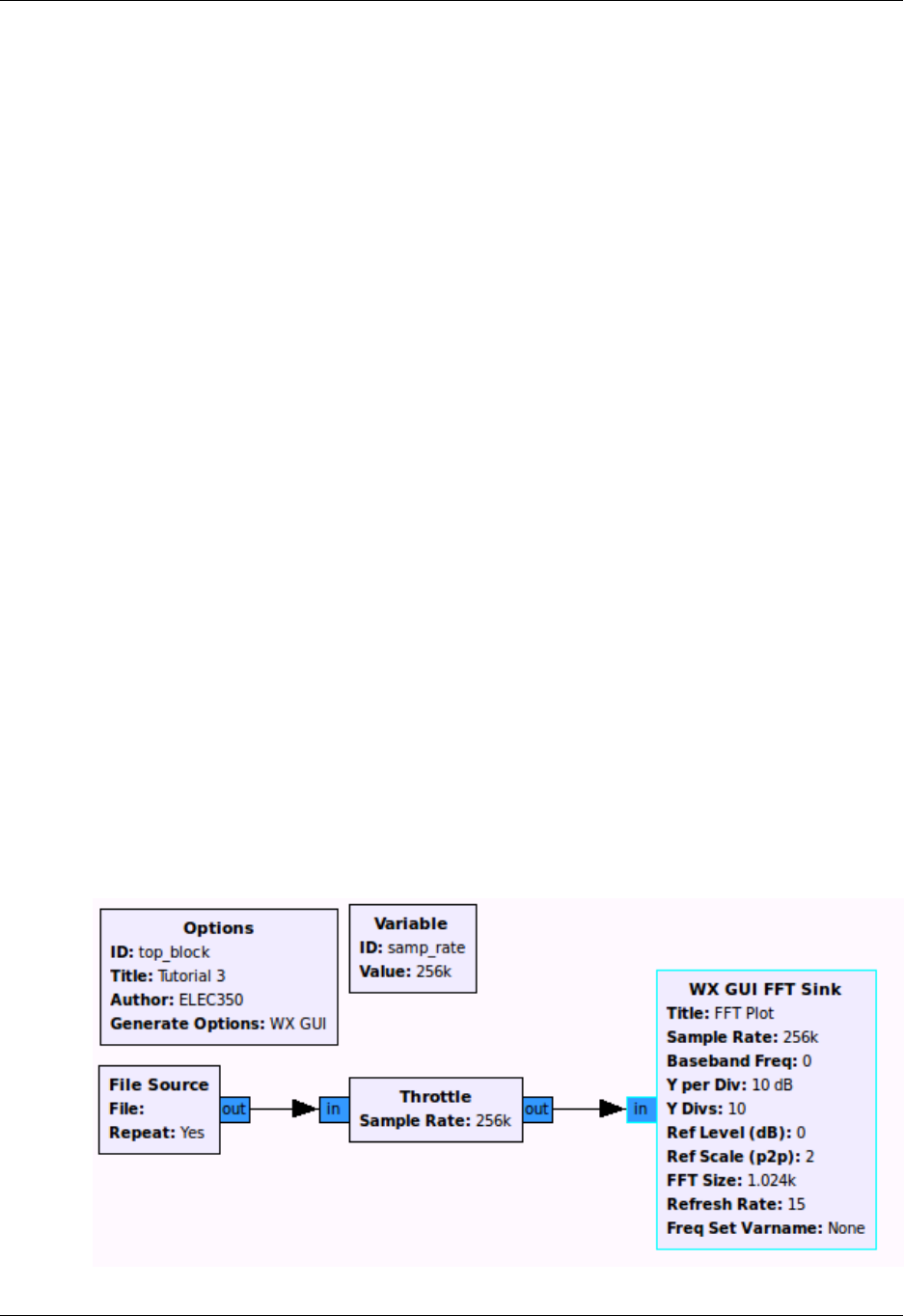
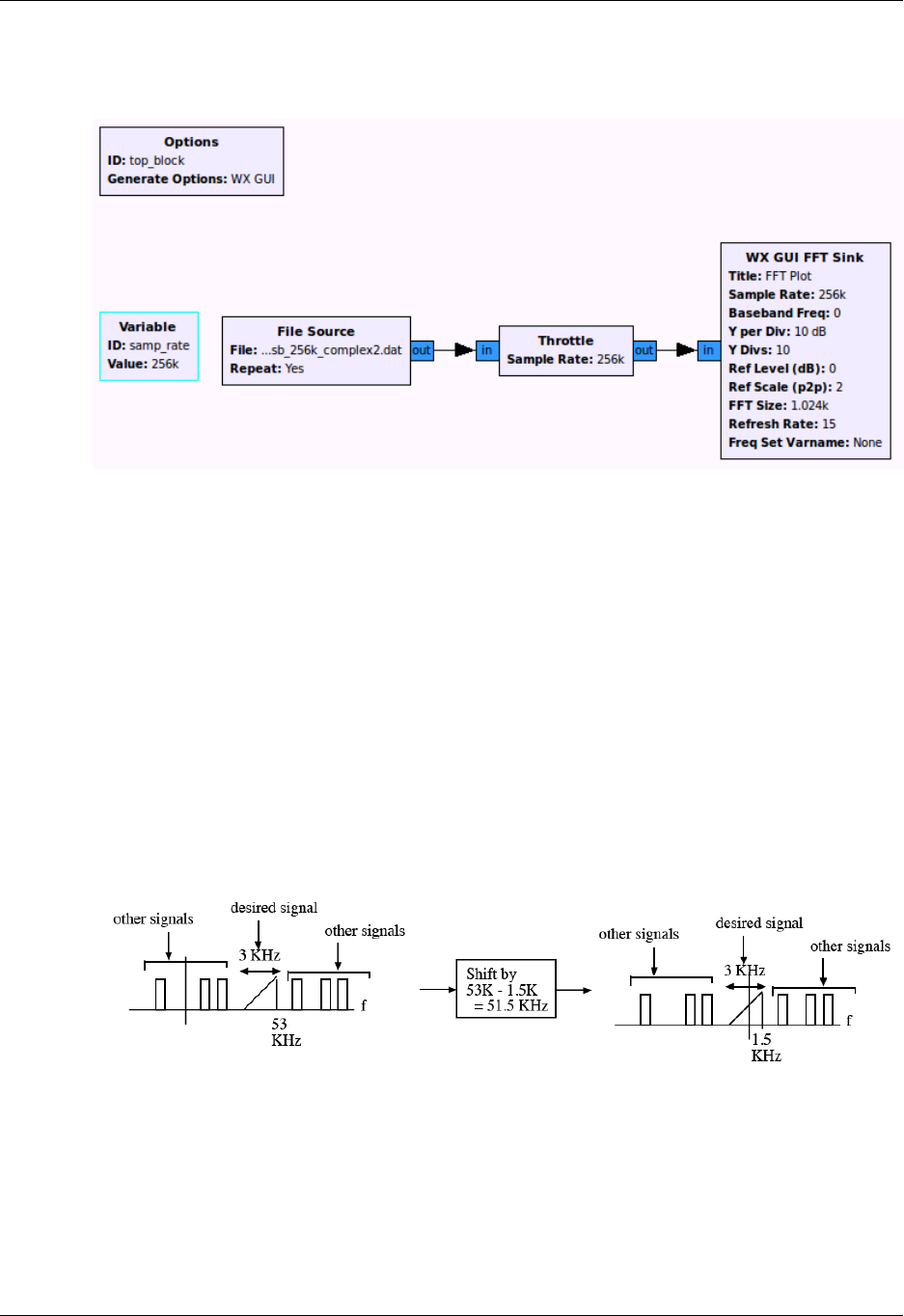
Construct the flow graph shown below consisting of a File Source, Throttle, and WX GUI FFT Sink. Set

the sample rate in the variable block to 256000. This is the rate at which the saved data was sampled.

ELEC350: Communica-

tions Theory and Systems I

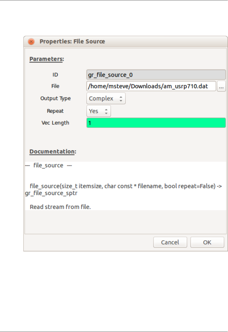
Double-click on the File Source block. Click on the ellipsis (…) next to the File entry box. Locate the

am_usrp710.dat file that you saved in the previous step. The path to your file will appear as shown in the

figure below. Set the Output Type to Complex. The use of complex data to describe and process waveforms

in SDR will be discussed in the next tutorial. Set Repeat to Yes. This will cause the data to repeat so that

you have a continuously playing signal.

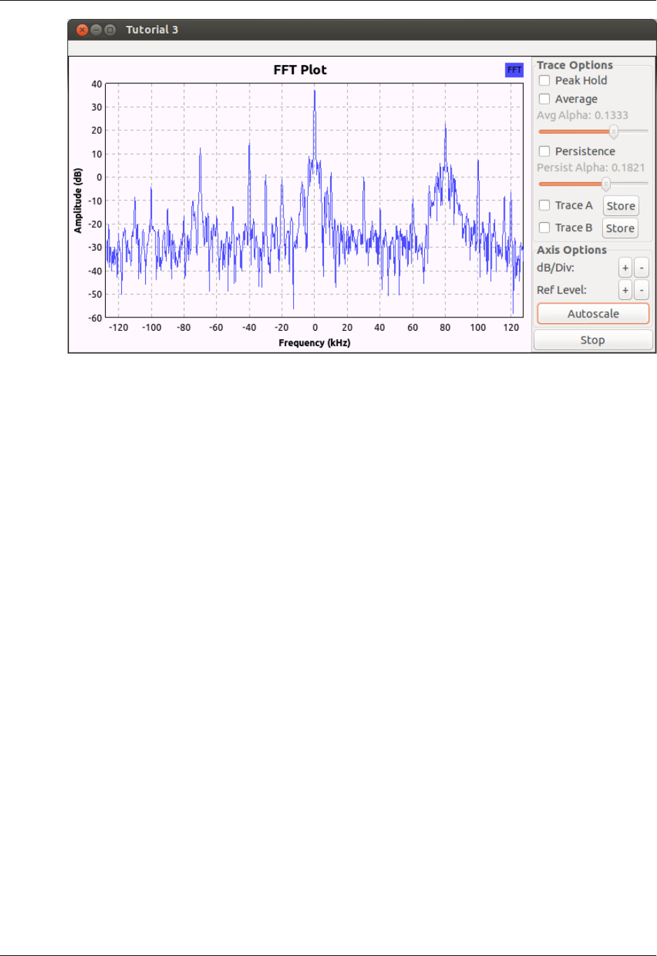
Save and execute the flow graph. You should observe an FFT display similar to the one shown below.

You may need to click on Autoscale button to scale the data as shown. Note the following:

• This data was recorded with a USRP set to 710KHz. Thus, the signal you see at the center (indicated as 0

KHz) is actually at 710 KHz. Similarly, the signal at 80 KHz is actually at 710KHz + 80KHz = 790KHz.

• The display spans a frequency range from just below -120KHz to just above 120KHz. This exact span

is 256KHz, which corresponds to the sample rate that the data was recorded at.

• The peaks that you observe on this display correspond to the carriers for AM broadcast signals. You

should also be able to observe the sidebands for the stronger waveforms.

ELEC350: Communica-

tions Theory and Systems I

Frequency Display Resolution

In this step we will expand the frequency scale on the FFT display so that you can view the signals with

greater resolution. Recall from the previous tutorial that the span of the frequency axis is determined by

the sample rate (256 kHz for this file). While we cannot change the original data, we can resample it to

either increase or decrease the sample rate. We will decrease the sample rate by using decimation. Modify

the flow graph as follows:

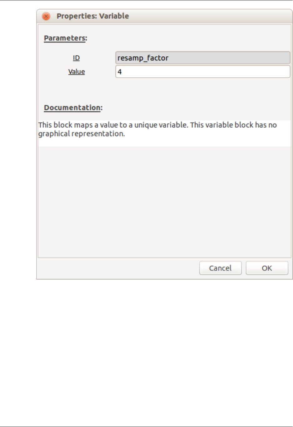
• Add a Variable block (under Variables category). Set the ID to resamp_factor and the Value to 4 as

shown below.

ELEC350: Communica-

tions Theory and Systems I

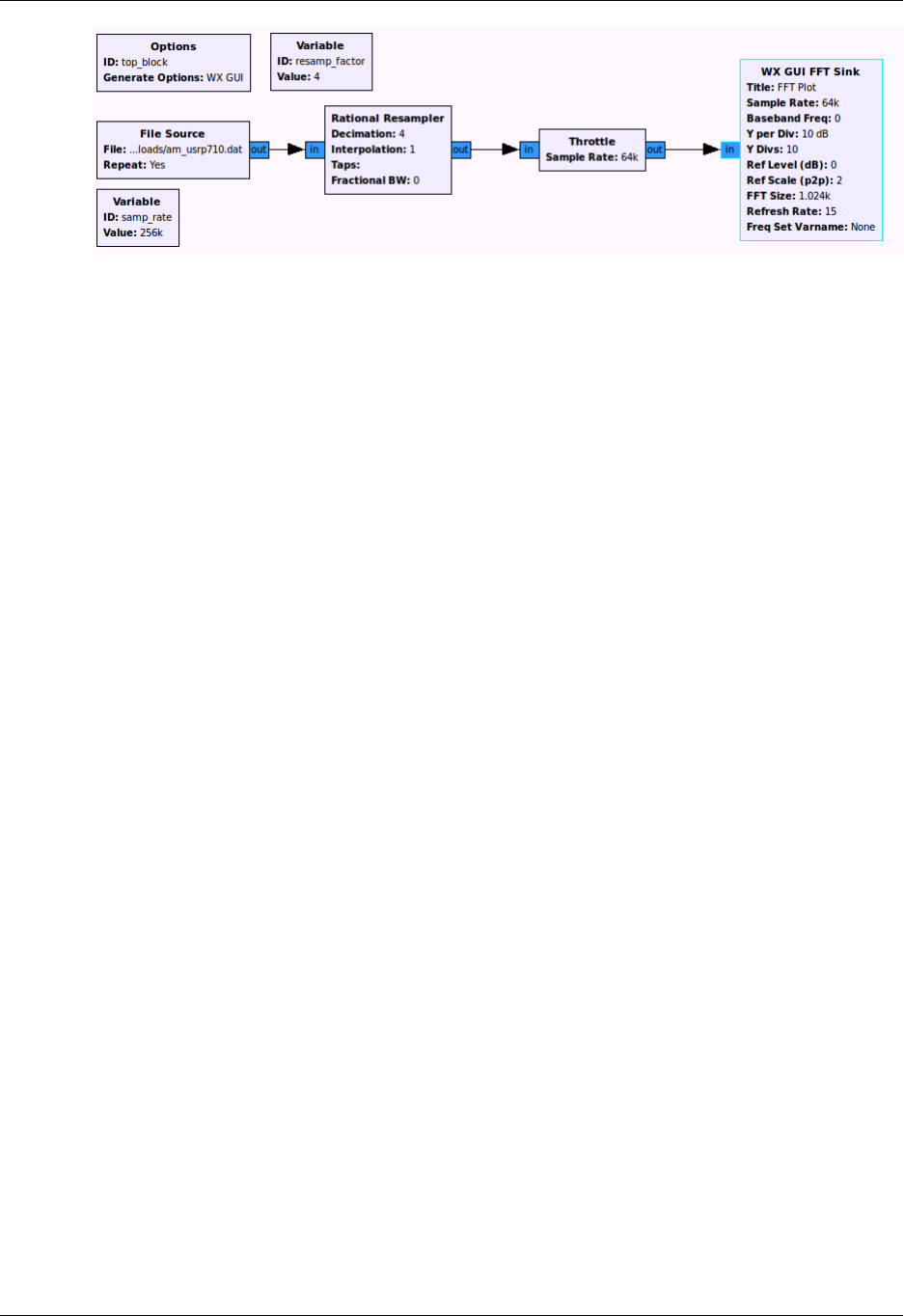
• Add the Rational Resampler block from the Filters menu as shown below. Set its decimation factor to

resamp_factor. It will use the value of the variable set in the previous step (4) to decimate the incoming

data. That means that it will divide the incoming data rate by the decimation factor. In this example, the

incoming 256K samp/sec data will be converted down to 256K/4 = 64K samp/sec.

• Note that the Throttle and FFT Sink now need their sample rates changed to correspond to this new rate.

Change the sample rate in both of these blocks to samp_rate/resamp_factor. Now we can change the

decimation factor in the Variable block and it will be reflected in each of the other blocks automatically.

• Your flow graph should now appear as shown below.

ELEC350: Communica-

tions Theory and Systems I

Execute the new flow graph. You should now observe a frequency span of only 64 kHz (-32 kHz to +32

kHz). What actual frequency range does this correspond to?

Selecting one channel by filtering

The bandwidth of an AM broadcast signal is 10 kHz (+/- 5 kHz from the carrier frequency). You may find

it useful to click the Stop button on the FFT plot to see this more clearly. Also, note that many stations

also include additional information outside of the 10 kHz bandwidth.

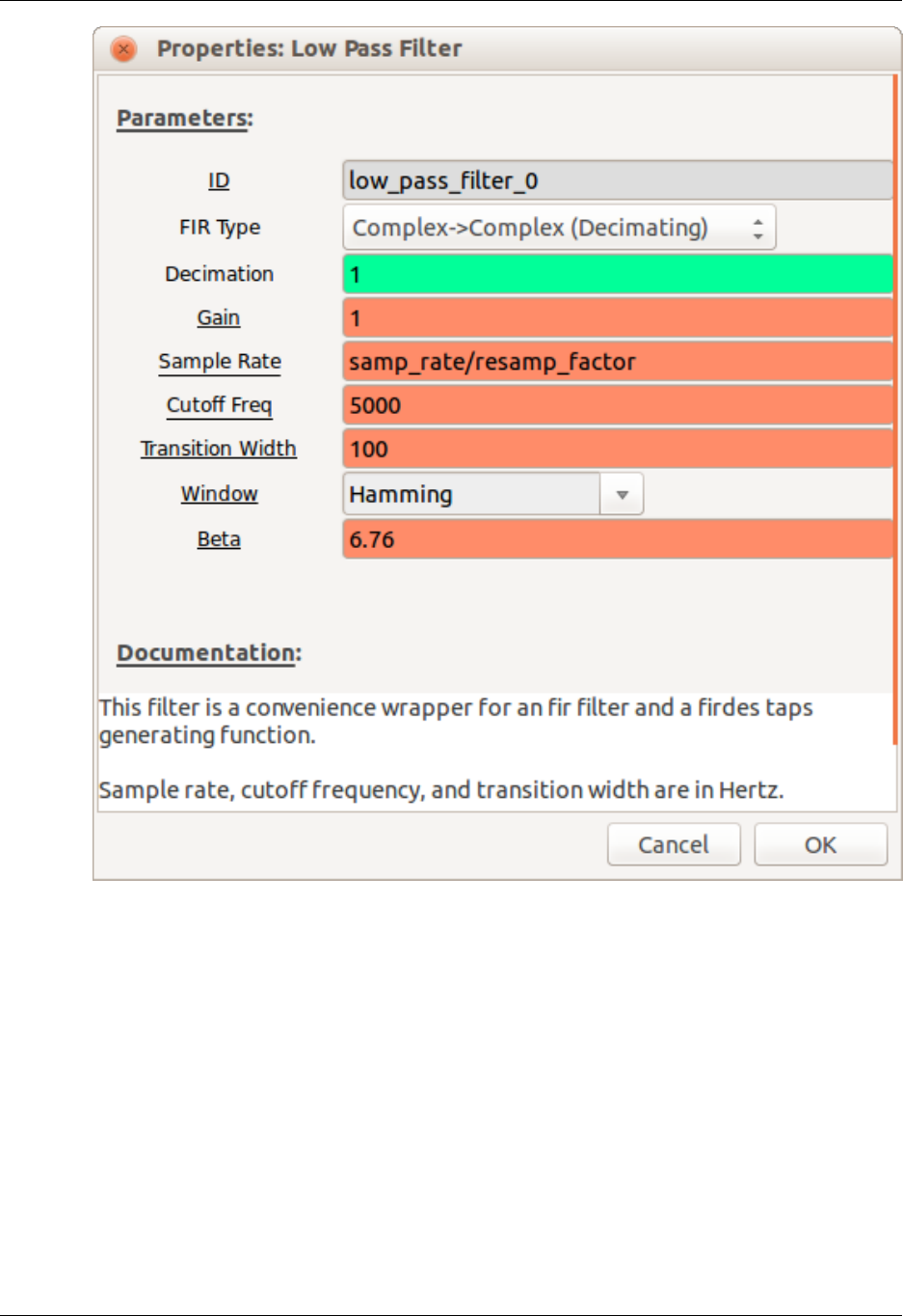
In order to select the station at 710 kHz (0 kHz on the FFT display) we need to insert a filter to eliminate

all but the one station that we want to receive. This is often referred to as a channel filter. Since the station

at 710 kHz has been moved to 0 kHz (in the USRP) we will use a low pass filter. The station bandwidth is

10 kHz, so we will use a low pass filter that cuts off at 5 kHz. Insert the Low Pass Filter (from the Filters

menu) between the Rational Resampler and the Throttle. Set the parameters as shown below.

ELEC350: Communica-

tions Theory and Systems I

Execute the flow graph. You should see that only the station between +/- 5 kHz remains.

AM Demodulation

The next step is to demodulate the signal. In the case of AM, the baseband signal is the envelope or

the magnitude of the modulated waveform. GNU Radio contains a Complex to Mag block (in the Type

Converters category) that can be used for this purpose. Again, the use of complex signal representation

will be dealt with in depth in the future. Insert this block between the Low Pass Filter and the Throttle.

Note that the titles of some of the blocks are now red and the Execute Flow Graph icon is dimmed. This

indicates an error. Prior to adding this block, all of the block inputs and outputs were complex values.

However, the output of the Complex to Mag block is Float (a real number). Thus, any blocks following

this block should be Type: Float. Modify the Throttle and WX GUI FFT Sink accordingly.

Execute the flow graph. You should now observe the spectrum of the baseband signal in the FFT Sink. Note

that since the input data type to the FFT Sink is Float, only the positive frequency spectrum is displayed.

ELEC350: Communica-

tions Theory and Systems I

Matching the Audio Sample Rate

The next step is to listen to this demodulated waveform to confirm that it is in fact receiving the baseband

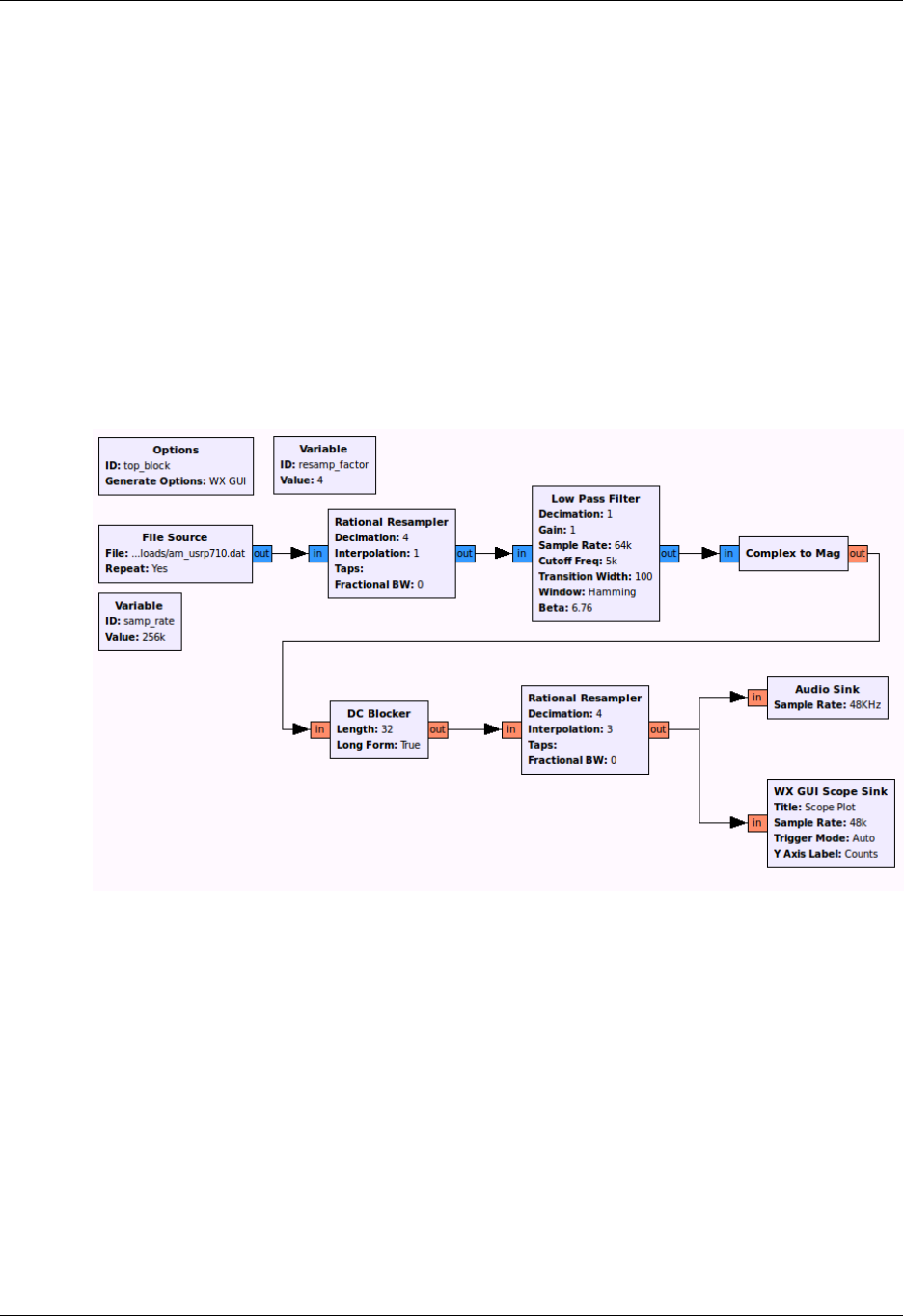
signal. Remove the Throttle and the FFT Blocks. Add an Audio Sink block to the output of the Complex

to Mag block. Set the sample rate of the Audio Sink to 48 kHz.

Note that the sample rate out of the Complex to Mag block is 64 kHz and the input to the Audio Sink is 48

kHz. In order to convert 64 kHz to 48 kHz we need to divide (decimate) by 4 and multiply (interpolate) by

3. Insert a Rational Resampler between the Complex to Mag and Audio Sink blocks and set the decimation

and interpolation as noted above. Also set its Type to Float->Float (Real Taps).

Since the output of the Complex to Mag is always positive, there will be a DC offset on the audio signal.

The signal going to the audio hardware should not have any DC offset. Place a DC Blocker (in the Filters

category) between the Complex to Mag block and the Rational Resampler added in the previous step.

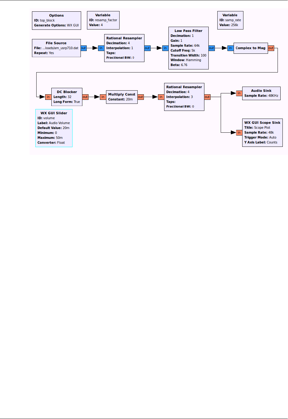
Place a WX GUI Scope Sink at the output of the Rational Resampler (in addition to the Audio Sink). Change

its Type to Float and set its sample rate to 48000. The flow graph should be similar to the one shown below.

Execute the flow graph. The WX GUI Scope Sink should open and display the output waveform. However,

you may not yet hear the audio from your speaker or it may be very distorted. This is due to the fact that

the values of the samples going in to the Audio Sink block are outside the range expected by the Audio

Sink. The Audio Sink requires that the sample values are between -1.0 and 1.0 in order to play them back

through the audio hardware.

Adding a Volume Control

Insert a Multiply Const block from the Math Operators category between the DC Blocker and the Rational

Resampler. Set the IO Type of the block to Float.

Add a WX GUI Slider block. Set the parameters as shown below.

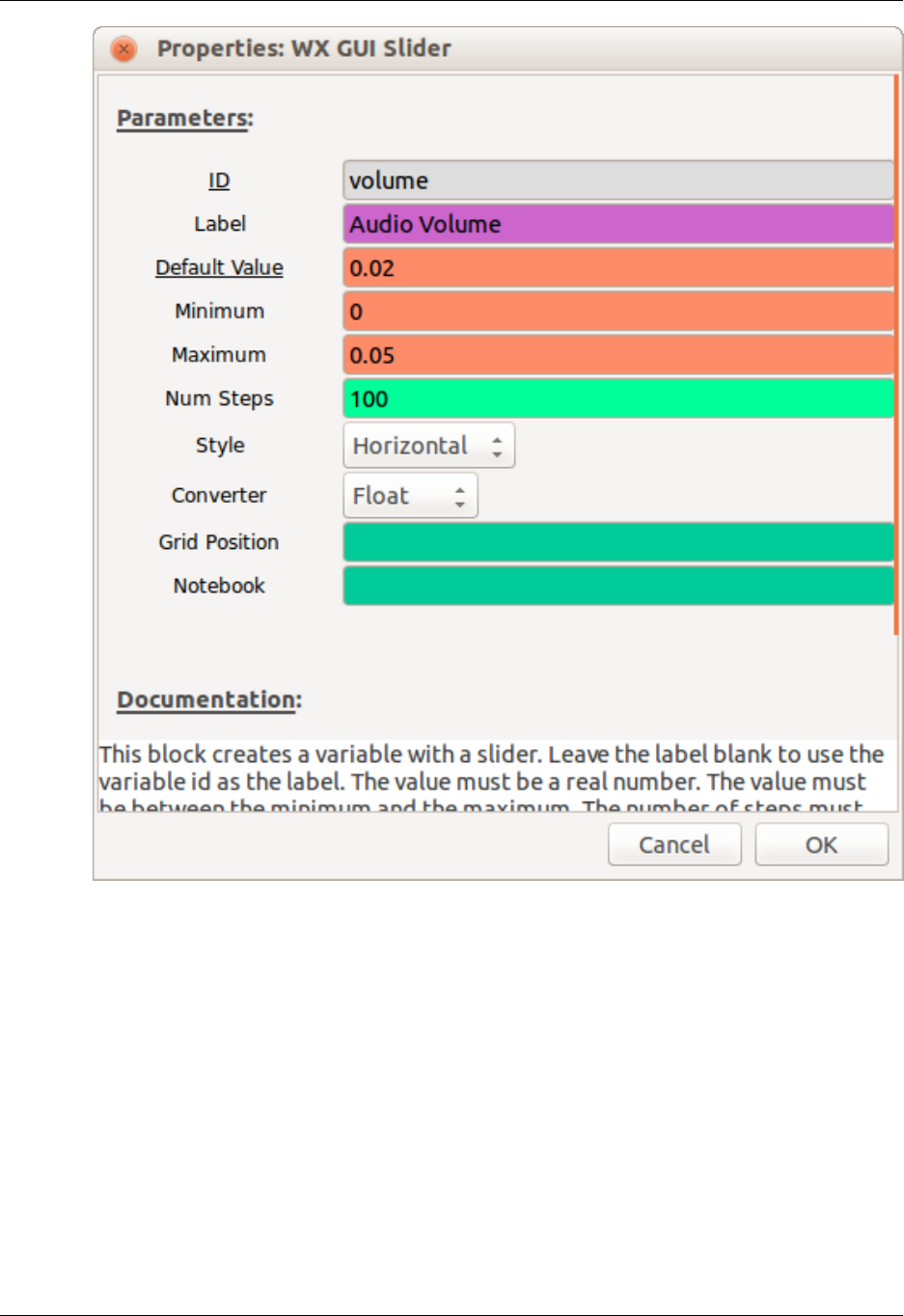
ELEC350: Communica-

tions Theory and Systems I

Set the constant in the Multiply Const block to "volume" so that the slider controls it. The final flow graph

is shown below.

ELEC350: Communica-

tions Theory and Systems I

Execute the flow graph. You should now hear the demodulated AM signal. Stop the flowgraph.

Double click on the Low Pass Filter. Note that it can also decimate. Change the decimation in the Low Pass

Filter block to resamp_factor and set the sample rate back to samp_rate. Remove the Rational Resampler

between the File Source and the Low Pass Filter. The filter now handles both operations. Test the receiver

again.

Tuning to a desired station (channel)

Review the theory of tuning to a radio station [data/350-2015-tuning.pdf].

Place an FFT Sink at the output of the File Source, leaving the rest of the flow graph unchanged. Execute

the flow graph and observe the location of the other stations in the spectrum. Note that there is a fairly

strong signal at 80 KHz (really 710 + 80 = 790 KHz).

In order to receive this signal we need to shift it down to zero frequency so that it will pass through the

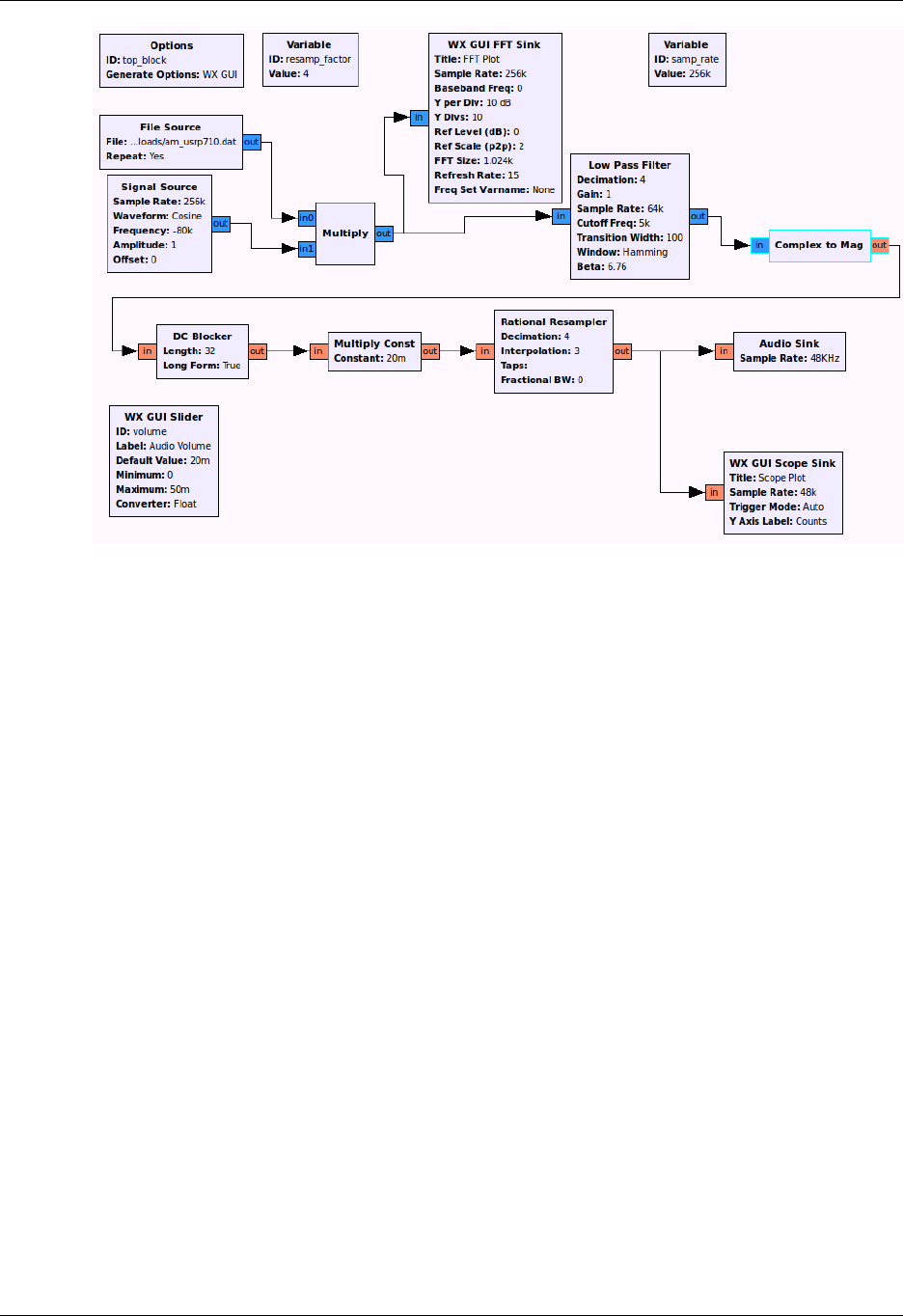
low pass filter. One way to accomplish this is to multiply it by a sinusoid. Modify the flow graph as

shown below. Add a Signal Source and set its parameters to output a cosine at a frequency of -80000. This

negative frequency will shift the entire spectrum to the left by 80KHz. Use a Multiply block and move the

FFT Sink to observe its output. Test this receiver.

ELEC350: Communica-

tions Theory and Systems I

Add another WX GUI Slider so that you can adjust the frequency with a slider. Set the minimum to -

samp_rate/2 and the maximum to samp_rate/2. Test your flow graph and demonstrate that it works. You

may need to adjust your volume slider for each station. This is because the stations are at varying distances

away from the receiver and have different transmitted power. (Remember the link equation?)

Automatic Gain Control

The volume adjustment can be automated with an Automatic Gain Control (AGC) block. This block works

by sampling its own output and adjusting its gain to keep the average output at a particular level. Insert the

AGC block (found under Level Controls) between the Low Pass Filter and the Complex to Mag block. The

AGC will adjust the gain so that the sample values are always in a suitable range for the audio hardware.

Leave the parameters at their default values.

You can now remove the Multiply Const and volume slider. Test the receiver again. Adjust the volume to

a comfortable level using the computer's volume control on the first station you hear. Now tune up and

down the band and notice that you no longer need to adjust the volume, but the noise level increases for

weaker stations. The radio functions the same as a hardware radio.

Tutorial 4: Complex Signals and Receiving SSB

Objectives

This tutorial is a guide to receiving SSB signals. It will also illustrate some of the properties of complex

(analytic) signals and show why we use them in communications systems. In this tutorial you will:

• Use the discrete Hilbert transform to create a complex signal from a real signal.

• Use a frequency-translating filter to perform filtering and tuning in one step.

• Construct an SSB demodulator using Weaver's Method.

ELEC350: Communica-

tions Theory and Systems I

Complex/Analytic Signals

Review the theory of analytic signals and SSB receivers [data/SSB_theory.pdf].

Open a new flow graph in GRC. Create the simple flow graph shown in the figure below. Set the Type in

each of the three blocks to Float as you have in the past. Other than that you can leave all of the values

at their default settings.

Execute the flow graph. The scope sink should open and display a sinusoidal signal. Convince yourself

that this signal has the amplitude and frequency that you expect.

Modify the flow graph by changing the Type in each of the three blocks to Complex. Execute the flow

graph. Your scope plot should now display two sinusoids that are 90° out of phase with each other. The

leading (channel 1) wave is the I or in-phase component of the complex signal and the lagging (channel

2) wave is the Q or quadrature component. When a signal source is set to Complex, it will output both

the I and Q components.

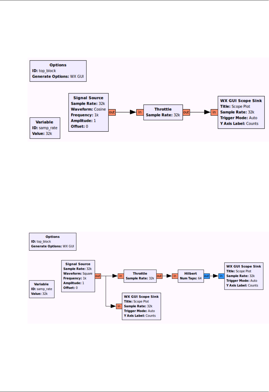
Modify your flow graph as shown in the figure below. The Signal Source should be set to output a Square

wave with a Type of Float. Thus, the first Scope Sink and the Throttle must also be set to accept Float

values.

The Hilbert block is found in the Filters category. This block outputs both the real input signal and the

Hilbert transform of the input signal as a complex signal. Leave the number of taps at its default setting of

64. Since the output of this block is complex, the second Scope Sink must be set to accept complex inputs.

Execute the flow graph. Two scope plots should open. One should contain the square wave output from

the Signal Source only. The other should include both the original square wave and its Hilbert Transform.

Do you understand why the Hilbert transform of a square wave looks this way?

ELEC350: Communica-

tions Theory and Systems I

As shown above, the Signal Source can be set to output a complex signal and display both the I and Q

components. Modify the flow graph as shown below.

Set the Signal Source to output a complex waveform. Make sure the Throttle and Scope Sink are also set to

complex. Execute the flow graph. Is the complex waveform displayed here the same as the one obtained

from the Hilbert transform? Your answer should be NO. This is incorrect. GRC is NOT displaying the

correct Q component of a complex square wave. The Hilbert transform did output the proper waveform.

Create the flow graph shown below. Make sure that all of the blocks are set to Type: Float. This flow

graph takes two sinusoids, at frequencies of 1KHz and 10 KHz and multiplies them together. Using a

trigonometric identity we know that the product of two cosines gives two cosines at the sum and difference

frequencies of the original signals. In this case we expect outputs at 9 kHz (difference) and 11 kHz (sum).

Execute the flow graph and confirm this result. Note that the FFT plot only shows the positive frequency

spectrum when it is set to Type: Float. We know that for real inputs the negative frequency components

are the same as positive frequency components.

Change ALL of the blocks to Type: Complex and execute the flow graph again. You should now observe

a single output at 11 kHz. This is the original 10 kHz signal shifted by the 1 kHz signal. If we want to shift

in the negative direction a frequency of -1000 can be used. Try this. From this example we see two of the

primary advantages of using analytic signals. A signal can be shifted (sum) without creating an additional

difference signal. Also, note that there are NO negative frequency components. Why is this?

Single Sideband (SSB) Signals

Click here [data/ssb_lsb_256k_complex2.dat] to download the data file used in this tutorial

ELEC350: Communica-

tions Theory and Systems I

Create a new flow graph as shown in the figure below. The File Source should be set to the data file

that you just downloaded. The Variable block which sets the sampling rate (samp_rate) should be set to

256000 as this is the data rate that the received signal was sampled at. The Throttle and FFT Sink can be

left at their default settings.

Execute the flow graph. After the FFT Plot window opens, adjust the Ref Level so that the amplitude values

start at 10 dB and set the dB/div to 10dB/div. You should view a section of the spectrum that is 256 kHz

wide (due to the sample rate). Note that there is one signal visible between 40 and 60 kHz.

When this signal was recorded, the USRP was set to a frequency of 50.3 MHz. Thus, the 0 kHz point on

the display corresponds to 50.3 MHz. While the FFT Plot is displayed move the cursor over the signal and

note the frequency along its right edge. It should be approximately 53 kHz. Since this is a lower sideband

(LSB) signal, this corresponds to the carrier frequency. Because the "zero" frequency corresponds to 50.3

MHz, the original carrier frequency of signal was 50.3 MHz + 53 kHz = 50.353 MHz. However, now that

the spectrum has been shifted down by 50.3 MHz, we use the carrier frequency of 53 kHz.

Frequency Translating Filter

The first step in building a receiver is to use a channel filter to pass the signal of interest and filter out

the rest of the signals in the band. The first step in this process is to shift the signal of interest down to

zero frequency as shown below.

The second step is to apply a low pass filter so that the other signals will be filtered out.

ELEC350: Communica-

tions Theory and Systems I

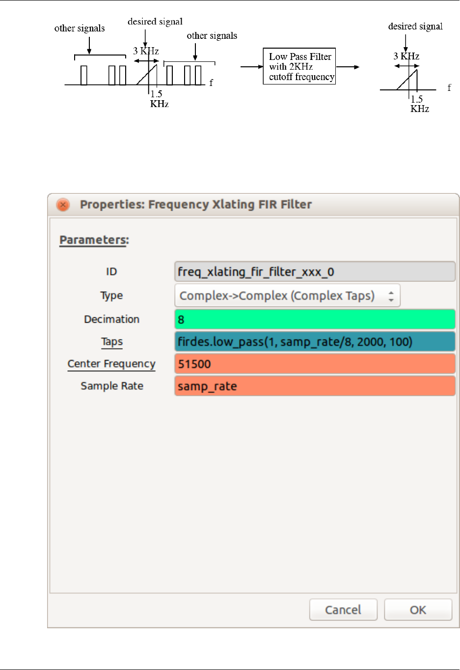
In GRC, the Frequency Xlating FIR Filter performs both of these operations. Insert this block between

the File Source and the Throttle. Complete the properties window as shown below. The center frequency

of 51500 will shift the entire spectrum down by 51500 Hz. The function indicated in the Taps parameter

generates the taps for a low pass filter with a gain of 1 (in the pass band), a sampling rate equal to samp_rate

(256 kHz), a cutoff frequency of 2 kHz and a transition width of 100 Hz.

ELEC350: Communica-

tions Theory and Systems I

Execute the flow graph. You will see that your signal has now moved down to the origin and is the only

signal present. Now that we have located the signal of interest, there is no reason that we need to be

concerned with so much of the adjacent spectrum. We can reduce the range of frequencies that are being

processed by reducing the sample rate (decimation). Re-open the Frequency Xlating FIR Filter block and

change the Decimation parameter to 8. This will reduce the sample rate to 256000/8 = 32000. Change

the sample rate of the Throttle and FFT Sink to this new rate. What frequency range to you expect the

FFT to display now?

Execute the flow graph again to see if you are correct. You should now observe an expanded version of

your signal. Select Autoscale on the FFT Plot so that the peaks of the signal are observed. Notice that after

a while, the signal level will be reduced for a few seconds. That occurs when the station stops transmitting.

Using the firdes Module

In the previous step, we used the firdes module of GNU Radio. The basic usage format is

firdes.filter_type(args) where filter_type(args) is one of:

• band_pass(gain, sampling_freq, low_cutoff_freq, high_cutoff_freq, transition_width)

• band_reject(gain, sampling_freq, low_cutoff_freq, high_cutoff_freq, transition_width)

• complex_band_pass(gain, sampling_freq, low_cutoff_freq, high_cutoff_freq, transition_width)

• high_pass(gain, sampling_freq, cutoff_freq, transition_width)

• low_pass(gain, sampling_freq, cutoff_freq, transition_width)

Additionally, each of these filter types has a "_2" version (ie: band_pass_2, low_pass_2). These versions

take an extra parameter which specifies the stop band attenuation in dB.

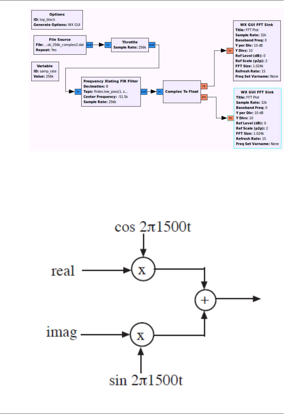
Weaver Demodulator

Recall that the signal is a complex (analytic) signal. One method of demodulating SSB voice is to operate

on the real and imaginary parts of the signal separately. The Complex to Float block will take a complex

signal and output its real (re) and imaginary (im) parts separately. Modify the flow graph to appear as

shown in the figure below. The outputs of the Complex to Float block are both real so the FFT Sinks need

to be changed to Type: Float.

ELEC350: Communica-

tions Theory and Systems I

Execute the flow graph. You should now observe the spectra of the real and imaginary parts of the signal.

Note that the signals extend out to 2KHz, the cutoff frequency of the filter.

One method of demodulating this SSB voice signal, known as Weaver’s method, takes the real and imag-

inary part of the signal and processes them as shown below. Use the Signal Source in GRC to generate

the cosine and sine waves needed to implement this demodulator. The Multiply and Add blocks can be

found in the Math Operators category.

ELEC350: Communica-

tions Theory and Systems I

Observe the output of the Add block using an FFT sink. This is the baseband signal that has been extracted

from the modulated SSB signal.

The final step is to listen to the demodulated signal. Add an Audio Sink as demonstrated in Tutorial 3.

Recall that you will need a Rational Resampler to adjust the sampling rate to one that works with the

Audio Sink. Also, you will need a multiplier to reduce the amplitude of the signal before it enters the Audio

Sink. Find a suitable value by first observing the maximum peak on a scope sink and using the reciprocal

of this value as the multiplier. Test your SSB receiver, you should hear the voice. It may be helpful to

add a waterfall sink.

The Weaver demodulator can also be implemented entirely with complex signals. Create a second SSB

receiver using only complex signals, with conversion to real just before the audio sink. Test this receiver

and confirm that it works in the same way as the receiver using real signals.

Test this receiver using a second data file found here [./da-

ta/SDRSharp_20130920_024052Z_14190kHz_IQ.wav]. This file is a wav file. To read it in GNURadio,

use a Wav File Source and a Float To Complex block. There are two SSB voice signals in this file, both

are upper sideband (USB), whereas the first data file was lower sideband (LSB). The Weaver demodulator

needs a small modification to work with USB.

A data file taken using a software receiver with a wire antenna about 6 meters above the ground is found

here [./data/SDRSharp_20130919_004154Z_14053kHz_IQ.wav]. Change the Wav File Source to read

this file, and test your receiver using this file. The file contains mostly Morse code signals, no voice signals.

Replace the fixed offset of 1500 Hz with a variable and control it with a WX GUI Slider. Explain what

happens when the slider is moved and why.

Save this flowgraph. You can modify it for use with an audio-output SDR (such as the "Softrock" described

in the next section) to listen to on-air signals by replacing the Wav File Source with an Audio Source.

"Softrock" SDR with analog IQ mixer

The "Softrock" family is a series of low-cost software-defined radio (SDR) kits that implement an IQ

mixer circuit in analog hardware.

This section is notes for reading only and is not a lab activity. These notes cover

• analog I-Q receiver functions

• observing the I-Q components on an oscilloscope

• Introduction to spectrum analyzer and the time-frequency representation of signals

• I-Q imbalance correction

• shortwave propagation of radio waves via the ionosphere

Start by reading the theory of I-Q signal, software-defined radio and the softrock kit here [http://

www.ece.uvic.ca/~elec350/lab_manual/data/350Lab0-2013.pdf]. Follow-up by reading Softrock Lite II

RX Builder's Notes [http://www.wb5rvz.org/softrock_lite_ii/], scroll down to "Theory of Operation" and

"Schematic" circuit diagram. While reviewing this information, try to keep the following questions in

mind:

• How many sections does the receiver have?

• What does each section do?

ELEC350: Communica-

tions Theory and Systems I

• What frequency does the local oscillator operate at?

• How does the mixer produce the in-phase (I) and quadrature (Q) outputs?

• Where is the Analog to Digital Converter (ADC)?

Lab 2. FM, IQ and USRP Tutorial

In this section you will use the Universal Software Radio Peripherial (USRP) for both receiving and trans-

mitting signals. The USRP is a I/Q receiver with wide bandwidth (100 MHz sampling rate), programmable

center frequency, programmable gain and choice of sample rates.

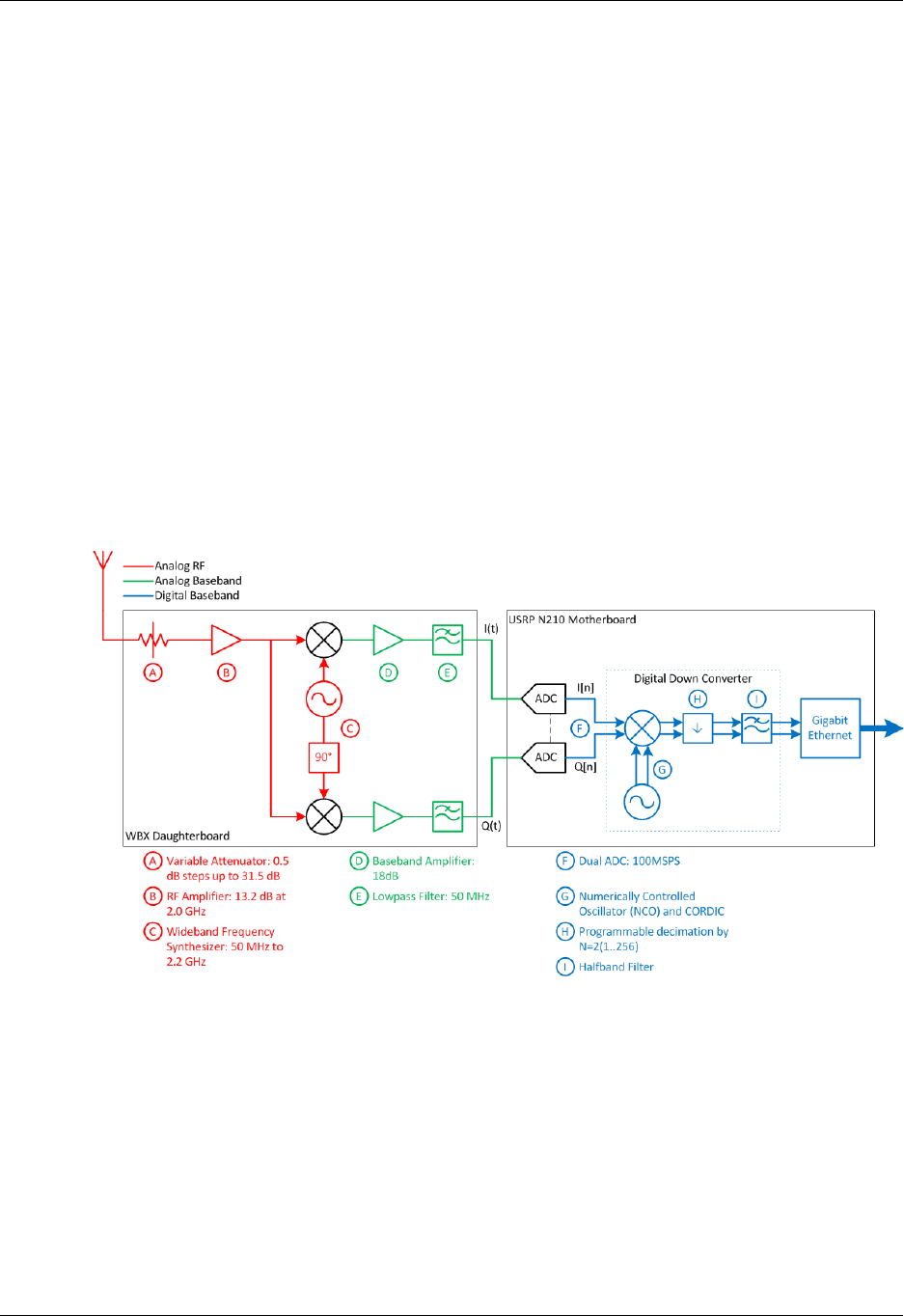
Refer to the block diagram below to understand the receive path of the USRP as it is set up in the lab.

The USRPs in the lab have the WBX daughtercard installed which feature a programmable attenuator,

programmable local oscillator and analog I/Q mixer. THe WBX daughterboard is an analog circuit simi-

lar to the "softrock" described in the previous section, but using a local oscillator implemented as a wide-

band frequency synthesizer, thus allowing the USRP to receive signals in the range from 50 MHz to 2.2

GHz. The WBX Daughterboard performs complex downconversion of a 100 MHz slice of spectrum in the

50-2200 MHz range down to -50 to +50 MHz range for processing by the USRP motherboard.

The main function of the USRP motherboard board is to act as a Digital Downconverter (DDC) [http://

en.wikipedia.org/wiki/Digital_down_converter]. The motherboard implements a digital I/Q mixer, sample

rate converter and lowpass filter. The samples are then sent to the host PC over a gigabit ethernet link.

In this section, we will first learn about FM waveform generation and reception in software simulation-only

without the URSP, then FM receiver implemented with the USRP, general IQ receiver implemented with

the USRP, and finally the USRP transmit function.

Deliverables

FM flowgraphs

• GRC files of FM transmitter and receiver showing FM transmitted waveforms, spectra and FM receiver

output.

USRP with FM

ELEC350: Communica-

tions Theory and Systems I

• Observations on practical FM receiver operation using live off-air signals

• bit rate of FSK signal at 142.17 MHz

• Estimate of URSP receiver dynamic range with FM signals

USRP with general IQ signals

• Estimate of the USRP receiver noise figure.

• IQ receiver measured frequency offset

• Observations of I and Q at different signal levels and effect of dynamic range

• USRP spectrum, minimum and maximum output power

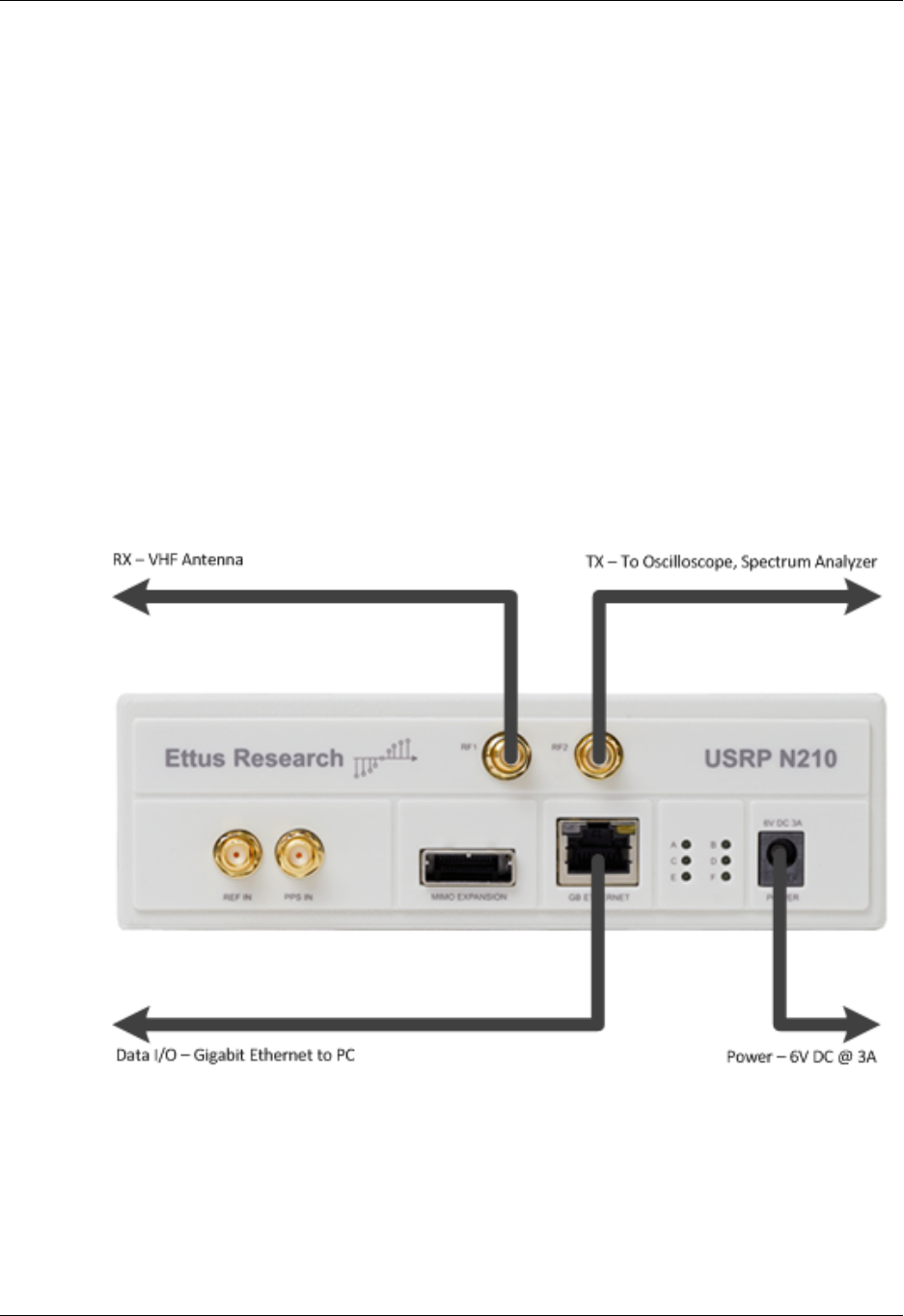
Setup

The small grey box is the USRP software#defined radio. The USRP digitally downconverts the received

(Rx) input signal into I/Q format and sends it via Ethernet to the computer. The USRP also digitally

upconverts an I/Q signal from the computer to an RF signal at the transmitter (Tx) output. The USRP’s Rx

input is connected to a VHF antenna on the ELW roof. The Tx output can be connected to the oscilloscope

and spectrum analyzer. Verify that the USRP at your station is connected as shown below.

FM Signal waveforms

Objectives

This tutorial is a guide to FM signal waveforms. In this tutorial you will learn:

• Theory and equations of FM signals, power spectrum, bandwidth, FM demodulation

ELEC350: Communica-

tions Theory and Systems I

• construct an FM transmitter flowgraph to generate an FM waveform with sinusoidal message and square

wave message

• construct an FM receiver flowgraph to recover the message from the FM waveform.

FM flowgraphs

In this section we build flowgraphs to transmit and receive FM signals that are simulation-only and do not

(yet) use the USRP. Review the theory on FM Signals [./data/FM_theory_TXRX2.pdf]

Carry out the steps in FM Tutorial [data/FM_procedures.pdf]

The following GRC file will be a useful starting point:

• FM_Transmitter.grc [data/FM_Transmitter.grc]

• fm_receiver.grc [data/fm_receiver.grc]

Start GRC as was done in the previous tutorials. If GRC is already open, simply create a new flowgraph

by selecting File->New.

FM Receivers

FM broadcast receiver

In this section, we consider a practical FM receiver that can receive real off-air FM signals using the USRP.

Open the GRC patch wfm_rx.grc [data/wfm_rx.grc]. Observe the flowgraph comprising various blocks

and interconnections, as well as predefined variable blocks not connected to anything. Blocks with blue

connection points signify complex signals (I and Q), and orange connection points signify real floating

point signals. The USRP source block represents the USRP receiver hardware. This block outputs a com-

plex signal that travels through various blocks (including sample rate conversion), eventually arriving at an

audio sink. The audio sink represents the computer’s audio output hardware. This flowgraph implements

an FM receiver.

Compare this receiveer to the FM receiver from the FM waveforms tutorial in the previous section. What

new blocks are added and what is their function? Which blocks are identical or perform similar functions?

Execute the flowgraph by first clicking the Generate button followed by the Execute button (see Figure 4).

The screen shows an FM receiver with a spectrum analyzer display and several sliders. The radio is tuned

to 98.1 MHz (an FM station in Seattle), the RF gain is set to 7 and the AF gain is set to 300m. The radio

can be tuned using the sliders or the keyboard arrow keys. Notice the noise level is around #100 dBm and

the signal peak level is 20#40 dB higher than that. Notice the spectrum analyzer covers a bandwidth of

250 KHz corresponding to the half the sampling rate set for the USRP source block in the flowgraph.

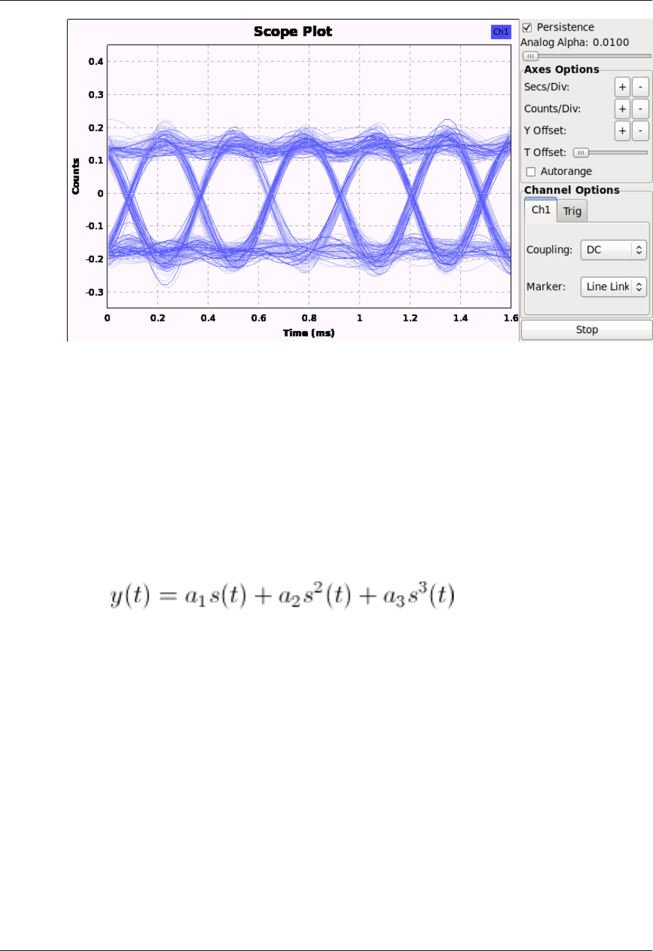
FM data receiver

Modify the FM receiver flowgraph by replacing the FM demodulation block with the "homemade" FM

demodulator using the Delay and Complex Conjugate blocks. Use the USRP to tune to the 2-level FSK

signal at 142.17 MHz. This signal is the control channel for the CREST public safety radio system [http://

www.crest.ca/]. Observe the demodulator output on the scope. Check the persistence box on the scope

and reduce the alpha to minimum. You will observe a so-called eye diagram [http://en.wikipedia.org/

wiki/Eye_pattern] of the data. The eye diagram shows the number of milliseconds per bit. Find the bit rate

(the number of bits per second).

ELEC350: Communica-

tions Theory and Systems I

Dynamic Range with FM

Review the theory of dynamic range [data/DynamicRange.pdf]. These notes will also be useful for subse-

quent sections on dynamic range with IQ signals and on noise figure.

Retune the USRP to the FM broadcast station at 98.1 MHz. Increase the RF gain from 7dB to 20dB or

more. Notice that the signal level increases and then suddenly both noise and signal jump up and the

audio changes to a different program. What is happening is that a strong signal somewhere within the

40 MHz bandwidth of the USRP’s receiver is clipping the 14 bit A/D converter in the USRP. The 14

bit A/D converter has a dynamic range of about 84 dB (14 bits times 6 dB per bit), so a signal above

about #100 dBm + 84 dB = #16 dBm will clip the converter. With the RF gain set to around 20 dB, the

receiver becomes non#linear and the audio from the strong signal is cross#modulating on top of the signal

at 98.1 MHz. Cross#modulation can be shown to occur by modelling the non#linear receiver as having the

output: (ignore higher order terms), where

s(t) is the sum of the strong and the weak signal. Reduce the RF gain and notice that the original signal

is restored. Next, we will look for this strong signal.

Tune the FM receiver to 101.9 MHz (the local UVic radio station CFUV). Notice that the signal level is

much higher (close to #30 dBm). Now increase the RF gain to at least 20 dB and observe the signal level

can be increased to above #16 dBm, however, the audio is not changed. This signal at 101.9 MHz was

causing the clipping.

Experiment more with the FM receiver. Notice that many signals can be received, FM signals are spaced

every 0.2 MHz with an odd last digit, from 88.1 MHz up to 107.9 MHz.

Write a brief one#paragraph summary of your observations of the FM receiver and what you learned.

I/Q Receiver

I/Q Receiver output

Review IQ theory [data/IQ-theory.pdf]

ELEC350: Communica-

tions Theory and Systems I

Open the GRC patch ra5.grc [data/ra5.grc]. This flowgraph implements the mathematics on the last page

of the IQ theory document. The USRP source does IQ downconversion on the WBX daughtercard and

outputs the complex signals I(t) + jQ(t). This output is connected to 4 blocks that extract the magnitude,

phase, real and imaginary parts of the complex signal, as well as an XY scope. The USRP source is tuned

to a fixed frequency of 200 MHz, i.e. the LO frequency synthesizer in the WBX daughtercard is set to

200 MHz. Double#click the USRP source block to bring up a window with all of the USRP parameters.

This general I/Q receiver is set up to receive a signal in a range around 200 MHz at level -40 dBm from

the signal generator at the back of the lab.

Execute the flowgraph. Observe the Output Display window with 5 tabs labelled Scope Plot, Magnitude,

Phase, Real and Imaginary. The Scope Plot tab should show a circle, Magnitude will show a (noisy) DC

level, Phase will show a phase ramp wrapping between -pi and pi, Real and Imaginary will show (noisy)

sine waves. The scope autorange may need to be switched off and the time base adjusted to get good

displays.

Determine the frequency of the sine waves using the Phase display as well as the Real and Imaginary

displays by placing your mouse cursor over the scope plot to show the time offset at different points on

the waveform. This frequency represents the offset between the received RF signal and the USRP local

oscillator.

The USRP source block has the clock source set to use an external 10 MHz clock reference frequency,

and the same external reference is used for the signal generator. Thus the frequency difference between

the USRP source block (local oscillator) and signal generator RF frequency will be observed to be exactly

as expected from their respective frequency settings.

If we change the USRP source block to use an internal clock reference, then expect to observe some

frequency error between the signal generator and the USRP frequency settings as they are running from

independent oscillators. Try changing the USRP clock source to internal and repeat the frequency mea-

surement of the I and Q outputs.

Dynamic range with IQ signals

Ask the TA to vary the 200 MHz signal generator level from #100 dBm to 0 dBm in 20 dB steps (or do it

yourself is there are no other groups working). Observe and describe how the signals look at each signal

level, and explain why. The waveform appearance is related to the clipping that caused cross-modulation

in a previous section.

Noise figure

Review link budget notes [data/350link4.pdf] equation (14).

When you tune the receiver to a frequency where there is no station broadcasting, there is still a residual

noise floor visible on the spectrum display. The noise level can be estimated by looking at the display and

observing the level in dBm (dB relative to one milliwatt). This is thermal noise that is calculated from the

formula P_{noise| = kT(S/N)WF, where k is Boltzmann's constant, T is the noise temperature, typically

290 degrees Kelvin, W is the bandwidth in Hz and F is a dimensionless noise figure representing imperfect

amplifiers. By taking logs of both sides of this formula, we can write in dB: P_{noise| = -228.6 + T +

(S/N) + W + F.

Estimate the noise figure of the receiver based on the noise level in dBm on the computer spectrum display

and the receiver bandwidth of 250 KHz. All the variables in the noise figure equation except F are known

or can be measured, so the equation can be solved for F.

ELEC350: Communica-

tions Theory and Systems I

Carrier Wave Transmitter

In this section, we test the transmit functions of the USRP that we can use later when building a commu-

nications system. We will observe the transmitted spectrum, minimum and maximum power level in dBm

(dB relative to one milliwatt). You will use both the osciloscope and the spectrum analyzer at your bench

to view and measure the output from the USRP transmitter.

Review the theory on Spectrum Analyzers [./data/Theory_Spectrum_Analyzer.pdf]. For more detailed

information, you may also wish to review Spectrum Analyzer Basics [./data/5965-7920E.pdf] and The

Basics of Spectrum Analyzers [./data/spec_analyzer.pdf]. The concepts presented here will be applicable

to any spectrum analyzer you may use in your career.

Open the GRC patch tx_carrier.grc [data/tx_carrier.grc]. Observe that the USRP sink center frequency

is set to 50MHz. This block represents the USRP transmitter hardware. Observe that the sine and cosine

signal sources are configured for 10 kHz. Connect the USRP Tx output to the spectrum analyzer and

execute the flowgraph. A scope display will come up along with three buttons that allow you to select

different values for Q(t).

Set the spectrum analyzer’s center frequency to 50 MHz and the span to 50 kHz by using the FREQUENCY

and SPAN buttons. Adjust the LEVEL as necessary.

What do you observe on the spectrum analyzer display with Q(t) = 0? Try the other two options for Q(t).

What do you observe on the spectrum analyzer?

What is the minimum and maximum signal power output from the USRP? The USRP output power level

can be set via the dialog box obtained by double#clicking on the USRP sink in the flowgraph. Measure

the power using both the oscilloscope and spectrum analyzer and verify they are the same.

To obtain an accurate measurement on the scope, the line from the USRP transmitter should be terminated

with a 50 Ohm terminator, or use the spectrum analyzer input which has a 50 ohm input impedance. It is

OK to use the spectrum analyser input in this case, because the maximum output from the USRP is less

than the maximum input allowed by the spectrum analyzer.

Lab 3. FLEX Frame Synchronizer

In this section, you will capture some frames from the FLEX [http://en.wikipedia.org/wi-

ki/FLEX_(protocol)] pager network and locate the frame synchronization word. The sync word allows the

decoder to synchronize with the beginning of the message bits. A standard method for detecting the sync

word is to correlate the incoming signal against the sync word.

You will also try to decode some of the message bits.

Review the theory on Frame Synchronization [./data/FrameSync.pdf]. Further description of frame syn-

chronization is in the text CR Johnson, WA Sethares, Software Receiver Design, Cambridge, 2011 chapter

8, section 8.5.

Deliverables

• Working flowgraph showing how the FLEX frames were captured.

• Code which prints out the start time of each sync word found in a file.

• A list of the 16 frame times that you extracted from the test file.

ELEC350: Communica-

tions Theory and Systems I

• A list of the frame times that you extracted from a file you captured of the air.

• A description of your observations about the FLEX protocol and the approach you would take to decode

actual message text.

• Identifying two different FSK signals and measuring their symbol rates.

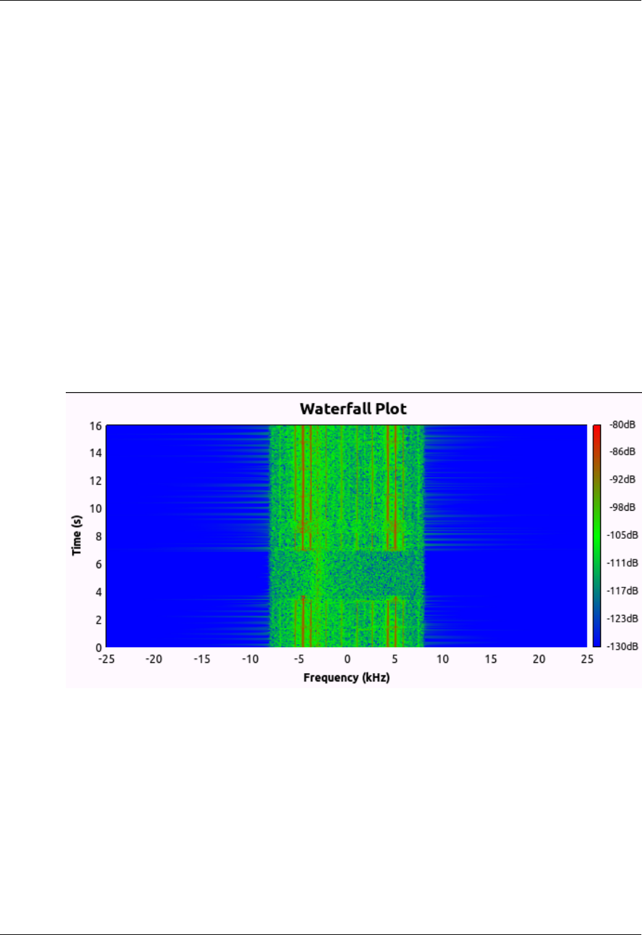
Frame Capture

There is a relatively strong FLEX pager network signal around 929.66 MHz. The FLEX signal is mul-

ti-level Frequency-Shift Keying, so an FM demodulator is needed to detect the data. Create a flowgraph to

receive this signal, starting with the IQ receiver from the previous section with a waterfall added. Set the

USRP receive gain high (30dB), tune your receiver to this frequency and view the signal on the waterfall

display. You may need to use the Autoscale function on the waterfall for a better view.

If you are not able to find the FLEX signal, there is a FLEX file source [./data/FLEX_bits.wav] that can

be used instead.

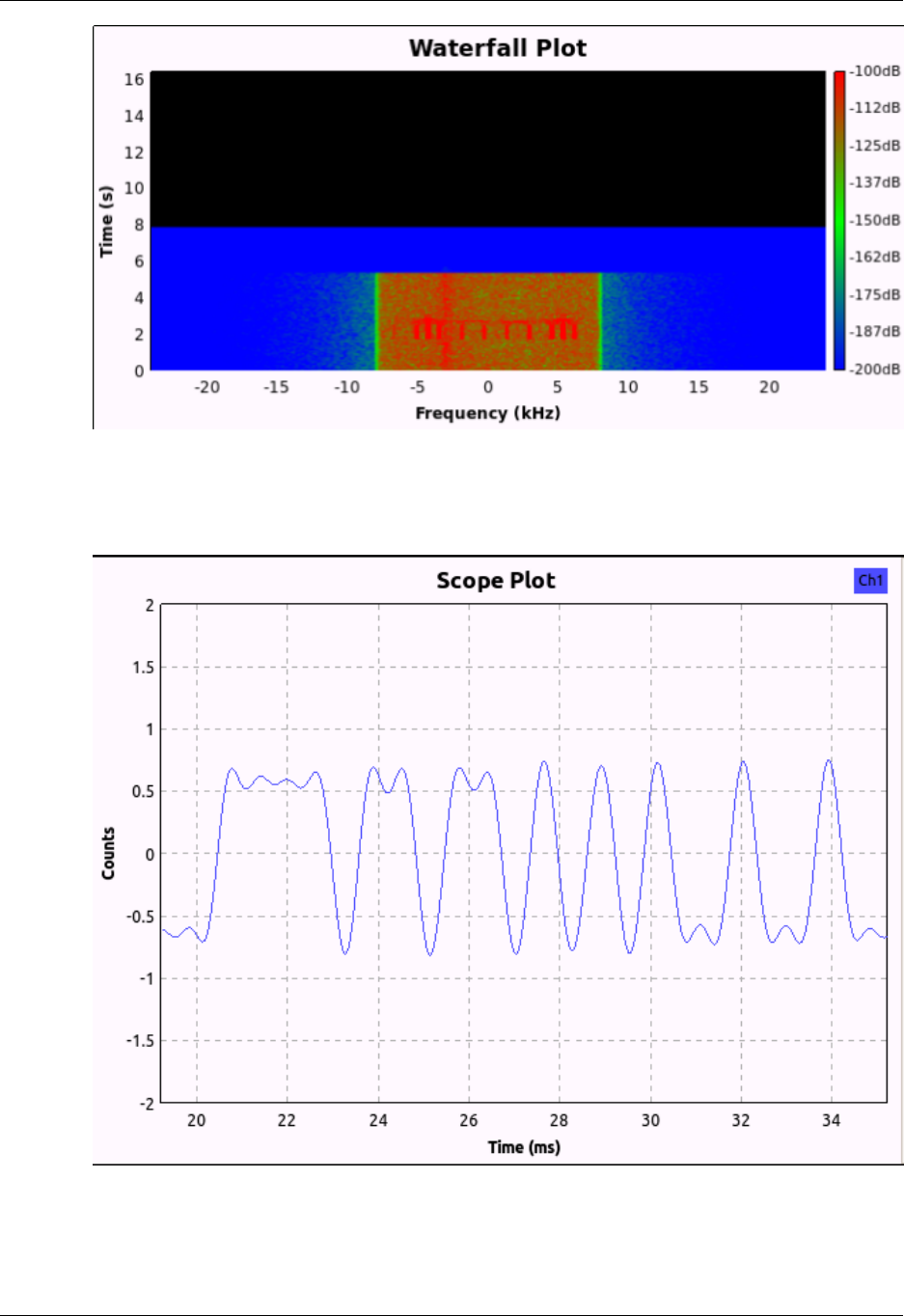
What do you observe? With some patience, you should periodically see two strong lines that are 9.6 kHz

apart with other weaker lines on either side (harmonics). 9.6 kHz is the frequency shift used by the FLEX

signal. The signal actually switches rapidly between the two frequencies, although the resolution of the

waterfall is not fine enough to show this detail.

You may also observe that the paging signal occurs in shorter bursts, as shown here.

ELEC350: Communica-

tions Theory and Systems I

Although FLEX can use a variety of modulation schemes, the sync word is always sent as 2-level FSK

at 1600 bits per second. Create an FM discriminator just as you did in the previous lab to demodulate the

FLEX signal. View the demodulated output on the scope. You should now see what looks like a digital

waveform.

Save the demodulated output to a file in one of the following ways:

ELEC350: Communica-

tions Theory and Systems I

1. In binary format using a File Sink at any sample rate. This file can be read in MATLAB using the

fread [http://www.mathworks.com/help/matlab/ref/fread.html] function or in any other language of

your choice.

2. In WAV format using a Wav File Sink at one of the accepted sample rates for WAV files (48kHz is

suggested). WAV files can be read in MATLAB using the wavread [http://www.mathworks.com/help/

matlab/ref/wavread.html] function or viewed in Audacity.

Bit and Frame Sync

To find the location of the marker sequence in this data waveform stored in a file reequires two steps:

1. find the bit stream from the waveform

2. find the marker in the bit stream

The bit stream can be found from the waveform by visual inspection of the waveform. In the example

waveform of the previous subsection, the data bits are 0011110110110101010010010, where we have

written 0 instead of -1 for convenience. To do this by computer requires a bit more thought. In this case,

since the USRP is phase locked to GPS, there is an integer number of samples per bit, which makes the

waveform-to-bits conversion much easier.

Write a program (in MATLAB or another language of your choice) to obtain the bit stream and correlate

the demodulated FLEX signal against the sync word. The sync word you should look for in this case is

0xA6C6AAAA or the 32-bit sequence: 1010 0110 1100 0110 1010 1010 1010 1010. You can use this

FLEX file source [./data/FLEX_bits.wav] as a sanity check. It contains 16 frames, with the first one starting

at 0.7126 seconds and the last one starting at 30.7126 seconds. Find the start times of all 16 frames.

Run your program on the frames you captured in the previous step and give the start times of each sync

word. How much time between frames (sync words)? Is there any larger pattern?

Decoding text

Try to decode some text, the letters and numbers are not encrypted. Some hints may be found here [http://

scholar.lib.vt.edu/theses/available/etd-10597-161936/unrestricted/THESIS.PDF], pages 4-11. It is not ex-

pected that successful decoding can be completed during the lab period, however, the approach you would

take with your TA.

Other data signals

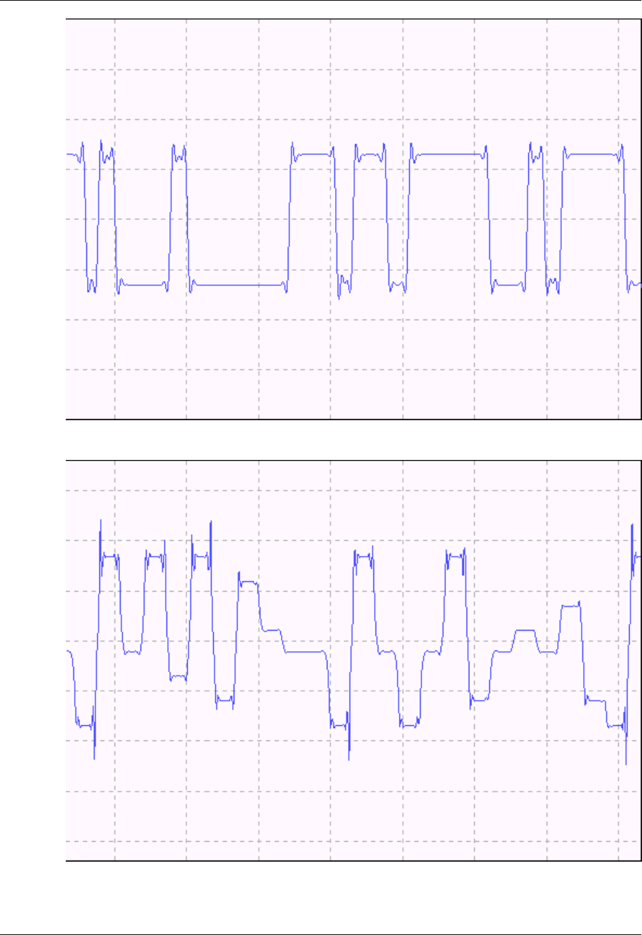
A data file [./data/fsk.dat] was recorded at a sample rate of 48 kHz containing complex samples of two FSK

signals. One signal is at an offset of -10 kHz while the other is at +15 kHz. One signal has two tones while

the other uses eight tones. Use a complex File Source block to read the file and your FM discriminator

from the previous section to demodulate the signals one at a time and determine:

• Which signal is at which offset?

• What is the symbol rate of each signal?

The demodulated two-tone signal should look similar to the one below on the scope display.

ELEC350: Communica-

tions Theory and Systems I

The demodulated eight-tone signal should look similar to the one below on the scope display.

ELEC350: Communica-

tions Theory and Systems I

Lab 4. PSK systems

Deliverables

• modified complex BPSK flowgraph

• block diagram version of modified complex BPSK flowgraph showing a mathematical representation

of the signal at each point

• a comment on the difference between two methods of pulse shaping: using square waves versus using

an impulse train as input to a pulse shaping filter.

• a few sentences explaing your observations with non-zero frequency offset

Testing a PSK system

In this section, we modify a complete PSK transmitter-receiver system assuming a perfect channel and

perfect synchronization (timing).

Start by reviewing the theory on PSK Signals [./data/Theory_PSK_2.pdf]. The following GRC patches

(flowgraphs) will help you understand how BPSK and QPSK are generated:

• Real BPSK: bpsk_txrx_real.grc [./data/bpsk_txrx_real.grc]

• Complex BPSK: bpsk_txrx_complex.grc [./data/bpsk_txrx_complex.grc]

• Real QPSK: qpsk_txrx_real.grc [./data/qpsk_txrx_real.grc]

• Complex QPSK: qpsk_txrx_complex.grc [./data/qpsk_txrx_complex.grc]

Observe that for each of these 4 flowgraphs, the signal source is a square wave (not an impulse train)

representing a 1010... data pattern represented at the given sample rate. What is the bit rate and the symbol

rate in each case? How many samples per symbol? Observe how the signal constellation rotates when the

frequency offset is not equal to zero.

We now modify the Complex BPSK flowgraph to use a random data pattern and a non-square pulse shape.

• Replace the signal source with a random data pattern generated using a generalized linear feedback shift

• The GLFSR source outputs one sample per bit. Use a Repeat block so that each data bit generates a

square pulse. What interpolation factor should be chosen and why?

• Add a scope sink at the output of the Repeat block to observe the square pulses.

• Add a low pass filter to shape the square pulses into more rounded pulses. What is the advantage of

using a rounded pulse rather than a square pulse?

• Add a scope sink at the output of the low pass filter to observe the transmitted eye diagram with rounded

pulses.

• Add a scope sink at the output of the receiver to observe the received eye diagram. Observe how the

received eye diagram changes as the frequency offset is changed from zero. Explain your observations.

• Add a scope sink in XY mode at the output of the receiver to observe the received signal constellation.

This constellation is not sampled, so it includes the entire waveform, not just the points where the data is

ELEC350: Communica-

tions Theory and Systems I

sampled. Observe how the constellation changes as the frequency offset is changed from zero. Explain

your observations.

In the following steps, we create the pulse shape using impulse inputs instead of square wave inputs.

This method enables the use of an FIR pulse shaping filter such as the Root Raised Cosine Filter whose

coefficients (taps) exactly represent the desired pulse shape.

• The GLFSR source outputs one sample per bit. We want to create an impulse train waveform with many

samples per bit that will be the input to a pulse shaping filter.

• Use an Interpolating FIR filter so that each data bit generates an impulse. The interpolation factor should

be chosen to be the same as before. Why? The filter has only one tap set to be the same as the interpolation

factor.

• Add a scope sink at the output of the Interpolating FIR filter to observe the impulse train waveform.

• Add an FIR low pass filter to shape the impulses into pulses with reasonable pulse shape.

• Replace the Interpolating FIR filter and the FIR low pass filter with a Root Raised Cosine Filter. The

input to the RRC filter is at the symbol rate (one sample per bit). The filter gain should be set to be the

same number as the interpolation factor. Set the RRC filter length to an appropriate value, try different

values and observe the effect.

• Add a scope sink at the output of the Root Raised Cosine Filter to observe the transmitted eye diagram.

• Add a scope sink at the output of the receiver to observe the received eye diagram. Observe how the

received eye diagram changes as the frequency offset is changed from zero.

• Add a scope sink in XY mode at the output of the receiver to observe the received signal constellation.

Observe how the constellation changes as the frequency offset is changed from zero. Explain your

observations.

Optional: repeat the above changes using the Complex QPSK flowgraph.

Optional modifications: add a noise source, receiver filter and bit error rate counter

Lab Manual

Navigation menu

Versions of this User Manual:

Views

Navigation