Lifev Manual

User Manual:

Open the PDF directly: View PDF .
Page Count: 22

Generalities
Learning by examples
- Reading data
- The Poisson problem
  - Variational formulation and finite element discretization
  - LifeV simulation

LifeV User Manual

Revision: 1.9, , UTC Printed: February 20, 2015

G. Fourestey, S. Deparis

This manual is for LifeV (version 3.8.3, January 2015), a library for scientiﬁc computing

using ﬁnite elements, specially aimed at ﬂuid-structure interaction and blood ﬂow simulation.

Contents

1 Generalities 4

1.1 Scope of the document ................................ 4

1.2 Language and nomenclature convention ...................... 4

1.3 Software Management ................................ 4

1.4 Compiling LifeV ................................... 5

1.4.1 Trilinos compilation ............................. 7

1.4.2 Compilation from git ............................. 8

1.4.3 Compilation from Oﬃcial Distribution ................... 9

1.4.4 Compiling Testsuites ............................. 10

2 Learning by examples 11

2.1 Reading data ..................................... 11

2.2 The Poisson problem ................................. 12

2.2.1 Variational formulation and ﬁnite element discretization ......... 12

2.2.2 LifeV simulation ............................... 13

List of Tables

Chapter 1

Generalities

1.1 Scope of the document

This is an informal document dedicated to amateur or inexperienced users of the software

library LIFE V (life 5).

The major objectives of this document are:

1. to compile the software library,

2. to provide examples of its use.

For a more detailed overview of LifeV ’s main features (management of boundary conditions,

time and space discretization, algebraic solvers and preconditioners, etc), see the doxygen

webpage: https://cmcsforge.epfl.ch/doxygen/lifev/.

1.2 Language and nomenclature convention

typesetting font style is used to indicate parts of computer code, conﬁgure shell scripts,

command-prompt instructions and webpages.

1.3 Software Management

The software source, its documentation and all related documents (this one included) are kept

in a repository under revision control using git1. Its goal is to provide tools to manage software

development in a concurrent environment. See http://git-scm.com/documentation for a

tutorial.

As mentioned above, a website `a la Sourceforge2http://cmcsforge.epfl.ch has been

set up to host the source code and help the software management. It requires that you open

an account3there and ask to join the project LifeV using the link at the bottom of the

developers’ list. Once you would become a member, you will gain access to all the facilities:

tracker, task manager, git repository, forums, document manager and a few other tools which

are very useful if not absolutely essential to such a project.

Finally, if you expect a frequent use of the git repository we recommend to costumize the

ssh and ssh-agent in order to gain acces without the need to type your password everytime

you issue a command. Please refer to http://mah.everybody.org/docs/ssh in order to

conﬁgure your ssh agent.

1git is the fast version control system.

2http://www.sourceforge.net

3https://cmcsforge.epfl.ch/account/register.php

1.4. COMPILING LIFEV CHAPTER 1. GENERALITIES

We advice every user to apply to the list lifev-users on http://groups.google.com where

one can get in touch with other users and developers.

1.4 Compiling LifeV

There are a few compilation tools and libraries we need to build and install before compiling

LifeV , here is a short presentation. Note that, in addition to the following description, the

complete installation steps are available on the following webpages:

1. http://www.lifev.org/documentation/installation-tutorial ,

2. https://cmcsforge.epfl.ch/projects/lifev/wiki/LifeV_on_MacOSX .

In computer science, a library is a set of subroutines or classes used to develop software.

Usually they are downloaded as a so called “tarball” ﬁle compressed using the tar command.

There are diﬀerent ways to compress libraries but the most common is to use the command

tar -cvf and further compress “zip” it with gzip. If your tarball has the suﬃx .tar.gz

equivalent to .tgz, you can decompress “unzip” it with gunzip followed by the name of the

.tar.gz ﬁle and extract its contents using tar -xvf followed by the name of the .tar ﬁle. If

you ﬁnd the libraries compressed with other formats please refer to the unix manuals man or

the numerous on-line documents for further information.

Software libraries need to be extracted, compiled and installed. In unix-like systems,

the libraries .a and .so ﬁles are installed usually in the directory /usr/lib, while header

ﬁles .h are installed in the /usr/include directory. Compilers search for libraries there by

default, but in principle they can be installed anywhere you want as long as you pass the

path to the library using the compiler ﬂag -L immediately followed by the library path (e.g.

-L/path/to/lib) and similarly for the header ﬁles using the compiler ﬂag -I followed by

the include path. Libraries compiled from source are usually installed in /usr/local/lib,

/usr/local/include.

Libraries are usually created with the preﬁx lib followed by the name of the library and

linked with the compiler ﬂag -l followed by its name (e.g. -lblas).

Compilation Environment

LifeV depends on a number of tools at compilation time that are part of the autotools from

the GNU project4available in most Linux OS:

•g++-4.0 or newer (currently 4.9.2).

•mpi, with preference to openmpi.

•CMake 2.8.11 or newer (currently 3.1.0).

In Mac OS X you get gcc in Xcode and cmake can be installed using MacPorts with the

command sudo port install cmake. You can check the version of a command typing the

command followed by --help, for example type cmake --help.

LifeV depends on several optimized libraries, you can check if you have them installed using

the locate command (after updating the search database with sudo updatedb) followed by

the name of the library, for example locate liblapack.a, or go to the /usr/lib directory

and search on the list with ls. It is important to notice that some libraries are linked to others

and they should be compatible, therefore you should build them in the order of dependency

and with compatible ﬂags and compilers.

These are the optimized libraries you need to have installed:

4http://www.gnu.org

1.4. COMPILING LIFEV CHAPTER 1. GENERALITIES

•A version of MPI. The message passing interface for C and Fortran compilers. For exam-

ple http://www.open-mpi.org/. Once installed you can check the necessary ﬂags for

its use by typing mpicc --show.

On a Debian system the command sudo apt-get install libopenmpi* should do the

trick.

In Mac OS X using MacPorts install a fortran compiler typing sudo port install gcc46

and openmpi with sudo port install openmpi. Note however that MPI should be na-

tively installed if you installed XCode.

•BOOST. Libraries which extend the functionality of C++. Check if they exist on your

computer, they are many libraries with the preﬁx libboost.

If you need to install them, try sudo apt-get install libboost* on Debian systems

or something similar for other Linux distros.

In Mac OS X using MacPorts type sudo port install boost.

If you need to compile from source, download the libraries at http://www.boost.org.

Make sure you include the line “using mpi;” in the conﬁguration text ﬁle project-config.jam.

You can specify the path to install using the ﬂag --prefix=/path/ when running ./bjam

install. But most of the time cross compilation of this library won’t work completely.

•HDF5 If you don’t have the library hdf5 installed in your system, you could use the sudo

apt-get install libhdf5-openmpi-dev command on Debian systems or something

similar for your particular distro. There are detailed instructions on-line on how to

build it for other systems and with other options, see http://micro.stanford.edu/

wiki/Install_HDF5#Build_and_Installation_from_Sources.

In Mac OS X using MacPorts type sudo port install hdf5 or build it from the sources

to link it to the correct openmpi compilers.

•BLAS. On Debian systems run sudo apt-get install libblas-dev.

In Mac OS X the system comes with blas and lapack as part of the Accelerate frame-

work -framework Accelerate, and if using MacPorts type sudo port install atlas

to install the atlas library (blas and lapack).

To compile from source, get the libraries e.g. at https://www.tacc.utexas.edu/research-development/

tacc-software/gotoblas2. To build just type make. To make use of the library remem-

ber to have the pthreads library and ﬂag -lpthread while linking to the blas library

libgoto2_xxxxx_xx.xx.a, whose exact name depends on the characteristics of your

hardware.

•LAPACK. Fortran 90 Linear Algebra Routines for systems of simultaneous linear algebra

equations, linear least-squares problems and matrix eigenvalue problems. You must pay

attention to build the lapack using an optimized blas like the GotoBLAS (see above).

Download it at http://www.netlib.org/lapack/. You need a fortran compiler (for

example gfortran). Copy make.inc.example to make.inc and edit the path to the

blas library followed by the ﬂag -lpthread and type make.

For a non-optimized version on a Debian system run sudo apt-get install liblapack-dev.

•PARMETIS. You can download ParMetis from http://glaros.dtc.umn.edu/gkhome/

metis/parmetis/download. Set CC=mpicc in Makefile.in. and type make. In Mac

OS X you need the include path ﬂags -I/usr/include and -I/usr/include/malloc.

•UMFPACK (now part of SuiteSparse). Set of routines for solving unsymmetric sparse

linear systems.

On a Debian system, install it with the command sudo apt-get install libsuitesparse-dev.

To compile SuiteSparse from source, download it from http://faculty.cse.tamu.edu/

davis/suitesparse.html and follow the instructions in the README.txt ﬁle (in particu-

lar, you’ll want to edit the SuiteSparse_config/SuiteSparse_config.mk ﬁle according

1.4. COMPILING LIFEV CHAPTER 1. GENERALITIES

to your conﬁguration).

For Mac OS X you must uncomment the special options given for this system, so you can

use the blas and lapack from atlas or from the Accelerate framework -framework Accelerate.

•TRILINOS. See the next section.

1.4.1 Trilinos compilation

LifeV depends on Trilinos, a set of object oriented C++ interfaces for packages like blas,

lapack, parmetis, umfpack and many more. A copy of the source code is available for download

at http://trilinos.org/download/.

After downloading, decompressing and extracting the tarball, you’ll need to make a build

directory anywhere you want to avoid build in the sources directory. (in the following script,

we assume that the directories trilinos and trilinos-build are at the same level) Trilinos

(latest version 11.12.1 at the time of writing) now requires the CMake build system 2.8.11 or

newer. Go to the build directory and write a do-configure shell script like the following

1#! / b in / b ash

3EXTRA_ARGS=$ @

5cmake \

6−D CMAKE_BUILD_TYPE :S T R I N G=RELEASE \

7−D Trilinos_ENABLE_Amesos :B O O L=O N \

8−D Trilinos_ENABLE_Anasazi :B O O L=O N \

9−D Trilinos_ENABLE_AztecOO :B O O L=O N \

10 −D Trilinos_ENABLE_Belos :B O O L=O N \

11 −D Trilinos_ENABLE_Epetra :B O O L=O N \

12 −D Trilinos_ENABLE_EpetraExt :B O O L=O N \

13 −D Trilinos_ENABLE_Galeri :B O O L=OFF \

14 −D Trilinos_ENABLE_Ifpack :B O O L=O N \

15 −D Trilinos_ENABLE_Isorropia :B O O L=OFF \

16 −D Trilinos_ENABLE_Kokkos :B O O L=O N \

17 −D Trilinos_ENABLE_ML :B O O L=O N \

18 −D Trilinos_ENABLE_TESTS :B O O L=OFF \

19 −D Trilinos_ENABLE_Teuchos :B O O L=O N \

20 −D Trilinos_ENABLE_ThreadPool :B O O L=O N \

21 −D Trilinos_ENABLE_Tpetra :B O O L=O N \

22 −D Trilinos_ENABLE_Triutils :B O O L=O N \

23 −D Trilinos_ENABLE_Zoltan :B O O L=O N \

24 \

25 −D Trilinos_EXTRA_LINK_FLAGS :S T R I N G=”−lpthread” \

26 −D TPL_ENABLE_Pthread :B O O L=O N \

27 \

28 −D T P L _ E N A B L E _ B L A S :B O O L=ON \

29 −D BLAS_INCLUDE_DIRS :P A T H=/b l a s /include/dir/\

30 −D BLAS_LIBRARY_DIRS :P A T H=/b l a s /lib/dir/\

31 −D BLAS_LIBRARY_NAMES :S T R I N G=” b l a s ” \

32 \

33 −D TPL_ENABLE_LAPACK :B O O L=O N \

34 −D L A P A C K _ I N C L U D E _ D I R S :P A T H =/l a p a c k /include/dir/\

35 −D L A P A C K _ L I B R A R Y _ D I R S :P A T H =/l a p a c k /lib/dir/\

36 −D LAPACK_LIBRARY_NAMES :S T R I N G=” l a p a c k ” \

37 \

38 −D T P L _ E N A B L E _ H D F 5 :B O O L=ON \

39 −D HDF5_INCLUDE_DIRS :P A T H /h d f 5 /include/dir/\

40 −D HDF5_LIBRARY_DIRS :P A T H=/h d f 5 /lib/dir/\

41 \

42 −D TPL_ENABLE_UMFPACK :B O O L=O N \

43 −D UMFPACK_INCLUDE_DIRS :P A T H =/ umfpack/include/dir/\

44 −D UMFPACK_LIBRARY_DIRS :P A T H =/ umfpack/lib/dir/\

45 −D UMFPACK_LIBRARY_NAMES :S T R I N G=” umfp ack ; amd” \

46 \

47 −D TPL_ENABLE_MPI :B O O L=O N \

48 −D MPI_BASE_DIR :P A T H =/usr/lib/openmpi/\

49 −D M P I _ B I N _ D I R :P A T H =/usr/bin \

50 \

51 −D T P L _ E N A B L E _ P a r M E T I S :B O O L=O N \

52 −D ParMETIS_LIBRARY_DIRS :P A T H =/parmetis/lib/dir/\

53 \

54 −D CMAKE_INSTALL_PREFIX :P A T H =./ \

1.4. COMPILING LIFEV CHAPTER 1. GENERALITIES

55 $EXTRA_ARGS \

56 . . / trilinos/

Simply modify the paths of libraries according to your particular conﬁguration and run

the shell script (chmod +x do-configure && ./do-configure). For example, instead of

lapack_library_name you should type the name of your lapack library without the lib

preﬁx and the .a suﬃx. The preﬁx and suﬃx are automatically added by CMake.

If SuiteSparse was compiled from source the UMFPACK_LIBRARY_NAMES variable has to be mod-

iﬁed so that it reads "umfpack;suitesparseconfig;cholmod;colamd;amd"

As an alternative to the above script, you can run

1c c m a k e . . / lifev

to get a graphical conﬁguration menu (however ccmake needs libncurses to be installed),

with many more options.

After the conﬁguration is done, just type

1m a k e

that will compile the static ﬁles and further

1make install

that will create and install the library ﬁles in two subdirectories lib and include, where it

will respectively pack the objects ﬁles into library ﬁles (.a and .la ﬁles) and copy the include

ﬁles ( .h or .hpp ﬁles ).

The Trilinos library is now installed in the build directory you created.

1.4.2 Compilation from git

You need ﬁrst to have an account on http://cmcsforge.epfl.ch and be part of the LifeV

project, see 1.3.

First, you need to checkout LifeV .git has been conﬁgured to use ssh and your ssh keys to

access the repository via ssh without entering your password. When your ssh agent is properly

conﬁgured, send your public key to the local administrator, such that it can be included in

the gitolite conﬁguration. Then you will be able to access the repositories without password.

It is now time to download and compile the code. Just type

1g it cl o n e g i t @ c m c s f o r g e .e p f l .c h :lifev .g it l i f e v

and go to the newly created directory

1c d l i f e v

Second, you must make a build directory apart from the lifev sources directory, for example

in your home you can have a lib directory with a lifev subdirectory and further an optimized

version subdirectory opt or the debugging mode subdirectory debug, or something similar

according to your own taste.

Third, you have to execute the following do-configure shell script (again, modiﬁed to

suite your conﬁguration) in the opt directory. It will automatically check the availability of

the needed components for LifeV compilation :

1#! / b in / b ash

1.4. COMPILING LIFEV CHAPTER 1. GENERALITIES

3EXTRA_ARGS=$ @

5TRILINOS_BUILD_DIR=/trilinos/build/dir/

7cmake \

8−D CMAKE_BUILD_TYPE :S T R I N G=RELEASE \

10 −D TPL_ENABLE_MPI :B O O L=O N \

11 \

12 −D ParMETIS_INCLUDE_DIRS :P A T H =/parmetis/include/dir/\

13 −D ParMETIS_LIBRARY_DIRS :P A T H =/parmetis/lib/dir/\

14 \

15 −D T P L _ E N A B L E _ B L A S :B O O L=ON \

16 −D BLAS_INCLUDE_DIRS :P A T H=/b l a s /include/dir/\

17 −D BLAS_LIBRARY_DIRS :P A T H=/b l a s /lib/dir/\

18 −D BLAS_LIBRARY_NAMES :S T R I N G=” b l a s ” \

19 \

20 −D TPL_ENABLE_LAPACK :B O O L=O N \

21 −D L A P A C K _ I N C L U D E _ D I R S :P A T H =/l a p a c k /include/dir/\

22 −D L A P A C K _ L I B R A R Y _ D I R S :P A T H =/l a p a c k /lib/dir/\

23 −D LAPACK_LIBRARY_NAMES :S T R I N G=” l a p a c k ” \

24 \

25 −D T P L _ E N A B L E _ H D F 5 :B O O L=ON \

26 −D HDF5_INCLUDE_DIRS :P A T H=/h d f 5 /include/dir/\

27 −D HDF5_LIBRARY_DIRS :P A T H=/h d f 5 /lib/dir/\

28 \

29 −D TPL_ENABLE_Boost :B O O L=O N \

30 −D Boost_INCLUDE_DIRS :P A T H =/ boost/include/dir/\

31 \

32 −D T P L _ E N A B L E _ T r i l i n o s :S T R I N G=ON \

33 −D Trilinos_DIR :P A T H=$TRILINOS_BUILD_DIR/lib/cmake/Trilinos \

34 −D Trilinos_INCLUDE_DIRS :P A T H=$TRILINOS_BUILD_DIR/include/\

35 −D Trilinos_LIBRARY_DIRS :P A T H=$TRILINOS_BUILD_DIR/lib/\

36 \

37 −D LifeV_VERBOSE_CONFIGURE :B O O L=OFF \

38 −D CMAKE_VERBOSE_MAKEFILE :B O O L=OFF \

39 \

40 −D LifeV_ENABLE_STRONG_CXX_COMPILE_WARNINGS :B O O L=OFF \

41 \

42 −D LifeV_ENABLE_ALL_PACKAGES :B O O L=O N \

43 −D LifeV_ENABLE_TESTS :B O O L=O N \

44 −D LifeV_ENABLE_EXAMPLES :B O O L=O N \

45 \

46 −D CMAKE_INSTALL_PREFIX :P A T H =./ \

47 $EXTRA_ARGS \

48 . . / lifev

Do the same in the debug directory, replacing the ﬁrst line by

3\n o i n d e n t F in a ll y ,y o u j u s t h a v e t o u s e \ixv{m a k e }to compile \l i f e v l i b r a r i e s and ←-

documentation .

4Enter

5\begin{lstlisting}

6m a k e −j n

7make install

where nis the number of parallel jobs.

Be careful because do-configure will fail if you have already compiled LifeV in the source

directory. Therefore is not a good idea to build inside the sources.

1.4.3 Compilation from Oﬃcial Distribution

The LifeV project provides releases, they are named using the following convention

lifev-x.y.z.tar.gz

Here is what you have to do:

1. download LifeV release lifev-x.y.z.tar.gz

2. unpack it

1.4. COMPILING LIFEV CHAPTER 1. GENERALITIES

1tar −xz f l i f e v −x.y.z.tar .gz

3. conﬁgure it following the instructions of the previous section,

4. compile and install it

1m a k e −j n

2make install

1.4.4 Compiling Testsuites

LifeV comes with testsuites covering a lot of features. They are located in diﬀerent directories,

mainly depending on the physical or technical aspects they are concerned with. For example,

you can ﬁnd a number of tests in the core directory (lifev/lifev/core/testsuite) but

darcy, fsi, navier_stokes, structure are other directories where you can ﬁnd tests.

All these tests are automatically compiled once you have installed LifeV . To run them just

type

1m a k e t e s t

Chapter 2

Learning by examples

2.1 Reading data

In order to read input data, LifeV is integrated with the open-source library GetPot (http:

//getpot.sourceforge.net/). GetPot allows to easily handle the data regarding the diﬀerent

phases of the simulation, typically providing the mesh name, the discretization order, the

physical parameters, the solver information and the time step (if any).

GetPot needs the name of the input ﬁle that can be linked through the ﬂags ”-f” or ”–ﬁle”

while launching the program, e.g.

1$. / myProgram .exe −f myData

The GetPot object allows to read the data from the ﬁle, and is constructed thanks to the

name of the input ﬁle. If no name is provided, then LifeV uses the default input name ”data”.

1G e t Po t c o m m a n d _ l i n e (arg c ,a r g v ) ;

2const std : : s t r i n g d a t a F i l e N a m e =command_line .f o l l o w (” data ” , 2 , ”−f ” ,”−− file”) ;

3G e t P o t d a t a F i l e (dataFileName ) ;

The input ﬁle must have a tree-structure, an example is as follows

1#−∗− getpot −∗− ( GetPot mode a c t i v a t i o n for emacs )

2#−−−−−−−−−−−−−−−−−−−−−−−−−−−−−−−−−−−−−−−−−−−−−−−−−

3#Data f i l e for t h e L a p l a c i a n exam pl e

4#−−−−−−−−−−−−−−−−−−−−−−−−−−−−−−−−−−−−−−−−−−−−−−−−−

6[finite_element ]

7d e g r e e =P1

9[m e s h ]

10 nx = 40

11 ny = 40

12 nz = 40

13 overlap = 0

14 verbose =f a l s e

16 [p r e c ]

17 prectype =I f p a c k #I f p a c k o r ML

18 displayList =f a l s e

20 [ . / i f p a c k ]

21 overlap = 2

23 [ . / f a c t ]

24 ilut_level−of−f i l l = 1

25 drop_tolerance = 1 . e−5

26 relax_value = 100

2.2. THE POISSON PROBLEM CHAPTER 2. LEARNING BY EXAMPLES

28 [ . . / a m e s o s ]

29 solvertype =Amesos_KLU #Amesos_KLU or Amesos_Umfpack

31 [ . . / partitioner ]

32 overlap = 0

34 [ . . / schwarz ]

35 reordering_type =n o n e #m et i s ,rcm ,n o n e

36 filter_singletons =t r u e

38 [../]

39 [../]

and the data can be read as in folders. For instance, if we have the previous data ﬁle and we

want to print the mesh sizes in the three directions, we only need to type

1std : : c o u t << ”Number o f e l e m e n t s i n e a ch d i r e c t i o n ”

2<< ”x : ” dataFile (”mesh/ nx” , 15 )

3<< ”y : ” dataFile (”mesh/ ny” , 15 )

4<< ” z : ” dataFile (”mesh / nz ” , 15 )

5<< std : : e n d l ;

where the values ”15” are set in LifeV as default sizes. More generally, in every LifeV-based

program, we need to access in the same manner the data through the GetPot object, providing

also a safe default value in case some variables are not speciﬁcally set.

You can browse the default data ﬁle in every testsuite directory to see examples. Generally,

some entries are compulsory (e.g. the mesh name for unstructured meshes), on the other hand

others are ﬁlled with a default value if not speciﬁed in the input ﬁle.

2.2 The Poisson problem

In this section, we go through a ﬁrst example dealing with the Poisson equation. At ﬁrst we

introduce the mathematical setting and well-posedness of the problem, presenting its ﬁnite

dimensional formulation and the error estimates. Then we explain how to solve the Poisson

problem using LifeV, going through the diﬀerent stages that characterize the simulation. More

in particular, we will cover the following topics:

•the preamble: including the headers and conﬁguring MPI

•the construction of a structured mesh and the deﬁnition of the ﬁnite elements space

•the assembly of the stiﬀness matrix, the right-hand-side and the setting of boundary

conditions

•the preconditioner and the solution of the linear system

•the exporting of data and the post-processing

2.2.1 Variational formulation and ﬁnite element discretization

Let Ω ⊂Rd, d = 2,3 be a regular open bounded domain and let ∂Ω be its boundary such that

∂Ω=ΓD∪ΓN,˚

ΓD∩˚

ΓN=∅, our problem reads











−∆u=fx∈Ω,

u=g(σ)σ∈ΓD,

∂nu=h(σ)σ∈ΓN,

2.2. THE POISSON PROBLEM CHAPTER 2. LEARNING BY EXAMPLES

where f=f(x) denotes the source term and g(σ), h(σ) denote the Dirichlet and Neumann

boundary conditions, respectively. Starting from the diﬀerential equation, we can derive the

weak formulation of the problem. We introduce the spaces

V=H1

d(Ω) = nv∈H1(Ω) : v|ΓD= 0o(2.1)

and

Vg=nv∈H1(Ω) : v|ΓD=g(σ)o.(2.2)

Finally, our problem reads: ﬁnd u∈Vg, such that

a(u, v) = F v ∀v∈V, (2.3)

where

a(u, v) = ZΩ

∇u· ∇vdxand F v =ZΩ

f(x)dx+ZΓN

h(σ)dσ. (2.4)

Under appropriate hypothesis, problem (2.3) is well-posed. In order to obtain a discrete

solution of problem (2.3) based on the ﬁnite element method, we introduce at ﬁrst a partition

Thof the domain Ω, and the ﬁnite-dimensional space

Vh=Xr

h=nvh∈C0(¯

Ω) : vh|K∈Pr(),∀K∈ Tho,(2.5)

where Prdenotes the polynomial functions of degree lower than or equal to r. For sake of

simplicity we suppose homogeneous Dirichlet boundary conditions, i.e. g= 0, in case g6= 0,

it is possible to operate a lifting to ring back to the homogeneous case.

Finally, the ﬁnite dimensional problem reads: ﬁnd uh∈Vhsuch that

a(uh, vh) = F vhvh∈Vh.(2.6)

Starting from equation (2.6), it is possible to write the problems in the form of a linear

system, and it is possible to prove that under appropriate assumptions about the data and

the regularity of the exact solution u, the discrete solution uhsatisﬁes the following error

estimates

ku−uhkL2(Ω) ≤Chr+1|u|Hr+1 ,(2.7)

ku−uhkH1(Ω) ≤Chr|u|Hr+1 ,(2.8)

where hdenotes the characteristic size of the mesh, rthe polynomial degree employed and C

is a constant independent of hand u, see e.g. [1].

2.2.2 LifeV simulation

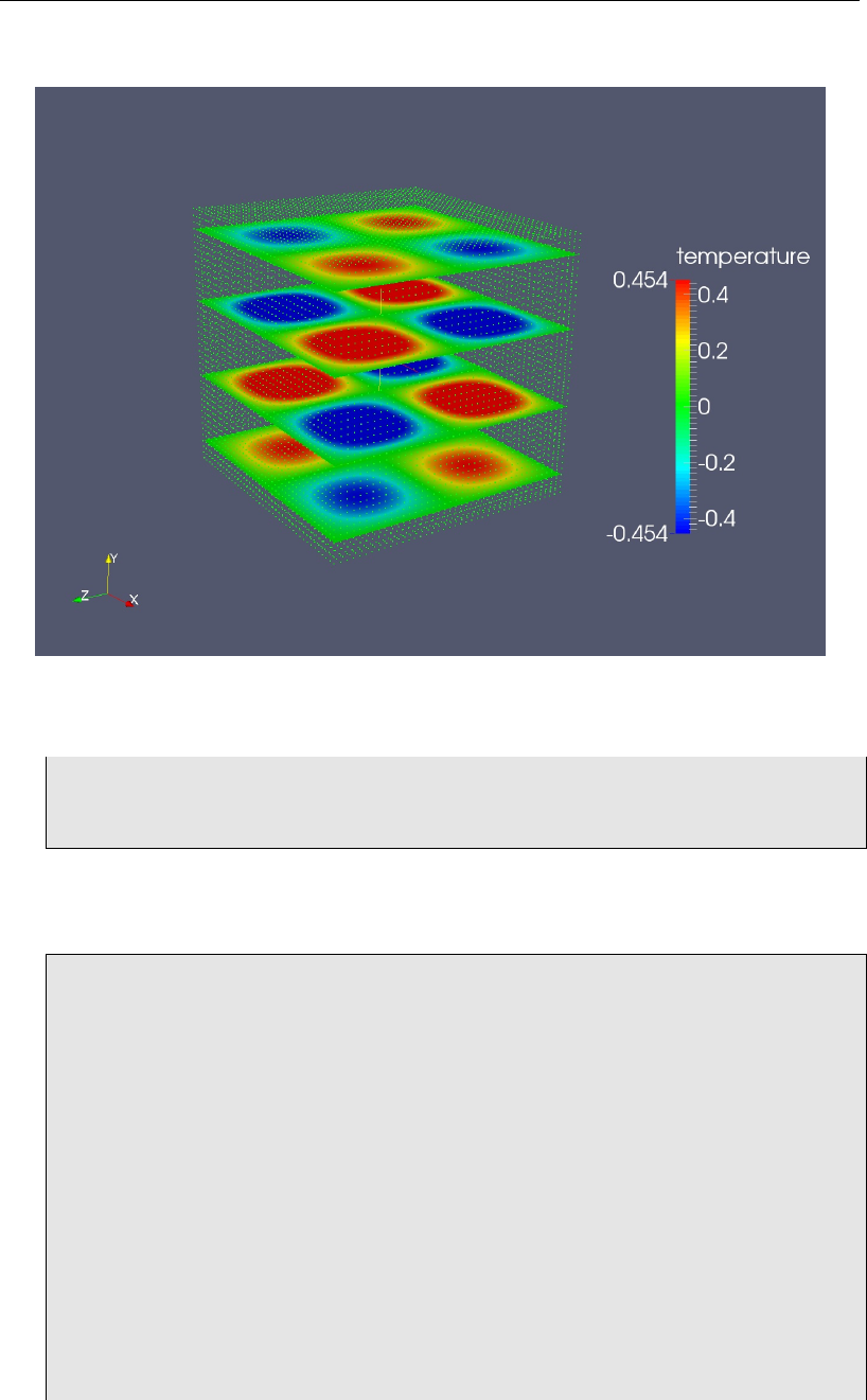
To the aim of solving problem (2.6) using LifeV, we set Ω = (−1,1)3, ΓD=∂Ω and the data

f, g, h such that the exact solution of the Poisson problem is u(x) = sin(πx)sin(πy)sin(πz).

Preamble: headers and MPI conﬁguration

We ﬁrst include the diﬀerent headers containing the data structures and the algorithms we

are employing along the simulation: At ﬁrst the Epetra data structures that allow the use of

MPI

•the deﬁnition of the MPI environment, that is made exploiting the Epetra framework

2.2. THE POISSON PROBLEM CHAPTER 2. LEARNING BY EXAMPLES

1#i n c l u d e <E p e t r a C o n f i g D e f s . h>

2#i f d e f EPETRA MPI

3#i n c l u d e <mpi . h>

4#i n c l u d e <Epetra MpiComm . h>

5#e l s e

6#i n c l u d e <Epetra Ser ialC omm . h>

7#e n d i f

•the deﬁnition of the basis structures of LifeV, in particular meshes, ﬁnite elements spaces

and expressions

1#i n c l u d e <l i f e v / co re / Lif e V . hpp>

2#i n c l u d e <l i f e v / co re / u t i l / Lif eChr onoM anag er . hpp>

3#i n c l u d e <l i f e v / c o r e /mesh/ M e s h P a r t i t i o n e r . hpp>

4#i n c l u d e <l i f e v / co re /mesh/ Reg ionMe sh3DS truct ured . hpp>

5#i n c l u d e <l i f e v / co re /mesh/ RegionMesh . hpp>

6#i n c l u d e <l i f e v / co re / ar r a y / Ma tr ix Ep et ra . hpp>

7#i n c l u d e <l i f e v / co re / fem /BCManage . hpp>

8#i n c l u d e <l i f e v / et a /fem /ETFESpace . hpp>

9#i n c l u d e <l i f e v / e t a / e x p r e s s i o n / BuildGr aph . hpp>

10 #i n c l u d e <l i f e v / e ta / e x p r e s s i o n / I n t e g r a t e . hpp>

11 #i n c l u d e <Epetra FECrsGraph .h>

•the deﬁnition of the solver and the exporting routines

1#i n c l u d e <T eu c h os Pa ra m e te r L is t . hpp>

2#i n c l u d e <Teuchos XMLParameterListHelpers .hpp>

3#i n c l u d e <Teuchos RCP . hpp>

4#i n c l u d e <l i f e v / c o re / a l go r i th m / L i n e a r S o l v e r . hpp>

5#i n c l u d e <l i f e v / c o r e / a l go r it h m / P r e c o n d i t i o n e r I f p a c k . hpp>

6#i n c l u d e <l i f e v / co re / f i l t e r / ExporterHDF5 . hpp>

•some other useful classes

1#i n c l u d e <b oo s t / s h a r e d p t r . hpp>

2#i n c l u d e <l i f e v / e t a / ex am ple s / l a p l a c i a n / l a p l a c i a n F u n c t o r . hpp>

Next, we deﬁne the LifeV namespace

1u s i n g n amespace LifeV ;

Structured mesh and ﬁnite element spaces

After having read the dataﬁle as explained in Section 2.1, we build a cubic structured

mesh and we divide it among the processors which are running the simulation

1// Mesh

2typedef RegionMesh<LinearTetra >mesh_Type ;

3boost : : shared_ptr<mesh_Type >fullMeshPtr (new mesh_Type (C o m m ) ) ;

5// Bu i l di n g s t r u c t u r e d mesh ( i n t h i s c a se a cu be )

6regularMesh3D (∗fullMeshPtr , 0 ,

7dataFile (”mesh/nx ” , 15 ) , dataFile (”mesh/ny ” , 15 ) ,

8dataFile (” mesh/ nz ” , 15 ) , dataFile (”mesh / v e r b o s e ” ,false ) ,

92 . 0 , 2 . 0 , 2 . 0 , −1.0 , −1 .0 , −1.0 ) ;

11 // P a r t i t i o n i n g mesh , p o s s i b l y wit h ov e rl a p

12 const UInt overlap (dataFile (”mesh/ o v e r l a p ” , 0 ) ) ;

13 boost : : shared_ptr<mesh_Type >localMeshPtr ;

15 MeshPartitioner<mesh_Type >meshPart ;

2.2. THE POISSON PROBLEM CHAPTER 2. LEARNING BY EXAMPLES

17 i f (overlap )

18 {

19 meshPart .setPartitionOverlap (overlap ) ;

20 }

22 meshPart .doPartition (fullMeshPtr ,C o m m ) ;

23 localMeshPtr =meshPart .meshPartition ( ) ;

25 // C l e a r i n g g l o b a l mesh

26 fullMeshPtr .reset ( ) ;

We notice that the domain origins from the point (−1−1,−1) and has a length of 2 in

each dimension. The overlap variable states the number of layers that are shared by

two processors with contiguous subdomains.

We next deﬁne the ﬁnite element space, whose dimension is read by the input ﬁle. Then

we build the corresponding Expression Template ﬁnite element space, whose use allows

the user to adopt the templated expressions that refer to the weak formulation of the

problem.

1// F i n i t e e l e m e n t s p a c e

2typedef FESpace<mesh_Type ,MapEpetra >uSpaceStd_Type ;

3typedef boost : : shared_ptr<uSpaceStd_Type >uSpaceStdPtr_Type ;

4typedef ETFESpace<mesh_Type ,MapEpetra , 3 , 1 >uSpaceETA_Type ;

5typedef boost : : shared_ptr<uSpaceETA_Type >uSpaceETAPtr_Type ;

6typedef FESpace<mesh_Type ,MapEpetra >: : function_Type function_Type ;

8// D e f i n i n g f i n i t e e l e m e n t s s t a n da r d and E x p r e s s i o n Te mp late s p a c e s

9u S p a c e S t d P t r _ T y p e u F E S pa c e (new uSpaceStd_Type (localMeshPtr ,

10 dataFile (” f i n i t e e l e m e n t / d e g r e e ” ,”P1” ) , 1 , C o m m ) ) ;

11 u S p a c e E T A P t r _ T y p e E T u F E S pa c e (new uSpaceETA_Type (localMeshPtr ,

12 & ( u F E S p a c e −>refFE ( ) ) , & ( u F E S p a c e −>f e ( ) . g e o M a p ( ) ) , ←-

C o m m ) ) ;

Assembly of the stiﬀness matrix, the right-hand-side and the setting of

boundary conditions

In order to assembly the system that corresponds to the ﬁnite element formulation,

we need to build at ﬁrst the graph that contains the topology of the matrix and then

assemblying the matrix by constructing the elements a(φj, φi)

1// M a t r i c e s and g r a ph s

2typedef E p e t r a _ F E C r s G r a p h g r a p h _ Ty p e ;

3typedef boost : : shared_ptr<Epetra_FECrsGraph>graphPtr_Type ;

4typedef MatrixEpetra<R e a l >matrix_Type ;

5typedef boost : : shared_ptr<MatrixEpetra<R e a l > > matrixPtr_Type ;

7g r a p h P t r _ T y p e s y s t e m G r a p h ;

8m a t r i x P t r _ T y p e s y s t e m M a t r i x ;

10 i f (overlap )

11 {

12 systemGraph .reset (new graph_Type (Co py ,∗(u F E S p a c e −>map ( ) . map (←-

U n i q u e ) ) , 5 0 , t r u e ) ) ;

13 }

14 e l s e

15 {

16 systemGraph .reset (new graph_Type (Co py ,∗(u F E S p a c e −>map ( ) . map (←-

U n i q u e ) ) , 50 ) ) ;

17 }

19 {

20 u s i n g n amespace ExpressionAssembly ;

22 buildGraph (

23 elements (localMeshPtr ) ,

24 u F E S p a c e −>qr ( ) ,

2.2. THE POISSON PROBLEM CHAPTER 2. LEARNING BY EXAMPLES

25 ETuFESpace ,

26 ETuFESpace ,

27 dot (g r a d (phi_i ) , g r a d (phi_j ) )

28 )

29 >> systemGraph ;

30 }

32 systemGraph−>GlobalAssemble ( ) ;

34 i f (overlap )

35 {

36 systemMatrix .reset (new matrix_Type (ETuFESpace−>map ( ) , ∗systemGraph ,t r u e )←-

) ;

37 }

38 e l s e

39 {

40 systemMatrix .reset (new matrix_Type (ETuFESpace−>map ( ) , ∗systemGraph ) ) ;

41 }

43 // C l e a r i n g p rob le m s m at ri x

44 systemMatrix−>z e r o ( ) ;

46 {

47 u s i n g n amespace ExpressionAssembly ;

49 integrate (

50 elements (localMeshPtr ) ,

51 u F E S p a c e −>qr ( ) ,

52 ETuFESpace ,

53 ETuFESpace ,

54 dot (g r a d (phi_i ) , g r a d (phi_j ) )

55 )

56 >> systemMatrix ;

57 }

Next, we build the solution and the right hand side vectors. For the latter, we employ the

laplacianFunctor class, that is constructed by providing the function that describes

the source term

1// Vectors

2typedef V e c t o r E p e t r a v e c t o r _ T y p e ;

3typedef boost : : shared_ptr<VectorEpetra>vectorPtr_Type ;

5vectorPtr_Type rhsLap ;

6v e c t o r P t r _ T y p e s o l u t i o n L a p ;

8i f (overlap )

10 r h s L a p .reset (new vector_Type (u F E S p a c e −>map ( ) , Unique ,Z e r o ) ) ;

11 solutionLap .reset (new vector_Type (u F E S p a c e −>map ( ) , Unique ,Z e r o ) ) ;

12 }

13 e l s e

14 {

15 r h s L a p .reset (new vector_Type (u F E S p a c e −>map ( ) , U n i q u e ) ) ;

16 solutionLap .reset (new vector_Type (u F E S p a c e −>map ( ) , U n i q u e ) ) ;

17 }

19 rhsLap−>z e r o ( ) ;

20 solutionLap−>z e r o ( ) ;

22 Real sourceFunction (const R e a l&/∗t∗/,const R e a l&x,

23 const R e a l&y,const R e a l&z,

24 const ID&/∗i∗/)

25 {

26 r e t u r n 3∗M _ P I ∗M _ P I

27 ∗sin (M _ P I ∗x)∗sin (M _ P I ∗y)∗sin (M _ P I ∗z) ;

28 }

30 boost : : shared_ptr<laplacianFunctor<R e a l > > laplacianSourceFunctor (new ←-

laplacianFunctor<R e a l >(sourceFunction ) ) ;

32 {

33 u s i n g n amespace ExpressionAssembly ;

35 integrate (

36 elements (localMeshPtr ) ,

2.2. THE POISSON PROBLEM CHAPTER 2. LEARNING BY EXAMPLES

37 u F E S p a c e −>qr ( ) ,

38 ETuFESpace ,

39 e v a l (laplacianSourceFunctor ,X)∗phi_i

40 )

41 >> r h s L a p ;

42 }

We remark here that the use of the expression templates allows the user to deﬁne the

equivalent of the weak formulation, in particular the elements of the matrix are built

using the test and trial functions phiiand phij, and setting the quadrature rule to adopt.

Boundary conditions

We explain here how to impose the boundary conditions. At ﬁrst we give an identiﬁcation

number to the faces of our domain, and then deﬁne the function gthat is assigned to the

boundarues, in this case we have homogeneous Dirichlet conditions, so we construct the

function zeroFunction that returns 0. for every value of the spatial domain. In LifeV,

it is possible to impose the boundaries through a BCHandler object, which imposes on

every boundary the corresponding Dirichlet datum by providing the keyword Essential.

1// Cube s w al l s i d e n t i f i e r s

2c o n s t i n t B A C K = 1 ;

3c o n s t i n t FRONT = 2 ;

4c o n s t i n t L E F T = 3 ;

5c o n s t i n t RIGHT = 4 ;

6c o n s t i n t B O T T O M = 5 ;

7c o n s t i n t TOP = 6 ;

9R ea l z e r o F u n c t i o n (const R e a l&/∗t∗/,const R e a l&/∗x∗/,const R e a l&/∗y∗/,←-

const R e a l&/∗z∗/,const I D&/∗i∗/)

10 {

11 r e t u r n 0.;

12 }

14 BCHandler bcHandler ;

16 BCFunctionBase ZeroBC (zeroFunction ) ;

17 BCFunctionBase OneBC (nonZeroFunction ) ;

19 bcHandler .addBC (”Back” ,B ACK ,Essential ,Scalar ,ZeroBC , 1 ) ;

20 bcHandler .addBC (” L e f t ” ,LE FT ,Essential ,Scalar ,ZeroBC , 1 ) ;

21 bcHandler .addBC (”Top” ,TOP ,Essential ,Scalar ,ZeroBC , 1 ) ;

22 bcHandler .addBC (” Fro nt ” ,F RO NT ,Essential ,Scalar ,ZeroBC , 1 ) ;

23 bcHandler .addBC (” Rig ht ” ,RI G HT ,Essential ,Scalar ,ZeroBC , 1 ) ;

24 bcHandler .addBC (”Bottom ” ,BOTTOM ,Essential ,Scalar ,ZeroBC , 1 ) ;

26 bcHandler .bcUpdate (∗u F E S p a c e −>m e s h ( ) , u F E S p a c e −>f e B d ( ) , u F E S p a c e −>dof ( ) ) ;

27 bcManage (∗systemMatrix ,∗rhsLap ,∗u F E S p a c e −>m e s h ( ) , u F E S p a c e −>dof ( ) ,

28 bcHandler ,u F E S p a c e −>f e B d ( ) , 1 . 0 , 0 . 0 ) ;

Preconditioning and solving the system

Since our computation employs a parallel architecture. before solving the linear system

we need to assemble both the matrix and the right hand side

1systemMatrix−>globalAssemble ( ) ;

2rhsLap−>globalAssemble ( ) ;

Next we set the solver parameters according to the input ﬁle SolverParamList.xml and

the preconditioner that employs the Additive Schwarz method

1// S o l ve r and p r e c o n d i t i o n e r

2.2. THE POISSON PROBLEM CHAPTER 2. LEARNING BY EXAMPLES

2typedef LinearSolver : : S o l v e r T y p e s o l v e r _ T y p e ;

3typedef LifeV : : Preconditioner basePrec_Type ;

4typedef boost : : shared_ptr<basePrec_Type>basePrecPtr_Type ;

5typedef PreconditionerIfpack prec_Type ;

6typedef boost : : shared_ptr<prec_Type>precPtr_Type ;

8LinearSolver linearSolver (C o m m ) ;

9linearSolver .setOperator (systemMatrix ) ;

11 Teuchos : : RCP<Teuchos : : ParameterList >aztecList =Teuchos : : rcp (new Teuchos←-

: : ParameterList ) ;

12 aztecList =Teuchos : : getParametersFromXmlFile (”SolverParamList . xml” ) ;

14 linearSolver .setParameters (∗aztecList ) ;

16 prec_Type∗precRawPtr ;

17 basePrecPtr_Type precPtr ;

18 precRawPtr =new prec_Type ;

19 precRawPtr−>setDataFromGetPot (d a t a F i l e ,” p r e c ” ) ;

20 precPtr .reset (precRawPtr ) ;

22 linearSolver .setPreconditioner (precPtr ) ;

And ﬁnally we solve the system

1linearSolver .setRightHandSide (r h s L a p ) ;

2linearSolver .solve (solutionLap ) ;

Exporting and post processing

We set the exporter that employs the library HDF5, the result is then visible using a

post processing tool, for instance Paraview (http://www.paraview.org/).

1// S e t t i n g e x p o r t e r

2ExporterHDF5<mesh_Type >exporter (d a t a F i l e ,” e x p o r t e r ” ) ;

3exporter .setMeshProcId (localMeshPtr ,Co mm−>MyPID ( ) ) ;

4exporter .setPrefix (”laplace” ) ;

5exporter .setPostDir (” . / ” ) ;

6exporter .addVariable (ExporterData<mesh_Type >: : ScalarField ,”temperature” ,←-

u F E S p a c e ,solutionLap ,U I n t ( 0 ) ) ;

7exporter .postProcess ( 0 ) ;

8exporter .closeFile ( ) ;

Now, suppose we want to investigate the trend of the error by varying the mesh size, to

check numerically the estimates (2.7), (2.8). At ﬁrst, we need to deﬁne the function u

and its gradient ∇uin our program, in the same way we deﬁned the source term f

1Real uExactFunction (const R e a l&/∗t∗/,const R e a l&x,const R e a l&y,const ←-

R e a l&z,const I D&/∗i∗/)

3r e t u r n sin (M _ P I ∗y)∗sin (M _ P I ∗z)∗sin (M _ P I ∗x) ;

6function_Type uEx(uExactFunction ) ;

8VectorSmall<3>uGradExactFunction (const R e a l&/∗t∗/,const R e a l&x,const ←-

R e a l&y,const R e a l&z,const ID&/∗i∗/)

10 VectorSmall<3>v;

12 v[ 0 ] = M _ P I ∗cos (M _ P I ∗x)∗sin (M _ P I ∗y)∗sin (M _ P I ∗z) ;

13 v[ 1 ] = M _ P I ∗sin (M _ P I ∗x)∗cos (M _ P I ∗y)∗sin (M _ P I ∗z) ;

14 v[ 2 ] = M _ P I ∗sin (M _ P I ∗x)∗sin (M _ P I ∗y)∗cos (M _ P I ∗z) ;

16 r e t u r n v;

17 }

2.2. THE POISSON PROBLEM CHAPTER 2. LEARNING BY EXAMPLES

Figure 2.1: Result of Poisson equation with homogeneous Dirichlet boundary conditions

19 boost : : shared_ptr<laplacianFunctor<R e a l > > laplacianExactFunctor (new ←-

laplacianFunctor<R e a l >(uExactFunction ) ) ;

20 boost : : shared_ptr<laplacianFunctor<VectorSmall<3> > > ←-

laplacianExactGradientFunctor (new laplacianFunctor<VectorSmall<3> >(←-

uGradExactFunction ) ) ;

Next, we need to evaluate the norms following their deﬁnition, and to do that we still

employ the Expression Templates provided in LifeV

1R e al L 2 E r r o r L a p = 0 . 0 ;

2Real TotL2ErrorLap = 0 . 0 ;

4Real H1SeminormLap = 0 . 0 ;

5Real TotH1SeminormLap = 0 . 0 ;

8u s i n g n amespace ExpressionAssembly ;

10 integrate (

11 elements (localMeshPtr ) ,

12 u F E S p a c e −>qr ( ) ,

13 (e v a l (laplacianExactFunctor ,X)−value (ETuFESpace ,∗←-

solutionLap ) )

14 ∗(e v a l (laplacianExactFunctor ,X)−value (ETuFESpace ,∗←-

solutionLap ) )

15 )>> L2ErrorLap ;

17 }

19 {

20 u s i n g n amespace ExpressionAssembly ;

22 integrate (

23 elements (localMeshPtr ) ,

24 u F E S p a c e −>qr ( ) ,

2.2. THE POISSON PROBLEM CHAPTER 2. LEARNING BY EXAMPLES

10 010 1

10 -2

10 -1

10 0

10 1

H1-Error-P1

H1-Error-P2

10 010 1

10 -4

10 -3

10 -2

10 -1

10 0

L2-Error-P1

L2-Error-P2

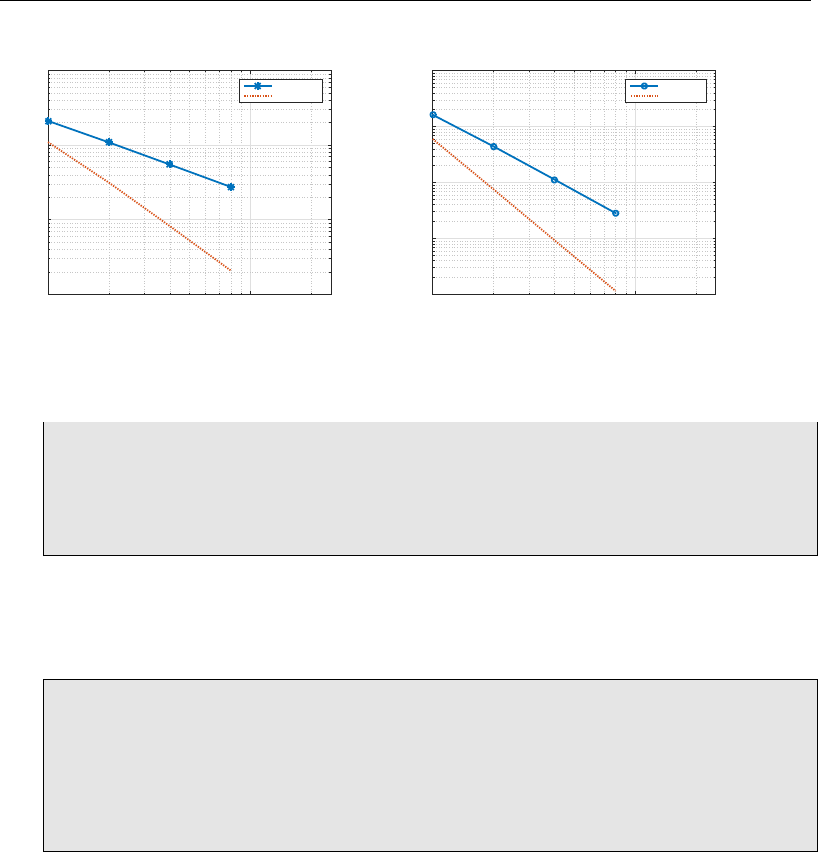
Figure 2.2: H1norm (left) and L2norm (right) vs mesh size for r= 1,2.

25 dot (e v a l (laplacianExactGradientFunctor ,X)−g r a d (ETuFESpace ,∗←-

solutionLap ) ,

26 e v a l (laplacianExactGradientFunctor ,X)−g r a d (ETuFESpace ,∗←-

solutionLap ) )

27 )>> H1SeminormLap ;

29 }

30 Co m m−>Barrier ( ) ;

Finally, we gather the results of the diﬀerent processors and print the norm. We collect

the results for diﬀerent mesh sizes and perform a convergence analysis, whose results are

shown in Fig. 2.2.

1Co m m−>S u m A l l (& L2ErrorLap , &TotL2ErrorLap , 1 ) ;

2Co m m−>S u m A l l (& H1SeminormLap , &TotH1SeminormLap , 1) ;

4i f (verbose )

6std : : c o u t << ” T o tE r ro r i n L2 norm i s ”

7<< s q r t (TotL2ErrorLap )<< std : : e n d l ;

8std : : c o u t << ” T o tE r ro r i n H1 norm i s ”

9<< s q r t (TotL2ErrorLap +TotH1SeminormLap )<< std : : e n d l ;

10 }

Bibliography

[1] A. Quarteroni. Numerical Models for Diﬀerential Problems. Modeling, Simulation

and Applications. Springer, Heidelberg, DE, 2009. Written for students of bache-

lor and master courses in scientiﬁc disciplines: engineering, mathematics, physics,

computational sciences, and information science.

Lifev Manual

Navigation menu

Versions of this User Manual:

Views

Navigation