Listed Volatility And Variance Derivatives A Python Based Guide
listed%20volatility%20and%20variance%20derivatives%20-%20a%20python-based%20guide%20(2016)
User Manual:
Open the PDF directly: View PDF ![]() .
.
Page Count: 357 [warning: Documents this large are best viewed by clicking the View PDF Link!]
- 10.1002@9781119167945.ch0.pdf (p.1-10)
- 10.1002@9781119167945.ch1.pdf (p.11-25)
- 10.1002@9781119167945.ch2.pdf (p.26-62)
- 10.1002@9781119167945.ch3.pdf (p.63-75)
- 10.1002@9781119167945.ch4.pdf (p.76-100)
- 10.1002@9781119167945.ch5.pdf (p.101-134)
- 10.1002@9781119167945.ch6.pdf (p.135-184)
- 10.1002@9781119167945.ch7.pdf (p.185-225)
- 10.1002@9781119167945.ch8.pdf (p.226-230)
- 10.1002@9781119167945.ch9.pdf (p.231-254)
- 10.1002@9781119167945.ch10.pdf (p.255-272)
- 10.1002@9781119167945.ch11.pdf (p.273-284)
- 10.1002@9781119167945.ch12.pdf (p.285-300)
- 10.1002@9781119167945.ch13.pdf (p.301-318)
- 10.1002@9781119167945.ch14.pdf (p.319-347)
- 10.1002@9781119167945.ch15.pdf (p.348-349)
- 10.1002@9781119167945.ch16.pdf (p.350-357)

Listed Volatility
and Variance
Derivatives
Founded in 1807, John Wiley & Sons is the oldest independent publishing company in the
United States. With ofces in North America, Europe, Australia and Asia, Wiley is glob-
ally committed to developing and marketing print and electronic products and services for
our customers’ professional and personal knowledge and understanding.
The Wiley Finance series contains books written specically for nance and invest-
ment professionals as well as sophisticated individual investors and their nancial advi-
sors. Book topics range from portfolio management to e-commerce, risk management,
nancial engineering, valuation and nancial instrument analysis, as well as much more.
For a list of available titles, visit our Web site at www.WileyFinance.com.

Listed Volatility
and Variance
Derivatives
A Python-based Guide
DR. YVES J. HILPISCH
This edition rst published 2017
©2017 Yves Hilpisch
Registered ofce
John Wiley & Sons Ltd, The Atrium, Southern Gate, Chichester, West Sussex, PO19 8SQ, United
Kingdom
For details of our global editorial ofces, for customer services and for information about how to apply
for permission to reuse the copyright material in this book please visit our website at www.wiley.com.
The right of the author to be identied as the author of this work has been asserted in accordance with
the Copyright, Designs and Patents Act 1988.
All rights reserved. No part of this publication may be reproduced, stored in a retrieval system, or
transmitted, in any form or by any means, electronic, mechanical, photocopying, recording or
otherwise, except as permitted by the UK Copyright, Designs and Patents Act 1988, without the prior
permission of the publisher.
Wiley publishes in a variety of print and electronic formats and by print-on-demand. Some material
included with standard print versions of this book may not be included in e-books or in
print-on-demand. If this book refers to media such as a CD or DVD that is not included in the version
you purchased, you may download this material at http://booksupport.wiley.com. For more information
about Wiley products, visit www.wiley.com.
Designations used by companies to distinguish their products are often claimed as trademarks. All
brand names and product names used in this book are trade names, service marks, trademarks or
registered trademarks of their respective owners. The publisher is not associated with any product or
vendor mentioned in this book.
Limit of Liability/Disclaimer of Warranty: While the publisher and author have used their best efforts
in preparing this book, they make no representations or warranties with respect to the accuracy or
completeness of the contents of this book and specically disclaim any implied warranties of
merchantability or tness for a particular purpose. It is sold on the understanding that the publisher is
not engaged in rendering professional services and neither the publisher nor the author shall be liable
for damages arising herefrom. If professional advice or other expert assistance is required, the services
of a competent professional should be sought.
Library of Congress Cataloging-in-Publication Data is available
A catalogue record for this book is available from the British Library.
ISBN 978-1-119-16791-4 (hbk) ISBN 978-1-119-16792-1 (ebk)
ISBN 978-1-119-16793-8 (ebk) ISBN 978-1-119-16794-5 (ebk)
Cover Design: Wiley
Top Image: ©grapestock/Shutterstock
Bottom Image: ©stocksnapper/iStock
Set in 10/12pt Times by Aptara Inc., New Delhi, India
Printed in Great Britain by TJ International Ltd, Padstow, Cornwall, UK

Contents
Preface xi
PART ONE
Introduction to Volatility and Variance
CHAPTER 1
Derivatives, Volatility and Variance 3
1.1 Option Pricing and Hedging 3
1.2 Notions of Volatility and Variance 6
1.3 Listed Volatility and Variance Derivatives 7
1.3.1 The US History 7
1.3.2 The European History 8
1.3.3 Volatility of Volatility Indexes 9
1.3.4 Products Covered in this Book 10
1.4 Volatility and Variance Trading 11
1.4.1 Volatility Trading 11
1.4.2 Variance Trading 13
1.5 Python as Our Tool of Choice 14
1.6 Quick Guide Through the Rest of the Book 14
CHAPTER 2
Introduction to Python 17
2.1 Python Basics 17
2.1.1 Data Types 17
2.1.2 Data Structures 20
2.1.3 Control Structures 22
2.1.4 Special Python Idioms 23
2.2 NumPy 28
2.3 matplotlib 34
2.4 pandas 38
2.4.1 pandas DataFrame class 39
2.4.2 Input-Output Operations 45
2.4.3 Financial Analytics Examples 47
2.5 Conclusions 53
v

vi CONTENTS
CHAPTER 3
Model-Free Replication of Variance 55
3.1 Introduction 55
3.2 Spanning with Options 56
3.3 Log Contracts 57
3.4 Static Replication of Realized Variance and Variance Swaps 57
3.5 Constant Dollar Gamma Derivatives and Portfolios 58
3.6 Practical Replication of Realized Variance 59
3.7 VSTOXX as Volatility Index 65
3.8 Conclusions 67
PART TWO
Listed Volatility Derivatives
CHAPTER 4
Data Analysis and Strategies 71
4.1 Introduction 71
4.2 Retrieving Base Data 71
4.2.1 EURO STOXX 50 Data 71
4.2.2 VSTOXX Data 74
4.2.3 Combining the Data Sets 76
4.2.4 Saving the Data 78
4.3 Basic Data Analysis 78
4.4 Correlation Analysis 83
4.5 Constant Proportion Investment Strategies 87
4.6 Conclusions 93
CHAPTER 5
VSTOXX Index 95
5.1 Introduction 95
5.2 Collecting Option Data 95
5.3 Calculating the Sub-Indexes 105
5.3.1 The Algorithm 106
5.4 Calculating the VSTOXX Index 114
5.5 Conclusions 118
5.6 Python Scripts 118
5.6.1 index collect option_data.py 118
5.6.2 index_subindex_calculation.py 123
5.6.3 index_vstoxx_calculation.py 127
CHAPTER 6
Valuing Volatility Derivatives 129
6.1 Introduction 129
6.2 The Valuation Framework 129
6.3 The Futures Pricing Formula 130

Contents vii
6.4 The Option Pricing Formula 132
6.5 Monte Carlo Simulation 135
6.6 Automated Monte Carlo Tests 141
6.6.1 The Automated Testing 141
6.6.2 The Storage Functions 145
6.6.3 The Results 146
6.7 Model Calibration 153
6.7.1 The Option Quotes 154
6.7.2 The Calibration Procedure 155
6.7.3 The Calibration Results 160
6.8 Conclusions 163
6.9 Python Scripts 163
6.9.1 srd_functions.py 163
6.9.2 srd simulation analysis.py 167
6.9.3 srd simulation results.py 171
6.9.4 srd model calibration.py 174
CHAPTER 7
Advanced Modeling of the VSTOXX Index 179
7.1 Introduction 179
7.2 Market Quotes for Call Options 179
7.3 The SRJD Model 182
7.4 Term Structure Calibration 183
7.4.1 Futures Term Structure 184
7.4.2 Shifted Volatility Process 190
7.5 Option Valuation by Monte Carlo Simulation 191
7.5.1 Monte Carlo Valuation 191
7.5.2 Technical Implementation 192
7.6 Model Calibration 195
7.6.1 The Python Code 196
7.6.2 Short Maturity 199
7.6.3 Two Maturities 201
7.6.4 Four Maturities 203
7.6.5 All Maturities 205
7.7 Conclusions 209
7.8 Python Scripts 210
7.8.1 srjd fwd calibration.py 210
7.8.2 srjd_simulation.py 212
7.8.3 srjd_model_calibration.py 215
CHAPTER 8
Terms of the VSTOXX and its Derivatives 221
8.1 The EURO STOXX 50 Index 221
8.2 The VSTOXX Index 221
8.3 VSTOXX Futures Contracts 223
8.4 VSTOXX Options Contracts 224
8.5 Conclusions 225

viii CONTENTS
PART THREE
Listed Variance Derivatives
CHAPTER 9
Realized Variance and Variance Swaps 229
9.1 Introduction 229
9.2 Realized Variance 229
9.3 Variance Swaps 235
9.3.1 Denition of a Variance Swap 235
9.3.2 Numerical Example 235
9.3.3 Mark-to-Market 239
9.3.4 Vega Sensitivity 241
9.3.5 Variance Swap on the EURO STOXX 50 242
9.4 Variance vs. Volatility 247
9.4.1 Squared Variations 247
9.4.2 Additivity in Time 247
9.4.3 Static Hedges 250
9.4.4 Broad Measure of Risk 250
9.5 Conclusions 250
CHAPTER 10
Variance Futures at Eurex 251
10.1 Introduction 251
10.2 Variance Futures Concepts 252
10.2.1 Realized Variance 252
10.2.2 Net Present Value Concepts 252
10.2.3 Traded Variance Strike 257
10.2.4 Traded Futures Price 257
10.2.5 Number of Futures 258
10.2.6 Par Variance Strike 258
10.2.7 Futures Settlement Price 258
10.3 Example Calculation for a Variance Future 258
10.4 Comparison of Variance Swap and Future 265
10.5 Conclusions 268
CHAPTER 11
Trading and Settlement 269
11.1 Introduction 269
11.2 Overview of Variance Futures Terms 269
11.3 Intraday Trading 270
11.4 Trade Matching 274
11.5 Different Traded Volatilities 275
11.6 After the Trade Matching 277
11.7 Further Details 279
11.7.1 Interest Rate Calculation 279
11.7.2 Market Disruption Events 280
11.8 Conclusions 280

Contents ix
PART FOUR
DX Analytics
CHAPTER 12
DX Analytics – An Overview 283
12.1 Introduction 283
12.2 Modeling Risk Factors 284
12.3 Modeling Derivatives 287
12.4 Derivatives Portfolios 290
12.4.1 Modeling Portfolios 292
12.4.2 Simulation and Valuation 293
12.4.3 Risk Reports 294
12.5 Conclusions 296
CHAPTER 13
DX Analytics – Square-Root Diffusion 297
13.1 Introduction 297
13.2 Data Import and Selection 297
13.3 Modeling the VSTOXX Options 301
13.4 Calibration of the VSTOXX Model 303
13.5 Conclusions 308
13.6 Python Scripts 308
13.6.1 dx srd calibration.py 308
CHAPTER 14
DX Analytics – Square-Root Jump Diffusion 315
14.1 Introduction 315
14.2 Modeling the VSTOXX Options 315
14.3 Calibration of the VSTOXX Model 320
14.4 Calibration Results 325
14.4.1 Calibration to One Maturity 325
14.4.2 Calibration to Two Maturities 325
14.4.3 Calibration to Five Maturities 325
14.4.4 Calibration without Penalties 331
14.5 Conclusions 332
14.6 Python Scripts 334
14.6.1 dx srjd calibration.py 334
Bibliography 345
Index 347

Preface
Volatility and variance trading has evolved from something opaque to a standard tool in
today’s nancial markets. The motives for trading volatility and variance as an asset class
of its own are numerous. Among others, it allows for effective option and equity portfolio hedg-
ing and risk management as well as straight out speculation on future volatility (index) move-
ments. The potential benets of volatility- and variance-based strategies are widely accepted
by researchers and practitioners alike.
With regard to products it mainly started out around 1993 with over-the-counter (OTC)
variance swaps. At about the same time, the Chicago Board Options Exchange introduced the
VIX volatility index. This index still serves today – after a signicant change in its method-
ology – as the underlying risk factor for some of the most liquidly traded listed derivatives
in this area. The listing of such derivatives allows for a more standardized, cost efcient and
transparent approach to volatility and variance trading.
This book covers some of the most important listed volatility and variance derivatives
with a focus on products provided by Eurex. Larger parts of the content are based on the
Eurex Advanced Services tutorial series which use Python to illustrate the main concepts of
volatility and variance products. I am grateful that Eurex allowed me to use the contents of the
tutorial series freely for this book.
Python has become not only one of the most widely used programming languages but also
one of the major technology platforms in the nancial industry. It is more like a platform since
the Python ecosystem provides a wealth of powerful libraries and packages useful for nancial
analytics and application building. It also integrates well with many other technologies, like
the statistical programming language R, used in the nancial industry. You can nd links to
all Python resources under http://lvvd.tpq.io.
I thank Michael Schwed for providing parts of the Python code. I also thank my family
for all their love and support over the years, especially my wife Sandra and our children Lilli
and Henry. I dedicate this book to my beloved dog Jil. I miss you.
Y
Voelklingen, Saarland, April 2016
xi

PART
One
Introduction to Volatility
and Variance

CHAPTER 1
Derivatives, Volatility and Variance
The rst chapter provides some background information for the rest of the book. It mainly
covers concepts and notions of importance for later chapters. In particular, it shows how the
delta hedging of options is connected with variance swaps and futures. It also discusses differ-
ent notions of volatility and variance, the history of traded volatility and variance derivatives
as well as why Python is a good choice for the analysis of such instruments.
1.1 OPTION PRICING AND HEDGING
In the Black-Scholes-Merton (1973) benchmark model for option pricing, uncertainty with
regard to the single underlying risk factor S(stock price, index level, etc.) is driven by a geo-
metric Brownian motion with stochastic differential equation (SDE)
dSt=𝜇Stdt +𝜎StdZt
Throughout we may think of the risk factor as being a stock index paying no dividends. Stis
then the level of the index at time t,𝜇the constant drift, 𝜎the instantaneous volatility and Ztis
a standard Brownian motion. In a risk-neutral setting, the drift 𝜇is replaced by the (constant)
risk-less short rate r
dSt=rStdt +𝜎StdZt
In addition to the index which is assumed to be directly tradable, there is also a risk-less bond
Bavailable for trading. It satises the differential equation
dBt=rBtdt
In this model, it is possible to derive a closed pricing formula for a vanilla European call option
Cmaturing at some future date Twith payoff max[ST−K,0], Kbeing the xed strike price.
It is
C(S,K,t,T,r,𝜎)=St⋅N(d1)−e−r(T−t)⋅K⋅N(d2)
3
Listed Volatility and Variance Derivatives: A
Python-based Guide
By Dr. Yves J. Hilpisch
© 2017 Yves Hilpisch

4LISTED VOLATILITY AND VARIANCE DERIVATIVES
where
N(d)=1
2𝜋∫d
−∞
e−1
2x2dx
d1=
log St
K+r+𝜎2
2(T−t)
𝜎T−t
d2=
log St
K+r−𝜎2
2(T−t)
𝜎T−t
The price of a vanilla European put option Pwith payoff max[K−ST, 0] is determined by
put-call parity as
Pt=Ct−St+e−r(T−t)K
There are multiple ways to derive this famous Black-Scholes-Merton formula. One way relies
on the construction of a portfolio comprised of the index and the risk-less bond that perfectly
replicates the option payoff at maturity. To avoid risk-less arbitrage, the value of the option
must equal the payoff of the replicating portfolio. Another method relies on calculating the
risk-neutral expectation of the option payoff at maturity and discounting it back to the present
by the risk-neutral short rate. For detailed explanations of these approaches refer, for example,
to Bj¨
ork (2009).
Yet another way, which we want to look at in a bit more detail, is to perfectly hedge
the risk resulting from an option (e.g. from the point of view of a seller of the option) by
dynamically trading the index and the risk-less bond. This approach is usually called delta
hedging (see Sinclair (2008), ch. 1). The delta of a European call option is given by the rst
partial derivative of the pricing formula with respect to the value of the risk factor, i.e. 𝛿t=𝛿Ct
𝛿St
.
More specically, we get
𝛿t=𝛿Ct
𝛿St
=N(d1)
When trading takes place continuously, the European call option position hedged by 𝛿tindex
units short is risk-less:
dΠt≡dCt−𝛿tSt=0
This is due to the fact that the only (instantaneous) risk results from changes in the index level
and all such (marginal) changes are compensated for by the delta short index position.
Continuous models and trading are a mathematically convenient description of the real
world. However, in practice trading and therefore hedging can only take place at discrete points
in time. This does not lead to a complete breakdown of the delta hedging approach, but it

Derivatives, Volatility and Variance 5
introduces hedge errors. If hedging takes place at every discrete time interval of length Δt,the
Prot-Loss (PL) for such a time interval is roughly (see Bossu (2014), p. 59)
PLΔt≈1
2Γ⋅ΔS2+Θ⋅Δt
Γis the gamma of the option and measures how the delta (marginally) changes with the chang-
ing index level. ΔSis the change in the index level over the time interval Δt. It is given by
Γ= 𝜕2C
𝜕S2=N′(d1)
S𝜎T−t
Θis the theta of the option and measures how the option value changes with the passage of
time. It is given approximately by (see Bossu (2014), p. 60)
Θ≈−
1
2ΓS2𝜎2
With this we get
PLΔt≈1
2Γ⋅ΔS2−1
2ΓS2𝜎2⋅Δt
=1
2Γ⋅S2ΔS
S2
−𝜎⋅Δt2
The quantity 1
2Γ⋅S2is called the dollar gamma of the option and gives the second order change
in the option price induced by a (marginal) change in the index level. (ΔS
S)2is the squared
realized return over the time interval Δt– it might be interpreted as the (instantaneously)
realized variance if the time interval is short enough and the drift is close to zero. Finally,
(𝜎⋅Δt)2is the xed, “theoretical” variance in the model for the time interval.
The above reasoning illustrates that the PL of a discretely delta hedged option position is
determined by the difference between the realized variance during the discrete hedge interval
and the theoretically expected variance given the model parameter for the volatility. The total
hedge error over N=T
Δtintervals is given by
Cumulative PLΔt≈1
2
N
t=1
Γt−1⋅S2
t−1ΔSt
St−12
−𝜎⋅Δt2(1.1)
This little exercise in option hedging leads us to a result which is already quite close to a
product intensively discussed in this book: listed variance futures. Variance futures, and their
Over-the-Counter (OTC) relatives variance swaps, pay to the holder the difference between
realized variance over a certain period of time and a xed variance strike.

6LISTED VOLATILITY AND VARIANCE DERIVATIVES
1.2 NOTIONS OF VOLATILITY AND VARIANCE
The previous section already touches on different notions of volatility and variance. This
section provides formal denitions for these and other quantities of importance. For a more
detailed exposition refer to Sinclair (2008). In what follows we assume that a time series is
given with quotes Sn,n∈{0, …,N} (see Hilpisch (2015, ch. 3)). We do not assume any spe-
cic model that might generate the time series data. The log return for n>0 is dened by
Rn≡log Sn−logSn−1=log Sn
Sn−1
realized or historical volatility: this refers to the standard deviation of the log returns of
a nancial time series; suppose we observe N(past) log returns Rn,n∈{1, …,N}, with
mean return ̂𝜇 =1
NN
n=1Rn; the realized or historical volatility ̂𝜎 is then given by
̂𝜎 =
1
N−1
N
n=1
(Rn−̂𝜇)2
instantaneous volatility: this refers to the volatility factor of a diffusion process; for
example, in the Black-Scholes-Merton model the instantaneous volatility 𝜎is found in
the respective (risk-neutral) stochastic differential equation (SDE)
dSt=rStdt +𝜎StdZt
implied volatility: this is the volatility that, if put into the Black-Scholes-Merton option
pricing formula, gives the market-observed price of an option; suppose we observe today
a price of C∗
0for a European call option; the implied volatility 𝜎imp is the quantity that
solves ceteris paribus the implicit equation
C∗
0=CBSM(S0,K,t=0, T,r,𝜎imp)
These volatilities all have squared counterparts which are then named variance, such as real-
ized variance, instantenous variance or implied variance. We have already encountered realized
variance in the previous section. Let us revisit this quantity for a moment. Simply applying the
above denition of realized volatility and squaring it we get
̂𝜎2=1
N−1
N
n=1
(Rn−̂𝜇)2
In practice, however, this denition usually gets adjusted to
̂𝜎2=1
N
N
n=1
R2
n

Derivatives, Volatility and Variance 7
The drift of the process is assumed to be zero and only the log return terms get squared. It
is also common practice to use the denition for the uncorrected (biased) standard deviation
with factor 1
Ninstead of the denition for the corrected (unbiased) standard deviation with
factor 1
N−1. This explains why we call the term ( ΔSt
St−1
)2from the delta hedge PL in the previous
section realized variance over the time interval Δt. In that case, however, the return is the
simple return instead of the log return.
Other adjustments in practice are to scale the value to an annual quantity by multiplying
it by 252 (trading days) and to introduce an additional scaling term (to get percent values
instead of decimal ones). One then usually ends up with (see chapter 9, Realized Variance and
Variance Swaps)
̂𝜎2≡10000 ⋅
252
N
⋅
N
n=1
R2
n
Later on we will also drop the hat notation when there is no ambiguity.
1.3 LISTED VOLATILITY AND VARIANCE DERIVATIVES
Volatility is one of the most important notions and concepts in derivatives pricing and analytics.
Early research and nancial practice considered volatility as a major input for pricing and
hedging. It is not that long ago that the market started thinking of volatility as an asset class
of its own and designed products to make it directly tradable.
The idea for a volatility index was conceived by Brenner and Galai in 1987 and pub-
lished in the note Brenner and Galai (1989) in the Financial Analysts Journal. They write in
their note:
“While there are efcient tools for hedging against general changes in overall market
directions, so far there are no effective tools available for hedging against changes
in volatility. …We therefore propose the construction of three volatility indexes on
which cash-settled options and futures can be traded.”
In what follows, we focus on the US and European markets.
1.3.1 The US History
The Chicago Board Options Exchange (CBOE) introduced an equity volatility index, called
VIX, in 1993. It was based on a methodology developed by Fleming, Ostdiek and Whaley
(1995) – a working paper version of which was circulated in 1993 – and data from S&P 100
index options. The methodology was changed in 2003 to the now standard practice which uses
the robust, model free replication results for variance (see chapter 3 Model-Free Replication
of Variance) and data from S&P 500 index options (see CBOE (2003)). While the rst version
represented a proxy for the 30 day at-the-money implied volatility, the current version is a
proxy for the 30 day variance swap rate, i.e. the xed variance strike which gives a zero value
for a respective swap at inception.
8LISTED VOLATILITY AND VARIANCE DERIVATIVES
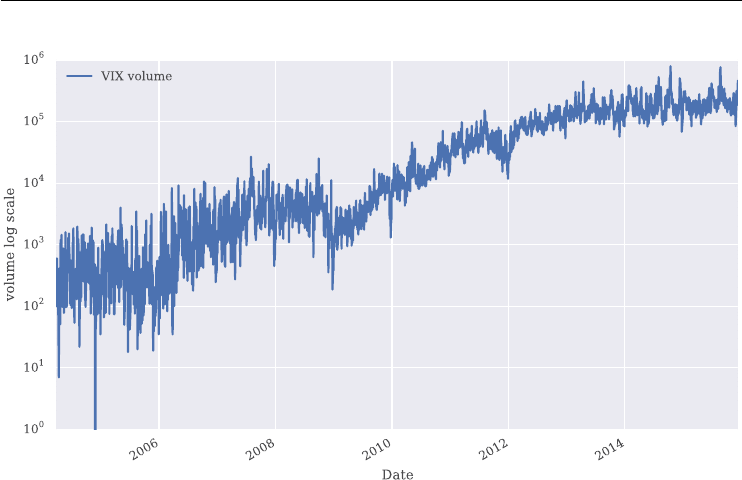
FIGURE 1.1 Historical volume of traded VIX derivatives on a log scale. Data source:
http://cfe.cboe.com/data/historicaldata.aspx
Carr and Lee (2009) provide a brief history of both OTC and listed volatility and variance
products. They claim that the rst OTC variance swap has been engineered and offered by
Union Bank of Switzerland (UBS) in 1993, at about the same time the CBOE announced the
VIX. These were also the rst traded contracts to attract some liquidity in contrast to volatility
swaps which were also introduced shortly afterwards. One reason for this is that variance swaps
can be robustly hedged – as we will see in later chapters – while volatility swaps, in general,
cannot. It is more or less the same reasoning behind the change of methodology for the VIX
in 2003.
Trading in futures on the VIX started in 2004 while the rst options on the index were
introduced in 2006. These instruments are already described in Whaley (1993), although their
market launch took more than 10 years after the introduction of the VIX. These were not the
rst listed volatility derivatives but the rst to attract signicant liquidity and they are more
actively traded at the time of writing than ever. Those listed instruments introduced earlier,
such as volatility futures launched in 1998 by Deutsche Terminb¨
orse (now Eurex), could not
attract enough liquidity and are now only a footnote in the nancial history books.
The volume of traded contracts on the VIX has risen sharply on average over recent years
as Figure 1.1 illustrates. The volume varies rather erratically and is inuenced inter alia by
seasonal effects and the general market environment (bullish or bearish sentiment).
In December 2012, the CBOE launched the S&P 500 variance futures contract –almost
20 years after their OTC counterparts started trading. After some early successes in building
liquidity in 2013, liquidity has dried up almost completely in 2014 and 2015.
1.3.2 The European History
Eurex – back then Deutsche Terminb¨
orse – introduced in 1994 the VDAX volatility index,an
index representing the 45 day implied volatility of DAX index options. As mentioned before,
Derivatives, Volatility and Variance 9
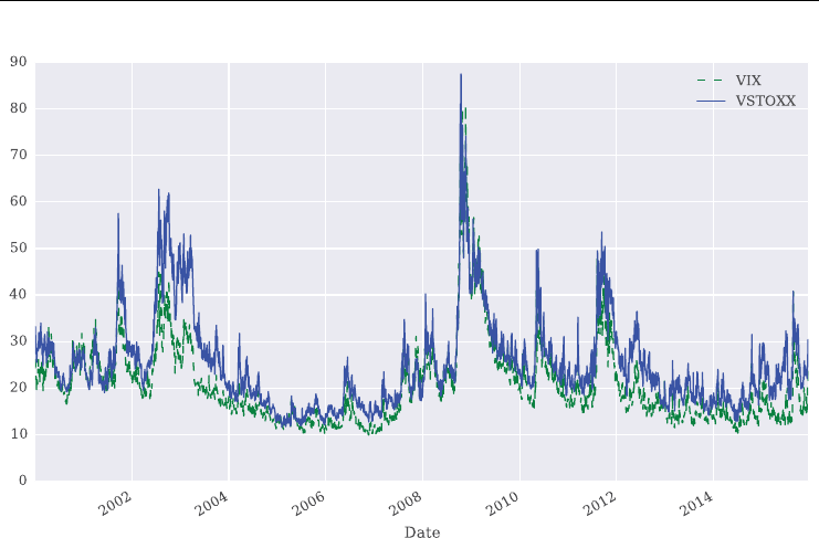
FIGURE 1.2 Historical daily closing levels for the VIX and the VSTOXX volatility indexes. Data
source: Yahoo! Finance and http://stoxx.com
in 1998 Eurex introduced futures on the VDAX which could, however, not attract enough
liquidity and were later delisted. In 2005, the methodolgy for calculating the index was also
changed to the more robust, model-free replication approach for variance swaps. The index
was renamed VDAX-NEW and a new futures contract on this index was introduced.
In 2005, Eurex also launched futures on the VSTOXX volatility index which is based on
options on the EURO STOXX 50 index and uses the by now standard methodology for volatil-
ity index calculation as laid out in CBOE (2003). In 2009 they were re-launched as “Mini
VSTOXX Futures” with the symbol FVS. At the same time, Eurex stopped the trading of
other volatility futures, such as those on the VDAX-NEW and the VSMI.
Since the launch of the new VSTOXX futures, they have attracted signicant liquidity and
are now actively traded. A major reason for this can be seen in the nancial crisis of 2007–2009
when volatility indexes saw their highest levels ever. This is illustrated in Figure 1.2 where the
maximum values for the VIX and VSTOXX are observed towards the end of 2008. This led
to a higher sensitivity of market participants to the risks that spikes in volatility can bring and
thus increased the demand for products to hedge against such adverse market environments.
Observe also in Figure 1.2 that the two indexes are positively correlated in general, over the
period shown with about +0.55.
In March 2010, Eurex introduced options on the VSTOXX index. These instruments also
attracted some liquidity and are at the time of writing actively traded. In September 2014,
Eurex then launched a variance futures contract on the EURO STOXX 50 index.
1.3.3 Volatility of Volatility Indexes
Nowadays, we are already one step further on. There are now indexes available that measure
the volatility of volatility (vol-vol). The so-called VVIX of the CBOE was introduced in March
10 LISTED VOLATILITY AND VARIANCE DERIVATIVES
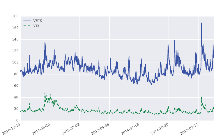
FIGURE 1.3 Historical daily closing levels for the VIX and the VVIX volatility (of volatility)
indexes. Data source: Thomson Reuters Eikon
2012. In October 2015 the index provider STOXX Limited introduced the V-VSTOXX indexes
which are described on www.stoxx.com as follows:
“The V-VSTOXX Indices are based on VSTOXX realtime options prices and are
designed to reect the market expectations of near-term up to long-term volatility-
of-volatility by measuring the square root of the implied variance across all options
of a given time to expiration.”
These new indexes and potential products written on them seem to be a benecial addition to
the volatility asset class. Such products might be used, for example, to hedge options written
on the volatility index itself since the vol-vol is stochastic in nature rather than constant or
deterministic.
The VVIX index is generally on a much higher level than the VIX index as Figure 1.3
illustrates. This indicates a much higher volatility for the VIX index itself compared to the
S&P 500 volatility.
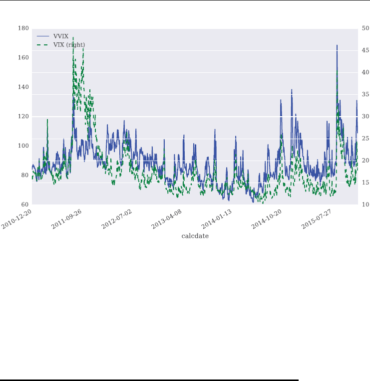
Over the period shown, the VVIX is highly positively correlated with the VIX at a level
of about +0.66. Figure 1.4 plots the time series data for the two indexes on two different scales
to show this stylized fact graphically.
1.3.4 Products Covered in this Book
There is quite a diverse spectrum of volatility and variance futures available. Out of all possible
products, the focus of this book is on the European market and these instruments:
VSTOXX as a volatility index
VSTOXX futures
VSTOXX options
Eurex Variance Futures.
Derivatives, Volatility and Variance 11
FIGURE 1.4 Different scalings for the VVIX and VIX indexes to illustrate the positive correlation.
Data Source: Thomson Reuters Eikon
The majority of the material has originally been developed as part of the Eurex Advanced
Services. Although the focus is on Europe, the methods and approaches presented can usu-
ally be tranferred easily to the American landscape, for instance. This results from the fact
that some methodological unication has taken place over the past few years with regard to
volatility and variance related indexes and products.
1.4 VOLATILITY AND VARIANCE TRADING
This section discusses motives and rationales for trading listed volatility and variance deriva-
tives. It does not cover volatility (variance) trading strategies that can be implemented with,
for example, regular equity options (see Cohen (2005), ch. 4).
1.4.1 Volatility Trading
It is instructive to rst list characteristics of volatility indexes. We focus on the VSTOXX
and distinguish between facts (which follow from construction) and stylized facts (which are
supported by empirical evidence):
market expection (fact): the VSTOXX represents a 30 day implied volatility average
from out-of-the money options, i.e. the market consensus with regard to the “to be real-
ized” volatility over the next 30 days
non-tradable asset (fact): the VSTOXX itself is not directly tradable, only derivatives on
the VSTOXX can be traded
mean-reverting nature (fact): the VSTOXX index is mean-reverting, it does not show a
positive or negative drift over longer periods of time
12 LISTED VOLATILITY AND VARIANCE DERIVATIVES
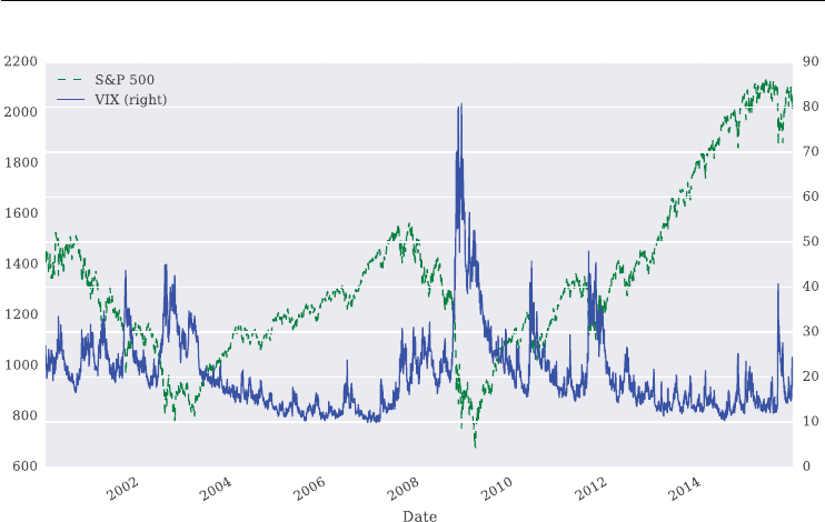
FIGURE 1.5 Different scalings for the S&P 500 and VIX indexes to illustrate the negative
correlation. Data source: Yahoo! Finance
negative correlation (stylized fact): the VSTOXX is (on average) negatively correlated
with the respective equity index, the EURO STOXX 50
positive jumps (stylized fact): during times of stock market crisis, the VSTOXX can jump
to rather high levels; the mean reversion generally happens much more slowly
higher than realized volatility (stylized fact): on average, the VSTOXX index is higher
than the realized volatility over the next 30 days.
Figure 1.5 illustrates the negative correlation between the S&P 500 index and the VIX index
graphically. Over the period shown, the correlation is about −0.75.
The value of a VSTOXX future represents the (market) expectation with regard to the
future value of the VSTOXX at the maturity date of the future. Given this background, typical
volatility trading strategies involving futures include the following:
long VSTOXX future: such a position can be used to hedge equity positions (due to the
negative correlation with the EURO STOXX 50) or to increase returns of an equity port-
folio (e.g. through a constant-proportion investment strategy, see chapter 4, Data Analysis
and Strategies); it can also be used to hedge a short realized volatility strategy
short VSTOXX future: such a trade can be entered, for example, when the VSTOXX
spikes and the expectation is that it will revert (fast enough) to its mean; it might also
serve to reduce vega exposure in long vega option portfolios
term structure arbitrage: for example, shorting the front month futures contract and
going long the nearby futures contract represents a typical term structure arbitrage strategy
when the term structure is in contango; this is due to different carries associated with
different futures contracts and maturities, respectively

Derivatives, Volatility and Variance 13
relative value arbitrage: VSTOXX futures can also be traded against other volatility/-
variance sensitive instruments and positions, like OTC variance swaps, equity options
portfolios, etc.
Similar and other strategies can be implemented involving VSTOXX options. With regard to
exercise they are European in nature and can be delta hedged by using VSTOXX futures which
is yet another motive for trading in futures. Typical trading strategies involving VSTOXX
options are:
long OTM calls: such a position might protect an equity portfolio from losses due to a
market crash (again due to the negative correlation between VSTOXX and EURO STOXX
50)
short ATM calls: writing ATM calls, and pocketing the option premium, might be attrac-
tive when the current implied volatility levels are relatively high
long ATM straddle: buying put and call options on the VSTOXX with same (ATM) strike
and maturity yields a prot when the VSTOXX moves fast enough in one direction; this
is typically to be expected when the volatility of volatility (vol-vol) is high.
For both VSTOXX futures and options many other strategies can be implemented that exploit
some special situation (e.g. contango or backwardation in the futures prices) or reect a certain
expectation of the trader (e.g. that realized volatility will be lower/higher than the implied/
expected volatility).
1.4.2 Variance Trading
The motives and rationales for trading in EURO STOXX 50 variance futures are not too dif-
ferent from those involving VSTOXX derivatives (see Bossu et al. (2005)). Typical strategies
include:
long variance future: this position benets when the realized variance is higher than
the variance strike (implied variance at inception); it might also be used to hedge equity
portfolio risks or short vega options positions
short variance future: this position benets when the realized variance is below the vari-
ance strike which tends to be the case on average; it can also hedge a long vega options
position
forward volatility/variance trading: since variance is additive over time (which volatil-
ity is not), one can get a perfect exposure to forward implied volatility by, for exam-
ple, shorting the September variance future and going long the October contract; this
gives an exposure to the forward implied volatility from September maturity to October
maturity
correlation trading: variance futures can be traded to exploit (statistical) arbitrage oppor-
tunities between, for example, the (implied) variance of an equity index and its compo-
nents or the (implied) variance of one equity index versus another one; in both cases, the
rationale is generally based on the correlation of the different assets and their variance,
respectively.

14 LISTED VOLATILITY AND VARIANCE DERIVATIVES
1.5 PYTHON AS OUR TOOL OF CHOICE
There are some general reasons why Python is a good choice for computational nance and
nancial data science these days. Among others, these are:
open source: Python is open source and can be used by students and big nancial insti-
tutions alike for free
syntax: Python’s readable and concise syntax make it a good choice for presenting formal
concepts, like those in nance
ecosystem: compared to other languages Python has an excellent ecosystem of libraries
and packages that are useful for data analytics and scientic computing in general and
nancial analytics in particular
performance: in recent years, the ecosystem of Python has grown especially in the
area of performance libraries, making it much easier to get to computing speeds more
than sufcient for the most computationally demanding algorithms, such as Monte Carlo
simulation
adoption: at the time of writing, Python has established itself as a core technology at
major nancial institutions, be it leading investment banks, big hedge funds or more tra-
ditional asset management rms
career: given the widespread adoption of Python, learning and mastering the language
seems like a good career move for everybody working in the industry or planning to
do so.
In view of the scope and style of the book, one special feature is noteworthy:
interactivity: the majority of the code examples presented in this book can be executed
in interactive fashion within the Jupyter Notebook environment (see http://jupyter.org);
in this regard, Python has a major advantage as an interpreted language compared to a
compiled one with its typical edit-compile-run cycle.
Chapter 1 of Hilpisch (2014) provides a more detailed overview of aspects related to
Python for Finance. All the code presented in this book is available via resources listed
under http://lvvd.tpq.io, especially on the Quant Platform for which you can register under
http://lvvd.quant-platform.com.
1.6 QUICK GUIDE THROUGH THE REST OF THE BOOK
The remainder of this introductory part of the book is organized as follows:
chapter 2: this chapter introduces Python as a technology platform for (interactive) nan-
cial analytics; a more detailed account of Python for Finance is provided in Hilpisch
(2014)
chapter 3: this chapter presents the model-free replication approach for variance; it is
important for both volatility indexes and derivatives written on them as well as for variance
futures.

Derivatives, Volatility and Variance 15
The second part of the book is about the VSTOXX and listed volatility derivatives. It comprises
the following chapters:
chapter 4: as a starting point, chapter 4 uses Python to analyze historical data for the
VSTOXX and EURO STOXX 50 indexes; a focal point is the analysis of some simple
trading strategies involving the VSTOXX
chapter 5: using the model-free replication approach for variance, this chapter shows in
detail how the VSTOXX index is calculated and how to use Python to (re-)calculate it
using raw option data as input
chapter 6:Gr
¨
unbichler and Longstaff (1996) were among the rst to propose a parame-
terized model to value futures and options on volatility indexes; chapter 6 presents their
model which is based on a square-root diffusion process and shows how to simulate and
calibrate it to volatility option market quotes
chapter 7: building on chapter 6, chapter 7 presents a more sophisticated framework – a
deterministic shift square-root jump diffusion (SRJD) process – to model the VSTOXX
index and to better capture the implied volatility smiles and volatility term structure
observed in the market; the exposition is slightly more formal compared to the rest of
the book
chapter 8: this brief chapter discusses terms of the VSTOXX volatility index as well as
the futures and options traded on the VSTOXX.
Part three of the book is about the Eurex Variance Futures contract as listed in September 2014.
This part comprises three chapters:
chapter 9: listed variance futures are mainly based on the popular OTC variance swap
contracts with some differences introduced by intraday trading; chapter 9 therefore cov-
ers variance swaps in some detail and also discusses differences between variance and
volatility as an underlying asset
chapter 10: this chapter provides a detailed discussion of all concepts related to the listed
Eurex Variance Futures contract and shows how to (re-)calculate its value given historical
data; it also features a comparison between the futures contract and a respective OTC
variance swap contract
chapter 11: this chapter discusses all those special characteristics of the Eurex Variance
Futures when it comes to (intraday) trading and settlement.
Part four of the book focuses on the DX Analytics nancial library (see http://dx-
analytics.com) to model the VSTOXX index and to calibrate different models to VSTOXX
options quotes. It consists of three chapters:
chapter 12: this chapter introduces basic concepts and API elements of the DX Analytics
library
chapter 13: using the square-root diffusion model as introduced in chapter 6, this chapter
implements a calibration study to a single maturity of VSTOXX options over the rst
quarter of 2014
chapter 14: chapter 14 replicates the same calibration study but in a more sophisticated
fashion; it calibrates the deterministic shift square-root jump diffusion process not only
to a single maturity of options but to as many as ve simultaneously.

CHAPTER 2
Introduction to Python
Python has become a powerful programming language and has developed a huge ecosystem
of helpful libraries over the last couple of years. This chapter provides a concise overview
of Python and two of the major pillars of the the so-called scientic stack:
NumPy (see http://numpy.scipy.org)
pandas (see http://pandas.pydata.org)
NumPy provides performant array operations on numerical data while pandas is specif-
ically designed to handle more complex data analytics operations, e.g. on (nancial) times
series data.
Such an introductory chapter – only addressing selected topics relevant to the contents
of this book – can of course not replace a thorough introduction to Python and the libraries
covered. However, if you are rather new to Python or programming in general you might get
a rst overview and a feeling of what Python is all about. If you are already experienced in
another language typically used in quantitative nance (e.g. Matlab, R, C++, VBA), you see
what typical data structures, programming paradigms and idioms in Python look like.
For a comprehensive overview of Python applied to nance see Hilpisch (2014). Other,
more general introductions to the language with a scientic and data analysis focus are Haenel
et al. (2013), Langtangen (2009) and McKinney (2012).
This chapter and the rest of the book is based on Python 2.7 although the majority of the
code should be easily transformed to Python 3.5 after some minor modications.
2.1 PYTHON BASICS
This section introduces basic Python data types and structures, control structures and some
Python idioms.
2.1.1 Data Types
It is noteworthy that Python is a dynamically typed system which means that types of objects
are inferred from their contexts. Let us start with numbers.
17
Listed Volatility and Variance Derivatives: A
Python-based Guide
By Dr. Yves J. Hilpisch
© 2017 Yves Hilpisch

18 LISTED VOLATILITY AND VARIANCE DERIVATIVES
In [1]: a=3 # defining an integer object
In [2]: type(a)
Out[2]: int
In [3]: a.bit_length() # number of bits used
Out[3]: 2
In [4]: b=5. # defining a float object
In [5]: type(b)
Out[5]: float
Python can handle arbitrarily large integers which is quite benecial for number of theoretical
applications, for instance:
In [6]: c = 10 ** 100 # googol number
In [7]: type(c)
Out[7]: long
In [8]: c# long integer object
Out[8]: 1000000000000000000000000000000000000000000000000000000000000000
0000000000000000000000000000000000000L
In [9]: c.bit_length() # number of bits used
Out[9]: 333
Arithmetic operations on these objects work as expected.
In [10]: 3/5. # division
Out[10]: 0.6
In [11]: a*b # multiplication
Out[11]: 15.0
In [12]: a-b # difference
Out[12]: -2.0
In [13]: b+a # addition
Out[13]: 8.0
In [14]: a**b # power
Out[14]: 243.0

Introduction to Python 19
However, be aware of the oor division which is standard in Python 2.7.
In [15]: 3/5 # int type inferred => floor division
Out[15]: 0
Many often used mathematical functions are found in the math module which is part of
Python’s standard library.
In [16]: import math # importing the library into the namespace
In [17]: math.log(a) # natural logarithm
Out[17]: 1.0986122886681098
In [18]: math.exp(a) # exponential function
Out[18]: 20.085536923187668
In [19]: math.sin(b) # sine function
Out[19]: -0.9589242746631385
Another important basic data type is string objects.
In [20]: s = 'Listed Volatility and Variance Derivatives.'
In [21]: type(s)
Out[21]: str
This object type has multiple methods attached.
In [22]: s.lower() # converting to lower case characters
Out[22]: 'listed volatility and variance derivatives.'
In [23]: s.upper() # converting to upper case characters
Out[23]: 'LISTED VOLATILITY AND VARIANCE DERIVATIVES.'
String objects can be easily sliced. Note that Python has in general zero-based numbering and
indexing.
In [24]: s[0:6]
Out[24]: 'Listed'

20 LISTED VOLATILITY AND VARIANCE DERIVATIVES
Such objects can also be combined using the +operator. The index value -1 represents the last
character of a string (or last element of a sequence in general).
In [25]: st = s[0:6] + s[-13:-1]
In [26]: print st
Listed Derivatives
String replacements are often used to parametrize text output.
In [27]: repl = "My name is %s,Iam%d years old and %4.2f m tall."
# replace %s by a string, %d by an integer and
# %4.2f by a float showing 2 decimal values
In [28]: print repl % ('Peter', 35, 1.88)
My name is Peter, I am 35 years old and 1.88 m tall.
A different way to reach the same goal is the following:
In [29]: repl = "My name is {:s}, I am {:d} years old and {:4.2f} m tall."
In [30]: print repl.format('Peter', 35, 1.88)
My name is Peter, I am 35 years old and 1.88 m tall.
2.1.2 Data Structures
A lightweight data structure is tuples. These are immutable collections of other objects and
are constucted by objects separated by commas – with or without parentheses.
In [31]: t1 = (a, b, st)
In [32]: t1
Out[32]: (3, 5.0, 'Listed Derivatives')
In [33]: type(t1)
Out[33]: tuple
In [34]: t2 = st, b, a
In [35]: t2
Out[35]: ('Listed Derivatives', 5.0, 3)
In [36]: type(t2)
Out[36]: tuple

Introduction to Python 21
Nested structures are also possible.
In [37]: t = (t1, t2)
In [38]: t
Out[38]: ((3, 5.0, 'Listed Derivatives'), ('Listed Derivatives', 5.0, 3))
In [39]: t[0][2] # take 3rd element of 1st element
Out[39]: 'Listed Derivatives'
List objects are mutable collections of other objects and are generally constructed by providing
a comma separated collection of objects in brackets.
In [40]: l = [a, b, st]
In [41]: l
Out[41]: [3, 5.0, 'Listed Derivatives']
In [42]: type(l)
Out[42]: list
In [43]: l.append(s.split()[3]) # append 4th word of string
In [44]: l
Out[44]: [3, 5.0, 'Listed Derivatives', 'Variance']
Sorting is a typical operation on list objects which can also be constructed using the list
constructor (here applied to a tuple object).
In [45]: l = list(('Z', 'Q', 'D', 'J', 'E', 'H', 5., a))
In [46]: l
Out[46]: ['Z', 'Q', 'D', 'J', 'E', 'H', 5.0, 3]
In [47]: l.sort() # in-place sorting
In [48]: l
Out[48]: [3, 5.0, 'D', 'E', 'H', 'J', 'Q', 'Z']
Dictionary objects are so-called key-value stores and are generally constructed with curly
brackets.

22 LISTED VOLATILITY AND VARIANCE DERIVATIVES
In [49]: d = {'int_obj': a,
....: 'float_obj': b,
....: 'string_obj': st}
....:
In [50]: type(d)
Out[50]: dict
In [51]: d
Out[51]: {'float_obj': 5.0, 'int_obj': 3, 'string_obj': 'Listed Derivatives'}
In [52]: d['float_obj'] # look-up of value given key
Out[52]: 5.0
In [53]: d['long_obj'] = c / 10 ** 90 # adding new key value pair
In [54]: d
Out[54]:
{'float_obj': 5.0,
'int_obj': 3,
'long_obj': 10000000000L,
'string_obj': 'Listed Derivatives'}
Keys and values of a dictionary object can be retrieved as list objects.
In [55]: d.keys()
Out[55]: ['long_obj', 'int_obj', 'float_obj', 'string_obj']
In [56]: d.values()
Out[56]: [10000000000L, 3, 5.0, 'Listed Derivatives']
2.1.3 Control Structures
Iterations are very important operations in programming in general and nancial analytics in
particular. Many Python objects are iterable which proves rather convenient in many circum-
stances. Consider the special list object constructor range.
In [57]: range(5) # all integers from zero to 5 excluded
Out[57]: [0, 1, 2, 3, 4]
In [58]: range(3, 15, 2) # start at 3, step with 2 until 15 excluded
Out[58]: [3, 5, 7, 9, 11, 13]

Introduction to Python 23
Such a list object constructor is often used in the context of a for loop.
In [59]: for iin range(5):
....: print i**2,
....:
014916
However, you can iterate over any sequence.
# iteration over list object
In [60]: for _in l:
....: print _,
....:
35.0DEHJQZ
# iteration over string object
In [61]: for cin st:
....: print c + '|',
....:
L|i|s|t|e|d||D|e|r|i|v|a|t|i|v|e|s|
while loops are similar to their counterparts in other languages.
In [62]: i=0 # initialize counter
In [63]: while i<5:
....: print i ** 0.5, # output
....: i+=1 # increase counter by 1
....:
0.0 1.0 1.41421356237 1.73205080757 2.0
The if-elif-else control structure is introduced below in the context of Python function
denitions.
2.1.4 Special Python Idioms
Python relies in many places on a number of special idioms. Let us start with a rather popular
one, the list comprehension.
In [64]: lc=[i**2for iin range(10)]
In [65]: lc
Out[65]: [0, 1, 4, 9, 16, 25, 36, 49, 64, 81]

24 LISTED VOLATILITY AND VARIANCE DERIVATIVES
As the name suggests, the result is a list object.
In [66]: type(lc)
Out[66]: list
So-called lambda or anonymous functions are useful helpers in many places.
In [67]: f=lambda x: math.cos(x) # returns cos of x
In [68]: f(5)
Out[68]: 0.28366218546322625
List comprehensions can be combined with lambda functions to achieve concise constructions
of list objects.
In [69]: lc = [f(x) for xin range(10)]
In [70]: lc
Out[70]:
[1.0,
0.5403023058681398,
-0.4161468365471424,
-0.9899924966004454,
-0.6536436208636119,
0.28366218546322625,
0.960170286650366,
0.7539022543433046,
-0.14550003380861354,
-0.9111302618846769]
However, there is an even more concise way of constructing the same list object – using func-
tional programming approaches, in the following case with map.
In [71]: map(lambda x: math.cos(x), range(10))
Out[71]:
[1.0,
0.5403023058681398,
-0.4161468365471424,
-0.9899924966004454,
-0.6536436208636119,
0.28366218546322625,
0.960170286650366,
0.7539022543433046,
-0.14550003380861354,
-0.9111302618846769]

Introduction to Python 25
In general, one works with regular Python functions (as opposed to lambda functions) which
are constructed as follows:
In [72]: def f(x):
....: return math.exp(x)
....:
The general construction looks like this:
In [73]: def f(*args): # multiple arguments
....: for arg in args:
....: print arg
....: return None # return result(s) (not necessary)
....:
In [74]: f(l)
[3, 5.0, 'D', 'E', 'H', 'J', 'Q', 'Z']
Consider the following function denition which returns different values/strings based on an
if-elif-else control structure:
In [75]: import random # import random number library
In [76]: a = random.randint(0, 999) # draw random number between 0 and 999
In [77]: print "Random number is %d"%a
Random number is 627
In [78]: def number_decide(number):
....: if a < 10:
....: return "Number is single digit."
....: elif 10 <= a < 100:
....: return "Number is double digit."
....: else:
....: return "Number is triple digit."
....: number_decide(a)
....:
Out[78]: 'Number is triple digit.'
A specialty of Python is generator objects. One constructor for such objects that is commonly
used is xrange.

26 LISTED VOLATILITY AND VARIANCE DERIVATIVES
In [79]: g = xrange(10)
In [80]: type(g) # object type
Out[80]: xrange
In [81]: g# object instance
Out[81]: xrange(10)
In [82]: for _in g:
....: print _, # integers are "generated" when needed
....:
0123456789
Generator objects can in many scenarios replace (typical) list objects and have the major advan-
tage that they are in general much more memory efcient. Consider a nancial algorithm that
requires 10 mn loops. Iterating over a list of integers from 0 to 9,999,999 is not efcient since
the algorithm (in general) does not need to have all these numbers available at the same time.
But this is what happens when using range for such a loop.
Consider the following construction of the respective list object containing all integers:
In [83]: %time r = range(10000000)
CPU times: user 87.4 ms, sys: 211 ms, total: 299 ms
Wall time: 299 ms
This object consumes 80 MB (!) of RAM (10 mn times 8 bytes).
In [84]: import sys
In [85]: sys.getsizeof(r) # size in bytes of object
Out[85]: 80000072
On the other hand, consider the analogous construction based on a generator (xrange) object.
It is much, much faster since no memory has to be allocated, no list object has to be generated
up-front, etc.
In [86]: %time xr = xrange(10000000)
CPU times: user 3 us, sys: 1e+03 ns, total: 4 us
Wall time: 5.96 us
Memory consumption is also much, much more efcient – 40 bytes compared to 80 MB.

Introduction to Python 27
In [87]: sys.getsizeof(xr)
Out[87]: 40
However, in practical applications the two can be used often interchangeably such that one
should always resort to the more efcient alternative when possible. The following examples
calculate – using the functional programming operation reduce – the sum of all integers
from 0 to 9,999,999. Although in this case there is hardly a performance difference, the rst
operation requires 80 MB of memory while the second might only require less than 100 bytes.
In [88]: %time reduce(lambda x, y:x+y,range(1000000))
CPU times: user 131 ms, sys: 15.9 ms, total: 147 ms
Wall time: 147 ms
Out[88]: 499999500000
In [89]: %time reduce(lambda x, y:x+y,xrange(1000000))
CPU times: user 118 ms, sys: 0 ns, total: 118 ms
Wall time: 117 ms
Out[89]: 499999500000
More Pythonic (and faster in general) is to calculate the sum using the built-in sum function
– in this case a signicant performance advantage for the generator approach emerges.
In [90]: %timeit sum(range(1000000))
10 loops, best of 3: 26.6 ms per loop
In [91]: %timeit sum(xrange(1000000))
100 loops, best of 3: 12.9 ms per loop
There is also a way of indirectly constructing a generator object, i.e. by the use of parentheses.
The following code results in a generator object for the sine values of the numbers from 0 to
99:
In [92]: g = (math.sin(x) for xin xrange(100))
In [93]: g
Out[93]: <generator object <genexpr> at 0x2ab247901f50>
Such an object stores its internal state and yields the next value when the method next() is
called.

28 LISTED VOLATILITY AND VARIANCE DERIVATIVES
In [94]: g.next()
Out[94]: 0.0
In [95]: g.next()
Out[95]: 0.8414709848078965
Yet another way of constructing a generator object is by a denition style that resembles the
standard function denition closely. The difference is that instead of the return statement,
the yield statement is used.
In [96]: def g(start, end):
....: while start <= end:
....: yield start # yield "next" value
....: start += 1 # increase by one
....:
Usage then might be as follows:
In [97]: go = g(15, 20)
In [98]: for _in go:
....: print _,
....:
15 16 17 18 19 20
2.2 NumPy
Many operations in computational nance take place over (large) arrays of numerical data.
NumPy is a Python library that allows the efcient handling of and operation on such data
structures. Although quite a mighty library with a wealth of functionality, it sufces for the
purposes of this book to cover the basics of NumPy.
In [99]: import numpy as np
The workhorse is the NumPy ndarray class which provides the data structure for n-
dimensional, immutable array objects. You can generate an ndarray object e.g. out of a
list object.

Introduction to Python 29
In [100]: a = np.array(range(24))
In [101]: a
Out[101]:
array([ 0, 1, 2, 3, 4, 5, 6, 7, 8, 9, 10, 11, 12, 13, 14, 15, 16,
17, 18, 19, 20, 21, 22, 23])
The power of these objects lies in the management of n-dimensional data structures (e.g. matri-
ces or cubes of data).
In [102]: b = a.reshape((4, 6))
In [103]: b
Out[103]:
array([[ 0, 1, 2, 3, 4, 5],
[ 6, 7, 8, 9, 10, 11],
[12, 13, 14, 15, 16, 17],
[18, 19, 20, 21, 22, 23]])
In [104]: c = a.reshape((2, 3, 4))
In [105]: c
Out[105]:
array([[[ 0, 1, 2, 3],
[4,5, 6, 7],
[ 8, 9, 10, 11]],
[[12, 13, 14, 15],
[16, 17, 18, 19],
[20, 21, 22, 23]]])
So-called standard arrays (in contrast to e.g. structured arrays) have a single dtype (i.e.
NumPy data type). Consider the following operation which changes the dtype parameter of
the bobject to oat:
In [106]: b = np.array(b, dtype=np.float)
In [107]: b
Out[107]:
array([[ 0., 1., 2., 3., 4., 5.],
[ 6., 7., 8., 9., 10., 11.],
[ 12., 13., 14., 15., 16., 17.],
[ 18., 19., 20., 21., 22., 23.]])

30 LISTED VOLATILITY AND VARIANCE DERIVATIVES
A major strength of NumPy is vectorized operations.
In [108]: 2*b
Out[108]:
array([[ 0., 2., 4., 6., 8., 10.],
[ 12., 14., 16., 18., 20., 22.],
[ 24., 26., 28., 30., 32., 34.],
[ 36., 38., 40., 42., 44., 46.]])
In [109]: b**2
Out[109]:
array([[ 0., 1., 4., 9., 16., 25.],
[ 36., 49., 64., 81., 100., 121.],
[ 144., 169., 196., 225., 256., 289.],
[ 324., 361., 400., 441., 484., 529.]])
You can also pass ndarray objects to lambda or standard Python functions.
In [110]: f=lambda x:x**2-2*x+0.5
In [111]: f(a)
Out[111]:
array([ 0.5, -0.5, 0.5, 3.5, 8.5, 15.5, 24.5, 35.5,
48.5, 63.5, 80.5, 99.5, 120.5, 143.5, 168.5, 195.5,
224.5, 255.5, 288.5, 323.5, 360.5, 399.5, 440.5, 483.5])
In many scenarios, only a (small) part of the data stored in an ndarray object is of interest.
NumPy supports basic and advanced slicing and other selection features.
In [112]: a[2:6] # 3rd to 6th element
Out[112]: array([2, 3, 4, 5])
In [113]: b[2, 4] # 3rd row, final (5th)
Out[113]: 16.0
In [114]: b[1:3, 2:4] # middle square of numbers
Out[114]:
array([[ 8., 9.],
[ 14., 15.]])
Boolean operations are also supported in many places.

Introduction to Python 31
# which numbers are larger than 10?
In [115]: b>10
Out[115]:
array([[False, False, False, False, False, False],
[False, False, False, False, False, True],
[ True, True, True, True, True, True],
[ True, True, True, True, True, True]], dtype=bool)
# only those numbers (flat) that are larger than 10
In [116]: b[b > 10]
Out[116]:
array([ 11., 12., 13., 14., 15., 16., 17., 18., 19., 20., 21.,
22., 23.])
Furthermore, ndarray objects have multiple (convenience) methods already built in.
In [117]: a.sum() # sum of all elements
Out[117]: 276
In [118]: b.mean() # mean of all elements
Out[118]: 11.5
In [119]: b.mean(axis=0) # mean along 1st axis
Out[119]: array([ 9., 10., 11., 12., 13., 14.])
In [120]: b.mean(axis=1) # mean along 2nd axis
Out[120]: array([ 2.5, 8.5, 14.5, 20.5])
In [121]: c.std() # standard deviation for all elements
Out[121]: 6.9221865524317288
Similarly, there is a wealth of so-called universal functions that the NumPy library provides.
Universal in the sense that they can be applied in general to NumPy ndarray objects and to
standard numerical Python data types.
In [122]: np.sum(a) # sum of all elements
Out[122]: 276
In [123]: np.mean(b, axis=0) # mean along 1st axis
Out[123]: array([ 9., 10., 11., 12., 13., 14.])
In [124]: np.sin(b).round(2) # sine of all elements (rounded)
Out[124]:
array([[ 0. , 0.84, 0.91, 0.14, -0.76, -0.96],
[-0.28, 0.66, 0.99, 0.41, -0.54, -1. ],

32 LISTED VOLATILITY AND VARIANCE DERIVATIVES
[-0.54, 0.42, 0.99, 0.65, -0.29, -0.96],
[-0.75, 0.15, 0.91, 0.84, -0.01, -0.85]])
In [125]: np.sin(4.5) # sine of Python float object
Out[125]: -0.97753011766509701
However, you should be aware that applying NumPy universal functions to standard Python
data types generally comes with a signicant performance burden.
In [126]: %time l = [np.sin(x) for x in xrange(100000)]
CPU times: user 188 ms, sys: 3.89 ms, total: 192 ms
Wall time: 192 ms
In [127]: import math
In [128]: %time l = [math.sin(x) for x in xrange(100000)]
CPU times: user 27.7 ms, sys: 0 ns, total: 27.7 ms
Wall time: 27.7 ms
Using the vectorized operations from NumPy is faster than both of the above alternatives which
result in list objects.
In [129]: %time np.sin(np.arange(100000))
CPU times: user 5.23 ms, sys: 0 ns, total: 5.23 ms
Wall time: 5.24 ms
Out[129]:
array([ 0. , 0.84147098, 0.90929743, ..., 0.10563876,
0.89383946, 0.86024828])
Here, we use the ndarray object constructor arange which yields an ndarray object of
integers – below is a simple example:
In [130]: ai = np.arange(10)
In [131]: ai
Out[131]: array([0, 1, 2, 3, 4, 5, 6, 7, 8, 9])
In [132]: ai.dtype
Out[132]: dtype('int64')
Using this constructor, you can also generate ndarray objects with different dtype
attributes:

Introduction to Python 33
In [133]: af = np.arange(0.5, 9.5, 0.5) # start, end, step size
In [134]: af
Out[134]:
array([ 0.5, 1. , 1.5, 2. , 2.5, 3. , 3.5, 4. , 4.5, 5. , 5.5,
6. , 6.5, 7. , 7.5, 8. , 8.5, 9. ])
In [135]: af.dtype
Out[135]: dtype('float64')
In this context the linspace operator is also useful, providing an ndarray object with
evenly spaced numbers.
In [136]: np.linspace(0, 10, 12) # start, end, number of elements
Out[136]:
array([ 0. , 0.90909091, 1.81818182, 2.72727273,
3.63636364, 4.54545455, 5.45454545, 6.36363636,
7.27272727, 8.18181818, 9.09090909, 10. ])
In nancial analytics one often needs (pseudo-)random numbers. NumPy provides many func-
tions to sample from different distributions. Those needed in this book are the standard normal
distribution and the Poisson distribution. The respective functions are found in the sub-library
numpy.random.
In [137]: np.random.standard_normal(10)
Out[137]:
array([ 1.70352821, -1.30223997, -0.16846238, -0.33605234, 0.84842565,
-0.7012202 , 1.31232816, 1.34394536, -0.08358828, 1.53690444])
In [138]: np.random.poisson(0.5, 10)
Out[138]: array([0, 1, 0, 1, 0, 0, 1, 2, 2, 0])
Let us generate an ndarray object which is a bit more “realistic” and which we work with
in what follows:
In [139]: np.random.seed(1000) # fix the rng seed value
In [140]: data = np.random.standard_normal(( 5, 100))
Although this is a slightly larger array one cannot expect that the 500 numbers are indeed
standard normally distributed in the sense that the rst moment is 0 and the second moment is
1. However, at least this can be easily corrected.

34 LISTED VOLATILITY AND VARIANCE DERIVATIVES
In [141]: data.mean() # should be 0.0
Out[141]: -0.02714981205311327
In [142]: data.std() # should be 1.0
Out[142]: 1.0016799134894265
The correction is called moment matching and can be implemented with NumPy by vectorized
operations.
In [143]: data = data - data.mean() # correction for the 1st moment
In [144]: data = data / data.std() # correction for the 2nd moment
In [145]: data.mean() # now really close to 0.0
Out[145]: 7.105427357601002e-18
In [146]: data.std() # now really close to 1.0
Out[146]: 1.0
2.3 matplotlib
At this stage, it makes sense to introduce plotting with matplotlib, the plotting work horse in the
Python ecosystem. We use matplotlib (see http://matplotlib.org) with the settings of another
library throughout, namely seaborn (see http://stanford.edu/∼mwaskom/software/seaborn/) –
this results in a more modern plotting style.
In [147]: import matplotlib.pyplot as plt # import main plotting library
In [148]: import seaborn as sns; sns.set() # set seaborn standards
In [149]: import matplotlib
# set font to serif
In [150]: matplotlib.rcParams['font.family'] = 'serif'
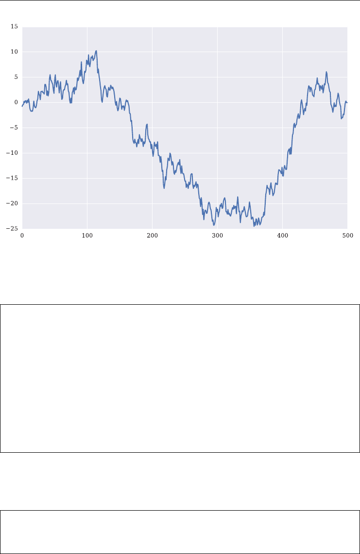
A standard plot is the line plot. The result of the code below is shown as Figure 2.1.
In [151]: plt.figure(figsize=(10, 6)); # size of figure
In [152]: plt.plot(data.cumsum()); # cumulative sum over all elements
Introduction to Python 35
FIGURE 2.1 Standard line plot with matplotlib.
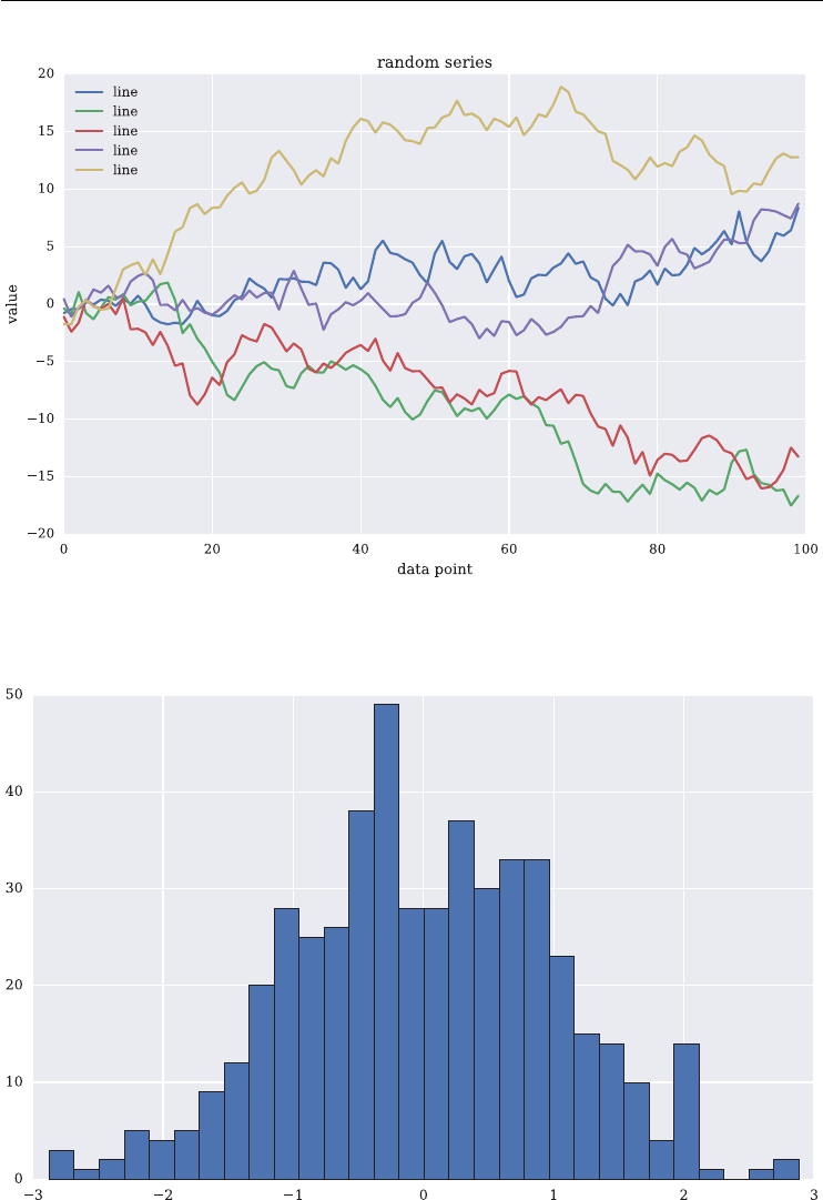
Multiple lines plots are also easy to generate (see Figure 2.2). The operator Tstands for
the transpose of the ndarray object (“matrix”).
In [153]: plt.figure(figsize=(10, 6)); # size of figure
# plotting five cumulative sums as lines
In [154]: plt.plot(data.T.cumsum(axis=0), label='line');
In [155]: plt.legend(loc=0); # legend in best location
In [156]: plt.xlabel('data point'); # x axis label
In [157]: plt.ylabel('value'); # y axis label
In [158]: plt.title('random series'); # figure title
Other important plotting types are histograms and bar charts. A histogram for all 500 values
of the data object is shown as Figure 2.3. In the code, the flatten() method is used to
generate a one-dimensional array from the two-dimensional one.
In [159]: plt.figure(figsize=(10, 6)); # size of figure
In [160]: plt.hist(data.flatten(), bins=30);
36 LISTED VOLATILITY AND VARIANCE DERIVATIVES
FIGURE 2.2 Multiple lines plot with matplotlib.
FIGURE 2.3 Histrogram with matplotlib.
Introduction to Python 37
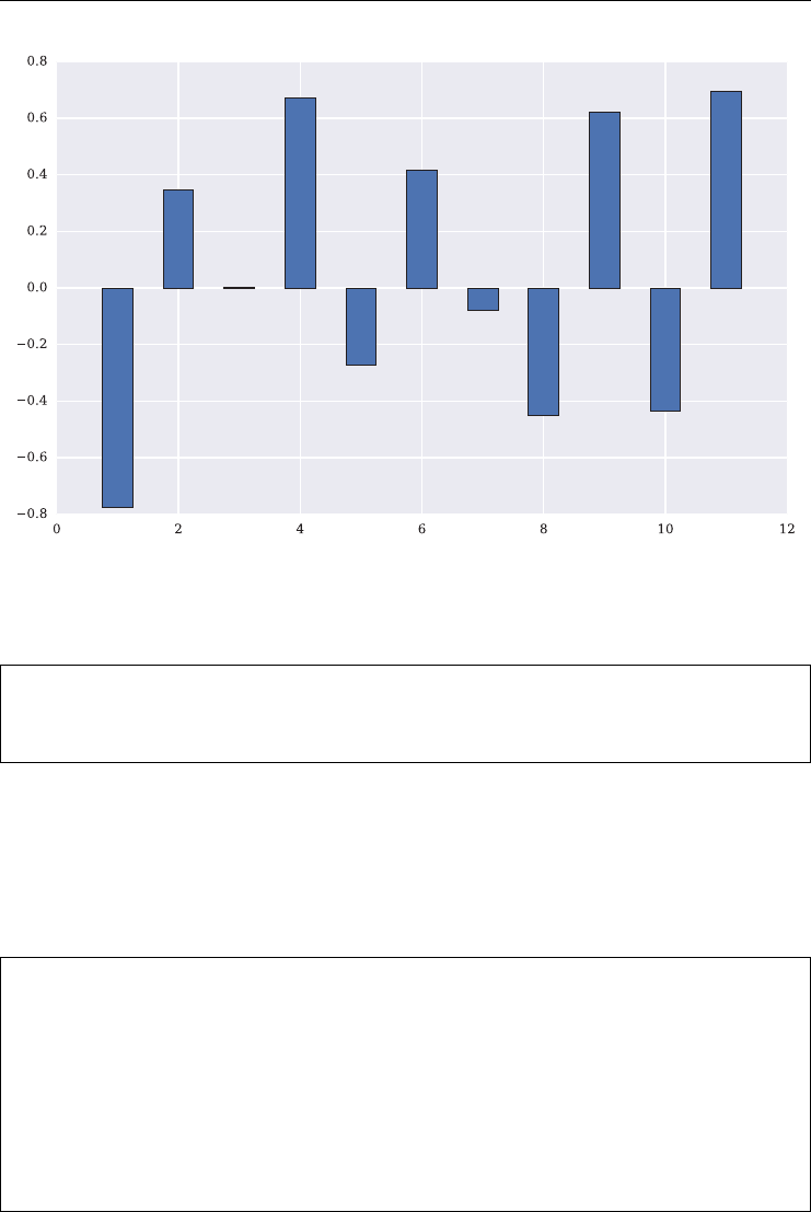
FIGURE 2.4 Bar chart with matplotlib.
Finally, consider the bar chart presented in Figure 2.4.
In [161]: plt.figure(figsize=(10, 6)); # size of figure
In [162]: plt.bar(np.arange(1, 12) - 0.25, data[0, :11], width=0.5);
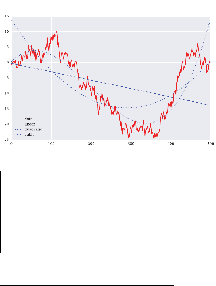
To conclude the introduction to matplotlib consider the ordinary least squares (OLS) regres-
sion of the sample data displayed in Figure 2.1. NumPy provides with the two functions
polyfit() and polyval() convenience functions to implement OLS based on sim-
ple monomials i.e. x,x2,x3,...,xn. For illustration purposes consider linear, quadratic and
cubic OLS.
In [163]: x = np.arange(len(data.cumsum()))
In [164]: y = data.cumsum()
In [165]: rg1 = np.polyfit(x, y, 1) # linear OLS
In [166]: rg2 = np.polyfit(x, y, 2) # quadratic OLS
In [167]: rg3 = np.polyfit(x, y, 3) # cubic OLS
Figure 2.5 illustrates the regression results graphically.
38 LISTED VOLATILITY AND VARIANCE DERIVATIVES
FIGURE 2.5 Linear, quadratic and cubic regression.
In [168]: plt.figure(figsize=(10, 6));
In [169]: plt.plot(x, y, 'r', label='data');
In [170]: plt.plot(x, np.polyval(rg1, x), 'b--', label='linear');
In [171]: plt.plot(x, np.polyval(rg2, x), 'b-.', label='quadratic');
In [172]: plt.plot(x, np.polyval(rg3, x), 'b:', label='cubic');
In [173]: plt.legend(loc=0);
2.4 pandas
pandas is a library with which you can manage and operate on time series data and other
tabular data structures. It allows implementation of even sophisticated data analytics tasks on
larger data sets. While the focus lies on in-memory operations, there are also multiple options
for out-of-memory (on-disk) operations. Although pandas provides a number of different data
structures, embodied by powerful classes, the structure most often used is the DataFrame
class which resembles a typical table of a relational (SQL) database and is used to manage,
for instance, nancial time series data. This is what we focus on in this section.

Introduction to Python 39
2.4.1 pandas DataFrame class
In its most basic form, a DataFrame object is characterized by an index, column names and
tabular data. To make this more specic, consider the following sample data set:
In [174]: np.random.seed(1000)
In [175]: a = np.random.standard_normal(( 10, 3)).cumsum(axis=0)
Also, consider the following dates which shall be our index:
In [176]: index = ['2016-1-31', '2016-2-28', '2016-3-31',
.....: '2016-4-30', '2016-5-31', '2016-6-30',
.....: '2016-7-31', '2016-8-31', '2016-9-30',
.....: '2016-10-31']
.....:
Finally, the column names:
In [177]: columns = ['no1', 'no2', 'no3']
The instantiation of a DataFrame object then looks as follows:
In [178]: import pandas as pd
In [179]: df = pd.DataFrame(a, index=index, columns=columns)
A look at the new object reveals its resemblance with a typical table from a relational database
(or e.g. an Excel spreadsheet).
In [180]: df
Out[180]:
no1 no2 no3
2016-1-31 -0.804458 0.320932 -0.025483
2016-2-28 -0.160134 0.020135 0.363992
2016-3-31 -0.267572 -0.459848 0.959027
2016-4-30 -0.732239 0.207433 0.152912
2016-5-31 -1.928309 -0.198527 -0.029466
2016-6-30 -1.825116 -0.336949 0.676227
2016-7-31 -0.553321 -1.323696 0.341391
2016-8-31 -0.652803 -0.916504 1.260779
2016-9-30 -0.340685 0.616657 0.710605
2016-10-31 -0.723832 -0.206284 2.310688

40 LISTED VOLATILITY AND VARIANCE DERIVATIVES
DataFrame objects have built in a multitude of basic, advanced and convenience methods, a
few of which are illustrated without much commentary below.
In [181]: df.head() # first five rows
Out[181]:
no1 no2 no3
2016-1-31 -0.804458 0.320932 -0.025483
2016-2-28 -0.160134 0.020135 0.363992
2016-3-31 -0.267572 -0.459848 0.959027
2016-4-30 -0.732239 0.207433 0.152912
2016-5-31 -1.928309 -0.198527 -0.029466
In [182]: df.tail() # last five rows
Out[182]:
no1 no2 no3
2016-6-30 -1.825116 -0.336949 0.676227
2016-7-31 -0.553321 -1.323696 0.341391
2016-8-31 -0.652803 -0.916504 1.260779
2016-9-30 -0.340685 0.616657 0.710605
2016-10-31 -0.723832 -0.206284 2.310688
In [183]: df.index # index object
Out[183]:
Index([u'2016-1-31', u'2016-2-28', u'2016-3-31', u'2016-4-30', u'2016-5-31',
u'2016-6-30', u'2016-7-31', u'2016-8-31', u'2016-9-30', u'2016-10-31'],
dtype='object')
In [184]: df.columns # column names
Out[184]: Index([u'no1', u'no2', u'no3'], dtype='object')
In [185]: df.info() # meta information
<class 'pandas.core.frame.DataFrame'>
Index: 10 entries, 2016-1-31 to 2016-10-31
Data columns (total 3 columns):
no1 10 non-null float64
no2 10 non-null float64
no3 10 non-null float64
dtypes: float64(3)
memory usage: 320.0+ bytes
In [186]: df.describe() # typical statistics
Out[186]:
no1 no2 no3
count 10.000000 10.000000 10.000000
mean -0.798847 -0.227665 0.672067
std 0.607430 0.578071 0.712430
min -1.928309 -1.323696 -0.029466

Introduction to Python 41
25% -0.786404 -0.429123 0.200031
50% -0.688317 -0.202406 0.520109
75% -0.393844 0.160609 0.896922
max -0.160134 0.616657 2.310688
Numerical operations are in general as easy with DataFrame objects as with NumPy ndar-
ray objects. They are also quite close in terms of syntax.
In [187]: df*2 # vectorized multiplication
Out[187]:
no1 no2 no3
2016-1-31 -1.608917 0.641863 -0.050966
2016-2-28 -0.320269 0.040270 0.727983
2016-3-31 -0.535144 -0.919696 1.918054
2016-4-30 -1.464479 0.414866 0.305823
2016-5-31 -3.856618 -0.397054 -0.058932
2016-6-30 -3.650232 -0.673898 1.352453
2016-7-31 -1.106642 -2.647393 0.682782
2016-8-31 -1.305605 -1.833009 2.521557
2016-9-30 -0.681369 1.233314 1.421210
2016-10-31 -1.447664 -0.412568 4.621376
In [188]: df.std() # standard deviation by column
Out[188]:
no1 0.607430
no2 0.578071
no3 0.712430
dtype: float64
In [189]: df.mean(axis=1) # mean by index value
Out[189]:
2016-1-31 -0.169670
2016-2-28 0.074664
2016-3-31 0.077202
2016-4-30 -0.123965
2016-5-31 -0.718767
2016-6-30 -0.495280
2016-7-31 -0.511875
2016-8-31 -0.102843
2016-9-30 0.328859
2016-10-31 0.460191
dtype: float64
In [190]: np.mean(df) # mean via universal function
Out[190]:

42 LISTED VOLATILITY AND VARIANCE DERIVATIVES
no1 -0.798847
no2 -0.227665
no3 0.672067
dtype: float64
Pieces of data can be looked up via different mechanisms.
In [191]: df['no2'] # 2nd column
Out[191]:
2016-1-31 0.320932
2016-2-28 0.020135
2016-3-31 -0.459848
2016-4-30 0.207433
2016-5-31 -0.198527
2016-6-30 -0.336949
2016-7-31 -1.323696
2016-8-31 -0.916504
2016-9-30 0.616657
2016-10-31 -0.206284
Name: no2, dtype: float64
In [192]: df.iloc[0] # 1st row
Out[192]:
no1 -0.804458
no2 0.320932
no3 -0.025483
Name: 2016-1-31, dtype: float64
In [193]: df.iloc[2:4] # 3rd & 4th row
Out[193]:
no1 no2 no3
2016-3-31 -0.267572 -0.459848 0.959027
2016-4-30 -0.732239 0.207433 0.152912
In [194]: df.iloc[2:4, 1] # 3rd & 4th row, 2nd column
Out[194]:
2016-3-31 -0.459848
2016-4-30 0.207433
Name: no2, dtype: float64
In [195]: df.no3.iloc[3:7] # dot look-up for column name
Out[195]:
2016-4-30 0.152912
2016-5-31 -0.029466
2016-6-30 0.676227
2016-7-31 0.341391
Name: no3, dtype: float64

Introduction to Python 43
In [196]: df.loc['2016-3-31'] # row given index value
Out[196]:
no1 -0.267572
no2 -0.459848
no3 0.959027
Name: 2016-3-31, dtype: float64
In [197]: df.loc['2016-5-31', 'no3'] # single data point
Out[197]: -0.02946577492329111
In [198]: df['no1'] + 3 * df['no3'] # vectorized arithmetic operations
Out[198]:
2016-1-31 -0.880907
2016-2-28 0.931841
2016-3-31 2.609510
2016-4-30 -0.273505
2016-5-31 -2.016706
2016-6-30 0.203564
2016-7-31 0.470852
2016-8-31 3.129533
2016-9-30 1.791130
2016-10-31 6.208233
dtype: float64
Data selections based on Boolean operations are also a strength of pandas.
In [199]: df['no3'] > 0.5
Out[199]:
2016-1-31 False
2016-2-28 False
2016-3-31 True
2016-4-30 False
2016-5-31 False
2016-6-30 True
2016-7-31 False
2016-8-31 True
2016-9-30 True
2016-10-31 True
Name: no3, dtype: bool
In [200]: df[df['no3'] > 0.5]
Out[200]:
no1 no2 no3
2016-3-31 -0.267572 -0.459848 0.959027
2016-6-30 -1.825116 -0.336949 0.676227
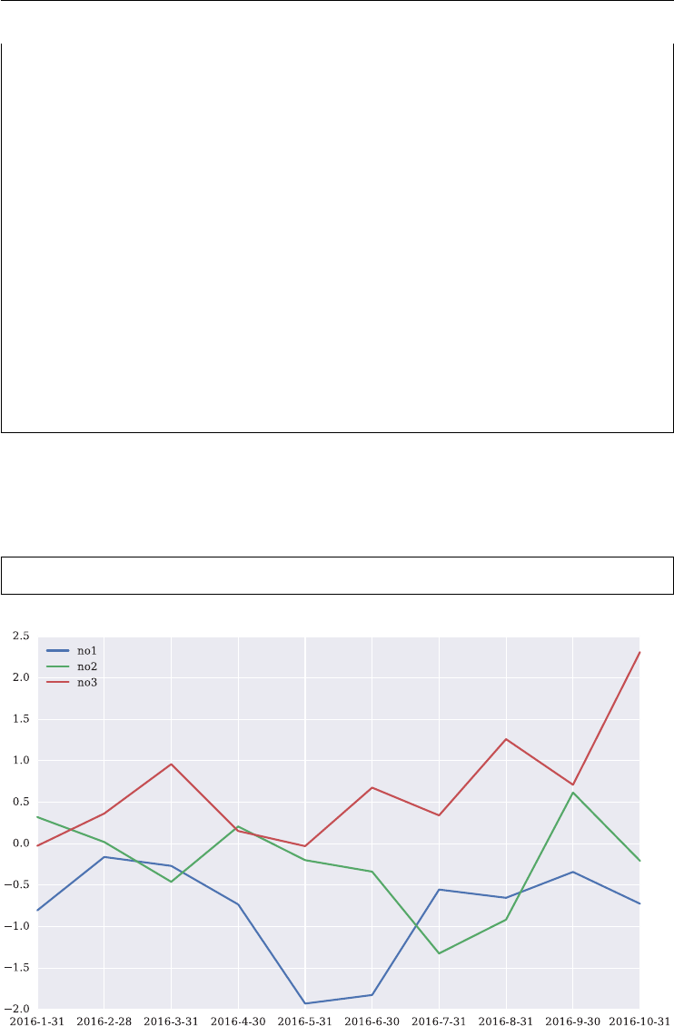
44 LISTED VOLATILITY AND VARIANCE DERIVATIVES
2016-8-31 -0.652803 -0.916504 1.260779
2016-9-30 -0.340685 0.616657 0.710605
2016-10-31 -0.723832 -0.206284 2.310688
In [201]: df[(df.no3 > 0.5) & (df.no2 > 0.25)]
Out[201]:
no1 no2 no3
2016-9-30 -0.340685 0.616657 0.710605
2016-10-31 -0.723832 -0.206284 2.310688
In [202]: df[df.index > '2016-4-30']
Out[202]:
no1 no2 no3
2016-5-31 -1.928309 -0.198527 -0.029466
2016-6-30 -1.825116 -0.336949 0.676227
2016-7-31 -0.553321 -1.323696 0.341391
2016-8-31 -0.652803 -0.916504 1.260779
2016-9-30 -0.340685 0.616657 0.710605
pandas is well integrated with the matplotlib library which makes it really convenient to
plot data stored in DataFrame objects. In general, a single method call does the trick (see
Figure 2.6).
In [203]: df.plot(figsize=(10, 6));
FIGURE 2.6 Line plot from pandas DataFrame.
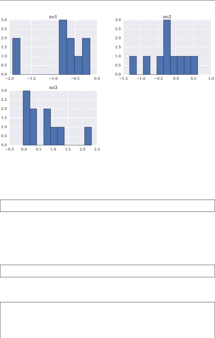
Introduction to Python 45
FIGURE 2.7 Histograms from pandas DataFrame.
Histograms are also generated this way (see Figure 2.7). In both cases, pandas takes care of
the handling of the single columns and automatically generates single lines (with respective
legend entries) and generates respective sub-plots with three different histograms.
In [204]: df.hist(figsize=(10, 6));
2.4.2 Input-Output Operations
Another strength of pandas is the exporting and importing of data to and from diverse data
storage formats. Consider the case of comma separated value (CSV) les.
In [205]: df.to_csv('data.csv') # exports to CSV file
Let us have a look at the le just saved with basic Python functionality.
In [206]: with open('data.csv') as f: # open file
.....: for lin f.readlines(): # iterate over all lines
.....: print l, # print line
.....:
,no1,no2,no3

46 LISTED VOLATILITY AND VARIANCE DERIVATIVES
2016-1-31,-0.804458303525,0.32093154709,-0.0254828804721
2016-2-28,-0.160134475098,0.0201348743028,0.363991673815
2016-3-31,-0.267571776789,-0.459848201058,0.959027175892
2016-4-30,-0.732239302984,0.20743310593,0.152911565449
2016-5-31,-1.92830913682,-0.19852705543,-0.0294657749233
2016-6-30,-1.82511624278,-0.336949044016,0.676226600036
2016-7-31,-0.553320966375,-1.32369637281,0.341391146824
2016-8-31,-0.652802664384,-0.916504272472,1.26077868603
2016-9-30,-0.340684654318,0.616656792886,0.710604821
2016-10-31,-0.723832065202,-0.206284170553,2.31068818906
Reading data from such les is also straightforward.
In [207]: from_csv = pd.read_csv('data.csv', # filename
.....: index_col=0, # index column
.....: parse_dates=True) # date index
.....:
In [208]: from_csv.head()
Out[208]:
no1 no2 no3
2016-01-31 -0.804458 0.320932 -0.025483
2016-02-28 -0.160134 0.020135 0.363992
2016-03-31 -0.267572 -0.459848 0.959027
2016-04-30 -0.732239 0.207433 0.152912
2016-05-31 -1.928309 -0.198527 -0.029466
However, in general you would store DataFrame objects on disk in more efcient binary
formats like HDF5 (see http://hdfgroup.org). pandas in this case wraps the functionality of
the PyTables library (see http://pytables.org). The constructor function to be used is HDFS-
tore().
In [209]: h5 = pd.HDFStore('data.h5', 'w') # open for writing
In [210]: h5['df'] = df # write object to database
In [211]: h5
Out[211]:
<class 'pandas.io.pytables.HDFStore'>
File path: data.h5
/df frame (shape->[10,3])
Data retrieval is as simple as writing.

Introduction to Python 47
In [212]: from_h5 = h5['df'] # reading from database
In [213]: h5.close() # closing the database
In [214]: from_h5.tail()
Out[214]:
no1 no2 no3
2016-6-30 -1.825116 -0.336949 0.676227
2016-7-31 -0.553321 -1.323696 0.341391
2016-8-31 -0.652803 -0.916504 1.260779
2016-9-30 -0.340685 0.616657 0.710605
2016-10-31 -0.723832 -0.206284 2.310688
In [215]: !rm data.csv data.h5 # remove the objects from disk
2.4.3 Financial Analytics Examples
When it comes to nancial data, there are useful data retrieval functions available that wrap
both the Yahoo! Finance and Google Finance nancial data APIs. The following code reads
historical daily data for the S&P 500 index and the VIX volatility index:
In [216]: from pandas_datareader import data as web
In [217]: spx = web.DataReader('ˆGSPC', data_source='yahoo',
end='2015-12-31')
In [218]: vix = web.DataReader('ˆVIX', data_source='yahoo',
end='2015-12-31')
In [219]: spx.info()
<class 'pandas.core.frame.DataFrame'>
DatetimeIndex: 1510 entries, 2010-01-04 to 2015-12-31
Data columns (total 6 columns):
Open 1510 non-null float64
High 1510 non-null float64
Low 1510 non-null float64
Close 1510 non-null float64
Volume 1510 non-null int64
Adj Close 1510 non-null float64
dtypes: float64(5), int64(1)
memory usage: 82.6 KB
In [220]: vix.info()
<class 'pandas.core.frame.DataFrame'>
DatetimeIndex: 1510 entries, 2010-01-04 to 2015-12-31

48 LISTED VOLATILITY AND VARIANCE DERIVATIVES
Data columns (total 6 columns):
Open 1510 non-null float64
High 1510 non-null float64
Low 1510 non-null float64
Close 1510 non-null float64
Volume 1510 non-null int64
Adj Close 1510 non-null float64
dtypes: float64(5), int64(1)
memory usage: 82.6 KB
Let us combine the respective Close columns into a single DataFrame object. There are
multiple ways to accomplish this goal.
# construction via join
In [221]: spxvix = pd.DataFrame(spx['Close']).join(vix['Close'] ,
.....: lsuffix='SPX', rsuffix='VIX')
.....:
In [222]: spxvix.info()
<class 'pandas.core.frame.DataFrame'>
DatetimeIndex: 1510 entries, 2010-01-04 to 2015-12-31
Data columns (total 2 columns):
CloseSPX 1510 non-null float64
CloseVIX 1510 non-null float64
dtypes: float64(2)
memory usage: 35.4 KB
# construction via merge
In [223]: spxvix = pd.merge(pd.DataFrame(spx['Close']),
.....: pd.DataFrame(vix['Close']),
.....: left_index=True, # merge on left index
.....: right_index=True, # merge on right index
.....: suffixes=['SPX', 'VIX'])
.....:
In [224]: spxvix.info()
<class 'pandas.core.frame.DataFrame'>
DatetimeIndex: 1510 entries, 2010-01-04 to 2015-12-31
Data columns (total 2 columns):
CloseSPX 1510 non-null float64
CloseVIX 1510 non-null float64
dtypes: float64(2)
memory usage: 35.4 KB
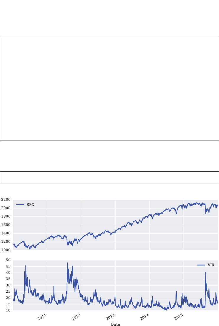
Introduction to Python 49
In a case like this, the approach via dictionary objects might be the best and most intuitive
way.
# construction via dictionary object
In [225]: spxvix = pd.DataFrame({'SPX': spx['Close'] ,
.....: 'VIX': vix['Close'] } ,
.....: index=spx.index)
.....:
In [226]: spxvix.info()
<class 'pandas.core.frame.DataFrame'>
DatetimeIndex: 1510 entries, 2010-01-04 to 2015-12-31
Data columns (total 2 columns):
SPX 1510 non-null float64
VIX 1510 non-null float64
dtypes: float64(2)
memory usage: 35.4 KB
Having available the merged data in a single object makes visual analysis straightforward (see
Figure 2.8).
In [227]: spxvix.plot(figsize=(10, 6), subplots=True, color='b');
FIGURE 2.8 Historical closing data for S&P 500 stock index and VIX volatility index.

50 LISTED VOLATILITY AND VARIANCE DERIVATIVES
pandas also allows vectorized operations on whole DataFrame objects. The following code
calculates the log returns over the two columns of the spxvix object simultaneously in vec-
torized fashion. The shift() method shifts the data set by the number of index values as
provided (in this particular case by one trading day).
In [228]: rets = np.log(spxvix / spxvix.shift(1))
In [229]: rets.head()
Out[229]:
SPX VIX
Date
2010-01-04 NaN NaN
2010-01-05 0.003111 -0.035038
2010-01-06 0.000545 -0.009868
2010-01-07 0.003993 -0.005233
2010-01-08 0.002878 -0.050024
There is one row of log returns missing at the very beginning. This row can be deleted via the
dropna() method.
In [230]: rets = rets.dropna()
In [231]: rets.head()
Out[231]:
SPX VIX
Date
2010-01-05 0.003111 -0.035038
2010-01-06 0.000545 -0.009868
2010-01-07 0.003993 -0.005233
2010-01-08 0.002878 -0.050024
2010-01-11 0.001745 -0.032514
Consider the plot in Figure 2.9 showing the VIX log returns against the SPX log returns in a
scatter plot with a linear regression. It illustrates a strong negative correlation between the two
indexes. This is a central result that is replicated in chapter 4, Data Analysis and Strategies for
the EURO STOXX 50 stock index and the VSTOXX volatility index, respectively.
In [232]: rets.plot(kind='scatter', x='SPX', y='VIX',
.....: style='.', figsize=(10, 6));
.....:
In [233]: rg = np.polyfit(rets['SPX'], rets['VIX'], 1)
In [234]: plt.plot(rets['SPX'], np.polyval(rg, rets['SPX']), 'r.-');
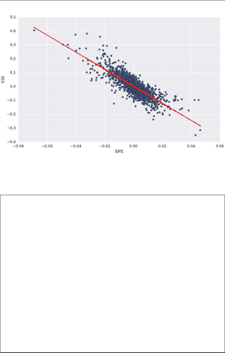
Introduction to Python 51
FIGURE 2.9 Daily log returns for S&P 500 stock index and VIX volatility index and regression line.
Having nancial time series data stored in a pandas DataFrame object makes the calculation
of typical statistics straightforward.
In [235]: ret = rets.mean() * 252 # annualized return
In [236]: ret
Out[236]:
SPX 0.098532
VIX -0.015992
dtype: float64
In [237]: vol = rets.std() * math.sqrt(252) # annualized volatility
In [238]: vol
Out[238]:
SPX 0.159335
VIX 1.185408
dtype: float64
In [239]: (ret - 0.01) / vol # Sharpe ratio with rf = 0.01
Out[239]:
SPX 0.555635
VIX -0.021926
dtype: float64
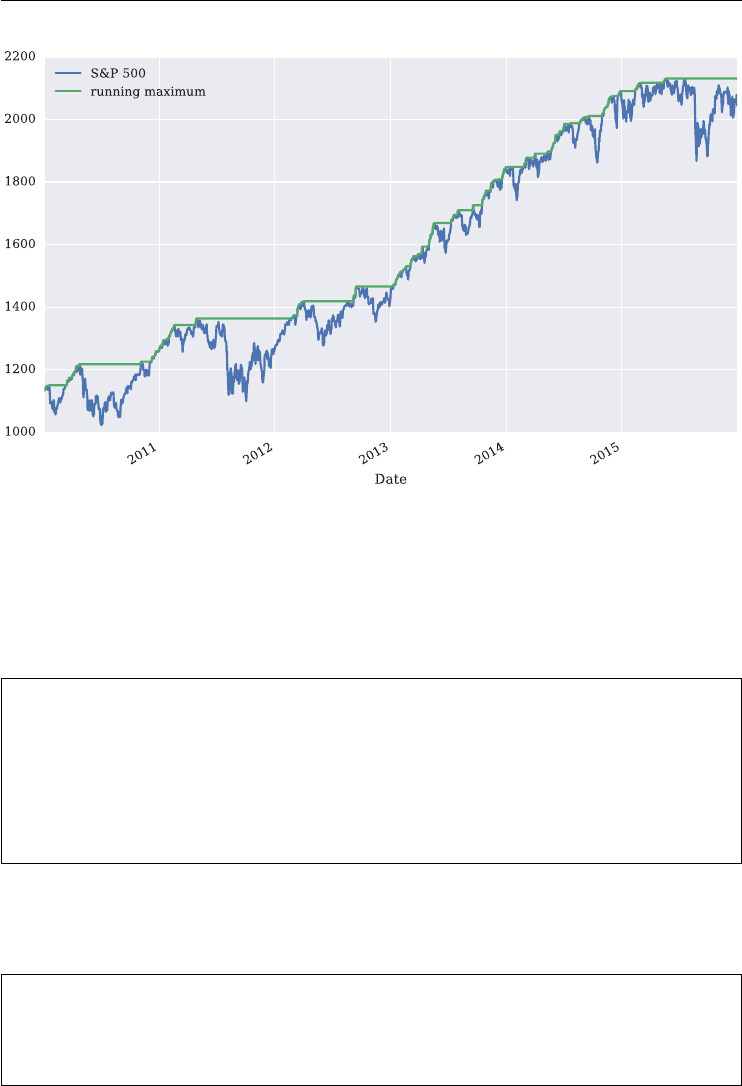
52 LISTED VOLATILITY AND VARIANCE DERIVATIVES
FIGURE 2.10 S&P 500 stock index and running maximum value.
The maximum drawdown, which we only calculate for the S&P 500 index, is a bit more
involved. For its calculation, we use the cummax() method which records the running, his-
torical maximum of the time series up to a certain date. Consider the plot in Figure 2.10 which
shows the S&P 500 index and the running maximum.
In [240]: plt.figure(figsize=(10, 6));
In [241]: spxvix['SPX'].plot(label='S&P 500');
In [242]: spxvix['SPX'].cummax().plot(label='running maximum');
In [243]: plt.legend(loc=0);
The maximum drawdown is the largest difference between the running maximum and the
current index level – in our particular case it is 264.
In [244]: adrawdown = spxvix['SPX'].cummax() - spxvix['SPX']
In [245]: adrawdown.max()
Out[245]: 264.38000499999998
The relative maximum drawdown might sometimes be slightly more meaningful. Here it is a
drawdown of about 20%.

Introduction to Python 53
In [246]: rdrawdown = (spxvix['SPX'].cummax() - spxvix['SPX']) /
spxvix['SPX'].cummax()
In [247]: rdrawdown.max()
Out[247]: 0.19388242085950988
The longest drawdown period is calculated as follows. The code below selects all those data
points where the drawdown is zero. It then calculates the difference between two consecutive
index values (i.e. trading dates) for which the drawdown is zero and takes the maximum value.
Given the data set we are analyzing, the longest drawdown period is 301 days.
In [248]: temp = adrawdown[adrawdown == 0]
In [249]: periods_spx = (temp.index[1:].to_pydatetime()
.....: - temp.index[:-1].to_pydatetime())
.....:
In [250]: periods_spx[50:60] # some selected data points
Out[250]:
array([datetime.timedelta(67), datetime.timedelta(1),
datetime.timedelta(1), datetime.timedelta(1),
datetime.timedelta(301), datetime.timedelta(3),
datetime.timedelta(1), datetime.timedelta(2),
datetime.timedelta(12), datetime.timedelta(2)], dtype=object)
In [251]: max(periods_spx)
Out[251]: datetime.timedelta(301)
See Appendix C of Hilpisch (2014) for the handling of date-time information with Python,
NumPy and pandas.
2.5 CONCLUSIONS
This chapter introduces basic data types and structures as well as certain Python idioms needed
for analyses in later chapters of the book. In addition, NumPy and the ndarray class are intro-
duced which allow the efcient handling of and operating on (numerical) data stored as arrays.
Some basic visualization techniques using the matplotlib library are also introduced. However,
working with pandas and its powerful DataFrame class for tabular and time series data makes
plotting a bit more convenient – in general only a single method call is needed. Using pandas
and the capabilities of the DataFrame class, the chapter also illustrates by means of some
basic nancial examples how to implement typical interactive nancial analytics tasks.

CHAPTER 3
Model-Free Replication of Variance
3.1 INTRODUCTION
Although volatility derivatives, variance swaps and futures are considered second generation
derivatives (since they are dened on volatility and variance directly), some of the most elegant
and robust results of quantitative nance apply to these kinds of derivatives. In particular, it is
possible to statically replicate realized variance without using any kind of specic model. This,
for example, does not apply to most other important concepts in option pricing and trading,
such as implied volatility or delta hedging of options.
This chapter mainly covers the following topics:
spanning with options: Breeden and Litzenberger (1978) showed in the 1970s how to
replicate state-contingent payoffs (satisfying certain conditions) by using positions in
options
log contracts: an important piece in the replication of (realized) variance and the valuation
of variance swaps is the so-called log contract
static replication of variance: this relates to the central result of replicating realized
variance by a log contract as well as static positions in options
derivatives with constant dollar gamma: in the replication and valuation of variance
swaps, constant dollar gamma positions play a central role
practical replication of variance swaps: using the theoretical insights and results, the
chapter also illustrates the generation of constant dollar gamma positions and thus the
practical replication of variance swaps based on numerical examples
VSTOXX as volatility index: using the central result, the nal section in this chapter
explains and justies the denition of the VSTOXX volatility index (and the VIX index
to this end).
The theoretical parts of this chapter roughly follow the lines of chapter 11 of Gatheral (2006).
Since they are of importance for both volatility and variance derivatives we have placed them
up front and present them in a connected fashion.
55
Listed Volatility and Variance Derivatives: A
Python-based Guide
By Dr. Yves J. Hilpisch
© 2017 Yves Hilpisch

56 LISTED VOLATILITY AND VARIANCE DERIVATIVES
3.2 SPANNING WITH OPTIONS
Breeden and Litzenberger (1978) use option prices to derive prices for elementary securities,
i.e. securities that pay exactly 1 unit of currency at a certain future date given a certain state
of the economy. In economics, Arrow-Debreu security is also a common term. The prices of
elementary securities are generally called state prices. Having state prices available, every
other contingent claim can be priced by multiplying the contingent claim’s state-dependent
payoff by the respective state prices.
Let t≥0 denote the current date and T>tthe future date of interest (e.g. maturity of a
derivative instrument). For simplicity, states of the economy should be distinguished by the
level of a stock index Sonly. Let p(ST,T;St,t) denote the state price given a stock index level
of Stat tfor a stock index level STat T, then:
p(ST,T;St,t)=𝜕2P(St,K,T)
𝜕K2ST=K
=𝜕2C(St,K,T)
𝜕K2ST=K
Here, Pand Crepresent prices (given by some pricing formula) of European put and call
options, respectively. Therefore, a state price can be derived by taking the second partial deriva-
tive of option pricing formula with respect to the strike of the option. Equipped with these state
prices, the value of a state-contingent claim with payoff function g(ST)is
Et(g(ST)St)=∫∞
0
g(K)p(K,T;St,t)dK
=∫F
0
g(K)𝜕2P(St,K,T)
𝜕K2dK +∫∞
F
g(K)𝜕2C(St,K,T)
𝜕K2dK
with Fbeing the T-forward price of the index at t(see Breeden and Litzenberger (1978)).
We now apply integration by parts. With u=u(x), v=v(x), du =u′(x)dx,dv =v′(x)dx,
integration by parts states that
∫u(x)v′(x)dx =u(x)v(x)−∫u′(x)v(x)dx
Therefore, we get
Et(g(ST)St)=g(K)𝜕P(St,K,T)
𝜕K
F
0
−∫F
0
g′(K)𝜕P(St,K,T)
𝜕KdK
+g(K)𝜕C(St,K,T)
𝜕K
∞
F
−∫∞
F
g′(K)𝜕C(St,K,T)
𝜕KdK
=g(F)−∫F
0
g′(K)𝜕P(St,K,T)
𝜕KdK −∫∞
F
g′(K)𝜕C(St,K,T)
𝜕KdK

Model-Free Replication of Variance 57
Applying integration by parts once again yields
Et(g(ST)St)=g(F)−g′(K)P(St,K,T)F
0+∫F
0
g′′(K)P(St,K,T)dK
−g′(K)C(St,K,T)∞
F+∫∞
F
g′′(K)C(St,K,T)dK
=g(F)+∫F
0
g′′(K)P(St,K,T)dK +∫∞
F
g′′(K)C(St,K,T)dK
As is evident from this last equation, in this setting any twice continuously differentiable payoff
gdue at Tcan be replicated by innite strips of European put and call options maturing at T.
In other words, these options span the space of twice continuously differentiable payoffs.
3.3 LOG CONTRACTS
So-called log contracts are a kind of derivative instrument that plays an important role in the
valuation of variance swaps. Recall that a long position in a variance contract pays at maturity
the difference between the realized variance over the life time of the swap and an up-front
xed variance strike.
Consider the payoff g(ST)=logST
F=logST−logF. Then
g′(ST)=1
ST
g′′(ST)=−1
S2
T
Valuing this contract by making use of the option spanning approach yields
Elog ST
FSt=logF
F+∫F
0
−1
K2P(St,K,T)dK +∫∞
F
−1
K2C(St,K,T)dK
=−
∫F
0
P(St,K,T)dK
K2−∫∞
F
C(St,K,T)dK
K2
As a consequence, the log contract can be replicated by (innite strips of) European put and
call options on the underlying. Every option is weighted by the square of the strike.
3.4 STATIC REPLICATION OF REALIZED VARIANCE AND
VARIANCE SWAPS
Assume for simplicity zero short rates such that F=St.Fort=0, one has
log ST
F=logST
S0
=∫T
0
dlog(St)
=∫T
0
dSt
St
−∫T
0
𝜎2(St)
2dt

58 LISTED VOLATILITY AND VARIANCE DERIVATIVES
Compare this result with equation 1.1. Such a comparison further illustrates the connection
between the (discrete) delta hedging of an option and (the valuation of) variance swaps. Above,
we use the fact that the total return over the interval [0, T] equals the integral over the marginal
returns of Sfor the same time interval. The second term in the last equation results from the
application of It̂
o’s lemma. This term is equal to half of the total variance of Sover the time
interval [0, T]. Taking the risk-neutral expectation of that expression gives
E∫T
0
𝜎2(St)dt=−2Elog ST
F
Combining the results with regard to the log contract replication and valuation with this last
insight shows that realized variance is given in a model-free manner through the prices of
European put and call options. This is due to the fact that realized variance can be replicated
by the use of a log contract.
3.5 CONSTANT DOLLAR GAMMA DERIVATIVES
AND PORTFOLIOS
Above, we establish the replication of realized variance by the log contract. The log contract
has, as a dening characteristic, a constant dollar gamma.Thegamma of a derivative dened
on some underlying Swith value ft(St) is dened as
Γt=𝜕2ft
𝜕S2
t
i.e. the second partial derivative of the pricing function with respect to the value of the under-
lying (assuming that the pricing function is indeed twice continuously differentiable).
Its dollar gamma is then dened by the product of the gamma and the square of the value
of the underlying (sometimes the factor 0.5 is added):
Γ$
t≡Γt⋅S2
t
Omitting the time index, a constant dollar gamma implies, for some xed value a, a gamma
of
Γ$=Γ⋅S2≡a
⇔Γ= a
S2
We therefore have
𝜕2f
𝜕S2=a
S2
This partial differential equation has a solution of the form
f(S)=alog(S)+bS +c

Model-Free Replication of Variance 59
Indeed, the log contract ts trivially into the general solution by setting a=1, b=0, c=0,
i.e.
f(S)=log(S)
illustrating its importance.
With ̂𝜎2being the realized variance and 𝜎2
Kbeing the xed variance strike, a long position
in a variance swap (with notional of 1 currency unit), pays at expiry
̂𝜎2−𝜎2
K
With this payoff, we get a replicating portfolio of
ft(St)=2log(St)+e−r(T−t)𝜎2
K
i.e. a=2, b=0, c=e−r(T−t)𝜎2
K. A variance swap therefore also has a constant dollar gamma.
This insight is used in the next section.
3.6 PRACTICAL REPLICATION OF REALIZED VARIANCE
Consider the Black-Scholes-Merton (1973) model economy (no dividends) with the present
value of a European call option given by
C(S,K,t,T,r,𝜎)=St⋅N(d1)−e−r(T−t)⋅K⋅N(d2)
N(d)=1
2𝜋∫d
−∞
e−1
2x2dx
d1=
log St
K+r+𝜎2
2(T−t)
𝜎T−t
d2=
log St
K+r−𝜎2
2(T−t)
𝜎T−t
Here, Stis the index level at date t,Kis the option strike, Tdate of maturity (in year fractions),
rthe constant, risk-less short rate and 𝜎the instantaneous volatility.
The gamma of an option in this model is given as follows
Γt=𝜕2Ct
𝜕S2
t
=N′(d1)
St𝜎T−t
with
N′(d)=1
2𝜋
e−1
2x2

60 LISTED VOLATILITY AND VARIANCE DERIVATIVES
Our aim in this section is to build a portfolio of European call options with a constant dollar
gamma, i.e. ΓPortfolio ⋅S2
t≡afor some xed value a.
The Python function dollar_gamma implements the dollar gamma formula for the
European call option.
In [1]: import math
In [2]: import numpy as np
In [3]: import scipy.stats as scs
In [4]: def dollar_gamma(St, K, t, T, r, sigma):
...: ''' Returns European call option dollar gamma. '''
...: d1 = ((np.log(St / K) + (r + 0.5 * sigma ** 2) * (T - t))
...: / sigma * math.sqrt(T- t))
...: gamma = scs.norm.pdf(d1) / (St * sigma * math.sqrt(T - t))
...: return gamma * St ** 2
...:
Let us parametrize the nancial model for t=0, leaving the values for the initial index level
S0and for the option strike Kundened for the moment.
In [5]: t = 0.0 # current date in year fractions
In [6]: T = 1.0 # maturity in year fractions
In [7]: r = 0.01 # constant risk-less short rate
In [8]: sigma = 0.2 # instantanous volatility
Next, we can calculate the dollar gamma values for different strikes of the European call
options over a range, respectively, of initial values for the index level.
In [9]: import pandas as pd
In [10]: import matplotlib.pyplot as plt
In [11]: import seaborn as sns; sns.set()
In [12]: import matplotlib
In [13]: matplotlib.rcParams['font.family'] = 'serif'

Model-Free Replication of Variance 61
In [14]: gammas = pd.DataFrame()
# 300 data points over the range form 0 to 300
In [15]: s_range = np.linspace(0.0001, 300, 300)
In [16]: strike_range = range(25, 226, 25)
In [17]: for Kin strike_range:
....: gammas['K=%d' % K] = dollar_gamma(s_range, K, t, T, r, sigma)
....:
For every strike level gamma values for 300 different initial values of the stock index have
been calculated and collected.
In [18]: gammas.info()
<class 'pandas.core.frame.DataFrame'>
RangeIndex: 300 entries, 0 to 299
Data columns (total 9 columns):
K=25 300 non-null float64
K=50 300 non-null float64
K=75 300 non-null float64
K=100 300 non-null float64
K=125 300 non-null float64
K=150 300 non-null float64
K=175 300 non-null float64
K=200 300 non-null float64
K=225 300 non-null float64
dtypes: float64(9)
memory usage: 21.2 KB
Having the data stored in a pandas DataFrame object, the results are easily visualized. From
Figure 3.1, you can see that dollar gamma is more pronounced the higher the strike of the
option. A doubling of the strike leads to a doubling of the maximum dollar gamma value
which is always achieved at the ATM level (see strikes 25, 50, 100, 200).
In [19]: gammas.plot(figsize=(10, 5));
In [20]: plt.xlabel('index level');
In [21]: plt.ylabel('dollar gamma');
Let us check what happens when we add all dollar gamma values up by simply composing a
portfolio in which every option has weight 1 or equal weight.
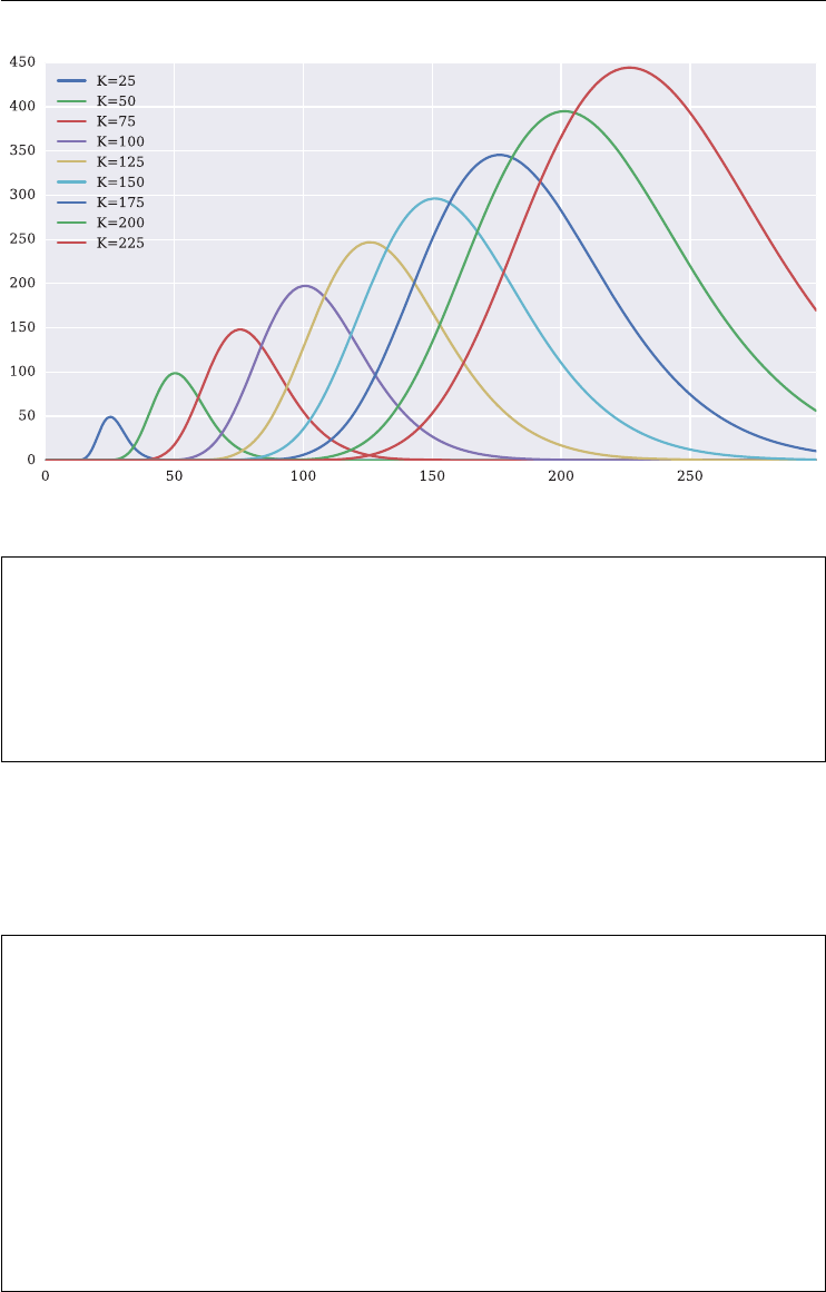
62 LISTED VOLATILITY AND VARIANCE DERIVATIVES
FIGURE 3.1 Dollar gamma values different strikes and 300 different initial stock index values.
In [22]: gammas['sum'] = gammas.sum(axis=1)
In [23]: gammas.plot(figsize=(10, 5));
In [24]: plt.xlabel('index level');
In [25]: plt.ylabel('dollar gamma');
Obviously, given Figure 3.2 the dollar gamma of the portfolio of equally weighted options is
all but constant. Let us try a different weighting scheme that attaches a higher weight to smaller
strikes and a lower weight to higher strikes. To this end, we divide all dollar gamma values by
the strike K. This brings all maximum dollar gamma values in line (to two in this case).
In [26]: gammas_k = pd.DataFrame()
In [27]: for Kin strike_range:
....: gammas_k['K=%d' % K] = dollar_gamma(s_range, K, t, T, r, sigma) / K
....:
In [28]: gammas_k['sum'] = gammas_k.sum(axis=1)
In [29]: gammas_k.plot(figsize=(10, 5));
In [30]: plt.xlabel('index level');
In [31]: plt.ylabel('$K$ weighted dollar gamma');
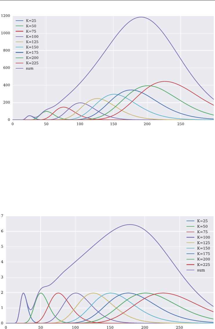
Model-Free Replication of Variance 63
FIGURE 3.2 Dollar gamma values added over the range of 300 different initial index levels.
According to Figure 3.3 this seems to be slightly better in the sense that although we still do
not have a constant dollar gamma we do at least have a range where dollar gamma is linear
(mainly between strikes of 75 and 150). Therefore, let us weight the dollar gammas by the
square of the strike (something we have already seen in the replication result for log con-
tract). In this case the highest dollar gamma values are observed for the lowest strikes and
vice versa.
FIGURE 3.3 Strike-weighted, added dollar gamma values.

64 LISTED VOLATILITY AND VARIANCE DERIVATIVES
In [32]: gammas_k2 = pd.DataFrame()
In [33]: for Kin strike_range:
....: gammas_k2['K=%d' % K] = dollar_gamma(s_range, K, t, T, r,
sigma) / K ** 2
....:
In [34]: gammas_k2['sum'] = gammas_k2.sum(axis=1)
In [35]: gammas_k2.plot(figsize=(10, 5));
In [36]: plt.xlabel('index level');
In [37]: plt.ylabel('$Kˆ2$ weighted dollar gamma');
As Figure 3.4 shows, this approach nally yields a constant dollar gamma value between
strikes of 75 and 150 at least. Let us have a nal look at a more dense grid of option strikes
since the theoretical result is based on innite strips of options. The graphical output is shown
in Figure 3.5.
# more dense strike range
In [38]: strike_range = range(10, 350, 5)
In [39]: gammas_k2 = pd.DataFrame()
In [40]: for Kin strike_range:
....: gammas_k2['K=%d' % K] = dollar_gamma(s_range, K, t, T, r,
sigma) / K ** 2
....:
In [41]: gammas_k2 ['sum'] = gammas_k2.sum(axis=1)
In [42]: gammas_k2.plot(figsize=(10, 5), legend=False);
In [43]: plt.xlabel('index level');
In [44]: plt.ylabel('$Kˆ2$ weighted dollar gamma');
This numerical example shows a constant dollar gamma over a much wider range from
about 25 to beyond 200. This further supports the theoretical result and the replication
approach.
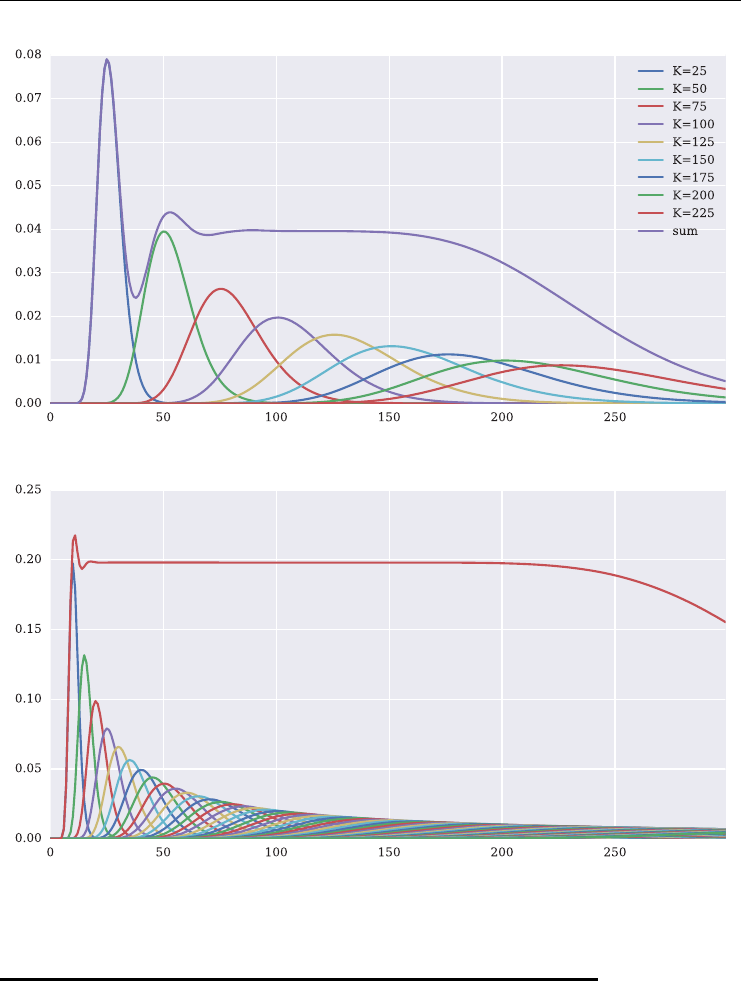
Model-Free Replication of Variance 65
FIGURE 3.4 Squared strike-weighted, added dollar gamma values.
FIGURE 3.5 Strike-weighted, added dollar gamma values.
3.7 VSTOXX AS VOLATILITY INDEX
The VSTOXX volatility index measures the implied total variance across all options written
on the EURO STOXX 50 stock index for a given time-to-maturity. Another interpretation is
that the VSTOXX gives the fair variance swap rate for a variance swap with the respective
maturity. The major index with symbol V2TX has a xed time-to-maturity of 30 days and is
calculated by the interpolation of two sub-indexes. Sub-indexes are calculated for a number of
xed maturity dates.

66 LISTED VOLATILITY AND VARIANCE DERIVATIVES
Assume now the following setting. The discounted, i.e. time t, prices Ci,i=0, ...,n,ofa
series of European call options on the EURO STOXX 50 stock index are given, with xed time-
to-maturity Tand strike prices Ki,i=0, ...,n, as well as the discounted prices Pi,i=0, ...,n,
of a series of European put options with the same time-to-maturity and strike prices. Let us
further hold Ki<Ki+1for all i∈{0, ....,n−1}.
The value of the VSTOXX (sub-)index Vat t=0 is dened by
V≡100 ⋅̂𝜎2
where
̂𝜎2≡2
T
n
i=0
ΔKi
Ki2erT Mi−1
TF
K∗
−12
with
ΔKi=
K1−K0,fori=0
Ki+1−Ki−1
2,fori=1, ...,n−1
Kn−Kn−1,fori=n
F=Kj+erT Cj−Pj, where j=min
i∈{0,...,n}{Ci−Pi}
K∗=max
Ki,i∈{0,...,n}{Ki<F}
Mi=
Pi,forKi<K∗
Pi−Ci
2,forKi=K∗
Ci,forKi>K∗
and rthe constant risk-free short rate appropriate for time-to-maturity T.
We are aiming to show that the dening equation for ̂𝜎2is indeed a valid approximation
for total variance. To this end, we combine the above equations for the log contract and the
total variance to obtain
̂𝜎2=−2⋅−∫F
0
P(St,K,T)dK
K2−∫∞
F
C(St,K,T)dK
K2⋅erT
⇔̂𝜎2T
2erT =∫F
0
P(St,K,T)dK
K2+∫∞
F
C(St,K,T)dK
K2
=∫K∗
0
P(St,K,T)dK
K2+∫∞
K∗
C(St,K,T)dK
K2
+∫F
K∗P(St,K,T)−C(St,K,T)dK
K2
=∫∞
0
M(St,K,T)dK
K2+∫F
K∗
e−rT [K−F]dK
K2

Model-Free Replication of Variance 67
The last term follows from the observation that only the call option is in-the-money, i.e.
e−rT [F−K]>0, given the integration boundaries. Then
̂𝜎2=2
T∫∞
0
erT M(St,K,T)dK
K2+2
T
1
K2
∗∫F
K∗
[K−F]dK
=2
T∫∞
0
erT M(St,K,T)dK
K2−1
T
(K∗−F)2
K2
∗
Note that
(K∗−F)2
K2
∗
=K2
∗−2K∗F+F2
K2
∗
=F2
K2
∗
−2F
K∗
+1
=F
K∗
−12
A possible discretization for the integral then is
̂𝜎2≈2
T
n
i=0
ΔKi
K2
i
erT Mi−1
TF
K∗
−12
giving the dening equation for ̂𝜎2.
The calculation of implied volatilities, or variances, naturally relies on some option pricing
model, like that one of Black-Scholes-Merton (1973). By contrast, the VSTOXX and VIX
volatility index calculation only takes as input market-observed options prices. This is possible
since realized variance at a given future date can be replicated by strips of European call and
put prices maturing at the same date. The realized volatility can then be extracted by taking
the square root of the realized variance. The calculation of the VSTOXX and VIX avoids a
“model-bias” and uses standard market practice for the valuation of important variance related
instruments, like variance swaps.
3.8 CONCLUSIONS
This chapter introduces the elegant theory of the model-free replication of realized variance
and variance swaps which dates back at least to Breeden and Litzenberger (1978). The role of
log contracts and constant dollar gamma positions is discussed. Numerical examples also illus-
trate how to construct constant dollar gamma options positions in practice. Finally, based on
this theory the denition of the VSTOXX and VIX volatility indexes is presented and justied.
Subsequent chapters draw in different ways on these cornerstones in the theory of volatility
and variance modeling, measuring and trading.

PART
Two
Listed Volatility Derivatives

CHAPTER 4
Data Analysis and Strategies
4.1 INTRODUCTION
This chapter is about the analysis of data and investment strategies related to the EURO
STOXX 50 and VSTOXX indexes. It uses public data sources (“open data”) and draws heavily
on the capabilities of the Python library pandas for data analytics.
The chapter has two major goals. First, it reproduces the stylized fact that stock indexes
and volatility indexes in general are negatively correlated. This suggests that (products based
on) volatility indexes are a means to hedge market risk resulting from stock indexes. The ques-
tion, however, is how to best exploit the negative correlation in asset allocation terms. There-
fore, the second goal is to illustrate the benets for equity investors resulting from constant
proportion investment strategies involving a volatility index like the VSTOXX. For simplic-
ity, the respective analysis assumes that a direct investment in the VSTOXX is possible. This
replicates results as found, for example, in the study by Guobuzaite and Martellini (2012).
4.2 RETRIEVING BASE DATA
This section shows how to retrieve and store historical daily closing data for the EURO STOXX
50 index and the VSTOXX volatility index. We mainly work with pandas in the following:
In [1]: import numpy as np
In [2]: import pandas as pd
In [3]: path = './source/data/' # path to data folder
4.2.1 EURO STOXX 50 Data
On the website http://stoxx.com of the index provider STOXX Limited, you nd text les
containing historical closing data for the EURO STOXX 50 index and others. Such data les
are found in this folder:
In [4]: source = 'https://www.stoxx.com/document/Indices/Current/HistoricalData/'
71
Listed Volatility and Variance Derivatives: A
Python-based Guide
By Dr. Yves J. Hilpisch
© 2017 Yves Hilpisch

72 LISTED VOLATILITY AND VARIANCE DERIVATIVES
The respective le for the EURO STOXX 50 index has the following name and is updated
daily after closing.
In [5]: es_url = source + 'hbrbcpe.txt'
Let us inspect the rst few rows of the data le directly, i.e. without pandas. We use the requests
library to read the le from the web source and to print the rst 1,000 characters of the string
object returned.
In [6]: import requests
In [7]: print requests.get(es_url).text[:1000].replace(' ', ' ')
PriceIndices–EUROCurrency
Date;Blue–Chip;Blue–Chip;Broad;Broad;ExUK;ExEuroZone;Blue–Chip;Broad
;Europe;Euro–Zone;Europe;Euro–Zone;;;Nordic;Nordic
;SX5P;SX5E;SXXP;SXXE;SXXF;SXXA;DK5F;DKXF
31.12.1986;775.00;900.82;82.76;98.58;98.06;69.06;645.26;65.56
01.01.1987;775.00;900.82;82.76;98.58;98.06;69.06;645.26;65.56
02.01.1987;770.89;891.78;82.57;97.80;97.43;69.37;647.62;65.81
05.01.1987;771.89;898.33;82.82;98.60;98.19;69.16;649.94;65.82
06.01.1987;775.92;902.32;83.28;99.19;98.83;69.50;652.49;66.06
07.01.1987;781.21;899.15;83.78;98.96;98.62;70.59;651.97;66.20
08.01.1987;777.62;887.37;83.52;97.87;97.68;71.01;645.57;65.62
09.01.1987;769.80;868.31;83.03;96.31;96.22;71.40;638.03;65.14
The le changes the format in which data rows are presented (at least at the time of writing)
such that we need to use a little trick to import the data correctly with pandas. Namely, we
have to add an additional column which we call DEL.
# new column names (without white space)
# adding column 'DEL' -- to be deleted after parsing
In [8]: columns = ['Date', 'SX5P', 'SX5E', 'SXXP', 'SXXE',
...: 'SXXF', 'SXXA', 'DK5F', 'DKXF', 'DEL']
...:
We also skip the rst four rows which we do not need and set a few other parameters for the
importing procedure with pandas.
In [9]: es = pd.read_csv(es_url, # url/filename
...: index_col=0, # index column (dates)
...: parse_dates=True, # parse date information
...: dayfirst=True, # day before month
...: header=None, # ignore header information

Data Analysis and Strategies 73
...: skiprows=4, # ignore first 4 rows
...: names=columns, # use custom column names
...: sep=';') # separator character
...:
The additional helper column can be deleted after the import because it is no longer needed
(and empty in any case).
In [10]: del es['DEL'] # deletes helper column
Let us inspect the rst few rows of the DataFrame object. Given the raw data from above,
we seem to have done everything right.
In [11]: es = es[es.index <= '2015-12-31'] # data until the end of 2015
In [12]: es.tail()
Out[12]:
SX5P SX5E SXXP SXXE SXXF SXXA DK5F DKXF
Date
2015-12-24 3108.11 3284.47 366.28 346.05 433.43 375.39 9931.72 614.38
2015-12-28 3093.61 3256.49 364.49 343.54 431.26 374.32 9873.94 611.58
2015-12-29 3139.28 3314.28 369.68 349.29 438.43 378.86 10023.66 620.66
2015-12-30 3118.07 3287.98 367.70 347.02 435.82 377.20 9956.22 617.48
2015-12-31 3100.26 3267.52 365.81 345.16 433.81 375.34 9978.59 618.73
The single time series starts at the end of 1986 and goes to the last available trading day or in
our case the nal trading day of 2015.
In [13]: es.info()
<class 'pandas.core.frame.DataFrame'>
DatetimeIndex: 7476 entries, 1986-12-31 to 2015-12-31
Data columns (total 8 columns):
SX5P 7476 non–null float64
SX5E 7476 non–null float64
SXXP 7476 non–null float64
SXXE 7476 non–null float64
SXXF 7476 non–null float64
SXXA 7476 non–null float64
DK5F 7476 non–null float64
DKXF 7476 non–null float64
dtypes: float64(8)
memory usage: 525.7 KB
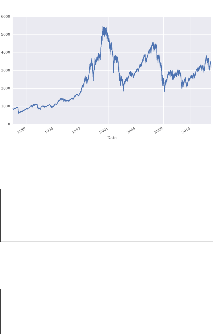
74 LISTED VOLATILITY AND VARIANCE DERIVATIVES
FIGURE 4.1 Historical EURO STOXX 50 index levels.
Before going on to the corresponding procedure for the VSTOXX data, the following visual-
izes the historical closing values for the EURO STOXX 50 index, i.e. for symbol SX5E (see
Figure 4.1):
In [14]: import seaborn as sns; sns.set()
In [15]: import matplotlib
In [16]: matplotlib.rcParams['font.family'] = 'serif' # set serif font
In [17]: es['SX5E'].plot(grid=True, figsize=(10, 6));
4.2.2 VSTOXX Data
Reading the data from the same source for the VSTOXX index is slightly more straightforward
since the respective data le does not change its format.
In [18]: vs_url = source + 'h_vstoxx.txt'
In [19]: print(requests.get(vs_url).text[160:1040])
Date,V2TX,V6I1,V6I2,V6I3,V6I4,V6I5,V6I6,V6I7,V6I8
04.01.1999,18.2033,21.2458,17.5555,31.2179,33.3124,33.7327,33.2232,31.8535,23.8209
05.01.1999,29.6912,36.6400,28.4274,32.6922,33.7326,33.1724,32.8457,32.2904,25.0532
06.01.1999,25.1670,25.4107,25.1351,32.2186,32.6459,31.9673,32.9260,33.2871,26.0107

Data Analysis and Strategies 75
07.01.1999,32.5205,35.4410,32.2004,36.1265,34.5150,33.1095,33.2843,33.7269,26.2205
08.01.1999,33.2296,35.8846,33.0020,36.0813,36.3964,33.4658,33.4837,33.9227,26.3672
11.01.1999,36.8411,46.9742,36.4643,39.9139,38.0755,34.6165,34.4576,34.6615,26.6732
12.01.1999,37.5664,48.6277,37.2998,40.5525,38.7981,35.0575,37.5290,36.5965,28.0273
13.01.1999,39.7373,55.2934,39.5218,43.0083,40.1301,36.0443,38.3889,37.2219,28.1443
14.01.1999,39.1373,NA,39.9544,41.7597,40.5913,36.3330,38.6781,37.4249,28.1515
15.01.1999,38.6741,NA,39.0602,40.1232,39.2451,35.9745,37.7796,36.7660,28.0793
The parametrization for pandas to import the data to a DataFrame object is as follows:
In [20]: vs = pd.read_csv(vs_url, # url/filename
....: index_col=0, # index column (dates)
....: parse_dates=True, # parse date information
....: dayfirst=True, # day before month
....: header=2) # header/column names
....:
In this case, data is available from the beginning of 1999 until the last available trading day.
However, we again select only data until the last trading day of 2015.
In [21]: vs = vs[vs.index <= '2015-12-31']
In [22]: vs.info()
<class 'pandas.core.frame.DataFrame'>
DatetimeIndex: 4327 entries, 1999-01-04 to 2015-12-30
Data columns (total 9 columns):
V2TX 4327 non–null float64
V6I1 3878 non–null float64
V6I2 4327 non–null float64
V6I3 4267 non–null float64
V6I4 4327 non–null float64
V6I5 4327 non–null float64
V6I6 4310 non–null float64
V6I7 4327 non–null float64
V6I8 4313 non–null float64
dtypes: float64(9)
memory usage: 338.0 KB
Figure 4.2 visualizes the times series data for the main volatility index with symbol V2TX.
Inspection of the gure reveals that the volatility index increases and even spikes when there
are crises in the markets – which is best seen towards the end of 2008.
In [23]: vs['V2TX'].plot(grid=True, figsize=(10, 6));
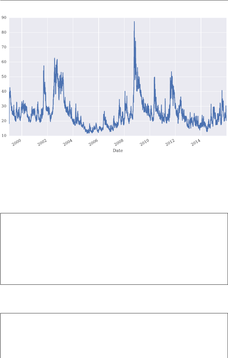
76 LISTED VOLATILITY AND VARIANCE DERIVATIVES
FIGURE 4.2 Historical VSTOXX index levels.
4.2.3 Combining the Data Sets
For what follows, we only need the time series data for the major indexes with symbols SX5E
and V2TX and only for those dates where data is available for both time series. To this end,
the following code generates a new DataFrame object out of the two original ones:
In [24]: import datetime as dt
In [25]: data = pd.DataFrame({'EUROSTOXX':
....: es['SX5E'][es.index > dt.datetime(1999, 1, 1)],
....: 'VSTOXX':
....: vs['V2TX'][vs.index > dt.datetime(1999, 1, 1)]})
....:
In [26]: data = data.dropna() # deletes those rows with NaN values
The code below provides an overview of the new data set and excerpts from all three
DataFrame objects:
In [27]: data.info()
<class 'pandas.core.frame.DataFrame'>
DatetimeIndex: 4326 entries, 1999-01-04 to 2015-12-30
Data columns (total 2 columns):
EUROSTOXX 4326 non–null float64
VSTOXX 4326 non–null float64

Data Analysis and Strategies 77
dtypes: float64(2)
memory usage: 101.4 KB
In [28]: es.iloc[–10:]
Out[28]:
SX5P SX5E SXXP SXXE SXXF SXXA DK5F DKXF
Date
2015-12-17 3095.83 3306.47 364.90 347.46 433.96 371.43 9857.04 610.15
2015-12-18 3065.07 3260.72 361.23 343.23 429.32 368.38 9722.97 602.49
2015-12-21 3022.51 3213.01 357.15 338.55 424.21 364.99 9707.52 601.18
2015-12-22 3019.26 3214.32 356.87 338.77 423.95 364.23 9691.72 599.53
2015-12-23 3109.23 3286.68 366.39 346.14 433.58 375.53 9927.33 614.12
2015-12-24 3108.11 3284.47 366.28 346.05 433.43 375.39 9931.72 614.38
2015-12-28 3093.61 3256.49 364.49 343.54 431.26 374.32 9873.94 611.58
2015-12-29 3139.28 3314.28 369.68 349.29 438.43 378.86 10023.66 620.66
2015-12-30 3118.07 3287.98 367.70 347.02 435.82 377.20 9956.22 617.48
2015-12-31 3100.26 3267.52 365.81 345.16 433.81 375.34 9978.59 618.73
In [29]: np.round(vs, 2).iloc[-10:]
Out[29]:
V2TX V6I1 V6I2 V6I3 V6I4 V6I5 V6I6 V6I7 V6I8
Date
2015-12-15 27.46 41.71 27.41 26.63 26.72 26.66 26.41 26.36 27.44
2015-12-16 25.44 49.12 25.44 25.21 25.34 25.57 25.54 25.77 26.65
2015-12-17 22.58 NaN 22.50 23.47 23.94 24.80 25.01 25.34 26.24
2015-12-18 23.90 NaN 23.76 24.78 25.06 25.80 25.75 25.91 26.54
2015-12-21 23.88 23.56 24.62 24.99 25.80 25.87 26.04 26.64 NaN
2015-12-22 22.54 21.92 23.64 24.14 25.25 25.31 25.64 26.04 26.05
2015-12-23 20.25 19.42 21.45 22.24 24.01 24.46 24.84 25.65 25.44
2015-12-28 22.45 21.43 23.08 23.65 24.70 24.91 25.25 25.46 25.34
2015-12-29 21.61 20.56 22.14 22.87 24.31 24.59 25.06 25.65 25.26
2015-12-30 22.17 21.13 22.64 23.33 24.64 24.72 25.15 25.48 25.16
In [30]: data.iloc[-10:]
Out[30]:
EUROSTOXX VSTOXX
Date
2015-12-15 3241.51 27.4591
2015-12-16 3246.78 25.4362
2015-12-17 3306.47 22.5761
2015-12-18 3260.72 23.8989
2015-12-21 3213.01 23.8836
2015-12-22 3214.32 22.5361
2015-12-23 3286.68 20.2504
2015-12-28 3256.49 22.4544
2015-12-29 3314.28 21.6067
2015-12-30 3287.98 22.1745

78 LISTED VOLATILITY AND VARIANCE DERIVATIVES
4.2.4 Saving the Data
Finally, the DataFrame objects are saved to a HDFStore object on disk for later use. Some-
thing not really needed when an internet connection is available, but helpful when it is not.
In [31]: h5 = pd.HDFStore(path + 'es_vs_data.h5', 'w')
In [32]: h5['es'] = es
In [33]: h5['vs'] = vs
In [34]: h5['data'] = data
In [35]: h5
Out[35]:
<class 'pandas.io.pytables.HDFStore'>
File path: ./source/data/es_vs_data.h5
/data frame (shape->[4326,2])
/es frame (shape->[7476,8])
/vs frame (shape->[4327,9])
In [36]: h5.close()
4.3 BASIC DATA ANALYSIS
To illustrate how to read the data from the HDFStore object, consider the following code
which is almost “symmetric” to the code that writes the data to disk:
In [37]: h5 = pd. HDFStore(path + 'es_vs_data.h5', 'r')
In [38]: h5
Out[38]:
<class 'pandas.io.pytables.HDFStore'>
File path: ./source/data/es_vs_data.h5
/data frame (shape->[4326,2])
/es frame (shape->[7476,8])
/vs frame (shape->[4327,9])
In [39]: es = h5['es']
In [40]: vs = h5['vs']
In [41]: data = h5['data']
In [42]: h5.close()
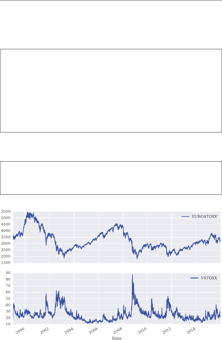
Data Analysis and Strategies 79
As seen in chapter 2, Introduction to Python, pandas provides a wealth of options to analyze
data stored in DataFrame objects. A method which is sometimes helpful is describe()
which provides selected meta statistics for the single data sub-sets stored in DataFrame
columns.
In [43]: data.describe()
Out[43]:
EUROSTOXX VSTOXX
count 4326.000000 4326.000000
mean 3265.935767 25.209891
std 770.513845 9.670981
min 1809.980000 11.596600
25% 2692.385000 18.670200
50% 3089.965000 23.162700
75% 3725.357500 28.310725
max 5464.430000 87.512700
Sub-plots of multiple data sub-sets are easily generated with pandas. The result of the following
plotting code is found as Figure 4.3:
In [44]: data.plot(subplots=True, # generate sub-plots per column
....: figsize=(10, 6), # sizing of the figure
....: color='blue'); # color to plot the data
....:
FIGURE 4.3 Historical EURO STOXX 50 and VSTOXX index levels.
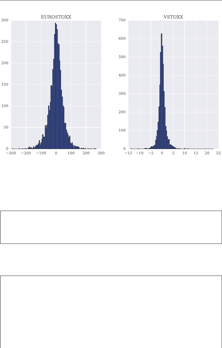
80 LISTED VOLATILITY AND VARIANCE DERIVATIVES
FIGURE 4.4 Histograms of historical absolute daily differences of EURO STOXX 50 and
VSTOXX.
Similarly, you can visualize the absolute differences (over time) by using the diff method
and plotting them as a histogram (see Figure 4.4).
In [45]: data.diff().hist(figsize=(10, 6), # figure sizing
....: color='blue', # color for the plotted data
....: bins=100); # number of bins to be used
....:
In a similar spirit, we can calculate the relative or percentage changes for the time series data.
In [46]: data.pct_change().ix[-10:]
Out[46]:
EUROSTOXX VSTOXX
Date
2015-12-15 0.032578 -0.097067
2015-12-16 0.001626 -0.073670
2015-12-17 0.018384 -0.112442
2015-12-18 -0.013837 0.058593
2015-12-21 -0.014632 -0.000640
2015-12-22 0.000408 -0.056419
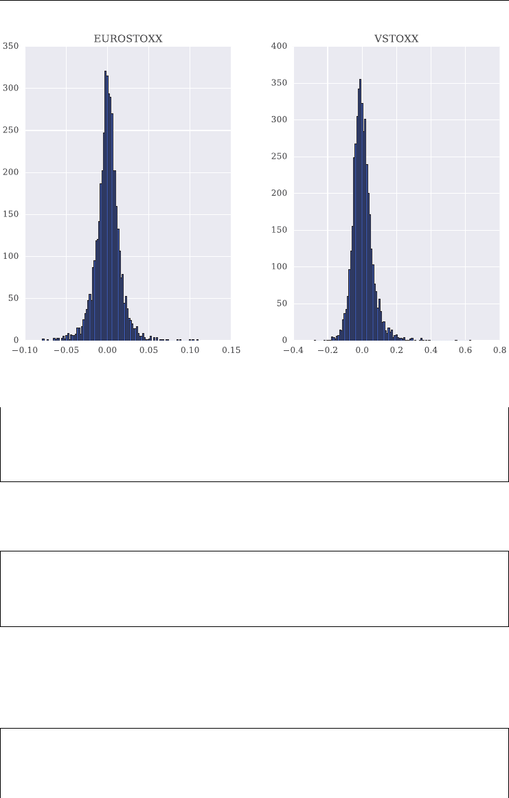
Data Analysis and Strategies 81
FIGURE 4.5 Histograms of historical percentage changes of EURO STOXX 50 and VSTOXX.
2015-12-23 0.022512 -0.101424
2015-12-28 -0.009186 0.108837
2015-12-29 0.017746 -0.037752
2015-12-30 -0.007935 0.026279
The code to visualize this kind of result is the same as before (see Figure 4.5).
In [47]: data.pct_change().hist(figsize=(10, 6),
....: color='blue',
....: bins=100);
....:
The majority of statistical analysis approaches rely on (log) returns and not on absolute time
series data. The next few lines of code calculate the log returns for the two time series and
store them in yet another DataFrame object, called log_rets.
In [48]: import numpy as np
# fully vectorized calculation of log returns
In [49]: log_rets = np.log(data / data.shift(1))
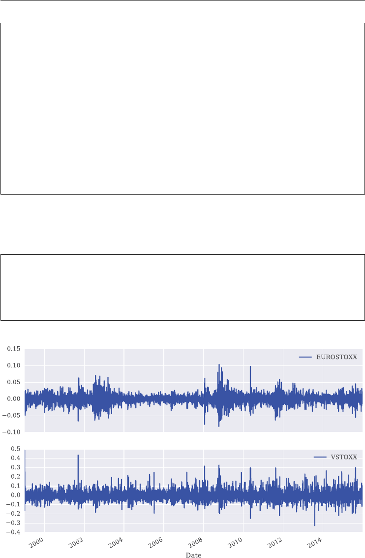
82 LISTED VOLATILITY AND VARIANCE DERIVATIVES
In [50]: log_rets.ix[:10]
Out[50]:
EUROSTOXX VSTOXX
Date
1999-01-04 NaN NaN
1999-01-05 0.017228 0.489248
1999-01-06 0.022138 -0.165317
1999-01-07 -0.015723 0.256337
1999-01-08 -0.003120 0.021570
1999-01-11 -0.019593 0.103173
1999-01-12 -0.012490 0.019496
1999-01-13 -0.048535 0.056180
1999-01-14 0.008648 -0.015214
1999-01-15 0.017855 -0.011906
Figure 4.6 visualizes the log returns times series for both the EURO STOXX 50 and VSTOXX
indexes.
In [51]: log_rets.plot(subplots=True,
....: figsize=(10, 6),
....: color='blue',
....: grid=True);
....:
FIGURE 4.6 Log returns of EURO STOXX 50 and VSTOXX over time.
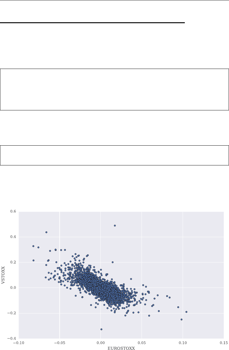
Data Analysis and Strategies 83
4.4 CORRELATION ANALYSIS
Equipped with the log returns, a thorough investigation of the correlation between the
EURO STOXX 50 and VSTOXX indexes is straightforward. For example, pandas provides
the corr() method to calculate correlations between time series data stored in different
DataFrame columns.
In [52]: log_rets.corr()
Out[52]:
EUROSTOXX VSTOXX
EUROSTOXX 1.000000 -0.735032
VSTOXX -0.735032 1.000000
Similar results are obtained by calculating the correlation of the data stored in one pandas
Series object with another data set in another Series object.
In [53]: log_rets['EUROSTOXX'].corr(log_rets['VSTOXX'])
Out[53]: 0.73503163966378138
The plot method of pandas DataFrame objects allows for different types of plots. For
example, scatter plots are helpful to visualize return data of two different time series (see
Figure 4.7).
FIGURE 4.7 Scatter plot of log returns of EURO STOXX 50 and VSTOXX.
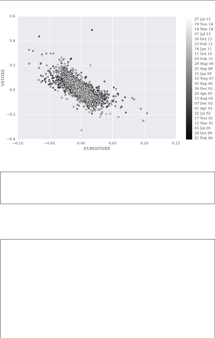
84 LISTED VOLATILITY AND VARIANCE DERIVATIVES
FIGURE 4.8 Scatter plot of log returns of EURO STOXX 50 and VSTOXX with dates.
# plot log returns as scatter plot
In [54]: log_rets.plot(x=' EUROSTOXX', y=' VSTOXX',
....: kind=' scatter', figsize=(10, 6));
....:
Figure 4.8 adds the time dimension to the data through shades of gray to illustrate the relation
between the two time series over time (during different “regimes”).
In [55]: log_rets = log_rets.dropna() # delete NaN values
In [56]: import matplotlib as mpl
In [57]: import matplotlib.pyplot as plt
In [58]: plt.ioff() # turn off interactive mode
In [59]: plt.set_cmap(mpl.cm.gray); # set color map
In [60]: mpl_dates = mpl.dates.date2num(log_rets.index.to_pydatetime())
# conversion
In [61]: plt.figure(figsize=(10, 6));
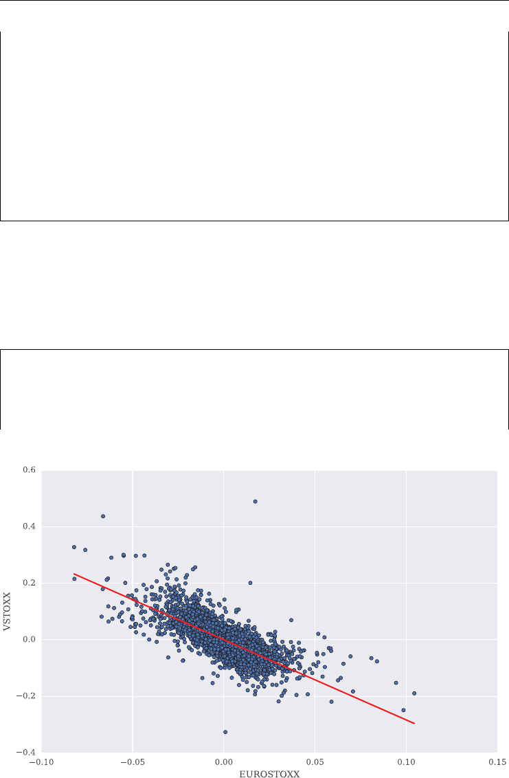
Data Analysis and Strategies 85
In [62]: plt.scatter(log_rets['EUROSTOXX'], log_rets['VSTOXX'],
....: c=mpl_dates, marker='o'); # the actual plot
....:
In [63]: plt.xlabel('EUROSTOXX');
In [64]: plt.ylabel('VSTOXX');
In [65]: plt.colorbar(ticks=mpl.dates.DayLocator(interval=250),
....: format=mpl.dates.DateFormatter('%d %b %y')); # adding bar
....:
Although the negative correlation between the two indexes is almost evident from Figures 4.7
and 4.8, let us formally calculate and represent the negative correlation by a linear regression
line. Figure 4.9 adds such a regression line to the raw log returns in the scatter plot. Negative
correlation translates into a negative slope of the regression line.
# conduct linear regression
In [66]: p = np.polyfit(log_rets['EUROSTOXX'].values,
....: log_rets['VSTOXX'].values,
....: deg=1) # the regression
....:
FIGURE 4.9 Scatter plot of log returns of EURO STOXX 50 and VSTOXX with regression line.
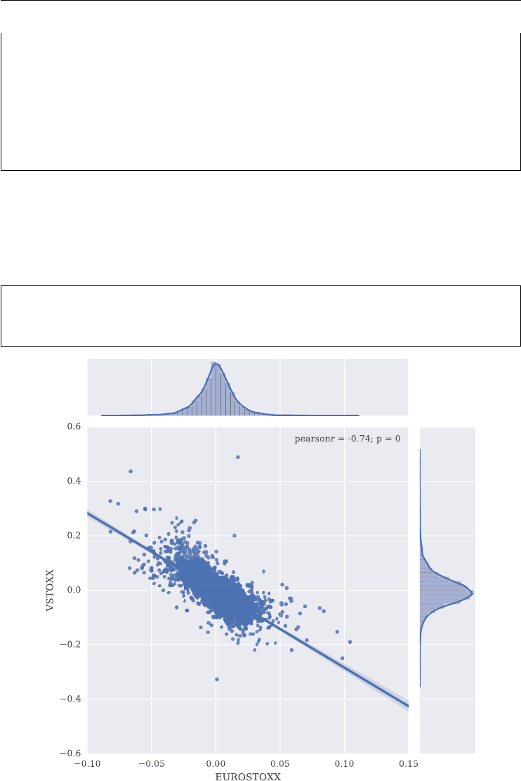
86 LISTED VOLATILITY AND VARIANCE DERIVATIVES
In [67]: log_rets.plot(x='EUROSTOXX', y='VSTOXX',
....: kind='scatter', figsize=(10, 6)); # the actual plotting
....:
# plot the regression line
In [68]: plt.plot(log_rets['EUROSTOXX'], np.polyval(p, log_rets['EUROSTOXX']),
....: 'r'); # adding the regression line
....:
The seaborn plotting library is specically developed with statistical applications in mind.
It therefore provides multiple useful, high level plotting capabilities. One of these is the
jointplot() function. The result of applying this function to the log return data is dis-
played as Figure 4.10. This is denitely the richest and most insightful presentation so far for
our purposes.
In [69]: sns.jointplot(x=log_rets['EUROSTOXX'], y=log_rets['VSTOXX'],
....: kind='reg', size=7);
....:
FIGURE 4.10 Scatter plot of log returns of EURO STOXX 50 and VSTOXX with
regression line and histograms.
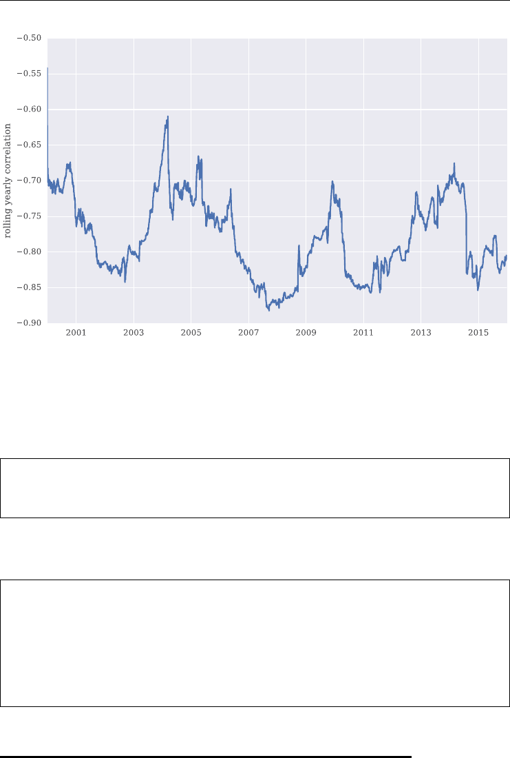
Data Analysis and Strategies 87
FIGURE 4.11 Rolling yearly correlation of EURO STOXX 50 and VSTOXX.
The nal analysis in this section considers correlation over time. To this end, pandas provides
the rolling() method which allows, among others, the vectorized calculation of correlation
for moving time windows via corr(). We chose a window size of 252 trading days which
represents roughly one year.
In [70]: data['CORR'] = log_rets['EUROSTOXX'].rolling(
....: window=252).corr(log_rets['VSTOXX'])
....:
Figure 4.11 plots the rolling correlation data and illustrates well that correlation uctuates for
different yearly windows but that it is negative for any chosen yearly window.
In [71]: to_plot = data.dropna() # drop NaN values
In [72]: plt.figure(figsize=(10, 6));
In [73]: plt.plot(data.index, data.CORR);
In [74]: plt.ylabel('rolling yearly correlation');
4.5 CONSTANT PROPORTION INVESTMENT STRATEGIES
One way to make use of the fact that the VSTOXX index is negatively correlated with the
EURO STOXX 50 index is to implement a constant proportion investment strategy. Respective

88 LISTED VOLATILITY AND VARIANCE DERIVATIVES
results are found, for example, in the study by Guobuzaite and Martellini (2012). Basically,
a constant (dollar) proportion investment strategy keeps the proportion of money invested in
securities of a portfolio over time constant by dynamic re-balancings given the movements in
the prices of the single securities.
In the example in this section, we assume that direct investments both in the EURO
STOXX 50 and the VSTOXX indexes are possible and that no transaction costs apply.
Although this might not be realistic, it simplies the anaylsis and illustrates the basic idea
pretty well. This application allows the use of, for example, VSTOXX futures with different
roll-over strategies and the inclusion of transaction costs.
To begin with, let us adjust the original data sets for the EURO STOXX 50 and VSTOXX
indexes by mainly normalizing both time series to starting values of 100.
In [75]: del data['CORR'] # delete correlation data
In [76]: data = data.dropna() # drop NaN values
In [77]: data = data / data.iloc[0] * 100 # normalization
In [78]: data.head()
Out[78]:
EUROSTOXX VSTOXX
Date
1999-01-04 100.000000 100.000000
1999-01-05 101.737744 163.108887
1999-01-06 104.015128 138.255152
1999-01-07 102.392538 178.651673
1999-01-08 102.073608 182.547121
First, we analyze a typical passive investment strategy allocating 30% of a portfolio to the
VSTOXX index and the remaining 70% to the EURO STOXX 50.
In [79]: invest = 100 # initial investment
In [80]: cratio = 0.3 # VSTOXX ratio in the beginning
# number of EURO STOXX (fictional) securities
In [81]: data['Equity'] = (1 - cratio) * invest / data['EUROSTOXX'][0]
# number of VSTOXX (fictional) securities
In [82]: data['Volatility'] = cratio * invest / data['VSTOXX'][0]
In vectorized fashion, we calculate next the absolute values of such a portfolio over time, i.e.
as a time series.
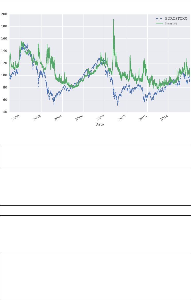
Data Analysis and Strategies 89
FIGURE 4.12 Passive investment strategy (hypothetical) with EURO STOXX 50 and VSTOXX.
In [83]: data['Passive'] = (data['Equity'] * data['EUROSTOXX']
....: + data['Volatility'] * data['VSTOXX'])
....:
Figure 4.12 illustrates the performance of this particular passive investment strategy in com-
parison to a passive strategy purely investing in the EURO STOXX 50 index. In times of crisis,
for example at the end of 2008, the strategy peforms better. However, over the whole period
there is hardly any difference in the end result.
In [84]: data[['EUROSTOXX', 'Passive']].plot(figsize=(10, 6), style=['—-', '–']);
Second, the active constant proportion investment strategy, which keeps the dollar proportion
invested in the VSTOXX index constant at 30% over time through daily re-balancings of the
portfolio. In this case, the single calculations are done step-by-step through looping over the
single historical trading dates.
In [85]: for iin range(1, len(data)): # daily re-balancing
....: evalue = data['Equity'][i - 1] * data['EUROSTOXX'][i]
....: vvalue = data['Volatility'][i - 1] * data['VSTOXX'][i]
....: tvalue = evalue + vvalue # total wealth
....: data['Equity'][i] = (1 - cratio) * tvalue / data['EUROSTOXX'][i]
....: data['Volatility'][i] = cratio * tvalue / data['VSTOXX'][i]
....:

90 LISTED VOLATILITY AND VARIANCE DERIVATIVES
Based on the results, calculate the absolute performance of this active strategy as before. Over
the rst few trading days no major performance differences arise.
In [86]: data['Active'] = (data['Equity'] * data['EUROSTOXX']
....: + data['Volatility'] * data['VSTOXX'])
....:
In [87]: np.round(data.head(), 2)
Out[87]:
EUROSTOXX VSTOXX Equity Volatility Passive Active
Date
1999-01-04 100.00 100.00 0.70 0.30 100.00 100.00
1999-01-05 101.74 163.11 0.83 0.22 120.15 120.15
1999-01-06 104.02 138.26 0.78 0.25 114.29 116.54
1999-01-07 102.39 178.65 0.86 0.21 125.27 125.48
1999-01-08 102.07 182.55 0.86 0.21 126.22 126.03
Over the whole time period, however, the active strategy – showing a 800+% gain – signi-
cantly outperforms the passive one.
In [88]: np.round(data.tail(), 2)
Out[88]:
EUROSTOXX VSTOXX Equity Volatility Passive Active
Date
2015-12-22 90.72 123.80 7.22 2.27 100.65 936.01
2015-12-23 92.76 111.25 6.96 2.49 98.31 922.28
2015-12-28 91.91 123.35 7.21 2.30 101.34 946.46
2015-12-29 93.54 118.70 7.09 2.39 101.09 947.50
2015-12-30 92.80 121.82 7.16 2.34 101.50 949.71
Let us briey verify whether the above implementation indeed yields constant proportions for
the two (ctional) securities in the portfolio.
In [89]: (data['Volatility'] * data['VSTOXX'] / data['Active'])[:5]
Out[89]:
Date
1999-01-04 0.3
1999-01-05 0.3
1999-01-06 0.3
1999-01-07 0.3
1999-01-08 0.3
dtype: float64
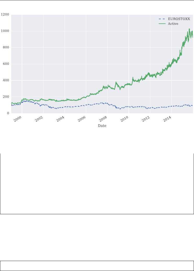
Data Analysis and Strategies 91
FIGURE 4.13 Active, constant proportion investment strategy (hypothetical) with EURO STOXX
50 and VSTOXX.
In [90]: (data['Equity'] * data['EUROSTOXX'] / data['Active'])[:5]
Out[90]:
Date
1999-01-04 0.7
1999-01-05 0.7
1999-01-06 0.7
1999-01-07 0.7
1999-01-08 0.7
dtype: float64
Being assured that we have indeed implemented a constant proportion trading strategy, have a
look at Figure 4.13 which impressively illustrates the outperformance of the active approach
over a passive investment in the stock index itself. However, bear in mind that all this rests on
a number of simplifying assumptions.
In [91]: data[['EUROSTOXX', 'Active']].plot(figsize=(10, 6), style=['—-', '–']);
The assumption of 30% invested in the VSTOXX index might seem a bit ad hoc. Therefore,
the following derives the optimal allocation for the given time period and data sets by a brute
force approach. First, we clean up the DataFrame object to reduce it again to the original
time series data for the two indexes.

92 LISTED VOLATILITY AND VARIANCE DERIVATIVES
# re-initialize DataFrame
In [92]: data = data[['EUROSTOXX', 'VSTOXX']]
The function below calculates the performance of a constant proportion investment strategy for
different VSTOXX dollar proportions and different starting and ending dates (both defaulting
to the data sets’ start and end dates).
In [93]: from copy import deepcopy
In [94]: def vstoxx_strategy(cratio, start=data.index[0], end=data.index[-1]):
....: base = deepcopy(data[(data.index >= start) & (data.index <= end)])
....: invest = 100 # initial invest
....: base['Equity'] = (1 - cratio) * invest / base['EUROSTOXX'][0]
....: base['Volatility'] = cratio * invest / base['VSTOXX'][0]
....: for iin range(1, len(base)): # daily re–balancing
....: evalue = base['Equity'][i - 1] * base['EUROSTOXX'][i]
....: vvalue = base['Volatility'][i - 1] * base['VSTOXX'][i]
....: tvalue = evalue + vvalue
....: base['Equity'][i] = (1 - cratio) * tvalue / base['EUROSTOXX'][i]
....: base['Volatility'][i] = cratio * tvalue / base['VSTOXX'][i]
....: base['Active'] = (base['Equity'] * base['EUROSTOXX']
....: + base['Volatility'] * base['VSTOXX']) # wealth position
....: print("A con. VSTOXX ratio of %.2f yields a net perform. of %6.1f %%.") \
....: % (cratio, (base['Active'][-1] / base['Active'][0] - 1) * 100)
....:
Equipped with this function, let us calculate the net perfomance for a VSTOXX dollar ratio of
30% as before.
In [95]: vstoxx_strategy(0.3)
A con. VSTOXX ratio of 0.30 yields a net perform.of 849.7%.
We do the same for 40% which obviously yields an even better result.
In [96]: vstoxx_strategy(0.4)
A con. VSTOXX ratio of 0.40 yields a net perform.of 1231.9%.
Applying an approach which is slightly more systematic, we get the following results for differ-
ent constant dollar proportion assumptions. Over the whole period for which data is available
a 50:50 investment strategy seems to be optimal with a net performance of more than 1,400%.

Data Analysis and Strategies 93
In [97]: for cratio in np.arange(0, 1.01, 0.1):
....: vstoxx_strategy(cratio)
....:
A con. VSTOXX ratio of 0.00 yields a net perform.of -7.2%.
A con. VSTOXX ratio of 0.10 yields a net perform.of 151.5%.
A con. VSTOXX ratio of 0.20 yields a net perform.of 445.4%.
A con. VSTOXX ratio of 0.30 yields a net perform.of 849.7%.
A con. VSTOXX ratio of 0.40 yields a net perform.of 1231.9%.
A con. VSTOXX ratio of 0.50 yields a net perform.of 1408.7%.
A con. VSTOXX ratio of 0.60 yields a net perform.of 1283.2%.
A con. VSTOXX ratio of 0.70 yields a net perform.of 928.4%.
A con. VSTOXX ratio of 0.80 yields a net perform.of 521.0%.
A con. VSTOXX ratio of 0.90 yields a net perform.of 204.9%.
A con. VSTOXX ratio of 1.00 yields a net perform.of 21.8%.
Let us implement the same analysis for the time period beginning in January 2013 and ending
with the last quarter of 2015. In this case, a constant dollar proportion invested in the VSTOXX
of again about 50% seems optimal and yields a net performance of close to 110%.
In [98]: for cratio in np.arange(0, 1.01, 0.1):
....: vstoxx_strategy(cratio, start='2013-1-1', end=' 2015-12-31')
....:
A con. VSTOXX ratio of 0.00 yields a net perform.of 21.3%.
A con. VSTOXX ratio of 0.10 yields a net perform.of 47.9%.
A con. VSTOXX ratio of 0.20 yields a net perform.of 72.4%.
A con. VSTOXX ratio of 0.30 yields a net perform.of 92.2%.
A con. VSTOXX ratio of 0.40 yields a net perform.of 105.0%.
A con. VSTOXX ratio of 0.50 yields a net perform.of 109.2%.
A con. VSTOXX ratio of 0.60 yields a net perform.of 104.3%.
A con. VSTOXX ratio of 0.70 yields a net perform.of 91.1%.
A con. VSTOXX ratio of 0.80 yields a net perform.of 71.2%.
A con. VSTOXX ratio of 0.90 yields a net perform.of 46.9%.
A con. VSTOXX ratio of 1.00 yields a net perform.of 20.8%.
4.6 CONCLUSIONS
This chapter is about the retrieval and analysis of EURO STOXX 50 and VSTOXX histori-
cal data. It shows how to use Python and pandas to retrieve and clean up historical data sets
from the index provider’s website http://stoxx.com with pandas. It also shows how to imple-
ment Python code to replicate central stylized facts about stock and volatility indexes, namely
their highly negative correlation and the benets of constant (dollar) proportion investment
strategies involving (products based on) equity and volatility indexes.

CHAPTER 5
VSTOXX Index
5.1 INTRODUCTION
This chapter is about the (re-)calculation of the VSTOXX index, the volatility index based on
EURO STOXX 50 index options. The goal is to achieve a good understanding of the processes
and underlying mechanics of calculating the VSTOXX index. You will nd all the background
information as well as Python code that will enable you to recalculate both historical VSTOXX
index values and current ones in (almost) real-time. Chapter 3, Model-Free Replication of
Variance provides the theoretical background for the concepts presented in this chapter.
The (main) VSTOXX index itself is based on two sub-indexes, which themselves are
derived from Eurex option series for both European puts and calls on the EURO STOXX 50
index. The algorithm, and therefore this chapter as well, are comprised of three main parts:
collect and clean-up the data of the necessary option series
compute the sub-indexes from the option data
compute the VSTOXX index from the relevant sub-indexes.
A few remarks about the option series and sub-indexes used and their expiry dates and time
horizons, respectively, seem in order. There are eight sub-indexes of the VSTOXX which each
measure the implied volatility of an option series with xed expiry. For example, the VSTOXX
1M sub-index starts with the option series that has one month expiry and is calculated up to
two days prior to the xed maturity date of the relevant option series. The VSTOXX index
measures the implied volatility of an “imaginary” options series with a xed time to expiry of
30 days. This is achieved through linear interpolation of the two nearest sub-indexes, generally
VSTOXX 1M and VSTOXX 2M. On the two days before VSTOXX 1M expiry, the VSTOXX
2M and VSTOXX 3M are used instead and an extrapolation takes place.
Table 5.1 lists all the sub-indexes and provides additional information.
5.2 COLLECTING OPTION DATA
As already pointed out, the VSTOXX is based on two sub-indexes, generally the VSTOXX
1M and VSTOXX 2M, sometimes the VSTOXX 2M and VSTOXX 3M. The sub-indexes
95
Listed Volatility and Variance Derivatives: A
Python-based Guide
By Dr. Yves J. Hilpisch
© 2017 Yves Hilpisch

96 LISTED VOLATILITY AND VARIANCE DERIVATIVES
TABLE 5.1 The VSTOXX sub-indexes.
Sub-index Code ISIN Settlement date of the option series used
VSTOXX 1M V6I1 DE000A0G87B2 The last available within 1 month
VSTOXX 2M V6I2 DE000A0G87C0 The last available within 2 months
VSTOXX 3M V6I3 DE000A0G87D8 The last available within 3 months
VSTOXX 6M V6I4 DE000A0G87E6 The last available within 6 months
VSTOXX 9M V6I5 DE000A0G87F3 The last available within 9 months
VSTOXX 12M V6I6 DE000A0G87G1 The last available within 12 months
VSTOXX 18M V6I7 DE000A0G87H9 The last available within 18 months
VSTOXX 24M V6I8 DE000A0G87J5 The last available within 24 months
themselves are based on the option series on the EURO STOXX 50 index with respective
time to expiry. We therefore need the prices of all options with maturities up to 3 months.
We use historical data as provided by Eurex itself as the data source. See the website
http://bit.ly/1GY5KCI.
The code to collect the data can be found in the module index_collect_option_
data.py (see sub-section 5.6.1, index_collect_option_data.py for the complete script). As
usual, the module starts with some imports and parameter denitions.
import requests
import datetime as dt
import pandas as pd
import numpy as np
from StringIO import *
from index_date_functions import *
#
# The URL template
#
url1 = 'http://www.eurexchange.com/action/exchange-en/'
url2 = '180106-180102/180102/onlineStats.do?productGroupId=846'
url3 = '&productId=19068&viewType=3&cp=%s&month=%s&year=%s&busDate=%s'
URL = url1 + url2 + url3
In addition, the module contains six functions. The rst is collect_option_series():
def collect_option_series(month, year, start):
''' Collects daily option data from web source.
Parameters
==========
month: int
maturity month
year: int
maturity year

VSTOXX Index 97
start: datetime object
starting date
Returns
=======
dataset: pandas DataFrame object
object containing the collected data
'''
end = dt.datetime.today()
delta = (end - start).days
dataset = pd.DataFrame()
for tin range(0, delta): # runs from start to today
date = start + dt.timedelta(t)
dummy = get_data(month, year, date) # get data for one day
if len(dummy) != 0:
if len(dataset) == 0:
dataset = dummy
else:
dataset = pd.concat((dataset, dummy)) # add data
return dataset
This function collects the data of the option series with maturity in the month month and year
year.Itiscalledbythefunction start_collecting() and calls the function
get_data() for every single day from the date start to today. It returns a complete set of
prices (both puts and calls) for that series.
The second function is get_data().
def get_data(month, year, date):
''' Get the data for an option series.
Parameters
==========
month: int
maturity month
year: int
maturity year
date: datetime object
the date for which the data is collected
Returns
=======
dataset: pandas DataFrame object
object containing call & put option data
'''

98 LISTED VOLATILITY AND VARIANCE DERIVATIVES
date_string = date.strftime('%Y%m%d')
# loads the call data from the web
data = get_data_from_www('Call', month, year, date_string)
calls = parse_data(data, date) # parse the raw data
calls = calls.rename(columns={'Daily settlem.price': 'Call_Price'})
calls = pd.DataFrame(calls.pop('Call_Price').astype(float))
# the same for puts
data = get_data_from_www('Put', month, year, date_string)
puts = parse_data(data, date)
puts = puts.rename(columns={'Daily settlem.price': 'Put_Price'})
puts = pd.DataFrame(puts.pop('Put_Price').astype(float))
dataset = merge_and_filter(puts, calls) # merges the two time series
return dataset
This one is called by the function collect_option_series() and calls itself the
functions get_data_from_www(),parse_data(data, date) and merge_and_
filter(). It returns the prices of the option series with expiry date in month month and year
year for the day date.
The third function is get_data_from_www().
def get_data_from_www(oType, matMonth, matYear, date):
''' Retrieves the raw data of an option series from the web.
Parameters
==========
oType: string
either 'Put' or 'Call'
matMonth: int
maturity month
matYear: int
maturity year
date: string
expiry in the format 'YYYYMMDD'
Returns
=======
a: string
raw text with option data
'''
url = URL % (oType, matMonth, matYear, date) # parametrizes the URL
a = requests.get(url).text
return a

VSTOXX Index 99
The function collects the prices of an option series for a single day (dened by date) from the
web. The option series is dened by the date of its expiry, given by matMonth and matYear;
the type of the options is given by oType which can be either Put or Call. It returns a
complete HTML le.
merge_and_filter() is the fourth function.
def merge_and_filter(puts, calls):
''' Gets two pandas time series for the puts and calls
(from the same option series), merges them, filters out
all options with prices smaller than 0.5 and
returns the resulting DataFrame object.
Parameters
==========
puts: pandas DataFrame object
put option data
calls: pandas DataFrame object
call option data
Returns
=======
df: pandas DataFrame object
merged & filtered options data
'''
df = calls.join(puts, how='inner') # merges the two time series
# filters all prices which are too small
df = df[(df.Put_Price >= 0.5) & (df.Call_Price >= 0.5)]
return df
This one gets two time series puts and calls (typically of the same option series), merges
them, lters out all options with prices below 0.5 and returns the resulting pandas DataFrame
object.
parse_data() is the fth function.
def parse_data(data, date):
''' Parses the HTML table and transforms it into a CSV compatible
format. The result can be directly imported into a pandas DataFrame.
Parameters
==========
data: string
document containing the Web content
date: datetime object
date for which the data is parsed

100 LISTED VOLATILITY AND VARIANCE DERIVATIVES
Returns
=======
dataset: pandas DataFrame object
transformed option raw data
'''
parts = data.split('<table')
parts2 = parts[1].split('</table')
dummy = parts2[0].replace(' class="odd"','')
dummy = dummy.replace(' class="even"','')
parts3 = dummy.split('<tr><td><b>Total</b>')
table = parts3[0] # the html table containing the data
table = table.replace('class="dataTable"><thead>', 'Pricing day')
# replace tags by commas and newlines
table = table.replace('</tr>', '\n')
table = table.replace(',', '')
table = table.replace('<td>', ',')
table = table.replace('</td>', '')
table = table.replace('<th>', ',')
table = table.replace('</th>', '')
table = table.replace('</thead><tbody>', '\n')
# the resulting string looks like a CSV file
date_string = date.strftime('%d.%m.%Y')
table = table.replace('<tr>', date_string)
string = StringIO(table) # mask the string as file
dataset = pd.read_csv(string, parse_dates=[0], index_col=(0, 1),
dayfirst=True) # read the 'file' as pandas DataFrame object
return dataset
It gets the string data which contains the HTML text delivered by function
get_data_from_www(), parses that string to a pandas DataFrame object with
double index date and strike price and returns that object.
The sixth and nal function is data_collection().
def data_collection(path):
''' Main function which saves data into the HDF5 file
'index_option_series.h5' for later use.
Parameters
==========
path: string
path to store the data

VSTOXX Index 101
'''
# file to store data
store = pd.HDFStore(path + 'index_option_series.h5', 'a')
today = dt.datetime.today()
start = today – dt.timedelta(31) # the last 31 days
day = start.day
month = start.month
year = start.year
for iin range(4): # iterates over the next 4 months
dummy_month = month + i
dummy_year = year
if dummy_month > 12:
dummy_month -= 12
dummy_year += 1
# collect daily data beginning 31 days ago (start) for
# option series with expiry dummy_month, dummy_year
dataset = collect_option_series(dummy_month, dummy_year, start)
dummy_date = dt.datetime(dummy_year, dummy_month, day)
# abbreviation for expiry date (for example Oct14)
series_name = dummy_date.strftime('%b%y')
if series_name in store.keys(): # if data for that series exists
index_old = store[series_name].index
index_new = dataset.index
if len(index_new – index_old) > 0:
dummy = pd.concat((store[series_name],
dataset.ix[index_new - index_old])) # add the new data
store[series_name] = dummy
else:
if len(dataset) > 0:
# if series is new, write whole data set into data store
store[series_name] = dataset
store.close()
This function is to initiate and nalize the collection of all relevant option series data sets. It
saves the resulting data in a le named index_option_series.h5.
In [1]: path = './source/data/'

102 LISTED VOLATILITY AND VARIANCE DERIVATIVES
Let us collect option data since all other steps depend on this data. We import the module as
icod.
In [2]: import numpy as np
In [3]: import pandas as pd
In [4]: import datetime as dt
In [5]: import index_collect_option_data as icod
Next, x a target day relative to today such that you hit a business day for which closing data
is available.
In [6]: today = dt.datetime.now()
# make sure to hit a business day
In [7]: target_day = today - dt.timedelta(days=1)
In [8]: ds = target_day.strftime('%Y%m%d')
In [9]: ds
Out[9]: '20160201'
Then, for example, collect option data for puts and calls with a maturity dened by the param-
eters as follows:
# adjust maturity parameters if necessary
In [10]: call_data = icod.get_data_from_www(oType='Call', matMonth=3,
....: matYear=2016, date=ds)
....:
In [11]: put_data = icod.get_data_from_www(oType='Put', matMonth=3,
....: matYear=2016, date=ds)
....:
The return objects need to be parsed.
# parse the raw data
In [12]: calls = icod.parse_data(call_data, target_day)
In [13]: puts = icod.parse_data(put_data, target_day)

VSTOXX Index 103
Let us have a look at some meta information about the call options data.
In [14]: calls.info()
<class 'pandas.core.frame.DataFrame'>
MultiIndex: 114 entries, (2016-02-01 00:00:00, 600.0) to
(2016-02-01 00:00:00, 6000.0)
Data columns (total 8 columns):
Version number 114 non-null float64
Opening price 114 non-null float64
Daily high 114 non-null float64
Daily low 114 non-null float64
Underlying closing price 114 non-null float64
Daily settlem. price 114 non-null float64
Traded contracts 114 non-null int64
Open interest (adj.)* 114 non-null int64
dtypes: float64(6), int64(2)
memory usage: 8.0+ KB
And about the put options data.
In [15]: puts.info()
<class 'pandas.core.frame.DataFrame'>
MultiIndex: 114 entries, (2016-02-01 00:00:00, 600.0) to
(2016-02-01 00:00:00, 6000.0)
Data columns (total 8 columns):
Version number 114 non-null float64
Opening price 114 non-null float64
Daily high 114 non-null float64
Daily low 114 non-null float64
Underlying closing price 114 non-null float64
Daily settlem. price 114 non-null float64
Traded contracts 114 non-null int64
Open interest (adj.)* 114 non-null int64
dtypes: float64(6), int64(2)
memory usage: 8.0+ KB
In a next step, we take out the daily settlement prices for both the puts and calls and dene two
new DataFrame objects.
In [16]: calls = pd.DataFrame(calls.rename(
....: columns={'Daily settlem. price': 'Call_Price'}
....: ).pop('Call_Price').astype(float))
....:

104 LISTED VOLATILITY AND VARIANCE DERIVATIVES
In [17]: puts = pd.DataFrame(puts.rename(
....: columns={'Daily settlem. price': 'Put_Price'}
....: ).pop('Put_Price').astype(float))
....:
These two are then merged via the function merge_and_filter() into another new
DataFrame object.
In [18]: dataset = icod.merge_and_filter(puts, calls)
In [19]: dataset.info()
<class 'pandas.core.frame.DataFrame'>
MultiIndex: 67 entries, (2016-02-01 00:00:00, 1900.0) to
(2016-02-01 00:00:00, 3625.0)
Data columns (total 2 columns):
Call_Price 67 non-null float64
Put_Price 67 non-null float64
dtypes: float64(2)
memory usage: 1.6+ KB
This whole procedure is implemented in the function collect_option_series() which
yields the same result.
In [20]: os = icod.collect_option_series(3, 2016, target_day)
In [21]: os.info()
<class 'pandas.core.frame.DataFrame'>
MultiIndex: 67 entries, (2016-02-01 00:00:00, 1900.0) to
(2016-02-01 00:00:00, 3625.0)
Data columns (total 2 columns):
Call_Price 67 non-null float64
Put_Price 67 non-null float64
dtypes: float64(2)
memory usage: 1.6+ KB
The function data_collection() repeats this procedure for all those dates for which
option data is available and writes (appends) the results in a HDF5 database le.
# uncomment to initiate the process (takes a while)
# %time icod.data_collection(path)
For the further analyses, we open this HDF5 database le.
In [22]: store = pd.HDFStore(path + 'index_option_series.h5', 'r')
In [23]: store

VSTOXX Index 105
Out[23]:
<class 'pandas.io.pytables.HDFStore'>
File path: ./source/data/index_option_series.h5
/Feb16 frame (shape->[1398,2])
/Jan16 frame (shape->[638,2])
/Mar16 frame (shape->[1385,2])
The collected option series data is easily read from the HDF5 database le in monthly chunks.
In [24]: Mar16 = store['Mar16']
In [25]: Mar16.info()
<class 'pandas.core.frame.DataFrame'>
MultiIndex: 1385 entries, (2015-12-18 00:00:00, 1500.0) to (2016-01-15
00:00:00, 3650.0)
Data columns (total 2 columns):
Call_Price 1385 non-null float64
Put_Price 1385 non-null float64
dtypes: float64(2)
memory usage: 32.5+ KB
In [26]: store.close()
Some selected option prices from the large data set:
In [27]: Mar16.ix[25:35]
Out[27]:
Call_Price Put_Price
Pricing day Strike price
2015-12-18 2675.0 600.4 21.9
2700.0 577.3 23.8
2725.0 554.3 25.9
2750.0 531.6 28.1
2775.0 509.0 30.6
2800.0 486.6 33.2
2825.0 464.5 36.1
2850.0 442.6 39.3
2875.0 421.0 42.6
2900.0 399.6 46.3
5.3 CALCULATING THE SUB-INDEXES
In this section, we use the data le created in the previous one. For all dates
of the data le, the Python module index_subindex_calculation.py (see

106 LISTED VOLATILITY AND VARIANCE DERIVATIVES
index_subindex_calculation.py for the complete script) used in this section decides whether
the VSTOXX 1M sub-index is dened or not (remember that the sub-index is not dened at the
nal settlement day and one day before). If it is dened, the script computes the value of the
sub-indexes VSTOXX 1M and VSTOXX 2M; if not, it computes the values of the sub-indexes
VSTOXX 2M and VSTOXX 3M, respectively. Finally, it returns a pandas DataFrame object
with the three time series.
5.3.1 The Algorithm
First, we focus on the computation of the value of a single sub-index for a given date. The
prices Ci,i∈{0, ...,n}, of a series of European call options on the EURO STOXX 50 with
xed maturity date Tand exercise prices Ki,i∈{0, ...,n} are given, as well as the prices Pi,i∈
{0, ...,n}, of a series of European put options on EURO STOXX 50 with the same maturity
date Tand exercise prices Ki. Let us further hold that Ki<Ki+1for all i∈{0, ....,n−1}.
Then, the value of the relevant sub-index Vis as follows (see chapter 3, Model-Free Repli-
cation of Variance):
V=100 ⋅̂𝜎2
with
̂𝜎2=2
T
n
i=0
ΔKi
Ki2erT Mi−1
TF
K∗
−12
where
ΔKi=
K1−K0for i=0
Ki+1−Ki−1
2for i=1, ...,n−1
Kn−Kn−1for i=n
r=constant risk-free short rate appropriate for maturity T
F=Kj+erT Cj−Pj, where j=min
i∈{0,...,n}{Ci−Pi}
K∗=max
Kii∈{0,...,n}
{Ki<F},
Mi=
Pifor Ki<K∗
Pi−Ci
2for Ki=K∗
Cifor Ki>K∗
We implement a function to compute one value of a single sub-index. Thereafter, we extend
that function to compute time series for both VSTOXX 1M and VSTOXX 2M indexes as well
as parts of the VSTOXX 3M index. Imports again make up the beginning of the script.

VSTOXX Index 107
import math
import numpy as np
import pandas as pd
import datetime as dt
import index_date_functions as idf
A core function of the script is compute_subindex().
def compute_subindex(data, delta_T, R):
''' Computes a sub-index for given option series data.
Parameters
==========
data: pandas.DataFrame object
contains the option data
delta_T: float
time interval
R: float
discount factor
Returns
=======
subVSTOXX: float
sub-index value
'''
# difference between put and call option with same strike
data['Diff_Put_Call'] = np.abs(data.Put_Price – data.Call_Price)
# converts the strike price which serves as index so far
# to a regular data column
data = data.reset_index()
data['delta_K'] = None
# differences between the different strikes of the series
data['delta_K'].iloc[1:–1] = [(data['Strike price'][i + 1]
– data['Strike price'][i – 1]) / 2 for iin data.index[1:–1]]
# where possible, for the i-th entry it is
# half of the difference between the (i-1)-th
# and (i+1)-th price
# for i=0 it is just the difference to the next strike
data['delta_K'].iloc[0] = data['Strike price'][1] – data['Strike price'][0]
data['delta_K'].iloc[data.index[–1:]] = float(data['Strike price'][–1:]) \
– float(data['Strike price'][-2:-1])
# for the last entry, it is just the difference
# between the second but last strike and the last strike price
# find the smallest difference between put and call price
min_index = data. Diff_Put_Call.argmin()

108 LISTED VOLATILITY AND VARIANCE DERIVATIVES
# the forward price of that option
forward_price = data['Strike price'][min_index] \
+ R * data.Diff_Put_Call[min_index]
K_0 = data['Strike price'][forward_price -
data['Strike price'] > 0].max()
# the index of the ATM strike
K_0_index = data.index[data['Strike price'] == K_0][0]
# selects the OTM options
data['M'] = pd.concat((data.Put_Price[0:K_0_index],
data.Call_Price[K_0_index:]))
# ATM we take the average of put and call price
data['M'].iloc[K_0_index] = (data['Call_Price'][K_0_index]
+ data['Put_Price'][K_0_index]) / 2
# the single OTM values
data['MFactor'] = (R * (data['delta_K'] * data['M'])
/ (data['Strike price']) ** 2)
# the forward term
fterm = 1. / delta_T *(forward_price / K_0 - 1) ** 2
# summing up
sigma = 2 / delta_T * np.sum(data.MFactor) – fterm
subVSTOXX = 100 * math.sqrt(sigma)
return subVSTOXX
This script calculates a single index value. It implements mainly the following steps:
the calculation of ΔKi
the computation of the forward price and the index of K∗
the selection of the at-the-money option and the out-of-the-money options
the combination of the results of the other three steps.
The next step is the derivation of time series data for the VSTOXX 1M and VSTOXX 2M as
well as parts of the VSTOXX 3M indexes and storage of the results in a pandas DataFrame
object. As data source we use the le created in the last section. Remember that this le con-
tains a dictionary-like HDFStore object with one entry for every options series. The keys for
the entries are three letter abbreviations of the respective month’s name plus the actual year
represented by two numbers, for example Mar16,Jun16 and so on. The value of an entry is
a pandas DataFrame object with a pandas MultiIndex (date, strike price) and prices for
the put and call options for the dates and strike prices.
All this is implemented as function make_subindex().
def make_subindex(path):
''' Depending on the content of the file 'index_option_series.h5',
the function computes the sub-indexes V6I1, V6I2 and parts
of V6I3 and returns a pandas DataFrame object with the results.

VSTOXX Index 109
Parameters
==========
path: string
string with path of data file
Returns
=======
df: pandas DataFrame object
sub-index data as computed by the function
'''
# the data source, created with index_collect_option_data.py
datastore = pd.HDFStore(path + 'index_option_series.h5', 'r')
max_date = dt.datetime.today() # find the latest date in the source
for series in datastore.keys():
dummy_date = datastore[series].index.get_level_values(0)[0]
dummy_date = dummy_date.to_pydatetime()
if dummy_date > max_date:
max_date = dummy_date
start_date = dt.datetime.today() # find the earliest date in the source
for series in datastore.keys():
dummy_date = datastore[series].index.get_level_values(0)[0]
dummy_data = dummy_date.to_pydatetime()
if dummy_date < start_date:
start_date = dummy_date
V1 = dict() # dicts to store the values, V stands for the sub-indices,
# T for their expiry
V2 = dict()
V3 = dict()
T1 = dict()
T2 = dict()
T3 = dict()
# from start_date to max_date, but only weekdays
for day in pd.bdate_range(start=start_date.date(), end=max_date.date()):
# is V6I1 defined?
is_V1_defined = idf.not_a_day_before_expiry(day)
# the settlement date
settlement_date = idf.first_settlement_day(day)
# abbreviation for the expiry date, like Oct14
key = settlement_date.strftime('%b%y')
# days until maturity
delta_T = idf.compute_delta(day, settlement_date)
try:
# data of the option series for that date
data = datastore[key].ix[day]
except:
continue

110 LISTED VOLATILITY AND VARIANCE DERIVATIVES
if is_V1_defined: # if V6I1 is defined
# compute its value
V1[day] = compute_subindex(data, delta_T,
math.exp(0.0015 * delta_T))
T1[day] = settlement_date
else:
# compute the value of V6I2 instead
V2[day] = compute_subindex(data, delta_T,
math.exp(0.0015 * delta_T))
T2[day] = settlement_date
settlement_date_2 = idf.second_settlement_day(day)
# the same for the next index
key_2 = settlement_date_2.strftime('%b%y')
delta_T_2 = idf.compute_delta(day, settlement_date_2)
data_2 = datastore[key_2].ix[day]
if is_V1_defined:
V2[day] = compute_subindex(data_2, delta_T_2,
math.exp(0.001 * delta_T_2))
T2[day] = settlement_date_2
else:
V3[day] = compute_subindex(data_2, delta_T_2,
math.exp(0.001 * delta_T_2))
T3[day] = settlement_date_2
datastore.close()
# create the pandas DataFrame object and return it
df = pd.DataFrame(data={'V6I1': V1, 'Expiry V6I1': T1, 'V6I2': V2,
'Expiry V6I2': T2, 'V6I3': V3, 'Expiry V6I3': T3})
return df
This function uses the collected option series data and selects those data sub-sets needed for
the calculation at hand. It generates sub-index values for all those days for which option data
is available. The result is a pandas DataFrame object.
Let us see how it works. To this end, we rst import the module as isc.
In [28]: import index_subindex_calculation as isc
In [29]: si = isc.make_subindex(path)
In [30]: si
Out[30]:
Expiry V6I1 Expiry V6I2 Expiry V6I3 V6I1 V6I2 \
2015-12-18 NaT 2016-01-15 2016-02-19 NaN 23.757165
2015-12-21 2016-01-15 2016-02-19 NaT 23.616427 24.665801
2015-12-22 2016-01-15 2016-02-19 NaT 21.908727 23.629867
2015-12-23 2016-01-15 2016-02-19 NaT 19.398907 21.488879

VSTOXX Index 111
2015-12-24 2016-01-15 2016-02-19 NaT 19.839390 21.677283
2015-12-28 2016-01-15 2016-02-19 NaT 21.493148 23.080926
2015-12-29 2016-01-15 2016-02-19 NaT 20.611811 22.199482
2015-12-30 2016-01-15 2016-02-19 NaT 21.522201 22.788559
2015-12-31 2016-01-15 2016-02-19 NaT 22.238762 23.016324
2016-01-04 2016-01-15 2016-02-19 NaT 28.926899 26.646698
2016-01-05 2016-01-15 2016-02-19 NaT 27.510874 25.983436
2016-01-06 2016-01-15 2016-02-19 NaT 27.451164 26.101145
2016-01-07 2016-01-15 2016-02-19 NaT 33.536380 29.502767
2016-01-08 2016-01-15 2016-02-19 NaT 33.400592 30.060601
2016-01-11 2016-01-15 2016-02-19 NaT 35.084411 30.005212
2016-01-12 2016-01-15 2016-02-19 NaT 33.266282 28.420558
2016-01-13 2016-01-15 2016-02-19 NaT 34.566710 28.058019
2016-01-14 NaT 2016-02-19 2016-03-18 NaN 29.864680
2016-01-15 NaT 2016-02-19 2016-03-18 NaN 34.195075
V6I3
2015-12-18 24.740060
2015-12-21 NaN
2015-12-22 NaN
2015-12-23 NaN
2015-12-24 NaN
2015-12-28 NaN
2015-12-29 NaN
2015-12-30 NaN
2015-12-31 NaN
2016-01-04 NaN
2016-01-05 NaN
2016-01-06 NaN
2016-01-07 NaN
2016-01-08 NaN
2016-01-11 NaN
2016-01-12 NaN
2016-01-13 NaN
2016-01-14 29.495976
2016-01-15 32.797564
For comparison, we retrieve the “real” historical VSTOXX (sub-)index values from the ofcial
website.
In [31]: vs_url = 'https://www.stoxx.com/document/'
In [32]: vs_url += 'Indices/Current/HistoricalData/h_vstoxx.txt'
In [33]: vs = pd.read_csv(vs_url, # filename
....: index_col=0, # index column (dates)
....: parse_dates=True, # parse date information

112 LISTED VOLATILITY AND VARIANCE DERIVATIVES
....: dayfirst=True, # day before month
....: header=2) # header/column names
....:
In [34]: vs.to_csv(path + 'vs.csv') # write as CSV file
In [35]: vs = vs[vs.index <= '2015-12-31']
In [36]: vs.info()
<class 'pandas.core.frame.DataFrame'>
DatetimeIndex: 4327 entries, 1999-01-04 to 2015-12-30
Data columns (total 9 columns):
V2TX 4327 non-null float64
V6I1 3878 non-null float64
V6I2 4327 non-null float64
V6I3 4267 non-null float64
V6I4 4327 non-null float64
V6I5 4327 non-null float64
V6I6 4310 non-null float64
V6I7 4327 non-null float64
V6I8 4313 non-null float64
dtypes: float64(9)
memory usage: 338.0 KB
Next, combine the re-calculated VSTOXX 2M values with the historical ones into a new
DataFrame object and add a new column with the absolute differences.
In [37]: comp = pd.concat((si['V6I2'], vs['V6I2']),
....: axis=1, join='inner')
....:
In [38]: comp.index = comp.index.normalize()
In [39]: comp.columns = ['CALC', 'REAL']
In [40]: comp['DIFF'] = comp['CALC'] - comp['REAL']
In [41]: comp
Out[41]:
CALC REAL DIFF
2015-12-18 23.757165 23.7604 -0.003235
2015-12-21 24.665801 24.6237 0.042101
2015-12-22 23.629867 23.6439 -0.014033
2015-12-23 21.488879 21.4523 0.036579
2015-12-28 23.080926 23.0757 0.005226
2015-12-29 22.199482 22.1429 0.056582
2015-12-30 22.788559 22.6419 0.146659

VSTOXX Index 113
FIGURE 5.1 Calculated VSTOXX 2M sub-index values vs. real ones.
Figure 5.1 shows the two time series in direct comparison.
In [42]: import seaborn as sns; sns.set()
In [43]: import matplotlib
In [44]: matplotlib.rcParams['font.family'] = 'serif' # set serif font
In [45]: comp[['CALC', 'REAL']].plot(style=['ro', 'b'], figsize=(10, 6));
Figure 5.2 shows the point-wise differences between the two time series.
In [46]: import matplotlib.pyplot as plt
In [47]: plt.figure(figsize=(10, 6));
In [48]: plt.bar(comp.index, comp['DIFF']);
In [49]: plt.gcf().autofmt_xdate();
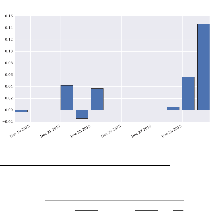
114 LISTED VOLATILITY AND VARIANCE DERIVATIVES
FIGURE 5.2 Differences of calculated VSTOXX 2M index values and real ones.
5.4 CALCULATING THE VSTOXX INDEX
If the values for the sub-indexes VSTOXX 1M and VSTOXX 2M, V1and V2say, are given,
then the value for the VSTOXX index itself, Vsay, is calculated by the linear interpolation of
V1and V2:
V=
T1⋅V2
1
⋅NT2−N30
NT2−NT1+T2⋅V2
2
⋅N30 −NT1
NT2−NT1⋅
N365
N30
where
NT1=time to expiry of V1’s options series in seconds
NT2=time to expiry of V2’s options series in seconds
N30 =30 days in seconds
N365 =time for a standard year in seconds
T1=NT1∕N365
T2=NT2∕N365.
Recall that the sub-index VSTOXX 1M is not dened on the nal settlement day of the under-
lying option series and the day before. For these dates, we use VSTOXX 2M and VSTOXX
3M as V1and V2, respectively.
The Python module index_vstoxx_calculation.py (see sub-section 5.6.3,
index_vstoxx_calculation.py for the module in its entirety) implements the VSTOXX index
calculation routine – given the respective sub-index time series data sets. The module starts as
usual with some imports.

VSTOXX Index 115
import pandas as pd
import numpy as np
import matplotlib.pyplot as plt
from index_date_functions import *
The function calculate_vstoxx() is the core of the module.
def calculate_vstoxx(path):
''' Function to calculate the VSTOXX volatility index given time series
of the relevant sub-indexes.
Parameters
==========
path: string
string with path of data files
Returns
=======
data: pandas DataFrame object
results of index calculation
'''
# constant parameters
seconds_year = 365 * 24 * 3600.
seconds_30_days = 30 * 24 * 3600.
# import historical VSTOXX data
data = pd.read_csv(path + 'vs.csv', index_col=0, parse_dates=True)
# determine the settlement dates for the two underlying option series
data['Settlement date 1'] = [first_settlement_day(a) for ain data.index]
data['Settlement date 2'] = [second_settlement_day(a) for ain data.index]
# deduce the life time (in seconds) from current date to
# final settlement Date
data['Life time 1'] = [(data['Settlement date 1'][i] - i).days
*24*60*60for iin data.index]
data['Life time 2'] = [(data['Settlement date 2'][i] - i).days
*24*60*60for iin data.index]
data['Use V6I2'] = data['V6I1'].notnull() # where V6I1 is not defined
data['Subindex to use 1'] = [data['V6I1'][i] if data['Use V6I2'][i]
else data['V6I2'][i] for iin data.index]
# if V6I1 is defined, use V6I1 and V6I2 as data set
data['Subindex to use 2'] = [data['V6I2'][i] if data['Use V6I2'][i]
else data['V6I3'][i] for iin data.index]
# else use V6I2 and V6I3
# the linear interpolation of the VSTOXX value
# from the two relevant sub-indexes

116 LISTED VOLATILITY AND VARIANCE DERIVATIVES
data['Part 1'] = data['Life time 1'] / seconds_year \
* data['Subindex to use 1'] ** 2 \
* ((data['Life time 2'] - seconds_30_days)
/ (data['Life time 2'] - data['Life time 1']))
data['Part 2'] = data['Life time 2'] / seconds_year \
* data['Subindex to use 2'] ** 2 \
* ((seconds_30_days - data['Life time 1'])
/ (data['Life time 2'] - data['Life time 1']))
data['VSTOXX'] = np.sqrt((data['Part 1'] + data['Part 2']) *
seconds_year / seconds_30_days)
# difference between original VSTOXX data and re-calculated values
data['Difference'] = data['V2TX'] – data['VSTOXX']
return data
As its single argument, the function takes the path to a CSV le containing historical VSTOXX
data for the index itself and the sub-indexes. The re-calculation of it then is as straightforward
as follows:
In [50]: import index_vstoxx_calculation as ivc
In [51]: %time data = ivc.calculate_vstoxx(path)
CPU times: user 1.19 s, sys: 38 us, total: 1.19 s
Wall time: 1.2 s
Let us inspect the pandas DataFrame which now contains the results of the previous code
execution:
In [52]: data.info()
<class 'pandas.core.frame.DataFrame'>
DatetimeIndex: 4357 entries, 1999-01-04 to 2016-02-12
Data columns (total 20 columns):
V2TX 4357 non-null float64
V6I1 3906 non-null float64
V6I2 4357 non-null float64
V6I3 4296 non-null float64
V6I4 4357 non-null float64
V6I5 4357 non-null float64
V6I6 4340 non-null float64
V6I7 4357 non-null float64
V6I8 4343 non-null float64
Settlement date 1 4357 non-null datetime64[ns]
Settlement date 2 4357 non-null datetime64[ns]
Life time 1 4357 non-null int64
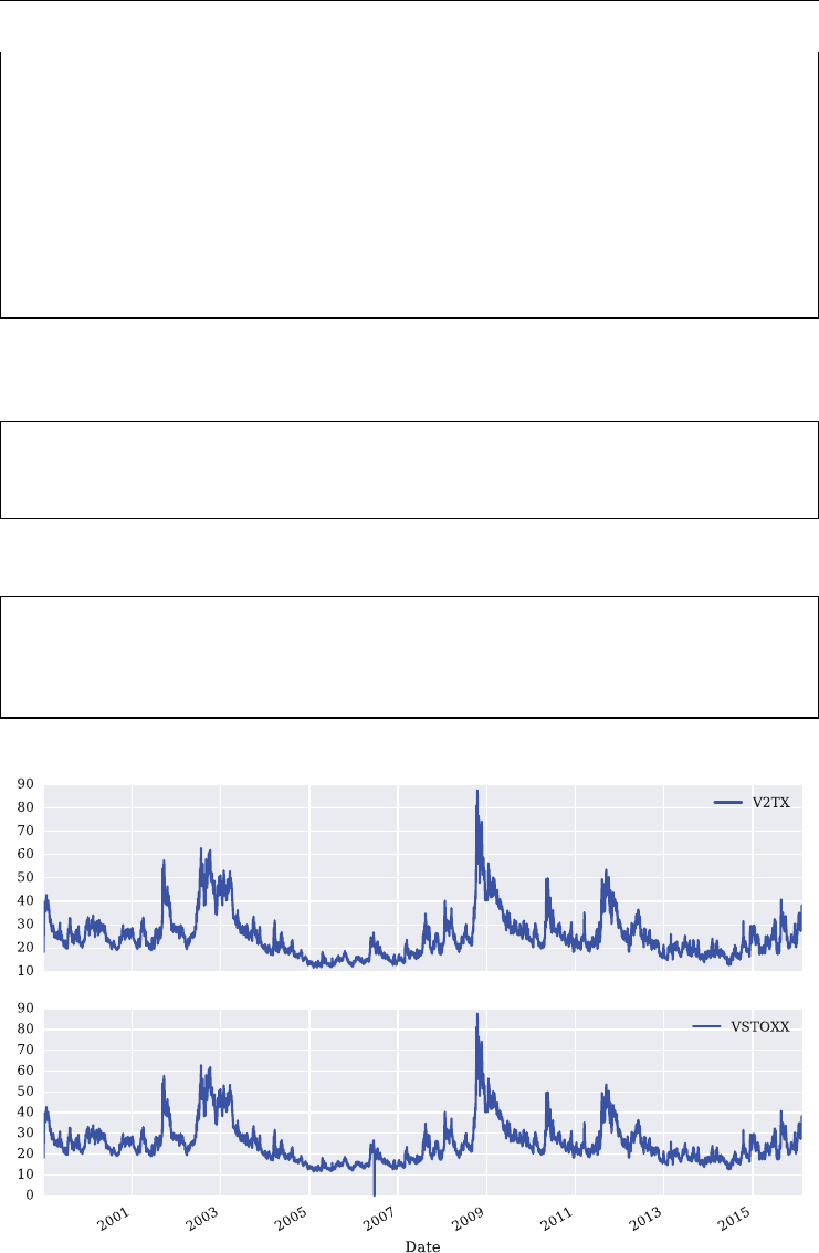
VSTOXX Index 117
Life time 2 4357 non-null int64
Use V6I2 4357 non-null bool
Subindex to use 1 4357 non-null float64
Subindex to use 2 4357 non-null float64
Part 1 4357 non-null float64
Part 2 4357 non-null float64
VSTOXX 4357 non-null float64
Difference 4357 non-null float64
dtypes: bool(1), datetime64[ns](2), float64(15), int64(2)
memory usage: 685.0 KB
A brief look at the absolute average error of the re-calculation reveals that the implementation
yields quite accurate results.
# output: average error of re-calculation
In [53]: data['Difference'].mean()
Out[53]: 0.0012799470095575995
Figure 5.3 compares the original V2TX time series with the re-calculated values.
# original vs. re-calculated VSTOXX index
In [54]: data[['V2TX', 'VSTOXX']].plot(subplots=True, figsize=(10, 6),
....: style="blue", grid=True);
....:
FIGURE 5.3 Historical VSTOXX index values re-calculated vs. real ones.
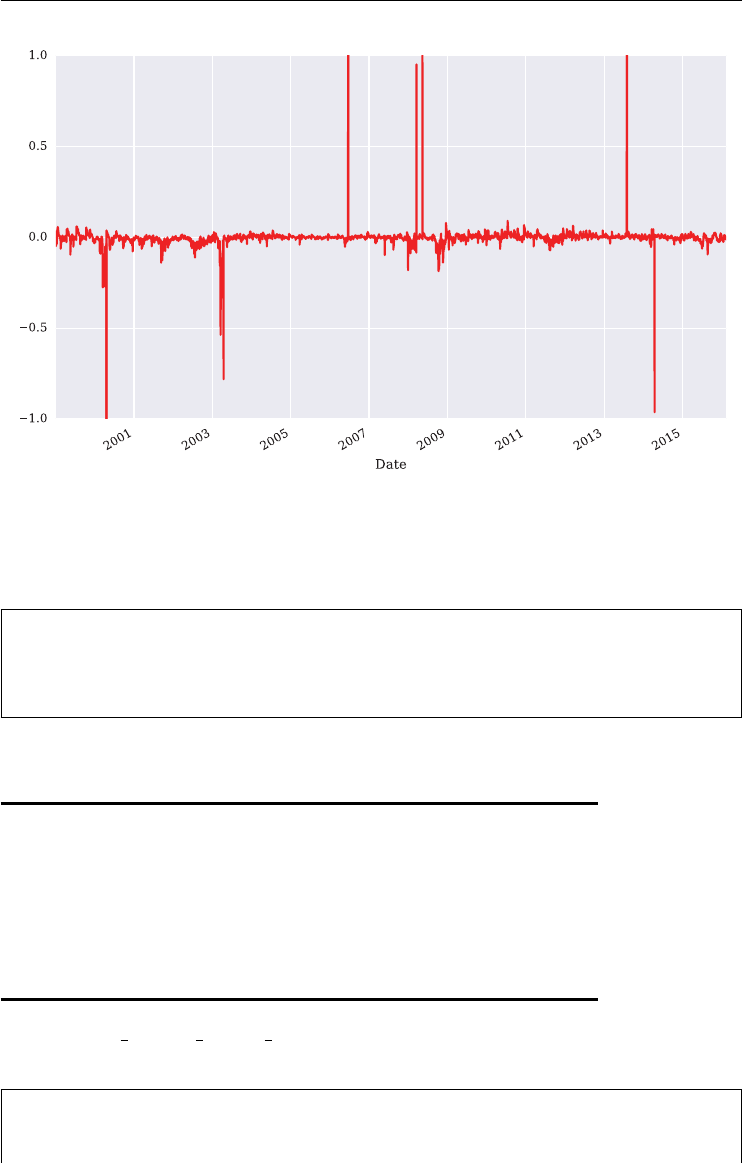
118 LISTED VOLATILITY AND VARIANCE DERIVATIVES
FIGURE 5.4 Differences of historical VSTOXX index values re-calculated vs. real ones.
Finally, Figure 5.4 presents the absolute differences. The gure shows that the differences are
in general marginal with a few outliers observed here and there.
# differences between single values
In [55]: data['Difference'].plot(figsize=(10, 6), style="r", grid=True,
....: ylim=(-1, 1));
....:
5.5 CONCLUSIONS
This chapter (re-)calculates the VSTOXX volatility index based on historical sub-index values
and based on the volatility index denition as derived in chapter 3, Model-Free Replication of
Variance. The chapter also shows how to calculate the sub-index values themselves based on
EURO STOXX 50 options data. Python code is provided to automatically collect such data
from the Eurex website.
5.6 PYTHON SCRIPTS
5.6.1 index collect option data.py
#
# Module to collect option series data
# from the web

VSTOXX Index 119
# Source: www.eurexchange.com
# Data is needed to calculate the VSTOXX
# and its sub-indexes
#
# (c) Dr. Yves J. Hilpisch
# Listed Volatility and Variance Derivatives
#
import requests
import datetime as dt
import pandas as pd
import numpy as np
from StringIO import *
from index_date_functions import *
#
# The URL template
#
url1 = 'http://www.eurexchange.com/action/exchange-en/'
url2 = '180106-180102/180102/onlineStats.do?productGroupId=846'
url3 = '&productId=19068&viewType=3&cp=%s &month=%s &year=%s &busDate=%s'
URL = url1 + url2 + url3
def collect_option_series(month, year, start):
''' Collects daily option data from web source.
Parameters
==========
month: int
maturity month
year: int
maturity year
start: datetime object
starting date
Returns
=======
dataset: pandas DataFrame object
object containing the collected data
'''
end = dt.datetime.today()
delta = (end – start).days
dataset = pd.DataFrame()
for tin range(0, delta): # runs from start to today
date = start + dt.timedelta(t)
dummy = get_data(month, year, date) # get data for one day
if len(dummy) != 0:

120 LISTED VOLATILITY AND VARIANCE DERIVATIVES
if len(dataset) == 0:
dataset = dummy
else:
dataset = pd.concat((dataset, dummy)) # add data
return dataset
def get_data(month, year, date):
''' Get the data for an option series.
Parameters
==========
month: int
maturity month
year: int
maturity year
date: datetime object
the date for which the data is collected
Returns
=======
dataset: pandas DataFrame object
object containing call & put option data
'''
date_string = date.strftime('%Y%m%d')
# loads the call data from the web
data = get_data_from_www('Call', month, year, date_string)
calls = parse_data(data, date) # parse the raw data
calls = calls.rename(columns={'Daily settlem.price': 'Call_Price'})
calls = pd.DataFrame(calls.pop('Call_Price').astype(float))
# the same for puts
data = get_data_from_www('Put', month, year, date_string)
puts = parse_data(data, date)
puts = puts.rename(columns={'Daily settlem.price': 'Put_Price'})
puts = pd.DataFrame(puts.pop('Put_Price').astype(float))
dataset = merge_and_filter(puts, calls) # merges the two time series
return dataset
def get_data_from_www(oType, matMonth, matYear, date):
''' Retrieves the raw data of an option series from the web.
Parameters
==========
oType: string
either 'Put' or 'Call'

VSTOXX Index 121
matMonth: int
maturity month
matYear: int
maturity year
date: string
expiry in the format 'YYYYMMDD'
Returns
=======
a: string
raw text with option data
'''
url = URL % (oType, matMonth, matYear, date) # parametrizes the URL
a = requests.get(url).text
return a
def merge_and_filter(puts, calls):
''' Gets two pandas time series for the puts and calls
(from the same option series), merges them, filters out
all options with prices smaller than 0.5 and
returns the resulting DataFrame object.
Parameters
==========
puts: pandas DataFrame object
put option data
calls: pandas DataFrame object
call option data
Returns
=======
df: pandas DataFrame object
merged & filtered options data
'''
df = calls.join(puts, how=' inner') # merges the two time series
# filters all prices which are too small
df = df[(df. Put_Price >= 0.5) & (df.Call_Price >= 0.5)]
return df
def parse_data(data, date):
''' Parses the HTML table and transforms it into a CSV compatible
format. The result can be directly imported into a pandas DataFrame.
Parameters
==========

122 LISTED VOLATILITY AND VARIANCE DERIVATIVES
data: string
document containing the Web content
date: datetime object
date for which the data is parsed
Returns
=======
dataset: pandas DataFrame object
transformed option raw data
'''
parts = data.split('<table')
parts2 = parts[1].split('</table')
dummy = parts2[0].replace('class="odd"','')
dummy = dummy.replace('class="even"','')
parts3 = dummy.split('<tr><td><b>Total</b>')
table = parts3[0] # the html table containing the data
table = table.replace('class="dataTable"><thead>', 'Pricing day')
# replace tags by commas and newlines
table = table.replace('</tr>', '\n')
table = table.replace(',', '')
table = table.replace('<td>', ',')
table = table.replace('</td>', '')
table = table.replace('<th>', ',')
table = table.replace('</th>', '')
table = table.replace('</thead><tbody>', '\n')
# the resulting string looks like a CSV file
date_string = date.strftime('%d .%m.%Y')
table = table.replace('<tr>', date_string)
string = StringIO(table) # mask the string as file
dataset = pd.read_csv(string, parse_dates=[0], index_col=(0, 1),
dayfirst=True) # read the 'file' as pandas DataFrame object
return dataset
def data_collection(path):
''' Main function which saves data into the HDF5 file
'index_option_series.h5' for later use.
Parameters
==========
path: string
path to store the data
'''
# file to store data
store = pd.HDFStore(path + 'index_option_series.h5', 'a')

VSTOXX Index 123
today = dt.datetime.today()
start = today - dt.timedelta(31) # the last 31 days
day = start.day
month = start.month
year = start.year
for iin range(4): # iterates over the next 4 months
dummy_month = month + i
dummy_year = year
if dummy_month > 12:
dummy_month -= 12
dummy_year += 1
# collect daily data beginning 31 days ago (start) for
# option series with expiry dummy_month, dummy_year
dataset = collect_option_series(dummy_month, dummy_year, start)
dummy_date = dt.datetime(dummy_year, dummy_month, day)
# abbreviation for expiry date (for example Oct14)
series_name = dummy_date.strftime('%b%y')
if series_name in store.keys(): # if data for that series exists
index_old = store[series_name].index
index_new = dataset.index
if len(index_new - index_old) > 0:
dummy = pd.concat((store[series_name],
dataset.ix[index_new - index_old])) # add the new data
store[series_name] = dummy
else:
if len(dataset) > 0:
# if series is new, write whole data set into data store
store[series_name] = dataset
store.close()
5.6.2 index subindex calculation.py
#
# Module with functions to compute VSTOXX sub-indexes
#
# Data as generated by the script index_collect_option_data.py
# is needed for the calculations in this module
#
# (c) Dr. Yves J. Hilpisch

124 LISTED VOLATILITY AND VARIANCE DERIVATIVES
# Listed Volatility and Variance Derivatives
#
import math
import numpy as np
import pandas as pd
import datetime as dt
import index_date_functions as idf
def compute_subindex(data, delta_T, R):
''' Computes a sub-index for given option series data.
Parameters
==========
data: pandas.DataFrame object
contains the option data
delta_T: float
time interval
R: float
discount factor
Returns
=======
subVSTOXX: float
sub-index value
'''
# difference between put and call option with same strike
data['Diff_Put_Call'] = np.abs(data. Put_Price - data.Call_Price)
# converts the strike price which serves as index so far
# to a regular data column
data = data.reset_index()
data['delta_K'] = None
# differences between the different strikes of the series
data['delta_K'].iloc[1:-1] = [(data['Strike price'][i + 1]
- data['Strike price'][i - 1]) / 2 for iin data.index[1:-1]]
# where possible, for the i-th entry it is
# half of the difference between the (i-1)-th
# and (i+1)-th price
# for i=0 it is just the difference to the next strike
data['delta_K'].iloc[0] = data['Strike price'][1] – data['Strike price'][0]
data['delta_K'].iloc[data.index[-1:]] = float(data['Strike price'][-1:]) \
- float(data['Strike price'][-2: -1])
# for the last entry, it is just the difference
# between the second but last strike and the last strike price
# find the smallest difference between put and call price
min_index = data. Diff_Put_Call.argmin()
# the forward price of that option
forward_price = data['Strike price'][min_index] \
+ R * data.Diff_Put_Call[min_index]

VSTOXX Index 125
K_0 = data['Strike price'][forward_price -
data['Strike price'] > 0].max()
# the index of the ATM strike
K_0_index = data.index[data['Strike price'] == K_0][0]
# selects the OTM options
data['M'] = pd.concat((data.Put_Price[0:K_0_index],
data.Call_Price[K_0_index:]))
# ATM we take the average of put and call price
data['M'].iloc[K_0_index] = (data['Call_Price'][K_0_index]
+ data['Put_Price'][K_0_index]) / 2
# the single OTM values
data['MFactor'] = (R * (data['delta_K'] * data['M'])
/ (data['Strike price']) ** 2)
# the forward term
fterm = 1. / delta_T * (forward_price / K_0 - 1) ** 2
# summing up
sigma = 2 / delta_T * np.sum(data.MFactor) - fterm
subVSTOXX = 100 * math.sqrt(sigma)
return subVSTOXX
def make_subindex(path):
''' Depending on the content of the file 'index_option_series.h5',
the function computes the sub-indexes V6I1, V6I2 and parts
of V6I3 and returns a pandas DataFrame object with the results.
Parameters
==========
path: string
string with path of data file
Returns
=======
df: pandas DataFrame object
sub-index data as computed by the function
'''
# the data source, created with index_collect_option_data.py
datastore = pd.HDFStore(path + 'index_option_series.h5', 'r')
max_date = dt.datetime.today() # find the latest date in the source
for series in datastore.keys():
dummy_date = datastore[series].index.get_level_values(0)[0]
dummy_date = dummy_date.to_pydatetime()
if dummy_date > max_date:
max_date = dummy_date
start_date = dt.datetime.today() # find the earliest date in the source
for series in datastore.keys():

126 LISTED VOLATILITY AND VARIANCE DERIVATIVES
dummy_date = datastore[series].index.get_level_values(0)[0]
dummy_data = dummy_date.to_pydatetime()
if dummy_date < start_date:
start_date = dummy_date
V1 = dict() # dicts to store the values, V stands for the sub-indices,
# T for their expiry
V2 = dict()
V3 = dict()
T1 = dict()
T2 = dict()
T3 = dict()
# from start_date to max_date, but only weekdays
for day in pd.bdate_range(start=start_date.date(), end=max_date.date()):
# is V6I1 defined?
is_V1_defined = idf.not_a_day_before_expiry(day)
# the settlement date
settlement_date = idf.first_settlement_day(day)
# abbreviation for the expiry date, like Oct14
key = settlement_date.strftime('%b%y')
# days until maturity
delta_T = idf.compute_delta(day, settlement_date)
try:
# data of the option series for that date
data = datastore[key].ix[day]
except:
continue
if is_V1_defined: # if V6I1 is defined
# compute its value
V1[day] = compute_subindex(data, delta_T,
math.exp(0.0015 * delta_T))
T1[day] = settlement_date
else:
# compute the value of V6I2 instead
V2[day] = compute_subindex(data, delta_T,
math.exp(0.0015 * delta_T))
T2[day] = settlement_date
settlement_date_2 = idf.second_settlement_day(day)
# the same for the next index
key_2 = settlement_date_2.strftime('%b%y')
delta_T_2 = idf.compute_delta(day, settlement_date_2)
data_2 = datastore[key_2].ix[day]
if is_V1_defined:
V2[day] = compute_subindex(data_2, delta_T_2,
math.exp(0.001 * delta_T_2))
T2[day] = settlement_date_2

VSTOXX Index 127
else:
V3[day] = compute_subindex(data_2, delta_T_2,
math.exp(0.001 * delta_T_2))
T3[day] = settlement_date_2
datastore.close()
# create the pandas DataFrame object and return it
df = pd.DataFrame(data={'V6I1': V1, 'Expiry V6I1': T1, 'V6I2': V2,
'Expiry V6I2': T2, 'V6I3': V3, 'Expiry V6I3': T3})
return df
5.6.3 index vstoxx calculation.py
#
# Module to compute VSTOXX index values
# given the values for the relevant sub-indexes
# as generated by the module index_subindex_calculation.py
#
# (c) Dr. Yves J. Hilpisch
# Listed Volatility and Variance Derivatives
#
import pandas as pd
import numpy as np
import matplotlib.pyplot as plt
from index_date_functions import *
def calculate_vstoxx(path):
''' Function to calculate the VSTOXX volatility index given time series
of the relevant sub-indexes.
Parameters
==========
path: string
string with path of data files
Returns
=======
data: pandas DataFrame object
results of index calculation
'''
# constant parameters
seconds_year = 365 * 24 * 3600.
seconds_30_days = 30 * 24 * 3600.
# import historical VSTOXX data
data = pd.read_csv(path + 'vs.csv', index_col=0, parse_dates=True)

128 LISTED VOLATILITY AND VARIANCE DERIVATIVES
# determine the settlement dates for the two underlying option series
data['Settlement date 1'] = [first_settlement_day(a) for ain data.index]
data['Settlement date 2'] = [second_settlement_day(a) for ain data.index]
# deduce the life time (in seconds) from current date to
# final settlement Date
data['Life time 1'] = [(data['Settlement date 1'][i] - i).days
*24*60*60for iin data.index]
data['Life time 2'] = [(data['Settlement date 2'][i] - i).days
*24*60*60for iin data.index]
data['Use V6I2'] = data['V6I1'].notnull() # where V6I1 is not defined
data['Subindex to use 1'] = [data['V6I1'][i] if data['Use V6I2'][i]
else data['V6I2'][i] for iin data.index]
# if V6I1 is defined, use V6I1 and V6I2 as data set
data['Subindex to use 2'] = [data['V6I2'][i] if data['Use V6I2'][i]
else data['V6I3'][i] for iin data.index]
# else use V6I2 and V6I3
# the linear interpolation of the VSTOXX value
# from the two relevant sub-indexes
data['Part 1'] = data['Life time 1'] / seconds_year \
* data['Subindex to use 1'] ** 2 \
* ((data['Life time 2'] - seconds_30_days)
/ (data['Life time 2'] - data['Life time 1']))
data['Part 2'] = data['Life time 2'] / seconds_year \
* data['Subindex to use 2'] ** 2 \
* ((seconds_30_days - data['Life time 1'])
/ (data['Life time 2'] - data['Life time 1'])) \
data['VSTOXX'] = np.sqrt((data['Part 1'] + data['Part 2']) *
seconds_year / seconds_30_days)
# difference between original VSTOXX data and re-calculated values
data['Difference'] = data['V2TX'] - data['VSTOXX']
return data

CHAPTER 6
Valuing Volatility Derivatives
6.1 INTRODUCTION
This chapter illustrates the valuation of volatility futures and options according to Gr¨
unbichler
and Longstaff (1996), abbreviated in the following by GL96. They derive a semi-analytical
(“closed”) pricing formula for European volatility call options which is as easy to use as
the famous Black-Scholes-Merton formula for equity options pricing. They model volatil-
ity directly and make the assumption that volatility follows a square-root diffusion process.
The model is quite simple and parsimonious, such that it lends itself pretty well to serve as a
starting point.
This chapter introduces the nancial model, the futures and option pricing formulas of
Gr¨
unbichler and Longstaff as well as a discretization of the model for Monte Carlo simulation
purposes. For both the formulas and the Monte Carlo simulation approach, Python implemen-
tations are presented. Finally, the chapter shows in detail how to calibrate the GL96 model to
market quotes for European call options on the VSTOXX volatility index.
6.2 THE VALUATION FRAMEWORK
Gr¨
unbichler and Longstaff (1996) model the volatility process (e.g. the process of a volatility
index) in direct fashion by a square-root diffusion or CIR process – named after the authors
John C. Cox, Jonathan E. Ingersoll and Stephen A. Ross, who rst introduced this type of
stochastic process to nance; see Cox et al. (1985). The stochastic differential equation describ-
ing the evolution of the volatility over time takes the form
dvt=𝜅(𝜃−vt)dt +𝜎vdZt
where
vtis the time tvalue of the volatility index, for example the VSTOXX
𝜃is the long-run mean of the volatility index
𝜅is the rate at which vtreverts to 𝜃
𝜎is the volatility of the volatility (“vol-vol”)
𝜃,𝜅,𝜎are assumed to be constant and positive
Ztis a standard Brownian motion.
129
Listed Volatility and Variance Derivatives: A
Python-based Guide
By Dr. Yves J. Hilpisch
© 2017 Yves Hilpisch

130 LISTED VOLATILITY AND VARIANCE DERIVATIVES
This process is known to exhibit convenient and realistic features for volatility modeling, such
as positivity and mean-reversion.
For the numerical examples in this chapter we use a parametrization as follows:
In [1]: import math
# model parameters
In [2]: v0 = 17.5 # initial level of volatility index
In [3]: kappa = 0.1 # speed of mean reversion
In [4]: theta = 20.0 # long-term index level
In [5]: sigma = 2.0 # volatility of volatility
In [6]: zeta = 0.0 # factor of the expected volatility risk premium
In [7]: r = 0.01 # risk-free short rate
# option parameters
In [8]: K = 20.0 # strike
In [9]: T = 1.0 # time horizon in year fractions
6.3 THE FUTURES PRICING FORMULA
Denote by F(v,T) the futures price of a futures contract on the volatility index vwith maturity
T. The pricing of such a contract is done by taking expectations of the index’s value at maturity
F(v,T)=E(vT). One obtains the following formula for the futures price:
F(v0,T)=(1 −e−𝜅T)⋅𝜃+e−𝜅T⋅v0
It is an exponentially weighted average of the long-run mean and the current value of the
volatility index. The function futures_price implements this formula in Python, in this
instance for a general volatility risk premium 𝜁≥0.
def futures_price(v0, kappa, theta, zeta, T):
''' Futures pricing formula in GL96 model.
Parameters
==========
v0: float (positive)
current volatility level

Valuing Volatility Derivatives 131
kappa: float (positive)
mean-reversion factor
theta: float (positive)
long-run mean of volatility
zeta: float (positive)
volatility risk premium
T: float (positive)
time-to-maturity
Returns
=======
future: float
price of a future
'''
alpha = kappa * theta
beta = kappa + zeta
future =(alpha / beta * (1 - math.exp(-beta * T))
+ math.exp(-beta * T) * v0)
return future
Application of the formula and function is straightforward. However, we have to rst import
the function from the module in which it is stored.
In [10]: from srd_functions import *
In [11]: futures_price(v0, kappa, theta, zeta, T)
Out[11]: 17.7379064549101
We obtain a futures term structure by calculating the futures prices for different maturities (see
Figure 6.1).
In [12]: import numpy as np
In [13]: import seaborn as sns; sns.set()
In [14]: import matplotlib
In [15]: matplotlib.rcParams['font.family'] = 'serif'
In [16]: import matplotlib.pyplot as plt
In [17]: maturities = np.linspace(0, 2, 24)
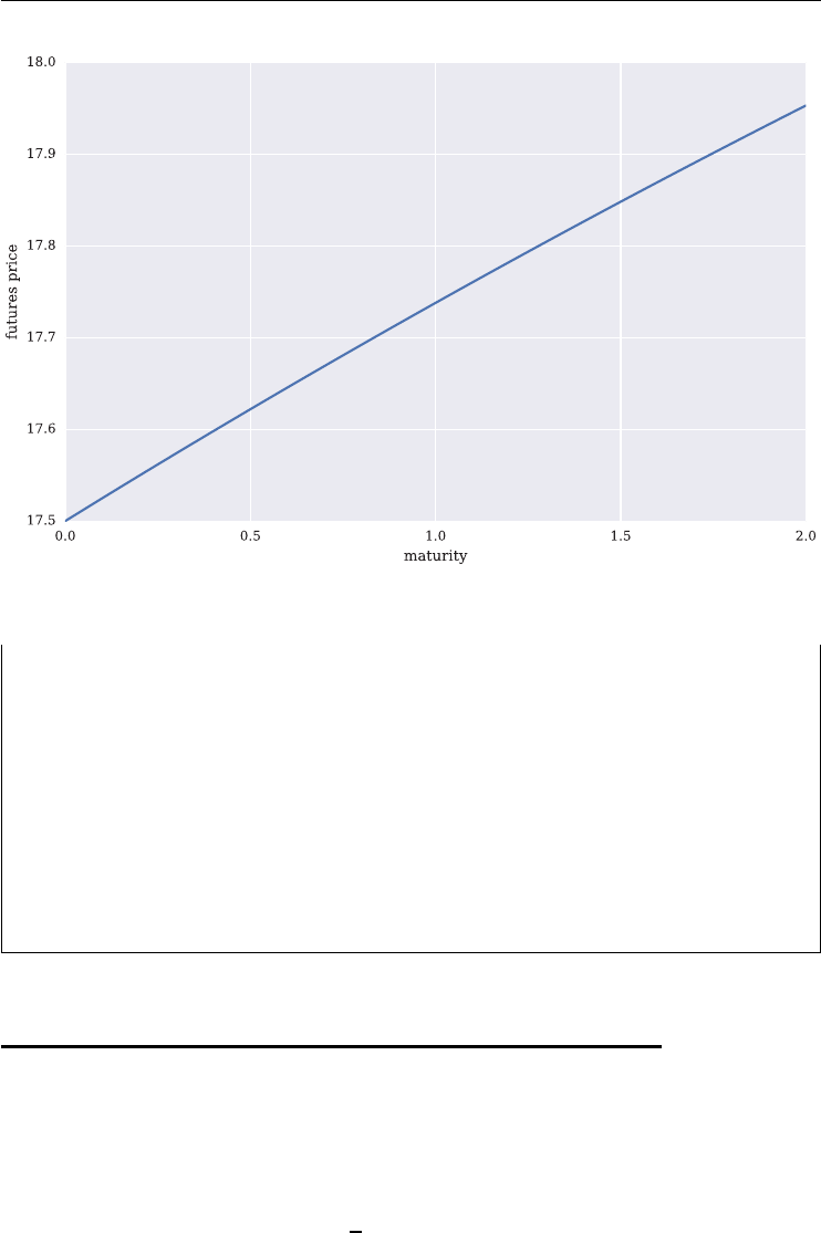
132 LISTED VOLATILITY AND VARIANCE DERIVATIVES
FIGURE 6.1 Futures prices from today to a maturity of 24 months.
In [18]: futures_prices = [futures_price(v0, kappa, theta, zeta, T)
....: for Tin maturities]
....:
In [19]: plt.figure(figsize=(10, 6));
In [20]: plt.plot(maturities, futures_prices);
In [21]: plt.xlabel('maturity');
In [22]: plt.ylabel('futures price');
6.4 THE OPTION PRICING FORMULA
A European call option on the underlying Vhas a payoff function max(VT−K, 0) at maturity T
where Kis the strike price of the option. Gr¨
unbichler and Longstaff (1996) derive the following
pricing formula for such a call option:
C(v0,K,T)=e−rT ⋅e−𝛽T⋅V0⋅Q(𝛾⋅K;𝜈+4, 𝜆)
+e−rT ⋅(𝛼
𝛽)⋅1−e−𝛽T⋅Q(𝛾⋅K;𝜈+2, 𝜆)
−e−rT ⋅K⋅Q(𝛾⋅K;𝜈,𝜆)

Valuing Volatility Derivatives 133
where
𝛼=𝜅𝜃
𝛽=𝜅+𝜁
𝛾=4𝛽
𝜎2(1 −e−𝛽T)
𝜈=4𝛼
𝜎2
𝜆=𝛾⋅e−𝛽T⋅v0
and e−rT as the discount factor for a xed short rate r. The parameter 𝜁denotes as before the
expected premium for volatility risk. In the following, we assume 𝜁=0.
Q(⋅;𝜈,𝜆) is the complementary non-central 𝜒2distribution with 𝜈degrees of freedom and
non-centrality parameter 𝜆.
In our Python implementation srd_functions.py (see sub-section 6.9.1,
srd_functions.py for the complete module), we use the function ncx2.cdf() from
the scipy.stats sub-library for the non-central 𝜒2distribution. We implement two
different functions, a helper function and the pricing function itself:
cx(): this function returns values for the complementary distribution of the non-central
chi-squared density
call_price(): the implementation of the valuation formula for European calls on the
volatility index.
The function cx() is as follows:
def cx(K, gamma, nu, lamb):
''' Complementary distribution function of non-central chi-squared density.
Parameters
==========
K: float (positive)
strike price
gamma: float (positive)
as defined in the GL96 model
nu: float (positive)
degrees of freedom
lamb: float (positive)
non-centrality parameter
Returns
=======
complementary distribution of nc cs density
'''
return 1 - scs.ncx2.cdf(gamma * K, nu, lamb)

134 LISTED VOLATILITY AND VARIANCE DERIVATIVES
The function cx() is used in the valuation function call_price().
def call_price(v0, kappa, theta, sigma, zeta, T, r, K):
''' Call option pricing formula in GL96 Model
Parameters
==========
v0: float (positive)
current volatility level
kappa: float (positive)
mean-reversion factor
theta: float (positive)
long-run mean of volatility
sigma: float (positive)
volatility of volatility
zeta: float (positive)
volatility risk premium
T: float (positive)
time-to-maturity
r: float (positive)
risk-free short rate
K: float(positive)
strike price of the option
Returns
=======
call: float
present value of European call option
'''
D = math.exp(-r * T) # discount factor
alpha = kappa * theta
beta = kappa + zeta
gamma = 4 * beta / (sigma ** 2 * (1 - math.exp(-beta * T)))
nu = 4 * alpha / sigma ** 2
lamb = gamma * math.exp(-beta * T) * v0
# the pricing formula
call = (D * math.exp(-beta * T) * v0 * cx(K, gamma, nu + 4, lamb)
+ D * (alpha / beta) * (1 - math.exp(-beta * T))
* cx(K, gamma, nu + 2, lamb)
- D * K * cx(K, gamma, nu, lamb))
return call
As before, being equipped with such a Python function makes applying the pricing formula
straightforward.

Valuing Volatility Derivatives 135
In [23]: call_price(v0, kappa, theta, sigma, zeta, T, r, K)
Out[23]: 3.3682878822902369
Let us calculate European call option prices over a wider range of strikes.
In [24]: import numpy as np
In [25]: import pandas as pd
In [26]: option_values = []
In [27]: strikes = np.linspace(15, 25)
In [28]: option_values = [call_price(v0, kappa, theta, sigma, zeta, T, r, k)
....: for kin strikes]
....:
In [29]: data = pd.DataFrame(option_values, index=strikes,
....: columns=['call values', ])
....:
In [30]: data.index.name = 'strike'
As Figure 6.2 shows, the European call option prices behave comparably to equity options:
the higher the strike price the lower the option present value ceteris paribus.
In [31]: data.plot(figsize=(10, 6));
6.5 MONTE CARLO SIMULATION
In this section, we solve the pricing problem for a European call option via Monte Carlo sim-
ulation, i.e. based on a large number of simulated volatility index paths. To this end, we have
to discretize the stochastic differential equation to obtain a difference equation which we can
evaluate numerically.
We use the same numerical parameters as before, but we have to dene some additional
parameters which will determine the discretization interval and the number of simulated paths:
# simulation parameters
In [32]: M=50 # time steps
In [33]: I = 20000 # number of MCS paths
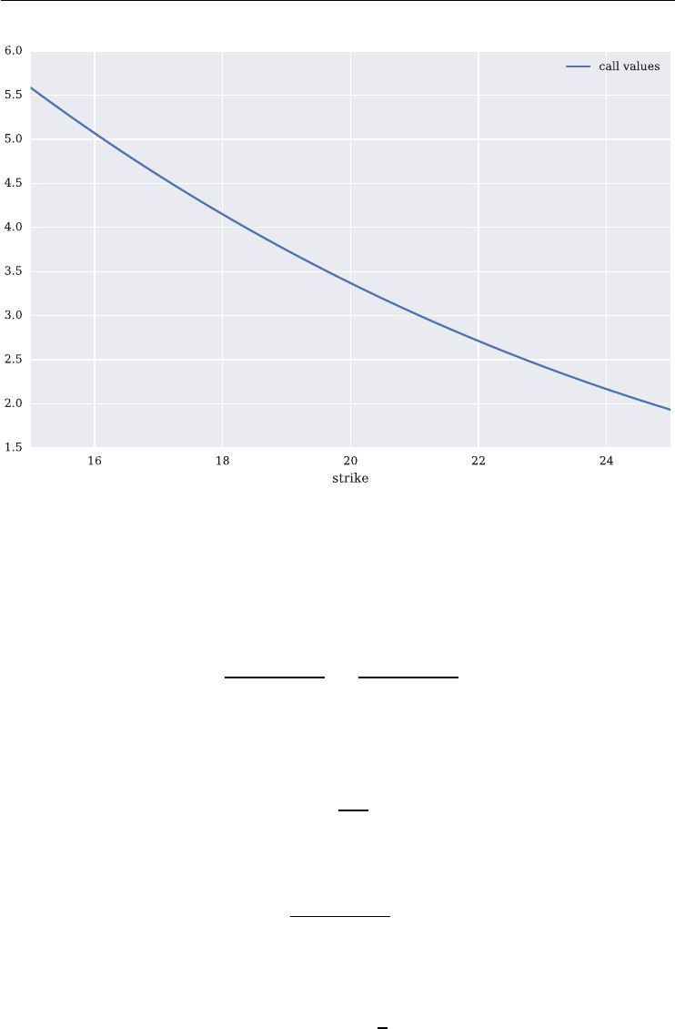
136 LISTED VOLATILITY AND VARIANCE DERIVATIVES
FIGURE 6.2 European call option prices for different volatility strikes in the GL96 model.
There is a large literature available about the discretization of the square-root diffusion (see
Hilpisch (2015), ch. 10). In the following, we will implement an exact discretization scheme.
First, we divide the time interval [0, T]intoMtime intervals with M+1 discrete points
in time: t∈{0, Δt,2Δt,…,T}. We have:
vt=𝜎2(1 −e−𝜅Δt)
4𝜅̃𝜒2
𝜈,𝜆
4−𝜅Δt
𝜎2(1 −e−𝜅Δt)
⋅vs
with s=t−Δt.
̃𝜒2
𝜈,𝜆denotes a non-central chi-squared distributed random variable with
𝜈=4𝜃𝜅
𝜎2
degrees of freedom and non-centrality parameter
𝜆=4𝜅e−𝜅Δt
𝜎2(1 −e−𝜅Δt)
⋅vs
As it may be more convenient to sample a chi-squared random variable instead of non-central
chi-squared one, we use the following equations:
𝜈>1: ̃𝜒2
𝜈,𝜆=(z+𝜆)2+𝜒2
𝜈−1
𝜈≤1: ̃𝜒2
𝜈,𝜆=𝜒2
𝜈+2P

Valuing Volatility Derivatives 137
where zis an independent standard normally distributed random variable and Pis a Poisson
distributed random variable with intensity 𝜆
2.
We again divide the implementation in Python into two functions:
generate_paths() generates simulated volatility level paths
call_estimator() simulates the volatility process and calculates the Monte Carlo
estimator for the European call option value.
The function to generate simulated volatility paths takes on a form as follows:
def generate_paths(x0, kappa, theta, sigma, T, M, I):
''' Simulation of square-root diffusion with exact discretization
Parameters
==========
x0: float (positive)
starting value
kappa: float (positive)
mean-reversion factor
theta: float (positive)
long-run mean
sigma: float (positive)
volatility (of volatility)
T: float (positive)
time-to-maturity
M: int
number of time intervals
I: int
number of simulation paths
Returns
=======
x: NumPy ndarray object
simulated paths
'''
dt = float(T) / M
x = np.zeros((M + 1, I), dtype=np.float)
x[0, :] = x0
# matrix filled with standard normal distributed rv
ran = np.random.standard_normal((M + 1, I))
d = 4 * kappa * theta / sigma ** 2
# constant factor in the integrated process of x
c = (sigma ** 2 * (1 - math.exp(-kappa * dt))) / (4 * kappa)
if d>1:
for tin range(1, M + 1):
# non-centrality parameter
l = x[t - 1, :] * math.exp(-kappa * dt) / c
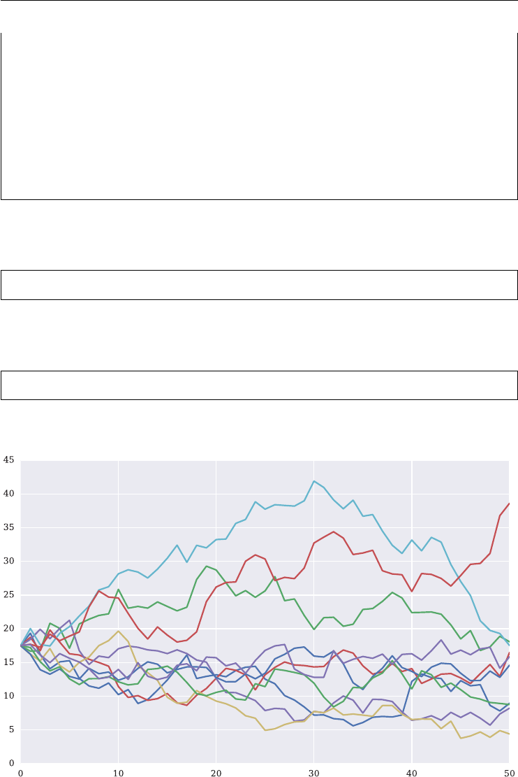
138 LISTED VOLATILITY AND VARIANCE DERIVATIVES
# matrix with chi-squared distributed rv
chi = np.random.chisquare(d - 1, I)
x[t, :] = c * ((ran[t] + np.sqrt(l)) ** 2 + chi)
else:
for tin range(1, M + 1):
l = x[t - 1, :] * math.exp(-kappa * dt) / c
N = np.random.poisson(l / 2, I)
chi = np.random.chisquare(d + 2 * N, I)
x[t, :] = c * chi
return x
An application of this function might look as follows:
In [34]: paths = generate_paths(v0, kappa, theta, sigma, T, M, I)
Figure 6.3 shows the rst 10 simulated volatility paths.
In [35]: pd.DataFrame(paths[:, :10]).plot(legend=False, figsize=(10, 6));
FIGURE 6.3 10 simulated volatility paths for GL96 model.

Valuing Volatility Derivatives 139
The Monte Carlo estimator for a European call option is dened by
C(v0,K,T)=e−rT 1
I
I
i=1
max(vi
T−K,0)
with max(vT−K, 0) being the payoff function of the European call option. Here, vi
Tis the i-th
simulated value for the volatility index at maturity. The function to calculate the Monte Carlo
estimator for the value of the European call option is presented below.
def call_estimator(v0, kappa, theta, sigma, T, r, K, M, I):
''' Estimation of European call option price in GL96 Model
via Monte Carlo simulation
Parameters
==========
v0: float (positive)
current volatility level
kappa: float (positive)
mean-reversion factor
theta: float (positive)
long-run mean of volatility
sigma: float (positive)
volatility of volatility
T: float (positive)
time-to-maturity
r: float (positive)
risk-free short rate
K: float (positive)
strike price of the option
M: int
number of time intervals
I: int
number of simulation paths
Returns
=======
callvalue: float
MCS estimator for European call option
'''
V = generate_paths(v0, kappa, theta, sigma, T, M, I)
callvalue = math.exp(-r * T) * np.sum(np.maximum(V[-1] - K, 0)) / I
return callvalue
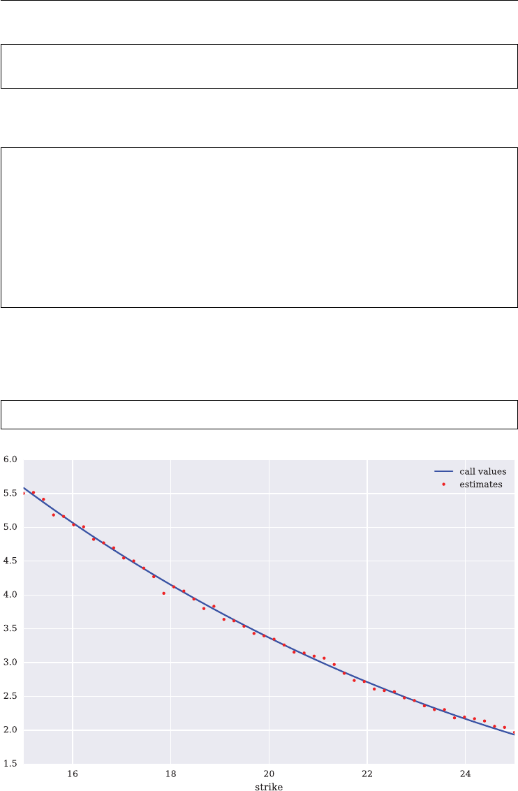
140 LISTED VOLATILITY AND VARIANCE DERIVATIVES
In [36]: call_estimator(v0, kappa, theta, sigma, T, r, K, M, I)
Out[36]: 3.3751776084056191
Again, let us calculate option prices over a wider range of strikes.
In [37]: %%time
....: estimates = []
....: for k in strikes:
....: estimates.append(call_estimator(v0, kappa, theta, sigma,
....: T, r, k, M, I))
....: data['estimates'] = estimates
....:
CPU times: user 11.4 s, sys: 38 us, total: 11.4 s
Wall time: 11.4 s
Figure 6.4 compares the Monte Carlo estimator values given the above parametrization with
the European call option values obtained from the formula by Gr¨
unbichler and Longstaff
(1996).
In [38]: data.plot(style=['b', 'r.'], figsize=(10, 6));
FIGURE 6.4 Monte Carlo estimates vs. European call values from formula in the GL96 model.

Valuing Volatility Derivatives 141
6.6 AUTOMATED MONTE CARLO TESTS
This section illustrates how to automate Monte Carlo-based valuation tests. Even if semi-
analytical option pricing formulas are available – as in the Gr¨
unbichler and Longstaff (1996)
model – in general one needs numerical methods as well. One of the most exible and pow-
erful methods when it comes to the valuation of more complex, exotic instruments is Monte
Carlo simulation (MCS).
When implementing MCS algorithms it is generally advised to benchmark the results from
these algorithms against results from other valuation methods which are known to deliver exact
values. Therefore, this section implements MCS for the Gr¨
unbichler and Longstaff (1996)
model and benchmarks the results against the semi-analytical formula for European volatility
call options as presented earlier in this chapter.
In the previous section, MCS was introduced and some benchmark results presented.
However, this section enhances the analysis and adds functionalities for the structured stor-
age and systematic analysis of valuation results. In this regard, the Python library pandas is
used in combination with the storage capabilities of PyTables, the Python wrapper for the
HDF5 database le format.
6.6.1 The Automated Testing
The following test procedures are based on the Python script srd_ simula-
tion_analysis.py (see sub-section 6.9.2, srd simulation analysis.py for the complete
code). To automate the valuation for a signicant number of options, a set of parameter values
and lists has to be specied. First, some imports and the parametrization of the nancial model.
import time
import math
import numpy as np
from datetime import datetime
from srd_functions import generate_paths, call_price
from srd_simulation_results import *
# Model Parameters
v0 = 20.0 # initial volatility
kappa = 3.0 # speed of mean reversion
theta = 20.0 # long-term volatility
sigma = 3.2 # standard deviation coefficient
zeta = 0.0 # factor of the expected volatility risk premium
r = 0.01 # risk-free short rate
The parameter values chosen are not too unrealistic, for example, for the VSTOXX volatility
index. Second, the following simulation parameters are assumed:
# General Simulation Parameters
write = True
var_red = [(False, False), (False, True), (True, False), (True, True)]

142 LISTED VOLATILITY AND VARIANCE DERIVATIVES
# 1st = mo_match -- random number correction (std + mean + drift)
# 2nd = anti_paths -- antithetic paths for variance reduction
# number of time steps
steps_list = [25, 50, 75, 100]
# number of paths per valuation
paths_list = [2500, 50000, 75000, 100000, 125000, 150000]
SEED = 100000 # seed value
runs = 3 # number of simulation runs
PY1 = 0.010 # performance yardstick 1: abs. error in currency units
PY2 = 0.010 # performance yardstick 2: rel. error in decimals
maturity_list = [1.0 / 12, 1.0 / 4, 1.0 / 2, 1.0] # maturity list
The single parameters and list objects have the following meanings:
write is just a ag to indicate that the results should be stored on disk
var_red contains the conguration for the variance reduction techniques, i.e. moment
matching of pseudo-random numbers and antithetic variates
steps_list is the list with the different numbers for the time steps to be used for the
discretization
paths_list contains the different numbers for the MCS paths for the volatility process
runs is a parameter which says how often the same option is valued for a single parameter
combination
SEED is a seed value for NumPy’s pseudo-random number generator; it is xed to make
it easier to compare results
PY1 is the performance yardstick for absolute differences
PY2 is the performance yardstick for relative differences
maturity_list is the list with times-to-maturity
strike_list nally is the list with the different strike prices.
For details on such Monte Carlo simulation analyses and the respective MCS background
information refer to Hilpisch (2015, ch. 10). For a detailed exposition of Monte Carlo methods
implemented in Python see also Hilpisch (2014, ch. 10).
The script srd_simulation_analysis.py used in this section relies on the MCS
function from the previous section. In addition, it uses the following function which imple-
ments two variance reduction techniques, moment matching and antithetic variates:
def randoms(M, I):
''' Function to generate pseudo-random numbers with variance reduction.
Parameters
==========
M: int
number of discrete time intervals
I: int
number of simulated paths

Valuing Volatility Derivatives 143
Returns
=======
rand: Numpy ndarray object
object with pseudo-random numbers
'''
if anti_paths is True:
rand_ = np.random.standard_normal((M + 1, I / 2))
rand = np.concatenate((rand_, -rand_), 1)
else:
rand = np.random.standard_normal((M + 1, I))
if mo_match is True:
rand = rand / np.std(rand)
rand = rand - np.mean(rand)
return rand
The main valuation and testing loop is implemented through the following code. Important
passages are commented inline.
t0 = time.time()
sim_results = pd.DataFrame()
for vr in var_red: # variance reduction techniques
mo_match, anti_paths = vr
for Min steps_list: # number of time steps
for Iin paths_list: # number of paths
t1 = time.time()
d1 = datetime.now()
abs_errors = []
rel_errors = []
l = 0.0
errors = 0
# name of the simulation setup
name = ('Call_' + str(runs) + '_'
+ str(M) + '_' + str(I / 1000)
+ '_' + str(mo_match)[0] + str(anti_paths)[0] +
'_' + str(PY1 * 100) + '_' + str(PY2 * 100))
np.random.seed(SEED) # RNG seed value
for run in range(runs): # simulation runs
print "\nSimulation Run %d of %d" % (run + 1, runs)
print " -----------------------------------------------------------"
print ("Elapsed Time in Minutes %8.2f"
% ((time.time() - t0) / 60))
print " -----------------------------------------------------------"
z=0
for Tin maturity_list: # time-to-maturity
dt=T/M # time interval in year fractions
V = generate_paths(v0, kappa, theta, sigma, T, M, I)
# volatility process paths
print "\nResults for Time-to-Maturity %6.3f"%T

144 LISTED VOLATILITY AND VARIANCE DERIVATIVES
print " ----------------------------------------------------"
for Kin strike_list: # Strikes
h = np.maximum(V[-1] - K, 0) # inner value matrix
# MCS estimator
call_estimate = math.exp(-r * T) * np.sum(h) /I*100
# BSM analytical value
callalue = call_price(v0, kappa, theta, sigma,
zeta, T, r, K) * 100
# errors
diff = call_estimate - callalue
rdiff = diff / callalue
abs_errors.append(diff)
rel_errors.append(rdiff * 100)
# output
b r = " -----------------------------------------------------"
print "\nResults for Strike %4.2f\n"%K
print (" European Op. Value MCS %8.4f"%
call_estimate)
print (" European Op. Value Closed %8.4f"%
callalue)
print " Valuation Error (abs) %8.4f" % diff
print " Valuation Error (rel) %8.4f" % rdiff
if abs(diff) < PY1 or abs(diff) / callalue < PY2:
print " Accuracy ok!\n"+br
CORR = True
else:
print " Accuracy NOT ok!\n"+br
CORR = False
errors = errors + 1
print "%d Errors, %d Values, %.1f Min." \
% (errors, len(abs_errors),
float((time.time() - t1) / 60))
print(" %d Time Intervals, %d Paths"
% (M, I))
z+=1
l+=1
t2 = time.time()
d2 = datetime.now()
if write is True: # append simulation results
sim_results = write_results(sim_results, name, SEED,
runs, M, I, mo_match, anti_paths,
l, PY1, PY2, errors,
float(errors) / l, np.array(abs_errors),
np.array(rel_errors), t2 - t1, (t2 - t1) / 60, d1, d2)
if write is True:
# write/append DataFrame to HDFStore object
write_to_database(sim_results)

Valuing Volatility Derivatives 145
6.6.2 The Storage Functions
The script srd_simulation_analysis.py from the previous sub-section generates a
number of results and a lot of printed output during execution. However, one generally wants
to store such results in a structured manner and maybe analyze it later on. To this end, we use
the pandas library which provides convenient data storage and analysis features. In combina-
tion with the PyTables library, simulation results are easily stored on disk and read from disk
later on.
Consider now the Python module srd_simulation_results.py with several func-
tions to store and analyze the data generated through the other script (see sub-section 6.9.3,
srd_simulation_results.py for the complete script). We will go through this script part by part.
Of course, there are some necessary imports and a lename for the database is also specied:
import numpy as np
import pandas as pd
import datetime as dt
import matplotlib.pyplot as plt
# filname for HDFStore to save results
filename = "../data/simulation_results.h5"
Having a DataFrame object instantiated (with results already stored or not), the following func-
tion allows us to add a set of valuation results to the DataFrame as an additional row:
def write_results(sim_results, name, SEED, runs, steps, paths, mo_match,
anti_paths, l, PY1, PY2, errors, error_ratio,
abs_errors, rel_errors, t1, t2, d1, d2):
''' Appends simulation results to pandas DataFrame df and returns it.
Parameters
==========
see srd_simulation_analysis.py
Returns
=======
df: pandas DataFrame object
updated results object
'''
results = {
'sim_name': name,
'seed': SEED,
'runs': runs,
'time_steps': steps,
'paths': paths,
'mo_match': mo_match,

146 LISTED VOLATILITY AND VARIANCE DERIVATIVES
'anti_paths': anti_paths,
'opt_prices': l,
'abs_tol': PY1,
'rel_tol': PY2,
'errors': errors,
'error_ratio': error_ratio,
'aval_err': sum(abs_errors) / l,
'abal_err': sum(abs(rel_errors)) / l,
'time_sec': t1,
'time_min': t2,
'time_opt': t1 / l,
'start_date': d1,
'end_date': d2
}
df = pd.concat([sim_results,
pd.DataFrame([results])],
ignore_index=True)
return df
Once all the single simulation results have been added to the DataFrame sim_results,
this should be stored on disk in a HDFStore le object. This is what the following function
accomplishes:
def write_to_database(sim_results, filename=filename):
''' Write pandas DataFrame sim_results to HDFStore object.
Parameters
==========
sim_results: pandas DataFrame object
object with simulation results
filename: string
name of the file for storage
'''
h5 = pd. HDFStore(filename, 'a')
h5.append('sim_results', sim_results, min_itemsize={'values': 30},
ignore_index=True)
h5.close()
6.6.3 The Results
Let us now turn to the analysis of valuation results. To this end, we work with the Python mod-
ule srd_simulation_results.py (see sub-section 6.9.3, srd_simulation_results.py for

Valuing Volatility Derivatives 147
the code). The function print_results() prints simulation results stored in the HDFS-
tore le object with name filename. If not otherwise parametrized, the function prints the
rst 50 results stored in the database (if that many exist).
def print_results(filename=filename, idl=0, idh=50):
''' Prints valuation results in detailed form.
Parameters
==========
filename: string
HDFStore with pandas.DataFrame with results
idl: int
start index value
idh: int
stop index value
'''
h5 = pd. HDFStore(filename, 'r')
sim_results = h5['sim_results']
br = "-----------------------------------------------------------"
for iin range(idl, min(len(sim_results), idh + 1)):
row = sim_results.iloc[i]
print br
print "Start Calculations %32s" % row['start_date'] + "\n"+br
print "ID Number %32d"%i
print "Name of Simulation %32s" % row['sim_name']
print "Seed Value for RNG %32d" % row['seed']
print "Number of Runs %32d" % row['runs']
print "Time Steps %32d" % row['time_steps']
print "Paths %32d" % row['paths']
print "Moment Matching %32s" % row['mo_match']
print "Antithetic Paths %32s" % row['anti_paths'] + "\n"
print "Option Prices %32d" % row['opt_prices']
print "Absolute Tolerance %32.4f" % row['abs_tol']
print "Relative Tolerance %32.4f" % row['rel_tol']
print "Errors %32d" % row['errors']
print "Error Ratio %32.4f" % row['error_ratio'] + "\n"
print "Aver Val Error %32.4f" % row['aval_err']
print "Aver Abs Val Error %32.4f" % row['abal_err']
print "Time in Seconds %32.4f" % row['time_sec']
print "Time in Minutes %32.4f" % row['time_min']
print "Time per Option %32.4f" % row['time_opt'] + "\n"+br
print "End Calculations %32s" % row['end_date']\
+"\n"+br+"\n"
print "Total number of rows in table %d" % len(sim_results)
h5.close()

148 LISTED VOLATILITY AND VARIANCE DERIVATIVES
Let us inspect selected valuation results from running the respective Python script
srd_simulation_analysis.py:
------------------------------------------------------------------
Start Calculations 2016-01-11 11:02:11.159464
------------------------------------------------------------------
ID Number 2
Name of Simulation Call_3_25_75_FF_1.0_1.0
Seed Value for RNG 100000
Number of Runs 3
Time Steps 25
Paths 75000
Moment Matching False
Antithetic Paths False
Option Prices 60
Absolute Tolerance 0.0100
Relative Tolerance 0.0100
Errors 9
Error Ratio 0.1500
Aver Val Error -0.1963
Aver Abs Val Error 0.4773
Time in Seconds 4.1964
Time in Minutes 0.0699
Time per Option 0.0699
------------------------------------------------------------------
End Calculations 2016-01-11 11:02:15.355906
------------------------------------------------------------------
------------------------------------------------------------------
Start Calculations 2016-01-11 11:02:15.362043
------------------------------------------------------------------
ID Number 3
Name of Simulation Call_3_25_100_FF_1.0_1.0
Seed Value for RNG 100000
Number of Runs 3
Time Steps 25
Paths 100000
Moment Matching False
Antithetic Paths False
Option Prices 60
Absolute Tolerance 0.0100
Relative Tolerance 0.0100
Errors 5

Valuing Volatility Derivatives 149
Error Ratio 0.0833
Aver Val Error -0.1645
Aver Abs Val Error 0.3589
Time in Seconds 5.7146
Time in Minutes 0.0952
Time per Option 0.0952
------------------------------------------------------------------
End Calculations 2016-01-11 11:02:21.076603
------------------------------------------------------------------
------------------------------------------------------------------
Start Calculations 2016-01-11 11:02:21.082678
------------------------------------------------------------------
ID Number 4
Name of Simulation Call_3_25_125_FF_1.0_1.0
Seed Value for RNG 100000
Number of Runs 3
Time Steps 25
Paths 125000
Moment Matching False
Antithetic Paths False
Option Prices 60
Absolute Tolerance 0.0100
Relative Tolerance 0.0100
Errors 2
Error Ratio 0.0333
Aver Val Error 0.0043
Aver Abs Val Error 0.2666
Time in Seconds 6.9533
Time in Minutes 0.1159
Time per Option 0.1159
------------------------------------------------------------------
End Calculations 2016-01-11 11:02:28.035962
------------------------------------------------------------------
“Time in Minutes” and “Time per Option” values coincide since 60 options are valued per run.
In principle, the results from these three different parametrizations already illustrate
that valuation accuracy is, in general, higher the higher the computational effort (in this
case the number of paths). The number of errors drops from 9 for 75,000 paths to 2 for
125,000 paths.
Finally, the second major function contained in the Python module is
plot_error_ratio() and plots the error ratios against the computational effort,
i.e. (number of simulation paths) x (number of time steps).

150 LISTED VOLATILITY AND VARIANCE DERIVATIVES
def plot_error_ratio(filename=filename):
''' Show error ratio vs. paths * time_steps (i.e.granularity).
Parameters
==========
filename: string
name of file with data to be plotted
'''
h5 = pd. HDFStore(filename, mode='r')
sim_results = h5['sim_results']
x = np.array(sim_results['paths'] * sim_results['time_steps'], dtype='d')
x = x / max(x)
y = sim_results['error_ratio']
plt.plot(x, y, 'bo', label=' error ratio')
rg = np.polyfit(x, y, deg=1)
plt.plot(np.sort(x), np.polyval(rg, np.sort(x)), 'r', label='regression',
linewidth=2)
plt.xlabel('time steps * paths (normalized)')
plt.ylabel('errors / option valuations')
plt.legend()
plt.grid(True)
h5.close()
Let us generate an overview plot with the above function. The graphical output is shown as
Figure 6.5.
In [39]: from srd_simulation_results import plot_error_ratio
In [40]: plot_error_ratio(filename)
<matplotlib.figure.Figure at 0x2ab25e711950>
The linear regression illustrates graphically the statement that the higher the computational
effort the higher in general the accuracy of the MCS valuations. The high variability of the
error ratios stems from the fact that it is not only the computational effort which inuences
valuation accuracy. For example, the use of variance reduction techniques also has a signicant
inuence.
This being said, one might be interested in analyzing the impact of the variance reduction
techniques on valuation accuracy. To this end, pandas provides powerful grouping methods
for the DataFrame object. First, we open the database in which the simulation results are
stored and read them into an in memory object:
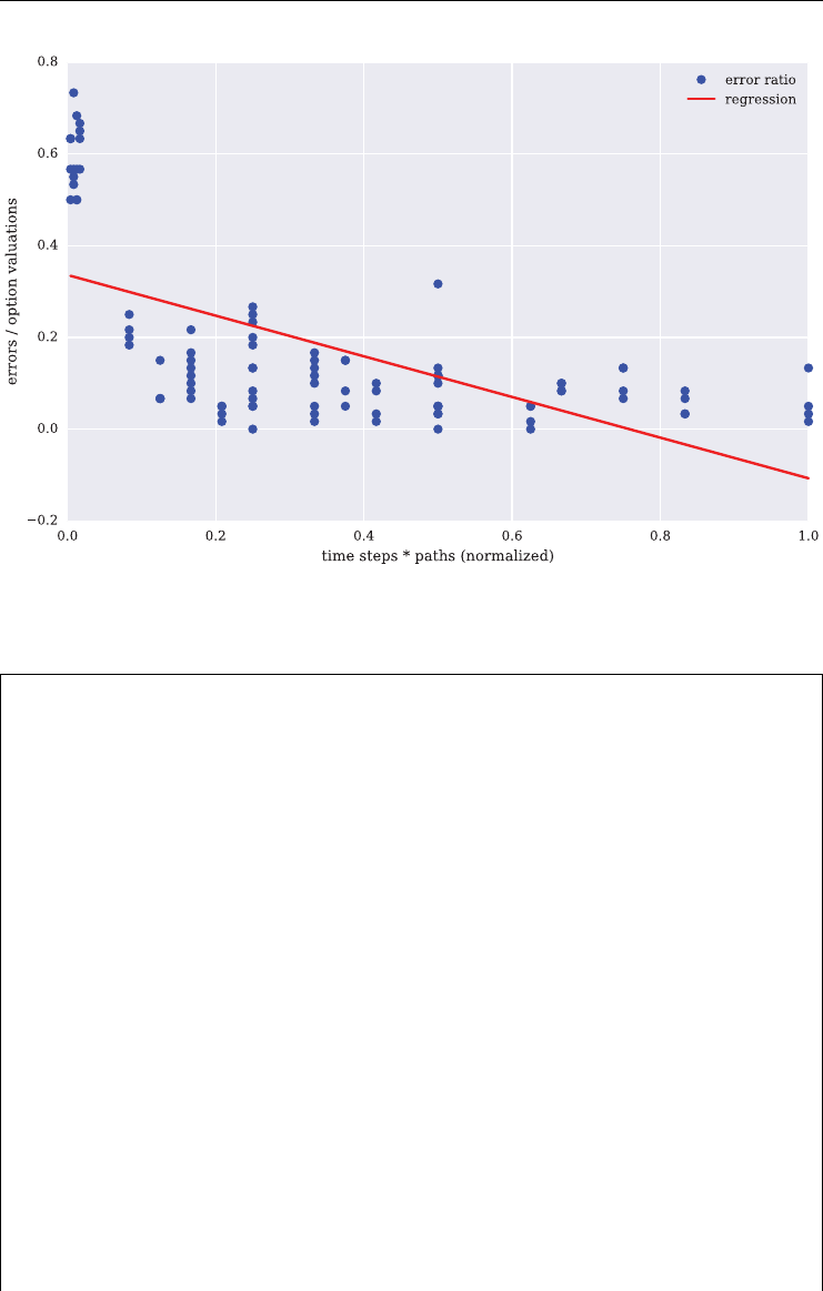
Valuing Volatility Derivatives 151
FIGURE 6.5 Error ratios of Monte Carlo valuation vs. computational effort.
In [41]: import pandas as pd
In [42]: h5 = pd.HDFStore(filename, 'r')
In [43]: data = h5['sim_results']
In [44]: h5.close()
In [45]: data.info()
<class 'pandas.core.frame.DataFrame'>
Int64Index: 96 entries, 0 to 95
Data columns (total 19 columns):
ab_val_err 96 non–null float64
abs_tol 96 non–null float64
anti_paths 96 non–null bool
av_val_err 96 non–null float64
end_date 96 non–null datetime64[ns]
error_ratio 96 non–null float64
errors 96 non–null int64
mo_match 96 non–null bool
opt_prices 96 non–null float64
paths 96 non–null int64
rel_tol 96 non–null float64

152 LISTED VOLATILITY AND VARIANCE DERIVATIVES
runs 96 non–null int64
seed 96 non–null int64
sim_name 96 non–null object
start_date 96 non–null datetime64[ns]
time_min 96 non–null float64
time_opt 96 non–null float64
time_sec 96 non–null float64
time_steps 96 non–null int64
dtypes: bool(2), datetime64[ns](2), float64(9), int64(5), object(1)
memory usage: 13.7+ KB
The simulation results are stored in 96 rows of the pandas DataFrame object. The method
groupby allows analyses of such data sets in “all directions and dimensions.” For example,
one gets the average error ratio depending on the use of moment matching with the following
code:
In [46]: data.groupby(['mo_match']).mean()[['error_ratio']]
Out[46]:
error_ratio
mo_match
False 0.193750
True 0.169097
In the simulations, moment matching obviously reduces the error ratio by slightly more than
2 percentage points from above 19% to less than 17%.
The same analysis can be done with more data columns, both for the grouping and the
output.
In [47]: data.groupby(['mo_match', 'anti_paths']).mean()[['error_ratio', 'errors']]
Out[47]:
error_ratio errors
mo_match anti_paths
False False 0.206944 12.416667
True 0.180556 10.833333
True False 0.159028 9.541667
True 0.179167 10.750000
Here, the results indicate that moment matching alone should be used. Adding antithetic paths
increases the error ratio ceteris paribus.
In similar fashion, the data can be grouped by time steps and paths – by analogy with the
analysis above. Figure 6.6 presents the results.
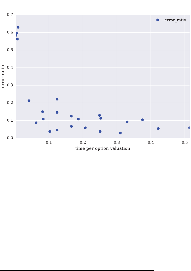
Valuing Volatility Derivatives 153
FIGURE 6.6 Error ratios of Monte Carlo valuation vs. time per option.
In [48]: df = data.groupby(['time_steps', 'paths']).mean()[['error_ratio',
'time_opt']]
In [49]: df.plot(x='time_opt', y='error_ratio', style='bo');
In [50]: plt.xlabel('time per option valuation');
In [51]: plt.ylabel('error ratio');
As expected, the general rule that accuracy increases with increasing computational effort is
again supported by this specic analysis. Of course, other analyses can be done with the data
generated and stored on disk.
6.7 MODEL CALIBRATION
Previous sections implement a theoretical valuation approach in that a parametric model is
given and parameter values are simply assumed. However, any realistic valuation of volatility
options has to incorporate at least some information from the market itself. This is generally
done by taking the quotes of liquidly traded vanilla options as input for a so-called model

154 LISTED VOLATILITY AND VARIANCE DERIVATIVES
calibration. During the calibration of a nancial model, parameters are determined for that
model which best replicate the observed option quotes. These parameters are in turn used to
value other, maybe more exotic, derivatives by means of numerical methods such as Monte
Carlo simulation. Such a procedure is often termed a market-based valuation approach.
This section illustrates how to calibrate the nancial model of Gr¨
unbichler and Longstaff
(1996) to option quotes for European volatility calls traded at Eurex. In the following, the
semi-analytical formula as introduced in section 6.4, The Option Pricing Formula is used to
accomplish the model calibration.
6.7.1 The Option Quotes
The remainder of this section will work with option quotes of VSTOXX call options traded at
Eurex which are all of European type. The data is as of March 31, 2014 and contains quotes
for the options with maturities for each month from April 2014 to November 2014. Let us have
a look at the data.
In [52]: import pandas as pd
In [53]: path = './source/data/'
In [54]: h5 = pd.HDFStore(path + 'vstoxx_option_quotes.h5', 'r')
In [55]: option_quotes = h5['option_quotes']
In [56]: option_quotes.info()
<class 'pandas.core.frame.DataFrame'>
Int64Index: 98 entries, 46219 to 46365
Data columns (total 8 columns):
DATE 98 non–null datetime64[ns]
EXP_YEAR 98 non–null int64
EXP_MONTH 98 non–null int64
TYPE 98 non–null object
STRIKE 98 non–null float64
PRICE 98 non–null float64
MATURITY 98 non–null datetime64[ns]
TTM 98 non–null float64
dtypes: datetime64[ns](2), float64(3), int64(2), object(1)
memory usage: 6.9+ KB
In [57]: option_quotes.iloc[25: 35]
Out[57]:
DATE EXP_YEAR EXP_MONTH TYPE STRIKE PRICE MATURITY TTM
46244 2014-03-31 2014 5 C 26.0 0.60 2014-05-16 0.126
46245 2014-03-31 2014 5 C 27.0 0.50 2014-05-16 0.126
46246 2014-03-31 2014 5 C 28.0 0.45 2014-05-16 0.126
46247 2014-03-31 2014 5 C 29.0 0.40 2014-05-16 0.126

Valuing Volatility Derivatives 155
46248 2014-03-31 2014 5 C 30.0 0.35 2014-05-16 0.126
46249 2014-03-31 2014 5 C 32.5 0.25 2014-05-16 0.126
46250 2014-03-31 2014 5 C 35.0 0.20 2014-05-16 0.126
46251 2014-03-31 2014 5 C 37.5 0.15 2014-05-16 0.126
46252 2014-03-31 2014 5 C 40.0 0.10 2014-05-16 0.126
46253 2014-03-31 2014 5 C 42.5 0.10 2014-05-16 0.126
As you can see, the data set comprises a total of 98 option quotes. Note that option quotes for
Eurex volatility options have tick sizes of 5 cents, i.e. 0.05 EUR. A detailed overview of the
terms of these options can be found in chapter 8, Terms of the VSTOXX and its Derivatives.In
what follows, we assume that each option is written on a single unit of the underlying, i.e. 1
point of the VSTOXX index translates into 1 EUR.
6.7.2 The Calibration Procedure
In simple terms, the problem of calibration is to nd parameters for an option model such
that observed market quotes of liquidly traded plain vanilla options are replicated as closely
as possible. To this end, one denes an error function that is to be minimized. Such a function
could be the Mean Squared Absolute Error (MSAE). The task is then to solve the problem
min
𝜅,𝜃,𝜎
1
N
N
n=1C∗
n−CGL96
n(𝜅,𝜃,𝜎)2
with the C∗
nbeing the market or input prices and the CGL96
nbeing the model or output prices
for the options n=1, …,N.
For some constellations, it might be more appropriate to minimize the Mean Squared
Relative Error (MSRE):
min
𝜅,𝜃,𝜎
1
N
N
n=1C∗
n−CGL96
n(𝜅,𝜃,𝜎)
C∗
n2
The Python script (see sub-section 6.9.4, srd_model_calibration.py) that implements a proce-
dure to calibrate the Gr¨
unbichler-Longstaff option pricing model is explained in the following
step-by-step procedure.
First, some imports and parameter specications.
import numpy as np
import pandas as pd
from srd_functions import call_price
import scipy.optimize as sco
import matplotlib.pyplot as plt
path = './source/data/'
# Fixed Parameters

156 LISTED VOLATILITY AND VARIANCE DERIVATIVES
v0 = 17.6639 # VSTOXX index on 31. March 2014
r = 0.01 # risk-less short rate
zeta = 0. # volatility risk premium factor
The function read_select_quotes() reads and selects option quotes for the calibration.
def read_select_quotes(path=path, tol=0.2):
''' Selects and read options quotes.
Parameters
==========
path: string
path to file with option quotes
Returns
=======
option_data: pandas DataFrame object
option data
'''
h5 = pd.HDFStore(path + 'vstoxx_march_2014.h5', 'r')
# read option data from file and close it
option_data = h5['vstoxx_options']
h5.close()
# select relevant date for call option quotes
option_data = option_data[(option_data.DATE == '2014-3-31')
& (option_data.TYPE == 'C')]
# calculate time-to-maturity in year fractions
option_data['TTM'] = (option_data.MATURITY - option_data.DATE).apply (
lambda x: x / np.timedelta64(1, 'D') / 365.)
# only those options close enough to the ATM level
option_data = option_data[(option_data.STRIKE > (1 - tol) * v0)
& (option_data.STRIKE < (1 + tol) * v0)]
return option_data
However, the core functions of the calibration script are the following. On the one hand,
valuation_function().
def valuation_function(p0):
''' Valuation function for set of strike prices
Parameters
==========
p0: list
set of model parameters

Valuing Volatility Derivatives 157
Returns
=======
call_prices: NumPy ndarray object
array of call prices
'''
kappa, theta, sigma = p0
call_prices = []
for strike in strikes:
call_prices.append(call_price(v0, kappa, theta,
sigma, zeta, ttm, r, strike))
call_prices = np.array(call_prices)
return call_prices
On the other hand, error_function().
def error_function(p0):
''' Error function for model calibration.
Parameters
==========
p0: tuple
set of model parameters
Returns
=======
MSE: float
mean squared (relative/absolute) error
'''
global i
call_prices = valuation_function(p0)
kappa, theta, sigma = p0
pen=0.
if 2 * kappa * theta < sigma ** 2:
pen = 1000.0
if kappa < 0 or theta < 0 or sigma < 0:
pen = 1000.0
if relative is True:
MSE = (np.sum(((call_prices - call_quotes) / call_quotes) ** 2)
/ len(call_quotes) + pen)
else:
MSE = np.sum((call_prices - call_quotes) ** 2) / len(call_quotes) + pen
if i==0:
print ("{:>6s}{:>6s}{:>6s}".format('kappa', 'theta', 'sigma')
+ "{:>12s}".format('MSE'))
# print intermediate results: every 100th iteration
if i % 100 == 0:

158 LISTED VOLATILITY AND VARIANCE DERIVATIVES
print "{:6.3f}{:6.3f}{:6.3f}".format(*p0) + "{:>12.5f}". format(MSE)
i+=1
return MSE
Function valuation_function() implements a valuation for the array of strikes under
consideration and the parameter values provided. Function error_function() calculates
either the MSAE or the MSRE – given the array of strikes and the parameter vector p0. Some
penalties are also added depending on the single parameter values or their constellation. For
details and a number of similar examples, refer to the book Hilpisch (2015, ch. 11).
Then standard functions from the scipy.optimize library (see Hilpisch (2014),
ch. 9) are used to implement both a global (i.e. via the brute() function) and a
local optimization (i.e. via the fmin() function). This is all wrapped into the function
model_calibration().
def model_calibration(option_data, rel=False, mat='2014-07-18'):
''' Function for global and local model calibration.
Parameters
==========
option_data: pandas DataFrame object
option quotes to be used
relative: boolean
relative or absolute MSE
maturity: string
maturity of option quotes to calibrate to
Returns
=======
opt: tuple
optimal parameter values
'''
global relative # if True: MSRE is used, if False: MSAE
global strikes
global call_quotes
global ttm
global i
relative = rel
# only option quotes for a single maturity
option_quotes = option_data[option_data.MATURITY == mat]
# time-to-maturity from the data set
ttm = option_quotes.iloc[0, -1]
# transform strike column and price column in ndarray object
strikes = option_quotes['STRIKE'].values

Valuing Volatility Derivatives 159
call_quotes = option_quotes['PRICE'].values
# global optimization
i=0 # counter for calibration iterations
p0 = sco.brute(error_function, ((5.0, 20.1, 1.0), (10., 30.1, 1.25),
(1.0, 9.1, 2.0)), finish=None)
# local optimization
i=0
opt = sco.fmin(error_function, p0, xtol=0.0000001, ftol=0.0000001,
maxiter=1000, maxfun=1500)
return opt
Finally, the results are visualized by plotting the model values against the market values
and providing the absolute differences separately. This is accomplished by the function
plot_calibration_results().
def plot_calibration_results(opt):
''' Function to plot market quotes vs. model prices.
Parameters
==========
opt: list
optimal parameters from calibration
'''
callalues = valuation_function(opt)
diffs = callalues - call_quotes
plt.figure()
plt.subplot(211)
plt.plot(strikes, call_quotes, label='market quotes')
plt.plot(strikes, callalues, 'ro', label='model prices')
plt.ylabel('option values')
plt.grid(True)
plt.legend()
plt.axis([min(strikes) - 0.5, max(strikes) + 0.5,
0.0, max(call_quotes) * 1.1])
plt.subplot(212)
wi = 0.3
plt.bar(strikes - wi / 2, diffs, width=wi)
plt.grid(True)
plt.xlabel('strike price')
plt.ylabel('difference')
plt.axis([min(strikes) - 0.5, max(strikes) + 0.5,
min(diffs) * 1.1, max(diffs) * 1.1])
plt.tight_layout()

160 LISTED VOLATILITY AND VARIANCE DERIVATIVES
6.7.3 The Calibration Results
We start with a calibration run for the option quotes with shorter maturity and using the MSAE
as a yardstick.
In [58]: from srd_model_calibration import *
In [59]: option_data = read_select_quotes()
In [60]: %time opt = model_calibration(option_data, rel=False, mat=
'2014-05-16')
kappa theta sigma MSE
5.000 10.000 1.000 7.78606
6.000 12.500 9.000 0.23173
7.000 16.250 9.000 0.40860
8.000 20.000 9.000 2.54160
9.000 23.750 9.000 9.70521
10.000 27.500 9.000 26.90758
12.000 10.000 9.000 3.75104
13.000 13.750 9.000 1.50070
14.000 17.500 9.000 0.06953
15.000 21.250 9.000 3.39340
16.000 25.000 9.000 18.12298
17.000 28.750 9.000 51.74883
19.000 11.250 9.000 5.14886
20.000 15.000 9.000 1.96050
kappa theta sigma MSE
15.000 18.750 7.000 0.01356
16.381 19.112 6.613 0.00834
27.671 18.969 8.513 0.00831
33.461 18.950 9.343 0.00831
33.457 18.950 9.342 0.00831
Optimization terminated successfully.
Current function value: 0.008311
Iterations: 247
Function evaluations: 450
CPU times: user 5.53 s, sys: 0 ns, total: 5.53 s
Wall time: 5.54 s
Figure 6.7 shows the calibration results.
In [61]: plot_calibration_results(opt)
<matplotlib.figure.Figure at 0x2ab247cec750>
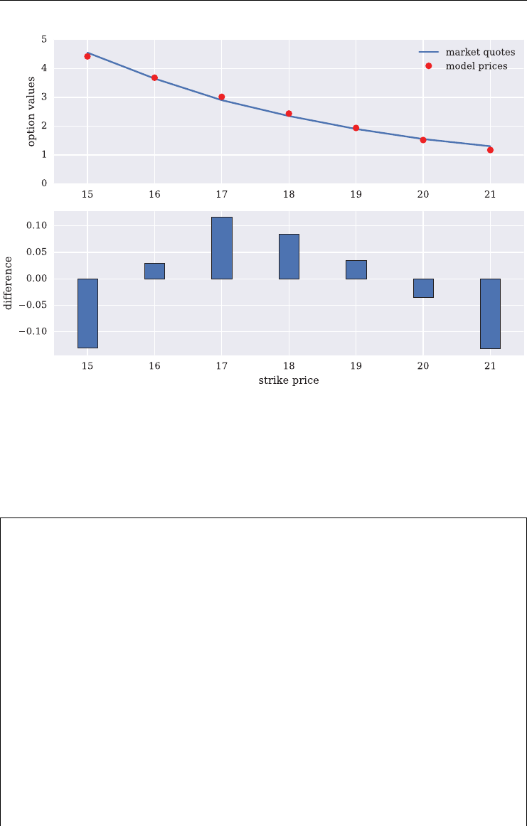
Valuing Volatility Derivatives 161
FIGURE 6.7 Calibration of option pricing model to option quotes for May 2014 maturity with
MSAE.
Now the calibration to the option quotes with a longer time-to-maturity and using the MSRE
as a yardstick.
In [62]: %time opt = model_calibration(option_data, rel=True, mat='2014-07-18')
kappa theta sigma MSE
5.000 10.000 1.000 1.00000
6.000 12.500 9.000 0.12866
7.000 16.250 9.000 0.01167
8.000 20.000 9.000 0.18546
9.000 23.750 9.000 1.20473
10.000 27.500 9.000 3.86826
12.000 10.000 9.000 0.73475
13.000 13.750 9.000 0.41208
14.000 17.500 9.000 0.05791
15.000 21.250 9.000 0.15684
16.000 25.000 9.000 1.57671
17.000 28.750 9.000 5.26237
19.000 11.250 9.000 0.81013
20.000 15.000 9.000 0.45062
kappa theta sigma MSE
5.000 20.000 5.000 0.00051
5.848 19.927 5.295 0.00050
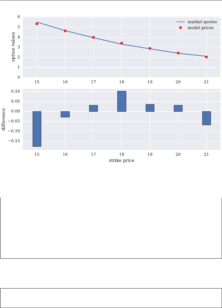
162 LISTED VOLATILITY AND VARIANCE DERIVATIVES
FIGURE 6.8 Calibration of option pricing model to option quotes for July 2014 maturity with
MSRE.
11.500 19.608 7.260 0.00049
12.731 19.585 7.638 0.00049
12.732 19.585 7.638 0.00049
Optimization terminated successfully.
Current function value: 0.000495
Iterations: 252
Function evaluations: 450
CPU times: user 5.6 s, sys: 0 ns, total: 5.6 s
Wall time: 5.61 s
The results of this calibration run are shown in Figure 6.8.
In [63]: plot_calibration_results(opt)
<matplotlib.figure.Figure at 0x2ab271446550>
Neither of the two ts is satisfactory for such small sets of option prices. The differences are
often higher than the tick size of 5 cents. Therefore, this model obviously does not paint too
realistic a picture of the real world. This may be due to the underlying, i.e. the VSTOXX
volatility index, exhibiting more and/or other properties than the ones captured in the model

Valuing Volatility Derivatives 163
of Gr¨
unbichler and Longstaff (1996). For example, a well documented stylized fact is that time
series of volatility indexes, like the VSTOXX, exhibit (positive) jumps of signicant size and
with signicant probability. Something that is, for example, not captured in the pricing model
used in this chapter.
6.8 CONCLUSIONS
Volatility derivatives, like futures and options on a volatility index, and their arbitrage-free
valuation are the focus of this chapter. The model of Gr¨
unbichler and Longstaff (1996) is
introduced since it serves pretty well as a benchmark case – due to its simplicity – for volatil-
ity modeling and volatility derivatives valuation. The model uses a square-root diffusion or
CIR process to describe the evolution of volatility (indexes) over time. Futures and European
call option pricing formulas are presented. Based on an exact discretization scheme, Monte
Carlo simulation is described as an alternative numerical pricing method. In addition, Python
code to implement automated Monte Carlo simulation studies is provided and used for such
a study. Finally, the GL96 model is calibrated to market quotes for European call options on
the VSTOXX volatility index. The results illustrate that the model might not be rich enough
to account for market realities.
6.9 PYTHON SCRIPTS
6.9.1 srd functions.py
#
# Module with functions for
#Gr
¨
unbichler and Longstaff (1996) model
#
# (c) Dr. Yves J. Hilpisch
# Listed Volatility and Variance Derivatives
#
import math
import numpy as np
import scipy.stats as scs
def futures_price(v0, kappa, theta, zeta, T):
''' Futures pricing formula in GL96 model.
Parameters
==========
v0: float (positive)
current volatility level
kappa: float (positive)
mean-reversion factor
theta: float (positive)
long-run mean of volatility

164 LISTED VOLATILITY AND VARIANCE DERIVATIVES
zeta: float (positive)
volatility risk premium
T: float (positive)
time-to-maturity
Returns
=======
future: float
price of a future
'''
alpha = kappa * theta
beta = kappa + zeta
future = (alpha / beta * (1 - math.exp(-beta * T))
+ math.exp(-beta * T) * v0)
return future
def cx(K, gamma, nu, lamb):
''' Complementary distribution function of non-central chi-squared density.
Parameters
==========
K: float (positive)
strike price
gamma: float (positive)
as defined in the GL96 model
nu: float (positive)
degrees of freedom
lamb: float (positive)
non-centrality parameter
Returns
=======
complementary distribution of nc cs density
'''
return 1 - scs.ncx2.cdf(gamma * K, nu, lamb)
def call_price(v0, kappa, theta, sigma, zeta, T, r, K):
''' Call option pricing formula in GL96 Model
Parameters
==========
v0: float (positive)
current volatility level
kappa: float (positive)
mean-reversion factor
theta: float (positive)
long-run mean of volatility
sigma: float (positive)
volatility of volatility

Valuing Volatility Derivatives 165
zeta: float (positive)
volatility risk premium
T: float (positive)
time-to-maturity
r: float (positive)
risk-free short rate
K: float(positive)
strike price of the option
Returns
=======
call: float
present value of European call option
'''
D = math.exp(-r * T) # discount factor
alpha = kappa * theta
beta = kappa + zeta
gamma = 4 * beta / (sigma ** 2 * (1 - math.exp(-beta * T)))
nu = 4 * alpha / sigma ** 2
lamb = gamma * math.exp(-beta * T) * v0
# the pricing formula
call = (D * math.exp(-beta * T) * v0 * cx(K, gamma, nu + 4, lamb)
+ D * (alpha / beta) * (1 - math.exp(-beta * T))
* cx(K, gamma, nu + 2, lamb)
-D*K*cx(K, gamma, nu, lamb))
return call
def generate_paths(x0, kappa, theta, sigma, T, M, I):
''' Simulation of square-root diffusion with exact discretization
Parameters
==========
x0: float (positive)
starting value
kappa: float (positive)
mean-reversion factor
theta: float (positive)
long-run mean
sigma: float (positive)
volatility (of volatility)
T: float (positive)
time-to-maturity
M: int
number of time intervals
I: int
number of simulation paths

166 LISTED VOLATILITY AND VARIANCE DERIVATIVES
Returns
=======
x: NumPy ndarray object
simulated paths
'''
dt = float(T) / M
x = np.zeros((M + 1, I), dtype=np.float)
x[0, :] = x0
# matrix filled with standard normal distributed rv
ran = np.random.standard_normal((M + 1, I))
d = 4 * kappa * theta / sigma ** 2
# constant factor in the integrated process of x
c = (sigma ** 2 * (1 - math.exp(-kappa * dt))) / (4 * kappa)
if d>1:
for tin range(1, M + 1):
# non-centrality parameter
l = x[t - 1, :] * math.exp(-kappa * dt) / c
# matrix with chi-squared distributed rv
chi = np.random.chisquare(d - 1, I)
x[t, :] = c * ((ran[t] + np.sqrt(l)) ** 2 + chi)
else:
for tin range(1, M + 1):
l = x[t - 1, :] * math.exp(-kappa * dt) / c
N = np.random.poisson(l / 2, I)
chi = np.random.chisquare(d + 2 * N, I)
x[t, :] = c * chi
return x
def call_estimator(v0, kappa, theta, sigma, T, r, K, M, I):
''' Estimation of European call option price in GL96 Model
via Monte Carlo simulation
Parameters
==========
v0: float (positive)
current volatility level
kappa: float (positive)
mean-reversion factor
theta: float (positive)
long-run mean of volatility
sigma: float (positive)
volatility of volatility
T: float (positive)
time-to-maturity
r: float (positive)
risk-free short rate
K: float (positive)
strike price of the option

Valuing Volatility Derivatives 167
M: int
number of time intervals
I: int
number of simulation paths
Returns
=======
callvalue: float
MCS estimator for European call option
'''
V = generate_paths(v0, kappa, theta, sigma, T, M, I)
callvalue = math.exp(-r * T) * np.sum(np.maximum(V[-1] - K, 0)) / I
return callvalue
6.9.2 srd simulation analysis.py
#
# Valuation of European volatility options
# by Monte Carlo simulation in
#Gr
¨
unbichler and Longstaff (1996) model
# -- analysis of valuation results
#
# (c) Dr. Yves J. Hilpisch
# Listed Volatility and Variance Derivatives
#
import time
import math
import numpy as np
from datetime import datetime
from srd_functions import generate_paths, call_price
from srd_simulation_results import *
# Model Parameters
v0 = 20.0 # initial volatility
kappa = 3.0 # speed of mean reversion
theta = 20.0 # long-term volatility
sigma = 3.2 # standard deviation coefficient
zeta = 0.0 # factor of the expected volatility risk premium
r = 0.01 # risk-free short rate
# General Simulation Parameters
write = True
var_red = [(False, False), (False, True), (True, False), (True, True)]
# 1st = mo_match -- random number correction (std + mean + drift)
# 2nd = anti_paths -- antithetic paths for variance reduction
# number of time steps
steps_list = [25, 50, 75, 100]

168 LISTED VOLATILITY AND VARIANCE DERIVATIVES
# number of paths per valuation
paths_list = [2500, 50000, 75000, 100000, 125000, 150000]
SEED = 100000 # seed value
runs = 3 # number of simulation runs
PY1 = 0.010 # performance yardstick 1: abs. error in currency units
PY2 = 0.010 # performance yardstick 2: rel. error in decimals
maturity_list = [1.0 / 12 , 1.0 / 4, 1.0 / 2, 1.0] # maturity list
strike_list = [15.0, 17.5, 20.0, 22.5, 25.0] # strike list
def generate_paths(x0, kappa, theta, sigma, T, M, I):
''' Simulation of square-root diffusion with exact discretization
Parameters
==========
x0: float (positive)
starting value
kappa: float (positive)
mean-reversion factor
theta: float (positive)
long-run mean
sigma: float (positive)
volatility (of volatility)
T: float (positive)
time-to-maturity
M: int
number of time intervals
I: int
number of simulation paths
Returns
=======
x: NumPy ndarray object
simulated paths
'''
dt = float(T) / M
x = np.zeros((M + 1, I), dtype=np.float)
x[0, :] = x0
# matrix filled with standard normally distributed rv
ran = randoms(M, I)
d = 4 * kappa * theta / sigma ** 2
# constant factor in the integrated process of x
c = (sigma ** 2 * (1 - math.exp(-kappa * dt))) / (4 * kappa)
if d>1:
for tin range(1, M + 1):
# non-centrality parameter
l = x[t - 1, :] * math.exp(-kappa * dt) / c
# matrix with chi-squared distributed rv
chi = np.random.chisquare(d - 1, I)
x[t, :]=c*((ran[t] + np.sqrt(l)) ** 2 + chi)

Valuing Volatility Derivatives 169
else:
for tin range(1, M + 1):
l = x[t - 1, :] * math.exp(-kappa * dt) / c
N = np.random.poisson(l / 2, I)
chi = np.random.chisquare(d +2*N,I)
x[t, :] = c * chi
return x
def randoms(M, I):
''' Function to generate pseudo-random numbers with variance reduction.
Parameters
==========
M: int
number of discrete time intervals
I: int
number of simulated paths
Returns
=======
rand: Numpy ndarray object
object with pseudo-random numbers
'''
if anti_paths is True:
rand_ = np.random.standard_normal((M + 1,I/2))
rand = np.concatenate((rand_, -rand_), 1)
else:
rand = np.random.standard_normal((M + 1, I))
if mo_match is True:
rand = rand / np.std(rand)
rand = rand - np.mean(rand)
return rand
t0 = time.time()
sim_results = pd.DataFrame()
for vr in var_red: # variance reduction techniques
mo_match, anti_paths = vr
for Min steps_list: # number of time steps
for Iin paths_list: # number of paths
t1 = time.time()
d1 = datetime.now()
abs_errors = []
rel_errors = []
l = 0.0
errors = 0
# name of the simulation setup
name = ('Call_' + str(runs) + '_'
+ str(M) + '_' + str(I / 1000)

170 LISTED VOLATILITY AND VARIANCE DERIVATIVES
+ '_' + str(mo_match)[0] + str(anti_paths)[0] +
'_' + str(PY1 * 100) + '-' + str(PY2 * 100))
np.random.seed(SEED) # RNG seed value
for run in range(runs): # simulation runs
print "\nSimulation Run %d of %d" % (run + 1, runs)
print " -----------------------------------------------------------"
print ("Elapsed Time in Minutes %8.2f"
% ((time.time() - t0) / 60))
print " -----------------------------------------------------------"
z=0
for Tin maturity_list: # time-to-maturity
dt=T/M # time interval in year fractions
V = generate_paths(v0, kappa, theta, sigma, T, M, I)
# volatility process paths
print "\nResults for Time-to-Maturity %6.3f"%T
print " -----------------------------------------------------------"
for Kin strike_list: # Strikes
h = np.maximum(V[-1] - K, 0) # inner value matrix
# MCS estimator
call_estimate = math.exp(-r * T) * np.sum(h) /I*100
# BSM analytical value
callalue = call_price(v0, kappa, theta, sigma,
zeta, T, r, K) * 100
# errors
diff = call_estimate - callalue
rdiff = diff / callalue
abs_errors.append(diff)
rel_errors.append(rdiff * 100)
# output
b r = " ----------------------------------------------"
print "\nResults for Strike %4.2f\n"%K
print (" European Op. Value MCS %8.4f"%
call_estimate)
print (" European Op. Value Closed %8.4f"%
callalue)
print " Valuation Error (abs) %8.4f" % diff
print " Valuation Error (rel) %8.4f" % rdiff
if abs(diff) < PY1 or abs(diff) / callalue < PY2:
print " Accuracy ok!\n"+br
CORR = True
else:
print " Accuracy NOT ok!\n"+br
CORR = False
errors = errors + 1
print "%d Errors, %d Values, %.1f Min. " \
% (errors, len(abs_errors),
float((time.time() - t1) / 60))
print (" %d Time Intervals, %d Paths"
% (M, I))

Valuing Volatility Derivatives 171
z=z+1
l=l+1
t2 = time.time()
d2 = datetime.now()
if write is True: # append simulation results
sim_results = write_results(sim_results, name, SEED,
runs, M, I, mo_match, anti_paths,
l, PY1, PY2, errors,
float(errors) / l, np.array(abs_errors),
np.array(rel_errors), t2 - t1, (t2 - t1) / 60, d1, d2)
if write is True:
# write/append DataFrame to HDFStore object
write_to_database(sim_results)
6.9.3 srd simulation results.py
#
# Valuation of European volatility options
# by Monte Carlo simulation in
#Gr
¨
unbichler and Longstaff (1996) model
# -- Creating a database for simulation results
# with pandas and PyTables
#
# (c) Dr. Yves J. Hilpisch
# Listed Volatility and Variance Derivatives
#
import numpy as np
import pandas as pd
import datetime as dt
import matplotlib.pyplot as plt
# filname for HDFStore to save results
filename = "../data/simulation_results.h5"
def write_results(sim_results, name, SEED, runs, steps, paths, mo_match,
anti_paths, l, PY1, PY2, errors, error_ratio,
abs_errors, rel_errors, t1, t2, d1, d2):
''' Appends simulation results to pandas DataFrame df and returns it.
Parameters
==========
see srd_simulation_analysis.py
Returns
=======

172 LISTED VOLATILITY AND VARIANCE DERIVATIVES
df: pandas DataFrame object
updated results object
'''
results = {
'sim_name': name,
'seed': SEED,
'runs': runs,
'time_steps': steps,
'paths': paths,
'mo_match': mo_match,
'anti_paths': anti_paths,
'opt_prices': l,
'abs_tol': PY1,
'rel_tol': PY2,
'errors': errors,
'error_ratio': error_ratio,
'aval_err': sum(abs_errors) / l,
'abal_err': sum(abs(rel_errors)) / l,
'time_sec': t1,
'time_min': t2,
'time_opt': t1 / l,
'start_date': d1,
'end_date': d2
}
df = pd.concat([sim_results,
pd.DataFrame([results])],
ignore_index=True)
return df
def write_to_database(sim_results, filename=filename):
''' Write pandas DataFrame sim_results to HDFStore object.
Parameters
==========
sim_results: pandas DataFrame object
object with simulation results
filename: string
name of the file for storage
'''
h5 = pd. HDFStore(filename, 'a')
h5.append('sim_results', sim_results, min_itemsize={'values': 30},
ignore_index=True)
h5.close()
def print_results(filename=filename, idl=0, idh=50):
''' Prints valuation results in detailed form.
Parameters
==========

Valuing Volatility Derivatives 173
filename: string
HDFStore with pandas.DataFrame with results
idl: int
start index value
idh: int
stop index value
'''
h5 = pd. HDFStore(filename, 'r')
sim_results = h5['sim_results']
b r = " -----------------------------------------------------------"
for iin range(idl, min(len(sim_results), idh + 1)):
row = sim_results.iloc[i]
print br
print "Start Calculations %32s" % row['start_date'] + "\n"+br
print "ID Number %32d"%i
print "Name of Simulation %32s" % row['sim_name']
print "Seed Value for RNG %32d" % row['seed']
print "Number of Runs %32d" % row['runs']
print "Time Steps %32d" % row['time_steps']
print "Paths %32d" % row['paths']
print "Moment Matching %32s" % row['mo_match']
print "Antithetic Paths %32s" % row['anti_paths'] + "\n"
print "Option Prices %32d" % row['opt_prices']
print "Absolute Tolerance %32.4f" % row['abs_tol']
print "Relative Tolerance %32.4f" % row['rel_tol']
print "Errors %32d" % row['errors']
print "Error Ratio %32.4f" % row['error_ratio'] + "\n"
print "Aver Val Error %32.4f" % row['aval_err']
print "Aver Abs Val Error %32.4f" % row['abal_err']
print "Time in Seconds %32.4f" % row['time_sec']
print "Time in Minutes %32.4f" % row['time_min']
print "Time per Option %32.4f" % row['time_opt'] + "\n"+br
print "End Calculations %32s" % row['end_date'] \
+"\n"+br+"\n"
print "Total number of rows in table %d" % len(sim_results)
h5.close()
def plot_error_ratio(filename=filename):
''' Show error ratio vs. paths * time_steps (i.e. granularity).
Parameters
==========
filename: string
name of file with data to be plotted
'''
h5 = pd. HDFStore(filename, mode='r')
sim_results = h5['sim_results']
x = np.array(sim_results['paths'] * sim_results['time_steps'], dtype='d')
x = x / max(x)

174 LISTED VOLATILITY AND VARIANCE DERIVATIVES
y = sim_results['error_ratio']
plt.plot(x, y, 'bo', label='error ratio')
rg = np.polyfit(x, y, deg=1)
plt.plot(np.sort (x), np.polyval(rg, np.sort(x)), 'r', label='regression',
linewidth=2)
plt.xlabel('time steps * paths (normalized)')
plt.ylabel('errors / option valuations')
plt.legend()
plt.grid(True)
h5.close()
6.9.4 srd model calibration.py
#
# Calibration of Gr¨
unbichler and Longstaff (1996)
# square-root diffusion model to
# VSTOXX call options traded at Eurex
# Data as of 31. March 2014
# All data from www.eurexchange.com
#
# (c) Dr. Yves J. Hilpisch
# Listed Volatility and Variance Derivatives
#
import numpy as np
import pandas as pd
from srd_functions import call_price
import scipy.optimize as sco
import matplotlib.pyplot as plt
path = './source/data/'
# Fixed Parameters
v0 = 17.6639 # VSTOXX index on 31. March 2014
r = 0.01 # risk-less short rate
zeta = 0. # volatility risk premium factor
def read_select_quotes(path=path, tol=0.2):
''' Selects and read options quotes.
Parameters
==========
path: string
path to file with option quotes
Returns
=======
option_data: pandas DataFrame object

Valuing Volatility Derivatives 175
option data
'''
h5 = pd.HDFStore(path + 'vstoxx_march_2014.h5', 'r')
# read option data from file and close it
option_data = h5['vstoxx_options']
h5.close()
# select relevant date for call option quotes
option_data = option_data[(option_data.DATE == '2014-3-31')
& (option_data.TYPE == 'C')]
# calculate time-to-maturity in year fractions
option_data['TTM'] = (option_data.MATURITY - option_data.DATE).apply(
lambda x: x / np.timedelta64(1, 'D') / 365.)
# only those options close enough to the ATM level
option_data = option_data[(option_data.STRIKE > (1 - tol) * v0)
& (option_data.STRIKE < (1 + tol) * v0)]
return option_data
def valuation_function(p0):
''' Valuation function for set of strike prices
Parameters
==========
p0: list
set of model parameters
Returns
=======
call_prices: NumPy ndarray object
array of call prices
'''
kappa, theta, sigma = p0
call_prices = []
for strike in strikes:
call_prices.append(call_price(v0, kappa, theta,
sigma, zeta, ttm, r, strike))
call_prices = np.array(call_prices)
return call_prices
def error_function(p0):
''' Error function for model calibration.
Parameters
==========
p0: tuple
set of model parameters
Returns
=======

176 LISTED VOLATILITY AND VARIANCE DERIVATIVES
MSE: float
mean squared (relative/absolute) error
'''
global i
call_prices = valuation_function(p0)
kappa, theta, sigma = p0
pen = 0.
if 2 * kappa * theta < sigma ** 2:
pen = 1000.0
if kappa < 0 or theta < 0 or sigma < 0:
pen = 1000.0
if relative is True:
MSE = (np.sum(((call_prices - call_quotes) / call_quotes) ** 2)
/ len(call_quotes) + pen)
else:
MSE = np.sum((call_prices - call_quotes) ** 2) / len(call_quotes) + pen
if i==0:
print ("{:>6s}{:>6s}{:>6s}".format('kappa', 'theta', 'sigma')
+ "{:>12s}".format('MSE'))
# print intermediate results: every 100th iteration
if i % 100 == 0:
print "{:6.3f} {:6.3f} {:6.3f}".format(*p0) + "{:>12.5f}".format(MSE)
i+=1
return MSE
def model_calibration(option_data, rel=False, mat=' 2014-07-18'):
''' Function for global and local model calibration.
Parameters
==========
option_data: pandas DataFrame object
option quotes to be used
relative: boolean
relative or absolute MSE
maturity: string
maturity of option quotes to calibrate to
Returns
=======
opt: tuple
optimal parameter values
'''
global relative # if True: MSRE is used, if False: MSAE
global strikes
global call_quotes
global ttm

Valuing Volatility Derivatives 177
global i
relative = rel
# only option quotes for a single maturity
option_quotes = option_data[option_data.MATURITY == mat]
# time-to-maturity from the data set
ttm = option_quotes.iloc[0, -1]
# transform strike column and price column in ndarray object
strikes = option_quotes['STRIKE'].values
call_quotes = option_quotes['PRICE'].values
# global optimization
i=0 # counter for calibration iterations
p0 = sco.brute(error_function, ((5.0, 20.1, 1.0), (10., 30.1, 1.25),
(1.0, 9.1, 2.0)), finish=None)
# local optimization
i=0
opt = sco.fmin(error_function, p0, xtol=0.0000001, ftol=0.0000001,
maxiter=1000, maxfun=1500)
return opt
def plot_calibration_results(opt):
''' Function to plot market quotes vs. model prices.
Parameters
==========
opt: list
optimal parameters from calibration
'''
callalues = valuation_function(opt)
diffs = callalues - call_quotes
plt.figure()
plt.subplot(211)
plt.plot(strikes, call_quotes, label='market quotes')
plt.plot(strikes, callalues, 'ro', labe='model prices')
plt.ylabel('option values')
plt.grid(True)
plt.legend()
plt.axis([min(strikes) - 0.5, max(strikes) + 0.5,
0.0, max(call_quotes) * 1.1])
plt.subplot(212)
wi = 0.3
plt.bar(strikes - wi / 2, diffs, width=wi)
plt.grid(True)
plt.xlabel('strike price')

178 LISTED VOLATILITY AND VARIANCE DERIVATIVES
plt.ylabel('difference')
plt.axis([min(strikes) - 0.5, max(strikes) + 0.5,
min(diffs) * 1.1, max(diffs) * 1.1])
plt.tight_layout()
if _ _name_ _ == '_ _main_ _':
option_data = read_select_quotes()
opt = model_calibration(option_data=option_data)

CHAPTER 7
Advanced Modeling of the
VSTOXX Index
7.1 INTRODUCTION
This chapter is somewhat different in style compared to the other chapters about the VSTOXX
volatility index and related derivatives. It introduces another parsimonious model, which is
called square-root jump diffusion (SRJD) to model the VSTOXX volatility index. This model,
which is essentially an extension of the Gr¨
unbichler and Longstaff (1996) model as analyzed
in the previous chapter, is capable of reproducing prices of European options written on the
VSTOXX reasonably well.
Two major enhancements characterize the SRJD model:
term structure: it allows us to capture the term structure as observed in the prices of
futures on the VSTOXX index
jump component: including a jump component allows better replication of option prices
in the short term
Adding these two components makes a market-consistent calibration of the model to a com-
prehensive set of European options on the VSTOXX index possible. For similar analyses and
modeling approaches including jumps for the volatility index refer, for example, to Psychoyios
(2005), Sepp (2008) or Psychoyios et al. (2010). For empirical evidence with regard to jumps
in volatility see Todorov and Tauchen (2011).
7.2 MARKET QUOTES FOR CALL OPTIONS
Before we introduce the model, let us set the stage by revisiting market quotes for European
call options written on the VSTOXX volatility index. First, we import the data:
In [1]: import pandas as pd
In [2]: path = './source/data/'
In [3]: h5 = pd. HDFStore(path + 'vstoxx_data_31032014.h5', 'r')
179
Listed Volatility and Variance Derivatives: A
Python-based Guide
By Dr. Yves J. Hilpisch
© 2017 Yves Hilpisch

180 LISTED VOLATILITY AND VARIANCE DERIVATIVES
We have both options data and futures data stored in this le with quotes from March 31, 2014.
In [4]: h5
Out[4]:
<class 'pandas.io.pytables.HDFStore'>
File path: ./source/data/vstoxx_data_31032014.h5
/futures_data frame (shape->[8,6])
/options_data frame (shape->[395,8])
Option market quotes are what we are concerned with for the moment.
In [5]: option_quotes = h5['options_data']
In [6]: option_quotes.info()
<class 'pandas.core.frame.DataFrame'>
Int64Index: 395 entries, 46170 to 46564
Data columns (total 8 columns):
DATE 395 non-null datetime64[ns]
EXP_YEAR 395 non-null int64
EXP_MONTH 395 non-null int64
TYPE 395 non-null object
STRIKE 395 non–null float64
PRICE 395 non–null float64
MATURITY 395 non-null datetime64[ns]
TTM 395 non–null float64
dtypes: datetime64[ns](2), float64(3), int64(2), object(1)
memory usage: 27.8+ KB
In [7]: option_quotes.head()
Out[7]:
DATE EXP_YEAR EXP_MONTH TYPE STRIKE PRICE MATURITY TTM
46170 2014-03-31 2014 4 C 1.0 16.85 2014-04-18 0.049
46171 2014-03-31 2014 4 C 2.0 15.85 2014-04-18 0.049
46172 2014-03-31 2014 4 C 3.0 14.85 2014-04-18 0.049
46173 2014-03-31 2014 4 C 4.0 13.85 2014-04-18 0.049
46174 2014-03-31 2014 4 C 5.0 12.85 2014-04-18 0.049
At any given point in time, there are options on the VSTOXX available for eight maturities.
In [8]: mats = sorted(set(option_quotes['MATURITY']))
In [9]: mats
Out[9]:

Advanced Modeling of the VSTOXX Index 181
[Timestamp('2014-04-18 00:00:00'),
Timestamp('2014-05-16 00:00:00'),
Timestamp('2014-06-20 00:00:00'),
Timestamp('2014-07-18 00:00:00'),
Timestamp('2014-08-15 00:00:00'),
Timestamp('2014-09-19 00:00:00'),
Timestamp('2014-10-17 00:00:00'),
Timestamp('2014-11-21 00:00:00')]
The spot level of the VSTOXX index on March 31, 2014 was 17.6639.
In [10]: v0 = 17.6639
In what follows, we only want to plot call option market quotes which are not too far in-the-
money nor out-of-the-money.
In [11]: tol = 0.4
In [12]: to_plot = option_quotes[(option_quotes['STRIKE'] > (1 - tol) * v0)
....: & (option_quotes['STRIKE'] < (1 + tol) * v0)]
....:
Figure 7.1 shows the VSTOXX European call option quotes which fulll the requirements.
The goal of this chapter is to replicate “all these option quotes” as closely as possible.
In [13]: import matplotlib.pyplot as plt
In [14]: import seaborn as sns; sns.set()
In [15]: import matplotlib
In [16]: matplotlib.rcParams['font.family'] = 'serif'
In [17]: markers = ['.', 'o', 'ˆ', 'v', 'x', 'D', 'd', '>', '<']
In [18]: plt.figure(figsize=(10, 6));
In [19]: for i, mat in enumerate(mats):
....: strikes = to_plot[(to_plot['MATURITY'] == mat)]['STRIKE']
....: prices = to_plot[(to_plot['MATURITY'] == mat)]['PRICE']
....: plt.plot(strikes, prices, 'b%s' % markers[i],
label=str(mat)[:10])
....:
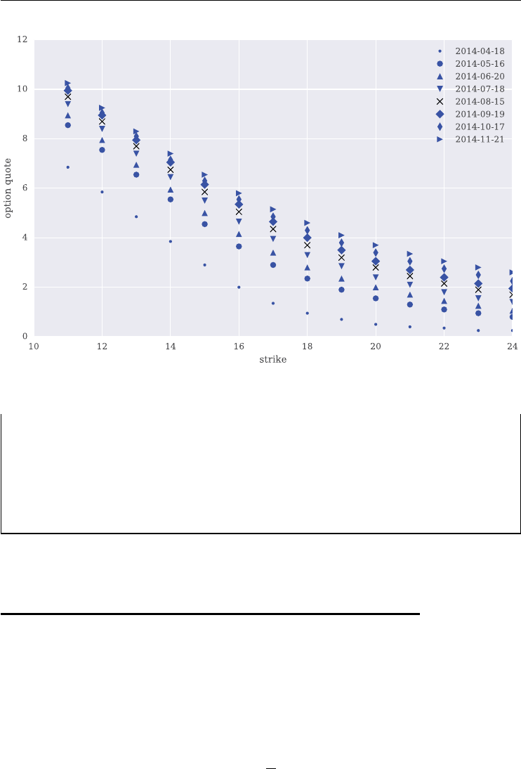
182 LISTED VOLATILITY AND VARIANCE DERIVATIVES
FIGURE 7.1 VSTOXX European call option quotes on March 31, 2014.
<matplotlib.figure.Figure at 0x2ab247d90d50>
In [20]: plt.legend();
In [21]: plt.xlabel('strike');
In [22]: plt.ylabel('option quote');
7.3 THE SRJD MODEL
A ltered probability space {Ω,,𝔽,P} representing uncertainty in the model economy is
given with nal date Twhere 0 <T<∞.Ωdenotes the continuous state space, a𝜎−algebra,
𝔽a ltration – i.e. a family of non-decreasing 𝜎−algebras 𝔽≡{t∈[0,T]} with 0≡{∅,Ω} and
T≡– and Pthe real or objective probability measure.
In the SRJD model, which is an afne jump diffusion (see Dufe et al. (2000)), the risk-
neutral dynamics of the VSTOXX volatility index are given by the following stochastic dif-
ferential equation (SDE):
dvt=𝜅(𝜃−vt)dt +𝜎vtdZt+JtvtdNt−rJdt
The meaning of the variables and parameters is:

Advanced Modeling of the VSTOXX Index 183
vtvolatility index level at date t
𝜅speed of adjustment of vtto…
…𝜃, the long-term mean of the index
𝜎volatility coefcient of the index level
Ztstandard Brownian motion
Jtjump at date twith distribution…
…log(1 +Jt)≈N(log(1 +𝜇)−𝛿2
2,𝛿2)
Ncumulative distribution function of a standard normal random variable
NtPoisson process with intensity 𝜆
rJ≡𝜆⋅(e𝜇+𝛿2∕2−1) drift correction for jump.
The stochastic process for vis adapted to the ltration 𝔽. Moreover, Zand Nare not correlated.
The time tvalue of a zero-coupon bond paying one unit of currency at T,0≤t<T,isBt(T)=
e−r(T−t)with r≥0 the constant risk-less short rate.
By the Fundamental Theorem of Asset Pricing, the time tvalue of an attainable, T-
measurable contingent claim VT≡hT(XT)≥0 (satisfying suitable integrability conditions) is
given by arbitrage as
Vt=EQ
tBt(T)VT
with V0=EQ
0(B0(T)VT) as the important special case for valuation purposes. Qis a P-
equivalent martingale measure. The contingent claim could be a European call option maturing
at Twith payoff VT=hT(vT)≡max[vT−K, 0]. It could also be a European put with payoff
VT=hT(vT)≡max[K−vT, 0]. In both cases, Kis the xed strike price of the option.
To simulate the nancial model, i.e. to generate numerical values for vt, it has to be dis-
cretized. To this end, divide the given time interval [0, T] in equidistant sub-intervals Δtsuch
that now t∈{0, Δt,2Δt,…,T}, i.e. there are M+1 points in time with M≡T∕Δt. With
s=t−Δt, a discretization of the continuous time market model is given by
̃vt=̃vs+𝜅(𝜃−̃v+
s)Δt+𝜎̃v+
sΔtz1
t
+e𝜇J+𝛿2z2
t−1̃v+
syt−rJΔt
vt=̃v+
t
for t∈{Δt,…,T} with x+≡max[x, 0] and the zn
tbeing standard normally distributed and yt
Poisson distributed. z1
t,z2
tand ytare uncorrelated. This discretization scheme is an Euler dis-
cretization and is generally called full trunction scheme. See Lord et al. (2008) for an analysis
of this and other biased discretization schemes for the square-root diffusion process.
7.4 TERM STRUCTURE CALIBRATION
The rst step in the calibration of the SRJD model is with regard to the futures term structure.

184 LISTED VOLATILITY AND VARIANCE DERIVATIVES
7.4.1 Futures Term Structure
It is difcult for parsimonious short rate models like that of Cox et al. (1985) to account for
different term structures of the interest rate. A possible solution is the introduction of time-
dependent parameters which, however, enlarges the number of parameters signicantly, sacri-
cing at the same time the convenience of a limited number of economic parameters. Another
solution is a deterministic shift approach according to Brigo and Mercurio (2001) which pre-
serves the basic structure of the model with all its advantages and which nevertheless allows
us to better account for different term structures of the short rate.
In this section, we transfer the deterministic shift approach for the short rate models of
Brigo and Mercurio (2001) to the SRJD model. Since the square-root diffusion and the jumps
are not correlated, we can rst apply the approach to the diffusion part and use this enhanced
component later on in conjunction with the jump component.
Before we present the theory, a look at the VSTOXX futures data rst.
In [23]: futures_quotes = h5['futures_data']
In [24]: futures_quotes.info()
<class 'pandas.core.frame.DataFrame'>
Int64Index: 8 entries, 496 to 503
Data columns (total 6 columns):
DATE 8 non-null datetime64[ns]
EXP_YEAR 8 non-null int64
EXP_MONTH 8 non-null int64
PRICE 8 non-null float64
MATURITY 8 non-null datetime64[ns]
TTM 8 non-null float64
dtypes: datetime64[ns](2), float64(2), int64(2)
memory usage: 448.0 bytes
Figure 7.2 presents the futures quotes for all eight maturities.
In [25]: ax = futures_quotes.plot(x='MATURITY', y='PRICE',
....: figsize=(10, 6), legend=False)
....:
<matplotlib.figure.Figure at 0x2ab25d177c50>
In [26]: futures_quotes.plot(x='MATURITY', y='PRICE', style='ro', ax=ax);
Consider for now the square-root diffusion volatility model of Gr¨
unbichler and Longstaff
(1996) as presented in the previous chapter, which is formally the same as the short rate model
of Cox et al. (1985) and which is a special case of the SRJD model:
dvt=𝜅(𝜃−vt)dt +𝜎vtdZt
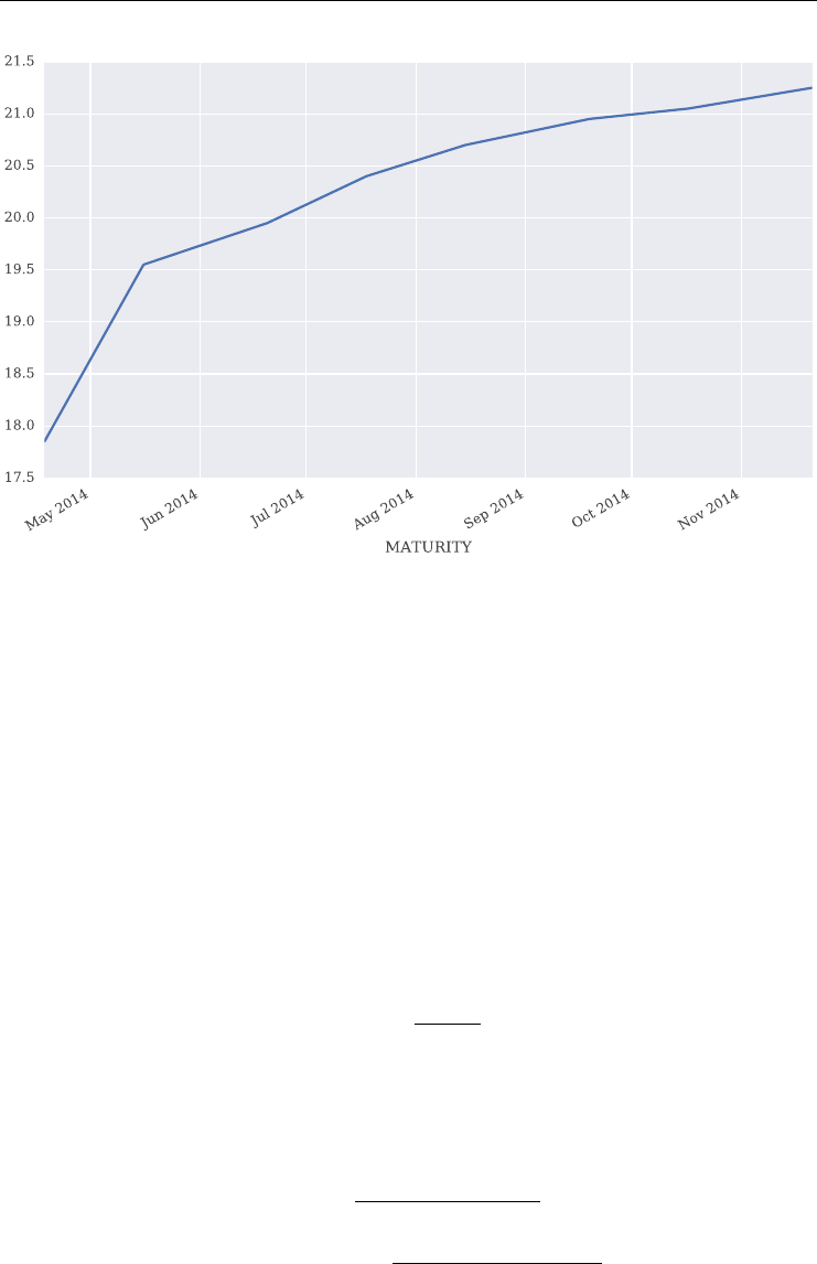
Advanced Modeling of the VSTOXX Index 185
FIGURE 7.2 VSTOXX futures quotes on March 31, 2014.
We want to calibrate this model to the observed volatility term structure, given by the above
presented set of prices for futures on the VSTOXX index with different maturities. We have
to minimize for all considered times tand a parameter set 𝛼=(𝜅,𝜃,𝜎,v0) simultaneously the
single differences
Δf(0, t)≡f(0, t)−fGL96(0, t;𝛼)
where f(0, t) is the time 0 market (instantaneous) forward volatility for time tand the quantity
fGL96(0, t;𝛼) is the model (instantaneous) forward volatility for time tgiven parameter set 𝛼.
Assume that there is a continuously differentiable volatility term structure function F(0, t)
available (i.e. there are innitely many volatility futures prices). The forward volatility then is
f(0, t)=𝜕F(0, t)
𝜕t
On the other hand, the model implied forward volatility is given as (see Brigo and Mercurio
(2001))
fGL96(0, t;𝛼)=𝜅𝜃(e𝛾t−1)
2𝛾+(𝜅+𝛾)(e𝛾t−1)
+v0
4𝛾2e𝛾t
(2𝛾+(𝜅+𝛾)(e𝛾t−1))2

186 LISTED VOLATILITY AND VARIANCE DERIVATIVES
with
𝛾≡𝜅2+2𝜎2
The Python script srjd_fwd_calibration.py contains the Python code to cal-
ibrate the forward volatilities to the VSTOXX futures prices (see sub-section 7.8.1,
srjd_fwd_calibration.py for the complete script). The beginning of the script is about library
imports, importing the data sets and making some selections.
import math
import numpy as np
import pandas as pd
import scipy.optimize as sco
v0 = 17.6639 # initial VSTOXX index level
i=0 # counter for calibration runs
# reading the VSTOXX futures quotes
path = 'source/data/'
h5 = pd.HDFStore(path + 'vstoxx_data_31032014.h5', 'r')
futures_quotes = h5['futures_data']
h5.close()
# selecting needed data columns and adding spot value
forwards = list(futures_quotes['PRICE'].values)
forwards.insert(0, v0)
forwards = np.array(forwards)
ttms = list(futures_quotes['TTM'].values)
ttms.insert(0, 0)
ttms = np.array(ttms)
The function srd_forwards() implements the forward formula from above for a given
parameter set.
def srd_forwards(p0):
''' Function for forward volatilities in GL96 Model.
Parameters
==========
p0: list
set of model parameters, where
kappa: float
mean-reversion factor

Advanced Modeling of the VSTOXX Index 187
theta: float
long-run mean
sigma: float
volatility factor
Returns
=======
forwards: NumPy ndarray object
forward volatilities
'''
t = ttms
kappa, theta, sigma = p0
g = math.sqrt(kappa ** 2 + 2 * sigma ** 2)
sum1 = ((kappa * theta * (np.exp(g * t) - 1)) /
(2 * g + (kappa + g) * (np.exp(g * t) - 1)))
sum2=v0*((4*g**2*np.exp(g * t)) /
(2*g+(kappa + g) * (np.exp(g * t) - 1)) ** 2)
forwards = sum1 + sum2
return forwards
To operationalize the calibration, we use the mean squared error (MSE) as our yardstick
min
𝛼
1
N
N
n=1fn−fGL96
n(𝛼)2
which is to be minimized. Here, we assume that we have Nobservations for the forward volatil-
ity. In Python this takes on the form of function srd_fwd_error().
def srd_fwd_error(p0):
''' Error function for GL96 forward volatilities calibration.
Parameters
==========
p0: tuple
parameter vector
Returns
=======
MSE: float
mean-squared error for p0
'''
global i
kappa, theta, sigma = p0
srd_fwds = srd_forwards(p0)
MSE = np.sum((forwards – srd_fwds) ** 2) / len(forwards)
if 2 * kappa * theta < sigma ** 2:
MSE = MSE + 100 # penalty

188 LISTED VOLATILITY AND VARIANCE DERIVATIVES
elif sigma < 0:
MSE = MSE + 100
# print intermediate results: every 50th iteration
if i%50==0:
print "{:6.3f} {:6.3f} {:6.3f}".format(* p0) + "{:>12.5f}".format(MSE)
i+=1
return MSE
Executing the script yields optimal parameters for the Gr¨
unbichler and Longstaff (1996) model
given the VSTOXX futures prices.
In [27]: %run source/scripts/srjd_fwd_calibration.py
1.000 17.500 1.000 35.99817
0.258 40.585 0.057 5.61895
1.575 46.996 0.392 0.22958
2.525 46.207 0.710 0.06348
3.447 44.752 0.972 0.04264
3.538 44.458 0.903 0.04261
3.947 43.495 0.610 0.04243
4.113 43.102 0.275 0.04219
4.187 42.969 0.019 0.04213
4.169 42.984 0.002 0.04213
4.170 42.984 0.000 0.04213
Optimization terminated successfully.
Current function value: 0.042129
Iterations: 292
Function evaluations: 526
In [28]: opt.round(3)
Out[28]: array([ 4.17 , 42.984, 0. ])
These optimal values can be used to calculate the model forward volatilities using function
srd_forwards().
In [29]: from srjd_fwd_calibration import *
In [30]: srd_fwds = srd_forwards(opt)
In [31]: srd_fwds
Out[31]:
array([ 17.6639 , 18.37130183, 19.22831373, 19.97504105,
20.3916346, 20.69048824, 20.95488999, 21.10239774, 21.23092346])
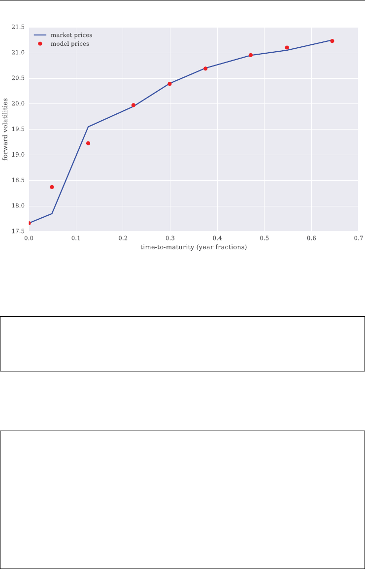
Advanced Modeling of the VSTOXX Index 189
FIGURE 7.3 VSTOXX futures market quotes vs. model prices.
The numerical differences to the market futures prices are:
In [32]: srd_fwds - forwards
Out[32]:
array([ 0. , 0.52130183, –0.32168627, 0.02504105, –0.0083654,
–0.00951176, 0.00488999, 0.05239774, –0.01907654])
Figure 7.3 compares the model futures prices (forward volatilities) with the VSTOXX futures
market quotes. For longer maturities the t is quite good.
In [33]: plt.figure(figsize=(10, 6));
In [34]: plt.plot(ttms, forwards, 'b', label='market prices');
In [35]: plt.plot(ttms, srd_fwds, 'ro', label='model prices');
In [36]: plt.legend(loc=0);
In [37]: plt.xlabel('time-to-maturity (year fractions)');
In [38]: plt.ylabel('forward volatilities');

190 LISTED VOLATILITY AND VARIANCE DERIVATIVES
Finally, we save the results from the term structure calibration for later use during the simula-
tion of the model.
In [39]: import pickle
In [40]: f = open('varphi', 'w') # open file on disk
# write ttms object and differences (varphi values) as dictionary
In [41]: pickle.dump({'ttms': ttms, 'varphi': srd_fwds – forwards}, f)
In [42]: f.close() # close file
7.4.2 Shifted Volatility Process
Assume that we are given a continuously differentiable futures price function (i.e. through
splines interpolation of discrete futures prices for different maturities). We consider now the
deterministically shifted volatility process (see Brigo and Mercurio (2001))
̂vt≡vt+𝜑(t,𝛼∗)
with 𝜑(t,𝛼∗)≡f(0, t)−fGL96(0, t;𝛼∗), the difference at time tbetween the market implied
forward volatility and the model implied forward volatility after calibration, i.e.for the optimal
parameter set 𝛼∗.𝜑(t,𝛼∗) corresponds to the differences (bars) in Figure 7.4.
FIGURE 7.4 Deterministic shift values to account for VSTOXX futures term structure.

Advanced Modeling of the VSTOXX Index 191
In [43]: plt.figure(figsize=(10, 6));
In [44]: plt.bar(ttms, srd_fwds – forwards,
....: width=0.05, label='$\\varphi(t,\\alphaˆ*)$');
....:
In [45]: plt.legend(loc=0);
In [46]: plt.xlabel('time-to-maturity (year fractions)');
In [47]: plt.ylabel('deterministic shift');
The SRJD model discretization can now be adjusted as follows:
̃vt=̃vs+𝜅(𝜃−̃v+
s)Δt+𝜎̃v+
sΔtz1
t
+e𝜇J+𝛿2z2
t−1̃v+
syt−rJΔt(7.1)
̂vt=̃v+
t+𝜑(t,𝛼∗) (7.2)
This is consistent since the diffusion and jump parts are not correlated and since the jump
part is added in such a way that the rst moment of the stochastic volatility process does not
change.
7.5 OPTION VALUATION BY MONTE CARLO SIMULATION
This section implements Monte Carlo simulation procedures for the SRJD model.
7.5.1 Monte Carlo Valuation
In what follows, the model option values are computed by Monte Carlo simulation (MCS).
Given the discrete version of the nancial model, the value of a European call option on the
volatility index is estimated by MCS as follows:
Algorithm 1: Simulation algorithm
for i=1, 2, …,Ido
for t=Δt,…,Tdo
draw pseudo-random numbers z1
t(i), z2
t(i), yt(i)1
apply these to equations (7.1) and (7.2) to calculate vt(i)2
calculate VT(i)=hT(i)≡max[vT(i)−K,0]3
sum up all payoffs at T, take the average and discount back to t=0:4
V0(K,T)≈e−rT ⋅
1
I
I
max[vT(i)−K,0]
V0is the MCS estimator for the European call option value.

192 LISTED VOLATILITY AND VARIANCE DERIVATIVES
7.5.2 Technical Implementation
Because we are using a numerical method like MCS for all valuation and calibration tasks,
the parametrization and implementation of the MCS algorithm play an important role. Some
major features of our implementation are:
discretization: the algorithm uses the Euler discretization scheme which is an approxi-
mation only but which might bring performance benets
random numbers: for every single option valuation the seed can be held constant such
that every option is valued with the same set of (pseudo-)random numbers
variance reduction: both antithetic variates and moment matching (for the rst two
moments of the pseudo-random numbers) are used as generic variance reduction tech-
niques
deterministic shift: the deterministic shift values 𝜑are determined only once through a
separate calibration and are held constant afterwards (even if model parameters change).
𝜑only has to be deterministic and integrable on closed intervals (see Brigo and Mercurio
(2001)), which is of course the case. For the approach to be valid, it is not important how we
originally came up with the 𝜑.
The Python code for simulating the SRJD model is found in the script
srjd_simulation.py (see sub-section 7.8.2, srjd_simulation.py for the complete
script). The beginning of the script shows several imports, the denition of example parame-
ters and also the cubic splines interpolation to be used for the estimation of the deterministic
shift parameters.
import math
import pickle
import numpy as np
import scipy.interpolate as scint
v0 = 17.6639 # initial VSTOXX index level
# parameters of square-root diffusion
kappa = 2.0 # speed of mean reversion
theta = 15.0 # long-term volatility
sigma = 1.0 # standard deviation coefficient
# parameters of log-normal jump
lamb = 0.4 # intensity (jumps per year)
mu = 0.4 # average jump size
delta = 0.1 # volatility of jump size
# general parameters
r = 0.01 # risk-free interest rate
K = 17.5 # strike
T = 0.5 # time horizon
M = 150 # time steps

Advanced Modeling of the VSTOXX Index 193
I = 10000 # number of MCS paths
anti_paths = True # antithetic variates
mo_match = True # moment matching
# deterministic shift parameters
varphi = pickle.load(open('varphi'))
tck = scint.splrep(varphi['ttms'], varphi['varphi'], k=1)
# linear splines interpolation of
# term structure calibration differences
The Python function random_number_gen() generates arrays of standard normally dis-
tributed pseudo-random numbers using both antithetic variates and moment matching as
generic variance reduction techniques.
def random_number_gen(M, I, fixed_seed=False):
''' Generate standard normally distributed pseudo-random numbers
Parameters
==========
M: int
number of time intervals
I: int
number of paths
Returns
=======
ran: NumPy ndarrayo object
random number array
'''
if fixed_seed is True:
np.random.seed(10000)
if anti_paths is True:
ran = np.random.standard_normal((M + 1, I / 2))
ran = np.concatenate((ran, -ran), axis=1)
else:
ran = np.standard_normal((M + 1, I))
if mo_match is True:
ran = ran / np.std(ran)
ran -= np.mean(ran)
return ran
The major function of this script is srjd_simulation() which implements the Monte
Carlo simulation for the SRJD model based on an Euler discretization scheme. The scheme
used here is usually called a full truncation scheme.

194 LISTED VOLATILITY AND VARIANCE DERIVATIVES
def srjd_simulation(x0, kappa, theta, sigma,
lamb, mu, delta, T, M, I, fixed_seed=False):
''' Function to simulate square-root jump Difusion.
Parameters
==========
x0: float
initial value
kappa: float
mean-reversion factor
theta: float
long-run mean
sigma: float
volatility factor
lamb: float
jump intensity
mu: float
expected jump size
delta: float
standard deviation of jump
T: float
time horizon/maturity
M: int
time steps
I: int
number of simulation paths
Returns
=======
x: NumPy ndarray object
array with simulated SRJD paths
'''
dt = float(T) / M # time interval
shift = scint.splev(np.arange(M + 1) * dt, tck, der=0)
# deterministic shift values
xh = np.zeros((M + 1, I), dtype=np.float)
x = np.zeros((M + 1, I), dtype=np.float)
xh[0, :] = x0
x[0, :] = x0
# drift contribution of jump p.a.
rj = lamb * (math.exp(mu + 0.5 * delta ** 2) - 1)
# 1st matrix with standard normal rv
ran1 = random_number_gen(M + 1, I, fixed_seed)
# 2nd matrix with standard normal rv
ran2 = random_number_gen(M + 1, I, fixed_seed)
# matrix with Poisson distributed rv

Advanced Modeling of the VSTOXX Index 195
ran3 = np.random.poisson(lamb * dt, (M + 1, I))
for tin range(1, M + 1):
xh[t, :] = (xh[t - 1, :] +
kappa * (theta - np.maximum(0, xh[t - 1, :])) * dt
+ np.sqrt(np.maximum(0, xh[t - 1, :])) * sigma
* ran1[t] * np.sqrt(dt)
+ (np.exp(mu + delta * ran2[t]) - 1) * ran3[t]
* np.maximum(0, xh[t - 1, :]) - rj * dt)
x[t, :] = np.maximum(0, xh[t, :]) + shift[t]
return x
Finally, the function srjd_call_valuation() estimates the value of a European call
option given the simulated volatility paths from srjd_simulation().
def srjd_call_valuation(v0, kappa, theta, sigma,
lamb, mu, delta, T, r, K, M=M, I=I,
fixed_seed=False):
''' Function to value European volatility call option in SRDJ model.
Parameters see function srjd_simulation.
Returns
=======
call_value: float
estimator for European call present value for strike K
'''
v = srjd_simulation(v0, kappa, theta, sigma,
lamb, mu, delta, T, M, I, fixed_seed)
call_value = np.exp(- r * T) * sum(np.maximum(v[-1] - K, 0)) / I
return call_value
Executing the script yields a MCS estimator for the European call option with the parameters
as assumed in the script of about 1 currency unit.
In [48]: %run source/scripts/srjd_simulation.py
Value of European call by MCS: 0.9959
7.6 MODEL CALIBRATION
This section now calibrates the SRJD model to market quotes for European call options on
VSTOXX futures. It considers calibrations to a single maturity as well as to multiple maturities.

196 LISTED VOLATILITY AND VARIANCE DERIVATIVES
7.6.1 The Python Code
The calibration of the SRJD model is similar to the procedure for the Gr¨
unbichler and Lonstaff
(1996) square-root diffusion model as presented in the previous chapter. The major difference
now is that we have to take into account more parameter values for the optimization. The
Python code is contained in script srjd_model_calibration.py (see sub-section 7.8.3,
srjd_model_calibration.py for the complete script). As usual a few imports and parameter
denitions rst.
import numpy as np
import pandas as pd
import scipy.optimize as sco
import matplotlib.pyplot as plt
from srd_model_calibration import path, read_select_quotes
from srjd_simulation import srjd_call_valuation
# fixed parameters
r = 0.01 # risk-less short rate
v0 = 17.6639 # VSTOXX index at 31.03.2014
M=15 # number of time intervals
I = 100 # number of simulated paths
In what follows, we want to calibrate the model simultaneously to multiple maturities for
the VSTOXX European call options. The valuation function srjd_valuation_function()
therefore now calculates the differences between model and market values directly and returns
an array with all differences (relative or absolute).
def srjd_valuation_function(p0):
''' Valuation ('difference') function for all options
of a given DataFrame object.
Parameters
==========
p0: list
set of model parameters
Returns
=======
diffs: NumPy ndarray object
array with valuation differences
'''
global relative, option_data
kappa, theta, sigma, lamb, mu, delta = p0
diffs = []
for i, option in option_data.iterrows():

Advanced Modeling of the VSTOXX Index 197
value = srjd_call_valuation(v0, kappa, theta, sigma,
lamb, mu, delta,
option['TTM'], r, option['STRIKE'],
M=M, I=I, fixed_seed=True)
if relative is True:
diffs.append((value - option['PRICE']) / option['PRICE'])
else:
diffs.append(value - option['PRICE'])
diffs = np.array(diffs)
return diffs
The error function srjd_error_function() for the SRJD model has to be enhanced
compared to the SRD case to account for the additional parameters of the model.
def srjd_error_function(p0):
''' Error function for model calibration.
Parameters
==========
p0: tuple
set of model parameters
Returns
=======
MSE: float
mean squared (relative/absolute) error
'''
global i, min_MSE, option_data
OD = len(option_data)
diffs = srjd_valuation_function(p0)
kappa, theta, sigma, lamb, mu, delta = p0
# penalties
pen = 0.
if 2 * kappa * theta < sigma ** 2:
pen = 1000.0
if kappa < 0 or theta < 0 or sigma < 0 or lamb < 0 or delta < 0:
pen = 1000.0
MSE = np.sum(diffs ** 2) / OD + pen # mean squared error
min_MSE = min(min_MSE, MSE) # running minimum value
if i==0:
print \'n' + ('{:>5s}'.format('its')
+ '{:>7s} {:>6s} {:>6s} {:>6s} {:>6s} {:>6s}'.format(

198 LISTED VOLATILITY AND VARIANCE DERIVATIVES
'kappa', 'theta', 'sigma', 'lamb', 'mu', 'delta')
+ '{:>12s}'.format('MSE') + '{:>12s}'.format('min_MSE'))
# print intermediate results: every 100th iteration
if i % 100 == 0:
print ('{:>5d}'.format(i)
+ '{:7.3f} {:6.3f} {:6.3f} {:6.3f} {:6.3f} {:6.3f}'.format(*p0)
+ '{:>12.5f}'.format(MSE) + '{:>12.5f}'.format(min_MSE))
i+=1
return MSE
The same holds true for the calibration function srjd_model_calibration() itself.
This function allows us to select certain maturities for the calibration.
def srjd_model_calibration(data, p0=None, rel=False, mats=None):
''' Function for global and local model calibration.
Parameters
==========
option_data: pandas DataFrame object
option quotes to be used
relative: bool
relative or absolute MSE
mats: list
list of maturities of option quotes to calibrate to
Returns
=======
opt: tuple
optimal parameter values
'''
global i, min_MSE, option_data
global relative # if True: MSRE is used, if False: MSAE
min_MSE = 5000. # dummy value
relative = rel # relative or absolute
option_data = data
if mats is not None:
# select the option data for the given maturities
option_data = option_data[option_data['MATURITY'].isin(mats)]
# global optimization
if p0 is None:
i=0 # counter for calibration iterations
p0 = sco.brute(srjd_error_function, (
(1.0, 9.1, 4.0), # kappa

Advanced Modeling of the VSTOXX Index 199
(10., 20.1, 10.0), # theta
(1.0, 3.1, 2.0), # sigma
(0.0, 0.81, 0.4), # lambda
(-0.2, 0.41, 0.3), #mu
(0.0, 0.31, 0.15)), # delta
finish=None)
# local optimization
i=0
opt = sco.fmin(srjd_error_function, p0,
xtol=0.0000001, ftol=0.0000001,
maxiter=550, maxfun=700)
return opt
7.6.2 Short Maturity
The addition of a jump component shall allow a better t to short-term call option market
quotes. Therefore, consider the following calibration to the shortest option maturity available:
In [49]: from srjd_model_calibration import *
# read option data, allow for 30% moneyness tolerance
In [50]: option_data = read_select_quotes(tol=0.3)
In [51]: %%time
....: opt_1 = srjd_model_calibration(option_data, p0=None,
....: rel=False, mats=['2014-4-18'])
....:
its kappa theta sigma lamb mu delta MSE min_MSE
0 1.000 10.000 1.000 0.000 -0.200 0.000 0.15785 0.15785
100 1.000 20.000 3.000 0.800 -0.200 0.000 0.10867 0.01976
200 5.000 20.000 3.000 0.400 -0.200 0.150 0.27793 0.01976
300 9.000 20.000 3.000 0.000 -0.200 0.300 0.70669 0.01976
its kappa theta sigma lamb mu delta MSE min_MSE
0 1.000 10.000 3.000 0.400 -0.200 0.000 0.01976 0.01976
100 1.016 9.216 2.996 0.476 -0.124 0.001 0.01956 0.01955
200 1.020 9.213 3.006 0.494 -0.128 0.001 0.01955 0.01955
300 0.976 8.895 3.000 0.392 -0.128 0.001 0.02214 0.01955
400 0.977 8.869 3.002 0.394 -0.128 0.001 0.01955 0.01955
500 0.976 8.866 3.002 0.394 -0.128 0.001 0.01955 0.01955

200 LISTED VOLATILITY AND VARIANCE DERIVATIVES
600 0.976 8.867 3.002 0.394 -0.128 0.001 0.01955 0.01955
Warning: Maximum number of function evaluations has been exceeded.
CPU times: user 14.7 s, sys: 7.97 ms, total: 14.7 s
Wall time: 14.7 s
The optimal parameter values are:
In [52]: opt_1
Out[52]:
array([ 9.75770825e-01, 8.86539094e+00, 3.00188833e+00,
3.93539089e-01, -1.28094441e-01, 1.26180667e-03])
Using these optimal parameter values, add the model prices to the DataFrame object con-
taining the option data.
In [53]: values = []
In [54]: kappa, theta, sigma, lamb, mu, delta = opt_1
In [55]: for i, option in option_data.iterrows():
....: value = srjd_call_valuation(v0, kappa, theta, sigma,
....: lamb, mu, delta,
....: option['TTM'], r, option['STRIKE'],
....: M=M, I=I, fixed_seed=True)
....: values.append(value)
....:
In [56]: option_data['MODEL'] = values
Figure 7.5 shows the calibration results graphically. Indeed, the t seems to be quite good,
reecting a MSAE of about 0.0015 only.
# selecting the data for the shortest maturity
In [57]: os = option_data[option_data.MATURITY == '2014-4-18']
# selecting corresponding strike prices
In [58]: strikes = os.STRIKE.values
# comparing the model prices with the market quotes
In [59]: fig, ax = plt.subplots(2, 1, sharex=True, figsize=(10, 6));
In [60]: ax[0].plot(strikes, os.PRICE.values, label='market quotes');
In [61]: ax[0].plot(strikes, os.MODEL.values, 'ro', label='model prices');
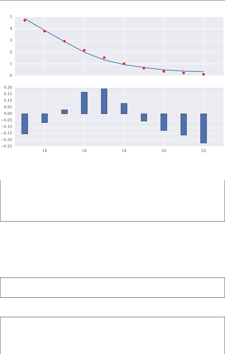
Advanced Modeling of the VSTOXX Index 201
FIGURE 7.5 Calibration of SRJD model to European call options on the VSTOXX for shortest
option maturity (April 2014).
In [62]: ax[1].bar(strikes - 0.15, os.MODEL.values - os.PRICE.values,
....: width=0.3);
....:
In [63]: ax[1].set_xlim(12.5, 23);
7.6.3 Two Maturities
Let us proceed with the simultaneous calibration of the model to the May and July maturities.
The MSE is also pretty low in this case (i.e. below 0.01).
# read option data, allow for 17.5% moneyness tolerance
In [64]: option_data = read_select_quotes(tol=0.175)
In [65]: %%time
....: opt_2 = srjd_model_calibration(option_data, rel=False,
....: mats=['2014-5-16', '2014-7-18'])
....:

202 LISTED VOLATILITY AND VARIANCE DERIVATIVES
its kappa theta sigma lamb mu delta MSE min_MSE
0 1.000 10.000 1.000 0.000 -0.200 0.000 8.71137 8.71137
100 1.000 20.000 3.000 0.800 -0.200 0.000 0.85126 0.10351
200 5.000 20.000 3.000 0.400 -0.200 0.150 0.59218 0.09015
300 9.000 20.000 3.000 0.000 -0.200 0.300 0.45081 0.01539
its kappa theta sigma lamb mu delta MSE min_MSE
0 5.000 20.000 3.000 0.800 0.400 0.000 0.01539 0.01539
100 4.471 19.655 3.256 0.762 0.424 0.000 0.00892 0.00892
200 4.010 19.231 2.730 0.761 0.575 0.002 0.00792 0.00792
300 4.023 18.987 2.321 0.721 0.668 0.003 0.01182 0.00688
400 3.803 18.830 2.115 0.722 0.701 0.003 0.00660 0.00660
500 3.823 18.799 2.106 0.723 0.706 0.003 0.00644 0.00644
600 3.998 18.681 1.916 0.728 0.749 0.003 0.00598 0.00598
Warning: Maximum number of function evaluations has been exceeded.
CPU times: user 17.1 s, sys: 10 us, total: 17.1 s
Wall time: 17.1 s
The optimal parameter values are:
In [66]: opt_2
Out[66]:
array([ 3.99997568e+00, 1.86836808e+01, 1.91679210e+00,
7.28298815e-01, 7.48260996e-01, 3.26197421e-03])
In what follows, we use the Python function plot_calibration_results() to gen-
erate the plots for the different valuation runs. This function allows for different numbers of
sub-plots, i.e. when the number of option maturities is changed. It is mainly a generalization
of the plotting code used above.
def plot_calibration_results(option_data, opt, mats):
''' Function to plot market quotes vs. model prices.
Parameters
==========
option_data: pandas DataFrame object
option data to plot
opt: list
optimal results from calibration
mats: list
maturities to be plotted
'''
kappa, theta, sigma, lamb, mu, delta = opt
# adding model values for optimal parameter set

Advanced Modeling of the VSTOXX Index 203
# to the DataFrame object
values = []
for i, option in option_data.iterrows():
value = srjd_call_valuation(v0, kappa, theta, sigma,
lamb, mu, delta,
option['TTM'], r, option['STRIKE'],
M=M, I=I, fixed_seed=True)
values.append(value)
option_data['MODEL'] = values
# plotting the market and model values
height = min(len(mats) * 3, 12)
fig, axarr = plt.subplots(len(mats), 2, sharex=True, figsize=(10, height))
for z, mat in enumerate(mats):
if z==0:
axarr[z, 0].set_title('values')
axarr[z, 1].set_title('differences')
os = option_data[option_data.MATURITY == mat]
strikes = os. STRIKE.values
axarr[z, 0].set_ylabel('%s' % str(mat)[: 10])
axarr[z, 0].plot(strikes, os.PRICE.values, label='market quotes')
axarr[z, 0].plot(strikes, os.MODEL.values, 'ro', label='model prices')
axarr[z, 0].legend(loc=0)
wi = 0.3
axarr[z, 1].bar(strikes - wi / 2, os.MODEL.values - os.PRICE.values,
width=wi)
if mat == mats[- 1]:
axarr[z, 0].set_xlabel('strike')
axarr[z, 1].set_xlabel('strike')
Figure 7.6 shows the results of the calibration graphically. It is obvious that the SRJD model
is able to account for multiple maturities at the same time which is mainly due to the term
structure component introduced by the deterministic shift approach.
In [67]: plot_calibration_results(option_data, opt_2, ['2014-5-16',
'2014-7-18'])
<matplotlib.figure.Figure at 0x2ab25d1b0190>
7.6.4 Four Maturities
In a next step, we consider four maturities – before we try to calibrate the model to all eight
maturities.
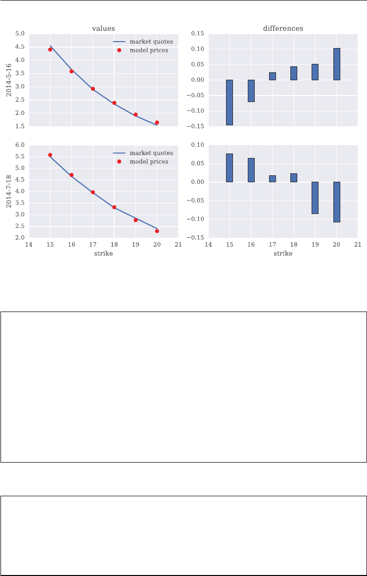
204 LISTED VOLATILITY AND VARIANCE DERIVATIVES
FIGURE 7.6 Calibration of SRJD model to European call options on the VSTOXX for May and
July 2014 maturities.
In [68]: mats = sorted(set(option_data['MATURITY']))
In [69]: mats
Out[69]:
[Timestamp('2014-04-18 00:00:00'),
Timestamp('2014-05-16 00:00:00'),
Timestamp('2014-06-20 00:00:00'),
Timestamp('2014-07-18 00:00:00'),
Timestamp('2014-08-15 00:00:00'),
Timestamp('2014-09-19 00:00:00'),
Timestamp('2014-10-17 00:00:00'),
Timestamp('2014-11-21 00:00:00')]
The four maturities for this particular calibration run are:
In [70]: mats[::2]
Out[70]:
[Timestamp('2014-04-18 00:00:00'),
Timestamp('2014-06-20 00:00:00'),
Timestamp('2014-08-15 00:00:00'),
Timestamp('2014-10-17 00:00:00')]

Advanced Modeling of the VSTOXX Index 205
For this calibration run, we use the optimal parameters from the previous calibration to two
maturities. Obviously, the more options to calibrate the model to, the longer the procedure
takes.
In [71]: %%time
....: opt_4 = srjd_model_calibration(option_data, p0=opt_2,
....: rel=False, mats=mats[::2])
....:
its kappa theta sigma lamb mu delta MSE min_MSE
0 4.000 18.684 1.917 0.728 0.748 0.003 0.52345 0.52345
100 4.202 18.938 1.980 0.727 0.623 0.003 0.27887 0.27681
200 3.650 21.465 3.293 0.744 -0.075 0.002 0.18617 0.18617
300 3.195 22.481 2.867 0.743 -0.223 0.000 0.14915 0.14915
400 3.107 22.191 2.990 0.745 -0.141 0.000 0.14609 0.14608
500 3.081 22.162 3.028 0.743 -0.138 0.000 0.14572 0.14570
600 3.057 22.100 3.041 0.738 -0.124 0.000 0.14521 0.14521
700 3.061 22.110 3.034 0.738 -0.126 0.000 0.14517 0.14517
Warning: Maximum number of function evaluations has been exceeded.
CPU times: user 22.9 s, sys: 16 ms, total: 22.9 s
Wall time: 22.9 s
In [72]: opt_4
Out[72]:
array([ 3.06082557e+00, 2.21100415e+01, 3.03422643e+00,
7.38054016e-01, -1.25823900e-01, 1.19890649e-06])
Even calibrating the model to four maturities yields quite a good t over these maturities as
Figure 7.7 illustrates.
In [73]: plot_calibration_results(option_data, opt_4, mats[::2])
<matplotlib.figure.Figure at 0x2ab247bec510>
7.6.5 All Maturities
Finally, let us attack the hardest calibration problem – the one involving all eight option
maturities.
In [74]: %%time
....: opt_8_MSAE = srjd_model_calibration(option_data,
....: rel=False, mats=mats)
....:
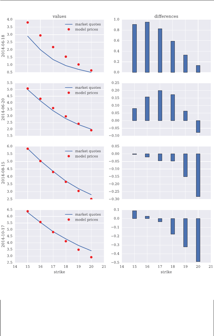
206 LISTED VOLATILITY AND VARIANCE DERIVATIVES
FIGURE 7.7 Calibration of SRJD model to European call options on the VSTOXX for four
maturities.
its kappa theta sigma lamb mu delta MSE min_MSE
0 1.000 10.000 1.000 0.000 -0.200 0.000 12.79035 12.79035
100 1.000 20.000 3.000 0.800 -0.200 0.000 1.13623 0.13849
200 5.000 20.000 3.000 0.400 -0.200 0.150 1.08765 0.13849
300 9.000 20.000 3.000 0.000 -0.200 0.300 1.27175 0.13849

Advanced Modeling of the VSTOXX Index 207
its kappa theta sigma lamb mu delta MSE min_MSE
0 1.000 20.000 3.000 0.400 0.400 0.150 0.13849 0.13849
100 1.007 20.567 2.921 0.396 0.326 0.155 0.12039 0.11935
200 1.018 21.609 3.266 0.404 0.032 0.163 0.10182 0.10096
300 1.033 22.713 3.222 0.407 -0.123 0.155 0.09869 0.09863
400 1.542 23.755 3.235 0.409 -0.985 0.067 0.08329 0.08120
500 1.860 23.848 2.967 0.410 -1.297 0.002 0.07686 0.07686
600 1.868 23.863 2.956 0.410 -1.303 -0.000 1000.07683 0.07683
Warning: Maximum number of function evaluations has been exceeded.
CPU times: user 1min 7s, sys: 16 ms, total: 1min 7s
Wall time: 1min 7s
In [75]: opt_8_MSAE
Out[75]:
array([ 1.86781293e+00, 2.38625952e+01, 2.95539873e+00,
4.10158642e-01, -1.30281337e+00, 8.30841775e-08])
Figure 7.8 shows that the t is still reasonable for eight maturities and that many options.
In [76]: plot_calibration_results(option_data, opt_8_MSAE, mats)
<matplotlib.figure.Figure at 0x2ab247b94250>
To check whether there is a (larger) difference when we calibrate the model using relative
differences (i.e. the MSRE) as a yardstick, consider the following calibration run:
In [77]: %%time
....: opt_8_MSRE = srjd_model_calibration(option_data, p0=opt_8_MSAE,
....: rel=True, mats=mats)
....:
its kappa theta sigma lamb mu delta MSE min_MSE
0 1.868 23.863 2.955 0.410 -1.303 0.000 0.02551 0.02551
100 1.599 24.888 2.619 0.392 -1.381 0.000 0.02099 0.02099
200 1.015 26.443 2.737 0.388 -1.676 0.000 0.02017 0.02017
300 0.915 27.147 2.723 0.388 -1.947 0.000 0.02046 0.02011
400 0.920 27.175 2.719 0.388 -2.142 0.000 0.02010 0.02010
500 0.927 27.082 2.724 0.389 -2.373 0.000 0.02009 0.02009
600 0.925 27.083 2.722 0.389 -2.409 0.000 0.02009 0.02009
700 0.925 27.086 2.722 0.389 -2.409 0.000 0.02009 0.02009
Warning: Maximum number of function evaluations has been exceeded.
CPU times: user 46.9 s, sys: 16 ms, total: 46.9 s
Wall time: 46.9 s
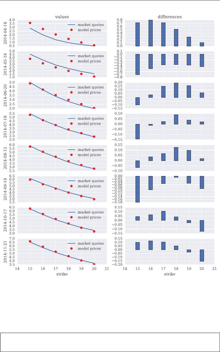
208 LISTED VOLATILITY AND VARIANCE DERIVATIVES
FIGURE 7.8 Calibration of SRJD model to European call options on the VSTOXX for all eight
maturities (MSAE used).
Figure 7.9 presents the results. They are not too dissimilar to the ones obtained using the MSAE
as a yardstick. The major difference is the weighting of the options in that now those options
with lower market quotes (higher strikes) get more weight.
In [78]: plot_calibration_results(option_data, opt_8_MSRE, mats)
<matplotlib.figure.Figure at 0x2ab25d453250>
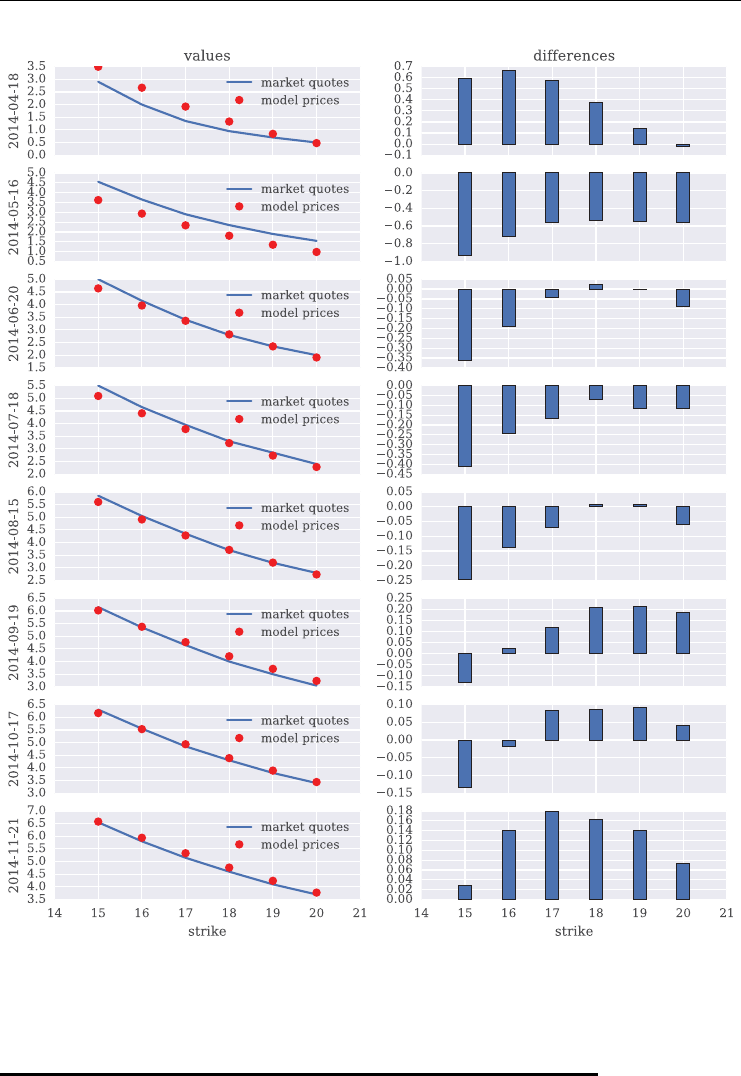
Advanced Modeling of the VSTOXX Index 209
FIGURE 7.9 Calibration of SRJD model to European call options on the VSTOXX for all eight
maturities (MSRE used).
7.7 CONCLUSIONS
This chapter introduces a more sophisticated model, the so-called square-root jump diffu-
sion model (SRJD), for the evolution of the VSTOXX volatility index over time. It enhances
the Gr¨
unbichler and Longstaff (1996) square-root diffusion model by two components: a log
normally distributed jump component and a deterministic shift component. While the rst

210 LISTED VOLATILITY AND VARIANCE DERIVATIVES
allows us to better calibrate the model to short term option quotes, the latter makes it pos-
sible to take the volatility term structure – as embodied by the eight futures on the VSTOXX
index – into account. All in all, the model yields good calibration results even in cases where
all eight option maturities are accounted for.
7.8 PYTHON SCRIPTS
7.8.1 srjd fwd calibration.py
#
# Script for term structure calibration of
# Square-Root Jump Diffusion (SRJD) model
#
# (c) Dr. Yves J. Hilpisch
# Listed Volatility and Variance Derivatives
#
import math
import numpy as np
import pandas as pd
import scipy.optimize as sco
v0 = 17.6639 # initial VSTOXX index level
i=0 # counter for calibration runs
# reading the VSTOXX futures quotes
path = 'source/data/'
h5 = pd.HDFStore(path + 'vstoxx_data_31032014.h5', 'r')
futures_quotes = h5['futures_data']
h5.close()
# selecting needed data columns and adding spot value
forwards = list(futures_quotes['PRICE'].values)
forwards.insert(0, v0)
forwards = np.array(forwards)
ttms = list(futures_quotes['TTM'].values)
ttms.insert(0, 0)
ttms = np.array(ttms)
def srd_forwards(p0):
''' Function for forward volatilities in GL96 Model.
Parameters
==========
p0: list

Advanced Modeling of the VSTOXX Index 211
set of model parameters, where
kappa: float
mean-reversion factor
theta: float
long-run mean
sigma: float
volatility factor
Returns
=======
forwards: NumPy ndarray object
forward volatilities
'''
t = ttms
kappa, theta, sigma = p0
g = math.sqrt(kappa **2+2*sigma ** 2)
sum1 = ((kappa * theta * (np.exp(g * t) - 1)) /
(2*g+(kappa + g) * (np.exp(g * t) - 1)))
sum2 = v0 * ((4*g**2*np.exp(g * t)) /
(2*g+(kappa + g) * (np.exp(g * t) - 1)) ** 2)
forwards = sum1 + sum2
return forwards
def srd_fwd_error(p0):
''' Error function for GL96 forward volatilities calibration.
Parameters
==========
p0: tuple
parameter vector
Returns
=======
MSE: float
mean-squared error for p0
'''
global i
kappa, theta, sigma = p0
srd_fwds = srd_forwards(p0)
MSE = np.sum((forwards - srd_fwds) ** 2) / len(forwards)
if 2 * kappa * theta < sigma ** 2:
MSE = MSE + 100 # penalty
elif sigma < 0:
MSE = MSE + 100
# print intermediate results: every 50th iteration

212 LISTED VOLATILITY AND VARIANCE DERIVATIVES
if i % 50 == 0:
print "{:6.3f} {:6.3f} {:6.3f}".format(*p0) + "{:>12.5f}".format(MSE)
i+=1
return MSE
if _ _name_ _ is '_ _main_ _':
p0 = 1.0, 17.5, 1.0
opt = sco.fmin(srd_fwd_error, p0,
xtol=0.00001, ftol=0.00001,
maxiter=1500, maxfun=2000)
7.8.2 srjd simulation.py
#
# Module with simulation functions for
# Square-Root Jump Diffusion (SRJD) model
#
# (c) Dr. Yves J. Hilpisch
# Listed Volatility and Variance Derivatives
#
import math
import pickle
import numpy as np
import scipy.interpolate as scint
v0 = 17.6639 # initial VSTOXX index level
# parameters of square-root diffusion
kappa = 2.0 # speed of mean reversion
theta = 15.0 # long-term volatility
sigma = 1.0 # standard deviation coefficient
# parameters of log-normal jump
lamb = 0.4 # intensity (jumps per year)
mu = 0.4 # average jump size
delta = 0.1 # volatility of jump size
# general parameters
r = 0.01 # risk-free interest rate
K = 17.5 # strike
T = 0.5 # time horizon
M = 150 # time steps
I = 10000 # number of MCS paths
anti_paths = True # antithetic variates
mo_match = True # moment matching

Advanced Modeling of the VSTOXX Index 213
# deterministic shift parameters
varphi = pickle.load(open('varphi'))
tck = scint.splrep(varphi['ttms'], varphi['varphi'], k=1)
# linear splines interpolation of
# term structure calibration differences
def random_number_gen(M, I, fixed_seed=False):
''' Generate standard normally distributed pseudo-random numbers
Parameters
==========
M: int
number of time intervals
I: int
number of paths
Returns
=======
ran: NumPy ndarrayo object
random number array
'''
if fixed_seed is True:
np.random.seed(10000)
if anti_paths is True:
ran = np.random.standard_normal((M + 1, I / 2))
ran = np.concatenate((ran, -ran), axis=1)
else:
ran = np.standard_normal((M + 1, I))
if mo_match is True:
ran = ran / np.std(ran)
ran -= np.mean(ran)
return ran
def srjd_simulation(x0, kappa, theta, sigma,
lamb, mu, delta, T, M, I, fixed_seed=False):
''' Function to simulate square-root jump Difusion.
Parameters
==========
x0: float
initial value
kappa: float
mean-reversion factor

214 LISTED VOLATILITY AND VARIANCE DERIVATIVES
theta: float
long-run mean
sigma: float
volatility factor
lamb: float
jump intensity
mu: float
expected jump size
delta: float
standard deviation of jump
T: float
time horizon/maturity
M: int
time steps
I: int
number of simulation paths
Returns
=======
x: NumPy ndarray object
array with simulated SRJD paths
'''
dt = float(T) / M # time interval
shift = scint.splev(np.arange (M + 1) * dt, tck, der=0)
# deterministic shift values
xh = np.zeros((M + 1, I), dtype=np.float)
x = np.zeros((M + 1, I), dtype=np.float)
xh[0, :] = x0
x[0, :] = x0
# drift contribution of jump p.a.
rj = lamb * (math.exp(mu + 0.5 * delta ** 2) - 1)
# 1st matrix with standard normal rv
ran1 = random_number_gen(M + 1, I, fixed_seed)
# 2nd matrix with standard normal rv
ran2 = random_number_gen(M + 1, I, fixed_seed)
# matrix with Poisson distributed rv
ran3 = np.random.poisson(lamb * dt, (M + 1, I))
for tin range(1, M + 1):
xh[t, :] = (xh[t - 1, :] +
kappa * (theta - np.maximum(0, xh[t - 1, :])) * dt
+ np.sqrt(np.maximum(0, xh[t - 1, :])) * sigma
* ran1[t] * np.sqrt(dt)
+ (np.exp(mu + delta * ran2[t]) - 1) * ran3[t]
* np.maximum(0, xh[t - 1, :]) - rj * dt)
x[t, :] = np.maximum(0, xh[t, :]) + shift[t]
return x

Advanced Modeling of the VSTOXX Index 215
def srjd_call_valuation(v0, kappa, theta, sigma,
lamb, mu, delta, T, r, K, M=M, I=I,
fixed_seed=False):
''' Function to value European volatility call option in SRDJ model.
Parameters see function srjd_simulation.
Returns
=======
call_value: float
estimator for European call present value for strike K
'''
v = srjd_simulation(v0, kappa, theta, sigma,
lamb, mu, delta, T, M, I, fixed_seed)
call_value = np.exp(-r * T) * sum(np.maximum(v[-1] - K, 0)) / I
return call_value
if __name__ is '_ _main_ _':
call_value = srjd_call_valuation(v0, kappa, theta, sigma,
lamb, mu, delta, T, r, K, M, I)
print "Value of European call by MCS: %10.4f" % call_value
7.8.3 srjd model calibration.py
#
# Calibration of square-root jump diffusion (SRJD) model
# to VSTOXX European call options traded at Eurex
# Data as of 31. March 2014
# All data from www.eurexchange.com
#
# (c) Dr. Yves J. Hilpisch
# Listed Volatility and Variance Derivatives
#
import numpy as np
import pandas as pd
import scipy.optimize as sco
import matplotlib.pyplot as plt
from srd_model_calibration import path, read_select_quotes
from srjd_simulation import srjd_call_valuation
# fixed parameters
r = 0.01 # risk-less short rate
v0 = 17.6639 # VSTOXX index at 31.03.2014
M=15 # number of time intervals
I = 100 # number of simulated paths

216 LISTED VOLATILITY AND VARIANCE DERIVATIVES
def srjd_valuation_function(p0):
''' Valuation ('difference') function for all options
of a given DataFrame object.
Parameters
==========
p0: list
set of model parameters
Returns
=======
diffs: NumPy ndarray object
array with valuation differences
'''
global relative, option_data
kappa, theta, sigma, lamb, mu, delta = p0
diffs = []
for i, option in option_data.iterrows():
value = srjd_call_valuation(v0, kappa, theta, sigma,
lamb, mu, delta,
option['TTM'], r, option['STRIKE'],
M=M, I=I, fixed_seed=True)
if relative is True:
diffs.append((value - option['PRICE']) / option['PRICE'])
else:
diffs.append(value - option['PRICE'])
diffs = np.array(diffs)
return diffs
def srjd_error_function(p0):
''' Error function for model calibration.
Parameters
==========
p0: tuple
set of model parameters
Returns
=======
MSE: float
mean squared (relative/absolute) error
'''
global i, min_MSE, option_data
OD = len(option_data)
diffs = srjd_valuation_function(p0)
kappa, theta, sigma, lamb, mu, delta = p0

Advanced Modeling of the VSTOXX Index 217
# penalties
pen=0.
if 2 * kappa * theta < sigma ** 2:
pen = 1000.0
if kappa < 0 or theta < 0 or sigma < 0 or lamb < 0 or delta < 0:
pen = 1000.0
MSE = np.sum(diffs ** 2) / OD + pen # mean squared error
min_MSE = min(min_MSE, MSE) # running minimum value
if i==0:
print '\n' + ('{:>5s}'.format('its')
+ '{:>7s} {:>6s} {:>6s} {:>6s} {:>6s} {:>6s}'.format(
'kappa', 'theta', 'sigma', 'lamb', 'mu', 'delta')
+ '{:>12s}'.format('MSE') + '{:>12s}'.format('min_MSE'))
# print intermediate results: every 100th iteration
if i % 100 == 0:
print ('{:>5d}'.format(i)
+ '{:7.3f} {:6.3f} {:6.3f} {:6.3f} {:6.3f} {:6.3f}'.format(*p0)
+ '{:>12.5f}'.format(MSE) + '{:>12.5f}'.format(min_MSE))
i+=1
return MSE
def srjd_model_calibration(data, p0= None, rel=False, mats=None):
''' Function for global and local model calibration.
Parameters
==========
option_data: pandas DataFrame object
option quotes to be used
relative: bool
relative or absolute MSE
mats: list
list of maturities of option quotes to calibrate to
Returns
=======
opt: tuple
optimal parameter values
'''
global i, min_MSE, option_data
global relative # if True: MSRE is used, if False: MSAE
min_MSE = 5000. # dummy value
relative = rel # relative or absolute
option_data = data

218 LISTED VOLATILITY AND VARIANCE DERIVATIVES
if mats is not None:
# select the option data for the given maturities
option_data = option_data[option_data['MATURITY'].isin(mats)]
# global optimization
if p0 is None:
i=0 # counter for calibration iterations
p0 = sco.brute(srjd_error_function, (
(1.0, 9.1, 4.0), # kappa
(10., 20.1, 10.0), # theta
(1.0, 3.1, 2.0), # sigma
(0.0, 0.81, 0.4), # lambda
(-0.2, 0.41, 0.3), #mu
(0.0, 0.31, 0.15)), # delta
finish=None)
# local optimization
i=0
opt = sco.fmin(srjd_error_function, p0,
xtol=0.0000001, ftol=0.0000001,
maxiter=550, maxfun=700)
return opt
def plot_calibration_results(option_data, opt, mats):
''' Function to plot market quotes vs. model prices.
Parameters
==========
option_data: pandas DataFrame object
option data to plot
opt: list
optimal results from calibration
mats: list
maturities to be plotted
'''
kappa, theta, sigma, lamb, mu, delta = opt
# adding model values for optimal parameter set
# to the DataFrame object
values = []
for i, option in option_data.iterrows():
value = srjd_call_valuation(v0, kappa, theta, sigma,
lamb, mu, delta,
option['TTM'], r, option['STRIKE'],
M=M, I=I, fixed_seed=True)
values.append(value)
option_data['MODEL'] = values

Advanced Modeling of the VSTOXX Index 219
# plotting the market and model values
height = min(len(mats) * 3, 12)
fig, axarr = plt.subplots(len(mats), 2, sharex=True,
figsize=(10, height))
for z, mat in enumerate(mats):
if z==0:
axarr[z, 0].set_title('values')
axarr[z, 1].set_title('differences')
os = option_data[option_data. MATURITY == mat]
strikes = os. STRIKE.values
axarr[z, 0].set_ylabel('%s' % str(mat)[:10])
axarr[z, 0].plot(strikes, os.PRICE.values, label='market quotes')
axarr[z, 0].plot(strikes, os.MODEL.values, 'ro', label='model prices')
axarr[z, 0].legend(loc=0)
wi = 0.3
axarr[z, 1].bar(strikes - wi / 2, os. MODEL.values - os.PRICE.values,
width=wi)
if mat == mats[-1]:
axarr[z, 0].set_xlabel('strike')
axarr[z, 1].set_xlabel('strike')
if _ _name_ _ == '_ _main_ _':
option_data = read_select_quotes('./source/data/', tol=0.1)
option_data['VALUE'] = 0.0
opt = srjd_model_calibration()

CHAPTER 8
Terms of the VSTOXX and
its Derivatives
This brief chapter is about the terms of the VSTOXX volatility index as well as futures and
options traded on it. The chapter starts, however, with a brief review of some facts about
the EURO STOXX 50 index whose options build the basis for the VSTOXX.
8.1 THE EURO STOXX 50 INDEX
The EURO STOXX 50 index is a European blue chip index introduced in February 1998 by
STOXX Limited, a company of Deutsche Boerse Group. It comprises the stocks of the 50
largest companies by market capitalization in the euro zone given their free oat. The weight-
ing of the single components is also according to the market capitalization with a 10% cap for
any given stock. The composition and single memberships are reviewed on an annual basis
in September. The index level itself is calculated during trading days between 9 am and 6 pm
CET. Although it was only introduced in 1998, it has been recalculated on a daily basis dating
back to December 31, 1986.
Table 8.1 shows the composition of the index by sector.
Table 8.2 shows the composition of the index by country. Note that countries like the
United Kingdom or Switzerland are not represented due to the euro zone criterion.
While the VSTOXX is based on an equity index with 50 stocks only, the VIX index is on
a broader index, namely the S&P 500 which comprises 500 companies. This and the fact that
the EURO STOXX 50 index is heavy on the nancial sector gives a generally higher level for
the VSTOXX index compared to the VIX index. In other words, 30 day implied volatility for
the EURO STOXX 50 index is on average higher than for the S&P 500 index.
8.2 THE VSTOXX INDEX
The calculation of the VSTOXX index is explained in detail in Chapter 5, VSTOXX Index.Its
calculation is based on out-of-the-money put and call options on the EURO STOXX 50 index.
221
Listed Volatility and Variance Derivatives: A
Python-based Guide
By Dr. Yves J. Hilpisch
© 2017 Yves Hilpisch

222 LISTED VOLATILITY AND VARIANCE DERIVATIVES
TABLE 8.1 Industry sector weighting in the
EURO STOXX 50 index.
Sector Weight
Banks 16.9%
Industrial Goods & Services 9.9%
Chemicals 9.5%
Insurance 8.0%
Health Care 6.8%
Oil & Gas 6.8%
Personal & Household Goods 6.5%
Automobiles & Parts 6.2%
Telecommunications 6.1%
Food & Beverage 5.9%
Data source: STOXX Limited, data as of 30
November 2015.
The methodology for its calculation makes use of the model-free replication approach for
variance swaps (see Chapter 3, Model-Free Replication of Variance). It yields an estimate for
the 30 day implied volatility by interpolating in general the implied volatilities from the two
nearby maturity months.
In addition to the main VSTOXX 30-day index with ticker symbol V2TX, eight sub-
indexes are calculated with maturities of 1, 2, 3, 6, 9, 12, 18 and 24 months reecting the
option series available for the EURO STOXX 50 index (see also Chapter 5, VSTOXX Index for
more details). There are other main VSTOXX indexes available with time ranges from 60 to
360 days (in intervals of 30 days).
Figure 8.1 shows the starting screen for the VSTOXX index at the Thomson Reuters Eikon
terminal. As you can see in the gure, the index mainly varied between 15% and 40% over the
period shown.
TABLE 8.2 Country weighting in the EURO
STOXX 50 index.
Country Weight
France 36.6%
Germany 32.1%
Spain 10.9%
Italy 7.7%
Netherlands 7.6%
Belgium 4.1%
Finland 1.1%
Data source: STOXX Limited, data as of 30
November 2015
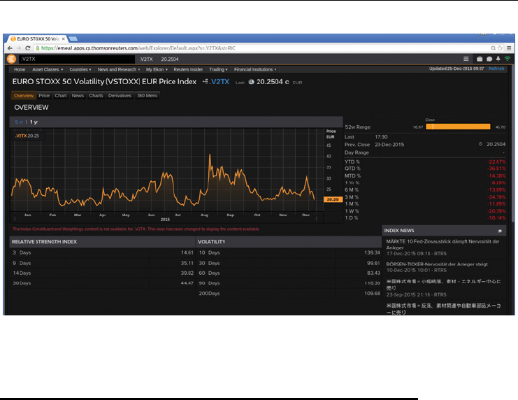
Terms of the VSTOXX and its Derivatives 223
FIGURE 8.1 Thomson Reuters Eikon starting screen for the VSTOXX volatility index (vendor
code: .V2TX).
8.3 VSTOXX FUTURES CONTRACTS
VSTOXX (mini) futures contracts, in the form they are traded today, were introduced in 2009.
Their product ID is FVS. Their main contract terms are described in the following list:
contract value: 100 EUR per index point of the underlying
settlement: cash settlement, on the rst day after nal settlement day
price quotation: the price quotation is in (volatility) points to two decimal places
minimum price change: the minimum price change is 0.05 (volatility) points, i.e. 5 EUR
contract months: the eight nearest successive calendar months
last trading day: last trading day is the nal settlement day
nal settlement day: 30 calendar days before the expiration day of the underlying options,
i.e. 30 calendar days before the third Friday of the expiration month of the underlying
options
daily settlement price: determinded for the current maturity month during the closing
auction of the respective futures contract; for the other maturity months it is determined
by the average bid/ask spread of the combination order book
nal settlement price: determined by Eurex Exchange on the last trading day based on
the values of the underlying VSTOXX index between 11:30 am and 12:00 pm CET
trading hours: 9 am to 10 pm CET (order book and Eurex Trade Entry Services)
block trade size: 1,000 contracts
vendor codes:FVSA Index (Bloomberg) and 0#FVS (Thomson Reuters).
Figure 8.2 shows a screen from the Thomson Reuters Eikon terminal with data about the
VSTOXX futures contracts.
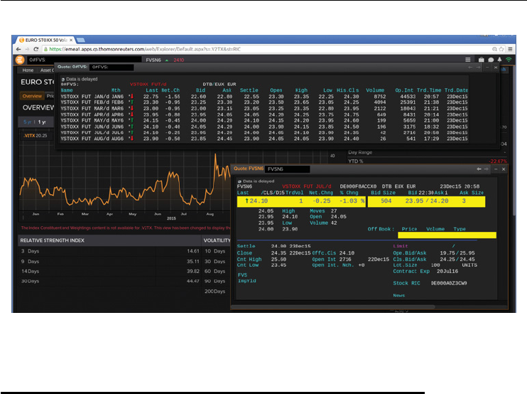
224 LISTED VOLATILITY AND VARIANCE DERIVATIVES
FIGURE 8.2 Thomson Reuters Eikon screen with VSTOXX futures contract information
(vendor code: 0#FVS).
8.4 VSTOXX OPTIONS CONTRACTS
The VSTOXX options contracts, with product ID OVS, were introduced in 2010. Their main
contract terms are described in the following list. They are mainly the same as for the futures
contracts:
contract value: 100 EUR per index point of the underlying
settlement: cash settlement, on the rst day after nal settlement day
price quotation: the price quotation is in (volatility) points with two decimal places
minimum price change: the minimum price change is 0.05 (volatility) points, i.e. 5 EUR
contract months: the eight nearest successive calendar months
last trading day: last trading day is the nal settlement day
nal settlement day: 30 calendar days before the expiration day of the underlying options,
i.e. 30 calendar days before the third Friday of the expiration month of the underlying
options
daily settlement price: determined by Eurex Exchange on the basis of the Black (1976)
model
nal settlement price: determined by Eurex Exchange on the last trading day based on
the values of the underlying VSTOXX index between 11:30 am and 12:00 pm CET
exercise: European style; exercise only on the nal settlement day of the option series
until 9 pm CET
exercise prices: minimum exercise price difference of 1 volatility point
number of exercise prices: at least 11 different exercise prices for both calls and puts
such that 5 are in-the-money, 1 at-the-money, 5 out-of-the-money
trading hours: 9 am to 10 pm CET (order book and Eurex Trade Entry Services)
block trade size: 1,000 contracts
vendor codes:V2X Index OMON (Bloomberg) and <0#FVS+> (Thomson Reuters).
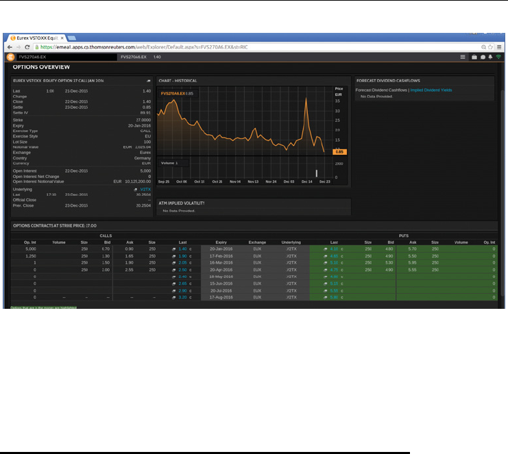
Terms of the VSTOXX and its Derivatives 225
FIGURE 8.3 Thomson Reuters Eikon screen with VSTOXX options contract information (vendor
code: FVS270A6.EX).
Figure 8.3 shows a screen from the Thomson Reuters Eikon terminal with VSTOXX call and
put options data for an exercise price of 27.
8.5 CONCLUSIONS
The previous three chapters cover the VSTOXX volatility index and derivatives written on
it from a conceptual and valuation point of view. This chapter adds information about the
concrete terms of the contracts to the mix. While perhaps not as important from an academic
point of view, they are of paramount importance for practitioners.

PART
Three
Listed Variance Derivatives

CHAPTER 9
Realized Variance and Variance Swaps
9.1 INTRODUCTION
This chapter discusses basic notions and concepts needed in the context of variance swaps and
futures. It covers among others the following topics:
realized variance: the basic measure on which variance swaps and variance futures are
dened
variance swap: the denition of a variance swap and some numerical examples
mark-to-market: the mark-to-market valuation approach for a variance swap
variance swap on EURO STOXX 50: simple re-calculation of a variance swap given
historical data
variance vs. volatility: major differences between the two measures.
9.2 REALIZED VARIANCE
Historical or realized variance 𝜎2generally is dened as
𝜎2≡252
N
⋅
N
n=1
R2
n
where, for a time series Sn,n=0, 1, ...,N, the log returns are given by
Rn≡log Sn
Sn−1
Here, it is assumed that there are 252 trading days per year and that the average daily return is
zero. The simple application of these denitions yields values as decimals. Scaling by a factor
of 1002=10,000 gives values in percent.
𝜎2≡10000 ⋅
252
N
⋅
N
n=1
R2
n
229
Listed Volatility and Variance Derivatives: A
Python-based Guide
By Dr. Yves J. Hilpisch
© 2017 Yves Hilpisch

230 LISTED VOLATILITY AND VARIANCE DERIVATIVES
To simplify notation, we use the notation 𝜎2instead of ̂𝜎2for the realized variance from
here on.
The concept of realized variance is easily illustrated by the use of historical data for the
EURO STOXX 50 stock index. To this end, we read data from the index provider’s web-
site http://www.stoxx.com with Python and the pandas library. For details on using the pan-
das library for interactive nancial analytics see chapter 2, Introduction to Python or refer to
Hilpisch (2014). As usual, we start with some Python library imports.
In [1]: import math
In [2]: import numpy as np
In [3]: import pandas as pd
First, we need the complete URL of the data set.
# text/csv file containing daily closing levels of EURO STOXX 50 index
In [4]: path = 'https://www.stoxx.com/document/Indices/Current/HistoricalData/'
In [5]: es_url = path + 'hbrbcpe.txt'
Second, we read the data with the pandas library from that source. The row structure of that
le changes at the end of 2001 such that we need to dene a helper column which is to be
deleted after importing the data (see also chapter 4, Data Analysis and Strategies).
# column names for the data set
In [6]: cols = ['Date', 'SX5P', 'SX5E', 'SXXP', 'SXXE',
...: 'SXXF', 'SXXA', 'DK5F', 'DKXF', 'DEL']
...:
In [7]: try:# reading the data with pandas
...: es = pd.read_csv(es_url, # filename
...: header=None, # ignore column names
...: index_col=0, # index column (dates)
...: parse_dates=True, # parse these dates
...: dayfirst=True, # format of dates
...: skiprows=4, # ignore these rows
...: sep=';', # data separator
...: names=cols) # use these column names
...: del es['DEL']
...: except:# read stored data if there is no Internet connection
...: es = pd.HDFStore('./source/data/SX5E.h5', 'r')['SX5E']
...:
In [8]: es = es[es.index < '2015-12-31']
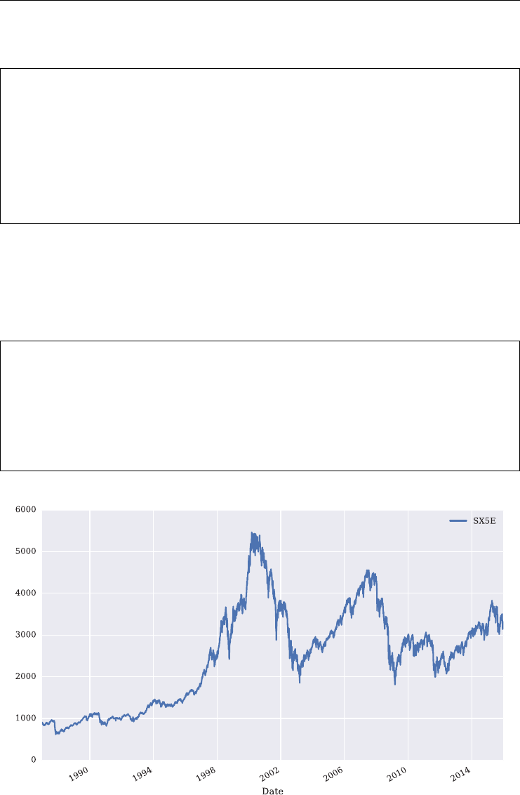
Realized Variance and Variance Swaps 231
Let us inspect the nal ve data rows.
In [9]: es.tail()
Out[9]:
SX5P SX5E SXXP SXXE SXXF SXXA DK5F DKXF
Date
2015-12-23 3109.23 3286.68 366.39 346.14 433.58 375.53 9927.33 614.12
2015-12-24 3108.11 3284.47 366.28 346.05 433.43 375.39 9931.72 614.38
2015-12-28 3093.61 3256.49 364.49 343.54 431.26 374.32 9873.94 611.58
2015-12-29 3139.28 3314.28 369.68 349.29 438.43 378.86 10023.66 620.66
2015-12-30 3118.07 3287.98 367.70 347.02 435.82 377.20 9956.22 617.48
Third, we select the EURO STOXX 50 index data from the data set just downloaded and
imported, i.e. the data sub-set for the symbol SX5E. Using this sub-set, we generate a new
pandas DataFrame object to store the data. The historical time series of daily closing levels
of the EURO STOXX 50 can then easily be inspected by a call of the plot method. Figure 9.1
shows the graphical output.
In [10]: import seaborn as sns; sns.set()
In [11]: import matplotlib
In [12]: matplotlib.rcParams['font.family'] = 'serif'
In [13]: data = pd.DataFrame({'SX5E': es['SX5E']})
In [14]: data.plot(figsize=(10, 6));
FIGURE 9.1 Historical index levels of EURO STOXX 50 index.

232 LISTED VOLATILITY AND VARIANCE DERIVATIVES
Fourth, the log returns are calculated (in vectorized fashion, i.e. simultaneously over the whole
time series) and stored as a new column in the pandas DataFrame object.
In [15]: data['R_n'] = np.log(data['SX5E'] / data['SX5E'].shift(1))
Let us inspect the last ve data rows of this new DataFrame object.
In [16]: data.tail()
Out[16]:
SX5E R_n
Date
2015-12-23 3286.68 0.022262
2015-12-24 3284.47 -0.000673
2015-12-28 3256.49 -0.008555
2015-12-29 3314.28 0.017590
2015-12-30 3287.98 -0.007967
In the fth step, we calculate the realized variance, again in vectorized fashion. With
the following code we calculate the realized variance for every single date of the time
series.
# np.cumsum calculates the element-wise cumulative sum of an array/time series
# np.arange(N) gives an array of the form [0, 1, ..., N-1]
In [17]: data['sigma**2'] = 10000 * 252 * (np.cumsum(data['R_n'] ** 2)
....: / np.arange(len(data)))
....:
The third column of the DataFrame object now contains the realized variance.
In [18]: data.tail()
Out[18]:
SX5E R_n sigma**2
Date
2015-12-23 3286.68 0.022262 446.280005
2015-12-24 3284.47 -0.000673 446.220423
2015-12-28 3256.49 -0.008555 446.185389
2015-12-29 3314.28 0.017590 446.230025
2015-12-30 3287.98 -0.007967 446.191722
In the sixth and nal step, one can now compare the index level time series with the realized
variance over time graphically – see Figure 9.2.
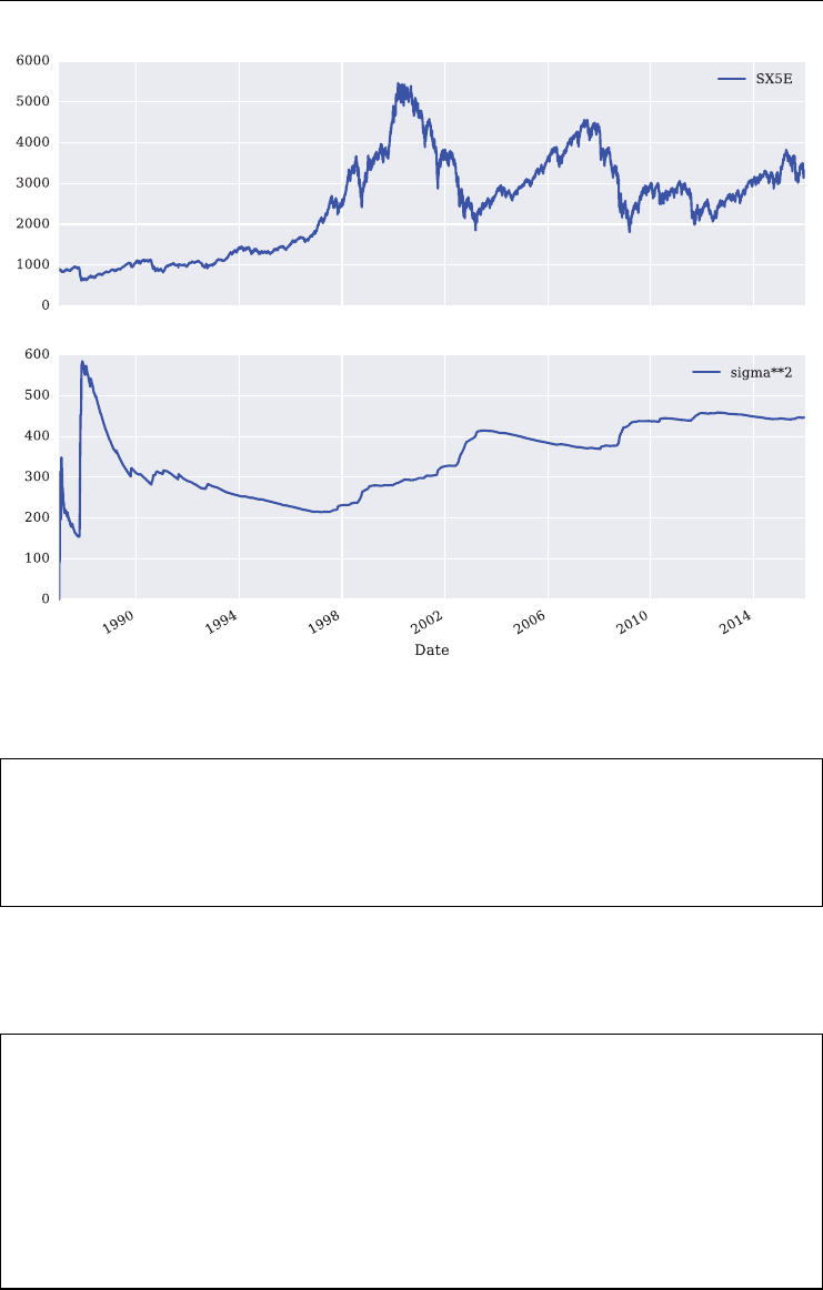
Realized Variance and Variance Swaps 233
FIGURE 9.2 Historical index levels of EURO STOXX 50 index and realized variance (long
term).
In [19]: data[['SX5E', 'sigma**2']].plot(subplots=True,
....: figsize=(10, 8),
....: color='blue',
....: grid=True);
....:
Now let us implement the same approach for a shorter, recent period of time, i.e. the second
half of the year 2015. The realized variance has to be re-calculated since there is now a new
starting date.
# select time series data with date later/earlier than given dates
In [20]: short = data[['SX5E', 'R_n']][(data.index > '2015-7-1')
....: & (data.index <= '2015-12-31')]
....:
# calculate the realized variance in percent values
In [21]: short['sigma**2'] = 10000 * 252 * (np.cumsum(short['R_n'] ** 2)
....: / np.arange(len(short)))
....:
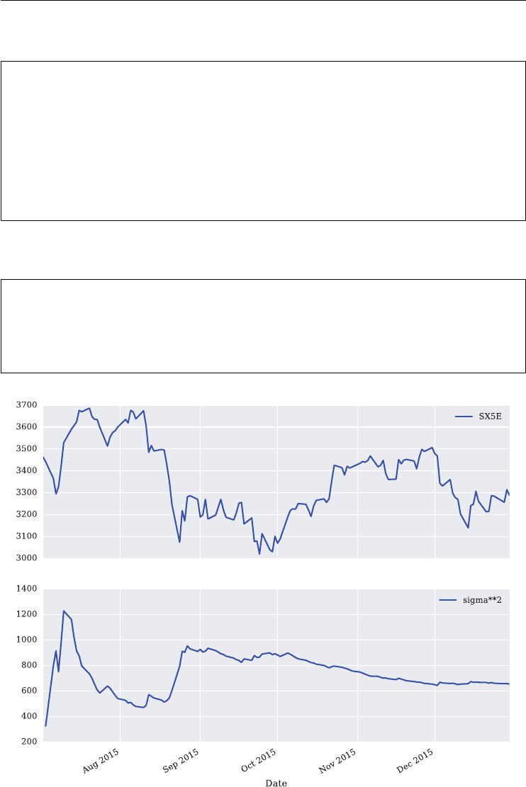
234 LISTED VOLATILITY AND VARIANCE DERIVATIVES
The rst ve rows of the new DataFrame object are as follows:
In [22]: short.head()
Out[22]:
SX5E R_n sigma**2
Date
2015-07-02 3463.25 -0.009492 inf
2015-07-03 3441.76 -0.006224 324.686954
2015-07-06 3365.20 -0.022496 799.967421
2015-07-07 3294.19 -0.021327 915.381074
2015-07-08 3327.50 0.010061 750.306250
A graphical comparison of the EUROS STOXX 50 time series data with its realized variance
for the shorter time frame is displayed in Figure 9.3.
In [23]: short[['SX5E', 'sigma**2']].plot(subplots=True,
....: figsize=(10, 8),
....: color='blue',
....: grid=True);
....:
FIGURE 9.3 Historical index levels of EURO STOXX 50 index and realized variance (short
term).

Realized Variance and Variance Swaps 235
9.3 VARIANCE SWAPS
Nowadays, variance swaps are popular nancial instruments for volatility/variance trading and
hedging purposes. See, for instance, the paper of Bossu et al. (2005) for an overview of the
features and characteristics of variance swaps.
9.3.1 Definition of a Variance Swap
A variance swap is a nancial instrument that allows investors to trade future realized variance
against current implied volatility (the “strike”). The characteristics and payoff of a variance
swap are more like those of a forward contract than those of a typical swap on interest rates,
currencies, equities, etc.
The payoff hTof a variance swap maturing at some future date Tis
hT=𝜎2
0,T−𝜎2
K
with 𝜎2
Kbeing the variance strike and 𝜎Kthe volatility strike.
At inception, i.e. at t=0, the volatility strike is set such that the value of the variance
swap is zero. This implies that the volatility strike is set equal to the implied volatility 𝜎i(0, T)
for the maturity T.
9.3.2 Numerical Example
Consider a Black-Scholes-Merton (1973) world with a geometric Brownian motion driving
uncertainty for the index level of relevance (see Black and Scholes (1973) and Merton (1973)).
The risk-neutral stochastic differential equation (SDE) in this model (without dividends) is
given by:
dSt=rStdt +𝜎StdZt
Stis the index level at time t,rthe constant risk-less short rate, 𝜎the instantaneous volatility and
Zta standard Brownian motion. For a comprehensive treatment of this and other continuous
time nancial models refer, for example, to Bj¨
ork (2009).
Instantaneous volatility (and variance) in this model world is constant which makes
implied volatility also constant, say 𝜎t=𝜎i=𝜎=0.2. Given, for example, a Monte Carlo sim-
ulation of this model, realized variance might deviate from 𝜎2=0.22=0.04. Let us implement
such a Monte Carlo simulation for the model. An Euler discretization scheme for the above
SDE is given for t≥Δtby
St=St−Δtexp r−𝜎2
2Δt+𝜎Δtzt
with Δtbeing the xed time interval used for the discretization and zta standard normally
distributed random variable.
A Python implementation might look as follows (refer to Hilpisch (2014) for details on
Monte Carlo simulation with Python):

236 LISTED VOLATILITY AND VARIANCE DERIVATIVES
def generate_path(S0, r, sigma, T, M):
''' Function to simulate a geometric Brownian motion.
Parameters
==========
S0: float
initial index level
r: float
constant risk-less short rate
sigma: float
instantaneous volatility
T: float
date of maturity (in year fractions)
M: int
number of time intervals
Returns
=======
path: pandas DataFrame object
simulated path
'''
# length of time interval
dt = float(T) / M
# random numbers
np.random.seed(100000)
rn = np.random.standard_normal(M + 1)
rn[0] = 0 # to keep the initial value
# simulation of path
path = S0 * np.exp(np.cumsum((r - 0.5 * sigma ** 2) * dt
+ sigma * math.sqrt(dt) * rn))
# setting initial value
path = pd.DataFrame(path, columns=['index'])
return path
Using this function and providing numerical parameters returns a pandas DataFrame with a
single simulated path for the model. A sample path is shown in Figure 9.4.
In [24]: S0 = 100 # initial index level
In [25]: r = 0.005 # risk-less short rate
In [26]: sigma = 0.2 # instantaneous volatility
In [27]: T = 1.0 # maturity date

Realized Variance and Variance Swaps 237
In [28]: M=50 # number of time intervals
In [29]: data = generate_path(S0, r, sigma, T, M)
In [30]: data.plot(figsize=(10, 5));
Given such a simulated path, one can calculate realized variance over time in the same fashion
as above for the EURO STOXX 50 index.
In [31]: data['R_t'] = np.log(data['index'] / data['index'].shift(1))
# scaling now byM/Tsince returns are not necessarily daily returns
In [32]: data['sigma**2'] = 10000 * M / T * (np.cumsum(data['R_t'] ** 2)
....: / np.arange(len(data)))
....:
In [33]: data.tail()
Out[33]:
index R_t sigma**2
46 86.914274 –0.020492 462.916655
47 86.263467 –0.007516 453.668339
48 87.101314 0.009666 445.190118
49 87.020414 –0.000929 436.113416
50 83.157399 –0.045408 448.009603
Figure 9.5 shows the results graphically.
FIGURE 9.4 Sample path based on geometric Brownian motion.
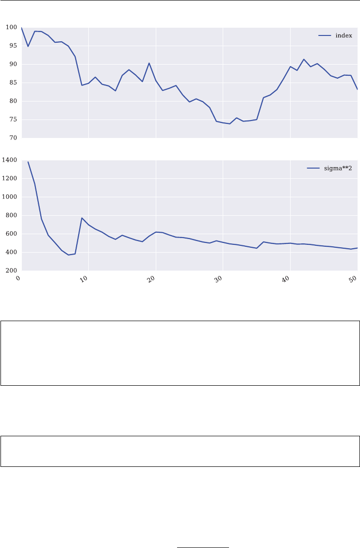
238 LISTED VOLATILITY AND VARIANCE DERIVATIVES
FIGURE 9.5 Geometric Brownian motion sample path with realized variance.
In [34]: data[['index', 'sigma**2']].plot(subplots=True,
....: figsize=(10, 8),
....: color='blue',
....: grid=True);
....:
In this case, the payoff hTof the variance swap at maturity is:
In [35]: data['sigma**2'].iloc[–1] – 20 ** 2
Out[35]: 48.009603247833468
In general, variance swaps have a notional that differs from a value of 1, i.e. the above value
would have to be multiplied by a notional not equal to 1. It is market practice to dene the
variance swap notional in volatility terms:
Notional =VegaNotional
2⋅Strike

Realized Variance and Variance Swaps 239
This can be done consistently due to the following relationship for a derivative instrument f
depending on some underlying Swith volatility 𝜎(and satisfying further technical assump-
tions):
𝜕f
𝜕𝜎 =𝜕f
𝜕(𝜎2)
⋅2𝜎
⇔𝜕f
𝜕(𝜎2)=
𝜕f
𝜕𝜎
2𝜎
Say we want a vega notional of 100,000 currency units, i.e.we want a payoff of 100,000 cur-
rency units per volatility point difference (e.g.when realized volatility is 1 percentage point
above the volatility strike). The variance notional then is
Notional =100000
2⋅20 =2500
In [36]: Notional = 100000. / (2 * 20)
In [37]: Notional
Out[37]: 2500.0
Given this value for the variance notional, the payoff of the variance swap in the above numer-
ical example would be:
In [38]: Notional * (data['sigma**2'].iloc[–1] – 20 ** 2)
Out[38]: 120024.00811958367
9.3.3 Mark-to-Market
What about the value of a variance swap over time? A major advantage of working with vari-
ance (instead of volatility) is that variance is additive over time (when a mean of about zero
is assumed). This gives rise to the following present value of a variance swap at time t,fora
constant short rate r:
Vt=Notional ⋅e−r(T−t)⋅t⋅𝜎2
0,t+(T−t)⋅𝜎2
i(t,T)
T−𝜎2
K
The major component of the mark-to-market value of the variance swap is the time weighted
average of realized variance 𝜎2
0,tup until time tand implied variance 𝜎2
i(t,T) for the remaining
life time from tonwards.

240 LISTED VOLATILITY AND VARIANCE DERIVATIVES
In the model economy, 𝜎2
i(t,T)=𝜎2
K=𝜎2=400. Therefore:
Vt=Notional ⋅e−r(T−t)⋅t⋅𝜎2
0,t+(T−t)⋅400
T−400
For t=0, this obviously gives Vt=0 as desired.
This is readily implemented in Python given that we already have realized variance in a
pandas DataFrame object. We calculate it again in vectorized fashion for t=0, Δt,2Δt...,T.
In [39]: dt=T/M
In [40]: t = np.arange(M + 1) * dt
In [41]: t
Out[41]:
array([0. , 0.02, 0.04, 0.06, 0.08, 0.1 , 0.12, 0.14, 0.16,
0.18, 0.2 , 0.22, 0.24, 0.26, 0.28, 0.3 , 0.32, 0.34,
0.36, 0.38, 0.4 , 0.42, 0.44, 0.46, 0.48, 0.5 , 0.52,
0.54, 0.56, 0.58, 0.6 , 0.62, 0.64, 0.66, 0.68, 0.7 ,
0.72, 0.74, 0.76, 0.78, 0.8 , 0.82, 0.84, 0.86, 0.88,
0.9 , 0.92, 0.94, 0.96, 0.98, 1. ])
In [42]: sigma_K = 20
In [43]: data['V_t'] = Notional * np.exp(–r * (T – t)) * ((t * data['sigma**2']
....: + (T – t) * sigma_K ** 2) / T – sigma_K ** 2)
....:
In [44]: data.tail()
Out[44]:
index R_t sigma**2 V_t
46 86.914274 –0.020492 462.916655 144650.434548
47 86.263467 –0.007516 453.668339 126082.766551
48 87.101314 0.009666 445.190118 108434.594165
49 87.020414 –0.000929 436.113416 88469.022898
50 83.157399 –0.045408 448.009603 120024.008120
Graphically, we get the result as presented in Figure 9.6.
In [45]: data[['index', 'sigma**2', 'V_t']].plot(subplots=True,
....: figsize=(10, 8),
....: color='blue',
....: grid=True);
....:
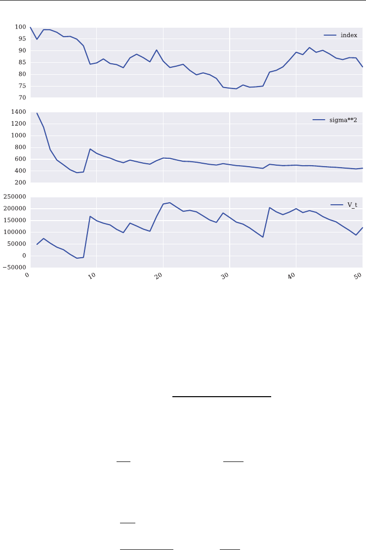
Realized Variance and Variance Swaps 241
FIGURE 9.6 Geometric Brownian motion sample path with realized variance and variance swap
mark-to-market values.
9.3.4 Vega Sensitivity
What is the sensitivity of the mark-to-market value of a variance swap with regard to implied
volatility? Recall that the value itself is given by
Vt=Notional ⋅e−r(T−t)⋅t⋅𝜎2
0,t+(T−t)⋅𝜎2
i(t,T)
T−𝜎2
K
Differentiation with respect to 𝜎igives a vega of
Vegat=𝜕Vt
𝜕𝜎i
=Notional ⋅e−r(T−t)⋅
T−t
T
⋅2𝜎i(t,T)
At inception of the variance swap, we have a vega of
Vega0=𝜕V0
𝜕𝜎i
=VegaNotional
2⋅𝜎i(0, T)
⋅e−r(T−t)⋅
T−t
T
⋅2𝜎i(0, T)
=e−rT ⋅VegaNotional

242 LISTED VOLATILITY AND VARIANCE DERIVATIVES
In this case, vega equals the discounted vega notional. For general t, we get
Vegat=𝜕Vt
𝜕𝜎i
=VegaNotional
2⋅𝜎i(t,T)
⋅e−r(T−t)⋅
T−t
T
⋅2𝜎i(t,T)
=e−r(T−t)⋅VegaNotional ⋅
T−t
T
This illustrates that vega sensitivity diminishes over time and that it is proportional to the
time-to-maturity.
9.3.5 Variance Swap on the EURO STOXX 50
We are now ready to do a historical re-calculation of a variance swap on the EURO STOXX
50. We will re-calculate a variance swap during June 2015. To this end we also use VSTOXX
sub-index data for the shortest maturity available which provides us with a time series for the
correct implied volatilities.
EURO STOXX 50 data is already available.
In [46]: es.info()
<class 'pandas.core.frame.DataFrame'>
DatetimeIndex: 7475 entries, 1986-12-31 to 2015-12-30
Data columns (total 8 columns):
SX5P 7475 non–null float64
SX5E 7475 non–null float64
SXXP 7475 non–null float64
SXXE 7475 non–null float64
SXXF 7475 non–null float64
SXXA 7475 non–null float64
DK5F 7475 non–null float64
DKXF 7475 non–null float64
dtypes: float64(8)
memory usage: 525.6 KB
The VSTOXX data can be read from the same source (see chapter 4, Data Analysis and Strate-
gies).
In [47]: vs_url = path + 'h_vstoxx.txt'
In [48]: try: # reading the data with pandas
....: vs = pd.read_csv(vs_url, # filename
....: index_col=0, # index column (dates)
....: parse_dates=True, # parse date information

Realized Variance and Variance Swaps 243
....: dayfirst=True, # day before month
....: header=2, # header/column names
....: sep=',') # separator character
....: except: # read stored data if there is no Internet connection
....: vs = pd. HDFStore('./source/data/V2TX.h5', 'r')
....:
In [49]: vs.info()
<class 'pandas.core.frame.DataFrame'>
DatetimeIndex: 4357 entries, 1999-01-04 to 2016-02-12
Data columns (total 9 columns):
V2TX 4357 non–null float64
V6I1 3906 non–null float64
V6I2 4357 non–null float64
V6I3 4296 non–null float64
V6I4 4357 non–null float64
V6I5 4357 non–null float64
V6I6 4340 non–null float64
V6I7 4357 non–null float64
V6I8 4343 non–null float64
dtypes: float64(9)
memory usage: 340.4 KB
The data column V6I2 contains the index values (=implied volatility) for the nearest option
series maturity available (i.e within a maximum of one month). For example, on June 1, 2015,
the index values represent implied volatilities for the maturity on the third Friday in June 2015,
i.e. June 19. Maturity Tthen is:
# 15 trading days
In [50]: T = 15.
The variance swap we want to re-calculate should start on June 1, 2015 and will have a maturity
until June 19. It will have a vega notional of 100,000 EUR.
First, let us select and collect the data needed from the available data sets.
In [51]: data = pd.DataFrame(es['SX5E'][(es.index > '2015-5-31')
....: & (es.index < '2015-6-20')])
....:
In [52]: data['V6I1'] = vs['V6I1'][(vs.index > '2015-5-31')
....: & (vs.index < '2015-6-20')]
....:

244 LISTED VOLATILITY AND VARIANCE DERIVATIVES
The new data set looks as follows. Note that the VSTOXX sub-index is only available up until
two days before the maturity date.
In [53]: data
Out[53]:
SX5E V6I1
Date
2015-06-01 3575.04 25.8710
2015-06-02 3561.89 25.9232
2015-06-03 3583.82 25.7958
2015-06-04 3556.38 26.2418
2015-06-05 3510.01 27.4496
2015-06-08 3468.31 27.2996
2015-06-09 3456.79 26.8020
2015-06-10 3526.48 25.8610
2015-06-11 3551.91 26.3897
2015-06-12 3502.77 29.7725
2015-06-15 3438.07 34.5593
2015-06-16 3454.09 36.2222
2015-06-17 3428.76 34.7235
2015-06-18 3450.45 NaN
2015-06-19 3455.80 NaN
We forward ll the NA values since for the vectorized calculations to follow we want to use
these data points but they will have a negligible or zero inuence anyway.
In [54]: data = data.fillna(method='ffill')
We save the data set for later re-use.
In [55]: h5 = pd.HDFStore('./source/data/SX5E_V6I1.h5')
In [56]: h5['SX5E_V6I1'] = data
In [57]: h5.close()
The implied volatility on June 1 was 25.871%. This gives rise to a variance swap
strike of 𝜎2
K=25.8712=669.31. For a vega notional of 100,000, the variance notional
therefore is
Notional =100000
2⋅25.871 =1932.67

Realized Variance and Variance Swaps 245
In [58]: data['V6I1'][0]
Out[58]: 25.870999999999999
In [59]: sigma_K = data['V6I1'][0]
In [60]: Notional = 100000 / (2. * sigma_K)
In [61]: Notional
Out[61]: 1932.665919369178
Three time series now have to be calculated:
log returns of the EURO STOXX 50 index
realized variance of the EURO STOXX 50 index
mark-to-market values of the variance swap.
First, the log returns.
In [62]: data['R_t'] = np.log(data['SX5E'] / data['SX5E'].shift (1))
Second, the realized variance which we scale by a factor of 10,000 to end up with percentage
values and not decimal values.
In [63]: data['sigma**2'] = 10000 * 252 * (np.cumsum(data['R_t'] ** 2)
....: / np.arange(len(data)))
....:
Third, the mark-to-market values. We start with the array of elapsed days.
In [64]: t = np.arange(1, 16)
In [65]: t
Out[65]: array([ 1, 2, 3, 4, 5, 6, 7, 8, 9, 10, 11, 12, 13, 14, 15])
We assume a xed short rate of 0.1%.
In [66]: r = 0.001
In [67]: data['V_t'] = np.exp(–r * (T – t) / 365.) * ((t * data['sigma**2']
....: + (T – t) * data['V6I1'] ** 2) / T – sigma_K ** 2)
....:
The initial value of the variance swap is zero.

246 LISTED VOLATILITY AND VARIANCE DERIVATIVES
In [68]: data['V_t'].loc['2015-06-01'] = 0.0
The complete results data set is given below.
In [69]: data
Out[69]:
SX5E V6I1 R_t sigma**2 V_t
Date
2015-06-01 3575.04 25.8710 NaN NaN 0.000000
2015-06-02 3561.89 25.9232 -0.003685 34.220799 -82.332277
2015-06-03 3583.82 25.7958 0.006138 64.580457 -124.049833
2015-06-04 3556.38 26.2418 -0.007686 92.677552 -139.593571
2015-06-05 3510.01 27.4496 -0.013124 178.023718 -107.644092
2015-06-08 3468.31 27.2996 -0.011951 214.408816 -136.380856
2015-06-09 3456.79 26.8020 -0.003327 183.323049 -200.634978
2015-06-10 3526.48 25.8610 0.019960 300.555651 -196.905901
2015-06-11 3551.91 26.3897 0.007185 279.249096 -223.189008
2015-06-12 3502.77 29.7725 -0.013931 302.564935 -172.129074
2015-06-15 3438.07 34.5593 -0.018644 359.901600 -86.887791
2015-06-16 3454.09 36.2222 0.004649 332.134168 -141.190592
2015-06-17 3428.76 34.7235 -0.007360 315.833038 -234.822528
2015-06-18 3450.45 34.7235 0.006306 299.246550 -309.629583
2015-06-19 3455.80 34.7235 0.001549 278.303868 -391.004773
The payoff of the variance swap at maturity given the variance notional then is:
In [70]: Notional * data['V_t'][-1]
Out[70]: -755681.59959400445
Finally, a plot of the major results is presented as Figure 9.7.
In [71]: data[['SX5E', 'sigma**2', 'V_t']].plot(subplots=True,
....: color='blue',
....: figsize=(10, 8));
....:
We save the data for use in the next chapter.
In [72]: h5 = pd.HDFStore('./source/data/var_data.h5', 'a')
In [73]: h5['var_swap'] = data
In [74]: h5.close()
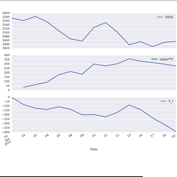
Realized Variance and Variance Swaps 247
FIGURE 9.7 EURO STOXX 50 historical index levels with realized variance and futures prices.
9.4 VARIANCE VS. VOLATILITY
Both variance and volatility are tradable asset classes. The following sub-sections discuss some
differences between the two measures of variability and the two asset classes, respectively. See
also Bennett and Gil (2012) on this topic.
9.4.1 Squared Variations
Squared variations are in many application scenarios the better measure for variability com-
pared to simple variations. By squaring variations, one makes sure that variations do not cancel
each other out. Since volatility is generally dened as the square root of variance, both mea-
sures avoid the cancelling of positive and negative variations.
9.4.2 Additivity in Time
Although both volatility and variance avoid the cancelling out of variations, there is a major
difference between both when it comes to additivity. While variance is additive (linear) in time,
volatility is convex (nonlinear) in time.

248 LISTED VOLATILITY AND VARIANCE DERIVATIVES
Assume we have Nreturn observations and assume 0 <M<N. We then have:
𝜎2≡252
N
⋅
N
n=1
R2
n
=252
N
⋅M
n=1
R2
n+
N
n=M+1
R2
n
=252
N
⋅
M
n=1
R2
n+252
N
⋅
N
n=M+1
R2
n
≡𝜎2
1+𝜎2
2
Here, 𝜎2
1is the variance for the rst part and 𝜎2
2for the second part of the return observations.
Note that one needs to keep the weighting factor constant at 252
Nin order to retain additivity.
This aspect can be illustrated by a simple numerical example. Consider rst a function to
calculate realized variance that we can re-use.
# function to calculate the realized variance
In [75]: rv =lambda ret_dat: 10000 * 252. / N * np.sum(ret_dat ** 2)
Second, a simple example data set...
In [76]: data = np.array([0.01, 0.02, 0.03, 0.04, 0.05])
…of length N=5.
In [77]: N = len(data)
In [78]: N
Out[78]: 5
Then, we can easily see additivity.
In [79]: rv(data[:2]) + rv(data[2:])
Out[79]: 2772.0000000000005
In [80]: rv(data)
Out[80]: 2772.0000000000005

Realized Variance and Variance Swaps 249
Next, we use the EURO STOXX 50 index data from before. Let us have a look at the year
2013 and the two halves of the year.
In [81]: data = pd.DataFrame(es['SX5E'][(es.index > '31-12-2012')
....: & (es.index < '01-01-2014')])
....:
# we need log returns
In [82]: data['R_t'] = np.log(data['SX5E'] / data['SX5E'].shift(1))
We have 256 index level observations and 255 return observations.
In [83]: N = len(data) – 1
In [84]: N
Out[84]: 255
In [85]: var_1st = rv(data['R_t'][data.index < '2013-07-01'])
In [86]: var_1st
Out[86]: 159.1490165508348
In [87]: var_2nd = rv(data['R_t'][data.index > '2013-06-30'])
In [88]: var_2nd
Out[88]: 98.3424775210876
Again, additivity is given for the realized variance.
In [89]: var_1st + var_2nd
Out[89]: 257.4914940719224
In [90]: var_full = rv(data['R_t'])
In [91]: var_full
Out[91]: 257.4914940719223
Obviously, this is different when considering realized volatility instead of variance.
In [92]: vol_1st = math.sqrt(rv(data['R_t'][data.index < '2013-07-01']))
In [93]: vol_1st
Out[93]: 12.615427719694438

250 LISTED VOLATILITY AND VARIANCE DERIVATIVES
In [94]: vol_2nd = math.sqrt(rv(data['R_t'][data.index > '2013-06-30']))
In [95]: vol_2nd
Out[95]: 9.916777577473823
In [96]: vol_1st + vol_2nd
Out[96]: 22.53220529716826
In [97]: vol_full = math.sqrt(rv(data['R_t']))
In [98]: vol_full
Out[98]: 16.04654149877544
This is something to be expected due to the sub-additivity a+b≤a+bof the square-
root function.
9.4.3 Static Hedges
Realized variance can be statically replicated (hedged) by positions in out-of-the money put
and call options. This is a well-known result which is presented in detail in chapter 3, Model-
Free Replication of Variance. It is the basic idea and approach underlying volatility indexes
like the VSTOXX and the VIX. This also makes it possible to statically replicate and hedge
variance swaps by the use of options – something not true for volatility swaps, for example.
9.4.4 Broad Measure of Risk
Implied volatility generally is only dened for a certain maturity and a certain strike. When the
spot moves, at-the-money implied volatility changes as well. By contrast, (implied) variance
is a measure taking into account all strikes for a given maturity. This can be seen from the fact
that the traded variance level of a variance swap is applicable independently of the spot of the
underlying (index).
9.5 CONCLUSIONS
This chapter introduces variance swaps both theoretically as well as based on concrete numer-
ical examples. Central notions are realized variance, variance/volatility strike and variance
notional. Mark-to-market valuations of such instruments are easily accomplished due to their
very nature. As a consequence, sensitivities of variance swaps, for example, with regard to vega
are also easily derived. The major numerical example is based on EURO STOXX 50 index and
log return data. A hypothetical variance swap with inception on June 1, 2015 and maturity on
June 19, 2015 is valued by the mark-to-market approach using VSTOXX sub-index data with
the very same maturity as a proxy for the implied volatility during the life time of the variance
swap.

CHAPTER 10
Variance Futures at Eurex
10.1 INTRODUCTION
Based on the previous chapter, this chapter introduces the Eurex variance futures contracts and
their major characteristics. It covers mainly the following topics:
introduction to and motivation for Eurex variance futures
variance futures concepts needed to understand and trade in Eurex variance futures
example calculation for a variance future illustrating the concepts by numerical results
comparison between variance swaps and futures based on the numerical example.
By introducing variance futures on the EURO STOXX 50 stock index, Eurex standardizes one
of the most popular types of volatility/variance derivatives, namely variance swaps. Such a
standardization brings a number of benets to the markets:
unied terms: standardization leads to unied, well-documented terms
transparency: centralized trading at Eurex increases transparency for all market partici-
pants
liquidity: standardization and centralization increase liquidity (market depth) in the vari-
ance futures
fungibility: variance futures are fully fungible and can be traded in and out at any point
over their life time
increased market integrity: clearing by Eurex ensures, among other things, low coun-
terparty risk and high risk management standards.
Variance futures replicate the payoff of Over-the-Counter (OTC) variance swaps and are traded
based on OTC conventions in vega notional and at volatility strikes. Daily margin payments
based on settlement prices add up to the nal settlement payoff of the OTC variance swap. The
start of trading for the variance futures of Eurex was September 22, 2014.
Net present value (NPV) effects are accounted for by two different pricing components:
discount factor as for the mark-to-market for variance swaps
accumulated return on modied variation margin (ARMVM) for the daily margin
payments.
251
Listed Volatility and Variance Derivatives: A
Python-based Guide
By Dr. Yves J. Hilpisch
© 2017 Yves Hilpisch

252 LISTED VOLATILITY AND VARIANCE DERIVATIVES
In order to perfectly mimic the cash ow of a variance swap with the same terms, variance
futures trading makes certain conversions necessary. This is mainly due to the variance swaps
being based on end-of-day returns of the respective index (which cannot be exactly known
during the day). Therefore, there are two conversions:
intraday: intraday trades are booked with the desired quantity and at preliminary futures
prices
end-of-day: at the end of the day, intraday trades are cancelled and re-booked with the
same quantity at the futures settlement prices (taking into account the realized variance
for the rest of the day, i.e. since the time the trade was initially booked).
All trades are booked and conversions are made by the Eurex T7 trading system. While vari-
ance futures are quoted in vega notional and volatility strikes, bookings and clearings are made
only in futures and futures prices.
10.2 VARIANCE FUTURES CONCEPTS
Standardized trading and settlement in variance futures is based on a number of nancial con-
cepts. This section introduces all necessary concepts and provides formal denitions.
10.2.1 Realized Variance
Realized variance 𝜎2for the Eurex variance futures is dened as
𝜎2≡10000 ⋅
252
N
⋅
N
n=1
R2
n
where, for a time series Sn,n=0, 1, …,N, of daily EURO STOXX 50 closing values, the log
returns are given by
Rn≡log Sn
Sn−1
Here, it is assumed that there are 252 trading days per year and that the average daily return is
zero. Note the scaling factor of 10,000 to get to the market convention of quoting variance in
percent and not in decimal values.
10.2.2 Net Present Value Concepts
There are two concepts that take into account that the daily margin cash ows of trading futures
leads, time-wise, to a different cash ow prole than the single payoff of a variance future at
maturity.

Variance Futures at Eurex 253
Discount Factor The rst is the discount factor DFtwhich is dened for a maturity date
Tand a current date tby
DFt=e−r(T−t)
365
Here, ris the relevant interest rate to be applied to the remaining time-to-maturity (T−t),
calculated in days. Eurex uses Euribor rates to calculate the discount factor.
Let us have a look at the development of the Euribor rates in 2014 from January to the
beginning of September. Euribor rates are available on the website www.euribor-rates.eu or
in a slightly more convenient form as Excel spreadsheet les for download on the website
www.emmi-benchmarks.eu/euribor-org/euribor-rates.html. From this last website, we have
downloaded Euribor rates data for 2014 which we use in the following. For details on the
Python usage that follows, see chapter 2, Introduction to Python or refer to Hilpisch (2014).
pandas is once again the library we are working with.
In [1]: import pandas as pd
With pandas, you can read data from a spreadsheet le as follows:
# read data from CSV file
In [2]: eb = pd.read_csv('./source/data/hist_EURIBOR_2015.csv', # filename
...: index_col=0, # index column
...: parse_dates=True, # parsing date information
...: dayfirst=True) # European date convention
...:
In [3]: eb. info()
<class 'pandas.core.frame.DataFrame'>
DatetimeIndex: 135 entries, 2015-01-02 to 2015-07-14
Data columns (total 8 columns):
1w 135 non-null float64
2w 135 non-null float64
1m 135 non-null float64
2m 135 non-null float64
3m 135 non-null float64
6m 135 non-null float64
9m 135 non-null float64
12m 135 non-null float64
dtypes: float64(8)
memory usage: 9.5 KB
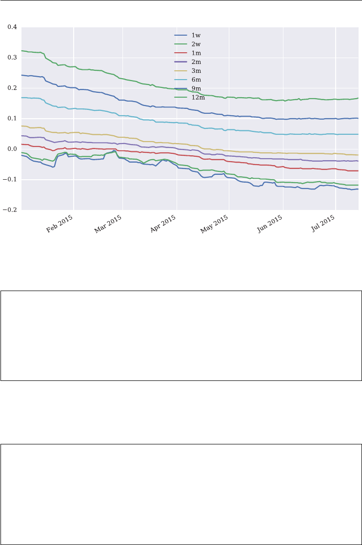
254 LISTED VOLATILITY AND VARIANCE DERIVATIVES
FIGURE 10.1 Historical Euribor rates.
Figure 10.1 shows the evolution of the eight different rates over time (values in percent).
In [4]: import seaborn as sns; sns. set()
In [5]: import matplotlib
In [6]: matplotlib.rcParams['font.family'] = 'serif'
In [7]: eb.plot(figsize=(10, 6));
Short term interest rates are pretty low, leading to a rather low impact of the discount factor in
such an environment. Let us calculate the discount factor for the longest maturity with the last
available rate for the 12 month horizon.
In [8]: eb.tail()
Out[8]:
1w 2w 1m 2m 3m 6m 9m 12m
2015-07-08 -0.131 -0.118 -0.071 -0.038 -0.018 0.049 0.101 0.164
2015-07-09 -0.131 -0.118 -0.071 -0.039 -0.018 0.049 0.100 0.163
2015-07-10 -0.133 -0.118 -0.071 -0.039 -0.018 0.049 0.101 0.164
2015-07-13 -0.131 -0.118 -0.071 -0.038 -0.019 0.049 0.102 0.166
2015-07-14 -0.131 -0.118 -0.071 -0.039 -0.019 0.049 0.101 0.168
For a 12 month period the discount effect is less than half a percent.

Variance Futures at Eurex 255
In [9]: import math
In [10]: math.exp(-0.00168 * 365. / 365)
Out[10]: 0.9983214104100598
ARMVM The accumulated return on modied variation margin (ARMVM) takes into account
that variance futures trading leads to daily margin payments that have an impact on the present
value of the variance future. For given dates tand t−1, ARMVM is given by
ARMV Mt=ARMV Mt−1⋅e
rΔt
365 +FS
t−1−Ce
rΔt
365 −1
Here, ris the relevant interest rate to be used, Δtis the difference between dates tand t−1in
days, FS
t−1is the variance futures settlement price at t−1 and Cis a constant xed at a level
of 3,000. If t=1, i.e. on the rst settlement day (say Monday), ARMVM1≡0 and FS
1≡C.
The relevant rate for the ARMVM calculation is the Eonia rate. On the web-
site www.emmi-benchmarks.eu/euribor-eonia-org/about-eonia.html you nd the following
explanation:
“Eonia®(Euro OverNight Index Average) is the effective overnight reference
rate for the euro. It is computed as a weighted average of all overnight
unsecured lending transactions in the interbank market, undertaken in the
European Union and European Free Trade Association (EFTA) countries.”
This website also provides historical Eonia data for download. Let us have a look at the his-
torical development of the Eonia rates for a couple of weeks in 2015.
# read data from Excel spreadsheet file
In [11]: eo = pd.read_csv('./source/data/hist_EONIA_2015.csv', # filename
....: index_col=0, # index column
....: parse_dates=True, # parsing date information
....: dayfirst=True) # European date convention
....:
In [12]: eo. info()
<class 'pandas.core.frame.DataFrame'>
DatetimeIndex: 60 entries, 2015-04-21 to 2015-07-14
Data columns (total 1 columns):
EONIA 60 non-null float64
dtypes: float64(1)
memory usage: 960.0 bytes
Again, we can easily visualize the data set (see Figure 10.2).

256 LISTED VOLATILITY AND VARIANCE DERIVATIVES
FIGURE 10.2 Historical Eonia rates.
In [13]: eo.plot(figsize=(10, 5))
Out[13]: <matplotlib.axes._subplots.AxesSubplot at 0x2ab2484c2d50>
<matplotlib.figure.Figure at 0x2ab247dd0050>
The last available values in the data set for Eonia are:
In [14]: eo.tail()
Out[14]:
EONIA
2015-07-08 -0.118
2015-07-09 -0.121
2015-07-10 -0.120
2015-07-13 -0.118
2015-07-14 -0.112
Let us work with a value (in decimals) of reo =−0.001.
In [15]: r_eo = -0.001
Now consider the second settlement day t=2 (say Tuesday), assume that a rate of reo applies
and remember that FS
1=3000. We then have
ARMV M2=0⋅e
reo⋅1
365 +(3000 −3000)e
reo⋅1
365 −1=0

Variance Futures at Eurex 257
Consider now the third settlement day t=3 (say Wednesday). Assume that the futures settle-
ment price has risen the day before to FS
2=3100. Now
ARMV M3=0⋅e
reo⋅1
365 +(3100 −3000)e
reo⋅1
365 −1
The effect is rather small.
In [16]: ARMVM3 = 0 * math.exp(r_eo / 365) + (3100 - 3000)
* (math.exp(r_eo / 365) - 1)
In [17]: ARMVM3
Out[17]: -0.0002739722274380796
One day later, on the fourth settlement day t=4, and assuming that the variance futures set-
tlement price has fallen the day before to F3=3050, we get
ARMV M4=ARMV M3⋅e
reo⋅1
365 +(3050 −3000)e
reo⋅1
365 −1
In [18]: ARMVM4 = (ARMVM3 * math.exp(r_eo / 365)
....: + (3050 - 3000) * (math.exp(r_eo / 365) - 1))
....:
In [19]: ARMVM4
Out[19]: -0.0004109575905493053
10.2.3 Traded Variance Strike
The traded variance strike 𝜎2
tat date tis the time weighted average of the realized variance 𝜎2
0,t
weighted by the number of elapsed days tand the traded implied variance 𝜎2
i(t,T) weighted
by the remaining life time of the variance future in days:
𝜎2
t=
t⋅𝜎2
0,t+(T−t)⋅𝜎2
i(t,T)
T
10.2.4 Traded Futures Price
The traded futures price Ftgiven the other quantities from before is then dened as
Ft=DFt⋅𝜎2
t−𝜎2
i(t,T)−ARMV Mt+3000
The scaling constant C=3000 is chosen to ensure that the futures price cannot become
negative.

258 LISTED VOLATILITY AND VARIANCE DERIVATIVES
10.2.5 Number of Futures
Variance futures are traded in vega notional and volatility strikes. However, settlement takes
place in futures (or variance notional) and variance strikes. The number of futures is calculated
according to the formula
futures =VegaNotional
2⋅𝜎i(t,T)
⋅
T
T−t
with 𝜎i(t,T) as the traded implied volatility strike.
10.2.6 Par Variance Strike
At daily settlement, i.e. when the log return for the EURO STOXX 50 for that day is
known, the par variance strike 𝜎2
pis calculated using the then current settled implied
volatility 𝜎i.
𝜎2
p=
t⋅𝜎2
0,t+(T−t)⋅𝜎2
i
T
10.2.7 Futures Settlement Price
Finally, the daily futures settlement price FS
tis calculated according to the following formula
where all components are as dened as before:
FS
t=DFt⋅𝜎2
p−𝜎2
K−ARMV Mt+3000
The futures settlement price is the mark-to-market value of the corresponding variance swap
minus the ARMVM plus the scaling factor of 3,000.
10.3 EXAMPLE CALCULATION FOR A VARIANCE FUTURE
In this section, we conduct an example calculation for the Eurex variance futures contract given
historical data as used in sub-section 9.3.5, Variance Swap on the EURO STOXX 50.
In [20]: import pandas as pd
In [21]: h5 = pd.HDFStore('./source/data/SX5E_V6I1.h5', 'r')
In [22]: data = h5['SX5E_V6I1']
In [23]: h5.close()
In [24]: data

Variance Futures at Eurex 259
Out[24]:
SX5E V6I1
Date
2015-06-01 3575.04 25.8710
2015-06-02 3561.89 25.9232
2015-06-03 3583.82 25.7958
2015-06-04 3556.38 26.2418
2015-06-05 3510.01 27.4496
2015-06-08 3468.31 27.2996
2015-06-09 3456.79 26.8020
2015-06-10 3526.48 25.8610
2015-06-11 3551.91 26.3897
2015-06-12 3502.77 29.7725
2015-06-15 3438.07 34.5593
2015-06-16 3454.09 36.2222
2015-06-17 3428.76 34.7235
2015-06-18 3450.45 34.7235
2015-06-19 3455.80 34.7235
We add Euribor and Eonia data to the pandas DataFrame object. For simplicity, we use the
2 week Euribor values throughout.
In [25]: data = data.join(eb['2w'], how='left')
In [26]: data = data.join(eo, how='left')
In [27]: data
Out[27]:
SX5E V6I1 2w EONIA
Date
2015-06-01 3575.04 25.8710 -0.108 -0.106
2015-06-02 3561.89 25.9232 -0.109 -0.122
2015-06-03 3583.82 25.7958 -0.109 -0.143
2015-06-04 3556.38 26.2418 -0.109 -0.138
2015-06-05 3510.01 27.4496 -0.109 -0.115
2015-06-08 3468.31 27.2996 -0.110 -0.127
2015-06-09 3456.79 26.8020 -0.110 -0.126
2015-06-10 3526.48 25.8610 -0.111 -0.117
2015-06-11 3551.91 26.3897 -0.111 -0.120
2015-06-12 3502.77 29.7725 -0.113 -0.125
2015-06-15 3438.07 34.5593 -0.108 -0.119
2015-06-16 3454.09 36.2222 -0.109 -0.125
2015-06-17 3428.76 34.7235 -0.109 -0.110
2015-06-18 3450.45 34.7235 -0.109 -0.118
2015-06-19 3455.80 34.7235 -0.108 -0.120

260 LISTED VOLATILITY AND VARIANCE DERIVATIVES
Let us add the log returns to the data set as well as the realized variance.
In [28]: import numpy as np
In [29]: data['R_t'] = np.log(data['SX5E'] / data['SX5E'].shift(1))
In [30]: data['sigma**2'] = 10000 * 252 * (np.cumsum(data['R_t'] ** 2)
....: / np.arange(len(data)))
....:
In [31]: data
Out[31]:
SX5E V6I1 2w EONIA R_t sigma**2
Date
2015-06-01 3575.04 25.8710 -0.108 -0.106 NaN NaN
2015-06-02 3561.89 25.9232 -0.109 -0.122 -0.003685 34.220799
2015-06-03 3583.82 25.7958 -0.109 -0.143 0.006138 64.580457
2015-06-04 3556.38 26.2418 -0.109 -0.138 -0.007686 92.677552
2015-06-05 3510.01 27.4496 -0.109 -0.115 -0.013124 178.023718
2015-06-08 3468.31 27.2996 -0.110 -0.127 -0.011951 214.408816
2015-06-09 3456.79 26.8020 -0.110 -0.126 -0.003327 183.323049
2015-06-10 3526.48 25.8610 -0.111 -0.117 0.019960 300.555651
2015-06-11 3551.91 26.3897 -0.111 -0.120 0.007185 279.249096
2015-06-12 3502.77 29.7725 -0.113 -0.125 -0.013931 302.564935
2015-06-15 3438.07 34.5593 -0.108 -0.119 -0.018644 359.901600
2015-06-16 3454.09 36.2222 -0.109 -0.125 0.004649 332.134168
2015-06-17 3428.76 34.7235 -0.109 -0.110 -0.007360 315.833038
2015-06-18 3450.45 34.7235 -0.109 -0.118 0.006306 299.246550
2015-06-19 3455.80 34.7235 -0.108 -0.120 0.001549 278.303868
Assume that the variance future comes to life on June 1, 2015 and that it matures on June 19,
2015. This is a maturity of T=15 trading days. Let us generate in addition an array with all
(elapsed) trading days over time.
In [32]: T = 15.
In [33]: data['t'] = np. arange(1, 16)
In [34]: data['t']
Out[34]:
Date
2015-06-01 1
2015-06-02 2
2015-06-03 3

Variance Futures at Eurex 261
2015-06-04 4
2015-06-05 5
2015-06-08 6
2015-06-09 7
2015-06-10 8
2015-06-11 9
2015-06-12 10
2015-06-15 11
2015-06-16 12
2015-06-17 13
2015-06-18 14
2015-06-19 15
Name: t, dtype: int64
Assuming a constant Euribor rate of −0.1%, we can add a new column to the DataFrame
object with the discount factors in vectorized fashion (see chapter 11, Trading and Settlement
for further details on the discount factor calculation).
In [35]: r_eb = -0.001
In [36]: data['DF_t'] = np.exp(-r_eb * (T - data['t']) / 365.)
In [37]: data
Out[37]:
SX5E V6I1 2w EONIA R_t sigma**2 t DF_t
Date
2015-06-01 3575.04 25.8710 -0.108 -0.106 NaN NaN 1 1.000038
2015-06-02 3561.89 25.9232 -0.109 -0.122 -0.003685 34.220799 2 1.000036
2015-06-03 3583.82 25.7958 -0.109 -0.143 0.006138 64.580457 3 1.000033
2015-06-04 3556.38 26.2418 -0.109 -0.138 -0.007686 92.677552 4 1.000030
2015-06-05 3510.01 27.4496 -0.109 -0.115 -0.013124 178.023718 5 1.000027
2015-06-08 3468.31 27.2996 -0.110 -0.127 -0.011951 214.408816 6 1.000025
2015-06-09 3456.79 26.8020 -0.110 -0.126 -0.003327 183.323049 7 1.000022
2015-06-10 3526.48 25.8610 -0.111 -0.117 0.019960 300.555651 8 1.000019
2015-06-11 3551.91 26.3897 -0.111 -0.120 0.007185 279.249096 9 1.000016
2015-06-12 3502.77 29.7725 -0.113 -0.125 -0.013931 302.564935 10 1.000014
2015-06-15 3438.07 34.5593 -0.108 -0.119 -0.018644 359.901600 11 1.000011
2015-06-16 3454.09 36.2222 -0.109 -0.125 0.004649 332.134168 12 1.000008
2015-06-17 3428.76 34.7235 -0.109 -0.110 -0.007360 315.833038 13 1.000005
2015-06-18 3450.45 34.7235 -0.109 -0.118 0.006306 299.246550 14 1.000003
2015-06-19 3455.80 34.7235 -0.108 -0.120 0.001549 278.303868 15 1.000000
The standard volatility strike is 𝜎K=25.871 and the standard variance strike is 𝜎2
K=
25.8712=669.31.

262 LISTED VOLATILITY AND VARIANCE DERIVATIVES
In [38]: sigma_K = data['V6I1'][0]
In [39]: sigma_K
Out[39]: 25.870999999999999
Assume a vega notional of 100,000. This translates into a variance notional of:
In [40]: Notional = 100000 / (2 * sigma_K)
In [41]: Notional
Out[41]: 1932.665919369178
The settlement price on the rst trading day is standardized to 3,000. We generate a new column
in the pandas DataFrame object and initialize the rst value (and all the others) accordingly.
In [42]: data['F_tS'] = 3000
In [43]: data
Out[43]:
SX5E V6I1 2w EONIA R_t sigma**2 t \
Date
2015-06-01 3575.04 25.8710 -0.108 -0.106 NaN NaN 1
2015-06-02 3561.89 25.9232 -0.109 -0.122 -0.003685 34.220799 2
2015-06-03 3583.82 25.7958 -0.109 -0.143 0.006138 64.580457 3
2015-06-04 3556.38 26.2418 -0.109 -0.138 -0.007686 92.677552 4
2015-06-05 3510.01 27.4496 -0.109 -0.115 -0.013124 178.023718 5
2015-06-08 3468.31 27.2996 -0.110 -0.127 -0.011951 214.408816 6
2015-06-09 3456.79 26.8020 -0.110 -0.126 -0.003327 183.323049 7
2015-06-10 3526.48 25.8610 -0.111 -0.117 0.019960 300.555651 8
2015-06-11 3551.91 26.3897 -0.111 -0.120 0.007185 279.249096 9
2015-06-12 3502.77 29.7725 -0.113 -0.125 -0.013931 302.564935 10
2015-06-15 3438.07 34.5593 -0.108 -0.119 -0.018644 359.901600 11
2015-06-16 3454.09 36.2222 -0.109 -0.125 0.004649 332.134168 12
2015-06-17 3428.76 34.7235 -0.109 -0.110 -0.007360 315.833038 13
2015-06-18 3450.45 34.7235 -0.109 -0.118 0.006306 299.246550 14
2015-06-19 3455.80 34.7235 -0.108 -0.120 0.001549 278.303868 15
DF_t F_tS
Date
2015-06-01 1.000038 3000
2015-06-02 1.000036 3000
2015-06-03 1.000033 3000
2015-06-04 1.000030 3000
2015-06-05 1.000027 3000

Variance Futures at Eurex 263
2015-06-08 1.000025 3000
2015-06-09 1.000022 3000
2015-06-10 1.000019 3000
2015-06-11 1.000016 3000
2015-06-12 1.000014 3000
2015-06-15 1.000011 3000
2015-06-16 1.000008 3000
2015-06-17 1.000005 3000
2015-06-18 1.000003 3000
2015-06-19 1.000000 3000
The ARMVM on the rst settlement day is zero. We again generate a new column and initialize
all values with zero.
In [44]: data['ARMVM_t'] = 0.0
The futures price on the second settlement day is given as:
In [45]: data['F_tS'][1] = data['DF_t'][1] * ((data['t'][1] * data['sigma**2'][1]
....: + (T - data['t'][1]) * data['V6I1'][1] ** 2) / T
....: - sigma_K ** 2) + 3000
....:
In [46]: data['F_tS'][1]
Out[46]: 2917
Analogously, we can calculate the settlement prices for all other settlement days. Note that
we take the index level of the EURO STOXX 50 at close and not the average of its level
between 11:50 and 12:00 CET at the nal settlement day (see chapter 11, Trading and
Settlement).
In [47]: for tin data.index[1:]:
....: data['ARMVM_t'][t] = (data['ARMVM_t'].shift(1)[t]
....: * math.exp(data['EONIA'].shift(1)[t] / 252)
....: + (data['F_tS'].shift(1)[t] - 3000)
....: * (math.exp(data['EONIA'].shift(1)[t] / 252) - 1))
....: data['F_tS'][t] = data['DF_t'][t] * ((data['t'][t] * data['sigma**2'][t]
....: + (T - data['t'][t]) * data['V6I1'][t] ** 2) / T
....: -sigma_K ** 2)- data['ARMVM_t'][t] + 3000
....:
We end up with a complete data set, and in particular the simulated variance futures settlement
values.

264 LISTED VOLATILITY AND VARIANCE DERIVATIVES
In [48]: data
Out[48]:
SX5E V6I1 2w EONIA R_t sigma**2 t \
Date
2015-06-01 3575.04 25.8710 -0.108 -0.106 NaN NaN 1
2015-06-02 3561.89 25.9232 -0.109 -0.122 -0.003685 34.220799 2
2015-06-03 3583.82 25.7958 -0.109 -0.143 0.006138 64.580457 3
2015-06-04 3556.38 26.2418 -0.109 -0.138 -0.007686 92.677552 4
2015-06-05 3510.01 27.4496 -0.109 -0.115 -0.013124 178.023718 5
2015-06-08 3468.31 27.2996 -0.110 -0.127 -0.011951 214.408816 6
2015-06-09 3456.79 26.8020 -0.110 -0.126 -0.003327 183.323049 7
2015-06-10 3526.48 25.8610 -0.111 -0.117 0.019960 300.555651 8
2015-06-11 3551.91 26.3897 -0.111 -0.120 0.007185 279.249096 9
2015-06-12 3502.77 29.7725 -0.113 -0.125 -0.013931 302.564935 10
2015-06-15 3438.07 34.5593 -0.108 -0.119 -0.018644 359.901600 11
2015-06-16 3454.09 36.2222 -0.109 -0.125 0.004649 332.134168 12
2015-06-17 3428.76 34.7235 -0.109 -0.110 -0.007360 315.833038 13
2015-06-18 3450.45 34.7235 -0.109 -0.118 0.006306 299.246550 14
2015-06-19 3455.80 34.7235 -0.108 -0.120 0.001549 278.303868 15
DF_t F_tS ARMVM_t
Date
2015-06-01 1.000038 3000 0.000000
2015-06-02 1.000036 2917 0.000000
2015-06-03 1.000033 2875 0.040173
2015-06-04 1.000030 2860 0.111062
2015-06-05 1.000027 2892 0.187647
2015-06-08 1.000025 2863 0.236836
2015-06-09 1.000022 2799 0.305743
2015-06-10 1.000019 2802 0.406065
2015-06-11 1.000016 2776 0.497784
2015-06-12 1.000014 2827 0.604188
2015-06-15 1.000011 2912 0.689681
2015-06-16 1.000008 2858 0.730901
2015-06-17 1.000005 2764 0.800957
2015-06-18 1.000003 2689 0.903601
2015-06-19 1.000000 2607 1.048771
Figure 10.3 shows the results graphically.
In [49]: data[['SX5E', 'sigma**2', 'F_tS']]. plot(subplots=True,
....: color='blue',
....: figsize=(10, 9));
....:
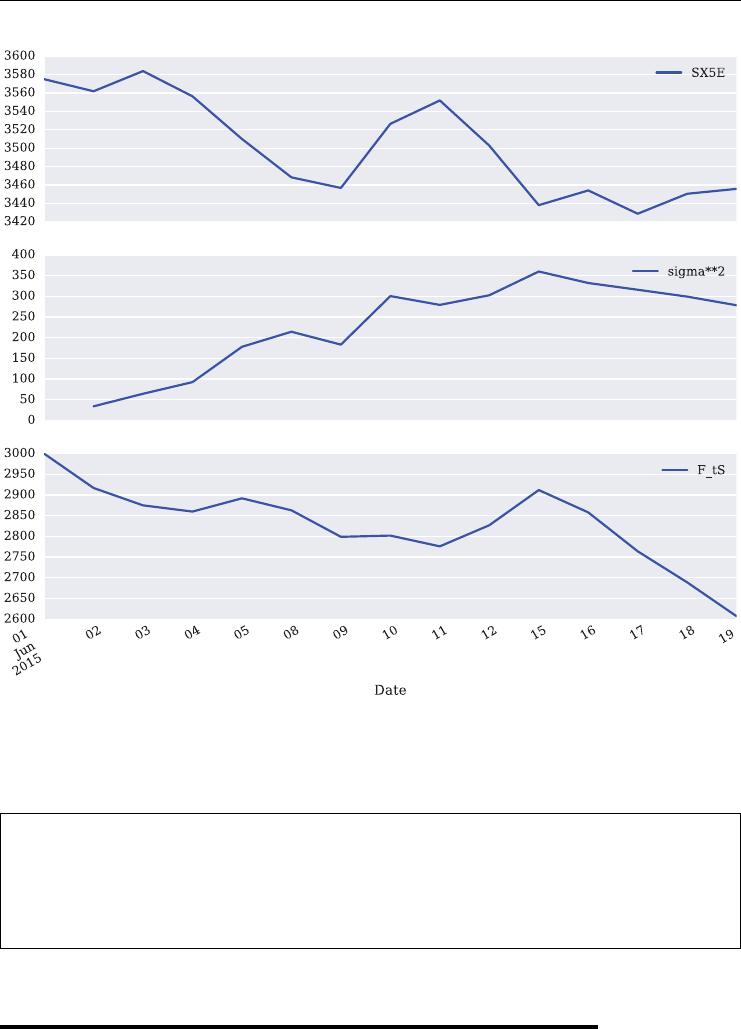
Variance Futures at Eurex 265
FIGURE 10.3 Calculated variance futures settlement values for the EURO STOXX 50.
We save the generated data set for re-use in the next section.
In [50]: h5 = pd.HDFStore('./source/data/var_data.h5', 'a')
In [51]: h5['var_future'] = data
In [52]: h5.close()
10.4 COMPARISON OF VARIANCE SWAP AND FUTURE
Eurex variance futures are a means to replicate the payoff of OTC-traded variance swaps with
a listed, standardized product. Let us compare the mark-to-market values of the variance swap
from sub-section 9.3.5, Variance Swap on the EURO STOXX 50 with the settlement values
calculated in the previous section.

266 LISTED VOLATILITY AND VARIANCE DERIVATIVES
To this end, we import the data for the variance swap rst.
In [53]: h5 = pd.HDFStore('./source/data/var_data.h5', 'r')
In [54]: var_swap = h5['var_swap']
In [55]: h5. close()
Next, we combine and plot the two time series for the variance swap and the variance future,
respectively, against each other. Note that we subtract the constant Cfor the comparison.
In [56]: comp = pd.DataFrame({'F_tS': data['F_tS'] - 3000,
....: 'V_t': var_swap['V_t']}, index=data.index)
....:
In [57]: comp
Out[57]:
F_tS V_t
Date
2015-06-01 0 0.000000
2015-06-02 -83 -82.332277
2015-06-03 -125 -124.049833
2015-06-04 -140 -139.593571
2015-06-05 -108 -107.644092
2015-06-08 -137 -136.380856
2015-06-09 -201 -200.634978
2015-06-10 -198 -196.905901
2015-06-11 -224 -223.189008
2015-06-12 -173 -172.129074
2015-06-15 -88 -86.887791
2015-06-16 -142 -141.190592
2015-06-17 -236 -234.822528
2015-06-18 -311 -309.629583
2015-06-19 -393 -391.004773
Figure 10.4 compares the two time series.
In [58]: comp.plot(style=['b', 'ro'], figsize=(9, 5));
Finally, Figure 10.5 presents the absolute differences which are quite small.
In [59]: (comp['F_tS'] - comp['V_t']).plot(style='rˆ', figsize=(9, 5));
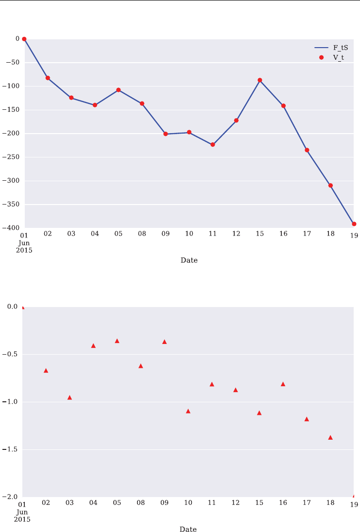
Variance Futures at Eurex 267
FIGURE 10.4 Variance swap and futures prices for EURO STOXX 50 compared.
FIGURE 10.5 Differences between variance swap and futures prices.

268 LISTED VOLATILITY AND VARIANCE DERIVATIVES
10.5 CONCLUSIONS
This chapter deals with the basic notions and concepts that need to be understood to trade
Eurex variance futures based on the EURO STOXX 50 stock index. It introduces all concepts
in a formal fashion and illustrates their calculation based on a concrete numerical example
which is based on the same data as the variance swap example calculation in the previous
chapter. This makes it possible to numerically show that the construction of the Eurex vari-
ance futures contract does indeed replicate the payoff of typical OTC variance contracts while
adding intraday liquidity and tradability. The next chapter covers special aspects that relate to
the intraday trading and end-of-day settlement of these derivatives products.

CHAPTER 11
Trading and Settlement
11.1 INTRODUCTION
This chapter covers practical aspects of trading Eurex variance futures. Among others, topics
are:
overview of major variance futures contract terms
intraday trading and trade conventions
trade matching at the end of the trading day
different traded volatilities with their impact on margining
after the trade matching until maturity
further details about interest rate calculation and market disruption events.
11.2 OVERVIEW OF VARIANCE FUTURES TERMS
The following list provides an overview of the major terms of the Eurex variance futures con-
tract. All technical terms are explained in chapter 10 Variance Futures at Eurex.
underlying: realized variance of EURO STOXX 50 stock index
interest rates: Euribor for present value factor DFtand Eonia for ARMVMt
standard strike: determined on rst trading day and equal to settled implied volatility for
the relevant maturity
1st settlement price: equal to 3,000 (i.e. for setting standard strike =settled implied
variance)
contract value: 1 EUR per variance futures point
minimum price change/tick value: 0.0001 variance futures points and 0.0001 EUR
settlement: in cash
terms: next three month ends and the next three quarter end months thereafter as well as
June and December thereafter
last trading day: one day before nal settlement day
nal settlement day/expiration: third Friday of maturity month
269
Listed Volatility and Variance Derivatives: A
Python-based Guide
By Dr. Yves J. Hilpisch
© 2017 Yves Hilpisch

270 LISTED VOLATILITY AND VARIANCE DERIVATIVES
nal settlement price: based on the average index level of EURO STOXX 50 between
11:50 am and 12:00 CET on nal settlement day
trade matching: variance futures trade in notional vega at volatility; upon matching
notional vega and volatility are converted into variance futures and variance futures prices,
respectively
continuous trading: from 9:00 am until 5:30 pm CET on each trading day of Eurex
Eurex trade entry services: from 6:30 pm until 9:00 pm CET on each trading day of
Eurex
order maintenance: notional vega at volatility, minimum order size 1 vega, minimum
price change 0.05 volatility points.
11.3 INTRADAY TRADING
Variance futures are traded on-exchange in terms of notional vega at volatility. However,
intraday there are no live futures prices quoted; they have to be calculated using live volatil-
ity quotes and the conversion parameters provided by Eurex. The conversion parameters are
those used for the calculation of the settlement price from the previous day, except that the
time-to-maturity (T−t) is reduced by 1 day and the number of elapsed days tis increased
by 1 day.
Let us get back to the numerical example from section 10.3 Example Calculation for a
Variance Future. The example simulates the calculation of daily settlement prices for a vari-
ance futures contract with inception on June 1, 2015 and a maturity on June 19, 2015 (i.e.
15 trading days). Since we have saved the data, we can continue from where we ended.
In [1]: import numpy as np
In [2]: a = np.random.standard_normal((10))
In [3]: np.round(a)
Out[3]: array([1., -0., -1., 1., 1., -0., 0., 0., 1., 1.])
In [4]: import pandas as pd
In [5]: h5 = pd.HDFStore('./source/data/var_data.h5', 'r')
In [6]: data = h5['var_future']
In [7]: h5.close()
In [8]: data.head()

Trading and Settlement 271
Out[8]:
SX5E V6I1 2w EONIA R_t sigma**2 t DF_t \
Date
2015-06-01 3575.04 25.8710 -0.108 -0.106 NaN NaN 1 1.000038
2015-06-02 3561.89 25.9232 -0.109 -0.122 -0.003685 34.220799 2 1.000036
2015-06-03 3583.82 25.7958 -0.109 -0.143 0.006138 64.580457 3 1.000033
2015-06-04 3556.38 26.2418 -0.109 -0.138 -0.007686 92.677552 4 1.000030
2015-06-05 3510.01 27.4496 -0.109 -0.115 -0.013124 178.023718 5 1.000027
F_tS ARMVM_t
Date
2015-06-01 3000 0.000000
2015-06-02 2917 0.000000
2015-06-03 2875 0.040173
2015-06-04 2860 0.111062
2015-06-05 2892 0.187647
We need to read out two central terms of the variance, namely the time-to-maturity in year
fractions and the standard volatility strike.
In [9]: T = data['t'][-1]
In [10]: T
Out[10]: 15
In [11]: sigma_K = data['V6I1'][0]
In [12]: sigma_K
Out[12]: 25.870999999999999
Similarly to the calculation in section 10.3, Example Calculation for a Variance Future,we
can now do the following calculation where we use the previous day’s input parameters but
today’s remaining time-to-maturity and today’s elapsed time (in days).
In [13]: data['F_ti'] = 3000.0
In [14]: for tin data.index[2:]:
....: data.loc[t, 'F_ti'] = data['DF_t'].shift(1)[t] * (
....: (data['t'][t] * data['sigma**2'].shift(1)[t]
....: +(T - data['t'][t]) * data['V6I1'].shift(1)[t]
** 2) / T
....: - sigma_K ** 2) - data['ARMVM_t'].shift(1)[t] + 3000
....:
The results are shown in the following table in the column F_ti for interim futures prices.

272 LISTED VOLATILITY AND VARIANCE DERIVATIVES
In [15]: data
Out[15]:
SX5E V6I1 2w EONIA R_t sigma**2 t \
Date
2015-06-01 3575.04 25.8710 -0.108 -0.106 NaN NaN 1
2015-06-02 3561.89 25.9232 -0.109 -0.122 -0.003685 34.220799 2
2015-06-03 3583.82 25.7958 -0.109 -0.143 0.006138 64.580457 3
2015-06-04 3556.38 26.2418 -0.109 -0.138 -0.007686 92.677552 4
2015-06-05 3510.01 27.4496 -0.109 -0.115 -0.013124 178.023718 5
2015-06-08 3468.31 27.2996 -0.110 -0.127 -0.011951 214.408816 6
2015-06-09 3456.79 26.8020 -0.110 -0.126 -0.003327 183.323049 7
2015-06-10 3526.48 25.8610 -0.111 -0.117 0.019960 300.555651 8
2015-06-11 3551.91 26.3897 -0.111 -0.120 0.007185 279.249096 9
2015-06-12 3502.77 29.7725 -0.113 -0.125 -0.013931 302.564935 10
2015-06-15 3438.07 34.5593 -0.108 -0.119 -0.018644 359.901600 11
2015-06-16 3454.09 36.2222 -0.109 -0.125 0.004649 332.134168 12
2015-06-17 3428.76 34.7235 -0.109 -0.110 -0.007360 315.833038 13
2015-06-18 3450.45 34.7235 -0.109 -0.118 0.006306 299.246550 14
2015-06-19 3455.80 34.7235 -0.108 -0.120 0.001549 278.303868 15
DF_t F_tS ARMVM_t F_ti
Date
2015-06-01 1.000038 3000 0.000000 3000.000000
2015-06-02 1.000036 2917 0.000000 3000.000000
2015-06-03 1.000033 2875 0.040173 2875.140910
2015-06-04 1.000030 2860 0.111062 2835.844331
2015-06-05 1.000027 2892 0.187647 2820.555454
2015-06-08 1.000025 2863 0.236836 2853.797523
2015-06-09 1.000022 2799 0.305743 2827.984087
2015-06-10 1.000019 2802 0.406065 2763.381425
2015-06-11 1.000016 2776 0.497784 2778.130966
2015-06-12 1.000014 2827 0.604188 2748.494268
2015-06-15 1.000011 2912 0.689681 2788.339034
2015-06-16 1.000008 2858 0.730901 2856.790440
2015-06-17 1.000005 2764 0.800957 2792.748076
2015-06-18 1.000003 2689 0.903601 2705.047722
2015-06-19 1.000000 2607 1.048771 2629.033294
As an example, assume that a trader buys on June 9, intraday 100,000 notional vega at a traded
implied volatility level of 26. The number of futures she has bought then is
futures =VegaNotional
2⋅𝜎ti
⋅
T
T−t
=100000
2⋅26
⋅
15
15 −7
=3605.77

Trading and Settlement 273
In [16]: futures = 100000. /(2 * 26) * T / (T - data['t']['2015-06-09'])
In [17]: futures
Out[17]: 3605.769230769231
The intraday futures price for the variance futures contract is:
In [18]: F_ti = data['F_ti']['2015-06-09']
In [19]: F_ti
Out[19]: 2827.9840866529353
The traded variance strike is
𝜎2
t=
t⋅𝜎2
0,t+(T−t)⋅𝜎2
i(t,T)
T
=7⋅13.542+(15 −7) ⋅262
15
=446.08
In [20]: sigma_t2 = (data['t']['2015-06-09'] * data['sigma**2']['2015-06-09']
....: + (T - data['t']['2015-06-09'] ) * 26 ** 2) / T
....:
In [21]: sigma_t2
Out[21]: 446.0840897506356
The traded futures price then is
Ft=DFt⋅(𝜎2
t−𝜎2
i(t,T))−ARMV Mt+3000 =2776.47
In [22]: F_t = (data['DF_t']['2015-06-09'] *
....: (sigma_t2 - data['V6I1']['2015-06-01'] ** 2)
....: - data['ARMVM_t']['2015-06-09'] + 3000)
....:
In [23]: F_t
Out[23]: 2776.4648130015858

274 LISTED VOLATILITY AND VARIANCE DERIVATIVES
Consequently, the trade has a value of:
In [24]: P_ti = futures * F_t
In [25]: P_ti
Out[25]: 10011291.393034564
11.4 TRADE MATCHING
At the end of the day, the trade in notional vega and volatility is conrmed. Notional vega and
volatility are, however, converted into variance futures at the variance futures settlement price.
To this end, the intraday transaction gets cancelled and replaced by a conrmed transaction
with the same number of futures but with the variance futures settlement price of the day.
In the example, we have:
In [26]: F_tS = data['F_tS']['2015-06-09']
In [27]: F_tS
Out[27]: 2799
Consequently, the transaction booked has a value of:
In [28]: P_t = futures * F_tS
In [29]: P_t
Out[29]: 10092548.076923078
The rst margin payment given these numbers then is:
In [30]: P_t - P_ti
Out[30]: 81256.683888513595
This is roughly the same as vega notional times the difference in settlement and traded
volatility:
margin =VegaNotional ⋅(𝜎i−𝜎i(t,T))
In [31]: 100000 * (data['V6I1']['2015-06-09'] - 26)
Out[31]: 80199.999999999956

Trading and Settlement 275
11.5 DIFFERENT TRADED VOLATILITIES
Let us now see what impact different traded volatilities have on the rst day margining of the
same trade as before. The necessary parameters and values can be calculated in vectorized
fashion. First, the array with the traded volatilities.
In [32]: import numpy as np
In [33]: trad_vols = np.arange(15, 25.01, 1)
In [34]: trad_vols
Out[34]: array([15., 16., 17., 18., 19., 20., 21., 22., 23., 24., 25.])
Second, the traded variance strikes.
In [35]: sigma_t2 = (data['t']['2015-06-09'] * data['sigma**2']['2015-06-09']
....: + (T - data['t']['2015-06-09']) * trad_vols ** 2) / T
....:
In [36]: sigma_t2
Out[36]:
array([205.55075642, 222.08408975, 239.68408975, 258.35075642,
278.08408975, 298.88408975, 320.75075642, 343.68408975,
367.68408975, 392.75075642, 418.88408975])
Third, the traded futures prices.
In [37]: F_t = (data['DF_t']['2015-06-09']
....: *(sigma_t2 - data['V6I1']['2015-06-01'] ** 2)
....: - data['ARMVM_t']['2015-06-09'] + 3000)
....:
In [38]: F_t
Out[38]:
array([ 2535.92620765, 2552.45990336, 2570.06028912, 2588.72736492,
2608.46113077, 2629.26158666, 2651.12873261, 2674.06256859,
2698.06309463, 2723.13031071, 2749.26421683])
Fourth, the rst day margins (P&L).
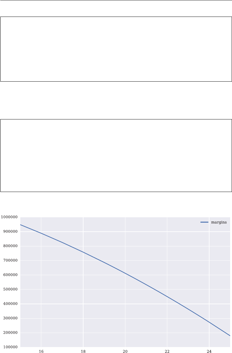
276 LISTED VOLATILITY AND VARIANCE DERIVATIVES
In [39]: margins = futures * (F_tS - F_t)
In [40]: margins
Out[40]:
array([ 948583.3858882 , 888966.69461993, 825503.76520532,
758194.59764436, 687039.19193707, 612037.54808344,
533189.66608347, 450495.54593716, 363955.18764451,
273568.59120552, 179335.75662019])
Let us visualize the results. The margins (P&L) are linear in traded volatility with the slope in
Figure 11.1 being equal to the vega notional of 100,000.
In [41]: import seaborn as sns; sns.set()
In [42]: import matplotlib
In [43]: matplotlib.rcParams['font.family'] = 'serif'
In [44]: results = pd.DataFrame({'margins' : margins}, index=trad_vols)
In [45]: results.plot(figsize=(10, 6));
FIGURE 11.1 Variance futures margins.

Trading and Settlement 277
11.6 AFTER THE TRADE MATCHING
What happens after the trade matching until maturity? To nd out, we can calculate the sub-
sequent margins as follows. We start with the differences between settlement prices.
In [46]: F_diffs = (data['F_tS'] - data['F_tS'].shift(1))
In [47]: F_diffs
Out[47]:
Date
2015-06-01 NaN
2015-06-02 -83.0
2015-06-03 -42.0
2015-06-04 -15.0
2015-06-05 32.0
2015-06-08 -29.0
2015-06-09 -64.0
2015-06-10 3.0
2015-06-11 -26.0
2015-06-12 51.0
2015-06-15 85.0
2015-06-16 -54.0
2015-06-17 -94.0
2015-06-18 -75.0
2015-06-19 -82.0
Name: F_tS, dtype: float64
With these differences, we can calculate the daily margins until maturity.
In [48]: margin_t = futures * F_diffs[F_diffs.index >= '2015-06-09']
In [49]: margin_t
Out[49]:
Date
2015-06-09 -230769.230769
2015-06-10 10817.307692
2015-06-11 -93750.000000
2015-06-12 183894.230769
2015-06-15 306490.384615
2015-06-16 -194711.538462
2015-06-17 -338942.307692
2015-06-18 -270432.692308
2015-06-19 -295673.076923
Name: F_tS, dtype: float64

278 LISTED VOLATILITY AND VARIANCE DERIVATIVES
The following code generates a pandas DataFrame object with the initial margins given the
traded volatility strike and the subsequent margins until maturity.
In [50]: results = pd.DataFrame(np.tile(margin_t, (len(trad_vols), 1)).T,
....: index=margin_t.index,
....: columns=trad_vols)
....:
In [51]: results.loc['2015-06-09', :] = margins # setting the first
day margins
In [52]: np.round(results)
Out[52]:
15.0 16.0 17.0 18.0 19.0 20.0 \
Date
2015-06-09 948583.0 888967.0 825504.0 758195.0 687039.0 612038.0
2015-06-10 10817.0 10817.0 10817.0 10817.0 10817.0 10817.0
2015-06-11 -93750.0 -93750.0 -93750.0 -93750.0 -93750.0 -93750.0
2015-06-12 183894.0 183894.0 183894.0 183894.0 183894.0 183894.0
2015-06-15 306490.0 306490.0 306490.0 306490.0 306490.0 306490.0
2015-06-16 -194712.0 -194712.0 -194712.0 -194712.0 -194712.0 -194712.0
2015-06-17 -338942.0 -338942.0 -338942.0 -338942.0 -338942.0 -338942.0
2015-06-18 -270433.0 -270433.0 -270433.0 -270433.0 -270433.0 -270433.0
2015-06-19 -295673.0 -295673.0 -295673.0 -295673.0 -295673.0 -295673.0
21.0 22.0 23.0 24.0 25.0
Date
2015-06-09 533190.0 450496.0 363955.0 273569.0 179336.0
2015-06-10 10817.0 10817.0 10817.0 10817.0 10817.0
2015-06-11 -93750.0 -93750.0 -93750.0 -93750.0 -93750.0
2015-06-12 183894.0 183894.0 183894.0 183894.0 183894.0
2015-06-15 306490.0 306490.0 306490.0 306490.0 306490.0
2015-06-16 -194712.0 -194712.0 -194712.0 -194712.0 -194712.0
2015-06-17 -338942.0 -338942.0 -338942.0 -338942.0 -338942.0
2015-06-18 -270433.0 -270433.0 -270433.0 -270433.0 -270433.0
2015-06-19 -295673.0 -295673.0 -295673.0 -295673.0 -295673.0
Figure 11.2 visualizes the cumulative P&L (assuming zero interest rates) for the different
traded volatility strikes.
In [53]: results.cumsum().plot(figsize=(10, 6), title='cumulative P&L');
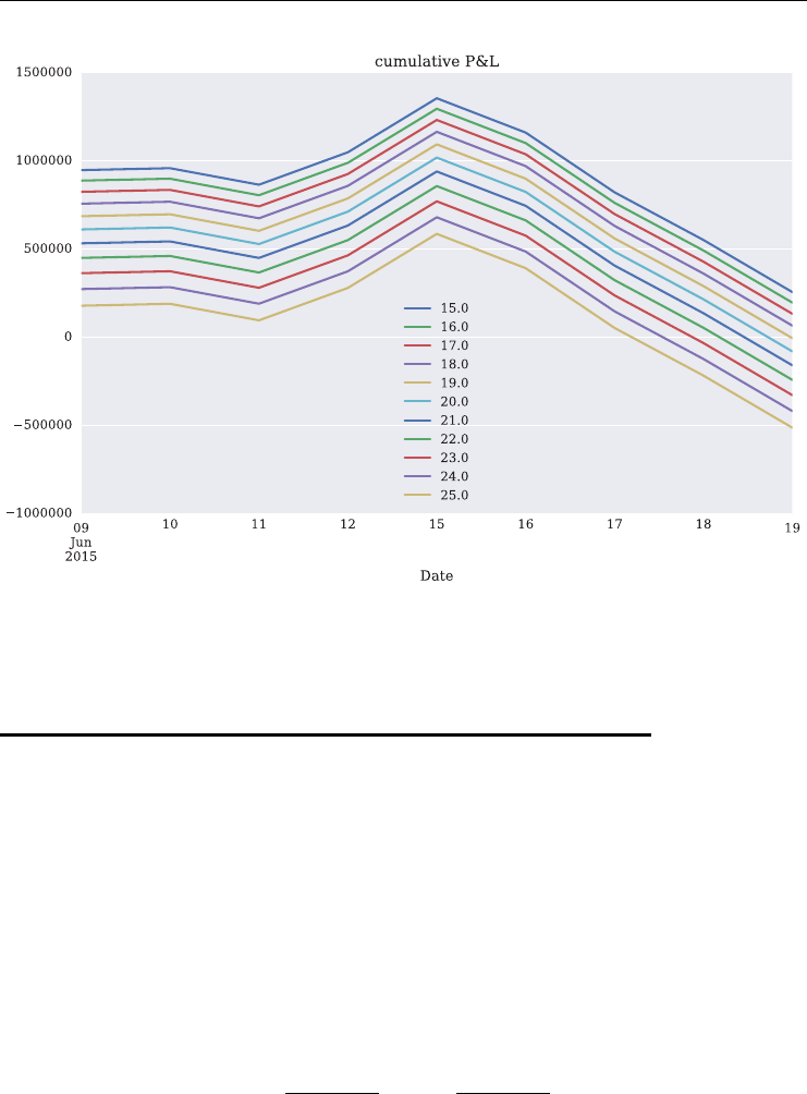
Trading and Settlement 279
FIGURE 11.2 Cumulative P&L for variance future.
11.7 FURTHER DETAILS
This section briey discusses some further details of importance for trading in Eurex variance
futures.
11.7.1 Interest Rate Calculation
ARMVM is calculated based on the Eonia rate as settled at 7 pm CET on the previous day. The
discount factors are calculated using the Euribor rates xed at 11:00 am CET and interpolated
to the respective maturities of the variance futures. The interpolation is done in linear fashion
using the following formula:
ri=r(Ti)=TK+1−Ti
TK+1−TK
r(TK)+Ti−TK
TK+1−TK
r(TK+1)
where TK+1is the maturity of the Euribor rate later than the futures maturity Tiand TKis the
maturity of the Euribor rate before the futures maturity Ti.

280 LISTED VOLATILITY AND VARIANCE DERIVATIVES
11.7.2 Market Disruption Events
There are three major market disruption events:
STOXX fails to provide a market closing level for the EURO STOXX 50
Eurex Exchange fails to open for trading during scheduled trading hours
Other market disruption events according to the European OTC standard.
11.8 CONCLUSIONS
The major difference between listed variance futures and OTC variance swaps is that the former
can be traded intraday. This chapter illustrates the major aspects of importance when it comes
to the trading and settlement of these instruments which are even liquid intraday (during the
trading day). Major concepts are the traded variance strike and the traded futures price. At
the end of the day, the original intraday trade gets cancelled and the traded futures price gets
replaced by the settlement price – however, the number of futures remains the same.

PART
Four
DX Analytics

CHAPTER 12
DX Analytics – An Overview
12.1 INTRODUCTION
Although Python is arguably a good programming language and ecosystem for nancial ana-
lytics (see chapter 1, Derivatives, Volatility and Variance or chapter 1 of Hilpisch (2014)),
dedicated libraries for nance are not that common. This is even more true when it comes to
derivatives analytics as a sub-discipline. One exception in this regard is DX Analytics (the “dx
library”), written by the author of this book, which has a major focus on advanced deriva-
tives and risk analytics. The central resource to get started with the library is the website
http://dx-analytics.com.
This chapter provides an overview of the relevant parts of the library for the purposes of the
case studies which follow. The development of the library is guided by two central principles:
global valuation approach: in practice, this approach translates into the non-redundant
modeling of all risk factors (e.g. option underlyings like equity indexes) and the valuation
of all derivative instruments by a unique, consistent numerical method – which is Monte
Carlo simulation in the case of DX Analytics
unlimited computing resources: Monte Carlo simulation is computationally and mem-
ory intensive and has therefore often been dismissed as an adequate numerical method to
implement, for example, front-ofce analytics libraries; in 2016, the technical infrastruc-
tures available to even smaller players in the nancial industry have reached performance
levels that 10 years ago seemed impossible or at least not nancially feasible; in that sense
“unlimited resources” is not to be understood literally but rather as the guiding principle
that hardware and computing resources generally are no longer a bottleneck
Among others, DX Analytics provides the following features:
models: models for risk factors include simple ones like geometric Brownian motion as
well as more sophisticated ones like stochastic volatility jump diffusion models
derivatives: derivatives models include single risk factor as well as multi risk factor mod-
els, both with European and American (Bermudan) exercise
283
Listed Volatility and Variance Derivatives: A
Python-based Guide
By Dr. Yves J. Hilpisch
© 2017 Yves Hilpisch

284 LISTED VOLATILITY AND VARIANCE DERIVATIVES
portfolios: derivatives portfolios can be arbitrarily complex with multiple, correlated
risk factors and multiple, diverse derivative instruments (single risk and multi risk);
simulations and valuations are implemented in such a way that both value and risk aggre-
gations are consistent for each Monte Carlo path.
The following sections illustrate the use of the library by means of a simple, yet still realistic,
example with two correlated risk factors and two different options.
12.2 MODELING RISK FACTORS
First, some necessary imports and in particular the import of the dx library.
In [1]: import dx
In [2]: import numpy as np
In [3]: np.random.seed(1000)
In [4]: import pandas as pd
In [5]: import datetime as dt
In [6]: import seaborn as sns; sns.set()
In [7]: import matplotlib as mpl;
Usually, the rst step is to dene a model for the risk-neutral discounting since all valuations
are based on the risk-neutral (or martingale) pricing approach (see Bj¨
ork (2009)). Throughout,
we will work with a constant short rate model although DX Analytics also provides determin-
istic yield curve and stochastic short rate models.
In [8]: r = dx.constant_short_rate('r', 0.01)
The next step is to dene a market environment containing the parameter specications needed.
Several objects might have different market environments but they might also share market
environments. The rst risk factor to be modeled is a geometric Brownian motion (Black-
Scholes-Merton (1973) model). The following market environment object contains all param-
eters needed for this model. Comments in the code explain the single elements.
# instantiation of market environment object
In [9]: me_1 = dx.market_environment('me', dt.datetime(2016, 1, 1))

DX Analytics – An Overview 285
# starting value of simulated processes
In [10]: me_1.add_constant('initial_value', 100.)
# volatility factor
In [11]: me_1.add_constant('volatility', 0.2)
# horizon for simulation
In [12]: me_1.add_constant('final_date', dt.datetime(2016, 6, 30))
# currency of instrument
In [13]: me_1.add_constant('currency', 'EUR')
# frequency for discretization (here: weekly)
In [14]: me_1.add_constant('frequency', 'W')
# number of paths
In [15]: me_1.add_constant('paths', 25000)
# short rate model for discount curve
In [16]: me_1.add_curve('discount_curve', r)
Equipped with this object, the model object for the risk factor can be instantiated.
In [17]: gbm_1 = dx.geometric_brownian_motion('gbm_1', me_1)
In [18]: gbm_1
Out[18]: <dx.dx_models.geometric_brownian_motion at 0x2b20c39c5510>
The get_instrument_values() method initiates a Monte Carlo simulation and delivers
back the simulated paths – given the parametrizations from the market environment object –
as a NumPy ndarray object.
In [19]: gbm_1.get_instrument_values()
Out [19]:
array([[ 100. , 100. , 100. , ..., 100. ,
100. , 100. ],
[ 103.99970675, 100.94138063, 101.87289049, ..., 101.57080458,
100.82390334, 98.15531921],
[ 101.93603717, 94.66240389, 91.81649108, ..., 101.20745936,
99.98530091, 102.49930045],
...,
[ 94.34847745, 111.87828236, 105.88943893, ..., 89.84492969,
109.03063645, 107.8625328 ],
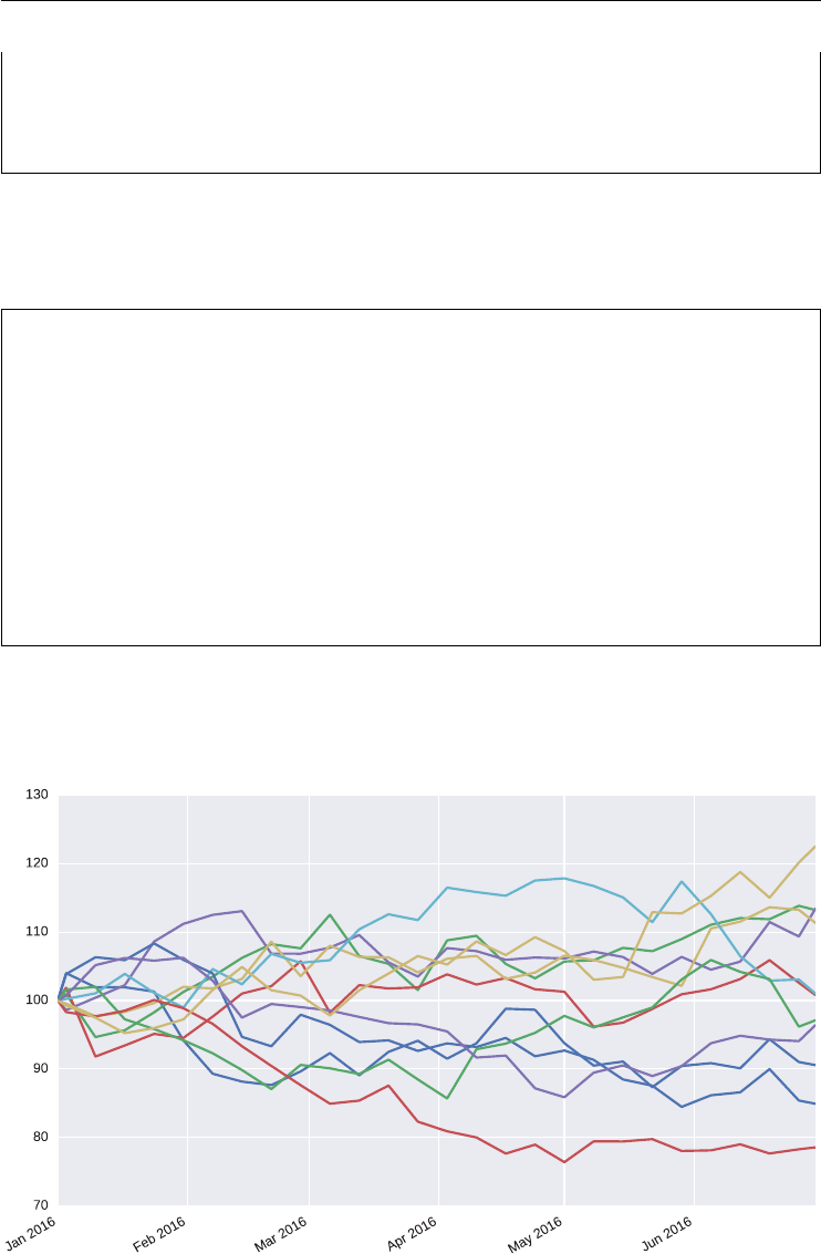
286 LISTED VOLATILITY AND VARIANCE DERIVATIVES
[ 91.01721535, 113.83465258, 102.59432299, ..., 92.09515398,
104.17599152, 101.67756176],
[ 90.56511589, 113.20730366, 100.79160449, ..., 90.91965416,
100.6385713 , 101.76583508]])
Via the time_grid attribute one can access the date-time information for the time series
data.
In [20]: gbm_1.time_grid[:10]
Out[20]:
array([datetime.datetime(2016, 1, 1, 0, 0),
datetime.datetime(2016, 1, 3, 0, 0),
datetime.datetime(2016, 1, 10, 0, 0),
datetime.datetime(2016, 1, 17, 0, 0),
datetime.datetime(2016, 1, 24, 0, 0),
datetime.datetime(2016, 1, 31, 0, 0),
datetime.datetime(2016, 2, 7, 0, 0),
datetime.datetime(2016, 2, 14, 0, 0),
datetime.datetime(2016, 2, 21, 0, 0),
datetime.datetime(2016, 2, 28, 0, 0)], dtype=object)
Combining both arrays to a single pandas DataFrame object makes plotting straightforward
(see Figure 12.1).
FIGURE 12.1 Simulated paths for the risk factor based on geometric Brownian motion.

DX Analytics – An Overview 287
In [21]: pdf_1 = pd.DataFrame(gbm_1.get_instrument_values(),
index=gbm_1.time_grid)
In [22]: pdf_1.ix[:, :10].plot(legend=False, figsize=(10, 6));
Next, we dene a second risk factor, again based on geometric Brownian motion. We use the
market environment information from the rst risk factor and only overwrite the volatility
value.
# instantiate new market environment object
In [23]: me_2 = dx.market_environment('me_2', me_1.pricing_date)
# add complete environment
In [24]: me_2.add_environment(me_1)
# overwrite volatility value
In [25]: me_2.add_constant('volatility', 0.5)
Using the updated market environment, dene the second risk factor as follows.
In [26]: gbm_2 = dx.geometric_brownian_motion('gbm_2', me_2)
The plot in Figure 12.2 illustrates the higher volatility of the second risk factor graphically.
In [27]: pdf_2 = pd.DataFrame(gbm_2.get_instrument_values(),
index=gbm_2.time_grid)
In [28]: ax = pdf_1.ix[:, :10].plot(legend=False, figsize=(10, 6),
style=11 * ['b']);
In [29]: pdf_2.ix [:, :10].plot(legend=False, style=11 * ['r'], ax=ax);
12.3 MODELING DERIVATIVES
Based on the risk factors, we can dene derivatives models for valuation. To this end, we need
to add at least one (the maturity), in general two (maturity and strike), parameters to
the market environment(s).
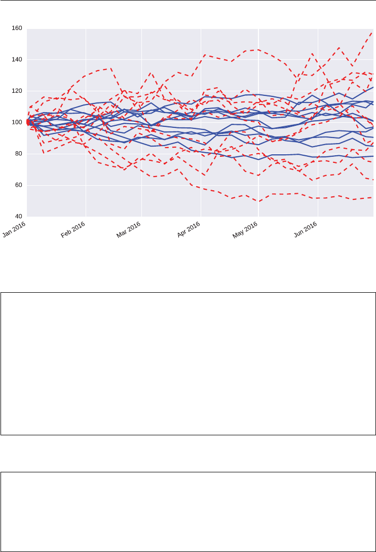
288 LISTED VOLATILITY AND VARIANCE DERIVATIVES
FIGURE 12.2 Simulated paths for the two risk factors; solid lines =low volatility, dashed lines =
high volatility.
# instantiation of market environment object for option
In [30]: me_opt = dx.market_environment('me_opt', me_1.pricing_date)
# add complete market environment
In [31]: me_opt.add_environment(me_1)
# add maturity date for option
In [32]: me_opt.add_constant('maturity', dt.datetime(2016, 6, 30))
# add strike for option
In [33]: me_opt.add_constant('strike', 110.)
The rst derivative is an American put option on the rst risk factor gbm_1.
In [34]: am_put = dx.valuation_mcs_american_single(
....: name='am_put', # name of the option as string
....: underlying=gbm_1, # the risk factor object
....: mar_env=me_opt, # the market environment
....: payoff_func='np.maximum(strike - instrument_values, 0)')
....:
Let us calculate a Monte Carlo present value estimate and estimates for the Greeks of the
American put.

DX Analytics – An Overview 289
In [35]: am_put.present_value() # Monte Carlo estimator
Out[35]: 11.799
In [36]: am_put.delta() # delta of the option
Out[36]: -0.6809
In [37]: am_put.gamma() # gamma of the option
Out[37]: 0.0149
In [38]: 0.5 * am_put.gamma() * am_put.underlying.initial_value ** 2
# dollar gamma
Out[38]: 74.5
In [39]: am_put.vega() # vega of the option
Out[39]: 23.8208
In [40]: am_put.theta() # theta of the option
Out[40]: -3.81
In [41]: am_put.rho() # rho of the option
Out[41]: -30.113
The second derivative is a European call option on the second risk factor gbm_2. It has the
same strike and maturity as the American put option.
In [42]: eur_call = dx.valuation_mcs_european_single(
....: name='eur_call',
....: underlying=gbm_2,
....: mar_env=me_opt,
....: payoff_func='np.maximum(maturity_value - strike, 0)')
....:
The major statistics for this option are:
In [43]: eur_call.present_value()
Out[43]: 10.364663
In [44]: eur_call.delta()
Out[44]: 0.4174
In [45]: eur_call.gamma()
Out[45]: 0.0121

290 LISTED VOLATILITY AND VARIANCE DERIVATIVES
In [46]: 0.5 * eur_call.gamma() * eur_call.underlying.initial_value ** 2
Out[46]: 60.5
In [47]: eur_call.vega()
Out[47]: 27.6147
In [48]: eur_call.theta()
Out[48]: -14.1996
In [49]: eur_call.rho()
Out[49]: 18.0684
Note that all these values might vary to a greater or lesser extent with the parameters chosen
for the Monte Carlo simulation.
To conclude this section, let us analyze the European call option in a bit more detail. We
want to estimate and collect the Greeks for different strikes. The following code implements
the necessary steps:
In [50]: k_list = np.arange(80., 120.5, 2.5)
In [51]: pv = []; de = []; ve = []; th = []; rh = []; ga = []
In [52]: for kin k_list:
....: eur_call.update(strike=k)
....: pv.append(eur_call.present_value())
....: de.append(eur_call.delta())
....: ve.append(eur_call.vega())
....: th.append(eur_call.theta())
....: rh.append(eur_call.rho())
....: ga.append(eur_call.gamma())
....:
Figure 12.3 shows the results graphically.
In [53]: dx.plot_option_stats_full(k_list, pv, de, ga, ve, th, rh)
12.4 DERIVATIVES PORTFOLIOS
The previous sections show how convenient and exible it is to model single derivatives with
DX Analytics. The numerical methods used and the API of the library mimic working with the
Black-Scholes-Merton closed option pricing formula when it comes to Greeks although the
derivative itself might be much more complex than a plain vanilla European call or put option
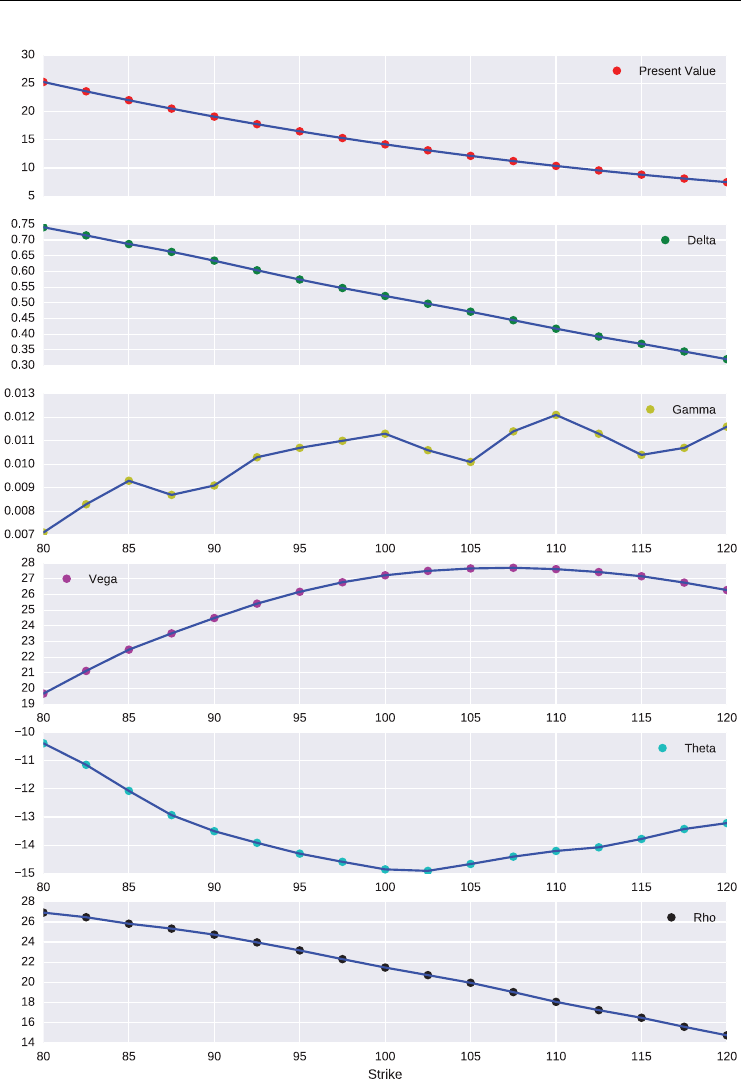
DX Analytics – An Overview 291
FIGURE 12.3 Greeks of the European call option for different strikes.

292 LISTED VOLATILITY AND VARIANCE DERIVATIVES
(e.g. it might have American exercise and an exotic payoff). However, the area which differ-
entiates DX Analytics most from other derivatives analytics libraries is the global valuation
approach for derivatives portfolios. How it works is explained in this section.
12.4.1 Modeling Portfolios
In a portfolio context, we need to add information about the model class(es) to be used by the
market environments of the risk factors.
In [54]: me_1.add_constant('model', 'gbm')
In [55]: me_2.add_constant('model', 'gbm')
To compose a portfolio consisting of the two options, we need to dene derivatives positions.
Note that this step is independent from the risk factor model and option model denitions. We
only use the market environment data and some additional information needed (e.g. payoff
functions).
In [56]: put = dx.derivatives_position(
....: name='put', # name as string
....: quantity=2, # number of options in the portfolio
....: underlyings=['gbm_1'], # the underlying(s) as list object
....: mar_env=me_opt, # the market environment object
....: otype='American single', # the option type
....: payoff_func='np.maximum(strike - instrument_values, 0)')
# the payoff
....:
In [57]: call = dx.derivatives_position(
....: name='call',
....: quantity=3,
....: underlyings=['gbm_2'],
....: mar_env=me_opt,
....: otype='European single',
....: payoff_func='np.maximum(maturity_value - strike, 0)')
....:
In a portfolio context, we also need to dene the market. It consists of the risk factors, the
correlation between them, the derivatives positions as well as the valuation environment.
In [58]: risk_factors = {'gbm_1': me_1, 'gbm_2': me_2} # as dictionary
In [59]: correlations = [['gbm_1', 'gbm_2', 0.4]] # as list
In [60]: positions = {'put' : put, 'call' : call} # as dictionary

DX Analytics – An Overview 293
The valuation environment (technically another market environment) contains all those param-
eters shared by all derivatives positions. This might imply that certain parameters from
the market environments of the derivatives get replaced for the portfolio simulations and
valuations.
In [61]: val_env = dx.market_environment('general', dt.datetime(2016, 1, 1))
In [62]: val_env.add_constant('frequency', 'W')
In [63]: val_env.add_constant('paths', 25000)
In [64]: val_env.add_constant('starting_date', val_env.pricing_date)
In [65]: val_env.add_constant('final_date', val_env.pricing_date)
In [66]: val_env.add_curve('discount_curve', r)
These new objects are needed to instantiate a portfolio object.
In [67]: port = dx.derivatives_portfolio(
....: name='portfolio', # name as string
....: positions=positions, # derivatives positions
....: val_env=val_env, # valuation environment
....: risk_factors=risk_factors, # relevant risk factors
....: correlations=correlations, # correlation between risk factors
....: parallel=False) # parallel valuation True/False
....:
12.4.2 Simulation and Valuation
Simulation and valuation are now as straightforward as in the single option case.
In [68]: port.get_values() # get all present values
Total
pos_value 54.103966
dtype: float64
Out[68]:
position name quantity otype risk_facts value currency \
0 put put 2 American single [gbm_1] 11.804000 EUR
1 call call 3 European single [gbm_2] 10.165322 EUR
pos_value
0 23.608000
1 30.495966

294 LISTED VOLATILITY AND VARIANCE DERIVATIVES
In [69]: port.get_statistics() # get major statistics
Totals
pos_value 54.1030
pos_delta 0.0082
pos_vega 130.9992
dtype: float64
Out[69]:
position name quantity otype risk_facts value currency \
0 put put 2 American single [gbm_1] 11.804 EUR
1 call call 3 European single [gbm_2] 10.165 EUR
pos_value pos_delta pos_vega
0 23.608 -1.4192 48.7344
1 30.495 1.4274 82.2648
12.4.3 Risk Reports
A strength of DX Analytics and the global valuation approach is that one can easily generate
consistent risk reports. By this we mean that single parameters are shocked and the effect on
the portfolio value is estimated. Think of a larger portfolio containing multiple options on the
S&P 500 equity index. By changing the spot value of the index, DX Analytics can estimate in
a single step what the impact is on the overall portfolio value (and not only on a single option
as in the case of a delta calculation).
When calling the get_port_risk() method you need to dene which parameter will
be shocked. You get back all hypothetical portfolio values and the benchmark value without
shock. The following estimates show the “portfolio deltas.”
In [70]: deltas, benchvalue = port.get_port_risk(Greek='Delta')
gbm_1
0.8 0.9 1.0 1.1 1.2
gbm_2
0.8 0.9 1.0 1.1 1.2
In [71]: benchvalue
Out[71]: 54.103966
In [72]: deltas
Out[72]:
<class 'pandas.core.panel.Panel'>
Dimensions: 2 (items) x 5 (major_axis) x 2 (minor_axis)
Items axis: gbm_1_Delta to gbm_2_Delta
Major_axis axis: 0.8 to 1.2
Minor_axis axis: factor to value

DX Analytics – An Overview 295
There is a convenience function called risk_report() in DX Analytics to nicely print the
results.
In [73]: dx.risk_report (deltas) # gives the resulting values ...
gbm_1_Delta
0.8 0.9 1.0 1.1 1.2
factor 80.00 90.00 100.0 110.00 120.00
value 90.51 70.89 54.1 42.19 35.37
gbm_2_Delta
0.8 0.9 1.0 1.1 1.2
factor 80.00 90.00 100.0 110.00 120.00
value 33.28 41.94 54.1 69.74 88.39
In [74]: dx.risk_report(deltas.ix[:, :, 'value'] - benchvalue,
....: gross=False) # ... as net changes
....:
gbm_1_Delta gbm_2_Delta
0.8 36.41 -20.83
0.9 16.79 -12.16
1.0 0.00 0.00
1.1 -11.92 15.63
1.2 -18.74 34.28
“Portfolio vegas” are calculated in the same way.
In [75]: vegas, benchvalue = port.get_port_risk(Greek='Vega', step=0.05)
gbm_1
0.8 0.85 0.9 0.95 1.0 1.05 1.1 1.15 1.2
gbm_2
0.8 0.85 0.9 0.95 1.0 1.05 1.1 1.15 1.2
In [76]: dx.risk_report(vegas)
gbm_1_Vega
0.80 0.85 0.90 0.95 1.00 1.05 1.10 1.15 1.20
factor 0.16 0.17 0.18 0.19 0.2 0.21 0.22 0.23 0.24
value 52.40 52.85 53.20 53.64 54.1 54.59 55.05 55.52 56.01
gbm_2_Vega
0.80 0.85 0.90 0.95 1.00 1.05 1.10 1.15 1.20
factor 0.40 0.43 0.45 0.48 0.5 0.53 0.55 0.58 0.60
value 45.92 47.95 50.00 52.05 54.1 56.16 58.22 60.28 62.34

296 LISTED VOLATILITY AND VARIANCE DERIVATIVES
In [77]: dx.risk_report(vegas.ix[:, :, 'value'] - benchvalue, gross=False)
gbm_1_Vega gbm_2_Vega
0.80 -1.70 -8.19
0.85 -1.26 -6.15
0.90 -0.91 -4.11
0.95 -0.47 -2.05
1.00 0.00 0.00
1.05 0.49 2.06
1.10 0.95 4.12
1.15 1.41 6.18
1.20 1.90 8.24
12.5 CONCLUSIONS
This chapter provides a quick start with DX Analytics, a Python-based nancial analytics
library with a focus on derivatives and risk analytics. The library offers many more features
than are covered in this brief chapter. It is recommended to check out the main page http://dx-
analytics.com and to work through the different parts of the documentation which are all based
on executable Jupyter Notebooks.
The focus of this chapter is on the basic tool set and a basic understanding of the API to
have a good foundation for the case studies in the two subsquent chapters. The case studies
use DX Analytics to model the VSTOXX volatility index by the square-root diffusion model
from chapter 6, Valuing Volatility Derivatives as well as the square-root jump diffusion model
from chapter 7, Advanced Modeling of the VSTOXX Index. The major goal of the case studies
is to analyze how well the two models perform over time in replicating the market quotes of
traded VSTOXX options.

CHAPTER 13
DX Analytics – Square-Root Diffusion
13.1 INTRODUCTION
This chapter uses DX Analytics to model the VSTOXX volatility index by a square-root dif-
fusion process as proposed in Gr¨
unbichler and Longstaff (1996) and discussed in chapter 6
Valuing Volatility Derivatives. It implements a study over a time period of three months to
analyze how well the model performs in replicating market quotes for VSTOXX options.
13.2 DATA IMPORT AND SELECTION
The data we are working with is for the rst quarter of 2014. The complete data set is contained
in the online resources accompanying this book. As usual, some imports rst.
In [1]: import numpy as np
In [2]: import pandas as pd
In [3]: import datetime as dt
Next, we read the data from the source into pandas DataFrame objects.
In [4]: h5 = pd.HDFStore('./source/data/vstoxx_march_2014.h5', 'r')
In [5]: vstoxx_index = h5['vstoxx_index'] # data for the index itself
In [6]: vstoxx_futures = h5['vstoxx_futures'] # data for the futures
In [7]: vstoxx_options = h5['vstoxx_options'] # data for the options
In [8]: h5.close()
297
Listed Volatility and Variance Derivatives: A
Python-based Guide
By Dr. Yves J. Hilpisch
© 2017 Yves Hilpisch

298 LISTED VOLATILITY AND VARIANCE DERIVATIVES
Inspecting the data sub-set for the VSTOXX index itself, we see that we are dealing with 63
trading days.
In [9]: vstoxx_index.info()
<class 'pandas.core.frame.DataFrame'>
DatetimeIndex: 63 entries, 2014-01-02 to 2014-03-31
Data columns (total 9 columns):
V2TX 63 non-null float64
V6I1 57 non-null float64
V6I2 63 non-null float64
V6I3 61 non-null float64
V6I4 63 non-null float64
V6I5 63 non-null float64
V6I6 62 non-null float64
V6I7 63 non-null float64
V6I8 63 non-null float64
dtypes: float64(9)
memory usage: 4.9 KB
In [10]: vstoxx_index.tail()
Out[10]:
V2TX V6I1 V6I2 V6I3 V6I4 V6I5 V6I6 \
Date
2014-03-25 18.2637 18.2303 18.3078 19.0371 19.8378 20.3065 18.1063
2014-03-26 17.5869 17.4810 17.7009 18.4499 19.4150 19.9961 20.2562
2014-03-27 17.6397 17.5032 17.7608 18.6249 19.4860 20.0477 20.1078
2014-03-28 17.0324 16.6849 17.2864 18.3281 19.3032 19.8332 20.1371
2014-03-31 17.6639 17.6087 17.6879 18.5689 19.4285 20.0430 19.9823
V6I7 V6I8
Date
2014-03-25 20.8292 21.2046
2014-03-26 20.4541 20.8563
2014-03-27 20.4865 20.9449
2014-03-28 20.3808 20.8210
2014-03-31 20.4448 20.8994
Per trading day, there are eight futures quotes for the eight different maturities of the VSTOXX
futures contract. This makes for a total of 504 futures quotes.
In [11]: vstoxx_futures.info()
<class 'pandas.core.frame.DataFrame'>
Int64Index: 504 entries, 0 to 503
Data columns (total 5 columns):
DATE 504 non-null datetime64[ns]

DX Analytics – Square-Root Diffusion 299
EXP_YEAR 504 non-null int64
EXP_MONTH 504 non-null int64
PRICE 504 non-null float64
MATURITY 504 non-null datetime64[ns]
dtypes: datetime64[ns](2), float64(1), int64(2)
memory usage: 23.6 KB
In [12]: vstoxx_futures. tail()
Out[12]:
DATE EXP_YEAR EXP_MONTH PRICE MATURITY
499 2014-03-31 2014 7 20.40 2014-07-18
500 2014-03-31 2014 8 20.70 2014-08-15
501 2014-03-31 2014 9 20.95 2014-09-19
502 2014-03-31 2014 10 21.05 2014-10-17
503 2014-03-31 2014 11 21.25 2014-11-21
By far the biggest data sub-set is the one for the VSTOXX options. For each trading day there
are market quotes for puts and calls for eight different maturities and a multitude of different
strike prices. This makes for a total of 46,960 option quotes for the rst quarter of 2014.
In [13]: vstoxx_options.info()
<class 'pandas.core.frame.DataFrame'>
Int64Index: 46960 entries, 0 to 46959
Data columns (total 7 columns):
DATE 46960 non-null datetime64[ns]
EXP_YEAR 46960 non-null int64
EXP_MONTH 46960 non-null int64
TYPE 46960 non-null object
STRIKE 46960 non-null float64
PRICE 46960 non-null float64
MATURITY 46960 non-null datetime64[ns]
dtypes: datetime64[ns](2), float64(2), int64(2), object(1)
memory usage: 2.9+ MB
In [14]: vstoxx_options.tail()
Out[14]:
DATE EXP_YEAR EXP_MONTH TYPE STRIKE PRICE MATURITY
46955 2014-03-31 2014 11 P 85.0 63.65 2014-11-21
46956 2014-03-31 2014 11 P 90.0 68.65 2014-11-21
46957 2014-03-31 2014 11 P 95.0 73.65 2014-11-21
46958 2014-03-31 2014 11 P 100.0 78.65 2014-11-21
46959 2014-03-31 2014 11 P 105.0 83.65 2014-11-21
Maturity-wise we are dealing with a total of eleven dates. This is due to the fact that at any
given time eight maturities for the VSTOXX futures and options contracts are available and
we are looking at data for three months.

300 LISTED VOLATILITY AND VARIANCE DERIVATIVES
In [15]: third_fridays = sorted(set(vstoxx_futures['MATURITY']))
In [16]: third_fridays
Out[16]:
[Timestamp('2014-01-17 00:00:00'),
Timestamp('2014-02-21 00:00:00'),
Timestamp('2014-03-21 00:00:00'),
Timestamp('2014-04-18 00:00:00'),
Timestamp('2014-05-16 00:00:00'),
Timestamp('2014-06-20 00:00:00'),
Timestamp('2014-07-18 00:00:00'),
Timestamp('2014-08-15 00:00:00'),
Timestamp('2014-09-19 00:00:00'),
Timestamp('2014-10-17 00:00:00'),
Timestamp('2014-11-21 00:00:00')]
When it comes to the calibration of the square-root diffusion model for the VSTOXX,
it is necessary to work with a selection from the large set of option quotes. The follow-
ing function implements such a selection procedure, using different conditions to gener-
ate a sensible set of option quotes around the forward at-the-money level. The function
srd_get_option_selection() is used in what follows to select the right sub-set of
option quotes for each day during the calibration.
def srd_get_option_selection(pricing_date, maturity, tol=tol):
''' Function to select option quotes from data set.
Parameters
==========
pricing_date: datetime object
date for which the calibration shall be implemented
maturity: datetime object
maturity date for the options to be selected
tol: float
moneyness tolerance for OTM and ITM options to be selected
Returns
=======
option_selection: DataFrame object
selected options quotes
forward: float
futures price for maturity at pricing_date
'''
forward = vstoxx_futures[(vstoxx_futures. DATE == pricing_date)
& (vstoxx_futures.MATURITY == maturity)]['PRICE'].values[0]

DX Analytics – Square-Root Diffusion 301
option_selection = \
vstoxx_options[(vstoxx_options.DATE == pricing_date)
& (vstoxx_options.MATURITY == maturity)
& (vstoxx_options.TYPE == 'C') # only calls
& (vstoxx_options.STRIKE > (1 - tol) * forward)
& (vstoxx_options.STRIKE < (1 + tol) * forward)]
return option_selection, forward
13.3 MODELING THE VSTOXX OPTIONS
The previous chapter illustrates how European options are modeled with DX Analytics based
on a geometric Brownian motion model (dx.geometric_brownian_motion()). To
model the VSTOXX options for the calibration, we just need to replace that model with the
square-root diffusion model dx.square_root_diffusion(). The respective market
environment then needs some additional parameters.
All the code used for the calibration is found in the Python script dx_srd_
calibration.py (see sub-section 14.6.1 dx_srd_calibration.py). After some imports, the
script starts by dening some general parameters and curves for the market environment. Dur-
ing the calibration process, some of these get updated to reect the current status of the opti-
mization procedure.
import dx
import time
import numpy as np
import pandas as pd
import datetime as dt
import scipy.optimize as spo
import matplotlib.pyplot as plt
import seaborn as sns; sns.set()
import matplotlib
matplotlib.rcParams['font.family'] = 'serif'
# importing the data
h5 = pd.HDFStore('../data/vstoxx_march_2014.h5', 'r')
vstoxx_index = h5['vstoxx_index']
vstoxx_futures = h5['vstoxx_futures']
vstoxx_options = h5['vstoxx_options']
h5.close()
# collecting the maturity dates
third_fridays = sorted(set(vstoxx_futures['MATURITY']))
# instantiation of market environment object with dummy pricing date
me_vstoxx = dx.market_environment('me_vstoxx', dt.datetime(2014, 1, 1))
me_vstoxx.add_constant('currency', 'EUR')
me_vstoxx.add_constant('frequency', 'W')

302 LISTED VOLATILITY AND VARIANCE DERIVATIVES
me_vstoxx.add_constant('paths', 5000)
# constant short rate model with somewhat arbitrary rate
csr = dx.constant_short_rate('csr', 0.01)
me_vstoxx.add_curve('discount_curve', csr)
# parameters to be calibrated later, dummies only
me_vstoxx.add_constant('kappa', 1.0)
me_vstoxx.add_constant('theta', 20)
me_vstoxx.add_constant('volatility', 1.0)
# payoff function for all European call options
payoff_func = 'np.maximum(maturity_value - strike, 0)'
tol = 0.2 # otm & itm moneyness tolerance
The function srd_get_option_models() creates valuation models for all options in a
given selection of option quotes.
def srd_get_option_models(pricing_date, maturity, option_selection):
''' Function to instantiate option pricing models.
Parameters
==========
pricing_date: datetime object
date for which the calibration shall be implemented
maturity: datetime object
maturity date for the options to be selected
option_selection: DataFrame object
selected options quotes
Returns
=======
vstoxx_model: dx.square_root_diffusion
model object for VSTOXX
option_models: dict
dictionary of dx.valuation_mcs_european_single objects
'''
# updating the pricing date
me_vstoxx.pricing_date = pricing_date
# setting the initial value for the pricing date
initial_value = vstoxx_index['V2TX'][ pricing_date]
me_vstoxx.add_constant('initial_value', initial_value)
# setting the final date given the maturity date
me_vstoxx.add_constant('final_date', maturity)
# instantiating the risk factor (VSTOXX) model

DX Analytics – Square-Root Diffusion 303
vstoxx_model = dx.square_root_diffusion('vstoxx_model', me_vstoxx)
# setting the maturity date for the valuation model(s)
me_vstoxx.add_constant('maturity', maturity)
option_models = {} # dictionary collecting all models
for option in option_selection.index:
# setting the strike for the option to be modeled
strike = option_selection['STRIKE'].ix[option]
me_vstoxx.add_constant('strike', strike)
# instantiating the option model
option_models[option] = \
dx.valuation_mcs_european_single(
'eur_call_%d' % strike,
vstoxx_model,
me_vstoxx,
payoff_func)
return vstoxx_model, option_models
13.4 CALIBRATION OF THE VSTOXX MODEL
Calibration of a parametrized model usually boils down to using global and local optimization
algorithms to nd parameters that minimize a given target function. This process is discussed
in detail in Hilpisch (2015, ch. 11). For the calibration process to follow, we use the helper
function srd_calculate_model_values() to calculate “at once” the model values
for the VSTOXX options at hand. The function parameter p0 is a tuple since this is what the
optimization functions provide as input.
def srd_calculate_model_values(p0):
''' Returns all relevant option values.
Parameters
===========
p0: tuple/list
tuple of kappa, theta, volatility
Returns
=======
model_values: dict
dictionary with model values
'''
# read the model parameters from input tuple
kappa, theta, volatility = p0
# update the option market environment
vstoxx_model.update(kappa=kappa,
theta=theta,
volatility=volatility)

304 LISTED VOLATILITY AND VARIANCE DERIVATIVES
# estimate and collect all option model present values
results = [option_models[option].present_value(fixed_seed=True)
for option in option_models]
# combine the results with the option models in a dictionary
model_values = dict(zip(option_models, results))
return model_values
The target function to be minimized during the calibration is the mean-squared
error of the model values given the market quotes of the VSTOXX options. Again,
refer to Hilpisch (2015, ch. 11) for details and alternative formulations. The func-
tion srd_mean_squared_error() implements this concept and uses the function
srd_calculate_model_values() for the option model value calculations.
def srd_mean_squared_error(p0, penalty=True):
''' Returns the mean-squared error given
the model and market values.
Parameters
===========
p0: tuple/list
tuple of kappa, theta, volatility
Returns
=======
MSE: float
mean-squared error
'''
# escape with high value for non-sensible parameter values
if p0[0] < 0 or p0[1] < 5. or p0[2] < 0 or p0[2] > 10.:
return 1000
# define/access global variables/objects
global option_selection, vstoxx_model, option_models, first, last
# calculate the model values for the option selection
model_values = srd_calculate_model_values(p0)
option_diffs = {} # dictionary to collect differences
for option in model_values:
# differences between model value and market quote
option_diffs[option] = (model_values[option]
- option_selection['PRICE'].loc[option])
# calculation of mean-squared error
MSE = np.sum(np.array(option_diffs.values()) ** 2) / len(option_diffs)
if first is True:
# if in global optimization, no penalty
penalty = 0.0
else:
# if in local optimization, penalize deviation from previous

DX Analytics – Square-Root Diffusion 305
# optimal parameter combination
penalty = (np.sum((p0 - last) ** 2)) / 100
if penalty is False:
return MSE
return MSE + penalty
Equipped with the target function to be minimized, we can dene the function for
the global and local calibration routine itself. The calibration takes place for one
or multiple maturities over the pricing date range dened. For example, the function
srd_get_parameter_series() can calibrate the model (separately) for the two matu-
rities May and June 2014 over the complete rst quarter 2014.
def srd_get_parameter_series(pricing_date_list, maturity_list):
''' Returns parameter series for the calibrated model over time.
Parameters
==========
pricing_date_list: pd.DatetimeIndex
object with relevant pricing dates
maturity_list: list
list with maturities to be calibrated
Returns
=======
parameters: pd.DataFrame
DataFrame object with parameter series
'''
# define/access global variables/objects
global option_selection, vstoxx_model, option_models, first, last
parameters = pd.DataFrame() # object to collect parameter series
for maturity in maturity_list:
first = True
for pricing_date in pricing_date_list:
# select relevant option quotes
option_selection, forward = srd_get_option_selection
(pricing_date, maturity)
# instantiate all model given option selection
vstoxx_model, option_models = srd_get_option_models
(pricing_date, maturity, option_selection)
if first is True:
# global optimization to start with
opt = spo.brute(srd_mean_squared_error,
((1.25, 6.51, 0.75), # range for kappa
(10., 20.1, 2.5), # range for theta
(0.5, 10.51, 2.5)), # range for volatility
finish=None)

306 LISTED VOLATILITY AND VARIANCE DERIVATIVES
# local optimization
opt = spo.fmin(srd_mean_squared_error, opt,
maxiter=550, maxfun=650,
xtol=0.0000001, ftol=0.0000001);
# calculate MSE for storage
MSE = srd_mean_squared_error(opt, penalty=False)
# store main parameters and results
parameters = parameters.append(
pd.DataFrame(
{'date' : pricing_date,
'maturity' : maturity,
'initial_value' :vstoxx_model.initial_value,
'kappa' : opt [0],
'theta' : opt [1],
'sigma' : opt [2],
'MSE' : MSE},
index = [0]), ignore_index=True)
first = False # set to False after first iteration
last = opt # store optimal parameters for reference
print ("Maturity %s" % str(maturity)[:10]
+ " | Pricing Date %s" % str(pricing_date)[:10]
+ " | MSE %6.5f " % MSE)
return parameters
The nal step is to start the calibration and collect the calibration results. The calibration we
implement is for the April 18, 2014 maturity.
if _ _name_ _ is '_ _main_ _ ':
t0 = time.time()
# define the dates for the calibration
pricing_date_list = pd.date_range('2014/1/2', '2014/3/31', freq='B')
# select the maturities
maturity_list = [third_fridays[3]] # only 18. April 2014 maturity
# start the calibration
parameters = srd_get_parameter_series(pricing_date_list, maturity_list)
# plot the results
for mat in maturity_list:
fig1, ax1 = plt. subplots()
to_plot = parameters [parameters.maturity ==
maturity_list[0]].set_index('date')[
['kappa', 'theta', 'sigma', 'MSE']]
to_plot.plot(subplots=True, color='b', figsize=(10, 12),
title='SRD | ' + str(mat)[:10], ax=ax1)
plt.savefig('../images/dx_srd_cali_1_ %s.pdf' % str(mat)[:10])
# plotting the histogram of the MSE values
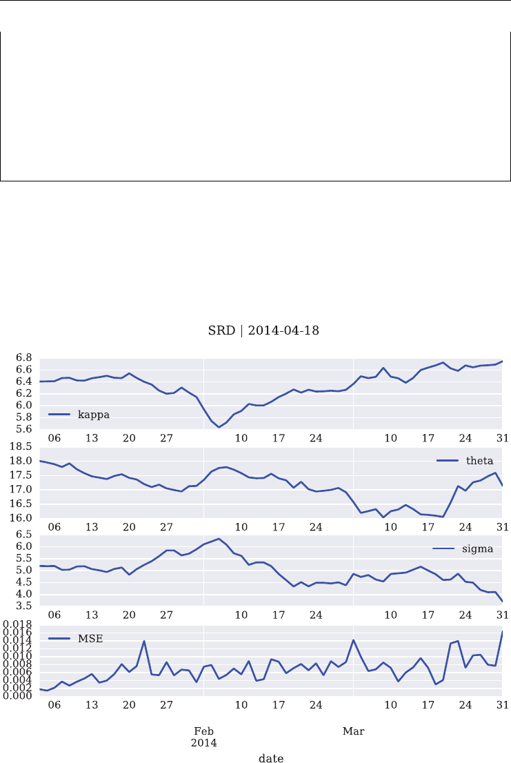
DX Analytics – Square-Root Diffusion 307
fig2, ax2 = plt. subplots()
dat = parameters.MSE
dat.hist(bins=30, ax=ax2)
plt.axvline(dat.mean(), color='r', ls='dashed',
lw=1.5, label='mean = %5.4f' % dat.mean())
plt.legend()
plt.savefig('../images/dx_srd_cali_1_hist_%s.pdf' % str(mat)[:10])
# measuring and printing the time needed for the script execution
print "Time in minutes %.2f" % ((time.time() - t0) / 60)
A visualization of the calibration results tells the whole story. Figure 13.1 shows the three
square-root diffusion parameters over time and the resulting MSE values.
As we can see throughout, the results are quite good given the low MSE values. The mean
MSE value is below 0.01 as seen in Figure 13.2.
FIGURE 13.1 Square-root diffusion parameters and MSE values from the calibration to a single
maturity (April 18, 2015).
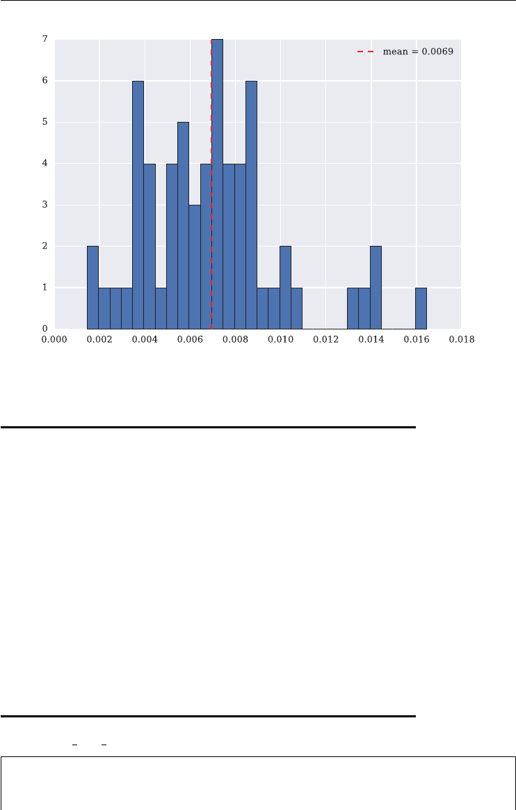
308 LISTED VOLATILITY AND VARIANCE DERIVATIVES
FIGURE 13.2 Histogram of the mean-squared errors for the calibration of the
square-root diffusion model to a single maturity (April 18, 2015).
13.5 CONCLUSIONS
This chapter uses DX Analytics to model the VSTOXX volatility index by a square-root dif-
fusion process. In similar vein, it is used to model traded European call options on the index
to implement a calibration of the VSTOXX model over time. The results show that when cal-
ibrating the model to a single options maturity only, the model performs quite well yielding
rather low MSE values throughout. The parameter values also seem to be in sensible regions
throughout (e.g. theta between 15 and 18) and they evolve rather smoothly.
There exist closed form solutions for the price of a European call option in the square-root
diffusion model of Gr¨
unbichler and Longstaff (1996) as shown in chapter 6, Valuing Volatility
Derivatives. For our analysis in this chapter we have nevertheless used the Monte Carlo valu-
ation model of DX Analytics since this approach is more general in that we can easily replace
one model by another, maybe more sophisticated, one. This is done in the next chapter where
the same study is implemented based on the square-root jump diffusion model presented in
chapter 7, Advanced Modeling of the VSTOXX Index. The only difference is that a few more
parameters need to be taken care of.
13.6 PYTHON SCRIPTS
13.6.1 dx srd calibration.py
#
# Calibration of Gr¨
unbichler and Longstaff (1996)
# Square-Root Diffusion (SRD) model to

DX Analytics – Square-Root Diffusion 309
# VSTOXX call options with DX Analytics
#
# All data from www.eurexchange.com
#
# (c) Dr. Yves J. Hilpisch
# Listed Volatility and Variance Derivatives
#
import dx
import time
import numpy as np
import pandas as pd
import datetime as dt
import scipy.optimize as spo
import matplotlib.pyplot as plt
import seaborn as sns; sns. set()
import matplotlib
matplotlib.rcParams['font.family'] = 'serif'
# importing the data
h5 = pd.HDFStore('../data/vstoxx_march_2014.h5', 'r')
vstoxx_index = h5['vstoxx_index']
vstoxx_futures = h5['vstoxx_futures']
vstoxx_options = h5['vstoxx_options']
h5.close()
# collecting the maturity dates
third_fridays = sorted(set(vstoxx_futures['MATURITY']))
# instantiation of market environment object with dummy pricing date
me_vstoxx = dx.market_environment('me_vstoxx', dt.datetime(2014, 1, 1))
me_vstoxx.add_constant('currency', 'EUR')
me_vstoxx.add_constant('frequency', 'W')
me_vstoxx.add_constant('paths', 5000)
# constant short rate model with somewhat arbitrary rate
csr = dx.constant_short_rate('csr', 0.01)
me_vstoxx.add_curve ('discount_curve', csr)
# parameters to be calibrated later, dummies only
me_vstoxx.add_constant('kappa', 1.0)
me_vstoxx.add_constant('theta', 20)
me_vstoxx.add_constant('volatility', 1.0)
# payoff function for all European call options
payoff_func = 'np.maximum(maturity_value - strike, 0)'
tol = 0.2 # otm & itm moneyness tolerance

310 LISTED VOLATILITY AND VARIANCE DERIVATIVES
def srd_get_option_selection (pricing_date, maturity, tol=tol):
''' Function to select option quotes from data set.
Parameters
==========
pricing_date: datetime object
date for which the calibration shall be implemented
maturity: datetime object
maturity date for the options to be selected
tol: float
moneyness tolerace for OTM and ITM options to be selected
Returns
=======
option_selection: DataFrame object
selected options quotes
forward: float
futures price for maturity at pricing_date
'''
forward = vstoxx_futures[(vstoxx_futures.DATE == pricing_date)
& (vstoxx_futures.MATURITY == maturity)]
['PRICE'].values[0]
option_selection = \
vstoxx_options[(vstoxx_options.DATE == pricing_date)
&(vstoxx_options.MATURITY == maturity)
&(vstoxx_options.TYPE == 'C') # only calls
&(vstoxx_options.STRIKE > (1 - tol) * forward)
&(vstoxx_options.STRIKE <(1 + tol) * forward)]
return option_selection, forward
def srd_get_option_models (pricing_date, maturity, option_selection):
''' Function to instantiate option pricing models.
Parameters
==========
pricing_date: datetime object
date for which the calibration shall be implemented
maturity: datetime object
maturity date for the options to be selected
option_selection: DataFrame object
selected options quotes
Returns
=======
vstoxx_model: dx.square_root_diffusion
model object for VSTOXX
option_models: dict

DX Analytics – Square-Root Diffusion 311
dictionary of dx.valuation_mcs_european_single objects
'''
# updating the pricing date
me_vstoxx.pricing_date = pricing_date
# setting the initial value for the pricing date
initial_value = vstoxx_index['V2TX'][pricing_date]
me_vstoxx.add_constant('initial_value', initial_value)
# setting the final date given the maturity date
me_vstoxx.add_constant('final_date', maturity)
# instantiating the risk factor (VSTOXX) model
vstoxx_model = dx.square_root_diffusion('vstoxx_model', me_vstoxx)
# setting the maturity date for the valuation model(s)
me_vstoxx.add_constant('maturity', maturity)
option_models = {} # dictionary collecting all models
for option in option_selection.index:
# setting the strike for the option to be modeled
strike = option_selection['STRIKE'].ix[option]
me_vstoxx.add_constant('strike', strike)
# instantiating the option model
option_models[option] = \
dx.valuation_mcs_european_single(
'eur_call_%d' % strike,
vstoxx_model,
me_vstoxx,
payoff_func)
return vstoxx_model, option_models
def srd_calculate_model_values(p0):
''' Returns all relevant option values.
Parameters
===========
p0: tuple/list
tuple of kappa, theta, volatility
Returns
=======
model_values: dict
dictionary with model values
'''
# read the model parameters from input tuple
kappa, theta, volatility = p0
# update the option market environment
vstoxx_model. update(kappa=kappa,
theta=theta,
volatility=volatility)

312 LISTED VOLATILITY AND VARIANCE DERIVATIVES
# estimate and collect all option model present values
results = [option_models[option].present_value(fixed_seed=True)
for option in option_models]
# combine the results with the option models in a dictionary
model_values = dict(zip(option_models, results))
return model_values
def srd_mean_squared_error(p0, penalty=True):
''' Returns the mean-squared error given
the model and market values.
Parameters
===========
p0: tuple/list
tuple of kappa, theta, volatility
Returns
=======
MSE: float
mean-squared error
'''
# escape with high value for non-sensible parameter values
if p0[0] < 0 or p0[1] < 5. or p0[2] < 0 or p0[2] > 10.:
return 1000
# define/access global variables/objects
global option_selection, vstoxx_model, option_models, first, last
# calculate the model values for the option selection
model_values = srd_calculate_model_values(p0)
option_diffs = {} # dictionary to collect differences
for option in model_values:
# differences between model value and market quote
option_diffs[option] = (model_values[option]
- option_selection['PRICE'].loc[option])
# calculation of mean-squared error
MSE = np.sum(np.array(option_diffs.values()) ** 2) / len(option_diffs)
if first is True:
# if in global optimization, no penalty
penalty = 0.0
else:
# if in local optimization, penalize deviation from previous
# optimal parameter combination
penalty = (np.sum((p0 - last) ** 2)) / 100
if penalty is False:
return MSE
return MSE + penalty

DX Analytics – Square-Root Diffusion 313
def srd_get_parameter_series(pricing_date_list, maturity_list):
'''Returns parameter series for the calibrated model over time.
Parameters
==========
pricing_date_list: pd.DatetimeIndex
object with relevant pricing dates
maturity_list: list
list with maturities to be calibrated
Returns
=======
parameters: pd.DataFrame
DataFrame object with parameter series
'''
# define/access global variables/objects
global option_selection, vstoxx_model, option_models, first, last
parameters = pd.DataFrame() # object to collect parameter series
for maturity in maturity_list:
first = True
for pricing_date in pricing_date_list:
# select relevant option quotes
option_selection, forward = srd_get_option_selection
(pricing_date, maturity)
# instantiate all model given option selection
vstoxx_model, option_models = srd_get_option_models
(pricing_date, maturity, option_selection)
if first is True:
# global optimization to start with
opt = spo.brute(srd_mean_squared_error,
((1.25, 6.51, 0.75), # range for kappa
(10., 20.1, 2.5), # range for theta
(0.5, 10.51, 2.5)), # range for volatility
finish=None)
# local optimization
opt = spo.fmin(srd_mean_squared_error, opt,
maxiter=550, maxfun=650,
xtol=0.0000001, ftol=0.0000001);
# calculate MSE for storage
MSE = srd_mean_squared_error(opt, penalty=False)
# store main parameters and results
parameters = parameters.append(
pd.DataFrame(
{'date' : pricing_date,
'maturity' : maturity,
'initial_value' : vstoxx_model.initial_value,
'kappa' : opt[0],

314 LISTED VOLATILITY AND VARIANCE DERIVATIVES
'theta' : opt[1],
'sigma' : opt[2],
'MSE' : MSE},
index=[0]), ignore_index=True)
first = False # set to False after first iteration
last = opt # store optimal parameters for reference
print ("Maturity %s" %str(maturity)[:10]
+ " | Pricing Date %s" % str(pricing_date)[:10]
+ " | MSE %6.5f " % MSE)
return parameters
if __name__ is '_ _main_ _':
t0 = time.time()
# define the dates for the calibration
pricing_date_list = pd.date_range('2014/1/2', '2014/3/31', freq='B')
# select the maturities
maturity_list = [third_fridays[3]] # only 18. April 2014 maturity
# start the calibration
parameters = srd_get_parameter_series(pricing_date_list,
maturity_list)
# plot the results
for mat in maturity_list:
fig1, ax1 = plt.subplots()
to_plot = parameters[parameters.maturity ==
maturity_list[0]].set_index('date')[
['kappa', 'theta', 'sigma', 'MSE']]
to_plot.plot(subplots=True, color='b', figsize=(10, 12),
title='SRD | ' + str(mat)[:10], ax=ax1)
plt.savefig('../images/dx_srd_cali_1_%s.pdf' % str(mat)[:10])
# plotting the histogram of the MSE values
fig2, ax2 = plt. subplots()
dat = parameters.MSE
dat.hist(bins=30, ax=ax2)
plt.axvline(dat.mean(), color='r', ls='dashed',
lw=1.5, label='mean = %5.4f' %dat.mean())
plt.legend()
plt.savefig('../images/dx_srd_cali_1_hist_%s.pdf' % str(mat)[:10])
# measuring and printing the time needed for the script execution
print "Time in minutes %.2f" % ((time.time()- t0)/ 60)

CHAPTER 14
DX Analytics – Square-Root
Jump Diffusion
14.1 INTRODUCTION
Similarly to the previous chapter, this chapter again uses DX Analytics to model the VSTOXX
index, but this time by the square-root jump diffusion (SRJD) process as introduced in chap-
ter 7, Advanced Modeling of the VSTOXX Index. The study this chapter implements is actu-
ally the same as in the previous one using the very same data set. However, the challenge is
increased in that we require multiple VSTOXX option maturities to be calibrated simultane-
ously and over time.
14.2 MODELING THE VSTOXX OPTIONS
DX Analytics provides a class for the deterministic shift square-root jump diffusion model. It is
called dx.square_root_jump_diffusion(). Although the calibration we are imple-
menting in this chapter is more or less the same as in the previous one, we need nevertheless
to adjust the code signicantly in many places. Therefore, we are stepping through the single
elements again in what follows. All the code used in this chapter is found in the Python script
dx_srjd_calibration.py (see sub-section 14.6.1, dx_srjd_calibration.py).
The beginning of the script is rather similar to the one implementing the calibration of the
square-root diffusion model. A major difference is that we need three additional parameters
lambda,mu and delta.
import dx
import time
import numpy as np
import pandas as pd
import datetime as dt
import scipy.optimize as spo
import matplotlib.pyplot as plt
import seaborn as sns; sns.set()
315
Listed Volatility and Variance Derivatives: A
Python-based Guide
By Dr. Yves J. Hilpisch
© 2017 Yves Hilpisch

316 LISTED VOLATILITY AND VARIANCE DERIVATIVES
import matplotlib
matplotlib.rcParams['font.family'] = 'serif'
from copy import deepcopy
# importing the data
h5 = pd.HDFStore('../data/vstoxx_march_2014.h5', 'r')
vstoxx_index = h5['vstoxx_index']
vstoxx_futures = h5['vstoxx_futures']
vstoxx_options = h5['vstoxx_options']
h5.close()
# collecting the maturity dates
third_fridays = sorted(set(vstoxx_futures['MATURITY']))
# instantiation of market environment object with dummy pricing date
me_vstoxx = dx.market_environment('me_vstoxx', dt.datetime(2014, 1, 1))
me_vstoxx.add_constant('currency', 'EUR')
me_vstoxx.add_constant('frequency', 'W')
me_vstoxx.add_constant('paths', 5000)
# constant short rate model with somewhat arbitrary rate
csr = dx.constant_short_rate('csr', 0.01)
me_vstoxx.add_curve('discount_curve', csr)
# parameters to be calibrated later, dummies only
# SRD part
me_vstoxx.add_constant('kappa', 1.0)
me_vstoxx.add_constant('theta', 20)
me_vstoxx.add_constant('volatility', 1.0)
# jump part
me_vstoxx.add_constant('lambda', 0.5)
me_vstoxx.add_constant('mu', -0.2)
me_vstoxx.add_constant('delta', 0.1)
# payoff function for all European call options
payoff_func = 'np.maximum(maturity_value - strike, 0)'
tol = 0.2 # otm & itm moneyness tolerance
first = True # flag for first calibration
The function srjd_get_option_selection() selects the options used for the calibra-
tion. In the current case, we can choose multiple option maturities to be included.
def srjd_get_option_selection(pricing_date, tol=tol):
' ' ' Function to select option quotes from data set.

DX Analytics – Square-Root Jump Diffusion 317
Parameters
==========
pricing_date: datetime object
date for which the calibration shall be implemented
tol: float
moneyness tolerance for OTM and ITM options to be selected
Returns
=======
option_selection: DataFrame object
selected options quotes
futures: DataFrame object
futures prices at pricing_date
'''
option_selection = pd.DataFrame()
mats = [third_fridays[3],] # list of maturity dates
# select the relevant futures prices
futures = vstoxx_futures[(vstoxx_futures.DATE == pricing_date)
& (vstoxx_futures.MATURITY.apply(lambda x: x in mats))]
# collect option data for the given option maturities
for mat in mats:
forward = futures[futures.MATURITY == mat]['PRICE'].values[0]
option_selection = option_selection.append(
vstoxx_options[(vstoxx_options.DATE == pricing_date)
& (vstoxx_options.MATURITY == mat)
& (vstoxx_options.TYPE == 'C') # only calls
& (vstoxx_options.STRIKE > (1 - tol) * forward)
& (vstoxx_options.STRIKE < (1 + tol) * forward)])
return option_selection, futures
The calibration of the SRJD model consists of two steps:
term structure calibration: using the futures prices at a given pricing date, this step
calibrates the forward rates of the model
option quote calibration: using market quotes of traded options, this step calibrates the
model parameters to optimally reect the market quotes.
Two functions are used to implement the rst step. The function srd_forward_error()
calculates the mean-squared error (MSE) for the futures term structure given a set of model
parameters.
def srd_forward_error(p0):
' ' ' Calculates the mean-squared error for the
term structure calibration for the SRD model part.
Parameters
===========

318 LISTED VOLATILITY AND VARIANCE DERIVATIVES
p0: tuple/list
tuple of kappa, theta, volatility
Returns
=======
MSE: float
mean-squared error
'''
global initial_value, f, t
if p0[0] < 0 or p0[1] < 0 or p0[2] < 0:
return 100
f_model = dx.srd_forwards(initial_value, p0, t)
MSE = np.sum((f - f_model) ** 2) / len(f)
return MSE
The second function is called generate_shift_base() and calculates the single deter-
ministic shift values to match the futures term structure perfectly – after the minimization
of the term structure MSE. Note that the perfect shift gets lost again later on when the SRD
parameters are updated during the calibration to the option quotes.
def generate_shift_base(pricing_date, futures):
' ' ' Generates the values for the deterministic shift for the
SRD model part.
Parameters
==========
pricing_date: datetime object
date for which the calibration shall be implemented
futures: DataFrame object
futures prices at pricing_date
Returns
=======
shift_base: ndarray object
shift values for the SRD model part
'''
global initial_value, f, t
# futures price array
f = list(futures['PRICE'].values)
f.insert(0, initial_value)
f = np.array(f)
# date array
t = [_.to_pydatetime() for _in futures['MATURITY']]
t.insert(0, pricing_date)
t = np.array(t)
# calibration to the futures values
opt = spo.fmin(srd_forward_error, (2., 15., 2.))

DX Analytics – Square-Root Jump Diffusion 319
# calculation of shift values
f_model = dx.srd_forwards(initial_value, opt, t)
shifts = f - f_model
shift_base = np.array((t, shifts)).T
return shift_base
As in the SRD calibration case, the function srjd_get_option_models() creates the
valuation models for all selected options.
def srjd_get_option_models(pricing_date, option_selection, futures):
' ' ' Function to instantiate option pricing models.
Parameters
==========
pricing_date: datetime object
date for which the calibration shall be implemented
maturity: datetime object
maturity date for the options to be selected
option_selection: DataFrame object
selected options quotes
Returns
=======
vstoxx_model: dx.square_root_diffusion
model object for VSTOXX
option_models: dict
dictionary of dx.valuation_mcs_european_single objects
'''
global initial_value
# updating the pricing date
me_vstoxx.pricing_date = pricing_date
# setting the initial value for the pricing date
initial_value = vstoxx_index['V2TX'][pricing_date]
me_vstoxx.add_constant('initial_value', initial_value)
# setting the final date given the maturity dates
final_date = max(futures.MATURITY).to_pydatetime()
me_vstoxx.add_constant('final_date', final_date)
# adding the futures term structure
me_vstoxx.add_curve('term_structure', futures)
# instantiating the risk factor (VSTOXX) model
vstoxx_model = dx.square_root_jump_diffusion_plus('vstoxx_model',
me_vstoxx)
# generating the shift values and updating the model
vstoxx_model.shift_base = generate_shift_base(pricing_date, futures)
vstoxx_model.update_shift_values()

320 LISTED VOLATILITY AND VARIANCE DERIVATIVES
option_models = {} # dictionary collecting all models
for option in option_selection.index:
# setting the maturity date for the given option
maturity = option_selection['MATURITY'].ix[option]
me_vstoxx.add_constant('maturity', maturity)
# setting the strike for the option to be modeled
strike = option_selection['STRIKE'].ix[option]
me_vstoxx.add_constant('strike', strike)
# instantiating the option model
option_models[option] = \
dx.valuation_mcs_european_single(
'eur_call_%d' % strike,
vstoxx_model,
me_vstoxx,
payoff_func)
return vstoxx_model, option_models
14.3 CALIBRATION OF THE VSTOXX MODEL
The function srjd_calculate_model_values() only differs from the SRD case in
that three more parameters need to be taken care of.
def srjd_calculate_model_values(p0):
' ' ' Returns all relevant option values.
Parameters
===========
p0: tuple/list
tuple of kappa, theta, volatility, lamb, mu, delt
Returns
=======
model_values: dict
dictionary with model values
'''
# read the model parameters from input tuple
kappa, theta, volatility, lamb, mu, delt = p0
# update the option market environment
vstoxx_model.update(kappa=kappa,
theta=theta,
volatility=volatility,
lamb=lamb,
mu=mu,
delt=delt)
# estimate and collect all option model present values

DX Analytics – Square-Root Jump Diffusion 321
results = [option_models[option].present_value(fixed_seed=True)
for option in option_models]
# combine the results with the option models in a dictionary
model_values = dict(zip(option_models, results))
return model_values
The same holds true for the function srjd_mean_squared_error() which now also
penalizes certain parameter ranges for the additional parameters of the SRJD model.
def srjd_mean_squared_error(p0, penalty=True):
' ' ' Returns the mean-squared error given
the model and market values.
Parameters
===========
p0: tuple/list
tuple of kappa, theta, volatility
Returns
=======
MSE: float
mean-squared error
'''
# escape with high value for non-sensible parameter values
if (p0[0] < 0 or p0[1] < 5. or p0[2] < 0 or p0[2] > 10.
or p0[3] < 0 or p0[4] < 0 or p0[5] < 0):
return 1000
# define/access global variables/objects
global option_selection, vstoxx_model, option_models, first, last
# calculate the model values for the option selection
model_values = srjd_calculate_model_values(p0)
option_diffs = {} # dictionary to collect differences
for option in model_values:
# differences between model value and market quote
option_diffs[option] = (model_values[option]
- option_selection['PRICE'].loc[option])
# calculation of mean-squared error
MSE = np.sum(np.array(option_diffs.values()) ** 2) / len(option_diffs)
if first is True:
# if in first optimization, no penalty
penalty = 0.0
else:
# if 2, 3, ... optimization, penalize deviation from previous
# optimal parameter combination
penalty = (np.sum((p0 - last) ** 2))
if penalty is False:
return MSE
return MSE + penalty

322 LISTED VOLATILITY AND VARIANCE DERIVATIVES
The function srjd_get_parameter_series() implementing the calibration routines
then takes on the form:
def srjd_get_parameter_series(pricing_date_list):
' ' ' Returns parameter series for the calibrated model over time.
Parameters
==========
pricing_date_list: pd.DatetimeIndex
object with relevant pricing dates
Returns
=======
parameters: pd.DataFrame
DataFrame object with parameter series
'''
# define/access global variables/objects
global initial_value, futures, option_selection, vstoxx_model, \
option_models, first, last
parameters = pd.DataFrame() # DataFrame object to collect parameter series
for pricing_date in pricing_date_list:
# setting the initial value for the VSTOXX
initial_value = vstoxx_index['V2TX'][pricing_date]
# select relevant option quotes
option_selection, futures = srjd_get_option_selection(pricing_date)
# instantiate all model given option selection
vstoxx_model, option_models = srjd_get_option_models(pricing_date,
option_selection,
futures)
# global optimization to start with
opt = spo.brute(srjd_mean_squared_error,
((1.25, 6.51, 0.75), # range for kappa
(10., 20.1, 2.5), # range for theta
(0.5, 10.51, 2.5), # range for volatility
(0.1, 0.71, 0.3), # range for lambda
(0.1, 0.71, 0.3), # range for mu
(0.1, 0.21, 0.1)), # range for delta
finish=None)
# local optimization
opt = spo.fmin(srjd_mean_squared_error, opt,
maxiter=550, maxfun=650,
xtol=0.0000001, ftol=0.0000001);
# calculate MSE for storage
MSE = srjd_mean_squared_error(opt, penalty=False)
# store main parameters and results
parameters = parameters.append(
pd.DataFrame(
{'date' : pricing_date,

DX Analytics – Square-Root Jump Diffusion 323
'initial_value' : vstoxx_model.initial_value,
'kappa' : opt[0],
'theta' : opt[1],
'sigma' : opt[2],
'lambda' : opt[3],
'mu' : opt[4],
'delta' : opt[5],
'MSE' : MSE},
index=[0]), ignore_index=True)
first = False # set to False after first iteration
last = opt # store optimal parameters for reference
print ("Pricing Date %s" % str(pricing_date)[:10]
+"|MSE%6.5f" % MSE)
return parameters
Finally, the function srjd_plot_model_fit() plots the results for the last pricing date of
the calibration procedure and compares the model values to the market quotes.
def srjd_plot_model_fit(parameters):
# last pricing date
pdate = max(parameters.date)
# optimal parameters for that date and the maturity
opt = np.array(parameters[parameters.date == pdate][[
'kappa', 'theta', 'sigma', 'lambda', 'mu', 'delta']])[0]
option_selection, futures = srjd_get_option_selection(pdate, tol=tol)
vstoxx_model, option_models = srjd_get_option_models(pdate,
option_selection,
futures)
model_values = srjd_calculate_model_values(opt)
model_values = pd.DataFrame(model_values.values(),
index=model_values.keys(),
columns=['MODEL'])
option_selection = option_selection.join(model_values)
mats = set(option_selection.MATURITY.values)
mats = sorted(mats)
# arranging the canvas for the subplots
height = max(8, 2 * len(mats))
if len(mats) == 1:
mat = mats[0]
fig, axarr = plt.subplots(2, figsize=(10, height))
os = option_selection[option_selection.MATURITY == mat]
strikes = os.STRIKE.values
axarr[0].set_ylabel('%s' % str(mat)[:10])
axarr[0].plot(strikes, os.PRICE.values, label='Market Quotes')
axarr[0].plot(strikes, os.MODEL.values, 'ro', label='Model Prices')
axarr[0].legend(loc=0)

324 LISTED VOLATILITY AND VARIANCE DERIVATIVES
wi = 0.3
axarr[1].bar(strikes - wi / 2, os.MODEL.values - os.PRICE.values,
width=wi)
axarr[0].set_xlabel('strike')
axarr[1].set_xlabel('strike')
else:
fig, axarr = plt.subplots(len(mats), 2, sharex=True,
figsize=(10, height))
for z, mat in enumerate(mats):
os = option_selection[option_selection.MATURITY == mat]
strikes = os.STRIKE.values
axarr[z, 0].set_ylabel('%s' % str(mat)[:10])
axarr[z, 0].plot(strikes, os.PRICE.values, label='Market Quotes')
axarr[z, 0].plot(strikes, os.MODEL.values, 'ro', label='Model
Prices')
axarr[z, 0].legend(loc=0)
wi = 0.3
axarr[z, 1].bar(strikes - wi / 2,
os.MODEL.values - os.PRICE.values, width=wi)
axarr[z, 0].set_xlabel('strike')
axarr[z, 1].set_xlabel('strike')
plt.savefig('../images/dx_srjd_cali_1_fit.pdf')
The nal step is to start the calibration, collect the calibration results and to
plot them. Remember that the maturities in this case are selected in the function
srjd_get_option_selection().
if __name__ is '_ _main_ _':
t0 = time.time()
# selecting the dates for the calibration
pricing_date_list = pd.date_range('2014/3/1', '2014/3/31', freq='B')
# conducting the calibration
parameters = srjd_get_parameter_series(pricing_date_list)
# storing the calibation results
date = str(dt.datetime.now())[:10]
h5 = pd.HDFStore('../data/srjd_calibration_%s_%s_%s'%
(me_vstoxx.get_constant('paths'),
me_vstoxx.get_constant('frequency'),
date.replace('-', '_')), 'w')
h5['parameters'] = parameters
h5.close()
# plotting the parameter time series data
fig1, ax1 = plt.subplots(1, figsize=(10, 12))
to_plot = parameters.set_index('date')[
['kappa', 'theta', 'sigma',
'lambda', 'mu', 'delta', 'MSE']]

DX Analytics – Square-Root Jump Diffusion 325
to_plot.plot(subplots=True, color='b', title='SRJD', ax=ax1)
plt.savefig('../images/dx_srjd_cali_1.pdf')
# plotting the histogram of the MSE values
fig2, ax2 = plt.subplots()
dat = parameters.MSE
dat.hist(bins=30, ax=ax2)
plt.axvline(dat.mean(), color='r', ls='dashed',
lw=1.5, label='mean = %5.4f' % dat.mean())
plt.legend()
plt.savefig('../images/dx_srjd_cali_1_hist.pdf')
# plotting the model fit at last pricing date
srjd_plot_model_fit(parameters)
# measuring and printing the time needed for the script execution
print "Time in minutes %.2f" % ((time.time() - t0) / 60)
14.4 CALIBRATION RESULTS
This section presents calibration results for three different calibration runs. The rst run imple-
ments a calibration to a single maturity, the second to two maturities simultaneously while the
third run does the same for ve maturities of the VSTOXX options. The nal run shows the
effects of not using penalties for deviations from previous optimal parameters which in general
would be used to get smoother parameter time series.
14.4.1 Calibration to One Maturity
First, we calibrate the SRJD model to a single maturity, April 18, 2014. The calibration takes
place for all trading days in the rst quarter of 2014. Figure 14.1 shows the time series data
for the parameters of the square-root jump diffusion over time and the resulting MSE values.
The MSE values are all quite low in general with a mean of about 0.1 and one outlier as
Figure 14.2 illustrates.
Figure 14.3 shows the calibration results for the last pricing date, i.e. on March 31, 2014.
14.4.2 Calibration to Two Maturities
Let us have a look at the results for the calibration to two maturities where the VSTOXX
futures term structure comes into play. Figure 14.4 shows the parameter time series data for
this case.
In this case, the resulting MSE values are even slightly lower on average with a mean of
about 0.05 as seen in Figure 14.5.
Figure 14.6 shows the calibration results for the last pricing date, i.e. on March 31, 2014.
14.4.3 Calibration to Five Maturities
Finally, let us have a look at the calibration to ve maturities simultaneously. This is the largest
number of maturities for which there is data over the whole time range from January to March
2014. Figure 14.7 shows the results for the model parameters and the MSE values.
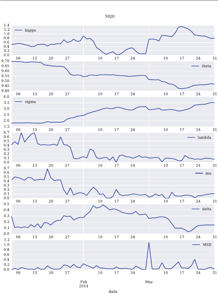
326 LISTED VOLATILITY AND VARIANCE DERIVATIVES
FIGURE 14.1 Square-root jump diffusion parameters and MSE values from the calibration to two
maturities.
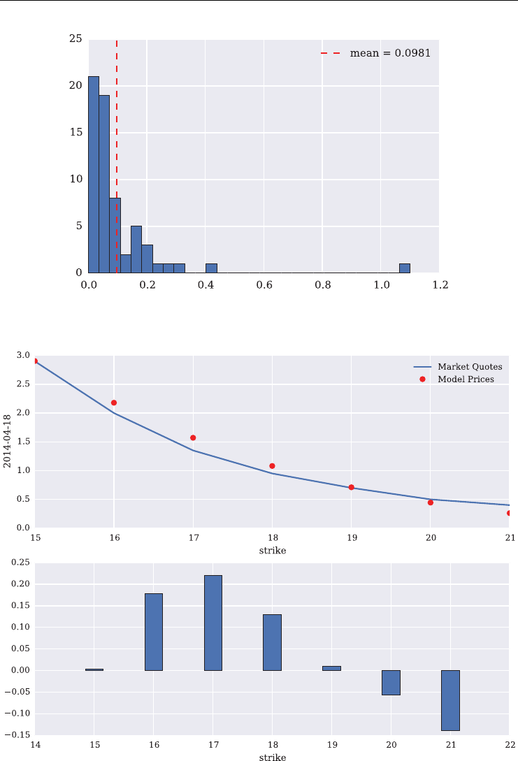
DX Analytics – Square-Root Jump Diffusion 327
FIGURE 14.2 Histogram of MSE values for SRJD calibration to two
maturities.
FIGURE 14.3 Model values from the SRJD calibration vs. market quotes as well as pricing errors
(bars) on March 31, 2014 (one maturity).
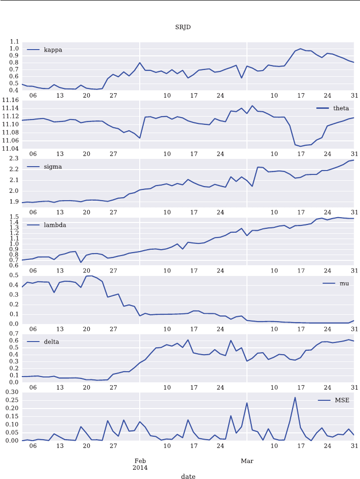
328 LISTED VOLATILITY AND VARIANCE DERIVATIVES
FIGURE 14.4 Square-root jump diffusion parameters and MSE values from the calibration to ve
maturities.
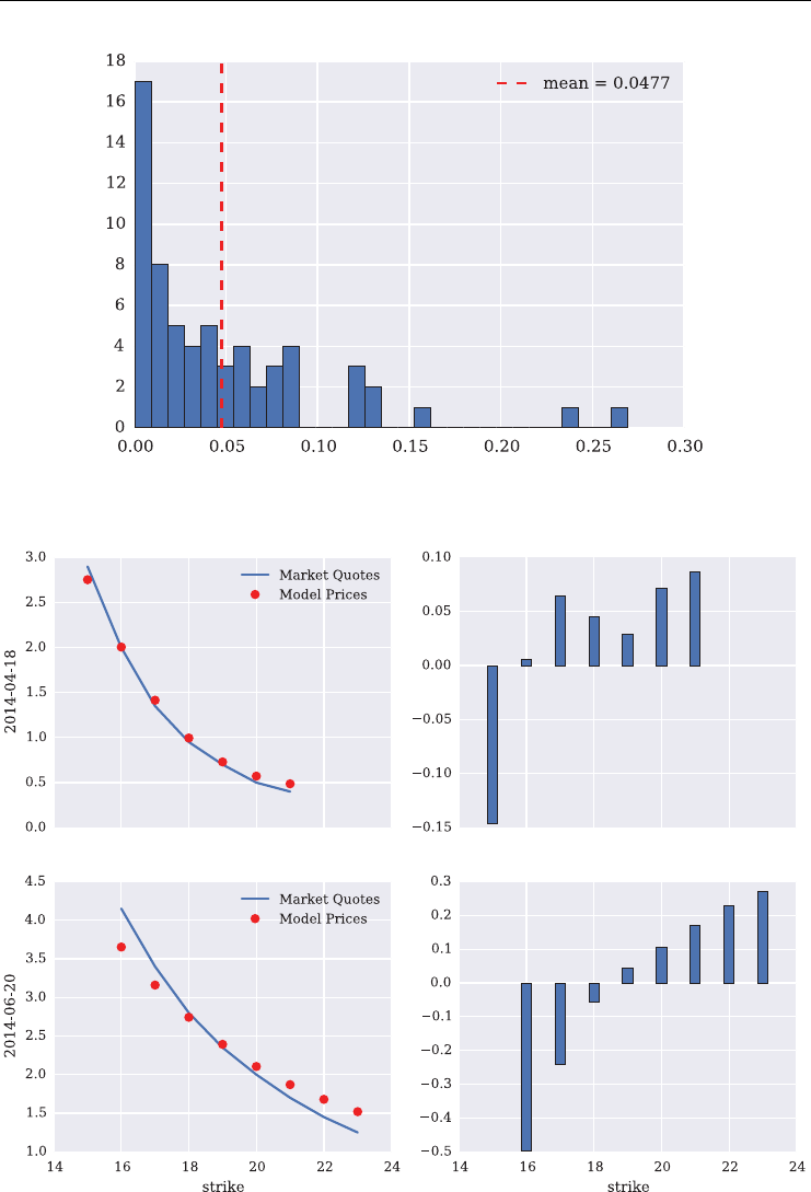
DX Analytics – Square-Root Jump Diffusion 329
FIGURE 14.5 Histogram of MSE values for SRJD calibration to ve
maturities.
FIGURE 14.6 Model values from the SRJD calibration vs. market quotes as well as pricing errors
(bars) on March 31, 2014 (two maturities).
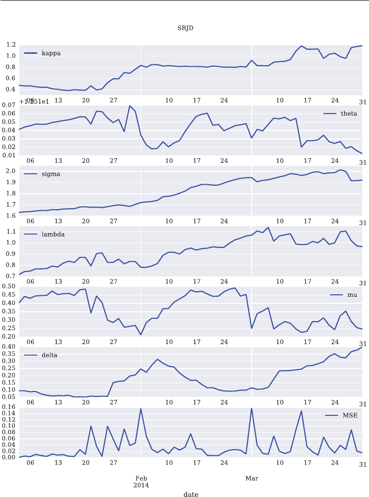
330 LISTED VOLATILITY AND VARIANCE DERIVATIVES
FIGURE 14.7 Square-root jump diffusion parameters and MSE values from the calibration to ve
maturities.
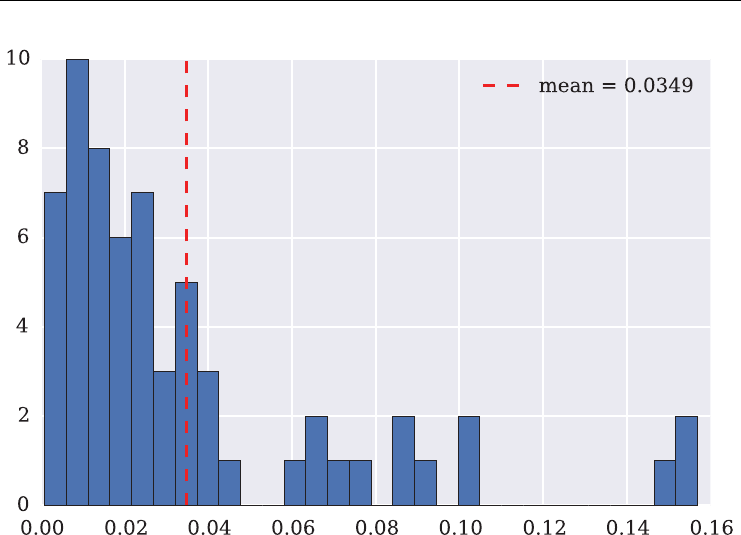
DX Analytics – Square-Root Jump Diffusion 331
FIGURE 14.8 Histogram of MSE values for SRJD calibration to ve maturities.
The resulting MSE values are again slightly lower on average. The mean MSE value is
about 0.035 (see Figure 14.8).
The nal plot (see Figure 14.9) again shows the calibration results at the last pricing date,
March 31, 2014. Given that the calibration includes options with different moneyness levels
over ve different maturity months, the performance of the SRJD model is satisfactory.
14.4.4 Calibration without Penalties
It might be surprising that the highest average MSE value is observed for the calibration case
with one maturity only. This is mainly due to the fact that we penalize deviations from previous
optimal parameter values quite heavily and also to the existence of one outlier. The advantage
of this is rather smooth time series for the single parameters, i.e. without too much variation.
This is usually desirable, for example, when such a model is used for hedging purposes and
hedge positions (indirectly) depend on the parameter values.
In this sub-section we therefore want to illustrate what changes when we do not penalize
deviations from the previous optimal parameter values. Figure 14.10 shows the results for the
model parameters and the MSE values from a calibration to one maturity (April 18, 2014)
without penalization. Inspection of the gure reveals how erratically the parameter time series
can behave in this case.
However, the advantage here is that there are excellent model ts to the market data with
a mean MSE value of 0.0007 only (see Figure 14.11).
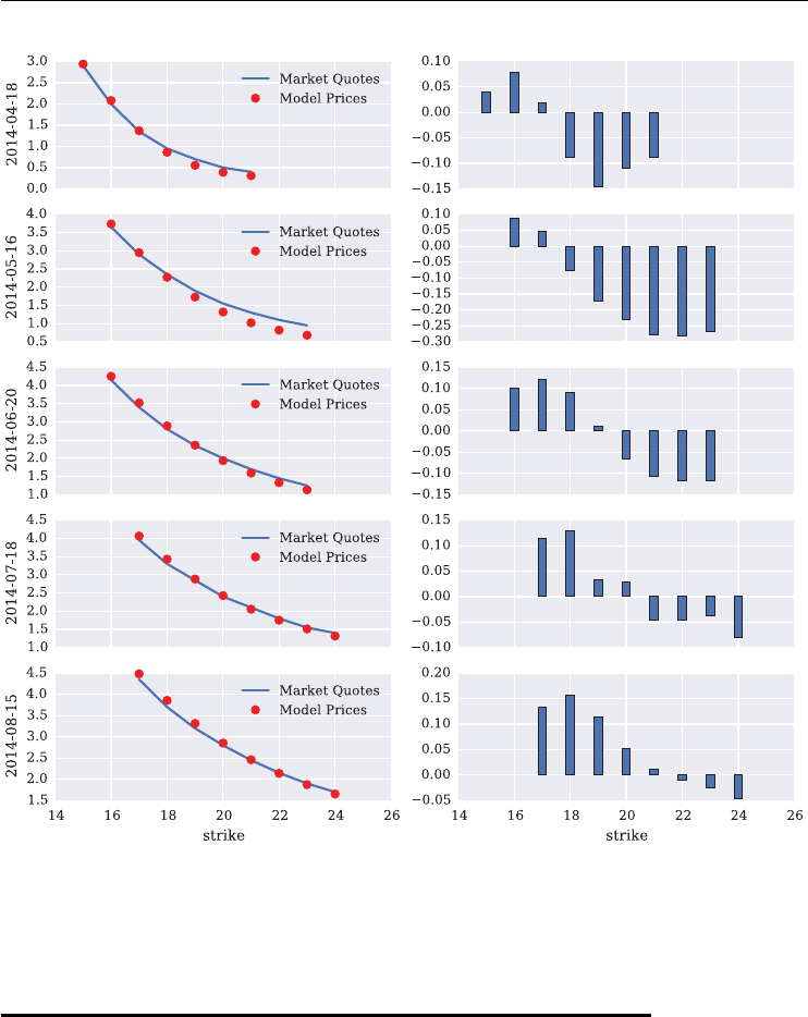
332 LISTED VOLATILITY AND VARIANCE DERIVATIVES
FIGURE 14.9 Model values from the SRJD calibration vs. market quotes as well as pricing errors
(bars) on March 31, 2014 (ve maturities).
14.5 CONCLUSIONS
This chapter calibrates the square-root jump diffusion (SRJD) model to both the VSTOXX
futures term structure and for multiple maturities for the VSTOXX options. It uses DX Ana-
lytics as in the previous chapter which provides exible modeling capabilities for volatility-
based derivatives based, among other things, on square-root diffusions and square-root jump
diffusions.
The results we achieve are quite good in that the typical mean-squared error values are
relatively low for all cases covered – and this over the complete three month period for which
we are updating the calibration with only a few outliers.
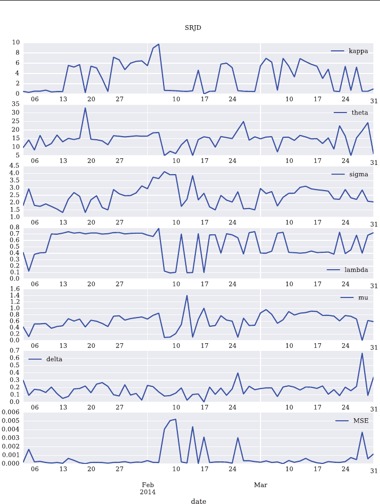
DX Analytics – Square-Root Jump Diffusion 333
FIGURE 14.10 Square-root jump diffusion parameters and MSE values from the calibration to one
maturity without penalization.
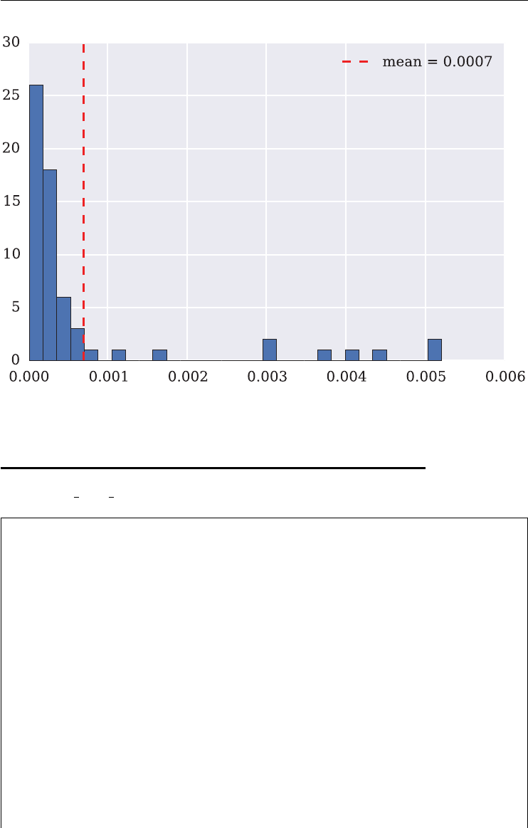
334 LISTED VOLATILITY AND VARIANCE DERIVATIVES
FIGURE 14.11 Histogram of MSE values for SRJD calibration to one maturity without
penalization.
14.6 PYTHON SCRIPTS
14.6.1 dx srjd calibration.py
#
# Calibration of Square–Root Jump Diffusion (SRJD)
# model to VSTOXX call options with DX Analytics
#
# All data from www.eurexchange.com
#
# (c) Dr. Yves J. Hilpisch
# Listed Volatility and Variance Derivatives
#
import dx
import time
import numpy as np
import pandas as pd
import datetime as dt
import scipy.optimize as spo
import matplotlib.pyplot as plt
import seaborn as sns ; sns.set()
import matplotlib

DX Analytics – Square-Root Jump Diffusion 335
matplotlib.rcParams['font.family'] = 'serif '
from copy import deepcopy
# importing the data
h5 = pd.HDFStore('../data/vstoxx_march_2014.h5', 'r')
vstoxx_index = h5['vstoxx_index']
vstoxx_futures = h5['vstoxx_futures']
vstoxx_options = h5['vstoxx_options']
h5.close()
# collecting the maturity dates
third_fridays = sorted(set(vstoxx_futures['MATURITY']))
# instantiation of market environment object with dummy pricing date
me_vstoxx = dx.market_environment('me_vstoxx', dt.datetime(2014, 1, 1))
me_vstoxx.add_constant('currency', 'EUR')
me_vstoxx.add_constant('frequency', 'W')
me_vstoxx.add_constant('paths', 5000)
# constant short rate model with somewhat arbitrary rate
csr = dx.constant_short_rate('csr', 0.01)
me_vstoxx.add_curve('discount_curve', csr)
# parameters to be calibrated later, dummies only
# SRD part
me_vstoxx.add_constant('kappa', 1.0)
me_vstoxx.add_constant('theta', 20)
me_vstoxx.add_constant('volatility', 1.0)
# jump part
me_vstoxx.add_constant('lambda', 0.5)
me_vstoxx.add_constant('mu', -0.2)
me_vstoxx.add_constant('delta', 0.1)
# payoff function for all European call options
payoff_func = 'np.maximum(maturity_value – strike, 0)'
tol = 0.2 # otm & itm moneyness tolerance
first = True # flag for first calibration
def srjd_get_option_selection(pricing_date, tol=tol):
' ' ' Function to select option quotes from data set.
Parameters
==========
pricing_date: datetime object
date for which the calibration shall be implemented
tol: float
moneyness tolerace for OTM and ITM options to be selected
Returns

336 LISTED VOLATILITY AND VARIANCE DERIVATIVES
=======
option_selection: DataFrame object
selected options quotes
futures: DataFrame object
futures prices at pricing_date
'''
option_selection = pd.DataFrame()
mats = [third_fridays[3],] # list of maturity dates
# select the relevant futures prices
futures = vstoxx_futures[(vstoxx_futures.DATE == pricing_date)
& (vstoxx_futures.MATURITY.apply(lambda x: x in mats))]
# collect option data for the given option maturities
for mat in mats:
forward = futures[futures.MATURITY == mat]['PRICE'].values[0]
option_selection = option_selection.append(
vstoxx_options[(vstoxx_options.DATE == pricing_date)
& (vstoxx_options.MATURITY == mat)
& (vstoxx_options.TYPE == 'C') # only calls
& (vstoxx_options.STRIKE > (1 - tol) * forward)
& (vstoxx_options.STRIKE < (1 + tol) * forward)])
return option_selection, futures
def srd_forward_error(p0):
' ' ' Calculates the mean-squared error for the
term structure calibration for the SRD model part.
Parameters
===========
p0: tuple/list
tuple of kappa, theta, volatility
Returns
=======
MSE: float
mean-squared error
'''
global initial_value, f, t
if p0[0] < 0 or p0[1] < 0 or p0[2] < 0:
return 100
f_model = dx.srd_forwards(initial_value, p0, t)
MSE = np.sum(( f - f_model) ** 2) / len(f)
return MSE
def generate_shift_base(pricing_date, futures):
' ' ' Generates the values for the deterministic shift for the
SRD model part.

DX Analytics – Square-Root Jump Diffusion 337
Parameters
==========
pricing_date: datetime object
date for which the calibration shall be implemented
futures: DataFrame object
futures prices at pricing_date
Returns
=======
shift_base: ndarray object
shift values for the SRD model part
'''
global initial_value, f, t
# futures price array
f = list(futures['PRICE'].values)
f.insert(0, initial_value)
f = np.array(f)
# date array
t = [_.to_pydatetime() for _in futures['MATURITY']]
t.insert(0, pricing_date)
t = np.array(t)
# calibration to the futures values
opt = spo.fmin(srd_forward_error, (2., 15., 2.))
# calculation of shift values
f_model = dx.srd_forwards(initial_value, opt, t)
shifts = f - f_model
shift_base = np.array(( t, shifts)).T
return shift_base
def srjd_get_option_models(pricing_date, option_selection, futures):
' ' ' Function to instantiate option pricing models.
Parameters
==========
pricing_date: datetime object
date for which the calibration shall be implemented
maturity: datetime object
maturity date for the options to be selected
option_selection: DataFrame object
selected options quotes
Returns
=======
vstoxx_model: dx.square_root_diffusion
model object for VSTOXX

338 LISTED VOLATILITY AND VARIANCE DERIVATIVES
option_models: dict
dictionary of dx.valuation_mcs_european_single objects
'''
global initial_value
# updating the pricing date
me_vstoxx.pricing_date = pricing_date
# setting the initial value for the pricing date
initial_value = vstoxx_index['V2TX'][pricing_date]
me_vstoxx.add_constant('initial_value', initial_value)
# setting the final date given the maturity dates
final_date = max(futures.MATURITY).to_pydatetime()
me_vstoxx.add_constant('final_date', final_date)
# adding the futures term structure
me_vstoxx.add_curve('term_structure', futures)
# instantiating the risk factor (VSTOXX) model
vstoxx_model = dx.square_root_jump_diffusion_plus('vstoxx_model',
me_vstoxx)
# generating the shift values and updating the model
vstoxx_model.shift_base = generate_shift_base(pricing_date, futures)
vstoxx_model.update_shift_values()
option_models = {} # dictionary collecting all models
for option in option_selection.index:
# setting the maturity date for the given option
maturity = option_selection['MATURITY'].ix[option]
me_vstoxx.add_constant('maturity', maturity)
# setting the strike for the option to be modeled
strike = option_selection['STRIKE'].ix[option]
me_vstoxx.add_constant('strike', strike)
# instantiating the option model
option_models[option] = \
dx.valuation_mcs_european_single(
'eur_call_ %d' % strike,
vstoxx_model,
me_vstoxx,
payoff_func)
return vstoxx_model, option_models
def srjd_calculate_model_values(p0):
' ' ' Returns all relevant option values.
Parameters
===========
p0: tuple/list
tuple of kappa, theta, volatility, lamb, mu, delt

DX Analytics – Square-Root Jump Diffusion 339
Returns
=======
model_values: dict
dictionary with model values
'''
# read the model parameters from input tuple
kappa, theta, volatility, lamb, mu, delt = p0
# update the option market environment
vstoxx_model.update(kappa=kappa,
theta=theta,
volatility=volatility,
lamb=lamb,
mu=mu,
delt=delt)
# estimate and collect all option model present values
results = [option_models[option].present_value(fixed_seed=True)
for option in option_models]
# combine the results with the option models in a dictionary
model_values = dict(zip(option_models, results))
return model_values
def srjd_mean_squared_error(p0, penalty=True):
' ' ' Returns the mean-squared error given
the model and market values.
Parameters
===========
p0: tuple/list
tuple of kappa, theta, volatility
Returns
=======
MSE: float
mean-squared error
'''
# escape with high value for non-sensible parameter values
if (p0[0] < 0 or p0[1] < 5. or p0[2] < 0 or p0[2] > 10.
or p0[3] < 0 or p0[4] < 0 or p0[5] < 0):
return 1000
# define/access global variables/objects
global option_selection, vstoxx_model, option_models, first, last
# calculate the model values for the option selection
model_values = srjd_calculate_model_values(p0)
option_diffs = {} # dictionary to collect differences
for option in model_values:
# differences between model value and market quote

340 LISTED VOLATILITY AND VARIANCE DERIVATIVES
option_diffs[option] = (model_values[option]
- option_selection['PRICE'].loc[option])
# calculation of mean-squared error
MSE = np.sum(np.array(option_diffs.values()) ** 2) / len(option_diffs)
if first is True:
# if in first optimization, no penalty
penalty = 0.0
else:
# if 2, 3, ... optimization, penalize deviation from previous
# optimal parameter combination
penalty =(np.sum(( p0 - last) ** 2))
if penalty is False:
return MSE
return MSE + penalty
def srjd_get_parameter_series(pricing_date_list):
' ' ' Returns parameter series for the calibrated model over time.
Parameters
==========
pricing_date_list: pd.DatetimeIndex
object with relevant pricing dates
Returns
=======
parameters: pd.DataFrame
DataFrame object with parameter series
'''
# define/access global variables/objects
global initial_value, futures, option_selection, vstoxx_model, \
option_models, first, last
parameters = pd.DataFrame() # DataFrame object to collect
parameter series
for pricing_date in pricing_date_list:
# setting the initial value for the VSTOXX
initial_value = vstoxx_index['V2TX'][pricing_date]
# select relevant option quotes
option_selection, futures = srjd_get_option_selection
(pricing_date)
# instantiate all model given option selection
vstoxx_model, option_models = srjd_get_option_models(pricing_date,
option_selection,
futures)
# global optimization to start with
opt = spo.brute(srjd_mean_squared_error,
((1.25, 6.51, 0.75), # range for kappa

DX Analytics – Square-Root Jump Diffusion 341
(10., 20.1, 2.5), # range for theta
(0.5, 10.51, 2.5), # range for volatility
(0.1, 0.71, 0.3), # range for lambda
(0.1, 0.71, 0.3), # range for mu
(0.1, 0.21, 0.1)), # range for delta
finish=None)
# local optimization
opt = spo.fmin(srjd_mean_squared_error, opt,
maxiter=550, maxfun=650,
xtol=0.0000001, ftol=0.0000001);
# calculate MSE for storage
MSE = srjd_mean_squared_error(opt, penalty=False)
# store main parameters and results
parameters = parameters.append(
pd.DataFrame(
{'date' : pricing_date,
'initial_value' : vstoxx_model.initial_value,
'kappa' : opt[0],
'theta' : opt[1],
'sigma' : opt[2],
'lambda' : opt[3],
'mu' : opt[4],
'delta' : opt[5],
'MSE' : MSE},
index=[0]), ignore_index=True)
first = False # set to False after first iteration
last = opt # store optimal parameters for reference
print ("Pricing Date %s" % str(pricing_date)[:10]
+"|MSE%6.5f" % MSE)
return parameters
def srjd_plot_model_fit(parameters):
# last pricing date
pdate = max(parameters.date)
# optimal parameters for that date and the maturity
opt = np.array(parameters[parameters.date == pdate][[
'kappa', 'theta', 'sigma', 'lambda', 'mu', 'delta']])[0]
option_selection, futures = srjd_get_option_selection(pdate, tol=tol)
vstoxx_model, option_models = srjd_get_option_models(pdate,
option_selection,
futures)
model_values = srjd_calculate_model_values(opt)
model_values = pd.DataFrame(model_values.values(),
index=model_values.keys(),
columns=['MODEL'])
option_selection = option_selection.join(model_values)

342 LISTED VOLATILITY AND VARIANCE DERIVATIVES
mats = set(option_selection.MATURITY.values)
mats = sorted(mats)
# arranging the canvas for the subplots
height = max(8, 2 * len(mats))
if len(mats) == 1:
mat = mats[0]
fig, axarr = plt.subplots(2, figsize=(10, height))
os = option_selection[option_selection.MATURITY == mat]
strikes = os.STRIKE.values
axarr[0].set_ylabel('%s' % str(mat)[:10])
axarr[0].plot(strikes, os.PRICE.values, label='Market Quotes')
axarr[0].plot(strikes, os.MODEL.values, 'ro', label='Model Prices')
axarr[0].legend(loc=0)
wi = 0.3
axarr[1].bar(strikes - wi / 2, os.MODEL.values os.PRICE.values,
width=wi)
axarr[0].set_xlabel('strike')
axarr[1].set_xlabel('strike')
else:
fig, axarr = plt.subplots(len(mats), 2, sharex=True,
figsize=(10, height))
for z, mat in enumerate(mats):
os = option_selection[option_selection.MATURITY == mat]
strikes = os.STRIKE.values
axarr[z, 0].set_ylabel('%s' % str(mat)[:10])
axarr[z, 0].plot(strikes, os.PRICE.values, label='Market Quotes')
axarr[z, 0].plot(strikes, os.MODEL.values, 'ro', label='Model
Prices')
axarr[z, 0].legend(loc=0)
wi = 0.3
axarr[z, 1].bar(strikes - wi / 2,
os.MODEL.values - os.PRICE.values, width=wi)
axarr[z, 0].set_xlabel('strike')
axarr[z, 1].set_xlabel('strike')
plt.savefig('../images/dx_srjd_cali_1_fit.pdf')
if _ _name_ _ is '_ _main_ _ ':
t0 = time.time()
# selecting the dates for the calibration
pricing_date_list = pd.date_range('2014/3/1', '2014/3/31', freq='B')
# conducting the calibration
parameters = srjd_get_parameter_series(pricing_date_list)
# storing the calibation results
date = str(dt.datetime.now())[:10]
h5 = pd.HDFStore('../data/srjd_calibration_%s_%s_%s'%
(me_vstoxx.get_constant('paths'),

DX Analytics – Square-Root Jump Diffusion 343
me_vstoxx.get_constant('frequency'),
date.replace('–', '_')), 'w')
h5['parameters'] = parameters
h5.close()
# plotting the parameter time series data
fig1, ax1 = plt.subplots(1, figsize =(10, 12))
to_plot = parameters.set_index('date')[
['kappa', 'theta', 'sigma',
'lambda', 'mu', 'delta', 'MSE']]
to_plot.plot(subplots=True, color='b', title='SRJD', ax=ax1)
plt.savefig('../images/dx_srjd_cali_1.pdf')
# plotting the histogram of the MSE values
fig2, ax2 = plt.subplots()
dat = parameters.MSE
dat.hist(bins=30, ax=ax2)
plt.axvline(dat.mean(), color='r', ls='dashed',
lw=1.5, label='mean = %5.4f' % dat.mean())
plt.legend()
plt.savefig('../images/dx_srjd_cali_1_hist.pdf')
# plotting the model fit at last pricing date
srjd_plot_model_fit(parameters)
# measuring and printing the time needed for the script execution
print "Time in minutes %.2f" % (( time.time() - t0) / 60)

Bibliography
Bennett, Collin and Miguel Gil (2012) Volatility Trading – Trading Volatility, Correlation, Term Structure
and Skew. Banco Santander.
Bj¨
ork, Tomas (2009) Arbitrage Theory in Continuous Time. 3rd ed., Oxford University Press, Oxford.
Black, Fischer (1976) “The Pricing of Commodity Contracts.” Journal of Financial Economics,Vol.3,
167–179.
Black, Fischer and Myron Scholes (1973) “The Pricing of Options and Corporate Liabilities.” Journal
of Political Economy, Vol. 81, No. 3, 637–654.
Bossu, Sebastian (2014) Advanced Equity Derivatives: Volatility and Correlation. Wiley Finance.
Bossu, Sebastien, Eva Strasser, Regis Guichard (2005) “Just What You Need To Know About Variance
Swaps.” JPMorgan.
Breeden, Douglas and Robert Litzenberger (1978) “Prices of State-Contingent Claims Implicit in Option
Prices.” Journal of Business, Vol. 51, No. 4, 621–651.
Brenner, Menachem and Dan Galai (1989) “New Financial Instruments for Hedging Changes in Volatil-
ity.” Financial Analysts Journal, Jul/Aug, Vol. 45, No. 4.
Brigo, Damiano and Fabio Mercurio (2001) “On Deterministic-Shift Extensions of Short-Rate Models.”
Working Paper, Banca IMI, Milano, www.damianobrigo.it.
Carr, Peter and Roger Lee (2009) “Volatility Derivatives.” Annual Review of Financial Economics,
Vol. 1, 1–21.
Chicago Board Options Exchange (2003) “The CBOE Volatility Index – VIX.” White Paper.
Cohen, Guy (2005) The Bible of Options Strategies. Pearson Education, Upper Saddle River.
Cox, John, Jonathan Ingersoll and Stephen Ross (1985) “A Theory of the Term Structure of Interest
Rates.” Econometrica, Vol. 53, No. 2, 385–407.
Dufe, Darrell, Jun Pan and Kenneth Singleton (2000) “Transform Analysis and Asset Pricing for Afne
Jump-Diffusions.” Econometrica, Vol. 68, No. 6, 1343–1376.
Fleming, Jeff, Barbara Ostdiek and Rober Whaley (1995) “Predicting Stock Market Volatility: A New
Measure.” The Journal of Futures Markets, Vol. 15, No. 3, 265–302.
Gatheral, Jim (2006) The Volatility Surface – A Practitioner”s Guide. John Wiley & Sons, Hoboken,
New Jersey.
Gr¨
unbichler, Andreas and Francis Longstaff (1996) “Valuing Futures and Options on Volatility.” Journal
of Banking and Finance, Vol. 20, 985–1001.
Guobuzaite, Renata and Lionel Martellini (2012) “The Benets of Volatility Derivatives in
Equity Portfolio Management.” EDHEC Risk Institute, http://www.eurexchange.com/exchange-en/
about-us/news/60036/.
Haenel, Valentin, Emmanuelle Gouillart and Ga¨
el Varoquaux (2013) “Python Scientic Lecture Notes.”
http://scipy-lectures.github.com.
Hilpisch, Yves (2015) Derivatives Analytics with Python – Data Analysis, Models, Simulation, Calibra-
tion and Hedging. Wiley Finance, http://derivatives-analytics-with-python.com.
Hilpisch, Yves (2014) Python for Finance — Analyze Big Financial Data. O’Reilly, http://python-for
-nance.com.
345
Listed Volatility and Variance Derivatives: A
Python-based Guide
By Dr. Yves J. Hilpisch
© 2017 Yves Hilpisch

346 BIBLIOGRAPHY
Langtangen, Hans Petter (2009) A Primer on Scientic Programming with Python. Springer Verlag,
Berlin.
Lord, Roger, Remmert Koekkoek and Dick van Dijk (2008) “A Comparison of Biased Simula-
tion Schemes for Stochastic Volatility Models.” Working Paper, Tinbergen Institute, Amsterdam,
www.ssrn.com.
McKinney, Wes (2012) Python for Data Analysis – Data Wrangling with Pandas, NumPy, and IPython.
O”Reilly, Beijing.
Merton, Robert (1973) “Theory of Rational Option Pricing.” Bell Journal of Economics and Management
Science, Vol. 4, No. 1, 141–183.
Psychoyios, Dimitris (2005) “Pricing Volatility Options in the Presence of Jumps.” Working Paper,
Athens University of Economics and Business, Athens.
Psychoyios, Dimitris, George Dotsis and Raphael Markellos (2010) “A Jump Diffusion Model for VIX
Volatility Options and Futures.” Review of Quantitative Finance and Accounting, Vol. 35, No. 3,
245–269.
Sepp, Artur (2008) “VIX Option Pricing in a Jump-Diffusion Model.” Risk Magazine, April, 84–89.
Sinclair, Euan (2008) Volatility Trading. John Wiley & Sons, Hoboken.
Todorov, Viktor and George Tauchen (2011): “Volatility Jumps.” Journal of Business & Economic Statis-
tics, Vol. 29, No. 3, 356–371.
Whaley, Robert (1993) “Derivatives on Market Volatility: Hedging Tools Long Overdue.” The Journal
of Derivatives, Vol. 1, No. 1, 71–84.

Index
accumulated return on modied variation
margin, 251, 256–57, 279
additivity in time, 247–50
ARMVM, 251, 256–57, 279
Arrow-Debreu security, 56
asset pricing theory, 183
bar grams, 35, 37
base data retrieval, 71–78
data set combining, 76–77
data set saving, 78
EURO STOXX 50 data, 71–74
VSTOXX data, 74–76
Bjork, T., 4, 284
Black-Scholes-Merton model, 3–5, 59–60,
235, 284
Bossu, S., 5, 235
Breeden, D., 58, 67
Brenner, M., 7
Brigo, D., 184–85, 190
calculation
interest rates, 279
intraday trading, 252, 270–74
longest drawdown, 53
maximum drawdown, 52–53
options data, 95–106
processes, 114–18, 221–22
python scripts, 118–28
realized variance, 230–34
sub-indexes, 105–14
variance futures, 258–65
VSTOXX sub-indexes, 105–14
calibration…See model calibration; term
structure calibration
call_estimator function, 137, 139–40
call options
dollar gamma formula, 60–61
estimation, 137, 139–40
implied volatility, 6
market quotes, 179–82
Monte Carlo estimation, 135–40
pricing formula, 132–35
quote calibration, 156, 317
call_price function, 132–35
Carr, P., 8
collect_option_series function,
96–97, 98, 104
compute_subindex function, 107–8
constant proportion investment strategies,
87–93
active investment strategies, 89–90
passive investment strategies, 88–89
control structures, 22–23, 25
correlation analysis, 83–87
correlation over time, 83–87
negative correlation, 85–86
rolling correlation, 87
correlation trading, 13
Cox, J., 129, 184
cx function, 132–33
daily margins
accumulated return on modied variation
margin, 255–57
after trade matching, 277–79
discount factors, 253–54
futures trading, 252–57
data analysis
base data retrieval, 71–78
base data set combining, 76–77
basic analysis procedures, 78–82
347
Listed Volatility and Variance Derivatives: A
Python-based Guide
By Dr. Yves J. Hilpisch
© 2017 Yves Hilpisch

348 INDEX
data analysis (Continued)
constant proportion investment strategies,
87–93
correlation analysis, 83–87
data_collection function, 100–101,
104
delta hedging, 4–5
derivatives modeling, 283, 287–90
derivatives portfolios, 283, 290–92
modeling, 292–93
simulation and valuation, 293–94
derivatives positions, 292
deterministic shift approach, 184, 190, 192,
209–10
discount factors, 253–54
discretization, 183, 192–93
dollar gamma derivatives, 58–65
dollar_gamma function, 60
Dufe, D., 182
DX Analytics, 283, 296
computing resources, 283
derivatives modeling, 283, 287–90
derivatives portfolios, 283, 290–92
modeling, 292–93
simulation and valuation, 293–94
development inuences, 283
global valuation approach, 283
risk factor modeling, 283–87
risk reports, 294–96
square root diffusion, 297
data import and selection, 297–301
VSTOXX model calibration, 303–8
VSTOXX options modeling, 301–3
square root jump diffusion
calibration results, 325–32
calibration without penalties, 331–32
option quote calibration, 317
term structure calibration, 317
VSTOXX option modeling, 315–20
dx_square_root_diffusion, 301
dx_srd_calibration.py, 301,
308–14
dx_srjd_calibration.py, 315–20,
334–43
elementary securities, 58
Eonia rates, 255–57
error_function, 157–58
errors
error ratios, 149–53
mean squared errors, 304
mean squared relative errors (MSRE), 155,
158–59, 161–62
plotting, 149–50
volatility derivatives, 149–53
Eurex, 8–9, 251
Eurex T7 trading system, 252
EURO STOXX 50 data
base data retrieval, 71–74
basic data analysis, 79–82
constant proportion strategies, 87–93
correlation analysis, 83–87
EURO STOXX 50 index
composition, 221
development, 9
variance futures calculation, 258–65
variance swaps, 242–47, 251
variance trading strategies, 13
rst day margins, 275–76
Fleming, J., 7
forward volatility/ variance trading, 12–13
futures term structures, 184–90
shifted volatility processes, 190–91
full truncation scheme, 193–95
fungibility, 251
futures_price function, 130–32
Galai, D., 7
generate_paths function, 137–38
generate_shift_base function, 318
generator objects, 25–28
geometric Brownian motions, 284–87
get_data_from_www function, 98–100
get_data function, 97–98
get_instrument_values function,
285
get_port_risk function, 294
Goubuzaite, R., 88
Gr¨
unbichler, A., 129, 132–33, 140–41,
154–55, 163, 184, 188
HDFStore, 46, 78
hedging
delta hedging, 4–5
static hedges, 250

Index 349
histograms, 35–36, 45
historical volatility formula, 6
if-elif-else control structure, 23, 26
implied volatility formula, 6
index_collect_option_data.py,
118–23
index_option_series function, 101
index_subindex_calculation.py,
105, 123–27
index_vstoxx_calculation
function, 114–16
index_vstoxx_calculation.py,
114–16, 127–28
instantaneous volatility formula, 6
interest rates, 279
intraday trading, 252, 270–74
investment strategies
active investment strategies, 89–90
constant proportion strategies, 87–93
passive investment strategies, 88–89
jointplot function, 86
jump modeling…See SRJD modeling
lambda functions, 24
Lee, R., 8
linspace operators, 33
liquidity, 251
listed volatility, 7
Litzenberger, R., 58, 67
log contracts, 57
log_rets function, 81–82
log returns, 81–87
Longstaff, F., 129, 132–33, 140–41, 154–55,
163, 184, 188
Lord, R., 183
make_subindex function, 108–10
margin payments, 251
market, 292
market disruption events, 280
market environment, 284–85
market expectation, 11
market integrity, 251
Martellini, L., 88
matplotlib, 34–38
matrix, 35
maturity_list function, 142
mean-reverting, 11
mean squared errors, 304
mean squared relative errors, 155, 158–59,
161–62
Mercurio, F., 184–85, 190
merge_and_filter function, 98–99, 104
model calibration, 153–54
DX Analytics
calibration results, 326–32
calibration without penalties, 331–32
option quote calibration, 317
square root diffusion, 303–8
square root jump diffusion, 317–34
term structure calibration, 317
option quotes, 154–55, 161–62
procedures, 155–59
results, 159–63
results plotting, 202–3
SRJD modeling, 196–209
VSTOXX square root diffusion, 303–8
VSTOXX square root jump diffusion,
317–34
model_calibration function, 158–59
Monte Carlo simulation, 135–40, 283
automated testing, 141–44
option valuation, 191–95
storage functions, 145–46
technical implementation, 192–95
test results, 146–53
MSRE, 155, 158–59, 161–62
MultiIndex, 108–9
ndarray objects, 28–34
negative correlations, 12, 84–86
net present value (NPV)
effects, 251
variance futures, 252–57
non-tradeable assets, 11
NumPy, 17, 28–34
benets of, 29–31, 33
linspace operators, 33
ndarray objects, 28–34
standard arrays, 29
universal functions, 31–32
vectorized operations, 30, 32

350 INDEX
open source, 14
option pricing, 58
delta hedging, 4
forumula, 132–35
hedging, 3–5
implied volatilities, 67
market quotes, 179–82
risk-neutral expectations, 4
spanning with options, 56–57
option quotes
market pricing, 179–82
model calibration, 154–55, 161–62
option valuation
Monte Carlo simulation, 191–95
pandas, 17, 38
DataFrame objects, 39–45, 61
data retrieval functions, 47–53
Input-Output operations, 45–47
longest drawdown calculation, 53
maximum drawdown calculation,
52–53
parameterization, 130
parse_data function, 98–100
par variance strikes, 258
passive investment strategies, 88–89
paths_list function, 142
plot_calibration_results, 159
plot_calibration_results
function, 202–3
plot_error_ratio function, 149
plotting
bar charts, 35, 37
calibration results, 159, 202–3
different time series, 83–85
errors, 149–50
histograms, 35–36, 45
with matplotlib, 34–38
plot lines, 34–35
seaborn plotting library, 86
polyfit,37
polyval,37
portfolio deltas, 294
portfolio objects, 293
portfolios…See also derivatives portfolios
contents, 292
portfolio vegas, 295
positive jumps, 12
pricing
asset pricing theory, 183
futures pricing
formula, 130–32
futures settlement prices, 258
traded futures prices, 257, 273, 275
Monte Carlo simulation, 135–40
automoted tests, 141–44
storage functions, 145–46
test results, 146–53
option pricing
delta hedging, 4
elementary securities, 58
formula, 132–35
hedging, 3–5
implied volatilities, 67
market quotes, 179–82
risk-neutral expectations, 4
spanning with options, 56–57
traded futures, 257, 273, 276
print_results function, 147
PY1, 142
PY2, 142
Python
benets of, 14, 26–27, 30
control structures, 22–23, 25
data structures, 20–22
data types, 17–20
generator objects, 25–28
interactivity of, 14
lambda functions, 24
matplotlib, 34–38
ndarray objects, 28–34
NumPy, 17, 28–34
special idioms, 23–28
standard arrays, 29
Python scripts
dx_square_root_diffusion, 301
dx_srd_calibration.py, 301,
308–14
dx_srjd_calibration.py, 315–20,
334–43
index_collect_option_data.py,
118–23
index_subindex_calculation.py,
105, 123–27
index_vstoxx_calculation.py,
114–16, 127–28

Index 351
srd_functions.py, 163–67
srd_model_calibration.py, 155,
174–78
srd_simulation_analysis.py,
141–43, 145, 148, 167–71
srd_simulation_results.py,
145–47, 171–74
srjd_fwd_calibration.py, 186,
210–12
srjd_model_calibration.py,
196–98, 215–19
srjd_simulation.py, 192–95,
212–15
random_number_gen function, 193
random numbers, 192–93
read_select_quotes function, 156
realized variance
calculation, 230–34
formula, 6–7, 229
principles, 229–34
traded variance strikes, 257, 273
variance futures, 252
vs. volatility, 249–50
realized volatility
formula, 6
volatility trading, 12
vs. variance, 249–50
recalculation…See calculation
replication of variance
constant dollar gamma derivatives, 58–65
examples, 59–65
log contracts, 57
spanning with options, 56–57
static replication, 57–58
VSTOXX volatility index, 66–67
risk, broad measures, 250
risk factor modeling, 283–87
risk neutral discounting, 284
risk_report function, 295
rolling correlation, 87
runs function, 142
seed function, 142
shifted volatility processes, 190–91
shift values, 317–18
sim_results function, 146
Sinclair, E., 4, 6
S&P 500 variance futures contract, 8
square-root jump diffusion modeling…See
SRJD
srd_calculate_model_values, 303,
304–5
srd_error_function, 197–98
srd_forward_error, 317–18
srd_forwards function, 186–89
srd_functions.py, 163–67
srd_fwd_error function, 187–88
srd_get_option_selection
function, 300–301
srd_get_parameter_series
function, 305–6
srd_mean_squared error function, 304
srd_model_calibration function,
198–99
srd_model_calibration.py, 155,
174–78
srd_simulation_analysis.py,
141–43, 145, 148, 167–71
srd_simulation_results.py,
145–47, 171–74
srjd_calculate_model_values
function, 320–21
srjd_call_valuation function, 196
srjd_fwd_calibration.py, 186,
210–12
srjd_get_option_models function,
319–20
srjd_get_option_selection
function, 316–17, 324–25
srjd_get_parameter_series
function, 322–23
srjd_mean_squared_error function,
321
srjd_model_calibration.py,
196–98, 215–19
SRJD modeling, 179, 182–83
all maturities models, 206–9
DX Analytics
calibration results, 325–32
calibration without penalties, 331–32
option quote calibration, 317
term structure calibration, 317
VSTOXX option modeling, 315–20

352 INDEX
SRJD modeling (Continued)
four maturities models, 203–6
futures term structure, 184–91
model calibration, 196–209
Monte Carlo valuation, 191–96
risk-neutral dynamics, 182
shifted volatility process, 190–91
short maturity, 189–201
technical implementation, 192–95
term structure calibration, 183–91
two maturities models, 201–3
srjd_plot_model_fit function, 323–24
srjd_simulation function, 193–96
srjd_simulation.py, 192–95, 212–15
srjd_valuation function, 198–99
standardization, 251
start_collecting function, 97
state prices, 58
static hedges, 250
static replication, 57–58
steps_list function, 142
strike_list function, 142
sub-indexes
algorithms, 106–14
calculation/recalculation, 105–14
functions, 105, 108–10, 123–27
syntax, 14
term structure calibration, 183–91, 317
time_grid attribute, 286
traded variance strikes, 257, 273, 275
trade matching, 274, 277–79
trading
intraday trading, 252, 270–74
trade matching, 274, 277–79
volatilities comparisons, 275–76
transparency, 251
tuples, 20
V2TX, 222
valuation, of volatility derivatives
error ratios, 149–53
framework for, 129–30
model calibration, 153–54, 174–78
option quotes, 154–55, 161–62
procedures, 155–59
results, 159–63
Monte Carlo simulation, 135–40
automated testing, 141–44
storage functions, 145–46
test results, 146–53
pricing formulae
futures pricing, 130–32
option pricing, 132–35
valuation environments, 293
valuation_function, 156–58
variance
additivity in time, 247–50
realized, 6–7
replication
constant dollar gamma derivatives,
58–65
examples, 59–65
log contracts, 57
spanning with options, 56–57
static replication, 57–58
VSTOXX, 66–67
squared variations, 247
types, 6–7
vs. volatility, 247–50
variance futures, 5
calculation examples, 258–65
end-of-day trade conversions, 252
Eurex, 251
futures settlement prices, 258
intraday trading, 252, 270–74
key terms, 269–70
net present value, 252–57
net present value (NPV) effects, 251
par variance strikes, 258
realized variance, 252
standardization benets, 251
traded futures prices, 257, 273, 276
traded variance strikes, 257, 273, 275
trade matching, 274
variance swaps, compared, 265–67
variance reduction, 192
variance swaps, 5
constant dollar gamma, 58–59
denition, 235
EURO STOXX, 242–47, 251
examples, 235–39
market-to-market valuation, 239–41
payoff, 235

Index 353
variance futures, compared, 265–67
vega sensitivity, 241–42
VSTOXX, 66–67
variance trading
par variance strikes, 258
strategies, 13
traded variance strikes, 257, 273, 275
var_red function, 142
VDAX volatility index, 8–9
vega notional times
trade matching, compared, 274
vega sensitivity
variance swaps, 241–42
VIX, 7–8
volatility
EU development, 8–9
importance, 7
listed volatility, generally, 7
over time, formula, 129–30
realized, 6, 12, 249–50
types, 6
US development, 7–8
vs. variance, 247–50
volatility derivatives
valuation
error ratios, 149–53
framework for, 129–30
model calibration, 153–54, 174–78
option quotes, 154–55, 161–62
procedures, 155–59
results, 159–63
Monte Carlo simulation, 135–40
automated testing, 141–44
storage functions, 145–46
test results, 146–53
pricing formulae
futures pricing, 130–32
option pricing, 132–35
volatility indexes…See also
EURO STOXX; VDAX;
VSTOXX
historical development, 7–9
volatility of volatility indexes,
9–10
volatility strikes, 235
volatility trading
characteristics, 11–13
futures
long futures, 12–13
relative value arbitrage, 13
short futures, 12–13
term structure arbitrage, 12
higher than realized volatility, 12
market expectation, 11
mean-reverting nature, 11
negative correlation, 12
non-tradable assets, 11
options
long ATM straddle, 13
long OTM calls, 13
short ATM calls, 13
positive jumps, 12
strategies, 12–13
correlation trading, 13
forward variance trading, 13
long futures, 12–13
relative value arbitrage, 13
short futures, 12–13
term structure arbitrage, 12
VSTOXX 30-day Index, 221–22
VSTOXX data
base data retrieval, 74–76
basic data analysis, 79–82
constant proportion strategies, 87–93
correlation analysis, 83–87
VSTOXX volatility index
background, 95, 221
block trade size, 224
calculation/ recalculation
options data, 95–106
processes, 114–18, 221–22
python scripts, 118–28
sub-indexes, 105–14
characteristics, 11–12, 221–22
data collection
options, 95–106
development, 9
exercise prices, 224
futures
contract terms, 223–24
options, 9, 13, 95–96
contract terms, 224–25
data collection, 95–106
market quotes, 179–82

354 INDEX
VSTOXX volatility index (Continued)
options modeling
DX Analytics square root diffusion,
301–3
DX Analytics SRJD, 315–20
model calibration, 303–8
settlement dates, 224
settlement prices, 224
sub-indexes, 66, 95–96
algorithms, 106–14
calculation, 105–14
trading days, 224
trading hours, 224
variance
replication of, 66–67
trading strategies, 12–13
vendor codes, 224
VVIX, 9–10
V-VSTOXX, 10
Whaley, R., 8
write function, 142
yield statements, 28
